Mechanical-Engineering-Design - Shigley's
382
Transcript of Mechanical-Engineering-Design - Shigley's


ISBN: 0073529281Author: Budynas / NisbettTitle: Shigley’s Mechanical Engineering Design, 8e
Front endsheetsColor: 2C (Black & PMS 540 U)Pages: 2,3

ISBN: 0073529281Author: Budynas / NisbettTitle: Shigley’s Mechanical Engineering Design, 8e
Front endsheetsColor: 2C (Black & PMS 540 U)Pages: 2,3

Shigley’sMechanicalEngineeringDesign
bud29281_fm_i-xxii_1.qxd 12/24/09 3:38 PM Page i epg Disk1:Desktop Folder:TEMPWORK:Don't-Delete Jobs:MHDQ196/Budynas:

McGRAW-HILL SERIES IN MECHANICAL ENGINEERING
Alciatore/Histand: Introduction to Mechatronics and Measurement SystemsAnderson: Computational Fluid Dynamics: The Basics with ApplicationsAnderson: Fundamentals of AerodynamicsAnderson: Introduction to FlightAnderson: Modern Compressible FlowBarber: Intermediate Mechanics of MaterialsBeer/Johnston: Vector Mechanics for Engineers: Statics and DynamicsBeer/Johnston: Mechanics of MaterialsBudynas: Advanced Strength and Applied Stress AnalysisBudynas/Nisbett: Shigley’s Mechanical Engineering DesignByers/Dorf: Technology Ventures: From Idea to EnterpriseÇengel: Heat and Mass Transfer: A Practical ApproachÇengel: Introduction to Thermodynamics & Heat TransferÇengel/Boles: Thermodynamics: An Engineering ApproachÇengel/Cimbala: Fluid Mechanics: Fundamentals and ApplicationsÇengel/Turner: Fundamentals of Thermal-Fluid SciencesCrespo da Silva: Intermediate DynamicsDieter: Engineering Design: A Materials & Processing ApproachDieter: Mechanical MetallurgyDoebelin: Measurement Systems: Application & DesignDunn: Measurement & Data Analysis for Engineering & ScienceEDS, Inc.: I-DEAS Student GuideFinnemore/Franzini: Fluid Mechanics with Engineering ApplicationsHamrock/Schmid/Jacobson: Fundamentals of Machine ElementsHeywood: Internal Combustion Engine FundamentalsHolman: Experimental Methods for EngineersHolman: Heat TransferHutton: Fundamentals of Finite Element AnalysisKays/Crawford/Weigand: Convective Heat and Mass TransferMeirovitch: Fundamentals of VibrationsNorton: Design of MachineryPalm: System DynamicsReddy: An Introduction to Finite Element MethodSchaffer et al.: The Science and Design of Engineering MaterialsSchey: Introduction to Manufacturing ProcessesSmith/Hashemi: Foundations of Materials Science and EngineeringTurns: An Introduction to Combustion: Concepts and ApplicationsUgural: Mechanical Design: An Integrated ApproachUllman: The Mechanical Design ProcessWhite: Fluid MechanicsWhite: Viscous Fluid FlowZeid: CAD/CAM Theory and PracticeZeid: Mastering CAD/CAM
bud29281_fm_i-xxii_1.qxd 12/24/09 3:38 PM Page ii epg Disk1:Desktop Folder:TEMPWORK:Don't-Delete Jobs:MHDQ196/Budynas:

Shigley’sMechanicalEngineeringDesignNinth Edition
Richard G. BudynasProfessor Emeritus, Kate Gleason College of Engineering, Rochester Institute of Technology
J. Keith NisbettAssociate Professor of Mechanical Engineering, Missouri University of Science and Technology
TM
bud29281_fm_i-xxii_1.qxd 12/24/09 3:38 PM Page iii epg Disk1:Desktop Folder:TEMPWORK:Don't-Delete Jobs:MHDQ196/Budynas:

SHIGLEY’S MECHANICAL ENGINEERING DESIGN, NINTH EDITION
Published by McGraw-Hill, a business unit of The McGraw-Hill Companies, Inc., 1221 Avenueof the Americas, New York, NY 10020. Copyright © 2011 by The McGraw-Hill Companies, Inc.All rights reserved. Previous edition © 2008. No part of this publication may be reproduced ordistributed in any form or by any means, or stored in a database or retrieval system, without theprior written consent of The McGraw-Hill Companies, Inc., including, but not limited to, in anynetwork or other electronic storage or transmission, or broadcast for distance learning.
Some ancillaries, including electronic and print components, may not be available to customersoutside the United States.
This book is printed on acid-free paper.
1 2 3 4 5 6 7 8 9 0 RJE/RJE 10 9 8 7 6 5 4 3 2 1 0
ISBN 978–0–07–352928–8MHID 0–07–352928–1
Vice President & Editor-in-Chief: Marty LangeVice President, EDP/Central Publishing Services: Kimberly Meriwether-DavidGlobal Publisher: Raghothaman SrinivasanSenior Sponsoring Editor: Bill StenquistDirector of Development: Kristine TibbettsDevelopmental Editor: Lora NeyensSenior Marketing Manager: Curt ReynoldsProject Manager: Melissa LeickSenior Production Supervisor: Kara KudronowiczDesign Coordinator: Margarite ReynoldsCover Designer: J. Adam NisbettSenior Photo Research Coordinator: John C. LelandCompositor: Aptara®, Inc.Typeface: 10/12 Times RomanPrinter: R. R. Donnelley
All credits appearing on page or at the end of the book are considered to be an extension of thecopyright page.
Library of Congress Cataloging-in-Publication Data
Budynas, Richard G. (Richard Gordon)Shigley’s mechanical engineering design / Richard G. Budynas, J. Keith Nisbett. —9th ed.
p. cm. — (McGraw-Hill series in mechanical engineering)Includes bibliographical references and index.ISBN 978-0-07-352928-8 (alk. paper)1. Machine design. I. Nisbett, J. Keith. II. Title. III. Series.
TJ230.S5 2011621.8�15—dc22 2009049802
www.mhhe.com
TM
bud29281_fm_i-xxii_1.qxd 12/30/09 1:34 PM Page iv epg Disk1:Desktop Folder:TEMPWORK:Don't-Delete Jobs:MHDQ196/Budynas:

Dedication
To my wife Joanne, my children and grandchildren, andto good friends, especially Sally and Peter.
Richard G. Budynas
To Professor T. J. Lawley, who first introduced me toShigley’s text, and who instigated in me a fascinationfor the details of machine design.
J. Keith Nisbett
bud29281_fm_i-xxii_1.qxd 12/24/09 3:38 PM Page v epg Disk1:Desktop Folder:TEMPWORK:Don't-Delete Jobs:MHDQ196/Budynas:

vi
Joseph Edward Shigley (1909–1994) is undoubtedly one of the most known andrespected contributors in machine design education. He authored or co-authored eightbooks, including Theory of Machines and Mechanisms (with John J. Uicker, Jr.), andApplied Mechanics of Materials. He was Coeditor-in-Chief of the well-known StandardHandbook of Machine Design. He began Machine Design as sole author in 1956, andit evolved into Mechanical Engineering Design, setting the model for such textbooks.He contributed to the first five editions of this text, along with co-authors Larry Mitchelland Charles Mischke. Uncounted numbers of students across the world got their firsttaste of machine design with Shigley’s textbook, which has literally become a classic.Practically every mechanical engineer for the past half century has referenced termi-nology, equations, or procedures as being from “Shigley.” McGraw-Hill is honored tohave worked with Professor Shigley for over 40 years, and as a tribute to his lastingcontribution to this textbook, its title officially reflects what many have already come tocall it—Shigley’s Mechanical Engineering Design.
Having received a Bachelor’s Degree in Electrical and Mechanical Engineeringfrom Purdue University and a Master of Science in Engineering Mechanics from TheUniversity of Michigan, Professor Shigley pursued an academic career at ClemsonCollege from 1936 through 1954. This lead to his position as Professor and Head ofMechanical Design and Drawing at Clemson College. He joined the faculty of theDepartment of Mechanical Engineering of The University of Michigan in 1956, wherehe remained for 22 years until his retirement in 1978.
Professor Shigley was granted the rank of Fellow of the American Society ofMechanical Engineers in 1968. He received the ASME Mechanisms Committee Awardin 1974, the Worcester Reed Warner Medal for outstanding contribution to the perma-nent literature of engineering in 1977, and the ASME Machine Design Award in 1985.
Joseph Edward Shigley indeed made a difference. His legacy shall continue.
Dedication to Joseph Edward Shigley
bud29281_fm_i-xxii_1.qxd 12/24/09 3:38 PM Page vi epg Disk1:Desktop Folder:TEMPWORK:Don't-Delete Jobs:MHDQ196/Budynas:

Richard G. Budynas is Professor Emeritus of the Kate Gleason College of Engineeringat Rochester Institute of Technology. He has over 40 years experience in teaching andpracticing mechanical engineering design. He is the author of a McGraw-Hill textbook,Advanced Strength and Applied Stress Analysis, Second Edition; and co-author of aMcGraw-Hill reference book, Roark’s Formulas for Stress and Strain, Seventh Edition.He was awarded the BME of Union College, MSME of the University of Rochester, andthe Ph.D. of the University of Massachusetts. He is a licensed Professional Engineer inthe state of New York.
J. Keith Nisbett is an Associate Professor and Associate Chair of MechanicalEngineering at the Missouri University of Science and Technology. He has over 25 yearsof experience with using and teaching from this classic textbook. As demonstratedby a steady stream of teaching awards, including the Governor’s Award for TeachingExcellence, he is devoted to finding ways of communicating concepts to the students.He was awarded the BS, MS, and Ph.D. of the University of Texas at Arlington.
About the Authors
vii
bud29281_fm_i-xxii_1.qxd 12/24/09 3:38 PM Page vii epg Disk1:Desktop Folder:TEMPWORK:Don't-Delete Jobs:MHDQ196/Budynas:

Brief Contents
Preface xv
Part 1 Basics 2
1 Introduction to Mechanical Engineering Design 3
2 Materials 31
3 Load and Stress Analysis 71
4 Deflection and Stiffness 147
Part 2 Failure Prevention 212
5 Failures Resulting from Static Loading 213
6 Fatigue Failure Resulting from Variable Loading 265
Part 3 Design of Mechanical Elements 358
7 Shafts and Shaft Components 359
8 Screws, Fasteners, and the Design ofNonpermanent Joints 409
9 Welding, Bonding, and the Design of Permanent Joints 475
10 Mechanical Springs 517
11 Rolling-Contact Bearings 569
12 Lubrication and Journal Bearings 617
13 Gears—General 673
14 Spur and Helical Gears 733
15 Bevel and Worm Gears 785
16 Clutches, Brakes, Couplings, and Flywheels 825
17 Flexible Mechanical Elements 879
18 Power Transmission Case Study 933
viii
bud29281_fm_i-xxii_1.qxd 12/24/09 3:38 PM Page viii epg Disk1:Desktop Folder:TEMPWORK:Don't-Delete Jobs:MHDQ196/Budynas:

Part 4 Analysis Tools 952
19 Finite-Element Analysis 953
20 Statistical Considerations 977
Appendixes
A Useful Tables 1003
B Answers to Selected Problems 1059
Index 1065
Brief Contents ix
bud29281_fm_i-xxii_1.qxd 12/24/09 3:38 PM Page ix epg Disk1:Desktop Folder:TEMPWORK:Don't-Delete Jobs:MHDQ196/Budynas:

Preface xv
Part 1 Basics 2
1 Introduction to MechanicalEngineering Design 3
1–1 Design 4
1–2 Mechanical Engineering Design 5
1–3 Phases and Interactions of the Design Process 5
1–4 Design Tools and Resources 8
1–5 The Design Engineer’s ProfessionalResponsibilities 10
1–6 Standards and Codes 12
1–7 Economics 12
1–8 Safety and Product Liability 15
1–9 Stress and Strength 15
1–10 Uncertainty 16
1–11 Design Factor and Factor of Safety 17
1–12 Reliability 18
1–13 Dimensions and Tolerances 19
1–14 Units 21
1–15 Calculations and Significant Figures 22
1–16 Design Topic Interdependencies 23
1–17 Power Transmission Case Study Specifications 24
Problems 26
2 Materials 31
2–1 Material Strength and Stiffness 32
2–2 The Statistical Significance of MaterialProperties 36
2–3 Strength and Cold Work 38
2–4 Hardness 41
2–5 Impact Properties 42
2–6 Temperature Effects 43
Contents
2–7 Numbering Systems 45
2–8 Sand Casting 46
2–9 Shell Molding 47
2–10 Investment Casting 47
2–11 Powder-Metallurgy Process 47
2–12 Hot-Working Processes 47
2–13 Cold-Working Processes 48
2–14 The Heat Treatment of Steel 49
2–15 Alloy Steels 52
2–16 Corrosion-Resistant Steels 53
2–17 Casting Materials 54
2–18 Nonferrous Metals 55
2–19 Plastics 58
2–20 Composite Materials 60
2–21 Materials Selection 61
Problems 67
3 Load and Stress Analysis 71
3–1 Equilibrium and Free-Body Diagrams 72
3–2 Shear Force and Bending Moments in Beams 77
3–3 Singularity Functions 79
3–4 Stress 79
3–5 Cartesian Stress Components 79
3–6 Mohr’s Circle for Plane Stress 80
3–7 General Three-Dimensional Stress 86
3–8 Elastic Strain 87
3–9 Uniformly Distributed Stresses 88
3–10 Normal Stresses for Beams in Bending 89
3–11 Shear Stresses for Beams in Bending 94
3–12 Torsion 101
3–13 Stress Concentration 110
3–14 Stresses in Pressurized Cylinders 113
3–15 Stresses in Rotating Rings 115x
bud29281_fm_i-xxii_1.qxd 12/24/09 3:38 PM Page x epg Disk1:Desktop Folder:TEMPWORK:Don't-Delete Jobs:MHDQ196/Budynas:

3–16 Press and Shrink Fits 116
3–17 Temperature Effects 117
3–18 Curved Beams in Bending 118
3–19 Contact Stresses 122
3–20 Summary 126
Problems 127
4 Deflection and Stiffness 147
4–1 Spring Rates 148
4–2 Tension, Compression, and Torsion 149
4–3 Deflection Due to Bending 150
4–4 Beam Deflection Methods 152
4–5 Beam Deflections by Superposition 153
4–6 Beam Deflections by Singularity Functions 156
4–7 Strain Energy 162
4–8 Castigliano’s Theorem 164
4–9 Deflection of Curved Members 169
4–10 Statically Indeterminate Problems 175
4–11 Compression Members—General 181
4–12 Long Columns with Central Loading 181
4–13 Intermediate-Length Columns with CentralLoading 184
4–14 Columns with Eccentric Loading 184
4–15 Struts or Short Compression Members 188
4–16 Elastic Stability 190
4–17 Shock and Impact 191
Problems 192
Part 2 Failure Prevention 212
5 Failures Resulting fromStatic Loading 213
5–1 Static Strength 216
5–2 Stress Concentration 217
5–3 Failure Theories 219
5–4 Maximum-Shear-Stress Theory for Ductile Materials 219
5–5 Distortion-Energy Theory for Ductile Materials 221
5–6 Coulomb-Mohr Theory for Ductile Materials 228
5–7 Failure of Ductile Materials Summary 231
5–8 Maximum-Normal-Stress Theory for BrittleMaterials 235
5–9 Modifications of the Mohr Theory for BrittleMaterials 235
5–10 Failure of Brittle Materials Summary 238
5–11 Selection of Failure Criteria 238
5–12 Introduction to Fracture Mechanics 239
5–13 Stochastic Analysis 248
5–14 Important Design Equations 254
Problems 256
6 Fatigue Failure Resultingfrom Variable Loading 265
6–1 Introduction to Fatigue in Metals 266
6–2 Approach to Fatigue Failure in Analysis andDesign 272
6–3 Fatigue-Life Methods 273
6–4 The Stress-Life Method 273
6–5 The Strain-Life Method 276
6–6 The Linear-Elastic Fracture Mechanics Method 278
6–7 The Endurance Limit 282
6–8 Fatigue Strength 283
6–9 Endurance Limit Modifying Factors 286
6–10 Stress Concentration and Notch Sensitivity 295
6–11 Characterizing Fluctuating Stresses 300
6–12 Fatigue Failure Criteria for Fluctuating Stress 303
6–13 Torsional Fatigue Strength underFluctuating Stresses 317
6–14 Combinations of Loading Modes 317
6–15 Varying, Fluctuating Stresses; CumulativeFatigue Damage 321
6–16 Surface Fatigue Strength 327
6–17 Stochastic Analysis 330
6–18 Road Maps and Important Design Equations for the Stress-Life Method 344
Problems 348
Contents xi
bud29281_fm_i-xxii_1.qxd 12/24/09 3:38 PM Page xi epg Disk1:Desktop Folder:TEMPWORK:Don't-Delete Jobs:MHDQ196/Budynas:

xii Mechanical Engineering Design
Part 3 Design of Mechanical Elements 358
7 Shafts and ShaftComponents 359
7–1 Introduction 360
7–2 Shaft Materials 360
7–3 Shaft Layout 361
7–4 Shaft Design for Stress 366
7–5 Deflection Considerations 379
7–6 Critical Speeds for Shafts 383
7–7 Miscellaneous Shaft Components 388
7–8 Limits and Fits 395
Problems 400
8 Screws, Fasteners, and theDesign of NonpermanentJoints 409
8–1 Thread Standards and Definitions 410
8–2 The Mechanics of Power Screws 414
8–3 Threaded Fasteners 422
8–4 Joints—Fastener Stiffness 424
8–5 Joints—Member Stiffness 427
8–6 Bolt Strength 432
8–7 Tension Joints—The External Load 435
8–8 Relating Bolt Torque to Bolt Tension 437
8–9 Statically Loaded Tension Joint with Preload 440
8–10 Gasketed Joints 444
8–11 Fatigue Loading of Tension Joints 444
8–12 Bolted and Riveted Joints Loaded in Shear 451
Problems 459
9 Welding, Bonding, and the Design of Permanent Joints 475
9–1 Welding Symbols 476
9–2 Butt and Fillet Welds 478
9–3 Stresses in Welded Joints in Torsion 482
9–4 Stresses in Welded Joints in Bending 487
9–5 The Strength of Welded Joints 489
9–6 Static Loading 492
9–7 Fatigue Loading 496
9–8 Resistance Welding 498
9–9 Adhesive Bonding 498
Problems 507
10 Mechanical Springs 517
10–1 Stresses in Helical Springs 518
10–2 The Curvature Effect 519
10–3 Deflection of Helical Springs 520
10–4 Compression Springs 520
10–5 Stability 522
10–6 Spring Materials 523
10–7 Helical Compression Spring Design for Static Service 528
10–8 Critical Frequency of Helical Springs 534
10–9 Fatigue Loading of Helical CompressionSprings 536
10–10 Helical Compression Spring Design for FatigueLoading 539
10–11 Extension Springs 542
10–12 Helical Coil Torsion Springs 550
10–13 Belleville Springs 557
10–14 Miscellaneous Springs 558
10–15 Summary 560
Problems 560
11 Rolling-Contact Bearings 569
11–1 Bearing Types 570
11–2 Bearing Life 573
11–3 Bearing Load Life at Rated Reliability 574
11–4 Bearing Survival: Reliability versus Life 576
11–5 Relating Load, Life, and Reliability 577
11–6 Combined Radial and Thrust Loading 579
11–7 Variable Loading 584
11–8 Selection of Ball and Cylindrical RollerBearings 588
11–9 Selection of Tapered Roller Bearings 590
11–10 Design Assessment for Selected Rolling-Contact Bearings 599
bud29281_fm_i-xxii_1.qxd 12/24/09 3:38 PM Page xii epg Disk1:Desktop Folder:TEMPWORK:Don't-Delete Jobs:MHDQ196/Budynas:

Contents xiii
11–11 Lubrication 603
11–12 Mounting and Enclosure 604
Problems 608
12 Lubrication and JournalBearings 617
12–1 Types of Lubrication 618
12–2 Viscosity 619
12–3 Petroff’s Equation 621
12–4 Stable Lubrication 623
12–5 Thick-Film Lubrication 624
12–6 Hydrodynamic Theory 625
12–7 Design Considerations 629
12–8 The Relations of the Variables 631
12–9 Steady-State Conditions in Self-ContainedBearings 645
12–10 Clearance 648
12–11 Pressure-Fed Bearings 650
12–12 Loads and Materials 656
12–13 Bearing Types 658
12–14 Thrust Bearings 659
12–15 Boundary-Lubricated Bearings 660
Problems 669
13 Gears—General 673
13–1 Types of Gear 674
13–2 Nomenclature 675
13–3 Conjugate Action 677
13–4 Involute Properties 678
13–5 Fundamentals 678
13–6 Contact Ratio 684
13–7 Interference 685
13–8 The Forming of Gear Teeth 687
13–9 Straight Bevel Gears 690
13–10 Parallel Helical Gears 691
13–11 Worm Gears 695
13–12 Tooth Systems 696
13–13 Gear Trains 698
13–14 Force Analysis—Spur Gearing 705
13–15 Force Analysis—Bevel Gearing 709
13–16 Force Analysis—Helical Gearing 712
13–17 Force Analysis—Worm Gearing 714
Problems 720
14 Spur and Helical Gears 733
14–1 The Lewis Bending Equation 734
14–2 Surface Durability 743
14–3 AGMA Stress Equations 745
14–4 AGMA Strength Equations 747
14–5 Geometry Factors I and J (ZI and YJ) 751
14–6 The Elastic Coefficient Cp (ZE) 756
14–7 Dynamic Factor Kv 756
14–8 Overload Factor Ko 758
14–9 Surface Condition Factor Cf (ZR) 758
14–10 Size Factor Ks 759
14–11 Load-Distribution Factor Km (KH) 759
14–12 Hardness-Ratio Factor CH 761
14–13 Stress Cycle Life Factors YN and ZN 762
14–14 Reliability Factor KR (YZ) 763
14–15 Temperature Factor KT (Yθ) 764
14–16 Rim-Thickness Factor KB 764
14–17 Safety Factors SF and SH 765
14–18 Analysis 765
14–19 Design of a Gear Mesh 775
Problems 780
15 Bevel and Worm Gears 785
15–1 Bevel Gearing—General 786
15–2 Bevel-Gear Stresses and Strengths 788
15–3 AGMA Equation Factors 791
15–4 Straight-Bevel Gear Analysis 803
15–5 Design of a Straight-Bevel Gear Mesh 806
15–6 Worm Gearing—AGMA Equation 809
15–7 Worm-Gear Analysis 813
15–8 Designing a Worm-Gear Mesh 817
15–9 Buckingham Wear Load 820
Problems 821
16 Clutches, Brakes, Couplings,and Flywheels 825
16–1 Static Analysis of Clutches and Brakes 827
16–2 Internal Expanding Rim Clutches and Brakes 832
bud29281_fm_i-xxii_1.qxd 12/24/09 3:38 PM Page xiii epg Disk1:Desktop Folder:TEMPWORK:Don't-Delete Jobs:MHDQ196/Budynas:

xiv Mechanical Engineering Design
16–3 External Contracting Rim Clutches and Brakes 840
16–4 Band-Type Clutches and Brakes 844
16–5 Frictional-Contact Axial Clutches 845
16–6 Disk Brakes 849
16–7 Cone Clutches and Brakes 853
16–8 Energy Considerations 856
16–9 Temperature Rise 857
16–10 Friction Materials 861
16–11 Miscellaneous Clutches and Couplings 864
16–12 Flywheels 866
Problems 871
17 Flexible MechanicalElements 879
17–1 Belts 880
17–2 Flat- and Round-Belt Drives 883
17–3 V Belts 898
17–4 Timing Belts 906
17–5 Roller Chain 907
17–6 Wire Rope 916
17–7 Flexible Shafts 924
Problems 925
18 Power Transmission Case Study 933
18–1 Design Sequence for Power Transmission 935
18–2 Power and Torque Requirements 936
18–3 Gear Specification 936
18–4 Shaft Layout 943
18–5 Force Analysis 945
18–6 Shaft Material Selection 945
18–7 Shaft Design for Stress 946
18–8 Shaft Design for Deflection 946
18–9 Bearing Selection 947
18–11 Key and Retaining Ring Selection 948
18–12 Final Analysis 951
Problems 951
Part 4 Analysis Tools 952
19 Finite-Element Analysis 953
19–1 The Finite-Element Method 955
19–2 Element Geometries 957
19–3 The Finite-Element Solution Process 959
19–4 Mesh Generation 962
19–5 Load Application 964
19–6 Boundary Conditions 965
19–7 Modeling Techniques 966
19–8 Thermal Stresses 969
19–9 Critical Buckling Load 969
19–10 Vibration Analysis 971
19–11 Summary 972
Problems 974
20 Statistical Considerations 977
20–1 Random Variables 978
20–2 Arithmetic Mean, Variance, and Standard Deviation 980
20–3 Probability Distributions 985
20–4 Propagation of Error 992
20–5 Linear Regression 994
Problems 997
Appendixes
A Useful Tables 1003
B Answers to SelectedProblems 1059
Index 1065
bud29281_fm_i-xxii_1.qxd 12/24/09 6:46 PM Page xiv epg Disk1:Desktop Folder:TEMPWORK:Don't-Delete Jobs:MHDQ196/Budynas:

ObjectivesThis text is intended for students beginning the study of mechanical engineeringdesign. The focus is on blending fundamental development of concepts with practi-cal specification of components. Students of this text should find that it inherentlydirects them into familiarity with both the basis for decisions and the standards ofindustrial components. For this reason, as students transition to practicing engineers,they will find that this text is indispensable as a reference text. The objectives of thetext are to:
• Cover the basics of machine design, including the design process, engineeringmechanics and materials, failure prevention under static and variable loading, andcharacteristics of the principal types of mechanical elements
• Offer a practical approach to the subject through a wide range of real-world applica-tions and examples
• Encourage readers to link design and analysis
• Encourage readers to link fundamental concepts with practical component specification.
New to This EditionEnhancements and modifications to the ninth edition are described in the followingsummaries:
• New and revised end-of-chapter problems. This edition includes 1017 end-of-chapter problems, a 43 percent increase from the previous edition. Of these prob-lems, 671 are new or revised, providing a fresh slate of problems that do not haveyears of previous circulation. Particular attention has been given to addingproblems that provide more practice with the fundamental concepts. With an eyetoward both the instructor and the students, the problems assist in the process ofacquiring knowledge and practice. Multiple problems with variations are availablefor the basic concepts, allowing for extra practice and for a rotation of similarproblems between semesters.
• Problems linked across multiple chapters. To assist in demonstrating the linkage oftopics between chapters, a series of multichapter linked problems is introduced.Table 1–1 on p. 24 provides a guide to these problems. Instructors are encouragedto select several of these linked problem series each semester to use in homeworkassignments that continue to build upon the background knowledge gained inprevious assignments. Some problems directly build upon the results of previousproblems, which can either be provided by the instructor or by the students’ resultsfrom working the previous problems. Other problems simply build upon the back-ground context of previous problems. In all cases, the students are encouraged tosee the connectivity of a whole process. By the time a student has worked through
Preface
xv
bud29281_fm_i-xxii_1.qxd 12/24/09 3:38 PM Page xv epg Disk1:Desktop Folder:TEMPWORK:Don't-Delete Jobs:MHDQ196/Budynas:

a series of linked problems, a substantial analysis has been achieved, addressingsuch things as deflection, stress, static failure, dynamic failure, and multiplecomponent selection. Since it comes one assignment at a time, it is no moredaunting than regular homework assignments. Many of the linked problems blendvery nicely with the transmission case study developed throughout the book, anddetailed in Chap. 18.
• Content changes. The bulk of the content changes in this edition falls into categoriesof pedagogy and keeping current. These changes include improved examples, clari-fied presentations, improved notations, and updated references. A detailed list ofcontent changes is available on the resource website, www.mhhe.com/shigley.
A few content changes warrant particular mention for the benefit of instructors familiarwith previous editions.
• Transverse shear stress is covered in greater depth (Sec. 3–11 and Ex. 3–7).• The sections on strain energy and Castigliano’s method are modified in presenta-
tion of equations and examples, particularly in the deflections of curved members(Secs. 4–7 through 4–9).
• The coverage of shock and impact loading is mathematically simplified by using anenergy approach (Sec. 4–17).
• The variable σrev is introduced to denote a completely reversed stress, avoidingconfusion with σa , which is the amplitude of alternating stress about a mean stress(Sec. 6–8).
• The method for determining notch sensitivity for shear loading is modified to bemore consistent with currently available data (Sec. 6–10).
• For tension-loaded bolts, the yielding factor of safety is defined and distinguishedfrom the load factor (Sec. 8–9).
• The presentation of fatigue loading of bolted joints now handles general fluctuatingstresses, treating repeated loading as a special case (Sec. 8–11).
• The notation for bearing life now distinguishes more clearly and consistently be-tween life in revolutions versus life in hours (Sec. 11–3).
• The material on tapered roller bearings is generalized to emphasize the conceptsand processes, and to be less dependent on specific manufacturer’s terminology(Sec. 11–9).
• Streamlining for clarity to the student. There is a fine line between being compre-hensive and being cumbersome and confusing. It is a continual process to refineand maintain focus on the needs of the student. This text is first and foremost aneducational tool for the initial presentation of its topics to the developing engi-neering student. Accordingly, the presentation has been examined with attentive-ness to how the beginning student would likely understand it. Also recognizingthat this text is a valued reference for practicing engineers, the authors have en-deavored to keep the presentation complete, accurate, properly referenced, andstraightforward.
Connect EngineeringThe 9th edition also features McGraw-Hill Connect Engineering, a Web-based assign-ment and assessment platform that allows instructors to deliver assignments, quizzes,and tests easily online. Students can practice important skills at their own pace and ontheir own schedule.
xvi Mechanical Engineering Design
bud29281_fm_i-xxii_1.qxd 12/24/09 3:38 PM Page xvi epg Disk1:Desktop Folder:TEMPWORK:Don't-Delete Jobs:MHDQ196/Budynas:

Additional media offerings available at www.mhhe.com/shigley include:
Student Supplements• Tutorials—Presentation of major concepts, with visuals. Among the topics covered
are pressure vessel design, press and shrink fits, contact stresses, and design for staticfailure.
• MATLAB® for machine design. Includes visual simulations and accompanying sourcecode. The simulations are linked to examples and problems in the text and demonstratethe ways computational software can be used in mechanical design and analysis.
• Fundamentals of Engineering (FE) exam questions for machine design. Interactiveproblems and solutions serve as effective, self-testing problems as well as excellentpreparation for the FE exam.
Instructor Supplements (under password protection)• Solutions manual. The instructor’s manual contains solutions to most end-of-chapter
nondesign problems.
• PowerPoint® slides. Slides of important figures and tables from the text are providedin PowerPoint format for use in lectures.
• C.O.S.M.O.S. A complete online solutions manual organization system that allowsinstructors to create custom homework, quizzes, and tests using end-of-chapterproblems from the text.
Electronic TextbooksEbooks are an innovative way for students to save money and create a greener environ-ment at the same time. An ebook can save students about half the cost of a traditionaltextbook and offers unique features like a powerful search engine, highlighting, and theability to share notes with classmates using ebooks.
McGraw-Hill offers this text as an ebook. To talk about the ebook options, contactyour McGraw-Hill sales rep or visit the site www.coursesmart.com to learn more.
AcknowledgmentsThe authors would like to acknowledge the many reviewers who have contributed tothis text over the past 40 years and eight editions. We are especially grateful to thosewho provided input to this ninth edition:
Amanda Brenner, Missouri University of Science and TechnologyC. Andrew Campbell, Conestoga CollegeGloria Starns, Iowa State UniversityJonathon Blotter, Brigham Young UniversityMichael Latcha, Oakland UniversityOm P. Agrawal, Southern Illinois UniversityPal Molian, Iowa State UniversityPierre Larochelle, Florida Institute of TechnologyShaoping Xiao, University of IowaSteve Yurgartis, Clarkson UniversityTimothy Van Rhein, Missouri University of Science and Technology
Preface xvii
bud29281_fm_i-xxii_1.qxd 12/24/09 4:29 PM Page xvii epg Disk1:Desktop Folder:TEMPWORK:Don't-Delete Jobs:MHDQ196/Budynas:

This page intentionally left blank

List of Symbols
This is a list of common symbols used in machine design and in this book. Specializeduse in a subject-matter area often attracts fore and post subscripts and superscripts. To make the table brief enough to be useful, the symbol kernels are listed. See Table 14–1, pp. 735–736 for spur and helical gearing symbols, and Table 15–1, pp. 789–790 for bevel-gear symbols.
A Area, coefficientA Area variatea Distance, regression constanta Regression constant estimatea Distance variateB CoefficientBhn Brinell hardnessB Variateb Distance, Weibull shape parameter, range number, regression constant,
widthb Regression constant estimateb Distance variateC Basic load rating, bolted-joint constant, center distance, coefficient of
variation, column end condition, correction factor, specific heat capacity,spring index
c Distance, viscous damping, velocity coefficientCDF Cumulative distribution functionCOV Coefficient of variationc Distance variateD Helix diameterd Diameter, distance E Modulus of elasticity, energy, errore Distance, eccentricity, efficiency, Naperian logarithmic baseF Force, fundamental dimension forcef Coefficient of friction, frequency, functionfom Figure of meritG Torsional modulus of elasticityg Acceleration due to gravity, functionH Heat, powerHB Brinell hardnessHRC Rockwell C-scale hardnessh Distance, film thicknesshC R Combined overall coefficient of convection and radiation heat transferI Integral, linear impulse, mass moment of inertia, second moment of areai Indexi Unit vector in x-direction
xix
bud29281_fm_i-xxii_1.qxd 12/24/09 3:38 PM Page xix epg Disk1:Desktop Folder:TEMPWORK:Don't-Delete Jobs:MHDQ196/Budynas:

J Mechanical equivalent of heat, polar second moment of area, geometry factorj Unit vector in the y-directionK Service factor, stress-concentration factor, stress-augmentation factor,
torque coefficientk Marin endurance limit modifying factor, spring ratek k variate, unit vector in the z-directionL Length, life, fundamental dimension length� Life in hoursLN Lognormal distributionl LengthM Fundamental dimension mass, momentM Moment vector, moment variatem Mass, slope, strain-strengthening exponentN Normal force, number, rotational speedN Normal distributionn Load factor, rotational speed, safety factornd Design factorP Force, pressure, diametral pitchPDF Probability density functionp Pitch, pressure, probabilityQ First moment of area, imaginary force, volumeq Distributed load, notch sensitivityR Radius, reaction force, reliability, Rockwell hardness, stress ratioR Vector reaction forcer Correlation coefficient, radiusr Distance vectorS Sommerfeld number, strengthS S variates Distance, sample standard deviation, stressT Temperature, tolerance, torque, fundamental dimension timeT Torque vector, torque variatet Distance, Student’s t-statistic, time, toleranceU Strain energyU Uniform distributionu Strain energy per unit volumeV Linear velocity, shear forcev Linear velocityW Cold-work factor, load, weightW Weibull distributionw Distance, gap, load intensityw Vector distanceX Coordinate, truncated numberx Coordinate, true value of a number, Weibull parameterx x variateY Coordinatey Coordinate, deflectiony y variateZ Coordinate, section modulus, viscosityz Standard deviation of the unit normal distributionz Variate of z
xx Mechanical Engineering Design
bud29281_fm_i-xxii_1.qxd 12/24/09 3:38 PM Page xx epg Disk1:Desktop Folder:TEMPWORK:Don't-Delete Jobs:MHDQ196/Budynas:

List of Symbols xxi
α Coefficient, coefficient of linear thermal expansion, end-condition forsprings, thread angle
β Bearing angle, coefficient� Change, deflectionδ Deviation, elongationε Eccentricity ratio, engineering (normal) strain� Normal distribution with a mean of 0 and a standard deviation of sε True or logarithmic normal strain Gamma functionγ Pitch angle, shear strain, specific weightλ Slenderness ratio for springsL Unit lognormal with a mean of l and a standard deviation equal to COVμ Absolute viscosity, population meanν Poisson ratioω Angular velocity, circular frequencyφ Angle, wave lengthψ Slope integralρ Radius of curvatureσ Normal stressσ ′ Von Mises stressS Normal stress variateσ Standard deviationτ Shear stress� Shear stress variateθ Angle, Weibull characteristic parameter¢ Cost per unit weight$ Cost
bud29281_fm_i-xxii_1.qxd 12/24/09 3:38 PM Page xxi epg Disk1:Desktop Folder:TEMPWORK:Don't-Delete Jobs:MHDQ196/Budynas:

This page intentionally left blank

Shigley’sMechanicalEngineeringDesign
bud29281_fm_i-xxii_1.qxd 12/24/09 3:38 PM Page 1 epg Disk1:Desktop Folder:TEMPWORK:Don't-Delete Jobs:MHDQ196/Budynas:

PART1Basics
bud29281_ch01_002-030.qxd 11/11/2009 5:34 pm Page 2 pinnacle s-171:Desktop Folder:Temp Work:Don't Delete (Jobs):MHDQ196/Budynas:

3
Chapter Outline
1–1 Design 4
1–2 Mechanical Engineering Design 5
1–3 Phases and Interactions of the Design Process 5
1–4 Design Tools and Resources 8
1–5 The Design Engineer’s Professional Responsibilities 10
1–6 Standards and Codes 12
1–7 Economics 12
1–8 Safety and Product Liability 15
1–9 Stress and Strength 15
1–10 Uncertainty 16
1–11 Design Factor and Factor of Safety 17
1–12 Reliability 18
1–13 Dimensions and Tolerances 19
1–14 Units 21
1–15 Calculations and Significant Figures 22
1–16 Design Topic Interdependencies 23
1–17 Power Transmission Case Study Specifications 24
1Introduction to MechanicalEngineering Design
bud29281_ch01_002-030.qxd 11/11/2009 5:35 pm Page 3 pinnacle s-171:Desktop Folder:Temp Work:Don't Delete (Jobs):MHDQ196/Budynas:

4 Mechanical Engineering Design
Mechanical design is a complex process, requiring many skills. Extensive relationshipsneed to be subdivided into a series of simple tasks. The complexity of the processrequires a sequence in which ideas are introduced and iterated.
We first address the nature of design in general, and then mechanical engineeringdesign in particular. Design is an iterative process with many interactive phases. Manyresources exist to support the designer, including many sources of information and anabundance of computational design tools. Design engineers need not only develop com-petence in their field but they must also cultivate a strong sense of responsibility andprofessional work ethic.
There are roles to be played by codes and standards, ever-present economics, safety,and considerations of product liability. The survival of a mechanical component is oftenrelated through stress and strength. Matters of uncertainty are ever-present in engineer-ing design and are typically addressed by the design factor and factor of safety, eitherin the form of a deterministic (absolute) or statistical sense. The latter, statisticalapproach, deals with a design’s reliability and requires good statistical data.
In mechanical design, other considerations include dimensions and tolerances,units, and calculations.
The book consists of four parts. Part 1, Basics, begins by explaining some differ-ences between design and analysis and introducing some fundamental notions andapproaches to design. It continues with three chapters reviewing material properties,stress analysis, and stiffness and deflection analysis, which are the principles necessaryfor the remainder of the book.
Part 2, Failure Prevention, consists of two chapters on the prevention of failure ofmechanical parts. Why machine parts fail and how they can be designed to prevent fail-ure are difficult questions, and so we take two chapters to answer them, one on pre-venting failure due to static loads, and the other on preventing fatigue failure due totime-varying, cyclic loads.
In Part 3, Design of Mechanical Elements, the concepts of Parts 1 and 2 are appliedto the analysis, selection, and design of specific mechanical elements such as shafts,fasteners, weldments, springs, rolling contact bearings, film bearings, gears, belts,chains, and wire ropes.
Part 4, Analysis Tools, provides introductions to two important methods used inmechanical design, finite element analysis and statistical analysis. This is optional studymaterial, but some sections and examples in Parts 1 to 3 demonstrate the use of these tools.
There are two appendixes at the end of the book. Appendix A contains many use-ful tables referenced throughout the book. Appendix B contains answers to selectedend-of-chapter problems.
1–1 DesignTo design is either to formulate a plan for the satisfaction of a specified need or to solvea specific problem. If the plan results in the creation of something having a physicalreality, then the product must be functional, safe, reliable, competitive, usable, manu-facturable, and marketable.
Design is an innovative and highly iterative process. It is also a decision-makingprocess. Decisions sometimes have to be made with too little information, occasion-ally with just the right amount of information, or with an excess of partially contradictoryinformation. Decisions are sometimes made tentatively, with the right reserved to adjustas more becomes known. The point is that the engineering designer has to be personallycomfortable with a decision-making, problem-solving role.
bud29281_ch01_002-030.qxd 11/11/2009 5:35 pm Page 4 pinnacle s-171:Desktop Folder:Temp Work:Don't Delete (Jobs):MHDQ196/Budynas:

Introduction to Mechanical Engineering Design 5
Design is a communication-intensive activity in which both words and pictures areused, and written and oral forms are employed. Engineers have to communicate effec-tively and work with people of many disciplines. These are important skills, and anengineer’s success depends on them.
A designer’s personal resources of creativeness, communicative ability, and problem-solving skill are intertwined with the knowledge of technology and first principles.Engineering tools (such as mathematics, statistics, computers, graphics, and languages)are combined to produce a plan that, when carried out, produces a product that is func-tional, safe, reliable, competitive, usable, manufacturable, and marketable, regardlessof who builds it or who uses it.
1–2 Mechanical Engineering DesignMechanical engineers are associated with the production and processing of energy andwith providing the means of production, the tools of transportation, and the techniquesof automation. The skill and knowledge base are extensive. Among the disciplinarybases are mechanics of solids and fluids, mass and momentum transport, manufactur-ing processes, and electrical and information theory. Mechanical engineering designinvolves all the disciplines of mechanical engineering.
Real problems resist compartmentalization. A simple journal bearing involves fluidflow, heat transfer, friction, energy transport, material selection, thermomechanicaltreatments, statistical descriptions, and so on. A building is environmentally controlled.The heating, ventilation, and air-conditioning considerations are sufficiently specializedthat some speak of heating, ventilating, and air-conditioning design as if it is separateand distinct from mechanical engineering design. Similarly, internal-combustion enginedesign, turbomachinery design, and jet-engine design are sometimes considered dis-crete entities. Here, the leading string of words preceding the word design is merely aproduct descriptor. Similarly, there are phrases such as machine design, machine-elementdesign, machine-component design, systems design, and fluid-power design. All ofthese phrases are somewhat more focused examples of mechanical engineering design.They all draw on the same bodies of knowledge, are similarly organized, and requiresimilar skills.
1–3 Phases and Interactions of the Design ProcessWhat is the design process? How does it begin? Does the engineer simply sit down ata desk with a blank sheet of paper and jot down some ideas? What happens next? Whatfactors influence or control the decisions that have to be made? Finally, how does thedesign process end?
The complete design process, from start to finish, is often outlined as in Fig. 1–1.The process begins with an identification of a need and a decision to do somethingabout it. After many iterations, the process ends with the presentation of the plansfor satisfying the need. Depending on the nature of the design task, several designphases may be repeated throughout the life of the product, from inception to termi-nation. In the next several subsections, we shall examine these steps in the designprocess in detail.
Identification of need generally starts the design process. Recognition of the needand phrasing the need often constitute a highly creative act, because the need may beonly a vague discontent, a feeling of uneasiness, or a sensing that something is not right.The need is often not evident at all; recognition can be triggered by a particular adverse
bud29281_ch01_002-030.qxd 11/11/2009 5:35 pm Page 5 pinnacle s-171:Desktop Folder:Temp Work:Don't Delete (Jobs):MHDQ196/Budynas:

6 Mechanical Engineering Design
circumstance or a set of random circumstances that arises almost simultaneously. Forexample, the need to do something about a food-packaging machine may be indicatedby the noise level, by a variation in package weight, and by slight but perceptible vari-ations in the quality of the packaging or wrap.
There is a distinct difference between the statement of the need and the definitionof the problem. The definition of problem is more specific and must include all the spec-ifications for the object that is to be designed. The specifications are the input and out-put quantities, the characteristics and dimensions of the space the object must occupy,and all the limitations on these quantities. We can regard the object to be designed assomething in a black box. In this case we must specify the inputs and outputs of the box,together with their characteristics and limitations. The specifications define the cost, thenumber to be manufactured, the expected life, the range, the operating temperature, andthe reliability. Specified characteristics can include the speeds, feeds, temperature lim-itations, maximum range, expected variations in the variables, dimensional and weightlimitations, etc.
There are many implied specifications that result either from the designer’s par-ticular environment or from the nature of the problem itself. The manufacturingprocesses that are available, together with the facilities of a certain plant, constituterestrictions on a designer’s freedom, and hence are a part of the implied specifica-tions. It may be that a small plant, for instance, does not own cold-working machin-ery. Knowing this, the designer might select other metal-processing methods thatcan be performed in the plant. The labor skills available and the competitive situa-tion also constitute implied constraints. Anything that limits the designer’s freedomof choice is a constraint. Many materials and sizes are listed in supplier’s catalogs,for instance, but these are not all easily available and shortages frequently occur.Furthermore, inventory economics requires that a manufacturer stock a minimumnumber of materials and sizes. An example of a specification is given in Sec. 1–17.This example is for a case study of a power transmission that is presented throughoutthis text.
The synthesis of a scheme connecting possible system elements is sometimescalled the invention of the concept or concept design. This is the first and most impor-tant step in the synthesis task. Various schemes must be proposed, investigated, and
Figure 1–1
The phases in design,acknowledging the manyfeedbacks and iterations.
Identification of need
Definition of problem
Synthesis
Analysis and optimization
Evaluation
Presentation
Iteration
bud29281_ch01_002-030.qxd 11/11/2009 5:35 pm Page 6 pinnacle s-171:Desktop Folder:Temp Work:Don't Delete (Jobs):MHDQ196/Budynas:

Introduction to Mechanical Engineering Design 7
quantified in terms of established metrics.1 As the fleshing out of the scheme progresses,analyses must be performed to assess whether the system performance is satisfactory orbetter, and, if satisfactory, just how well it will perform. System schemes that do notsurvive analysis are revised, improved, or discarded. Those with potential are optimizedto determine the best performance of which the scheme is capable. Competing schemesare compared so that the path leading to the most competitive product can be chosen.Figure 1–1 shows that synthesis and analysis and optimization are intimately anditeratively related.
We have noted, and we emphasize, that design is an iterative process in which weproceed through several steps, evaluate the results, and then return to an earlier phaseof the procedure. Thus, we may synthesize several components of a system, analyze andoptimize them, and return to synthesis to see what effect this has on the remaining partsof the system. For example, the design of a system to transmit power requires attentionto the design and selection of individual components (e.g., gears, bearings, shaft).However, as is often the case in design, these components are not independent. In orderto design the shaft for stress and deflection, it is necessary to know the applied forces.If the forces are transmitted through gears, it is necessary to know the gear specifica-tions in order to determine the forces that will be transmitted to the shaft. But stockgears come with certain bore sizes, requiring knowledge of the necessary shaft diame-ter. Clearly, rough estimates will need to be made in order to proceed through theprocess, refining and iterating until a final design is obtained that is satisfactory for eachindividual component as well as for the overall design specifications. Throughout thetext we will elaborate on this process for the case study of a power transmission design.
Both analysis and optimization require that we construct or devise abstract modelsof the system that will admit some form of mathematical analysis. We call these mod-els mathematical models. In creating them it is our hope that we can find one that willsimulate the real physical system very well. As indicated in Fig. 1–1, evaluation is asignificant phase of the total design process. Evaluation is the final proof of a success-ful design and usually involves the testing of a prototype in the laboratory. Here wewish to discover if the design really satisfies the needs. Is it reliable? Will it competesuccessfully with similar products? Is it economical to manufacture and to use? Is iteasily maintained and adjusted? Can a profit be made from its sale or use? How likelyis it to result in product-liability lawsuits? And is insurance easily and cheaplyobtained? Is it likely that recalls will be needed to replace defective parts or systems?The project designer or design team will need to address a myriad of engineering andnon-engineering questions.
Communicating the design to others is the final, vital presentation step in the designprocess. Undoubtedly, many great designs, inventions, and creative works have been lost toposterity simply because the originators were unable or unwilling to properly explain theiraccomplishments to others. Presentation is a selling job. The engineer, when presenting anew solution to administrative, management, or supervisory persons, is attempting to sellor to prove to them that their solution is a better one. Unless this can be done successfully,the time and effort spent on obtaining the solution have been largely wasted. Whendesigners sell a new idea, they also sell themselves. If they are repeatedly successful inselling ideas, designs, and new solutions to management, they begin to receive salaryincreases and promotions; in fact, this is how anyone succeeds in his or her profession.
1An excellent reference for this topic is presented by Stuart Pugh, Total Design—Integrated Methods forSuccessful Product Engineering, Addison-Wesley, 1991. A description of the Pugh method is also providedin Chap. 8, David G. Ullman, The Mechanical Design Process, 3rd ed., McGraw-Hill, 2003.
bud29281_ch01_002-030.qxd 11/11/2009 5:35 pm Page 7 pinnacle s-171:Desktop Folder:Temp Work:Don't Delete (Jobs):MHDQ196/Budynas:

8 Mechanical Engineering Design
Design Considerations
Sometimes the strength required of an element in a system is an important factor in thedetermination of the geometry and the dimensions of the element. In such a situationwe say that strength is an important design consideration. When we use the expressiondesign consideration, we are referring to some characteristic that influences the designof the element or, perhaps, the entire system. Usually quite a number of such charac-teristics must be considered and prioritized in a given design situation. Many of theimportant ones are as follows (not necessarily in order of importance):
1 Functionality 14 Noise2 Strength/stress 15 Styling3 Distortion/deflection/stiffness 16 Shape4 Wear 17 Size5 Corrosion 18 Control6 Safety 19 Thermal properties7 Reliability 20 Surface8 Manufacturability 21 Lubrication9 Utility 22 Marketability
10 Cost 23 Maintenance11 Friction 24 Volume12 Weight 25 Liability13 Life 26 Remanufacturing/resource recovery
Some of these characteristics have to do directly with the dimensions, the material, theprocessing, and the joining of the elements of the system. Several characteristics maybe interrelated, which affects the configuration of the total system.
1–4 Design Tools and ResourcesToday, the engineer has a great variety of tools and resources available to assist in thesolution of design problems. Inexpensive microcomputers and robust computer soft-ware packages provide tools of immense capability for the design, analysis, and simu-lation of mechanical components. In addition to these tools, the engineer always needstechnical information, either in the form of basic science/engineering behavior or thecharacteristics of specific off-the-shelf components. Here, the resources can range fromscience/engineering textbooks to manufacturers’ brochures or catalogs. Here too, thecomputer can play a major role in gathering information.2
Computational Tools
Computer-aided design (CAD) software allows the development of three-dimensional (3-D) designs from which conventional two-dimensional orthographic views with auto-matic dimensioning can be produced. Manufacturing tool paths can be generated from the3-D models, and in some cases, parts can be created directly from a 3-D database by usinga rapid prototyping and manufacturing method (stereolithography)—paperless manufac-turing! Another advantage of a 3-D database is that it allows rapid and accurate calcula-tions of mass properties such as mass, location of the center of gravity, and mass momentsof inertia. Other geometric properties such as areas and distances between points arelikewise easily obtained. There are a great many CAD software packages available such
2An excellent and comprehensive discussion of the process of “gathering information” can be found inChap. 4, George E. Dieter, Engineering Design, A Materials and Processing Approach, 3rd ed., McGraw-Hill, New York, 2000.
bud29281_ch01_002-030.qxd 11/11/2009 5:35 pm Page 8 pinnacle s-171:Desktop Folder:Temp Work:Don't Delete (Jobs):MHDQ196/Budynas:

Introduction to Mechanical Engineering Design 9
as Aries, AutoCAD, CadKey, I-Deas, Unigraphics, Solid Works, and ProEngineer, toname a few.
The term computer-aided engineering (CAE) generally applies to all computer-related engineering applications. With this definition, CAD can be considered as a sub-set of CAE. Some computer software packages perform specific engineering analysisand/or simulation tasks that assist the designer, but they are not considered a tool for thecreation of the design that CAD is. Such software fits into two categories: engineering-based and non-engineering-specific. Some examples of engineering-based software formechanical engineering applications—software that might also be integrated within aCAD system—include finite-element analysis (FEA) programs for analysis of stressand deflection (see Chap. 19), vibration, and heat transfer (e.g., Algor, ANSYS, andMSC/NASTRAN); computational fluid dynamics (CFD) programs for fluid-flow analy-sis and simulation (e.g., CFD++, FIDAP, and Fluent); and programs for simulation ofdynamic force and motion in mechanisms (e.g., ADAMS, DADS, and Working Model).
Examples of non-engineering-specific computer-aided applications include softwarefor word processing, spreadsheet software (e.g., Excel, Lotus, and Quattro-Pro), andmathematical solvers (e.g., Maple, MathCad, MATLAB,3 Mathematica, and TKsolver).
Your instructor is the best source of information about programs that may be availableto you and can recommend those that are useful for specific tasks. One caution, however:Computer software is no substitute for the human thought process. You are the driver here;the computer is the vehicle to assist you on your journey to a solution. Numbers generatedby a computer can be far from the truth if you entered incorrect input, if you misinterpretedthe application or the output of the program, if the program contained bugs, etc. It is yourresponsibility to assure the validity of the results, so be careful to check the application andresults carefully, perform benchmark testing by submitting problems with known solu-tions, and monitor the software company and user-group newsletters.
Acquiring Technical Information
We currently live in what is referred to as the information age, where information is gen-erated at an astounding pace. It is difficult, but extremely important, to keep abreast of pastand current developments in one’s field of study and occupation. The reference in Footnote2 provides an excellent description of the informational resources available and is highlyrecommended reading for the serious design engineer. Some sources of information are:
• Libraries (community, university, and private). Engineering dictionaries and encyclo-pedias, textbooks, monographs, handbooks, indexing and abstract services, journals,translations, technical reports, patents, and business sources/brochures/catalogs.
• Government sources. Departments of Defense, Commerce, Energy, and Transportation;NASA; Government Printing Office; U.S. Patent and Trademark Office; NationalTechnical Information Service; and National Institute for Standards and Technology.
• Professional societies. American Society of Mechanical Engineers, Society ofManufacturing Engineers, Society of Automotive Engineers, American Society forTesting and Materials, and American Welding Society.
• Commercial vendors. Catalogs, technical literature, test data, samples, and costinformation.
• Internet. The computer network gateway to websites associated with most of thecategories listed above.4
3MATLAB is a registered trademark of The MathWorks, Inc.4Some helpful Web resources, to name a few, include www.globalspec.com, www.engnetglobal.com,www.efunda.com, www.thomasnet.com, and www.uspto.gov.
bud29281_ch01_002-030.qxd 11/11/2009 5:35 pm Page 9 pinnacle s-171:Desktop Folder:Temp Work:Don't Delete (Jobs):MHDQ196/Budynas:

10 Mechanical Engineering Design
This list is not complete. The reader is urged to explore the various sources ofinformation on a regular basis and keep records of the knowledge gained.
1–5 The Design Engineer’s Professional ResponsibilitiesIn general, the design engineer is required to satisfy the needs of customers (man-agement, clients, consumers, etc.) and is expected to do so in a competent, responsi-ble, ethical, and professional manner. Much of engineering course work and practicalexperience focuses on competence, but when does one begin to develop engineeringresponsibility and professionalism? To start on the road to success, you should startto develop these characteristics early in your educational program. You need to cul-tivate your professional work ethic and process skills before graduation, so thatwhen you begin your formal engineering career, you will be prepared to meet thechallenges.
It is not obvious to some students, but communication skills play a large role here,and it is the wise student who continuously works to improve these skills—even if itis not a direct requirement of a course assignment! Success in engineering (achieve-ments, promotions, raises, etc.) may in large part be due to competence but if you can-not communicate your ideas clearly and concisely, your technical proficiency may becompromised.
You can start to develop your communication skills by keeping a neat and clearjournal/logbook of your activities, entering dated entries frequently. (Many companiesrequire their engineers to keep a journal for patent and liability concerns.) Separatejournals should be used for each design project (or course subject). When starting aproject or problem, in the definition stage, make journal entries quite frequently. Others,as well as yourself, may later question why you made certain decisions. Good chrono-logical records will make it easier to explain your decisions at a later date.
Many engineering students see themselves after graduation as practicing engineersdesigning, developing, and analyzing products and processes and consider the need ofgood communication skills, either oral or writing, as secondary. This is far from thetruth. Most practicing engineers spend a good deal of time communicating with others,writing proposals and technical reports, and giving presentations and interacting withengineering and nonengineering support personnel. You have the time now to sharpenyour communication skills. When given an assignment to write or make any presenta-tion, technical or nontechnical, accept it enthusiastically, and work on improving yourcommunication skills. It will be time well spent to learn the skills now rather than onthe job.
When you are working on a design problem, it is important that you develop asystematic approach. Careful attention to the following action steps will help you toorganize your solution processing technique.
• Understand the problem. Problem definition is probably the most significant step in theengineering design process. Carefully read, understand, and refine the problem statement.
• Identify the knowns. From the refined problem statement, describe concisely whatinformation is known and relevant.
• Identify the unknowns and formulate the solution strategy. State what must be deter-mined, in what order, so as to arrive at a solution to the problem. Sketch the compo-nent or system under investigation, identifying known and unknown parameters.Create a flowchart of the steps necessary to reach the final solution. The steps mayrequire the use of free-body diagrams; material properties from tables; equations
bud29281_ch01_002-030.qxd 11/11/2009 5:35 pm Page 10 pinnacle s-171:Desktop Folder:Temp Work:Don't Delete (Jobs):MHDQ196/Budynas:

Introduction to Mechanical Engineering Design 11
from first principles, textbooks, or handbooks relating the known and unknownparameters; experimentally or numerically based charts; specific computational toolsas discussed in Sec. 1–4; etc.
• State all assumptions and decisions. Real design problems generally do not haveunique, ideal, closed-form solutions. Selections, such as the choice of materials, andheat treatments, require decisions. Analyses require assumptions related to themodeling of the real components or system. All assumptions and decisions should beidentified and recorded.
• Analyze the problem. Using your solution strategy in conjunction with your decisionsand assumptions, execute the analysis of the problem. Reference the sources of allequations, tables, charts, software results, etc. Check the credibility of your results.Check the order of magnitude, dimensionality, trends, signs, etc.
• Evaluate your solution. Evaluate each step in the solution, noting how changes in strat-egy, decisions, assumptions, and execution might change the results, in positive or neg-ative ways. Whenever possible, incorporate the positive changes in your final solution.
• Present your solution. Here is where your communication skills are important. Atthis point, you are selling yourself and your technical abilities. If you cannot skill-fully explain what you have done, some or all of your work may be misunderstoodand unaccepted. Know your audience.
As stated earlier, all design processes are interactive and iterative. Thus, it may be nec-essary to repeat some or all of the above steps more than once if less than satisfactoryresults are obtained.
In order to be effective, all professionals must keep current in their fields ofendeavor. The design engineer can satisfy this in a number of ways by: being an activemember of a professional society such as the American Society of MechanicalEngineers (ASME), the Society of Automotive Engineers (SAE), and the Society ofManufacturing Engineers (SME); attending meetings, conferences, and seminars ofsocieties, manufacturers, universities, etc.; taking specific graduate courses or programsat universities; regularly reading technical and professional journals; etc. An engineer’seducation does not end at graduation.
The design engineer’s professional obligations include conducting activities in anethical manner. Reproduced here is the Engineers’ Creed from the National Society ofProfessional Engineers (NSPE)5:
As a Professional Engineer I dedicate my professional knowledge and skill to theadvancement and betterment of human welfare.I pledge:
To give the utmost of performance;To participate in none but honest enterprise;To live and work according to the laws of man and the highest standards of pro-fessional conduct;To place service before profit, the honor and standing of the profession beforepersonal advantage, and the public welfare above all other considerations.
In humility and with need for Divine Guidance, I make this pledge.
5Adopted by the National Society of Professional Engineers, June 1954. “The Engineer’s Creed.” Reprintedby permission of the National Society of Professional Engineers. NSPE also publishes a much more extensiveCode of Ethics for Engineers with rules of practice and professional obligations. For the current revision, July 2007 (at the time of this book’s printing), see the website www.nspe.org/Ethics/CodeofEthics/index.html.
bud29281_ch01_002-030.qxd 11/11/2009 5:35 pm Page 11 pinnacle s-171:Desktop Folder:Temp Work:Don't Delete (Jobs):MHDQ196/Budynas:

12 Mechanical Engineering Design
1–6 Standards and CodesA standard is a set of specifications for parts, materials, or processes intended toachieve uniformity, efficiency, and a specified quality. One of the important purposesof a standard is to limit the multitude of variations that can arise from the arbitrary cre-ation of a part, material, or process.
A code is a set of specifications for the analysis, design, manufacture, and con-struction of something. The purpose of a code is to achieve a specified degree of safety,efficiency, and performance or quality. It is important to observe that safety codes donot imply absolute safety. In fact, absolute safety is impossible to obtain. Sometimesthe unexpected event really does happen. Designing a building to withstand a 120 mi/hwind does not mean that the designers think a 140 mi/h wind is impossible; it simplymeans that they think it is highly improbable.
All of the organizations and societies listed below have established specificationsfor standards and safety or design codes. The name of the organization provides a clueto the nature of the standard or code. Some of the standards and codes, as well asaddresses, can be obtained in most technical libraries or on the Internet. The organiza-tions of interest to mechanical engineers are:
Aluminum Association (AA)American Bearing Manufacturers Association (ABMA)American Gear Manufacturers Association (AGMA)American Institute of Steel Construction (AISC)American Iron and Steel Institute (AISI)American National Standards Institute (ANSI)American Society of Heating, Refrigerating and Air-Conditioning Engineers(ASHRAE)American Society of Mechanical Engineers (ASME)American Society of Testing and Materials (ASTM)American Welding Society (AWS)ASM InternationalBritish Standards Institution (BSI)Industrial Fasteners Institute (IFI)Institute of Transportation Engineers (ITE)Institution of Mechanical Engineers (IMechE)International Bureau of Weights and Measures (BIPM)International Federation of Robotics (IFR)International Standards Organization (ISO)National Association of Power Engineers (NAPE)National Institute for Standards and Technology (NIST)Society of Automotive Engineers (SAE)
1–7 EconomicsThe consideration of cost plays such an important role in the design decision processthat we could easily spend as much time in studying the cost factor as in the study ofthe entire subject of design. Here we introduce only a few general concepts and sim-ple rules.
First, observe that nothing can be said in an absolute sense concerning costs.Materials and labor usually show an increasing cost from year to year. But the costs
bud29281_ch01_002-030.qxd 11/11/2009 5:35 pm Page 12 pinnacle s-171:Desktop Folder:Temp Work:Don't Delete (Jobs):MHDQ196/Budynas:

of processing the materials can be expected to exhibit a decreasing trend because ofthe use of automated machine tools and robots. The cost of manufacturing a singleproduct will vary from city to city and from one plant to another because of over-head, labor, taxes, and freight differentials and the inevitable slight manufacturingvariations.
Standard Sizes
The use of standard or stock sizes is a first principle of cost reduction. An engineer whospecifies an AISI 1020 bar of hot-rolled steel 53 mm square has added cost to the prod-uct, provided that a bar 50 or 60 mm square, both of which are preferred sizes, woulddo equally well. The 53-mm size can be obtained by special order or by rolling ormachining a 60-mm square, but these approaches add cost to the product. To ensure thatstandard or preferred sizes are specified, designers must have access to stock lists of thematerials they employ.
A further word of caution regarding the selection of preferred sizes is necessary.Although a great many sizes are usually listed in catalogs, they are not all readily avail-able. Some sizes are used so infrequently that they are not stocked. A rush order forsuch sizes may add to the expense and delay. Thus you should also have access to a listsuch as those in Table A–17 for preferred inch and millimeter sizes.
There are many purchased parts, such as motors, pumps, bearings, and fasteners,that are specified by designers. In the case of these, too, you should make a specialeffort to specify parts that are readily available. Parts that are made and sold in largequantities usually cost somewhat less than the odd sizes. The cost of rolling bearings,for example, depends more on the quantity of production by the bearing manufacturerthan on the size of the bearing.
Large Tolerances
Among the effects of design specifications on costs, tolerances are perhaps most sig-nificant. Tolerances, manufacturing processes, and surface finish are interrelated andinfluence the producibility of the end product in many ways. Close tolerances maynecessitate additional steps in processing and inspection or even render a part com-pletely impractical to produce economically. Tolerances cover dimensional variationand surface-roughness range and also the variation in mechanical properties resultingfrom heat treatment and other processing operations.
Since parts having large tolerances can often be produced by machines withhigher production rates, costs will be significantly smaller. Also, fewer such parts willbe rejected in the inspection process, and they are usually easier to assemble. A plotof cost versus tolerance/machining process is shown in Fig. 1–2, and illustrates thedrastic increase in manufacturing cost as tolerance diminishes with finer machiningprocessing.
Breakeven Points
Sometimes it happens that, when two or more design approaches are compared for cost,the choice between the two depends on a set of conditions such as the quantity of pro-duction, the speed of the assembly lines, or some other condition. There then occurs apoint corresponding to equal cost, which is called the breakeven point.
Introduction to Mechanical Engineering Design 13
bud29281_ch01_002-030.qxd 11/11/2009 5:35 pm Page 13 pinnacle s-171:Desktop Folder:Temp Work:Don't Delete (Jobs):MHDQ196/Budynas:

14 Mechanical Engineering Design
As an example, consider a situation in which a certain part can be manufactured atthe rate of 25 parts per hour on an automatic screw machine or 10 parts per hour on ahand screw machine. Let us suppose, too, that the setup time for the automatic is 3 h andthat the labor cost for either machine is $20 per hour, including overhead. Figure 1–3 isa graph of cost versus production by the two methods. The breakeven point for thisexample corresponds to 50 parts. If the desired production is greater than 50 parts, theautomatic machine should be used.
Figure 1–2
Cost versus tolerance/machining process.(From David G. Ullman, TheMechanical Design Process,3rd ed., McGraw-Hill, NewYork, 2003.)
Figure 1–3
A breakeven point.
20
40
60
80
100
120
140
160
180
200
220
240
260
280
300
320
340
360
380
400
Rough turnSemi-finishturn
Finishturn Grind Hone
Machining operations
Material: steel
Cos
ts, %
Nominal tolerances (inches)
Nominal tolerance (mm)
�0.030 �0.015 �0.010 �0.005 �0.003 �0.001 �0.0005 �0.00025
�0.75 �0.50 �0.50 �0.125 �0.063 �0.025 �0.012 �0.006
00 20 40 60 80 100
20
40
60
80
100
120
140
Breakeven point
Automatic screwmachine
Hand screw machine
Production
Cos
t, $
bud29281_ch01_002-030.qxd 11/11/2009 5:35 pm Page 14 pinnacle s-171:Desktop Folder:Temp Work:Don't Delete (Jobs):MHDQ196/Budynas:

Introduction to Mechanical Engineering Design 15
Cost Estimates
There are many ways of obtaining relative cost figures so that two or more designscan be roughly compared. A certain amount of judgment may be required in someinstances. For example, we can compare the relative value of two automobiles bycomparing the dollar cost per pound of weight. Another way to compare the cost ofone design with another is simply to count the number of parts. The design havingthe smaller number of parts is likely to cost less. Many other cost estimators can beused, depending upon the application, such as area, volume, horsepower, torque,capacity, speed, and various performance ratios.6
1–8 Safety and Product LiabilityThe strict liability concept of product liability generally prevails in the United States.This concept states that the manufacturer of an article is liable for any damage or harmthat results because of a defect. And it doesn’t matter whether the manufacturer knewabout the defect, or even could have known about it. For example, suppose an articlewas manufactured, say, 10 years ago. And suppose at that time the article could not havebeen considered defective on the basis of all technological knowledge then available.Ten years later, according to the concept of strict liability, the manufacturer is stillliable. Thus, under this concept, the plaintiff needs only to prove that the article wasdefective and that the defect caused some damage or harm. Negligence of the manu-facturer need not be proved.
The best approaches to the prevention of product liability are good engineering inanalysis and design, quality control, and comprehensive testing procedures. Advertisingmanagers often make glowing promises in the warranties and sales literature for a prod-uct. These statements should be reviewed carefully by the engineering staff to eliminateexcessive promises and to insert adequate warnings and instructions for use.
1–9 Stress and StrengthThe survival of many products depends on how the designer adjusts the maximumstresses in a component to be less than the component’s strength at critical locations.The designer must allow the maximum stress to be less than the strength by a sufficientmargin so that despite the uncertainties, failure is rare.
In focusing on the stress-strength comparison at a critical (controlling) location,we often look for “strength in the geometry and condition of use.” Strengths are themagnitudes of stresses at which something of interest occurs, such as the proportionallimit, 0.2 percent-offset yielding, or fracture (see Sec. 2–1). In many cases, such eventsrepresent the stress level at which loss of function occurs.
Strength is a property of a material or of a mechanical element. The strength of anelement depends on the choice, the treatment, and the processing of the material.Consider, for example, a shipment of springs. We can associate a strength with a spe-cific spring. When this spring is incorporated into a machine, external forces are appliedthat result in load-induced stresses in the spring, the magnitudes of which depend on itsgeometry and are independent of the material and its processing. If the spring isremoved from the machine unharmed, the stress due to the external forces will return
6For an overview of estimating manufacturing costs, see Chap. 11, Karl T. Ulrich and Steven D. Eppinger,Product Design and Development, 3rd ed., McGraw-Hill, New York, 2004.
bud29281_ch01_002-030.qxd 11/11/2009 5:35 pm Page 15 pinnacle s-171:Desktop Folder:Temp Work:Don't Delete (Jobs):MHDQ196/Budynas:

16 Mechanical Engineering Design
to zero. But the strength remains as one of the properties of the spring. Remember, then,that strength is an inherent property of a part, a property built into the part because ofthe use of a particular material and process.
Various metalworking and heat-treating processes, such as forging, rolling, andcold forming, cause variations in the strength from point to point throughout a part. Thespring cited above is quite likely to have a strength on the outside of the coils differentfrom its strength on the inside because the spring has been formed by a cold windingprocess, and the two sides may not have been deformed by the same amount.Remember, too, therefore, that a strength value given for a part may apply to only a par-ticular point or set of points on the part.
In this book we shall use the capital letter S to denote strength, with appropriatesubscripts to denote the type of strength. Thus, Sy is a yield strength, Su an ultimatestrength, Ssy a shear yield strength, and Se an endurance strength.
In accordance with accepted engineering practice, we shall employ the Greek let-ters σ (sigma) and τ (tau) to designate normal and shear stresses, respectively. Again,various subscripts will indicate some special characteristic. For example, σ1 is a princi-pal normal stress, σy a normal stress component in the y direction, and σr a normal stresscomponent in the radial direction.
Stress is a state property at a specific point within a body, which is a function ofload, geometry, temperature, and manufacturing processing. In an elementary course inmechanics of materials, stress related to load and geometry is emphasized with somediscussion of thermal stresses. However, stresses due to heat treatments, molding,assembly, etc. are also important and are sometimes neglected. A review of stress analy-sis for basic load states and geometry is given in Chap. 3.
1–10 UncertaintyUncertainties in machinery design abound. Examples of uncertainties concerning stressand strength include
• Composition of material and the effect of variation on properties.
• Variations in properties from place to place within a bar of stock.
• Effect of processing locally, or nearby, on properties.
• Effect of nearby assemblies such as weldments and shrink fits on stress conditions.
• Effect of thermomechanical treatment on properties.
• Intensity and distribution of loading.
• Validity of mathematical models used to represent reality.
• Intensity of stress concentrations.
• Influence of time on strength and geometry.
• Effect of corrosion.
• Effect of wear.
• Uncertainty as to the length of any list of uncertainties.
Engineers must accommodate uncertainty. Uncertainty always accompanies change.Material properties, load variability, fabrication fidelity, and validity of mathematicalmodels are among concerns to designers.
There are mathematical methods to address uncertainties. The primary techniquesare the deterministic and stochastic methods. The deterministic method establishes adesign factor based on the absolute uncertainties of a loss-of-function parameter and a
bud29281_ch01_002-030.qxd 11/11/2009 5:35 pm Page 16 pinnacle s-171:Desktop Folder:Temp Work:Don't Delete (Jobs):MHDQ196/Budynas:

Introduction to Mechanical Engineering Design 17
maximum allowable parameter. Here the parameter can be load, stress, deflection, etc.Thus, the design factor nd is defined as
nd = loss-of-function parameter
maximum allowable parameter(1–1)
If the parameter is load, then the maximum allowable load can be found from
Maximum allowable load = loss-of-function load
nd(1–2)
EXAMPLE 1–1 Consider that the maximum load on a structure is known with an uncertainty of ±20 per-cent, and the load causing failure is known within ±15 percent. If the load causing fail-ure is nominally 2000 lbf, determine the design factor and the maximum allowable loadthat will offset the absolute uncertainties.
Solution To account for its uncertainty, the loss-of-function load must increase to 1/0.85, whereasthe maximum allowable load must decrease to 1/1.2. Thus to offset the absolute uncer-tainties the design factor, from Eq. (1–1), should be
Answer nd = 1/0.85
1/1.2= 1.4
From Eq. (1–2), the maximum allowable load is found to be
Answer Maximum allowable load = 2000
1.4= 1400 lbf
Stochastic methods (see Chap. 20) are based on the statistical nature of the designparameters and focus on the probability of survival of the design’s function (that is, onreliability). Sections 5–13 and 6–17 demonstrate how this is accomplished.
1–11 Design Factor and Factor of SafetyA general approach to the allowable load versus loss-of-function load problem is thedeterministic design factor method, and sometimes called the classical method ofdesign. The fundamental equation is Eq. (1–1) where nd is called the design factor. Allloss-of-function modes must be analyzed, and the mode leading to the smallest designfactor governs. After the design is completed, the actual design factor may change asa result of changes such as rounding up to a standard size for a cross section or usingoff-the-shelf components with higher ratings instead of employing what is calculatedby using the design factor. The factor is then referred to as the factor of safety, n. Thefactor of safety has the same definition as the design factor, but it generally differsnumerically.
Since stress may not vary linearly with load (see Sec. 3–19), using load as the loss-of-function parameter may not be acceptable. It is more common then to express the designfactor in terms of a stress and a relevant strength. Thus Eq. (1–1) can be rewritten as
nd = loss-of-function strength
allowable stress= S
σ (or τ )(1–3)
bud29281_ch01_002-030.qxd 11/11/2009 5:35 pm Page 17 pinnacle s-171:Desktop Folder:Temp Work:Don't Delete (Jobs):MHDQ196/Budynas:

18 Mechanical Engineering Design
The stress and strength terms in Eq. (1–3) must be of the same type and units. Also, thestress and strength must apply to the same critical location in the part.
EXAMPLE 1–2 A rod with a cross-sectional area of A and loaded in tension with an axial force of P �2000 lbf undergoes a stress of σ = P/A. Using a material strength of 24 kpsi and adesign factor of 3.0, determine the minimum diameter of a solid circular rod. UsingTable A–17, select a preferred fractional diameter and determine the rod’s factor of safety.
Solution Since A = πd2/4, σ = P/A, and from Eq. (1–3), σ = S/nd , then
σ = P
A= P
πd2/4= S
nd
Solving for d yields
Answer d =(
4Pnd
πS
)1/2
=(
4(2000)3
π(24 000)
)1/2
= 0.564 in
From Table A–17, the next higher preferred size is 58 in � 0.625 in. Thus, when nd is
replaced with n in the equation developed above, the factor of safety n is
Answer n = πSd2
4P= π(24 000)0.6252
4(2000)= 3.68
Thus rounding the diameter has increased the actual design factor.
1–12 ReliabilityIn these days of greatly increasing numbers of liability lawsuits and the need to conform toregulations issued by governmental agencies such as EPA and OSHA, it is very importantfor the designer and the manufacturer to know the reliability of their product. The reliabil-ity method of design is one in which we obtain the distribution of stresses and the distribu-tion of strengths and then relate these two in order to achieve an acceptable success rate.
The statistical measure of the probability that a mechanical element will not fail inuse is called the reliability of that element. The reliability R can be expressed by
R = 1 � pf (1–4)
where pf is the probability of failure, given by the number of instances of failures pertotal number of possible instances. The value of R falls in the range 0 � R � 1. A reli-ability of R = 0.90 means that there is a 90 percent chance that the part will performits proper function without failure. The failure of 6 parts out of every 1000 manufacturedmight be considered an acceptable failure rate for a certain class of products. This rep-resents a reliability of
R = 1 − 6
1000= 0.994
or 99.4 percent.In the reliability method of design, the designer’s task is to make a judicious selec-
tion of materials, processes, and geometry (size) so as to achieve a specific reliability
bud29281_ch01_002-030.qxd 11/11/2009 5:35 pm Page 18 pinnacle s-171:Desktop Folder:Temp Work:Don't Delete (Jobs):MHDQ196/Budynas:

goal. Thus, if the objective reliability is to be 99.4 percent, as above, what combinationof materials, processing, and dimensions is needed to meet this goal? If a mechanicalsystem fails when any one component fails, the system is said to be a series system. Ifthe reliability of component i is Ri in a series system of n components, then the relia-bility of the system is given by
R =n∑
i=1
Ri (1–5)
For example, consider a shaft with two bearings having reliabilities of 95 percent and98 percent. From Eq. (1–5), the overall reliability of the shaft system is then
R = R1 R2 = 0.95 (0.98) = 0.93
or 93 percent.Analyses that lead to an assessment of reliability address uncertainties, or their
estimates, in parameters that describe the situation. Stochastic variables such as stress,strength, load, or size are described in terms of their means, standard deviations, anddistributions. If bearing balls are produced by a manufacturing process in which adiameter distribution is created, we can say upon choosing a ball that there is uncertaintyas to size. If we wish to consider weight or moment of inertia in rolling, this size uncer-tainty can be considered to be propagated to our knowledge of weight or inertia. Thereare ways of estimating the statistical parameters describing weight and inertia fromthose describing size and density. These methods are variously called propagation oferror, propagation of uncertainty, or propagation of dispersion. These methods areintegral parts of analysis or synthesis tasks when probability of failure is involved.
It is important to note that good statistical data and estimates are essential to per-form an acceptable reliability analysis. This requires a good deal of testing and valida-tion of the data. In many cases, this is not practical and a deterministic approach to thedesign must be undertaken.
1–13 Dimensions and TolerancesThe following terms are used generally in dimensioning:
• Nominal size. The size we use in speaking of an element. For example, we may spec-ify a 1 1
2 -in pipe or a 12 -in bolt. Either the theoretical size or the actual measured size
may be quite different. The theoretical size of a 1 12 -in pipe is 1.900 in for the outside
diameter. And the diameter of the 12 -in bolt, say, may actually measure 0.492 in.
• Limits. The stated maximum and minimum dimensions.
• Tolerance. The difference between the two limits.
• Bilateral tolerance. The variation in both directions from the basic dimension. Thatis, the basic size is between the two limits, for example, 1.005 ± 0.002 in. The twoparts of the tolerance need not be equal.
• Unilateral tolerance. The basic dimension is taken as one of the limits, and variationis permitted in only one direction, for example,
1.005 +0.004−0.000 in
• Clearance. A general term that refers to the mating of cylindrical parts such as a boltand a hole. The word clearance is used only when the internal member is smaller thanthe external member. The diametral clearance is the measured difference in the twodiameters. The radial clearance is the difference in the two radii.
Introduction to Mechanical Engineering Design 19
bud29281_ch01_002-030.qxd 11/11/2009 5:35 pm Page 19 pinnacle s-171:Desktop Folder:Temp Work:Don't Delete (Jobs):MHDQ196/Budynas:

20 Mechanical Engineering Design
EXAMPLE 1–3 A shouldered screw contains three hollow right circular cylindrical parts on the screwbefore a nut is tightened against the shoulder. To sustain the function, the gap w mustequal or exceed 0.003 in. The parts in the assembly depicted in Fig. 1–4 have dimen-sions and tolerances as follows:
a = 1.750 ± 0.003 in b = 0.750 ± 0.001 in
c = 0.120 ± 0.005 in d = 0.875 ± 0.001 in
Figure 1–4
An assembly of threecylindrical sleeves of lengths a,b, and c on a shoulder boltshank of length a. The gap w isof interest.
a
b c d w
All parts except the part with the dimension d are supplied by vendors. The part con-taining the dimension d is made in-house.(a) Estimate the mean and tolerance on the gap w.(b) What basic value of d will assure that w � 0.003 in?
Solution (a) The mean value of w is given by
Answer w = a − b − c − d = 1.750 − 0.750 − 0.120 − 0.875 = 0.005 in
For equal bilateral tolerances, the tolerance of the gap is
Answer tw =∑
all
t = 0.003 + 0.001 + 0.005 + 0.001 = 0.010 in
Then, w = 0.005 ± 0.010 in, and
wmax = w + tw = 0.005 + 0.010 = 0.015 in
wmin = w − tw = 0.005 − 0.010 = −0.005 in
Thus, both clearance and interference are possible.(b) If wmin is to be 0.003 in, then, w = wmin + tw = 0.003 + 0.010 = 0.013 in. Thus,
Answer d = a − b − c − w = 1.750 − 0.750 − 0.120 − 0.013 = 0.867 in
• Interference. The opposite of clearance, for mating cylindrical parts in which theinternal member is larger than the external member (e.g., press-fits).
• Allowance. The minimum stated clearance or the maximum stated interference formating parts.
When several parts are assembled, the gap (or interference) depends on the dimen-sions and tolerances of the individual parts.
bud29281_ch01_002-030.qxd 11/11/2009 5:35 pm Page 20 pinnacle s-171:Desktop Folder:Temp Work:Don't Delete (Jobs):MHDQ196/Budynas:

Introduction to Mechanical Engineering Design 21
The previous example represented an absolute tolerance system. Statistically, gapdimensions near the gap limits are rare events. Using a statistical tolerance system, theprobability that the gap falls within a given limit is determined.7 This probability dealswith the statistical distributions of the individual dimensions. For example, if the distri-butions of the dimensions in the previous example were normal and the tolerances, t, weregiven in terms of standard deviations of the dimension distribution, the standard devia-
tion of the gap w would be tw =√∑
all
t2 . However, this assumes a normal distribution
for the individual dimensions, a rare occurrence. To find the distribution of w and/or theprobability of observing values of w within certain limits requires a computer simulationin most cases. Monte Carlo computer simulations are used to determine the distributionof w by the following approach:
1 Generate an instance for each dimension in the problem by selecting the value ofeach dimension based on its probability distribution.
2 Calculate w using the values of the dimensions obtained in step 1.3 Repeat steps 1 and 2 N times to generate the distribution of w. As the number of
trials increases, the reliability of the distribution increases.
1–14 UnitsIn the symbolic units equation for Newton’s second law, F � ma,
F = M LT −2 (1–6)
F stands for force, M for mass, L for length, and T for time. Units chosen for any threeof these quantities are called base units. The first three having been chosen, the fourthunit is called a derived unit. When force, length, and time are chosen as base units, themass is the derived unit and the system that results is called a gravitational system ofunits. When mass, length, and time are chosen as base units, force is the derived unitand the system that results is called an absolute system of units.
In some English-speaking countries, the U.S. customary foot-pound-second system(fps) and the inch-pound-second system (ips) are the two standard gravitational systemsmost used by engineers. In the fps system the unit of mass is
M = FT 2
L= (pound-force)(second)2
foot= lbf · s2/ft = slug (1–7)
Thus, length, time, and force are the three base units in the fps gravitational system.The unit of force in the fps system is the pound, more properly the pound-force. We
shall often abbreviate this unit as lbf; the abbreviation lb is permissible however, sincewe shall be dealing only with the U.S. customary gravitational system. In some branchesof engineering it is useful to represent 1000 lbf as a kilopound and to abbreviate it askip. Note: In Eq. (1–7) the derived unit of mass in the fps gravitational system is thelbf · s2/ft and is called a slug; there is no abbreviation for slug.
The unit of mass in the ips gravitational system is
M = FT 2
L= (pound-force)(second)2
inch= lbf · s2/in (1–8)
The mass unit lbf · s2/in has no official name.
7See Chapter 20 for a description of the statistical terminology.
bud29281_ch01_002-030.qxd 11/11/2009 5:35 pm Page 21 pinnacle s-171:Desktop Folder:Temp Work:Don't Delete (Jobs):MHDQ196/Budynas:

22 Mechanical Engineering Design
The International System of Units (SI) is an absolute system. The base unitsare the meter, the kilogram (for mass), and the second. The unit of force is derivedby using Newton’s second law and is called the newton. The units constituting thenewton (N) are
F = ML
T 2= (kilogram)(meter)
(second)2= kg · m/s2 = N (1–9)
The weight of an object is the force exerted upon it by gravity. Designating the weightas W and the acceleration due to gravity as g, we have
W = mg (1–10)
In the fps system, standard gravity is g � 32.1740 ft/s2. For most cases this is roundedoff to 32.2. Thus the weight of a mass of 1 slug in the fps system is
W = mg = (1 slug)(32.2 ft /s2) = 32.2 lbf
In the ips system, standard gravity is 386.088 or about 386 in/s2. Thus, in this system,a unit mass weighs
W = (1 lbf · s2/in)(386 in/s2) = 386 lbf
With SI units, standard gravity is 9.806 or about 9.81 m/s. Thus, the weight of a 1-kgmass is
W = (1 kg)(9.81 m/s2) = 9.81 N
A series of names and symbols to form multiples and submultiples of SI units hasbeen established to provide an alternative to the writing of powers of 10. Table A–1includes these prefixes and symbols.
Numbers having four or more digits are placed in groups of three and separated bya space instead of a comma. However, the space may be omitted for the special case ofnumbers having four digits. A period is used as a decimal point. These recommenda-tions avoid the confusion caused by certain European countries in which a commais used as a decimal point, and by the English use of a centered period. Examples ofcorrect and incorrect usage are as follows:
1924 or 1 924 but not 1,9240.1924 or 0.192 4 but not 0.192,4192 423.618 50 but not 192,423.61850
The decimal point should always be preceded by a zero for numbers less than unity.
1–15 Calculations and Significant FiguresThe discussion in this section applies to real numbers, not integers. The accuracy of a realnumber depends on the number of significant figures describing the number. Usually, butnot always, three or four significant figures are necessary for engineering accuracy. Unlessotherwise stated, no less than three significant figures should be used in your calculations.The number of significant figures is usually inferred by the number of figures given(except for leading zeros). For example, 706, 3.14, and 0.002 19 are assumed to be
bud29281_ch01_002-030.qxd 11/11/2009 5:35 pm Page 22 pinnacle s-171:Desktop Folder:Temp Work:Don't Delete (Jobs):MHDQ196/Budynas:

numbers with three significant figures. For trailing zeros, a little more clarification is nec-essary. To display 706 to four significant figures insert a trailing zero and display either706.0, 7.060 × 10², or 0.7060 × 10³. Also, consider a number such as 91 600. Scientificnotation should be used to clarify the accuracy. For three significant figures express thenumber as 91.6 × 10³. For four significant figures express it as 91.60 × 10³.
Computers and calculators display calculations to many significant figures. However,you should never report a number of significant figures of a calculation any greater thanthe smallest number of significant figures of the numbers used for the calculation. Ofcourse, you should use the greatest accuracy possible when performing a calculation. Forexample, determine the circumference of a solid shaft with a diameter of d = 0.40 in. Thecircumference is given by C = πd . Since d is given with two significant figures, C shouldbe reported with only two significant figures. Now if we used only two significant figuresfor π our calculator would give C = 3.1 (0.40) = 1.24 in. This rounds off to two signif-icant figures as C = 1.2 in. However, using π = 3.141 592 654 as programmed in thecalculator, C = 3.141 592 654 (0.40) = 1.256 637 061 in. This rounds off to C = 1.3in, which is 8.3 percent higher than the first calculation. Note, however, since d is givenwith two significant figures, it is implied that the range of d is 0.40 ± 0.005. This meansthat the calculation of C is only accurate to within ±0.005/0.40 = ±0.0125 = ±1.25%.The calculation could also be one in a series of calculations, and rounding each calcula-tion separately may lead to an accumulation of greater inaccuracy. Thus, it is consideredgood engineering practice to make all calculations to the greatest accuracy possible andreport the results within the accuracy of the given input.
1–16 Design Topic InterdependenciesOne of the characteristics of machine design problems is the interdependencies of thevarious elements of a given mechanical system. For example, a change from a spur gearto a helical gear on a drive shaft would add axial components of force, which wouldhave implications on the layout and size of the shaft, and the type and size of the bear-ings. Further, even within a single component, it is necessary to consider many differ-ent facets of mechanics and failure modes, such as excessive deflection, static yielding,fatigue failure, contact stress, and material characteristics. However, in order to providesignificant attention to the details of each topic, most machine design textbooks focuson these topics separately and give end-of-chapter problems that relate only to thatspecific topic.
To help the reader see the interdependence between the various design topics, thistextbook presents many ongoing and interdependent problems in the end-of-chapterproblem sections. Each row of Table 1–1 shows the problem numbers that apply to thesame mechanical system that is being analyzed according to the topics being presentedin that particular chapter. For example, in the second row, Probs. 3–40, 5-65, and 5–66correspond to a pin in a knuckle joint that is to be analyzed for stresses in Chap. 3 andthen for static failure in Chap. 5. This is a simple example of interdependencies, but ascan be seen in the table, other systems are analyzed with as many as 10 separate prob-lems. It may be beneficial to work through some of these continuing sequences as thetopics are covered to increase your awareness of the various interdependencies.
In addition to the problems given in Table 1–1, Sec. 1–17 describes a power trans-mission case study where various interdependent analyses are performed throughoutthe book, when appropriate in the presentation of the topics. The final results of the casestudy are then presented in Chap. 18.
Introduction to Mechanical Engineering Design 23
bud29281_ch01_002-030.qxd 11/11/2009 5:35 pm Page 23 pinnacle s-171:Desktop Folder:Temp Work:Don't Delete (Jobs):MHDQ196/Budynas:

24 Mechanical Engineering Design
1–17 Power Transmission Case Study SpecificationsA case study incorporating the many facets of the design process for a power transmis-sion speed reducer will be considered throughout this textbook. The problem will beintroduced here with the definition and specification for the product to be designed.Further details and component analysis will be presented in subsequent chapters.Chapter 18 provides an overview of the entire process, focusing on the design sequence,the interaction between the component designs, and other details pertinent to transmis-sion of power. It also contains a complete case study of the power transmission speedreducer introduced here.
Many industrial applications require machinery to be powered by engines or elec-tric motors. The power source usually runs most efficiently at a narrow range of rota-tional speed. When the application requires power to be delivered at a slower speed thansupplied by the motor, a speed reducer is introduced. The speed reducer should trans-mit the power from the motor to the application with as little energy loss as practical,while reducing the speed and consequently increasing the torque. For example, assumethat a company wishes to provide off-the-shelf speed reducers in various capacities andspeed ratios to sell to a wide variety of target applications. The marketing team has
Table 1–1
Problem Numbers for Linked End-of-Chapter Problems*
3–1 4–50 4–74
3–40 5–65 5–66
3–68 4–23 4–29 4–35 5–39 6–37 7–7 11–14
3–69 4–24 4–30 4–36 5–40 6–38 7–8 11–15
3–70 4–25 4–31 4–37 5–41 6–39 7–9 11–16
3–71 4–26 4–32 4–38 5–42 6–40 7–10 11–17
3–72 4–27 4–33 4–39 5–43 6–41 7–11 7–19 7–20 7–34 11–27 11–28 13–38 14–36
3–73 4–28 4–34 4–40 5–44 6–42 7–12 7–21 7–22 7–35 11–29 11–30 13–39 14–37
3–74 5–45 6–43 7–13 11–41 13–42
3–76 5–46 6–44 7–14 11–42 13–42
3–77 5–47 6–45 7–15 11–18 13–40 14–38
3–79 5–48 6–46 7–16 11–19 13–41 14–39
3–80 4–41 4–71 5–49 6–47
3–81 5–50 6–48
3–82 5–51 6–49
3–83 5–52 6–50
3–84 4–43 4–73 5–53 5–56 6–51
3–85 5–54 6–52
3–86 5–55 6–53
3–87 5–56
*Each row corresponds to the same mechanical component repeated for a different design concept.
bud29281_ch01_002-030.qxd 11/12/2009 6:40 pm Page 24 pinnacle s-171:Desktop Folder:Temp Work:Don't Delete (Jobs):MHDQ196/Budynas:

determined a need for one of these speed reducers to satisfy the following customerrequirements.
Design Requirements
Power to be delivered: 20 hpInput speed: 1750 rev/minOutput speed: 85 rev/minTargeted for uniformly loaded applications, such as conveyor belts, blowers,and generatorsOutput shaft and input shaft in-lineBase mounted with 4 boltsContinuous operation6-year life, with 8 hours/day, 5 days/wkLow maintenanceCompetitive costNominal operating conditions of industrialized locationsInput and output shafts standard size for typical couplings
In reality, the company would likely design for a whole range of speed ratios foreach power capacity, obtainable by interchanging gear sizes within the same overalldesign. For simplicity, in this case study only one speed ratio will be considered.
Notice that the list of customer requirements includes some numerical specifics, butalso includes some generalized requirements, e.g., low maintenance and competitive cost.These general requirements give some guidance on what needs to be considered in thedesign process, but are difficult to achieve with any certainty. In order to pin down thesenebulous requirements, it is best to further develop the customer requirements into a set ofproduct specifications that are measurable. This task is usually achieved through the workof a team including engineering, marketing, management, and customers. Various toolsmay be used (see footnote 1, p. 7) to prioritize the requirements, determine suitablemetrics to be achieved, and to establish target values for each metric. The goal of thisprocess is to obtain a product specification that identifies precisely what the product mustsatisfy. The following product specifications provide an appropriate framework for thisdesign task.
Design Specifications
Power to be delivered: 20 hpPower efficiency: >95%Steady state input speed: 1750 rev/minMaximum input speed: 2400 rev/minSteady-state output speed: 82–88 rev/minUsually low shock levels, occasional moderate shockInput and output shafts extend 4 in outside gearboxInput and output shaft diameter tolerance: ±0.001 inInput and output shafts in-line: concentricity ±0.005 in, alignment ±0.001 radMaximum allowable loads on input shaft: axial, 50 lbf; transverse, 100 lbfMaximum allowable loads on output shaft: axial, 50 lbf; transverse, 500 lbfMaximum gearbox size: 14-in � 14-in base, 22-in heightBase mounted with 4 boltsMounting orientation only with base on bottom100% duty cycle
Introduction to Mechanical Engineering Design 25
bud29281_ch01_002-030.qxd 11/11/2009 5:35 pm Page 25 pinnacle s-171:Desktop Folder:Temp Work:Don't Delete (Jobs):MHDQ196/Budynas:

Maintenance schedule: lubrication check every 2000 hours; change of lubrica-tion every 8000 hours of operation; gears and bearing life >12,000 hours;infinite shaft life; gears, bearings, and shafts replaceableAccess to check, drain, and refill lubrication without disassembly or opening ofgasketed joints.Manufacturing cost per unit: <$300Production: 10,000 units per yearOperating temperature range: −10◦ to 120◦FSealed against water and dust from typical weatherNoise: <85 dB from 1 meter
PROBLEMS1–1 Select a mechanical component from Part 3 of this book (roller bearings, springs, etc.), go to
your university’s library or the appropriate internet website, and, using the Thomas Register ofAmerican Manufacturers (www.thomasnet.com), report on the information obtained on fivemanufacturers or suppliers.
1–2 Select a mechanical component from Part 3 of this book (roller bearings, springs, etc.), go to theInternet, and, using a search engine, report on the information obtained on five manufacturers orsuppliers.
1–3 Select an organization listed in Sec. 1–6, go to the Internet, and list what information is availableon the organization.
1–4 Go to the Internet and connect to the NSPE website (www.nspe.org/ethics). Read the history ofthe Code of Ethics and briefly discuss your reading.
1–5 Go to the Internet and connect to the NSPE website (www.nspe.org/ethics). Read the completeNSPE Code of Ethics for Engineers and briefly discuss your reading.
1–6 Go to the Internet and connect to the NSPE website (www.nspe.org/ethics). Go to Ethics Resourcesand review one or more of the topics given. A sample of some of the topics may be:(a) Education Publications(b) Ethics Case Search(c) Ethics Exam(d ) FAQ(e) Milton Lunch Contest( f ) Other Resources(g) You Be the JudgeBriefly discuss your reading.
1–7 Estimate the relative cost of grinding a steel part to a tolerance of ±0.0005 in versus turning it toa tolerance of ±0.003 in.
1–8 The costs to manufacture a part using methods A and B are estimated by CA = 10 + 0.8 P andCB = 60 + 0.8 P − 0.005 P 2 respectively, where the cost C is in dollars and P is the number ofparts. Estimate the breakeven point.
1–9 A cylindrical part of diameter d is loaded by an axial force P. This causes a stress of P�A, whereA = πd2/4. If the load is known with an uncertainty of ±10 percent, the diameter is knownwithin ±5 percent (tolerances), and the stress that causes failure (strength) is known within ±15percent, determine the minimum design factor that will guarantee that the part will not fail.
26 Mechanical Engineering Design
bud29281_ch01_002-030.qxd 11/11/2009 5:35 pm Page 26 pinnacle s-171:Desktop Folder:Temp Work:Don't Delete (Jobs):MHDQ196/Budynas:

1–10 When one knows the true values x1 and x2 and has approximations X1 and X2 at hand, one cansee where errors may arise. By viewing error as something to be added to an approximation toattain a true value, it follows that the error ei , is related to Xi , and xi as xi = Xi + ei
(a) Show that the error in a sum X1 + X2 is
(x1 + x2) − (X1 + X2) = e1 + e2
(b) Show that the error in a difference X1 − X2 is
(x1 − x2) − (X1 − X2) = e1 − e2
(c) Show that the error in a product X1 X2 is
x1x2 − X1 X2 = X1 X2
(e1
X1+ e2
X2
)(d ) Show that in a quotient X1/X2 the error is
x1
x2− X1
X2= X1
X2
(e1
X1− e2
X2
)1–11 Use the true values x1 = √
7 and x2 = √8
(a) Demonstrate the correctness of the error equation from Prob. 1–10 for addition if three cor-rect digits are used for X1 and X2.
(b) Demonstrate the correctness of the error equation for addition using three-digit significantnumbers for X1 and X2.
1–12 A solid circular rod of diameter d undergoes a bending moment M = 1000 lbf � in inducing astress σ = 16M�(πd3). Using a material strength of 25 kpsi and a design factor of 2.5, deter-mine the minimum diameter of the rod. Using Table A–17 select a preferred fractional diameterand determine the resulting factor of safety.
1–13 A mechanical system comprises three subsystems in series with reliabilities of 98, 96, and94 percent. What is the overall reliability of the system?
1–14 Three blocks A, B, and C and a grooved block D have dimensions a, b, c, and d as follows:
a = 1.500 ± 0.001 in b = 2.000 ± 0.003 in
c = 3.000 ± 0.004 in d = 6.520 ± 0.010 in
(a) Determine the mean gap w and its tolerance.(b) Determine the mean size of d that will assure that w ≥ 0.010 in.
1–15 The volume of a rectangular parallelepiped is given by V = xyz. If
x = a ±�a, y = b ±�b, z = c ±�c, show that
�V
V=�a
a+�b
b+�c
c
d
a b
B C
D
A
cw
Introduction to Mechanical Engineering Design 27
Problem 1–14
bud29281_ch01_002-030.qxd 11/11/2009 5:35 pm Page 27 pinnacle s-171:Desktop Folder:Temp Work:Don't Delete (Jobs):MHDQ196/Budynas:
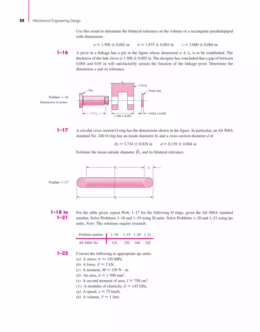
Use this result to determine the bilateral tolerance on the volume of a rectangular parallelepipedwith dimensions
a = 1.500 ± 0.002 in b = 1.875 ± 0.003 in c = 3.000 ± 0.004 in
1–16 A pivot in a linkage has a pin in the figure whose dimension a ± ta is to be established. Thethickness of the link clevis is 1.500 ± 0.005 in. The designer has concluded that a gap of between0.004 and 0.05 in will satisfactorily sustain the function of the linkage pivot. Determine thedimension a and its tolerance.
1–17 A circular cross section O ring has the dimensions shown in the figure. In particular, an AS 568Astandard No. 240 O ring has an inside diameter Di and a cross-section diameter d of
Di = 3.734 ± 0.028 in d = 0.139 ± 0.004 in
Estimate the mean outside diameter Do and its bilateral tolerance.
For the table given, repeat Prob. 1–17 for the following O rings, given the AS 568A standardnumber. Solve Problems 1–18 and 1–19 using SI units. Solve Problems 1–20 and 1–21 using ipsunits. Note: The solutions require research.
Problem number 1–18 1–19 1–20 1–21
AS 568A No. 110 220 160 320
1–22 Convert the following to appropriate ips units:(a) A stress, σ = 150 MPa.(b) A force, F = 2 kN.(c) A moment, M = 150 N � m.(d ) An area, A = 1 500 mm2.(e) A second moment of area, I = 750 cm4.( f ) A modulus of elasticity, E = 145 GPa.(g) A speed, v = 75 km/h.(h) A volume, V = 1 liter.
1–18 to1–21
Di d
D0
Pin
a ± ta 0.042 ± 0.0021.500 ± 0.005
Snap ring
Clevis
28 Mechanical Engineering Design28 Mechanical Engineering Design
Problem 1–16
Dimensions in inches.
Problem 1–17
bud29281_ch01_002-030.qxd 11/11/2009 5:35 pm Page 28 pinnacle s-171:Desktop Folder:Temp Work:Don't Delete (Jobs):MHDQ196/Budynas:

1–23 Convert the following to appropriate SI units:(a) A length, l = 5 ft.(b) A stress, σ = 90 kpsi.(c) A pressure, p = 25 psi.(d ) A section modulus, Z = 12 in3.(e) A unit weight, w = 0.208 lbf/in.( f ) A deflection, � = 0.001 89 in.(g) A velocity, v = 1 200 ft/min.(h) A unit strain, � = 0.002 15 in/in.(i) A volume, V = 1830 in3.
1–24 Generally, final design results are rounded to or fixed to three digits because the given data can-not justify a greater display. In addition, prefixes should be selected so as to limit number stringsto no more than four digits to the left of the decimal point. Using these rules, as well as those forthe choice of prefixes, solve the following relations:(a) σ = M�Z, where M = 1770 lbf � in and Z = 0.934 in3.(b) σ = F�A, where F = 9440 lbf and A = 23.8 in2.(c) y = Fl 3�3EI, where F = 270 lbf, l = 31.5 in, E = 30 Mpsi, and I = 0.154 in4.(d) θ = Tl�GJ, where T = 9 740 lbf � in, l = 9.85 in, G = 11.3 Mpsi, and d = 1.00 in.
1–25 Repeat Prob. 1–24 for the following:(a) σ = F�wt, where F = 1 kN, w = 25 mm, and t = 5 mm.(b) I = bh3�12, where b = 10 mm and h = 25 mm.(c) I = πd 4�64, where d = 25.4 mm.(d) τ = 16 T�πd 3, where T = 25 N � m, and d = 12.7 mm.
1–26 Repeat Prob. 1–24 for:(a) τ = F�A, where A = πd 2�4, F = 2 700 lbf, and d = 0.750 in.(b) σ = 32 Fa�πd 3, where F = 180 lbf, a = 31.5 in, and d = 1.25 in.(c) Z = π (do
4 � di4)�(32 do) for do = 1.50 in and di = 1.00 in.
(d) k = (d 4 G)�(8 D3 N), where d = 0.062 5 in, G = 11.3 Mpsi, D = 0.760 in, and N = 32 (a dimensionless number).
Introduction to Mechanical Engineering Design 29Introduction to Mechanical Engineering Design 29
bud29281_ch01_002-030.qxd 11/11/2009 5:35 pm Page 29 pinnacle s-171:Desktop Folder:Temp Work:Don't Delete (Jobs):MHDQ196/Budynas:

This page intentionally left blank

Chapter Outline
2–1 Material Strength and Stiffness 32
2–2 The Statistical Significance of Material Properties 36
2–3 Strength and Cold Work 38
2–4 Hardness 41
2–5 Impact Properties 42
2–6 Temperature Effects 43
2–7 Numbering Systems 45
2–8 Sand Casting 46
2–9 Shell Molding 47
2–10 Investment Casting 47
2–11 Powder-Metallurgy Process 47
2–12 Hot-Working Processes 47
2–13 Cold-Working Processes 48
2–14 The Heat Treatment of Steel 49
2–15 Alloy Steels 52
2–16 Corrosion-Resistant Steels 53
2–17 Casting Materials 54
2–18 Nonferrous Metals 55
2–19 Plastics 58
2–20 Composite Materials 60
2–21 Materials Selection 61
2Materials
31
bud29281_ch02_031-070.qxd 11/11/09 09:31 PM Page 31 Debd Hard Disk1:Desktop Folder:Temp Work:Satya 10/11/09:
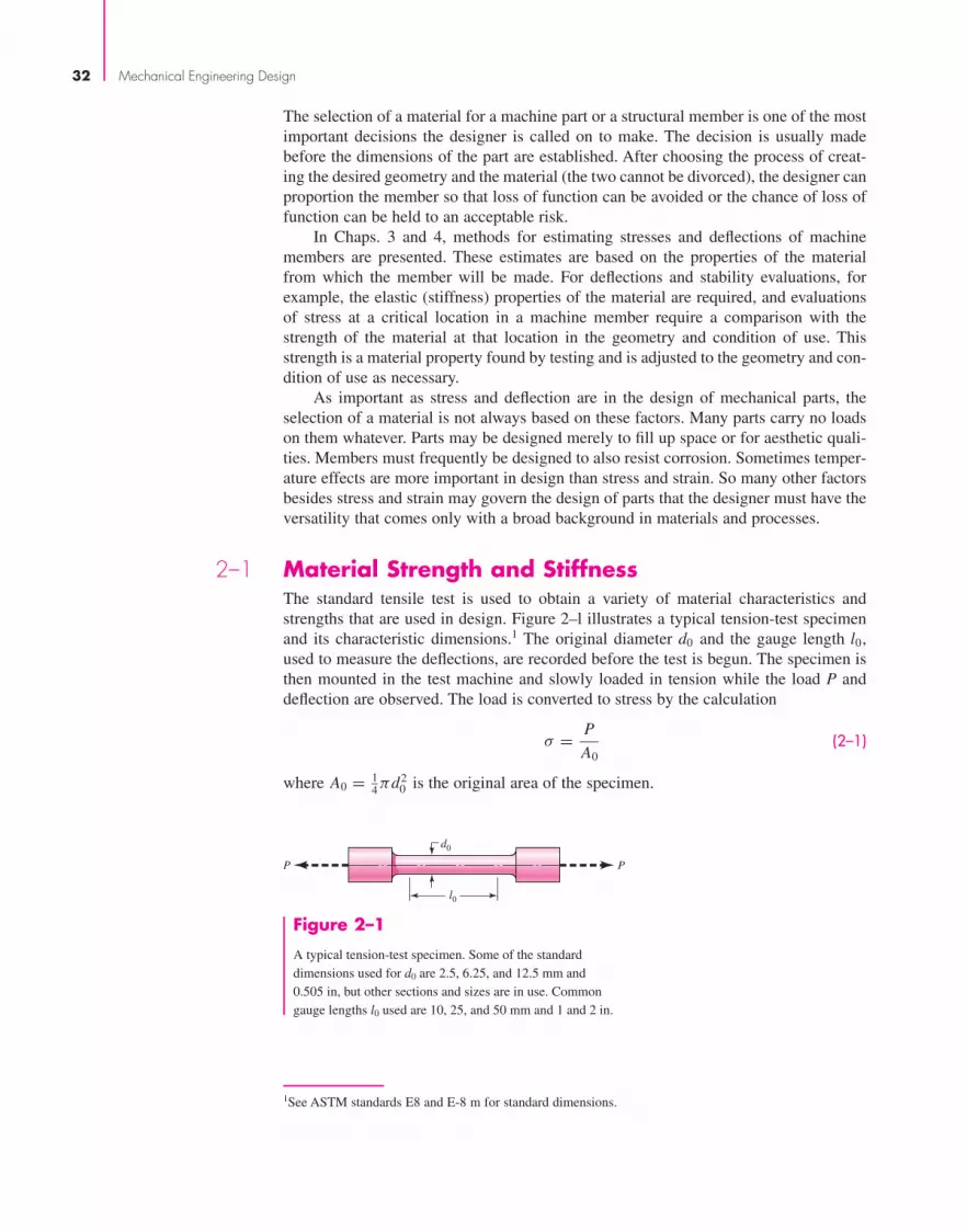
32 Mechanical Engineering Design
1See ASTM standards E8 and E-8 m for standard dimensions.
The selection of a material for a machine part or a structural member is one of the mostimportant decisions the designer is called on to make. The decision is usually madebefore the dimensions of the part are established. After choosing the process of creat-ing the desired geometry and the material (the two cannot be divorced), the designer canproportion the member so that loss of function can be avoided or the chance of loss offunction can be held to an acceptable risk.
In Chaps. 3 and 4, methods for estimating stresses and deflections of machinemembers are presented. These estimates are based on the properties of the materialfrom which the member will be made. For deflections and stability evaluations, forexample, the elastic (stiffness) properties of the material are required, and evaluationsof stress at a critical location in a machine member require a comparison with thestrength of the material at that location in the geometry and condition of use. Thisstrength is a material property found by testing and is adjusted to the geometry and con-dition of use as necessary.
As important as stress and deflection are in the design of mechanical parts, theselection of a material is not always based on these factors. Many parts carry no loadson them whatever. Parts may be designed merely to fill up space or for aesthetic quali-ties. Members must frequently be designed to also resist corrosion. Sometimes temper-ature effects are more important in design than stress and strain. So many other factorsbesides stress and strain may govern the design of parts that the designer must have theversatility that comes only with a broad background in materials and processes.
2–1 Material Strength and StiffnessThe standard tensile test is used to obtain a variety of material characteristics andstrengths that are used in design. Figure 2–l illustrates a typical tension-test specimenand its characteristic dimensions.1 The original diameter d0 and the gauge length l0,used to measure the deflections, are recorded before the test is begun. The specimen isthen mounted in the test machine and slowly loaded in tension while the load P anddeflection are observed. The load is converted to stress by the calculation
σ = P
A0(2–1)
where A0 = 14πd2
0 is the original area of the specimen.
d0
l0
P P
Figure 2–1
A typical tension-test specimen. Some of the standarddimensions used for d0 are 2.5, 6.25, and 12.5 mm and0.505 in, but other sections and sizes are in use. Commongauge lengths l0 used are 10, 25, and 50 mm and 1 and 2 in.
bud29281_ch02_031-070.qxd 11/11/09 09:31 PM Page 32 Debd Hard Disk1:Desktop Folder:Temp Work:Satya 10/11/09:

Materials 33
u
y
aO �y �u
Strain �St
ress
� =
P/A
0 elpl
f
Su
Sf
Sy
�f
(a)
u, fy
Strain �
(b)
a
SutSy
Figure 2–2
Stress-strain diagram obtainedfrom the standard tensile test(a) Ductile material; (b) brittlematerial.pl marks the proportional limit;el, the elastic limit; y, theoffset-yield strength as definedby offset strain a; u, themaximum or ultimate strength;and f, the fracture strength.
2Usage varies. For a long time engineers used the term ultimate strength, hence the subscript u in Su or Sut .However, in material science and metallurgy the term tensile strength is used.
The deflection, or extension of the gauge length, is given by l − l0 where l is thegauge length corresponding to the load P. The normal strain is calculated from
ε = l − l0
l0(2–2)
The results are plotted as a stress-strain diagram. Figure 2–2 depicts typical stress-strain diagrams for ductile and brittle materials. Ductile materials deform much morethan brittle materials.
Point pl in Fig. 2–2a is called the proportional limit. This is the point at which thecurve first begins to deviate from a straight line. No permanent set will be observablein the specimen if the load is removed at this point. In the linear range, the uniaxialstress-strain relation is given by Hooke’s law as
σ = Eε (2–3)
where the constant of proportionality E, the slope of the linear part of the stress-straincurve, is called Young’s modulus or the modulus of elasticity. E is a measure of thestiffness of a material, and since strain is dimensionless, the units of E are the same asstress. Steel, for example, has a modulus of elasticity of about 30 Mpsi (207 GPa)regardless of heat treatment, carbon content, or alloying. Stainless steel is about27.5 Mpsi (190 GPa).
Point el in Fig. 2–2 is called the elastic limit. If the specimen is loaded beyond thispoint, the deformation is said to be plastic and the material will take on a permanent setwhen the load is removed. Between pl and el the diagram is not a perfectly straightline, even though the specimen is elastic.
During the tension test, many materials reach a point at which the strain begins toincrease very rapidly without a corresponding increase in stress. This point is called theyield point. Not all materials have an obvious yield point, especially for brittlematerials. For this reason, yield strength Sy is often defined by an offset method asshown in Fig. 2–2, where line ay is drawn at slope E. Point a corresponds to a definiteor stated amount of permanent set, usually 0.2 percent of the original gauge length(ε = 0.002), although 0.01, 0.1, and 0.5 percent are sometimes used.
The ultimate, or tensile, strength Su or Sut corresponds to point u in Fig. 2–2 andis the maximum stress reached on the stress-strain diagram.2 As shown in Fig. 2–2a,
bud29281_ch02_031-070.qxd 11/12/2009 7:59 pm Page 33 pinnacle s-171:Desktop Folder:Temp Work:Don't Delete (Jobs):MHDQ196/Budynas:

34 Mechanical Engineering Design
some materials exhibit a downward trend after the maximum stress is reached and frac-ture at point f on the diagram. Others, such as some of the cast irons and high-strengthsteels, fracture while the stress-strain trace is still rising, as shown in Fig. 2–2b, wherepoints u and f are identical.
As noted in Sec. 1–9, strength, as used in this book, is a built-in property of a mate-rial, or of a mechanical element, because of the selection of a particular material orprocess or both. The strength of a connecting rod at the critical location in the geome-try and condition of use, for example, is the same no matter whether it is already an ele-ment in an operating machine or whether it is lying on a workbench awaiting assemblywith other parts. On the other hand, stress is something that occurs in a part, usually asa result of its being assembled into a machine and loaded. However, stresses may bebuilt into a part by processing or handling. For example, shot peening produces a com-pressive stress in the outer surface of a part, and also improves the fatigue strength ofthe part. Thus, in this book we will be very careful in distinguishing between strength,designated by S, and stress, designated by σ or τ .
The diagrams in Fig. 2–2 are called engineering stress-strain diagrams because thestresses and strains calculated in Eqs. (2–1) and (2–2) are not true values. The stresscalculated in Eq. (2–1) is based on the original area before the load is applied. In real-ity, as the load is applied the area reduces so that the actual or true stress is larger thanthe engineering stress. To obtain the true stress for the diagram the load and the cross-sectional area must be measured simultaneously during the test. Figure 2–2a representsa ductile material where the stress appears to decrease from points u to f. Typically,beyond point u the specimen begins to “neck” at a location of weakness where the areareduces dramatically, as shown in Fig. 2–3. For this reason, the true stress is much higherthan the engineering stress at the necked section.
The engineering strain given by Eq. (2–2) is based on net change in length from theoriginal length. In plotting the true stress-strain diagram, it is customary to use a termcalled true strain or, sometimes, logarithmic strain. True strain is the sum of the incre-mental elongations divided by the current gauge length at load P, or
ε =∫ l
l0
dl
l= ln
l
l0(2–4)
where the symbol ε is used to represent true strain. The most important characteristicof a true stress-strain diagram (Fig. 2–4) is that the true stress continually increases allthe way to fracture. Thus, as shown in Fig. 2–4, the true fracture stress σ f is greater thanthe true ultimate stress σu . Contrast this with Fig. 2–2a, where the engineering fracturestrength Sf is less than the engineering ultimate strength Su.
Compression tests are more difficult to conduct, and the geometry of the test spec-imens differs from the geometry of those used in tension tests. The reason for this is thatthe specimen may buckle during testing or it may be difficult to distribute the stressesevenly. Other difficulties occur because ductile materials will bulge after yielding.However, the results can be plotted on a stress-strain diagram also, and the samestrength definitions can be applied as used in tensile testing. For most ductile materialsthe compressive strengths are about the same as the tensile strengths. When substantialdifferences occur between tensile and compressive strengths, however, as is the case with
Figure 2–3
Tension specimen afternecking.
bud29281_ch02_031-070.qxd 11/11/09 09:32 PM Page 34 Debd Hard Disk1:Desktop Folder:Temp Work:Satya 10/11/09:

Materials 35
Tru
e st
ress
True strain
�u
�f f
u
�f�u
Figure 2–4
True stress-strain diagramplotted in Cartesiancoordinates.
the cast irons, the tensile and compressive strengths should be stated separately, Sut,Suc , where Suc is reported as a positive quantity.
Torsional strengths are found by twisting solid circular bars and recording the torqueand the twist angle. The results are then plotted as a torque-twist diagram. The shearstresses in the specimen are linear with respect to radial location, being zero at the cen-ter of the specimen and maximum at the outer radius r (see Chap. 3). The maximum shearstress τmax is related to the angle of twist θ by
τmax = Gr
l0θ (2–5)
where θ is in radians, r is the radius of the specimen, l0 is the gauge length, and G isthe material stiffness property called the shear modulus or the modulus of rigidity. Themaximum shear stress is also related to the applied torque T as
τmax = T r
J(2–6)
where J = 12πr4 is the polar second moment of area of the cross section.
The torque-twist diagram will be similar to Fig. 2–2, and, using Eqs. (2–5) and(2–6), the modulus of rigidity can be found as well as the elastic limit and the torsionalyield strength Ssy . The maximum point on a torque-twist diagram, corresponding topoint u on Fig. 2–2, is Tu. The equation
Ssu = Tur
J(2–7)
defines the modulus of rupture for the torsion test. Note that it is incorrect to call Ssu
the ultimate torsional strength, as the outermost region of the bar is in a plastic state atthe torque Tu and the stress distribution is no longer linear.
All of the stresses and strengths defined by the stress-strain diagram of Fig. 2–2 andsimilar diagrams are specifically known as engineering stresses and strengths or nomi-nal stresses and strengths. These are the values normally used in all engineering designcalculations. The adjectives engineering and nominal are used here to emphasize thatthe stresses are computed by using the original or unstressed cross-sectional area of thespecimen. In this book we shall use these modifiers only when we specifically wish tocall attention to this distinction.
bud29281_ch02_031-070.qxd 11/11/09 09:32 PM Page 35 Debd Hard Disk1:Desktop Folder:Temp Work:Satya 10/11/09:

36 Mechanical Engineering Design
In addition to providing strength values for a material, the stress-strain diagramprovides insight into the energy-absorbing characteristics of a material. This is becausethe stress-strain diagram involves both loads and deflections, which are directly relatedto energy. The capacity of a material to absorb energy within its elastic range is calledresilience. The modulus of resilience uR of a material is defined as the energy absorbed perunit volume without permanent deformation, and is equal to the area under the stress-strain curve up to the elastic limit. The elastic limit is often approximated by the yieldpoint, since it is more readily determined, giving
u R∼=
∫ εy
0σdε (2–8)
where εy is the strain at the yield point. If the stress-strain is linear to the yield point,then the area under the curve is simply a triangular area; thus
u R∼= 1
2Syεy = 1
2(Sy)(Sy/E) = S2
y
2E(2–9)
This relationship indicates that for two materials with the same yield strength, theless stiff material (lower E), will have a greater resilience, that is, an ability to absorbmore energy without yielding.
The capacity of a material to absorb energy without fracture is called toughness.The modulus of toughness uT of a material is defined as the energy absorbed per unitvolume without fracture, which is equal to the total area under the stress-strain curve upto the fracture point, or
uT =∫ ε f
0σdε (2–10)
where ε f is the strain at the fracture point. This integration is often performed graphi-cally from the stress-strain data, or a rough approximation can be obtained by using theaverage of the yield and ultimate strengths and the strain at fracture to calculate an area;that is,
uT∼=
(Sy + Sut
2
)ε f (2–11)
The units of toughness and resilience are energy per unit volume (lbf � in/in3 or J/m3),which are numerically equivalent to psi or Pa. These definitions of toughness andresilience assume the low strain rates that are suitable for obtaining the stress-straindiagram. For higher strain rates, see Sec. 2–5 for impact properties.
2–2 The Statistical Significance of Material PropertiesThere is some subtlety in the ideas presented in the previous section that should be pon-dered carefully before continuing. Figure 2–2 depicts the result of a single tension test(one specimen, now fractured). It is common for engineers to consider these importantstress values (at points pl, el, y, u , and f ) as properties and to denote them as strengthswith a special notation, uppercase S, in lieu of lowercase sigma σ, with subscriptsadded: Spl for proportional limit, Sy for yield strength, Su for ultimate tensile strength(Sut or Suc , if tensile or compressive sense is important).
If there were 1000 nominally identical specimens, the values of strength obtainedwould be distributed between some minimum and maximum values. It follows that the
bud29281_ch02_031-070.qxd 11/12/2009 7:59 pm Page 36 pinnacle s-171:Desktop Folder:Temp Work:Don't Delete (Jobs):MHDQ196/Budynas:
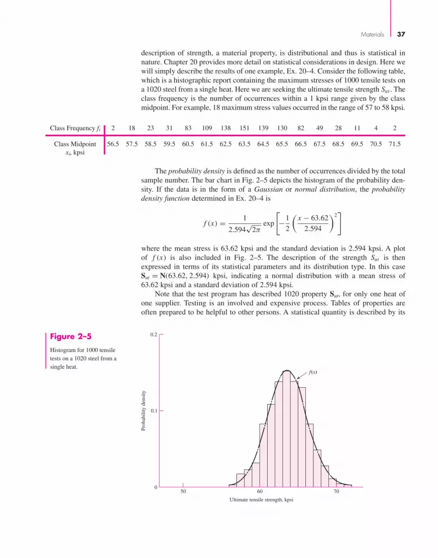
Materials 37
description of strength, a material property, is distributional and thus is statistical innature. Chapter 20 provides more detail on statistical considerations in design. Here wewill simply describe the results of one example, Ex. 20–4. Consider the following table,which is a histographic report containing the maximum stresses of 1000 tensile tests ona 1020 steel from a single heat. Here we are seeking the ultimate tensile strength Sut . Theclass frequency is the number of occurrences within a 1 kpsi range given by the classmidpoint. For example, 18 maximum stress values occurred in the range of 57 to 58 kpsi.
Figure 2–5
Histogram for 1000 tensiletests on a 1020 steel from asingle heat.
f(x)
50 60 700
0.1
0.2
Prob
abili
ty d
ensi
ty
Ultimate tensile strength, kpsi
Class Frequency fi 2 18 23 31 83 109 138 151 139 130 82 49 28 11 4 2
Class Midpoint 56.5 57.5 58.5 59.5 60.5 61.5 62.5 63.5 64.5 65.5 66.5 67.5 68.5 69.5 70.5 71.5xi, kpsi
The probability density is defined as the number of occurrences divided by the totalsample number. The bar chart in Fig. 2–5 depicts the histogram of the probability den-sity. If the data is in the form of a Gaussian or normal distribution, the probabilitydensity function determined in Ex. 20–4 is
f (x) = 1
2.594√
2πexp
[−1
2
(x − 63.62
2.594
)2]
where the mean stress is 63.62 kpsi and the standard deviation is 2.594 kpsi. A plotof f (x) is also included in Fig. 2–5. The description of the strength Sut is thenexpressed in terms of its statistical parameters and its distribution type. In this caseSut = N(63.62, 2.594) kpsi, indicating a normal distribution with a mean stress of63.62 kpsi and a standard deviation of 2.594 kpsi.
Note that the test program has described 1020 property Sut, for only one heat ofone supplier. Testing is an involved and expensive process. Tables of properties areoften prepared to be helpful to other persons. A statistical quantity is described by its
bud29281_ch02_031-070.qxd 11/12/2009 7:59 pm Page 37 pinnacle s-171:Desktop Folder:Temp Work:Don't Delete (Jobs):MHDQ196/Budynas:

38 Mechanical Engineering Design
mean, standard deviation, and distribution type. Many tables display a single number,which is often the mean, minimum, or some percentile, such as the 99th percentile.Always read the foonotes to the table. If no qualification is made in a single-entry table,the table is subject to serious doubt.
Since it is no surprise that useful descriptions of a property are statistical in nature,engineers, when ordering property tests, should couch the instructions so the data gen-erated are enough for them to observe the statistical parameters and to identify the dis-tributional characteristic. The tensile test program on 1000 specimens of 1020 steel isa large one. If you were faced with putting something in a table of ultimate tensilestrengths and constrained to a single number, what would it be and just how would yourfootnote read?
2–3 Strength and Cold WorkCold working is the process of plastic straining below the recrystallization temperaturein the plastic region of the stress-strain diagram. Materials can be deformed plasticallyby the application of heat, as in forging or hot rolling, but the resulting mechanicalproperties are quite different from those obtained by cold working. The purpose of thissection is to explain what happens to the significant mechanical properties of a materialwhen that material is cold worked.
Consider the stress-strain diagram of Fig. 2–6a. Here a material has been stressedbeyond the yield strength at y to some point i, in the plastic region, and then the loadremoved. At this point the material has a permanent plastic deformation εp . If the loadcorresponding to point i is now reapplied, the material will be elastically deformed bythe amount εe. Thus at point i the total unit strain consists of the two components εp andεe and is given by the equation
ε = εp + εe (a)
This material can be unloaded and reloaded any number of times from and to point i,and it is found that the action always occurs along the straight line that is approximatelyparallel to the initial elastic line Oy. Thus
εe = σi
E(b)
�
�e�pUnit strain, �
Nom
inal
str
ess,
�
(a)
�i
Su
iu
y
O
Sy
f
Loa
d, P
(b)
Area deformation (reduction)
Pi
Pu
u
f
y
i
Py
A0 A�i Ai Af
Figure 2–6
(a) Stress-strain diagramshowing unloading andreloading at point i in theplastic region; (b) analogousload-deformation diagram.
bud29281_ch02_031-070.qxd 11/11/09 09:33 PM Page 38 Debd Hard Disk1:Desktop Folder:Temp Work:Satya 10/11/09:

Materials 39
The material now has a higher yield point, is less ductile as a result of a reduction instrain capacity, and is said to be strain-hardened. If the process is continued, increasingεp , the material can become brittle and exhibit sudden fracture.
It is possible to construct a similar diagram, as in Fig. 2–6b, where the abscissa isthe area deformation and the ordinate is the applied load. The reduction in area corre-sponding to the load Pf , at fracture, is defined as
R = A0 − Af
A0= 1 − Af
A0(2–12)
where A0 is the original area. The quantity R in Eq. (2–12) is usually expressed in per-cent and tabulated in lists of mechanical properties as a measure of ductility. SeeAppendix Table A–20, for example. Ductility is an important property because it mea-sures the ability of a material to absorb overloads and to be cold-worked. Thus suchoperations as bending, drawing, heading, and stretch forming are metal-processingoperations that require ductile materials.
Figure 2–6b can also be used to define the quantity of cold work. The cold-workfactor W is defined as
W = A0 − A′i
A0≈ A0 − Ai
A0(2–13)
where A′i corresponds to the area after the load Pi has been released. The approxima-
tion in Eq. (2–13) results because of the difficulty of measuring the small diametralchanges in the elastic region. If the amount of cold work is known, then Eq. (2–13) canbe solved for the area A′
i . The result is
A′i = A0(1 − W ) (2–14)
Cold working a material produces a new set of values for the strengths, as canbe seen from stress-strain diagrams. Datsko3 describes the plastic region of the truestress–true strain diagram by the equation
σ = σ0εm (2–15)
where σ = true stress
σ0 = a strength coefficient, or strain-strengthening coefficient
ε = true plastic strain
m = strain-strengthening exponent
It can be shown4 that
m = εu (2–16)
provided that the load-deformation curve exhibits a stationary point (a place of zeroslope).
3Joseph Datsko, “Solid Materials,” Chap. 32 in Joseph E. Shigley, Charles R. Mischke, and Thomas H. Brown, Jr. (eds.), Standard Handbook of Machine Design, 3rd ed., McGraw-Hill, New York, 2004. See alsoJoseph Datsko, “New Look at Material Strength,” Machine Design, vol. 58, no. 3, Feb. 6, 1986, pp. 81–85.4See Sec. 5–2, J. E. Shigley and C. R. Mischke, Mechanical Engineering Design, 6th ed., McGraw-Hill,New York, 2001.
bud29281_ch02_031-070.qxd 11/11/09 09:33 PM Page 39 Debd Hard Disk1:Desktop Folder:Temp Work:Satya 10/11/09:

40 Mechanical Engineering Design
Difficulties arise when using the gauge length to evaluate the true strain in theplastic range, since necking causes the strain to be nonuniform. A more satisfactoryrelation can be obtained by using the area at the neck. Assuming that the change in vol-ume of the material is small, Al = A0 l0. Thus, l/ l0 = A0/A, and the true strain isgiven by
ε = lnl
l0= ln
A0
A(2–17)
Returning to Fig. 2–6b, if point i is to the left of point u, that is, Pi < Pu , then thenew yield strength is
S′y = Pi
A′i
= σ0εmi Pi ≤ Pu (2–18)
Because of the reduced area, that is, because A′i < A0, the ultimate strength also
changes, and is
S′u = Pu
A′i
(c)
Since Pu = Su A0, we find, with Eq. (2–14), that
S′u = Su A0
A0(1 − W )= Su
1 − Wεi ≤ εu (2–19)
which is valid only when point i is to the left of point u.For points to the right of u, the yield strength is approaching the ultimate strength,
and, with small loss in accuracy,
S′u
.= S′y
.= σ0εmi εi > εu (2–20)
A little thought will reveal that a bar will have the same ultimate load in tension afterbeing strain-strengthened in tension as it had before. The new strength is of interestto us not because the static ultimate load increases, but—since fatigue strengthsare correlated with the local ultimate strengths—because the fatigue strength im-proves. Also the yield strength increases, giving a larger range of sustainable elasticloading.
EXAMPLE 2–1 An annealed AISI 1018 steel (see Table A–22) has Sy = 32.0 kpsi, Su = 49.5 kpsi,σ f = 91.1 kpsi, σ0 = 90 kpsi, m = 0.25, and ε f = 1.05 in/in. Find the new values ofthe strengths if the material is given 15 percent cold work.
Solution From Eq. (2–16), we find the true strain corresponding to the ultimate strength to be
εu = m = 0.25
The ratio A0/Ai is, from Eq. (2–13),
A0
Ai= 1
1 − W= 1
1 − 0.15= 1.176
bud29281_ch02_031-070.qxd 11/11/09 09:33 PM Page 40 Debd Hard Disk1:Desktop Folder:Temp Work:Satya 10/11/09:

The true strain corresponding to 15 percent cold work is obtained from Eq. (2–17). Thus
εi = lnA0
Ai= ln 1.176 = 0.1625
Since εi < εu , Eqs. (2–18) and (2–19) apply. Therefore,
Answer S′y = σ0ε
mi = 90(0.1625)0.25 = 57.1 kpsi
Answer S′u = Su
1 − W= 49.5
1 − 0.15= 58.2 kpsi
2–4 HardnessThe resistance of a material to penetration by a pointed tool is called hardness. Thoughthere are many hardness-measuring systems, we shall consider here only the two ingreatest use.
Rockwell hardness tests are described by ASTM standard hardness method E–18and measurements are quickly and easily made, they have good reproducibility, andthe test machine for them is easy to use. In fact, the hardness number is read directlyfrom a dial. Rockwell hardness scales are designated as A, B, C, . . . , etc. The inden-ters are described as a diamond, a 1
16 -in-diameter ball, and a diamond for scales A, B,and C, respectively, where the load applied is either 60, 100, or 150 kg. Thus theRockwell B scale, designated RB , uses a 100-kg load and a No. 2 indenter, which isa 1
16 -in-diameter ball. The Rockwell C scale RC uses a diamond cone, which is theNo. 1 indenter, and a load of 150 kg. Hardness numbers so obtained are relative.Therefore a hardness RC = 50 has meaning only in relation to another hardness num-ber using the same scale.
The Brinell hardness is another test in very general use. In testing, the indentingtool through which force is applied is a ball and the hardness number HB is found asa number equal to the applied load divided by the spherical surface area of the inden-tation. Thus the units of HB are the same as those of stress, though they are seldomused. Brinell hardness testing takes more time, since HB must be computed from thetest data. The primary advantage of both methods is that they are nondestructive inmost cases. Both are empirically and directly related to the ultimate strength of thematerial tested. This means that the strength of parts could, if desired, be tested partby part during manufacture.
Hardness testing provides a convenient and nondestructive means of estimating thestrength properties of materials. The Brinell hardness test is particularly well known forthis estimation, since for many materials the relationship between the minimumultimate strength and the Brinell hardness number is roughly linear. The constant ofproportionality varies between classes of materials, and is also dependent on the loadused to determine the hardness. There is a wide scatter in the data, but for rough approx-imations for steels, the relationship is generally accepted as
Su ={
0.5HB kpsi
3.4HB MPa(2–21)
Materials 41
bud29281_ch02_031-070.qxd 11/11/09 09:33 PM Page 41 Debd Hard Disk1:Desktop Folder:Temp Work:Satya 10/11/09:

42 Mechanical Engineering Design
5D. E. Krause, “Gray Iron—A Unique Engineering Material,” ASTM Special Publication 455, 1969,pp. 3–29, as reported in Charles F. Walton (ed.), Iron Castings Handbook, Iron Founders Society, Inc., Cleveland, 1971, pp. 204, 205.6Ibid.
Similar relationships for cast iron can be derived from data supplied by Krause.5
The minimum strength, as defined by the ASTM, is found from these data to be
Su ={
0.23HB − 12.5 kpsi
1.58HB − 86 MPa(2–22)
Walton6 shows a chart from which the SAE minimum strength can be obtained, whichis more conservative than the values obtained from Eq. (2–22).
EXAMPLE 2–2 It is necessary to ensure that a certain part supplied by a foundry always meets orexceeds ASTM No. 20 specifications for cast iron (see Table A–24). What hardnessshould be specified?
Solution From Eq. (2–22), with (Su)min = 20 kpsi, we have
Answer HB = Su + 12.5
0.23= 20 + 12.5
0.23= 141
If the foundry can control the hardness within 20 points, routinely, then specify145 < HB < 165. This imposes no hardship on the foundry and assures the designerthat ASTM grade 20 will always be supplied at a predictable cost.
2–5 Impact PropertiesAn external force applied to a structure or part is called an impact load if the time ofapplication is less than one-third the lowest natural period of vibration of the part orstructure. Otherwise it is called simply a static load.
The Charpy (commonly used) and Izod (rarely used) notched-bar tests utilize bars ofspecified geometries to determine brittleness and impact strength. These tests are helpfulin comparing several materials and in the determination of low-temperature brittleness. Inboth tests the specimen is struck by a pendulum released from a fixed height, and theenergy absorbed by the specimen, called the impact value, can be computed from theheight of swing after fracture, but is read from a dial that essentially “computes” the result.
The effect of temperature on impact values is shown in Fig. 2–7 for a materialshowing a ductile-brittle transition. Not all materials show this transition. Notice thenarrow region of critical temperatures where the impact value increases very rapidly. Inthe low-temperature region the fracture appears as a brittle, shattering type, whereas theappearance is a tough, tearing type above the critical-temperature region. The criticaltemperature seems to be dependent on both the material and the geometry of the notch.For this reason designers should not rely too heavily on the results of notched-bar tests.
The average strain rate used in obtaining the stress-strain diagram is about0.001 in/(in · s) or less. When the strain rate is increased, as it is under impact conditions,
bud29281_ch02_031-070.qxd 11/11/09 09:33 PM Page 42 Debd Hard Disk1:Desktop Folder:Temp Work:Satya 10/11/09:

Materials 43
–400 0 200 4000
20
40
60
Cha
rpy,
ft�
lbf
Temperature, °F
–200
Figure 2–7
A mean trace shows the effectof temperature on impactvalues. The result of interest isthe brittle-ductile transitiontemperature, often defined asthe temperature at which themean trace passes through the15 ft · lbf level. The criticaltemperature is dependent onthe geometry of the notch,which is why the CharpyV notch is closely defined.
10–6 10–4 10–2 1 102 1040
20
40
60
80
100
0
20
40
60
80
100
Stre
ngth
, kps
i
Strain rate, s–1
Rat
io, S
y/S
u, %
Elo
ngat
ion,
%
Ratio, Sy /Su
Ultimatestrength, Su
Total elongation
Yield strength, Sy
Figure 2–8
Influence of strain rate ontensile properties.
the strengths increase, as shown in Fig. 2–8. In fact, at very high strain rates the yieldstrength seems to approach the ultimate strength as a limit. But note that the curves showlittle change in the elongation. This means that the ductility remains about the same.Also, in view of the sharp increase in yield strength, a mild steel could be expected tobehave elastically throughout practically its entire strength range under impact conditions.
The Charpy and Izod tests really provide toughness data under dynamic, rather thanstatic, conditions. It may well be that impact data obtained from these tests are as depen-dent on the notch geometry as they are on the strain rate. For these reasons it may be bet-ter to use the concepts of notch sensitivity, fracture toughness, and fracture mechanics,discussed in Chaps. 5 and 6, to assess the possibility of cracking or fracture.
2–6 Temperature EffectsStrength and ductility, or brittleness, are properties affected by the temperature of theoperating environment.
The effect of temperature on the static properties of steels is typified by thestrength versus temperature chart of Fig. 2–9. Note that the tensile strength changes
bud29281_ch02_031-070.qxd 11/11/09 09:33 PM Page 43 Debd Hard Disk1:Desktop Folder:Temp Work:Satya 10/11/09:

44 Mechanical Engineering Design
1st stage2nd stage 3rd stage
Time
Cre
ep d
efor
mat
ion
Figure 2–10
Creep-time curve.
only a small amount until a certain temperature is reached. At that point it falls offrapidly. The yield strength, however, decreases continuously as the environmental tem-perature is increased. There is a substantial increase in ductility, as might be expected,at the higher temperatures.
Many tests have been made of ferrous metals subjected to constant loads for longperiods of time at elevated temperatures. The specimens were found to be permanentlydeformed during the tests, even though at times the actual stresses were less than theyield strength of the material obtained from short-time tests made at the same temper-ature. This continuous deformation under load is called creep.
One of the most useful tests to have been devised is the long-time creep test underconstant load. Figure 2–10 illustrates a curve that is typical of this kind of test. Thecurve is obtained at a constant stated temperature. A number of tests are usually runsimultaneously at different stress intensities. The curve exhibits three distinct regions.In the first stage are included both the elastic and the plastic deformation. This stage showsa decreasing creep rate, which is due to the strain hardening. The second stage showsa constant minimum creep rate caused by the annealing effect. In the third stage thespecimen shows a considerable reduction in area, the true stress is increased, and ahigher creep eventually leads to fracture.
When the operating temperatures are lower than the transition temperature(Fig. 2–7), the possibility arises that a part could fail by a brittle fracture. This subjectwill be discussed in Chap. 5.
Of course, heat treatment, as will be shown, is used to make substantial changes inthe mechanical properties of a material.
1.0
0.9
0.8
0.7
0.6
0.50 200 400 600
S T/S
RT
Sy
RTTemperature, °C
Sut
Figure 2–9
A plot of the results of 145 testsof 21 carbon and alloy steelsshowing the effect of operatingtemperature on the yieldstrength Sy and the ultimatestrength Sut . The ordinate is the ratio of the strength at theoperating temperature to thestrength at room temperature.The standard deviations were0.0442 ≤ σSy ≤ 0.152 for Sy
and 0.099 ≤ σSut ≤ 0.11 forSut . (Data source: E. A.Brandes (ed.), Smithells MetalReference Book, 6th ed.,Butterworth, London, 1983pp. 22–128 to 22–131.)
bud29281_ch02_031-070.qxd 11/11/09 09:34 PM Page 44 Debd Hard Disk1:Desktop Folder:Temp Work:Satya 10/11/09:

Materials 45
7Many of the materials discussed in the balance of this chapter are listed in the Appendix tables. Be sure toreview these.
Heating due to electric and gas welding also changes the mechanical properties.Such changes may be due to clamping during the welding process, as well as heating;the resulting stresses then remain when the parts have cooled and the clamps have beenremoved. Hardness tests can be used to learn whether the strength has been changed bywelding, but such tests will not reveal the presence of residual stresses.
2–7 Numbering SystemsThe Society of Automotive Engineers (SAE) was the first to recognize the need, and toadopt a system, for the numbering of steels. Later the American Iron and Steel Institute(AISI) adopted a similar system. In 1975 the SAE published the Unified NumberingSystem for Metals and Alloys (UNS); this system also contains cross-reference num-bers for other material specifications.7 The UNS uses a letter prefix to designate thematerial, as, for example, G for the carbon and alloy steels, A for the aluminum alloys,C for the copper-base alloys, and S for the stainless or corrosion-resistant steels. Forsome materials, not enough agreement has as yet developed in the industry to warrantthe establishment of a designation.
For the steels, the first two numbers following the letter prefix indicate the compo-sition, excluding the carbon content. The various compositions used are as follows:
G10 Plain carbon
G11 Free-cutting carbon steel withmore sulfur or phosphorus
G13 Manganese
G23 Nickel
G25 Nickel
G31 Nickel-chromium
G33 Nickel-chromium
G40 Molybdenum
G41 Chromium-molybdenum
G43 Nickel-chromium-molybdenum
The second number pair refers to the approximate carbon content. Thus, G10400 is aplain carbon steel with a nominal carbon content of 0.40 percent (0.37 to 0.44 percent).The fifth number following the prefix is used for special situations. For example, the olddesignation AISI 52100 represents a chromium alloy with about 100 points of carbon.The UNS designation is G52986.
The UNS designations for the stainless steels, prefix S, utilize the older AISI des-ignations for the first three numbers following the prefix. The next two numbers arereserved for special purposes. The first number of the group indicates the approximatecomposition. Thus 2 is a chromium-nickel-manganese steel, 3 is a chromium-nickelsteel, and 4 is a chromium alloy steel. Sometimes stainless steels are referred to by theiralloy content. Thus S30200 is often called an 18-8 stainless steel, meaning 18 percentchromium and 8 percent nickel.
G46 Nickel-molybdenum
G48 Nickel-molybdenum
G50 Chromium
G51 Chromium
G52 Chromium
G61 Chromium-vanadium
G86 Chromium-nickel-molybdenum
G87 Chromium-nickel-molybdenum
G92 Manganese-silicon
G94 Nickel-chromium-molybdenum
bud29281_ch02_031-070.qxd 11/11/09 09:34 PM Page 45 Debd Hard Disk1:Desktop Folder:Temp Work:Satya 10/11/09:

46 Mechanical Engineering Design
The prefix for the aluminum group is the letter A. The first number following theprefix indicates the processing. For example, A9 is a wrought aluminum, while A0 isa casting alloy. The second number designates the main alloy group as shown inTable 2–1. The third number in the group is used to modify the original alloy or todesignate the impurity limits. The last two numbers refer to other alloys used with thebasic group.
The American Society for Testing and Materials (ASTM) numbering system forcast iron is in widespread use. This system is based on the tensile strength. Thus ASTMA18 speaks of classes; e.g., 30 cast iron has a minimum tensile strength of 30 kpsi. Notefrom Appendix A-24, however, that the typical tensile strength is 31 kpsi. You shouldbe careful to designate which of the two values is used in design and problem workbecause of the significance of factor of safety.
2–8 Sand CastingSand casting is a basic low-cost process, and it lends itself to economical productionin large quantities with practically no limit to the size, shape, or complexity of the partproduced.
In sand casting, the casting is made by pouring molten metal into sand molds. Apattern, constructed of metal or wood, is used to form the cavity into which the moltenmetal is poured. Recesses or holes in the casting are produced by sand cores introducedinto the mold. The designer should make an effort to visualize the pattern and castingin the mold. In this way the problems of core setting, pattern removal, draft, and solid-ification can be studied. Castings to be used as test bars of cast iron are cast separatelyand properties may vary.
Steel castings are the most difficult of all to produce, because steel has the highestmelting temperature of all materials normally used for casting. This high temperatureaggravates all casting problems.
The following rules will be found quite useful in the design of any sand casting:
1 All sections should be designed with a uniform thickness.2 The casting should be designed so as to produce a gradual change from section to
section where this is necessary.3 Adjoining sections should be designed with generous fillets or radii.4 A complicated part should be designed as two or more simple castings to be
assembled by fasteners or by welding.
Steel, gray iron, brass, bronze, and aluminum are most often used in castings. Theminimum wall thickness for any of these materials is about 5 mm, though with partic-ular care, thinner sections can be obtained with some materials.
Table 2–1
Aluminum Alloy
Designations
Aluminum 99.00% pure and greater Ax1xxx
Copper alloys Ax2xxx
Manganese alloys Ax3xxx
Silicon alloys Ax4xxx
Magnesium alloys Ax5xxx
Magnesium-silicon alloys Ax6xxx
Zinc alloys Ax7xxx
bud29281_ch02_031-070.qxd 11/11/09 09:34 PM Page 46 Debd Hard Disk1:Desktop Folder:Temp Work:Satya 10/11/09:

Materials 47
2–9 Shell MoldingThe shell-molding process employs a heated metal pattern, usually made of cast iron,aluminum, or brass, which is placed in a shell-molding machine containing a mixtureof dry sand and thermosetting resin. The hot pattern melts the plastic, which, togetherwith the sand, forms a shell about 5 to 10 mm thick around the pattern. The shell is thenbaked at from 400 to 700°F for a short time while still on the pattern. It is then strippedfrom the pattern and placed in storage for use in casting.
In the next step the shells are assembled by clamping, bolting, or pasting; they areplaced in a backup material, such as steel shot; and the molten metal is poured into thecavity. The thin shell permits the heat to be conducted away so that solidification takesplace rapidly. As solidification takes place, the plastic bond is burned and the mold col-lapses. The permeability of the backup material allows the gases to escape and the cast-ing to air-cool. All this aids in obtaining a fine-grain, stress-free casting.
Shell-mold castings feature a smooth surface, a draft that is quite small, and closetolerances. In general, the rules governing sand casting also apply to shell-mold casting.
2–10 Investment CastingInvestment casting uses a pattern that may be made from wax, plastic, or other material.After the mold is made, the pattern is melted out. Thus a mechanized method of casting agreat many patterns is necessary. The mold material is dependent upon the melting pointof the cast metal. Thus a plaster mold can be used for some materials while others wouldrequire a ceramic mold. After the pattern is melted out, the mold is baked or fired; whenfiring is completed, the molten metal may be poured into the hot mold and allowed to cool.
If a number of castings are to be made, then metal or permanent molds may be suit-able. Such molds have the advantage that the surfaces are smooth, bright, and accurate,so that little, if any, machining is required. Metal-mold castings are also known as diecastings and centrifugal castings.
2–11 Powder-Metallurgy ProcessThe powder-metallurgy process is a quantity-production process that uses powders froma single metal, several metals, or a mixture of metals and nonmetals. It consists essen-tially of mechanically mixing the powders, compacting them in dies at high pressures, andheating the compacted part at a temperature less than the melting point of the majoringredient. The particles are united into a single strong part similar to what would beobtained by melting the same ingredients together. The advantages are (1) the elimina-tion of scrap or waste material, (2) the elimination of machining operations, (3) the lowunit cost when mass-produced, and (4) the exact control of composition. Some of the dis-advantages are (1) the high cost of dies, (2) the lower physical properties, (3) the highercost of materials, (4) the limitations on the design, and (5) the limited range of materialsthat can be used. Parts commonly made by this process are oil-impregnated bearings,incandescent lamp filaments, cemented-carbide tips for tools, and permanent magnets.Some products can be made only by powder metallurgy: surgical implants, for example.The structure is different from what can be obtained by melting the same ingredients.
2–12 Hot-Working ProcessesBy hot working are meant such processes as rolling, forging, hot extrusion, and hotpressing, in which the metal is heated above its recrystallation temperature.
bud29281_ch02_031-070.qxd 11/11/09 09:34 PM Page 47 Debd Hard Disk1:Desktop Folder:Temp Work:Satya 10/11/09:

48 Mechanical Engineering Design
Hot rolling is usually used to create a bar of material of a particular shape anddimension. Figure 2–11 shows some of the various shapes that are commonly producedby the hot-rolling process. All of them are available in many different sizes as well asin different materials. The materials most available in the hot-rolled bar sizes are steel,aluminum, magnesium, and copper alloys.
Tubing can be manufactured by hot-rolling strip or plate. The edges of the strip arerolled together, creating seams that are either butt-welded or lap-welded. Seamless tub-ing is manufactured by roll-piercing a solid heated rod with a piercing mandrel.
Extrusion is the process by which great pressure is applied to a heated metal billetor blank, causing it to flow through a restricted orifice. This process is more commonwith materials of low melting point, such as aluminum, copper, magnesium, lead, tin,and zinc. Stainless steel extrusions are available on a more limited basis.
Forging is the hot working of metal by hammers, presses, or forging machines. Incommon with other hot-working processes, forging produces a refined grain structurethat results in increased strength and ductility. Compared with castings, forgings havegreater strength for the same weight. In addition, drop forgings can be made smootherand more accurate than sand castings, so that less machining is necessary. However, theinitial cost of the forging dies is usually greater than the cost of patterns for castings,although the greater unit strength rather than the cost is usually the deciding factorbetween these two processes.
2–13 Cold-Working ProcessesBy cold working is meant the forming of the metal while at a low temperature (usuallyroom temperature). In contrast to parts produced by hot working, cold-worked partshave a bright new finish, are more accurate, and require less machining.
Cold-finished bars and shafts are produced by rolling, drawing, turning, grinding,and polishing. Of these methods, by far the largest percentage of products are made bythe cold-rolling and cold-drawing processes. Cold rolling is now used mostly for theproduction of wide flats and sheets. Practically all cold-finished bars are made by colddrawing but even so are sometimes mistakenly called “cold-rolled bars.” In the drawingprocess, the hot-rolled bars are first cleaned of scale and then drawn by pulling themthrough a die that reduces the size about 1
32 to 116 in. This process does not remove
material from the bar but reduces, or “draws” down, the size. Many different shapes ofhot-rolled bars may be used for cold drawing.
Cold rolling and cold drawing have the same effect upon the mechanical proper-ties. The cold-working process does not change the grain size but merely distorts it.Cold working results in a large increase in yield strength, an increase in ultimate
Round Square Half oval
(a) Bar shapes
Flat Hexagon
(b) Structural shapes
Wide flange Channel Angle Tee Zee
Figure 2–11
Common shapes availablethrough hot rolling.
bud29281_ch02_031-070.qxd 11/11/09 09:34 PM Page 48 Debd Hard Disk1:Desktop Folder:Temp Work:Satya 10/11/09:

Materials 49
0 0.2 0.4 0.60
20
40
60
80
100
Elongation, in
Stre
ngth
, kps
i
Yield point
Yield point
Cold-drawn
Hot-rolled
Figure 2–12
Stress-strain diagram forhot-rolled and cold-drawn UNS G10350 steel.
strength and hardness, and a decrease in ductility. In Fig. 2–12 the properties of a cold-drawn bar are compared with those of a hot-rolled bar of the same material.
Heading is a cold-working process in which the metal is gathered, or upset. Thisoperation is commonly used to make screw and rivet heads and is capable of producing awide variety of shapes. Roll threading is the process of rolling threads by squeezing androlling a blank between two serrated dies. Spinning is the operation of working sheet mate-rial around a rotating form into a circular shape. Stamping is the term used to describepunch-press operations such as blanking, coining, forming, and shallow drawing.
2–14 The Heat Treatment of SteelHeat treatment of steel refers to time- and temperature-controlled processes that relieveresidual stresses and/or modifies material properties such as hardness (strength), duc-tility, and toughness. Other mechanical or chemical operations are sometimes groupedunder the heading of heat treatment. The common heat-treating operations are anneal-ing, quenching, tempering, and case hardening.
Annealing
When a material is cold- or hot-worked, residual stresses are built in, and, in addition, thematerial usually has a higher hardness as a result of these working operations. These oper-ations change the structure of the material so that it is no longer represented by the equi-librium diagram. Full annealing and normalizing is a heating operation that permits thematerial to transform according to the equilibrium diagram. The material to be annealedis heated to a temperature that is approximately 100°F above the critical temperature. It isheld at this temperature for a time that is sufficient for the carbon to become dissolved anddiffused through the material. The object being treated is then allowed to cool slowly, usu-ally in the furnace in which it was treated. If the transformation is complete, then it is saidto have a full anneal. Annealing is used to soften a material and make it more ductile, torelieve residual stresses, and to refine the grain structure.
The term annealing includes the process called normalizing. Parts to be normalizedmay be heated to a slightly higher temperature than in full annealing. This produces acoarser grain structure, which is more easily machined if the material is a low-carbon steel.In the normalizing process the part is cooled in still air at room temperature. Since thiscooling is more rapid than the slow cooling used in full annealing, less time is available forequilibrium, and the material is harder than fully annealed steel. Normalizing is often usedas the final treating operation for steel. The cooling in still air amounts to a slow quench.
bud29281_ch02_031-070.qxd 11/11/09 09:34 PM Page 49 Debd Hard Disk1:Desktop Folder:Temp Work:Satya 10/11/09:

50 Mechanical Engineering Design
Quenching
Eutectoid steel that is fully annealed consists entirely of pearlite, which is obtainedfrom austenite under conditions of equilibrium. A fully annealed hypoeutectoid steelwould consist of pearlite plus ferrite, while hypereutectoid steel in the fully annealedcondition would consist of pearlite plus cementite. The hardness of steel of a givencarbon content depends upon the structure that replaces the pearlite when full anneal-ing is not carried out.
The absence of full annealing indicates a more rapid rate of cooling. The rate ofcooling is the factor that determines the hardness. A controlled cooling rate is calledquenching. A mild quench is obtained by cooling in still air, which, as we have seen, isobtained by the normalizing process. The two most widely used media for quenchingare water and oil. The oil quench is quite slow but prevents quenching cracks caused byrapid expansion of the object being treated. Quenching in water is used for carbon steelsand for medium-carbon, low-alloy steels.
The effectiveness of quenching depends upon the fact that when austenite is cooledit does not transform into pearlite instantaneously but requires time to initiate and com-plete the process. Since the transformation ceases at about 800°F, it can be preventedby rapidly cooling the material to a lower temperature. When the material is cooledrapidly to 400°F or less, the austenite is transformed into a structure called martensite.Martensite is a supersaturated solid solution of carbon in ferrite and is the hardest andstrongest form of steel.
If steel is rapidly cooled to a temperature between 400 and 800°F and held therefor a sufficient length of time, the austenite is transformed into a material that is gener-ally called bainite. Bainite is a structure intermediate between pearlite and martensite.Although there are several structures that can be identified between the temperaturesgiven, depending upon the temperature used, they are collectively known as bainite. Bythe choice of this transformation temperature, almost any variation of structure may beobtained. These range all the way from coarse pearlite to fine martensite.
Tempering
When a steel specimen has been fully hardened, it is very hard and brittle and has highresidual stresses. The steel is unstable and tends to contract on aging. This tendencyis increased when the specimen is subjected to externally applied loads, because theresultant stresses contribute still more to the instability. These internal stresses canbe relieved by a modest heating process called stress relieving, or a combination ofstress relieving and softening called tempering or drawing. After the specimen has beenfully hardened by being quenched from above the critical temperature, it is reheated tosome temperature below the critical temperature for a certain period of time and thenallowed to cool in still air. The temperature to which it is reheated depends upon thecomposition and the degree of hardness or toughness desired.8 This reheating operationreleases the carbon held in the martensite, forming carbide crystals. The structureobtained is called tempered martensite. It is now essentially a superfine dispersion ofiron carbide(s) in fine-grained ferrite.
The effect of heat-treating operations upon the various mechanical properties of alow alloy steel is shown graphically in Fig. 2–13.
8For the quantitative aspects of tempering in plain carbon and low-alloy steels, see Charles R. Mischke, “TheStrength of Cold-Worked and Heat-Treated Steels,” Chap. 33 in Joseph E. Shigley, Charles R. Mischke, andThomas H. Brown, Jr. (eds.), Standard Handbook of Machine Design, 3rd ed., McGraw-Hill, New York, 2004.
bud29281_ch02_031-070.qxd 11/11/09 09:34 PM Page 50 Debd Hard Disk1:Desktop Folder:Temp Work:Satya 10/11/09:
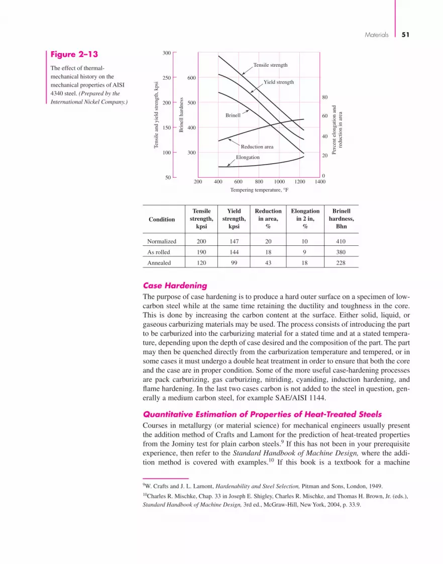
Materials 51
50
100
150
200
250
300
300
400
500
600
200 400 600 800 1000 1200 14000
20
40
60
80
Tempering temperature, °F
Bri
nell
hard
ness
Perc
ent e
long
atio
n an
dre
duct
ion
in a
rea
Tens
ile a
nd y
ield
str
engt
h, k
psi
Condition
Normalized
As rolled
Annealed
Tensilestrength,
kpsi
Yieldstrength,
kpsi
Reductionin area,
%
Elongationin 2 in,
%
Brinellhardness,
Bhn
200
190
120
147
144
99
20
18
43
10
9
18
410
380
228
Tensile strength
Yield strength
Brinell
Reduction area
Elongation
Figure 2–13
The effect of thermal-mechanical history on themechanical properties of AISI4340 steel. (Prepared by theInternational Nickel Company.)
9W. Crafts and J. L. Lamont, Hardenability and Steel Selection, Pitman and Sons, London, 1949. 10Charles R. Mischke, Chap. 33 in Joseph E. Shigley, Charles R. Mischke, and Thomas H. Brown, Jr. (eds.), Standard Handbook of Machine Design, 3rd ed., McGraw-Hill, New York, 2004, p. 33.9.
Case Hardening
The purpose of case hardening is to produce a hard outer surface on a specimen of low-carbon steel while at the same time retaining the ductility and toughness in the core.This is done by increasing the carbon content at the surface. Either solid, liquid, orgaseous carburizing materials may be used. The process consists of introducing the partto be carburized into the carburizing material for a stated time and at a stated tempera-ture, depending upon the depth of case desired and the composition of the part. The partmay then be quenched directly from the carburization temperature and tempered, or insome cases it must undergo a double heat treatment in order to ensure that both the coreand the case are in proper condition. Some of the more useful case-hardening processesare pack carburizing, gas carburizing, nitriding, cyaniding, induction hardening, andflame hardening. In the last two cases carbon is not added to the steel in question, gen-erally a medium carbon steel, for example SAE/AISI 1144.
Quantitative Estimation of Properties of Heat-Treated Steels
Courses in metallurgy (or material science) for mechanical engineers usually presentthe addition method of Crafts and Lamont for the prediction of heat-treated propertiesfrom the Jominy test for plain carbon steels.9 If this has not been in your prerequisiteexperience, then refer to the Standard Handbook of Machine Design, where the addi-tion method is covered with examples.10 If this book is a textbook for a machine
bud29281_ch02_031-070.qxd 11/11/09 09:34 PM Page 51 Debd Hard Disk1:Desktop Folder:Temp Work:Satya 10/11/09:

52 Mechanical Engineering Design
elements course, it is a good class project (many hands make light work) to study themethod and report to the class.
For low-alloy steels, the multiplication method of Grossman11 and Field12 isexplained in the Standard Handbook of Machine Design (Secs. 29.6 and 33.6).
Modern Steels and Their Properties Handbook explains how to predict the Jominycurve by the method of Grossman and Field from a ladle analysis and grain size.13
Bethlehem Steel has developed a circular plastic slide rule that is convenient to the purpose.
2–15 Alloy SteelsAlthough a plain carbon steel is an alloy of iron and carbon with small amounts ofmanganese, silicon, sulfur, and phosphorus, the term alloy steel is applied when one ormore elements other than carbon are introduced in sufficient quantities to modify itsproperties substantially. The alloy steels not only possess more desirable physicalproperties but also permit a greater latitude in the heat-treating process.
Chromium
The addition of chromium results in the formation of various carbides of chromium thatare very hard, yet the resulting steel is more ductile than a steel of the same hardness pro-duced by a simple increase in carbon content. Chromium also refines the grain structureso that these two combined effects result in both increased toughness and increased hard-ness. The addition of chromium increases the critical range of temperatures and movesthe eutectoid point to the left. Chromium is thus a very useful alloying element.
Nickel
The addition of nickel to steel also causes the eutectoid point to move to the left andincreases the critical range of temperatures. Nickel is soluble in ferrite and does notform carbides or oxides. This increases the strength without decreasing the ductility.Case hardening of nickel steels results in a better core than can be obtained with plaincarbon steels. Chromium is frequently used in combination with nickel to obtain thetoughness and ductility provided by the nickel and the wear resistance and hardnesscontributed by the chromium.
Manganese
Manganese is added to all steels as a deoxidizing and desulfurizing agent, but if the sul-fur content is low and the manganese content is over 1 percent, the steel is classified as amanganese alloy. Manganese dissolves in the ferrite and also forms carbides. It causesthe eutectoid point to move to the left and lowers the critical range of temperatures. Itincreases the time required for transformation so that oil quenching becomes practicable.
Silicon
Silicon is added to all steels as a deoxidizing agent. When added to very-low-carbonsteels, it produces a brittle material with a low hysteresis loss and a high magneticpermeability. The principal use of silicon is with other alloying elements, such asmanganese, chromium, and vanadium, to stabilize the carbides.
11M. A. Grossman, AIME, February 1942.12J. Field, Metals Progress, March 1943.13Modern Steels and Their Properties, 7th ed., Handbook 2757, Bethlehem Steel, 1972, pp. 46–50.
bud29281_ch02_031-070.qxd 11/11/09 09:34 PM Page 52 Debd Hard Disk1:Desktop Folder:Temp Work:Satya 10/11/09:

Materials 53
Molybdenum
While molybdenum is used alone in a few steels, it finds its greatest use when combinedwith other alloying elements, such as nickel, chromium, or both. Molybdenum formscarbides and also dissolves in ferrite to some extent, so that it adds both hardness andtoughness. Molybdenum increases the critical range of temperatures and substantiallylowers the transformation point. Because of this lowering of the transformation point,molybdenum is most effective in producing desirable oil-hardening and air-hardeningproperties. Except for carbon, it has the greatest hardening effect, and because it alsocontributes to a fine grain size, this results in the retention of a great deal of toughness.
Vanadium
Vanadium has a very strong tendency to form carbides; hence it is used only in smallamounts. It is a strong deoxidizing agent and promotes a fine grain size. Since some vana-dium is dissolved in the ferrite, it also toughens the steel. Vanadium gives a wide harden-ing range to steel, and the alloy can be hardened from a higher temperature. It is verydifficult to soften vanadium steel by tempering; hence, it is widely used in tool steels.
Tungsten
Tungsten is widely used in tool steels because the tool will maintain its hardness evenat red heat. Tungsten produces a fine, dense structure and adds both toughness and hard-ness. Its effect is similar to that of molybdenum, except that it must be added in greaterquantities.
2–16 Corrosion-Resistant SteelsIron-base alloys containing at least 12 percent chromium are called stainless steels.The most important characteristic of these steels is their resistance to many, but not all,corrosive conditions. The four types available are the ferritic chromium steels, theaustenitic chromium-nickel steels, and the martensitic and precipitation-hardenablestainless steels.
The ferritic chromium steels have a chromium content ranging from 12 to 27 per-cent. Their corrosion resistance is a function of the chromium content, so that alloyscontaining less than 12 percent still exhibit some corrosion resistance, although theymay rust. The quench-hardenability of these steels is a function of both the chromiumand the carbon content. The very high carbon steels have good quench hardenability upto about 18 percent chromium, while in the lower carbon ranges it ceases at about13 percent. If a little nickel is added, these steels retain some degree of hardenability upto 20 percent chromium. If the chromium content exceeds 18 percent, they become dif-ficult to weld, and at the very high chromium levels the hardness becomes so great thatvery careful attention must be paid to the service conditions. Since chromium is expen-sive, the designer will choose the lowest chromium content consistent with the corro-sive conditions.
The chromium-nickel stainless steels retain the austenitic structure at room tem-perature; hence, they are not amenable to heat treatment. The strength of these steelscan be greatly improved by cold working. They are not magnetic unless cold-worked.Their work hardenability properties also cause them to be difficult to machine. Allthe chromium-nickel steels may be welded. They have greater corrosion-resistant prop-erties than the plain chromium steels. When more chromium is added for greater cor-rosion resistance, more nickel must also be added if the austenitic properties are to beretained.
bud29281_ch02_031-070.qxd 11/11/09 09:34 PM Page 53 Debd Hard Disk1:Desktop Folder:Temp Work:Satya 10/11/09:

54 Mechanical Engineering Design
2–17 Casting MaterialsGray Cast Iron
Of all the cast materials, gray cast iron is the most widely used. This is because it hasa very low cost, is easily cast in large quantities, and is easy to machine. The principalobjections to the use of gray cast iron are that it is brittle and that it is weak in tension.In addition to a high carbon content (over 1.7 percent and usually greater than 2 percent),cast iron also has a high silicon content, with low percentages of sulfur, manganese,and phosphorus. The resultant alloy is composed of pearlite, ferrite, and graphite, andunder certain conditions the pearlite may decompose into graphite and ferrite. Theresulting product then contains all ferrite and graphite. The graphite, in the form ofthin flakes distributed evenly throughout the structure, darkens it; hence, the name graycast iron.
Gray cast iron is not readily welded, because it may crack, but this tendency maybe reduced if the part is carefully preheated. Although the castings are generally used inthe as-cast condition, a mild anneal reduces cooling stresses and improves the machin-ability. The tensile strength of gray cast iron varies from 100 to 400 MPa (15 to 60 kpsi),and the compressive strengths are 3 to 4 times the tensile strengths. The modulus ofelasticity varies widely, with values extending all the way from 75 to 150 GPa (11 to22 Mpsi).
Ductile and Nodular Cast Iron
Because of the lengthy heat treatment required to produce malleable cast iron, engineershave long desired a cast iron that would combine the ductile properties of malleableiron with the ease of casting and machining of gray iron and at the same time wouldpossess these properties in the as-cast conditions. A process for producing such a materialusing magnesium-containing material seems to fulfill these requirements.
Ductile cast iron, or nodular cast iron, as it is sometimes called, is essentially thesame as malleable cast iron, because both contain graphite in the form of spheroids.However, ductile cast iron in the as-cast condition exhibits properties very close tothose of malleable iron, and if a simple 1-h anneal is given and is followed by a slowcool, it exhibits even more ductility than the malleable product. Ductile iron is made byadding MgFeSi to the melt; since magnesium boils at this temperature, it is necessaryto alloy it with other elements before it is introduced.
Ductile iron has a high modulus of elasticity (172 GPa or 25 Mpsi) as comparedwith gray cast iron, and it is elastic in the sense that a portion of the stress-straincurve is a straight line. Gray cast iron, on the other hand, does not obey Hooke’s law,because the modulus of elasticity steadily decreases with increase in stress. Likegray cast iron, however, nodular iron has a compressive strength that is higher thanthe tensile strength, although the difference is not as great. In 40 years it has becomeextensively used.
White Cast Iron
If all the carbon in cast iron is in the form of cementite and pearlite, with no graphitepresent, the resulting structure is white and is known as white cast iron. This may beproduced in two ways. The composition may be adjusted by keeping the carbon andsilicon content low, or the gray-cast-iron composition may be cast against chills in orderto promote rapid cooling. By either method, a casting with large amounts of cementiteis produced, and as a result the product is very brittle and hard to machine but also veryresistant to wear. A chill is usually used in the production of gray-iron castings in order
bud29281_ch02_031-070.qxd 11/11/09 09:34 PM Page 54 Debd Hard Disk1:Desktop Folder:Temp Work:Satya 10/11/09:

Materials 55
to provide a very hard surface within a particular area of the casting, while at the sametime retaining the more desirable gray structure within the remaining portion. This pro-duces a relatively tough casting with a wear-resistant area.
Malleable Cast Iron
If white cast iron within a certain composition range is annealed, a product calledmalleable cast iron is formed. The annealing process frees the carbon so that it is pres-ent as graphite, just as in gray cast iron but in a different form. In gray cast iron thegraphite is present in a thin flake form, while in malleable cast iron it has a nodularform and is known as temper carbon. A good grade of malleable cast iron may havea tensile strength of over 350 MPa (50 kpsi), with an elongation of as much as 18 per-cent. The percentage elongation of a gray cast iron, on the other hand, is seldom over1 percent. Because of the time required for annealing (up to 6 days for large andheavy castings), malleable iron is necessarily somewhat more expensive than graycast iron.
Alloy Cast Irons
Nickel, chromium, and molybdenum are the most common alloying elements used incast iron. Nickel is a general-purpose alloying element, usually added in amounts up to5 percent. Nickel increases the strength and density, improves the wearing qualities, andraises the machinability. If the nickel content is raised to 10 to 18 percent, an austeniticstructure with valuable heat- and corrosion-resistant properties results. Chromiumincreases the hardness and wear resistance and, when used with a chill, increases thetendency to form white iron. When chromium and nickel are both added, the hardnessand strength are improved without a reduction in the machinability rating. Molybdenumadded in quantities up to 1.25 percent increases the stiffness, hardness, tensile strength,and impact resistance. It is a widely used alloying element.
Cast Steels
The advantage of the casting process is that parts having complex shapes can be man-ufactured at costs less than fabrication by other means, such as welding. Thus thechoice of steel castings is logical when the part is complex and when it must also havea high strength. The higher melting temperatures for steels do aggravate the castingproblems and require closer attention to such details as core design, section thicknesses,fillets, and the progress of cooling. The same alloying elements used for the wroughtsteels can be used for cast steels to improve the strength and other mechanical proper-ties. Cast-steel parts can also be heat-treated to alter the mechanical properties, and,unlike the cast irons, they can be welded.
2–18 Nonferrous MetalsAluminum
The outstanding characteristics of aluminum and its alloys are their strength-weightratio, their resistance to corrosion, and their high thermal and electrical conductivity.The density of aluminum is about 2770 kg/m3 (0.10 lbf/in3), compared with 7750 kg/m3
(0.28 lbf/in3) for steel. Pure aluminum has a tensile strength of about 90 MPa (13 kpsi),but this can be improved considerably by cold working and also by alloying with othermaterials. The modulus of elasticity of aluminum, as well as of its alloys, is 71.7 GPa(10.4 Mpsi), which means that it has about one-third the stiffness of steel.
bud29281_ch02_031-070.qxd 11/11/09 09:34 PM Page 55 Debd Hard Disk1:Desktop Folder:Temp Work:Satya 10/11/09:

56 Mechanical Engineering Design
Considering the cost and strength of aluminum and its alloys, they are among themost versatile materials from the standpoint of fabrication. Aluminum can be processedby sand casting, die casting, hot or cold working, or extruding. Its alloys can be machined,press-worked, soldered, brazed, or welded. Pure aluminum melts at 660°C (1215°F),which makes it very desirable for the production of either permanent or sand-moldcastings. It is commercially available in the form of plate, bar, sheet, foil, rod, and tubeand in structural and extruded shapes. Certain precautions must be taken in joiningaluminum by soldering, brazing, or welding; these joining methods are not recommendedfor all alloys.
The corrosion resistance of the aluminum alloys depends upon the formation of athin oxide coating. This film forms spontaneously because aluminum is inherently veryreactive. Constant erosion or abrasion removes this film and allows corrosion to takeplace. An extra-heavy oxide film may be produced by the process called anodizing. Inthis process the specimen is made to become the anode in an electrolyte, which may bechromic acid, oxalic acid, or sulfuric acid. It is possible in this process to control thecolor of the resulting film very accurately.
The most useful alloying elements for aluminum are copper, silicon, manganese,magnesium, and zinc. Aluminum alloys are classified as casting alloys or wroughtalloys. The casting alloys have greater percentages of alloying elements to facilitatecasting, but this makes cold working difficult. Many of the casting alloys, and some ofthe wrought alloys, cannot be hardened by heat treatment. The alloys that are heat-treatable use an alloying element that dissolves in the aluminum. The heat treatmentconsists of heating the specimen to a temperature that permits the alloying element topass into solution, then quenching so rapidly that the alloying element is not precipi-tated. The aging process may be accelerated by heating slightly, which results in evengreater hardness and strength. One of the better-known heat-treatable alloys is duralu-minum, or 2017 (4 percent Cu, 0.5 percent Mg, 0.5 percent Mn). This alloy hardens in4 days at room temperature. Because of this rapid aging, the alloy must be stored underrefrigeration after quenching and before forming, or it must be formed immediatelyafter quenching. Other alloys (such as 5053) have been developed that age-harden muchmore slowly, so that only mild refrigeration is required before forming. After forming,they are artificially aged in a furnace and possess approximately the same strength andhardness as the 2024 alloys. Those alloys of aluminum that cannot be heat-treated canbe hardened only by cold working. Both work hardening and the hardening producedby heat treatment may be removed by an annealing process.
Magnesium
The density of magnesium is about 1800 kg/m3 (0.065 lb/in3), which is two-thirds thatof aluminum and one-fourth that of steel. Since it is the lightest of all commercial met-als, its greatest use is in the aircraft and automotive industries, but other uses are nowbeing found for it. Although the magnesium alloys do not have great strength, becauseof their light weight the strength-weight ratio compares favorably with the strongeraluminum and steel alloys. Even so, magnesium alloys find their greatest use in appli-cations where strength is not an important consideration. Magnesium will not withstandelevated temperatures; the yield point is definitely reduced when the temperature israised to that of boiling water.
Magnesium and its alloys have a modulus of elasticity of 45 GPa (6.5 Mpsi) in ten-sion and in compression, although some alloys are not as strong in compression as intension. Curiously enough, cold working reduces the modulus of elasticity. A range ofcast magnesium alloys are also available.
bud29281_ch02_031-070.qxd 11/11/09 09:34 PM Page 56 Debd Hard Disk1:Desktop Folder:Temp Work:Satya 10/11/09:

Materials 57
Titanium
Titanium and its alloys are similar in strength to moderate-strength steel but weigh halfas much as steel. The material exhibits very good resistence to corrosion, has low ther-mal conductivity, is nonmagnetic, and has high-temperature strength. Its modulus ofelasticity is between those of steel and aluminum at 16.5 Mpsi (114 GPa). Because ofits many advantages over steel and aluminum, applications include: aerospace and mil-itary aircraft structures and components, marine hardware, chemical tanks and process-ing equipment, fluid handling systems, and human internal replacement devices. Thedisadvantages of titanium are its high cost compared to steel and aluminum and the dif-ficulty of machining it.
Copper-Base Alloys
When copper is alloyed with zinc, it is usually called brass. If it is alloyed with anotherelement, it is often called bronze. Sometimes the other element is specified too, as, for ex-ample, tin bronze or phosphor bronze. There are hundreds of variations in each category.
Brass with 5 to 15 Percent ZincThe low-zinc brasses are easy to cold work, especially those with the higher zinc con-tent. They are ductile but often hard to machine. The corrosion resistance is good. Alloysincluded in this group are gilding brass (5 percent Zn), commercial bronze (10 percent Zn),and red brass (15 percent Zn). Gilding brass is used mostly for jewelry and articles tobe gold-plated; it has the same ductility as copper but greater strength, accompanied bypoor machining characteristics. Commercial bronze is used for jewelry and for forgingsand stampings, because of its ductility. Its machining properties are poor, but it hasexcellent cold-working properties. Red brass has good corrosion resistance as well ashigh-temperature strength. Because of this it is used a great deal in the form of tubing orpiping to carry hot water in such applications as radiators or condensers.
Brass with 20 to 36 Percent ZincIncluded in the intermediate-zinc group are low brass (20 percent Zn), cartridge brass(30 percent Zn), and yellow brass (35 percent Zn). Since zinc is cheaper than copper,these alloys cost less than those with more copper and less zinc. They also have bettermachinability and slightly greater strength; this is offset, however, by poor corrosionresistance and the possibility of cracking at points of residual stresses. Low brass is verysimilar to red brass and is used for articles requiring deep-drawing operations. Of thecopper-zinc alloys, cartridge brass has the best combination of ductility and strength.Cartridge cases were originally manufactured entirely by cold working; the processconsisted of a series of deep draws, each draw being followed by an anneal to place thematerial in condition for the next draw, hence the name cartridge brass. Although thehot-working ability of yellow brass is poor, it can be used in practically any other fab-ricating process and is therefore employed in a large variety of products.
When small amounts of lead are added to the brasses, their machinability is greatlyimproved and there is some improvement in their abilities to be hot-worked. Theaddition of lead impairs both the cold-working and welding properties. In this group arelow-leaded brass (32 1
2 percent Zn, 12 percent Pb), high-leaded brass (34 percent Zn,
2 percent Pb), and free-cutting brass (35 12 percent Zn, 3 percent Pb). The low-leaded
brass is not only easy to machine but has good cold-working properties. It is used forvarious screw-machine parts. High-leaded brass, sometimes called engraver’s brass, isused for instrument, lock, and watch parts. Free-cutting brass is also used for screw-machine parts and has good corrosion resistance with excellent mechanical properties.
bud29281_ch02_031-070.qxd 11/11/09 09:34 PM Page 57 Debd Hard Disk1:Desktop Folder:Temp Work:Satya 10/11/09:

58 Mechanical Engineering Design
Admiralty metal (28 percent Zn) contains 1 percent tin, which imparts excellent cor-rosion resistance, especially to saltwater. It has good strength and ductility but only fairmachining and working characteristics. Because of its corrosion resistance it is used inpower-plant and chemical equipment. Aluminum brass (22 percent Zn) contains 2 percentaluminum and is used for the same purposes as admiralty metal, because it has nearly thesame properties and characteristics. In the form of tubing or piping, it is favored overadmiralty metal, because it has better resistance to erosion caused by high-velocity water.
Brass with 36 to 40 Percent ZincBrasses with more than 38 percent zinc are less ductile than cartridge brass and cannotbe cold-worked as severely. They are frequently hot-worked and extruded. Muntz metal(40 percent Zn) is low in cost and mildly corrosion-resistant. Naval brass has the samecomposition as Muntz metal except for the addition of 0.75 percent tin, which con-tributes to the corrosion resistance.
BronzeSilicon bronze, containing 3 percent silicon and 1 percent manganese in addition to thecopper, has mechanical properties equal to those of mild steel, as well as good corro-sion resistance. It can be hot- or cold-worked, machined, or welded. It is useful wher-ever corrosion resistance combined with strength is required.
Phosphor bronze, made with up to 11 percent tin and containing small amounts ofphosphorus, is especially resistant to fatigue and corrosion. It has a high tensile strengthand a high capacity to absorb energy, and it is also resistant to wear. These propertiesmake it very useful as a spring material.
Aluminum bronze is a heat-treatable alloy containing up to 12 percent aluminum. Thisalloy has strength and corrosion-resistance properties that are better than those of brass, andin addition, its properties may be varied over a wide range by cold working, heat treating,or changing the composition. When iron is added in amounts up to 4 percent, the alloy hasa high endurance limit, a high shock resistance, and excellent wear resistance.
Beryllium bronze is another heat-treatable alloy, containing about 2 percent beryl-lium. This alloy is very corrosion resistant and has high strength, hardness, and resis-tance to wear. Although it is expensive, it is used for springs and other parts subjectedto fatigue loading where corrosion resistance is required.
With slight modification most copper-based alloys are available in cast form.
2–19 PlasticsThe term thermoplastics is used to mean any plastic that flows or is moldable when heatis applied to it; the term is sometimes applied to plastics moldable under pressure. Suchplastics can be remolded when heated.
A thermoset is a plastic for which the polymerization process is finished in a hotmolding press where the plastic is liquefied under pressure. Thermoset plastics cannotbe remolded.
Table 2–2 lists some of the most widely used thermoplastics, together with someof their characteristics and the range of their properties. Table 2–3, listing some of thethermosets, is similar. These tables are presented for information only and should notbe used to make a final design decision. The range of properties and characteristics thatcan be obtained with plastics is very great. The influence of many factors, such as cost,moldability, coefficient of friction, weathering, impact strength, and the effect of fillersand reinforcements, must be considered. Manufacturers’ catalogs will be found quitehelpful in making possible selections.
bud29281_ch02_031-070.qxd 11/11/09 09:34 PM Page 58 Debd Hard Disk1:Desktop Folder:Temp Work:Satya 10/11/09:

Materials 59
Table 2–2
The Thermoplastics Source: These data have been obtained from the Machine Design Materials Reference Issue, published by Penton/IPC,Cleveland. These reference issues are published about every 2 years and constitute an excellent source of data on a great variety of materials.
Table 2–3
The Thermosets Source: These data have been obtained from the Machine Design Materials Reference Issue, published by Penton/IPC,Cleveland. These reference issues are published about every 2 years and constitute an excellent source of data on a great variety of materials.
Su E Hardness Elongation Dimensional Heat ChemicalName kpsi Mpsi Rockwell % Stability Resistance Resistance Processing
ABS group 2–8 0.10–0.37 60–110R 3–50 Good * Fair EMST
Acetal group 8–10 0.41–0.52 80–94M 40–60 Excellent Good High M
Acrylic 5–10 0.20–0.47 92–110M 3–75 High * Fair EMS
Fluoroplastic 0.50–7 · · · 50–80D 100–300 High Excellent Excellent MPR†
group
Nylon 8–14 0.18–0.45 112–120R 10–200 Poor Poor Good CEM
Phenylene 7–18 0.35–0.92 115R, 106L 5–60 Excellent Good Fair EFMoxide
Polycarbonate 8–16 0.34–0.86 62–91M 10–125 Excellent Excellent Fair EMS
Polyester 8–18 0.28–1.6 65–90M 1–300 Excellent Poor Excellent CLMR
Polyimide 6–50 · · · 88–120M Very low Excellent Excellent Excellent† CLMP
Polyphenylene 14–19 0.11 122R 1.0 Good Excellent Excellent Msulfide
Polystyrene 1.5–12 0.14–0.60 10–90M 0.5–60 · · · Poor Poor EMgroup
Polysulfone 10 0.36 120R 50–100 Excellent Excellent Excellent† EFM
Polyvinyl 1.5–7.5 0.35–0.60 65–85D 40–450 · · · Poor Poor EFMchloride
*Heat-resistant grades available.†With exceptions.C Coatings L Laminates R Resins E Extrusions M Moldings S Sheet F Foams P Press and sinter methods T Tubing
Su E Hardness Elongation Dimensional Heat ChemicalName kpsi Mpsi Rockwell % Stability Resistance Resistance Processing
Alkyd 3–9 0.05–0.30 99M* · · · Excellent Good Fair M
Allylic 4–10 · · · 105–120M · · · Excellent Excellent Excellent CM
Amino 5–8 0.13–0.24 110–120M 0.30–0.90 Good Excellent* Excellent* LRgroup
Epoxy 5–20 0.03–0.30* 80–120M 1–10 Excellent Excellent Excellent CMR
Phenolics 5–9 0.10–0.25 70–95E · · · Excellent Excellent Good EMR
Silicones 5–6 · · · 80–90M · · · · · · Excellent Excellent CLMR
*With exceptions.C Coatings L Laminates R Resins E Extrusions M Moldings S Sheet F Foams P Press and sinter methods T Tubing
bud29281_ch02_031-070.qxd 11/12/2009 7:59 pm Page 59 pinnacle s-171:Desktop Folder:Temp Work:Don't Delete (Jobs):MHDQ196/Budynas:

60 Mechanical Engineering Design
2–20 Composite Materials14
Composite materials are formed from two or more dissimilar materials, each of whichcontributes to the final properties. Unlike metallic alloys, the materials in a compositeremain distinct from each other at the macroscopic level.
Most engineering composites consist of two materials: a reinforcement called afiller and a matrix. The filler provides stiffness and strength; the matrix holds the mate-rial together and serves to transfer load among the discontinuous reinforcements. Themost common reinforcements, illustrated in Fig. 2–14, are continuous fibers, eitherstraight or woven, short chopped fibers, and particulates. The most common matricesare various plastic resins although other materials including metals are used.
Metals and other traditional engineering materials are uniform, or isotropic, in nature.This means that material properties, such as strength, stiffness, and thermal conductivity,are independent of both position within the material and the choice of coordinate system.The discontinuous nature of composite reinforcements, though, means that material prop-erties can vary with both position and direction. For example, an epoxy resin reinforcedwith continuous graphite fibers will have very high strength and stiffness in the directionof the fibers, but very low properties normal or transverse to the fibers. For this reason,structures of composite materials are normally constructed of multiple plies (laminates)where each ply is oriented to achieve optimal structural stiffness and strength performance.
High strength-to-weight ratios, up to 5 times greater than those of high-strengthsteels, can be achieved. High stiffness-to-weight ratios can also be obtained, as much as8 times greater than those of structural metals. For this reason, composite materials arebecoming very popular in automotive, marine, aircraft, and spacecraft applicationswhere weight is a premium.
The directionality of properties of composite materials increases the complexity ofstructural analyses. Isotropic materials are fully defined by two engineering constants:Young’s modulus E and Poisson’s ratio ν. A single ply of a composite material, however,requires four constants, defined with respect to the ply coordinate system. The constantsare two Young’s moduli (the longitudinal modulus in the direction of the fibers, E1, andthe transverse modulus normal to the fibers, E2), one Poisson’s ratio (ν12, called the majorPoisson’s ratio), and one shear modulus (G12). A fifth constant, the minor Poisson’s ratio,ν21, is determined through the reciprocity relation, ν21/E2 = ν12/E1. Combining thiswith multiple plies oriented at different angles makes structural analysis of complex struc-tures unapproachable by manual techniques. For this reason, computer software is avail-able to calculate the properties of a laminated composite construction.15
Particulatecomposite
Randomly orientedshort fiber composite
Unidirectional continuousfiber composite
Woven fabriccomposite
Figure 2–14
Composites categorized bytype of reinforcement.
14For references see I. M. Daniel and O. Ishai, Engineering Mechanics of Composite Materials, OxfordUniversity Press, 1994, and ASM Engineered Materials Handbook: Composites, ASM International,Materials Park, OH, 1988.15About Composite Materials Software listing, http://composite.about.com/cs/software/index.htm.
bud29281_ch02_031-070.qxd 11/11/09 09:34 PM Page 60 Debd Hard Disk1:Desktop Folder:Temp Work:Satya 10/11/09:

Materials 61
2–21 Materials SelectionAs stated earlier, the selection of a material for a machine part or structural member isone of the most important decisions the designer is called on to make. Up to this pointin this chapter we have discussed many important material physical properties, variouscharacteristics of typical engineering materials, and various material production pro-cesses. The actual selection of a material for a particular design application can be aneasy one, say, based on previous applications (1020 steel is always a good candidatebecause of its many positive attributes), or the selection process can be as involved anddaunting as any design problem with the evaluation of the many material physical, eco-nomical, and processing parameters. There are systematic and optimizing approachesto material selection. Here, for illustration, we will only look at how to approach somematerial properties. One basic technique is to list all the important material propertiesassociated with the design, e.g., strength, stiffness, and cost. This can be prioritized byusing a weighting measure depending on what properties are more important thanothers. Next, for each property, list all available materials and rank them in order begin-ning with the best material; e.g., for strength, high-strength steel such as 4340 steelshould be near the top of the list. For completeness of available materials, this mightrequire a large source of material data. Once the lists are formed, select a manageableamount of materials from the top of each list. From each reduced list select the materi-als that are contained within every list for further review. The materials in the reducedlists can be graded within the list and then weighted according to the importance ofeach property.
M. F. Ashby has developed a powerful systematic method using materials selec-tion charts.16 This method has also been implemented in a software package calledCES Edupack.17 The charts display data of various properties for the families andclasses of materials listed in Table 2–4. For example, considering material stiffnessproperties, a simple bar chart plotting Young’s modulus E on the y axis is shown
16M. F. Ashby, Materials Selection in Mechanical Design, 3rd ed., Elsevier Butterworth-Heinemann,Oxford, 2005.17Produced by Granta Design Limited. See www.grantadesign.com.
Family Classes Short Name
Aluminum alloys Al alloysCopper alloys Cu alloysLead alloys Lead alloysMagnesium alloys Mg alloysNickel alloys Ni alloysCarbon steels SteelsStainless steels Stainless steelsTin alloys Tin alloysTitanium alloys Ti alloysTungsten alloys W alloysLead alloys Pb alloysZinc alloys Zn alloys
Metals(the metals and alloys ofengineering)
Table 2–4
Material Families and
Classes
(continued)
bud29281_ch02_031-070.qxd 11/11/09 09:34 PM Page 61 Debd Hard Disk1:Desktop Folder:Temp Work:Satya 10/11/09:

Family Classes Short Name
Alumina Al2O3
Aluminum nitride AlNBoron carbide B4CSilicon carbide SiCSilicon nitride Si3N4
Tungsten carbide WCBrick BrickConcrete ConcreteStone Stone
Soda-lime glass Soda-lime glassBorosilicate glass Borosilicate glassSilica glass Silica glassGlass ceramic Glass ceramic
Acrylonitrile butadiene styrene ABSCellulose polymers CAIonomers IonomersEpoxies EpoxyPhenolics PhenolicsPolyamides (nylons) PAPolycarbonate PCPolyesters Polyester Polyetheretherkeytone PEEKPolyethylene PEPolyethylene terephalate PET or PETEPolymethylmethacrylate PMMAPolyoxymethylene(Acetal) POMPolypropylene PPPolystyrene PSPolytetrafluorethylene PTFEPolyvinylchloride PVC
Butyl rubber Butyl rubberEVA EVAIsoprene IsopreneNatural rubber Natural rubberPolychloroprene (Neoprene) NeoprenePolyurethane PUSilicon elastomers Silicones
Carbon-fiber reinforced polymers CFRPGlass-fiber reinforced polymers GFRPSiC reinforced aluminum Al-SiCFlexible polymer foams Flexible foamsRigid polymer foams Rigid foamsCork CorkBamboo BambooWood Wood
From M. F. Ashby, Materials Selection in Mechanical Design, 3rd ed., Elsevier Butterworth-Heinemann,Oxford, 2005. Table 4–1, pp. 49–50.
CeramicsTechnical ceramics (fineceramics capable of load-bearing application)
Nontechnical ceramics(porous ceramics ofconstruction)
Glasses
Polymers(the thermoplastics andthermosets of engineering)
Elastomers(engineering rubbers, naturaland synthetic)
HybridsComposites
Foams
Natural materials
Table 2–4 (continued)
62
bud29281_ch02_031-070.qxd 11/12/2009 8:00 pm Page 62 pinnacle s-171:Desktop Folder:Temp Work:Don't Delete (Jobs):MHDQ196/Budynas:

Materials 63
in Fig. 2–15. Each vertical line represents the range of values of E for a particularmaterial. Only some of the materials are labeled. Now, more material informationcan be displayed if the x axis represents another material property, say density. Figure 2–16, called a “bubble” chart, represents Young’s modulus E plotted againstdensity ρ. The line ranges for each material property plotted two-dimensionally nowform ellipses, or bubbles. Groups of bubbles outlined according to the material familiesof Table 2–4 are also shown. This plot is more useful than the two separate bar chartsof each property. Now, we also see how stiffness/weight for various materials relate.The ratio of Young’s modulus to density, E�r, is known as the specific modulus, orspecific stiffness. This ratio is of particular interest when it is desired to minimizeweight where the primary design limitation is deflection, stiffness, or natural frequency,rather than strength. Machine parts made from materials with higher specific moduluswill exhibit lower deflection, higher stiffness, and higher natural frequency.
In the lower right corner of the chart in Figure 2–16, dotted lines indicate ratios ofEb�r. Several parallel dotted lines are shown for b= 1 that represent different values ofthe specific modulus E�r. This allows simple comparison of the specific modulusbetween materials. It can be seen, for example, that some woods and aluminum alloys haveabout the same specific modulus as steels. Different values of b allow comparisons for
Tungsten carbides
Low-alloy steel
Copper alloys
Nickel alloys
Titanium alloys
Soda-lime glass
GFRP, epoxy matrix (isotropic)
Flexible polymer foam (VLD)
Cast iron, gray
Wood, typical along grain
Acrylonitrile butadiene styrene (ABS)
You
ng's
mod
ulus
, GPa
PolyesterWood, typical across grain
Rigid polymer foam (MD)
Polyurethane
Butyl rubber
1000
100
10
1
0.1
0.01
1e-3
1e-4
Cork
Figure 2–15
Young’s modulus E for various materials. (Figure courtesy of Prof. Mike Ashby, Granta Design, Cambridge, U.K.)
bud29281_ch02_031-070.qxd 11/11/09 09:34 PM Page 63 Debd Hard Disk1:Desktop Folder:Temp Work:Satya 10/11/09:

64 Mechanical Engineering Design
various relationships between stiffness and weight, such as in different loadingconditions. The relationship is linear (β = 1) for axial loading, but nonlinear (β = 1�2)for bending loading [see Eq. (2–31) and its development]. Since the plot is on a log-logscale, the exponential functions still plot as straight lines. The β = 1 lines can also beused to represent constant values of the speed of sound in a material, since the rela-tionship between E and r is linear in the equation for the speed of sound in a material,c = (E�r)1�2. The same can be shown for natural frequency, which is a function of theratio of stiffness to mass.
To see how β fits into the mix, consider the following. The performance metric Pof a structural element depends on (1) the functional requirements, (2) the geometry,and (3) the material properties of the structure. That is,
or, symbolically,
P = f (F, G, M) (2–23)
P � [(functional ),requirements F (material )]properties M
(geometric ),parameters G
1000
100
10
1
Rigid polymerfoams
Longitudinalwave speed
Wood⊥
grain
Wood || grain
PMMA
GFRP
Polyester
CFRP
B4C
Si3N4
Al2O3SiC
Mg alloys
Al alloys
Ti alloysNi alloys
W alloys
Cu alloys
Lead alloysZinc alloys
Concrete
PEEKPET
EpoxiesPC
Metals
WCSteels
Glass
Naturalmaterials
Foams
Polymers
Composites
PA
PS
PP
PE
Leather
EVA
Cork
Flexible polymerfoams Butyl
rubber
Neoprene
Guidelines forminimum mass
design
Polyurethane
Silicone elastomers
Elastomers
Density �, Mg/m3
Isoprene
10�1
104 m/s
103 m/s
102 m/s
10�2
10�3
10�4
0.01 0.1 1 10
E1/2
�
E�
MFA C4
You
ng's
mod
ulus
E, G
Pa
E1/3
�PTFE
Technicalceramics
Figure 2–16
Young’s modulus E versus density ρ for various materials. (Figure courtesy of Prof. Mike Ashby, Granta Design, Cambridge, U.K.)
bud29281_ch02_031-070.qxd 11/12/2009 8:00 pm Page 64 pinnacle s-171:Desktop Folder:Temp Work:Don't Delete (Jobs):MHDQ196/Budynas:

If the function is separable, which it often is, we can write Eq. (2–23) as
P = f1(F) · f2(G) · f3(M) (2–24)
For optimum design, we desire to maximize or minimize P. With regards to materialproperties alone, this is done by maximizing or minimizing f3(M), called the materialefficiency coefficient.
For illustration, say we want to design a light, stiff, end-loaded cantilever beam witha circular cross section. For this we will use the mass m of the beam for the performancemetric to minimize. The stiffness of the beam is related to its material and geometry. Thestiffness of a beam is given by k = F/δ, where F and δ are the end load and deflection,respectively (see Chap. 4). The end deflection of an end-loaded cantilever beam is givenin Table A–9, beam 1, as δ = ymax = (Fl3)/(3E I ), where E is Young’s modulus, I thesecond moment of the area, and l the length of the beam. Thus, the stiffness is given by
k = F
δ= 3E I
l3(2–25)
From Table A–18, the second moment of the area of a circular cross section is
I = π D4
64= A2
4π(2–26)
where D and A are the diameter and area of the cross section, respectively. SubstitutingEq. (2–26) in (2–25) and solving for A, we obtain
A =(
4πkl3
3E
)1/2
(2–27)
The mass of the beam is given by
m = Alρ (2–28)
Substituting Eq. (2–27) into (2–28) and rearranging yields
m = 2
√π
3(k1/2)(l5/2)
( ρ
E1/2
)(2–29)
Equation (2–29) is of the form of Eq. (2–24). The term 2√
π/3 is simply a constant andcan be associated with any function, say f1(F). Thus, f1(F) = 2
√π/3(k1/2) is the func-
tional requirement, stiffness; f2(G) = (l5/2), the geometric parameter, length; and thematerial efficiency coefficient
f3(M) = ρ
E1/2(2–30)
is the material property in terms of density and Young’s modulus. To minimize m wewant to minimize f3(M), or maximize
M = E1/2
ρ(2–31)
where M is called the material index, and β = 12 . Returning to Fig. 2–16, draw lines of
various values of E1/2/ρ as shown in Fig. 2–17. Lines of increasing M move up and tothe left as shown. Thus, we see that good candidates for a light, stiff, end-loaded can-tilever beam with a circular cross section are certain woods, composites, and ceramics.
Other limits/constraints may warrant further investigation. Say, for further illustra-tion, the design requirements indicate that we need a Young’s modulus greater than
Materials 65
bud29281_ch02_031-070.qxd 11/11/09 09:35 PM Page 65 Debd Hard Disk1:Desktop Folder:Temp Work:Satya 10/11/09:

66 Mechanical Engineering Design
IndexE1/2/� � 3
ModulusE � 50 GPa
Modulus–density
Composites
CeramicsMetals
1000
100
10
1
0.1
0.010.1 1 10 100
Woods
Foams Elastomers
Polymers
MFA 04
Density, Mg/m3
You
ng's
mod
ulus
E, G
Pa
Searchregion
Figure 2–18
The search region of Fig. 2–16further reduced by restricting E ≥ 50 GPa, (From M. F.Ashby, Materials Selection inMechanical Design, 3rd ed.,Elsevier Butterworth-Heinemann, Oxford, 2005.)
Figure 2–17
A schematic E versus ρ chartshowing a grid of lines forvarious values the materialindex M = E1/2/ρ. (From M. F. Ashby, Materials Selectionin Mechanical Design, 3rd ed.,Elsevier Butterworth-Heinemann, Oxford, 2005.)
Modulus–density
Composites
CeramicsMetals
31000
100
10
1
0.1
0.010.1 1 10 100
10.3
0.1
Increasing valuesof index E1/2/�
Woods
Foams
E1/2/�(GPa)1/2/(Mg/m)3
Elastomers
Polymers
MFA 04
Density, Mg/m3
You
ng's
mod
ulus
E, G
Pa
Searchregion
50 GPa. Figure 2–18 shows how this further restricts the search region. This eliminateswoods as a possible material.
Another commonly useful chart, shown in Fig. 2–19, represents strength versusdensity for the material families. The ratio of strength to density is known as specificstrength, and is particularly useful when it is desired to minimize weight where the pri-mary design limitation is strength, rather than deflection. The guidelines in the lowerright corner represent different relationships between strength and density, in the formof Sb�r. Following an approach similar to that used before, it can be shown that foraxial loading, b = 1, and for bending loading, b = 2�3.
Certainly, in a given design exercise, there will be other considerations such asenvironment, cost, availability, and machinability, and other charts may be necessary toinvestigate. Also, we have not brought in the material process selection part of the pic-ture. If done properly, material selection can result in a good deal of bookkeeping. Thisis where software packages such as CES Edupack become very effective.
bud29281_ch02_031-070.qxd 11/11/09 09:35 PM Page 66 Debd Hard Disk1:Desktop Folder:Temp Work:Satya 10/11/09:

PROBLEMS2–1 Determine the tensile and yield strengths for the following materials:
(a) UNS G10200 hot-rolled steel.(b) SAE 1050 cold-drawn steel.(c) AISI 1141 steel quenched and tempered at 540°C.(d ) 2024-T4 aluminum alloy.(e) Ti-6Al-4V annealed titanium alloy.
2–2 Assume you were specifying an AISI 1060 steel for an application. Using Table A–21,(a) how would you specify it if you desired to maximize the yield strength?(b) how would you specify it if you desired to maximize the ductility?
2–3 Determine the yield strength-to-weight density ratios (specific strength) in units of kN � m/kg forAISI 1018 CD steel, 2011-T6 aluminum, Ti-6Al-4V titanium alloy, and ASTM No. 40 gray cast iron.
2–4 Determine the stiffness-to-weight density ratios (specific modulus) in units of inches for AISI 1018CD steel, 2011-T6 aluminum, Ti-6Al-4V titanium alloy, and ASTM No. 40 gray cast iron.
2–5 Poisson’s ratio ν is a material property and is the ratio of the lateral strain and the longitudinalstrain for a member in tension. For a homogeneous, isotropic material, the modulus of rigidity Gis related to Young’s modulus as
G = E
2(1 + ν)
Materials 67
Figure 2–19
Strength S versus density ρ for various materials. For metals, S is the 0.2 percent offset yield strength. For polymers, S is the 1 percent yieldstrength. For ceramics and glasses, S is the compressive crushing strength. For composites, S is the tensile strength. For elastomers, S is the tearstrength. (Figure courtesy of Prof. Mike Ashby, Granta Design, Cambridge, U.K.)
Rigid polymerfoams
Wood� to grain
Butylrubber
Cork
Al2O3
Si3N4
Naturalmaterials
Foams
Flexible polymerfoams
CFRP
PA PETPC
PMMA
Al alloys
Ti alloysSteels
Ni alloys
Copperalloys
Zinc alloysLead alloys
Tungstenalloys
Tungstencarbide
SiC
Guide lines forminimum mass
design
Siliconeelastomers
Concrete
S1/2
�
S2/3
�
S�
MFA D4
Polymers andelastomers
Composites
Ceramics
Metals
Density �, Mg/m30.01 0.1 1 10
10000
Stre
ngth
S, M
Pa
1000
100
10
1
0.1
0.01
PPPPA
T
Mg alloys
PEEKGFRP
Strength–density
Metals and polymers yield strengthCeramics and glasses MGRElastomers tensile tear strengthComposites tensile failure
Wood�� to grain
bud29281_ch02_031-070.qxd 11/11/09 09:35 PM Page 67 Debd Hard Disk1:Desktop Folder:Temp Work:Satya 10/11/09:

Using the tabulated values of G and E in Table A–5, calculate Poisson’s ratio for steel, aluminum,beryllium copper, and gray cast iron. Determine the percent difference between the calculatedvalues and the values tabulated in Table A–5.
2–6 A specimen of steel having an initial diameter of 0.503 in was tested in tension using a gaugelength of 2 in. The following data were obtained for the elastic and plastic states:
Note that there is some overlap in the data. (a) Plot the engineering or nominal stress-strain diagram using two scales for the unit strain ε,
one scale from zero to about 0.02 in/in and the other scale from zero to maximum strain.(b) From this diagram find the modulus of elasticity, the 0.2 percent offset yield strength, the ulti-
mate strength, and the percent reduction in area.(c) Characterize the material as ductile or brittle. Explain your reasoning.(d ) Identify a material specification from Table A–20 that has a reasonable match to the data.
2–7 Compute the true stress and the logarithmic strain using the data of Prob. 2–6 and plot the results onlog-log paper. Then find the plastic strength coefficient σ0 and the strain-strengthening exponent m.Find also the yield strength and the ultimate strength after the specimen has had 20 percent cold work.
2–8 The stress-strain data from a tensile test on a cast-iron specimen are
Engineeringstress, kpsi 5 10 16 19 26 32 40 46 49 54
Engineering strain, 0.20 0.44 0.80 1.0 1.5 2.0 2.8 3.4 4.0 5.0� � 10�3 in/in
Plot the stress-strain locus and find the 0.1 percent offset yield strength, and the tangent modulusof elasticity at zero stress and at 20 kpsi.
2–9 A part made from annealed AISI 1018 steel undergoes a 20 percent cold-work operation.(a) Obtain the yield strength and ultimate strength before and after the cold-work operation.
Determine the percent increase in each strength.(b) Determine the ratios of ultimate strength to yield strength before and after the cold-work
operation. What does the result indicate about the change of ductility of the part?
2–10 Repeat Prob. 2–9 for a part made from hot-rolled AISI 1212 steel.
2–11 Repeat Prob. 2–9 for a part made from 2024-T4 aluminum alloy.
2–12 A steel member has a Brinell of HB = 275. Estimate the ultimate strength of the steel in MPa.
Plastic StateLoad P Area Ai
lbf in2
8 800 0.1984
9 200 0.1978
9 100 0.1963
13 200 0.1924
15 200 0.1875
17 000 0.1563
16 400 0.1307
14 800 0.1077
Elastic StateLoad P Elongation
lbf in
1 000 0.0004
2 000 0.0006
3 000 0.0010
4 000 0.0013
7 000 0.0023
8 400 0.0028
8 800 0.0036
9 200 0.0089
68 Mechanical Engineering Design
bud29281_ch02_031-070.qxd 11/11/09 09:35 PM Page 68 Debd Hard Disk1:Desktop Folder:Temp Work:Satya 10/11/09:

2–13 A gray cast iron part has a Brinell hardness number of HB = 200. Estimate the ultimate strengthof the part in kpsi. Make a reasonable assessment of the likely grade of cast iron by comparingboth hardness and strength to material options in Table A–24.
2–14 A part made from 1040 hot-rolled steel is to be heat treated to increase its strength to approxi-mately 100 kpsi. What Brinell hardness number should be expected from the heat-treated part?
2–15 Brinell hardness tests were made on a random sample of 10 steel parts during processing. Theresults were HB values of 230, 232(2), 234, 235(3), 236(2), and 239. Estimate the mean andstandard deviation of the ultimate strength in kpsi.
2–16 Repeat Prob. 2–15 assuming the material to be cast iron.
2–17 For the material in Prob. 2–6: (a) Determine the modulus of resilience, and (b) Estimate the mod-ulus of toughness, assuming that the last data point corresponds to fracture.
2–18 Some commonly used plain carbon steels are AISI 1010, 1018, and 1040. Research these steelsand provide a comparative summary of their characteristics, focusing on aspects that make eachone unique for certain types of application. Product application guides provided on the Internetby steel manufacturers and distributors are one source of information.
2–19 Repeat Prob. 2–18 for the commonly used alloy steels, AISI 4130 and 4340.
2–20 An application requires the support of an axial load of 100 kips with a round rod without exceed-ing the yield strength of the material. Assume the current cost per pound for round stock is givenin the table below for several materials that are being considered. Material properties are avail-able in Tables A–5, A–20, A–21, and A–24. Select one of the materials for each of the followingadditional design goals.(a) Minimize diameter.(b) Minimize weight.(c) Minimize cost.(d) Minimize axial deflection.
Materials 69
Material Cost/lbf
1020 HR $0.27
1020 CD $0.30
1040 Q&T @800°F $0.35
4140 Q&T @800°F $0.80
Wrought Al 2024 T3 $1.10
Titanium alloy (Ti-6Al-4V) $7.00
A 1-in-diameter rod, 3 ft long, of unknown material is found in a machine shop. A variety ofinexpensive nondestructive tests are readily available to help determine the material, as describedbelow:(a) Visual inspection.(b) Scratch test: Scratch the surface with a file; observe color of underlying material and depth
of scratch.(c) Check if it is attracted to a magnet.(d ) Measure weight (±0.05 lbf ).(e) Inexpensive bending deflection test: Clamp one end in a vise, leaving 24 in cantilevered.
Apply a force of 100 lbf (±1 lbf ). Measure deflection of the free end (within ±1�32 in).( f ) Brinell hardness test.
2–21 to2–23
bud29281_ch02_031-070.qxd 11/12/09 8:27 PM Page 69

Choose which tests you would actually perform, and in what sequence, to minimize time andcost, but to determine the material with a reasonable level of confidence. The table below pro-vides results that would be available to you if you choose to perform a given test. Explain yourprocess, and include any calculations. You may assume the material is one listed in Table A–5. Ifit is carbon steel, try to determine an approximate specification from Table A–20.
70 Mechanical Engineering Design
Test Results if test were madeProb. 2–21 Prob. 2–22 Prob. 2–23
(a) Dark gray, rough surface Silvery gray, smooth surface Reddish-brown, tarnished,
finish, moderate scale finish, slightly tarnished smooth surface finish
(b) Metallic gray, moderate Silvery gray, deep scratch Shiny brassy color, deep
scratch scratch
(c) Magnetic Not magnetic Not magnetic
(d) W = 7.95 lbf W = 2.90 lbf W = 9.00 lbf
(e) d = 5�16 in d = 7�8 in d = 17�32 in
( f ) HB = 200 HB = 95 HB = 70
2–24 Search the website noted in Sec. 2–20 (http://composite.about.com/cs/software/) and report yourfindings. Your instructor may wish to elaborate on the level of this report. The website contains alarge variety of resources. The activity for this problem can be divided among the class.
2–25 Research the material Inconel, briefly described in Table A–5. Compare it to various carbon andalloy steels in stiffness, strength, ductility, and toughness. What makes this material so special?
2–26 Consider a rod transmitting a tensile force. The following materials are being considered: tung-sten carbide, high-carbon heat-treated steel, polycarbonate polymer, aluminum alloy. Using theAshby charts, recommend one or two of the materials for a design situation in which failure is byexceeding the strength of the material, and it is desired to minimize the weight.
2–27 Repeat Prob. 2–26, except that the design situation is failure by excessive deflection, and it isdesired to minimize the weight.
2–28 Consider a cantilever beam that is loaded with a transverse force at its tip. The following materialsare being considered: tungsten carbide, high-carbon heat-treated steel, polycarbonate polymer,aluminum alloy. Using the Ashby charts, recommend one or two of the materials for a designsituation in which failure is by exceeding the strength of the material and it is desired to minimizethe weight.
2–29 Repeat Prob. 2–28, except that the design situation is failure by excessive deflection, and it isdesired to minimize the weight.
2–30 For an axially loaded rod, prove that b = 1 for the Eb�r guidelines in Fig. 2–16.
2–31 For an axially loaded rod, prove that b = 1 for the Sb�r guidelines in Fig. 2–19.
2–32 For a cantilever beam loaded in bending, prove that b= 1�2 for the E b�r guidelines in Fig. 2–16.
2–33 For a cantilever beam loaded in bending, prove that b= 2�3 for the Sb�r guidelines in Fig. 2–19.
2–34 Consider a tie rod transmitting a tensile force F. The corresponding tensile stress is given byσ = F/A, where A is the area of the cross section. The deflection of the rod is given by Eq. (4–3),which is δ = (Fl)/(AE), where l is the length of the rod. Using the Ashby charts of Figs. 2–16and 2–19, explore what ductile materials are best suited for a light, stiff, and strong tie rod.Hint: Consider stiffness and strength separately.
bud29281_ch02_031-070.qxd 11/11/09 09:35 PM Page 70 Debd Hard Disk1:Desktop Folder:Temp Work:Satya 10/11/09:

Load and Stress Analysis
Chapter Outline
3–1 Equilibrium and Free-Body Diagrams 72
3–2 Shear Force and Bending Moments in Beams 75
3–3 Singularity Functions 77
3–4 Stress 79
3–5 Cartesian Stress Components 79
3–6 Mohr’s Circle for Plane Stress 80
3–7 General Three-Dimensional Stress 86
3–8 Elastic Strain 87
3–9 Uniformly Distributed Stresses 88
3–10 Normal Stresses for Beams in Bending 89
3–11 Shear Stresses for Beams in Bending 94
3–12 Torsion 101
3–13 Stress Concentration 110
3–14 Stresses in Pressurized Cylinders 113
3–15 Stresses in Rotating Rings 115
3–16 Press and Shrink Fits 116
3–17 Temperature Effects 117
3–18 Curved Beams in Bending 118
3–19 Contact Stresses 122
3–20 Summary 126
3
71
bud29281_ch03_071-146.qxd 11/24/09 3:01PM Page 71 ntt 203:MHDQ196:bud29281:0073529281:bud29281_pagefiles:

72 Mechanical Engineering Design
One of the main objectives of this book is to describe how specific machine componentsfunction and how to design or specify them so that they function safely without failingstructurally. Although earlier discussion has described structural strength in terms ofload or stress versus strength, failure of function for structural reasons may arise fromother factors such as excessive deformations or deflections.
Here it is assumed that the reader has completed basic courses in statics of rigidbodies and mechanics of materials and is quite familiar with the analysis of loads, andthe stresses and deformations associated with the basic load states of simple prismaticelements. In this chapter and Chap. 4 we will review and extend these topics briefly.Complete derivations will not be presented here, and the reader is urged to return tobasic textbooks and notes on these subjects.
This chapter begins with a review of equilibrium and free-body diagrams associatedwith load-carrying components. One must understand the nature of forces beforeattempting to perform an extensive stress or deflection analysis of a mechanical com-ponent. An extremely useful tool in handling discontinuous loading of structuresemploys Macaulay or singularity functions. Singularity functions are described inSec. 3–3 as applied to the shear forces and bending moments in beams. In Chap. 4, theuse of singularity functions will be expanded to show their real power in handlingdeflections of complex geometry and statically indeterminate problems.
Machine components transmit forces and motion from one point to another. Thetransmission of force can be envisioned as a flow or force distribution that can be fur-ther visualized by isolating internal surfaces within the component. Force distributedover a surface leads to the concept of stress, stress components, and stress transforma-tions (Mohr’s circle) for all possible surfaces at a point.
The remainder of the chapter is devoted to the stresses associated with the basicloading of prismatic elements, such as uniform loading, bending, and torsion, and topicswith major design ramifications such as stress concentrations, thin- and thick-walledpressurized cylinders, rotating rings, press and shrink fits, thermal stresses, curved beams,and contact stresses.
3–1 Equilibrium and Free-Body DiagramsEquilibrium
The word system will be used to denote any isolated part or portion of a machine orstructure—including all of it if desired—that we wish to study. A system, under thisdefinition, may consist of a particle, several particles, a part of a rigid body, an entirerigid body, or even several rigid bodies.
If we assume that the system to be studied is motionless or, at most, has constantvelocity, then the system has zero acceleration. Under this condition the system is saidto be in equilibrium. The phrase static equilibrium is also used to imply that the systemis at rest. For equilibrium, the forces and moments acting on the system balance suchthat ∑
F = 0 (3–1)∑M = 0 (3–2)
which states that the sum of all force and the sum of all moment vectors acting upon asystem in equilibrium is zero.
bud29281_ch03_071-146.qxd 11/24/09 3:01PM Page 72 ntt 203:MHDQ196:bud29281:0073529281:bud29281_pagefiles:

Load and Stress Analysis 73
Free-Body Diagrams
We can greatly simplify the analysis of a very complex structure or machine by suc-cessively isolating each element and studying and analyzing it by the use of free-bodydiagrams. When all the members have been treated in this manner, the knowledgeobtained can be assembled to yield information concerning the behavior of the total sys-tem. Thus, free-body diagramming is essentially a means of breaking a complicatedproblem into manageable segments, analyzing these simple problems, and then, usually,putting the information together again.
Using free-body diagrams for force analysis serves the following important purposes:
• The diagram establishes the directions of reference axes, provides a place to recordthe dimensions of the subsystem and the magnitudes and directions of the knownforces, and helps in assuming the directions of unknown forces.
• The diagram simplifies your thinking because it provides a place to store one thoughtwhile proceeding to the next.
• The diagram provides a means of communicating your thoughts clearly and unam-biguously to other people.
• Careful and complete construction of the diagram clarifies fuzzy thinking by bringingout various points that are not always apparent in the statement or in the geometryof the total problem. Thus, the diagram aids in understanding all facets of the problem.
• The diagram helps in the planning of a logical attack on the problem and in settingup the mathematical relations.
• The diagram helps in recording progress in the solution and in illustrating themethods used.
• The diagram allows others to follow your reasoning, showing all forces.
EXAMPLE 3–1 Figure 3–1a shows a simplified rendition of a gear reducer where the input and outputshafts AB and CD are rotating at constant speeds ωi and ωo, respectively. The input andoutput torques (torsional moments) are Ti = 240 lbf · in and To, respectively. The shaftsare supported in the housing by bearings at A, B, C, and D. The pitch radii of gears G1
and G2 are r1 = 0.75 in and r2 = 1.5 in, respectively. Draw the free-body diagrams ofeach member and determine the net reaction forces and moments at all points.
Solution First, we will list all simplifying assumptions.
1 Gears G1 and G2 are simple spur gears with a standard pressure angle φ = 20°(see Sec. 13–5).
2 The bearings are self-aligning and the shafts can be considered to be simplysupported.
3 The weight of each member is negligible.4 Friction is negligible.5 The mounting bolts at E, F, H, and I are the same size.
The separate free-body diagrams of the members are shown in Figs. 3–1b–d. Note thatNewton’s third law, called the law of action and reaction, is used extensively whereeach member mates. The force transmitted between the spur gears is not tangential butat the pressure angle φ. Thus, N = F tan φ.
bud29281_ch03_071-146.qxd 11/24/09 3:01PM Page 73 ntt 203:MHDQ196:bud29281:0073529281:bud29281_pagefiles:

74 Mechanical Engineering Design
Summing moments about the x axis of shaft AB in Fig. 3–1d gives∑Mx = F(0.75) − 240 = 0
F = 320 lbf
The normal force is N = 320 tan 20° = 116.5 lbf.Using the equilibrium equations for Figs. 3–1c and d, the reader should verify that:
RAy = 192 lbf, RAz = 69.9 lbf, RBy = 128 lbf, RBz = 46.6 lbf, RCy = 192 lbf, RCz =69.9 lbf, RDy = 128 lbf, RDz = 46.6 lbf, and To = 480 lbf · in. The direction of the outputtorque To is opposite ωo because it is the resistive load on the system opposing the motion ωo.
Note in Fig. 3–1b the net force from the bearing reactions is zero whereas the netmoment about the x axis is (1.5 + 0.75) (192) + (1.5 + 0.75) (128) = 720 lbf · in. Thisvalue is the same as Ti + To = 240 + 480 = 720 lbf · in, as shown in Fig. 3–1a. Thereaction forces RE , RF , RH , and RI , from the mounting bolts cannot be determinedfrom the equilibrium equations as there are too many unknowns. Only three equationsare available,
∑Fy = ∑
Fz = ∑Mx = 0. In case you were wondering about assump-
tion 5, here is where we will use it (see Sec. 8–12). The gear box tends to rotate aboutthe x axis because of a pure torsional moment of 720 lbf · in. The bolt forces must provide
(a) Gear reducer
5 in
4 in
C
A
I
EB
D
F
H
G2
G1
�o
To
�i, Ti � 240 lbf � in
(c) Input shaft
BTi � 240 lbf � in
G1
r1
RBzRBy
1.5 in1 in
NA
F�
RAzRAy
(d ) Output shaft
D
G2
r2
T0
RDz
RDy
N F�
C
RCzRCy
(b) Gear box
z
y
x5 in
4 in
C
A
I
E
D
F
H
B
RDy
RBy
RBzRDz
RCy
RAy
RAz
RF
RH
RCz
RI
RE
Figure 3–1
(a) Gear reducer; (b–d) free-body diagrams. Diagrams are not drawn to scale.
bud29281_ch03_071-146.qxd 11/24/09 3:01PM Page 74 ntt 203:MHDQ196:bud29281:0073529281:bud29281_pagefiles:

Load and Stress Analysis 75
an equal but opposite torsional moment. The center of rotation relative to the bolts lies atthe centroid of the bolt cross-sectional areas. Thus if the bolt areas are equal: the centerof rotation is at the center of the four bolts, a distance of
√(4/2)2 + (5/2)2 = 3.202 in
from each bolt; the bolt forces are equal (RE = RF = RH = RI = R), and each bolt forceis perpendicular to the line from the bolt to the center of rotation. This gives a net torquefrom the four bolts of 4R(3.202) = 720. Thus, RE = RF = RH = RI = 56.22 lbf.
3–2 Shear Force and Bending Moments in BeamsFigure 3–2a shows a beam supported by reactions R1 and R2 and loaded by the con-centrated forces F1, F2, and F3. If the beam is cut at some section located at x = x1 andthe left-hand portion is removed as a free body, an internal shear force V and bendingmoment M must act on the cut surface to ensure equilibrium (see Fig. 3–2b). The shearforce is obtained by summing the forces on the isolated section. The bending moment isthe sum of the moments of the forces to the left of the section taken about an axis throughthe isolated section. The sign conventions used for bending moment and shear force in thisbook are shown in Fig. 3–3. Shear force and bending moment are related by the equation
V = d M
dx(3–3)
Sometimes the bending is caused by a distributed load q(x), as shown in Fig. 3–4;q(x) is called the load intensity with units of force per unit length and is positive in the
Figure 3–2
Free-body diagram of simply-supported beam with V and Mshown in positive directions.
Figure 3–3
Sign conventions for bendingand shear.
Figure 3–4
Distributed load on beam.
Positive bending
Positive shear Negative shear
Negative bending
x
y q (x)
x1x1
y y
F1 F2 F3 F1
xx
R1 R2 R1
V
M
(a) (b)
bud29281_ch03_071-146.qxd 11/24/09 3:01PM Page 75 ntt 203:MHDQ196:bud29281:0073529281:bud29281_pagefiles:

76 Mechanical Engineering Design
positive y direction. It can be shown that differentiating Eq. (3–3) results in
dV
dx= d2 M
dx2= q (3–4)
Normally the applied distributed load is directed downward and labeled w (e.g., seeFig. 3–6). In this case, w = −q.
Equations (3–3) and (3–4) reveal additional relations if they are integrated. Thus,if we integrate between, say, xA and xB , we obtain∫ VB
VA
dV = VB − VA =∫ xB
xA
q dx (3–5)
which states that the change in shear force from A to B is equal to the area of the load-ing diagram between xA and xB .
In a similar manner,∫ MB
MA
d M = MB − MA =∫ xB
xA
V dx (3–6)
which states that the change in moment from A to B is equal to the area of the shear-force diagram between xA and xB .
Function Graph of fn (x) Meaning
〈x − a〉−2 = 0 x �= a
〈x − a〉−2 = ±∞ x = a∫〈x − a〉−2 dx = 〈x − a〉−1
Concentrated 〈x − a〉−1 = 0 x �= aforce 〈x − a〉−1 = +∞ x = a(unit impulse) ∫
〈x − a〉−1 dx = 〈x − a〉0
Unit step 〈x − a〉0 ={
0 x < a
1 x ≥ a∫〈x − a〉0 dx = 〈x − a〉1
Ramp 〈x − a〉1 ={
0 x < a
x − a x ≥ a∫〈x − a〉1 dx = 〈x − a〉2
2
†W. H. Macaulay, “Note on the deflection of beams,” Messenger of Mathematics, vol. 48, pp. 129–130, 1919.
x
〈x – a〉–2
a
x
〈x – a〉–1
a
x
〈x – a〉0
a
1
x
〈x – a〉1
a
1
1
Table 3–1
Singularity (Macaulay†)
FunctionsConcentratedmoment(unit doublet)
bud29281_ch03_071-146.qxd 11/24/09 3:01PM Page 76 ntt 203:MHDQ196:bud29281:0073529281:bud29281_pagefiles:

Load and Stress Analysis 77
3–3 Singularity FunctionsThe four singularity functions defined in Table 3–1, using the angle brackets 〈 〉, consti-tute a useful and easy means of integrating across discontinuities. By their use, generalexpressions for shear force and bending moment in beams can be written when the beamis loaded by concentrated moments or forces. As shown in the table, the concentratedmoment and force functions are zero for all values of x not equal to a. The functions areundefined for values of x = a. Note that the unit step and ramp functions are zero onlyfor values of x that are less than a. The integration properties shown in the table con-stitute a part of the mathematical definition too. The first two integrations of q(x) forV (x) and M(x) do not require constants of integration provided all loads on the beamare accounted for in q(x). The examples that follow show how these functions are used.
EXAMPLE 3–2 Derive the loading, shear-force, and bending-moment relations for the beam of Fig. 3–5a.
Solution Using Table 3–1 and q(x) for the loading function, we find
Answer q = R1〈x〉−1 − 200〈x − 4〉−1 − 100〈x − 10〉−1 + R2〈x − 20〉−1 (1)
Integrating successively gives
Answer V =∫
q dx = R1〈x〉0 − 200〈x − 4〉0 − 100〈x − 10〉0 + R2〈x − 20〉0 (2)
Answer M =∫
V dx = R1〈x〉1 − 200〈x − 4〉1 − 100〈x − 10〉1 + R2〈x − 20〉1 (3)
Note that V � M � 0 at x � 0�.The reactions R1 and R2 can be found by taking a summation of moments and
forces as usual, or they can be found by noting that the shear force and bending momentmust be zero everywhere except in the region 0 ≤ x ≤ 20 in. This means that Eq. (2)
Figure 3–5
(a) Loading diagram for asimply-supported beam. (b) Shear-force diagram. (c) Bending-moment diagram.
20 in
4 in10 in
200 lbf 100 lbf
y
R1 R2
O
O
O(c)
V (lbf)
(b)
(a)
–90
900
210
10
840
x
x
x
M (lbf in)�
bud29281_ch03_071-146.qxd 11/30/2009 5:03 pm Page 77 pinnacle 203:MHDQ196:bud29281:0073529281:bud29281_pagefiles:

78 Mechanical Engineering Design
should give V = 0 at x slightly larger than 20 in. Thus
R1 − 200 − 100 + R2 = 0 (4)
Since the bending moment should also be zero in the same region, we have, from Eq. (3),
R1(20) − 200(20 − 4) − 100(20 − 10) = 0 (5)
Equations (4) and (5) yield the reactions R1� 210 lbf and R2 � 90 lbf.The reader should verify that substitution of the values of R1 and R2 into Eqs. (2)
and (3) yield Figs. 3–5b and c.
(a)
(b)
D
CBA
y
q
x
10 in
7 in
3 in
R1
M1
20 lbf/in 240 lbf � in
x
V (lbf)
O
StepRamp
(c)
x
M (lbf � in)
O
–160
80
Parabolic Step
80
240
RampSlope = 80 lbf � in/in
Figure 3–6
(a) Loading diagram for abeam cantilevered at A.(b) Shear-force diagram.(c) Bending-moment diagram.
EXAMPLE 3–3 Figure 3–6a shows the loading diagram for a beam cantilevered at A with a uniformload of 20 lbf/in acting on the portion 3 in ≤ x ≤ 7 in, and a concentrated counter-clockwise moment of 240 lbf · in at x = 10 in. Derive the shear-force and bending-moment relations, and the support reactions M1 and R1.
Solution Following the procedure of Example 3–2, we find the load intensity function to be
q = −M1〈x〉−2 + R1〈x〉−1 − 20〈x − 3〉0 + 20〈x − 7〉0 − 240〈x − 10〉−2 (1)
Note that the 20〈x − 7〉0 term was necessary to “turn off” the uniform load at C.Integrating successively gives
Answers V = −M1〈x〉−1 + R1〈x〉0 − 20〈x − 3〉1 + 20〈x − 7〉1 − 240〈x − 10〉−1 (2)
M = −M1〈x〉0 + R1〈x〉1 − 10〈x − 3〉2 + 10〈x − 7〉2 − 240〈x − 10〉0 (3)
The reactions are found by making x slightly larger than 10 in, where both V and M arezero in this region. Noting that 〈10〉−1 = 0, Eq. (2) will then give
−M1(0) + R1(1) − 20(10 − 3) + 20(10 − 7) − 240(0) = 0
bud29281_ch03_071-146.qxd 11/26/09 5:56PM Page 78 ntt G4 Mac OS 9.2:Desktop Folder:MHDQ196/Budynas:
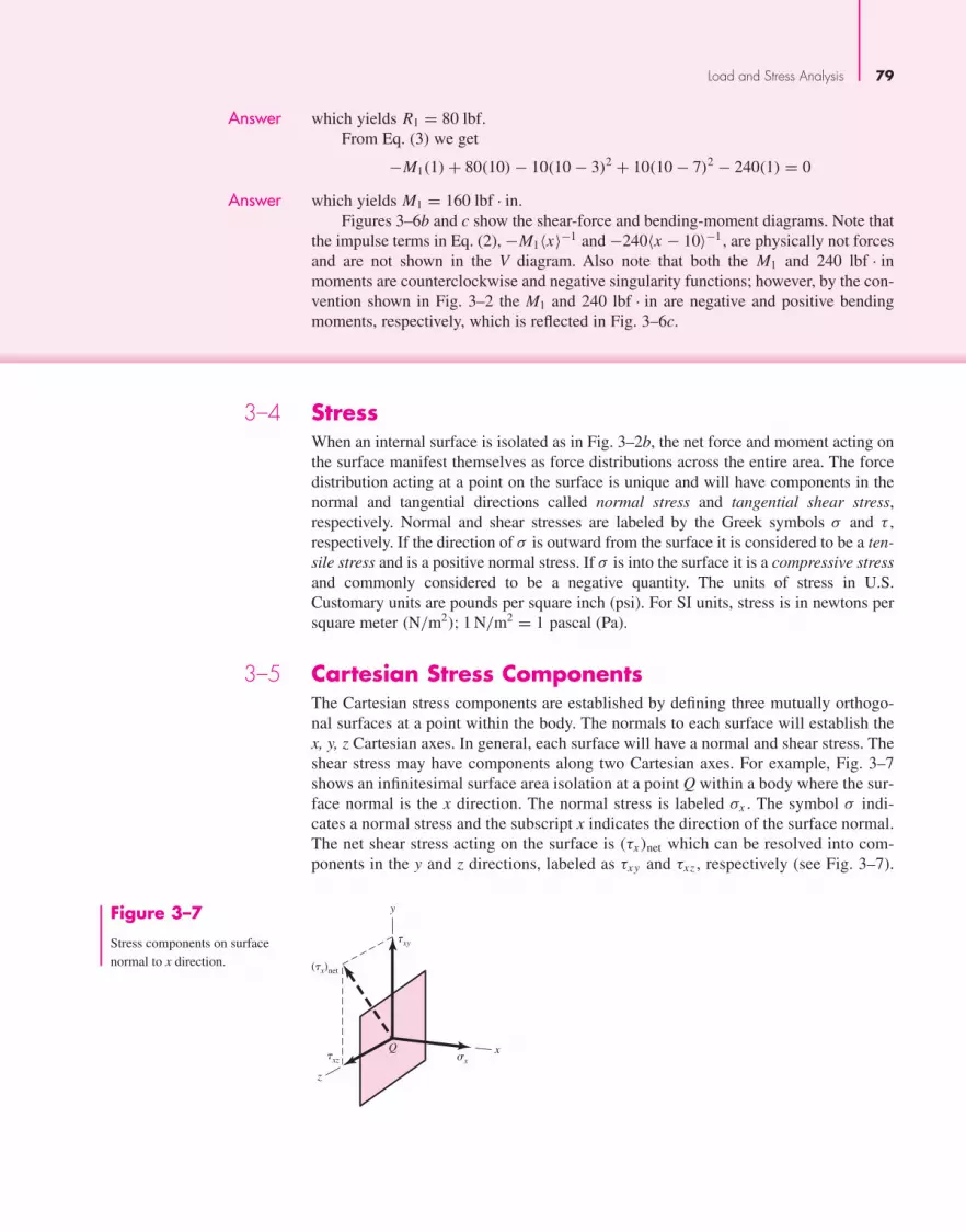
Figure 3–7
Stress components on surfacenormal to x direction.
Load and Stress Analysis 79
Answer which yields R1 = 80 lbf.From Eq. (3) we get
−M1(1) + 80(10) − 10(10 − 3)2 + 10(10 − 7)2 − 240(1) = 0
Answer which yields M1 = 160 lbf · in.
Figures 3–6b and c show the shear-force and bending-moment diagrams. Note thatthe impulse terms in Eq. (2), −M1〈x〉−1 and −240〈x − 10〉−1, are physically not forcesand are not shown in the V diagram. Also note that both the M1 and 240 lbf · inmoments are counterclockwise and negative singularity functions; however, by the con-vention shown in Fig. 3–2 the M1 and 240 lbf · in are negative and positive bendingmoments, respectively, which is reflected in Fig. 3–6c.
3–4 StressWhen an internal surface is isolated as in Fig. 3–2b, the net force and moment acting onthe surface manifest themselves as force distributions across the entire area. The forcedistribution acting at a point on the surface is unique and will have components in thenormal and tangential directions called normal stress and tangential shear stress,respectively. Normal and shear stresses are labeled by the Greek symbols σ and τ ,respectively. If the direction of σ is outward from the surface it is considered to be a ten-sile stress and is a positive normal stress. If σ is into the surface it is a compressive stressand commonly considered to be a negative quantity. The units of stress in U.S.Customary units are pounds per square inch (psi). For SI units, stress is in newtons persquare meter (N/m2); 1 N/m2 = 1 pascal (Pa).
3–5 Cartesian Stress ComponentsThe Cartesian stress components are established by defining three mutually orthogo-nal surfaces at a point within the body. The normals to each surface will establish thex, y, z Cartesian axes. In general, each surface will have a normal and shear stress. Theshear stress may have components along two Cartesian axes. For example, Fig. 3–7shows an infinitesimal surface area isolation at a point Q within a body where the sur-face normal is the x direction. The normal stress is labeled σx . The symbol σ indi-cates a normal stress and the subscript x indicates the direction of the surface normal.The net shear stress acting on the surface is (τx)net which can be resolved into com-ponents in the y and z directions, labeled as τxy and τxz , respectively (see Fig. 3–7).
Q
y
x
z
�x
�xy
�xz
(�x)net
bud29281_ch03_071-146.qxd 11/24/09 3:01PM Page 79 ntt 203:MHDQ196:bud29281:0073529281:bud29281_pagefiles:

80 Mechanical Engineering Design
Note that double subscripts are necessary for the shear. The first subscript indicatesthe direction of the surface normal whereas the second subscript is the direction ofthe shear stress.
The state of stress at a point described by three mutually perpendicular surfaces isshown in Fig. 3–8a. It can be shown through coordinate transformation that this is suf-ficient to determine the state of stress on any surface intersecting the point. As thedimensions of the cube in Fig. 3–8a approach zero, the stresses on the hidden facesbecome equal and opposite to those on the opposing visible faces. Thus, in general, acomplete state of stress is defined by nine stress components, σx , σy, σz, τxy,
τxz, τyx , τyz, τzx , and τzy .
For equilibrium, in most cases, “cross-shears” are equal, hence
τyx = τxy τzy = τyz τxz = τzx (3–7)
This reduces the number of stress components for most three-dimensional states ofstress from nine to six quantities, σx , σy, σz, τxy, τyz, and τzx .
A very common state of stress occurs when the stresses on one surface are zero.When this occurs the state of stress is called plane stress. Figure 3–8b shows a state ofplane stress, arbitrarily assuming that the normal for the stress-free surface is thez direction such that σz = τzx = τzy = 0. It is important to note that the element inFig. 3–8b is still a three-dimensional cube. Also, here it is assumed that the cross-shearsare equal such that τyx = τxy, and τyz = τzy = τxz = τzx = 0.
3–6 Mohr’s Circle for Plane StressSuppose the dx dy dz element of Fig. 3–8b is cut by an oblique plane with a normal n atan arbitrary angle φ counterclockwise from the x axis as shown in Fig. 3–9. Here, we areconcerned with the stresses σ and τ that act upon this oblique plane. By summing theforces caused by all the stress components to zero, the stresses σ and τ are found to be
σ = σx + σy
2+ σx − σy
2cos 2φ + τxy sin 2φ (3–8)
τ = −σx − σy
2sin 2φ + τxy cos 2φ (3–9)
Equations (3–8) and (3–9) are called the plane-stress transformation equations.
y y
x
�y
�yx
�xy
�xy
�xy
�x y
�xy
�xz
�x
�x
�y
�x
�y
�z
x
z
�yz
�zy
�z x
(a) (b)
Figure 3–8
(a) General three-dimensionalstress. (b) Plane stress with“cross-shears” equal.
bud29281_ch03_071-146.qxd 11/24/09 3:01PM Page 80 ntt 203:MHDQ196:bud29281:0073529281:bud29281_pagefiles:

Load and Stress Analysis 81
Differentiating Eq. (3–8) with respect to φ and setting the result equal to zeromaximizes σ and gives
tan 2φp = 2τxy
σx − σy(3–10)
Equation (3–10) defines two particular values for the angle 2φp, one of which definesthe maximum normal stress σ1 and the other, the minimum normal stress σ2. These twostresses are called the principal stresses, and their corresponding directions, the princi-pal directions. The angle between the two principal directions is 90°. It is important tonote that Eq. (3–10) can be written in the form
σx − σy
2sin 2φp − τxy cos 2φp = 0 (a)
Comparing this with Eq. (3–9), we see that τ = 0, meaning that the perpendicular sur-faces containing principal stresses have zero shear stresses.
In a similar manner, we differentiate Eq. (3–9), set the result equal to zero, and obtain
tan 2φs = −σx − σy
2τxy(3–11)
Equation (3–11) defines the two values of 2φs at which the shear stress τ reaches anextreme value. The angle between the two surfaces containing the maximum shearstresses is 90°. Equation (3–11) can also be written as
σx − σy
2cos 2φp + τxy sin 2φp = 0 (b)
Substituting this into Eq. (3–8) yields
σ = σx + σy
2(3–12)
Equation (3–12) tells us that the two surfaces containing the maximum shear stressesalso contain equal normal stresses of (σx + σy)/2.
Comparing Eqs. (3–10) and (3–11), we see that tan 2φs is the negative reciprocalof tan 2φp. This means that 2φs and 2φp are angles 90° apart, and thus the anglesbetween the surfaces containing the maximum shear stresses and the surfaces contain-ing the principal stresses are ±45◦.
Formulas for the two principal stresses can be obtained by substituting the angle 2φp from Eq. (3–10) in Eq. (3–8). The result is
σ1, σ2 = σx + σy
2±
√(σx − σy
2
)2
+ τ 2xy (3–13)
x
n
y
�
��
��x
�xy dxds
dy
��
�y�xy
dx
dsdy
Figure 3–9
bud29281_ch03_071-146.qxd 11/24/09 3:01PM Page 81 ntt 203:MHDQ196:bud29281:0073529281:bud29281_pagefiles:

82 Mechanical Engineering Design
In a similar manner the two extreme-value shear stresses are found to be
τ1, τ2 = ±√(
σx − σy
2
)2
+ τ 2xy (3–14)
Your particular attention is called to the fact that an extreme value of the shear stressmay not be the same as the actual maximum value. See Sec. 3–7.
It is important to note that the equations given to this point are quite sufficient forperforming any plane stress transformation. However, extreme care must be exercisedwhen applying them. For example, say you are attempting to determine the principalstate of stress for a problem where σx = 14 MPa, σy = −10 MPa, and τxy = −16 MPa.Equation (3–10) yields φp = −26.57◦ and 63.43°, which locate the principal stress sur-faces, whereas, Eq. (3–13) gives σ1 = 22 MPa and σ2 = −18 MPa for the principalstresses. If all we wanted was the principal stresses, we would be finished. However,what if we wanted to draw the element containing the principal stresses properly ori-ented relative to the x, y axes? Well, we have two values of φp and two values for theprincipal stresses. How do we know which value of φp corresponds to which value ofthe principal stress? To clear this up we would need to substitute one of the values ofφp into Eq. (3–8) to determine the normal stress corresponding to that angle.
A graphical method for expressing the relations developed in this section, calledMohr’s circle diagram, is a very effective means of visualizing the stress state at a pointand keeping track of the directions of the various components associated with plane stress.Equations (3–8) and (3–9) can be shown to be a set of parametric equations for σ and τ ,where the parameter is 2φ. The parametric relationship between σ and τ is that of a cir-cle plotted in the σ, τ plane, where the center of the circle is located at C = (σ, τ) =[(σx + σy)/2, 0] and has a radius of R =
√[(σx − σy)/2]2 + τ 2
xy . A problem arises inthe sign of the shear stress. The transformation equations are based on a positive φbeing counterclockwise, as shown in Fig. 3–9. If a positive τ were plotted above theσ axis, points would rotate clockwise on the circle 2φ in the opposite direction ofrotation on the element. It would be convenient if the rotations were in the samedirection. One could solve the problem easily by plotting positive τ below the axis.However, the classical approach to Mohr’s circle uses a different convention for theshear stress.
Mohr’s Circle Shear Convention
This convention is followed in drawing Mohr’s circle:
• Shear stresses tending to rotate the element clockwise (cw) are plotted above theσ axis.
• Shear stresses tending to rotate the element counterclockwise (ccw) are plotted belowthe σ axis.
For example, consider the right face of the element in Fig. 3–8b. By Mohr’s circle con-vention the shear stress shown is plotted below the σ axis because it tends to rotate theelement counterclockwise. The shear stress on the top face of the element is plottedabove the σ axis because it tends to rotate the element clockwise.
In Fig. 3–10 we create a coordinate system with normal stresses plotted along theabscissa and shear stresses plotted as the ordinates. On the abscissa, tensile (positive)normal stresses are plotted to the right of the origin O and compressive (negative) nor-mal stresses to the left. On the ordinate, clockwise (cw) shear stresses are plotted up;counterclockwise (ccw) shear stresses are plotted down.
bud29281_ch03_071-146.qxd 11/24/09 3:01PM Page 82 ntt 203:MHDQ196:bud29281:0073529281:bud29281_pagefiles:

Using the stress state of Fig. 3–8b, we plot Mohr’s circle, Fig. 3–10, by first look-ing at the right surface of the element containing σx to establish the sign of σx and thecw or ccw direction of the shear stress. The right face is called the x face whereφ = 0◦. If σx is positive and the shear stress τxy is ccw as shown in Fig. 3–8b, we canestablish point A with coordinates (σx , τ
ccwxy ) in Fig. 3–10. Next, we look at the top y
face, where φ = 90◦, which contains σy, and repeat the process to obtain point B withcoordinates (σy, τ
cwxy ) as shown in Fig. 3–10. The two states of stress for the element
are �φ = 90◦ from each other on the element so they will be 2�φ = 180◦ from eachother on Mohr’s circle. Points A and B are the same vertical distance from the σ axis.Thus, AB must be on the diameter of the circle, and the center of the circle C is whereAB intersects the σ axis. With points A and B on the circle, and center C, the completecircle can then be drawn. Note that the extended ends of line AB are labeled x and yas references to the normals to the surfaces for which points A and B represent thestresses.
The entire Mohr’s circle represents the state of stress at a single point in a struc-ture. Each point on the circle represents the stress state for a specific surface intersect-ing the point in the structure. Each pair of points on the circle 180° apart represent thestate of stress on an element whose surfaces are 90° apart. Once the circle is drawn, thestates of stress can be visualized for various surfaces intersecting the point being ana-lyzed. For example, the principal stresses σ1 and σ2 are points D and E, respectively,and their values obviously agree with Eq. (3–13). We also see that the shear stressesare zero on the surfaces containing σ1 and σ2. The two extreme-value shear stresses, oneclockwise and one counterclockwise, occur at F and G with magnitudes equal to theradius of the circle. The surfaces at F and G each also contain normal stresses of(σx + σy)/2 as noted earlier in Eq. (3–12). Finally, the state of stress on an arbitrarysurface located at an angle φ counterclockwise from the x face is point H.
Load and Stress Analysis 83
�x
�y (�x – �y)
O
�x + �y
2
�x – �y
2F
(�y , �xycw)
(�x , �ccw)
yB
C
G
D
H
E
�xy
�y�2�
�1�x
2�
A2�p
�xy
x
� cw
� ccw
�x – �
y2 + � 2xy
��
�2
xy
Figure 3–10
Mohr’s circle diagram.
bud29281_ch03_071-146.qxd 11/24/09 3:01PM Page 83 ntt 203:MHDQ196:bud29281:0073529281:bud29281_pagefiles:

84 Mechanical Engineering Design
At one time, Mohr’s circle was used graphically where it was drawn to scale veryaccurately and values were measured by using a scale and protractor. Here, we are strictlyusing Mohr’s circle as a visualization aid and will use a semigraphical approach, calculat-ing values from the properties of the circle. This is illustrated by the following example.
EXAMPLE 3–4 A stress element has σx = 80 MPa and τxy = 50 MPa cw, as shown in Fig. 3–11a.(a) Using Mohr’s circle, find the principal stresses and directions, and show these
on a stress element correctly aligned with respect to the xy coordinates. Draw anotherstress element to show τ1 and τ2, find the corresponding normal stresses, and label thedrawing completely.
(b) Repeat part a using the transformation equations only.
Solution (a) In the semigraphical approach used here, we first make an approximate freehandsketch of Mohr’s circle and then use the geometry of the figure to obtain the desiredinformation.
Draw the σ and τ axes first (Fig. 3–11b) and from the x face locate σx = 80 MPaalong the σ axis. On the x face of the element, we see that the shear stress is 50 MPa inthe cw direction. Thus, for the x face, this establishes point A (80, 50cw) MPa.Corresponding to the y face, the stress is σ = 0 and τ = 50 MPa in the ccw direction.This locates point B (0, 50ccw) MPa. The line AB forms the diameter of the required cir-cle, which can now be drawn. The intersection of the circle with the σ axis defines σ1
and σ2 as shown. Now, noting the triangle AC D, indicate on the sketch the length of thelegs AD and C D as 50 and 40 MPa, respectively. The length of the hypotenuse AC is
Answer τ1 =√
(50)2 + (40)2 = 64.0 MPa
and this should be labeled on the sketch too. Since intersection C is 40 MPa from theorigin, the principal stresses are now found to be
Answer σ1 = 40 + 64 = 104 MPa and σ2 = 40 − 64 = −24 MPa
The angle 2φ from the x axis cw to σ1 is
Answer 2φp = tan−1 5040 = 51.3◦
To draw the principal stress element (Fig. 3–11c), sketch the x and y axes parallelto the original axes. The angle φp on the stress element must be measured in the samedirection as is the angle 2φp on the Mohr circle. Thus, from x measure 25.7° (half of51.3°) clockwise to locate the σ1 axis. The σ2 axis is 90° from the σ1 axis and the stresselement can now be completed and labeled as shown. Note that there are no shearstresses on this element.
The two maximum shear stresses occur at points E and F in Fig. 3–11b. The twonormal stresses corresponding to these shear stresses are each 40 MPa, as indicated.Point E is 38.7° ccw from point A on Mohr’s circle. Therefore, in Fig. 3–11d, draw astress element oriented 19.3° (half of 38.7°) ccw from x. The element should then belabeled with magnitudes and directions as shown.
In constructing these stress elements it is important to indicate the x and y direc-tions of the original reference system. This completes the link between the originalmachine element and the orientation of its principal stresses.
bud29281_ch03_071-146.qxd 11/24/09 3:01PM Page 84 ntt 203:MHDQ196:bud29281:0073529281:bud29281_pagefiles:

Load and Stress Analysis 85
(b) The transformation equations are programmable. From Eq. (3–10),
φp = 1
2tan−1
(2τxy
σx − σy
)= 1
2tan−1
(2(−50)
80
)= −25.7◦, 64.3◦
From Eq. (3–8), for the first angle φp = −25.7◦,
σ = 80 + 0
2+ 80 − 0
2cos[2(−25.7)] + (−50) sin[2(−25.7)] = 104.03 MPa
The shear on this surface is obtained from Eq. (3–9) as
τ = −80 − 0
2sin[2(−25.7)] + (−50) cos[2(−25.7)] = 0 MPa
which confirms that 104.03 MPa is a principal stress. From Eq. (3–8), for φp = 64.3◦,
σ = 80 + 0
2+ 80 − 0
2cos[2(64.3)] + (−50) sin[2(64.3)] = −24.03 MPa
Figure 3–11
All stresses in MPa.
�cw
�ccw
�1
x
A
DC
E
38.7° 64
50
51.3°40 40
2�p
��1
�x = 80
�y = 0�2
B
F
�2y
(b)
(80, 50cw)
(0, 50ccw)
(c)
y 2
�2 = –24
�1 = 104
25.7°
x
1
(d )
y
� = 40
�2 = 64
�1 = 64
19.3°
� = 40
xE
F
(a)
y
x
50
50
80
Answer
bud29281_ch03_071-146.qxd 11/24/09 3:01PM Page 85 ntt 203:MHDQ196:bud29281:0073529281:bud29281_pagefiles:

86 Mechanical Engineering Design
Substituting φp = 64.3◦ into Eq. (3–9) again yields τ = 0, indicating that −24.03 MPais also a principal stress. Once the principal stresses are calculated they can be orderedsuch that σ1 ≥ σ2. Thus, σ1 = 104.03 MPa and σ2 = −24.03 MPa.
Answer
Since for σ1 = 104.03 MPa, φp = −25.7◦, and since φ is defined positive ccw in thetransformation equations, we rotate clockwise 25.7° for the surface containing σ1. Wesee in Fig. 3–11c that this totally agrees with the semigraphical method.
To determine τ1 and τ2, we first use Eq. (3–11) to calculate φs :
φs = 1
2tan−1
(−σx − σy
2τxy
)= 1
2tan−1
(− 80
2(−50)
)= 19.3◦, 109.3◦
For φs = 19.3◦, Eqs. (3–8) and (3–9) yield
Answer σ = 80 + 0
2+ 80 − 0
2cos[2(19.3)] + (−50) sin[2(19.3)] = 40.0 MPa
τ = −80 − 0
2sin[2(19.3)] + (−50) cos[2(19.3)] = −64.0 MPa
Remember that Eqs. (3–8) and (3–9) are coordinate transformation equations. Imaginethat we are rotating the x, y axes 19.3° counterclockwise and y will now point up andto the left. So a negative shear stress on the rotated x face will point down and to theright as shown in Fig. 3–11d. Thus again, results agree with the semigraphical method.
For φs = 109.3◦, Eqs. (3–8) and (3–9) give σ = 40.0 MPa and τ = +64.0 MPa.Using the same logic for the coordinate transformation we find that results again agreewith Fig. 3–11d.
3–7 General Three-Dimensional StressAs in the case of plane stress, a particular orientation of a stress element occurs in spacefor which all shear-stress components are zero. When an element has this particular ori-entation, the normals to the faces are mutually orthogonal and correspond to the prin-cipal directions, and the normal stresses associated with these faces are the principalstresses. Since there are three faces, there are three principal directions and three prin-cipal stresses σ1, σ2, and σ3. For plane stress, the stress-free surface contains the thirdprincipal stress which is zero.
In our studies of plane stress we were able to specify any stress state σx , σy , andτxy and find the principal stresses and principal directions. But six components ofstress are required to specify a general state of stress in three dimensions, and theproblem of determining the principal stresses and directions is more difficult. Indesign, three-dimensional transformations are rarely performed since most maxi-mum stress states occur under plane stress conditions. One notable exception is con-tact stress, which is not a case of plane stress, where the three principal stresses aregiven in Sec. 3–19. In fact, all states of stress are truly three-dimensional, wherethey might be described one- or two-dimensionally with respect to specific coordi-nate axes. Here it is most important to understand the relationship among the threeprincipal stresses. The process in finding the three principal stresses from the six
bud29281_ch03_071-146.qxd 11/24/09 3:01PM Page 86 ntt 203:MHDQ196:bud29281:0073529281:bud29281_pagefiles:

Load and Stress Analysis 87
stress components σx , σy, σz, τxy, τyz, and τzx , involves finding the roots of the cubicequation1
σ 3 − (σx + σy + σz)σ2 + (
σxσy + σxσz + σyσz − τ 2xy − τ 2
yz − τ 2zx
)σ
− (σxσyσz + 2τxyτyzτzx − σxτ
2yz − σyτ
2zx − σzτ
2xy
) = 0 (3–15)
In plotting Mohr’s circles for three-dimensional stress, the principal normalstresses are ordered so that σ1 ≥ σ2 ≥ σ3. Then the result appears as in Fig. 3–12a. Thestress coordinates σ , τ for any arbitrarily located plane will always lie on the bound-aries or within the shaded area.
Figure 3–12a also shows the three principal shear stresses τ1/2, τ2/3, and τ1/3.2
Each of these occurs on the two planes, one of which is shown in Fig. 3–12b. The fig-ure shows that the principal shear stresses are given by the equations
τ1/2 = σ1 − σ2
2τ2/3 = σ2 − σ3
2τ1/3 = σ1 − σ3
2(3–16)
Of course, τmax = τ1/3 when the normal principal stresses are ordered (σ1 > σ2 > σ3),so always order your principal stresses. Do this in any computer code you generate andyou’ll always generate τmax.
3–8 Elastic StrainNormal strain ε is defined and discussed in Sec. 2–1 for the tensile specimen and isgiven by Eq. (2–2) as ε = δ/ l , where δ is the total elongation of the bar within thelength l. Hooke’s law for the tensile specimen is given by Eq. (2–3) as
σ = Eε (3–17)
where the constant E is called Young’s modulus or the modulus of elasticity.
�1/2
�1/3
�
�2/3
�1�2�3�
(b)(a)
�1/2
�1
�
�2
Figure 3–12
Mohr’s circles for three-dimensional stress.
1For development of this equation and further elaboration of three-dimensional stress transformations see:Richard G. Budynas, Advanced Strength and Applied Stress Analysis, 2nd ed., McGraw-Hill, New York,1999, pp. 46–78.2Note the difference between this notation and that for a shear stress, say, τxy . The use of the shilling mark isnot accepted practice, but it is used here to emphasize the distinction.
bud29281_ch03_071-146.qxd 11/24/09 3:01PM Page 87 ntt 203:MHDQ196:bud29281:0073529281:bud29281_pagefiles:

88 Mechanical Engineering Design
When a material is placed in tension, there exists not only an axial strain, but alsonegative strain (contraction) perpendicular to the axial strain. Assuming a linear,homogeneous, isotropic material, this lateral strain is proportional to the axial strain. Ifthe axial direction is x, then the lateral strains are εy = εz = −νεx . The constant of pro-portionality v is called Poisson’s ratio, which is about 0.3 for most structural metals.See Table A–5 for values of v for common materials.
If the axial stress is in the x direction, then from Eq. (3–17)
εx = σx
Eεy = εz = −ν
σx
E(3–18)
For a stress element undergoing σx , σy , and σz simultaneously, the normal strainsare given by
εx = 1
E
[σx − ν(σy + σz)
]εy = 1
E
[σy − ν(σx + σz)
](3–19)
εz = 1
E
[σz − ν(σx + σy)
]Shear strain γ is the change in a right angle of a stress element when subjected to
pure shear stress, and Hooke’s law for shear is given by
τ = Gγ (3–20)
where the constant G is the shear modulus of elasticity or modulus of rigidity. It can be shown for a linear, isotropic, homogeneous material, the three elastic con-
stants are related to each other by
E = 2G(1 + ν) (3–21)
3–9 Uniformly Distributed StressesThe assumption of a uniform distribution of stress is frequently made in design. Theresult is then often called pure tension, pure compression, or pure shear, dependingupon how the external load is applied to the body under study. The word simple is some-times used instead of pure to indicate that there are no other complicating effects.The tension rod is typical. Here a tension load F is applied through pins at the ends ofthe bar. The assumption of uniform stress means that if we cut the bar at a sectionremote from the ends and remove one piece, we can replace its effect by applying a uni-formly distributed force of magnitude σA to the cut end. So the stress σ is said to beuniformly distributed. It is calculated from the equation
σ = F
A(3–22)
This assumption of uniform stress distribution requires that:
• The bar be straight and of a homogeneous material
• The line of action of the force contains the centroid of the section
• The section be taken remote from the ends and from any discontinuity or abruptchange in cross section
bud29281_ch03_071-146.qxd 11/24/09 3:01PM Page 88 ntt 203:MHDQ196:bud29281:0073529281:bud29281_pagefiles:

Load and Stress Analysis 89
For simple compression, Eq. (3–22) is applicable with F normally being consid-ered a negative quantity. Also, a slender bar in compression may fail by buckling, andthis possibility must be eliminated from consideration before Eq. (3–22) is used.3
Another type of loading that assumes a uniformly distributed stress is known asdirect shear. This occurs when there is a shearing action with no bending. An exampleis the action on a piece of sheet metal caused by the two blades of tin snips. Bolts andpins that are loaded in shear often have direct shear. Think of a cantilever beam with aforce pushing down on it. Now move the force all the way up to the wall so there is nobending moment, just a force trying to shear the beam off the wall. This is direct shear.Direct shear is usually assumed to be uniform across the cross section, and is given by
τ = V
A(3–23)
where V is the shear force and A is the area of the cross section that is being sheared.The assumption of uniform stress is not accurate, particularly in the vicinity where theforce is applied, but the assumption generally gives acceptable results.
3–10 Normal Stresses for Beams in BendingThe equations for the normal bending stresses in straight beams are based on the fol-lowing assumptions.
• The beam is subjected to pure bending. This means that the shear force is zero, andthat no torsion or axial loads are present (for most engineering applications it is as-sumed that these loads affect the bending stresses minimally).
• The material is isotropic and homogeneous.
• The material obeys Hooke’s law.
• The beam is initially straight with a cross section that is constant throughout thebeam length.
• The beam has an axis of symmetry in the plane of bending.
• The proportions of the beam are such that it would fail by bending rather than bycrushing, wrinkling, or sidewise buckling.
• Plane cross sections of the beam remain plane during bending.
In Fig. 3–13 we visualize a portion of a straight beam acted upon by a positivebending moment M shown by the curved arrow showing the physical action of themoment together with a straight arrow indicating the moment vector. The x axis iscoincident with the neutral axis of the section, and the xz plane, which contains the
3See Sec. 4–11.
Figure 3–13
Straight beam in positivebending.
M
M
x
y
z
bud29281_ch03_071-146.qxd 11/24/09 3:01PM Page 89 ntt 203:MHDQ196:bud29281:0073529281:bud29281_pagefiles:

90 Mechanical Engineering Design
neutral axes of all cross sections, is called the neutral plane. Elements of the beamcoincident with this plane have zero stress. The location of the neutral axis withrespect to the cross section is coincident with the centroidal axis of the cross section.
The bending stress varies linearly with the distance from the neutral axis, y, and isgiven by
σx = − My
I(3–24)
where I is the second-area moment about the z axis. That is,
I =∫
y2d A (3–25)
The stress distribution given by Eq. (3–24) is shown in Fig. 3–14. The maximum magni-tude of the bending stress will occur where y has the greatest magnitude. Designating σmax
as the maximum magnitude of the bending stress, and c as the maximum magnitude of y
σmax = Mc
I(3–26a)
Equation (3–24) can still be used to ascertain whether σmax is tensile or compressive.Equation (3–26a) is often written as
σmax = M
Z(3–26b)
where Z = I/c is called the section modulus.
EXAMPLE 3–5 A beam having a T section with the dimensions shown in Fig. 3–15 is subjected to a bend-ing moment of 1600 N · m, about the negative z axis, that causes tension at the top surface.Locate the neutral axis and find the maximum tensile and compressive bending stresses.
Solution Dividing the T section into two rectangles, numbered 1 and 2, the total area is A � 12(75) � 12(88) � 1956 mm2. Summing the area moments of these rectanglesabout the top edge, where the moment arms of areas 1 and 2 are 6 mm and (12 �88/2) � 56 mm respectively, we have
1956c1 = 12(75)(6) + 12(88)(56)
and hence c1 = 32.99 mm. Therefore c2 = 100 − 32.99 = 67.01 mm.Next we calculate the second moment of area of each rectangle about its own cen-
troidal axis. Using Table A–18, we find for the top rectangle
I1 = 1
12bh3 = 1
12(75)123 = 1.080 × 104 mm4
Compression
Neutral axis, Centroidal axis
Tension
x
c
y
y
Figure 3–14
Bending stresses according toEq. (3–24).
bud29281_ch03_071-146.qxd 11/26/09 5:56PM Page 90 ntt G4 Mac OS 9.2:Desktop Folder:MHDQ196/Budynas:

Load and Stress Analysis 91
75
12
12
2
c2
z
c1
100
1
yFigure 3–15
Dimensions in millimeters.
For the bottom rectangle, we have
I2 = 1
12(12)883 = 6.815 × 105 mm4
We now employ the parallel-axis theorem to obtain the second moment of area of thecomposite figure about its own centroidal axis. This theorem states
Iz = Ica + Ad2
where Ica is the second moment of area about its own centroidal axis and Iz is the sec-ond moment of area about any parallel axis a distance d removed. For the top rectan-gle, the distance is
d1 = 32.99 − 6 = 26.99 mm
and for the bottom rectangle,
d2 = 67.01 − 88
2= 23.01 mm
Using the parallel-axis theorem for both rectangles, we now find that
I = [1.080 × 10⁴ + 12(75)26.992] + [6.815 × 10⁵ + 12(88)23.012]
= 1.907 × 106 mm4
Finally, the maximum tensile stress, which occurs at the top surface, is found to be
Answer σ = Mc1
I= 1600(32.99)10−3
1.907(10−6)= 27.68(106) Pa = 27.68 MPa
Similarly, the maximum compressive stress at the lower surface is found to be
Answer σ = − Mc2
I= −1600(67.01)10−3
1.907(10−6)= −56.22(106) Pa = −56.22 MPa
bud29281_ch03_071-146.qxd 11/24/09 3:01PM Page 91 ntt 203:MHDQ196:bud29281:0073529281:bud29281_pagefiles:

92 Mechanical Engineering Design
Two-Plane Bending
Quite often, in mechanical design, bending occurs in both xy and xz planes. Consideringcross sections with one or two planes of symmetry only, the bending stresses are given by
σx = − Mz y
Iz+ Myz
Iy(3–27)
where the first term on the right side of the equation is identical to Eq. (3–24), My isthe bending moment in the xz plane (moment vector in y direction), z is the distancefrom the neutral y axis, and Iy is the second area moment about the y axis.
For noncircular cross sections, Eq. (3–27) is the superposition of stresses causedby the two bending moment components. The maximum tensile and compressive bend-ing stresses occur where the summation gives the greatest positive and negative stresses,respectively. For solid circular cross sections, all lateral axes are the same and the planecontaining the moment corresponding to the vector sum of Mz and My contains themaximum bending stresses. For a beam of diameter d the maximum distance from theneutral axis is d/2, and from Table A–18, I = πd4/64. The maximum bending stress fora solid circular cross section is then
σm = Mc
I= (M2
y + M2z )1/2(d/2)
πd4/64= 32
πd3(M2
y + M2z )1/2 (3–28)
EXAMPLE 3–6 As shown in Fig. 3–16a, beam OC is loaded in the xy plane by a uniform load of50 lbf/in, and in the xz plane by a concentrated force of 100 lbf at end C. The beam is8 in long.
50 lbf/in
C
A
z
x
1.5 in
0.75 in
(a)
y
BO
100 lbf
50 lbf/in
1600 lbf-in
Mz
(lbf-in)
0
�1600
400 lbf
(b)
x
x
CO
y
100 lbf
100 lbf
800 lbf-in
My
(lbf-in)800
0
(c)
x
CO
z
x
Figure 3–16
(a) Beam loaded in twoplanes; (b) loading andbending-moment diagramsin xy plane; (c) loading andbending-moment diagramsin xz plane.
bud29281_ch03_071-146.qxd 11/24/09 3:01PM Page 92 ntt 203:MHDQ196:bud29281:0073529281:bud29281_pagefiles:

Load and Stress Analysis 93
Beams with Asymmetrical Sections4
The bending stress equations, given by Eqs. (3–24) and (3–27), can also be applied tobeams having asymmetrical cross sections, provided the planes of bending coincidewith the area principal axes of the section. The method for determining the orientationof the area principal axes and the values of the corresponding principal second-areamoments can be found in any statics book. If a section has an axis of symmetry, thataxis and its perpendicular axis are the area principal axes.
For example, consider a beam in bending, using an equal leg angle as shown inTable A–6. Equation (3–27) cannot be used if the bending moments are resolved aboutaxis 1–1 and/or axis 2–2. However, Eq. (3–27) can be used if the moments are resolved
(a) For the cross section shown determine the maximum tensile and compressivebending stresses and where they act.
(b) If the cross section was a solid circular rod of diameter, d = 1.25 in, determinethe magnitude of the maximum bending stress.
Solution (a) The reactions at O and the bending-moment diagrams in the xy and xz planes areshown in Figs. 3–16b and c, respectively. The maximum moments in both planes occurat O where
(Mz)O = −1
2(50)82 = −1600 lbf-in (My)O = 100(8) = 800 lbf-in
The second moments of area in both planes are
Iz = 1
12(0.75)1.53 = 0.2109 in4 Iy = 1
12(1.5)0.753 = 0.05273 in4
The maximum tensile stress occurs at point A, shown in Fig. 3–16a, where the maxi-mum tensile stress is due to both moments. At A, yA = 0.75 in and z A = 0.375 in. Thus,from Eq. (3–27)
Answer (σx)A = −−1600(0.75)
0.2109+ 800(0.375)
0.05273= 11 380 psi = 11.38 kpsi
The maximum compressive bending stress occurs at point B where, yB = −0.75 in andzB = −0.375 in. Thus
Answer (σx)B = −−1600(−0.75)
0.2109+ 800(−0.375)
0.05273= −11 380 psi = −11.38 kpsi
(b) For a solid circular cross section of diameter, d = 1.25 in, the maximum bendingstress at end O is given by Eq. (3–28) as
Answer σm = 32
π(1.25)3
[8002 + (−1600)2]1/2 = 9329 psi = 9.329 kpsi
4For further discussion, see Sec. 5.3, Richard G. Budynas, Advanced Strength and Applied Stress Analysis,2nd ed.,McGraw-Hill, New York, 1999.
bud29281_ch03_071-146.qxd 11/25/09 4:55PM Page 93 ntt 203:MHDQ196:bud29281:0073529281:bud29281_pagefiles:

94 Mechanical Engineering Design
about axis 3–3 and its perpendicular axis (let us call it, say, axis 4–4). Note, for thiscross section, axis 4–4 is an axis of symmetry. Table A–6 is a standard table, and forbrevity, does not directly give all the information needed to use it. The orientation ofthe area principal axes and the values of I2–2, I3–3, and I4–4 are not given because theycan be determined as follows. Since the legs are equal, the principal axes are oriented±45° from axis 1–1, and I2–2 � I1–1. The second-area moment I3–3 is given by
I3−3 = A(k3−3)2 (a)
where k3–3 is called the radius of gyration. The sum of the second-area moments for across section is invariant, so I1–1 � I2–2 � I3–3 � I4–4. Thus, I4–4 is given by
I4−4 = 2 I1−1 − I3−3 (b)
where I2–2 � I1–1. For example, consider a 3 � 3 � 14 angle. Using Table A–6 and Eqs.
(a) and (b), I3–3 � 1.44 (0.592)2 � 0.505 in4, and I4–4 � 2 (1.24) � 0.505 � 1.98 in4.
3–11 Shear Stresses for Beams in BendingMost beams have both shear forces and bending moments present. It is only occasion-ally that we encounter beams subjected to pure bending, that is to say, beams havingzero shear force. The flexure formula is developed on the assumption of pure bending.This is done, however, to eliminate the complicating effects of shear force in the devel-opment. For engineering purposes, the flexure formula is valid no matter whether ashear force is present or not. For this reason, we shall utilize the same normal bending-stress distribution [Eqs. (3–24) and (3–26)] when shear forces are also present.
In Fig. 3–17a we show a beam segment of constant cross section subjected to ashear force V and a bending moment M at x. Because of external loading and V, theshear force and bending moment change with respect to x. At x + dx the shear forceand bending moment are V + dV and M + d M , respectively. Considering forces in thex direction only, Fig. 3–17b shows the stress distribution σx due to the bendingmoments. If dM is positive, with the bending moment increasing, the stresses on theright face, for a given value of y, are larger in magnitude than the stresses on the leftface. If we further isolate the element by making a slice at y = y1 (see Fig. 3–17b), thenet force in the x direction will be directed to the left with a value of ∫ c
y1
(d M)y
Id A
as shown in the rotated view of Fig. 3–17c. For equilibrium, a shear force on the bottomface, directed to the right, is required. This shear force gives rise to a shear stress τ ,where, if assumed uniform, the force is τb dx . Thus
τb dx =∫ c
y1
(d M)y
Id A (a)
The term dM/I can be removed from within the integral and b dx placed on the rightside of the equation; then, from Eq. (3–3) with V = d M/dx , Eq. (a) becomes
τ = V
I b
∫ c
y1
yd A (3–29)
In this equation, the integral is the first moment of the area A′ with respect to the neu-tral axis (see Fig. 3–17c). This integral is usually designated as Q. Thus
Q =∫ c
y1
yd A = y′ A′ (3–30)
bud29281_ch03_071-146.qxd 11/24/09 3:01PM Page 94 ntt 203:MHDQ196:bud29281:0073529281:bud29281_pagefiles:

Load and Stress Analysis 95
where, for the isolated area y1 to c, y′ is the distance in the y direction from the neutralplane to the centroid of the area A′. With this, Eq. (3–29) can be written as
τ = V Q
I b(3–31)
This stress is known as the transverse shear stress. It is always accompanied with bend-ing stress.
In using this equation, note that b is the width of the section at y = y1. Also, I isthe second moment of area of the entire section about the neutral axis.
Because cross shears are equal, and area A′ is finite, the shear stress τ given by Eq. (3–31) and shown on area A′ in Fig. 3–17c occurs only at y = y1. The shear stresson the lateral area varies with y, normally maximum at y = 0 (where y′A′ is maximum)and zero at the outer fibers of the beam where A′ � 0.
The shear stress distribution in a beam depends on how Q/b varies as a functionof y1. Here we will show how to determine the shear stress distribution for a beam witha rectangular cross section and provide results of maximum values of shear stress forother standard cross sections. Figure 3–18 shows a portion of a beam with a rectangu-lar cross section, subjected to a shear force V and a bending moment M. As a result ofthe bending moment, a normal stress σ is developed on a cross section such as A–A,which is in compression above the neutral axis and in tension below. To investigate theshear stress at a distance y1 above the neutral axis, we select an element of area d A ata distance y above the neutral axis. Then, d A = b dy, and so Eq. (3–30) becomes
Q =∫ c
y1
y d A = b∫ c
y1
y dy = by2
2
∣∣∣∣c
y1
= b
2
(c2 − y2
1
)(b)
Substituting this value for Q into Eq. (3–31) gives
τ = V
2I
(c2 − y2
1
)(3–32)
This is the general equation for shear stress in a rectangular beam. To learn somethingabout it, let us make some substitutions. From Table A–18, the second moment of areafor a rectangular section is I = bh3/12; substituting h = 2c and A = bh = 2bc gives
I = Ac2
3(c)
(a)
dx
w(x)y
xM � dM
V � dV
M
V
x
x
dx
c
(b)
�x � � �MyI
dMyI��x � �
MyI �
y1
(c)
F � dM y
I
x
dxy
A�
b ��
c
y1Figure 3–17
Beam section isolation. Note:Only forces shown in xdirection on dx element in (b).
bud29281_ch03_071-146.qxd 11/25/09 4:55PM Page 95 ntt 203:MHDQ196:bud29281:0073529281:bud29281_pagefiles:

96 Mechanical Engineering Design
If we now use this value of I for Eq. (3–32) and rearrange, we get
τ = 3V
2A
(1 − y2
1
c2
)(3–33)
We note that the maximum shear stress exists when y1 = 0, which is at the bending neu-tral axis. Thus
τmax = 3V
2A(3–34)
for a rectangular section. As we move away from the neutral axis, the shear stressdecreases parabolically until it is zero at the outer surfaces where y1 = ±c, as shownin Fig. 3–18c. Horizontal shear stress is always accompanied by vertical shear stressof the same magnitude, and so the distribution can be diagrammed as shown in Fig. 3–18d. Figure 3–18c shows that the shear τ on the vertical surfaces varies withy. We are almost always interested in the horizontal shear, τ in Fig. 3–18d, which isnearly uniform over dx with constant y � y1. The maximum horizontal shear occurswhere the vertical shear is largest. This is usually at the neutral axis but may not beif the width b is smaller somewhere else. Furthermore, if the section is such that bcan be minimized on a plane not horizontal, then the horizontal shear stress occurson an inclined plane. For example, with tubing, the horizontal shear stress occurs ona radial plane and the corresponding “vertical shear” is not vertical, but tangential.
The distributions of transverse shear stresses for several commonly used cross sec-tions are shown in Table 3–2. The profiles represent the VQ/Ib relationship, which is afunction of the distance y from the neutral axis. For each profile, the formula for themaximum value at the neutral axis is given. Note that the expression given for theI beam is a commonly used approximation that is reasonable for a standard I beam witha thin web. Also, the profile for the I beam is idealized. In reality the transition from theweb to the flange is quite complex locally, and not simply a step change.
Figure 3–18
Transverse shear stresses in arectangular beam.
bd A
c
�max =3V2A
y
xh
y y1
O
VM
y
A
A
(a)
(d )
(b) (c)
x z
d y
y
�
c
y
y1 x
�
�
O
dx
bud29281_ch03_071-146.qxd 11/24/09 3:01PM Page 96 ntt 203:MHDQ196:bud29281:0073529281:bud29281_pagefiles:

Load and Stress Analysis 97
It is significant to observe that the transverse shear stress in each of these commoncross sections is maximum on the neutral axis, and zero on the outer surfaces. Since thisis exactly the opposite of where the bending and torsional stresses have their maximumand minimum values, the transverse shear stress is often not critical from a designperspective.
Let us examine the significance of the transverse shear stress, using as an examplea cantilever beam of length L, with rectangular cross section b � h, loaded at the free endwith a transverse force F. At the wall, where the bending moment is the largest, at a dis-tance y from the neutral axis, a stress element will include both bending stress andtransverse shear stress. In Sec. 5–4 it will be shown that a good measure of the com-bined effects of multiple stresses on a stress element is the maximum shear stress.Inserting the bending stress (My/I) and the transverse shear stress (VQ/Ib) into themaximum shear stress equation, Eq. (3–14), we obtain a general equation for the max-imum shear stress in a cantilever beam with a rectangular cross section. This equationcan then be normalized with respect to L/h and y/c, where c is the distance from theneutral axis to the outer surface (h/2), to give
τmax =√(σ
2
)2+ τ 2= 3F
2bh
√4(L/h)2(y/c)2 + [
1 − (y/c)2]2
(d)
To investigate the significance of transverse shear stress, we plot τmax as a functionof L/h for several values of y/c, as shown in Fig. 3–19. Since F and b appear only aslinear multipliers outside the radical, they will only serve to scale the plot in the verti-cal direction without changing any of the relationships. Notice that at the neutral axiswhere y/c � 0, τmax is constant for any length beam, since the bending stress is zero atthe neutral axis and the transverse shear stress is independent of L. On the other hand,on the outer surface where y/c � 1, τmax increases linearly with L/h because of thebending moment. For y/c between zero and one, τmax is nonlinear for low values of L/h,but behaves linearly as L/h increases, displaying the dominance of the bending stressas the moment arm increases. We can see from the graph that the critical stress element(the largest value of τmax) will always be either on the outer surface (y/c � 1) or at theneutral axis (y/c � 0), and never between. Thus, for the rectangular cross section, thetransition between these two locations occurs at L/h � 0.5 where the line for y/c � 1crosses the horizontal line for y/c � 0. The critical stress element is either on the outer
Table 3–2
Formulas for Maximum
Transverse Shear Stress
from VQ/Ib
Beam Shape Formula Beam Shape Formula
Rectangular
�avc =VA
Circular
�avc =VA
Hollow, thin-walled round
�avc =VA�max = 3V
2A
�max = 4V
3A
�max = 2V
A
�max.= V
Aweb
Structural I beam (thin-walled)
Aweb
bud29281_ch03_071-146.qxd 12/02/2009 4:14 pm Page 97 pinnacle s-171:Desktop Folder:Temp Work:Don't Delete (Jobs):MHDQ196/Budynas:

98 Mechanical Engineering Design
surface where the transverse shear is zero, or if L/h is small enough, it is on the neutralaxis where the bending stress is zero.
The conclusions drawn from Fig. 3–19 are generally similar for any cross sectionthat does not increase in width farther away from the neutral axis. This notably includessolid round cross sections, but not I beams or channels. Care must be taken with I beamsand channels that have thin webs that extend far enough from the neutral axis that thebending and shear may both be significant on the same stress element (See Ex. 3–7). Forany common cross section beam, if the beam length to height ratio is greater than 10, thetransverse shear stress is generally considered negligible compared to the bending stressat any point within the cross section.
EXAMPLE 3–7 A beam 12 in long is to support a load of 488 lbf acting 3 in from the left support, asshown in Fig. 3–20a. The beam is an I beam with the cross-sectional dimensionsshown. To simplify the calculations, assume a cross section with square corners, asshown in Fig. 3–20c. Points of interest are labeled (a, b, c, and d) at distances y fromthe neutral axis of 0 in, 1.240� in, 1.240� in, and 1.5 in (Fig. 3–20c). At the criticalaxial location along the beam, find the following information.
(a) Determine the profile of the distribution of the transverse shear stress, obtain-ing values at each of the points of interest.
(b) Determine the bending stresses at the points of interest.(c) Determine the maximum shear stresses at the points of interest, and compare them.
Solution First, we note that the transverse shear stress is not likely to be negligible in this casesince the beam length to height ratio is much less than 10, and since the thin web andwide flange will allow the transverse shear to be large. The loading, shear-force, andbending-moment diagrams are shown in Fig. 3–20b. The critical axial location is atx � 3� where the shear force and the bending moment are both maximum.
(a) We obtain the area moment of inertia I by evaluating I for a solid 3.0-in � 2.33-inrectangular area, and then subtracting the two rectangular areas that are not part of thecross section.
I = (2.33)(3.00)3
12− 2
[(1.08)(2.48)3
12
]= 2.50 in4
Figure 3–19
Plot of maximum shear stressfor a cantilever beam,combining the effects ofbending and transverse shearstresses.
1200
1000
800
600
400
200
1400
00 0.5 1 2 3 41.5 2.5 3.5
L/h
y ⁄c = 1
y ⁄c = 2�3
y ⁄c = 1�3
y ⁄c = 0
� max
(MPa
)
bud29281_ch03_071-146.qxd 11/24/09 3:01PM Page 98 ntt 203:MHDQ196:bud29281:0073529281:bud29281_pagefiles:
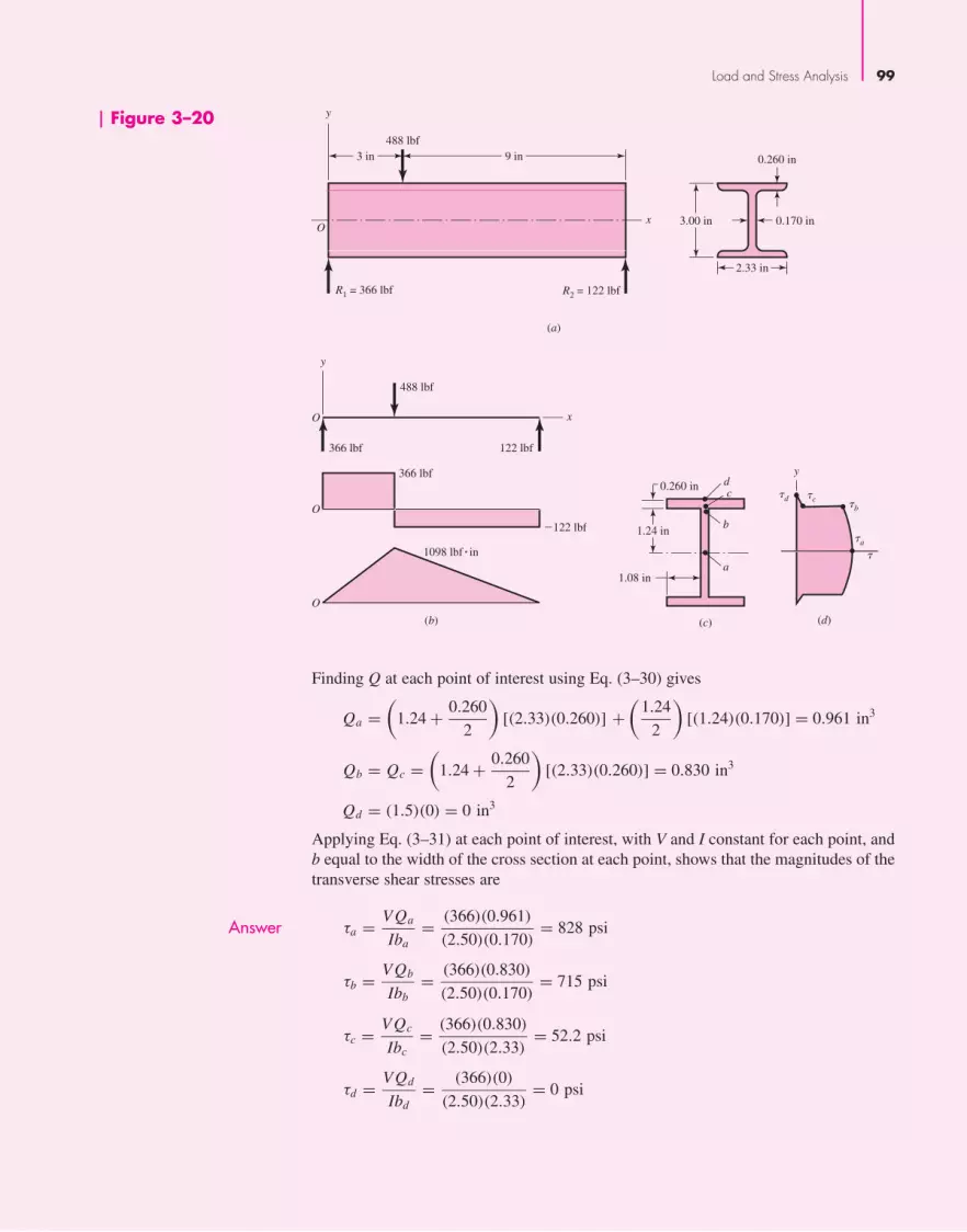
Load and Stress Analysis 99
Finding Q at each point of interest using Eq. (3–30) gives
Qa =(
1.24 + 0.260
2
)[(2.33)(0.260)] +
(1.24
2
)[(1.24)(0.170)] = 0.961 in3
Qb = Qc =(
1.24 + 0.260
2
)[(2.33)(0.260)] = 0.830 in3
Qd = (1.5)(0) = 0 in3p
Applying Eq. (3–31) at each point of interest, with V and I constant for each point, andb equal to the width of the cross section at each point, shows that the magnitudes of thetransverse shear stresses are
Answer τa = VQa
Iba= (366)(0.961)
(2.50)(0.170)= 828 psi
τb = VQb
Ibb= (366)(0.830)
(2.50)(0.170)= 715 psi
τc = VQc
Ibc= (366)(0.830)
(2.50)(2.33)= 52.2 psi
τd = VQd
Ibd= (366)(0)
(2.50)(2.33)= 0 psi
Figure 3–20
R1 = 366 lbf R2 = 122 lbf
488 lbf9 in3 in
y
xO
3.00 in
2.33 in
0.170 in
0.260 in
(a)
y
366 lbf 122 lbf
366 lbf
2122 lbf
1098 lbf � in
488 lbf
xO
O
O
(b)
1.08 in
1.24 in
0.260 in dc
b
a
(c)
�b
�c�d
�a
�
(d)
y
bud29281_ch03_071-146.qxd 11/25/09 5:15PM Page 99 ntt G4 Mac OS 9.2:Desktop Folder:

100 Mechanical Engineering Design
The magnitude of the idealized transverse shear stress profile through the beamdepth will be as shown in Fig. 3–20d.
(b) The bending stresses at each point of interest are
Answer σa = Mya
I= (1098)(0)
2.50= 0 psi
σb = σc = − Myb
I= − (1098)(1.24)
2.50= −545 psi
σd = − Myd
I= − (1098)(1.50)
2.50= −659 psi
(c) Now at each point of interest, consider a stress element that includes the bend-ing stress and the transverse shear stress. The maximum shear stress for each stresselement can be determined by Mohr’s circle, or analytically by Eq. (3–14) withσy = 0,
τmax =√(σ
2
)2+ τ 2
Thus, at each point
τmax,a =√
0 + (828)2 = 828 psi
τmax,b =√(−545
2
)2
+ (715)2 = 765 psi
τmax,c =√(−545
2
)2
+ (52.2)2 = 277 psi
τmax,d =√(−659
2
)2
+ 0 = 330 psi
Answer Interestingly, the critical location is at point a where the maximum shear stress is thelargest, even though the bending stress is zero. The next critical location is at point b inthe web, where the thin web thickness dramatically increases the transverse shear stresscompared to points c or d. These results are counterintuitive, since both points a and bturn out to be more critical than point d, even though the bending stress is maximum atpoint d. The thin web and wide flange increase the impact of the transverse shear stress.If the beam length to height ratio were increased, the critical point would move frompoint a to point b, since the transverse shear stress at point a would remain constant,but the bending stress at point b would increase. The designer should be particularlyalert to the possibility of the critical stress element not being on the outer surface withcross sections that get wider farther from the neutral axis, particularly in cases withthin web sections and wide flanges. For rectangular and circular cross sections, how-ever, the maximum bending stresses at the outer surfaces will dominate, as was shownin Fig. 3–19.
bud29281_ch03_071-146.qxd 11/24/09 3:01PM Page 100 ntt 203:MHDQ196:bud29281:0073529281:bud29281_pagefiles:

Load and Stress Analysis 101
3–12 TorsionAny moment vector that is collinear with an axis of a mechanical element is called atorque vector, because the moment causes the element to be twisted about that axis. Abar subjected to such a moment is also said to be in torsion.
As shown in Fig. 3–21, the torque T applied to a bar can be designated by drawingarrows on the surface of the bar to indicate direction or by drawing torque-vector arrowsalong the axes of twist of the bar. Torque vectors are the hollow arrows shown on thex axis in Fig. 3–21. Note that they conform to the right-hand rule for vectors.
The angle of twist, in radians, for a solid round bar is
θ = T l
G J(3–35)
where T = torque
l = length
G = modulus of rigidity
J = polar second moment of area
Shear stresses develop throughout the cross section. For a round bar in torsion,these stresses are proportional to the radius ρ and are given by
τ = Tρ
J(3–36)
Designating r as the radius to the outer surface, we have
τmax = T r
J(3–37)
The assumptions used in the analysis are:
• The bar is acted upon by a pure torque, and the sections under consideration areremote from the point of application of the load and from a change in diameter.
• The material obeys Hooke’s law.
• Adjacent cross sections originally plane and parallel remain plane and parallel aftertwisting, and any radial line remains straight.
Figure 3–21
x
y
lT
A
d xB
T
rC
C'
z
B'
O�
�
�
bud29281_ch03_071-146.qxd 11/24/09 3:01PM Page 101 ntt 203:MHDQ196:bud29281:0073529281:bud29281_pagefiles:

The last assumption depends upon the axisymmetry of the member, so it does nothold true for noncircular cross sections. Consequently, Eqs. (3–35) through (3–37)apply only to circular sections. For a solid round section,
J = πd4
32(3–38)
where d is the diameter of the bar. For a hollow round section,
J = π
32
(d4
o − d4i
)(3–39)
where the subscripts o and i refer to the outside and inside diameters, respectively.There are some applications in machinery for noncircular cross section members
and shafts where a regular polygonal cross section is useful in transmitting torque to agear or pulley that can have an axial change in position. Because no key or keyway isneeded, the possibility of a lost key is avoided. The development of equations for stressand deflection for torsional loading of noncircular cross sections can be obtained fromthe mathematical theory of elasticity. In general, the shear stress does not vary linearlywith the distance from the axis, and depends on the specific cross section. In fact, for arectangular section bar the shear stress is zero at the corners where the distance fromthe axis is the largest. The maximum shearing stress in a rectangular b × c section baroccurs in the middle of the longest side b and is of the magnitude
τmax = T
αbc2
.= T
bc2
(3 + 1.8
b/c
)(3–40)
where b is the width (longer side) and c is the thickness (shorter side). They can not beinterchanged. The parameter α is a factor that is a function of the ratio b/c as shown inthe following table.5 The angle of twist is given by
θ = T l
βbc3G(3–41)
where β is a function of b/c, as shown in the table.
b/c 1.00 1.50 1.75 2.00 2.50 3.00 4.00 6.00 8.00 10 ∞
α 0.208 0.231 0.239 0.246 0.258 0.267 0.282 0.299 0.307 0.313 0.333
β 0.141 0.196 0.214 0.228 0.249 0.263 0.281 0.299 0.307 0.313 0.333
Equation (3–40) is also approximately valid for equal-sided angles; these can be con-sidered as two rectangles, each of which is capable of carrying half the torque.6
It is often necessary to obtain the torque T from a consideration of the power andspeed of a rotating shaft. For convenience when U. S. Customary units are used, threeforms of this relation are
H = FV
33 000= 2πT n
33 000(12)= T n
63 025(3–42)
102 Mechanical Engineering Design
5S. Timoshenko, Strength of Materials, Part I, 3rd ed., D. Van Nostrand Company, New York, 1955, p. 290.6For other sections see W. C. Young and R. G. Budynas, Roark’s Formulas for Stress and Strain, 7th ed.,McGraw-Hill, New York, 2002.
bud29281_ch03_071-146.qxd 11/24/09 3:01PM Page 102 ntt 203:MHDQ196:bud29281:0073529281:bud29281_pagefiles:

where H = power, hp
T = torque, lbf · in
n = shaft speed, rev/min
F = force, lbf
V = velocity, ft/min
When SI units are used, the equation is
H = T ω (3–43)
where H = power, W
T = torque, N · m
ω = angular velocity, rad/s
The torque T corresponding to the power in watts is given approximately by
T = 9.55H
n(3–44)
where n is in revolutions per minute.
EXAMPLE 3–8 Figure 3–22 shows a crank loaded by a force F = 300 lbf that causes twisting andbending of a 3
4 -in-diameter shaft fixed to a support at the origin of the reference system.In actuality, the support may be an inertia that we wish to rotate, but for the purposesof a stress analysis we can consider this a statics problem.
(a) Draw separate free-body diagrams of the shaft AB and the arm BC, and com-pute the values of all forces, moments, and torques that act. Label the directions of thecoordinate axes on these diagrams.
(b) Compute the maxima of the torsional stress and the bending stress in the armBC and indicate where these act.
(c) Locate a stress element on the top surface of the shaft at A, and calculate all thestress components that act upon this element.
(d ) Determine the maximum normal and shear stresses at A.
Load and Stress Analysis 103
Figure 3–22
A
z
y
1.5 in
4 in
x
FC
B
5 in
114 in
14 in
34 in dia. 1
2 in dia.
bud29281_ch03_071-146.qxd 11/24/09 3:01PM Page 103 ntt 203:MHDQ196:bud29281:0073529281:bud29281_pagefiles:

104 Mechanical Engineering Design
Solution (a) The two free-body diagrams are shown in Fig. 3–23. The results are
At end C of arm BC: F = −300j lbf, TC = −450k lbf · in
At end B of arm BC: F = 300j lbf, M1 = 1200i lbf · in, T1 = 450k lbf · in
At end B of shaft AB: F = −300j lbf, T2 = −1200i lbf · in, M2 = −450k lbf · in
At end A of shaft AB: F = 300j lbf, MA = 1950k lbf · in, TA = 1200i lbf · in
(b) For arm BC, the bending moment will reach a maximum near the shaft at B.If we assume this is 1200 lbf · in, then the bending stress for a rectangular sectionwill be
Answer σ = M
I/c= 6M
bh2= 6(1200)
0.25(1.25)2= 18 400 psi = 18.4 kpsi
Of course, this is not exactly correct, because at B the moment is actually being trans-ferred into the shaft, probably through a weldment.
For the torsional stress, use Eq. (3–43). Thus
Answer τmax = T
bc2
(3 + 1.8
b/c
)= 450
1.25(0.252)
(3 + 1.8
1.25/0.25
)= 19 400 psi = 19.4 kpsi
This stress occurs at the middle of the 1 14 -in side.
(c) For a stress element at A, the bending stress is tensile and is
Answer σx = M
I/c= 32M
πd3= 32(1950)
π(0.75)3= 47 100 psi = 47.1 kpsi
Figure 3–23F
TC
F
F F
M1
M2
MA
T1
TA
T2
B
B
C
y
y
x
x
z
z
4 in
5 inA
bud29281_ch03_071-146.qxd 11/24/09 3:02PM Page 104 ntt 203:MHDQ196:bud29281:0073529281:bud29281_pagefiles:

Load and Stress Analysis 105
The torsional stress is
Answer τxz = −T
J/c= −16T
πd3= −16(1200)
π(0.75)3= −14 500 psi = −14.5 kpsi
where the reader should verify that the negative sign accounts for the direction of τxz .(d) Point A is in a state of plane stress where the stresses are in the xz plane. Thus
the principal stresses are given by Eq. (3–13) with subscripts corresponding to thex, z axes.
Answer The maximum normal stress is then given by
σ1 = σx + σz
2+
√(σx − σz
2
)2
+ τ 2xz
= 47.1 + 0
2+
√(47.1 − 0
2
)2
+ (−14.5)2 = 51.2 kpsi
Answer The maximum shear stress at A occurs on surfaces different than the surfaces contain-ing the principal stresses or the surfaces containing the bending and torsional shearstresses. The maximum shear stress is given by Eq. (3–14), again with modified sub-scripts, and is given by
τ1 =√(
σx − σz
2
)2
+ τ 2xz =
√(47.1 − 0
2
)2
+ (−14.5)2 = 27.7 kpsi
EXAMPLE 3–9 The 1.5-in-diameter solid steel shaft shown in Fig. 3–24a is simply supported at the ends.Two pulleys are keyed to the shaft where pulley B is of diameter 4.0 in and pulley C is ofdiameter 8.0 in. Considering bending and torsional stresses only, determine the locationsand magnitudes of the greatest tensile, compressive, and shear stresses in the shaft.
Solution Figure 3–24b shows the net forces, reactions, and torsional moments on the shaft.Although this is a three-dimensional problem and vectors might seem appropriate, wewill look at the components of the moment vector by performing a two-plane analysis.Figure 3–24c shows the loading in the xy plane, as viewed down the z axis, where bend-ing moments are actually vectors in the z direction. Thus we label the moment diagramas Mz versus x. For the xz plane, we look down the y axis, and the moment diagram isMy versus x as shown in Fig. 3–24d.
The net moment on a section is the vector sum of the components. That is,
M =√
M2y + M2
z (1)
At point B,MB =
√20002 + 80002 = 8246 lbf · in
At point C,MC =
√40002 + 40002 = 5657 lbf · in
bud29281_ch03_071-146.qxd 11/24/09 3:02PM Page 105 ntt 203:MHDQ196:bud29281:0073529281:bud29281_pagefiles:

106 Mechanical Engineering Design
Max. compressionand shear
E
�
(e)
F
Max. tensionand shear
� = tan–1 = 76°80002000
8246 lbf � in8000 lbf� in
2000 lbf � in
Location: at B (x = 10+)
Figure 3–24
100 lbf500 lbf
1000 lbf
z
y
A
x
10 in
10 in
10 in
200 lbfB
C
D
(a)
1200 lbf
600 lbf
1600 lbf � in
1600 lbf � in
400 lbf400 lbf
800 lbf
200 lbf
10 in
10 in
10 in
x
A
C
B
D
y
z
(b)
1200 lbf
800 lbf
8000
4000
400 lbf
BA
O
C D
z
x
x
(d)
My(lbf � in)
600 lbf
200 lbf4000
2000
400 lbf
BA
O
C D
y
x
x
(c)
Mz(lbf � in)
bud29281_ch03_071-146.qxd 11/24/09 3:02PM Page 106 ntt 203:MHDQ196:bud29281:0073529281:bud29281_pagefiles:

Load and Stress Analysis 107
Thus the maximum bending moment is 8246 lbf · in and the maximum bending stressat pulley B is
σ = M d/2
πd4/64= 32M
πd3= 32(8246)
π(1.53)= 24 890 psi = 24.89 kpsi
The maximum torsional shear stress occurs between B and C and is
τ = T d/2
πd4/32= 16T
πd3= 16(1600)
π(1.53)= 2414 psi = 2.414 kpsi
The maximum bending and torsional shear stresses occur just to the right of pulleyB at points E and F as shown in Fig. 3–24e. At point E, the maximum tensile stress willbe σ1 given by
Answer σ1 = σ
2+
√(σ
2
)2
+ τ 2 = 24.89
2+
√(24.89
2
)2
+ 2.4142 = 25.12 kpsi
At point F, the maximum compressive stress will be σ2 given by
Answer σ2 = −σ
2−
√(−σ
2
)2
+ τ 2 = −24.89
2−
√(−24.89
2
)2
+ 2.4142 = −25.12 kpsi
The extreme shear stress also occurs at E and F and is
Answer τ1 =√(±σ
2
)2
+ τ 2 =√(±24.89
2
)2
+ 2.4142 = 12.68 kpsi
Closed Thin-Walled Tubes (t �� r)7
In closed thin-walled tubes, it can be shown that the product of shear stress times thicknessof the wall τ t is constant, meaning that the shear stress τ is inversely proportional to thewall thickness t. The total torque T on a tube such as depicted in Fig. 3–25 is given by
T =∫
τ tr ds = (τ t)∫
r ds = τ t (2Am) = 2Amtτ
where Am is the area enclosed by the section median line. Solving for τ gives
τ = T
2Amt(3–45)
For constant wall thickness t, the angular twist (radians) per unit of length of the tubeθ1 is given by
θ1 = T Lm
4G A2mt
(3–46)
7See Sec. 3–13, F. P. Beer, E. R. Johnston, and J. T. De Wolf, Mechanics of Materials, 5th ed., McGraw-Hill,NewYork, 2009.
bud29281_ch03_071-146.qxd 11/24/09 3:02PM Page 107 ntt 203:MHDQ196:bud29281:0073529281:bud29281_pagefiles:

108 Mechanical Engineering Design
where Lm is the length of the section median line. These equations presume the buck-ling of the tube is prevented by ribs, stiffeners, bulkheads, and so on, and that thestresses are below the proportional limit.
EXAMPLE 3–10 A welded steel tube is 40 in long, has a 18 -in wall thickness, and a 2.5-in by 3.6-in
rectangular cross section as shown in Fig. 3–26. Assume an allowable shear stress of11 500 psi and a shear modulus of 11.5(106) psi.
(a) Estimate the allowable torque T.(b) Estimate the angle of twist due to the torque.
Solution (a) Within the section median line, the area enclosed is
Am = (2.5 − 0.125)(3.6 − 0.125) = 8.253 in2
and the length of the median perimeter is
Lm = 2[(2.5 − 0.125) + (3.6 − 0.125)] = 11.70 in
Answer From Eq. (3–45) the torque T is
T = 2Amtτ = 2(8.253)0.125(11 500) = 23 730 lbf · in
Answer (b) The angle of twist θ from Eq. (3–46) is
θ = θ1l = T Lm
4G A2mt
l = 23 730(11.70)
4(11.5 × 10⁶)(8.2532)(0.125)(40) = 0.0284 rad = 1.62◦
t
d s
r
�
dAm = rds12
Median line
Figure 3–25
The depicted cross section iselliptical, but the section neednot be symmetrical nor ofconstant thickness.
2.5 in
3.6 in
40 in
18
in
Figure 3–26
A rectangular steel tubeproduced by welding.
bud29281_ch03_071-146.qxd 11/24/09 3:02PM Page 108 ntt 203:MHDQ196:bud29281:0073529281:bud29281_pagefiles:

Load and Stress Analysis 109
EXAMPLE 3–11 Compare the shear stress on a circular cylindrical tube with an outside diameter of 1 inand an inside diameter of 0.9 in, predicted by Eq. (3–37), to that estimated byEq. (3–45).
Solution From Eq. (3–37),
τmax = T r
J= T r
(π/32)(d4
o − d4i
) = T (0.5)
(π/32)(14 − 0.94)= 14.809T
From Eq. (3–45),
τ = T
2Amt= T
2(π0.952/4)0.05= 14.108T
Taking Eq. (3–37) as correct, the error in the thin-wall estimate is −4.7 percent.
Open Thin-Walled Sections
When the median wall line is not closed, the section is said to be an open section. Fig-ure 3–27 presents some examples. Open sections in torsion, where the wall is thin, haverelations derived from the membrane analogy theory8 resulting in:
τ = Gθ1c = 3T
Lc2(3–47)
where τ is the shear stress, G is the shear modulus, θ1 is the angle of twist per unitlength, T is torque, and L is the length of the median line. The wall thickness isdesignated c (rather than t) to remind you that you are in open sections. By study-ing the table that follows Eq. (3–41) you will discover that membrane theory pre-sumes b/c → ∞. Note that open thin-walled sections in torsion should be avoidedin design. As indicated in Eq. (3–47), the shear stress and the angle of twist areinversely proportional to c2 and c3, respectively. Thus, for small wall thickness,stress and twist can become quite large. For example, consider the thin round tubewith a slit in Fig. 3–27. For a ratio of wall thickness of outside diameter ofc/do = 0.1, the open section has greater magnitudes of stress and angle of twist byfactors of 12.3 and 61.5, respectively, compared to a closed section of the samedimensions.
8See S. P. Timoshenko and J. N. Goodier, Theory of Elasticity, 3rd ed., McGraw-Hill, New York, 1970, Sec. 109.
L
cFigure 3–27
Some open thin-wall sections.
bud29281_ch03_071-146.qxd 11/24/09 3:02PM Page 109 ntt 203:MHDQ196:bud29281:0073529281:bud29281_pagefiles:

110 Mechanical Engineering Design
EXAMPLE 3–12 A 12-in-long strip of steel is 18 in thick and 1 in wide, as shown in Fig. 3–28. If the
allowable shear stress is 11 500 psi and the shear modulus is 11.5(106) psi, find thetorque corresponding to the allowable shear stress and the angle of twist, in degrees,(a) using Eq. (3–47) and (b) using Eqs. (3–40) and (3–41).
Solution (a) The length of the median line is 1 in. From Eq. (3–47),
T = Lc2τ
3= (1)(1/8)211 500
3= 59.90 lbf · in
θ = θ1l = τ l
Gc= 11 500(12)
11.5(106)(1/8)= 0.0960 rad = 5.5°
A torsional spring rate kt can be expressed as T/θ :
kt = 59.90/0.0960 = 624 lbf · in/rad
(b) From Eq. (3–40),
T = τmaxbc2
3 + 1.8/(b/c)= 11 500(1)(0.125)2
3 + 1.8/(1/0.125)= 55.72 lbf · in
From Eq. (3–41), with b/c = 1/0.125 = 8,
θ = T l
βbc3G= 55.72(12)
0.307(1)0.1253(11.5)106= 0.0970 rad = 5.6°
kt = 55.72/0.0970 = 574 lbf · in/rad
The cross section is not thin, where b should be greater than c by at least a factorof 10. In estimating the torque, Eq. (3–47) provides a value of 7.5 percent higher thanEq. (3–40), and is 8.5 percent higher than when the table on page 102 is used.
3–13 Stress ConcentrationIn the development of the basic stress equations for tension, compression, bending, andtorsion, it was assumed that no geometric irregularities occurred in the member underconsideration. But it is quite difficult to design a machine without permitting somechanges in the cross sections of the members. Rotating shafts must have shouldersdesigned on them so that the bearings can be properly seated and so that they will takethrust loads; and the shafts must have key slots machined into them for securing pul-leys and gears. A bolt has a head on one end and screw threads on the other end, bothof which account for abrupt changes in the cross section. Other parts require holes, oilgrooves, and notches of various kinds. Any discontinuity in a machine part alters thestress distribution in the neighborhood of the discontinuity so that the elementary stressequations no longer describe the state of stress in the part at these locations. Such dis-continuities are called stress raisers, and the regions in which they occur are calledareas of stress concentration. Stress concentrations can also arise from some irregular-ity not inherent in the member, such as tool marks, holes, notches, grooves, or threads.
1 in
T
18
in
Figure 3–28
The cross-section of a thin stripof steel subjected to a torsionalmoment T.
bud29281_ch03_071-146.qxd 11/24/09 3:02PM Page 110 ntt 203:MHDQ196:bud29281:0073529281:bud29281_pagefiles:

Load and Stress Analysis 111
A theoretical, or geometric, stress-concentration factor Kt or Kts is used to relatethe actual maximum stress at the discontinuity to the nominal stress. The factors aredefined by the equations
Kt = σmax
σ0Kts = τmax
τ0(3–48)
where Kt is used for normal stresses and Kts for shear stresses. The nominal stress σ0 orτ0 is the stress calculated by using the elementary stress equations and the net area, ornet cross section. Sometimes the gross cross section is used instead, and so it is alwayswise to double check the source of Kt or Kts before calculating the maximum stress.
The stress-concentration factor depends for its value only on the geometry of thepart. That is, the particular material used has no effect on the value of Kt. This is whyit is called a theoretical stress-concentration factor.
The analysis of geometric shapes to determine stress-concentration factors is adifficult problem, and not many solutions can be found. Most stress-concentrationfactors are found by using experimental techniques.9 Though the finite-elementmethod has been used, the fact that the elements are indeed finite prevents finding thetrue maximum stress. Experimental approaches generally used include photoelasticity,grid methods, brittle-coating methods, and electrical strain-gauge methods. Of course,the grid and strain-gauge methods both suffer from the same drawback as the finite-element method.
Stress-concentration factors for a variety of geometries may be found inTables A–15 and A–16.
An example is shown in Fig. 3–29, that of a thin plate loaded in tension where theplate contains a centrally located hole.
In static loading, stress-concentration factors are applied as follows. In ductilematerials (ε f ≥ 0.05), the stress-concentration factor is not usually applied to predictthe critical stress, because plastic strain in the region of the stress is localized andhas a strengthening effect. In brittle materials (ε f < 0.05), the geometric stress-concentration factor Kt is applied to the nominal stress before comparing it withstrength. Gray cast iron has so many inherent stress raisers that the stress raisers intro-duced by the designer have only a modest (but additive) effect.
9The best source book is W. D. Pilkey and D. F. Pilkey, Peterson’s Stress Concentration Factors, 3rd ed.,John Wiley & Sons, New York, 2008.
Figure 3–29
Thin plate in tension or simplecompression with a transversecentral hole. The net tensileforce is F = σwt, where t isthe thickness of the plate. Thenominal stress is given by
σ0 = F
(w − d)t= w
(w − d)σ
02.0
0.1 0.2 0.3 0.4 0.5 0.6 0.7 0.8
2.2
2.4
2.6
2.8
3.0
d/w
Kt
d
w �
bud29281_ch03_071-146.qxd 11/25/09 5:15PM Page 111 ntt G4 Mac OS 9.2:Desktop Folder:

112 Mechanical Engineering Design
Consider a part made of a ductile material and loaded by a gradually applied sta-tic load such that the stress in an area of a stress concentration goes beyond the yieldstrength. The yielding will be restricted to a very small region, and the permanentdeformation as well as the residual stresses after the load is released will be insignifi-cant and normally can be tolerated. If yielding does occur, the stress distributionchanges and tends toward a more uniform distribution. In the region where yieldingoccurs, there is little danger of fracture of a ductile material, but if the possibility of abrittle fracture exists, the stress concentration must be taken seriously. Brittle fractureis not just limited to brittle materials. Materials often thought of as being ductile canfail in a brittle manner under certain conditions, e.g., any single application or combi-nation of cyclic loading, rapid application of static loads, loading at low temperatures,and parts containing defects in their material structures (see Sec. 5–12). The effects ona ductile material of processing, such as hardening, hydrogen embrittlement, andwelding, may also accelerate failure. Thus, care should always be exercised when deal-ing with stress concentrations.
For dynamic loading, the stress concentration effect is significant for both ductileand brittle materials and must always be taken into account (see Sec. 6–10).
EXAMPLE 3–13 The 2-mm-thick bar shown in Fig. 3–30 is loaded axially with a constant force of 10 kN.The bar material has been heat treated and quenched to raise its strength, but as a con-sequence it has lost most of its ductility. It is desired to drill a hole through the centerof the 40-mm face of the plate to allow a cable to pass through it. A 4-mm hole is suf-ficient for the cable to fit, but an 8-mm drill is readily available. Will a crack be morelikely to initiate at the larger hole, the smaller hole, or at the fillet?
Solution Since the material is brittle, the effect of stress concentrations near the discontinuitiesmust be considered. Dealing with the hole first, for a 4-mm hole, the nominal stress is
σ0 = F
A= F
(w − d)t= 10 000
(40 − 4)2= 139 MPa
The theoretical stress concentration factor, from Fig. A–15–1, with d/w � 4/40 � 0.1,is Kt � 2.7. The maximum stress is
Answer σmax = Ktσ0 = 2.7(139) = 380 MPa
Similarly, for an 8-mm hole,
σ0 = F
A= F
(w − d)t= 10 000
(40 − 8)2= 156 MPa
With d/w = 8/40 = 0.2, then Kt � 2.5, and the maximum stress is
Figure 3–30
40 mm 34 mm
1 mm rad
10 kN
bud29281_ch03_071-146.qxd 11/25/09 4:55PM Page 112 ntt 203:MHDQ196:bud29281:0073529281:bud29281_pagefiles:

Load and Stress Analysis 113
Answer σmax = Ktσ0 = 2.5(156) = 390 MPa
Though the stress concentration is higher with the 4-mm hole, in this case the increasednominal stress with the 8-mm hole has more effect on the maximum stress.
For the fillet,
σ0 = F
A= 10 000
(34)2= 147 MPa
From Table A–15–5, D/d = 40/34 = 1.18, and r/d = 1/34 = 0.026. Then Kt = 2.5.
Answer σmax = Ktσ0 = 2.5(147) = 368 MPa
Answer The crack will most likely occur with the 8-mm hole, next likely would be the 4-mmhole, and least likely at the fillet.
3–14 Stresses in Pressurized CylindersCylindrical pressure vessels, hydraulic cylinders, gun barrels, and pipes carrying fluidsat high pressures develop both radial and tangential stresses with values that dependupon the radius of the element under consideration. In determining the radial stress σr
and the tangential stress σt , we make use of the assumption that the longitudinalelongation is constant around the circumference of the cylinder. In other words, a rightsection of the cylinder remains plane after stressing.
Referring to Fig. 3–31, we designate the inside radius of the cylinder by ri, the out-side radius by ro, the internal pressure by pi, and the external pressure by po. Then it canbe shown that tangential and radial stresses exist whose magnitudes are10
σt = pir2i − por2
o − r2i r2
o (po − pi )/r2
r2o − r2
i(3–49)
σr = pir2i − por2
o + r2i r2
o (po − pi )/r2
r2o − r2
i
As usual, positive values indicate tension and negative values, compression.For the special case of po = 0, Eq. (3–49) gives
σt = r2i pi
r2o − r2
i
(1 + r2
o
r2
)(3–50)
σr = r2i pi
r2o − r2
i
(1 − r2
o
r2
)
10See Richard G. Budynas, Advanced Strength and Applied Stress Analysis, 2nd ed., McGraw-Hill, NewYork, 1999, pp. 348–352.
po
r
dr
ri ro
pi
Figure 3–31
A cylinder subjected to bothinternal and external pressure.
bud29281_ch03_071-146.qxd 11/25/09 4:55PM Page 113 ntt 203:MHDQ196:bud29281:0073529281:bud29281_pagefiles:

114 Mechanical Engineering Design
The equations of set (3–50) are plotted in Fig. 3–32 to show the distribution of stressesover the wall thickness. It should be realized that longitudinal stresses exist when theend reactions to the internal pressure are taken by the pressure vessel itself. This stressis found to be
σl = pir2i
r2o − r2
i
(3–51)
We further note that Eqs. (3–49), (3–50), and (3–51) apply only to sections taken a sig-nificant distance from the ends and away from any areas of stress concentration.
Thin-Walled Vessels
When the wall thickness of a cylindrical pressure vessel is about one-tenth, or less, ofits radius, the radial stress that results from pressurizing the vessel is quite small com-pared with the tangential stress. Under these conditions the tangential stress can beobtained as follows: Let an internal pressure p be exerted on the wall of a cylinder ofthickness t and inside diameter di. The force tending to separate two halves of a unitlength of the cylinder is pdi . This force is resisted by the tangential stress, also calledthe hoop stress, acting uniformly over the stressed area. We then have pdi = 2tσt , or
(σt)av = pdi
2t(3–52)
This equation gives the average tangential stress and is valid regardless of the wall thick-ness. For a thin-walled vessel an approximation to the maximum tangential stress is
(σt)max = p(di + t)
2t(3–53)
where di + t is the average diameter.In a closed cylinder, the longitudinal stress σl exists because of the pressure upon
the ends of the vessel. If we assume this stress is also distributed uniformly over thewall thickness, we can easily find it to be
σl = pdi
4t(3–54)
(a) Tangential stressdistribution
(b) Radial stress distribution
ro
ropi
pi
�t
�r
po = 0 po = 0
ri
ri
Figure 3–32
Distribution of stresses in athick-walled cylinder subjectedto internal pressure.
bud29281_ch03_071-146.qxd 11/24/09 3:02PM Page 114 ntt 203:MHDQ196:bud29281:0073529281:bud29281_pagefiles:

Load and Stress Analysis 115
EXAMPLE 3–14 An aluminum-alloy pressure vessel is made of tubing having an outside diameter of 8 inand a wall thickness of 1
4 in.(a) What pressure can the cylinder carry if the permissible tangential stress is
12 kpsi and the theory for thin-walled vessels is assumed to apply?(b) On the basis of the pressure found in part (a), compute the stress components
using the theory for thick-walled cylinders.
Solution (a) Here di = 8 − 2(0.25) = 7.5 in, ri = 7.5/2 = 3.75 in, and ro = 8/2 = 4 in. Thent/ri = 0.25/3.75 = 0.067. Since this ratio is less than 0.1, the theory for thin-walledvessels should yield safe results.
We first solve Eq. (3–53) to obtain the allowable pressure. This gives
Answer p = 2t (σt)max
di + t= 2(0.25)(12)(10)3
7.5 + 0.25= 774 psi
(b) The maximum tangential stress will occur at the inside radius, and so we user = ri in the first equation of Eq. (3–50). This gives
Answer (σt)max = r2i pi
r2o − r2
i
(1 + r2
o
r2i
)= pi
r2o + r2
i
r2o − r2
i
= 77442 + 3.752
42 − 3.752= 12 000 psi
Similarly, the maximum radial stress is found, from the second equation of Eq. (3–50)to be
Answer σr = −pi = −774 psi
The stresses σt and σr are principal stresses, since there is no shear on these surfaces.Note that there is no significant difference in the stresses in parts (a) and (b), and so thethin-wall theory can be considered satisfactory for this problem.
3–15 Stresses in Rotating RingsMany rotating elements, such as flywheels and blowers, can be simplified to a rotatingring to determine the stresses. When this is done it is found that the same tangential andradial stresses exist as in the theory for thick-walled cylinders except that they arecaused by inertial forces acting on all the particles of the ring. The tangential and radialstresses so found are subject to the following restrictions:
• The outside radius of the ring, or disk, is large compared with the thickness ro ≥ 10t.
• The thickness of the ring or disk is constant.
• The stresses are constant over the thickness.
The stresses are11
σt = ρω2
(3 + ν
8
)(r2
i + r2o + r2
i r2o
r2− 1 + 3ν
3 + νr2
)(3–55)
σr = ρω2
(3 + ν
8
)(r2
i + r2o − r2
i r2o
r2− r2
)11Ibid, pp. 348–357.
bud29281_ch03_071-146.qxd 11/24/09 3:02PM Page 115 ntt 203:MHDQ196:bud29281:0073529281:bud29281_pagefiles:

116 Mechanical Engineering Design
where r is the radius to the stress element under consideration, ρ is the mass density,and ω is the angular velocity of the ring in radians per second. For a rotating disk, useri = 0 in these equations.
3–16 Press and Shrink FitsWhen two cylindrical parts are assembled by shrinking or press fitting one part uponanother, a contact pressure is created between the two parts. The stresses resulting fromthis pressure may easily be determined with the equations of the preceding sections.
Figure 3–33 shows two cylindrical members that have been assembled with a shrinkfit. Prior to assembly, the outer radius of the inner member was larger than the inner radiusof the outer member by the radial interference δ.. After assembly, an interference contactpressure p develops between the members at the nominal radius R, causing radial stressesσr = −p in each member at the contacting surfaces. This pressure is given by12
p = δ
R
[1
Eo
(r2
o + R2
r2o − R2
+ νo
)+ 1
Ei
(R2 + r2
i
R2 − r2i
− νi
)] (3–56)
where the subscripts o and i on the material properties correspond to the outer andinner members, respectively. If the two members are of the same material withEo = Ei = E, νo = vi , the relation simplifies to
p = Eδ
2R3
[(r2
o − R2)(R2 − r2i )
r2o − r2
i
](3–57)
For Eqs. (3–56) or (3–57), diameters can be used in place of R, ri , and ro, provided δ isthe diametral interference (twice the radial interference).
With p, Eq. (3–49) can be used to determine the radial and tangential stresses ineach member. For the inner member, po = p and pi = 0, For the outer member, po = 0and pi = p. For example, the magnitudes of the tangential stresses at the transitionradius R are maximum for both members. For the inner member
(σt)i
∣∣∣∣r=R
= −pR2 + r2
i
R2 − r2i
(3–58)
12Ibid, pp. 348–354.
(a) (b)
�
ri
R
ro
Figure 3–33
Notation for press and shrinkfits. (a) Unassembled parts;(b) after assembly.
bud29281_ch03_071-146.qxd 11/24/09 3:02PM Page 116 ntt 203:MHDQ196:bud29281:0073529281:bud29281_pagefiles:

Load and Stress Analysis 117
and, for the outer member
(σt)o
∣∣∣∣r=R
= pr2
o + R2
r2o − R2
(3–59)
Assumptions
It is assumed that both members have the same length. In the case of a hub that has beenpress-fitted onto a shaft, this assumption would not be true, and there would be an increasedpressure at each end of the hub. It is customary to allow for this condition by employing astress-concentration factor. The value of this factor depends upon the contact pressure andthe design of the female member, but its theoretical value is seldom greater than 2.
3–17 Temperature EffectsWhen the temperature of an unrestrained body is uniformly increased, the body expands,and the normal strain is
εx = εy = εz = α(�T ) (3–60)
where α is the coefficient of thermal expansion and �T is the temperature change, indegrees. In this action the body experiences a simple volume increase with the compo-nents of shear strain all zero.
If a straight bar is restrained at the ends so as to prevent lengthwise expansion andthen is subjected to a uniform increase in temperature, a compressive stress will developbecause of the axial constraint. The stress is
σ = −εE = −α(�T )E (3–61)
In a similar manner, if a uniform flat plate is restrained at the edges and also sub-jected to a uniform temperature rise, the compressive stress developed is given by theequation
σ = −α(�T )E
1 − ν(3–62)
The stresses expressed by Eqs. (3–61) and (3–62) are called thermal stresses.They arise because of a temperature change in a clamped or restrained member. Suchstresses, for example, occur during welding, since parts to be welded must be clampedbefore welding. Table 3–3 lists approximate values of the coefficients of thermalexpansion.
Material Celsius Scale (°C�1) Fahrenheit Scale (°F−1)
Aluminum 23.9(10)−6 13.3(10)−6
Brass, cast 18.7(10)−6 10.4(10)−6
Carbon steel 10.8(10)−6 6.0(10)−6
Cast iron 10.6(10)−6 5.9(10)−6
Magnesium 25.2(10)−6 14.0(10)−6
Nickel steel 13.1(10)−6 7.3(10)−6
Stainless steel 17.3(10)−6 9.6(10)−6
Tungsten 4.3(10)−6 2.4(10)−6
Table 3–3
Coefficients of Thermal
Expansion (Linear
Mean Coefficients
for the Temperature
Range 0–100°C)
bud29281_ch03_071-146.qxd 11/24/09 3:02PM Page 117 ntt 203:MHDQ196:bud29281:0073529281:bud29281_pagefiles:

118 Mechanical Engineering Design
3–18 Curved Beams in Bending13
The distribution of stress in a curved flexural member is determined by using thefollowing assumptions:
• The cross section has an axis of symmetry in the plane of bending.
• Plane cross sections remain plane after bending.
• The modulus of elasticity is the same in tension as in compression.
We shall find that the neutral axis and the centroidal axis of a curved beam,unlike the axes of a straight beam, are not coincident and also that the stress doesnot vary linearly from the neutral axis. The notation shown in Fig. 3–34 is definedas follows:
ro = radius of outer fiber
ri = radius of inner fiber
h = depth of section
co = distance from neutral axis to outer fiber
ci = distance from neutral axis to inner fiber
rn = radius of neutral axis
rc = radius of centroidal axis
e = distance from centroidal axis to neutral axis
M = bending moment; positive M decreases curvature
Figure 3–34 shows that the neutral and centroidal axes are not coincident. The locationof the neutral axis with respect to the center of curvature O is given by the equation
rn = A∫d A
r
(3–63)
Figure 3–34
Note that y is positive in thedirection toward the center ofcurvature, point O.
O
d
O
rrn
rc
ey
rn
ri
ro
co
y
a b' b
cM
h
Neutral axis
Centroidalaxis
dc'
ci
M
13For a complete development of the relations in this section, see Richard G. Budynas, Advanced Strengthand Applied Stress Analysis, 2nd ed., Mcgraw-Hill, New York, 1999, pp. 309–317.
bud29281_ch03_071-146.qxd 11/24/09 3:02PM Page 118 ntt 203:MHDQ196:bud29281:0073529281:bud29281_pagefiles:

Load and Stress Analysis 119
Furthermore, it can be shown that the stress distribution is given by
σ = My
Ae(rn − y)(3–64)
where M is positive in the direction shown in Fig. 3–34. The stress distribution givenby Eq. (3–64) is hyperbolic and not linear as is the case for straight beams. The criticalstresses occur at the inner and outer surfaces where y = ci and y =�co, respectively,and are
σi = Mci
Aeriσo = − Mco
Aero(3–65)
These equations are valid for pure bending. In the usual and more general case, such asa crane hook, the U frame of a press, or the frame of a C clamp, the bending moment isdue to a force acting at a distance from the cross section under consideration. Thus, thecross section transmits a bending moment and an axial force. The axial force is locatedat the centroidal axis of the section and the bending moment is then computed at thislocation. The tensile or compressive stress due to the axial force, from Eq. (3–22), is thenadded to the bending stresses given by Eqs. (3–64) and (3–65) to obtain the resultantstresses acting on the section.
EXAMPLE 3–15 Plot the distribution of stresses across section A–A of the crane hook shown inFig. 3–35a. The cross section is rectangular, with b = 0.75 in and h = 4 in, and the loadis F = 5000 lbf.
Solution Since A = bh, we have d A = b dr and, from Eq. (3–63),
rn = A∫d A
r
= bh∫ ro
ri
b
rdr
= h
lnro
ri
(1)
From Fig. 3–35b, we see that ri = 2 in, ro = 6 in, rc = 4 in, and A = 3 in2. Thus, fromEq. (1),
rn = h
ln(ro/ri )= 4
ln 62
= 3.641 in
and the eccentricity is e = rc − rn = 4 − 3.641 = 0.359 in. The moment M is positiveand is M = Frc = 5000(4) = 20 000 lbf · in. Adding the axial component of stress toEq. (3–64) gives
σ = F
A+ My
Ae(rn − y)= 5000
3+ (20 000)(3.641 − r)
3(0.359)r(2)
Substituting values of r from 2 to 6 in results in the stress distribution shown inFig. 3–35c. The stresses at the inner and outer radii are found to be 16.9 and −5.63 kpsi,respectively, as shown.
bud29281_ch03_071-146.qxd 12/31/09 3:12 PM Page 119 epg Disk1:Desktop Folder:TEMPWORK:Don't-Delete Jobs:MHDQ196/Budynas:

120 Mechanical Engineering Design
Figure 3–35
(a) Plan view of crane hook;(b) cross section and notation;(c) resulting stress distribution.There is no stress concentration.
Note in the hook example, the symmetrical rectangular cross section causes themaximum tensile stress to be 3 times greater than the maximum compressive stress. Ifwe wanted to design the hook to use material more effectively we would use morematerial at the inner radius and less material at the outer radius. For this reason, trape-zoidal, T, or unsymmetric I, cross sections are commonly used. Sections most fre-quently encountered in the stress analysis of curved beams are shown in Table 3–4.
Alternative Calculations for eCalculating rn and rc mathematically and subtracting the difference can lead to largeerrors if not done carefully, since rn and rc are typically large values compared to e.Since e is in the denominator of Eqs. (3–64) and (3–65), a large error in e can lead toan inaccurate stress calculation. Furthermore, if you have a complex cross section thatthe tables do not handle, alternative methods for determining e are needed. For a quickand simple approximation of e, it can be shown that14
e.= I
rc A(3–66)
rc
rn
y
e
2 in
r
6 in
4 in
(a)
�
2 3
+
–
4 5 6r
16.9 kpsi
–5.63 kpsi
Section A–A
(b)
(c)
2-in R.
AAF
6-in R.0.75 in
14Ibid., pp. 317–321. Also presents a numerical method.
bud29281_ch03_071-146.qxd 12/31/09 3:42 PM Page 120 epg Disk1:Desktop Folder:TEMPWORK:Don't-Delete Jobs:MHDQ196/Budynas:

Table 3–4
Formulas for Sections
of Curved Beams
rc = ri + h
2
rn = h
ln (ro/ri )
rc = ri + h
3
bi + 2bo
bi + bo
rn = A
bo − bi + [(biro − bori )/h] ln(ro/ri )
rc = ri + bi c 21 + 2boc1c2 + boc 2
2
2(boc2 + bi c1)
rn = bi c1 + boc2
bi ln[(ri + c1)/ri )] + bo ln[ro/(ri + c1)]
rc = ri + R
rn = R2
2
(rc −
√r2
c − R2
)
rc = ri +1
2h2t + 1
2t2i (bi − t) + to(bo − t)(h − to/2)
ti (bi − t) + to(bo − t) + ht
rn = ti (bi − t) + to(bo − t) + hto
bi lnri + t
ri+ t ln
ro − tori + ti
+ bo lnro
ro − to
rc = ri +1
2h2t + 1
2t2i (b − t) + to(b − t)(h − to/2)
ht + (b − t)(ti + to)
rn = (b − t)(ti + to) + ht
b
(ln
ri + tiri
+ lnro
ro − to
)+ t ln
ro − tori + ti
h
rn
ri
rc
ro
rc
h
rnbi
bo
e
ri
ro
rnrc
c2
c1
bi
bo
e
ri
ro
rnri
rc
eR
h
ro
e
bo
to
ti
bi
ri
rnrc
t
b
to
ti
h
ro
ri
rnrc
et2
t2
121
bud29281_ch03_071-146.qxd 11/24/09 3:02PM Page 121 ntt 203:MHDQ196:bud29281:0073529281:bud29281_pagefiles:

122 Mechanical Engineering Design
This approximation is good for a large curvature where e is small with rn.= rc .
Substituting Eq. (3–66) into Eq. (3–64), with rn − y = r , gives
σ.= My
I
rc
r(3–67)
If rn.= rc , which it should be to use Eq. (3–67), then it is only necessary to calculate rc,
and to measure y from this axis. Determining rc for a complex cross section can be doneeasily by most CAD programs or numerically as shown in the before-mentioned refer-ence. Observe that as the curvature increases, r → rc , and Eq. (3–67) becomes thestraight-beam formulation, Eq. (3–24). Note that the negative sign is missing because yin Fig. 3–34 is vertically downward, opposite that for the straight-beam equation.
EXAMPLE 3–16 Consider the circular section in Table 3–4 with rc = 3 in and R = 1 in. Determine e byusing the formula from the table and approximately by using Eq. (3–66). Compare theresults of the two solutions.
Solution Using the formula from Table 3–4 gives
rn = R2
2(rc − √
r2c − R2
) = 12
2(3 − √
32 − 1) = 2.914 21 in
This gives an eccentricity of
Answer e = rc − rn = 3 − 2.914 21 = 0.085 79 in
The approximate method, using Eq. (3–66), yields
Answer e.= I
rc A= π R4/4
rc(π R2)= R2
4rc= 12
4(3)= 0.083 33 in
This differs from the exact solution by −2.9 percent.
3–19 Contact StressesWhen two bodies having curved surfaces are pressed together, point or line contactchanges to area contact, and the stresses developed in the two bodies are three-dimensional. Contact-stress problems arise in the contact of a wheel and a rail, in auto-motive valve cams and tappets, in mating gear teeth, and in the action of rollingbearings. Typical failures are seen as cracks, pits, or flaking in the surface material.
The most general case of contact stress occurs when each contacting body has adouble radius of curvature; that is, when the radius in the plane of rolling is differentfrom the radius in a perpendicular plane, both planes taken through the axis of the con-tacting force. Here we shall consider only the two special cases of contacting spheresand contacting cylinders.15 The results presented here are due to Hertz and so are fre-quently known as Hertzian stresses.
15A more comprehensive presentation of contact stresses may be found in Arthur P. Boresi and RichardJ. Schmidt, Advanced Mechanics of Materials, 6th ed., Wiley, New York, 2003, pp. 589–623.
bud29281_ch03_071-146.qxd 11/24/09 3:02PM Page 122 ntt 203:MHDQ196:bud29281:0073529281:bud29281_pagefiles:

Load and Stress Analysis 123
Spherical Contact
When two solid spheres of diameters d1 and d2 are pressed together with a forceF, a circular area of contact of radius a is obtained. Specifying E1, ν1 and E2, ν2 as therespective elastic constants of the two spheres, the radius a is given by the equation
a = 3
√3F
8
(1 − ν2
1
) /E1 + (
1 − ν22
) /E2
1/d1 + 1/d2
(3–68)
The pressure distribution within the contact area of each sphere is hemispherical, as shownin Fig. 3–36b. The maximum pressure occurs at the center of the contact area and is
pmax = 3F
2πa2(3–69)
Equations (3–68) and (3–69) are perfectly general and also apply to the contact ofa sphere and a plane surface or of a sphere and an internal spherical surface. For a planesurface, use d = ∞. For an internal surface, the diameter is expressed as a negativequantity.
The maximum stresses occur on the z axis, and these are principal stresses. Theirvalues are
σ1 = σ2 = σx = σy = −pmax
⎡⎢⎢⎣(1 −
∣∣∣∣ z
a
∣∣∣∣ tan−1 1
|z/a|)
(1 + ν) − 1
2
(1 + z2
a2
)⎤⎥⎥⎦
(3–70)
σ3 = σz = −pmax
1 + z2
a2(3–71)
F
F
z
(a)
x
y y
F
F
z
(b)
d1
d2
2a
Figure 3–36
(a) Two spheres held in contactby force F; (b) contact stresshas a hemispherical distributionacross contact zone diameter 2a.
bud29281_ch03_071-146.qxd 11/24/09 3:02PM Page 123 ntt 203:MHDQ196:bud29281:0073529281:bud29281_pagefiles:

124 Mechanical Engineering Design
These equations are valid for either sphere, but the value used for Poisson’s ratiomust correspond with the sphere under consideration. The equations are even more com-plicated when stress states off the z axis are to be determined, because here the x and ycoordinates must also be included. But these are not required for design purposes,because the maxima occur on the z axis.
Mohr’s circles for the stress state described by Eqs. (3–70) and (3–71) are a pointand two coincident circles. Since σ1 = σ2, we have τ1/2 = 0 and
τmax = τ1/3 = τ2/3 = σ1 − σ3
2= σ2 − σ3
2(3–72)
Figure 3–37 is a plot of Eqs. (3–70), (3–71), and (3–72) for a distance to 3a below thesurface. Note that the shear stress reaches a maximum value slightly below the surface.It is the opinion of many authorities that this maximum shear stress is responsible forthe surface fatigue failure of contacting elements. The explanation is that a crack orig-inates at the point of maximum shear stress below the surface and progresses to the sur-face and that the pressure of the lubricant wedges the chip loose.
Cylindrical Contact
Figure 3–38 illustrates a similar situation in which the contacting elements are twocylinders of length l and diameters d1 and d2. As shown in Fig. 3–38b, the area of con-tact is a narrow rectangle of width 2b and length l, and the pressure distribution iselliptical. The half-width b is given by the equation
b =√
2F
πl
(1 − ν2
1
) /E1 + (
1 − ν22
) /E2
1/d1 + 1/d2
(3–73)
The maximum pressure is
pmax = 2F
πbl(3–74)
1.0
0.8
0.6
0.4
0.2
0
�, �
0 0.5a a 1.5a 2a 2.5a 3az
�z
�x, �y
�max
Distance from contact surface
�Rat
io o
f st
ress
to p
max
�
Figure 3–37
Magnitude of the stresscomponents below the surfaceas a function of the maximumpressure of contacting spheres.Note that the maximum shearstress is slightly below thesurface at z = 0.48a and isapproximately 0.3pmax. Thechart is based on a Poissonratio of 0.30. Note that thenormal stresses are allcompressive stresses.
bud29281_ch03_071-146.qxd 11/24/09 3:02PM Page 124 ntt 203:MHDQ196:bud29281:0073529281:bud29281_pagefiles:

Load and Stress Analysis 125
Equations (3–73) and (3–74) apply to a cylinder and a plane surface, such as a rail, by mak-ing d = ∞ for the plane surface. The equations also apply to the contact of a cylinder andan internal cylindrical surface; in this case d is made negative for the internal surface.
The stress state along the z axis is given by the equations
σx = −2νpmax
(√1 + z2
b2−
∣∣∣∣ z
b
∣∣∣∣)
(3–75)
σy = −pmax
⎛⎜⎜⎝ 1 + 2z2
b2√1 + z2
b2
− 2
∣∣∣∣ z
b
∣∣∣∣⎞⎟⎟⎠ (3–76)
σ3 = σz = −pmax√1 + z2/b2
(3–77)
These three equations are plotted in Fig. 3–39 up to a distance of 3b below the surface.For 0 ≤ z ≤ 0.436b, σ1 = σx , and τmax = (σ1 − σ3)/2 = (σx − σz)/2. For z ≥ 0.436b,
σ1 = σy, and τmax = (σy − σz)/2. A plot of τmax is also included in Fig. 3–39, where thegreatest value occurs at z/b = 0.786 with a value of 0.300 pmax.
Hertz (1881) provided the preceding mathematical models of the stress field when thecontact zone is free of shear stress. Another important contact stress case is line of contactwith friction providing the shearing stress on the contact zone. Such shearing stresses aresmall with cams and rollers, but in cams with flatfaced followers, wheel-rail contact, andgear teeth, the stresses are elevated above the Hertzian field. Investigations of the effect onthe stress field due to normal and shear stresses in the contact zone were begun theoreticallyby Lundberg (1939), and continued by Mindlin (1949), Smith-Liu (1949), and Poritsky(1949) independently. For further detail, see the reference cited in Footnote 15, p. 122.
F
F
z
(a)
x
x
yl
y
F
F
z
(b)
d1
d2
2b
Figure 3–38
(a) Two right circular cylindersheld in contact by forces Funiformly distributed alongcylinder length l. (b) Contactstress has an ellipticaldistribution across thecontact zone width 2b.
bud29281_ch03_071-146.qxd 11/25/09 4:55PM Page 125 ntt 203:MHDQ196:bud29281:0073529281:bud29281_pagefiles:

00
0.5b b 1.5b 2b 2.5b 3bz
�, �
0.2
0.4
0.6
0.8
1.0
�y�z
�x
�max
Distance from contact surface
�Rat
io o
f st
ress
to p
max
�
Figure 3–39
Magnitude of the stresscomponents below the surfaceas a function of the maximumpressure for contactingcylinders. The largest value of�max occurs at z/b = 0.786. Itsmaximum value is 0.30pmax.The chart is based on a Poissonratio of 0.30. Note that allnormal stresses arecompressive stresses.
126 Mechanical Engineering Design
3–20 SummaryThe ability to quantify the stress condition at a critical location in a machine elementis an important skill of the engineer. Why? Whether the member fails or not is assessedby comparing the (damaging) stress at a critical location with the corresponding mate-rial strength at this location. This chapter has addressed the description of stress.
Stresses can be estimated with great precision where the geometry is sufficientlysimple that theory easily provides the necessary quantitative relationships. In othercases, approximations are used. There are numerical approximations such as finiteelement analysis (FEA, see Chap. 19), whose results tend to converge on the true val-ues. There are experimental measurements, strain gauging, for example, allowing infer-ence of stresses from the measured strain conditions. Whatever the method(s), the goalis a robust description of the stress condition at a critical location.
The nature of research results and understanding in any field is that the longer wework on it, the more involved things seem to be, and new approaches are sought tohelp with the complications. As newer schemes are introduced, engineers, hungry forthe improvement the new approach promises, begin to use the approach. Optimismusually recedes, as further experience adds concerns. Tasks that promised to extendthe capabilities of the nonexpert eventually show that expertise is not optional.
In stress analysis, the computer can be helpful if the necessary equations are available.Spreadsheet analysis can quickly reduce complicated calculations for parametric studies,easily handling “what if ” questions relating trade-offs (e.g., less of a costly material ormore of a cheaper material). It can even give insight into optimization opportunities.
When the necessary equations are not available, then methods such as FEA areattractive, but cautions are in order. Even when you have access to a powerful FEAcode, you should be near an expert while you are learning. There are nagging questionsof convergence at discontinuities. Elastic analysis is much easier than elastic-plasticanalysis. The results are no better than the modeling of reality that was used to formulatethe problem. Chapter 19 provides an idea of what finite-element analysis is and how itcan be used in design. The chapter is by no means comprehensive in finite-element the-ory and the application of finite elements in practice. Both skill sets require much expo-sure and experience to be adept.
bud29281_ch03_071-146.qxd 11/24/09 3:02PM Page 126 ntt 203:MHDQ196:bud29281:0073529281:bud29281_pagefiles:

Load and Stress Analysis 127
PROBLEMSProblems marked with an asterisk (*) are linked with problems in other chapters, as summarizedin Table 1–1 of Sec. 1–16, p. 24.
Sketch a free-body diagram of each element in the figure. Compute the magnitude and directionof each force using an algebraic or vector method, as specified.
3–1* to3–4
Problem 3–1* Problem 3–2
Problem 3–3 Problem 3–4
O BA C
y
x
R1 R2
9 kN 5 kN
900300 300
CO
y
A Bx
8 in 6 in
40 lbf/in500 lbf
6 in
O BA C
y
x
R1 R2
2 kN 4 kN
1 m 1 m1.2 mO CA B D
y
x
R1 R2 R3
400 lbf
Hinge
40 lbf/in
4 in 4 in 2 in 10 in
6 in 12 in
B
y
O
12 in
C
A
100 lbf
x
10 in 10 in 10 in
10 in
C
B
A
100 lbf
O
OA
B D
E
51
3
4
y
C
2
30°F = 400 N
x
9 m
60° 60°1.9 m
1
F = 0.8 kN
A
By
Ox
3
2
0.9
m
60°
For the beam shown, find the reactions at the supports and plot the shear-force and bending-moment diagrams. Label the diagrams properly and provide values at all key points.
3–5 to3–8
Problem 3–5
Dimensions in millimeters
Problem 3–6
Problem 3–7 Problem 3–8
bud29281_ch03_071-146.qxd 11/25/09 4:55PM Page 127 ntt 203:MHDQ196:bud29281:0073529281:bud29281_pagefiles:

128 Mechanical Engineering Design
3–9 Repeat Prob. 3–5 using singularity functions exclusively (including reactions).
3–10 Repeat Prob. 3–6 using singularity functions exclusively (including reactions).
3–11 Repeat Prob. 3–7 using singularity functions exclusively (including reactions).
3–12 Repeat Prob. 3–8 using singularity functions exclusively (including reactions).
3–13 For a beam from Table A–9, as specified by your instructor, find general expressions for theloading, shear-force, bending-moment, and support reactions. Use the method specified by yourinstructor.
3–14 A beam carrying a uniform load is simply supported with the supports set back a distance a fromthe ends as shown in the figure. The bending moment at x can be found from summing momentsto zero at section x : ∑
M = M + 1
2w(a + x)2 − 1
2wlx = 0
or
M = w
2[lx − (a + x)2]
where w is the loading intensity in lbf/in. The designer wishes to minimize the necessary weightof the supporting beam by choosing a setback resulting in the smallest possible maximum bend-ing stress.(a) If the beam is configured with a = 2.25 in, l = 10 in, and w = 100 lbf/in, find the magnitude
of the severest bending moment in the beam.(b) Since the configuration in part (a) is not optimal, find the optimal setback a that will result in
the lightest-weight beam.
3–15 For each of the plane stress states listed below, draw a Mohr’s circle diagram properly labeled,find the principal normal and shear stresses, and determine the angle from the x axis to σ1. Drawstress elements as in Fig. 3–11c and d and label all details.(a) σx = 20 kpsi, σy = −10 kpsi, τxy = 8 kpsi cw(b) σx = 16 kpsi, σy = 9 kpsi, τxy = 5 kpsi ccw(c) σx = 10 kpsi, σy = 24 kpsi, τxy = 6 kpsi ccw(d ) σx = −12 kpsi, σy = 22 kpsi, τxy = 12 kpsi cw
3–16 Repeat Prob. 3–15 for:(a) σx = −8 MPa, σy = 7 MPa, τxy = 6 MPa cw(b) σx = 9 MPa, σy = −6 MPa, τxy = 3 MPa cw(c) σx = −4 MPa, σy = 12 MPa, τxy = 7 MPa ccw(d ) σx = 6 MPa, σy = −5 MPa, τxy = 8 MPa ccw
x
xa a
l
w, lbf/in
w(a + x)
V
M
wl2
Problem 3–14
bud29281_ch03_071-146.qxd 11/24/09 3:02PM Page 128 ntt 203:MHDQ196:bud29281:0073529281:bud29281_pagefiles:

Load and Stress Analysis 129
3–17 Repeat Prob. 3–15 for:(a) σx = 12 kpsi, σy = 6 kpsi, τxy = 4 kpsi cw(b) σx = 30 kpsi, σy = −10 kpsi, τxy = 10 kpsi ccw(c) σx = −10 kpsi, σy = 18 kpsi, τxy = 9 kpsi cw(d ) σx = 9 kpsi, σy = 19 kpsi, τxy = 8 kpsi cw
3–18 For each of the stress states listed below, find all three principal normal and shear stresses. Drawa complete Mohr’s three-circle diagram and label all points of interest.(a) σx = −80 MPa, σy = −30 MPa, τxy = 20 MPa cw(b) σx = 30 MPa, σy = −60 MPa, τxy = 30 MPa cw(c) σx = 40 MPa, σz = −30 MPa, τxy = 20 MPa ccw(d ) σx = 50 MPa, σz = −20 MPa, τxy = 30 MPa cw
3–19 Repeat Prob. 3–18 for:(a) σx = 10 kpsi, σy = −4 kpsi(b) σx = 10 kpsi, τxy = 4 kpsi ccw(c) σx = −2 kpsi, σy = −8 kpsi, τxy = 4 kpsi cw(d ) σx = 10 kpsi, σy = −30 kpsi, τxy = 10 kpsi ccw
3–20 The state of stress at a point is σx = −6, σy = 18, σz = −12, τxy = 9, τyz = 6, and τzx =−15 kpsi. Determine the principal stresses, draw a complete Mohr’s three-circle diagram, label-ing all points of interest, and report the maximum shear stress for this case.
3–21 Repeat Prob. 3–20 with σx = 20, σy = 0, σz = 20, τxy = 40, τyz = −20√
2, and τzx = 0 kpsi.
3–22 Repeat Prob. 3–20 with σx = 10, σy = 40, σz = 40, τxy = 20, τyz = −40, and τzx = −20 MPa.
3–23 A 34 -in-diameter steel tension rod is 5 ft long and carries a load of 15 kip. Find the tensile stress,
the total deformation, the unit strains, and the change in the rod diameter.
3–24 Repeat Prob. 3–23 except change the rod to aluminum and the load to 3000 lbf.
3–25 A 30-mm-diameter copper rod is 1 m long with a yield strength of 70 MPa. Determine the axialforce necessary to cause the diameter of the rod to reduce by 0.01 percent, assuming elastic defor-mation. Check that the elastic deformation assumption is valid by comparing the axial stress tothe yield strength.
3–26 A diagonal aluminum alloy tension rod of diameter d and initial length l is used in a rectangular frameto prevent collapse. The rod can safely support a tensile stress of σ allow. If d = 0.5 in, l = 8 ft, andσallow = 20 kpsi, determine how much the rod must be stretched to develop this allowable stress.
3–27 Repeat Prob. 3–26 with d = 16 mm, l = 3 m, and σallow = 140 MPa.
3–28 Repeat Prob. 3–26 with d = 58 in, l = 10 ft, and σallow = 15 kpsi.
3–29 Electrical strain gauges were applied to a notched specimen to determine the stresses in the notch.The results were εx = 0.0019 and εy = −0.00072. Find σx and σy if the material is carbon steel.
3–30 Repeat Prob. 3–29 for a material of aluminum.
3–31 The Roman method for addressing uncertainty in design was to build a copy of a design that wassatisfactory and had proven durable. Although the early Romans did not have the intellectualtools to deal with scaling size up or down, you do. Consider a simply supported, rectangular-cross-section beam with a concentrated load F, as depicted in the figure.(a) Show that the stress-to-load equation is
F = σbh2l
6ac
bud29281_ch03_071-146.qxd 11/24/09 3:02PM Page 129 ntt 203:MHDQ196:bud29281:0073529281:bud29281_pagefiles:

Problem 3–31
a
l
cF
R2
R1
h
b
3–32 Using our experience with concentrated loading on a simple beam, Prob. 3–31, consider a uni-formly loaded simple beam (Table A–9–7). (a) Show that the stress-to-load equation for a rectangular-cross-section beam is given by
W = 4
3
σbh2
lwhere W = wl.
(b) Subscript every parameter with m (for model) and divide the model equation into the proto-type equation. Introduce the scale factor s as in Prob. 3–31, setting σm /σ = 1. Express Wm
and wm in terms of the scale factor, and comment on what you have learned.
3–33 The Chicago North Shore & Milwaukee Railroad was an electric railway running between thecities in its corporate title. It had passenger cars as shown in the figure, which weighed 104.4 kip,had 32-ft, 8-in truck centers, 7-ft-wheelbase trucks, and a coupled length of 55 ft, 3 1
4 in. Considerthe case of a single car on a 100-ft-long, simply supported deck plate girder bridge. (a) What was the largest bending moment in the bridge?(b) Where on the bridge was the moment located?(c) What was the position of the car on the bridge?(d ) Under which axle is the bending moment?
Problem 3–33
Copyright 1963 by Central Electric Railfans Association, Bull. 107, p. 145, reproduced by permission.
130 Mechanical Engineering Design
32 ft, 8 in7 ft
(b) Subscript every parameter with m (for model) and divide into the above equation. Introducea scale factor, s = am /a = bm /b = cm /c etc. Since the Roman method was to not “lean on”the material any more than the proven design, set σm /σ = 1. Express Fm in terms of the scalefactors and F, and comment on what you have learned.
bud29281_ch03_071-146.qxd 11/26/2009 10:07 pm Page 130 pinnacle s-171:Desktop Folder:Temp Work:Don't Delete (Jobs):MHDQ196/Budynas:

Load and Stress Analysis 131
3–34 For each section illustrated, find the second moment of area, the location of the neutral axis, andthe distances from the neutral axis to the top and bottom surfaces. Consider that the section istransmitting a positive bending moment about the z axis, Mz, where Mz = 10 kip · in if the dimen-sions of the section are given in ips units, or Mz = 1.13 kN . m if the dimensions are in SI units.Determine the resulting stresses at the top and bottom surfaces and at every abrupt change in thecross section.
For the beam illustrated in the figure, find the locations and magnitudes of the maximum tensilebending stress due to M and the maximum shear stress due to V.
3–35 to3–38
1 in 38
in
38
in
12
in
38
in 34
1 in
y
z
D
C
B
A
(b)(a)
z
25 mmD
C
B
A
40 mm
6 mm25 mm
25 mm
4 in
y
z
C
B
A
(d)
78 in
12
2 in
78
in
y
y
z 75
12.5
12.5
100
2550
100
Dimensions in mm(c)
D
C
BA
12.5
Problem 3–34
Problem 3–35 Problem 3–36
Problem 3–37 Problem 3–38
O
y
A Bx
4500 N
300 mm 150 mm
20 mm
40 mm 2 in
O B
y
x
8 in 8 inA
1 inw = 100 lbf/in
34 in
O A B C
y
x
5 in 15 in 5 in
3000 lbf 1000 lbf
2 inA B
y
x
100 mm 200 mm
w = 6 kN/mm
O50 mm dia
bud29281_ch03_071-146.qxd 11/25/09 4:55PM Page 131 ntt 203:MHDQ196:bud29281:0073529281:bud29281_pagefiles:
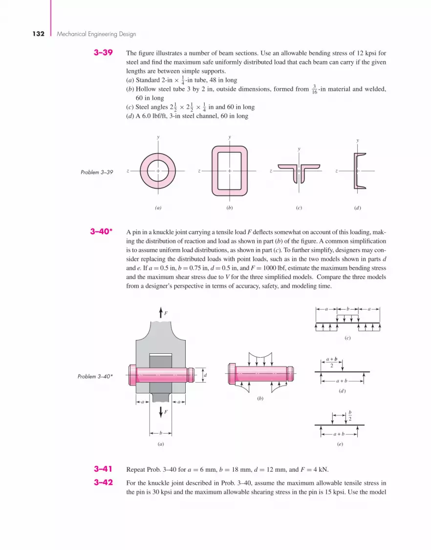
132 Mechanical Engineering Design
3–39 The figure illustrates a number of beam sections. Use an allowable bending stress of 12 kpsi forsteel and find the maximum safe uniformly distributed load that each beam can carry if the givenlengths are between simple supports.(a) Standard 2-in × 1
4 -in tube, 48 in long(b) Hollow steel tube 3 by 2 in, outside dimensions, formed from 3
16 -in material and welded,60 in long
(c) Steel angles 2 12 × 2 1
2 × 14 in and 60 in long
(d) A 6.0 lbf/ft, 3-in steel channel, 60 in long
(d )
z
y
(c)
z
y
(a)
z
y
(b)
z
y
3–40* A pin in a knuckle joint carrying a tensile load F deflects somewhat on account of this loading, mak-ing the distribution of reaction and load as shown in part (b) of the figure. A common simplificationis to assume uniform load distributions, as shown in part (c). To further simplify, designers may con-sider replacing the distributed loads with point loads, such as in the two models shown in parts dand e. If a = 0.5 in, b = 0.75 in, d = 0.5 in, and F = 1000 lbf, estimate the maximum bending stressand the maximum shear stress due to V for the three simplified models. Compare the three modelsfrom a designer’s perspective in terms of accuracy, safety, and modeling time.
Problem 3–39
Problem 3–40*
a a
d
b
(a)
F
F
(b)
b aa
(c)
a + b
a + bb2
(d )
(e)
a + b
b2
3–41 Repeat Prob. 3–40 for a = 6 mm, b = 18 mm, d = 12 mm, and F = 4 kN.
3–42 For the knuckle joint described in Prob. 3–40, assume the maximum allowable tensile stress inthe pin is 30 kpsi and the maximum allowable shearing stress in the pin is 15 kpsi. Use the model
bud29281_ch03_071-146.qxd 11/30/2009 5:34 pm Page 132 pinnacle s-171:Desktop Folder:Temp Work:Don't Delete (Jobs):MHDQ196/Budynas:

Problem 3–44
CBA
1800 lbf300 lbf/in
30 in10 in
3 in
3 in
1 in
Cross section (enlarged)
1 in
Load and Stress Analysis 133
shown in part c of the figure to determine a minimum pin diameter for each of the followingpotential failure modes. (a) Consider failure based on bending at the point of maximum bending stress in the pin.(b) Consider failure based on the average shear stress on the pin cross section at the interface
plane of the knuckle and clevis.(c) Consider failure based on shear at the point of the maximum transverse shear stress in the pin.
3–43 The figure illustrates a pin tightly fitted into a hole of a substantial member. A usual analysisis one that assumes concentrated reactions R and M at distance l from F. Suppose the reactionis distributed linearly along distance a. Is the resulting moment reaction larger or smaller thanthe concentrated reaction? What is the loading intensity q? What do you think of using theusual assumption?
3–45 A cantilever beam with a 1-in-diameter round cross section is loaded at the tip with a trans-verse force of 1000 lbf, as shown in the figure. The cross section at the wall is also shown, withlabeled points A at the top, B at the center, and C at the midpoint between A and B. Study the
Problem 3–43
Problem 3–45
Cross section at the wall
z
y
A
C
B
y
z
L
x
1 in dia.
1000 lbf
lF
a
3–44 For the beam shown, determine (a) the maximum tensile and compressive bending stresses,(b) the maximum shear stress due to V, and (c) the maximum shear stress in the beam.
bud29281_ch03_071-146.qxd 11/25/09 4:55PM Page 133 ntt 203:MHDQ196:bud29281:0073529281:bud29281_pagefiles:

134 Mechanical Engineering Design
significance of the transverse shear stress in combination with bending by performing thefollowing steps.(a) Assume L = 10 in. For points A, B, and C, sketch three-dimensional stress elements, labeling
the coordinate directions and showing all stresses. Calculate magnitudes of the stresses on thestress elements. Do not neglect transverse shear stress. Calculate the maximum shear stressfor each stress element.
(b) For each stress element in part (a), calculate the maximum shear stress if the transverse shearstress is neglected. Determine the percent error for each stress element from neglecting thetransverse shear stress.
(c) Repeat the problem for L = 4, 1, and 0.1 in. Compare the results and state any conclusionsregarding the significance of the transverse shear stress in combination with bending.
3–46 Consider a simply supported beam of rectangular cross section of constant width b and variabledepth h, so proportioned that the maximum stress σx at the outer surface due to bending is con-stant, when subjected to a load F at a distance a from the left support and a distance c from theright support. Show that the depth h at location x is given by
h =√
6Fcx
lbσmax0 ≤ x ≤ a
3–47 In Prob. 3–46, h → 0 as x → 0, which cannot occur. If the maximum shear stress τmax due todirect shear is to be constant in this region, show that the depth h at location x is given by
h = 3
2
Fc
lbτmax0 ≤ x ≤ 3
8
Fcσmax
lbτ 2max
3–48 and The beam shown is loaded in the xy and xz planes. 3–49 (a) Find the yz components of the reactions at the supports.
(b) Plot the shear-force and bending-moment diagrams for the xy and xz planes. Label the dia-grams properly and provide the values at key points.
(c) Determine the net shear-force and bending-moment at the key points of part (b).(d) Determine the maximum tensile bending stress. For Prob. 3–48, use the cross section given in
Prob. 3–34, part (a). For Prob. 3–49, use the cross section given in Prob. 3–39, part (b).
2 kN/m
1.5 m
1.5 kN
0.5 m1 m
AO
B
Cx
y
z
30°
R1y
R1z
R2y
R2z
1000 lbf
600 lbf
4 in
6 in4
11
3A
O
B x
z
y
Problem 3–48 Problem 3–49
3–50 Two steel thin-wall tubes in torsion of equal length are to be compared. The first is of square crosssection, side length b, and wall thickness t. The second is a round of diameter b and wall thick-ness t. The largest allowable shear stress is τall and is to be the same in both cases. How does theangle of twist per unit length compare in each case?
bud29281_ch03_071-146.qxd 11/25/09 4:55PM Page 134 ntt 203:MHDQ196:bud29281:0073529281:bud29281_pagefiles:

t
rmri
1 in
1 in
Load and Stress Analysis 135
3–52 The thin-walled open cross-section shown is transmitting torque T. The angle of twist per unitlength of each leg can be determined separately using Eq. (3–47) and is given by
θ1 = 3Ti
GLi c3i
where for this case, i = 1, 2, 3, and Ti represents the torque in leg i. Assuming that the angle oftwist per unit length for each leg is the same, show that
T = Gθ1
3
3∑i=1
Li c3i and τmax = Gθ1cmax
Problem 3–51
Problem 3–52
c2
c3
c1
L 2
TL1 L3
3–53 to Using the results from Prob. 3–52, consider a steel section with τallow = 12 kpsi. 3–55 (a) Determine the torque transmitted by each leg and the torque transmitted by the entire section.
(b) Determine the angle of twist per unit length.
ProblemNumber c1 L1 c2 L2 c3 L3
3–53 2 mm 20 mm 3 mm 30 mm 0 0
3–54 116 in 3
4 in 18 in 1 in 1
16 in 58 in
3–55 2 mm 20 mm 3 mm 30 mm 2 mm 25 mm
3–56 Two 300-mm-long rectangular steel strips are placed together as shown. Using a maximum allow-able shear stress of 80 MPa, determine the maximum torque and angular twist, and the torsional
3–51 Consider a 1-in-square steel thin-walled tube loaded in torsion. The tube has a wall thicknesst = 1
16 in, is 36 in long, and has a maximum allowable shear stress of 12 kpsi. Determine the max-imum torque that can be applied and the corresponding angle of twist of the tube.(a) Assume that the internal radius at the corners ri = 0.(b) Assume that the internal radius at the corners is more realistically ri = 1
8 in.
bud29281_ch03_071-146.qxd 11/30/2009 5:03 pm Page 135 pinnacle 203:MHDQ196:bud29281:0073529281:bud29281_pagefiles:

136 Mechanical Engineering Design
spring rate. Compare these with a single strip of cross section 30 mm by 4 mm. Solve the prob-lem two ways: (a) using Eqs. (3–40) and (3–41), and (b) using Eq. (3–47). Compare and discussyour results
4 mm
2 mm
30 mmT
Problem 3–56
3–57 Using a maximum allowable shear stress of 70 MPa, find the shaft diameter needed to transmit40 kW when(a) The shaft speed is 2500 rev/min. (b) The shaft speed is 250 rev/min.
3–58 Repeat Prob. 3–57 with an allowable shear stress of 20 kpsi and a power of 50 hp.
3–59 Using an allowable shear stress of 50 MPa, determine the power that can be transmitted at 2000 rpmthrough a shaft with a 30-mm diameter.
3–60 A 20-mm-diameter steel bar is to be used as a torsion spring. If the torsional stress in the bar isnot to exceed 110 MPa when one end is twisted through an angle of 15°, what must be the lengthof the bar?
3–61 A 2-ft-long steel bar with a 34 -in diameter is to be used as a torsion spring. If the torsional stress
in the bar is not to exceed 30 kpsi, what is the maximum angle of twist of the bar?
3–62 A 40-mm-diameter solid steel shaft, used as a torque transmitter, is replaced with a hollowshaft having a 40-mm OD and a 36-mm ID. If both materials have the same strength, what isthe percentage reduction in torque transmission? What is the percentage reduction in shaftweight?
3–63 Generalize Prob. 3–62 for a solid shaft of diameter d replaced with a hollow shaft of the samematerial with an outside diameter d, and an inside diameter that is a fraction of the outside diam-eter, x × d, where x is any fraction between zero and one. Obtain expressions for percentagereduction in torque transmission and percentage reduction in weight in terms of only x. Noticethat the length and diameter of the shaft, and the material, are not needed for this comparison.Plot both results on the same axis for the range 0 < x < 1. From the plot, what is the approxi-mate value of x to obtain the greatest difference between the percent decrease in weight and thepercent decrease in torque?
3–64 A hollow steel shaft is to transmit 4200 N · m of torque and is to be sized so that the torsionalstress does not exceed 120 MPa.(a) If the inside diameter is 70 percent of the outside diameter, what size shaft should be used?
Use preferred sizes.(b) What is the stress on the inside of the shaft when full torque is applied?
3–65 The figure shows an endless-belt conveyor drive roll. The roll has a diameter 120 mm and isdriven at 10 rev/min by a geared-motor source rated at 1.5 kW. Determine a suitable shaft diam-eter dC for an allowable torsional stress of 80 MPa.(a) What would be the stress in the shaft you have sized if the motor starting torque is twice the
running torque?(b) Is bending stress likely to be a problem? What is the effect of different roll lengths B on
bending?
bud29281_ch03_071-146.qxd 11/24/09 3:02PM Page 136 ntt 203:MHDQ196:bud29281:0073529281:bud29281_pagefiles:

CA
x
BA
dA dB dA dC
y
(b)(a)
Load and Stress Analysis 137
Problem 3–65
Problem 3–68* Problem 3–69*
3–66 The conveyer drive roll in the figure for Prob. 3–65 is 5 in in diameter and is driven at 8 rev/minby a geared-motor source rated at 1 hp. Find a suitable shaft diameter dC based on an allowabletorsional stress of 15 kpsi.
3–67 Consider two shafts in torsion, each of the same material, length, and cross-sectional area. Oneshaft has a solid square cross section and the other shaft has a solid circular section.(a) Which shaft has the greater maximum shear stress and by what percentage?(b) Which shaft has the greater angular twist θ and by what percentage?
3–68* to A countershaft carrying two V-belt pulleys is shown in the figure. Pulley A receives power from a 3–71* motor through a belt with the belt tensions shown. The power is transmitted through the shaft and
delivered to the belt on pulley B. Assume the belt tension on the loose side at B is 15 percent ofthe tension on the tight side.(a) Determine the tensions in the belt on pulley B, assuming the shaft is running at a constant
speed.(b) Find the magnitudes of the bearing reaction forces, assuming the bearings act as simple
supports.(c) Draw shear-force and bending-moment diagrams for the shaft. If needed, make one set for the
horizontal plane and another set for the vertical plane.(d) At the point of maximum bending moment, determine the bending stress and the torsional
shear stress.(e) At the point of maximum bending moment, determine the principal stresses and the maximum
shear stress.
A
8-in dia.75 lbf
500 lbfz
12 in
18 in
10 in
O
T1
T2
y
CB
10-in dia.
1 -in dia.x
14
O
T1 B
230 mm
T2
C
30-mm dia.
A
250-mm dia.
400-mm dia.
1800 N
z
y
x
280 mm
270 N
300 mm
bud29281_ch03_071-146.qxd 11/25/09 4:55PM Page 137 ntt 203:MHDQ196:bud29281:0073529281:bud29281_pagefiles:

138 Mechanical Engineering Design
3–72* to A gear reduction unit uses the countershaft shown in the figure. Gear A receives power from 3–73* another gear with the transmitted force FA applied at the 20� pressure angle as shown. The power
is transmitted through the shaft and delivered through gear B through a transmitted force FB atthe pressure angle shown.(a) Determine the force FB, assuming the shaft is running at a constant speed.(b) Find the magnitudes of the bearing reaction forces, assuming the bearings act as simple supports.(c) Draw shear-force and bending-moment diagrams for the shaft. If needed, make one set for the
horizontal plane and another set for the vertical plane.(d) At the point of maximum bending moment, determine the bending stress and the torsional
shear stress.(e) At the point of maximum bending moment, determine the principal stresses and the maximum
shear stress.
x
300 lbf
50 lbf
z
8
8
8 dia.
6 dia.
6
y
1 dia.
T2
T1
O
A
B
C
z
300
400
150
O
y
250 dia.
20 dia.
A
45°
T2
T1
45 N 300 N
B
C
300 dia.
x
Problem 3–71*
Dimensions in millimeters.
Problem 3–70*
Dimensions in inches.
z
y
16 in
14 in
9 in
20°
O
FB
A
x
Gear A20-in dia.
1.25-in dia.
Gear B8-in dia.
20°
C
B
� 300 lbfFA
z
400 mm
350 mm
O
B C
y
20°
Gear A, 600-mm dia.
x
300 mm 25°
Gear B, 300-mm dia.
50-mm dia.
A
� 11 kNFA
FB
Problem 3–72* Problem 3–73*
3–74* In the figure, shaft AB transmits power to shaft CD through a set of bevel gears contacting at pointE. The contact force at E on the gear of shaft CD is determined to be (FE)CD = –92.8i – 362.8j +808.0k lbf. For shaft CD: (a) draw a free-body diagram and determine the reactions at C and D
bud29281_ch03_071-146.qxd 11/30/2009 5:35 pm Page 138 pinnacle s-171:Desktop Folder:Temp Work:Don't Delete (Jobs):MHDQ196/Budynas:
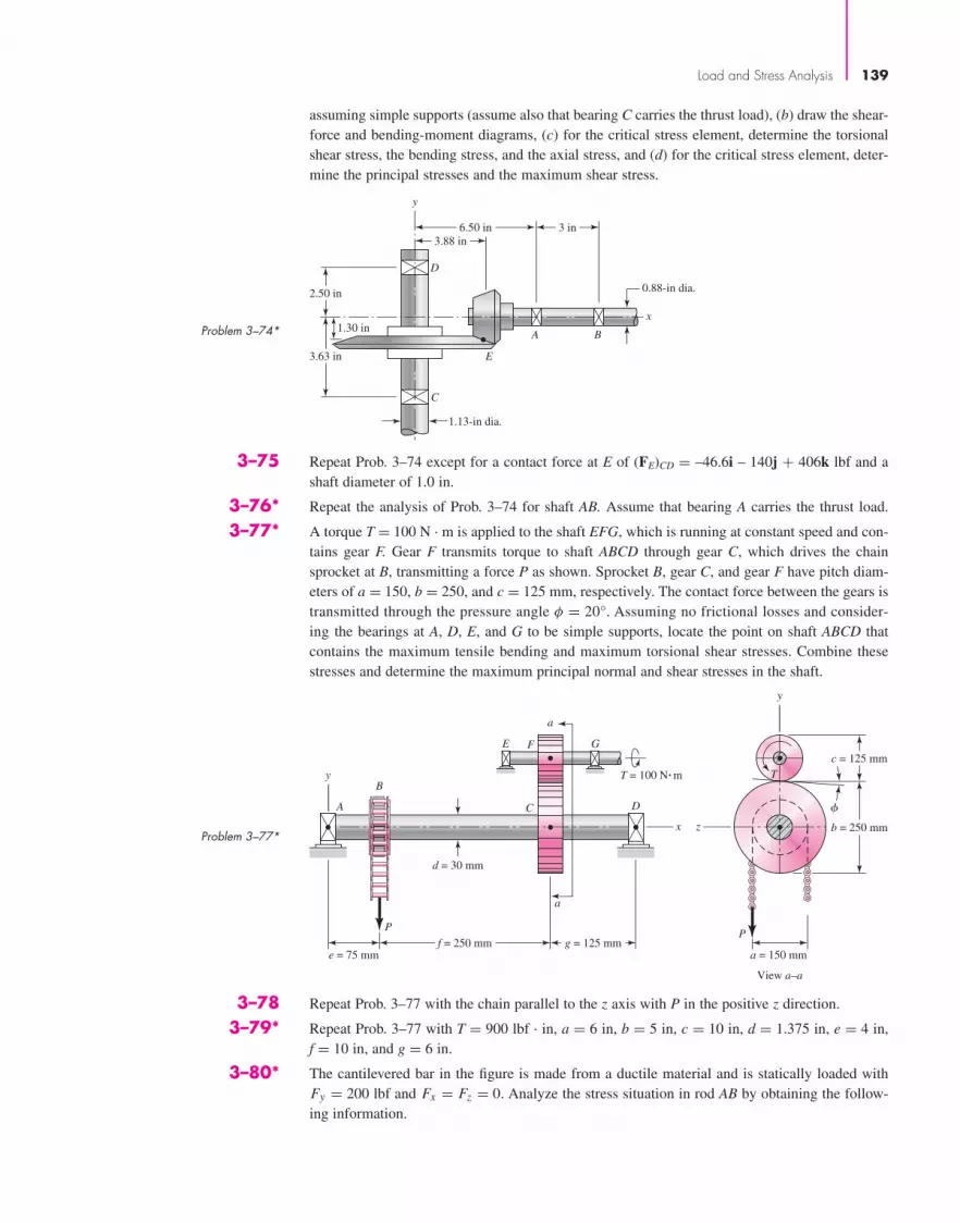
View a–a
�
T = 100 N�m
e = 75 mmf = 250 mm
d = 30 mm
g = 125 mma = 150 mm
b = 250 mm
c = 125 mm
DA
y
x
B
C
a
a
GE F
PP
y
z
T
Load and Stress Analysis 139
Problem 3–74*
Problem 3–77*
assuming simple supports (assume also that bearing C carries the thrust load), (b) draw the shear-force and bending-moment diagrams, (c) for the critical stress element, determine the torsionalshear stress, the bending stress, and the axial stress, and (d) for the critical stress element, deter-mine the principal stresses and the maximum shear stress.
3–75 Repeat Prob. 3–74 except for a contact force at E of (FE)CD = –46.6i – 140j + 406k lbf and ashaft diameter of 1.0 in.
3–76* Repeat the analysis of Prob. 3–74 for shaft AB. Assume that bearing A carries the thrust load.
3–77* A torque T = 100 N · m is applied to the shaft EFG, which is running at constant speed and con-tains gear F. Gear F transmits torque to shaft ABCD through gear C, which drives the chainsprocket at B, transmitting a force P as shown. Sprocket B, gear C, and gear F have pitch diam-eters of a = 150, b = 250, and c = 125 mm, respectively. The contact force between the gears istransmitted through the pressure angle φ = 20°. Assuming no frictional losses and consider-ing the bearings at A, D, E, and G to be simple supports, locate the point on shaft ABCD thatcontains the maximum tensile bending and maximum torsional shear stresses. Combine thesestresses and determine the maximum principal normal and shear stresses in the shaft.
3.63 in
2.50 in
1.30 in
C
D
E
BA
x
y
3 in3.88 in
6.50 in
0.88-in dia.
1.13-in dia.
3–78 Repeat Prob. 3–77 with the chain parallel to the z axis with P in the positive z direction.
3–79* Repeat Prob. 3–77 with T = 900 lbf · in, a = 6 in, b = 5 in, c = 10 in, d = 1.375 in, e = 4 in,f = 10 in, and g = 6 in.
3–80* The cantilevered bar in the figure is made from a ductile material and is statically loaded withFy = 200 lbf and Fx = Fz = 0. Analyze the stress situation in rod AB by obtaining the follow-ing information.
bud29281_ch03_071-146.qxd 11/25/09 4:55PM Page 139 ntt 203:MHDQ196:bud29281:0073529281:bud29281_pagefiles:

140 Mechanical Engineering Design
Problem 3–80*
Problem 3–84*
3–81* Repeat Prob. 3–80 with Fx = 0, Fy = 175 lbf, and Fz = 100 lbf.
3–82* Repeat Prob. 3–80 with Fx = 75 lbf, Fy = −200 lbf, and Fz = 100 lbf.
3–83* For the handle in Prob. 3–80, one potential failure mode is twisting of the flat plate BC. Determinethe maximum value of the shear stress due to torsion in the main section of the plate, ignoringthe complexities of the interfaces at B and C.
3–84* The cantilevered bar in the figure is made from a ductile material and is statically loaded with Fy = 250 lbf and Fx = Fz = 0. Analyze the stress situation in the small diameter at the shoulder at A by obtaining the following information.
(a) Determine the precise location of the critical stress element.(b) Sketch the critical stress element and determine magnitudes and directions for all stresses act-
ing on it. (Transverse shear may only be neglected if you can justify this decision.)(c) For the critical stress element, determine the principal stresses and the maximum shear stress.
A
z
y
2 in
5 in
x
C
B
6 in
14 in
1-in dia.Fy
FzFx
1 12 in
A
-in R.18
1 -in dia.12
z
1-in dia.
2 in
2 in
12 in
B
C
x
O
y
D
9 in
1 12 -in dia.
34 -in dia.-in dia.Fy
FzFx
bud29281_ch03_071-146.qxd 11/30/2009 5:50 pm Page 140 pinnacle 203:MHDQ196:bud29281:0073529281:bud29281_pagefiles:

Load and Stress Analysis 141
(a) Determine the precise location of the critical stress element at the cross section at A.(b) Sketch the critical stress element and determine magnitudes and directions for all stresses
acting on it. (Transverse shear may be neglected if you can justify this decision.)(c) For the critical stress element, determine the principal stresses and the maximum shear stress.
3–85* Repeat Prob. 3–84 with Fx = 300 lbf, Fy = 250 lbf, and Fz = 0.
3–86* Repeat Prob. 3–84 with Fx = 300 lbf, Fy = 250 lbf, and Fz = –100 lbf.
3–87* Repeat Prob. 3–84 for a brittle material, requiring the inclusion of stress concentration in thefillet radius.
3–88 Repeat Prob. 3–84 with Fx = 300 lbf, Fy = 250 lbf, and Fz = 0, and for a brittle material, requir-ing the inclusion of stress concentration in the fillet radius.
3–89 Repeat Prob. 3–84 with Fx = 300 lbf, Fy = 250 lbf, and Fz = –100 lbf, and for a brittle material,requiring the inclusion of stress concentration in the fillet radius.
3–90 The figure shows a simple model of the loading of a square thread of a power screw transmittingan axial load F with an application of torque T. The torque is balanced by the frictional force Ff
acting along the top surface of the thread. The forces on the thread are considered to be distrib-uted along the circumference of the mean diameter dm over the number of engaged threads, nt.From the figure, dm = dr + p/2, where dr is the root diameter of the thread and p is the pitch ofthe thread.(a) Considering the thread to be a cantilever beam as shown in the cutaway view, show that the
bending stress at the root of the thread can be approximated by
σb = ± 6F
πdr nt p
(b) Show that the axial and maximum torsional shear stresses in the body of the shaft can beapproximated by
σa = − 4F
πd2r
and τt = 16T
πd3r
(c) For the stresses of parts (a) and (b) show a three-dimensional representation of the stateof stress on an element located at the intersection of the lower thread root base and the
Problem 3–90
dm
dr
Ff
d
F
y
x
F
T
p/2
p/2
bud29281_ch03_071-146.qxd 11/26/09 5:56PM Page 141 ntt G4 Mac OS 9.2:Desktop Folder:MHDQ196/Budynas:
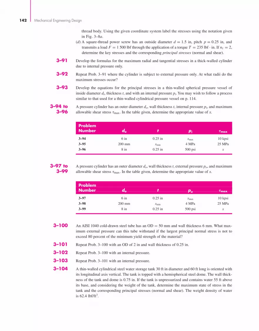
142 Mechanical Engineering Design
thread body. Using the given coordinate system label the stresses using the notation givenin Fig. 3–8a.
(d) A square-thread power screw has an outside diameter d = 1.5 in, pitch p = 0.25 in, andtransmits a load F = 1 500 lbf through the application of a torque T = 235 lbf · in. If nt = 2,determine the key stresses and the corresponding principal stresses (normal and shear).
3–91 Develop the formulas for the maximum radial and tangential stresses in a thick-walled cylinderdue to internal pressure only.
3–92 Repeat Prob. 3–91 where the cylinder is subject to external pressure only. At what radii do themaximum stresses occur?
3–93 Develop the equations for the principal stresses in a thin-walled spherical pressure vessel ofinside diameter di, thickness t, and with an internal pressure pi. You may wish to follow a processsimilar to that used for a thin-walled cylindrical pressure vessel on p. 114.
3–94 to A pressure cylinder has an outer diameter do, wall thickness t, internal pressure pi, and maximum 3–96 allowable shear stress τmax. In the table given, determine the appropriate value of x.
ProblemNumber do t pi �max
3–94 6 in 0.25 in xmax 10 kpsi
3–95 200 mm xmin 4 MPa 25 MPa
3–96 8 in 0.25 in 500 psi x
3–97 to A pressure cylinder has an outer diameter do, wall thickness t, external pressure po, and maximum 3–99 allowable shear stress τmax. In the table given, determine the appropriate value of x.
ProblemNumber do t po �max
3–97 6 in 0.25 in xmax 10 kpsi
3–98 200 mm xmin 4 MPa 25 MPa
3–99 8 in 0.25 in 500 psi x
3–100 An AISI 1040 cold-drawn steel tube has an OD = 50 mm and wall thickness 6 mm. What max-imum external pressure can this tube withstand if the largest principal normal stress is not toexceed 80 percent of the minimum yield strength of the material?
3–101 Repeat Prob. 3–100 with an OD of 2 in and wall thickness of 0.25 in.
3–102 Repeat Prob. 3–100 with an internal pressure.
3–103 Repeat Prob. 3–101 with an internal pressure.
3–104 A thin-walled cylindrical steel water storage tank 30 ft in diameter and 60 ft long is oriented withits longitudinal axis vertical. The tank is topped with a hemispherical steel dome. The wall thick-ness of the tank and dome is 0.75 in. If the tank is unpressurized and contains water 55 ft aboveits base, and considering the weight of the tank, determine the maximum state of stress in thetank and the corresponding principal stresses (normal and shear). The weight density of wateris 62.4 lbf/ft3.
bud29281_ch03_071-146.qxd 11/25/09 4:55PM Page 142 ntt 203:MHDQ196:bud29281:0073529281:bud29281_pagefiles:

Load and Stress Analysis 143
3–105 Repeat Prob. 3–104 with the tank being pressurized to 50 psig.
3–106 Find the maximum shear stress in a 5 12 -in-diameter circular saw blade if it runs idle at 5000 rev/min.
The saw is 14 gauge (0.0747 in) steel and is used on a 58 -in-diameter arbor. The thickness is uni-
form. What is the maximum radial component of stress?
3–107 The maximum recommended speed for a 250-mm-diameter abrasive grinding wheel is 2000 rev/min.Assume that the material is isotropic; use a bore of 20 mm, ν = 0.24, and a mass density of 3320 kg/m3, and find the maximum tensile stress at this speed.
3–108 An abrasive cutoff wheel has a diameter of 5 in, is 116 in thick, and has a 3
4 -in bore. It weighs 5 ozand is designed to run at 12 000 rev/min. If the material is isotropic and ν = 0.20, find themaximum shear stress at the design speed.
3–109 A rotary lawnmower blade rotates at 3500 rev/min. The steel blade has a uniform cross section 18 in
thick by 1 14 in wide, and has a 1
2 -in-diameter hole in the center as shown in the figure. Estimatethe nominal tensile stress at the central section due to rotation.
Problem 3–109
30 in
15 in
14
1 in
18
in
3–110 to The table lists the maximum and minimum hole and shaft dimensions for a variety of standard 3–115 press and shrink fits. The materials are both hot-rolled steel. Find the maximum and minimum
values of the radial interference and the corresponding interface pressure. Use a collar diameterof 100 mm for the metric sizes and 4 in for those in inch units.
Problem Fit Basic Hole ShaftNumber Designation† Size Dmax Dmin dmax dmin
3–110 50H7�p6 50 mm 50.025 50.000 50.042 50.026
3–111 (2 in)H7�p6 2 in 2.0010 2.0000 2.0016 2.0010
3–112 50H7�s6 50 mm 50.025 50.000 50.059 50.043
3–113 (2 in)H7�s6 2 in 2.0010 2.0000 2.0023 2.0017
3–114 50H7�u6 50 mm 50.025 50.000 50.086 50.070
3–115 (2 in)H7�u6 2 in 2.0010 2.0000 2.0034 2.0028
†Note: See Table 7–9 for description of fits.
3–116 to The table gives data concerning the shrink fit of two cylinders of differing materials and 3–119 dimensional specification in inches. Elastic constants for different materials may be found in
Table A–5. Identify the radial interference δ, then find the interference pressure p, and thetangential normal stress on both sides of the fit surface. If dimensional tolerances are given atfit surfaces, repeat the problem for the highest and lowest stress levels.
Problem Inner Cylinder Outer CylinderNumber Material di d0 Material Di D0
3–116 Steel 0 2.002 Steel 2.000 3.00
3–117 Steel 0 2.002 Cast iron 2.000 3.00
3–118 Steel 0 1.002/1.003 Steel 1.001/1.002 2.00
3–119 Aluminum 0 2.003/2.006 Steel 2.000/2.002 3.00
bud29281_ch03_071-146.qxd 11/25/09 5:50PM Page 143 ntt G4 Mac OS 9.2:Desktop Folder:

Problem 3–126
4 in
No. 12 gauge (0.1094 in)
A
A
F
-in R.18
34
in
Section A–A
144 Mechanical Engineering Design
3–121 Repeat Prob. 3–120 with d = 0.75 in, F = 750 lbf, L = 10 in, and Di = 2.5 in.
3–122 The steel eyebolt shown in the figure is loaded with a force F = 300 N. The bolt is formed fromwire of diameter d = 6 mm to a radius R = 10 mm in the eye and at the shank. Estimate thestresses at the inner and outer surfaces at section A–A.
3–120 A utility hook was formed from a round rod of diameter d = 20 mm into the geometry shown inthe figure. What are the stresses at the inner and outer surfaces at section A–A if F = 4 kN,L = 250 mm, and Di = 75 mm?
Problem 3–120
L
d
F
FA
A
Di
Di
Problem 3–122 F F
A
A B
B
R
R
d
3–123 For Prob. 3–122 estimate the stresses at the inner and outer surfaces at section B–B.
3–124 Repeat Prob. 3–122 with d = 14 in, R = 1
2 in, and F = 75 lbf.
3–125 Repeat Prob. 3–123 with d = 14 in, R = 1
2 in, and F = 75 lbf.
3–126 Shown in the figure is a 12-gauge (0.1094-in) by 34 -in latching spring that supports a load of
F = 3 lbf. The inside radius of the bend is 18 in.
(a) Using straight-beam theory, determine the stresses at the top and bottom surfaces immediatelyto the right of the bend.
(b) Using curved-beam theory, determine the stresses at the inner and outer surfaces at the bend.(c) By comparing the stresses at the bend with the nominal stresses before the bend, estimate
effective stress concentration factors for the inner and outer surfaces.
3–127 Repeat Prob. 3–126 with a 10-gauge (0.1406-in) material thickness.
bud29281_ch03_071-146.qxd 11/25/09 4:55PM Page 144 ntt 203:MHDQ196:bud29281:0073529281:bud29281_pagefiles:

Problem 3–129
Dimensions in mm
200
A
A
F2
F1
15025 R.
25
Nylon bushing
Section A–A
87
3128
47
9
60°
Load and Stress Analysis 145
3–128 Repeat Prob. 3–126 with a bend radius of 14 in.
3–129 The cast-iron bell-crank lever depicted in the figure is acted upon by forces F1 of 2.4 kN and F2
of 3.2 kN. The section A–A at the central pivot has a curved inner surface with a radius ofri = 25 mm. Estimate the stresses at the inner and outer surfaces of the curved portion of the lever.
Problem 3–132
4.5 in
1.25-in R.
0.5 in
1.25 in
0.5-in R.
2000 lbf
0.5 in
3–130 The crane hook depicted in Fig. 3–35 has a 34-in-diameter hole in the center of the critical section.
For a load of 6 kip, estimate the bending stresses at the inner and outer surfaces at the critical section.
3–131 An offset tensile link is shaped to clear an obstruction with a geometry as shown in the figure. Thecross section at the critical location is elliptical, with a major axis of 3 in and a minor axis of 1.5 in.For a load of 20 kip, estimate the stresses at the inner and outer surfaces of the critical section.
Problem 3–131 9 in
12-in R.
3–132 A cast-steel C frame as shown in the figure has a rectangular cross section of 1.25 in by 2 in, witha 0.5-in-radius semicircular notch on both sides that forms midflank fluting as shown. Estimate A,rc , rn , and e, and for a load of 2000 lbf, estimate the inner and outer surface stresses at the throatC. Note: Table 3–4 can be used to determine rn for this section. From the table, the integral∫
d A/r can be evaluated for a rectangle and a circle by evaluating A/rn for each shape [seeEq. (3–64)]. Subtracting A/rn of the circle from that of the rectangle yields
∫d A/r for the C
frame, and rn can then be evaluated.
bud29281_ch03_071-146.qxd 11/25/09 4:55PM Page 145 ntt 203:MHDQ196:bud29281:0073529281:bud29281_pagefiles:

146 Mechanical Engineering Design
3–133 Two carbon steel balls, each 30 mm in diameter, are pressed together by a force F . In terms ofthe force F , find the maximum values of the principal stress, and the maximum shear stress, inMPa.
3–134 A carbon steel ball with 25-mm diameter is pressed together with an aluminum ball with a40-mm diameter by a force of 10 N. Determine the maximum shear stress, and the depth atwhich it will occur for the aluminum ball. Assume Fig. 3–37, which is based on a typicalPoisson’s ratio of 0.3, is applicable to estimate the depth at which the maximum shear stressoccurs for these materials.
3–135 Repeat Prob. 3–134 but determine the maximum shear stress and depth for the steel ball.
3–136 A carbon steel ball with a 30-mm diameter is pressed against a flat carbon steel plate with a forceof 20 N. Determine the maximum shear stress, and the depth in the plate at which it will occur.
3–137 An AISI 1018 steel ball with 1-in diameter is used as a roller between a flat plate made from 2024T3 aluminum and a flat table surface made from ASTM No. 30 gray cast iron. Determine themaximum amount of weight that can be stacked on the aluminum plate without exceeding a max-imum shear stress of 20 kpsi in any of the three pieces. Assume Fig. 3–37, which is based on atypical Poisson’s ratio of 0.3, is applicable to estimate the depth at which the maximum shearstress occurs for these materials.
3–138 An aluminum alloy cylindrical roller with diameter 1.25 in and length 2 in rolls on the inside ofa cast-iron ring having an inside radius of 6 in, which is 2 in thick. Find the maximum contactforce F that can be used if the shear stress is not to exceed 4000 psi.
3–139 A pair of mating steel spur gears with a 0.75-in face width transmits a load of 40 lbf. Forestimating the contact stresses, make the simplifying assumption that the teeth profiles can betreated as cylindrical with instantaneous radii at the contact point of interest of 0.47 in and0.62 in, respectively. Estimate the maximum contact pressure and the maximum shear stressexperienced by either gear.
3–140 to A wheel of diameter d and width w carrying a load F rolls on a flat rail. 3–142 Assume that Fig. 3–39, which is based on a Poisson’s ratio of 0.3, is applicable to estimate the
depth at which the maximum shear stress occurs for these materials. At this critical depth, calcu-late the Hertzian stresses σx , σy , σz , and τmax for the wheel.
Problem Wheel RailNumber d w F Material Material
3–140 5 in 2 in 600 lbf Steel Steel
3–141 150 mm 40 mm 2 kN Steel Cast iron
3–142 3 in 1.25 mm 250 lbf Cast iron Cast iron
bud29281_ch03_071-146.qxd 11/25/09 4:55PM Page 146 ntt 203:MHDQ196:bud29281:0073529281:bud29281_pagefiles:

4 Deflection and Stiffness
Chapter Outline
4–1 Spring Rates 148
4–2 Tension, Compression, and Torsion 149
4–3 Deflection Due to Bending 150
4–4 Beam Deflection Methods 152
4–5 Beam Deflections by Superposition 153
4–6 Beam Deflections by Singularity Functions 156
4–7 Strain Energy 162
4–8 Castigliano’s Theorem 164
4–9 Deflection of Curved Members 169
4–10 Statically Indeterminate Problems 175
4–11 Compression Members—General 181
4–12 Long Columns with Central Loading 181
4–13 Intermediate-Length Columns with Central Loading 184
4–14 Columns with Eccentric Loading 184
4–15 Struts or Short Compression Members 188
4–16 Elastic Stability 190
4–17 Shock and Impact 191
147
bud29281_ch04_147-211.qxd 11/27/09 2:55PM Page 147 ntt 203:MHDQ196:bud29281:0073529281:bud29281_pagefiles:

148 Mechanical Engineering Design
All real bodies deform under load, either elastically or plastically. A body can be suffi-ciently insensitive to deformation that a presumption of rigidity does not affect an analy-sis enough to warrant a nonrigid treatment. If the body deformation later proves to be notnegligible, then declaring rigidity was a poor decision, not a poor assumption. A wirerope is flexible, but in tension it can be robustly rigid and it distorts enormously underattempts at compressive loading. The same body can be both rigid and nonrigid.
Deflection analysis enters into design situations in many ways. A snap ring, or retain-ing ring, must be flexible enough to be bent without permanent deformation andassembled with other parts, and then it must be rigid enough to hold the assembled partstogether. In a transmission, the gears must be supported by a rigid shaft. If the shaft bendstoo much, that is, if it is too flexible, the teeth will not mesh properly, and the result willbe excessive impact, noise, wear, and early failure. In rolling sheet or strip steel to pre-scribed thicknesses, the rolls must be crowned, that is, curved, so that the finished productwill be of uniform thickness. Thus, to design the rolls it is necessary to know exactly howmuch they will bend when a sheet of steel is rolled between them. Sometimes mechanicalelements must be designed to have a particular force-deflection characteristic. Thesuspension system of an automobile, for example, must be designed within a very narrowrange to achieve an optimum vibration frequency for all conditions of vehicle loading,because the human body is comfortable only within a limited range of frequencies.
The size of a load-bearing component is often determined on deflections, ratherthan limits on stress.
This chapter considers distortion of single bodies due to geometry (shape) andloading, then, briefly, the behavior of groups of bodies.
4–1 Spring RatesElasticity is that property of a material that enables it to regain its original configurationafter having been deformed. A spring is a mechanical element that exerts a force whendeformed. Figure 4–1a shows a straight beam of length l simply supported at the endsand loaded by the transverse force F. The deflection y is linearly related to the force, aslong as the elastic limit of the material is not exceeded, as indicated by the graph. Thisbeam can be described as a linear spring.
In Fig. 4–1b a straight beam is supported on two cylinders such that the lengthbetween supports decreases as the beam is deflected by the force F. A larger force isrequired to deflect a short beam than a long one, and hence the more this beam isdeflected, the stiffer it becomes. Also, the force is not linearly related to the deflection,and hence this beam can be described as a nonlinear stiffening spring.
Figure 4–1c is an edge-view of a dish-shaped round disk. The force necessary to flat-ten the disk increases at first and then decreases as the disk approaches a flat configuration,
Figure 4–1
(a) A linear spring; (b) a stiffening spring; (c) a softening spring.
l
F
F
y
l
F
y
dF
y
(a)
y
F
(b)
y
F
(c)
y
bud29281_ch04_147-211.qxd 12/10/2009 4:05 pm Page 148 pinnacle s-171:Desktop Folder:Temp Work:Don't Delete (Jobs):MHDQ196/Budynas:

Deflection and Stiffness 149
as shown by the graph. Any mechanical element having such a characteristic is called anonlinear softening spring.
If we designate the general relationship between force and deflection by the equation
F = F(y) (a)
then spring rate is defined as
k(y) = lim�y→0
�F
�y= d F
dy(4–1)
where y must be measured in the direction of F and at the point of application of F. Mostof the force-deflection problems encountered in this book are linear, as in Fig. 4–1a. Forthese, k is a constant, also called the spring constant; consequently Eq. (4–1) is written
k = F
y(4–2)
We might note that Eqs. (4–1) and (4–2) are quite general and apply equally well fortorques and moments, provided angular measurements are used for y. For linear dis-placements, the units of k are often pounds per inch or newtons per meter, and forangular displacements, pound-inches per radian or newton-meters per radian.
4–2 Tension, Compression, and TorsionThe total extension or contraction of a uniform bar in pure tension or compression,respectively, is given by
δ = Fl
AE(4–3)
This equation does not apply to a long bar loaded in compression if there is a possibil-ity of buckling (see Secs. 4–11 to 4–15). Using Eqs. (4–2) and (4–3) with δ = y , we seethat the spring constant of an axially loaded bar is
k = AE
l(4–4)
The angular deflection of a uniform solid or hollow round bar subjected to a twist-ing moment T was given in Eq. (3–35), and is
θ = T l
G J(4–5)
where θ is in radians. If we multiply Eq. (4–5) by 180/π and substitute J = πd4/32 fora solid round bar, we obtain
θ = 583.6T l
Gd4(4–6)
where θ is in degrees.Equation (4–5) can be rearranged to give the torsional spring rate as
k = T
θ= G J
l(4–7)
Equations (4–5), (4–6), and (4–7) apply only to circular cross sections. Torsional load-ing for bars with noncircular cross sections is discussed in Sec. 3–12 (p. 101). For theangular twist of rectangular cross sections, closed thin-walled tubes, and open thin-walled sections, refer to Eqs. (3–41), (3–46), and (3–47), respectively.
bud29281_ch04_147-211.qxd 11/27/09 2:55PM Page 149 ntt 203:MHDQ196:bud29281:0073529281:bud29281_pagefiles:

150 Mechanical Engineering Design
4–3 Deflection Due to BendingThe problem of bending of beams probably occurs more often than any other loadingproblem in mechanical design. Shafts, axles, cranks, levers, springs, brackets, and wheels,as well as many other elements, must often be treated as beams in the design and analy-sis of mechanical structures and systems. The subject of bending, however, is one thatyou should have studied as preparation for reading this book. It is for this reason thatwe include here only a brief review to establish the nomenclature and conventions to beused throughout this book.
The curvature of a beam subjected to a bending moment M is given by
1
ρ= M
E I(4–8)
where ρ is the radius of curvature. From studies in mathematics we also learn that thecurvature of a plane curve is given by the equation
1
ρ= d2 y/dx2
[1 + (dy/dx)2]3/2(4–9)
where the interpretation here is that y is the lateral deflection of the centroidal axis ofthe beam at any point x along its length. The slope of the beam at any point x is
θ = dy
dx(a)
For many problems in bending, the slope is very small, and for these the denominatorof Eq. (4–9) can be taken as unity. Equation (4–8) can then be written
M
E I= d2 y
dx2(b)
Noting Eqs. (3–3) and (3–4) and successively differentiating Eq. (b) yields
V
E I= d3 y
dx3(c)
q
E I= d4 y
dx4(d )
It is convenient to display these relations in a group as follows:
q
E I= d4 y
dx4(4–10)
V
E I= d3 y
dx3(4–11)
M
E I= d2 y
dx2(4–12)
θ = dy
dx(4–13)
y = f (x) (4–14)
bud29281_ch04_147-211.qxd 11/27/09 2:55PM Page 150 ntt 203:MHDQ196:bud29281:0073529281:bud29281_pagefiles:

Deflection and Stiffness 151
The nomenclature and conventions are illustrated by the beam of Fig. 4–2. Here, a beamof length l = 20 in is loaded by the uniform load w = 80 lbf per inch of beam length.The x axis is positive to the right, and the y axis positive upward. All quantities—loading, shear, moment, slope, and deflection—have the same sense as y; they are pos-itive if upward, negative if downward.
The reactions R1 = R2 = +800 lbf and the shear forces V0 = +800 lbf andVl = −800 lbf are easily computed by using the methods of Chap. 3. The bendingmoment is zero at each end because the beam is simply supported. For a simply-supported beam, the deflections are also zero at each end.
Figure 4–2
(a)
(b)
(c)
(d)
(e)
l = 20 in
R1 = wl2
R2 = wl2
y
Loading, ww = 80 lbf/inx
+
+
–
V0
M0 Ml
Vl
V
M
x
–
–
+
EI�
EI�0
EI�l
x
x
Shear, VV0 = +800 lbfVl = –800 lbf
EIy
xDeflection, EIyy0 = yl = 0
Moment, MM0 = Ml = 0
Slope, EI��l /2 = 0
w
EXAMPLE 4–1 For the beam in Fig. 4–2, the bending moment equation, for 0 ≤ x ≤ l, is
M = wl
2x − w
2x2
Using Eq. (4–12), determine the equations for the slope and deflection of the beam, theslopes at the ends, and the maximum deflection.
Solution Integrating Eq. (4–12) as an indefinite integral we have
E Idy
dx=
∫M dx = wl
4x2 − w
6x3 + C1 (1)
where C1 is a constant of integration that is evaluated from geometric boundary conditions.We could impose that the slope is zero at the midspan of the beam, since the beam and
bud29281_ch04_147-211.qxd 11/27/09 2:55PM Page 151 ntt 203:MHDQ196:bud29281:0073529281:bud29281_pagefiles:

152 Mechanical Engineering Design
loading are symmetric relative to the midspan. However, we will use the given bound-ary conditions of the problem and verify that the slope is zero at the midspan. IntegratingEq. (1) gives
E I y =∫∫
M dx = wl
12x3 − w
24x4 + C1x + C2 (2)
The boundary conditions for the simply supported beam are y = 0 at x = 0 and l.Applying the first condition, y = 0 at x = 0, to Eq. (2) results in C2 = 0. Applying thesecond condition to Eq. (2) with C2 = 0,
E I y(l) = wl
12l3 − w
24l4 + C1l = 0
Solving for C1 yields C1 = −wl3/24. Substituting the constants back into Eqs. (1) and(2) and solving for the deflection and slope results in
y = wx
24E I(2lx2 − x3 − l3) (3)
θ = dy
dx= w
24E I(6lx2 − 4x3 − l3) (4)
Comparing Eq. (3) with that given in TableA–9, beam 7, we see complete agreement.For the slope at the left end, substituting x = 0 into Eq. (4) yields
θ |x=0 = − wl3
24E I
and at x = l,
θ |x= l = wl3
24E I
At the midspan, substituting x = l/2 gives dy/dx = 0, as earlier suspected.The maximum deflection occurs where dy/dx = 0. Substituting x = l/2 into
Eq. (3) yields
ymax = − 5wl4
384E I
which again agrees with Table A–9–7.
The approach used in the example is fine for simple beams with continuousloading. However, for beams with discontinuous loading and/or geometry such as a stepshaft with multiple gears, flywheels, pulleys, etc., the approach becomes unwieldy. Thefollowing section discusses bending deflections in general and the techniques that areprovided in this chapter.
4–4 Beam Deflection MethodsEquations (4–10) through (4–14) are the basis for relating the intensity of loading q,vertical shear V, bending moment M, slope of the neutral surface θ, and the trans-verse deflection y. Beams have intensities of loading that range from q = constant
bud29281_ch04_147-211.qxd 11/27/09 2:55PM Page 152 ntt 203:MHDQ196:bud29281:0073529281:bud29281_pagefiles:

Deflection and Stiffness 153
1Warren C. Young and Richard G. Budynas, Roark’s Formulas for Stress and Strain, 7th ed., McGraw-Hill,New York, 2002.2See Chap. 9, F. P. Beer, E. R. Johnston Jr., and J. T. DeWolf, Mechanics of Materials, 5th ed., McGraw-Hill,New York, 2009.3See Sec. 4–4, J. E. Shigley and C. R. Mischke, Mechanical Engineering Design, 6th ed., McGraw-Hill,New York, 2001.4Warren C. Young and Richard G. Budynas, Roark’s Formulas for Stress and Strain, 7th ed., McGraw-Hill,New York, 2002.
(uniform loading), variable intensity q(x), to Dirac delta functions (concentratedloads).
The intensity of loading usually consists of piecewise contiguous zones, theexpressions for which are integrated through Eqs. (4–10) to (4–14) with varyingdegrees of difficulty. Another approach is to represent the deflection y(x) as a Fourierseries, which is capable of representing single-valued functions with a finite number offinite discontinuities, then differentiating through Eqs. (4–14) to (4–10), and stoppingat some level where the Fourier coefficients can be evaluated. A complication is thepiecewise continuous nature of some beams (shafts) that are stepped-diameter bodies.
All of the above constitute, in one form or another, formal integration methods,which, with properly selected problems, result in solutions for q, V, M, θ, and y. Thesesolutions may be
1 Closed-form, or2 Represented by infinite series, which amount to closed form if the series are rapidly
convergent, or3 Approximations obtained by evaluating the first or the first and second terms.
The series solutions can be made equivalent to the closed-form solution by the use of acomputer. Roark’s1 formulas are committed to commercial software and can be used ona personal computer.
There are many techniques employed to solve the integration problem for beamdeflection. Some of the popular methods include:
• Superposition (see Sec. 4–5)
• The moment-area method2
• Singularity functions (see Sec. 4–6)
• Numerical integration3
The two methods described in this chapter are easy to implement and can handle a largearray of problems.
There are methods that do not deal with Eqs. (4–10) to (4–14) directly. An energymethod, based on Castigliano’s theorem, is quite powerful for problems not suitable forthe methods mentioned earlier and is discussed in Secs. 4–7 to 4–10. Finite elementprograms are also quite useful for determining beam deflections.
4–5 Beam Deflections by SuperpositionThe results of many simple load cases and boundary conditions have been solvedand are available. Table A–9 provides a limited number of cases. Roark’s4 providesa much more comprehensive listing. Superposition resolves the effect of combinedloading on a structure by determining the effects of each load separately and adding
bud29281_ch04_147-211.qxd 11/27/09 2:55PM Page 153 ntt 203:MHDQ196:bud29281:0073529281:bud29281_pagefiles:

154 Mechanical Engineering Design
the results algebraically. Superposition may be applied provided: (1) each effect islinearly related to the load that produces it, (2) a load does not create a condition thataffects the result of another load, and (3) the deformations resulting from any spe-cific load are not large enough to appreciably alter the geometric relations of theparts of the structural system.
The following examples are illustrations of the use of superposition.
Figure 4–3
x
y
R1
F
wa b
l
BA
C
R2
If the maximum deflection of a beam is desired, it will occur either where the slopeis zero or at the end of the overhang if the beam has a free end. In the previous example,there is no overhang, so setting dy/dx = 0 will yield the equation for x that locateswhere the maximum deflection occurs. In the example there are two equations for ywhere only one will yield a solution. If a = l/2, the maximum deflection would obvi-ously occur at x = l/2 because of symmetry. However, if a < l/2, where would themaximum deflection occur? It can be shown that as F moves toward the left support,the maximum deflection moves toward the left support also, but not as much as F (seeProb. 4–34). Thus, we would set dyBC/dx = 0 and solve for x. If a > l/2, then wewould set dyAB�dx = 0. For more complicated problems, plotting the equations usingnumerical data is the simplest approach to finding the maximum deflection.
EXAMPLE 4–2 Consider the uniformly loaded beam with a concentrated force as shown in Fig. 4–3.Using superposition, determine the reactions and the deflection as a function of x.
Solution Considering each load state separately, we can superpose beams 6 and 7 of Table A–9.For the reactions we find
Answer R1 = Fb
l+ wl
2
Answer R2 = Fa
l+ wl
2
The loading of beam 6 is discontinuous and separate deflection equations are givenfor regions AB and BC. Beam 7 loading is not discontinuous so there is only one equa-tion. Superposition yields
Answer yAB = Fbx
6E Il(x2 + b2 − l2) + wx
24E I(2lx2 − x3 − l3)
Answer yBC = Fa(l − x)
6E Il(x2 + a2 − 2lx) + wx
24E I(2lx2 − x3 − l3)
bud29281_ch04_147-211.qxd 11/27/09 2:55PM Page 154 ntt 203:MHDQ196:bud29281:0073529281:bud29281_pagefiles:
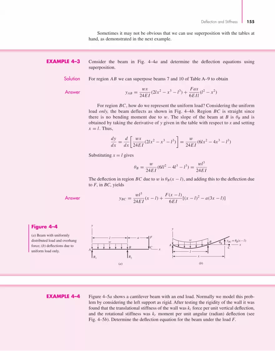
Deflection and Stiffness 155
EXAMPLE 4–3 Consider the beam in Fig. 4–4a and determine the deflection equations usingsuperposition.
Solution For region AB we can superpose beams 7 and 10 of Table A–9 to obtain
Answer yAB = wx
24E I(2lx2 − x3 − l3) + Fax
6E Il(l2 − x2)
For region BC , how do we represent the uniform load? Considering the uniformload only, the beam deflects as shown in Fig. 4–4b. Region BC is straight sincethere is no bending moment due to w. The slope of the beam at B is θB and isobtained by taking the derivative of y given in the table with respect to x and settingx = l . Thus,
dy
dx= d
dx
[wx
24E I(2lx2 − x3 − l3)
]= w
24E I(6lx2 − 4x3 − l3)
Substituting x = l gives
θB = w
24E I(6ll2 − 4l3 − l3) = wl3
24E I
The deflection in region BC due to w is θB(x − l), and adding this to the deflection dueto F, in BC, yields
Answer yBC = wl3
24E I(x − l) + F(x − l)
6E I[(x − l)2 − a(3x − l)]
x
y
R1
Fw
al
BA
C
R2
(a)
x
y
w
xl
B �ByBC = �B(x – l )
AC
(b)
Figure 4–4
(a) Beam with uniformlydistributed load and overhangforce; (b) deflections due touniform load only.
EXAMPLE 4–4 Figure 4–5a shows a cantilever beam with an end load. Normally we model this prob-lem by considering the left support as rigid. After testing the rigidity of the wall it wasfound that the translational stiffness of the wall was kt force per unit vertical deflection,and the rotational stiffness was kr moment per unit angular (radian) deflection (seeFig. 4–5b). Determine the deflection equation for the beam under the load F.
Sometimes it may not be obvious that we can use superposition with the tables athand, as demonstrated in the next example.
bud29281_ch04_147-211.qxd 11/27/09 2:55PM Page 155 ntt 203:MHDQ196:bud29281:0073529281:bud29281_pagefiles:
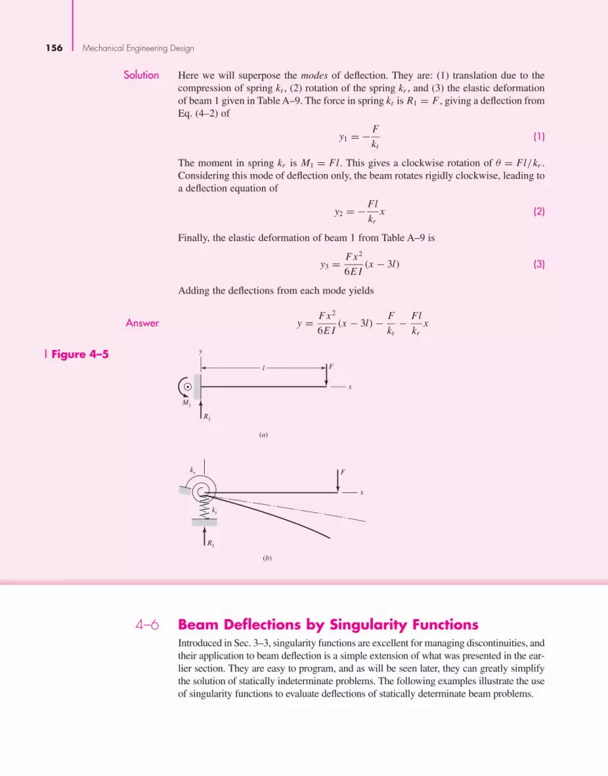
156 Mechanical Engineering Design
Solution Here we will superpose the modes of deflection. They are: (1) translation due to thecompression of spring kt , (2) rotation of the spring kr , and (3) the elastic deformationof beam 1 given in Table A–9. The force in spring kt is R1 = F , giving a deflection fromEq. (4–2) of
y1 = − F
kt(1)
The moment in spring kr is M1 = Fl . This gives a clockwise rotation of θ = Fl/kr .Considering this mode of deflection only, the beam rotates rigidly clockwise, leading toa deflection equation of
y2 = − Fl
krx (2)
Finally, the elastic deformation of beam 1 from Table A–9 is
y3 = Fx2
6E I(x − 3l) (3)
Adding the deflections from each mode yields
Answer y = Fx2
6E I(x − 3l) − F
kt− Fl
krx
4–6 Beam Deflections by Singularity FunctionsIntroduced in Sec. 3–3, singularity functions are excellent for managing discontinuities, andtheir application to beam deflection is a simple extension of what was presented in the ear-lier section. They are easy to program, and as will be seen later, they can greatly simplifythe solution of statically indeterminate problems. The following examples illustrate the useof singularity functions to evaluate deflections of statically determinate beam problems.
x
y
R1
Fl
(a)
M1
x
kr
kt
F
(b)
R1
Figure 4–5
bud29281_ch04_147-211.qxd 11/27/09 2:55PM Page 156 ntt 203:MHDQ196:bud29281:0073529281:bud29281_pagefiles:

Deflection and Stiffness 157
EXAMPLE 4–5 Consider beam 6 of Table A–9, which is a simply supported beam having a concen-trated load F not in the center. Develop the deflection equations using singularityfunctions.
Solution First, write the load intensity equation from the free-body diagram,
q = R1〈x〉−1 − F〈x − a〉−1 + R2〈x − l〉−1 (1)
Integrating Eq. (1) twice results in
V = R1〈x〉0 − F〈x − a〉0 + R2〈x − l〉0 (2)
M = R1〈x〉1 − F〈x − a〉1 + R2〈x − l〉1 (3)
Recall that as long as the q equation is complete, integration constants are unnecessaryfor V and M; therefore, they are not included up to this point. From statics, settingV = M = 0 for x slightly greater than l yields R1 = Fb/ l and R2 = Fa/ l . Thus Eq. (3)becomes
M = Fb
l〈x〉1 − F〈x − a〉1 + Fa
l〈x − l〉1
Integrating Eqs. (4–12) and (4–13) as indefinite integrals gives
E Idy
dx= Fb
2l〈x〉2 − F
2〈x − a〉2 + Fa
2l〈x − l〉2 + C1
E I y = Fb
6l〈x〉3 − F
6〈x − a〉3 + Fa
6l〈x − l〉3 + C1x + C2
Note that the first singularity term in both equations always exists, so 〈x〉2 = x2
and 〈x〉3 = x3. Also, the last singularity term in both equations does not exist untilx = l, where it is zero, and since there is no beam for x > l we can drop the last term.Thus
E Idy
dx= Fb
2lx2 − F
2〈x − a〉2 + C1 (4)
E I y = Fb
6lx3 − F
6〈x − a〉3 + C1x + C2 (5)
The constants of integration C1 and C2 are evaluated by using the two boundary con-ditions y = 0 at x = 0 and y = 0 at x = l. The first condition, substituted into Eq. (5),gives C2 = 0 (recall that 〈0 − a〉3 = 0). The second condition, substituted into Eq. (5),yields
0 = Fb
6ll3 − F
6(l − a)3 + C1l = Fbl2
6− Fb3
6+ C1l
Solving for C1 gives
C1 = − Fb
6l(l2 − b2)
bud29281_ch04_147-211.qxd 11/27/09 2:55PM Page 157 ntt 203:MHDQ196:bud29281:0073529281:bud29281_pagefiles:

158 Mechanical Engineering Design
Figure 4–6
x
y
R1
w
l
a
BA
C
R2
Finally, substituting C1 and C2 in Eq. (5) and simplifying produces
y = F
6E Il[bx(x2 + b2 − l2) − l〈x − a〉3] (6)
Comparing Eq. (6) with the two deflection equations for beam 6 in Table A–9, we notethat the use of singularity functions enables us to express the deflection equation witha single equation.
EXAMPLE 4–6 Determine the deflection equation for the simply supported beam with the load distribu-tion shown in Fig. 4–6.
Solution This is a good beam to add to our table for later use with superposition. The load inten-sity equation for the beam is
q = R1〈x〉−1 − w〈x〉0 + w〈x − a〉0 + R2〈x − l〉−1 (1)
where the w〈x − a〉0 is necessary to “turn off” the uniform load at x = a.From statics, the reactions are
R1 = wa
2l(2l − a) R2 = wa2
2l(2)
For simplicity, we will retain the form of Eq. (1) for integration and substitute the valuesof the reactions in later.
Two integrations of Eq. (1) reveal
V = R1〈x〉0 − w〈x〉1 + w〈x − a〉1 + R2〈x − l〉0 (3)
M = R1〈x〉1 − w
2〈x〉2 + w
2〈x − a〉2 + R2〈x − l〉1 (4)
As in the previous example, singularity functions of order zero or greater starting atx = 0 can be replaced by normal polynomial functions. Also, once the reactions aredetermined, singularity functions starting at the extreme right end of the beam can beomitted. Thus, Eq. (4) can be rewritten as
M = R1x − w
2x2 + w
2〈x − a〉2 (5)
bud29281_ch04_147-211.qxd 11/27/2009 7:54 pm Page 158 pinnacle s-171:Desktop Folder:Temp Work:Don't Delete (Jobs):MHDQ196/Budynas:

Deflection and Stiffness 159
Integrating two more times for slope and deflection gives
E Idy
dx= R1
2x2 − w
6x3 + w
6〈x − a〉3 + C1 (6)
E I y = R1
6x3 − w
24x4 + w
24〈x − a〉4 + C1x + C2 (7)
The boundary conditions are y = 0 at x = 0 and y = 0 at x = l. Substituting the firstcondition in Eq. (7) shows C2 = 0. For the second condition
0 = R1
6l3 − w
24l4 + w
24(l − a)4 + C1l
Solving for C1 and substituting into Eq. (7) yields
E I y = R1
6x(x2 − l2) − w
24x(x3 − l3) − w
24lx(l − a)4 + w
24〈x − a〉4
Finally, substitution of R1 from Eq. (2) and simplifying results gives
Answer y = w
24E Il[2ax(2l − a)(x2 − l2) − xl(x3 − l3) − x(l − a)4 + l〈x − a〉4]
As stated earlier, singularity functions are relatively simple to program, as they areomitted when their arguments are negative, and the 〈 〉 brackets are replaced with ( )parentheses when the arguments are positive.
EXAMPLE 4–7 The steel step shaft shown in Fig. 4–7a is mounted in bearings at A and F. A pulleyis centered at C where a total radial force of 600 lbf is applied. Using singularityfunctions evaluate the shaft displacements at 1
2 -in increments. Assume the shaft issimply supported.
Solution The reactions are found to be R1 = 360 lbf and R2 = 240 lbf. Ignoring R2, usingsingularity functions, the moment equation is
M = 360x − 600〈x − 8〉1 (1)
This is plotted in Fig. 4–7b.For simplification, we will consider only the step at D. That is, we will assume sec-
tion AB has the same diameter as BC and section EF has the same diameter as DE.Since these sections are short and at the supports, the size reduction will not add muchto the deformation. We will examine this simplification later. The second area momentsfor BC and DE are
IBC = π
641.54 = 0.2485 in4 IDE = π
641.754 = 0.4604 in4
bud29281_ch04_147-211.qxd 11/27/09 2:55PM Page 159 ntt 203:MHDQ196:bud29281:0073529281:bud29281_pagefiles:

160 Mechanical Engineering Design
A plot of M/I is shown in Fig. 4–7c. The values at points b and c, and the step change are(M
I
)b
= 2760
0.2485= 11 106.6 lbf/in3
(M
I
)c
= 2760
0.4604= 5 994.8 lbf/in3
�
(M
I
)= 5 994.8 − 11 106.6 = −5 111.8 lbf/in3
The slopes for ab and cd, and the change are
mab = 2760 − 2880
0.2485(0.5)= −965.8 lbf/in4 mcd = −5 994.8
11.5= −521.3 lbf/in4
�m = −521.3 − (−965.8) = 444.5 lbf/in4
Dividing Eq. (1) by IBC and, at x � 8.5 in, adding a step of −5 111.8 lbf/in3 and a rampof slope 444.5 lbf/in4, gives
M
I= 1 448.7x − 2 414.5〈x − 8〉1 − 5 111.8〈x − 8.5〉0 + 444.5〈x − 8.5〉1 (2)
Integration gives
Edy
dx= 724.35x2 − 1207.3〈x − 8〉2 − 5 111.8〈x − 8.5〉1
+ 222.3〈x − 8.5〉2 + C1 (3)
Integrating again yields
Ey = 241.5x3 − 402.4〈x − 8〉3 − 2 555.9〈x − 8.5〉2 + 74.08〈x − 8.5〉3 + C1x + C2
(4)
At x = 0, y = 0. This gives C2 = 0 (remember, singularity functions do not exist untilthe argument is positive). At x = 20 in, y = 0, and
0 = 241.5(20)3 − 402.4(20 − 8)3 − 2 555.9(20 − 8.5)2 + 74.08(20 − 8.5)3 + C1(20)
M/I
M
a b
EDCBA
R2
Fx
c
d
2880 lbf-in 2760 lbf-in
1.0001.7501.500
0.58
600 lbf
1.000
8.519.5
20R1
y
(a)
(b)
(c)
Figure 4–7
Dimensions in inches.
bud29281_ch04_147-211.qxd 11/27/2009 7:54 pm Page 160 pinnacle s-171:Desktop Folder:Temp Work:Don't Delete (Jobs):MHDQ196/Budynas:

Deflection and Stiffness 161
Solving, gives C1 = −50 565 lbf/in2. Thus, Eq. (4) becomes, with E = 30(10)6 psi,
y = 1
30(106)(241.5x3 − 402.4〈x − 8〉3 − 2 555.9〈x − 8.5〉2
+ 74.08〈x − 8.5〉3 − 50 565x)
(5)
When using a spreadsheet, program the following equations:
y = 1
30(106)(241.5x3 − 50 565x) 0 ≤ x ≤ 8 in
y = 1
30(106)[241.5x3 − 402.4(x − 8)3 − 50 565x] 8 ≤ x ≤ 8.5 in
y = 1
30(106)[241.5x3 − 402.4 (x − 8)3 − 2 555.9 (x − 8.5)2
+ 74.08 (x − 8.5)3 − 50 565x] 8.5 ≤ x ≤ 20 in
The following table results.
x y x y x y x y x y
0 0.000000 4.5 �0.006851 9 �0.009335 13.5 �0.007001 18 �0.002377
0.5 �0.000842 5 �0.007421 9.5 �0.009238 14 �0.006571 18.5 �0.001790
1 �0.001677 5.5 �0.007931 10 �0.009096 14.5 �0.006116 19 �0.001197
1.5 �0.002501 6 �0.008374 10.5 �0.008909 15 �0.005636 19.5 �0.000600
2 �0.003307 6.5 �0.008745 11 �0.008682 15.5 �0.005134 20 0.000000
2.5 �0.004088 7 �0.009037 11.5 �0.008415 16 �0.004613
3 �0.004839 7.5 �0.009245 12 �0.008112 16.5 �0.004075
3.5 �0.005554 8 �0.009362 12.5 �0.007773 17 �0.003521
4 �0.006227 8.5 �0.009385 13 �0.007403 17.5 �0.002954
where x and y are in inches. We see that the greatest deflection is at x = 8.5 in, wherey = −0.009385 in.
Substituting C1 into Eq. (3) the slopes at the supports are found to be θA = 1.686(10−3)rad = 0.09657 deg, and θF = 1.198(10−3) rad = 0.06864 deg. You might think these tobe insignificant deflections, but as you will see in Chap. 7, on shafts, they are not.
A finite-element analysis was performed for the same model and resulted in
y|x=8.5 in = −0.009380 in θA = −0.09653◦ θF = 0.06868◦
Virtually the same answer save some round-off error in the equations.If the steps of the bearings were incorporated into the model, more equations result,
but the process is the same. The solution to this model is
y|x=8.5 in = −0.009387 in θA = −0.09763◦ θF = 0.06973◦
The largest difference between the models is of the order of 1.5 percent. Thus the sim-plification was justified.
bud29281_ch04_147-211.qxd 11/27/09 2:55PM Page 161 ntt 203:MHDQ196:bud29281:0073529281:bud29281_pagefiles:

162 Mechanical Engineering Design
In Sec. 4–9, we will demonstrate the usefulness of singularity functions in solvingstatically indeterminate problems.
4–7 Strain EnergyThe external work done on an elastic member in deforming it is transformed into strain,or potential, energy. If the member is deformed a distance y, and if the force-deflectionrelationship is linear, this energy is equal to the product of the average force and thedeflection, or
U = F
2y = F2
2k(4–15)
This equation is general in the sense that the force F can also mean torque, or moment,provided, of course, that consistent units are used for k. By substituting appropriateexpressions for k, strain-energy formulas for various simple loadings may be obtained.For tension and compression, for example, we employ Eq. (4–4) and obtain
U = F2l
2AE(4–16)
or
U =∫
F2
2AEdx
tension and compression
(4–17)
where the first equation applies when all the terms are constant throughout the length,and the more general integral equation allows for any of the terms to vary through thelength.
Similarly, from Eq. (4–7), the strain energy for torsion is given by
U = T 2l
2G J(4–18)
or
U =∫
T 2
2G Jdx
torsion
(4–19)
To obtain an expression for the strain energy due to direct shear, consider the elementwith one side fixed in Fig. 4–8a. The force F places the element in pure shear, and thework done is U = Fδ/2. Since the shear strain is γ = δ/ l = τ/G = F/AG, we have
U = F2l
2AG(4–20)
or
U =∫
F2
2AGdx
direct shear
(4–21)
dx
A
O
Bds
d��
(a) Pure shear element (b) Beam bending element
F
F
F
�
�
l
Figure 4–8
⎫⎪⎬⎪⎭
⎫⎪⎬⎪⎭
⎫⎪⎬⎪⎭
bud29281_ch04_147-211.qxd 11/27/2009 7:54 pm Page 162 pinnacle s-171:Desktop Folder:Temp Work:Don't Delete (Jobs):MHDQ196/Budynas:

Deflection and Stiffness 163
The strain energy stored in a beam or lever by bending may be obtained by refer-ring to Fig. 4–8b. Here AB is a section of the elastic curve of length ds having a radiusof curvature ρ. The strain energy stored in this element of the beam is dU = (M/2)dθ.
Since ρ dθ = ds , we have
dU = M ds
2ρ(a)
We can eliminate ρ by using Eq. (4–8), ρ = E I/M . Thus
dU = M2 ds
2E I(b)
For small deflections, ds.= dx . Then, for the entire beam
U =∫
dU =∫
M2
2E Idx (c)
The integral equation is commonly needed for bending, where the moment is typicallya function of x. Summarized to include both the integral and nonintegral form, the strainenergy for bending is
U = M2l
2E I(4–22)
or
U =∫
M2
2E Idx
bending
(4–23)
Equations (4–22) and (4–23) are exact only when a beam is subject to pure bend-ing. Even when transverse shear is present, these equations continue to give quite goodresults, except for very short beams. The strain energy due to shear loading of a beamis a complicated problem. An approximate solution can be obtained by using Eq. (4–20)with a correction factor whose value depends upon the shape of the cross section. If weuse C for the correction factor and V for the shear force, then the strain energy due toshear in bending is
U = CV 2l
2AG(4–24)
or
U =∫
CV 2
2AGdx
transverse shear
(4–25)
Values of the factor C are listed in Table 4–1.
Table 4–1
Strain-Energy Correction
Factors for Transverse
Shear
Source: Richard G. Budynas,Advanced Strength and AppliedStress Analysis, 2nd ed.,McGraw-Hill, New York, 1999. Copyright © 1999 TheMcGraw-Hill Companies.
Beam Cross-Sectional Shape Factor C
Rectangular 1.2
Circular 1.11
Thin-walled tubular, round 2.00
Box sections† 1.00
Structural sections† 1.00
†Use area of web only.
⎫⎪⎬⎪⎭
⎫⎪⎬⎪⎭
bud29281_ch04_147-211.qxd 11/27/2009 7:54 pm Page 163 pinnacle s-171:Desktop Folder:Temp Work:Don't Delete (Jobs):MHDQ196/Budynas:

164 Mechanical Engineering Design
EXAMPLE 4–8 A cantilever beam with a round cross section has a concentrated load F at the end, asshown in Fig. 4–9a. Find the strain energy in the beam.
Solution To determine what forms of strain energy are involved with the deflection of the beam, webreak into the beam and draw a free-body diagram to see the forces and moments beingcarried within the beam. Figure 4–9b shows such a diagram in which the transverse shearis V = −F , and the bending moment is M = −Fx . The variable x is simply a variable ofintegration and can be defined to be measured from any convenient point. The same resultswill be obtained from a free-body diagram of the right-hand portion of the beam with xmeasured from the wall. Using the free end of the beam usually results in reduced effortsince the ground reaction forces do not need to be determined.
For the transverse shear, using Eq. (4–24) with the correction factor C = 1.11 fromTable 4–2, and noting that V is constant through the length of the beam,
Ushear = CV 2l
2AG= 1.11F2l
2AG
For the bending, since M is a function of x, Eq. (4–23) gives
Ubend =∫
M2dx
2E I= 1
2E I
∫ l
0(−Fx)2dx = F2l3
6E I
The total strain energy is
Answer U = Ubend + Ushear = F2l3
6E I+ 1.11F2l
2AG
Note, except for very short beams, the shear term (of order l) is typically small com-pared to the bending term (of order l3). This will be demonstrated in the next example.
ymax
F
l
(a)
Figure 4–9 F
M
V
x
(b)
4–8 Castigliano’s TheoremA most unusual, powerful, and often surprisingly simple approach to deflection analysisis afforded by an energy method called Castigliano’s theorem. It is a unique way of ana-lyzing deflections and is even useful for finding the reactions of indeterminate structures.Castigliano’s theorem states that when forces act on elastic systems subject to small dis-placements, the displacement corresponding to any force, in the direction of the force, isequal to the partial derivative of the total strain energy with respect to that force. The
bud29281_ch04_147-211.qxd 11/27/2009 7:54 pm Page 164 pinnacle s-171:Desktop Folder:Temp Work:Don't Delete (Jobs):MHDQ196/Budynas:

Deflection and Stiffness 165
terms force and displacement in this statement are broadly interpreted to apply equallyto moments and angular displacements. Mathematically, the theorem of Castigliano is
δi = ∂U
∂ Fi(4–26)
where δi is the displacement of the point of application of the force Fi in the directionof Fi . For rotational displacement Eq. (4–26) can be written as
θi = ∂U
∂Mi(4–27)
where θi is the rotational displacement, in radians, of the beam where the momentMi exists and in the direction of Mi .
As an example, apply Castigliano’s theorem using Eqs. (4–16) and (4–18) to getthe axial and torsional deflections. The results are
δ = ∂
∂ F
(F2l
2AE
)= Fl
AE(a)
θ = ∂
∂T
(T 2l
2G J
)= T l
G J(b)
Compare Eqs. (a) and (b) with Eqs. (4–3) and (4–5).
EXAMPLE 4–9 The cantilever of Ex. 4–8 is a carbon steel bar 10 in long with a 1-in diameter and isloaded by a force F = 100 lbf.(a) Find the maximum deflection using Castigliano’s theorem, including that due to shear.(b) What error is introduced if shear is neglected?
Solution (a) From Ex. 4–8, the total energy of the beam is
U = F2l3
6E I+ 1.11F2l
2AG(1)
Then, according to Castigliano’s theorem, the deflection of the end is
ymax = ∂U
∂ F= Fl3
3E I+ 1.11Fl
AG(2)
We also find that
I = πd4
64= π(1)4
64= 0.0491 in4
A = πd2
4= π(1)2
4= 0.7854 in2
Substituting these values, together with F = 100 lbf, l = 10 in, E = 30 Mpsi, andG = 11.5 Mpsi, in Eq. (3) gives
Answer ymax = 0.022 63 + 0.000 12 = 0.022 75 in
Note that the result is positive because it is in the same direction as the force F.
Answer (b) The error in neglecting shear for this problem is (0.02275 − 0.02263)/0.02275 =0.0053 = 0.53 percent.
bud29281_ch04_147-211.qxd 11/27/09 2:55PM Page 165 ntt 203:MHDQ196:bud29281:0073529281:bud29281_pagefiles:

166 Mechanical Engineering Design
The relative contribution of transverse shear to beam deflection decreases as thelength-to-height ratio of the beam increases, and is generally considered negligible forl/d > 10. Note that the deflection equations for the beams in Table A–9 do not includethe effects of transverse shear.
Castigliano’s theorem can be used to find the deflection at a point even though noforce or moment acts there. The procedure is:
1 Set up the equation for the total strain energy U by including the energy due to afictitious force or moment Q acting at the point whose deflection is to be found.
2 Find an expression for the desired deflection δ, in the direction of Q, by taking thederivative of the total strain energy with respect to Q.
3 Since Q is a fictitious force, solve the expression obtained in step 2 by setting Qequal to zero. Thus, the displacement at the point of application of the fictitiousforce Q is
δ = ∂U
∂ Q
∣∣∣∣Q=0
(4–28)
In cases where integration is necessary to obtain the strain energy, it is more effi-cient to obtain the deflection directly without explicitly finding the strain energy, bymoving the partial derivative inside the integral. For the example of the bending case,
δi = ∂U
∂ Fi= ∂
∂ Fi
(∫M2
2E Idx
)=
∫∂
∂ Fi
(M2
2E I
)dx =
∫ 2M∂M
∂ Fi
2E Idx
=∫
1
E I
(M
∂M
∂ Fi
)dx
This allows the derivative to be taken before integration, simplifying the mathematics.This method is especially helpful if the force is a fictitious force Q, since it can be setto zero as soon as the derivative is taken. The expressions for the common cases inEqs. (4–17), (4–19), and (4–23) are rewritten as
δi = ∂U
∂ Fi=
∫1
AE
(F
∂ F
∂ Fi
)dx tension and compression (4–29)
θi = ∂U
∂Mi=
∫1
G J
(T
∂T
∂Mi
)dx torsion (4–30)
δi = ∂U
∂ Fi=
∫1
E I
(M
∂M
∂ Fi
)dx bending (4–31)
EXAMPLE 4–10 Using Castigliano’s method, determine the deflections of points A and B due to theforce F applied at the end of the step shaft shown in Fig. 4–10. The second areamoments for sections AB and BC are I1 and 2I1, respectively.
Solution To avoid the need to determine the ground reaction forces, define the origin of x at theleft end of the beam as shown. For 0 ≤ x ≤ l , the bending moment is
M = −Fx (1)
bud29281_ch04_147-211.qxd 12/9/09 8:51PM Page 166 ntt 203:MHDQ196:bud29281:0073529281:bud29281_pagefiles:

Deflection and Stiffness 167
Since F is at A and in the direction of the desired deflection, the deflection at A fromEq. (4–31) is
δA = ∂U
∂ F=
∫ l
0
1
E I
(M
∂M
∂ F
)dx (2)
Substituting Eq. (1) into Eq. (2), noting that I = I1 for 0 ≤ x ≤ l/2, and I = 2I1 forl/2 ≤ x ≤ l, we get
Answer
δA = 1
E
[∫ l/2
0
1
I1(−Fx) (−x) dx +
∫ l
l/2
1
2I1(−Fx) (−x) dx
]
= 1
E
[Fl3
24I1+ 7Fl3
48I1
]= 3
16
Fl3
E I1
which is positive, as it is in the direction of F.For B, a fictitious force Q is necessary at the point. Assuming Q acts down at B,
and x is as before, the moment equation is
M = −Fx 0 ≤ x ≤ l/2
M = −Fx − Q
(x − l
2
)l/2 ≤ x ≤ l
(3)
For Eq. (4–31), we need ∂M/∂ Q. From Eq. (3),
∂M
∂ Q= 0 0 ≤ x ≤ l/2
∂M
∂ Q= −
(x − l
2
)l/2 ≤ x ≤ l
(4)
Once the derivative is taken, Q can be set to zero, so Eq. (4–31) becomes
δB =[∫ l
0
1
E I
(M
∂M
∂ Q
)dx
]Q=0
= 1
E I1
∫ l/2
0(−Fx)(0)dx + 1
E(2I1)
∫ l
l/2(−Fx)
[−
(x − l
2
)]dx
Evaluating the last integral gives
Answer δB = F
2E I1
(x3
3− lx2
4
) ∣∣∣∣∣l
l/2
= 5
96
Fl3
E I1
which again is positive, in the direction of Q.
F
A B C
l/2l/2
I1 2I1
Q
x
yFigure 4–10
bud29281_ch04_147-211.qxd 11/27/09 2:55PM Page 167 ntt 203:MHDQ196:bud29281:0073529281:bud29281_pagefiles:

EXAMPLE 4–11 For the wire form of diameter d shown in Fig. 4–11a, determine the deflection ofpoint B in the direction of the applied force F (neglect the effect of transverse shear).
Solution Figure 4–11b shows free body diagrams where the body has been broken in each section,and internal balancing forces and moments are shown. The sign convention for the forceand moment variables is positive in the directions shown. With energy methods, signconventions are arbitrary, so use a convenient one. In each section, the variable x isdefined with its origin as shown. The variable x is used as a variable of integration foreach section independently, so it is acceptable to reuse the same variable for each sec-tion. For completeness, the transverse shear forces are included, but the effects of trans-verse shear on the strain energy (and deflection) will be neglected.
Element BC is in bending only so from Eq. (4–31),5
∂UBC
∂ F= 1
E I
∫ a
0(Fx)(x) dx = Fa3
3E I(1)
Element C D is in bending and in torsion. The torsion is constant so Eq. (4–30) can bewritten as
∂U
∂ Fi=
(T
∂T
∂ Fi
)l
G J
168 Mechanical Engineering Design
5It is very tempting to mix techniques and try to use superposition also, for example. However, some subtlethings can occur that you may visually miss. It is highly recommended that if you are using Castigliano’stheorem on a problem, you use it for all parts of the problem.
Figure 4–11
B
G
F
aC b
c
D
(a)
MBC = FxVBC = F
MCD = Fx
MDG1 = Fa
MDG2 = Fb
VCD = F
TCD = FaB B B
C
F F F
F
xa
x
a
x
bC
D
(b)
bud29281_ch04_147-211.qxd 12/10/2009 10:20 pm Page 168 pinnacle s-171:Desktop Folder:Temp Work:Don't Delete (Jobs):MHDQ196/Budynas:

Deflection and Stiffness 169
where l is the length of the member. So for the torsion in member CD, Fi = F, T = Fa,
and l = b. Thus, (∂UCD
∂ F
)torsion
= (Fa)(a)b
G J= Fa2b
G J(2)
For the bending in CD,(∂UCD
∂ F
)bending
= 1
E I
∫ b
0(Fx)(x) dx = Fb3
3E I(3)
Member DG is axially loaded and is bending in two planes. The axial loading isconstant, so Eq. (4–29) can be written as
∂U
∂ Fi=
(F
∂ F
∂ Fi
)l
AE
where l is the length of the member. Thus, for the axial loading of DG , Fi = F, l = c,and (
∂UDG
∂ F
)axial
= Fc
AE(4)
The bending moments in each plane of DG are constant along the length, withMDG2 = Fb and MDG1 = Fa. Considering each one separately in the form ofEq. (4–31) gives(
∂UDG
∂ F
)bending
= 1
E I
∫ c
0(Fb)(b) dx + 1
E I
∫ c
0(Fa)(a) dx (5)
= Fc(a2 + b2)
E I
Adding Eqs. (1) to (5), noting that I = πd4/64, J = 2I, A = πd2/4, and G =E/[2(1 + ν)], we find that the deflection of B in the direction of F is
Answer (δB)F = 4F
3π Ed4[16(a3 + b3) + 48c(a2 + b2) + 48(1 + ν)a2b + 3cd2]
Now that we have completed the solution, see if you can physically account for eachterm in the result using an independent method such as superposition.
4–9 Deflection of Curved MembersMachine frames, springs, clips, fasteners, and the like frequently occur as curvedshapes. The determination of stresses in curved members has already been described inSec. 3–18. Castigliano’s theorem is particularly useful for the analysis of deflections incurved parts too.6 Consider, for example, the curved frame of Fig. 4–12a. We are
6For more solutions than are included here, see Joseph E. Shigley, “Curved Beams and Rings,” Chap. 38 inJoseph E. Shigley, Charles R. Mischke, and Thomas H. Brown, Jr. (eds.), Standard Handbook of MachineDesign, 3rd ed., McGraw-Hill, New York, 2004.
bud29281_ch04_147-211.qxd 11/27/09 2:55PM Page 169 ntt 203:MHDQ196:bud29281:0073529281:bud29281_pagefiles:

170 Mechanical Engineering Design
interested in finding the deflection of the frame due to F and in the direction of F . Thetotal strain energy consists of four terms, and we shall consider each separately. Thefirst is due to the bending moment and is7
U1 =∫
M2 dθ
2AeE(4–32)
In this equation, the eccentricity e is
e = R − rn (4–33)
where rn is the radius of the neutral axis as defined in Sec. 3–18 and shown in Fig. 3–34.The strain energy component due to the normal force Fθ consists of two parts, one
of which is axial and analogous to Eq. (4–17). This part is
U2 =∫
F2θ R dθ
2AE(4–34)
The force Fθ also produces a moment, which opposes the moment M in Fig. 4–12b. Theresulting strain energy will be subtractive and is
U3 = −∫
M Fθ dθ
AE(4–35)
The negative sign of Eq. (4–35) can be appreciated by referring to both parts ofFig. 4–12. Note that the moment M tends to decrease the angle dθ . On the other hand,the moment due to Fθ tends to increase dθ . Thus U3 is negative. If Fθ had been actingin the opposite direction, then both M and Fθ would tend to decrease the angle dθ .
The fourth and last term is the transverse shear energy due to Fr . AdaptingEq. (4–25) gives
U4 =∫
C F2r R dθ
2AG(4–36)
where C is the correction factor of Table 4–1.
Figure 4–12
(a) Curved bar loaded by force F. R = radius to centroidal axis of section;h = section thickness. (b) Diagram showing forces acting on section taken atangle θ. Fr = V = shear component of F; Fθ is component of F normal tosection; M is moment caused by force F.
� F�
Fr
FM
d�
(a)
F
Rh
�
(b)
7See Richard G. Budynas, Advanced Strength and Applied Stress Analysis, 2nd ed., Sec. 6.7, McGraw-Hill,New York, 1999.
bud29281_ch04_147-211.qxd 11/27/09 2:55PM Page 170 ntt 203:MHDQ196:bud29281:0073529281:bud29281_pagefiles:

Deflection and Stiffness 171
Combining the four terms gives the total strain energy
U =∫
M2 dθ
2AeE+
∫F2
θ R dθ
2AE−
∫M Fθ dθ
AE+
∫C F2
r R dθ
2AG(4–37)
The deflection produced by the force F can now be found. It is
δ = ∂U
∂ F=
∫M
AeE
(∂M
∂ F
)dθ +
∫Fθ R
AE
(∂ Fθ
∂ F
)dθ
−∫
1
AE
∂(M Fθ )
∂ Fdθ +
∫C Fr R
AG
(∂ Fr
∂ F
)dθ (4–38)
This equation is general and may be applied to any section of a thick-walled circularcurved beam with application of appropriate limits of integration.
For the specific curved beam in Fig. 4–12b, the integrals are evaluated from 0 to π.
Also, for this case we find
M = F R sin θ∂M
∂ F= R sin θ
Fθ = F sin θ∂ Fθ
∂ F= sin θ
MFθ = F2 R sin2 θ∂(M Fθ )
∂ F= 2F R sin2 θ
Fr = F cos θ∂ Fr
∂ F= cos θ
Substituting these into Eq. (4–38) and factoring yields
δ = F R2
AeE
∫ π
0sin2 θ dθ + F R
AE
∫ π
0sin2 θ dθ − 2F R
AE
∫ π
0sin2 θ dθ
+ C F R
AG
∫ π
0cos2 θ dθ
= π F R2
2AeE+ π F R
2AE− π F R
AE+ πC F R
2AG= π F R2
2AeE− π F R
2AE+ πC F R
2AG(4–39)
Because the first term contains the square of the radius, the second two terms will besmall if the frame has a large radius.
For curved sections in which the radius is significantly larger than the thickness, sayR/h > 10, the effect of the eccentricity is negligible, so that the strain energies can beapproximated directly from Eqs. (4–17), (4–23), and (4–25) with a substitution of R dθ
for dx. Further, as R increases, the contributions to deflection from the normal forceand tangential force becomes negligibly small compared to the bending component.Therefore, an approximate result can be obtained for a thin circular curved member as
U.=
∫M2
2E IR dθ R/h > 10 (4–40)
δ = ∂U
∂ F.=
∫1
E I
(M
∂M
∂ F
)R dθ R/h > 10 (4–41)
bud29281_ch04_147-211.qxd 11/27/09 2:55PM Page 171 ntt 203:MHDQ196:bud29281:0073529281:bud29281_pagefiles:

172 Mechanical Engineering Design
EXAMPLE 4–12 The cantilevered hook shown in Fig. 4–13a is formed from a round steel wire with adiameter of 2 mm. The hook dimensions are l = 40 and R = 50 mm. A force P of 1 Nis applied at point C. Use Castigliano’s theorem to estimate the deflection at point D atthe tip.
Solution Since l/d and R/d are significantly greater than 10, only the contributions dueto bending will be considered. To obtain the vertical deflection at D, a fictitiousforce Q will be applied there. Free-body diagrams are shown in Figs. 4–13b, c, andd, with breaks in sections AB, BC, and CD, respectively. The normal and shearforces, N and V respectively, are shown but are considered negligible in the deflec-tion analysis.
For section AB, with the variable of integration x defined as shown in Fig. 4–13b,summing moments about the break gives an equation for the moment in section AB,
MAB = P(R + x) + Q(2R + x) (1)
∂MAB/∂ Q = 2R + x (2)
Since the derivative with respect to Q has been taken, we can set Q equal to zero. FromEq. (4–31), inserting Eqs. (1) and (2),
(δD)AB =∫ l
0
1
E I
(MAB
∂MAB
∂ Q
)dx = 1
E I
∫ l
0P(R + x)(2R + x)dx
= P
E I
∫ l
0(2R2 + 3Rx + x2)dx = P
E I(2R2l + 3
2l2 R + 1
3l3)
(3)
Figure 4–13
�
l
x
A BD
C
R
P P
C C
B
Q Q
D D
Q
D
MAB NBCVBC
MBC
VCD
NCDMCD
VAB
P
R R�
(a)
(c) (d)(b)
bud29281_ch04_147-211.qxd 11/27/2009 7:54 pm Page 172 pinnacle s-171:Desktop Folder:Temp Work:Don't Delete (Jobs):MHDQ196/Budynas:

Deflection and Stiffness 173
For section BC, with the variable of integration θ defined as shown in Fig. 4–13c, sum-ming moments about the break gives the moment equation for section BC.
MBC = Q(R + R sin θ ) + PR sin θ (4)
∂MBC/∂ Q = R(1 + sin θ) (5)
From Eq. (4–41), inserting Eqs. (4) and (5) and setting Q = 0, we get
(δD)BC =∫ π/2
0
1
E I
(MBC
∂MBC
∂ Q
)R dθ = R
E I
∫ π/2
0(PR sin θ)[R(1 + sin θ)] dx
= P R3
E I
(1 + π
4
) (6)
Noting that the break in section CD contains nothing but Q, and after setting Q = 0, wecan conclude that there is no actual strain energy contribution in this section.Combining terms from Eqs. (3) and (6) to get the total vertical deflection at D,
δD = (δD)AB + (δD)BC = P
E I(2R2l + 3
2l2 R + 1
3l3) + P R3
E I
(1 + π
4
)= P
E I(1.785R3 + 2R2l + 1.5 Rl2 + 0.333l3)
(7)
Substituting values, and noting I = πd4/64, and E = 207 GPa for steel, we get
Answer δD = 1
207(109)[π(0.0024)/64][1.785(0.053) + 2(0.052)0.04
+ 1.5(0.05)0.042 + 0.333(0.043)]
= 3.47(10−3) m = 3.47 mm
EXAMPLE 4–13 Deflection in a Variable-Cross-Section Punch-Press Frame
The general result expressed in Eq. (4–39),
δ = π F R2
2AeE− π F R
2AE+ πC F R
2AG
is useful in sections that are uniform and in which the centroidal locus is circular. Thebending moment is largest where the material is farthest from the load axis.Strengthening requires a larger second area moment I. A variable-depth cross section isattractive, but it makes the integration to a closed form very difficult. However, if youare seeking results, numerical integration with computer assistance is helpful.
Consider the steel C frame depicted in Fig. 4–14a in which the centroidal radius is32 in, the cross section at the ends is 2 in × 2 in, and the depth varies sinusoidally with
bud29281_ch04_147-211.qxd 11/27/2009 8:14 pm Page 173 pinnacle s-171:Desktop Folder:Temp Work:Don't Delete (Jobs):MHDQ196/Budynas:

174 Mechanical Engineering Design
Figure 4–14
(a) A steel punch press has a C frame with a varying-depthrectangular cross sectiondepicted. The cross sectionvaries sinusoidally from2 in × 2 in at θ = 0◦ to2 in × 6 in at θ = 90◦, andback to 2 in × 2 in at θ = 180◦.Of immediate interest to thedesigner is the deflection in theload axis direction under theload. (b) Finite-element model.
�
1000 lbf
1000 lbf32- in R
(a) (b)
1000 lbf
an amplitude of 2 in. The load is 1000 lbf. It follows that C = 1.2, G = 11.5(106) psi,E = 30(106) psi. The outer and inner radii are
Rout = 33 + 2 sin θ Rin = 31 − 2 sin θ
The remaining geometrical terms are
h = Rout − Rin = 2(1 + 2 sin θ) -
A = bh = 4(1 + 2 sin θ)
rn = h
ln(Rout/Rin)= 2(1 + 2 sin θ)
ln[(33 + 2 sin θ)/(31 − 2 sin θ)]1
e = R − rn = 32 − rn
Note thatM = F R sin θ ∂M/∂F = R sin θ
Fθ = F sin θ ∂ Fθ /∂F = sin θ
M Fθ = F2 R sin2 θ ∂M Fθ /∂F = 2F R sin2 θ
Fr = F cos θ ∂ Fr/∂F = cos θ
Substitution of the terms into Eq. (4–38) yields three integrals
δ = I1 + I2 + I3 (1)where the integrals are
I1 = 8.5333(10−3)
∫ π
0
sin2 θ dθ
(1 + 2 sin θ)
⎡⎢⎢⎣32 − 2(1 + 2 sin θ)
ln
(33 + 2 sin θ
31 − 2 sin θ
)⎤⎥⎥⎦
(2)
I2 = −2.6667(10−4)
∫ π
0
sin2 θ dθ
1 + 2 sin θ(3)
I3 = 8.3478(10−4)
∫ π
0
cos2 θ dθ
1 + 2 sin θ(4)
bud29281_ch04_147-211.qxd 11/27/09 2:55PM Page 174 ntt 203:MHDQ196:bud29281:0073529281:bud29281_pagefiles:

Deflection and Stiffness 175
The integrals may be evaluated in a number of ways: by a program using Simpson’srule integration,8 by a program using a spreadsheet, or by mathematics software. UsingMathCad and checking the results with Excel gives the integrals as I1 = 0.076 615,
I2 = −0.000 159, and I3 = 0.000 773. Substituting these into Eq. (1) gives
Answer δ = 0.077 23 in
Finite-element (FE) programs are also very accessible. Figure 4–14b shows asimple half-model, using symmetry, of the press consisting of 216 plane-stress (2-D)elements. Creating the model and analyzing it to obtain a solution took minutes.Doubling the results from the FE analysis yielded δ = 0.07790 in, a less than 1 percentvariation from the results of the numerical integration.
4–10 Statically Indeterminate ProblemsA system is overconstrained when it has more unknown support (reaction) forces and/ormoments than static equilibrium equations. Such a system is said to be statically indeter-minate and the extra constraint supports are called redundant supports. In addition to thestatic equilibrium equations, a deflection equation is required for each redundant supportreaction in order to obtain a solution. For example, consider a beam in bending with a wallsupport on one end and a simple support on the other, such as beam 12 of Table A–9.There are three support reactions and only two static equilibrium equations are available.This beam has one redundant support. To solve for the three unknown support reactionswe use the two equilibrium equations and one additional deflection equation. For anotherexample, consider beam 15 of Table A–9. This beam has a wall on both ends, giving riseto two redundant supports requiring two deflection equations in addition to the equationsfrom statics. The purpose of redundant supports is to provide safety and reduce deflection.
A simple example of a statically indeterminate problem is furnished by the nestedhelical springs in Fig. 4–15a. When this assembly is loaded by the compressive force F,it deforms through the distance δ. What is the compressive force in each spring?
Only one equation of static equilibrium can be written. It is∑F = F − F1 − F2 = 0 (a)
which simply says that the total force F is resisted by a force F1 in spring 1 plus theforce F2 in spring 2. Since there are two unknowns and only one static equilibriumequation, the system is statically indeterminate.
To write another equation, note the deformation relation in Fig. 4–15b. The twosprings have the same deformation. Thus, we obtain the second equation as
δ1 = δ2 = δ (b)
If we now substitute Eq. (4–2) in Eq. (b), we have
F1
k1= F2
k2(c)
8See Case Study 4, p. 203, J. E. Shigley and C. R. Mischke, Mechanical Engineering Design, 6th ed.,McGraw-Hill, New York, 2001.
bud29281_ch04_147-211.qxd 11/27/09 2:55PM Page 175 ntt 203:MHDQ196:bud29281:0073529281:bud29281_pagefiles:

176 Mechanical Engineering Design
Now we solve Eq. (c) for F1 and substitute the result in Eq. (a). This gives
F − k1
k2F2 − F2 = 0 or F2 = k2 F
k1 + k2(d)
Substituting F2 into Eq. (c) gives F1 = k1 F/(k1 + k2) and so δ = δ1 = δ2 =F/(k1 + k2) . Thus, for two springs in parallel, the overall spring constant isk = F/δ = k1 + k2 .
In the spring example, obtaining the necessary deformation equation was verystraightforward. However, for other situations, the deformation relations may not be aseasy. A more structured approach may be necessary. Here we will show two basic pro-cedures for general statically indeterminate problems.
Procedure 1
1 Choose the redundant reaction(s). There may be alternative choices (See Ex-ample 4–14).
2 Write the equations of static equilibrium for the remaining reactions in terms of theapplied loads and the redundant reaction(s) of step 1.
3 Write the deflection equation(s) for the point(s) at the locations of theredundant reaction(s) of step 1 in terms of the applied loads and the redundantreaction(s) of step 1. Normally the deflection(s) is (are) zero. If a redundantreaction is a moment, the corresponding deflection equation is a rotationaldeflection equation.
4 The equations from steps 2 and 3 can now be solved to determine the reactions.
In step 3 the deflection equations can be solved in any of the standard ways. Herewe will demonstrate the use of superposition and Castigliano’s theorem on a beamproblem.
Figure 4–15
(a)
(b)
k1 k2
F1 F2
F
k2k1
�
�
bud29281_ch04_147-211.qxd 11/27/09 2:55PM Page 176 ntt 203:MHDQ196:bud29281:0073529281:bud29281_pagefiles:

Deflection and Stiffness 177
EXAMPLE 4–14 The indeterminate beam 11 of Appendix Table A–9 is reproduced in Fig. 4–16.Determine the reactions using procedure 1.
Solution The reactions are shown in Fig. 4–16b. Without R2 the beam is a statically determinatecantilever beam. Without M1 the beam is a statically determinate simply supportedbeam. In either case, the beam has only one redundant support. We will first solve thisproblem using superposition, choosing R2 as the redundant reaction. For the secondsolution, we will use Castigliano’s theorem with M1 as the redundant reaction.
Solution 1 1 Choose R2 at B to be the redundant reaction.2 Using static equilibrium equations solve for R1 and M1 in terms of F and R2. This
results in
R1 = F − R2 M1 = Fl
2− R2l (1)
3 Write the deflection equation for point B in terms of F and R2. Using superpositionof beam 1 of Table A–9 with F = −R2, and beam 2 of Table A–9 with a = l/2,
the deflection of B, at x = l, is
δB = − R2l2
6E I(l − 3l) + F(l/2)2
6E I
(l
2− 3l
)= R2l3
3E I− 5Fl3
48E I= 0 (2)
4 Equation (2) can be solved for R2 directly. This yields
Answer R2 = 5F
16(3)
Next, substituting R2 into Eqs. (1) completes the solution, giving
Answer R1 = 11F
16M1 = 3Fl
16(4)
Note that the solution agrees with what is given for beam 11 in Table A–9.
Solution 2 1 Choose M1 at O to be the redundant reaction.2 Using static equilibrium equations solve for R1 and R2 in terms of F and M1. This
results in
R1 = F
2+ M1
lR2 = F
2− M1
l(5)
Figure 4–16
xO
A
F
Bl2
y y
l
(a)
xO
A
R1M1
F
B
R2
(b)
x
bud29281_ch04_147-211.qxd 11/27/09 2:55PM Page 177 ntt 203:MHDQ196:bud29281:0073529281:bud29281_pagefiles:

178 Mechanical Engineering Design
3 Since M1 is the redundant reaction at O, write the equation for the angulardeflection at point O. From Castigliano’s theorem this is
θO = ∂U
∂M1(6)
We can apply Eq. (4–31), using the variable x as shown in Fig. 4–16b. However, sim-pler terms can be found by using a variable x that starts at B and is positive to the left.With this and the expression for R2 from Eq. (5) the moment equations are
M =(
F
2− M1
l
)x 0 ≤ x ≤ l
2(7)
M =(
F
2− M1
l
)x − F
(x − l
2
)l
2≤ x ≤ l (8)
For both equations
∂M
∂M1= − x
l(9)
Substituting Eqs. (7) to (9) in Eq. (6), using the form of Eq. (4–31) where Fi = M1, gives
θO = ∂U
∂M1= 1
E I
{∫ l/2
0
(F
2− M1
l
)x
(− x
l
)dx +
∫ l
l/2
[(F
2− M1
l
)x
− F
(x − l
2
)](− x
l
)dx
}= 0
Canceling 1/E Il, and combining the first two integrals, simplifies this quite readily to(F
2− M1
l
)∫ l
0x2 dx− F
∫ l
l/2
(x − l
2
)x d x = 0
Integrating gives(F
2− M1
l
)l3
3− F
3
[l3 −
(l
2
)3]+ Fl
4
[l2 −
(l
2
)2]= 0
which reduces to
M1 = 3Fl
16(10)
4 Substituting Eq. (10) into (5) results in
R1 = 11F
16R2 = 5F
16(11)
which again agrees with beam 11 of Table A–9.
bud29281_ch04_147-211.qxd 11/27/09 2:55PM Page 178 ntt 203:MHDQ196:bud29281:0073529281:bud29281_pagefiles:

Deflection and Stiffness 179
For some problems even procedure 1 can be a task. Procedure 2 eliminates sometricky geometric problems that would complicate procedure 1. We will describe the pro-cedure for a beam problem.
Procedure 2
1 Write the equations of static equilibrium for the beam in terms of the applied loadsand unknown restraint reactions.
2 Write the deflection equation for the beam in terms of the applied loads and unknownrestraint reactions.
3 Apply boundary conditions to the deflection equation of step 2 consistent with therestraints.
4 Solve the equations from steps 1 and 3.
EXAMPLE 4–15 The rods AD and C E shown in Fig. 4–17a each have a diameter of 10 mm. The second-area moment of beam ABC is I = 62.5(103) mm4. The modulus of elasticity of thematerial used for the rods and beam is E = 200 GPa. The threads at the ends of the rodsare single-threaded with a pitch of 1.5 mm. The nuts are first snugly fit with bar ABChorizontal. Next the nut at A is tightened one full turn. Determine the resulting tensionin each rod and the deflections of points A and C.
Solution There is a lot going on in this problem; a rod shortens, the rods stretch in tension, andthe beam bends. Let’s try the procedure!
1 The free-body diagram of the beam is shown in Fig. 4–17b. Summing forces, andmoments about B, gives
FB − FA − FC = 0 (1)
4FA − 3FC = 0 (2)
2 Using singularity functions, we find the moment equation for the beam is
M = −FAx + FB 〈x − 0.2〉1
where x is in meters. Integration yields
E Idy
dx= − FA
2x2 + FB
2〈x − 0.2〉2 + C1
E I y = − FA
6x3 + FB
6〈x − 0.2〉3 + C1x + C2 (3)
The term E I = 200(109) 62.5(10−9) = 1.25(104) N · m2 .
B CA
D
E
150200
600800
(a)
B CA
FB
FCFA 150200
x
(b) Free-body diagram of beam ABC
Figure 4–17
Dimensions in mm.
bud29281_ch04_147-211.qxd 11/27/09 2:55PM Page 179 ntt 203:MHDQ196:bud29281:0073529281:bud29281_pagefiles:

180 Mechanical Engineering Design
3 The upward deflection of point A is (Fl/AE)AD − N p, where the first term is theelastic stretch of AD, N is the number of turns of the nut, and p is the pitch of thethread. Thus, the deflection of A in meters is
yA = FA(0.6)π
4(0.010)2(200)(109)
− (1)(0.0015)
= 3.8197(10−8)FA − 1.5(10−3)
(4)
The upward deflection of point C is (Fl/AE)C E , or
yC = FC(0.8)π
4(0.010)2(200)(109)
= 5.093(10−8)FC (5)
Equations (4) and (5) will now serve as the boundary conditions for Eq. (3). Atx = 0, y = yA. Substituting Eq. (4) into (3) with x = 0 and E I = 1.25(104), notingthat the singularity function is zero for x = 0, gives
−4.7746(10−4)FA + C2 = −18.75 (6)
At x = 0.2 m, y = 0, and Eq. (3) yields
−1.3333(10−3)FA + 0.2C1 + C2 = 0 (7)
At x = 0.35 m, y = yC . Substituting Eq. (5) into (3) with x = 0.35 m and E I =1.25(104) gives
−7.1458(10−3)FA + 5.625(10−4)FB − 6.3662(10−4)FC + 0.35C1 + C2 = 0 (8)
Equations (1), (2), (6), (7), and (8) are five equations in FA, FB, FC , C1, and C2.
Written in matrix form, they are⎡⎢⎢⎢⎣−1 1 −1 0 0
4 0 −3 0 0−4.7746(10−4) 0 0 0 1−1.3333(10−3) 0 0 0.2 1−7.1458(10−3) 5.625(10−4) −6.3662(10−4) 0.35 1
⎤⎥⎥⎥⎦⎧⎪⎪⎪⎪⎨⎪⎪⎪⎪⎩
FA
FB
FC
C1
C2
⎫⎪⎪⎪⎪⎬⎪⎪⎪⎪⎭ =
⎧⎪⎪⎪⎪⎨⎪⎪⎪⎪⎩00
−18.7500
⎫⎪⎪⎪⎪⎬⎪⎪⎪⎪⎭Solving these equations yields
Answer FA = 2988 N FB = 6971 N FC = 3983 N
C1 = 106.54 N · m2 C2 = −17.324 N · m3
Equation (3) can be reduced to
y = −(39.84x3 − 92.95〈x − 0.2〉3 − 8.523x + 1.386)(10−3)
Answer At x = 0, y = yA = −1.386(10−3) m = −1.386 mm.
Answer At x = 0.35 m, y = yC = −[39.84(0.35)3 − 92.95(0.35 − 0.2)3 − 8.523(0.35)
+ 1.386](10−3) = 0.203(10−3) m = 0.203 mm
bud29281_ch04_147-211.qxd 11/27/09 2:55PM Page 180 ntt 203:MHDQ196:bud29281:0073529281:bud29281_pagefiles:

Note that we could have easily incorporated the stiffness of the support at B if wewere given a spring constant.
4–11 Compression Members—GeneralThe analysis and design of compression members can differ significantly from that ofmembers loaded in tension or in torsion. If you were to take a long rod or pole, such asa meterstick, and apply gradually increasing compressive forces at each end, nothingwould happen at first, but then the stick would bend (buckle), and finally bend so muchas to fracture. Try it. The other extreme would occur if you were to saw off, say, a 5-mmlength of the meterstick and perform the same experiment on the short piece. You wouldthen observe that the failure exhibits itself as a mashing of the specimen, that is, asimple compressive failure. For these reasons it is convenient to classify compressionmembers according to their length and according to whether the loading is central oreccentric. The term column is applied to all such members except those in which fail-ure would be by simple or pure compression. Columns can be categorized then as:
1 Long columns with central loading2 Intermediate-length columns with central loading3 Columns with eccentric loading4 Struts or short columns with eccentric loading
Classifying columns as above makes it possible to develop methods of analysis anddesign specific to each category. Furthermore, these methods will also reveal whetheror not you have selected the category appropriate to your particular problem. The foursections that follow correspond, respectively, to the four categories of columns listedabove.
4–12 Long Columns with Central LoadingFigure 4–18 shows long columns with differing end (boundary) conditions. If the axialforce P shown acts along the centroidal axis of the column, simple compression of themember occurs for low values of the force. However, under certain conditions, whenP reaches a specific value, the column becomes unstable and bending as shown in Fig. 4–18 develops rapidly. This force is determined by writing the bending deflectionequation for the column, resulting in a differential equation where when the boundaryconditions are applied, results in the critical load for unstable bending.9 The criticalforce for the pin-ended column of Fig. 4–18a is given by
Pcr = π2 E I
l2(4–42)
which is called the Euler column formula. Equation (4–42) can be extended to apply toother end-conditions by writing
Pcr = Cπ2 E I
l2(4–43)
where the constant C depends on the end conditions as shown in Fig. 4–18.
Deflection and Stiffness 181
9See F. P. Beer, E. R. Johnston, Jr., and J. T. DeWolf, Mechanics of Materials, 5th ed., McGraw-Hill,New York, 2009, pp. 610–613.
bud29281_ch04_147-211.qxd 11/27/09 2:55PM Page 181 ntt 203:MHDQ196:bud29281:0073529281:bud29281_pagefiles:

182 Mechanical Engineering Design
Using the relation I = Ak2, where A is the area and k the radius of gyration,enables us to rearrange Eq. (4–43) into the more convenient form
Pcr
A= Cπ2 E
(l/k)2(4–44)
where l/k is called the slenderness ratio. This ratio, rather than the actual columnlength, will be used in classifying columns according to length categories.
The quantity Pcr/A in Eq. (4–44) is the critical unit load. It is the load per unit areanecessary to place the column in a condition of unstable equilibrium. In this state anysmall crookedness of the member, or slight movement of the support or load, will causethe column to begin to collapse. The unit load has the same units as strength, but this isthe strength of a specific column, not of the column material. Doubling the length of amember, for example, will have a drastic effect on the value of Pcr/A but no effect atall on, say, the yield strength Sy of the column material itself.
Equation (4–44) shows that the critical unit load depends only upon the end con-ditions, the modulus of elasticity, and the slenderness ratio. Thus a column obeying theEuler formula made of high-strength alloy steel is no stronger than one made of low-carbon steel, since E is the same for both.
The factor C is called the end-condition constant, and it may have any one of thetheoretical values 1
4 , 1, 2, and 4, depending upon the manner in which the load isapplied. In practice it is difficult, if not impossible, to fix the column ends so that thefactor C = 2 or C = 4 would apply. Even if the ends are welded, some deflection willoccur. Because of this, some designers never use a value of C greater than unity.However, if liberal factors of safety are employed, and if the column load is accuratelyknown, then a value of C not exceeding 1.2 for both ends fixed, or for one end roundedand one end fixed, is not unreasonable, since it supposes only partial fixation. Of course,the value C = 1
4 must always be used for a column having one end fixed and one endfree. These recommendations are summarized in Table 4–2.
When Eq. (4–44) is solved for various values of the unit load Pcr/A in terms of theslenderness ratio l/k, we obtain the curve PQR shown in Fig. 4–19. Since the yieldstrength of the material has the same units as the unit load, the horizontal line throughSy and Q has been added to the figure. This would appear to make the figure Sy Q Rcover the entire range of compression problems from the shortest to the longest
Figure 4–18
(a) Both ends rounded orpivoted; (b) both ends fixed; (c) one end free and one endfixed; (d) one end rounded andpivoted, and one end fixed.
(a) C � 1 (b) C � 4 (c) C � 14
A
B
P
l2
l4
l4
(d ) C � 2
l
P
l
0.70
7l
A
P
x
y
l
P
bud29281_ch04_147-211.qxd 11/27/09 2:55PM Page 182 ntt 203:MHDQ196:bud29281:0073529281:bud29281_pagefiles:

Deflection and Stiffness 183
compression member. Thus it would appear that any compression member having anl/k value less than (l/k)Q should be treated as a pure compression member while allothers are to be treated as Euler columns. Unfortunately, this is not true.
In the actual design of a member that functions as a column, the designer will beaware of the end conditions shown in Fig. 4–18, and will endeavor to configure the ends,using bolts, welds, or pins, for example, so as to achieve the required ideal end condi-tions. In spite of these precautions, the result, following manufacture, is likely to containdefects such as initial crookedness or load eccentricities. The existence of such defectsand the methods of accounting for them will usually involve a factor-of-safety approachor a stochastic analysis. These methods work well for long columns and for simplecompression members. However, tests show numerous failures for columns withslenderness ratios below and in the vicinity of point Q, as shown in the shaded area inFig. 4–19. These have been reported as occurring even when near-perfect geometricspecimens were used in the testing procedure.
A column failure is always sudden, total, unexpected, and hence dangerous. Thereis no advance warning. A beam will bend and give visual warning that it is over-loaded, but not so for a column. For this reason neither simple compression methodsnor the Euler column equation should be used when the slenderness ratio is near(l/k)Q . Then what should we do? The usual approach is to choose some point T onthe Euler curve of Fig. 4–19. If the slenderness ratio is specified as (l/k)1 correspond-ing to point T, then use the Euler equation only when the actual slenderness ratio is
Table 4–2
End-Condition Constants
for Euler Columns [to Be
Used with Eq. (4–43)]
End-Condition Constant CColumn End Theoretical Conservative RecommendedConditions Value Value Value*
Fixed-free 14
14
14
Rounded-rounded 1 1 1
Fixed-rounded 2 1 1.2
Fixed-fixed 4 1 1.2
*To be used only with liberal factors of safety when the column load is accurately known.
Figure 4–19
Euler curve plotted usingEq. (4–43) with C = 1.
T
Q
P
REuler curve
Slenderness ratio
Paraboliccurve
Uni
t loa
d
lk
lk
� �1
lk� �
Q
P cr
A
Sy
bud29281_ch04_147-211.qxd 11/27/2009 7:54 pm Page 183 pinnacle s-171:Desktop Folder:Temp Work:Don't Delete (Jobs):MHDQ196/Budynas:

184 Mechanical Engineering Design
greater than (l/k)1.. Otherwise, use one of the methods in the sections that follow. SeeExamples 4–17 and 4–18.
Most designers select point T such that Pcr/A = Sy/2. Using Eq. (4–43), we findthe corresponding value of (l/k)1 to be(
l
k
)1
=(
2π2C E
Sy
)1/2
(4–45)
4–13 Intermediate-Length Columns with Central LoadingOver the years there have been a number of column formulas proposed and used for therange of l/k values for which the Euler formula is not suitable. Many of these are basedon the use of a single material; others, on a so-called safe unit load rather than the crit-ical value. Most of these formulas are based on the use of a linear relationship betweenthe slenderness ratio and the unit load. The parabolic or J. B. Johnson formula nowseems to be the preferred one among designers in the machine, automotive, aircraft, andstructural-steel construction fields.
The general form of the parabolic formula is
Pcr
A= a − b
(l
k
)2
(a)
where a and b are constants that are evaluated by fitting a parabola to the Euler curveof Fig. 4–19 as shown by the dashed line ending at T . If the parabola is begun at Sy ,then a = Sy . If point T is selected as previously noted, then Eq. (4–42) gives the valueof (l/k)1 and the constant b is found to be
b =(
Sy
2π
)2 1
C E(b)
Upon substituting the known values of a and b into Eq. (a), we obtain, for the parabolicequation,
Pcr
A= Sy −
(Sy
2π
l
k
)2 1
C E
l
k≤
(l
k
)1
(4–46)
4–14 Columns with Eccentric LoadingWe have noted before that deviations from an ideal column, such as load eccentrici-ties or crookedness, are likely to occur during manufacture and assembly. Thoughthese deviations are often quite small, it is still convenient to have a method ofdealing with them. Frequently, too, problems occur in which load eccentricities areunavoidable.
Figure 4–20a shows a column in which the line of action of the column forces isseparated from the centroidal axis of the column by the eccentricity e. From Fig. 4–20b,M = −P(e + y) . Substituting this into Eq. (4–12), d2 y/dx2 = M/E I, results in thedifferential equation
d2 y
dx2+ P
E Iy = − Pe
E I(a)
bud29281_ch04_147-211.qxd 11/27/09 2:55PM Page 184 ntt 203:MHDQ196:bud29281:0073529281:bud29281_pagefiles:

Deflection and Stiffness 185
The solution of Eq. (a), for the boundary conditions that y � 0 at x � 0, l is
(b)
By substituting x = l/2 in Eq. (b) and using a trigonometric identity, we obtain
(4–47)
The magnitude of the maximum bending moment also occurs at midspan and is
Mmax = P(e + δ) = Pe sec
(l
2
√P
E I
)(4–48)
The magnitude of the maximum compressive stress at midspan is found by superposingthe axial component and the bending component. This gives
σc = P
A+ Mc
I= P
A+ Mc
Ak2(c)
Substituting Mmax from Eq. (4–48) yields
σc = P
A
[1 + ec
k2sec
(l
2k
√P
E A
)](4–49)
By imposing the compressive yield strength Syc as the maximum value of σc, we canwrite Eq. (4–49) in the form
P
A= Syc
1 + (ec/k2) sec[(l/2k)√
P/AE](4–50)
This is called the secant column formula. The term ec/k2 is called the eccentricityratio. Figure 4–21 is a plot of Eq. (4–50) for a steel having a compressive (and tensile)
� e[sec( ) � 1]2l
EIP
�
y � e[tan( l )sin( x ) � cos( x ) � 1]2 EIP
EIP
EIP
�
Pe
P
P
P
M
Py y
y
e
A
O
l
x
x
(a) (b)
x
Figure 4–20
Notation for an eccentricallyloaded column.
bud29281_ch04_147-211.qxd 11/27/09 2:55PM Page 185 ntt 203:MHDQ196:bud29281:0073529281:bud29281_pagefiles:

186 Mechanical Engineering Design
yield strength of 40 kpsi. Note how the P/A contours asymptotically approach the Eulercurve as l/k increases.
Equation (4–50) cannot be solved explicitly for the load P . Design charts, in thefashion of Fig. 4–21, can be prepared for a single material if much column designis to be done. Otherwise, a root-finding technique using numerical methods mustbe used.
EXAMPLE 4–16 Develop specific Euler equations for the sizes of columns having(a) Round cross sections(b) Rectangular cross sections
Solution (a) Using A = πd2/4 and k = √I/A = [(πd4/64)/(πd2/4)]1/2 = d/4 with Eq. (4–44)
gives
Answer d =(
64Pcrl2
π3C E
)1/4
(4–51)
(b) For the rectangular column, we specify a cross section h × b with therestriction that h ≤ b. If the end conditions are the same for buckling in both directions,then buckling will occur in the direction of the least thickness. Therefore
I = bh3
12A = bh k2 = I/A = h2
12
Substituting these in Eq. (4–44) gives
Answer b = 12Pcrl2
π2C Eh3h ≤ b (4–52)
Note, however, that rectangular columns do not generally have the same end conditionsin both directions.
Figure 4–21
Comparison of secant andEuler equations for steel withSy = 40 kpsi.
Euler's curve
Slenderness ratio l/k
Uni
t loa
d P
/A
Sy
0 50 100 150 200 250
ec/k2 = 0.1
0.3
0.61.0
bud29281_ch04_147-211.qxd 11/27/2009 7:54 pm Page 186 pinnacle s-171:Desktop Folder:Temp Work:Don't Delete (Jobs):MHDQ196/Budynas:

EXAMPLE 4–17 Specify the diameter of a round column 1.5 m long that is to carry a maximum loadestimated to be 22 kN. Use a design factor nd = 4 and consider the ends as pinned(rounded). The column material selected has a minimum yield strength of 500 MPa anda modulus of elasticity of 207 GPa.
Solution We shall design the column for a critical load of
Pcr = nd P = 4(22) = 88 kN
Then, using Eq. (4–51) with C = 1 (see Table 4–2) gives
d =(
64Pcrl2
π3C E
)1/4
=[
64(88)(1.5)2
π3(1)(207)
]1/4 (103
109
)1/4
(103) = 37.48 mm
Table A–17 shows that the preferred size is 40 mm. The slenderness ratio for this size is
l
k= l
d/4= 1.5(103)
40/4= 150
To be sure that this is an Euler column, we use Eq. (5–51) and obtain(l
k
)1
=(
2π2C E
Sy
)1/2
=[
2π2(1)(207)
500
]1/2 (109
106
)1/2
= 90.4
which indicates that it is indeed an Euler column. So select
Answer d = 40 mm
EXAMPLE 4–18 Repeat Ex. 4–16 for J. B. Johnson columns.
Solution (a) For round columns, Eq. (4–46) yields
Answer d = 2
(Pcr
π Sy+ Syl2
π2C E
)1/2
(4–53)
(b) For a rectangular section with dimensions h ≤ b, we find
Answer b = Pcr
hSy
(1 − 3l2Sy
π2C Eh2
) h ≤ b (4–54)
EXAMPLE 4–19 Choose a set of dimensions for a rectangular link that is to carry a maximum compres-sive load of 5000 lbf. The material selected has a minimum yield strength of 75 kpsiand a modulus of elasticity E = 30 Mpsi. Use a design factor of 4 and an end condi-tion constant C = 1 for buckling in the weakest direction, and design for (a) a lengthof 15 in, and (b) a length of 8 in with a minimum thickness of 1
2 in.
Deflection and Stiffness 187
bud29281_ch04_147-211.qxd 11/27/09 2:55PM Page 187 ntt 203:MHDQ196:bud29281:0073529281:bud29281_pagefiles:

Solution (a) Using Eq. (4–44), we find the limiting slenderness ratio to be(l
k
)1
=(
2π2C E
Sy
)1/2
=[
2π2(1)(30)(106)
75(10)3
]1/2
= 88.9
By using Pcr = nd P = 4(5000) = 20 000 lbf, Eqs. (4–52) and (4–54) are solved, usingvarious values of h, to form Table 4–3. The table shows that a cross section of 5
8 by 34 in,
which is marginally suitable, gives the least area.(b) An approach similar to that in part (a) is used with l = 8 in. All trial computa-
tions are found to be in the J. B. Johnson region of l/k values. A minimum area occurswhen the section is a near square. Thus a cross section of 1
2 by 34 in is found to be suit-
able and safe.
188 Mechanical Engineering Design
Table 4–3
Table Generated to Solve
Ex. 4–19, part (a)
h b A l/k Type Eq. No.
0.375 3.46 1.298 139 Euler (4–52)
0.500 1.46 0.730 104 Euler (4–52)
0.625 0.76 0.475 83 Johnson (4–54)
0.5625 1.03 0.579 92 Euler (4–52)
4–15 Struts or Short Compression MembersA short bar loaded in pure compression by a force P acting along the centroidal axiswill shorten in accordance with Hooke’s law, until the stress reaches the elastic limit ofthe material. At this point, permanent set is introduced and usefulness as a machinemember may be at an end. If the force P is increased still more, the material eitherbecomes “barrel-like” or fractures. When there is eccentricity in the loading, the elasticlimit is encountered at smaller loads.
A strut is a short compression member such as the one shown in Fig. 4–22. Themagnitude of the maximum compressive stress in the x direction at point B in an inter-mediate section is the sum of a simple component P/A and a flexural componentMc/I ; that is,
σc = P
A+ Mc
I= P
A+ PecA
I A= P
A
(1 + ec
k2
)(4–55)
where k = (I/A)1/2 and is the radius of gyration, c is the coordinate of point B, and eis the eccentricity of loading.
Note that the length of the strut does not appear in Eq. (4–55). In order to use theequation for design or analysis, we ought, therefore, to know the range of lengths forwhich the equation is valid. In other words, how long is a short member?
The difference between the secant formula Eq. (4–50) and Eq. (4–55) is that thesecant equation, unlike Eq. (4–55), accounts for an increased bending moment due tobending deflection. Thus the secant equation shows the eccentricity to be magnified bythe bending deflection. This difference between the two formulas suggests that one way
Figure 4–22
Eccentrically loaded strut.
y
x
P
P
l
c
B
e
bud29281_ch04_147-211.qxd 12/9/09 8:51PM Page 188 ntt 203:MHDQ196:bud29281:0073529281:bud29281_pagefiles:

of differentiating between a “secant column” and a strut, or short compression member,is to say that in a strut, the effect of bending deflection must be limited to a certain smallpercentage of the eccentricity. If we decide that the limiting percentage is to be 1 per-cent of e, then, from Eq. (4–44), the limiting slenderness ratio turns out to be(
l
k
)2
= 0.282
(AE
P
)1/2
(4–56)
This equation then gives the limiting slenderness ratio for using Eq. (4–55). If the actualslenderness ratio is greater than (l/k)2, then use the secant formula; otherwise, useEq. (4–55).
EXAMPLE 4–20 Figure 4–23a shows a workpiece clamped to a milling machine table by a bolt tight-ened to a tension of 2000 lbf. The clamp contact is offset from the centroidal axis of thestrut by a distance e = 0.10 in, as shown in part b of the figure. The strut, or block, issteel, 1 in square and 4 in long, as shown. Determine the maximum compressive stressin the block.
Solution First we find A = bh = 1(1) = 1 in2, I = bh3/12 = 1(1)3/12 = 0.0833 in4, k2 =I/A = 0.0833/1 = 0.0833 in2, and l/k = 4/(0.0833)1/2 = 13.9. Equation (4–56)gives the limiting slenderness ratio as(
l
k
)2
= 0.282
(AE
P
)1/2
= 0.282
[1(30)(106)
1000
]1/2
= 48.8
Thus the block could be as long as
l = 48.8k = 48.8(0.0833)1/2 = 14.1 in
before it need be treated by using the secant formula. So Eq. (4–55) applies and themaximum compressive stress is
Answer σc = P
A
(1 + ec
k2
)= 1000
1
[1 + 0.1(0.5)
0.0833
]= 1600 psi
Deflection and Stiffness 189
P
P = 1000 lbf
(a) (b)
4 in
0.10 in
1-in square
Figure 4–23
A strut that is part of aworkpiece clamping assembly.
bud29281_ch04_147-211.qxd 11/27/09 2:55PM Page 189 ntt 203:MHDQ196:bud29281:0073529281:bud29281_pagefiles:

4–16 Elastic StabilitySection 4–12 presented the conditions for the unstable behavior of long, slender columns.Elastic instability can also occur in structural members other than columns. Compressiveloads/stresses within any long, thin structure can cause structural instabilities (buckling).The compressive stress may be elastic or inelastic and the instability may be global or local.Global instabilities can cause catastrophic failure, whereas local instabilities may causepermanent deformation and function failure but not a catastrophic failure. The bucklingdiscussed in Sec. 4–12 was global instability. However, consider a wide flange beam inbending. One flange will be in compression, and if thin enough, can develop localizedbuckling in a region where the bending moment is a maximum. Localized buckling canalso occur in the web of the beam, where transverse shear stresses are present at the beamcentroid. Recall, for the case of pure shear stress τ , a stress transformation will show thatat 45◦, a compressive stress of σ = −τ exists. If the web is sufficiently thin where the shearforce V is a maximum, localized buckling of the web can occur. For this reason, additionalsupport in the form of bracing is typically applied at locations of high shear forces.10
Thin-walled beams in bending can buckle in a torsional mode as illustrated in Fig. 4–24. Here a cantilever beam is loaded with a lateral force, F. As F is increasesfrom zero, the end of the beam will deflect in the negative y direction normally accord-ing to the bending equation, y = −F L3/(3E I ). However, if the beam is long enoughand the ratio of b/h is sufficiently small, there is a critical value of F for which the beamwill collapse in a twisting mode as shown. This is due to the compression in the bottomfibers of the beam which cause the fibers to buckle sideways (z direction).
There are a great many other examples of unstable structural behavior, such as thin-walled pressure vessels in compression or with outer pressure or inner vacuum, thin-walledopen or closed members in torsion, thin arches in compression, frames in compression, andshear panels. Because of the vast array of applications and the complexity of their analyses,further elaboration is beyond the scope of this book. The intent of this section is to make thereader aware of the possibilities and potential safety issues. The key issue is that thedesigner should be aware that if any unbraced part of a structural member is thin, and/orlong, and in compression (directly or indirectly), the possibility of buckling should beinvestigated.11
For unique applications, the designer may need to revert to a numerical solutionsuch as using finite elements. Depending on the application and the finite-element codeavailable, an analysis can be performed to determine the critical loading (see Fig. 4–25).
190 Mechanical Engineering Design
Figure 4–24
Torsional buckling of athin-walled beam in bending.
Figure 4–25
Finite-element representationof flange buckling of a channelin compression.
y
xh
b
F
y
z
z
10See C. G. Salmon, J. E. Johnson, and F. A. Malhas, Steel Structures: Design and Behavior, 5th ed.,Prentice Hall, Upper Saddle River, NJ, 2009.11See S. P. Timoshenko and J. M. Gere, Theory of Elastic Stability, 2nd ed., McGraw-Hill, New York, 1961.See also, Z. P. Bazant and L. Cedolin, Stability of Structures, Oxford University Press, New York, 1991.
bud29281_ch04_147-211.qxd 11/27/2009 7:54 pm Page 190 pinnacle s-171:Desktop Folder:Temp Work:Don't Delete (Jobs):MHDQ196/Budynas:

4–17 Shock and ImpactImpact refers to the collision of two masses with initial relative velocity. In some casesit is desirable to achieve a known impact in design; for example, this is the case in thedesign of coining, stamping, and forming presses. In other cases, impact occurs becauseof excessive deflections, or because of clearances between parts, and in these cases it isdesirable to minimize the effects. The rattling of mating gear teeth in their tooth spacesis an impact problem caused by shaft deflection and the clearance between the teeth.This impact causes gear noise and fatigue failure of the tooth surfaces. The clearancespace between a cam and follower or between a journal and its bearing may result incrossover impact and also cause excessive noise and rapid fatigue failure.
Shock is a more general term that is used to describe any suddenly applied force ordisturbance. Thus the study of shock includes impact as a special case.
Figure 4–26 represents a highly simplified mathematical model of an automobilein collision with a rigid obstruction. Here m1 is the lumped mass of the engine. Thedisplacement, velocity, and acceleration are described by the coordinate x1 and itstime derivatives. The lumped mass of the vehicle less the engine is denoted by m2, andits motion by the coordinate x2 and its derivatives. Springs k1, k2, and k3 represent thelinear and nonlinear stiffnesses of the various structural elements that composethe vehicle. Friction and damping can and should be included, but is not shown in thismodel. The determination of the spring rates for such a complex structure will almostcertainly have to be performed experimentally. Once these values—the k’s, m’s, dampingand frictional coefficients—are obtained, a set of nonlinear differential equations can bewritten and a computer solution obtained for any impact velocity. For sake of illustra-tion, assuming the springs to be linear, isolate each mass and write their equations ofmotion. This results in
mx1 + k1x1 + k2(x1 − x2) = 0
mx2 + k3x2 − k2(x1 − x2) = 0(4–57)
The analytical solution of the Eq. (4–57) pair is harmonic and is studied in a course onmechanical vibrations.12 If the values of the m’s and k’s are known, the solution can beobtained easily using a program such as MATLAB.
Suddenly Applied Loading
A simple case of impact is illustrated in Fig. 4–27a. Here a weight W falls a distance hand impacts a cantilever of stiffness EI and length l. We want to find the maximumdeflection and the maximum force exerted on the beam due to the impact.
Deflection and Stiffness 191
Figure 4–26
Two-degree-of-freedommathematical model of anautomobile in collision with arigid obstruction.
x1
k1 k2
k3
x2
m1m2
12See William T. Thomson and Marie Dillon Dahleh, Theory of Vibrations with Applications, 5th ed.,Prentice Hall, Upper Saddle River, NJ, 1998.
bud29281_ch04_147-211.qxd 11/27/09 2:55PM Page 191 ntt 203:MHDQ196:bud29281:0073529281:bud29281_pagefiles:

192 Mechanical Engineering Design
Figure 4–27b shows an abstract model of the system considering the beam as a sim-ple spring. For beam 1 of Table A–9, we find the spring rate to be k = F/y = 3E I/ l3 .The beam mass and damping can be accounted for, but for this example will be con-sidered negligible. If the beam is considered massless, there is no momentum transfer,only energy. If the maximum deflection of the spring (beam) is considered to be δ, thedrop of the weight is h + δ, and the loss of potential energy is W (h + δ) . The resultingincrease in potential (strain) energy of the spring is 1
2 kδ2 . Thus, for energy conserva-tion, 1
2 kδ2 = W (h + δ) . Rearranging this gives
δ2 − 2W
kδ − 2
W
kh = 0 (a)
Solving for δ yields
δ = W
k± W
k
(1 + 2hk
W
)1/2
(b)
The negative solution is possible only if the weight “sticks” to the beam and vibratesbetween the limits of Eq. (b). Thus, the maximum deflection is
δ = W
k+ W
k
(1 + 2hk
W
)1/2
(4–58)
The maximum force acting on the beam is now found to be
F = kδ = W + W
(1 + 2hk
W
)1/2
(4–59)
Note, in this equation, that if h = 0, then F = 2W . This says that when the weight isreleased while in contact with the spring but is not exerting any force on the spring, thelargest force is double the weight.
Most systems are not as ideal as those explored here, so be wary about using theserelations for nonideal systems.
PROBLEMSProblems marked with an asterisk (*) are linked to problems in other chapters, as summarized inTable 1–1 of Sec. 1–16, p. 24.
4–1 The figure shows a torsion bar O A fixed at O , simply supported at A, and connected to a can-tilever AB . The spring rate of the torsion bar is kT , in newton-meters per radian, and that of thecantilever is kl, in newtons per meter. What is the overall spring rate based on the deflection y atpoint B?
Figure 4–27
(a) A weight free to fall adistance h to free end of abeam. (b) Equivalent springmodel.
h
W
(b)
k
h
W
(a)
EI, l
bud29281_ch04_147-211.qxd 11/27/09 2:55PM Page 192 ntt 203:MHDQ196:bud29281:0073529281:bud29281_pagefiles:

Deflection and Stiffness 193
4–2 For Prob. 4–1, if the simple support at point A were eliminated and the cantilever spring rateof OA is given by kL , determine the overall spring rate of the bar based on the deflection ofpoint B.
4–3 A torsion-bar spring consists of a prismatic bar, usually of round cross section, that is twistedat one end and held fast at the other to form a stiff spring. An engineer needs a stiffer one thanusual and so considers building in both ends and applying the torque somewhere in the cen-tral portion of the span, as shown in the figure. This effectively creates two springs in paral-lel. If the bar is uniform in diameter, that is, if d = d1 = d2 , (a) determine how the spring rateand the end reactions depend on the location x at which the torque is applied, (b) determine thespring rate, the end reactions, and the maximum shear stress, if d = 0.5 in, x = 5 in, l = 10 in,T = 1500 lbf · in, and G = 11.5 Mpsi.
Problem 4–1L
O
A
R
B
F
l
y
Problem 4–3
x
l
T
d1
d2
4–4 An engineer is forced by geometric considerations to apply the torque on the spring of Prob. 4–3at the location x = 0.4l . For a uniform-diameter spring, this would cause one leg of the span tobe underutilized when both legs have the same diameter. For optimal design the diameter of eachleg should be designed such that the maximum shear stress in each leg is the same. This problemis to redesign the spring of part (b) of Prob. 4–3. Using x = 0.4l , l = 10 in, T = 1500 lbf · in,and G = 11.5 Mpsi, design the spring such that the maximum shear stresses in each leg are equaland the spring has the same spring rate (angle of twist) as part (b) of Prob. 4–3. Specify d1, d2,the spring rate k, and the torque and the maximum shear stress in each leg.
4–5 A bar in tension has a circular cross section and includes a tapered portion of length l, asshown.(a) For the tapered portion, use Eq. (4–3) in the form of δ =
∫ l
0[F/(AE)] dx to show that
δ = 4
π
Fl
d1d2 E
bud29281_ch04_147-211.qxd 11/27/09 2:55PM Page 193 ntt 203:MHDQ196:bud29281:0073529281:bud29281_pagefiles:

Problem 4–11
450 lbf
6 ft 4 ft 10 ft Cx
300 lbf
O
y
A B
Problem 4–10
xB
AO
2 m
1 kN/m
3 m2.5 kN
y
194 Mechanical Engineering Design
4–11 A simply supported beam loaded by two forces is shown in the figure. Select a pair of struc-tural steel channels mounted back to back to support the loads in such a way that the deflec-tion at midspan will not exceed 1
2 in and the maximum stress will not exceed 15 kpsi. Usesuperposition.
Problem 4–5
(b) Determine the elongation of each portion if d1 = 0.5 in, d2 = 0.75 in, l = l1 = l2 = 2.0 in,E = 30 Mpsi, and F = 1000 lbf.
y
l2l1 l
dl d2x FF
4–6 Instead of a tensile force, consider the bar in Prob. 4–5 to be loaded by a torque T.
(a) Use Eq. (4–5) in the form of θ =∫ l
0[T/(G J )] dx to show that the angle of twist of the
tapered portion is
θ = 32
3π
T l(d2
1 + d1d2 + d22
)Gd3
1 d32
(b) Using the same geometry as in Prob. 4–5b with T = 1500 lbf · in and G = 11.5 Mpsi, deter-mine the angle of twist in degrees for each portion.
4–7 When a vertically suspended hoisting cable is long, the weight of the cable itself contributes tothe elongation. If a 500-ft steel cable has an effective diameter of 0.5 in and lifts a load of5000 lbf, determine the total elongation and the percent of the total elongation due to the cable’sown weight.
4–8 Derive the equations given for beam 2 in Table A–9 using statics and the double-integrationmethod.
4–9 Derive the equations given for beam 5 in Table A–9 using statics and the double-integrationmethod.
4–10 The figure shows a cantilever consisting of steel angles size 100 × 100 × 12 mm mounted backto back. Using superposition, find the deflection at B and the maximum stress in the beam.
bud29281_ch04_147-211.qxd 11/27/2009 7:54 pm Page 194 pinnacle s-171:Desktop Folder:Temp Work:Don't Delete (Jobs):MHDQ196/Budynas:

Deflection and Stiffness 195
4–13 A rectangular steel bar supports the two overhanging loads shown in the figure. Using superposition,find the deflection at the ends and at the center.
4–14 An aluminum tube with outside diameter of 2 in and inside diameter of 1.5 in is cantilevered andloaded as shown. Using the formulas in Appendix Table A–9 and superposition, find the deflec-tion at B.
Problem 4–12150 lbf/ft
x
340 lbf
O
y
A
B
15 in 24 in
1.5 in-dia. shaft
Problem 4–13
Dimensions in millimeters. xO
y
C
300300
Bar, b = 6, h = 32
400 N400 N
B
500
A
4–12 Using superposition, find the deflection of the steel shaft at A in the figure. Find the deflection atmidspan. By what percentage do these two values differ?
4–15 The cantilever shown in the figure consists of two structural-steel channels size 3 in, 5.0 lbf/ft.Using superposition, find the deflection at A. Include the weight of the channels.
Problem 4–14
y
O AB
x2 ft 2 ft
200 lbf300 lbf
Problem 4–15
y
O Ax
150 lbf
60 in
5 lbf/in
bud29281_ch04_147-211.qxd 11/27/09 2:55PM Page 195 ntt 203:MHDQ196:bud29281:0073529281:bud29281_pagefiles:

196 Mechanical Engineering Design
Problem 4–16
Dimensions in millimeters.
550 N
x
375 N 375 N
O
y
A B C
D
250 250 250 250
Problem 4–17x
y
F
CB
l a
MA
R1
A
R2
Problem 4–18
4–16 Using superposition for the bar shown, determine the minimum diameter of a steel shaft forwhich the maximum deflection is 2 mm.
4–18 Calculating beam deflections using superposition is quite convenient provided you have a com-prehensive table to refer to. Because of space limitations, this book provides a table that coversa great deal of applications, but not all possibilities. Take for example, Prob. 4–19, which fol-lows this problem. Problem 4–19 is not directly solvable from Table A–9, but with the additionof the results of this problem, it is. For the beam shown, using statics and double integration,show that
R1 = wa
2l(2l − a) R2 = wa2
2lVAB = w
2l[2l(a − x) − a2] VBC = −wa2
2l
MAB = wx
2l(2al − a2 − lx) MBC = wa2
2l(l − x)
yAB = wx
24EIl[2ax2(2l − a) − lx3 − a2(2l − a)2] yBC = yAB + w
24E I(x − a)4
4–17 A simply supported beam has a concentrated moment MA applied at the left support and a con-centrated force F applied at the free end of the overhang on the right. Using superposition, deter-mine the deflection equations in regions AB and BC.
x
y
R1
w
al
BA C
R2
Problem 4–19
4–19 Using the results of Prob. 4–18, use superposition to determine the deflection equations for thethree regions of the beam shown.
x
y
R1
wa
b
l
B CA
D
R2
bud29281_ch04_147-211.qxd 12/9/09 8:51PM Page 196 ntt 203:MHDQ196:bud29281:0073529281:bud29281_pagefiles:

Deflection and Stiffness 197
Problem 4–22
3 ft Section A–A
A
F
A h
b
4–20 Like Prob. 4–18, this problem provides another beam to add to Table A–9. For the simply sup-ported beam shown with an overhanging uniform load, use statics and double integration toshow that
R1 = wa2
2lR2 = wa
2l(2l + a) VAB = −wa2
2lVBC = w(l + a − x)
MAB = −wa2
2lx MBC = −w
2(l + a − x)2
yAB = wa2x
12E Il(l2 − x2) yBC = − w
24E I[(l + a − x)4 − 4a2(l − x)(l + a) − a4]
4–21 Consider the uniformly loaded simply supported steel beam with an overhang as shown. Thesecond-area moment of the beam is I = 0.05 in4. Use superposition (with Table A–9 and theresults of Prob. 4–20) to determine the reactions and the deflection equations of the beam. Plotthe deflections.
Problem 4–20
l
x
y
R1
C
R2
a
w
BA
Problem 4–21C
BA
y y10 in 4 in
w = 100 lbf/in
4–22 Illustrated is a rectangular steel bar with simple supports at the ends and loaded by a force F atthe middle; the bar is to act as a spring. The ratio of the width to the thickness is to be aboutb = 10h, and the desired spring scale is 1800 lbf/in.(a) Find a set of cross-section dimensions, using preferred fractional sizes from Table A–17.(b) What deflection would cause a permanent set in the spring if this is estimated to occur at a
normal stress of 60 kpsi?
For the steel countershaft specified in the table, find the deflection and slope of the shaft atpoint A. Use superposition with the deflection equations in Table A–9. Assume the bearings con-stitute simple supports.
4–23* to4–28*
bud29281_ch04_147-211.qxd 11/27/09 2:55PM Page 197 ntt 203:MHDQ196:bud29281:0073529281:bud29281_pagefiles:

198 Mechanical Engineering Design
For the steel countershaft specified in the table, find the slope of the shaft at each bearing. Usesuperposition with the deflection equations in Table A–9. Assume the bearings constitute simplesupports.
4–29* to4–34*
4–41* The cantilevered handle in the figure is made from mild steel that has been welded at the joints.For Fy = 200 lbf, Fx = Fz = 0, determine the vertical deflection (along the y axis) at the tip.Use superposition. See the discussion on p. 102 for the twist in the rectangular cross section insection BC.
For the steel countershaft specified in the table, assume the bearings have a maximum slope spec-ification of 0.06° for good bearing life. Determine the minimum shaft diameter.
4–35* to4–40*
Problem, PageProblem Number DefiningNumber Shaft
4–29* 3–68, 137
4–30* 3–69, 137
4–31* 3–70, 137
4–32* 3–71, 137
4–33* 3–72, 138
4–34* 3–73, 138
Problem, PageProblem Number DefiningNumber Shaft
4–35* 3–68, 137
4–36* 3–69, 137
4–37* 3–70, 137
4–38* 3–71, 137
4–39* 3–72, 138
4–40* 3–73, 138
Problem, PageProblem Number DefiningNumber Shaft
4–23* 3–68, 137
4–24* 3–69, 137
4–25* 3–70, 137
4–26* 3–71, 137
4–27* 3–72, 138
4–28* 3–73, 138
bud29281_ch04_147-211.qxd 11/27/2009 7:54 pm Page 198 pinnacle s-171:Desktop Folder:Temp Work:Don't Delete (Jobs):MHDQ196/Budynas:

Deflection and Stiffness 199
4–42 For the cantilevered handle in Prob. 4–41, let Fx = −150 lbf, Fy = 0 lbf, Fz = −100 lbf. Findthe deflection at the tip along the x axis.
4–43* The cantilevered handle in Prob. 3–84, p. 140, is made from mild steel. Let Fy = 250 lbf,Fx = Fz = 0. Determine the angle of twist in bar OC, ignoring the fillets but including thechanges in diameter along the 13-in effective length. Compare the angle of twist if the bar OC issimplified to be all of uniform 1-in diameter. Use superposition to determine the vertical deflec-tion (along the y axis) at the tip, using the simplified bar OC.
4–44 A flat-bed trailer is to be designed with a curvature such that when loaded to capacity the trailerbed is flat. The load capacity is to be 3000 lbf/ft between the axles, which are 25 ft apart, and thesecond-area moment of the steel structure of the bed is I = 485 in4. Determine the equation forthe curvature of the unloaded bed and the maximum height of the bed relative to the axles.
4–45 The designer of a shaft usually has a slope constraint imposed by the bearings used. This limitwill be denoted as ξ . If the shaft shown in the figure is to have a uniform diameter d except inthe locality of the bearing mounting, it can be approximated as a uniform beam with simple sup-ports. Show that the minimum diameters to meet the slope constraints at the left and right bear-ings are, respectively,
dL =∣∣∣∣∣32Fb(l2 − b2)
3π Elξ
∣∣∣∣∣1/4
dR =∣∣∣∣∣32Fa(l2 − a2)
3π Elξ
∣∣∣∣∣1/4
Problem 4–45
4–46 A steel shaft is to be designed so that it is supported by roller bearings. The basic geometry isshown in the figure from Prob. 4–45, with l = 300 mm, a = 100 mm, and F = 3 kN. The allow-able slope at the bearings is 0.001 mm/mm without bearing life penalty. For a design factor
Problem 4–41
A
z
y
2 in
5 in
x
C
DB
6 in
1-in dia.
112 in
14 in
3 4
-in dia.
Fz
Fx
Fy
�
a b
l
F
F
y
x
bud29281_ch04_147-211.qxd 12/9/09 8:51PM Page 199 ntt 203:MHDQ196:bud29281:0073529281:bud29281_pagefiles:

200 Mechanical Engineering Design
of 1.28, what uniform-diameter shaft will support the load without penalty? Determine themaximum deflection of the shaft.
4–47 If the diameter of the steel beam shown is 1.25 in, determine the deflection of the beam atx = 8 in.
4–48 For the beam of Prob. 4–47, plot the magnitude of the displacement of the beam in 0.1-in incre-ments. Approximate the maximum displacement and the value of x where it occurs.
4–49 Shown in the figure is a uniform-diameter shaft with bearing shoulders at the ends; the shaft is sub-jected to a concentrated moment M = 1000 lbf · in. The shaft is of carbon steel and has a = 4 inand l = 10 in. The slope at the ends must be limited to 0.002 rad. Find a suitable diameter d.
Problem 4–50*
Problem 4–47
Dimensions in inches.
The figure shows a rectangular member OB, made from 14 -in-thick aluminum plate, pinned to the
ground at one end and supported by a 12 -in-diameter round steel rod with hooks formed on the
ends. A load of 100 lbf is applied as shown. Use superposition to determine the vertical deflec-tion at point B.
4–50* and4–51
x
y
z
B
A15
10
5150 lbf
250 lbf
Problem 4–49
l
a b
B
MB
2 in
6 in 12 in
-in thick
BO
12 in
C-in dia.1
2
14
A
100 lbf 12 in2 in
6 in 12 in
7 in
-in thick
B
C
O
-in dia.12
14
A D
100 lbf
Problem 4–51
4–52 The figure illustrates a stepped torsion-bar spring O A with an actuating cantilever AB . Bothparts are of carbon steel. Use superposition and find the spring rate k corresponding to a force Facting at B.
bud29281_ch04_147-211.qxd 11/27/09 2:55PM Page 200 ntt 203:MHDQ196:bud29281:0073529281:bud29281_pagefiles:

Deflection and Stiffness 201
4–53 Consider the simply supported beam 5 with a center load in Appendix A–9. Determine the deflec-tion equation if the stiffness of the left and right supports are k1 and k2 , respectively.
4–54 Consider the simply supported beam 10 with an overhanging load in Appendix A–9. Determinethe deflection equation if the stiffness of the left and right supports are k1 and k2 , respectively.
4–55 Prove that for a uniform-cross-section beam with simple supports at the ends loaded by a singleconcentrated load, the location of the maximum deflection will never be outside the range of0.423l ≤ x ≤ 0.577l regardless of the location of the load along the beam. The importance of thisis that you can always get a quick estimate of ymax by using x = l/2.
4–56 Solve Prob. 4–10 using singularity functions. Use statics to determine the reactions.
4–57 Solve Prob. 4–11 using singularity functions. Use statics to determine the reactions.
4–58 Solve Prob. 4–12 using singularity functions. Use statics to determine the reactions.
4–59 Solve Prob. 4–21 using singularity functions to determine the deflection equation of the beam. Usestatics to determine the reactions.
4–60 Solve Prob. 4–13 using singularity functions. Since the beam is symmetric, only write the equa-tion for half the beam and use the slope at the beam center as a boundary condition. Use staticsto determine the reactions.
4–61 Solve Prob. 4–17 using singularity functions. Use statics to determine the reactions.
4–62 Solve Prob. 4–19 using singularity functions to determine the deflection equation of the beam.Use statics to determine the reactions.
4–63 Using singularity functions, write the deflection equation for the steel beam shown. Since thebeam is symmetric, write the equation for only half the beam and use the slope at the beam cen-ter as a boundary condition. Plot your results and determine the maximum deflection.
Problem 4–63
Problem 4–52
z
x
y
0.4 m
12 mm
18 mm
8 mm
0.2 m
O
A
B
F
C
0.2 m
3 in
1.375-in diameter 1.375-in diameterw = 180 lbf/in
10 in 3 in
1.75-in diameter
4–64 Determine the deflection equation for the cantilever beam shown using singularity functions.Evaluate the deflections at B and C and compare your results with Example 4–10.
bud29281_ch04_147-211.qxd 11/27/09 2:55PM Page 201 ntt 203:MHDQ196:bud29281:0073529281:bud29281_pagefiles:

202 Mechanical Engineering Design
4–65 Use Castigliano’s theorem to verify the maximum deflection for the uniformly loaded beam 7 ofAppendix Table A–9. Neglect shear.
4–66 Use Castigliano’s theorem to verify the maximum deflection for the uniformly loaded cantileverbeam 3 of Appendix Table A–9. Neglect shear.
4–67 Solve Prob. 4–15 using Castigliano’s theorem.
4–68 Solve Prob. 4–52 using Castigliano’s theorem.
4–69 Determine the deflection at midspan for the beam of Prob. 4–63 using Castigliano’s theorem.
4–70 Using Castigliano’s theorem, determine the deflection of point B in the direction of the force Ffor the steel bar shown.
Problem 4–64A B C2I1 I1 x
F
yl/2l/2
Problem 4–70
F = 15 lbf
B
O
A
3
4
15 in
7 in
1 2
-in dia.
4–71* Solve Prob. 4–41 using Castigliano’s theorem. Since Eq. (4–18) for torsional strain energy wasderived from the angular displacement for circular cross sections, it is not applicable for sectionBC. You will need to obtain a new strain energy equation for the rectangular cross section fromEqs. (4–15) and (3–41).
4–72 Solve Prob. 4–42 using Castigliano’s theorem.
4–73* The cantilevered handle in Prob. 3–84 is made from mild steel. Let Fy = 250 lbf andFx = Fz = 0. Using Castigliano’s theorem, determine the vertical deflection (along the y axis) atthe tip. Repeat the problem with shaft OC simplified to a uniform diameter of 1 in for its entirelength. What is the percent error from this simplification?
4–74* Solve Prob. 4–50 using Castigliano’s theorem.
4–75 Solve Prob. 4–51 using Castigliano’s theorem.
4–76 The steel curved bar shown has a rectangular cross section with a radial height h = 6 mm, and athickness b = 4 mm. The radius of the centroidal axis is R = 40 mm. A force P = 10 N isapplied as shown. Find the vertical deflection at B. Use Castigliano’s method for a curved flexuralmember, and since R/h < 10, do not neglect any of the terms.
bud29281_ch04_147-211.qxd 11/27/09 2:55PM Page 202 ntt 203:MHDQ196:bud29281:0073529281:bud29281_pagefiles:

Deflection and Stiffness 203
4–77 Repeat Prob. 4–76 to find the vertical deflection at A.
4–78 For the curved steel beam shown, F = 6.7 kips. Determine the relative deflection of the appliedforces.
Problem 4–76
4–79 A steel piston ring has a mean diameter of 70 mm, a radial height h = 4.5 mm, and a thicknessb = 3 mm. The ring is assembled using an expansion tool that separates the split ends a distanceδ by applying a force F as shown. Use Castigliano’s theorem and determine the force F neededto expand the split ends a distance δ = 1 mm.
P
R
B
AC
Problem 4–78
FF AA
4 in
3 in
2 in
1.375 in
1.375 in
1.5 in0.75 in
Section A–A
Problem 4–79
Problem 4–80
4–80 For the steel wire form shown, use Castigliano’s method to determine the horizontal reactionforces at A and B and the deflection at C.
F
F
h = 4.5 mm
�
+
C
A B
40 mm30 N
2-mm dia.
bud29281_ch04_147-211.qxd 11/30/2009 12:50 pm Page 203 pinnacle s-171:Desktop Folder:Temp Work:Don't Delete (Jobs):MHDQ196/Budynas:

204 Mechanical Engineering Design
4–83 Repeat Prob. 4–81 for the vertical deflection at point A.
4–84 Repeat Prob. 4–82 for the vertical deflection at point A.
4–85 A hook is formed from a 2-mm-diameter steel wire and fixed firmly into the ceiling as shown. A1-kg mass is hung from the hook at point D. Use Castigliano’s theorem to determine the verticaldeflection of point D.
The part shown is formed from a 18 -in diameter steel wire, with R = 5 in and l = 4 in. A force is
applied with P = 1 lbf. Use Castigliano’s method to estimate the horizontal deflection at point A.Justify any components of strain energy that you choose to neglect.
4–81 and4–82
4–86 The figure shows a rectangular member OB, made from 14 -in-thick aluminum plate, pinned to the
ground at one end, and supported by a 12 -in-diameter round steel rod that is formed into an arc
and pinned to the ground at C. A load of 100 lbf is applied at B. Use Castigliano’s theorem todetermine the vertical deflection at point B. Justify any choices to neglect any components ofstrain energy.
Problem 4–85
Problem 4–86
P
C
B
A
Rl
B
A
C
P
R
l
Problem 4–81 Problem 4–82
A
B
C
D
E
8 cm
4 cm
2-mm dia.
2 in
10 in 10 in 10 in
10 in
B
C
O
-in dia.12
-in thick14
A
100 lbf
4–87 Repeat Prob. 4–86 for the vertical deflection at point A.
bud29281_ch04_147-211.qxd 11/27/2009 7:54 pm Page 204 pinnacle s-171:Desktop Folder:Temp Work:Don't Delete (Jobs):MHDQ196/Budynas:
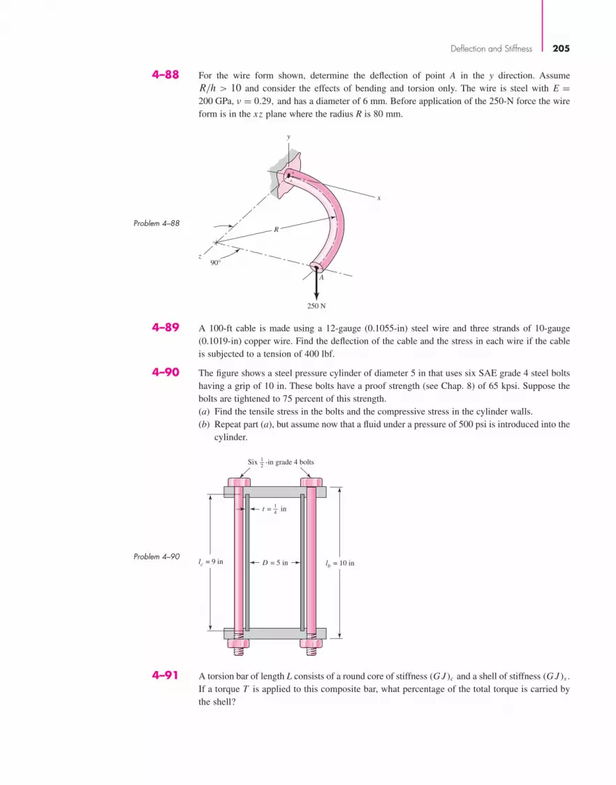
Deflection and Stiffness 205
4–89 A 100-ft cable is made using a 12-gauge (0.1055-in) steel wire and three strands of 10-gauge(0.1019-in) copper wire. Find the deflection of the cable and the stress in each wire if the cableis subjected to a tension of 400 lbf.
4–90 The figure shows a steel pressure cylinder of diameter 5 in that uses six SAE grade 4 steel boltshaving a grip of 10 in. These bolts have a proof strength (see Chap. 8) of 65 kpsi. Suppose thebolts are tightened to 75 percent of this strength.(a) Find the tensile stress in the bolts and the compressive stress in the cylinder walls.(b) Repeat part (a), but assume now that a fluid under a pressure of 500 psi is introduced into the
cylinder.
4–88 For the wire form shown, determine the deflection of point A in the y direction. AssumeR/h > 10 and consider the effects of bending and torsion only. The wire is steel with E =200 GPa, ν = 0.29, and has a diameter of 6 mm. Before application of the 250-N force the wireform is in the xz plane where the radius R is 80 mm.
4–91 A torsion bar of length L consists of a round core of stiffness (G J )c and a shell of stiffness (G J )s .If a torque T is applied to this composite bar, what percentage of the total torque is carried bythe shell?
Problem 4–90
Problem 4–88
A
250 N
R
x
y
z90°
lb = 10 inD = 5 inlc = 9 in
t = in
Six -in grade 4 bolts12
14
bud29281_ch04_147-211.qxd 11/27/09 2:55PM Page 205 ntt 203:MHDQ196:bud29281:0073529281:bud29281_pagefiles:

206 Mechanical Engineering Design
4–92 A rectangular aluminum bar 10 mm thick and 60 mm wide is welded to fixed supports at the ends,and the bar supports a load W = 4 kN, acting through a pin as shown. Find the reactions at thesupports and the deflection of point A.
4–93 Solve Prob. 4–92 using Castigliano’s method and procedure 1 from Sec. 4–10.
4–94 An aluminum step bar is loaded as shown. (a) Verify that end C deflects to the rigid wall, and(b) determine the wall reaction forces, the stresses in each member, and the deflection of B.
4–96 Repeat Prob. 4–95 with the diameters of section OA being 0.5 in and section AB being 0.75 in.
4–97 The figure shows a 12 - by 1-in rectangular steel bar welded to fixed supports at each end. The bar
is axially loaded by the forces FA = 12 kip and FB = 6 kip acting on pins at A and B. Assumingthat the bar will not buckle laterally, find the reactions at the fixed supports, the stress in section AB,and the deflection of point A. Use procedure 1 from Sec. 4–10.
4–95 The steel shaft shown in the figure is subjected to a torque of 200 lbf � in applied at point A. Findthe torque reactions at O and B; the angle of twist at A, in degrees; and the shear stress in sectionsOA and AB.
Problem 4–92
Problem 4–95
Problem 4–94
(Not drawn to scale)
600 mm
400 mm
60 mm
10 mm thick
y
B
A
W
O
x
A B C
8 in 5 in
0.005 in
3 kip
0.75-in dia. 0.5-in dia.
2 kip
x
y
BA
200 lbf�in
O
4 in
-in dia.
6 in
12
10 in
A BC
x
y
O
20 in
1 in
15 in
in thick
FA FB
1 2
Problem 4–97
bud29281_ch04_147-211.qxd 11/30/2009 12:50 pm Page 206 pinnacle s-171:Desktop Folder:Temp Work:Don't Delete (Jobs):MHDQ196/Budynas:

Deflection and Stiffness 207
4–98 For the beam shown, determine the support reactions using superposition and procedure 1 fromSec. 4–10.
4–102 The steel beam ABC D shown is supported at C as shown and supported at B and D by shouldersteel bolts, each having a diameter of 8 mm. The lengths of B E and DF are 50 mm and 65 mm,respectively. The beam has a second area moment of 21(103) mm4. Prior to loading, the membersare stress-free. A force of 2 kN is then applied at point A. Using procedure 2 of Sec. 4–10,determine the stresses in the bolts and the deflections of points A, B, and D.
Problem 4–98
a
A B C
w
l
4–99 Solve Prob. 4–98 using Castigliano’s theorem and procedure 1 from Sec. 4–10.
4–100 Consider beam 13 in Table A–9, but with flexible supports. Let w = 500 lbf/ft, l = 2 ft, E = 30Mpsi, and I = 0.85 in4. The support at the left end has a translational spring constant ofk1 = 1.5(106) lbf/in and a rotational spring constant of k2 = 2.5(106) lbf � in. The right supporthas a translational spring constant of k3 = 2.0 (106) lbf/in. Using procedure 2 of Sec. 4–10,determine the reactions at the supports and the deflection at the midpoint of the beam.
4–101 The steel beam ABC D shown is simply supported at A and supported at B and D by steel cables,each having an effective diameter of 0.5 in. The second area moment of the beam is I = 1.2 in4.A force of 5 kips is applied at point C. Using procedure 2 of Sec. 4–10 determine the stresses inthe cables and the deflections of B, C, and D.
E
B CA
F
D
38 in
16 in16 in16 in
5 kips
Problem 4–101
Problem 4–102
B C
E
DA
F
75 mm75 mm
2 kN
75 mm
4–103 A thin ring is loaded by two equal and opposite forces F in part a of the figure. A free-body dia-gram of one quadrant is shown in part b. This is a statically indeterminate problem, because themoment MA cannot be found by statics. (a) Find the maximum bending moment in the ring dueto the forces F, and (b) find the increase in the diameter of the ring along the y axis. Assume thatthe radius of the ring is large so that Eq. (4–41) can be used.
bud29281_ch04_147-211.qxd 11/27/09 2:55PM Page 207 ntt 203:MHDQ196:bud29281:0073529281:bud29281_pagefiles:

208 Mechanical Engineering Design
4–104 A round tubular column has outside and inside diameters of D and d, respectively, and a diame-tral ratio of K = d/D. Show that buckling will occur when the outside diameter is
D =[
64Pcrl2
π3C E(1 − K 4)
]1/4
4–105 For the conditions of Prob. 4–104, show that buckling according to the parabolic formula willoccur when the outside diameter is
D = 2
[Pcr
π Sy (1 − K 2)+ Syl2
π2C E(1 + K 2)
]1/2
4–106 Link 2, shown in the figure, is 25 mm wide, has 12-mm-diameter bearings at the ends, and is cutfrom low-carbon steel bar stock having a minimum yield strength of 165 MPa. The end-conditionconstants are C = 1 and C = 1.2 for buckling in and out of the plane of the drawing, respectively.(a) Using a design factor nd = 4, find a suitable thickness for the link.(b) Are the bearing stresses at O and B of any significance?
4–107 Link 3, shown schematically in the figure, acts as a brace to support the 270-lbf load. For buck-ling in the plane of the figure, the link may be regarded as pinned at both ends. For out-of-planebuckling, the ends are fixed. Select a suitable material and a method of manufacture, such as forg-ing, casting, stamping, or machining, for casual applications of the brace in oil-field machinery.Specify the dimensions of the cross section as well as the ends so as to obtain a strong, safe, well-made, and economical brace.
Problem 4–106
Problem 4–103
x
CB
AO
y
1
23
800 N500 mm
750 mm900 mm
C O
D
B
F
F
Ax
R
y
(a)
O MA
B
F2
Ax
d�
�
ds
y
(b)
bud29281_ch04_147-211.qxd 11/27/09 2:55PM Page 208 ntt 203:MHDQ196:bud29281:0073529281:bud29281_pagefiles:

Deflection and Stiffness 209
4–108 The hydraulic cylinder shown in the figure has a 2-in bore and is to operate at a pressure of 1500 psi.With the clevis mount shown, the piston rod should be sized as a column with both ends rounded forany plane of buckling. The rod is to be made of forged AISI 1030 steel without further heat treatment.
(a) Use a design factor nd = 2.5 and select a preferred size for the rod diameter if the columnlength is 50 in.
(b) Repeat part (a) but for a column length of 16 in.(c) What factor of safety actually results for each of the cases above?
4–109 The figure shows a schematic drawing of a vehicular jack that is to be designed to support amaximum mass of 300 kg based on the use of a design factor nd = 3.50. The opposite-handedthreads on the two ends of the screw are cut to allow the link angle θ to vary from 15 to 70◦ . Thelinks are to be machined from AISI 1010 hot-rolled steel bars. Each of the four links is to consistof two bars, one on each side of the central bearings. The bars are to be 350 mm long and have abar width of w = 30 mm. The pinned ends are to be designed to secure an end-condition constantof at least C = 1.4 for out-of-plane buckling. Find a suitable preferred thickness and the result-ing factor of safety for this thickness.
Problem 4–107
Problem 4–108
3 ft
60
2
1
B
Ax
F = 270 1bf
y
3
O
d
2 in
Problem 4–109
�
W
w
bud29281_ch04_147-211.qxd 11/30/2009 4:12 pm Page 209 pinnacle s-171:Desktop Folder:Temp Work:Don't Delete (Jobs):MHDQ196/Budynas:

4–110 If drawn, a figure for this problem would resemble that for Prob. 4–90. A strut that is a standardhollow right circular cylinder has an outside diameter of 3 in and a wall thickness of 1
4 in and iscompressed between two circular end plates held by four bolts equally spaced on a bolt circleof 4.5-in diameter. All four bolts are hand-tightened, and then bolt A is tightened to a tensionof 1500 lbf and bolt C, diagonally opposite, is tightened to a tension of 9000 lbf. The strutaxis of symmetry is coincident with the center of the bolt circles. Find the maximum compres-sive load, the eccentricity of loading, and the largest compressive stress in the strut.
4–111 Design link C D of the hand-operated toggle press shown in the figure. Specify the cross-sectiondimensions, the bearing size and rod-end dimensions, the material, and the method of processing.
210 Mechanical Engineering Design
4–112 Find the maximum values of the spring force and deflection of the impact system shown in thefigure if W = 30 lbf, k = 100 lbf/in, and h = 2 in. Ignore the mass of the spring and solve usingenergy conservation.
Problem 4–113
Problem 4–111
L = 9 in, l = 3 in, θmin = 0°.
Problem 4–112
4–113 As shown in the figure, the weight W1 strikes W2 from a height h. If W1 = 40 N, W2 = 400 N,h = 200 mm, and k = 32 kN/m, find the maximum values of the spring force and the deflectionof W2. Assume that the impact between W1 and W2 is inelastic, ignore the mass of the spring, andsolve using energy conservation.
D
�
L
A
F
B
C
l
l
W
k
h
y
W2
W1
k
y
h
bud29281_ch04_147-211.qxd 11/30/2009 8:50 pm Page 210 pinnacle 203:MHDQ196:bud29281:0073529281:bud29281_pagefiles:

Deflection and Stiffness 211
Problem 4–114
4–114 Part a of the figure shows a weight W mounted between two springs. If the free end of springk1 is suddenly displaced through the distance x = a, as shown in part b, determine the maximumdisplacement y of the weight. Let W = 5 lbf, k1 = 10 lbf/in, k2 = 20 lbf/in, and a = 0.25 in.Ignore the mass of each spring and solve using energy conservation.
a
y
k1 k2
x
(a) (b)
t
x
W
bud29281_ch04_147-211.qxd 11/27/09 2:55PM Page 211 ntt 203:MHDQ196:bud29281:0073529281:bud29281_pagefiles:

PART 2 Failure Prevention
bud29281_ch05_212-264.qxd 11/27/2009 6:46 pm Page 212 pinnacle s-171:Desktop Folder:Temp Work:Don't Delete (Jobs):MHDQ196/Budynas:

5Failures Resulting from Static Loading
Chapter Outline
5–1 Static Strength 216
5–2 Stress Concentration 217
5–3 Failure Theories 219
5–4 Maximum-Shear-Stress Theory for Ductile Materials 219
5–5 Distortion-Energy Theory for Ductile Materials 221
5–6 Coulomb-Mohr Theory for Ductile Materials 228
5–7 Failure of Ductile Materials Summary 231
5–8 Maximum-Normal-Stress Theory for Brittle Materials 235
5–9 Modifications of the Mohr Theory for Brittle Materials 235
5–10 Failure of Brittle Materials Summary 238
5–11 Selection of Failure Criteria 239
5–12 Introduction to Fracture Mechanics 239
5–13 Stochastic Analysis 248
5–14 Important Design Equations 259
213
bud29281_ch05_212-264.qxd 11/27/2009 6:46 pm Page 213 pinnacle s-171:Desktop Folder:Temp Work:Don't Delete (Jobs):MHDQ196/Budynas:

214 Mechanical Engineering Design
In Chap. 1 we learned that strength is a property or characteristic of a mechanicalelement. This property results from the material identity, the treatment and processingincidental to creating its geometry, and the loading, and it is at the controlling or criticallocation.
In addition to considering the strength of a single part, we must be cognizantthat the strengths of the mass-produced parts will all be somewhat different from theothers in the collection or ensemble because of variations in dimensions, machining,forming, and composition. Descriptors of strength are necessarily statistical innature, involving parameters such as mean, standard deviations, and distributionalidentification.
A static load is a stationary force or couple applied to a member. To be stationary,the force or couple must be unchanging in magnitude, point or points of application,and direction. A static load can produce axial tension or compression, a shear load, abending load, a torsional load, or any combination of these. To be considered static, theload cannot change in any manner.
In this chapter we consider the relations between strength and static loading in orderto make the decisions concerning material and its treatment, fabrication, and geometryfor satisfying the requirements of functionality, safety, reliability, competitiveness,usability, manufacturability, and marketability. How far we go down this list is relatedto the scope of the examples.
“Failure” is the first word in the chapter title. Failure can mean a part has sepa-rated into two or more pieces; has become permanently distorted, thus ruining itsgeometry; has had its reliability downgraded; or has had its function compromised,whatever the reason. A designer speaking of failure can mean any or all of these pos-sibilities. In this chapter our attention is focused on the predictability of permanentdistortion or separation. In strength-sensitive situations the designer must separatemean stress and mean strength at the critical location sufficiently to accomplish hisor her purposes.
Figures 5–1 to 5–5 are photographs of several failed parts. The photographs exem-plify the need of the designer to be well-versed in failure prevention. Toward this endwe shall consider one-, two-, and three-dimensional stress states, with and withoutstress concentrations, for both ductile and brittle materials.
Figure 5–1
(a) Failure of a truck drive-shaft spline due to corrosionfatigue. Note that it wasnecessary to use clear tapeto hold the pieces in place.(b) Direct end view of failure.
bud29281_ch05_212-264.qxd 11/27/2009 6:46 pm Page 214 pinnacle s-171:Desktop Folder:Temp Work:Don't Delete (Jobs):MHDQ196/Budynas:
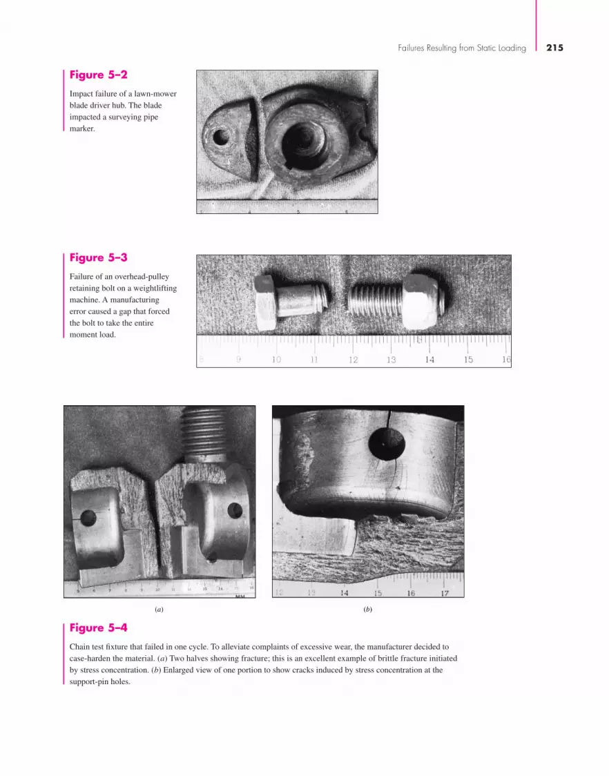
Figure 5–2
Impact failure of a lawn-mowerblade driver hub. The bladeimpacted a surveying pipemarker.
Figure 5–3
Failure of an overhead-pulleyretaining bolt on a weightliftingmachine. A manufacturingerror caused a gap that forcedthe bolt to take the entiremoment load.
Figure 5–4
Chain test fixture that failed in one cycle. To alleviate complaints of excessive wear, the manufacturer decided tocase-harden the material. (a) Two halves showing fracture; this is an excellent example of brittle fracture initiatedby stress concentration. (b) Enlarged view of one portion to show cracks induced by stress concentration at thesupport-pin holes.
Failures Resulting from Static Loading 215
bud29281_ch05_212-264.qxd 11/27/2009 9:05 pm Page 215 pinnacle s-171:Desktop Folder:Temp Work:Don't Delete (Jobs):MHDQ196/Budynas:

216 Mechanical Engineering Design
Figure 5–5
Valve-spring failure caused byspring surge in an overspedengine. The fractures exhibitthe classic 45° shear failure.
5–1 Static StrengthIdeally, in designing any machine element, the engineer should have available the resultsof a great many strength tests of the particular material chosen. These tests should bemade on specimens having the same heat treatment, surface finish, and size as the elementthe engineer proposes to design; and the tests should be made under exactly the sameloading conditions as the part will experience in service. This means that if the part is toexperience a bending load, it should be tested with a bending load. If it is to be subjectedto combined bending and torsion, it should be tested under combined bending and torsion.If it is made of heat-treated AISI 1040 steel drawn at 500°C with a ground finish, thespecimens tested should be of the same material prepared in the same manner. Such testswill provide very useful and precise information. Whenever such data are available fordesign purposes, the engineer can be assured of doing the best possible job of engineering.
The cost of gathering such extensive data prior to design is justified if failure of thepart may endanger human life or if the part is manufactured in sufficiently large quan-tities. Refrigerators and other appliances, for example, have very good reliabilitiesbecause the parts are made in such large quantities that they can be thoroughly testedin advance of manufacture. The cost of making these tests is very low when it is dividedby the total number of parts manufactured.
You can now appreciate the following four design categories:
1 Failure of the part would endanger human life, or the part is made in extremelylarge quantities; consequently, an elaborate testing program is justified duringdesign.
2 The part is made in large enough quantities that a moderate series of tests is feasible.3 The part is made in such small quantities that testing is not justified at all; or the
design must be completed so rapidly that there is not enough time for testing.4 The part has already been designed, manufactured, and tested and found to be
unsatisfactory. Analysis is required to understand why the part is unsatisfactoryand what to do to improve it.
bud29281_ch05_212-264.qxd 11/27/2009 6:46 pm Page 216 pinnacle s-171:Desktop Folder:Temp Work:Don't Delete (Jobs):MHDQ196/Budynas:

Failures Resulting from Static Loading 217
More often than not it is necessary to design using only published values of yieldstrength, ultimate strength, percentage reduction in area, and percentage elongation,such as those listed in Appendix A. How can one use such meager data to design againstboth static and dynamic loads, two- and three-dimensional stress states, high and lowtemperatures, and very large and very small parts? These and similar questions will beaddressed in this chapter and those to follow, but think how much better it would be tohave data available that duplicate the actual design situation.
5–2 Stress ConcentrationStress concentration (see Sec. 3–13) is a highly localized effect. In some instances itmay be due to a surface scratch. If the material is ductile and the load static, the designload may cause yielding in the critical location in the notch. This yielding can involvestrain strengthening of the material and an increase in yield strength at the small criti-cal notch location. Since the loads are static and the material is ductile, that part cancarry the loads satisfactorily with no general yielding. In these cases the designer setsthe geometric (theoretical) stress-concentration factor Kt to unity.
The rationale can be expressed as follows. The worst-case scenario is that of anidealized non–strain-strengthening material shown in Fig. 5–6. The stress-strain curverises linearly to the yield strength Sy , then proceeds at constant stress, which is equal toSy . Consider a filleted rectangular bar as depicted in Fig. A–15–5, where the cross-section area of the small shank is 1 in2. If the material is ductile, with a yield point of40 kpsi, and the theoretical stress-concentration factor (SCF) Kt is 2,
• A load of 20 kip induces a nominal tensile stress of 20 kpsi in the shank as depictedat point A in Fig. 5–6. At the critical location in the fillet the stress is 40 kpsi, and theSCF is K = σmax/σnom = 40/20 = 2.
• A load of 30 kip induces a nominal tensile stress of 30 kpsi in the shank at point B.The fillet stress is still 40 kpsi (point D), and the SCF K = σmax/σnom = Sy/σ =40/30 = 1.33.
• At a load of 40 kip the induced tensile stress (point C) is 40 kpsi in the shank.At the critical location in the fillet, the stress (at point E) is 40 kpsi. The SCFK = σmax/σnom = Sy/σ = 40/40 = 1.
50
0
Sy
Tensile strain, �
Tens
ile s
tres
s �
, kps
i
A
B
D E
C
Figure 5–6
An idealized stress-straincurve. The dashed line depictsa strain-strengthening material.
bud29281_ch05_212-264.qxd 12/7/09 7:22PM Page 217 ntt G4 Mac OS 9.2:Desktop Folder:MHDQ196/Budynas:

218 Mechanical Engineering Design
For materials that strain-strengthen, the critical location in the notch has a higher Sy .The shank area is at a stress level a little below 40 kpsi, is carrying load, and is verynear its failure-by-general-yielding condition. This is the reason designers do notapply Kt in static loading of a ductile material loaded elastically, instead settingKt = 1.
When using this rule for ductile materials with static loads, be careful to assureyourself that the material is not susceptible to brittle fracture (see Sec. 5–12) in theenvironment of use. The usual definition of geometric (theoretical) stress-concentrationfactor for normal stress Kt and shear stress Kts is given by Eq. pair (3–48) as
σmax = Ktσnom (a)
τmax = Ktsτnom (b)
Since your attention is on the stress-concentration factor, and the definition of σnom orτnom is given in the graph caption or from a computer program, be sure the value ofnominal stress is appropriate for the section carrying the load.
As shown in Fig. 2–2b, p. 33, brittle materials do not exhibit a plastic range. Thestress-concentration factor given by Eq. (a) or (b) could raise the stress to a level tocause fracture to initiate at the stress raiser, and initiate a catastrophic failure of themember.
An exception to this rule is a brittle material that inherently contains microdiscon-tinuity stress concentration, worse than the macrodiscontinuity that the designer has inmind. Sand molding introduces sand particles, air, and water vapor bubbles. The grainstructure of cast iron contains graphite flakes (with little strength), which are literallycracks introduced during the solidification process. When a tensile test on a cast iron isperformed, the strength reported in the literature includes this stress concentration. Insuch cases Kt or Kts need not be applied.
An important source of stress-concentration factors is R. E. Peterson, who com-piled them from his own work and that of others.1 Peterson developed the style ofpresentation in which the stress-concentration factor Kt is multiplied by the nominalstress σnom to estimate the magnitude of the largest stress in the locality. His approxi-mations were based on photoelastic studies of two-dimensional strips (Hartman andLevan, 1951; Wilson and White, 1973), with some limited data from three-dimensionalphotoelastic tests of Hartman and Levan. A contoured graph was included in thepresentation of each case. Filleted shafts in tension were based on two-dimensionalstrips. Table A–15 provides many charts for the theoretical stress-concentration factorsfor several fundamental load conditions and geometry. Additional charts are also avail-able from Peterson.2
Finite element analysis (FEA) can also be applied to obtain stress-concentrationfactors. Improvements on Kt and Kts for filleted shafts were reported by Tipton, Sorem,and Rolovic.3
1R. E. Peterson, “Design Factors for Stress Concentration,” Machine Design, vol. 23, no. 2, February 1951;no. 3, March 1951; no. 5, May 1951; no. 6, June 1951; no. 7, July 1951.2Walter D. Pilkey and Deborah Pilkey, Peterson’s Stress-Concentration Factors, 3rd ed, John Wiley & Sons,New York, 2008.3S. M. Tipton, J. R. Sorem Jr., and R. D. Rolovic, “Updated Stress-Concentration Factors for Filleted Shafts inBending and Tension,” Trans. ASME, Journal of Mechanical Design, vol. 118, September 1996, pp. 321–327.
bud29281_ch05_212-264.qxd 12/7/09 7:22PM Page 218 ntt G4 Mac OS 9.2:Desktop Folder:MHDQ196/Budynas:

Failures Resulting from Static Loading 219
5–3 Failure TheoriesSection 5–1 illustrated some ways that loss of function is manifested. Events such asdistortion, permanent set, cracking, and rupturing are among the ways that a machineelement fails. Testing machines appeared in the 1700s, and specimens were pulled, bent,and twisted in simple loading processes.
If the failure mechanism is simple, then simple tests can give clues. Just what issimple? The tension test is uniaxial (that’s simple) and elongations are largest in the axialdirection, so strains can be measured and stresses inferred up to “failure.” Just what isimportant: a critical stress, a critical strain, a critical energy? In the next several sections,we shall show failure theories that have helped answer some of these questions.
Unfortunately, there is no universal theory of failure for the general case of mate-rial properties and stress state. Instead, over the years several hypotheses have beenformulated and tested, leading to today’s accepted practices. Being accepted, we willcharacterize these “practices” as theories as most designers do.
Structural metal behavior is typically classified as being ductile or brittle, althoughunder special situations, a material normally considered ductile can fail in a brittlemanner (see Sec. 5–12). Ductile materials are normally classified such that ε f ≥ 0.05and have an identifiable yield strength that is often the same in compression as in ten-sion (Syt = Syc = Sy). Brittle materials, ε f < 0.05, do not exhibit an identifiable yieldstrength, and are typically classified by ultimate tensile and compressive strengths, Sut
and Suc, respectively (where Suc is given as a positive quantity). The generally acceptedtheories are:
Ductile materials (yield criteria)
• Maximum shear stress (MSS), Sec. 5–4
• Distortion energy (DE), Sec. 5–5
• Ductile Coulomb-Mohr (DCM), Sec. 5–6
Brittle materials (fracture criteria)
• Maximum normal stress (MNS), Sec. 5–8
• Brittle Coulomb-Mohr (BCM), Sec. 5–9
• Modified Mohr (MM), Sec. 5–9
It would be inviting if we had one universally accepted theory for each materialtype, but for one reason or another, they are all used. Later, we will provide rationalesfor selecting a particular theory. First, we will describe the bases of these theories andapply them to some examples.
5–4 Maximum-Shear-Stress Theory for Ductile MaterialsThe maximum-shear-stress (MSS) theory predicts that yielding begins whenever themaximum shear stress in any element equals or exceeds the maximum shear stress in atension-test specimen of the same material when that specimen begins to yield. TheMSS theory is also referred to as the Tresca or Guest theory.
Many theories are postulated on the basis of the consequences seen from tensiletests. As a strip of a ductile material is subjected to tension, slip lines (called Lüderlines) form at approximately 45° with the axis of the strip. These slip lines are the
bud29281_ch05_212-264.qxd 11/27/2009 6:46 pm Page 219 pinnacle s-171:Desktop Folder:Temp Work:Don't Delete (Jobs):MHDQ196/Budynas:

220 Mechanical Engineering Design
beginning of yield, and when loaded to fracture, fracture lines are also seen at anglesapproximately 45° with the axis of tension. Since the shear stress is maximum at 45°from the axis of tension, it makes sense to think that this is the mechanism of failure. Itwill be shown in the next section, that there is a little more going on than this. However,it turns out the MSS theory is an acceptable but conservative predictor of failure; andsince engineers are conservative by nature, it is quite often used.
Recall that for simple tensile stress, σ = P/A, and the maximum shear stressoccurs on a surface 45° from the tensile surface with a magnitude of τmax = σ/2. So themaximum shear stress at yield is τmax = Sy/2. For a general state of stress, three prin-cipal stresses can be determined and ordered such that σ1 ≥ σ2 ≥ σ3. The maximumshear stress is then τmax = (σ1 − σ3)/2 (see Fig. 3–12). Thus, for a general state ofstress, the maximum-shear-stress theory predicts yielding when
τmax = σ1 − σ3
2≥ Sy
2or σ1 − σ3 ≥ Sy (5–1)
Note that this implies that the yield strength in shear is given by
Ssy = 0.5Sy (5–2)
which, as we will see later is about 15 percent low (conservative).For design purposes, Eq. (5–1) can be modified to incorporate a factor of safety, n.
Thus,
τmax = Sy
2nor σ1 − σ3 = Sy
n(5–3)
Plane stress is a very common state of stress in design. However, it is extremelyimportant to realize that plane stress is a three-dimensional state of stress. Plane stresstransformations in Sec. 3–6 are restricted to the in-plane stresses only, where the in-plane principal stresses are given by Eq. (3–13) and labeled as σ1 and σ2. It is true thatthese are the principal stresses in the plane of analysis, but out of plane there is a thirdprincipal stress and it is always zero for plane stress. This means that if we are going touse the convention of ordering σ1 ≥ σ2 ≥ σ3 for three-dimensional analysis, uponwhich Eq. (5–1) is based, we cannot arbitrarily call the in-plane principal stresses σ1
and σ2 until we relate them with the third principal stress of zero. To illustrate the MSStheory graphically for plane stress, we will first label the principal stresses given byEq. (3–13) as σA and σB , and then order them with the zero principal stress accordingto the convention σ1 ≥ σ2 ≥ σ3. Assuming that σA ≥ σB , there are three cases to con-sider when using Eq. (5–1) for plane stress:
Case 1: σA ≥ σB ≥ 0. For this case, σ1 = σA and σ3 = 0. Equation (5–1)reduces to a yield condition of
σA ≥ Sy (5–4)
Case 2: σA ≥ 0 ≥ σB . Here, σ1 = σA and σ3 = σB , and Eq. (5–1) becomes
σA − σB ≥ Sy (5–5)
Case 3: 0 ≥ σA ≥ σB . For this case, σ1 = 0 and σ3 = σB , and Eq. (5–1) gives
σB ≤ −Sy (5–6)
Equations (5–4) to (5–6) are represented in Fig. 5–7 by the three lines indicated in theσA, σB plane. The remaining unmarked lines are cases for σB ≥ σA, which completesthe stress yield envelope but are not normally used. The maximum-shear-stress theorypredicts yield if a stress state is outside the shaded region bordered by the stress yieldenvelope. In Fig. 5–7, suppose point a represents the stress state of a critical stress element
bud29281_ch05_212-264.qxd 11/27/2009 6:46 pm Page 220 pinnacle s-171:Desktop Folder:Temp Work:Don't Delete (Jobs):MHDQ196/Budynas:

Failures Resulting from Static Loading 221
of a member. If the load is increased, it is typical to assume that the principal stresseswill increase proportionally along the line from the origin through point a. Such a loadline is shown. If the stress situation increases along the load line until it crosses thestress failure envelope, such as at point b, the MSS theory predicts that the stress ele-ment will yield. The factor of safety guarding against yield at point a is given by theratio of strength (distance to failure at point b) to stress (distance to stress at point a),that is n = Ob/Oa.
Note that the first part of Eq. (5–3), τmax = Sy/2n, is sufficient for design purposesprovided the designer is careful in determining τmax. For plane stress, Eq. (3–14) doesnot always predict τmax. However, consider the special case when one normal stress iszero in the plane, say σx and τxy have values and σy = 0. It can be easily shown that thisis a Case 2 problem, and the shear stress determined by Eq. (3–14) is τmax. Shaft designproblems typically fall into this category where a normal stress exists from bendingand/or axial loading, and a shear stress arises from torsion.
5–5 Distortion-Energy Theory for Ductile MaterialsThe distortion-energy theory predicts that yielding occurs when the distortion strainenergy per unit volume reaches or exceeds the distortion strain energy per unit volumefor yield in simple tension or compression of the same material.
The distortion-energy (DE) theory originated from the observation that ductilematerials stressed hydrostatically (equal principal stresses) exhibited yield strengthsgreatly in excess of the values given by the simple tension test. Therefore it was postu-lated that yielding was not a simple tensile or compressive phenomenon at all, but,rather, that it was related somehow to the angular distortion of the stressed element.To develop the theory, note, in Fig. 5–8a, the unit volume subjected to any three-dimensional stress state designated by the stresses σ1, σ2, and σ3. The stress state shownin Fig. 5–8b is one of hydrostatic normal stresses due to the stresses σav acting in eachof the same principal directions as in Fig. 5–8a. The formula for σav is simply
σav = σ1 + σ2 + σ3
3(a)
Thus the element in Fig. 5–8b undergoes pure volume change, that is, no angular dis-tortion. If we regard σav as a component of σ1, σ2, and σ3, then this component can besubtracted from them, resulting in the stress state shown in Fig. 5–8c. This element issubjected to pure angular distortion, that is, no volume change.
ab
O
�B
�A
Load line
Case 1
Case 2
Nonyi
eld r
egio
n
Case 3
–Sy
–Sy
Sy
Sy
Figure 5–7
The maximum-shear-stress(MSS) theory yield envelopefor plane stress, where σA andσB are the two nonzeroprincipal stresses.
bud29281_ch05_212-264.qxd 11/27/2009 6:46 pm Page 221 pinnacle s-171:Desktop Folder:Temp Work:Don't Delete (Jobs):MHDQ196/Budynas:

222 Mechanical Engineering Design
The strain energy per unit volume for simple tension is u = 12εσ . For the element
of Fig. 5–8a the strain energy per unit volume is u = 12 [ε1σ1 + ε2σ2 + ε3σ3].
Substituting Eq. (3–19) for the principal strains gives
u = 1
2E
[σ2
1 + σ22 + σ2
3 − 2ν(σ1σ2 + σ2σ3 + σ3σ1)]
(b)
The strain energy for producing only volume change uv can be obtained by substitut-ing σav for σ1, σ2, and σ3 in Eq. (b). The result is
uv = 3σ 2av
2E(1 − 2ν) (c)
If we now substitute the square of Eq. (a) in Eq. (c) and simplify the expression, we get
uv = 1 − 2ν
6E
(σ 2
1 + σ 22 + σ 2
3 + 2σ1σ2 + 2σ2σ3 + 2σ3σ1)
(5–7)
Then the distortion energy is obtained by subtracting Eq. (5–7) from Eq. (b). Thisgives
ud = u − uv = 1 + ν
3E
[(σ1 − σ2)
2 + (σ2 − σ3)2 + (σ3 − σ1)
2
2
](5–8)
Note that the distortion energy is zero if σ1 = σ2 = σ3.For the simple tensile test, at yield, σ1 = Sy and σ2 = σ3 = 0, and from Eq. (5–8)
the distortion energy is
ud = 1 + ν
3ES2
y (5–9)
So for the general state of stress given by Eq. (5–8), yield is predicted if Eq. (5–8)equals or exceeds Eq. (5–9). This gives[
(σ1 − σ2)2 + (σ2 − σ3)
2 + (σ3 − σ1)2
2
]1/2
≥ Sy (5–10)
If we had a simple case of tension σ , then yield would occur when σ ≥ Sy . Thus, theleft of Eq. (5–10) can be thought of as a single, equivalent, or effective stress for theentire general state of stress given by σ1, σ2, and σ3. This effective stress is usually
Figure 5–8
(a) Element with triaxial stresses; this element undergoes both volumechange and angular distortion. (b) Element under hydrostatic normalstresses undergoes only volume change. (c) Element has angulardistortion without volume change.
�3�1 > �2 > �3
�2
�1
(a) Triaxial stresses (b) Hydrostatic component
�3 – �av
�2 – �av
�1 – �av
(c) Distortional component
�av
�av
�av
= +
bud29281_ch05_212-264.qxd 11/27/2009 6:46 pm Page 222 pinnacle s-171:Desktop Folder:Temp Work:Don't Delete (Jobs):MHDQ196/Budynas:

Failures Resulting from Static Loading 223
called the von Mises stress, σ ′, named after Dr. R. von Mises, who contributed to thetheory. Thus Eq. (5–10), for yield, can be written as
σ ′ ≥ Sy (5–11)
where the von Mises stress is
σ ′ =[(σ1 − σ2)
2 + (σ2 − σ3)2 + (σ3 − σ1)
2
2
]1/2
(5–12)
For plane stress, the von Mises stress can be represented by the principal stressesσA, σB , and zero. Then from Eq. (5–12), we get
σ ′ = (σ 2
A − σAσB + σ 2B
)1/2(5–13)
Equation (5–13) is a rotated ellipse in the σA, σB plane, as shown in Fig. 5–9 withσ ′ = Sy . The dotted lines in the figure represent the MSS theory, which can be seen tobe more restrictive, hence, more conservative.4
Using xyz components of three-dimensional stress, the von Mises stress can bewritten as
σ ′ = 1√2
[(σx − σy)
2 + (σy − σz)2 + (σz − σx)
2 + 6(τ 2
xy + τ 2yz + τ 2
zx
)]1/2(5–14)
and for plane stress,
σ ′ = (σ 2
x − σxσy + σ 2y + 3τ 2
xy
)1/2(5–15)
The distortion-energy theory is also called:
• The von Mises or von Mises–Hencky theory
• The shear-energy theory
• The octahedral-shear-stress theory
Understanding octahedral shear stress will shed some light on why the MSS is conser-vative. Consider an isolated element in which the normal stresses on each surface are
4The three-dimensional equations for DE and MSS can be plotted relative to three-dimensional σ1, σ2, σ3,coordinate axes. The failure surface for DE is a circular cylinder with an axis inclined at 45° from eachprincipal stress axis, whereas the surface for MSS is a hexagon inscribed within the cylinder. See Arthur P.Boresi and Richard J. Schmidt, Advanced Mechanics of Materials, 6th ed., John Wiley & Sons, New York,2003, Sec. 4.4.
Figure 5–9
The distortion-energy (DE)theory yield envelope for planestress states. This is a plot of points obtained from Eq. (5–13) with σ ′ = Sy .
–Sy
–Sy Sy
Sy
�B
�A
DEMSS
Pure shear load line (�A � ��B � �)
Nonyie
ld reg
ion
bud29281_ch05_212-264.qxd 11/27/2009 6:46 pm Page 223 pinnacle s-171:Desktop Folder:Temp Work:Don't Delete (Jobs):MHDQ196/Budynas:

224 Mechanical Engineering Design
equal to the hydrostatic stress σav. There are eight surfaces symmetric to the principaldirections that contain this stress. This forms an octahedron as shown in Fig. 5–10. Theshear stresses on these surfaces are equal and are called the octahedral shear stresses(Fig. 5–10 has only one of the octahedral surfaces labeled). Through coordinate trans-formations the octahedral shear stress is given by5
τoct = 1
3
[(σ1 − σ2)
2 + (σ2 − σ3)2 + (σ3 − σ1)
2]1/2(5–16)
Under the name of the octahedral-shear-stress theory, failure is assumed to occur when-ever the octahedral shear stress for any stress state equals or exceeds the octahedralshear stress for the simple tension-test specimen at failure.
As before, on the basis of the tensile test results, yield occurs when σ1 = Sy andσ2 = σ3 = 0. From Eq. (5–16) the octahedral shear stress under this condition is
τoct =√
2
3Sy (5–17)
When, for the general stress case, Eq. (5–16) is equal or greater than Eq. (5–17), yieldis predicted. This reduces to[
(σ1 − σ2)2 + (σ2 − σ3)
2 + (σ3 − σ1)2
2
]1/2
≥ Sy (5–18)
which is identical to Eq. (5–10), verifying that the maximum-octahedral-shear-stresstheory is equivalent to the distortion-energy theory.
The model for the MSS theory ignores the contribution of the normal stresses onthe 45° surfaces of the tensile specimen. However, these stresses are P/2A, and not thehydrostatic stresses which are P/3A. Herein lies the difference between the MSS andDE theories.
The mathematical manipulation involved in describing the DE theory might tendto obscure the real value and usefulness of the result. The equations given allow themost complicated stress situation to be represented by a single quantity, the von Misesstress, which then can be compared against the yield strength of the material throughEq. (5–11). This equation can be expressed as a design equation by
σ ′ = Sy
n(5–19)
Figure 5–10
Octahedral surfaces.
�2
�1
�3
�oct
�av
5For a derivation, see Arthur P. Boresi, op. cit., pp. 36–37.
bud29281_ch05_212-264.qxd 11/27/2009 6:46 pm Page 224 pinnacle s-171:Desktop Folder:Temp Work:Don't Delete (Jobs):MHDQ196/Budynas:

Failures Resulting from Static Loading 225
The distortion-energy theory predicts no failure under hydrostatic stress and agreeswell with all data for ductile behavior. Hence, it is the most widely used theory for duc-tile materials and is recommended for design problems unless otherwise specified.
One final note concerns the shear yield strength. Consider a case of pure shear τxy ,where for plane stress σx = σy = 0. For yield, Eq. (5–11) with Eq. (5–15) gives(
3τ 2xy
)1/2 = Sy or τxy = Sy√3
= 0.577Sy (5–20)
Thus, the shear yield strength predicted by the distortion-energy theory is
Ssy = 0.577Sy (5–21)
which as stated earlier, is about 15 percent greater than the 0.5 Sy predicted by the MSStheory. For pure shear, τxy the principal stresses from Eq. (3–13) are σA = −σB = τxy .The load line for this case is in the third quadrant at an angle of 45o from the σA, σB
axes shown in Fig. 5–9.
EXAMPLE 5–1 A hot-rolled steel has a yield strength of Syt = Syc = 100 kpsi and a true strain at fractureof ε f = 0.55. Estimate the factor of safety for the following principal stress states:(a) σx = 70 kpsi, σy = 70 kpsi, τxy = 0 kpsi(b) σx = 60 kpsi, σy = 40 kpsi, τxy = −15 kpsi(c) σx = 0 kpsi, σy = 40 kpsi, τxy = 45 kpsi(d) σx = −40 kpsi, σy = −60 kpsi, τxy = 15 kpsi(e) σ1 = 30 kpsi, σ2 = 30 kpsi, σ3 = 30 kpsi
Solution Since ε f > 0.05 and Syt and Syc are equal, the material is ductile and both thedistortion-energy (DE) theory and maximum-shear-stress (MSS) theory apply. Bothwill be used for comparison. Note that cases a to d are plane stress states.
(a) Since there is no shear stress on this stress element, the normal stresses areequal to the principal stresses. The ordered principal stresses are σA = σ1 = 70,
σB = σ2 = 70, σ3 = 0 kpsi.
DE From Eq. (5–13),
σ ′ = [702 − 70(70) + 702]1/2 = 70 kpsi
From Eq. (5–19),
Answer n = Sy
σ ′ = 100
70= 1.43
MSS Noting that the two nonzero principal stresses are equal, τmax will be from thelargest Mohr’s circle, which will incorporate the third principal stress at zero. FromEq. (3–16),
τmax = σ1 − σ3
2= 70 − 0
2= 35 kpsi
From Eq. (5–3),
Answer n = Sy/2
τmax= 100/2
35= 1.43
bud29281_ch05_212-264.qxd 11/27/2009 6:46 pm Page 225 pinnacle s-171:Desktop Folder:Temp Work:Don't Delete (Jobs):MHDQ196/Budynas:
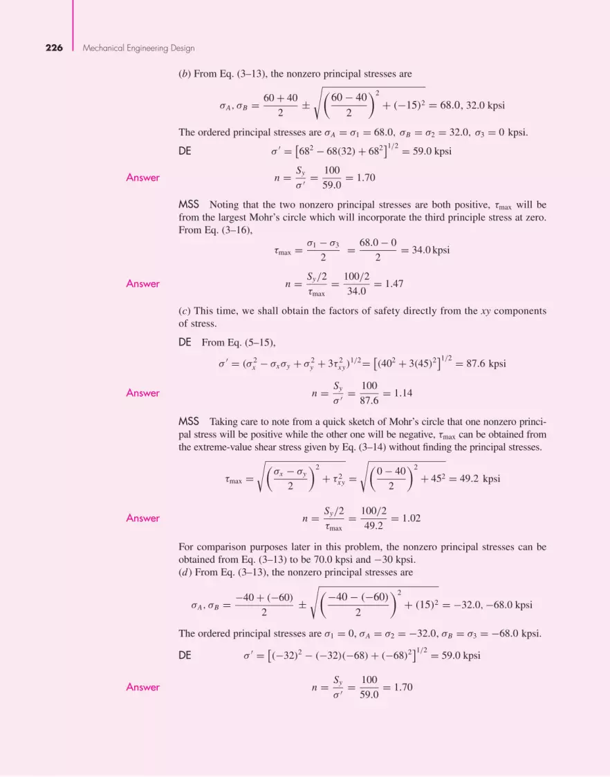
226 Mechanical Engineering Design
(b) From Eq. (3–13), the nonzero principal stresses are
σA, σB = 60 + 40
2±
√(60 − 40
2
)2
+ (−15)2 = 68.0, 32.0 kpsi
The ordered principal stresses are σA = σ1 = 68.0, σB = σ2 = 32.0, σ3 = 0 kpsi.
DE σ ′ = [682 − 68(32) + 682]1/2 = 59.0 kpsi
Answer n = Sy
σ ′ = 100
59.0= 1.70
MSS Noting that the two nonzero principal stresses are both positive, τmax will befrom the largest Mohr’s circle which will incorporate the third principle stress at zero.From Eq. (3–16),
τmax = σ1 − σ3
2= 68.0 − 0
2= 34.0 kpsi
Answer n = Sy/2
τmax= 100/2
34.0= 1.47
(c) This time, we shall obtain the factors of safety directly from the xy componentsof stress.
DE From Eq. (5–15),
σ ′ = (σ 2x − σxσy + σ 2
y + 3τ 2xy)
1/2= [(402 + 3(45)2]1/2 = 87.6 kpsi
Answer n = Sy
σ ′ = 100
87.6= 1.14
MSS Taking care to note from a quick sketch of Mohr’s circle that one nonzero princi-pal stress will be positive while the other one will be negative, τmax can be obtained fromthe extreme-value shear stress given by Eq. (3–14) without finding the principal stresses.
τmax =√(
σx − σy
2
)2
+ τ 2xy =
√(0 − 40
2
)2
+ 452 = 49.2 kpsi
Answer n = Sy/2
τmax= 100/2
49.2= 1.02
For comparison purposes later in this problem, the nonzero principal stresses can beobtained from Eq. (3–13) to be 70.0 kpsi and −30 kpsi.(d ) From Eq. (3–13), the nonzero principal stresses are
σA, σB = −40 + (−60)
2±
√(−40 − (−60)
2
)2
+ (15)2 = −32.0,−68.0 kpsi
The ordered principal stresses are σ1 = 0, σA = σ2 = −32.0, σB = σ3 = −68.0 kpsi.
DE σ ′ = [(−32)2 − (−32)(−68) + (−68)2]1/2 = 59.0 kpsi
Answer n = Sy
σ ′ = 100
59.0= 1.70
bud29281_ch05_212-264.qxd 11/27/2009 6:46 pm Page 226 pinnacle s-171:Desktop Folder:Temp Work:Don't Delete (Jobs):MHDQ196/Budynas:

Failures Resulting from Static Loading 227
MSS From Eq. (3–16),
τmax = σ1 − σ3
2= 0 − (−68.0)
2= 34.0 kpsi
Answer n = Sy/2
τmax= 100/2
34.0= 1.47
(e) The ordered principal stresses are σ1 = 30, σ2 = 30, σ3 = 30 kpsi
DE From Eq. (5–12),
σ ′ =[(30 − 30)2 + (30 − 30)2 + (30 − 30)2
2
]1/2
= 0 kpsi
Answer n = Sy
σ ′ = 100
0→ ∞
MSS From Eq. (5–3),
Answer n = Sy
σ1 − σ3= 100
30 − 30→ ∞
A tabular summary of the factors of safety is included for comparisons.
(a) (b) (c) (d) (e)
DE 1.43 1.70 1.14 1.70 ∞MSS 1.43 1.47 1.02 1.47 ∞
Since the MSS theory is on or within the boundary of the DE theory, it will always pre-dict a factor of safety equal to or less than the DE theory, as can be seen in the table.For each case, except case (e), the coordinates and load lines in the σA, σB plane areshown in Fig. 5–11. Case (e) is not plane stress. Note that the load line for case (a) isthe only plane stress case given in which the two theories agree, thus giving the samefactor of safety.
Figure 5–11
Load lines for Example 5–1.
–Sy
–Sy
Sy
Sy
�B
�A
(a)
(b)
(c)
(d )
DEMSSLoad lines
�A
�B
bud29281_ch05_212-264.qxd 11/27/2009 6:46 pm Page 227 pinnacle s-171:Desktop Folder:Temp Work:Don't Delete (Jobs):MHDQ196/Budynas:

228 Mechanical Engineering Design
5–6 Coulomb-Mohr Theory for Ductile MaterialsNot all materials have compressive strengths equal to their corresponding tensilevalues. For example, the yield strength of magnesium alloys in compression may beas little as 50 percent of their yield strength in tension. The ultimate strength of graycast irons in compression varies from 3 to 4 times greater than the ultimate tensilestrength. So, in this section, we are primarily interested in those theories that canbe used to predict failure for materials whose strengths in tension and compressionare not equal.
Historically, the Mohr theory of failure dates to 1900, a date that is relevant to itspresentation. There were no computers, just slide rules, compasses, and French curves.Graphical procedures, common then, are still useful today for visualization. The idea ofMohr is based on three “simple” tests: tension, compression, and shear, to yielding if thematerial can yield, or to rupture. It is easier to define shear yield strength as Ssy than it isto test for it.
The practical difficulties aside, Mohr’s hypothesis was to use the results oftensile, compressive, and torsional shear tests to construct the three circles of Fig. 5–12defining a failure envelope tangent to the three circles, depicted as curve ABCDE inthe figure. The argument amounted to the three Mohr circles describing the stressstate in a body (see Fig. 3–12) growing during loading until one of them became tan-gent to the failure envelope, thereby defining failure. Was the form of the failure enve-lope straight, circular, or quadratic? A compass or a French curve defined the failureenvelope.
A variation of Mohr’s theory, called the Coulomb-Mohr theory or the internal-frictiontheory, assumes that the boundary BCD in Fig. 5–12 is straight. With this assumption onlythe tensile and compressive strengths are necessary. Consider the conventional ordering ofthe principal stresses such that σ1 ≥ σ2 ≥ σ3. The largest circle connects σ1 and σ3, asshown in Fig. 5–13. The centers of the circles in Fig. 5–13 are C1, C2, and C3. TrianglesOBiCi are similar, therefore
B2C2 − B1C1
OC2 − OC1= B3C3 − B1C1
OC3 − OC1
or,B2C2 − B1C1
C1C2= B3C3 − B1C1
C1C3
Figure 5–12
Three Mohr circles, one for theuniaxial compression test, onefor the test in pure shear, andone for the uniaxial tension test,are used to define failure by theMohr hypothesis. The strengthsSc and St are the compressiveand tensile strengths,respectively; they can be usedfor yield or ultimate strength.
�
�
A
Mohr failure curveB
CD
E
–Sc St
bud29281_ch05_212-264.qxd 11/27/2009 6:46 pm Page 228 pinnacle s-171:Desktop Folder:Temp Work:Don't Delete (Jobs):MHDQ196/Budynas:

Failures Resulting from Static Loading 229
where B1C1 = St/2, B2C2 = (σ1 − σ3)/2, and B3C3 = Sc/2, are the radii of the right,center, and left circles, respectively. The distance from the origin to C1 is St/2, to C3 isSc/2, and to C2 (in the positive σ direction) is (σ1 + σ3)/2. Thus
σ1 − σ3
2− St
2St
2− σ1 + σ3
2
=Sc
2− St
2St
2+ Sc
2
Canceling the 2 in each term, cross-multiplying, and simplifying reduces this equa-tion to
σ1
St− σ3
Sc= 1 (5–22)
where either yield strength or ultimate strength can be used.For plane stress, when the two nonzero principal stresses are σA ≥ σB , we have
a situation similar to the three cases given for the MSS theory, Eqs. (5–4) to (5–6).That is, the failure conditions are
Case 1: σA ≥ σB ≥ 0. For this case, σ1 = σA and σ3 = 0. Equation (5–22)reduces to
σA ≥ St (5–23)
Case 2: σA ≥ 0 ≥ σB . Here, σ1 = σA and σ3 = σB , and Eq. (5–22) becomes
σA
St− σB
Sc≥ 1 (5–24)
Case 3: 0 ≥ σA ≥ σB . For this case, σ1 = 0 and σ3 = σB , and Eq. (5–22) gives
σB ≤ −Sc (5–25)
A plot of these cases, together with the normally unused cases corresponding toσB ≥ σA , is shown in Fig. 5–14.
For design equations, incorporating the factor of safety n, divide all strengths by n.For example, Eq. (5–22) as a design equation can be written as
σ1
St− σ3
Sc= 1
n(5–26)
Figure 5–13
Mohr’s largest circle for ageneral state of stress.
�
��1 St�3–Sc
O
Coulomb-Mohrfailure line
B3 B2
B1
C1C2C3
bud29281_ch05_212-264.qxd 11/27/2009 6:46 pm Page 229 pinnacle s-171:Desktop Folder:Temp Work:Don't Delete (Jobs):MHDQ196/Budynas:

230 Mechanical Engineering Design
Figure 5–14
Plot of the Coulomb-Mohrtheory failure envelope forplane stress states.
�B
�ASt–Sc
–Sc
St
Nonfai
lure r
egion
EXAMPLE 5–2 A 25-mm-diameter shaft is statically torqued to 230 N · m. It is made of cast 195-T6aluminum, with a yield strength in tension of 160 MPa and a yield strength in com-pression of 170 MPa. It is machined to final diameter. Estimate the factor of safety ofthe shaft.
Solution The maximum shear stress is given by
τ = 16T
πd3= 16(230)
π[25
(10−3
)]3 = 75(106) N/m2 = 75 MPa
The two nonzero principal stresses are 75 and −75 MPa, making the ordered principalstresses σ1 = 75, σ2 = 0, and σ3 = −75 MPa. From Eq. (5–26), for yield,
Answer n = 1
σ1/Syt − σ3/Syc= 1
75/160 − (−75)/170= 1.10
Alternatively, from Eq. (5–27),
Ssy = Syt Syc
Syt + Syc= 160(170)
160 + 170= 82.4 MPa
and τmax = 75 MPa. Thus,
Answer n = Ssy
τmax= 82.4
75= 1.10
Since for the Coulomb-Mohr theory we do not need the torsional shear strengthcircle we can deduce it from Eq. (5–22). For pure shear τ, σ1 = −σ3 = τ . The torsionalyield strength occurs when τmax = Ssy . Substituting σ1 = −σ3 = Ssy into Eq. (5–22)and simplifying gives
Ssy = Syt Syc
Syt + Syc(5–27)
bud29281_ch05_212-264.qxd 11/27/2009 6:46 pm Page 230 pinnacle s-171:Desktop Folder:Temp Work:Don't Delete (Jobs):MHDQ196/Budynas:

Failures Resulting from Static Loading 231
5–7 Failure of Ductile Materials SummaryHaving studied some of the various theories of failure, we shall now evaluate them andshow how they are applied in design and analysis. In this section we limit our studies tomaterials and parts that are known to fail in a ductile manner. Materials that fail in a brit-tle manner will be considered separately because these require different failure theories.
To help decide on appropriate and workable theories of failure, Marin6 collecteddata from many sources. Some of the data points used to select failure theories for duc-tile materials are shown in Fig. 5–15.7 Mann also collected many data for copper andnickel alloys; if shown, the data points for these would be mingled with those alreadydiagrammed. Figure 5–15 shows that either the maximum-shear-stress theory or thedistortion-energy theory is acceptable for design and analysis of materials that wouldfail in a ductile manner.
The selection of one or the other of these two theories is something that you, theengineer, must decide. For design purposes the maximum-shear-stress theory is easy,quick to use, and conservative. If the problem is to learn why a part failed, then thedistortion-energy theory may be the best to use; Fig. 5–15 shows that the plot of thedistortion-energy theory passes closer to the central area of the data points, and thus isgenerally a better predictor of failure. However, keep in mind that though a failure curvepassing through the center of the experimental data is typical of the data, its reliabilityfrom a statistical standpoint is about 50 percent. For design purposes, a larger factor ofsafety may be warranted when using such a failure theory.
Figure 5–15
Experimental data superposedon failure theories. (From Fig. 7.11, p. 257, MechanicalBehavior of Materials, 2nd ed.,N. E. Dowling, Prentice Hall,Englewood Cliffs, N.J., 1999.Modified to show only ductilefailures.)
�2/Sc
�1/Sc
Max. shear
Oct. shear
0 1.0
1.0
–1.0
–1.0
Yielding (Sc = Sy)
Ni-Cr-Mo steel
AISI 1023 steel
2024-T4 Al
3S-H Al
6Joseph Marin was one of the pioneers in the collection, development, and dissemination of material on thefailure of engineering elements. He has published many books and papers on the subject. Here thereference used is Joseph Marin, Engineering Materials, Prentice-Hall, Englewood Cliffs, N.J., 1952.(See pp. 156 and 157 for some data points used here.)7Note that some data in Fig. 5–15 are displayed along the top horizontal boundary where σB ≥ σA . This is oftendone with failure data to thin out congested data points by plotting on the mirror image of the line σB = σA .
bud29281_ch05_212-264.qxd 11/27/2009 6:46 pm Page 231 pinnacle s-171:Desktop Folder:Temp Work:Don't Delete (Jobs):MHDQ196/Budynas:

232 Mechanical Engineering Design
EXAMPLE 5–3 This example illustrates the use of a failure theory to determine the strength of a mechan-ical element or component. The example may also clear up any confusion existingbetween the phrases strength of a machine part, strength of a material, and strength ofa part at a point.
A certain force F applied at D near the end of the 15-in lever shown in Fig. 5–16,which is quite similar to a socket wrench, results in certain stresses in the cantileveredbar OABC. This bar (OABC) is of AISI 1035 steel, forged and heat-treated so that it hasa minimum (ASTM) yield strength of 81 kpsi. We presume that this component wouldbe of no value after yielding. Thus the force F required to initiate yielding can beregarded as the strength of the component part. Find this force.
Solution We will assume that lever DC is strong enough and hence not a part of the problem. A 1035steel, heat-treated, will have a reduction in area of 50 percent or more and hence is a duc-tile material at normal temperatures. This also means that stress concentration at shoulderA need not be considered. A stress element at A on the top surface will be subjected to atensile bending stress and a torsional stress. This point, on the 1-in-diameter section, is theweakest section, and governs the strength of the assembly. The two stresses are
σx = M
I/c= 32M
πd3= 32(14F)
π(13)= 142.6F
τzx = T r
J= 16T
πd3= 16(15F)
π(13)= 76.4F
A
18
-in R.
1 12
-in D.
1 12
-in D.
z
1-in D.
2 in
2 in
15 in
F
B
C
x
O
y
D
12 in
Figure 5–16
For ductile materials with unequal yield strengths, Syt in tension and Syc in com-pression, the Mohr theory is the best available. However, the theory requires the resultsfrom three separate modes of tests, graphical construction of the failure locus, and fit-ting the largest Mohr’s circle to the failure locus. The alternative to this is to use theCoulomb-Mohr theory, which requires only the tensile and compressive yield strengthsand is easily dealt with in equation form.
bud29281_ch05_212-264.qxd 11/27/2009 6:46 pm Page 232 pinnacle s-171:Desktop Folder:Temp Work:Don't Delete (Jobs):MHDQ196/Budynas:

Failures Resulting from Static Loading 233
Employing the distortion-energy theory, we find, from Eq. (5–15), that
σ ′ = (σ 2
x + 3τ 2zx
)1/2 = [(142.6F)2 + 3(76.4F)2]1/2 = 194.5F
Equating the von Mises stress to Sy , we solve for F and get
Answer F = Sy
194.5= 81 000
194.5= 416 lbf
In this example the strength of the material at point A is Sy = 81 kpsi. The strength ofthe assembly or component is F = 416 lbf.
Let us apply the MSS theory for comparison. For a point undergoing plane stresswith only one nonzero normal stress and one shear stress, the two nonzero principalstresses will have opposite signs, and hence the maximum shear stress is obtained fromthe Mohr’s circle between them. From Eq. (3–14)
τmax =√(σx
2
)2+ τ 2
zx =√(
142.6F
2
)2
+ (76.4F)2 = 104.5F
Setting this equal to Sy/2, from Eq. (5–3) with n = 1, and solving for F, we get
F = 81 000/2
104.5= 388 lbf
which is about 7 percent less than found for the DE theory. As stated earlier, the MSStheory is more conservative than the DE theory.
EXAMPLE 5–4 The cantilevered tube shown in Fig. 5–17 is to be made of 2014 aluminum alloy treatedto obtain a specified minimum yield strength of 276 MPa. We wish to select a stock-sizetube from Table A–8 using a design factor nd = 4. The bending load is F = 1.75 kN,the axial tension is P = 9.0 kN, and the torsion is T = 72 N · m. What is the realizedfactor of safety?
Solution The critical stress element is at point A on the top surface at the wall, where the bend-ing moment is the largest, and the bending and torsional stresses are at their maximumvalues. The critical stress element is shown in Fig. 5–17b. Since the axial stress andbending stress are both in tension along the x axis, they are additive for the normalstress, giving
σx = P
A+ Mc
I= 9
A+ 120(1.75)(do/2)
I= 9
A+ 105do
I(1)
where, if millimeters are used for the area properties, the stress is in gigapascals.The torsional stress at the same point is
τzx = T r
J= 72(do/2)
J= 36do
J(2)
bud29281_ch05_212-264.qxd 11/27/2009 6:46 pm Page 233 pinnacle s-171:Desktop Folder:Temp Work:Don't Delete (Jobs):MHDQ196/Budynas:

234 Mechanical Engineering Design
For accuracy, we choose the distortion-energy theory as the design basis. The von Misesstress from Eq. (5–15), is
σ ′ = (σ 2
x + 3τ 2zx
)1/2(3)
On the basis of the given design factor, the goal for σ ′ is
σ ′ ≤ Sy
nd= 0.276
4= 0.0690 GPa (4)
where we have used gigapascals in this relation to agree with Eqs. (1) and (2).Programming Eqs. (1) to (3) on a spreadsheet and entering metric sizes from
Table A–8 reveals that a 42 × 5-mm tube is satisfactory. The von Mises stress is foundto be σ ′ = 0.06043 GPa for this size. Thus the realized factor of safety is
Answer n = Sy
σ ′ = 0.276
0.06043= 4.57
For the next size smaller, a 42 × 4-mm tube, σ ′ = 0.07105 GPa giving a factor ofsafety of
n = Sy
σ ′ = 0.276
0.07105= 3.88
Figure 5–17
120 mm
y
z
F
Tx
P
A
(a)
(b)
�zx
�x
z
x
bud29281_ch05_212-264.qxd 11/27/2009 6:46 pm Page 234 pinnacle s-171:Desktop Folder:Temp Work:Don't Delete (Jobs):MHDQ196/Budynas:

Failures Resulting from Static Loading 235
5–8 Maximum-Normal-Stress Theoryfor Brittle MaterialsThe maximum-normal-stress (MNS) theory states that failure occurs whenever one ofthe three principal stresses equals or exceeds the strength. Again we arrange the prin-cipal stresses for a general stress state in the ordered form σ1 ≥ σ2 ≥ σ3. This theorythen predicts that failure occurs whenever
σ1 ≥ Sut or σ3 ≤ −Suc (5–28)
where Sut and Suc are the ultimate tensile and compressive strengths, respectively, givenas positive quantities.
For plane stress, with the principal stresses given by Eq. (3–13), with σA ≥ σB,
Eq. (5–28) can be written as
σA ≥ Sut or σB ≤ −Suc (5–29)
which is plotted in Fig. 5–18.As before, the failure criteria equations can be converted to design equations. We
can consider two sets of equations where σA ≥ σB as
σA = Sut
nor σB = − Suc
n(5–30)
As will be seen later, the maximum-normal-stress theory is not very good at pre-dicting failure in the fourth quadrant of the σA, σB plane. Thus, we will not recommendthe theory for use. It has been included here mainly for historical reasons.
5–9 Modifications of the Mohr Theoryfor Brittle MaterialsWe will discuss two modifications of the Mohr theory for brittle materials: the Brittle-Coulomb-Mohr (BCM) theory and the modified Mohr (MM) theory. The equationsprovided for the theories will be restricted to plane stress and be of the design typeincorporating the factor of safety.
Figure 5–18
Graph of maximum-normal-stress (MNS) theory failureenvelope for plane stress states.
Sut
�B
�ASut–Suc
–Suc
Nonfai
lure r
egion
bud29281_ch05_212-264.qxd 11/27/2009 9:05 pm Page 235 pinnacle s-171:Desktop Folder:Temp Work:Don't Delete (Jobs):MHDQ196/Budynas:

236 Mechanical Engineering Design
The Coulomb-Mohr theory was discussed earlier in Sec. 5–6 with Eqs. (5–23) to(5–25). Written as design equations for a brittle material, they are:
Brittle-Coulomb-Mohr
σA = Sut
nσA ≥ σB ≥ 0 (5–31a)
σA
Sut− σB
Suc= 1
nσA ≥ 0 ≥ σB (5–31b)
σB = − Suc
n0 ≥ σA ≥ σB (5–31c)
On the basis of observed data for the fourth quadrant, the modified Mohr theoryexpands the fourth quadrant with the solid lines shown in the second and fourth quad-rants of Fig. 5–19.
Modified Mohr
σA = Sut
nσA ≥ σB ≥ 0
σA ≥ 0 ≥ σB and
∣∣∣∣σB
σA
∣∣∣∣ ≤ 1(5–32a)
(Suc − Sut) σA
Suc Sut− σB
Suc= 1
nσA ≥ 0 ≥ σB and
∣∣∣∣σB
σA
∣∣∣∣ > 1 (5–32b)
σB = − Suc
n0 ≥ σA ≥ σB (5–32c)
Data are still outside this extended region. The straight line introduced by the modifiedMohr theory, for σA ≥ 0 ≥ σB and |σB/σA| > 1, can be replaced by a parabolic relation
Figure 5–19
Biaxial fracture data of graycast iron compared withvarious failure criteria.(Dowling, N. E., MechanicalBehavior of Materials, 2nd ed.,1999, p. 261. Reprinted bypermission of PearsonEducation, Inc., Upper SaddleRiver, New Jersey.)
Sut
–Suc
–Suc
Sut
�B, MPa
�A, MPa
–Sut
300
0
–300
–700
300–300–700
max. normal
mod. Mohr
Coulomb - Mohr
Torsion
Gray cast-iron data
bud29281_ch05_212-264.qxd 12/9/09 6:53PM Page 236 ntt G4 Mac OS 9.2:Desktop Folder:MHDQ196/Budynas:

Failures Resulting from Static Loading 237
EXAMPLE 5–5 Consider the wrench in Ex. 5–3, Fig. 5–16, as made of cast iron, machined to dimen-sion. The force F required to fracture this part can be regarded as the strength of thecomponent part. If the material is ASTM grade 30 cast iron, find the force F with(a) Coulomb-Mohr failure model.(b) Modified Mohr failure model.
Solution We assume that the lever DC is strong enough, and not part of the problem. Since grade30 cast iron is a brittle material and cast iron, the stress-concentration factors Kt and Kts
are set to unity. From Table A–24, the tensile ultimate strength is 31 kpsi and the com-pressive ultimate strength is 109 kpsi. The stress element at A on the top surface will besubjected to a tensile bending stress and a torsional stress. This location, on the 1-in-diameter section fillet, is the weakest location, and it governs the strength of the assem-bly. The normal stress σx and the shear stress at A are given by
σx = KtM
I/c= Kt
32M
πd3= (1)
32(14F)
π(1)3= 142.6F
τxy = KtsT r
J= Kts
16T
πd3= (1)
16(15F)
π(1)3= 76.4F
From Eq. (3–13) the nonzero principal stresses σA and σB are
σA, σB = 142.6F + 0
2±
√(142.6F − 0
2
)2
+ (76.4F)2 = 175.8F,−33.2F
This puts us in the fourth-quadrant of the σA, σB plane.(a) For BCM, Eq. (5–31b) applies with n = 1 for failure.
σA
Sut− σB
Suc= 175.8F
31(103)− (−33.2F)
109(103)= 1
Solving for F yields
Answer F = 167 lbf
(b) For MM, the slope of the load line is |σB/σA| = 33.2/175.8 = 0.189 < 1.
Obviously, Eq. (5–32a) applies.
σA
Sut= 175.8F
31(103)= 1
Answer F = 176 lbf
As one would expect from inspection of Fig. 5–19, Coulomb-Mohr is more conservative.
which can more closely represent some of the data.8 However, this introduces a nonlin-ear equation for the sake of a minor correction, and will not be presented here.
8See J. E. Shigley, C. R. Mischke, R. G. Budynas, Mechanical Engineering Design, 7th ed., McGraw-Hill,New York, 2004, p. 275.
bud29281_ch05_212-264.qxd 11/27/2009 6:46 pm Page 237 pinnacle s-171:Desktop Folder:Temp Work:Don't Delete (Jobs):MHDQ196/Budynas:

238 Mechanical Engineering Design
5–10 Failure of Brittle Materials SummaryWe have identified failure or strength of brittle materials that conform to the usualmeaning of the word brittle, relating to those materials whose true strain at fractureis 0.05 or less. We also have to be aware of normally ductile materials that for somereason may develop a brittle fracture or crack if used below the transition tempera-ture. Figure 5–20 shows data for a nominal grade 30 cast iron taken under biaxialstress conditions, with several brittle failure hypotheses shown, superposed. We notethe following:
• In the first quadrant the data appear on both sides and along the failure curves ofmaximum-normal-stress, Coulomb-Mohr, and modified Mohr. All failure curves arethe same, and data fit well.
• In the fourth quadrant the modified Mohr theory represents the data best, whereas themaximum-normal-stress theory does not.
• In the third quadrant the points A, B, C, and D are too few to make any suggestionconcerning a fracture locus.
5–11 Selection of Failure CriteriaFor ductile behavior the preferred criterion is the distortion-energy theory, althoughsome designers also apply the maximum-shear-stress theory because of its simplicityand conservative nature. In the rare case when Syt �= Syc , the ductile Coulomb-Mohrmethod is employed.
For brittle behavior, the original Mohr hypothesis, constructed with tensile, compres-sion, and torsion tests, with a curved failure locus is the best hypothesis we have. However,the difficulty of applying it without a computer leads engineers to choose modifications,
Figure 5–20
A plot of experimental datapoints obtained from tests oncast iron. Shown also are thegraphs of three failure theoriesof possible usefulness forbrittle materials. Note points A,B, C, and D. To avoidcongestion in the first quadrant,points have been plotted forσA > σB as well as for theopposite sense. (Source ofdata: Charles F. Walton (ed.),Iron Castings Handbook, Iron Founders’ Society, 1971, pp. 215, 216, Cleveland, Ohio.)
30
–30
–60
–90
–120
–150
30–30–60–90–120
–Sut
–Suc
Sut
Sut
�B
�B
�A
�A
Modified Mohr
Coulomb-Mohr
Maximum-normal-stress
ASTM No. 30 C.I.Sut = 31 kpsi, Suc = 109 kpsi
D
CA
B
�A
�B = –1
– Suc
–Sut
bud29281_ch05_212-264.qxd 11/27/2009 6:46 pm Page 238 pinnacle s-171:Desktop Folder:Temp Work:Don't Delete (Jobs):MHDQ196/Budynas:

Failures Resulting from Static Loading 239
namely, Coulomb Mohr, or modified Mohr. Figure 5–21 provides a summary flowchart forthe selection of an effective procedure for analyzing or predicting failures from staticloading for brittle or ductile behavior. Note that the maximum-normal-stress theory isexcluded from Fig. 5–21 as the other theories better represent the experimental data.
5–12 Introduction to Fracture MechanicsThe idea that cracks exist in parts even before service begins, and that cracks can growduring service, has led to the descriptive phrase “damage-tolerant design.” The focus ofthis philosophy is on crack growth until it becomes critical, and the part is removedfrom service. The analysis tool is linear elastic fracture mechanics (LEFM). Inspectionand maintenance are essential in the decision to retire parts before cracks reach cata-strophic size. Where human safety is concerned, periodic inspections for cracks aremandated by codes and government ordinance.
We shall now briefly examine some of the basic ideas and vocabulary needed forthe potential of the approach to be appreciated. The intent here is to make the readeraware of the dangers associated with the sudden brittle fracture of so-called ductilematerials. The topic is much too extensive to include in detail here and the reader isurged to read further on this complex subject.9
Figure 5–21
Failure theory selectionflowchart.
9References on brittle fracture include:H. Tada, P. C. Paris, and G. R. Irwin, The Stress Analysis of Cracks Handbook, 3rd ed., ASME Press,
New York, 2000.D. Broek, Elementary Engineering Fracture Mechanics, 4th ed., Martinus Nijhoff, London, 1985.D. Broek, The Practical Use of Fracture Mechanics, Kluwar Academic Pub., London, 1988.David K. Felbeck and Anthony G. Atkins, Strength and Fracture of Engineering Solids, 2nd ed.,
Prentice-Hall, Englewood Cliffs, N.J., 1995.Kåre Hellan, Introduction to Fracture Mechanics, McGraw-Hill, New York, 1984.
Syt = Syc?·Conservative?
�f
Mod. Mohr(MM)
Eq. (5–32)
Brittle Coulomb-Mohr(BCM)
Eq. (5–31)
Ductile Coulomb-Mohr(DCM)
Eq. (5–26)
Distortion-energy(DE)
Eqs. (5–15)and (5–19)
Brittle behavior Ductile behavior
< 0.05 ≥ 0.05
No NoYes
Conservative?
Maximum shear stress(MSS)
Eq. (5–3)
No Yes
Yes
bud29281_ch05_212-264.qxd 11/27/2009 6:46 pm Page 239 pinnacle s-171:Desktop Folder:Temp Work:Don't Delete (Jobs):MHDQ196/Budynas:

240 Mechanical Engineering Design
The use of elastic stress-concentration factors provides an indication of the averageload required on a part for the onset of plastic deformation, or yielding; these factorsare also useful for analysis of the loads on a part that will cause fatigue fracture.However, stress-concentration factors are limited to structures for which all dimensionsare precisely known, particularly the radius of curvature in regions of high stress con-centration. When there exists a crack, flaw, inclusion, or defect of unknown small radiusin a part, the elastic stress-concentration factor approaches infinity as the root radiusapproaches zero, thus rendering the stress-concentration factor approach useless.Furthermore, even if the radius of curvature of the flaw tip is known, the high localstresses there will lead to local plastic deformation surrounded by a region of elasticdeformation. Elastic stress-concentration factors are no longer valid for this situation,so analysis from the point of view of stress-concentration factors does not lead to cri-teria useful for design when very sharp cracks are present.
By combining analysis of the gross elastic changes in a structure or part that occuras a sharp brittle crack grows with measurements of the energy required to produce newfracture surfaces, it is possible to calculate the average stress (if no crack were present)that will cause crack growth in a part. Such calculation is possible only for parts withcracks for which the elastic analysis has been completed, and for materials that crack in arelatively brittle manner and for which the fracture energy has been carefully measured.The term relatively brittle is rigorously defined in the test procedures,10 but it means,roughly, fracture without yielding occurring throughout the fractured cross section.
Thus glass, hard steels, strong aluminum alloys, and even low-carbon steel belowthe ductile-to-brittle transition temperature can be analyzed in this way. Fortunately,ductile materials blunt sharp cracks, as we have previously discovered, so that fractureoccurs at average stresses of the order of the yield strength, and the designer is preparedfor this condition. The middle ground of materials that lie between “relatively brittle”and “ductile” is now being actively analyzed, but exact design criteria for these materi-als are not yet available.
Quasi-Static Fracture
Many of us have had the experience of observing brittle fracture, whether it is the break-ing of a cast-iron specimen in a tensile test or the twist fracture of a piece of blackboardchalk. It happens so rapidly that we think of it as instantaneous, that is, the cross sectionsimply parting. Fewer of us have skated on a frozen pond in the spring, with no one nearus, heard a cracking noise, and stopped to observe. The noise is due to cracking. Thecracks move slowly enough for us to see them run. The phenomenon is not instantaneous,since some time is necessary to feed the crack energy from the stress field to the crack forpropagation. Quantifying these things is important to understanding the phenomenon “inthe small.” In the large, a static crack may be stable and will not propagate. Some level ofloading can render the crack unstable, and the crack propagates to fracture.
The foundation of fracture mechanics was first established by Griffith in 1921using the stress field calculations for an elliptical flaw in a plate developed by Inglis in1913. For the infinite plate loaded by an applied uniaxial stress σ in Fig. 5–22, the max-imum stress occurs at (±a, 0) and is given by
(σy)max =(
1 + 2a
b
)σ (5–33)
10BS 5447:1977 and ASTM E399-78.
bud29281_ch05_212-264.qxd 11/27/2009 6:46 pm Page 240 pinnacle s-171:Desktop Folder:Temp Work:Don't Delete (Jobs):MHDQ196/Budynas:

Failures Resulting from Static Loading 241
Note that when a = b, the ellipse becomes a circle and Eq. (5–33) gives a stress-concentration factor of 3. This agrees with the well-known result for an infinite plate witha circular hole (see Table A–15–1). For a fine crack, b/a → 0, and Eq. (5–34) predictsthat (σy)max → ∞. However, on a microscopic level, an infinitely sharp crack is ahypothetical abstraction that is physically impossible, and when plastic deformationoccurs, the stress will be finite at the crack tip.
Griffith showed that the crack growth occurs when the energy release rate fromapplied loading is greater than the rate of energy for crack growth. Crack growth can bestable or unstable. Unstable crack growth occurs when the rate of change of the energyrelease rate relative to the crack length is equal to or greater than the rate of change ofthe crack growth rate of energy. Griffith’s experimental work was restricted to brittlematerials, namely glass, which pretty much confirmed his surface energy hypothesis.However, for ductile materials, the energy needed to perform plastic work at the cracktip is found to be much more crucial than surface energy.
Crack Modes and the Stress Intensity Factor
Three distinct modes of crack propagation exist, as shown in Fig. 5–23. A tensile stressfield gives rise to mode I, the opening crack propagation mode, as shown in Fig. 5–23a.This mode is the most common in practice. Mode II is the sliding mode, is due to in-plane shear, and can be seen in Fig. 5–23b. Mode III is the tearing mode, whicharises from out-of-plane shear, as shown in Fig. 5–23c. Combinations of these modescan also occur. Since mode I is the most common and important mode, the remainderof this section will consider only this mode.
Figure 5–22 y
x
a
b
�
�
Figure 5–23
Crack propagation modes.
(b) Mode II(a) Mode I (c) Mode III
bud29281_ch05_212-264.qxd 12/7/09 7:22PM Page 241 ntt G4 Mac OS 9.2:Desktop Folder:MHDQ196/Budynas:

242 Mechanical Engineering Design
Consider a mode I crack of length 2a in the infinite plate of Fig. 5–24. By usingcomplex stress functions, it has been shown that the stress field on a dx dy element inthe vicinity of the crack tip is given by
σx = σ
√a
2rcos
θ
2
(1 − sin
θ
2sin
3θ
2
)(5–34a)
σy = σ
√a
2rcos
θ
2
(1 + sin
θ
2sin
3θ
2
)(5–34b)
τxy = σ
√a
2rsin
θ
2cos
θ
2cos
3θ
2(5–34c)
σz ={
0 (for plane stress)ν(σx + σy) (for plane strain)
(5–34d)
The stress σy near the tip, with θ = 0, is
σy|θ=0 = σ
√a
2r(a)
As with the elliptical crack, we see that σy|θ=0 → ∞ as r → 0, and again the conceptof an infinite stress concentration at the crack tip is inappropriate. The quantityσy|θ=0
√2r = σ
√a, however, does remain constant as r → 0. It is common practice to
define a factor K called the stress intensity factor given by
K = σ√
πa (b)
where the units are MPa√
m or kpsi√
in. Since we are dealing with a mode I crack,Eq. (b) is written as
KI = σ√
πa (5–35)
The stress intensity factor is not to be confused with the static stress-concentrationfactors Kt and Kts defined in Secs. 3–13 and 5–2.
Thus Eqs. (5–34) can be rewritten as
σx = KI√2πr
cosθ
2
(1 − sin
θ
2sin
3θ
2
)(5–36a)
σy = KI√2πr
cosθ
2
(1 + sin
θ
2sin
3θ
2
)(5–36b)
Figure 5–24
Mode I crack model.
y
xr
dxdy
a
�
�
�
bud29281_ch05_212-264.qxd 12/7/09 7:23PM Page 242 ntt G4 Mac OS 9.2:Desktop Folder:MHDQ196/Budynas:

Failures Resulting from Static Loading 243
11See, for example:H. Tada, P. C. Paris, and G. R. Irwin, The Stress Analysis of Cracks Handbook, 3rd ed., ASME Press,
New York, 2000.G. C. Sib, Handbook of Stress Intensity Factors for Researchers and Engineers, Institute of Fracture and
Solid Mechanics, Lehigh University, Bethlehem, Pa., 1973.Y. Murakami, ed., Stress Intensity Factors Handbook, Pergamon Press, Oxford, U.K., 1987.W. D. Pilkey, Formulas for Stress, Strain, and Structural Matrices, 2nd ed. John Wiley & Sons,
New York, 2005.
τxy = KI√2πr
sinθ
2cos
θ
2cos
3θ
2(5–36c)
σz ={
0 (for plane stress)ν(σx + σy) (for plane strain)
(5–36d)
The stress intensity factor is a function of geometry, size and shape of the crack,and the type of loading. For various load and geometric configurations, Eq. (5–35) canbe written as
KI = βσ√
πa (5–37)
where β is the stress intensity modification factor. Tables for β are available in the lit-erature for basic configurations.11 Figures 5–25 to 5–30 present a few examples of β formode I crack propagation.
Figure 5–25
Off-center crack in a plate inlongitudinal tension; solidcurves are for the crack tip at A; dashed curves are for the tip at B.
�
a�d ratio0 0.2 0.4 0.6 0.8
1.0
1.2
1.4
1.6
1.8
2.0
2.2
2a
�
�
2b
d
A B
A A
A
B
B
0.2
0.4
0.4
0.2d�b = 1.0
bud29281_ch05_212-264.qxd 11/27/2009 9:05 pm Page 243 pinnacle s-171:Desktop Folder:Temp Work:Don't Delete (Jobs):MHDQ196/Budynas:

Figure 5–27
Beams of rectangular crosssection having an edge crack.
a�h ratio0 0.2 0.4 0.6 0.8
1.0
1.2
1.4
= 4
1.6
1.8
2.0
a
a
M
h
h
M
F
F2
l l
F2
lh
Pure bending
lh
= 2
�
Figure 5–26
Plate loaded in longitudinaltension with a crack at theedge; for the solid curve thereare no constraints to bending;the dashed curve was obtainedwith bending constraintsadded.
a�b ratio0 0.2 0.4 0.6 0.8
1.0
2.0
3.0
4.0
5.0
1.0
6.0
7.0
b
ah
h
�
�
h�b = 0.5
�
244
bud29281_ch05_212-264.qxd 11/27/2009 6:46 pm Page 244 pinnacle s-171:Desktop Folder:Temp Work:Don't Delete (Jobs):MHDQ196/Budynas:

Failures Resulting from Static Loading 245
Figure 5–28
Plate in tension containing acircular hole with two cracks.
a�b ratio0.20 0.4 0.6 0.8
0
1
2
3
2a
�
�
2b
r
= 0rb
= 0.5rb
= 0.25rb
�
Figure 5–29
A cylinder loading in axialtension having a radial crack ofdepth a extending completelyaround the circumference ofthe cylinder.
a�(ro – ri) ratio0.20 0.4 0.6 0.8
0.8
0.1
1.0
2.0
3.0
4.0
rori
a a
�
�
ri�ro = 0
0.4�
Fracture Toughness
When the magnitude of the mode I stress intensity factor reaches a critical value,KI c , crack propagation initiates. The critical stress intensity factor KI c is a materialproperty that depends on the material, crack mode, processing of the material, temper-ature, loading rate, and the state of stress at the crack site (such as plane stress versusplane strain). The critical stress intensity factor KI c is also called the fracture toughnessof the material. The fracture toughness for plane strain is normally lower than that forplane stress. For this reason, the term KI c is typically defined as the mode I, plane strainfracture toughness. Fracture toughness KI c for engineering metals lies in the range20 ≤ KI c ≤ 200 MPa · √m; for engineering polymers and ceramics, 1 ≤ KI c ≤5 MPa · √m. For a 4340 steel, where the yield strength due to heat treatment rangesfrom 800 to 1600 MPa, KI c decreases from 190 to 40 MPa · √m.
Table 5–1 gives some approximate typical room-temperature values of KI c forseveral materials. As previously noted, the fracture toughness depends on many factorsand the table is meant only to convey some typical magnitudes of KI c. For an actualapplication, it is recommended that the material specified for the application be certi-fied using standard test procedures [see the American Society for Testing and Materials(ASTM) standard E399].
bud29281_ch05_212-264.qxd 11/27/2009 6:46 pm Page 245 pinnacle s-171:Desktop Folder:Temp Work:Don't Delete (Jobs):MHDQ196/Budynas:

246 Mechanical Engineering Design
Table 5–1
Values of KIc for Some
Engineering Materials
at Room Temperature
Material KIc, MPa√
Aluminum2024 26 4557075 24 4957178 33 490
TitaniumTi-6AL-4V 115 910Ti-6AL-4V 55 1035
Steel4340 99 8604340 60 151552100 14 2070
One of the first problems facing the designer is that of deciding whether the condi-tions exist, or not, for a brittle fracture. Low-temperature operation, that is, operationbelow room temperature, is a key indicator that brittle fracture is a possible failuremode. Tables of transition temperatures for various materials have not been published,possibly because of the wide variation in values, even for a single material. Thus, inmany situations, laboratory testing may give the only clue to the possibility of a brittlefracture. Another key indicator of the possibility of fracture is the ratio of the yieldstrength to the ultimate strength. A high ratio of Sy/Su indicates there is only a small
Figure 5–30
Cylinder subjected to internalpressure p, having a radialcrack in the longitudinaldirection of depth a. UseEq. (4–51) for the tangentialstress at r = r0.
a�(ro – ri) ratio0 0.2 0.4 0.6 0.8
1.0
1.4
1.8
2.2
2.6
3.0
3.4
a
ri
pi
ro
0.35
0.75ri�ro = 0.9
�
Sy, MPam
bud29281_ch05_212-264.qxd 11/27/2009 6:46 pm Page 246 pinnacle s-171:Desktop Folder:Temp Work:Don't Delete (Jobs):MHDQ196/Budynas:

Failures Resulting from Static Loading 247
ability to absorb energy in the plastic region and hence there is a likelihood of brittlefracture.
The strength-to-stress ratio KI c/KI can be used as a factor of safety as
n = KI c
KI(5–38)
EXAMPLE 5–6 A steel ship deck plate is 30 mm thick and 12 m wide. It is loaded with a nominal uni-axial tensile stress of 50 MPa. It is operated below its ductile-to-brittle transition tem-perature with KI c equal to 28.3 MPa. If a 65-mm-long central transverse crack ispresent, estimate the tensile stress at which catastrophic failure will occur. Compare thisstress with the yield strength of 240 MPa for this steel.
Solution For Fig. 5–25, with d = b, 2a = 65 mm and 2b = 12 m, so that d/b = 1 and a/d =65/12(103) = 0.00542. Since a/d is so small, β = 1, so that
KI = σ√
πa = 50√
π(32.5 × 10⁻³) = 16.0 MPa√
m
From Eq. (5–38),
n = KI c
KI= 28.3
16.0= 1.77
The stress at which catastrophic failure occurs is
Answer σc = KI c
KIσ = 28.3
16.0(50) = 88.4 MPa
The yield strength is 240 MPa, and catastrophic failure occurs at 88.4/240 = 0.37, orat 37 percent of yield. The factor of safety in this circumstance is KI c/KI =28.3/16 = 1.77 and not 240/50 = 4.8.
EXAMPLE 5–7 A plate of width 1.4 m and length 2.8 m is required to support a tensile force in the2.8-m direction of 4.0 MN. Inspection procedures will detect only through-thicknessedge cracks larger than 2.7 mm. The two Ti-6AL-4V alloys in Table 5–1 are being con-sidered for this application, for which the safety factor must be 1.3 and minimumweight is important. Which alloy should be used?
Solution (a) We elect first to estimate the thickness required to resist yielding. Since σ = P/wt,we have t = P/wσ. For the weaker alloy, we have, from Table 5–1, Sy = 910 MPa.Thus,
σall = Sy
n= 910
1.3= 700 MPa
Thus
t = P
wσall= 4.0(10)3
1.4(700)= 4.08 mm or greater
bud29281_ch05_212-264.qxd 11/27/2009 6:46 pm Page 247 pinnacle s-171:Desktop Folder:Temp Work:Don't Delete (Jobs):MHDQ196/Budynas:

For the stronger alloy, we have, from Table 5–1,
σall = 1035
1.3= 796 MPa
and so the thickness is
Answer t = P
wσall= 4.0(10)3
1.4(796)= 3.59 mm or greater
(b) Now let us find the thickness required to prevent crack growth. Using Fig. 5–26, wehave
h
b= 2.8/2
1.4= 1
a
b= 2.7
1.4(103)= 0.001 93
Corresponding to these ratios we find from Fig. 5–26 that β.= 1.1, and KI = 1.1σ
√πa.
n = KI c
KI= 115
√103
1.1σ√
πa, σ = KI c
1.1n√
πa
From Table 5–1, KI c = 115 MPa√
m for the weaker of the two alloys. Solving for σ withn = 1 gives the fracture stress
σ = 115
1.1√
π(2.7 × 10⁻³)= 1135 MPa
which is greater than the yield strength of 910 MPa, and so yield strength is the basisfor the geometry decision. For the stronger alloy Sy = 1035 MPa, with n = 1 the frac-ture stress is
σ = KI c
nKI= 55
1(1.1)√
π(2.7 × 10⁻³)= 542.9 MPa
which is less than the yield strength of 1035 MPa. The thickness t is
t = P
wσall= 4.0(103)
1.4(542.9/1.3)= 6.84 mm or greater
This example shows that the fracture toughness KI c limits the geometry when thestronger alloy is used, and so a thickness of 6.84 mm or larger is required. When theweaker alloy is used the geometry is limited by the yield strength, giving a thickness ofonly 4.08 mm or greater. Thus the weaker alloy leads to a thinner and lighter weightchoice since the failure modes differ.
248 Mechanical Engineering Design
12Review Chap. 20 before reading this section.
5–13 Stochastic Analysis12
Reliability is the probability that machine systems and components will perform theirintended function satisfactorily without failure. Up to this point, discussion in this chap-ter has been restricted to deterministic relations between static stress, strength, and thedesign factor. Stress and strength, however, are statistical in nature and very much tiedto the reliability of the stressed component. Consider the probability density functions
bud29281_ch05_212-264.qxd 11/27/2009 6:46 pm Page 248 pinnacle s-171:Desktop Folder:Temp Work:Don't Delete (Jobs):MHDQ196/Budynas:
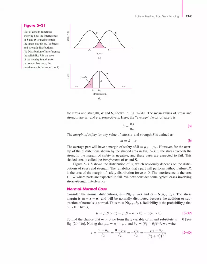
Failures Resulting from Static Loading 249
S
(a)
f(s)
, f(
�)
�
�� �s
Stress
m
R
(b)
f(m
)
�m
Stress margin0
(1 – R)
– +�
for stress and strength, � and S, shown in Fig. 5–31a. The mean values of stress andstrength are μσ and μS , respectively. Here, the “average” factor of safety is
n = μS
μσ
(a)
The margin of safety for any value of stress σ and strength S is defined as
m = S − σ (b)
The average part will have a margin of safety of m = μS − μσ . However, for the over-lap of the distributions shown by the shaded area in Fig. 5–31a, the stress exceeds thestrength, the margin of safety is negative, and these parts are expected to fail. Thisshaded area is called the interference of � and S.
Figure 5–31b shows the distribution of m, which obviously depends on the distri-butions of stress and strength. The reliability that a part will perform without failure, R,is the area of the margin of safety distribution for m > 0. The interference is the area1 − R where parts are expected to fail. We next consider some typical cases involvingstress-strength interference.
Normal-Normal Case
Consider the normal distributions, S = N(μS, σS) and � = N(μσ , σσ ). The stressmargin is m = S − �, and will be normally distributed because the addition or sub-traction of normals is normal. Thus m = N(μm, σm). Reliability is the probability p thatm > 0. That is,
R = p(S > σ) = p(S − σ > 0) = p(m > 0) (5–39)
To find the chance that m > 0 we form the z variable of m and substitute m = 0 [SeeEq. (20–16)]. Noting that μm = μS − μσ and σm = (σ 2
S + σ 2σ )1/2, we write
z = m − μm
σm= 0 − μm
σm= −μm
σm= − μS − μσ(
σ 2S + σ 2
σ
)1/2 (5–40)
Figure 5–31
Plot of density functionsshowing how the interferenceof S and � is used to obtain the stress margin m. (a) Stressand strength distributions.(b) Distribution of interference;the reliability R is the area of the density function for m greater than zero; theinterference is the area (1 − R).
bud29281_ch05_212-264.qxd 11/27/2009 6:46 pm Page 249 pinnacle s-171:Desktop Folder:Temp Work:Don't Delete (Jobs):MHDQ196/Budynas:

250 Mechanical Engineering Design
Equation (5–40) is called the normal coupling equation. The reliability associated withz is given by
R =∫ ∞
x
1√2π
exp
(− u2
2
)du = 1 − F = 1 − (z) (5–41)
The body of Table A–10 gives R when z > 0 and (1 − R = F) when z ≤ 0. Noting thatn = μS/μσ , square both sides of Eq. (5–40), and introduce CS and Cσ whereCS = σS/μS and Cσ = σσ /μσ . Solve the resulting quadratic for n to obtain
n =1 ±
√1 − (
1 − z2C2S
) (1 − z2C2
σ
)1 − z2C2
S
(5–42)
The plus sign is associated with R > 0.5, and the minus sign with R < 0.5.
Lognormal–Lognormal Case
Consider the lognormal distributions S = LN(μS, σS) and � = LN(μσ , σσ ). If weinterfere their companion normals using Eqs. (20–18) and (20–19), we obtain
μln S = ln μS − ln√
1 + C2S
σln S =√
ln(1 + C2
S
) (strength)
and
μln σ = ln μσ − ln√
1 + C2σ
σln σ =√
ln(1 + C2
σ
) (stress)
Using Eq. (5–40) for interfering normal distributions gives
z = − μln S − μln σ(σ 2
ln S + σ 2ln σ
)1/2 = −ln
(μS
μσ
√1 + C2
σ
1 + C2S
)√
ln[(
1 + C2S
) (1 + C2
σ
)] (5–43)
The reliability R is expressed by Eq. (5–41). The design factor n is the random variablethat is the quotient of S/�. The quotient of lognormals is lognormal, so pursuing thez variable of the lognormal n, we note
μn = μS
μσ
Cn =√
C2S + C2
σ
1 + C2σ
σn = Cnμn
The companion normal to n = LN(μn, σn), from Eqs. (20–18) and (20–19), has a meanand standard deviation of
μy = ln μn − ln√
1 + C2n σy =
√ln
(1 + C2
n
)The z variable for the companion normal y distribution is
z = y − μy
σy
bud29281_ch05_212-264.qxd 11/27/2009 6:46 pm Page 250 pinnacle s-171:Desktop Folder:Temp Work:Don't Delete (Jobs):MHDQ196/Budynas:

Failures Resulting from Static Loading 251
Failure will occur when the stress is greater than the strength, when n < 1, or wheny < 0.
z = 0 − μy
σy= −μy
σy= − ln μn − ln
√1 + C2
n√ln
(1 + C2
n
) = − ln(μn/
√1 + C2
n
)√ln
(1 + C2
n
) (5–44)
Solving for μn gives
μn = n = exp
[−z
√ln
(1 + C2
n
) + ln√
1 + C2n
].= exp
[Cn
(− z + Cn
2
)](5–45)
Equations (5–42) and (5–45) are remarkable for several reasons:
• They relate design factor n to the reliability goal (through z) and the coefficients ofvariation of strength and stress.
• They are not functions of the means of stress and strength.
• They estimate the design factor necessary to achieve the reliability goal beforedecisions involving means are made. The CS depends slightly on the particularmaterial. The Cσ has the coefficient of variation (COV) of the load, and that is gen-erally given.
EXAMPLE 5–8 A round cold-drawn 1018 steel rod has an 0.2 percent yield strength Sy = N(78.4, 5.90)kpsi and is to be subjected to a static axial load of P = N(50, 4.1) kip. What value ofthe design factor n corresponds to a reliability of 0.999 against yielding (z = −3.09)?Determine the corresponding diameter of the rod.
Solution CS = 5.90/78.4 = 0.0753, and
� = PA
= 4Pπd2
Since the COV of the diameter is an order of magnitude less than the COV of the loador strength, the diameter is treated deterministically:
Cσ = CP = 4.1
50= 0.082
From Eq. (5–42),
n � � 1.4161 � 1 � [1 �(�3.09)2(0.07532)][1 �(�3.09)2(0.0822)]
1 �(�3.09)2(0.07532)
The diameter is found deterministically:
Answerd =
√4P
π Sy/n=
√4(50 000)
π(78 400)/1.416= 1.072 in
bud29281_ch05_212-264.qxd 11/27/2009 6:46 pm Page 251 pinnacle s-171:Desktop Folder:Temp Work:Don't Delete (Jobs):MHDQ196/Budynas:

252 Mechanical Engineering Design
Check Sy = N(78.4, 5.90) kpsi, P = N(50, 4.1) kip, and d = 1.072 in. Then
A = πd2
4= π(1.0722)
4= 0.9026 in2
σ = P
A= (50 000)
0.9026= 55 400 psi
CP = Cσ = 4.1
50= 0.082
σσ = Cσ σ = 0.082(55 400) = 4540 psi
σS = 5.90 kpsi
From Eq. (5–40)z = − 78.4 − 55.4
(5.902 + 4.542)1/2= −3.09
From Appendix Table A–10, R = (−3.09) = 0.999.
EXAMPLE 5–9 Rework Ex. 5–8 with lognormally distributed stress and strength.
Solution CS = 5.90/78.4 = 0.0753, and Cσ = CP = 4.1/50 = 0.082. Then
� = PA
= 4Pπd2
Cn =√
C2S + C2
σ
1 + C2σ
=√
0.07532 + 0.0822
1 + 0.0822= 0.1110
From Table A–10, z = −3.09. From Eq. (5–45),
n = exp[−(−3.09)
√ln(1 + 0.1112) + ln
√1 + 0.1112
]= 1.416
d =√
4P
π Sy/n=
√4(50 000)
π(78 400)/1.416= 1.0723 in
Check Sy = LN(78.4, 5.90), P = LN(50, 4.1) kip. Then
A = πd2
4= π(1.07232)
4= 0.9031
σ = P
A= 50 000
0.9031= 55 365 psi
Cσ = CP = 4.1
50= 0.082
σσ = Cσμσ = 0.082(55 367) = 4540 psi
From Eq. (5–43),
z = −ln
⎛⎝ 78.4
55.365
√1 + 0.0822
1 + 0.07532
⎞⎠√
ln[(1 + 0.07532)(1 + 0.0822)]= −3.1343
Appendix Table A–10 gives R = 0.99950.
bud29281_ch05_212-264.qxd 11/27/2009 6:46 pm Page 252 pinnacle s-171:Desktop Folder:Temp Work:Don't Delete (Jobs):MHDQ196/Budynas:

Failures Resulting from Static Loading 253
Interference—General
In the previous segments, we employed interference theory to estimate reliability when thedistributions are both normal and when they are both lognormal. Sometimes, however, itturns out that the strength has, say, a Weibull distribution while the stress is distributedlognormally. In fact, stresses are quite likely to have a lognormal distribution, because themultiplication of variates that are normally distributed produces a result that approacheslognormal. What all this means is that we must expect to encounter interference problemsinvolving mixed distributions and we need a general method to handle the problem.
It is quite likely that we will use interference theory for problems involving distri-butions other than strength and stress. For this reason we employ the subscript 1 todesignate the strength distribution and the subscript 2 to designate the stress distribu-tion. Figure 5–32 shows these two distributions aligned so that a single cursor x can beused to identify points on both distributions. We can now write( Probability that
stress is lessthan strength
)= dp(σ < x) = d R = F2(x) d F1(x)
By substituting 1 − R2 for F2 and −d R1 for d F1, we have
d R = −[1 − R2(x)] d R1(x)
The reliability for all possible locations of the cursor is obtained by integrating xfrom −∞ to ∞; but this corresponds to an integration from 1 to 0 on the reliability R1.Therefore
R = −∫ 0
1[1 − R2(x)] d R1(x)
which can be written
R = 1 −∫ 1
0R2 d R1 (5–46)
Figure 5–32
(a) PDF of the strengthdistribution; (b) PDF of theload-induced stressdistribution.
f1(S)
dF1(x) = f1(x) dx
f2(�)
dxS
�
Cursor
R2(x)F2(x)
(a)
(b)
x
bud29281_ch05_212-264.qxd 11/27/2009 6:46 pm Page 253 pinnacle s-171:Desktop Folder:Temp Work:Don't Delete (Jobs):MHDQ196/Budynas:

where
R1(x) =∫ ∞
xf1(S) dS (5–47)
R2(x) =∫ ∞
xf2(σ ) dσ (5–48)
For the usual distributions encountered, plots of R1 versus R2 appear as shown inFig. 5–33. Both of the cases shown are amenable to numerical integration and com-puter solution. When the reliability is high, the bulk of the integration area is under theright-hand spike of Fig. 5–33a.
5–14 Important Design EquationsThe following equations and their locations are provided as a summary. Note for planestress: The principal stresses in the following equations that are labeled σA and σB rep-resent the principal stresses determined from the two-dimensional Eq. (3–13).
Maximum Shear Theory
p. 220 τmax = σ1 − σ3
2= Sy
2n(5–3)
Distortion-Energy Theory
Von Mises stress, p. 223
σ ′ =[(σ1 − σ2)
2 + (σ2 − σ3)2 + (σ3 − σ1)
2
2
]1/2
(5–12)
p. 223 σ ′ = 1√2
[(σx − σy)
2 + (σy − σz)2 + (σz − σx)
2 + 6(τ 2xy + τ 2
yz + τ 2zx)
]1/2
(5–14)
Plane stress, p. 223
σ ′ = (σ 2A − σAσB + σ 2
B)1/2 (5–13)
p. 223 σ ′ = (σ 2x − σxσy + σ 2
y + 3τ 2xy)
1/2 (5–15)
254 Mechanical Engineering Design
Figure 5–33
Curve shapes of the R1 R2 plot. In each case the shaded area is equal to 1 − R and is obtained by numerical integration. (a) Typical curve for asymptotic distributions; (b) curve shapeobtained from lower truncated distributions such as the Weibull.
R1 1
R2
1
(a)
R1 1
R2
1
(b)
bud29281_ch05_212-264.qxd 11/27/2009 6:46 pm Page 254 pinnacle s-171:Desktop Folder:Temp Work:Don't Delete (Jobs):MHDQ196/Budynas:

Yield design equation, p. 224
σ ′ = Sy
n(5–19)
Shear yield strength, p. 225
Ssy = 0.577 Sy (5–21)
Coulomb-Mohr Theory
p. 225σ1
St− σ3
Sc= 1
n(5–26)
where St is tensile yield (ductile) or ultimate tensile (brittle), and St is compressiveyield (ductile) or ultimate compressive (brittle) strengths.
Modified Mohr (Plane Stress)
σA = Sut
nσA ≥ σB ≥ 0
σA ≥ 0 ≥ σB and
∣∣∣∣σB
σA
∣∣∣∣ ≤ 1
(5–32a)
p. 236(Suc − Sut)σA
Suc Sut− σB
Suc= 1
nσA ≥ 0 ≥ σB and
∣∣∣σB
σA
∣∣∣ > 1 (5–32b)
σB = − Suc
n0 ≥ σA ≥ σB (5–32c)
Failure Theory Flowchart
Fig. 5–21, p. 239
Failures Resulting from Static Loading 255
Syt = Syc?·Conservative?
�f
Mod. Mohr(MM)
Eq. (5–32)
Brittle Coulomb-Mohr(BCM)
Eq. (5–31)
Ductile Coulomb-Mohr(DCM)
Eq. (5–26)
Distortion-energy(DE)
Eqs. (5–15)and (5–19)
Brittle behavior Ductile behavior
< 0.05 ≥ 0.05
No NoYes
Conservative?
Maximum shear stress(MSS)
Eq. (5–3)
No Yes
Yes
bud29281_ch05_212-264.qxd 11/27/2009 6:46 pm Page 255 pinnacle s-171:Desktop Folder:Temp Work:Don't Delete (Jobs):MHDQ196/Budynas:

Fracture Mechanics
p. 243 KI = βσ√
πa (5–37)
where β is found in Figs. 5–25 to 5–30 (pp. 243 to 246)
p. 247 n = KI c
KI(5–38)
where KI c is found in Table 5–1 (p. 246)
Stochastic Analysis
Mean factor of safety defined as n = μS/μσ (μS and μσ are mean strength and stress,respectively)
Normal-Normal Case
p. 250 n =1 ±
√1 − (1 − z2C2
S)(1 − z2C2σ )
1 − z2C2S
(5–42)
where z can be found in Table A–10, CS = σS/μS , and Cσ = σσ /μσ .
Lognormal-Lognormal Case
p. 251 n = exp
[−z
√ln(1 + C2
n) + ln√
1 + C2n
].= exp
[Cn
(−z + Cn
2
)](5–45)
where
Cn =√
C2S + C2
σ
1 + C2σ
(See other definitions in normal-normal case.)
PROBLEMSProblems marked with an asterisk (*) are linked to problems in other chapters, as summarized inTable 1–1 of Sec. 1–16, p. 24.
5–1 A ductile hot-rolled steel bar has a minimum yield strength in tension and compression of 350 MPa.Using the distortion-energy and maximum-shear-stress theories determine the factors of safetyfor the following plane stress states:(a) σx = 100 MPa, σy = 100 MPa(b) σx = 100 MPa, σy = 50 MPa(c) σx = 100 MPa, τxy = −75 MPa(d) σx = −50 MPa, σy = −75 MPa, τxy = −50 MPa(e) σx = 100 MPa, σy = 20 MPa, τxy = −20 MPa
5–2 Repeat Prob. 5–1 with the following principal stresses obtained from Eq. (3–13):(a) σA = 100 MPa, σB = 100 MPa(b) σA = 100 MPa, σB = −100 MPa(c) σA = 100 MPa, σB = 50 MPa(d) σA = 100 MPa, σB = −50 MPa(e) σA = −50 MPa, σB = −100 MPa
256 Mechanical Engineering Design
bud29281_ch05_212-264.qxd 11/27/2009 6:46 pm Page 256 pinnacle s-171:Desktop Folder:Temp Work:Don't Delete (Jobs):MHDQ196/Budynas:

5–3 Repeat Prob. 5–1 for a bar of AISI 1030 hot-rolled steel and:(a) σx = 25 kpsi, σy = 15 kpsi(b) σx = 15 kpsi, σy = −15 kpsi(c) σx = 20 kpsi, τxy = −10 kpsi(d) σx = −12 kpsi, σy = 15 kpsi, τxy = −9 kpsi(e) σx = −24 kpsi, σy = −24 kpsi, τxy = −15 kpsi
5–4 Repeat Prob. 5–1 for a bar of AISI 1015 cold-drawn steel with the following principal stressesobtained from Eq. (3–13):(a) σA = 30 kpsi, σB = 30 kpsi(b) σA = 30 kpsi, σB = −30 kpsi(c) σA = 30 kpsi, σB = 15 kpsi(d) σA = −30 kpsi, σB = −15 kpsi(e) σA = −50 kpsi, σB = 10 kpsi
5–5 Repeat Prob. 5–1 by first plotting the failure loci in the σA , σB plane to scale; then, for each stressstate, plot the load line and by graphical measurement estimate the factors of safety.
5–6 Repeat Prob. 5–3 by first plotting the failure loci in the σA , σB plane to scale; then, for each stressstate, plot the load line and by graphical measurement estimate the factors of safety.
An AISI 1018 steel has a yield strength, Sy = 295 MPa. Using the distortion-energy theory forthe given state of plane stress, (a) determine the factor of safety, (b) plot the failure locus, the loadline, and estimate the factor of safety by graphical measurement.
5–12 A ductile material has the properties Syt = 60 kpsi and Syc = 75 kpsi. Using the ductile Coulomb-Mohr theory, determine the factor of safety for the states of plane stress given in Prob. 5–3.
5–13 Repeat Prob. 5–12 by first plotting the failure loci in the σA, σB plane to scale; then for each stressstate, plot the load line and by graphical measurement estimate the factor of safety.
An AISI 4142 steel Q&T at 800°F exhibits Syt = 235 kpsi, Syc = 285 kpsi, and ε f = 0.07. Forthe given state of plane stress, (a) determine the factor of safety, (b) plot the failure locus and theload line, and estimate the factor of safety by graphical measurement.
Problem Number Sx (kpsi) Sy (kpsi) Txy (kpsi)
5–14 150 −50 0
5–15 −150 50 0
5–16 125 0 −75
5–17 −80 −125 50
5–18 125 80 −75
5–14 to5–18
Problem Number Sx (MPa) Sy (MPa) Txy (MPa)
5–7 75 −35 0
5–8 −100 30 0
5–9 100 0 −25
5–10 −30 −65 40
5–11 −80 30 −10
5–7 to5–11
Failures Resulting from Static Loading 257
bud29281_ch05_212-264.qxd 11/27/2009 9:06 pm Page 257 pinnacle s-171:Desktop Folder:Temp Work:Don't Delete (Jobs):MHDQ196/Budynas:

5–19 A brittle material has the properties Sut = 30 kpsi and Suc = 90 kpsi. Using the brittle Coulomb-Mohr and modified-Mohr theories, determine the factor of safety for the following states ofplane stress.(a) σx = 25 kpsi, σy = 15 kpsi(b) σx = 15 kpsi, σy = −15 kpsi(c) σx = 20 kpsi, τxy = −10 kpsi(d ) σx = −15 kpsi, σy = 10 kpsi, τxy = −15 kpsi(e) σx = −20 kpsi, σy = −20 kpsi, τxy = −15 kpsi
5–20 Repeat Prob. 5–19 by first plotting the failure loci in the σA, σB plane to scale; then for each stressstate, plot the load line and by graphical measurement estimate the factor of safety.
For an ASTM 30 cast iron, (a) find the factors of safety using the BCM and MM theories,(b) plot the failure diagrams in the σA, σB plane to scale and locate the coordinates of the stressstate, and (c) estimate the factors of safety from the two theories by graphical measurementsalong the load line.
A cast aluminum 195-T6 exhibits Sut = 36 kpsi, Suc = 35 kpsi, and ε f = 0.045. For the givenstate of plane stress, (a) using the Coulomb-Mohr theory, determine the factor of safety, (b) plotthe failure locus and the load line, and estimate the factor of safety by graphical measurement.
Repeat Probs. 5–26 to 5–30 using the modified-Mohr theory.
Problem number 5–31 5–32 5–33 5–34 5–35
Repeat problem 5–26 5–27 5–28 5–29 5–30
5–36 This problem illustrates that the factor of safety for a machine element depends on the particularpoint selected for analysis. Here you are to compute factors of safety, based upon the distortion-energy theory, for stress elements at A and B of the member shown in the figure. This bar ismade of AISI 1006 cold-drawn steel and is loaded by the forces F = 0.55 kN, P = 4.0 kN,and T = 25 N · m.
5–31 to5–35
Problem Number Sx (kpsi) Sy (kpsi) Txy (kpsi)
5–26 15 −10 0
5–27 −15 10 0
5–28 12 0 −8
5–29 −10 −15 10
5–30 15 8 −8
5–26 to5–30
Problem Number Sx (kpsi) Sy (kpsi) Txy (kpsi)
5–21 15 10 0
5–22 15 −50 0
5–23 15 0 −10
5–24 −10 −25 −10
5–25 −35 13 −10
5–21 to5–25
258 Mechanical Engineering Design
bud29281_ch05_212-264.qxd 11/27/2009 9:06 pm Page 258 pinnacle s-171:Desktop Folder:Temp Work:Don't Delete (Jobs):MHDQ196/Budynas:

5–37 For the beam in Prob. 3–44, p. 133, determine the minimum yield strength that should be con-sidered to obtain a minimum factor of safety of 2 based on the distortion-energy theory.
5–38 A 1020 CD steel shaft is to transmit 20 hp while rotating at 1750 rpm. Determine the minimumdiameter for the shaft to provide a minimum factor of safety of 3 based on the maximum-shear-stress theory.
For the problem specified in the table, build upon the results of the original problem to determinethe minimum factor of safety for yielding. Use both the maximum-shear-stress theory and thedistortion-energy theory, and compare the results. The material is 1018 CD steel.
5–39* to5–55*
Problem Number Original Problem, Page Number
5–39* 3–68, 137
5–40* 3–69, 137
5–41* 3–70, 137
5–42* 3–71, 137
5–43* 3–72, 138
5–44* 3–73, 138
5–45* 3–74, 138
5–46* 3–76, 139
5–47* 3–77, 139
5–48* 3–79, 139
5–49* 3–80, 139
5–50* 3–81, 140
5–51* 3–82, 140
5–52* 3–83, 140
5–53* 3–84, 140
5–54* 3–85, 141
5–55* 3–86, 141
Failures Resulting from Static Loading 259
Problem 5–36
15-mm D.
100 mm
y
z
B
A
T P
F
x
bud29281_ch05_212-264.qxd 12/9/09 7:15PM Page 259 ntt 203:MHDQ196:bud29281:0073529281:bud29281_pagefiles:

5–64 By modern standards, the shaft design of Prob. 5–63 is poor because it is so long. Suppose it isredesigned by halving the length dimensions. Using the same material and design factor as inProb. 5–63, find the new shaft diameter.
5–65* Build upon the results of Prob. 3–40, p. 132, to determine the factor of safety for yielding basedon the distortion-energy theory for each of the simplified models in parts c, d, and e of the figure
260 Mechanical Engineering Design
5–56* Build upon the results of Probs. 3–84 and 3–87 to compare the use of a low-strength, ductile mate-rial (1018 CD) in which the stress-concentration factor can be ignored to a high-strength but morebrittle material (4140 Q&T @ 400°F) in which the stress-concentration factor should be included.For each case, determine the factor of safety for yielding using the distortion-energy theory.
5–57 Design the lever arm CD of Fig. 5–16 by specifying a suitable size and material.
5–58 A spherical pressure vessel is formed of 16-gauge (0.0625-in) cold-drawn AISI 1020 sheet steel.If the vessel has a diameter of 15 in, use the distortion-energy theory to estimate the pressurenecessary to initiate yielding. What is the estimated bursting pressure?
5–59 This problem illustrates that the strength of a machine part can sometimes be measured in unitsother than those of force or moment. For example, the maximum speed that a flywheel can reachwithout yielding or fracturing is a measure of its strength. In this problem you have a rotating ringmade of hot-forged AISI 1020 steel; the ring has a 6-in inside diameter and a 10-in outside diameterand is 1.5 in thick. Using the distortion-energy theory, determine the speed in revolutions perminute that would cause the ring to yield. At what radius would yielding begin? [Note: The maxi-mum radial stress occurs at r = (rori )
1/2; see Eq. (3–55).]
5–60 A light pressure vessel is made of 2024-T3 aluminum alloy tubing with suitable end closures.This cylinder has a 3 1
2 -in OD, a 0.065-in wall thickness, and ν = 0.334. The purchase order spec-ifies a minimum yield strength of 46 kpsi. Using the distortion-energy theory, determine the factorof safety if the pressure-release valve is set at 500 psi.
5–61 A cold-drawn AISI 1015 steel tube is 300 mm OD by 200 mm ID and is to be subjected to anexternal pressure caused by a shrink fit. Using the distortion-energy theory, determine the maxi-mum pressure that would cause the material of the tube to yield.
5–62 What speed would cause fracture of the ring of Prob. 5–59 if it were made of grade 30 cast iron?
5–63 The figure shows a shaft mounted in bearings at A and D and having pulleys at B and C. Theforces shown acting on the pulley surfaces represent the belt tensions. The shaft is to be made ofAISI 1035 CD steel. Using a conservative failure theory with a design factor of 2, determine theminimum shaft diameter to avoid yielding.
Problem 5–63
59 lbf
x
A
392 lbf
300 lbf
50 lbf
z
8 in
8 in
8-in D.
6-in D.
6 in
y
C
D
B
bud29281_ch05_212-264.qxd 12/7/09 7:23PM Page 260 ntt G4 Mac OS 9.2:Desktop Folder:MHDQ196/Budynas:

Failures Resulting from Static Loading 261
Problem 5–67
A
for Prob. 3–40. The pin is machined from AISI 1018 hot-rolled steel. Compare the three modelsfrom a designer’s perspective in terms of accuracy, safety, and modeling time.
5–66* For the clevis pin of Prob. 3–40, p. 132, redesign the pin diameter to provide a factor of safety of2.5 based on a conservative yielding failure theory, and the most conservative loading model fromparts c, d, and e of the figure for Prob. 3–40. The pin is machined from AISI 1018 hot-rolled steel.
5–67 A split-ring clamp-type shaft collar is shown in the figure. The collar is 50 mm OD by 25 mmID by 12 mm wide. The screw is designated as M 6 � 1. The relation between the screw tight-ening torque T, the nominal screw diameter d, and the tension in the screw Fi is approximatelyT = 0.2 Fi d . The shaft is sized to obtain a close running fit. Find the axial holding force Fx ofthe collar as a function of the coefficient of friction and the screw torque.
5–68 Suppose the collar of Prob. 5–67 is tightened by using a screw torque of 20 N · m. The collarmaterial is AISI 1035 steel heat-treated to a minimum tensile yield strength of 450 MPa.(a) Estimate the tension in the screw.(b) By relating the tangential stress to the hoop tension, find the internal pressure of the shaft on
the ring.(c) Find the tangential and radial stresses in the ring at the inner surface.(d) Determine the maximum shear stress and the von Mises stress.(e) What are the factors of safety based on the maximum-shear-stress and the distortion-energy
theories?
5–69 In Prob. 5–67, the role of the screw was to induce the hoop tension that produces the clamping.The screw should be placed so that no moment is induced in the ring. Just where should the screwbe located?
5–70 A tube has another tube shrunk over it. The specifications are:
Inner Member Outer Member
ID 1.250 ± 0.003 in 2.001 ± 0.0004 in
OD 2.002 ± 0.0004 in 3.000 ± 0.004 in
Both tubes are made of a plain carbon steel.(a) Find the nominal shrink-fit pressure and the von Mises stresses at the fit surface.(b) If the inner tube is changed to solid shafting with the same outside dimensions, find the
nominal shrink-fit pressure and the von Mises stresses at the fit surface.
5–71 Two steel tubes have the specifications:
Inner Tube Outer Tube
ID 20 ± 0.050 mm 39.98 ± 0.008 mm
OD 40 ± 0.008 mm 65 ± 0.10 mm
bud29281_ch05_212-264.qxd 11/27/2009 6:46 pm Page 261 pinnacle s-171:Desktop Folder:Temp Work:Don't Delete (Jobs):MHDQ196/Budynas:

These are shrink-fitted together. Find the nominal shrink-fit pressure and the von Mises stress ineach body at the fit surface.
5–72 Repeat Prob. 5–71 for maximum shrink-fit conditions.
5–73 A solid steel shaft has a gear with ASTM grade 20 cast-iron hub (E = 14.5 Mpsi) shrink-fittedto it. The shaft diameter is 2.001 ± 0.0004 in. The specifications for the gear hub are
2.000+ 0.0004
− 0.0000in
ID with an OD of 4.00 ± 132 in. Using the midrange values and the modified Mohr theory,
estimate the factor of safety guarding against fracture in the gear hub due to the shrink fit.
5–74 Two steel tubes are shrink-fitted together where the nominal diameters are 40, 45, and 50 mm.Careful measurement before fitting determined the diametral interference between the tubes to be0.062 mm. After the fit, the assembly is subjected to a torque of 900 N · m and a bending-momentof 675 N · m. Assuming no slipping between the cylinders, analyze the outer cylinder at the innerand outer radius. Determine the factor of safety using distortion energy with Sy = 415 MPa.
5–75 Repeat Prob. 5–74 for the inner tube.
For the problem given in the table, the specifications for the press fit of two cylinders are givenin the original problem from Chap. 3. If both cylinders are hot-rolled AISI 1040 steel, determinethe minimum factor of safety for the outer cylinder based on the distortion-energy theory.
5–76 to5–81
262 Mechanical Engineering Design
Problem Number Original Problem, Page Number
5–76 3–110, 143
5–77 3–111, 143
5–78 3–112, 143
5–79 3–113, 143
5–80 3–114, 143
5–81 3–115, 143
5–82 For Eqs. (5–36) show that the principal stresses are given by
σ1 = K I√2πr
cosθ
2
(1 + sin
θ
2
)
σ2 = K I√2πr
cosθ
2
(1 − sin
θ
2
)
σ3 =⎧⎨⎩
0 (plane stress)√2
πrνK I cos
θ
2(plane strain)
5–83 Use the results of Prob. 5–82 for plane strain near the tip with θ = 0 and ν = 13 . If the yield
strength of the plate is Sy , what is σ1 when yield occurs?(a) Use the distortion-energy theory.(b) Use the maximum-shear-stress theory. Using Mohr’s circles, explain your answer.
bud29281_ch05_212-264.qxd 11/27/2009 9:24 pm Page 262 pinnacle s-171:Desktop Folder:Temp Work:Don't Delete (Jobs):MHDQ196/Budynas:
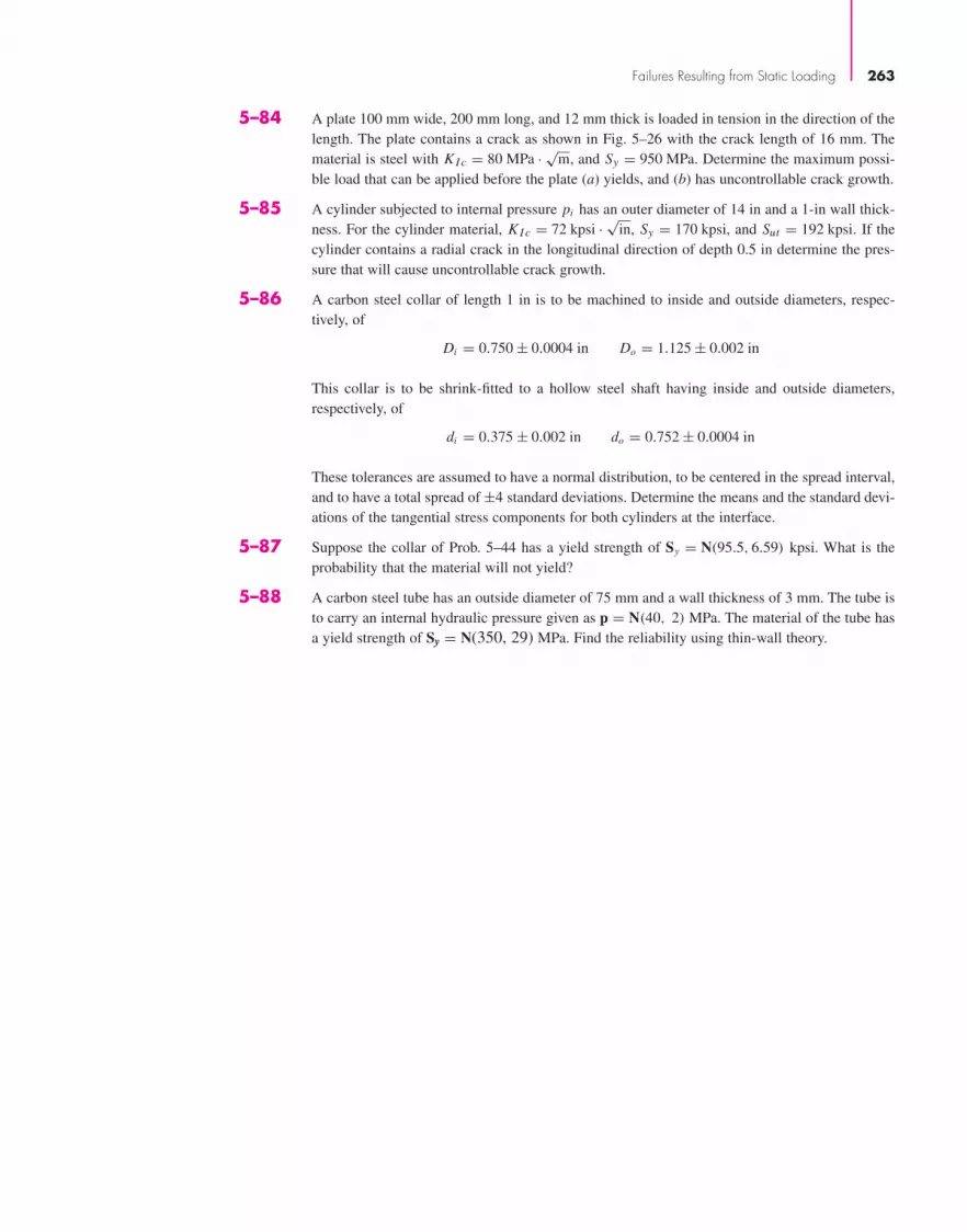
5–84 A plate 100 mm wide, 200 mm long, and 12 mm thick is loaded in tension in the direction of thelength. The plate contains a crack as shown in Fig. 5–26 with the crack length of 16 mm. Thematerial is steel with KI c = 80 MPa · √m, and Sy = 950 MPa. Determine the maximum possi-ble load that can be applied before the plate (a) yields, and (b) has uncontrollable crack growth.
5–85 A cylinder subjected to internal pressure pi has an outer diameter of 14 in and a 1-in wall thick-ness. For the cylinder material, KI c = 72 kpsi · √in, Sy = 170 kpsi, and Sut = 192 kpsi. If thecylinder contains a radial crack in the longitudinal direction of depth 0.5 in determine the pres-sure that will cause uncontrollable crack growth.
5–86 A carbon steel collar of length 1 in is to be machined to inside and outside diameters, respec-tively, of
Di = 0.750 ± 0.0004 in Do = 1.125 ± 0.002 in
This collar is to be shrink-fitted to a hollow steel shaft having inside and outside diameters,respectively, of
di = 0.375 ± 0.002 in do = 0.752 ± 0.0004 in
These tolerances are assumed to have a normal distribution, to be centered in the spread interval,and to have a total spread of ±4 standard deviations. Determine the means and the standard devi-ations of the tangential stress components for both cylinders at the interface.
5–87 Suppose the collar of Prob. 5–44 has a yield strength of Sy = N(95.5, 6.59) kpsi. What is theprobability that the material will not yield?
5–88 A carbon steel tube has an outside diameter of 75 mm and a wall thickness of 3 mm. The tube isto carry an internal hydraulic pressure given as p = N(40, 2) MPa. The material of the tube hasa yield strength of Sy = N(350, 29) MPa. Find the reliability using thin-wall theory.
Failures Resulting from Static Loading 263
bud29281_ch05_212-264.qxd 11/27/2009 6:46 pm Page 263 pinnacle s-171:Desktop Folder:Temp Work:Don't Delete (Jobs):MHDQ196/Budynas:

This page intentionally left blank

6 Fatigue Failure Resultingfrom Variable Loading
Chapter Outline
6–1 Introduction to Fatigue in Metals 266
6–2 Approach to Fatigue Failure in Analysis and Design 272
6–3 Fatigue-Life Methods 273
6–4 The Stress-Life Method 273
6–5 The Strain-Life Method 276
6–6 The Linear-Elastic Fracture Mechanics Method 278
6–7 The Endurance Limit 282
6–8 Fatigue Strength 283
6–9 Endurance Limit Modifying Factors 286
6–10 Stress Concentration and Notch Sensitivity 295
6–11 Characterizing Fluctuating Stresses 300
6–12 Fatigue Failure Criteria for Fluctuating Stress 303
6–13 Torsional Fatigue Strength under Fluctuating Stresses 317
6–14 Combinations of Loading Modes 317
6–15 Varying, Fluctuating Stresses; Cumulative Fatigue Damage 321
6–16 Surface Fatigue Strength 327
6–17 Stochastic Analysis 330
6–18 Road Maps and Important Design Equations for the Stress-Life Method 344
265
bud29281_ch06_265-357.qxd 11/30/2009 4:23 pm Page 265 pinnacle s-171:Desktop Folder:Temp Work:Don't Delete (Jobs):MHDQ196/Budynas:

266 Mechanical Engineering Design
In Chap. 5 we considered the analysis and design of parts subjected to static loading.The behavior of machine parts is entirely different when they are subjected to time-varying loading. In this chapter we shall examine how parts fail under variable loadingand how to proportion them to successfully resist such conditions.
6–1 Introduction to Fatigue in MetalsIn most testing of those properties of materials that relate to the stress-strain diagram,the load is applied gradually, to give sufficient time for the strain to fully develop.Furthermore, the specimen is tested to destruction, and so the stresses are applied onlyonce. Testing of this kind is applicable, to what are known as static conditions; suchconditions closely approximate the actual conditions to which many structural andmachine members are subjected.
The condition frequently arises, however, in which the stresses vary with time orthey fluctuate between different levels. For example, a particular fiber on the surface ofa rotating shaft subjected to the action of bending loads undergoes both tension and com-pression for each revolution of the shaft. If the shaft is part of an electric motor rotatingat 1725 rev/min, the fiber is stressed in tension and compression 1725 times each minute.If, in addition, the shaft is also axially loaded (as it would be, for example, by a helicalor worm gear), an axial component of stress is superposed upon the bending component.In this case, some stress is always present in any one fiber, but now the level of stress isfluctuating. These and other kinds of loading occurring in machine members producestresses that are called variable, repeated, alternating, or fluctuating stresses.
Often, machine members are found to have failed under the action of repeated orfluctuating stresses; yet the most careful analysis reveals that the actual maximumstresses were well below the ultimate strength of the material, and quite frequently evenbelow the yield strength. The most distinguishing characteristic of these failures is thatthe stresses have been repeated a very large number of times. Hence the failure is calleda fatigue failure.
When machine parts fail statically, they usually develop a very large deflection,because the stress has exceeded the yield strength, and the part is replaced before fractureactually occurs. Thus many static failures give visible warning in advance. But a fatiguefailure gives no warning! It is sudden and total, and hence dangerous. It is relatively sim-ple to design against a static failure, because our knowledge is comprehensive. Fatigue isa much more complicated phenomenon, only partially understood, and the engineer seek-ing competence must acquire as much knowledge of the subject as possible.
A fatigue failure has an appearance similar to a brittle fracture, as the fracture sur-faces are flat and perpendicular to the stress axis with the absence of necking. The frac-ture features of a fatigue failure, however, are quite different from a static brittle fracturearising from three stages of development. Stage I is the initiation of one or more micro-cracks due to cyclic plastic deformation followed by crystallographic propagationextending from two to five grains about the origin. Stage I cracks are not normally dis-cernible to the naked eye. Stage II progresses from microcracks to macrocracks formingparallel plateau-like fracture surfaces separated by longitudinal ridges. The plateaus aregenerally smooth and normal to the direction of maximum tensile stress. These surfacescan be wavy dark and light bands referred to as beach marks or clamshell marks, as seenin Fig. 6–1. During cyclic loading, these cracked surfaces open and close, rubbingtogether, and the beach mark appearance depends on the changes in the level or fre-quency of loading and the corrosive nature of the environment. Stage III occurs duringthe final stress cycle when the remaining material cannot support the loads, resulting in
bud29281_ch06_265-357.qxd 11/30/2009 4:23 pm Page 266 pinnacle s-171:Desktop Folder:Temp Work:Don't Delete (Jobs):MHDQ196/Budynas:

Fatigue Failure Resulting from Variable Loading 267
Figure 6–1
Fatigue failure of a bolt due torepeated unidirectional bending.The failure started at the threadroot at A, propagated acrossmost of the cross section shownby the beach marks at B, before final fast fracture at C.(From ASM Handbook, Vol. 12: Fractography,2nd printing, 1992, ASM International, Materials Park, OH 44073-0002, fig 50, p. 120. Reprinted by permission ofASM International®, www.asminternational.org.)
1See the ASM Handbook, Fractography, ASM International, Metals Park, Ohio, vol. 12, 9th ed., 1987.
a sudden, fast fracture. A stage III fracture can be brittle, ductile, or a combination ofboth. Quite often the beach marks, if they exist, and possible patterns in the stage III frac-ture called chevron lines, point toward the origins of the initial cracks.
There is a good deal to be learned from the fracture patterns of a fatigue failure.1
Figure 6–2 shows representations of failure surfaces of various part geometries underdiffering load conditions and levels of stress concentration. Note that, in the case ofrotational bending, even the direction of rotation influences the failure pattern.
Fatigue failure is due to crack formation and propagation. A fatigue crack will typ-ically initiate at a discontinuity in the material where the cyclic stress is a maximum.Discontinuities can arise because of:
• Design of rapid changes in cross section, keyways, holes, etc. where stress concen-trations occur as discussed in Secs. 3–13 and 5–2.
• Elements that roll and/or slide against each other (bearings, gears, cams, etc.) underhigh contact pressure, developing concentrated subsurface contact stresses (Sec. 3–19)that can cause surface pitting or spalling after many cycles of the load.
• Carelessness in locations of stamp marks, tool marks, scratches, and burrs; poor jointdesign; improper assembly; and other fabrication faults.
• Composition of the material itself as processed by rolling, forging, casting, extrusion,drawing, heat treatment, etc. Microscopic and submicroscopic surface and subsurfacediscontinuities arise, such as inclusions of foreign material, alloy segregation, voids,hard precipitated particles, and crystal discontinuities.
Various conditions that can accelerate crack initiation include residual tensile stresses,elevated temperatures, temperature cycling, a corrosive environment, and high-frequencycycling.
The rate and direction of fatigue crack propagation is primarily controlled by local-ized stresses and by the structure of the material at the crack. However, as with crackformation, other factors may exert a significant influence, such as environment, tem-perature, and frequency. As stated earlier, cracks will grow along planes normal to the
bud29281_ch06_265-357.qxd 12/9/09 7:17PM Page 267 ntt 203:MHDQ196:bud29281:0073529281:bud29281_pagefiles:

268 Mechanical Engineering Design
Figure 6–2
Schematics of fatigue fracturesurfaces produced in smoothand notched components withround and rectangular crosssections under various loadingconditions and nominal stresslevels. (From ASM MetalsHandbook, Vol. 11: FailureAnalysis and Prevention, 1986,ASM International, MaterialsPark, OH 44073-0002, fig 18, p. 111. Reprinted by permissionof ASM International®, www.asminternational.org.)
bud29281_ch06_265-357.qxd 11/30/2009 4:23 pm Page 268 pinnacle s-171:Desktop Folder:Temp Work:Don't Delete (Jobs):MHDQ196/Budynas:

Fatigue Failure Resulting from Variable Loading 269
Figure 6–3
Fatigue fracture of an AISI4320 drive shaft. The fatiguefailure initiated at the end ofthe keyway at points B andprogressed to final rupture at C.The final rupture zone is small,indicating that loads were low.(From ASM Handbook, Vol. 12: Fractography, 2nd printing, 1992, ASMInternational, Materials Park,OH 44073-0002, fig 51, p. 120.Reprinted by permission ofASM International®, www.asminternational.org.)
Figure 6–4
Fatigue fracture surface of anAISI 8640 pin. Sharp cornersof the mismatched greaseholes provided stressconcentrations that initiated two fatigue cracksindicated by the arrows. (From ASM Handbook, Vol. 12: Fractography, 2nd printing, 1992, ASMInternational, Materials Park,OH 44073-0002, fig 520, p. 331. Reprinted by permissionof ASM International®,www.asminternational.org.)
maximum tensile stresses. The crack growth process can be explained by fracturemechanics (see Sec. 6–6).
A major reference source in the study of fatigue failure is the 21-volume ASM Metals Handbook. Figures 6–1 to 6–8, reproduced with permission from ASMInternational, are but a minuscule sample of examples of fatigue failures for a greatvariety of conditions included in the handbook. Comparing Fig. 6–3 with Fig. 6–2, wesee that failure occurred by rotating bending stresses, with the direction of rotationbeing clockwise with respect to the view and with a mild stress concentration and lownominal stress.
bud29281_ch06_265-357.qxd 12/02/2009 6:49 pm Page 269 pinnacle s-171:Desktop Folder:Temp Work:Don't Delete (Jobs):MHDQ196/Budynas:

270 Mechanical Engineering Design
Figure 6–5
Fatigue fracture surface of aforged connecting rod of AISI 8640 steel. The fatiguecrack origin is at the left edge, atthe flash line of the forging, butno unusual roughness of theflash trim was indicated. Thefatigue crack progressedhalfway around the oil holeat the left, indicated by the beach marks, before final fastfracture occurred. Note thepronounced shear lip in the final fracture at the right edge.(From ASM Handbook,Vol. 12: Fractography, 2nd printing, 1992, ASMInternational, Materials Park,OH 44073-0002, fig 523, p. 332.Reprinted by permission of ASM International®, www.asminternational.org.)
Figure 6–6
Fatigue fracture surface of a 200-mm (8-in) diameter piston rod of an alloysteel steam hammer used for forging. This is an example of a fatigue fracturecaused by pure tension where surface stress concentrations are absent and acrack may initiate anywhere in the cross section. In this instance, the initialcrack formed at a forging flake slightly below center, grew outwardsymmetrically, and ultimately produced a brittle fracture without warning.(From ASM Handbook, Vol. 12: Fractography, 2nd printing, 1992, ASMInternational, Materials Park, OH 44073-0002, fig 570, p. 342. Reprinted bypermission of ASM International®, www.asminternational.org.)
bud29281_ch06_265-357.qxd 12/02/2009 6:49 pm Page 270 pinnacle s-171:Desktop Folder:Temp Work:Don't Delete (Jobs):MHDQ196/Budynas:

Fatigue Failure Resulting from Variable Loading 271
Figure 6–7
Fatigue failure of an ASTM A186 steel double-flange trailer wheel caused by stamp marks. (a) Coke-oven car wheel showing position of stamp marks and fractures in the rib and web. (b) Stamp mark showing heavy impression and fracture extending along the base of the lower row of numbers. (c) Notches, indicated by arrows, created from the heavily indented stamp marks from which cracks initiated along the top at the fracture surface. (From ASM Metals Handbook, Vol. 11: Failure Analysis and Prevention, 1986, ASM International, Materials Park, OH 44073-0002, fig 51, p. 130. Reprinted by permission of ASM International®, www.asminternational.org.)
Aluminum alloy 7075-T73Rockwell B 85.5
Original design
10.200
A
Lug(1 of 2)
25.54.94
Fracture
3.62 dia Secondaryfracture
1.750-in.-diabushing,0.090-in. wall
Primary-fracturesurfaceLubrication hole
1 in
Lubrication hole
Improved design
Detail A
(a)
Figure 6–8
Aluminum alloy 7075-T73landing-gear torque-armassembly redesign to eliminatefatigue fracture at a lubricationhole. (a) Arm configuration,original and improved design(dimensions given in inches).(b) Fracture surface wherearrows indicate multiple crackorigins. (From ASM MetalsHandbook, Vol. 11: FailureAnalysis and Prevention, 1986,ASM International, MaterialsPark, OH 44073-0002, fig 23, p. 114. Reprintedby permission of ASMInternational®,www.asminternational.org.)
Medium-carbon steel(ASTM A186)
(a) Coke-oven-car wheel
Web30 dia
Flange(1 of 2)
Fracture
TreadFracture
bud29281_ch06_265-357.qxd 12/02/2009 6:49 pm Page 271 pinnacle s-171:Desktop Folder:Temp Work:Don't Delete (Jobs):MHDQ196/Budynas:

272 Mechanical Engineering Design
6–2 Approach to Fatigue Failure in Analysis and DesignAs noted in the previous section, there are a great many factors to be considered, evenfor very simple load cases. The methods of fatigue failure analysis represent a combi-nation of engineering and science. Often science fails to provide the complete answersthat are needed. But the airplane must still be made to fly—safely. And the automobilemust be manufactured with a reliability that will ensure a long and troublefree life andat the same time produce profits for the stockholders of the industry. Thus, while sci-ence has not yet completely explained the complete mechanism of fatigue, the engineermust still design things that will not fail. In a sense this is a classic example of the truemeaning of engineering as contrasted with science. Engineers use science to solve theirproblems if the science is available. But available or not, the problem must be solved,and whatever form the solution takes under these conditions is called engineering.
In this chapter, we will take a structured approach in the design against fatiguefailure. As with static failure, we will attempt to relate to test results performed on sim-ply loaded specimens. However, because of the complex nature of fatigue, there ismuch more to account for. From this point, we will proceed methodically, and in stages.In an attempt to provide some insight as to what follows in this chapter, a brief descrip-tion of the remaining sections will be given here.
Fatigue-Life Methods (Secs. 6–3 to 6–6)
Three major approaches used in design and analysis to predict when, if ever, a cyclicallyloaded machine component will fail in fatigue over a period of time are presented. Thepremises of each approach are quite different but each adds to our understanding of themechanisms associated with fatigue. The application, advantages, and disadvantages ofeach method are indicated. Beyond Sec. 6–6, only one of the methods, the stress-lifemethod, will be pursued for further design applications.
Fatigue Strength and the Endurance Limit (Secs. 6–7 and 6–8)
The strength-life (S-N) diagram provides the fatigue strength Sf versus cycle life N of amaterial. The results are generated from tests using a simple loading of standard laboratory-controlled specimens. The loading often is that of sinusoidally reversing pure bending.The laboratory-controlled specimens are polished without geometric stress concentra-tion at the region of minimum area.
For steel and iron, the S-N diagram becomes horizontal at some point. The strengthat this point is called the endurance limit S′
e and occurs somewhere between 106 and 107
cycles. The prime mark on S′e refers to the endurance limit of the controlled laboratory
specimen. For nonferrous materials that do not exhibit an endurance limit, a fatiguestrength at a specific number of cycles, S′
f , may be given, where again, the prime denotesthe fatigue strength of the laboratory-controlled specimen.
The strength data are based on many controlled conditions that will not be the sameas that for an actual machine part. What follows are practices used to account for thedifferences between the loading and physical conditions of the specimen and the actualmachine part.
Endurance Limit Modifying Factors (Sec. 6–9)
Modifying factors are defined and used to account for differences between the speci-men and the actual machine part with regard to surface conditions, size, loading, tem-perature, reliability, and miscellaneous factors. Loading is still considered to be simpleand reversing.
bud29281_ch06_265-357.qxd 11/30/2009 4:23 pm Page 272 pinnacle s-171:Desktop Folder:Temp Work:Don't Delete (Jobs):MHDQ196/Budynas:

Fatigue Failure Resulting from Variable Loading 273
Stress Concentration and Notch Sensitivity (Sec. 6–10)
The actual part may have a geometric stress concentration by which the fatigue behav-ior depends on the static stress-concentration factor and the component material’ssensitivity to fatigue damage.
Fluctuating Stresses (Secs. 6–11 to 6–13)
These sections account for simple stress states from fluctuating load conditions that arenot purely sinusoidally reversing axial, bending, or torsional stresses.
Combinations of Loading Modes (Sec. 6–14)
Here a procedure based on the distortion-energy theory is presented for analyzingcombined fluctuating stress states, such as combined bending and torsion. Here it isassumed that the levels of the fluctuating stresses are in phase and not time varying.
Varying, Fluctuating Stresses; CumulativeFatigue Damage (Sec. 6–15)
The fluctuating stress levels on a machine part may be time varying. Methods are pro-vided to assess the fatigue damage on a cumulative basis.
Remaining Sections
The remaining three sections of the chapter pertain to the special topics of surfacefatigue strength, stochastic analysis, and road maps with important equations.
6–3 Fatigue-Life MethodsThe three major fatigue life methods used in design and analysis are the stress-lifemethod, the strain-life method, and the linear-elastic fracture mechanics method. Thesemethods attempt to predict the life in number of cycles to failure, N, for a specific levelof loading. Life of 1 ≤ N ≤ 103 cycles is generally classified as low-cycle fatigue,whereas high-cycle fatigue is considered to be N > 103 cycles.
The stress-life method, based on stress levels only, is the least accurate approach,especially for low-cycle applications. However, it is the most traditional method, sinceit is the easiest to implement for a wide range of design applications, has ample sup-porting data, and represents high-cycle applications adequately.
The strain-life method involves more detailed analysis of the plastic deformation atlocalized regions where the stresses and strains are considered for life estimates. Thismethod is especially good for low-cycle fatigue applications. In applying this method,several idealizations must be compounded, and so some uncertainties will exist in theresults. For this reason, it will be discussed only because of its value in adding to theunderstanding of the nature of fatigue.
The fracture mechanics method assumes a crack is already present and detected. Itis then employed to predict crack growth with respect to stress intensity. It is most prac-tical when applied to large structures in conjunction with computer codes and a peri-odic inspection program.
6–4 The Stress-Life MethodTo determine the strength of materials under the action of fatigue loads, specimens aresubjected to repeated or varying forces of specified magnitudes while the cycles orstress reversals are counted to destruction. The most widely used fatigue-testing device
bud29281_ch06_265-357.qxd 12/7/09 7:25PM Page 273 ntt 203:MHDQ196:bud29281:0073529281:bud29281_pagefiles:

274 Mechanical Engineering Design
7163
0.30 in
in
9 in R.78
aF F
aF F
Figure 6–9
Test-specimen geometry for theR. R. Moore rotating-beammachine. The bending momentis uniform, M = Fa, over the curved length and at thehighest-stressed section at themid-point of the beam.
100
50
100
101 102 103 104 105 106 107 108
Number of stress cycles, N
Se
Sut
Fatig
ue s
tren
gth
S f ,
kpsi
Low cycle High cycle
Finite life Infinite
life
Figure 6–10
An S-N diagram plotted fromthe results of completelyreversed axial fatigue tests.Material: UNS G41300 steel,normalized; Sut = 116 kpsi;maximum Sut = 125 kpsi.(Data from NACA Tech. Note
3866, December 1966.)
is the R. R. Moore high-speed rotating-beam machine. This machine subjects the specimento pure bending (no transverse shear) by means of weights. The specimen, shown inFig. 6–9, is very carefully machined and polished, with a final polishing in an axialdirection to avoid circumferential scratches. Other fatigue-testing machines are avail-able for applying fluctuating or reversed axial stresses, torsional stresses, or combinedstresses to the test specimens.
To establish the fatigue strength of a material, quite a number of tests are necessarybecause of the statistical nature of fatigue. For the rotating-beam test, a constant bend-ing load is applied, and the number of revolutions (stress reversals) of the beam requiredfor failure is recorded. The first test is made at a stress that is somewhat under the ulti-mate strength of the material. The second test is made at a stress that is less than thatused in the first. This process is continued, and the results are plotted as an S-N diagram(Fig. 6–10). This chart may be plotted on semilog paper or on log-log paper. In the caseof ferrous metals and alloys, the graph becomes horizontal after the material has beenstressed for a certain number of cycles. Plotting on log paper emphasizes the bend inthe curve, which might not be apparent if the results were plotted by using Cartesiancoordinates.
The ordinate of the S-N diagram is called the fatigue strength Sf ; a statement ofthis strength value must always be accompanied by a statement of the number of cyclesN to which it corresponds.
bud29281_ch06_265-357.qxd 12/02/2009 6:49 pm Page 274 pinnacle s-171:Desktop Folder:Temp Work:Don't Delete (Jobs):MHDQ196/Budynas:

Fatigue Failure Resulting from Variable Loading 275
8070
60
50
4035
30
25
20181614
12
10
87
6
5103 104 105 106 107 108 109
Life N, cycles (log)
Peak
alte
rnat
ing
bend
ing
stre
ss S
, kps
i (lo
g)
Sand cast
Permanent mold cast
Wrought
Figure 6–11
S-N bands for representativealuminum alloys, excludingwrought alloys withSut < 38 kpsi. (From R. C.Juvinall, EngineeringConsiderations of Stress, Strain and Strength. Copyright© 1967 by The McGraw-HillCompanies, Inc. Reprinted bypermission.)
Soon we shall learn that S-N diagrams can be determined either for a test specimenor for an actual mechanical element. Even when the material of the test specimen andthat of the mechanical element are identical, there will be significant differencesbetween the diagrams for the two.
In the case of the steels, a knee occurs in the graph, and beyond this knee failurewill not occur, no matter how great the number of cycles. The strength correspondingto the knee is called the endurance limit Se, or the fatigue limit. The graph of Fig. 6–10never does become horizontal for nonferrous metals and alloys, and hence these mate-rials do not have an endurance limit. Figure 6–11 shows scatter bands indicating the S-Ncurves for most common aluminum alloys excluding wrought alloys having a tensilestrength below 38 kpsi. Since aluminum does not have an endurance limit, normally thefatigue strength Sf is reported at a specific number of cycles, normally N = 5(108)
cycles of reversed stress (see Table A–24).The S-N diagram is usually obtained by completely reversed stress cycles, in which
the stress level alternates between equal magnitudes of tension and compression. Wenote that a stress cycle (N = 1) constitutes a single application and removal of a loadand then another application and removal of the load in the opposite direction. ThusN = 1
2 means the load is applied once and then removed, which is the case with thesimple tension test.
The body of knowledge available on fatigue failure from N = 1 to N = 1000cycles is generally classified as low-cycle fatigue, as indicated in Fig. 6–10. High-cyclefatigue, then, is concerned with failure corresponding to stress cycles greater than 103
cycles.We also distinguish a finite-life region and an infinite-life region in Fig. 6–10. The
boundary between these regions cannot be clearly defined except for a specific material;but it lies somewhere between 106 and 107 cycles for steels, as shown in Fig. 6–10.
As noted previously, it is always good engineering practice to conduct a testingprogram on the materials to be employed in design and manufacture. This, in fact, is arequirement, not an option, in guarding against the possibility of a fatigue failure.
bud29281_ch06_265-357.qxd 11/30/2009 4:23 pm Page 275 pinnacle s-171:Desktop Folder:Temp Work:Don't Delete (Jobs):MHDQ196/Budynas:

276 Mechanical Engineering Design
Because of this necessity for testing, it would really be unnecessary for us to proceedany further in the study of fatigue failure except for one important reason: the desire toknow why fatigue failures occur so that the most effective method or methods can beused to improve fatigue strength. Thus our primary purpose in studying fatigue is tounderstand why failures occur so that we can guard against them in an optimum man-ner. For this reason, the analytical design approaches presented in this book, or in anyother book, for that matter, do not yield absolutely precise results. The results should betaken as a guide, as something that indicates what is important and what is not impor-tant in designing against fatigue failure.
As stated earlier, the stress-life method is the least accurate approach especiallyfor low-cycle applications. However, it is the most traditional method, with muchpublished data available. It is the easiest to implement for a wide range of designapplications and represents high-cycle applications adequately. For these reasons thestress-life method will be emphasized in subsequent sections of this chapter.However, care should be exercised when applying the method for low-cycle applications,as the method does not account for the true stress-strain behavior when localizedyielding occurs.
6–5 The Strain-Life MethodThe best approach yet advanced to explain the nature of fatigue failure is called by somethe strain-life method. The approach can be used to estimate fatigue strengths, but whenit is so used it is necessary to compound several idealizations, and so some uncertain-ties will exist in the results. For this reason, the method is presented here only becauseof its value in explaining the nature of fatigue.
A fatigue failure almost always begins at a local discontinuity such as a notch,crack, or other area of stress concentration. When the stress at the discontinuity exceedsthe elastic limit, plastic strain occurs. If a fatigue fracture is to occur, there must existcyclic plastic strains. Thus we shall need to investigate the behavior of materials sub-ject to cyclic deformation.
In 1910, Bairstow verified by experiment Bauschinger’s theory that the elastic lim-its of iron and steel can be changed, either up or down, by the cyclic variations of stress.2
In general, the elastic limits of annealed steels are likely to increase when subjected tocycles of stress reversals, while cold-drawn steels exhibit a decreasing elastic limit.
R. W. Landgraf has investigated the low-cycle fatigue behavior of a large numberof very high-strength steels, and during his research he made many cyclic stress-strainplots.3 Figure 6–12 has been constructed to show the general appearance of these plotsfor the first few cycles of controlled cyclic strain. In this case the strength decreaseswith stress repetitions, as evidenced by the fact that the reversals occur at ever-smallerstress levels. As previously noted, other materials may be strengthened, instead, bycyclic stress reversals.
The SAE Fatigue Design and Evaluation Steering Committee released a report in1975 in which the life in reversals to failure is related to the strain amplitude �ε/2.4
2L. Bairstow, “The Elastic Limits of Iron and Steel under Cyclic Variations of Stress,” PhilosophicalTransactions, Series A, vol. 210, Royal Society of London, 1910, pp. 35–55.3R. W. Landgraf, Cyclic Deformation and Fatigue Behavior of Hardened Steels, Report no. 320, Departmentof Theoretical and Applied Mechanics, University of Illinois, Urbana, 1968, pp. 84–90.4Technical Report on Fatigue Properties, SAE J1099, 1975.
bud29281_ch06_265-357.qxd 11/30/2009 4:23 pm Page 276 pinnacle s-171:Desktop Folder:Temp Work:Don't Delete (Jobs):MHDQ196/Budynas:

Fatigue Failure Resulting from Variable Loading 277
4th
2d
1st reversal
3d5th
A
B
Δ�
Δ�p Δ�e
Δ�
�
�Figure 6–12
True stress–true strainhysteresis loops showing thefirst five stress reversals of acyclic-softening material. Thegraph is slightly exaggeratedfor clarity. Note that the slopeof the line AB is the modulus of elasticity E. The stress range is �σ , �εp is the plastic-strain range, and �εe is the elastic strain range.The total-strain range is�ε = �εp + �εe .
The report contains a plot of this relationship for SAE 1020 hot-rolled steel; the graphhas been reproduced as Fig. 6–13. To explain the graph, we first define the followingterms:
• Fatigue ductility coefficient ε′F is the true strain corresponding to fracture in one re-
versal (point A in Fig. 6–12). The plastic-strain line begins at this point in Fig. 6–13.
• Fatigue strength coefficient σ ′F is the true stress corresponding to fracture in one
reversal (point A in Fig. 6–12). Note in Fig. 6–13 that the elastic-strain line begins atσ ′
F/E .
• Fatigue ductility exponent c is the slope of the plastic-strain line in Fig. 6–13 and isthe power to which the life 2N must be raised to be proportional to the true plastic-strain amplitude. If the number of stress reversals is 2N, then N is the number ofcycles.
10010–4
10–3
10–2
10–1
100
101 102 103 104 105 106
Reversals to failure, 2N
Stra
in a
mpl
itude
, Δ�/2
�'F
c
1.0
b1.0
� 'FE
Total strainPlastic strain
Elastic strain
Figure 6–13
A log-log plot showing how the fatigue life is related tothe true-strain amplitude forhot-rolled SAE 1020 steel.(Reprinted with permissionfrom SAE J1099_200208 © 2002 SAE International.)
bud29281_ch06_265-357.qxd 11/30/2009 4:23 pm Page 277 pinnacle s-171:Desktop Folder:Temp Work:Don't Delete (Jobs):MHDQ196/Budynas:
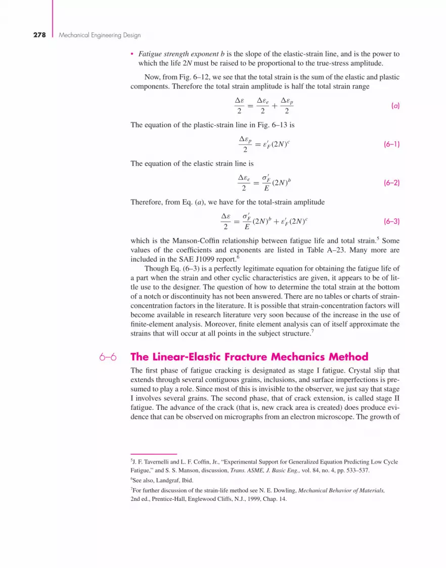
278 Mechanical Engineering Design
• Fatigue strength exponent b is the slope of the elastic-strain line, and is the power towhich the life 2N must be raised to be proportional to the true-stress amplitude.
Now, from Fig. 6–12, we see that the total strain is the sum of the elastic and plasticcomponents. Therefore the total strain amplitude is half the total strain range
�ε
2= �εe
2+ �εp
2(a)
The equation of the plastic-strain line in Fig. 6–13 is
�εp
2= ε′
F(2N )c (6–1)
The equation of the elastic strain line is
�εe
2= σ ′
F
E(2N )b (6–2)
Therefore, from Eq. (a), we have for the total-strain amplitude
�ε
2= σ ′
F
E(2N )b + ε′
F(2N )c (6–3)
which is the Manson-Coffin relationship between fatigue life and total strain.5 Somevalues of the coefficients and exponents are listed in Table A–23. Many more areincluded in the SAE J1099 report.6
Though Eq. (6–3) is a perfectly legitimate equation for obtaining the fatigue life ofa part when the strain and other cyclic characteristics are given, it appears to be of lit-tle use to the designer. The question of how to determine the total strain at the bottomof a notch or discontinuity has not been answered. There are no tables or charts of strain-concentration factors in the literature. It is possible that strain-concentration factors willbecome available in research literature very soon because of the increase in the use offinite-element analysis. Moreover, finite element analysis can of itself approximate thestrains that will occur at all points in the subject structure.7
6–6 The Linear-Elastic Fracture Mechanics MethodThe first phase of fatigue cracking is designated as stage I fatigue. Crystal slip thatextends through several contiguous grains, inclusions, and surface imperfections is pre-sumed to play a role. Since most of this is invisible to the observer, we just say that stageI involves several grains. The second phase, that of crack extension, is called stage IIfatigue. The advance of the crack (that is, new crack area is created) does produce evi-dence that can be observed on micrographs from an electron microscope. The growth of
5J. F. Tavernelli and L. F. Coffin, Jr., “Experimental Support for Generalized Equation Predicting Low CycleFatigue,’’ and S. S. Manson, discussion, Trans. ASME, J. Basic Eng., vol. 84, no. 4, pp. 533–537.6See also, Landgraf, Ibid.7For further discussion of the strain-life method see N. E. Dowling, Mechanical Behavior of Materials,2nd ed., Prentice-Hall, Englewood Cliffs, N.J., 1999, Chap. 14.
bud29281_ch06_265-357.qxd 12/9/09 7:17PM Page 278 ntt 203:MHDQ196:bud29281:0073529281:bud29281_pagefiles:
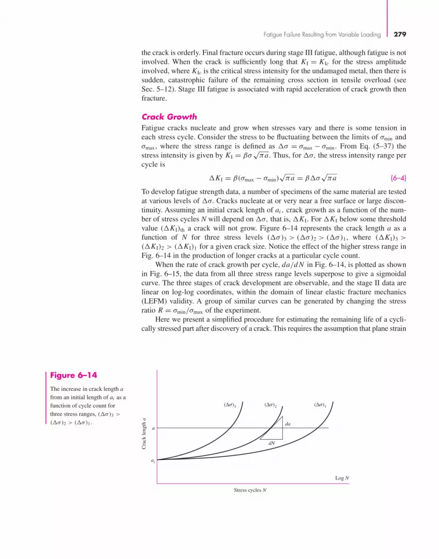
Fatigue Failure Resulting from Variable Loading 279
the crack is orderly. Final fracture occurs during stage III fatigue, although fatigue is notinvolved. When the crack is sufficiently long that KI = KIc for the stress amplitudeinvolved, where KIc is the critical stress intensity for the undamaged metal, then there issudden, catastrophic failure of the remaining cross section in tensile overload (seeSec. 5–12). Stage III fatigue is associated with rapid acceleration of crack growth thenfracture.
Crack Growth
Fatigue cracks nucleate and grow when stresses vary and there is some tension ineach stress cycle. Consider the stress to be fluctuating between the limits of σmin andσmax, where the stress range is defined as �σ = σmax − σmin. From Eq. (5–37) thestress intensity is given by KI = βσ
√πa. Thus, for �σ, the stress intensity range per
cycle is
�KI = β(σmax − σmin)√
πa = β�σ√
πa (6–4)
To develop fatigue strength data, a number of specimens of the same material are testedat various levels of �σ. Cracks nucleate at or very near a free surface or large discon-tinuity. Assuming an initial crack length of ai , crack growth as a function of the num-ber of stress cycles N will depend on �σ, that is, �KI. For �KI below some thresholdvalue (�KI)th a crack will not grow. Figure 6–14 represents the crack length a as afunction of N for three stress levels (�σ)3 > (�σ)2 > (�σ)1, where (�KI)3 >
(�KI)2 > (�KI)1 for a given crack size. Notice the effect of the higher stress range inFig. 6–14 in the production of longer cracks at a particular cycle count.
When the rate of crack growth per cycle, da/d N in Fig. 6–14, is plotted as shownin Fig. 6–15, the data from all three stress range levels superpose to give a sigmoidalcurve. The three stages of crack development are observable, and the stage II data arelinear on log-log coordinates, within the domain of linear elastic fracture mechanics(LEFM) validity. A group of similar curves can be generated by changing the stressratio R = σmin/σmax of the experiment.
Here we present a simplified procedure for estimating the remaining life of a cycli-cally stressed part after discovery of a crack. This requires the assumption that plane strain
Log N
Stress cycles N
Cra
ck le
ngth
a
a
ai
(Δ�)3 (Δ�)2 (Δ�)1
da
dN
Figure 6–14
The increase in crack length afrom an initial length of ai as afunction of cycle count forthree stress ranges, (�σ)3 >
(�σ)2 > (�σ)1.
bud29281_ch06_265-357.qxd 11/30/2009 4:23 pm Page 279 pinnacle s-171:Desktop Folder:Temp Work:Don't Delete (Jobs):MHDQ196/Budynas:

280 Mechanical Engineering Design
conditions prevail.8 Assuming a crack is discovered early in stage II, the crack growth inregion II of Fig. 6–15 can be approximated by the Paris equation, which is of the form
da
d N= C(�KI)
m (6–5)
where C and m are empirical material constants and �KI is given by Eq. (6–4).Representative, but conservative, values of C and m for various classes of steels arelisted in Table 6–1. Substituting Eq. (6–4) and integrating gives∫ Nf
0d N = Nf = 1
C
∫ af
ai
da
(β�σ√
πa)m(6–6)
Here ai is the initial crack length, af is the final crack length corresponding to failure,and Nf is the estimated number of cycles to produce a failure after the initial crack isformed. Note that β may vary in the integration variable (e.g., see Figs. 5–25 to 5–30).
Log ΔK
Log dadN
Increasingstress ratio
R
Crackpropagation
Region II
Crackinitiation
Region I
Crackunstable
Region III
(ΔK)th
Kc
Figure 6–15
When da/d N is measured in Fig. 6–14 and plotted onlog-log coordinates, the data for different stress rangessuperpose, giving rise to asigmoid curve as shown.(�KI)th is the threshold valueof �KI, below which a crackdoes not grow. From thresholdto rupture an aluminum alloywill spend 85–90 percent of life in region I, 5–8 percent inregion II, and 1–2 percent in region III.
Table 6–1
Conservative Values of
Factor C and Exponent
m in Eq. (6–5) for
Various Forms of Steel
(R = σmax/σmin.= 0)
Material C,m/cycle(
MPa√
m)m
C,in/cycle(kpsi
√in
)m
Ferritic-pearlitic steels 6.89(10−12) 3.60(10−10) 3.00
Martensitic steels 1.36(10−10) 6.60(10−9) 2.25
Austenitic stainless steels 5.61(10−12) 3.00(10−10) 3.25
From J. M. Barsom and S. T. Rolfe, Fatigue and Fracture Control in Structures, 2nd ed., Prentice Hall,Upper Saddle River, NJ, 1987, pp. 288–291, Copyright ASTM International. Reprinted with permission.
8Recommended references are: Dowling, op. cit.; J. A. Collins, Failure of Materials in Mechanical Design,John Wiley & Sons, New York, 1981; H. O. Fuchs and R. I. Stephens, Metal Fatigue in Engineering, JohnWiley & Sons, New York, 1980; and Harold S. Reemsnyder, “Constant Amplitude Fatigue Life AssessmentModels,” SAE Trans. 820688, vol. 91, Nov. 1983.
m
bud29281_ch06_265-357.qxd 12/02/2009 9:37 pm Page 280 pinnacle s-171:Desktop Folder:Temp Work:Don't Delete (Jobs):MHDQ196/Budynas:
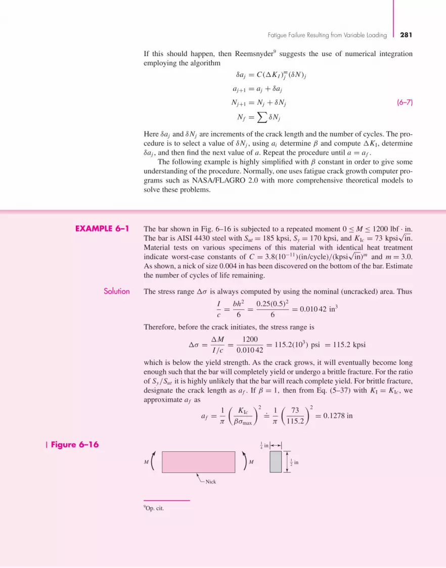
Fatigue Failure Resulting from Variable Loading 281
If this should happen, then Reemsnyder9 suggests the use of numerical integrationemploying the algorithm
δaj = C(�KI )mj (δN )j
aj+1 = aj + δaj
Nj+1 = Nj + δNj (6–7)
Nf =∑
δNj
Here δaj and δNj are increments of the crack length and the number of cycles. The pro-cedure is to select a value of δNj , using ai determine β and compute �KI, determineδaj , and then find the next value of a. Repeat the procedure until a = af .
The following example is highly simplified with β constant in order to give someunderstanding of the procedure. Normally, one uses fatigue crack growth computer pro-grams such as NASA/FLAGRO 2.0 with more comprehensive theoretical models tosolve these problems.
EXAMPLE 6–1 The bar shown in Fig. 6–16 is subjected to a repeated moment 0 ≤ M ≤ 1200 lbf · in.The bar is AISI 4430 steel with Sut = 185 kpsi, Sy = 170 kpsi, and KIc = 73 kpsi
√in.
Material tests on various specimens of this material with identical heat treatmentindicate worst-case constants of C = 3.8(10−11)(in/cycle)/(kpsi
√in)m and m = 3.0.
As shown, a nick of size 0.004 in has been discovered on the bottom of the bar. Estimatethe number of cycles of life remaining.
Solution The stress range �σ is always computed by using the nominal (uncracked) area. Thus
I
c= bh2
6= 0.25(0.5)2
6= 0.010 42 in3
Therefore, before the crack initiates, the stress range is
�σ = �M
I/c= 1200
0.010 42= 115.2(103) psi = 115.2 kpsi
which is below the yield strength. As the crack grows, it will eventually become longenough such that the bar will completely yield or undergo a brittle fracture. For the ratioof Sy/Sut it is highly unlikely that the bar will reach complete yield. For brittle fracture,designate the crack length as af . If β = 1, then from Eq. (5–37) with KI = KIc , weapproximate af as
af = 1
π
(KIc
βσmax
)2.= 1
π
(73
115.2
)2
= 0.1278 in
Figure 6–16
M M
Nick
in12
in14
9Op. cit.
bud29281_ch06_265-357.qxd 11/30/2009 4:23 pm Page 281 pinnacle s-171:Desktop Folder:Temp Work:Don't Delete (Jobs):MHDQ196/Budynas:

282 Mechanical Engineering Design
From Fig. 5–27, we compute the ratio af/h as
af
h= 0.1278
0.5= 0.256
Thus af/h varies from near zero to approximately 0.256. From Fig. 5–27, for this rangeβ is nearly constant at approximately 1.07. We will assume it to be so, and re-evaluateaf as
af = 1
π
(73
1.07(115.2)
)2
= 0.112 in
Thus, from Eq. (6–6), the estimated remaining life is
Nf = 1
C
∫ af
ai
da
(β�σ√
πa)m= 1
3.8(10−11)
∫ 0.112
0.004
da
[1.07(115.2)√
πa]3
= −5.047(103)√a
∣∣∣∣0.112
0.004
= 64.7 (103) cycles
6–7 The Endurance LimitThe determination of endurance limits by fatigue testing is now routine, though a lengthyprocedure. Generally, stress testing is preferred to strain testing for endurance limits.
For preliminary and prototype design and for some failure analysis as well, a quickmethod of estimating endurance limits is needed. There are great quantities of data inthe literature on the results of rotating-beam tests and simple tension tests of specimenstaken from the same bar or ingot. By plotting these as in Fig. 6–17, it is possible to seewhether there is any correlation between the two sets of results. The graph appears tosuggest that the endurance limit ranges from about 40 to 60 percent of the tensilestrength for steels up to about 210 kpsi (1450 MPa). Beginning at about Sut = 210 kpsi(1450 MPa), the scatter appears to increase, but the trend seems to level off, as sug-gested by the dashed horizontal line at S′
e = 105 kpsi.We wish now to present a method for estimating endurance limits. Note that esti-
mates obtained from quantities of data obtained from many sources probably have alarge spread and might deviate significantly from the results of actual laboratory tests ofthe mechanical properties of specimens obtained through strict purchase-order specifi-cations. Since the area of uncertainty is greater, compensation must be made by employ-ing larger design factors than would be used for static design.
For steels, simplifying our observation of Fig. 6–17, we will estimate the endurancelimit as
S′e =
⎧⎨⎩0.5Sut Sut ≤ 200 kpsi (1400 MPa)
100 kpsi Sut > 200 kpsi
700 MPa Sut > 1400 MPa
(6–8)
where Sut is the minimum tensile strength. The prime mark on S′e in this equation refers
to the rotating-beam specimen itself. We wish to reserve the unprimed symbol Se for theendurance limit of an actual machine element subjected to any kind of loading. Soonwe shall learn that the two strengths may be quite different.
Answer
bud29281_ch06_265-357.qxd 12/02/2009 6:49 pm Page 282 pinnacle s-171:Desktop Folder:Temp Work:Don't Delete (Jobs):MHDQ196/Budynas:

Fatigue Failure Resulting from Variable Loading 283
Steels treated to give different microstructures have different S′e/Sut ratios. It
appears that the more ductile microstructures have a higher ratio. Martensite has a verybrittle nature and is highly susceptible to fatigue-induced cracking; thus the ratio is low.When designs include detailed heat-treating specifications to obtain specific micro-structures, it is possible to use an estimate of the endurance limit based on test data forthe particular microstructure; such estimates are much more reliable and indeed shouldbe used.
The endurance limits for various classes of cast irons, polished or machined, aregiven in Table A–24. Aluminum alloys do not have an endurance limit. The fatiguestrengths of some aluminum alloys at 5(108) cycles of reversed stress are given inTable A–24.
6–8 Fatigue StrengthAs shown in Fig. 6–10, a region of low-cycle fatigue extends from N = 1 to about 103 cycles. In this region the fatigue strength Sf is only slightly smaller than the tensilestrength Sut . An analytical approach has been given by Shigley, Mischke, and Brown10
0 20 40 60 80 100 120 140 160 180 200 260 300220 240 280
Tensile strength Sut , kpsi
0
20
40
60
80
100
120
140
End
uran
ce li
mit
S' e,
kps
i 105 kpsi
0.4
0.5
S 'eS u
= 0.6
Carbon steels
Alloy steels
Wrought irons
Figure 6–17
Graph of endurance limits versus tensile strengths from actual test results for a large number of wroughtirons and steels. Ratios of S′
e/Sut of 0.60, 0.50, and 0.40 are shown by the solid and dashed lines. Notealso the horizontal dashed line for S′
e = 105 kpsi. Points shown having a tensile strength greater than 210 kpsi have a mean endurance limit of S′
e = 105 kpsi and a standard deviation of 13.5 kpsi. (Collatedfrom data compiled by H. J. Grover, S. A. Gordon, and L. R. Jackson in Fatigue of Metals and Structures,Bureau of Naval Weapons Document NAVWEPS 00-25-534, 1960; and from Fatigue Design Handbook,SAE, 1968, p. 42.)
10J. E. Shigley, C. R. Mischke, and T. H. Brown, Jr., Standard Handbook of Machine Design, 3rd ed.,McGraw-Hill, New York, 2004, pp. 29.25–29.27.
bud29281_ch06_265-357.qxd 11/30/2009 4:23 pm Page 283 pinnacle s-171:Desktop Folder:Temp Work:Don't Delete (Jobs):MHDQ196/Budynas:

284 Mechanical Engineering Design
for both high-cycle and low-cycle regions, requiring the parameters of the Manson-Coffin equation plus the strain-strengthening exponent m. Engineers often have to workwith less information.
Figure 6–10 indicates that the high-cycle fatigue domain extends from 103 cyclesfor steels to the endurance limit life Ne, which is about 106 to 107 cycles. The purposeof this section is to develop methods of approximation of the S-N diagram in the high-cycle region, when information may be as sparse as the results of a simple tension test.Experience has shown high-cycle fatigue data are rectified by a logarithmic transformto both stress and cycles-to-failure. Equation (6–2) can be used to determine the fatiguestrength at 103 cycles. Defining the specimen fatigue strength at a specific number ofcycles as (S′
f )N = E�εe/2, write Eq. (6–2) as
(S′f )N = σ ′
F(2N )b (6–9)
At 103 cycles,
(S′f )103 = σ ′
F(2 · 103)b = f Sut
where f is the fraction of Sut represented by (S′f )103 cycles. Solving for f gives
f = σ ′F
Sut(2 · 103)b (6–10)
Now, from Eq. (2–15), σ ′F = σ0ε
m , with ε = ε′F . If this true-stress–true-strain equation
is not known, the SAE approximation11 for steels with HB ≤ 500 may be used:
σ ′F = Sut + 50 kpsi or σ ′
F = Sut + 345 MPa (6–11)
To find b, substitute the endurance strength and corresponding cycles, S′e and Ne,
respectively into Eq. (6–9) and solving for b
b = − log(σ ′
F/S′e
)log (2N e)
(6–12)
Thus, the equation S′f = σ ′
F (2N )b is known. For example, if Sut = 105 kpsi andS′
e = 52.5 kpsi with Ne = 106 cycles,
Eq. (6–11) σ ′F = 105 + 50 = 155 kpsi
Eq. (6–12) b = − log(155/52.5)
log(2 · 106
) = −0.0746
Eq. (6–10) f = 155
105
(2 · 103)−0.0746 = 0.837
and for Eq. (6–9), with S′f = (S′
f )N ,
S′f = 155(2N )−0.0746 = 147 N−0.0746 (a)
11Fatigue Design Handbook, vol. 4, Society of Automotive Engineers, New York, 1958, p. 27.
bud29281_ch06_265-357.qxd 11/30/2009 4:23 pm Page 284 pinnacle s-171:Desktop Folder:Temp Work:Don't Delete (Jobs):MHDQ196/Budynas:

Fatigue Failure Resulting from Variable Loading 285
The process given for finding f can be repeated for various ultimate strengths.Figure 6–18 is a plot of f for 70 ≤ Sut ≤ 200 kpsi. To be conservative, for Sut < 70 kpsi,let f = 0.9.
For an actual mechanical component, S′e is reduced to Se (see Sec. 6–9) which is
less than 0.5 Sut . However, unless actual data is available, we recommend using thevalue of f found from Fig. 6–18. Equation (a), for the actual mechanical component, canbe written in the form
Sf = a N b (6–13)
where N is cycles to failure and the constants a and b are defined by the points 103,(Sf
)103 and 106, Se with
(Sf
)103 = f Sut . Substituting these two points in Eq. (6–13) gives
a = ( f Sut)2
Se(6–14)
b = −1
3log
(f Sut
Se
)(6–15)
If a completely reversed stress σrev is given, setting Sf = σrev in Eq. (6–13), the numberof cycles-to-failure can be expressed as
N =(σrev
a
)1/b(6–16)
Note that the typical S-N diagram, and thus Eq. (6–16), is only applicable for com-pletely reversed loading. For general fluctuating loading situations, it is necessary toobtain a completely reversed stress that may be considered to be equivalent in fatiguedamage as the actual fluctuating stress (see Ex. 6–12, p. 313).
Low-cycle fatigue is often defined (see Fig. 6–10) as failure that occurs in a rangeof 1 ≤ N ≤ 103 cycles. On a log-log plot such as Fig. 6–10 the failure locus in thisrange is nearly linear below 103 cycles. A straight line between 103, f Sut and 1, Sut
(transformed) is conservative, and it is given by
Sf ≥ Sut N (log f )/3 1 ≤ N ≤ 103 (6–17)
70 80 90 100 110 120 130 140 150 160 170 200180 190
Sut , kpsi
f
0.76
0.78
0.8
0.82
0.84
0.86
0.88
0.9Figure 6–18
Fatigue strength fraction, f,of Sut at 103 cycles forSe = S′
e = 0.5Sut at 106 cycles.
bud29281_ch06_265-357.qxd 11/30/2009 4:23 pm Page 285 pinnacle s-171:Desktop Folder:Temp Work:Don't Delete (Jobs):MHDQ196/Budynas:

286 Mechanical Engineering Design
EXAMPLE 6–2 Given a 1050 HR steel, estimate(a) the rotating-beam endurance limit at 106 cycles.(b) the endurance strength of a polished rotating-beam specimen corresponding to 104
cycles to failure(c) the expected life of a polished rotating-beam specimen under a completely reversed
stress of 55 kpsi.
Solution (a) From Table A–20, Sut = 90 kpsi. From Eq. (6–8),
Answer S′e = 0.5(90) = 45 kpsi
(b) From Fig. 6–18, for Sut = 90 kpsi, f .= 0.86. From Eq. (6–14),
a = [0.86(90)]2
45= 133.1 kpsi
From Eq. (6–15),
b = −1
3log
[0.86(90)
45
]= −0.0785
Thus, Eq. (6–13) is
S′f = 133.1 N−0.0785
Answer For 104 cycles to failure, S′f = 133.1(104)−0.0785 = 64.6 kpsi
(c) From Eq. (6–16), with σrev = 55 kpsi,
Answer N =(
55
133.1
)1/−0.0785
= 77 500 = 7.75(104) cycles
Keep in mind that these are only estimates. So expressing the answers using three-placeaccuracy is a little misleading.
6–9 Endurance Limit Modifying FactorsWe have seen that the rotating-beam specimen used in the laboratory to determineendurance limits is prepared very carefully and tested under closely controlled condi-tions. It is unrealistic to expect the endurance limit of a mechanical or structural mem-ber to match the values obtained in the laboratory. Some differences include
• Material: composition, basis of failure, variability
• Manufacturing: method, heat treatment, fretting corrosion, surface condition, stressconcentration
• Environment: corrosion, temperature, stress state, relaxation times
• Design: size, shape, life, stress state, speed, fretting, galling
bud29281_ch06_265-357.qxd 11/30/2009 4:23 pm Page 286 pinnacle s-171:Desktop Folder:Temp Work:Don't Delete (Jobs):MHDQ196/Budynas:

Fatigue Failure Resulting from Variable Loading 287
Marin12 identified factors that quantified the effects of surface condition, size, loading,temperature, and miscellaneous items. The question of whether to adjust the endurancelimit by subtractive corrections or multiplicative corrections was resolved by an exten-sive statistical analysis of a 4340 (electric furnace, aircraft quality) steel, in which acorrelation coefficient of 0.85 was found for the multiplicative form and 0.40 for theadditive form. A Marin equation is therefore written as
Se = kakbkckdkek f S′e (6–18)
where ka = surface condition modification factor
kb = size modification factor
kc = load modification factor
kd = temperature modification factor
ke = reliability factor13
kf = miscellaneous-effects modification factor
S′e = rotary-beam test specimen endurance limit
Se = endurance limit at the critical location of a machine part in the geometry and condition of use
When endurance tests of parts are not available, estimations are made by applyingMarin factors to the endurance limit.
Surface Factor ka
The surface of a rotating-beam specimen is highly polished, with a final polishing in theaxial direction to smooth out any circumferential scratches. The surface modificationfactor depends on the quality of the finish of the actual part surface and on the tensilestrength of the part material. To find quantitative expressions for common finishes ofmachine parts (ground, machined, or cold-drawn, hot-rolled, and as-forged), the coordi-nates of data points were recaptured from a plot of endurance limit versus ultimatetensile strength of data gathered by Lipson and Noll and reproduced by Horger.14 Thedata can be represented by
ka = aSbut (6–19)
where Sut is the minimum tensile strength and a and b are to be found in Table 6–2.
12Joseph Marin, Mechanical Behavior of Engineering Materials, Prentice-Hall, Englewood Cliffs, N.J.,1962, p. 224.13Complete stochastic analysis is presented in Sec. 6–17. Until that point the presentation here is one of adeterministic nature. However, we must take care of the known scatter in the fatigue data. This means thatwe will not carry out a true reliability analysis at this time but will attempt to answer the question: What isthe probability that a known (assumed) stress will exceed the strength of a randomly selected componentmade from this material population?14C. J. Noll and C. Lipson, “Allowable Working Stresses,” Society for Experimental Stress Analysis, vol. 3,no. 2, 1946, p. 29. Reproduced by O. J. Horger (ed.), Metals Engineering Design ASME Handbook,McGraw-Hill, New York, 1953, p. 102.
bud29281_ch06_265-357.qxd 11/30/2009 4:23 pm Page 287 pinnacle s-171:Desktop Folder:Temp Work:Don't Delete (Jobs):MHDQ196/Budynas:

288 Mechanical Engineering Design
EXAMPLE 6–3 A steel has a minimum ultimate strength of 520 MPa and a machined surface.Estimate ka.
Solution From Table 6–2, a = 4.51 and b =−0.265. Then, from Eq. (6–19)
Answer ka = 4.51(520)−0.265 = 0.860
Factor a ExponentSurface Finish Sut, kpsi Sut, MPa b
Ground 1.34 1.58 −0.085
Machined or cold-drawn 2.70 4.51 −0.265
Hot-rolled 14.4 57.7 −0.718
As-forged 39.9 272. −0.995
Table 6–2
Parameters for Marin
Surface Modification
Factor, Eq. (6–19)
From C.J. Noll and C. Lipson, “Allowable Working Stresses,” Society for ExperimentalStress Analysis, vol. 3, no. 2, 1946 p. 29. Reproduced by O.J. Horger (ed.) MetalsEngineering Design ASME Handbook, McGraw-Hill, New York. Copyright © 1953 by The McGraw-Hill Companies, Inc. Reprinted by permission.
Again, it is important to note that this is an approximation as the data is typicallyquite scattered. Furthermore, this is not a correction to take lightly. For example, if inthe previous example the steel was forged, the correction factor would be 0.540, a sig-nificant reduction of strength.
Size Factor kb
The size factor has been evaluated using 133 sets of data points.15 The results for bend-ing and torsion may be expressed as
kb =
⎧⎪⎪⎪⎨⎪⎪⎪⎩(d/0.3)−0.107 = 0.879d−0.107 0.11 ≤ d ≤ 2 in
0.91d−0.157 2 < d ≤ 10 in
(d/7.62)−0.107 = 1.24d−0.107 2.79 ≤ d ≤ 51 mm
1.51d−0.157 51 < d ≤ 254 mm
( 6–20)
For axial loading there is no size effect, so
kb = 1 (6–21)
but see kc.One of the problems that arises in using Eq. (6–20) is what to do when a round bar
in bending is not rotating, or when a noncircular cross section is used. For example,what is the size factor for a bar 6 mm thick and 40 mm wide? The approach to be used
15Charles R. Mischke, “Prediction of Stochastic Endurance Strength,” Trans. of ASME, Journal of Vibration,Acoustics, Stress, and Reliability in Design, vol. 109, no. 1, January 1987, Table 3.
bud29281_ch06_265-357.qxd 12/02/2009 6:49 pm Page 288 pinnacle s-171:Desktop Folder:Temp Work:Don't Delete (Jobs):MHDQ196/Budynas:

Fatigue Failure Resulting from Variable Loading 289
here employs an equivalent diameter de obtained by equating the volume of materialstressed at and above 95 percent of the maximum stress to the same volume in therotating-beam specimen.16 It turns out that when these two volumes are equated,the lengths cancel, and so we need only consider the areas. For a rotating round section,the 95 percent stress area is the area in a ring having an outside diameter d and an insidediameter of 0.95d. So, designating the 95 percent stress area A0.95σ , we have
A0.95σ = π
4[d2 − (0.95d)2] = 0.0766d2 (6–22)
This equation is also valid for a rotating hollow round. For nonrotating solid or hollowrounds, the 95 percent stress area is twice the area outside of two parallel chords hav-ing a spacing of 0.95d, where d is the diameter. Using an exact computation, this is
A0.95σ = 0.01046d2 (6–23)
With de in Eq. (6–22), setting Eqs. (6–22) and (6–23) equal to each other enables us tosolve for the effective diameter. This gives
de = 0.370d (6–24)
as the effective size of a round corresponding to a nonrotating solid or hollow round.A rectangular section of dimensions h × b has A0.95σ = 0.05hb. Using the same
approach as before,
de = 0.808(hb)1/2 (6–25)
Table 6–3 provides A0.95σ areas of common structural shapes undergoing non-rotating bending.
EXAMPLE 6–4 A steel shaft loaded in bending is 32 mm in diameter, abutting a filleted shoulder 38 mmin diameter. The shaft material has a mean ultimate tensile strength of 690 MPa.Estimate the Marin size factor kb if the shaft is used in(a) A rotating mode.(b) A nonrotating mode.
Solution (a) From Eq. (6–20)
Answer kb =(
d
7.62
)−0.107
=(
32
7.62
)−0.107
= 0.858
(b) From Table 6–3,
de = 0.37d = 0.37(32) = 11.84 mm
From Eq. (6–20),
Answer kb =(
11.84
7.62
)−0.107
= 0.954
16See R. Kuguel, “A Relation between Theoretical Stress-Concentration Factor and Fatigue Notch FactorDeduced from the Concept of Highly Stressed Volume,” Proc. ASTM, vol. 61, 1961, pp. 732–748.
bud29281_ch06_265-357.qxd 12/7/09 7:29PM Page 289 ntt 203:MHDQ196:bud29281:0073529281:bud29281_pagefiles:
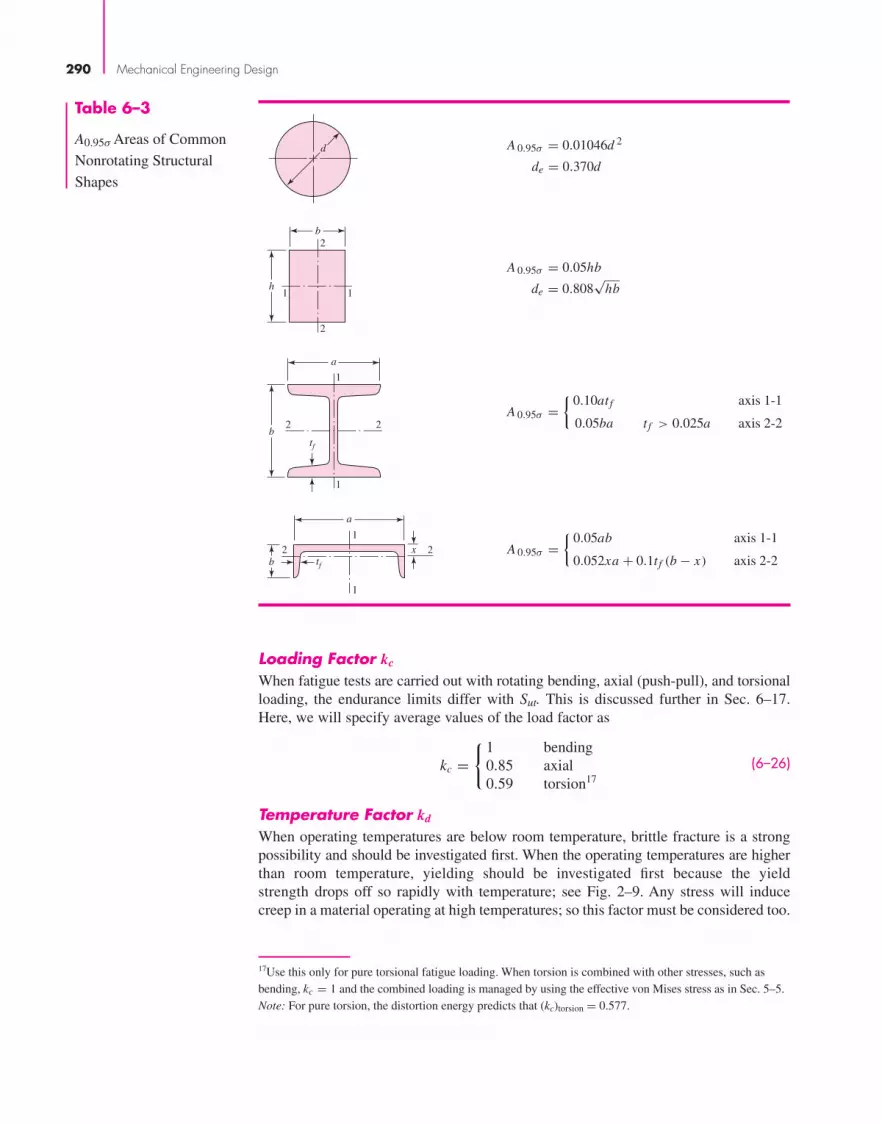
290 Mechanical Engineering Design
Loading Factor kc
When fatigue tests are carried out with rotating bending, axial (push-pull), and torsionalloading, the endurance limits differ with Sut. This is discussed further in Sec. 6–17.Here, we will specify average values of the load factor as
kc ={ 1 bending
0.85 axial0.59 torsion17
(6–26)
Temperature Factor kd
When operating temperatures are below room temperature, brittle fracture is a strongpossibility and should be investigated first. When the operating temperatures are higherthan room temperature, yielding should be investigated first because the yieldstrength drops off so rapidly with temperature; see Fig. 2–9. Any stress will inducecreep in a material operating at high temperatures; so this factor must be considered too.
A 0.95σ ={
0.05ab axis 1-1
0.052xa + 0.1t f (b − x) axis 2-2
122
1
a
b tf
x
A 0.95σ ={
0.10atf axis 1-1
0.05ba tf > 0.025a axis 2-2
1
2 2
1
a
btf
A 0.95σ = 0.05hb
de = 0.808√
hb
b
h
2
2
11
A 0.95σ = 0.01046d 2
de = 0.370d
d
Table 6–3
A0.95σ Areas of Common
Nonrotating Structural
Shapes
17Use this only for pure torsional fatigue loading. When torsion is combined with other stresses, such asbending, kc = 1 and the combined loading is managed by using the effective von Mises stress as in Sec. 5–5.Note: For pure torsion, the distortion energy predicts that (kc)torsion = 0.577.
bud29281_ch06_265-357.qxd 11/30/2009 4:23 pm Page 290 pinnacle s-171:Desktop Folder:Temp Work:Don't Delete (Jobs):MHDQ196/Budynas:

Fatigue Failure Resulting from Variable Loading 291
Finally, it may be true that there is no fatigue limit for materials operating at high tem-peratures. Because of the reduced fatigue resistance, the failure process is, to someextent, dependent on time.
The limited amount of data available show that the endurance limit for steelsincreases slightly as the temperature rises and then begins to fall off in the 400 to 700°Frange, not unlike the behavior of the tensile strength shown in Fig. 2–9. For this reasonit is probably true that the endurance limit is related to tensile strength at elevated tem-peratures in the same manner as at room temperature.18 It seems quite logical, therefore,to employ the same relations to predict endurance limit at elevated temperatures as areused at room temperature, at least until more comprehensive data become available. Atthe very least, this practice will provide a useful standard against which the perfor-mance of various materials can be compared.
Table 6–4 has been obtained from Fig. 2–9 by using only the tensile-strength data.Note that the table represents 145 tests of 21 different carbon and alloy steels. A fourth-order polynomial curve fit to the data underlying Fig. 2–9 gives
kd = 0.975 + 0.432(10−3)TF − 0.115(10−5)T 2F
+ 0.104(10−8)T 3F − 0.595(10−12)T 4
F
( 6–27)
where 70 ≤ TF ≤ 1000◦F.Two types of problems arise when temperature is a consideration. If the rotating-
beam endurance limit is known at room temperature, then use
kd = ST
SRT(6–28)
Temperature, °C ST/SRT Temperature, °F ST/SRT
20 1.000 70 1.000
50 1.010 100 1.008
100 1.020 200 1.020
150 1.025 300 1.024
200 1.020 400 1.018
250 1.000 500 0.995
300 0.975 600 0.963
350 0.943 700 0.927
400 0.900 800 0.872
450 0.843 900 0.797
500 0.768 1000 0.698
550 0.672 1100 0.567
600 0.549
*Data source: Fig. 2–9.
Table 6–4
Effect of Operating
Temperature on the
Tensile Strength of
Steel.* (ST = tensile
strength at operating
temperature;
SRT = tensile strength
at room temperature;
0.099 ≤ σ ≤ 0.110)
18For more, see Table 2 of ANSI/ASME B106. 1M-1985 shaft standard, and E. A. Brandes (ed.), Smithell’sMetals Reference Book, 6th ed., Butterworth, London, 1983, pp. 22–134 to 22–136, where endurance limitsfrom 100 to 650°C are tabulated.
bud29281_ch06_265-357.qxd 11/30/2009 4:23 pm Page 291 pinnacle s-171:Desktop Folder:Temp Work:Don't Delete (Jobs):MHDQ196/Budynas:

292 Mechanical Engineering Design
from Table 6–4 or Eq. (6–27) and proceed as usual. If the rotating-beam endurance limitis not given, then compute it using Eq. (6–8) and the temperature-corrected tensilestrength obtained by using the factor from Table 6–4. Then use kd = 1.
EXAMPLE 6–5 A 1035 steel has a tensile strength of 70 kpsi and is to be used for a part that sees 450°Fin service. Estimate the Marin temperature modification factor and (Se)450◦ if(a) The room-temperature endurance limit by test is (S′
e)70◦ = 39.0 kpsi.(b) Only the tensile strength at room temperature is known.
Solution (a) First, from Eq. (6–27),
kd = 0.975 + 0.432(10−3)(450) − 0.115(10−5)(4502)
+ 0.104(10−8)(4503) − 0.595(10−12)(4504) = 1.007
Thus,
Answer (Se)450◦ = kd(S′e)70◦ = 1.007(39.0) = 39.3 kpsi
(b) Interpolating from Table 6–4 gives
(ST /SRT )450◦ = 1.018 + (0.995 − 1.018)450 − 400
500 − 400= 1.007
Thus, the tensile strength at 450°F is estimated as
(Sut)450◦ = (ST /SRT )450◦ (Sut)70◦ = 1.007(70) = 70.5 kpsi
From Eq. (6–8) then,
Answer (Se)450◦ = 0.5(Sut)450◦ = 0.5(70.5) = 35.2 kpsi
Part a gives the better estimate due to actual testing of the particular material.
Reliability Factor ke
The discussion presented here accounts for the scatter of data such as shown inFig. 6–17 where the mean endurance limit is shown to be S′
e/Sut.= 0.5, or as given by
Eq. (6–8). Most endurance strength data are reported as mean values. Data presentedby Haugen and Wirching19 show standard deviations of endurance strengths of less than8 percent. Thus the reliability modification factor to account for this can be written as
ke = 1 − 0.08 za (6–29)
where za is defined by Eq. (20–16) and values for any desired reliability can be deter-mined from Table A–10. Table 6–5 gives reliability factors for some standard specifiedreliabilities.
For a more comprehensive approach to reliability, see Sec. 6–17.
19E. B. Haugen and P. H. Wirsching, “Probabilistic Design,” Machine Design, vol. 47, no. 12, 1975,pp. 10–14.
bud29281_ch06_265-357.qxd 12/10/2009 4:46 pm Page 292 pinnacle s-171:Desktop Folder:Temp Work:Don't Delete (Jobs):MHDQ196/Budynas:

Fatigue Failure Resulting from Variable Loading 293
Miscellaneous-Effects Factor kf
Though the factor kf is intended to account for the reduction in endurance limit due toall other effects, it is really intended as a reminder that these must be accounted for,because actual values of kf are not always available.
Residual stresses may either improve the endurance limit or affect it adversely.Generally, if the residual stress in the surface of the part is compression, the endurancelimit is improved. Fatigue failures appear to be tensile failures, or at least to be causedby tensile stress, and so anything that reduces tensile stress will also reduce the possi-bility of a fatigue failure. Operations such as shot peening, hammering, and cold rollingbuild compressive stresses into the surface of the part and improve the endurance limitsignificantly. Of course, the material must not be worked to exhaustion.
The endurance limits of parts that are made from rolled or drawn sheets or bars,as well as parts that are forged, may be affected by the so-called directional character-istics of the operation. Rolled or drawn parts, for example, have an endurance limitin the transverse direction that may be 10 to 20 percent less than the endurance limit inthe longitudinal direction.
Parts that are case-hardened may fail at the surface or at the maximum core radius,depending upon the stress gradient. Figure 6–19 shows the typical triangular stress dis-tribution of a bar under bending or torsion. Also plotted as a heavy line in this figure arethe endurance limits Se for the case and core. For this example the endurance limit of thecore rules the design because the figure shows that the stress σ or τ, whichever applies,at the outer core radius, is appreciably larger than the core endurance limit.
Se (case)
� or �
Se (core)
Case
Core
Figure 6–19
The failure of a case-hardenedpart in bending or torsion. Inthis example, failure occurs inthe core.
Reliability, % Transformation Variate za Reliability Factor ke
50 0 1.000
90 1.288 0.897
95 1.645 0.868
99 2.326 0.814
99.9 3.091 0.753
99.99 3.719 0.702
99.999 4.265 0.659
99.9999 4.753 0.620
Table 6–5
Reliability Factors ke
Corresponding to
8 Percent Standard
Deviation of the
Endurance Limit
bud29281_ch06_265-357.qxd 11/30/2009 4:23 pm Page 293 pinnacle s-171:Desktop Folder:Temp Work:Don't Delete (Jobs):MHDQ196/Budynas:

294 Mechanical Engineering Design
CorrosionIt is to be expected that parts that operate in a corrosive atmosphere will have a loweredfatigue resistance. This is, of course, true, and it is due to the roughening or pitting ofthe surface by the corrosive material. But the problem is not so simple as the one offinding the endurance limit of a specimen that has been corroded. The reason for this isthat the corrosion and the stressing occur at the same time. Basically, this means that intime any part will fail when subjected to repeated stressing in a corrosive atmosphere.There is no fatigue limit. Thus the designer’s problem is to attempt to minimize the fac-tors that affect the fatigue life; these are:
• Mean or static stress
• Alternating stress
• Electrolyte concentration
• Dissolved oxygen in electrolyte
• Material properties and composition
• Temperature
• Cyclic frequency
• Fluid flow rate around specimen
• Local crevices
Electrolytic PlatingMetallic coatings, such as chromium plating, nickel plating, or cadmium plating, reducethe endurance limit by as much as 50 percent. In some cases the reduction by coatingshas been so severe that it has been necessary to eliminate the plating process. Zincplating does not affect the fatigue strength. Anodic oxidation of light alloys reducesbending endurance limits by as much as 39 percent but has no effect on the torsionalendurance limit.
Metal SprayingMetal spraying results in surface imperfections that can initiate cracks. Limited testsshow reductions of 14 percent in the fatigue strength.
Cyclic FrequencyIf, for any reason, the fatigue process becomes time-dependent, then it also becomesfrequency-dependent. Under normal conditions, fatigue failure is independent of fre-quency. But when corrosion or high temperatures, or both, are encountered, the cyclicrate becomes important. The slower the frequency and the higher the temperature, thehigher the crack propagation rate and the shorter the life at a given stress level.
Frettage CorrosionThe phenomenon of frettage corrosion is the result of microscopic motions of tightlyfitting parts or structures. Bolted joints, bearing-race fits, wheel hubs, and any set oftightly fitted parts are examples. The process involves surface discoloration, pitting, andeventual fatigue. The frettage factor kf depends upon the material of the mating pairsand ranges from 0.24 to 0.90.
bud29281_ch06_265-357.qxd 11/30/2009 4:23 pm Page 294 pinnacle s-171:Desktop Folder:Temp Work:Don't Delete (Jobs):MHDQ196/Budynas:

Fatigue Failure Resulting from Variable Loading 295
6–10 Stress Concentration and Notch SensitivityIn Sec. 3–13 it was pointed out that the existence of irregularities or discontinuities,such as holes, grooves, or notches, in a part increases the theoretical stresses signifi-cantly in the immediate vicinity of the discontinuity. Equation (3–48) defined a stress-concentration factor Kt (or Kts), which is used with the nominal stress to obtain themaximum resulting stress due to the irregularity or defect. It turns out that some mate-rials are not fully sensitive to the presence of notches and hence, for these, a reducedvalue of Kt can be used. For these materials, the effective maximum stress in fatigue is,
σmax = K f σ0 or τmax = K f sτ0 (6–30)
where K f is a reduced value of Kt and σ0 is the nominal stress. The factor K f is com-monly called a fatigue stress-concentration factor, and hence the subscript f. So it isconvenient to think of Kf as a stress-concentration factor reduced from Kt because oflessened sensitivity to notches. The resulting factor is defined by the equation
K f = maximum stress in notched specimen
stress in notch-free specimen(a)
Notch sensitivity q is defined by the equation
q = K f − 1
Kt − 1or qshear = K f s − 1
Kts − 1(6–31)
where q is usually between zero and unity. Equation (6–31) shows that if q = 0, thenK f = 1, and the material has no sensitivity to notches at all. On the other hand, ifq = 1, then K f = Kt , and the material has full notch sensitivity. In analysis or designwork, find Kt first, from the geometry of the part. Then specify the material, find q, andsolve for Kf from the equation
K f = 1 + q(Kt − 1) or K f s = 1 + qshear(Kts − 1) (6–32)
Notch sensitivities for specific materials are obtained experimentally. Publishedexperimental values are limited, but some values are available for steels and aluminum.Trends for notch sensitivity as a function of notch radius and ultimate strength areshown in Fig. 6–20 for reversed bending or axial loading, and Fig. 6–21 for reversed
0 0.02 0.04 0.06 0.08 0.10 0.12 0.14 0.16
0 0.5 1.0 1.5 2.0 2.5 3.0 3.5 4.0
0
0.2
0.4
0.6
0.8
1.0
Notch radius r, in
Notch radius r, mm
Not
ch s
ensi
tivity
q
S ut= 200 kpsi
(0.4)
60
100
150 (0.7)
(1.0)
(1.4 GPa)
Steels
Alum. alloy
Figure 6–20
Notch-sensitivity charts forsteels and UNS A92024-Twrought aluminum alloyssubjected to reversed bendingor reversed axial loads. Forlarger notch radii, use thevalues of q correspondingto the r = 0.16-in (4-mm)ordinate. (From George Sinesand J. L. Waisman (eds.), MetalFatigue, McGraw-Hill, NewYork. Copyright © 1969 by TheMcGraw-Hill Companies, Inc.Reprinted by permission.)
bud29281_ch06_265-357.qxd 12/7/09 7:25PM Page 295 ntt 203:MHDQ196:bud29281:0073529281:bud29281_pagefiles:

296 Mechanical Engineering Design
torsion. In using these charts it is well to know that the actual test results from whichthe curves were derived exhibit a large amount of scatter. Because of this scatter it isalways safe to use K f = Kt if there is any doubt about the true value of q. Also, notethat q is not far from unity for large notch radii.
Figure 6–20 has as its basis the Neuber equation, which is given by
K f = 1 + Kt − 1
1 + √a/r
(6–33)
where √
a is defined as the Neuber constant and is a material constant. EquatingEqs. (6–31) and (6–33) yields the notch sensitivity equation
q = 1
1 +√
a√r
(6–34)
correlating with Figs. 6–20 and 6–21 as
Bending or axial:√
a = 0.246 − 3.08(10−3)Sut + 1.51(10−5)S2ut − 2.67(10−8)S3
ut
(6–35a)
Torsion:√
a = 0.190 − 2.51(10−3)Sut + 1.35(10−5)S2ut − 2.67(10−8)S3
ut (6–35b)
where the equations apply to steel and Sut is in kpsi. Equation (6–34) used in conjunctionwith Eq. pair (6–35) is equivalent to Figs. (6–20) and (6–21). As with the graphs, theresults from the curve fit equations provide only approximations to the experimental data.
The notch sensitivity of cast irons is very low, varying from 0 to about 0.20,depending upon the tensile strength. To be on the conservative side, it is recommendedthat the value q = 0.20 be used for all grades of cast iron.
EXAMPLE 6–6 A steel shaft in bending has an ultimate strength of 690 MPa and a shoulder with a filletradius of 3 mm connecting a 32-mm diameter with a 38-mm diameter. Estimate Kf using:(a) Figure 6–20.(b) Equations (6–33) and (6–35).
0 0.02 0.04 0.06 0.08 0.10 0.12 0.14 0.16
0 0.5 1.0 1.5 2.0 2.5 3.0 3.5 4.0
0
0.2
0.4
0.6
0.8
1.0
Notch radius r, in
Notch radius r, mm
Not
ch s
ensi
tivity
qsh
ear
Steels
Alum. alloy
S ut= 200 kpsi (1.4 GPa)
60 (0.4)100 (0
.7)150 (1.0)
Figure 6–21
Notch-sensitivity curves formaterials in reversed torsion.For larger notch radii, use the values of qshear
corresponding to r = 0.16 in (4 mm).
bud29281_ch06_265-357.qxd 12/11/2009 4:56 pm Page 296 pinnacle 203:MHDQ196:bud29281:0073529281:bud29281_pagefiles:

Solution From Fig. A–15–9, using D/d = 38/32 = 1.1875, r/d = 3/32 = 0.093 75, we readthe graph to find Kt
.= 1.65.(a) From Fig. 6–20, for Sut = 690 MPa and r = 3 mm, q
.= 0.84. Thus, from Eq. (6–32)
Answer K f = 1 + q(Kt − 1).= 1 + 0.84(1.65 − 1) = 1.55
(b) From Eq. (6–35a) with Sut = 690 MPa = 100 kpsi, √
a = 0.0622√
in = 0.313√
mm.Substituting this into Eq. (6–33) with r = 3 mm gives
Answer K f = 1 + Kt − 1
1 + √a/r
.= 1 + 1.65 − 1
1 + 0.313√3
= 1.55
Some designers use 1/Kf as a Marin factor to reduce Se. For simple loading, infi-nite life problems, it makes no difference whether Se is reduced by dividing it by Kf orthe nominal stress is multiplied by Kf. However, for finite life, since the S-N diagramis nonlinear, the two approaches yield differing results. There is no clear evidencepointing to which method is better. Furthermore, in Sec. 6–14, when we consider com-bining loads, there generally are multiple fatigue stress-concentration factors occurringat a point (e.g. Kf for bending and Kfs for torsion). Here, it is only practical to modifythe nominal stresses. To be consistent in this text, we will exclusively use the fatiguestress-concentration factor as a multiplier of the nominal stress.
EXAMPLE 6–7 For the step-shaft of Ex. 6–6, it is determined that the fully corrected endurance limit isSe = 280 MPa. Consider the shaft undergoes a fully reversing nominal stress in the fil-let of (σrev)nom = 260 MPa. Estimate the number of cycles to failure.
Solution From Ex. 6–6, Kf = 1.55, and the ultimate strength is Sut = 690 MPa = 100 kpsi. Themaximum reversing stress is
(σrev)max = K f (σrev)nom = 1.55(260) = 403 MPa
From Fig. 6–18, f = 0.845. From Eqs. (6–14), (6–15), and (6–16)
a = ( f Sut)2
Se= [0.845(690)]2
280= 1214 MPa
b = −1
3log
f Sut
Se= −1
3log
[0.845(690)
280
]= −0.1062
Answer N =(σrev
a
)1/b=
(403
1214
)1/−0.1062
= 32.3(103) cycles
Up to this point, examples illustrated each factor in Marin’s equation and stressconcentrations alone. Let us consider a number of factors occurring simultaneously.
Fatigue Failure Resulting from Variable Loading 297
bud29281_ch06_265-357.qxd 12/7/09 7:25PM Page 297 ntt 203:MHDQ196:bud29281:0073529281:bud29281_pagefiles:

298 Mechanical Engineering Design
EXAMPLE 6–8 A 1015 hot-rolled steel bar has been machined to a diameter of 1 in. It is to be placedin reversed axial loading for 70 000 cycles to failure in an operating environment of550°F. Using ASTM minimum properties, and a reliability of 99 percent, estimate theendurance limit and fatigue strength at 70 000 cycles.
Solution From Table A–20, Sut = 50 kpsi at 70°F. Since the rotating-beam specimen endurancelimit is not known at room temperature, we determine the ultimate strength at the ele-vated temperature first, using Table 6–4. From Table 6–4,(
ST
SRT
)550◦
= 0.995 + 0.963
2= 0.979
The ultimate strength at 550°F is then
(Sut)550◦ = (ST /SRT )550◦ (Sut)70◦ = 0.979(50) = 49.0 kpsi
The rotating-beam specimen endurance limit at 550°F is then estimated from Eq. (6–8)as
S′e = 0.5(49) = 24.5 kpsi
Next, we determine the Marin factors. For the machined surface, Eq. (6–19) withTable 6–2 gives
ka = aSbut = 2.70(49−0.265) = 0.963
For axial loading, from Eq. (6–21), the size factor kb = 1, and from Eq. (6–26) the load-ing factor is kc = 0.85. The temperature factor kd = 1, since we accounted for the tem-perature in modifying the ultimate strength and consequently the endurance limit. For99 percent reliability, from Table 6–5, ke = 0.814. Finally, since no other conditionswere given, the miscellaneous factor is kf = 1. The endurance limit for the part is esti-mated by Eq. (6–18) as
AnswerSe = kakbkckdkek f S′
e
= 0.963(1)(0.85)(1)(0.814)(1)24.5 = 16.3 kpsi
For the fatigue strength at 70 000 cycles we need to construct the S-N equation. Fromp. 285, since Sut = 49 < 70 kpsi, then f � 0.9. From Eq. (6–14)
a = ( f Sut)2
Se= [0.9(49)]2
16.3= 119.3 kpsi
and Eq. (6–15)
b = −1
3log
(f Sut
Se
)= −1
3log
[0.9(49)
16.3
]= −0.1441
Finally, for the fatigue strength at 70 000 cycles, Eq. (6–13) gives
Answer Sf = a N b = 119.3(70 000)−0.1441 = 23.9 kpsi
bud29281_ch06_265-357.qxd 11/30/2009 4:23 pm Page 298 pinnacle s-171:Desktop Folder:Temp Work:Don't Delete (Jobs):MHDQ196/Budynas:

Fatigue Failure Resulting from Variable Loading 299
EXAMPLE 6–9 Figure 6–22a shows a rotating shaft simply supported in ball bearings at A and D andloaded by a nonrotating force F of 6.8 kN. Using ASTM “minimum” strengths, estimatethe life of the part.
Solution From Fig. 6–22b we learn that failure will probably occur at B rather than at C or at thepoint of maximum moment. Point B has a smaller cross section, a higher bendingmoment, and a higher stress-concentration factor than C, and the location of maximummoment has a larger size and no stress-concentration factor.
We shall solve the problem by first estimating the strength at point B, since the strengthwill be different elsewhere, and comparing this strength with the stress at the same point.
From Table A–20 we find Sut = 690 MPa and Sy = 580 MPa. The endurance limitS′
e is estimated as
S′e = 0.5(690) = 345 MPa
From Eq. (6–19) and Table 6–2,
ka = 4.51(690)−0.265 = 0.798
From Eq. (6–20),
kb = (32/7.62)−0.107 = 0.858
Since kc = kd = ke = kf = 1,
Se = 0.798(0.858)345 = 236 MPa
To find the geometric stress-concentration factor Kt we enter Fig. A–15–9 with D/d =38/32 = 1.1875 and r/d = 3/32 = 0.093 75 and read Kt
.= 1.65. SubstitutingSut = 690/6.89 = 100 kpsi into Eq. (6–35a) yields
√a = 0.0622
√in = 0.313
√mm.
Substituting this into Eq. (6–33) gives
K f = 1 + Kt − 1
1 + √a/r
= 1 + 1.65 − 1
1 + 0.313/√
3= 1.55
(a)
(b)
A B
MB
MC
Mmax
C D
30 3032 3538
10 10
A B C D6.8 kN
250 12510075
R2R1
Figure 6–22
(a) Shaft drawing showing alldimensions in millimeters; all fillets 3-mm radius. The shaft rotates and the load is stationary; material ismachined from AISI 1050cold-drawn steel. (b) Bending-moment diagram.
bud29281_ch06_265-357.qxd 11/30/2009 4:23 pm Page 299 pinnacle s-171:Desktop Folder:Temp Work:Don't Delete (Jobs):MHDQ196/Budynas:

300 Mechanical Engineering Design
The next step is to estimate the bending stress at point B. The bending momentis
MB = R1x = 225F
550250 = 225(6.8)
550250 = 695.5 N · m
Just to the left of B the section modulus is I/c = πd3/32 = π323/32 = 3.217 (103) mm3.The reversing bending stress is, assuming infinite life,
σrev = K fMB
I/c= 1.55
695.5
3.217(10)−6 = 335.1(106) Pa = 335.1 MPa
This stress is greater than Se and less than Sy. This means we have both finite life andno yielding on the first cycle.
For finite life, we will need to use Eq. (6–16). The ultimate strength, Sut = 690MPa = 100 kpsi. From Fig. 6–18, f = 0.844. From Eq. (6–14)
a = ( f Sut)2
Se= [0.844(690)]2
236= 1437 MPa
and from Eq. (6–15)
b = −1
3log
(f Sut
Se
)= −1
3log
[0.844(690)
236
]= −0.1308
From Eq. (6–16),
Answer N =(σrev
a
)1/b=
(335.1
1437
)−1/0.1308
= 68(103) cycles
6–11 Characterizing Fluctuating StressesFluctuating stresses in machinery often take the form of a sinusoidal pattern becauseof the nature of some rotating machinery. However, other patterns, some quite irreg-ular, do occur. It has been found that in periodic patterns exhibiting a single maxi-mum and a single minimum of force, the shape of the wave is not important, but thepeaks on both the high side (maximum) and the low side (minimum) are important.Thus Fmax and Fmin in a cycle of force can be used to characterize the force pattern.It is also true that ranging above and below some baseline can be equally effectivein characterizing the force pattern. If the largest force is Fmax and the smallest forceis Fmin, then a steady component and an alternating component can be constructedas follows:
Fm = Fmax + Fmin
2Fa =
∣∣∣∣ Fmax − Fmin
2
∣∣∣∣where Fm is the midrange steady component of force, and Fa is the amplitude of thealternating component of force.
bud29281_ch06_265-357.qxd 11/30/2009 4:23 pm Page 300 pinnacle s-171:Desktop Folder:Temp Work:Don't Delete (Jobs):MHDQ196/Budynas:

Fatigue Failure Resulting from Variable Loading 301
Figure 6–23 illustrates some of the various stress-time traces that occur. The com-ponents of stress, some of which are shown in Fig. 6–23d, are
σmin = minimum stress σm = midrange component
σmax = maximum stress σr = range of stress
σa = amplitude component σs = static or steady stress
The steady, or static, stress is not the same as the midrange stress; in fact, it may haveany value between σmin and σmax. The steady stress exists because of a fixed load or pre-load applied to the part, and it is usually independent of the varying portion of the load.A helical compression spring, for example, is always loaded into a space shorter thanthe free length of the spring. The stress created by this initial compression is called thesteady, or static, component of the stress. It is not the same as the midrange stress.
We shall have occasion to apply the subscripts of these components to shear stressesas well as normal stresses.
The following relations are evident from Fig. 6–23:
σm = σmax + σmin
2
σa =∣∣∣∣σmax − σmin
2
∣∣∣∣ (6–36)
Time
Time
Time
Time
Time
Time
Stre
ss
Stre
ssSt
ress
Stre
ss
Stre
ssSt
ress
(a)
(b)
(c)
�a
�a
�r
�m
�min
�max
�a
�a
�r
�a
�a
�r
�m
�max
O
O
O
(d )
(e)
( f )
�min = 0
�m = 0
+
Figure 6–23
Some stress-time relations:(a) fluctuating stress with high-frequency ripple; (b and c)nonsinusoidal fluctuatingstress; (d) sinusoidal fluctuatingstress; (e) repeated stress;( f ) completely reversedsinusoidal stress.
bud29281_ch06_265-357.qxd 11/30/2009 4:23 pm Page 301 pinnacle s-171:Desktop Folder:Temp Work:Don't Delete (Jobs):MHDQ196/Budynas:

302 Mechanical Engineering Design
In addition to Eq. (6–36), the stress ratio
R = σmin
σmax(6–37)
and the amplitude ratio
A = σa
σm(6–38)
are also defined and used in connection with fluctuating stresses.Equations (6–36) utilize symbols σa and σm as the stress components at the loca-
tion under scrutiny. This means, in the absence of a notch, σa and σm are equal to thenominal stresses σao and σmo induced by loads Fa and Fm , respectively; in the presenceof a notch they are K f σao and K f σmo, respectively, as long as the material remainswithout plastic strain. In other words, the fatigue stress-concentration factor K f isapplied to both components.
When the steady stress component is high enough to induce localized notch yield-ing, the designer has a problem. The first-cycle local yielding produces plastic strainand strain-strengthening. This is occurring at the location where fatigue crack nucle-ation and growth are most likely. The material properties (Sy and Sut ) are new anddifficult to quantify. The prudent engineer controls the concept, material and conditionof use, and geometry so that no plastic strain occurs. There are discussions concerningpossible ways of quantifying what is occurring under localized and general yieldingin the presence of a notch, referred to as the nominal mean stress method, residualstress method, and the like.20 The nominal mean stress method (set σa = K f σao andσm = σmo) gives roughly comparable results to the residual stress method, but both areapproximations.
There is the method of Dowling21 for ductile materials, which, for materials with apronounced yield point and approximated by an elastic–perfectly plastic behaviormodel, quantitatively expresses the steady stress component stress-concentration factorK f m as
K f m = K f K f |σmax,o| < Sy
K f m = Sy − K f σao
|σmo| K f |σmax,o| > Sy
K f m = 0 K f |σmax,o − σmin,o| > 2Sy
(6–39)
For the purposes of this book, for ductile materials in fatigue,
• Avoid localized plastic strain at a notch. Set σa = K f σa,o and σm = K f σmo .
• When plastic strain at a notch cannot be avoided, use Eqs. (6–39); or conservatively,set σa = K f σao and use K f m = 1, that is, σm = σmo .
20R. C. Juvinall, Stress, Strain, and Strength, McGraw-Hill, New York, 1967, articles 14.9–14.12; R. C.Juvinall and K. M. Marshek, Fundamentals of Machine Component Design, 4th ed., Wiley, New York, 2006,Sec. 8.11; M. E. Dowling, Mechanical Behavior of Materials, 2nd ed., Prentice Hall, Englewood Cliffs,N.J., 1999, Secs. 10.3–10.5.21Dowling, op. cit., pp. 437–438.
bud29281_ch06_265-357.qxd 12/7/09 7:25PM Page 302 ntt 203:MHDQ196:bud29281:0073529281:bud29281_pagefiles:

Fatigue Failure Resulting from Variable Loading 303
6–12 Fatigue Failure Criteria for Fluctuating StressNow that we have defined the various components of stress associated with a part sub-jected to fluctuating stress, we want to vary both the midrange stress and the stressamplitude, or alternating component, to learn something about the fatigue resistance ofparts when subjected to such situations. Three methods of plotting the results of suchtests are in general use and are shown in Figs. 6–24, 6–25, and 6–26.
The modified Goodman diagram of Fig. 6–24 has the midrange stress plotted alongthe abscissa and all other components of stress plotted on the ordinate, with tension inthe positive direction. The endurance limit, fatigue strength, or finite-life strength,whichever applies, is plotted on the ordinate above and below the origin. The midrange-stress line is a 45◦ line from the origin to the tensile strength of the part. The modifiedGoodman diagram consists of the lines constructed to Se (or Sf ) above and below theorigin. Note that the yield strength is also plotted on both axes, because yielding wouldbe the criterion of failure if σmax exceeded Sy .
Another way to display test results is shown in Fig. 6–25. Here the abscissa repre-sents the ratio of the midrange strength Sm to the ultimate strength, with tension plot-ted to the right and compression to the left. The ordinate is the ratio of the alternatingstrength to the endurance limit. The line BC then represents the modified Goodmancriterion of failure. Note that the existence of midrange stress in the compressive regionhas little effect on the endurance limit.
The very clever diagram of Fig. 6–26 is unique in that it displays four of the stresscomponents as well as the two stress ratios. A curve representing the endurance limitfor values of R beginning at R = −1 and ending with R = 1 begins at Se on the σa axisand ends at Sut on the σm axis. Constant-life curves for N = 105 and N = 104 cycles
Figure 6–24
Modified Goodman diagramshowing all the strengths andthe limiting values of all thestress components for aparticular midrange stress.
Su
Sy
Se
Sy Su�m
�max
Max. stress
�min
Midr
ange
stres
s
Min
. stre
ss
Stre
ss
0
Se
Midrange stress
Para
llel
45°
�a�a
�a
�r
+
bud29281_ch06_265-357.qxd 11/30/2009 4:23 pm Page 303 pinnacle s-171:Desktop Folder:Temp Work:Don't Delete (Jobs):MHDQ196/Budynas:

304 Mechanical Engineering Design
have been drawn too. Any stress state, such as the one at A, can be described by the min-imum and maximum components, or by the midrange and alternating components. Andsafety is indicated whenever the point described by the stress components lies below theconstant-life line.
Figure 6–26
Master fatigue diagram createdfor AISI 4340 steel havingSut = 158 and Sy = 147 kpsi.The stress components at A areσmin = 20, σmax = 120,σm = 70, and σa = 50, all inkpsi. (Source: H. J. Grover,Fatigue of Aircraft Structures,U.S. Government PrintingOffice, Washington, D.C., 1966,pp. 317, 322. See also J. A.Collins, Failure of Materials inMechanical Design, Wiley,New York, 1981, p. 216.)
–120 –100 –80 –60 –40 –20 0 20 40 60 80 100 120 140 160 180
20
40
60
80
100
120
A = �R = –1.0
20
40
60
80
100
120
140
160
180
Midr
ange
stres
s �m
, kps
i
20
40
60
80
100
120
Alternating stress �a , kpsi
RA
4.0–0.6
2.33–0.4
1.5–0.2
A = 1R = 0
0.670.2
0.430.4
0.250.6
0.110.8
01.0
Max
imum
str
ess
� max
, kps
i
Minimum stress �min, kpsi
105
106
104 cycles
A
Sut
Se
Figure 6–25
Plot of fatigue failures for midrange stresses in both tensile and compressive regions. Normalizingthe data by using the ratio of steady strength component to tensile strength Sm/Sut , steady strengthcomponent to compressive strength Sm/Suc and strength amplitude component to endurance limit Sa/S′
e enables a plot of experimental results for a variety of steels. [Data source: Thomas J. Dolan,“Stress Range,” Sec. 6.2 in O. J. Horger (ed.), ASME Handbook—Metals Engineering Design,McGraw-Hill, New York, 1953.]
–1.2 –1.0 –0.8 –0.6 –0.4 –0.2 0 0.2 0.4 0.6 0.8 1.0
0.2
0.4
0.6
0.8
1.0
1.2
Midrange ratio
Compression Sm /Suc Tension Sm /Sut
Am
plitu
de r
atio
Sa/S
' e
A B
C
bud29281_ch06_265-357.qxd 12/02/2009 9:29 pm Page 304 pinnacle s-171:Desktop Folder:Temp Work:Don't Delete (Jobs):MHDQ196/Budynas:

Fatigue Failure Resulting from Variable Loading 305
When the midrange stress is compression, failure occurs whenever σa = Se orwhenever σmax = Syc , as indicated by the left-hand side of Fig. 6–25. Neither a fatiguediagram nor any other failure criteria need be developed.
In Fig. 6–27, the tensile side of Fig. 6–25 has been redrawn in terms of strengths,instead of strength ratios, with the same modified Goodman criterion together with fouradditional criteria of failure. Such diagrams are often constructed for analysis anddesign purposes; they are easy to use and the results can be scaled off directly.
The early viewpoint expressed on a σm , σa diagram was that there existed a locuswhich divided safe from unsafe combinations of σm and σa . Ensuing proposals includedthe parabola of Gerber (1874), the Goodman (1890)22 (straight) line, and the Soderberg(1930) (straight) line. As more data were generated it became clear that a fatigue criterion,rather than being a “fence,” was more like a zone or band wherein the probability of fail-ure could be estimated. We include the failure criterion of Goodman because
• It is a straight line and the algebra is linear and easy.
• It is easily graphed, every time for every problem.
• It reveals subtleties of insight into fatigue problems.
• Answers can be scaled from the diagrams as a check on the algebra.
We also caution that it is deterministic and the phenomenon is not. It is biased and wecannot quantify the bias. It is not conservative. It is a stepping-stone to understanding; itis history; and to read the work of other engineers and to have meaningful oral exchangeswith them, it is necessary that you understand the Goodman approach should it arise.
Either the fatigue limit Se or the finite-life strength Sf is plotted on the ordinate ofFig. 6–27. These values will have already been corrected using the Marin factors ofEq. (6–18). Note that the yield strength Sy is plotted on the ordinate too. This serves asa reminder that first-cycle yielding rather than fatigue might be the criterion of failure.
The midrange-stress axis of Fig. 6–27 has the yield strength Sy and the tensilestrength Sut plotted along it.
Figure 6–27
Fatigue diagram showingvarious criteria of failure. Foreach criterion, points on or“above” the respective lineindicate failure. Some point Aon the Goodman line, forexample, gives the strength Sm
as the limiting value of σm
corresponding to the strengthSa , which, paired with σm , isthe limiting value of σa .
Alte
rnat
ing
stre
ss �
a
Midrange stress �m
0 Sm
A
SutSy
0
Sa
Se
Sy
Soderberg line
Modified Goodman line
ASME-elliptic line
Load line, slope r = Sa/Sm
Gerber line
Yield (Langer) line
22It is difficult to date Goodman’s work because it went through several modifications and was neverpublished.
bud29281_ch06_265-357.qxd 11/30/2009 4:23 pm Page 305 pinnacle s-171:Desktop Folder:Temp Work:Don't Delete (Jobs):MHDQ196/Budynas:

306 Mechanical Engineering Design
Five criteria of failure are diagrammed in Fig. 6–27: the Soderberg, the modifiedGoodman, the Gerber, the ASME-elliptic, and yielding. The diagram shows that onlythe Soderberg criterion guards against any yielding, but is biased low.
Considering the modified Goodman line as a criterion, point A represents a limit-ing point with an alternating strength Sa and midrange strength Sm. The slope of the loadline shown is defined as r = Sa/Sm .
The criterion equation for the Soderberg line is
Sa
Se+ Sm
Sy= 1 (6–40)
Similarly, we find the modified Goodman relation to be
Sa
Se+ Sm
Sut= 1 (6–41)
Examination of Fig. 6–25 shows that both a parabola and an ellipse have a betteropportunity to pass among the midrange tension data and to permit quantification of theprobability of failure. The Gerber failure criterion is written as
Sa
Se+
(Sm
Sut
)2
= 1 (6–42)
and the ASME-elliptic is written as(Sa
Se
)2
+(
Sm
Sy
)2
= 1 (6–43)
The Langer first-cycle-yielding criterion is used in connection with the fatiguecurve:
Sa + Sm = Sy (6–44)
The stresses nσa and nσm can replace Sa and Sm , where n is the design factor or factorof safety. Then, Eq. (6–40), the Soderberg line, becomes
Soderbergσa
Se+ σm
Sy= 1
n(6–45)
Equation (6–41), the modified Goodman line, becomes
mod-Goodmanσa
Se+ σm
Sut= 1
n(6–46)
Equation (6–42), the Gerber line, becomes
Gerbernσa
Se+
(nσm
Sut
)2
= 1 (6–47)
Equation (6–43), the ASME-elliptic line, becomes
ASME-elliptic(
nσa
Se
)2
+(
nσm
Sy
)2
= 1 (6–48)
We will emphasize the Gerber and ASME-elliptic for fatigue failure criterion and theLanger for first-cycle yielding. However, conservative designers often use the modifiedGoodman criterion, so we will continue to include it in our discussions. The designequation for the Langer first-cycle-yielding is
Langer static yield σa + σm = Sy
n(6–49)
bud29281_ch06_265-357.qxd 11/30/2009 4:23 pm Page 306 pinnacle s-171:Desktop Folder:Temp Work:Don't Delete (Jobs):MHDQ196/Budynas:

Fatigue Failure Resulting from Variable Loading 307
Intersecting Equations Intersection Coordinates
Sa
Se+
(Sm
Sut
)2
= 1 Sa = r2S2ut
2Se
⎡⎣−1 +√
1 +(
2Se
r Sut
)2⎤⎦
Load line r = Sa
SmSm = Sa
r
Sa
Sy+ Sm
Sy= 1 Sa = r Sy
1 + r
Load line r = Sa
SmSm = Sy
1 + r
Sa
Se+
(Sm
Sut
)2
= 1 Sm = S2ut
2Se
⎡⎣1 −√
1 +(
2Se
Sut
)2 (1 − Sy
Se
) ⎤⎦Sa
Sy+ Sm
Sy= 1 Sa = Sy − Sm, rcrit = Sa/Sm
Fatigue factor of safety
n f = 1
2
(Sut
σm
)2σa
Se
⎡⎣−1 +√
1 +(
2σm Se
Sutσa
)2⎤⎦ σm > 0
Table 6–7
Amplitude and Steady
Coordinates of Strength
and Important
Intersections in First
Quadrant for Gerber and
Langer Failure Criteria
Intersecting Equations Intersection Coordinates
Sa
Se+ Sm
Sut= 1 Sa = r Se Sut
r Sut + Se
Load line r = Sa
SmSm = Sa
r
Sa
Sy+ Sm
Sy= 1 Sa = r Sy
1 + r
Load line r = Sa
SmSm = Sy
1 + r
Sa
Se+ Sm
Sut= 1 Sm =
(Sy − Se
)Sut
Sut − Se
Sa
Sy+ Sm
Sy= 1 Sa = Sy − Sm, rcrit = Sa/Sm
Fatigue factor of safety
n f = 1σa
Se+ σm
Sut
Table 6–6
Amplitude and Steady
Coordinates of Strength
and Important
Intersections in First
Quadrant for Modified
Goodman and Langer
Failure Criteria
The failure criteria are used in conjunction with a load line, r = Sa/Sm = σa/σm .Principal intersections are tabulated in Tables 6–6 to 6–8. Formal expressions forfatigue factor of safety are given in the lower panel of Tables 6–6 to 6–8. The first rowof each table corresponds to the fatigue criterion, the second row is the static Langercriterion, and the third row corresponds to the intersection of the static and fatigue
bud29281_ch06_265-357.qxd 12/02/2009 6:49 pm Page 307 pinnacle s-171:Desktop Folder:Temp Work:Don't Delete (Jobs):MHDQ196/Budynas:

308 Mechanical Engineering Design
criteria. The first column gives the intersecting equations and the second column theintersection coordinates.
There are two ways to proceed with a typical analysis. One method is to assumethat fatigue occurs first and use one of Eqs. (6–45) to (6–48) to determine n or size,depending on the task. Most often fatigue is the governing failure mode. Thenfollow with a static check. If static failure governs then the analysis is repeated usingEq. (6–49).
Alternatively, one could use the tables. Determine the load line and establish whichcriterion the load line intersects first and use the corresponding equations in the tables.
Some examples will help solidify the ideas just discussed.
EXAMPLE 6–10 A 1.5-in-diameter bar has been machined from an AISI 1050 cold-drawn bar. This partis to withstand a fluctuating tensile load varying from 0 to 16 kip. Because of the ends,and the fillet radius, a fatigue stress-concentration factor K f is 1.85 for 106 or largerlife. Find Sa and Sm and the factor of safety guarding against fatigue and first-cycleyielding, using (a) the Gerber fatigue line and (b) the ASME-elliptic fatigue line.
Solution We begin with some preliminaries. From Table A–20, Sut = 100 kpsi and Sy = 84 kpsi.Note that Fa = Fm = 8 kip. The Marin factors are, deterministically,
ka = 2.70(100)−0.265 = 0.797: Eq. (6–19), Table 6–2, p. 288
kb = 1 (axial loading, see kc)
Intersecting Equations Intersection Coordinates(Sa
Se
)2
+(
Sm
Sy
)2
= 1 Sa =√√√√ r2S2
e S2y
S2e + r2S2
y
Load line r = Sa/Sm Sm = Sa
r
Sa
Sy+ Sm
Sy= 1 Sa = r Sy
1 + r
Load line r = Sa/Sm Sm = Sy
1 + r(Sa
Se
)2
+(
Sm
Sy
)2
= 1 Sa = 0,2Sy S2
e
S2e + S2
y
Sa
Sy+ Sm
Sy= 1 Sm = Sy − Sa, rcrit = Sa/Sm
Fatigue factor of safety
n f =√
1
(σa/Se)2 + (
σm/Sy)2
Table 6–8
Amplitude and Steady
Coordinates of Strength
and Important
Intersections in First
Quadrant for ASME-
Elliptic and Langer
Failure Criteria
bud29281_ch06_265-357.qxd 12/02/2009 9:29 pm Page 308 pinnacle s-171:Desktop Folder:Temp Work:Don't Delete (Jobs):MHDQ196/Budynas:

Fatigue Failure Resulting from Variable Loading 309
kc = 0.85: Eq. (6–26), p. 290
kd = ke = kf = 1
Se = 0.797(1)0.850(1)(1)(1)0.5(100) = 33.9 kpsi: Eqs. (6–8), (6–18), p. 282, p. 287
The nominal axial stress components σao and σmo are
σao = 4Fa
πd2= 4(8)
π1.52= 4.53 kpsi σmo = 4Fm
πd2= 4(8)
π1.52= 4.53 kpsi
Applying K f to both components σao and σmo constitutes a prescription of no notchyielding:
σa = K f σao = 1.85(4.53) = 8.38 kpsi = σm
(a) Let us calculate the factors of safety first. From the bottom panel from Table 6–7 thefactor of safety for fatigue is
Answer n f = 1
2
(100
8.38
)2 (8.38
33.9
)⎧⎨⎩−1 +√
1 +[
2(8.38)33.9
100(8.38)
]2⎫⎬⎭ = 3.66
From Eq. (6–49) the factor of safety guarding against first-cycle yield is
Answer ny = Sy
σa + σm= 84
8.38 + 8.38= 5.01
Thus, we see that fatigue will occur first and the factor of safety is 3.68. This can beseen in Fig. 6–28 where the load line intersects the Gerber fatigue curve first at point B.If the plots are created to true scale it would be seen that n f = O B/O A.
From the first panel of Table 6–7, r = σa/σm = 1,
Answer Sa = (1)21002
2(33.9)
⎧⎨⎩−1 +√
1 +[
2(33.9)
(1)100
]2⎫⎬⎭ = 30.7 kpsi
Stre
ss a
mpl
itude
�a, k
psi
Midrange stress �m, kpsi
0 30.78.38
8.38
42 50 64 84 1000
20
33.930.7
42
50 Load line
Langer line
rcrit
84
100
Gerberfatigue curve
A
B
C
D
Figure 6–28
Principal points A, B, C, and Don the designer’s diagramdrawn for Gerber, Langer, andload line.
bud29281_ch06_265-357.qxd 12/02/2009 6:49 pm Page 309 pinnacle s-171:Desktop Folder:Temp Work:Don't Delete (Jobs):MHDQ196/Budynas:

310 Mechanical Engineering Design
Answer Sm = Sa
r= 30.7
1= 30.7 kpsi
As a check on the previous result, n f = O B/O A = Sa/σa = Sm/σm = 30.7/8.38 =3.66 and we see total agreement.
We could have detected that fatigue failure would occur first without drawingFig. 6–28 by calculating rcrit . From the third row third column panel of Table 6–7, theintersection point between fatigue and first-cycle yield is
Sm = 1002
2(33.9)
⎡⎣1 −√
1 +(
2(33.9)
100
)2 (1 − 84
33.9
)⎤⎦ = 64.0 kpsi
Sa = Sy − Sm = 84 − 64 = 20 kpsi
The critical slope is thus
rcrit = Sa
Sm= 20
64= 0.312
which is less than the actual load line of r = 1. This indicates that fatigue occurs beforefirst-cycle-yield.(b) Repeating the same procedure for the ASME-elliptic line, for fatigue
Answer n f =√
1
(8.38/33.9)2 + (8.38/84)2= 3.75
Again, this is less than ny = 5.01 and fatigue is predicted to occur first. From the firstrow second column panel of Table 6–8, with r = 1, we obtain the coordinates Sa andSm of point B in Fig. 6–29 as
Stre
ss a
mpl
itude
�a, k
psi
Midrange stress �m, kpsi
0 8.38 31.4 42 50 60.5 84 1000
8.38
31.4
23.5
42
50 Load line
Langer line
84
100
ASME-elliptic line
A
B
C
D
Figure 6–29
Principal points A, B, C, and Don the designer’s diagramdrawn for ASME-elliptic,Langer, and load lines.
bud29281_ch06_265-357.qxd 11/30/2009 4:23 pm Page 310 pinnacle s-171:Desktop Folder:Temp Work:Don't Delete (Jobs):MHDQ196/Budynas:

Fatigue Failure Resulting from Variable Loading 311
EXAMPLE 6–11 A flat-leaf spring is used to retain an oscillating flat-faced follower in contact with aplate cam. The follower range of motion is 2 in and fixed, so the alternating componentof force, bending moment, and stress is fixed, too. The spring is preloaded to adjust tovarious cam speeds. The preload must be increased to prevent follower float or jump.For lower speeds the preload should be decreased to obtain longer life of cam andfollower surfaces. The spring is a steel cantilever 32 in long, 2 in wide, and 1
4 in thick,as seen in Fig. 6–30a. The spring strengths are Sut = 150 kpsi, Sy = 127 kpsi, and Se =28 kpsi fully corrected. The total cam motion is 2 in. The designer wishes to preloadthe spring by deflecting it 2 in for low speed and 5 in for high speed.(a) Plot the Gerber-Langer failure lines with the load line.(b) What are the strength factors of safety corresponding to 2 in and 5 in preload?
Solution We begin with preliminaries. The second area moment of the cantilever cross section is
I = bh3
12= 2(0.25)3
12= 0.00260 in4
Since, from Table A–9, beam 1, force F and deflection y in a cantilever are related byF = 3E I y/ l3, then stress σ and deflection y are related by
σ = Mc
I= 32Fc
I= 32(3E I y)
l3
c
I= 96Ecy
l3= K y
where K = 96Ec
l3= 96(30 · 106)0.125
323= 10.99(103) psi/in = 10.99 kpsi/in
Now the minimums and maximums of y and σ can be defined by
ymin = δ ymax = 2 + δ
σmin = K δ σmax = K (2 + δ)
Answer Sa =√
(1)233.92(84)2
33.92 + (1)2842= 31.4 kpsi, Sm = Sa
r= 31.4
1= 31.4 kpsi
To verify the fatigue factor of safety, n f = Sa/σa = 31.4/8.38 = 3.75.As before, let us calculate rcrit. From the third row second column panel of
Table 6–8,
Sa = 2(84)33.92
33.92 + 842= 23.5 kpsi, Sm = Sy − Sa = 84 − 23.5 = 60.5 kpsi
rcrit = Sa
Sm= 23.5
60.5= 0.388
which again is less than r = 1, verifying that fatigue occurs first with n f = 3.75.The Gerber and the ASME-elliptic fatigue failure criteria are very close to each
other and are used interchangeably. The ANSI/ASME Standard B106.1M–1985 usesASME-elliptic for shafting.
bud29281_ch06_265-357.qxd 11/30/2009 4:23 pm Page 311 pinnacle s-171:Desktop Folder:Temp Work:Don't Delete (Jobs):MHDQ196/Budynas:

312 Mechanical Engineering Design
The stress components are thus
σa = K (2 + δ) − K δ
2= K = 10.99 kpsi
σm = K (2 + δ) + K δ
2= K (1 + δ) = 10.99(1 + δ)
For δ = 0, σa = σm = 10.99 = 11 kpsi
2 in
32 in
(a)
� = 2 in
� = 5 in
� = 2 in preload
� = 5 in preload
14
in+
+
+
Figure 6–30
Cam follower retaining spring.(a) Geometry; (b) designer’sfatigue diagram for Ex. 6–11.
Am
plitu
de s
tres
s co
mpo
nent
�a,
kps
i
Steady stress component �m, kpsi
(b)
11 33 50 65.9 100 116 116.9 127 1500
50
100
150
A A' A"
Gerber line
Langer line
bud29281_ch06_265-357.qxd 11/30/2009 4:23 pm Page 312 pinnacle s-171:Desktop Folder:Temp Work:Don't Delete (Jobs):MHDQ196/Budynas:

Fatigue Failure Resulting from Variable Loading 313
For δ = 2 in, σa = 11 kpsi, σm = 10.99(1 + 2) = 33 kpsi
For δ = 5 in, σa = 11 kpsi, σm = 10.99(1 + 5) = 65.9 kpsi
(a) A plot of the Gerber and Langer criteria is shown in Fig. 6–30b. The three preloaddeflections of 0, 2, and 5 in are shown as points A, A′, and A′′. Note that since σa isconstant at 11 kpsi, the load line is horizontal and does not contain the origin. Theintersection between the Gerber line and the load line is found from solving Eq. (6–42)for Sm and substituting 11 kpsi for Sa :
Sm = Sut
√1 − Sa
Se= 150
√1 − 11
28= 116.9 kpsi
The intersection of the Langer line and the load line is found from solving Eq. (6–44)for Sm and substituting 11 kpsi for Sa :
Sm = Sy − Sa = 127 − 11 = 116 kpsi
The threats from fatigue and first-cycle yielding are approximately equal.(b) For δ = 2 in,
Answer n f = Sm
σm= 116.9
33= 3.54 ny = 116
33= 3.52
and for δ = 5 in,
Answer n f = 116.9
65.9= 1.77 ny = 116
65.9= 1.76
EXAMPLE 6–12 A steel bar undergoes cyclic loading such that σmax = 60 kpsi and σmin = −20 kpsi. Forthe material, Sut = 80 kpsi, Sy = 65 kpsi, a fully corrected endurance limit of Se =40 kpsi, and f = 0.9. Estimate the number of cycles to a fatigue failure using:(a) Modified Goodman criterion.(b) Gerber criterion.
Solution From the given stresses,
σa = 60 − (−20)
2= 40 kpsi σm = 60 + (−20)
2= 20 kpsi
(a) For the modified Goodman criterion, Eq. (6–46), the fatigue factor of safety basedon infinite life is
n f = 1σa
Se+ σm
Sut
= 140
40+ 20
80
= 0.8
This indicates a finite life is predicted. The S-N diagram is only applicable for completelyreversed stresses. To estimate the finite life for a fluctuating stress, we will obtain anequivalent completely reversed stress that is expected to be as damaging as the fluctuat-ing stress. A commonly used approach is to assume that since the modified Goodmanline represents all stress situations with a constant life of 106 cycles, other constant-lifelines can be generated by passing a line through (Sut, 0) and a fluctuating stress point (σm , σa). The point where this line intersects the σa axis represents a completely reversedstress (since at this point σm = 0), which predicts the same life as the fluctuating stress.
bud29281_ch06_265-357.qxd 12/02/2009 6:49 pm Page 313 pinnacle s-171:Desktop Folder:Temp Work:Don't Delete (Jobs):MHDQ196/Budynas:

314 Mechanical Engineering Design
This completely reversed stress can be obtained by replacing Se with σrev in Eq. (6–46)for the modified Goodman line resulting in
σrev = σa
1 − σm
Sut
= 40
1 − 20
80
= 53.3 kpsi
From the material properties, Eqs. (6–14) to (6–16), p. 285, give
a = ( f Sut)2
Se= [0.9(80)]2
40= 129.6 kpsi
b = −1
3log
(f Sut
Se
)= −1
3log
[0.9(80)
40
]= −0.0851
N =(σrev
a
)1/b=
( σrev
129.6
)−1/0.0851(1)
Substituting σrev into Eq. (1) yields
Answer N =(
53.3
129.6
)−1/0.0851.= 3.4(104) cycles
(b) For Gerber, similar to part (a), from Eq. (6–47),
σrev = σa
1 −(
σm
Sut
)2 = 40
1 −(
20
80
)2 = 42.7 kpsi
Again, from Eq. (1),
Answer N =(
42.7
129.6
)−1/0.0851.= 4.6(105) cycles
Comparing the answers, we see a large difference in the results. Again, the modifiedGoodman criterion is conservative as compared to Gerber for which the moderate dif-ference in Sf is then magnified by a logarithmic S, N relationship.
For many brittle materials, the first quadrant fatigue failure criteria follows a con-cave upward Smith-Dolan locus represented by
Sa
Se= 1 − Sm/Sut
1 + Sm/Sut(6–50)
or as a design equation,nσa
Se= 1 − nσm/Sut
1 + nσm/Sut(6–51)
For a radial load line of slope r, we substitute Sa/r for Sm in Eq. (6–50) and solve forSa , obtaining the intersect
Sa = r Sut + Se
2
[−1 +
√1 + 4r Sut Se
(r Sut + Se)2
](6–52)
The fatigue diagram for a brittle material differs markedly from that of a ductile materialbecause:
• Yielding is not involved since the material may not have a yield strength.
• Characteristically, the compressive ultimate strength exceeds the ultimate tensilestrength severalfold.
bud29281_ch06_265-357.qxd 12/02/2009 6:49 pm Page 314 pinnacle s-171:Desktop Folder:Temp Work:Don't Delete (Jobs):MHDQ196/Budynas:

Fatigue Failure Resulting from Variable Loading 315
• First-quadrant fatigue failure locus is concave-upward (Smith-Dolan), for example,and as flat as Goodman. Brittle materials are more sensitive to midrange stress, beinglowered, but compressive midrange stresses are beneficial.
• Not enough work has been done on brittle fatigue to discover insightful generalities,so we stay in the first and a bit of the second quadrant.
The most likely domain of designer use is in the range from −Sut ≤ σm ≤ Sut . Thelocus in the first quadrant is Goodman, Smith-Dolan, or something in between. The por-tion of the second quadrant that is used is represented by a straight line between thepoints −Sut , Sut and 0, Se, which has the equation
Sa = Se +(
Se
Sut− 1
)Sm −Sut ≤ Sm ≤ 0 (for cast iron) (6–53)
Table A–24 gives properties of gray cast iron. The endurance limit stated is reallykakb S′
e and only corrections kc, kd , ke, and kf need be made. The average kc for axialand torsional loading is 0.9.
EXAMPLE 6–13 A grade 30 gray cast iron is subjected to a load F applied to a 1 by 38 -in cross-section
link with a 14 -in-diameter hole drilled in the center as depicted in Fig. 6–31a. The sur-
faces are machined. In the neighborhood of the hole, what is the factor of safety guard-ing against failure under the following conditions:(a) The load F = 1000 lbf tensile, steady.(b) The load is 1000 lbf repeatedly applied.(c) The load fluctuates between −1000 lbf and 300 lbf without column action.Use the Smith-Dolan fatigue locus.
Sa = 18.5 kpsi
Sa = 7.63
Se
Sut
–Sut –9.95 7.630 10 20 30 Sut
Midrange stress �m, kpsi
Alternating stress, �a
14 in D. drill
F
F
1 in
Sm
r = 1
r = –1.86
(b)(a)
38 in
Figure 6–31
The grade 30 cast-iron part in axial fatigue with (a) its geometry displayed and (b) its designer’s fatigue diagram for thecircumstances of Ex. 6–13.
bud29281_ch06_265-357.qxd 11/30/2009 4:23 pm Page 315 pinnacle s-171:Desktop Folder:Temp Work:Don't Delete (Jobs):MHDQ196/Budynas:

316 Mechanical Engineering Design
Solution Some preparatory work is needed. From Table A–24, Sut = 31 kpsi, Suc = 109 kpsi,kakb S′
e = 14 kpsi. Since kc for axial loading is 0.9, then Se = (kakb S′e)kc = 14(0.9) =
12.6 kpsi. From Table A–15–1, A = t (w − d) = 0.375(1 − 0.25) = 0.281 in2 , d/w =0.25/1 = 0.25, and Kt = 2.45. The notch sensitivity for cast iron is 0.20 (see p. 296),so
K f = 1 + q(Kt − 1) = 1 + 0.20(2.45 − 1) = 1.29
(a) σa = K f Fa
A= 1.29(0)
0.281= 0 σm = K f Fm
A= 1.29(1000)
0.281(10−3) = 4.59 kpsi
and
Answer n = Sut
σm= 31.0
4.59= 6.75
(b) Fa = Fm = F
2= 1000
2= 500 lbf
σa = σm = K f Fa
A= 1.29(500)
0.281(10−3) = 2.30 kpsi
r = σa
σm= 1
From Eq. (6–52),
Sa = (1)31 + 12.6
2
[−1 +
√1 + 4(1)31(12.6)
[(1)31 + 12.6]2
]= 7.63 kpsi
Answer n = Sa
σa= 7.63
2.30= 3.32
(c) Fa = 1
2|300 − (−1000)| = 650 lbf σa = 1.29(650)
0.281(10−3) = 2.98 kpsi
Fm = 1
2[300 + (−1000)] = −350 lbf σm = 1.29(−350)
0.281(10−3) = −1.61 kpsi
r = σa
σm= 3.0
−1.61= −1.86
From Eq. (6–53), Sa = Se + (Se/Sut − 1)Sm and Sm = Sa/r . It follows that
Sa = Se
1 − 1
r
(Se
Sut− 1
) = 12.6
1 − 1
−1.86
(12.6
31− 1
) = 18.5 kpsi
Answer n = Sa
σa= 18.5
2.98= 6.20
Figure 6–31b shows the portion of the designer’s fatigue diagram that was constructed.
bud29281_ch06_265-357.qxd 11/30/2009 4:23 pm Page 316 pinnacle s-171:Desktop Folder:Temp Work:Don't Delete (Jobs):MHDQ196/Budynas:

Fatigue Failure Resulting from Variable Loading 317
6–13 Torsional Fatigue Strengthunder Fluctuating StressesExtensive tests by Smith23 provide some very interesting results on pulsating torsionalfatigue. Smith’s first result, based on 72 tests, shows that the existence of a torsionalsteady-stress component not more than the torsional yield strength has no effect onthe torsional endurance limit, provided the material is ductile, polished, notch-free, andcylindrical.
Smith’s second result applies to materials with stress concentration, notches, orsurface imperfections. In this case, he finds that the torsional fatigue limit decreasesmonotonically with torsional steady stress. Since the great majority of parts will havesurfaces that are less than perfect, this result indicates Gerber, ASME-elliptic, and otherapproximations are useful. Joerres of Associated Spring-Barnes Group, confirmsSmith’s results and recommends the use of the modified Goodman relation for pulsat-ing torsion. In constructing the Goodman diagram, Joerres uses
Ssu = 0.67Sut (6–54)
Also, from Chap. 5, Ssy = 0.577Syt from distortion-energy theory, and the mean loadfactor kc is given by Eq. (6–26), or 0.577. This is discussed further in Chap. 10.
6–14 Combinations of Loading ModesIt may be helpful to think of fatigue problems as being in three categories:
• Completely reversing simple loads
• Fluctuating simple loads
• Combinations of loading modes
The simplest category is that of a completely reversed single stress which is han-dled with the S-N diagram, relating the alternating stress to a life. Only one type ofloading is allowed here, and the midrange stress must be zero. The next category incor-porates general fluctuating loads, using a criterion to relate midrange and alternatingstresses (modified Goodman, Gerber, ASME-elliptic, or Soderberg). Again, only onetype of loading is allowed at a time. The third category, which we will develop in thissection, involves cases where there are combinations of different types of loading, suchas combined bending, torsion, and axial.
In Sec. 6–9 we learned that a load factor kc is used to obtain the endurance limit,and hence the result is dependent on whether the loading is axial, bending, or torsion.In this section we want to answer the question, “How do we proceed when the loadingis a mixture of, say, axial, bending, and torsional loads?” This type of loading introducesa few complications in that there may now exist combined normal and shear stresses,each with alternating and midrange values, and several of the factors used in determin-ing the endurance limit depend on the type of loading. There may also be multiplestress-concentration factors, one for each mode of loading. The problem of how to dealwith combined stresses was encountered when developing static failure theories. Thedistortion energy failure theory proved to be a satisfactory method of combining the
23James O. Smith, “The Effect of Range of Stress on the Fatigue Strength of Metals,” Univ. of Ill. Eng. Exp.Sta. Bull. 334, 1942.
bud29281_ch06_265-357.qxd 11/30/2009 4:23 pm Page 317 pinnacle s-171:Desktop Folder:Temp Work:Don't Delete (Jobs):MHDQ196/Budynas:

318 Mechanical Engineering Design
multiple stresses on a stress element of a ductile material into a single equivalent vonMises stress. The same approach will be used here.
The first step is to generate two stress elements—one for the alternating stresses andone for the midrange stresses. Apply the appropriate fatigue stress-concentration factorsto each of the stresses; i.e., apply (K f )bending for the bending stresses, (K f s)torsion for thetorsional stresses, and (K f )axial for the axial stresses. Next, calculate an equivalent vonMises stress for each of these two stress elements, σ ′
a and σ ′m . Finally, select a fatigue
failure criterion (modified Goodman, Gerber, ASME-elliptic, or Soderberg) to completethe fatigue analysis. For the endurance limit, Se, use the endurance limit modifiers,ka , kb, and kc, for bending. The torsional load factor, kc = 0.59 should not be applied as itis already accounted for in the von Mises stress calculation (see footnote 17 on p. 290). Theload factor for the axial load can be accounted for by dividing the alternating axial stressby the axial load factor of 0.85. For example, consider the common case of a shaft withbending stresses, torsional shear stresses, and axial stresses. For this case, the von Misesstress is of the form σ ′ = (
σx2 + 3τxy
2)1/2
. Considering that the bending, torsional, andaxial stresses have alternating and midrange components, the von Mises stresses for thetwo stress elements can be written as
σ ′a =
{[(K f )bending(σa)bending + (K f )axial
(σa)axial
0.85
]2
+ 3[(K f s)torsion(τa)torsion
]2
}1/2
(6–55)
σ ′m =
{[(K f )bending(σm)bending + (K f )axial(σm)axial
]2 + 3[(K f s)torsion(τm)torsion
]2}1/2
(6–56)
For first-cycle localized yielding, the maximum von Mises stress is calculated. Thiswould be done by first adding the axial and bending alternating and midrange stresses toobtain σmax and adding the alternating and midrange shear stresses to obtain τmax. Thensubstitute σmax and τmax into the equation for the von Mises stress. A simpler and more con-servative method is to add Eq. (6–55) and Eq. (6–56). That is, let σ ′
max.= σ ′
a + σ ′m .
If the stress components are not in phase but have the same frequency, the maximacan be found by expressing each component in trigonometric terms, using phase angles,and then finding the sum. If two or more stress components have differing frequencies,the problem is difficult; one solution is to assume that the two (or more) componentsoften reach an in-phase condition, so that their magnitudes are additive.
EXAMPLE 6–14 A rotating shaft is made of 42- × 4-mm AISI 1018 cold-drawn steel tubing and has a6-mm-diameter hole drilled transversely through it. Estimate the factor of safety guard-ing against fatigue and static failures using the Gerber and Langer failure criteria for thefollowing loading conditions:(a) The shaft is subjected to a completely reversed torque of 120 N · m in phase with acompletely reversed bending moment of 150 N · m.(b) The shaft is subjected to a pulsating torque fluctuating from 20 to 160 N · m and asteady bending moment of 150 N · m.
Solution Here we follow the procedure of estimating the strengths and then the stresses, followedby relating the two.
bud29281_ch06_265-357.qxd 12/7/09 7:26PM Page 318 ntt 203:MHDQ196:bud29281:0073529281:bud29281_pagefiles:

Fatigue Failure Resulting from Variable Loading 319
From Table A–20 we find the minimum strengths to be Sut = 440 MPa and Sy =370 MPa. The endurance limit of the rotating-beam specimen is 0.5(440) = 220 MPa.The surface factor, obtained from Eq. (6–19) and Table 6–2, p. 287, is
ka = 4.51S−0.265ut = 4.51(440)−0.265 = 0.899
From Eq. (6–20) the size factor is
kb =(
d
7.62
)−0.107
=(
42
7.62
)−0.107
= 0.833
The remaining Marin factors are all unity, so the modified endurance strength Se is
Se = 0.899(0.833)220 = 165 MPa
(a) Theoretical stress-concentration factors are found from Table A–16. Using a/D =6/42 = 0.143 and d/D = 34/42 = 0.810, and using linear interpolation, we obtainA = 0.798 and Kt = 2.366 for bending; and A = 0.89 and Kts = 1.75 for torsion.Thus, for bending,
Znet = π A
32D(D4 − d4) = π(0.798)
32(42)[(42)4 − (34)4] = 3.31 (103)mm3
and for torsion
Jnet = π A
32(D4 − d4) = π(0.89)
32[(42)4 − (34)4] = 155 (103)mm4
Next, using Figs. 6–20 and 6–21, pp. 295–296, with a notch radius of 3 mm we find thenotch sensitivities to be 0.78 for bending and 0.81 for torsion. The two correspondingfatigue stress-concentration factors are obtained from Eq. (6–32) as
K f = 1 + q(Kt − 1) = 1 + 0.78(2.366 − 1) = 2.07
K f s = 1 + 0.81(1.75 − 1) = 1.61
The alternating bending stress is now found to be
σxa = K fM
Znet= 2.07
150
3.31(10−6)= 93.8(106)Pa = 93.8 MPa
and the alternating torsional stress is
τxya = K f sTD
2Jnet= 1.61
120(42)(10−3)
2(155)(10−9)= 26.2(106)Pa = 26.2 MPa
The midrange von Mises component σ ′m is zero. The alternating component σ ′
a is givenby
σ ′a = (
σ 2xa + 3τ 2
xya
)1/2 = [93.82 + 3(26.22)]1/2 = 104.2 MPa
Since Se = Sa , the fatigue factor of safety n f is
Answer n f = Sa
σ ′a
= 165
104.2= 1.58
bud29281_ch06_265-357.qxd 12/02/2009 6:49 pm Page 319 pinnacle s-171:Desktop Folder:Temp Work:Don't Delete (Jobs):MHDQ196/Budynas:
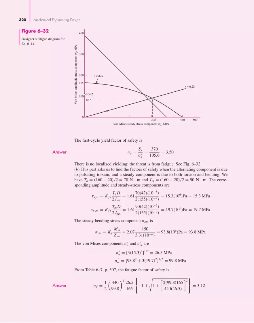
320 Mechanical Engineering Design
The first-cycle yield factor of safety is
Answer ny = Sy
σ ′a
= 370
105.6= 3.50
There is no localized yielding; the threat is from fatigue. See Fig. 6–32.(b) This part asks us to find the factors of safety when the alternating component is dueto pulsating torsion, and a steady component is due to both torsion and bending. Wehave Ta = (160 − 20)/2 = 70 N · m and Tm = (160 + 20)/2 = 90 N · m. The corre-sponding amplitude and steady-stress components are
τxya = K f sTa D
2Jnet= 1.61
70(42)(10−3)
2(155)(10−9)= 15.3(106)Pa = 15.3 MPa
τxym = K f sTm D
2Jnet= 1.61
90(42)(10−3)
2(155)(10−9)= 19.7(106)Pa = 19.7 MPa
The steady bending stress component σxm is
σxm = K fMm
Znet= 2.07
150
3.31(10−6)= 93.8(106)Pa = 93.8 MPa
The von Mises components σ ′a and σ ′
m are
σ ′a = [3(15.3)2]1/2 = 26.5 MPa
σ ′m = [93.82 + 3(19.7)2]1/2 = 99.8 MPa
From Table 6–7, p. 307, the fatigue factor of safety is
Answer n f = 1
2
(440
99.8
)2 26.5
165
⎧⎨⎩−1 +√
1 +[
2(99.8)165
440(26.5)
]2⎫⎬⎭ = 3.12
Von
Mis
es a
mpl
itude
str
ess
com
pone
nt �
a, M
Pa'
Von Mises steady stress component �m, MPa'305 500440
165
100104.2
85.5
200
300
400
0
Gerber
r = 0.28
Figure 6–32
Designer’s fatigue diagram forEx. 6–14.
bud29281_ch06_265-357.qxd 11/30/2009 4:23 pm Page 320 pinnacle s-171:Desktop Folder:Temp Work:Don't Delete (Jobs):MHDQ196/Budynas:

Fatigue Failure Resulting from Variable Loading 321
From the same table, with r = σ ′a/σ
′m = 26.5/99.8 = 0.28, the strengths can be shown
to be Sa = 85.5 MPa and Sm = 305 MPa. See the plot in Fig. 6–32.The first-cycle yield factor of safety ny is
Answer ny = Sy
σ ′a + σ ′
m
= 370
26.5 + 99.8= 2.93
There is no notch yielding. The likelihood of failure may first come from first-cycleyielding at the notch. See the plot in Fig. 6–32.
6–15 Varying, Fluctuating Stresses;Cumulative Fatigue DamageInstead of a single fully reversed stress history block composed of n cycles, suppose amachine part, at a critical location, is subjected to
• A fully reversed stress σ1 for n1 cycles, σ2 for n2 cycles, . . . , or
• A “wiggly” time line of stress exhibiting many and different peaks and valleys.
What stresses are significant, what counts as a cycle, and what is the measure ofdamage incurred? Consider a fully reversed cycle with stresses varying 60, 80, 40, and60 kpsi and a second fully reversed cycle −40, −60, −20, and −40 kpsi as depicted inFig. 6–33a. First, it is clear that to impose the pattern of stress in Fig. 6–33a on a partit is necessary that the time trace look like the solid lines plus the dashed lines in Fig.6–33a. Figure 6–33b moves the snapshot to exist beginning with 80 kpsi and endingwith 80 kpsi. Acknowledging the existence of a single stress-time trace is to discover a“hidden” cycle shown as the dashed line in Fig. 6–33b. If there are 100 applications ofthe all-positive stress cycle, then 100 applications of the all-negative stress cycle, the
100
50
0
–50
100
50
0
–50
(a) (b)
Figure 6–33
Variable stress diagramprepared for assessingcumulative damage.
bud29281_ch06_265-357.qxd 11/30/2009 4:23 pm Page 321 pinnacle s-171:Desktop Folder:Temp Work:Don't Delete (Jobs):MHDQ196/Budynas:

322 Mechanical Engineering Design
hidden cycle is applied but once. If the all-positive stress cycle is applied alternatelywith the all-negative stress cycle, the hidden cycle is applied 100 times.
To ensure that the hidden cycle is not lost, begin on the snapshot with the largest(or smallest) stress and add previous history to the right side, as was done in Fig. 6–33b.Characterization of a cycle takes on a max–min–same max (or min–max–same min)form. We identify the hidden cycle first by moving along the dashed-line trace inFig. 6–33b identifying a cycle with an 80-kpsi max, a 60-kpsi min, and returning to80 kpsi. Mentally deleting the used part of the trace (the dashed line) leaves a 40, 60,40 cycle and a −40, −20, −40 cycle. Since failure loci are expressed in terms of stressamplitude component σa and steady component σm , we use Eq. (6–36) to construct thetable below:
The most damaging cycle is number 1. It could have been lost.Methods for counting cycles include:
• Number of tensile peaks to failure.
• All maxima above the waveform mean, all minima below.
• The global maxima between crossings above the mean and the global minimabetween crossings below the mean.
• All positive slope crossings of levels above the mean, and all negative slope cross-ings of levels below the mean.
• A modification of the preceding method with only one count made between succes-sive crossings of a level associated with each counting level.
• Each local max–min excursion is counted as a half-cycle, and the associated ampli-tude is half-range.
• The preceding method plus consideration of the local mean.
• Rain-flow counting technique.
The method used here amounts to a variation of the rain-flow counting technique.The Palmgren-Miner24 cycle-ratio summation rule, also called Miner’s rule, is
written ∑ ni
Ni= c (6–57)
where ni is the number of cycles at stress level σi and Ni is the number of cycles to fail-ure at stress level σi . The parameter c has been determined by experiment; it is usuallyfound in the range 0.7 < c < 2.2 with an average value near unity.
Cycle Number �max �min �a �m
1 80 �60 70 10
2 60 40 10 50
3 �20 �40 10 �30
24A. Palmgren, “Die Lebensdauer von Kugellagern,” ZVDI, vol. 68, pp. 339–341, 1924; M. A. Miner,“Cumulative Damage in Fatigue,” J. Appl. Mech., vol. 12, Trans. ASME, vol. 67, pp. A159–A164, 1945.
bud29281_ch06_265-357.qxd 11/30/2009 4:23 pm Page 322 pinnacle s-171:Desktop Folder:Temp Work:Don't Delete (Jobs):MHDQ196/Budynas:

Fatigue Failure Resulting from Variable Loading 323
Using the deterministic formulation as a linear damage rule we write
D =∑ ni
Ni(6–58)
where D is the accumulated damage. When D = c = 1, failure ensues.
EXAMPLE 6–15 Given a part with Sut = 151 kpsi and at the critical location of the part, Se = 67.5 kpsi.For the loading of Fig. 6–33, estimate the number of repetitions of the stress-time blockin Fig. 6–33 that can be made before failure.
Solution From Fig. 6–18, p. 285, for Sut = 151 kpsi, f = 0.795. From Eq. (6–14),
a = ( f Sut)2
Se= [0.795(151)]2
67.5= 213.5 kpsi
From Eq. (6–15),
b = −1
3log
(f Sut
Se
)= −1
3log
[0.795(151)
67.5
]= −0.0833
So,
Sf = 213.5N−0.0833 N =(
Sf
213.5
)−1/0.0833
(1), (2)
We prepare to add two columns to the previous table. Using the Gerber fatigue criterion,Eq. (6–47), p. 306, with Se = Sf , and n = 1, we can write
Sf ={ σa
1 − (σm/Sut)2σm > 0
Se σm ≤ 0(3)
where Sf is the fatigue strength associated with a completely reversed stress, σrev,equivalent to the fluctuating stresses [see Ex. 6–12, part (b)].
Cycle 1: r = σa/σm = 70/10 = 7, and the strength amplitude from Table 6–7, p. 307, is
Sa = 721512
2(67.5)
⎧⎨⎩−1 +√
1 +[
2(67.5)
7(151)
]2⎫⎬⎭ = 67.2 kpsi
Since σa > Sa , that is, 70 > 67.2, life is reduced. From Eq. (3),
Sf = 70
1 − (10/151)2= 70.3 kpsi
and from Eq. (2)
N =(
70.3
213.5
)−1/0.0833
= 619(103) cycles
Cycle 2: r = 10/50 = 0.2, and the strength amplitude is
Sa = 0.221512
2(67.5)
⎧⎨⎩−1 +√
1 +[
2(67.5)
0.2(151)
]2⎫⎬⎭ = 24.2 kpsi
Since σa < Sa , that is 10 < 24.2, then Sf = Se and indefinite life follows. Thus, N ∞�.←
bud29281_ch06_265-357.qxd 12/02/2009 6:49 pm Page 323 pinnacle s-171:Desktop Folder:Temp Work:Don't Delete (Jobs):MHDQ196/Budynas:

324 Mechanical Engineering Design
Cycle 3: r = 10/−30 = −0.333, and since σm < 0, Sf = Se , indefinite life follows andN ∞
From Eq. (6–58) the damage per block is
D =∑ ni
Ni= N
[1
619(103)+ 1
∞ + 1
∞]
= N
619(103)
Answer Setting D = 1 yields N = 619(103) cycles.
Cycle Number Sf, kpsi N, cycles
1 70.3 619(103)
2 67.5 ∞3 67.5 ∞
←
To further illustrate the use of the Miner rule, let us consider a steel having theproperties Sut = 80 kpsi, S′
e,0 = 40 kpsi, and f = 0.9, where we have used the desig-nation S′
e,0 instead of the more usual S′e to indicate the endurance limit of the virgin, or
undamaged, material. The log S–log N diagram for this material is shown in Fig. 6–34by the heavy solid line. From Eqs. (6–14) and (6–15), p. 285, we find that a = 129.6 kpsiand b = −0.085 091. Now apply, say, a reversed stress σ1 = 60 kpsi for n1 = 3000cycles. Since σ1 > S′
e,0, the endurance limit will be damaged, and we wish to find thenew endurance limit S′
e,1 of the damaged material using the Miner rule. The equation ofthe virgin material failure line in Fig. 6–34 in the 103 to 106 cycle range is
Sf = aN b = 129.6N−0.085 091
The cycles to failure at stress level σ1 = 60 kpsi are
N1 =(
σ1
129.6
)−1/0.085 091
=(
60
129.6
)−1/0.085 091
= 8520 cycles
72
60
4038.6
103 104 105 106
6543
4.9
4.8
4.7
4.6
4.5
Log
Sf
S f k
psi
N
Log N
�1
0.9Sut
n1 = 3(103)
n2 = 0.648(106)
Sf, 0
Sf,2
S'e,0
S'e,1
Sf, 1
N1 = 8.52(103)
N1 – n1 = 5.52(103)
Figure 6–34
Use of the Miner rule to predict the endurance limit of a material that has beenoverstressed for a finite numberof cycles.
bud29281_ch06_265-357.qxd 12/02/2009 7:23 pm Page 324 pinnacle s-171:Desktop Folder:Temp Work:Don't Delete (Jobs):MHDQ196/Budynas:

Fatigue Failure Resulting from Variable Loading 325
Figure 6–34 shows that the material has a life N1 = 8520 cycles at 60 kpsi, and conse-quently, after the application of σ1 for 3000 cycles, there are N1 − n1 = 5520 cycles oflife remaining at σ1. This locates the finite-life strength Sf,1 of the damaged material, asshown in Fig. 6–34. To get a second point, we ask the question: With n1 and N1 given,how many cycles of stress σ2 = S′
e,0 can be applied before the damaged material fails?This corresponds to n2 cycles of stress reversal, and hence, from Eq. (6–58), we have
n1
N1+ n2
N2= 1 (a)
Solving for n2 gives
n2 = (N1 − n1)N2
N1(b)
Then
n2 = [8.52
(103) − 3
(103)] 106
8.52(103
) = 0.648(106) cycles
This corresponds to the finite-life strength Sf,2 in Fig. 6–34. A line through Sf,1 and Sf,2
is the log S–log N diagram of the damaged material according to the Miner rule. Twopoints, (N1 − n1, σ1) and (n2, σ2), determine the new equation for the line, Sf = a′N b ′
.Thus, σ1 = a′(N1 − n1)
b ′, and σ2 = a′nb
2′. Dividing the two equations, taking the loga-
rithm of the results, and solving for b′ gives
b′ = log (σ1/σ2)
log
(N1 − n1
n2
)Substituting n2 from Eq. (b) and simplifying gives
b′ = log (σ1/σ2)
log (N1/N2)
For the undamaged material, N1 = (σ1/a)1/b and N2 = (σ2/a)1/b , then
b′ = log (σ1/σ2)
log[(σ1/a)1/b/(σ2/a)1/b
] = log (σ1/σ2)
(1/b) log (σ1/σ2)= b
This means that the damaged material line has the same slope as the virgin material line,and the two lines are parallel. The value of a′ is then found from a′ = Sf /N b .
For the case we are illustrating, a′ = 60/[5.52(10)3]−0.085 091 = 124.898 kpsi, andthus the new endurance limit is S′
e,1 = a′N be = 124.898[(10)6]−0.085 091 = 38.6 kpsi.
Though the Miner rule is quite generally used, it fails in two ways to agree withexperiment. First, note that this theory states that the static strength Sut is damaged, thatis, decreased, because of the application of σ1; see Fig. 6–34 at N = 103 cycles.Experiments fail to verify this prediction.
The Miner rule, as given by Eq. (6–58), does not account for the order in which thestresses are applied, and hence ignores any stresses less than S′
e,0. But it can be seen inFig. 6–34 that a stress σ3 in the range S′
e,1 < σ3 < S′e,0 would cause damage if applied
after the endurance limit had been damaged by the application of σ1.Manson’s25 approach overcomes both of the deficiencies noted for the Palmgren-
Miner method; historically it is a much more recent approach, and it is just as easy to
25S. S. Manson, A. J. Nachtigall, C. R. Ensign, and J. C. Fresche, “Further Investigation of a Relation forCumulative Fatigue Damage in Bending,” Trans. ASME, J. Eng. Ind., ser. B, vol. 87, No. 1, pp. 25–35,February 1965.
bud29281_ch06_265-357.qxd 12/02/2009 6:49 pm Page 325 pinnacle s-171:Desktop Folder:Temp Work:Don't Delete (Jobs):MHDQ196/Budynas:

326 Mechanical Engineering Design
use. Except for a slight change, we shall use and recommend the Manson method inthis book. Manson plotted the S–log N diagram instead of a log S–log N plot as isrecommended here. Manson also resorted to experiment to find the point of conver-gence of the S–log N lines corresponding to the static strength, instead of arbitrarilyselecting the intersection of N = 103 cycles with S = 0.9Sut as is done here. Ofcourse, it is always better to use experiment, but our purpose in this book has beento use the simple test data to learn as much as possible about fatigue failure.
The method of Manson, as presented here, consists in having all log S–log N lines,that is, lines for both the damaged and the virgin material, converge to the same point,0.9Sut at 103 cycles. In addition, the log S–log N lines must be constructed in the samehistorical order in which the stresses occur.
The data from the preceding example are used for illustrative purposes. Theresults are shown in Fig. 6–35. Note that the strength Sf,1 corresponding toN1 − n1 = 5.52(103) cycles is found in the same manner as before. Through thispoint and through 0.9Sut at 103 cycles, draw the heavy dashed line to meet N = 106
cycles and define the endurance limit S′e,1 of the damaged material. Again, with two
points on the line, b′ = [log (72/60)]/log [(103)/5.52 (103)] = −0.106 722, anda′ = 60/[5.52 (103)]−0.106 722 = 150.487 kpsi. In this case, the new endurance limit isS′
e,1 = a′N be
′ = 150.487 (106)−0.106 722 = 34.4 kpsi, which is somewhat less than thatfound by the Miner method.
It is now easy to see from Fig. 6–35 that a reversed stress σ = 36 kpsi, say, wouldnot harm the endurance limit of the virgin material, no matter how many cycles it mightbe applied. However, if σ = 36 kpsi should be applied after the material was damagedby σ1 = 60 kpsi, then additional damage would be done.
Both these rules involve a number of computations, which are repeated every timedamage is estimated. For complicated stress-time traces, this might be every cycle.Clearly a computer program is useful to perform the tasks, including scanning the traceand identifying the cycles.
72
60
40
103 104 105 106
6543
4.9
4.8
4.7
4.6
4.5
Log
Sf
S f k
psi
N
Log N
�1
0.9Sut
n1 = 3(103)
Sf, 0
S'e,0
S'e,1
Sf, 1
N1 = 8.52(103)
N1 – n1 = 5.52(103)
34.4
Figure 6–35
Use of the Manson method topredict the endurance limit of a material that has beenoverstressed for a finite numberof cycles.
bud29281_ch06_265-357.qxd 12/02/2009 7:26 pm Page 326 pinnacle s-171:Desktop Folder:Temp Work:Don't Delete (Jobs):MHDQ196/Budynas:

Fatigue Failure Resulting from Variable Loading 327
Collins said it well: “In spite of all the problems cited, the Palmgren linear damagerule is frequently used because of its simplicity and the experimental fact that othermore complex damage theories do not always yield a significant improvement in fail-ure prediction reliability.”26
6–16 Surface Fatigue StrengthThe surface fatigue mechanism is not definitively understood. The contact-affectedzone, in the absence of surface shearing tractions, entertains compressive principalstresses. Rotary fatigue has its cracks grown at or near the surface in the presence oftensile stresses that are associated with crack propagation, to catastrophic failure. Thereare shear stresses in the zone, which are largest just below the surface. Cracks seem togrow from this stratum until small pieces of material are expelled, leaving pits on the sur-face. Because engineers had to design durable machinery before the surface fatigue phe-nomenon was understood in detail, they had taken the posture of conducting tests,observing pits on the surface, and declaring failure at an arbitrary projected area of hole,and they related this to the Hertzian contact pressure. This compressive stress didnot produce the failure directly, but whatever the failure mechanism, whatever thestress type that was instrumental in the failure, the contact stress was an index to itsmagnitude.
Buckingham27 conducted a number of tests relating the fatigue at 108 cycles toendurance strength (Hertzian contact pressure). While there is evidence of an endurancelimit at about 3(107) cycles for cast materials, hardened steel rollers showed no endurancelimit up to 4(108) cycles. Subsequent testing on hard steel shows no endurance limit.Hardened steel exhibits such high fatigue strengths that its use in resisting surface fatigueis widespread.
Our studies thus far have dealt with the failure of a machine element by yielding,by fracture, and by fatigue. The endurance limit obtained by the rotating-beam test isfrequently called the flexural endurance limit, because it is a test of a rotating beam. Inthis section we shall study a property of mating materials called the surface enduranceshear. The design engineer must frequently solve problems in which two machine ele-ments mate with one another by rolling, sliding, or a combination of rolling and sliding contact. Obvious examples of such combinations are the mating teeth of a pair of gears,a cam and follower, a wheel and rail, and a chain and sprocket. A knowledge of the sur-face strength of materials is necessary if the designer is to create machines having along and satisfactory life.
When two surfaces roll or roll and slide against one another with sufficient force,a pitting failure will occur after a certain number of cycles of operation. Authorities arenot in complete agreement on the exact mechanism of the pitting; although the subjectis quite complicated, they do agree that the Hertz stresses, the number of cycles, the sur-face finish, the hardness, the degree of lubrication, and the temperature all influence thestrength. In Sec. 3–19 it was learned that, when two surfaces are pressed together, amaximum shear stress is developed slightly below the contacting surface. It is postulatedby some authorities that a surface fatigue failure is initiated by this maximum shearstress and then is propagated rapidly to the surface. The lubricant then enters the crackthat is formed and, under pressure, eventually wedges the chip loose.
26J. A. Collins, Failure of Materials in Mechanical Design, John Wiley & Sons, New York, 1981, p. 243.27Earle Buckingham, Analytical Mechanics of Gears, McGraw-Hill, New York, 1949.
bud29281_ch06_265-357.qxd 11/30/2009 4:23 pm Page 327 pinnacle s-171:Desktop Folder:Temp Work:Don't Delete (Jobs):MHDQ196/Budynas:

328 Mechanical Engineering Design
To determine the surface fatigue strength of mating materials, Buckingham designeda simple machine for testing a pair of contacting rolling surfaces in connection with hisinvestigation of the wear of gear teeth. Buckingham and, later, Talbourdet gathered largenumbers of data from many tests so that considerable design information is nowavailable. To make the results useful for designers, Buckingham defined a load-stressfactor, also called a wear factor, which is derived from the Hertz equations. Equations(3–73) and (3–74), p. 124, for contacting cylinders are found to be
b =√
2F
πl
(1 − ν2
1
)/E1 + (
1 − ν22
)/E2
(1/d1) + (1/d2)(6–59)
pmax = 2F
πbl(6–60)
where b = half width of rectangular contact area
F = contact force
l = length of cylinders
ν = Poisson’s ratio
E = modulus of elasticity
d = cylinder diameter
It is more convenient to use the cylinder radius, so let 2r = d . If we then designatethe length of the cylinders as w (for width of gear, bearing, cam, etc.) instead of l andremove the square root sign, Eq. (6–59) becomes
b2 = 4F
πw
(1 − ν2
1
)/E1 + (
1 − ν22
)/E2
1/r1 + 1/r2(6–61)
We can define a surface endurance strength SC using
pmax = 2F
πbw(6–62)
as
SC = 2F
πbw(6–63)
which may also be called contact strength, the contact fatigue strength, or the Hertzianendurance strength. The strength is the contacting pressure which, after a specifiednumber of cycles, will cause failure of the surface. Such failures are often called wearbecause they occur over a very long time. They should not be confused with abrasivewear, however. By squaring Eq. (6–63), substituting b2 from Eq. (6–61), and rearrang-ing, we obtain
F
w
(1
r1+ 1
r2
)= π S2
C
[1 − ν2
1
E1+ 1 − ν2
2
E2
]= K1 (6–64)
The left expression consists of parameters a designer may seek to control independently.The central expression consists of material properties that come with the material andcondition specification. The third expression is the parameter K1, Buckingham’s load-stress factor, determined by a test fixture with values F, w, r1, r2 and the number of
bud29281_ch06_265-357.qxd 11/30/2009 4:23 pm Page 328 pinnacle s-171:Desktop Folder:Temp Work:Don't Delete (Jobs):MHDQ196/Budynas:

Fatigue Failure Resulting from Variable Loading 329
cycles associated with the first tangible evidence of fatigue. In gear studies a similarK factor is used:
Kg = K1
4sin φ (6–65)
where φ is the tooth pressure angle, and the term [(1 − ν21)/E1 + (1 − ν2
2)/E2] isdefined as 1/(πC2
P), so that
SC = CP
√F
w
(1
r1+ 1
r2
)(6–66)
Buckingham and others reported K1 for 108 cycles and nothing else. This gives only onepoint on the SC N curve. For cast metals this may be sufficient, but for wrought steels, heat-treated, some idea of the slope is useful in meeting design goals of other than 108 cycles.
Experiments show that K1 versus N, Kg versus N, and SC versus N data are recti-fied by log-log transformation. This suggests that
K1 = α1 Nβ1 Kg = aN b SC = αNβ
The three exponents are given by
β1 = log(K1/K2)
log(N1/N2)b = log(Kg1/Kg2)
log(N1/N2)β = log(SC1/SC2)
log(N1/N2)(6–67)
Data on induction-hardened steel on steel give (SC)107 = 271 kpsi and (SC)108 =239 kpsi, so β , from Eq. (6–67), is
β = log(271/239)
log(107/108)= −0.055
It may be of interest that the American Gear Manufacturers Association (AGMA) usesβ � �0.056 between 104 < N < 1010 if the designer has no data to the contrarybeyond 107 cycles.
A longstanding correlation in steels between SC and HB at 108 cycles is
(SC)108 ={
0.4HB − 10 kpsi2.76HB − 70 MPa
(6–68)
AGMA uses0.99(SC)107 = 0.327HB + 26 kpsi (6–69)
Equation (6–66) can be used in design to find an allowable surface stress by usinga design factor. Since this equation is nonlinear in its stress-load transformation, thedesigner must decide if loss of function denotes inability to carry the load. If so, thento find the allowable stress, one divides the load F by the design factor nd :
σC = CP
√F
wnd
(1
r1+ 1
r2
)= CP√
nd
√F
w
(1
r1+ 1
r2
)= SC√
nd
and nd = (SC/σC)2. If the loss of function is focused on stress, then nd = SC/σC . It isrecommended that an engineer
• Decide whether loss of function is failure to carry load or stress.
• Define the design factor and factor of safety accordingly.
• Announce what he or she is using and why.
• Be prepared to defend his or her position.
bud29281_ch06_265-357.qxd 12/02/2009 6:49 pm Page 329 pinnacle s-171:Desktop Folder:Temp Work:Don't Delete (Jobs):MHDQ196/Budynas:

In this way everyone who is party to the communication knows what a design factor(or factor of safety) of 2 means and adjusts, if necessary, the judgmental perspective.
6–17 Stochastic Analysis28
As already demonstrated in this chapter, there are a great many factors to consider ina fatigue analysis, much more so than in a static analysis. So far, each factor has beentreated in a deterministic manner, and if not obvious, these factors are subject to vari-ability and control the overall reliability of the results. When reliability is important,then fatigue testing must certainly be undertaken. There is no other way. Consequently,the methods of stochastic analysis presented here and in other sections of this bookconstitute guidelines that enable the designer to obtain a good understanding of thevarious issues involved and help in the development of a safe and reliable design.
In this section, key stochastic modifications to the deterministic features and equa-tions described in earlier sections are provided in the same order of presentation.
Endurance Limit
To begin, a method for estimating endurance limits, the tensile strength correlationmethod, is presented. The ratio � = S′
e/Sut is called the fatigue ratio.29 For ferrousmetals, most of which exhibit an endurance limit, the endurance limit is used as anumerator. For materials that do not show an endurance limit, an endurance strength ata specified number of cycles to failure is used and noted. Gough30 reported the sto-chastic nature of the fatigue ratio � for several classes of metals, and this is shown inFig. 6–36. The first item to note is that the coefficient of variation is of the order 0.10to 0.15, and the distribution varies for classes of metals. The second item to note is thatGough’s data include materials of no interest to engineers. In the absence of testing,engineers use the correlation that � represents to estimate the endurance limit S′
e fromthe mean ultimate strength Sut .
Gough’s data are for ensembles of metals, some chosen for metallurgical interest,and include materials that are not commonly selected for machine parts. Mischke31
analyzed data for 133 common steels and treatments in varying diameters in rotatingbending,32 and the result was
� = 0.445d−0.107LN(1, 0.138)
where d is the specimen diameter in inches and LN(1, 0.138) is a unit lognormal vari-ate with a mean of 1 and a standard deviation (and coefficient of variation) of 0.138. Forthe standard R. R. Moore specimen,
�0.30 = 0.445(0.30)−0.107LN(1, 0.138) = 0.506LN(1, 0.138)
330 Mechanical Engineering Design
28Review Chap. 20 before reading this section.29From this point, since we will be dealing with statistical distributions in terms of means, standarddeviations, etc. A key quantity, the ultimate strength, will here be presented by its mean value, Sut . Thismeans that certain terms that were defined earlier in terms of the minimum value of Sut will change slightly.30In J. A. Pope, Metal Fatigue, Chapman and Hall, London, 1959.31Charles R. Mischke, “Prediction of Stochastic Endurance Strength,” Trans. ASME, Journal of Vibration,Acoustics, Stress, and Reliability in Design, vol. 109, no. 1, January 1987, pp. 113–122.32Data from H. J. Grover, S. A. Gordon, and L. R. Jackson, Fatigue of Metals and Structures, Bureau ofNaval Weapons, Document NAVWEPS 00-2500435, 1960.
bud29281_ch06_265-357.qxd 12/02/2009 6:49 pm Page 330 pinnacle s-171:Desktop Folder:Temp Work:Don't Delete (Jobs):MHDQ196/Budynas:

Fatigue Failure Resulting from Variable Loading 331
Also, 25 plain carbon and low-alloy steels with Sut > 212 kpsi are described by
S′e = 107LN(1, 0.139) kpsi
In summary, for the rotating-beam specimen,
S′e =
⎧⎪⎨⎪⎩0.506Sut LN(1, 0.138) kpsi or MPa Sut ≤ 212 kpsi (1460 MPa)
107LN(1, 0.139) kpsi Sut > 212 kpsi
740LN(1, 0.139) MPa Sut > 1460 MPa
(6–70)
where Sut is the mean ultimate tensile strength.Equations (6–70) represent the state of information before an engineer has chosen
a material. In choosing, the designer has made a random choice from the ensemble ofpossibilities, and the statistics can give the odds of disappointment. If the testing is lim-ited to finding an estimate of the ultimate tensile strength mean Sut with the chosenmaterial, Eqs. (6–70) are directly helpful. If there is to be rotary-beam fatigue testing,then statistical information on the endurance limit is gathered and there is no need forthe correlation above.
Table 6–9 compares approximate mean values of the fatigue ratio φ0.30 for severalclasses of ferrous materials.
Endurance Limit Modifying Factors
A Marin equation can be written as
Se = kakbkckdkf S′e (6–71)
where the size factor kb is deterministic and remains unchanged from that given inSec. 6–9. Also, since we are performing a stochastic analysis, the “reliability factor” ke
is unnecessary here.The surface factor ka cited earlier in deterministic form as Eq. (6–20), p. 288, is
now given in stochastic form by
ka = aSbut LN(1, C) (Sut in kpsi or MPa) (6–72)
where Table 6–10 gives values of a, b, and C for various surface conditions.
0.3 0.4 0.5 0.6 0.70
5
Prob
abili
ty d
ensi
ty
Rotary bending fatigue ratio �b
2
1
34
5
1
2
3
4
5
All metals
Nonferrous
Iron and carbon steels
Low-alloy steels
Special alloy steels
380
152
111
78
39
Class No.Figure 6–36
The lognormal probabilitydensity PDF of the fatigue ratioφb of Gough.
bud29281_ch06_265-357.qxd 12/03/2009 9:47 am Page 331 pinnacle 203:MHDQ196:bud29281:0073529281:bud29281_pagefiles:

332 Mechanical Engineering Design
Table 6–9
Comparison of
Approximate Values of
Mean Fatigue Ratio for
Some Classes of Metals
Material Class φ0.30
Wrought steels 0.50
Cast steels 0.40
Powdered steels 0.38
Gray cast iron 0.35
Malleable cast iron 0.40
Normalized nodular cast iron 0.33
Table 6–10
Parameters in Marin
Surface Condition Factor
ka � aSbut LN(1, C)
a Coefficient ofSurface Finish kpsi MPa b Variation, C
Ground* 1.34 1.58 −0.086 0.120
Machined or Cold-rolled 2.67 4.45 −0.265 0.058
Hot-rolled 14.5 58.1 −0.719 0.110
As-forged 39.8 271 −0.995 0.145
*Due to the wide scatter in ground surface data, an alternate function is ka = 0.878LN(1, 0.120). Note: Sut in kpsi or MPa.
EXAMPLE 6–16 A steel has a mean ultimate strength of 520 MPa and a machined surface. Estimate ka .
Solution From Table 6–10,
ka = 4.45(520)−0.265LN(1, 0.058)
ka = 4.45(520)−0.265(1) = 0.848
σka = Cka = (0.058)4.45(520)−0.265 = 0.049
Answer so ka = LN(0.848, 0.049).
The load factor kc for axial and torsional loading is given by
(kc)axial = 1.23S−0.0778ut LN(1, 0.125) (6–73)
(kc)torsion = 0.328S0.125ut LN(1, 0.125) (6–74)
where Sut is in kpsi. There are fewer data to study for axial fatigue. Equation (6–73) wasdeduced from the data of Landgraf and of Grover, Gordon, and Jackson (as cited earlier).
Torsional data are sparser, and Eq. (6–74) is deduced from data in Grover et al.Notice the mild sensitivity to strength in the axial and torsional load factor, so kc inthese cases is not constant. Average values are shown in the last column of Table 6–11,and as footnotes to Tables 6–12 and 6–13. Table 6–14 shows the influence of materialclasses on the load factor kc. Distortion energy theory predicts (kc)torsion = 0.577 formaterials to which the distortion-energy theory applies. For bending, kc = LN(1, 0).
bud29281_ch06_265-357.qxd 12/02/2009 6:49 pm Page 332 pinnacle s-171:Desktop Folder:Temp Work:Don't Delete (Jobs):MHDQ196/Budynas:

Table 6–13
Average Marin Loading
Factor for Torsional
Load
Table 6–14
Average Marin Torsional
Loading Factor kc for
Several Materials
Material Range n kc σkc
Wrought steels 0.52–0.69 31 0.60 0.03
Wrought Al 0.43–0.74 13 0.55 0.09
Wrought Cu and alloy 0.41–0.67 7 0.56 0.10
Wrought Mg and alloy 0.49–0.60 2 0.54 0.08
Titanium 0.37–0.57 3 0.48 0.12
Cast iron 0.79–1.01 9 0.90 0.07
Cast Al, Mg, and alloy 0.71–0.91 5 0.85 0.09
Source: The table is an extension of P. G. Forrest, Fatigue of Metals, Pergamon Press, London, 1962,Table 17, p. 110, with standard deviations estimated from range and sample size using Table A–1 in J. B. Kennedy and A. M. Neville, Basic Statistical Methods for Engineers and Scientists, 3rd ed.,Harper & Row, New York, 1986, pp. 54–55.
Table 6–11
Parameters in Marin
Loading Factor
Table 6–12
Average Marin Loading
Factor for Axial Load
Fatigue Failure Resulting from Variable Loading 333
kc � αSut−β LN(1, C)
Mode of α AverageLoading kpsi MPa β C kc
Bending 1 1 0 0 1
Axial 1.23 1.43 −0.0778 0.125 0.85
Torsion 0.328 0.258 0.125 0.125 0.59
Sut, kpsi k*c
50 0.907
100 0.860
150 0.832
200 0.814
*Average entry 0.85.
Sut, kpsi k*c
50 0.535
100 0.583
150 0.614
200 0.636
*Average entry 0.59.
bud29281_ch06_265-357.qxd 12/10/2009 4:46 pm Page 333 pinnacle s-171:Desktop Folder:Temp Work:Don't Delete (Jobs):MHDQ196/Budynas:
334 Mechanical Engineering Design
EXAMPLE 6–17 Estimate the Marin loading factor kc for a 1–in-diameter bar that is used as follows.(a) In bending. It is made of steel with Sut = 100LN(1, 0.035) kpsi, and the designerintends to use the correlation S′
e = �0.30 Sut to predict S′e.
(b) In bending, but endurance testing gave S′e = 55LN(1, 0.081) kpsi.
(c) In push-pull (axial) fatigue, Sut = LN(86.2, 3.92) kpsi, and the designer intended touse the correlation S′
e = �0.30 Sut .(d) In torsional fatigue. The material is cast iron, and S′
e is known by test.
Solution (a) Since the bar is in bending,
Answer kc = (1, 0)
(b) Since the test is in bending and use is in bending,
Answer kc = (1, 0)
(c) From Eq. (6–73),
Answer (kc)ax = 1.23(86.2)−0.0778LN(1, 0.125)
kc = 1.23(86.2)−0.0778(1) = 0.870
σkc = Ckc = 0.125(0.870) = 0.109
(d ) From Table 6–15, kc = 0.90, σkc = 0.07, and
Answer Ckc = 0.07
0.90= 0.08
The temperature factor kd is
kd = kdLN(1, 0.11) (6–75)
where kd = kd , given by Eq. (6–27), p. 291.Finally, kf is, as before, the miscellaneous factor that can come about from a great
many considerations, as discussed in Sec. 6–9, where now statistical distributions, pos-sibly from testing, are considered.
Stress Concentration and Notch Sensitivity
Notch sensitivity q was defined by Eq. (6–31), p. 295. The stochastic equivalent is
q = K f − 1
Kt − 1(6–76)
where Kt is the theoretical (or geometric) stress-concentration factor, a deterministicquantity. A study of lines 3 and 4 of Table 20–6, will reveal that adding a scalar to (orsubtracting one from) a variate x will affect only the mean. Also, multiplying (or divid-ing) by a scalar affects both the mean and standard deviation. With this in mind, we can
bud29281_ch06_265-357.qxd 11/30/2009 4:23 pm Page 334 pinnacle s-171:Desktop Folder:Temp Work:Don't Delete (Jobs):MHDQ196/Budynas:

Fatigue Failure Resulting from Variable Loading 335
relate the statistical parameters of the fatigue stress-concentration factor K f to those ofnotch sensitivity q. It follows that
q = LN(
K f − 1
Kt − 1,
C K f
Kt − 1
)where C = CK f and
q = K f − 1
Kt − 1
σq = C K f
Kt − 1(6–77)
Cq = C K f
K f − 1
The fatigue stress-concentration factor K f has been investigated more in England than inthe United States. For K f , consider a modified Neuber equation (after Heywood33),where the fatigue stress-concentration factor is given by
K f = Kt
1 + 2(Kt − 1)
Kt
√a√r
(6–78)
where Table 6–15 gives values of √
a and CK f for steels with transverse holes,shoulders, or grooves. Once K f is described, q can also be quantified using the setEqs. (6–77).
The modified Neuber equation gives the fatigue stress-concentration factor as
K f = K f LN(1, CK f
)(6–79)
Table 6–15
Heywood’s Parameter√a and coefficients of
variation CKf for steels
EXAMPLE 6–18 Estimate K f and q for the steel shaft given in Ex. 6–6, p. 296.
Solution From Ex. 6–6, a steel shaft with Sut = 690 MPa and a shoulder with a fillet of 3 mmwas found to have a theoretical stress-concentration factor of Kt
.= 1.65. From Table 6–15,
√a = 139
Sut= 139
690= 0.2014
√mm
33R. B. Heywood, Designing Against Fatigue, Chapman & Hall, London, 1962.
, , Coefficient ofNotch Type Sut in kpsi Sut in MPa Variation CKf
Transverse hole 5/Sut 174/Sut 0.10
Shoulder 4/Sut 139/Sut 0.11
Groove 3/Sut 104/Sut 0.15
√a(
√mm)
√a(
√in)
bud29281_ch06_265-357.qxd 12/7/09 9:42PM Page 335 ntt G4 Mac OS 9.2:Desktop Folder:MHDQ196/Budynas:

From Eq. (6–78),
K f = Kt
1 + 2(Kt − 1)
Kt
√a√r
= 1.65
1 + 2(1.65 − 1)
1.65
0.2014√3
= 1.51
which is 2.5 percent lower than what was found in Ex. 6–6.From Table 6–15, CK f = 0.11. Thus from Eq. (6–79),
Answer K f = 1.51 LN(1, 0.11)
From Eq. (6–77), with Kt = 1.65
q = 1.51 − 1
1.65 − 1= 0.785
Cq = CK f K f
K f − 1= 0.11(1.51)
1.51 − 1= 0.326
σq = Cqq = 0.326(0.785) = 0.256
So,
Answer q = LN(0.785, 0.256)
EXAMPLE 6–19 The bar shown in Fig. 6–37 is machined from a cold-rolled flat having an ultimatestrength of Sut = LN(87.6, 5.74) kpsi. The axial load shown is completely reversed.The load amplitude is Fa = LN(1000, 120) lbf.(a) Estimate the reliability.(b) Reestimate the reliability when a rotating bending endurance test shows that S′
e =LN(40, 2) kpsi.
Solution (a) From Eq. (6–70), S′e = 0.506Sut LN(1, 0.138) = 0.506(87.6)LN(1, 0.138)
= 44.3LN(1, 0.138) kpsi
From Eq. (6–72) and Table 6–10,
ka = 2.67S−0.265ut LN(1, 0.058) = 2.67(87.6)−0.265LN(1, 0.058)
= 0.816LN(1, 0.058)
kb = 1 (axial loading)
34 -in D.
316
-in R.
in
14
2 in 12
1 in
14
1000 lbf 1000 lbf
Figure 6–37
336 Mechanical Engineering Design
bud29281_ch06_265-357.qxd 12/02/2009 9:46 pm Page 336 pinnacle s-171:Desktop Folder:Temp Work:Don't Delete (Jobs):MHDQ196/Budynas:

Fatigue Failure Resulting from Variable Loading 337
From Eq. (6–73),
kc = 1.23S−0.0778ut LN(1, 0.125) = 1.23(87.6)−0.0778LN(1, 0.125)
= 0.869LN(1, 0.125)
kd = k f = (1, 0)
The endurance strength, from Eq. (6–71), is
Se = kakbkckdk f S′e
Se = 0.816LN(1, 0.058)(1)0.869LN(1, 0.125)(1)(1)44.3LN(1, 0.138)
The parameters of Se are
Se = 0.816(0.869)44.3 = 31.4 kpsi
CSe = (0.0582 + 0.1252 + 0.1382)1/2 = 0.195
so Se = 31.4LN(1, 0.195) kpsi.In computing the stress, the section at the hole governs. Using the terminology
of Table A–15–1 we find d/w = 0.50, therefore Kt.= 2.18. From Table 6–15,√
a = 5/Sut = 5/87.6 = 0.0571 and Ck f = 0.10. From Eqs. (6–78) and (6–79) withr = 0.375 in,
K f = Kt
1 + 2(Kt − 1)
Kt
√a√r
LN(1, CK f
) = 2.18
1 + 2(2.18 − 1)
2.18
0.0571√0.375
LN(1, 0.10)
= 1.98LN(1, 0.10)
The stress at the hole is
� = K fFA
= 1.98LN(1, 0.10)1000LN(1, 0.12)
0.25(0.75)
σ = 1.981000
0.25(0.75)10−3 = 10.56 kpsi
Cσ = (0.102 + 0.122)1/2 = 0.156
so stress can be expressed as � = 10.56LN(1, 0.156) kpsi.34
The endurance limit is considerably greater than the load-induced stress, indicat-ing that finite life is not a problem. For interfering lognormal-lognormal distributions,Eq. (5–43), p. 250, gives
z = −ln
(Se
σ
√1 + C2
σ
1 + C2Se
)√
ln[(
1 + C2Se
) (1 + C2
σ
)] = −ln
⎛⎝ 31.4
10.56
√1 + 0.1562
1 + 0.1952
⎞⎠√
ln[(1 + 0.1952)(1 + 0.1562)]= −4.37
From Table A–10 the probability of failure pf = �(−4.37) = .000 006 35, and thereliability is
Answer R = 1 − 0.000 006 35 = 0.999 993 65
34Note that there is a simplification here. The area is not a deterministic quantity. It will have a statisticaldistribution also. However no information was given here, and so it was treated as being deterministic.
bud29281_ch06_265-357.qxd 11/30/2009 4:24 pm Page 337 pinnacle s-171:Desktop Folder:Temp Work:Don't Delete (Jobs):MHDQ196/Budynas:

(b) The rotary endurance tests are described by S′e = 40LN(1, 0.05) kpsi whose mean
is less than the predicted mean in part a. The mean endurance strength Se is
Se = 0.816(0.869)40 = 28.4 kpsi
CSe = (0.0582 + 0.1252 + 0.052)1/2 = 0.147
so the endurance strength can be expressed as Se = 28.3LN(1, 0.147) kpsi. FromEq. (5–43),
z = −ln
⎛⎝ 28.4
10.56
√1 + 0.1562
1 + 0.1472
⎞⎠√
ln[(1 + 0.1472)(1 + 0.1562)]= −4.65
Using Table A–10, we see the probability of failure pf = �(−4.65) = 0.000 001 71,and
R = 1 − 0.000 001 71 = 0.999 998 29
an increase! The reduction in the probability of failure is (0.000 001 71 − 0.000006 35)/0.000 006 35 = −0.73, a reduction of 73 percent. We are analyzing an existingdesign, so in part (a) the factor of safety was n = S/σ = 31.4/10.56 = 2.97. In part (b)n = 28.4/10.56 = 2.69, a decrease. This example gives you the opportunity to see the roleof the design factor. Given knowledge of S, CS, σ, Cσ , and reliability (through z), the meanfactor of safety (as a design factor) separates S and σ so that the reliability goal is achieved.Knowing n alone says nothing about the probability of failure. Looking at n = 2.97 andn = 2.69 says nothing about the respective probabilities of failure. The tests did not reduceSe significantly, but reduced the variation CS such that the reliability was increased.
When a mean design factor (or mean factor of safety) defined as Se/σ is said tobe silent on matters of frequency of failures, it means that a scalar factor of safetyby itself does not offer any information about probability of failure. Nevertheless,some engineers let the factor of safety speak up, and they can be wrong in theirconclusions.
338 Mechanical Engineering Design
As revealing as Ex. 6–19 is concerning the meaning (and lack of meaning) of adesign factor or factor of safety, let us remember that the rotary testing associated withpart (b) changed nothing about the part, but only our knowledge about the part. Themean endurance limit was 40 kpsi all the time, and our adequacy assessment had tomove with what was known.
Fluctuating Stresses
Deterministic failure curves that lie among the data are candidates for regression mod-els. Included among these are the Gerber and ASME-elliptic for ductile materials, and,for brittle materials, Smith-Dolan models, which use mean values in their presentation.Just as the deterministic failure curves are located by endurance strength and ultimatetensile (or yield) strength, so too are stochastic failure curves located by Se and by Sut
or Sy . Figure 6–32, p. 320, shows a parabolic Gerber mean curve. We also need toestablish a contour located one standard deviation from the mean. Since stochastic
bud29281_ch06_265-357.qxd 11/30/2009 4:24 pm Page 338 pinnacle s-171:Desktop Folder:Temp Work:Don't Delete (Jobs):MHDQ196/Budynas:

Fatigue Failure Resulting from Variable Loading 339
curves are most likely to be used with a radial load line we will use the equation givenin Table 6–7, p. 307, expressed in terms of the strength means as
Sa = r2 S2ut
2Se
⎡⎣−1 +√
1 +(
2Se
r Sut
)2⎤⎦ (6–80)
Because of the positive correlation between Se and Sut , we increment Se by CSe Se , Sut
by CSut Sut , and Sa by CSa Sa , substitute into Eq. (6–80), and solve for CSa to obtain
CSa = (1 + CSut)2
1 + CSe
⎧⎨⎩−1 +√
1 +[
2Se(1 + CSe)
r Sut(1 + CSut)
]2⎫⎬⎭⎡⎣−1 +
√1 +
(2Se
r Sut
)2⎤⎦ − 1 (6–81)
Equation (6–81) can be viewed as an interpolation formula for CSa , which falls betweenCSe and CSut depending on load line slope r. Note that Sa = SaLN(1, CSa).
Similarly, the ASME-elliptic criterion of Table 6–8, p. 308, expressed in terms ofits means is
Sa = r Sy Se√r2 S2
y + S2e
(6–82)
Similarly, we increment Se by CSe Se , Sy by CSy Sy , and Sa by CSa Sa , substitute intoEq. (6–82), and solve for CSa :
CSa = (1 + CSy)(1 + CSe)
√√√√ r2 S2y + S2
e
r2 S2y(1 + CSy)2 + S2
e (1 + CSe)2− 1 (6–83)
Many brittle materials follow a Smith-Dolan failure criterion, written deterministi-cally as
nσa
Se= 1 − nσm/Sut
1 + nσm/Sut(6–84)
Expressed in terms of its means,
Sa
Se= 1 − Sm/Sut
1 + Sm/Sut(6–85)
For a radial load line slope of r, we substitute Sa/r for Sm and solve for Sa , obtaining
Sa = r Sut + Se
2
⎡⎣−1 +√
1 + 4r Sut Se
(r Sut + Se)2
⎤⎦ (6–86)
and the expression for CSa is
CSa = r Sut(1 + CSut) + Se(1 + CSe)
2Sa
·{
−1 +√
1 + 4r Sut Se(1 + CSe)(1 + CSut)
[r Sut(1 + CSut) + Se(1 + CSe)]2
}− 1
(6–87)
bud29281_ch06_265-357.qxd 11/30/2009 4:24 pm Page 339 pinnacle s-171:Desktop Folder:Temp Work:Don't Delete (Jobs):MHDQ196/Budynas:

340 Mechanical Engineering Design
EXAMPLE 6–20 A rotating shaft experiences a steady torque T = 1360LN(1, 0.05) lbf · in, and at ashoulder with a 1.1-in small diameter, a fatigue stress-concentration factor K f =1.50LN(1, 0.11), K f s = 1.28LN(1, 0.11), and at that location a bending moment ofM = 1260LN(1, 0.05) lbf · in. The material of which the shaft is machined is hot-rolled1035 with Sut = 86.2LN(1, 0.045) kpsi and Sy = 56.0LN(1, 0.077) kpsi. Estimate thereliability using a stochastic Gerber failure zone.
Solution Establish the endurance strength. From Eqs. (6–70) to (6–72) and Eq. (6–20), p. 288,
S′e = 0.506(86.2)LN(1, 0.138) = 43.6LN(1, 0.138) kpsi
ka = 2.67(86.2)−0.265LN(1, 0.058) = 0.820LN(1, 0.058)
kb = (1.1/0.30)−0.107 = 0.870
kc = kd = k f = LN(1, 0)
Se = 0.820LN(1, 0.058)0.870(43.6)LN(1, 0.138)
Se = 0.820(0.870)43.6 = 31.1 kpsi
CSe = (0.0582 + 0.1382)1/2 = 0.150
and so Se = 31.1LN(1, 0.150) kpsi.
Stress (in kpsi):
σa = 32K f Ma
πd3= 32(1.50)LN(1, 0.11)1.26LN(1, 0.05)
π(1.1)3
σa = 32(1.50)1.26
π(1.1)3= 14.5 kpsi
Cσa = (0.112 + 0.052)1/2 = 0.121
�m = 16K f sTm
πd3= 16(1.28)LN(1, 0.11)1.36LN(1, 0.05)
π(1.1)3
τm = 16(1.28)1.36
π(1.1)3= 6.66 kpsi
Cτm = (0.112 + 0.052)1/2 = 0.121
σ ′a = (
σ 2a + 3τ 2
a
)1/2 = [14.52 + 3(0)2]1/2 = 14.5 kpsi
σ ′m = (
σ 2m + 3τ 2
m
)1/2 = [0 + 3(6.66)2]1/2 = 11.54 kpsi
r = σ ′a
σ ′m
= 14.5
11.54= 1.26
Strength: From Eqs. (6–80) and (6–81),
Sa = 1.26286.22
2(31.1)
⎧⎨⎩−1 +√
1 +[
2(31.1)
1.26(86.2)
]2⎫⎬⎭ = 28.9 kpsi
bud29281_ch06_265-357.qxd 12/02/2009 6:49 pm Page 340 pinnacle s-171:Desktop Folder:Temp Work:Don't Delete (Jobs):MHDQ196/Budynas:

CSa = (1 + 0.045)2
1 + 0.150
−1 +√
1 +[
2(31.1)(1 + 0.15)
1.26(86.2)(1 + 0.045)
]2
−1 +√
1 +[
2(31.1)
1.26(86.2)
]2− 1 = 0.134
Reliability: Since Sa = 28.9LN(1, 0.134) kpsi and �′a = 14.5LN(1, 0.121) kpsi,
Eq. (5–43), p. 250, gives
z = −ln
(Sa
σa
√1 + C2
σa
1 + C2Sa
)√
ln[(
1 + C2Sa
) (1 + C2
σa
)] = −ln
⎛⎝28.9
14.5
√1 + 0.1212
1 + 0.1342
⎞⎠√
ln[(1 + 0.1342)(1 + 0.1212)]= −3.83
From Table A–10 the probability of failure is pf = 0.000 065, and the reliability is,against fatigue,
Answer R = 1 − pf = 1 − 0.000 065 = 0.999 935
The chance of first-cycle yielding is estimated by interfering Sy with �′max. The
quantity �′max is formed from �′
a + �′m . The mean of �′
max is σ ′a + σ ′
m = 14.5 +11.54 = 26.04 kpsi. The coefficient of variation of the sum is 0.121, since bothCOVs are 0.121, thus Cσ max = 0.121. We interfere Sy = 56LN(1, 0.077) kpsi with�′
max = 26.04LN (1, 0.121) kpsi. The corresponding z variable is
z = −ln
⎛⎝ 56
26.04
√1 + 0.1212
1 + 0.0772
⎞⎠√
ln[(1 + 0.0772)(1 + 0.1212)]= −5.39
which represents, from Table A–10, a probability of failure of approximately 0.07358[which represents 3.58(10−8)] of first-cycle yield in the fillet.
The probability of observing a fatigue failure exceeds the probability of a yieldfailure, something a deterministic analysis does not foresee and in fact could lead oneto expect a yield failure should a failure occur. Look at the �′
aSa interference and the�′
maxSy interference and examine the z expressions. These control the relative proba-bilities. A deterministic analysis is oblivious to this and can mislead. Check your sta-tistics text for events that are not mutually exclusive, but are independent, to quantifythe probability of failure:
pf = p(yield) + p(fatigue) − p(yield and fatigue)
= p(yield) + p(fatigue) − p(yield)p(fatigue)
= 0.358(10−7) + 0.65(10−4) − 0.358(10−7)0.65(10−4) = 0.650(10−4)
R = 1 − 0.650(10−4) = 0.999 935
against either or both modes of failure.
Fatigue Failure Resulting from Variable Loading 341
bud29281_ch06_265-357.qxd 11/30/2009 4:24 pm Page 341 pinnacle s-171:Desktop Folder:Temp Work:Don't Delete (Jobs):MHDQ196/Budynas:

342 Mechanical Engineering Design
Examine Fig. 6–38, which depicts the results of Ex. 6–20. The problem distributionof Se was compounded of historical experience with S′
e and the uncertainty manifestationsdue to features requiring Marin considerations. The Gerber “failure zone” displays this.The interference with load-induced stress predicts the risk of failure. If additional infor-mation is known (R. R. Moore testing, with or without Marin features), the stochasticGerber can accommodate to the information. Usually, the accommodation to additionaltest information is movement and contraction of the failure zone. In its own way the sto-chastic failure model accomplishes more precisely what the deterministic models andconservative postures intend. Additionally, stochastic models can estimate the probabilityof failure, something a deterministic approach cannot address.
The Design Factor in Fatigue
The designer, in envisioning how to execute the geometry of a part subject to the imposedconstraints, can begin making a priori decisions without realizing the impact on thedesign task. Now is the time to note how these things are related to the reliability goal.
The mean value of the design factor is given by Eq. (5–45), repeated here as
n = exp
[−z
√ln
(1 + C2
n
) + ln√
1 + C2n
].= exp[Cn(−z + Cn/2)] (6–88)
in which, from Table 20–6 for the quotient n = S/�,
Cn =√
C2S + C2
σ
1 + C2σ
where CS is the COV of the significant strength and Cσ is the COV of the significantstress at the critical location. Note that n is a function of the reliability goal (through z)and the COVs of the strength and stress. There are no means present, just measuresof variability. The nature of CS in a fatigue situation may be CSe for fully reversedloading, or CSa otherwise. Also, experience shows CSe > CSa > CSut , so CSe can beused as a conservative estimate of CSa . If the loading is bending or axial, the form of
50
40
30
20
10
00 10 20 30 40 50 60 70 80 90
Mean Langer curve
+1 Sigma curve
Mean Gerber curve
–1 Sigma curve
Steady stress component �m, kpsi
Am
plitu
de s
tres
s co
mpo
nent
�a, k
psi
Load line �Sa
��a
Sa
_
�a
_
Figure 6–38
Designer’s fatigue diagramfor Ex. 6–20.
bud29281_ch06_265-357.qxd 11/30/2009 4:24 pm Page 342 pinnacle s-171:Desktop Folder:Temp Work:Don't Delete (Jobs):MHDQ196/Budynas:

Fatigue Failure Resulting from Variable Loading 343
�′a might be
�′a = K f
Mac
Ior �′
a = K fFA
respectively. This makes the COV of �′a , namely Cσ ′
a, expressible as
Cσ ′a= (
C2K f + C2
F
)1/2
again a function of variabilities. The COV of Se, namely CSe , is
CSe = (C2
ka + C2kc + C2
kd + C2k f + C2
Se′)1/2
again, a function of variabilities. An example will be useful.
EXAMPLE 6–21 A strap to be made from a cold-drawn steel strip workpiece is to carry a fully reversedaxial load F = LN(1000, 120) lbf as shown in Fig. 6–39. Consideration of adjacentparts established the geometry as shown in the figure, except for the thickness t. Make adecision as to the magnitude of the design factor if the reliability goal is to be 0.999 95,then make a decision as to the workpiece thickness t.
Solution Let us take each a priori decision and note the consequence:
These eight a priori decisions have quantified the mean design factor as n = 2.65.Proceeding deterministically hereafter we write
σ ′a = Se
n= K f
F
(w − d)t
from which
t = K f n F
(w − d)Se(1)
A Priori Decision Consequence
Use 1018 CD steel Sut = 87.6 kpsi, CSut = 0.0655
Function:
Carry axial load CF = 0.12, Ckc = 0.125
R ≥ 0.999 95 z = �3.891
Machined surfaces Cka = 0.058
Hole critical CKf = 0.10, C��a� (0.102 � 0.122)1/2 = 0.156
Ambient temperature Ckd = 0
Correlation method CS�e = 0.138
Hole drilled CSe = (0.0582 + 0.1252 + 0.1382)1/2 = 0.195
Cn =√√√√C2
Se + C2σ ′
a
1 + C2σ ′
a
=√
0.1952 + 0.1562
1 + 0.1562 = 0.2467
n = exp[− (−3.891)
√ln(1 + 0.24672) + ln
√1 + 0.24672
]= 2.65
38 -in D. drill
Fa = 1000 lbf
Fa = 1000 lbf
34 in
Figure 6–39
A strap with a thickness t issubjected to a fully reversedaxial load of 1000 lbf. Example 6–21 considers thethickness necessary to attain areliability of 0.999 95 againsta fatigue failure.
bud29281_ch06_265-357.qxd 12/02/2009 6:49 pm Page 343 pinnacle s-171:Desktop Folder:Temp Work:Don't Delete (Jobs):MHDQ196/Budynas:
To evaluate the preceding equation we need Se and K f . The Marin factors are
ka = 2.67S−0.265ut LN(1, 0.058) = 2.67(87.6)−0.265LN(1, 0.058)
ka = 0.816
kb = 1
kc = 1.23S−0.078ut LN(1, 0.125) = 0.868LN(1, 0.125)
kc = 0.868
kd = k f = 1
and the endurance strength is
Se = 0.816(1)(0.868)(1)(1)0.506(87.6) = 31.4 kpsi
The hole governs. From Table A–15–1 we find d/w = 0.50, therefore Kt = 2.18. FromTable 6–15
√a = 5/Sut = 5/87.6 = 0.0571, r = 0.1875 in. From Eq. (6–78) the
fatigue stress-concentration factor is
K f = 2.18
1 + 2(2.18 − 1)
2.18
0.0571√0.1875
= 1.91
The thickness t can now be determined from Eq. (1)
t ≥ K f n F
(w − d)Se= 1.91(2.65)1000
(0.75 − 0.375)31 400= 0.430 in
Use 12 -in-thick strap for the workpiece. The 1
2 -in thickness attains and, in the roundingto available nominal size, exceeds the reliability goal.
The example demonstrates that, for a given reliability goal, the fatigue design factorthat facilitates its attainment is decided by the variabilities of the situation. Furthermore,the necessary design factor is not a constant independent of the way the concept unfolds.Rather, it is a function of a number of seemingly unrelated a priori decisions that are madein giving definition to the concept. The involvement of stochastic methodology can belimited to defining the necessary design factor. In particular, in the example, the designfactor is not a function of the design variable t; rather, t follows from the design factor.
6–18 Road Maps and Important Design Equations for the Stress-Life MethodAs stated in Sec. 6–15, there are three categories of fatigue problems. The importantprocedures and equations for deterministic stress-life problems are presented here.
Completely Reversing Simple Loading
1 Determine S′e either from test data or
p. 282 S′e =
⎧⎪⎨⎪⎩0.5Sut Sut ≤ 200 kpsi (1400 MPa)
100 kpsi Sut > 200 kpsi
700 MPa Sut > 1400 MPa
(6–8)
344 Mechanical Engineering Design
bud29281_ch06_265-357.qxd 11/30/2009 4:24 pm Page 344 pinnacle s-171:Desktop Folder:Temp Work:Don't Delete (Jobs):MHDQ196/Budynas:

Fatigue Failure Resulting from Variable Loading 345
2 Modify S′e to determine Se.
p. 287 Se = kakbkckdkek f S′e (6–18)
ka = aSbut (6–19)
Reliability, % Transformation Variate za Reliability Factor ke
50 0 1.000
90 1.288 0.897
95 1.645 0.868
99 2.326 0.814
99.9 3.091 0.753
99.99 3.719 0.702
99.999 4.265 0.659
99.9999 4.753 0.620
Table 6–5
Reliability Factor ke
Corresponding to
8 Percent Standard
Deviation of the
Endurance Limit
Factor a ExponentSurface Finish Sut, kpsi Sut, MPa b
Ground 1.34 1.58 −0.085
Machined or cold-drawn 2.70 4.51 −0.265
Hot-rolled 14.4 57.7 −0.718
As-forged 39.9 272. −0.995
Table 6–2
Parameters for Marin
Surface Modification
Factor, Eq. (6–19)
Rotating shaft. For bending or torsion,
p. 288 kb =
⎧⎪⎪⎪⎪⎨⎪⎪⎪⎪⎩(d/0.3)−0.107 = 0.879d−0.107 0.11 ≤ d ≤ 2 in
0.91d−0.157 2 < d ≤ 10 in
(d/7.62)−0.107 = 1.24d−0.107 2.79 ≤ d ≤ 51 mm
1.51d−0.157 51 < 254 mm
(6–20)
For axial,
kb = 1 (6–21)
Nonrotating member. Use Table 6–3, p. 290, for de and substitute into Eq. (6–20) for d.
p. 290 kc =
⎧⎪⎨⎪⎩1 bending
0.85 axial
0.59 torsion
(6–26)
p. 291 Use Table 6–4 for kd, or
kd = 0.975 + 0.432(10−3)TF − 0.115(10−5)T 2F
+ 0.104(10−8)T 3F − 0.595(10−12)T 4
F (6–27)
pp. 292–293, ke
bud29281_ch06_265-357.qxd 12/02/2009 9:30 pm Page 345 pinnacle s-171:Desktop Folder:Temp Work:Don't Delete (Jobs):MHDQ196/Budynas:

346 Mechanical Engineering Design
pp. 293–294, kf
3 Determine fatigue stress-concentration factor, K f or K f s . First, find Kt or Kts fromTable A–15.
p. 295 K f = 1 + q(Kt − 1) or K f s = 1 + q(Kts − 1) (6–32)
Obtain q from either Fig. 6–20 or 6–21, pp. 295–296.
Alternatively,
p. 296 K f = 1 + Kt − 1
1 + √a/r
(6–33)
For √
a in units of √
in, and Sut in kpsi
Bending or axial: √
a = 0.246 − 3.08(10−3)Sut + 1.51(10−5)S2ut − 2.67(10−8)S3
ut(6–35a)
Torsion: √
a = 0.190 − 2.51(10−3)Sut + 1.35(10−5)S2ut − 2.67(10−8)S3
ut (6–35b)
4 Apply K f or K f s by either dividing Se by it or multiplying it with the purelyreversing stress, not both.
5 Determine fatigue life constants a and b. If Sut ≥ 70 kpsi, determine f from Fig. 6–18, p. 285. If Sut < 70 kpsi, let f = 0.9.
p. 285 a = ( f Sut )2/Se (6–14)
b = −[log( f Sut/Se)]/3 (6–15)
6 Determine fatigue strength Sf at N cycles, or, N cycles to failure at a reversingstress σrev
(Note: this only applies to purely reversing stresses where σm = 0).
p. 285 Sf = aN b (6–13)
N = (σrev/a)1/b (6–16)
Fluctuating Simple Loading
For Se, K f or K f s , see previous subsection.
1 Calculate σm and σa . Apply K f to both stresses.
p. 301 σm = (σmax + σmin)/2 σa = |σmax − σmin|/2 (6–36)
2 Apply to a fatigue failure criterion, p. 306
σm ≥ 0
Soderburg σa/Se + σm/Sy = 1/n (6–45)
mod-Goodman σa/Se + σm/Sut = 1/n (6–46)
Gerber nσa/Se + (nσm/Sut )2 = 1 (6–47)
ASME-elliptic (σa/Se)2 + (σm/Sy)2 = 1/n2 (6–48)
σm < 0
p. 305 σa = Se/n
bud29281_ch06_265-357.qxd 11/30/2009 4:24 pm Page 346 pinnacle s-171:Desktop Folder:Temp Work:Don't Delete (Jobs):MHDQ196/Budynas:

Fatigue Failure Resulting from Variable Loading 347
Torsion. Use the same equations as apply for σm ≥ 0, except replace σm and σa withτm and τa , use kc = 0.59 for Se, replace Sut with Ssu = 0.67Sut [Eq. (6–54), p. 317],and replace Sy with Ssy = 0.577Sy [Eq. (5–21), p. 297]
3 Check for localized yielding.
p. 306 σa + σm = Sy/n (6–49)
or, for torsion, τa + τm = 0.577Sy/n
4 For finite-life fatigue strength, equivalent completely reversed stress (see Ex. 6–12,pp. 313–314),
mod-Goodman σrev = σa
1 − (σm/Sut)
Gerber σrev = σa
1 − (σm/Sut)2
If determining the finite life N with a factor of safety n, substitute σrev/n for σrev inEq. (6–16). That is,
N =(
σrev/n
a
)1/b
Combination of Loading Modes
See previous subsections for earlier definitions.
1 Calculate von Mises stresses for alternating and midrange stress states, σ ′a and σ ′
m .When determining Se , do not use kc nor divide by K f or K f s . Apply K f and/orK f s directly to each specific alternating and midrange stress. If axial stress ispresent divide the alternating axial stress by kc = 0.85. For the special case ofcombined bending, torsional shear, and axial stresses
p. 318
σ ′a =
{[(K f )bending(σa)bending + (K f )axial
(σa)axial
0.85
]2
+ 3[(K f s)torsion(τa)torsion
]2
}1/2
(6–55)
σ ′m =
{[(K f )bending(σm)bending + (K f )axial(σm)axial
]2 + 3[(K f s)torsion(τm)torsion
]2}1/2
(6–56)
2 Apply stresses to fatigue criterion [see Eqs. (6–45) to (6–48), p. 346 in previoussubsection].
3 Conservative check for localized yielding using von Mises stresses.
p. 306 σ ′a + σ ′
m = Sy/n (6–49)
bud29281_ch06_265-357.qxd 12/9/09 7:19PM Page 347 ntt 203:MHDQ196:bud29281:0073529281:bud29281_pagefiles:

PROBLEMSProblems marked with an asterisk (*) are linked to problems in other chapters, as summarized inTable 1–1 of Sec. 1–16, p. 24.
Problems 6–1 to 6–63 are to be solved by deterministic methods. Problems 6–64 to 6–78 areto be solved by stochastic methods. Problems 6–71 to 6–78 are computer problems.
Deterministic Problems
6–1 A 10-mm drill rod was heat-treated and ground. The measured hardness was found to be 300 Brinell.Estimate the endurance strength in MPa if the rod is used in rotating bending.
6–2 Estimate S′e in kpsi for the following materials:
(a) AISI 1035 CD steel.(b) AISI 1050 HR steel.(c) 2024 T4 aluminum.(d) AISI 4130 steel heat-treated to a tensile strength of 235 kpsi.
6–3 A steel rotating-beam test specimen has an ultimate strength of 120 kpsi. Estimate the life of thespecimen if it is tested at a completely reversed stress amplitude of 70 kpsi.
6–4 A steel rotating-beam test specimen has an ultimate strength of 1600 MPa. Estimate the life ofthe specimen if it is tested at a completely reversed stress amplitude of 900 MPa.
6–5 A steel rotating-beam test specimen has an ultimate strength of 230 kpsi. Estimate the fatiguestrength corresponding to a life of 150 kcycles of stress reversal.
6–6 Repeat Prob. 6–5 with the specimen having an ultimate strength of 1100 MPa.
6–7 A steel rotating-beam test specimen has an ultimate strength of 150 kpsi and a yield strength of135 kpsi. It is desired to test low-cycle fatigue at approximately 500 cycles. Check if this is pos-sible without yielding by determining the necessary reversed stress amplitude.
6–8 Derive Eq. (6–17). Rearrange the equation to solve for N.
6–9 For the interval 103 ≤ N ≤ 106 cycles, develop an expression for the axial fatigue strength(S′
f )ax for the polished specimens of 4130 used to obtain Fig. 6–10. The ultimate strength isSut = 125 kpsi and the endurance limit is (S′
e)ax = 50 kpsi.
6–10 Estimate the endurance strength of a 1.5-in-diameter rod of AISI 1040 steel having a machinedfinish and heat-treated to a tensile strength of 110 kpsi.
6–11 Two steels are being considered for manufacture of as-forged connecting rods. One is AISI 4340Cr-Mo-Ni steel capable of being heat-treated to a tensile strength of 260 kpsi. The other is a plain car-bon steel AISI 1040 with an attainable Sut of 113 kpsi. If each rod is to have a size giving an equiva-lent diameter de of 0.75 in, is there any advantage to using the alloy steel for this fatigue application?
6–12 A 1-in-diameter solid round bar has a groove 0.1-in deep with a 0.1-in radius machined into it.The bar is made of AISI 1020 CD steel and is subjected to a purely reversing torque of 1800 lbf · in.For the S-N curve of this material, let f = 0.9.(a) Estimate the number of cycles to failure.(b) If the bar is also placed in an environment with a temperature of 750◦F, estimate the number
of cycles to failure.
6–13 A solid square rod is cantilevered at one end. The rod is 0.6 m long and supports a completelyreversing transverse load at the other end of ±2 kN. The material is AISI 1080 hot-rolled steel.If the rod must support this load for 104 cycles with a factor of safety of 1.5, what dimensionshould the square cross section have? Neglect any stress concentrations at the support end.
348 Mechanical Engineering Design
bud29281_ch06_265-357.qxd 11/30/2009 4:24 pm Page 348 pinnacle s-171:Desktop Folder:Temp Work:Don't Delete (Jobs):MHDQ196/Budynas:

Fatigue Failure Resulting from Variable Loading 349
6–14 A rectangular bar is cut from an AISI 1020 cold-drawn steel flat. The bar is 2.5 in wide by 38 in
thick and has a 0.5-in-dia. hole drilled through the center as depicted in Table A–15–1. The baris concentrically loaded in push-pull fatigue by axial forces Fa , uniformly distributed acrossthe width. Using a design factor of nd = 2, estimate the largest force Fa that can be appliedignoring column action.
6–15 A solid round bar with diameter of 2 in has a groove cut to a diameter of 1.8 in, with a radius of0.1 in. The bar is not rotating. The bar is loaded with a repeated bending load that causes thebending moment at the groove to fluctuate between 0 and 25 000 lbf · in. The bar is hot-rolledAISI 1095, but the groove has been machined. Determine the factor of safety for fatigue basedon infinite life and the factor of safety for yielding.
6–16 The rotating shaft shown in the figure is machined from AISI 1020 CD steel. It is subjected to aforce of F = 6 kN. Find the minimum factor of safety for fatigue based on infinite life. If the lifeis not infinite, estimate the number of cycles. Be sure to check for yielding.
Problem 6–17
10 in 10 in3 in
F1
A B
F2
8 in8 in
1 14
in
12
inin R.All fillets 1
16
8 in
12
in
1 58
in 1 78
in 1 34
in 1 14
in
Problem 6–19
d dd/10 R.
d/5 R.
1.4 d
1 in
R1 R2
F = 8 kip
10 in 5 in 5 in
6–18 Solve Prob. 6–17 except with forces F1 = 1200 lbf and F2 = 2400 lbf.
6–19 Bearing reactions R1 and R2 are exerted on the shaft shown in the figure, which rotates at950 rev/min and supports an 8-kip bending force. Use a 1095 HR steel. Specify a diameter d using a design factor of nd = 1.6 for a life of 10 hr. The surfaces are machined.
500
20
20280
20
18020
F
25 D.3 R.25 D.
175
50 D.35 D.Problem 6–16
Dimensions in millimeters
6–17 The shaft shown in the figure is machined from AISI 1040 CD steel. The shaft rotates at 1600 rpmand is supported in rolling bearings at A and B. The applied forces are F1 = 2500 lbf and F2 = 1000 lbf. Determine the minimum fatigue factor of safety based on achieving infinite life.If infinite life is not predicted, estimate the number of cycles to failure. Also check for yielding.
bud29281_ch06_265-357.qxd 12/9/09 7:19PM Page 349 ntt 203:MHDQ196:bud29281:0073529281:bud29281_pagefiles:

6–20 A bar of steel has the minimum properties Se = 40 kpsi, Sy = 60 kpsi, and Sut = 80 kpsi. Thebar is subjected to a steady torsional stress of 15 kpsi and an alternating bending stress of 25 kpsi.Find the factor of safety guarding against a static failure, and either the factor of safety guardingagainst a fatigue failure or the expected life of the part. For the fatigue analysis use:(a) Modified Goodman criterion.(b) Gerber criterion.(c) ASME-elliptic criterion.
6–21 Repeat Prob. 6–20 but with a steady torsional stress of 20 kpsi and an alternating bending stressof 10 kpsi.
6–22 Repeat Prob. 6–20 but with a steady torsional stress of 15 kpsi, an alternating torsional stress of10 kpsi, and an alternating bending stress of 12 kpsi.
6–23 Repeat Prob. 6–20 but with an alternating torsional stress of 30 kpsi.
6–24 Repeat Prob. 6–20 but with an alternating torsional stress of 15 kpsi and a steady bending stressof 15 kpsi.
6–25 The cold-drawn AISI 1040 steel bar shown in the figure is subjected to a completely reversedaxial load fluctuating between 28 kN in compression to 28 kN in tension. Estimate the fatiguefactor of safety based on achieving infinite life, and the yielding factor of safety. If infinite life isnot predicted, estimate the number of cycles to failure.
350 Mechanical Engineering Design
6–26 Repeat Prob. 6–25 for a load that fluctuates from 12 kN to 28 kN. Use the Modified Goodman,Gerber, and ASME-elliptic criteria and compare their predictions.
6–27 Repeat Prob. 6–25 for each of the following loading conditions:(a) 0 kN to 28 kN(b) 12 kN to 28 kN(c) –28 kN to 12 kN
6–28 The figure shows a formed round-wire cantilever spring subjected to a varying force. The hard-ness tests made on 50 springs gave a minimum hardness of 400 Brinell. It is apparent from themounting details that there is no stress concentration. A visual inspection of the springs indicatesthat the surface finish corresponds closely to a hot-rolled finish. What number of applications islikely to cause failure? Solve using:(a) Modified Goodman criterion.(b) Gerber criterion.
Problem 6–28
12 in
38
in D.
Fmax = 40 lbfFmin = 20 lbf
Problem 6–25
6-mm D.
25 mm
10 mm
bud29281_ch06_265-357.qxd 11/30/2009 4:24 pm Page 350 pinnacle s-171:Desktop Folder:Temp Work:Don't Delete (Jobs):MHDQ196/Budynas:

Fatigue Failure Resulting from Variable Loading 351
Problem 6–30F F
h
w1 w2
rA
Ad
Section A–A
6–29 The figure is a drawing of a 4- by 20-mm latching spring. A preload is obtained during assem-bly by shimming under the bolts to obtain an estimated initial deflection of 2 mm. The latch-ing operation itself requires an additional deflection of exactly 4 mm. The material is groundhigh-carbon steel, bent then hardened and tempered to a minimum hardness of 490 Bhn. Theradius of the bend is 4 mm. Estimate the yield strength to be 90 percent of the ultimatestrength.(a) Find the maximum and minimum latching forces.(b) Is it likely the spring will achieve infinite life?
6–30 The figure shows the free-body diagram of a connecting-link portion having stress concentrationat three sections. The dimensions are r = 0.25 in, d = 0.40 in, h = 0.50 in, w1 = 3.50 in, andw2 = 3.0 in. The forces F fluctuate between a tension of 5 kip and a compression of 16 kip.Neglect column action and find the least factor of safety if the material is cold-drawn AISI 1018steel.
140
4
20
SectionA–A
A
A
F
Problem 6–29
Dimensions in millimeters
6–31 Solve Prob. 6–30 except let w1 = 2.5 in, w2 = 1.5 in, and the force fluctuates between a tensionof 16 kips and a compression of 4 kips.
6–32 For the part in Prob. 6–30, recommend a fillet radius r that will cause the fatigue factor of safetyto be the same at the hole and at the fillet.
6–33 The torsional coupling in the figure is composed of a curved beam of square cross section that iswelded to an input shaft and output plate. A torque is applied to the shaft and cycles from zero to T. The cross section of the beam has dimensions of 3
16 × 316 in, and the centroidal axis of the
beam describes a curve of the form r = 0.75 + 0.4375 θ/π , where r and θ are in inches andradians, respectively (0 ≤ θ ≤ 4π ). The curved beam has a machined surface with yield and ulti-mate strength values of 60 and 110 kpsi, respectively.(a) Determine the maximum allowable value of T such that the coupling will have an infinite life
with a factor of safety, n = 3, using the modified Goodman criterion.(b) Repeat part (a) using the Gerber criterion.(c) Using T found in part (b), determine the factor of safety guarding against yield.
bud29281_ch06_265-357.qxd 12/02/2009 6:49 pm Page 351 pinnacle s-171:Desktop Folder:Temp Work:Don't Delete (Jobs):MHDQ196/Budynas:

6–34 Repeat Prob. 6–33 ignoring curvature effects on the bending stress.
6–35 A part is loaded with a combination of bending, axial, and torsion such that the following stressesare created at a particular location:
Bending: Completely reversed, with a maximum stress of 60 MPaAxial: Constant stress of 20 MPaTorsion: Repeated load, varying from 0 MPa to 50 MPa
Assume the varying stresses are in phase with each other. The part contains a notch such thatKf,bending = 1.4, Kf,axial = 1.1, and Kf,torsion = 2.0. The material properties are Sy = 300 MPa andSu = 400 MPa. The completely adjusted endurance limit is found to be Se = 200 MPa. Find thefactor of safety for fatigue based on infinite life. If the life is not infinite, estimate the number ofcycles. Be sure to check for yielding.
6–36 Repeat the requirements of Prob. 6–35 with the following loading conditions:
Bending: Fluctuating stress from –40 MPa to 150 MPaAxial: NoneTorsion: Mean stress of 90 MPa, with an alternating stress of 10 percent of the mean
stress
6–37* to For the problem specified in the table, build upon the results of the original problem to determine 6–46* the minimum factor of safety for fatigue based on infinite life. The shaft rotates at a constant
speed, has a constant diameter, and is made from cold-drawn AISI 1018 steel.
Problem Number Original Problem, Page Number6–37* 3–68, 137
6–38* 3–69, 137
6–39* 3–70, 137
6–40* 3–71, 137
6–41* 3–72, 138
6–42* 3–73, 138
6–43* 3–74, 138
6–44* 3–76, 139
6–45* 3–77, 139
6–46* 3–79, 139
352 Mechanical Engineering Design
Problem 6–33
T
T
2.5
(Dimensions in inches)
316
34
bud29281_ch06_265-357.qxd 12/02/2009 6:49 pm Page 352 pinnacle s-171:Desktop Folder:Temp Work:Don't Delete (Jobs):MHDQ196/Budynas:

6–47* to For the problem specified in the table, build upon the results of the original problem to determine 6–50* the minimum factor of safety for fatigue based on infinite life. If the life is not infinite, estimate
the number of cycles. The force F is applied as a repeated load. The material is AISI 1018 CDsteel. The fillet radius at the wall is 0.1 in, with theoretical stress concentrations of 1.5 for bend-ing, 1.2 for axial, and 2.1 for torsion.
Problem Number Original Problem, Page Number6–47* 3–80, 139
6–48* 3–81, 140
6–49* 3–82, 140
6–50* 3–83, 140
6–51* to For the problem specified in the table, build upon the results of the original problem to determine 6–53* the minimum factor of safety for fatigue at point A, based on infinite life. If the life is not infi-
nite, estimate the number of cycles. The force F is applied as a repeated load. The material is AISI1018 CD steel.
Problem Number Original Problem, Page Number6–51* 3–84, 140
6–52* 3–85, 141
6–53* 3–86, 141
6–54 Solve Prob. 6–17 except include a steady torque of 2500 lbf · in being transmitted through theshaft between the points of application of the forces.
6–55 Solve Prob. 6–18 except include a steady torque of 2200 lbf · in being transmitted through theshaft between the points of application of the forces.
6–56 In the figure shown, shaft A, made of AISI 1020 hot-rolled steel, is welded to a fixed support and issubjected to loading by equal and opposite forces F via shaft B. A theoretical stress-concentrationfactor Kts of 1.6 is induced by the 1
8-in fillet. The length of shaft A from the fixed support to theconnection at shaft B is 2 ft. The load F cycles from 150 to 500 lbf.(a) For shaft A, find the factor of safety for infinite life using the modified Goodman fatigue fail-
ure criterion.(b) Repeat part (a) using the Gerber fatigue failure criterion.
Fatigue Failure Resulting from Variable Loading 353
F
F
1 in
Shaft BShaft A
10 mm
-in dia
1 in
infillet
78
18
Problem 6–56
bud29281_ch06_265-357.qxd 12/9/09 7:19PM Page 353 ntt 203:MHDQ196:bud29281:0073529281:bud29281_pagefiles:

6–57 A schematic of a clutch-testing machine is shown. The steel shaft rotates at a constant speed ω.An axial load is applied to the shaft and is cycled from zero to P. The torque T induced by theclutch face onto the shaft is given by
T = f P(D + d)
4
where D and d are defined in the figure and f is the coefficient of friction of the clutch face. Theshaft is machined with Sy = 120 kpsi and Sut = 145 kpsi. The theoretical stress-concentrationfactors for the fillet are 3.0 and 1.8 for the axial and torsional loading, respectively.
Assume the load variation P is synchronous with shaft rotation. With f = 0.3, find the max-imum allowable load P such that the shaft will survive a minimum of 106 cycles with a factor ofsafety of 3. Use the modified Goodman criterion. Determine the corresponding factor of safetyguarding against yielding.
354 Mechanical Engineering Design
6–58 For the clutch of Prob. 6–57, the external load P is cycled between 4.5 kips and 18 kips.Assuming that the shaft is rotating synchronous with the external load cycle, estimate the num-ber of cycles to failure. Use the modified Goodman fatigue failure criteria.
6–59 A flat leaf spring has fluctuating stress of σmax = 360 MPa and σmin = 160 MPa applied for8 (104) cycles. If the load changes to σmax = 320 MPa and σmin = −200 MPa, how many cyclesshould the spring survive? The material is AISI 1020 CD and has a fully corrected endurancestrength of Se = 175 MPa. Assume that f = 0.9.(a) Use Miner’s method.(b) Use Manson’s method.
6–60 A rotating-beam specimen with an endurance limit of 50 kpsi and an ultimate strength of 140 kpsiis cycled 20 percent of the time at 95 kpsi, 50 percent at 80 kpsi, and 30 percent at 65 kpsi. Letf = 0.8 and estimate the number of cycles to failure.
6–61 A machine part will be cycled at ±350 MPa for 5 (103) cycles. Then the loading will be changedto ±260 MPa for 5 (104) cycles. Finally, the load will be changed to ±225 MPa. How manycycles of operation can be expected at this stress level? For the part, Sut = 530 MPa, f = 0.9,and has a fully corrected endurance strength of Se = 210 MPa.(a) Use Miner’s method.(b) Use Manson’s method.
6–62 The material properties of a machine part are Sut = 85 kpsi, f = 0.86, and a fully correctedendurance limit of Se = 45 kpsi. The part is to be cycled at σa = 35 kpsi and σm = 30 kpsi
P
Friction pad D = 6 in
d = 1.2 inR = 0.1 in�
Problem 6–57
bud29281_ch06_265-357.qxd 12/7/09 7:26PM Page 354 ntt 203:MHDQ196:bud29281:0073529281:bud29281_pagefiles:

Fatigue Failure Resulting from Variable Loading 355
for 12 (103) cycles. Using the Gerber criterion, estimate the new endurance limit aftercycling.(a) Use Miner’s method.(b) Use Manson’s method.
6–63 Repeat Prob. 6–62 using the Goodman criterion.
Stochastic Problems
6–64 Solve Prob. 6–1 if the ultimate strength of production pieces is found to be Sut = 1030LN(1, 0.0508) MPa.
6–65 The situation is similar to that of Prob. 6–14 wherein the imposed completely reversed axialload Fa = 3.8LN (1, 0.20) kip is to be carried by the link with a thickness to be specified by you,the designer. Use the 1020 cold-drawn steel of Prob. 6–14 with Sut = 68LN (1, 0.28) andSyt = 57LN(1, 0.058) kpsi. The reliability goal must exceed 0.99. Using the correlation method,specify the thickness t.
6–66 A solid round steel bar is machined to a diameter of 32 mm. A groove 3 mm deep with a radiusof 3 mm is cut into the bar. The material has a mean tensile strength of 780 MPa. A completelyreversed bending moment M = 160 N · m is applied. Estimate the reliability. The size factorshould be based on the gross diameter. The bar rotates.
6–67 Repeat Prob. 6–66, with a completely reversed torsional moment of T = 160 N · m applied.
6–68 A 1 12 -in-diameter hot-rolled steel bar has a 3
16 -in diameter hole drilled transversely through it. Thebar is nonrotating and is subject to a completely reversed bending moment of M = 1500 lbf · inin the same plane as the axis of the transverse hole. The material has a mean tensile strength of76 kpsi. Estimate the reliability. The size factor should be based on the gross size. Use Table A–16for Kt .
6–69 Repeat Prob. 6–68, with the bar subject to a completely reversed torsional moment of 2000 lbf · in.
6–70 The plan view of a link is the same as in Prob. 6–30; however, the forces F are completelyreversed, the reliability goal is 0.998, and the material properties are Sut = 64LN(1, 0.045) kpsiand Sy = 54LN(1, 0.077) kpsi. Treat Fa as deterministic, and specify the thickness h.
Computer Problems
6–71 A 14 by 1 1
2 -in steel bar has a 34 -in drilled hole located in the center, much as is shown in
Table A–15–1. The bar is subjected to a completely reversed axial load with a deterministic loadof 1200 lbf. The material has a mean ultimate tensile strength of Sut = 80 kpsi.(a) Estimate the reliability.(b) Conduct a computer simulation to confirm your answer to part a.
6–72 From your experience with Prob. 6–71 and Ex. 6–19, you observed that for completely reversedaxial and bending fatigue, it is possible to
• Observe the COVs associated with a priori design considerations.
• Note the reliability goal.
• Find the mean design factor nd that will permit making a geometric design decision that willattain the goal using deterministic methods in conjunction with nd .
Formulate an interactive computer program that will enable the user to find nd . While the mater-ial properties Sut , Sy , and the load COV must be input by the user, all of the COVs associated with
bud29281_ch06_265-357.qxd 11/30/2009 4:24 pm Page 355 pinnacle s-171:Desktop Folder:Temp Work:Don't Delete (Jobs):MHDQ196/Budynas:

�0.30 , ka , kc , kd , and K f can be internal, and answers to questions will allow Cσ and CS , as wellas Cn and nd , to be calculated. Later you can add improvements. Test your program with prob-lems you have already solved.
6–73 When using the Gerber fatigue failure criterion in a stochastic problem, Eqs. (6–80) and (6–81)are useful. They are also computationally complicated. It is helpful to have a computer subrou-tine or procedure that performs these calculations. When writing an executive program, and itis appropriate to find Sa and CSa , a simple call to the subroutine does this with a minimum ofeffort. Also, once the subroutine is tested, it is always ready to perform. Write and test such aprogram.
6–74 Repeat Problem. 6–73 for the ASME-elliptic fatigue failure locus, implementing Eqs. (6–82)and (6–83).
6–75 Repeat Prob. 6–73 for the Smith-Dolan fatigue failure locus, implementing Eqs. (6–86) and (6–87).
6–76 Write and test computer subroutines or procedures that will implement(a) Table 6–2, returning a, b, C, and ka .(b) Equation (6–20) using Table 6–4, returning kb .(c) Table 6–11, returning α, β , C, and kc .(d) Equations (6–27) and (6–75), returning kd and Ckd .
6–77 Write and test a computer subroutine or procedure that implements Eqs. (6–76) and (6–77),returning q , σq , and Cq .
6–78 Write and test a computer subroutine or procedure that implements Eq. (6–78) and Table 6–15,returning
√a, CK f , and K f .
356 Mechanical Engineering Design
bud29281_ch06_265-357.qxd 11/30/2009 4:24 pm Page 356 pinnacle s-171:Desktop Folder:Temp Work:Don't Delete (Jobs):MHDQ196/Budynas:

This page intentionally left blank