MEASURING THE SHADOW ECONOMY WITH THE CURRENCY DEMAND APPROACH

A REINTERPRETATION OF THE METHODOLOGY, WITH AN APPLICATION TO ITALY

GUERINO ARDIZZI

CARMELO PETRAGLIA

MASSIMILIANO PIACENZA

GILBERTO TURATI

Working paper No. 22 - September 2011

DEPARTMENT OF ECONOMICS AND

PUBLIC FINANCE “G. PRATO” WORKING PAPER SERIES

Founded in 1404

UNIVERSITÀ DEGLI STUDI

DI TORINO

ALMA UNIVERSITAS TAURINENSIS

Measuring the Shadow Economy with the Currency Demand Approach A Reinterpretation of the methodology, with an application to Italy §

Guerino ARDIZZI (Bank of Italy, guerino.ardizzi@bancaditalia.it)

Carmelo PETRAGLIA (University of Napoli Federico II and University of Basilicata, petragli@unina.it)

Massimiliano PIACENZA (University of Torino, piacenza@econ.unito.it)

Gilberto TURATI ** (University of Torino, turati@econ.unito.it)

September 2011

Abstract We contribute to the debate on how to assess the size of the shadow economy by proposing a reinterpretation of

the traditional Currency Demand Approach (CDA) a là Tanzi. In particular, we introduce three main

innovations. First, we take a direct measure of cash transactions (the flow of cash withdrawn from bank

accounts relative to total noncash payments) as the dependent variable in the money demand equation. This

allows us to avoid using the Fisher equation, overcoming two severe critiques to the traditional CDA. Second,

we include among covariates two distinct measures of ‘detected’ tax evasion, in place of the tax burden level.

Finally, we control also for a new ‘criminal’ component of the shadow economy, considering money demand for

illegal activities like drug dealing and prostitution. We propose an application of this ‘modified – CDA’ to a

panel of 91 Italian provinces for the years 2005-2008.

Keywords: Shadow economy, Currency demand approach, Cash transactions, Evasion, Crime JEL classification: E26, E41, H26, K42, O17

§ We wish to thank Fabio Bagliano, Michele Bernasconi, Fabio Berton, Gerardo Coppola, Domenico Depalo, Joras Ferwerda, Erich Kirchler, Michael Pickhardt, Alessandra Sanelli, Alessandro Santoro, Luca Sessa, Paolo Sestito, Jordi Sardà, Brigitte Unger, Roberta Zizza, and all seminar participants at the 2011 Conference on Shadow Economy, Tax Evasion and Money Laundering (Münster University, Germany) and at the Lunch Seminar held at the Bank of Italy (Roma, June 16, 2011), for their helpful comments. Usual disclaimers apply.

** Corresponding author: University of Torino, Department of Economics and Public Finance “G. Prato”, Corso Unione Sovietica 218 bis, 10134 Torino – ITALY. Phone: +39-011-670.6046; fax: +39-011-670.6062.

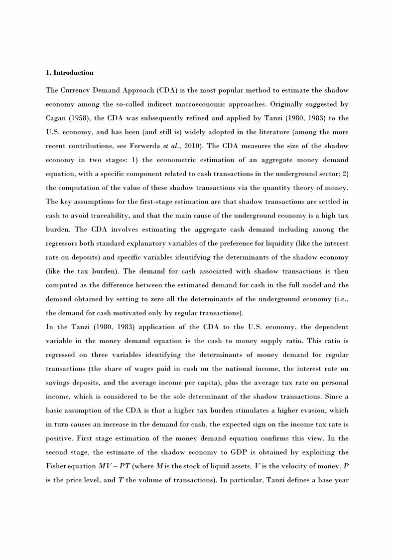
1. Introduction

The Currency Demand Approach (CDA) is the most popular method to estimate the shadow

economy among the so-called indirect macroeconomic approaches. Originally suggested by

Cagan (1958), the CDA was subsequently refined and applied by Tanzi (1980, 1983) to the

U.S. economy, and has been (and still is) widely adopted in the literature (among the more

recent contributions, see Ferwerda et al., 2010). The CDA measures the size of the shadow

economy in two stages: 1) the econometric estimation of an aggregate money demand

equation, with a specific component related to cash transactions in the underground sector; 2)

the computation of the value of these shadow transactions via the quantity theory of money.

The key assumptions for the first-stage estimation are that shadow transactions are settled in

cash to avoid traceability, and that the main cause of the underground economy is a high tax

burden. The CDA involves estimating the aggregate cash demand including among the

regressors both standard explanatory variables of the preference for liquidity (like the interest

rate on deposits) and specific variables identifying the determinants of the shadow economy

(like the tax burden). The demand for cash associated with shadow transactions is then

computed as the difference between the estimated demand for cash in the full model and the

demand obtained by setting to zero all the determinants of the underground economy (i.e.,

the demand for cash motivated only by regular transactions).

In the Tanzi (1980, 1983) application of the CDA to the U.S. economy, the dependent

variable in the money demand equation is the cash to money supply ratio. This ratio is

regressed on three variables identifying the determinants of money demand for regular

transactions (the share of wages paid in cash on the national income, the interest rate on

savings deposits, and the average income per capita), plus the average tax rate on personal

income, which is considered to be the sole determinant of the shadow transactions. Since a

basic assumption of the CDA is that a higher tax burden stimulates a higher evasion, which

in turn causes an increase in the demand for cash, the expected sign on the income tax rate is

positive. First stage estimation of the money demand equation confirms this view. In the

second stage, the estimate of the shadow economy to GDP is obtained by exploiting the

Fisher equation MV = PT (where M is the stock of liquid assets, V is the velocity of money, P

is the price level, and T the volume of transactions). In particular, Tanzi defines a base year

3

in which the contribution of the shadow economy to GDP is assumed to be zero, and

computes the velocity of money as the ratio between the official GDP (PT) and the stock of

liquid assets (M). Assuming then that this velocity is the same for the regular economy and

the shadow sector, the value of the latter is obtained by multiplying V for the estimated

‘excess demand’ for cash.

Schneider and Enste (2000, 2002) identify and discuss many substantial drawbacks of the

CDA, pointing to three main criticisms of the basic assumptions of this methodology:1 the

absence of any transactions in the shadow economy in a given base year; the same velocity of

money in both the official and the irregular economy; the excessive tax burden as the only

determinant of the shadow economy. Our aim here is to contribute to the debate on the

measurement of the shadow economy by proposing a revision of the CDA that overcome all

these three drawbacks. In particular, we propose a ‘modified – CDA’ introducing three main

innovations to the traditional methodology: first, we take a direct measure of cash

transactions (the flow of cash withdrawn from bank accounts relative to total noncash

payments) as the dependent variable in the money demand equation, which avoid using the

Fisher equation; second, we include among covariates two distinct measures of ‘detected’ tax

evasion, in place of the tax burden level; finally, we also control for a new ‘criminal’

component of the shadow economy, considering money demand for illegal activities like drug

dealing and prostitution. We then propose an original application of this ‘modified – CDA’ to

Italy, a country where the weight of the shadow economy is remarkable compared to other

Western countries.

The remainder of the paper is structured as follows. Section 2 discusses the innovations we

introduce in the CDA, and how these help overcome (most of) the drawbacks highlighted by

Schneider and Enste (2000, 2002). In section 3 we present the application of our ‘modified –

CDA’ to Italy, discussing the model specification and the estimation results. In particular,

besides country level estimates, we examine also disaggregated territorial estimates for

country macro-areas. We finally include here a comparison with the estimates obtained in

other studies on Italy. Section 4 provides brief concluding remarks.

1 Ahumada et al. (2007) and Breusch (2005) point to critiques specifically related to econometric issues, partly addressed by Pickhardt and Sarda (2010) within the standard CDA approach.

4

2. Reinterpreting the Currency Demand Approach

Our starting point are the criticism to most of the assumptions of the traditional CDA

advanced by Schneider and Enste (2000, 2002). We focus here on three main issues: (1) the

hypothesis of the absence of any transactions in the shadow economy in a given base year is

rather unrealistic; (2) the assumption of equality in the velocity of money for both the official

and the irregular economy introduces a restriction in the estimation method which is not

justified on reasonable grounds; (3) also considering the excessive tax burden as the only

determinant of the shadow economy is a quite restrictive assumption, as other factors – such

as markets regulation (especially the labour market regulation), the trust in political

institutions, and the citizens’ tax morale – can substantially affect the decision to participate

in the underground sector.

To avoid these critiques, we introduce three innovations in this study as compared to the

traditional CDA a là Tanzi. First, instead of using the stock of liquid assets as the dependent

variable in the money demand equation, here we take a direct measure of cash transactions:

the flow of cash withdrawn from bank accounts with respect to total payments settled by

instruments other than cash. This is a substantial modification of the model, which eliminates

the need to rely on the quantitative theory of money and the Fisher equation. In this way, we

are able to overcome the critique (1), concerning the need to arbitrarily chose a base year for

calculating the velocity of money, and the critique (2), concerning the equality assumption of

the velocity of money in both the official economy and the shadow sector. Notice that the

cash withdrawals we refer to also help to deal with the problematic measurement of the stock

of liquid assets in each country of the EMU zone after the introduction of the euro, which can

severely limit the application of the traditional CDA.

Second, in order to answer critique (3), direct measures of detected tax evasion are included

among the factors determining the (irregular) transactions settled in cash. In this way, we

remove the need to identify a set of variables that can adequately capture all the relevant

determinants of the phenomenon besides the level of tax burden, which is the key variable in

the classic Tanzi-approach and does not take into account the presence of other possible

factors underlying the decisions of noncompliance (e.g., Ferwerda et al., 2010; Schneider,

2010).

5

Finally, with reference again to criticism (3), we argue that evasion is just one component of

the shadow economy. Hence, the methodology we propose also controls for the presence of

criminal transactions. These are shadow transactions not motivated by a high tax burden or

other reasons which could lead a taxpayer to carry out legal productive activities usually

object of revenue collection by Tax Authorities in an irregular way. We consider in particular

two criminal activities like drug dealing and prostitution, which are illegal transactions

typically regulated in cash. Almost all scholars agree in classifying these among the activities

that make up the underground economy.2 According to the definition proposed, among

others, by Smith (1994, p. 18), «the shadow economy includes any market-based production of

goods and services, whether legal or illegal, that escapes detection in the official estimates of GDP».

Notice that these transactions identify a second important component of the shadow

economy, with distinct origins and different implications in terms of law enforcement policies.

The choices of individuals operating in the two sectors of the underground economy (evasion

and crime) are affected by different motivations and incentive mechanisms, including the role

played by deterrence actions. The two components also differ remarkably in terms of their

effects on public finances, as it is possible to identify potential revenue subtracted to Tax

Authorities only for shadow economy due to evasion. Despite these differences, the

decomposition of total shadow economy in tax evasion and crime is an issue rarely

investigated in the literature, mainly because of the difficulty in delineating the boundaries of

the analysis and the lack of reliable information.3 Here we focus on crime indicators related to

both drug dealing and prostitution, defining more precisely the excess demand of money due

to evasion and that due to crime, and introducing a third innovation with respect to the

traditional CDA.

2 See the classification originally proposed by Lippert and Walker (1997) and subsequently integrated by Schneider and Enste (2000, 2002) and Schneider (2010). 3 For a comprehensive analysis of the shadow economy in different countries with a discussion of the contribution of the two components, see the study by Thomas (1992). A recent application that takes into account the role of criminal activities and relies on the traditional CDA is Ferwerda et al. (2010). In particular, to reply to criticism (3) raised by Schneider and Enste (2000, 2002), the authors propose some modifications to the Tanzi-approach, by including in the model several proxies for the determinants of the shadow economy in substitution of the income tax rate. The variables considered are unemployment rate, government expenditure indicators, crime indicators, and measures of the degree of education and social inequality. However, the results are judged unsatisfactory by the authors, since none of the proxies adopted significantly explains the shadow economy as measured by excess demand for cash. The authors conclude therefore by highlighting the need to identify variables more closely related to the decision to operate in the underground sector. Our contribution goes just in this direction and also tries to disentangle the criminal component of the shadow economy.

6

3. An application of the ‘modified – CDA’

3.1. Defining the demand for cash payments

In this section of the paper we provide a first application of the ‘modified – CDA’ to a

balanced panel of 91 Italian provinces observed from 2005 to 2008. We first need to discuss

the definition of the demand for cash payments, and then its determinants. As for the

demand of cash payments, departing from the standard CDA, we exploit information on the

flow of cash rather than the stock of liquid assets. Hence, we base our assessment of the size of

the shadow economy on a direct measure of the value of transactions at the provincial level.

In particular, the dependent variable in the estimated equation of the demand for cash

payments is the ratio of the value of cash withdrawn from bank accounts to the value of total

payments settled by instruments other than cash (CASH). This represents a measure of the

demand for untraced payments per euro of traceable ones (i.e., payments settled by bank

transfers, cheques, credit cards).

The transactions theory of money demand relies on liquid assets as such (e.g., M1) rather

than on the concept of payment, the latter necessarily implying a cash flow and precise

technical and organizational procedures by which these flows circulate in the economy.

However, even in the presence of reliable statistics, stock indicators can be highly inaccurate

for three reasons: a) quantifying the level of national currency used outside national borders

is problematic, and this is particularly true in the Euro area after the euro entered circulation

in 2002; b) a certain amount of money can be held for purposes other than transactions:

traditional theories of money demand discuss, for instance, the ‘speculative motive’ for

holding money reserves; c) the velocity of money is assumed to be constant with respect to

several GDP components, including the informal sector, without taking into account, inter

alia, trade in intermediate goods and services. Hence, there may be compensatory phenomena

within the same stock of banknotes in circulation, both between different purposes for

holding money reserves, and between the use of cash in the formal and the informal sector.

This is confirmed by the recent trend of the currency-to-GDP ratio in the countries belonging

to the G10 and to the Eurosystem: the ratio has remained stable or even increased since 2004

in those countries that should have been more affected by the replacement of banknotes with

digital money. Similar considerations hold for other stock-based indicators of currency

demand, such as the stocks of M1 (currency and deposits repayable on demand). Notice that –

7

although being a signal of a higher preference for liquidity – an increase in a stock-based

monetary aggregate is not informative about the underlying reasons, including for instance

the rebalancing of portfolio assets, the adjustment in liquidity buffers, the need to hide

transactions (whether for evading taxes or because they are illegal). The European Central

Bank has noted that, on the occasion of the so-called cash changeover, the stock of euro

banknotes in circulation has increased (even compared to M1 or M2) more than the previous

circulation of national currencies would have suggested (ECB, 2008). According to he ECB,

«this is reasonable, in particular, in an environment of low interest rates and low inflation

expectations», not to mention that an estimate up to 20% percent of banknotes in circulation

is held outside of the Euro area. It then becomes difficult – if not impossible – to estimate the

component of cash held to settle payments within the underground economy using stock

infomation. This is the reason why researchers need to select monetary indicators more

directly related to the transaction motive.

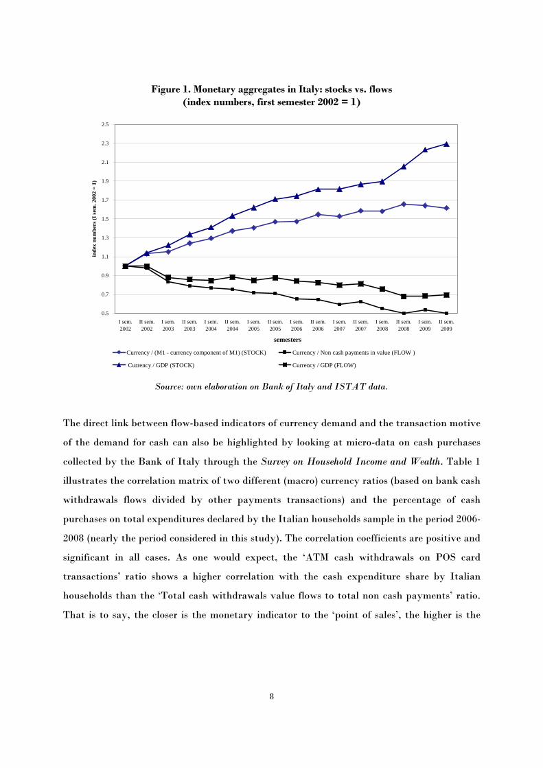
In order to better clarify this issue, Figure 1 shows the recent trends of the currency-to-GDP

and the currency-to-M1 ratios as compared to their respective flows in Italy. Two diverging

trends can be observed: the stocks show a rising trend, while the flows are declining. An

explanation of the increasing trend of stocks is given by the above mentioned explanation

provided by the ECB. The decreasing trend of flows is instead consistent with the diffusion of

electronic payment instruments in commercial transactions, which allow some substitution

between alternative instruments, at least in the formal economy. Furthermore, the common

trend of the two flow-based indicators confirms the higher coherence of these indicators with

the transaction motive of the demand for cash. The combined evidence of such a ‘substitution

effect’ of cash flows and the growing trend of the stock of banknotes suggests a slowing down

of the overall velocity of circulation of legal money in order to meet liquidity needs other than

purely transactional ones. All these considerations seem to support the criticisms raised to the

traditional CDA based on the quantity theory of money and the Fisher equation.

8

Figure 1. Monetary aggregates in Italy: stocks vs. flows (index numbers, first semester 2002 = 1)

0.5

0.7

0.9

1.1

1.3

1.5

1.7

1.9

2.1

2.3

2.5

I sem.2002

II sem.2002

I sem.2003

II sem.2003

I sem.2004

II sem.2004

I sem.2005

II sem.2005

I sem.2006

II sem.2006

I sem.2007

II sem.2007

I sem.2008

II sem.2008

I sem.2009

II sem.2009

semesters

inde

x nu

mbe

rs (I

sem

. 200

2 =

1)

Currency / (M1 - currency component of M1) (STOCK) Currency / Non cash payments in value (FLOW )

Currency / GDP (STOCK) Currency / GDP (FLOW)

Source: own elaboration on Bank of Italy and ISTAT data.

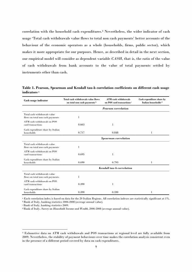
The direct link between flow-based indicators of currency demand and the transaction motive

of the demand for cash can also be highlighted by looking at micro-data on cash purchases

collected by the Bank of Italy through the Survey on Household Income and Wealth. Table 1

illustrates the correlation matrix of two different (macro) currency ratios (based on bank cash

withdrawals flows divided by other payments transactions) and the percentage of cash

purchases on total expenditures declared by the Italian households sample in the period 2006-

2008 (nearly the period considered in this study). The correlation coefficients are positive and

significant in all cases. As one would expect, the ‘ATM cash withdrawals on POS card

transactions’ ratio shows a higher correlation with the cash expenditure share by Italian

households than the ‘Total cash withdrawals value flows to total non cash payments’ ratio.

That is to say, the closer is the monetary indicator to the ‘point of sales’, the higher is the

9

correlation with the household cash expenditures.4 Nevertheless, the wider indicator of cash

usage ‘Total cash withdrawals value flows to total non cash payments’ better accounts of the

behaviour of the economic operators as a whole (households, firms, public sector), which

makes it more appropriate for our purposes. Hence, as described in detail in the next section,

our empirical model will consider as dependent variable CASH, that is, the ratio of the value

of cash withdrawals from bank accounts to the value of total payments settled by

instruments other than cash.

Table 1. Pearson, Spearman and Kendall tau-b correlation coefficients on different cash usage indicators a

Cash usage indicator Total cash withdrawals value flows on total non cash payments b

ATM cash withdrawals on POS card transactions c

Cash expenditure share by Italian households d

Pearson correlation

Total cash withdrawals value flows on total non cash payments 1

ATM cash withdrawals on POS card transactions 0.663 1

Cash expenditure share by Italian households 0.717

0.848 1

Spearman correlation

Total cash withdrawals value flows on total non cash payments 1

ATM cash withdrawals on POS card transactions 0.695 1

Cash expenditure share by Italian households 0.690

0.793 1

Kendall tau-b correlation

Total cash withdrawals value flows on total non cash payments 1

ATM cash withdrawals on POS card transactions 0.490 1

Cash expenditure share by Italian households 0.490

0.590 1

a Each correlation index is based on data for the 20 Italian Regions. All correlation indexes are statistically significant at 1%.

b Bank of Italy, banking statistics 2006-2008 (average annual value). c Bank of Italy, banking statistics 2009. d Bank of Italy, Survey on Household Income and Wealth, 2006-2008 (average annual value).

4 Exhaustive data on ATM cash withdrawals and POS transactions at regional level are fully available from 2009. Nevertheless, the stability of payment behaviours over time makes the correlation analysis consistent even in the presence of a different period covered by data on cash expenditures.

10

3.2. Defining the determinants of cash payments

In line with the discussion in Section 2, we classify the determinants of CASH in three

groups, thus identifying three components of the demand for cash payments: the structural

component, the tax evasion component, and the crime component. A description of the

variables affecting each of the three components is provided below. The Appendix reports

descriptive statistics and information on data sources (see Tables A1 and A2).

3.2.1. The structural component of the demand for cash payments

Drawing from the literature on the demand for cash (e.g., Goodhart and Krueger, 2001), we

identify four conventional determinants of the structural demand for cash payments: the

level of economic development; the degree of spatial diffusion of banking activities; the

technology of payments; the interest rate. The level of development of the (formal) economy

is measured by per capita GDP at the provincial level (YPC). As suggested by several

authors (e.g., Schneider and Enste, 2000; Schneider, 2010), YPC has a negative expected

sign: the higher the living standard, the lower the use of cash (and the higher the demand for

alternative payment instruments). Income is highly correlated to education (both general

education and ‘financial literacy’), and more education usually leads to a lower use of cash,

since more educated individuals show greater confidence in alternative payment instruments

(World Bank, 2005; Ferwerda et al., 2010).

We use the number of per capita bank accounts (BANK) as a proxy of the spatial diffusion of

banking activities, thus controlling for the structural impact of the degree of bank branches

diffusion in provincial economies on the demand for cash payments. The expected sign of

BANK coefficient is negative, as a higher diffusion of current accounts reduces the need to

withdraw cash from ATMs for payments.

Several studies (e.g., Drehmann and Goodhart, 2000; Goodhart and Krueger, 2001; Schneider,

2009) emphasize the importance of the technology of payments, with a particular reference to

the supply of electronic instruments. We account for available technology by including the

variable ELECTRO among the structural determinants of CASH. ELECTRO measures the

ratio of the value of transactions settled by electronic payments to provincial GDP. Since a

higher share of electronic transactions (via POS and internet banking) implies a lower number

of cash transactions, the expected sign of the ELECTRO coefficient is negative.

11

The interest rate on bank deposits INT is the fourth determinant of the structural

component of CASH. Based on standard economic theory, the interest rate is expected to

have a negative effect on the demand for money, via its role of opportunity cost of holding

cash in alternative to interest-bearing assets. Notice, however, that our model deals with cash

flows rather than stocks of liquid assets, which implies an ambiguous effect of the interest

rate.5 Higher interest rates might even have a positive impact on flows, for instance, by

pushing towards forms of cash raising alternative to the banking channel. However, due to

the usual ‘speculative’ motive, we can not exclude that the interest rate on bank deposits

may also negatively affect the propensity to withdraw cash in alternative to the use of other

payment instruments. Thus, the expected sign of the INT coefficient is a priori unclear.

3.2.2. The tax evasion component of the demand for cash payments

We innovate the traditional CDA by considering measures of detected tax evasion instead of

the usual variables proxying for the tax burden, like the (average) income tax rate.

Information on detected tax evasion are retrieved from a dataset concerning inspection

activities with law enforcement purposes by the Guardia di Finanza (the Italian tax police).

The availability of such information is particularly relevant for two reasons. First, as already

discussed above, many factors – beyond the burden of taxes and social security contributions

– would be likely to influence the decision to escape Tax Authorities (market regulation, tax

morale of citizens, efficiency of public administration, etc.), and each of such factors would

need a proper proxy.6 Second, since we aim at providing disaggregated territorial estimates of

the shadow economy, there are no data on the effective tax rate at the provincial level in

Italy, and the calculation of some measures of fiscal pressure for Italian provinces is not a

trivial task, as taxes are levied by four different levels of government. In order to overcome

these problems, we selected two variables that provide a direct measure of the diffusion of the

productive activities (partially or totally) unknown to Tax Authorities at the provincial level.

5 Several studies investigating the role of innovative payment systems in cash demand of Italian families (e.g., Ardizzi and Tresoldi, 2003; Lippi and Secchi, 2008; Alvarez and Lippi, 2009) point out that the progress in transaction technology may substantially reduce (or even eliminate) the impact of the interest rate on the cash demand of buyers. 6 For a discussion on the determinants of the agents’ decision to participate in the shadow economy, besides the fiscal burden, see, among the others, Friedman et al. (2000), Schneider and Enste (2000, 2002), Feld and Frey (2007), Dreher et al. (2009), Torgler and Schneider (2009), and Dreher and Schneider (2010).

12

EVAS1 is defined by the number of specific tax audits7 in a given province divided by its

sample mean value (this is a measure of tax evasion intensity at the provincial level) and then

weighed by a GDP concentration index.8 This latter standardization allows us to compare

provinces characterized by remarkable differences in the level of economic development, thus

avoiding attaching higher levels of tax evasion to provinces with a number of audits above

the sample mean. The second variable (EVAS2) accounts for irregularities detected by the

Guardia di Finanza during inspections to retailers. EVAS2 is given by the ratio of the

number of positive audits on cash registers and tax receipts to the number of existing POS in

the province.9 The standardization for the number of POS is made necessary by the high

variability in the presence of POS across provinces, which is likely to affect the opportunity

to evade (lower where the number of POS is higher). Considering the number of tax frauds

per unit of POS (instead of their absolute value) seems a proper way to control for these

differences at the provincial level. The inclusion of both EVAS1 and EVAS2 in our model is

motivated by the fact that the former refers to inspections which may relate to any assumed

fiscal irregularity (evasion of income and indirect taxes or social security contributions) in

any type of business, while the latter certainly detects only tax frauds in sales by retailers

(VAT and income tax evasion). Thus, EVAS1 and EVAS2 are expected to jointly provide a

more comprehensive evaluation of the tax evasion component of shadow economy.

3.2.3. The criminal component of the demand for cash payments

We introduce another innovation in the traditional CDA by computing an index of crime

(CRIME) to account for the illegal component of the shadow economy. CRIME is defined as

the share of crimes violating the laws on drugs and prostitution over the total number of

reported crimes in each considered province.10 The selection of the appropriate variables to

estimate the size of the criminal component of the shadow economy deserves a brief

explanation. Our choice of drug- and prostitution-related offenses is motivated by the focus

on illegal activities which – in line with the definition of both the shadow economy discussed

7 These audits are specific in the sense that they imply inspections to firms based on ex-ante information about frauds that occurred within a particular operation (e.g., payment of salaries) and/or are related to a single item of the tax base (e.g., income taxes or social security contributions). 8 The GDP concentration index is defined as the ratio of provincial GDP to its sample mean value. 9 Here positive stands for audits with detected evasion. The ratio is weighed for the GDP concentration index for the same reasons discussed above. 10 In analogy with tax evasion variables, also this indicator has been weighed by a GDP concentration index.

13

above (e.g., Smith, 1994) and the illegal economy provided by the OECD (2002) – imply an

exchange between a seller and a buyer relying on a mutual agreement and a voluntary cash

payment. Therefore, we excluded all those crimes which, to some extent, are based on the use

of violence made to persons or properties (burglary, extortion, etc), and then imply

‘payments’ which do not follow an ‘agreement’ between the thief, for instance, and the

victim.11 We also excluded those offences with possible ambiguous effects on the size of cash

withdrawals. This is, for instance, the case of thefts, which could also have a negative impact

on CASH due to the fact that – in an area were more robberies occur – individuals will find

too dangerous to hold money in cash. In essence, our choice is consistent with the model to be

estimated, which exploits information on cash withdrawals from bank accounts motivated by

a voluntary transactional motive.

3.3. Estimation methodology and results

Equation [1] provides the complete model of the demand for cash payments to be estimated,

that is, the structural demand reflecting the ordinary preference for liquidity augmented by

the two components of the shadow economy, evasion and crime:

itititit

ititititit

CRIMEαEVASαEVASαINTαELECTROαBANKαYPCααCASH

ε++++++++=

765

43210

21

[1]

We apply model [1] to a balanced panel of 91 Italian provinces observed from 2005 to 2008.

By this, we depart from the existing CDA literature on Italy, which has so far dealt with

country-level data. The units included in the sample represent about 90% of all the Italian

provinces (103), and are those for which complete information were available for all the

variables included in Equation [1].

The panel structure of the database allows us to account for the existence of unobservable

residual heterogeneity across provinces. To this end, we used a random-effects Tobit model

(Wooldridge, 2002). This model has the advantage – as compared to a standard panel

regression with individual random effects – to accommodate for the particular distribution of

11 We do not account for money laundering in our analysis, since this is a criminal offense which results from other underlying criminal activities that amplifies in a cumulative way the impact of organized crime on both regular and irregular economies. The definition of recycling implies that the income stemming from a crime needs to be ‘cleaned up’ through the legal channel (e.g., bank transactions) in order to lower the likelihood for the criminal agent of being caught. After this, the ‘cleaned up’ money can be reinvested in legal activities.

14

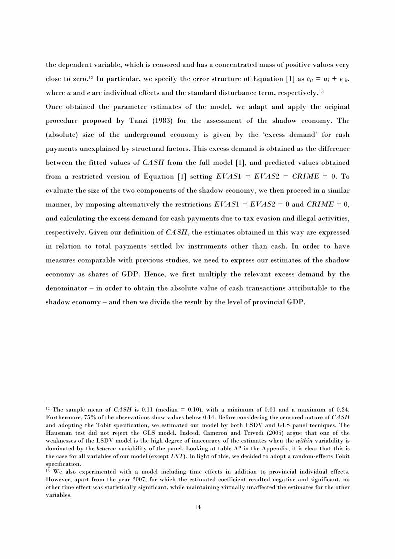
the dependent variable, which is censored and has a concentrated mass of positive values very

close to zero.12 In particular, we specify the error structure of Equation [1] as εit = ui + e it,

where u and e are individual effects and the standard disturbance term, respectively.13

Once obtained the parameter estimates of the model, we adapt and apply the original

procedure proposed by Tanzi (1983) for the assessment of the shadow economy. The

(absolute) size of the underground economy is given by the ‘excess demand’ for cash

payments unexplained by structural factors. This excess demand is obtained as the difference

between the fitted values of CASH from the full model [1], and predicted values obtained

from a restricted version of Equation [1] setting EVAS1 = EVAS2 = CRIME = 0. To

evaluate the size of the two components of the shadow economy, we then proceed in a similar

manner, by imposing alternatively the restrictions EVAS1 = EVAS2 = 0 and CRIME = 0,

and calculating the excess demand for cash payments due to tax evasion and illegal activities,

respectively. Given our definition of CASH, the estimates obtained in this way are expressed

in relation to total payments settled by instruments other than cash. In order to have

measures comparable with previous studies, we need to express our estimates of the shadow

economy as shares of GDP. Hence, we first multiply the relevant excess demand by the

denominator – in order to obtain the absolute value of cash transactions attributable to the

shadow economy – and then we divide the result by the level of provincial GDP.

12 The sample mean of CASH is 0.11 (median = 0.10), with a minimum of 0.01 and a maximum of 0.24. Furthermore, 75% of the observations show values below 0.14. Before considering the censored nature of CASH and adopting the Tobit specification, we estimated our model by both LSDV and GLS panel tecniques. The Hausman test did not reject the GLS model. Indeed, Cameron and Trivedi (2005) argue that one of the weaknesses of the LSDV model is the high degree of inaccuracy of the estimates when the within variability is dominated by the between variability of the panel. Looking at table A2 in the Appendix, it is clear that this is the case for all variables of our model (except INT). In light of this, we decided to adopt a random-effects Tobit specification. 13 We also experimented with a model including time effects in addition to provincial individual effects. However, apart from the year 2007, for which the estimated coefficient resulted negative and significant, no other time effect was statistically significant, while maintaining virtually unaffected the estimates for the other variables.

15

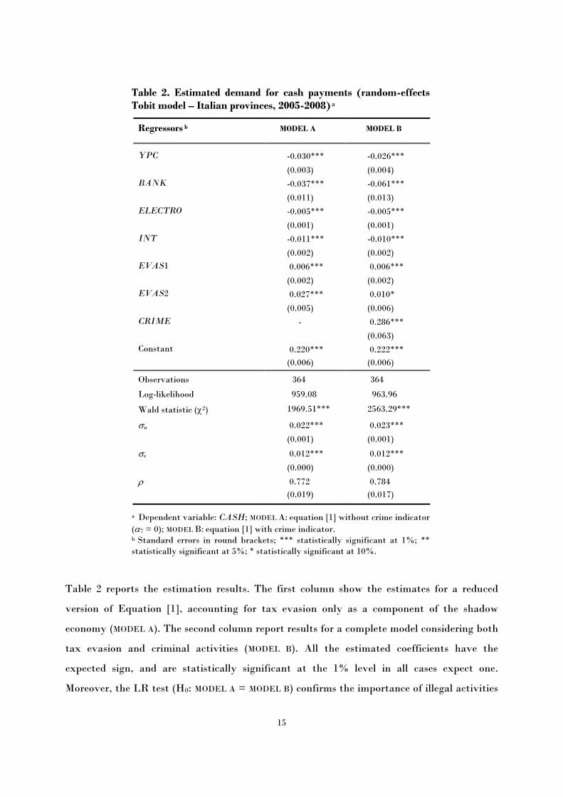
Table 2. Estimated demand for cash payments (random-effects Tobit model – Italian provinces, 2005-2008) a

Regressors b MODEL A MODEL B

YPC -0.030*** -0.026*** (0.003) (0.004) BANK -0.037*** -0.061*** (0.011) (0.013) ELECTRO -0.005*** -0.005*** (0.001) (0.001) INT -0.011*** -0.010*** (0.002) (0.002) EVAS1 0.006*** 0.006*** (0.002) (0.002) EVAS2 0.027*** 0.010* (0.005) (0.006) CRIME - 0.286*** (0.063) Constant 0.220*** 0.222*** (0.006) (0.006)

Observations 364 364

Log-likelihood 959.08 963.96

Wald statistic (χ2) 1969.51*** 2563.29***

σu 0.022*** 0.023*** (0.001) (0.001)

σe 0.012*** 0.012***

(0.000) (0.000)

ρ 0.772 0.784 (0.019) (0.017)

a Dependent variable: CASH; MODEL A: equation [1] without crime indicator (α7 = 0); MODEL B: equation [1] with crime indicator. b Standard errors in round brackets; *** statistically significant at 1%; ** statistically significant at 5%; * statistically significant at 10%.

Table 2 reports the estimation results. The first column show the estimates for a reduced

version of Equation [1], accounting for tax evasion only as a component of the shadow

economy (MODEL A). The second column report results for a complete model considering both

tax evasion and criminal activities (MODEL B). All the estimated coefficients have the

expected sign, and are statistically significant at the 1% level in all cases expect one.

Moreover, the LR test (H0: MODEL A = MODEL B) confirms the importance of illegal activities

16

(drug dealing and prostitution) for assessing the overall extent of shadow economy based on

the CDA, as the inclusion of CRIME significantly improves the goodness of fit of the model

(χ2(1) = 9.76, p-value = 0.002). Finally, for both specifications the coefficient ρ – which

measures the proportion of total residual variance explained by individual effects (u) in

relation to the proportion explained by noise (e) – is close to 0.80, highlighting the importance

of using panel techniques, in order to control for the presence of unobserved heterogeneity

due to provincial-specific idiosyncratic random shocks.

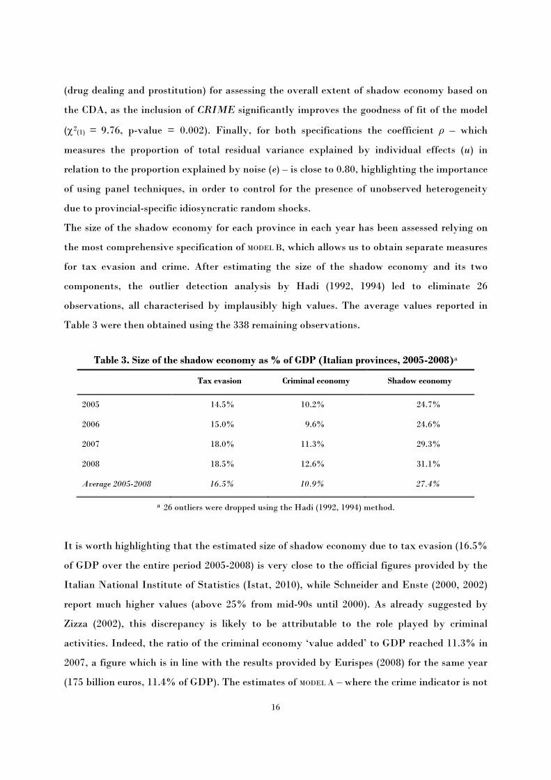
The size of the shadow economy for each province in each year has been assessed relying on

the most comprehensive specification of MODEL B, which allows us to obtain separate measures

for tax evasion and crime. After estimating the size of the shadow economy and its two

components, the outlier detection analysis by Hadi (1992, 1994) led to eliminate 26

observations, all characterised by implausibly high values. The average values reported in

Table 3 were then obtained using the 338 remaining observations.

Table 3. Size of the shadow economy as % of GDP (Italian provinces, 2005-2008)a

Tax evasion Criminal economy Shadow economy

2005 14.5% 10.2% 24.7%

2006 15.0% 9.6% 24.6%

2007 18.0% 11.3% 29.3%

2008 18.5% 12.6% 31.1%

Average 2005-2008 16.5% 10.9% 27.4%

a 26 outliers were dropped using the Hadi (1992, 1994) method.

It is worth highlighting that the estimated size of shadow economy due to tax evasion (16.5%

of GDP over the entire period 2005-2008) is very close to the official figures provided by the

Italian National Institute of Statistics (Istat, 2010), while Schneider and Enste (2000, 2002)

report much higher values (above 25% from mid-90s until 2000). As already suggested by

Zizza (2002), this discrepancy is likely to be attributable to the role played by criminal

activities. Indeed, the ratio of the criminal economy ‘value added’ to GDP reached 11.3% in

2007, a figure which is in line with the results provided by Eurispes (2008) for the same year

(175 billion euros, 11.4% of GDP). The estimates of MODEL A – where the crime indicator is not

17

included – confirms that neglecting the component of the criminal economy in the application

of the CDA leads to overestimate shadow economy related to tax non-compliance: when

compared with MODEL B, MODEL A leads to higher values, 21.4% on average in 2005-2008, not

far from the estimates presented by Schneider (2010), but below the sum of tax evasion and

criminal economy estimated in MODEL B (27.4%).14 Hence, ignoring crime as a component of

the shadow economy brings about two possible measurement errors: muddling up tax evasion

and illegal behaviours, on the one side, and under-estimating the total size of the shadow

economy, on the other.

With reference to the temporal dynamics, one can observe an increasing trend from 2005 to

2008 for both components, although the increase appears more marked for tax evasion (+4%)

compared to the criminal economy (+2.4%), with a sharp jump in the transition from 2006 to

2007 (+3% and +1.7%, respectively). Such evidence may be, at least in part, due to the fact

that in 2007 the Italian economy, like other countries in the euro zone, began to suffer the

cyclical downturn caused by the severe world financial crisis, with a sharp slowdown in

consumptions and investments and a strong deterioration in firms’ trust indicators (Bank of

Italy, 2007). The negative expectations of the operators may then have led to an increased

subtraction of taxable income to Fiscal Authorities, and a more marked use of the black

labour market, and/or even to turn to illegal sectors of the economy (e.g., prostitution, drug

dealing).15

Finally, the assessment of the two components of the underground economy is of particular

interest in the Italian case. In the light of the marked regional differentials in tax bases and

the concentration of the organized crime in specific regions, at least two questions deserve to

be explored. First, given the higher degree of economic and industrial development of the

Central-Northern regions, does the size of shadow economy from tax evasion differ between

the North and the South of the country? Second, does the prevalent localization of the

‘headquarters’ of criminal organizations in the South of Italy imply a higher contribution of 14 The average incidence of the shadow economy estimated by Schneider (2010) in the years 2005-2007 amounted to 23.3% of GDP. However, it is worth remarking that - as the estimates for the more recent years were derived from a combination of the MIMIC method with the CDA - the comparison in this case is more difficult than for the values computed up to 2000 and presented in Schneider and Enste (2000, 2002). For additional details, see Schneider (2010). 15 Note that these changes in the economic cycle involve likely variations in the velocity of money, which presumably fell in the official economy and increased in the underground sector. This further supports the adoption of an estimation approach – such as the ‘revised – CDA’ proposed here – that overcomes the restriction of the velocity of money constant over time and identical between regular and underground economy.

18

the Southern regions to the formation of the illegal component of the shadow economy? Or,

instead, is it reasonable to expect minor territorial differences, due to the high mobility of

criminal resources?

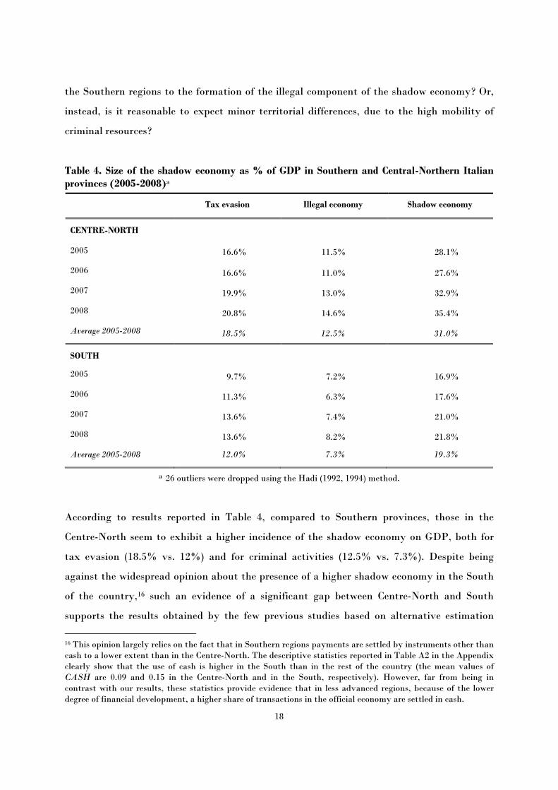
Table 4. Size of the shadow economy as % of GDP in Southern and Central-Northern Italian provinces (2005-2008)a

Tax evasion Illegal economy Shadow economy

CENTRE-NORTH

2005 16.6% 11.5% 28.1%

2006 16.6% 11.0% 27.6%

2007 19.9% 13.0% 32.9%

2008 20.8% 14.6% 35.4%

Average 2005-2008 18.5% 12.5% 31.0%

SOUTH

2005 9.7% 7.2% 16.9%

2006 11.3% 6.3% 17.6%

2007 13.6% 7.4% 21.0%

2008 13.6% 8.2% 21.8%

Average 2005-2008 12.0% 7.3% 19.3%

a 26 outliers were dropped using the Hadi (1992, 1994) method.

According to results reported in Table 4, compared to Southern provinces, those in the

Centre-North seem to exhibit a higher incidence of the shadow economy on GDP, both for

tax evasion (18.5% vs. 12%) and for criminal activities (12.5% vs. 7.3%). Despite being

against the widespread opinion about the presence of a higher shadow economy in the South

of the country,16 such an evidence of a significant gap between Centre-North and South

supports the results obtained by the few previous studies based on alternative estimation

16 This opinion largely relies on the fact that in Southern regions payments are settled by instruments other than cash to a lower extent than in the Centre-North. The descriptive statistics reported in Table A2 in the Appendix clearly show that the use of cash is higher in the South than in the rest of the country (the mean values of CASH are 0.09 and 0.15 in the Centre-North and in the South, respectively). However, far from being in contrast with our results, these statistics provide evidence that in less advanced regions, because of the lower degree of financial development, a higher share of transactions in the official economy are settled in cash.

19

methodologies. Relying on time series from the early 80s to the late 90s, Bovi et al. (2002) find

several periods with higher tax evasion in the North (either North-East or North-West,

depending on the years) than in the South. More recently, looking at data on personal income

taxation (IRPEF) and productive activities taxation (IRAP), Marino and Zizza (2008) and

Pisani and Polito (2006) both conclude that in many cases tax evasion is higher in the Centre-

North than in the rest of the country. The results delivered in 2011 by the Working Group

Economia non osservata e flussi finanziari (literally, ‘Unobserved economy and financial

flows’) – established by the Ministry of Economy and chaired by the President of the Italian

Statistical Office – go in the same direction. Finally, a recent survey by one of the three

biggest unions shows the significant increase in the diffusion of irregular workers in the

Northern regions (UIL, 2011). As for the criminal component of the shadow economy, the

higher incidence observed for the Centre-North is probably justified by the fact that the use

of cash for illegal transactions related to criminal activities is higher where the ‘retail

markets’ for goods and services such as drug and prostitution are more lucrative. Hence,

despite criminal organizations having their ‘headquarters’ predominantly localized in the

South, our evidence seems to suggest their ability to export illegal activities in the richest

areas of the country.17

4. Conclusions

In this paper we contribute to the debate on assessing the size of the shadow economy by

providing a reinterpretation of the CDA a là Tanzi, which aims at overcoming its most

relevant weaknesses highlighted in Scheider and Enste (2000, 2002). Our main contributions

can be summarized as follows. First, we introduce a direct measure of cash transactions as the

dependent variable in the money demand equation. In particular, we use the flow of cash

withdrawn from bank accounts with respect to total noncash payments in substitution of the

traditional money stock variable. This departure from the standard CDA has made possible

to avoid using the Fisher equation, and the associated unrealistic assumptions of a common

velocity of money in both the regular and the irregular sectors. Second, instead of considering

the tax burden as the only determinant of a multi-faceted behaviour, we capture the ‘excess

17 The ability of criminal organizations to ‘export’ their businesses is not new in the literature. It has been discussed, e.g., in Varese (2011).

20

demand’ for cash payments due to tax evasion by using two measures of detected tax non-

compliance, thus avoiding finding suitable proxies able to capture all the relevant causes of

the phenomenon. Third, besides evasion, we identify a criminal component of the shadow

economy, by introducing an appropriate determinant of the demand for money due to crime.

We present an application of this ‘modified – CDA’ exploiting original data on monetary

variables, tax evasion and reported illegal activities for the Italian Provinces over the period

2005-2008. Our results show an average value of the shadow economy due to evasion up to

16.5% of GDP, which is consistent with the recent estimates available from official statistical

sources relying on microeconomic methods of measurement, but appears to be lower than the

values obtained for Italy in the international literature (e.g., Schneider and Enste, 2000, 2002

and Schneider, 2010). We show that this discrepancy is likely to be due to the omission of

criminal activities in the application of the traditional CDA. Not surprisingly, when the

model accounts for shadow criminal transactions, our estimates of the shadow economy

increase by about 11% of GDP. This evidence points out that, ignoring illegal activities, one

could not only mistakenly attribute to evasion a part of the shadow economy due to criminal

transactions – for which it is not possible to implement law enforcement policies to recover

lost tax revenues –, but could also underestimate the total value of underground economy.

Given the availability of relevant information at a disaggregated territorial level, we also

provide estimates of the shadow economy by macro-areas. This is an important step in the

understanding of the underground economy and its size, because of the marked North-South

divide in the level of economic development, institutional quality and social capital in Italy.

The evidence we provide suggests that, compared to Southern provinces, those in the Centre-

North exhibit a higher incidence of the shadow economy relative to GDP, both for tax

evasion and crime. While the result on crime provides fresh insights on the ability of criminal

organizations to ‘export’ illegal activities (especially prostitution and drug dealing) in the

richest areas where the demand is presumably higher, the finding concerning tax evasion

stimulates future research on the determinants of this higher propensity to evade in the

North of the country.

21

References

Ahumada, H., Alvaredo, F. and Canavese, A. (2007), “The Monetary Method and the Size of

the Shadow Economy: A Critical Assessment”, Review of Income and Wealth, 53(2), 363-

371.

Alvarez, F. and Lippi, F. (2009), “Financial Innovation and the Transactions Demand for

Cash”, Econometrica, 77(2), 363-402.

Ardizzi, G. and Tresoldi, C. (2003), “Spunti di riflessione sull’uso del contante nei pagamenti”,

Banca Impresa Società, 2, 153-188.

Bank of Italy (2007), Relazione Annuale, Rome.

Bank of Italy (various years), Survey on Household Income and Wealth, Rome.

Bovi, M., Hermann, A., Pappalardo, C. and Sica, F. (2002), “Il sommerso: cause, intensità

territoriali, politiche di regolarizzazione”, in ISAE (a cura di), Rapporto Trimestrale –

Priorità nazionali: trasparenza, flessibilità, opportunità, n. 9, 55-100.

Breusch, T. (2005), Fragility of Tanzi’s Method of Estimating the Underground Economy,

Working Paper, School of Economics, Australian National University: Canberra.

Cagan, P. (1958), “The Demand for Currency Relative to Total Money Supply”, Journal of

Political Economy, 66, 303-328.

Cameron, A.C., and Trivedi, P.K. (2005), Microeconometrics: Methods and Applications,

Cambridge University Press, New York.

Dreher, A. and Schneider, F. (2010), “Corruption and the Shadow Economy: An Empirical

Analysis”, 144(2), Public Choice, 215-238.

Dreher, A., Kotsogiannis, C. and McCorriston, S. (2009), “How Do Institutions Affect

Corruption and the Shadow Economy?”, International Tax and Public Finance, 16(4),

773-796.

Drehmann, M. and Goodhart, C.A.E. (2000), Is Cash Becoming Technologically Outmoded? Or

Does it Remain Necessary to Facilitate Bad Behaviour? An Empirical Investigation into the

Determinants of Cash Holdings, Financial Markets Group Research Centre, Discussion

Paper 358, LSE.

Eurispes (2008), Rapporto Italia 2008, Istituto di Studi Politici Economici e Sociali, Rome.

European Central Bank (2008), Economic Bulletin, special edition, May.

22

Feld, L. and Frey, B.S. (2007), “Tax Compliance as the Result of a Psychological Tax

Contract: The Role of Incentives and Responsive Regulation”, Law and Policy, 29(1), 102-

120.

Ferwerda, J, Deleanu, I. and Unger, B. (2010), Revaluating the Tanzi-Model to Estimate the

Underground Economy, Tjalling C. Koopmans Research Institute, Discussion Paper 10-04,

Utrecht School of Economics, February.

Friedman, E., Johnson, S., Kaufmann, D. and Zoido-Lobatón, P. (2000), “Dodging the

Grabbing Hand: The Determinants of Unofficial Activity in 69 Countries”, 76(3), Journal

of Public Economics, 459-493.

Goodhart, C. and Krueger, M (2001), The Impact of Technology on Cash Usage, Financial

Markets Group Research Centre, Discussion Paper 374, LSE.

Hadi, A.S. (1992), “Identifying Multiple Outliers in Multivariate Data”, Journal of the Royal

Statistical Society, Series B, 54, 761-771.

Hadi, A.S. (1994), “A Modification of a Method for the Detection of Outliers in Multivariate

Samples”, Journal of the Royal Statistical Society, Series B, 56, 393-396.

Istat (2010), “La misura dell’economia sommersa secondo le statistiche ufficiali. Anni 2000-

2008”, Conti Nazionali – Statistiche in Breve, Istituto Nazionale di Statistica, Rome.

Lippert, O. and Walker M. (1997), The Underground Economy: Global Evidences of its Size and

Impact, Vancouver: The Frazer Institute.

Lippi., F. and Secchi, A. (2008), Technological Change and the Demand for Currency: An

Analysis with Household Data, Bank of Italy, Temi di Discussione, Nr. 697, Roma.

Marino, M.R. and Zizza, R. (2008), L’evasione dell’Irpef: una stima per tipologia di

contribuente, mimeo, Bank of Italy, Rome.

OECD (2002), Measuring the Non-Observed Economy – A Handbook, Paris.

Pickhardt, M. and Sarda J. (2010), The Size of the Underground Economy in Germany: A

Correction of the Record and New Evidence from the Modified-Cash-Deposit-Ratio Approach,

Institute of Spatial and Housing Economics, Working Paper 201036, University of

Münster.

Pisani, S. and Polito C. (2006), Analisi dell’evasione fondata sui dati IRAP – Anni 1998-2002,

Ministero dell’Economia e delle Finanze, Agenzia dell’Entrate, Documenti di lavoro

dell’Ufficio Studi.

23

Schneider, F (2010), “The Influence of Public Institutions on the Shadow Economy: An

Empirical Investigation for OECD Countries”, Review of Law and Economics, 6(3), 441-

468.

Schneider, F. (2009), The Shadow Economy in Europe. Using Payment Systems to Combat the

Shadow Economy, A.T. Kearney Research Report, September.

Schneider, F. and Enste D.H. (2000), “Shadow Economies: Size, Causes and Consequences”,

Journal of Economic Literature, 38(1), 77-114.

Schneider, F. and Enste, D.H. (2002), The Shadow Economy: Theoretical Approaches,

Empirical Studies, and Political Implications, Cambridge University Press, UK.

Smith, P. (1994), “Assessing the Size of the Underground Economy: The Canadian Statistical

Perspectives”, Canadian Economic Observer, 7(5), May.

Tanzi, V. (1980), “The Underground Economy in the United States: Estimates and

Implications”, Banca Nazionale del Lavoro Quarterly Review, 135(4), 427-453.

Tanzi, V. (1983), “The Underground Economy in the United States: Annual Estimates 1930-

1980”, IMF Staff Papers, 30(2), 283-305.

Thomas, J.J. (1992), Informal Economic Activity, LSE Handbooks in Economics, London:

Harvester Wheatsheaf.

Torgler, B. and Schneider F. (2009) “The Impact of Tax Morale and Institutional Quality on

the Shadow Economy”, Journal of Economic Psychology, 30(2), 228-245.

UIL (2011), 2° Rapporto UIL sul lavoro sommerso, Servizio Politiche del Lavoro e della

Formazione, Rome.

Varese, F. (2011), Mafias on the Move: How Organized Crime Conquers New Territories,

Princeton University Press, Princeton.

Wooldridge, J.M. (2002), Econometric Analysis of Cross Section and Panel Data, MIT Press,

Cambridge, Massachusetts.

World Bank (2005), International Migration, Remittances, and the Brain Drain, M. Schiff and

C. Ozden (eds.), Washington, D.C.

Zizza, R. (2002), Metodologie di stima dell’economia sommersa: un’applicazione al caso italiano,

Bank of Italy, Temi di Discussione, Nr. 463, December.

24

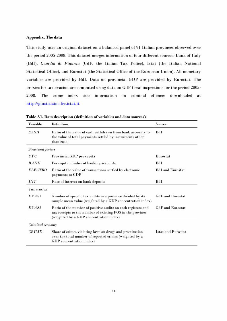
Appendix. The data

This study uses an original dataset on a balanced panel of 91 Italian provinces observed over

the period 2005-2008. This dataset merges information of four different sources: Bank of Italy

(BdI), Guardia di Finanza (GdF, the Italian Tax Police), Istat (the Italian National

Statistical Office), and Eurostat (the Statistical Office of the European Union). All monetary

variables are provided by BdI. Data on provincial GDP are provided by Eurostat. The

proxies for tax evasion are computed using data on GdF fiscal inspections for the period 2005-

2008. The crime index uses information on criminal offences downloaded at

http://giustiziaincifre.istat.it.

Table A1. Data description (definition of variables and data sources)

Variable Definition Source

CASH Ratio of the value of cash withdrawn from bank accounts to the value of total payments settled by instruments other than cash

BdI

Structural factors

YPC Provincial GDP per capita Eurostat

BANK Per capita number of banking accounts BdI

ELECTRO Ratio of the value of transactions settled by electronic payments to GDP

BdI and Eurostat

INT Rate of interest on bank deposits BdI

Tax evasion

EVAS1 Number of specific tax audits in a province divided by its sample mean value (weighted by a GDP concentration index)

GdF and Eurostat

EVAS2 Ratio of the number of positive audits on cash registers and tax receipts to the number of existing POS in the province (weighted by a GDP concentration index)

GdF and Eurostat

Criminal economy

CRIME Share of crimes violating laws on drugs and prostitution over the total number of reported crimes (weighted by a GDP concentration index)

Istat and Eurostat

25

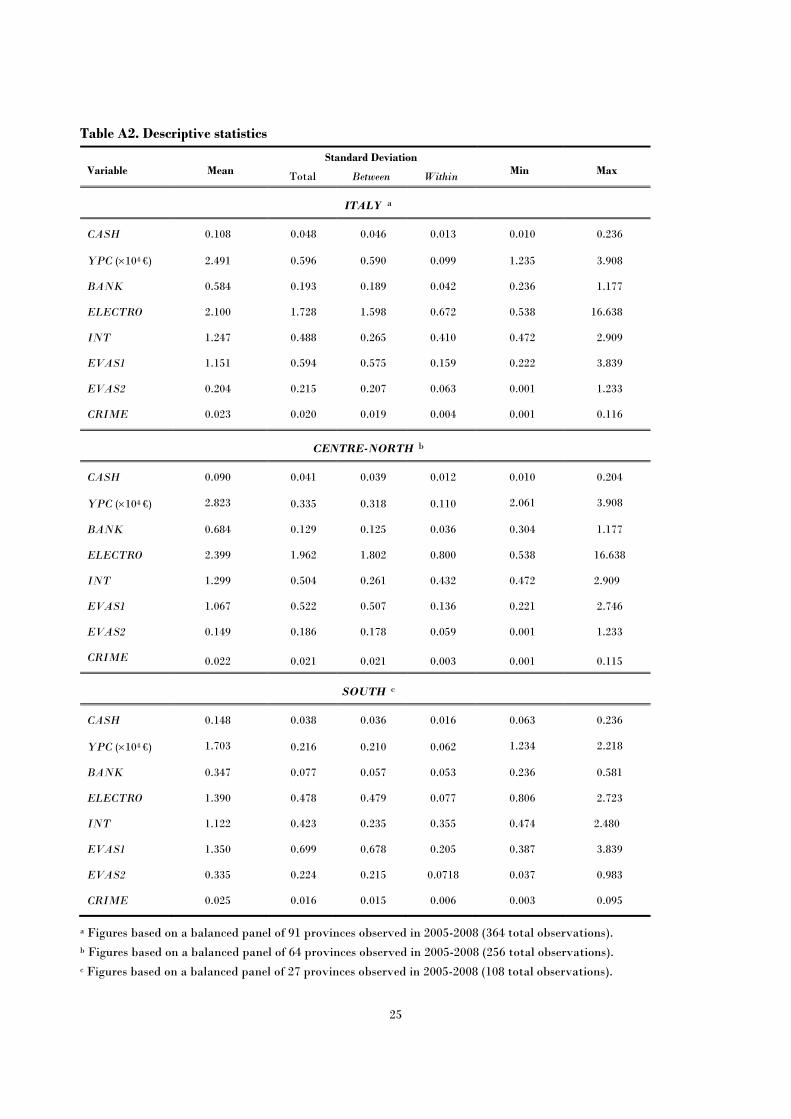
Table A2. Descriptive statistics

Variable Mean Standard Deviation

Min Max Total Between Within

ITALY a

CASH 0.108 0.048 0.046 0.013 0.010 0.236

YPC (×104 €) 2.491 0.596 0.590 0.099 1.235 3.908

BANK 0.584 0.193 0.189 0.042 0.236 1.177

ELECTRO 2.100 1.728 1.598 0.672 0.538 16.638

INT 1.247 0.488 0.265 0.410 0.472 2.909

EVAS1 1.151 0.594 0.575 0.159 0.222 3.839

EVAS2 0.204 0.215 0.207 0.063 0.001 1.233

CRIME 0.023 0.020 0.019 0.004 0.001 0.116

CENTRE-NORTH b

CASH 0.090 0.041 0.039 0.012 0.010 0.204

YPC (×104 €) 2.823 0.335 0.318 0.110 2.061 3.908

BANK 0.684 0.129 0.125 0.036 0.304 1.177

ELECTRO 2.399 1.962 1.802 0.800 0.538 16.638

INT 1.299 0.504 0.261 0.432 0.472 2.909

EVAS1 1.067 0.522 0.507 0.136 0.221 2.746

EVAS2 0.149 0.186 0.178 0.059 0.001 1.233

CRIME 0.022 0.021 0.021 0.003 0.001 0.115

SOUTH c

CASH 0.148 0.038 0.036 0.016 0.063 0.236

YPC (×104 €) 1.703 0.216 0.210 0.062 1.234 2.218

BANK 0.347 0.077 0.057 0.053 0.236 0.581

ELECTRO 1.390 0.478 0.479 0.077 0.806 2.723

INT 1.122 0.423 0.235 0.355 0.474 2.480

EVAS1 1.350 0.699 0.678 0.205 0.387 3.839

EVAS2 0.335 0.224 0.215 0.0718 0.037 0.983

CRIME 0.025 0.016 0.015 0.006 0.003 0.095

a Figures based on a balanced panel of 91 provinces observed in 2005-2008 (364 total observations). b Figures based on a balanced panel of 64 provinces observed in 2005-2008 (256 total observations). c Figures based on a balanced panel of 27 provinces observed in 2005-2008 (108 total observations).

DEPARTMENT OF ECONOMICS AND PUBLIC FINANCE “G. PRATO”

UNIVERSITY OF TORINO Corso Unione Sovietica 218 bis - 10134 Torino (ITALY)

Phone: +39 011 6706128 - Fax: +39 011 6706062 Web page: http://eco83.econ.unito.it/prato/