Measures of structural complexity in digital images formonitoring the ecological signature of an old-growthforest ecosystem

Raphael Proulx, Lael Parrott *

Complex Systems Laboratory, Department of Geography, University of Montreal, C.P. 6128 succursale Centre-ville, Montreal, Que.,

Canada H3C 3J7

e c o l o g i c a l i n d i c a t o r s 8 ( 2 0 0 8 ) 2 7 0 – 2 8 4

a r t i c l e i n f o

Article history:

Received 28 September 2006

Received in revised form

14 February 2007

Accepted 19 February 2007

Keywords:

Ecological orientor

Structural complexity

Imagery

Forest

Spatiotemporal dynamics

Shannon entropy

Mean information gain

a b s t r a c t

Conducting field samples for monitoring ecological dynamics across multiple spatiotem-

poral scales is a difficult task using standard protocols. One alternative is to measure a

restricted set of variables which can serve as an ecological orientor (EO) for quantifying

habitat change. The objective of this article is to derive from digital images a measure of

structural complexity that may serve as a proximate EO for monitoring forest dynamics in

space and time. The mean information gain (MIG) index was used as a measure of structural

complexity in photographs taken directly in the field over the entire growing season. At a

small scene extent, the complexity of light intensity variations in digital images was

positively related to species richness. At larger scene extents, forest understorey and

overstorey layers showed predictable ecological signatures in structural complexity. In

general, intensity and chroma were the two color space components which yielded the

greatest sensitivity to habitat change through time. Within the framework of a standardized

photographic protocol, it seems therefore reasonable to consider MIG as a suitable EO for

monitoring forest dynamics in both space and time. Our results support the idea that it is

possible on one hand to adopt a more holistic view of ecological processes to gain, on the

other hand, spatial and temporal degrees of freedom for testing multiple scale hypotheses in

the field.

# 2007 Elsevier Ltd. All rights reserved.

avai lable at www.sc iencedi rec t .com

journal homepage: www.e lsev ier .com/ locate /ecol ind

1. Introduction

It is well established that although mechanisms driving

ecological dynamics are not well understood at the commu-

nity (intermediate) level, ecosystem theory is nonetheless

supported by robust principles occurring at either larger (e.g.,

landscape scaling laws; Lawton, 1999; Gaston, 2000) or smaller

(e.g., individual based allometric laws; Turchin, 2001; Marquet

et al., 2005; West and Brown, 2005) levels of taxonomic

resolution (see also Simberloff, 2004). Notwithstanding this

fact, ecologists are now faced with the additional challenge of

* Corresponding author. Tel.: +1 514 343 8064; fax: +1 514 343 8008.E-mail addresses: raphael.proulx@umontreal.ca (R. Proulx), lael.pa

1470-160X/$ – see front matter # 2007 Elsevier Ltd. All rights reservedoi:10.1016/j.ecolind.2007.02.005

uncovering organizing principles governing ecological

dynamics across multiple spatial and temporal scales (Sole

et al., 1999; Brown et al., 2002; Storch and Gaston, 2004).

In this context, organizing principles in natural systems

may be regarded as an epiphenomenon of heuristic ecological

goal functions (Wilhelm and Bruggeman, 2000) which encom-

pass the formation of higher-level structures emerging from

lower-level interactions (Margalef, 1963; Christensen, 1995;

Ulanowicz, 2004; Muller, 2005). In the last century the search

for goal functions, also more properly termed ecological

orientors (EO) in Muller and Leupelt (1998), has spread so

rrott@umontreal.ca (L. Parrott).

d.

e c o l o g i c a l i n d i c a t o r s 8 ( 2 0 0 8 ) 2 7 0 – 2 8 4 271

widely among ecosystem theories that reviewing all of them

would necessitate an article length task. Any proximate EO (as

opposed to an absolute or universal one) is defined as the

quantity a living system tends to optimize, from a nonteleo-

logical view, in the course of its development. Contemporary

examples include concepts of: fitness, productivity, stability,

resilience, exergy, emergy, ascendancy, network efficiency,

metabolic activity, and criticality among others (Odum, 1969;

Kauffman, 1995; Muller and Leupelt, 1998; Jorgensen and

Muller, 2000; Fath et al., 2001). All these concepts are useful

descriptors of ecological communities, but share the common

drawback that their estimation requires excessively large

amounts of input data and variables that are difficult to

measure in the field.

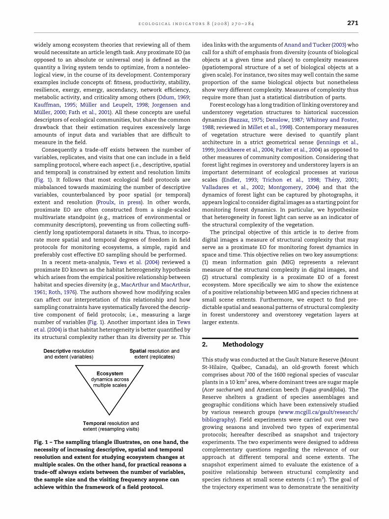
Consequently a trade-off exists between the number of

variables, replicates, and visits that one can include in a field

sampling protocol, where each aspect (i.e., descriptive, spatial

and temporal) is constrained by extent and resolution limits

(Fig. 1). It follows that most ecological field protocols are

misbalanced towards maximizing the number of descriptive

variables, counterbalanced by poor spatial (or temporal)

extent and resolution (Proulx, in press). In other words,

proximate EO are often constructed from a single-scaled

multivariate standpoint (e.g., matrices of environmental or

community descriptors), preventing us from collecting suffi-

ciently long spatiotemporal datasets in situ. Thus, to incorpo-

rate more spatial and temporal degrees of freedom in field

protocols for monitoring ecosystems, a simple, rapid and

preferably cost effective EO sampling should be performed.

In a recent meta-analysis, Tews et al. (2004) reviewed a

proximate EO known as the habitat heterogeneity hypothesis

which arises from the empirical positive relationship between

habitat and species diversity (e.g., MacArthur and MacArthur,

1961; Roth, 1976). The authors showed how modifying scales

can affect our interpretation of this relationship and how

sampling constraints have systematically favored the descrip-

tive component of field protocols; i.e., measuring a large

number of variables (Fig. 1). Another important idea in Tews

et al. (2004) is that habitat heterogeneity is better quantified by

its structural complexity rather than its diversity per se. This

Fig. 1 – The sampling triangle illustrates, on one hand, the

necessity of increasing descriptive, spatial and temporal

resolution and extent for studying ecosystem changes at

multiple scales. On the other hand, for practical reasons a

trade-off always exists between the number of variables,

the sample size and the visiting frequency anyone can

achieve within the framework of a field protocol.

idea links with the arguments of Anand and Tucker (2003) who

call for a shift of emphasis from diversity (counts of biological

objects at a given time and place) to complexity measures

(spatiotemporal structure of a set of biological objects at a

given scale). For instance, two sites may well contain the same

proportion of the same biological objects but nonetheless

show very different complexity. Measures of complexity thus

require more than just a statistical distribution of parts.

Forest ecology has a long tradition of linking overstorey and

understorey vegetation structures to historical succession

dynamics (Bazzaz, 1975; Denslow, 1987; Whitney and Foster,

1988; reviewed in Millet et al., 1998). Contemporary measures

of vegetation structure were devised to quantify plant

architecture in a strict geometrical sense (Jennings et al.,

1999; Jonckheere et al., 2004; Parker et al., 2004) as opposed to

other measures of community composition. Considering that

forest light regimes in overstorey and understorey layers is an

important determinant of ecological processes at various

scales (Endler, 1993; Trichon et al., 1998; Thery, 2001;

Valladares et al., 2002; Montgomery, 2004) and that the

dynamics of forest light can be captured by photographs, it

appears logical to consider digital images as a starting point for

monitoring forest dynamics. In particular, we hypothesize

that heterogeneity in forest light can serve as an indicator of

the structural complexity of the vegetation.

The principal objective of this article is to derive from

digital images a measure of structural complexity that may

serve as a proximate EO for monitoring forest dynamics in

space and time. This objective relies on two key assumptions:

(1) mean information gain (MIG) represents a relevant

measure of the structural complexity in digital images, and

(2) structural complexity is a proximate EO of a forest

ecosystem. More specifically we aim to show the existence

of a positive relationship between MIG and species richness at

small scene extents. Furthermore, we expect to find pre-

dictable spatial and seasonal patterns of structural complexity

in forest understorey and overstorey vegetation layers at

larger extents.

2. Methodology

This study was conducted at the Gault Nature Reserve (Mount

St-Hilaire, Quebec, Canada), an old-growth forest which

comprises about 700 of the 1600 regional species of vascular

plants in a 10 km2 area, where dominant trees are sugar maple

(Acer saccharum) and American beech (Fagus grandifolia). The

Reserve shelters a gradient of species assemblages and

geographic conditions which have been extensively studied

by various research groups (www.mcgill.ca/gault/research/

bibliography). Field experiments were carried out over two

growing seasons and involved two types of experimental

protocols; hereafter described as snapshot and trajectory

experiments. The two experiments were designed to address

complementary questions regarding the relevance of our

approach at different temporal and scene extents. The

snapshot experiment aimed to evaluate the existence of a

positive relationship between structural complexity and

species richness at small scene extents (<1 m2). The goal of

the trajectory experiment was to demonstrate the sensitivity

Fig. 2 – Schematic plane view of photographic settings in

snapshot and trajectory experiments. See Table 1 for

complementary information.

e c o l o g i c a l i n d i c a t o r s 8 ( 2 0 0 8 ) 2 7 0 – 2 8 4272

of our structural complexity measure in detecting habitat

related features and temporal variations at a larger scene

extent (up to 900 m2).

2.1. Photographic settings

Digital images were taken with a digital camera (EOS Rebel 6.3

MP, Canon Inc., Tokyo, Japan) equipped with a 18–55 mm lens

(EF-S f3.5-5.6, Canon Inc., Tokyo, Japan), which is roughly

equivalent to a 30–90 mm lens under 35 mm standards. The

photographic settings for each experiment are given in Table 1

and Fig. 2. Since both the aperture and the focal length were

fixed, the shutter speed was used as a measure of the

luminance (i.e., sum of all illumination sources reaching the

lens). Under the aperture priority mode, the camera uses its

internal light meter to optimally expose the scene by adjusting

the shutter speed. The exact relationship between scene

luminance and shutter speed is a specific function of the

settings in Table 1. The more illuminated the scene is; the

faster the shutter speed and vice versa. The illumination of a

forest scene is sensitive to the sun orientation (daylight hour),

the shooting direction, weather conditions, and canopy

closure. It is important to stress that the average intensity

in an image is independent of the scene luminance (see

below). Discussions and field excursions with a professional

photographer confirmed the above settings.

Commercial digital cameras, such as the one described

above, typically record images in the RGB (red, green and blue)

color space. Because in commercial cameras the distribution of

transmittances overlaps considerably among these three

spectral bands, the representation of each image was converted

to the HSV (hue, saturation and value) color space following

Smith (1978). This color representation is more natural to a

human observer since it separates the pure color component

(hue) from chroma (saturation) and intensity (value) compo-

nents. Color intuitively refers to the dominance of wavelengths

in the light signal. Intensity is the grey tone, that is, the

departure of a hue from black, the color of zero energy. Finally,

chroma is defined as how much the light spectrum differs from

boththepurecolor and theachromatic component (i.e., the grey

of the same intensity). The three components are expected be of

ecological relevance for quantifying structural complexity in

natural scenes (cf., Endler, 1993; Thery, 2001).

Table 1 – Photographic settings for snapshot (summer 2004) anMount St-Hilaire Reserve, Quebec, Canada

Setting Snapshot e

Focal length 55.0 mm

Light metering mode 35 segment

Aperture diameter 5.6 mm

Focus distance 1.25 m

Tripod’s head above ground 0.25 m

Depth of field (DF) 1.05–1.45 m

Exposure mode Aperture pr

Camera pointing direction Inward

Time window for shooting 11 h30–12 h

Visual obstruction < DF Manually cl

White balance mode Manual

Image size 3.2MP (ca. 1

2.2. Structural complexity measures

Measures of structural complexity were derived from digital

images by applying information theoretic indices on each

component of the HSV color space. Prior to the analysis, each

pixel value was linearly rescaled to an integer between 1 and

10. From the relative distribution of rescaled pixel values gi in

the image it is possible to calculate an index of aspatial

heterogeneity (dominance sensu O’Neill et al., 1988) using

Shannon’s formula for entropy:

H½g� ¼ �XN

i¼1

pðg iÞ log pðg iÞ; (1)

where p(gi) is the probability of observing a pixel value inde-

pendently of its location in the image (i.e., aspatial hetero-

geneity) and N is the number of frequency bins (categories) of

pixel values. Similarly, it is possible to calculate an index of

spatial heterogeneity (contagion sensu O’Neill et al., 1988) as

follows:

H½x� ¼ �XN4

i¼1

pðxiÞ log pðxiÞ; (2)

d trajectory (summer 2005) experiments performed at the

xperiment Trajectory experiment

18.0 mm

s evaluative 35 segments evaluative

6.3 mm

15.0 m

1.0 m

2.0 m–infinity

iority Aperture priority

Outward

30 9 h30–15 h30

eared Avoided

Natural light

000 � 3000) 1.6MP (ca. 1000 � 1500)

e c o l o g i c a l i n d i c a t o r s 8 ( 2 0 0 8 ) 2 7 0 – 2 8 4 273

whereherep(xi)denotestheprobabilityoffindingaspecific2 � 2

colored combinationxi in the image andN4 represents the num-

ber of theoretical 2 � 2 combinations. Since H[x] also expresses

the joint entropy (JE) among neighbor pixels we can write:

JE = H[x] = H[g(x,y), g(x+1,y), g(x+1,y+1), g(x,y+1)]. Superscripts in par-

entheses indicate relative locations to the right (x + 1, y), on the

diagonal (x + 1, y + 1), and underneath (x, y + 1) pixel coordinate

(x, y), thus returning different 2 � 2 squares of color combina-

tions. Following the same reasoning, H[g] represents the mar-

ginal entropy (ME) of the joint distribution. We can appreciate

from theabove observations that spatial heterogeneity depends

on the degree of aspatial heterogeneity in the image. For this

reason, to quantify structural complexity one needs an index

which is able to partition these two heterogeneity fractions.

The mean information gain (MIG) index was used to

quantify structural complexity (Andrienko et al., 2000) and

calculated as follows:

MIG ¼ H½x� �H½g�log N4 � log N1 ¼

JE�ME

log N4 � log N1 : (3)

MIG determines the amount of spatial heterogeneity (i.e.,

JE) that excludes the fraction devoted to aspatial heterogeneity

(i.e., ME). The fixed quantity (log N4 � log N1) represents the

maximum obtained for equiprobable distributions of both ME

and JE and it serves to normalize MIG estimates over the range

0–1. MIG is zero for uniform patterns and is maximal (MIG = 1)

for random ones. Although formula (3) predicts the existence

of a linear 1:1 relationship between ME and MIG for random

(structureless) processes, it is far from obvious why any linear

trend should hold in natural scenes, particularly at high ME

values (e.g., Fig. 3). Therefore, the presence of a relationship

other than 1:1 between structural complexity (i.e., MIG) and

aspatial heterogeneity (i.e., ME) in natural scenes might

suggest an intrinsic organizing process.

To avoid biasing the MIG index because not all possible 2 � 2

combinations are observable (sufficiently frequent) in the

image, the ratio of the total number of pixels to N4 should not

fallunder 100.Thisapproximation is based uponWolf’s formula

for a 1% relative precision (Wolf, 1999). Herein, we used N = 10,

which yielded a ratio of ca. 150 for the 1.6MP images (snapshot

experiment) and a ratio of ca. 600 for the 3.2MP ones (trajectory

experiment). The MIG index has been successfully used before

to study time-series in various ecological contexts (Klemm and

Lange, 1999; Lange, 1999) and is a well known complexity

measure in statistical physics (Wackerbauer et al., 1994).

Because MIG increases monotonously with spatial ran-

domness it may be difficult to assert which value amongst

several is the more complex in terms of its distance to

simplicity (see Parrott, 2005), as MIG can be anywhere between

the extremes of order (uniformity) and disorder (randomness).

To further investigate this aspect, the fourth-order mean

mutual information (MMI) was calculated on our images

(Wackerbauer et al., 1994) as:

MMI ¼ 4H½g� �H½x�4 log N1 � log N1 ¼

4ME� JE

4 log N1 � log N1 ; (4)

where the notation is the same as in formula (3). The MMI

function is maximal (MMI = 1) for uniform patterns and zero

for random ones; it indicates the presence of inherent spatial

correlations in the image. Lopez-Ruiz et al. (1995) proposed a

simple complexity index which tends to zero towards the

extremes of ordered and disordered patterns (see also Shiner

et al., 1999). Here, we can use their formalism to construct a

convex complexity index G from the interplay between MIG (as

a measure of disorder) and MMI (as a measure of order) as

follows:

G ¼ MIG�MMI (5)

Fig. 3 reports MIG, MMI, and G estimates obtained for a

gradient of spatial autocorrelation scales. For the present

purposes, G will be used to determine an intermediate MIG

value which identifies the critical state between order and

disorder in the dataset. This intermediate value will then serve

as a structural complexity orientor for interpreting the results.

MIG has two main advantages over G: (1) it is a well defined

index in statistical physics, and (2) it allows to the classifica-

tion of spatial patterns above (i.e., towards disorder) and below

(i.e., towards order) a critical state, a property not shared by G

(Shiner et al., 1999). All digital images were routinely processed

using batch routines in Matlab 6.5 (MathWorks Inc., Natick,

MA).

2.3. Snapshot experiment

From 7 June to 16 August 2004, diversity measures and digital

images were obtained at 225 sites. The sampling frame

consisted of a 0.5 m wide cubic quadrat made of small plastic

tubes. The frame was easy to dismount and to carry from place

to place in the Reserve. When a site was selected, the frame

was carefully mounted over the vegetation without disturbing

the material inside. Nine sites were simultaneously sampled

in 1 day. Each site was visited once during the season (i.e.,

snapshot) and purposely chosen to capture a mixture of biotic–

abiotic conditions (Fig. 4). These conditions ranged from rocky

summits to boggy lowlands, and from rangeland to forest

shade stands. More extreme conditions such as sites full of

woody debris, crowded with small boulders, or simply lying on

bare soils were also included to assess the robustness of the

method.

Each site was photographed around noon on two adjacent

sides of the cubic quadrat; the camera held outside and

pointing inward towards the quadrat (Fig. 2). For each image

the shutter speed was recorded and used as a proxy for the

luminance. To quantify biological diversity a complete survey

of the vegetation at each site was conducted. The survey

involved the identification of all fern, herb, shrub, and tree

species. A given species was counted whenever one of its

parts was visible inside the cubic quadrat. Additionally, the

total percent filling was estimated for all species together

using 10% increments. While percent cover serves to evaluate

the visual obstruction of a two-dimensional surface by

vegetation, percent filling aims at the same in three dimen-

sions. Thus, sites full of abiotic material received a low

percent filling value and heavily vegetated sites received high

values. Total percent filling inside each quadrat was eval-

uated by a single person from lateral obstruction estimates of

the vegetation.

Fig. 3 – Artificial ornaments created to return increasing (decreasing) MIG (MMI) values in the interval (0.2–0.7). Although

each image has a different MIG value, all have the maximal ME. For this reason, one cannot predict the presence of a

relationship between MIG and ME in a specific set of digital images, particularly at high ME values for non-random patterns,

since at this level the measure of structural complexity is less severely constrained by the aspatial heterogeneity (see text).

The convex complexity index G is maximal at intermediate MIG values and vanishes towards the extremes.

e c o l o g i c a l i n d i c a t o r s 8 ( 2 0 0 8 ) 2 7 0 – 2 8 4274

2.4. Trajectory experiment

This experiment was designed for monitoring temporal

fluctuations (i.e., trajectory) in structural complexity. Eighteen

sites were visited on a weekly basis for a total of 26 weeks from

May 10 to November 10 2005. The sites were visited in the same

sequence each week and sampled within a 48 h period from

Tuesday to Thursday. The 18 sampling sites were selected

from a larger set of 69 permanent stations put in place for

quantifying multivariate relationships between community,

environmental and geographic descriptors at the Gault

Reserve (Gilbert and Lechowicz, 2004). The final selection

was based on plant species lists (Gilbert, pers. commun.) and

direct observations in the field to ensure a suitable topography

for photographic purposes. Nine sites were located directly

above or right next to small creeks of varying width (ca. 0.2–

1.5 m), whereas another group of nine were located in drier

sites (Fig. 4). At the center of each site a steel rod was planted in

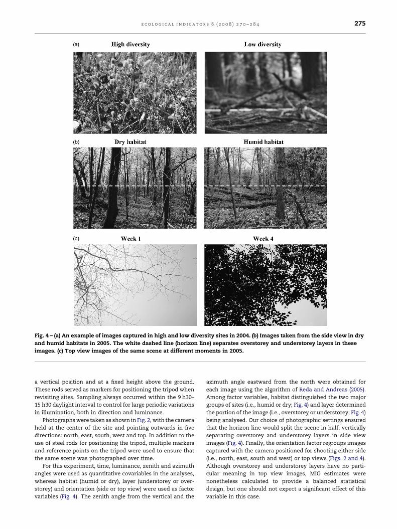
Fig. 4 – (a) An example of images captured in high and low diversity sites in 2004. (b) Images taken from the side view in dry

and humid habitats in 2005. The white dashed line (horizon line) separates overstorey and understorey layers in these

images. (c) Top view images of the same scene at different moments in 2005.

e c o l o g i c a l i n d i c a t o r s 8 ( 2 0 0 8 ) 2 7 0 – 2 8 4 275

a vertical position and at a fixed height above the ground.

These rods served as markers for positioning the tripod when

revisiting sites. Sampling always occurred within the 9 h30–

15 h30 daylight interval to control for large periodic variations

in illumination, both in direction and luminance.

Photographs were taken as shown in Fig. 2, with the camera

held at the center of the site and pointing outwards in five

directions: north, east, south, west and top. In addition to the

use of steel rods for positioning the tripod, multiple markers

and reference points on the tripod were used to ensure that

the same scene was photographed over time.

For this experiment, time, luminance, zenith and azimuth

angles were used as quantitative covariables in the analyses,

whereas habitat (humid or dry), layer (understorey or over-

storey) and orientation (side or top view) were used as factor

variables (Fig. 4). The zenith angle from the vertical and the

azimuth angle eastward from the north were obtained for

each image using the algorithm of Reda and Andreas (2005).

Among factor variables, habitat distinguished the two major

groups of sites (i.e., humid or dry; Fig. 4) and layer determined

the portion of the image (i.e., overstorey or understorey; Fig. 4)

being analysed. Our choice of photographic settings ensured

that the horizon line would split the scene in half, vertically

separating overstorey and understorey layers in side view

images (Fig. 4). Finally, the orientation factor regroups images

captured with the camera positioned for shooting either side

(i.e., north, east, south and west) or top views (Figs. 2 and 4).

Although overstorey and understorey layers have no parti-

cular meaning in top view images, MIG estimates were

nonetheless calculated to provide a balanced statistical

design, but one should not expect a significant effect of this

variable in this case.

Fig. 5 – Convex relationship between MIG and G for the

three color space components, for both trajectory and

snapshot experiments. Hue: solid (—); chroma: dotted

(- - -); intensity: dashed (– –). G is maximal when MIG is

close to the identified critical state of 0.4. The sample size

of each curve is n = 4705. Curves were smoothed using a

weighted moving average (LOWESS interpolator; tension

sets to 0.3) on raw estimates.

e c o l o g i c a l i n d i c a t o r s 8 ( 2 0 0 8 ) 2 7 0 – 2 8 4276

2.5. Statistical analyses

For both the snapshot and trajectory experiments, bivariate

regressions were assessed between ME and MIG for each

image component to determine their deviation from the 1:1

relationship predicted for random processes.

For the snapshot experiment, relationships were inspected

between: (1) MIG estimates on two adjacent sides of the same

cubic quadrat, (2) percent filling and MIG, and (3) species

richness and MIG, where MIG was independently calculated

for the color (hue), chroma (saturation) and intensity (value)

components of each image. Luminance, as measured by

shutter speed, was not significantly related to MIG in the

snapshot experiment. Consequently, to simplify the presenta-

tion of the results, luminance was not considered in relation-

ships between species richness (or percent filling) and MIG.

For the trajectory experiment, general linear models (GLM)

were obtained to predict the main effects (and interaction) of

habitat and layer factors on MIG, with time, luminance, zenith

and azimuth as covariables. Individual bivariate regressions

were performed between each covariable and MIG variables to

detect significant dependency. Only covariables showing

significant dependency with MIG were retained for statistical

modeling. One GLM was performed for each dependent MIG

color space (i.e., color, chroma and intensity) and each

orientation (i.e., side or top view), for a total of six statistical

models. The number of terms included in the model was kept

at the minimum and stepwise selection procedures were

avoided.

The luminance variable was log transformed prior to

statistical analysis. Omnibus (Legendre and Legendre, 1998)

and log transformations were applied on time to linearize the

variable. The temporal order of the images was reorganized in

a systematic fashion by permuting blocks of weeks as follows:

the original series of 26 weeks [(1, 2, 3, 4), (5, 6, 7, 8), (9, 10, 11, 12,

13, 14), (15, 16, 17, 18), (19, 20, 21, 22), (23, 24, 25, 26)] was

omnibus transformed to [(1, 2, 3, 4), (23, 24, 25, 26), (19, 20, 21,

22), (5, 6, 7, 8), (15, 16, 17, 18), (9, 10, 11, 12, 13, 14)]. This

permutation positions early-spring and late-fall samples at

the beginning of the series, and mid-summer samples at the

end.

Since our objective was to demonstrate the sensitivity of

our structural complexity measure in detecting habitat and

temporal changes using common statistical tools, MIG

estimates for multiple images across space were averaged

to avoid dealing with intricate autocorrelation functions and

pseudo-replication that could be linked to sampling loca-

tions. Each week, the results for the four directions in each

site and the nine sites in each habitat-layer combination

were averaged to conserve only four estimates per week.

The overall number of degrees of freedom in the analyses

was decreased to 104, thus reducing the probability of doing

a type I error and buffering occasional outliers (if any) in

this large dataset. Each of the 104 points therefore

represents the MIG average of either 36 side view or 9 top

view images. This statistical framework may be overly

conservative but possesses the advantage of providing

straightforward interpretable results. The complete inves-

tigation of the spatiotemporal autocorrelation structure in

these sequences will be the focus of a forthcoming article.

All statistical tests were performed with Systat 11.0 (Systat

Software Inc., Richmond, CA).

3. Results

3.1. Relationships between G, MMI and ME in the images

Fig. 5 shows the convex relationship between MIG and G for

each of the three color space components. For the chroma and

intensity components, G is maximal for MIG values in the

range (0.35–0.45). The hue curve did not behave as a convex

function and was found below the two other curves, probably

because of low estimates of aspatial diversity in this

component. Therefore, for the remainder of this text the

notions of high and low structural complexity in digital images

will refer to their relative distance from MIG = 0.4.

For the three color space components, linear regression

slopes between ME and MIG in both experiments deviated

significantly from one (Fig. 6), indicating a non-random spatial

structure in the images. For the snapshot experiment, slope

estimates were 0.22, 0.25 and 0.26 for color, chroma and

intensity, respectively. For the trajectory experiment, slopes

for color, chroma and intensity were respectively 0.36, 0.59

and 0.41 in side view images while being 0.41, 0.46 and 0.25 in

top view images. Lower R2 were the result of MIG estimates

obtained for a narrow range of high ME values and forming

clumps visible in Fig. 6.

3.2. Snapshot experiment

Because the MIG estimates obtained on two adjacent sides of

the same quadrat were well correlated (Pearson’s r: 0.65, 0.73

and 0.82 for color, chroma and intensity) only one of the two

estimates was retained for the ensuing analyses. The above

Fig. 6 – Relationships between ME and MIG, for side view (*) and top view (*) images obtained from snapshot (n = 225) and

trajectory (n = 936) experiments. The first column of panels shows results for the snapshot experiment. Relationships are

reported for each of the three image components in the HSV color space. The expected relationship for a random process is

represented by the 1:1 dashed line. Least-square determination coefficients (R2) were low for chroma and intensity (0.20 and

0.11), but moderate for color (0.64) in the snapshot experiment. In the trajectory experiment, R2 varied among components as

follows—side view: 0.58, 0.57, 0.32 and top view: 0.76, 0.67, 0.33, respectively for color, chroma and intensity.

e c o l o g i c a l i n d i c a t o r s 8 ( 2 0 0 8 ) 2 7 0 – 2 8 4 277

correlations suggest that MIG efficiently captures site specific

signatures, probably in relation to the structural complexity of

the vegetation.

3.2.1. Relationship between species richness and structuralcomplexitySpecies richness alone was a better determinant of structural

complexity than percent filling which yielded correlations to

MIG close to zero (Fig. 7). A positive association was observed

between species richness and MIG (mean � 1S.E.) in the

intensity component, whereas no such behaviors were

detected for color and chroma (Fig. 7b). Results from the

snapshot experiment at a small scene extent indicate that

structural complexity was maximal for more diversified sites.

3.3. Trajectory experiment

Among our set of covariables time and luminance showed

significant dependency on MIG using raw observations

(n = 4680), whereas zenith and azimuth did not (R2 < 0.05).

Fig. 7 – Relationships (mean W 1S.E.) between (a) percent

filling and MIG, (b) species richness and MIG, for the

snapshot experiment. The sample sizes are reported in

the top margins for each semi-quantitative category.

e c o l o g i c a l i n d i c a t o r s 8 ( 2 0 0 8 ) 2 7 0 – 2 8 4278

Even when forcing zenith and azimuth variables into our

models to check if these could explain some of the residual

variance, their specific contribution remained at trivial levels.

The time omnibus transformation was well fitted by a third-

order polynomial function and constituted an acceptable

linearization of time in all statistical models. Usual statistical

prerequisites of the GLM such as residual heteroscadicity and

normality were inspected and fulfilled.

3.3.1. Effect of time, luminance, habitat and layer on

structural complexityIn addition to an intercept, six more terms were included in

our GLM: time, luminance, habitat, layer, habitat � layer and

habitat � time. The layer � time interaction was initially

included but explained minor fractions of the variation in

MIG and was removed before fitting final models. Transformed

time and luminance covariables were found to be respectively

negatively and positively associated to MIG. However, lumi-

nance did not always show significant relationships because a

part of its variation was shared by other variables in the model.

In fact, when removing luminance from models the MIG

fraction of the variation explained by this term was almost

entirely transferred to the time explanatory fraction. Such an

observation suggests that luminance differences in response

to weather conditions have only a weak effect on structural

complexity estimates. Note that this assertion is also true for

the snapshot experiment. Structural complexity was at a

minimum during early-spring and fall surveys and at a

maximum during weeks 7–10 (i.e., late-June to early-July 2005).

For side view images, we found a significant effect of

habitat and layer factors in the intensity component (overall

R2 = 0.73). These two factors explained little of the variation in

MIG for the color and chroma models (Table 2). The MIG

estimate for intensity was the most complex in understorey

layers of dry habitats (Fig. 8; time adjusted mean

MIG � 1S.E. = 0.39 � 0.01) and the less complex in overstorey

layers of humid habitats (Fig. 8; time adjusted mean

MIG � 1S.E. = 0.48 � 0.01). An interaction between habitat

and time for intensity was also detected (Table 2; Fig. 8). A

significant difference in structural complexity between humid

and dry habitats was present in spring and fall, but remained

untraceable in summer samples as indicated by the habi-

tat � time interaction. For top view images, the GLM showed a

significant effect of habitat in all color space components

(Table 3). Habitat effects are depicted in Fig. 9 for intensity and

chroma, as well as for the habitat � time interaction in chroma

(Fig. 9). As expected, the layer factor was not significant in top

view images. It is interesting to note that a MIG value of about

0.4 behaved as an orientor in both sets of images. MIG

estimates of 0.4 were reached in early-spring and late-fall

samples among top view images, while reached in mid-

summer samples among side view images (Figs. 8 and 9).

4. Discussion

Major findings of this study revealed that MIG, as a measure of

structural complexity, can capture site specific differences

across space and time in an old-growth temperate forest. At a

small scene extent, the complexity of light intensity variations

in digital images was positively related to species richness.

The understorey and overstorey (side views) as well as the

canopy (top view) vegetation patterns showed trends in their

structural complexity signatures through time. Intensity and,

to a lesser degree, chroma, were the two image components

which yielded the greatest sensitivity to habitat changes

independently of the scene luminance and sun orientation.

Within the framework of a standardized photographic proto-

col, it seems therefore reasonable to consider MIG as a suitable

EO (ecological orientor) for monitoring forest dynamics.

4.1. Relationship between aspatial heterogeneity (ME) andstructural complexity (MIG)

It is intriguing that within an experimental treatment a linear

relationship between ME and MIG was found in many color

space components. Furthermore, the slope of these relation-

ships varied significantly among and between experimental

treatments (each color space component, in each set of

images, in each experiment). One may therefore conjecture

that once photographic settings are fixed then habitat

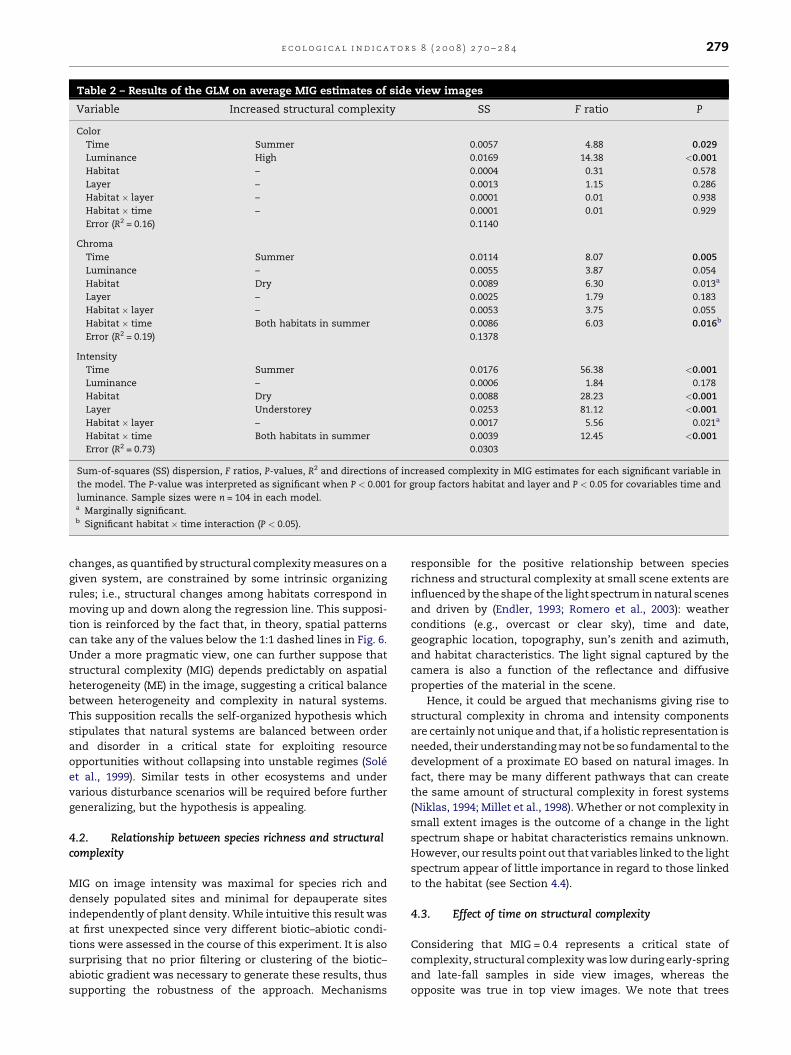
Table 2 – Results of the GLM on average MIG estimates of side view images

Variable Increased structural complexity SS F ratio P

Color

Time Summer 0.0057 4.88 0.029

Luminance High 0.0169 14.38 <0.001

Habitat – 0.0004 0.31 0.578

Layer – 0.0013 1.15 0.286

Habitat � layer – 0.0001 0.01 0.938

Habitat � time – 0.0001 0.01 0.929

Error (R2 = 0.16) 0.1140

Chroma

Time Summer 0.0114 8.07 0.005

Luminance – 0.0055 3.87 0.054

Habitat Dry 0.0089 6.30 0.013a

Layer – 0.0025 1.79 0.183

Habitat � layer – 0.0053 3.75 0.055

Habitat � time Both habitats in summer 0.0086 6.03 0.016b

Error (R2 = 0.19) 0.1378

Intensity

Time Summer 0.0176 56.38 <0.001

Luminance – 0.0006 1.84 0.178

Habitat Dry 0.0088 28.23 <0.001

Layer Understorey 0.0253 81.12 <0.001

Habitat � layer – 0.0017 5.56 0.021a

Habitat � time Both habitats in summer 0.0039 12.45 <0.001

Error (R2 = 0.73) 0.0303

Sum-of-squares (SS) dispersion, F ratios, P-values, R2 and directions of increased complexity in MIG estimates for each significant variable in

the model. The P-value was interpreted as significant when P < 0.001 for group factors habitat and layer and P < 0.05 for covariables time and

luminance. Sample sizes were n = 104 in each model.a Marginally significant.b Significant habitat � time interaction (P < 0.05).

e c o l o g i c a l i n d i c a t o r s 8 ( 2 0 0 8 ) 2 7 0 – 2 8 4 279

changes, as quantified by structural complexity measures on a

given system, are constrained by some intrinsic organizing

rules; i.e., structural changes among habitats correspond in

moving up and down along the regression line. This supposi-

tion is reinforced by the fact that, in theory, spatial patterns

can take any of the values below the 1:1 dashed lines in Fig. 6.

Under a more pragmatic view, one can further suppose that

structural complexity (MIG) depends predictably on aspatial

heterogeneity (ME) in the image, suggesting a critical balance

between heterogeneity and complexity in natural systems.

This supposition recalls the self-organized hypothesis which

stipulates that natural systems are balanced between order

and disorder in a critical state for exploiting resource

opportunities without collapsing into unstable regimes (Sole

et al., 1999). Similar tests in other ecosystems and under

various disturbance scenarios will be required before further

generalizing, but the hypothesis is appealing.

4.2. Relationship between species richness and structuralcomplexity

MIG on image intensity was maximal for species rich and

densely populated sites and minimal for depauperate sites

independently of plant density. While intuitive this result was

at first unexpected since very different biotic–abiotic condi-

tions were assessed in the course of this experiment. It is also

surprising that no prior filtering or clustering of the biotic–

abiotic gradient was necessary to generate these results, thus

supporting the robustness of the approach. Mechanisms

responsible for the positive relationship between species

richness and structural complexity at small scene extents are

influenced by the shape of the light spectrum in natural scenes

and driven by (Endler, 1993; Romero et al., 2003): weather

conditions (e.g., overcast or clear sky), time and date,

geographic location, topography, sun’s zenith and azimuth,

and habitat characteristics. The light signal captured by the

camera is also a function of the reflectance and diffusive

properties of the material in the scene.

Hence, it could be argued that mechanisms giving rise to

structural complexity in chroma and intensity components

are certainly not unique and that, if a holistic representation is

needed, their understanding may not be so fundamental to the

development of a proximate EO based on natural images. In

fact, there may be many different pathways that can create

the same amount of structural complexity in forest systems

(Niklas, 1994; Millet et al., 1998). Whether or not complexity in

small extent images is the outcome of a change in the light

spectrum shape or habitat characteristics remains unknown.

However, our results point out that variables linked to the light

spectrum appear of little importance in regard to those linked

to the habitat (see Section 4.4).

4.3. Effect of time on structural complexity

Considering that MIG = 0.4 represents a critical state of

complexity, structural complexity was low during early-spring

and late-fall samples in side view images, whereas the

opposite was true in top view images. We note that trees

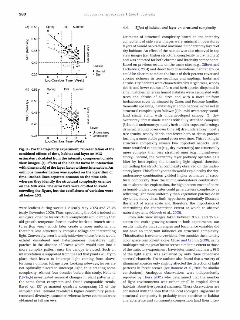
Fig. 8 – For the trajectory experiment, representation of the

combined effects of time, habitat and layer on MIG

estimates calculated from the intensity component of side

view images. (a) Effects of the habitat factor in interaction

with time and (b) of the layer factor without interaction. An

omnibus transformation was applied on the logarithm of

time. Dashed lines separate seasons on the time axis,

whereas they identify the structural complexity orientor

on the MIG axis. The error bars were omitted to avoid

crowding the figure, but the coefficients of variation were

all below 10%.

e c o l o g i c a l i n d i c a t o r s 8 ( 2 0 0 8 ) 2 7 0 – 2 8 4280

were leafless during weeks 1–2 (early May 2005) and 25–26

(early November 2005). Thus, speculating that 0.4 is indeed an

ecological orientor for structural complexity would imply that

old-growth temperate forests evolve intricate branch struc-

tures (top view) which later create a more uniform, and

therefore less structurally complex foliage for intercepting

light. Conversely, seen laterally (side view) these forests would

exhibit disordered and heterogeneous overstorey light

patches in the absence of leaves which would turn into a

more complex pattern once the canopy is closed. Such an

interpretation is supported from the fact that plants will try to

place their leaves to intercept light coming from above,

forming a uniform foliage layer. Looking sideways, leaves are

not optimally placed to intercept light, thus creating some

complexity. Almost four decades before this study, Holland

(1971a,b) investigated seasonal changes in plant patterns on

the same forest ecosystem and found comparable trends.

Based on 137 permanent quadrats comprising 1% of the

sampled area, Holland revealed a higher community persis-

tence and diversity in summer, whereas lower estimates were

obtained in fall surveys.

4.4. Effect of habitat and layer on structural complexity

Estimates of structural complexity based on the intensity

component of side view images were minimal in overstorey

layers of humid habitats and maximal in understorey layers of

dry habitats. An effect of the habitat was also observed in top

view images (i.e., higher structural complexity in dry habitats)

and was detected for both chroma and intensity components.

Based on previous results on the same sites (e.g., Gilbert and

Lechowicz, 2004) and direct field observations, habitat groups

could be discriminated on the basis of their percent cover and

species richness in tree seedlings and saplings, herbs and

shrubs. Dry habitats were characterized by larger trees, woody

debris and lower counts of fern and herb species dispersed in

small patches, whereas humid habitats were associated with

trees and shrubs of all sizes and with a more uniform

herbaceous cover dominated by Carex and Poaceae families.

Generally speaking, habitat-layer combinations increased in

structural complexity as follows: (1) humid-overstorey: wood-

land shade stand with underdeveloped canopy; (2) dry-

overstorey: forest shade stands with fully stratified canopies;

(3) humid-understorey: mostly herb and fern species forming a

dynamic ground cover over time; (4) dry-understorey: mostly

tree trunks, woody debris and fewer herb or shrub patches

forming a more stable ground cover over time. This ranking in

structural complexity reveals two important aspects. First,

more stratified canopies (e.g., dry-overstorey) are structurally

more complex than less stratified ones (e.g., humid-over-

storey). Second, the overstorey layer probably operates as a

filter by intercepting the incoming light signal, therefore

controlling the structural complexity observed on the under-

storey layer. This filter hypothesis would explain why the dry-

understorey combination yielded higher estimates of struc-

tural complexity than the humid-understorey combination.

As an alternative explanation, the high percent cover of herbs

in humid-understorey sites could generate less complexity by

reflecting light more uniformly than vegetation patches do in

dry-understorey sites. Both hypotheses potentially illustrate

the effect of scene scale and, therefore, the importance of

determining the characteristic extent at which to observe

natural systems (Habeeb et al., 2005).

From side view images taken between 9 h30 and 15 h30

across the entire growing season in both experiments, our

results indicate that sun angles and luminance variables did

not have an important influence on structural complexity.

This situation is even more evident if we consider the intensity

color space component alone. Chiao and Cronin (2000), using

multispectral images of forest scenes similar in extent to those

of the trajectory experiment, have determined that nearly 98%

of the light signal was explained by only three broadband

spectral channels. These authors also found that a variety of

illuminant sources only slightly affected the detection of light

patterns in forest scenes (see Romero et al., 2003 for similar

conclusions). Analogous observations were independently

reported by Thery (2001) who determined that the number

of light environments was rather small in tropical forest

habitats; about five spectral channels. These observations are

consistent with the idea that the local ecological signature in

structural complexity is probably more sensitive to habitat

characteristics and community composition (and their inter-

Table 3 – Results of the GLM on average MIG estimates of top view images

Variable Increased structural complexity SS F ratio P

Color

Time Spring and fall 0.0151 16.69 <0.001

Luminance High 0.0231 25.48 <0.001

Habitat Dry 0.0098 10.86 <0.001

Layer – 0.0002 0.21 0.644

Habitat � layer – 0.0127 14.08 <0.001a

Habitat � time – 0.0009 1.07 0.303

Error (R2 = 0.66) 0.0878

Chroma

Time Spring and fall 0.0387 41.63 <0.001

Luminance High 0.0389 41.88 <0.001

Habitat Dry 0.0286 30.79 <0.001

Layer – 0.0014 1.53 0.218

Habitat � layer – 0.0234 25.21 <0.001a

Habitat � time – 0.0056 6.09 0.015b

Error (R2 = 0.80) 0.0903

Intensity

Time Spring and fall 0.0339 114.23 <0.001

Luminance High 0.0143 48.08 <0.001

Habitat Dry 0.0117 39.31 <0.001

Layer – 0.0001 0.14 0.411

Habitat � layer – 0.0109 36.94 <0.001a

Habitat � time – 0.0001 0.44 0.508

Error (R2 = 0.88) 0.0288

Sum-of-squares (SS) dispersion, F ratios, P-values, R2 and directions of increased complexity in MIG estimates for each significant variable in

the model. The P-value was interpreted as significant when P < 0.001 for group factors habitat and layer and P < 0.05 for covariables time and

luminance. Sample sizes were n = 104 in each model.a Since there is a significant effect of habitat and that no effect was expected for layer (see text), the significance value of their interaction

should not be interpreted.b Significant habitat � time interaction (P < 0.05).

e c o l o g i c a l i n d i c a t o r s 8 ( 2 0 0 8 ) 2 7 0 – 2 8 4 281

action) than to the shape of the light spectrum itself. In fact,

recent studies suggest that many different sets of functional

trade-offs in plants may well translate into an equal overall

fitness within a habitat (Niklas, 1994; Lei and Lechowicz, 1998;

Marks and Lechowicz, 2006). Using a three-dimensional

modeling program of leaf and crown characteristics, Valla-

dares et al. (2002) examined the light capture efficiency of 24

seedling and herbaceous species in a lowland rainforest.

Despite important differences in all morphological (structural)

variables, the species were highly similar in their light capture

efficiency based on measures of photon flux densities

(Valladares et al., 2002). Consequently, although the number

of different light spectra may be relatively low in forest scenes,

the variety of living structures evolved locally by the ecological

community is expected to be much broader.

4.5. General comments on the photographic approach

The present study is not the first to consider digital images to

characterize habitat features. Marsden et al. (2002) used

filtered and binarized side view images for measuring the

complexity of understorey vegetation in tropical forests

following logging activities. Alados et al. (1999) investigated

the effect of grazing through fractal and lacunarity analyses of

preprocessed, filtered and binarized side view images of a

Mediterranean shrub (Anthullis cytisoides). Using hemispherical

photography in the tropical rainforest, Trichon et al. (1998)

reported differences in gap patterns which they related to

three disturbance phases; gap, building and mature phases.

Spatial patterns were therein quantified by canopy openness,

spherical variance and plant area indices. The above-cited

studies revealed interesting results in regards to their

hypotheses, but required specifically designed image seg-

mentation protocols. These studies were also directed to

answer specific questions and, as a consequence, were not

discussed in the context of a proximate EO for monitoring

ecosystem dynamics in space and time.

To incorporate more spatial and temporal degrees of

freedom in field protocols, a simple, rapid and preferably cost

effective EO sampling should be performed. In this context,

satellite based sensors have led to the greatest advances,

including standardized measures like the Normalized Differ-

ence Vegetation Index (cf., Badeck et al., 2004; Stockli and

Vidale, 2004) and the Leaf Area Index (cf., Jonckheere et al.,

2004). Although satellites can return data on a landscape scale

their limits are reached at local scales, and they are not always

appropriate for detecting vertical structures under the canopy

cover. Moreover, airborne remote sensing is not what one

would call a simple and cost effective approach for monitoring

changes in space and time. Atmospheric and geometric

corrections are often tedious and the low temporal resolution

of most remotely sensed data makes monitoring short term

dynamics difficult. Alternatively, the deployment of field

sensor networks (Baldocchi et al., 2001; Green et al., 2005)

such as ARTS (Automated Radio Telemetry System), NEON

(National Ecological Observatory Network) and FLUXNET will

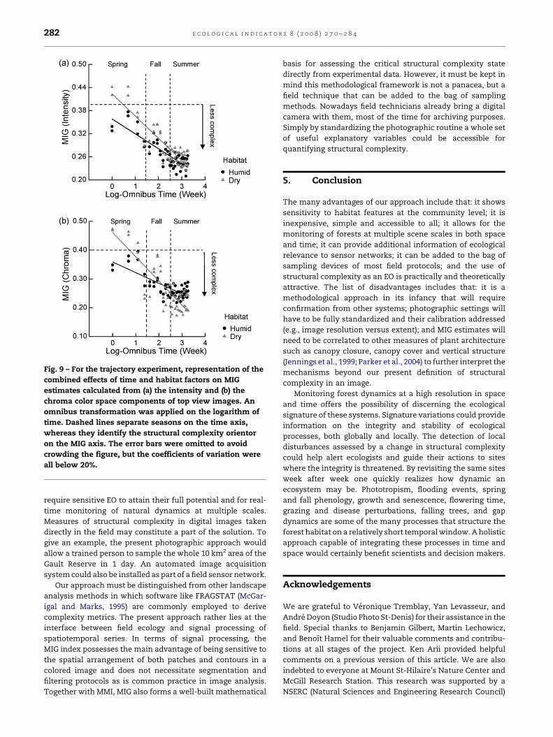
Fig. 9 – For the trajectory experiment, representation of the

combined effects of time and habitat factors on MIG

estimates calculated from (a) the intensity and (b) the

chroma color space components of top view images. An

omnibus transformation was applied on the logarithm of

time. Dashed lines separate seasons on the time axis,

whereas they identify the structural complexity orientor

on the MIG axis. The error bars were omitted to avoid

crowding the figure, but the coefficients of variation were

all below 20%.

e c o l o g i c a l i n d i c a t o r s 8 ( 2 0 0 8 ) 2 7 0 – 2 8 4282

require sensitive EO to attain their full potential and for real-

time monitoring of natural dynamics at multiple scales.

Measures of structural complexity in digital images taken

directly in the field may constitute a part of the solution. To

give an example, the present photographic approach would

allow a trained person to sample the whole 10 km2 area of the

Gault Reserve in 1 day. An automated image acquisition

system could also be installed as part of a field sensor network.

Our approach must be distinguished from other landscape

analysis methods in which software like FRAGSTAT (McGar-

igal and Marks, 1995) are commonly employed to derive

complexity metrics. The present approach rather lies at the

interface between field ecology and signal processing of

spatiotemporal series. In terms of signal processing, the

MIG index possesses the main advantage of being sensitive to

the spatial arrangement of both patches and contours in a

colored image and does not necessitate segmentation and

filtering protocols as is common practice in image analysis.

Together with MMI, MIG also forms a well-built mathematical

basis for assessing the critical structural complexity state

directly from experimental data. However, it must be kept in

mind this methodological framework is not a panacea, but a

field technique that can be added to the bag of sampling

methods. Nowadays field technicians already bring a digital

camera with them, most of the time for archiving purposes.

Simply by standardizing the photographic routine a whole set

of useful explanatory variables could be accessible for

quantifying structural complexity.

5. Conclusion

The many advantages of our approach include that: it shows

sensitivity to habitat features at the community level; it is

inexpensive, simple and accessible to all; it allows for the

monitoring of forests at multiple scene scales in both space

and time; it can provide additional information of ecological

relevance to sensor networks; it can be added to the bag of

sampling devices of most field protocols; and the use of

structural complexity as an EO is practically and theoretically

attractive. The list of disadvantages includes that: it is a

methodological approach in its infancy that will require

confirmation from other systems; photographic settings will

have to be fully standardized and their calibration addressed

(e.g., image resolution versus extent); and MIG estimates will

need to be correlated to other measures of plant architecture

such as canopy closure, canopy cover and vertical structure

(Jennings et al., 1999; Parker et al., 2004) to further interpret the

mechanisms beyond our present definition of structural

complexity in an image.

Monitoring forest dynamics at a high resolution in space

and time offers the possibility of discerning the ecological

signature of these systems. Signature variations could provide

information on the integrity and stability of ecological

processes, both globally and locally. The detection of local

disturbances assessed by a change in structural complexity

could help alert ecologists and guide their actions to sites

where the integrity is threatened. By revisiting the same sites

week after week one quickly realizes how dynamic an

ecosystem may be. Phototropism, flooding events, spring

and fall phenology, growth and senescence, flowering time,

grazing and disease perturbations, falling trees, and gap

dynamics are some of the many processes that structure the

forest habitat on a relatively short temporal window. A holistic

approach capable of integrating these processes in time and

space would certainly benefit scientists and decision makers.

Acknowledgements

We are grateful to Veronique Tremblay, Yan Levasseur, and

Andre Doyon (Studio Photo St-Denis) for their assistance in the

field. Special thanks to Benjamin Gilbert, Martin Lechowicz,

and Benoıt Hamel for their valuable comments and contribu-

tions at all stages of the project. Ken Arii provided helpful

comments on a previous version of this article. We are also

indebted to everyone at Mount St-Hilaire’s Nature Center and

McGill Research Station. This research was supported by a

NSERC (Natural Sciences and Engineering Research Council)

e c o l o g i c a l i n d i c a t o r s 8 ( 2 0 0 8 ) 2 7 0 – 2 8 4 283

grant to L. Parrott and a FQRNT (Fond Quebecois de Recherche

sur la Nature et les Technologies) scholarship to R. Proulx.

r e f e r e n c e s

Alados, C.L., Escos, J., Emlen, J.M., Freeman, D.C., 1999.Characterization of branch complexity by fractal analyses.Int. J. Plant Sci. 160, S147–S155.

Anand, M., Tucker, B.C., 2003. Defining biocomplexity: anecological perspective. Comments Theor. Biol. 8, 497–510.

Andrienko, Y.A., Brilliantov, N.V., Kurths, J., 2000. Complexity oftwo-dimensional patterns. Eur. Phys. J. 15, 539–546.

Badeck, F.-W., Bondeau, A., Bottcher, K., Dokor, D., Lucht, W.,Schaber, J., Sitch, S., 2004. Responses of spring phenology toclimate change. New Phytol. 162, 295–309.

Baldocchi, D.D., Falge, E., Gu, L., Olson, R., Hollinger, D.,Running, S., Anthoni, P., Bernhofer, Ch., Davis, K., Evans, R.,Fuentes, J., Goldstein, A., Katul, G., Law, B., Lee, X., Malhi, Y.,Meyers, T., Munger, J.W., Oechel, W., Pilegaard, K., Schmid,H.P., Valentini, R., Verma, S., Vesala, T., Wilson, K., Wofsy,S., 2001. FLUXNET, a new tool to study the temporal andspatial variability of ecosystem-scale carbon dioxide, watervapor and energy flux densities. Bull. Am. Meteorol. Soc. 82,2415–2434.

Bazzaz, F.A., 1975. Plant species diversity in old-fieldsuccessional ecosystems in Southern Illinois. Ecology 56,485–488.

Brown, J.H., Gupta, V.K., Li, B.-L., Milne, B.T., Restrepo, C., West,G.B., 2002. The fractal nature of nature: power laws,ecological complexity and biodiversity. Phil. Trans. R Soc.Lond. B: Biol. Sci. 357, 619–626.

Chiao, C.-C., Cronin, T.W., 2000. Color signal in natural scenes:characteristics of reflectance spectra and effect of naturalilluminants. J. Opt. Soc. Am. A 17, 218–224.

Christensen, V., 1995. Ecosystem maturity-towardsquantification. Ecol. Model. 77, 3–32.

Denslow, J.S., 1987. Tropical rainforest gaps and tree speciesdiversity. Annu. Rev. Ecol. Syst. 18, 431–451.

Endler, J.A., 1993. The color of light in forest and its implication.Ecol. Monogr. 63, 1–27.

Fath, B.D., Patten, B.C., Choi, J.S., 2001. Complementarity ofecological goal functions. J. Theor. Biol. 208, 493–506.

Gaston, K.J., 2000. Global patterns in biodiversity. Nature 405,220–227.

Gilbert, B., Lechowicz, M.J., 2004. Neutrality, niches, anddispersal in a temperate forest understorey. Proc. Natl.Acad. Sci. 101, 7651–7656.

Green, J.L., Hasting, A., Arzberger, P., Ayala, F.J., Cottingham,K.L., Cuddington, K., Davis, F., Dunne, J.A., Fortin, M.-J.,Gerber, L., Neubert, M., 2005. Complexity in ecology andconservation, mathematical, statistical, and computationalchallenges. Bioscience 55, 501–510.

Habeeb, R.L., Trebilco, J., Wotherspoon, S., Johnson, C.R., 2005.Determining natural scales of ecological systems. Ecol.Monogr. 75, 467–487.

Holland, P.G., 1971a. Seasonal change in the shoot flora diversityof hardwood forest stands on Mount St. Hilaire, Quebec.Can. J. Bot. 49, 1713–1720.

Holland, P.G., 1971b. Seasonal change in the plant patterns ofdeciduous forest in southern Quebec (Canada). Oikos 22,137–148.

Jennings, S.B., Brown, N.D., Sheil, D., 1999. Assessing forestcanopies and understorey illumination: canopy closure,canopy cover and other measures. Forestry 72, 59–73.

Jonckheere, I., Fleck, S., Nackaerts, K., Muys, B., Coppin, P.,Weiss, M., Baret, F., 2004. Review of methods for in situ leaf

area index determination. Part I. Theories, sensors andhemispherical photography. Agric. For. Meteorol. 121,19–35.

Jorgensen, S.E., Muller, F. (Eds.), 2000. Handbook of EcosystemTheories and Management. CRC Press/Lewis Publishers,Boca Raton.

Kauffman, S., 1995. At home in the Universe: The Search for theLaws of Self-organization and Complexity. OxfordUniversity Press, New York.

Klemm, O., Lange, H., 1999. Trends of air pollution in theFichtelgebirge Mountains, Bavaria. Environ. Sci. Pollut. Res.6, 193–199.

Lange, H., 1999. Are ecosystems dynamical systems? Int. J.Comput. Anticipatory Syst. 3, 169–186.

Lawton, J.H., 1999. Are there general laws in ecology? Oikos 84,177–192.

Legendre, P., Legendre, L., 1998. Numerical Ecology, 2nd Englished. Elsevier, New York.

Lei, T.T., Lechowicz, M.J., 1998. Diverse responses of maplesaplings to forest light regimes. Ann. Bot. 82, 9–19.

Lopez-Ruiz, R., Mancini, H.L., Calbert, X., 1995. A statisticalmeasure of complexity. Phys. Lett. A 209, 321–326.

MacArthur, R.H., MacArthur, J.W., 1961. On bird speciesdiversity. Ecology 42, 594–598.

Margalef, R., 1963. On certain unifying principles in ecology. Am.Nat. 97, 357–374.

Marquet, P.A., Quinones, R.A., Abades, S., Labra, F., Tognelli, M.,Arim, M., Rivadeneira, M., 2005. Scaling and power-laws inecological systems. J. Exp. Biol. 208, 1749–1769.

Marks, C.O., Lechowicz, M.J., 2006. Alternative designs and theevolution of functional diversity. Am. Nat. 167, 55–66.

Marsden, S.J., Fielding, A.H., Mead, C., Hussin, M.Z., 2002. Atechnique for measuring the density and complexity ofunderstorey vegetation in tropical forests. For. Ecol.Manage. 165, 117–123.

McGarigal, K., Marks, B.J., 1995. FRAGSTATS: Spatial PatternAnalysis Program for Quantifying Landscape Structure,PNW-GTR-351. United States Department of Agriculture,Pacific Northwest Research Station, Oregon.

Millet, J., Bouchard, A., Edelin, C., 1998. Plant succession andtree architecture: an attempt at reconciling two scales ofanalysis of vegetation dynamics. Acta Biotheor. 46, 1–22.

Montgomery, R.A., 2004. Effects of understorey foliage onpatterns of light attenuation near the forest floor. Biotropica36, 33–39.

Muller, F., 2005. Indicating ecosystem and landscapeorganisation. Ecol. Indicat. 5, 280–294.

Muller, F., Leupelt, M. (Eds.), 1998. Eco Targets, Goal Functionsand Orientors. Springer, Berlin.

Niklas, K.J., 1994. Morphological evolution through complexdomains of fitness. Proc. Natl. Acad. Sci. 91, 6772–6779.

Odum, E.P., 1969. The strategy of ecosystem development.Science 164, 262–270.

O’Neill, R.V., Krumme1, J.R., Gardner, R.H., Sugihara, G., Jackson,B., DeAngelist, D.L., Milne, B.T., Turner, M.G., Zygmunt, B.,Christensen, S.W., Dale, V.H., Graham, R.L., 1988. Indices oflandscape pattern. Landscape Ecol. 3, 153–162.

Parker, G.G., Harmon, M.E., Lefsky, M.A., Chen, J., Van Pelt, R.,Weiss, S.B., Thomas, S.C., Winner, W.E., Shaw, D.C.,Franklin, J.F., 2004. Three-dimensional structure of an old-growth Pseudotsuga-tsuga canopy and its implications forradiation balance, microclimate, and gas exchange.Ecosystems 7, 440–453.

Parrott, L., 2005. Quantifying the complexity of simulatedspatiotemporal population dynamics. Ecol. Complex. 2,175–184.

Proulx, R., in press. Ecological complexity for unifying ecologicaltheory across scales, a field ecologist’s perspective. Ecol.Complex.

e c o l o g i c a l i n d i c a t o r s 8 ( 2 0 0 8 ) 2 7 0 – 2 8 4284

Reda, I., Andreas, A., 2005. Solar position algorithm for solarradiation application. National Renewable EnergyLaboratory (NREL) Technical report NREL/TP-560-34302,Colorado.

Romero, J., Hernandez-Andres, J., Nieves, J.L., Garcia, J.A., 2003.Color coordinates of objects with daylight changes. ColorRes. Appl. 28, 25–35.

Roth, R.R., 1976. Spatial heterogeneity and bird species diversity.Ecology 57, 773–782.

Shiner, J.S., Davidson, M., Landsberg, P.T., 1999. Simple measurefor complexity. Phys. Rev. E 59, 1459–1464.

Simberloff, D., 2004. Community ecology: is it time to move on?Am. Nat. 163, 787–799.

Smith, A.R., 1978. Color Gamut Transform Pairs. In: Beatty, J.C.,Booth, K.S. (Eds.), 1982. Tutorial, Computer Graphics, 2nded. IEEE Computer Society Press, Silver Spring, pp. 376–383.

Sole, R.V., Manrubia, S.C., Benton, M., Kauffman, S., Bak, P.,1999. Criticality and scaling in evolutionary ecology. TrendsEcol. Evol. 14, 156–160.

Stockli, R., Vidale, P.L., 2004. European plant phenology andclimate as seen in a 20-year AVHRR land-surface parameterdataset. Int. J. Remote Sens. 25, 3303–3330.

Storch, D., Gaston, K.J., 2004. Untangling ecological complexityon different scales of space and time. Basic Appl. Ecol. 5,389–400.

Tews, J., Brose, U., Grimm, V., Tielborger, K., Wichmann, M.C.,Schwager, M., Jeltsch, F., 2004. Animal species diversitydriven by habitat heterogeneity/diversity, the importance ofkeystone structures. J. Biogeogr. 31, 79–92.

Thery, M., 2001. Forest light and its influence on habitatselection. Plant Ecol. 163, 251–261.

Trichon, V., Walter, J-M.N., Laumonier, Y., 1998. Identifyingspatial patterns in the tropical rain forest usinghemispherical photographs. Plant Ecol. 137, 227–244.

Turchin, P., 2001. Does population ecology have general laws?Oikos 94, 17–26.

Ulanowicz, R.E., 2004. On the nature of ecodynamics. Ecol.Complex. 1, 341–354.

Valladares, F., Skillman, J.B., Pearcy, R.W., 2002. Convergence inlight capture efficiencies among tropical forest understoryplants with contrasting crown architectures: a case ofmorphological compensation. Am. J. Bot. 89, 1275–1284.

Wackerbauer, R., Witt, A., Atmanspacher, H., Kurths, J.,Scheingraber, H., 1994. A comparative classification ofcomplexity measures. Chaos Solitons Fractals 4, 133–173.

West, G.B., Brown, J.H., 2005. The origin of allometric scalinglaws in biology from genomes to ecosystems, towards aquantitative unifying theory of biological structure andorganization. J. Exp. Biol. 208, 1575–1592.

Whitney, G.G., Foster, D.R., 1988. Overstorey composition andage as determinant of the understorey flora of woods ofcentral New England. J. Ecol. 76, 867–876.

Wilhelm, T., Bruggeman, R., 2000. Goal functions for thedevelopment of natural systems. Ecol. Model. 132, 231–246.

Wolf, F., 1999. Berechnung von information and komplexitat inZeitreihen: Analyse des wasserhaushalts von bewaldeteneinzugsgebieten. PhD Thesis, University of Bayreuth,Bayreuth (in German).