Measure Projection Analysis: A Probabilistic Approach to EEG Source Comparison and Multi-Subject...

Revision submitted for publication May 11, 2012

1

Measure Projection Analysis: A Probabilistic Approach to EEG Independent Component Source Comparison and Multi-Subject Inference

Nima Bigdely-Shamlo,1,2* Tim Mullen,1,3 Kenneth Kreutz-Delgado,1,2 Scott Makeig1

1Swartz Center for Computational Neuroscience, Institute for Neural Computation, University of California San Diego, La Jolla CA 92093-0559, USA

2Department of Electrical and Computer Engineering, University of California San Diego, La Jolla CA, USA 3Department of Cognitive Science, University of California San Diego, La Jolla CA, USA

Abstract

A crucial question for the analysis of multi-subject and/or multi-session EEG data is how to combine information across multiple recordings from different subjects and/or sessions, each associated with its own set of process activities and scalp projections. Applied to sufficient high-quality data, the scalp projections of many maximally independent component (IC) processes contributing to recorded high-density electroencephalographic (EEG) data closely match the projection of a single model dipole located in or near brain cortex. Here we introduce a novel statistical method for characterizing the spatial consistency of EEG dynamics across a study. Measure Projection Analysis (MPA) first finds voxels in a common template brain space for which the dynamics of nearby IC processes are consistent, then computes local-mean EEG measure values for this voxel subspace using statistical models of IC localization error and between-subject anatomical variation. Finally, clustering the mean measure voxel values within this locally consistent brain subspace can characterize brain spatial domains with distinguishable EEG dynamics in the study. MPA has fewer analysis parameters than IC cluster analysis and provides 3-D maps with statistical significance estimates for each EEG measure of interest. We demonstrate the application of MPA to a multi-subject EEG study and compare the results with a standard k-means IC clustering approach using EEGLAB (sccn.ucsd.edu/eeglab). We also validated the method using simulated data. A Measure Projection Toolbox (MPT) plug-in for EEGLAB is available for download (sccn.ucsd.edu/wiki/MPT). MPA allows source resolved EEG data to be treated as a 3-D cortical imaging modality with near-cm scale spatial resolution.

Key words: electroencephalogram; EEG; independent component analysis; ICA; rapid serial visual presentation; RSVP; Clustering; Group-ICA, MPA Acronyms introduced: EEG, ICA, IC, MPA, MNI, ERP, ERSP, ITC

*Correspondence to: Nima Bigdely-Shamlo E-mail: [email protected]


2

Introduction Independent Component Analysis (ICA) [Bell and Sejnowski, 1995] has become a method of widespread interest for analysis of EEG data [Makeig et al., 1996], [Makeig et al., 1997], [Lee et al., 1999], [Jung et al., 2001] [Delorme and Makeig, 2004]. In this approach to EEG source analysis, the EEG scalp channel data (without applying averaging) are decomposed into independent component (IC) processes by learning a set of spatial filters that have fixed relative projections to the recording electrodes and produce maximally independent individual time courses from the data. ICA thus learns what independent processes (information sources) contribute to the data and also reveals their individual scalp projection patterns (scalp maps), thereby simplifying the EEG inverse source localization problem to that of estimating where each source is generated, a much simpler problem than estimating the source distributions of their ever-varying linear mixtures as recorded by the scalp electrodes themselves. The IC filters linearly transform the representational basis of EEG data from scalp channels by time points to a sum of component processes with maximally independent time courses and fixed scalp projections (scalp maps) that are often strongly overlapping. Many ICs predominately account for the contributions to the channel data from a non-brain (‘artifactual’) source process -- for example potentials arising from eye movements, scalp muscle activity, the electrocardiogram, line noise, etc., while many other ICs are compatible with a source within the brain itself, in particular within its convoluted cortical shell. Although far-field projections of locally synchronous field activity within sub-cortical brain structures are possible, the internal geometry and spatiotemporal dynamics of sub-cortical structures may not be as suitable for projecting coherent far-field potentials as far (electrically) as the scalp with sufficient amplitude to be distinguished from the many cortical plus non-brain sources that are summed at the scalp electrodes. However, the spatiotemporal properties of field activity in sub-cortical structures have not been well studied -- and much work also remains to fully characterize the complexities of local cortical field synchrony. Since ICA uses slight waveform differences to separate independent sources, and these depend on the exact placements of the scalp electrodes and the individual subject cortical geography, optimal separation is achieved when it is applied to data channels recorded simultaneously from a single subject with a single scalp montage. As EEG channel locations and conductance values may slightly differ across subjects and sessions, separate ICA decompositions are best trained on each recorded session or smaller data set from one session, though the length of the training data must be sufficient for the number of recording channels. Many of the resulting brain-based (‘non-artifactual’) IC scalp topographies may be modeled by a single equivalent dipole inside the brain volume [Makeig et al., 2002]. ICA algorithms return


3

many such ‘dipolar’ IC data sources for which much of the spatial variance of the electric field pattern they produce on the scalp (typically well over 85%) is accounted for by the projection of a single ‘equivalent’ dipole. Further, on average the more independent the resulting ICs returned by an linear ICA decomposition method, the more near-dipolar ICs are returned [Delorme et al., 2012]. Such dipolar ICs are compatible at least with an origin in locally-synchronous cortical field activity within a single cortical patch, which by biophysics must be located near to and aligned generally perpendicular to the equivalent dipole. Although finding the cortical patch generating a given dipolar IC may be difficult [Acar et al., 2009], as it requires (at least) a good quality MR head image for the subject and accurately recorded scalp electrode positions [Acar and Makeig, 2010], Given a good estimate, of where the scalp electrodes were placed on the head, under ideal conditions the location of the equivalent dipole for a near-dipolar IC can, in most cases, be found reliably with less than a centimeter error [Akalin Acar, unpublished data]. In turn, biophysical simulations show that the equivalent dipole for a cm2-scale cortical patch source is, on average, less than 2 mm from the center of the generating patch [Akalin Acar, unpublished data]. Thus, a unique advantage of ICA applied to EEG is that localizing sources from its single-source IC scalp maps avoids uncertainties associated with multiple local minima that limit the accuracy of estimated source distributions computed from scalp maps that sum projections of multiple sources -- for example most raw EEG scalp maps or scalp maps from peaks in average ERPs. A standard way to analyze EEG data is to first conduct an experiment in which a number of (outwardly) similar events occur, typically stimulus (e.g., image) presentation and behavioral events (e.g., impulsive button presses). Sets of EEG activity epochs recorded in some latency window around these events (experimental trial epochs) are extracted, averaged, and compared. A number of mean measures of EEG trial data have been developed in recent years and incorporated into freely available software toolboxes including EEGLAB [Delorme and Makeig, 2004], Fieldtrip [Oostenveld et al., 2011], the SPM toolkit [Friston, 2007], and ICALAB [Cichocki and Amari, 2002]. These measures, including the average Event-Related Potential (ERP) and the Event-Related Spectral Perturbation (ERSP) [Makeig, 1993] generalizing the ERD/ERS of [Pfurtscheller et al., 1977], may equally be computed for single ICs as well as for single scalp channels. For each subject session and associated ICA decomposition, each IC has a unique scalp map and EEG time course. To support group-level inferences about EEG measure differences across task trial conditions, subject groups, recording sessions, etc., IC location and EEG measure information must be integrated across subjects and sessions In contrast to the typical and straightforward approach to obtaining group inferences from channel data, i.e. by assuming equivalence across subjects of electrode derivations from standardized scalp locations [Picton et al., 2000] [Kiebel and Friston, 2004], combining results across different ICA decompositions is non-trivial. Several methods have been proposed for this


4

task. These typically fit into two categories: IC clustering ([Makeig et al., 2002], [Onton et al., 2006], [Onton and Makeig, 2006]) and joint decomposition methods such as group-ICA ([Eichele et al., 2009], [Kovacevic and McIntosh, 2007], [Calhoun et al., 2009], [Congedo et al., 2010]), multiset canonical correlation analysis [Li et al., 2009] and J-BSS [Li et al., 2011] [Via et al., 2011] . In this paper we introduce a probabilistic approach that we call Measure Projection Analysis (MPA) for population-level inference from ICA-decomposed EEG signals. We demonstrate the application of measure projection analysis to an example EEG study and compare its results to those of PCA-based IC clustering. In addition, we conduct a simulation-based assessment of the performance of the method across different noise levels and parameter choices. Methods Experimental data. EEG data were collected from 128 scalp locations at a sampling rate of 256 Hz using a Biosemi (Amsterdam) Active View 2 system and a whole-head elastic electrode cap (E-Cap, Inc.) forming a custom, near-uniform montage across the scalp, neck, and bony parts of the upper face.

====== Figure 1 here ======= Subject task. Our sample study consisted of data from 15 sessions recorded from 8 subjects performing a Rapid Serial Visual Presentation (RSVP) task [Bigdely-Shamlo et al., 2008] (raw data available at ftp://sccn.ucsd.edu/pub/headit/RSVP, EEGLAB Study available from ftp://sccn.ucsd.edu/pub/measure_projection/rsvp_study). Each session comprised 504 4.9-s image bursts of 49 oval image clips from a large satellite image of London presented at a rate of 12/s. Some (60%) of these bursts contained one image in which a target white airplane shape was introduced at a random position and orientation. Following each burst, subjects were asked to press one of two buttons to indicate whether or not they had detected a target airplane in the burst. Figure 1 shows a time-line of each RSVP burst. For further details see [Bigdely-Shamlo et al., 2008]. Data preprocessing. A separate ICA decomposition was performed for each recording session after preprocessing which involved re-referencing, from the active-reference Biosemi EEG data to an electrode over the right mastoid, high-pass filtering above 2 Hz, and artifact rejection. The subset of ICs that could be represented by an equivalent dipole model with low error (here defined as more than 85% of channel variance in the IC scalp map being accounted for by a single equivalent dipole or a bilaterally symmetric equivalent dipole pair) were selected for analysis. ICs with equivalent dipoles located outside the MNI brain volume (e.g., those with an


5

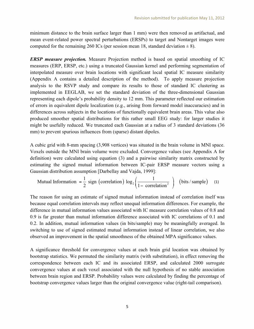
minimum distance to the brain surface larger than 1 mm) were then removed as artifactual, and mean event-related power spectral perturbations (ERSPs) to target and Nontarget images were computed for the remaining 260 ICs (per session mean 18, standard deviation ± 8). ERSP measure projection. Measure Projection method is based on spatial smoothing of IC measures (ERP, ERSP, etc.) using a truncated Gaussian kernel and performing segmentation of interpolated measure over brain locations with significant local spatial IC measure similarity (Appendix A contains a detailed description of the method). To apply measure projection analysis to the RSVP study and compare its results to those of standard IC clustering as implemented in EEGLAB, we set the standard deviation of the three-dimensional Gaussian representing each dipole’s probability density to 12 mm. This parameter reflected our estimation of errors in equivalent dipole localization (e.g., arising from forward model inaccuracies) and in differences across subjects in the locations of functionally equivalent brain areas. This value also produced smoother spatial distributions for this rather small EEG study: for larger studies it might be usefully reduced. We truncated each Gaussian at a radius of 3 standard deviations (36 mm) to prevent spurious influences from (sparse) distant dipoles. A cubic grid with 8-mm spacing (3,908 vertices) was situated in the brain volume in MNI space. Voxels outside the MNI brain volume were excluded. Convergence values (see Appendix A for definition) were calculated using equation (3) and a pairwise similarity matrix constructed by estimating the signed mutual information between IC-pair ERSP measure vectors using a Gaussian distribution assumption [Darbellay and Vajda, 1999]:

(1)

The reason for using an estimate of signed mutual information instead of correlation itself was because equal correlation intervals may reflect unequal information differences. For example, the difference in mutual information values associated with IC measure correlation values of 0.8 and 0.9 is far greater than mutual information difference associated with IC correlations of 0.1 and 0.2. In addition, mutual information values (in bits/sample) may be meaningfully averaged. In switching to use of signed estimated mutual information instead of linear correlation, we also observed an improvement in the spatial smoothness of the obtained MPA significance values. A significance threshold for convergence values at each brain grid location was obtained by bootstrap statistics. We permuted the similarity matrix (with substitution), in effect removing the correspondence between each IC and its associated ERSP, and calculated 2000 surrogate convergence values at each voxel associated with the null hypothesis of no stable association between brain region and ERSP. Probability values were calculated by finding the percentage of bootstrap convergence values larger than the original convergence value (right-tail comparison).

( ) ( )2 2

1 1Mutual Information sign correlation log bits / sample2 1 correlation

⎛ ⎞= ⎜ ⎟−⎝ ⎠


6

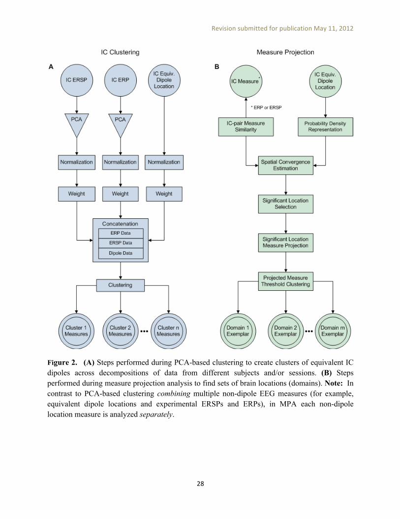
The significance threshold using a group-wise p < 0.05, after correcting for multiple comparisons with the False Discovery Rate (FDR) method [Benjamini and Hochberg, 1995], required a raw voxel significance threshold of p < 0.0075. In the next step, we found locations in the brain volume at which the local similarity of IC ERSPs was significantly higher than what could be expected by chance given these data. ERSP domain clustering. To simplify the analysis of projected source measure values, we separated them into several distinguishable spatial domains by threshold-based Affinity Propagation clustering (described in Appendix B) based on a similarity matrix of pair-wise correlations between the projected measure values at each voxel position. Affinity propagation automatically finds an appropriate number of clusters (here referred to as spatial domains) based on the maximum allowed correlation between cluster exemplars, automatically increasing the number of clusters until any other potential cluster exemplar becomes too similar to one of the existing exemplars. Here, maximal exemplar pair similarity (forcing creation of additional clusters) was set to a correlation value of 0.8, and outlier detection similarity threshold (increasing existing clusters) to a correlation value of 0.7. Note that the voxel clustering procedure does not force clustered voxels to be contiguous; for example near-identical ERSPs may be produced in bilaterally symmetric cortical regions, which may then be identified by affinity clustering as a single measure domain. . Alternative clustering methods developed for identifying regions of similarly activated voxels in fMRI data, such as Cluster-Based Analysis (CBA) [Heller et al., 2006], could also be applied here. Figure 2B summarizes the steps performed in MPA to create distinguishable spatial source domains for each EEG measure.

====== Figure 2 here ======= PCA-based IC clustering. In the PCA-based IC clustering approach, cross-session IC equivalence classes are typically defined by applying a clustering algorithm such as k-means to an L2-weighted combination of EEG measures of interest (e.g., IC equivalent dipole locations, scalp-map topographies, mean power spectra, average ERPs, etc.) so as to produce a desired number of IC clusters (10-30). Cluster-level mean EEG measure values may then be calculated by averaging across the members of each IC cluster, and may then be used for group-level inference and stimulus or task condition comparison. For example, the default IC clustering options in EEGLAB result in the creation of a pre-clustering array that represents each IC as positioned in a joint-measure feature space by performing the following operations: • Mean EEG measure computation: For each IC, set of experimental trials (trial condition),

and EEG measure of interest (ERP, mean power spectrum, ERSP, and/or Inter-Trial


7

Coherence (ITC)), measure values are first computed and then concatenated across conditions (for the time/frequency measures, in the time dimension).

• Measure dimensionality reduction: Next, the dimensionality of the concatenated condition measures for each IC is reduced by PCA to a principal component subspace. The subspace dimensionality is heuristically determined based on the amount of trial data available. Measure values associated with each IC in the PCA-reduced coordinates are normalized by dividing them by the standard deviation of the first principal component.

• Equivalent dipole locations: Dipole (x,y,z) location values in the adult template MNI brain space (Montreal Neurological Institute and Hospital, [Evans et al., 1993]) are normalized and then multiplied by a user-specified scalar weight, which determines their relative influence in the subsequent clustering.

• Joint-measure IC-space representation: Dimensions associated with each EEG measure (after preprocessing steps describe above) are concatenated to represent each IC in a joint space. For example, ERSP information may be represented by 10 PCA dimensions and concatenated with 5 PCA dimensions representing ERP information and 3 (x,y,z) location dimensions representing dipole position to form a joint 10+5+3 = 18 dimensional space in which each IC is characterized.

• IC clustering: ICs in this joint-measure IC space are then clustered using k-means or some

other clustering method. A major issue concerning IC clustering is the lack of objective criteria for determining the optimal number of clusters.

Figure 2A shows a flowchart of this clustering method. All ICs, represented by features in the resulting pre-clustering array, are then clustered with the k-means method provided in the Matlab Statistics Toolbox (The Mathworks, Inc.). For more details and an example of this procedure, see [Onton and Makeig, 2006]. PCA-based ERSP measure clustering. EEGLAB default (PCA) clustering was used to create 15 clusters using ERSP and Dipole measures. ERSP values for Target and Nontarget conditions were concatenated across the time dimension for each IC and were reduced to 10 principal dimensions by PCA. After default normalization, equivalent dipole location values were weighted by the default factor 10. The MATLAB implementation of the k-means method was then used to form IC clusters. Clustering results for different numbers of clusters were first examined by eye and the number of clusters was thereby determined such that (a) dipoles assigned to a given cluster formed a single, relatively focal cluster, in anatomical (MNI) space (although it is possible for multiple distal


8

brain regions to display similar EEG dynamics, resulting in clusters with dipoles localized to multiple brain regions, we have found that such clusters usually appear as a consequence of cluster merging when the number of clusters is set too low); and (b) clusters are maximally non-overlapping and contain a reasonable number of dipoles (overlapping and/or small-size clusters may occur when the number of clusters is either too low or too high). These criteria did not take into account the similarity structure of other measures (e.g., the ERP) which would ideally further influence the choice of cluster number. Results

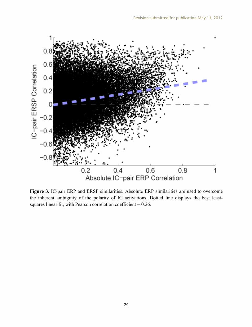
====== Figure 3 here ======= ERSP measures for PCA-based IC clusters. Figure 3 shows a scatter-plot of computed IC-pair ERP and ERSP similarities. Because of the inherent ambiguity in the polarity of IC activations, absolute-value correlations of ERPs for each IC pair was used as an upper bound on their ERP similarity. As can be seen in this figure, as the correlation between these two sets of values is low (0.26), the similarity structures of (absolute) ERP and ERSP measures are not identical. Thus, if one is interested in the distribution of a particular measure, it may be better to analyze it separately instead of combining it with another measure during clustering (e.g., affirming our decision here to not include ERP measure data in ERSP clustering).

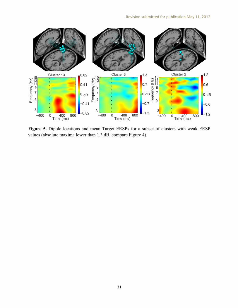
====== Figures 4 & 5 here ======= Figures 4 and 5 show cluster dipole locations and Target ERSP values averaged over ICs belonging to each cluster. Figure 4 shows a subset of clusters with large (more than 1.7-dB) mean Target ERSP values, while Figure 5 shows clusters with mean Target ERSP values below 1.3 dB. Nontarget ERSP values were lower (p < 0.05) or close to zero for all these clusters. Statistical significance analysis of differences between Target and Nontarget ERSPs was performed by bootstrap statistics permuting Target and Nontarget conditions across ICs belonging to each cluster. This statistical test has to be performed within each cluster separately and does not evaluate the significance of cluster IC memberships (i.e., to determine whether the measures for members of the cluster are significantly similar to each other and sufficiently different from others). This seems to us a key drawback of the PCA-based IC clustering approach.

====== Figure 6 here =======


9

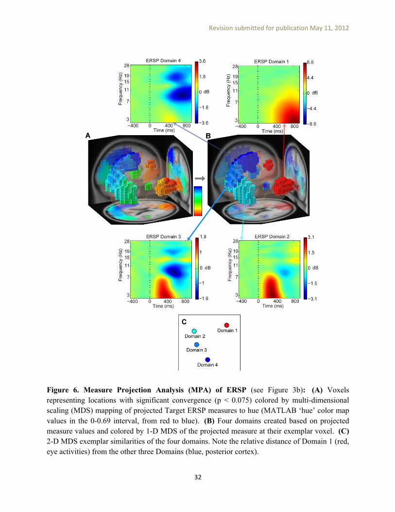
ERSP measure projection results. Figure 6A shows the significant (p<0.0075, group-wise p < 0.05 by FDR) locations (displayed as voxels) colored by applying multi-dimensional scaling (MDS) to the projected (concatenated Target and Nontarget) ERSP measure mapped to the 0-0.69 hue interval in the MATLAB hue color scale (from red to blue). This allows locations with similar projected measure to be colored similarly. Figure 6B shows four measure-consistent IC domains colored by one-dimensional MDS of the projected measure associated with their most representative member (the domain exemplar), obtained from the Affinity Propagation method implemented as threshold-based clustering (Appendix B). By comparing figures 6A and 6B we can see how these four domains summarize the projected measure values: Figure 6A shows roughly four colored regions that map into four domains displayed in Figure 6B. Note that the clustering procedure leading to the creation of the four MP domains is fundamentally different from PCA-based clustering: (a) Domain clustering is only employed to summarize projected results at significant locations and does not change the projected values. In contrast, cluster-mean values obtained by the PCA clustering method are highly dependent on the number of clusters and weight parameters; (b) PCA clustering typically operates on a weighted combination of different measures, which prevents the use of meaningful similarity thresholds in the threshold-based clustering described in Appendix B. In contrast, it is possible to set meaningful similarity thresholds (for example, a maximum correlation of 0.8) to find domains based on projected measures. This has the advantage of not having to specify the final number of clusters beforehand as threshold-based affinity clustering finds the appropriate number of clusters based on the given similarity threshold. Using different maximum correlation thresholds only change the granularity of the segmentation (of locations with significant measure consistency into domains) and does not fundamentally affect the values assigned to domains. For example, using maximum correlation of 0.9 would result in more domains, but many of them would look similar to each other.

====== Figure 7 here =======

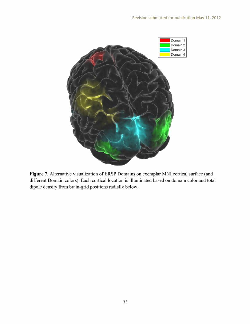
Figure 7 shows an alternative visualization of ERSP Domains: exemplar MNI cortical surface is colored by domain color, weighted by dipole density, from brain-grid positions radially below each cortical location. Comparison of MPA and PCA-based clustering methods. Now we can compare the results obtained from PCA-based IC clustering to measure projection analysis (MPA).

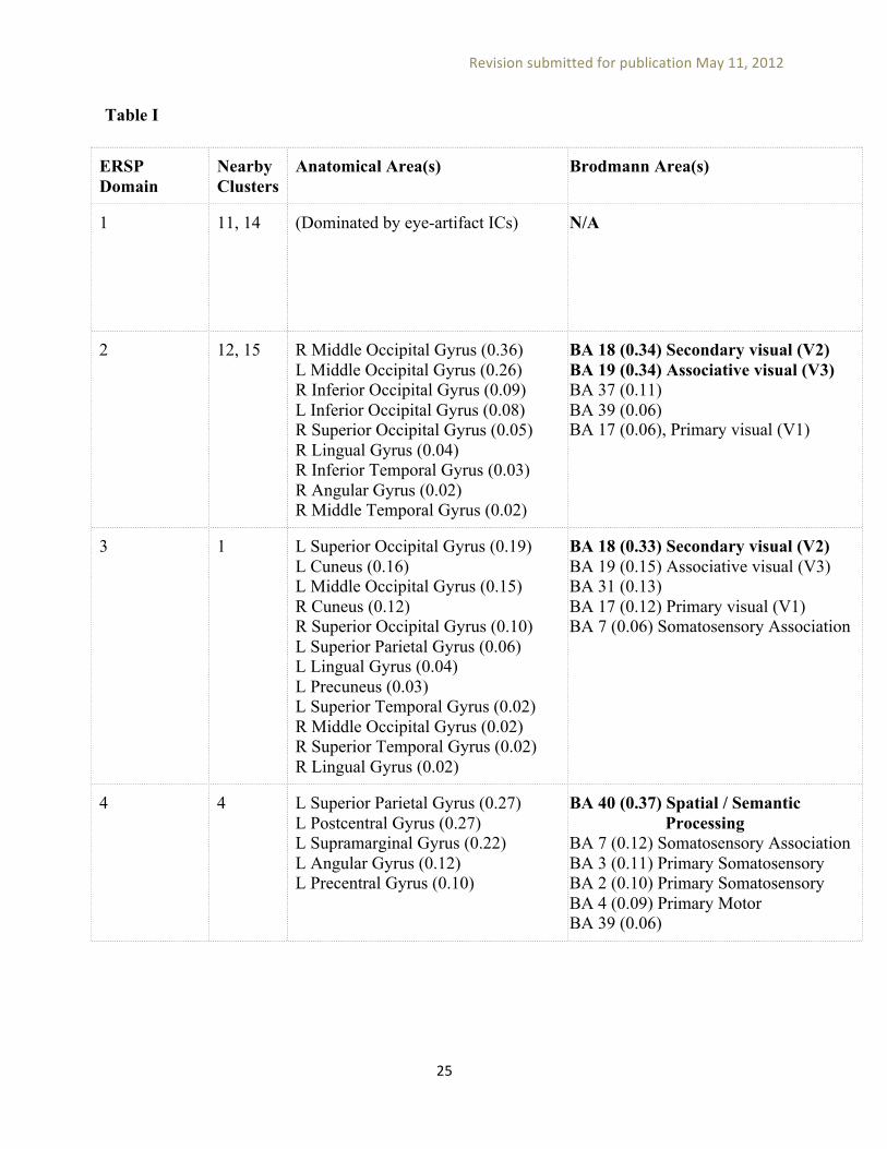
====== Table I here =======


10

Table I gives the cluster number(s) located in or near each domain. Average ERSPs for these clusters are highly similar to those of respective domain exemplars, indicating that here measure projection analysis produced results in close agreement with IC clustering. PCA-based clustering, on the other hand, produced 15 clusters, many not associated with any significantly convergent MPA region. For example, Clusters 2 and 4 in Figure 5 are relatively far from brain areas with significant ERSP convergence shown in Figure 6A. This indicates there may not be enough statistical evidence in the data, based on MPA spatial convergence significance, to support results associated with these clusters. In other words, ICs associated with these PCA-based clusters have fairly dissimilar ERSP measures. Table I also lists anatomical locations associated with each ERSP domain based on the LONI project probabilistic atlas [Shattuck et al., 2008] and Brodmann areas [Brodmann, 1909] from [Lancaster et al., 2000]. The listed functional associations of these areas are based on Brodmann's Interactive Atlas (http://www.fmriconsulting.com/brodmann/Introduction.html). Upon close inspection, because of errors in dipole localization related to insufficient electrical head modeling in the complex peri-orbital regions, many eye-artifact ICs (13 out of 16 highly contributing ICs) in this study were localized inside the brain volume and in fact became the main contributors to ERSP Domain 1 and Cluster 11. Within the measure projection concept, brain and non-brain ICs should not be mixed. Performing an additional artifact IC rejection step, using methods for identifying eye artifact ICs from their activity profiles as well as their equivalent dipole locations such as CORRMAP [Viola et al., 2009] or ADJUST [Mognon et al., 2011] should be done before MPA to improve the quality of results in frontal regions. Of similar concern are ICs accounting for scalp muscle activity, which (in EEG montages with sufficient scalp coverage) have scalp maps consistent with an equivalent dipole at the insertion of the muscle into the skull. These may be differentiated from brain ICs prior to measure projection by their dipole locations (outside the skull) and by their characteristic electromyographic (EMG) spectra with a minimum below 20 Hz and a level plateau at higher frequencies. Domains 2 and 3 are both associated with Secondary (V2), Associative (V3) and Primary (V1) visual cortex (BA 18,19 and 17) [Marcar et al., 2004] [Dougherty et al., 2003]. Domain 3 is close to BA 31 which has been reported to support high-demand visual processing and discrimination [Deary et al., 2004]. Domain 2 is near BA 37 and fusiform gyrus bilaterally (with a right bias) which is also reported in a published fMRI study of visual perceptual decision making task [Philiastides and Sajda, 2007]. Similar low-theta band activity occurring about 400 ms after visual target detection in these brain areas was reported in [Makeig et al., 2004].

There is some evidence of mu rhythm desynchronization (suppression) in Domain 4, located near right-hand Primary Somatomotor, Primary Motor and Somatosensory Association areas (BA


11

7,3,2,4), which may be related to subjects holding a button in their right hand. Subjects were asked to wait until the end of RSVP image burst before pressing any button. The mu rhythm activity in this area reflects cortical inhibitory (or ‘idling’) dynamics that may decrease the chance of prematurely pressing the button. Activation in BA 40 and 7 is also consistent with a preliminary FMRI study conducted by [Gerson et al., 2005] in which BOLD activation was observed during rapid discrimination of visual objects accompanied by a motor response.

====== Figure 8 here =======

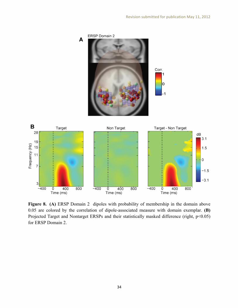
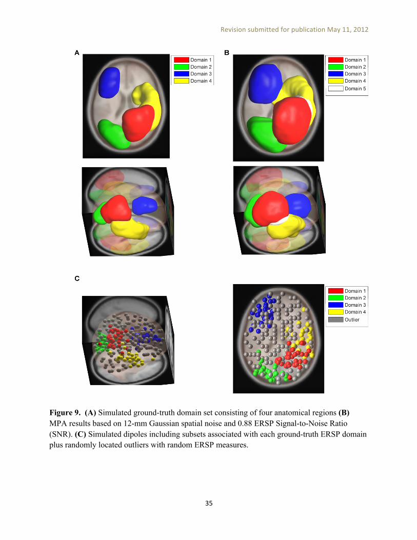
Based on MPA assumptions of (a) representing each dipole location by a Gaussian density and (b) creating domains from locations with significant local convergence, we expect to find dipoles that are positioned near domains to have EEG measures similar to the domain exemplar measure. To verify this prediction, in Figure 8A we plotted such dipoles (e.g., having total probability density inside the domain above 0.05) for one ERSP domain and colored them by the correlation of their EEG measures with the domain exemplar. As expected, the majority of these dipoles had an ERSP similar to their domain exemplar. In Figure 8B, domain exemplar ERSPs for Target and Nontarget conditions and their statistically masked difference are plotted. To perform statistical significance analysis we projected the measure associated with Target and Nontarget conditions for each session separately to domain locations and calculated the average (weighted by dipole density) over these locations. A two-tailed T test was performed to calculate p values for the difference between conditions. Finally, domain exemplar measure difference across conditions was masked (with zeros) at non-significant (p>0.05) time-frequency points. Simulation We validated MPA by conducting various simulations to investigate the performance of the method across different noise levels and parameter choices. We started by selecting four anatomical domains (Figure 9A: R Superior Parietal Gyrus, L Inferior Occipital Gyrus, L Lateral Orbitofrontal Gyrus and R Superior Temporal Gyrus, from LONI LPBA40 atlas [Shattuck et al., 2008]) in MNI space as ground truth and assigned to each the ERSP pattern from one our RSVP-experiment domains. We then placed 31 dipoles by randomly selecting locations from ground truth domains and adding Gaussian spatial noise in the dipole location with 12-mm std. dev. to them in order to simulate subject variability and the errors in localization of IC equivalent dipoles. The number of dipoles per ground-truth domain (31) was selected as the average number of dipoles that larger than 10% of their density, modeled by a truncated 3D Gaussian, was located in an ERSP domain from our RSVP experiment). We considered two simulation conditions: (1) assigning this ERSP patterns to simulated IC dipoles associated with each ground-truth domain (zero noise) (2) adding 0.2 dB RMS amplitude noise to the ERSP pattern associated with each IC dipoles (simulating experiment noise).


12

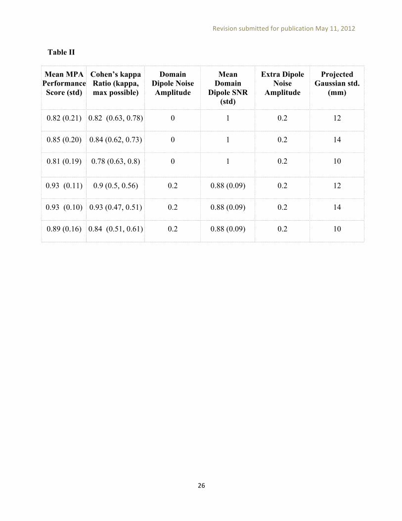
We then sequentially added to the model 142 other dipoles, each placed at the brain volume location (on an 8-mm grid) maximally furthest from all other existing dipoles. Pseudo-ERSP measures composed of random 0.2-dB white noise samples were assigned to these dipoles. The simulation thus contained the same number of brain dipoles as our RSVP experiment, with spatially coherent measure values only in the four model domains. MPA was then performed on this simulated collection of dipole locations and associated ERSP measures. The resulting domains were then compared to ground-truth domains for the two simulation noise conditions mentioned above (Figure 9B). We used two scoring methods to evaluate the performance of MPA method (a) Cohen’s kappa [Cohen, 1960], a measure of inter-rater agreement (b) the average percentage of ground-truth domain locations that were associated with the correct domain in the results. In both scoring methods we accounted for permutations in domain labels and included the locations which should not be associated with any ground-truth domain as an extra category (they should not be assigned to any domains in the results). Table II shows MPA performance scores for simulation results with a voxel significance p-value threshold of 0.05, maximum exemplar correlation threshold of 0.8, and varying noise levels. To explore the sensitivity of MPA results to the choice of the location uncertainty parameter (the standard deviation of the Gaussian representing each dipole), we also tested different values of this parameter for two ERSP noise level (noiseless and 0.2 dB). These results show that MPA can recover brain domain locations with high accuracy (> %80) in the presence of noise, and that using inaccurate dipole density extent priors (e.g., using a 10-mm or a 14-mm instead of the ground-truth 12-mm std. dev. for the spatial-perturbation Gaussian) has relatively little effect on their locations.

Discussion

The localized EEG source estimates returned by ICA decomposition bring closer the promise of performing functional cortical imaging using non-invasive EEG with fine temporal resolution. However, performing ICA-based EEG imaging in studies on multiple subjects and/or sessions requires a method for combining source location and activity measure information from multiple data sets. Here we demonstrated the application of measure projection analysis (MPA) to EEG collected in a visual RVSP task and decomposed using extended infomax ICA. We compared the results to results of applying k-means clustering to the collection of brain-localized ICs and their EEG measures. MPA results were consistent with IC clustering but depended on fewer parameters and also provided statistical significance values. Also: • MPA requires only one parameter per EEG measure, the similarity threshold used in domain

clustering, and one parameter, shared between measures, which controls the width of Gaussian density representing each dipole (in total three parameters for two EEG measures). In comparison, PCA clustering requires two parameters per EEG measure used in the clustering (the number of principal dimensions retained, and the relative measure


13

weighting value), plus the relative weighting of equivalent dipole location and the number of clusters to create (in total six parameters for both measures). The MPA parameters are also more physiologically interpretable and less likely to require tuning in applications to different studies.

• MPA provides statistics indicating locations with significant local measure homogeneity for

each EEG measure. PCA clustering and Group ICA (discussed below), on the other hand, do not provide such statistics.

• MPA is more suited to comparing results for subject sub-groups as it uses continuous dipole density values instead of discrete cluster memberships that may introduce noise in group comparisons.

Problems with direct IC clustering. Although PCA-based IC clustering has been used in many EEG studies with some level of success, there are several problems associated with this approach: Cluster parameters. A number of issues are rooted in the relatively large number of parameters often used in IC clustering: apart from choosing a subset of IC measures (features) for clustering, data from these measures are usually weighted a priori according to their perceived importance. Also, most clustering methods require the final number of clusters to be provided a priori. Since there is no mathematically proven or established objective method for choosing these parameters, they are often set by the experimenter to produce most desirable results. Because of the relatively large number of such variables (e.g., EEGLAB default PCA-based clustering has up to 12 parameters) and the sensitivity of final clustering results to their values, experimenter parameter settings may have profound effects on inferences at the group-level. This introduces a significant and undesirable lack of objectivity in interpreting EEG data and hinders the calculating of significance statistics for group-level or session-level results. In fact, even if there were well- justified ways to set the IC clustering parameters, it would be still quite difficult to determine the statistical significance (including p-values) of cluster measure means because these statistical methods are often based on bootstrap null-hypothesis testing that is not easily and directly applicable to the formation of IC clusters. Cluster membership. In addition, the PCA-based IC clustering approach limits the types of group-level analysis methods that may be applied to EEG data. For example common clustering methods (e.g., k-means or linkage clustering) output a set of binary (“hard decision”) cluster membership values: each IC either fully belongs to a certain cluster or not. As the formation of these clusters is often highly dependent on the multitude of clustering parameters, it is difficult to separate the effect on the clustering results due to choosing these parameters from the contributions of group-level differences in IC features. As an example, a cluster of interest (e.g.,


14

having a particular target ERP feature) may mostly contain ICs associated with a certain participant subpopulation. At the same time, ICs with similar features may exist in nearby clusters and may have been included if a lower number of clusters or slightly different weight parameters were applied to IC measures during IC clustering. It then becomes unclear whether participants have meaningfully different ERPs (in terms of equivalent dipole locations or ERP time courses) from a parent or alternate population, or whether the aggregation of ICs from this subject group into a particular IC cluster is an artifact of selecting a particular set of clustering parameters. This problem could be alleviated if ICs could have fractional (fuzzy) memberships and if noise were not introduced during the quantization of membership values by the clustering procedure. Measure projection allows such improvements by adopting a probabilistic spatial representation of the IC equivalent dipole locations. Cluster shape. IC clustering does not explicitly specify brain areas whose EEG-source signals are reactive within a class of experimental conditions. K-means clustering, in particular, is biased towards creating spherical clusters. Further, when an IC cluster is represented by the spatial centroid of its member IC equivalent dipole locations, the spatial extent of each cluster is not investigated statistically. MPA, on the other hand, operates in brain source domain coordinates and thus gives source domains that are not restricted in shape and may even be discontinuous (e.g., to represent bilaterally symmetric activations of an IC accounting for synchronous activity within two tightly-connected but non-contiguous cortical areas). Cluster equivalence across measures. Another problem associated with PCA-based IC clustering stems from the fundamental assumption of IC cluster equivalence across all EEG measures. In this method it is assumed that those ICs that are similar in one respect (for example, in ERP time courses) are also similar in other aspects (say in their ERSPs or mean spectra), so that combining different measures before clustering (e.g. by concatenation when forming the IC pre-clustering array, Figure 3A) should produce better results (cluster distinctness is increased by combining measures). This rests on the assumption that the similarity structures of each measure of interest are dominated by the same or a compatible IC cluster structure. If this assumption is violated, as our results in Fig 2 indicate for the RSVP data, combining different IC measures may actually degrade clustering results since they attempt to merge conflicting IC similarity structures. For example, imagine a situation in which certain brain areas produce an ERP response to a stimulus event class (e.g., visual targets), but that significantly different, yet overlapping, brain areas produce transient mean (ERSP) changes in the IC power spectrum following events of this class. An IC clustering performed on a combination of these two measures (plus equivalent dipole locations) will at best find the spatial overlap between the two areas associated with ERP and ERSP measures, potentially a much smaller area than the areas associated with each EEG


15

measure separately. If the goal of the analysis is, for example, to learn about ERP responses to visual target, it would appear better to use only the ERP measure in combination with equivalent dipole location instead of including both measures. Subject comparisons. Since IC clustering gives disjoint clusters, it is not always easy to compare the EEG dynamics of each subject to the group cluster solution. Some clusters may contain no ICs belonging to some subjects. Since so many variable parameters enter into a particular clustering solution, it would be hard to argue that the absence of a cluster IC from a given subject necessarily reflects the absence of equivalent EEG source activity for that subject. This issue worsens as the number of clusters increases and fewer subjects contribute ICs to each cluster. MPA overcomes this difficulty by probabilistic representation of dipole locations and abandoning the notion of disjoint IC clusters. Group-Level ICA decomposition. ICA was initially applied at the group level as spatial ICA decomposition of group fMRI data [Calhoun et al., 2001], [Schmithorst and Holland, 2004], [Beckmann and Smith, 2005] [Esposito et al., 2005]. This method has also been applied on resting-state EEG [Congedo et al., 2010] and for joint decomposition of concurrently recorded EEG-fMRI data [Moosmann et al., 2008], [Eichele et al., 2009], [Kovacevic and McIntosh, 2007], [Calhoun et al., 2009]. Group-ICA is implemented in the EEGIFT toolbox (http://icatb.sourceforge.net/) for EEG analysis. In this approach (as implemented in the EEGIFT toolbox available at http://icatb.sourceforge.net/), data from multiple subjects is either, (a) concatenated in time, assuming common group IC scalp topographies, or (b) concatenated as separate channels, after some preprocessing (e.g., PCA-based dimensionality reduction), assuming shared event-locked group IC time-courses. Each of these methods violates the physiological assumptions underlying ICA, arising from differences in brain anatomy and volume conduction [Nunez and Srinivasan, 2006]. By concatenating EEG recordings from different subjects along the time/latency dimension, thus assuming that subject ICs share scalp-maps, the first approach ignores significant differences across subjects in cortical anatomy (e.g., differences in scalp projection topography arising from differences in cortical folding) and in functional specificity of corresponding cortical areas [Onton and Makeig, 2006]. The second approach, which concatenates event-related response time series data from different subjects along the spatial (channel) dimension, assumes that ICs share event-related time courses. Here, for all but the very earliest (brainstem and primary cortical) ERP features a highly unrealistic degree of common event-related time-locking is assumed. Also, this procedure is intrinsically unable to capture time-locked but not phase-locked dynamics, (as, e.g., captured by ERSPs).


16

In addition, during preprocessing (as described in [Rachakonda et al., 2011]), the channel data are usually strongly reduced in dimension using PCA (e.g., from 64 channels to 30 principal components) to keep the final number of dimensions after concatenation (across subjects) manageable for application of ICA. As the number of participants increases, even more aggressive PCA dimensionality reduction is necessary to keep the dimensionality of the concatenated data more or less constant (since the number of time points used in group-ICA remains constant and the final ICA requires a certain number of time-points for calculation of each weight in the unmixing matrix). But since PCA only takes into account second-order (correlation) dependencies across channel data, it has lower performance in terms of reducing mutual information compared to ICA, and therefore the remaining dimensions after PCA preprocessing may potentially lack subspace information necessary for proper ICA separation at either the single subject or group levels. Another issue with applying group ICA decomposition to event-related EEG data concatenated across channels is that it injects a bias towards finding patterns that are common across subjects. Such a bias may exist because PCA-reduced activities from each subject are time-locked to the event and subsequent group ICA processing tries to find components that are common across subjects. ERPs for a subset of these group ICs may then just be an artifact of the Group ICA decomposition process (since the common subspace across subjects is amplified and concentrated into a few Group ICs). This bias in data preparation makes calculating proper statistics difficult if not impossible. One would need to perform some type of bootstrap permutation test to estimate the significance of the common activity discovered by this approach, though performing a large number of Group-ICA decompositions on surrogate trial collections may prove computationally impractical. There are two newer methods that improve on group-ICA for performing group-level joint decomposition: Multiset Canonical Correlation Analysis (M-CCA) [Li et al., 2009], which uses an extension of Canonical Correlation analysis to maximize the correlation among the extracted source activations, and blind source separation by joint diagonalization of cumulant matrices [Li et al., 2011] [Via et al., 2011]. These algorithms avoid the PCA dimensionality reduction of group-ICA but they both also assume that significant linear correlations are present across source activations. EEG source activities across a group of subjects can only be hypothesized to be similar or linearly correlated if they are all time-locked to a relevant event type (e.g., a rhythmic stimulus) and their duration are limited to portions that contain an ERP, which is usually about 1 s after or before the event. Outside of such time periods, no reliable correlation should exist that can be exploited by group-level decomposition methods. This limits the applicability of these methods for high-density EEG since the portion of data that can be assumed to contain group-level correlations is much shorter than the whole recording so there will be less data available to


17

perform blind source separation (e.g., as compared to Infomax ICA decomposition of data from the entire session). This is likely to adversely affect the performance of the decomposition. Additionally, many EEG phenomena occur in time-frequency domain and produce few or no features in average ERPs (e.g., spectral changes induced by changes in alertness level [Makeig and Jung, 1995]). Since all group-level decomposition methods mentioned above operate in the time domain, they are not amenable to time-domain group ICA approaches. Recently, [Hyvarinen, 2011] has suggested a method to test the inter-subject consistency of ICA solutions statistically based on scalp-map similarities. Because of the differences in dipole orientation arising from between-subject variations in cortical volumes and folding, ICs represented by dipoles in the same functional brain area may have significantly different scalp maps. Hence this method is more suitable for different sessions of the same subject and should only provide a lower bound on inter-subject consistency (similar scalp maps are typically associated with similar ICs but not necessarily vice versa). The same argument also applies to IC clusters obtained from this method, as they do not take into account equivalent dipole locations associated with ICs. Conclusion Here we have introduced measure projection analysis, a statistical method for combining localized EEG source information across data sets. A MATLAB toolbox, MPT, implementing the method and operating as an EEGLAB plug-in is freely available for download at sccn.ucsd.edu/wiki/MPT. We also have presented empirical and simulated results and have discussed the advantages of measure projection relative to previously proposed independent component clustering methods. Measure projection puts results of EEG research into the same brain imaging framework and coordinate system as other brain imaging methods, thereby allowing EEG to be treated and used as a three-dimensional functional imaging modality. ACKNOWLEDGMENTS Research was sponsored by the Army Research Laboratory and was accomplished under Cooperative Agreement Number W911NF-10-2-0022 and NIH grant 1R01MH084819-03. The views and the conclusions contained in this document are those of the authors and should not be interpreted as representing the official policies, either expressed or implied, of the Army Research Laboratory or the U.S Government. The U.S Government is authorized to reproduce and distribute reprints for Government purposes notwithstanding any copyright notation herein.


18

Appendix A Measure Projection Analysis (MPA) Method Description Measure Projection Analysis (MPA) Problem. A subset of EEG independent component (IC) processes obtained by applying ICA decomposition to preprocessed channel activities from each recording session of a study consisting of multiple sessions and/or subjects may be accurately modeled by single (or in some cases bilaterally symmetrically located pairs of) equivalent dipoles located in the co-registered standard MNI brain coordinate system [Delorme et al., 2012]. In this analysis we only consider equivalent dipoles within the MNI model brain volume (V), although the proposed method should also be separately applicable to equivalent dipoles located outside brain, such as in the eyes and at attachments of neck muscles to the scalp. Furthermore, we do not consider ICs that cannot be modeled as single, or dual symmetric, dipoles.

In practice, in any decomposition there may be an IC that can be accurately modeled by an equivalent dipole ( )D x located at any model brain location 3x V R∈ ⊂ . Consider a measure vector ( )M x , obtained by vectorizing ERP time-course or ERSP time-frequency image, associated with an IC with an equivalent dipole ( )D x . Measure vectors typically estimate mean event-related changes in IC source activity, which are often monotonically related to the recorded scalp potential changes accounted for by the IC. Because of subject differences in skull thickness and brain dynamics, these measure vectors may have dissimilar and unknown differences in scale and/or offset across subjects. For example, two subjects may show a similar (circa 10-Hz) central-lateral mu rhythm desynchronization pattern (reduction in power) during hand-motor imagery, but the maximum dB change for each subject may be quite different, as reflected in ERSP measures for one or more ICs from each subject’s data.

During the set of experimental sessions in the study, up to n IC processes associated with n distinct equivalent dipoles ( )i iD D x≡ (with indices , 1,..,i i nx = ) may be active. We desire to estimate an interpolated measure vector ( )M y , defined across possible brain locations y V∈ , and to estimate the statistical significance (p -value) of this assignment at each of these locations. These p-values are associated with the (null) hypothesis that the measure vectors have a random spatial distribution in the brain and there is no significant similarity between them within neighborhoods centered at brain locations y V∈ .

Approach. Let σ be the standard deviation of a spherical 3-D multivariate Gaussian with covariance 2·Iσ centered at an estimated dipole location ˆ jx . We spherically truncate the density

at a radial distance (to center) of tσ . After normalization to insure that densities both deep inside the brain volume and near the brain surface have unity mass within the brain volume, this


19

truncated Gaussian is used to represent the probability density of the true equivalent dipole location given its estimated location. The parameterσ encapsulates errors in dipole localization arising through errors in tissue conductivity estimates, head co-registration, numerical data decomposition, data noise, and between-subject variability in the locations (with respect to the head model) of equivalent functional cortical areas. We place a renormalized truncated Gaussian at each estimated dipole location. According to this model, the probability of estimated dipole

jD being truly located at position y V∈ is 2ˆ( ) ( ; , · , )j jP y TN y x I tσ= , where ˆ jx is the estimated

location of jD (and TN is a normalized truncated Gaussian distribution). For an arbitrary location

y V∈ , the expected, or projected, value for the measure vector is

{ } 1

1

( )( ) ( )

( )

n

i iin

ii

P y ME M y M y

P y

=

=

= 〈〉 =∑

∑ (2)

If an equivalent dipole were truly located at y V∈ , it would have the measure projection ( )M y

provided by (1). We want an estimate of ( )M y given by1

( ) ( )n

ii

M y P y M=

〈〉 =∑ , where ( )P y is

the probability that ( ) ( )iM y M y= . Since the probabilities have to sum to one (1

1n

iiP

=

=∑ ), it is

natural to define

1

( )( )( )

ii n

ii

P yP yP y

=

≡

∑. This gives (1) and shows that our estimate is given by a

convex combination (weighted average) of measure values iM that depends on equivalent dipole location y V∈ .

Now that we have an estimate of the measure vector at each brain voxel location, we need to estimate the probability distribution of projected measures ( )M y under the null hypothesis that an estimated measure vector is actually produced by a random, set of measure vectors iM in the spatial neighborhood. This is necessary to be able to assign any statistical meaning to the projected values. There are at least two ways to do so. The first is to calculate p-values for each dimension of projected measure vector ( )M y . There are, however, two drawbacks to this approach. Firstly, unknown scale and constant offset differences associated with measure values for different subjects may act as additional sources of variability (unless an effective measure normalization method is applied) reducing the power of statistical tests. Secondly, if measure vector ( )M y is high dimensional the issue of robustly correcting for multiple comparisons becomes critical, especially when a high-resolution spatial grid is placed in the brain volume. For example, an ERSP measure may typically consist of a matrix of 200 latencies by 100 frequencies


20

giving 20,000 dimensions -- if brain voxels with 8-mm spacing are investigated, there will be about 4,000 locations being examined, each associated with a 20,000-dimension vector. This would result in performing about 8x107 t-tests or some other type of null-hypothesis testing, which is undesirable: although methods for robust correction for multiple comparisons, including cluster-based techniques [Maris and Oostenveld, 2007] and Gaussian random field theory [Worsley et al., 2004] have been developed for high-dimensional data such as time-frequency images and fMRI voxel maps, use of these methods require one to make certain assumptions, such as joint Gaussianity or smoothness, and further investigation is needed to determine the applicability of these methods to MPA.

Measure convergence. An alternative method for obtaining significance values is to identify brain areas or neighborhoods that exhibit statistically significant similarities in one or more measures between IC equivalent dipoles within the neighborhood. To do so, we define the quantity ( )C y (measure convergence) at each brain location y V∈

( ) ( ){ }( ) ( )

( ) ( )

,

1

1

1,

1 ,

n

i j i jj j i

n

i jj j

i

i

n

n

i

yy y

y

P y P SC

P P yE S = ≠

= ≠

=

=

= =∑

∑

∑

∑ (3)

In this equation, ( )iP y is the probability of dipole i being at location y V∈ and ,i jS is

the degree of similarity between measure vectors associated with dipoles i and j .

Convergence ( )C y is the expected value of similarity at location y V∈ assuming that

the joint probability of each dipole pair i and j being located at y V∈ can be written (factorized based on independence assumption) as ( ) ( )i jP y P y . Problems caused by

unknown scaling and offsets may be avoided by choosing a similarity matrix impervious to these distortions, such as normalized mutual information or linear correlation.

Calculated convergence ( )C y is a scalar and is larger for areas in which the IC measures are

homogeneous (similar). The probability of making an error of Type I may be obtained for each brain location by comparing ( )C y to a distribution of surrogate convergence values

( ), 1,...,C iy kʹ′ = constructed from k randomized surrogates. Each surrogate convergence value is

obtained by destroying the association between dipoles and their measure vectors by randomly selecting, with substitution, n surrogate measure vectors , 1,...,iM i nʹ′ = and associating them with

dipoles , 1,...,iD i n= . The surrogate similarity matrix ,i jS ʹ′ is obtained by calculating similarities

between these surrogate measure vectors.


21

By repeating the process above k times, a distribution of surrogate convergence values ( ), 1,..,iC y i kʹ′ = at each brain location y V∈ is obtained and the significance of convergence( )C y is obtained by comparing it to the right tail of this null distribution. This p-value is equal

to the proportion of surrogate ( )C yʹ′ values higher than the actual convergence value ( )C y

#{ : ( ) ( ); 1,.., }{ ( )} ii C y C y i kp value C y

kʹ′ > ∈

− = (4)

After p-values are calculated for each brain voxel, they may be corrected for multiple comparisons across MNI brain grid locations and only those voxels with significant measure convergence (e.g., p < 0.05 after correction for multiple corrections) selected for further analysis. Since ( )C y is a scalar value and often has a much lower dimension than measure value ( )M y , the multiple comparison problem is more manageable when dealing with convergence values.

Spatial domain clustering. Projected measure vectors associated with these locations may then be clustered to identify spatial domains exhibiting similar measure vectors in the data. Note that spatial domain clustering in MPA is different from IC clustering: in MPA, clustering is performed on the projected measure vectors ( ),M y y V∈ at each brain space voxel, so changes in domain clustering parameters do not change the voxel measures themselves. MPA operations such as subject or condition comparisons act directly on these voxel measures and not on domain exemplars. Mean measures of IC clusters, on the other hand, may take different values depending on the IC clustering parameters used, and only these mean measures are used in subject or group comparisons.

MPA toolbox. We have implemented the MPA method under MATLAB (The Mathworks, Inc.) as a plug-in for EEGLAB [Delorme and Makeig, 2004]. The Measure Projection Toolbox (MPT), freely available for download at http://sccn.ucsd.edu/wiki/MPT, includes high-level MATLAB software objects and methods that simplify the application of MPA to EEG studies. The toolbox also utilizes the probabilistic atlas of human cortical structures LPBA40, provided by the LONI project† [Shattuck et al., 2008], to define anatomical regions of interest (ROIs) and find ratios of domain dipole masses for cortical structures of interest.

† Available for download at http://www.loni.ucla.edu/Atlases/Atlas_Detail.jsp?atlas_id=12


22

Appendix B Threshold-based Clustering and Outlier Rejection using Affinity Propagation Estimating the optimum number of clusters is an outstanding problem in the field of data clustering (Milligan & Cooper 1985, Gordon 1996). There have been several solutions proposed for this problem, each based on certain assumptions regarding noise and underlying cluster structure (Hardy 1996, Kryszczuk & Hurley 2010). On the other hand, in practice often the goodness of a clustering solution is evaluated by comparing a subset of its properties (e.g., the dissimilarity between cluster centers) with common domain or expert knowledge. For example, suppose that linear correlation is used as a similarity measure to obtain clusters using agglomerative hierarchical clustering (Hastie et al. 2009) and the clustering solution contains twenty clusters, two of which have exemplars (data points comprising cluster centers) more similar to each other than 0.95. Then additional domain knowledge such as assumed or expected noise level may allow us to infer that a better solution could be obtained with fewer clusters.

Another issue that arises in many practical clustering applications is the existence of outliers and their effect on the clustering solution. Outliers are defined as data points that are far from all cluster exemplars (centers) and should therefore not be assigned to any of them (in which case they can be grouped into a special ‘outlier cluster’). A common way to deal with this issue is to obtain a clustering solution while treating outliers as any other data point, and then removing them post hoc in some principled manner. For example, a simple way to do this would be to remove all points that are further than a given distance threshold to any cluster center (such a method would be especially applicable if a distance or similarity threshold could be established based on domain or expert knowledge). A problem with this approach is that the clustering solution is affected by all data points, in particular the outliers which are removed in the second step. In cases in which the outliers in the total data set are significant in number, or are much more distant than regular points to cluster centers, the clustering solution may be visibly deteriorated by their presence.

Here we propose the use of Affinity Propagation clustering (Frey & Dueck, 2007) to address the abovementioned difficulties by incorporating two threshold values based on domain knowledge. Affinity propagation method finds exemplars by passing real-values messages between pairs of data points. The magnitude of these messages is based on the affinity of each point for choosing the other as its exemplar. This algorithm is shown to be equal or better than K-means in minimizing clustering error on large datasets. It also only requires a pair-wise similarity matrix as input, a property exploited by our proposed method to find an appropriate number of clusters while ignoring outliers during the clustering process. Although our method is based on the use of Affinity Propagation clustering, it may, in principle, be combined with any clustering method that accepts a pairwise similarity matrix.


23

Let be a pairwise similarity matrix for input points to be clustered. Our objective is to find a clustering solution in which:

(a) Outliers, defined by points that are less similar than oT R∈ to any cluster exemplar (centroid)

, are assigned to a special outlier cluster.

(b) The data is clustered into the maximum number of clusters such that no cluster exemplar

is more similar to another than a given similarity threshold eT R∈ .

To achieve objective (a), we augment the original pairwise similarity matrix to include a

new virtual point that has a constant similarity to all original data points :

(5)

The augmented similarity matrix is then used for clustering.

During the clustering process, points compete for becoming exemplars of others. These dynamically formed exemplars compete for assignment to data points and since the virtual point

has a constant similarity to all other points, any point which is less similar than to all exemplars will be assigned to the cluster which contains the virtual point as its exemplar. This point hence becomes an exemplar for all outlier points in the data.

After the clustering process is finished, one of the following conditions will be met:

1. There are one or more outliers in the data, in which case they will be assigned to a cluster that includes the virtual point (e.g. Figure 1c).

2. There are no outliers in the data and the virtual point is assigned as the exemplar of a cluster with only one member (itself).

3. There are no outliers in the data, but the virtual point is assigned to a cluster that is not an outlier cluster.

To distinguish between conditions 1 and 3 above, we can calculate the similarity between all exemplars and members of the cluster that includes the virtual point. If any similarity value is greater than then condition 3 must be the case. Our use of an augmented similarity matrix thus achieves the first goal of separating outlier points during the clustering process.

n nS × n Pi , i =1,!,n

kE

kE

n nS ×

1nP + oT iP

!Sn+1,n+1 =

S1,1 ... S1,n T0! ! T0Sn ,1 ... Sn ,n T0T0 T0 T0 T0

"

#

$$$$$$

%

&

''''''

1, 1n nS + +ʹ′

1nP + oT oT

oT


24

To achieve objective (b) we begin by clustering into a minimum number of clusters (1 or

2) and iteratively increase the number of clusters (if using Affinity Propagation, this is achieved by increasing the similarity value assigned between each data point and itself in the similarity matrix, which indirectly controls the number of clusters). In each iteration we calculate the minimum similarity Tmin between cluster exemplars and compare it with . If Tmin > Te then the procedure terminates and returns the clustering solution obtained in the previous iteration, satisfying objective (b).

====== Figure A1 here =======

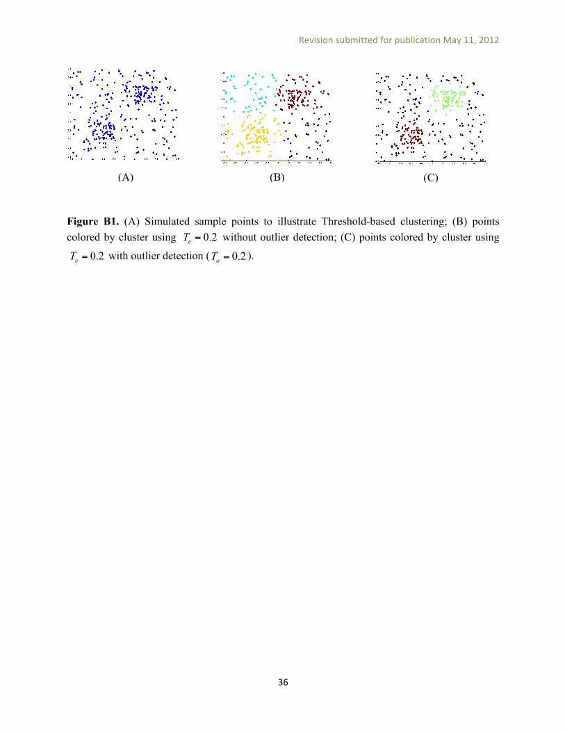
Figure B1 (A) shows a simulated 2-D point cloud generated by adding to a low uniform point distribution two rectangular areas of increased probability density. Figure B1 (B) shows Affinity Propagation clustering results using maximum exemplar similarity and no outlier detection. Of the four clusters produced by this solution, two consist mostly of outlier points. Figure B1 (C) shows the clustering solution obtained using outlier detection with and

. Here, the two high-density areas are separated into distinct clusters and other points are assigned to a third ‘background’ cluster.

1, 1n nS + +ʹ′

eT

0.2eT =

0.2oT =

0.2eT =


25

Table I

ERSP Domain

Nearby Clusters

Anatomical Area(s) Brodmann Area(s)

1 11, 14 (Dominated by eye-artifact ICs) N/A

2 12, 15 R Middle Occipital Gyrus (0.36) L Middle Occipital Gyrus (0.26) R Inferior Occipital Gyrus (0.09) L Inferior Occipital Gyrus (0.08) R Superior Occipital Gyrus (0.05) R Lingual Gyrus (0.04) R Inferior Temporal Gyrus (0.03) R Angular Gyrus (0.02) R Middle Temporal Gyrus (0.02)

BA 18 (0.34) Secondary visual (V2) BA 19 (0.34) Associative visual (V3) BA 37 (0.11) BA 39 (0.06) BA 17 (0.06), Primary visual (V1)

3 1 L Superior Occipital Gyrus (0.19) L Cuneus (0.16) L Middle Occipital Gyrus (0.15) R Cuneus (0.12) R Superior Occipital Gyrus (0.10) L Superior Parietal Gyrus (0.06) L Lingual Gyrus (0.04) L Precuneus (0.03) L Superior Temporal Gyrus (0.02) R Middle Occipital Gyrus (0.02) R Superior Temporal Gyrus (0.02) R Lingual Gyrus (0.02)

BA 18 (0.33) Secondary visual (V2) BA 19 (0.15) Associative visual (V3) BA 31 (0.13) BA 17 (0.12) Primary visual (V1) BA 7 (0.06) Somatosensory Association

4 4 L Superior Parietal Gyrus (0.27) L Postcentral Gyrus (0.27) L Supramarginal Gyrus (0.22) L Angular Gyrus (0.12) L Precentral Gyrus (0.10)

BA 40 (0.37) Spatial / Semantic Processing BA 7 (0.12) Somatosensory Association BA 3 (0.11) Primary Somatosensory BA 2 (0.10) Primary Somatosensory BA 4 (0.09) Primary Motor BA 39 (0.06)


26

Table II

Mean MPA Performance Score (std)

Cohen’s kappa Ratio (kappa, max possible)

Domain Dipole Noise Amplitude

Mean Domain

Dipole SNR (std)

Extra Dipole Noise

Amplitude

Projected Gaussian std.

(mm)

0.82 (0.21) 0.82 (0.63, 0.78) 0 1 0.2 12

0.85 (0.20) 0.84 (0.62, 0.73) 0 1 0.2 14

0.81 (0.19) 0.78 (0.63, 0.8) 0 1 0.2 10

0.93 (0.11) 0.9 (0.5, 0.56) 0.2 0.88 (0.09) 0.2 12

0.93 (0.10) 0.93 (0.47, 0.51) 0.2 0.88 (0.09) 0.2 14

0.89 (0.16) 0.84 (0.51, 0.61) 0.2 0.88 (0.09) 0.2 10


27

Figure 1. Time-line of each RSVP burst. Participant response feedback (‘Correct’ or ‘Incorrect’) was delivered only during Training sessions (rightmost panel).


28

Figure 2. (A) Steps performed during PCA-based clustering to create clusters of equivalent IC dipoles across decompositions of data from different subjects and/or sessions. (B) Steps performed during measure projection analysis to find sets of brain locations (domains). Note: In contrast to PCA-based clustering combining multiple non-dipole EEG measures (for example, equivalent dipole locations and experimental ERSPs and ERPs), in MPA each non-dipole location measure is analyzed separately.


29

Figure 3. IC-pair ERP and ERSP similarities. Absolute ERP similarities are used to overcome the inherent ambiguity of the polarity of IC activations. Dotted line displays the best least-squares linear fit, with Pearson correlation coefficient = 0.26.


30

Figure 4. Dipole locations and cluster-mean ERSPs for 3 of 15 clusters obtained from PCA-based clustering (see Figure 3A) with relatively large Target event-related ERSP values, most in the low theta frequency band (maxima equal or exceeding 1.7 dB). Cluster 11 is dominated by eye artifacts.


31

Figure 5. Dipole locations and mean Target ERSPs for a subset of clusters with weak ERSP values (absolute maxima lower than 1.3 dB, compare Figure 4).


32

Figure 6. Measure Projection Analysis (MPA) of ERSP (see Figure 3b): (A) Voxels representing locations with significant convergence (p < 0.075) colored by multi-dimensional scaling (MDS) mapping of projected Target ERSP measures to hue (MATLAB ‘hue’ color map values in the 0-0.69 interval, from red to blue). (B) Four domains created based on projected measure values and colored by 1-D MDS of the projected measure at their exemplar voxel. (C) 2-D MDS exemplar similarities of the four domains. Note the relative distance of Domain 1 (red, eye activities) from the other three Domains (blue, posterior cortex).


33

Figure 7. Alternative visualization of ERSP Domains on exemplar MNI cortical surface (and different Domain colors). Each cortical location is illuminated based on domain color and total dipole density from brain-grid positions radially below.


34

Figure 8. (A) ERSP Domain 2 dipoles with probability of membership in the domain above 0.05 are colored by the correlation of dipole-associated measure with domain exemplar. (B) Projected Target and Nontarget ERSPs and their statistically masked difference (right, p<0.05) for ERSP Domain 2.


35

Figure 9. (A) Simulated ground-truth domain set consisting of four anatomical regions (B) MPA results based on 12-mm Gaussian spatial noise and 0.88 ERSP Signal-to-Noise Ratio (SNR). (C) Simulated dipoles including subsets associated with each ground-truth ERSP domain plus randomly located outliers with random ERSP measures.


36

Figure B1. (A) Simulated sample points to illustrate Threshold-based clustering; (B) points colored by cluster using without outlier detection; (C) points colored by cluster using

with outlier detection ( 0.2oT = ).

0.2eT =

0.2eT =

(A) (B) (C)


37

References

Acar ZA, Makeig S. (2010): Neuroelectromagnetic Forward Head Modeling Toolbox. Journal of Neuroscience Methods 190(2):258-270.

Acar ZA, Worrell G, Makeig S. Patch-basis electrocortical source imaging in epilepsy; 2009 3-6 Sept. 2009. p 2930-2933.

Beckmann CF, Smith SM. (2005): Tensorial extensions of independent component analysis for multisubject FMRI analysis. NeuroImage 25(1):294-311.

Bell AJ, Sejnowski TJ. (1995): An Information Maximization Approach to Blind Separation and Blind Deconvolution. Neural Computation 7(6):1129-1159.

Benjamini Y, Hochberg Y. (1995): Controlling the False Discovery Rate - a Practical and Powerful Approach to Multiple Testing. Journal of the Royal Statistical Society Series B-Methodological 57(1):289-300.

Bigdely-Shamlo N, Vankov A, Ramirez RR, Makeig S. (2008): Brain Activity-Based Image Classification From Rapid Serial Visual Presentation. Ieee Transactions on Neural Systems and Rehabilitation Engineering 16(5):432-441.

Brodmann K. (1909): Vergleichende Lokalisationslehre der Grosshirnrinde. ihren Prinzipien dargestellt auf Grund des Zellenbaues.

Calhoun VD, Adali T, Pearlson GD, Pekar JJ. (2001): A method for making group inferences from functional MRI data using independent component analysis. Human Brain Mapping 14(3):140-151.

Calhoun VD, Liu J, Adali T. (2009): A review of group ICA for fMRI data and ICA for joint inference of imaging, genetic, and ERP data. NeuroImage 45(1):S163-S172.

Cichocki A, Amari Si. 2002. Adaptive blind signal and image processing : learning algorithms and applications. Chichester ; New York: J. Wiley. xxxi, 554 p. p.

Cohen J. (1960): A Coefficient of Agreement for Nominal Scales. Educational and Psychological Measurement 20(1):37-46.

Congedo M, John RE, De Ridder D, Prichep L. (2010): Group independent component analysis of resting state EEG in large normative samples. International journal of psychophysiology : official journal of the International Organization of Psychophysiology 78(2):89-99.

Darbellay GA, Vajda I. (1999): Estimation of the information by an adaptive partitioning of the observation space. Ieee Transactions on Information Theory 45(4):1315-1321.


38

Deary IJ, Simonotto E, Meyer M, Marshall A, Marshall I, Goddard N, Wardlaw JM. (2004): The functional anatomy of inspection time: an event-related fMRI study. NeuroImage 22(4):1466-79.

Delorme A, Makeig S. (2004): EEGLAB: an open source toolbox for analysis of single-trial EEG dynamics including independent component analysis. Journal of Neuroscience Methods 134(1):9-21.

Delorme A, Palmer J, Onton J, Oostenveld R, Makeig S. (2012): Independent EEG sources are dipolar. PloS one 7(2):e30135.

Dougherty RF, Koch VM, Brewer AA, Fischer B, Modersitzki J, Wandell BA. (2003): Visual field representations and locations of visual areas V1/2/3 in human visual cortex. Journal of Vision 3(10):586-598.

Eichele T, Calhoun VD, Debener S. (2009): Mining EEG-fMRI using independent component analysis. International Journal of Psychophysiology 73(1):53-61.

Esposito F, Scarabino T, Hyvarinen A, Himberg J, Formisano E, Comani S, Tedeschi G, Goebel R, Seifritz E, Di Salle F. (2005): Independent component analysis of fMRI group studies by self-organizing clustering. NeuroImage 25(1):193-205.

Evans AC, Collins DL, Mills SR, Brown ED, Kelly RL, Peters TM. 3D statistical neuroanatomical models from 305 MRI volumes; 1993 31 Oct-6 Nov 1993. p 1813-1817 vol.3.

Friston KJ. 2007. Statistical parametric mapping : the analysis of funtional brain images. Amsterdam ; Boston: Elsevier/Academic Press. vii, 647 p. p.

Gerson AD, Parra LC, Sajda P. (2005): Cortical origins of response time variability during rapid discrimination of visual objects. NeuroImage 28(2):342-53.

Heller R, Stanley D, Yekutieli D, Rubin N, Benjamini Y. (2006): Cluster-based analysis of FMRI data. NeuroImage 33(2):599-608.

Hyvarinen A. (2011): Testing the ICA mixing matrix based on inter-subject or inter-session consistency. NeuroImage 58(1):122-136.

Jung TP, Makeig S, McKeown MJ, Bell AJ, Lee TW, Sejnowski TJ. (2001): Imaging brain dynamics using independent component analysis. Proceedings of the Ieee 89(7):1107-1122.

Kiebel SJ, Friston KJ. (2004): Statistical parametric mapping for event-related potentials: I. Generic considerations. NeuroImage 22(2):492-502.


39

Kovacevic N, McIntosh AR. (2007): Groupwise independent component decomposition of EEG data and partial least square analysis. NeuroImage 35(3):1103-1112.

Lancaster JL, Woldorff MG, Parsons LM, Liotti M, Freitas ES, Rainey L, Kochunov PV, Nickerson D, Mikiten SA, Fox PT. (2000): Automated Talairach Atlas labels for functional brain mapping. Human Brain Mapping 10(3):120-131.

Lee TW, Girolami M, Sejnowski TJ. (1999): Independent component analysis using an extended infomax algorithm for mixed subgaussian and supergaussian sources. Neural Computation 11(2):417-441.

Li XL, Adali T, Anderson M. (2011): Joint blind source separation by generalized joint diagonalization of cumulant matrices. Signal Processing 91(10):2314-2322.

Li YO, Adali T, Wang W, Calhoun VD. (2009): Joint Blind Source Separation by Multi-set Canonical Correlation Analysis. IEEE transactions on signal processing : a publication of the IEEE Signal Processing Society 57(10):3918-3929.

Makeig S. (1993): Auditory Event-Related Dynamics of the Eeg Spectrum and Effects of Exposure to Tones. Electroencephalography and Clinical Neurophysiology 86(4):283-293.

Makeig S, Bell AJ, Jung TP, Sejnowski T. (1996): Independent component analysis of electroencephalographic data. Advances in Neural Information Processing Systems 8:145-151

Makeig S, Delorme A, Westerfield M, Jung TP, Townsend J, Courchesne E, Sejnowski TJ. (2004): Electroencephalographic brain dynamics following manually responded visual targets. Plos Biology 2(6):747-762.

Makeig S, Jung TP. (1995): Changes in alertness are a principal component of variance in the EEG spectrum. Neuroreport 7(1):213-6.

Makeig S, Jung TP, Bell AJ, Ghahremani D, Sejnowski TJ. (1997): Blind separation of auditory event-related brain responses into independent components. Proceedings of the National Academy of Sciences of the United States of America 94(20):10979-10984.

Makeig S, Westerfield M, Jung TP, Enghoff S, Townsend J, Courchesne E, Sejnowski TJ. (2002): Dynamic brain sources of visual evoked responses. Science 295(5555):690-694.

Marcar VL, Loenneker T, Straessle A, Jaggy S, Kucian K, Martin E. (2004): An fMRI study of the cerebral macro network involved in 'cue invariant' form perception and how it is influenced by stimulus complexity. NeuroImage 23(3):947-55.

Maris E, Oostenveld R. (2007): Nonparametric statistical testing of EEG- and MEG-data. Journal of Neuroscience Methods 164(1):177-90.


40

Mognon A, Jovicich J, Bruzzone L, Buiatti M. (2011): ADJUST: An automatic EEG artifact detector based on the joint use of spatial and temporal features. Psychophysiology 48(2):229-240.

Moosmann M, Eichele T, Nordby H, Hugdahl K, Calhoun VD. (2008): Joint independent component analysis for simultaneous EEG-fMRI: Principle and simulation. International Journal of Psychophysiology 67(3):212-221.

Nunez PL, Srinivasan R. 2006. Electric fields of the brain : the neurophysics of EEG. Oxford ; New York: Oxford University Press. xvi, 611 p. p.

Onton J, Makeig S. (2006): Information-based modeling of event-related brain dynamics. Event-Related Dynamics of Brain Oscillations 159:99-120.

Onton J, Westerfield M, Townsend J, Makeig S. (2006): Imaging human EEG dynamics using independent component analysis. Neuroscience and Biobehavioral Reviews 30(6):808-822.

Oostenveld R, Fries P, Maris E, Schoffelen JM. (2011): FieldTrip: Open source software for advanced analysis of MEG, EEG, and invasive electrophysiological data. Comput Intell Neurosci 2011:156869.

Pfurtscheller G, Aranibarand A, Maresch H. (1977): Occipital Alpha Activity during Initiation of Movement. Electroencephalography and Clinical Neurophysiology 43(4):486-487.

Philiastides MG, Sajda P. (2007): EEG-informed fMRI reveals spatiotemporal characteristics of perceptual decision making. J Neurosci 27(48):13082-91.

Picton TW, Bentin S, Berg P, Donchin E, Hillyard SA, Johnson R, Miller GA, Ritter W, Ruchkin DS, Rugg MD and others. (2000): Guidelines for using human event-related potentials to study cognition: Recording standards and publication criteria. Psychophysiology 37(2):127-152.

Rachakonda S, Eichele T, Calhoun V. 2011. Group ICA of EEG Toolbox (EEGIFT) Walk Through

Schmithorst VJ, Holland SK. (2004): Comparison of three methods for generating group statistical inferences from independent component analysis of functional magnetic resonance imaging data. Journal of Magnetic Resonance Imaging 19(3):365-368.

Shattuck DW, Mirza M, Adisetiyo V, Hojatkashani C, Salamon G, Narr KL, Poldrack RA, Bilder RM, Toga AW. (2008): Construction of a 3D probabilistic atlas of human cortical structures. NeuroImage 39(3):1064-1080.

Via J, Anderson M, Li X-L, Adali T. Joint blind source separation from second-order statistics: Necessary and sufficient identifiability conditions; 2011 22-27 May 2011. p 2520-2523.


41

Viola FC, Thorne J, Edmonds B, Schneider T, Eichele T, Debener S. (2009): Semi-automatic identification of independent components representing EEG artifact. Clinical Neurophysiology 120(5):868-877.

Worsley KJ, Taylor JE, Tomaiuolo F, Lerch J. (2004): Unified univariate and multivariate random field theory. NeuroImage 23 Suppl 1:S189-95.

Measure Projection Analysis: A Probabilistic Approach to EEG Source Comparison and Multi-Subject...

Documents

Transcript of Measure Projection Analysis: A Probabilistic Approach to EEG Source Comparison and Multi-Subject...