Maximum a Posteriori Joint State Path and Parameter ... - arXiv
143
Universidade Federal de Minas Gerais Programa de Pós-Graduação em Engenharia Elétrica Maximum a Posteriori Joint State Path and Parameter Estimation in Stochastic Differential Equations Dimas Abreu Dutra arXiv:1704.01847v1 [math.ST] 6 Apr 2017
-
Upload
khangminh22 -
Category
Documents
-
view
4 -
download
0
Transcript of Maximum a Posteriori Joint State Path and Parameter ... - arXiv

Universidade Federal de Minas GeraisPrograma de Pós-Graduação em Engenharia Elétrica
Maximum a Posteriori Joint State Pathand Parameter Estimation in
Stochastic Differential Equations
Dimas Abreu Dutra
arX
iv:1
704.
0184
7v1
[m
ath.
ST]
6 A
pr 2
017


Having all the answers just means you’ve been askingboring questions.
Emily Horn and Joey ComeauA Softer World #869, The freedom of uncertainty


Abstract
A wide variety of phenomena of engineering and scientific interest are of acontinuous-time nature and can be modeled by stochastic differential equations(SDEs), which represent the evolution of the uncertainty in the states of asystem. For systems of this class, some parameters of the SDE might beunknown and the measured data often includes noise, so state and parameterestimators are needed to perform inference and further analysis using thesystem state path. One such application is the flight testing of aircraft, inwhich flight path reconstruction or some other data smoothing technique isused before proceeding to the aerodynamic analysis or system identification.
The distributions of SDEs which are nonlinear or subject to non-Gaussianmeasurement noise do not admit tractable analytic expressions, so state andparameter estimators for these systems are often approximations based onheuristics, such as the extended and unscented Kalman smoothers, or theprediction error method using nonlinear Kalman filters. However, the Onsager–Machlup functional can be used to obtain fictitious densities for the parametersand state-paths of SDEs with analytic expressions.
In this thesis, we provide a unified theoretical framework for maximum aposteriori (MAP) estimation of general random variables, possibly infinite-dimensional, and show how the Onsager–Machlup functional can be used toconstruct the joint MAP state-path and parameter estimator for SDEs. Wealso prove that the minimum energy estimator, which is often thought tobe the MAP state-path estimator, actually gives the state paths associatedto the MAP noise paths. Furthermore, we prove that the discretized MAPstate-path and parameter estimators, which have emerged recently as powerfulalternatives to nonlinear Kalman smoothers, converge hypographically asthe discretization step vanishes. Their hypographical limit, however, is theMAP estimator for SDEs when the trapezoidal discretization is used and theminimum energy estimator when the Euler discretization is used, associatingdifferent interpretations to each discretized estimate.
Example applications of the proposed estimators are also shown, with bothsimulated and experimental data. The MAP and minimum energy estimatorsare compared with each other and with other popular alternatives.
vii


Resumo
Uma grande variedade de fenômenos de interesse para engenharia e ciênciasão a tempo contínuo por natureza e podem ser modelados por equaçõesdiferenciais estocásticas (EDEs), que representam a evolução da incerteza nosestados do sistema. Para sistemas dessa classe, alguns parâmetros da EDEpodem ser desconhecidos e os dados coletados frequentemente incluem ruídos,de modo que estimatores de esstados e parâmetros são necessários para realizarinferência e análises adicionais usando a trajetória dos estados do sistema. Umadessas aplicações é em ensaios em voo de aeronaves, para os quais reconstruçãode trajetória de voo ou outras técnicas de suavização são utilizadas antes de seproceder para análise aerodinâmica ou identificação de sistemas.
As distribuições de EDEs não lineares ou sujeitas a ruído de mediçãonão Gaussiano não admitem expressões analíticas utilizáveis, o que leva aestimadores de estados e parâmetros para esses sistemas a basearem-se emheurísticas como os suavizadores de Kalman estendido e unscented, ou o métodode predição de erro utilizando filtros de Kalman não lineares. No entanto, ofuncional de Onsager–Machlup pode ser utilizado para obter densidades fictíciasconjuntas para trajetórias de estado e parâmetros de EDEs com expressõesanalíticas.
Nesta tese, um arcabouço teórico unificado é desenvolvido para estimaçãomáxima a posteriori (MAP) de variáveis aleatórias genéricas, possivelmenteinfinito-dimensionais, e é mostrado como o funcional de Onsager–Machluppode ser utilizado para a construção do estimador MAP conjunto de trajetóriasde estado e parâmetros de EDEs. Também é provado que o estimador demínima energia, comumente confundido com com o estimador de MAP, obtémas trajetórias de estado associadas às trajetórias de ruído MAP. Além disso, éprovado que os estimadores conjuntos de trajetória de estados e parâmetrosMAP discretizados, que emergiram recentemente como alternativas poderosaspara os estimadores de Kalman não lineares, convergem hipograficamente àmedida que o passo de discretização diminue. O seu limite hipográfico, noentanto, é o estimador MAP para EDEs quando a discretização trapezoidal éutilizada e o estimador de mínima energia quando a discretização de Euler éutilizada, associando interpretações diferentes a cada estimativa discretizada.
ix

x Resumo
Exemplos de aplicações dos estimadores propostos são apresentadas comdados simulados e experimentais, nas quais os estimadores MAP e de mínimaenergia são comparados entre si e com alternativas mais bem sedimentadas.
Contents
Abstract vii
Resumo ix
Notation xiii
List of Acronyms xvii
1 Introduction 11.1 A brief survey of the related literature . . . . . . . . . . . . . . 11.2 Purpose and contributions of this thesis . . . . . . . . . . . . . 121.3 Outline of this thesis . . . . . . . . . . . . . . . . . . . . . . . . 15
2 MAP estimation in SDEs 172.1 Foundations of MAP estimation . . . . . . . . . . . . . . . . . . 172.2 Joint MAP state path and parameter estimation in SDEs . . . 242.3 Minimum-energy state path and parameter estimation . . . . . 43
3 MAP estimation in discretized SDEs 473.1 Hypo-convergence . . . . . . . . . . . . . . . . . . . . . . . . . 483.2 Euler-discretized estimator . . . . . . . . . . . . . . . . . . . . . 493.3 Trapezoidally-discretized estimator . . . . . . . . . . . . . . . . 57
4 Example applications 674.1 Simulated examples . . . . . . . . . . . . . . . . . . . . . . . . 674.2 Applications with experimental data . . . . . . . . . . . . . . . 86
5 Conclusions 955.1 Conclusions . . . . . . . . . . . . . . . . . . . . . . . . . . . . . 955.2 Future work . . . . . . . . . . . . . . . . . . . . . . . . . . . . . 96
A Collected theorems and definitions 99A.1 Simple identities . . . . . . . . . . . . . . . . . . . . . . . . . . 99A.2 Linear algebra . . . . . . . . . . . . . . . . . . . . . . . . . . . . 100A.3 Analysis . . . . . . . . . . . . . . . . . . . . . . . . . . . . . . . 100
xi

xii Contents
A.4 Probability theory and stochastic processes . . . . . . . . . . . 104
Bibliography 111
Index 123

Notation
A foolish consistency is the hobgoblin of little minds.Ralph Waldo Emerson, Self-Reliance
Here is a list of the mathematical typography and notation used throughoutthis thesis. Most are referenced on first use and are standard in the literature,still they are collected here for easy reference. To avoid a notational overload,many representations have a simpler form omitting parameters which can beclearly deduced from the context.
Typographical conventions
We begin with some typographical conventions used to represent differentmathematical objects. Note that these conventions are sometimes brokenwhen they become cumbersome or deviate from the standard convention ofthe literature.
Identifing subscripts are typeset upright, e.g., 𝑥a, 𝑥b.Matrices are typeset in uppercase bold, e.g., 𝑨, 𝑩, 𝜞, 𝜱.Random variables are typeset in uppercase while values they might take are
represented in lowercase, e.g., if 𝑋∶ 𝛺 → IR is a IR-valued randomvariable over the probability space (𝛺, ℰ, 𝑃), then 𝑥 ∈ IR can be used torepresent specific values it can take. The dependence on the outcome 𝜔will be omitted when unambiguous.
Sets are typeset in uppercase blackboard bold, e.g., 𝔸, 𝔹.𝑘-chains are typeset in lowercase blackboard bold, e.g., 𝕒, 𝕓.Time indices of stochastic processes are typeset as subscripts when unambigu-
ous, e.g., if 𝑋∶ IR × 𝛺 → IR is an IR-valued stochastic process over theprobability space (𝛺, ℰ, 𝑃), then 𝑋(𝑡, 𝜔) can be written as 𝑋u�(𝜔) or 𝑋u�.
Topological spaces are typeset in uppercase calligraphic, e.g., 𝒜, ℬ.
General symbols
IN ∶= {1, 2, 3, … } is the set of natural numbers (strictly positive integers).
xiii

xiv Notation
IR is the set of real numbers.IR≥0 ∶= {𝑥 ∈ IR | 𝑥 ≥ 0} is the set of nonnegative real numbers.IR>0 ∶= {𝑥 ∈ IR | 𝑥 > 0} is the set of strictly positive real numbers.IR ∶= IR ∪ {−∞, ∞} is the extended real number line.
Linear algebra
𝑨−1 is the inverse of the matrix 𝑨.𝑨𝖳 is the transpose of the matrix 𝑨.𝑰u� is an 𝑛 × 𝑛 identity matrix. The subscript indicating the size might be
dropped if it can be deduced from the context.𝑨(u�u�) is the element in the 𝑖th row and 𝑗th column of the matrix 𝑨.𝑎(u�) is the 𝑖th element of the vector 𝑎.
Probability and measure theory
(𝛺, ℰ, 𝑃) is a standard probability space (see Ikeda and Watanabe, 1981,Defn. 1.3.3) on which all random variables are defined.
𝜔 ∈ 𝛺 is the random outcome.ℬu� is the Borel 𝜎-algebra of the topological space 𝒳, i.e., the 𝜎-algebra of
subsets of 𝒳 generated by the topology of 𝒳.{ℰu�}u�≥0 is a filtration on the probability space (𝛺, ℰ, 𝑃), i.e., ℰu� ⊂ ℰu� ⊂ ℰ for
all 𝑡, 𝑠 ∈ [0, ∞) such that 𝑡 ≤ 𝑠.J𝐴, 𝐵K is the process of quadratic covariation between 𝐴 and 𝐵.supp(𝜇) is the support of a measure 𝜇 over a measurable space (𝒳, ℬu�), i.e.,
the set 𝔸 ∈ ℬu� of all points whose every open neighbourhood has strictlypositive 𝜇-measure (cf. Ikeda and Watanabe, 1981, Sec. 6.8).
𝐼𝔸(𝑥) is the indicator function of the set 𝔸, i.e., 𝐼𝔸(𝑥) ∶= 1 if 𝑥 ∈ 𝔸, 0 if 𝑥 ∉ 𝔸.
In addition, we will use the piece of jargon “for 𝑃-almost all 𝜔 ∈ 𝔼” to saythat a property holds for all but a zero-measure subset of an event 𝐸 ∈ ℰ,i.e., when the property holds for all 𝜔 ∈ 𝔼\ℕ, where ℕ ∈ ℰ is a 𝑃-null event𝑃(ℕ) = 0.
Analysis
|𝑥| is the Euclidean norm of 𝑥 ∈ IRu�.‖𝑥‖ is a norm of 𝑥. If unambiguous, the norm shall be inferred from the space
of 𝑥.

xv
|||𝑓||| ∶= maxu�∈u� ‖𝑓(𝑥)‖u� is the supremum norm of a function 𝑓∶ 𝒳 → 𝒴, alsoknown as the infinity or uniform norm.
⟨𝑎, 𝑏⟩ is the inner product between 𝑎 and 𝑏. If 𝑎, 𝑏 ∈ IRu�, the Euclideaninner product is implied ⟨𝑎, 𝑏⟩2 ∶= 𝑎𝖳𝑏, unless otherwise specified by asubscript.
𝐿u�u�(𝒳, ℱ, 𝜇) is the Banach space of 𝑓∶ 𝒳 → IRu� functions endowed with the
norm ‖𝑓‖u�u�u�
∶= (∫u�
‖𝑓(𝑥)‖u� d𝜇(𝑥))1u� , where (𝒳, ℱ, 𝜇) is a measure space.
For 𝒳 ⊂ IRu� the Lebesgue 𝜎-algebra and measure are implied and thenotation may be shortend to 𝐿u�
u�(𝒳). Additionally, the subscript may beommited for 𝑛 = 1, i.e., 𝐿u� ∶= 𝐿u�
1 .𝐿2
u�(𝒳, ℱ, 𝜇) is the Hilbert space of 𝑓∶ 𝒳 → IRu� functions endowed withthe inner product ⟨𝑓, 𝑔⟩u�2
u�∶= ∫
u�𝑓(𝑥)𝖳𝑔(𝑥) d𝜇(𝑥), where (𝒳, ℱ, 𝜇) is a
measure space. For 𝒳 ⊂ IRu� the Lebesgue 𝜎-algebra and measure areimplied and the notation may be shortend to 𝐿2
u�(𝒳). Additionally, thesuperscript may be ommited for 𝑛 = 1, i.e., 𝐿2 ∶= 𝐿2
1.𝒲2
u�([𝑎, 𝑏]) is the Hilbert space of absolutely continuous 𝑔∶ [𝑎, 𝑏] → IRu� func-tions with square-integrable weak derivatives 𝑔 ∈ 𝐿2
u�([𝑎, 𝑏]), endowedwith the inner product ⟨𝑓, 𝑔⟩u�2
u�∶= 𝑓(𝑎)𝖳𝑔(𝑎) + ∫u�
u�𝑓(𝑡)𝖳 𝑔(𝑡) d𝑡, which is
the direct sum of 𝑛 copies of the Sobolev space 𝒲2,1([𝑎, 𝑏]).𝒞(𝒳, 𝒴) is the space of continuous functions 𝑓∶ 𝒳 → 𝒴 between the topological
spaces 𝒳 and 𝒴. The domain and codomain can be ommited if they canbe inferred from the context. If 𝒳 is a compact Hausdorff space, likea closed interval of IR, and 𝒴 = IRu�, then 𝒞 is assumed to be endowedwith the supremum norm |||⋅|||, unless otherwise noted.
PL(𝒫, 𝒴) is the space of piecewise linear functions, with breaks over thepartition 𝒫, from [min(𝒫), max(𝒫)] to 𝒴.
𝜕𝔸, 𝜕𝕒 is the boundary of a set 𝔸 or the boundary of a 𝑘 − 𝑐ℎ𝑎𝑖𝑛 𝕒.�� is the closure of a set 𝔸.int 𝔸 is the interior of a set 𝔸.∫ 𝐴 ∘ d𝐵 is the Stratonovich integral of the process 𝐴 with respect to the
process 𝐵.
Miscellaneous
∇x𝑓(𝑎) ∶= [ u�u�(u�)
u�u�(u�) (𝑎)](u�u�)
is the Jacobian matrix of the function 𝑓 with respectto the input 𝑥, evaluated at the point 𝑎.
divx 𝑓(𝑎) ∶= ∑u�u�u�(u�)u�u�(u�) (𝑎) is the divergence of the function 𝑓 with respect to
the input 𝑥, evaluated at the point 𝑎, i.e., the trace tr(∇x𝑓(𝑎)) of itsJacobian matrix with respect to 𝑥.


List of Acronyms
BVP boundary value problem,COIN-OR computational infrastructure for operations research,EKF extended Kalman filter,EKS extended Kalman smoother,IPOPT interior point optimizer,JMAPSPPE joint maximum a posteriori state path and parameter estimator,IAE integrated absolute error,ISE integrated square error,MAP maximum a posteriori,MEE minimum energy estimator,MMSE minimum mean square error,NLP nonlinear program,ODE ordinary differential equation,OEM output error method,PEM prediction error method,SDE stochastic differential equation,UKF unscented Kalman filter,UKS unscented Kalman smoother,UFMG Universidade Federal de Minas Gerais.
xvii


Chapter 1
Introduction
The subject of this thesis is joint maximum a posteriori state path and param-eter estimation in systems described by stochastic differential equations, andits main contribution is the introduction of two new estimators. Besides theirobvious use in joint state path parameter estimation, the proposed estimatorscan also be employed in system identification and in smoothing, i.e., in appli-cations where both the parameters of the system and its states are unknownbut either only the parameters or the states are sought after. Consequently,this thesis is concerned not only with the intersection of parameter and stateestimation, but also with each of these fields of study independently.
We begin this chapter with an overview of smoothing and dynamicalsystem parameter estimation, presented in Section 1.1, covering both theirhistorical developments and the state of the art. We then proceed to presentthe motivation, objectives and contributions of this thesis in Section 1.2.
1.1 A brief survey of the related literatureIn this section we present a brief survey of the literature related to the top-ics investigated herein. We begin by presenting important definitions andterminology which will be used throughout this thesis.
1.1.1 Classes of models and state estimation
To best estimate quantities associated with dynamical systems from measure-ments spread out over time, the measured values should be used in conjunctionwith knowledge of the system dynamics. This is especially important whenboth the measurements and the dynamics are uncertain, and described by astochastic model instead of deterministic functions. Taking into account thatfor most real-world systems all models are approximations and all measure-ments have finite precision, models that take into account these shortcomingsare more realistic than those that do not.
1

2 Chapter 1. Introduction
time
signa
ls
discrete-time
statemeas.
time
continuous-time
statemeas.
time
continuous–discrete
statemeas.
Figure 1.1: Graphical representation of the state and measurements for thethree model classes.
The uncertainty in stochastic dynamical models can be due to unknownexternal disturbances acting on the system or can be simply a way for themodeler to express his lack of confidence and repeatability on the outcomes ofthe system. Examples of random external disturbances include electromag-netic interference in a circuit, thermal noise in a conductor, turbulence in anairplane and solar wind in a satellite, to name a few. Whether the behavior ofthe system—or of the corresponding disturbances—is truly random does notmatter, stochastic models for dynamical systems are an important tool to makeinference taking into account the uncertainties involved in the dynamics anddata acquisition. These tools can be used with both the subjectivist and ob-jectivist Bayesian points of view (for more information on these interpretationsand their dichotomy see Press, 2003, Chap. 1).
Stochastic models for dynamical systems can be classified into three majorclasses, according to how the dynamics and measurements are represented (cf.Jazwinski, 1970, p. 144):
discrete-time models are those in which both the measurements and the under-lying system dynamics are represented in discrete-time, over a possiblyinfinite but countable set of time points;
continuous-time models are those in which both the measurements and theunderlying system dynamics are represented in continuous-time, over anuncountable set of time points;
continuous–discrete models, also known as sampled-data or hybrid models,are those in which the measurements are taken in discrete-time butthe underlying system dynamics is represented in continuous-time. Themeasurements times are then a countable subset of the time interval overwhich the dynamics is represented.
These classes are illustrated graphically in Figure 1.1. Continuous–discretemodels are particularly important as various phenomena of interest to science

1.1. A brief survey of the related literature 3
timemeasurements
most recentinitial
times of interestsmoothing predictionfiltering
Figure 1.2: Graphical representation of the classes of state estimation.
and engineering are of a continuous-time nature, yet the measurements availablefor inference are sampled at discrete time instants.
The dynamics of discrete-time systems are usually represented by sto-chastic difference equations. Likewise, the dynamics of continuous-time andcontinuous–discrete systems are usually represented by stochastic differentialequations (SDEs). Models represented by SDEs are used to make inferencein a wide range of applications, including but not limited to radar tracking(Arasaratnam et al., 2010), aircraft flight path reconstruction (Mulder et al.,1999) and investment finance and option pricing (Black and Scholes, 1973); seethe reviews by Kloeden and Platen (1992, Chap. 7), and Nielsen et al. (2000)for a comprehensive list.
In a very influential article, Kalman (1960) defined three related classes ofestimation problems for signals under noise, given measurements spread outover time. His definitions are now standard terminology, and consist of thefollowing classes:
filtering, where the goal is to estimate the signal at the time of the latestmeasurement;
prediction, also known as extrapolation or forecasting, where the goal is toestimate the signal at a time beyond that of the latest measurement;
smoothing, also known as interpolation, where the goal is to estimate thesignal over times up to that of the latest measurement.
The filtering and prediction problem usually arise in online (real-time) ap-plications, such as process control and supervision. The smoothing problem,on the other hand, arises in offline (post-mortem, after the fact) applications,or online applications where a delay between measurement and estimation istolerable. In smoothing, future data (with respect to the estimate) is used toobtain better estimates (Jazwinski, 1970, p. 143). These classes are representedgraphically in Figure 1.2.
Three additional subclasses of the smoothing problem were defined byMeditch (1967) and have also been adopted into the jargon:
fixed-interval smoothing, where the goal is to estimate the whole signal inbetween the earliest and latest measurement;

4 Chapter 1. Introduction
fixed-point smoothing, where the goal is to estimate the signal at a specifictime-point before the latest measurement;
fixed-lag smoothing, where the goal is to estimate the signal at a specifictime-distance from the latest measurement.
The difference between fixed-point and fixed-lag smoothing is only relevant inonline applications.
In the context of Bayesian statistics, the smoothing estimates are usuallychosen as the posterior mean or the posterior mode. The posterior meanis known as the minimum mean square error (MMSE), as it minimizes theexpected square error with respect to the true states, over all outcomes forwhich the measured values would have been observed. The posterior modeis known as the maximum a posteriori (MAP) estimate, as it maximizes theposterior density. It is interpreted as the most probable outcome, given themeasurements. Fixed-interval MAP smoothing can, furthermore, be dividedinto two classes:
MAP state-path smoothing, where the estimates are the joint posterior modeof the states along all time instants in the interval, given all the mea-surements available;
MAP single instant smoothing, where the estimate for each time instant isthe marginal posterior mode of the state at the instant, given all themeasurements available.
Godsill et al. (2001) refer to these classes as the joint and marginal MAPestimation. The MAP state-path smoothing is also referred to as MAPstate-trajectory smoothing or, in the discrete-time case, MAP state-sequencesmoothing. As there is not much literature on this class of estimators, theterminology is not well cemented.
1.1.2 Smoothing
The modern theory of smoothing has its origins in the works of Wiener (1964)1
and Kolmogorov (1941)2, who developed the solution to stationary linearsystems subject to additive Gaussian noise. Wiener solved the continuous-time problem while Kolmogorov solved the discrete-time one. Their approachused the impulse response representation of systems to derive the results andrepresent the solutions. Wiener’s work seems to have pioneered the use ofstatistics and probability theory to both formulate and solve the problem offiltering and smoothing of signals subject to noise.
While many built uppon the Wiener–Kolmogorov filtering theory—refer toMeditch (1973) for a comprehensive survey—the main breakthrough came in
1Originally circulated in 1942 as a classified memorandum, connected to the war effort.2 In Russian, for an English translation see Kolmogorov (1992).

1.1. A brief survey of the related literature 5
the seminal work of Kalman (1960), who solved the problem of non-stationaryestimation in linear discrete-time and continuous–discrete systems subject toadditive Gaussian noise. The Kalman filter differed significantly from theWiener filter by the use of the state-space formulation in the time domainto derive the results and represent the solution. Shortly after, Kalman andBucy (1961) proposed the Kalman–Bucy filter, the analog of the Kalmanfilter for continuous-time systems with continuous-time measurements. Itshould be noted that for linear–Gaussian systems there exist exact formulasfor the discretization, so there is little difference between the discrete-time andcontinuous–discrete formulations.
In his initial paper, Kalman (1960) mentions that smoothing falls withinthe theory developed, but he does not address the smoothing problem directly.The Kalman filter was, however, readily extended to solve the smoothingproblem by Bryson and Frazier (1963) for the continuous-time case, and byCox (1964) and Rauch et al. (1965)3 for the discrete-time case. The abovementioned smoothers work by combining the results of a standard forwardKalman filter with a backward smoothing pass, which led to them beingclassified as forward–backward smoothers. Another approach, introduced byMayne (1966), consists of combining the results of two Kalman filters, onerunning forward in time and another one running backward, which came to becalled two-filter smoothing.
The two-filter and forward backward smoothers can also be adapted togeneral nonlinear systems and to non-Gaussian systems. However, in thesegenearal cases, the smoothing distributions do not admit known closed-formexpressions, except in some very specific cases. For these systems, consequently,practical smoothers must rely on approximations. One of the first of theseapproximations was the linearization of the system dynamics, which led tothe development of the extended Kalman filter and smoothers (for a historicalperspective on its development see Schmidt, 1981).
Nonlinear Kalman smoothers like the extended Kalman smoother followroughly the same steps as their linear counterparts, summarizing the relevantdistributions by their mean and variance. This implies that their underlyingassumption is that the densities involved in the smoothing problem are ap-proximately Gaussian. Consequently, the two-filter Rauch–Tung–Striebel orBryson–Frazier formulas can be used if appropriate linear–Gaussian approx-imations are made. Besides the extended Kalman approach of linearizationby truncating the Taylor series of the model functions, other approaches toobtain linear–Gaussian approximations include the unscented transform (Julierand Uhlmann, 1997), the statistical linear regression (Lefebvre et al., 2002)or Monte Carlo methods (Kotecha and Djuric, 2003), to name a few. Theunscented Kalman filter of Julier and Uhlmann (1997), in particular, was
3An early version of this paper was published in 1963 as a company report.

6 Chapter 1. Introduction
formalized for smoothing with the two-filter formula by Wan and van derMerwe (2001, Sec. 7.3.2) and with the Rauch–Tung–Striebel forward–backwardcorrection by Särkkä (2006, 2008).
More general smoothers for nonlinear systems are based on non-Gaussianapproximations of the smoothing distributions. The two-filter smoother ofKitagawa (1994), for example, uses Gaussian mixtures to represent the dis-tributions and the Gaussian sum filters of Sorenson and Alspach (1971) toperform the estimation. Sequential Monte Carlo two-filter (Kitagawa, 1996;Klaas et al., 2006) and forward–backward smoothers (Doucet et al., 2000;Godsill et al., 2004) represent the distributions by weighted samples using thesequential importance resampling method of Gordon et al. (1993). SequentialMonte Carlo methods can also be used for MAP state-path smoothing byemploying a forward filter in conjunction with the Viterbi algorithm to selectthe most probable particle sequence, as proposed by Godsill et al. (2001).
MAP state-path smoothers, nevertheless, do not need to be formulatedor implemented in the sequential Bayesian estimator framework. For a widevariety of systems, the posterior state-path probability density admits tractableclosed-form expressions4 which can be easily evaluated on digital computers.Therefore, by the use of nonlinear optimization tools, the MAP state-path canbe obtained without resorting to Bayesian filters.
Since the early developments in Kalman smoothing, MAP state-path esti-mation by means of nonlinear optimization was considered as a generalizationof linear smoothing to nonlinear systems subject to Gaussian noise (Brysonand Frazier, 1963; Cox, 1964; Meditch, 1970). However, the limitation ofthe computers available at the time meant that the estimates could not beobtained by solving a single large-scale nonlinear program. Therefore, thedivision of the large problem into several small problems, as performed by theextended Kalman smoother, was advantageous. Furthermore, for discrete-timesystems, the extended Kalman smoother was shown (Bell, 1994; Johnstonand Krishnamurthy, 2001) to be equivalent to Gauss–Newton steps in themaximization of the posterior state-path density. Because of those similarities,the terminology is still not standard, with many different methods falling underthe umbrella of Kalman smoothers. In this thesis, we will refer to as nonlinearKalman smoothers those methods which rely on two-filter or forward–backwardformulas, and as MAP state-path smoothers those methods which rely onnonlinear optimization to obtain their estimates.
As the tools of nonlinear optimization matured, optimization-based MAPstate-path smoothers emerged again as powerful alternatives to nonlinearKalman smoothers (Aravkin et al., 2011, 2012a,b,c, 2013; Bell et al., 2009;Dutra et al., 2012, 2014; Farahmand et al., 2011; Monin, 2013). Furthermore,unlike nonlinear Kalman smoothers, these smoothers are not limited to sys-
4Up to a constant factor which does not influence the location of maxima.

1.1. A brief survey of the related literature 7
tems with approximatelly Gaussian distributions, which lends them a widerapplicability. It also opens the possibility to model the systems with non-Gaussian noise. Heavy-tailed distributions are often used to add robustnessto the estimator against outliers, even when the measurements actually comefrom a different distribution. Examples of robust MAP state-path smoothingwith heavy-tailed distributions include the work of Aravkin et al. (2011) andFarahmand et al. (2011) with the ℓ1-Laplace, and the work of Aravkin et al.(2012a,c) with piecewise linear-quadratic log densities and Student’s 𝑡. Distri-butions with limited support, such as the truncated normal, can also be usedto model constraints (Bell et al., 2009).
One theoretical issue with MAP state-path smoothing that persistedup to recently was its correct definition, interpretation, and formulationfor continuous-time or continuous–discrete systems, and the applicabilityof discrete-time methods to discretized continuous systems. The definition isnot trivial because the state-paths of these systems lie in infinite-dimensionalseparable Banach spaces, for which there is no analog of the Lebesgue measure,i.e., a locally finite, strictly positive and translation-invariant measure. Conse-quently, the measure-theoretic definition of density as the Radon–Nikodymderivative of the probability measure is not applicable for the purposes ofobtaining the posterior mode (Dürr and Bach, 1978, p. 155).
Nevertheless, systems described by stochastic differential equations dopossess asymptotic probability of small balls, given by the Onsager–Machlupfunctional. This functional, first derived by Stratonovich (1971) for nonlinearSDEs, can be thought of as an analog of the probability density for the purposeof defining the mode. In the statistics and physics literature, a consensusarose that the maxima of the Onsager–Machlup functional represented themost probable paths of diffusion processes (Dürr and Bach, 1978; Ito, 1978;Takahashi and Watanabe, 1981; Ikeda and Watanabe, 1981, Sec. VI.9; Haraand Takahashi, 1996) and that it should be used for construction of MAPstate-path estimators (Zeitouni and Dembo, 1987).
Despite that, in the automatic control and signal processing literature,the Onsager–Machlup functional seemed to be virtually unknown until thelate 20th century. One of the few uses of the Onsager–Machlup functionalfor MAP state-path estimation in the engineering literature was the work ofAihara and Bagchi (1999a,b), which did not enjoy much popularity.5 In fact,as is detailed in the next paragraph, many authors incorrectly obtained theenergy functional as the merit function for MAP state-path estimation. Theenergy functional differs from the Onsager–Machlup functional by the lack ofa correction term which, when ommitted, can lead to different estimates.
Cox (1963, Chap. III), for example, obtained the energy functional by
5Only one citation from other authors, up to 2013, was found for both these articles inthe SciVerse Scopus, Web of Science, and Google Scholar databases.
8 Chapter 1. Introduction
applying the probability density functional of Parzen (1963) to the drivingnoise of the SDE, without taking into account that the nonlinear drift mightcause the mode of the state path to differ from the mode of the noise path, asproved to be the case in Chapter 2 of this thesis and in one of its derivativeworks (Dutra et al., 2014). Mortensen (1968) obtained the energy functional byFeynman path integration in function spaces, but apparently used an incorrectintegrand, as the Onsager–Machlup function is the correct Lagrangian in thepath integral formulation of diffusion processes (Graham, 1977).6 Jazwinski(1970, p. 155), on the other hand, obtained the energy by considering thelimit of the mode of the Euler-discretized systems. However, as argued byHorsthemke and Bach (1975), the Euler discretization cannot be used for suchpurposes due to insufficent approximation order.
The recent renewed interest in MAP state-path estimators, afforded bythe maturity of the necessary optimization tools, focused mostly on discrete-time systems. When applied to continuous-discrete systems described bySDEs, discretization schemes were used, as done by Bell et al. (2009) andAravkin et al. (2011, 2012c). For nonlinear systems, SDE discretizationschemes are approximations which improve as the discretization step decreases.Applications in Kalman filtering that use such discretization schemes, forexample, usually require fine discretizations to produce meaningful results(Arasaratnam et al., 2010; Särkkä and Solin, 2012). An important requirementfor the adoption of discrete-time MAP state-path smoothing for discretizedcontinuous-time systems is then understanding if and how the discretized MAPstate path relates to the MAP state path of the original system.
In this thesis we proved that, under some regularity conditions, discretizedMAP state-path estimation converges hypographically to variational estimationproblems, as the discretization step vanishes. However, the limit depends onthe discretization scheme used. For the Euler discretization scheme, themost popular, the discretization converges to the minimum energy estimation,which is proved to correspond to the state path associated with the MAPnoise path. When the trapezoidal scheme is used, on the other hand, theestimation converges to the MAP state-path estimation using the Onsager–Machlup functional. Our work also offers a formal definition of mode andMAP estimation of general random variables in possibly infinite-dimensionalspaces, under the framework of Bayesian decision theory. Finally, it highlightsthe links between continuous–discrete MAP state-path estimation and optimalcontrol, opening up an even wider range of tools for this class of estimationproblems. These results were published in a derivative work of this thesis(Dutra et al., 2014).
Having layed down a solid theoretical foundation for MAP state-path
6The exact integrand used could not be found, as the derivation was performed in“mimeographed lecture notes” which could not be recovered.
1.1. A brief survey of the related literature 9
estimation in systems described by SDEs, the field is now ripe for its use in non-Gaussian applications, such as robust smoothing, and fields typically dominatedby nonlinear Kalman smoothing, such as aircraft flight path reconstruction(Mulder et al., 1999; Jategaonkar, 2006, Chap. 10; Teixeira et al., 2011).
1.1.3 System identification
System identification is the inverse problem of obtaining a description for thebehavior of a system based on observations of its behavior. For dynamicalsystems, the system is represented by a suitable mathematical model and theobservations are measured input–output signals of its operation. The processof dynamical-system identification is often structured as composed of four maintasks:
data collection, the process of planning and executing tests to obtain repre-sentative observations of the system dynamics;
model structure determination, the process of choosing a parametrized struc-ture and mathematical representation for the model, using both a prioriinformation and some of the collected data;
parameter estimation, the process of obtaining parameter values from thecollected data and prior knowledge;
model validation, the process of evaluating if the chosen model with its esti-mated parameters is an adequate description of the system.
Each of these tasks is dependent upon the preceding ones, but the overall processcan be iterative and involve multiple repetitions until a suitable combinationof data, model, and parameters is found.
With respect to the model structure, three main classes are usually consid-ered:
white-box models, also known as phenomenological models, constructed fromfirst principles and knowledge of the system internals;
black-box models, also known as behavioral models, of a general structurechosen to represent the input–output relationship without regard to thesystem internals;
grey-box models, those which combine aspects of both white- and black-boxmodels, featuring components whose dynamics are derived from firstprinciples and others whose dynamics only represent some cause–effectrelationship.
Grey- and white-box models have the advantage that their parameters can havephysical meaning and can be related to other sources. Often, discrete-timemodels are used in black-box modelling, and continuous-time and continuous–discrete models are used in grey- and white-box modelling, as phenomenological
10 Chapter 1. Introduction
descriptions of the dynamics of most systems are formulated in continuous-time. Additionally, the representation of the state dynamics by stochasticdifferentential equations is a valuable tool for grey-box modelling, as it canput together a simplified phenomenological representation with a source ofuncertainty that accounts for the simplifications performed (cf. Kristensenet al., 2004a,b).
1.1.4 Parameter estimation in stochastic differentialequations
In the process of system identification, parameter estimation can be thoughtof as procedures for extracting the information from the data. For systemsfor which the states are directly observable, without measurement noise, thefield is well-consolidated and there exist a plethora of estimation techniques;see Nielsen et al. (2000, Secs. 3–4) and Bishwal (2008) for reviews. However,while the assumption of no measurement noise might be realistic for stockmarket and finantial modelling, it is overly optimistic for most engineeringapplications. When measurement noise is considered, the estimation problembecomes more complex and the field is still under active development.
In the remainder of this section, we will focus only on methods and tech-niques which take measurement noise into account. As the states are notdirectly measured, this class of parameter estimators is closely related to stateestimators. Intuitively thinking, to model the evolution of the states one firstneeds estimates of their values.
For Markovian systems, the likelihood function can be decomposed into theproduct of the one-step-ahead predicted output densities, given all previousmeasurements, evaluated at the measured values. Consequently, for linearsystems subject to Gaussian noise, the likelihood function can be obtainedby employing a Kalman filter to obtain the predicted output distributions.This approach was pioneered by Mehra (1971) and came to be known as theprediction-error method or filter-error method. Among its first applicationswas the parameter estimation of aircraft models from flight-test data collectedunder turbulence (Mehra et al., 1974). These methods can be used for bothmaximum likelihood and maximum a posteriori parameter estimation; see thesurvey by Åström (1980) for a review of its early developments.
Just like the Kalman filter was adapted to nonlinear systems by linearizationof the model functions, the prediction-error method was readily adaptedto nonlinear systems by employing the extended Kalman filter to obtainthe predicted output densities (Mehra et al., 1974). Like its underlyingnonlinear Kalman filter, this approach is based on the the implicit assumptionthat the the state and output distributions involved are all approximatelyconditionally Gaussian, given the parameters. Similarly, any other nonlinearfiltering approach, such as the unscented Kalman filter (Chow et al., 2007)

1.1. A brief survey of the related literature 11
or particle filters (Andrieu et al., 2004; Doucet and Tadić, 2003), can beused in prediction error methods. The limitations and difficulties associatedwith these methods are, likewise, those of their underlying nonlinear filters.Furthermore, the performance of the filters is usually significantly degradedwhen the parameters are far from the optimum, which can make the estimatorsensitive to the initial guess.
Another popular approach for parameter estimation worth mentioningconsists of treating parameters as augmented states and using standard stateestimation techniques (see Jazwinski, 1970, Sec. 8.4; or Ljung, 1979, and thereferences therein). These methods have the serious disadvantage, however,that if no process noise is assumed to act on the augmented states correspondingto the parameters, their estimated variance will converge to zero. Given all theapproximations involved, that is overly optimistic and, furthermore, can causethe estimators to fail. Consequently, a small artificial noise is assumed to acton the dynamics of, but this workaround also introduces its own drawbacks.The choice of the “parameter noise” variance is difficult and its effect on theoriginal problem is not always clear. Also, the final output of the methodis not a single estimate for the parameters but a time-varying one. It is notobviuos how to choose one instant or combine the estimate a different instantsto obtain the best value.
Up to the early 21st century, not much new development was done inparameter estimation in systems described by SDEs subject to measurementnoise, as argued by Kristensen et al. (2004b, p. 225). A review by Nielsenet al. (2000) pointed to the decades-old prediction error method with theextended Kalman filter as the “most general and useful approach” at the timefor parameter estimation in this class of systems.
A new development came in the work of Varziri et al. (2008b), whichthey termed the approximate maximum likelihood estimator. As explainedin (Varziri et al., 2008a, p. 830), their estimator can be interpreted as a jointMAP state-path and parameter estimator with a non-informative parameterprior. If the state-path and parameter posterior is then approximately jointlysymmetric, the estimated parameter should be close to the true maximumlikelihood estimate. However, it should be noted that they used the energyfunctional, as derived by Jazwinski (1970, p. 155), instead of the Onsager–Machlup functional to construct their merit function. This means that theirestimates have a different interpretation than intended, as is proved in Chapter 2of this thesis. In Chapter 3 of this thesis we prove, furthermore that theirderivation would be the one intended if the trapezoidal discretization schemehad been used instead of the Euler scheme.
One limitation of Varziri’s approximate maximum likelihood estimator wasthat the measurement and process noise variances had to be known a priori.That limitation was overcome first by using iterative procedures based on

12 Chapter 1. Introduction
heuristics (Karimi and McAuley, 2014b; Varziri et al., 2008c). However, amore rigorous and promising approach is using the Laplace approximation tomarginalize the states in the joint state-path and parameter density to obtainan approximation of the parameter likelihood function (Karimi and McAuley,2013, 2014a; Varziri et al., 2008a). In this context, the Laplace approximationis a technique to marginalize the state-path out of the posterior joint state-path and paremeter density, obtaining the posterior parameter density. Itconsists of making a Gaussian approximation of the state-path at its modefrom the Hessian of the log-density. It should be noted that the assumptionthat the posterior state-path smoothing distribution is approximately Gaussianis usually less strict than the assumption that the one-step-ahead predictedoutput is approximately Gaussian.
Once again, these estimators used the energy functional instead of theOnsager–Machlup functional, implying that they are, in fact, applying theLaplace approximation to marginalize the noise path out of the joint noise-pathand parameter distribution. The noise-path is usually less observable than thestate-path, implying that the Hessian of its log-posterior usually has a smallernorm and the Laplace approximation is coarser. We also remark that, althougheasily adapted to non-Gaussian measurement and prior distributions, theliterature on these estimators is restricted to the case where these distributionsare all Gaussian (Karimi and McAuley, 2013, 2014a,b; Varziri et al., 2008a,b;Varziri et al., 2008c).
We can then see that joint MAP state-path and parameter estimatorsfigure as an important tool for further development in parameter estimatorsfor systems described by stochastic differential equations. However, theoreticaldifficulties with the correct definition of MAP state-path and the effects ofdiscretizations must be clearly resolved for these methods to gain a wideradoption. Once these issues are resolved, these estimators can be used inapplications dominated by nonlinear-Kalman prediction-error methods andnon-Gaussian applications. In particular, just like with MAP state-pathestimation, heavy-tailed distributions can be used to perform robust systemidentification in the presence of outliers.
1.2 Purpose and contributions of this thesis
In this section, we lay down the purpose and contributions of this thesis toits related fields of study. We begin with its theoretical and technologicalmotivations and proceed to the objectives of this work and its contributions tothe literature.

1.2. Purpose and contributions of this thesis 13
1.2.1 Motivations
The motivations of this thesis are twofold: a technological driver based ondemand from applications; and the need to better understand the theorybehind maximum a posteriori state-path and joint state-path and parameterestimation in systems described by stochastic differential equations. Inportanttheoretical considerations that need a better understanding are the probabilisticinterpretations of the minimum energy and MAP joint state-path and parameterestimators and their relationship to the discretized estimators.
The Universidade Federal de Minas Gerais7 (UFMG) is one of the lead-ing centers of aeronautical technology research and education in Brazil. Itsactivities encompass all aspects of aeronautical engineering, including desing,construction and operation of airplanes and aeronautical systems. Among itscurrent projects are a light airplane with assisted piloting, a racing airplaneto beat world speed records, and hand-lauched autonomous unmanned aerialvehicles.
Flight testing is an integral part of design and operation of aircraft andaeronautical systems. Its purposes include analysis of aircraft performanceand behaviour; identification of dynamical models for control and simulation;and testing of systems and algorithms. Flight test data is subject to noiseand sensor imperfections; it is typically preprocessed before any analysis isdone. The process of recovering the flight path from test data is known asflight-path reconstruction (Mulder et al., 1999; Jategaonkar, 2006, Chap. 10;Klein and Morelli, 2006, Chap. 10) and is an essential step for flight-test dataanalysis. In adition, flight vehicle system identification is an indispensable toolin aeronautics with great engineering utility; see the editorial by Jategaonkar(2005) from the special issues of the Journal of Aircraft on this topic and someof the reviews therein (Jategaonkar et al., 2004; Morelli and Klein, 2005; Wangand Iliff, 2004) for more information.
Small hand-launched unmanned aerial vehicles, like the ones being de-signed and operated at UFMG, present additional challenges to flight-pathreconstruction and system identification. Their small payload limits the weightof the flight-test instrumentation that can be carried onboard, restricting theinstrumentation to lightweight sensors with more noise, bias and imperfections.Their small weight also makes them more sensitive to turbulence, which needsto be accounted for. The technological motivation of this thesis is then todevelop state and parameter estimators for flight-path reconstruction andsystem identification which are appropriate for use in small hand-launchedunmanned aircraft.
Related to our technological motivation, we have that the tools of MAPstate-path estimation, which show great promise for our intended application,
7Federal University of Minas Gerais

14 Chapter 1. Introduction
still has an unclear definition for systems described by stochastic differentialequations. Furthermore, the relationship between discretized estimators andthe continuous-time underlying problem needs to be understood with a rigorousmathematical analysis. Consequently, our theoretical motivations are to providea firm theoretical basis for MAP state-path and parameter estimation incontinuous-time and continuous–discrete systems.
1.2.2 Objectives and contributions
Having stated the motivations behind this work, the objectives of this thesisare then
• to provide a rigorous definition of mode and MAP estimation for randomvariables in possibly infinite-dimensional spaces which coincides with theusual definition for continuous and discrete random variables;
• to derive the joint MAP state-path and parameter estimator for systemsdescribed by SDEs, together with conditions and assumptions for itsapplicability;
• to obtain a probabilistic interpretation for the joint minimum energystate-path and parameter estimator, together with conditions and as-sumptions for its applicability;
• to relate discretized joint MAP state-path and parameter estimators totheir continuous-time counterparts;
• to demonstrate the viability of the derived estimators in example appli-cations with both simulated and experimental data.
We believe these are important steps for further advancement of the field andthe use of these techniques in novel and challenging applications.
The specific contributions and novelties of this thesis are
• formalization of the concept of fictitious densities, in Definition 2.4;• formalization of the concept of mode and MAP estimator for random
variables in metric spaces, using the concept of fictitious densities, inProposition 2.6 and Definitions 2.5 and 2.7;
• derivation of the Onsager–Machlup functional for systems with unknownparameters and possibly singular diffusion matrix, in Theorem 2.9;
• probabilistic interpretation of the energy functional as the fictitious den-sity of the associated noise path, in Theorem 2.26, extending the resultspublished in (Dutra et al., 2014) to systems with unknown parametersand possibly singular diffusion matrices;
• derivation of the hypographical limits of the Euler- and trapezoidally-discretized joint state path and parameter densities, in Theorems 3.7and 3.14, once more extending the results published in (Dutra et al.,

1.3. Outline of this thesis 15
2014) to systems with unknown parameters and possibly singular diffusionmatrices.
1.3 Outline of this thesisThe remainder of this thesis is organized as follows. In Chapter 2 we formallydefine the MAP estimator for general random variables and derive it forjoint state-path and parameter estimation in systems described by SDEs. Inaddition, we define the minimum energy estimator for state-path and parameterestimation in SDEs and prove that it is associated with the MAP noise-pathsand parameters. In Chapter 3, we briefly present the concepts of hypographicalconvergence and show how it can be applied to the discretized MAP estimation.We then derive the Euler- and trapezoidally-discretized joint MAP state-pathand parameter estimators and obtain their hypographical limits. The proposedestimators are then demonstrated in Chapter 4 with both simulated andexperimental data and the conclusions and future directions for extension ofthis work presented in Chapter 5.


Chapter 2
MAP estimation in SDEs
Don’t panic!Douglas Adams, The Hitchhiker’s Guide to the Galaxy
This chapter contains the main theoretical contributions of this thesis. Webegin with the definition and interpretations of maximum a posteriori (MAP)estimation in Section 2.1, and then proceed to apply the concepts developedfor the derivation of the joint MAP state-path and parameter estimator forsystems described by stochastic differential equations (SDEs) in Section 2.2.Then, in Section 2.3, the joint MAP noise-path and parameter estimator isderived and shown to be the minimum energy estimator obtained by omittingthe drift divergence in the Onsager–Machlup functional.
2.1 Foundations of MAP estimationIn this section, we present the theoretical foundations of maximum a posteriori(MAP) estimation. We begin with a brief presentation of Bayesian pointestimation and show how some parameters of the posterior distribution, suchas the mean and mode, are the Bayesian estimates associated with popularloss functions. We then define the mode of discrete and continuous randomvariables over IRu� and extend this definition to random variables over generalmetric spaces, like paths of stochastic processes. The MAP estimator is thendefined as the posterior mode and interpreted in the context of Bayesiandecision theory.
2.1.1 General Bayesian estimation
In Bayesian statistics, the posterior distribution of a random quantity ofinterest, given an observed event, is the aggregate of all the information availableon the quantity (Migon and Gamerman, 1999, p. 79). This information isrepresented in the form of a probabilistic description, and includes the prior,
17

18 Chapter 2. MAP estimation in SDEs
what was known before the observation, and the likelihood, what is added bythe observation. This information can be used to make optimal decisions inthe face of uncertainty, with the application of Bayesian decision theory.
In Bayesian decision theory, a loss function is chosen to represent theundesirability of each choice and random outcome. The Bayesian choice is thenthat which minimizes the expected posterior loss, over all possible decisions(Robert, 2001). Alternatively, the problem can be modeled in terms of the gainassociated with each choice and random outcome, in which case the Bayesianchoice is the one which maximizes the expected posterior gain. Gain functionsare also refered to as utility functions.
One application of Bayesian decision theory is Bayesian point estimation.Although any summarization of the posterior distribution leads to some loss ofinformation, it is often necessary to reduce the distribution of a random variableto a single value for some reason, among them reporting, communication orfurther analysis which warrants a single, most representative, value. A lossfunction is then used to quantify the suitability of each estimate, for eachpossible outcome of the random variable of interest, and the point estimateis the choice which minimizes the expected posterior loss. This concept isdetailed below.
Let 𝑋 be an 𝒳-valued random variable of interest and 𝑌 be a 𝒴-valuedobserved random variable. An estimator is a deterministic rule 𝛿 ∶ 𝒴 → 𝒳to obtain estimates for 𝑋 given observed values of 𝑌. The performance ofestimators is compared using measurable loss functions 𝐿∶ 𝒳 × 𝒳 → IR≥0. Foreach outcome 𝑋 = 𝑥, 𝐿( 𝑥, 𝑥) evaluates the penalty (or error) associated withestimate 𝑥. The integrated risk (or Bayes risk) associated with each estimatoris then defined by
𝑟(𝛿) ∶= E[𝐿(𝛿(𝑌), 𝑋)] ,
where E[⋅] denotes the expectation operator. The risk is the mean loss over allpossible values of the variable of interest and the observation. Having chosenan appropriate loss function for the problem at hand, the Bayesian estimatorsare defined as follows.
Definition 2.1 (Bayesian estimator). A Bayesian estimator 𝛿b ∶ 𝒴 → 𝒳 forthe random variable 𝑋, associated with the loss function 𝐿, given the observedvalue 𝑦 ∈ 𝒴 of 𝑌, is any which minimizes the expected posterior loss, i.e.,
E[𝐿(𝛿b(𝑦), 𝑋) ∣ 𝑌 = 𝑦] = minu�∈u�
E[𝐿(𝑥, 𝑋) | 𝑌 = 𝑦] .
Note that the minimum—and hence the Bayesian estimator—is not guar-anteed to exist and might not be unique. However, when it exists, no otherestimator is better according to the criterion defined by 𝐿, the probabilisticmodel in 𝑃 and the observation 𝑦. Multiplicity of minima means that there

2.1. Foundations of MAP estimation 19
exist several choices which are indistinguishable with respect to that criterion.In addition, if a Bayesian estimator exists for 𝑃u�-almost everywhere 𝑦, then itattains the lowest possible integrated risk (Robert, 2001, Thm. 2.3.2).
One way to interpret these quantities is making an analogy to a game ofchance. The estimate 𝑥 is a bet on the value of 𝑋, given that the player knows𝑌 = 𝑦 about the state of the game. The estimator represents a betting strategyand the loss function the financial losses for each outcome and bet, that is, thepayoff. The integrated risk is then the average loss expected for a given bettingstrategy. Thus, an optimal betting strategy would minimize the integratedrisk, leading to the minimum financial losses in the long run.1
There exist many canonical loss functions whose Bayesian estimators arecertain statistics of the posterior distribution. Take, for example, quadraticerror losses:
𝐿2( 𝑥, 𝑥) ∶= ℎ(𝑥 − 𝑥, 𝑥 − 𝑥),
where ℎ∶ 𝒳 × 𝒳 → IR≥0 is a coercive and bounded bilinear functional. For𝒳 = IRu� then ℎ is a positive-definite quadratic form, i.e.,
𝐿2( 𝑥, 𝑥) = (𝑥 − 𝑥)𝖳𝑄(𝑥 − 𝑥)
for any positive definite 𝑄 ∈ IRu�×u�. The Bayesian estimator associated withthis family of loss functions is the posterior mean of 𝑋. This result was provedfor IR-valued random variables by Gauss and Legendre (see Robert, 2001,Sec. 2.5.1) but also holds, under some regularity assumptions, when 𝒳 is amore general reflexive Banach space.
A similar result holds for the absolute error loss,
𝐿1( 𝑥, 𝑥) ∶= ‖ 𝑥 − 𝑥‖ .
When 𝑋 is an absolutely integrable IR-valued random variable, then theBayesian estimator associated with the 𝐿1 loss is is the posterior median, aresult initially proved by Laplace (see Robert, 2001, Prop. 2.5.5). When 𝑋is IRu�-valued and E[|𝑋| | 𝑌 = 𝑦] < ∞, then the posterior spatial median (alsoknown as the 𝐿1-median) is the Bayesian estimator associated with the 𝐿1loss. This concept also generalizes well to infinite-dimensional–valued 𝑋; thespatial median is also the Bayesian estimator associated with the 𝐿1 loss when𝒳 is a reflexive Banach space (Averous and Meste, 1997).
The modes, which are known as maximum a posteriori estimates, are onlydegenerate Bayesian estimates, however, for random variables over general
1The requirement of u� ≥ 0 would not attract many gamblers to the game, however,since it means that no bet and outcome combination yields profit. In this case the beststrategy would actually be not entering the game. Perhaps this is a critique of gambling bythe Bayesian decision theorists.
20 Chapter 2. MAP estimation in SDEs
spaces. Nevertheless, they can be interpreted in the framework of Bayesiandecision theory and Bayesian point estimation. Before showing how MAPestimation fits into this framework, we present in the following subsectionthe formal definition of modes for random variables over possibly infinite-dimensional spaces.
2.1.2 Modes of random variables
The modes of a random variable are population parameters that correspondto the region of the variable’s sample space where the probability is mostconcentrated. For discrete random variables, i.e., when there is a countablesubset of the variable’s sample space with probability one, then the modes areits most probable outcomes. For continuous random variables over IRu�, i.e.,those whose probability measure admits a density with respect to the Lebesguemeasure, all individual outcomes of the random variable have probability zero,so the modes are defined as the densest outcomes (Prokhorov, 2002). Thesedefinitions are formalized below.
Definition 2.2 (modes of discrete random variables). Let 𝑋 be an 𝒳-valuedrandom variable such that there exists a countable set 𝔸 ⊂ 𝒳 with 𝑃u�(𝔸) = 1.The modes of 𝑋 are the points 𝑥 ∈ 𝒳 satisfying
𝑃(𝑋 = 𝑥) = maxu�∈u�
𝑃(𝑋 = 𝑥),
at least one which exists.
Definition 2.3 (modes of continuous random variables). Let 𝑋 be an IRu�-valued random variable that admits a continuous density 𝑓∶ IRu� → IR≥0 withrespect to the Lebesgue measure. The modes of 𝑋, if they exist, are the points
𝑥 ∈ IRu� satisfying𝑓( 𝑥) = max
u�∈IRu�𝑓(𝑥).
We note that Definition 2.3 is restricted to random variables with continuousdensities because otherwise the definition is ambiguous. Any function whichis equal Lebesgue-almost everywhere to a probability density function is alsoa density for the same random variable. If the random variable admits acontinuous density, then the continuous one is considered as the best density,as it is the one with the largest Lebesgue set and coincides everywhere withthe Lebesgue derivative of the induced probability measure (Stein and Rami,2005, p. 104). If the random variable only admits discontinuous densities,however, then it is not clear which density is the best and should be used forcalculating the mode.
When generalizing the above definitions for paths of diffusion processes,probability densities (in the measure-theoretic sense) cannot be used. Thatis because for infinite-dimensional separable Banach spaces, like the space of
2.1. Foundations of MAP estimation 21
paths of IRu�-valued diffusions, there is no analog of the Lebesgue measure,i.e., a translation-invariant, locally finite and strictly positive measure. Anytranslation-invariant measure on an infinite-dimensional separable Banachspace would assign either infinite or zero measure to all open sets. Thus anymeasure with respect to which a density (Radon–Nikodym derivative) is takenwould weight equally-sized2 neighbourhoods differently. Similar problems arisein more general metric spaces, like the space of paths of diffusion processesover manifolds (cf. Takahashi and Watanabe, 1981).
This limitation is overcome by using a functional that quantifies the con-centration of probability in the neighborhood of paths but, unlike the density,cannot be used to recover the probability of events via integration. The con-centration is quantified by the asymptotic probability of metric 𝜖-balls, as 𝜖vanishes. The normalization factor of this asymptotic probability weights ballsof equal radius equally. Stratonovich (1971), who first proposed these ideas,called it the probability density functional of paths of diffusion processes. Webelieve, however, that the nomenclature of Takahashi and Watanabe (1981) ismore appropriate: the functional is “an ideal density with respect to a fictitiousuniform measure”3. Zeitouni (1989) shortened this nomenclature to fictitiousdensity, which is the term that is used in this thesis. This concept is formalizedbelow.
Definition 2.4 (fictitious density). Let 𝑋 be an 𝒳-valued random variable,where (𝒳, 𝑑) is a metric space. The function 𝑓∶ 𝒳 → IR≥0 is an ideal densitywith respect to a fictitious uniform measure, or a fictitious density for short, ifthere exists 𝑔∶ IR>0 → IR>0 such that
limu�↓0
𝑃(𝑑(𝑋, 𝑥) < 𝜖)𝑔(𝜖)
= 𝑓(𝑥) for all 𝑥 ∈ 𝒳 (2.1)
and 𝑓(𝑥) > 0 for at least one 𝑥 ∈ 𝒳.
Both probability mass functions and continuous probability density func-tions are fictitious densities, according to Definition 2.4. As the modes ofdiscrete and continuous random variables are the location of the maxima of thefictitious density, it is natural to define the mode of general random variablesthat admit a fictitious density as the location of the maxima of the fictitiousdensities.
Definition 2.5 (mode in metric spaces). Let 𝑋 be an 𝒳-valued randomvariable, where (𝒳, 𝑑) is a metric space. If 𝑋 admits a fictitious density 𝑓, itsmode, if it exists, is any 𝑥 ∈ 𝒳 that satisfies
𝑓( 𝑥) = maxu�∈u�
𝑓(𝑥).
2Such as metric balls of the same radius or translations of the same set.3Emphasis in the original.

22 Chapter 2. MAP estimation in SDEs
An alternative way to define the mode, which can help with the inter-pretation of the its statistical meaning, is the definition proposed in one ofthe derivative works of this thesis (Dutra et al., 2014, Defn. 1) and presentedbelow.
Proposition 2.6 (alternative definition of mode). Let 𝑋 be an 𝒳-valuedrandom variable, where (𝒳, 𝑑) is a metric space. Any 𝑥 ∈ 𝒳 is a mode of 𝑋,according to Definition 2.5, if and only if
limu�↓0
𝑃(𝑑(𝑋, 𝑥) < 𝜖)𝑃(𝑑(𝑋, 𝑥) < 𝜖)
≤ 1 for all 𝑥 ∈ 𝒳. (2.2)
Proof. If 𝑥 is the mode of 𝑋 according to Definition 2.5, 𝑓 is a fictitious densityand 𝑔(𝜖) is the fictitious uniform measure of an 𝜖-ball, then
limu�↓0
𝑃(𝑑(𝑋, 𝑥) < 𝜖)𝑃(𝑑(𝑋, 𝑥) < 𝜖)
= 𝑓(𝑥)maxu�′∈u� 𝑓(𝑥′)
≤ 1 for all 𝑥 ∈ 𝒳.
conversely, if (2.2) is satisfied for some 𝑥 ∈ 𝒳, then 𝑋 admits a fictitiousdensity using 𝑔(𝜖) ∶= 𝑃(𝑑(𝑋, 𝑥) < 𝜖) as a fictitious uniform measure of 𝜖-balls.Futhermore, the maximum of the fictitious density, which is equal to one, isattained at 𝑥, implying that it is a mode.
Proposition 2.6 means that, if 𝑥 is a mode and 𝑥 is not, then there exists an𝜖 ∈ IR>0 such that, for all 𝜖 ∈ (0, 𝜖 ] the 𝑥-centered 𝜖-ball has higher probability
than the 𝑥-centered one. Additionally, if both 𝑥 and 𝑥 are modes, then for all𝛿 ∈ IR>0 there exists an 𝜖 ∈ IR>0 such that, for all 𝜖 ∈ (0, 𝜖],
(1 − 𝛿)𝑃(𝑑(𝑋, 𝑥) < 𝜖) < 𝑃(𝑑(𝑋, 𝑥) < 𝜖) < (1 + 𝛿)𝑃(𝑑(𝑋, 𝑥) < 𝜖) ,
that is, the probabilities of 𝜖-balls centered on both values is arbitrarily close.
2.1.3 Maximum a posteriori and Bayesian estimation
A maximum a posteriori (MAP) estimate of a random variable, given an obser-vation, consists of the mode of its posterior distribution. From the definitionsof the preceding section (Sec. 2.1.2), we have that it can be interpreted as thepoint of the variable’s sample space around which the posterior probability ismost concentrated. The MAP estimator is the Bayesian equivalent of the max-imum likelihood estimator (Robert, 2001, Sec. 4.1.2; Migon and Gamerman,1999, p. 83). It differs from the latter by the inclusion of prior information,and can also be interpreted as a penalized maximum likelihood estimator ofclassical statistics. Its definition is formalized below.
Definition 2.7 (maximum a posteriori estimator). Let 𝑋 be an 𝒳-valuedrandom variable, where (𝒳, 𝑑) is a metric space. A maximum a posteriori

2.1. Foundations of MAP estimation 23
estimator of 𝑋, given an observation 𝑦 ∈ 𝒴, if it exists, is any which returnsits mode under the posterior distribution 𝑃u�(⋅ | 𝑌 = 𝑦).
When the variable of interest 𝑋 is a discrete random variable, i.e., whenthere is a countable subset of 𝒳 with 𝑃u�-measure one, the MAP estimator isthe Bayesian estimator associated with the 0–1 loss:
𝐿01( 𝑥, 𝑥) ∶= {0, if 𝑥 = 𝑥1, if 𝑥 ≠ 𝑥.
For these variables, the expected posterior 0–1 loss can be written in terms ofthe posterior probability mass function,
E[𝐿01( 𝑥, 𝑋) | 𝑌 = 𝑦] = 1 − 𝑃(𝑋 = 𝑥 | 𝑌 = 𝑦) , (2.3)
and the posterior modes, according to Definition 2.2, are the Bayesian estimates.For random variables over general metric spaces (𝒳, 𝑑), however, the MAP
estimator is usually not associated with any single loss function. It can,nonetheless, be associated with a series of loss functions which approximatethe 0–1 loss:
𝐿u�( 𝑥, 𝑥) ∶= {0, if 𝑑( 𝑥, 𝑥) < 𝜖1, if 𝑑( 𝑥, 𝑥) ≥ 𝜖.
Similarly to what was done to the 0–1 loss in (2.3), the expected posterior 𝐿u�loss can be written in terms of the probability of 𝜖-balls:
E[𝐿u�(𝑥, 𝑋) | 𝑌 = 𝑦] = 1 − 𝑃(𝑑(𝑥, 𝑋) < 𝜖 ∣ 𝑌 = 𝑦) .
Recalling the interpretation of the mode that followed from Proposition 2.6,we can then place MAP estimation in the framework of Bayesian decisiontheory and Bayesian estimation point estimation. If 𝑥 is a MAP estimate and𝑥 is not, then there exists an 𝜖 ∈ IR>0 such that for all 𝜖 ∈ (0, 𝜖 ] the expectedposterior 𝐿u� loss associated with 𝑥 is smaller than that associated with 𝑥.
We note that many authors define the MAP estimate, in the context ofBayesian decision theory, as the limit of the Bayesian estimates associatedwith 𝐿u�, as 𝜖 → 0 (Robert, 2001, Sec. 4.1.2; Mitchell, 2012, Sec. 10.2; Webb,1999, Sec. B.1.4). This definition is only applicable, however, when theposterior distribution of the variable of interest is unimodal. If the posteriordistribution is multimodal, then the limit of any convergent subsequenceof Bayesian estimates associated with 𝐿u� is a MAP estimate, under someregularity conditions (Daniel, 1969, p. 30). However, it is possible that notall modes are, necessarily, limits of Bayesian estimates associated with 𝐿u�.Because of these limitations, we believe that Definition 2.7 is preferable, dueto its greater generality. Hypo-convergence and variational analysis, which areused in Chapter 3 to relate sequences of maximization problems, are powerful
24 Chapter 2. MAP estimation in SDEs
tools to better understand the relation between the MAP estimator and theBayesian estimators associated with 𝐿u�.
In the sequence, we derive the joint posterior fictitious density of statepaths and parameters of systems described by stochastic differential equationsand, consequently, their MAP estimators.
2.2 Joint MAP state path and parameterestimation in SDEs
In this section, we apply the concepts developed in Section 2.1 for jointMAP state-path and parameter estimation in systems described by SDEs. InSection 2.2.1 the prior joint fictitious density is derived and in Section 2.2.2 itis used to obtain the posterior joint fictitious density.
2.2.1 Prior fictitious density
We now show how the Onsager–Machlup functional can be used to construct thejoint fictitious density of state paths and parameters of Itō diffusion processes,under some regularity conditions. This functional was initially proposedby Onsager and Machlup (1953) for Gaussian diffusions, in the context ofthermodynamic systems. Tisza and Manning (1957) later interpreted themaxima of this functional as the “most probable region” of paths of diffusionprocesses, which has since then become a consensus in various fields such asphysics (Adib, 2008; Dürr and Bach, 1978), mathematical statistics (Takahashiand Watanabe, 1981; Ikeda and Watanabe, 1981, Sec. VI.9; Zeitouni andDembo, 1987) and engineering (Aihara and Bagchi, 1999a,b; Dutra et al.,2014).
Stratonovich (1971) extended these ideas to diffusions with nonlinear driftand provided a rigorous mathematical background. Other developments relatedthe Onsager–Machlup functional include its generalization to diffusions onmanifolds (Takahashi and Watanabe, 1981); the extension of its domain to theCameron–Martin space of paths (Shepp and Zeitouni, 1992); and proving that italso corresponds to the mode, according to Definition 2.5, with respect to othermetrics besides the one induced by the supremum norm (Capitaine, 1995, 2000;Shepp and Zeitouni, 1993). In this section, we extend the Onsager–Machlupfunctional for diffusions with unknown parameters in the drift function andrank-deficient diffusion matrices. Our approach for handling rank-deficientdiffusion matrices is similar to that of Aihara and Bagchi (1999a,b), but wenote that their proofs are incomplete.
To begin, let 𝑋 and 𝑍 be IRu�- and IRu�-valued stochastic processes, re-spectively, representing the state of a dynamical system over the time interval𝒯 ∶= [0, 𝑡f]. We consider systems whose dynamics are given by a system of

2.2. Joint MAP state path and parameter estimation in SDEs 25
stochastic differential equations (SDEs) of the form
d𝑋u� = 𝑓(𝑡, 𝑋u�, 𝑍u�, 𝛩) d𝑡 + 𝑮 d𝑊u�, (2.4a)d𝑍u� = ℎ(𝑡, 𝑋u�, 𝑍u�, 𝛩) d𝑡, (2.4b)
where 𝑡 ∈ 𝒯 is the time instant; 𝑓∶ 𝒯 × IRu� × IRu� × IRu� → IRu� and ℎ∶ 𝒯 ×IRu� ×IRu� ×IRu� → IRu� are the drift functions; the IRu�-valued random variable𝛩 is the unknown parameter vector; 𝑊 is an 𝑛-dimensional Wiener processover IR≥0, with respect to the filtration {ℰu�}u�≥0, representing the processnoise; and 𝑮 ∈ IRu�×u� is the diffusion matrix. As the process 𝑋 is under directinfluence of noise and 𝑍 is not, they will be denoted the noisy and clean stateprocesses, respectively. Note that since the diffusion matrix does not dependon the state, the SDE can be interpreted in both the Itō or Stratonovich senses.
The following assumptions will be made on the system dynamics and priordistribution.
Assumption 2.8 (prior and system dynamics).
a. The initial states 𝑋0 and 𝑍0 and the parameter vector 𝛩 are ℰ0-measurable.b. The initial states 𝑋0 and 𝑍0 and the parameter vector 𝛩 admit a continuous
joint prior density 𝜋∶ IRu� × IRu� × IRu� → IR≥0.c. The drift functions 𝑓 and ℎ are uniformly continuous with respect to all of
their arguments in 𝒯×IRu� ×IRu� ×supp(𝑃u�), where supp(𝑃u�) indicates thetopological support of the probability measure induced by 𝛩, i.e., there exists𝜌u� ∶ IR≥0 → IR≥0 and 𝜌ℎ ∶ IR≥0 → IR≥0 such that limu�↓0 𝜌u�(𝜖) + 𝜌ℎ(𝜖) = 0and
∣𝑓(𝑡, 𝑥, 𝑧, 𝜃) − 𝑓(𝑡′, 𝑥′, 𝑧′, 𝜃′)∣ ≤ 𝜌u�(𝜖), (2.5a)∣ℎ(𝑡, 𝑥, 𝑧, 𝜃) − ℎ(𝑡′, 𝑥′, 𝑧′, 𝜃′)∣ ≤ 𝜌ℎ(𝜖), (2.5b)
for all 𝑡, 𝑡′ ∈ 𝒯, 𝑥, 𝑥′ ∈ IRu�, 𝑧, 𝑧′ ∈ IRu� and 𝜃, 𝜃′ ∈ supp(𝑃u�) such that|𝑡 − 𝑡′| ≤ 𝜖, |𝑥 − 𝑥′| ≤ 𝜖, |𝑧 − 𝑧′| ≤ 𝜖 and |𝜃 − 𝜃′| ≤ 𝜖.
d. For each 𝜃 ∈ supp(𝑃u�), the drift functions 𝑓 and ℎ are Lipschitz continuouswith respect to their second and third arguments 𝑥 and 𝑧, uniformly overtheir first argument 𝑡, i.e., there exist 𝐿u�
f , 𝐿u�h ∈ IR>0 such that for all 𝑡 ∈ 𝒯,
𝑥, 𝑥′ ∈ IRu� and 𝑧, 𝑧′ ∈ IRu�,
∣𝑓(𝑡, 𝑥, 𝑧, 𝜃) − 𝑓(𝑡, 𝑥′, 𝑧′, 𝜃)∣ ≤ 𝐿u�f (∣𝑥 − 𝑥′∣ + ∣𝑧 − 𝑧′∣) , (2.6a)
∣ℎ(𝑡, 𝑥, 𝑧, 𝜃) − ℎ(𝑡, 𝑥′, 𝑧′, 𝜃)∣ ≤ 𝐿u�h (∣𝑥 − 𝑥′∣ + ∣𝑧 − 𝑧′∣) . (2.6b)
e. For all 𝑡 ∈ 𝒯 and 𝜃 ∈ supp(𝑃u�), the noisy drift function 𝑓 is twicedifferentiable with respect to its second argument 𝑥 and differentiable withrespect to its first and third arguments 𝑡 and 𝑧. Furthermore, its first andsecond derivatives mentioned above are continuous with respect to all theirarguments.

26 Chapter 2. MAP estimation in SDEs
f. The diffusion matrix 𝑮 has full rank.g. The drift function 𝑓, the diffusion matrix 𝑮, the state processes 𝑋 and 𝑍,
and the parameter vector 𝛩 are such that
E[exp(∫1
0∣𝑮−1𝑓(𝑡, 𝑋u�, 𝑍u�, 𝛩)∣2 d𝑡)] < ∞.
Assumption 2.8a ensures that the state process 𝑋 is adapted to the filtra-tion {ℰu�}u�≥0. Assumption 2.8b, like the requirement of continuity of densitiesin Definition 2.3, makes 𝜋 the best joint density for 𝑋0, 𝑍0 and 𝛩, as itsLebesgue points are its whole domain. Assumption 2.8d ensures, togetherwith Lemma A.9 of Appendix A, that there exists, almost surely, a uniquestrong solution to the system of SDEs (2.4). Assumption 2.8f serves to en-force the consistency of the division of the clean and noisy states of (2.4).Assumption 2.8g is known as Novikov’s condition, and can be interpreted as arequirement that the expected “energy” exerted by and upon the system duringthe experiment is finite (cf. Stummer, 1993). The easiest way to guarantee thatit holds is ensuring that 𝑓 is bounded. More general requirements on the drift𝑓 to guarantee that Novikov’s condition is satisfied can be obtained by usingCorollary 3.5.16 of Karatzas and Shreve (1991) together with Lemma A.9.The remaining assumptions are used to ensure the existence of the fictitiousdensity.
Having stated the assumptions we have made on the system dynamics, weare now ready to derive the joint fictitious density of the 𝑋 path and the 𝑍0and 𝛩 vectors. We first state the theorem then a series of lemmas which areused for its proof, which is presented at the end of the subsection, on page 38.As mentioned in the beginning of this section, the fictitious density of pathsof diffusion processes can be taken with respect to many norms of functionspaces, all of them leading to the same density. However, the assumptionsused to guarantee the existence of the fictitious density depends on the norm.In this thesis, we choose the supremum norm (also known as the uniform orinfinity norm), as it requires the weakest assumptions. This metric is a naturalchoice as it is the metric of the classical Wiener space.
The supremum norm is defined by
|||𝑥||| ∶= supu�∈u� ‖𝑥(𝑡)‖ , (2.7)
where any finite-dimensional norm can be used on the right-hand side. Underthis metric the 𝜖-balls represent tubes (sometimes also referred to as sausages)of radius 𝜖, like the ones represented graphically in Figure 2.1. The choiceof the underlying finite-dimensional norm in (2.7) defines the geometry ofthe tubes’ transversal cross section. The Euclidean distance is implied unlessotherwise noted, leading to circular cross sections.

2.2. Joint MAP state path and parameter estimation in SDEs 27
𝑥(𝑡)
2𝜀
𝑥(𝑡)2𝜀
𝑡
𝑋u�
Figure 2.1: Graphical representation of 𝜖-balls under the supremum norm. Thedashed lines correspond to the centers and all sample paths of the IR-valuedprocess in the shaded region belong to the ball.
There are two main approaches to derive the Onsager–Machlup functional.One is acomplished by performing a Taylor expansion of the drift process ofthe SDE, and the other by using the stochastic Stokes’ theorem, as pioneeredby Takahashi and Watanabe (1981). Once more, in this thesis we use thestochastic Stokes route since it requires weaker assumptions, leading to a widerapplicability of the theorem. However, to use the stochastic Stokes’ theorem,the underlying finite-dimensional norm of the supremum norm must be theMahalanobis distance associated with the diffusion matrix, i.e., the norm withrespect to which the fictitious density of the 𝑋 paths is taken must be
|||𝑥|||u� ∶= supu�∈u� ∣𝑮−1𝑥(𝑡)∣ . (2.8)
Most of the results of this chapter still hold for the supremum norm withother underlying finite-dimensional norms, albeit with different assumptions.In particular, the Jacobian matrix of the noisy drift 𝑓 with respect to 𝑥 mustbe Lipschitz continuous with respect to 𝑥 (cf. Capitaine, 1995).
Throughout this section, we will denote by {𝔹u�}u�∈IR>0⊂ ℰ the family
of events, indexed by 𝜖 ∈ IR>0, corresponding to the outcomes in which 𝑋,𝑍0 and 𝛩 are inside 𝜖-balls centered around the test points 𝑥 ∈ 𝒞(𝒯, IRu�),𝑧0 ∈ IRu�, and 𝜃 ∈ IRu�, respectively, i.e.,
𝔹u� ∶= {𝜔 ∈ 𝛺 ∣ |||𝑋(𝜔) − 𝑥|||u� < 𝜖, |𝑍0(𝜔) − 𝑧0| < 𝜖, |𝛩(𝜔) − 𝜃| < 𝜖} . (2.9)
In addition, 𝒲2u� will denote the Sobolev space of absolutely continuous func-
tions from 𝒯 to IRu� whose weak derivative is in 𝐿2u�(𝒯). The joint fictitious
density of 𝑋, 𝑍0 and 𝛩 is then given by the theorem below.
Theorem 2.9 (joint fictitious density of state paths and parameters). IfAssumption 2.8 is satisfied, then there exist 𝑎1, 𝑎2 ∈ IR>0 such that for all𝑥 ∈ 𝒲2
u�, 𝑧0 ∈ IRu�, and 𝜃 ∈ IRu�,
limu�↓0
𝑃(𝔹u�)𝑎1 exp(−u�2
u�2 ) 𝜖u�+u�+u� = 𝜋(𝑥(0), 𝑧0, 𝜃) exp(𝐽(𝑥, 𝑧0, 𝜃)) , (2.10)

28 Chapter 2. MAP estimation in SDEs
where 𝔹u� is the 𝜖-ball centered in 𝑥, 𝑧0, and 𝜃, defined in (2.9), and the theOnsager–Machlup functional 𝐽∶ 𝒲2
u� × IRu� × IRu� → IR is defined by
𝐽(𝑥, 𝑧0, 𝜃) ∶= −12
∫u�
∣𝑮−1 [𝑓(𝑡, 𝑥(𝑡), 𝑧(𝑡), 𝜃) − 𝑥(𝑡)]∣2 d𝑡
− 12
∫u�
divx 𝑓(𝑡, 𝑥(𝑡), 𝑧(𝑡), 𝜃) d𝑡, (2.11)
and 𝑧 ∈ 𝒲2u� is the solution to the initial value problem
𝑧(𝑡) = ℎ(𝑡, 𝑥(𝑡), 𝑧(𝑡), 𝜃) , 𝑧(0) = 𝑧0. (2.12)
We now present a series of helping lemmas which culminate in the proof ofTheorem 2.9 on page 38. We begin by remarking that if the theorem holds forthe unit time interval, then it holds for any 𝑡f ∈ IR>0. This is done so that thesubsequent lemmas can be made simpler by considering 𝑡f = 1.
Remark 2.10 (reduction to the unit interval). If Theorem 2.9 holds for 𝑡f = 1,then it holds for any 𝑡f ∈ IR>0.
Proof. If 𝒯u ∶= [0, 1] denotes the unit time interval, then the linear map𝑢(𝜏) ∶= 𝜏𝑡f is a diffeomorphism between 𝒯u and 𝒯. Defining the processes�� ∶ 𝒯u × 𝛺 → IRu� and 𝑍 ∶ 𝒯u × 𝛺 → IRu� by
��(𝜏, 𝜔) ∶= 𝑋(𝑢(𝜏), 𝜔), 𝑍(𝜏, 𝜔) ∶= 𝑍(𝑢(𝜏), 𝜔),
we have that they satisfy the following SDEs:
d��u� ∶= 𝑡f𝑓(𝑢(𝜏), ��u�, 𝑍u�, 𝛩) d𝜏 + √𝑡f 𝑮 d��u�,
d 𝑍u� ∶= 𝑡fℎ(𝑢(𝜏), ��u�, 𝑍u�, 𝛩) d𝜏,
where, because of the Wiener process scaling property, the process
��(𝜏, 𝜔) ∶= 1√u�f
𝑊(𝑡f𝜏, 𝜔)
is an 𝑛-dimensional Wiener process with respect to a time-changed filtration.With this transformation we have that, for all 𝑥∶ 𝒯 → IRu� and 𝜖 ∈ IR>0,
𝑃(supu�∈u�|𝑮−1[𝑥(𝑡) − 𝑋u�]| < 𝜖) = 𝑃(supu�∈u�u|𝑮−1[𝑥(𝜏𝑡f) − ��u�]| < 𝜖) ,
implying that the joint fictitious density of 𝑋 over 𝒯, 𝑍0 and 𝛩 is the same asthat of �� over 𝒯u, 𝑍0 and 𝛩.
Next, note that if the original system satisfies Assumption 2.8, then thetime-changed one satisfies it as well. If Theorem 2.9 holds for the unit interval,

2.2. Joint MAP state path and parameter estimation in SDEs 29
we then have that the joint fictitious density of both systems is given by (2.10),whith the Onsager–Machlup functional 𝐽 given by
𝐽(𝑥, 𝑧0, 𝜃) ∶= −12
∫u�u
divx 𝑓(𝑢(𝜏), 𝑧(𝑢(𝜏), 𝑥(𝑢(𝜏)), 𝜃) 𝑡f d𝜏
− 12
∫u�u
∣𝑮−1 [𝑓(𝑢(𝜏), 𝑧(𝑢(𝜏)), 𝑥(𝑢(𝜏)), 𝜃) − 𝑥(𝑢(𝜏))]∣2 𝑡f d𝜏.
Performing a change in the region of integration using 𝑢, we obtain the sameexpression for 𝐽 as in (2.11), since d𝑡 = 𝑡fd𝜏.
Using Remark 2.10, we will now consider 𝑡f = 1 for simplicity. In addition,to further simplify the notation and the equations that follow, we define theIRu�- and IRu�-valued stochastic processes 𝐹 and 𝐻 as
𝐹u� ∶= 𝑓(𝑡, 𝑋u�, 𝑍u�, 𝛩) , 𝐻u� ∶= ℎ(𝑡, 𝑋u�, 𝑍u�, 𝛩) , (2.13)
and the functions 𝑓 ∶ 𝒯 → IRu� and ℎ ∶ 𝒯 → IRu� as
𝑓(𝑡) ∶= 𝑓(𝑡, 𝑥(𝑡), 𝑧(𝑡), 𝜃) , ℎ(𝑡) ∶= ℎ(𝑡, 𝑥(𝑡), 𝑧(𝑡), 𝜃) , (2.14)
where 𝑧 is the solution to the initial value problem (2.12).We now present a lemma which states that if 𝑋, 𝑍0 and 𝛩 are contained in
𝜖-balls, then the clean state path 𝑍 is also contained in an 𝜀-ball with respectto the supremum norm. The center of this ball is the solution to the initialvalue problem (2.12) and its radius 𝜀 vanishes when 𝜖 vanishes.
Lemma 2.11 (clean states growth bound). For a system satisfying Assump-tion 2.8, then for all 𝑥 ∈ 𝒞(𝒯, IRu�), 𝑧0 ∈ IRu�, and 𝜃 ∈ supp(𝑃u�) there exists𝑎3 ∈ IR>0 such that, almost surely,
|||𝑍 − 𝑧||| ≤ 𝑎3 [𝜌u�(|𝛩 − 𝜃|) + |𝑍0 − 𝑧0| + |||𝑋 − 𝑥|||] ,
where 𝑧 ∈ 𝒲2u� is the solution to the initial value problem (2.12) and 𝜌u� is the
modulus of continuity of 𝑓, which is assumed to exist by Assumption 2.8c.
Proof. Using the process 𝐻 and the function ℎ defined in (2.13) and (2.14),the differential equations (2.4b) and (2.12) admit the following representationin their integral forms:
𝑍u� = 𝑍0 + ∫u�
0𝐻u� d𝜏, 𝑧(𝑡) = 𝑧0 + ∫
u�
0ℎ(𝜏) d𝜏.
Using the triangle inequality we then have that, for all 𝑡 ∈ 𝒯, the differencebetween 𝑍 and 𝑧 is bounded by
|𝑍u� − 𝑧(𝑡)| ≤ |𝑍0 − 𝑧0| + ∫u�
0∣𝐻u� − ℎ(𝜏)∣ d𝜏. (2.15)

30 Chapter 2. MAP estimation in SDEs
The difference between 𝐻 and ℎ, on the other hand, can be bounded almostsurely:
|𝐻u� − ℎ(𝑡)| = |𝐻u� − ℎ(𝑡, 𝑋u�, 𝑍u�, 𝜃) + ℎ(𝑡, 𝑍u�, 𝑋u�, 𝜃) − ℎ(𝑡)|
≤ |𝐻u� − ℎ(𝑡, 𝑋u�, 𝑍u�, 𝜃)| + |ℎ(𝑡, 𝑋u�, 𝑍u�, 𝜃) − ℎ(𝑡)| (2.16a)≤ 𝜌ℎ(|𝛩 − 𝜃|) + 𝐿u�
h |𝑋u� − 𝑥(𝑡)| + 𝐿u�h |𝑍u� − 𝑧(𝑡)| , (2.16b)
where to obtain (2.16a) the triangle inequality was used and to obtain (2.16b)the Assumptions 2.8c–d on the uniform and Lipschitz continuity assumptionsof ℎ were used. Also note that (2.16b) only holds almost surely because ℎ isonly assumed to be uniformly continuous for 𝜃 on the support of 𝛩.
Substituting (2.16b) into (2.15), we then obtain
|𝑍u� − 𝑧(𝑡)| ≤ 𝐿u�h |||𝑋 − 𝑥||| + 𝜌ℎ(|𝛩 − 𝜃|) + |𝑍0 − 𝑧0| + 𝐿u�
h ∫u�
0|𝑍u� − 𝑧(𝑡)| d𝜏
Applying the Grönwall–Bellman inequality, Lemma A.8, we then have that
|||𝑍 − 𝑧||| ≤ [𝐿u�h |||𝑋 − 𝑥||| + 𝜌ℎ(|𝛩 − 𝜃|) + |𝑍0 − 𝑧0|] exp(𝐿u�
h) .
The next helping lemma is a change of measure which is used to representthe 𝜖-ball probabilities as conditional expectations of a random variable.
Lemma 2.12 (change of measure). For a system satisfying Assumption 2.8 anda given 𝑥 ∈ 𝒲2
u�, define the IR-valued random variable 𝑀 and the IRu�-valuedstochastic processes 𝑈, �� and ��o as
𝑈u� ∶= 𝑮−1 [𝐹u� − 𝑥(𝑡)] (2.17a)
��u� ∶= 𝑮−1 [𝑋u� − 𝑥(𝑡)] (2.17b)
��ou� ∶= ��u� − ��0 (2.17c)
𝑀 ∶= exp(− ∫1
0𝑈𝖳
u� d𝑊u� − 12
∫1
0|𝑈u�|2 d𝑡) (2.17d)
and the measure 𝑃 ∶ ℰ → IR≥0 as
𝑃(𝔼) ∶= ∫𝔼
𝑀(𝜔) d𝑃(𝜔).
Then 𝑃 is a probability measure equivalent4 to 𝑃. Furthermore, ��o is a𝑛-dimensional Wiener process with respect to the filtration {ℰu�}u�≥0 under 𝑃and
𝑀−1 = exp(∫10
𝑈𝖳u� d��u� − 1
2 ∫10
|𝑈u�|2 d𝑡) almost surely, (2.18a)
𝑃(𝔼) = ∫𝔼
𝑀−1(𝜔) d 𝑃(𝜔) for all 𝔼 ∈ ℰ, (2.18b)𝑃(𝔼) = 𝑃(𝔼) for all 𝔼 ∈ ℰ0. (2.18c)
4That is, mutually absolutely continuous with respect to one another.

2.2. Joint MAP state path and parameter estimation in SDEs 31
Proof. This is simply an application of the Girsanov transformation of measures(Øksendal, 2003, Sec. 8.6). By substituting (2.4a) into (2.17b), we have that�� satisfies the SDE
d��u� = 𝑮−1 [𝑓(𝑡, 𝑍u�, 𝑋u�, 𝛩) − 𝑥(𝑡)] d𝑡 + d𝑊u�. (2.19)
Novikov’s condition for the the removal of the drift of (2.19) is
E[exp(12 ∫1
0∣𝑮−1[𝐹u� − 𝑥(𝑡)]∣2 d𝑡)]
≤ E[exp(12 ∫1
0[|𝑮−1𝐹u�| + |𝑮−1 𝑥(𝑡)|]2d𝑡)] (2.20a)
≤ E[exp(∫10
∣𝑮−1𝑓(𝑡, 𝑋u�, 𝑍u�, 𝛩)∣2 d𝑡)] exp(∫10
|𝑮−1 𝑥(𝑡)|2d𝑡) (2.20b)
< ∞. (2.20c)
Equation (2.20a) is obtained from the triangle inequality, (2.20b) by applyingthe simple identity of Lemma A.2, and (2.20c) from Assumption 2.8g andthe fact that 𝑥 ∈ 𝒲2
u�. Applying the Girsanov transformation of measures(Øksendal, 2003, Sec. 8.6) we then obtain the results stated in the lemma.
Next, we obtain the fictitious uniform measure of 𝜖-balls with respect towhich the joint fictitious density of the state-paths and parameters is taken,i.e., the denominator of the left-hand side of (2.1) in the definition of fictitiousdensities (Definition 2.4).
Lemma 2.13 (𝜖-ball fictitious uniform measure). For a system satisfyingAssumption 2.8, there exist 𝑎1, 𝑎2 ∈ IR>0 such that, for all 𝑥 ∈ 𝒲2
u� with𝑥(0) ∈ supp(𝑃u�0
), 𝑧0 ∈ supp(𝑃u�0), and 𝜃 ∈ supp(𝑃u�),
limu�↓0
𝑃(𝔹u�)𝑎1 exp(−u�2
u�2 ) 𝜖u�+u�+u� = 𝜋(𝑥(0), 𝑧0, 𝜃) limu�↓0
E[𝑀−1 ∣ 𝔹u�] , (2.21)
whenever the limit on the right-hand side of (2.21) exists. Additionally,𝑃(𝔹u�) > 0 for all 𝜖 ∈ IR>0, so the conditional expectation is well-defined.
Proof. Applying Lemma 2.12 we can obtain the probability of 𝔹u� in terms of𝑀−1 and the measure 𝑃. For any event 𝔸 ∈ ℰ such that 𝑃(𝔸) > 0, (2.18b)implies that
𝑃(𝔸) = ∫𝔸
𝑀−1d 𝑃(𝜔) = E[𝑀−1 ∣ 𝔸] 𝑃(𝔸) .
Hence, to prove that (2.21) holds we need to show that, under the conditionsspecified in the Lemma’s statement, 𝑃(𝔹u�) > 0 for all 𝜖 ∈ IR>0 and thefollowing limit holds:
limu�↓0
𝑃(𝔹u�)exp(−u�2
u�2 ) 𝜖u�+u�+u� = 𝜋(𝑥(0), 𝑧0, 𝜃) 𝑎1. (2.22)

32 Chapter 2. MAP estimation in SDEs
To see that (2.22) indeed holds, we begin by obtaining an expression for𝑃(𝔹u�). From Assumption 2.8a, we have that 𝑋0, 𝑍0, and 𝛩 are ℰ0-measurable.
Additionally, from (2.18c) of the change of measure lemma (Lemma 2.12), weknow that 𝑃 and 𝑃 coincide on ℰ0-events. Consequently, Assumption 2.8bimplies that the joint prior density of 𝑋0, 𝑍0, and 𝛩 under 𝑃 is also givenby 𝜋. Finally, from Lemma 2.12 we have that, given 𝑋0, 𝑋 is independent ofℰ0 under 𝑃 and, as a consequence, independent of 𝑍0 and 𝛩 under 𝑃. Usingthe definition of the 𝔹u� event in (2.9), we then have its 𝑃 measure is given by
𝑃(𝔹u�) = ∭ℚu�ℝu�𝕊u�
𝜋( 𝑥 + 𝑥(0), 𝑧 + 𝑧0, 𝜃 + 𝜃)
× 𝑃(|||𝑋 − 𝑥|||u� < 𝜖 ∣ 𝑋0 = 𝑥 + 𝑥(0)) d 𝑥 d 𝑧 d 𝜃, (2.23)
where the family of sets ℚu�, ℝu�, and 𝕊u� are zero-centered 𝜖-balls defined as
ℚu� ∶= {𝑥 ∈ IRu� ∣ |𝑮−1𝑥| < 𝜖} ,ℝu� ∶= {𝑧 ∈ IRu� ∣ |𝑧| < 𝜖} ,𝕊u� ∶= {𝜃 ∈ IRu� ∣ |𝜃| < 𝜖} .
From the definition of the |||⋅|||u� norm in (2.8) and the definition of the ��process in (2.17b) we have that
|||𝑋 − 𝑥|||u� = |||��|||,
implying that
𝑃(|||𝑋 − 𝑥|||u� < 𝜖 ∣ 𝑋0 = 𝑥 + 𝑥(0)) = 𝑃(|||��||| < 𝜖 ∣ ��0 = 𝑮−1 𝑥) . (2.24)
Using the Wiener process scaling property, we have that the process 𝜖𝑊u�u�−2
has the same distribution as 𝑊u�, so the right-hand side of (2.24) can be furthersimplified
𝑃(|||��||| < 𝜖 ∣ ��0 = 𝑮−1 𝑥) = 𝑃(sup0≤u�≤1 |𝜖𝑊u�u�−2 | < 𝜖 ∣ 𝑊0 = 𝑮−1 𝑥)
= 𝑃(sup0≤u�≤u�−2 |𝑊u�| < 1 ∣ 𝑊0 = 𝑮−1 𝑥) . (2.25)
As it so happens, the right-hand side of (2.25) is the probability that theWiener process starting at 𝑮−1 𝑥 sojourns in the unit sphere
𝕌 ∶= {𝑢 ∈ IRu� ∣ |𝑢| < 1}
for longer than 𝜖−2, which according to Theorem A.15 satisfies a boundaryvalue problem whose solution is given by Proposition A.17:
𝑃(|||��||| < 𝜖 ∣ ��0 = ��) =∞∑u�=1
exp(−𝜆u�𝜖−2)𝛾u�(��) ∫𝕌
𝛾u�(𝑤) d𝑤, (2.26)

2.2. Joint MAP state path and parameter estimation in SDEs 33
where {𝛾u�}∞u�=1 are the eigenfunctions and {𝜆u�}∞
u�=1 the corresponding eigen-values of the Dirichlet eigenvalue problem on the unit sphere 𝕌, as defined inLemma A.16.
From (2.26) we can see that, for all 𝜖 ∈ IR>0 and �� ∈ 𝕌,
𝑃(|||��||| < 𝜖 ∣ ��0 = ��) > 0.
Consequently, from (2.23) we can then conclude that 𝑃(𝔹u�) > 0, as since 𝑥(0),𝑧0, and 𝜃 are in their prior’s support, 𝑃(𝑋0 ∈ ℚu�, 𝑍0 ∈ ℝu�, 𝛩 ∈ 𝕊u�) > 0 andthe integral of a nonzero function over a positive measure set is always positive.
Finally, performing a change of variables, we have that (2.23) can besimplified to
𝑃(𝔹u�) = 𝜖u�+u�+u� |det 𝑮| ∭𝕌 ℝ1𝕊1
𝜋(𝜖𝑮�� + 𝑥(0), 𝜖 𝑧 + 𝑧0, 𝜖 𝜃 + 𝜃)
× (∞∑u�=1
exp(−𝜆u�𝜖2 ) 𝛾u�(��) ∫
𝕌𝛾u�(𝑤) d𝑤) d�� d 𝑧 d 𝜃,
Using the bounded convergence theorem we then have that (2.22) and (2.21)hold with
𝑎1 = 𝜇(ℝ1)𝜇(𝕊1) |det 𝑮| (∫𝔾
𝛾1(𝑤) d𝑤)2
, 𝑎2 = 𝜆1, (2.27)
where 𝜇 denotes the Lebesgue measure.
It should be noted that the constants obtained in (2.27) are consistent withthose of the Onsager–Machlup with initial condition (Fujita and Kotani, 1982,p. 129). From Lemma 2.13 we have that for (2.10) in Theorem 2.9 to hold, theexpectation in the right-hand side of (2.21) should converge to the exponentialof the Onsager–Machlup functional. From the expression of 𝑀−1 in (2.18a),we should expect that its quadratic term converges to the quadratic term ofthe Onsager–Machlup functional in (2.11). This is shown with the help of theLemma below.
Lemma 2.14 (energy term of the Onsager–Machlup functional). If Assump-tion 2.8 is satisfied, then for all 𝑐 ∈ IR, 𝑥 ∈ 𝒲2
u� with 𝑥(0) ∈ supp(𝑃u�0),
𝑧0 ∈ supp(𝑃u�0), and 𝜃 ∈ supp(𝑃u�),
lim supu�↓0
E[exp(𝑐 ∫1
0(|𝑈u�|2 − ∣𝑮−1 [ 𝑓(𝑡) − 𝑥(𝑡)]∣
2) d𝑡) ∣ 𝔹u�] ≤ 1. (2.28)
Proof. To begin, define 𝜀 ∈ IR>0 by
𝜀 ∶= 𝑎3[𝜌u�(𝜖) + 2𝜖] + 𝜖.

34 Chapter 2. MAP estimation in SDEs
From Lemma 2.11 we then have that it bounds both |||𝑋 − 𝑥||| and |||𝑍 − 𝑧|||for almost all 𝜔 ∈ 𝔹u�, i.e.,
|||𝑋 − 𝑥||| + |||𝑍 − 𝑧||| ≤ 𝜀 for 𝑃-almost all 𝜔 ∈ 𝔹u�.
Expanding the integrand of (2.28), we obtain
|𝑈u�|2 − ∣𝑮−1 [ 𝑓(𝑡) − 𝑥(𝑡)]∣2
=
(|𝑈u�| − ∣𝑮−1 [ 𝑓(𝑡) − 𝑥(𝑡)]∣) (|𝑈u�| + ∣𝑮−1 [ 𝑓(𝑡) − 𝑥(𝑡)]∣) . (2.29)
Using the reverse triangle inequality, (2.5a) and (2.13), we then have that, foralmost all 𝜔 ∈ 𝔹u�,
∣ |𝑈u�| − |𝑮−1[ 𝑓(𝑡) − 𝑥(𝑡)]|∣ ≤ ∣𝑮−1[𝐹u� − 𝑓(𝑡)]∣ ≤ ∥𝑮−1∥ 𝜌u�(𝜀), (2.30)
where the induced operator norm is used for 𝑮−1. Next, using the triangleinequality, we have that
∣ |𝑈u�| + |𝑮−1[ 𝑓(𝑡) − 𝑥(𝑡)]|∣ ≤ ∥𝑮−1∥ (|𝐹u�| + 2 | 𝑥| + ∣ 𝑓(𝑡)∣) . (2.31)
A bound for the 𝐹 process can be found using the triangle inequality and theuniform continuity of 𝑓 as well:
|𝐹u�| ≤ |𝐹u� − 𝑓(𝑡)| + | 𝑓(𝑡)| ≤ 𝜌u�(𝜀) + | 𝑓(𝑡)|. (2.32)
Next noting that 𝑓 is bounded since it is continuous over a compact spaceand that 𝑥 ∈ 𝐿1
u� according to Lemma A.6, define
𝑎4 ∶= 2||| 𝑓||| + 2‖ 𝑥‖u�u�1, 𝑎5 ∶= ‖𝑮−1‖2.
Then, collecting (2.29) to (2.32), we have that for almost all 𝜔 ∈ 𝔹u�
∫1
0(|𝑈u�|2 − ∣𝑮−1 [ 𝑓(𝑡) − 𝑥(𝑡)]∣
2) d𝑡 ≤ 𝑎5𝜌u�(𝜀)[𝑎4 + 𝜌u�(𝜀)].
Letting 𝜖 vanish we can then see that (2.28) holds.
Next, from the expression of 𝑀−1 in (2.18a), we should expect that its Itōintegral term converges to the drift divergence term of the Onsager–Machlupfunctional in (2.11). This is proved with the help of the lemmas that follow.
Lemma 2.15 (conversion to Stratonovich integral). If Assumption 2.8 issatisfied, then
∫1
0[𝑮−1𝐹u�]𝖳 d��u� = ∫
1
0[𝑮−1𝐹u�]𝖳 ∘ d��u� − 1
2∫
1
0divx 𝑓(𝑡, 𝑋u�, 𝑍u�, 𝛩) d𝑡,
(2.33)
where ∫ 𝐴 ∘ d𝐵 denotes the Stratonovich integral of 𝐴 with respect to 𝐵.

2.2. Joint MAP state path and parameter estimation in SDEs 35
Proof. From the definition of the 𝐹 and 𝐻 processes in (2.13) we have that itsstochastic differential is given by
d𝐹u� = u�u�u�u� (𝑡, 𝑋u�, 𝑍u�, 𝛩) d𝑡 + ∇x𝑓(𝑡, 𝑋u�, 𝑍u�, 𝛩) d𝑋u�
+ ∇z𝑓(𝑡, 𝑋u�, 𝑍u�, 𝛩)𝐻u� d𝑡
In addition, from the definition of the �� process in (2.17b) we have that
𝑋u� = 𝑮��u� + 𝑥(𝑡), d𝑋u� = 𝑮 d��u� + 𝑥(𝑡) d𝑡, (2.34)
Consequently,
d��𝖳u� 𝑮−1 d𝐹u� = d��𝖳
u� 𝑮−1∇x𝑓(𝑡, 𝑋u�, 𝑍u�, 𝛩)𝑮 d��u�
= tr(𝑮−1∇x𝑓(𝑡, 𝑋u�, 𝑍u�, 𝛩)𝑮) d𝑡,= tr(∇x𝑓(𝑡, 𝑋u�, 𝑍u�, 𝛩)) d𝑡, (2.35)
where to obtain (2.35) we used the fact that the trace is invariant to similaritytransformations. The quadratic covariation process of ��𝖳 and 𝑮−1𝐹 is thengiven by
r𝑮−1𝐹𝖳, ��
zu�
= ∫u�
0divx 𝑓(𝑡, 𝑋u�, 𝑍u�, 𝛩) d𝑡.
Converting the Itō integral to a Stratonovich integral we then obtain (2.33).
Lemma 2.16 (convergence of divergences). If Assumption 2.8 is satisfied,then for all 𝑐 ∈ IR, 𝑥 ∈ 𝒲2
u� with 𝑥(0) ∈ supp(𝑃u�0), 𝑧0 ∈ supp(𝑃u�0
), and𝜃 ∈ supp(𝑃u�),
lim supu�↓0
E[exp(𝑐 ∫10
tr [∇x𝑓(𝑡, 𝑋u�, 𝑍u�, 𝛩) − ∇x𝑓(𝑡, 𝑥(𝑡), 𝑧(𝑡), 𝜃)] d𝑡) ∣ 𝔹u�] ≤ 1.
Proof. Without loss of generality, consider that 𝜖 ≤ 1. Lemma 2.11 andthe definition of the 𝜖-ball (2.9) then imply that 𝑋, 𝑍, and 𝛩 are boundedfor almost all 𝜔 ∈ 𝔹u�. From Assumption 2.8e, we then have that the driftdivergence is continuous, and continuous functions over compact spaces areuniformly continuous. Consequently,
limu�↓0
supu�∈𝔹u�
supu�∈u�
|divx 𝑓(𝑡, 𝑋u�, 𝑍u�, 𝛩) − divx 𝑓(𝑡, 𝑥(𝑡), 𝑧(𝑡), 𝜃)| = 0.

36 Chapter 2. MAP estimation in SDEs
Lemma 2.17. If Assumption 2.8 is satisfied, then for all 𝑥 ∈ 𝒲2u� with
𝑥(0) ∈ supp(𝑃u�0), 𝑧0 ∈ supp(𝑃u�0
), and 𝜃 ∈ supp(𝑃u�),
∫1
0[𝑮−1𝐹u�]𝖳 ∘ d��u� = 𝑓(1, ��1, 𝜔)𝖳��1 − 𝑓(0, ��0, 𝜔)𝖳��0
− ∫1
0
𝜕 𝑓𝜕𝑡
(𝑡, ��u�, 𝜔)𝖳��u� d𝑡 −u�
∑u�,u�=1
∫1
0
𝜕 𝑓(u�)
𝜕𝑥(u�) (𝑡, ��u�, 𝜔) d𝑆(u�u�)u�
− 12
u�∑
u�,u�=1∫
1
0( 𝜕2 𝑓(u�)
𝜕𝑥(u�)𝜕𝑥(u�) (𝑡, ��u�, 𝜔)��(u�) − 𝜕2 𝑓(u�)
𝜕𝑥(u�)𝜕𝑥(u�) (𝑡, ��u�, 𝜔)��(u�)) d𝑡,
(2.36)
where the function 𝑓 ∶ 𝒯 × IRu� × 𝛺 is defined as
𝑓(𝑡, 𝑥, 𝜔) ∶= ∫1
0𝑮−1𝑓(𝑡, 𝜏𝑮 𝑥 + 𝑥(𝑡), 𝑍u�, 𝛩) d𝜏
and the process 𝑆∶ 𝒯 × 𝛺 → IRu�×u� is the stochastic area enclosed by ��:
𝑆(u�u�)u� ∶= ∫
1
0��(u�)
u� ∘ d��(u�)u� − ∫
1
0��(u�)
u� ∘ d��(u�)u� .
Proof. From (2.34) and definition of the 𝐹 process in (2.13) we have that
𝐹u� = 𝑓(𝑡, 𝑮��u� + 𝑥(𝑡), 𝑍u�, 𝛩) .
Consequently, applying the stochastic Stokes’ theorem (Lemma A.18) on thespace-time 1-form
𝛽(𝑡, 𝑥) ∶=u�
∑u�=1
[𝑮−1𝑓(𝑡, 𝑮 𝑥 + 𝑥(𝑡), 𝑍u�, 𝛩)](u�) d 𝑥(u�),
we obtain that
∫1
0[𝑮−1𝐹u�]𝖳 ∘ d��u� = 𝑓(1, ��1, 𝜔)𝖳��1 − 𝑓(0, ��0, 𝜔)𝖳��0
− ∫1
0
𝜕 𝑓𝜕𝑡
(𝑡, ��u�, 𝜔)𝖳��u� d𝑡 −u�
∑u�,u�=1
∫1
0
𝜕 𝑓(u�)
𝜕𝑥(u�) (𝑡, ��u�, 𝜔) ∘ d𝑆(u�u�)u� . (2.37)
Next, note that since the quadratic covariationr
��(u�), ��(u�)z
= 0 for 𝑖 ≠ 𝑗,
𝑆(u�u�)u� = ∫
1
0��(u�)
u� d��(u�)u� − ∫
1
0��(u�)
u� d��(u�)u� . (2.38)

2.2. Joint MAP state path and parameter estimation in SDEs 37
Consequently, if we define the process 𝐹 as
𝐹(u�u�)u� ∶= 𝜕 𝑓(u�)
𝜕𝑥(u�) (𝑡, ��u�, 𝜔),
then its quadratic covariation process with the area process 𝑆 is
q 𝐹(u�u�), 𝑆(u�u�)yu�
= ∫u�
0
𝜕2 𝑓(u�)
𝜕𝑥(u�)𝜕𝑥(u�) (𝜏, ��u�, 𝜔)��(u�)u� d𝜏
− ∫u�
0
𝜕2 𝑓(u�)
𝜕𝑥(u�)𝜕𝑥(u�) (𝜏, ��u�, 𝜔)��(u�)u� d𝜏.
Converting the Stratonovich integral on the right-hand side of (2.37) to its Itōform we then obtain (2.36).
Lemma 2.18. If Assumption 2.8 is satisfied, then for all 𝑐 ∈ IR, 𝑖, 𝑗, 𝑘 ∈{1, … , 𝑛}, 𝑥 ∈ 𝒲2
u� with 𝑥(0) ∈ supp(𝑃u�0), 𝑧0 ∈ supp(𝑃u�0
), and 𝜃 ∈supp(𝑃u�),
lim supu�↓0
E[exp(𝑐 𝑓(1, ��1, 𝜔)𝖳��1 − 𝑐 𝑓(0, ��0, 𝜔)𝖳��0) ∣ 𝔹u�] ≤ 1, (2.39a)
lim supu�↓0
E[exp(𝑐 ∫1
0
𝜕 𝑓𝜕𝑡
(𝑡, ��u�, 𝜔)𝖳��u� d𝑡) ∣ 𝔹u�] ≤ 1, (2.39b)
lim supu�↓0
E[exp(𝑐 ∫1
0
𝜕2 𝑓(u�)
𝜕𝑥(u�)𝜕𝑥(u�) (𝑡, ��u�, 𝜔)��(u�)u� d𝑡) ∣ 𝔹u�] ≤ 1. (2.39c)
Proof. Lemma 2.11 and the definition of the 𝜖-ball (2.9) imply that, for all𝜖 ≤ 1, the arguments of 𝑓 and its derivatives in (2.39) are bounded for almost all𝜔 ∈ 𝔹u�. From continuity it then follows that 𝑓 and its derivatives are boundedfor almost all 𝜔 ∈ 𝔹u�. Consequently, (2.39) then holds as |||��||| → 0.
Lemma 2.19. If Assumption 2.8 is satisfied, we then have that for all 𝑐 ∈ IR,𝑖, 𝑗 ∈ {1, … , 𝑛}, 𝑥 ∈ 𝒲2
u� with 𝑥(0) ∈ supp(𝑃u�0), 𝑧0 ∈ supp(𝑃u�0
), and𝜃 ∈ supp(𝑃u�),
lim supu�↓0
E[exp(𝑐 ∫1
0
𝜕 𝑓(u�)
𝜕𝑥(u�) (𝑡, ��u�, 𝜔) d𝑆(u�u�)u� ) ∣ 𝔹u�] ≤ 1. (2.40)
Proof. Define the IR3-valued process 𝐵 by
𝐵(1)u� ∶= |��0| + ∫
u�
0
��𝖳u�
|��u�|d��u�, 𝐵(2)
u� ∶= |𝑍0| , 𝐵(3)u� ∶= |𝛩| . (2.41)
Using the Itō isometry, we then have that
q𝐵(1)y
u�=
u�∑u�=0
∫u�
0
��(u�)2u�
|��u�|2d𝑡 = 𝑡,

38 Chapter 2. MAP estimation in SDEs
implying that 𝐵(1) − 𝐵(1)0 is a Wiener process, by Lévy’s characterization.
Consequently, 𝐵 is a square-integrable martingale with the predictable repre-sentation property adapted with respect to the filtration {ℰu�}u�≥0. Furthermore,by Itō’s lemma we have that
d|��u�|2 = 𝑛 d𝑡 + 2|��u�| d𝐵(1)u� ,
implying that the random variable |||𝑋 − 𝑥|||u� = |||��||| and the event 𝔹u� aremeasurable with respect to the 𝜎-algebra generated by 𝐵.
Next, from (2.38) and (2.41) note that
d𝐵(1)u� d𝑆(u�u�)
u� = ��(u�)u� ��(u�)
u� d��(u�)u� d��(u�)
u�
|��u�|− ��(u�)
u� ��(u�)u� d��(u�)
u� d��(u�)u�
|��u�|= 0,
implying thatq𝐵(1), d𝑆(u�u�)y = 0, i.e., the martingales are orthogonal. Addi-
tionally, the quadratic variation of 𝑆 satisfies
q𝑆(u�u�)y
u�= ∫
u�
0[��(u�)2
u� + ��(u�)2u� ] d𝜏 ≤ 𝜖2 for all 𝜔 ∈ 𝔹u�
and from continuity of the derivatives of 𝑓 we have that the integrand of (2.40)is bounded for almost all 𝜔 ∈ 𝔹u�. Applying Lemma A.19 we then have that
E[exp(𝑐 ∫1
0
𝜕 𝑓(u�)
𝜕𝑥(u�) (𝑡, ��u�, 𝜔) d𝑆(u�u�)u� ) ∣ 𝔹u�]
≤ (E[exp(2𝑐 ∫1
0
𝜕 𝑓(u�)
𝜕𝑥(u�) (𝑡, ��u�, 𝜔)2 dq𝑆(u�u�)y
u�) ∣ 𝔹u�])
1/2
. (2.42)
Consequently, the integral on the right-hand side of (2.42) vanishes as 𝜖 ↓ 0and (2.40) holds.
We are now ready to prove the main result of this section.
Proof of Theorem 2.9. First, note that if either 𝑥(0) ∉ supp(𝑃u�0), 𝑧0 ∉
supp(𝑃u�0), or 𝜃 ∉ supp(𝑃u�), that is, if these variables lie outside the prior
support of their corresponding random variables, then (2.10) is satisfied triv-ially, as 𝜋(𝑥(0), 𝑧0, 𝜃) = 0 and there exists some 𝜖 ∈ IR>0 such that, for all𝜖 ∈ (0, 𝜖 ],
𝑃(𝔹u�) ≤ 𝑃(|𝑋0 − 𝑥(0)| < 𝜖, |𝑍0 − 𝑧0| < 𝜖, |𝛩 − 𝜃| < 𝜖) = 0. (2.43)
We now prove that (2.10) holds for all 𝑥(0) ∈ supp(𝑃u�0), 𝑧0 ∈ supp(𝑃u�0
),and 𝜃 ∈ supp(𝑃u�). From Lemma 2.13 we have that it suffices to prove that
limu�↓0
E[𝑀−1 ∣ 𝔹u�] = exp(𝐽(𝑧0, 𝑥, 𝜃))

2.2. Joint MAP state path and parameter estimation in SDEs 39
or, equivalently, that
limu�↓0
E[exp(∫1
0𝑈𝖳
u� d��u� − 12
∫1
0|𝑈u�|2 d𝑡 − 𝐽(𝑧0, 𝑥, 𝜃)) ∣ 𝔹u�] = 1. (2.44)
Using Lemmas 2.15 and 2.17 we then have that the exponent of (2.44) can beexpanded to
∫1
0𝑈𝖳
u� d��u� − 12
∫1
0|𝑈u�|2 d𝑡 − 𝐽(𝑧0, 𝑥, 𝜃) =
− 12
∫1
0(|𝑈u�|2 − ∣𝑮−1 [ 𝑓(𝑡) − 𝑥(𝑡)]∣
2) d𝑡
− 12
∫1
0tr [∇x𝑓(𝑡, 𝑋u�, 𝑍u�, 𝛩) − ∇x𝑓(𝑡, 𝑥(𝑡), 𝑧(𝑡), 𝜃)] d𝑡
− ∫1
0[𝑮−1 𝑥(𝑡)]𝖳 d��u� − 𝑓(1, ��1, 𝜔)𝖳��1 − 𝑓(0, ��0, 𝜔)𝖳��0
− ∫1
0
𝜕 𝑓𝜕𝑡
(𝑡, ��u�, 𝜔)𝖳��u� d𝑡 −u�
∑u�,u�=1
∫1
0
𝜕 𝑓(u�)
𝜕𝑥(u�) (𝑡, ��u�, 𝜔) d𝑆(u�u�)u�
− 12
u�∑
u�,u�=1∫
1
0( 𝜕2 𝑓(u�)
𝜕𝑥(u�)𝜕𝑥(u�) (𝑡, ��u�, 𝜔)��(u�) − 𝜕2 𝑓(u�)
𝜕𝑥(u�)𝜕𝑥(u�) (𝑡, ��u�, 𝜔)��(u�)) d𝑡.
(2.45)
Using Lemma A.13 we then have that (2.44) will hold if (A.13) holds for everyelement of the right-hand side of (2.45). For the Itō integral of 𝑥, we have thatfrom the theorem of Shepp and Zeitouni (1992),
limu�↓0
E[exp(𝑐 ∫1
0[𝑮−1 𝑥(𝑡)]𝖳 d��u�) ∣ 𝔹u�] = 1 for all 𝑐 ∈ IR.
For the remaining terms of (2.45), we have that the conditional exponentialmoments vanish from Lemmas 2.14, 2.16, 2.18, and 2.19.
For paths around 𝑥 ∉ 𝒲2u�, outside the Cameron–Martin space, we assume
that the fictitious density is null. This assumption was explicitly made in aderivative work of this thesis (Dutra et al., 2014) and is implicit wheneverthe Onsager–Machlup functional is used for MAP estimation (Aihara andBagchi, 1999a,b; Zeitouni and Dembo, 1987), as the search space is, at most,the Cameron–Martin space. This is formalized in the conjecture below. Wealso note that a draft proof of this conjecture was done by George Lowther inthe research mathematics forum MathOverflow.5
5See http://mathoverflow.net/q/160599.

40 Chapter 2. MAP estimation in SDEs
Conjecture 2.20. For all 𝑥 ∉ 𝒲2u�, 𝑧0 ∈ IRu�, and 𝜃 ∈ IRu�,
limu�↓0
𝑃(ℂu�)𝑎1 exp(−u�2
u�2 ) 𝜖u�+u�+u� = 0
where 𝑎1, 𝑎2 ∈ IR>0 are the constants of Theorem 2.9 and ℂu� is the 𝜖-ballcentered in 𝑥, 𝑧0, 𝜃, as defined below:
ℂu� ∶= {𝜔 ∈ 𝛺 ∣ |||𝑋(𝜔) − 𝑥|||u� < 𝜖, |𝑍(𝜔) − 𝑧0| < 𝜖, |𝛩(𝜔) − 𝜃| < 𝜖} .
Finally, we note that a wide range of systems of interest do not satisfyAssumptions 2.8d–c, but it still makes sense applying the joint MAP statepath and parameter estimator to them. This is because the model functionsare only valid on a small envelope, and the system dynamics looses its meaningoutside of it. A rigid body airplane model, for example, is only valid forsmall accelerations. For large accelerations flexibility effects become apparentand the rigid-body model is not representative. Larger accelerations stillwould cause structural failure. Consequently, the model function must onlyhave the specified form inside the validity envelope and the regularization ofRemark A.11 of Appendix A can be used to ensure the model satisfies therequired regularity conditions.
2.2.2 Joint posterior fictitious density of state paths andparameters
We now show how the joint prior fictitious density derived in the previoussubsection can be used to construct the joint posterior fictitious density and,with it, the MAP estimator. We begin by presenting the measurement modeland its assumptions in a general abstract setting which covers many widespreaduse cases.
Assumption 2.21 (measurements).
a. The 𝒴-valued random variable 𝑌 is observed, where 𝒴 is a metric space.b. For all 𝑥 ∈ 𝒞(𝒯, IRu�), 𝑧 ∈ 𝒞(𝒯, IRu�), and 𝜃 ∈ IRu�, the conditional
probability measure induced by 𝑌, conditioned on 𝑋 = 𝑥, 𝑍 = 𝑧 and 𝛩 = 𝜃,is absolutely continuous with respect to a measure 𝜈 over (𝒴, ℬu�) and admitsa conditional density 𝜓 with respect to it, i.e., for all 𝔹 ∈ ℬu�
𝑃(𝑌 ∈ 𝔹 | 𝑋 = 𝑥, 𝑍 = 𝑧, 𝛩 = 𝜃) = ∫𝔹
𝜓(𝑦 | 𝑥, 𝑧, 𝜃) d𝜈(𝑦). (2.46)
c. For the observed value 𝑦 ∈ 𝒴 of 𝑌, the likelihood 𝜓 is continuous with respectto its second argument 𝑥 (with respect to the supremum norm) and withrespect to its third argument 𝜃.

2.2. Joint MAP state path and parameter estimation in SDEs 41
d. For the observed value 𝑦 ∈ 𝒴 of 𝑌, E[𝜓(𝑦 | 𝑋, 𝑍, 𝛩)] > 0.
Assumption 2.21 and its underlying representation cover many measure-ment models and distributions. For 𝒴 = IRu� and 𝜈 as the Lebesgue measure,for example, 𝑌 can be a continuous random variable with 𝜓 its conditionalprobability density function, as examplified in Sections 4.1.1 and 4.1.2. Sim-ilarly, 𝜈 can be the counting measure, 𝑌 a discrete random variable and 𝜓its probability mass function, as examplified in Section 4.1.3. To representcontinuous-time measurements when 𝑌 is a diffusion depending on 𝑋, 𝑍, and𝛩, 𝜈 can be the Gaussian measure over 𝒞(𝒯, IRu�) of the driving process and𝜓 is given by variations of the Kallianpur–Striebel formula (Kallianpur andStriebel, 1968, 1969; Kallianpur, 1980, Sec. 11.3; van Handel, 2007, Lem. 1.1.5).
Using these assumptions, the joint posterior fictitious density of 𝑋, 𝑍0 and𝛩 is then given by the theorem below.
Theorem 2.22 (joint posterior fictitious density of state paths and param-eters). If a system of the form of (2.4) satisfies Assumption 2.8 and hasmeasurements satisfying Assumption 2.21, then there exist 𝑎1, 𝑎2 ∈ IR>0 suchthat for all 𝑥 ∈ 𝒲2
u�, 𝑧0 ∈ IRu�, and 𝜃 ∈ IRu�,
limu�↓0
𝑃(𝔹u� | 𝑌 = 𝑦)𝑎1 exp(−u�2
u�2 ) 𝜖u�+u�+u� =𝜓(𝑦 | 𝑥, 𝑧, 𝜃) 𝜋(𝑥(0), 𝑧0, 𝜃) exp(𝐽(𝑧0, 𝑥, 𝜃))
E[𝜓(𝑦 | 𝑋, 𝑍, 𝛩)],
(2.47)
where 𝔹u� is the 𝜖-ball centered in 𝑥, 𝑧0, and 𝜃, as defined in (2.9); 𝑧 ∈ 𝒲2u� is
the solution to the initial value problem (2.12); and 𝐽 is the Onsager–Machlupfunctional defined in (2.11).
Proof. First, note that (2.47) is satisfied trivially for 𝑥(0) ∉ supp(𝑃u�0), 𝑧0 ∉
supp(𝑃u�0), or 𝜃 ∉ supp(𝑃u�), as 𝜋(𝑥(0), 𝑧0, 𝜃) = 0 and there exists some
𝜖 ∈ IR>0 such that (2.43) holds for all 𝜖 ∈ (0, 𝜖 ].Next, assume that 𝑥(0) ∈ supp(𝑃u�0
), 𝑧0 ∈ supp(𝑃u�0), and 𝜃 ∈ supp(𝑃u�).
Using the measure-theoretic formulation of Bayes’ theorem (Schervish, 1995,Thm. 1.31), we have that
𝑃(𝔹u� | 𝑌 = 𝑦) =∫𝔹u�
𝜓(𝑦 | 𝑋(𝜔), 𝑍(𝜔), 𝛩(𝜔)) d𝑃(𝜔)
E[𝜓(𝑦 | 𝑋, 𝑍, 𝛩)]. (2.48)
As Lemma 2.13 guarantees that 𝑃(𝔹u�) > 0, (2.48) can be simplified to
𝑃(𝔹u� | 𝑌 = 𝑦) = E[𝜓(𝑦 | 𝑋, 𝑍, 𝛩) | 𝔹u�] 𝑃(𝔹u�)E[𝜓(𝑦 | 𝑋, 𝑍, 𝛩)]
.
Due to the continuity of 𝜓 (Assumption 2.21c),
limu�↓0
E[𝜓(𝑦 | 𝑋, 𝑍, 𝛩) | 𝔹u�] = 𝜓(𝑦 | 𝑥, 𝑧, 𝜃) ,

42 Chapter 2. MAP estimation in SDEs
which together with Theorem 2.9 implies that (2.47) holds.
From Definition 2.7 and Theorem 2.22, we have that the joint MAPestimator of 𝑋, 𝑍0 and 𝛩 is obtained by maximizing posterior joint fictitiousdensity, the left-hand side of (2.47), subject to having 𝑧 satisfy the initial valueproblem (2.12). For analysis and implementation of the estimator, however,it is more tractable to work with the logarithm of fictitious posterior density,which is known as the log-posterior for short. In addition, the denominator canbe dropped since it is constant and does not influence the location of maxima.
The joint MAP state-path and parameter estimator is then the solution tothe following optimization problem:
maximizeu�∈u�2
u�, u�∈u�2u�, u�∈IRu�
ℓ(𝑥, 𝑧, 𝜃)
subject to 𝑧(𝑡) = ℎ(𝑡, 𝑥(𝑡), 𝑧(𝑡), 𝜃) ,where the log-posterior ℓ ∶ 𝒲2
u� × 𝒲2u� × IRu� → IR is given by
ℓ(𝑥, 𝑧, 𝜃) ∶= ln 𝜓(𝑦 | 𝑥, 𝑧, 𝜃) + ln 𝜋(𝑥(0), 𝑧(0), 𝜃)
− 12
∫u�
∣𝑮−1 [𝑓(𝑡, 𝑥(𝑡), 𝑧(𝑡), 𝜃) − 𝑥(𝑡)]∣2 d𝑡
− 12
∫u�
divx 𝑓(𝑡, 𝑥(𝑡), 𝑧(𝑡), 𝜃) d𝑡. (2.49)
Alternatively, the search space can be expanded and more constraints addedto obtain the following equivalent optimization problem:
maximizeu�,u�∈u�2
u�, u�∈u�2u�, u�∈IRu�
ℓa(𝑥, 𝑧, 𝜃, 𝑤)
subject to 𝑥(𝑡) = 𝑓(𝑡, 𝑥(𝑡), 𝑧(𝑡), 𝜃) + 𝑮��(𝑡),𝑧(𝑡) = ℎ(𝑡, 𝑥(𝑡), 𝑧(𝑡), 𝜃)
(2.50)
where the alternative log-posterior ℓa ∶ 𝒲2u� × 𝒲2
u� × IRu� × 𝒲2u� → IR is given
by
ℓa(𝑥, 𝑧, 𝜃, 𝑤) ∶= ln 𝜓(𝑦 | 𝑥, 𝑧, 𝜃) + ln 𝜋(𝑥(0), 𝑧(0), 𝜃) − 12‖𝑤‖2
u�2u�
− 12
∫u�
divx 𝑓(𝑡, 𝑥(𝑡), 𝑧(𝑡), 𝜃) d𝑡. (2.51)
The optimization in the form (2.50) is analogous to an optimal control problemand is more tractable for numerical implementation and some theoreticalanalyses.

2.3. Minimum-energy state path and parameter estimation 43
2.3 Minimum-energy state path and parameterestimation
Throughout the literature, a commonly used alternative to the MAP state-pathestimator is obtained by using a functional equal to the log-posterior withoutthe drift divergence term (Bryson and Frazier, 1963; Cox, 1963, Chap. III;Mortensen, 1968; Jazwinski, 1970, p. 155). This was denoted the minimumenergy estimator by Hijab (1980), since its estimates minimize the input energyof the associated control system.
For many years, the minimum energy estimator was believed to be a goodMAP estimator (Zeitouni and Dembo, 1987, p. 234). Hijab (1984) showedthat, for systems with continuous-time measurements under Gaussian noise,the minimum energy merit is the limit optimal smoother when the intensity ofboth the process and measurement noise vanishes. In a derivative work of thisthesis (Dutra et al., 2014), we proved that the minimum energy estimates arestate paths corresponding to MAP noise paths. In this section, we extend ourprevious work by also covering the case where there are unknown parametersand not all states are under direct influence of noise.
We begin by stating the fictitious density of Wiener processes with thefollowing theorem, a variant of Theorem 2.9 with no drift and a fixed initialstate.
Theorem 2.23 (Fujita and Kotani, 1982, Capitaine, 1995). Let 𝑊 be an 𝑛-dimensional Wiener process. Then there exists 𝑎11, 𝑎12 ∈ IR>0 such that, forall 𝑤 ∈ 𝒲2
u� with 𝑤(0) = 0,
limu�↓0
𝑃(|||𝑊 − 𝑤||| < 𝜖)𝑎11 exp(−u�12
u�2 )= exp(−1
2‖��‖2u�2
u�) .
We are now ready to derive the prior joint fictitious density of 𝑊, 𝑋0, 𝑍0,and 𝛩. We will denote by 𝔹n
u� ∈ ℰ the event that 𝑊, 𝑋0, 𝑍0 and 𝛩 are insidean 𝜖-ball centered in some 𝑤 ∈ 𝒞(𝒯, IRu�), 𝑥0 ∈ IRu�, 𝑧0 ∈ IRu� and 𝜃 ∈ IRu�,for 𝜖 ∈ IR>0:
𝔹nu� ∶= {𝜔 ∈ 𝛺 ∣ |||𝑤 − 𝑊(𝜔)||| < 𝜖, |𝑋0(𝜔) − 𝑥0| < 𝜖,
|𝑍0(𝜔) − 𝑧0| < 𝜖, |𝛩(𝜔) − 𝜃| < 𝜖}. (2.52)
Theorem 2.24. If Assumption 2.8 is satisfied, then there exist 𝑎11, 𝑎12 ∈ IR>0such that, for all 𝑤 ∈ 𝒲2
u� with 𝑤(0) = 0, 𝑥0 ∈ IRu�, 𝑧0 ∈ IRu�, and 𝜃 ∈ IRu�,
limu�↓0
𝑃(𝔹nu� )
𝑎11 exp(−u�12u�2 ) 𝜖u�+u�+u� = 𝜋(𝑥0, 𝑧0, 𝜃) exp(−1
2‖��‖2u�2
u�) , (2.53)
where 𝔹nu� is the 𝜖-ball defined in (2.52).

44 Chapter 2. MAP estimation in SDEs
Proof. From Assumption 2.8a we have that 𝑋0, 𝑍0, and 𝛩 are ℰ0-measurableand, consequently, independent of 𝑊. Applying the Lebesgue differentiationtheorem and Theorem 2.23 we then have that (2.53) holds.
Next, to calculate the fictitious joint posterior density of noise paths, weshow that for each 𝑤, 𝑥0, 𝑧0 and 𝜃 there exists an associated state path suchthat its largest distance from 𝑋, for all 𝜔 ∈ 𝔹n
u� , vanishes with 𝜖. This lemmais similar to Lemma 2.11.
Lemma 2.25 (associated state path). If Assumption 2.8 is satisfied then, forall for all 𝑤 ∈ 𝒲2
u� with 𝑤(0) = 0, 𝑥0 ∈ IRu�, 𝑧0 ∈ IRu�, and 𝜃 ∈ supp(𝑃u�),
limu�↓0
supu�∈𝔹n
u�
|||𝑋(𝜔) − 𝑥||| = 0, limu�↓0
supu�∈𝔹n
u�
|||𝑍(𝜔) − 𝑧||| = 0,
where 𝔹nu� is the 𝜖-ball defined in (2.52) and 𝑥 ∈ 𝒲2
u� and 𝑧 ∈ 𝒲2u� are the unique
solutions to the following integral equations, for all 𝑡 ∈ 𝒯:
𝑥(𝑡) = 𝑥0 + ∫u�
0𝑓(𝜏, 𝑥(𝜏), 𝑧(𝜏), 𝜃) d𝜏 + 𝑮𝑤(𝑡) (2.54a)
𝑧(𝑡) = 𝑧0 + ∫u�
0ℎ(𝜏, 𝑥(𝜏), 𝑧(𝜏), 𝜃) d𝜏. (2.54b)
Proof. Taking the difference between the integral representation of 𝑥 and 𝑧 in(2.54) and 𝑋 and 𝑍 in (2.4) we have that
𝑋u� − 𝑥(𝑡) = 𝑋0 − 𝑥0 + ∫u�
0[𝐹u� − 𝑓(𝜏)] d𝜏 + 𝑮[𝑊u� − 𝑤(𝑡)],
𝑍u� − 𝑧(𝑡) = 𝑍0 − 𝑧0 + ∫u�
0[𝐻u� − ℎ(𝜏)] d𝜏,
where the helping functions and processes 𝑓, ℎ, 𝐹, and 𝐻 of (2.13) and (2.14)were used. Taking the norm on both sides an applying the triangle inequalitywe have that, for all 𝜔 ∈ 𝔹n
u� ,
|𝑋u� − 𝑥(𝑡)| < 𝜖 + ∫u�
0∣𝐹u� − 𝑓(𝜏)∣ d𝜏 + 𝜖 ‖𝑮‖ ,
|𝑍u� − 𝑧(𝑡)| < 𝜖 + ∫u�
0∣𝐻u� − ℎ(𝜏)∣ d𝜏,
where the matrix norm of ‖𝑮‖ is the one induced by the Euclidean norm.Next, note that
∣𝐹u� − 𝑓(𝑡)∣ = ∣𝐹u� − 𝑓(𝑡, 𝑋u�, 𝑍u�, 𝜃) + 𝑓(𝑡, 𝑋u�, 𝑍u�𝜃) − 𝑓(𝑡)∣ ,
≤ |𝐹u� − 𝑓(𝑡, 𝑋u�, 𝑍u�, 𝜃)| + ∣𝑓(𝑡, 𝑋u�, 𝑍u�, 𝜃) − 𝑓(𝑡)∣ , (2.55a)≤ 𝜌u�(|𝛩 − 𝜃|) + 𝐿u�
f |𝑋u� − 𝑥(𝑡)| + 𝐿u�f |𝑍u� − 𝑧(𝑡)| , (2.55b)

2.3. Minimum-energy state path and parameter estimation 45
where (2.55a) is obtained by using the triangle inequality and (2.55b) by usingthe uniform and Lipschitz continuity of 𝑓 from Assumptions 2.8c–d. Similarly,for the clean states we have that
∣𝐻u� − ℎ(𝑡)∣ ≤ 𝜌ℎ(|𝛩 − 𝜃|) + 𝐿u�h |𝑋u� − 𝑥(𝑡)| + 𝐿u�
h |𝑍u� − 𝑧(𝑡)| .
Consequently, we have that for all 𝜔 ∈ 𝔹nu� ,
|𝑋u� − 𝑥(𝑡)| + |𝑍u� − 𝑧(𝑡)| < 2𝜖 + 𝜖 ‖𝑮‖ + 𝜌u�(𝜖) + 𝜌ℎ(𝜖)
+ (𝐿u�f + 𝐿u�
h) ∫u�
0(|𝑋u� − 𝑥(𝜏)| + |𝑍u� − 𝑧(𝜏)|) d𝜏.
Applying the Grönwall–Bellman inequality, Lemma A.8, we then have that
supu�∈𝔹n
u�
|||𝑋(𝜔) − 𝑥(𝑡)||| + |||𝑍(𝜔) − 𝑧(𝑡)|||
≤ [2𝜖 + 𝜖 ‖𝑮‖ + 𝜌u�(𝜖) + 𝜌ℎ(𝜖)] exp(𝐿u�f + 𝐿u�
h).
Since the state path, given 𝔹nu� , converges to the associated state path, the
posterior fictitious density of 𝑋0, 𝑍0 𝛩 and 𝑊 is simply the product of theprior fictitious density and the likelihood evaluated at the associated statepath. The statement and proof of the following theorem are analogous to thoseof Theorem 2.22.
Theorem 2.26 (joint posterior fictitious density of noise paths and parame-ters). If Assumptions 2.8 and 2.21 are satisfied, then there exist 𝑎11, 𝑎12 ∈ IR>0such that, for all 𝑤 ∈ 𝒲2
u� with 𝑤(0) = 0, 𝑥0 ∈ IRu�, 𝑧0 ∈ IRu�, and 𝜃 ∈ IRu�,
limu�↓0
𝑃(𝔹nu� | 𝑌 = 𝑦)
𝑎11 exp(−u�12u�2 ) 𝜖u�+u�+u� = 𝜓(𝑦 | 𝑥, 𝑧, 𝜃) 𝜋(𝑥0, 𝑧0, 𝜃) exp(−1
2‖��‖2u�2
u�) ,
(2.56)
where 𝔹nu� is the 𝜖-ball defined in (2.52) and 𝑥 and 𝑧 are the associated noise
paths satisfying the integral equations (2.54).
Proof. As in the proof of Theorem 2.22, we assume that 𝑥0 ∈ supp(𝑃u�0),
𝑧0 ∈ supp(𝑃u�0), and 𝜃 ∈ supp(𝑃u�) as (2.56) is satisfied trivially otherwise.
Then, using the measure-theoretic formulation of Bayes’ theorem (Schervish,1995, Thm. 1.31), we have that
𝑃(𝔹nu� | 𝑌 = 𝑦) =
∫𝔹n
u�𝜓(𝑦 | 𝑋(𝜔), 𝑍(𝜔), 𝛩(𝜔)) d𝑃(𝜔)
E[𝜓(𝑦 | 𝑋, 𝑍, 𝛩)]. (2.57)
As 𝑃(𝔹u�) > 0, (2.57) can be simplified to
𝑃(𝔹nu� | 𝑌 = 𝑦) = E[𝜓(𝑦 | 𝑋, 𝑍, 𝛩) | 𝔹u�] 𝑃(𝔹n
u� )E[𝜓(𝑦 | 𝑋, 𝑍, 𝛩)]
.

46 Chapter 2. MAP estimation in SDEs
From Lemma 2.25 and the continuity of 𝜓 (Assumption 2.21c),
limu�↓0
E[𝜓(𝑦 | 𝑋, 𝑍, 𝛩) | 𝔹nu� ] = 𝜓(𝑦 | 𝑥, 𝑧, 𝜃) ,
which together with Theorem 2.24 implies that (2.56) holds.
Having an expression for the the joint posterior fictitious density, we cantake its logarithm and construct the minimum energy estimation problem:
maximizeu�,u�∈u�2
u�, u�∈u�2u�, u�∈IRu�
ln 𝜓(𝑦 | 𝑥, 𝑧, 𝜃) + ln 𝜋(𝑥(0), 𝑧(0), 𝜃) − 12‖𝑤‖u�2
u�
subject to 𝑥(𝑡) = 𝑓(𝑡, 𝑥(𝑡), 𝑧(𝑡), 𝜃) + 𝑮��(𝑡),𝑧(𝑡) = ℎ(𝑡, 𝑥(𝑡), 𝑧(𝑡), 𝜃) .
(2.58)
Note that for any 𝑤 satisfying the constraints,
��(𝑡) = 𝑮−1 [ 𝑥(𝑡) − 𝑓(𝑡, 𝑥(𝑡), 𝑧(𝑡), 𝜃)] ,
implying that (2.58) is equivalent to
maximizeu�∈u�2
u�, u�∈u�2u�, u�∈IRu�
ℓe(𝑥, 𝑧, 𝜃)
subject to 𝑧(𝑡) = ℎ(𝑡, 𝑥(𝑡), 𝑧(𝑡), 𝜃) ,(2.59)
where the energy log-posterior ℓe ∶ 𝒲2u� × 𝒲2
u� × IRu� → IR is defined as
ℓe(𝑥, 𝑧, 𝜃) ∶= ln 𝜓(𝑦 | 𝑥, 𝑧, 𝜃) + ln 𝜋(𝑥(0), 𝑧(0), 𝜃)
− 12
∫u�
∣𝑮−1 [ 𝑥(𝑡) − 𝑓(𝑡, 𝑥(𝑡), 𝑧(𝑡), 𝜃)]∣2 d𝑡. (2.60)

Chapter 3
MAP estimation indiscretized SDEs
In the context of discrete-time dynamical systems, maximum a posteriori(MAP) state-path estimation has become viable in the recent years due tothe availability of efficient software packages for nonlinear optimization oflarge-scale problems. It can be applied to nonlinear discrete-time systemswith general initial, transition and measurement densities, giving it a largerapplicability than nonlinear Kalman smoothers and filters.1 Furthermere, thepossibility to use heavy-tailed measurement distributions such as Student’s𝑡 and the ℓ1-Laplace with these estimators lends them robustness againstoutlier measurements (Aravkin et al., 2011, 2012a,b,c, 2013; Dutra et al., 2014;Farahmand et al., 2011).
Many systems and phenomena of engineering interest are continuous-timein nature and can be modelled by stochastic differential equations. To applydiscrete-time MAP state-path estimation to these systems, their dynamicsfirst needs to be discretized. However, while the discretization of linearsystems can be exact, for general nonlinear SDEs it is necessary to employapproximations which improve as the discretization step vanishes; see Kloedenand Platen (1992) for a thourough review of many such discretization schemes.Applications of MAP state-path estimation to discretized systems are presentedby Bell et al. (2009) and Aravkin et al. (2011, 2012c).
Nevertheless, the estimates of the discretized state-paths are only meaning-ful if they have some statistical interpretation under the original continuous-time model. In particular one would expect that, as the discretization step
1In this thesis, we group the robust Kalman smoothers of Bell et al. (2009) and Aravkinet al. (2011, 2012a,b,c, 2013) with MAP state-path estimators instead of with nonlinearKalman smoothers, as they maximize the posterior log-density of the state-paths insteadof approximating the posterior mean and covariance of the states with heuristics and thenapplying Kalman smoothing algorithms (as do the extended and unscented Kalman smoothers,for example).
47

48 Chapter 3. MAP estimation in discretized SDEs
decreases and the discretization improves, the discretized MAP state-pathsconverge to the MAP state-path of the continuous-time system, as defined inChapter 2. In a derivative work of this thesis (Dutra et al., 2014) we provedthat, under some regularity conditions, MAP estimators discretized with boththe Euler and trapezoidal schemes converge hypographically2 as the discretiza-tion step vanishes. However, the hypographical limit of these discretizedestimators is not, in general, the same; the Euler-discretized estimator hypo-converges to the minimum energy estimator and the trapezoidally-discretizedestimator hypo-converges to the MAP state-path estimator. Hypographicalconvergence of log-densities is used as the mode of convergence because it hasimplications on the convergence of the MAP estimates.
In this chapter, we extend the results of Dutra et al. (2014) to jointMAP state-path and parameter estimation with possibly singular diffusionmatrices and more general measurements. The results are analogous, i.e.,the Euler-discretized estimator hypo-converges to the joint minimum energystate-path and parameter estimator and the trapezoidally-discretized estimatorhypo-converges to the joint MAP state-path and parameter estimator.
The remainder of this chapter is organized as follows: in Section 3.1 wedefine hypographical convergence and state its implications. Then, in Sections3.2 and 3.3 we obtain the hypographical limits of the Euler- and trapezoidally-discretized joint MAP state-path and parameter estimators, respectively.
3.1 Hypo-convergence
Hypographical convergence is a mode of convergence of functions which iswidely used for the analysis of approximations to optimization functions. Itsimportance lies in the fact that if a sequence of functions converge hypographi-cally, then any limit point of their sequence of maximizers is a maximizer of thehypographical limit. Hypo-convergence is formally defined as the Kuratowskiconvergence of hypographs, but many equivalent and easier-to-work-with defi-nitions exist (see Attouch, 1984, Sec. 1.2). The definition in the lemma below,adapted from Attouch (1984, Prop. 1.14), is the one used in this thesis.
Lemma 3.1 (hypo-convergence). Let (𝒳, 𝜏) be a first-countable topologicalspace and {𝑓u�}∞
u�=1 be a sequence of functions 𝑓u� ∶ 𝒳 → IR, where IR is theextended real line. Then 𝑓u� is said to converge hypographically to a function𝑓∶ 𝒳 → IR if and only if
a. for every convergent sequece {𝑥u�}∞u�=1 of 𝑥u� ∈ 𝒳
lim supu�→∞
𝑓u�(𝑥u�) ≤ 𝑓(𝑥), where 𝑥 ∶= limu�→∞
𝑥u�;
2In a slight abuse of notation, we will say that MAP estimators converge hypographicallyif their log-posteriors do so.

3.2. Euler-discretized estimator 49
b. for every 𝑥 ∈ 𝒳 there exists a convergent sequence {𝑥u�}∞u�=1 of 𝑥u� ∈ 𝒳 such
that
limu�→∞
𝑥u� = 𝑥, lim infu�→∞
𝑓u�(𝑥u�) ≥ 𝑓(𝑥).
The importance of hypo-convergence lies in the following lemma, adaptedfrom Polak (1997, Thm. 3.3.3), which relates the maximizers of a sequence offunctions to the maximizer of its hypographical limit.
Lemma 3.2. Let (𝒳, 𝜏) be a first-countable space, and {𝑓u�}∞u�=1 be a sequence
of functions 𝑓u� ∶ 𝒳 → IR which converges hypographically to 𝑓∶ 𝒳 → IR. Then,for any convergent sequence {𝑥∗
u�}u�∈u� indexed over 𝒩 ⊂ IN of maximizers𝑥∗
u� ∈ 𝒳 of 𝑓u�, i.e.,
supu�∈u�
𝑓u�(𝑥) = 𝑓u�(𝑥∗u�) for all 𝑖 ∈ 𝒩,
we have that their limit point 𝑥∗ ∶= limu�→∞ 𝑥u� is a maximizer of 𝑓, i.e.,
supu�∈u�
𝑓(𝑥) = 𝑓(𝑥∗).
Next we apply these concepts to the discretized joint MAP state-path andparameter estimation.
3.2 Euler-discretized estimatorThe stochastic Euler scheme (Kloeden and Platen, 1992, Sec. 9.1), also knownas the Euler–Maruyama scheme, is the simplest and one of the most widelyused SDE discretization schemes. Throughout this section, we will assumethat 𝑓, ℎ, 𝑋, 𝑍, 𝛩, and 𝑊 are the same as defined in Section 2.2 and thatthe system and measurements satisfy Assumptions 2.8 and 2.21. Next, let𝒫 ∶= {𝑡0, … , 𝑡u�} be a partition of 𝒯, with 𝑡0 = 0, 𝑡u� = 𝑡f, and 𝑡u� < 𝑡u�+1.The Euler scheme approximates the SDEs (2.4) at the partition points withthe following system of difference equations:
��u�u�+1= ��u�u�
+ 𝑓(𝑡u�, ��u�u�, 𝑍u�u�
, 𝛩)𝛿u� + 𝑮𝛥𝑊u�, (3.1a)𝑍u�u�+1
= 𝑍u�u�+ ℎ(𝑡u�, ��u�u�
, 𝑍u�u�, 𝛩)𝛿u�, (3.1b)
where 𝛿u� ∶= 𝑡u�+1 − 𝑡u� is the time increment, 𝛥𝑊u� ∶= 𝑊u�u�+1− 𝑊u�u�
is theWiener process increment, and the processes �� and 𝑍 are the approximationsto 𝑋 and 𝑍 with ��0 ∶= 𝑋0 and 𝑍0 ∶= 𝑍0.
For the remaining time-points, we consider �� to be the piecewise linearinterpolation of the ��u�u�
, i.e., for all 𝑡 ∈ [𝑡u�, 𝑡u�+1],
��u� =𝑡u�+1 − 𝑡
𝛿u���u�u�
+ 𝑡 − 𝑡u�𝛿u�
��u�u�+1,
𝑍u� =𝑡u�+1 − 𝑡
𝛿u�𝑍u�u�
+ 𝑡 − 𝑡u�𝛿u�
𝑍u�u�+1.

50 Chapter 3. MAP estimation in discretized SDEs
This interpolation is often used in association with the Euler scheme (Kloedenand Platen, 1992, p. 307) and was chosen due to its simplicity and the factthat the resulting functions are absolutely continuous. The results of thissubsection hold, nonetheless, for any other absolutely continuous interpolationscheme which is a convex combination of the adjacent interpolation points.In what follows, we will denote by PL(𝒫, IRu�) the space of piecewise linearfunctions from 𝒯 to IRu� with breaks over the partition 𝒫.
The joint density of ��u�0, … , ��u�u�
, 𝑍0 and 𝛩, which will be denoted theEuler-discretized joint state-path and parameter density, can be found fromthe joint density of ��0, 𝑍0, 𝛩 and 𝛥𝑊0, … , 𝛥𝑊u�−1 through a change ofvariables (Lemma A.20), since from (3.1) we have that both groups of variablesare related by a diffeomorphism. Recalling the definition of the Wiener process,we have that the 𝛥𝑊u� are independent normally distributed random variableswith zero mean and variance 𝛿u�𝑰u�. Furthermore, 𝛥𝑊 is independent of ��0,
𝑍0, and 𝛩. Consequently, the Euler-discretized joint posterior state-path andparameter density is given by
𝑝( 𝑥, 𝑧0, 𝜗 | 𝑦) = 𝜓(𝑦 | 𝑥, 𝑧, 𝜗)E[𝜓(𝑦 | 𝑋, 𝑍, 𝛩)]
𝜋( 𝑥(0), 𝑧0, 𝜗)
×u�−1∏u�=0
exp(−𝛿u�12 ∣𝑮−1 [u�u�u�
u�u�− 𝑓(𝑡u�, 𝑥(𝑡u�), 𝑧(𝑡u�), 𝜗)]∣
2)
|det 𝐺| √𝛿u�(2π)u�, (3.2)
where 𝛥 𝑥u� ∶= 𝑥(𝑡u�+1) − 𝑥(𝑡u�) and 𝑧 ∈ PL(𝒫, IRu�) is the Euler-discretizedclean-state path associated with 𝑥, 𝑧0 and 𝜗, i.e., 𝑧(0) = 𝑧0 and
𝑧(𝑡) = 𝑧(𝑡u�) + ∫u�
u�u�
ℎ(𝑡u�, 𝑥(𝑡u�), 𝑧(𝑡u�), 𝜗) d𝑠 for all 𝑡 ∈ (𝑡u�, 𝑡u�+1].
It should be noted that any fictitious density of �� with respect to thesupremum norm (with whatever underlying finite-dimensional norm) evaluatedat 𝑥 ∈ PL(𝒫, IRu�) is proportional to the joint density of ��u�0
, … , ��u�u�, with
respect to the Lebesgue measure, evaluated at 𝑥(𝑡0), … , 𝑥(𝑡u�). Consequently,we may refer to the joint fictitious density of ��, 𝑍, and 𝛩 and to the jointdensity of ��u�0
, … , ��u�u�, 𝑍0, and 𝛩, interchangeably, as the Euler-discretized
state-path and parameter density, and analogously to the posterior densities.Due to a better numerical tractability, it is more convenient to minimize
the logarithm of the posterior density instead of the density itself. Thelogarithm over IR≥0 is a strictly increasing function and as such does notchange the location of maxima. Taking the logarithm of (3.2) and removingthe constant terms, which do not change the location of maxima as well, weobtain ℓ ∶ PL(𝒫, IRu�) × IRu� × IRu� → IR, the Euler-discretized joint state-path

3.2. Euler-discretized estimator 51
and parameter log-posterior:
ℓ( 𝑥, 𝑧0, 𝜗) ∶= ln 𝜓(𝑦 | 𝑥, 𝑧, 𝜗) + ln 𝜋( 𝑥(0), 𝑧0, 𝜗)
− 12
u�−1∑u�=0
𝛿u� ∣𝑮−1 [u�u�u�u�u�
− 𝑓(𝑡u�, 𝑥(𝑡u�), 𝑧(𝑡u�), 𝜗)]∣2
, (3.3)
where, as in (3.2), 𝑧 is the Euler-discretized clean-state path associated with𝑥, 𝑧0 and 𝜗.
Comparing the above expression of the Euler-discretized log-posterior(3.3) to the energy merit (2.59) in page 46, a great similarity is apparent.We will now prove that for a sequence of partitions with a vanishing mesh,the Euler-discretized log-posterior converges hypographically to the energylog-posterior.
3.2.1 Hypo-convergence of the Euler-discretized log-posterior
Let {𝒫u�}∞u�=1 be a sequence of nested partitions 𝒫u� ∶= {𝑡u�,u�}u�u�
u�=0 of 𝒯 with avanishing mesh, i.e., 𝒫u� ⊂ 𝒫u�+1,
𝛿u�u� ∶= 𝑡u�+1,u� − 𝑡u�u�, 𝛿u� ∶= max0≤u�<u�u�
𝛿u�u�, limu�→∞
𝛿u� = 0.
The variable 𝛿u� represents the mesh of 𝒫u� and the comma in the variables withdouble subscript may be dropped if unambiguous (𝑡u�,u� = 𝑡u�u�).
For each 𝒫u�, we consider its corresponding Euler-discretized joint state-path and parameter log-posterior ℓu� ∶ 𝒲2
u�(𝒯)×IRu� ×IRu� → IR. We extend itsdomain to non piecewise linear functions by setting its value to negative infinity,i.e., ℓu�(𝑥, 𝜁u�, 𝜗u�) ∶= −∞ for 𝑥 ∉ PL(𝒫u�, IRu�), while for 𝑥u� ∈ PL(𝒫u�, IRu�)
ℓu�( 𝑥u�, 𝜁u�, 𝜗u�) ∶= ln 𝜓(𝑦 | 𝑥u�, 𝑧u�, 𝜗u�) + ln 𝜋( 𝑥u�(0), 𝜁u�, 𝜗u�)
− 12
u�u�−1
∑u�=0
𝛿u�u� ∣𝑮−1 [u�u�u�u�u�u�u�
− 𝑓(𝑡u�u�, 𝑥u�(𝑡u�u�), 𝑧u�(𝑡u�u�), 𝜗u�)]∣2
, (3.4)
where 𝛥 𝑥u�u� ∶= 𝑥u�(𝑡u�+1,u�) − 𝑥u�(𝑡u�u�) and 𝑧u� ∈ PL(𝒫u�, IRu�) is the Euler-discretized clean-state path associated with 𝑥u�, 𝜁u� and 𝜗u�, i.e., 𝑧u�(0) = 𝜁u�and, for all 𝑡 ∈ (𝑡u�u�, 𝑡u�+1,u�],
𝑧u�(𝑡) = 𝑧u�(𝑡u�u�) + ∫u�
u�u�u�
ℎ(𝑡u�u�, 𝑥u�(𝑡u�u�), 𝑧u�(𝑡u�u�), 𝜗u�) d𝑠. (3.5)
The convergence of the discretized paths will be taken with respect to thetopology of the reproducing kernel Hilbert space 𝒲2
u�. This topology can be

52 Chapter 3. MAP estimation in discretized SDEs
generated by the following inner product and its induced norm:
⟨𝑎, 𝑏⟩u�2u�
∶= 𝑎(0)𝖳𝑏(0) + ∫u�f
0𝑎(𝑡)𝖳 𝑏(𝑡) d𝑡,
‖𝑎‖u�2u�
∶= √⟨𝑎, 𝑎⟩u�2u�
= (|𝑎(0)|2 + ∫u�f
0| 𝑎(𝑡)|2 d𝑡)
1/2
.
A useful property of this norm is that it dominates the supremum norm, whichis proved in Lemma A.7 of Appendix A. Next, we prove that all 𝑥 ∈ 𝒲2
u� canbe written as 𝒲2
u�-limits of piecewise linear functions over the sequence ofpartitions.
Lemma 3.3. For all 𝑥 ∈ 𝒲2u�, there exists a sequence of 𝑥u� ∈ PL(𝒫u�, IRu�)
such that limu�→∞ ‖ 𝑥u� − 𝑥‖u�2u�
= 0.
Proof. Let {𝜙u�}∞u�=1 be a sequence of continuous functions 𝜙u� ∈ 𝒞(𝒯, IRu�) such
thatlim
u�→∞∥𝜙u� − 𝑥∥
u�2u�
= 0.
Such a sequence exists because the space of continuous functions over a compactinterval is dense in 𝐿2
u�. Next, let 𝜑u�u� ∶ 𝒯 → IRu� be the right-continuouspiecewise constant interpolation of 𝜙u� over the partition 𝒫u�, i.e.,
𝜑u�u�(𝑡) ∶=u�u�−1
∑u�=0
𝜙u�(𝑡u�u�)𝐼[u�u�u�,u�u�+1,u�)(𝑡) + 𝜙u�(𝑡f)𝐼{u�f}(𝑡).
Since continuous functions over a compact interval such as 𝒯 are absolutellycontinuous, limu�→∞ ∥𝜑u�u� − 𝜙u�∥
u�2u�
= 0.
Now let 𝜉u� be the 𝜑u�u� closest to 𝑥, for all 𝑘 ≤ 𝑖 and 𝑗 ≤ 𝑖, i.e.,
𝜉u� ∶= arg min{u�u�u� ∣ u�,u�∈{1,…,u�}}
∥𝜑u�u� − 𝑥∥u�2
u�.
Consequently, for all 𝜀 ∈ IR>0 there exist 𝑘, 𝑗 ∈ IN such that ∥𝜙u� − 𝑥∥u�2
u�≤ u�
2
and ∥𝜑u�u� − 𝜙u�∥u�2
u�≤ u�
2 , implying that ‖𝜉u� − 𝑥‖u�2u�
≤ 𝜖 for all 𝑖 ≥ max(𝑘, 𝑗) andlimu�→∞ ‖𝜉u� − 𝑥‖u�2
u�= 0. If we then define
𝑥u�(𝑡) ∶= 𝑥(0) + ∫u�
0𝜉u�(𝑠) d𝑠,
then 𝑥u� is piecewise linear and limu�→∞ ‖ 𝑥u� − 𝑥‖u�2u�
= 0.
Next, we show that the Euler-discretized clean-state path converges uni-formly to the clean-state path when the noisy-state path, inital clean stateand parameter vector converge. We begin by proving that the sequence ofEuler-discretized clean-state paths is bounded.

3.2. Euler-discretized estimator 53
Lemma 3.4. Let { 𝑥u�, 𝜁u�, 𝜗u�}∞u�=1 be a sequence of 𝑥u� ∈ PL(𝒫u�, IRu�), 𝜁u� ∈ IRu�,
and 𝜗u� ∈ IRu� such that limu�→∞ ‖ 𝑥u� − 𝑥‖u�2u�
+ |𝜁u� − 𝑧0| + |𝜗u� − 𝜃| = 0 forsome 𝑥 ∈ 𝒲2
u�, 𝑧0 ∈ IRu�, and 𝜃 ∈ int supp(𝑃u�). Then the sequence {||| 𝑧u�|||}∞u�=1
is bounded, where 𝑧u� ∈ PL(𝒫u�) is the Euler-discretized clean-state path with𝑧u�(0) = 𝜁u� and associated with 𝑥u� and 𝜗u�, satisfying (3.5).
Proof. First, note that since 𝑧u� is piecewise linear,
||| 𝑧u�||| = max0≤u�≤u�u�
| 𝑧u�(𝑡u�u�)| . (3.6)
Next, from the definition of the Euler scheme and the triangle inequality,
∣ 𝑧u�(𝑡u�u�)∣ ≤ |𝜁u�| +u�−1
∑u�=0
|ℎ(𝑡u�u�, 𝑥u�(𝑡u�u�), 𝑧u�(𝑡u�u�), 𝜗u�)| 𝛿u�u�. (3.7)
Using the triangle inequality again, we have that the argument of the summationcan be expanded as
|ℎ(𝑡u�u�, 𝑥u�(𝑡u�u�), 𝑧u�(𝑡u�u�), 𝜗u�)|≤ |ℎ(𝑡u�u�, 𝑥u�(𝑡u�u�), 𝑧u�(𝑡u�u�), 𝜗u�) − ℎ(𝑡u�u�, 𝑥u�(𝑡u�u�), 𝑧u�(𝑡u�u�), 𝜃)|
+ |ℎ(𝑡u�u�, 𝑥u�(𝑡u�u�), 𝑧u�(𝑡u�u�), 𝜃) − ℎ(𝑡u�u�, 𝑥u�(𝑡u�u�), 0, 𝜃)|+ |ℎ(𝑡u�u�, 𝑥u�(𝑡u�u�), 0, 𝜃)| . (3.8)
The first term of right-hand side of (3.8) is bounded since as 𝜃 lies in theinterior of the support of 𝛩, there exists some 𝑗 ∈ IN such that 𝜗u� ∈ supp(𝑃u�)for all 𝑖 > 𝑗. The function ℎ is assumed to be uniformly continuous in thesupport of 𝛩, so
limu�→∞
|ℎ(𝑡u�u�, 𝑥u�(𝑡u�u�), 𝑧u�(𝑡u�u�), 𝜗u�) − ℎ(𝑡u�u�, 𝑥u�(𝑡u�u�), 𝑧u�(𝑡u�u�), 𝜃)| = 0,
and every convergent sequence in IR is bounded. For the second term ofright-hand side of (3.8), using the Lipschitz continuity assumption on ℎ weobtain the bound
|ℎ(𝑡u�u�, 𝑥u�(𝑡u�u�), 𝑧u�(𝑡u�u�), 𝜃) − ℎ(𝑡u�u�, 𝑥u�(𝑡u�u�), 0, 𝜃)| ≤ 𝐿u�h | 𝑧u�(𝑡u�u�)| .
Finally, for the third term of the right-hand side of (3.8), we have that since||| 𝑥u�||| converges, it is bounded. Consequently, as continuous funtions over acompact space are bounded, |ℎ(𝑡u�u�, 𝑥u�(𝑡u�u�), 0, 𝜃)| is bounded.
Returning to (3.7) and noting that |𝜁u�| is also bounded since it converges,we have that there exists some 𝑎17 ∈ IR>0 such that
∣ 𝑧u�(𝑡u�u�)∣ ≤ 𝑎17 +u�−1
∑u�=0
𝐿u�h𝛿u�u� | 𝑧u�(𝑡u�u�)| .

54 Chapter 3. MAP estimation in discretized SDEs
Applying the discrete Grönwall inequality (Clark, 1987), we have that
∣ 𝑧u�(𝑡u�u�)∣ ≤ 𝑎17
u�−1
∏u�=0
(1 + 𝐿u�h𝛿u�u�).
From Lemma A.3 and (3.6) we then obtain
||| 𝑧u�||| ≤ 𝑎17 exp(𝐿u�h𝑡f) for all 𝑖 ∈ IN.
Lemma 3.5. Let { 𝑥u�, 𝜁u�, 𝜗u�}∞u�=1 be a sequence of 𝑥u� ∈ PL(𝒫u�, IRu�), 𝜁u� ∈ IRu�,
and 𝜗u� ∈ IRu� such that limu�→∞ ‖ 𝑥u� − 𝑥‖u�2u�
+|𝜁u� − 𝑧0|+|𝜗u� − 𝜃| = 0 for some𝑥 ∈ 𝒲2
u�, 𝑧0 ∈ IRu�, and 𝜃 ∈ int supp(𝑃u�). Then,
limu�→∞
||| 𝑧u� − 𝑧||| = 0, (3.9)
where 𝑧u� ∈ PL(𝒫u�) is the Euler-discretized clean-state path with 𝑧u�(0) = 𝜁u� andassociated with 𝑥u� and 𝜗u�, satisfying (3.5), and 𝑧 ∈ 𝒲2
u� is the unique solutionto the initial value problem
𝑧(𝑡) = ℎ(𝑡, 𝑥(𝑡), 𝑧(𝑡), 𝜃) , 𝑧(0) = 𝑧0.
Proof. From Picard’s lemma (Lem. A.10), we have that the distance between𝑧 and 𝑧u�, with respect to the supremum norm, is bounded by
|||𝑧 − 𝑧u�||| ≤ exp(𝐿u�h𝑡f) (|𝑧0 − 𝜁u�| + ∫
u�f
0∣ 𝑧u�(𝑡) − ℎ(𝑡, 𝑥(𝑡), 𝑧u�(𝑡), 𝜃)∣ d𝑡) .
(3.10)
As |𝑧0 − 𝜁u�| → 0 trivially, to prove that (3.9) holds we have only to show thatthe integral in the right-hand side of (3.10) vanishes as 𝑖 → ∞. From (3.5) wehave the expression for 𝑧u�, leading to
∫u�f
0∣ 𝑧u�(𝑡) − ℎ(𝑡, 𝑥(𝑡), 𝑧u�(𝑡), 𝜃)∣ d𝑡
≤u�u�−1
∑u�=0
u�u�+1,u�
∫u�u�u�
|ℎ(𝑡u�u�, 𝑥u�(𝑡u�u�), 𝑧u�(𝑡u�u�), 𝜗u�) − ℎ(𝑡, 𝑥(𝑡), 𝑧u�(𝑡), 𝜃)| d𝑠. (3.11)
Using the triangle inequality, the integrand of (3.11) can be expanded into
|ℎ(𝑡u�u�, 𝑥u�(𝑡u�u�), 𝑧u�(𝑡u�u�), 𝜗u�) − ℎ(𝑡, 𝑥(𝑡), 𝑧u�(𝑡), 𝜃)|≤ |ℎ(𝑡u�u�, 𝑥u�(𝑡u�u�), 𝑧u�(𝑡u�u�), 𝜗u�) − ℎ(𝑡, 𝑥(𝑡), 𝑧u�(𝑡u�u�), 𝜃)|
+ |ℎ(𝑡, 𝑥(𝑡), 𝑧u�(𝑡u�u�), 𝜃) − ℎ(𝑡, 𝑥(𝑡), 𝑧u�(𝑡), 𝜃)| . (3.12)

3.2. Euler-discretized estimator 55
Letting 𝜌u� denote the modulus of continuity of 𝑥 and using the triangleinequality again we have that, for all 𝑡 ∈ [𝑡u�u�, 𝑡u�+1,u�],
| 𝑥u�(𝑡u�u�) − 𝑥(𝑡)| ≤ | 𝑥u�(𝑡u�u�) − 𝑥(𝑡u�u�)| + |𝑥(𝑡u�u�) − 𝑥(𝑡)| ≤ ||| 𝑥u� − 𝑥||| + 𝜌u�( 𝛿u�).
If we then denote by 𝜌ℎ the modulus of continuity of ℎ, we have that the firstterm of the right-hand side of (3.12), for all 𝑡 ∈ [𝑡u�u�, 𝑡u�+1,u�], is bounded by
|ℎ(𝑡u�u�, 𝑥u�(𝑡u�u�), 𝑧u�(𝑡u�u�), 𝜗u�) − ℎ(𝑡, 𝑥(𝑡), 𝑧u�(𝑡u�u�), 𝜃)|≤ 𝜌ℎ( max( 𝛿u�, ||| 𝑥u� − 𝑥||| + 𝜌u�( 𝛿u�), |𝜗u� − 𝜃|)) ,
implying that for (3.9) to hold it suffices to prove that
limu�→∞
u�u�−1
∑u�=0
u�u�+1,u�
∫u�u�u�
|ℎ(𝑡, 𝑥(𝑡), 𝑧u�(𝑡u�u�), 𝜃) − ℎ(𝑡, 𝑥(𝑡), 𝑧u�(𝑡), 𝜃)| d𝑠 = 0. (3.13)
Using the Lipschitz property of ℎ we have that the integrand of (3.13) satisfies
|ℎ(𝑡, 𝑥(𝑡), 𝑧u�(𝑡u�u�), 𝜃) − ℎ(𝑡, 𝑥(𝑡), 𝑧u�(𝑡), 𝜃)| ≤ 𝐿u�h | 𝑧u�(𝑡u�u�) − 𝑧u�(𝑡)| . (3.14)
The right-hand side of (3.14) can be further simplified using (3.5):
| 𝑧u�(𝑡u�u�) − 𝑧u�(𝑡)| ≤ ∫u�
u�u�u�
|ℎ(𝑡u�u�, 𝑥u�(𝑡u�u�), 𝑧u�(𝑡u�u�), 𝜗u�)| d𝑠, (3.15)
for all 𝑡 ∈ [𝑡u�u�, 𝑡u�+1,u�]. Lemmas A.7 and 3.4, together with the fact that the𝑥u�, 𝜁u� and 𝜗u� converge, imply that the arguments of ℎ in (3.15) are bounded.
As ℎ is continuous, this implies that there exists some 𝑎18 ∈ IR>0 such that,for all 𝑖 ∈ IN and 𝑘 ∈ {0, … , 𝑁u�},
|ℎ(𝑡u�u�, 𝑥u�(𝑡u�u�), 𝑧u�(𝑡u�u�), 𝜗u�)| ≤ 𝑎18,
which implies that, for all 𝑡 ∈ [𝑡u�u�, 𝑡u�+1,u�],
| 𝑧u�(𝑡u�u�) − 𝑧u�(𝑡)| ≤ ∫u�
u�u�u�
𝑎18d𝑠 ≤ 𝑎18𝛿u�. (3.16)
Substituting (3.14) and (3.16) into (3.13), we obtain
u�u�−1
∑u�=0
u�u�+1,u�
∫u�u�u�
|ℎ(𝑡, 𝑥(𝑡), 𝑧u�(𝑡u�u�), 𝜃) − ℎ(𝑡, 𝑥(𝑡), 𝑧u�(𝑡), 𝜃)| d𝑠 ≤ 𝛿u�𝐿u�h𝑎18𝑡f → 0.
We are now ready to prove prove that, for convergent sequences of piecewiselinear functions, the Euler-discretized log-posterior converges to the energylog-posterior.

56 Chapter 3. MAP estimation in discretized SDEs
Lemma 3.6. Let { 𝑥u�, 𝜁u�, 𝜗u�}∞u�=1 be a sequence of 𝑥u� ∈ PL(𝒫u�, IRu�), 𝜁u� ∈ IRu�,
and 𝜗u� ∈ IRu� such that limu�→∞ ‖ 𝑥u� − 𝑥‖u�2u�
+|𝜁u� − 𝑧0|+|𝜗u� − 𝜃| = 0 for some𝑥 ∈ 𝒲2
u�, 𝑧0 ∈ IRu�, and 𝜃 ∈ IRu�. Then
limu�→∞
ℓ( 𝑥u�, 𝜁u�, 𝜗u�) = ℓe(𝑥, 𝑧0, 𝜃). (3.17)
Proof. First, consider the case where 𝜃 ∉ int supp(𝑃u�), for which ℓe(𝑥, 𝑧0, 𝜃) =−∞. As the summation on the right-hand side of (3.4) is nonpositive, we havethat
ℓu�( 𝑥u�, 𝜁u�, 𝜗u�) ≤ ln 𝜓(𝑦 | 𝑥u�, 𝑧u�, 𝜗u�) + ln 𝜋( 𝑥u�(0), 𝜁u�, 𝜗u�) .
Then, due to the continuity of 𝜋 and 𝜓,
lim supu�→∞
ℓ( 𝑥u�, 𝜁u�, 𝜗u�) ≤ lim supu�→∞
ln 𝜓(𝑦 | 𝑥u�, 𝑧u�, 𝜗u�) + ln 𝜋( 𝑥u�(0), 𝜁u�, 𝜗u�) = −∞.
As the limit superior dominates the limit inferior, both coincide and (3.17)holds.
Next, consider the case where 𝜃 ∈ int supp(𝑃u�). From Lemma 3.5 we thenhave that 𝑧u� → 𝑧 uniformly. Additionally, from the continuity of 𝜋 and 𝜓, wehave that
limu�→∞
ln 𝜓(𝑦 | 𝑥u�, 𝑧u�, 𝜗u�) + ln 𝜋( 𝑥u�(0), 𝜁u�, 𝜗u�) = ln 𝜓(𝑦 | 𝑥, 𝑧, 𝜃) + ln 𝜋(𝑥(0), 𝑧0, 𝜃) ,
so for (3.17) to hold it suffices to prove that the summation of the right-handside of (3.4) converges to the integral of the right-hand side of (2.60). Letℎu� ∶ 𝒯 → IRu� be the right-continuous piecewise constant interpolation, withpieces defined by 𝒫u�, of ℎ(𝑡, 𝑥u�(𝑡), 𝑧u�(𝑡), 𝜗u�) using the left endpoint. Then
−12
u�u�−1
∑u�=0
𝛿u�u� ∣𝑮−1 [u�u�u�u�u�u�u�
− 𝑓(𝑡u�u�, 𝑥u�(𝑡u�u�), 𝑧u�(𝑡u�u�), 𝜗u�)]∣2
= −12
∥ 𝑥u� − ℎu�∥2
u�2u�
.
Consequently, as exponentiatin and the norm and continuous operations,for (3.17) to hold it suffices to prove that 𝑥u� → 𝑥 in 𝐿2
u� and ℎu�(𝑡) →ℎ(𝑡, 𝑥(𝑡), 𝑧(𝑡), 𝜃) uniformly. The former holds trivially from the definitionof the 𝒲2
u� norm. For the latter, note that for all 𝑡 ∈ [𝑡u�u�, 𝑡u�+1,u�],
| 𝑥u�(𝑡u�u�) − 𝑥(𝑡)| ≤ ||| 𝑥u� − 𝑥||| + 𝜌u�( 𝛿u�),| 𝑧u�(𝑡u�u�) − 𝑥(𝑡)| ≤ ||| 𝑧u� − 𝑧||| + 𝜌u�( 𝛿u�),
where 𝜌u� and 𝜌u� are the moduli of continuity of 𝑥 and 𝑧, respectively. Togetherwith the uniform continuity property of ℎ, this implies that
limu�→∞
supu�∈u�
∣ℎu�(𝑡) − ℎ(𝑡, 𝑥(𝑡), 𝑧(𝑡), 𝜃)∣ = 0.
We are now ready to prove hypo-convergence of the Euler-discretizedlog-density.

3.3. Trapezoidally-discretized estimator 57
Theorem 3.7. The Euler-discretized joint state-path and parameter log-posterior ℓu�, defined in (3.4), hypo-converges to the energy log-posterior ℓedefined in (2.60).
Proof. From Lemma 3.6 we have that for any convergent sequence { 𝑥u�, 𝜁u�, 𝜗u�}∞u�=1
of 𝑥u� ∈ PL(𝒫u�, IRu�), 𝜁u� ∈ IRu�, and 𝜗u� ∈ IRu�, then the Euler-discretized log-posterior converges to the energy log-posterior as in (3.17). It suffices thatthis holds for sequences of 𝑥u� ∈ PL(𝒫u�, IRu�) as ℓu� equals negative infinitywhenever its first argument lies outside of PL(𝒫u�, IRu�). Furthermore, fromLemma 3.3 we have that for all 𝑥 ∈ 𝒲2
u�, 𝑧0 ∈ IRu�, and 𝜃 ∈ IRu� there existssuch a sequence which converges to 𝑥, 𝑧0, and 𝜃.
A direct corollary of Theorem 3.7 and Lemma 3.2 is then that any clusterpoint of any sequence of Euler-discretized MAP estimates is a minimum energyestimate.
3.3 Trapezoidally-discretized estimatorThe trapezoidal scheme for SDEs (Kloeden and Platen, 1992, p. 500) isconverges weakly to the true solution of the SDE with order 2, making it moreappropriate to approximate the state-path density then the Euler scheme,as argued by Horsthemke and Bach (1975, p. 191). As in the beginning ofSection 3.2, let 𝒫 ∶= {𝑡0, … , 𝑡u�} be a partition of 𝒯, with 𝑡0 = 0, 𝑡u� = 𝑡f,and 𝑡u� < 𝑡u�+1. The trapezoidal scheme approximates the SDEs (2.4) at thepartition points with the following implicit difference equations:
𝛥��u� = 12
[𝑓(𝑡u�, ��u�u�, 𝑍u�u�
, 𝛩) + 𝑓(𝑡u�+1, ��u�u�+1, 𝑍u�u�+1
, 𝛩)] 𝛿u� + 𝑮𝛥𝑊u�,(3.18a)
𝛥 𝑍u� = 12
[ℎ(𝑡u�, ��u�u�, 𝑍u�u�
, 𝛩) + ℎ(𝑡u�+1, ��u�u�+1, 𝑍u�u�+1
, 𝛩)] 𝛿u�, (3.18b)
where, as in the previous subsection, the processes �� and 𝑍 are the approxi-mations to 𝑋 and 𝑍 with ��0 ∶= 𝑋0 and 𝑍0 ∶= 𝑍0 and
𝛥��u� ∶= ��u�u�+1− ��u�u�
, 𝛿u� ∶= 𝑡u�+1 − 𝑡u�,
𝛥 𝑍u� ∶= 𝑍u�u�+1− 𝑍u�u�
, 𝛥𝑊u� ∶= 𝑊u�u�+1− 𝑊u�u�
.
For the remaining time-points, we consider the trapezoidal approximations tobe the piecewise linear interpolation of the values at the partition points, i.e.,for all 𝑡 ∈ [𝑡u�, 𝑡u�+1],
��u� = ��u�u�+ 𝑡 − 𝑡u�
𝛿u�𝛥��u�, 𝑍u� = 𝑍u�u�
+ 𝑡 − 𝑡u�𝛿u�
𝛥 𝑍u�.
To ensure that there exists a unique solution to the difference equation(3.18), almost surely, we make the following additional assumptions.

58 Chapter 3. MAP estimation in discretized SDEs
Assumption 3.8 (trapezoidal scheme).
a. Restricted to the support of 𝛩, the functions 𝑓 and ℎ are Lipschitz continuouswith respect to their second and third arguments 𝑥 and 𝑧, uniformly overtheir first and fourth arguments 𝑡 and 𝜃, i.e., there exist 𝐿f, 𝐿h ∈ IR>0 suchthat, for all 𝑡 ∈ 𝒯, 𝑥′, 𝑥″ ∈ IRu�, 𝑧′, 𝑧″ ∈ IRu� and 𝜃 ∈ supp(𝑃u�),
∣𝑓(𝑡, 𝑥′, 𝑧′, 𝜃) − 𝑓(𝑡, 𝑥″, 𝑧″, 𝜃)∣ ≤ (∣𝑥′ − 𝑥″∣ + ∣𝑧′ − 𝑧″∣)𝐿f, (3.20a)∣ℎ(𝑡, 𝑥′, 𝑧′, 𝜃) − ℎ(𝑡, 𝑥″, 𝑧″, 𝜃)∣ ≤ (∣𝑥′ − 𝑥″∣ + ∣𝑧′ − 𝑧″∣)𝐿h. (3.20b)
b. The partition is sufficiently fine such that (𝐿f + 𝐿h) 𝛿 < 2, where 𝛿 ∶=max0≤u�<u� 𝛿u� is the mesh of the partition 𝒫.
The next lemma follows as a corollary of Assumption 3.8.
Lemma 3.9 (existence and uniqueness of solutions to the trapezoidal scheme).If Assumption 3.8 is satisfied, then a unique solution to (3.18) exists almostsurely.
Proof. First, note that ��0 = 𝑋0 and 𝑍0 = 𝑍0 by definition. Next, assumethat there exist unique ��u�0
, … , ��u�u�and 𝑍u�0
, … , 𝑍u�u�that satisfy (3.18). Then
it suffices to prove that there exist unique ��u�u�+1and 𝑍u�u�+1
that satisfy (3.18);the proposition then follows by induction.
If we define 𝑞 ∶ IRu� × IRu� → IRu� × IRu� by
𝑞(𝑥, 𝑧) ∶= [𝑋u�u�+ 1
2𝑓(𝑡u�, ��u�u�, 𝑍u�u�
, 𝛩)𝛿u� + 12𝑓(𝑡u�+1, 𝑥, 𝑧, 𝛩)𝛿u� + 𝑮𝛥𝑊u�
𝑍u�u�+ 1
2ℎ(𝑡u�, ��u�u�, 𝑍u�u�
, 𝛩)𝛿u� + 12ℎ(𝑡u�+1, 𝑥, 𝑧, 𝛩)𝛿u�
] ,
then (3.18) is satisfied if and only if
[��u�u�+1, 𝑍u�u�+1
] = 𝑞(��u�u�+1, 𝑍u�u�+1
). (3.21)
Under the norm ‖[𝑥, 𝑧]‖ ∶= |𝑥| + |𝑧| in IRu� × IRu�, the function 𝑞 is Lipschitzcontinuous with Lipschitz constant 𝛿u�(𝐿f + 𝐿h)/2. Assumption 3.8b thenimplies that 𝑞 is a contraction mapping which, by the Banach fixed-pointtheorem, admits a unique solution that satisfies (3.21).
Having proved that the trapezoidal scheme is well-defined, we can thenproceed to obtain the joint posterior state path and parameter density for thediscretized process. The joint density of ��u�0
, … , ��u�u�, 𝑍0 and 𝛩, which will be
denoted the trapezoidally-discretized joint state-path and parameter density,can be found from the joint density of ��0, 𝑍0, 𝛩, and 𝛥𝑊0, … , 𝛥𝑊u�−1 by achange of variables (Lemma A.20), since from the definition of the trapezoidalscheme in (3.18) we have that both groups of variables are related by a

3.3. Trapezoidally-discretized estimator 59
diffeomorphism. Consequently, the trapezoidally-discretized joint posteriorstate-path and parameter density is given by
𝑝( 𝑥, 𝑧0, 𝜗 | 𝑦) = 𝜓(𝑦 | 𝑥, 𝑧, 𝜗)E[𝜓(𝑦 | 𝑋, 𝑍, 𝛩)]
𝜋( 𝑥(0), 𝑧0, 𝜗)
×u�−1∏u�=0
det(𝑰 − 12∇x𝑓(𝑡u�+1, 𝑥(𝑡u�+1), 𝑧(𝑡u�+1), 𝜗) 𝛿u�)
×u�−1∏u�=0
exp(−𝛿u�12 ∣𝑮−1 [u�u�u�
u�u�− 1
2𝑓u� − 1
2𝑓u�+1]∣
2)
|det 𝐺| √𝛿u�(2π)u�, (3.22)
where 𝛥 𝑥u� ∶= 𝑥(𝑡u�+1) − 𝑥(𝑡u�),
𝑓u� ∶= 𝑓(𝑡u�, 𝑥(𝑡u�), 𝑧(𝑡u�), 𝜗) , ℎu� ∶= ℎ(𝑡u�, 𝑥(𝑡u�), 𝑧(𝑡u�), 𝜗) , (3.23)
and 𝑧u� ∈ PL(𝒫, IRu�) is the Euler-discretized clean-state path associated with𝑥, 𝑧0 and 𝜗, i.e., 𝑧(0) = 𝑧0 and, for all 𝑡 ∈ (𝑡u�, 𝑡u�+1], 𝑧 is the unique solution
to the implicit equation
𝑧(𝑡) = 𝑧(𝑡u�) + 12
∫u�
u�u�
(ℎu� + ℎu�+1) d𝑠.
Because of its implicit nonlinear formulation, the trapezoidally-discretizedstate-path may depend nonlinearly on the associated noise path. Consequently,its density may not be proportional to the associated noise path density; italso depends on the change of the volume element, quantified by the jacobiandeterminant of the diffeomorphism which relates both groups of variables.This appears in the joint posterior state path and parameter density as themultiplication on the second line of the right-hand side of (3.22).
Due to better numerical tractability, it is more convenient to minimize thelogarithm of the posterior density instead of the density itself. Taking thelogarithm of (3.22) and removing the constant terms, which do not changethe location of maxima, we obtain ℓ ∶ PL(𝒫, IRu�) × IRu� × IRu� → IR, thetrapezoidally-discretized joint state-path and parameters log-posterior:
ℓ( 𝑥, 𝑧0, 𝜗) ∶= ln 𝜓(𝑦 | 𝑥, 𝑧, 𝜗) + ln 𝜋( 𝑥(0), 𝑧0, 𝜗)
+u�−1∑u�=0
ln det(𝑰 − 12
∇x𝑓(𝑡u�+1, 𝑥(𝑡u�+1), 𝑧(𝑡u�+1), 𝜗) 𝛿u�)
− 12
u�−1∑u�=0
𝛿u� ∣𝑮−1 [u�u�u�u�u�
− 12
𝑓u� − 12
𝑓u�+1]∣2
,
where, as in (3.22), 𝑓u� is given by (3.23) and 𝑧 is the trapezoidally-discretizedclean-state path associated with 𝑥, 𝑧0, and 𝜗. We now show that, as the parti-tion mesh vanishes, the trapezoidally-discretized log-posterior hypo-convergesto the log-posterior.

60 Chapter 3. MAP estimation in discretized SDEs
3.3.1 Hypo-convergence of the trapezoidally-discretizedlog-posterior
Let {𝒫u�}∞u�=1 be a sequence of nested partitions 𝒫u� ∶= {𝑡u�,u�}u�u�
u�=0 of 𝒯 with avanishing mesh, i.e., 𝒫u� ⊂ 𝒫u�+1,
𝛿u�u� ∶= 𝑡u�+1,u� − 𝑡u�u�, 𝛿u� ∶= max0≤u�<u�u�
𝛿u�u�, limu�→∞
𝛿u� = 0.
The variable 𝛿u� represents the mesh of 𝒫u�, and we assume that it is sufficientlyfine such that Assumption 3.8b is satisfied for all 𝑖 ∈ IN. The trapezoidalscheme is then well-defined for all partitions.
For each 𝒫u�, we consider its corresponding trapezoidally-discretized jointstate-path and parameter log-posterior ℓu� ∶ 𝒲2
u�(𝒯) × IRu� × IRu� → IR. Asexplained in Section 3.1, we extend its domain to non piecewise linear functionsby setting its value to −∞, i.e., ℓu�(𝑥, 𝜁u�, 𝜗u�) ∶= −∞ for 𝑥 ∉ PL(𝒫u�, IRu�), whilefor 𝑥u� ∈ PL(𝒫u�, IRu�)
ℓu�( 𝑥u�, 𝜁u�, 𝜗u�) ∶= ln 𝜓(𝑦 | 𝑥u�, 𝑧u�, 𝜗u�) + ln 𝜋( 𝑥u�(0), 𝜁u�, 𝜗u�)
+u�u�−1
∑u�=0
ln det(𝑰 − 12∇x𝑓(𝑡u�+1,u�, 𝑥u�(𝑡u�+1,u�), 𝑧u�(𝑡u�+1,u�), 𝜗u�) 𝛿u�u�)
− 12
u�u�−1
∑u�=0
𝛿u�u� ∣𝑮−1 [u�u�u�u�u�u�u�
− 12
𝑓u�u� − 12
𝑓u�+1,u�]∣2
, (3.24)
where 𝛥 𝑥u�u� ∶= 𝑥u�(𝑡u�+1) − 𝑥(𝑡u�),
𝑓u�u� ∶= 𝑓(𝑡u�u�, 𝑥u�(𝑡u�u�), 𝑧u�(𝑡u�u�), 𝜗u�) , ℎu�u� ∶= ℎ(𝑡u�u�, 𝑥u�(𝑡u�u�), 𝑧u�(𝑡u�u�), 𝜗u�) ,
and 𝑧u� ∈ PL(𝒫u�, IRu�) is the trapezoidally-discretized clean-state path associ-ated with 𝑥u�, 𝜁u� and 𝜗u�, i.e., 𝑧u�(0) = 𝜁u� and, for all 𝑡 ∈ (𝑡u�u�, 𝑡u�+1,u�], 𝑧u� is theunique solution to the implicit equation
𝑧u�(𝑡) = 𝑧u�(𝑡u�u�) + 12
∫u�
u�u�u�
(ℎu�u� + ℎu�+1,u�) d𝑠. (3.25)
As in the previous subsection, the convergence of the discretized pathswill be taken with respect to the topology of the reproducing kernel Hilbertspace 𝒲2
u�. The proof of hypo-convergence of the trapezoidally-discretizedlog-posterior will follow roughly the same steps as that of the Euler-discretizedlog-posterior. We begin by proving that, for any convergent sequence of itsarguments, the associated trapezoidally-discretized clean-state path sequenceis uniformly bounded.

3.3. Trapezoidally-discretized estimator 61
Lemma 3.10. Let { 𝑥u�, 𝜁u�, 𝜗u�}∞u�=1 be a sequence of 𝑥u� ∈ PL(𝒫u�, IRu�), 𝜁u� ∈ IRu�,
and 𝜗u� ∈ IRu� such that
limu�→∞
‖ 𝑥u� − 𝑥‖u�2u�
+ |𝜁u� − 𝑧0| + |𝜗u� − 𝜃| = 0
for some 𝑥 ∈ 𝒲2u�, 𝑧0 ∈ IRu�, and 𝜃 ∈ int supp(𝑃u�). Then the sequence
{||| 𝑧u�|||}∞u�=1 is bounded, where 𝑧u� ∈ PL(𝒫u�) is the trapezoidally-discretized
clean-state path with 𝑧u�(0) = 𝜁u� and associated with 𝑥u� and 𝜗u�, satisfying(3.25).
Proof. For any 𝑖 ∈ IN and 𝑘 ∈ {0, … , 𝑁u� − 1}, define 𝑞 ∶ IRu� → IRu� by
𝑞(𝑧) ∶= 𝑧u�(𝑡u�u�) + 12 ℎu�u�𝛿u�u� + 1
2ℎ(𝑡u�+1,u�, 𝑥u�(𝑡u�+1,u�), 𝑧, 𝜗u�) 𝛿u�u�. (3.26)
We then have that 𝑧u�(𝑡u�+1,u�) is the unique solution to
𝑧u�(𝑡u�+1,u�) = 𝑞( 𝑧u�(𝑡u�+1,u�))
and 𝑞 is Lipschitz continuous with Lipschitz constant 𝐿q = 12𝐿h𝛿u�u�. Applying
the Banach fixed-point theorem with the iteration starting at 𝑧u�(𝑡u�u�), we havethat
∣ 𝑧u�(𝑡u�+1,u�) − 𝑧u�(𝑡u�u�)∣ ≤ 11 − 𝐿q
| 𝑧u�(𝑡u�u�) − 𝑞( 𝑧u�(𝑡u�u�))| ,
and, from (3.26), and the triangle inequality,
| 𝑧u�(𝑡u�u�) − 𝑞( 𝑧u�(𝑡u�u�))| ≤ 12𝛿u�u� [∣ℎu�u�∣ + ∣ℎ(𝑡u�+1,u�, 𝑥u�(𝑡u�+1,u�), 𝑧u�(𝑡u�u�), 𝜗u�)∣] .
Assumption 3.8b implies that 𝐿q < 1, so defining 𝑎19 ∶= 11−u�q
we have that
∣ 𝑧u�(𝑡u�u�)∣ ≤ |𝜁u�| +u�−1
∑u�=0
[∣ℎu�u�∣ + ∣ℎ(𝑡u�+1,u�, 𝑥u�(𝑡u�+1,u�), 𝑧u�(𝑡u�u�), 𝜗u�)∣] 12𝑎19𝛿u�u�.
(3.27)
Furthermore, using the triangle inequality we have that
∣ℎu�u�∣ ≤ ∣ℎu�u� − ℎ(𝑡u�+1,u�, 𝑥u�(𝑡u�+1,u�), 0, 𝜗u�)∣ + ∣ℎ(𝑡u�+1,u�, 𝑥u�(𝑡u�+1,u�), 0, 𝜗u�)∣ .(3.28)
and
∣ℎ(𝑡u�+1,u�, 𝑥u�(𝑡u�+1,u�), 𝑧u�(𝑡u�u�), 𝜗u�)∣≤ ∣ℎ(𝑡u�+1,u�, 𝑥u�(𝑡u�+1,u�), 𝑧u�(𝑡u�u�), 𝜗u�) − ℎ(𝑡u�+1,u�, 𝑥u�(𝑡u�+1,u�), 0, 𝜗u�)∣
+ ∣ℎ(𝑡u�+1,u�, 𝑥u�(𝑡u�+1,u�), 0, 𝜗u�)∣ . (3.29)
From the Lipschitz continuity of ℎ (3.20b), we have that the first terms of theright-hand side of both (3.28) and (3.29) are bounded by 𝐿h | 𝑧u�(𝑡u�u�)|. The

62 Chapter 3. MAP estimation in discretized SDEs
second terms of both equations, in turn, are bounded since ℎ is continuousand its arguments are bounded. Returning to (3.27) and noting that |𝜁u�| isalso bounded since it converges, we have that there exists some 𝑎20 ∈ IR>0,indepencent of 𝑖, such that
∣ 𝑧u�(𝑡u�u�)∣ ≤ 𝑎20 +u�−1
∑u�=0
| 𝑧u�(𝑡u�u�)| 𝐿h𝑎19𝛿u�u�.
Applying the discrete Grönwall inequality (Clark, 1987), we have that
∣ 𝑧u�(𝑡u�u�)∣ ≤ 𝑎20
u�−1
∏u�=0
(1 + 𝑎19𝐿h𝛿u�u�).
From Lemma A.3 and (3.6) we then obtain
||| 𝑧u�||| ≤ 𝑎20 exp(𝑎19𝐿h𝑡f). for all 𝑖 ∈ IN.
Corollary 3.11. Let { 𝑥u�, 𝜁u�, 𝜗u�}∞u�=1 be a sequence of 𝑥u� ∈ PL(𝒫u�, IRu�), 𝜁u� ∈
IRu�, and 𝜗u� ∈ IRu� such that
limu�→∞
‖ 𝑥u� − 𝑥‖u�2u�
+ |𝜁u� − 𝑧0| + |𝜗u� − 𝜃| = 0
for some 𝑥 ∈ 𝒲2u�, 𝑧0 ∈ IRu�, and 𝜃 ∈ int supp(𝑃u�). Furthermore, let { 𝑧u�}∞
u�=1be the sequence of trapezoidally-discretized clean-state paths 𝑧u� ∈ PL(𝒫u�) with
𝑧u�(0) = 𝜁u� and associated with 𝑥u� and 𝜗u�, satisfying (3.25). Then the 𝑧u� areLipschitz equicontinuous, i.e., there exists some 𝐿z ∈ IR>0 such that, for all𝑡, 𝜏 ∈ 𝒯 and 𝑖 ∈ IN,
| 𝑧u�(𝑡) − 𝑧u�(𝜏)| ≤ 𝐿z |𝑡 − 𝜏| . (3.30)
Proof. From (3.25) we have that, for all 𝑡, 𝜏 ∈ [𝑡u�u�, 𝑡u�+1,u�] such that 𝑡 ≤ 𝜏
| 𝑧u�(𝑡) − 𝑧u�(𝜏)| ≤ 12
∫u�
u�∣ℎu�u� + ℎu�+1,u�∣ d𝑠.
Furthermore, note that 𝒯 is bounded by definition; 𝑥u� is uniformly boundedin 𝑖 and 𝑡 since it is convergent in 𝒲2
u� and the supremum norm is dominatedby the 𝒲2
u� norm (Lemma A.7); 𝑧u� is uniformly bounded in 𝑖 and 𝑡 fromLemma 3.10; and 𝜗u� is uniformly bounded since it is convergent. Consequently,ℎu�u� is uniformly bounded in 𝑘 and 𝑖 and (3.30) is satisfied with
𝐿z ∶= supu�∈IN
sup0≤u�≤u�u�
∣ℎu�u�∣ .
We now prove that the trapezoidally-discretized clean-state path sequenceconverges to the clean-state path associated with the limits of the noisy-statepath, initial clean state and parameter vector.
3.3. Trapezoidally-discretized estimator 63
Lemma 3.12. Let { 𝑥u�, 𝜁u�, 𝜗u�}∞u�=1 be a sequence of 𝑥u� ∈ PL(𝒫u�, IRu�), 𝜁u� ∈ IRu�,
and 𝜗u� ∈ IRu� such that
limu�→∞
‖ 𝑥u� − 𝑥‖u�2u�
+ |𝜁u� − 𝑧0| + |𝜗u� − 𝜃| = 0
for some 𝑥 ∈ 𝒲2u�, 𝑧0 ∈ IRu�, and 𝜃 ∈ int supp(𝑃u�). Then,
limu�→∞
||| 𝑧u� − 𝑧||| = 0, (3.31)
where 𝑧u� ∈ PL(𝒫u�) is the trapezoidally-discretized clean-state path associatedwith 𝑥u� and 𝜗u�, satisfying (3.25) and 𝑧u�(0) = 𝜁u�; and 𝑧 ∈ 𝒲2
u� is the uniquesolution to the initial value problem
𝑧(𝑡) = ℎ(𝑡, 𝑥(𝑡), 𝑧(𝑡), 𝜃) , 𝑧(0) = 𝑧0.
Proof. From Picard’s lemma (Lem. A.10), we have that the distance between𝑧 and 𝑧u�, with respect to the supremum norm, is bounded by
|||𝑧 − 𝑧u�||| ≤ exp(𝐿u�h𝑡f) (|𝑧0 − 𝜁u�| + ∫
u�f
0∣ 𝑧u�(𝑡) − ℎ(𝑡, 𝑥(𝑡), 𝑧u�(𝑡), 𝜃)∣ d𝑡) .
(3.32)
As |𝑧0 − 𝜁u�| → 0 trivially, to prove that (3.31) holds we have only to show thatthe integral in the right-hand side of (3.32) vanishes as 𝑖 → ∞. From (3.25)we have the expression for 𝑧u�, leading to
∫u�f
0∣ 𝑧u�(𝑡) − ℎ(𝑡, 𝑥(𝑡), 𝑧u�(𝑡), 𝜃)∣ d𝑡
≤u�u�−1
∑u�=0
u�u�+1,u�
∫u�u�u�
∣12 ℎu�u� + 1
2 ℎu�+1,u� − ℎ(𝑡, 𝑥(𝑡), 𝑧u�(𝑡), 𝜃)∣ d𝑡.
Letting 𝜌u� denote the modulus of continuity of 𝑥 and using the triangleinequality we have that, for all 𝑡 ∈ [𝑡u�u�, 𝑡u�+1,u�],
| 𝑥u�(𝑡u�u�) − 𝑥(𝑡)|≤ | 𝑥u�(𝑡u�u�) − 𝑥(𝑡u�u�)| + |𝑥(𝑡u�u�) − 𝑥(𝑡)| ≤ ||| 𝑥u� − 𝑥||| + 𝜌u�( 𝛿u�). (3.33)
Together with Corollary 3.11 and the uniform continuity of ℎ, this impliesthat for all 𝑡 ∈ [𝑡u�u�, 𝑡u�+1,u�],
∣ℎu�u� − ℎ(𝑡, 𝑥(𝑡), 𝑧u�(𝑡), 𝜃)∣ ≤ 𝜌ℎ( max( 𝛿u�, ||| 𝑥u� − 𝑥||| + 𝜌u�( 𝛿u�), 𝐿z𝛿u�, |𝜗u� − 𝜃|)) ,
with the same bound holding for ∣ℎu�+1,u� − ℎ(𝑡, 𝑥(𝑡), 𝑧u�(𝑡), 𝜃)∣, implying that
∫u�f
0∣ 𝑧u�(𝑡) − ℎ(𝑡, 𝑥(𝑡), 𝑧u�(𝑡), 𝜃)∣ d𝑡
≤ 𝑡f𝜌ℎ( max( 𝛿u�, ||| 𝑥u� − 𝑥||| + 𝜌u�( 𝛿u�), 𝐿z𝛿u�, |𝜗u� − 𝜃|)) → 0.

64 Chapter 3. MAP estimation in discretized SDEs
We are now ready to prove prove that, for convergent sequences of piecewiselinear functions, the trapezoidally-discretized log-posterior converges to thecontinuous log-posterior.
Lemma 3.13. Let { 𝑥u�, 𝜁u�, 𝜗u�}∞u�=1 be a sequence of 𝑥u� ∈ PL(𝒫u�, IRu�), 𝜁u� ∈ IRu�,
and 𝜗u� ∈ IRu� such that
limu�→∞
‖ 𝑥u� − 𝑥‖u�2u�
+ |𝜁u� − 𝑧0| + |𝜗u� − 𝜃| = 0 (3.34)
for some 𝑥 ∈ 𝒲2u�, 𝑧0 ∈ IRu�, and 𝜃 ∈ IRu�. Then
limu�→∞
ℓ( 𝑥u�, 𝜁u�, 𝜗u�) = ℓ(𝑥, 𝑧0, 𝜃). (3.35)
Proof. First, consider the case where 𝜃 ∉ int supp(𝑃u�), for which ℓe(𝑥, 𝑧0, 𝜃) =−∞. As the summation on the right-hand side of (3.24) is nonpositive, wehave that
ℓu�( 𝑥u�, 𝜁u�, 𝜗u�) ≤ ln 𝜓(𝑦 | 𝑥u�, 𝑧u�, 𝜗u�) + ln 𝜋( 𝑥u�(0), 𝜁u�, 𝜗u�) .
Then, due to the continuity of 𝜋 and 𝜓,
lim supu�→∞
ℓ( 𝑥u�, 𝜁u�, 𝜗u�) ≤ lim supu�→∞
ln 𝜓(𝑦 | 𝑥u�, 𝑧u�, 𝜗u�) + ln 𝜋( 𝑥u�(0), 𝜁u�, 𝜗u�) = −∞.
As the limit superior dominates the limit inferior, both coincide and (3.35)holds.
Next, consider the case where 𝜃 ∈ int supp(𝑃u�). From Lemma 3.12 wethen have that 𝑧u� → 𝑧 uniformly. Additionally, from the continuity of 𝜋 and𝜓, we have that
limu�→∞
ln 𝜓(𝑦 | 𝑥u�, 𝑧u�, 𝜗u�) + ln 𝜋( 𝑥u�(0), 𝜁u�, 𝜗u�) = ln 𝜓(𝑦 | 𝑥, 𝑧, 𝜃) + ln 𝜋(𝑥(0), 𝑧0, 𝜃) ,
so for (3.35) to hold it suffices to prove that the summations on the second lineand third lines of the right-hand side of (3.24) converge to the drift-divergenceintegral and the energy term of (2.51), respectively.
Let the noisy-state drift Jacobian at the partition points be denoted by
𝑱u�u� ∶= ∇x𝑓(𝑡u�u�, 𝑥u�(𝑡u�u�), 𝑧u�(𝑡u�u�), 𝜗u�) . (3.36)
As 𝑓 is assumed to be differentiable with respect to its second argument 𝑥,Assumption 3.8a implies that ∣ 𝑱u�u�∣ ≤ 𝐿f. As the spectral radius is dominatedby consistent matrix norms, Assumption 3.8b implies that the spectral radiusof 1
2𝑱u�+1,u�𝛿u�u� is smaller than unity for all 𝑘 and 𝑖. Lemmas A.4 and A.5 then
imply that
ln det(𝑰 − 12
𝑱u�u�𝛿u�u�) =∞∑u�=1
(−1)u� 𝛿u�u�u�2𝑗
tr( 𝑱u�u�u�) .

3.3. Trapezoidally-discretized estimator 65
Truncating the series, we have that by Assumption 3.8b there exists some𝑎22 ∈ IR>0 such that
∣−12 tr( 𝑱u�u�)𝛿u�u� − ln det(𝑰 − 1
2𝑱u�u�𝛿u�u�)∣ ≤ 𝑎22
𝛿2u� .
In addition, from (3.34) and Lemmas 3.10 and A.7, we have that thearguments of the drift Jacobian in the right-hand side of (3.36) are bounded.As the Jacobian is assumed to be continuous, this implies that it is uniformlycontinuous on the subset of its domain being analysed. Denoting by 𝜌J itsmodulus of continuity we have that, for all 𝑡 ∈ [𝑡u�u�, 𝑡u�+1,u�],
∣tr( 𝑱u�u�) − divx 𝑓(𝑡, 𝑥(𝑡), 𝑧(𝑡), 𝜃)∣
≤ 𝜌J( max( 𝛿u�, ||| 𝑥u� − 𝑥||| + 𝜌u�( 𝛿u�), 𝐿z𝛿u�, |𝜗u� − 𝜃|)) , (3.37)
where (3.33) and Corollary 3.11 were used. Consequently,
limu�→∞
u�u�−1
∑u�=0
ln det(𝑰 − 12
𝑱u�+1,u�𝛿u�u�) = −12
∫u�f
0divx 𝑓(𝑡, 𝑥(𝑡), 𝑧(𝑡), 𝜃) .
Similarly to (3.37), for the energy term we have that for all 𝑡 ∈ [𝑡u�u�, 𝑡u�+1,u�],
∣ 𝑓u�u� − 𝑓(𝑡, 𝑥(𝑡), 𝑧u�(𝑡), 𝜃)∣ ≤ 𝜌u�( max( 𝛿u�, ||| 𝑥u� − 𝑥||| + 𝜌u�( 𝛿u�), 𝐿z𝛿u�, |𝜗u� − 𝜃|)) ,
with the same bound holding for ∣ 𝑓u�+1,u� − 𝑓(𝑡, 𝑥(𝑡), 𝑧u�(𝑡), 𝜃)∣, implying that
limu�→∞
u�u�−1
∑u�=0
∣𝑮−1 [u�u�u�u�u�u�u�
− 12
𝑓u�u� − 12
𝑓u�+1,u�]∣2
𝛿u�u�
= ∫u�f
0∣𝑮−1[ 𝑥(𝑡) − 𝑓(𝑡, 𝑥(𝑡), 𝑧(𝑡), 𝜃)]∣2 d𝑡.
We are now ready to prove hypo-convergence of the trapezoidally-discretizedlog-density.
Theorem 3.14. The trapezoidally-discretized joint state-path and parameterlog-posterior ℓu�, defined in (3.24), hypo-converges to the continuous-time log-posterior ℓ defined in (2.49)
Proof. For any convergent sequence { 𝑥u�, 𝜁u�, 𝜗u�}∞u�=1 of 𝑥u� ∈ PL(𝒫u�, IRu�), 𝜁u� ∈
IRu�, and 𝜗u� ∈ IRu�, by Lemma 3.13 we have that the trapezoidally-discretizedlog-posterior converges to the continuous log-posterior as in (3.35). Note that itsuffices that this holds for sequences of 𝑥u� ∈ PL(𝒫u�, IRu�) as ℓu� equals negativeinfinity whenever its first argument lies outside of PL(𝒫u�, IRu�). Furthermore,from Lemma 3.3 we have that for all 𝑥 ∈ 𝒲2
u�, 𝑧0 ∈ IRu�, and 𝜃 ∈ IRu� thereexists such a sequence which converges to 𝑥, 𝑧0, and 𝜃.

66 Chapter 3. MAP estimation in discretized SDEs
A direct corollary of Theorem 3.14 and Lemma 3.2 is then that any clusterpoint of any sequence of trapezoidally-discretized MAP estimates is a MAPestimate of the continuous-time system.

Chapter 4
Example applications
Figures often beguile me, particularly when I have the arranging of themmyself; in which case the remark attributed to Disraeli would often applywith justice and force: “There are three kinds of lies: lies, damned lies,and statistics.”
Mark Twain, Chapters from My Autobiography
In this chapter, we demonstrate example applications of the proposedmethods with both simulated and experimental data. Direct transcriptionmethods were used to implement both the joint maximum a posteriori statepath and parameter estimator (JMAPSPPE) and the minimum energy estima-tor (MEE). The variational optimization problems were translated to nonlinearprogramming problems using a direct transcription technique equivalent to theHermite–Simpson method (Betts, 2010, Sec. 4.5), and the resulting nonlinearprogram was solved using the IPOPT solver of Wächter and Biegler (2006),part of the COIN-OR project. The large-scale sparse linear systems underlyingthe optimization were solved with the MA57 solver of the HSL MathematicalSoftware Library.1
As argued at the end of Section 2.2.1, the regularization of Remark A.11can be used to ensure that the systems presented in this section satisfy As-sumption 2.8. The states and parameters are meaningless too far away fromthe origin and the regularized systems can be used without loss of generality.
4.1 Simulated examples
In this section we present simulated example applications on benchmarknonlinear models. All stochastic differential equations (SDEs) were simulatedusing the strong explicit order 1.5 scheme (Kloeden and Platen, 1992, Sec. 11.2),
1HSL(2013). A collection of Fortran codes for large scale scientific computation. http://www.hsl.rl.ac.uk
67

68 Chapter 4. Example applications
with a time step of 0.005 and the initial states sampled from the initial-stateprior. All realizations of each simulation were performed with the samenominal parameter values. Both the JMAPSPPE and MEE were applied tothe simulated data and their estimates compared to those of the predictionerror method (PEM, cf. Kristensen et al., 2004a) using the unscented Kalmanfilter (UKF).
To implement the PEM, the unscented SDE prediction step of Arasaratnamet al. (2010) was used. The unscented Kalman smoother with the backwardcorrection step of Särkkä (2008) was used to obtain the optimal state-path as-sociated with the PEM-estimated MAP parameters. To be more favorable withthe PEM and avoid local minima in its optimization, the nominal parametervalues were used as the optimization’s start point.
For the JMAPSPPE and the MEE, on the other hand, the initial guessfor each optimization was obtained using only the measured data. As in allexamples the measurements correspond to the noise-contaminated 𝑧 state, itsguessed path was obtained with a least-squares spline approximation of themeasurements. The guess for the 𝑥 state path, which is the derivative of the 𝑧path in all examples, was then obtained as the derivative of the fitted spline.Finally, the parameter guess was obtained by a least-squares regression usingthe spline’s second derivative and the guesses for the 𝑧 and 𝑥 paths.
The normalized integrated square error (ISE) metric was used to quantita-tively evaluate the state-path estimation error:
ISE ∶= 1𝑡f
∫u�f
0( |𝑋u� − 𝑥(𝑡)|2 + |𝑍u� − 𝑧(𝑡)|2) d𝑡 (4.1)
where 𝑋 and 𝑍 are the simulated processes and 𝑥 and 𝑧 are the estimatedstate paths. We note, however, that the same qualitative behaviour of thestate-path error observed in the examples is also observed with other metricslike the integrated absolute error (IAE).
The first example, presented in Section 4.1.1, is on the Duffing oscillatorwith Gaussian measurement noise. It is chosen so that the UKF and itsPEM are applicable and can be used as a benchmark state and parameterestimator. Then, in Section 4.1.2, we show an example application on theDuffing oscillator with non-Gaussian measurements. We demonstrate howthe MAP and minimum energy estimators can be used with heavy-tailedmeasurement distributions for robust state estimation and system identificationin the presence of outlier measurements. Finally, in Section 4.1.3 we showan example on the Holmes–Rand oscillator with quantitized measurements,showing how the MAP and minimum energy estimators can be used to takeinto account analog to digital conversion in the modeling and estimation.

4.1. Simulated examples 69
4.1.1 Duffing oscillator with Gaussian measurements
The first simulated application is made on the Duffing oscillator, a benchmarkmodel for modeling nonlinear dynamics and chaos (Aguirre and Letellier, 2009,Sec. A.3) and state estimation in SDEs (Ghosh et al., 2008; Khalil et al., 2009;Namdeo and Manohar, 2007). The system has two states and its dynamics isgiven by the following SDEs:
d𝑋u� = [−𝐴𝑍3u� − 𝐵𝑍u� − 𝐷𝑋u� + 𝛾 cos(𝑡)] d𝑡 + 𝜎D d𝑊u�, (4.2a)
d𝑍u� = 𝑋u� d𝑡, (4.2b)
where 𝐴, 𝐵, and 𝐷 are parameters considered unknown, to be estimated;𝛾 and 𝜎D are parameters considered known; and 𝑊 is a Wiener processrepresenting the process noise. The initial states 𝑋0 and 𝑍0 were drawn fromindependent normal distributions with zero mean and standard deviations 𝜎xand 𝜎z respectively, i.e.,
𝑋0 ∼ 𝒩(0, 𝜎2x) , 𝑍0 ∼ 𝒩(0, 𝜎2
z) . (4.3)
The total duration of the experiment 𝑡f was varied across experiments,taking the values 50, 100, and 200. The nominal values of the parametersused in the simulation are presented in Table 4.1. The system exhibits chaoswith the parameters at these nominal values and is characterized by a double-well potential. An example of the system’s simulated state path is shown inFigure 4.1.
Discrete-time measurements of the 𝑍 state, corrupted by independentGaussian noise, were sampled with period 𝑡s. Given 𝑍 and 𝛩, each element 𝑌u�of the measurement vector 𝑌 ∶= [𝑌0, … , 𝑌u�] was drawn independentelly froma Gaussian distribution with mean 𝑍u�u�s
and standard deviation given by theunknown parameter 𝛴y, i.e.,
𝑌u�|𝑍, 𝛩 ∼ 𝒩(𝑍u�u�s, 𝛴2
y) .
For the estimation, we used the same dynamic and measurement model thatwas used for generating the data. For the drift parameters, non-informativeGaussian priors were used for the estimation, with zero mean and a largestandard deviation:
𝐴 ∼ 𝒩(0, 𝜎2θ) , 𝐵 ∼ 𝒩(0, 𝜎2
θ) , 𝐷 ∼ 𝒩(0, 𝜎2θ) . (4.4)
Table 4.1: Nominal parameter values for the Duffing oscillator experiment
symbol 𝐴 𝐵 𝐷 𝛴y 𝛾 𝜎D 𝜎x 𝜎z 𝜎θ 𝑟 𝑠 𝑡svalue 1.0 -1.0 0.2 0.1 0.3 0.1 0.4 0.4 10 1.1 10 0.1

70 Chapter 4. Example applications
−1.5 −1 −0.5 0 0.5 1 1.5
−1
0
1
𝑧 state
𝑥st
ate
Figure 4.1: Example sample path of the Duffing oscillator, in the state space,with the double well visible.
For the measurement parameter 𝛴y, the gamma distribution with shape 𝑟 anda large scale parameter 𝑠 was used for the prior:
𝛴y ∼ 𝛤(𝑟, 𝑠). (4.5)
Putting the estimation model in the format of Chapter 2, we have that itis characterized by the unknown parameter vector 𝜃 ∶= [𝑎, 𝑏, 𝑑, 𝜎y], the driftfunctions
𝑓(𝑡, 𝑥, 𝑧, 𝜃) ∶= −𝑎𝑧3 − 𝑏𝑧 − 𝑑𝑥 + 𝛾 cos(𝑡), ℎ(𝑡, 𝑥, 𝑧, 𝜃) ∶= 𝑥, (4.6)
the diffusion matrix 𝑮 ∶= [𝜎D], the prior log-density
ln 𝜋(𝑥, 𝑧, 𝜃) ∶= −12
(𝑥2
𝜎2x
+ 𝑧2
𝜎2z
+ 𝑎2 + 𝑏2 + 𝑑2
𝜎2θ
) + (𝑟 − 1) ln 𝜎y − 1𝑠
𝜎y, (4.7)
where the constant terms are omitted as they do not influence the locationof maxima, the measurement space 𝒴 ∶= IRu�+1, and the measurement log-likelihood
ln 𝜓(𝑦 | 𝑥, 𝑧, 𝜃) ∶= −12
u�∑u�=0
(𝑦u� − 𝑧(𝑘𝑡s))2
𝜎2y
− (𝑁 + 1) ln 𝜎y,
where the constant terms have been omitted as well. Additionally, we note thatthe measure 𝜈 with respect to which the density 𝜓 is defined is the Lebesguemeasure over 𝒴.
A total of 100 Monte Carlo simulations were performed for each value of thetotal experiment duration 𝑡f. The simulated and estimated state paths for oneof the simulations are shown in Figure 4.2 for the whole experiment interval

4.1. Simulated examples 71
and in Figure 4.3 for a portion of it, so that finer details can be noticed. Forthis experiment, the approximations of nonlinear Kalman filters are reasonableand the PEM is an adequate ground truth for evaluation of the MAP andminimum energy estimates. It can be seen that all estimated state-paths arefairly close and that their overall error is comparable. This can also be seen inFigure 4.4, which shows boxplots of the state-path estimation error, quantifiedby the ISE metric defined in (4.1). It can be seen that the state estimationerror of all three methods is statistically comparable. We note that, althoughnot shown here, the same qualitative behaviour of Figure 4.4 is also observedwith the integrated absolute error (IAE) metric.
Although the state-path estimates of all three methods are very similar,however, their parameter estimates are not. Boxplots of the parameter esti-mates obtained with all three methods are shown in Figure 4.5. We can seethat the minimum energy 𝐷 parameter estimates are consistently lower thanthe MAP and PEM estimates. This can be understood by noting that thedivergence of the noisy drift is given by
div 𝑓(𝑡, 𝑥, 𝑧, 𝜃) = −𝑑.
Consequently, the Onsager–Machlup functional favors higher 𝑑 values, as theyattenuate the fluctuations due to the process noise. The energy functional,on the other hand, favors lower 𝑑 values, as noise paths with less energyare needed to maintain the same state path. This is also evident from aphysical interpretation of the parameters, as 𝑑 is the oscillators’ dampingconstant and is proportional to the rate at which the unforced system losesenergy (Kanamaru, 2008). The estimates for the remaining parameters driftparameters 𝐴 and 𝐵 with all methods were statistically very similar. Both theMEE and JMAPSPPE also have a small bias for the 𝜎y parameter, while thePEM estimator displays no bias.
Another result of this experiment was that, for the drift parameters, theMAP estimates obtained with the PEM were very close to the estimates of theJMAPSPPE, that is, the marginal and joint modes were close, especially forthe longer experiment. We believe this qualitative behaviour should occur formost systems for which the Kalman filter is applicable, i.e., systems subject toGaussian noise and with frequent measurements, for which the state posterioris approximately Gaussian. For these systems, the joint MAP state-path andparameter estimator could be used as a replacement for Kalman-filter basedprediction error methods with similar results, similarly to what was proposedby Varziri et al. (2008b). The MAP and minimum energy estimators areapplicable for systems with more general measurement distributions, however,which we illustrate with the next examples.

72 Chapter 4. Example applications
−2
−1.5
−1
−0.5
0
0.5
1
1.5
2
𝑧st
ate
simulated measured PEM MEE JMAPSPPE
0 10 20 30 40 50 60 70 80 90 100−1.2
−1
−0.8
−0.6
−0.4
−0.2
0
0.2
0.4
0.6
0.8
1
time 𝑡
𝑥st
ate
Figure 4.2: Simulated and estimated state paths for one of the Monte Carlosimulations of the Duffing oscillator, with 𝑡f = 100.

4.1. Simulated examples 73
−1.5
−1
−0.5
0
𝑧st
ate
simulated measured PEM MEE JMAPSPPE
50 52 54 56 58 60 62 64 66 68 70
−0.5
0
0.5
time 𝑡
𝑥st
ate
Figure 4.3: Detail of the simulated and estimated state paths for one of theMonte Carlo simulations of the Duffing oscillator, with 𝑡f = 100.
2 3 4
⋅10−3
PEMJMAPSPPE
MEE
ISE
𝑡f = 50
2.5 3 3.5 4
⋅10−3ISE
𝑡s = 100
3 3.5
⋅10−3ISE
𝑡s = 200
Figure 4.4: Boxplots of the integrated square error (ISE) of the Duffingoscillator estimated state paths over all Monte Carlo simulations.

74 Chapter 4. Example applications
PEMJMAPSPPE
MEE
𝑡f = 50 𝑡f = 50
PEMJMAPSPPE
MEE
𝑡f = 100 𝑡f = 100
0.9 1 1.1PEM
JMAPSPPEMEE
𝑎 estimates
𝑡f = 200
−1.1 −1 −0.9𝑏 estimates
𝑡f = 200
PEMJMAPSPPE
MEE
𝑡f = 50 𝑡f = 50
PEMJMAPSPPE
MEE
𝑡f = 100 𝑡f = 100
0.1 0.2 0.3PEM
JMAPSPPEMEE
𝑑 estimates
𝑡f = 200
0.09 0.1 0.11𝜎y estimates
𝑡f = 200
Figure 4.5: Boxplot of the Duffing oscillator parameter estimates. The nominalparameter values, 𝑎 = 1, 𝑏 = −1, 𝑑 = 0.2, and 𝜎y = 0.1, are marked withgridlines in the plots.

4.1. Simulated examples 75
4.1.2 Duffing oscillator with outlier measurements
For the second simulated example we used the Duffing oscillator, as in theprevious example, but with measurements containing outliers, as in the ex-amples of Aravkin et al. (2011, 2012c) and Dutra et al. (2014). The system’sdynamics are given by the SDE (4.2) and its initial states sampled accordingto (4.3). The total simulation length was 𝑡f = 100.
Discrete-time measurements of the 𝑍 state, corrupted by independent noise,were sampled with period 𝑡s. Given 𝑍, each element 𝑌u� of the measurementvector 𝑌 ∶= [𝑌0, … , 𝑌u�] was drawn independentelly from the Gaussian mixturedistribution
𝑌u�|𝑍 ∼ 𝑝o𝒩(𝑍u�u�s, 𝜎2
o) + (1 − 𝑝o)𝒩(𝑍u�u�s, 𝜎2
r ) ,
where 𝜎r, 𝜎o ∈ IR>0 are the regular measurements’ and outliers’ standarddeviation, respectively, and 𝑝o ∈ IR>0 is the outlier probability. The outlierprobability 𝑝o was varied to investigate different outlier noise contaminationscenarios.
As in Section 4.1.1, for the estimation the unknown parameter vector wasgiven by 𝜃 ∶= [𝑎, 𝑏, 𝑑, 𝜎y]. The estimators used the same dynamic model thatwas used to generate the data, with the 𝑓 and ℎ functions given by (4.6)and the diffusion matrix 𝑮 ∶= [𝜎D]. In addition, the same initial state andparameter priors of the previous section were used as well, with distributionsgiven by (4.4)–(4.5) and log-density given by (4.7).
A different measurement model was used in the estimation, however, toinvestigate robustness of the estimator against outliers. Like in (Aravkin et al.,2012c; Dutra et al., 2014), Student’s 𝑡-distribution with 4 degrees of freedomwas used as the measurement distribution, with the following expression forits log-likelihood:
ln 𝜓(𝑦 | 𝑥, 𝑧, 𝜃) ∶= −52
u�∑u�=0
ln(1 +(𝑦u� − 𝑧(𝑘𝑡s))2
4𝜎2y
) − ln 𝜎y,
where the constant terms, which do not influence the location of maxima, havebeen omitted and the unknown parameter 𝜎y is the measurement noise scale,to be estimated. Additionally, we note that the measure 𝜈 with respect towhich the density 𝜓 is taken is the Lebesgue measure over 𝒴 ∶= IRu�+1.
The nominal values of the parameters used in the simulation are presented inTable 4.2. The simulated and estimated state paths for one of these simulationsare shown in Figure 4.6 for the whole experiment interval and in Figure 4.7for a portion of it. For each tested value of 𝑝o, a total of 100 Monte Carlosimulations were performed.
Boxplots of the state-path estimation error, quantified by the ISE metricdefined in (4.1), are shown in Figure 4.8. We can see that the state-path

76 Chapter 4. Example applications
Table 4.2: Nominal parameter values for the Duffing oscillator experimentwith outliers.symbol 𝐴 𝐵 𝐷 𝛾 𝜎D 𝜎x 𝜎z 𝜎θ 𝜎o 𝜎r 𝑟 𝑠 𝑡svalue 1 -1 0.2 0.3 0.1 0.4 0.4 10 1 0.2 1.1 10 0.1
−3
−2
−1
0
1
2
3
𝑧st
ate
simulated measured min. energy MAP
0 10 20 30 40 50 60 70 80 90 100
−1
−0.5
0
0.5
1
time 𝑡
𝑥st
ate
Figure 4.6: Simulated and estimated state paths for one of the Monte Carlo sim-ulations of the Duffing oscillator with outliers, for 𝑝o = 0.4. The measurementsoutside the plot range are shown at ±3.

4.1. Simulated examples 77
−2
0
2
𝑧st
ate
simulated measured PEM MEE JMAPSPPE
50 52 54 56 58 60 62 64 66 68 70
−0.5
0
0.5
time 𝑡
𝑥st
ate
Figure 4.7: Detail of the simulated and estimated state paths for one of theMonte Carlo simulations of the Duffing oscillator experiment with outliers, for𝑝o = 0.4.
estimation error of both the JMAPSPPE and the MEE is comparable on alltested values of 𝑝o. The state-path estimation error of the PEM, however,is significantly larger. This is because the outliers make the measurementdistribution heavy-tailed and, consequently, better represented by Student’s𝑡-distribution than by the normal distribution.
Boxplots of the parameter estimates of all three methods are shown inFigure 4.9. Like in the previous example, it can be seen that the MEE is clearlybiased in the 𝑑 parameter, due to the fact that it ignores the amplification ofthe noise by the drift.
In this example, we have shown that the JMAPSPPE and MEE can be usedfor robust state-path and parameter estimation in systems with measurements

78 Chapter 4. Example applications
0.5 1 1.5⋅10−2
PEMMEE
JMAPSPPE
ISE
𝑝o = 0.1
1 2 3⋅10−2ISE
𝑝o = 0.25
1 2 3 4⋅10−2ISE
𝑝o = 0.4
Figure 4.8: Boxplots of the state-path integrated square error (ISE) for theDuffing oscillator with outlier measurements.
under intense outlier contamination for which nonlinear Kalman smoothers andthe prediction error method yields larger errors. Robustness against outlierswas gained by modeling the measurements with heavy-tailed distributions. Inthe next example, we show how modeling the measurements with slender-taileddistributions can be used extract more information from the data by takinginto account the analog to digital conversion.
4.1.3 Holmes–Rand oscillator with quantitized measurements
The final simulated application is made on the Holmes–Rand oscillator, ageneral nonlinear system which includes both the Duffing and Van der Poloscillators as special cases (Holmes and Rand, 1980). The system has twostates and its dynamics is given by the following SDEs:
d𝑋u� = [−(𝐴 + 𝛤𝑍2u� )𝑋u� − 𝐵𝑍u� − 𝐷𝑍3
u� + 𝜙 cos(𝑡)] d𝑡 + 𝜎D d𝑊u�,d𝑍u� = 𝑋u� d𝑡,
where 𝐴, 𝛤, 𝐵, and 𝐷 are parameters considered unknown, to be estimated;𝜙 and 𝜎D are parameters considered known; and 𝑊 is a Wiener processrepresenting the process noise. The initial states 𝑋0 and 𝑍0 were drawn fromindependent normal distributions with zero mean and standard deviations 𝜎xand 𝜎z respectively, i.e.,
𝑋0 ∼ 𝒩(0, 𝜎2x) , 𝑍0 ∼ 𝒩(0, 𝜎2
z) .
The nominal parameter values used in the simulation are presented in Table 4.3.The system exhibits chaos with these parameters values and is characterizedby a double-well potential. An example of the system’s simulated state path isshown in Figure 4.10.
Discrete-time measurements of the 𝑍 state corrupted by independent noisewere sampled at regular time intervals. A sampling period 𝑡s = 0.1 was chosenand a total of 𝑁 + 1 ∶= 501 measurements were taken in each realization of the

4.1. Simulated examples 79
PEMJMAPSPPE
MEE
𝑝o = 0.1 𝑝o = 0.1
PEMJMAPSPPE
MEE
𝑝o = 0.25 𝑝o = 0.25
0.8 1 1.2PEM
JMAPSPPEMEE
𝑎 estimates
𝑝o = 0.4
−1.2 −1 −0.8𝑏 estimates
𝑝o = 0.4
PEMJMAPSPPE
MEE
𝑝o = 0.1 𝑝o = 0.1
PEMJMAPSPPE
MEE
𝑝o = 0.25 𝑝o = 0.25
0.15 0.2 0.25 0.3PEM
JMAPSPPEMEE
𝑑 estimates
𝑝o = 0.4
0.4 0.5 0.6 0.7𝜎y estimates
𝑝o = 0.4
Figure 4.9: Boxplot of the Duffing oscillator parameter estimates with outliermeasurements. The nominal parameter values, 𝑎 = 1, 𝑏 = −1 and 𝑑 = 0.2, aremarked with gridlines in the plots.

80 Chapter 4. Example applications
Table 4.3: Nominal parameter values for the Holmes–Rand oscillator experi-ment.
symbol 𝐴 𝐵 𝛤 𝐷 𝜙 𝜎D 𝜎x 𝜎z 𝜎θ 𝑟 𝑙b 𝑡fvalue 0.2 -1.0 0.2 1.0 0.4 0.1 0.1 0.1 10 4 0.05 50
−1.5 −1 −0.5 0 0.5 1 1.5
−0.5
0
0.5
𝑧 state
𝑥st
ate
Figure 4.10: Example sample path of the Holmes–Rand oscillator, in the statespace, with the double well visible.
simulation. To further emulate the effect of digital data aquisition, each element𝑌u� of the measurement vector 𝑌 ∶= [𝑌0, … , 𝑌u�] was drawn independentelly,given 𝑍 and 𝛩, from a the Gaussian mixture distribution with mean 𝑍u�u�s
andstandard deviation 𝛴y and then rounded towards the nearest multiple of thebit length 𝑙b. The nominal value of the unknown parameter 𝛴y was then variedto evaluate different analog to digital conversion scenarios. The measurementprobabilities of this model are illustrated graphically in Figure 4.11. Theprobability mass function and likelihood function of the measurements, fordifferent 𝑙b/𝜎y ratios, are also shown in Figures 4.12 and 4.13, respectively.
For the estimation, we used the same dynamic and measurement modelthat was used for generating the data. Non-informative Gaussian priors wereused for the estimation of the drift parameters, with zero mean and a largestandard deviation 𝜎θ:
𝐴 ∼ 𝒩(0, 𝜎2θ) , 𝐵 ∼ 𝒩(0, 𝜎2
θ) , 𝛤 ∼ 𝒩(0, 𝜎2θ) 𝐷 ∼ 𝒩(0, 𝜎2
θ) .
For the measurement parameter 𝛴y, the gamma distribution with shape 𝑟 andscale u�b
3 was used for the prior:
𝛴y ∼ 𝛤(𝑟, u�b3 ) .
Putting the estimation model in the format of Chapter 2, we have that it ischaracterized by the unknown parameter vector 𝜃 ∶= [𝑎, 𝑏, 𝛾, 𝑑, 𝜎y], the drift
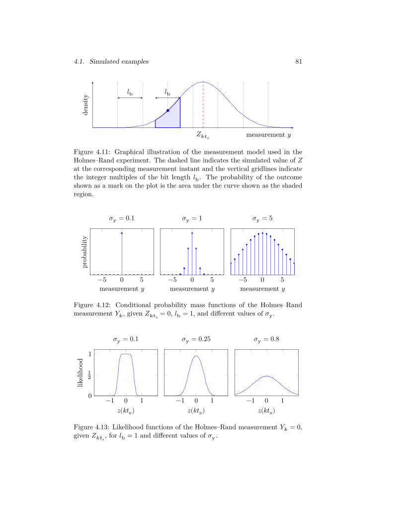
4.1. Simulated examples 81
𝑍u�u�s
𝑙b𝑙b
measurement 𝑦
dens
ity
Figure 4.11: Graphical illustration of the measurement model used in theHolmes–Rand experiment. The dashed line indicates the simulated value of 𝑍at the corresponding measurement instant and the vertical gridlines indicatethe integer multiples of the bit length 𝑙b. The probability of the outcomeshown as a mark on the plot is the area under the curve shown as the shadedregion.
−5 0 5measurement 𝑦
prob
abili
ty
𝜎y = 0.1
−5 0 5measurement 𝑦
𝜎y = 1
−5 0 5measurement 𝑦
𝜎y = 5
Figure 4.12: Conditional probability mass functions of the Holmes–Randmeasurement 𝑌u�, given 𝑍u�u�s
= 0, 𝑙b = 1, and different values of 𝜎y.
−1 0 10
12
1
𝑧(𝑘𝑡s)
likel
ihoo
d
𝜎y = 0.1
−1 0 1𝑧(𝑘𝑡s)
𝜎y = 0.25
−1 0 1𝑧(𝑘𝑡s)
𝜎y = 0.8
Figure 4.13: Likelihood functions of the Holmes–Rand measurement 𝑌u� = 0,given 𝑍u�u�s
, for 𝑙b = 1 and different values of 𝜎y.

82 Chapter 4. Example applications
functions
𝑓(𝑡, 𝑥, 𝑧, 𝜃) ∶= −(𝑎 + 𝛾𝑧2)𝑥 − 𝑏𝑧 − 𝑑𝑧3 + 𝜙 cos(𝑡), (4.8a)ℎ(𝑡, 𝑥, 𝑧, 𝜃) ∶= 𝑥, (4.8b)
the diffusion matrix 𝑮 ∶= [𝜎D], the prior log-density
ln 𝜋(𝑥, 𝑧, 𝜃) ∶= −12
(𝑥2
𝜎2x
+ 𝑧2
𝜎2z
+ 𝑎2 + 𝑏2 + 𝛾2 + 𝑑2
𝜎2θ
) + (𝑟 − 1) ln 𝜎y − 3𝑙b
𝜎y,
where the constant terms are omitted as they do not influence the locationof maxima, the measurement space 𝒴 ∶= IRu�+1, and the measurement log-likelihood
ln 𝜓(𝑦 | 𝑥, 𝑧, 𝜃) ∶=u�
∑u�=0
ln(𝛷(u�(u�u�s)−u�u�+ 12 u�b
u�y) − 𝛷(u�(u�u�s)−u�u�− 1
2 u�bu�y
)) ,
where 𝛷 is the standard normal cumulative distribution function. Additionally,we note that the measure 𝜈 with respect to which the density 𝜓 is defined isthe counting measure over 𝒴, as 𝑌 is a discrete random variable.
For each scenario 100 Monte Carlo simulations were performed. As in theprevious examples, the ISE metric defined in (4.1) was used to quantify the stateestimation error. It can be seen that when 𝜎y is of the same order of magnitudeas 𝑙b, then the state-path estimation error of all three methods is comparable.However, when the noise standard deviation 𝜎y is much smaller than thebit length 𝑙b, then the PEM yields larger errors. This can be understoodby analysing Figure 4.13 once more. When 𝑙b ≤ 𝜎y, then the measurementlikelihood is approximatelly Gaussian. When 𝜎y decreases, however, thenthe measurement likelihood approaches the uniform distribution, which is notwell represeted by the Gaussian distribution. The simulated, measured, andestimated processes for one Monte Carlo simulation can be seen in Figure 4.15for the whole experiment interval and in Figure 4.16 for a portion of it. Itcan be seen qualitatively that the measurements are indeed not Gaussian.Boxplots of the parameter estimates obtained with all three methods are shownin Figure 4.17. Unlike in the Duffing oscillator, a clear biasing of the MEE forthe damping parameters is not observed.
In this example, it can be seen that the general form of the JMAPSPPEand MEE allows them to better model analog to digital conversion. It showsthat, overall, the prediction error method attains a higher state-path estimationerror when the measurement noise is much smaller than the bit length, as itdoes not represent well the analog-to-digital conversion.

4.1. Simulated examples 83
4 6 8⋅10−4
JMAPSPPEMEEPEM
ISE
𝛴y = 0.04
1.5 2 2.5⋅10−4ISE
𝛴y = 0.005
Figure 4.14: Boxplots of the integrated square error (ISE) of the Holmes–Randoscillator estimated state paths over all Monte Carlo simulations.
−1
0
1
𝑧st
ate
simulated measured PEM min. energy MAP
0 10 20 30 40 50 60 70 80 90 100
−0.5
0
0.5
time 𝑡
𝑥st
ate
Figure 4.15: Simulated and estimated state paths for one of the Monte Carlosimulations of the Holmes–Rand oscillator, with 𝛴y = 0.005.

84 Chapter 4. Example applications
0.2
0.4
0.6
0.8
1
1.2𝑧
stat
e
simulated measured PEM min. energy MAP
19 20 21 22 23 24 25
−0.6
−0.4
−0.2
0
0.2
0.4
0.6
0.8
time 𝑡
𝑥st
ate
Figure 4.16: Detail of the simulated and estimated state paths for one of theMonte Carlo simulations of the Holmes–Rand oscillator, with 𝛴y = 0.005.

4.1. Simulated examples 85
JMAPSPPEMEEPEM
𝜎y = 0.04 𝜎y = 0.04
0.15 0.2 0.25JMAPSPPE
MEEPEM
𝑎 estimate
𝜎y = 0.005
−1.01 −1 −0.99𝑏 estimate
𝜎y = 0.005
JMAPSPPEMEEPEM
𝜎y = 0.04 𝜎y = 0.04
0.15 0.2 0.25JMAPSPPE
MEEPEM
𝛾 estimate
𝜎y = 0.005
0.99 1 1.01𝑑 estimate
𝜎y = 0.005
4 4.5⋅10−2
JMAPSPPEMEEPEM
𝜎y estimate
𝛴y = 0.04
0 0.5 1 1.5⋅10−2𝜎y estimate
𝛴y = 0.005
Figure 4.17: Boxplots of the Holmes–Rand oscillator parameter estimates. Thenominal parameter values, 𝑎 = 0.2, 𝑏 = −1, 𝛾 = 0.2, and 𝑑 = 1, are markedwith gridlines in the plots.
86 Chapter 4. Example applications
4.2 Applications with experimental dataTo illustrate a more practical application of the proposed estimators, we usethem for flight-path reconstruction. In flight testing of aircraft, data fromvarious sensors is collected on a wide range of physical quantities related to itsmovement. Common sensors are altimeters, airspeed sensors, accelerometers,global positioning system (GPS), gyroscopes, and magnetometers, to namea few. The physical quantities these sensors measure are all related througha well-known kinematic model. However, biases and noise in the sensorreadings make the measured paths incoherent with the model. For example,the measured velocities might differ from the integral of the acceleration, themeasured positions might differ from the integral of the velocity. Similar effectsoccur for the attitude, angular velocities, and angular accelerations. Flight-path reconstruction overcomes these limitations by using the kinematic modelof the aircraft to obtain a coherent flight path and measurement model fromthe data (Mulder et al., 1999; Jategaonkar, 2006, Chap. 10; Klein and Morelli,2006, Chap. 10). In the context of flight testing, flight path reconstruction isalso known as data compatibility check.
For this example we used data collected from a VFW-Fokker 614 of theGerman Aerospace Center’s (DLR) Advanced Technologies Testing AircraftSystem (ATTAS) project, corresponding to a bank-to-bank roll manuever. Thisdata accompanies the book “Flight Vehicle System Identification” (Jategaonkar,2006) and is used with the author’s permission. The measurements werecollected at a rate of 25 Hz and correspond to the following quantities: airspeed𝑣m, angle of attack at the noseboom 𝛼m, angle of sideslip at the noseboom
𝛽m, roll angle 𝜙m, pitch angle 𝜃m, yaw angle 𝜓m, altitude ℎm, roll rate 𝑝m,pitch rate 𝑞m, yaw rate 𝑟m, longitudinal acceleration 𝑎xm, lateral acceleration𝑎ym, and vertical acceleration 𝑎zm.
For the estimation, we considered the derivatives 𝐷x, 𝐷y and 𝐷z of theexternal accelerations the derivatives 𝐷l, 𝐷m, 𝐷n and of the normalizedmoments of force to be linear diffusion processes evolving according to thefollowing SDEs:
d𝐷x(𝑡) = −𝐾a𝐷x(𝑡) d𝑡 + 𝜎a d𝑊(1)u� ,
d𝐷y(𝑡) = −𝐾a𝐷y(𝑡) d𝑡 + 𝜎a d𝑊(2)u� ,
d𝐷z(𝑡) = −𝐾a𝐷z(𝑡) d𝑡 + 𝜎a d𝑊(3)u� ,
d𝐷l(𝑡) = −𝐾m𝐷l(𝑡) d𝑡 + 𝜎m d𝑊(4)u� ,
d𝐷m(𝑡) = −𝐾m𝐷m(𝑡) d𝑡 + 𝜎m d𝑊(5)u� ,
d𝐷n(𝑡) = −𝐾m𝐷n(𝑡) d𝑡 + 𝜎m d𝑊(6)u� ,
where 𝐾a and 𝐾m are unknown parameters representing the damping coeffi-cient of the diffusion, 𝜎a and 𝜎m are the diffusion coefficients of the accelerations

4.2. Applications with experimental data 87
and the moments, respectively, and 𝑊(u�) are Wiener processes representingthe process noise. The remaining states are not directly subject to noise. Thisrepresentation is similar to the estimation before modeling (EBM) approach(Sri-Jayantha and Stengel, 1988; Jategaonkar, 2006, Sec. 10.4).
The gamma distribution was used as the prior of 𝐾a and 𝐾m parame-ters. For the remaining parameters and the initial conditions, non-informativeGaussian priors were used. For the measurement model, similarly, we con-siders that all sensors were subject to independent Gaussian noise, and thatthe accelerometers and gyrometers had, furthermore, unknown biases to beestimated. Putting the whole model in the format of Chapter 2, we have thatit is characterized as follows. The clean state vector 𝑧 ∈ IR16 is composed ofthe following elements, in order: roll angle 𝜙a, pitch angle 𝜃a, yaw angle 𝜓a,roll rate 𝑝, pitch rate 𝑞, yaw rate 𝑟, normalized rolling moment ℓ, normalizedpitching moment 𝑚, normalized yawing moment 𝑛, altitude ℎa, longitudinalinertial velocity 𝑢, lateral inertial velocity 𝑣, vertical inertial velocity 𝑤, longi-tudinal inertial acceleration 𝑎x, lateral inertial acceleration 𝑎y, vertical inertialacceleration 𝑎z. The noisy state vector 𝑥 ∈ IR6, in turn, is composed of thefollowing elements, in order: longitudinal, lateral and vertical jerk 𝑑x, 𝑑y, and𝑑z, and rolling, pitching and yawing jerk 𝑑l, 𝑑m, and 𝑑n. The parameter vector𝜃 ∈ IR8 is composed of the following elements, in order: the angular velocitymeasurement biases 𝑏p, 𝑏q, and 𝑏r, the acceleration measurement biases 𝑏ax,𝑏ay, and 𝑏az, and the damping coefficients 𝑘a and 𝑘m. The unnormalizedpitching, rolling and yawing moments, respectively, can be obtained from thenormalized moments as
𝐽x𝐽z − 𝐽2xu�
𝐽zℓ, 1
𝐽y𝑚, 𝐽x𝐽z − 𝐽2
xu�𝐽x
𝑛.
The noisy drift function is given by the following linear model:
𝑓(𝑡, 𝑥, 𝑧, 𝜃) ∶=
⎡⎢⎢⎢⎢⎢⎣
−𝑘a𝑑x−𝑘a𝑑y−𝑘a𝑑z−𝑘m𝑑l−𝑘m𝑑m−𝑘m𝑑n
⎤⎥⎥⎥⎥⎥⎦
.
The clean drift, in turn, is given by the equations of rigid body kinematics

88 Chapter 4. Example applications
(Sri-Jayantha and Stengel, 1988; Jategaonkar, 2006, Eq. 10.26):
ℎ(𝑡, 𝑥, 𝑧, 𝜃) ∶=
⎡⎢⎢⎢⎢⎢⎢⎢⎢⎢⎢⎢⎢⎢⎢⎢⎢⎢⎣
𝑝 + 𝑞 sin(𝜙a) tan(𝜃a) + 𝑟 cos(𝜙a) tan(𝜃a)𝑞 cos(𝜙a) − 𝑟 sin(𝜙a)
𝑞 sin(𝜙a) sec(𝜃a) + 𝑟 cos(𝜙a) sec(𝜃a)𝑝𝑞𝐶11 + 𝑞𝑟𝐶12 + 𝑞𝐶13 + ℓ + 𝑛𝐶14𝑝𝑟𝐶21 + (𝑟2 − 𝑝2)𝐶22 − 𝑟𝐶23 + 𝑚𝑝𝑞𝐶31 + 𝑞𝑟𝐶32 + 𝑞𝐶33 + ℓ𝐶34 + 𝑛
𝑑l𝑑m𝑑n
𝑢 sin(𝜃a) − 𝑣 cos(𝜃a) sin(𝜙a) − 𝑤 cos(𝜃a) cos(𝜙a)−𝑞𝑤 + 𝑟𝑣 − 𝑔 sin(𝜃a) + 𝑎x
−𝑟𝑢 + 𝑝𝑤 + 𝑔 cos(𝜃a) sin(𝜙a) + 𝑎y𝑞𝑢 − 𝑝𝑣 + 𝑔 cos(𝜃a) cos(𝜙a) + 𝑎z
𝑑x𝑑y𝑑z
⎤⎥⎥⎥⎥⎥⎥⎥⎥⎥⎥⎥⎥⎥⎥⎥⎥⎥⎦
.
The prior log-density is given by
ln 𝜋(𝑥, 𝑧, 𝜃) ∶= −𝜙2a + 𝜃2
a + 𝜓2a + 𝑝2 + 𝑞2 + 𝑟2 + ℓ2 + 𝑚2 + 𝑛2
2𝜎0
−𝑢2 + 𝑣2 + 𝑤2 + 𝑎2
z + 𝑎2y + 𝑎2
z + 𝑑2x + 𝑑2
y + 𝑑2z + 𝑑2
l + 𝑑2m + 𝑑2
n
2𝜎0
−𝑏2
ax + 𝑏2ay + 𝑏2
az + 𝑏2p + 𝑏2
q + 𝑏2r
2𝜎0+ 9 ln(𝑘a𝑘m) − 9(𝑘a + 𝑘m),
where a large value for the standard deviation 𝜎0 was chosen to make the priornon-informative. The measurement log-likelihood is given by
ln 𝜓(𝑦|𝑥, 𝑧, 𝜃) ∶=u�
∑u�=0
ln 𝜓u�(𝑦u�|𝑥(𝑘𝑡s), 𝑧(𝑘𝑡s), 𝜃) ,
where 𝜓u� ∶ IR13 × IR16 × IR6 × IR12 → IR≥0, the log-likelihood of each mea-surement, is given by
ln 𝜓u�(𝑦|𝑥, 𝑧, 𝜃) ∶= −(𝜙m − 𝜙a)2
2𝜎2ϕ
− (𝜃m − 𝜃a)2
2𝜎2θ
− (𝜓m − 𝜓a)2
2𝜎2ψ
− [𝛼m − atan2(𝑤 − 𝑞𝑥nb + 𝑝𝑦nb, 𝑢 − 𝑟𝑦nb + 𝑞𝑧nb)]2
2𝜎2α
− [𝛽m − atan2(𝑣 − 𝑝𝑧nb + 𝑟𝑥nb, 𝑢 − 𝑟𝑦nb + 𝑞𝑧nb)]2
2𝜎2α

4.2. Applications with experimental data 89
− (ℎm − ℎa)2
2𝜎2h
−(𝑝m − 𝑏p − 𝑝)2
2𝜎2p
−(𝑞m − 𝑏q − 𝑞)2
2𝜎2q
− (𝑟m − 𝑏r − 𝑟)2
2𝜎2r
− (𝑏ax + 𝑎x + 𝑞𝑧as − 𝑟𝑦as − 𝑎xm)2
2𝜎2ax
−(𝑏ay + 𝑎y + 𝑟𝑥as − 𝑝𝑧as − 𝑎ym)2
2𝜎2ay
− (𝑏az + 𝑎z + 𝑝𝑦as − 𝑞𝑥as − 𝑎zm)2
2𝜎2az
− [ 𝑣m −√
𝑢2 + 𝑣2 + 𝑤2]2
2𝜎2v
,
where 𝑥nb, 𝑦nb and 𝑧nb are the coordinates, with respect to the center ofgravity, of the tip of the nose boom where the aerodynamic probe is located,𝑥as, 𝑦as and 𝑧as are the coordinates of the location of the accelerometer, 𝑔is the acceleration of gravity, and 𝜎− are the measurement noise standarddeviations. Constant terms which do not influence the location of maximahave been omitted from the expression above and the standard deviations weretreated as known parameters, chosen empirically.
Both the JMAPSPPE and MEE estimates were compared with the outputerror method (OEM) described in (Jategaonkar, 2006, Sec. 10.5) and imple-mented in its accompanying materials. The outputs corresponding to thereconstructed paths can be seen in Figures 4.18 to 4.22
This example mostly demonstrates the feasibility of applying the proposed
55 60 65 70 75 80−30
−20
−10
0
10
time 𝑡 (s)
chan
geof
altit
ude
ℎ(m
)
measured JMAPSPPE MEE OEM
Figure 4.18: Altitude output corresponding to the reconstructed flight pathusing the various methods.

90 Chapter 4. Example applications
129
130
131
132
133
134ai
rspe
ed𝑣(m
/s)
measured JMAPSPPE MEE OEM
1.5
2
2.5
angl
eof
atta
ck𝛼
(∘ )
55 60 65 70 75 80−4
−2
0
2
4
time 𝑡 (s)
angl
eof
sides
lip𝛽
(∘ )
Figure 4.19: Velocity outputs corresponding to the reconstructed flight pathusing the various methods.

4.2. Applications with experimental data 91
−20
0
20
roll
angl
e𝜙 a
(∘ )measured JMAPSPPE MEE OEM
0
1
2
3
4
pitc
han
gle
𝜃 a(∘ )
55 60 65 70 75 806
8
10
12
14
16
time 𝑡 (s)
yaw
angl
e𝜓 a
(∘ )
Figure 4.20: Attitude outputs corresponding to the reconstructed flight pathusing the various methods.

92 Chapter 4. Example applications
−20
0
20ro
llra
te𝑝
(∘ /s)
measured JMAPSPPE MEE OEM
−1
0
1
2
pitc
hra
te𝑞
(∘ /s)
55 60 65 70 75 80
−4
−2
0
2
4
6
time 𝑡 (s)
yaw
rate
𝑟(∘ /
s)
Figure 4.21: Angular velocity outputs corresponding to the reconstructed flightpath using the various methods.

4.2. Applications with experimental data 93
0.3
0.4
0.5
0.6
0.7
acce
lera
tion
𝑎 x(m
/s2)
measured JMAPSPPE MEE OEM
−1
0
1
acce
lera
tion
𝑎 y(m
/s2)
55 60 65 70 75 80
−11
−10
−9
−8
−7
time 𝑡 (s)
acce
lera
tion
𝑎 z(m
/s2)
Figure 4.22: Acceleration outputs corresponding to the reconstructed flightpath using the various methods.

94 Chapter 4. Example applications
JMAPSPPE and MEE in a practical problem of technological interest witha high dimensionality. We note that the use of flight-path reconstructionin industry and production requires some further tuning of the algorithm,dynamical model structure, and measurement model which is outside thescope of this thesis. Nevertheless, the results of this example suggest thatthe MAP estimator can be a good substitute for the output error methodin flight path reconstruction of small unmanned aerial vehicles for which thesmall payload limits the quality of the inertial sensors. The OEM relies onhigh-quality inertial sensors and provides inadequate results when this is notthe case (Mulder et al., 1999).

Chapter 5
Conclusions
Cueball: I used to think correlation implied causation.Then I took a statistics class. Now I don’t.Megan: Sounds like the statistics class helped.Cueball: Well, maybe.
Randall Munroe, xkcd #552: Correlation
In this chapter we recall the conclusions and contributions of this thesis,and finalize with directions for future work.
5.1 ConclusionsThe main contribution of this thesis is building a solid theoretical foundationfor maximum a posteriori (MAP) estimation in stochastic differential equations(SDEs). The first one is laying out a rigorous definition of mode and MAPestimation for general random variables in possibly infinite-dimensional spaces,presented in Section 2.1. This definition is shown to be coincident with thetraditional one for continous and discrete random variables, and its interpreta-tions in the context of Bayesian decision theory and Bayesian estimation areprovided.
Next, we showed how this definition of mode can be used to obtain theposterior and prior joint fictious state-path and parameter densities for systemsdescribed by SDEs where not necessarily all states are under direct influence ofnoise. In addition, we showed that the minimum energy estimates correspondto the state-paths associated with the joint MAP noise-paths and parameters.
We then related the popular approach of using the discretized SDE forjoint MAP state-path and parameter estimation to the continuous-time MAPestimators by using variational analysis. We proved that the Euler-discretizedMAP estimator converges hypographically to the minimum energy estimator.The trapezoidally-discretized MAP estimator, on the other hand, convergeshypographically to the continuous-time MAP estimator. This implies that the
95

96 Chapter 5. Conclusions
discretized estimates might have different interpretations depending on thediscretization method used.
Some example applications with both simulated and experimental werethen presented. In the simulated examples, we saw that the state-path es-timates of both methods were comparable. However, the minimum-energyestimates of parameters which appear in the drift divergence were biased.This is because the Onsager–Machlup functional penalizes parameter valueswhich increase the amplification of the noise by the system, while the energyfunctional does not. In addition, the use of the proposed estimators was demon-strated in non-Gaussian applications in which nonlinear Kalman smoothersand prediction error methods yield poor results or are not applicable. Theexample with experimental data showed the viability of the proposed methodsin an application of technological interest with high model order and systemcomplexity.
The theoretical foundations built with these contributions provide a firmbasis on which new work can be built upon.
5.2 Future work
The work herein can be expanded in a number of directions. Importantquestions that need to be answered are conditions for existence of the MAPestimates. Preliminary analysis indicates that when the negative of the log-prior is coercive and the measurement likelihood and drift divergence arebounded in the parameter support, then at least one MAP estimate exists.
Under some regularity conditions, the posterior fictious density of state-paths and parameters admit a second order Fréchet derivative. We believethat this derivative is analogous to the Hessian matrix of posterior probabilitydensity function in IRu�, itself the Bayesian equivalent of the Fisher informa-tion matrix. The second Fréchet derivative of the fictitious density seems,furthermore, related to reproducing kernels associated with Gaussian processes(Parzen, 1963). As such it could be used to build Gaussian approximations tothe posterior state-path and parameter distribution, and to provide a measureof uncertainty associated with the modal estimates.
Preliminary analysis shows that the inverse of the optimization problem’sHessian matrix is very close to the covariance matrices obtained with theunscented Kalman smoother. These ideas underlie the approach of (Karimiand McAuley, 2013, 2014a; Varziri et al., 2008a) to marginalization of the states.Care should be taken to understand and develop the theoretical foundationsof this approach, however. In particular, to use the Hessian matrix of theoptimization problem its relationship to the original problem’s second orderderivative should be understood using tools such as second-order variationalanalysis and hypo-convergence (cf. Rockafellar and Wets, 1998, Chap. 13).

5.2. Future work 97
The hypo-convergence of the Euler and trapezoidal discretizations can bestrengthened by proving 𝜏/𝜎-equi-semicontinuity (Attouch, 1984, Sec. 2.6.2).This would imply hypo-convergence in the weak topology, which can guaranteethe existence of a convergent sequence discretized MAP estimates. In addition,the techniques of variational analysis used in this thesis can be used to prove thehypo-convergence of the Legendre–Gauss–Lobatto direct transcription methodsused in Chapter 4 to discretize the optimization problems. A particular strongkind of hypo-convergence seems to hold, in which not only the decision variablesbut also the adoint variables (co-states) converge hypographically. We alsobelieve that 𝜏/𝜎-equi-semicontinuity holds under some regularity conditions.
With respect to applications, we intend to use the MAP estimator for flightpath reconstruction and system identification of the small-scale hand-launchedunmanned aerial vehicles being developed at the Universidade Federal de MinasGerais. Additionally, we believe that the MAP state-path estimates can beused together with particle smoothers (Klaas et al., 2006) to help design aproposal distribution that samples in regions of high posterior probability.similar to the unscented particle filter (van der Merwe et al., 2000).


Appendix A
Collected theorems anddefinitions
In this chapter, we collect some useful theorems and definitions which are usedthroughout the thesis.
A.1 Simple identities
Lemma A.1. For all 𝑎, 𝑏 ∈ IR≥0,√
𝑎 +√
𝑏 ≤√
2√
𝑎 + 𝑏. (A.1)
Proof. The square root is a concave function, so from Jensen’s inequality wehave that
√𝑎 +
√𝑏
2≤ √𝑎 + 𝑏
2.
Rearranging, we obtain (A.1).
Lemma A.2. For all 𝑎, 𝑏 ∈ IR,
(𝑎 + 𝑏)2 ≤ 2(𝑎2 + 𝑏2).
Proof. Since (𝑎 − 𝑏)2 ≥ 0,
(𝑎 + 𝑏)2 ≤ (𝑎 + 𝑏)2 + (𝑎 − 𝑏)2 = 2𝑎2 + 2𝑏2.
Lemma A.3. For all 𝑥 ∈ IR≥0, exp(𝑥) ≥ 1 + 𝑥.
Proof. From the Taylor series expansion of the exponential we have that
exp(𝑥) − (1 + 𝑥) =∞∑u�=2
𝑥u�
𝑘!≥ 0
99

100 Appendix A. Collected theorems and definitions
A.2 Linear algebraLemma A.4 (matrix Mercator series, Higham and Al-Mohy, 2010, Sec. 5.2).For all matrices 𝑨 ∈ IRu�×u� with spectral radius smaller than unity, we havethat the matrix logarithm satisfies
ln(𝑰 + 𝑨) =∞∑u�=1
(−1)u�+1 𝑨u�
𝑘.
Lemma A.5 (matrix exponential determinant, Bernstein, 2009, Cor. 11.2.4).For all matrices 𝑨 ∈ IRu�×u�, the determinant of a matrix exponential satisfies
det exp(𝑨) = exp(tr 𝑨) .
A.3 Analysis
Lemma A.6 (Dominance of ‖⋅‖u�1u�
by ‖⋅‖u�2u�). Let (𝒳, ℱ, 𝜇) be a finite measure
space. Then, for all 𝑓 ∈ 𝐿2u�(𝒳, ℱ, 𝜇),
‖𝑓‖u�1u�
≤ √𝜇(𝒳) ‖𝑓‖u�2u�
Proof. From the Cauchy–Schwarz inequality we have that
‖𝑓‖u�1u�
= ∫u�
|𝑓(𝑥)| d𝜇(𝑥) ≤ (∫u�
|1|2 d𝜇(𝑥))1/2
(∫u�
|𝑓(𝑥)|2 d𝜇(𝑥))1/2
Lemma A.7 (Dominance of |||⋅||| by ‖⋅‖u�2u�). Let 𝒯 ∶= [0, 𝑡f]. Then there some
𝑐 ∈ IR>0 such that, for all 𝑥 ∈ 𝒲2u�(𝒯),
|||𝑥||| ≤ 𝑐 ‖𝑥‖u�2u�
, (A.2)
where |||𝑥||| ∶= supu�∈u� |𝑥(𝑡)| and ‖𝑥‖u�2u�
∶= (|𝑥(0)|2 + ∫u�f
0| 𝑥(𝑡)|2 d𝑡)
1/2.
Proof. Every 𝑥 ∈ 𝒲2u� is absolutely continuous, meaning that for all 𝑡 ∈ 𝒯
𝑥(𝑡) = 𝑥(0) + ∫u�
0𝑥(𝑡) d𝑡,
implying that
|||𝑥||| = supu�∈u�
∣𝑥(0) + ∫u�
0𝑥(𝑡) d𝑡∣ ≤ |𝑥(0)| + ∫
u�f
0| 𝑥(𝑡)| d𝑡.
A.3. Analysis 101
Next, using Lemma A.6 we have that
|||𝑥||| ≤ |𝑥(0)| + √𝑡f (∫u�f
0| 𝑥(𝑡)|2 d𝑡)
1/2
.
Lemma A.1, in turn, gives us
|||𝑥||| ≤√
2 (|𝑥(0)|2 + 𝑡f ∫u�f
0| 𝑥(𝑡)|2 d𝑡)
1/2
.
Consequently, (A.2) is satisfied with 𝑐 ∶= max(√2𝑡f,√
2).
Lemma A.8 (Grönwall–Bellman inequality, Lem. 5.6.4 of Polak, 1997). Let𝑐, 𝐾, 𝑡f ∈ IR≥0 and 𝒯 ∶= [0, 𝑡f]. Then, if an integrable function ℎ∶ 𝒯 → IRsatisfies
ℎ(𝑡) ≤ 𝑐 + 𝐾 ∫u�
0ℎ(𝜏) d𝜏 for all 𝑡 ∈ 𝒯,
we have thatℎ(𝑡) ≤ 𝑐 exp(𝐾𝑡f) for all 𝑡 ∈ 𝒯.
Lemma A.9 (adapted from Lemma 5.6.3 of Polak, 1997). Let 𝑡f ∈ IR>0,𝒯 ∶= [0, 𝑡f], and 𝑤 ∈ 𝒞(𝒯, IRu�). In addition, let the continuous function𝑓∶ 𝒯 × IRu� → IRu� be Lipschitz continuous with respect to its second argument,uniformly with respect to its first, i.e., there exists 𝐿 ∈ IR>0 such that for all𝑡 ∈ 𝒯 and 𝑥′, 𝑥″ ∈ IRu�
∣𝑓(𝑡, 𝑥′) − 𝑓(𝑡, 𝑥″)∣ ≤ 𝐿 ∣𝑥′ − 𝑥″∣ . (A.3)
We then have that, for all 𝑥0 ∈ IRu� there is a unique solution 𝑥∶ 𝒯 → IRu� tothe integral equation
𝑥(𝑡) = 𝑥0 + ∫u�
0𝑓(𝑡, 𝑥(𝜏)) d𝜏 + 𝑤(𝑡), (A.4)
which satisfies, for all 𝑥 ∈ 𝒲2u�(𝒯), the inequality
||| 𝑥 − 𝑥||| ≤ exp(𝐿𝑡f) (|𝑥0 − 𝑥(0)| + |||𝑤||| + ∫u�f
0∣ 𝑥(𝑡) − 𝑓(𝑡, 𝑥(𝑡))∣ d𝑡) . (A.5)
Proof. First, note that the triangle inequality implies that
|𝑓(𝑡, 𝑥)| ≤ |𝑓(𝑡, 𝑥) − 𝑓(𝑡, 0)| + |𝑓(𝑡, 0)| for all 𝑡 ∈ 𝒯, 𝑥 ∈ IRu�.
The Lipschitz condition (A.3) and the extreme value theorem, in turn, implythat there exists 𝑐 ∈ IR>0 such that
|𝑓(𝑡, 𝑥)| ≤ 𝐿 |𝑥| + 𝑐 for all 𝑡 ∈ 𝒯, 𝑥 ∈ IRu�. (A.6)

102 Appendix A. Collected theorems and definitions
Next, let { 𝑥u�}∞u�=0 be a sequence of continuous functions 𝑥u� ∈ 𝒞(𝒯, IRu�)
with its first element 𝑥0 ∶= 𝑥. The following elements of the sequence are givenby the recursion
𝑥u�+1(𝑡) ∶= 𝑥0 + ∫u�
0𝑓(𝜏, 𝑥u�(𝜏)) d𝜏 + 𝑤(𝑡), for all 𝑡 ∈ 𝒯. (A.7)
The growth bound (A.6) implies that 𝑡 ↦ 𝑓(𝑡, 𝑥u�(𝑡)) is integrable if 𝑥u� iscontinuous. Furthermore, (A.7) and the continuity of 𝑤 imply that 𝑥u�+1 iscontinuous if 𝑥u� is continuous. As 𝑥0 is integrable, by recursion we then havethat all 𝑥u� are well-defined and continuous.
Since 𝑥 ∈ 𝒲2u�(𝒯), we have that it is weakly differentiable and satisfies
𝑥(𝑡) = 𝑥(0) + ∫u�
0
𝑥(𝜏) d𝜏, for all 𝑡 ∈ 𝒯.
Together with (A.7) and the fact that 𝑥0 ∶= 𝑥, this implies that
| 𝑥1(𝑡) − 𝑥0(𝑡)| ≤ |𝑥0 − 𝑥(0)| + |||𝑤||| + ∫u�f
0∣ 𝑥(𝑡) − 𝑓(𝑡, 𝑥(𝑡))∣ d𝑡 =∶ 𝜖.
For any 𝑖 > 0 and 𝑡 ∈ 𝒯, from the recursion (A.7) and the Lipschitz condition(A.3) we have that
| 𝑥u�+1(𝑡) − 𝑥u�(𝑡)| ≤ ∫u�
0|𝑓(𝜏, 𝑥u�(𝜏)) − 𝑓(𝜏, 𝑥u�−1(𝜏))| d𝜏
≤ ∫u�
0𝐿 | 𝑥u�(𝜏) − 𝑥u�−1(𝜏)| d𝜏.
By induction we then have that for all 𝑖 ∈ {0, 1, … }
| 𝑥u�+1(𝑡) − 𝑥u�(𝑡)| ≤ (𝐿𝑡)u�
𝑖!𝜖,
which in turn implies that
||| 𝑥u�+1 − 𝑥u�||| ≤ (𝐿𝑡f)u�
𝑖!𝜖, ||| 𝑥ℓ − 𝑥u�||| ≤ 𝜖
ℓ−1∑u�=u�
(𝐿𝑡f)u�
𝑖!. (A.8)
Noting the similarity to the Taylor series expansion of the exponential, wecan then see that { 𝑥u�}∞
u�=1 is a Cauchy sequence, which converges due tocompleteness of 𝒞(𝒯, IRu�). Denoting its limit by 𝑥, we then have by (A.8) thatfor all 𝑖 ∈ {0, 1, … },
|||𝑥 − 𝑥u�||| ≤ 𝜖∞∑u�=0
(𝐿𝑡f)u�
𝑖!= exp(𝐿𝑡f)𝜖,

A.3. Analysis 103
implying that (A.5) holds.Finally, to see that (A.4) holds for the limit of the sequence, note that
limu�→∞
∣∫u�
0[𝑓(𝜏, 𝑥u�(𝜏)) − 𝑓(𝜏, 𝑥(𝜏))] d𝜏∣ ≤ lim
u�→∞𝐿𝑡f ||| 𝑥u� − 𝑥||| = 0.
Consequently, by letting 𝑖 → ∞ in (A.7) we obtain (A.4).
Corollary A.10. Let 𝒯 and 𝑓 be as in Lemma A.9. Then for all 𝑥0 ∈ IRu�
there exists a unique solution 𝑥 ∈ 𝒲2u�([0, 𝜏]) to the initial value problem
𝑥(𝑡) = 𝑓(𝑡, 𝑥(𝑡)) , 𝑥(0) = 𝑥0. (A.9)
Furthermore, for all 𝑥 ∈ 𝒲2u�([0, 𝜏]),
||| 𝑥 − 𝑥||| ≤ exp(𝐿𝜏) (|𝑥(0) − 𝑥(0)| + ∫u�
0∣ 𝑥(𝑡) − 𝑓(𝑡, 𝑥(𝑡))∣ d𝑡) .
Proof. This corollary follows directly from Lemma A.9 by letting 𝑤 = 0. If𝑥𝒞(𝒯, IRu�) is the solution to the integral equation
𝑥(𝑡) = 𝑥0 + ∫u�
0𝑓(𝑡, 𝑥(𝜏)) d𝜏 + 𝑤(𝑡),
then by Lebesgue’s differentiation theorem we have that it is also a solution tothe initial value problem (A.9).
Remark A.11 (regularization to ensure Lipschitz continuity). Let 𝑟 ∶ IR → IRand 𝑓∶ IRu� → IRu� be continuously differentiable and let 𝑟 satisfy, for some𝑀 ∈ IR>0,
𝑟(𝜖) = {1 if 𝜖 ≤ 𝑀0 if 𝜖 ≥ 2𝑀.
Then the function 𝑓(𝑥) ∶= 𝑓(𝑥)𝑟(|𝑥|) is bounded, Lipschitz continuous, andsatisfies 𝑓(𝑥) = 𝑓(𝑥) for all |𝑥| ≤ 𝑀.
Proof. From the definition of 𝑟 and 𝑓, we have that
supu�∈IRu�
∣ 𝑓(𝑥)∣ = sup|u�|≤2u�
∣ 𝑓(𝑥)∣
supu�∈IRu�
∣∇ 𝑓(𝑥)∣ = sup|u�|≤2u�
∣∇ 𝑓(𝑥)∣ .
From the extreme value theorem we then have that both 𝑓 and its derivativesare bounded. To conclude, we have that differentiable functions with boundedderivatives are Lipschitz continuous.

104 Appendix A. Collected theorems and definitions
A.4 Probability theory and stochastic processesThe following two lemmas are adapted from Ikeda and Watanabe (1981, p. 449)and are frequently used to obtain the Onsager–Machlup functional.
Lemma A.12 (limit of conditional exponential moments). Let {𝔸u�}u�∈IR>0be
a family of non-null events in ℰ. Then, if 𝐴 is a IR-valued random variablesuch that
lim supu�↓0
E[exp(𝑐𝐴) | 𝔸u�] ≤ 1 for all 𝑐 ∈ IR (A.10)
thenlimu�↓0
E[exp(𝑐𝐴) | 𝔸u�] = 1 for all 𝑐 ∈ IR. (A.11)
Proof. Applying the Cauchy–Schwarz inequality we have that, for all 𝑐 ∈ IR,
1 = (E[exp(u�u�2 ) exp(−u�u�
2 ) ∣ 𝔸u�])2 ≤ E[exp(𝑐𝐴) | 𝔸u�] E[exp(−𝑐𝐴) | 𝔸u�] .
This in turn implies that
E[exp(𝑐𝐴) | 𝔸u�] ≥ 1E[exp(−𝑐𝐴) | 𝔸u�]
.
Taking the limit inferior and applying (A.10) we obtain the following bound:
lim infu�↓0
E[exp(𝑐𝐴) | 𝔸u�] ≥ 1lim supu�↓0 E[exp(−𝑐𝐴) | 𝔸u�]
≥ 1. (A.12)
As the limit superior is always greater than or equal to the limit inferior,we conclude that the limits of (A.10) and (A.12) coincide and equal to one.Consequently, (A.11) holds.
Lemma A.13 (conditional exponential moments of a sum). Let {𝔸u�}u�∈IR>0be a family of non-null events in ℰ. Then, if 𝐴1, … , 𝐴u� are IR-valued randomvariables such that
lim supu�↓0
E[exp(𝑐𝐴u�) | 𝔸u�] ≤ 1 for all 𝑐 ∈ IR and 𝑖 = 1, … , 𝑛, (A.13)
then
limu�↓0
E[exp(𝑐𝐴1 + ⋯ + 𝑐𝐴u�) | 𝔸u�] = 1 for all 𝑐 ∈ IR. (A.14)
Proof. Define the IR-valued random variables 𝐵u�, 𝑖 = 1, … , 𝑛 as
𝐵u� ∶=u�
∑u�=1
𝐴u�.

A.4. Probability theory and stochastic processes 105
We then have that, for 𝑖 = 1,
lim supu�↓0
E[exp(𝑐𝐵u�) | 𝔸u�] ≤ 1 for all 𝑐 ∈ IR. (A.15)
Next, assume that (A.15) holds for some 𝑖 < 𝑛. Then, applying the Cauchy–Scharwz inequality,
E[exp(𝑐𝐵u�) exp(𝑐𝐴u�+1) | 𝔸u�] ≤ √E[exp(2𝑐𝐵u�) | 𝔸u�] E[exp(2𝑐𝐴u�+1) | 𝔸u�].
Taking the limit superior and applying (A.13) and (A.15) we then have that(A.15) holds for 𝑖 + 1 and, by induction, up to 𝑖 = 𝑛. Applying Lemma A.12we then have that (A.14) holds.
Lemma A.14 (Dembo and Zeitouni, 1998, Lemma 5.2.1). For all 𝜏, 𝛿 ∈ IR>0,if 𝑊 is an 𝑛-dimensional Wiener process then
𝑃(supu�∈[0,u�] ‖𝑊u�‖ ≥ 𝛿) ≤ 4𝑛 exp(− 𝛿2
2𝑛𝜏) .
The following three lemmas are used to calculate what is referred to inthe literature as the first exit or sojourn probability of the Wiener process (cf.Fujita and Kotani, 1982; Gasanenko, 1999). It corresponds to the probabilitythat the Wiener process starting at 𝑤 sojourns in a set 𝒲 for longer than𝑡. Theorem A.15 is one of the many connections between partial differentialequations and diffusion processes.
Theorem A.15 (sojourn probability of the Wiener process, Patie and Winter,2008, Thm. 7). Let 𝑊 be an 𝑛-dimensinal Wiener process over IR≥0, 𝒲 ⊂ IRu�
be an open, bounded and connected domain with a smooth boundary 𝜕𝒲, theIR-valued random variable 𝑇u� be the time of first exit of the Wiener processstarting at 𝑤 from 𝒲 and 𝑢∶ IR≥0 × �� → [0, 1] be the probability that 𝑇u�occurs after a given time interval, i.e.,
𝑇u�(𝜔) ∶= inf {𝑡 ∈ IR≥0 ∣ 𝑤 + 𝑊u� ∉ 𝒲} , 𝑢(𝑤, 𝑡) ∶= 𝑃(𝑇u� > 𝑡) .
Then 𝑢 satisfies the boundary value problem
𝜕𝑢𝜕𝑡
(𝑡, 𝑤) = 12
tr ∇2w𝑢(𝑡, 𝑤) for all 𝑤 ∈ 𝒲 and 𝑡 ∈ IR≥0 (A.16a)
𝑢(𝑡, 𝑤) = 0 for all 𝑤 ∈ 𝜕𝒲 and 𝑡 ∈ IR>0 (A.16b)𝑢(0, 𝑤) = 1 for all 𝑤 ∈ 𝒲, (A.16c)
where tr ∇2w𝑢 denotes the Laplacian operator applied to 𝑢, i.e., the trace of its
Hessian matrix with respect to its second argument 𝑤.

106 Appendix A. Collected theorems and definitions
The boundary value problem (A.16) in Theorem A.15 happens to havean analytical solution, which is useful in calculating assymptotic sojournprobabilities for more general diffusion processes, as done in Sec. 2.2.1. Toobtain these solutions, we first state the following lemma.
Lemma A.16 (Dirichlet eigenfunction basis). Let 𝒲 ⊂ IRu� be an open,bounded and connected domain with a smooth boundary 𝜕𝒲. Then thereexists a sequence of not identically zero 𝒞(��, IR) functions {𝜙u�}∞
u�=1 and acorresponding nondecreasing sequence of IR>0 numbers {𝜆u�}∞
u�=1 that solve theDirichlet eigenvalue problem
𝜆u�𝜙u�(𝑤) = −12
tr ∇2𝜙u�(𝑤) for all 𝑤 ∈ 𝒲 (A.17a)
𝜙u�(𝑤) = 0 for all 𝑤 ∈ 𝜕𝒲. (A.17b)
Furthermore, {𝜙u�}∞u�=1 is an orthonormal basis for 𝐿2(��) and 0 < 𝜆1 < 𝜆2.
For a proof of Lemma A.16 and some other interesting properties of theeigenvalue problem, refer to Larsson and Thomée (2003, Chap. 6). In particular,the fact that the eigenfunctions form an orthonormal basis for 𝐿2(��) is provedin Theorem 6.4; the fact that the eigenvalues are nondecreasing and 𝜆1 < 𝜆2 isproved with Theorem 6.3. The eigenvalues and eigenfunctions of Theorem A.16are used to construct the solution to the boundary value problem (A.16) ofTheorem A.15, as proved in the proposion below.
Proposition A.17 (solution to the sojourn probability BVP). Let 𝒲 ⊂ IRu�
be an open, bounded and connected domain with a smooth boundary 𝜕𝒲. Thenthe solution 𝑢∶ IR≥0 × �� → [0, 1] to the boundary value problem (A.16) over𝒲 is given by
𝑢(𝑡, 𝑤) =∞∑u�=1
exp(−𝜆u�𝑡)𝜙u�(𝑤) ∫u�
𝜙u�(𝑣) d𝑣. (A.18)
Proof. To begin, note that (A.16a) is satisfied since
𝜕𝑢𝜕𝑡
(𝑡, 𝑤) = −∞∑u�=1
exp(−𝜆u�𝑡)𝜆u�𝜙u�(𝑤) ∫u�
𝜙u�(𝑣) d𝑣 (A.19a)
=∞∑u�=1
exp(−𝜆u�𝑡)12
tr ∇2𝜙u�(𝑤) ∫u�
𝜙u�(𝑣) d𝑣 (A.19b)
= 12
tr ∇2w𝑢(𝑡, 𝑤), (A.19c)
where to obtain (A.19b) the eigenfunction partial differential equation (A.17a)was used. In addition, the boundary condition (A.16b) is trivially satisfiedsince 𝜙u�(𝑤) = 0 for all 𝑤 ∈ 𝜕𝒲 due to the eigenvalue problem boundarycondition (A.17b).

A.4. Probability theory and stochastic processes 107
Finally, to see that the boundary condition (A.16c) is also satisfied bythe expression (A.18), recall that {𝜙u�}∞
u�=1 is an orthonormal basis for 𝐿2(��),according to Theorem A.16. This means that any function 𝑔 ∈ 𝐿2(��) can bewritten as an orthogonal projection onto the basis:
𝑔(𝑤) =∞∑u�=1
𝜙u�(𝑤) ∫u�
𝑔(𝑣)𝜙u�(𝑣) d𝑣. (A.20)
If we take 𝑔(𝑤) = 1 for all 𝑤 ∈ 𝒲 and substitute (A.20) into (A.18), we getthat
𝑢(0, 𝑤) =∞∑u�=1
𝜙u�(𝑤) ∫u�
𝜙u�(𝑣) d𝑣 = 1 for all 𝑤 ∈ 𝒲.
The next theorem is a stochastic version of Stokes’ theorem. It was firstproved by Takahashi and Watanabe (1981, Lem. 2.3) for use in obtainingthe Onsager–Machlup functional for diffusions in manifolds (see also Haraand Takahashi, 1996, Lem. 4.3; Capitaine, 2000, Lem. 2). We generalizethe original theorems for random differential forms and integrators startingoutside the origin. This generalizations are necessary for use in obtainingthe Onsager–Machlup functional for diffusions with unknown parameters andinitial conditions.
Lemma A.18 (stochastic Stokes’ theorem). Let 𝑋 be an IRu�-valued semi-martingale over 𝒯 ∶= [0, 1], adapted to the filtration {ℰu�}u�≥0; and the function𝑓∶ 𝒯 × IRu� × 𝛺 → IRu� be almost surely differentiable with respect to itsfirst argument and twice continuously differentiable with respect to its secondargument. In addition, let the process 𝐹, defined as
𝐹u� ∶= 𝑓(𝑡, 𝑋u�, 𝜔),
be adapted to the filtration {ℰu�}u�≥0 as well. Then,
∫1
0𝐹𝖳
u� ∘ d𝑋u� + 𝑓(0, 𝑋0, 𝜔)𝖳𝑋0 − 𝑓(1, 𝑋1, 𝜔)𝖳𝑋1
= − ∫1
0
𝜕 𝑓𝜕𝑡
(𝑡, 𝑋u�, 𝜔)𝖳𝑋u� d𝑡 −u�
∑u�,u�=1
∫1
0
𝜕 𝑓(u�)
𝜕𝑥(u�) (𝑡, 𝑋u�, 𝜔) ∘ d𝑆(u�u�)u� (A.21)
where 𝑆∶ 𝒯 × 𝛺 → IRu�×u� is Lévy’s area process.
𝑆(u�u�)u� ∶= ∫
u�
0𝑋(u�)
u� ∘ d𝑋(u�)u� − ∫
u�
0𝑋(u�)
u� ∘ d𝑋(u�)u�
and the function 𝑓 ∶ 𝒯 × IRu� × 𝛺 → IRu� is defined as
𝑓(𝑡, 𝑥, 𝜔) ∶= ∫1
0𝑓(𝑡, 𝜏𝑥, 𝜔) d𝜏. (A.22)

108 Appendix A. Collected theorems and definitions
Proof. To begin, define the 𝑋u� and 𝐹u� processes, for all 𝑁 ∈ IN, as thepiecewise linear interpolations of 𝑋 and 𝐹 over the sets 𝒯u� ∶= {0, 1/u�, … , 1}.In addition, define the polygonal space-time 2-chains 𝕔u� as
𝕔u� ∶= {(𝑡, 𝑢𝑋u�u� ), 0 ≤ 𝑢 ≤ 1, 0 ≤ 𝑡 ≤ 1} (A.23)
and the almost-surely differentiable space-time 1-form 𝛽 as
𝛽 =u�
∑u�=1
𝑓(u�)(𝑡, 𝑥, 𝜔) d𝑥(u�). (A.24)
Applying the classical Stokes’ theorem, we have that
∫u�𝕔u�
𝛽 = ∫𝕔u�
d𝛽, (A.25)
where the exterior derivative of 𝛽 is the differential 2-form given by
d𝛽 =u�
∑u�=1
𝜕𝑓(u�)
𝜕𝑡(𝑡, 𝑥, 𝜔) d𝑡 ∧ d𝑥(u�) +
u�∑
u�,u�=1
𝜕𝑓(u�)
𝜕𝑥(u�) (𝑡, 𝑥, 𝜔) d𝑥(u�) ∧ d𝑥(u�), (A.26)
where ∧ is the wedge product.From the definition of the chain and the differential 1-form in (A.23) and
(A.24), we have that the left-hand side of (A.25) is given by
∫u�𝕔u�
𝛽 = ∫1
0𝑓(0, 𝑢𝑋0, 𝜔)𝖳𝑋0 d𝑢 + ∫
1
0𝑓(𝑡, 𝑋u�
u� , 𝜔)𝖳 d𝑋u�u�
+ ∫0
1𝑓(1, 𝑢𝑋1, 𝜔)𝖳𝑋1 d𝑢, (A.27)
where the second integral on the right-hand side of (A.27) can be taken aseither a Riemann–Stieltjes, an Itō or a Stratonovich integral since 𝑋u� is abounded variation process. The integrals of the right-hand side of (A.27)correspond to a closed cycle at the boundary of 𝕔u� obtained by, starting at𝑡 and 𝑢 at the origin, increasing 𝑢 up to one, then increasing 𝑡 up to onewhile keeping 𝑢 = 1, then decreasing 𝑢 down to zero while keeping 𝑡 = 1, thendrecreasing 𝑡 down to zero while 𝑢 = 0. We note that integral correspondingto the last edge of the path is zero since 𝑢𝑋u�
u� does not change when 𝑢 = 0.Using the function 𝑓 defined in (A.22), (A.27) can be simplified to
∫u�𝕔u�
𝛽 = 𝑓(0, 𝑋0, 𝜔)𝖳𝑋0 + ∫1
0𝑓(𝑡, 𝑋u�
u� , 𝜔)𝖳 d𝑋u�u� − 𝑓(1, 𝑋1, 𝜔)𝖳𝑋1. (A.28)
Similarly, from the definition of the chain in (A.23) and the formula of theexterior derivative of 𝛽 in (A.26), we have that the right-hand side of (A.25)

A.4. Probability theory and stochastic processes 109
is given by
∫𝕔u�
d𝛽 = − ∫1
0∫
1
0
𝜕𝑓𝜕𝑡
(𝑡, 𝑢𝑋u�, 𝜔)𝖳𝑋u�u� d𝑢 d𝑡
−u�
∑u�,u�=1
∫1
0∫
1
0
𝜕𝑓(u�)
𝜕𝑥(u�) (𝑡, 𝑢𝑋u�u� , 𝜔) (𝑋u�(u�)
u� ��u�(u�)u� − 𝑋u�(u�)
u� ��u�(u�)u� ) 𝑢 d𝑢 d𝑡. (A.29)
Using the function 𝑓 defined in (A.22), (A.29) can be simplified to
∫𝕔u�
d𝛽 = − ∫1
0
𝜕 𝑓𝜕𝑡
(𝑡, 𝑋u�u� , 𝜔)𝖳𝑋u�
u� d𝑡
−u�
∑u�,u�=1
∫1
0
𝜕 𝑓(u�)
𝜕𝑥(u�) (𝑡, 𝑋u�u� , 𝜔) (𝑋u�(u�)
u� d𝑋u�(u�)u� − 𝑋u�(u�)
u� d𝑋u�(u�)u� ) , (A.30)
where the last two integral can be interpreted as either a Riemann–Stieltjes,an Itō or a Stratonovich integral.
Next, by letting 𝑁 → ∞ we have that the integrals with respect to 𝑋u�
on the right-hand side of both (A.28) and (A.30) converge almost surely toStratonovich integrals with respect to 𝑋 (Sussmann, 1978). Substituting(A.28) and (A.30) into (A.25) we then obtain (A.21).
Lemma A.19 (Capitaine 2000, Lem. 3). Let the processes 𝐴∶ 𝒯 × 𝛺 →IR and 𝐵∶ 𝒯 × 𝛺 → IRu� be two continuous square-integrable martingalesover 𝒯 ∶= [0, 1] with respect to the filtration {ℰu�}u�≥0, such that 𝐵 has thepredictable representation property and J𝐴, 𝐵K = 0, i.e., 𝐴 and 𝐵 are orthogonalmartingales. Additionally, let 𝔹 ∈ ℰ be an event from the 𝜎-algebra generatedby 𝐵. Then, for all IR-valued process 𝐹 adapted to {ℰu�}u�≥0 for which thereexists 𝑐 ∈ IR such that
supu�∈𝔹
supu�∈u�
J𝐴K1 (𝜔) + |𝐹u�(𝜔)| ≤ 𝑐,
we have that
E[exp(∫1
0𝐹u� d𝐴u�) ∣ 𝔹] ≤ (E[exp(2 ∫
1
0𝐹2
u� d J𝐴Ku�) ∣ 𝔹])1/2
.
Lemma A.20 (Georgii, 2008, Prop. 9.1). Let 𝐴 be an IRu�-valued randomvariable admitting a probability density. If 𝑞 ∶ IRu� → IRu� is a 𝐶1 diffeomorphismand the IRu�-valued random variable 𝐵 is defined as 𝐵 ∶= 𝑞(𝐴), then 𝐵 admitsthe probability density given by
𝑝u�(𝑏) = ∣det ∇𝑞−1(𝑏)∣ 𝑝u�(𝑞−1(𝑏)) ,
where det ∇𝑞−1(𝑏) is the Jacobian determinant of the inverse of 𝑞, evaluatedat 𝑏.


Bibliography
Adib, Artur B. (2008). “Stochastic Actions for Diffusive Dynamics: Reweighting,Sampling, and Minimization”. The Journal of Physical Chemistry B 112(19), pp. 5910–5916. issn: 1520-6106. doi: 10.1021/jp0751458 (cit. onp. 24).
Aguirre, L. A. and C. Letellier (2009). “Modeling nonlinear dynamics andchaos: a review”. Mathematical Problems in Engineering 2009, p. 238960.doi: 10.1155/2009/238960 (cit. on p. 69).
Aihara, Shin Ichi and Arunabha Bagchi (1999a). “On maximum likelihoodnonlinear filter under discrete-time observations”. In: Proceedings of theAmerican Control Conference. (San Diego, California, USA). Vol. 1, pp. 450–454. doi: 10.1109/ACC.1999.782868 (cit. on pp. 7, 24, 39).
— (1999b). “On the Mortensen equation for maximum likelihood state esti-mation”. IEEE Transactions on Automatic Control 44 (10), pp. 1955–1961.issn: 0018-9286. doi: 10.1109/9.793785 (cit. on pp. 7, 24, 39).
Andrieu, C., A. Doucet, S. S Singh, and V. B Tadić (2004). “Particle methodsfor change detection, system identification, and control”. Proceedings ofthe IEEE 92.3, pp. 423–438. issn: 0018-9219. doi: 10.1109/JPROC.2003.823142 (cit. on p. 11).
Arasaratnam, Ienkaran, Simon Haykin, and Thomas R. Hurd (2010). “Cu-bature Kalman Filtering for Continuous-Discrete Systems: Theory andSimulations”. IEEE Transactions on Signal Processing 58 (10), pp. 4977–4993. issn: 1053-587X, 1941-0476. doi: 10.1109/TSP.2010.2056923 (cit.on pp. 3, 8, 68).
Aravkin, Aleksandr Y., Bradley M. Bell, James V. Burke, and GianluigiPillonetto (2011). “An ℓ1-Laplace Robust Kalman Smoother”. IEEE Trans-actions on Automatic Control 56 (12), pp. 2898–2911. issn: 0018-9286.doi: 10.1109/TAC.2011.2141430 (cit. on pp. 6–8, 47, 75).
Aravkin, Aleksandr Y., James V. Burke, and Gianluigi Pillonetto (2012a).“A Statistical and Computational Theory for Robust and Sparse KalmanSmoothing”. In: Proceedings of the 16th IFAC Symposium on SystemIdentification. (Brussels, Belgium, July 11–13, 2012), pp. 894–899. doi:10.3182/20120711-3-BE-2027.00282 (cit. on pp. 6, 7, 47).
111
112 Bibliography
Aravkin, Aleksandr Y., James V. Burke, and Gianluigi Pillonetto (2012b).“Nonsmooth regression and state estimation using piecewise quadraticlog-concave densities”. In: Proceedings of the IEEE 51st Annual Conferenceon Decision and Control. (Maui, Hawaii, USA, Dec. 10–13, 2012), pp. 4101–4106. doi: 10.1109/CDC.2012.6426893 (cit. on pp. 6, 47).
— (2012c). “Robust and Trend-Following Kalman Smoothers Using Student’st”. In: Proceedings of the 16th IFAC Symposium on System Identification.(Brussels, Belgium, July 11–13, 2012), pp. 1215–1220. doi: 10.3182/20120711-3-BE-2027.00283 (cit. on pp. 6–8, 47, 75).
— (2013). “Sparse/Robust Estimation and Kalman Smoothing with Non-smooth Log-Concave Densities: Modeling, Computation, and Theory”.Journal of Machine Learning Research 14 (Sep), pp. 2689–2728. issn:1532-4435 (cit. on pp. 6, 47).
Åström, K. J. (1980). “Maximum likelihood and prediction error methods”.Automatica 16 (5), pp. 551–574. issn: 0005-1098. doi: 10.1016/0005-1098(80)90078-3 (cit. on p. 10).
Attouch, Hédy (1984). “Variational convergence for functions and operators”.In: Applicable mathematics. Pitman Advanced Publishing Program. isbn:0-273-08583-2 (cit. on pp. 48, 97).
Averous, Jean and Michel Meste (1997). “Median Balls: An Extension of theInterquantile Intervals to Multivariate Distributions”. Journal of Multivari-ate Analysis 63 (2), pp. 222–241. issn: 0047-259X. doi: 10.1006/jmva.1997.1707 (cit. on p. 19).
Bell, Bradley M. (1994). “The Iterated Kalman Smoother as a Gauss–NewtonMethod”. SIAM Journal on Optimization 4 (3), p. 626. issn: 1052-6234.doi: 10.1137/0804035 (cit. on p. 6).
Bell, Bradley M., James V. Burke, and Gianluigi Pillonetto (2009). “Aninequality constrained nonlinear Kalman–Bucy smoother by interior pointlikelihood maximization”. Automatica 45 (1), pp. 25–33. issn: 0005-1098.doi: 10.1016/j.automatica.2008.05.029 (cit. on pp. 6–8, 47).
Bernstein, Dennis S. (2009). Matrix Mathematics: Theory, Facts, and Formulas.2nd ed. Princeton University Press. 1184 pp. isbn: 978-0-691-14039-1 (cit.on p. 100).
Betts, John T. (2010). Practical methods for optimal control and estimationusing nonlinear programming. 2nd ed. Advances in design and control 19.SIAM. 448 pp. isbn: 978-0-898716-88-7 (cit. on p. 67).
Bishwal, Jaya P. N. (2008). Parameter Estimation in Stochastic DifferentialEquations. Lecture Notes in Mathematics 1923. Springer Berlin Heidelberg.isbn: 978-3-540-74448-1. doi: 10.1007/978- 3- 540- 74448- 1 (cit. onp. 10).
Black, Fischer and Myron Scholes (1973). “The pricing of options and corporateliabilities”. Journal of Political Economy 81 (3), pp. 637–654. issn: 0022-3808. doi: 10.1086/260062 (cit. on p. 3).

Bibliography 113
Bryson, A. E. and M. Frazier (1963). “Smoothing for linear and nonlineardynamic systems”. In: Proceedings of the Optimum System Synthesis Confer-ence. (Wright–Patterson Air Force Base, Ohio, Sept. 11–13, 1962). TechnicalDocumentary Report No. ASD-TDR-63-119, pp. 353–364 (cit. on pp. 5, 6,43).
Capitaine, Mireille (1995). “Onsager–Machlup functional for some smoothnorms on Wiener space”. Probability Theory and Related Fields 102 (2),pp. 189–201. issn: 0178-8051, 1432-2064. doi: 10.1007/BF01213388 (cit.on pp. 24, 27, 43).
— (2000). “On the Onsager–Machlup functional for elliptic diffusion processes”.In: Séminaire de Probabilités XXXIV. Ed. by Jacques Azéma, MichelLedoux, Michel Émery, and Marc Yor. Lecture Notes in Mathematics 1729.Springer Berlin Heidelberg, pp. 313–328. isbn: 978-3-540-67314-9. doi:10.1007/BFb0103810 (cit. on pp. 24, 107, 109).
Chow, Sy-Miin, Emilio Ferrer, and John R. Nesselroade (2007). “An UnscentedKalman Filter Approach to the Estimation of Nonlinear Dynamical SystemsModels”. Multivariate Behavioral Research 42 (2), pp. 283–321. issn: 0027-3171. doi: 10.1080/00273170701360423 (cit. on p. 10).
Clark, Dean S. (1987). “Short proof of a discrete Gronwall inequality”. DiscreteApplied Mathematics 16 (3), pp. 279–281. issn: 0166-218X. doi: 10.1016/0166-218X(87)90064-3 (cit. on pp. 54, 62).
Cox, Henry (1963). “Estimation of state variables for noisy dynamic systems”.PhD thesis. Cambridge, Massachusetts, USA: Massachusetts Institute ofTechnology (cit. on pp. 7, 43).
— (1964). “On the estimation of state variables and parameters for noisydynamic systems”. IEEE Transactions on Automatic Control 9 (1), pp. 5–12. issn: 0018-9286. doi: 10.1109/TAC.1964.1105635 (cit. on pp. 5, 6).
Daniel, James W. (1969). “On the Approximate Minimization of Functionals”.Mathematics of Computation 23 (107), pp. 573–581. issn: 0025-5718. doi:10.2307/2004385 (cit. on p. 23).
Dembo, Amir and Ofer Zeitouni (1998). Large Deviations Techniques andApplications. 2nd ed. Vol. 38. Stochastic Modelling and Applied Probability.Springer Berlin Heidelberg. isbn: 978-3-642-03310-0. doi: 10.1007/978-3-642-03311-7 (cit. on p. 105).
Doucet, Arnaud, Simon Godsill, and Christophe Andrieu (2000). “On se-quential Monte Carlo sampling methods for Bayesian filtering”. Statisticsand Computing 10 (3), pp. 197–208. issn: 0960-3174, 1573-1375. doi:10.1023/A:1008935410038 (cit. on p. 6).
Doucet, Arnaud and Vladislav B. Tadić (2003). “Parameter estimation ingeneral state-space models using particle methods”. Annals of the Instituteof Statistical Mathematics 55.2, pp. 409–422. issn: 0020-3157. doi: 10.1007/BF02530508 (cit. on p. 11).
Dürr, Detlef and Alexander Bach (1978). “The Onsager–Machlup function asLagrangian for the most probable path of a diffusion process”. Commu-

114 Bibliography
nications in Mathematical Physics 60 (2), pp. 153–170. issn: 0010-3616,1432-0916. doi: 10.1007/BF01609446 (cit. on pp. 7, 24).
Dutra, Dimas Abreu, Bruno Otávio Soares Teixeira, and Luis Antonio Aguirre(2012). “Joint maximum a posteriori smoother for state and parameterestimation in nonlinear dynamical systems”. In: Proceedings of the 16thIFAC Symposium on System Identification. (Brussels, Belgium, July 11–13,2012), pp. 900–905. doi: 10.3182/20120711-3-BE-2027.00218 (cit. onp. 6).
— (2014). “Maximum a Posteriori State Path Estimation: DiscretizationLimits and their Interpretation”. Automatica 50 (5), pp. 1360–1368. doi:10.1016/j.automatica.2014.03.003 (cit. on pp. 6, 8, 14, 22, 24, 39, 43,47, 48, 75).
Farahmand, S., G. B. Giannakis, and D. Angelosante (2011). “Doubly RobustSmoothing of Dynamical Processes via Outlier Sparsity Constraints”. IEEETransactions on Signal Processing 59 (10), pp. 4529–4543. issn: 1053-587X.doi: 10.1109/TSP.2011.2161300 (cit. on pp. 6, 7, 47).
Fujita, Takahiko and Shin-ichi Kotani (1982). “The Onsager–Machlup functionfor diffusion processes”. Journal of Mathematics of Kyoto University 22(1), pp. 115–130. issn: 2154-3321 (cit. on pp. 33, 43, 105).
Gasanenko, V. A. (1999). “Complete asymptotic decomposition of the sojournprobability of a diffusion process in thin domains with moving boundaries”.Ukrainian Mathematical Journal 51 (9), pp. 1303–1313. issn: 0041-5995,1573-9376. doi: 10.1007/BF02592997 (cit. on p. 105).
Georgii, Hans-Otto (2008). Stochastics: Introduction to Probability and Statis-tics. De Gruyter Textbook. Walter de Gruyter. 370 pp. isbn: 978-3-11-019145-5 (cit. on p. 109).
Ghosh, S. J., C. S. Manohar, and D. Roy (2008). “A sequential importancesampling filter with a new proposal distribution for state and parameterestimation of nonlinear dynamical systems”. Proceedings of the Royal SocietyA 464 (2089), pp. 25–47. issn: 1471-2946. doi: 10.1098/rspa.2007.0075(cit. on p. 69).
Godsill, J., Arnaud Doucet, and Mike West (2004). “Monte Carlo smoothingfor non-linear time series”. Journal of the American Statistical Association99, pp. 156–168 (cit. on p. 6).
Godsill, Simon, Arnaud Doucet, and Mike West (2001). “Maximum a PosterioriSequence Estimation Using Monte Carlo Particle Filters”. Annals of theInstitute of Statistical Mathematics 53 (1), pp. 82–96. issn: 0020-3157. doi:10.1023/A:1017968404964 (cit. on pp. 4, 6).
Gordon, N. J., D. J. Salmond, and A. F. M. Smith (1993). “Novel approachto nonlinear/non-Gaussian Bayesian state estimation”. Radar and SignalProcessing, IEE Proceedings F 140 (2), pp. 107–113. issn: 0956-375X (cit.on p. 6).

Bibliography 115
Graham, Robert (1977). “Path integral formulation of general diffusion pro-cesses”. Zeitschrift für Physik B Condensed Matter 26 (3), pp. 281–290.issn: 0722-3277. doi: 10.1007/BF01312935 (cit. on p. 8).
Hara, Keisuke and Yoichiro Takahashi (1996). “Lagrangian for pinned diffusionprocess”. In: Itô’s Stochastic Calculus and Probability Theory. Ed. byNobuyuki Ikeda, Shinzo Watanabe, Masatoshi Fukushima, and HiroshiKunita. Springer Japan, pp. 117–128. isbn: 978-4-431-68532-6. doi: 10.1007/978-4-431-68532-6_7 (cit. on pp. 7, 107).
Higham, Nicholas J. and Awad H. Al-Mohy (2010). “Computing matrix func-tions”. Acta Numerica 19, pp. 159–208. doi: 10.1017/S0962492910000036(cit. on p. 100).
Hijab, Omar Bakri (1980). “Minimum energy estimation”. Ph. D. Berkeley,California, USA: University of California, Berkeley (cit. on p. 43).
— (1984). “Asymptotic Bayesian estimation of a first order equation withsmall diffusion”. The Annals of Probability 12 (3), pp. 890–902. JSTOR:2243337 (cit. on p. 43).
Holmes, P. and D. Rand (1980). “Phase portraits and bifurcations of thenon-linear oscillator: 𝑥 + (𝛼 + 𝛾𝑥2) 𝑥 + 𝛽𝑥 + 𝛿𝑥3 = 0”. International Journalof Non-Linear Mechanics 15 (6), pp. 449–458. issn: 0020-7462. doi: 10.1016/0020-7462(80)90031-1 (cit. on p. 78).
Horsthemke, W. and A. Bach (1975). “Onsager–Machlup function for onedimensional nonlinear diffusion processes”. Zeitschrift für Physik B Con-densed Matter 22 (2), pp. 189–192. issn: 0722-3277, 1431-584X. doi:10.1007/BF01322364 (cit. on pp. 8, 57).
Ikeda, Nobuyuki and Shinzo Watanabe (1981). Stochastic Differential Equationsand Diffusion Processes. North Holland. 572 pp. isbn: 978-0-444-86172-6(cit. on pp. xiv, 7, 24, 104).
Ito, Hidemi (1978). “Probabilistic Construction of Lagrangean of DiffusionProcess and Its Application”. Progress of Theoretical Physics 59 (3), pp. 725–741. issn: 1347-4081. doi: 10.1143/PTP.59.725 (cit. on p. 7).
Jategaonkar, Ravindra V. (2005). “Flight Vehicle System Identification: En-gineering Utility”. Journal of Aircraft 42 (1), pp. 11–11. issn: 0021-8669.doi: 10.2514/1.15766 (cit. on p. 13).
— (2006). Flight Vehicle System Identification. Progress in Astronautics andAeronautics 216. Reston, Virginia, USA: American Institute of Aeronauticsand Astronautics. isbn: 978-1-56347-836-9. doi: 10.2514/4.866852 (cit.on pp. 9, 13, 86–89).
Jategaonkar, Ravindra V., Dietrich Fischenberg, and Wolfgang Gruenhagen(2004). “Aerodynamic Modeling and System Identification from FlightData: Recent Applications at DLR”. Journal of Aircraft 41 (4), pp. 681–691. issn: 0021-8669. doi: 10.2514/1.3165 (cit. on p. 13).
Jazwinski, Andrew H. (1970). Stochastic Processes and Filtering Theory. Dover.400 pp. isbn: 978-0-486-46274-5 (cit. on pp. 2, 3, 8, 11, 43).

116 Bibliography
Johnston, L. A. and V. Krishnamurthy (2001). “Derivation of a sawtoothiterated extended Kalman smoother via the AECM algorithm”. IEEETransactions on Signal Processing 49 (9), pp. 1899–1909. issn: 1053-587X.doi: 10.1109/78.942619 (cit. on p. 6).
Julier, S. J. and J. K. Uhlmann (1997). “A new extension of the Kalman filterto nonlinear systems”. In: Proceedings of the AeroSense: 11th InternationalSymposium on Aerospace/Defense Sensing, Simulation, and Controls.(Orlando, Florida, USA), pp. 182–193 (cit. on p. 5).
Kallianpur, G. and C. Striebel (1968). “Estimation of Stochastic Systems:Arbitrary System Process with Additive White Noise Observation Errors”.The Annals of Mathematical Statistics 39 (3), pp. 785–801. issn: 0003-4851,2168-8990. doi: 10.1214/aoms/1177698311 (cit. on p. 41).
— (1969). “Stochastic Differential Equations Occurring in the Estimationof Continuous Parameter Stochastic Processes”. Theory of Probability &Its Applications 14 (4), pp. 567–594. issn: 0040-585X, 1095-7219. doi:10.1137/1114076 (cit. on p. 41).
Kallianpur, Gopinath (1980). Stochastic Filtering Theory. Stochastic Modellingand Applied Probability 13. Springer New York. isbn: 978-1-4419-2810-8,978-1-4757-6592-2. doi: 10.1007/978-1-4757-6592-2 (cit. on p. 41).
Kalman, R. E. (1960). “A New Approach to Linear Filtering and PredictionProblems”. Transactions of the ASME – Journal of Basic Engineering 82(Series D), pp. 35–45 (cit. on pp. 3, 5).
Kalman, R. E. and R. S. Bucy (1961). “New results in linear filtering and pre-diction theory”. Transactions of the ASME – Journal of Basic Engineering83 (Series D), pp. 95–108 (cit. on p. 5).
Kanamaru, T. (2008). “Duffing oscillator”. Scholarpedia 3 (3). revision #91210,p. 6327. doi: 10.4249/scholarpedia.6327 (cit. on p. 71).
Karatzas, Ioannis and Steven E. Shreve (1991). Brownian Motion and StochasticCalculus. 2nd ed. Vol. 113. Graduate Texts in Mathematics. Springer US.isbn: 978-1-4684-0304-6. doi: 10.1007/978- 1- 4684- 0302- 2 (cit. onp. 26).
Karimi, Hadiseh and Kimberley B. McAuley (2013). “An Approximate Expec-tation Maximization Algorithm for Estimating Parameters, Noise Variances,and Stochastic Disturbance Intensities in Nonlinear Dynamic Models”. In-dustrial & Engineering Chemistry Research 52 (51), pp. 18303–18323. issn:0888-5885. doi: 10.1021/ie4023989 (cit. on pp. 12, 96).
— (2014a). “A maximum-likelihood method for estimating parameters, sto-chastic disturbance intensities and measurement noise variances in non-linear dynamic models with process disturbances”. Computers & Chem-ical Engineering 67 (4), pp. 178–198. issn: 0098-1354. doi: 10.1016/j.compchemeng.2014.04.007 (cit. on pp. 12, 96).
— (2014b). “An approximate expectation maximisation algorithm for estimat-ing parameters in nonlinear dynamic models with process disturbances”.

Bibliography 117
The Canadian Journal of Chemical Engineering 92 (5), pp. 835–850. issn:1939-019X. doi: 10.1002/cjce.21932 (cit. on p. 12).
Khalil, M., A. Sarkar, and S. Adhikari (2009). “Nonlinear filters for chaoticoscillatory systems”. Nonlinear Dynamics 55 (1-2), pp. 113–137. issn:0924-090X. doi: 10.1007/s11071-008-9349-z (cit. on p. 69).
Kitagawa, G. (1994). “The two-filter formula for smoothing and an implemen-tation of the Gaussian-sum smoother”. Annals of the Institute of StatisticalMathematics 46 (4), pp. 605–623 (cit. on p. 6).
Kitagawa, Genshiro (1996). “Monte Carlo Filter and Smoother for Non-Gaussian Nonlinear State Space Models”. Journal of Computational andGraphical Statistics 5 (1), pp. 1–25. issn: 1061-8600. doi: 10.2307/1390750(cit. on p. 6).
Klaas, Mike, Mark Briers, Nando de Freitas, Arnaud Doucet, Simon Maskell,and Dustin Lang (2006). “Fast Particle Smoothing: If I Had a MillionParticles”. In: Proceedings of the 23rd International Conference on MachineLearning. (Pittsburgh, Pennsylvania, USA). Ed. by William Cohen andAndrew Moore. Association for Computing Machinery, pp. 481–488. isbn:1-59593-383-2. doi: 10.1145/1143844.1143905 (cit. on pp. 6, 97).
Klein, Vladislav and Eugene A. Morelli (2006). Aircraft system identification:theory and practice. AIAA education series 213. American Institute ofAeronautics and Astronautics. 484 pp. isbn: 978-1-60086-022-5. doi: 10.2514/4.861505 (cit. on pp. 13, 86).
Kloeden, Peter E. and Eckhard Platen (1992). Numerical Solution of StochasticDifferential Equations. 1st ed. corrected 3rd printing. Applications ofMathematics 23. Springer. xxxvi + 636 pp. isbn: 978-3-642-08107-1. doi:10.1007/978-3-662-12616-5 (cit. on pp. 3, 47, 49, 50, 57, 67).
Kolmogorov, Andrey N. (1941). “Interpolation and Extrapolation of StationaryRandom Sequences”. In Russian. Izv. Akad. Nauk SSSR Ser. Mat. 5, pp. 3–14 (cit. on p. 4).
— (1992). “Interpolation and Extrapolation of Stationary Random Sequences”.In: Selected Works of A. N. Kolmogorov. Volume II Probability Theoryand Mathematical Statistics. Ed. by A. N. Shiryayev. Mathematics andits Applications 26. Springer Netherlands. Chap. 28, pp. 272–280. isbn:978-94-011-2260-3. doi: 10.1007/978-94-011-2260-3_28 (cit. on p. 4).
Kotecha, J. H. and P. M. Djuric (2003). “Gaussian particle filtering”. IEEETransactions on Signal Processing 51 (10), pp. 2592–2601. issn: 1053-587X.doi: 10.1109/TSP.2003.816758 (cit. on p. 5).
Kristensen, Niels Rode, Henrik Madsen, and Sten Bay Jørgensen (2004a).“A method for systematic improvement of stochastic grey-box models”.Computers & Chemical Engineering 28 (8), pp. 1431–1449. issn: 0098-1354.doi: 10.1016/j.compchemeng.2003.10.003 (cit. on pp. 10, 68).
— (2004b). “Parameter estimation in stochastic grey-box models”. Automatica40 (2), pp. 225–237. issn: 0005-1098. doi: 10.1016/j.automatica.2003.10.001 (cit. on pp. 10, 11).

118 Bibliography
Larsson, Stig and Vidar Thomée (2003). Partial Differential Equations withNumerical Methods. first softcover printing. Vol. 45. Texts in AppliedMathematics. Springer. isbn: 978-3-540-88705-8. doi: 10.1007/978-3-540-88706-5 (cit. on p. 106).
Lefebvre, T., H. Bruyninckx, and J. De Schuller (2002). “Comment on “Anew method for the nonlinear transformation of means and covariances infilters and estimators””. IEEE Transactions on Automatic Control 47 (8),pp. 1406–1409. issn: 0018-9286. doi: 10.1109/TAC.2002.800742 (cit. onp. 5).
Ljung, L. (1979). “Asymptotic behavior of the extended Kalman filter as aparameter estimator for linear systems”. IEEE Transactions on AutomaticControl 24 (1), pp. 36–50. issn: 0018-9286. doi: 10.1109/TAC.1979.1101943 (cit. on p. 11).
Mayne, D. Q. (1966). “A solution of the smoothing problem for linear dynamicsystems”. Automatica 4 (2), pp. 73–92. issn: 0005-1098. doi: 10.1016/0005-1098(66)90019-7 (cit. on p. 5).
Meditch, J. S. (1967). “On optimal linear smoothing theory”. Informationand Control 10 (6), pp. 598–615. issn: 0019-9958. doi: 10.1016/S0019-9958(67)91040-6 (cit. on p. 3).
— (1970). “Newton’s Method in Discrete-Time Nonlinear Data Smoothing”.The Computer Journal 13 (4), pp. 387–391. issn: 0010-4620, 1460-2067.doi: 10.1093/comjnl/13.4.387 (cit. on p. 6).
— (1973). “A survey of data smoothing for linear and nonlinear dynamicsystems”. Automatica 9 (2), pp. 151–162. issn: 0005-1098. doi: 10.1016/0005-1098(73)90070-8 (cit. on p. 4).
Mehra, R. K. (1971). “Identification of stochastic linear dynamic systemsusing Kalman filter representation”. AIAA Journal 9 (1), pp. 28–31. issn:0001-1452. doi: 10.2514/3.6120 (cit. on p. 10).
Mehra, Raman K., David E. Stepner, and James S. Tyler (1974). “MaximumLikelihood Identification of Aircraft Stability and Control Derivatives”.Journal of Aircraft 11 (2), pp. 81–89. issn: 0021-8669. doi: 10.2514/3.60327 (cit. on p. 10).
Migon, Helio S. and Dani Gamerman (1999). Statistical Inference: An IntegratedApproach. 338 Euston Road, London NW1 3BH: Arnold. isbn: 978-0-340-74059-0 (cit. on pp. 17, 22).
Mitchell, H. B. (2012). Data Fusion: Concepts and Ideas. 2nd ed. Springer. xiv+ 346 pp. isbn: 978-3-642-27221-9 (cit. on p. 23).
Monin, A. (2013). “Modal Trajectory Estimation Using Maximum GaussianMixture”. IEEE Transactions on Automatic Control 58 (3), pp. 763–768.issn: 0018-9286. doi: 10.1109/TAC.2012.2211439 (cit. on p. 6).
Morelli, Eugene A. and Vladislav Klein (2005). “Application of System Identi-fication to Aircraft at NASA Langley Research Center”. Journal of Aircraft42 (1), pp. 12–25. issn: 0021-8669. doi: 10.2514/1.3648 (cit. on p. 13).

Bibliography 119
Mortensen, R. E. (1968). “Maximum-likelihood recursive nonlinear filtering”.Journal of Optimization Theory and Applications 2 (6), pp. 386–394. issn:0022-3239, 1573-2878. doi: 10.1007/BF00925744 (cit. on pp. 8, 43).
Mulder, J. A., Q. P. Chu, J. K. Sridhar, J. H. Breeman, and M. Laban (1999).“Non-linear aircraft flight path reconstruction review and new advances”.Progress in aerospace sciences 35 (7), pp. 673–726. issn: 0376-0421. doi:10.1016/S0376-0421(99)00005-6 (cit. on pp. 3, 9, 13, 86, 94).
Namdeo, Vikas and C. S. Manohar (2007). “Nonlinear structural dynamicalsystem identification using adaptive particle filters”. Journal of Sound andVibration 306 (3-5), pp. 524–563. issn: 0022-460X. doi: 10.1016/j.jsv.2007.05.040 (cit. on p. 69).
Nielsen, Jan Nygaard, Henrik Madsen, and Peter C. Young (2000). “Parame-ter estimation in stochastic differential equations: An overview”. AnnualReviews in Control 24, pp. 83–94. issn: 1367-5788. doi: 10.1016/S1367-5788(00)90017-8 (cit. on pp. 3, 10, 11).
Øksendal, Bernt (2003). Stochastic Differential Equations: An Introductionwith Applications. Universitext. Springer Berlin Heidelberg. isbn: 978-3-540-04758-2. doi: 10.1007/978-3-642-14394-6 (cit. on p. 31).
Onsager, L. and S. Machlup (1953). “Fluctuations and Irreversible Processes”.Physical Review 91 (6), pp. 1505–1512. doi: 10.1103/PhysRev.91.1505(cit. on p. 24).
Parzen, Emanuel (1963). “Probability density functionals and reproducingkernel Hilbert spaces”. In: Time Series Analysis. Symposium on Time SeriesAnalysis. (Brown University, June 11–14, 1962). Ed. by Rosenblatt Murray.New York: John Wiley & Sons, pp. 155–169 (cit. on pp. 8, 96).
Patie, P. and C. Winter (2008). “First exit time probability for multidimensionaldiffusions: A PDE-based approach”. Journal of Computational and AppliedMathematics 222 (1), pp. 42–53. issn: 0377-0427. doi: 10.1016/j.cam.2007.10.043 (cit. on p. 105).
Polak, Elijah (1997). Optimization: Algorithms and Consistent Approximations.Applied Mathematical Sciences 124. Springer. 828 pp. isbn: 978-0-387-94971-0 (cit. on pp. 49, 101).
Press, S. James (2003). Subjective and Objective Bayesian Statistics: Principles,Models, and Applications. Wiley Series in Probability and Statistics. JohnWiley & Sons. isbn: 978-0-470-31794-5. doi: 10.1002/9780470317105(cit. on p. 2).
Prokhorov, A. V. (2002). “Mode”. In: Encyclopaedia of Mathematics. Ed. byMichiel Hazewinkel. Springer. isbn: 1-4020-0609-8 (cit. on p. 20).
Rauch, H. E., F. Tung, and C. T. Striebel (1965). “Maximum LikelihoodEstimates of Linear Dynamic Systems”. AIAA Journal 3 (8), pp. 1445–1450. issn: 0001-1452 (cit. on p. 5).
Robert, Christian (2001). The Bayesian Choice: From Decision-TheoreticFoundations to Computational Implementation. 2nd ed. Springer Texts in
120 Bibliography
Statistics. Springer. 602 pp. isbn: 978-0-387-71598-8 (cit. on pp. 18, 19, 22,23).
Rockafellar, R. Tyrrell and Roger J.-B. Wets (1998). Variational Analysis.1st ed. corrected 3rd printing. Vol. 317. Grundlehren der mathematischenWissenschaften. xiv + 736 pp. isbn: 978-3-540-62772-2. doi: 10.1007/978-3-642-02431-3 (cit. on p. 96).
Särkkä, Simo (2006). “Recursive Bayesian Inference on Stochastic DifferentialEquations”. PhD thesis. Espoo, Finland: Helsinki University of Technology.isbn: 951-22-8127-9 (cit. on p. 6).
— (2008). “Unscented Rauch–Tung–Striebel Smoother”. IEEE Transactionson Automatic Control 53 (3), pp. 845–849. issn: 0018-9286. doi: 10.1109/TAC.2008.919531 (cit. on pp. 6, 68).
Särkkä, Simo and Arno Solin (2012). “On continuous-discrete cubature Kalmanfiltering”. In: Proceedings of the 16th IFAC Symposium on System Iden-tification. (Brussels, Belgium, July 11–13, 2012), pp. 1221–1226. doi:10.3182/20120711-3-BE-2027.00188 (cit. on p. 8).
Schervish, Mark J. (1995). Theory of Statistics. Springer Series in Statistics.Springer New York. isbn: 978-1-4612-8708-7. doi: 10.1007/978-1-4612-4250-5 (cit. on pp. 41, 45).
Schmidt, S. F. (1981). “The Kalman filter: Its recognition and developmentfor aerospace applications”. Journal of Guidance, Control, and Dynamics 4(1), pp. 4–7. issn: 0731-5090. doi: 10.2514/3.19713 (cit. on p. 5).
Shepp, Lawrence Alan and Ofer Zeitouni (1992). “A Note on ConditionalExponential Moments and Onsager–Machlup Functionals”. The Annalsof Probability 20 (2), pp. 652–654. issn: 0091-1798. doi: 10.1214/aop/1176989796 (cit. on pp. 24, 39).
— (1993). “Exponential estimates for convex norms and some applications”.In: Barcelona Seminar on Stochastic Analysis. (St. Feliu de Guíxols, 1991).Ed. by David Nualart and Marta Sanz Solé. Progress in Probability 32.Birkhäuser Basel, pp. 203–215. isbn: 978-3-0348-9677-1. doi: 10.1007/978-3-0348-8555-3_11 (cit. on p. 24).
Sorenson, H. W. and D. L. Alspach (1971). “Recursive Bayesian estimationusing Gaussian sums”. Automatica 7 (4), pp. 465–479. issn: 0005-1098. doi:10.1016/0005-1098(71)90097-5 (cit. on p. 6).
Sri-Jayantha, Muthuthamby and Robert F. Stengel (1988). “Determination ofnonlinear aerodynamic coefficients using the estimation-before-modelingmethod”. Journal of Aircraft 25 (9), pp. 796–804. issn: 0021-8669. doi:10.2514/3.45662 (cit. on pp. 87, 88).
Stein, Elias M. and Shakarchi Rami (2005). Real Analysis: Measure Theory,Integration, and Hilbert Spaces. Princeton Lectures in Analysis III. 41William Street, Princeton, New Jersey, 08540: Princeton University Press.392 pp. isbn: 978-0-691-11386-9 (cit. on p. 20).

Bibliography 121
Stratonovich, R. L. (1971). “On the probability functional of diffusion pro-cesses”. Selected Translations in Mathematical Statistics and Probability 10,pp. 273–286 (cit. on pp. 7, 21, 24).
Stummer, Wolfgang (1993). “The Novikov and entropy conditions of mul-tidimensional diffusion processes with singular drift”. Probability Theoryand Related Fields 97 (4), pp. 515–542. issn: 0178-8051, 1432-2064. doi:10.1007/BF01192962 (cit. on p. 26).
Sussmann, Hector J. (1978). “On the Gap Between Deterministic and StochasticOrdinary Differential Equations”. The Annals of Probability 6 (1), pp. 19–41. issn: 0091-1798. doi: 10.1214/aop/1176995608 (cit. on p. 109).
Takahashi, Y. and S. Watanabe (1981). “The probability functionals (Onsager–Machlup functions) of diffusion processes”. In: Stochastic Integrals. 19thLMS Durham Symposium. (July 7–17, 1980). Vol. 851. Lecture Notes inMathematics. Springer Berlin Heidelberg, pp. 433–463. isbn: 978-3-540-10690-6. doi: 10.1007/BFb0088735 (cit. on pp. 7, 21, 24, 27, 107).
Teixeira, B. O. S., L. A. B. Tôrres, P. Iscold, and L. A. Aguirre (2011). “Flightpath reconstruction: A comparison of nonlinear Kalman filter and smootheralgorithms”. Aerospace Science and Technology 15 (1), pp. 60–71. issn:1270-9638. doi: 10.1016/j.ast.2010.07.005 (cit. on p. 9).
Tisza, Laszlo and Irwin Manning (1957). “Fluctuations and Irreversible Ther-modynamics”. Physical Review 105 (6), pp. 1695–1705. doi: 10.1103/PhysRev.105.1695 (cit. on p. 24).
Van der Merwe, Rudolph, Arnaud Doucet, Nando de Freitas, and Eric Wan(2000). The unscented particle filter. Technical Report CUED/F-INFENG/TR 380. Cambridge University Engineering Department (cit. on p. 97).
Van Handel, Ramon (2007). “Filtering, Stability and Robustness”. Ph. D.Pasadena, California, USA: California Institute of Technology. xiv + 154pp. (Cit. on p. 41).
Varziri, M. S., K. B. McAuley, and P. J. McLellan (2008a). “Parameter andstate estimation in nonlinear stochastic continuous-time dynamic modelswith unknown disturbance intensity”. The Canadian Journal of ChemicalEngineering 86 (5), pp. 828–837. issn: 1939-019X. doi: 10.1002/cjce.20100 (cit. on pp. 11, 12, 96).
Varziri, M. S., A. A. Poyton, K. B. McAuley, P. J. McLellan, and J. O. Ram-say (2008b). “Selecting optimal weighting factors in iPDA for parameterestimation in continuous-time dynamic models”. Computers & ChemicalEngineering 32 (12), pp. 3011–3022. issn: 0098-1354. doi: 10.1016/j.compchemeng.2008.04.005 (cit. on pp. 11, 12, 71).
Varziri, M. Saeed, Kim B. McAuley, and P. James McLellan (2008c). “Approx-imate Maximum Likelihood Parameter Estimation for Nonlinear DynamicModels: Application to a Laboratory-Scale Nylon Reactor Model”. Indus-trial & Engineering Chemistry Research 47 (19), pp. 7274–7283. issn:0888-5885. doi: 10.1021/ie800503v (cit. on p. 12).

122 Bibliography
Wächter, Andreas and Lorenz T. Biegler (2006). “On the implementationof an interior-point filter line-search algorithm for large-scale nonlinearprogramming”. Mathematical Programming 106 (1), pp. 25–57. issn: 0025-5610, 1436-4646. doi: 10.1007/s10107-004-0559-y (cit. on p. 67).
Wan, Eric A. and Rudolph van der Merwe (2001). “The Unscented KalmanFilter”. In: Kalman Filtering and Neural Networks. Ed. by Simon Haykin.John Wiley & Sons, pp. 221–280. isbn: 978-0-471-36998-1. doi: 10.1002/0471221546.ch7 (cit. on p. 6).
Wang, K. Charles and Kenneth W. Iliff (2004). “Retrospective and RecentExamples of Aircraft Parameter Identification at NASA Dryden FlightResearch Center”. Journal of Aircraft 41 (4), pp. 752–764. issn: 0021-8669.doi: 10.2514/1.332 (cit. on p. 13).
Webb, Andrew R. (1999). Statistical Pattern Recognition. 338 Euston Road,London NW1 3BH: Arnold. isbn: 978-0-340-74164-1 (cit. on p. 23).
Wiener, Norbert (1964). Extrapolation, Interpolation, and Smoothing of Sta-tionary Time Series: With Engineering Applications. The MIT Press.176 pp. isbn: 978-0-262-73005-1 (cit. on p. 4).
Zeitouni, Ofer (1989). “On the Onsager–Machlup Functional of DiffusionProcesses Around Non 𝐶2 Curves”. The Annals of Probability 17 (3),pp. 1037–1054. issn: 0091-1798. doi: 10.1214/aop/1176991255 (cit. onp. 21).
Zeitouni, Ofer and Amir Dembo (1987). “A Maximum a Posteriori Estimatorfor Trajectories of Diffusion Processes”. Stochastics 20 (3), pp. 221–246.issn: 0090-9491. doi: 10.1080/17442508708833444 (cit. on pp. 7, 24, 39,43).

Index
Bayesian decision theory, 18Bayesian estimator, 18Bayesian point estimation, 18Borel 𝜎-algebra, xiv
continuous random variable, 20continuous–discrete
model, 2continuous-time
model, 2
discrete random variable, 20discrete-time
model, 2
fictitious density, 21filtering
definition, 3filtration, xiv
gain function, 18
indicator function, xivinner product, xvintegrated risk, 18
log-posterior, 42loss function, 18
0–1, 23absolute error, 19canonical, 19quadratic error, 19
MAP, see maximum a posteriorimaximum a posteriori
estimator, 22
minimum energy estimator, 43, 46mode, 20
continuous random variable, 20discrete random variable, 20metric spaces, 21
norm, xiv
Onsager–Machlupfunctional, 24
outcome, xiv
predictiondefinition, 3
prediction-error method, 10probability space, xivprocess noise, 25
smootherforward–backward, 5Kalman, 5two-filter, 5
smoothingdefinition, 3fixed-interval, 3fixed-lag, 4fixed-point, 3MAP single instant, 4MAP state-path, 4
state vectorclean, 25noisy, 25
support, xivsupremum norm, xv
utility function, 18
123