Maximizing the Area of Overlap of Two Unions of Disks Under Rigid Motion

Maximizing the Area of Overlap of two Unions of Disks under

Rigid Motion∗

Mark de Berg† Sergio Cabello‡ Panos Giannopoulos§¶ Christian Knauer‖

Rene van Oostrum∗∗ Remco C. Veltkamp∗∗

AbstractLet A and B be two sets of n resp. m disjoint unit disks in the plane, with m ≥ n. We

consider the problem of finding a translation or rigid motion of A that maximizes the totalarea of overlap with B. The function describing the area of overlap is quite complex, evenfor combinatorially equivalent translations and, hence, we turn our attention to approx-imation algorithms. We give deterministic (1 − ε)-approximation algorithms for transla-tions and for rigid motions, which run in O((nm/ε2) log(m/ε)) and O((n2m2/ε3) log m))time, respectively. For rigid motions, we can also compute a (1 − ε)-approximation inO((m2n4/3∆1/3/ε3) log n log m) time, where ∆ is the diameter of set A. Under the con-dition that the maximum area of overlap is at least a constant fraction of the area ofA, we give a probabilistic (1− ε)-approximation algorithm for rigid motions that runs inO((m2/ε4) log2(m/ε) log m) time and succeeds with high probability. Our results gener-alize to the case where A and B consist of possibly intersecting disks of different radii,provided that (i) the ratio of the radii of any two disks in A ∪ B is bounded, and (ii)within each set, the maximum number of disks with a non-empty intersection is bounded.

Keywords: Geometric Optimization, Approximation Algorithms, Shape Matching, Area of Over-lap, Unions of Disks, Rigid Motions.

1 Introduction

Shape matching is a fundamental problem in computer vision: given two shapes A and B, onewants to determine how closely A resembles B, according to some distance measure between

∗A preliminary version of this paper appeared in Proc. 9th Scandinavian Workshop on Algorithm Theory,pages 138–149, 2004.

†Faculty of Mathematics and Computing Science, TU Eindhoven, P.O. Box 513, 5600 MB Eindhoven, TheNetherlands; [email protected]. Partially supported by the Netherlands’ Organization for Scientific Research(NWO) under project no. 639.023.301.

‡Department of Mathematics, IMFM, and Department of Mathematics, FMF, University of Ljubljana,Jadranska 19, SI-1000 Ljubljana, Slovenia; [email protected]. Research conducted at IICS, UtrechtUniversity, The Netheralnds, and partially supported by the Cornelis Lely Stichting.

§Corresponding author.¶Humbolt-Universitat zu Berlin, Institut fur Informatik, Unter den Linden 6, D-10099 Berlin, Germany;

[email protected]. Research conducted at IICS, Utrecht University, The Netherlands, and par-tially supported by the Dutch Technology Foundation STW, project UIF 5055, and by a Marie Curie Scolarshipof the EC programme ‘Combinatorics, Geometry, and Computation’, FU Berlin, HPMT-CT-2001-00282.

‖Institut fur Informatik, Freie Universitat Berlin, Takustraße 9, D-14195 Berlin, Germany;[email protected].

∗∗Institute of Information and Computing Sciences, Utrecht University, P.O. Box 80.089, 3508 TB Utrecht,The Netherlands; rene, [email protected].

1

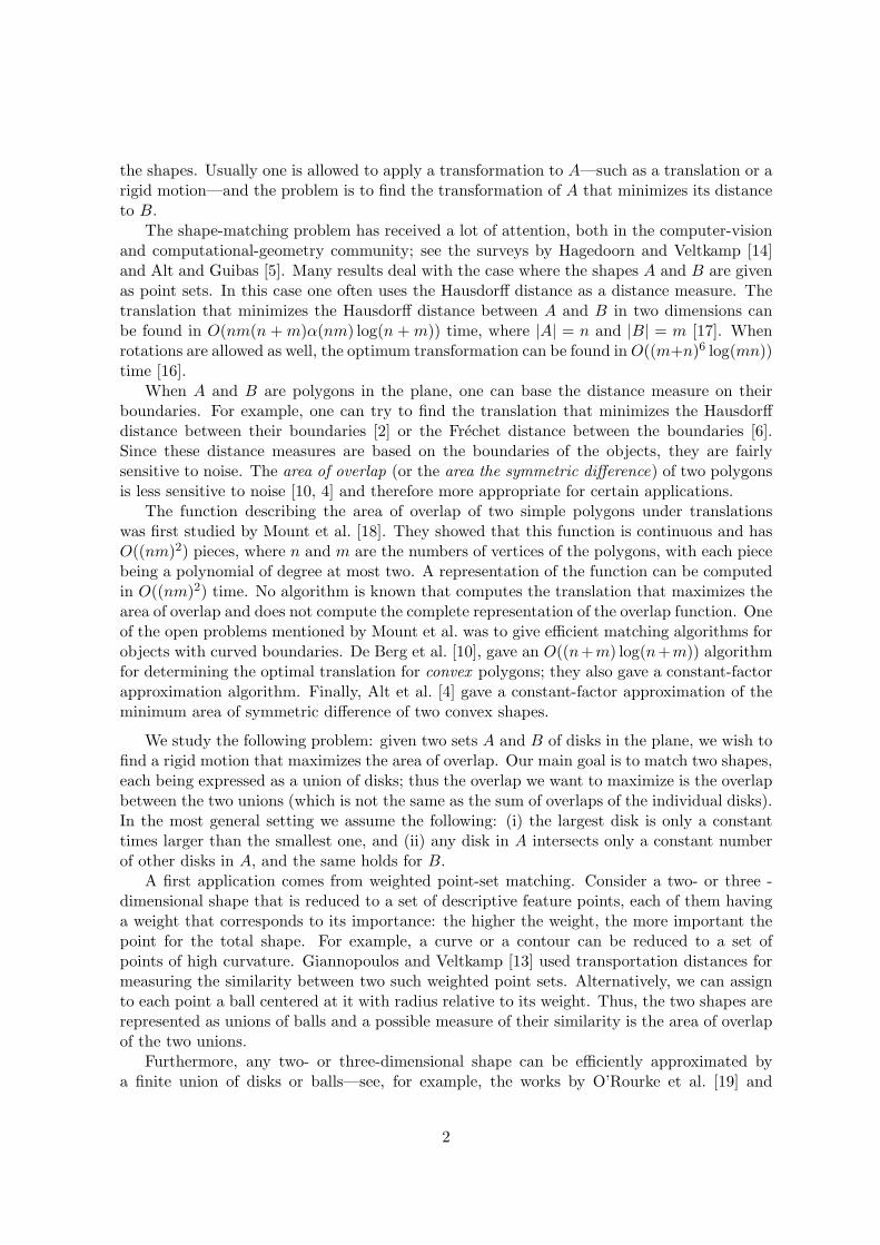
the shapes. Usually one is allowed to apply a transformation to A—such as a translation or arigid motion—and the problem is to find the transformation of A that minimizes its distanceto B.

The shape-matching problem has received a lot of attention, both in the computer-visionand computational-geometry community; see the surveys by Hagedoorn and Veltkamp [14]and Alt and Guibas [5]. Many results deal with the case where the shapes A and B are givenas point sets. In this case one often uses the Hausdorff distance as a distance measure. Thetranslation that minimizes the Hausdorff distance between A and B in two dimensions canbe found in O(nm(n + m)α(nm) log(n + m)) time, where |A| = n and |B| = m [17]. Whenrotations are allowed as well, the optimum transformation can be found in O((m+n)6 log(mn))time [16].

When A and B are polygons in the plane, one can base the distance measure on theirboundaries. For example, one can try to find the translation that minimizes the Hausdorffdistance between their boundaries [2] or the Frechet distance between the boundaries [6].Since these distance measures are based on the boundaries of the objects, they are fairlysensitive to noise. The area of overlap (or the area the symmetric difference) of two polygonsis less sensitive to noise [10, 4] and therefore more appropriate for certain applications.

The function describing the area of overlap of two simple polygons under translationswas first studied by Mount et al. [18]. They showed that this function is continuous and hasO((nm)2) pieces, where n and m are the numbers of vertices of the polygons, with each piecebeing a polynomial of degree at most two. A representation of the function can be computedin O((nm)2) time. No algorithm is known that computes the translation that maximizes thearea of overlap and does not compute the complete representation of the overlap function. Oneof the open problems mentioned by Mount et al. was to give efficient matching algorithms forobjects with curved boundaries. De Berg et al. [10], gave an O((n+m) log(n+m)) algorithmfor determining the optimal translation for convex polygons; they also gave a constant-factorapproximation algorithm. Finally, Alt et al. [4] gave a constant-factor approximation of theminimum area of symmetric difference of two convex shapes.

We study the following problem: given two sets A and B of disks in the plane, we wish tofind a rigid motion that maximizes the area of overlap. Our main goal is to match two shapes,each being expressed as a union of disks; thus the overlap we want to maximize is the overlapbetween the two unions (which is not the same as the sum of overlaps of the individual disks).In the most general setting we assume the following: (i) the largest disk is only a constanttimes larger than the smallest one, and (ii) any disk in A intersects only a constant numberof other disks in A, and the same holds for B.

A first application comes from weighted point-set matching. Consider a two- or three -dimensional shape that is reduced to a set of descriptive feature points, each of them havinga weight that corresponds to its importance: the higher the weight, the more important thepoint for the total shape. For example, a curve or a contour can be reduced to a set ofpoints of high curvature. Giannopoulos and Veltkamp [13] used transportation distances formeasuring the similarity between two such weighted point sets. Alternatively, we can assignto each point a ball centered at it with radius relative to its weight. Thus, the two shapes arerepresented as unions of balls and a possible measure of their similarity is the area of overlapof the two unions.

Furthermore, any two- or three-dimensional shape can be efficiently approximated bya finite union of disks or balls—see, for example, the works by O’Rourke et al. [19] and

2

Amenta et al. [7]. Fournier et al. [20] also used the union of disks or spheres representationto interpolate between two shapes. Provided that, in addition, the assumptions (i) and (ii)above are satisfied for the approximating sets, our algorithms can be used to match a varietyof shapes; however, the constant in assumption (i) may become large when the approximatedobjects have fine details.

Finally, both assumptions make perfect sense in molecular modelling with the hard spheremodel [15]. Under this model the radii range of the spheres is fairly restricted and no centerof a sphere can be inside another sphere; a simple packing argument shows that the latterimplies assumption (ii). A related problem with applications in protein shape matching wasexamined by Agarwal et al. [1], who gave algorithms for minimizing the Hausdorff distancebetween two unions of discs or balls under translations.

Independently of this work, Cheong et al. [8] presented a general technique for solvingproblems where the goal is to maximize the area of some region that depends on a multi-dimensional parameter. They observed that this technique can be directly applied to ourproblem, and gave an O((m/ε4) log3 m), probabilistic approximation algorithm that computesthe maximum area of overlap under translations up to an absolute error with high probability.When the maximum overlap is at least a constant fraction of the area of one of the two sets,the absolute error is in fact a relative error; this is good enough for measuring the similarityof two shapes that are not too dissimilar.

Our contributions are the following. First, we show in Section 2 that the maximumnumber of combinatorially distinct translations of A with respect to B can be as high asΘ(n2m). When rotations are considered as well, the complexity is O(n3m2). Moreover, thefunction describing the area of overlap is quite complex, even for combinatorially equivalentplacements. Therefore, the focus of our paper is on approximation algorithms. Next, we givea lower bound on the maximum area of overlap under translations, expressed in the numberof pairs of disks that contribute to that area. This is a vital ingredient of almost all ouralgorithms.

In the remaining sections, we present our approximation algorithms. For the sake ofclarity we describe the algorithms for the case of disjoint unit disks. It is not hard to adaptthe algorithms to sets of disks satisfying assumptions (i) and (ii) above; the necessary changescan be found in Section 7. For any ε > 0, our algorithms compute a (1− ε)-approximation ofthe optimum overlap. For translations we give an algorithm that runs in O((nm/ε2) log(m/ε))time. Compared to the result of Cheong et al. mentioned above, our algorithm is slower buthas a better dependence on ε, it is deterministic and its error is always relative, even when theoptimum is small. It also forms an ingredient to our algorithm for rigid motions, which runs inO((n2m2/ε3) log m) time. If ∆ is the diameter of set A the running time of the latter becomesO((m2n4/3∆1/3/ε3) log n log m), which yields an improvement when ∆ = o(n2/ log3 n). Notethat in many applications the union will be connected, which implies that the diameterwill be O(n). Finally, for the case where the area of overlap is a given fraction α of thearea of the union of A, we present a probabilistic algorithm for rigid motions that runs inO((m2/α3ε4) log2(m/ε) log m) time and succeeds with high probability.

Our algorithms are based on a simple two-step framework in which an approximation ofthe best translation is followed by an approximation of the best rotation (for rigid motions).This way, we first achieve an absolute error on the optimum, which, we then argue, is also arelative error because of the lower bound on the overlap in terms of the number of overlappingpairs. The deterministic algorithms employ a sampling of transformation space, directed by

3

some special properties of the function of the area of overlap of two disks. The probabilisticalgorithm is a combination of sampling the translation space using a uniform grid and randomsampling of both input sets.

2 Basic properties of the overlap function

We start by introducing some notation. Let A = A1, . . . , An and B = B1, . . . , Bm, betwo sets of disjoint unit disks in the plane, with n ≤ m. We consider the disks to be closed.Both A and B lie in the same two-dimensional coordinate space, which we call the work space;their initial position is denoted simply by A and B. We consider B to be fixed, while A canbe translated and/or rotated relative to B.

Let I be the infinite set of all possible rigid motions—also called isometries—in the plane;we call I the configuration space. We denote by Rθ a rotation about the origin by someangle θ ∈ [0, 2π) and by T~t a translation by some ~t ∈ R2. It will be convenient to modelthe space [0, 2π) of rotations by points on the circle S1. For simplicity, rotated only versionsof A are denoted by A(θ) = A1(θ), . . . , An(θ). Similarly, translated only versions of A aredenoted by A(~t) = A1(~t), . . . , An(~t). Any rigid motion I ∈ I can be uniquely defined as atranslation followed by a rotation, that is, I = I~t,θ = Rθ T~t, for some θ ∈ S1 and ~t ∈ R2.Alternatively, a rigid motion can be seen as a rotation followed by some translation; it willbe always clear from the context which definition is used. In general, transformed versions ofA are denoted by A(~t, θ) = A1(~t, θ), . . . , An(~t, θ) for some I~t,θ ∈ I.

Let Int(C), V (C) be, respectively, the interior and area of a compact set C ∈ R2, and letVij(~t, θ) = V (Ai(~t, θ) ∩ Bj). The area of overlap of A(~t, θ) and B, as ~t, θ vary, is a functionV : I → R with V(~t, θ) = V ((

⋃A(~t, θ))∩ (

⋃B)). Thus the problem that we are studying can

be stated as follows:Given two sets A,B, defined as above, compute a rigid motion I~topt,θopt

that maximizesV(~t, θ).

Let dij(~t, θ) be the Euclidean distance between the centers of Ai(~t, θ) and Bj . Also, let ri

be the Euclidean distance of Ai’s center to the origin. The Minkowski sum of two planar setsA and B, denoted by A ⊕ B, is the set p1 + p2 : p1 ∈ A, p2 ∈ B. Similarly the Minkowskidifference AB is the set p1 − p2 : p1 ∈ A, p2 ∈ B.

For simplicity, we write V(~t),Vij(~t), dij(~t) when θ is fixed and V(θ),Vij(θ), dij(θ) when ~tis fixed.

Theorem 1 Let A be a set of n disjoint unit disks in the plane, and B a set of m disjointunit disks, with n ≤ m. The maximum number of combinatorially distinct placements of Awith respect to B is Θ(n2m) under translations, and O(n3m2) under rigid motions.

Proof: Let us assume for a moment that A is first rotated about the origin by some fixedangle θ ∈ [0, 2π). We define Tij(θ) = Bj Ai(θ); Vij(~t, θ) > 0 if and only if ~t ∈ Int(Tij(θ)).Let T (A,B)(θ) = Tij(θ) : Ai ∈ A and Bj ∈ B. Then, V(~t, θ) > 0 if and only if ~t ∈Int(T (A,B)(θ)). The boundaries of the Minkowski differences Tij(θ) ∈ T (A,B)(θ) induce aplanar subdivision T (θ). Each cell in this arrangement is a set of combinatorially equivalenttranslations of A(θ) relative to B, that is, the set of all overlapping pairs (Ai(~t, θ), Bj) isthe same for all ~t in the cell. T (θ) can be non-simple and non-connected, and its maximumcomplexity is Θ(n2m). We first prove the upper bound and then give a lower bound example.In the next paragraph, we omit θ since it is fixed.

4

. . .

. . .A

B

d

d + ε

|A| = n

|B| = m > n

...

O(n) O(n) O(n)

m times

Figure 1: Two sets A and B and part of their configuration space T (A,B) with highestΘ(n2m) complexity.

Each set Bj Ai is a disk of radius 2. Since the disks in both sets are closed and disjoint,no disk of one set can intersect more than five disks of the other set at any position. This isdue to the ‘kissing’ or Hadwiger number of open unit disks, which is six [11]. This impliesthat a point in the configuration space cannot be covered by more than five of the m disksBj Ai, for any fixed i, 1 ≤ j ≤ m. In total, considering all values of i, no point in thetotal arrangement can be covered by more than 5n disks Bj Ai. A similar argument forthe disks in B gives that no point can be covered by more than 5m disks Bj Ai. Thus, themaximum depth of any point in the arrangement is 5 minm,n = 5n. Since the complexityof the arrangement of n pseudodisks with maximum depth k is O(nk) [21], the complexity ofthe configuration space is O(n2m).

To see that the bound is tight consider the sets A and B shown in Figure 1. Let d bethe distance between the centers of any two consecutive disks in A and d′ = d + ε, ε 6= 0,the distance between the centers of any two consecutive disks in B. These two sets give anarrangement of which the part of highest complexity is shown in Figure 1. In each of the Ω(m)‘bunches’ of Θ(n) disks, the complexity is Θ(n2), since each disk intersects all the others. Intotal, the complexity is Θ(n2m).

As θ varies, the combinatorial structure of T (θ) changes: each Tij(θ) rotates about thecenter of Bj and, as a result, new cells are created or existing cells disappear. Such a changeoccurs in one of the following two cases: (i) when two arcs in T (θ) become tangent at someθ (double event) or (ii) three arcs in T (θ) intersect at a point (triple event). By the analysisof Chew et al. [9], the number of double events is O(n2m2) and the number of triple eventsis O(n3m2). Thus, the total number of cells created is O(n3m2) and the complexity of theconfiguration space1 is O(n3m2) as well.

This theorem implies that explicitly computing the subdivision of the configuration space1Abusing the terminology slightly, we will sometimes use the term ‘configuration space’ when we are actually

referring to the decomposition of the configuration space induced by the infinite family of sets T (A, B)(θ) forall θ ∈ [0, 2π).

5

into cells with combinatorially equivalent placements is highly expensive. Moreover, thecomputation for rigid motions is numerically unstable since it involves univariate equationsof degree six [5]. Finally, the optimization problem in a cell of this decomposition is far fromeasy: one has to maximize a function consisting of a linear number of terms. Therefore weturn our attention to approximation algorithms. The following theorem, which gives a lowerbound on the maximum area of overlap, will be our fundamental took to convert an absoluteerror into a relative error.

Theorem 2 Let A = A1, . . . , An and B = B1, . . . , Bm be two sets of disjoint unit disksin the plane. Let ~topt be the translation that maximizes the area of overlap V(~t) of A(~t) and Bover all possible translations ~t of set A. If kopt is the number of overlapping pairs Ai(~topt), Bj,then V(~topt) is Θ(kopt).

Proof: First, note that V(~topt) ≤ koptπ. Since we are considering only translations, the con-figuration space is two dimensional. For each pair Ai(~topt), Bj for which Ai(~topt)∩Bj 6= ∅, wedraw, in configuration space, the region of translations Kij that bring the center of Ai(~topt)into Bj ; see Figure 2. Such a region is a unit disk that is centered at a distance at most 2

3

Kij

R

1

~topt

Figure 2: All disks Kij are confined within a disk R of area 9π.

from ~topt. Thus, all regions Kij are fully contained in a disk R, centered at ~topt, of radius 3.By a simple volume argument, there must be a point ~t] ∈ R (which represents a translation)that is covered by at least kopt/9 disks Kij . Each of the corresponding pairs Ai(~t]), Bj has anoverlap of at least 2π/3−

√3/2. Thus, V(~topt) ≥ V(~t]) ≥ (2π/27−

√3/18)kopt.

3 Approximation algorithms for translations

Theorem 2 suggests the following simple approximation algorithm: compute the arrangementof the regions Kij , with i = 1, . . . , n and j = 1, . . . ,m, and pick any point of maximum depth.Such a point corresponds to a translation ~t that gives a constant-factor approximation. Ananalysis similar to that of Theorem 2 leads to a factor of (2/3−

√3/2π) ≈ 0.39. It is possible

to do much better, however.We present a deterministic (1− ε)-approximation algorithm; see Cheong et al.’s [8] for a

probabilistic (1 − ε)-approximation algorithm. Since both A and B consist of disjoint disks,

6

we have V(~t) =∑

Ai∈A,Bj∈B Vij(~t). The algorithm is based on sampling the configurationspace by using a uniform grid. This is possible due to the following lemma, which tells that,in terms of absolute error, it is not too bad if we choose a translation which is close to theoptimal one. As mentioned before, we can then use Theorem 2 to convert it to a relativeerror.

Lemma 3 Let k be the number of overlapping pairs Ai(~t, θ), Bj for some ~t ∈ R2, θ ∈ [0, 2π).For any given δ > 0 and any ~t′ ∈ R2 for which |~t − ~t′| = O(δ), we have V(~t, θ) − V(~t′, θ) =O(kδ).

Proof: Consider a pair of disks Ai(~t, θ) and Bj for which Vij(~t, θ) 6= 0. If Ai is trans-lated by ~t′, instead of ~t, then dij(~t′, θ) − dij(~t, θ) = |~t − ~t′|. Observe that the largest lossper pair, Vij(~t, θ) − Vij(~t′, θ), occurs when Ai moves in the direction of the line connectingthe centers of Ai and Bj , and away from Bj . Since the diameter of both disks is equal to2, we have that Vij(~t, θ) − Vij(~t′, θ) < 2|~t − ~t′| = O(δ). We have k such pairs, hence2 ,V(~t, θ)− V(~t′, θ) = O(kδ).

The computation of V(~t) for every grid translation is not done directly, but instead we use avoting scheme, which speeds up the algorithm by a linear factor. Algorithm Translation(A,B, ε) is shown in Figure 3.

Translation(A,B, ε):

1. Initialize an empty binary search tree S with entries of the form (~t,V(~t)) where ~t is the key.Let G be a uniform grid of spacing cε, where c is a suitable constant.

2. For each pair of disks Ai ∈ A and Bj ∈ B do:

(a) Determine all grid points ~tg of G such that ~tg ∈ Tij , where Tij = Bj Ai. For eachsuch ~tg do:

• If ~tg is in S, then V(~tg) := V(~tg) + Vij(~tg) otherwise, insert ~tg in S with V(~tg) :=Vij(~tg).

3. Report the grid point ~tapx that maximizes V(~tg).

Figure 3: Algorithm Translation(A,B, ε).

Theorem 4 Let A = A1, . . . , An and B = B1, . . . , Bm be two sets of disjoint unit disksin the plane, with n ≤ m. Let ~topt be a translation that maximizes V(~t). Then, for any givenε > 0, Translation(A,B, ε) computes a translation ~tapx, for which V(~tapx) ≥ (1− ε)V(~topt),in O((mn/ε2) log(m/ε)) time.

Proof: It follows from Theorem 2 that there must be at least one pair of disks with significantoverlap in an optimal translation. This implies that the grid point closest to the optimum musthave a pair of overlapping disks, and so the algorithm checks at least one grid translation ~tg forwhich |~topt −~tg| = O(ε). Let kopt be the number of overlapping pairs Ai(~topt), Bj . According

2Note that by translating A by ~t′ instead of ~t and then rotating it by θ, new pairs might overlap but thiscan only decrease the total loss.

7

to Lemma 3, by setting θ = 0, we have that V(~topt) − V(~tapx) ≤ V(~topt) − V(~tg) = O(koptε).By Theorem 2, we have V(~topt) = Θ(kopt), and the approximation bound follows.

The algorithm considers O(1/ε2) grid translations ~tg per pair of disks. Each translationis handled in O(log(nm/ε2)) time. Thus, the total running time is O((nm/ε2) log(nm/ε2)) =O((nm/ε2) log(m/ε)).

4 The rotational case

This section considers the following restricted scenario: set B is fixed, and set A can berotated about the origin. This will be used in the next section, where we consider generalrigid motions.

Observe that this problem has a one-dimensional configuration space: the angle of rota-tion. Consider the function V : [0, 2π) → R with

V(θ) := V ((⋃

A(θ)) ∩ (⋃

B)) =∑

Ai∈A,Bj∈B

Vij(θ).

For now, our objective is to guarantee an absolute error on V rather than a relative one. Westart with a result that bounds the difference in overlap for two relatively similar rotations.Recall that ri is the distance of Ai’s center to the origin.

Lemma 5 Let Ai, Bj be any fixed pair of disks. For any given δ > 0 and any θ1, θ2 for which|θ1 − θ2| ≤ δ/(2ri), we have |Vij(θ1)− Vij(θ2)| ≤ 2δ.

Proof: Without loss of generality, we assume that θ1 = 0 and that Ai is centered at (ri, 0)with ri > 0; see Figure 4. We want to see that V (Ai ∩ Bj) − V (Ai(θ) ∩ Bj) ≤ 2δ for any0 ≤ θ ≤ δ/(2ri). Consider the function v(θ) = V (Ai ∩Ai(θ)) with θ ∈ [0, π/2]. We will provethat if 0 ≤ θ ≤ δ/(2ri) then v(θ) ≥ π − δ, and therefore V (Ai \ Ai(θ)) = V (Ai(θ) \ Ai) ≤ δ.Using that for any sets X, Y we have V (X) − V (Y ) = V (X \ Y ) − V (Y \X), then for any0 ≤ θ ≤ δ/(2ri) it holds

|V (Ai ∩Bj)− V (Ai(θ) ∩Bj)|= |V ((Ai ∩Bj) \ (Ai(θ) ∩Bj))− V ((Ai(θ) ∩Bj) \ (Ai ∩Bj))|≤ |V ((Ai ∩Bj) \ (Ai(θ) ∩Bj))|+ |V ((Ai(θ) ∩Bj) \ (Ai ∩Bj))|≤ V (Ai \Ai(θ)) + V (Ai(θ) \Ai)≤ 2δ,

and the lemma follows.We will show that v(θ) ≥ π − δ using the mean-value theorem. The center of Ai(θ) is

positioned at (ri cos(θ), ri sin(θ)) and the distance between the centers of Ai and Ai(θ) is√r2i (1− cos θ)2 + r2

i sin2 θ = ri

√2(1− cos(θ)).

The area of overlap of two unit disks whose centers are d apart is

2 arccosd

2− d

√4− d2

2,

8

(ri, 0)

(0, 0)

Ai

Ai(θ)

θ

(ri cos θ, ri sin θ)

Figure 4: Notation in Lemma 5. The area of the grey region corresponds to v(θ).

and therefore we get

∂v(θ)∂θ

=∂v(θ)∂d

· ∂d

∂θ

= −√

4− 2r2i (1− cos(θ)) · ri sin(θ)√

2(1− cos(θ))

= −ri

√2 + 2 cos(θ)− r2

i sin2(θ) ≥ −2ri,

where in the last inequality we used 2 ≥ 2 cos(θ) − ri sin2(θ). We conclude that if 0 ≤ θ ≤δ/(2ri) then ∂v(θ)/∂θ ≥ −δ/θ.

Using the mean-value theorem we see that, for any θ ∈ [0, δ/(2ri)] there exists θ′ ∈ [0, θ]such that

v(θ)− v(0)θ − 0

=v(θ)− π

θ=

∂v(θ′)∂θ

.

Since, 0 ≤ θ′ ≤ δ/(2ri), we have ∂v(θ′)/∂θ ≥ − δθ and so we conclude that v(θ)− π ≥ −δ.

For a pair Ai, Bj , we define the interval Rij = θ ∈ [0, 2π) : Ai(θ) ∩ Bj 6= ∅ on S1, thecircle of rotations. We denote the length of Rij by |Rij |. Instead of computing Vij(θ) at eachθ ∈ Rij , we would like to sample it at regular intervals whose length is at most δ/(2ri). Atfirst, it looks as if we would have to take an infinite number of sample points as ri → ∞.However, as the following lemma shows, |Rij | decreases as ri increases, and the number ofsamples we need to consider is bounded.

Lemma 6 For any Ai, Bj with ri > 0, and any given given δ > 0, we have |Rij |/(δ/(2ri)) =O(1/δ).

Proof: Without loss of generality, we can assume that Ai is centered at (ri, 0) and Bj iscentered at (rj , 0). Note that the distance between the center of Ai(θ) and Bj is

dij(θ) =√

(ri cos θ − rj)2 + (ri sin θ)2 =√

r2i + r2

j − 2rirj cos θ.

Under these assumptions, Rij is of the form [−θij , θij ], where θij is the largest value for which

Ai(θij) ∩Bj 6= ∅, that is, dij(θij) = 2. We have θij = arccosr2i +r2

j−4

2rirj.

As shown in Figure 5, the center of Ai(θij) is always placed on C, the circle of radius twoand concentric with Bj . Therefore, the value θij is maximized when it equals the slope of the

9

(rj , 0)(0, 0)

Bj

center of Ai(θij) in the worst case

C

p

Figure 5: Notation in Lemma 6. The center of Ai(θij) is placed in the circle C. Therefore,θij is maximized for the dashed line through the origin and tangent to C.

line through the origin and tangent to C. Let p be the point of tangency. Since the triangle

p, (0, 0), (rj , 0) is right on p, we conclude that θij is maximized when rj =√

r2i + 4. Therefore

|Rij | = 2arccosr2i + r2

j − 42rirj

≤ 2 arccos

√1− 4

r2i + 4

.

Using L’Hopital’s rule we can compute that

limri→∞

|Rij |1/ri

≤ limri→∞

2 arccos√

1− 4r2i +4

1/ri= lim

ri→∞

41 + 4

r2i

= 4.

It follows that the function |Rij | · ri is bounded for any ri > 0, and so |Rij |δ/(2ri)

= O(1/δ).

This lemma implies that we have to consider only O(1/δ) sample rotations per pair ofdisks. Thus we need to check O(nm/δ) rotations in total. It seems that we would have tocompute all overlaps at every rotation from scratch, but here Lemma 5 comes to the rescue:in between two consecutive rotations θ, θ′ defined for a given pair Ai, Bj there may be manyother rotations, but if we conservatively estimate the overlap of Ai, Bj as the minimum overlapof θ and θ′, we do not loose too much. This is the idea for algorithm Rotation, describedin detail in Figure 6; the value V(θ) is the conservative estimate of V(θ), as just explained.

Lemma 7 Let θopt be a rotation that maximizes V(θ) and let kopt be the number of overlap-ping pairs Ai(θopt), Bj. For any given δ > 0, the rotation θapx reported by Rotation(A,B, δ)satisfies V(θopt) − V(θapx) = O(koptδ), and can be computed in O(m log n + (|Π|/δ) log m)time, where Π is the set of pairs Ai, Bj with Ri,j 6= ∅.

Proof: First, we show that V(θ) ≥ V(θ) ≥ V(θ)− 2kθδ for any θ ∈ Θ where kθ is the numberof overlapping pairs between A(θ) and B. That is, V is a fair approximation of V from belowfor the values in Θ. It is important that the estimation V(θ) is from below: since kθ could bemuch larger than kopt, an estimation from above with an error of kθδ could be very large.

By checking whether Vij increases or decreases at θsij and adding the appropriate value to

V(θ), each pair Ai, Bj contributes Vij(θsij) ≤ Vij(θ) to V(θ) for some θs

ij for which |θ − θsij | ≤

δ/(2ri). By Lemma 5 we have Vij(θ)−Vij(θsij) ≤ 2δ. Thus, in total, 0 ≤ V(θ)− V(θ) ≤ 2kθδ.

10

Rotation(A,B, δ):

1. For each pair of disks Ai ∈ A and Bj ∈ B with Rij 6= ∅, choose a set Θij := θ1ij , . . . , θ

sij

ij of rotations as follows. First put the midpoint of Rij in Θij , and then put all rotations inΘij that are in Rij and are at distance k · δ/(2ri) from the midpoint for some integer k.Finally, put both endpoints of Rij in Θij . In other words, Θij consists of rotations with auniform spacing of δ/(2ri)—except for the cases of endpoints whose distance to their neighborrotations is less than δ/(2ri)—with the midpoint of Rij being one of them.

2. Sort the values Θ :=⋃

i,j Θij , keeping repetitions and solving ties arbitrarily. Let θ0, θ1, . . .

be the ordering of Θ. In steps 3 and 4, we will compute a value V(θ) for each θ ∈ Θ.

3. (a) Initialize V(θ0) := 0.

(b) For each pair Ai ∈ A,Bj ∈ B for which θ0 ∈ Rij do:

• If Vij is decreasing at θ0, or θ0 is the midpoint of Rij , then V(θ0) := V(θ0)+Vij(θij),where θij is the closest value to θ0 in Θij with θij > θ0.

• If Vij is increasing at θ0, then V(θ0) := V(θ0) + Vij(θij), where θij is the closestvalue to θ0 in Θij with θij < θ0.

4. For each θl in increasing order of l, compute V(θl) from V(θl−1) by updating the contributionof the pair Ai, Bj defining θl, as follows. Let θl be the s-th point in Θij , that is, θl = θs

ij

• If Vij is increasing at θsij , then V(θl) := V(θl−1)− Vij(θs−1

ij ) + Vij(θsij)

• If Vij is the midpoint of Rij , then V(θl) := V(θl−1)− Vij(θs−1ij ) + Vij(θs+1

ij )

• If Vij is decreasing at θsij , then V(θl) := V(θl−1)− Vij(θs

ij) + Vij(θs+1ij )

5. Report the θapx ∈ Θ that maximizes V(θ).

Figure 6: Algorithm Rotation(A,B, δ).

In a similar fashion, consider now the kopt overlapping pairs of disks at θopt, and let AM

be the disk furthest from the origin that participates in the optimal solution, i.e. AM (θopt)∩(⋃

B) 6= ∅. Let θ ∈ Θ be the closest value to θopt. We have

|θ − θopt| ≤ δ/(2rM ) ≤ δ/(2ri)

for all Ai in the optimal solution. Again, according to Lemma 5, the loss per pair Ai, Bj isVij(θopt)− Vij(θ) ≤ 2δ. In total, V(θopt)− V(θ) ≤ 2koptδ.

Observe that since both endpoints of every interval Rij are in Θ, no new pairs withnon-zero overlap are formed when ‘moving’ from θopt to θ. Hence, it holds that kθ = kopt.

Putting it all together we get

V(θopt)− V(θapx) =(V(θopt)− V(θ)

)+

(V(θ)− V(θ)

)+

(V(θ)− V(θapx)

)+

(V(θapx)− V (θapx)

)≤ 2koptδ + 2kθδ + 0 + 0 ≤ 4koptδ.

The running time of the algorithm is bounded as follows. First, we discuss how to constructthe set Π, that is, pairs Ai, Bj with Rij 6= ∅. We store the disks of A in a balanced search tree

11

T sorted by the distance from their center to the origin. This takes O(n log n) time. Considera fixed disk Bj , and let Πj be the pairs Ai, Bj in Π. Note that Rij 6= ∅ if and only if thedistance from the origin to the centers of Ai and Bj differs by at most two. Therefore, wecan use T to construct Πj in O(|Πj | + log n) time. By considering each Bj , we construct Πin O(n log n) + O(

∑j |Πj |+ m log n) = O(Π + m log n) time.

Once we have Π, we can construct the set Θ, which consists of |Π| subsets Θij , each withO(1/δ) rotations by Lemma 6. Each subset Θij can easily be generated as a sorted sequence,so what remains is to merge the sorted sequences, which can be done in O((|Π|/δ) log |Π|) =O((|Π|/δ) log m) time.

5 Approximation algorithms for rigid motions

Any rigid motion can be described as a translation followed by a rotation around the origin.This is used in algorithm RigidMotion described in Figure 7, which combines the algorithmsfor translations and for rotations to obtain a deterministic (1 − ε)-approximation for rigidmotions.

RigidMotion(A,B, ε):

1. Let G be a uniform grid of spacing cε, where c is a suitable constant. For each pair of disksAi ∈ A and Bj ∈ B do:

(a) Set the center of rotation, i.e. the origin, to be Bj ’s center by translating B appropri-ately.

(b) Let Tij = Bj Ai, and determine all grid points ~tg of G such that ~tg ∈ Tij . For eachsuch ~tg do:

• run Rotation(A(~tg), B, c′ε), where c′ is an appropriate constant.Let θg

apx be the rotation returned. Compute V(~tg, θgapx).

2. Report the pair (~tapx, θapx) that maximizes V(~tg, θgapx).

Figure 7: Algorithm RigidMotion(A,B, ε).

Theorem 8 Let A = A1, . . . , An and B = B1, . . . , Bm, with n ≤ m, be two sets ofdisjoint unit disks in the plane. Let I~topt,θopt

be a rigid motion that maximizes V(~t, θ). Then,for any given ε > 0, RigidMotion(A,B, ε) computes a rigid motion I~tapx,θapx

such thatV(~tapx, θapx) ≥ (1− ε)V(~topt, θopt) in O((n2m2/ε3) log m) time.

Proof: We will show that V(~tapx, θapx) approximates V(~topt, θopt) up to an absolute error. Toconvert the absolute error into a relative error, and hence show the algorithm’s correctness,we use again Theorem 2.

Let Aopt be the set of disks in A that participate in the optimal solution and let |Aopt| =kopt. Since the ‘kissing’ number of unit open disks is six, we have that kopt < 6kopt,where kopt is the number of overlapping pairs in the optimal solution. Next, imagine thatRigidMotion(Aopt, B, ε) is run instead of RigidMotion(A,B, ε). Of course, an optimal

12

rigid motion for Aopt is an optimal rigid motion for A and the error we make by applying anon-optimal rigid motion to Aopt bounds the error we make when applying the same rigidmotion to A.

Consider a disk Ai ∈ Aopt and an intersecting pair Ai(~topt, θopt), Bj . Since, at somestage, the algorithm will use Bj ’s center as the center of rotation, and I~topt,θopt

= Rθopt T~topt,

we have that Ai(~topt) ∩ Bj 6= ∅ if and only if Ai(~topt, θopt) ∩ Bj 6= ∅. Hence, we have that~topt ∈ Tij and the algorithm will consider some grid translation ~tg ∈ Tij = Bj Ai, for which|~topt − ~tg| = O(ε). By Lemma 3 we have V(~topt, θopt)− V(~tg, θopt) = O(koptε) = O(koptε).

Let θgopt be the optimal rotation for ~tg. Then, V(~tg, θopt) ≤ V(~tg, θ

gopt). The algorithm

computes, in its second loop, a rotation θgapx for which V(~tg, θ

gopt) − V(~tg, θ

gapx) = O(kg

optε),where kg

opt is the number of pairs at the optimal rotation θgopt of Aopt(~tg). Since we are only

considering Aopt we have that kgopt < 6kopt, thus, V(~tg, θ

gopt)− V(~tg, θ

gapx) = O(koptε).

Now, using the fact that V(~tg, θgapx) ≤ V(~tapx, θapx) and that kopt ≤ kopt, and putting it

all together we get

V(~topt, θopt)− V(~tapx, θapx) =(V(~topt, θopt)− V(~tg, θopt)

)+

(V(~tg, θopt)− V(~tg, θ

gopt)

)+

(V(~tg, θ

gopt)− V(~tg, θg

apx))

+(V(~tg, θg

apx)− V(~tapx, θapx))

< O(koptε) + 0 + O(koptε) + 0 = O(koptε).

Since the optimal rigid motion can be also defined as a rotation followed by some translation,Theorem 2 holds for V(~topt, θopt) as well. Thus, V(~topt, θopt) = Θ(kopt) and the approximationbound follows.

Finally, the running time of the algorithm is dominated by its first step. We can computeV(~tg, θ

gapx) by a simple plane sweep in O(m log m) time. Since there are Θ(ε−2) grid point in

each Tij , each execution of the loop in the first step takes O(m + 1/ε2 + (1/ε2)(Π/ε) log m +(1/ε2)m log m) = O((nm/ε3) log m) time since Π = O(nm). The step is executed nm times,thus the algorithm runs in O((n2m2/ε3) log m) time.

5.1 An improvement for sets with small diameter

We can modify the algorithm such that its running time depends on the diameter ∆ of theset A. The main idea is to convert our algorithm into one that is sensitive to the numberof pairs of disks in A and B that have approximately the same distance, and then use thecombinatorial bounds by Gavrilov et al. [12]. Namely, we will use the following result (notethat an extra log n factor is missing in the reference due to a typographic error).

Lemma 9 [12, Theorem 4.1] Given a S set of n points whose closest pair is at distanceat least 2, there are O(n4/3t1/3 log n) pairs of points in S whose distance is in the range[t− 4, t + 4].

This lemma and a careful implementation of Rotation allows us to improve the analysis ofthe running time of RigidMotion for small values of ∆. In many applications it is reasonableto assume bounds of the type ∆ = O(n) [12], and therefore the result below is relevant. Forexample, if ∆ = O(n) this result shows that we can compute a (1 − ε)-approximation inO((m2n5/3)/ε3 log n log m) time.

13

Theorem 10 Let A = A1, . . . , An and B = B1, . . . , Bm, with n ≤ m, be two sets ofdisjoint unit disks in the plane. Let ∆ be the diameter of A, and let I~topt,θopt

be the rigidmotion maximizing V(~t, θ). For any ε > 0, we can find in O((m2n4/3∆1/3/ε3) log n log m)time a rigid motion I~tapx,θapx

such that V(~tapx, θapx) ≥ (1− ε)V(~topt, θopt).

Proof: For indices i, j, let Zij be the set of pairs Ai′ , Bj′ such that

d(cBj , cBj′ )− 4 ≤ d(cAi , cAi′ ) ≤ d(cBj , cBj′ ) + 4,

where cAi denotes the center of Ai and cBj denotes the center of Bj . If A has diameter ∆, then∑i,j |Zij | = O(m2n4/3∆1/3 log n): for each of the O(m2) pairs j, j′, there are O(n4/3∆1/3 log n)

pairs i, i′ because of Lemma 9.Consider one of the calls to Rotation that RigidMotion makes. The origin is set

at the center of some Bj , and some Ai intersects Bj . The pairs of disks Ai′ , Bj′ withRi′j′ 6= ∅ is a subset of Zi,j , and from Lemma 7 we conclude that the call to Rotationtakes O(m log n + (|Zij |/ε) log m) time. For each pair of disks Ai, Bj , the algorithm Rigid-Motion makes O(1/ε2) calls to Rotation. Therefore, the total running time can be boundedby

O

∑i,j

O(1/ε2) O(m log n + (|Zij |/ε) log m)

= O

nm2 log n/ε2 + (ε−3 log m)∑i,j

|Zij |)

= O

(nm2 log n/ε2 + (ε−3 log m)m2n4/3∆1/3 log n

)= O((m2n4/3∆1/3/ε3) log n log m).

6 A Monte Carlo algorithm for rigid motions

In this section we present a Monte Carlo algorithm that computes a (1 − ε)-approximationfor rigid motions in O((m2/α3ε4) log2(m/ε) log m) time, where α is an input parameter thatshould have the property that the maximum area of overlap is at least αV (A).

The algorithm is simple and follows the two-step framework of Section 5 in which anapproximation of the best translation is followed by an approximation of the best rotation.However, now, the first step is a combination of grid sampling of the space of translationsand random sampling of set A. This random sampling is based on the observation that thedeterministic algorithm of Section 5 will compute a (1− ε)-approximation kopt times, wherekopt is the number of pairs of overlapping disks in an optimal solution. Intuitively, the largerthis number is, the quicker such a pair will be tried out in the first step. Similar observationswere made by Akutsu et al. [3] who gave exact Monte Carlo algorithms for the largest commonpoint set problem.

The second step is a direct application of the technique by Cheong et al. that allows us tomaximize, up to an absolute error, the area of overlap under rotation in almost linear time,by computing a point of maximum depth in a one dimensional arrangement.

14

Rotations. Let S be a set of points from⋃

A. For each point s ∈ S, we define W (s) =θ ∈ [0, 2π)|s(θ) ∈ B where s(θ) denotes a copy of s rotated by θ. Let AB(S) be thearrangement of all regions W (s), s ∈ S; it is a one-dimensional arrangement of unions ofrotational intervals. The following lemma follows by a direct modification in the proof ofLemma 4.2 in Cheong et al. [8].

Lemma 11 Let θopt be the rotation that maximizes V(θ). For any given δ > 0, let S be auniform random sample of points in

⋃A with |S| ≥ c1δ

−2 log(m/δ), where c1 is an appropriateconstant. A vertex θapx of AB(S) of maximum depth satisfies |V(θopt) − V(θapx)| ≤ δV (A)with probability at least 1− δ2/m6.

Note that the arrangement AB(S) has O((m/δ2) log(m/δ)) complexity and can be com-puted in O((m/δ2) log2(m/δ)) time. A vertex θapx of AB(S) of maximum depth can be foundby a simple traversal of this arrangement.

We could apply the idea above directly to rigid motions, with δ = αε, and consider thethree-dimensional regions W (s) with respect to rigid motions of S. Lemma 11 holds for thearrangement of all these regions and a vertex of maximum depth gives an absolute error onV(~topt, θopt). Computing this arrangement explicitly is quite cumbersome since each W (s)is bounded by curved surfaces. However, one need not compute the whole arrangement,but rather test all its possible vertices. Chew et al. [9] showed that this arrangement hasO(|S|3m2) = O((m2/δ6) log3(m/δ)) vertices that correspond — in workspace — to combi-nations of triples of points in S and triples of disks in B such that each point lies on theboundary of a disk. They also showed that all such possible combinations can be found inO((m2/δ6) log4(m/δ)) time using dynamic Voronoi diagrams. However, computing the actualrigid motion for any such combination is not trivial, as it requires solving algebraic equationsof degree six. By applying the technique to rotations only, thus computing a one-dimensionalarrangement, we avoid this complication in addition to achieving a better dependence on ε.

Rigid motions. Since we assume that V(~topt, θopt) ≥ αV (A), for some given value 0 < α ≤1, we have that kopt ≥ αn. Based also on the fact that the number of disks in A that partic-ipate in an optimal solution is at least kopt/6, we can easily prove that the probability thatΘ(α−1 log m) uniform random draws of disks from A will all fail to give a disk participatingin an optimal solution is at most 1/m5. This, together with Lemma 11 is the main idea usedin Algorithm RandomRigidMotion, given in Figure 8.

Theorem 12 Let A = A1, . . . , An and B = B1, . . . , Bm, with m ≤ n be two sets ofdisjoint unit disks in the plane, and let I~topt,θopt

be a rigid motion that maximizes V(~t, θ).Assume that V(~topt, θopt) ≥ αV (A), for some given value 0 < α ≤ 1. For any given ε > 0,RandomRigidMotion(A,B, α, ε) computes a rigid motion I~tapx,θapx

such that V(~tapx, θapx) ≥(1− ε)V(~topt, θopt) in O((m2/α3ε4) log2(m/ε) log m) time. The algorithm succeeds with prob-ability 1−O(m−5).

Proof: Recall that Aopt is the set of disks in A that participate in an optimal solution, andthat |Aopt| = kopt. Since kopt > kopt/6, we have that Pr[(Ai /∈ Aopt)] < 1− kopt

6n , for a randomAi ∈ A. Let RA be a set of disks randomly drawn from A. The probability that all |RA|random draws from A will fail to give a disk that belongs to an optimal pair is

Pr[RA ∩Aopt = ∅] ≤ (1− kopt

6n)|RA| ≤ e−kopt|RA|/(6n) ≤ e−α|RA|/6.

15

RandomRigidMotion(A,B, α, ε):

1. Choose a uniform random sample S of points in⋃

A, with |S| = Θ(δ−2 log(m/δ)), whereδ = αε.

2. Let G be a uniform grid of spacing cε, where c is a suitable constant.Repeat Θ(α−1 log m) times:

(a) Choose a random Ai from A.

(b) For each Bj ∈ B do:

i. Set the center of rotation, i.e. the origin, to be Bj ’s center by translating Bappropriately.

ii. Let Tij = Bj Ai, and determine all grid points ~tg of G such that ~tg ∈ Tij . Foreach such ~tg do:• Compute a vertex θg

apx of maximum depth in AB(S(~tg)), and V(~tg, θgapx).

3. Report the pair (~tapx, θapx) that maximizes V(~tg, θgapx).

Figure 8: Algorithm RandomRigidMotion(A,B, α, ε).

By choosing |RA| ≥ (30/ log e)α−1 log m, we have that Pr[RA ∩Aopt = ∅] ≤ m−5.For bounding the error in the approximation, we assume from now on that RA ∩ Aopt 6=

∅. For each translation ~tg that the algorithm tries in step 2(b)ii, Lemma 11 implies that|V(~tg, θ

gopt) − V(~tg, θ

gapx)| ≤ δV (A) = αεV (A), with probability at least 1 − 1/m6. Since we

are using O(m/αε2) times Lemma 11, the probability of error in any of them is bounded byO(m/αε2)(δ2/m6) = O(m−5). From now on, we also assume that all uses of Lemma 11 arecorrect.

Under the assumption that RA ∩ Aopt 6= ∅, the algorithm will try one intersecting pairAi(~topt, θopt), Bj in the first loop, and, in particular, it will try a translation ~tg such that |~topt−~tg| ≤ cε. As in Theorem 8, we have that V(~topt, θopt) − V(~tg, θopt) = O(koptε), V(~tg, θopt) ≤V(~tg, θ

gopt) and V(~tg, θ

gapx) ≤ V(~tapx, θapx). Hence

V(~topt, θopt)− V(~tapx, θapx) = O(koptε) + αεV (A) = O(koptε).

Using that V(~topt, θopt) = Θ(kopt), the approximation bound follows. The algorithm fails toreturn such a pair ~tapx, θapx if and only if it fails to obtain RA ∩ Aopt 6= ∅ or any of the usesof Lemma 11 fails. From the discussion above, it follows that this happens with probabilityO(m−5).

As for the running time, the random sampling of set A can be done in O((n/δ2) log(m/δ)) =O((n/α2ε2) log(m/ε)) time, where we have used that α ≥ 1/n. In the second step, for each ofthe O((m/αε2) log m) grid translations ~tg, we spend O((m/δ2) log2(m/δ)) = O((m/α2ε2)) log2

(m/ε)) time to construct the arrangement AB(S(~tg)), to find a vertex of maximum depth θgapx,

and to evaluate V(~tg, θgapx). Therefore, we spend O((m2/α3ε4) log2(m/ε) log m) time in to-

tal.

16

7 Sets of intersecting disks with different radii

We can generalize our results to the case where A and B consist of possibly intersecting andvarious size disks. Let rs and rl be the smallest, resp. largest disk radius among all disks inA ∪ B. We define the depth of a point p ∈ R2 with respect to a set of disks as the numberof disks in the set that contain it. Our algorithms work under the following two conditions:(i) rl/rs = ρ, for some constant ρ > 0; without loss of generality we assume that rs = 1 andrl = ρ, and (ii) the depth of any point p ∈ R2 with respect to A and the depth of any pointp ∈ R2 with respect to B are both bounded by some constant β.

First, we show that the assumptions result in denser sampling of configuration space withconstants that depend on the parameters ρ and β as well. Then, we discuss their algorithmicimplications.

Translations. First, consider Lemma 3. The maximum loss per pair is now determinedby a pair of disks of radius ρ each: Vij(~topt, θopt) − Vij(~t, θopt) < 2ρ|~topt − ~t| = O(δ). There-fore, V(~topt, θopt) − V(~t, θopt) < 2koptρ|~topt − ~t| = O(koptδ) and the lemma holds. Moreover,Theorem 2 holds as well, with the constant in the Θ-notation depending on both ρ and β.

Regarding the algorithm Translation, special care needs to be taken to avoid over-counting V(~tg). We can do this in the following way: Consider the arrangement A of all disksAi ∈ A in the work space. Since the maximum depth in A is constant, A has O(n) complexityand can be computed in O(n log n) time. Next, we compute a vertical decomposition VD(A)of A; VD(A) has O(n) disjoint cells3 each of constant complexity and can be computed inO(n log n) time. Similarly, we compute B and VD(B) both in O(m log m) time. The loopin step 2 is now executed for every pair of cells ci ∈ VD(A) and cj ∈ VD(B) and instead ofcomputing Vij(~tg), we compute V (ci(~tg)∩cj). The voting scheme proceeds as before and runswithin the same time bounds.

Rotations. Consider Lemma 5 and its proof: the length of sampling intervals is now de-termined by a pair of disks of radius ρ each. For such a pair Ai, Bj we have ∂v(θ)

∂θ ≥ −2riρ.Therefore, for any pair of disks Ai ∈ A and Bj ∈ B, we can sample Vij(θ) at regular intervalswhose length is at most δ/(2riρ) assuring that the loss per pair is at most 2δ. We also haveto make sure that the number of samples per pair remains bounded, see Lemma 6. Indeed,|Rij | is maximized for the ‘worst case’ pair of disks of radius ρ each; this is a scaled, by ρ,version of the original problem.

Regarding algorithm Rotation(A,B, δ), we use spacing of δ/(2riρ) in its first step. Un-fortunately, the simple technique used in the algorithm of Figure 6 to approximate V(θ) forall the values θ ∈ Θ does not work here since the disks in each set are possibly intersect-ing and the area of overlap accumulated in V(θ) can be a bad approximation of V(θ). Wecan overcome this problem in the following way. We compute VD(A) and VD(B) as before.Observe that every cell ci ∈ VD(A) is fully contained in some disk in A; similarly, everycell cj ∈ VD(B) is fully contained in some disk in B. Consider the function V (ci(θ) ∩ cj),θ ∈ [0, 2π); for every pair (ci, cj), the error in V (ci(θ) ∩ cj) is bounded by the error in thepair of their corresponding disks. Since each cell in both decompositions has at most twovertical walls and at most two circular segments, the function has a bounded number of localminima/maxima. We insert all these values, for every pair of cells, in set Θ. Also, each disk

3For our purpose, we only consider cells that are insideS

A.

17

Ai is decomposed into O(1) cells in VD(A) because it intersects at most 9ρ2β other disksof A. The same holds for any disk Bj in VD(B). Hence, the total number of the additionalvalues in Θ is of O(Π). The algorithm proceeds as before by considering whether V (ci(θ)∩cj)increases, decreases or reaches an optimum at each θ ∈ Θ. Rotation now runs again inO((Π/δ) log m) time and its correctness can be shown as in the proof of Lemma 7.

Rigid Motions. In addition to the relevant changes mentioned in the previous paragraphs,observe that a simple volume argument shows that any disk Ai(~t, θ) cannot intersect morethan 9ρ2β disks Bj for any ~t, θ. Thus, |Aopt| > kopt/(9ρ2β).

In RigidMotion, we compute V(~tg, θgapx) for each pair (~tg, θ

gapx) in a straightforward way

as follows: we compute V (⋃

A) in O(n log n) time, by computing VD(A) and summing upthe areas of all its O(n) cells. Similarly, we compute V (

⋃B) in O(m log m) time and, for each

pair (~tg, θgapx), V ((

⋃A(~tg, θ

gapx)) ∪ (

⋃B)) in O(m log m) time. It follows that for each pair

(~tg, θgapx) we can compute V ((

⋃A(~tg, θ

gapx)) ∩ (

⋃B)) in O(m log m) time. By incorporating

all these changes, we can prove Theorem 8 as before.Regarding the extension of Theorem 10, we apply the same method that we use in its proof,

namely computing in Rotation the disks Ai′ , Bj′ such that Ri′j′ is not empty. Then, for eachcell ci′ ∈ Ai′ ∩ VD(A) and each cell cj′ ∈ Bj′ ∩ VD(B) we proceed like before. We also needto keep track of the pairs ci′ , cj′ that have been already added to avoid overcounting them.To show that the same time bound holds, we need to argue that there are asymptotically thesame number of pairs ci′ ∈ VD(A) and cj′ ∈ VD(B) with Ri′j′ 6= ∅ as we had for the case ofdisjoint unit disks. Since each disk Ai′ is decomposed into O(1) cells in VD(A), and the sameholds for any Bj′ in VD(B), each pair of disks Ai′ , Bj′ that we need to consider gives rise toO(1) pairs of cells ci′ , cj′ .

It remains to bound the number of pairs Ai′ , Bj′ such that Ri′j′ 6= ∅. For this, observethat set A can be decomposed into O(1) disjoint groups of disjoint disks. This can be shownusing a greedy procedure: compute a maximal set of disjoint disks A ⊂ A, that is, any diskin A intersects some disk in A; then take A as a disjoint group and proceed recursively withA \ A. After 9ρ2β + 1 steps all the disks must be in some group, as any remaining disk mustintersect a disk in each of the 9ρ2β + 1 groups, which is not possible. Then, we can applyLemma 9 to each of the disjoint groups, and since there are a constant number of groups, weget the same asymptotic running time as in the case of disjoint, unit disks.

In RandomRigidMotion the size of RA has to be at least (54ρ4β/ log e)α−1 log m sincethe condition V(~topt, θopt) ≥ αV (A) now gives that kopt ≥ αn/ρ2. Note that Lemma 11 holdsfor any two planar regions A and B and thus for the two unions

⋃A and

⋃B as well. We

can compute the sample points in A using VD(A). Last we compute each W (s) by checkingall disks in B in O(m log m) time. The running time of the algorithm stays the same andTheorem 12 can now be proven as before.

8 Concluding remarks

We have presented approximation algorithms for the maximum area of overlap of two sets ofdisks in the plane. Theorem 2 on the lower bound on the maximum area of overlap generalizesto three dimensions in a straightforward way. The approximation algorithm for translationsgeneralizes as well, in the following way: the arrangement of n spheres (under the assumptions(i) and (ii) of Section 1) has O(n) complexity and can be computed in O(n log n) time [15].

18

In addition, there exists a decomposition of this arrangement into O(n) simple cells that canbe computed in O(n log n) time [15]. By using these cells in the voting scheme, the runningtime of the algorithm is O((mn/ε3) log(mn/ε)).

Although our algorithms for rigid motions generalize to 3D, their running times increasedramatically. It would be worthwhile to study this case in detail, refine our ideas and givemore efficient algorithms.

References

[1] P. K. Agarwal, S.Har-Peled, M. Sharir, and Y. Wang. Hausdorff distance under trans-lation for points, disks, and balls. In Proc. 19th Annu. ACM Sympos. Comput. Geom.,pages 282–291, 2003.

[2] P. K. Agarwal, M. Sharir, and S. Toledo. Applications of parametric searching in geo-metric optimization. J. Algorithms, 17:292–318, 1994.

[3] T. Akutsu, H. Tamaki, and T. Tokuyama. Distribution of distances and triangles in apoint set and algorithms for computing the largest common point sets. Discrete Comput.Geom., 20, 1998.

[4] H. Alt, U. Fuchs, G. Rote, and G. Weber. Matching convex shapes with respect to thesymmetric difference. Algorithmica, 21:89–103, 1998.

[5] H. Alt and L. Guibas. Discrete geometric shapes: Matching, interpolation, and approx-imation. In J.R. Sack and J. Urrutia, editors, Handbook of Computational Geometry,pages 121–153. Elsevier Science Publishers B.V. North-Holland, Amsterdam, 1999.

[6] H. Alt, C. Knauer, and C. Wenk. Matching polygonal curves with respect to the Frechetdistance. In Proc. 18th Internat. Sympos. Theoretical Aspects of Computer Science,volume 2010 of Lecture Notes in Computer Science, pages 63–74, 2001.

[7] N. Amenta and R. Kolluri. Accurate and efficient unions of balls. In Proc. 16th Annu.ACM Sympos. Comput. Geom., pages 119–128, 2000.

[8] O. Cheong, A. Efrat, and S. Har-Peled. On finding a guard that sees most and a shop thatsells most, 2005. Accepted for publication in Discrete Comput. Geom. and available ashttp://tclab.kaist.ac.kr/∼otfried/Papers/ceh-fgsmssm.pdf. A preliminary ver-sion appeared in Proc. 15th ACM-SIAM Sympos. Discrete Algorithms, pages 1098–1107,2004.

[9] P. Chew, M. Goodrich, D. P. Huttenlocher, K. Kedem, J. M. Kleinberg, and D. Kravets.Geometric pattern matching under euclidean motion. Comput. Geom. Theory Appl.,7:113–124, 1997.

[10] M. de Berg, O. Devillers, M. van Kreveld, O. Schwarzkopf, and M. Teillaud. Comput-ing the maximum overlap of two convex polygons under translations. Theory Comput.Systems, 31:613–628, 1998.

[11] G. Fejes Toth. Packing and covering. In J. E. Goodman and J. O’Rourke, editors,Handbook of Discrete and Computational Geometry, chapter 2, pages 19–42. CRC PressLLC, Boca Raton, FL, 1997.

19

[12] M. Gavrilov, P. Indyk, R. Motwani, and S. Venkatasubramanian. Combinatorial andexperimental methods for approximate point pattern matching. Algorithmica, 38(1):59–90, 2003.

[13] P. Giannopoulos and R. C. Veltkamp. A pseudo-metric for weighted point sets. InProc. 7th European Conf. Computer Vision, volume 2352 of Lecture Notes in ComputerScience, pages 715–731. Springer, 2002.

[14] M. Hagedoorn and R. C. Veltkamp. State-of-the-art in shape matching. In M. Lew,editor, Principles of Visual Information Retrieval, pages 87–119. Springer, 2001.

[15] D. Halperin and M. H. Overmars. Spheres, molecules, and hidden surface removal.Comput. Geom. Theory Appl., 11(2):83–102, 1998.

[16] D. P. Huttenlocher, K. Kedem, and J. M. Kleinberg. On dynamic Voronoi diagrams andthe minimum Hausdorff distance for point sets under euclidean motion in the plane. InProc. 8th Annu. ACM Sympos. Comput. Geom., pages 110–120, 1992.

[17] D. P. Huttenlocher, K. Kedem, and M. Sharir. The upper envelope of Voronoi surfacesand its applications. Discrete Comput. Geom., 9:267–291, 1993.

[18] D. M. Mount, R. Silverman, and A. Y. Wu. On the area of overlap of translated polygons.Computer Vision and Image Understanding, 64:53–61, 1996.

[19] J. O’Rourke and N. Badler. Decomposition of three dimensional objects into spheres.IEEE Trans. Pattern Analysis Machine Intelligence, 1(3):295–305, July 1979.

[20] V. Ranjan and A. Fournier. Matching and interpolation of shapes using unions of circles.Computer Graphics Forum, 15(3):129–142, 1996.

[21] M. Sharir. On k-sets in arrangements of curves and surfaces. Discrete Comput. Geom.,6:593–613, 1991.

20

Maximizing the Area of Overlap of Two Unions of Disks Under Rigid Motion

Documents

Transcript of Maximizing the Area of Overlap of Two Unions of Disks Under Rigid Motion