1

Maximal Consistency, Theory of Evidence andBayesian Conditioning in the Investigative Domain

Aldo Franco Dragoni

Istituto di InformaticaUniversity of Ancona,

via Brecce Bianche, I-60131 Ancona, Italy

1 Introduction

During the upstream phase of an inquiry, much of the detectives’ and magistrates’ everyday

task consists in

1. acquiring information from investigations on the spot and witnesses’ depositions

2. introducing hypothetical rules to link the various hypotheses into evidential networks

3. finding the contradictions inside and across the various depositions

4. judging the credibility of the information items

5. judging the reliability of the witnesses

In Artificial Intelligence, finding contradictions (or incompatibilities) and rearranging the

knowledge base in order to remove them is often referred to as “belief revision”. Somewhat

departing from the literature on this subject (see [37] for a survey), we conceived a model

for belief revision that suited the multi-source characteristic of the inquiry domain [38].

That model layed down the architecture of an Inquiry Support System (hereafter called ISS)

that could help a detective to perform the activities 3, 4 and 5 (see [16]). That ISS’s

ultimate tasks were those of:

1. finding the maximal consistent subsets of the beliefs about the case under consideration

2. ordering them w.r.t. their global degree of believability.

However, the credibility of the information items, as well as the reliability of the witnesses,

were estimated in some strange and rather naive ways. One of ISS’ worst characteristic was

that such values were dependent (at least theoretically) from the particular chronological

sequence of the depositions received from the various witnesses.

Recently we realized that the Belief-Function Formalism adopted to aggregate audit

evidence [13,18,19] works as well here, and, expecially, that the Dempster’s Rule of

Combination is a powerful tool to combinate testimonies coming from different independent

information sources. By “independent” we mean that each source refer information

2

perceived directly as eyewitness and that s/he does not arrange the deposition with some

other sources. On the other hand, we also realized that the classic probabilistic technique of

Bayesian Conditioning is a good method to estimate the witnesses’ reliability, since it

satisfies what we defined “safety norm” (see section 4.1) and since it sets at zero the

reliability of a witness that contradicts him/herself (as we believe it should be done, see

again section 4.1). Consequently, we re-engineerized the system to take advantage of the

potentiality of these techniques. The resulting new ISS is described in this paper which is

organized as follows. Section 2 introduces the model for belief revision in a multi-source

environment that is the core of both, the old and the new ISS. Section 3 presents the Belief-

Function Formalism and the Bayesian Conditioning as applied in this multi-sources

environment. Section 4 illustrates the new ISS discussing the relevance of these ideas in the

inquiry domain. Section 5 contains an example and section 6 discusses merits and limits of

ISS.

2 A Model for Belief Revision in a Multi-Source Environment

Since the seminal, influential and philosophical work of Alchourrón, Gärdenfors and

Makinson [39], the ideas on “belief revision” have been progressively refined [22,37] and

ameliorated toward normative, effective and quasi-computable paradigms [26,29].

Defined as a symbolic model-theoretical problem, belief revision has immediately been

approached both as a qualitative syntactic process and as a numerical mathematical issue.

Trying to give a unitary (although approximate) perspective of this composite subject, we

begin by saying that belief revision can be given both a syntactic and a semantic

characterization, as depicted in Figure 1. The cognitive state K and the incoming

information A can be represented either as sets of sentences or as sets of possible worlds

(the models of the sets of sentences). The numbers α i can be either reals (normally between

0 and 1), representing explicitly the credibility of the sentences/models, or ordinals,

representing implicitly the believability of the sentences/models w.r.t. the other ones.

Essentially, the belief revision process consists in the redefinition of these weights of

credibility in the light of the incoming information. The resulting revised cognitive state is

generally denoted KA* .

3

α1Α:

Α…

→Β:αn

¬ Β

Α:

Α

…

→Β:

¬Β:…

?

?

?

+

=

possible world 1:

possible world n:…

possible world j

possible world k…

α1

αm

possible world 1:

possible world n:…

?

?

+

=

Cognitive State

K

Incoming Information

A

Revised Cognitive State

KA*

Syntactic Connotation Semantic Connotation

Fig 1. Syntactic and Semantic connotations of the Belief Revision process

Most of the methods for belief revision developed so far obey the following three rationality

principles [1,2,22-27]:

BR1. Consistency: KA* should be consistent (whatever it coud mean in a numerical setting)

BR2. Minimal Change: KA* should be as close as possible to K

BR3. Priority of Incoming Information: KA* must embody A (this is the reason why A

comes without a weight in Figure 1; its weight is undertaken to be “1”)

According to us, in a multi-agent environment, where information comes from a variety of

human or artificial sources with different degrees of reliability, belief revision has to

depart considerably from the original framework. Particularly, the last principle should be

abandoned. While giving priority to the incoming information is acceptable when updating

the representation of an evolving world, it is not generally justified when revising the

representation of a static situation. In this case, the chronological sequence of the

informative acts has nothing to do with their credibility or importance. Furthermore,

accepting the incoming information (hoping that it is not inconsistent) and remaining

consistent, imply throwing away part of the previously held knowledge, but this change

should not be irrevocable: for any B derivable from K but not from KA* , another

information C may arrive such that B is again derivable from ( )KA*

C

* (even if B does not

follows from C) simply because C causes the rejection of A which previously caused the

4

set-back of B, so that now there are no longer reasons for B to remain unbelieved (i.e., B is

recovered).

To make practical and useful belief revision in a multi-agent environment, we substitute

the priority to the incoming information principle with the following one [28].

BR3. Recoverability: any previously believed information item must belong to the current

knowledge space if it is consistent with it.

The rationale for this principle in a multi-source domain is that, if someone gave a piece of

information (so that there is someone, or something, that supports it) and currently there is

no stronger reason to reject it, then we should accept it!

Along the paper we will represent beliefs as sentences of a propositional language L, with

the standard connectives ∧ , ∨ , → and ¬ . Ξ is the set of the propositional letters. Beliefs

introduced directly by the sources are called assumptions. Those deductively derived from

the assumptions are called consequences. Each belief is embodied in an ATMS node [20]:

<Identifier, Belief, Source, Origin Set >

If the node represents a consequence, then Source (S) contains only the tag “derived ” and

Origin Set (OS) (we borrowed the name from [21]) contains the identifiers of the

assumptions from which it has been derived (and upon which it ultimately depends). If the

node represents an assumption, then S contains its source and OS contains the identifier of

the node itself. A same information item may appear in multiple nodes with different OSs.1

We call Knowledge Base (KB) the set of the assumptions introduced from the various

sources, and we call Knowledge Space (KS) the set of all the beliefs (assumptions +

consequences).

Example 2.1. Let U, W and T be three sources, and let a, b and c be three atomic

propositions. Suppose that U says b, W says a and c , and finally, T says that a →(¬b).

Suppose that we (or an assisted theorem prover) deduce ¬b from a →(¬b) and a. There

are five beliefs: four assumptions and one consequence:

<A1, b, U, A1> KB KS<A2, a, W, A2><A3, c, W, A3>

<A4, a →( ¬b), T, A4>

1 in particular, the same sentence can appear in an assumption node and in derived nodes at the same time

5

<C1, ¬b, derived,A2,A4>

2.1 Maximal consistency and minimal inconsistency

KB and KS grow monotonically since none of their nodes is ever erased from memory.

Normally both contain contradictions. A contradiction is a pair of nodes as follows:

<_, α,_,_> , <_, ¬α,_,_>

Since propositional languages are decidable, we can find all the contradictions in a finite

amount of time. Inspired by Kleer [20], we define “nogood” a minimal inconsistent subset

of KB, i.e., a subset of KB that supports a contradiction or an incompatibility and is not a

superset of any other nogood. Dually, we define “good” a maximal consistent subset of KB,

i.e., a subset of KB that is neither a superset of any nogood nor a subset of any other good.

Each good has a corresponding “context” , which is the subset of KS made of all the nodes

whose OS is a subset of that good. Any node can belong to multiple contexts. Managing

multiple contexts makes it possible to compare the credibility of different goods as a whole

rather than confronting the credibility of single beliefs.

Procedurally, our method of belief revision consists of four steps:

S1. Generating the set NG of all the nogoods and the set G of all the goods in KB

S2. Defining a credibility ordering ≤KB over the assumptions in KB

S3. Extending ≤KB into a credibility ordering ≤G over the goods in G

S4. Selecting the preferred good CG with its corresponding context CC.

The step S1

S1 deals with consistency and works with the symbolic part of the beliefs. Given an

inconsistent KB, G and NG are duals: if we remove from KB exactly one element for each

nogood in NG, what remains is a good.

Let us recall here the definition of “minimal hitting-set”. If F is a collection of sets, a

hitting-set for F is a set H⊂ SS∈ FU such that H∩S≠∅ for each S∈ F. A hitting-set is minimal if

none of its proper subsets is a hitting-set for F. It should be clear that G can be found by

calculating all the minimal hitting-sets for NG, and keeping the complement of each of them

w.r.t. KB.

We adopt the set-covering algorithm described in [14] to find NG and the corresponding G,

i.e., to perform S1. This algorithm is briefly described in Appendix A.

6

The step S2

S2 deals with uncertainty and works with the “weight”, or the “strenght”, of the beliefs. A

question is: should ≤KB be a symbolic (qualitative, implicit) ordering (relative classification

without numerical weights) or should it be a numerical (quantitative, explicit) one?. The

first approach seems closer to the human cognitive behavior (which normally refrains from

numerical calculus). The second approach seems more informative because it takes into

account not just relative positions but also the gaps between the degrees of credibility of the

various information items. Among the methods of this kind, in our multi-source method for

belief revision, we adopted the Demster-Shafer Theory of Evidence since it provides a very

intuitive tool to combine evidences from different sources (see the next section).

The step S3

S3 also deals with uncertainty, but at the goods’ level, i.e. it extends the ordering defined at

S2 from the assumptions to the goods. A good is logically equivalent to a sentence of L, the

conjunction of its elements. Hence, if the method adopted at S2 is able to attach a degree of

credibility to any sentence of L (as the Demster-Shafer Theory of Evidence), then S3 could

be superflous. However, by splitting the two steps one gains in flexibility, being not

committed to a single mechanism. In our case, we’ll see that the way the belief-function

formalism estimates the credibility of a good is rather unsatisfactory.

The method to extend ≤KB into ≤G could take into account either the symbolic ordering or

the numerical weights of the assumptions. Let G’ and G” be two elements of G. Among the

former methods, Benferhat et al. [29] suggest the following three ways:

• best-out method. Let g’ and g” be the most credible assumptions (according to ≤KB),

respectively, in KB\G’ and KB\G”. Then G”≤GG’ iff g’≤KBg”.

• inclusion-based method. Let G’i and G” i denote the subsets of, respectively, G’ and G”,

made of all the assumptions with a priority i in ≤KB. G”≤GG’ iff a degree i exists such

that G’ i⊃ G” i and for any j>i, G’ j= G” j.. The goods with the highest priority obtained

with this method are the same obtainable with the best-out method.

• lexicographic method. G”<GG’ iff a degree i exists such that |G’ i|>|G” i| and for any j>i

|G’ j|=|G” j|, and G”= GG’ iff for any j, |G’ j|=|G” j|.

7

Although the “best-out” method is easy to implement, it is also very rough since it

discriminates the goods by confronting only two assumptions. The lexicographic method

could be justified in some particular application domains (e.g. diagnosys). The inclusion-

based method seems the most reasonable one since the best goods are obtained by deleting

the least credible assumption for each nogood.

Example 2.2. Suppose we have the following “stratified” KB, with the corresponding

goods:

KB 1 2 31 (a∧ b)→c G1 (a∧ b)→c a b2 a b G2 (a∧ b)→c a ¬c3 ¬c G3 (a∧ b)→c b ¬c

G4 a b ¬c

In this case, best-out and lexicographic methods give the same result:

Inferiors Good SuperiorsG2,G3,G4 G1

G4 G2, G3 G1G4 G1,G2,G3

(if there were a good G5=(a∧ b)→c, ¬c then it would stay at the same level of G2 and G3

with the best-out method, while it would occupy an intermediate position between that level

and the level of G4 with the lexicographic one). G1 is the only preferred good (since it only

has no superiors), while G4 is the only least credible one (since it only has no inferiors). G2

and G3 are equally credible. This situation happens when the ordering ≤KB is not strict and

the information items that discrimates the goods belong to the same level of credibility.

Inclusion-based method yields a somewhat different result

Inferiors Good SuperiorsG2,G3,G4 G1

G4 G2 G1G4 G3 G1

G4 G1,G2,G3

In this case, G2 and G3 are incomparable (since a is not a superset nor a subset of b).

Thus, the resulting ordering is incomplete (but it is strict).

In the special case in which the ordering ≤KB is complete and strict, the three methods

produces the same ordering ≤G. In this case, the algorithm in figure 2 (adapted from [34]) is

a natural implementation of the method (albeit not the most efficient one).

8

INPUT: Set of goods G

OUTPUT: List of goods ordered according to ≤G in the case that ≤KB is strict and completeG1 := Grepeat

stack := KB ordered by ≤KB (most credible on the top)G2 := G1

repeatpop an assumption A from stackif there exists a good in G2 containing A

then delete from G2 the goods not containing Auntil G2 contains only one good G

put G in reverse_ordered_goodsdelete G from G1

until G1 = ∅return reverse(reverse_ordered_goods )

Fig. 2. An algorithm to sort the maximal consistent subsets (“goods”) of the knowledge base.

Among the “quantitative” explicit methods to perform S3, ordering the goods according to

the average credibility of their elements seems reasonable and easy to calculate. A main

difference w.r.t. the previous methods is that the preferred good(s) may no longer

necessarily contain the most credible piece(s) of information.

The step S4

S4 consists of two substeps.

a) Selecting a good CG from G. Normally, CG is the good with the highest priority in ≤G,.

In case of ties, CG might be either one of those with the same highest priority (randomly

selected) or their intersection (see [29] and [30]). This latter case means rejecting all the

conflicting but equally credible information items. The result is not a good (it is not

maximally consistent) and thus implies rejecting more assumptions than necessary to

restore consistency. We believe that this could be avoided by simply considering ≤G as a

primary ordering that could be combined with whatsoever user-defined classification to

reduce or eliminate the cases of ties.

b) selecting from KS the derived sentences whose OS is subset of CG to build CC. We

could relax the definition of OS to that of “the set of assumptions used (but not all

necessary) to derive the consequence”. This is easier to compute and does not have

pernicious repercussions; the worst that can happen is that, this relaxed OS being a

superset of the real one, is not necessarily a subset of CG (whenever the real OS is), and

thus the consequence node is erroneously removed from CC.

9

3 The Belief-Function Formalism in a multi-source environment

We see that the “belief-function formalism”, in the special guise in which Shafer and

Srivastava apply it to auditing [13], is a natural way to perform S3 in a multi-source

environment. By treating all the evidences as if they had been provided at the same time,

this process gives responses that do not depend on their chronological sequence. Its main

constraint is that, the underlying probabilistic framework requires the “independence” of the

information sources.

The main reference for the Dempster-Shafer Theory of Evidence is still [31]; a general

discussion on the belief-function formalism can be found in [32]. The reasons why it fits

better than the probabilistic approach the requirements of the auditing domain are explained

in [13], while [18] and [19] presents methods to propagate the belief-function values on

evidential networks. We recapitulate here the main concepts, definitions and rules, as they

have been exploited in our belief revision mechanism.

3.1 Combining the various evidences

To begin with, we introduce two data structures: the reliability set and the information set.

Let S=S1,…,Sn be the set of the sources and I= I1,…,Im be the set of the information

items given by these sources. Then:

• reliability set = <S1, R1>,…,<Sn, Rn>, where Ri (a real in [0,1]) is the reliability of Si,

interpreted as the “a priori” probability that Si is reliable.

• information set = <I1, Bel1>,…,<Im, Belm>, where Beli (a real in [0,1]) is the credibility

of I i.

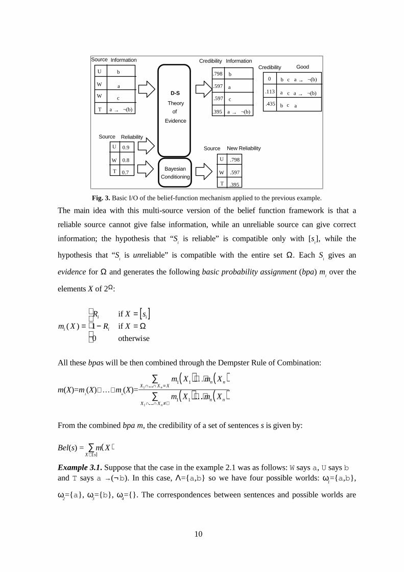
The reliability set is one of the two inputs of the belief-function formalism (see figure 3).

The other one is the set <S1, s1>,…,<Sn, sn>, where si is the subset of I made of all the

information items given by Si. The information set is the main output of the belief-function

formalism. Figure 3 presents the I/O mechanism applied to the case in the previous example.

Let us see now how the mechanism works. Remember that Ξ denotes the set of the atomic

propositions of L. The power set of Ξ, Ω=2Ξ, is called frame of discernment. Each element

ω of Ω is a “possible world”or an “interpretation” for L (the one in which all the

propositional letters in ω are true and the others are false). Given a set of sentences s⊆ I (i.e.,

a conjunction of sentences), [s] denotes the interpretations which are a model for all the

sentences in s.

10

U

W

W

T

b

a

c

¬(b)a →

U

W

T

0.9

0.8

0.7

Source

Source Information

Reliability

D-S

Theory

of

Evidence

InformationCredibility

.798

.597

.395

b

a

c

¬(b)a →

.597

U

W

T

.798

.597

.395

Source New Reliability

GoodCredibility

.113

b

a

c.435

¬(b)a →c

¬(b)a →c

ab

0

Bayesian

Conditioning

Fig. 3. Basic I/O of the belief-function mechanism applied to the previous example.

The main idea with this multi-source version of the belief function framework is that a

reliable source cannot give false information, while an unreliable source can give correct

information; the hypothesis that “Si is reliable” is compatible only with [s

i], while the

hypothesis that “Si is unreliable” is compatible with the entire set Ω. Each S

i gives an

evidence for Ω and generates the following basic probability assignment (bpa) mi over the

elements X of 2Ω:

[ ]m X

R X s

R Xi

i i

i( ) ==

− =

if

if

otherwise

1

0

Ω

All these bpas will be then combined through the Dempster Rule of Combination:

m(X)=m1(X)⊗ …⊗ m

n(X)=

( ) ( )( ) ( )

m X m X

m X m X

n nX X X

n nX X

n

n

1 1

1 1

1

1

⋅ ⋅

⋅ ⋅∩ ∩ =

∩ ∩ ≠∅

∑

∑

KK

K

K

From the combined bpa m, the credibility of a set of sentences s is given by:

Bel(s) = ( )[ ]m X

X s⊆∑

Example 3.1. Suppose that the case in the example 2.1 was as follows: W says a, U says band T says a →(¬b). In this case, Λ=a,b so we have four possible worlds: ω

1=a,b,

ω2=a, ω

3=b, ω

4=. The correspondences between sentences and possible worlds are

11

as follows: [a]= ω1, ω

2; [b]= ω

1, ω

3; [a→(¬b)]= ω

2, ω

3, ω

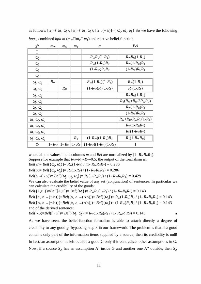
4 So we have the following

bpas, combined bpa m (mW⊗ mU⊗ mT) and relative belief function:

2Ω mW mU mT m Bel

∅ω

1RWRU(1-RT) RWRU(1-RT)

ω2

RW(1-RU)RT RW(1-RU)RT

ω3

(1-RW)RURT (1-RW)RURT

ω4

ω1, ω

2RW RW(1-RU)(1-RT) RW(1-RT)

ω1, ω

3RU (1-RW)RU(1-RT) RU(1-RT)

ω1, ω

4RWRU(1-RT)

ω2, ω

3RT(RW+RU-2RWRU)

ω2, ω

4RW(1-RU)RT

ω3, ω

4(1-RW)RURT

ω1, ω

2, ω

3RW+RU-RWRU(1-RT)

ω1, ω

2, ω

4RW(1-RURT)

ω1, ω

3, ω

4RU(1-RWRT)

ω2, ω

3, ω

4RT (1-RW)(1-RU)RT RT(1-RWRU)

Ω 1- RW 1- RU 1- RT (1-RW)(1-RU)(1-RT) 1

where all the values in the columns m and Bel are normalized by (1- RWRURT).Suppose for example that RW=RU=RT=0.5; the output of the formalism is:Bel(a)= Bel( ω

1, ω

2)= RW(1-RT) / (1- RWRURT) = 0.286

Bel(b)= Bel( ω1, ω

3)= RU(1-RT) / (1- RWRURT) = 0.286

Bel(a→(¬b))= Bel( ω2, ω

3, ω

4)= RT(1-RWRU) / (1- RWRURT) = 0.429

We can also evaluate the belief value of any set (conjunction) of sentences. In particular wecan calculate the credibility of the goods:Bel( a,b )=Bel([a,b])= Bel( ω

1)= RWRU(1-RT) / (1- RWRURT) = 0.143

Bel( a, a →(¬b))=Bel([a, a →(¬b)])= Bel( ω2)= RW(1-RU)RT / (1- RWRURT) = 0.143

Bel( b, a →(¬b))=Bel([b, a →(¬b)])= Bel( ω3)= (1-RW)RURT / (1- RWRURT) = 0.143

and of the derived sentence:Bel(¬b)=Bel([¬b])= Bel( ω

2, ω

4)= RW(1-RU)RT / (1- RWRURT) = 0.143

As we have seen, the belief-function formalism is able to attach directly a degree of

credibility to any good g, bypassing step 3 in our framework. The problem is that if a good

contains only part of the information items supplied by a source, then its credibility is null!

In fact, an assumption is left outside a good G only if it contradicts other assumptions in G.

Now, if a source SA has an assumption A’ inside G and another one A” outside, then SA

12

conflicts with some sources supporting assumptions in G. G is supported by a conflicting set

of sources, and a conflicting set of sources provides no evidence at all for the information

they provide as a whole. It is unreasonable to set at zero the credibility of a good just

because its supporting sources are in conflict for pieces of information which are outside of

the good; unfortunately, the event is all but infrequent, so that often the credibility of all the

goods is null. This is the reason why we adopt the best-out or the “average” method to

perform S3 in our system.

3.2 Estimating the “a posteriori” reliability of the sources

In figure 3, we see another output of the mechanism, obtained through Bayesian

Conditioning: the set <S1, NR1>,…,<Sn, NRn>, where NRi is the new reliability of Si.

Following Shafer and Srivastava, we defined the “a priori” reliability of a source as the

probability that the source is reliable. These degrees of probability are “translated” by the

Theory of Evidence into belief-function values on the given pieces of information. However,

after all the sources have completed their depositions, we may also want to estimate their “a

posteriori” degree of reliability from the cross-examination of their evidences. To be

congruent with the “a priori” reliability, also the “a posteriori” reliability must be a

probability value, not a belief-function one. This is the reason why we adopt the Bayesian

Conditioning instead of the Theory of Evidence to calculate it. Let us see in detail how it

works here.

Let us consider the hypothesis that only the sources belonging to Φ⊆ S are reliable. If the

sources are independent, then the probability of this hypothesis is R(Φ)= ( )R RiS

iSi i∈ ∉

∏ ∏⋅ −Φ Φ

1 .

We could calculate this “combined reliability” for any subset of S. It holds that ( )RS

ΦΦ∈∑

2=1.

Possibly, the sources belonging to a certain Φ cannot all be considered reliable because they

gave contradictory information, i.e., a set of information items s such that [s]=∅ . In this

case, the combined reliabilities of the remaining subsets of S are subjected to the Bayesian

Conditioning so that they sum up again to “1”; i.e., we divide each of them by “1- R(Φ)”. In

the case where there are more subsets of S, say Φ1, …,Φl, containing sources which cannot

all be considered reliable, then R(Φ)=R(Φ1)+ …+R(Φl). We define the revised reliability NRi

13

of a source Si as the sum of the conditioned combined reliabilities of the “surviving” subsets

of S containing Si.

An important feature of this way to recalculate the sources’ reliability is that if Si is involved

in contradictions, then NRi≤Ri, otherwise NRi=Ri.

3.3 The computational complexity of the Belief-Function Formalism

The main problem with the belief funcion formalism is the computational complexity of the

Dempster’s Rule of Combination; the straight-forward application of the rule is exponential

in the frame of discernment (which is |Ξ|; however, normally |Ξ|<|KB|) and the number of

evidences. Yet, from an input-output analysis of the mechanism we realised that two

properties hold.

1. An information item I j not involved in contradictions and received from a single source

Si, does not contribute to the mechanism, in the sense that the degrees of credibility of

the other pieces of information do not depend on it and Bel(I j)=NRi.

2. Multiple contradictions involving information items received exclusively from exactly the

same sources are redundant; all the pieces of information from the same source receive

the same degree of credibility, independently of the number and the cardinality of the

contradictions.

Property (1) implies that we can temporarly leave out of the process those sentences

received from a single source that are not involved in contradictions. In many cases, this

dramatically reduces the size of Ω. Property (2) says that, what is important is that a set of

sources was contradictory, not how many times nor about what or about how many pieces

of information they did. This also allows us to temporarly leave out of the process some

sentences involved in contradictions; this is significant in situations like that of two sources

systematically in contradiction only with each other.

Besides these two properties, it is important to say that much effort has been spent in

reducing the complexity of the Dempster’s Rule of Combination. Such methods range from

“efficient implementations” [41] to “qualitative approaches” [42] through “approximate

techniques” [40].

14

4 The Inquiry Support System

The model for belief revision in a multi-source environment described in the previous

sections fits very well the investigative domain. This section illustrates the ISS discussing

the relevance of its theoretical framework in the inquiry domain.

4.1 The investigative domain

During the upstream phase of an inquiry, much of the detectives’ task consists in

1. acquiring information from investigations on the spot and testimonies

2. introducing hypothetical rules to link the various hypotheses into evidential networks

3. finding the contradictions inside and across the various depositions

4. judging the credibility of the information items

5. judging the reliability of the witnesses

A testimony is the narration of some facts from a witness’ experience. The witness’

reliability has been traditionally considered dependent on his\her accuracy and credibility.

Accuracy is the informer’s ability to record and recall from memory the details of the

story; it depends on memory, perception and cognition. Credibility depends on the

informant’s behavior during the interrogatory (his/her posture) and his/her personal

interests in the facts. The witness’ accuracy can be influenced by many factors. We

summarize from various studies [3-11] the following partial list: age, sex, race, elapsed

time, various deficits (perceptive, mnemonic or cognitive), stress, stereotypes and

prejudices, unconscious memory transfer, interrogatory technique, wish to please.

Regarding the witness’ credibility, it has been noted that the will to cheat excites the

organism, so various semi-unconscious gestures could be considered suspicious: dilation of

the pupil, fixing the eyes, winking, smiling, gesticulating, shaking one’s head, continuous

movements of legs and feet, delaying the answers, extending the answers, giving irrelevant

information, hesitating.

However, in spite of these studies, many researchers think that there is no absolute

correlation between the will to lie and any observable physiological behavior.

Also important in judging a witness’ credibility are his/her personal implications in the

case, since a sane person lies only if he has strong reasons to hide the truth. This should

imply that a defendant would be less credible than a disinterested external witness who is

not a relative nor a friend or a partner of the defendant himself. However, this is a prickly

15

question because it’s obviously dangerous to consider unreliable a person just for his being

accused; besides, a not implicated person could as well have unknown reasons to lie.

In conclusion we can say that human intuition seems insufficient to judge a witness’

reliability, so the spot has recently been moved from the informant’s truthfulness to the

information’s credibility. Undeutsch [12] reports various veracity criteria for a testimony;

the following is a partial list:

a) amount of details furnished,

b) clearness, precision and vividness of the images presented,

c) narration free from clichés and stereotypes,

d) intrinsic connection of the narration,

e) intrinsic coherence of the narration,

f) coherence of the narration with the physical laws,

g) coherence of the narration with the observed and/or already verified facts.

Evidently, a liar is not oriented to furnish many particulars in his evidence because any detail

he offers is an occasion for the magistrate to unmask him. A witness that gives vivid

descriptions free from stereotypes is either sincere or is a good dramatic actor. There are

some disputes on the fourth criterion. By “connection” we mean that the elements of the

story are linked in an acceptable causal/explanatory chain. Often a witness tends to give not

just information items but the rules to link them as well. However, many magistrates are not

always well disposed toward such testimonies because they prefer to be free to make their

own connections in the story and they suspect that the “pre-compiled” links are attempts to

divert the inquiry. The fifth criterion seems very important. By “coherence” or

“consistency” we mean that the testimony contains no incompatible or inconsistent

information items. One of the main tactics of a Public Prosecutor is that of compelling the

accused to contradict him/herself; if he succeeds in that, then he is near to win the suit. It is

interesting to notice here that estimating the “a posteriori” reliability of such a witness

through Bayesian Conditioning (as ISS does) satisfies this requirement as well since it sets

at zero his/her reliability.

The sixth and the seventh criteria may be synthesized into the following one:

g) coherence with the most credible information currently available.

The criteria dealing with coherence (e-g) are captured by Dempster’s Rule of Combination

that reinforces concording evidence and weakens conflicting evidence. In another paper (see

16

the example in [16], p. 965) we said that coherence is more important than connection;

essentially, connection is a rather subjective matter and can be easily artificially constructed

to divert the inquiry, while incoherence is a rather objective matter and can hardly be

concealed. We can only suspect a witnesses/defendant whose testimony revealed some

disconnections, but we can, and do accuse him/her if we find contradictions in his/her

deposition.

4.1 Safe criteria to evaluate the reliability of a witness from his/her testimony.

While we are writing, there is a great debate in Italy on the role and the importance of the

“pentiti” in the fight against “mafia” and corruption. The italian phenomenon of the

“pentitismo” (confessed culprits turned informers) has an equivalent in, e.g., Britain’s

supergrass system. A supergrass is a person who has belonged to an illegal organization and

now claims to collaborate with justice. If the conversion is sincere, then the supergrass

becomes a very important witness; the problem is that of evaluating his truthfulness and

reliability. Mass-media point out the importance of the objective verifications in judging a

supergrass’ testimony.1 Roughly stated, the criteria sounds like these:

R1. A supergrass should not be considered reliable until his/her evidence is confirmed by

some objective verifications

R2. A supergrass’ reliability should increase with the number and the “importance” of these

objective verifications

R3. The more reliable the supergrass, the more credible his/her testimony.

These rules would suggest a very simple criterion to mechanically compute a supergrass’

trustworthiness. Let si and s

j be the sets of information items given by S

i. and S

j. If ο

i ⊆ s

i and

ο j ⊆ s

j are information items that has been objectively verified, then S

i. is more reliable than

Sj. iff |ο

i |>|ο

j |.2 The ascertainment of one of the information items in s

i\ο

i causes the

1 By “objective verification”, common thinking means an ascertainment made by an absolutely reliable

source through unalterable and very confident tests, checks, controls etc.2 if the information items have an associated “degree of importance” w.r.t. the case under consideration,

then the comparison should be that of weighted sums of the degrees of importance of the information items.

17

increase of Si.’s reliability and, from R3, the increase of the credibility of all the other still

unverified information items in si.

However, increasing a witness’ reliability after his/her testimony has been partially

confirmed by some ascertainments, is very dangerous. A false supergrass can easily stuff

his/her testimony with lots of easily verifiable but unessential information items just for the

purpose of gaining reliability. If a witness says that:

I1 = “The sun was shining”

I2 = “John shot Ted”

I3= “(John shot Ted) with a Colt 45”

neither the ascertainment of I1 (by some weather-station’s files) nor the verification of I

3

(from the examination of the bullet) should increase the credibility of the main core of the

testimony, I2; hence the application of the rules R2 and R3 would be misleading.

Instead of increasing a witness' reliability after that his testimony is partially confirmed by

the observations, we propose the following criteria :

R*1. Initially, a supergrass should be considered as reliable as the other sources

R*2. A supergrass’ reliability should decrease with the number and the “importance” of the

negative objective verifications (safety norm)

By “negative objective verifications” we mean the incompatibility of part of his/her

deposition with verified facts. However, a witness’ testimony is prevalently contradicted not

by objective verifications but by other witnesses’ testimonies. So we need methods to

rearrange the distributions of the degrees of credibility of the information items (1) and the

reliability of the sources (2) after the discovery of cross-incompatibilities and contradictions

or confirmations among their testimonies. We see that the Dempster’s Rule of Combination

provides a simple and reasonable way to perform (1), while Bayesian Conditioning is a right

way to perform (2).

4.2 The Inquiry Support System

Figure 4 depicts the basic architecture of ISS, the main blocks of which are explained in

what follows.

18

U1AAAAAAAAAAAAAAAAAAAAAAAAAAAAAAAAAAAAAAAAAAAAAAAAAAAAAAAA

AAAAAAAAAAAAAAAAAAAAAAAAAAAAAAAAAAAAAAAAAAAAAAAAAAAAAAAA

AAAAAAAAAAAAAAAAAAAAAAAAAAAAAAAAAAAAAAAAAAAAAAAAAAAAAAAA

AAAAAAAAAAAAAAAAAAAAAAAAAAAAAAAAAAAAAAAAAAAAAAAAAAAAAAAA

AAAAAAAAAAAAAAAAAAAAAAAAAAAAAAAAAAAAAAAAAAAAAAAAAAAAAAAA

AAAAAAAAAAAAAAAAAAAAAAAAAAAAAAAAAAAAAAAAAAAAAAAAAAAAAAAA

CC

U3

U5

ProblemSolver

U= User

A

T

M

S

Chooser

AAAAAAAAAAAAAAAAAAAA

AAAAAAAAAAAAAAAAAAAA

AAAAAAAAAAAAAAAA

AAAAAAAAAAAAAAAA

AAAAAAAAAAAAAAAAAAAAAAAAAAAA

AAAAAAAAAAAAAAAAAAAA

AAAAAAAAAAAAAAAAAAAA

AAAAAAAAAAAAAAAAAAAA

AAAAAAAAAAAAAAAAAAAA

AAAAAAAAAAAAAAAA

AAAAAAAAAAAAAAAA

AAAAAAAAAAAAAAAAAAAAAAAAAAAA

AAAAAAAAAAAAAAAAAAAA

AAAAAAAAAAAAAAAAAAAA

AAAAAAAAAAAAAAAAAAAAAAAAAAAAAAAAAAAAAAAAAAAAAAAAAAAAAAAAAAAA

AAAAAAAAAAAAAAAAAAAAAAAAAAAAAAAAAAAAAAAAAAAAAAAAAAAAAAAAAAAA

AAAAAAAAAAAAAAAAAAAAAAAAAAAAAAAAAAAAAAAAAAAAAAAAAAAAAAAAAAAA

AAAAAAAAAAAAAAAAAAAAAAAAAAAAAAAAAAAAAAAAAAAAAAAAAAAAAAAAAAAA

AAAAAAAAAAAAAAAAAAAAAAAAAAAAAAAAAAAAAAAAAAAAAAAAAAAAAAAAAAAA

AAAAAAAAAAAAAAAAAAAAAAAAAAAAAAAAAAAAAAAAAAAAAAAAAAAAAAAAAAAA

AAAAAAAAAAAAAAAAAAAAAAAAAAAAAAAAAAAAAAAAAAAAAAAAAAAAAAAAAAAA

AAAAAAAAAAAAAAAAAAAAAAAAAAAAAAAAAAAAAAAAAAAAAAAAAAAAAAAAAAAA

AAAAAAAAAAAAAAAAAAAAAAAAAAAAAAAAAAAAAAAAAAAAAAAAAAAAAAAAAAAA

KSKB

AAAAAAAAAAAAAAAAAAAA

AAAAAAAAAAAAAAAAAAAA

CG

U4

goods

U

S1

Sn

U2

Figure 4. The proposed basic architecture for an Inquiry Support System

The inputs

The inputs of ISS are the depositions of the various sources. By “source” we mean every

actor which provides information items, i.e., defendants, witnesses, experts and the user of

the system, which provides hypothetical facts and rules to link the various information items

into evidential networks (U1).

The depositions are represented as sentences of a propositional language (translated from

natural language by the user). As long as the case goes on, the atomic propositions are

stored for eventual subsequent reuse; it is the task of the user that of avoiding the “open

texture” problem by reusing atomic propositions whenever it is possible.

Sentences are immediately converted into clauses, thus the beliefs in KB and KS are clauses.

In the inquiry domain, normally the information items are ground literals (atomic

propositions or negation of atomic propositions) so that the conversion has no effect at all.

An interesting characteristic of the inquiry domain is that most of the information items are

representable as (sets of) Horn clauses: this assures that contradictions will be detected in

linear time!

A consequence of the conversion in clausal form is that while a deposition may be

contradictory, a single belief can never be inconsistent.

19

The Problem Solver

Tasks executed by the Problem Solver are:

PS1. finding the set NG of all the nogoods in KB

PS2. finding the minimal subsets of KB that constitute an origin set for a sentence

interesting to the user (U2)

We have already defined a contradiction as a pair of nodes as follows:

<_, α,_,_> , <_, ¬α,_,_>

In the inquiry domain, dealing with commonsense knowledge, we need to extend this notion

to that of “incompatible set of nodes”. An incompatibility is a tuple:

<_, α,_,_> , <_, β,_,_> , … , <_, ζ,_,_>

such that the beliefs α, β,…, ζ cannot all be true; in the user’s mind there is a rule χ such

that from α, β,…, ζ, χ a contradiction can be derived. Incompatibilities could also come

from software systems for specific tasks as the control of the temporal consistency of the

statements [36].

Example 4.1. In the example 2.1, suppose that the atomic propositions a, b and c were as

follows:

a: “the window was open”

b: “ the room was saturated with gas”

c : “ the temperature in the room was high”

Then A1, C1 is a contradiction while A2, A3 might be regarded by the user as an

incompatibility (coming from a single source!) if he believes in the rule a→(¬c )

The Assumption-based Truth Maintenance System (ATMS)

The ATMS maintains the belief dependency structure. Furthermore, it generates the set G

of the goods by applying the set covering algorithm (described in appendix A) to the set NG

of the nogoods, augmented with all the incompatibilities provided by the user (U3).

The Chooser

The Chooser is comprised of two mechanisms. The Belief-Function process attaches a

degree of credibility to each sentence in KS, thus implicitly defining an ordering ≤KB over

KB. Subsequently, another mechanism extends ≤KB into an ordering ≤G over the goods. In

U4, the user can choose one (or a combination) of the methods (in our system only the

“best-out” and the “average credibility”) described in section 2.

20

The Belief-Function Formalism is able to attach a degree of credibility to any sentence of L.

In particular, for each given information item α, we can calculate Bel(¬α), here called

“negative belief function values” of α. We could take advantage of this capability by

modifying the “best-out” and the “average” methods.

• modified best-out method: let g’ and g” be the assumptions in KB with the highest

negative belief function value, respectively, in KB\G’ and KB\G”. Then G”≤ G’ iff

Bel(¬g”) ≤ Bel(¬g’).

• modified average-based method: the credibility of a good G is the average of the

positive belief-function values of the sentences inside G (as in the classic average-based

method) and of the negative belief-function values of the sentences outside G.

5. Example

The following is a short abstract of a didactic case that ran on the program (written in

LPA™ MacPROLOG) which implements the system. The extreme simplicity of the case

should ease the comprehension of the basic mechanism. The text in courier has been just

translated in English directly from the Input/Output text files (which were written in Italian

language). In this example, goods are printed out ordered according to the “best-out”

method, however we have provided also their “average credibility” and their belief-function

value. The case starts with three sources, B, M and A, that refer three facts regarding A

(which is the defendant in the trial). The sources are assigned the same degree of reliability

(0.5 ). The other two special sources are OBS (a fictitious source that give only verified facts;

reliability 0.9 ) and U (which represents the user and introduces only hypothetical facts

and/or rules; reliability 0.3 ).

INITIAL INPUT:B asserts: 'A is a partner of R'M asserts: 'A was driving the car of S'A asserts: it is false that 'A knows S'

“a priori” reliability of A, B and M: 0.5

There are no contradictions; there is one good and the degrees of reliability don’t change.

A is a partner of R | 0.500 A was driving the car of S | 0.500 it is false that A knows S | 0.500______________________________________________________________________________GOOD 1 Bel 0.1 25 Average 0.500==============================================================================

21

“a posteriori” rel. | FALL | OLD | NEW |_________________________________________________ B | 0.000 | 0.500 | 0.500 | A | 0.000 | 0.500 | 0.500 | M | 0.000 | 0.500 | 0.500 |

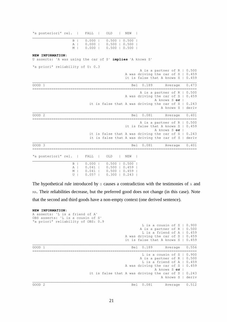
NEW INFORMATION:U asserts: ' A was using the car of S ' implies ' A knows S '

“a priori” reliability of U: 0.3 A is a partner of R | 0.500 A was driving the car of S | 0.459 it is false that A knows S | 0.459______________________________________________________________________________GOOD 1 Bel 0.189 Average 0. 473============================================================================== A is a partner of R | 0.500 A was driving the car of S | 0.459 A knows S or | it is false that A was driving the car of S | 0.243 A knows S | deriv______________________________________________________________________________GOOD 2 Bel 0.081 Average 0. 401=============================================== =============================== A is a partner of R | 0.500 it is false that A knows S | 0.459 A knows S or | it is false that A was driving the car of S | 0.243 it is false that A was driving the car of S | deriv______________________________________________________________________________GOOD 3 Bel 0.081 Average 0. 401==============================================================================

“a posteriori” rel. | FALL | OLD | NEW |_________________________________________________ B | 0.000 | 0.500 | 0.500 | A | 0.041 | 0.500 | 0.459 | M | 0.041 | 0.500 | 0.459 | U | 0.057 | 0.300 | 0.243 |

The hypothetical rule introduced by U causes a contradiction with the testimonies of A and

MA. Their reliabilities decrease, but the preferred good does not change (in this case). Note

that the second and third goods have a non-empty context (one derived sentence).

NEW INFORMATION:A asserts: ' L is a friend of A 'OBS asserts: ' L is a cousin of S '“a priori” reliability of OBS: 0. 9 L is a cousin of S | 0.900 A is a partner of R | 0.500 L is a friend of A | 0.459 A was driving the car of S | 0.459 it is false that A knows S | 0.459______________________________________________________________________________GOOD 1 Bel 0.189 Average 0.556============================================================================== L is a cousin of S | 0.900 A is a partner of R | 0.500 L is a friend of A | 0.459 A was driving the car of S | 0.459 A knows S or | it is false that A was driving the car of S | 0.243 A knows S | deriv______________________________________________________________________________GOOD 2 Bel 0.081 Average 0.512

22

============================================================================== L is a cousin of S | 0.900 A is a partner of R | 0.500 L is a friend of A | 0.459 it is false that A knows S | 0.459 A knows S or | it is false that A was driving the car of S | 0.243 it is false that A was driving the car of S | deriv______________________________________________________________________________GOOD 3 Bel 0.081 Average 0.512==============================================================================

“a posteriori” rel. | FALL | OLD | NEW |_________________________________________________ OBS | 0.000 | 0.900 | 0.900 | B | 0.000 | 0.500 | 0.500 | A | 0.041 | 0.500 | 0.459 | M | 0.041 | 0.500 | 0.459 | U | 0.057 | 0.300 | 0.243 |

An incoming information that does not contradict nor confirms anything (like ' A is

associated with R' and ' L is friend of A' at this stage) belongs to all the goods; its

belief-function value is exactly the “a posteriori” reliability of its source (respectively 0.5

for B and 0. 459459459 5 for A) as results from the Bayesian Conditioning.

Sources that give information not contradicted nor confirmed by others (like OBS and B at

this stage) maintain their “a priori” reliability. Of course, these general rules simplify

enormously the computation.

NEW INFORMATION:U asserts: ' L is friend of A ' and 'L is cousin of S' implies ' A knows S '

L is a cousin of S | 0.892 A is a partner of R | 0.500 A was driving the car of S | 0.496 L is a friend of A | 0.417 it is false that A knows S | 0.417______________________________________________________________________________GOOD 1 Bel 0.184 Average 0.544============================================================================== L is a cousin of S | 0.892 A is a partner of R | 0.500 A was driving the car of S | 0.496 L is a friend of A | 0.417 A knows S or | it is false that L is a friend of A or | it is false that L is a cousin of S | 0.184 A knows S or | it is false that A was driving the car of S | 0.184 A knows S | deriv______________________________________________________________________________GOOD 2 Bel 0.000 Average 0.445==============================================================================

23

L is a cousin of S | 0.892 A is a partner of R | 0.500 A was driving the car of S | 0.496 it is false that A knows S | 0.417 A knows S or | it is false that L is a friend of A or | it is false that L is a cousin of S | 0.184 it is false that L is a friend of A | deriv______________________________________________________________________________GOOD 3 Bel 0.000 Average 0.498============================================================================== L is a cousin of S | 0.892 A is a partner of R | 0.500 L is a friend of A | 0.417 it is false that A knows S | 0.417 A knows S or | it is false that A was driving the car of S | 0.184 it is false that A was driving the car of S | deriv______________________________________________________________________________GOOD 4 Bel 0.000 Average 0.482============================================================================== L is a cousin of S | 0.892 A is a partner of R | 0.500 it is false that A knows S | 0.417 A knows S or | it is false that L is a friend of A or | it is false that L is a cousin of S | 0.184 A knows S or | it is false that A was driving the car of S | 0.184 it is false that A was driving the car of S | deriv it is false that L is a friend of A | deriv______________________________________________________________________________GOOD 5 Bel 0.000 Average 0.435============================================================================== A is a partner of R | 0.500 A was driving the car of S | 0.496 L is a friend of A | 0.417 it is false that A knows S | 0.417 A knows S or | it is false that L is a friend of A or | it is false that L is a cousin of S | 0.184 it is false that L is a cousin of S | deriv______________________________________________________________________________GOOD 6 Bel 0.000 Average 0.403============================================================================== A is a partner of R | 0.500 L is a friend of A | 0.417 it is false that A knows S | 0.417 A knows S or | it is false that L is a friend of A or | it is false that L is a cousin of S | 0.184 A knows S or | it is false that A was driving the car of S | 0.184 it is false that A was driving the car of S | deriv it is false that L is a cousin of S | deriv______________________________________________________________________________GOOD 7 Bel 0.009 Average 0.340==============================================================================

“a posteriori” rel. | FALL | OLD | NEW |_________________________________________________ B | 0.000 | 0.500 | 0.500 | M | 0.004 | 0.500 | 0.496 | OBS | 0.008 | 0.900 | 0.892 | A | 0.083 | 0.500 | 0.417 | U | 0.116 | 0.300 | 0.184 |

24

The new hypotetical rule introduced by U (the user of the system) yields another

contradiction (with ' L is friend of A' and 'L is cousin of S' ). The reliability of the

three sources involved (U, A and OBS) slightly decrease. Also the credibility of all the

information items they provided decrease, not only the credibility of the propositions

directly involved in the contradiction (see the information ' A was using the car of S'

implies ' A knows S ' that falls from 0. 243243243 2 to 0. 183673469 4).

Until now, the hypothetical rules introduced by the user have been discarded from the

preferred good. The hypothesis 'A knows S' belongs to the context (derived sentences) of

the third good. Suppose now that it comes out a letter of recommendation written by A to

S. This can be taken as a proof that 'A knows S' .

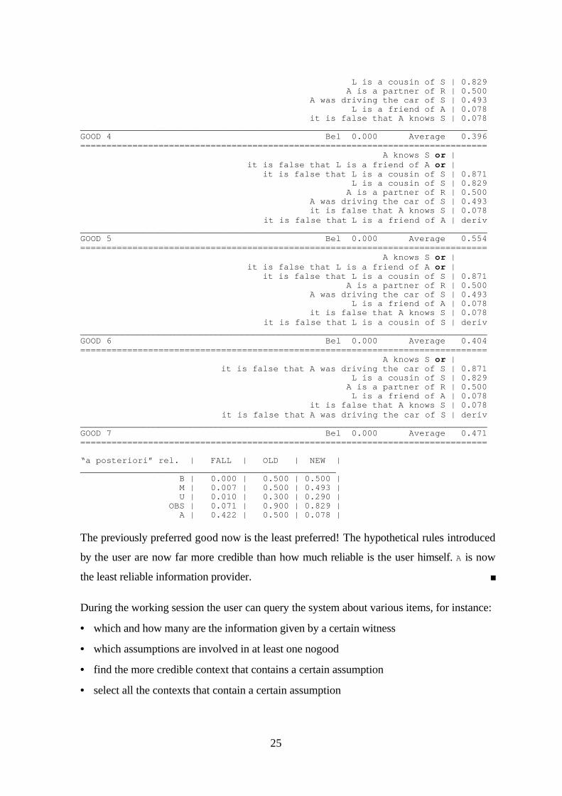
NEW INFORMATION:OBS asserts: 'A knows S'

A knows S or | it is false that L is a friend of A or | it is false that L is a cousin of S | 0.871 A knows S or | it is false that A was driving the car of S | 0.871 A knows S | 0.843 L is a cousin of S | 0.829 A is a partner of R | 0.500 A was driving the car of S | 0.493 L is a friend of A | 0.078______________________________________________________________________________GOOD 1 Bel 0.000 Average 0.641============================================================================== A knows S or | it is false that L is a friend of A or | it is false that L is a cousin of S | 0.871 A knows S or | it is false that A was driving the car of S | 0.871 L is a cousin of S | 0.829 A is a partner of R | 0.500 it is false that A knows S | 0.078 it is false that A was driving the car of S | deriv it is false that L is a friend of A | deriv______________________________________________________________________________GOOD 2 Bel 0.000 Average 0.630============================================================================== A knows S or | it is false that L is a friend of A or | it is false that L is a cousin of S | 0.871 A knows S or | it is false that A was driving the car of S | 0.871 A is a partner of R | 0.500 L is a friend of A | 0.078 it is false that A knows S | 0.078 it is false that A was driving the car of S | deriv it is false that L is a cousin of S | deriv______________________________________________________________________________GOOD 3 Bel 0.014 Average 0.480==============================================================================

25

L is a cousin of S | 0.829 A is a partner of R | 0.500 A was driving the car of S | 0.493 L is a friend of A | 0.078 it is false that A knows S | 0.078______________________________________________________________________________GOOD 4 Bel 0.000 Average 0.396============================================================================== A knows S or | it is false that L is a friend of A or | it is false that L is a cousin of S | 0.871 L is a cousin of S | 0.829 A is a partner of R | 0.500 A was driving the car of S | 0.493 it is false that A knows S | 0.078 it is false that L is a friend of A | deriv______________________________________________________________________________GOOD 5 Bel 0.000 Average 0.554============================================================================== A knows S or | it is false that L is a friend of A or | it is false that L is a cousin of S | 0.871 A is a partner of R | 0.500 A was driving the car of S | 0.493 L is a friend of A | 0.078 it is false that A knows S | 0.078 it is false that L is a cousin of S | deriv______________________________________________________________________________GOOD 6 Bel 0.000 Average 0.404============================================================================== A knows S or | it is false that A was driving the car of S | 0.871 L is a cousin of S | 0.829 A is a partner of R | 0.500 L is a friend of A | 0.078 it is false that A knows S | 0.078 it is false that A was driving the car of S | deriv______________________________________________________________________________GOOD 7 Bel 0.000 Average 0.471==============================================================================

“a posteriori” rel. | FALL | OLD | NEW |_________________________________________________ B | 0.000 | 0.500 | 0.500 | M | 0.007 | 0.500 | 0.493 | U | 0.010 | 0.300 | 0.290 | OBS | 0.071 | 0.900 | 0.829 | A | 0.422 | 0.500 | 0.078 |

The previously preferred good now is the least preferred! The hypothetical rules introduced

by the user are now far more credible than how much reliable is the user himself. A is now

the least reliable information provider.

During the working session the user can query the system about various items, for instance:

• which and how many are the information given by a certain witness

• which assumptions are involved in at least one nogood

• find the more credible context that contains a certain assumption

• select all the contexts that contain a certain assumption

26

• list of all the assumptions in KB ordered according to their belief-function values

• list of all the sources ordered according to their “a posteriori” reliabilities

6. Conclusions

The main improvements w.r.t the system presented in [16] is that the credibility of the

information items are revised through the Dempster-Shafer Theory of Evidence. Each

source of information is regarded as an evidence about the facts of the story. Each source

has a weight, its “a priori” reliability, and all these weighted evidences will be combined

through the Dempster’s Rule of Combination.

An advantage of this approach is that all the information items are treated as they had been

received at the same time, so as to avoid the problem of “chronological dependency”

(different sequence of information items yields different results). These changes render the

system more intuitive to most readers, without impacting on the following limits and merits.

6.1 Criticism s

• Criticism. ISS attaches a single global measurement of reliability to a given source while

that value should depend on the various information items coming from that source. The

same source could be considered reliable when s/he says α and unreliable when s/he says

β, or vice-versa. What ISS really measures is a sort of general attitude of the source to

lie (intentionally or not), independently from the discourse’s domain. Sometimes that

measurement could be too coarse.

Answer. An obvious solution could be that of partitioning a witness’ (e.g., John_Doe)

deposition as it were given by different persons (i.e., John_Doe-professional_man,

John_Doe-father, John_Doe-politician ...) with different degrees of reliability. However,

this method has two serious drawbacks. First, it introduces two levels of arbitrarity, in

the definition of the different functional charachterizatios of the witness, and in the

definition of their corresponding degrees of “a priori” reliability. Second, by multiplying

the sources, it increases exponentially the computational cost of the Dempster’s Rule of

Combination. However, this “schizophrenic” approach has an interesting consequence: a

witness under a characterization A may contradict him/herself under a characterization B

without loosing completely his/her reliability (the conflict is treaten as it would happened

amongst two different persons).

27

• Criticism. In estimating the reliability of a witness, ISS disregards the motivations,

his/her intentions and personal implications in the case under consideration. ISS does not

distinguish insincerity from incompetence; as a consequence, it doesn’t discriminate in

any way a witness from a defendant.

Answer. This is not necessarily to be considered a limit, but a form of warranty for the

defendant. However, in countries where any accused who lies does not commit a crime

(like in Italy), it seems reasonable (to some people but not to us) to attach a lower

degree of “a priori” reliability to the defendant.

• Criticism. In estimating the reliability of a witness, ISS takes into account only what s/he

said, not what s/he didn’t say while it should have been said.

Answer. True. For the moment, ISS doesn’t deal with the incompleteness of the

depositions and it doesn’t distinguish between spontaneous and extorted depositions. It

is not clear to me how to estimate the reliability of a witness whose deposition has been

extorted.

6.2 Merits

• The ISS’ behavior can be interactively influenced and controlled by the user in four

ways. Referring to the figure 3, the user can:

U1. freely introduce hypotheses suggested by his/her human and professional experience

U2. freely introduce derived sentences

U3. freely introduce incompatibilities amongst the assumptions

U4. freely change the reliability values of any sources; in this way the user can recover

all those abilities to judge which come from his/her human and professional

experience

U5. freely change the preferred context selecting his own preferred one, for instance the

first one containing a certain assumption which he considers particularly credible,

and so on.

• The way ISS recalculates the reliability of the various witnessess (through Bayesian

conditioning) respects the safety norm: “do not increase the reliability of a witness

whose deposition has been confirmed, but decrease the reliability of a witness whose

testimony has been disconfirmed”.

• ISS has been considered useful both by detectives and magistrates. The former point out

its utility during the preliminary inquiries, the latter suggest its employment after the

28

trial’s conclusion; if the sentencing is based on motivations and judgements incompatible

with the information in the preferred context furnished by the ISS, then the judges may

well have to explain their decision.

• During the inquiry (or the trial) the inspector (or the magistrate) must carefully avoid

prejudice. In particular it would be better if the investigation's bias is not conditioned on

the chronology of the informative events. This means that the current detective's opinion

regarding the credibilities of the evidences and the reliability of the witnesses should be

the same as all the information about the case would have been received simultaneously.

Such a machinery could support the user in this important ability.

6.3 Future work and developments

• We would like to represent the structure of the proofs graphically. The most significant

information structures in the system are the good and its associated context. Each

context can be associated with an and/or graph whose nodes are its atomic information

items, while the arcs represent its rules (those given by the various information sources)

and the hypothetical rules of the Reasoner eventually involved in the production of an

“autohypothesis” inside the context. We could define a module that automatically builds

and represents graphically the structure of each context; in this way one could compare

not just flat sets of atomic pieces of information but alternative proof structures.

• A major conceptual improvement would be that of automatic extraction of advice by the

system, regarding the future course of the inquiry. We could apply some techniques (like

the “minimum entropy” one, see [35]) to drive the acquisition of new evidence regarding

the case under consideration, in order to further differentiate among the goods.

References

[1] P. Gärdenfors, Belief Revision: an introduction, in Gärdenfors P. (eds.), BeliefRevision, Cambridge University Press.

[2] Dubois and Prade, A Survey of Belief Revision and Update Rules in VariousUncertainty Models, in International Journal of Intelligent Systems, 9, pp. 61-100,1994

[3] Trankell A, Reliability of evidence, Beckmans, Stockholm, 1972[4] Kuehn, L, Looking down a gun barrel: person perception and violent crime,

Perceptual and Motor Skills, 39, pp 1159-1164, 1974[5] Knapp, M L, Hart, RP, and Dennis, H S, An exploration of deception as a

communication construct, Human Communication Research, 15, 1974[6] Cohen, R L, Children's testimony and mediated (hearsay) evidence, Report to Law

Reform Commission, Ottawa, 1975

29

[7] Dent, M R, and Stephenson, G M, An experimental study of the effectiveness ofdifferent techniques of questioning child witness, British Journal of Social andCriminal Psychology, 18, pp 41-45 (1979)

[8] Loftus, E F, Eyewitness Testimony, Harvard University Press, Cambridge, 1979[9] Zuckermann, M, De Paulo, B, and Rosenthal, R, Verbal and non-verbal

communications of deception, Adv in Exp Soc Psychology, 14, 2 (1981)[10] Timm, H W, Eyewitness recall and recognition by the elderly, Victimology, 1-4, p

425 (1985)[11] Ruback, R B, and Greenberg M S, Crime Victims as Witnesses: their accuracy and

credibility, Victimology, 1-4, p 410 (1985)[12] Undeutsch U, Coortroom evaluation of eyewitness testimony, International Review

of Applied Psychology, vol 33, 1 (1984)[13] G. Shafer and S. Srivastava, The Bayesian and Belief-Function Formalisms a

General Perpsective for Auditing, in G. Shafer and J. Pearl (eds.), Readings inUncertain Reasoning, Morgan Kaufmann Publishers.

[14] R. Reiter, A Theory of Diagnosis from First Principles, in Artificial Intelligence,32(1), 1987.

[16] A.F.Dragoni, M. Di Manzo, Supporting Complex Inquiries, International Journal ofIntelligent Systems, 10(11), pp. 959-986, 1995.

[17] Pearl, J., Probabilistic Reasoning In Intelligent Systems: Networks of PlausibleInference,revised second printing, Morgan Kaufmann Publishers, San Mateo (CA),1988

[18] R.P. Srivastava, The Belief-Function approach to Aggregating Audit Evidence,International Journal of Intelligent Systems, 10, pp. 329-356, 1995.

[19] R.P. Srivastava, P.P. Shenoy and G. Shafer, Propagating Belief Functions in AND-Trees, International Journal of Intelligent Systems, 10, pp. 647-664, 1995.

[20] J. de Kleer, An Assumption Based Truth Maintenance System, Artificial Intelligence,28, pp. 127-162, (1986).

[21] J.P. Martins and S.C. Shapiro, A Model for Belief Revision, Artificial Intelligence, 35,pp. 25-79 (1988).

[22] Gärdenfors P. (1988), Knowledge in Flux: Modeling the Dynamics of EpistemicStates, Cambridge, Mass., MIT Press.

[23] Katsuno H. and Mendelzon A.O. (1991b), Propositional knowledge base revisionand minimal change, in «Artificial Intelligence», 52, pp. 263-294.

[24] Lehmann D. (1995), Belief Revision, revised, in Proc. of the 14th Inter. Joint Conf.on Artificial Intelligence, pp. 1534-1540.

[25] Lévy F. (1994), A Survey of Belief Revision and Updating in Classical Logic,International Journal of Intelligent Systems, 9, pp. 29-59.

[26] Nebel B. (1994), Base Revision Operations and Schemes: Semantics,Representation, and Complexity, in Cohn A.G. (eds.), Proc. of the 11th EuropeanConference on Artificial Intelligence, John Wiley & Sons.

[27] Williams M.A. (1995), Iterated Theory Base Change: A Computational Model, inProc. of the 14th Inter. Joint Conf. on Artificial Intelligence, pp. 1541-1547.

[28] Dragoni A.F., Mascaretti F. and Puliti P. (1995), A Generalized Approach toConsistency-Based Belief Revision, in Gori, M. and Soda, G. (Eds.), Topics inArtificial Intelligence, Proc. of the Conference of the Italian Association for ArtificialIntelligence, LNAI 992, Springer Verlag.

30

[29] Benferhat S., Cayrol C., Dubois D., Lang J. and Prade H. (1993), InconsistencyManagement and Prioritized Syntax-Based Entailment, in Proc. of the 13th Inter.Joint Conf. on Artificial Intelligence, pp. 640-645.

[30] Roos N. (1992), A Logic for Reasoning with Inconsistent Knowledge, in «ArtificialIntelligence», 57, pp. 69-103.

[31] Shafer G. (1976), A Mathematical Theory of Evidence, Princeton Unicersity Pres,Princeton, New Jersey.

[32] Shafer G. (1990), Belief Functions, in G. Shafer and J. Pearl (eds.), Readings inUncertain Reasoning, Morgan Kaufmann Publishers.

[33] Gärdenfors P. (1990), Belief Revision and Non Monotonic Logic: Two Sides of theSame Coin?, in Proc. of the 9th European Conference on Artificial Intelligence,John Wiley & Sons.

[34] Dragoni A.F. (1992), A Model for Belief Revision in a Multi-Agent Environment, inWerner E. and Demazeau Y. (eds.), Decentralized A. I. 3, North Holland ElsevierScience Publisher.

[35] J. de Kleer and B. C. Williams, Diagnosing Multiple Faults, Artificial Intelligence,32(1), 1987.

[36] B. Knight, J. Ma and E. Nissan, Temporal Consistency of Legal Statements,Proceedings of the “5to Congreso Iberoamericano de Derecho e Informatica”, LaHabana, march 4-9 1996.

[37] Gärdenfors P., Belief Revision, Cambridge University Press, 1992.[38] A.F. Dragoni, Belief Revision: from Theory to Practice, submitted to The Knowledge

Engineering Review, Cambridge University Press, 1997.[39] Alchourrón C.E., Gärdenfors P., and Makinson D., On the Logic of Theory Change:

Partial meet Contraction and Revision Functions, in The Journal of Simbolic Logic,50, pp. 510-530, 1985.

[40] Moral, S. and Wilson, N., Importance Sampling Monte-Carlo Algorithms for theCalculation of Dempster-Shafer Belief, Proceeding of IPMU’96, Granada, 1996.

[41] Kennes, R., Computational Aspects of the Möbius Transform of a Graph, IEEETransactions in Systems, Man and Cybernetics, 22, pp 201-223, 1992.

[42] Parson, S., Some qualitative approaches to applying the Demster-Shafer theory,Information and Decision Technologies, 19, pp 321-337, 1994.

Appendix A

Given a Knowledge Base KB, we calculate goods and nogoods by means of the algorithm

presented in [14] to calculate model-based diagnoses. In order to keep the paper self-

contained, we recall here the basic definitions.

Let F be a collection of sets. A hitting-set for F is a set H⊂ SS F∈U such that H∩S≠∅ for each S

∈ F. A hitting-set is minimal if none of its proper subsets is a hitting-set for F.

Example. Let F=1,5,7, 2,5,6), 1,2. The minimal hitting sets for F are: 1,2, 1,5,

1,6, 5,2, 7,6,1 and 7,2.

An HS-Tree for F is a smallest labelled tree T such that:

(1) its root is labelled with √ if F=∅ ; otherwise its root is labelled with an element of F

31

(2) if n is a node of T, let H(n) be the set of the labels of the arcs on the path from the node to the root. If

n is labelled with √, then it has no successors in T. If n is labelled with an element Σ of F, then for

each element σ∈ Σ, n has a successors node nσ joined with n by an arc labelled with σ. The label of

nσ is a set S∈ F such that S∩H(n)=∅ if it exists, otherwise n is labelled with √

If n is labelled with √, then H(n) is a hitting-set for F. The set of all the H(n) of the nodes labelled with √

includes all the minimal hitting-sets for F. An HS-Tree generated and pruned according to the following

five rules, minimizes the accesses to F while preserving all the paths, from the leaves to the root,

corresponding to the minimal hitting sets.

1. The HS-Tree must be generated breadth first

2. If a node n is labelled with S and n' is another node such that H(n')∩S=∅ , then label n' with S

3. If a node n is labelled with √ and n' is another node such that H(n)⊆ H(n'), then n' must be pruned

4. If a node n has already been generated and n' is another node such that H(n)=H(n'), then n' must be

pruned

5. If a node n is labelled with S and n' is labelled with S' with S'⊂ S, then for each σ∈ S-S', the arc starting

from n and labelled with σ must be pruned

For an HS-Tree for F generated and pruned with these rules, the set:

H(n) | n is a node of T labelled with √

is the collection of all the minimal hitting sets for F.

Given KB, the collection of the goods and the collection of the nogoods are dual. If we

remove from KB exactly one element for each nogood, what remains is a good. Hence the

collection of the goods can be found by calculating all the minimal hitting-sets for the

collection N of the nogoods, and keeping the complement of each of them w.r.t. KB.

If F is a collection of sets and F'⊆ F is the collection of all the minimal elements (w.r.t. set

inclusion) of F, then F and F' have the same minimal hitting-sets. This simplifies our task

since we do not need to calculate the collection N of the nogoods (i.e. minimally

inconsistent subsets of KB) but just a collection M⊇ N of inconsistent subsets of KB, which

is much easier. It can be proved that, given a collection F of sets, in any HS-Tree T relative

to F, generated and pruned with the rules 1-5, every minimal element of F appears as the

label of at least one node of T. So, if M contains all the nogoods N, then all of them will be

used as labels of the nodes of T. During the generation of a node n, the rule 5 imposes to

check if there is a label S which is a superset of the just calculated label S' for n, so we have

simply to eliminate such an S if it exists. Finding the nogoods is useful for the step 3 of the

revision process since the method that we adopt (the belief function formalism) revises the

weights expecially on the basis of minimal contradictions.

32

The collection M⊇ N can be generated while generating the HS-Tree. After reducing in

clausal normal form all the sentences in KB, we start a refutation process on it. If we find

the empty clause, we label the root of T with the set of clauses in KB that have been

involved in the refutation. Each clause σm in this node labels an arc toward a successor

node. To calculate the label of this successor node we start a tentative refutation on KB\σm.

If KB\σm is consistent, then the node is labelled with √, otherwise it is labelled with the

proper subset of KB\σm from which the empty clause has been derived. The process iterates

until there are no more successor nodes. Summarizing, the following algorithm generates all

the goods and the nogoods in KB. Inc(C) is a function on set of clauses that returns √ if C

is consistent, returns a set D⊆ C if D is inconsistent.

1. NG := ∅ , G := ∅

2. when a node n needs a new label, give it the label Inc(KB\H(n)) and add it to NG

3. when the rule 5 applies, eliminate S from NG

4. for each H(n) such that n is labelled with √, put KB\H(n) in G

5. return NG and G