MATLAB Function Reference (Volume 2: Graphics)

MATLABThe Language of Technical Computing

Computation

Visualization

Programming

MATLAB Function Reference

Version 5

(Volume 2: Graphics)

How to Contact The MathWorks:

(508) 647-7000 Phone

(508) 647-7001 Fax

The MathWorks, Inc. Mail24 Prime Park WayNatick, MA 01760-1500

http://www.mathworks.com Webftp.mathworks.com Anonymous FTP servercomp.soft-sys.matlab Newsgroup

[email protected] Technical [email protected] Product enhancement [email protected] Bug [email protected] Documentation error [email protected] Subscribing user [email protected] Order status, license renewals, [email protected] Sales, pricing, and general information

MATLAB Function Reference (online version, January 1998: Revised for MATLAB 5.2) COPYRIGHT 1984 - 1998 by The MathWorks, Inc. All Rights Reserved.The software described in this document is furnished under a license agreement. The software may be usedor copied only under the terms of the license agreement. No part of this manual may be photocopied or repro-duced in any form without prior written consent from The MathWorks, Inc.

U.S. GOVERNMENT: If Licensee is acquiring the software on behalf of any unit or agency of the U. S.Government, the following shall apply:

(a) for units of the Department of Defense:RESTRICTED RIGHTS LEGEND: Use, duplication, or disclosure by the Government is subject to restric-tions as set forth in subparagraph (c)(1)(ii) of the Rights in Technical Data and Computer Software Clauseat DFARS 252.227-7013.(b) for any other unit or agency:NOTICE - Notwithstanding any other lease or license agreement that may pertain to, or accompany thedelivery of, the computer software and accompanying documentation, the rights of the Governmentregarding its use, reproduction and disclosure are as set forth in Clause 52.227-19(c)(2) of the FAR.Contractor/manufacturer is The MathWorks Inc., 24 Prime Park Way, Natick, MA 01760-1500.

MATLAB, Simulink, Handle Graphics, and Real-Time Workshop are registered trademarks and Stateflow andTarget Language Compiler are trademarks of The MathWorks, Inc.

Other product or brand names are trademarks or registered trademarks of their respective holders.

FAXMAIL

INTERNET

@

Contents

1Command Summary

Graphical Visualization . . . . . . . . . . . . . . . . . . . . . . . . . . . . . . . . . . . . . 1-2

Graphical User Interface Creation . . . . . . . . . . . . . . . . . . . . . . . . . . 1-7

2Reference

List of Commands

Function Names . . . . . . . . . . . . . . . . . . . . . . . . . . . . . . . . . . . . . . . . . . . . . A–2

i

ii Contents

1
Command Summary
This chapter lists MATLAB commands by functional area.

1 Command Summary

Graphical Visualization

Basic Plots and Graphsbar Vertical bar chartbarh Horizontal bar charthist Plot histogramshold Hold current graphloglog Plot using log-log scalespie Pie plotplot Plot vectors or matrices.polar Polar coordinate plotsemilogx Semi-log scale plotsemilogy Semi-log scale plotsubplot Create axes in tiled positions

Three-Dimensional Plottingbar3 Vertical 3-D bar chartbar3h Horizontal 3-D bar chartcomet3 3-D comet plotcylinder Generate cylinderfill3 Draw filled 3-D polygons in 3-spaceplot3 Plot lines and points in 3-D spacequiver3 3-D quiver (or velocity) plotslice Volumetric slice plotsphere Generate spherestem3 Plot discrete surface datawaterfall Waterfall plot

Plot Annotation and Gridsclabel Add contour labels to a contour plotdatetick Date formatted tick labelsgrid Grid lines for 2-D and 3-D plotsgtext Place text on a 2-D graph using a mouselegend Graph legend for lines and patchesplotyy Plot graphs with Y tick labels on the left and righttitle Titles for 2-D and 3-D plotsxlabel X-axis labels for 2-D and 3-D plotsylabel Y-axis labels for 2-D and 3-D plotszlabel Z-axis labels for 3-D plots

1-2

Surface, Mesh, and Contour Plotscontour Contour (level curves) plotcontourc Contour computationcontourf Filled contour plothidden Mesh hidden line removal modemeshc Combination mesh/contourplotmesh 3-D mesh with reference planepeaks A sample function of two variablessurf 3-D shaded surface graphsurface Create surface low-level objectssurfc Combination surf/contourplotsurfl 3-D shaded surface with lightingtrimesh Triangular mesh plottrisurf Triangular surface plot

Domain Generationgriddata Data gridding and surface fittingmeshgrid Generation of X and Y arrays for 3-D plots

Specialized Plottingarea Area plotbox Axis box for 2-D and 3-D plotscomet Comet plotcompass Compass ploterrorbar Plot graph with error barsezplot Easy to use function plotterfeather Feather plotfill Draw filled 2-D polygonsfplot Plot a functionpareto Pareto chartpie3 3-D pie plotplotmatrix Scatter plot matrixpcolor Pseudocolor (checkerboard) plotrose Plot rose or angle histogramquiver Quiver (or velocity) plotribbon Ribbon plotstairs Stairstep graphscatter Scatter plotscatter3 3-D scatter plotstem Plot discrete sequence dataconvhull Convex hull

1-3

1 Command Summary

delaunay Delaunay triangulationdsearch Search Delaunay triangulation for nearest pointinpolygon True for points inside a polygonal regionpolyarea Area of polygontsearch Search for enclosing Delaunay trianglevoronoi Voronoi diagram

View Controlcamdolly Move camera position and targetcamlookat View specific objectscamorbit Orbit about camera targetcampan Rotate camera target about camera positioncampos Set or get camera positioncamproj Set or get projection typecamroll Rotate camera about viewing axiscamtarget Set or get camera targetcamup Set or get camera up-vectorcamva Set or get camera view anglecamzoom Zoom camera in or outdaspect Set or get data aspect ratiopbaspect Set or get plot box aspect ratioview 3-D graph viewpoint specification.viewmtx Generate view transformation matricesxlim Set or get the current x-axis limitsylim Set or get the current y-axis limitszlim Set or get the current z-axis limits

Lightingcamlight Cerate or position Lightdiffuse Diffuse reflectancelighting Lighting modematerial Material reflectance modespecular Specular reflectance

Color Operationsbrighten Brighten or darken color mapbwcontr Contrasting black and/or colorcaxis Pseudocolor axis scalingcolorbar Display color bar (color scale)colorcube Enhanced color-cube color map

1-4

colordef Set up color defaultscolormap Set the color look-up tablegraymon Graphics figure defaults set for grayscale monitorhsv2rgb Hue-saturation-value to red-green-blue conversionrgb2hsv RGB to HSVconversionrgbplot Plot color mapshading Color shading modespinmap Spin the colormapsurfnorm 3-D surface normalswhitebg Change axes background color for plots

Colormapsautumn Shades of red and yellow color mapbone Gray-scale with a tinge of blue color mapcontrast Gray color map to enhance image contrastcool Shades of cyan and magenta color mapcopper Linear copper-tone color mapflag Alternating red, white, blue, and black color mapgray Linear gray-scale color maphot Black-red-yellow-white color maphsv Hue-saturation-value (HSV) color mapjet Variant of HSVlines Line color colormapprism Colormap of prism colorsspring Shades of magenta and yellow color mapsummer . . . . . . . . . . . . . . . . . . . Shades of green and yellow colormapwinter Shades of blue and green color map

Printingframeedit Create or edit printframeshardcopy Save figure window to fileorient Hardcopy paper orientationprint Print graph or save graph to fileprintopt Configure local printer defaultssavtoner Modify graphic objects to print on a white background

Handle Graphics, Generalcopyobj Make a copy of a graphics object and its childrenfindobj Find objects with specified property valuesgcbo Return object whose callback is currently executing

1-5

1 Command Summary

gco Return handle of current objectget Get object propertiesrotate Rotate objects about specified origin and directionishandle True for graphics objectsset Set object properties

Handle Graphics, Object Creationaxes Create Axes objectfigure Create Figure (graph) windowsimage Create Image (2-D matrix)light Create Light object (illuminates Patch and Surface)line Create Line object (3-D polylines)patch Create Patch object (polygons)surface Create Surface (quadrilaterals)text Create Text object (character strings)uicontext Create context menu (popup associated with object)

Handle Graphics, Figure Windowscapture Screen capture of the current figureclc Clear figure windowclf Clear figureclg Clear figure (graph window)close Close specified windowgcf Get current figure handlenewplot Graphics M-file preamble for NextPlot propertyrefresh Refresh figure

Handle Graphics, Axesaxis Plot axis scaling and appearancecla Clear Axesgca Get current Axes handle

Object Manipulationpropedit Edit all properties of any selected objectreset Reset axis or figurerotate3d Interactively rotate the view of a 3-D plotselectmoveresizeInteractively select, move, or resize objectsshg Show graph window

1-6

Interactive User Inputginput Graphical input from a mouse or cursorzoom Zoom in and out on a 2-D plot

Region of Interestdragrect Drag XOR rectangles with mousedrawnow Complete any pending drawingrbbox Rubberband box

Graphical User Interface CreationDialog Boxes

dialog Create a dialog boxerrordlg Create error dialog boxhelpdlg Display help dialog boxinputdlg Create input dialog boxlistdlg Create list selection dialog boxmsgbox Create message dialog boxpagedlg Display page layout dialog boxprintdlg Display print dialog boxquestdlg Create question dialog boxuigetfile Display dialog box to retrieve name of file for readinguiputfile Display dialog box to retrieve name of file for writinguisetcolor Interactively set a ColorSpec using a dialog boxuisetfont Interactively set a font using a dialog boxwarndlg Create warning dialog box

User Interface Objectsmenu Generate a menu of choices for user inputmenuedit Menu editoruicontextmenuCreate context menuuicontrol Create user interface controluimenu Create user interface menu

Other Functionsdragrect Drag rectangles with mousegcbo Return handle of object whose callback is executingrbbox Create rubberband box for area selectionselectmoveresizeSelect, move, resize, or copy Axes and Uicontrol graphics objectstextwrap Return wrapped string matrix for given Uicontrol

1-7

1 Command Summary

uiresume Used with uiwait, controls program executionuiwait Used with uiresume, controls program executionwaitbar Display wait barwaitforbuttonpressWait for key/buttonpress over figure

1-8

2
Reference
This chapter describes all MATLAB operators, commands,and functions in alphabetical order.

2 Reference

2-2

area

2areaPurpose Area fill of a two-dimensional plot

Syntax area(Y)area(X,Y)area(...,ymin)area(...,'PropertyName',PropertyValue,...)h = area(...)

Description An area plot displays elements in Y as one or more curves and fills the areabeneath each curve. When Y is a matrix, the curves are stacked showing therelative contribution of each row element to the total height of the curve at eachx interval.

area(Y) plots the vector Y or the sum of each column in matrix Y. The x-axisautomatically scales depending on length(Y) when Y is a vector, and onsize(Y,1)when Y is a matrix.

area(X,Y) plots Y at the corresponding values of X. If X is a vector, length(X)must equal length(Y) and X must be monotonic. If X is a matrix, size(X) mustequal size(Y) and each column in X must be monotonic. To make a vector ormatrix monotonic, use sort.

area(...,ymin) specifies the lower limit in the y direction for the area fill. Thedefault ymin is 0.

area(...,'PropertyName',PropertyValue,...) specifies property nameand property value pairs for the Patch graphics object created by area.

h = area(...) returns handles of Patch graphics objects. area creates onePatch object per column in Y.

Remarks area creates one curve from all elements in a vector or one curve per column ina matrix. The colors of the curves are selected from equally spaced intervalsthroughout the entire range of the colormap.

2-3

area

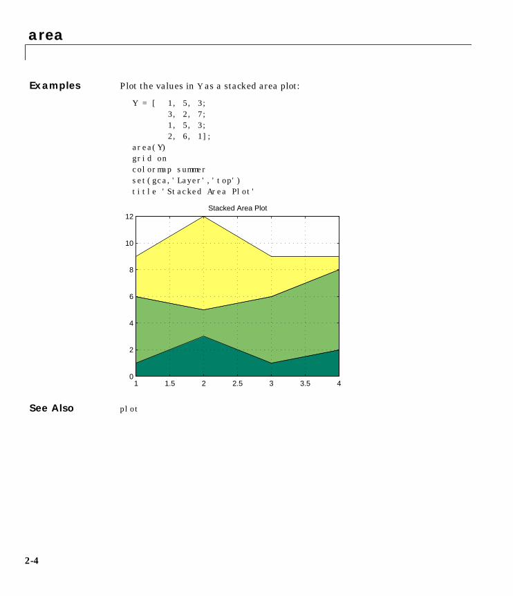
Examples Plot the values in Y as a stacked area plot:

Y = [ 1, 5, 3;3, 2, 7;1, 5, 3;2, 6, 1];

area(Y)grid oncolormap summerset(gca,'Layer','top')title 'Stacked Area Plot'

See Also plot

Stacked Area Plot

1 1.5 2 2.5 3 3.5 40

2

4

6

8

10

12

2-4

axes

2axesPurpose Create Axes graphics object

Syntax axesaxes('PropertyName',PropertyValue,...)axes(h)h = axes(...)

Description axes is the low-level function for creating Axes graphics objects.

axes creates an Axes graphics object in the current Figure using defaultproperty values.

axes('PropertyName',PropertyValue,...) creates an Axes object havingthe specified property values. MATLAB uses default values for any propertiesthat you do not explicitly define as arguments.

axes(h) makes existing axes h the current Axes. It also makes h the first Axeslisted in the Figure’s Children property and sets the Figure’s CurrentAxesproperty to h. The current Axes is the target for functions that draw Image,Line, Patch, Surface, and Text graphics objects.

h = axes(...) returns the handle of the created Axes object.

Remarks MATLAB automatically creates an Axes, if one does not already exist, whenyou issue a command that draws Image, Light, Line, Patch, Surface, or Textgraphics objects.

The axes function accepts property name/property value pairs, structurearrays, and cell arrays as input arguments (see the set and get commands forexamples of how to specify these data types). These properties, which controlvarious aspects of the Axes object, are described in the “Axes Properties”section.

Use the set function to modify the properties of an existing Axes or the getfunction to query the current values of Axes properties. Use the gca commandto obtain the handle of the current Axes.

The axis (not axes) function provides simplified access to commonly usedproperties that control the scaling and appearance of Axes.

2-5

axes

While the basic purpose of an Axes object is to provide a coordinate system forplotted data, Axes properties provide considerable control over the wayMATLAB displays data.

Stretch-to-FillBy default, MATLAB stretches the Axes to fill the Axes position rectangle (therectangle defined by the last two elements in the Position property). Thisresults in graphs that use the available space in the rectangle. However, some3-D graphs (such as a sphere) appear distorted because of this stretching, andare better viewed with a specific three-dimensional aspect ratio.

Stretch-to-fill is active when the DataAspectRatioMode,PlotBoxAspectRatioMode, and CameraViewAngleMode are all auto (thedefault). However, stretch-to-fill is turned off when the DataAspectRatio,PlotBoxAspectRatio, or CameraViewAngle is user-specified, or when one ormore of the corresponding modes is set to manual (which happensautomatically when you set the corresponding property value).

This picture shows the same sphere displayed both with and without thestretch-to-fill. The dotted lines show the Axes Position rectangle.

When stretch-to-fill is disabled, MATLAB sets the size of the Axes to be as largeas possible within the constraints imposed by the Position rectangle withoutintroducing distortion. In the picture above, the height of the rectangleconstrains the Axes size.

Stretch-to-fill active

−1 −0.5 0 0.5 1−1

−0.8

−0.6

−0.4

−0.2

0

0.2

0.4

0.6

0.8

1

−1 −0.8 −0.6 −0.4 −0.2 0 0.2 0.4 0.6 0.8 11

8

6

4

2

0

2

4

6

8

1

Stretch-to-fill disabled

2-6

axes

Examples Zooming

Zoom in using aspect ratio and limits:

sphereset(gca,'DataAspectRatio',[1 1 1],...

'PlotBoxAspectRatio',[1 1 1],'ZLim',[−0.6 0.6])

Zoom in and out using the CameraViewAngle:

sphereset(gca,'CameraViewAngle',get(gca,'CameraViewAngle')−5)set(gca,'CameraViewAngle',get(gca,'CameraViewAngle')+5)

Note that both examples disable MATLAB’s stretch-to-fill behavior.

Positioning the AxesThe Axes Position property enables you to define the location of the Axeswithin the Figure window. For example,

h = axes('Position',position_rectangle)

creates an Axes object at the specified position within the current Figure andreturns a handle to it. Specify the location and size of the Axes with a rectangledefined by a four-element vector,

position_rectangle = [left, bottom, width, height];

The left and bottom elements of this vector define the distance from thelower-left corner of the Figure to the lower-left corner of the rectangle. Thewidth and height elements define the dimensions of the rectangle. You specifythese values in units determined by the Units property. By default, MATLABuses normalized units where (0,0) is the lower-left corner and (1.0,1.0) is theupper-right corner of the Figure window.

You can define multiple Axes in a single Figure window:

axes('position',[.1 .1 .8 .6])mesh(peaks(20));axes('position',[.1 .7 .8 .2])pcolor([1:10;1:10]);

2-7

axes

In this example, the first plot occupies the bottom two-thirds of the Figure, andthe second occupies the top third.

See Also axis, cla, clf, figure, gca, grid, subplot, title, xlabel, ylabel, zlabel,view

05

1015

20

05

1015

20−10

−5

0

5

10

1 2 3 4 5 6 7 8 9 101

1.5

2

2-8

axes

ObjectHierarchy

Setting Default PropertiesYou can set default Axes properties on the Figure and Root levels:

set(0,'DefaultAxesPropertyName',PropertyValue,...)set(gcf,'DefaultAxesPropertyName',PropertyValue,...)

where PropertyName is the name of the Axes property and PropertyValue isthe value you are specifying. Use set and get to access Axes properties.

Property List The following table lists all Axes properties and provides a brief description ofeach. The property name links take you an expanded description of theproperties.

Uimenu

Line

Uicontrol

Image

Figure

Uicontextmenu

Light SurfacePatch Text

Root

Axes

Property Name Property Description Property Value

Controlling Style and Appearance

Box Toggle axes plot box on and off Values: on, offDefault: off

Clipping This property has no effect; axes arealways clipped to the figure window

GridLineStyle Line style used to draw axes gridlines

Values: −, −− , :, -., noneDefault: : (dotted line)

Layer Draw axes above or below graphs Values: bottom, topDefault: bottom

2-9

axes

LineStyleOrder Sequence of line styles used formultiline plots

Values: LineSpecDefault: − (solid line for)

LineWidth Width of axis lines, in points (1/72"per point)

Values: number of pointsDefault: 0.5 points

SelectionHighlight Highlight axes when selected(Selected property set to on)

Values: on, off Default: on

TickDir Direction of axis tick marks Values: in, outDefault: in (2-D), out (3-D)

TickDirMode Use MATLAB or user-specified tickmark direction

Values: auto, manualDefault: auto

TickLength Length of tick marks normalized toaxis line length, specified astwo-element vector

Values: [2-D 3-D]Default: [0.01 0.025

Visible Make axes visible or invisible Values: on, offDefault: on

XGrid, YGrid, ZGrid Toggle grid lines on and off inrespective axis

Values: on, offDefault: off

General Information About the Axes

Children Handles of the Images, Lights, Lines,Patches, Surfaces, and Text objectsdisplayed in the axes

Values: vector of handles

CurrentPoint Location of last mouse button clickdefined in the axes data units

Values: a 2-by-3 matrix

HitTest Specify whether axes can become thecurrent object (see FigureCurrentObject property)

Values: on, offDefault: on

Parent Handle of the Figure windowcontaining the axes

Values: scalar Figure handle


2-10

axes

Position Location and size of axes within thefigure

Values: [left bottom widthheight]Default: [0.1300 0.11000.7750 0.8150] innormalized Units

Selected Indicate whether axes is in a“selected” state


Tag User-specified label Values: any stringDefault: '' (empty string)

Type The type of graphics object (readonly)

Value: the string 'axes'

Units Units used to interpret the Positionproperty

Values: inches, centimeters,characters, normalized,points, pixels Default:normalized

UserData User-specified data Values: any matrixDefault: [] (empty matrix)

Selecting Fonts and Labels

FontAngle Select italic or normal font Values: normal, italic,obliqueDefault: normal

FontName Font family name (e.g., Helvetica,Courier)

Values: a font supported byyour systemDefault: Typically Helvetica

FontSize Size of the font used for title andlabels

Values: an integer inFontUnits Default: 10

FontUnits Units used to interpret the FontSizeproperty

Values: points, normalized,inches, centimeters, pixelsDefault: points


2-11

axes

FontWeight Select bold or normal font Values: normal, bold, light,demiDefault: normal

Title Handle of the title text object Values: any valid text objecthandle

XLabel, YLabel, ZLabel Handles of the respective axis labeltext objects

Values: any valid text objecthandle

XTickLabel, YTickLabel,ZTickLabel

Specify tick mark labels for therespective axis

Values: matrix of stringsDefaults: numeric valuesselected automatically byMATLAB

XTickLabelMode,YTickLabelMode,ZTickLabelMode

Use MATLAB or user-specified tickmark labels


Controlling Axis Scaling

XAxisLocation Specify the location of the x-axis Values: top, bottomDefault: bottom

YAxisLocation Specify the location of the y-axis Values: right leftDefault: left

XDir, YDir, ZDir Specify the direction of increasingvalues for the respective axes

Values: normal, reverseDefault: normal

XLim, YLim, ZLim Specify the limits to the respectiveaxes

Values: [min max]Default: min and maxdetermined automatically byMATLAB

XLimMode, YLimMode,ZLimMode

Use MATLAB or user-specifiedvalues for the respective axis limits



2-12

axes

XScale, YScale, ZScale Select linear or logarithmic scaling ofthe respective axis

Values: linear, logDefault: linear (changed byplotting commands thatcreate nonlinear plots)

XTick, YTick, ZTick Specify the location of the axis ticksmarks

Values: a vector of datavalues locating tick marksDefault: MATLABautomatically determinestick mark placement

XTickMode, YTickMode,ZTickMode

Use MATLAB or user-specifiedvalues for the respective tick marklocations


Controlling the View

CameraPosition Specify the position of point fromwhich you view the scene

Values: [x,y,z] axescoordinatesDefault: automaticallydetermined by MATLAB

CameraPositionMode Use MATLAB or user-specifiedcamera position


CameraTarget Center of view pointed to by camera Values: [x,y,z] axescoordinatesDefault: automaticallydetermined by MATLAB

CameraTargetMode Use MATLAB or user-specifiedcamera target


CameraUpVector Direction that is oriented up Values: [x,y,z] axescoordinatesDefault: automaticallydetermined by MATLAB


2-13

axes

CameraUpVectorMode Use MATLAB or user-specifiedcamera up vector


CameraViewAngle Camera field of view Values: angle in degreesbetween 0 and 180Default: automaticallydetermined by MATLAB

CameraViewAngleMode Use MATLAB or user-specifiedcamera view angle


Projection Select type of projection Values: orthographic,perspectiveDefault: orthographic

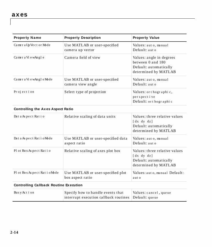
Controlling the Axes Aspect Ratio

DataAspectRatio Relative scaling of data units Values: three relative values[dx dy dz]Default: automaticallydetermined by MATLAB

DataAspectRatioMode Use MATLAB or user-specified dataaspect ratio


PlotBoxAspectRatio Relative scaling of axes plot box Values: three relative values[dx dy dz]Default: automaticallydetermined by MATLAB

PlotBoxAspectRatioMode Use MATLAB or user-specified plotbox aspect ratio

Values: auto, manual Default:auto

Controlling Callback Routine Execution

BusyAction Specify how to handle events thatinterrupt execution callback routines

Values: cancel, queueDefault: queue


2-14

axes

ButtonDownFcn Define a callback routine thatexecutes when a button is pressedover the axes

Values: stringDefault: an empty strin

CreateFcn Define a callback routine thatexecutes when an axes is created

Values: stringDefault: an empty string

DeleteFcn Define a callback routine thatexecutes when an axes is created

Values: string Default: anempty string

Interruptible Control whether an executingcallback routine can be interrupted

Values: on, off Default: on

UIContextMenu Associate a context menu with theaxes

Values: handle of aUicontextmenu

Specifying the Rendering Mode

DrawMode Specify the rendering method to usewith the Painters renderer

Values: normal, fastDefault: normal

Targeting Axes for Graphics Display

HandleVisibility Control access to a specific axes’handle

Values: on, callback, offDefault: on

NextPlot Determine the eligibility of the axesfor displaying graphics

Values: add, replace,replacechildrenDefault: replace

Properties that Specify Color

AmbientLightColor Color of the background light in ascene

Values: ColorSpecDefault: [1 1 1]

CLim Control how data is mapped tocolormap

Values: [cmin cmax]Default: automaticallydetermined by MATLAB

CLimMode Use MATLAB or user-specifiedvalues for CLim



2-15

axes

Color Color of the axes background Values: none, ColorSpecDefault: none

ColorOrder Line colors used for multiline plots Values: m-by-3 matrix ofRGB valuesDefault: depends on colorscheme used

XColor, YColor, ZColor Colors of the axis lines and tickmarks

Values: ColorSpecDefault: depends on currentcolor scheme


2-16

Axes Properties

2Axes PropertiesAxesProperties

This section lists property names along with the types of values each accepts.Curly braces enclose default values.

AmbientLightColor ColorSpec

The background light in a scene. Ambient light is a directionless light thatshines uniformly on all objects in the Axes. However, if there are no visibleLight objects in the Axes, MATLAB does not use AmbientLightColor. If thereare Light objects in the Axes, the AmbientLightColor is added to the other lightsources.

AspectRatio (Obsolete)

This property produces a warning message when queried or changed. It hasbeen superseded by the DataAspectRatio[Mode] andPlotBoxAspectRatio[Mode] properties.

Box on | off

Axes box mode. This property specifies whether to enclose the Axes extent in abox for 2-D views or a cube for 3-D views. The default is to not display the box.

BusyAction cancel | queue

Callback routine interruption. The BusyAction property enables you to controlhow MATLAB handles events that potentially interrupt executing callbackroutines. If there is a callback routine executing, subsequently invokedcallback routines always attempt to interrupt it. If the Interruptible propertyof the object whose callback is executing is set to on (the default), theninterruption occurs at the next point where the event queue is processed. If theInterruptible property is off, the BusyAction property (of the object owningthe executing callback) determines how MATLAB handles the event. Thechoices are:

• cancel – discard the event that attempted to execute a second callbackroutine.

• queue – queue the event that attempted to execute a second callback routineuntil the current callback finishes.

ButtonDownFcn string

Button press callback routine. A callback routine that executes whenever youpress a mouse button while the pointer is within the Axes, but not over another

2-17

Axes Properties

graphics object displayed in the Axes. For 3-D views, the active area is definedby a rectangle that encloses the Axes.

Define this routine as a string that is a valid MATLAB expression or the nameof an M-file. The expression executes in the MATLAB workspace.

CameraPosition [x, y, z] Axes coordinates

The location of the camera. This property defines the position from which thecamera views the scene. Specify the point in Axes coordinates.

If you fix CameraViewAngle, you can zoom in and out on the scene by changingthe CameraPosition, moving the camera closer to the CameraTarget to zoom inand farther away from the CameraTarget to zoom out. As you change theCameraPosition, the amount of perspective also changes, if Projection isperspective. You can also zoom by changing the CameraViewAngle; however,this does not change the amount of perspective in the scene.

CameraPositionMode auto | manual

Auto or manual CameraPosition. When set to auto, MATLAB automaticallycalculates the CameraPosition such that the camera lies a fixed distance fromthe CameraTarget along the azimuth and elevation specified by view. Setting avalue for CameraPosition sets this property to manual.

CameraTarget [x, y, z] Axes coordinates

Camera aiming point. This property specifies the location in the Axes that thecamera points to. The CameraTarget and the CameraPosition define the vector(the view axis) along which the camera looks.

CameraTargetMode auto | manual

Auto or manual CameraTarget placement. When this property is auto,MATLAB automatically positions the CameraTarget at the centroid of the Axesplotbox. Specifying a value for CameraTarget sets this property to manual.

CameraUpVector [x, y, z] Axes coordinates

Camera rotation. This property specifies the rotation of the camera around theviewing axis defined by the CameraTarget and the CameraPosition properties.Specify CameraUpVector as a three-element array containing the x, y, and zcomponents of the vector. For example, [0 1 0] specifies the positive y-axis asthe up direction.

2-18

Axes Properties

The default CameraUpVector is [0 0 1], which defines the positive z-axis as theup direction.

CameraUpVectorMode auto | manual

Default or user-specified up vector. When CameraUpVectorMode is auto,MATLAB uses a value of [0 0 1] (positive z-direction is up) for 3-D views and[0 1 0] (positive y-direction is up) for 2-D views. Setting a value forCameraUpVector sets this property to manual.

CameraViewAngle scalar greater than 0 and less than or equal to180 (angle in degrees)

The field of view. This property determines the camera field of view. Changingthis value affects the size of graphics objects displayed in the Axes, but does notaffect the degree of perspective distortion. The greater the angle, the larger thefield of view, and the smaller objects appear in the scene.

CameraViewAngleModeauto | manual

Auto or manual CameraViewAngle. When in auto mode, MATLAB setsCameraViewAngle to the minimum angle that captures the entire scene (up to180˚).

The following table summarizes MATLAB’s automatic camera behavior.

CameraViewAngle

CameraTarget

CameraPosition

Behavior

auto auto auto CameraTarget is set to plot box centroid,CameraViewAngle is set to capture entire scene,CameraPosition is set along the view axis.

auto auto manual CameraTarget is set to plot box centroid,CameraViewAngle is set to capture entire scene.

auto manual auto CameraViewAngle is set to capture entire scene,CameraPosition is set along the view axis.

auto manual manual CameraViewAngle is set to capture entire scene.

manual auto auto CameraTarget is set to plot box centroid,CameraPosition is set along the view axis.

2-19

Axes Properties

Children vector of graphics object handles

Children of the Axes. A vector containing the handles of all graphics objectsrendered within the Axes (whether visible or not). The graphics objects thatcan be children of Axes are Images, Lights, Lines, Patches, Surfaces, and Text.

The Text objects used to label the x-, y-, and z-axes are also children of Axes,but their HandleVisibility properties are set to callback. This means theirhandles do not show up in the Axes Children property unless you set the RootShowHiddenHandles property to on.

CLim [cmin, cmax]

Color axis limits. A two-element vector that determines how MATLAB mapsthe CData values of Surface and Patch objects to the Figure’s colormap. cmin isthe value of the data mapped to the first color in the colormap, and cmax is thevalue of the data mapped to the last color in the colormap. Data values inbetween are linearly interpolated across the colormap, while data valuesoutside are clamped to either the first or last colormap color, whichever isclosest.

When CLimMode is auto (the default), MATLAB assigns cmin the minimumdata value and cmax the maximum data value in the graphics object’s CData.This maps CData elements with minimum data value to the first colormapentry and with maximum data value to the last colormap entry.

If the Axes contains multiple graphics objects, MATLAB sets CLim to span therange of all objects’ CData.

CLimMode auto | manual

Color axis limits mode. In auto mode, MATLAB sets the CLim property to spanthe CData limits of the graphics objects displayed in the Axes. If CLimMode ismanual, MATLAB does not change the value of CLim when the CData limits ofAxes children change. Setting the CLim property sets this property to manual.

manual auto manual CameraTarget is set to plot box centroid

manual manual auto CameraPosition is set along the view axis.

manual manual manual All Camera properties are user-specified.

CameraViewAngle

CameraTarget

CameraPosition

Behavior

2-20

Axes Properties

Clipping on | off

This property has no effect on Axes.

Color none | ColorSpec

Color of the Axes back planes. Setting this property to none means the Axes istransparent and the Figure color shows through. A ColorSpec is athree-element RGB vector or one of MATLAB’s predefined names. Note thatwhile the default value is none, the matlabrc.m file may set the Axes color toa specific color.

ColorOrder m-by-3 matrix of RGB values

Colors to use for multiline plots. ColorOrder is an m-by-3 matrix of RGB valuesthat define the colors used by the plot and plot3 functions to color each lineplotted. If you do not specify a line color with plot and plot3, these functionscycle through the ColorOrder to obtain the color for each line plotted. To obtainthe current ColorOrder, which may be set during startup, get the propertyvalue:

get(gca,'ColorOrder')

Note that if the Axes NextPlot property is set to replace (the default),high-level functions like plot reset the ColorOrder property beforedetermining the colors to use. If you want MATLAB to use a ColorOrder thatis different from the default, set NextPlot to replacedata. You can also specifyyour own default ColorOrder.

CreateFcn string

Callback routine executed during object creation. This property defines acallback routine that executes when MATLAB creates an Axes object. Youmust define this property as a default value for Axes. For example, thestatement,

set(0,'DefaultAxesCreateFcn','set(gca,''Color'',''b'')')

defines a default value on the Root level that sets the current Axes’ backgroundcolor to blue whenever you (or MATLAB) create an Axes. MATLAB executesthis routine after setting all properties for the Axes. Setting this property on anexisting Axes object has no effect.

The handle of the object whose CreateFcn is being executed is accessible onlythrough the Root CallbackObject property, which can be queried using gcbo.

2-21

Axes Properties

CurrentPoint 2-by-3 matrix

Location of last button click, in Axes data units. A 2-by-3 matrix containing thecoordinates of two points defined by the location of the pointer. These twopoints lie on the line that is perpendicular to the plane of the screen and passesthrough the pointer. The 3-D coordinates are the points, in the axes coordinatesystem, where this line intersects the front and back surfaces of the Axesvolume (which is defined by the Axes x, y, and z limits).

The returned matrix is of the form:

MATLAB updates the CurrentPoint property whenever a button-click eventoccurs. The pointer does not have to be within the Axes, or even the Figurewindow; MATLAB returns the coordinates with respect to the requested Axesregardless of the pointer location.

DataAspectRatio [dx dy dz]

Relative scaling of data units. A three-element vector controlling the relativescaling of data units in the x, y, and z directions. For example, setting thisproperty t o [1 2 1] causes the length of one unit of data in the x direction tobe the same length as two units of data in the y direction and one unit of datain the z direction.

Note that the DataAspectRatio property interacts with thePlotBoxAspectRatio, XLimMode, YLimMode, and ZLimMode properties to controlhow MATLAB scales the x-, y-, and z-axis. Setting the DataAspectRatio willdisable the Stretch-to-fill behavior, if DataAspectRatioMode,PlotBoxAspectRatioMode, and CameraViewAngleMode are all auto. Thefollowing table describes the interaction between properties whenstretch-to-fill behavior is disabled.

xback yback zbackxfront yfront zfront

2-22

Axes Properties

DataAspectRatioModeauto | manual

User or MATLAB controlled data scaling. This property controls whether thevalues of the DataAspectRatio property are user defined or selectedautomatically by MATLAB. Setting values for the DataAspectRatio property

X-, Y-,Z-Limits

DataAspectRatio

PlotBoxAspectRatio

Behavior

auto auto auto Limits chosen to span data range in alldimensions.

auto auto manual Limits chosen to span data range in alldimensions. DataAspectRatio is modified toachieve the requested PlotBoxAspectRatiowithin the limits selected by MATLAB.

auto manual auto Limits chosen to span data range in alldimensions. PlotBoxAspectRatio is modified toachieve the requested DataAspectRatio withinthe limits selected by MATLAB.

auto manual manual Limits chosen to completely fit and center theplot within the requested PlotBoxAspectRatiogiven the requested DataAspectRatio (this mayproduce empty space around 2 of the 3dimensions).

manual auto auto Limits are honored. The DataAspectRatio andPlotBoxAspectRatio are modified as necessary.

manual auto manual Limits and PlotBoxAspectRatio are honored.The DataAspectRatio is modified as necessary.

manual manual auto Limits and DataAspectRatio are honored. ThePlotBoxAspectRatio is modified as necessary.

1 manual2 auto

manual manual The 2 automatic limits are selected to honor thespecified aspect ratios and limit. See “Examples”

2 or 3manual

manual manual Limits and DataAspectRatio are honored; thePlotBoxAspectRatio is ignored.

2-23

Axes Properties

automatically sets this property to manual. Changing DataAspectRatioMode tomanual disables the stretch-to-fill behavior, if DataAspectRatioMode,PlotBoxAspectRatioMode, and CameraViewAngleMode are all auto.

DeleteFcn string

Delete Axes callback routine. A callback routine that executes when the Axesobject is deleted (e.g., when you issue a delete or a close command). MATLABexecutes the routine before destroying the object’s properties so the callbackroutine can query these values.

The handle of the object whose DeleteFcn is being executed is accessible onlythrough the Root CallbackObject property, which can be queried using gcbo.

DrawMode normal | fast

Rendering method. This property controls the method MATLAB uses to rendergraphics objects displayed in the Axes, when the Figure Renderer property ispainters.

• normal mode draws objects in back to front ordering based on the currentview in order to handle hidden surface elimination and object intersections.

• fast mode draws objects in the order in which you specify the drawingcommands, without considering the relationships of the objects in threedimensions. This results in faster rendering because it requires no sorting ofobjects according to location in the view, but may produce undesirableresults because it bypasses the hidden surface elimination and objectintersection handling provided by normal DrawMode.

When the Figure Renderer is zbuffer, DrawMode is ignored, and hidden surfaceelimination and object intersection handling are always provided.

FontAngle normal | italic | oblique

Select italic or normal font. This property selects the character slant for Axestext. normal specifies a nonitalic font. italic and oblique specify italic font.

FontName The default is Helvetica on many systems

Font family name. The font family name specifying the font to use for Axeslabels. To display and print properly, FontName must be a font that your systemsupports. Note that the x-, y-, and z-axis labels do not display in a new font untilyou manually reset them (by setting the XLabel, YLabel, and ZLabel properties

2-24

Axes Properties

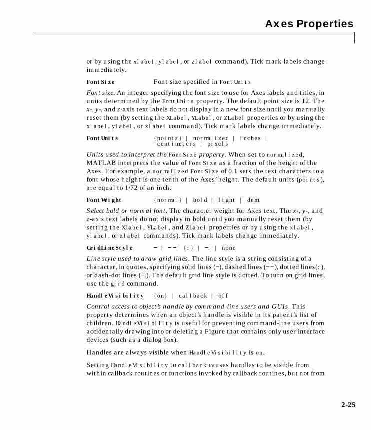
or by using the xlabel, ylabel, or zlabel command). Tick mark labels changeimmediately.

FontSize Font size specified in FontUnits

Font size. An integer specifying the font size to use for Axes labels and titles, inunits determined by the FontUnits property. The default point size is 12. Thex-, y-, and z-axis text labels do not display in a new font size until you manuallyreset them (by setting the XLabel, YLabel, or ZLabel properties or by using thexlabel, ylabel, or zlabel command). Tick mark labels change immediately.

FontUnits points | normalized | inches |centimeters | pixels

Units used to interpret the FontSize property. When set to normalized,MATLAB interprets the value of FontSize as a fraction of the height of theAxes. For example, a normalized FontSize of 0.1 sets the text characters to afont whose height is one tenth of the Axes’ height. The default units (points),are equal to 1/72 of an inch.

FontWeight normal | bold | light | demi

Select bold or normal font. The character weight for Axes text. The x-, y-, andz-axis text labels do not display in bold until you manually reset them (bysetting the XLabel, YLabel, and ZLabel properties or by using the xlabel,ylabel, or zlabel commands). Tick mark labels change immediately.

GridLineStyle − | − −| : | −. | none

Line style used to draw grid lines. The line style is a string consisting of acharacter, in quotes, specifying solid lines (−), dashed lines (−− ), dotted lines(:),or dash-dot lines (−.). The default grid line style is dotted. To turn on grid lines,use the grid command.

HandleVisibility on | callback | off

Control access to object’s handle by command-line users and GUIs. Thisproperty determines when an object’s handle is visible in its parent’s list ofchildren. HandleVisibility is useful for preventing command-line users fromaccidentally drawing into or deleting a Figure that contains only user interfacedevices (such as a dialog box).

Handles are always visible when HandleVisibility is on.

Setting HandleVisibility to callback causes handles to be visible fromwithin callback routines or functions invoked by callback routines, but not from

2-25

Axes Properties

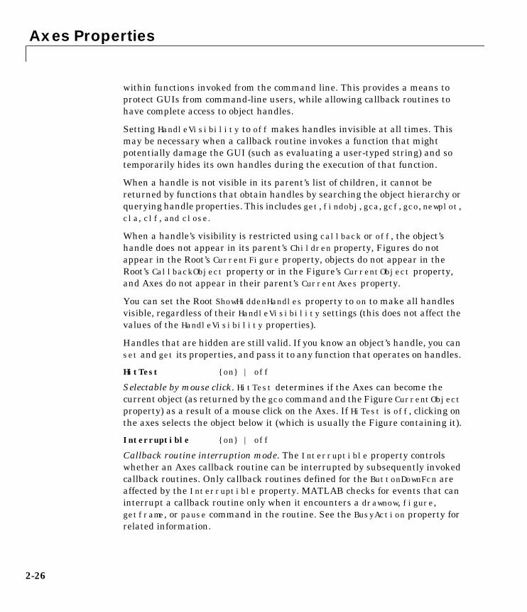
within functions invoked from the command line. This provides a means toprotect GUIs from command-line users, while allowing callback routines tohave complete access to object handles.

Setting HandleVisibility to off makes handles invisible at all times. Thismay be necessary when a callback routine invokes a function that mightpotentially damage the GUI (such as evaluating a user-typed string) and sotemporarily hides its own handles during the execution of that function.

When a handle is not visible in its parent’s list of children, it cannot bereturned by functions that obtain handles by searching the object hierarchy orquerying handle properties. This includes get, findobj, gca, gcf, gco, newplot,cla, clf, and close.

When a handle’s visibility is restricted using callback or off, the object’shandle does not appear in its parent’s Children property, Figures do notappear in the Root’s CurrentFigure property, objects do not appear in theRoot’s CallbackObject property or in the Figure’s CurrentObject property,and Axes do not appear in their parent’s CurrentAxes property.

You can set the Root ShowHiddenHandles property to on to make all handlesvisible, regardless of their HandleVisibility settings (this does not affect thevalues of the HandleVisibility properties).

Handles that are hidden are still valid. If you know an object’s handle, you canset and get its properties, and pass it to any function that operates on handles.

HitTest on | off

Selectable by mouse click. HitTest determines if the Axes can become thecurrent object (as returned by the gco command and the Figure CurrentObjectproperty) as a result of a mouse click on the Axes. If HiTest is off, clicking onthe axes selects the object below it (which is usually the Figure containing it).

Interruptible on | off

Callback routine interruption mode. The Interruptible property controlswhether an Axes callback routine can be interrupted by subsequently invokedcallback routines. Only callback routines defined for the ButtonDownFcn areaffected by the Interruptible property. MATLAB checks for events that caninterrupt a callback routine only when it encounters a drawnow, figure,getframe, or pause command in the routine. See the BusyAction property forrelated information.

2-26

Axes Properties

Setting Interruptible to on allows any graphics object’s callback routine tointerrupt callback routines originating from an Axes property. Note thatMATLAB does not save the state of variables or the display (e.g., the handlereturned by the gca or gcf command) when an interruption occurs.

Layer bottom | top

Draw axis lines below or above graphics objects. This property determines ifaxis lines and tick marks draw on top or below Axes children objects for any 2-Dview (i.e., when you are looking along the x-, y-, or z-axis). This is useful forplacing grid lines and tick marks on top of images.

LineStyleOrder LineSpec

Order of line styles and markers used in a plot. This property specifies whichline styles and markers to use and in what order when creating multiple-lineplots. For example,

set(gca,'LineStyleOrder', '−∗|:|o')

sets LineStyleOrder to solid line with asterisk marker, dotted line, and hollowcircle marker. The default is (−), which specifies a solid line for all data plotted.Alternatively, you can create a cell array of character strings to define the linestyles:

set(gca,'LineStyleOrder','−*',':','o')

MATLAB supports four line styles, which you can specify any number of timesin any order. MATLAB cycles through the line styles only after using all colorsdefined by the ColorOrder property. For example, the first eight lines plotteduse the different colors defined by ColorOrder with the first line style.MATLAB then cycles through the colors again, using the second line stylespecified, and so on.

You can also specify line style and color directly with the plot and plot3functions or by altering the properties of the Line objects.

Note that, if the Axes NextPlot property is set to replace (the default),high-level functions like plot reset the LineStyleOrder property beforedetermining the line style to use. If you want MATLAB to use aLineStyleOrder that is different from the default, set NextPlot toreplacedata. You can also specify your own default LineStyleOrder.

2-27

Axes Properties

LineWidth linewidth in points

Width of axis lines. This property specifies the width, in points, of the x-, y-, andz-axis lines. The default line width is 0.5 points (1 point = 1/72 inch).

NextPlot add | replace | replacechildren

Where to draw the next plot. This property determines how high-level plottingfunctions draw into an existing Axes.

• add — use the existing Axes to draw graphics objects.

• replace — reset all Axes properties, except Position, to their defaults anddelete all Axes children before displaying graphics (equivalent to cla reset).

• replacechildren — remove all child objects, but do not reset Axesproperties (equivalent to cla).

The newplot function simplifies the use of the NextPlot property and is usedby M-file functions that draw graphs using only low-level object creationroutines. See the M-file pcolor.m for an example. Note that Figure graphicsobjects also have a NextPlot property.

Parent Figure handle

Axes parent. The handle of the Axes’ parent object. The parent of an Axes objectis the Figure in which it is displayed. The utility function gcf returns thehandle of the current Axes’ Parent. You can reparent Axes to other Figureobjects.

PlotBoxAspectRatio [px py pz]

Relative scaling of Axes plotbox. A three-element vector controlling the relativescaling of the plot box in the x-, y-, and z-directions. The plot box is a boxenclosing the Axes data region as defined by the x-, y-, and z-axis limits.

Note that the PlotBoxAspectRatio property interacts with theDataAspectRatio, XLimMode, YLimMode, and ZLimMode properties to control theway graphics objects are displayed in the Axes. Setting thePlotBoxAspectRatio disables stretch-to-fill behavior, ifDataAspectRatioMode, PlotBoxAspectRatioMode, and CameraViewAngleModeare all auto.

PlotBoxAspectRatioModeauto | manual

User or MATLAB controlled axis scaling. This property controls whether thevalues of the PlotBoxAspectRatio property are user defined or selected

2-28

Axes Properties

automatically by MATLAB. Setting values for the PlotBoxAspectRatioproperty automatically sets this property to manual. Changing thePlotBoxAspectRatioMode to manual disables stretch-to-fill behavior, ifDataAspectRatioMode, PlotBoxAspectRatioMode, and CameraViewAngleModeare all auto.

Position four-element vector

Position of Axes. A four-element vector specifying a rectangle that locates theAxes within the Figure window. The vector is of the form:

[left bottom width height]

where left and bottom define the distance from the lower-left corner of theFigure window to the lower-left corner of the rectangle. width and height arethe dimensions of the rectangle. All measurements are in units specified by theUnits property.

When Axes stretch-to-fill behavior is enabled (when DataAspectRatioMode,PlotBoxAspectRatioMode, CameraViewAngleMode are all auto), the Axes arestretched to fill the Position rectangle. When stretch-to-fill is disabled, theAxes are made as large as possible, while obeying all other properties, withoutextending outside the Position rectangle

Projection orthographic | perspective

Type of projection. This property selects between two projection types:

• orthographic – This projection maintains the correct relative dimensions ofgraphics objects with regard to the distance a given point is from the viewer.Parallel lines in the data are drawn parallel on the screen.

• perspective – This projection incorporates foreshortening, which allows youto perceive depth in 2-D representations of 3-D objects. Perspectiveprojection does not preserve the relative dimensions of objects; a distant linesegment displays smaller than a nearer line segment of the same length.Parallel lines in the data may not appear parallel on screen.

Selected on | off

Is object selected. When you set this property to on, MATLAB displays selection“handles” at the corners and midpoints if the SelectionHighlight property isalso on (the default). You can, for example, define the ButtonDownFcn callback

2-29

Axes Properties

routine to set this property to on, thereby indicating that the axes has beenselected.

SelectionHighlight on | off

Objects highlight when selected. When the Selected property is on, MATLABindicates the selected state by drawing four edge handles and four cornerhandles. When SelectionHighlight is off, MATLAB does not draw thehandles.

Tag string

User-specified object label. The Tag property provides a means to identifygraphics objects with a user-specified label. This is particularly useful whenconstructing interactive graphics programs that would otherwise need todefine object handles as global variables or pass them as arguments betweencallback routines.

For example, suppose you want to direct all graphics output from an M-file toa particular Axes, regardless of user actions that may have changed thecurrent Axes. To do this, identify the Axes with a Tag:

axes('Tag','Special Axes')

Then make that Axes the current Axes before drawing by searching for the Tagwith findobj:

axes(findobj('Tag','Special Axes'))

TickDir in | out

Direction of tick marks. For 2-D views, the default is to direct tick marksinward from the axis lines; 3-D views direct tick marks outward from the axisline.

TickDirMode auto | manual

Automatic tick direction control. In auto mode, MATLAB directs tick marksinward for 2-D views and outward for 3-D views. When you specify a setting forTickDir, MATLAB sets TickDirMode to manual. In manual mode, MATLABdoes not change the specified tick direction.

TickLength [2DLength 3DLength]

Length of tick marks. A two-element vector specifying the length of Axes tickmarks. The first element is the length of tick marks used for 2-D views and the

2-30

Axes Properties

second element is the length of tick marks used for 3-D views. Specify tick marklengths in units normalized relative to the longest of the visible X-, Y-, or Z-axisannotation lines.

Title handle of text object

Axes title. The handle of the Text object that is used for the Axes title. You canuse this handle to change the properties of the title Text or you can set Titleto the handle of an existing Text object. For example, the following statementchanges the color of the current title to red:

set(get(gca,'Title'),'Color','r')

To create a new title, set this property to the handle of the Text object you wantto use:

set(gca,'Title',text('String','New Title','Color','r'))

However, it is generally simpler to use the title command to create or replacean Axes title:

title('New Title','Color','r')

Type string (read only)

Type of graphics object. This property contains a string that identifies the classof graphics object. For Axes objects, Type is always set to 'axes'.

UIContextMenu handle of a uicontextmenu object

Associate a context menu with the axes. Assign this property the handle of aUicontextmenu object created in the Axes’ parent Figure. Use theuicontextmenu function to create the context menu. MATLAB displays thecontext menu whenever you right-click over the Axes (Control-click onMacintosh systems).

Units inches | centimeters | normalized |points | pixels | characters

Position units. The units used to interpret the Position property. All units aremeasured from the lower-left corner of the Figure window.

2-31

Axes Properties

• normalized units map the lower-left corner of the Figure window to (0,0) andthe upper-right corner to (1.0, 1.0).

• inches, centimeters, and points are absolute units (one point equals 1/72 ofan inch).

• Character units are defined by characters from the default system font; thewidth of one character is the width of the letter x, the height of one characteris the distance between the baselines of two lines of text.

UserData matrix

User specified data. This property can be any data you want to associate withthe Axes object. The Axes does not use this property, but you can access it usingthe set and get functions.

View Obsolete

The functionality provided by the View property is now controlled by the Axescamera properties – CameraPosition, CameraTarget, CameraUpVector, andCameraViewAngle. See the view command.

Visible on | off

Visibility of Axes. By default, Axes are visible. Setting this property to offprevents axis lines, tick marks, and labels from being displayed. The visibleproperty does not affect children of Axes.

XAxisLocation top | bottom

Location of x-axis tick marks and labels. This property controls whereMATLAB displays the x-axis tick marks and labels. Setting this property to topmoves the x-axis to the top of the plot from its default position at the bottom.

YAxisLocation right | left

Location of y-axis tick marks and labels. This property controls whereMATLAB displays the y-axis tick marks and labels. Setting this property toright moves the y-axis to the right side of the plot from its default position onthe left side. See the plotyy function for a simple way to use two y-axes.

Properties That Control the X-, Y-, or Z-AxisXColor, YColor, ZColorColorSpec

Color of axis lines. A three-element vector specifying an RGB triple, or apredefined MATLAB color string. This property determines the color of the

2-32

Axes Properties

axis lines, tick marks, tick mark labels, and the axis grid lines of the respectivex-, y-, and z-axis. The default axis color is white. See ColorSpec for details onspecifying colors.

XDir, YDir, ZDir normal | reverse

Direction of increasing values. A mode controlling the direction of increasingaxis values. Axes form a right-hand coordinate system. By default,

• x-axis values increase from left to right. To reverse the direction of increasingx values, set this property to reverse.

• y-axis values increase from bottom to top (2-D view) or front to back (3-Dview). To reverse the direction of increasing y values, set this property toreverse.

• z-axis values increase pointing out of the screen (2-D view) or from bottom totop (3-D view). To reverse the direction of increasing z values, set thisproperty to reverse.

XGrid, YGrid, ZGrid on | off

Axis gridline mode. When you set any of these properties to on, MATLAB drawsgrid lines perpendicular to the respective axis (i.e., along lines of constant x, y,or z values). Use the grid command to set all three properties on or off at once.

XLabel, YLabel, ZLabelhandle of text object

Axis labels. The handle of the Text object used to label the x, y, or z-axis,respectively. To assign values to any of these properties, you must obtain thehandle to the text string you want to use as a label. This statement defines aText object and assigns its handle to the XLabel property:

set(gca,'Xlabel',text('String','axis label'))

MATLAB places the string 'axis label' appropriately for an x-axis label. AnyText object whose handle you specify as an XLabel, YLabel, or ZLabel propertyis moved to the appropriate location for the respective label.

Alternatively, you can use the xlabel, ylabel, and zlabel functions, whichgenerally provide a simpler means to label axis lines.

XLim, YLim, ZLim [minimum maximum]

Axis limits. A two-element vector specifying the minimum and maximumvalues of the respective axis.

2-33

Axes Properties

Changing these properties affects the scale of the x-, y-, or z-dimension as wellas the placement of labels and tick marks on the axis. The default values forthese properties are [0 1].

XLimMode, YLimMode, ZLimModeauto | manual

MATLAB or user-controlled limits. The axis limits mode determines whetherMATLAB calculates axis limits based on the data plotted (i.e., the XData,YData, or ZData of the Axes children) or uses the values explicitly set with theXLim, YLim, or ZLim property, in which case, the respective limits mode is set tomanual.

XScale, YScale, ZScalelinear | log

Axis scaling. Linear or logarithmic scaling for the respective axis. See alsologlog, semilogx, and semilogy.

XTick, YTick, ZTickvector of data values locating tick marks

Tick spacing. A vector of x-, y-, or z-data values that determine the location oftick marks along the respective axis. If you do not want tick marks displayed,set the respective property to the empty vector, [ ]. These vectors must containmonotonically increasing values.

XTickLabel, YTickLabel, ZTickLabelstring

Tick labels. A matrix of strings to use as labels for tick marks along therespective axis. These labels replace the numeric labels generated byMATLAB. If you do not specify enough text labels for all the tick marks,MATLAB uses all of the labels specified, then reuses the specified labels.

For example, the statement,

set(gca,'XTickLabel','One';'Two';'Three';'Four')

labels the first four tick marks on the x-axis and then reuses the labels until allticks are labeled.

Labels can be specified as cell arrays of strings, padded string matrices, stringvectors separated by vertical slash characters, or as numeric vectors (where

2-34

Axes Properties

each number is implicitly converted to the equivalent string using num2str). Allof the following are equivalent:

set(gca,'XTickLabel','1';'10';'100')set(gca,'XTickLabel','1|10|100')set(gca,'XTickLabel',[1;10;100])set(gca,'XTickLabel',['1 ';'10 ';'100'])

Note that tick labels do not interpret TeX character sequences (however, theTitle, XLabel, YLabel, and ZLabel properties do).

XTickMode, YTickMode, ZTickModeauto | manual

MATLAB or user controlled tick spacing. The axis tick modes determinewhether MATLAB calculates the tick mark spacing based on the range of datafor the respective axis (auto mode) or uses the values explicitly set for any ofthe XTick, YTick, and ZTick properties (manual mode). Setting values for theXTick, YTick, or ZTick properties sets the respective axis tick mode to manual.

XTickLabelMode, YTickLabelMode, ZTickLabelModeauto | manual

MATLAB or user determined tick labels. The axis tick mark labeling modedetermines whether MATLAB uses numeric tick mark labels that span therange of the plotted data (auto mode) or uses the tick mark labels specified withthe XTickLabel, YTickLabel, or ZTickLabel property (manual mode). Settingvalues for the XTickLabel, YTickLabel, or ZTickLabel property sets therespective axis tick label mode to manual.

2-35

axis

2axisPurpose Axis scaling and appearance

Syntax axis([xmin xmax ymin ymax])axis([xmin xmax ymin ymax zmin zmax])v = axis

axis autoaxis manualaxis tightaxis fill

axis ijaxis xy

axis equalaxis imageaxis squareaxis vis3daxis normal

axis offaxis on[mode,visibility,direction] = axis('state')

Description axis manipulates commonly used Axes properties. (See Algorithm section.)

axis([xmin xmax ymin ymax]) sets the limits for the x- and y-axis of thecurrent Axes.

axis([xmin xmax ymin ymax zmin zmax]) sets the limits for the x-, y-, andz-axis of the current Axes.

v = axis returns a row vector containing scaling factors for the x-, y-, andz-axis. v has four or six components depending on whether the current Axes is2-D or 3-D, respectively. The returned values are the current Axes’ XLim, Ylim,and ZLim properties.

2-36

axis

axis auto sets MATLAB to its default behavior of computing the currentAxes’ limits automatically, based on the minimum and maximum values of x,y, and z data. You can restrict this automatic behavior to a specific axis. Forexample, axis 'auto x' computes only the x-axis limits automatically; axis'auto yz' computes the y- and z-axis limits automatically.

axis manual and axis(axis) freezes the scaling at the current limits, so thatif hold is on, subsequent plots use the same limits. This sets the XLimMode,YLimMode, and ZLimMode properties to manual.

axis tight sets the aspect ratio so that the data units are the same in everydirection. This differs from axis equal because the plot box aspect ratioautomatically adjusts.

axis fill sets the axis limits to the range of the data.

axis ij places the coordinate system origin in the upper-left corner. Thei-axis is vertical, with values increasing from top to bottom. The j-axis ishorizontal with values increasing from left to right.

axis xy draws the graph in the default Cartesian axes format with thecoordinate system origin in the lower-left corner. The x-axis is horizontal withvalues increasing from left to right. The y-axis is vertical with values increasingfrom bottom to top.

axis equal sets the aspect ratio so that the data units are the same in everydirection. The aspect ratio of the x-, y-, and z-axis is adjusted automaticallyaccording to the range of data units in the x, y, and z directions.

axis image is the same as axis equal except that the plot box fits tightlyaround the data.

axis square makes the current Axes region square (or cubed whenthree-dimensional). MATLAB adjusts the x-axis, y-axis, and z-axis so that theyhave equal lengths and adjusts the increments between data units accordingly.

axis vis3d freezes aspect ratio properties to enable rotation of 3-D objectsand overrides stretch-to-fill.

2-37

axis

axis normal automatically adjusts the aspect ratio of the Axes and the aspectratio of the data units represented on the Axes to fill the plot box.

axis off turns off all axis lines, tick marks, and labels.

axis on turns on all axis lines, tick marks, and labels.

[mode,visibility,direction] = axis('state') returns three stringsindicating the current setting of Axes properties:

mode is auto if XLimMode, YLimMode, and ZLimMode are all set to auto. IfXLimMode, YLimMode, or ZLimMode is manual, mode is manual.

Examples The statements

x = 0:.025:pi/2;plot(x,tan(x),'-ro')

Output Argument Strings Returned

mode 'auto' | 'manual'

visibility 'on' | 'off'

direction 'xy' | 'ij'

2-38

axis

use the automatic scaling of the y-axis based on ymax = tan(1.57), which iswell over 1000:

0 0.2 0.4 0.6 0.8 1 1.2 1.4 1.60

200

400

600

800

1000

1200

1400

2-39

axis

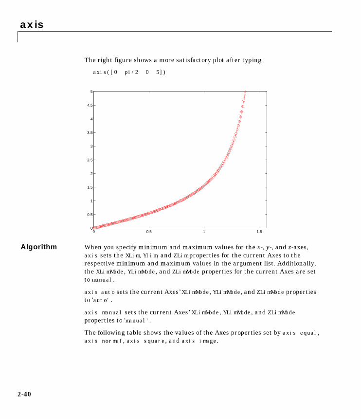
The right figure shows a more satisfactory plot after typing

axis([0 pi/2 0 5])

Algorithm When you specify minimum and maximum values for the x-, y-, and z-axes,axis sets the XLim, Ylim, and ZLim properties for the current Axes to therespective minimum and maximum values in the argument list. Additionally,the XLimMode, YLimMode, and ZLimMode properties for the current Axes are setto manual.

axis auto sets the current Axes’ XLimMode, YLimMode, and ZLimMode propertiesto 'auto'.

axis manual sets the current Axes’ XLimMode, YLimMode, and ZLimModeproperties to 'manual'.

The following table shows the values of the Axes properties set by axis equal,axis normal, axis square, and axis image.

0 0.5 1 1.50

0.5

1

1.5

2

2.5

3

3.5

4

4.5

5

2-40

axis

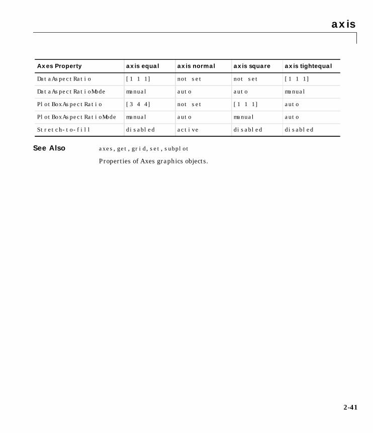
See Also axes, get, grid, set, subplot

Properties of Axes graphics objects.

Axes Property axis equal axis normal axis square axis tightequal

DataAspectRatio [1 1 1] not set not set [1 1 1]

DataAspectRatioMode manual auto auto manual

PlotBoxAspectRatio [3 4 4] not set [1 1 1] auto

PlotBoxAspectRatioMode manual auto manual auto

Stretch-to-fill disabled active disabled disabled

2-41

bar, barh

2bar, barhPurpose Bar chart

Syntax bar(Y)bar(x,Y)bar(...,width)bar(...,'style')bar(...,LineSpec)[xb,yb] = bar(...)h = bar(...)

barh(...)[xb,yb] = barh(...)h = barh(...)

Description A bar chart displays the values in a vector or matrix as horizontal or verticalbars.

bar(Y) draws one bar for each element in Y. If Y is a matrix, bar groupstogether the bars produced by the elements in each row. The x-axis scale rangesfrom 1 to length(Y) when Y is a vector, and 1 to size(Y,1), which is thenumber of rows, when Y is a matrix.

bar(x,Y) draws a bar for each element in Y at locations specified in x, where xis a monotonically increasing vector defining the x-axis intervals for thevertical bars. If Y is a matrix, bar clusters the elements in the same row in Y atlocations corresponding to an element in x.

bar(...,width) sets the relative bar width and controls the separation of barswithin a group. The default width is 0.8, so if you do not specify x, the barswithin a group have a slight separation. If width is 1, the bars within a grouptouch one another.

bar(...,'style') specifies the style of the bars. 'style' is 'group' or'stack'. 'group' is the default mode of display.

2-42

bar, barh

• 'group' displays n groups of m vertical bars, where n is the number of rowsand m is the number of columns in Y. The group contains one bar per columnin Y.

• 'stack' displays one bar for each row in Y. The bar height is the sum of theelements in the row. Each bar is multi-colored, with colors corresponding todistinct elements and showing the relative contribution each row elementmakes to the total sum.

bar(...,LineSpec) displays all bars using the color specified by LineSpec.

[xb,yb] = bar(...) returns vectors that you plot using plot(xb,yb) orpatch(xb,yb,C). This gives you greater control over the appearance of a graph,for example, to incorporate a bar chart into a more elaborate plot statement.

h = bar(...) returns a vector of handles to Patch graphics objects. barcreates one Patch graphics object per column in Y.

barh(...), [xb,yb] = barh(...), and h = barh(...) create horizontalbars. Y determines the bar length. The vector x is a monotonic vector definingthe y-axis intervals for horizontal bars.

2-43

bar, barh

Examples Plot a bell shaped curve:

x = –2.9:0.2:2.9;bar(x,exp(–x.∗x))colormap hsv

Create four subplots showing the effects of some bar arguments:

Y = round(rand(5,3)∗10);subplot(2,2,1)bar(Y,'group')title 'Group'

subplot(2,2,2)bar(Y,'stack')title 'Stack'

subplot(2,2,3)barh(Y,'stack')title 'Stack'

subplot(2,2,4)bar(Y,1.5)title 'Width = 1.5'

−3 −2 −1 0 1 2 30

0.1

0.2

0.3

0.4

0.5

0.6

0.7

0.8

0.9

1

2-44

bar, barh

See Also bar3, ColorSpec, patch, stairs, hist

1 2 3 4 50

2

4

6

8

10Group

1 2 3 4 50

5

10

15

20

25Stack

0 5 10 15 20 25

1

2

3

4

5

Stack

1 2 3 4 50

2

4

6

8

10Width = 1.5

2-45

bar3, bar3h

2bar3, bar3hPurpose Three-dimensional bar chart

Syntax bar3(Y)bar3(x,Y)bar3(...,width)bar3(...,'style')bar3(...,LineSpec)h = bar3(...)

bar3h(...)h = bar3h(...)

Description bar3 and bar3h draw three-dimensional vertical and horizontal bar charts.

bar3(Y) draws a three-dimensional bar chart, where each element in Ycorresponds to one bar. When Y is a vector, the x-axis scale ranges from 1 tolength(Y). When Y is a matrix, the x-axis scale ranges from 1 to size(Y,2),which is the number of columns, and the elements in each row are groupedtogether.

bar3(x,Y) draws a bar chart of the elements in Y at the locations specified inx, where x is a monotonic vector defining the y-axis intervals for vertical bars.If Y is a matrix, bar3 clusters elements from the same row in Y at locationscorresponding to an element in x. Values of elements in each row are groupedtogether.

bar3(...,width) sets the width of the bars and controls the separation of barswithin a group. The default width is 0.8, so if you do not specify x, bars withina group have a slight separation. If width is 1, the bars within a group touchone another.

bar3(...,'style') specifies the style of the bars. 'style' is 'detached','grouped', or 'stacked'. 'detached' is the default mode of display.

• 'detached' displays the elements of each row in Y as separate blocks behindone another in the x direction.

2-46

bar3, bar3h

• 'grouped' displays n groups of m vertical bars, where n is the number ofrows and m is the number of columns in Y. The group contains one bar percolumn in Y.

• 'stacked' displays one bar for each row in Y. The bar height is the sum ofthe elements in the row. Each bar is multi-colored, with colors correspondingto distinct elements and showing the relative contribution each row elementmakes to the total sum.

bar3(...,LineSpec) displays all bars using the color specified by LineSpec.

h = bar3(...) returns a vector of handles to Patch graphics objects. bar3creates one Patch object per column in Y.

bar3h(...) and h = bar3h(...) create horizontal bars. Y determines the barlength. The vector x is a monotonic vector defining the y-axis intervals forhorizontal bars.

2-47

bar3, bar3h

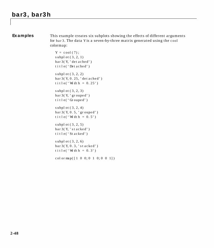
Examples This example creates six subplots showing the effects of different argumentsfor bar3. The data Y is a seven-by-three matrix generated using the coolcolormap:

Y = cool(7);subplot(3,2,1)bar3(Y,’detached’)title(‘Detached’)

subplot(3,2,2)bar3(Y,0.25,’detached’)title(‘Width = 0.25’)

subplot(3,2,3)bar3(Y,’grouped’)title(‘Grouped’)

subplot(3,2,4)bar3(Y,0.5,’grouped’)title(‘Width = 0.5’)

subplot(3,2,5)bar3(Y,’stacked’)title(‘Stacked’)

subplot(3,2,6)bar3(Y,0.3,’stacked’)title(‘Width = 0.3’)

colormap([1 0 0;0 1 0;0 0 1])

2-48

bar3, bar3h

See Also bar, LineSpec, patch

12

34

56

7

0

0.5

1

Detached

12

34

56

7

0

0.5

1

Width = 0.25

12

34

56

7

0

0.5

1Grouped

12

34

56

7

0

0.5

1Width = 0.5

12

34

56

7

0

0.5

1

1.5

2Stacked

12

34

56

7

0

0.5

1

1.5

2Width = 0.3

2-49

box

2boxPurpose Control Axes border

Syntax box onbox offbox

Description box on displays the boundary of the current Axes.

box off does not display the boundary of the current Axes.

box toggles the visible state of the current Axes’ boundary.

Algorithm The box function sets the Axes Box property to on or off.

See Also axes

2-50

brighten

2brightenPurpose Brighten or darken colormap

Syntax brighten(beta)brighten(h,beta)newmap = brighten(beta)newmap = brighten(cmap,beta)

Description brighten increases or decreases the color intensities in a colormap. Themodified colormap is brighter if 0 < beta < 1 and darker if –1 < beta < 0.

brighten(beta) replaces the current colormap with a brighter or darkercolormap of essentially the same colors. brighten(beta), followed bybrighten(–beta), where beta < 1, restores the original map.

brighten(h,beta) brightens all objects that are children of the Figure havingthe handle h.

newmap = brighten(beta) returns a brighter or darker version of the currentcolormap without changing the display.

newmap = brighten(cmap,beta) returns a brighter or darker version of thecolormap cmap without changing the display.

Examples Brighten then darken the current colormap:

beta = .5; brighten(beta);beta = —.5; brighten(beta);

Algorithm The values in the colormap are raised to the power of gamma, where gamma is

brighten has no effect on graphics objects defined with true color.

See Also colormap, rgbplot

γ1 β, β 0>–

11 β+-------------, β 0≤

=

2-51

brighten

2-52

camdolly

2camdollyPurpose Move the camera position and target

Syntax camdolly(dx,dy,dz)camdolly(dx,dy,dz,'targetmode')camdolly(dx,dy,dz,'targetmode','coordsys')camdolly(axes_handle,...)

Description camdolly moves the camera position and the camera target by the specifiedamounts.

camdolly(dx,dy,dz) moves the camera position and the camera target by thespecified amounts (see Coordinate Systems).

camdolly(dx,dy,dz,'targetmode') The targetmode argument can take ontwo values that determine how MATLAB moves the camera:

• movetarget (default) – move both the camera and the target

• fixtarget – move only the camera

camdolly(dx,dy,dz,'targetmode','coordsys') The coordsys argumentcan take on three values that determine how MATLAB interprets dx, dy, anddz:

CoordinateSystems

• camera (default) – move in the camera’s coordinate system. dx moves left/right, dy moves down/up, dz moves along the viewing axis. The units arenormalized to the scene.

For example, setting dx to 1 moves the camera to the right, which pushes thescene to the left edge of the box formed by the axes position rectangle. Anegative value moves the scene in the other direction. Setting dz to .5 movesthe camera to a position half way in between the camera position and thecamera target

• pixels – interpret dx and dy as pixel offsets. dz is ignored.

• data – interpret dx, dy, and dz in axes data coordinates.

camdolly(axes_handle,...) operates on the axes identified by the firstargument, axes_handle. When you do not specify an axes handle, camdollyoperates on the current axes.

2-53

camdolly

Remarks camdolly sets the Axes CameraPosition and CameraTarget properties, whichin turn causes the CameraPositionMode and CameraTargetMode properties tobe set to manual.

Examples This example moves the camera along the x- and y-axes in a series of steps:

surf(peaks)axis vis3dt = 0:pi/20:2*pi;dx = sin(t)./40;dy = cos(t)./40;for i = 1:length(t);

camdolly(dx(i),dy(i),0)drawnow

end

See Also axes, campos, camproj, camtarget, camup, camva

The Axes properties CameraPosition, CameraTarget, CameraUpVector,CameraViewAngle, Projection

The “Camera Properties” section in the Using MATLAB Graphics manual

2-54

camlight

2camlightPurpose Create or move a Light object in camera coordinates

Syntax camlight headlightcamlight rightcamlight leftcamlightcamlight(az,el)camlight(...‘style’)camlight(light_handle,...)light_handle = camlight(...)

Description camlight('headlight') creates a Light at the camera position.

camlight('right') creates a Light right and up from camera.

camlight('left') creates a Light left and up from camera.

camlight with no argments is the same as camlight('right').

camlight(az,el) creates a Light at the specified azimuth (az) and elevation(el) with respect to the camera position. The camera target is the center ofrotation and az and el are in degrees.

camlight(...,'style') The style argument can take on the two values:

• local (default) – the Light is a point source that radiates from the locationin all directions.

• infinite – the Light shines in parallel rays

camlight(light_handle,...) uses the Light specified in light_handle.

light_handle = camlight(...) returns the Light’s handle.

Remarks camlight sets the Light object Position and Style properties. A Light createdwith camlight will not track the camera. In order for the Light to stay in aconstant position relative to the camera, you must call camlight whenever youmove the camera.

2-55

camlight

Examples This example creates a Light positioned to the left of the camera and thenrepositions the Light each time the camera is moved:

surf(peaks)axis vis3dh = camlight(‘left’);for i = 1:20;

camorbit(10,0)camlight(h, ‘left’)drawnow;

end

2-56

camlookat

2camlookatPurpose Position the camera to view an object or group of objects

Syntax camlookat(h)camlookat(axes_handle)camlookat

Description camlookat(handles) views the objects identified in the vector handles. Thevector can contain the handles of Axes children.

camlookat(axes_handle) views the objects that are children of the Axesidentified by axes_handle.

camlookat views the objects that are in the current Axes.

Remarks camlookat moves the camera position and camera target while preserving therelative view direction and camera view angle. The object (or objects) beingviewed roughly fill the axes position rectangle.

camlookat sets the Axes CameraPosition and CameraTarget properties.

Examples This example creates three spheres at different locations and thenprogressively positions the camera so that each sphere is the object aroundwhich the scene is composed:

[x y z] = sphere;s1 = surf(x,y,z);hold ons2 = surf(x+3,y,z+3);s3 = surf(x,y,z+6);daspect([1 1 1])view(30,10)camproj perspectivecamlookat(gca) % Compose the scene around the current axespause(2)camlookat(s1) % Compose the scene around sphere s1pause(2)camlookat(s2) % Compose the scene around sphere s2pause(2)camlookat(s3) % Compose the scene around sphere s3pause(2)camlookat(gca)

2-57

camlookat

See Also campos, camtarget

2-58

camorbit

2camorbitPurpose Rotate the camera position around the camera target

Syntax camorbit(dtheta,dphi)camorbit(dtheta,dphi,'coordsys')camorbit(dtheta,dphi,'coordsys','direction')camorbit(axes_handle,...)

Description camorbit(dtheta,dphi) rotates the camera position around the cameratarget by the amounts specified in dtheta and dphi (both in degrees). dthetais the horizontal rotation and dphi is the vertical rotation.

camorbit(dtheta,dphi,'coordsys') The coordsys argument determinesthe center of rotation. It can take on two values:

• data (default) – rotate the camera around an axis defined by the cameratarget and the direction (default is the positive z direction).

• camera – rotate the camera about the point defined by the camera target.

camorbit(dtheta,dphi,'coordsys','direction') The directionargument, in conjunction with the camera target, defines the axis of rotationfor the data coordinate system. Specify direction as a three-element vectorcontaining the x, y, and z-components of the direction or one of the characters:x, y, or z, to indicate [1 0 0], [0 1 0], or [0 0 1] respectively.

camorbit(axes_handle,...) operates on the axes identified by the firstargument, axes_handle. When you do not specify an axes handle, camorbitoperates on the current axes.

Examples Compare rotation in the two coordinate systems with these for loops. The firstrotates the camera horizontally about a line defined by the camera target pointand a direction that is parallel to the y-axis. Visualize this rotation as a cone

2-59

camorbit

formed with the camera target at the apex and the camera position forming thebase:

surf(peaks)axis vis3dfor i=1:36

camorbit(10,0,'data',[0 1 0])drawnow

end

Rotation in the camera coordinate system orbits the camera around the axesalong a circle while keeping the center of a circle at the camera target.

surf(peaks)axis vis3dfor i=1:36

camorbit(10,0,'camera')drawnow

end

See Also axes, axis('vis3d'), camdolly, campan, camzoom, camroll

2-60

campan

2campanPurpose Rotate the camera target around the camera position

Syntax campan(dtheta,dphi)campan(dtheta,dphi,'coordsys')campan(dtheta,dphi,'coordsys','direction')campan(axes_handle,...)

Description campan(dtheta,dphi) rotates the camera target around the camera positionby the amounts specified in dtheta and dphi (both in degrees). dtheta is thehorizontal rotation and dphi is the vertical rotation.

campan(dtheta,dphi,'coordsys') The coordsys argument determines thecenter of rotation. It can take on two values:

• data (default) – rotate the camera target around an axis defined by thecamera position and the direction (default is the positive z direction)

• camera – rotate the camera about the point defined by the camera target.

campan(dtheta,dphi,'coordsys','direction') The direction argument,in conjunction with the camera position, defines the axis of rotation for the datacoordinate system. Specify direction as a three-element vector containing thex, y, and z-components of the direction or one of the characters: x, y, or z, toindicate [1 0 0], [0 1 0], or [0 0 1] respectively.

campan(axes_handle,...) operates on the axes identified by the firstargument, axes_handle. When you do not specify an axes handle, campanoperates on the current axes.

See Also axes, camdolly, camorbit, camtarget, camzoom, camroll

2-61

campos

2camposPurpose Set or query the camera position

Syntax camposcampos([camera_position])campos('mode')campos('auto'campos('manual')campos(axes_handle,...)

Description campos with no arguments returns the camera position in the current axes.

campos([camera_position]) sets the position of the camera in the currentaxes to the specified value. Specify the position as a three-element vectorcontaining the x-, y-, and z-coordinates of the desired location in the data unitsof the axes.

campos('mode') returns the value of the camera position mode, which can beeither auto (the default) or manual.

campos('auto') sets the camera position mode to auto.

campos('manual') sets the camera position mode to manual.

campos(axes_handle,...) performs the set or query on the axes identified bythe first argument, axes_handle. When you do not specify an axes handle,campos operates on the current axes.

Remarks campos sets or queries values of the Axes CameraPosition andCameraPositionMode properties. The camera position is the point in theCartesian coordinate system of the axes from which you view the scene.

Examples This example moves the camera along the x-axis in a series of steps:

surf(peaks)axis vis3d offfor x = −200:5:200

campos([x,5,10])drawnow

end

2-62

campos

See Also axis, camproj, camtarget, camup, camva


2-63

camproj

2camprojPurpose Set or query the projection type

Syntax camprojcamproj(projection_type)camproj(axes_handle,...)

Description The projection type determines whether MATLAB uses a perspective ororthographic projection for 3-D views. (See the “View Projection Types” sectionin the Using MATLAB Graphics manual for illustrations.)

camproj with no arguments returns the projection type setting in the currentaxes.

camproj('projection_type') sets the projection type in the current axes tothe specified value. Possible values for projection_type are: orthographicand perspective.

camproj(axes_handle,...) performs the set or query on the axes identifiedby the first argument, axes_handle. When you do not specify an axes handle,camproj operates on the current axes.

Remarks camproj sets or queries values of the Axes object Projection property.

See Also campos, camtarget, camup, camva


2-64

camroll

2camrollPurpose Rotate the camera about the view axis

Syntax camroll(dtheta)camroll(axes_handle,dtheta)

Description camroll(dtheta) rotates the camera around the camera viewing axis by theamounts specified in dtheta (in degrees). The viewing axis is defined by theline passing through the camera position and the camera target.

camroll(axes_handle,dtheta) operates on the axes identified by the firstargument, axes_handle. When you do not specify an axes handle, camrolloperates on the current axes.

Remarks camroll set the Axes CameraUpVector property and thereby also sets theCameraUpVectorMode property to manual.

See Also axes, axis('vis3d'), camdolly, camorbit, camzoom, campan

2-65

camtarget

2camtargetPurpose Set or query the location of the camera target

Syntax camtargetcamtarget([camera_target])camtarget('mode')camtarget('auto')camtarget('manual')camtarget(axes_handle,...)

Description The camera target is the location in the axes that the camera points to. Thecamera remains oriented towards this point regardless of its position.

camtarget with no arguments returns the location of the camera target in thecurrent axes.

camtarget([camera_target]) sets the camera target in the current axes tothe specified value. Specify the target as a three-element vector containing thex-, y-, and z-coordinates of the desired location in the data units of the axes.

camtarget('mode') returns the value of the camera target mode, which can beeither auto (the default) or manual.

camtarget('auto') sets the camera target mode to auto.

camtarget('manual') sets the camera target mode to manual.

camtarget(axes_handle,...) performs the set or query on the axes identifiedby the first argument, axes_handle. When you do not specify an axes handle,camtarget operates on the current axes.

Remarks camtarget sets or queries values of the Axes object Cameratarget andCameraTargetMode properties.

When the camera target mode is auto, MATLAB positions the camera target atthe center of the axes plot box.

2-66

camtarget

Examples This example moves the camera position and the camera target along thex-axis in a series of steps:

surf(peaks);axis vis3dxp = linspace(−150,40,50);xt = linspace(25,50,50);for i=1:50 campos([xp(i),25,5]); camtarget([xt(i),30,0]) drawnowend

See Also axis, camproj, campos, camup, camva


2-67

camup

2camupPurpose Set or query the camera up vector

Syntax camupcamup([up_vector])camup('mode')camup('auto')camup('manual')camup(axes_handle,...)

Description The camera up vector specifies the direction that is oriented up in the scene.

camup with no arguments returns the camera up vector setting in the currentaxes.

camup([up_vector]) sets the up vector in the current axes to the specifiedvalue. Specify the up vector as x-, y-, and z-components. See Remarks.

camup('mode') returns the current value of the camera up vector mode, whichcan be either auto (the default) or manual.

camup('auto') sets the camera up vector mode to auto. In auto mode,MATLAB uses a value for the up vector of [0 1 0] for 2-D views. This meansthe z-axis points up.

camup('manual') sets the camera up vector mode to manual. In manual mode,MATLAB does not change the value of the camera up vector.

camup(axes_handle,...) performs the set or query on the axes identified bythe first argument, axes_handle. When you do not specify an axes handle,camup operates on the current axes.

Remarks camup sets or queries values of the Axes object CameraUpVector andCameraUpVectorMode properties.

Specify the camera up vector as the x-, y-, and z-coordinates of a point in theaxes coordinate system that forms the directed line segment PQ, where P is thepoint (0,0,0) and Q is the specified x-, y-, and z-coordinates. This line alwayspoints up. The length of the line PQ has no effect on the orientation of the scene.This means a value of [0 0 1] produces the same results as [0 0 25].

2-68

camup

See Also axis, camproj, campos, camtarget, camva


The “Camera Properties” section in the Using MATLAB Graphics manual.

2-69

camva

2camvaPurpose Set or query the camera view angle

Syntax camvacamva(view_angle)camva('mode')camva('auto')camva('manual')camva(axes_handle,...)

Description The camera view angle determines the field of view of the camera. Largerangles produce a smaller view of the scene. You can implement zooming bychanging the camera view angle.

camva with no arguments returns the camera view angle setting in the currentaxes.

camva(view_angle) sets the view angle in the current axes to the specifiedvalue. Specify the view angle in degrees.

camva('mode') returns the current value of the camera view angle mode,which can be either auto (the default) or manual. See Remarks.

camva('auto') sets the camera view angle mode to auto.

camva('manual') sets the camera view angle mode to manual. See Remarks.

camva(axes_handle,...) performs the set or query on the axes identified bythe first argument, axes_handle. When you do not specify an axes handle,camva operates on the current axes.

Remarks camva sets or queries values of the Axes object CameraViewAngle andCameraViewAngleMode properties.

When the camera view angle mode is auto, MATLAB adjusts the camera viewangle so that the scene fills the available space in the window. If you move thecamera to a different position, MATLAB changes the camera view angle tomaintain a view of the scene that fills the available area in the window.

2-70

camva

Setting a camera view angle or setting the camera view angle to manualdisables MATLAB’s stretch-to-fill feature (stretching of the axes to fit thewindow). This means setting the camera view angle to its current value,

camva(camva)

can cause a change it the way the graphs look. See the Remarks section of theaxes function description and the “Camera Properties” section in the UsingMATLAB Graphics manual.

Examples This example creates two pushbuttons, one that zooms in and another thatzooms out.

uicontrol('Style','pushbutton',...'String','Zoom In',...'Position',[20 20 60 20],...'Callback','if camva <= 1;return;else;camva(camva-1);end');

uicontrol('Style','pushbutton',...'String','Zoom Out',...'Position',[100 20 60 20],...'Callback','if camva >= 179;return;else;camva(camva+1);end');

Now create a graph to zoom in and out on:

surf(peaks);

Note the range checking in the callback statements. This keeps the values forthe camera view angle in the range, greater than zero and less than 180.

See Also axis, camproj, campos, camup, camtarget


2-71

camzoom

2camzoomPurpose Zoom in and out on a scene

Syntax camzoom(zoom_factor)camzoom(axes_handle,...)

Description camzoom(zoom_factor) zooms in or out on the scene depending on the valuespecified by zoom_factor. If zoom_factor is greater than 1, the scene appearslarger; if zoom_factor is greater than zero and less than 1, the scene appearssmaller.

camzoom(axes_handle,...) operates on the axes identified by the firstargument, axes_handle. When you do not specify an axes handle, camzoomoperates on the current axes.

Remarks camzoom sets the Axes CameraViewAngle property, which in turn causes theCameraViewAngleMode property to be set to manual. Note that setting theCameraViewAngle property disables MATLAB’s stretch-to-fill feature(stretching of the axes to fit the window). This may result in a change to theaspect ratio of your graph. See the axes function for more information on thisbehavior.

See Also axes, camorbit, campan, camroll, camdolly

The “Camera Properties” section in the Using MATLAB Graphics manual

2-72

capture

2capturePurpose Screen capture

Syntax capturecapture(h)[X,cmap] = capture(h)

Description capture creates a bitmap copy of the contents of the current Figure, includingany Uicontrol graphics objects. It creates a new Figure and displays the bitmapcopy as an Image graphics object in the new Figure.

capture(h) creates a new Figure that contains a copy of the Figure identifiedby h.

[X,cmap] = capture(h) returns an image matrix X and a colormap. Youdisplay this information using the statements

colormap(cmap)image(X)

Remarks The resolution of a bitmap copy is less than that obtained with the printcommand.

See Also image, print

2-73

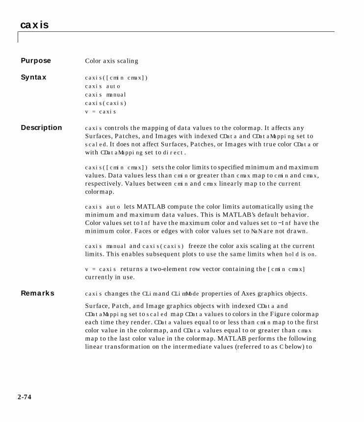
caxis

2caxisPurpose Color axis scaling

Syntax caxis([cmin cmax])caxis autocaxis manualcaxis(caxis)v = caxis

Description caxis controls the mapping of data values to the colormap. It affects anySurfaces, Patches, and Images with indexed CData and CDataMapping set toscaled. It does not affect Surfaces, Patches, or Images with true color CData orwith CDataMapping set to direct.

caxis([cmin cmax]) sets the color limits to specified minimum and maximumvalues. Data values less than cmin or greater than cmax map to cmin and cmax,respectively. Values between cmin and cmax linearly map to the currentcolormap.

caxis auto lets MATLAB compute the color limits automatically using theminimum and maximum data values. This is MATLAB’s default behavior.Color values set to Inf have the maximum color and values set to −Inf have theminimum color. Faces or edges with color values set to NaN are not drawn.

caxis manual and caxis(caxis) freeze the color axis scaling at the currentlimits. This enables subsequent plots to use the same limits when hold is on.

v = caxis returns a two-element row vector containing the [cmin cmax]currently in use.

Remarks caxis changes the CLim and CLimMode properties of Axes graphics objects.

Surface, Patch, and Image graphics objects with indexed CData andCDataMapping set to scaled map CData values to colors in the Figure colormapeach time they render. CData values equal to or less than cmin map to the firstcolor value in the colormap, and CData values equal to or greater than cmaxmap to the last color value in the colormap. MATLAB performs the followinglinear transformation on the intermediate values (referred to as C below) to

2-74

caxis

map them to an entry in the colormap (whose length is m, and whose row indexis referred to as index below):

index = fix((C–cmin)/(cmax–cmin)∗m)+1

Examples Create (X,Y,Z) data for a sphere and view the data as a Surface:

[X,Y,Z] = sphere;C = Z;surf(X,Y,Z,C)

Values of C have the range [−1 1]. Values of C near −1 are assigned the lowestvalues in the colormap; values of C near 1 are assigned the highest values inthe colormap.

To map the top half of the surface to the highest value in the color table, set :

caxis([−1 0])

To use only the bottom half of the color table, enter

caxis([−1 3])

which maps the lowest CData values to the bottom of the colormap, and thehighest values to the middle of the colormap (by specifying a cmax whose valueis equal to cmin plus twice the range of the CData).

The command

caxis auto

resets axis scaling back to auto-ranging and you see all the colors in theSurface. In this case, entering

caxis

returns

[–1 1]

Adjusting the color axis can be useful when using images with scaled colordata. For example, load the image data and colormap for Cape Code,Massachusetts:

load cape

2-75

caxis

This command loads the images data X and the image’s colormap map into theworkspace. Now display the image with CDataMapping set to scaled and installthe image’s colormap:

image(X,'CDataMapping','scaled')colormap(map)

MATLAB sets the color limits to span the range of the image data, which is 1to 192:

caxisans =

1 192

2-76

caxis

The blue color of the ocean is the first color in the colormap and is mapped tothe lowest data value (1). We can effectively move sealevel by changing thelower color limit value. For example:

See Also axes, axis, colormap, get, mesh, pcolor, set, surf

The CLim and CLimMode properties of Axes graphics objects.

The Colormap property of Figure graphics objects.

The Axes chapter in the Using MATLAB Graphics manual.

Caxis = [1 192]

100 200 300

50

100

150

200

250

300

Caxis = [3 192]

100 200 300

50

100

150

200

250

300

Caxis = [5 192]

100 200 300

50

100

150

200

250

300

Caxis = [6 192]

100 200 300

50

100

150

200

250

300

2-77

cla

2claPurpose Clear current Axes

Syntax clacla reset

Description cla deletes from the current Axes all graphics objects whose handles are nothidden (i.e., their HandleVisibility property is set to on).

cla reset deletes from the current Axes all graphics objects regardless of thesetting of their HandleVisibility property and resets all Axes properties,except Position and Units, to their default values.

Remarks The cla command behaves the same way when issued on the command line asit does in callback routines – it does not recognize the HandleVisibilitysetting of callback. This means that when issued from within a callbackroutine, cla deletes only those objects whose HandleVisibility property is setto on.

See Also clf, hold, newplot, reset

2-78

clabel

2clabelPurpose Contour plot elevation labels

Syntax clabel(C,h)clabel(C,h,v)clabel(C,h,'manual')

clabel(C)clabel(C,v)clabel(C,'manual')

Description The clabel function adds height labels to a two-dimensional contour plot.

clabel(C,h) rotates the labels and inserts them in the contour lines. Thefunction inserts only those labels that fit within the contour, due to the size ofthe contour.

clabel(C,h,v) creates labels only for those contour levels given in vector v,then rotates the labels and inserts them in the contour lines.

clabel(C,h,'manual') places contour labels at locations you select with amouse. Press the left mouse button (the mouse button on a single-buttonmouse) or the space bar to label a contour at the closest location beneath thecenter of the cursor. Press the Return key while the cursor is within the Figurewindow to terminate labeling. The labels are rotated and inserted in thecontour lines.

clabel(C) adds labels to the current contour plot using the contour structureC output from contour. The function labels all contours displayed andrandomly selects label positions.

clabel(C,v) labels only those contour levels given in vector v.

clabel(C,'manual') places contour labels at locations you select with amouse.

Remarks When the syntax includes the argument h, this function rotates the labels andinserts them in the contour lines (see Example). Otherwise, the labels aredisplayed upright and a '+' indicates which contour line the label isannotating.

2-79

clabel

Examples Generate, draw, and label a simple contour plot:

[x,y] = meshgrid(–2:.2:2);z = x.^exp(–x.^2–y.^2);[C,h] = contour(x,y,z);clabel(C,h);

See Also contour, contourc, contourf

−2 −1.5 −1 −0.5 0 0.5 1 1.5 2−2

−1.5

−1

−0.5

0

0.5

1

1.5

2

−0.2

−0.2

−9.869e−

17

−9.869e−17

0.2

0.2

0.2

0.2

0.2

0.4

0.4

0.4

0.4

0.60.

6

0.6

0.6

0.6

0.8

0.8

0.8

0.8

0.8

1

1

11

2-80

clc

2clcPurpose Clear command window

Syntax clc

Description clc clears the command window.

Examples Display a sequence of random matrices at the same location in the commandwindow:

clcfor i =1:25

homeA = rand(5)

end

See Also clf, home

2-81

clf

2clfPurpose Clear current Figure window

Syntax clfclf reset

Description clf deletes from the current Figure all graphics objects whose handles are nothidden (i.e., their HandleVisibility property is set to on).

clf reset deletes from the current Figure all graphics objects regardless ofthe setting of their HandleVisibility property and resets all Figureproperties, except Position, Units, PaperPosition, and PaperUnits to theirdefault values.

Remarks The clf command behaves the same way when issued on the command line asit does in callback routines – it does not recognize the HandleVisibilitysetting of callback. This means that when issued from within a callbackroutine, clf deletes only those objects whose HandleVisibility property is setto on.

See Also cla, clc, hold, reset

2-82

close

2closePurpose Delete specified Figure

Syntax closeclose(h)close nameclose allclose all hiddenstatus = close(...)

Description close deletes the current Figure or the specified Figure(s). It optionallyreturns the status of the close operation.

close deletes the current Figure (equivalent to close(gcf)).

close(h) deletes the Figure identified by h. If h is a vector or matrix, closedeletes all Figures identified by h.

close name deletes the Figure with the specified name.

close all deletes all Figures whose handles are not hidden.

close all hidden deletes all figures including those with hidden handles.

status = close(...) returns 1 if the specified windows have been deletedand 0 otherwise.

Remarks The close function works by evaluating the specified Figure’sCloseRequestFcn property with the statement:

eval(get(h,'CloseRequestFcn'))

The default CloseRequestFcn, closereq, deletes the current Figure usingdelete(get(0,'CurrentFigure')). If you specify multiple Figure handles,close executes each Figure’s CloseRequestFcn in turn. If MATLABencounters an error that terminates the execution of a CloseRequestFcn, theFigure is not deleted. Note that using your computer’s window manager (i.e.,the Close menu item) also calls the Figure’s CloseRequestFcn.

If a Figure’s handle is hidden (i.e., the Figure’s HandleVisibility property isset to callback or off and the Root ShowHiddenHandles property is set no),

2-83

close

you must specify the hidden option when trying to access a Figure using theall option.

To unconditionally delete all Figures, use the statements:

set(0,'ShowHiddenHandles','on')delete(get(0,'Children'))

The delete function does not execute the Figure’s CloseRequestFcn; it simplydeletes the specified Figure.

The Figure CloseRequestFcn allows you to either delay or abort the closing ofa Figure once the close function has been issued. For example, you can displaya dialog box to see if the user really wants to delete the Figure or save andcleanup before closing.

See Also delete, figure, gcf

The Figure HandleVisibility property

The Root ShowHiddenHandles property

2-84

colorbar

2colorbarPurpose Display colorbar showing the color scale

Syntax colorbarcolorbar('vert')colorbar('horiz')colorbar(h)h = colorbar(...)

Description The colorbar function displays the current colormap in the current Figure andresizes the current Axes to accommodate the colorbar.

colorbar updates the most recently created colorbar or, when the currentAxes does not have a colorbar, colorbar adds a new vertical colorbar.

colorbar('vert') adds a vertical colorbar to the current Axes.

colorbar('horiz') adds a horizontal colorbar to the current Axes.

colorbar(h) places a colorbar in the Axes identified by h. The colorbar ishorizontal if the width of the Axes is greater than its height, as determined bythe Axes Position property.

h = colorbar(...) returns a handle to the colorbar, which is an Axesgraphics object.

Remarks colorbar works with two-dimensional and three-dimensional plots.

2-85

colorbar

Examples Display a colorbar beside the Axes:

surf(peaks(30))colormap coolcolorbar

See Also colormap

05

1015

2025

30

0

5

10

15

20

25

30−8

−6

−4

−2

0

2

4

6

8

10

−6

−4

−2

0

2

4

6

8

2-86

colordef

2colordefPurpose Sets default property values to display different color schemes

Syntax colordef whitecolordef blackcolordef nonecolordef(fig,color_option)h = colordef('new',color_option)

Description colordef enables you to select either a white or black background for graphicsdisplay. It sets axis lines and labels to show up against the background color.

colordef white sets the axis background color to white, the axis lines andlabels to black, and the Figure background color to light gray.

colordef black sets the axis background color to black, the axis lines andlabels to white, and the Figure background color to dark gray.

colordef none sets the Figure coloring to that used by MATLAB Version 4(essentially a black background).

colordef(fig,color_option) sets the color scheme of the Figure identifiedby the handle fig to the color option 'white', 'black', or 'none'.

h = colordef('new',color_option) returns the handle to a new Figurecreated with the specified color options (i.e., 'white', 'black', or 'none').

Remarks colordef affects only subsequently drawn Figures, not those currently on thedisplay. This is because colordef works by setting default property values (onthe Root or Figure level). You can list the currently set default values on theRoot level with the statement:

get(0,'defaults')

You can remove all default values using the reset command:

reset(0)

See the get and reset references pages for more information.

See Also whitebg

2-87

colormap

2colormapPurpose Set and get the current colormap

Syntax colormap(map)colormap('default')cmap = colormap

Description A colormap is an m-by-3 matrix of real numbers between 0.0 and 1.0. Each rowis an RGB vector that defines one color. The kth row of the colormap defines thek-th color, where map(k,:) = [r(k) g(k) b(k)]) specifies the intensity of red,green, and blue.

colormap(map) sets the colormap to the matrix map. If any values in map areoutside the interval [0 1], MATLAB returns the error: Colormap must havevalues in [0,1].

colormap('default') sets the current colormap to the default colormap.

cmap = colormap; retrieves the current colormap. The values returned are inthe interval [0 1].

Specifying ColormapsM-files in the color directory generate a number of colormaps. Each M-fileaccepts the colormap size as an argument. For example,

colormap(hsv(128))

creates an hsv colormap with 128 colors. If you do not specify a size, MATLABcreates a colormap the same size as the current colormap.

Supported ColormapsMATLAB supports a number of colormaps.

• autumn varies smoothly from red, through orange, to yellow.

• bone is a grayscale colormap with a higher value for the blue component.This colormap is useful for adding an “electronic” look to grayscale images.

• colorcube contains as many regularly spaced colors in RGB colorspace aspossible, while attempting to provide more steps of gray, pure red, puregreen, and pure blue.

2-88

colormap

• cool consists of colors that are shades of cyan and magenta. It variessmoothly from cyan to magenta.

• copper varies smoothly from black to bright copper.

• flag consists of the colors red, white, blue, and black. This colormapcompletely changes color with each index increment.

• gray returns a linear grayscale colormap.

• hot varies smoothly from black, through shades of red, orange, and yellow,to white.

• hsv varies the hue component of the hue-saturation-value color model. Thecolors begin with red, pass through yellow, green, cyan, blue, magenta, andreturn to red. The colormap is particularly appropriate for displayingperiodic functions. hsv(m) is the same as hsv2rgb([h ones(m,2)]) where his the linear ramp, h = (0:m–1)'/m.

• jet ranges from blue to red, and passes through the colors cyan, yellow, andorange. It is a variation of the hsv colormap. The jet colormap is associatedwith an astrophysical fluid jet simulation from the National Center forSupercomputer Applications. See the “Examples” section.

• lines produces a colormap of colors specified by the Axes ColorOrderproperty and a shade of gray.

• pink contains pastel shades of pink. The pink colormap provides sepia tonecolorization of grayscale photographs.

• prism repeats the six colors red, orange, yellow, green, blue, and violet.

• spring consists of colors that are shades of magenta and yellow.

• summer consists of colors that are shades of green and yellow.

• white is an all white monochrome colormap.

• winter consists of colors that are shades of blue and green.

Examples The Images and colormaps demo, imagedemo, provides an introduction tocolormaps. Select Color Spiral from the menu (starts automatically on theMacintosh). This uses the pcolor function to display a 16-by-16 matrix whoseelements vary from 0 to 255 in a rectilinear spiral. The hsv colormap startswith red in the center, then passes through yellow, green, cyan, blue, andmagenta before returning to red at the outside end of the spiral. SelectingColormap Menu gives access to a number of other colormaps (except on theMacintosh).

2-89

colormap

The rgbplot function plots colormap values. Try rgbplot(hsv),rgbplot(gray), and rgbplot(hot).

The following commands display the flujet data using the jet colormap:

load flujetimage(X)colormap(jet)

2-90

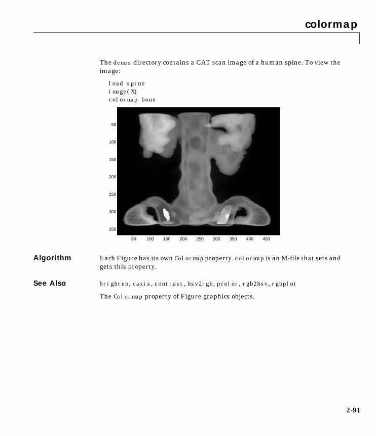
colormap

The demos directory contains a CAT scan image of a human spine. To view theimage:

load spineimage(X)colormap bone

Algorithm Each Figure has its own Colormap property. colormap is an M-file that sets andgets this property.

See Also brighten, caxis, contrast, hsv2rgb, pcolor, rgb2hsv, rgbplot

The Colormap property of Figure graphics objects.

50 100 150 200 250 300 350 400 450

50

100

150

200

250

300

350

2-91

ColorSpec

2ColorSpecPurpose Color specification

Description ColorSpec is not a command; it refers to the three ways in which you specifycolor in MATLAB:

• RGB triple

• Short name

• Long name

The short names and long names are MATLAB strings that specify one of eightpredefined colors. The RGB triple is a three-element row vector whose elementsspecify the intensities of the red, green, and blue components of the color; theintensities must be in the range [0 1]. The following table lists the predefinedcolors and their RGB equivalents.

Remarks The eight predefined colors and any colors you specify as RGB values are notpart of a Figure’s colormap, nor are they affected by changes to the Figure’scolormap. They are referred to as fixed colors, as opposed to colormap colors.

RGB Value Short Name Long Name

[1 1 0] y yellow

[1 0 1] m magenta

[0 1 1] c cyan

[1 0 0] r red

[0 1 0] g green

[0 0 1] b blue

[1 1 1] w white

[0 0 0] k black

2-92

ColorSpec

Examples To change the background color of a Figure to green, specify the color with ashort name, a long name, or an RGB triple. These statements generateequivalent results:

whitebg('g')whitebg('green')whitebg([0 1 0]);

You can use ColorSpec anywhere you need to define a color. For example, thisstatement changes the Figure background color to pink:

set(gcf,'Color',[1 .4 .6])

See Also bar, bar3, colordef, colormap, fill, fill3, whitebg

2-93

comet

2cometPurpose Two-dimensional comet plot

Syntax comet(y)comet(x,y)comet(x,y,p)

Description A comet plot is an animated graph in which a circle (the comet head) traces thedata points on the screen. The comet body is a trailing segment that follows thehead. The tail is a solid line that traces the entire function.

comet(y) displays a comet plot of the vector y.

comet(x,y) displays a comet plot of vector y versus vector x.

comet(x,y,p) specifies a comet body of length p∗length(y). p defaults to 0.1.

Remarks Note that the trace left by comet is created by using an EraseMode of none,which means you cannot print the plot (you get only the comet head) and itdisappears if you cause a redraw (e.g., by resizing the window).

Examples Create a simple comet plot:

t = 0:.01:2∗pi;x = cos(2∗t).∗(cos(t).^2);y = sin(2∗t).∗(sin(t).^2);comet(x,y);

See Also comet3

2-94

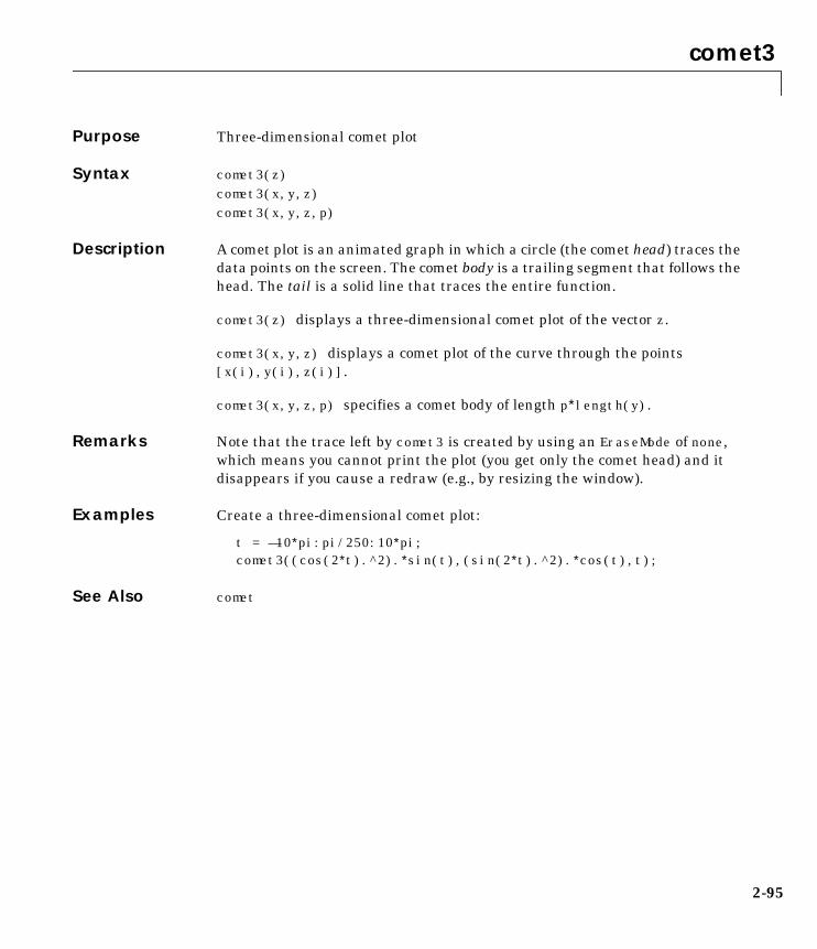
comet3

2comet3Purpose Three-dimensional comet plot

Syntax comet3(z)comet3(x,y,z)comet3(x,y,z,p)

Description A comet plot is an animated graph in which a circle (the comet head) traces thedata points on the screen. The comet body is a trailing segment that follows thehead. The tail is a solid line that traces the entire function.

comet3(z) displays a three-dimensional comet plot of the vector z.

comet3(x,y,z) displays a comet plot of the curve through the points[x(i),y(i),z(i)].

comet3(x,y,z,p) specifies a comet body of length p∗length(y).

Remarks Note that the trace left by comet3 is created by using an EraseMode of none,which means you cannot print the plot (you get only the comet head) and itdisappears if you cause a redraw (e.g., by resizing the window).

Examples Create a three-dimensional comet plot:

t = —10∗pi:pi/250:10∗pi;comet3((cos(2∗t).^2).∗sin(t),(sin(2∗t).^2).∗cos(t),t);

See Also comet

2-95

compass

2compassPurpose Plot arrows emanating from the origin

Syntax compass(X,Y)compass(Z)compass(...,LineSpec)h = compass(...)

Description A compass plot displays direction or velocity vectors as arrows emanating fromthe origin. X, Y, and Z are in Cartesian coordinates and plotted on a circulargrid.

compass(X,Y) displays a compass plot having n arrows, where n is the numberof elements in X or Y. The location of the base of each arrow is the origin. Thelocation of the tip of each arrow is a point relative to the base and determinedby [X(i),Y(i)].

compass(Z) displays a compass plot having n arrows, where n is the numberof elements in Z. The location of the base of each arrow is the origin. Thelocation of the tip of each arrow is relative to the base as determined by the realand imaginary components of Z. This syntax is equivalent tocompass(real(Z),imag(Z)).

compass(...,LineSpec) draws a compass plot using the line type, markersymbol, and color specified by LineSpec.

h = compass(...) returns handles to Line objects.

Examples Draw a compass plot of the eigenvalues of a matrix:

Z = eig(randn(20,20));compass(Z)

2-96

compass

See Also feather, LineSpec, rose

1.0538

2.1076

3.1613

4.2151

5.2689

30

210

60

240

90

270

120

300

150

330

180 0

2-97

contour

2contourPurpose Two-dimensional contour plot

Syntax contour(Z)contour(Z,n)contour(Z,v)contour(X,Y,Z)contour(X,Y,Z,n)contour(X,Y,Z,v)contour(...,LineSpec)[C,h] = contour(...)

Description A contour plot displays isolines of matrix Z. Label the contour lines usingclabel.

contour(Z) draws a contour plot of matrix Z, where Z is interpreted as heightswith respect to the x-y plane. Z must be at least a 2-by-2 matrix. The numberof contour levels and the values of the contour levels are chosen automaticallybased on the minimum and maximum values of Z. The ranges of the x- andy-axis are [1:n] and [1:m], where [m,n] = size(Z).

contour(Z,n) draws a contour plot of matrix Z with n contour levels.

contour(Z,v) draws a contour plot of matrix Z with contour lines at the datavalues specified in vector v. The number of contour levels is equal to length(v).To draw a single contour of level i, use contour(Z,[i i]).

contour(X,Y,Z), contour(X,Y,Z,n), and contour(X,Y,Z,v) draw contourplots of Z. X and Y specify the x- and y-axis limits. When X and Y are matrices,they must be the same size as Z, in which case they specify a surface as surfdoes.

contour(...,LineSpec) draws the contours using the line type and colorspecified by LineSpec. contour ignores marker symbols.

[C,h] = contour(...) returns the contour matrix C (see contourc) and avector of handles to graphics objects. clabel uses the contour matrix C to createthe labels. contour creates Patch graphics objects unless you specify LineSpec,in which case contour creates Line graphics objects.

2-98

contour

Remarks If you do not specify LineSpec, colormap and caxis control the color.

If X or Y is irregularly spaced, contour calculates contours using a regularlyspaced contour grid, then transforms the data to X or Y.

Examples To view a contour plot of the function

over the range –2 ≤ x ≤ 2, –2 ≤ y ≤ 3, create matrix Z using the statements

[X,Y] = meshgrid(–2:.2:2,–2:.2:3);Z = X.∗exp(–X.^2–Y.^2);

Then, generate a contour plot of Z:

[C,h] = contour(X,Y,Z);clabel(C,h)colormap cool

z xe x2 y2––( )=

−2 −1.5 −1 −0.5 0 0.5 1 1.5 2−2

−1.5

−1

−0.5

0

0.5

1

1.5

2

2.5

3

−0.3

−0.2

−0.2

−0.1

−0.1

−0.1

0 0

0.1

0.1

0.1

0.2

0.2

0.3

0.4

2-99

contour

View the same function over the same range with 20 evenly spaced contourlines and colored with the default colormap jet:

contour(X,Y,Z,20)

Use interp2 and contour to create smoother contours:

Z = magic(4);[C,h] = contour(interp2(Z,4));clabel(C,h)

−2 −1.5 −1 −0.5 0 0.5 1 1.5 2−2

−1.5

−1

−0.5

0

0.5

1

1.5

2

2.5

3

2-100

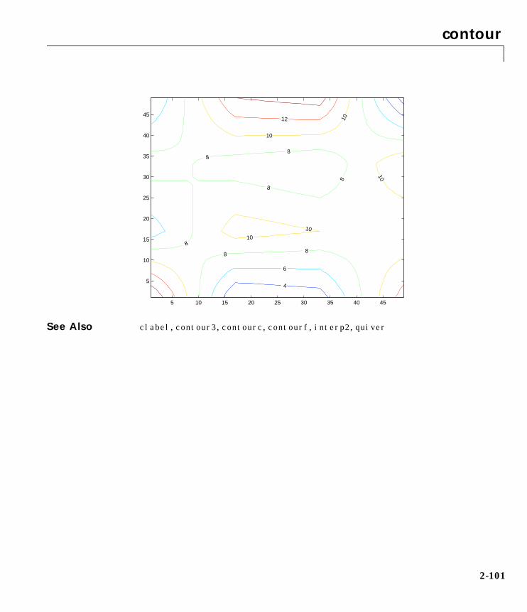
contour

See Also clabel, contour3, contourc, contourf, interp2, quiver

5 10 15 20 25 30 35 40 45

5

10

15

20

25

30

35

40

45

4

6

8 8

8

8

8

8 8

10

10

10

10

10

12

2-101

contour3

2contour3Purpose Three-dimensional contour plot

Syntax contour3(Z)contour3(Z,n)contour3(Z,v)contour3(X,Y,Z)contour3(X,Y,Z,n)contour3(X,Y,Z,v)contour3(...,LineSpec)[C,h] = contour3(...)

Description contour3 creates a three-dimensional contour plot of a surface defined on arectangular grid.

contour3(Z) draws a contour plot of matrix Z in a three-dimensional view. Zis interpreted as heights with respect to the x-y plane. Z must be at least a2-by-2 matrix. The number of contour levels and the values of contour levelsare chosen automatically. The ranges of the x- and y-axis are [1:n] and [1:m],where [m,n] = size(Z).

contour3(Z,n) draws a contour plot of matrix Z with n contour levels in athree-dimensional view.

contour3(Z,v) draws a contour plot of matrix Z with contour lines at thevalues specified in vector v. The number of contour levels is equal to length(v).To draw a single contour of level i, use contour(Z,[i i]).

contour3(X,Y,Z), contour3(X,Y,Z,n), and contour3(X,Y,Z,v) use X and Yto define the x- and y-axis limits. If X is a matrix, X(1,:) defines the x-axis. IfY is a matrix, Y(:,1) defines the y-axis. When X and Y are matrices, they mustbe the same size as Z, in which case they specify a surface as surf does.

contour3(...,LineSpec) draws the contours using the line type and colorspecified by LineSpec.

[C,h] = contour3(...) returns the contour matrix C as described in thefunction contourc and a column vector containing handles to graphics objects.contour3 creates Patch graphics objects unless you specify LineSpec, in whichcase contour3 creates Line graphics objects.

2-102

contour3

Remarks If you do not specify LineSpec, colormap and caxis control the color.

If X or Y is irregularly spaced, contour3 calculates contours using a regularlyspaced contour grid, then transforms the data to X or Y.

Examples Plot the three-dimensional contour of a function and superimpose a surfaceplot to enhance visualization of the function:

[X,Y] = meshgrid([-2:.25:2]);Z = X.*exp(-X.^2-Y.^2);contour3(X,Y,Z,30)surface(X,Y,Z,’EdgeColor’,[.8 .8 .8],’FaceColor’,’none’)grid offview(-15,25)colormap cool

See Also contour, contourc, meshc, meshgrid, surfc

−2 −1.5 −1 −0.5 0 0.5 1 1.5 2

−2

−1

0

1

2

−0.5

0

0.5

2-103

contourc

2contourcPurpose Low-level contour plot computation

Syntax C = contourc(Z)C = contourc(Z,n)C = contourc(Z,v)C = contourc(x,y,Z)C = contourc(x,y,Z,n)C = contourc(x,y,Z,v)

Description contourc calculates the contour matrix C used by contour, contour3, andcontourf. The values in Z determine the heights of the contour lines withrespect to a plane. The contour calculations use a regularly spaced griddetermined by the dimensions of Z.

C = contourc(Z) computes the contour matrix from data in matrix Z, whereZ must be at least a 2-by-2 matrix. The contours are isolines in the units of Z.The number of contour lines and the corresponding values of the contour linesare chosen automatically.

C = contourc(Z,n) computes contours of matrix Z with n contour levels.

C = contourc(Z,v) computes contours of matrix Z with contour lines at thevalues specified in vector v. The length of v determines the number of contourlevels. To compute a single contour of level i, use contourc(Z,[i i]).

C = contourc(x,y,Z), C = contourc(x,y,Z,n), andC = contourc(x,y,Z,v) compute contours of Z using vectors x and y todetermine the x- and y-axis limits. x and y must be monotonically increasing.

Remarks C is a two-row matrix specifying all the contour lines. Each contour line definedin matrix C begins with a column that contains the value of the contour(specified by v and used by clabel), and the number of (x,y) vertices in thecontour line. The remaining columns contain the data for the (x,y)pairs.

C = [value1 xdata(1) xdata(2)...value2 xdata(1) xdata(2)...;dim1 ydata(1) ydata(2)...dim2 ydata(1) ydata(2)...]

Specifying irregularly spaced x and y vectors is not the same as contouringirregularly spaced data. If x or y is irregularly spaced, contourc calculates

2-104

contourc

contours using a regularly spaced contour grid, then transforms the data to xor y.

See Also clabel, contour, contour3, contourf

2-105

contourf

2contourfPurpose Filled two-dimensional contour plot

Syntax contourf(Z)contourf(Z,n)contourf(Z,v)contourf(X,Y,Z)contourf(X,Y,Z,n)contourf(X,Y,Z,v)[C,h,CF] = contourf(...)

Description A filled contour plot displays isolines calculated from matrix Z and fills theareas between the isolines using constant colors. The color of the filled areasdepends on the current Figure’s colormap.

contourf(Z) draws a contour plot of matrix Z, where Z is interpreted asheights with respect to a plane. Z must be at least a 2-by-2 matrix. The numberof contour lines and the values of the contour lines are chosen automatically.

contourf(Z,n) draws a contour plot of matrix Z with n contour levels.

contourf(Z,v) draws a contour plot of matrix Z with contour levels at thevalues specified in vector v.

contourf(X,Y,Z), contourf(X,Y,Z,n), and contourf(X,Y,Z,v) producecontour plots of Z using X and Y to determine the x- and y-axis limits. When Xand Y are matrices, they must be the same size as Z, in which case they specifya surface as surf does.

[C,h,CF] = contourf(...) returns the contour matrix C as calculated by thefunction contourc and used by clabel, a vector of handles h to Patch graphicsobjects, and a contour matrix CF for the filled areas.

Remarks If X or Y is irregularly spaced, contourf calculates contours using a regularlyspaced contour grid, then transforms the data to X or Y.

2-106

contourf

Examples Create a filled contour plot of the peaks function:

[C,h] = contourf(peaks(20),10);colormap autumn

See Also clabel, contour, contour3, contourc, quiver

2 4 6 8 10 12 14 16 18 20

2

4

6

8

10

12

14

16

18

20

2-107

contrast

2contrastPurpose Grayscale colormap for contrast enhancement

Syntax cmap = contrast(X)cmap = contrast(X,m)

Description The contrast function enhances the contrast of an image. It creates a new graycolormap, cmap, that has an approximately equal intensity distribution. Allthree elements in each row are identical.

cmap = contrast(X) returns a gray colormap that is the same length as thecurrent colormap.

cmap = contrast(X,m) returns an m-by-3 gray colormap.

Examples Add contrast to the clown image defined by X:

load clown;cmap = contrast(X);image(X);colormap(cmap);

See Also brighten, colormap, image

2-108

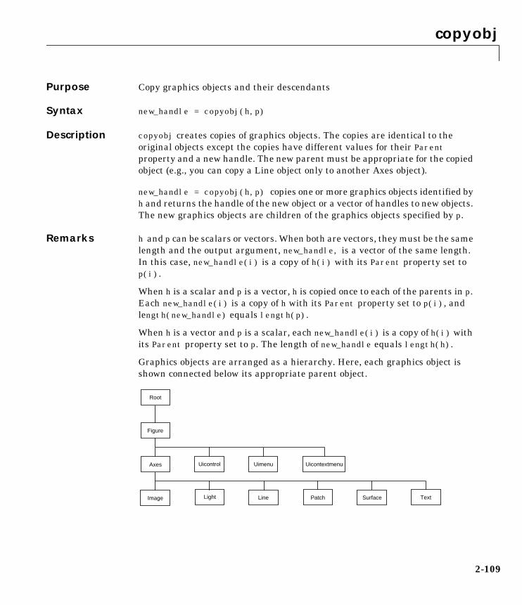
copyobj

2copyobjPurpose Copy graphics objects and their descendants

Syntax new_handle = copyobj(h,p)

Description copyobj creates copies of graphics objects. The copies are identical to theoriginal objects except the copies have different values for their Parentproperty and a new handle. The new parent must be appropriate for the copiedobject (e.g., you can copy a Line object only to another Axes object).

new_handle = copyobj(h,p) copies one or more graphics objects identified byh and returns the handle of the new object or a vector of handles to new objects.The new graphics objects are children of the graphics objects specified by p.

Remarks h and p can be scalars or vectors. When both are vectors, they must be the samelength and the output argument, new_handle, is a vector of the same length.In this case, new_handle(i) is a copy of h(i) with its Parent property set top(i).

When h is a scalar and p is a vector, h is copied once to each of the parents in p.Each new_handle(i) is a copy of h with its Parent property set to p(i), andlength(new_handle) equals length(p).

When h is a vector and p is a scalar, each new_handle(i) is a copy of h(i) withits Parent property set to p. The length of new_handle equals length(h).

Graphics objects are arranged as a hierarchy. Here, each graphics object isshown connected below its appropriate parent object.

Patch

Root

Text

Uimenu

SurfaceLine

Axes Uicontrol

Image

Figure

Uicontextmenu

Light

2-109

copyobj

Examples Copy a Surface to a new Axes within a different Figure:

h = surf(peaks);colormap hotfigure % Create a new Figureaxes % Create an Axes object in the Figurenew_handle = copyobj(h,gca);colormap hotview(3)grid on

Note that while the Surface is copied, the colormap (Figure property), view,and grid (Axes properties) are not copies.

See Also findobj, gcf, gca, gco, get, set

Parent property for all graphics objects

2-110

cylinder

2cylinderPurpose Generate cylinder

Syntax [X,Y,Z] = cylinder[X,Y,Z] = cylinder(r)[X,Y,Z] = cylinder(r,n)cylinder(...)

Description cylinder generates x, y, and z coordinates of a unit cylinder. You can draw thecylindrical object using surf or mesh, or draw it immediately by not providingoutput arguments.

[X,Y,Z] = cylinder returns the x, y, and z coordinates of a cylinder with aradius equal to 1. The cylinder has 20 equally spaced points around itscircumference.

[X,Y,Z] = cylinder(r) returns the x, y, and z coordinates of a cylinder usingr to define a profile curve. cylinder treats each element in r as a radius atequally spaced heights along the unit height of the cylinder. The cylinder has20 equally spaced points around its circumference.

[X,Y,Z] = cylinder(r,n) returns the x, y, and z coordinates of a cylinderbased on the profile curve defined by vector r. The cylinder has n equallyspaced points around its circumference.

cylinder(...), with no output arguments, plots the cylinder using surf.

Remarks cylinder treats its first argument as a profile curve. The resulting Surfacegraphics object is generated by rotating the curve about the x-axis, and thenaligning it with the z-axis.

2-111

cylinder

Examples Create a cylinder with randomly colored faces.

cylinderaxis squareh = findobj('Type','surface');set(h,'CData',rand(size(get(h,'CData'))))

Generate a cylinder defined by the profile function 2+sin(t):

t = 0:pi/10:2*pi;[X,Y,Z] = cylinder(2+cos(t));surf(X,Y,Z)axis square

−1

−0.5

0

0.5

1

−1

−0.5

0

0.5

10

0.2

0.4

0.6

0.8

1

2-112

cylinder

See Also sphere, surf

−4

−2

0

2

4

−4

−2

0

2

40

0.2

0.4

0.6

0.8

1

2-113

cylinder

2-114

daspect

2daspectPurpose Set or query the axes data aspect ratio

Syntax daspectdaspect([aspect_ratio])daspect('mode')daspect('auto')daspect('manual')daspect(axes_handle,...)

Description The data aspect ratio determines the relative scaling of the data units along thex-, y-, and z-axes.

daspect with no arguments returns the data aspect ratio of the current axes.

daspect([aspect_ratio]) sets the data aspect ratio in the current axes to thespecified value. Specify the aspect ratio as three relative values representingthe ratio of the x-, y-, and z-axis scaling (e.g., [1 1 3] means one unit in x isequal in length to one unit in y and three unit in z).

daspect('mode') returns the current value of the data aspect ratio mode,which can be either auto (the default) or manual. See Remarks.

daspect('auto') sets the data aspect ratio mode to auto.

daspect('manual') sets the data aspect ratio mode to manual.

daspect(axes_handle,...) performs the set or query on the axes identifiedby the first argument, axes_handle. When you do not specify an axes handle,daspect operates on the current axes.

Remarks daspect sets or queries values of the Axes object DataAspectRatio andDataAspectRatioMode properties.

When the data aspect ratio mode is auto, MATLAB adjusts the data aspectratio so that each axis spans the space available in the Figure window. If youare displaying a representation of a real-life object, you should set the dataaspect ratio to [1 1 1] to produce the correct proportions.

Setting a value for data aspect ratio or setting the data aspect ratio mode tomanual disables MATLAB’s stretch-to-fill feature (stretching of the axes to fit

2-115

daspect

the window). This means setting the data aspect ratio to a value, including itscurrent value,

daspect(daspect)

can cause a change in the way the graphs look. See the Remarks section of theaxes function description and the “Aspect Ratio” section in the Using MATLABGraphics manual for more information.

Examples The following surface plot of the function is useful to illustratethe data aspect ratio. First plot the function over the range –2 ≤ x ≤ 2, –2 ≤ y ≤ 2,

[x,y] = meshgrid([-2:.2:2]);z = x.*exp(-x.^2 - y.^2);surf(x,y,z)

Querying the data aspect ratio shows how MATLAB has drawn the surface:

daspectans =

4 4 1

z xe x2 y2––( )=

−2−1

01

2

−2

−1

0

1

2−0.5

0

0.5

2-116

daspect

Setting the data aspect ratio to [1 1 1] produces a surface plot with equalscaling alone each axis:

daspect([1 1 1])

See Also axis, pbaspect, xlim, ylim, zlim

The Axes properties DataAspectRatio, PlotBoxAspectRatio, XLim, YLim, ZLim

The “Aspect Ratio” section in the Using MATLAB Graphics manual.

−2

−1

0

1

2

−2

−1.5

−1

−0.5

0

0.5

1

1.5

2−0.5

0

0.5

2-117

datetick

2datetickPurpose Label tick lines using dates

Syntax datetick(tickaxis)datetick(tickaxis,dateform)

Description datetick(tickaxis) labels the tick lines of an axis using dates, replacing thedefault numeric labels. tickaxis is the string 'x', 'y', or 'z'. The default is'x'. datetick selects a label format based on the minimum and maximumlimits of the specified axis.

datetick(tickaxis,dateform) formats the labels according to the integerdateform (see table). To produce correct results, the data for the specified axismust be serial date numbers (as produced by datenum).

Dateform Format Example

0 day-month-year hour:minute 01-Mar-1995 03:45

1 day-month-year 01-Mar-1995

2 month/day/year 03/01/95

3 month, three letters Mar

4 month, single letter M

5 month, numeral 3

6 month/day 03/01

7 day of month 1

8 day of week, three letters Wed

9 day of week, single letter W

10 year, four digit 1995

11 year, two digit 95

2-118

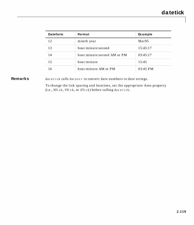
datetick

Remarks datetick calls datestr to convert date numbers to date strings.

To change the tick spacing and locations, set the appropriate Axes property(i.e., XTick, YTick, or ZTick) before calling datetick.

12 month year Mar95

13 hour:minute:second 15:45:17

14 hour:minute:second AM or PM 03:45:17

15 hour:minute 15:45

16 hour:minute AM or PM 03:45 PM

Dateform Format Example

2-119

datetick

Example Consider graphing population data based on the 1990 U.S. census:

t = (1900:10:1990)'; % Time intervalp = [75.995 91.972 105.711 123.203 131.669 ...

150.697 179.323 203.212 226.505 249.633]'; % Populationplot(datenum(t,1,1),p) % Convert years to date numbers and plotgrid ondatetick('x',11) % Replace x-axis ticks with 2-digit year labels

See Also The Axes properties XTick, YTick, and ZTick.

datenum, datestr

00 20 40 60 80 0060

80

100

120

140

160

180

200

220

240

260

2-120

default4

2default4Purpose MATLAB Version 4.0 Figure and Axes defaults

Syntax default4default4(h)

Description default4 sets Figure and Axes defaults to match MATLAB Version 4.0defaults.

default4(h) only affects the Figure with handle h.

See Also colordef

2-121

drawnow

2drawnowPurpose Complete pending drawing events

Syntax drawnow

Description drawnow flushes the event queue and updates the Figure window.

Remarks Other events that cause MATLAB to flush the event queue and draw theFigure windows include:

• Returning to the MATLAB prompt

• A pause statement

• A waitforbuttonpress statement

• A waitfor statement

• A getframe statement

• A figure statement

Examples Executing the statements,

x = –pi:pi/20:pi;plot(x,cos(x))drawnowtitle('A Short Title')grid on

as an M-file updates the current Figure after executing the drawnow functionand after executing the final statement.

See Also waitfor, pause, waitforbuttonpress

2-122

errorbar

2errorbarPurpose Plot error bars along a curve

Syntax errorbar(Y,E)errorbar(X,Y,E)errorbar(X,Y,L,U)errorbar(...,LineSpec)h = errorbar(...)

Description Error bars show the confidence level of data or the deviation along a curve.

errorbar(Y,E) plots Y and draws an error bar at each element of Y. The errorbar is a distance of E(i) above and below the curve so that each bar issymmetric and 2∗E(i) long.

errorbar(X,Y,E) plots X versus Y with symmetric error bars 2∗E(i) long. X, Y,E must be the same size. When they are vectors, each error bar is a distance ofE(i) above and below the point defined by (X(i),Y(i)). When they arematrices, each error bar is a distance of E(i,j) above and below the pointdefined by (X(i,j),Y(i,j)).

errorbar(X,Y,L,U) plots X versus Y with error bars L(i)+U(i) long specifyingthe lower and upper error bars. X, Y, L, and Umust be the same size. When theyare vectors, each error bar is a distance of L(i) below and U(i) above the pointdefined by (X(i),Y(i)). When they are matrices, each error bar is a distanceof L(i,j) below and U(i,j) above the point defined by (X(i,j),Y(i,j)).

errorbar(...,LineSpec) draws the error bars using the line type, markersymbol, and color specified by LineSpec.

h = errorbar(...) returns a vector of handles to Line graphics objects.

Remarks When the arguments are all matrices, errorbar draws one line per matrixcolumn. If X and Y are vectors, they specify one curve.

2-123

errorbar

Examples Draw symmetric error bars that are two standard deviation units in length:

X = 0:pi/10:pi;Y = sin(X);E = std(Y)*ones(size(X));errorbar(X,Y,E)

See Also LineSpec, plot, std

−0.5 0 0.5 1 1.5 2 2.5 3 3.5−0.4

−0.2

0

0.2

0.4

0.6

0.8

1

1.2

1.4

2-124

ezplot

2ezplotPurpose Easy to use function plotter.

Syntax ezplot(f)ezplot(f,[xmin xmax])ezplot(f,[xmin xmax],fig)

Description ezplot(f) plots a graph of f(x), where f is a symbolic expression representinga mathematical expression involving a single symbolic variable, say x. Thedomain on the x-axis is usually [–2*pi, 2*pi].

ezplot(f,[xmin xmax]) uses the specified x-domain instead of the default[–2*pi, 2*pi].

ezplot(f,[xmin xmax],fig) uses the specified Figure number instead of thecurrent Figure. It also omits the title of the graph.

Examples Either of the following commands,

ezplot('erf(x)')ezplot erf(x)

2-125

ezplot

plot a graph of the error function::

The statement,

ezplot('sin(x)',[0 2*pi])

creates the plot:

−2 −1.5 −1 −0.5 0 0.5 1 1.5 2

−1

−0.5

0

0.5

1

x

erf(x)

2-126

ezplot

Algorithm ezplot determines the interval of the x-axis by sampling the function between–2*pi and 2*pi and then selecting a subinterval where the variation issignificant. For the range of the y-axis, ezplot omits extreme values associatedwith singularities.

See Also fplot

0 1 2 3 4 5 6

−1

−0.5

0

0.5

1

x

sin(x)

2-127

feather

2featherPurpose Plot velocity vectors

Syntax feather(U,V)feather(Z)feather(...,LineSpec)

Description A feather plot displays vectors emanating from equally spaced points along ahorizontal axis. You express the vector components relative to the origin of therespective vector.

feather(U,V) displays the vectors specified by U and V, where U contains thex components as relative coordinates, and V contains the y components asrelative coordinates.

feather(Z) displays the vectors specified by the complex numbers in Z. Thisis equivalent to feather(real(Z),imag(Z)).

feather(...,LineSpec) draws a feather plot using the line type, markersymbol, and color specified by LineSpec.

Examples Create a feather plot showing the direction of theta:

theta = (–90:10:90)∗pi/180;r = 2∗ones(size(theta));[u,v] = pol2cart(theta,r);feather(u,v);

2-128

feather

See Also compass, LineSpec, rose

0 2 4 6 8 10 12 14 16 18 20−2

−1.5

−1

−0.5

0

0.5

1

1.5

2

2-129

figflag

2figflagPurpose Test if Figure is on screen

Syntax [flag] = figflag('figurename')[flag,fig] = figflag('figurename')[...] = figflag('figurename',silent)

Description Use figflag to determine if a particular Figure exists, bring a Figure to theforeground, or set the window focus to a Figure.

[flag] = figflag('figurename') returns a 1 if the Figure named'figurename' exists and pops the Figure to the foreground; otherwise thisfunction returns 0.

[flag,fig] = figflag('figurename') returns a 1 in flag, returns theFigure’s handle in fig, and pops the Figure to the foreground, if the Figurenamed 'figurename' exists. Otherwise this function returns 0.

[...] = figflag('figurename',silent) pops the Figure window to theforeground if silent is 0, and leaves the Figure in its current position if silentis 1.

Examples To determine if a Figure window named 'Fluid Jet Simulation' exists, type

[flag,fig] = figflag('Fluid Jet Simulation')

MATLAB returns:

flag =1

fig =1

If two Figures with handles 1 and 3 have the name 'Fluid Jet Simulation',MATLAB returns:

flag =1

fig =1 3

See Also figure

2-130

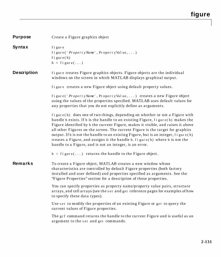
figure

2figurePurpose Create a Figure graphics object

Syntax figurefigure('PropertyName',PropertyValue,...)figure(h)h = figure(...)

Description figure creates Figure graphics objects. Figure objects are the individualwindows on the screen in which MATLAB displays graphical output.

figure creates a new Figure object using default property values.

figure('PropertyName',PropertyValue,...) creates a new Figure objectusing the values of the properties specified. MATLAB uses default values forany properties that you do not explicitly define as arguments.

figure(h) does one of two things, depending on whether or not a Figure withhandle h exists. If h is the handle to an existing Figure, figure(h) makes theFigure identified by h the current Figure, makes it visible, and raises it aboveall other Figures on the screen. The current Figure is the target for graphicsoutput. If h is not the handle to an existing Figure, but is an integer, figure(h)creates a Figure, and assigns it the handle h. figure(h) where h is not thehandle to a Figure, and is not an integer, is an error.

h = figure(...) returns the handle to the Figure object.

Remarks To create a Figure object, MATLAB creates a new window whosecharacteristics are controlled by default Figure properties (both factoryinstalled and user defined) and properties specified as arguments. See the“Figure Properties” section for a description of these properties.

You can specify properties as property name/property value pairs, structurearrays, and cell arrays (see the set and get reference pages for examples of howto specify these data types).

Use set to modify the properties of an existing Figure or get to query thecurrent values of Figure properties.

The gcf command returns the handle to the current Figure and is useful as anargument to the set and get commands.

2-131

figure

Example To create a Figure window that is one quarter the size of your screen and ispositioned in the upper-left corner, use the Root object’s ScreenSize propertyto determine the size. ScreenSize is a four-element vector: [left, bottom,width, height]:

scrsz = get(0,'ScreenSize');figure('Position',[1 scrsz(4)/2 scrsz(3)/2 scrsz(4)/2])

See Also axes, uicontrol, uimenu, close, clf, gcf, rootobject

ObjectHierarchy

Setting Default PropertiesYou can set default Figure properties only on the Root level:

set(0,'DefaultFigureProperty',PropertyValue...)

Where Property is the name of the Figure property and PropertyValue is thevalue you are specifying. Use set and get to access Figure properties.

Property List The following table lists all Figure properties and provides a brief descriptionof each. The property name links bring you an expanded description of theproperties.

Uimenu

Line

Axes Uicontrol

Image

Uicontextmenu


Root

Figure

2-132

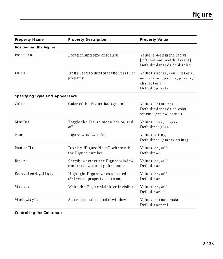
figure


Positioning the Figure

Position Location and size of Figure Value: a 4-element vector[left, bottom, width, height]Default: depends on display

Units Units used to interpret the Positionproperty

Values: inches, centimeters,normalized, points, pixels,charactersDefault: pixels

Specifying Style and Appearance

Color Color of the Figure background Values: ColorSpecDefault: depends on colorscheme (see colordef)

MenuBar Toggle the Figure menu bar on andoff

Values: none, figureDefault: figure

Name Figure window title Values: stringDefault: '' (empty string)

NumberTitle Display “Figure No. n”, where n isthe Figure number


Resize Specify whether the Figure windowcan be resized using the mouse


SelectionHighlight Highlight Figure when selected(Selected property set to on)


Visible Make the Figure visible or invisible Values: on, offDefault: on

WindowStyle Select normal or modal window Values: normal, modalDefault: normal

Controlling the Colormap

2-133

figure

Colormap The Figure colormap Values: m-by-3 matrix ofRGB valuesDefault: the jet colormap

Dithermap Colormap used for truecolor data onpseudocolor displays

Values: m-by-3 matrix ofRGB valuesDefault: colormap with fullrange of colors

DithermapMode Enable MATLAB-generateddithermap

Values: auto, manualDefault: manual

FixedColors Colors not obtained from colormap Values: m-by-3 matrix ofRGB values (read only)

MinColormap Minimum number of system colortable entries to use

Values: scalarDefault: 64

ShareColors Allow MATLAB to share systemcolor table slots

Values on, offDefault: on

Specifying the Renderer

BackingStore Enable off screen pixel buffering Values: on, offDefault: on

Renderer Rendering method used for screenand printing

Values: painters, zbuffer,OpenGLDefault: automatic selectionby MATLAB

General Information About the Figure

Children Handle of any Uicontrol, Uimenu,and Uicontextmenu objects displayedin the Figure


Parent The Root object is the parent of allFigures

Value: always 0


2-134

figure

Selected Indicate whether Figure is in a“selected” state.


Tag User-specified label Value: any stringDefault: '' (empty string)


Value: the string 'figure'


RendererMode Automatic or user-selected renderer Values: auto, manualDefault: auto

Information About Current State

CurrentAxes Handle of the current Axes in thisFigure

Values: Axes handle

CurrentCharacter The last key pressed in this Figure Values: single character(read only)

CurrentObject Handle of the current object in thisFigure

Values: graphics objecthandle

CurrentPoint Location of the last button click inthis Figure

Values: 2-element vector[x-coord, y-coord]

SelectionType Mouse selection type (read only) Values: normal, extended,alt, open

Callback Routine Execution

BusyAction Specify how to handle callbackroutine interruption


ButtonDownFcn Define a callback routine thatexecutes when a mouse button ispressed on an unoccupied spot in theFigure

Values: stringDefault: empty string


2-135

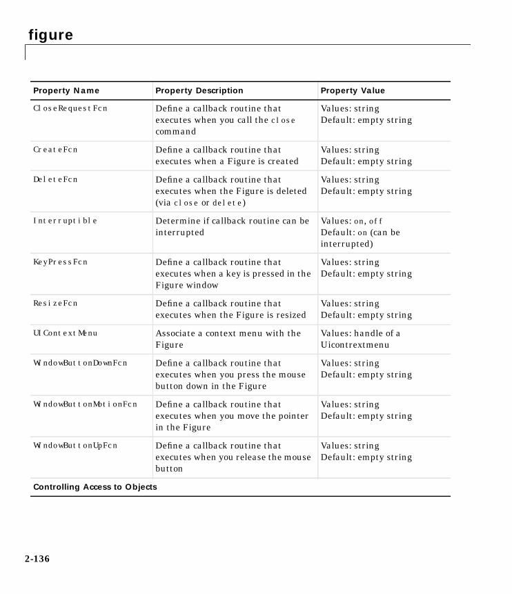
figure

CloseRequestFcn Define a callback routine thatexecutes when you call the closecommand


CreateFcn Define a callback routine thatexecutes when a Figure is created


DeleteFcn Define a callback routine thatexecutes when the Figure is deleted(via close or delete)


Interruptible Determine if callback routine can beinterrupted

Values: on, offDefault: on (can beinterrupted)

KeyPressFcn Define a callback routine thatexecutes when a key is pressed in theFigure window


ResizeFcn Define a callback routine thatexecutes when the Figure is resized


UIContextMenu Associate a context menu with theFigure

Values: handle of aUicontrextmenu

WindowButtonDownFcn Define a callback routine thatexecutes when you press the mousebutton down in the Figure


WindowButtonMotionFcn Define a callback routine thatexecutes when you move the pointerin the Figure


WindowButtonUpFcn Define a callback routine thatexecutes when you release the mousebutton


Controlling Access to Objects


2-136

figure

IntegerHandle Specify integer or noninteger Figurehandle

Values: on, offDefault: on (integer handle)

HandleVisibility Determine if Figure handle is visibleto users or not


HitTest Determine if the Figure can becomethe current object (see the FigureCurrentObject property)


NextPlot Determine how to display additionalgraphics to this Figure

Values: add, replace,replacechildrenDefault: add

Defining the Pointer

Pointer Select the pointer symbol Values: crosshair, arrow,watch, topl, topr, botl, botr,circle, cross, fleur, left,right, top, bottom,fullcrosshair, ibeam,customDefault: arrow

PointerShapeCData Data that defines the pointer Values: 16-by-16 matrixDefault: set Pointer tocustom and see

PointerShapeHotSpot Specify the pointer active spot Values: 2-element vector[row, column]Default: [1,1]

Properties That Affect Printing

InvertHardcopy Change Figure colors for printing Values: on, offDefault: on

PaperOrientation Horizontal or vertical paperorientation

Values: portrait, landscapeDefault: portrait


2-137

figure

PaperPosition Control positioning Figure on printedpage

Values: 4-element vector[left, bottom, width, height]

PaperPositionMode Enable WYSIWYG printing of Figure Values: auto, manualDefault: manual

PaperSize Size of the current PaperTypespecified in PaperUnits (read only)

Values: [width, height]

PaperType Select from standard paper sizes Values: see propertydescriptionDefault: usletter

PaperUnits Units used to specify the PaperSizeand PaperPosition

Values: normalized, inches,centimeters, pointsDefault: inches


2-138

Figure Properties

2Figure PropertiesFigureProperties

This section lists property names along with the type of values each accepts.Curly braces enclose default values.

BackingStore on | off

Off screen pixel buffer. When BackingStore is on, MATLAB stores a copy of theFigure window in an off-screen pixel buffer. When obscured parts of the Figurewindow are exposed, MATLAB copies the window contents from this bufferrather than regenerating the objects on the screen. This increases the speedwith which the screen is redrawn.

While refreshing the screen quickly is generally desirable, the buffers requireddo consume system memory. If memory limitations occur, you can setBackingStore to off to disable this feature and release the memory used by thebuffers. If your computer does not support backingstore, setting theBackingStore property results in a warning message, but has no other effect.

Setting BackingStore to off can increase the speed of animations because iteliminates the need to draw into both an off-screen buffer and the Figurewindow.






Button press callback function. A callback routine that executes whenever youpress a mouse button while the pointer is in the Figure window, but not over achild object (i.e., Uicontrol, Axes, or Axes child). Define this routine as a string

2-139

Figure Properties

that is a valid MATLAB expression or the name of an M-file. The expressionexecutes in the MATLAB workspace.

Children vector of handles

Children of the Figure. A vector containing the handles of all Axes, Uicontrol,and Uimenu objects displayed within the Figure. You can change the order ofthe handles and thereby change the stacking of the objects on the display.

Clipping on | off

This property has no effect on Figures.

CloseRequestFcn string

Function executed on Figure close. This property defines a function thatMATLAB executes whenever you issue the close command (either aclose(figure_handle) or a close all) or when you close a Figure windowfrom the computer’s window manager menu.

The CloseRequestFcn provides a mechanism to intervene in the closing of aFigure. It allows you to, for example, display a dialog box to ask a user toconfirm or cancel the close operation or to prevent users from closing a Figurethat contains a GUI.

The basic mechanism is:

• A user issues the close command from the command line or by closing thewindow from the computer’s window manager menu.

• The close operation executes the function defined by the FigureCloseRequestFcn. The default function is named closereq and is predefinedas:

delete(get(0,'CurrentFigure'))

This statement unconditionally deletes the current Figure, destroying thewindow. closereq takes advantage of the fact that the close command makesall Figures specified as arguments the current Figure before calling therespective close request function.

You can set CloseRequestFcn to any string that is a valid MATLAB statement,including the name of an M-file. For example,

set(gcf,'CloseRequestFcn','disp(''This window is immortal'')')

2-140

Figure Properties

This close request function never closes the Figure window; it simply echoes“This window is immortal” on the command line. Unless the close requestfunction calls delete, MATLAB never closes the Figure.

A more useful application of the close request function is to display a questiondialog box asking the user to confirm the close operation. The following M-fileillustrates how to do this:

% my_closereq% User-defined close request function% to display a question dialog box

selection = questdlg('Close Specified Figure?',... 'Close Request Function',... 'Yes','No','Yes');switch selection, case 'Yes', delete(get(0,'CurrentFigure')) case 'No' returnend

Now assign this M-file to the CloseRequestFcn of a Figure:

set(figure_handle,'CloseRequestFcn','my_closereq')

To make this M-file your default close request function, set a default value onthe Root level:

set(0,'DefaultFigureCloseRequestFcn','my_closereq')

MATLAB then uses this setting for the CloseRequestFcn of all subsequentlycreated Figures.

Color ColorSpec

Background color. This property controls the Figure window background color.You can specify a color using a three-element vector of RGB values or one ofMATLAB’s predefined names. See ColorSpec for more information.

Colormap m-by-3 matrix of RGB values

Figure colormap. This property is an m-by-3 array of red, green, and blue(RGB) intensity values that define m individual colors. MATLAB accesses

2-141

Figure Properties

colors by their row number. For example, an index of 1 specifies the first RGBtriplet, an index of 2 specifies the second RGB triplet, and so on. Colormaps canbe any length (up to 256 only on MS-Windows and Macintosh), but must bethree columns wide. The default Figure colormap contains 64 predefinedcolors.

Colormaps affect the rendering of Surface, Image, and Patch objects, butgenerally do not affect other graphics objects. See colormap and ColorSpec formore information.

CreateFcn string

Callback routine executed during object creation. This property defines acallback routine that executes when MATLAB creates a Figure object. Youmust define this property as a default value for Figures. For example, thestatement,

set(0,'DefaultFigureCreateFcn',...'set(gcbo,''IntegerHandle'',''off'')')

defines a default value on the Root level that causes the created Figure to usenoninteger handles whenever you (or MATLAB) create a Figure. MATLABexecutes this routine after setting all properties for the Figure. Setting thisproperty on an existing Figure object has no effect.

The handle of the object whose CreateFcn is being executed is accessible onlythrough the Root CallbackObject property, which you can query using gcbo.

CurrentAxes handle of current Axes

Target Axes in this Figure. MATLAB sets this property to the handle of theFigure’s current Axes (i.e., the handle returned by the gca command when thisFigure is the current Figure). In all Figures for which Axes children exist, thereis always a current Axes. The current Axes does not have to be the topmostaxes, and setting an Axes to be the CurrentAxes does not restack it above allother Axes.

You can make an Axes current using the axes and set commands. Forexample, axes(axes_handle) and set(gcf,'CurrentAxes',axes_handle)both make the Axes identified by the handle axes_handle the current Axes. Inaddition, axes(axes_handle) restacks the Axes above all other Axes in theFigure.

2-142

Figure Properties

If a Figure contains no Axes, get(gcf,'CurrentAxes') returns the emptymatrix. Note that the gca function actually creates an Axes if one does notexist.

CurrentCharacter single character (read only)

Last key pressed. MATLAB sets this property to the last key pressed in theFigure window. CurrentCharacter is useful for obtaining user input.

CurrentMenu (Obsolete)

This property produces a warning message when queried. It has beensuperseded by the Root CallbackObject property.

CurrentObject object handle

Handle of current object. MATLAB sets this property to the handle of the objectthat is under the current point (see the CurrentPoint property). This object isthe front-most object in the stacking order. You can use this property todetermine which object a user has selected. The function gco provides aconvenient way to retrieve the CurrentObject of the CurrentFigure.

CurrentPoint two-element vector: [x-coordinate, y-coordinate]

Location of last button click in this Figure. MATLAB sets this property to thelocation of the pointer at the time of the most recent mouse button press.MATLAB updates this property whenever you press the mouse button whilethe pointer is in the Figure window.

In addition, MATLAB updates CurrentPoint before executing callbackroutines defined for the Figure WindowButtonMotionFcn andWindowButtonUpFcn properties. This enables you to query CurrentPoint fromthese callback routines. It behaves like this:

• If there is no callback routine defined for the WindowButtonMotionFcn or theWindowButtonUpFcn, then MATLAB updates the CurrentPoint only whenthe mouse button is pressed down within the Figure window.

• If there is a callback routine defined for the WindowButtonMotionFcn, thenMATLAB updates the CurrentPoint just before executing the callback. Notethat the WindowButtonMotionFcn executes only within the Figure windowunless the mouse button is pressed down within the window and then helddown while the pointer is moved around the screen. In this case, the routine

2-143

Figure Properties

executes (and the CurrentPoint is updated) anywhere on the screen untilthe mouse button is released.

• If there is a callback routine defined for the WindowButtonUpFcn, MATLABupdates the CurrentPoint just before executing the callback. Note that theWindowButtonUpFcn executes only while the pointer is within the Figurewindow unless the mouse button is pressed down initially within thewindow. In this case, releasing the button anywhere on the screen triggerscallback execution, which is preceded by an update of the CurrentPoint.

The Figure CurrentPoint is updated only when certain events occur, aspreviously described. In some situations, (such as when theWindowButtonMotionFcn takes a long time to execute and the pointer is movedvery rapidly) the CurrentPoint may not reflect the actual location of thepointer, but rather the location at the time when the WindowButtonMotionFcnbegan execution.

The CurrentPoint is measured from the lower-left corner of the Figurewindow, in units determined by the Units property.

The Root PointerLocation property contains the location of the pointerupdated synchronously with pointer movement. However, the location ismeasured with respect to the screen, not a Figure window.

DeleteFcn string

Delete Figure callback routine. A callback routine that executes when theFigure object is deleted (e.g., when you issue a delete or a close command).MATLAB executes the routine before destroying the object’s properties sothese values are available to the callback routine.

The handle of the object whose DeleteFcn is being executed is accessible onlythrough the Root CallbackObject property, which you can query using gcbo.

Dithermap m-by-3 matrix of RGB values

Colormap used for true-color data on pseudocolor displays. This propertydefines a colormap that MATLAB uses to dither true-color CData for display onpseudocolor (8-bit or less) displays. MATLAB maps each RGB color defined astrue-color CData to the closest color in the dithermap. The default Dithermapcontains colors that span the full spectrum so any color values map reasonablywell.

2-144

Figure Properties

However, if the true-color data contains a wide range of shades in one color, youmay achieve better results by defining your own dithermap. See theDithermapMode property.

DithermapMode auto | manual

MATLAB generated dithermap. In manual mode, MATLAB uses the colormapdefined in the Dithermap property to display direct color on pseudocolordisplays. When DithermapMode is auto, MATLAB generates a dithermap basedon the colors currently displayed. This is useful if the default dithermap doesnot produce satisfactory results.

The process of generating the dithermap can be quite time consuming and isrepeated whenever MATLAB re-renders the display (e.g., when you add a newobject or resize the window). You can avoid unnecessary regeneration bysetting this property back to manual and save the generated dithermap (whichMATLAB loaded into the Dithermap property).

FixedColors m-by-3 matrix of RGB values (read only)

Non-colormap colors. Fixed colors define all colors appearing in a Figurewindow that are not obtained from the Figure colormap. These colors includeaxis lines and labels, the color of Line, Text, Uicontrol, and Uimenu objects, andany colors that you explicitly define, for example, with a statement like:

set(gcf,'Color',[0.3 0.7 0.9]).

Fixed color definitions reside in the system color table and do not appear in theFigure colormap. For this reason, fixed colors can limit the number ofsimultaneously displayed colors if the number of fixed colors plus the numberof entries in the Figure colormap exceed your system’s maximum number ofcolors.

(See the Root ScreenDepth property for information on determining the totalnumber of colors supported on your system. See the MinColorMap andShareColors properties for information on how MATLAB shares colorsbetween applications.)


Control access to object’s handle by command-line users and GUIs. Thisproperty determines when an object’s handle is visible in its parent’s list ofchildren. HandleVisibility is useful for preventing command-line users from

2-145

Figure Properties

accidentally drawing into or deleting a Figure that contains only user interfacedevices (such as a dialog box).


Setting HandleVisibility to callback causes handles to be visible fromwithin callback routines or functions invoked by callback routines, but not fromwithin functions invoked from the command line. This provides a means toprotect GUIs from command-line users, while allowing callback routines tohave complete access to object handles.

Setting HandleVisibility to off makes handles invisible at all times. Thismay be necessary when a callback routine invokes a function that mightpotentially damage the GUI (such as evaluating a user-typed string), and sotemporarily hides its own handles during the execution of that function.





HitTest on | off

Selectable by mouse click. HitTest determines if the Figure can become thecurrent object (as returned by the gco command and the Figure CurrentObjectproperty) as a result of a mouse click on the Figure. If HiTest is off, clickingon the Figure sets the CurrentObject to the empty matrix.

2-146

Figure Properties

IntegerHandle on | off

Figure handle mode. Figure object handles are integers by default. Whencreating a new Figure, MATLAB uses the lowest integer that is not used by anexisting Figure. If you delete a Figure, its integer handle can be reused.

If you set this property to off, MATLAB assigns nonreusable real-numberhandles (e.g., 67.0001221) instead of integers. This feature is designed fordialog boxes where removing the handle from integer values reduces thelikelihood of inadvertently drawing into the dialog box.


Callback routine interruption mode. The Interruptible property controlswhether a Figure callback routine can be interrupted by subsequently invokedcallback routines. Only callback routines defined for the ButtonDownFcn,KeyPressFcn, WindowButtonDownFcn, WindowButtonMotionFcn, andWindowButtonUpFcn are affected by the Interruptible property. MATLABchecks for events that can interrupt a callback routine only when it encountersa drawnow, figure, getframe, or pause command in the routine. See theBusyAction property for related information.

InvertHardcopy on | off

Change hardcopy to black objects on white background. This property affectsonly printed output. Printing a Figure having a background color (Colorproperty) that is not white results in poor contrast between graphics objectsand the Figure background and also consumes a lot of printer toner.

When InvertHardCopy is on, MATLAB eliminates this effect by changing thecolor of the Figure and Axes to white and the axis lines, tick marks, axis labels,etc., to black. Lines, Text, and the edges of Patches and Surfaces may bechanged depending on the print command options specified.

If you set InvertHardCopy to off, the printed output matches the colorsdisplayed on the screen.

See print for more information on printing MATLAB Figures.

KeyPressFcn string

Key press callback function. A callback routine invoked by a key press occurringin the Figure window. You can define KeyPressFcn as any legal MATLABexpression or the name of an M-file.

2-147

Figure Properties

The callback routine can query the Figure’s CurrentCharacter property todetermine what particular key was pressed and thereby limit the callbackexecution to specific keys.

The callback routine can also query the Root PointerWindow property todetermine in which Figure the key was pressed. Note that pressing a key whilethe pointer is in a particular Figure window does not make that Figure thecurrent Figure (i.e., the one referred by the gcf command).

MenuBar none | figure

Enable-disable Figure menu bar. This property enables you to display or hidethe menu bar placed at the top of a Figure window. The default (figure) is todisplay the menu bar.

Note that on Macintosh systems, the menu bar for the active window appearsacross the top of the screen. Menu bars are not displayed across the top of theFigure window as they are on X-Windows and MS-Windows systems, and onlyone window’s menu bar is visible at any given time.

This property affects only built in menus. Menus defined with the uimenucommand are not affected by this property.

MinColormap scalar (default = 64)

Minimum number of color table entries used. This property specifies theminimum number of system color table entries used by MATLAB to store thecolormap defined for the Figure (see the ColorMap property). In certainsituations, you may need to increase this value to ensure proper use of colors.

For example, suppose you are running color-intensive applications in additionto MATLAB and have defined a large Figure colormap (e.g., 150 to 200 colors).MATLAB may select colors that are close but not exact from the existing colorsin the system color table because there are not enough slots available to defineall the colors you specified.

To ensure MATLAB uses exactly the colors you define in the Figure colormap,set MinColorMap equal to the length of the colormap:

set(gcf,'MinColormap',length(get(gcf,'ColorMap')))

Note that the larger the value of MinColorMap, the greater the likelihood otherwindows (including other MATLAB Figure windows) will display in falsecolors.

2-148

Figure Properties

Name string

Figure window title. This property specifies the title displayed in the Figurewindow. By default, Name is empty and the Figure title is displayed asFigure No. 1, Figure No. 2, and so on. When you set this parameter to astring, the Figure title becomes Figure No. 1: <string>. See the NumberTitleproperty.

NextPlot add | replace | replacechildren

How to add next plot. NextPlot determines which Figure MATLAB uses todisplay graphics output. If the value of the current Figure is:

• add — use the current Figure to display graphics (the default).

• replace — reset all Figure properties, except Position, to their defaults anddelete all Figure children before displaying graphics (equivalent to clfreset).

• replacechildren — remove all child objects, but do not reset Figureproperties (equivalent to clf).

The newplot function provides an easy way to handle the NextPlot property.Also see the NextPlot property of Axes and the Using MATLAB Graphicsmanual.

NumberTitle on | off

Figure window title number. This property determines whether the stringFigure No. N (where N is the Figure number) is prefixed to the Figure windowtitle. See the Name property.

PaperOrientation portrait | landscape

Horizontal or vertical paper orientation. This property determines how printedFigures are oriented on the page. portrait orients the longest page dimensionvertically; landscape orients the longest page dimension horizontally. See theorient command for more detail.

PaperPosition four-element rect vector

Location on printed page. A rectangle that determines the location of the Figureon the printed page. Specify this rectangle with a vector of the form

rect = [left, bottom, width, height]

where left specifies the distance from the left side of the paper to the left sideof the rectangle and bottom specifies the distance from the bottom of the page

2-149

Figure Properties

to the bottom of the rectangle. Together these distances define the lower-leftcorner of the rectangle. width and height define the dimensions of therectangle. The PaperUnits property specifies the units used to define thisrectangle.

PaperPositionMode auto | manual

WYSIWYG printing of Figure. In manual mode, MATLAB honors the valuespecified by the PaperPosition property. In auto mode, MATLAB prints theFigure the same size as it appears on the computer screen, centered on thepage.

PaperSize [width height] (read only)

Paper size. This property contains the size of the current PaperType, measuredin PaperUnits. See PaperType to select standard paper sizes.

PaperType Select a value from the following table

Selection of standard paper size. This property sets the PaperSize to the one ofthe following standard sizes:

Property Value Size (Width x Height)

usletter (default) 8.5-by-11 inches

uslegal 11-by-14 inches

tabloid 11-by-17 inches

A0 841-by-1189mm

A1 594-by-841mm

A2 420-by-594mm

A3 297-by-420mm

A4 210-by-297mm

A5 148-by-210mm

B0 1029-by-1456mm

B1 728-by-1028mm

2-150

Figure Properties

Note that you may need to change the PaperPosition property in order toproperly position the printed Figure on the new paper size. One solution is touse normalized PaperUnits which enables MATLAB to automatically size theFigure to occupy the same relative amount of the printed page, regardless ofthe paper size.

PaperUnits normalized | inches | centimeters |points

Hardcopy measurement units. This property specifies the units used to definethe PaperPosition and PaperSize properties. All units are measured from thelower-left corner of the page. normalized units map the lower-left corner of thepage to (0, 0) and the upper-right corner to (1.0, 1.0). inches, centimeters, andpoints are absolute units (one point equals 1/72 of an inch).

B2 514-by-728mm

B3 364-by-514mm

B4 257-by-364mm

B5 182-by-257mm

arch-A 9-by-12 inches

arch-B 12-by-18 inches

arch-C 18-by-24 inches

arch-D 24-by-36 inches

arch-E 36-by-48 inches

A 8.5-by-11 inches

B 11-by-17 inches

C 17-by-22 inches

D 22-by-34 inches

E 34-by-43 inches

Property Value Size (Width x Height)

2-151

Figure Properties

If you change the value of PaperUnits, it is good practice to return it to itsdefault value after completing your computation so as not to affect otherfunctions that assume PaperUnits is set to the default value.

Parent handle

Handle of Figure’s parent. The parent of a Figure object is the Root object. Thehandle to the Root is always 0.

Pointer crosshair | arrow | watch | topl |topr | botl | botr | circle | cross |fleur | left | right | top | bottom |fullcrosshair | ibeam | custom

Pointer symbol selection. This property determines the symbol used to indicatethe pointer (cursor) position in the Figure window. Setting Pointer to customallows you to define your own pointer symbol. See the PointerShapeCDataproperty for more information. See also the Using MATLAB Graphics manual.

PointerShapeCData 16-by-16 matrix

User-defined pointer. This property defines the pointer that is used when youset the Pointer property to custom. It is a 16-by-16 element matrix defining the16-by-16 pixel pointer using the following values:

• 1 – color pixel black

• 2 – color pixel white

• NaN – make pixel transparent (underlying screen shows through)

Element (1,1) of the PointerShapeCData matrix corresponds to the upper-leftcorner of the pointer. Setting the Pointer property to one of the predefinedpointer symbols does not change the value of the PointerShapeCData.Computer systems supporting 32-by-32 pixel pointers fill only one quarter ofthe available pixmap.

PointerShapeHotSpot2-element vector

Pointer active area. A two-element vector specifying the row and columnindices in the PointerShapeCData matrix defining the pixel indicating thepointer location. The location is contained in the CurrentPoint property andthe Root object’s PointerLocation property. The default value is element (1,1),which is the upper-left corner.

2-152

Figure Properties

Position four-element vector

Figure position. This property specifies the size and location on the screen ofthe Figure window. Specify the position rectangle with a four-element vector ofthe form:

rect = [left, bottom, width, height]

where left and bottom define the distance from the lower-left corner of thescreen to the lower-left corner of the Figure window. width and height definethe dimensions of the window. See the Units property for information on theunits used in this specification. The left and bottom elements can be negativeon systems that have more than one monitor.

You can use the get function to obtain this property and determine the positionof the Figure and you can use the set function to resize and move the Figure toa new location.

Renderer painters | zbuffer

Rendering method used for screen and printing. This property enables you toselect the method used to render MATLAB graphics. The choices are:

• painters – MATLAB’s original rendering method is faster when the Figurecontains only simple or small graphics objects.

• zbuffer – MATLAB draws graphics object faster and more accuratelybecause objects are colored on a per pixel basis and MATLAB renders onlythose pixels that are visible in the scene (thus eliminating front-to-backsorting errors). Note that this method can consume a lot of system memoryif MATLAB is displaying a complex scene.

• OpenGL – OpenGL is a renderer that is available on many computer systems.This renderer is generally faster than painters or zbuffer and in some casesenables MATLAB to access graphics hardware that is available on somesystems.

Using theOpenGLRenderer

The Figure Renderer property supports a new value that enables MATLAB touse OpenGL as the renderer. The command to enable OpenGL on the currentFigure is:

set(gcf,'Renderer','OpenGL')

2-153

Figure Properties

OpenGL increases performance for most 2-D and 3-D graphs drawn withMATLAB.

Hardware Vs. Software OpenGL ImplementationsThere are two kinds of OpenGL implementations – hardware and software.

The hardware implementation makes use of special graphics hardware toincrease performance and is therefore significantly faster than the softwareversion. Many computers have this special hardware available as an option ormay come with this hardware right out of the box.

Software implementations of OpenGL are much like the ZBuffer renderer thatis available on MATLAB version 5.0, however, OpenGL generally providessuperior performance to ZBuffer.

OpenGL AvailabilityOpenGL is available on all computers that MATLAB runs on with theexception of VMS. MATLAB automatically finds hardware versions of OpenGlif they are available. If the hardware version is not available, then MATLABuses the software version.

The software versions that are available on different platforms are:

• On UNIX and MacIntosh systems, MATLAB uses the software version ofOpenGL that is included in the MATLAB distribution.

• On MS-Windows NT 4.0, OpenGL is available as part of the operatingsystem.

• On MS-Windows 95, OpenGL is included in the Windows 95 OSR 2 release.If you do not have this release, the libraries are available on the Microsoft ftpsite:

Microsoft version is available at the URL:ftp://ftp.microsoft.com/softlib/mslfiles/opengl95.exe

There is also a Silicon Graphics version of OpenGL for Windows 95 that isavailable at the URL:

http://www.sgi.com

2-154

Figure Properties

Tested Hardware VersionsOn MS-Windows platforms, there are many graphics boards that accelerateOpenGL. The MathWorks has tested MATLAB on the AccelECLIPSE boardfrom AccelGraphics.

On UNIX platforms, The MathWorks has tested MATLAB on Sparc Ultra withthe Creator 3D board and Silicon Graphics computers running IRIX 6.4 ornewer.

Determining What Version You Are UsingTo determine the version and vendor of the OpenGL library that MATLAB isusing on your system, type the following command at the MATLAB prompt:

feature GetOpenGLInfo

This command also returns a string of extensions to the OpenGL specificationthat are available with the particular library MATLAB is using. Thisinformation is helpful to The MathWorks so please include this information ifyou need to report bugs.

OpenGL Vs. Other MATLAB RenderersThere are some difference between drawings created with OpenGL and thosecreated with the other renderers. The OpenGL specific differences include:

• OpenGL does not do colormap interpolation. If you create a Surface or Patchusing indexed color and interpolated face or edge coloring, OpenGL willinterpolate the colors through the RGB color cube instead of through thecolormap.

• OpenGL does not support the phong value for the FaceLighting andEdgeLighting properties of Surfaces and Patches.

MATLAB issues a warning if you request nonsupported behavior.

Printing from OpenGLWhen you print a Figure that was drawn with OpenGL, MATLAB switches tothe ZBuffer renderer to produce output, which has a resolution determined bythe print command’s −r option. This may cause flashing of the Figure as therenderer changes.

2-155

Figure Properties

Implementations of OpenGL Tested by TMWThe following hardware versions have been tested:

• AccelECLIPSE by AccelGraphics

• Sol2/Creator 3D

• SGI

The following software versions have been tested:

• Mesa

• CosmoGL

• Microsoft’s Windows 95 implementation

• NT 4.0

RendererMode auto | manual

Automatic, or user selection of Renderer. This property enables you to specifywhether MATLAB should choose the Renderer based on the contents of thefigure window, or whether the Renderer should remain unchanged.

When the RendererMode property is set to auto, MATLAB selects the renderingmethod for printing as well as for screen display based on the size andcomplexity of the graphics objects in the Figure.

For printing, MATLAB switches to zbuffer at a greater scene complexity thanfor screen rendering because printing from a Z-buffered Figure can beconsiderably slower than one using the painters rendering method, and canresult in large PostScript files. However, the output does always match what ison the screen. The same holds true for OpenGL, the output is the same as thatproduced by the ZBuffer renderer – a bitmap with a resolution determined bythe print command’s −r option

When the RendererMode property is set to manual, MATLAB does not changethe Renderer, regardless of changes to the Figure contents.

Resize on | off

Window resize mode. This property determines if you can resize the Figurewindow with the mouse. on means you can resize the window, off means youcannot. When Resize is off, the Figure window does not display any resizingcontrols (such as boxes at the corners) to indicate that it cannot be resized.

2-156

Figure Properties

ResizeFcn string

Window resize callback routine. MATLAB executes the specified callbackroutine whenever you resize the Figure window. You can query the Figure’sPosition property to determine the new size and position of the Figurewindow. During execution of the callback routine, the handle to the Figurebeing resized is accessible only through the Root CallbackObject property,which you can query using gcbo.

You can use ResizeFcn to maintain a GUI layout that is not directly supportedby MATLAB’s Position/Units paradigm.

For example, consider a GUI layout that maintains an object at a constantheight in pixels and attached to the top of the Figure, but always matches thewidth of the Figure. The following ResizeFcn accomplishes this; it keeps theUicontrol whose Tag is 'StatusBar' 20 pixels high, as wide as the Figure, andattached to the top of the Figure. Note the use of the Tag property to retrievethe Uicontrol handle, and the gcbo function to retrieve the Figure handle. Alsonote the defensive programming regarding Figure Units, which the callbackrequires to be in pixels in order to work correctly, but which the callback alsorestores to their previous value afterwards:

u = findobj('Tag','StatusBar');fig = gcbo;old_units = get(fig,'Units');set(fig,'Units','pixels');figpos = get(fig,'Position');upos = [0, figpos(4) - 20, figpos(3), 20];set(u,'Position',upos);set(fig,'Units',old_units);

You can change the Figure Position from within the ResizeFcn callback;however the ResizeFcn is not called again as a result.

Note that the print command can cause the ResizeFcn to be called if thePaperPositionMode property is set to manual and you have defined a resizefunction. If you do not want your resize function called by print, set thePaperPositionMode to auto.

2-157

Figure Properties

Selected on | off

Is object selected. This property indicates whether the Figure is selected. Youcan, for example, define the ButtonDownFcn to set this property, allowing usersto select the object with the mouse.


Figures do not indicate selection.

SelectionType normal | extend | alt | open(this property is read only)

Mouse selection type. MATLAB maintains this property to provide informationabout the last mouse button press that occurred within the Figure window.This information indicates the type of selection made. Selection types areactions that are generally associated with particular responses from the userinterface software (e.g., single clicking on a graphics object places it in move orresize mode; double-clicking on a filename opens it, etc.).

The physical action required to make these selections varies on differentplatforms. However, all selection types exist on all platforms.

Selection Type MS-Windows X-Windows Macintosh

Normal Click leftmouse button

Click leftmouse button

Click mousebutton

Extend Shift - click leftmouse button orclick both leftand right mousebuttons

Shift - click leftmouse buttonor clickmiddle mousebutton

Shift - clickmouse button

Alternate Control - clickleft mousebutton or clickright mousebutton

Control - clickleft mousebuttonor clickright mousebutton

Option - clickmouse button

Open Double click anymouse button

Double click anymouse button

Double clickmouse button

2-158

Figure Properties

Note that the ListBox style of Uicontrols set the Figure SelectionTypeproperty to normal to indicate a single mouse click or to open to indicate adouble mouse click.

ShareColors on | off

Share slots in system colortable with like colors. This property affects the wayMATLAB stores the Figure colormap in the system color table. By default,MATLAB looks at colors already defined and uses those slots to assign pixelcolors. This leads to an efficient use of color resources (which are limited onsystems capable of displaying 256 or less colors) and extends the number ofFigure windows that can simultaneously display correct colors.

However, in situations where you want to change the Figure colormap quicklywithout causing MATLAB to re-render the displayed graphics objects, youshould disable color sharing (set ShareColors to off). In this case, MATLABcan swap one colormap for another without changing pixel color assignmentssince all the slots in the system color table used for the first colormap arereplaced with the corresponding color in the second colormap. (Note that thisapplies only in cases where both colormaps are the same length and where thecomputer hardware allows user modification of the system color table.)

Tag string


For example, suppose you want to direct all graphics output from an M-file toa particular Figure, regardless of user actions that may have changed thecurrent Figure. To do this, identify the Figure with a Tag:

figure('Tag','Plotting Figure')

Then make that Figure the current Figure before drawing by searching for theTag with findobj:

figure(findobj('Tag','Plotting Figure'))

2-159

Figure Properties


Object class. This property identifies the kind of graphics object. For Figureobjects, Type is always the string 'figure'.


Associate a context menu with the Figure. Assign this property the handle of aUicontextmenu object created in the Figure. Use the uicontextmenu functionto create the context menu. MATLAB displays the context menu whenever youright-click over the Figure (Control-click on Macintosh systems).

Units pixels | normalized | inches |centimeters | points | character

Units of measurement. This property specifies the units MATLAB uses tointerpret size and location data. All units are measured from the lower-leftcorner of the window.

• normalized units map the lower-left corner of the Figure window to (0,0) andthe upper-right corner to (1.0,1.0).

• inches, centimeters, and points are absolute units (one point equals 1/72of an inch).

• The size of a pixel depends on screen resolution.

• Character units are defined by characters from the default system font; thewidth of one character is the width of the letter x, the height of one characteris the distance between the baselines of two lines of text.

This property affects the CurrentPoint and Position properties. If you changethe value of Units, it is good practice to return it to its default value aftercompleting your computation so as not to affect other functions that assumeUnits is set to the default value.

When specifying the units as property/value pairs during object creation, youmust set the Units property before specifying the properties that you want touse these units.

UserData matrix

User specified data. You can specify UserData as any matrix you want toassociate with the Figure object. The object does not use this data, but you canaccess it using the set and get commands.

2-160

Figure Properties

Visible on | off

Object visibility. The Visible property determines whether an object isdisplayed on the screen. If the Visible property of a Figure is off, the entireFigure window is invisible.

WindowButtonDownFcnstring

Button press callback function. Use this property to define a callback routinethat MATLAB executes whenever you press a mouse button while the pointeris in the Figure window. Define this routine as a string that is a valid MATLABexpression or the name of an M-file. The expression executes in the MATLABworkspace.

WindowButtonMotionFcnstring

Mouse motion callback function. Use this property to define a callback routinethat MATLAB executes whenever you move the pointer within the Figurewindow. Define this routine as a string that is a valid MATLAB expression orthe name of an M-file. The expression executes in the MATLAB workspace.

WindowButtonUpFcn string

Button release callback function. Use this property to define a callback routinethat MATLAB executes whenever you release a mouse button. Define thisroutine as a string that is a valid MATLAB expression or the name of an M-file.The expression executes in the MATLAB workspace.

The button up event is associated with the Figure window in which thepreceding button down event occurred. Therefore, the pointer need not be in theFigure window when you release the button to generate the button up event.

If the callback routines defined by WindowButtonDownFcn orWindowButtonMotionFcn contain drawnow commands or call other functionsthat contain drawnow commands and the Interruptible property is set to off,the WindowButtonUpFcn may not be called. You can prevent this problem bysetting Interruptible to on.

WindowStyle normal | modal

Normal or modal window behavior. When WindowStyle is set to modal, theFigure window traps all keyboard and mouse events over all MATLABwindows as long as they are visible. Windows belonging to applications otherthan MATLAB are unaffected. Modal Figures remain stacked above all normalFigures and the MATLAB command window. When multiple modal windows

2-161

Figure Properties

exist, the most recently created window keeps focus and stays above all otherwindows until it becomes invisible, or is returned to WindowStyle normal, or isdeleted. At that time, focus reverts to the window that last had focus.

Figures with WindowStyle modal and Visible off do not behave modally untilthey are made visible, so it is acceptable to hide a modal window instead ofdestroying it when you want to reuse it.

You can change the WindowStyle of a Figure at any time, including when theFigure is visible and contains children. However, on some systems this maycause the Figure to flash or disappear and reappear, depending on thewindowing-system’s implementation of normal and modal windows. For bestvisual results, you should set WindowStyle at creation time or when the Figureis invisible.

Modal Figures do not display Uimenu children or built-in menus, but it is notan error to create Uimenus in a modal Figure or to change WindowStyle tomodal on a Figure with Uimenu children. The Uimenu objects exist and theirhandles are retained by the Figure. If you reset the Figure’s WindowStyle tonormal, the Uimenus are displayed.

Use modal Figures to create dialog boxes that force the user to respond withoutbeing able to interact with other windows. Typing Control C at the MATLABprompt causes all Figures with WindowStyle modal to revert to WindowStylenormal, allowing you to type at the command line.

2-162

fill

2fillPurpose Filled two-dimensional polygons

Syntax fill(X,Y,C)fill(X,Y,ColorSpec)fill(X1,Y1,C1,X2,Y2,C2,...)fill(...,'PropertyName',PropertyValue)h = fill(...)

Description The fill function creates colored polygons.

fill(X,Y,C) creates filled polygons from the data in X and Y with vertex colorspecified by C. C is a vector or matrix used as an index into the colormap. If C isa row vector, length(C) must equal size(X,2) and size(Y,2); if C is a columnvector, length(C) must equal size(X,1) and size(Y,1). If necessary, fillcloses the polygon by connecting the last vertex to the first.

fill(X,Y,ColorSpec) fills two-dimensional polygons specified by X and Y withthe color specified by ColorSpec.

fill(X1,Y1,C1,X2,Y2,C2,...) specifies multiple two-dimensional filledareas.

fill(...,'PropertyName',PropertyValue) allows you to specify propertynames and values for a Patch graphics object.

h = fill(...) returns a vector of handles to Patch graphics objects, onehandle per Patch object.

Remarks If X or Y is a matrix, and the other is a column vector with the same number ofelements as rows in the matrix, fill replicates the column vector argument toproduce a matrix of the required size. fill forms a vertex from correspondingelements in X and Y and creates one polygon from the data in each column.

The type of color shading depends on how you specify color in the argument list.If you specify color using ColorSpec, fill generates flat-shaded polygons bysetting the Patch object’s FaceColor property to the corresponding RGB triple.

If you specify color using C, fill scales the elements of C by the values specifiedby the Axes property CLim. After scaling C, C indexes the current colormap.

2-163

fill

If C is a row vector, fill generates flat-shaded polygons where each elementdetermines the color of the polygon defined by the respective column of the Xand Y matrices. Each Patch object’s FaceColor property is set to 'flat'. Eachrow element becomes the CData property value for the n-th Patch object, wheren is the corresponding column in X or Y.

If C is a column vector or a matrix, fill uses a linear interpolation of the vertexcolors to generate polygons with interpolated colors. It sets the Patch graphicsobject FaceColor property to 'interp' and the elements in one column becomethe CData property value for the respective Patch object. If C is a column vector,fill replicates the column vector to produce the required sized matrix.

Examples Create a red octagon:

t = (1/16:1/8:1)'*2*pi;x = sin(t);y = cos(t);fill(x,y,'r')axis square

See Also axis, caxis, colormap, ColorSpec, fill3, patch

−1 −0.8 −0.6 −0.4 −0.2 0 0.2 0.4 0.6 0.8 1−1

−0.8

−0.6

−0.4

−0.2

0

0.2

0.4

0.6

0.8

1

2-164

fill3

2fill3Purpose Filled three-dimensional polygons

Syntax fill3(X,Y,Z,C)fill3(X,Y,Z,ColorSpec)fill3(X1,Y1,Z1,C1,X2,Y2,Z2,C2,...)fill3(...,'PropertyName',PropertyValue)h = fill3(...)

Description The fill3 function creates flat-shaded and Gouraud-shaded polygons.

fill3(X,Y,Z,C) fills three-dimensional polygons. X, Y, and Z triplets specifythe polygon vertices. If X, Y, or Z is a matrix, fill3 creates n polygons, where nis the number of columns in the matrix. fill3 closes the polygons byconnecting the last vertex to the first when necessary.

C specifies color, where C is a vector or matrix of indices into the currentcolormap. If C is a row vector, length(C) must equal size(X,2) and size(Y,2);if C is a column vector, length(C) must equal size(X,1) and size(Y,1).

fill3(X,Y,Z,ColorSpec) fills three-dimensional polygons defined by X, Y,and Z with color specified by ColorSpec.

fill3(X1,Y1,Z1,C1,X2,Y2,Z2,C2,...) specifies multiple filledthree-dimensional areas.

fill3(...,'PropertyName',PropertyValue) allows you to set values forspecific Patch properties.

h = fill3(...) returns a vector of handles to Patch graphics objects, onehandle per Patch.

Algorithm If X, Y, and Z are matrices of the same size, fill3 forms a vertex from thecorresponding elements of X, Y, and Z (all from the same matrix location), andcreates one polygon from the data in each column.

If X, Y, or Z is a matrix, fill3 replicates any column vector argument to producematrices of the required size.

If you specify color using ColorSpec, fill3 generates flat-shaded polygons andsets the Patch object FaceColor property to an RGB triple.

2-165

fill3

If you specify color using C, fill3 scales the elements of C by the Axes propertyCLim, which specifies the color axis scaling parameters, before indexing thecurrent colormap.

If C is a row vector, fill3 generates flat-shaded polygons and sets theFaceColor property of the Patch objects to 'flat'. Each element becomes theCData property value for the respective Patch object.

If C is a column vector or a matrix, fill3 generates polygons with interpolatedcolors and sets the patch object FaceColor property to 'interp'. fill3 uses alinear interpolation of the vertex colormap indices when generating polygonswith interpolated colors. The elements in one column become the CDataproperty value for the respective Patch object. If C is a column vector, fill3replicates the column vector to produce the required sized matrix.

Examples Create four triangles with interpolated colors.

X = [0 1 1 2;1 1 2 2;0 0 1 1];Y = [1 1 1 1;1 0 1 0;0 0 0 0];Z = [1 1 1 1;1 0 1 0;0 0 0 0];C = [0.5000 1.0000 1.0000 0.5000;

1.0000 0.5000 0.5000 0.1667;0.3330 0.3330 0.5000 0.5000];

fill3(X,Y,Z,C)

2-166

fill3

See Also axis, caxis, colormap, ColorSpec, fill, patch

2-167

findobj

2findobjPurpose Locate graphics objects

Syntax h = findobjh = findobj('PropertyName',PropertyValue,...)h = findobj(objhandles,...)h = findobj(objhandles,'flat','PropertyName',PropertyValue,...)

Description findobj locates graphics objects and returns their handles. You can limit thesearch to objects with particular property values and along specific branches ofthe hierarchy.

h = findobj returns the handles of the Root object and all its descendants.

h = findobj('PropertyName',PropertyValue,...) returns the handles ofall graphics objects having the property PropertyName, set to the valuePropertyValue. You can specify more than one property/value pair, in whichcase, findobj returns only those objects having all specified values.

h = findobj(objhandles,...) restricts the search to objects listed inobjhandles and their descendants.

h = findobj(objhandles,'flat','PropertyName',PropertyValue,...)restricts the search to those objects listed in objhandles and does not searchdescendants.

Remarks findobj returns an error if a handle refers to a non-existent graphics object.

When you specify a property value, use the same format as get returns. Forexample, you must use the RGB format to specify a color value and when thevalue is a string, you must specify the entire character string.

When a graphics object is a descendant of more than one object identified inobjhandles, MATLAB searches the object each time findobj encounters itshandle. Therefore, implicit references to a graphics object can result in itshandle being returned multiple times.

Examples Find all Line objects in the current Axes:

h = findobj(gca,'Type','line')

2-168

findobj

See Also copyobj, gcf, gca, gcbo, gco, get, set

Graphics objects include:

axes, figure, image, light, line, patch, surface, text, uicontrol, uimenu

2-169

fplot

2fplotPurpose Plot a function between specified limits

Syntax fplot('function',limits)fplot('function',limits,LineSpec)fplot('function',limits,tol)fplot('function',limits,tol,LineSpec)[x,Y] = fplot(...)

Description fplot plots a function between specified limits. The function must be of theform y = f(x), where x is a vector whose range specifies the limits, and y is avector the same size as x and contains the function’s value at the points in x(see the first example). If the function returns more than one value for a givenx, then y is a matrix whose columns contain each component of f(x) (see thesecond example).

fplot('function',limits) plots 'function' between the limits specified bylimits. limits is a vector specifying the x-axis limits ([xmin xmax]), or the x-and y-axis limits, ([xmin xmax ymin ymax]).

fplot('function',limits,LineSpec) plots 'function' using the linespecification LineSpec. 'function' is a name of a MATLAB M-file or a stringcontaining the variable x.

fplot('function',limits,tol) plots 'function' using the relative errortolerance tol (default is 2e–3). The maximum number of x steps is (1/tol)+1.

fplot('function',limits,tol,LineSpec) plots 'function' using therelative error tolerance tol and a line specification that determines line type,marker symbol, and color.

[x,Y] = fplot(...) returns the abscissas and ordinates for 'function' in xand Y. No plot is drawn on the screen. You plot the function using plot(x,Y).

Remarks fplot uses adaptive step control to produce a representative graph,concentrating its evaluation in regions where the function’s rate of change isthe greatest.

2-170

fplot

Examples Plot the hyperbolic tangent function from -2 to 2:

fplot('tanh',[-2 2])

Create an M-file, myfun, that returns a two column matrix:

function Y = myfun(x)Y(:,1) = 200∗sin(x(:))./x(:);Y(:,2) = x(:).^2;

Plot the function with the statement:

fplot('myfun',[–20 20]

−2 −1.5 −1 −0.5 0 0.5 1 1.5 2−1

−0.8

−0.6

−0.4

−0.2

0

0.2

0.4

0.6

0.8

1

2-171

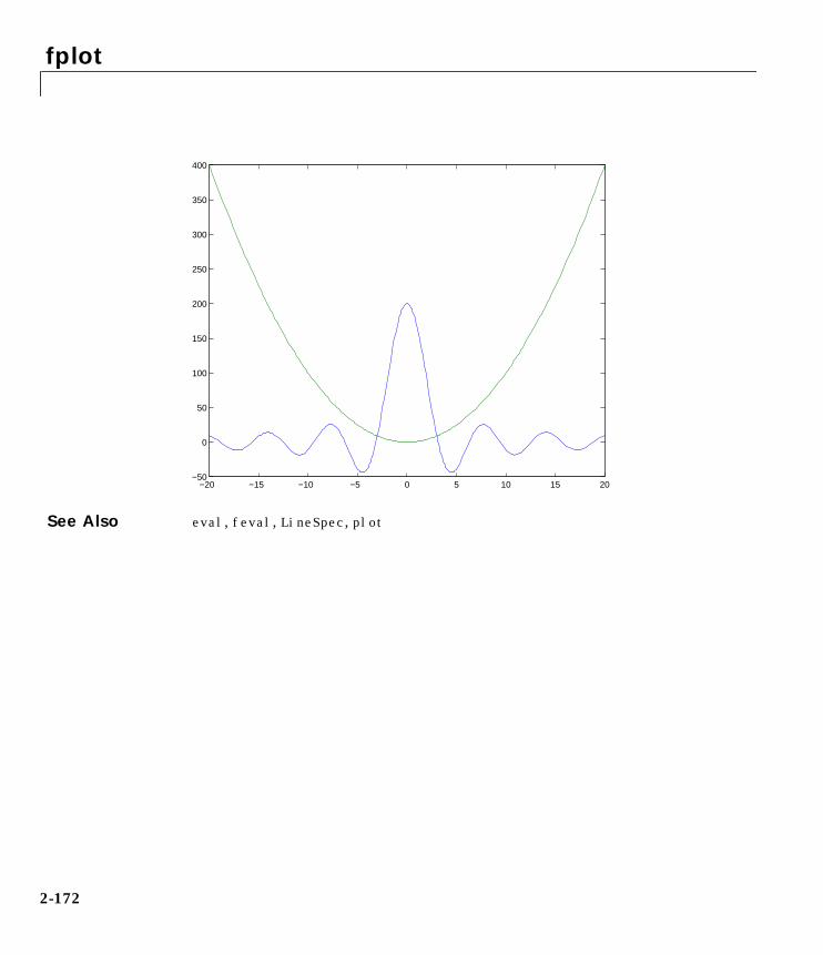
fplot

See Also eval, feval, LineSpec, plot

−20 −15 −10 −5 0 5 10 15 20−50

0

50

100

150

200

250

300

350

400

2-172

frame2im

2frame2imPurpose Convert movie frame to indexed image

Syntax [X,Map] = frame2im(F)

Description [X,Map] = frame2im(F) converts the single movie frame F into the indexedimage X and associated colormap Map. A single column of a movie matrix is onemovie frame. The functions getframe and im2frame create a movie frame.

See Also capture, im2frame, movie

2-173

frame2im

2-174

frameedit

2frameeditPurpose Create and edit printframes for Simulink block diagrams

Syntax frameeditframeedit filename

Description frameedit invokes the printframe editor, a graphical user interface you use tocreate printframes for Simulink block diagrams. Printframes are borderscontaining information relevant to the Simulink block diagram, such as thename of the block diagram. After creating a printframe, you can use Simulinkto print a block diagram with a printframe. See the sample below.

frameedit opens the PrintFrame Editor window with a new file.

frameedit filename opens the PrintFrame Editor window with the specifiedfilename, where filename is a .fig file you previously created and saved usingframeedit.

1 of 3

Simulinkblockdiagram

Printframeborders

Information included in printframe

Engine DivisionAdvanced Design Group

engine/Throttle & ManifoldPagemargins

175

frameedit

Remarks Printframe Editor InterfaceType frameedit at the MATLAB prompt. The PrintFrame Editor windowappears. Below is an illustration of the PrintFrame Editor window includingthe default printframe that the window opens with.

The default printframe has two rows. The top row consists of one cell and thebottom row has two cells. Default information (entries) appears in the cells, asshown below. You can keep this information, or remove the default entries and

Buttons to create and edit borders

List box and button for addinginformation in cells, such astext or the date

File menu for page setup, and saving and opening printframes Information included in cells

Rows

Zoom in onselected cell

Zoom out Cells – areas where you can include information

Buttons for aligning informationwithin a cell

Close box

176

frameedit

add your own. You can also add new rows and cells and then add informationin them.

Summary of the Printframe ProcessBelow are the basic steps to create and use printframes. Subsequent sectionsprovide details for performing each step.

• Design the printframe and specify the page setup.

• Create printframe borders (rows and cells), and then resize them as needed.

• Add information to the cells and edit it as needed.

• Save the printframe as a .fig file.

• Print a Simulink block diagram with the printframe.

Where to Start – Designing PrintframesBefore you begin creating a printframe using the printframe editor, determinethe type of information you want to include in it and how you want theinformation to appear.

In a printframe, you can include variable information that is automaticallysupplied at the time of printing, such as the date the Simulink block diagramis being printed, or fixed information, such as the name and address of yourorganization.

%<blockdiagram>

%<fullsystemname> %<page>

Default printframe includesvariable entries for:

The Simulink block diagram

The page number of theSimulink block diagram

The full system name for theSimulink block diagram

177

frameedit

You can design a printframe you intend to use for one particular Simulinkblock diagram, or you can design a more generic printframe for printing withdifferent Simulink block diagrams.

Specifying the Printframe Page SetupAfter you have an idea of the design of your printframe, specify the page setupfor the printframe. In the PrintFrame Editor window, select Page Setup fromthe File menu.

The PrintFrame Page Setup dialog box appears. In the dialog box, specify:

• Paper Type – for example, usletter• Paper Orientation – portrait or landscape

• Margins for the printframe; note that you can select the Units in which tospecify the margins

Click Apply to see the effects of the changes you made. Then click OK to closethe dialog box.

178

frameedit

Note: Always begin creating a new printframe with PrintFrame Page Setup. Ifinstead you begin by creating borders and adding information, and then laterchange the page setup, you might have to correct the borders and placement ofthe information. For example, if you add information to cells and then changethe page setup paper orientation from landscape to portrait, the informationyou added might not fit in the cells, given the new orientation.

Creating Borders (Rows and Cells)After setting up the page, specify borders (cells) in which the Simulink blockdiagram and information will be placed. In the printframe editor, you createborders using rows, and then create cells within the rows.

You can add and remove rows in a printframe. First, click within an existingrow to select it. If a row consists of multiple cells, click in any of the cells in therow to select that row.

When a row is selected, handles appear on all four corners. If handles appearon only two corners, you clicked on and only selected the line, not the row.

After selecting a row, click the add row button to create a new row. The newrow appears above the row you selected. To remove a row, select the row andclick the delete row button.

To create multiple cells within a row, select the row. Then click the split cellbutton. The row is split into two cells. If the row already consists of more thanone cell, you can split any of the cells into two cells. First select the cell byclicking within in it. Then click the split cell button – the cell splits. To removea cell, first select the cell and then click the delete cell button.

Cell (or row) selected - note4 handles and arrow cursor

Line selected - note 2 handlesand double-arrow cursor

179

frameedit

Resizing Rows and CellsTo change the dimensions of a row or cell, drag one side of the row or cell. Morespecifically, click on the line you want to move – a handle appears on both endsof the line and the cursor becomes a double-arrow cursor. Then drag the line tothe new location. For example, to make a row taller, click on the top line thatforms the row. Then drag the line up and the height of the row increases.

Note that the overall size of the printframe is fixed so that when you changethe dimensions of one element, the dimensions of the element next to it changein an inverse direction. For example, if you drag the top line of a row to makeit taller, the row above it becomes shorter by the same amount.

Adding Information to CellsFirst select the cell where you want to add the information. Then, from the Filllist box, select the type of information you want to add. Finally, click the Addbutton – an edit box containing that information appears in the cell. (The editbox for your platform might look slightly different from those in the figurebelow.)

Note: If you click the Add button and nothing happens, it might be because youdid not select a cell first.

For Text, type the text you want to include in that cell, for example, the nameof your organization. Press the Enter key (or Return key on a Macintosh) if youwant to type additional text on a new line. Note that you can type specialcharacters, for example, Greek symbols, using embedded TeX sequences – seethe Text command String property for a list of allowable sequences.

Select item from Fill list box.

Click Add button.

For Text, an emptyedit box appears.

For variable information, thevariable’s name appears in theedit box. In this example, thevariable information is Date.

180

frameedit

All of the items in the Fill list box, except for the Text item, are for addingvariable information, which is supplied at the time of printing. When you printa Simulink block diagram with a printframe that contains variableinformation, the information for that particular Simulink block diagram printsin those fields.

The variable entries you can include are:

• Block Diagram – This entry indicates where the Simulink block diagram isto be printed. Block Diagram is a mandatory entry. If Block Diagram is notin one of the cells, you cannot save the printframe and therefore cannot printa Simulink block diagram with it.

• Date – The date that the Simulink block diagram and printframe areprinted, in dd-mmm-yyyy format, for example, 05-Dec.-1997.

• Time – The time that the Simulink block diagram and printframe areprinted, in hh:mm format, for example, 14:22.

• Page Number – The page of the Simulink block diagram being printed.

• Total Pages – The total number of pages being printed for the Simulinkblock diagram, which depends on the Simulink printing options specified.

• System Name – The name of the Simulink block diagram being printed.

• Full System Name – The name of the Simulink block diagram being printed,including its position from the root system through the current system, forexample, engine/Throttle & Manifold.

• File Name – The filename of the Simulink block diagram, for example,engine.mdl.

• Full File Name – The full path and filename for the Simulink block diagram,for example, \\matlab\toolbox\simulink\simdemos\engine.mdl.

Note: Adding the system name or filename does not mean that you can specifya Simulink system or filename in the printframe editor. It means that whenyou print a block diagram from Simulink and specify that it print with aprintframe, the system name or filename of that Simulink block diagramprints in the specified cell of the printframe.

181

frameedit

When you add a variable entry, a percent sign, %, is automatically included toidentify the entry as variable information rather than a text string, and thetype of entry, for example, page, appears in angle brackets, < >. The entryconsists of the entire string, for example, %<page>, for Page Number.

You can include multiple entries in one cell. Select the cell and then addanother item from the list box. The new entry is added after the last entry inthat cell. You can also type descriptive text to any of the variable entrieswithout using the Text item in the Fill list box – type text in the edit box beforeor after an entry and the text prints with the block diagram.

Note: You cannot include multiple entries or text in the cell that contains theblock diagram entry – %<blockdiagram> must be the only information in thatcell. If there is any other information in that cell, you cannot save theprintframe and therefore cannot print it with a Simulink block diagram.

ZoomingWhile using the printframe editor, you might need to zoom in on an area tobetter see the information you added. Click in the cell you want to zoom in onand then click the zoom in button. The area is magnified. Click the zoom inbutton repeatedly to continue zooming in.

To zoom out, which reduces the magnification in an area, click the zoom outbutton. Click the zoom out button repeatedly to continue zooming out.

Aligning the Information in a CellTo align the information within a cell, click within the cell to select it and thenclick on one of the Align buttons. L aligns the information with the left edge ofthe cell, C centers the information within the cell, and R aligns the informationwith the right edge of the cell. Alignment does not apply to the cell thatcontains the %<blockdiagram> entry – the Simulink block diagram isautomatically scaled and centered to fit in that cell at the time of printing.

Zoom in Zoom out

182

frameedit

Editing Text StringsYou can change text you typed in a cell:

1 Double-click on the information you want to edit.

An edit box appears around all of the information in that cell.

2 Click at the start of the text you want to change and drag to the end of thetext to be changed. This highlights the text.

3 Type the replacement text. It automatically replaces the highlighted text.

Be careful not to edit the text of a variable entry, because then the variableinformation will not print. For example, if you accidentally remove the %from the %<page> entry, the text <page> will print instead of the actual pagenumber.

4 Click somewhere outside of the edit box to end editing mode.

Removing and Copying EntriesYou can cut, copy, paste, and delete an entry:

1 Double-click the cursor on the information you want to remove or copy.

An edit box appears around all of the information in that cell.

2 Click at the start of the entry you want to edit and drag to the end of thatentry. This highlights the entry.

For variable information, be sure to include the entire string, for example,%<page>.

Note that for Windows, you can select all of the entries in a cell byright-clicking on the information and choosing Select All from the pop-upmenu.

183

frameedit

3 Use the standard editing techniques for your platform to cut, copy or deletethe highlighted information.

- For Windows, right-click in the edit box and select Cut, Copy, or Deletefrom the pop-up menu.

- For Macintosh, press the command+X keys to cut, command+C keys tocopy, or the Delete key to delete.

- For UNIX, highlighting the information automatically copies it to theclipboard. If you want to remove it, press the Delete key.

If you make a mistake, use your platform’s standard undo technique. Forexample for Windows, right-click in the edit box and select Undo from thepop-up menu.

4 If you cut or copied the information to the clipboard and want to paste it,double-click on the entry where you want to paste it and position the cursorat the new location in that edit box. Then use the standard paste techniquefor your platform.

- For Windows, right-click at the new location and select Paste from thepop-up menu.

- For Macintosh, press the command+V keys at the new location.

- For UNIX, click at the new location and then click the middle mousebutton.

5 Click somewhere outside of the edit box to end editing mode.

Changing the Font CharacteristicsYou can change the font characteristics for the information in any cell.Specifically, you can specify the font size, style, color, and family.

184

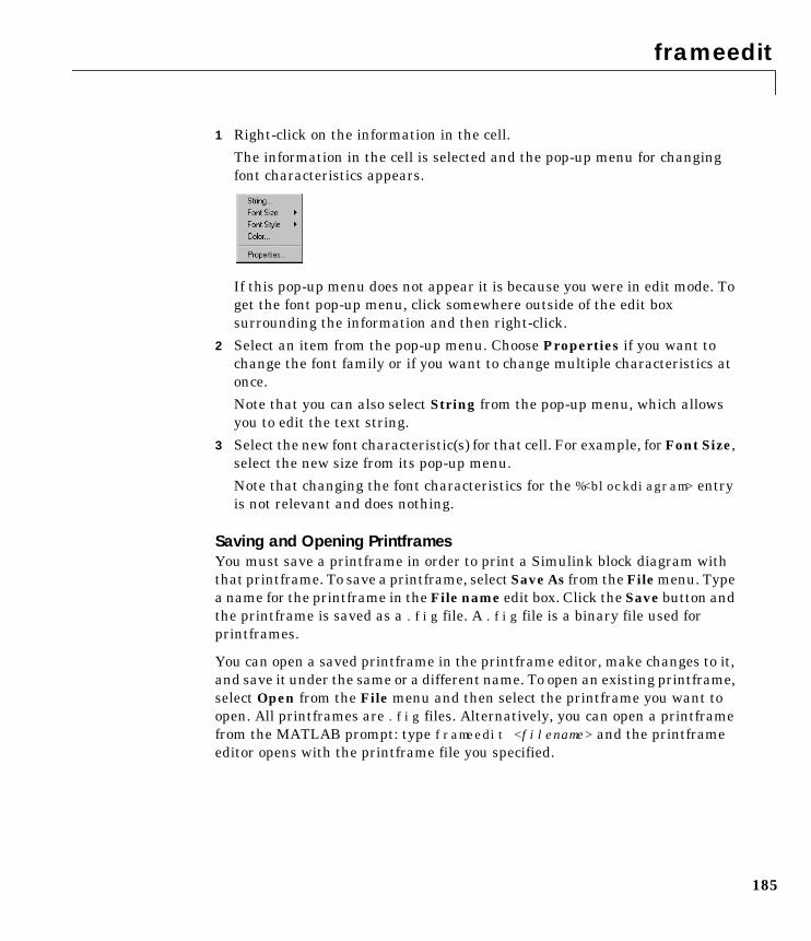
frameedit

1 Right-click on the information in the cell.

The information in the cell is selected and the pop-up menu for changingfont characteristics appears.

If this pop-up menu does not appear it is because you were in edit mode. Toget the font pop-up menu, click somewhere outside of the edit boxsurrounding the information and then right-click.

2 Select an item from the pop-up menu. Choose Properties if you want tochange the font family or if you want to change multiple characteristics atonce.

Note that you can also select String from the pop-up menu, which allowsyou to edit the text string.

3 Select the new font characteristic(s) for that cell. For example, for Font Size,select the new size from its pop-up menu.

Note that changing the font characteristics for the %<blockdiagram> entryis not relevant and does nothing.

Saving and Opening PrintframesYou must save a printframe in order to print a Simulink block diagram withthat printframe. To save a printframe, select Save As from the File menu. Typea name for the printframe in the File name edit box. Click the Save button andthe printframe is saved as a .fig file. A .fig file is a binary file used forprintframes.

You can open a saved printframe in the printframe editor, make changes to it,and save it under the same or a different name. To open an existing printframe,select Open from the File menu and then select the printframe you want toopen. All printframes are .fig files. Alternatively, you can open a printframefrom the MATLAB prompt: type frameedit <filename> and the printframeeditor opens with the printframe file you specified.

185

frameedit

Closing the Printframe EditorTo close the PrintFrame Editor window, click the close box in the upper rightcorner, or select Close from the File menu.

Printing Simulink Block Diagrams with PrintframesWhen using Simulink, you can print a block diagram with the printframe.Select Print from the Simulink File menu.

Check this box to printthe block diagramwith a printframe.

Type the path andfilename of theprintframe you wantthe block diagram toprint with,

or

click the ... button andthen select theprintframe file.

Print Model dialog box for Windows platform – the dialog box for your platform might look slightly different

186

frameedit

In the Print Model dialog box:

1 Check the Frame box.

2 Supply the filename for the printframe you want to use. Either type the pathand filename directly in the edit box, or click the ... button and select theprintframe file you saved using the printframe editor.

Note that the default printframe filename, sldefaultframe.fig, appears inthe filename edit box until you specify a different filename.

3 Specify other printing options in the Print dialog box. For example, forWindows, specify options under Properties.

Note: Specify the paper orientation for printing the way you normally would.The paper orientation you specified in the printframe editor’s PrintFramePage Setup dialog box is not the same as the paper orientation used forprinting. For example, assume you specified a landscape-oriented printframein the printframe editor. If you want the printed page to have a landscapeorientation, you must specify that at the time of printing. For example, forWindows, click the Properties button in the Simulink Print Model dialogbox, and for Page Setup, specify the Orientation as Landscape.

4 Click OK in the Print dialog box.

The Simulink block diagram prints with the printframe you specified.

187

frameedit

Examples This example uses a Simulink demo engine model. It involves two parts – firstcreating a printframe, and then printing the engine model with thatprintframe. The final result is:

Create the Printframe

1 At the MATLAB prompt, type frameedit.

The PrintFrame Editor window appears.

2 Set up the page:

a Select Page Setup from the File menu.

The PrintFrame Page Setup dialog box opens.

b For Paper Type, select a size that is appropriate for your printer.

1 of 3

Simulinkblockdiagram

Printframeborders

Variable information included in printframe

Engine DivisionAdvanced Design Group

engine/Throttle & Manifold

.75 inchpagemargins

Fixed information included in printframe

188

frameedit

c For this example, keep the Paper Orientation as Landscape and theMargins set to .75 inches.

d Click the OK button.

The dialog box closes. If you changed the Paper Type, the printframe yousee in the PrintFrame Editor window will reflect your change.

3 Add a row at the top.

a Click within the upper row in the printframe – this is the row thatcontains the %<blockdiagram> entry.

Be sure that handles appear on all four corners of the row.

b Click the add row button.

A new row appears at the top, above the row you selected.

4 Make the new row shorter.

a Click on the horizontal line that separates the top row (the row you justadded) from the row beneath it (the row containing the %<blockdiagram>entry).

Be sure that only two handles appear, one at each end of the line. If yousee four handles in either row, click directly on the horizontal line and theother two handles disappear.

b Drag the line up until the top row is about the same height as the row atthe bottom of the printframe.

5 Add information in the top row.

a Click within the top row (the row you just added).

b Select Text from the Fill drop-down menu.

c Click the Add button.

An edit box appears in the cell.

d Type Engine Division, press the Enter key to advance the cursor to thenext line, and then type Advanced Design Group.

Click the zoom in button if you need to magnify the entry.

e Click outside of the edit box to end editing mode.

189

frameedit

6 In the left cell of the bottom row, align the information on the left.

a Click the zoom out button if you need to.

b Click within the left cell of the bottom row to select it.

c Click the L button.

The entry moves to the left.

7 Make the information in the left cell of the bottom row appear in bold.

a Right-click on the entry in the cell.

b Select Font Style from the pop-up menu.

If the pop-up menu for font properties does not appear, you are in editingmode. Click outside of the edit box to end editing mode and thenright-click on the text to access the pop-up menu.

c From the Font Style pop-up menu, select bold.

The entry in the cell appears in bold and the information will appear in boldwhen the printframe is printed with a Simulink diagram.

8 Add the total number of pages to the right cell in the bottom row.

a Click within the cell to select it.

b Add the total pages entry: select Total Pages from the Fill drop-downmenu and click the Add button.

The %<npages> entry appears after the %<page> entry. If you need to,zoom in to see the entry.

c Add the text of after the page number entry: click the cursor after the%<page> entry, and then type of (type a space before and after the word).

The information in the cell now is: %<page> of %<npages>.

9 Optional – you can experiment and make changes on your own.

10 Save the printframe – select Save As from the File menu. In the SaveFrame dialog box, type engdivl for the File name. Click the Save button.

The printframe is saved as a .fig file.

11 You can close the PrintFrame Editor window if you want to – click the closebox.

190

frameedit

Print the Simulink Block Diagram with the Printframe

1 To view the Simulink engine model, type engine at the MATLAB prompt.

The engine model appears in a Simulink window.

2 Double-click on the Throttle & Manifold block.

The Throttle & Manifold subsystem opens in a new window.

3 In the Throttle & Manifold window, select Print from the File menu.

The Print Model dialog box opens.

191

frameedit

4 In the Print Model dialog box, set the page orientation to landscape. Thisexample uses the techniques for the Windows platform. Use the methods foryour own platform to change the page orientation for printing.

a Click the Properties button.

The Document Properties dialog box opens.

b Go to the Page Setup tab.

c For Orientation, select Landscape.

d Click OK.

The Document Properties dialog box closes.

5 In the Print Model dialog box, under Options, select Current system andbelow.

This specifies that the Throttle & Manifold block diagram and itssubsystems will print.

6 Check the Frame check box.

7 Specify the printframe to use.

a Click the ... button

b In the Frame File Selection dialog box, find the filename of theprintframe you just created, engdivl.fig, and select it.

c Click the Open button.

The path and filename appear in the Frame edit box.

8 Click the OK button in the Print Model dialog box.

The Throttle & Manifold block diagram prints with the printframe; it shouldlook similar to the figure shown at the start of this example.

In addition, the Throttle block diagram prints on page 2, and the IntakeManifold block diagram on page 3. These block diagrams also print with theengdivl printframe, but note that their variable information in theprintframe is different.

192

gca

2gcaPurpose Get current Axes handle

Syntax h = gca

Description h = gca returns the handle to the current Axes for the current Figure. If noAxes exists, MATLAB creates one and returns its handle. You can use thestatement,

get(gcf,'CurrentAxes')

if you do not want MATLAB to create an Axes if one does not already exist.

The current Axes is the target for graphics output when you create Axeschildren. Graphics commands such as plot, text, and surf draw their resultsin the current Axes. Changing the current Figure also changes the currentAxes.

See Also axes, cla, delete, gcf, gcbo, gco, hold, subplot, findobjFigure CurrentAxes property

2-193

gcf

2gcfPurpose Get current Figure handle

Syntax h = gcf

Description h = gcf returns the handle of the current Figure. The current Figure is theFigure window in which graphics commands such as plot, title, and surfdraw their results. If no Figure exists, MATLAB creates one and returns itshandle. You can use the statement,

get(0,'CurrentFigure')

if you do not want MATLAB to create a Figure if one does not already exist.

See Also axes, clf, close, delete, figure, gca, gcbo, gco, subplot

Root CurrentFigure property

2-194

gco

2gcoPurpose Return handle of current object

Syntax h = gcoh = gco(figure_handle)

Description h = gco returns the handle of the current object.

h = gco(figure_handle) returns the value of the current object for theFigure specified by figure_handle.

Remarks The current object is the last object clicked on, excluding Uimenus. If the mouseclick did not occur over a Figure child object, the Figure becomes the currentobject. MATLAB stores the handle of the current object in the Figure’sCurrentObject property.

The CurrentObject of the CurrentFigure does not always indicate the objectwhose callback is being executed. Interruptions of callbacks by other callbackscan change the CurrentObject or even the CurrentFigure. Some callbacks,such as CreateFcn and DeleteFcn, and Uimenu Callback intentionally do notupdate CurrentFigure or CurrentObject.

gcbo provides the only completely reliable way to retrieve the handle to theobject whose callback is executing, at any point in the callback function,regardless of the type of callback or of any previous interruptions.

Examples This statement returns the handle to the current object in Figure window 2:

h = gco(2)

See Also gca, gcbo, gcf

The Root object description

2-195

get

2getPurpose Get object properties

Syntax get(h)get(h,'PropertyName')<m-by-n value cell array> = get(H,<property cell array>)a = get(h)a = get(0,'Factory')a = get(0,'FactoryObjectTypePropertyName')a = get(h,'Default')a = get(h,'DefaultObjectTypePropertyName')

Description get(h) returns all properties and their current values of the graphics objectidentified by the handle h.

get(h,'PropertyName') returns the value of the property 'PropertyName' ofthe graphics object identified by h.

<m-by-n value cell array> = get(H,pn) returns n property values for mgraphics objects in the m-by-n cell array, where m = length(H) and n is equalto the number of property names contained in pn.

a = get(h) returns a structure whose field names are the object’s propertynames and whose values are the current values of the correspondingproperties. h must be a scalar. If you do not specify an output argument,MATLAB displays the information on the screen.

a = get(0,'Factory') returns the factory-defined values of all user-settableproperties. a is a structure array whose field names are the object propertynames and whose field values are the values of the corresponding properties.If you do not specify an output argument, MATLAB displays the informationon the screen.

a = get(0,'FactoryObjectTypePropertyName') returns the factory-definedvalue of the named property for the specified object type. The argument,FactoryObjectTypePropertyName is the word Factory concatenated with theobject type (e.g., Figure) and the property name (e.g., Color):

FactoryFigureColor

2-196

get

a = get(h,'Default') returns all default values currently defined on objecth. a is a structure array whose field names are the object property names andwhose field values are the values of the corresponding properties. If you do notspecify an output argument, MATLAB displays the information on the screen.

a = get(h,'DefaultObjectTypePropertyName') returns the factory-definedvalue of the named property for the specified object type. The argument,DefaultObjectTypePropertyName is the word Default concatenated with theobject type (e.g., Figure) and the property name (e.g., Color):

DefaultFigureColor

Examples You can obtain the default value of the LineWidth property for Line graphicsobjects defined on the Root level with the statement:

get(0,'DefaultLineLineWidth')

ans = 0.5000

To query a set of properties on all Axes children define a cell array of propertynames:

props = 'HandleVisibility', 'Interruptible';'SelectionHighlight', 'Type';

output = get(get(gca,'Children'),props);

The variable output is a cell array of dimension:length(get(gca,'Children')−by−4.

For example, type:

patch;surface;text;lineoutput = get(get(gca,'Children'),props)output =

'on' 'on' 'on' 'line''on’ 'off' 'on' 'text''on' 'on' 'on' 'surface''on' 'on' 'on' 'patch'

See Also findobj, gca, gcf, gco, set

2-197

getframe

2getframePurpose Get movie frame

Synopsis M = getframeM = getframe(h)M = getframe(h,rect)[X,Map] = getframe(...)

Description getframe returns a column vector containing one movie frame. The frame is asnapshot (pixmap) of the current Axes.

M = getframe gets a frame from the current Axes.

M = getframe(h) gets a frame from the Figure or Axes graphics objectidentified by h.

M = getframe(h,rect) specifies a rectangular area from which to copy thepixmap. rect is relative to the lower-left corner of the Figure or Axes graphicsobject identified by h, in pixel units. rect is a four-element vector in the form[left bottom width height], where width and height define the dimensionsof the rectangle.

[X,Map] = getframe(...) returns the frame as an indexed image matrix Xand a colormap Map. In this case, h is a handle to a Figure or Axes object. Youdisplay the image matrix using image or imagesc.

Remarks Usually, getframe is put in a for loop to assemble movie matrix M for playbackusing movie. To provide more efficient memory use, use moviein to allocatemovie matrix M before building the movie. This generates an appropriate sizematrix of zeros.

Note that M = getframe; returns the contents of the current Axes, exclusive ofthe axis labels, title, or tick labels. M = getframe(gcf); captures the entireinterior of the current Figure window.

If you plan to convert the MATLAB movie to another format (such asQuickTime) and you want to include the axis labels in this new format, youshould capture the Figure, not just the Axes. If you are using moviein topre-allocate the movie matrix, be sure to specify the same Figure handle thatyou use with getframe.

2-198

getframe

Examples Make the peaks function vibrate:

Z = peaks; surf(Z)M = moviein(20);axis manual % Freeze Axes limitsset(gca,'nextplot','replacechildren');for j = 1:20

surf(sin(2*pi*j/20)*Z,Z)M(:,j) = getframe;

endmovie(M,20) % Play the movie twenty times

See Also movie, moviein,qtwrite

2-199

ginput

2ginputPurpose Input data using the mouse

Syntax [x,y] = ginput(n)[x,y] = ginput[x,y,button] = ginput(...)

Description ginput enables you to select points from the Figure using the mouse or arrowkeys for cursor positioning. The Figure must have focus before ginput receivesinput.

[x,y] = ginput(n) enables you to select n points from the current Axes andreturns the x- and y-coordinates in the column vectors x and y, respectively.You can press the Return key to terminate the input before entering n points.

[x,y] = ginput gathers an unlimited number of points until you press theReturn key.

[x,y,button] = ginput(...) returns the x-coordinates, the y-coordinates,and the button or key designation. button is a vector of integers indicatingwhich mouse buttons you pressed (1 for left, 2 for middle, 3 for right), or ASCIInumbers indicating which keys on the keyboard you pressed.

Remarks If you select points from multiple Axes, the results you get are relative to thoseAxes coordinates systems.

Examples Pick 10 two-dimensional points from the Figure window.

[x,y] = ginput(10)

Position the cursor with the mouse (or the arrow keys on terminals without amouse, such as Tektronix emulators). Enter data points by pressing a mousebutton or a key on the keyboard. To terminate input before entering 10 points,press the Return key.

See Also gtext

2-200

gplot

2gplotPurpose Plot set of nodes using an adjacency matrix

Synopsis gplot(A,Coordinates)gplot(A,Coordinates,LineSpec)

Description The gplot function graphs a set of coordinates using an adjacency matrix.

gplot(A,Coordinates) plots a graph of the nodes defined in Coordinatesaccording to the n-by-n adjacency matrix A, where n is the number of nodes.Coordinates is an n-by-2 or an n-by-3 matrix, where n is the number of nodesand each coordinate pair or triple represents one node.

gplot(A,Coordinates,LineSpec) plots the nodes using the line type, markersymbol, and color specified by LineSpec.

Remarks For two-dimensional data, Coordinates(i,:) = [x(i) y(i)] denotes node i,and Coordinates(j,:) = [x(j) y(j)] denotes node j. If node i and node j arejoined, A(i,j) or A(j,i) are nonzero; otherwise, A(i,j) and A(j,i) are zero.

2-201

gplot

Examples To draw half of a Bucky ball with asterisks at each node:

k = 1:30;[B,XY] = bucky;gplot(B(k,k),XY(k,:),'-*')axis square

See Also LineSpec, sparse, spy

−1 −0.8 −0.6 −0.4 −0.2 0 0.2 0.4 0.6 0.8 1−1

−0.8

−0.6

−0.4

−0.2

0

0.2

0.4

0.6

0.8

1

2-202

graymon

2graymonPurpose Set default Figure properties for grayscale monitors

Syntax graymon

Description graymon sets defaults for graphics properties to produce more legible displaysfor grayscale monitors.

See Also axes, figure

2-203

grid

2gridPurpose Grid lines for two- and three-dimensional plots

Syntax grid ongrid offgrid

Description The grid function turns the current Axes’ grid lines on and off.

grid on adds grid lines to the current Axes.

grid off removes grid lines from the current Axes.

grid toggles the grid visibility state.

Algorithm grid sets the XGrid, YGrid, and ZGrid properties of the current Axes.

See Also axes, plot

The XGrid, YGrid, and ZGrid properties of Axes objects.

2-204

gtext

2gtextPurpose Mouse placement of text in two-dimensional view

Syntax gtext('string')h = gtext('string')

Description gtext displays a text string in the current Figure window after you select alocation with the mouse.

gtext('string') waits for you to press a mouse button or keyboard key whilethe pointer is within a Figure window. Pressing a mouse button or any keyplaces 'string' on the plot at the selected location.

h = gtext('string') returns a handle to a Text graphics objects after youplace 'string' on the plot at the selected location.

Remarks As you move the pointer into a Figure window, the pointer becomes a crosshairto indicate that gtext is waiting for you to select a location. gtext uses thefunctions ginput and text.

Examples Place a label on the current plot:

gtext('Note this divergence!')

See Also ginput, text

2-205

hidden

2hiddenPurpose Remove hidden lines from a mesh plot

Syntax hidden onhidden offhidden

Description Hidden line removal draws only those lines that are not obscured by otherobjects in the field of view.

hidden on turns on hidden line removal for the current graph so lines in theback of a mesh are hidden by those in front. This is the default behavior.

hidden off turns off hidden line removal for the current graph.

hidden toggles the hidden line removal state.

Algorithm hidden on sets the FaceColor property of a Surface graphics object to thebackground Color of the Axes (or of the Figure if Axes Color is none).

Examples Set hidden line removal off and on while displaying the peaks function:

mesh(peaks)hidden offhidden on

See Also shading

The Surface properties FaceColor and EdgeColor

2-206

hist

2histPurpose Histogram plot

Syntax n = hist(Y)n = hist(Y,x)n = hist(Y,nbins)[n,xout] = hist(...)

Description A histogram shows the distribution of data values.

n = hist(Y) draws a histogram of the elements in Y, binning the data into tenequally spaced containers and returns the number of elements in eachcontainer. If Y is a matrix, hist works down the columns. hist distributes thebins along the x-axis between the minimum and maximum values of Y.

n = hist(Y,x) draws a histogram using n bins, where n is length(x). x alsospecifies the locations on the x-axis where hist places the bins. For example, ifx is a 5-element vector, hist distributes the elements of Y into five binscentered on the x-axis at the elements in x.

n = hist(Y,nbins) draws a histogram with no more bins than nbins.

[n,xout] = hist(...) returns vectors n and xout containing the frequencycounts and the bin locations. This syntax does not generate a plot. This is usefulwhen you need more control over the appearance of a graph, for example, tocombine a histogram into a more elaborate plot. You can use bar(xout,n) toplot the histogram.

Remarks All elements in vector Y or in one column of matrix Y are grouped according totheir numeric range. Each group is shown as one bin.

The histogram’s x-axis reflects the range of values in Y. The histogram’s y-axisshows the number of elements that fall within the groups; therefore, the y-axisranges from 0 to the greatest number of elements deposited in any bin.

The histogram is created with a Patch graphics object. If you want to changethe color of the graph, you can set Patch properties. See the “Example” sectionfor more information. By default, the graph color is controlled by the currentcolormap, which maps the bin color to the first color in the colormap.

2-207

hist

Examples Generate a bell-curve histogram from Gaussian data:

x = –2.9:0.1:2.9;y = randn(10000,1);hist(y,x)

−3 −2 −1 0 1 2 30

50

100

150

200

250

300

350

400

2-208

hist

Change the color of the graph so that the bins are red and the edges of the binsare white:

h = get(gca,'Children');set(h,'FaceColor','r',EdgeColor','w')

See Also bar,ColorSpec, patch, stairs

−3 −2 −1 0 1 2 30

50

100

150

200

250

300

350

400

2-209

hold

2holdPurpose Hold current graph in the Figure

Syntax hold onhold offhold

Description The hold function determines whether new graphics objects are added to thegraph or replace objects in the graph.

hold on retains the current plot and certain Axes properties so thatsubsequent graphing commands add to the existing graph.

hold off resets Axes properties to their defaults before drawing new plots.hold off is the default.

hold toggles the hold state between adding to the graph and replacing thegraph.

Remarks Test the hold state using the ishold function.

Although the hold state is on, some Axes properties change to accommodateadditional graphics objects. For example, the Axes’ limits increase when thedata requires them to do so.

Algorithm The hold function sets the NextPlot property of the current Figure and thecurrent Axes. If several Axes objects exist in a Figure window, each Axes hasits own hold state. hold also creates an Axes if one does not exist.

hold on sets the NextPlot property of the current Figure and Axes to add.

hold off sets the NextPlot property of the current Axes to replace.

hold toggles the NextPlot property between the add and replace states.

See Also axis, cla, ishold, newplot

The NextPlot property of Axes and Figure graphics objects.

2-210

home

2homePurpose Send the cursor home

Syntax home

Description home returns the cursor to the upper-left corner of the command window.

Examples Display a sequence of random matrices at the same location in the commandwindow:

clcfor i =1:25

homeA = rand(5)

end

See Also clc

2-211

hsv2rgb

2hsv2rgbPurpose Convert HSV colormap to RGB colormap

Syntax M = hsv2rgb(H)

Description M = hsv2rgb(H) converts a hue-saturation-value (HSV) colormap to ared-green-blue (RGB) colormap. H is an m-by-3 matrix, where m is the numberof colors in the colormap. The columns of H represent hue, saturation, andvalue, respectively. M is an m-by-3 matrix. Its columns are intensities of red,green, and blue, respectively.

Remarks As H(:,1) varies from 0 to 1, the resulting color varies from red, throughyellow, green, cyan, blue, and magenta, and returns to red. When H(:,2) is 0,the colors are unsaturated (i.e., shades of gray). When H(:,2) is 1, the colorsare fully saturated (i.e., they contain no white component). As H(:,3) variesfrom 0 to 1, the brightness increases.

The MATLAB hsv colormap uses hsv2rgb([hue saturation value]) wherehue is a linear ramp from 0 to 1, and saturation and value are all 1’s.

See Also brighten, colormap, rgb2hsv

2-212

im2frame

2im2framePurpose Convert indexed image into movie frame

Syntax F = im2frame(X,Map)

Description F = im2frame(X,Map) converts the indexed image X and associated colormapMap into a movie frame F. You can use im2frame to convert a sequence of imagesinto a movie.

Example To use im2frame to convert a sequence of images into a movie, first pre-allocatematrix using movein:

M = moviein(n);M(:,1) = im2frame(X1,map);M(:,2) = im2frame(X2,map);...M(:,n) = im2frame(Xn,map);movie(M)

See Also capture, frame2im, movie, moviein

2-213

image

2imagePurpose Display Image object

Syntax image(C)image(x,y,C)image(...,'PropertyName',PropertyValue,...)image('PropertyName',PropertyValue,...) Formal synatx – PN/PV onlyhandle = image(...)

Description image creates an Image graphics object by interpreting each element in amatrix as an index into the Figure’s colormap or directly as RGB values,depending on the data specified.

The image function has two forms:

• A high-level function that calls newplot to determine where to draw thegraphics objects and sets the following Axes properties:

XLim and YLim to enclose the Image

Layer to top to place the Image in front of the tick marks and grid lines

YDir to reverse

View to [0 90]

• A low-level function that adds the Image to the current Axes without callingnewplot. The low-level function argument list can contain only propertyname/property value pairs.

You can specify properties as property name/property value pairs, structurearrays, and cell arrays (see the set and get reference pages for examples ofhow to specify these data types).

image(C) displays matrix C as an Image. Each element of C specifies the colorof a rectangular segment in the Image.

image(x,y,C) where x and y are two-element vectors, specifies the range ofthe x- and y-axis labels, but produces the same Image as image(C). This can beuseful, for example, if you want the axis tick labels to correspond to realphysical dimensions represented by the image.

2-214

image

image(x,y,C,'PropertyName',PropertyValue,...) is a high-level functionthat also specifies property name/property value pairs. This syntax callsnewplot before drawing the Image.

image('PropertyName',PropertyValue,...) is the low-level syntax of theimage function. It specifies only property name/property value pairs as inputarguments.

handle = image(...) returns the handle of the Image object it creates. Youcan obtain the handle with all forms of the image function.

Remarks Image data can be either indexed or true color. An indexed image stores colorsas an array of indices into the Figure colormap. A true color image does not usea colormap; instead, the color values for each pixel are stored directly as RGBtriplets. In MATLAB , the CData property of a truecolor Image object is athree-dimensional (m-by-n-by-3) array. This array consists of three m-by-nmatrices (representing the red, green, and blue color planes) concatenatedalong the third dimension.

The imread function reads image data into MATLAB arrays from graphics filesin various standard formats, such as TIFF. You can write MATLAB image datato graphics files using the imwrite function. imread and imwrite both supporta variety of graphics file formats and compression schemes.

When you read image data into MATLAB using imread, the data is stored asan array of 8-bit integers. This is a much more efficient storage method thanthe double-precision (64-bit) floating-point numbers that MATLAB typically

2-215

image

uses. However, it is necessary for MATLAB to interpret 8-bit image datadifferently from 64-bit data. This table summarizes these differences:

Indexed imagesIn an indexed image of class double, the value 1 points to the first row in thecolormap, the value 2 points to the second row, and so on. In a uint8 indexedimage, there is an offset; the value 0 points to the first row in the colormap, thevalue 1 points to the second row, and so on. The uint8 convention is also usedin graphics file formats, and enables 8-bit indexed images to support up to 256colors. Note that when you read in an indexed image with imread, the resultingimage array is always of class uint8. (The colormap, however, is of classdouble; see below.)

If you want to convert a uint8 indexed image to double, you need to add 1 tothe result. For example:

X64 = double(X8) + 1;

To convert from double to uint8, you need to first subtract 1, and then useround to ensure all the values are integers:

X8 = uint8(round(X64 – 1));

ImageType

Double-precision Data(double array)

8-bit Data (uint8 array)

indexed(colormap)

Image is stored as atwo-dimensional (m-by-n) arrayof integers in the range [1,length(colormap)]; colormapis an m-by-3 array offloating-point values in therange [0, 1]

Image is stored as atwo-dimensional (m-by-n)array of integers in therange [0, 255]; colormapis an m-by-3 array offloating-point values inthe range [0, 1]

truecolor(RGB)

Image is stored as athree-dimensional(m-by-n-by-3) array offloating-point values in therange [0, 1]

Image is stored as athree-dimensional(m-by-n-by-3) array ofintegers in the range[0, 255]

2-216

image

The order of the operations must be as shown in these examples, because youcannot perform mathematical operations on uint8 arrays.

When you write an indexed image using imwrite, MATLAB automaticallyconverts the values if necessary.

ColormapsColormaps in MATLAB are alway m-by-3 arrays of double-precisionfloating-point numbers in the range [0, 1]. In most graphics file formats,colormaps are stored as integers, but MATLAB does not support colormapswith integer values. imread and imwrite automatically convert colormapvalues when reading and writing files.

True Color ImagesIn a truecolor image of class double, the data values are floating-point numbersin the range [0, 1]. In a truecolor image of class uint8, the data values areintegers in the range [0, 255].

If you want to convert a truecolor image from one data type to the other, youmust rescale the data. For example, this call converts a uint8 truecolor imageto double:

RGB64 = double(RGB8)/255;

This statement converts a double truecolor image to uint8:

RGB8 = uint8(round(RGB*255));

The order of the operations must be as shown in these examples, because youcannot perform mathematical operations on uint8 arrays.

When you write a truecolor image using imwrite, MATLAB automaticallyconverts the values if necessary.

2-217

image

ObjectHierarchy

Setting Default PropertiesYou can set default Image properties on the Axes, Figure, and Root levels:

set(0,'DefaultImageProperty',PropertyValue...)set(gcf,'DefaultImageProperty',PropertyValue...)set(gca,'DefaultImageProperty',PropertyValue...)

Where Property is the name of the Image property and PropertyValue is thevalue you are specifying. Use set and get to access Image properties.

The following table lists all Image properties and provides a brief descriptionof each. The property name links take you to an expanded description of theproperties.

Patch

Root

Text

Uimenu

SurfaceLine

Axes Uicontrol

Image

Figure

Uicontextmenu

Light


Data Defining the Object

CData The image data Values: matrix orm-by-n-by-3 arrayDefault: enterimage;axis image ijand see

CDataMapping Specify the mapping of data tocolormap

Values: scaled, directDefault: direct

2-218

image

XData Control placement of image alongx-axis

Values: [min max]Default: [1 size(CData,2)]

YData Control placement of image alongy-axis

Values: [min max]Default: [1 size(CData,1)]

Controlling the Appearance

Clipping Clipping to Axes rectangle Values: on, offDefault: on

EraseMode Method of drawing and erasing theimage (useful for animation)

Values: normal, none, xor,backgroundDefault: normal

SelectionHighlight Highlight image when selected(Selected property set to on)


Visible Make the image visible or invisible Values: on, offDefault: on


HandleVisibility Determines if and when the theLine’s handle is visible to otherfunctions


HitTest Determine if image can become thecurrent object (see the FigureCurrentObject property)


General Information About the Image

Children Image objects have no children Values: [] (empty matrix)

Parent The parent of an image object isalways an Axes object

Value: Axes handle

Selected Indicate whether image is in a“selected” state.



2-219

image



Value: the string 'image'


Properties Related to Callback Routine Execution



ButtonDownFcn Define a callback routine thatexecutes when a mouse button ispressed on over the image


CreateFcn Define a callback routine thatexecutes when an image is created


DeleteFcn Define a callback routine thatexecutes when the image is deleted(via close or delete)




UIContextMenu Associate a context menu with theimage



2-220

Image Properties

2Image PropertiesImageProperties

This section lists property names along with the types of values each propertyaccepts.


Callback routine interruption. The BusyAction property enables you to controlhow MATLAB handles events that potentially interrupt executing callbackroutines. If there is a callback routine executing, subsequently invokedcallback routes always attempt to interrupt it. If the Interruptible propertyof the object whose callback is executing is set to on (the default), theninterruption occurs at the next point where the event queue is processed. If theInterruptible property is off, the BusyAction property (of the object owningthe executing callback) determines how MATLAB handles the event. Thechoices are:




Button press callback routine. A callback routine that executes whenever youpress a mouse button while the pointer is over the Image object. Define thisroutine as a string that is a valid MATLAB expression or the name of an M-file.The expression executes in the MATLAB workspace.

CData matrix or m-by-n-by-3 array

The Image data. A matrix of values specifying the color of each rectangulararea defining the Image. image(C) assigns the values of C to CData. MATLABdetermines the coloring of the Image in one of three ways:

• Using the elements of CData as indices into the current colormap (thedefault)

• Scaling the elements of CData to range between the valuesmin(get(gca,'CLim')) and max(get(gca,'CLim')) (CDataMapping set toscaled)

• Interpreting the elements of CData directly as RGB values (true colorspecification)

2-221

Image Properties

A true color specification for CData requires an m-by-n-by-3 array of RGBvalues. The first page contains the red component, the second page the greencomponent, and the third page the blue component of each element in theImage. RGB values range from 0 to 1. The following picture illustrates therelative dimensions of CData for the two color models:

If CData has only one row or column, the height or width respectively is alwaysone data unit and is centered about the first YData or XData elementrespectively. For example, using a 4-by-1 matrix of random data,

C = rand(4,1);image(C,'CDataMapping','scaled')axis image

Red

GreenBlue

CData

CData

Indexed Colors True Colors

2-222

Image Properties

produces:

CDataMapping scaled | direct

Direct or scaled indexed colors. This property determines whether MATLABinterprets the values in CData as indices into the Figure colormap (the default)or scales the values according to the values of the Axes CLim property.

When CDataMapping is direct, the values of CData should be in the range 1 tolength(get(gcf,'Colormap')). If you use true color specification for CData,this property has no effect.

Children handles

The empty matrix; Image objects have no children.

Clipping on | off

Clipping mode. By default, MATLAB clips Images to the Axes rectangle. If youset Clipping to off, the Image can display outside the Axes rectangle. Forexample, if you create an Image, set hold to on, freeze axis scaling (axismanual), and then create a larger Image, it extends beyond the axis limits.

0.5 1 1.5

0.5

1

1.5

2

2.5

3

3.5

4

4.5

2-223

Image Properties

CreateFcn string

Callback routine executed during object creation. This property defines acallback routine that executes when MATLAB creates an Image object. Youmust define this property as a default value for Images. For example, thestatement,

set(0,'DefaultImageCreateFcn','axis image')

defines a default value on the Root level that sets the aspect ratio and the axislimits so the Image has square pixels. MATLAB executes this routine aftersetting all Image properties. Setting this property on an existing Image objecthas no effect.


DeleteFcn string

Delete Image callback routine. A callback routine that executes when youdelete the Image object (i.e., when you issue a delete command or clear theAxes or Figure containing the Image). MATLAB executes the routine beforedestroying the object’s properties so these values are available to the callbackroutine.


EraseMode normal | none | xor | background

Erase mode. This property controls the technique MATLAB uses to draw anderase Image objects. Alternative erase modes are useful for creating animatedsequences, where control of the way individual objects redraw is necessary toimprove performance and obtain the desired effect.

• normal (the default) — Redraw the affected region of the display, performingthe three-dimensional analysis necessary to ensure that all objects arerendered correctly. This mode produces the most accurate picture, but is theslowest. The other modes are faster, but do not perform a complete redrawand are therefore less accurate.

• none – Do not erase the Image when it is moved or changed. While the objectis still visible on the screen after erasing with EraseMode none, you cannotprint it because MATLAB stores no information about its former location.

2-224

Image Properties

• xor – Draw and erase the Image by performing an exclusive OR (XOR) withthe color of the screen beneath it. This mode does not damage the color of theobjects beneath the Image. However, the Image’s color depends on the colorof whatever is beneath it on the display.

• background – Erase the Image by drawing it in the Axes’ background Color,or the Figure background Color if the Axes Color is set to none. Thisdamages objects that are behind the erased Image, but Images are alwaysproperly colored.

Printing with Non-normal Erase Modes. MATLAB always prints Figures as if theEraseMode of all objects is normal. This means graphics objects created withEraseMode set to none, xor, or background can look different on screen than onpaper. On screen, MATLAB may mathematically combine layers of colors (e.g.,XORing a pixel color with that of the pixel behind it) and ignorethree-dimensional sorting to obtain greater rendering speed. However, thesetechniques are not applied to the printed output.

You can use the MATLAB capture command or other screen captureapplication to create an image of a Figure containing non-normal mode objects.




Setting HandleVisibility to callback causes handles to be visible fromwithin callback routines or functions invoked by callback routines, but not fromwithin functions invoked from the command line. This provide a means toprotect GUIs from command-line users, while allowing callback routines tohave complete access to object handles.

Setting HandleVisibility to off makes handles invisible at all times. Thismay be necessary when a callback routine invokes a function that mightpotentially damage the GUI (such as evaling a user-typed string), and sotemporarily hides its own handles during the execution of that function.

2-225

Image Properties





HitTest on | off

Selectable by mouse click. HitTest determines if the Image can become thecurrent object (as returned by the gco command and the Figure CurrentObjectproperty) as a result of a mouse click on the Image. If HiTest is off, clicking onthe Image selects the object below it (which maybe the Axes containing it).


Callback routine interruption mode. The Interruptible property controlswhether an Image callback routine can be interrupted by subsequently invokedcallback routines. Only callback routines defined for the ButtonDownFcn areaffected by the Interruptible property. MATLAB checks for events that caninterrupt a callback routine only when it encounters a drawnow, figure,getframe, or pause command in the routine.

Parent handle of parent Axes

Image’s parent. The handle of the Image object’s parent Axes. You can move anImage object to another Axes by changing this property to the new Axeshandle.

Selected on | off

Is object selected. When this property is on, MATLAB displays selectionhandles if the SelectionHighlight property is also on. You can, for example,

2-226

Image Properties

define the ButtonDownFcn to set this property, allowing users to select theobject with the mouse.


Objects highlight when selected. When the Selected property is on, MATLABindicates the selected state by drawing four edge handles and four cornerhandles. When SelectionHighlight is off, MATLAB does not draw thehandles.

Tag string

User-specified object label. The Tag property provides a means to identifygraphics objects with a user-specified label. This is particularly useful whenconstructing interactive graphics programs that would otherwise need todefine object handles as global variables or pass them as arguments betweencallback routines. You can define Tag as any string.


Type of graphics object. This property contains a string that identifies the classof graphics object. For Image objects, Type is always 'image'.


Associate a context menu with the Image. Assign this property the handle of aUicontextmenu object created in the same Figure as the Image. Use theuicontextmenu function to create the context menu. MATLAB displays thecontext menu whenever you right-click over the Image (Control-click onMacintosh systems).

UserData matrix

User specified data. This property can be any data you want to associate withthe Image object. The Image does not use this property, but you can access itusing set and get.

Visible on | off

Image visibility. By default, Image objects are visible. Setting this property tooff prevents the Image from being displayed. However, the object still existsand you can set and query its properties.

XData [1 size(CData,2)] by default

Control placement of image along x-axis. A vector specifying the locations of thecenters of the elements CData(1,1) and CData(m,n), where CData has a size of

2-227

Image Properties

m-by-n. Element CData(1,1) is centered over the coordinate defined by the firstelements in XData and YData. Element CData(m,n) is centered over thecoordinate defined by the last elements in XData and YData. The centers of theremaining elements of CData are evenly distributed between those two points.

The width of each CData element is determined by the expression:

(XData(2)-XData(1))/(size(CData,2)-1)

You can also specify a single value for XData. In this case, image centers thefirst element at this coordinate and centers each following element one unitapart.

YData [1 size(CData,1)] by default

Control placement of image along y-axis. A vector specifying the locations of thecenters of the elements CData(1,1) and CData(m,n), where CData has a size ofm-by-n. Element CData(1,1) is centered over the coordinate defined by the firstelements in XData and YData. Element CData(m,n) is centered over thecoordinate defined by the last elements in XData and YData. The centers of theremaining elements of CData are evenly distributed between those two points.

The height of each CData element is determined by the expression:

(YData(2)-YData(1))/(size(CData,1)-1)

You can also specify a single value for YData. In this case, image centers thefirst element at this coordinate and centers each following elements one unitapart.

See Also colormap, imfinfo, imread, imwrite, pcolor, newplot, surface

The “Image” chapter the Using MATLAB Graphics manual

2-228

imagesc

2imagescPurpose Scale data and display an Image object

Syntax imagesc(C)imagesc(x,y,C)imagesc(...,clims)h = imagesc(...)

Description The imagesc function scales image data to the full range of the currentcolormap and displays the image. (See the illustration on the following page.)

imagesc(C) displays C as an image. Each element of C corresponds to arectangular area in the image. The values of the elements of C are indices intothe current colormap that determine the color of each patch.

imagesc(x,y,C) displays C as an Image and specifies the bounds of the x- andy-axis with vectors x and y.

imagesc(...,clims) normalizes the values in C to the range specified byclims and displays C as an Image. clims is a two-element vector that limits therange of data values in C. These values map to the full range of values in thecurrent colormap.

h = imagesc(...) returns the handle for an Image graphics object.

Remarks x and y do not affect the elements in C; they only affect the annotation of theAxes. If length(x) > 2 or length(y) > 2, imagesc ignores all except the firstand last elements of the respective vector.

Algorithm imagesc creates an image with CDataMapping set to scaled, and sets the AxesCLim to the value passed in clims.

2-229

imagesc

Examples If the size of the current colormap is 81-by-3,

The left Image maps to the gray colormap using the statements

load clownimagesc(X)colormap(gray)

The right Image has values between 10 and 60 scaled to the full range of thegray colormap using the statements

load clownclims = [10 60];imagesc(X,clims)colormap(gray)

81807978

4321

605958

1110

12

81

1

Data Colormap ValuesValues

the statements

clims = [10 60]imagesc(C,clims)

map the data values in C to the colormap,as shown to the right.

50 100 150 200 250 300

20

40

60

80

100

120

140

160

180

20050 100 150 200 250 300

20

40

60

80

100

120

140

160

180

200

2-230

imagesc

See Also image, colorbar

2-231

imfinfo

2imfinfoPurpose Return information about a graphics file

Synopsis info = imfinfo(filename,fmt)info = imfinfo(filename)

Description info = imfinfo(filename,fmt) returns a structure whose fields containinformation about an image in a graphics file. filename is a string thatspecifies the name of the graphics file, and fmt is a string that specifies theformat of the file. The file must be in the current directory or in a directory onthe MATLAB path. If imfinfo cannot find a file named filename, it looks for afile namedfilename.fmt.

This table lists the possible values for fmt:

If filename is a TIFF or HDF file containing more than one image, info is astructure array with one element (i.e., an individual structure) for each imagein the file. For example, info(3) would contain information about the thirdimage in the file.

Format File type

'bmp' Windows Bitmap (BMP)

'hdf' Hierarchical Data Format (HDF)

'jpg' or 'jpeg' Joint Photographic Experts Group (JPEG)

'pcx' Windows Paintbrush (PCX)

'tif' or 'tiff' Tagged Image File Format (TIFF)

'xwd' X Windows Dump (XWD)

2-232

imfinfo

The set of fields in info depends on the individual file and its format. However,the first seven fields are always the same. This table lists these fields anddescribes their values:

info = imfinfo(filename) attempts to infer the format of the file from itscontent.

Field Value

Filename A string containing the name of the file; if the file isnot in the current directory, the string contains thefull pathname of the file

Format A string containing the file format, as specified by fmt;for JPEG and TIFF files, the three-letter variant isreturned

FormatVersion A string or number describing the version of theformat

Width An integer indicating the width of the image in pixels

Height An integer indicating the height of the image in pixels

BitDepth An integer indicating the number of bits per pixel

ColorType A string indicating the type of image; either'truecolor' for a truecolor RGB image, 'grayscale'for a grayscale intensity image, or 'indexed' for anindexed image

2-233

imfinfo

Example info = imfinfo('flower.bmp')

info =

Filename: 'flower.bmp' Format: 'bmp' FormatVersion: 'Version 3 (Microsoft Windows 3.x)' Width: 227 Height: 149 BitDepth: 8 ColorType: 'indexed' FormatSignature: 'BM' NumColormapEntries: 256 Colormap: [256x3 double] RedMask: [] GreenMask: [] BlueMask: [] FileSize: 35050 ImageDataOffset: 1078 BitmapHeaderSize: 40 NumPlanes: 1 CompressionType: 'none' BitmapSize: 33972 HorzResolution: 0 VertResolution: 0 NumColorsUsed: 256 NumImportantColors: 0

See Also imread, imwrite

2-234

imread

2imreadPurpose Read image from graphics file

Synopsis A = imread(filename,fmt)[X,map] = imread(filename,fmt)[...] = imread(filename)[...] = imread(...,idx)[...] = imread(...,ref)

Description A = imread(filename,fmt) reads the image in filename into A, whose class isuint8. If the file contains a grayscale intensity image, A is a two-dimensionalarray. If the file contains a truecolor (RGB) image, A is a three-dimensional(m-by-n-by-3) array. filename is a string that specifies the name of the graphicsfile, and fmt is a string that specifies the format of the file. The file must be inthe current directory or in a directory in the MATLAB path. If imread cannotfind a file named filename, it looks for a file named filename.fmt.


[X,map] = imread(filename,fmt) reads the indexed image in filename intoX and its associated colormap into map. X is of class uint8, and map is of classdouble. The colormap values are rescaled when they are read to have the range[0, 1].

[...] = imfread(filename) attempts to infer the format of the file from itscontent.

Format File type



'jpg' or 'jpeg' Joint Photographic Experts Group (JPEG)




2-235

imread

[...] = imread(...,idx) reads in one image from a multi-image TIFF file.idx is an integer value that specifies the order that the image appears in thefile. For example, if idx is 3, imread reads the third image in the file. If you omitthis argument, imread reads the first image in the file.

[...] = imread(...,ref) reads in one image from a multi-image HDF file.ref is an integer value that specifies the reference number used to identify theimage. For example, if ref is 12, imread reads the image whose referencenumber is 12. (Note that in an HDF file the reference numbers do notnecessarily correspond with the order of the images in the file.) If you omit thisargument, imread reads the first image in the file.

This table summarizes the types of images that imread can read:

Examples This example reads the sixth image in a TIFF file:

[X,map] = imread('flower.tif',6);

This example reads the fourth image in an HDF file:

info = imfinfo('skull.hdf');[X,map] = imread('skull.hdf',info(4).Reference);

See Also imfinfo, imwrite

Format Variants

BMP 1-bit, 4-bit, 8-bit, and 24-bit uncompressed images; 4-bitand 8-bit run-length encoded (RLE) images

HDF 8-bit raster image datasets, with or without associatedcolormap; 24-bit raster image datasets

JPEG Any baseline JPEG image; JPEG images with somecommonly used extensions

PCX 1-bit, 8-bit, and 24-bit images

TIFF Any baseline TIFF image, including 1-bit, 8-bit, and 24-bituncompressed images; 1-bit, 8-bit, and 24-bit images withpackbit compression; 1-bit images with CCITT compression

XWD 1-bit and 8-bit ZPixmaps; XYBitmaps; 1-bit XYPixmaps

2-236

imwrite

2imwritePurpose Write an image to a graphics file

Synopsis imwrite(A,filename,fmt)imwrite(X,map,filename,fmt)imwrite(...,filename)imwrite(...,Parameter,Value,...)

Description imwrite(A,filename,fmt) writes the image in A to filename. filename is astring that specifies the name of the output file, and fmt is a string thatspecifies the format of the file. If A is a grayscale intensity image or a truecolor(RGB) image of class uint8, imwrite writes the actual values in the array tothe file. If A is of class double, imwrite rescales the values in the array beforewriting, using uint8(round(255*A)). This operation converts thefloating-point numbers in the range [0, 1] to 8-bit integers in the range [0, 255].


imwrite(X,map,filename,fmt) writes the indexed image in X, and itsassociated colormap map, to filename. If X is of class uint8, imwrite writes theactual values in the array to the file. If X is of class double, imwrite offsets thevalues in the array before writing, using uint8(X–1). map must be of classdouble; imwrite rescales the values in map using uint8(round(255*map)).

imwrite(...,filename) writes the image to filename, inferring the format touse from the filename’s extension. The extension must be one of the legalvalues for fmt.

Format File type



'jpg' or 'jpeg' Joint Photographers Expert Group (JPEG)




2-237

imwrite

imwrite(...,Parameter,Value,...) specifies parameters that controlvarious characteristics of the output file. Parameters are currently supportedfor HDF, JPEG, and TIFF files.

This table describes the available parameters for HDF files:

This table describes the available parameters for JPEG files:

Parameter Values Default

'Compression' One of these strings: 'none', 'rle','jpeg'

'rle'

'Quality' A number between 0 and 100;parameter applies only if'Compression' is 'jpeg'; highernumbers mean quality is better (lessimage degradation due tocompression), but the resulting filesize is larger

75

'WriteMode' One of these strings: 'overwrite','append'

'overwrite'


'Quality' A number between 0 and 100; highernumbers mean quality is better (lessimage degradation due tocompression), but the resulting filesize is larger

75

2-238

imwrite

This table describes the available parameters for TIFF files:

This table summarizes the types of images that imwrite can write:

Example imwrite(X,map,'eggs.hdf','Compression','none','WriteMode','append')

See Also imfinfo, imread


'Compression'

One of these strings: 'none','packbits', 'ccitt'; 'ccitt' isvalid for binary images only

'ccitt' forbinary images;'packbits' for allother images

'Description'

Any string; fills in theImageDescription field returned byimfinfo

empty

Format Variants

BMP 8-bit and 24-bit uncompressed images

HDF 8-bit raster image datasets, with or without associatedcolormap; 24-bit raster image datasets

JPEG Baseline JPEG images

PCX 8-bit images

TIFF Baseline TIFF images, including 1-bit, 8-bit, and 24-bituncompressed images; 1-bit, 8-bit, and 24-bit images withpackbit compression; 1-bit images with CCITT compression

XWD 8-bit ZPixmaps

2-239

ishandle

2ishandlePurpose Determines if values are valid graphics object handles

Syntax array = ishandle(h)

Description array = ishandle(h) returns an array that contains 1’s where the elementsof h are valid graphics handles and 0’s where they are not.

Examples Determine whether the handles previously returned by fill remain handlesof existing graphical objects:

X = rand(4); Y = rand(4);h = fill(X,Y,'blue')...delete(h(3))...ishandle(h)ans =

1101

See Also findobj

2-240

ishold

2isholdPurpose Return hold state

Syntax k = ishold

Description k = ishold returns the hold state of the current Axes. If hold is on k = 1, ifhold is off, k = 0.

Examples ishold is useful in graphics M-files where you want to perform a particularaction only if hold is not on. For example, these statements set the view to 3-Donly if hold is off:

if ~isholdview(3);

end

See Also axes, figure, hold, newplot

2-241

legend

2legendPurpose Display a legend for an Axes

Syntax legend('string1','string2',...)legend(Strings)legend(h,Strings)legend('off')legend(h,...)legend(...,pos)h = legend(...)

Description legend places a legend on a graph. For each line in the plot, the legend showsa sample of the line type, marker symbol, and color beside the text label youspecify. When plotting filled areas, the legend contains a sample of the facecolor next to the text label. After the legend appears, you can move it using themouse.

legend('string1','string2',...) displays a legend in the current Axesusing the specified strings to label each set of data.

legend(Strings) adds a legend containing the rows of the matrix Strings aslabels. This is the same as legend(Strings(1,:),Strings(2,:),...).

legend(h,Strings) associates each row of the matrix Strings with thecorresponding graphics object in the vector h.

legend('off') removes the legend from the current Axes or the Axesspecified by h.

legend(h,...) specifies the legend for the Axes specified by h.

legend(...,pos) uses pos to determine where to place the legend.

• pos = –1 places the legend outside the Axes boundary on the right side.

• pos = 0 places the legend inside the Axes boundary, obscuring as few pointsas possible.

• pos = 1 places the legend in the upper-right corner of the Axes (default).

• pos = 2 places the legend in the upper-left corner of the Axes.

• pos = 3 places the legend in the lower-left corner of the Axes.

2-242

legend

• pos = 4 places the legend in the lower-right corner of the Axes.

• pos = [XlowerLeft YlowerLeft] explicitly specifies the lower-left legendposition in normalized coordinates.

h = legend(...) returns a handle to the legend, which is an Axes graphicsobject.

Remarks legend associates strings with the objects in the Axes in the same order thatthey are listed in the Axes Children property. By default, the legend annotatesthe current Axes.

MATLAB displays only one legend per Axes. legend positions the legend basedon a variety of factors, such as what objects the legend obscures. You move thelegend by pressing the mouse button while the cursor is over the legend anddragging the legend to a new location. If your mouse has more than one button,you press the left mouse button.

2-243

legend

Examples Add a legend to a graph showing a sine and cosine function:

x = –pi:pi/20:pi;plot(x,cos(x),'−r',x,sin(x),'−.b')h = legend('cos','sin',0);

In this example, the plot command specifies a solid, red line ('−r') for thecosine function and a dash-dot, blue line ('−.b') for the sine function.

See Also LineSpec, plot

−4 −3 −2 −1 0 1 2 3 4−1

−0.8

−0.6

−0.4

−0.2

0

0.2

0.4

0.6

0.8

1

cossin

2-244

light

2lightPurpose Create a Light object

Syntax light('PropertyName',PropertyValue,...)handle = light(...)

Description light creates a Light object in the current Axes. Lights affect only Patch andSurface object.

light('PropertyName',PropertyValue,...) creates a Light object using thespecified values for the named properties. MATLAB parents the Light to thecurrent Axes unless you specify another Axes with the Parent property.

Remarks You cannot see a Light object per se, but you can see the effects of the lightsource on Patch and Surface objects. You can also specify an Axes-wide ambientlight color that illuminates these objects. However, ambient light is visible onlywhen at least one Light object is present and visible in the Axes.

You can specify properties as property name/property value pairs, structurearrays, and cell arrays (see set and get for examples of how to specify thesedata types).

See also the Patch and Surface AmbientStrength, DiffuseStrength,SpecularStrength, SpecularExponent, SpecularColorReflectance, andVertexNormals properties. Also see the lighting and material commands.

Examples Light the peaks surface plot with a light source located at infinity and orientedalong the direction defined by the vector [1 0 0], that is, along the x-axis.

h = surf(peaks);set(h,’FaceLighting’,’phong’,'FaceColor',’interp’,...

'AmbientStrength',0.5)light('Position’,[1 0 0],’Style’,’infinite’);

2-245

light

ObjectHierarchy

Setting Default PropertiesYou can set default Light properties on the Axes, Figure, and Root levels:

set(0,'DefaultLightProperty',PropertyValue...)set(gcf,'DefaultLightProperty',PropertyValue...)set(gca,'DefaultLightProperty',PropertyValue...)

Where Property is the name of the Light property and PropertyValue is thevalue you are specifying. Use set and get to access Light properties.

The following table lists all Light properties and provides a brief description ofeach. The property name links take you to an expanded description of theproperties.

Patch

Root

Text

Uimenu

SurfaceLine

Axes Uicontrol

Image

Figure

Uicontextmenu

Light


Defining the Light

Color Color of the light produced by theLight object

Values: ColorSpec

Position Location of Light in the axes Values: x-, y-, z-coordinatesin Axes unitsDefault: [1 0 1]

Style Parallel or divergent light source Values: infinite, local


2-246

light

SelectionHighlight This property is not used by Lightobjects


Visible Make the effects of the Light visibleor invisible





HitTest Light objects do use this property Values: on, offDefault: on

General Information About the Light

Children Light objects have no children Values: [] (empty matrix)

Parent The parent of a Light object is alwaysan Axes object

Value: Axes handle

Selected Light objects do use this property Values: on, offDefault: on



Value: the string 'light'





ButtonDownFcn This property is not used by Lightobjects



2-247

light

CreateFcn Define a callback routine thatexecutes when a Light is created

Values: string (command orM-file name)Default: empty string

DeleteFcn Define a callback routine thatexecutes when the Light is deleted(via close or delete)

Values: string (command orM-file name)Default: empty string



UIContextMenu This property is not used by Lightobjects



2-248

Light Properties

2Light PropertiesLightProperties

This section lists property names along with the type of values each accepts.






This property is not useful on Lights.

Children handles

The empty matrix; Light objects have no children.

Clipping on | off

Clipping has no effect on Light objects.

Color ColorSpec

Color of Light. This property defines the color of the light emanating from theLight object. Define it as three-element RGB vector or one of MATLAB’spredefined names. See the ColorSpec reference page for more information.

CreateFcn string

Callback routine executed during object creation. This property defines acallback routine that executes when MATLAB creates a Light object. You mustdefine this property as a default value for Lights. For example, the statement,

set(0,'DefaultLightCreateFcn','set(gcf,''Colormap'',hsv)')

2-249

Light Properties

sets the current Figure colormap to hsv whenever you create a Light object.MATLAB executes this routine after setting all Light properties. Setting thisproperty on an existing Light object has no effect.


DeleteFcn string

Delete Light callback routine. A callback routine that executes when you deletethe Light object (i.e., when you issue a delete command or clear the Axes orFigure containing the Light). MATLAB executes the routine before destroyingthe object’s properties so these values are available to the callback routine.








2-250

Light Properties




HitTest on | off

This property is not used by Light objects.


Callback routine interruption mode. Light object callback routines defined forthe DeleteFcn property are not affected by the Interruptible property.

Parent handle of parent Axes

Light objects parent. The handle of the Light object’s parent Axes. You canmove a Light object to another Axes by changing this property to the new Axeshandle.

Position [x,y,z] in Axes data units

Location of Light object. This property specifies a vector defining the location ofthe Light object. The vector is defined from the origin to the specified x, y, andz coordinates. The placement of the Light depends on the setting of the Styleproperty:

• If the Style property is set to local, Position specifies the actual location ofthe Light (which is then a point source that radiates from the location in alldirections).

• If the Style property is set to infinite, Position specifies the direction fromwhich the light shines in parallel rays.

Selected on | off


2-251

Light Properties



Style infinite | local

Parallel or divergent light source. This property determines whether MATLABplaces the Light object at infinity, in which case the light rays are parallel, orat the location specified by the Position property, in which case the light raysdiverge in all directions. See the Position property.

Tag string



Type of graphics object. This property contains a string that identifies the classof graphics object. For Light objects, Type is always 'light'.



UserData matrix

User specified data. This property can be any data you want to associate withthe Light object. The Light does not use this property, but you can access itusing set and get.

Visible on | off

Light visibility. While Light objects themselves are not visible, you can see thelight on Patch and Surface objects. When you set Visible to off, the lightemanating from the source is not visible. There must be at least one Lightobject in the Axes whose Visible property is on for any lighting features to beenabled (including the Axes AmbientLightColor and Patch and SurfaceAmbientStrength).

See Also lighting, material, patch, surface

2-252

lightangle

2lightanglePurpose Create or position a Light object in spherical coordinates

Syntax lightangle(az,el)light_handle = lightangle(az,el)lightangle(light_handle,az,el)[ax el] = lightangle(light_handle)

Description lightangle(az,el) creates a Light at the position specified by azimuth andelevation. az is the azimuthal (horizontal) rotation and el is the verticalelevation (both in degrees). The interpretation of azimuth and elevation is thesame as that of the view command.

light_handle = lightangle(az,el) creates a Light and returns the handleof the light in light_handle.

lightangle(light_handle,az,el) sets the position of the Light specified bylight_handle.

[az,el] = lightangle(light_handle) returns the azimuth and elevation ofthe Light specified by light_handle.

Remarks By default, when a Light is created, its style is infinite. If the Light handlepassed into lightangle refers to a local light, the distance between the lightand the camera target is preserved as the position is changed.

Examples surf(peaks)axis vis3dh = light;for az = −50:10:50

lightangle(h,az,30)drawnow

end

See Also light, camlight, view

2-253

lighting

2lightingPurpose Select the lighting algorithm

Syntax lighting flatlighting gouraudlighting phonglighting none

Description lighting selects the algorithm used to calculate the effects of Light objects onall Surface and Patch objects in the current Axes.

lighting flat selects flat lighting.

lighting gouraund selects gouraud lighting.

lighting phong selects phong lighting.

lighting none turns off lighting.

Remarks The surf, mesh, pcolor, fill, fill3, surface, and patch functions creategraphics objects that are affected by light sources. The lighting command setsthe FaceLighting and EdgeLighting properties of Surfaces and Patchesappropriately for the graphics object.

See Also light, material, patch, surface

2-254

line

2linePurpose Create Line object

Syntax line(X,Y)line(X,Y,Z)line(X,Y,Z,'PropertyName',PropertyValue,...)line('PropertyName',PropertyValue,...) Formal–PN/PV pairs onlyh = line(...)

Description line creates a Line object in the current Axes. You can specify the color, width,line style, and marker type, as well as other characteristics.

The line function has two forms:

• Automatic color and line style cycling. When you specify matrix coordinatedata using the informal syntax (i.e., the first three arguments areinterpreted as the coordinates),line(X,Y,Z)

MATLAB cycles through the Axes ColorOrder and LineStyleOrder propertyvalues the way the plot function does. However, unlike plot, line does notcall the newplot function.

• Purely low-level behavior. When you call line with only property name/property value pairs,line('XData',x,'YData',y,'ZData',z)

MATLAB draws a Line object in the current Axes using the default Line color(see the colordef function for information on color defaults). Note that youcannot specify matrix coordinate data with the low-level form of the linefunction.

line(X,Y) adds the Line defined in vectors X and Y to the current Axes. If Xand Y are matrices of the same size, line draws one Line per column.

line(X,Y,Z) creates Lines in three-dimensional coordinates.

line(X,Y,Z,'PropertyName',PropertyValue,...) creates a Line using thevalues for the property name/property value pairs specified and default valuesfor all other properties.

See the LineStyle and Marker properties for a list of supported values.

2-255

line

line('XData',x,'YData',y,'ZData',z,'PropertyName',PropertyValue,...) creates a Line in the current Axes using the property values defined asarguments. This is the low-level form of the line function, which does notaccept matrix coordinate data as the other informal forms described above.

h = line(...) returns a column vector of handles corresponding to each Lineobject the function creates.

Remarks In its informal form, the line function interprets the first three arguments(two for 2-D) as the X, Y, and Z coordinate data, allowing you to omit theproperty names. You must specify all other properties as name/value pairs. Forexample,

line(X,Y,Z,'Color','r','LineWidth',4)

The low-level form of the line function can have arguments that are onlyproperty name/property value paris. For example,

line('XData',x,'YData',y,'ZData',z,'Color','r','LineWidth',4)

Line properties control various aspects of the Line object and are described inthe “Line Properties” section. You can also set and query property values aftercreating the Line using set and get.

You can specify properties as property name/property value pairs, structurearrays, and cell arrays (see the set and get reference pages for examples ofhow to specify these data types).

Unlike high-level functions such as plot, line does not respect the setting ofthe Figure and Axes NextPlot properties. It simply adds Line objects to thecurrent Axes. However, Axes properties that are under automatic control suchas the axis limits can change to accommodate the Line within the current Axes.

Examples This example uses the line function to add a shadow to plotted data. First, plotsome data and save the Line’s handle:

t = 0:pi/20:2*pi;hline1 = plot(t,sin(t),’k’);

Next, add a shadow by offsetting the x coordinates. Make the shadow Line lightgray and wider than the default LineWidth:

hline2 = line(t+.06,sin(t),'LineWidth',4,'Color',[.8 .8 .8]);

2-256

line

Finally, pop the first Line to the front:

set(gca,'Children',[hline1 hline2])

Input Argument Dimensions – Informal FormThis statement reuses the one column matrix specified for ZData to produce twolines, each having four points.

line(rand(4,2),rand(4,2),rand(4,1))

If all the data has the same number of columns and one row each, MATLABtransposes the matrices to produce data for plotting. For example,


is changed to:


0 1 2 3 4 5 6 7−1

−0.8

−0.6

−0.4

−0.2

0

0.2

0.4

0.6

0.8

1

2-257

line

This also applies to the case when just one or two matrices have one row. Forexample, the statement,


is equivalent to:


ObjectHierarchy

Setting Default PropertiesYou can set default Line properties on the Axes, Figure, and Root levels:

set(0,'DefaultLinePropertyName',PropertyValue,...)set(gcf,'DefaultLinePropertyName',PropertyValue,...)set(gca,'DefaultLinePropertyName',PropertyValue,...)

Where PropertyName is the name of the Line property and PropertyValue isthe value you are specifying. Use set and get to access Line properties.

The following table lists all Line properties and provides a brief description ofeach. The property name links take you to an expanded description of theproperties.

Patch

Root

Text

Uimenu

SurfaceLine

Axes Uicontrol

Image

Figure

Uicontextmenu

Light

2-258

line



XData The x-coordinates defining the Line Values: vector or matrixDefault: [0 1]

YData The y-coordinates defining the Line Values: vector or matrixDefault: [0 1]

ZData The z-coordinates defining the Line Values: vector or matrixDefault: [] empty matrix

Defining Line Styles and Markers

LineStyle Select from five line styles. Values: −, −− , :, −., noneDefault: −

LineWidth The width of the Line in points Values: scalarDefault: 0.5 points

Marker Marker symbol to plot at data points Values: see Marker propertyDefault: none

MarkerEdgeColor Color of marker or the edge color forfilled markers

Values: ColorSpec, none,autoDefault: auto

MarkerFaceColor Fill color for markers that are closedshapes

Values: ColorSpec, none,autoDefault: none

MarkerSize Size of marker in points Values: size in pointsDefault: 6



EraseMode Method of drawing and erasing theLine (useful for animation)


2-259

line

SelectionHighlight Highlight Line when selected(Selected property set to on)


Visible Make the Line visible or invisible Values: on, offDefault: on

Color Color of the Line ColorSpec


XData The x-coordinates defining the Line Values: vector or matrixDefault: [0 1]

YData The y-coordinates defining the Line Values: vector or matrixDefault: [0 1]

ZData The z-coordinates defining the Line Values: vector or matrixDefault: [] empty matrix




HitTest Determines if the Line can becomethe current object (see the FigureCurrentObject property)


General Information About the Line

Children Line objects have no children Values: [] (empty matrix)

Parent The parent of a Line object is alwaysan Axes object

Value: Axes handle

Selected Indicate whether the Line is in a“selected” state.




2-260

line


Value: the string 'line'





ButtonDownFcn Define a callback routine thatexecutes when a mouse button ispressed on over the Line

Values: stringDefault: '' (empty string)

CreateFcn Define a callback routine thatexecutes when an Line is created


DeleteFcn Define a callback routine thatexecutes when the Line is deleted(via close or delete)




UIContextMenu Associate a context menu with theLine



2-261

Line Properties

2Line PropertiesLine Properties This section lists property names along with the type of values each accepts.Curly braces enclose default values.






Button press callback routine. A callback routine that executes whenever youpress a mouse button while the pointer is over the Line object. Define thisroutine as a string that is a valid MATLAB expression or the name of an M-file.The expression executes in the MATLAB workspace.


The empty matrix; Line objects have no children.

Clipping on | off

Clipping mode. MATLAB clips Lines to the Axes plot box by default. If you setClipping to off, Lines display outside the Axes plot box. This can occur if youcreate a Line, set hold to on, freeze axis scaling (axis manual), and then createa longer Line.

Color ColorSpec

Line color. A three-element RGB vector or one of MATLAB’s predefined names,specifying the Line color. See the ColorSpec reference page for moreinformation on specifying color.

2-262

Line Properties

CreateFcn string

Callback routine executed during object creation. This property defines acallback routine that executes when MATLAB creates a Line object. You mustdefine this property as a default value for Lines. For example, the statement,

set(0,'DefaultLineCreateFcn','set(gca,''LineStyleOrder'',''-.|--'')')

defines a default value on the Root level that sets the Axes LineStyleOrderwhenever you create a Line object. MATLAB executes this routine after settingall Line properties. Setting this property on an existing Line object has noeffect.


DeleteFcn string

Delete Line callback routine. A callback routine that executes when you deletethe Line object (e.g., when you issue a delete command or clear the Axes orFigure). MATLAB executes the routine before deleting the object’s propertiesso these values are available to the callback routine.



Erase mode. This property controls the technique MATLAB uses to draw anderase Line objects. Alternative erase modes are useful for creating animatedsequences, where control of the way individual objects redraw is necessary toimprove performance and obtain the desired effect.

• normal (the default) — Redraw the affected region of the display, performingthe three-dimensional analysis necessary to ensure that all objects arerendered correctly. This mode produces the most accurate picture, but is theslowest. The other modes are faster, but do not perform a complete redrawand are therefore less accurate.

• none – Do not erase the Line when it is moved or destroyed. While the objectis still visible on the screen after erasing with EraseMode none, you cannotprint it because MATLAB stores no information about its former location.

• xor – Draw and erase the Line by performing an exclusive OR (XOR) withthe color of the screen beneath it. This mode does not damage the color of the

2-263

Line Properties

objects beneath the Line. However, the Line’s color depends on the color ofwhatever is beneath it on the display.

• background – Erase the Line by drawing it in the Axes’ background Color,or the Figure background Color if the Axes Color is set to none. Thisdamages objects that are behind the erased Line, but Lines are alwaysproperly colored.



HitTest on | off

Selectable by mouse click. HitTest determines if the Line can become thecurrent object (as returned by the gco command and the Figure CurrentObjectproperty) as a result of a mouse click on the Line. If HiTest is off, clicking onthe Line selects the object below it (which maybe the Axes containing it).





2-264

Line Properties

Setting HandleVisibility to off makes handles invisible at all times. Thismay be necessary when a callback routine invoke a function that mightpotentially damage the GUI (such as evaling a user-typed string), and sotemporarily hides its own handles during the execution of that function.

When a handle is not visible in its parent’s list of children, it can not bereturned by functions which obtain handles by searching the object hierarchyor querying handle propertes. This includes get, findobj, gca, gcf, gco,newplot, cla, clf, and close.





Callback routine interruption mode. The Interruptible property controlswhether a Line callback routine can be interrupted by subsequently invokedcallback routines. Only callback routines defined for the ButtonDownFcn areaffected by the Interruptible property. MATLAB checks for events that caninterrupt a callback routine only when it encounters a drawnow, figure,getframe, or pause command in the routine.

2-265

Line Properties

LineStyle − | −− | : | −. | none

Line style. This property specifies the line style. The available line styles are:

You can use LineStyle none when you want to place a marker at each point,but do not want the points connected with a Line (see the Marker property).

LineWidth scalar

The width of the Line object. Specify this value in points (1 point = 1/72 inch).The default LineWidth is 0.5 points.

Marker character (see table)

Marker symbol. The Marker property specifies marks that display at datapoints. You can set values for the Marker property independently from theLineStyle property. Supported markers include:

Symbol Line Style

− solid line (default)

−− dashed line

: dotted line

−. dash-dot line

none no line

Marker Specifier Description

+ plus sign

o circle

* asterisk

. point

x cross

s square

d diamond

2-266

Line Properties

MarkerEdgeColor ColorSpec | none | auto

Marker edge color. The color of the marker or the edge color for filled markers(circle, square, diamond, pentagram, hexagram, and the four triangles).ColorSpec defines the color to use. none specifies no color, which makesnonfilled markers invisible. auto sets MarkerEdgeColor to the same color asthe Line’s Color property.

MarkerFaceColor ColorSpec | none | auto

Marker face color. The fill color for markers that are closed shapes (circle,square, diamond, pentagram, hexagram, and the four triangles). ColorSpecdefines the color to use. none makes the interior of the marker transparent,allowing the background to show through. auto sets the fill color to the Axescolor, or the Figure color, if the Axes Color property is set to none (which is thefactory default for Axes).

MarkerSize size in points

Marker size. A scalar specifying the size of the marker, in points. The defaultvalue for MarkerSize is six points (1 point = 1/72 inch). Note that MATLABdraws the point marker (specified by the '.' symbol) at one-third the specifiedsize.

Parent handle

Line’s parent. The handle of the Line object’s parent Axes. You can move a Lineobject to another Axes by changing this property to the new Axes handle.

^ upward pointing triangle

v downward pointing triangle

> right pointing triangle

< left pointing triangle

p five-pointed star (pentagram)

h six-pointed star (hexagram)

none no marker (default)


2-267

Line Properties

Selected on | off

Is object selected. When this property is on. MATLAB displays selectionhandles if the SelectionHighlight property is also on. You can, for example,define the ButtonDownFcn to set this property, allowing users to select theobject with the mouse.


Objects highlight when selected. When the Selected property is on, MATLABindicates the selected state by drawing handles at each vertex. WhenSelectionHighlight is off, MATLAB does not draw the handles.

Tag string



Class of graphics object. For Line objects, Type is always the string 'line'.


Associate a context menu with the Line. Assign this property the handle of aUicontextmenu object created in same Figure as the Line. Use theuicontextmenu function to create the context menu. MATLAB displays thecontext menu whenever you right-click over the Line (Control-click onMacintosh systems).

UserData matrix

User-specified data. Any data you want to associate with the Line object.MATLAB does not use this data, but you can access it using the set and getcommands.

Visible on | off

Line visibility. By default, all Lines are visible. When set to off, the Line is notvisible, but still exists and you can get and set its properties.

2-268

Line Properties

XData vector of coordinates

X-coordinates. A vector of x-coordinates defining the Line. YData and ZDatamust have the same number of rows. (See “Examples”).

YData vector or matrix of coordinates

Y-coordinates. A vector of y-coordinates defining the Line. XData and ZDatamust have the same number of rows. (See “Examples”).

ZData vector of coordinates

Z-coordinates. A vector of z-coordinates defining the Line. XData and YDatamust have the same number of rows. (See “Examples”).

See Also axes,newplot, plot, plot3

2-269

LineSpec

2LineSpecPurpose Line specification syntax

Description LineSpec is an argument to plotting functions, such as plot, that defines threecomponents used to specify lines in MATLAB:

• Line style

• Color

• Marker symbol

For example,

plot(x,y,'−.ro')

plots y versus x using a dash-dot line (−.), colored red (r), and places circularmarkers (o) at the data points. If you specify a marker, but no a linesytle,MATLAB plots only the markers.

The following tables list the symbols you use to define the line style, color, andmarker. Specify these symbols (in any order) as a quoted string after the dataarguments.

Symbol Line Style Symbol Line Style

− solid line (default) : dotted line

−− dashed line −. dash-dot line

Symbol Color Symbol Color

y yellow g green

m magenta b blue

c cyan w white

r red k black

2-270

LineSpec

RelatedProperties

When using the plot and plot3 functions, you can also specify othercharacteristics of lines using graphics properties:

• LineWidth – specifies the width (in points) of the line

• MarkerEdgeColor – specifies the color of the marker or the edge color forfilledmarkers (circle, square, diamond, pentagram, hexagram, and the fourtriangles).

• MarkerFaceColor – specifies the color of the face of filled markers.

• MarkerSize – specifies the size of the marker in points.

In addition, you can specify the LineStyle, Color, and Marker propertiesinstead of using the symbol string. This is useful if you want to specific a colorthat is not in the list by using RGB values. See the ColorSpec for moreinformation on color.


+ plus sign

o circle

* asterisk

. point

x cross

s square

d diamond







2-271

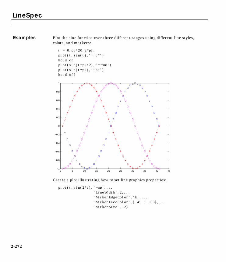
LineSpec

Examples Plot the sine function over three different ranges using different line styles,colors, and markers:

t = 0:pi/20:2*pi;plot(t,sin(t),'−.r*')hold onplot(sin(t−pi/2),’−−mo’)plot(sin(t−pi),’:bs’)hold off

Create a plot illustrating how to set line graphics properties:

plot(t,sin(2*t),’−mo’,...’LineWidth’,2,...’MarkerEdgeColor’,’k’,...’MarkerFaceColor’,[.49 1 .63],...’MarkerSize’,12)

0 5 10 15 20 25 30 35 40 45−1

−0.8

−0.6

−0.4

−0.2

0

0.2

0.4

0.6

0.8

1

2-272

LineSpec

See Also line, plot, surface, patch, Axes LineStyleOrder propert.

0 1 2 3 4 5 6 7−1

−0.8

−0.6

−0.4

−0.2

0

0.2

0.4

0.6

0.8

1

2-273

loglog

2loglogPurpose Log-log scale plot

Syntax loglog(Y)loglog(X1,Y1,...)loglog(X1,Y1,LineSpec,...)loglog(...,'PropertyName',PropertyValue,...)h = loglog(...)

Description loglog(Y) plots the columns of Y versus their index if Y contains real numbers.If Y contains complex numbers, loglog(Y) and loglog(real(Y),imag(Y)) areequivalent. loglog ignores the imaginary component in all other uses of thisfunction.

loglog(X1,Y1,...) plots all Xn versus Yn pairs. If only Xn or Yn is a matrix,loglog plots the vector argument versus the rows or columns of the matrix,depending on whether the vector’s row or column dimension matches thematrix.

loglog(X1,Y1,LineSpec,...) plots all lines defined by the Xn,Yn,LineSpectriples, where LineSpec determines line type, marker symbol, and color of theplotted lines. You can mix Xn,Yn,LineSpec triples with Xn,Yn pairs, forexample,

loglog(X1,Y1,X2,Y2,LineSpec,X3,Y3)

loglog(...,' PropertyName', PropertyValue,...) sets property values forall Line graphics objects created by loglog. See the line reference page formore information.

h = loglog(...) returns a column vector of handles to Line graphics objects,one handle per Line.

Remarks If you do not specify a color when plotting more than one Line, loglogautomatically cycles through the colors and line styles in the order specified bythe current Axes.

2-274

loglog

Examples Create a simple loglog plot with square markers:

x = logspace(−1,2);loglog(x,exp(x),'−s')grid on

See Also line, LineSpec, plot, semilogx, semilogy

10−1

100

101

102

100

105

1010

1015

1020

1025

1030

1035

1040

1045

2-275

loglog

2-276

material

2materialPurpose Controls the reflectance properties of Surfaces and Patches

Syntax material shinymaterial dullmaterial metalmaterial([ka kd ks])material([ka kd ks n])material([ka kd ks n sc])material default

Description material sets the lighting characteristics of Surface and Patch objects.

material shiny sets the reflectance properties so that the object has a highspecular reflectance relative the diffuse and ambient light and the color of thespecular light depends only on the color of the light source.

material dull sets the reflectance properties so that the object reflects morediffuse light, has no specular highlights, but the color of the reflected lightdepends only on the light source.

material metal sets the reflectance properties so that the object has a veryhigh specular reflectance, very low ambient and diffuse reflectance, and thecolor of the reflected light depends on both the color of the light source and thecolor of the object.

material([ka kd ks]) sets the ambient/diffuse/specular strength of theobjects.

material([ka kd ks n]) sets the ambient/diffuse/specular strength andspecular exponent of the objects.

material([ka kd ks n sc]) sets the ambient/diffuse/specular strength,specular exponent, and specular color reflectance of the objects.

material metal sets the ambient/diffuse/specular strength, specularexponent, and specular color reflectance of the objects to their defaults.

Remarks The material command sets the AmbientStrength, DiffuseStrength,SpecularStrength, SpecularExponent, and SpecularColorReflectance

2-277

material

properties of all Surface and Patch objects in the Axes. There must be visibleLight objects in the Axes for lighting to be enabled. Look at the materal.mM-file to see the actual values set (enter the command: type material).

See Also light, lighting, patch, surface

2-278

mesh, meshc, meshz

2mesh, meshc, meshzPurpose Mesh plots

Syntax mesh(X,Y,Z)mesh(Z)mesh(...,C)meshc(...)meshz(...)h = mesh(...)h = meshc(...)h = meshz(...)

Description mesh, meshc, and meshz create wireframe parametric surfaces specified by X, Y,and Z, with color specified by C.

mesh(X,Y,Z) draws a wireframe mesh with color determined by Z, so color isproportional to surface height. If X and Y are vectors, length(X) = n andlength(Y) = m, where [m,n] = size(Z). In this case,are the intersections of the wireframe grid lines; X and Y correspond to thecolumns and rows of Z, respectively. If X and Y are matrices,

are the intersections of the wireframe grid lines.

mesh(Z) draws a wireframe mesh using X = 1:n and Y = 1:m, where [m,n] =size(Z). The height, Z, is a single-valued function defined over a rectangulargrid. Color is proportional to surface height.

mesh(...,C) draws a wireframe mesh with color determined by matrix C.MATLAB performs a linear transformation on the data in C to obtain colorsfrom the current colormap. If X, Y, and Z are matrices, they must be the samesize as C.

meshc(...) draws a contour plot beneath the mesh.

meshz(...) draws a curtain plot (i.e., a reference plane) around the mesh.

h = mesh(...), h = meshc(...), and h = meshz(...) return a handle to aSurface graphics object.

Remarks A mesh is drawn as a Surface graphics object with the viewpoint specified byview(3). The face color is the same as the background color (to simulate a

X j( ) Y i( ) Z i j,( ), ,( )

X i j,( ) Y i j,( ) Z i j,( ), ,( )

2-279

mesh, meshc, meshz

wireframe with hidden-surface elimination), or none when drawing a standardsee-through wireframe. The current colormap determines the edge color. Thehidden command controls the simulation of hidden-surface elimination in themesh, and the shading command controls the shading model.

Examples Produce a combination mesh and contour plot of the peaks surface:

[X,Y] = meshgrid(–3:.125:3);Z = peaks(X,Y);meshc(X,Y,Z);axis([–3 3 –3 3 –10 5])

−3−2

−10

12

3

−3−2

−10

12

3−10

−5

0

5

2-280

mesh, meshc, meshz

Generate the curtain plot for the peaks function:

[X,Y] = meshgrid(–3:.125:3);Z = peaks(X,Y);meshz(X,Y,Z)

Algorithm The range of X, Y, and Z, or the current setting of the Axes XLimMode, YLimMode,and ZLimMode properties determine the axis limits. axis sets these properties.

The range of C, or the current setting of the Axes CLim and CLimMode properties(also set by the caxis function), determine the color scaling. The scaled colorvalues are used as indices into the current colormap.

The mesh rendering functions produce color values by mapping the z datavalues (or an explicit color array) onto the current colormap. MATLAB’s defaultbehavior computes the color limits automatically using the minimum andmaximum data values (also set using caxis auto). Theminimum data valuemaps to the first color value in the colormap and the maximum data valuemaps to the last color value in the colormap. MATLAB performs a lineartransformation on the intermediate values to map them to the currentcolormap.

−3−2

−10

12

3

−4

−2

0

2

4−10

−5

0

5

10

2-281

mesh, meshc, meshz

meshc calls mesh, turns hold on, and then calls contour and positions thecontour on the x-y plane. For additional control over the appearance of thecontours, you can issue these commands directly. You can combine other typesof graphs in this manner, for example surf and pcolor plots.

meshc assumes that X and Y are monotonically increasing. If X or Y is irregularlyspaced, contour3 calculates contours using a regularly spaced contour grid,then transforms the data to X or Y.

See Also contour, hidden, meshgrid, surf, surfc, surfl, waterfall

The functions axis, caxis, colormap, hold, shading, and view all set graphicsobject properties that affect mesh, meshc, and meshz.

For a discussion of parametric surfaces plots, refer to surf.

2-282

movie

2moviePurpose Play recorded movie frames

Syntax movie(M)movie(M,n)movie(M,n,fps)movie(h,...)movie(h,M,n,fps,loc)

Description movie plays the movie defined by a matrix whose columns are movie frames(usually produced by getframe).

movie(M) plays the movie in matrix M once.

movie(M,n) plays the movie n times. If n is negative, each cycle is shownforward then backward. If n is a vector, the first element is the number of timesthe movie is played, and the second through last elements specify the order inwhich to play the frames. For example, if M has three columns, n = [10 3 2 1]plays the movie backwards 10 times.

movie(M,n,fps) plays the movie at fps frames per second. The default is 12frames per second. Computers that cannot achieve the specified speed play asfast as possible.

movie(h,...) plays the movie in the Figure or Axes identified by h.

movie(h,M,n,fps,loc) specifies a four-element location vector, [x y 0 0],where the lower-left corner of the movie frame is anchored (only the first twoelements in the vector are used). The location is relative to the lower-left cornerof the Figure or Axes specified by handle and in units of pixels, regardless ofthe object’s Units property.

Remarks The movie function displays each frame as it loads the data into memory, andthen plays the movie. This eliminates long delays with a blank screen when youload a memory-intensive movie. The movie’s load cycle is not considered one ofthe movie repetitions.

2-283

movie

Examples Animate the peaks function as you scale the values of Z:

Z = peaks;surf(Z);M = moviein(20);

% Freeze Axes limitsaxis manualset(gca,'nextplot','replacechildren');

% Record the moviefor j = 1:20

surf(sin(2∗pi∗j/20)∗Z,Z)M(:,j) = getframe;

end

% Play the movie twenty timesmovie(M,20)

See Also getframe, moviein

2-284

moviein

2movieinPurpose Allocate matrix for movie frames

Syntax M = moviein(n)M = moviein(n,h)M = moviein(n,h,rect)

Description moviein allocates an appropriately sized matrix for the getframe function.

M = moviein(n) creates matrix M having n columns to store n frames of amovie based on the size of the current Axes.

M = moviein(n,h) specifies a handle for a valid Figure or Axes graphics objecton which to base the memory requirement. You must use the same handle withgetframe. If you want to capture the axis

M = moviein(n,h,rect) specifies the rectangular area from which to copy thebitmap, relative to the lower-left corner of the Figure or Axes graphics objectidentified by h. rect = [left bottom width height], where left and bottomspecify the lower-left corner of the rectangle, and width and height specify thedimensions of the rectangle. Components of rect are in pixel units. You mustuse the same handle and rectangle with getframe.

Examples Use moviein to allocate a matrix for the movie frames and getframe to createthe movie:

Z = peaks;surf(Z);M = moviein(20);

% Freeze Axes limitsaxis manualset(gca,'nextplot','replacechildren');

% Record the moviefor j = 1:20

surf(sin(2∗pi∗j/20)∗Z,Z)M(:,j) = getframe;

end

% Play the movie twenty timesmovie(M,20)

2-285

moviein

See Also getframe, movie

2-286

newplot

2newplotPurpose Determine where to draw graphics objects

Syntax newploth = newplot

Description newplot prepares a Figure and Axes for subsequent graphics commands.

h = newplot prepares a Figure and Axes for subsequent graphics commandsand returns a handle to the current Axes.

Remarks Use newplot at the beginning of high-level graphics M-files to determine whichFigure and Axes to target for graphics output. Calling newplot can change thecurrent Figure and current Axes. Basically, there are three options whendrawing graphics in existing Figures and Axes:

• Add the new graphics without changing any properties or deleting anyobjects.

• Delete all existing objects whose handles are not hidden before drawing thenew objects.

• Delete all existing objects regardless of whether or not their handles arehidden and reset most properties to their defaults before drawing the newobjects (refer to the following table for specific information).

The Figure and Axes NextPlot properties determine how nextplot behaves.The following two tables describe this behavior with various property values.

2-287

newplot

First, newplot reads the current Figure’s NextPlot property and actsaccordingly:

NextPlot What Happens

add Draw to the current Figure without clearing anygraphics objects already present.

replacechildren Remove all child objects whose HandleVisibilityproperty is set to on and reset Figure NextPlotproperty to add.This clears the current Figure and is equivalent toissuing the clf command.

replace Remove all child objects (regardless of the setting ofthe HandleVisibility property) and reset Figureproperties to their defaults, except:

• NextPlot is reset to add regardless of user-defineddefaults)

• Position, Units, PaperPosition, and PaperUnitsare not reset

This clears and resets the current Figure and isequivalent to issuing the clf reset command.

2-288

newplot

After newplot establishes which Figure to draw in, it reads the current Axes’NextPlot property and acts accordingly:

See Also axes, cla, clf, figure, hold, ishold, reset

The NextPlot property for Figure and Axes graphics objects.

NextPlot Description

add Draw into the current Axes, retaining all graphicsobjects already present.

replacechildren Remove all child objects whose HandleVisibilityproperty is set to on, but do not reset Axes properties.This clears the current Axes like the cla command.

replace Removes all child objects (regardless of the setting ofthe HandleVisibility property) and resets Axesproperties to their defaults, except Position andUnitsThis clears and resets the current Axes like the clareset command.

2-289

noanimate

2noanimatePurpose Change EraseMode of all objects to normal

Syntax noanimate(state,fig_handle)noanimate(state)

Description noanimate(state,fig_handle) sets the EraseMode of all Image, Line, PatchSurface, and Text graphics object in the specified Figure to normal. state canbe the following strings:

• 'save' – set the values of the EraseMode properties to normal for all theappropriate objects in the designated Figure.

• 'restore' – restore the EraseMode properties to the previous values (i.e., thevalues before calling noanimate with the 'save' argument).

noanimate(state) operates on the current Figure.

noanimate is useful if you want to print the Figure to a Tiff or JPEG format.

See Also print

2-290

orient

2orientPurpose Set paper orientation for printed output

Syntax orientorient landscapeorient portraitorient tallorient(fig_handle), orient(simulink_model)orient(fig_handle,orientation), orient(simulink_model,orientation)

Description orient returns a string with the current paper orientation, either portrait,landscape, or tall.

orient landscape sets the paper orientation of the current Figure to full-pagelandscape, orienting the longest page dimension horizontally. The Figure iscentered on the page and scaled to fit the page with a 0.25 inch border.

orient portrait sets the paper orientation of the current Figure to portrait,orienting the longest page dimension vertically. The portrait option returnsthe page orientation to MATLAB’s default. (Note that the result of using theportrait option is affected by changes you make to Figure properties. See the“Algorithm” section for more specific information.)

orient tall maps the current Figure to the entire page in portraitorientation, leaving a 0.25 inch border.

orient(fig_handle), orient(simulink_model) returns the currentorientation of the specified Figure or Simulink model.

orient(fig_handle,orientation), orient(simulink_model,orientation)

sets the orientation for the specified Figure or Simulink model to the specifiedorientation (landscape, portrait, or tall).

Algorithm orient sets the PaperOrientation, PaperPosition, and PaperUnitsproperties of the current Figure. Subsequent print operations use theseproperties. The result of using the portrait option can be affected by defaultproperty values as follows:

• If the current Figure PaperType is the same as the default Figure PaperTypeand the default Figure PaperOrientation has been set to landscape, then

2-291

orient

the orient portrait command uses the current values of PaperOrientationand PaperPosition to place the Figure on the page.

• If the current Figure PaperType is the same as the default Figure PaperTypeand the default Figure PaperOrientation has been set to landscape, thenthe orient portrait command uses the default Figure PaperPosition withthe x, y and width, height values reversed (i.e., [y,x,height,width]) to positionthe Figure on the page.

• If the current Figure PaperType is different from the default FigurePaperType, then the orient portrait command uses the current FigurePaperPosition with the x, y and width, height values reversed (i.e.,[y,x,height,width]) to position the Figure on the page.

See Also print, set

PaperOrientation, PaperPosition, PaperSize, PaperType, and PaperUnitsproperties of Figure graphics objects.

2-292

pareto

2paretoPurpose Pareto chart

Syntax pareto(Y)pareto(Y,names)pareto(Y,X)H = pareto(...)

Description Pareto charts display the values in the vector Y as bars drawn in descendingorder.

pareto(Y) labels each bar with its element index in Y.

pareto(Y,names) labels each bar with the associated name in the string matrixor cell array names.

pareto(Y,X) labels each bar with the associated value from X.

H = pareto(...) returns a combination of Patch and Line object handles.

See Also hist, bar

2-293

patch

2patchPurpose Create Patch graphics object

Syntax patch(X,Y,C)patch(X,Y,Z,C)patch(...'PropertyName',PropertyValue...)patch('PropertyName',PropertyValue...) PN/PV pairs onlyhandle = patch(...)

Description patch is the low-level graphics function for creating Patch graphics objects. APatch object is one or more polygons defined by the coordinates of its vertices.You can specify the coloring and lighting of the Patch. See the “3-D Modeling”chapter in Using MATLAB Graphics for more information on Patches.

patch(X,Y,C) adds the filled two-dimensional Patch to the current Axes. Theelements of X and Y specify the vertices of a polygon. If X and Y are matrices,MATLAB draws one polygon per column. C determines the color of the Patch.It can be a single ColorSpec, one color per face, or one color per vertex (see“Remarks”). If C is a 1-by-3 vector, it is assumed to be an RGB triplet,specifying a color directly.

patch(X,Y,Z,C) creates a Patch in three-dimensional coordinates.

patch(...'PropertyName',PropertyValue...) follows the X, Y, (Z), and Carguments with property name/property value pairs to specify additionalPatch properties.

patch('PropertyName',PropertyValue,...) specifies all properties usingproperty name/property value pairs. This form enables you to omit the colorspecification because MATLAB uses the default face color and edge color,unless you explicitly assign a value to the FaceColor and EdgeColorproperties. This form also allows you to specify the Patch using the Faces andVertices properties instead of x-, y-, and z-coordinates. See the “Examples”section for more information.

handle = patch(...) returns the handle of the Patch object it creates.

Remarks Unlike high-level area creation functions, such as fill or area, patch does notcheck the settings of the Figure and Axes NextPlot properties. It simply addsthe Patch object to the current Axes.

2-294

patch

If the coordinate data does not define closed polygons, patch closes thepolygons. The data can define concave or intersecting polygons. However, if theedges of an individual Patch face intersect themselves, the resulting face mayor may not be completely filled. In the case, it is better to break up the face intosmaller polygons.

Specifying Patch PropertiesYou can specify properties as property name/property value pairs, structurearrays, and cell arrays (see the set and get reference pages for examples of howto specify these data types).

There are two Patch properties that specify color:

• CData – use when specifying x-, y-, and z-coordinates (XData, YData, ZData).

• FaceVertexCData – use when specifying vertices and connection matrix(Vertices and Faces).

The CData and FaceVertexCData properties accept color data as indexed or truecolor (RGB) values. See the CData and FaceVertexCData property descriptionsfor information on how to specify color.

Indexed color data can represent either direct indices into the colormap orscaled values that map the data linearly to the entire colormap (see the caxisfunction for more information on this scaling). The CDataMapping propertydetermines how MATLAB interprets indexed color data:

Color Specification

FaceVertexCData

CData

Indexed

True Color

direct

scaled

(CDataMapping)

Color Interpretation by MATLAB

Color Mapping

2-295

patch

Color Data InterpretationYou can specify Patch colors as:

• A single color for all faces

• One color for each face enabling flat coloring

• One color for each vertex enabling interpolated coloring

The following tables summarize how MATLAB interprets color data defined bythe CData and FaceVertexCData properties.

Interpretation of the CData Property

Interpretation of the FaceVertexCData Property

[X,Y,Z]Data CData Required for Results ObtainedDimensions Indexed True Color

m-by-n scalar 1-by-1-by-3 Use the single color specified for all Patch faces.Edges can be only a single color.

m-by-n 1-by-n(n >= 4)

1-by-n-by-3 Use one color for each Patch face. Edges can be only asingle color.

m-by-n m-by-n m-by-n-3 Assign a color to each vertex. Patch faces can be flat (asingle color) or interpolated. Edges can be flat orinterpolated.

Vertices Faces FaceVertexCDataRequired for

Results Obtained

Dimensions Dimensions Indexed True Color

m-by-n k-by-3 scalar 1-by-3 Use the single color specified for allPatch faces. Edges can be only a singlecolor.

m-by-n k-by-3 k-by-1 k-by-3 Use one color for each Patch face. Edgescan be only a single color.

m-by-n k-by-3 m-by-1 m-by-3 Assign a color to each vertex. Patch facescan be flat (a single color) orinterpolated. Edges can be flat orinterpolated.

2-296

patch

Examples This example creates a Patch object using two different methods:

• Specifying x-, y-, and z-coordinates and color data (XData, YData, ZData, andCData properties).

• Specifying vertices, the connection matrix, and color data (Vertices, Faces,FaceVertexCData, and FaceColor properties).

Specifying X, Y, and Z CoordinatesThe first approach specifies the coordinates of each vertex. In this example, thecoordinate data defines two triangular faces, each having three vertices. Usingtrue color, the top face is set to white and the bottom face to gray:

x = [0 0;0 1;1 1];y = [1 1;2 2;2 1];z = [1 1;1 1;1 1];tcolor(1,1,1:3) = [1 1 1];tcolor(1,2,1:3) = [.7 .7 .7];patch(x,y,z,tcolor)

Notice that each face shares two vertices with the other face (V1-V4 and V3-V5).

0 0.2 0.4 0.6 0.8 11

1.1

1.2

1.3

1.4

1.5

1.6

1.7

1.8

1.9

2

V2 V3V5

V6V1

V4

2-297

patch

Specifying Vertices and FacesThe Vertices property contains the coordinates of each unique vertex definingthe Patch. The Faces property specifies how to connect these vertices to formeach face of the Patch. For this example, two vertices share the same locationso you need to specify only four of the six vertices. Each row contains the x, y,and z-coordinates of each vertex:

vert = [0 1 1;0 2 1;1 2 1;1 1 1];

There are only two faces, defined by connecting the vertices in the orderindicated:

fac = [1 2 3;1 3 4];

To specify the face colors, define a 2-by-3 matrix containing two RGB colordefinitions:

tcolor = [1 1 1;.7 .7 .7];

With two faces and two colors, MATLAB can color each face with flat shading.This means you must set the FaceColor property to flat, since the faces/vertices technique is available only as a low-level function call (i.e., only byspecifying property name/property value pairs).

Create the Patch by specifying the Faces, Vertices, and FaceVertexCDataproperties as well as the FaceColor property :

patch('faces',fac,'vertices',vert,'FaceVertexCData',tcolor,...'FaceColor','flat')

2-298

patch

Specifying only unique vertices and their connection matrix can reduce the sizeof the data for Patches having many faces. See the descriptions of the Faces,Vertices, and FaceVertexCData properties for information on how to definethem.

MATLAB does not require each face to have the same number of vertices. Incases where they do not, pad the Faces matrix with NaNs. To define a Patchwith faces that do not close, add one or more NaN to the row in the Verticesmatrix that defines the vertex you do not want connected.

ObjectHierarchy

0 0.2 0.4 0.6 0.8 11

1.1

1.2

1.3

1.4

1.5

1.6

1.7

1.8

1.9

2

V1

V2 V3

V4

Face 1

Face 2

Patch

Root

Text

Uimenu

SurfaceLine

Axes Uicontrol

Image

Figure

Uicontextmenu

Light

2-299

patch

Setting Default PropertiesYou can set default Patch properties on the Axes, Figure, and Root levels:

set(0,'DefaultPatchPropertyName',PropertyValue...)set(gcf,'DefaultPatchPropertyName',PropertyValue...)set(gca,'DefaultPatchPropertyName',PropertyValue...)

Where PropertyName is the name of the Patch property and PropertyValue isthe value you are specifying. Use set and get to access Patch properties.

Property List The following table lists all Patch properties and provides a brief description ofeach. The property name links take you to an expanded description of theproperties.



Faces Connection matrix for Vertices Values: m-by-n matrixDefault: [1,2,3]

Vertices Matrix of x-, y-, and z-coordinates ofthe vertices (used with Faces)

Values: matrixDefault: [0,1;1,1;0,0]

XData The x-coordinates of the vertices ofthe Patch

Values: vector or matrixDefault: [0;1;0]

YData The y-coordinates of the vertices ofthe Patch

Values: vector or matrixDefault: [1;1;0]

ZData The z-coordinates of the vertices ofthe Patch

Values: vector or matrixDefault: [] empty matrix

Specifying Color

CData Color data for use with the XData/YData/ZData method

Values: scalar, vector, ormatrixDefault: [] empty matrix

CDataMapping Controls mapping of CData tocolormap

Values: scaled, directDefault: scaled

2-300

patch

EdgeColor Color of face edges Values: ColorSpec, none,flat, interpDefault: ColorSpec

FaceColor Color of face Values: ColorSpec, none,flat, interpDefault: ColorSpec

FaceVertexCData Color data for use with Faces/Vertices method

Values: matrixDefault: [] empty matrix





Controlling the Effects of Lights

AmbientStrength Intensity of the ambient light Values: scalar >=0 and <=1Default: 0.3

BackFaceLighting Controls lighting of faces pointingaway from camera

Values: unlit, lit,reverselitDefault: reverselit

DiffuseStrength Intensity of diffuse light Values: scalar >=0 and <=1Default: 0.6

EdgeLighting Method used to light edges Values: none, flat, gouraud,phongDefault: none

FaceLighting Method used to light edges Values: none, flat, gouraud,phongDefault: none


2-301

patch

NormalMode MATLAB-generated or user-specifiednormal vectors


SpecularColorReflectance Composit color of specularly reflectedlight

Values: scalar 0 to 1Default: 1

SpecularExponent Harshness of specular reflection Values: scalar >= 1Default: 10

SpecularStrength Intensity of specular light Values: scalar >=0 and <=1Default: 0.9

VertexNormals Vertex normal vectors Values: matrix

Defining Edges and Markers


LineWidth The width of the edge in points Values: scalarDefault: 0.5 points





EraseMode Method of drawing and erasing thePatch (useful for animation)


SelectionHighlight Highlight Patch when selected(Selected property set to on)



2-302

patch

Visible Make the Patch visible or invisible Values: on, offDefault: on


HandleVisibility Determines if and when the thePatch’s handle is visible to otherfunctions


HitTest Determines if the Patch can becomethe current object (see the FigureCurrentObject property)





ButtonDownFcn Define a callback routine thatexecutes when a mouse button ispressed on over the Patch


CreateFcn Define a callback routine thatexecutes when an Patch is created


DeleteFcn Define a callback routine thatexecutes when the Patch is deleted(via close or delete)




UIContextMenu Associate a context menu with thePatch


General Information About the Patch

Children Patch objects have no children Values: [] (empty matrix)


2-303

patch

Parent The parent of a Patch object isalways an Axes object

Value: Axes handle

Selected Indicate whether the Patch is in a“selected” state.




Value: the string 'patch'



2-304

Patch Properties

2Patch PropertiesPatchProperties


AmbientStrength scalar >= 0 and <= 1

Strength of ambient light. This property sets the strength of the ambient light,which is a nondirectional light source that illuminates the entire scene. Youmust have at least one visible Light object in the Axes for the ambient light tobe visible. The Axes AmbientColor property sets the color of the ambient light,which is therefore the same on all objects in the Axes.

You can also set the strength of the diffuse and specular contribution of Lightobjects. See the DiffuseStrength and SpecularStrength properties.

BackFaceLighting unlit | lit | reverselit

Face lighting control. This property determines how faces are lit when theirvertex normals point away from the camera.

• unlit – face is not lit

• lit – face lit in normal way

• reverselit – face is lit as if the vertex pointed towards the camera

This property is useful for discriminating between the internal and externalsurfaces of an object. See the Using MATLAB Graphics manual for an example.





2-305

Patch Properties


Button press callback routine. A callback routine that executes whenever youpress a mouse button while the pointer is over the Patch object. Define thisroutine as a string that is a valid MATLAB expression or the name of an M-file.The expression executes in the MATLAB workspace.

CData scalar, vector, or matrix

Patch colors. This property specifies the color of the Patch. You can specifycolor for each vertex, each face, or a single color for the entire Patch. The wayMATLAB interprets CData depends on the type of data supplied. The data canbe numeric values that are scaled to map linearly into the current colormap,integer values that are used directly as indices into the current colormap, orarrays of RGB values. RGB values are not mapped into the current colormap,but interpreted as the colors defined. On true color systems, MATLAB uses theactual colors defined by the RGB triples. On pseudocolor systems, MATLABuses dithering to approximate the RGB triples using the colors in the Figure’sColormap and Dithermap.

The following two diagrams illustrate the dimensions of CData with respect tothe coordinate data arrays, XData, YData, and ZData. The first diagramillustrates the use of indexed color:

2-306

Patch Properties

Single Color

CData

[X,Y,Z]Data

Face1

Face2

Face3

Face4

Face5

One ColorPer Face

CData

One ColorPer Vertex

CData

[X,Y,Z]Data

[X,Y,Z]Data

2-307

Patch Properties

The second diagram illustrates the use of true color. True color requiresm-by-n-by-3 arrays to define red, green, and blue components for each color.

Note that if CData contains NaNs, MATLAB does not color the faces.

See also the Faces, Vertices, and FaceVertexCData properties for analternative method of Patch definition.


Direct or scaled color mapping. This property determines how MATLABinterprets indexed color data used to color the Patch. (If you use true colorspecification for CData or FaceVertexCData, this property has no effect.)

• scaled – transform the color data to span the portion of the colormapindicated by the Axes CLim property, linearly mapping data values to colors.See the caxis command for more information on this mapping.

• direct – use the color data as indices directly into the colormap. When notscaled, the data are usually integer values ranging from 1 to

Single Color One ColorPer Face

One ColorPer Vertex

BG

R

CData

Face1

Face2

Face3

Face4

Face5

RG

B

CDataRed

GreenBlue

CData

[X,Y,Z]Data

[X,Y,Z]Data [X,Y,Z]Data

2-308

Patch Properties

length(colormap). MATLAB maps values less than 1 to the first color in thecolormap, and values greater than length(colormap) to the last color in thecolormap. Values with a decimal portion are fixed to the nearest, lowerinteger.

Children matrix of handles

Always the empty matrix; Patch objects have no children.

Clipping on | off

Clipping to Axes rectangle. When Clipping is on, MATLAB does not display anyportion of the Patch outside the Axes rectangle.

CreateFcn string

Callback routine executed during object creation. This property defines acallback routine that executes when MATLAB creates a Patch object. Youmust define this property as a default value for Patches. For example, thestatement,

set(0,'DefaultPatchCreateFcn','set(gcf,''DitherMap'',my_dither_map)')

defines a default value on the Root level that sets the Figure DitherMapproperty whenever you create a Patch object. MATLAB executes this routineafter setting all properties for the Patch created. Setting this property on anexisting Patch object has no effect.


DeleteFcn string

Delete Patch callback routine. A callback routine that executes when you deletethe Patch object (e.g., when you issue a delete command or clear the Axes (cla)or Figure (clf) containing the Patch). MATLAB executes the routine beforedeleting the object’s properties so these values are available to the callbackroutine.


2-309

Patch Properties

DiffuseStrength scalar >= 0 and <= 1

Intensity of diffuse light. This property sets the intensity of the diffusecomponent of the light falling on the Patch. Diffuse light comes from Lightobjects in the Axes.

You can also set the intensity of the ambient and specular components of thelight on the Patch object. See the AmbientStrength and SpecularStrengthproperties.

EdgeColor ColorSpec | none | flat | interp

Color of the Patch edge. This property determines how MATLAB colors theedges of the individual faces that make up the Patch.

• ColorSpec – A three-element RGB vector or one of MATLAB’s predefinednames, specifying a single color for edges. The default edge color is black. SeeColorSpec for more information on specifying color.

• none – Edges are not drawn.

• flat – The color of each vertex controls the color of the edge that follows it.This means flat edge coloring is dependent on the order you specify thevertices:

• interp – Linear interpolation of the CData or FaceVertexCData values at thevertices determines the edge color.

EdgeLighting none | flat | gouraud | phong

Algorithm used for lighting calculations. This property selects the algorithmused to calculate the effect of Light objects on Patch edges. Choices are:

• none – Lights do not affect the edges of this object.

• flat – The effect of Light objects is uniform across each edge of the Patch.

Vertex controlling thecolor of the following edge

2-310

Patch Properties

• gouraud – The effect of Light objects is calculated at the vertices and thenlinearly interpolated across the edge lines.

• phong – The effect of Light objects is determined by interpolating the vertexnormals across each edge line and calculating the reflectance at each pixel.Phong lighting generally produces better results than Gouraud lighting, buttakes longer to render.


Erase mode. This property controls the technique MATLAB uses to draw anderase Patch objects. Alternative erase modes are useful in creating animatedsequences, where control of the way individual objects redraw is necessary toimprove performance and obtain the desired effect.

• normal – Redraw the affected region of the display, performing thethree-dimensional analysis necessary to ensure that all objects are renderedcorrectly. This mode produces the most accurate picture, but is the slowest.The other modes are faster, but do not perform a complete redraw and aretherefore less accurate.

• none – Do not erase the Patch when it is moved or destroyed. While the objectis still visible on the screen after erasing with EraseMode none, you cannotprint it because MATLAB stores no information about its former location.

• xor– Draw and erase the Patch by performing an exclusive OR (XOR) witheach pixel index of the screen behind it. Erasing the Patch does not damagethe color of the objects behind it. However, Patch color depends on the colorof the screen behind it and is correctly colored only when over the Axesbackground Color, or the Figure background Color if the Axes Color is setto none.

• background – Erase the Patch by drawing it in the Axes’ background Color,or the Figure background Color if the Axes Color is set to none. Thisdamages objects that are behind the erased Patch, but the Patch is alwaysproperly colored.

Printing with Non-normal Erase Modes. MATLAB always prints Figures as if theEraseMode of all objects is normal. This means graphics objects created withEraseMode set to none, xor, or background can look different on screen than onpaper. On screen, MATLAB may mathematically combine layers of colors (e.g.,XORing a pixel color with that of the pixel behind it) and ignore

2-311

Patch Properties

three-dimensional sorting to obtain greater rendering speed. However, thesetechniques are not applied to the printed output.


FaceColor ColorSpec | none | flat | interp

Color of the Patch face. This property can be any of the following:

• ColorSpec – A three-element RGB vector or one of MATLAB’s predefinednames, specifying a single color for faces. See ColorSpec for moreinformation on specifying color.

• none – Do not draw faces. Note that edges are drawn independently of faces.

• flat – The values of CData or FaceVertexCData determine the color for eachface in the Patch. The color data at the first vertex determines the color ofthe entire face.

• interp – Bilinear interpolation of the color at each vertex determines thecoloring of each face.

FaceLighting none | flat | gouraud | phong

Algorithm used for lighting calculations. This property selects the algorithmused to calculate the effect of Light objects on Patch faces. Choices are:

• none – Lights do not affect the faces of this object.

• flat – The effect of Light objects is uniform across the faces of the Patch.Select this choice to view faceted objects.

• gouraud – The effect of Light objects is calculated at the vertices and thenlinearly interpolated across the faces. Select this choice to view curvedsurfaces.

• phong – The effect of Light objects is determined by interpolating the vertexnormals across each face and calculating the reflectance at each pixel. Selectthis choice to view curved surfaces. Phong lighting generally produces betterresults than Gouraud lighting, but takes longer to render.

Faces m-by-n matrix

Vertex connection defining each face. This property is the connection matrixspecifying which vertices in the Vertices property are connected. The Facesmatrix defines m faces with up to n vertices each. Each row designates the

2-312

Patch Properties

connections for a single face, and the number of elements in that row that arenot NaN defines the number of vertices for that face.

The Faces and Vertices properties provide an alternative way to specify aPatch that can be more efficient than using x, y, and z coordinates in mostcases. For example, consider the following Patch. It is composed of eighttriangular faces defined by nine vertices:

The corresponding Faces and Vertices properties are shown to the right of thePatch. Note how some faces share vertices with other faces. For example, thefifth vertex (V5) is used six times, once each by faces one, two, and three andsix, seven, and eight. Without sharing vertices, this same Patch requires 24vertex definitions.

FaceVertexCData matrix

Face and vertex colors. The FaceVertexCData property specifies the color ofPatches defined by the Faces and Vertices properties, and the values are usedwhen FaceColor, EdgeColor, MarkerFaceColor, or MarkerEdgeColor are setappropriately. The interpretation of the values specified for FaceVertexCDatadepends on the dimensions of the data:

For indexed colors, FaceVertexCData can be:

V1 V4 5

V1 5 V2

V2 5 V6

V2 V6 V3

V4 V7 V8

V4 V8 7

V8 V9

5 V9 V60 0.2 0.4 0.6 0.8 1 1.2 1.4 1.6 1.8 2

0

0.2

0.4

0.6

0.8

1

1.2

1.4

1.6

1.8

2

F1

Faces property

V5

V5

V5

V5

F5 F7

F1 F3

F6 F8

F4F2

F2

F3

F4

F5

F6

F7

F8

V7 V8 V9

V4 V5

V1

V6

V2 V3

V5 X1 Y1 Z1

X2 Y2 Z2

X3 Y3 Z3

X4 Y4 Z4

X5 Y5 Z5

Vertices property

X6 Y6 Z6

X7 Y7 Z7

X8 Y8 Z8

X9 Y9 Z9

X5 Y5 Z5

V1

V2

V3

V4

V5

V6

V7

V8

V9

V5

2-313

Patch Properties

• A single value, which applies a single color to the entire Patch

• An n-by-1 matrix, where n is the number of rows in the Faces property,which specifies one color per face

• An n-by-1 matrix, where n is the number of rows in the Vertices property,which specifies one color per vertex

For true colors, FaceVertexCData can be:

• A 1-by-3 matrix , which applies a single color to the entire Patch

• An n-by-3 matrix, where n is the number of rows in the Faces property,which specifies one color per face

• An n-by-3 matrix, where n is the number of rows in the Vertices property,which specifies one color per vertex

The following diagram illustrates the various forms of the FaceVertexCDataproperty for a Patch having eight faces and nine vertices. The CDataMapping

2-314

Patch Properties

property determines how MATLAB interprets the FaceVertexCData propertywhen you specify indexed colors.




Setting HandleVisibility to callback causes handles to be visible fromwithin callback routines or functions invoked by callback routines, but not fromwithin functions invoked from the command line. This provide a means to

B9B9

B1

B2

B3

B4

B5

B6

B7

B8

BGC1

C2

C3

C4

C5

C6

C7

C8

C1

C2

C3

C4

C5

C6

C7

C8

C9

C R G1

G2

G3

G4

G5

G6

G7

G8

R1

R2

R3

R4

R5

R6

R7

R8

B1

B2

B3

B4

B5

B6

B7

B8

G1

G2

G3

G4

G5

G6

G7

G8

R1

R2

R3

R4

R5

R6

R7

R8

R9

FaceVertexCData

Indexed

Single colorOne colorper face

One colorper vertex

True color

Single colorOne colorper face

One colorper vertex

2-315

Patch Properties

protect GUIs from command-line users, while allowing callback routines tohave complete access to object handles.






HitTest on | off

Selectable by mouse click. HitTest determines if the Patch can become thecurrent object (as returned by the gco command and the Figure CurrentObjectproperty) as a result of a mouse click on the Patch. If HiTest is off, clicking onthe Patch selects the object below it (which maybe the Axes containing it).


Callback routine interruption mode. The Interruptible property controlswhether a Patch callback routine can be interrupted by subsequently invokedcallback routines. Only callback routines defined for the ButtonDownFcn areaffected by the Interruptible property. MATLAB checks for events that caninterrupt a callback routine only when it encounters a drawnow, figure,getframe, or pause command in the routine. See the BusyAction property forrelated information.

2-316

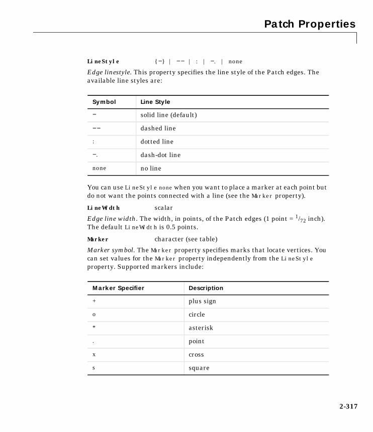
Patch Properties

LineStyle − | −− | : | −. | none

Edge linestyle. This property specifies the line style of the Patch edges. Theavailable line styles are:

You can use LineStyle none when you want to place a marker at each point butdo not want the points connected with a line (see the Marker property).

LineWidth scalar

Edge line width. The width, in points, of the Patch edges (1 point = 1/72 inch).The default LineWidth is 0.5 points.

Marker character (see table)

Marker symbol. The Marker property specifies marks that locate vertices. Youcan set values for the Marker property independently from the LineStyleproperty. Supported markers include:

Symbol Line Style


−− dashed line

: dotted line

−. dash-dot line

none no line


+ plus sign

o circle

* asterisk

. point

x cross

s square

2-317

Patch Properties

MarkerEdgeColor ColorSpec | none | auto | flat

Marker edge color. The color of the marker or the edge color for filled markers(circle, square, diamond, pentagram, hexagram, and the four triangles).ColorSpec defines the color to use. none specifies no color, which makesnonfilled markers invisible. auto sets MarkerEdgeColor to the same color as theEdgeColor property.

MarkerFaceColor ColorSpec | none | auto | flat

Marker face color. The fill color for markers that are closed shapes (circle,square, diamond, pentagram, hexagram, and the four triangles). ColorSpecdefines the color to use. none makes the interior of the marker transparent,allowing the background to show through. auto sets the fill color to the Axescolor, or the Figure color, if the Axes Color property is set to none.


Marker size. A scalar specifying the size of the marker, in points. The defaultvalue for MarkerSize is six points (1 point = 1/72 inch). Note that MATLABdraws the point marker at 1/3 of the specified size.

NormalMode auto | manual

MATLAB-generated or user-specified normal vectors. When this property isauto, MATLAB calculates vertex normals based on the coordinate data. If you

d diamond









2-318

Patch Properties

specify your own vertex normals, MATLAB sets this property to manual anddoes not generate its own data. See also the VertexNormals property.

Parent Axes handle

Patch’s parent. The handle of the Patch’s parent object. The parent of a Patchobject is the Axes in which it is displayed. You can move a Patch object toanother Axes by setting this property to the handle of the new parent.

Selected on | off

Is object selected. When this property is on, MATLAB displays selectionhandles or a dashed box (depending on the number of faces) if theSelectionHighlight property is also on. You can, for example, define theButtonDownFcn to set this property, allowing users to select the object with themouse.


Objects highlight when selected. When the Selected property is on, MATLABindicates the selected state by:

• Drawing handles at each vertex for a single-faced Patch.

• Drawing a dashed bounding box for a multi-faced Patch.

When SelectionHighlight is off, MATLAB does not draw the handles.

SpecularColorReflectancescalar in the range 0 to 1

Color of specularly reflected light. When this property is 0, the color of thespecularly reflected light depends on both the color of the object from which itreflects and the color of the light source. When set to 1, the color of thespecularly reflected light depends only on the color or the light source (i.e., theLight object Color property). The proportions vary linearly for values inbetween.

SpecularExponent scalar >= 1

Harshness of specular reflection. This property controls the size of the specularspot. Most materials have exponents in the range of 5 to 20.

SpecularStrength scalar >= 0 and <= 1

Intensity of specular light. This property sets the intensity of the specularcomponent of the light falling on the Patch. Specular light comes from Lightobjects in the Axes.

2-319

Patch Properties

You can also set the intensity of the ambient and diffuse components of thelight on the Patch object. See the AmbientStrength and DiffuseStrengthproperties.

Tag string


For example, suppose you use Patch objects to create borders for a group ofUicontrol objects and want to change the color of the borders in a Uicontrol’scallback routine. You can specify a Tag with the Patch definition:

patch(X,Y,'k','Tag','PatchBorder')

Then use findobj in the Uicontrol’s callback routine to obtain the handle of thePatch and set its FaceColor property:

set(findobj('Tag','PatchBorder'),'FaceColor','w')


Class of the graphics object. For Patch objects, Type is always the string'patch'.


Associate a context menu with the Patch. Assign this property the handle of aUicontextmenu object created in the same Figure as the Patch. Use theuicontextmenu function to create the context menu. MATLAB displays thecontext menu whenever you right-click over the Patch (Control-click onMacintosh systems).

UserData matrix

User-specified data. Any matrix you want to associate with the Patch object.MATLAB does not use this data, but you can access it using set and get.

VertexNormals matrix

Surface normal vectors. This property contains the vertex normals for thePatch. MATLAB generates this data to perform lighting calculations. You can

2-320

Patch Properties

supply your own vertex normal data, even if it does not match the coordinatedata. This can be useful to produce interesting lighting effects.

Vertices matrix

Vertex coordinates. A matrix containing the x-, y-, z-coordinates for each vertex.See the Faces property for more information.

Visible on | off

Patch object visibility. By default, all Patches are visible. When set to off, thePatch is not visible, but still exists and you can query and set its properties.

XData vector or matrix

X-coordinates. The x-coordinates of the points at the vertices of the Patch. IfXData is a matrix, each column represents the x-coordinates of a single face ofthe Patch. In this case, XData, YData, and ZData must have the samedimensions.

YData vector or matrix

Y-coordinates. The y-coordinates of the points at the vertices of the Patch. IfYData is a matrix, each column represents the y-coordinates of a single face ofthe Patch. In this case, XData, YData, and ZData must have the samedimensions.

ZData vector or matrix

Z-coordinates. The z-coordinates of the points at the vertices of the Patch. IfZData is a matrix, each column represents the z-coordinates of a single face ofthe Patch. In this case, XData, YData, and ZData must have the samedimensions.

See Also area, caxis, fill, fill3, surface

2-321

pbaspect

2pbaspectPurpose Set or query the plot box aspect ratio

Syntax pbaspectpbaspect([aspect_ratio])pbaspect('mode')pbaspect('auto')pbaspect('manual')pbaspect(axes_handle,...)

Description The plot box aspect ratio determines the relative size of the x-, y-, and z-axes.

pbaspect with no arguments returns the plot box aspect ratio of the currentaxes.

pbaspect([aspect_ratio]) sets the plot box aspect ratio in the current axesto the specified value. Specify the aspect ratio as three relative valuesrepresenting the ratio of the x-, y-, and z-axes size. For example, a value of[1 1 1] (the default) means the plot box is a cube (although with stretch-to-fillenabled, it may not appear as a cube). See Remarks.

pbaspect('mode') returns the current value of the plot box aspect ratio mode,which can be either auto (the default) or manual. See Remarks.

pbaspect('auto') sets the plot box aspect ratio mode to auto.

pbaspect('manual') sets the plot box aspect ratio mode to manual.

pbaspect(axes_handle,...) performs the set or query on the axes identifiedby the first argument, axes_handle. If you do not specify an axes handle,pbaspect operates on the current axes.

Remarks pbaspect sets or queries values of the Axes object PlotBoxAspectRatio andPlotBoxAspectRatioMode properties.

When the plot box aspect ratio mode is auto, MATLAB sets the ratio to[1 1 1], but may change it to accommodate manual settings of the data aspectratio, camera view angle, or axis limits. See the Axes DataAspectRatioproperty for a table listing the interactions between various properties.

2-322

pbaspect

Setting a value for the plot box aspect ratio or setting the plot box aspect ratiomode to manual disables MATLAB’s stretch-to-fill feature (stretching of theaxes to fit the window). This means setting the plot box aspect ratio to itscurrent value,

pbaspect(pbaspect)

can cause a change it the way the graphs look. See the Remarks section of theaxes reference description and the “Aspect Ratio” section in the UsingMATLAB Graphics manual for a discussion of stretch-to-fill.

Examples The following surface plot of the function is useful to illustratethe plot box aspect ratio. First plot the function over the range–2 ≤ x ≤ 2, –2 ≤ y ≤ 2,

[x,y] = meshgrid([-2:.2:2]);z = x.*exp(-x.^2 - y.^2);surf(x,y,z)

Querying the plot box aspect ratio shows that the plot box is square:

pbaspectans =

1 1 1

z xe x2 y2––( )=

−2−1

01

2

−2

−1

0

1

2−0.5

0

0.5

2-323

pbaspect

It is also interesting to look at the data aspect ratio selected by MATLAB:

daspectans =

4 4 1

To illustrate the interaction between the plot box and data aspect ratios, set thedata aspect ratio to [1 1 1] and again query the plot box aspect ratio:

daspect([1 1 1])

pbaspectans =

4 4 1

−2

−1

0

1

2

−2

−1.5

−1

−0.5

0

0.5

1

1.5

2−0.5

0

0.5

2-324

pbaspect

The plot box aspect ratio has changed to accommodate the specified data aspectratio. Now suppose you want the plot box aspect ratio to be [1 1 1] as well:

pbaspect([1 1 1])

Notice how MATLAB changed the axes limits because of the constraintsintroduced by specifying both the plot box and data aspect ratios.

You can also use pbaspect to disable stretch-to-fill. For example, displayingtwo subplots in one Figure can give surface plots a squashed appearance.Disabling stretch-to-fill :

upper_plot = subplot(211);surf(x,y,z)lower_plot = subplot(212);surf(x,y,z)pbaspect(upper_plot,'manual')

−2

−1

0

1

2

−2

−1

0

1

2−2

−1.5

−1

−0.5

0

0.5

1

1.5

2

2-325

pbaspect

See Also axis, daspect, xlim, ylim, zlim

The Axes properties DataAspectRatio, PlotBoxAspectRatio, XLim, YLim, ZLim


−20

2

−2

0

2−0.5

0

0.5

−2−1

01

2

−2−1

01

2−0.5

0

0.5

2-326

pcolor

2pcolorPurpose Pseudocolor plot

Syntax pcolor(C)pcolor(X,Y,C)h = pcolor(...)

Description A pseudocolor plot is a rectangular array of cells with colors determined by C.MATLAB creates a pseudocolor plot by using each set of four adjacent points inC to define a Surface patch (i.e., cell).

pcolor(C) draws a pseudocolor plot. The elements of C are linearly mapped toan index into the current colormap. The mapping from C to the currentcolormap is defined by colormap and caxis.

pcolor(X,Y,C) draws a pseudocolor plot of the elements of C at the locationsspecified by X and Y. The plot is a logically rectangular, two-dimensional gridwith vertices at the points [X(i,j), Y(i,j)]. X and Y are vectors or matricesthat specify the spacing of the grid lines. If X and Y are vectors, X correspondsto the columns of C and Y corresponds to the rows. If X and Y are matrices, theymust be the same size as C.

h = pcolor(...) returns a handle to a Surface graphics object.

Remarks A pseudocolor plot is a flat Surface plot viewed from above. pcolor(X,Y,C) isthe same as viewing surf(X,Y,0∗Z,C) using view([0 90]).

When you use shading faceted or shading flat, the constant color of each cellis the color associated with the corner having the smallest x-y coordinates.Therefore, C(i,j) determines the color of the cell in the ith row and jth column.The last row and column of C are not used.

When you use shading interp, each cell’s color results from a bilinearinterpolation of the colors at its four vertices and all elements of C are used.

2-327

pcolor

Examples A Hadamard matrix has elements that are +1 and –1. A colormap with only twoentries is appropriate when displaying a pseudocolor plot of this matrix:

pcolor(hadamard(20))colormap(gray(2))axis ijaxis square

2 4 6 8 10 12 14 16 18 20

2

4

6

8

10

12

14

16

18

20

2-328

pcolor

A simple color wheel illustrates a polar coordinate system:

n = 6;r = (0:n)'/n;theta = pi∗(–n:n)/n;X = r∗cos(theta);Y = r∗sin(theta);C = r∗cos(2∗theta);pcolor(X,Y,C)axis equal tight

Algorithm The number of vertex colors for pcolor(C) is the same as the number of cellsfor image(C). pcolor differs from image in that pcolor(C) specifies the colorsof vertices, which are scaled to fit the colormap; changing the Axes climproperty changes this color mapping. image(C) specifies the colors of cells anddirectly indexes into the colormap without scaling. Additionally,pcolor(X,Y,C) can produce parametric grids, which is not possible with image.

See Also caxis, image, mesh, shading, surf, view

−1 −0.5 0 0.5 1−1

−0.8

−0.6

−0.4

−0.2

0

0.2

0.4

0.6

0.8

1

2-329

peaks

2peaksPurpose A sample function of two variables.

Syntax Z = peaks;Z = peaks(n);Z = peaks(V);Z = peaks(X,Y);

peaks;peaks(N);peaks(V);peaks(X,Y);

[X,Y,Z] = peaks;[X,Y,Z] = peaks(n);[X,Y,Z] = peaks(V);

Description peaks is a function of two variables, obtained by translating and scalingGaussian distributions, which is useful for demonstrating mesh, surf, pcolor,contour, etc.

Z = peaks; returns a 49-by-49 matrix.

Z = peaks(n); returns an n-by-n matrix.

Z = peaks(V); returns an n-by-n matrix, where n = length(V).

Z = peaks(X,Y); evaluates peaks at the given X and Y (which must be the samesize) and returns a matrix the same size.

peaks(...) (with no output argument), plots the peaks function with surf.

[X,Y,Z] = peaks(...); returns two additional matrices, X and Y, forparametric plots, for example, surf(X,Y,Z,del2(Z)). If not given as input, theunderlying matrices X and Y are:

[X,Y] = meshgrid(V,V)

where V is a given vector, or V is a vector of length n with elements equallyspaced from −3 to 3. If no input argument is given, the default n is 49.

See Also meshgrid, surf

2-330

pie

2piePurpose Pie chart

Syntax pie(X)pie(X,explode)h = pie(...)

Description pie(X) draws a pie chart using the data in X. Each element in X is representedas a slice in the pie chart.

pie(X,explode) offsets a slice from the pie. explode is a vector or matrix ofzeros and nonzeros that correspond to X. A non-zero value offsets thecorresponding slice from the center of the pie chart, so that X(i,j) is offsetfrom the center if explode(i,j) is nonzero. explode must be the same size as X.

h = pie(...) returns a vector of handles to Patch and Text graphics objects.

Remarks The values in X are normalized via X/sum(X) to determine the area of each sliceof the pie. If sum(X)≤1, the values in X directly specify the are of the pie slices.MATLAB draws only a partial pie if sum(X)<1.

2-331

pie

Examples Emphasize the second slice in the chart by setting its corresponding explodeelement to 1:

x = [1 3 0.5 2.5 2];explode = [0 1 0 0 0];pie(x,explode)colormap jet

See Also pie3

11%

33%

6%

28%

22%

2-332

pie3

2pie3Purpose Three-dimensional pie chart

Syntax pie3(X)pie3(X,explode)h = pie3(...)

Description pie3(X) draws a three-dimensional pie chart using the data in X. Eachelement in X is represented as a slice in the pie chart.

pie3(X,explode) specifies whether to offset a slice from the center of the piechart. X(i,j) is offset from the center of the pie chart if explode(i,j) isnonzero. explode must be the same size as X.

h = pie(...) returns a vector of handles to Patch, Surface, and Text graphicsobjects.

Remarks The values in X are normalized via X/sum(X) to determine the area of each sliceof the pie. If sum(X)≤1, the values in X directly specify the area of the pie slices.MATLAB draws only a partial pie if sum(X)<1.

Examples A slice in the pie chart is offset by setting the corresponding explode elementto 1:

x = [1 3 0.5 2.5 2]explode = [0 1 0 0 0]pie3(x,explode)colormap hsv

28%

6%

22%

33%

11%

2-333

pie3

See Also pie

2-334

plot

2plotPurpose Linear 2–D plot

Syntax plot(Y)plot(X1,Y1,...)plot(X1,Y1,LineSpec,...)plot(...,'PropertyName',PropertyValue,...)h = plot(...)

Description plot(Y) plots the columns of Y versus their index if Y is a real number. If Y iscomplex, plot(Y) is equivalent to plot(real(Y),imag(Y)). In all other uses ofplot, the imaginary component is ignored.

plot(X1,Y1,...) plots all lines defined by Xn versus Yn pairs. If only Xn or Ynis a matrix, the vector is plotted versus the rows or columns of the matrix,depending on whether the vector’s row or column dimension matches thematrix.

plot(X1,Y1,LineSpec,...) plots all lines defined by the Xn,Yn,LineSpectriples, where LineSpec is a line specification that determines line type,marker symbol, and color of the plotted lines. You can mix Xn,Yn,LineSpectriples with Xn,Yn pairs: plot(X1,Y1,X2,Y2,LineSpec,X3,Y3)

plot(...,'PropertyName',PropertyValue,...) sets properties to thespecified property values for all Line graphics objects created by plot. (See the“Examples” section for examples.)

h = plot(...) returns a column vector of handles to Line graphics objects,one handle per Line.

Remarks If you do not specify a color when plotting more than one line, plotautomatically cycles through the colors in the order specified by the currentAxes ColorOrder property. After cycling through all the colors defined byColorOrder, plot then cycles through the line styles defined in the AxesLineStyleOrder property.

Note that by default, MATLAB resets the ColorOrder and LineStyleOrderproperties each time you call plot. If you want changes you make to these

2-335

plot

properties to persist, then you must define these changes as default values. Forexample,

set(0,'DefaultAxesColorOrder',[0 0 0],...'DefaultAxesLineStyleOrder','-|-.|--|:')

sets the default ColorOrder to use only the color black and sets theLineStyleOrder to use solid, dash-dot, dash-dash, and dotted line styles.

See the “Axes” chapter in the Using MATLAB Graphics manual for moreinformation on the color of lines used for plotting. See axes for a list ofproperties. See LineSpec for more information on specifying line styles andcolors. See set and get and the Using MATLAB Graphics manual forinformation on default properties.

Examples Plotting Only the Data Points

Suppose you have two vectors:

X = 0:pi/15:4*pi;Y = exp(2*cos(X));

2-336

plot

plot(X,Y,'b+') plots a blue plus sign at each data point:

Plotting Data Points with Connecting Lines

plot(X,Y,'r–',X,Y,'ko') plots a solid red line and circular markers withblack edges at each data point:

0 2 4 6 8 10 12 140

1

2

3

4

5

6

7

8

2-337

plot

Specifying Line Styles

Line styles and markers allow you to discriminate different data sets on thesame plot when color is not available. For example, these statements

X = 0:pi/15:4*pi;Y1 = exp(2*cos(X));Y2 = exp(2*sin(X));plot(X,Y1,'−k*',X,Y2,'−.ko')

create a graph using solid and dash-dot lines as well as different markersymbols:

0 2 4 6 8 10 12 140

1

2

3

4

5

6

7

8

2-338

plot

Specifying the Color and Size of Markers

You can also specify other line characteristics using graphics properties (seeline for a description of these properties):

• LineWidth – specifies the width (in points) of the line

• MarkerEdgeColor – specifies the color of the marker or the edge color forfilled markers (circle, square, diamond, pentagram, hexagram, and the fourtriangles).

• MarkerFaceColor – specifies the color of the face of filled markers.

• MarkerSize – specifies the size of the marker in units of points.

0 2 4 6 8 10 12 140

1

2

3

4

5

6

7

8

2-339

plot

For example, these statements,

x = −pi:pi/10:pi;y = tan(sin(x)) − sin(tan(x));plot(x,y,'−−rs','LineWidth',2,... 'MarkerEdgeColor','k',... 'MarkerFaceColor','g',... 'MarkerSize',10)

produce this graph:

Specifying Tick Mark Location and Labeling

You can adjust the axis tick-mark locations and the labels appearing at eachtick. For example, this plot of the sine function relabels the x-axis with moremeaningful values:

x = −pi:.1:pi;y = sin(x);plot(x,y)set(gca,'XTick',−pi:pi/2:pi)set(gca,'XTickLabel','−pi','−pi/2','0','pi/2','pi')

−4 −3 −2 −1 0 1 2 3 4−3

−2

−1

0

1

2

3

2-340

plot

Now add axis labels and annotate the point −pi/4, sin(−pi/4):

Adding Titles, Axis Labels, and Annotations

MATLAB enables you to add axis labels and titles. For example, using thegraph from the previous example, add an x- and y-axis label:

xlabel('−\pi \leq \Theta \leq \pi')ylabel('sin(\Theta)')title('Plot of sin(\Theta)')text(−pi/4,sin(−pi/4),'\leftarrow sin(−\pi\div4)',...

'HorizontalAlignment','left')

Now change the line color to red by first finding the handle of the Line objectcreated by plot and then setting its Color property. In the same statement, setthe LineWidth property to 2 points:

set(findobj(gca,'Type','line','Color',[0 0 1]),...'Color','red',...

‘LineWidth',2)

−pi −pi/2 0 pi/2 pi−1

−0.8

−0.6

−0.4

−0.2

0

0.2

0.4

0.6

0.8

1

2-341

plot

See Also axis, grid, line, LineSpec, loglog, plotedit, plotyy, semilogx, semilogy,xlabel, xlim, ylabel, ylim, zlabel, zlim

See the text String property for a list of symbols and how to display them.

−pi −pi/2 0 pi/2 pi−1

−0.8

−0.6

−0.4

−0.2

0

0.2

0.4

0.6

0.8

1

−π ≤ Θ ≤ π

sin(

Θ)

Plot of sin(Θ)

← sin(−π÷4)

2-342

plot3

2plot3Purpose Linear 3-D plot

Syntax plot3(X1,Y1,Z1,...)plot3(X1,Y1,Z1,LineSpec,...)plot3(...,'PropertyName',PropertyValue,...)h = plot3(...)

Description The plot3 function displays a three-dimensional plot of a set of data points.

plot3(X1,Y1,Z1,...), where X1, Y1, Z1 are vectors or matrices, plots one ormore lines in three-dimensional space through the points whose coordinatesare the elements of X1, Y1, and Z1.

plot3(X1,Y1,Z1,LineSpec,...) creates and displays all lines defined by theXn,Yn,Zn,LineSpec quads, where LineSpec is a line specification thatdetermines line style, marker symbol, and color of the plotted lines.

plot3(...,'PropertyName',PropertyValue,...) sets properties to thespecified property values for all Line graphics objects created by plot3.

h = plot3(...) returns a column vector of handles to Line graphics objects,with one handle per Line.

Remarks If one or more of X1, Y1, Z1 is a vector, the vectors are plotted versus the rowsor columns of the matrix, depending whether the vectors’ lengths equal thenumber of rows or the number of columns.

You can mix Xn,Yn,Zn triples with Xn,Yn,Zn,LineSpec quads, for example,

plot3(X1,Y1,Z1,X2,Y2,Z2,LineSpec,X3,Y3,Z3)

See LineSpec and plot for information on line types and markers.

Examples Plot a three-dimensional helix:

t = 0:pi/50:10∗pi;plot3(sin(t),cos(t),t)grid onaxis square

2-343

plot3

See Also axis, grid, line, LineSpec, loglog, plot, semilogx, semilogy

−1

−0.5

0

0.5

1

−1

−0.5

0

0.5

10

5

10

15

20

25

30

35

2-344

plotmatrix

2plotmatrixPurpose Draw scatter plots

Syntax plotmatrix(X,Y)plotmatrix(...,'LineSpec')[H,AX,BigAx,P] = plotmatrix(...)

Description plotmatrix(X,Y) scatter plots the columns of X against the columns of Y. If Xis p-by-m and Y is p-by-n, plotmatrix produces an n-by-m matrix of Axes.plotmatrix(Y) is the same as plotmatrix(Y,Y) except that the diagonal isreplaced by hist(Y(:,i)).

plotmatrix(...,'LineSpec') uses a LineSpec to create the scatter plot.Thedefault is '.' (see LineSpec for possible values).

[H,AX,BigAx,P] = plotmatrix(...) returns a matrix of handles to the objectscreated in H, a matrix of handles to the individual subaxes in AX, a handle to abig (invisible) Axes that frames the subaxes in BigAx, and a matrix of handlesfor the histogram plots in P. BigAx is left as the current Axes so that asubsequent title, xlabel, or ylabel commands are centered with respect tothe matrix of Axes.

Examples Generate plots of random data.

x = randn(50,3); y = x*[-1 2 1;2 0 1;1 -2 3;]';plotmatrix(y,'*r')

2-345

plotmatrix

See Also scatter, scatter3

−10 −5 0 5 10−5 0 5 10−5 0 5

−10

−5

0

5

10

−5

0

5

10

−5

0

5

2-346

plotyy

2plotyyPurpose Create graphs with y axes on both left and right side

Syntax plotyy(X1,Y1,X2,Y2)plotyy(X1,Y1,X2,Y2,'function')plotyy(X1,Y1,X2,Y2,'function1','function2')[AX,H1,H2] = plotyy(...)

Description plotyy(X1,Y1,X2,Y2) plots X1 versus Y1 with y-axis labeling on the left andplots X2 versus Y2 with y-axis labeling on the right.

plotyy(X1,Y1,X2,Y2,'function') uses the plotting function specified by thestring 'function' instead of plot to produce each graph. 'function' can be plot,semilogx, semilogy, loglog, stem or any MATLAB function that accepts thesyntax:

h = function(x,y)

plotyy(X1,Y1,X2,Y2,'function1','function2') uses function1(X1,Y1) toplot the data for the left axis and function1(X2,Y2) to plot the data for theright axis.

[AX,H1,H2] = plotyy(...) returns the handles of the two Axes created in AXand the handles of the graphics objects from each plot in H1 and H2. AX(1) isthe left Axes and AX(2) is the right Axes.

Examples Create a graph using the plot function and two y-axes:

t = 0:pi/20:2*pi;y1 = sin(t);y2 = 0.5*sin(t-1.5);plotyy(t,y1,t,y2,’plot’)

2-347

plotyy

See Also plot, loglog, semilogx, semilogy, Axes properties: XAxisLocation,YAxisLocation

The Axes chapter in the Using MATLAB Graphics manual for information onmulti-axis axes.

0 1 2 3 4 5 6 7−1

0

1

0 1 2 3 4 5 6 7−0.5

0

0.5

2-348

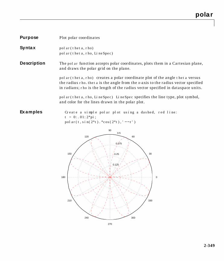
polar

2polarPurpose Plot polar coordinates

Syntax polar(theta,rho)polar(theta,rho,LineSpec)

Description The polar function accepts polar coordinates, plots them in a Cartesian plane,and draws the polar grid on the plane.

polar(theta,rho) creates a polar coordinate plot of the angle theta versusthe radius rho. theta is the angle from the x-axis to the radius vector specifiedin radians; rho is the length of the radius vector specified in dataspace units.

polar(theta,rho,LineSpec) LineSpec specifies the line type, plot symbol,and color for the lines drawn in the polar plot.

Examples Create a simple polar plot using a dashed, red line:t = 0:.01:2∗pi;polar(t,sin(2∗t).∗cos(2∗t),'−−r')

0.125

0.25

0.375

0.5

30

210

60

240

90

270

120

300

150

330

180 0

2-349

polar

See Also cart2pol, compass, LineSpec, plot, pol2cart, rose

2-350

print, printopt

2print, printoptPurpose Create hardcopy output

Syntax printprint –devicetype –options filename[pcmd,dev] = printopt

Description print and printopt produce hardcopy output. All arguments to the printcommand are optional. You can use them in any combination or order.

print sends the contents of the current Figure, including bitmaprepresentations of any user interface controls, to the printer using the deviceand system print command defined by printopt.

print –devicetype specifies a device type, overriding the value returned byprintopt. The Devices section lists all supported device types.

print –options specifies print options that modify the action of the printcommand. (For example, the –noui option suppresses printing of user interfacecontrols.) The Options section lists available options.

print filename directs the output to the file designated by filename. Iffilename does not include an extension, print appends an appropriateextension, depending on the device (e.g., .eps). If you omit filename, printsends the file to the default output device (except for −dmeta and −dbitmap,which place their output on the clipboard).

[pcmd,dev] = printopt returns strings containing the currentsystem-dependent print command and output device. printopt is an M-fileused by print to produce the hardcopy output. You can edit the M-fileprintopt.m to set your default printer type and destination.

2-351

print, printopt

pcmd and dev are platform-dependent strings. pcmd contains the command thatprint uses to send a file to the printer. dev contains the device option for theprint command. Their defaults are platform dependent.

Devices The table below lists device types supported by MATLAB’s built-in drivers.Generally, Level 2 PostScript files are smaller and render more quickly whenprinting than Level 1 PostScript files. However, not all PostScript printerssupport Level 2, so determine the capabilities of your printer before using thosedevices. Level 2 PostScript is the default for UNIX, VAX/VMS, and Macintoshcomputers. You can change this default by editing the printopt.m file.

The TIFF image format is supported on all platforms by almost all wordprocessors for importing images. JPEG is a lossy highly compressed formatthat is supported on all platforms for image processing and for inclusion intoHTML documents on the World Wide Web. To create these formats, MATLABrenders the Figure using the Z-buffer rendering method and the resultingpixmap is then saved to the specified file. You can specify the resolution of theimage using the −r resolution switch.

Platform pcmd dev

UNIX lpr –r –s –dps2

VMS PRINT/DELETE –dps2

Windows COPY /B %s LPT1: –dwin

Macintosh (not applicable) –dps2

Device Description

–dps Level 1 black and white PostScript

–dpsc Level 1 color PostScript

–dps2 Level 2 black and white PostScript

–dpsc2 Level 2 color PostScript

–deps Level 1 black and white Encapsulated PostScript (EPS)

2-352

print, printopt

This table lists additional devices supported via the Ghostscriptpost-processor, which converts PostScript files into other formats. (This featureis not available on Macintosh systems.)

–depsc Level 1 color Encapsulated PostScript (EPS)

–deps2 Level 2 black and white Encapsulated PostScript (EPS)

–depsc2 Level 2 color Encapsulated PostScript (EPS)

–dhpgl HPGL compatible with HP 7475A plotter

–dill Adobe Illustrator 88 compatible illustration file

–dmfile M-file, and MAT-file when appropriate, containing HandleGraphics commands to re-create the Figure and its children

–dtiff 24-bit RGB TIFF with packbits compression (Figures only)

–dtiffn 24-bit RGB TIFF with no compression (Figures only)

–djpeg Baseline JPEG image, quality factor defaults to 75 (Figuresonly)

–djpegnn Baseline JPEG image with nn (0-100) quality factor(Figures only)

Device Description

–dlaserjet HP LaserJet

–dljetplus HP LaserJet+

–dljet2p HP LaserJet IIP

–dljet3 HP LaserJet III

–ddeskjet HP DeskJet and DeskJet Plus

–ddjet500 HP Deskjet 500

–dcdjmono HP DeskJet 500C printing black only

Device Description

2-353

print, printopt

–dcdjcolor HP DeskJet 500C with 24 bit/pixel color andhigh-quality color (Floyd-Steinberg) dithering

–dcdj500 HP DeskJet 500C

–dcdj550 HP Deskjet 550C

–dpaintjet HP PaintJet color printer

–dpjxl HP PaintJet XL color printer

–dpjetxl HP PaintJet XL color printer

–dpjxl300 HP PaintJet XL300 color printer

–ddnj650c HP DesignJet 650C

–dbj10e Canon BubbleJet BJ10e

–dbj200 Canon BubbleJet BJ200

–dbjc600 Canon Color BubbleJet BJC-600 and BJC-4000

–dln03 DEC LN03 printer

–depson Epson-compatible dot matrix printers (9- or 24-pin)

–depsonc Epson LQ-2550 and Fujitsu 3400/2400/1200

–deps9high Epson-compatible 9-pin, interleaved lines (tripleresolution)

–dibmpro IBM 9-pin Proprinter

–dbmp256 8-bit (256-color) BMP file format

–dbmp16m 24-bit BMP file format

–dpcxmono Monochrome PCX file format

–dpcx16 Older color PCX file format (EGA/VGA, 16-color)

–dpcx256 Newer color PCX file format (256-color)

Device Description

2-354

print, printopt

This table summarizes additional devices available on Windows systems.

–dpcx24b 24-bit color PCX file format, three 8-bit planes

–dpbm Portable Bitmap (plain format)

–dpbmraw Portable Bitmap (raw format)

–dpgm Portable Graymap (plain format)

–dpgmraw Portable Graymap (raw format)

–dppm Portable Pixmap (plain format)

–dppmraw Portable Pixmap (raw format)

Device Description

−dwin Use Windows printing services (black and white)

−dwinc Use Windows printing services (color)

–dmeta Copy to clipboard in Enhanced Windows metafile format(color)

–dbitmap Copy to clipboard in Windows bitmap (BMP) format(color)

–dsetup Display Print Setup dialog box, but do not print

–v Verbose mode to display Print dialog box (suppressed bydefault)

Device Description

2-355

print, printopt

This table summarizes additional devices available on Macintosh systems.

Options This table summarizes printing options that you can specify when you enterthe print command.

Device Description

–dpict Create PICT file

–v Verbose mode to display Print dialog box (suppressed bydefault)

Option Description

–tiff Add color TIFF preview to Encapsulated PostScript

–loose Use loose bounding box for EPS and PS devices

–cmyk Use CMYK colors in PostScript instead of RGB

–append Append to existing PostScript file without overwriting

–rnumber Specify resolution in dots per inch

–adobecset Use PostScript default character set encoding

–Pprinter Specify printer to use (UNIX only)

–fhandle Handle of a Figure graphics object to print (currentFigure by default; see gcf)

–swindowtitle Name of SIMULINK system window to print (currentsystem by default; see gcs)

–painters Render using painter’s algorithm

–zbuffer Render using Z-buffer

–noui Suppress printing of user interface controls

2-356

print, printopt

Paper Sizes MATLAB supports a number of standard paper sizes. You can select from thefollowing list by setting the PaperType property of the Figure or selecting asupported paper sizes from the print dialog box:

Property Value Size (Width-by-Height)

usletter 8.5-by-11 inches

uslegal 11-by-14 inches

tabloid 11-by-17 inches

A0 841-by-1189mm

A1 594-by-841mm

A2 420-by-594mm

A3 297-by-420mm

A4 210-by-297mm

A5 148-by-210mm

B0 1029-by-1456mm

B1 728-by-1028mm

B2 514-by-728mm

B3 364-by-514mm

B4 257-by-364mm

B5 182-by-257mm

arch-A 9-by-12 inches

arch-B 12-by-18 inches

arch-C 18-by-24 inches

arch-D 24-by-36 inches

2-357

print, printopt

Printing Tips This section includes information about specific printing issues.

Troubleshooting MS-Windows PrintingIf you encounter problems such as segmentation violations , general protectionfaults, application errors, or the output does not appear as you expect whenusing MS-Windows printer drivers, try the following:

• If your printer is PostScript compatible, print with one of MATLAB’s built-inPostScript drivers. There are various PostScript device options that you canuse with the print command: they all start with −dps, or −deps.

• The behavior you are experiencing may occur only with certain versions ofthe print driver. Contact the print driver vendor for information on how toobtain and install a different driver. If you are using Windows 95, tryinstalling the drivers that ship with the Windows 95 CD-ROM.

• Try printing with one of MATLAB’s built-in GhostScript devices. Thesedevices use GhostScript to convert PostScript files into other formats, suchas HP LaserJet, PCX, Canon BubbleJet, and so on.

• Copy the Figure as a Windows Metafile using the Edit-->CopyFigure menuitem on the Figure window menu or the print −dmeta option at the commandline. You can then import the file into another application for printing.

You can set copy options in the Figure’s File-->Preferences...-->CopyingOptions dialog box. The Windows Metafile clipboard format produces abetter quality image than Windows Bitmap.

arch-E 36-by-48 inches

A 8.5-by-11 inches

B 11-by-17 inches

C 17-by-22 inches

D 22-by-34 inches

E 34-by-43 inches

Property Value Size (Width-by-Height)

2-358

print, printopt

Printing Thick Lines on Windows95Due to a limitation in Windows95, MATLAB is set up to print lines as either:

• Solid lines of the specified thickness (LineWidth)

• Thin (one pixel wide) lines with the specified line style (LineStyle)

If you create lines that are thicker than one pixel and use nonsolid line styles,MATLAB prints these lines with the specified line style, but one pixel wide(i.e., as thin lines).

However, you can change this behavior so that MATLAB prints thick, styledlines as thick, solid lines by editing your matlab.ini file, which is in yourWindows directory. In this file, find the section:

[Matlab Settings]

and in this section change the assignment,

ThinLineStyles=1

to

ThinLineStyles=0

then restart MATLAB.

Printing MATLAB GUIsYou can generally obtain better results when printing a Figure window thatcontains MATLAB uicontrols by setting these key properties:

• Set the Figure PaperPositionMode property to auto. This ensures theprinted version is the same size as the onscreen version. WithPaperPositionMode set to auto MATLAB does not resize the Figure to fit thecurrent value of the PaperPosition. This is particularly important if youhave specified a Figure ResizeFcn because if MATLAB resizes the Figureduring the print operation, the ResizeFcn is automatically called.

To set PaperPositionMode on the current Figure, use the command:set(gcf,'PaperPositionMode','auto')

• Set the Figure InvertHardcopy property to off. By default, MATLABchanges the Figure background color of printed output to white, but does notchange the color of Uicontrols. If you have set the background color to, for

2-359

print, printopt

example, match the gray of the GUI devices, you must set InvertHardcopyto off to preserve the color scheme.

To set InvertHardcopy on the current Figure, use the command:set(gcf,'InvertHardcopy','off')

• Use a color device if you want lines and text that are in color on the screento be written to the output file as colored objects. Black and white devicesconvert colored lines and text to black or white to provide the best contrastwith the background and to aviod dithering.

• Use the print command’s −loose option to prevent MATLAB from using abounding box that is tightly wrapped around objects contained in the Figure.This is important if you have intentionally used space between Uicontrols orAxes and the edge of the Figure and you want to maintain this visualappearance in the printed output.

Notes on Printing Interpolated Shading with PostScript DriversMATLAB can print Surface objects (such as graphs created with surf or mesh)using interpolated colors. However, only Patch objects that are composed oftriangular faces can be printed using interpolated shading.

Printed output is always interpolated in RGB space, not in the colormap colors.This means, if you are using indexed color and interpolated face coloring, theprinted output can look different from what is displayed on screen. See“Interpolating in Indexed vs. Truecolor” in the Using MATLAB Graphicsmanual for an illustration of each type of interpolation.

PostScript files generated for interpolated shading contain the colorinformation of the graphics object’s vertices and require the printer to performthe interpolation calculations. This can take an excessive amount of time andin some cases, printers may actually “time-out" before finishing the print job.One solution to this problem is to interpolate the data and generate a greaternumber of faces, which can then be flat shaded.

To ensure that the printed output matches what you see on the screen, printusing the -zbuffer option. To obtain higher resolution (for example, to maketext look better), use the −r option to increase the resolution. There is, however,a trade-off between the resolution and the size of the created PostScript file,which can be quite large at higher resolutions. The default resolution of 150 dpigenerally produces good results. You can reduce the size of the output file by

2-360

print, printopt

making the Figure smaller before printing it and setting the FigurePaperPositionMode to auto, or by just setting the PaperPosition property toa smaller size.

Note that in some UNIX environments, the default lpr command cannot printfiles larger than 1 Mbyte unless you use the −s option, which MATLAB doesby default. See the lpr man page for more information.

Example This example prints a surface plot with interploted shading. Setting thecurrent Figure’s (gcf) PaperPositionMode to auto enables you to resize theFigure window and print it at the size you see on the screen. See Options andthe previous section for information on the −zbuffer and −r200 options.

surf(peaks)shading interpset(gcf,'PaperPositionMode','auto')print −dpsc2 −zbuffer −r200

See Also orient, figure

See the Using MATLAB Graphics manual for detailed information aboutprinting in MATLAB.

2-361

qtwrite

2qtwritePurpose Write QuickTime movie file

Syntax qtwrite(D,size,Map,'filename')qtwrite(M,Map,'filename')qtwrite(...,options)

Description qtwrite(D,size,Map,'filename') writes the indexed image deck D with sizesize and colormap Map to the QuickTime movie file 'filename'. If 'filename'exists, it is replaced.

qtwrite(M,Map,'filename') writes the MATLAB movie matrix M withcolormap Map to the QuickTime movie file 'filename'.

qtwrite(...,options) sets the frame rate, spatial quality, and compressortype:

Remarks qtwrite requires QuickTime and works only on the Macintosh.

Option Description

options(1) Frame rate in frames per second. The default is10.

options(2) Compressor type:

• 1 is video (default)

• 2 is jpeg

• 3 is animation

options(3) Spatial quality:

• 1 - minimum

• 2 - low

• 3 - normal (default)

• 4 - high

• 5 - maximum

• 6 - lossless

2-362

quiver

2quiverPurpose Quiver or velocity plot

Syntax quiver(U,V)quiver(X,Y,U,V)quiver(...,scale)quiver(...,LineSpec)quiver(...,LineSpec,'filled')h = quiver(...)

Description A quiver plot displays vectors with components (u,v) at the points (x,y).

quiver(U,V) draws vectors specified by U and V at the coordinates defined byx = 1:n and y = 1:m, where [m,n] = size(U) = size(V). This syntax plots Uand V over a geometrically rectangular grid. quiver automatically scales thevectors based on the distance between them to prevent them from overlapping.

quiver(X,Y,U,V) draws vectors at each pair of elements in X and Y. If X and Yare vectors, length(X) = n and length(Y) = m, where[m,n] = size(U) = size(V). The vector X corresponds to the columns of U andV, and vector Y corresponds to the rows of U and V.

quiver(...,scale) automatically scales the vectors to prevent them fromoverlapping, then multiplies them by scale. scale = 2 doubles their relativelength and scale = 0.5 halves them. Use scale = 0 to plot the velocity vectorswithout the automatic scaling.

quiver(...,LineSpec) specifies line style, marker symbol, and color usingany valid LineSpec. quiver draws the markers at the origin of the vectors.

quiver(...,LineSpec,'filled') fills markers specified by LineSpec.

h = quiver(...) returns a vector of Line handles.

Remarks If X and Y are vectors, this function behaves as

[X,Y] = meshgrid(x,y)quiver(X,Y,U,V)

2-363

quiver

Examples Plot the gradient field of the function :

[X,Y] = meshgrid(–2:.2:2);Z = X.∗exp(–X.^2 – Y.^2);[DX,DY] = gradient(Z,.2,.2);contour(X,Y,Z)hold onquiver(X,Y,DX,DY)colormap hsvgrid offhold off

See Also contour, LineSpec, plot, quiver3

z xe x2 y2––( )=

−2 −1.5 −1 −0.5 0 0.5 1 1.5 2−2

−1.5

−1

−0.5

0

0.5

1

1.5

2

2-364

quiver3

2quiver3Purpose Three-dimensional velocity plot

Syntax quiver3(Z,U,V,W)quiver3(X,Y,Z,U,V,W)quiver3(...,scale)quiver3(...,LineSpec)quiver3(...,LineSpec,'filled')h = quiver3(...)

Description A three-dimensional quiver plot displays vectors with components (u,v,w) atthe points (x,y,z).

quiver3(Z,U,V,W) plots the vectors at the equally spaced surface pointsspecified by matrix Z. quiver3 automatically scales the vectors based on thedistance between them to prevent them from overlapping.

quiver3(X,Y,Z,U,V,W) plots vectors with components (u,v,w) at the points(x,y,z). The matrices X, Y, Z, U, V, W must all be the same size and contain thecorresponding position and vector components.

quiver3(...,scale) automatically scales the vectors to prevent them fromoverlapping, then multiplies them by scale. scale = 2 doubles their relativelength and scale = 0.5 halves them. Use scale = 0 to plot the vectors withoutthe automatic scaling.

quiver3(...,LineSpec) specify line type and color using any valid LineSpec.

quiver3(...,LineSpec,'filled') fills markers specified by LineSpec.

h = quiver3(...) returns a vector of Line handles.

2-365

quiver3

Examples Plot the surface normals of the function :

[X,Y] = meshgrid(–2:0.25:2,–1:0.2:1);Z = X.* exp(–X.^2 – Y.^2);[U,V,W] = surfnorm(X,Y,Z);quiver3(X,Y,Z,U,V,W,0.5);hold onsurf(X,Y,Z);colormap hsvview(-35,45)axis ([-2 2 -1 1 -.6 .6])hold off

See Also axis, contour, LineSpec, plot, plot3, quiver, surfnorm, view

z xe x2 y2––( )=

−2

−1

0

1

2

−1

−0.5

0

0.5

1

−0.4

−0.2

0

0.2

0.4

0.6

2-366

refresh

2refreshPurpose Redraw current Figure

Syntax refreshrefresh(h)

Description refresh erases and redraws the current Figure.

refresh(h) redraws the Figure identified by h.

2-367

reset

2resetPurpose Reset graphics object properties to their defaults

Syntax reset(h)

Description reset(h) resets all properties having factory defaults on the object identifiedby h. To see the list of factory defaults, use the statement,

get(0,'factory')

If h is a Figure, MATLAB does not reset Position, Units, PaperPosition, andPaperUnits. If h is an Axes, MATLAB does not reset Position and Units.

Examples reset(gca) resets the properties of the current Axes.

reset(gcf) resets the properties of the current Figure.

See Also cla, clf, gca, gcf, hold

2-368

rgb2hsv

2rgb2hsvPurpose Convert RGB colormap to HSV colormap

Syntax cmap = rgb2hsv(M)

Description cmap = rgb2hsv(M) converts a RGB colormap, M, to a HSV colormap, cmap.Both colormaps are m-by-3 matrices. The elements of both colormaps are in therange 0 to 1.

The columns of the input matrix, M, represent intensities of red, green, andblue, respectively. The columns of the output matrix, cmap, represent hue,saturation, and value, respectively.

See Also brighten, colormap, hsv2rgb,rgbplot

2-369

rgbplot

2rgbplotPurpose Plot colormap

Syntax rgbplot(cmap)

Description rgbplot(cmap) plots the three columns of cmap, where cmap is an m-by-3colormap matrix. rgbplot draws the first column in red, the second in green,and the third in blue.

Examples Plot the RGB values of the copper colormap:

rgbplot(copper)

See Also colormap

0 10 20 30 40 50 60 700

0.1

0.2

0.3

0.4

0.5

0.6

0.7

0.8

0.9

1

2-370

ribbon

2ribbonPurpose Ribbon plot

Syntax ribbon(Y)ribbon(X,Y)ribbon(X,Y,width)h = ribbon(...)

Description ribbon(Y) plots the columns of Y as separate three-dimensional ribbons usingX = 1:size(Y,1).

ribbon(X,Y) plots X versus the columns of Y as three-dimensional strips. Xand Y are vectors of the same size or matrices of the same size. Additionally, Xcan be a row or a column vector, and Y a matrix with length(X) rows.

ribbon(X,Y,width) specifies the width of the ribbons. The default is 0.75.

h = ribbon(...) returns a vector of handles to Surface graphics objects.ribbon returns one handle per strip.

2-371

ribbon

Examples Create a ribbon plot of the peaks function:

[x,y] = meshgrid(-3:.5:3,-3:.1:3);z = peaks(x,y);ribbon(y,z)colormap hsv

See Also plot, plot3, surface

0

5

10

15

−4

−2

0

2

4−10

−5

0

5

10

2-372

root object

2root objectPurpose Root object properties

Description The Root is a graphics object that corresponds to the computer screen. There isonly one Root object and it has no parent. The children of the Root object areFigures.

The Root object exists when you start MATLAB; you never have to create it andyou cannot destroy it. Use set and get to access the Root properties.

See Also diary, echo, figure, format, gcf, get, set

ObjectHierarchy

Property List The following table lists all Root properties and provides a brief description ofeach. The property name links take you to an expanded description of theproperties. This table does not include properties that are defined for, but notused by the Root object.

Uimenu

Line

Axes Uicontrol

Image

Figure

Uicontextmenu


Root


Information about MATLAB’s state

CallbackObject Handle of object whose callback isexecuting

Values: object handle

CurrentFigure Handle of current Figure Values: object handle

ErrorMessage Text of last error message Value: character string

2-373

root object

PointerLocation Current location of pointer Values: x-, and y-coordinates

PointerWindow Hanlde of window containing thepointer

Values: Figure hanlde

ShowHiddenHandles Show or hide handles marked ashidden


Controlling MATLAB’s behavior

Diary Enable the diary file Values: on, offDefault: off

DiaryFile Name of the diary file Values: filename (string)Default: diary

Echo Display each line of script M-file asexecuted


Format Format used to display numbers Values: short, shortE, long,longE, bank, hex, +, ratDefault: shortE

FormatSpacing Display or omit extra line feed Values: compact, looseDefault: loose

Language System environment setting Values: stringDefault: english

RecursionLimit Maximum number of nested M-filecalls

Values: integerDefalut: 2.1478e+009

Units Units for PointerLocation andScreenSize properties

Values: pixels, normalized,inches, centimeters, pointsDefault: pixels

Information about the display

ScreenDepth Depth of the display bitmap Values: bits per pixel


2-374

root object

ScreenSize Size of the screen Values: [left, bottom, width,height]

Information about terminals (X-Windows only)

TerminalHideGraphCommands Command to hide graphics window Values: string

TerminalOneWindow Indicates if there is only one graphicswindow


TerminalDimensions Size of the terminal Values: scalar in pixels

TerminalProtocol Identifies the type of terminal Values: none, x, tek401x,tek410x

TerminalShowGraphCommand Command to display graphicswindow

Value: string

General Information About Root Objects

Children Handles of all nonhidden Figueobjects


Parent The Root object has no parent Value: [] (empty matrix)

Selected Indicate whether the Text is in a“selected” state.




Value: the string 'root'


MATLAB profiler

Profile Enable/disable profiler Values: on, offDefault: off


2-375

root object

ProfileFile Specify the name of M-file to profile Values: pathname to M-file

ProfileCount Output of profiler Values: n-by-1 vector

ProfileInterval Time increment at with to profileM-file

Values: scalar (seconds)Default: 0.01 seconds


2-376

Root Properties

2Root PropertiesRoot Properties This section lists property names along with the type of values each accepts.Curly braces enclose default values.


Not used by the Root object.


Not used by the Root object.

CallbackObject handle (read only)

Handle of current callback’s object. This property contains the handle of theobject whose callback routine is currently executing. If no callback routines areexecuting, this property contains the empty matrix [ ]. See also the gcocommand.

CaptureMatrix (obsolete)

This property has been superseded by the getframe command.

CaptureRect (obsolete)

This property has been superseded by the getframe command.


Handles of child objects. A vector containing the handles of all nonhiddenFigure objects. You can change the order of the handles and thereby change thestacking order of the Figures on the display.

Clipping on | off

Clipping has no effect on the Root object.

CreateFcn

The Root does not use this property.

CurrentFigure Figure handle

Handle of the current Figure window, which is the one most recently created,clicked in, or made current with the statement:

figure(h)

which restacks the Figure to the top of the screen, or

set(0,'CurrentFigure',h)

2-377

Root Properties

which does not restack the Figures. In these statements, h is the handle of anexisting Figure. If there are no Figure objects,

get(0,'CurrentFigure')

returns the empty matrix. Note, however, that gcf always returns a Figurehandle, and creates one if there are no Figure objects.

DeleteFcn string

This property is not used since you cannot delete the Root object

Diary on | off

Diary file mode. When this property is on, MATLAB maintains a file (whosename is specified by the DiaryFile property) that saves a copy of all keyboardinput and most of the resulting output. See also the diary command.

DiaryFile string

Diary filename. The name of the diary file. The default name is diary.

Echo on | off

Script echoing mode. When Echo is on, MATLAB displays each line of a scriptfile as it executes. See also the echo command.

ErrorMessage string

Text of last error message. This property contains the last error message issuedby MATLAB.

Format short | shortE | long | longE | bank |hex | + | rat

Output format mode. This property sets the format used to display numbers.See also the format command.

• short – Fixed-point format with 5 digits.

• shortE – Floating-point format with 5 digits.

• shortG – Fixed- or floating-point format displaying as many significantfigures as possible with 5 digits.

• long – Scaled fixed-point format with 15 digits.

• longE – Floating-point format with 15 digits.

• longG – Fixed- or floating-point format displaying as many significant figuresas possible with 15 digits.

2-378

Root Properties

• bank – Fixed-format of dollars and cents.

• hex – Hexadecimal format.

• + – Displays + and – symbols.

• rat – Approximation by ratio of small integers.

FormatSpacing compact | loose

Output format spacing (see also format command).

• compact — Suppress extra line feeds for more compact display.

• loose — Display extra line feeds for a more readable display.


This property is not useful on the Root object.

HitTest on | off




Language string

System environment setting.

Parent handle

Handle of parent object. This property always contains the empty matrix, as theRoot object has no parent.

PointerLocation [x,y]

Current location of pointer. A vector containing the x- and y-coordinates of thepointer position, measured from the lower-left corner of the screen. You canmove the pointer by changing the values of this property. The Units propertydetermines the units of this measurement.

This property always contains the instantaneous pointer location, even if thepointer is not in a MATLAB window. A callback routine querying thePointerLocation can get a different value than the location of the pointer whenthe callback was triggered. This difference results from delays in callbackexecution caused by competition for system resources.

2-379

Root Properties

PointerWindow handle (read only)

Handle of window containing the pointer. MATLAB sets this property to thehandle of the Figure window containing the pointer. If the pointer is not in aMATLAB window, the value of this property is 0. A callback routine queryingthe PointerWindow can get the wrong window handle if you move the pointer toanother window before the callback executes. This error results from delays incallback execution caused by competition for system resources.

Profile on | off

M-file profiler on or off. Setting this property to on activates the profiler whenyou execute the M-files named in ProfileFile. The profiler determines whatpercentage of time MATLAB spends executing each line of the M-file. See alsothe profile command.

ProfileFile M-file name

M-file to profile. Set this property to the full path name of the M-file to profile.

ProfileCount vector

Profiler output. This property is a n-by-1 vector, where n is the number of linesof code in the profiled M-file. Each element in this vector represents thenumber of times the profiler found MATLAB executing a particular line ofcode. The ProfileInterval property determines how often MATLAB profiles(i.e., determines which line is executing).

ProfileInterval scalar

Time increment to profile M-file. This property sets the time interval at whichthe profiler checks to see what line in the M-file is executing.

RecursionLimit integer

Number of nested M-file calls. This property sets a limit to the number ofnested calls to M-files MATLAB will make before stoping (or potentiallyrunning out of memory). By default the value is set to a large value. Setting thisproperty to a smaller value (something like 150, for example) should preventMATLAB from running out of memory and will instead cause MATLAB toissue an error when the limit is reached.

2-380

Root Properties

ScreenDepth bits per pixel

Screen depth. The depth of the display bitmap (i.e., the number of bits perpixel). The maximum number of simultaneously displayed colors on the currentgraphics device is 2 raised to this power.

ScreenDepth supersedes the BlackAndWhite property. To override automatichardware checking, set this property to 1. This value causes MATLAB toassume the display is monochrome. This is useful if MATLAB is running oncolor hardware but is displaying on a monochrome terminal. Such a situationcan cause MATLAB to determine erroneously that the display is color.

ScreenSize 4-element rectangle vector (read only)

Screen size. A four-element vector,

[left,bottom,width,height]

that defines the display size. left and bottom are 0 for all Units except pixels,in which case left and bottom are 1. width and height are the screendimensions in units specified by the Units property.

Selected on | off

This property has no effect on the Root level.



ShowHiddenHandles on | off

Show or hide handles marked as hidden. When set to on, this property disableshandle hiding and exposes all object handles, regardless of the setting of anobject’s HandleVisibility property. When set to off, all objects so markedremain hidden within the graphics hierarchy.

Tag string

User-specified object label. The Tag property provides a means to identifygraphics objects with a user-specified label. While it is not necessary to identifythe Root object with a tag (since its handle is always 0), you can use thisproperty to store any string value which you can later retrieve using set.

TerminalHideGraphCommandstring X-Windows only

Hide graph window command. This property specifies the escape sequence thatMATLAB issues to hide the graph window when switching from graph mode

2-381

Root Properties

back to command mode. This property is used only by the terminal graphicsdriver. Consult your terminal manual for the correct escape sequence.

TerminalOneWindow on | off X-Windows only

One window terminal. This property indicates whether there is only onewindow on your terminal. If the terminal uses only one window, MATLABwaits for you to press a key before it switches from graphics mode back tocommand mode. This property is used only by the terminal graphics driver.

TerminalDimensions pixels X-Windows only

Size of default terminal. This property defines the size of the terminal.

TerminalProtocol none | x | tek401x | tek410x X-Windows only

Type of terminal. This property tells MATLAB what type of terminal you areusing. Specify tek401x for terminals that emulate Tektronix 4010/4014terminals. Specify tek410x for terminals that emulate Tektronix 4100/4105terminals. If you are using X Windows and MATLAB can connect to your Xdisplay server, this property is automatically set to x.

Once this property is set, you cannot change it unless you quit and restartMATLAB.

TerminalShowGraphCommandstring X-Windows only

Display graph window command. This property specifies the escape sequencethat MATLAB issues to display the graph window when switching fromcommand mode to graph mode. This property is only used by the terminalgraphics driver. Consult your terminal manual for the appropriate escapesequence.


Class of graphics object. For the Root object, Type is always 'root'.

UIContextMenu handle


Units pixels | normalized | inches | centimeters|points

Unit of measurement. This property specifies the units MATLAB uses tointerpret size and location data. All units are measured from the lower-leftcorner of the screen. Normalized units map the lower-left corner of the screen

2-382

Root Properties

to (0,0) and the upper right corner to (1.0,1.0). inches, centimeters, and pointsare absolute units (one point equals 1/72 of an inch).

This property affects the PointerLocation and ScreenSize properties. If youchange the value of Units, it is good practice to return it to its default valueafter completing your operation so as not to affect other functions that assumeUnits is set to the default value.

UserData matrix

User specified data. This property can be any data you want to associate withthe Root object. MATLAB does not use this property, but you can access it usingthe set and get functions.

Visible on | off

Object visibility. This property has no effect on the Root object.

2-383

rose

2rosePurpose Angle histogram

Syntax rose(theta)rose(theta,x)rose(theta,nbins)[tout,rout] = rose(...)

Description rose creates an angle histogram, which is a polar plot showing thedistribution of values grouped according to their numeric range. Each group isshown as one bin.

rose(theta) plots an angle histogram showing the distribution of theta in 20angle bins or less. The vector theta, expressed in radians, determines the anglefrom the origin of each bin. The length of each bin reflects the number ofelements in theta that fall within a group, which ranges from 0 to the greatestnumber of elements deposited in any one bin.

rose(theta,x) uses the vector x to specify the number and the locations ofbins. length(x) is the number of bins and the values of x specify the centerangle of each bin. For example, if x is a five-element vector, rose distributesthe elements of theta in five bins centered at the specified x values.

rose(theta,nbins) plots nbins equally spaced bins in the range [0, 2∗pi].The default is 20.

[tout,rout] = rose(...) returns the vectors tout and rout sopolar(tout,rout) generates the histogram for the data. This syntax does notgenerate a plot.

Example Create a rose plot showing the distribution of 50 random numbers:

theta = 2*pi*rand(1,50);rose(theta)

2-384

rose

See Also compass, feather, hist, polar

1

2

3

4

5

30

210

60

240

90

270

120

300

150

330

180 0

2-385

rotate

2rotatePurpose Rotate object about a specified direction

Syntax rotate(h,direction,alpha)rotate(...,origin)

Description The rotate function rotates a graphics object in three-dimensional space,according to the right-hand rule.

rotate(h,direction,alpha) rotates the graphics object h by alpha degrees.direction is a two- or three-element vector that describes the axis of rotationin conjunction with the origin.

rotate(...,origin) specifies the origin of the axis of rotation as athree-element vector. The default is origin is the center of the plot box.

Remarks The graphics object you want rotated must be a child of the same Axes. Theobject’s data is modified by the rotation transformation. This is in contrast toview and rotate3d, which only modify the viewpoint.

The axis of rotation is defined by an origin and a point P relative to the origin.P is expressed as the spherical coordinates [theta phi], or as Cartesiancoordinates.

The two-element form for direction specifies the axis direction using thespherical coordinates [theta phi]. theta is the angle in the xy plane

Z

Y

X

P

originaxis of ro

tation

2-386

rotate

counterclockwise from the positive x-axis. phi is the elevation of the directionvector from the xy plane.

The three-element form for direction specifies the axis direction usingCartesian coordinates. The direction vector is the vector from the origin to(X,Y,Z).

Examples Rotate a graphics object 180° about the x-axis:

h = surf(peaks(20));rotate(h,[1 0 0],180)

Rotate a Surface graphics object 45° about its center in the z direction:

h = surf(peaks(20));zdir = [0 0 1];center = [10 10 0];rotate(h,zdir,45,center)

Remarks rotate changes the Xdata, Ydata, and Zdata properties of the appropriategraphics object.

See Also rotate3d, sph2cart, view

The Axes CameraPosition, CameraTarget, CameraUpVector, CameraViewAngle

Z

Y

X

theta

P

phi

r

2-387

rotate3d

2rotate3dPurpose Rotate Axes using mouse

Syntax rotate3drotate3d onrotate3d off

Description rotate3d on enables interactive Axes rotation within the current Figure usingthe mouse. When interactive Axes rotation is enabled, clicking on an Axesdraws an animated box, which rotates as the mouse is dragged, showing theview that will result when the mouse button is released. A numeric readoutappears in the lower-left corner of the figure during this time, showing thecurrent azimuth and elevation of the animated box. Releasing the mousebutton removes the animated box and the readout, and changes the view of theAxes to correspond to the last orientation of the animated box.

rotate3d off disables interactive Axes rotation in the current Figure.

rotate3d toggles interactive Axes rotation in the current Figure.

See Also rotate, view

2-388

scatter

2scatterPurpose 2-D Scatter plot

Syntax scatter(X,Y,S,C)scatter(X,Y)scatter(X,Y,S)scatter(...,markertype)scatter(...,'filled')h = scatter(...,)

Description scatter(X,Y,S,C) displays colored circles at the locations specified by thevectors X and Y (which must be the same size).

S determines the size of each marker (specified in points^2). S can be a vectorthe same length as X and Y or a scalar. If S is a scalar, MATLAB draws all themarkers the same size.

C determines the colors of each marker. When C is a vector the same length asX and Y, the values in C are linearly mapped to the colors in the currentcolormap. When C is a length(X)-by-3 matrix, it specifies the colors of themarkers as RGB values. C can also be a color string (see ColorSpec for a list ofcolor string specifiers)

scatter(X,Y) draws the markers in the default size and color.

scatter(X,Y,S) draws the markers at the specified sizes (S) with a single color.

scatter(...,markertype) uses the marker type specified instead of 'o' (seeLineSpec for a list of marker specifiers).

scatter(...,'filled') fills the markers.

h = scatter(...) returns the handles to the Line objects created by scatter(see line for a list of properties you can specify using the object handles andset).

Remarks Use plot for single color, single marker size scatter plots.

Examples load seamountscatter(x,y,5,z)

2-389

scatter

See Also scatter3, plot, plotmatrix

210.8 210.9 211 211.1 211.2 211.3 211.4 211.5 211.6 211.7 211.8−48.45

−48.4

−48.35

−48.3

−48.25

−48.2

−48.15

−48.1

−48.05

−48

−47.95

2-390

scatter3

2scatter3Purpose 3-D scatter plot

Syntax scatter3(X,Y,Z,S,C)scatter3(X,Y,Z)scatter3(X,Y,Z,S)scatter3(...,markertype)scatter3(...,'filled')h = scatter3(...,)

Description scatter3(X,Y,Z,S,C) displays colored circles at the locations specified by thevectors X, Y, and Z (which must all be the same size).

S determines the size of each marker (specified in points). S can be a vector thesame length as X, Y, and Z or a scalar. If S is a scalar, MATLAB draws all themarkers the same size.

C determines the colors of each marker. When C is a vector the same length asX, Y, and Z, the values in C are linearly mapped to the colors in the currentcolormap. When C is a length(X)-by-3 matrix, it specifies the colors of themarkers as RGB values. C can also be a color string (see ColorSpec for a list ofcolor string specifiers)

scatter3(X,Y,Z) draws the markers in the default size and color.

scatter3(X,Y,Z,S) draws the markers at the specified sizes (S) with a singlecolor.

scatter3(...,markertype) uses the marker type specified instead of 'o' (seeLineSpec for a list of marker specifiers).

scatter3(...,'filled') fills the markers.

h = scatter3(...) returns the handles to the Line objects created by scatter3(see line for a list of properties you can specify using the object handles andset).

Remarks Use plot3 for single color, single marker size 3-D scatter plots.

2-391

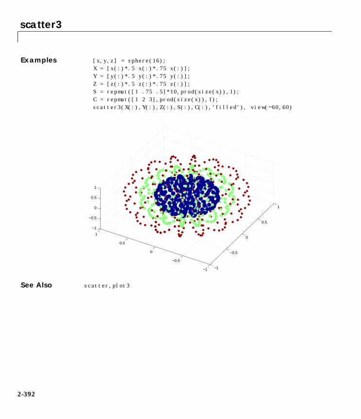
scatter3

Examples [x,y,z] = sphere(16);X = [x(:)*.5 x(:)*.75 x(:)];Y = [y(:)*.5 y(:)*.75 y(:)];Z = [z(:)*.5 z(:)*.75 z(:)];S = repmat([1 .75 .5]*10,prod(size(x)),1);C = repmat([1 2 3],prod(size(x)),1);scatter3(X(:),Y(:),Z(:),S(:),C(:),’filled’), view(−60,60)

See Also scatter, plot3

−1

−0.5

0

0.5

1

−1

−0.5

0

0.5

1

−1

−0.5

0

0.5

1

2-392

semilogx, semilogy

2semilogx, semilogyPurpose Semi-logarithmic plots

Syntax semilogx(Y)semilogx(X1,Y1,...)semilogx(X1,Y1,LineSpec,...)semilogx(...,'PropertyName',PropertyValue,...)h = semilogx(...)

semilogy(...)h = semilogy(...)

Description semilogx and semilogy plot data as logarithmic scales for the x- and y-axis,respectively. logarithmic

semilogx(Y) creates a plot using a base 10 logarithmic scale for the x-axis anda linear scale for the y-axis. It plots the columns of Y versus their index if Ycontains real numbers. semilogx(Y) is equivalent to semilogx(real(Y),imag(Y)) if Y contains complex numbers. semilogx ignores the imaginarycomponent in all other uses of this function.

semilogx(X1,Y1,...) plots all Xn versus Yn pairs. If only Xn or Yn is a matrix,semilogx plots the vector argument versus the rows or columns of the matrix,depending on whether the vector’s row or column dimension matches thematrix.

semilogx(X1,Y1,LineSpec,...) plots all lines defined by theXn,Yn,LineSpec triples. LineSpec determines line style, marker symbol, andcolor of the plotted lines.

semilogx(...,'PropertyName',PropertyValue,...) sets property valuesfor all Line graphics objects created by semilogx.

semilogy(...) creates a plot using a base 10 logarithmic scale for the y-axisand a linear scale for the x-axis.

h = semilogx(...) and h = semilogy(...) return a vector of handles toLine graphics objects, one handle per Line.

2-393

semilogx, semilogy

Remarks If you do not specify a color when plotting more than one line, semilogx andsemilogy automatically cycle through the colors and line styles in the orderspecified by the current Axes ColorOrder and LineStyleOrder properties.

You can mix Xn,Yn pairs with Xn, Yn, LineSpec triples, for example,

semilogx(X1,Y1,X2,Y2,LineSpec,X3,Y3)

Examples A simple semilogy plot is:

x = 0:.1:10;semilogy(x,10.^x)

See Also line, LineSpec, loglog, plot

0 1 2 3 4 5 6 7 8 9 1010

0

101

102

103

104

105

106

107

108

109

1010

2-394

set

2setPurpose Set object properties

Syntax set(H,'PropertyName',PropertyValue,...)set(H,a)set(H,pn,pv...)set(H,pn,<m-by-n cell array>)a= set(h)a= set(0,'Factory')a= set(0,'FactoryObjectTypePropertyName')a= set(h,'Default')a= set(h,'DefaultObjectTypePropertyName')<cell array> = set(h,'PropertyName')

Description set(H,'PropertyName',PropertyValue,...) sets the named properties tothe specified values on the object(s) identified by H. H can be a vector of handles,in which case set sets the properties’ values for all the objects.

set(H,a) sets the named properties to the specified values on the object(s)identified by H. a is a structure array whose field names are the object propertynames and whose field values are the values of the corresponding properties.

set(H,pn,pv,...) sets the named properties specified in the cell array pn tothe corresponding value in the cell array pv for all objects identified in H.

set(H,pn,<m-by-n cell array>) sets n property values on each of m graphicsobjects, where m = length(H) and n is equal to the number of property namescontained in the cell array pn. This allows you to set a given group of propertiesto different values on each object.

a = set(h) returns the user-settable properties and possible values for theobject identified by h. a is a structure array whose field names are the object’sproperty names and whose field values are the possible values of thecorresponding properties. If you do not specify an output argument, MATLABdisplays the information on the screen. h must be scalar.

a = set(0,'Factory') returns the properties whose defaults are usersettable for all objects and lists possible values for each property. a is astructure array whose field names are the object’s property names and whosefield values are the possible values of the corresponding properties. If you do

2-395

set

not specify an output argument, MATLAB displays the information on thescreen.

a = set(0,'FactoryObjectTypePropertyName') returns the possible valuesof the named property for the specified object type, if the values are strings.The argument FactoryObjectTypePropertyName is the word Factoryconcatenated with the object type (e.g., Axes) and the property name (e.g.,CameraPosition).

a = set(h,'Default') returns the names of properties having default valuesset on the object identified by h. set also returns the possible values if they arestrings. h must be scalar.

a = set(h,'DefaultObjectTypePropertyName') returns the possible valuesof the named property for the specified object type, if the values are strings.The argument DefaultObjectTypePropertyName is the word Defaultconcatenated with the object type (e.g., Axes) and the property name (e.g.,CameraPosition). For example, DefaultAxesCameraPosition. h must bescalar.

pv = set(h,'PropertyName') returns the possible values for the namedproperty. If the possible values are strings, set returns each in a cell of the cellarray, pv. For other properties, set returns an empty cell array. If you do notspecify an output argument, MATLAB displays the information on the screen.h must be scalar.

Remarks You can use any combination of property name/property value pairs, structurearrays, and cell arrays in one call to set.

Examples Set the Color property of the current Axes to blue:

set(gca,'Color','b')

Change all the Lines in a plot to black:

plot(peaks)set(findobj('Type','line'),'Color','k')

You can define a group of properties in a structure to better organize your code.For example, these statements define a structure called active, whichcontains a set of property definitions used for the Uicontrol objects in a

2-396

set

particular Figure. When this Figure becomes the current Figure, MATLABchanges colors and enables the controls:

active.BackgroundColor = [.7 .7 .7];active.Enable = 'on';active.ForegroundColor = [0 0 0];

if gcf == control_fig_handleset(findobj(control_fig_handle,'Type','uicontrol'),active)

end

You can use cell arrays to set properties to different values on each object. Forexample, these statements define a cell array to set three properties:

PropName(1) = 'BackgroundColor';PropName(2) = 'Enable';PropName(3) = 'ForegroundColor';

These statements define a cell array containing three values for each of threeobjects (i.e., a 3-by-3 cell array):

PropVal(1,1) = [.5 .5 .5];PropVal(1,2) = 'off';PropVal(1,3) = [.9 .9 .9];

PropVal(2,1) = [1 0 0];PropVal(2,2) = 'on';PropVal(2,3) = [1 1 1];

PropVal(3,1) = [.7 .7 .7];PropVal(3,2) = 'on';PropVal(3,3) = [0 0 0];

Now pass the arguments to set,

set(H,PropName,PropVal)

where length(H) = 3 and each element is the handle to a Uicontrol.

See Also findobj, gca, gcf, gco, gcbo, get

2-397

shading

2shadingPurpose Set color shading properties

Syntax shading flatshading facetedshading interp

Description The shading function controls the color shading of Surface and Patch graphicsobjects.

shading flat each mesh line segment and face has a constant colordetermined by the color value at the end point of the segment or the corner ofthe face that has the smallest index or indices.

shading faceted flat shading with superimposed black mesh lines. This isthe default shading mode.

shading interp varies the color in each line segment and face byinterpolating the colormap index or true color value across the line or face.

Examples Compare a flat, faceted, and interpolated-shaded sphere:

subplot(3,1,1)sphere(16)axis squareshading flattitle('Flat Shading')

subplot(3,1,2)sphere(16)axis squareshading facetedtitle('Faceted Shading')

subplot(3,1,3)sphere(16)axis squareshading interptitle('Interpolated Shading')

2-398

shading

Algorithm shading sets the EdgeColor and FaceColor properties of all Surface and Patchgraphics objects in the current Axes. shading sets the appropriate values,depending on whether the Surface or Patch objects represent meshes or solidsurfaces.

2-399

shading

See Also fill, fill3, hidden, mesh, patch, pcolor, surfThe EdgeColor and FaceColor properties for Surface and Patch graphicsobjects.

2-400

slice

2slicePurpose Volumetric slice plot

Syntax slice(V,sx,sy,sz)slice(X,Y,Z,V,sx,sy,sz)slice(V,XI,YI,ZI)slice(X,Y,Z,V,XI,YI,ZI)slice(...,'method')h = slice(...)

Description slice displays orthogonal slice planes through volumetric data.

slice(V,sx,sy,sz) draws slices along the x, y, z directions in the volume V atthe points in the vectors sx, sy, and sz. V is an m-by-n-by-p volume arraycontaining data values at the default location X = 1:n, Y = 1:m, Z = 1:p. Eachelement in the vectors sx, sy, and sz defines a slice plane in the x-, y-, or z-axisdirection.

slice(X,Y,Z,V,sx,sy,sz) draws slices of the volume V. X, Y, and Z arethree-dimensional arrays specifying the coordinates for V. X, Y, and Z must bemonotonic and orthogonally spaced (as if produced by the function meshgrid).The color at each point is determined by 3-D interpolation into the volume V.

slice(V,XI,YI,ZI) draws data in the volume V for the slices defined by XI, YI,and ZI. XI, YI, and ZI are matrices that define a surface, and the volume isevaluated at the surface points. XI, YI, and ZI must all be the same size.

slice(X,Y,Z,V,XI,YI,ZI) draws slices through the volume V along thesurface defined by the arrays XI, YI, ZI.

slice(...,'method') specifies the interpolation method. 'method' is'linear', 'cubic', or 'nearest'.

• 'linear' specifies trilinear interpolation (the default).

• 'cubic' specifies tricubic interpolation.

• 'nearest' specifies nearest neighbor interpolation.

h = slice(...) returns a vector of handles to Surface graphics objects.

2-401

slice

Remarks The color drawn at each point is determined by interpolation into the volume V.

Examples Visualize the function

over the range –2 ≤x ≤2, –2 ≤y ≤2, – 2 ≤z ≤2:

[x,y,z] = meshgrid(−2:.2:2, −2:.25:2, −2:.16:2);v = x.∗exp(−x.^2−y.^2−z.^2);xslice = [−1.2 .8 2]; yslice = 2; zslice = [−2 0];slice(x,y,z,v,xslice,yslice,zslice)colormap hsv

You can also create slices that are oriented in arbitrary planes. To do this,

• Create a slice surface in the domain of the volume.

• Orient this surface with respect the the axes.

v xe x2 y2– z2––( )=

−2−1

01

2

−2

−1

0

1

2−2

−1.5

−1

−0.5

0

0.5

1

1.5

2

2-402

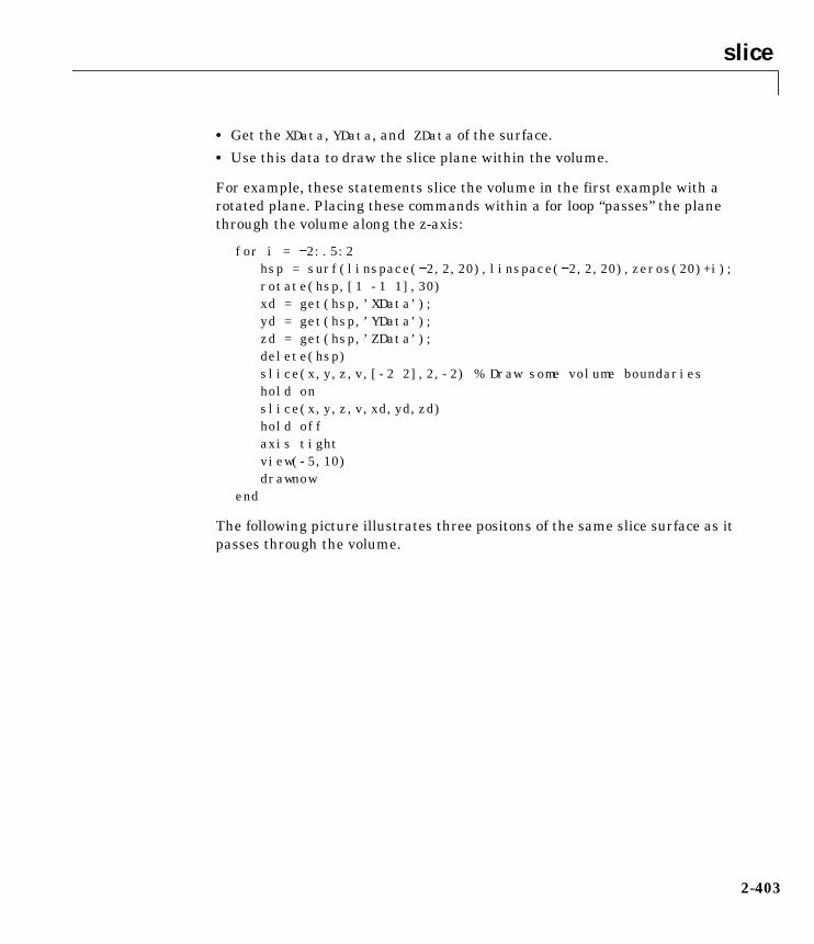
slice

• Get the XData, YData, and ZData of the surface.

• Use this data to draw the slice plane within the volume.

For example, these statements slice the volume in the first example with arotated plane. Placing these commands within a for loop “passes” the planethrough the volume along the z-axis:

for i = −2:.5:2hsp = surf(linspace(−2,2,20),linspace(−2,2,20),zeros(20)+i);rotate(hsp,[1 -1 1],30)xd = get(hsp,’XData’);yd = get(hsp,’YData’);zd = get(hsp,’ZData’);delete(hsp)slice(x,y,z,v,[-2 2],2,-2) % Draw some volume boundarieshold onslice(x,y,z,v,xd,yd,zd)hold offaxis tightview(-5,10)drawnow

end

The following picture illustrates three positons of the same slice surface as itpasses through the volume.

2-403

slice

−2.5 −2 −1.5 −1 −0.5 0 0.5 1 1.5 2 2.5−20

2

−2

−1.5

−1

−0.5

0

0.5

1

1.5

2

2-404

slice

You can slice the volume with any surface. This example probes the volumecreated in the previous example by passing a spherical slice surface throughthe volume.

[xsp,ysp,zsp] = sphere;slice(x,y,z,v,[-2 2],2,-2) % Draw some volume boundaries

for i = -3:.2:3hsp = surface(xsp+i,ysp,zsp);rotate(hsp,[1 0 0],90)xd = get(hsp,’XData’);yd = get(hsp,’YData’);zd = get(hsp,’ZData’);delete(hsp)hold onhslicer = slice(x,y,z,v,xd,yd,zd);axis tightxlim([-3 3])view(-10,35)drawnowdelete(hslicer)hold off

end

The following picture illustrates three positons of the same slice surface as itpasses through the volume.

2-405

slice

See Also interp3, meshgrid

−3 −2 −1 0 1 2 3−2

−1

0

1

2

−2

−1.5

−1

−0.5

0

0.5

1

1.5

2

2-406

sphere

2spherePurpose Generate sphere

Syntax spheresphere(n)[X,Y,Z] = sphere(...)

Description The sphere function generates the x-, y-, and z-coordinates of a unit sphere foruse with surf and mesh.

sphere generates a sphere consisting of 20-by-20 faces.

sphere(n) draws a surf plot of an n-by-n sphere in the current Figure.

[X,Y,Z] = sphere(n) returns the coordinates of a sphere in three matricesthat are (n+1)–by–(n+1) in size. You draw the sphere with surf(X,Y,Z) ormesh(X,Y,Z).

Examples Generate and plot a sphere:

sphereaxis equal

−1

−0.5

0

0.5

1

−1

−0.5

0

0.5

1−1

−0.5

0

0.5

1

2-407

sphere

See Also cylinder, axis

2-408

spinmap

2spinmapPurpose Spin colormap

Syntax spinmapspinmap(t)spinmap(t,inc)spinmap('inf')

Description The spinmap function shifts the colormap RGB values by some incrementalvalue. For example, if the increment equals 1, color 1 becomes color 2, color 2becomes color 3, etc.

spinmap cyclically rotates the colormap for approximately five seconds usingan incremental value of 2.

spinmap(t) rotates the colormap for approximately 10∗t seconds. The amountof time specified by t depends on your hardware configuration (e.g., if you arerunning MATLAB over a network).

spinmap(t,inc) rotates the colormap for approximately 10∗t seconds andspecifies an increment inc by which the colormap shifts. When inc is 1, therotation appears smoother than the default (i.e., 2). Increments greater than 2are less smooth than the default. A negative increment (e.g., –2) rotates thecolormap in a negative direction.

spinmap('inf') rotates the colormap for an infinite amount of time. To breakthe loop, press Ctrl-C .

See Also colormap

2-409

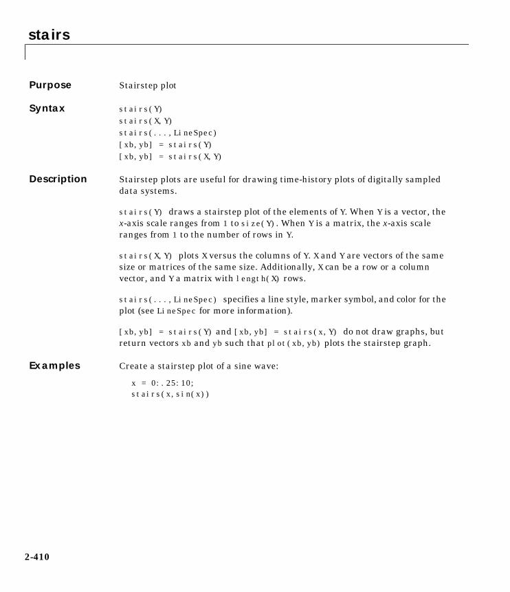
stairs

2stairsPurpose Stairstep plot

Syntax stairs(Y)stairs(X,Y)stairs(...,LineSpec)[xb,yb] = stairs(Y)[xb,yb] = stairs(X,Y)

Description Stairstep plots are useful for drawing time-history plots of digitally sampleddata systems.

stairs(Y) draws a stairstep plot of the elements of Y. When Y is a vector, thex-axis scale ranges from 1 to size(Y). When Y is a matrix, the x-axis scaleranges from 1 to the number of rows in Y.

stairs(X,Y) plots X versus the columns of Y. X and Y are vectors of the samesize or matrices of the same size. Additionally, X can be a row or a columnvector, and Y a matrix with length(X) rows.

stairs(...,LineSpec) specifies a line style, marker symbol, and color for theplot (see LineSpec for more information).

[xb,yb] = stairs(Y) and [xb,yb] = stairs(x,Y) do not draw graphs, butreturn vectors xb and yb such that plot(xb,yb) plots the stairstep graph.

Examples Create a stairstep plot of a sine wave:

x = 0:.25:10;stairs(x,sin(x))

2-410

stairs

See Also bar, hist

0 2 4 6 8 10−1

−0.8

−0.6

−0.4

−0.2

0

0.2

0.4

0.6

0.8

1

2-411

stem

2stemPurpose Plot discrete sequence data

Syntax stem(Y)stem(X,Y)stem(...,'fill')stem(...,LineSpec)h = stem(...)

Description A two-dimensional stem plot displays data as lines extending from the x-axis.A circle (the default) or other marker whose y-position represents the datavalue terminates each stem.

stem(Y) plots the data sequence Y as stems that extend from equally spacedand automatically generated values along the x-axis. When Y is a matrix, stemplots all elements in a row against the same x value.

stem(X,Y) plots X versus the columns of Y. X and Y are vectors or matrices ofthe same size. Additionally, X can be a row or a column vector and Y a matrixwith length(X) rows.

stem(...,'fill') specifies whether to color the circle at the end of the stem.

stem(...,LineSpec) specifies the line style, marker symbol, and color for thestem plot. See LineSpec for more information.

h = stem(...) returns handles to Line graphics objects.

2-412

stem

Examples Create a stem plot of 10 random numbers:

y = linspace(0,2,10);stem(exp(-y),'fill','–.')axis ([0 11 0 1])

See Also bar, plot, stairs, stem3

0 2 4 6 8 100

0.1

0.2

0.3

0.4

0.5

0.6

0.7

0.8

0.9

1

2-413

stem3

2stem3Purpose Plot three-dimensional discrete sequence data

Syntax stem3(Z)stem3(X,Y,Z)stem3(...,'fill')stem3(...,LineSpec)h = stem3(...)

Description Three-dimensional stem plots display lines extending from the xy-plane. Acircle (the default) or other marker symbol whose z-position represents thedata value, terminates each stem.

stem3(Z) plots the data sequence Z as stems that extend from the xy-plane.x and y are generated automatically. When Z is a row vector, stem3 plots allelements at equally spaced x values against the same y value. When Z is acolumn vector, stem3 plots all elements at equally spaced y values against thesame x value.

stem3(X,Y,Z) plots the data sequence Z at values specified by X and Y. X, Y,and Z must all be vectors or matrices of the same size.

stem3(...,'fill') specifies whether to color the interior of the circle at theend of the stem.

stem3(...,LineSpec) specifies the line style, marker symbol, and color forthe stems. See LineSpec for more information.

h = stem3(...) returns handles to Line graphics objects.

Examples Create a three-dimensional stem plot to visualize a function of two variables:

X = linspace(0,1,10);Y = X./2;Z = sin(X) + cos(Y);stem3(X,Y,Z,'fill')view(-25,30)

2-414

stem3

:

See Also bar, plot, stairs, stem

00.2

0.40.6

0.81

00.1

0.20.3

0.40.5

0

0.5

1

1.5

2

2-415

subplot

2subplotPurpose Create and control multiple Axes

Syntax subplot(m,n,p)subplot(h)subplot('Position',[left bottom width height])h = subplot(...)

Description subplot divides the current Figure into rectangular panes that are numberedrow-wise. Each pane contains an Axes. Subsequent plots are output to thecurrent pane.

subplot(m,n,p) creates an Axes in the p-th pane of a Figure divided into anm-by-n matrix of rectangular panes. The new Axes becomes the current Axes.

subplot(h) makes the Axes with handle h current for subsequent plottingcommands.

subplot('Position',[left bottom width height]) creates an Axes at theposition specified by a four-element vector. left, bottom, width, and heightare in normalized coordinates in the range from 0.0 to 1.0.

h = subplot(...) returns the handle to the new Axes.

Remarks If a subplot specification causes a new Axes to overlap an existing Axes,subplot deletes the existing Axes. subplot(1,1,1) or clf deletes all Axesobjects and returns to the default subplot(1,1,1) configuration.

You can omit the parentheses and specify subplot as:

subplot mnp

where m refers to the row, n refers to the column, and p specifies the pane.

Special Case – subplot(111)The command subplot(111) is not identical in behavior to subplot(1,1,1)and exists only for compatibility with previous releases. This syntax does notimmediately create an Axes, but instead sets up the Figure so that the nextgraphics command executes a clf reset (deleting all Figure children) andcreates a new Axes in the default position. This syntax does not return a

2-416

subplot

handle, so it is an error to specify a return argument. (This behavior isimplemented by setting the Figure’s NextPlot property to replace.)

Examples To plot income in the top half of a Figure and outgo in the bottom half,

income = [3.2 4.1 5.0 5.6];outgo = [2.5 4.0 3.35 4.9];subplot(2,1,1); plot(income)subplot(2,1,2); plot(outgo)

The following illustration shows four subplot regions and indicates thecommand used to create each:

See Also axes, cla, clf, figure, gca

2-417

surf, surfc

2surf, surfcPurpose 3-D shaded surface plot

Syntax surf(Z)surf(X,Y,Z)surf(X,Y,Z,C)surf(...,'PropertyName',PropertyValue)surfc(...)h = surf(...)h = surfc(...)

Description Use surf and surfc to view mathematical functions over a rectangular region.surf and surfc create colored parametric surfaces specified by X, Y, and Z, withcolor specified by Z or C.

surf(Z) creates a a three-dimensional shaded surface from the z componentsin matrix Z, using x = 1:n and y = 1:m, where [m,n] = size(Z). The height,Z, is a single-valued function defined over a geometrically rectangular grid. Zspecifies the color data as well as surface height, so color is proportional tosurface height.

surf(X,Y,Z) creates a shaded Surface using Z for the color data as well assurface height. X and Y are vectors or matrices defining the x and y componentsof a Surface. If X and Y are vectors, length(X) = n and length(Y) = m, where[m,n] = size(Z). In this case, the vertices of the surface faces are

triples.

surf(X,Y,Z,C) creates a shaded surface, with color defined by C. MATLABperforms a linear transformation on this data to obtain colors from the currentcolormap.

surf(...,'PropertyName',PropertyValue) specifies Surface propertiesalong with the data.

surfc(...) draws a contour plot beneath the surface.

h = surf(...) and h = surfc(...) return a handle to a Surface graphicsobject.

X j( ) Y i( ) Z i j,( ), ,( )

2-418

surf, surfc

Algorithm Abstractly, a parametric surface is parametrized by two independentvariables, i and j, which vary continuously over a rectangle, for example,1 ≤ i ≤ m and 1 ≤ j ≤ n. The three functions, x(i,j), y(i,j), and z(i,j)specify the surface. When i and j are integer values, they define a rectangulargrid with integer grid points. The functions x(i,j), y(i,j), and z(i,j)become three m-by-n matrices, X, Y and Z. Surface color is a fourth function,c(i,j), denoted by matrix C.

Each point in the rectangular grid can be thought of as connected to its fournearest neighbors:

i–1,j |

i,j–1 – i,j – i,j+1 | i+1,j

This underlying rectangular grid induces four-sided patches on the surface. Toexpress this another way, [X(:) Y(:) Z(:)] returns a list of triples specifyingpoints in 3-space. Each interior point is connected to the four neighborsinherited from the matrix indexing. Points on the edge of the surface havethree neighbors; the four points at the corners of the grid have only twoneighbors. This defines a mesh of quadrilaterals or a quad-mesh.

Surface color can be specified in two different ways – at the vertices or at thecenters of each patch. In this general setting, the surface need not be a singlevalued function of x and y. Moreover, the four-sided surface patches need notbe planar. For example, you can have surfaces defined in polar, cylindrical, andspherical coordinate systems.

The shading function sets the shading. If the shading is interp, C must be thesame size as X, Y, and Z; it specifies the colors at the vertices. The color withina surface patch is a bilinear function of the local coordinates. If the shading isfaceted (the default) or flat, C(i,j) specifies the constant color in the surfacepatch:

(i,j) – (i,j+1)| C(i,j) |

(i+1,j) – (i+1,j+1)

2-419

surf, surfc

In this case, C can be the same size as X, Y, and Z and its last row and columnare ignored, Alternatively, its row and column dimensions can be one less thanthose of X, Y, and Z.

The surf and surfc functions specify the view point using view(3).

The range of X, Y, and Z, or the current setting of the Axes XLimMode, YLimMode,and ZLimMode properties (also set by the axis function) determine the axislabels.

The range of C, or the current setting of the Axes CLim and ClimMode properties(also set by the caxis function) determine the color scaling. The scaled colorvalues are used as indices into the current colormap.

Examples Display a surface and contour plot of the peaks surface:

[X,Y,Z] = peaks(30);surfc(X,Y,Z)colormap hsvaxis([−3 3 −3 3 −10 5])

−3−2

−10

12

3

−3

−2

−1

0

1

2

3−10

−5

0

5

2-420

surf, surfc

Color a sphere with the pattern of +1s and -1s in a Hadamard matrix:

k = 5;n = 2^k–1;[x,y,z] = sphere(n);c = hadamard(2^k);surf(x,y,z,c);colormap([1 1 0; 0 1 1])axis equal

See Also axis, caxis, colormap, contour, mesh, pcolor, shading, view

Properties for Surface graphics objects

−1−0.5

00.5

1

−1

−0.5

0

0.5

1−1

−0.5

0

0.5

1

2-421

surface

2surfacePurpose Create Surface object

Syntax surface(Z)surface(Z,C)surface(X,Y,Z)surface(X,Y,Z,C)surface(...'PropertyName',PropertyValue,...)h = surface(...)

Description surface is the low-level function for creating Surface graphics objects. Surfacesare plots of matrix data created using the row and column indices of eachelement as the x- and y-coordinates and the value of each element as thez-coordinate.

surface(Z) plots the Surface specified by the matrix Z. Here, Z is asingle-valued function, defined over a geometrically rectangular grid.

surface(Z,C) plots the Surface specified by Z and colors it according to thedata in C (see “Examples”).

surface(X,Y,Z,C) plots the parametric surface specified by X, Y and Z, withcolor specified by C.

surface(X,Y,Z) uses C = Z, so color is proportional to surface height above thex-y plane.

surface(x,y,Z), surface(x,y,Z,C) replaces the first two matrix argumentswith vectors and must have length(x) = n and length(y) = m where[m,n] = size(Z). In this case, the vertices of the Surface facets are the triples(x(j),y(i),Z(i,j)). Note that x corresponds to the columns of Z and ycorresponds to the rows of Z. For a complete discussion of parametric surfaces,see the surf function.

surface(...'PropertyName',PropertyValue,...) follows the X, Y, Z, and Carguments with property name/property value pairs to specify additionalSurface properties. These properties are described in the “Surface Properties”section.

h = surface(...) returns a handle to the created Surface object.

2-422

surface

Remarks Unlike high-level area creation functions, such as surf or mesh, surface doesnot respect the settings of the Figure and Axes NextPlot properties. It simplyadds the Surface object to the current Axes.

If you do not specify separate color data (C), MATLAB uses the matrix (Z) todetermine the coloring of the Surface. In this case, color is proportional tovalues of Z. You can specify a separate matrix to color the Surfaceindependently of the data defining the area of the Surface.

You can specify properties as property name/property value pairs, structurearrays, and cell arrays (see set and get for examples of how to specify thesedata types).

surface provides convenience forms that allow you to omit the property namefor the XData, YData, ZData, and CData properties. For example,

surface('XData',X,'YData',Y,'ZData',Z,'CData',C)

is equivalent to:

surface(X,Y,Z,C)

When you specify only a single matrix input argument,

surface(Z)

MATLAB assigns the data properties as if you specified,

surface('XData',[1:size(Z,2)],...'YData',[1:size(Z,1)],...'ZData',Z,...'CData',Z)

The axis, caxis, colormap, hold, shading, and view commands set graphicsproperties that affect Surfaces. You can also set and query Surface propertyvalues after creating them using the set and get commands.

Example This example creates a Surface using the peaks M-file to generate the data,and colors it using the clown image. The ZData is a 49-by-49 element matrix,

2-423

surface

while the CData is a 200-by-320 matrix. You must set the Surface’s FaceColorto texturemap to use ZData and CData of different dimensions.

load clownsurface(peaks,flipud(X),...

'FaceColor','texturemap',...'EdgeColor','none',...'CDataMapping','direct')

colormap(map)view(-35,45)

Note the use of the surface(Z,C) convenience form combined with propertyname/property value pairs.

Since the clown data (X) is typically viewed with the image command, whichMATLAB normally displays with 'ij' axis numbering and directCDataMapping, this example reverses the data in the vertical direction usingflipud and sets the CDataMapping property to direct.

See Also ColorSpec, mesh, patch, pcolor, surf

2-424

surface

ObjectHierarchy

Setting Default PropertiesYou can set default Surface properties on the Axes, Figure, and Root levels:

set(0,'DefaultSurfaceProperty',PropertyValue...)set(gcf,'DefaultSurfaceProperty',PropertyValue...)set(gca,'DefaultSurfaceProperty',PropertyValue...)

Where Property is the name of the Surface property whose default value youwant to set and PropertyValue is the value you are specifying. Use set and getto access the Surface properties.

Property List The following table lists all Surface properties and provides a brief descriptionof each. The property name links take you to an expanded description of theproperties.

Root

Text

Uimenu

Line

Axes Uicontrol

Image

Figure

Uicontextmenu

Light SurfacePatch



XData The x-coordinates of the vertices ofthe Surface

Values: vector or matrix

YData The y-coordinates of the vertices ofthe Surface

Values: vector or matrix

ZData The z-coordinates of the vertices ofthe Surface

Values: matrix

2-425

surface

Specifying Color

CData Color data Values: scalar, vector, ormatrixDefault: [] empty matrix

CDataMapping Controls mapping of CData tocolormap

Values: scaled, directDefault: scaled

EdgeColor Color of face edges Values: ColorSpec, none,flat, interpDefault: ColorSpec

FaceColor Color of face Values: ColorSpec, none,flat, interpDefault: ColorSpec





Controlling the Effects of Lights

AmbientStrength Intensity of the ambient light Values: scalar >=0 and <=1Default: 0.3

BackFaceLighting Controls lighting of faces pointingaway from camera

Values: unlit, lit,reverselitDefault: reverselit

DiffuseStrength Intensity of diffuse light Values: scalar >=0 and <=1Default: 0.6

EdgeLighting Method used to light edges Values: none, flat, gouraud,phongDefault: none


2-426

surface

FaceLighting Method used to light edges Values: none, flat, gouraud,phongDefault: none

NormalMode MATLAB-generated or user-specifiednormal vectors


SpecularColorReflectance Composit color of specularly reflectedlight

Values: scalar 0 to 1Default: 1

SpecularExponent Harshness of specular reflection Values: scalar >= 1Default: 10

SpecularStrength Intensity of specular light Values: scalar >=0 and <=1Default: 0.9

VertexNormals Vertex normal vectors Values: matrix

Defining Edges and Markers


LineWidth The width of the edge in points Values: scalarDefault: 0.5 points





EraseMode Method of drawing and erasing theSurface (useful for animation)



2-427

surface

MeshStyle Wpecifies whether to draw all edgelines or just row or column edge lines

Values: both, row, columnDefaults: both

SelectionHighlight Highlight Surface when selected(Selected property set to on)


Visible Make the Surface visible or invisible Values: on, offDefault: on


HandleVisibility Determines if and when the theSurface’s handle is visible to otherfunctions


HitTest Determines if the Surface canbecome the current object (see theFigure CurrentObject property)





ButtonDownFcn Define a callback routine thatexecutes when a mouse button ispressed on over the Surface


CreateFcn Define a callback routine thatexecutes when an Surface is created


DeleteFcn Define a callback routine thatexecutes when the Surface is deleted(via close or delete)




UIContextMenu Associate a context menu with theSurface



2-428

surface

General Information About the Surface

Children Surface objects have no children Values: [] (empty matrix)

Parent The parent of a Surface object isalways an Axes object

Value: Axes handle

Selected Indicate whether the Surface is in a“selected” state.




Value: the string 'surface'



2-429

Surface Properties

2Surface PropertiesSurfaceProperties

This section lists property names along with the types of values each accepts.Curly braces enclose default values.

AmbientStrength scalar >= 0 and <= 1

Strength of ambient light. This property sets the strength of the ambient light,which is a nondirectional light source that illuminates the entire scene. Youmust have at least one visible Light object in the Axes for the ambient light tobe visible. The Axes AmbientLightColor property sets the color of the ambientlight, which is therefore the same on all objects in the Axes.

You can also set the strength of the diffuse and specular contribution of Lightobjects. See the Surface DiffuseStrength and SpecularStrength properties.

BackFaceLighting unlit | lit | reverselit

Face lighting control. This property determines how faces are lit when theirvertex normals point away from the camera.

• unlit – face is not lit

• lit – face lit in normal way

• reverselit – face is lit as if the vertex pointed towards the camera

This property is useful for discriminating between the internal and externalsurfaces of an object. See the Using MATLAB Graphics manual for an example.





2-430

Surface Properties


Button press callback routine. A callback routine that executes whenever youpress a mouse button while the pointer is over the Surface object. Define thisroutine as a string that is a valid MATLAB expression or the name of an M-file.The expression executes in the MATLAB workspace.

CData matrix

Vertex colors. A matrix containing values that specify the color at every pointin ZData. If you set the FaceColor property to texturemap, CData does not needto be the same size as ZData. In this case, MATLAB maps CData to conform tothe Surface defined by ZData.

You can specify color as indexed values or true color. Indexed color dataspecifies a single value for each vertex. These values are either scaled to maplinearly into the current colormap (see caxis) or interpreted directly as indicesinto the colormap, depending on the setting of the CDataMapping property.

True color defines an RGB value for each vertex. If the coordinate data (XDatafor example) are contained in m-by-n matrices, then CData must be an m-by-n-3array. The first page contains the red components, the second the greencomponents, and the third the blue components of the colors.

On computer displays that cannot display true color (e.g., 8-bit displays),MATLAB uses dithering to approximate the RGB triples using the colors in theFigure’s Colormap and Dithermap. By default, Dithermap uses thecolorcube(64) colormap. You can also specify your own dithermap.


Direct or scaled color mapping. This property determines how MATLABinterprets indexed color data used to color the Surface. (If you use true colorspecification for CData, this property has no effect.)

• scaled – transform the color data to span the portion of the colormapindicated by the Axes CLim property, linearly mapping data values to colors.See the caxis reference page for more information on this mapping.

• direct – use the color data as indices directly into the colormap. The colordata should then be integer values ranging from 1 to length(colormap).MATLAB maps values less than 1 to the first color in the colormap, andvalues greater than length(colormap) to the last color in the colormap.Values with a decimal portion are fixed to the nearest, lower integer.

2-431

Surface Properties

Children matrix of handles

Always the empty matrix; Surface objects have no children.

Clipping on | off

Clipping to Axes rectangle. When Clipping is on, MATLAB does not display anyportion of the Surface that is outside the Axes rectangle.

CreateFcn string

Callback routine executed during object creation. This property defines acallback routine that executes when MATLAB creates a Surface object. Youmust define this property as a default value for Surfaces. For example, thestatement,

set(0,'DefaultSurfaceCreateFcn',...'set(gcf,''DitherMap'',my_dithermap)')

defines a default value on the Root level that sets the Figure DitherMapproperty whenever you create a Surface object. MATLAB executes this routineafter setting all Surface properties. Setting this property on an existing Surfaceobject has no effect.


DeleteFcn string

Delete Surface callback routine. A callback routine that executes when youdelete the Surface object (e.g., when you issue a delete command or clear theAxes or Figure). MATLAB executes the routine before destroying the object’sproperties so these values are available to the callback routine.


DiffuseStrength scalar >= 0 and <= 1

Intensity of diffuse light. This property sets the intensity of the diffusecomponent of the light falling on the Surface. Diffuse light comes from Lightobjects in the Axes.

You can also set the intensity of the ambient and specular components of thelight on the Surface object. See the AmbientStrength and SpecularStrengthproperties.

2-432

Surface Properties

EdgeColor ColorSpec | none | flat | interp

Color of the Surface edge. This property determines how MATLAB colors theedges of the individual faces that make up the Surface:

• ColorSpec — A three-element RGB vector or one of MATLAB’s predefinednames, specifying a single color for edges. The default EdgeColor is black. SeeColorSpec for more information on specifying color.

• none — Edges are not drawn.

• flat — The CData value of the first vertex for a face determines the color ofeach edge:

• interp — Linear interpolation of the CData values at the face verticesdetermines the edge color.

EdgeLighting none | flat | gouraud | phong

Algorithm used for lighting calculations. This property selects the algorithmused to calculate the effect of Light objects on Surface edges. Choices are:

• none – Lights do not affect the edges of this object.

• flat – The effect of Light objects is uniform across each edge of the Surface.

• gouraud – The effect of Light objects is calculated at the vertices and thenlinearly interpolated across the edge lines.

• phong – The effect of Light objects is determined by interpolating the vertexnormals across each edge line and calculating the reflectance at each pixel.Phong lighting generally produces better results than Gouraud lighting, buttakes longer to render.

Vertex controlling the

Direction of

Direction ofcolor of adjacent edges

increasing y data

increasing x data

2-433

Surface Properties


Erase mode. This property controls the technique MATLAB uses to draw anderase Surface objects. Alternative erase modes are useful for creating animatedsequences, where control of the way individual objects redraw is necessary toimprove performance and obtain the desired effect.

• normal — Redraw the affected region of the display, performing thethree-dimensional analysis necessary to ensure that all objects are renderedcorrectly. This mode produces the most accurate picture, but is the slowest.The other modes are faster, but do not perform a complete redraw and aretherefore less accurate.

• none — Do not erase the Surface when it is moved or destroyed. While theobject is still visible on the screen after erasing with EraseMode none, youcannot print it because MATLAB stores no information about its formerlocation.

• xor — Draw and erase the Surface by performing an exclusive OR (XOR)with each pixel index of the screen behind it. Erasing the Surface does notdamage the color of the objects behind it. However, Surface color depends onthe color of the screen behind it and is correctly colored only when over theAxes background Color, or the Figure background Color if the Axes Color isset to none.

• background — Erase the Surface by drawing it in the Axes’ backgroundColor, or the Figure background Color if the Axes Color is set to none. Thisdamages objects that are behind the erased object, but Surface objects arealways properly colored.



2-434

Surface Properties

FaceColor ColorSpec | none | flat | interp

Color of the Surface face. This property can be any of the following:

• ColorSpec — A three-element RGB vector or one of MATLAB’s predefinednames, specifying a single color for faces. See ColorSpec for moreinformation on specifying color.

• none — Do not draw faces. Note that edges are drawn independently of faces.

• flat — The values of CData determine the color for each face of the Surface.The color data at the first vertex determines the color of the entire face.

• interp — Bilinear interpolation of the values at each vertex (the CData)determines the coloring of each face.

• texturemap — Texture map the CData to the Surface. MATLAB transformsthe color data so that it conforms to the Surface. (See “Examples”)

FaceLighting none | flat | gouraud | phong

Algorithm used for lighting calculations. This property selects the algorithmused to calculate the effect of Light objects on the Surface. Choices are:

• none – Lights do not affect the faces of this object.

• flat – The effect of Light objects is uniform across the faces of the Surface.Select this choice to view faceted objects.

• gouraud – The effect of Light objects is calculated at the vertices and thenlinearly interpolated across the faces. Select this choice to view curvedsurfaces.

• phong – The effect of Light objects is determined by interpolating the vertexnormals across each face and calculating the reflectance at each pixel. Selectthis choice to view curved surfaces. Phong lighting generally produces betterresults than Gouraud lighting, but takes longer to render.


Control access to object’s handle by command-line users and GUIs. Thisproperty determines when an object’s handle is visible in its parent’s list ofchildren. This property is useful for preventing command-line users fromaccidentally drawing into or deleting a Figure that contains only user interfacedevices (such as a dialog box).


2-435

Surface Properties







HitTest on | off

Selectable by mouse click. HitTest determines if the Surface can become thecurrent object (as returned by the gco command and the Figure CurrentObjectproperty) as a result of a mouse click on the Surface. If HiTest is off, clickingon the Surface selects the object below it (which maybe the Axes containing it).


Callback routine interruption mode. The Interruptible property controlswhether a Surface callback routine can be interrupted by subsequently invokedcallback routines. Only callback routines defined for the ButtonDownFcn areaffected by the Interruptible property. MATLAB checks for events that caninterrupt a callback routine only when it encounters a drawnow, figure,

2-436

Surface Properties

getframe, or pause command in the routine. See the BusyAction property forrelated information.

LineStyle - | -- | : | -. | none

Edge line type. This property determines the line style used to draw Surfaceedges. The available line styles are:

LineWidth scalar

Edge line width. The width of the lines in points used to draw Surface edges.The default width is 0.5 points (1 point = 1/72 inch).

Marker marker symbol (see table)

Marker symbol. The Marker property specifies symbols that display at vertices.You can set values for the Marker property independently from the LineStyleproperty.

Symbol Line Style


−− dashed line

: dotted line

−. dash-dot line

none no line

2-437

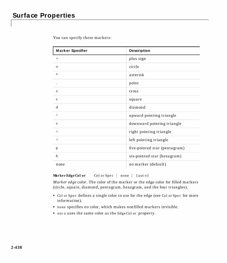
Surface Properties

You can specify these markers:

MarkerEdgeColor ColorSpec | none | auto

Marker edge color. The color of the marker or the edge color for filled markers(circle, square, diamond, pentagram, hexagram, and the four triangles).

• ColorSpec defines a single color to use for the edge (see ColorSpec for moreinformation).

• none specifies no color, which makes nonfilled markers invisible.

• auto uses the same color as the EdgeColor property.


+ plus sign

o circle

* asterisk

. point

x cross

s square

d diamond








2-438

Surface Properties

MarkerFaceColor ColorSpec | none | auto

Marker face color. The fill color for markers that are closed shapes (circle,square, diamond, pentagram, hexagram, and the four triangles).

• ColorSpec defines a single color to use for all marker on the Surface (seeColorSpec for more information).

• none makes the interior of the marker transparent, allowing the backgroundto show through.

• auto uses the CData for the vertex located by the marker to determine thecolor.


Marker size. A scalar specifying the marker size, in points. The default valuefor MarkerSize is six points (1 point = 1/72 inch). Note that MATLAB draws thepoint marker at 1/3 the specified marker size.

MeshStyle both | row | column

Row and column lines. This property specifies whether to draw all edge linesor just row or column edge lines.

• both draws edges for both rows and columns.

• row draws row edges only.

• column draws column edges only.

NormalMode auto | manual

MATLAB -generated or user-specified normal vectors. When this property isauto, MATLAB calculates vertex normals based on the coordinate data. If youspecify your own vertex normals, MATLAB sets this property to manual anddoes not generate its own data. See also the VertexNormals property.

Parent handle

Surface’s parent object. The parent of a Surface object is the Axes in which it isdisplayed. You can move a Surface object to another Axes by setting thisproperty to the handle of the new parent.

Selected on | off

Is object selected. When this property is on, MATLAB displays a dashedbounding box around the Surface if the SelectionHighlight property is also

2-439

Surface Properties

on. You can, for example, define the ButtonDownFcn to set this property,allowing users to select the object with the mouse.


Objects highlight when selected. When the Selected property is on, MATLABindicates the selected state by drawing a dashed bounding box around theSurface. When SelectionHighlight is off, MATLAB does not draw thehandles.

SpecularColorReflectancescalar in the range 0 to 1

Color of specularly reflected light. When this property is 0, the color of thespecularly reflected light depends on both the color of the object from which itreflects and the color of the light source. When set to 1, the color of thespecularly reflected light depends only on the color or the light source (i.e., theLight object Color property). The proportions vary linearly for values inbetween.

SpecularExponent scalar >= 1

Harshness of specular reflection. This property controls the size of the specularspot. Most materials have exponents in the range of 5 to 20.

SpecularStrength scalar >= 0 and <= 1

Intensity of specular light. This property sets the intensity of the specularcomponent of the light falling on the Surface. Specular light comes from Lightobjects in the Axes.

You can also set the intensity of the ambient and diffuse components of thelight on the Surface object. See the AmbientStrength and DiffuseStrengthproperties. Also see the material function.

Tag string



Class of the graphics object. The class of the graphics object. For Surfaceobjects, Type is always the string 'surface'.

2-440

Surface Properties


Associate a context menu with the Surface. Assign this property the handle of aUicontextmenu object created in the same Figure as the Surface. Use theuicontextmenu function to create the context menu. MATLAB displays thecontext menu whenever you right-click over the Surface (Control-click onMacintosh systems).

UserData matrix

User-specified data. Any matrix you want to associate with the Surface object.MATLAB does not use this data, but you can access it using the set and getcommands.

VertexNormals vector or matrix

Surface normal vectors. This property contains the vertex normals for theSurface. MATLAB generates this data to perform lighting calculations. Youcan supply your own vertex normal data, even if it does not match thecoordinate data. This can be useful to produce interesting lighting effects.

Visible on | off

Surface object visibility. By default, all Surfaces are visible. When set to off,the Surface is not visible, but still exists and you can query and set itsproperties.

XData vector or matrix

X-coordinates. The x-position of the surface points. If you specify a row vector,surface replicates the row internally until it has the same number of columnsas ZData.

YData vector or matrix

Y-coordinates. The y-position of the surface points. If you specify a row vector,surface replicates the row internally until it has the same number of rows asZData.

ZData matrix

Z-coordinates. Z-position of the surface points. See the Description section formore information.

2-441

surfl

2surflPurpose Surface plot with colormap-based lighting

Syntax surfl(Z)surfl(X,Y,Z)surfl(...,s)surfl(X,Y,Z,s,k)h = surfl(...)

Description The surfl function displays a shaded Surface based on a combination ofambient, diffuse, and specular lighting models.

surfl(Z) and surfl(X,Y,Z) create three-dimensional shaded Surfaces usingthe default direction for the light source and the default lighting coefficients forthe shading model. X, Y, and Z are vectors or matrices that define the x, y, andz components of a Surface.

surfl(...,’light’) produces a colored, lighted surface using the Lightobject. This produces different results than the default lighting method,surfl(...,'cdata'), which changes the color data for the surface to be thereflectance of the surface.

surfl(...,s) specifies the direction of the light source. s is a two- orthree-element vector that specifies the direction from a Surface to a lightsource. s = [sx sy sz] or s = [azimuth elevation]. The default s is 45˚counterclockwise from the current view direction.

surfl(X,Y,Z,s,k) specifies the reflectance constant. k is a four-elementvector defining the relative contributions of ambient light, diffuse reflection,specular reflection, and the specular shine coefficient. k = [ka kd ks shine]and defaults to [.55,.6,.4,10].

h = surfl(...) returns a handle to a Surface graphics object.

Remarks For smoother color transitions, use colormaps that have linear intensityvariations (e.g., gray, copper, bone, pink).

The ordering of points in the X, Y, and Z matrices define the inside and outsideof parametric surfaces. If you want the opposite side of the surface to reflect the

2-442

surfl

light source, use surfl(X',Y',Z'). Due to the way surface normal vectors arecomputed, surfl requires matrices that are at least 3-by-3.

Examples View peaks using colormap-based lighting:

[x,y] = meshgrid(–3:1/8:3);z = peaks(x,y);surfl(x,y,z);shading interpcolormap(gray);axis([–3 3 –3 3 –8 8])

2-443

surfl

To plot a lighted surface from a view direction other than the default:

view([10 10])grid onhold onsurfl(peaks)shading interpcolormap copperhold off

See Also colormap, shading, light

2-444

surfnorm

2surfnormPurpose Compute and display 3-D surface normals

Syntax surfnorm(Z)surfnorm(X,Y,Z)[Nx,Ny,Nz] = surfnorm(...)

Description The surfnorm function computes surface normals for the Surface defined by X,Y, and Z. The surface normals are unnormalized and valid at each vertex.Normals are not shown for Surface elements that face away from the viewer.

surfnorm(Z) and surfnorm(X,Y,Z) plot a Surface and its surface normals. Zis a matrix that defines the z component of the Surface. X and Y are vectors ormatrices that define the x and y components of the Surface.

[Nx,Ny,Nz] = surfnorm(...) returns the components of thethree-dimensional surface normals for the Surface.

Remarks The direction of the normals is reversed by calling surfnorm with transposedarguments:

surfnorm(X',Y',Z')

surfl uses surfnorm to compute surface normals when calculating thereflectance of a Surface.

Algorithm The surface normals are based on a bicubic fit of the data in X, Y, and Z. Foreach vertex, diagonal vectors are computed and crossed to form the normal.

Examples Plot the normal vectors for a truncated cone.

[x,y,z] = cylinder(1:10);surfnorm(x,y,z)axis([−12 12 −12 12 −0.1 1])

2-445

surfnorm

See Also surf, quiver3

−10−5

05

10

−10−5

05

10

0

0.2

0.4

0.6

0.8

1

2-446

terminal

2terminalPurpose Set graphics terminal type

Syntax terminalterminal('type')

Description To add terminal-specific settings (e.g., escape characters, line length), edit thefile terminal.m.

terminal displays a menu of graphics terminal types, prompts for a choice,then configures MATLAB to run on the specified terminal.

terminal('type') accepts a terminal type string. Valid 'type' strings are

Type Description

tek401x Tektronix 4010/4014

tek4100 Tektronix 4100

tek4105 Tektronix 4105

retro Retrographics card

sg100 Selanar Graphics 100

sg200 Selanar Graphics 200

vt240tek VT240 & VT340 Tektronix mode

ergo Ergo terminal

graphon Graphon terminal

citoh C.Itoh terminal

xtermtek xterm, Tektronix graphics

wyse Wyse WY-99GT

kermit MS-DOS Kermit 2.23

2-447

terminal

hp2647 Hewlett-Packard 2647

versa Macintosh with VersaTerm (Tektronix 4010/4014)

versa4100 Macintosh with VersaTerm (Tektronix 4100)

versa4105 Color/grayscale Macintosh with VersaTerm (Tektronix4105)

hds Human Designed Systems

Type Description (Continued)

2-448

text

2textPurpose Create Text object in current Axes

Syntax text(x,y,'string')text(x,y,z,'string')text(...'PropertyName',PropertyValue...)h = text(...)

Description text is the low-level function for creating Text graphics objects. Use text toplace character strings at specified locations.

text(x,y,'string') adds the string in quotes to the location specified by thepoint (x,y).

text(x,y,z,'string') adds the string in 3-D coordinates.

text(x,y,z,'string','PropertyName',PropertyValue....) adds thestring in quotes to location defined by the coordinates and uses the values forthe specified Text properties. See the “Text Properties” section for a list of Textobject properties.

text('PropertyName',PropertyValue....) omits the coordinates entirelyand specifies all properties using property name/property value pairs.

h = text(..) returns a column vector of handles to Text objects, one handleper object. All forms of the text function optionally return this outputargument.

See the String property for a list of symbols, including Greek letters.

Remarks Specify the Text location coordinates (the x, y, and z arguments) in the dataunits of the current Axes (see “Examples”). The Extent, VerticalAlignment,and HorizontalAlignment properties control the positioning of the characterstring with regard to the Text location point.

If the coordinates are vectors, text writes the string at all locations defined bythe list of points. If the character string is an array the same length as x, y, andz, text writes the corresponding row of the string array at each point specified.

When specifying strings for multiple Text objects, the string can be

2-449

text

• a cell array of strings

• a padded string matrix

• a string vector using vertical slash characters (‘|’) as separators.

Each element of the specified string array creates a different Text object.

When specifying the string for a single Text object, cell arrays of strings andpadded string matrices result in a Text object with a multiline string, whilevertical slash characters are not interpreted as separators and result in asingle line string containing vertical slashes.

text is a low-level function that accepts property name/property value pairs asinput arguments, however, the convenience form,

text(x,y,z,'string')

is equivalent to:

text('XData',x,'YData',y,'ZData',z,'String','string')

You can specify other properties only as property name/property value pairs.See the “Text Properties” section for a description of each property. You canspecify properties as property name/property value pairs, structure arrays, andcell arrays (see the set and get reference pages for examples of how to specifythese data types).

text does not respect the setting of the Figure or Axes NextPlot property. Thisallows you to add Text objects to an existing Axes without setting hold to on.

Examples The statements,

plot(0:pi/20:2*pi,sin(0:pi/20:2*pi))text(pi,0,' \leftarrow sin(\pi)','FontSize',18)

2-450

text

annotate the point at (pi,0) with the string sin(π):

The statement,

text(x,y,'\ite^i\omega\tau = cos(\omega\tau) + i sin(\omega\tau)')

uses embedded TeX sequences to produce:

See Also gtext, int2str, num2str, title, xlabel, ylabel, zlabel

The Axes chapter in the Using MATLAB Graphics manual discussespositioning text.

0 1 2 3 4 5 6 7−1

−0.8

−0.6

−0.4

−0.2

0

0.2

0.4

0.6

0.8

1

← sin(π)

eiωτ = cos(ωτ) + i sin(ωτ)

2-451

text

ObjectHierarchy

Setting Default PropertiesYou can set default Text properties on the Axes, Figure, and Root levels:

set(0,'DefaulttextProperty',PropertyValue...)set(gcf,'DefaulttextProperty',PropertyValue...)set(gca,'DefaulttextProperty',PropertyValue...)

Where Property is the name of the Text property and PropertyValue is thevalue you are specifying. Use set and get to access Text properties.

Property List The following table lists all Text properties and provides a brief description ofeach. The property name links take you to an expanded description of theproperties.

Root

Uimenu

Line

Axes Uicontrol

Image

Figure

Uicontextmenu



Defining the character string

Editing Enable or disable editing mode. Values: on, offDefault: off

Interpreter Enable or disable TeX interpretation Values: tex, noneDefault: tex

String The character string (including list ofTeX character sequences)

Value: character string

Positioning the character string

2-452

text

Extent Position and size of Text object Values: [left, bottom, width,height]

HorizontalAlignment Horizontal alignment of Text string Values: left, center, rightDefault: left

Position Position of Text Extent rectangle Values: [x, y, z] coordinatesDefault: [] empty matrix

Rotation Orientation of Text object Values: scalar (degrees)Default: 0

Units Units for Extent and Positionproperties

Values: pixels, normalized,inches, centimeters,points, dataDefault: data

VerticalAlignment Vertical alignment of Text string Values: top, cap, middle,baseline, bottomDefault: middle

Specifying the Font

FontAngle Select italic-style font Values: normal, italic,obliqueDefault: normal

FontName Select font family Values: font nameDefault: Helvetica

FontSize Size of font Values: size in FontUnitsDefault: 10 points

FontUnits Units for FontSize property Values: points, normalized,inches, centimeters, pixelsDefault: points

FontWeight Weight of text characters Values: light, normal, demi,boldDefault: normal


2-453

text



EraseMode Method of drawing and erasing theText (useful for animation)


SelectionHighlight Highlight Text when selected(Selected property set to on)


Visible Make the Text visible or invisible Values: on, offDefault: on

Color Color of the Text ColorSpec

Controlling Access to Text Objects

HandleVisibility Determines if and when the theText’s handle is visible to otherfunctions


HitTest Determines if the Text can becomethe current object (see the FigureCurrentObject property)


General Information About Text Objects

Children Text objects have no children Values: [] (empty matrix)

Parent The parent of a Text object is alwaysan Axes object

Value: Axes handle

Selected Indicate whether the Text is in a“selected” state.




Value: the string 'text'


2-454

text





ButtonDownFcn Define a callback routine thatexecutes when a mouse button ispressed on over the Text


CreateFcn Define a callback routine thatexecutes when an Text is created


DeleteFcn Define a callback routine thatexecutes when the Text is deleted(via close or delete)




UIContextMenu Associate a context menu with theText



2-455

Text Properties

2Text PropertiesText Properties This section lists property names along with the types of values each accepts.Curly braces enclose default values.






Button press callback routine. A callback routine that executes whenever youpress a mouse button while the pointer is over the Text object. Define thisroutine as a string that is a valid MATLAB expression or the name of an M-file.The expression executes in the MATLAB workspace.

Children matrix (read only)

The empty matrix; Text objects have no children.

Clipping on | off

Clipping mode. When Clipping is on, MATLAB does not display any portionof the Text that is outside the Axes.

Color ColorSpec

Text color. A three-element RGB vector or one of MATLAB ’s predefined names,specifying the Text color. The default value for Color is white. See ColorSpecfor more information on specifying color.

2-456

Text Properties

CreateFcn string

Callback routine executed during object creation. This property defines acallback routine that executes when MATLAB creates a Text object. You mustdefine this property as a default value for Text. For example, the statement,

set(0,'DefaultTextCreateFcn',...'set(gcf,''Pointer'',’'crosshair'')')

defines a default value on the Root level that sets the Figure Pointer propertyto a crosshair whenever you create a Text object. MATLAB executes thisroutine after setting all Text properties. Setting this property on an existingText object has no effect.


DeleteFcn string

Delete Text callback routine. A callback routine that executes when you deletethe Text object (e.g., when you issue a delete command or clear the Axes orFigure). MATLAB executes the routine before destroying the object’sproperties so these values are available to the callback routine.


Editing on | off

Enable or disable editing mode. When this property is set to the default of off,you cannot edit the text string interactively (i.e., you must change the Stringproperty to change the text). When this property is set to on, MATLAB placesan insert cursor at the beginning of the text string and enables editing. Toapply the new text string:

• Press the ESC key

• Clicking in any Figure window (including the current Figure)

• Reset the Editing property to off

MATLAB then updates the String property to contain the new text and resetsthe Editing property to off. You must reset the Editing property to on toagain resume editing.

2-457

Text Properties


Erase mode. This property controls the technique MATLAB uses to draw anderase Text objects. Alternative erase modes are useful for creating animatedsequences, where controlling the way individual object redraw is necessary toimprove performance and obtain the desired effect.

• normal — Redraw the affected region of the display, performing thethree-dimensional analysis necessary to ensure that all objects are renderedcorrectly. This mode produces the most accurate picture, but is the slowest.The other modes are faster, but do not perform a complete redraw and aretherefore less accurate.

• none — Do not erase the Text when it is moved or destroyed. While the objectis still visible on the screen after erasing with EraseMode none, you cannotprint it because MATLAB stores no information about its former location.

• xor — Draw and erase the Text by performing an exclusive OR (XOR) witheach pixel index of the screen beneath it. When the Text is erased, it does notdamage the objects beneath it. However, when Text is drawn in xor mode, itscolor depends on the color of the screen beneath it and is correctly coloredonly when over Axes background Color, or the Figure background Color ifthe Axes Color is set to none.

• background — Erase the Text by drawing it in the background Color, or theFigure background Color if the Axes Color is set to none. This damagesobjects that are behind the erased Text, but Text is always properly colored.



2-458

Text Properties

Extent position rectangle (read only)

Position and size of Text. A four-element read-only vector that defines the sizeand position of the Text string:


If the Units property is set to data (the default), left and bottom are the x andy coordinates of the lower-left corner of the Text Extent rectangle.

For all other values of Units, left and bottom are the distance from thelower-left corner of the Axes position rectangle to the lower-left corner of theText Extent rectangle. width and height are the dimensions of the Extentrectangle. All measurements are in units specified by the Units property.


Character slant. MATLAB uses this property to select a font from thoseavailable on your particular system. Generally, setting this property to italicor oblique selects a slanted font.

FontName string

Font family. A string specifying the name of the font to use for the Text object.To display and print properly, this must be a font that your system supports.The default font is Helvetica.

FontSize size in FontUnits

Font size. An integer specifying the font size to use for Text, in unitsdetermined by the FontUnits property. The default point size is 10 (1 point =1/72 inch).

FontWeight light | normal | demi | bold

Weight of Text characters. MATLAB uses this property to select a font fromthose available on your particular system. Generally, setting this property tobold or demi causes MATLAB to use a bold font.


Font size units. MATLAB uses this property to determine the units used by theFontSize property. Normalized units interpret FontSize as a fraction of theheight of the parent Axes. When you resize the Axes, MATLAB modifies thescreen FontSize accordingly. pixels, inches, centimeters, and points areabsolute units (1 point = 1/72 inch).

2-459

Text Properties






When a handle is not visible in its parent’s list of children, it cannot be returnedby functions that obtain handles by searching the object hierarchy or queryinghandle properties. This includes get, findobj, gca, gcf, gco, newplot, cla, clf,and close.




HitTest on | off

Selectable by mouse click. HitTest determines if the Text can become thecurrent object (as returned by the gco command and the Figure CurrentObject

2-460

Text Properties

property) as a result of a mouse click on the Text. If HiTest is off, clicking onthe Text selects the object below it (which is usually the Axes containing it).

For example, suppose you define the button down function of an Image (see theButtonDownFcn property) to display text at the location you click on with themouse,

First define the callback routine,

function bd_functionpt = get(gca,'CurrentPoint');text(pt(1,1),pt(1,2),pt(1,3),...

'\fontsize20\oplus The spot to label',...'HitTest','off')

Now display an Image, setting its ButtonDownFcn property to the callbackroutine:

load earthimage(X,'ButtonDownFcn','bd_function'); colormap(map)

When you click on the Image, MATLAB displays the text string at thatlocation. With HitTest set to off, existing text cannot intercept anysubsequent button down events that occur over the text. This enables theImage’s button down function to execute.

HorizontalAlignmentleft | center | right

Horizontal alignment of Text. This property specifies the horizontaljustification of the Text string. It determines where MATLAB places the stringwith regard to the point specified by the Position property. The followingpicture illustrates the alignment options:

See the Extent property for related information.

Left Center Right

Text HorizontalAlignment property viewed with the VerticalAlignmentproperty set to middle (the default).

2-461

Text Properties

Interpreter tex | none

Interpret Tex instructions. This property controls whether MATLAB interpretscertain characters in the String property as Tex instructions (default) ordisplays all characters literally. See the String property for a list of supportTex instructions.


Callback routine interruption mode. The Interruptible property controlswhether a Text callback routine can be interrupted by subsequently invokedcallback routines. Text objects have four properties that define callbackroutines: ButtonDownFcn, CreateFcn, and DeleteFcn. See the BusyActionproperty for information on how MATLAB executes callback routines.

Parent handle

Text object’s parent. The handle of the Text object’s parent object. The parent ofa Text object is the Axes in which it is displayed. You can move a Text object toanother Axes by setting this property to the handle of the new parent.

Position [x,y,[z]]

Location of Text. A two- or three-element vector, [x y [z]], that specifies thelocation of the text in three dimensions. If you omit the z value, it defaults to 0.All measurements are in units specified by the Units property. Initial value is[0 0 0].

Rotation scalar (default = 0)

Text orientation. This property determines the orientation of the Text string.Specify values of rotation in degrees (positive angles cause counterclockwiserotation).

Selected on | off

Is object selected. When this property is on, MATLAB displays selection handlesif the SelectionHighlight property is also on. You can, for example, define theButtonDownFcn to set this property, allowing users to select the object with themouse.


Objects highlight when selected. When the Selected property is on, MATLABindicates the selected state by drawing four edge handles and four corner

2-462

Text Properties

handles. When SelectionHighlight is off, MATLAB does not draw thehandles.

String string

The Text string. Specify this property as a quoted string for single-line strings,or as a cell array of strings or a padded string matrix for multiline strings.MATLAB displays this string at the specified location. Vertical slashcharacters are not interpreted as linebreaks in Text strings, and are drawn aspart of the Text string. See the “Remarks” section for more information.

When the Text Interpreter property is Tex (the default), you can use a subsetof TeX commands embedded in the string to produce special characters such asGreek letters and mathematical symbols. The following table lists thesecharacters and the character sequence used to define them.

CharacterSequence

Symbol CharacterSequence


Symbol

\alpha α \upsilon υ \sim ∼

\beta β \phi ϕ \leq ≤

\gamma γ \chi χ \infty ∞

\delta δ \psi ψ \clubsuit ♣

\epsilon ε \omega ω \diamondsuit ♦

\zeta ζ \Gamma Γ \heartsuit ♥

\eta η \Delta ∆ \spadesuit ♠

\theta θ \Theta Θ \leftrightarrow ↔

\vartheta υ \Lambda Λ \leftarrow ←

\iota ι \Xi Ξ \uparrow ↑

\kappa κ \Pi Π \rightarrow →

\lambda λ \Sigma Σ \downarrow ↓

\mu µ \Upsilon Υ \circ °

2-463

Text Properties

You can also specify stream modifiers that control the font used. The first fourmodifiers are mutually exclusive. However, you can use \fontname incombination with one of the other modifiers:

\nu ν \Phi Φ \pm ±

\xi ξ \Psi Ψ \geq ≥

\pi π \Omega Ω \propto ∝

\rho ρ \forall ∀ \partial ∂

\sigma σ \exists ∃ \bullet •

\varsigma ζ \ni ∋ \div ÷

\tau τ \cong ≅ \neq ≠

\equiv ≡ \approx ≈ \aleph ℵ

\Im ℑ \Re ℜ \wp ℘

\otimes ⊗ \oplus ⊕ \oslash ∅

\cap ∩ \cup ∪ \supseteq ⊇

\supset ⊃ \subseteq ⊆ \subset ⊂

\int ∫ \in ∈ \o ο

\rfloor \lceil \nabla ∇

\lfloor \cdot ⋅ \ldots …

\perp ⊥ \neg ¬ \prime ′

\wedge ∧ \times × \0 ∅

\rceil \surd √ \mid |

\vee ∨ \varpi ϖ \copyright

\langle ⟨ \rangle ⟩

CharacterSequence



Symbol

2-464

Text Properties

• \bf – bold font

• \it – italics font

• \sl – oblique font (rarely available)

• \rm – normal font

• \fontnamefontname – specify the name of the font family to use.

• \fontsizefontsize – specify the font size in FontUnits.

Stream modifiers remain in effect until the end of the string or only within thecontext defined by braces .

The subscript character “_” and the superscript character “^” modify thecharacter or substring defined in braces immediately following.

To print the special characters used to define the Tex strings whenInterpreter is Tex, prefix them with the backslash “\” character: \\, \, \ \_,\^.

See the “Example” section for more information.

When Interpreter is none, no characters in the String are interpreted, and allare displayed when the text is drawn.

Tag string



Class of graphics object. For Text objects, Type is always the string 'text'.

Units pixels | normalized | inches |centimeters | points | data

Units of measurement. This property specifies the units MATLAB uses tointerpret the Extent and Position properties. All units are measured from thelower-left corner of the Axes plotbox. Normalized units map the lower-leftcorner of the rectangle defined by the Axes to (0,0) and the upper-right cornerto (1.0,1.0). pixels, inches, centimeters, and points are absolute units (1point = 1/72 inch). data refers to the data units of the parent Axes.

2-465

Text Properties

If you change the value of Units, it is good practice to return it to its defaultvalue after completing your computation so as not to affect other functions thatassume Units is set to the default value.

UserData matrix

User-specified data. Any data you want to associate with the Text object.MATLAB does not use this data, but you can access it using set and get.


Associate a context menu with the Text. Assign this property the handle of aUicontextmenu object created in the same Figure as the Text. Use theuicontextmenu function to create the context menu. MATLAB displays thecontext menu whenever you right-click over the Text (Control-click onMacintosh systems)

VerticalAlignment top | cap | middle | baseline |bottom

Vertical alignment of Text. This property specifies the vertical justification ofthe text string. It determines where MATLAB places the string with regard tothe value of the Position property. The possible values mean:

• top – Place the top of the string’s Extent rectangle at the specified y-position.

• cap – Place the string so that the top of a capital letter is at the specifiedy-position.

• middle – Place the middle of the string at specified y-position.

• baseline – Place font baseline at the specified y-position.

• bottom – Place the bottom of the string’s Extent rectangle at the specifiedy-position.

2-466

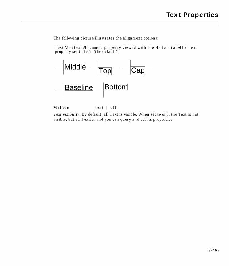
Text Properties

The following picture illustrates the alignment options:

Visible on | off

Text visibility. By default, all Text is visible. When set to off, the Text is notvisible, but still exists and you can query and set its properties.

Middle Top Cap

Baseline Bottom

Text VerticalAlignment property viewed with the HorizontalAlignmentproperty set to left (the default).

2-467

title

2titlePurpose Add title to current Axes

Syntax title('string')title(fname)title(...,'PropertyName',PropertyValue,...)h = title(...)

Description Each Axes graphics object can have one title. The title is located at the top andin the center of the axes.

title('string') outputs the string at the top and in the center of the currentaxes.

title(fname) evaluates the function that returns a string and displays thestring at the top and in the center of the current axes.

title(...,'PropertyName',PropertyValue,...) specifies property nameand property value pairs for the Text graphics object that title creates.

h = title(...) returns the handle to the text object used as the title.

Examples Display today’s date in the current Axes:

title(date)

Include a variable’s value in a title:

f = 70;c = (f—32)/1.8;title(['Temperature is ',num2str(c),'C'])

Include a variable’s value in a title and set the color of the title to yellow:

n = 3;title(['Case number #',int2str(n)],'Color','y')

Include Greek symbols in a title:

title('\ite^\omega\tau = cos(\omega\tau) + isin(\omega\tau)’)

The Text object String property lists the available symbols.

2-468

title

Remarks title sets the Title property of the current Axes graphics object to a new Textgraphics object. See the Text String property for more information.

See Also gtext, int2str, num2str, plot, text, xlabel, ylabel, zlabel

2-469

trimesh

2trimeshPurpose Triangular mesh plot

Syntax trimesh(Tri,X,Y,Z)trimesh(Tri,X,Y,Z,C)trimesh(...'PropertyName',PropertyValue...)h = trimesh(...)

Description trimesh(Tri,X,Y,Z) displays triangles defined in the m-by-3 face matrix Trias a mesh. Each row of Tri defines a single triangular face by indexing into thevectors or matrices that contain the X, Y, and Z vertices.

trimesh(Tri,X,Y,Z,C) specifies color defined by C in the same manner as thesurf function. MATLAB performs a linear transformation on this data toobtain colors from the current colormap.

trimesh(...'PropertyName',PropertyValue...) specifies additional Patchproperty names and values for the Patch graphics object created by thefunction.

h = trimesh(...) returns a handle to a Patch graphics object.

Example Create vertex vectors and a face matrix, then create a triangular mesh plot.

x = rand(1,50);y = rand(1,50);z = peaks(6*x–3,6*x–3);tri = delaunay(x,y);trimesh(tri,x,y,z)

See Also patch, trisurf, delaunay

2-470

trisurf

2trisurfPurpose Triangular surface plot

Syntax trisurf(Tri,X,Y,Z)trisurf(Tri,X,Y,Z,C)trisurf(...'PropertyName',PropertyValue...)h = trisurf(...)

Description trisurf(Tri,X,Y,Z) displays triangles defined in the m-by-3 face matrix Trias a surface. Each row of Tri defines a single triangular face by indexing intothe vectors or matrices that contain the X, Y, and Z vertices.

trisurf(Tri,X,Y,Z,C) specifies color defined by C in the same manner as thesurf function. MATLAB performs a linear transformation on this data toobtain colors from the current colormap.

trisurf(...'PropertyName',PropertyValue...) specifies additional Patchproperty names and values for the Patch graphics object created by thefunction.

h = trisurf(...) returns a Patch handle.

Example Create vertex vectors and a face matrix, then create a triangular surface plot.

x = rand(1,50);y = rand(1,50);z = peaks(6*x–3,6*x–3);tri = delaunay(x,y);trisurf(tri,x,y,z)

See Also patch, surf, trimesh, delaunay

2-471

view

2viewPurpose Viewpoint specification

Syntax view(az,el)view([az,el])view([x,y,z])view(2)view(3)view(T)

[az,el] = viewT = view

Description The position of the viewer (the viewpoint) determines the orientation of theAxes. You specify the viewpoint in terms of azimuth and elevation, or by a pointin three-dimensional space.

view(az,el) and view([az,el]) set the viewing angle for athree-dimensional plot. The azimuth, az, is the horizontal rotation about thez-axis as measured in degrees from the negative y-axis. Positive values indicatecounterclockwise rotation of the viewpoint. el is the vertical elevation of theviewpoint in degrees. Positive values of elevation correspond to moving abovethe object; negative values correspond to moving below the object.

view([x,y,z]) sets the viewpoint to the Cartesian coordinates x, y, and z. Themagnitude of (x,y,z) is ignored.

view(2) sets the default two-dimensional view, az = 0, el = 90.

view(3) sets the default three-dimensional view, az = —37.5, el = 30.

view(T) sets the view according to the transformation matrix T, which is a4-by-4 matrix such as a perspective transformation generated by viewmtx.

[az,el] = view returns the current azimuth and elevation.

T = view returns the current 4-by-4 transformation matrix.

2-472

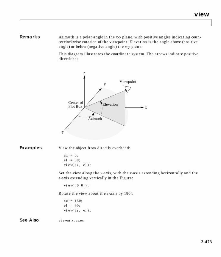
view

Remarks Azimuth is a polar angle in the x-y plane, with positive angles indicating coun-terclockwise rotation of the viewpoint. Elevation is the angle above (positiveangle) or below (negative angle) the x-y plane.

This diagram illustrates the coordinate system. The arrows indicate positivedirections:

Examples View the object from directly overhead:

az = 0;el = 90;view(az, el);

Set the view along the y-axis, with the x-axis extending horizontally and thez-axis extending vertically in the Figure:

view([0 0]);

Rotate the view about the z-axis by 180°:

az = 180;el = 90;view(az, el);

See Also viewmtx, axes

Center of

Viewpoint

z

x

y

Azimuth

Elevation

-y

Plot Box

2-473

view

Axes graphics object properties: CameraPosition, CameraTarget,CameraViewAngle, Projection.

2-474

viewmtx

2viewmtxPurpose View transformation matrices

Syntax T = viewmtx(az,el)T = viewmtx(az,el,phi)T = viewmtx(az,el,phi,xc)

Description viewmtx computes a 4-by-4 orthographic or perspective transformation matrixthat projects four-dimensional homogeneous vectors onto a two-dimensionalview surface (e.g., your computer screen).

T = viewmtx(az,el) returns an orthographic transformation matrixcorresponding to azimuth az and elevation el. az is the azimuth (i.e.,horizontal rotation) of the viewpoint in degrees. el is the elevation of theviewpoint in degrees. This returns the same matrix as the commands

view(az,el)T = view

but does not change the current view.

T = viewmtx(az,el,phi) returns a perspective transformation matrix. phi isthe perspective viewing angle in degrees. phi is the subtended view angle of thenormalized plot cube (in degrees) and controls the amount of perspectivedistortion:

You can use the matrix returned to set the view transformation with view(T).The 4-by-4 perspective transformation matrix transforms four-dimensionalhomogeneous vectors into unnormalized vectors of the form (x,y,z,w), where w isnot equal to 1. The x- and y-components of the normalized vector (x/w, y/w, z/w,1) are the desired two-dimensional components (see example below).

Phi Description

0 degrees Orthographic projection

10 degrees Similar to telephoto lens

25 degrees Similar to normal lens

60 degrees Similar to wide angle lens

2-475

viewmtx

T = viewmtx(az,el,phi,xc) returns the perspective transformation matrixusing xc as the target point within the normalized plot cube (i.e., the camera islooking at the point xc). xc is the target point that is the center of the view. Youspecify the point as a three-element vector, xc = [xc,yc,zc], in the interval[0,1]. The default value is xc = [0,0,0].

Remarks A four-dimensional homogenous vector is formed by appending a 1 to thecorresponding three-dimensional vector. For example, [x,y,z,1] is thefour-dimensional vector corresponding to the three-dimensional point [x,y,z].

Examples Determine the projected two-dimensional vector corresponding to thethree-dimensional point (0.5,0.0,—3.0) using the default view direction. Notethat the point is a column vector.

A = viewmtx(—37.5,30);x4d = [.5 0 —3 1]';x2d = A∗x4d;x2d = x2d(1:2)x2d =

0.3967—2.4459

Vectors that trace the edges of a unit cube are

x = [0 1 1 0 0 0 1 1 0 0 1 1 1 1 0 0];y = [0 0 1 1 0 0 0 1 1 0 0 0 1 1 1 1];z = [0 0 0 0 0 1 1 1 1 1 1 0 0 1 1 0];

2-476

viewmtx

Transform the points in these vectors to the screen, then plot the object:

A = viewmtx(—37.5,30);[m,n] = size(x);x4d = [x(:),y(:),z(:),ones(m*n,1)]';x2d = A*x4d;x2 = zeros(m,n); y2 = zeros(m,n);x2(:) = x2d(1,:);y2(:) = x2d(2,:);plot(x2,y2)

Use a perspective transformation with a 25 degree viewing angle:

A = viewmtx(—37.5,30,25);x4d = [.5 0 —3 1]';x2d = A∗x4d;x2d = x2d(1:2)/x2d(4) % Normalizex2d =

0.1777—1.8858

−0.8 −0.6 −0.4 −0.2 0 0.2 0.4 0.6 0.80

0.2

0.4

0.6

0.8

1

1.2

1.4

1.6

2-477

viewmtx

Transform the cube vectors to the screen and plot the object:

A = viewmtx(—37.5,30,25);[m,n] = size(x);x4d = [x(:),y(:),z(:),ones(m*n,1)]';x2d = A*x4d;x2 = zeros(m,n); y2 = zeros(m,n);x2(:) = x2d(1,:)./x2d(4,:);y2(:) = x2d(2,:)./x2d(4,:);plot(x2,y2)

See Also view

−0.6 −0.4 −0.2 0 0.2 0.4 0.6 0.8−0.8

−0.6

−0.4

−0.2

0

0.2

0.4

0.6

2-478

waterfall

2waterfallPurpose Waterfall plot

Syntax waterfall(Z)waterfall(X,Y,Z)waterfall(...,C)

h = waterfall(...)

Description The waterfall function draws a mesh similar to the meshz function, but it doesnot generate lines from the columns of the matrices. This produces a“waterfall” effect.

waterfall(Z) creates a waterfall plot using x = 1:size(Z,1) andy = 1:size(Z,1). Z determines the color, so color is proportional to surfaceheight.

waterfall(X,Y,Z) creates a waterfall plot using the values specified in X, Y,and Z. Z also determines the color, so color is proportional to the surface height.If X and Y are vectors, X corresponds to the columns of Z, and Y corresponds tothe rows, where length(x) = n, length(y) = m, and [m,n] = size(Z). X andY are vectors or matrices that define the x and y coordinates of the plot. Z is amatrix that defines the z coordinates of the plot (i.e., height above a plane). IfC is omitted, color is proportional to Z.

waterfall(...,C) uses scaled color values to obtain colors from the currentcolormap. Color scaling is determined by the range of C, which must be thesame size as Z. MATLAB performs a linear transformation on C to obtain colorsfrom the current colormap.

h = waterfall(...) returns the handle of the Patch graphics object used todraw the plot.

Remarks For column-oriented data analysis, use waterfall(Z') orwaterfall(X',Y',Z').

2-479

waterfall

Examples Produce a waterfall plot of the peaks function:

[X,Y,Z] = peaks(30);waterfall(X,Y,Z)

Algorithm The range of X, Y, and Z, or the current setting of the Axes Llim, YLim, and ZLimproperties, determines the range of the Axes (also set by axis). The range of C,or the current setting of the Axes Clim property, determines the color scaling(also set by caxis).

The CData property for the Patch graphics objects specifies the color at everypoint along the edge of the Patch, which determines the color of the lines.

The waterfall plot looks like a mesh surface, however, it is a Patch graphicsobject. To create a Surface plot similar to waterfall, use the meshz functionand set the MeshStyle property of the Surface to 'Row'. For a discussion ofparametric surfaces and related color properties, see surf.

See Also axes, axis, caxis, meshz, surf

Properties for Patch graphics objects.

−3−2

−10

12

3

−4

−2

0

2

4−10

−5

0

5

10

2-480

whitebg

2whitebgPurpose Change Axes background color

Syntax whitebgwhitebg(h)whitebg(ColorSpec)whitebg(h,ColorSpec)

Description whitebg complements the colors in the current Figure.

whitebg(h) complements colors in all Figures specified in the vector h.

whitebg(ColorSpec) and whitebg(h,ColorSpec) change the color of theAxes, which are children of the Figure, to the color specified by ColorSpec.

Remarks whitebg changes the colors of the Figure’s children, with the exception ofshaded surfaces. This ensures that all objects are visible against the newbackground color. whitebg sets the default properties on the Root such that allsubsequent Figure use the new background color.

Examples Set the background color to blue-gray:

whitebg([0 .5 .6])

Set the background color to blue:

whitebg('blue')

See Also ColorSpec

The Figure graphics object property InvertHardCopy.

2-481

xlabel, ylabel, zlabel

2xlabel, ylabel, zlabelPurpose Label the x-, y-, and z-axis

Syntax xlabel('string')xlabel(fname)xlabel(...,'PropertyName',PropertyValue,...)h = xlabel(...)

ylabel(...)h = ylabel(...)

zlabel(...)h = zlabel(...)

Description Each Axes graphics object can have one label for the x-, y-, and z-axis. The labelappears beneath its respective axis in a two-dimensional plot and to the side orbeneath the axis in a three-dimensional plot.

xlabel('string') labels the x-axis of the current Axes.

xlabel(fname) evaluates the function fname, which must return a string,then displays the string beside the x-axis.

xlabel(...,'PropertName',PropertyValue,...) specifies property nameand property value pairs for the Text graphics object created by xlabel.

h = xlabel(...), h = ylabel(...), and h = zlabel(...) return thehandle to the Text object used as the label.

ylabel(...) and zlabel(...) label the y-axis and z-axis, respectively, of thecurrent Axes.

Remarks Re-issuing an xlabel, ylabel, or zlabel command causes the new label toreplace the old label.

For three-dimensional graphics, MATLAB puts the label in the front or side,so that it is never hidden by the plot.

See Also text, title

2-482

xlim, ylim, zlim

2xlim, ylim, zlimPurpose Set or query axis limits

Syntax Note that the syntax for each of these three functions is the same; only the xlimfunction is used for simplicity. Each operates on the respective x-, y-, or z-axis.

xlimxlim([xmin xmax])xlim('mode')xlim('auto')xlim('manual')xlim(axes_handle,...)

Description xlim with no arguments return the respective limits of the current axes.

xlim([xmin xmax]) sets the axis limits in the current axes to the specifiedvalues.

xlim('mode') returns the current value of the axis limits mode, which can beeither auto (the default) or manual.

xlim('auto') sets the axis limit mode to auto.

xlim('manual') sets the respective axis limit mode to manual.

xlim(axes_handle,...) performs the set or query on the axes identified bythe first argument, axes_handle. When you do not specify an axes handle,these functions operate on the current axes.

Remarks xlim, ylim, and zlim set or query values of the Axes object XLim, YLim, ZLim,and XLimMode, YLimMode, ZLimMode properties.

When the axis limit modes are auto (the default), MATLAB uses limits thatspan the range of the data being displayed and are round numbers. Setting avalue for any of the limits also sets the corresponding mode to manual. Notethat high-level plotting functions like plot and surf reset both the modes andthe limits. If you set the limits on an existing graph and want to maintain theselimits while adding more graphs, use the hold command.

2-483

xlim, ylim, zlim

Examples This example illustrates how to set the x- and y-axis limits to match the actualrange of the data, rather than the rounded values of [-2 3] for the x-axis and[-2 4] for the y-axis originally selected by MATLAB.

[x,y] = meshgrid([−1.75:.2:3.25]);z = x.*exp(−x.^2−y.^2);surf(x,y,z)xlim([−1.75 3.25])ylim([−1.75 3.25])

See Also axis

The Axes properties XLim, YLim, ZLim


−10

12

3

−1

0

1

2

3

−0.5

0

0.5

2-484

zoom

2zoomPurpose Zoom in and out on a 2-D plot

Syntax zoom onzoom offzoom outzoom resetzoomzoom xonzoom yonzoom(factor)zoom(fig, option)

Description zoom on turns on interactive zooming. When interactive zooming is enabled ina Figure, pressing a mouse button while your cursor is within an Axes zoomsinto the point or out from the point beneath the mouse. Zooming changes theAxes limits.

• For a single-button mouse, zoom in by pressing the mouse button and zoomout by simultaneously pressing Shift and the mouse button.

• For a two- or three-button mouse, zoom in by pressing the left mouse buttonand zoom out by pressing the right mouse button.

Clicking and dragging over an Axes when interactive zooming is enabled drawsa rubber-band box. When the mouse button is released, the Axes zoom in to theregion enclosed by the rubber-band box.

Double-clicking over an Axes returns the Axes to its initial zoom setting.

zoom off turns interactive zooming off.

zoom out returns the plot to its initial zoom setting.

zoom reset remembers the current zoom setting as the initial zoom setting.Later calls to zoom out, or double-clicks when interactive zoom mode isenabled, will return to this zoom level.

zoom toggles the interactive zoom status.

zoom xon and zoom yon sets zoom on for the x- and y-axis, respectively.

2-485

zoom

zoom(factor) zooms in or out by the specified zoom factor, without affectingthe interactive zoom mode. Values greater than 1 zoom in by that amount,while numbers greater than 0 and less than 1 zoom out by 1/factor.

zoom(fig, option) Any of the above options can be specified on a figure otherthan the current figure using this syntax.

Remarks zoom changes the Axes limits by a factor of two (in or out) each time you pressthe mouse button while the cursor is within an Axes. You can also click anddrag the mouse to define a zoom area, or double-click to return to the initialzoom level.

2-486

dialog

2dialogPurpose Create and display dialog box

Syntax h = dialog('PropertyName',PropertyValue,...)

Description h = dialog('PropertyName',PropertyValue,...) returns a handle to adialog box. This function creates a Figure graphics object and sets the Figureproperties recommended for dialog boxes. You can specify any valid Figureproperty value.

See Also errordlg, figure, helpdlg, inputdlg, pagedlg, printdlg, questdlg, uiwait,uiresume, warndlg

2-487

dragrect

2dragrectPurpose Drag rectangles with mouse

Syntax [finalrect] = dragrect(initialrect)[finalrect] = dragrect(initialrect,stepsize)

Description [finalrect] = dragrect(initialrect) tracks one or more rectanglesanywhere on the screen. The n-by-4 matrix, rect, defines the rectangles. Eachrow of rect must contain the initial rectangle position as[left bottom width height] values. dragrect returns the final position of therectangles in finalrect.

[finalrect] = dragrect(initialrect,steprize) moves the rectangles inincrements of stepsize. The lower-left corner of the first rectangle isconstrained to a grid of size stepsize starting at the lower-left corner of thefigure, and all other rectangles maintain their original offset from the firstrectangle. [finalRect] = dragrect(...) returns the final positions of therectangles when the mouse button is released. The default stepsize is 1.

Remarks dragrect returns immediately if a mouse button is not currently pressed. Usedragrect in a ButtonDownFcn, or from the commandline in conjunction withwaitforbuttonpress to ensure that the mouse button is down when dragrectis called. dragrect returns when you release the mouse button.

Example Drag a rectangle that is 50 pixels wide and 100 pixels in height.

waitforbuttonpresspoint1 = get(gcf,'CurrentPoint') % button down detectedrect = [point1(1,1) point1(1,2) 50 100][r2] = dragrect(rect)

See Also rbbox, waitforbuttonpress

2-488

errordlg

2errordlgPurpose Create and display an error dialog box

Syntax errordlgerrordlg('errorstring')errordlg('errorstring','dlgname')errordlg('errorstring','dlgname','on')h = errordlg(...)

Description errordlg creates an error dialog box, or if the named dialog exists, errordlgpops the named dialog in front of other windows.

errordlg displays a dialog box named 'Error Dialog' that contains thestring 'This is the default error string.'

errordlg('errorstring') displays a dialog box named 'Error Dialog' thatcontains the string 'errorstring'.

errordlg('errorstring','dlgname') displays a dialog box named'dlgname' that contains the string 'errorstring'.

errordlg('errorstring','dlgname','on') specifies whether to replace anexisting dialog box having the same name. 'on' brings an existing error dialoghaving the same name to the foreground. In this case, errordlg does not createa new dialog.

h = errordlg(...) returns the handle of the dialog box.

Remarks MATLAB sizes the dialog box to fit the string 'errorstring'. The error dialogbox has an OK pushbutton and remains on the screen until you press the OKbutton or the Return key. After pressing the button, the error dialog boxdisappears.

The appearance of the dialog box depends on the windowing system you use.

Examples The function

errordlg('File not found','File Error');

2-489

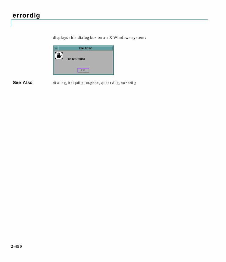
errordlg

displays this dialog box on an X-Windows system:

See Also dialog, helpdlg, msgbox, questdlg, warndlg

2-490

gcbo

2-491

2gcboPurpose Return the handle of the object whose callback is currently executing

Syntax h = gcbo

[h, figure] = gcbo

Description h = gcbo returns the handle of the graphics object whose callback is executing.

[h, figure] = gcbo returns the handle of the current callback object and thehandle of the Figure containing this object.

Remarks MATLAB stores the handle of the object whose callback is executing in theRoot’s CallbackObject property. If a callback interrupts another callback,MATLAB replaces the CallbackObject value with the handle of the objectwhose callback is interrupting. When that callback completes, MATLABrestores the handle of the object whose callback was interrupted.

The Root CallbackObject property is read-only, so its value is always valid atany time during callback execution. The Root CurrentFigure property, andthe Figure CurrentAxes and CurrentObject properties (returned by gcf, gca,and gco respectively) are user settable, so they can change during theexecution of a callback, especially if that callback is interrupted by anothercallback. Therefore, those functions are not reliable indicators of which object’scallback is executing.

When you write callback routines for the CreateFcn and DeleteFcn of anyobject and the Figure ResizeFcn, you must use gcbo since those callbacks donot update the Root’s CurrentFigure property, or the Figure’s CurrentObjector CurrentAxis properties; they only update the Root’s CallbackObjectproperty.

When no callbacks are executing, gcbo returns [] (an empty matrix).

See Also gca, gcf, gco, rootobject

helpdlg

2-492

2helpdlgPurpose Create a help dialog box

Syntax helpdlghelpdlg('helpstring')helpdlg('helpstring','dlgname')h = helpdlg(...)

Description helpdlg creates a help dialog box or brings the named help dialog box to thefront.

helpdlg displays a dialog box named 'Help Dialog' containing the string'This is the default help string.'

helpdlg('helpstring') displays a dialog box named 'Help Dialog'containing the string specified by 'helpstring'.

helpdlg('helpstring','dlgname') displays a dialog box named 'dlgname'containing the string 'helpstring'.

h = helpdlg(...) returns the handle of the dialog box.

Remarks MATLAB wraps the text in 'helpstring' to fit the width of the dialog box. Thedialog box remains on your screen until you press the OK button or the Returnkey. After pressing the button, the help dialog box disappears.

Examples The statement,

helpdlg('Choose 10 points from the figure','Point Selection');

displays this dialog box:

See Also dialog, errordlg, questdlg, warndlg

inputdlg

2inputdlgPurpose Create input dialog box

Syntax answer = inputdlg(prompt)answer = inputdlg(prompt,title)answer = inputdlg(prompt,title,lineNo)answer = inputdlg(prompt,title,lineNo,defAns)answer = inputdlg(prompt,title,lineNo,defAns,Resize)

Description answer = inputdlg(prompt) creates a modal dialog box and returns userinputs in the cell array. prompt is a cell array containing prompt strings.

answer = inputdlg(prompt,title) title specifies a title for the dialog box.

answer = inputdlg(prompt,title,lineNo) lineNo specifies the number oflines for each user entered value. lineNo can be a scalar, column vector, ormatrix.

• If lineNo is a scalar, it applies to all prompts.

• If lineNo is a column vector, each element specifies the number of lines ofinput for a prompt.

• If lineNo is a matrix, it should be size m-by-2, where m is the number ofprompts on the dialog box. Each row refers to a prompt. The first columnspecifies the number of lines of input for a prompt. The second columnspecifies the width of the field in characters.

answer = inputdlg(prompt,title,lineNo,defAns) defAns specifies thedefault value to display for each prompt. defAns must contain the samenumber of elements as prompt and all elements must be strings.

answer = inputdlg(prompt,title,lineNo,defAns,Resize) Resize specifieswhether or not the dialog box can be resized. Permissible values are 'on' and'off' where 'on' means that the dialog box can be resized and that the dialogbox is not modal.

2-493

inputdlg

2-4

Example Create a dialog box to input an integer and colormap name. Allow one line foreach value.

prompt = 'Enter matrix size:','Enter colormap name:';title = 'Input for peaks function';lines= 1;def = '20','hsv';answer = inputdlg(prompt,title,lines,def);

See Also textwrap, dialog, warndlg, helpdlg, questdlg, errordlg

94

listdlg

2listdlgPurpose Create list selection dialog box

Syntax [Selection,ok] = listdlg('ListString',S,...)

Description [Selection,ok] = listdlg('ListString',S) creates a modal dialog boxthat enables you to select one or more values from a list. Selection is a vectorof indices of the selected strings (in single selection mode, its length is 1).Selection is [] when ok is 0. ok is 1 if you push the OK button, or 0 if you pushthe Cancel button or close the dialog box. Double-clicking on an item orpressing Return when multiple items are selected has the same effect asclicking the OK button. The dialog box has a Select all button (when inmultiple selection mode) that enables you to select all list items.

Inputs are in parameter/value pairs:

Parameter Description

'ListString' Cell array of strings that specify the list box items.

'SelectionMode' String indicating whether one or many items can beselected:'single' or 'multiple' (the default).

'ListSize' List box size in pixels, specified as a two elementvector, [width height]. Default is [160 300].

'InitialValue' Vector of indices of the list box items that areinitially selected. Default is 1, the first item.

'Name' String for the dialog box’s title. Default is ''.

'PromptString' String matrix or cell array of strings that appearsas text above the list box. Default is .

'OKString' String for the OK button. Default is 'OK'.

'CancelString' String for the Cancel button. Default is 'Cancel'.

'uh' Uicontrol button height, in pixels. Default is 18.

'fus' Frame/uicontrol spacing, in pixels. Default is 8.

'ffs' Frame/figure spacing, in pixels. Default is 8.

2-495

listdlg

Example This example displays a dialog box that enables the user to select a file fromthe current directory. The function returns a vector. Its first element is theindex to the selected file; its second element is 0 if no selection is made, or 1 ifa selection is made.

d = dir;str = d.name;[s,v] = listdlg('PromptString','Select a file:',...

'SelectionMode','single',...'ListString',str)

See Also dir

2-496

msgbox

2-497

2msgboxPurpose Display message box

Syntax msgbox(message)msgbox(message,title)msgbox(message,title,'icon')msgbox(message,title,'custom',iconData,iconCmap)msgbox(...,'createMode');h = msgbox(...)

Description msgbox(message) creates a message box that automatically wraps message tofit an appropriately sized Figure. message is a string vector, string matrix, orcell array.

msgbox(message,title) specifies the title of the message box.

msgbox(message,title,'icon') specifies which icon to display in themessage box. 'icon’ is 'none', 'error', 'help', 'warn', or 'custom'. Thedefault is 'none'.

msgbox(message,title,'custom',iconData,iconCmap) defines a customizedicon. iconData contains image data defining the icon; iconCmap is the colormapused for the image.

msgbox(...,'createMode') specifies whether the message box is modal ornonmodal, and if it is nonmodal, whether to replace another message box withthe same title. Valid values for 'createMode' are 'modal', 'non-modal', and'replace'.

h = msgbox(...) returns the handle of the box in h, which is a handle to aFigure graphics object.

See Also dialog, errordlg, questdlg, inputdlg, helpdlg, textwrap, warndlg

Error Icon Help Icon Warning Icon

pagedlg

2-4

2pagedlgPurpose Display page position dialog box

Syntax pagedlgpagedlg(fig)

Description pagedlg displays a page position dialog box for the current figure. The dialogbox enables you to set page layout properties.

pagedlg(fig) displays a page position dialog box for the Figure identified bythe handle fig.

Remarks This dialog box enables you to set Figure properties that determine howMATLAB lays out the Figure on the printed paper. See the dialog box help formore information.

See Also The Figure properties – PaperPosition, PaperOrientation, PaperUnits

98

printdlg

2printdlgPurpose Display print dialog box

Syntax printdlgprintdlg(fig)printdlg('-crossplatform’,fig)

Description printdlg prints the current Figure.

printdlg(fig) creates a dialog box from which you can print the Figurewindow identified by the handle fig. Note that Uimenus do not print.

printdlg('-crossplatform’,fig) displays the standard cross-platformMATLAB printing dialog rather than the built-in printing dialog box forMicrosoft Windows and Macintosh computers. Insert this option before the figargument.

2-499

questdlg

2-5

2questdlgPurpose Create and display question dialog box

Syntax button = questdlg('qstring')button = questdlg('qstring','title')button = questdlg('qstring','title','default')button = questdlg('qstring','title','str1','str2','default')button =

questdlg('qstring','title','str1','str2','str3','default')

Description button = questdlg('qstring') displays a modal dialog presenting thequestion 'qstring'. The dialog has three default buttons—No, Cancel, andYes. 'qstring' is a cell array or a string that automatically wraps to fit withinthe dialog box. button contains the name of the button pressed.

button = questdlg('qstring','title') displays a question dialog with'title' displayed in the dialog’s title bar.

button = questdlg('qstring','title','default') specifies which pushbutton is the default in the event that the Return key is pressed. 'default'must be 'Yes', 'No', or 'Cancel'.

button = questdlg('qstring','title','str1','str2','default')creates a question dialog box with two push buttons labeled 'str1' and'str2'. 'default' specifies the default button selection and must be 'str1' or'str2'.

button =questdlg('qstring','title','str1','str2','str3','default') createsa question dialog box with three push buttons labeled 'str1', 'str2', and'str3'. 'default' specifies the default button selection and must be 'str1','str2', or 'str3'.

00

questdlg

Example Create a question dialog asking the user whether to continue a hypotheticaloperation:

button = questdlg('Do you want to continue?',...'Continue Operation','Yes','No','Help','No')if strcmp(button,'Yes')

disp('Creating file')elseif strcmp(button,'No')

disp('Canceled file operation')elseif strcmp(button,'Help')

disp('Sorry, no help available')end

See Also dialog, errordlg, helpdlg, inputdlg, msgbox, warndlg

2-501

rbbox

2-5

2rbboxPurpose Create rubberband box for area selection

Synopsis rbboxrbbox(initialRect)rbbox(initialRect,fixedPoint)rbbox(initialRect,fixedPoint,stepSize)finalRect = rbbox(...)

Description rbbox initializes and tracks a rubberband box in the current Figure. It sets theinitial rectangular size of the box to 0, anchors the box at the Figure’sCurrentPoint, and begins tracking from this point.

rbbox(initialRect) specifies the initial location and size of the rubberbandbox as [x y width height], where x and y define the lower-left corner, andwidth and height define the size. initialRect is in the units specified by thecurrent Figure’s Units property, and measured from the lower-left corner ofthe Figure window. The corner of the box closest to the pointer position followsthe pointer until rbbox receives a button-up event.

rbbox(initialRect,fixedPoint) specifies the corner of the box that remainsfixed. All arguments are in the units specified by the current Figure’s Unitsproperty, and measured from the lower-left corner of the Figure window.fixedPoint is a two-element vector, [x y]. The tracking point is the cornerdiametrically opposite the anchored corner defined by fixedPoint.

rbbox(initialRect,fixedPoint,stepSize) specifies how frequently therubberband box is updated. When the tracking point exceeds stepSize Figureunits, rbbox redraws the rubberband box. The default stepsize is 1.

finalRect = rbbox(...) returns a four-element vector, [x y width height],where x and y are the x and y components of the lower-left corner of the box,and width and height are the dimensions of the box.

Remarks rbbox is useful for defining and resizing a rectangular region:

02

rbbox

• For box definition, initialRect is [x y 0 0], where (x,y) is the Figure’sCurrentPoint.

• For box resizing, initialRect defines the rectangular region that you resize(e.g., a legend). fixedPoint is the corner diametrically opposite the trackingpoint.

rbbox returns immediately if a button is not currently pressed. Therefore, youuse rbbox with waitforbuttonpress so that the mouse button is down whenrbbox is called. rbbox returns when you release the mouse button.

Examples Assuming the current view is view(2), use the current Axes’ CurrentPointproperty to determine the extent of the rectangle in dataspace units:

k = waitforbuttonpress;

point1 = get(gca,'CurrentPoint'); % button down detectedfinalRect = rbbox; % return Figure unitspoint2 = get(gca,'CurrentPoint'); % button up detected

point1 = point1(1,1:2); % extract x and ypoint2 = point2(1,1:2);

p1 = min(point1,point2); % calculate locationsoffset = abs(point1-point2); % and dimensions

x = [p1(1) p1(1)+offset(1) p1(1)+offset(1) p1(1) p1(1)];y = [p1(2) p1(2) p1(2)+offset(2) p1(2)+offset(2) p1(2)];

hold onaxis manualplot(x,y) % redraw in dataspace units

See Also axis, dragrect, waitforbuttonpress

2-503

selectmoveresize

2-504

2selectmoveresizePurpose Select, move, resize, or copy Axes and Uicontrol graphics objects

Syntax A = selectmoveresize;set(h,'ButtonDownFcn','selectmoveresize')

Description selectmoveresize is a function that you can use as the callback routine forAxes and Uicontrol button down functions. When executed, it selects the objectand allows you to move, resize, and copy it.

For example, this statement sets the button down function of the current Axesto selectmoveresize:

set(gca,'ButtonDownFcn','selectmoveresize')

A = selectmoveresize returns a structure array containing:

• A.Type: a sting containing the action type, which can be Select, Move,Resize, or Copy

• A.Handles: a list of the selected handles or for a Copy an m-by-2 matrixcontaining the original handles in the first column and the new handles inthe second column.

See Also The ButtonDownFcn of Axes and Uicontrol graphics objects

textwrap

2textwrapPurpose Return wrapped string matrix for given Uicontrol

Syntax outstring = textwrap(h,instring)[outstring,position] = textwrap(h,instring)

Description outstring = textwrap(h,instring) returns a wrapped string cell array,outstring, that fits inside the Uicontrol with handle h. instring is a cellarray, with each cell containing a single line of text. outstring is the wrappedstring matrix in cell array format. Each cell of the input string is considered aparagraph.

[outstring,position]=textwrap(h,instring) returns the recommendedposition of the Uicontrol in the units of the Uicontrol. position considers theextent of the multi-line text in the x and y directions.

Example Place a textwrapped string in a Uicontrol:

pos = [10 10 100 10];h = uicontrol('Style','Text','Position',pos);string = 'This is a string for the uicontrol.',

'It should be correctly wrapped inside.';[outstring,newpos] = textwrap(h,string);pos(4) = newpos(4);set(h,'String',outstring,'Position',[pos(1),pos(2),pos(3)+10,pos(4)])

See Also uicontrol

2-505

textwrap

2-506

uicontextmenu

2uicontextmenuPurpose Create a context menu

Syntax handle = uicontextmenu('PropertyName',PropertyValue,...);

Description uicontextmenu creates a context menu, which is a menu that is accessed whenthe user right-clicks on the graphics object associated with the menu. On aMacintosh, perform a right-click using a Ctrl-click.

You create context menu items using the uimenu function. Menu items appearin the order the uimenu statements appear. You associate a context menu withan object using the UIContextMenu property for the object and specifying thecontext menu’s handle as the property value.

More information about context menus.

Properties This table lists all uicontextmenu properties, grouping them by function. Eachproperty name acts as a link to a description of the property.



Clipping This property has no effect onUicontextmenu objects

SelectionHighlight This property has no effect onUicontextmenu objects

Visible Uicontextmenu visibility Value: on, offDefault: on

General Information About the Object

Children The Uimenus defined for theUicontextmenu

Value: matrix

Parent Uicontextmenu object’s parent Value: scalar Figure handle

Selected This property has no effect onUicontextmenu objects

Tag User-specified object identifier Value: string

2-507

uicontextmenu

Type Class of graphics object Value: string (read-only)Default: uicontrol

UserData User-specified data Value: matrix


BusyAction Callback routine interruption Value: cancel, queueDefault: queue

ButtonDownFcn This property has no effect onUicontextmenu objects

Callback Control action Value: string

CreateFcn Callback routine executed duringobject creation

Value: string

DeleteFcn Callback routine executed duringobject deletion

Value: string

Interruptible Callback routine interruption mode Value: on, offDefault: on

UIContextMenu This property has no effect onUicontextmenu objects


HandleVisibility Whether handle is accessible fromcommand line and GUIs

Value: on, callback, offDefault: on

HitTest This property has no effect onUicontextmenu objects


2-508

uicontextmenu

Example These statements define a context menu associated with a line. When the userextend-clicks anywhere on the line, the menu appears. Menu items enable theuser to change the line style.

% Define the context menucmenu = uicontextmenu;% Define the line and associate it with the context menuhline = plot(1:10, 'UIContextMenu', cmenu);% Define callbacks for context menu itemscb1 = ['set(hline, ''LineStyle'', ''--'')'];cb2 = ['set(hline, ''LineStyle'', '':'')'];cb3 = ['set(hline, ''LineStyle'', ''-'')'];% Define the context menu itemsitem1 = uimenu(cmenu, 'Label', 'dashed', 'Callback', cb1);item2 = uimenu(cmenu, 'Label', 'dotted', 'Callback', cb2);item3 = uimenu(cmenu, 'Label', 'solid', 'Callback', cb3);

When the user extend-clicks on the line, the context menu appears, as shownin this figure:

2-509

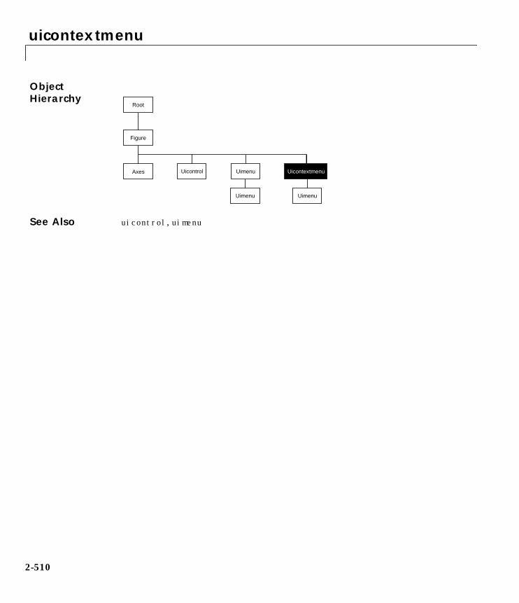
uicontextmenu

ObjectHierarchy

See Also uicontrol, uimenu

Root

UimenuAxes Uicontrol

Figure

Uicontextmenu

Uimenu Uimenu

2-510

uicontextmenu Properties

2uicontextmenu PropertiesUicontextmenuProperties


Callback routine interruption. The BusyAction property enables you to controlhow MATLAB handles events that potentially interrupt executing callbackroutines. If a callback routine is executing, subsequently invoked callbackroutines always attempt to interrupt it. If the Interruptible property of theobject whose callback is executing is set to on (the default), then interruptionoccurs at the next point where the event queue is processed. If theInterruptible property is off, the BusyAction property of the object whosecallback is executing determines how MATLAB handles the event. The choicesare:




This property has no effect on Uicontextmenu objects.

Callback string

Control action. A routine that executes whenever you right-click on an objectfor which a context menu is defined. The routine executes immediately beforethe context menu is posted. Define this routine as a string that is a validMATLAB expression or the name of an M-file. The expression executes in theMATLAB workspace.

Children matrix

The Uimenus defined for the Uicontextmenu.

Clipping on | off


CreateFcn string

Callback routine executed during object creation. This property defines acallback routine that executes when MATLAB creates a Uicontextmenu object.You must define this property as a default value for Uicontextmenus. Forexample, this statement:

set(0,'DefaultUicontextmenuCreateFcn',...'set(gcf,''IntegerHandle'',''off'')')

2-511


defines a default value on the Root level that sets the Figure IntegerHandleproperty to off whenever you create a Uicontextmenu object. MATLABexecutes this routine after setting all property values for the Uicontextmenu.Setting this property on an existing Uicontextmenu object has no effect.


DeleteFcn string

Delete Uicontextmenu callback routine. A callback routine that executes whenyou delete the Uicontextmenu object (e.g., when you issue a delete commandor clear the Figure containing the Uicontextmenu). MATLAB executes theroutine before destroying the object’s properties so these values are availableto the callback routine.







When a handle is not visible in its parent’s list of children, it cannot be returnedby functions that obtain handles by searching the object hierarchy or queryinghandle properties. This includes get, findobj, gca, gcf, gco, newplot, cla, clf,and close.

2-512





HitTest on | off



Callback routine interruption mode. The Interruptible property controlswhether a Uicontextmenu callback routine can be interrupted by subsequentlyinvoked callback routines. By default (off), a callback routine executes tocompletion before another can begin.

Only callback routines defined for the ButtonDownFcn and Callback propertiesare affected by the Interruptible property. MATLAB checks for events thatcan interrupt a callback routine only when it encounters a drawnow, figure,getframe, or pause command in the routine.

Parent handle

Uicontextmenu’s parent. The handle of the Uicontextmenu’s parent object. Theparent of a Uicontextmenu object is the Figure in which it appears. You canmove a Uicontextmenu object to another Figure by setting this property to thehandle of the new parent.

Selected on | off




2-513


Tag string


Type string

Class of graphics object. For Uicontextmenu objects, Type is always the string'uicontextmenu'.


This property has no effect on Uicontextmenus.

UserData matrix

User-specified data. Any data you want to associate with the Uicontextmenuobject. MATLAB does not use this data, but you can access it using set and get.

Visible on | off

Uicontextmenu visibility. The Visible property determines or indicateswhether the context menu is posted. The property is normally controlledautomatically, returning on when the menu is posted as a result of a right-clickand off after a menu item has been selected and the context menu iswithdrawn. You can use the property to force the context menu to be postedwithout a menu click or to be withdrawn before an item is selected.

2-514

uicontrol

2uicontrolPurpose Create user interface control object

Syntax handle = uicontrol(parent)handle = uicontrol(...,'PropertyName',PropertyValue,...)

Description uicontrol creates Uicontrol graphics objects (user interface controls). Youimplement graphical user interfaces using Uicontrols. When selected, mostUicontrol objects perform a predefined action. MATLAB supports numerousstyles of Uicontrols, each suited for a different purpose:

• Check boxes

• Editable text

• Frames

• List boxes

• Pop-up menus

• Push buttons

• Radio buttons

• Sliders

• Static text

• Toggle buttons

Check boxes generate an action when pressed. These devices are useful whenproviding the user with a number of independent choices. To activate a checkbox, click the mouse button on the object. The state of the device is indicated onthe display.

Editable text boxes are fields that enable users to enter or modify text values.Use editable text when you want text as input. To execute the callback routinefor an editable text object, type in the desired text, then press Ctl-Return (formultiline), Return (for single line) or move the focus off the object.

On Microsoft Windows and Macintosh systems, if an editable text box hasfocus, clicking on the menu bar does not cause the editable text callback routineto execute. However, it does cause execution on UNIX systems. Therefore, afterclicking on the menu bar, the statement,

get(edit_handle,'String')

2-515

uicontrol

does not return the current contents of the edit box on Microsoft Windows andMacintosh systems because MATLAB must execute the callback routine toupdate the String property (even though the text string has changed on thescreen). This behavior is consistent with the respective platform conventions.

Frames are boxes that visually enclose regions of a figure window. Frames canmake a user interface easier to understand by visually grouping relatedcontrols. Frames have no callback routines associated with them. OnlyUicontrols can appear within frames.

Frames are opaque, not transparent, so the order you define Uicontrols isimportant in determining whether Uicontrols within a frame are covered bythe frame or are visible. Stacking order determines the order objects are drawn:objects defined first are drawn first; objects defined later are drawn overexisting objects. If you use frames to enclose objects, you must define theframes before you define the objects.

List boxes display a list of items and enable users to select one or more items.The Min and Max properties control the selection mode. The Value propertyindicates selected entries and contains the indices into the list of strings; avector value indicates multiple selections. MATLAB evaluates the list box’scallback routine after any mouse button up event that changes the Valueproperty. Therefore, you may need to add a “Done” button to delay actioncaused by multiple clicks on list items. List boxes differentiate between singleand double clicks and set the Figure SelectionType property to normal or openaccordingly before evaluating the list box’s Callback property.

Pop-up menus open when pressed to display a list of choices. When notactivated, they display a single button with text indicating the current setting.Pop-up menus are useful when you want to provide users with a number ofmutually exclusive choices, but do not want to take up the amount of space thata series of radio buttons requires. You must specify a value for the Stringproperty.

Push buttons generate an action with each press, but do not remain in a pressedstate. To activate a push button, click the mouse button on the object. Pushbuttons are useful when the action you want to perform is not related to anyother action executable by the user interface (for example, an “OK” button).

Radio buttons are similar to check boxes, but are intended to be mutuallyexclusive within a group of related radio buttons (i.e., only one is in a pressed

2-516

uicontrol

state at any given time). To activate a radio button, click the mouse button onthe object. The state of the device is indicated on the display. Note that yourcode can implement the mutually exclusive behavior of radio buttons.

Sliders accept numeric input within a specific range by enabling the user tomove a sliding bar. Users move the bar by pressing the mouse button anddragging the pointer over the bar, or by clicking in the trough or on an arrow.The location of the bar indicates a numeric value, which is selected by releasingthe mouse button. You can set the minimum, maximum, and current values ofthe slider.

Static text boxes display lines of text. Static text is typically used to label othercontrols, provide directions to the user, or indicate values associated with aslider. Users cannot change static text interactively and there is no way toinvoke the callback routine associated with it.

Toggle buttons are controls that execute callbacks when clicked on and indicatetheir state, either on or off. Toggle buttons are useful for building toolbars.More information about toggle buttons.

Remarks The uicontrol function accepts property name/property value pairs,structures, and cell arrays as input arguments and optionally returns thehandle of the created object. You can also set and query property values aftercreating the object using the set and get functions.

Uicontrol objects are children of Figures and therefore do not require an Axesto exist when placed in a Figure window.

Properties This table lists all uicontrol properties, grouping them by function. Eachproperty name acts as a link to a description of the property.

2-517

uicontrol



BackgroundColor Object background color Value: ColorSpecDefault: [0.8 0.8 0.8]

CData Truecolor image displayed on thecontrol

Value: matrix

Clipping This property has no effect onUicontrol objects

ForegroundColor Color of text Value: ColorSpecDefault: [0 0 0]

SelectionHighlight Object highlighted when selected Value: on, offDefault: on

String Uicontrol label Value: string

Visible Uicontrol visibility Value: on, offDefault: on


Children Uicontrol objects have no children

Enable Enable or disable the Uicontrol Value: on, inactive, offDefault: on

Parent Uicontrol object’s parent Value: scalar Figure handle

Selected Whether object is selected Value: on, offDefault: off

SliderStep Slider step size Value: two-element vectorDefault: [0.01 0.1]

2-518

uicontrol

Style Type of Uicontrol object Value: pushbutton,togglebutton,radiobutton, checkbox,edit, text, slider, frame,listbox, popupmenuDefault: pushbutton


TooltipString Content of object’s tooltip Value: string

Type Class of graphics object Value: string (read-only)Default: uicontrol


Controlling the Object Position

Position Size and location of Uicontrol object Value: position rectangleDefault: [20 20 60 20]

Units Units to interpret position vector Value: pixels, normalized,inches, centimeters,points, charactersDefault: pixels

Controlling Fonts and Labels

FontAngle Character slant Value: normal, italic,obliqueDefault: normal

FontName Font family Value: stringDefault: system dependent

FontSize Font size Value: size in FontUnitsDefault: system dependent


2-519

uicontrol

FontUnits Font size units Value: points, normalized,inches, centimeters,pixelsDefault: points

FontWeight Weight of text characters Value: light, normal, demi,boldDefault: normal

HorizontalAlignment Alignment of label string Value: left, center, rightDefault: depends onUicontrol object

String Uicontrol object label Value: string



ButtonDownFcn Button press callback routine Value: string



Value: string


Value: string


UIContextMenu Uicontextmenu object associatedwith the Uicontrol

Value: handle

Information About the Current State

ListboxTop Index of top-most string displayedin list box

Value: scalarDefault: [1]


2-520

uicontrol

Examples The following statement creates a push button that clears the current axeswhen pressed:

h = uicontrol('Style', 'pushbutton', 'String', 'Clear',...'Position', [20 150 100 70], 'Callback', 'cla');

You can create a Uicontrol object that changes Figure colormaps by specifyinga pop-up menu and supplying an M-file name as the object’s Callback:

hpop = uicontrol('Style', 'popup',...'String', 'hsv|hot|cool|gray',...'Position', [20 320 100 50],...'Callback', 'setmap');

The above call to uicontrol defines four individual choices in the menu: hsv,hot, cool, and gray. You specify these choices with the String property,separating the choices with the “|” character.

Max Maximum value (depends onUicontrol object)

Value: scalarDefault: object dependent

Min Minimum value (depends onUicontrol object)

Value: scalarDefault: object dependent

Value Current value of Uicontrol object Value: scalar or vectorDefault: object dependent




HitTest Whether selectable by mouse click Value: on, offDefault: on


2-521

uicontrol

The Callback, in this case setmap, is the name of an M-file that defines a morecomplicated set of instructions than a single MATLAB command. setmapcontains these statements:

val = get(hpop,'Value');if val == 1

colormap(hsv)elseif val == 2

colormap(hot)elseif val == 3

colormap(cool)elseif val == 4

colormap(gray)end

The Value property contains a number that indicates the selected choice. Thechoices are numbered sequentially from one to four. The setmap M-file can getand then test the contents of the Value property to determine what action totake.

ObjectHierarchy

See Also textwrap, uimenu

Root


Figure

Uicontextmenu

Uimenu Uimenu

2-522

uicontrol Properties

2uicontrol PropertiesUicontrolProperties

You can set default Uicontrol properties on the Figure and Root levels:

set(0,'DefaultUicontrolProperty',PropertyValue...)set(gcf,'DefaultUicontrolProperty',PropertyValue...)

where Property is the name of the Uicontrol property whose default value youwant to set and PropertyValue is the value you are specifying. Use set and getto access Uicontrol properties.

Curly braces enclose the default value.

BackgroundColor ColorSpec

Object background color. The color used to fill the rectangle defined by theUicontrol. Specify a color using a three-element RGB vector or one ofMATLAB’s predefined names. The default color is light gray. See ColorSpec formore information on specifying color.

On Microsoft Windows systems, you cannot specify the background color ofpush buttons because of Windows limitations.


Callback routine interruption. The BusyAction property enables you to controlhow MATLAB handles events that potentially interrupt executing callbackroutines. If a callback routine is executing, subsequently invoked callbackroutines always attempt to interrupt it. If the Interruptible property of theobject whose callback is executing is set to on (the default), then interruptionoccurs at the next point where the event queue is processed. If theInterruptible property is off, the BusyAction property of the object whosecallback is executing determines how MATLAB handles the event. The choicesare:




Button press callback routine. A callback routine that executes whenever youpress a mouse button while the pointer is in a five-pixel wide border around theUicontrol. When the Uicontrol’s Enable property is set to inactive or off, theButtonDownFcn executes when you click the mouse in the five-pixel border or

2-523


on the control itself. This is useful for implementing actions to interactivelymodify control object properties, such as size and position, when they areclicked on (using selectmoveresize, for example).

Define this routine as a string that is a valid MATLAB expression or the nameof an M-file. The expression executes in the MATLAB workspace.

The Callback property defines the callback routine that executes when youactivate the enabled Uicontrol (e.g., click on a push button).

Callback string

Control action. A routine that executes whenever you activate the Uicontrolobject (e.g., when you click on a push button or move a slider). Define thisroutine as a string that is a valid MATLAB expression or the name of an M-file.The expression executes in the MATLAB workspace. Note that callbackroutines defined for frames and static text do not execute because no action isassociated with these objects.

CData matrix

Truecolor image displayed on control. A three-dimensional matrix of RGBvalues that defines a truecolor image displayed on either a push button ortoggle button. Each value must be between 0.0 and 1.0. More information aboutthis property.

Children matrix

The empty matrix; Uicontrol objects have no children.

Clipping on | off

This property has no effect on Uicontrols.

CreateFcn string

Callback routine executed during object creation. This property defines acallback routine that executes when MATLAB creates a Uicontrol object. Youmust define this property as a default value for Uicontrols. For example, thisstatement:

set(0,'DefaultUicontrolCreateFcn',...'set(gcf,''IntegerHandle'',''off'')')

defines a default value on the Root level that sets the Figure IntegerHandleproperty to off whenever you create a Uicontrol object. MATLAB executes this

2-524


routine after setting all property values for the Uicontrol. Setting this propertyon an existing Uicontrol object has no effect.


DeleteFcn string

Delete Uicontrol callback routine. A callback routine that executes when youdelete the Uicontrol object (e.g., when you issue a delete command or clear theFigure containing the Uicontrol). MATLAB executes the routine beforedestroying the object’s properties so these values are available to the callbackroutine.


Enable on | inactive | off

Enable or disable the Uicontrol. This property controls how Uicontrols respondto mouse button clicks.

• on – The Uicontrol is operational. When you activate the Uicontrol (generallyby clicking on it) MATLAB executes the callback routine defined by theCallback property. When you click the mouse within a 5-pixel border outsidethe Uicontrol, MATLAB executes the callback routine defined by theButtonDownFcn.

• inactive – The Uicontrol is not operational, but it is not dimmed (i.e., itlooks the same as when Enable is on). MATLAB executes the ButtonDownFcnif you click the mouse on or within a 5-pixel border around the Uicontrol, butdoes not execute the Callback routine.

• off – The Uicontrol does not respond visually to mouse actions, does notexecute its Callback routine, and its label (string property) is grayed out.MATLAB executes the ButtonDownFcn if you click the mouse on or within a5-pixel border around the Uicontrol.

Setting this property to inactive or off enables you to implement object“dragging” via the ButtonDownFcn callback routine.

2-525


Extent position rectangle (read only)

Size of Uicontrol character string. A four-element vector that defines the sizeand position of the character string used to label the Uicontrol. It has the form:

[0,0,width,height]

The first two elements are always zero. width and height are the dimensionsof the rectangle. All measurements are in units specified by the Units property.

Since the Extent property is defined in the same units as the Uicontrol itself,you can use this property to determine proper sizing for the Uicontrol withregard to its label. Do this by

• Defining the String property and selecting the font using the relevantproperties.

• Getting the value of the Extent property.

• Defining the width and height of the Position property to be somewhatlarger than the width and height of the Extent.

For multiline strings, the Extent rectangle encompasses all the lines of text.For single line strings, the Extent is returned as a single line, even if the stringwraps when displayed on the control.


Character slant. MATLAB uses this property to select a font from thoseavailable on your particular system. Setting this property to italic or obliqueselects a slanted version of the font, when it is available on your system.

FontName string

Font family. The name of the font in which to display the String. To displayand print properly, this must be a font that your system supports. The defaultfont is system dependent.

FontSize size in FontUnits

Font size. A number specifying the size of the font in which to display theString, in units determined by the FontUnits property. The default point sizeis system dependent.

2-526



Font size units. MATLAB uses this property to determine the units used by theFontSize property. Normalized units interpret FontSize as a fraction of theheight of the Uicontrol. When you resize the Uicontrol, MATLAB modifies thescreen FontSize accordingly. pixels, inches, centimeters, and points areabsolute units (1 point = 1/72 inch).

FontWeight light | normal | demi | bold

Weight of Text characters. MATLAB uses this property to select a font fromthose available on your particular system. Setting this property to bold causesMATLAB to use a bold version of the font, when it is available on your system.

ForegroundColor ColorSpec

Color of text. This property determines the color of the text defined for theString property (the Uicontrol label). Specify a color using a three-elementRGB vector or one of MATLAB ’s predefined names. The default text color isblack. See ColorSpec for more information on specifying color.






When a handle is not visible in its parent’s list of children, it cannot bereturned by functions that obtain handles by searching the object hierarchy or

2-527


querying handle properties. This includes get, findobj, gca, gcf, gco, newplot,cla, clf, and close.




HitTest on | off

Selectable by mouse click. This property has no effect on Uicontrol objects.

HorizontalAlignment left | center | right

Horizontal alignment of label string. This property determines the justificationof the text defined for the String property (the Uicontrol label):

• left — Text is left justified with respect to the Uicontrol.

• center — Text is centered with respect to the Uicontrol.

• right — Text is right justified with respect to the Uicontrol.

On Microsoft Windows and Macintosh systems, this property affects only editand text Uicontrols.


Callback routine interruption mode. The Interruptible property controlswhether a Uicontrol callback routine can be interrupted by subsequentlyinvoked callback routines. By default (off), a callback routine executes tocompletion before another can begin.

Only callback routines defined for the ButtonDownFcn and Callback propertiesare affected by the Interruptible property. MATLAB checks for events thatcan interrupt a callback routine only when it encounters a drawnow, figure,getframe, or pause command in the routine.

2-528


ListboxTop scalar

Index of top-most string displayed in list box. This property applies only to thelistbox style of Uicontrol. It specifies which string appears in the top-mostposition in a list box that is not large enough to display all list entries.ListboxTop is an index into the array of strings defined by the String propertyand must have a value between 1 and the number of strings. Noninteger valuesare fixed to the next lowest integer.

Max scalar

Maximum value. This property specifies the largest value allowed for the Valueproperty. Different styles of Uicontrols interpret Max differently:

• Check boxes – Max is the setting of the Value property while the Uicontrol isin the on position.

• Editable text – If Max − Min > 1, then editable text boxes accept multilineinput. If Max − Min <= 1, then editable text boxes accept only single line input.

• List boxes – If Max − Min > 1, then list boxes allow multiple item selection. IfMax − Min <= 1, then list boxes do not allow multiple item selection.

• Radio buttons – Max is the setting of the Value property while the Uicontrolis in the on position.

• Sliders – Max is the largest value you can select and must be greater than theMin property. The default maximum is 1.

• Toggle buttons – Max is the value of the Value property when the togglebutton is selected. The default is 1.

• Frames, pop-up menus, and static text do not use the Max property.

Min scalar

Minimum value. This property specifies the smallest value allowed for theValue property. Different styles of Uicontrols interpret Min differently:

• Check boxes – Min is the setting of the Value property while the Uicontrol isin the off position.

• Editable text – If Max − Min > 1, then editable text boxes accept multilineinput. If Max − Min <= 1, then editable text boxes accept only single line input.

• List boxes – If Max − Min > 1, then list boxes allow multiple item selection. IfMax − Min <= 1, then list boxes allow only single item selection.

2-529


• Radio buttons – Min is the setting of the Value property while the Uicontrolis in the off position.

• Sliders – Min is the smallest value you can select and must be less than Max.The default minimum is 0.

• Toggle buttons – Min is the value of the Value property when the togglebutton is not selected. The default is 0.

Parent handle

Uicontrol’s parent. The handle of the Uicontrol’s parent object. The parent of aUicontrol object is the Figure in which it appears. You can move a Uicontrolobject to another Figure by setting this property to the handle of the newparent.

Position position rectangle

Size and location of Uicontrol. The rectangle defined by this property specifiesthe size and location of the control within the Figure window. Specify Positionas


left and bottom are the distance from the lower-left corner of the Figurewindow to the lower-left corner of the Uicontrol object. width and height arethe dimensions of the Uicontrol rectangle. All measurements are in unitsspecified by the Units property.

On Microsoft Windows systems, the height of pop-up menus is automaticallydetermined by the size of the font. The value you specify for the height of thePostion property has no effect.

Selected on | off

Is object selected. When this property is on, MATLAB displays selectionhandles if the SelectionHighlight property is also on. You can, for example,define the ButtonDownFcn to set this property, allowing users to select theobject with the mouse.


Object highlight when selected. When the Selected property is on, MATLABindicates the selected state by drawing four edge handles and four cornerhandles. When SelectionHighlight is off, MATLAB does not draw thehandles.

2-530


SliderStep [min_step max_step]

Slider step size. This property controls the amount the slider Value changeswhen you click the mouse on the arrow button (min_step) or on the slidertrough (max_step). Specify SliderStep as a two-element vector; each valuemust be in the range [0, 1]. The actual step size is a function of the specifiedSliderStep and the total slider range (Max − Min). The default, [0.01 0.10],provides a 1 percent change for clicks on the arrow button and a 10 percentchange for clicks in the trough.

For example, if you create the following slider,

uicontrol('Style','slider','Min',1,'Max',7,...'SliderStep',[0.1 0.6])

clicking on the arrow button moves the indicator by,

0.1*(7–1)ans =

0.6000

and clicking in the trough moves the indicator by,

0.6*(7–1)ans =

3.6000

Note that if the specified step size moves the slider to a value outside the range,the indicator moves only to the Max or Min value.

See also the Max, Min, and Value properties.

String string

Uicontrol label. A string specifying the text displayed on check boxes, editabletext, list boxes, pop-up menus, push buttons, radio buttons, static text, andtoggle buttons.

For multiple items on a pop-up menu or a list box, items can be specified as acell array of strings, a padded string matrix, or within a string vector separatedby vertical slash (‘|’) characters.

For multiple line editable text or static text controls, line breaks occur betweeneach row of the string matrix, each cell of a cell array of strings, and after any\n characters embedded in the string. Vertical slash (‘|’) characters are not

2-531


interpreted as linebreaks, and instead show up in the text displayed in theuicontrol.

For the remaining Uicontrol objects, which display only one line of text, onlythe first string of a cell array of strings or of a padded string matrix isdisplayed; the rest are ignored. Vertical slash (‘|’) characters are notinterpreted as linebreaks and instead show up in the text displayed in theUicontrol.

For editable text, this property is set to the string typed in by the user.

Style pushbutton | togglebutton | radiobutton |checkbox | edit | text | slider | frame |listbox | popupmenu

Style of Uicontrol object to create. The Style property specifies the kind ofUicontrol to create. See the “Description” section for information on each type.

Tag string


TooltipString string

Content of tooltip for object. The TooltipString property specifies the text ofthe tooltip associated with the Uicontrol. When the user moves the mousepointer over the control and leaves it there, the tooltip is displayed. Moreinformation about this property.


Class of graphics object. For Uicontrol objects, Type is always the string'uicontrol'.


Associate a context menu with Uicontrol. Assign this property the handle of aUicontextmenu object. MATLAB displays the context menu whenever youright-click over the Uicontrol (Ctrl-click on Macintosh systems). Use theuicontextmenu function to create the context menu. More information aboutthis property.

2-532


Units pixels | normalized | inches |centimeters | points | characters

Units of measurement. The units MATLAB uses to interpret the Extent andPosition properties. All units are measured from the lower-left corner of theFigure window. Normalized units map the lower-left corner of the Figurewindow to (0,0) and the upper-right corner to (1.0,1.0). pixels, inches,centimeters, and points are absolute units (1 point = 1/72 inch). Characterunits are characters using the default system font; the width of one characteris the width of the letter x, the height of one character is the distance betweenthe baselines of two lines of text. More information about character units.

If you change the value of Units, it is good practice to return it to its defaultvalue after completing your computation so as not to affect other functions thatassume Units is set to the default value.

UserData matrix

User-specified data. Any data you want to associate with the Uicontrol object.MATLAB does not use this data, but you can access it using set and get.

Value scalar or vector

Current value of Uicontrol. The Uicontrol style determines the possible valuesthis property can have:

• Check boxes set Value to Max when they are on (when the indicator is filled)and Min when off (not filled).

• List boxes set Value to a vector of indices corresponding to the selected listentries, where 1 corresponds to the first item in the list.

• Pop-up menus set Value to the index of the item selected, where 1corresponds to the first item on the menu. The “Examples” section showshow to use the Value property to determine which item has been selected.

• Radio buttons set Value to Max when they are on (when the indicator is filled)and Min when off (not filled).

• Sliders set Value to the number indicated by the slider bar, which is withinthe range established by Min and Max.

• Toggle buttons set Value to Max when they are down (selected) and Min whenup (not selected).

• Editable text, frames, push buttons, and static text do not set this property.

2-533


Set the Value property either interactively with the mouse or through a call tothe set function. The display reflects changes made to Value.

Visible on | off

Uicontrol visibility. By default, all Uicontrols are visible. When set to off, theUicontrol is not visible, but still exists and you can query and set its properties.

2-534

uigetfile

2uigetfilePurpose Interactively retrieve a filename

Syntax uigetfileuigetfile('FilterSpec')uigetfile('FilterSpec','DialogTitle')uigetfile('FilterSpec','DialogTitle',x,y)[fname,pname] = uigetfile(...)

Description uigetfile displays a dialog box used to retrieve a file. The dialog box lists thefiles and directories in the current directory.

uigetfile('FilterSpec') displays a dialog box that lists files in the currentdirectory. FilterSpec determines the initial display of files and can be a fullfilename or include the * wildcard. For example, '∗.m' (the default) causes thedialog box list to show only MATLAB M-files. The Macintosh ignores thisargument.

uigetfile('FilterSpec','DialogTitle') displays a dialog box that has thetitle DialogTitle. On the Macintosh, this argument specifies text that appearsabove the current folder name.

uigetfile('FilterSpec','DialogTitle',x,y) positions the dialog box atposition [x,y], where x and y are the the distance in pixel units from the left andtop edges of the screen. Note that some platforms may not support dialog boxplacement. On the Macintosh, the dialog box cannot overlap the menu bar.

[fname,pname] = uigetfile(...) returns the name and path of the fileselected in the dialog box. After you press the Done button, fname contains thename of the file selected and pname contains the name of the path selected. Ifyou press the Cancel button or if an error occurs, fname and pname are set to 0.

Remarks If you select a file that does not exist, an error dialog appears. You can thenenter another filename, or press the Cancel button.

Examples This statement displays a dialog box that enables you to retrieve a file. Thestatement lists all MATLAB M-files within a selected directory. The figure

2-535

uigetfile

shows the dialog box on a Macintosh. The name and path of the selected file arereturned in fname and pname.

[fname,pname] = uigetfile('*.m','Sample Dialog Box')

The exact appearance of the dialog box depends on your windowing system.

See Also uiputfile

2-536

uimenu

2uimenuPurpose Create menus on Figure windows

Syntax uimenu('PropertyName',PropertyValue,...)uimenu(parent,'PropertyName',PropertyValue,...)handle = uimenu('PropertyName',PropertyValue,...)handle = uimenu(parent,'PropertyName',PropertyValue,...)

Description uimenu creates a hierarchy of menus and submenus that are displayed in theFigure window’s menu bar. You can also use uimenu to create menu items forcontext menus. More information about context menus.

handle = uimenu('PropertyName',PropertyValue,...) creates a menu inthe current Figure’s menu bar using the values of the specified properties andassigns the menu handle to handle.

handle = uimenu(parent,'PropertyName',PropertyValue,...) creates asubmenu of a parent menu or a menu item on a context menu specified byparent and assigns the menu handle to handle. If parent refers to a Figureinstead of another Uimenu object or a Uicontextmenu, MATLAB creates a newmenu on the referenced Figure’s menu bar.

Remarks MATLAB adds the new menu to the existing menu bar. Each menu choice canitself be a menu that displays its submenu when selected.

uimenu accepts property name/property value pairs, as well as structures andcell arrays of properties as input arguments. The Uimenu Callback propertydefines the action taken when you activate the menu item. uimenu optionallyreturns the handle to the created Uimenu object.

Uimenus only appear in Figures whose WindowStyle is normal. If a Figurecontaining Uimenu children is changed to WindowStyle modal, the Uimenuchildren still exist and are contained in the Children list of the Figure, but arenot displayed until the WindowStyle is changed to normal.

The value of the Figure MenuBar property affects the location of the Uimenu onthe Figure menu bar. When MenuBar is figure, a set of built-in menus precedesthe Uimenus on the menu bar (MATLAB controls the built-in menus and theirhandles are not available to the user). When MenuBar is none, Uimenus are theonly items on the menu bar (that is, the built-in menus do not appear).

2-537

uimenu

You can set and query property values after creating the menu using set andget.

Properties This table lists all uimenu properties, grouping them by function. Eachproperty name acts as a link to a description of the property.



Checked Menu check indicator Value: on, offDefault: off

Clipping This property has no effect onUimenu objects

ForegroundColor Color of text Value: ColorSpecDefault: [0 0 0]

Label Menu label Value: string

SelectionHighlight Object highlighted when selected Value: on, offDefault: on

Separator Separator line mode Value: on, offDefault: off

Visible Uimenu visibility Value: on, offDefault: on


Accelerator Keyboard equivalent Value: character

Children Handles of submenus Value: vector of handles

Enable Enable or disable the Uimenu Value: on, offDefault: on

Parent Uimenu object’s parent Value: handle

Selected This property has no effect onUimenu objects

2-538

uimenu


Type Class of graphics object Value: string (read-only)Default: uimenu


Controlling the Object Position

Position Relative Uimenu position Value: scalarDefault: [1]



ButtonDownFcn Button press callback routine Value: string



Value: string


Value: string


UIContextMenu This property has no effect onUimenu objects




HitTest Whether selectable by mouse click Value: on, offDefault: on


2-539

uimenu

Examples This example creates a menu labeled Workspace whose choices allow users tocreate a new Figure window, save workspace variables, and exit out ofMATLAB. In addition, it defines an accelerator key for the Quit option (whichwould not work on a Macintosh because Command-Q is reserved).

f = uimenu('Label','Workspace');uimenu(f,'Label','New Figure','Callback','figure');uimenu(f,'Label','Save','Callback','save');uimenu(f,'Label','Quit','Callback','exit',...

'Separator','on','Accelerator','Q');

ObjectHierarchy

See Also uicontrol, uicontextmenu, gcbo, set, get, figure

Root


Figure

Uicontextmenu

Uimenu Uimenu

2-540

uimenu Properties

2uimenu PropertiesUimenuProperties


You can set default Uimenu properties on the Figure and Root levels:

set(0,'DefaultUimenuPropertyName',PropertyValue...)set(gcf,'DefaultUimenuPropertyName',PropertyValue...)set(menu_handle,'DefaultUimenuProperty',PropertyValue...)

Where PropertyName is the name of the Uimenu property and PropertyValueis the value you are specifying. Use set and get to access Uimenu properties.

Accelerator character

Keyboard equivalent. A character specifying the keyboard equivalent for themenu item. This allows users to select a particular menu choice by pressing thespecified character in conjunction with another key, instead of selecting themenu item with the mouse. The key sequence is platform specific:

• For Microsoft Windows systems, the sequence is Ctrl-Accelerator. Thesekeys are reserved for default menu items: c, v, and x.

• For UNIX systems, the sequence is Ctrl-Accelerator. These keys arereserved for default menu items: o, p, s, and w.

• For Macintosh systems, the sequence is Command-Accelerator. Thesekeys are reserved for default menu items: a, c, n, o, p, q, s, v, w, x, z, and thenumber keys.

You can define an accelerator only for menu items that do not have childrenmenus. Accelerators work only for menu items that directly execute a callbackroutine, not items that bring up other menus.

Note that the menu item does not have to be displayed (e.g., a submenu) for theaccelerator key to work. However, the window focus must be in the Figurewhen the key sequence is entered.


Callback routine interruption. The BusyAction property enables you to controlhow MATLAB handles events that potentially interrupt executing callbackroutines. If there is a callback routine executing, subsequently invokedcallback routes always attempt to interrupt it. If the Interruptible propertyof the object whose callback is executing is set to on (the default), theninterruption occurs at the next point where the event queue is processed. If the

2-541

uimenu Properties

Interruptible property is off, the BusyAction property (of the object owningthe executing callback) determines how MATLAB handles the event. Thechoices are:




The button down function has no effect on Uimenu objects.

Callback string

Menu action. A callback routine that executes whenever you select the menu.Define this routine as a string that is a valid MATLAB expression or the nameof an M-file. The expression executes in the MATLAB workspace.

A menu with children (submenus) executes its callback routine beforedisplaying the submenus. A menu without children executes its callbackroutine when you release the mouse button (i.e., on the button up event).

Checked on | off

Menu check indicator. Setting this property to on places a check mark next tothe corresponding menu item. Setting it to off removes the check mark. Youcan use this feature to create menus that indicate the state of a particularoption. Note that there is no formal mechanism for indicating that anunchecked menu item will become checked when selected. Also, this propertydoes not check top level menus or submenus, although you can change thevalue of the property for these menus.


Handles of submenus. A vector containing the handles of all children of theUimenu object. The children objects of Uimenus are other Uimenus, whichfunction as submenus. You can use this property to re-order the menus.

Clipping on | off

Clipping has no effect on Uimenu objects.

2-542

uimenu Properties

CreateFcn string

Callback routine executed during object creation. This property defines acallback routine that executes when MATLAB creates a Uimenu object. Youmust define this property as a default value for Uimenus. For example, thestatement,

set(0,'DefaultUimenuCreateFcn','set(gcf,''IntegerHandle'',''off''’))

defines a default value on the Root level that sets the Figure IntegerHandleproperty to off whenever you create a Uimenu object. Setting this property onan existing Uimenu object has no effect. MATLAB executes this routine aftersetting all property values for the Uimenu.


DeleteFcn string

Delete Uimenu callback routine. A callback routine that executes when youdelete the Uimenu object (e.g., when you issue a delete command or cause theFigure containing the Uimenu to reset). MATLAB executes the routine beforedestroying the object’s properties so these values are available to the callbackroutine.

The handle of the object whose DeleteFcn is being executed is accessible onlythrough the Root CallbackObject property, which is more simply queriedusing gcbo.

Enable on | off

Enable or disable the Uimenu. This property controls the selectability of amenu item. When not enabled (set to off), the menu Label appears dimmed,indicating the user cannot select it.

ForegroundColor ColorSpec X-Windows only

Color of menu label string. This property determines color of the text definedfor the Label property. Specify a color using a three-element RGB vector or oneof MATLAB’s predefined names. The default text color is black. See ColorSpecfor more information on specifying color.


Control access to object’s handle by command-line users and GUIs. Thisproperty determines when an object’s handle is visible in its parent’s list of

2-543

uimenu Properties

children. HandleVisibility is useful for preventing command-line users fromaccidentally drawing into or deleting a Figure that contains only user interfacedevices (such as a dialog box).









Callback routine interruption mode. The Interruptible property controlswhether a Uimenu callback routine can be interrupted by subsequentlyinvoked callback routines. By default (off), a callback routine executes tocompletion before another can begin. Only the Callback Uimenu property isaffected by the Interruptible property.

2-544

uimenu Properties

Label string

Menu label. A string specifying the text label on the menu item. You can specifya mnemonic using the “&” character. Whatever character follows the “&” in thestring appears underlined and selects the menu item when you type thatcharacter while the menu is visible. The “&” character is not displayed. OnMacintosh systems, MATLAB ignores (and does not print) the “&” character.To display the “&” character in a label, use two “&” characters in the string:

‘O&pen selection’ yields Open selection

‘Save && Go’ yields Save & Go

Parent handle

Uimenu’s parent. The handle of the Uimenu’s parent object. The parent of aUimenu object is the Figure on whose menu bar it displays, or the Uimenu ofwhich it is a submenu. You can move a Uimenu object to another Figure bysetting this property to the handle of the new parent.

Position scalar

Relative menu position. The value of Position indicates placement on themenu bar or within a menu. Top-level menus are placed from left to right onthe menu bar according to the value of their Position property, with 1representing the left-most position. The individual items within a given menuare placed from top to bottom according to the value of their Position property,with 1 representing the top-most position.

Selected on | off

This property is not used for Uimenu objects.


This property is not used for Uimenu objects.

Separator on | off

Separator line mode. Setting this property to on draws a dividing line above themenu item.

Tag string

User-specified object label. The Tag property provides a means to identifygraphics objects with a user-specified label. This is particularly useful whenconstructing interactive graphics programs that would otherwise need to

2-545

uimenu Properties

define object handles as global variables or pass them as arguments betweencallback routines. You can define Tag as any string.


Class of graphics object. For Uimenu objects, Type is always the string'uimenu'.

UserData matrix

User-specified data. Any matrix you want to associate with the Uimenu object.MATLAB does not use this data, but you can access it using the set and getcommands.

Visible on | off

Uimenu visibility. By default, all Uimenus are visible. When set to off, theUimenu is not visible, but still exists and you can query and set its properties.

2-546

uiputfile

2uiputfilePurpose Interactively select a file for writing

Syntax uiputfileuiputfile('InitFile')uiputfile('InitFile','DialogTitle')uiputfile('InitFile','DialogTitle',x,y)[fname,pname] = uiputfile(...)

Description uiputfile displays a dialog box used to select a file for writing. The dialog boxlists the files and directories in the current directory.

uiputfile('InitFile') displays a dialog box that contains a list of files inthe current directory determined by InitFile. InitFile is a full filename orincludes the * wildcard. For example, specifying '∗.m' (the default) causes thedialog box list to show only MATLAB M-files. The Macintosh ignores the firstargument.

uiputfile('InitFile','DialogTitle') displays a dialog box that has thetitle DialogTitle. On the Macintosh, the second argument is the label for thefilename prompt. See the example below.

uiputfile('InitFile','DialogTitle',x,y) positions the dialog box atscreen position [x,y], where x and y are the distance in pixel units from the leftand top edges of the screen. Note that positioning may not work on allplatforms. On the Macintosh, the dialog box cannot overlap the menu bar.

[fname,pname] = uiputfile(...) returns the name and path of the fileselected in the dialog box. If you press the Cancel button or an error occurs,fname and pname are set to 0.

Remarks If you select a file that already exists, a prompt asks whether you want tooverwrite the file. If you choose to, the function successfully returns but doesnot delete the existing file (which is the responsibility of the calling routines).If you select Cancel in response to the prompt, the function returns control backto the dialog box so you can enter another filename.

Examples This statement displays a dialog box titled 'Save file name' (the exactappearance of the dialog box depends on your windowing system) with the

2-547

uiputfile

filename animinit.m. On the Macintosh, the second argument specifies thefilename prompt.

[newfile,newpath] = uiputfile('animinit.m','Save file name');

See Also uigetfile

MicrosoftWindows

Macintosh

2-548

uiresume, uiwait

2uiresume, uiwaitPurpose Control program execution

Syntax uiwait(h)uiwaituiresume(h)

Description The uiwait and uiresume functions block and resume MATLAB programexecution.

uiwait blocks execution until uiresume is called or the current Figure isdeleted. This syntax is the same as uiwait(gcf).

uiwait(h) blocks execution until uiresume is called or the Figure h is deleted.

uiresume(h) resumes the M-file execution that uiwait suspended.

Remarks When creating a dialog, you should have a Uicontrol with a callback that callsuiresume or a callback that destroys the dialog box. These are the only methodsthat resume program execution after the uiwait function blocks execution.

uiwait is a convenient way to use the waitfor command. You typically use itin conjunction with a dialog box. It provides a way to block the execution of theM-file that created the dialog, until the user responds to the dialog box. Whenused in conjunction with a modal dialog, uiwait/uiresume can block theexecution of the M-file and restrict user interaction to the dialog only.

See Also uicontrol, uimenu, waitfor, figure, dialog

2-549

uisetcolor

2uisetcolorPurpose Set an object’s ColorSpec from a dialog box interactively

Syntax c = uisetcolor(h_or_c, 'DialogTitle');

Description uisetcolor displays a dialog box for the user to fill in, then applies the selectedcolor to the appropriate property of the graphics object identified by the firstargument.

h_or_c can be either a handle to a graphics object or an RGB triple. If youspecify a handle, it must specify a graphics object that have a Color property.If you specify a color, it must be a valid RGB triple (e.g., [1 0 0] for red). Thecolor specified is used to initialize the dialog box. If no initial RGB is specified,the dialog box initializes the color to black.

DialogTitle is a string that is used as the title of the dialog box.

c is the RGB value selected by the user. If the user presses Cancel from thedialog box, or if any error occurs, c is set to the input RGB triple, if provided;otherwise, it is set to 0.

See Also ColorSpec

2-550

uisetfont

2uisetfontPurpose Modify font characteristics for objects interactively

Syntax uisetfontuisetfont(h)uisetfont(S)uisetfont(h,'DialogTitle')uisetfont(S,'DialogTitle')S = uisetfont(...)

Description uisetfont enables you to change font properties (FontName, FontUnits,FontSize, FontWeight, and FontAngle) for a Text, Axes, or Uicontrol object.The function returns a structure consisting of font properties and values. Youcan specify an alternate title for the dialog box.

uisetfont displays the dialog box and returns the selected font properties.

uisetfont(h) displays a dialog box, initializing the font property values withthe values of those properties for the object whose handle is h. Selected fontproperty values are applied to the current object. If a second argument issupplied, it specifies a name for the dialog box (ignored on the Macintosh).

uisetfont(S) displays a dialog box, initializing the font property values withthe values defined for the specified structure (S). S must define legal values forone or more of these properties: FontName, FontUnits, FontSize, FontWeight,and FontAngle and the field names must match the property names exactly. Ifother properties are defined, they are ignored. If a second argument issupplied, it specifies a name for the dialog box (ignored on the Macintosh).

uisetfont('DialogTitle') displays a dialog box with the title DialogTitleand returns the values of the font properties selected in the dialog box. TheMacintosh ignores this argument.

If a left-hand argument is specified, the properties FontName, FontUnits,FontSize, FontWeight, and FontAngle are returned as fields in a structure. Ifthe user presses Cancel from the dialog box or if an error occurs, the outputvalue is set to 0.

2-551

uisetfont

Example These statements create a Text object, then display a dialog box (labeledUpdate Font) that enables you to change the font characteristics:

h = text(.5,.5,'Figure Annotation');uisetfont(h,'Update Font')

These statements create two Uicontrol objects, then set the font properties ofone based on the values set for the other:

% Create push button with string ABCc1 = uicontrol('Style', 'pushbutton', ...

'Position', [10 10 100 20], 'String', 'ABC');% Create push button with string XYZc2 = uicontrol('Style', 'pushbutton', ...

'Position', [10 50 100 20], 'String', 'XYZ');% Display set font dialog box for c1, make selections, save to dd = uisetfont(c1)% Apply those settings to c2set(c2, d)

See Also axes, text, uicontrol

2-552

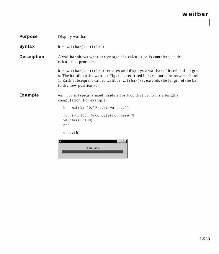
waitbar

2waitbarPurpose Display waitbar

Syntax h = waitbar(x,'title')

Description A waitbar shows what percentage of a calculation is complete, as thecalculation proceeds.

h = waitbar(x,'title') creates and displays a waitbar of fractional lengthx. The handle to the waitbar Figure is returned in h. x should be between 0 and1. Each subsequent call to waitbar, waitbar(x), extends the length of the barto the new position x.

Example waitbar is typically used inside a for loop that performs a lengthycomputation. For example,

h = waitbar(0,'Please wait...');

for i=1:100, % computation here %waitbar(i/100)end

close(h)

2-553

waitfor

2waitforPurpose Wait for condition

Syntax waitfor(h)waitfor(h,'PropertyName')waitfor(h,'PropertyName',PropertyValue)

Description The waitfor function blocks the caller’s execution stream so thatcommand-line expressions, callbacks, and statements in the blocked M-file donot execute until a specified condition is satisfied.

waitfor(h) returns when the graphics object identified by h is deleted or whena Ctrl-C is typed in the Command Window. If h does not exist, waitfor returnsimmediately without processing any events.

waitfor(h,'PropertyName'), in addition to the conditions in the previoussyntax, returns when the value of 'PropertyName' for the graphics object hchanges. If 'PropertyName' is not a valid property for the object, waitforreturns immediately without processing any events.

waitfor(h,'PropertyName',PropertyValue), in addition to the conditions inthe previous syntax, waitfor returns when the value of 'PropertyName' for thegraphics object h changes to PropertyValue. waitfor returns immediatelywithout processing any events if 'PropertyName' is set to PropertyValue.

Remarks While waitfor blocks an execution stream, other execution streams in the formof callbacks may execute as a result of various events (e.g., pressing a mousebutton).

waitfor can block nested execution streams. For example, a callback invokedduring a waitfor statement can itself invoke waitfor.

See Also uiresume, uiwait

2-554

waitforbuttonpress

2waitforbuttonpressPurpose Wait for key or mouse button press

Syntax k = waitforbuttonpress

Description k = waitforbuttonpress blocks the caller’s execution stream until thefunction detects that the user has pressed a mouse button or a key while theFigure window is active. The function returns

• 0 if it detects a mouse button press

• 1 if it detects a key press

Additional information about the event that causes execution to resume isavailable through the Figure’s CurrentCharacter, SelectionType, andCurrentPoint properties.

If a WindowButtonDownFcn is defined for the Figure, its callback is executedbefore waitforbuttonpress returns a value.

Example These statements display text in the Command Window when the user eitherclicks a mouse button or types a key in the Figure window:

w = waitforbuttonpress;if w == 0

disp('Button press')else

disp('Key press')end

See Also dragrect, figure, gcf, ginput, rbbox, waitfor

2-555

warndlg

2-5

2warndlgPurpose Display warning dialog box

Syntax h = warndlg('warningstring','dlgname')

Description warndlg displays a dialog box named 'Warning Dialog' containing the string'This is the default warning string.' The warning dialog box disappearsafter you press the OK push button.

warndlg('warningstring') displays a dialog box with the title 'WarningDialog' containing the string specified by warningstring.

warndlg('warningstring','dlgname') displays a dialog box with the titledlgname that contains the string warningstring.

h = warndlg(...) returns the handle of the dialog box.

Examples The statement

warndlg('Pressing OK will clear memory','!! Warning !!')

displays this dialog box:

See Also dialog, errordlg, helpdlg, msgbox

56

List of Com-mands
A
List of Commands

Function Namesarea ………………………… 2-3axes ………………………… 2-5Axes Properties ……… 2-17axis ……………………… 2-36bar, barh ……………… 2-42bar3, bar3h …………… 2-46box ……………………… 2-50brighten ………………… 2-51camdolly………………… 2-53camlight ………………… 2-55camlookat ……………… 2-57camorbit ………………… 2-59campan ………………… 2-61campos ………………… 2-62camproj ………………… 2-64camroll ………………… 2-65camtarget ……………… 2-66camup …………………… 2-68camva …………………… 2-70camzoom………………… 2-72capture ………………… 2-73caxis …………………… 2-74cla ……………………… 2-78clabel …………………… 2-79clc………………………… 2-81clf ………………………… 2-82close……………………… 2-83colorbar ………………… 2-85colordef ………………… 2-87colormap………………… 2-88ColorSpec ……………… 2-92comet …………………… 2-94comet3 ………………… 2-95compass ………………… 2-96contour ………………… 2-98contour3 ………………… 2-102contourc ………………… 2-104contourf ………………… 2-106contrast ………………… 2-108copyobj ………………… 2-109cylinder ………………… 2-111

daspect ………………… 2-115datetick………………… 2-118default4 ……………… 2-121drawnow ……………… 2-122errorbar ……………… 2-123ezplot…………………… 2-125feather ………………… 2-128figflag ………………… 2-130figure…………………… 2-131Figure Properties …… 2-139fill ……………………… 2-163fill3 …………………… 2-165findobj ………………… 2-168fplot …………………… 2-170frame2im ……………… 2-173frameedit ……………… 2-175gca ……………………… 2-193gcf ……………………… 2-194gco ……………………… 2-195get ……………………… 2-196getframe ……………… 2-198ginput ………………… 2-200gplot …………………… 2-201graymon ……………… 2-203grid …………………… 2-204gtext …………………… 2-205hidden ………………… 2-206hist……………………… 2-207hold …………………… 2-210home …………………… 2-211hsv2rgb………………… 2-212im2frame ……………… 2-213image…………………… 2-214Image Properties …… 2-221imagesc………………… 2-229imfinfo ………………… 2-232imread ………………… 2-235imwrite ………………… 2-237ishandle ……………… 2-240ishold…………………… 2-241legend ………………… 2-242light …………………… 2-245Light Properties ……… 2-249lightangle……………… 2-253

lighting ………………… 2-254line ……………………… 2-255Line Properties ………… 2-262LineSpec………………… 2-270loglog …………………… 2-274material ………………… 2-277mesh, meshc, meshz … 2-279movie …………………… 2-283moviein ………………… 2-285newplot ………………… 2-287noanimate ……………… 2-290orient …………………… 2-291pareto …………………… 2-293patch …………………… 2-294Patch Properties ……… 2-305pbaspect ………………… 2-322pcolor …………………… 2-327peaks …………………… 2-330pie ……………………… 2-331pie3 ……………………… 2-333plot ……………………… 2-335plot3 …………………… 2-343plotmatrix ……………… 2-345plotyy …………………… 2-347polar …………………… 2-349print, printopt ………… 2-351qtwrite ………………… 2-362quiver …………………… 2-363quiver3 ………………… 2-365refresh…………………… 2-367reset……………………… 2-368rgb2hsv ………………… 2-369rgbplot…………………… 2-370ribbon …………………… 2-371root object ……………… 2-373Root Properties ………… 2-377rose ……………………… 2-384rotate …………………… 2-386rotate3d ………………… 2-388scatter …………………… 2-389scatter3 ………………… 2-391semilogx, semilogy …… 2-393set ……………………… 2-395shading ………………… 2-398

-2

List of Commands

slice …………………… 2-401sphere ………………… 2-407spinmap………………… 2-409stairs …………………… 2-410stem …………………… 2-412stem3 …………………… 2-414subplot ………………… 2-416surf, surfc ……………… 2-418surface ………………… 2-422Surface Properties …… 2-430surfl …………………… 2-442surfnorm ……………… 2-445terminal ……………… 2-447text ……………………… 2-449Text Properties ……… 2-456title……………………… 2-468trimesh ………………… 2-470trisurf…………………… 2-471view …………………… 2-472viewmtx………………… 2-475waterfall ……………… 2-479whitebg ………………… 2-481xlabel, ylabel, zlabel … 2-482xlim, ylim, zlim ……… 2-483zoom …………………… 2-485dialog …………………… 2-487dragrect………………… 2-488errordlg ………………… 2-489gcbo …………………… 2-491helpdlg ………………… 2-492inputdlg………………… 2-493listdlg…………………… 2-495msgbox ………………… 2-497pagedlg ………………… 2-498printdlg ………………… 2-499questdlg………………… 2-500rbbox …………………… 2-502selectmoveresize ……… 2-504textwrap ……………… 2-505uicontextmenu………… 2-507uicontextmenu Properties……2-511uicontrol ……………… 2-515uicontrol Properties … 2-523

uigetfile ………………… 2-535uimenu…………………… 2-537uimenu Properties …… 2-541uiputfile ………………… 2-547uiresume, uiwait ……… 2-549uisetcolor………………… 2-550uisetfont ………………… 2-551waitbar ………………… 2-553waitfor …………………… 2-554waitforbuttonpress …… 2-555warndlg ………………… 2-556

-3

Index

AAccelerator

Uimenu property 2-541

all 2-175

AmbientLightColor, Axes property 2-17

AmbientStrength

Patch property 2-305

Surface property 2-430

area 2-3

aspect ratio of axes 2-115, 2-322

Axescreating 2-5

defining default properties 2-9

property descriptions 2-17

axessetting and querying data aspect ratio 2-115

setting and querying limits 2-483

setting and querying plot box aspect ratio2-322

axes 2-5

axis 2-36

azimuth of viewpoint 2-473

BBackFaceLighting



BackGroundColor

Uicontrol property 2-523

BackingStore, Figure property 2-139

bar 2-42

bar3 2-46

bar3h 2-46

barh 2-42

bold font 2-465

box 2-50

Box, Axes property 2-17

brighten 2-51

BusyAction

Axes property 2-17

Figure property 2-139

Image property 2-221

Light property 2-249

Line property 2-262


Root property 2-377


Text property 2-456

Uicontextmenu property 2-511



ButtonDownFcn

Axes property 2-17




Line property 2-262


Root property 2-377


Text property 2-456




CCallBack




CallbackObject, Root property 2-377

I-1

Index

I-2

camdolly 2-53

cameradollying position 2-53

moving camera and target postions 2-53

placing a light at 2-55

positioning to view objects 2-57

rotating around camera target 2-59, 2-61

rotating around viewing axis 2-65

setting and querying position 2-62

setting and querying projection type 2-64

setting and querying target 2-66

setting and querying up vector 2-68

setting and querying view angle 2-70

CameraPosition, Axes property 2-18

CameraPositionMode, Axes property 2-18

CameraTarget, Axes property 2-18

CameraTargetMode, Axes property 2-18

CameraUpVector, Axes property 2-18

CameraUpVectorMode, Axes property 2-19

CameraViewAngle, Axes property 2-19

CameraViewAngleMode, Axes property 2-19

camlight 2-55

camlookat 2-57

camorbit 2-59

campan 2-61

campos 2-62

camproj 2-64

camroll 2-65

camtarget 2-66

camup 2-68

camva 2-70

camzoom 2-72

capture 2-73

CaptureMatrix, Root property 2-377

CaptureRect, Root property 2-377

caxis 2-74

CData





CDataMapping




check boxes 2-515

Checked, Uimenu property 2-542

Children

Axes property 2-20




Line property 2-262


Root property 2-377


Text property 2-456




cla 2-78

clabel 2-79

clc 2-81

clf 2-82

CLim, Axes property 2-20

CLimMode, Axes property 2-20

Clipping

Axes property 2-21




Line property 2-262


Root property 2-377

Index


Text property 2-456




close 2-83

CloseRequestFcn, Figure property 2-140

Color

Axes property 2-21



Line property 2-262

Text property 2-456

colorbar 2-85

colormap 2-88

ColorMap, Figure property 2-141

colormapsconverting from RGB to HSV 2-369

plotting RGB components 2-370

ColorOrder, Axes property 2-21

ColorSpec 2-92

comet 2-94

comet3 2-95

compass 2-96

contour 2-98

contour3 2-102

contourc 2-104

contourf 2-106

contrast 2-108

coordinate system and viewpoint 2-473

copyobj 2-109

CreateFcn

Axes property 2-21




Line property 2-263


Root property 2-377


Text property 2-457




CurrentAxes 2-142CurrentAxes, Figure property 2-142

CurrentCharacter, Figure property 2-143

CurrentFigure, Root property 2-377

CurrentMenu, Figure property (obsolete) 2-143

CurrentObject, Figure property 2-143

CurrentPoint

Axes property 2-22


cylinder 2-111

Ddaspect 2-115

data aspect ratio of axes 2-115

DataAspectRatio, Axes property 2-22

DataAspectRatioMode, Axes property 2-23

default4 2-121

DeleteFcn 2-263Axes property 2-24





Root property 2-378


Text property 2-457




I-3

Index

I-4

Diary, Root property 2-378

DiaryFile, Root property 2-378

DiffuseStrength



Dithermap 2-144Dithermap, Figure property 2-144

DithermapMode, Figure property 2-145

dolly camera 2-53

dragrect 2-488

DrawMode, Axes property 2-24

drawnow 2-122

EEcho, Root property 2-378

EdgeColor



EdgeLighting



editable text 2-515

elevation of viewpoint 2-473

Enable



EraseMode


Line property 2-263



Text property 2-458

errorbar 2-123

ErrorMessage, Root property 2-378

ErrorType, Root property 2-378

Extent

Text property 2-459


ezplot 2-125

FFaceColor



FaceLighting



Faces, Patch property 2-312

FaceVertexCData, Patch property 2-313

feather 2-128

fig file 2-175

figflag 2-130

Figurecreating 2-131


properties 2-139

redrawing 2-367

figure 2-131

filefig 2-175

fill 2-163

fill3 2-165findobj 2-168

FixedColors, Figure property 2-145

FontAngle

Axes property 2-24

Text property 2-459


FontName

Axes property 2-24

Text property 2-459


Index

fontsbold 2-465

italics 2-465

specifying family 2-465

specifying size of TeX characters 2-465

FontSize

Axes property 2-25

Text property 2-459


FontUnits

Axes property 2-25

Text property 2-459


FontWeight

Axes property 2-25

Text property 2-459


ForegroundColor



Format 2-378FormatSpacing, Root property 2-379

fplot 2-170

frame 2-175

frame2im 2-173

frameedit 2-175

frames 2-516

Ggca 2-193

gcf 2-194

gco 2-195

get 2-196

getframe 2-198

ginput 2-200

gplot 2-201

graphics objectsAxes 2-5

Figure 2-131

getting properties 2-196

Light 2-245

Line 2-255

Patch 2-294

resetting properties 2-368

Root 2-373

setting properties 2-395

Surface 2-422

Text 2-449

Uicontrol 2-515

Uimenu 2-537

graymon 2-203

Greek letters and mathematical symbols 2-463

grid 2-204

GridLineStyle, Axes property 2-25

gtext 2-205

GUIs, printing 2-359

HHandleVisibility

Axes property 2-25




Line property 2-264


Root property 2-379


Text property 2-460




hidden 2-206

I-5

Index

I-6

hist 2-207

HitTest

Axes property 2-26




Line property 2-264


Root property 2-379


Text property 2-460



hold 2-210

home 2-211

HorizontalAlignment

Text property 2-461


hsv2rgb 2-212

Iim2frame 2-213

Imagecreating 2-214


properties 2-221

image 2-214

imagesc 2-229

interpolated shading and printing 2-360

Interpreter, Text property 2-462

Interruptible

Axes property 2-26




Line property 2-265


Root property 2-379


Text property 2-462




InvertHardCopy, Figure property 2-147

ishandle 2-240

ishold 2-241

italics font 2-465

KKeyPressFcn, Figure property 2-147

LLabel, Uimenu property 2-545

labelingaxes 2-482

LaTeX, see TeX 2-463

Layer, Axes property 2-27

legend 2-242

Lightcreating 2-245


positioning in camera coordinates 2-55

properties 2-249

light 2-245

lightangle 2-253

lighting 2-254

limits of axes, setting and querying 2-483

Linecreating 2-255


properties 2-262

Index

line 2-255

LineSpec 2-270

LineStyle

Line property 2-266


Surface object 2-437

LineStyleOrder

Axes property 2-27

LineWidth

Axes property 2-28

Line property 2-266



list boxes 2-516

ListboxTop, Uicontrol property 2-529

logarithmplotting 2-274

loglog 2-274

MMarker

Line property 2-266



MarkerEdgeColor

Line property 2-267



MarkerFaceColor

Line property 2-267



MarkerSize

Line property 2-267



material 2-277

Max, Uicontrol property 2-529

MenuBar, Figure property 2-148

mesh 2-279

meshc 2-279

MeshStyle, Surface property 2-439

meshz 2-279

Min, Uicontrol property 2-529

MinColorMap, Figure property 2-148

movie 2-283

moviein 2-285

NName, Figure property 2-149

newplot 2-287

NextPlot

Axes property 2-28


NormalMode



NumberTitle, Figure property 2-149

OOpenGL 2-153

orient 2-291orthographic projection, setting and querying

2-64

Ppage setup 2-178

pagedlg 2-498

PaperOrientation, Figure property 2-149

PaperPosition, Figure property 2-149

I-7

Index

I-8

PaperPositionMode, Figure property 2-150

PaperSize, Figure property 2-150

PaperType, Figure property 2-150

PaperUnits, Figure property 2-151

Parent

Axes property 2-28




Line property 2-267


Root property 2-379


Text property 2-462




pareto 2-293Patch

creating 2-294


properties 2-305

patch 2-294

pbaspect 2-322

pcolor 2-327

perspective projection, setting and querying 2-64

pie 2-331

pie3 2-333

plot 2-335

plot box aspect ratio of axes 2-322

plot, volumetricslice plot 2-401

plot3 2-343PlotBoxAspectRatio, Axes property 2-28

PlotBoxAspectRatioMode, Axes property 2-28

plotmatrix 2-345plotting

2-D plot 2-335

3-D plot 2-343

errorbars 2-123

feather plots 2-128

function plots 2-125, 2-170

histogram plots 2-207

loglog plot 2-274

mesh plot 2-279

plot with two y-axes 2-347

ribbon plot 2-371

rose plot 2-384

scatter plot 2-345, 2-389

scatter plot, 3-D 2-391

semilogarithmic plot 2-393

stairstep plot 2-410

stem plot 2-412

stem plot, 3-D 2-414

surface plot 2-418

volumetric slice plot 2-401

plotyy 2-347Pointer, Figure property 2-152

PointerLocation, Root property 2-379

PointerShapeCData, Figure property 2-152

PointerShapeHotSpot, Figure property 2-152

PointerWindow, Root property 2-380

polar 2-349, 2-349polygon

creating with patch 2-294pop-up menus 2-516

Position

Axes property 2-29



Text property 2-462



position of camera

Index

dollying 2-53

position of camera, setting and querying 2-62

PostScriptprinting interpolated shading 2-360

print 2-351

print driversinterploated shading 2-360

supported 2-352

printdlg 2-499

printframe 2-175

printframe editor 2-176

printingGUIs 2-359

interpolated shading 2-360

line styles on Windows95 2-359

on MS-Windows 2-358

thick lines on Windows95 2-359

with frames 2-175

with non-normal EraseMode 2-225, 2-264, 2-311,

2-434, 2-458with printframes 2-186

printing tips 2-358

printopt 2-351Profile, Root property 2-380

ProfileFile, Root property 2-380

ProfileFunction, Root property 2-380

ProfileInterval, Root property 2-380

projection type, setting and querying 2-64

ProjectionType, Axes property 2-29

push buttons 2-516

Qqtwrite 2-362QuickTime movie 2-362

quiver 2-363

quiver3 2-365

Rradio buttons 2-516

rbbox 2-367

RecursionLimit

Root property 2-380

refresh 2-367

rendererOpenGL 2-153

painters 2-153

zbuffer 2-153

Renderer, Figure property 2-153

RendererMode, Figure property 2-156

reset 2-368

Resize, Figure property 2-156

ResizeFcn, Figure property 2-157

RGB, converting to HSV 2-369

rgb2hsv 2-369

rgbplot 2-370

ribbon 2-371

rolling camera 2-65

root 2-373

Root graphics object 2-373

root object 2-373

root, see rootobject 2-373

rose 2-383, 2-384rotate 2-386

rotate3d 2-388

rotating camera 2-59

rotating camera target 2-61

Rotation, Text property 2-462

rubberband 2-502

Sscatter 2-389scatter3 2-391ScreenDepth, Root property 2-381

I-9

Index

I-10

ScreenSize, Root property 2-381

Selected

Axes property 2-29




Line property 2-268


Root property 2-381


Text property 2-462




selecting areas 2-502

SelectionHighlight

Axes property 2-30




Line property 2-268



Text property 2-462



SelectionType, Figure property 2-158

semilogx 2-393

semilogy 2-393Separator, Uimenu property 2-545

set 2-395

shading 2-398

shading colors in surface plots 2-398

ShareColors, Figure property 2-159

ShowHiddenHandles, Root property 2-381

Simulinkprinting with frames 2-175

size of fonts, see also FontSize property 2-465

slice 2-401

sliders 2-517

SliderStep, Uicontrol property 2-531

SpecularColorReflectance



SpecularExponent



SpecularStrength



sphere 2-407

sphereical coordinatesdefining a Light position in 2-253

spinmap 2-409

stairs 2-410

static text 2-517

stem 2-412

stem3 2-414

stretch-to-fill 2-6

String

Text property 2-463


Style



subplot 2-416

surf 2-418

Surfacecreating 2-422


properties 2-430

surface 2-422

surfc 2-418

surfl 2-442

Index

surfnorm 2-445

symbols in text 2-463

TTag

Axes property 2-30




Line property 2-268


Root property 2-381


Text property 2-465




target, of camera 2-66

terminal 2-447

TerminalDimensions, Root property 2-382

TerminalHideGraphCommand, Root property 2-381

TerminalOneWindow, Root property 2-382

TerminalProtocol, Root property 2-382

TerminalShowGraphCommand, Root property 2-382

TeX commands in text 2-463

Textcreating 2-449


properties 2-456

text 2-449

TickDir, Axes property 2-30

TickDirMode, Axes property 2-30

TickLength, Axes property 2-30

title 2-468

Title, Axes property 2-31

toggle buttons 2-517

TooltipString


trimesh 2-470

trisurf 2-471

Type

Axes property 2-31




Line property 2-268


Root property 2-382


Text property 2-465




UUIContextMenu

Axes property 2-31




Line property 2-268



Text property 2-466

UiContextMenu


Uicontextmenuproperties 2-511

Uicontextmenu


Uicontrolcreating 2-515

I-11

Index

I-12


properties 2-523

types of 2-515

uicontrol 2-487, 2-515

uigetfile 2-535

Uimenucreating 2-537


properties 2-541

uimenu 2-537

uiputfile 2-547

uiresume 2-549

uisetcolor 2-550uisetfont 2-551

Units

Axes property 2-31


Root property 2-382

Text property 2-465


up vector, of camera 2-68

UserData

Axes property 2-32




Line property 2-268


Root property 2-383


Text property 2-466




VValue, Uicontrol property 2-533

VertexNormals



VerticalAlignment, Text property 2-466

Vertices, Patch property 2-321

view 2-57

azimuth of viewpoint 2-473

coordinate system defining 2-473

elevation of viewpoint 2-473

view 2-472

view angle, of camera 2-70

View, Axes property (obsolete) 2-32

viewinga group of object 2-57

a specific object in a scene 2-57

viewmtx 2-475

Visible

Axes property 2-32




Line property 2-268


Root property 2-383


Text property 2-467




Wwaitbar 2-553

waitfor 2-554

waitforbuttonpress 2-555

Index

warndlg 2-556

waterfall 2-479

whitebg 2-481

WindowButtonDownFcn, Figure property 2-161

WindowButtonMotionFcn, Figure property 2-161

WindowButtonUpFcn, Figure property 2-161

Windows95, printing 2-359

WindowStyle, Figure property 2-161

Xx-axis limits, setting and querying 2-483

XAxisLocation, Axes property 2-32

XColor, Axes property 2-32

XData


Line property 2-269



XDir, Axes property 2-33

XGrid, Axes property 2-33

xlabel 2-482

XLabel, Axes property 2-33

xlim 2-483

XLim, Axes property 2-33

XLimMode, Axes property 2-34

XOR, printing 2-225, 2-264, 2-311, 2-434, 2-458

XScale, Axes property 2-34

XTick, Axes property 2-34

XTickLabel, Axes property 2-34

XTickLabelMode, Axes property 2-35

XTickMode, Axes property 2-35

Yy-axis limits, setting and querying 2-483

YAxisLocation, Axes property 2-32

YColor, Axes property 2-32

YData


Line property 2-269



YDir, Axes property 2-33

YGrid, Axes property 2-33

ylabel 2-482YLabel, Axes property 2-33

ylim 2-483

YLim, Axes property 2-33

YLimMode, Axes property 2-34

YScale, Axes property 2-34

YTick, Axes property 2-34

YTickLabel, Axes property 2-34

YTickLabelMode, Axes property 2-35

YTickMode, Axes property 2-35

Zz-axis limits, setting and querying 2-483

ZColor, Axes property 2-32

ZData

Line property 2-269



ZDir, Axes property 2-33

ZGrid, Axes property 2-33

zlabel 2-482zlim 2-483

ZLim, Axes property 2-33

ZLimMode, Axes property 2-34

zoom 2-485

ZScale, Axes property 2-34

ZTick, Axes property 2-34

ZTickLabel, Axes property 2-34

I-13

Index

I-14

ZTickLabelMode, Axes property 2-35

ZTickMode, Axes property 2-35

MATLAB Function Reference (Volume 2: Graphics)

Documents

Transcript of MATLAB Function Reference (Volume 2: Graphics)