
Mathematics and Statistics - Horizon Research Publishing
72
-
Upload
khangminh22 -
Category
Documents
-
view
1 -
download
0
Transcript of Mathematics and Statistics - Horizon Research Publishing

Horizon Research Publishing, USA
Mathematics and Statisticshttp://www.hrpub.org
ISSN: 2332-2071Volume 7 Number 4A 2019Special Edition on Discovering New Knowledge through Research
Editors: Assoc. Prof. Dr. Sharidan Shafie (Universiti Teknologi Malaysia) Dr. Mohd Rijal Ilias (Universiti Teknologi MARA, Malaysia) Fazillah Bosli (Universiti Teknologi MARA, Malaysia)


http://www.hrpub.org
Mathematics and Statistics Mathematics and Statistics is an international peer-reviewed journal that publishes original and high-quality research papers in all areas of mathematics and statistics. As an important academic exchange platform, scientists and researchers can know the most up-to-date academic trends and seek valuable primary sources for reference. The subject areas include, but are not limited to the following fields: Algebra, Analysis, Applied mathematics, Approximation theory, Combinatorics, Computational statistics, Computing in Mathematics, Design of experiments, Discrete mathematics, Dynamical systems, Geometry and Topology, Logic and Foundations of mathematics, Number theory, Numerical analysis, Probability theory, Quantity, Recreational mathematics, Sample Survey, Statistical modelling, Statistical theory.
General Inquires Publish with HRPUB, learn about our policies, submission guidelines etc. Email: [email protected] Tel: +1-626-626-7940
Subscriptions Journal Title: Mathematics and Statistics Journal’s Homepage: http://www.hrpub.org/journals/jour_info.php?id=34 Publisher: Horizon Research Publishing Co.,Ltd Address: 2880 ZANKER RD STE 203 SAN JOSE, CA 95134 USA Publication Frequency: bimonthly Electronic Version: freely online available at http://www.hrpub.org/journals/jour_info.php?id=34
Online Submission Manuscripts should be submitted by Online Manuscript Tracking System (http://www.hrpub.org/submission.php). If you are experiencing difficulties during the submission process, please feel free to contact the editor at [email protected].
Copyright Authors retains all copyright interest or it is retained by other copyright holder, as appropriate and agrees that the manuscript remains permanently open access in HRPUB 's site under the terms of the Creative Commons Attribution International License (CC BY). HRPUB shall have the right to use and archive the content for the purpose of creating a record and may reformat or paraphrase to benefit the display of the record.
Creative Commons Attribution License (CC-BY) All articles published by HRPUB will be distributed under the terms and conditions of the Creative Commons Attribution License(CC-BY). So anyone is allowed to copy, distribute, and transmit the article on condition that the original article and source is correctly cited.
Open Access Open access is the practice of providing unrestricted access to peer-reviewed academic journal articles via the internet. It is also increasingly being provided to scholarly monographs and book chapters. All original research papers published by HRPUB are available freely and permanently accessible online immediately after publication. Readers are free to copy and distribute the contribution under creative commons attribution-non commercial licence. Authors can benefit from the open access publication model a lot from the following aspects: • High Availability and High Visibility-free and unlimited accessibility of the publication over the internet without any
restrictions; • Rigorous peer review of research papers----Fast, high-quality double blind peer review; • Faster publication with less cost----Papers published on the internet without any subscription charge; • Higher Citation----open access publications are more frequently cited.

Mathematics and Statistics Editor-in-Chief
Prof. Dshalalow Jewgeni Florida Inst. of Technology, USA
Members of Editorial Board
Jiafeng Lu
Nadeem-ur Rehman
Debaraj Sen
Mauro Spreafico
Veli Shakhmurov
Antonio Maria Scarfone
Liang-yun Zhang
Ilgar Jabbarov
Mohammad Syed Pukhta
Vadim Kryakvin
Rakhshanda Dzhabarzadeh
Sergey Sudoplatov
Birol Altın
Araz Aliev
Francisco Gallego Lupianez
Hui Zhang
Yusif Abilov
Evgeny Maleko
İmdat İşcan
Emanuele Galligani
Mahammad Nurmammadov
Zhejiang Normal University, China
Aligarh Muslim University, India
Concordia University, Canada
University of São Paulo, Brazil
Okan University, Turkey
Institute of Complex Systems - National Research Council, Italy
Nanjing Agricultural University, China
Ganja state university, Azerbaijan
Sher-e-Kashmir University of Agricultural Sciences and Technology, India
Southern Federal University, Russia
National Academy of Science of Azerbaijan, Azerbaijan
Sobolev Institute of Mathematics, Russia
Gazi University, Turkey
Baku State University, Azerbaijan
Universidad Complutense de Madrid, Spain
St. Jude Children's Research Hospital, USA
Odlar Yurdu University, Azerbaijan
Magnitogorsk State Technical University, Russia
Giresun University, Turkey
University of Modena and Reggio Emillia, Italy
Baku State University, Azerbaijan
Horizon Research Publishing http://www.hrpub.org

Special Issue Scientific Committee
Prof. Dr. Goh Kim Leng, University Malaya, Malaysia
Assoc. Prof. Dr. Mohd Bakri Adam, Universiti Putra Malaysia
Assoc. Prof. Dr. Nazirah Ramli, Universiti Teknologi MARA, Malaysia
Assoc. Prof. Dr. Nicoleta Caragea, Ecological University of Bucharest, Romania
Dr. Agus Maman Abadi, Universitas Negeri Yogyakarta, Indonesia
Dr. Dharini A/p Pathmanathan, Universiti Malaya, Malaysia
Dr. Hartono, Universitas Negeri Yogyakarta, Indonesia
Dr. Kismiantini, Universitas Negeri Yogyakarta, Indonesia
Dr. Nur Haizum Abd Rahman, Universiti Putra Malaysia, Malaysia
Dr. Nurul Sima Mohamad Shariff, Universiti Sains Islam Malaysia, Malaysia
Dr. Rohayu Binti Mohd Salleh, Universiti Tun Hussein Onn Malaysia, Malaysia
Dr. Shazlyn Milleana Shaharudin, Universiti Pendidikan Sultan Idris, Malaysia
Dr. Siti Marponga Tolos, International Islamic University Malaysia, Malaysia
Dr. Syafrina Abdul Halim, Universiti Putra Malaysia, Malaysia
Dr. Zeina Mueen, University of Baghdad, Iraq
Mofeng Yang, University of Maryland, USA

ISSN: 2332-2071 Table of Contents Mathematics and Statistics
Volume 7 Number 4A 2019
The Investigation on the Impact of Financial Crisis on Bursa Malaysia Using Minimal Spanning Tree (https://www.doi.org/10.13189/ms.2019.070701) Hafizah Bahaludin, Mimi Hafizah Abdullah, Lam Weng Siew, Lam Weng Hoe ............................................................ 1
A 2-Component Laplace Mixture Model: Properties and Parametric Estimations (https://www.doi.org/10.13189/ms.2019.070702) Zakiah I. Kalantan, Faten Alrewely ................................................................................................................................. 9
Comparison of Queuing Performance Using Queuing Theory Model and Fuzzy Queuing Model at Check-in Counter in Airport (https://www.doi.org/10.13189/ms.2019.070703) Noor Hidayah Mohd Zaki, Aqilah Nadirah Saliman, Nur Atikah Abdullah, Nur Su Ain Abu Hussain, Norani Amit .. 17
Performance of Classification Analysis: A Comparative Study between PLS-DA and Integrating PCA+LDA (https://www.doi.org/10.13189/ms.2019.070704) Nurazlina Abdul Rashid, Wan Siti Esah Che Hussain, Abd Razak Ahmad, Fatihah Norazami Abdullah ..................... 24
Application of ARIMAX Model to Forecast Weekly Cocoa Black Pod Disease Incidence (https://www.doi.org/10.13189/ms.2019.070705) Ling, A. S. C., Darmesah, G., Chong, K. P., Ho, C. M. ................................................................................................. 29
Outlier Detection in Local Level Model: Impulse Indicator Saturation Approach (https://www.doi.org/10.13189/ms.2019.070706) F. Z. Che Rose, M. T. Ismail, N. A. K. Rosili ................................................................................................................ 41
Investigation on the Clusterability of Heterogeneous Dataset by Retaining the Scale of Variables (https://www.doi.org/10.13189/ms.2019.070707) Norin Rahayu Shamsuddin, Nor Idayu Mahat ............................................................................................................... 49
Tree-based Threshold Model for Non-stationary Extremes with Application to the Air Pollution Index Data (https://www.doi.org/10.13189/ms.2019.070708) Afif Shihabuddin, Norhaslinda Ali, Mohd Bakri Adam ................................................................................................ 58

Mathematics and Statistics 7(4A): 1-8, 2019 http://www.hrpub.org DOI: 10.13189/ms.2019.070701
The Investigation on the Impact of Financial Crisis on Bursa Malaysia Using Minimal Spanning Tree
Hafizah Bahaludin1, Mimi Hafizah Abdullah1,*, Lam Weng Siew2,3, Lam Weng Hoe2,3
1Department of Computational and Theoretical Sciences, International Islamic University Malaysia, Malaysia 2Department of Physical and Mathematical Science, Universiti Tunku Abdul Rahman, Malaysia
3Centre for Mathematical Sciences, Universiti Tunku Abdul Rahman, Kampar Campus, Jalan Universiti, Malaysia
Received July 11, 2019; Revised September 5, 2019; Accepted September 19, 2019
Copyright©2019 by authors, all rights reserved. Authors agree that this article remains permanently open access under the terms of the Creative Commons Attribution License 4.0 International License
Abstract In recent years, there has been a growing interest in financial network. The financial network helps to visualize the complex relationship between stocks traded in the market. This paper investigates the stock market network in Bursa Malaysia during the 2008 global financial crisis. The financial network is based on the top hundred companies listed on Bursa Malaysia. Minimal spanning tree (MST) is employed to construct the financial network and uses cross-correlation as an input. The impact of the global financial crisis on the companies is evaluated using centrality measurements such as degree, betweenness, closeness and eigenvector centrality . The results indicate that there are some changes on the linkages between securities after the financial crisis, that can have some significant effect in investment decision making.
Keywords Financial Network, Minimal Spanning Tree, Centrality Measures
1. IntroductionRelationship between two stocks can be measured using
a cross-correlation coefficient that uses series of log return as an input. Cross-correlation coefficients play a major role in many areas such as portfolio optimization theory and risk management model. However, if the number of stocks is large, the correlations between stocks cannot be visualised clearly. Thus, building a financial network is necessary so that the interactions between stocks can be displayed clearly. Financial network helps market participants get an overview of the connections between stocks traded in the market.
Minimal spanning tree (MST) is one of the approaches to construct a financial network as suggested by Mantegna [1]. This approach is widely used specifically in analysing
the emerging market networks such as the Indian stock market [2], United States stock market [3], Chinese stock market[4], Hong Kong stock market [5],Brazilian stock market [6,7], and Malaysian stock market [8]. Further, researchers are motivated to examine the impact of financial crisis in stock market network. For instance, [9] investigated the structural changes in the minimal spanning tree of the Korean stock market around the global financial crisis. The result showed that there were changes in terms of the topological structure and the central hub of the network for the period before, during and after crisis. [10] showed that the global financial crisis has an impact towards South African stock market in which the network clustered differently in terms of degree centrality, sectorial betweenness centrality and domination strength sub-metric. There are several papers stated that the global financial crisis has different impacts on MST structure such as [3,9,11,12].
Although previous literature applied MST in examining the financial network of various stock markets, to the best of our knowledge, no studies have been found in investigating the impact of global financial crisis on Bursa Malaysia. Thus, this paper aims to examine the effect of a global financial crisis towards Bursa Malaysia by using MST.
This paper is structured as follows. Section 2 presents the data set. Section 3 elaborates the methods to construct the financial network. Section 4 reports the result on how the network changes during pre-, during and post-crises. Section 5 presents the conclusion.
2. DataThis paper utilises the adjusted closing price in which
adjusted for dividends and split of hundred companies based on top hundreds of market capitalisation listed on

2 The Investigation on the Impact of Financial Crisis on Bursa Malaysia Using Minimal Spanning Tree
Bursa Malaysia. The data is obtained from Thomson Reuters Data stream database. The period of the data is from June 2, 2006, to December 30, 2010. The period of the data is divided into three parts; pre-, during and post-crises by referring to the seminal works of Lee and Nobi [9]. This paper considers the period of pre-crisis from June 2, 2006, until November 30, 2007. The duration of crisis period is from December 3, 2007, until June 30, 2009, due to the high mean volatility in all indices[13]. This period is based on the global financial crisis which was started from the bankruptcy of Lehman Brothers [14]. The post-crisis period is from July 1, 2007, until November 30, 2010, in which the mean volatility of some developed markets return to normal state [9]. The number of stocks for each period varies due to the availability of the data in which pre-crisis has 69 companies, during crisis has 70 companies, and post-crisis has 74 companies. The stocks are divided into twelve sectors: industrial, products and services, energy, property, transportation and logistics, health care, consumer products and services, plantation, financial services, real estate investment trusts, telecommunications and media, utilities, technology and construction. The details of the corresponding symbols, and the sectors of companies are listed in Appendix.
3. Methodology This section presents the procedure to construct a
financial network by using minimal spanning tree. The first subsection explains the procedure to construct the network using minimal spanning tree and the second subsection shows the calculation of centrality measures.
3.1. Minimal Spanning Tree
L Firstly, cross-correlation matrices based on the log return of adjusted closing prices are calculated. The correlation coefficient, ijC , between stocks i and j is given by
( ) ( )222 2
i j i jij
i i j j
r r r rC
r r r r
−=
− − − (1)
where ir is the vector of the log-returns. The log-returns can be compute as ( ) ( ) ( )ln lni i ir t P t P tτ= + − and ( )iP t is the price of
stock i on date t . The symbol ... represents an average over time. Correlation coefficients obtained within the range of 1 1ijC− ≤ ≤ , indicate that -1 means inversely correlated and 1 means completely correlated between stocks. The value of 0 means the stocks are uncorrelated. The correlation coefficient between stocks i and j will form the symmetric N N× matrix.
Secondly, correlation coefficients are transformed into a distance matrix as suggested by [1] and [15]However, correlation coefficients cannot be considered as a distance between two stocks because they do not satisfy the properties of Euclidean metric which are
0ij
ij ji
ij ik kj
dd d
d d d
≥ = ≤ +
(2)
Thus, the distance between stock and stock can be calculated as follows:
( )2 1ij ijD C= − (3)
Thirdly, financial network is constructed using the minimum spanning tree based on the distance matrix via a Kruskal algorithm[16].There are several steps listed in Kruskal algorithm which are, 1) sort the distance between two stocks in ascending order, 2) choose a pair of stocks with the smallest distance and connect them with an edge, 3) choose a second small distance, 4)connect the nearest pair and ignore the pair if it forms a cycle in the network, and 5) repeat the steps until all the stocks are connected in a unique network.
3.2. Centrality Measures
Centrality measures are employed for further analyses of the financial network. This study uses four types of centrality measures, namely, degree, betweenness, closeness and eigenvector centrality.
Degree centrality represents the total number of stocks that are connected to a stock i . The calculation of degree centrality is as follows:
( )1
Nijj
Degree
AC i
N=
−∑ (4)
where 1ijA = if the stock i and stock j is connected and 0 otherwise.
Closeness centrality for one node can be calculated as the average distance of all distances from this node to all other nodes in the network [17] as in equation (5).A stock that has the highest value of closeness centrality is considered important when studying the effect of crisis situation in the network. Further, a stock with a high closeness centrality shows that the overall impact of the connectivity and distance in the network is severe.
( ) ( )1
1,
N
closenessj
C i d i j−
=
= ∑ (5)
where ( ),d i j is the shortest path from stock i and stock
j .
Betweenness centrality evaluates whether a stock plays a
i j

Mathematics and Statistics 7(4A): 1-8, 2019 3
role as an intermediate between many stocks. It means that the stock lies between other stocks with respect to their shortest paths. The higher the value of betweenness centrality, the more important is the stock, since it controls the flow of information between many nodes [17]. The betweenness centrality can be evaluated using the following equation (6)
( ) ( )jkBetweenness
j k jk
g iC i i k j
g<
= ≠ ≠∑ (6)
where jkg is the total number of shortest path from node
j to k and ( )jkg i is the number of paths that pass through i .
The importance of stocks i within the financial network can be measured with eigenvector centrality. The value of this measure relies on a number of other crucial stocks that are linked to stock i. Eigenvector centrality is based on an adjacency matrix of the network and can be calculated as in equation (7)
( )1
1 N
eigen ij jj
C i A xλ =
= ∑ (7)
where jx is the eigenvector of stock j and ijA is an element of the adjacency matrix.
Since each centrality represents different measurements, this paper uses principal component analysis to summarize the performances of stocks in the financial network. The score of stock based on the overall centrality measure can be evaluated as
( ) ( ) ( ) ( )1 2 3 4i Degree Betweenness Closeness EigenvectorU e C i e C i e C i e C i= + + +
(8)
where ( )1 2 3 4, , , te e e e e= is the eigenvector of a covariance matrix S from the vector matrix of size N p×
and p is the first until the fourth column representing the score of degree, betweenness, closeness and eigenvector centrality. This eigenvector is associated with the largest eigenvalue.
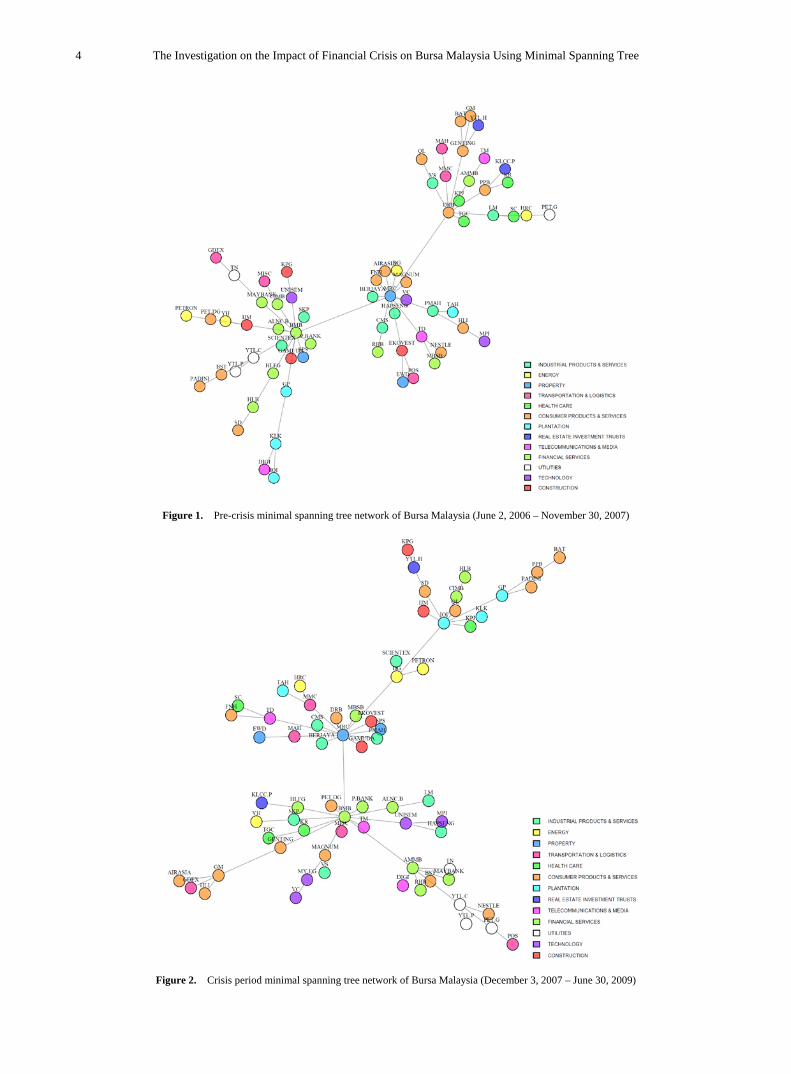
4. Results and Discussion Figure 1 shows the pre-crisis minimal spanning tree
network of Bursa Malaysia. From the figure, there are three clustered groups in the network, led by Bursa Malaysia Berhad (BMB), Malaysian Resources Corporation (MRC) and DRB-Hicom (DRB). BMB is considered as the centre of the network and is connected with other 14 companies, MRC is connected with other 13 companies, and DRB is connected with other nine companies. In addition, it shows that before the global financial crisis, Malaysian market has a strong reliance on financial services, property, consumer products and service sectors.
However, there are some changes in the network during the crisis period as depicted in Figure 2. BMB and MRC maintained as the centres of the network with additional companies included such as IOI Corporation (IOI) and AMMB Holdings (AMMB). However, DRB was no longer considered as a hub of the network. MST shows that the companies were clustered into four groups during crisis period instead of three groups as before the crisis.
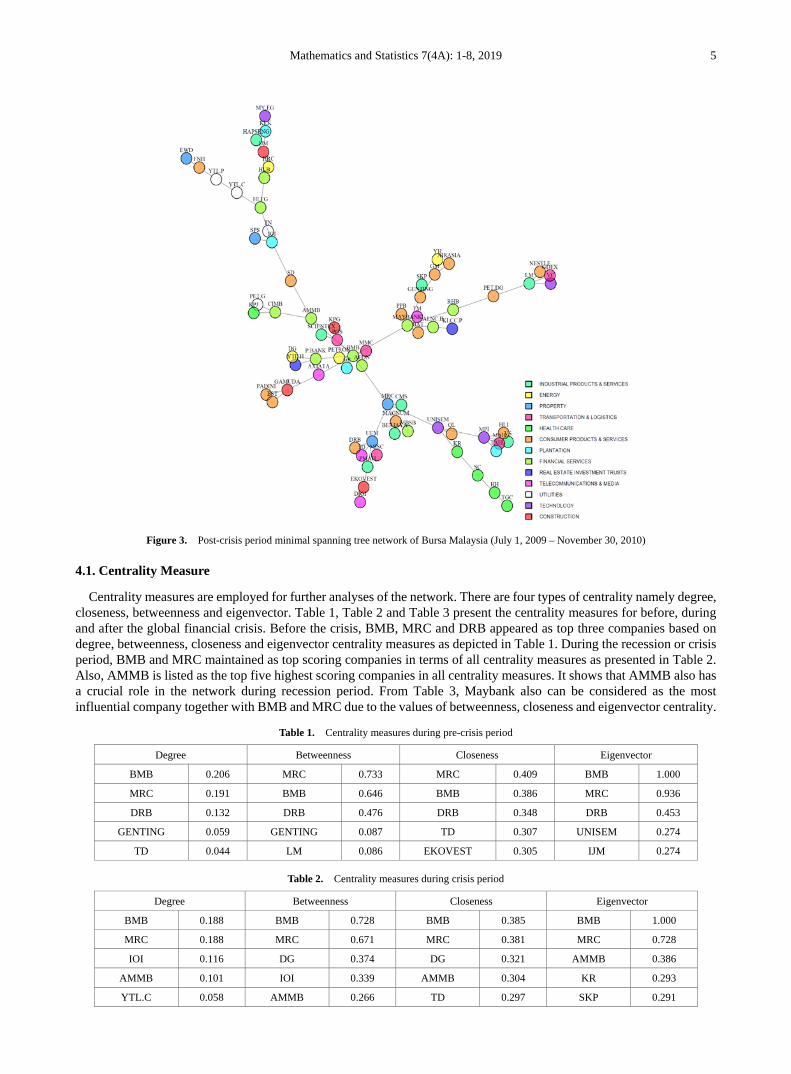
Contrary, after the crisis, the hub of the network disappeared as shown in Figure 3. This changes was similar to the German stock exchange [18] and the Korean stock market [19]. BMB sustained its position as the hub of the network which was connected with 10 companies. Meanwhile, 7 companies were connected to Maybank and MRC, UEM and MPI were connected to 5 companies. The empirical evidence shows that after the global financial crisis, the number of nodes that have links with a hub decreased.
i
4 The Investigation on the Impact of Financial Crisis on Bursa Malaysia Using Minimal Spanning Tree
Figure 1. Pre-crisis minimal spanning tree network of Bursa Malaysia (June 2, 2006 – November 30, 2007)
Figure 2. Crisis period minimal spanning tree network of Bursa Malaysia (December 3, 2007 – June 30, 2009)
Mathematics and Statistics 7(4A): 1-8, 2019 5
Figure 3. Post-crisis period minimal spanning tree network of Bursa Malaysia (July 1, 2009 – November 30, 2010)
4.1. Centrality Measure
Centrality measures are employed for further analyses of the network. There are four types of centrality namely degree, closeness, betweenness and eigenvector. Table 1, Table 2 and Table 3 present the centrality measures for before, during and after the global financial crisis. Before the crisis, BMB, MRC and DRB appeared as top three companies based on degree, betweenness, closeness and eigenvector centrality measures as depicted in Table 1. During the recession or crisis period, BMB and MRC maintained as top scoring companies in terms of all centrality measures as presented in Table 2. Also, AMMB is listed as the top five highest scoring companies in all centrality measures. It shows that AMMB also has a crucial role in the network during recession period. From Table 3, Maybank also can be considered as the most influential company together with BMB and MRC due to the values of betweenness, closeness and eigenvector centrality.
Table 1. Centrality measures during pre-crisis period
Degree Betweenness Closeness Eigenvector
BMB 0.206 MRC 0.733 MRC 0.409 BMB 1.000
MRC 0.191 BMB 0.646 BMB 0.386 MRC 0.936
DRB 0.132 DRB 0.476 DRB 0.348 DRB 0.453
GENTING 0.059 GENTING 0.087 TD 0.307 UNISEM 0.274
TD 0.044 LM 0.086 EKOVEST 0.305 IJM 0.274
Table 2. Centrality measures during crisis period
Degree Betweenness Closeness Eigenvector
BMB 0.188 BMB 0.728 BMB 0.385 BMB 1.000
MRC 0.188 MRC 0.671 MRC 0.381 MRC 0.728
IOI 0.116 DG 0.374 DG 0.321 AMMB 0.386
AMMB 0.101 IOI 0.339 AMMB 0.304 KR 0.293
YTL.C 0.058 AMMB 0.266 TD 0.297 SKP 0.291

6 The Investigation on the Impact of Financial Crisis on Bursa Malaysia Using Minimal Spanning Tree
Table 3. Centrality measures during post-crisis period
Degree Betweenness Closeness Eigenvector
BMB 0.188 BMB 0.728 BMB 0.267 BMB 1.000
MRC 0.188 MRC 0.671 MRC 0.239 MAYBANK 0.565
IOI 0.116 DG 0.374 AMMB 0.233 MRC 0.448
AMMB 0.101 IOI 0.339 MAYBANK 0.230 POS 0.359
YTL.C 0.058 AMMB 0.266 AXIATA 0.209 P.BANK 0.337
Principal component analysis is used to determine the most influential stock in the network for each period. Before the crisis, the most prominent stocks belong to MRC, BMB and DRB. MRC and BMB are still selected as the companies with the highest scores in overall centrality measures together with AMMB during crisis. After the global financial crisis, MRC, BMB and MAYBANK are the most crucial stocks in Bursa Malaysia.
The dominated stock for each period give the influence in the market in terms of comovement of stock price relatively towards the connected stocks. Besides, the most influential stock has effect on stock returns and the more vital within the network of stock market typically had higher revenue for compensation since they endured greater exposure to correlation risk.
5. Conclusions This paper aims to investigate the effects of global financial crisis on the correlation of stocks traded on Bursa
Malaysia using a minimal spanning tree. The Period of data used is divided into three parts: before, during and after the global financial crisis. In general, minimal spanning tree topology changes for each period. Before the crisis, the stocks clustered clearly into three groups and during the crisis, the stocks are dispersed into four groups. However, the stocks are scattered throughout the map after the financial crisis. The results were further assessed using degree, betweeness, closeness and eigenvector centrality. The empirical evidence shows that MRC and BMB are the most crucial stocks before, during and after the crisis.
Acknowledgements The authors thank the Ministry of Higher Education Malaysia (MOHE) under Fundamental Research Grant Scheme
(FRGS15-191-0432) and International Islamic University Malaysia under Research Initiative Grant Scheme (P-RIGS18-031-0031) for the financial support provided.
Appendix Table 4. Companies, sectors and their corresponding symbols
Symbol Company Sector Symbol Company Sector
VS VS INDUSTRY Industrial Products & Services GDEX GD EXPRESS CARRIER Transportation &
Logistics
PETRON PETRON MAL.REFN.& MKTG. Energy BERJAYA BERJAYA CORPORATION Industrial Products &
Services SPS SP SETIA Property HH HARTALEGA HOLDINGS Health Care
SKP SKP RESOURCES BERHAD
Industrial Products & Services HLI HONG LEONG INDUSTRIES Consumer Products &
Services
MMC MMC CORPORATION Transportation & Logistics TN TENAGA NASIONAL Utilities
HRC HENGYUAN REFINING COMPANY Energy SC SUPERMAX CORPORATION Health Care
KR KOSSAN RUBBER Health Care UNISEM UNISEM (M) Technology
SD SIME DARBY Consumer Products & Services AIRASIA AIRASIA GROUP Consumer Products &
Services
PET.DG PETRONAS DAGANGAN
Consumer Products & Services PADINI PADINI HOLDINGS Consumer Products &
Services

Mathematics and Statistics 7(4A): 1-8, 2019 7
MAGNUM MAGNUM Consumer Products & Services KLK KUALA LUMPUR KEPONG Plantation
CMS CAHYA MATA SARAWAK
Industrial Products & Services HAPSENG HAP SENG CONSOLIDATED Industrial Products &
Services
IOI IOI CORPORATION Plantation DIGI DIGI.COM Telecommunications & Media
AEON AEON CREDIT SERVICE Financial Services PET.G PETRONAS GAS Utilities
GENTING GENTING Consumer Products & Services BST BERJAYA SPORTS TOTO Consumer Products &
Services
KLCC.P KLCC PROPERTY
HOLDINGS STAPLED UNITS
Real Estate Investment Trusts MISC MISC BHD. Transportation &
Logistics
DRB DRB-HICOM Consumer Products & Services CIMB CIMB GROUP HOLDINGS Financial Services
TD TIME DOTCOM Telecommunications & Media QL QL RESOURCES Consumer Products &
Services
LM LAFARGE MALAYSIA
Industrial Products & Services KPG KERJAYA PROSPEK GROUP Construction
PPB PPB GROUP Consumer Products & Services ALNC.B ALLIANCE BANK MALAYSIA Financial Services
MAH MALAYSIA AIRPORTS HDG.
Transportation & Logistics TAH TA ANN HOLDINGS Plantation
TGC TOP GLOVE CORPORATION Health Care EWD ECO WORLD DEV.GROUP Property
GP GENTING PLANTATIONS Plantation GM GENTING MALAYSIA Consumer Products &
Services
FNH FRASER & NEAVE HOLDINGS
Consumer Products & Services YTL.H YTL HOSPITALITY REIT Real Estate
Investment Trusts
MAYBANK MALAYAN BANKING Financial Services POS POS MALAYSIA Transportation & Logistics
NESTLE NESTLE (MALAYSIA) Consumer Products & Services BAT BRIT.AMER.TOB.(MALAYSIA) Consumer Products &
Services P.BANK PUBLIC BANK Financial Services HLFG HONG LEONG FINL.GP. Financial Services
HLB HONG LEONG BANK Financial Services KPJ KPJ HEALTHCARE Health Care
RHB RHB BANK BHD Financial Services AMMB AMMB HOLDINGS Financial Services
YTL.C YTL CORPORATION Utilities PMAH PRESS METAL ALUMINIUM HOLDINGS
Industrial Products & Services
YTL.P YTL POWER INTERNATIONAL Utilities IJM IJM CORPORATION Construction
MBSB MALAYSIA BUILDING SOC. Financial Services MPI MALAYSIAN PACIFIC INDS. Technology
MY.EG MY EG SERVICES Technology DG DIALOG GROUP Energy
BMB BURSA MALAYSIA Financial Services TM TELEKOM MALAYSIA Telecommunications & Media
YH YINSON HOLDINGS Energy EKOVEST EKOVEST Construction
UEM UEM SUNRISE Property SCIENTEX SCIENTEX Industrial Products & Services
VC VITROX CORPORATION Technology GAMUDA GAMUDA Construction
MRC MALAYSIAN RESOURCES
CORPORATION Property AXIATA AXIATA GROUP Telecommunications
& Media
8 The Investigation on the Impact of Financial Crisis on Bursa Malaysia Using Minimal Spanning Tree
REFERENCES R. N. Mantegna. Hierarchical structure in financial markets. [1]
The European Physical Journal B, Vol.11, No.1, 193-197, 1999.
S. Sinha, R. K. Pan. Uncovering the internal structure of the [2]Indian financial market: large ross-correlation behavior in the NSE. Econophysics of Markets and Business Networks, Vol. 66, 3-19, 2007.
Y. Tang, J. J. Xiong, Z. Jia, Y. Zhang. Complexities in [3]financial network topological dynamics: modeling of emerging and developed stock markets. Complexity, 1-31, 2018.
W-Q. Hunag, X-T. Zhuang, S. Yao. A network analysis of [4]the Chiense stock market. Physica A: Statistical Mechanics and its Applications, Vol.388, No.14, 2956-2964, 2009.
W. Zhang, J. Wen, Y. Zhu. Minimal spanning tree analysis [5]of topological structures: the case of Hang Seng Index. Iberian Journal of Information System and Technologies, Vol.7, 145-155, 2016.
B. M. Tabak, T. R. Serra, D. O. Cajueiro. Topological [6]properties of stock market networks: The case of Brazil. Physica A, Vol.389, 3240-3249, 2010.
L. Sandoval. A map of the Brazilian stock market. Advances [7]in Complex Systems 2, Vol.15, No.4, 2012.
L. S. Yee, R. M. Salleh, N. M. Asrah. Multidimensional [8]minimal spanning tree: The Bursa Malaysia. Journal of Science and Technology, Vol.10, 136-143, 2018.
J. W. Lee, A. Nobi. State and network structures of stock [9]markets around the global financial crisis. Computational Economics. Vol.51, No.2, 195-210, 2017.
M. Majapa, S. J. Gossel. Topology of the South African [10]stock market network across the 2008 financial crisis. Physica A, Vol.445, 35-47, 2016.
E. Kantar, M. Keskin, B. Deviren. Analysis of the effects of [11]the global financial crisis on the Turkish economy, using hierarchical methods. Physica A, Vol.391, 2342-2352, 2012.
L. Xia, D. You, X Jiang, Q. Guo. Comparison between [12]global financial crisis and local stock disaster on top of Chinese stock network. Physica A: Statistical Mechanics and its Applications, Vol.490, 222-230, 2018.
A. Nobi, S. E. Maeng, G. G. Ha, J. W. Lee. Random matrix [13]theory and cross-correlations in global financial indices and local stock market indices. Journal-Korean Physical Society, Vol.62, No.4, 569-574, 2013.
N. Baba, F. Packer. From turnoil to crisis: Dislocations in the [14]FX swap market before and after the failure of Lehman Brothers. Journal of International Money and Finance, Vol.28, No.8, 1350-1374, 2009.
G. Bonanno, G. Caldarelli, F. Lillo, S. Miccich. Networks of [15]equities in financial markets. Physics of Condensed Matter, Vol.38, No.2, 363-371, 2004.
J. Kruskal. On the shortest spanning subtree of a graph and [16]the traveling salesman problem. Proceedings of the American Mathematical Society, Vol.7, No.1, 48-50, 1956.
M. E. J. Newman. A measure of betweenness centrality [17]based on random walks. Social Networks, Vol.27, No.1, 39-54, 2005.
M. Wiliński, A. Sienkiewicz, T. Gubiec, R. Kutner, Z. R. [18]Struzik. Structural and topological phase transitions on the German Stock Exchange. Physica A: Statistical Mechanics and its Applications, Vol.392, 5963-5973, 2013.
A. Nobi, S. E. Maeng, G. G. Ha, J. W. Lee. Structural [19]changes in the minimal spanning tree and the hierarchical network in the Korean stock market around the global financial crisis G. Journal of the Korean Physical Society, Vol.66, No.8, 1153-1159, 2015.
Mathematics and Statistics 7(4A): 9-16, 2019 http://www.hrpub.org DOI: 10.13189/ms.2019.070702
A 2-Component Laplace Mixture Model: Properties and Parametric Estimationsi
Zakiah I. Kalantan1,*, Faten Alrewely2
1Faculyu of Science, King Abdulaziz University, Jeddah, Saudi Arabia 2Faculty of Science, Al Jouf University, Sakaka, Saudi Arabia
Received July 1, 2019; Revised August 28, 2019; Accepted September 20, 2019
Copyright©2019 by authors, all rights reserved. Authors agree that this article remains permanently open access under the terms of the Creative Commons Attribution License 4.0 International License
Abstract Mixture distributions have received considerable attention in life applications. This paper presents a finite Laplace mixture model with two components. We discuss the model properties and derive the parameters estimations using the method of moments and maximum likelihood estimation. We study the relationship between the parameters and the shape of the proposed distribution. The simulation study discusses the effectiveness of parameters estimations of Laplace mixture distribution.
Keywords Laplace Distribution, Mixture Distribution, Method of Moments, Maximum Likelihood Estimation
1. IntroductionLaplace distribution has wide applications in various
fields such as engineering, business, medicine, and others. It is also known as a double exponential distribution because it is considered as two exponential distributions with additional location parameter. It considers as a member of lifetime distributions.
Mixture distributions and the problem of mixture decomposition about the identification of the constituent components and parameters dates back to 1846, but most of the reference is made due to the work of Karl Pearson in 1894 [7]. The approach taken by Pearson was to fit a univariate mixture of two normal to data through the choice of five parameters of the mixture in a way that empirical moments matched the model. The work by Pearson was successful in identifying two distinct sub-populations and also showing the flexibility of mixtures as a moment matching tool. Other later works focused on addressing the problems, but the invention of the modern computer and the popularization of the maximum likelihood parameterization techniques caused a stir in research work on mixture models [6]. In 2002, Figueiredo and Jain
applied the finite mixture to unsupervised learning models and gave important insights into mixture models [3]. Bhowmick et al introduced the Laplace mixture model instead of the Gaussian mixture model due to the tail length and a weight of the Laplace distribution, then applied the mixture micro-experiments [2]. Ali and Nadarajah found the information matrices for the Gaussian distribution mixture and the Laplace distribution mixture [5]. A mixture of asymmetric Laplace and Gaussian distributions was estimated using the EM algorithm by Shenoy and Gorinevsky [11]. Amini-Seresht and Zhang provided random comparisons of two finite-mixture models with different mixing ratios and independent variables [1].
Most of the references presented comprehensive studies and applications of finite mixture models which is based on the work of McLachlan, and Peel [6]. Ramana et al., introduced the two-component mixture of Laplace and Laplace type bimodal distributions, and they find the properties and estimation for the common parameters between the two-component mixture [9]. The previous studies are based on equal mixing parameters or constant scale parameters. The aim of this paper is to study the two components Laplace mixture model and estimate its parameters in the case of unknown all model parameters using parametric estimation methods.
The paper is organized as follows: Section 2 presents the definition of Laplace mixture distribution. Section 3 discusses the distribution function. The properties of the proposed distribution are studied in Section 4. The estimation methods are presented in Section 5. The simulation studies are presented in Section 6. Finally, conclusions are drawn in Section 7.
2. Laplace Mixture Distribution
2.1. Definition of Mixture Distribution
The Consider dataset 𝑋𝑋 = (𝑥1, 𝑥2, . . . , 𝑥𝑛) be

10 A 2-Component Laplace Mixture Model: Properties and Parametric Estimations
N-dimensional random variable, then 𝑋𝑋 follows 𝑘 components Laplace mixture distribution if its probability density function can be written as:
𝑓�𝑥; 𝜃� = ∑ 𝛼𝑖𝑘𝑖=1 𝑓𝑖�𝑥; 𝜃𝑖� (1)
where 𝛼𝑖 , 𝑖 = 1,2, … , 𝑘 are the mixing probabilities that satisfy 𝛼𝑖 ≥ 0 and ∑ 𝛼𝑖𝑘
𝑖=1 = 1.
2.2. Mixture of a Two Laplace Distribution
Let 𝑋𝑋 a random variable, the overall formula of the distribution of Laplace is
𝑓(𝑥; 𝜃) = 12𝜆
𝑒𝑥𝑝 �−│𝑥−𝜇│𝜆
�, (2)
where −∞ < 𝑥 < ∞,−∞ < 𝜇𝜇 < ∞, and 𝜆 > 0. In this paper, we will consider two components (k=2) for
Laplace mixture (A2-CLPM) distribution, where the first component provides the proportion α1 and density parameters 𝜇𝜇1, 𝜆1. The second one provides the proportion 𝛼2 = (1 − 𝛼1) and the second density parameters 𝜇𝜇2, 𝜆2, then the A2-CLPM distribution can be written as:
𝑓�𝑥; 𝜃� = 𝛼1 𝐿𝑎𝑝𝑙𝑎𝑐𝑒(𝜇𝜇1, 𝜆1) + (1 − 𝛼1) 𝐿𝑎𝑝𝑙𝑎𝑐𝑒(𝜇𝜇2, 𝜆2) (3)
Then, the probability density function (pdf) for A2-CLPM distribution is
𝑓�𝑥; 𝜃� = 𝛼12𝜆1
𝑒𝑥𝑝 �−│𝑥−𝜇1│𝜆1
� + (1−𝛼1)2𝜆2
𝑒𝑥𝑝 �−│𝑥−𝜇2│𝜆2
�, (4)
where −∞ < 𝑥 < ∞,−∞ < 𝜇𝜇1,𝜇𝜇2 < ∞, 𝜆1, 𝜆2 > 0 , and 𝛼1 + (1 − 𝛼1) = 1.
Figure 1 presents the curve of A2-CLPM distribution with parameters equal 𝜃 = (𝛼1, 𝜇𝜇1,𝜇𝜇2, 𝜆1, 𝜆2).
Figure 1. The frequency curves of the mixture Laplace distribution.
3. The Cumulative Density Function (CDF)
We state that the given pdf is a density function by computing the integral of the mixture distribution over its range, then we have
∫ 𝑓�𝑥; 𝜃�+∞−∞ 𝑑𝑥 = ∫ � 𝛼1
2𝜆1 𝑒𝑥𝑝 �−│𝑥−𝜇1│
𝜆1� +∞
−∞(1−𝛼1)2𝜆2
𝑒𝑥𝑝 �−│𝑥−𝜇2│𝜆2
�� 𝑑𝑥 = 1. (5)
The cumulative distribution function (CDF) of 𝑋𝑋 defines as:
𝐹(𝑥) = � 𝑓�𝑤; 𝜃�𝑑𝑤𝑥
−∞
𝐹(𝑥) = � �𝛼1
2𝜆1 𝑒𝑥𝑝 �−
│𝑤 − 𝜇𝜇1│𝜆1
�𝑥
−∞
+(1 − 𝛼1)
2𝜆2 𝑒𝑥𝑝 �−
│𝑤 − 𝜇𝜇2│𝜆2
�� 𝑑𝑤
then we have
𝐹(𝑥) =12
�𝛼1 𝑒𝑥𝑝 �𝑥 − 𝜇𝜇1𝜆1
� + (1 − 𝛼1) 𝑒𝑥𝑝 � 𝑥 − 𝜇𝜇2𝜆2
��,
for 𝑥 ≤ 𝜇𝜇1,𝜇𝜇2 and
𝐹(𝑥) = 𝛼1 �1 −12𝑒𝑥𝑝 �−
(𝑥 − 𝜇𝜇1)𝜆1
��
+ (1 − 𝛼1) �1 −12𝑒𝑥𝑝 �−
(𝑥 − 𝜇𝜇2)𝜆2
��,
for 𝑥 > 𝜇𝜇1,𝜇𝜇2 (6)
4. The Properties of Laplace Mixture Distribution
In what follows, the distribution properties are studied by obtaining the mean, the mode, the median, and the variance of A2-CLPM distribution. The mean of the random variable 𝑋𝑋 is
𝜇𝜇 = 𝐸(𝑥) = � 𝑥𝑓�𝑥; 𝜃� +∞
−∞𝑑𝑥
𝜇𝜇 =𝛼1
2𝜆1∫ 𝑥𝑒𝑥𝑝 �− │𝑥−𝜇𝜇1│
𝜆1�+∞
−∞ 𝑑𝑥 +
(1− 𝛼1)2𝜆2
∫ 𝑥 𝑒𝑥𝑝 �− │𝑥−𝜇𝜇2│
𝜆2�+∞
−∞ 𝑑𝑥 = 𝛼1𝜇𝜇1 + (1 − 𝛼1)𝜇𝜇2.
(7)
The mode of the random variable 𝑋𝑋 given from 𝑑𝑑𝑥𝑓�𝑥; 𝜃� = 0. (8)
when derived the equation (4) were 𝑥 ≥ 𝜇𝜇 or 𝑥 < 𝜇𝜇, we get the same mode for both of them, the formula are following as:
𝑥 = 𝜆2𝜇1+𝜆1𝜇2𝜆1+𝜆2
. (9)
The median of this distribution can be obtained as 𝑝(𝑥 ≤ 𝑐 ) = 1
2 , (10)
Mathematics and Statistics 7(4A): 9-16, 2019 11
because of symmetry, we can suppose that
𝑐 ≤ 𝜆2𝜇1+𝜆1𝜇2𝜆1+𝜆2
. (11)
The variance and standard deviation of the mixture distribution.
The variance is defined as:
𝜎2 = 𝑣𝑎𝑟(𝑥) = 𝐸(𝑥2) − �𝐸(𝑥)�2. (12)
Then, we find 𝐸(𝑥2), as following as:
𝐸(𝑥2) = ∫ 𝑥2 𝑓�𝑥; 𝜃�+∞−∞ 𝑑𝑥.
𝐸(𝑥2) =𝛼1
2𝜆1� 𝑥2 exp�−
│𝑥 − 𝜇𝜇│𝜆1
�+∞
−∞𝑑𝑥 +
(1 − 𝛼1)
2𝜆2� 𝑥2 𝑒𝑥𝑝 �−
│𝑥 − 𝜇𝜇│𝜆2
�+∞
−∞𝑑𝑥
𝐸(𝑥2) = 𝛼1�𝜇𝜇12 + 2𝜆12� + (1 − 𝛼1)�𝜇𝜇22 + 2𝜆2
2�. (13)
Then, substitute Eq (7) and Eq (13) in Eq (12), we get
𝜎2 = 𝑣𝑎𝑟(𝑥)
𝜎2 = 𝛼1�𝜇𝜇12 + 2𝜆12� + (1 − 𝛼1)�𝜇𝜇22 + 2𝜆2
2� − [𝛼1𝜇𝜇1 + (1 − 𝛼1)𝜇𝜇2]2. (14)
The stander deviation of the random variable 𝑋𝑋 is the square root of the variance.
𝜎 = �𝑣𝑎𝑟(𝑥)
𝜎 = �𝛼1�𝜇𝜇12 + 2𝜆12� + (1 − 𝛼1)�𝜇𝜇22 + 2𝜆2
2� − 𝛼1𝜇𝜇1 +(1 − 𝛼1)𝜇𝜇2. (15)
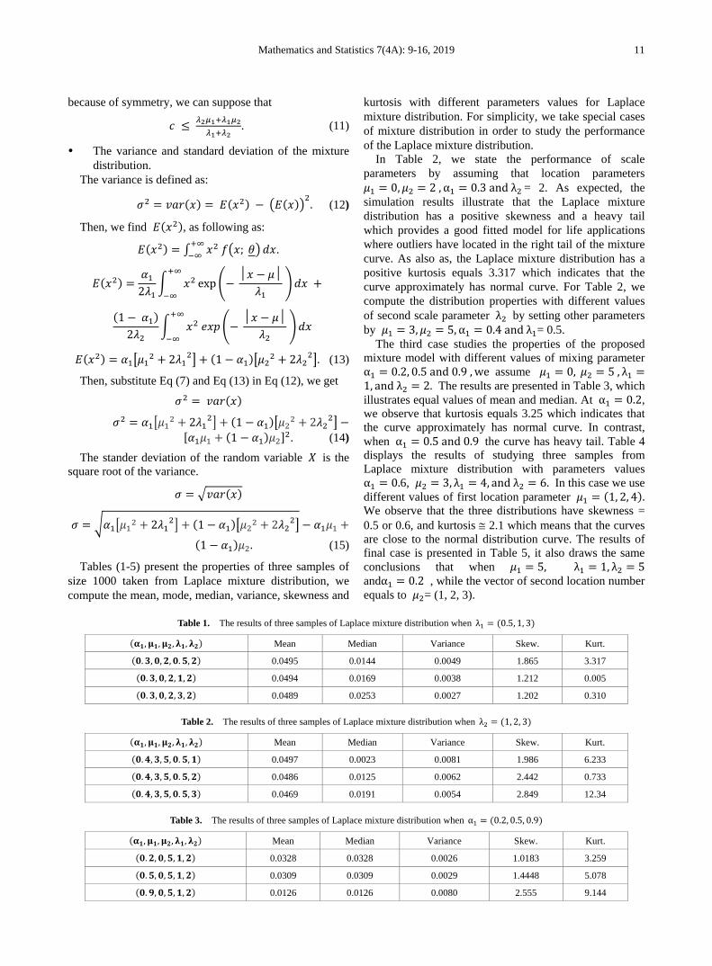
Tables (1-5) present the properties of three samples of size 1000 taken from Laplace mixture distribution, we compute the mean, mode, median, variance, skewness and
kurtosis with different parameters values for Laplace mixture distribution. For simplicity, we take special cases of mixture distribution in order to study the performance of the Laplace mixture distribution.
In Table 2, we state the performance of scale parameters by assuming that location parameters 𝜇𝜇1 = 0,𝜇𝜇2 = 2 ,α1 = 0.3 and λ2 = 2. As expected, the simulation results illustrate that the Laplace mixture distribution has a positive skewness and a heavy tail which provides a good fitted model for life applications where outliers have located in the right tail of the mixture curve. As also as, the Laplace mixture distribution has a positive kurtosis equals 3.317 which indicates that the curve approximately has normal curve. For Table 2, we compute the distribution properties with different values of second scale parameter λ2 by setting other parameters by 𝜇𝜇1 = 3,𝜇𝜇2 = 5,α1 = 0.4 and λ1= 0.5.
The third case studies the properties of the proposed mixture model with different values of mixing parameter α1 = 0.2, 0.5 and 0.9 , we assume 𝜇𝜇1 = 0, 𝜇𝜇2 = 5 , λ1 =1, and λ2 = 2. The results are presented in Table 3, which illustrates equal values of mean and median. At α1 = 0.2, we observe that kurtosis equals 3.25 which indicates that the curve approximately has normal curve. In contrast, when α1 = 0.5 and 0.9 the curve has heavy tail. Table 4 displays the results of studying three samples from Laplace mixture distribution with parameters values α1 = 0.6, 𝜇𝜇2 = 3, λ1 = 4, and λ2 = 6. In this case we use different values of first location parameter 𝜇𝜇1 = (1, 2, 4). We observe that the three distributions have skewness = 0.5 or 0.6, and kurtosis ≅ 2.1 which means that the curves are close to the normal distribution curve. The results of final case is presented in Table 5, it also draws the same conclusions that when 𝜇𝜇1 = 5, λ1 = 1, λ2 = 5 andα1 = 0.2 , while the vector of second location number equals to 𝜇𝜇2= (1, 2, 3).
Table 1. The results of three samples of Laplace mixture distribution when λ1 = (0.5, 1, 3)
(𝛂𝟏,𝛍𝟏,𝛍𝟐,𝛌𝟏,𝛌𝟐) Mean Median Variance Skew. Kurt.
(𝟎.𝟑,𝟎,𝟐,𝟎.𝟓,𝟐) 0.0495 0.0144 0.0049 1.865 3.317
(𝟎.𝟑,𝟎,𝟐,𝟏,𝟐) 0.0494 0.0169 0.0038 1.212 0.005
(𝟎.𝟑,𝟎,𝟐,𝟑,𝟐) 0.0489 0.0253 0.0027 1.202 0.310
Table 2. The results of three samples of Laplace mixture distribution when λ2 = (1, 2, 3)
(𝛂𝟏,𝛍𝟏,𝛍𝟐,𝛌𝟏,𝛌𝟐) Mean Median Variance Skew. Kurt.
(𝟎.𝟒,𝟑,𝟓,𝟎.𝟓,𝟏) 0.0497 0.0023 0.0081 1.986 6.233
(𝟎.𝟒,𝟑,𝟓,𝟎.𝟓,𝟐) 0.0486 0.0125 0.0062 2.442 0.733
(𝟎.𝟒,𝟑,𝟓,𝟎.𝟓,𝟑) 0.0469 0.0191 0.0054 2.849 12.34
Table 3. The results of three samples of Laplace mixture distribution when α1 = (0.2, 0.5, 0.9)
(𝛂𝟏,𝛍𝟏,𝛍𝟐,𝛌𝟏,𝛌𝟐) Mean Median Variance Skew. Kurt.
(𝟎.𝟐,𝟎,𝟓,𝟏,𝟐) 0.0328 0.0328 0.0026 1.0183 3.259
(𝟎.𝟓,𝟎,𝟓,𝟏,𝟐) 0.0309 0.0309 0.0029 1.4448 5.078
(𝟎.𝟗,𝟎,𝟓,𝟏,𝟐) 0.0126 0.0126 0.0080 2.555 9.144

12 A 2-Component Laplace Mixture Model: Properties and Parametric Estimations
Table 4. The results of three samples of Laplace mixture distribution when 𝜇𝜇1 = (1, 2, 4)
(𝛂𝟏,𝛍𝟏,𝛍𝟐,𝛌𝟏,𝛌𝟐) Mean Median Variance Skew. Kurt.
(𝟎.𝟔,𝟏,𝟑,𝟒,𝟔) 0.0430 0.0364 0.0007 0.5553 2.082
(𝟎.𝟔,𝟐,𝟑,𝟒,𝟔) 0.0428 0.0360 0.0007 0.622 2.294
(𝟎.𝟔,𝟒,𝟑,𝟒,𝟔) 0.0418 0.0360 0.0008 0.5604 2.170
Table 5. The results of three samples of Laplace mixture distribution when 𝜇𝜇2 = (1, 2, 3)
(𝛂𝟏,𝛍𝟏,𝛍𝟐,𝛌𝟏,𝛌𝟐) Mean Median Variance Skew. Kurt.
(𝟎.𝟕,𝟓,𝟏,𝟑,𝟏.𝟓) 0.0464 0.0346 0.002 0.4193 1.693
(𝟎.𝟕,𝟓,𝟐,𝟑,𝟏.𝟓) 0.0464 0.0306 0.002 0.6367 1.912
(𝟎.𝟕,𝟓,𝟑,𝟑,𝟏.𝟓) 0.0463 0.0273 0.002 0.9090 2.433
5. Parametric Estimation Methods In this section, we obtain the parameter estimates of Laplace mixture distribution using two parametric estimation
methods: method of moments (MME) and maximum likelihood estimation (MLE) method. The illustrations are presented in the following subsections.
5.1. The Method of Moments (MME)
Let 𝑋𝑋 be a random variable with A2-CLPM (α1,µ1, µ2, λ1, λ2) distribution. The 𝑟 𝑡ℎ moments are defined as:
𝐸(𝑥𝑟) = � 𝑥𝑟 𝑓�𝑥; 𝜃�𝑑𝑥+∞
−∞
= ∫ 𝒙𝒓 � 𝜶𝟏𝟐𝝀𝟏
𝒆𝒙𝒑 �−│𝒙−𝛍𝟏│𝝀𝟏
� + (𝟏−𝜶𝟏)𝟐𝝀𝟐
𝒆𝒙𝒑 �−│𝒙−𝛍𝟐│𝝀𝟐
��𝒅𝒙 ∞−∞ . (16)
For simplicity, we use the Taylor series instead of integration, because, we need to find eight moments, and solve these integrations are very hard, see [8], as following as:
𝜇𝜇�� = 𝐸(𝑥𝑟)
= �𝛂𝟏𝟐���
𝒓!(𝒓 − 𝒌)!
𝛌𝟏𝒌𝛍𝟏(𝒓−𝒌)�𝟏 + (−𝟏)𝒌�� + �
(𝟏 − 𝛂𝟏)𝟐
���𝒓!
(𝒓 − 𝒌)! 𝛌𝟐
𝒌𝛍𝟐(𝒓−𝒌)�𝟏+ (−𝟏)𝒌��𝒓
𝒌=𝟎
𝒓
𝒌=𝟎
.
𝜇𝜇𝑟 = �0 , 𝑖𝑓 𝑟 𝑖𝑠 𝑜𝑑𝑑,
2α1 λ1𝑟 𝑟! + 2(1 − α1) λ2
𝑟 𝑟! , 𝑖𝑓 𝑟 𝑖𝑠 𝑒𝑣𝑒𝑛. (17)
The 𝑟𝑡ℎ means of the population are equal to
𝑀/𝑟 = 𝑃1
∑ 𝑥𝑖1𝑟𝑛
𝑖=1𝑛1
+ (1 − 𝑃1) ∑ 𝑥𝑖2
𝑟𝑛𝑖=1𝑛2
, (18)
where 𝑟 = 1,2,3, … ,𝑛 and 𝑃1 + (1 − 𝑃1) = 1 they are population mixing parameters. Then, by solve equations, as following as:
𝜇𝜇�� = 𝑀/𝑟. (19)
The estimations are made for the five parameters 𝜃 = (𝛼1,𝜇𝜇1, 𝜇𝜇2, 𝜆1, 𝜆2). For this mixture distribution, we compute the first eight raw moments in order to obtain the moment estimations of distribution parameters. It is noted that, we find parameter estimation 𝛼�2 from compute 1 − 𝛼�1. Also, it is noted that 𝐸(𝑥𝑟) = 0, for odd values > 1 𝑜𝑓 𝑟 therefore, we base our estimation on the first moment and the even moments. Now, from Eq (17) we get the first moment, as following as: when 𝑟 = 1
𝜇𝜇1 = 𝐸(𝑥) = 𝛼1𝜇𝜇1 + (1 − 𝛼1)𝜇𝜇2. (20)
when 𝑟 = 2
Mathematics and Statistics 7(4A): 9-16, 2019 13
��𝜇2 = 𝐸(𝑥2) = 𝛼1 �𝜇𝜇12+2𝜆1
2�+ (1−𝛼1 ) �𝜇𝜇22+2 𝜆2
2�. (21)
when 𝑟 = 4
��𝜇4 = 𝐸(𝑥4) = 𝛼1 �𝜇𝜇14 + 12 𝜆12 𝜇𝜇12 + 24 𝜆1
4� + (1 − 𝛼1 )�𝜇𝜇24 + 12 𝜆22 𝜇𝜇22 + 24 𝜆2
4�. (22)
when 𝑟 = 6
��𝜇6 = 𝐸(𝑥6) = 𝛼1 �𝜇𝜇16 + 30 𝜆1
2 𝜇𝜇14 + 360 𝜆1
4 𝜇𝜇12 + 720 𝜆1
6�+ (1−𝛼1 )
�𝜇𝜇26 + 30 𝜆22 𝜇𝜇24 + 360 𝜆2
4 𝜇𝜇22 + 720 𝜆26�. (23)
when 𝑟 = 8 ��𝜇8 = 𝐸(𝑥8) = 𝛼1 �µ18 + 56 𝜆1
2 µ16 + 1680 𝜆14 µ14 + 20160 𝜆1
6 µ12 + 40320 𝜆18�
+(1 − 𝛼1 )�µ28 + 56 𝜆22 µ26 + 1680 𝜆2
4 µ24 + 20160 𝜆26 µ22 + 40320 𝜆2
8�. (24)
To obtain estimates of the distribution parameters, equate the five equations above with Eq (18) for 𝑟 = 1,2,4,6,8 and then solving them. As following as:
𝜇𝜇/1 = 𝑀/
1
𝛼1𝜇𝜇1 + (1 − 𝛼1)𝜇𝜇2 = 𝑃1 ∑ 𝑥𝑖1𝑛𝑖=1𝑛1
+ (1 − 𝑃1) ∑ 𝑥𝑖2𝑛𝑖=1𝑛2
. (25)
𝜇𝜇/2 = 𝑀/
2
𝛼1 �𝜇𝜇12+2𝜆12� + (1 − 𝛼1 )�𝜇𝜇22+2 𝜆2
2�
= 𝑃1 ∑ 𝑥𝑖1
2𝑛𝑖=1𝑛1
+ (1 − 𝑃1) ∑ 𝑥𝑖22𝑛
𝑖=1𝑛2
. (26)
𝜇𝜇/4 = 𝑀/
4
𝛼1 �𝜇𝜇14 + 12 𝜆12 𝜇𝜇12 + 24 𝜆1
4� + (1 − 𝛼1 )
�𝜇𝜇24 + 12 𝜆22 𝜇𝜇22 + 24 𝜆2
4� = 𝑃1 ∑ 𝑥𝑖1
4𝑛𝑖=1𝑛1
+ (1 − 𝑃1) ∑ 𝑥𝑖24𝑛
𝑖=1𝑛2
. (27)
𝜇𝜇/6 = 𝑀/
6
𝛼1 �𝜇𝜇16 + 30 𝜆12 𝜇𝜇14 + 360 𝜆1
4 𝜇𝜇12 + 720 𝜆16�
+(1 − 𝛼1 )�𝜇𝜇26 + 30 𝜆22 𝜇𝜇24 + 360 𝜆2
4 𝜇𝜇22 + 720 𝜆26�
= 𝑃1 ∑ 𝑥𝑖1
6𝑛𝑖=1𝑛1
+ (1 − 𝑃1) ∑ 𝑥𝑖26𝑛
𝑖=1𝑛2
. (28)
𝜇𝜇/8 = 𝑀/
8
𝛼1 �µ18 + 56 𝜆12 µ16 + 1680 𝜆1
4 µ14 + 20160 𝜆16 µ12 + 40320 𝜆1
8� +
(1 − 𝛼1 )�µ28 + 56 𝜆22 µ26 + 1680 𝜆2
4 µ24 + 20160 𝜆26 µ22 + 40320 𝜆2
8� = P1 ∑ 𝑥𝑖1
8𝑛𝑖=1n1
+ (1 − P1) ∑ 𝑥𝑖28𝑛
𝑖=1n2
. (29)
Hence, the parameter estimates using method of moments can be obtained by solving the above equations numerically via R software.
2. The Maximum Likelihood Estimation (MLE)
The maximum likelihood estimation method (MLE) is used to estimate the parameters of the distribution. Now, let 𝑋𝑋 = (𝑥1 , 𝑥2, . . . . , 𝑥𝑛) is a random sample then the likelihood function of a given distribution is defined as:
𝐿 (𝜃) = ∏ 𝑓 � 𝑥𝑖 ; 𝜃�𝑛𝑖=1 . (30)
The maximum likelihood estimates for θ is calculated by finding a value of θ that maximizes log-likelihood function. i.e.
𝜃 = arg𝑚𝑎𝑥∑ 𝑙𝑜𝑔𝑓�𝑥𝑖 ; 𝜃�𝑛𝑖=1 . (31)
For Laplace mixture distribution, define 𝐿(𝜃) = 𝐿(𝛼1, 𝜆1, 𝜆2| 𝑥), where the location parameters are known, and equals 𝜇𝜇1 = 0,𝜇𝜇1 = 2. Then
14 A 2-Component Laplace Mixture Model: Properties and Parametric Estimations
𝐿(𝜃) = ∏ 𝑓(𝑥𝑖;𝛼1, 𝜆1, 𝜆2) =𝑛𝑖=1 ∏ � 𝛼1
2𝜆1 𝑒𝑥𝑝 �−│𝑥𝑖│
𝜆1� + (1−𝛼1)
2𝜆2 𝑒𝑥𝑝 �−│𝑥𝑖−2│
𝜆2��𝑛
𝑖=1 . (32)
log 𝐿(𝜃) = ∑ 𝑙𝑜𝑔 � 𝛼12𝜆1
𝑒𝑥𝑝 �−│𝑥𝑖│𝜆1� + 𝛼2
2𝜆2 𝑒𝑥𝑝 �−│𝑥𝑖−2│
𝜆2��𝑛
𝑖=1 . (33)
Next, to find the maximization of log-Likelihood we need to find the derivatives of log-likelihood function with respect to distribution parameters see [10], then we have
𝜕𝑙𝜕𝛼1
= ∑1
2𝜆1 𝑒𝑥𝑝�−
│𝑥𝑖│𝜆1
�− 12𝜆2
𝑒𝑥𝑝�−│𝑥𝑖−2│𝜆2
�
� 𝛼12𝜆1 𝑒𝑥𝑝�−
│𝑥𝑖│𝜆1
�+ 𝛼22𝜆2
𝑒𝑥𝑝�−│𝑥𝑖−2│𝜆2
�� 𝑛
𝑖=1 . (34)
𝜕𝑙𝜕𝜆1
= ∑𝑒𝑥𝑝�−
│𝑥𝑖│𝜆1
��𝛼1│𝑥𝑖│−𝛼1 𝜆1�
2𝜆13� 𝛼12𝜆1
𝑒𝑥𝑝�−│𝑥𝑖│𝜆1
�+ 𝛼22𝜆2
𝑒𝑥𝑝�−│𝑥𝑖−2│𝜆2
�� 𝑛
𝑖=1 . (35)
𝜕𝑙𝜕𝜆2
= ∑𝑒𝑥𝑝�−
│𝑥𝑖−2│𝜆2
��𝛼2│𝑥𝑖│−𝛼2 𝜆2�
2𝜆23� 𝛼12𝜆1
𝑒𝑥𝑝�−│𝑥𝑖│𝜆1
�+ 𝛼22𝜆2
𝑒𝑥𝑝�−│𝑥𝑖−2│𝜆2
��
𝑛𝑖=1 . (36)
The next step is to set the equation (34), equation (35), and equation (36) to zero. Then, solve the system for the three parameters α1, 𝜆1 and 𝜆2, this step obtains the MLE of α1, 𝜆1 and 𝜆2. In practical, the parameter estimations via MLE method are obtained numerically using Newton-Raphson method by providing initial values for parameters. This is done through the implementation of method using R software
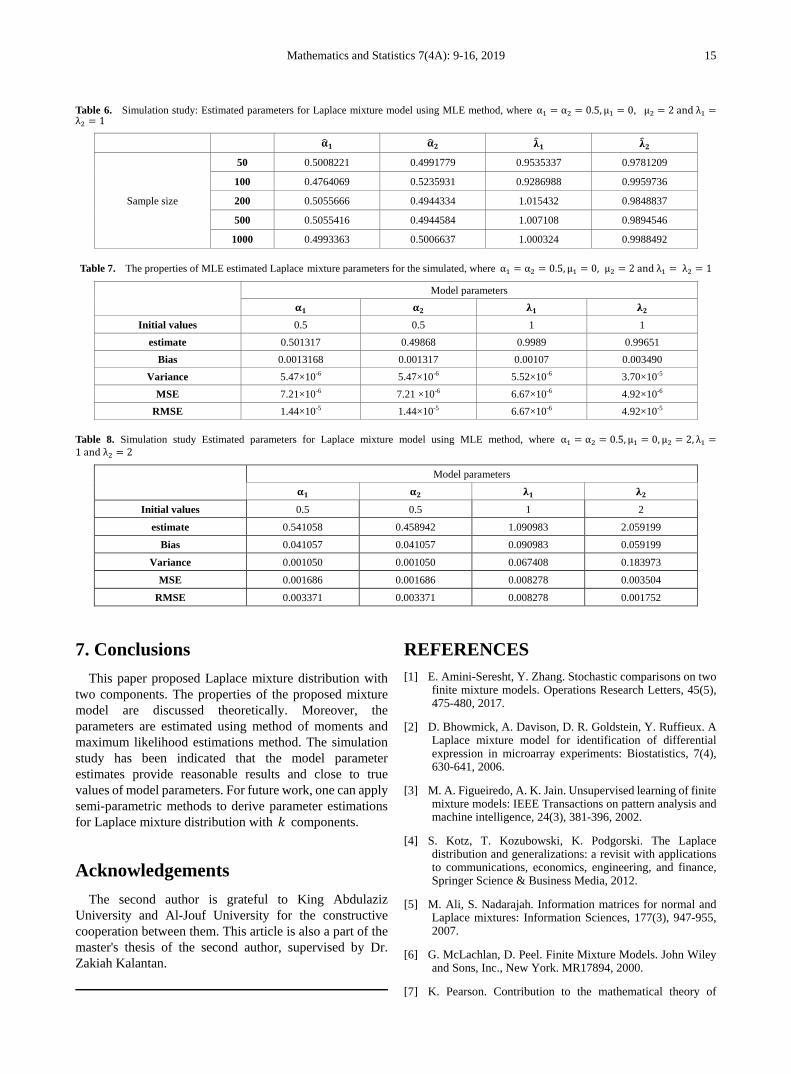
6. Simulation Study We study the effectiveness of Laplace mixture model by providing two scenarios. Firstly, we obtain the MLE
estimations for a two components Laplace mixture distribution, and for simplicity, we assume that the location parameters 𝜇𝜇1 = 0 and 𝜇𝜇2 = 2. We study two case studies as illustrated in what follows:
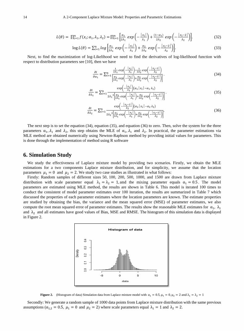
Firstly: Random samples of different sizes 50, 100, 200, 500, 1000, and 1500 are drawn from Laplace mixture distribution with scale parameter equal λ1 = λ2 = 1, and the mixing parameter equals α1 = 0.5 . The model parameters are estimated using MLE method, the results are shown in Table 6. This model is iterated 100 times to conduct the consistent of model parameter estimates over 100 iteration, the results are summarized in Table 7 which discussed the properties of each parameter estimates where the location parameters are known. The estimate properties are studied by obtaining the bias, the variance and the mean squared error (MSE) of parameter estimates, we also compute the root mean squared error of parameter estimates. The results show the reasonable MLE estimates for α1, λ1 and λ2 and all estimates have good values of Bias, MSE and RMSE. The histogram of this simulation data is displayed in Figure 2.
Figure 2. (Histogram of data) Simulation data from Laplace mixture model with α1 = 0.5,µ1 = 0, µ2 = 2 and λ1 = λ2 = 1
Secondly: We generate a random sample of 1000 data points from Laplace mixture distribution with the same previous assumptions (α1,2 = 0.5, 𝜇𝜇1 = 0 and 𝜇𝜇2 = 2) where scale parameters equal λ1 = 1 and λ2 = 2.
Mathematics and Statistics 7(4A): 9-16, 2019 15
Table 6. Simulation study: Estimated parameters for Laplace mixture model using MLE method, where α1 = α2 = 0.5,µ1 = 0, µ2 = 2 and λ1 =λ2 = 1
𝛂�𝟏 𝛂�𝟐 𝛌�𝟏 𝛌�𝟐
Sample size
50 0.5008221 0.4991779 0.9535337 0.9781209
100 0.4764069 0.5235931 0.9286988 0.9959736
200 0.5055666 0.4944334 1.015432 0.9848837
500 0.5055416 0.4944584 1.007108 0.9894546
1000 0.4993363 0.5006637 1.000324 0.9988492
Table 7. The properties of MLE estimated Laplace mixture parameters for the simulated, where α1 = α2 = 0.5,µ1 = 0, µ2 = 2 and λ1 = λ2 = 1
Model parameters
𝛂𝟏 𝛂𝟐 𝛌𝟏 𝛌𝟐 Initial values 0.5 0.5 1 1
estimate 0.501317 0.49868 0.9989 0.99651 Bias 0.0013168 0.001317 0.00107 0.003490
Variance 5.47×10⁻⁶ 5.47×10⁻⁶ 5.52×10⁻⁶ 3.70×10⁻⁵ MSE 7.21×10⁻⁶ 7.21 ×10⁻⁶ 6.67×10⁻⁶ 4.92×10⁻⁶
RMSE 1.44×10⁻⁵ 1.44×10⁻⁵ 6.67×10⁻⁶ 4.92×10⁻⁵
Table 8. Simulation study Estimated parameters for Laplace mixture model using MLE method, where α1 = α2 = 0.5,µ1 = 0, µ2 = 2, λ1 =1 and λ2 = 2
Model parameters
𝛂𝟏 𝛂𝟐 𝛌𝟏 𝛌𝟐
Initial values 0.5 0.5 1 2
estimate 0.541058 0.458942 1.090983 2.059199
Bias 0.041057 0.041057 0.090983 0.059199
Variance 0.001050 0.001050 0.067408 0.183973
MSE 0.001686 0.001686 0.008278 0.003504
RMSE 0.003371 0.003371 0.008278 0.001752
7. Conclusions This paper proposed Laplace mixture distribution with
two components. The properties of the proposed mixture model are discussed theoretically. Moreover, the parameters are estimated using method of moments and maximum likelihood estimations method. The simulation study has been indicated that the model parameter estimates provide reasonable results and close to true values of model parameters. For future work, one can apply semi-parametric methods to derive parameter estimations for Laplace mixture distribution with 𝑘 components.
Acknowledgements The second author is grateful to King Abdulaziz
University and Al-Jouf University for the constructive cooperation between them. This article is also a part of the master's thesis of the second author, supervised by Dr. Zakiah Kalantan.
REFERENCES E. Amini-Seresht, Y. Zhang. Stochastic comparisons on two [1]
finite mixture models. Operations Research Letters, 45(5), 475-480, 2017.
D. Bhowmick, A. Davison, D. R. Goldstein, Y. Ruffieux. A [2]Laplace mixture model for identification of differential expression in microarray experiments: Biostatistics, 7(4), 630-641, 2006.
M. A. Figueiredo, A. K. Jain. Unsupervised learning of finite [3]mixture models: IEEE Transactions on pattern analysis and machine intelligence, 24(3), 381-396, 2002.
S. Kotz, T. Kozubowski, K. Podgorski. The Laplace [4]distribution and generalizations: a revisit with applications to communications, economics, engineering, and finance, Springer Science & Business Media, 2012.
M. Ali, S. Nadarajah. Information matrices for normal and [5]Laplace mixtures: Information Sciences, 177(3), 947-955, 2007.
G. McLachlan, D. Peel. Finite Mixture Models. John Wiley [6]and Sons, Inc., New York. MR17894, 2000.
K. Pearson. Contribution to the mathematical theory of [7]

16 A 2-Component Laplace Mixture Model: Properties and Parametric Estimations
evolution. Philosophical Transactions of the Royal Society, 185, 71–110, 1894.
J. Philip, Davis & R. Philip. Methods of numerical [8]integration. Courier Corporation, 0486453391, 2007.
DV Ramana Murty, G. Arti, M, Vivekananda Murty. Two [9]component mixture of Laplace and Laplace type distributions with applications to manpower planning models. International Journal of Statistics and Applied Mathematics, 3(4), 01-11, 2018.
R. M. Norton. The Double Exponential Distribution: Using [10]Calculus to Find a Maximum Likelihood Estimator. The American Statistician, 38 (2), 135–136, 1984.
S. Shenoy, D. Gorinevsky. Gaussian-Laplace mixture model [11]for electricity market. Paper presented at the Decision and Control (CDC), 2014 IEEE 53rd Annual Conference on, 2014.
i Conference Papers Zakiah Kalantan, Faten Alrewely, A 2-Components Laplace Mixture Model: Properties and Parametric Estimations, Conference: The 4 International Conference on Computing, Mathematics and Statistics 2019 (iCMS2019). At: Ombak Villa, Langkawi Island, Malaysia.
Mathematics and Statistics 7(4A): 17-23, 2019 http://www.hrpub.org DOI: 10.13189/ms.2019.070703
Comparison of Queuing Performance Using Queuing Theory Model and Fuzzy Queuing Model at
Check-in Counter in Airport
Noor Hidayah Mohd Zaki*, Aqilah Nadirah Saliman, Nur Atikah Abdullah, Nur Su Ain Abu Hussain, Norani Amit
Faculty Computer and Mathematical Sciences, Universiti Teknologi MARA Negeri Sembilan, Malaysia
Received July 1, 2019; Revised August 28, 2019; Accepted September 20, 2019
Copyright©2019 by authors, all rights reserved. Authors agree that this article remains permanently open access under the terms of the Creative Commons Attribution License 4.0 International License
Abstract A queuing system is a process to measure the efficiency of a model by underlying the concepts of queue models: arrival and service time distributions, queue disciplines and queue behaviour. The main aim of this study is to compare the behaviour of a queuing system at check-in counters using the Queuing Theory Model and Fuzzy Queuing Model. The Queuing Theory Model gives performance measures of a single value while the Fuzzy Queuing Model has a range of values. The Dong, Shah and Wong (DSW) algorithm is used to define the membership function of performance measures in the Fuzzy Queuing Model. Based on the observation, the problem often occurs when customers are required to wait in the queue for a long time, thus indicating that the service systems are inefficient. Data including the variables were collected, such as arrival time in the queue (server) and service time. Results show that the performance measures of the Queuing Theory Model lie in the range of the computed performance measures of the Fuzzy Queuing Model. Hence, the results obtained from the Fuzzy Queuing Model are consistent to measure the queuing performance of an airline company in order to solve the problem in waiting line and will improve the quality of services provided by airline company.
Keywords Queuing Theory Model, Fuzzy Queuing Model, Dong, Shah and Wong (DSW) Algorithm
1. IntroductionQueues happen at any place such as airport terminal,
hospital, grocery store and even petrol station. Customers queue while getting service either at counters or machines before they are served. Long queuing lines can be seen at an airport check-in counter especially during the arrival
and departure of planes. The long queues may happen due to an insufficient service system and low service quality, thus increasing the waiting time. Reducing waiting time and providing quick service are very important in service-related operations [1]. Service-related companies place importance on reducing the waiting time of customers in order to increase customer satisfaction through improving their service quality. The queuing theory can be measured using the quantitative analysis technique to predict the characteristics of a waiting line [2]. The queuing theory is used to translate the customer’s arrival time as well as analyze the queuing behaviour mathematically from the amount of time that a customer needs to wait in the system based on a real queuing situation [3].
Fuzzy queuing can be defined as a new technique which is often seen in a real world situation. According to [4], the existence of fuzzy numbers can help the manager to facilitate the service time with uncertainty and at the same time maximize the profit. In addition, fuzzy queuing also can be applied into the fuzzy possibilistic-queuing model where the main objectives are to minimize total cost and cost for transportation [5]. Furthermore, the fuzzy set theory is easily adaptable compared to other theories [6]. The fuzzy set theory is also done as an assessment for sensitive stochastic delay of flights [7]. In relation to the airport system, the fuzzy theory is also used to define the arrival and service times in airports [8] [9].
This study focuses on the queuing line system at passenger check-in counters in an airport terminal. The aim of this paper is to compare the queuing theory model and fuzzy queuing theory model on queuing performance measures. Queuing theory model has provided the limited capability in explaining some situation in real life while fuzzy queuing theory has a capability of making decision from multiple inputs or criteria. The Dong, Shah and Wong

18 Comparison of Queuing Performance Using Queuing Theory Model and Fuzzy Queuing Model at Check-in Counter in Airport
(DSW) algorithm is used for the fuzzy queuing model for an α-cut method. The DSW algorithm is used to define a membership function of the performance measures in a multi-server fuzzy queuing model [10]. Both models are compared based on the results of the average number of customers in the queue (Lq), average number of customers in the system (L), average waiting time of a customer in the queue (Wq), and average waiting time of a customer in the system (W).
2. Methods
2.1. Queuing Theory Model
The queuing theory was first introduced by A.K. Erlang in 1909. In this study, Lq, Ls, Wq and Ws are computed for the multi-server channel single phase (M/M/s) [11].
The average server utilization,
(1)
Probability of zero customers in the system,
(2)
The average number of customers in the waiting line,
(3)
The average number of customers waiting in the system,
(4)
The average time a customer waits for service,
(5)
The average time a customer is in the system,
(6)
2.2. Fuzzy Queuing Theory Model
Zadeh [12] invented the idea of a fuzzy set in the queuing theory and transformed the idea into fuzzy queue models, as implemented by [13], [14] and others. Shanmugasundaram [15] also stated that the fuzzy queuing theory seems to be more practical to be implemented in a real queuing situation rather than the queuing theory model.
2.2.1. Preliminaries The following are preliminaries to compute the
performance measures of the fuzzy queuing theory.
Interval Analysis Arithmetic Thamotharan [16] has provided the interval analysis
arithmetic to constitute the output interval for membership functions for the - cut levels that are selected.
Consider the interval and where and
Addition
(7)
Subtraction
(8)
Multiplication
(9)
Division
[ ] [ ] [ ]
[ ]provided that
,
,
÷ ×
∉
1 1
0
e, f x, y = e, f ,y x
x y (10)
From max and min, the range values will be computed as below:
[ ] [ ][ ]
for for < 0
,α = α α α > α α α
0
e fe, ff, e
(11)
Strong and Weak - cut According to [17], for a fuzzy set of A, it is defined on x
for any . The - cut will be shown according to the following crisp set.
Strong - cut, Aα
( ){ }A∈ µ > αx X | x (12)
ρ
=sλρµ
0P
01
0
1
1 1 1! ! 1
−
=
= + − ∑
n ss
n
P
n sλ λµ µ ρ
Lq
( )2! 1
=−
s
qLs
λρµ
ρ
sL
= +s qL L λµ
Wq
LW
λ
Ws
= ss
LW
λ
α
[ ]e, f [ ]x, y ≤e f≤x y
[ ] [ ] [ ]e, f + x, y = e + x, f + y
[ ] [ ] [ ]− − −e, f x, y = e x , f y
[ ] [ ] ( ) ( )min max, × e, f x, y = ex,ey, fx, fy ef,ey, fx, fy
α
[ ]α = 0,1 α
α
Mathematics and Statistics 7(4A): 17-23, 2019 19
Weak α-cut, Aα
( ){ }A∈ µ α≥x X | x (13)
Trapezoidal Fuzzy Number [18]
(14)
(15)
(16)
Let be the family of h-trapezoidal fuzzy numbers, that is;
( ) ( ), , ; ,
< ≤
= ≤ ≤ ≤ =
1 2
0 1
:
TN3, 4 1 2 3 4F h
h
A a a a a h a a a a
(17)
The - cut interval for Trapezoidal Fuzzy Number [18]
(18)
(19)
By using equation (18) and (19), equation (20) is obtained
( ) ( )4 4 3 2 1 1,for 0 1
− − ≤ ≤ − +
≤ ≤
ha a a hx a a hah
α α (20)
Therefore, the equation (21) for the range of Trapezoidal Fuzzy Number is obtained
(21)
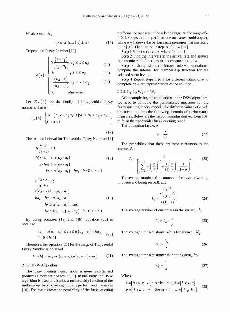
2.2.2. DSW Algorithm The fuzzy queuing theory model is more realistic and
produces a more refined result [19]. In this study, the DSW algorithm is used to describe a membership function of the multi-server fuzzy queuing model’s performance measures [10]. The α-cut shows the possibility of the fuzzy queuing
performance measure in the related range. At the range of α = 0, it shows that the performance measures could appear, while α = 1 shows the performance measures that are likely to be [20]. There are four steps to follow [21]:
Step 1 Select α cut value where 0 ≤ α ≤ 1. Step 2 Find the intervals in the arrival rate and service
rate membership functions that correspond to this α. Step 3 Using standard binary interval operations,
compute the interval for membership function for the selected α-cut levels.
Step 4 Repeat steps 1 to 3 for different values of α to complete an α-cut representation of the solution.
2.2.3. Lq, Ls, Wq and Ws
After completing the calculations in the DSW algorithm, we need to compute the performance measures for the fuzzy queuing theory model. The different values of α will be substituted into the following formula of performance measures. Below are the lists of formulas derived from [16] to form the trapezoidal fuzzy queuing model.
The utilization factor, ρ
(22)
The probability that there are zero customers in the system, :
(23)
The average number of customers in the system (waiting in queue and being served), Lq :
(24)
The average number of customers in the system,
(25)
The average time a customer waits for service,
(26)
The average time a customer is in the system,
(27)
Where
[ ] [ ][ ] [ ]
, : Arrival rate, , , ,
, : Service rate, , , ,
= + − =
= + − =
x b e b c d e
y f i f g h i
α α λ
α α µ (28)
( )
( )( )
( )( )
≤ ≤
≤ ≤
≤ ≤
x - a1h ,a x a1 2a - a2 1h ,a x a 1 2A x =
a - x4h ,a x a43a - a4 30 ,otherwise
( )TNF h
α
( ) ( )( )( ) for
≥
≥ α
≥ α
≥ α + ≤ ≤
1
0 1
1
2 1
1 2 1
1 2 1
2 1 1
x - ah
a - ah x - a a - a
hx - ha a - a
hx a - a ha h
( ) ( )( )( )
( ) for
4
4 3
4 4 3
4 4 3
4 3 4
4 4 3
a - xh
a - ah a - x a - a
ha hx a - a
-hx a - a ha
hx ha a - a h
≥
≥ α
− ≥ α
≥ α −
≤ − α ≤ ≤
1
0 1
( ) ( ) ( ){ }4 4 3 2 1 1, TNF h ha a a a a ha= − − − +α α
=xsy
ρ
0P
01
0
1
1 1 1! ! 1
−
=
= + − ∑
n ss
n
Px x
n y s y ρ
( )
0
2! 1
=−
s
q
x Py
Ls
ρ
ρ
sL
= +s qxL Ly
Wq
LW
x
Ws
= ss
LW
x
20 Comparison of Queuing Performance Using Queuing Theory Model and Fuzzy Queuing Model at Check-in Counter in Airport
Both arrival and service rates are represented as trapezoidal fuzzy numbers. The trapezoidal fuzzy numbers are represented as and respectively. The minimum and maximum for arrival rate,
are represented by [b,e], whereas for service rate the minimum and maximum are represented by [f,i].
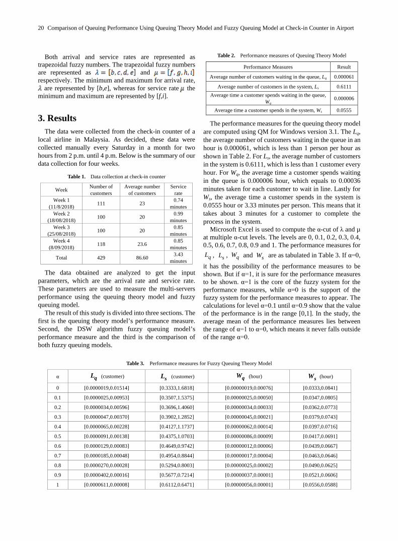
3. Results The data were collected from the check-in counter of a
local airline in Malaysia. As decided, these data were collected manually every Saturday in a month for two hours from 2 p.m. until 4 p.m. Below is the summary of our data collection for four weeks.
Table 1. Data collection at check-in counter
Week Number of customers
Average number of customers
Service rate
Week 1 (11/8/2018) 111 23 0.74
minutes Week 2
(18/08/2018) 100 20 0.99 minutes
Week 3 (25/08/2018) 100 20 0.85
minutes Week 4
(8/09/2018) 118 23.6 0.85 minutes
Total 429 86.60 3.43 minutes
The data obtained are analyzed to get the input parameters, which are the arrival rate and service rate. These parameters are used to measure the multi-servers performance using the queuing theory model and fuzzy queuing model.
The result of this study is divided into three sections. The first is the queuing theory model’s performance measure. Second, the DSW algorithm fuzzy queuing model’s performance measure and the third is the comparison of both fuzzy queuing models.
Table 2. Performance measures of Queuing Theory Model
Performance Measures Result
Average number of customers waiting in the queue, Lq 0.000061
Average number of customers in the system, Ls 0.6111 Average time a customer spends waiting in the queue,
Wq 0.000006
Average time a customer spends in the system, Ws 0.0555
The performance measures for the queuing theory model are computed using QM for Windows version 3.1. The Lq, the average number of customers waiting in the queue in an hour is 0.000061, which is less than 1 person per hour as shown in Table 2. For Ls, the average number of customers in the system is 0.6111, which is less than 1 customer every hour. For Wq, the average time a customer spends waiting in the queue is 0.000006 hour, which equals to 0.00036 minutes taken for each customer to wait in line. Lastly for Ws, the average time a customer spends in the system is 0.0555 hour or 3.33 minutes per person. This means that it takes about 3 minutes for a customer to complete the process in the system.
Microsoft Excel is used to compute the α-cut of λ and µ at multiple α-cut levels. The levels are 0, 0.1, 0.2, 0.3, 0.4, 0.5, 0.6, 0.7, 0.8, 0.9 and 1. The performance measures for
, , and are as tabulated in Table 3. If α=0,
it has the possibility of the performance measures to be shown. But if α=1, it is sure for the performance measures to be shown. α=1 is the core of the fuzzy system for the performance measures, while α=0 is the support of the fuzzy system for the performance measures to appear. The calculations for level α=0.1 until α=0.9 show that the value of the performance is in the range [0,1]. In the study, the average mean of the performance measures lies between the range of α=1 to α=0, which means it never falls outside of the range α=0.
Table 3. Performance measures for Fuzzy Queuing Theory Model
α (customer) (customer) (hour) (hour)
0 [0.0000019,0.01514] [0.3333,1.6818] [0.00000019,0.00076] [0.0333,0.0841]
0.1 [0.0000025,0.00953] [0.3507,1.5375] [0.00000025,0.00050] [0.0347,0.0805]
0.2 [0.0000034,0.00596] [0.3696,1.4060] [0.00000034,0.00033] [0.0362,0.0773]
0.3 [0.0000047,0.00370] [0.3902,1.2852] [0.00000045,0.00021] [0.0379,0.0743]
0.4 [0.0000065,0.00228] [0.4127,1.1737] [0.00000062,0.00014] [0.0397,0.0716]
0.5 [0.0000091,0.00138] [0.4375,1.0703] [0.00000086,0.00009] [0.0417,0.0691]
0.6 [0.0000129,0.00083] [0.4649,0.9742] [0.00000012,0.00006] [0.0439,0.0667]
0.7 [0.0000185,0.00048] [0.4954,0.8844] [0.00000017,0.00004] [0.0463,0.0646]
0.8 [0.0000270,0.00028] [0.5294,0.8003] [0.00000025,0.00002] [0.0490,0.0625]
0.9 [0.0000402,0.00016] [0.5677,0.7214] [0.00000037,0.00001] [0.0521,0.0606]
1 [0.0000611,0.00008] [0.6112,0.6471] [0.00000056,0.00001] [0.0556,0.0588]
qL sL qW sW
qL sL qW sW
Mathematics and Statistics 7(4A): 17-23, 2019 21
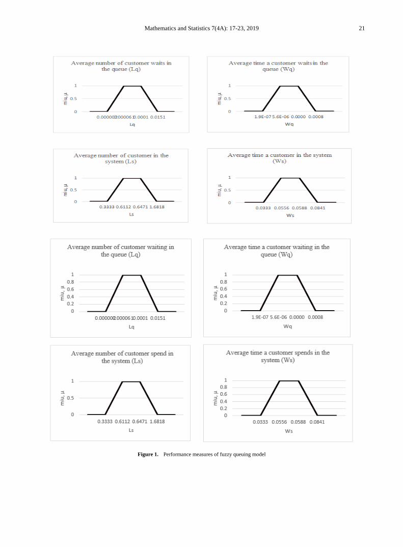
Figure 1. Performance measures of fuzzy queuing model

22 Comparison of Queuing Performance Using Queuing Theory Model and Fuzzy Queuing Model at Check-in Counter in Airport
The graphs of membership function of , ,
and for the fuzzy queuing model with trapezoidal fuzzy number is shown in Figure 1. The performance measures fall between range of α=1 and never falls outside the range of α=0. The range for the average number of customers waiting in the queue is between 0.000002 and 0.0151. At α=0, it will lie between 0.0000002 and 0.0151 while for α=1, the range is between 0.000061 and 0.0001. Hence, it shows that the number of customers waiting in the queue is less than 1 per hour. The range for the average number of customers in the system is between 0.3333 and 1.6818. At α=0, it will lie between 0.3333 and 1.6818 while for α=1, the range is between 0.6112 and 0.6471. Hence, the value of α-cut values is less than 1 which shows that the number of customers in the system is more than 1 customer per hour. The range for the average time a customer waits in the system is between 0.00000019 and 0.00076 hour. At α=0, it will lie between 0.00000019 and 0.00076 while for α=1, the range is between 0.00000056 and 0.00001. Hence, it shows that the time a customer waits in the queue is less than 1 minute per customer. The range for the average time a customer spends in the system is between 0.3333 and 0.0841 hour. At α=0, it will lie between 0.3333 and 0.0841 while for α=1, the range is between 0.0556 and 0.0588. Hence, it shows that the time a customer spends in the system is more than 1 minute per customer.
4. Discussion Table 4. Comparison performance measures between the Queuing Theory Model and Fuzzy Queuing Model
Performance Measures Queuing Theory Model Fuzzy Queuing, α = 1
0.000061 [0.0000611,0.00008]
0.6111 [0.6112,06471]
0.000006 hour (0.00036 minutes) [0.00000056,0.00001]
0.0555 hour (3.33 minutes) [0.0556,0.0588]
Based on the table above, the performance measures for the queuing theory model is compatible with the fuzzy queuing model. The queuing theory model and fuzzy queuing model show that Lq is approximately less than 1 customer queuing in the waiting line, Ls is approximately less than 1 customer queuing in the system, Wq is the customer waiting less than 1 minute in the waiting line, and Ws is the customer waiting more than 1 minute in the system. The values of Lq, Ls, Wq and Ws for the queuing theory model lie in the fuzzy queuing model range value for α=1. Hence, the results of performance measures for the queuing theory model and fuzzy queuing model show both
models are equivalent. Since the value of queuing theory model obtained are lay in the range of performance measures of fuzzy queuing model. Therefore, it shows the result obtained is consistent.
5. Conclusions In this study, the result shows that the performance
measures Lq, Ls, Wq and Ws for both Queuing Theory Model and Fuzzy Queuing Model were computed and compared. Based on the result, the Fuzzy Queuing Model is much more effective and efficient to measure the performance of multi-server in a queuing system since the Fuzzy set theory is more easily adaptable compared to other theories [6]. Garai and Garg (2019) stated that the vagueness or uncertainty situation can be solve using fuzzy model [22]. Applying the Fuzzy queuing model provides broader information, which will be very useful in defining a queuing system. Thus, this study concludes that fuzzy queuing is one of the alternative ways to compute the performance measures since the information obtained from the application is much easier to understand and interpret. Therefore, the Fuzzy Queuing Model is an alternative way to measure the performance of multi-server in a queuing system.
REFERENCES B. T. Taylor. Introduction To Management Science, [1]
England : Pearson Education Limited, 2016.
N. Amit, N. A. Ghazali. Using simulation model queuing [2]problem at a fast-food restaurant, In: Regional Conference on Science Technology and Social Sciences (RCSTSS), 1055-1062, Singapore:Springer , 2018.
A. B. N. Yakubu, U. Najim. An application of queuing [3]theory to ATM service optimization: A case study, Mathematical Theory and Modelling, 11-23, 2014.
M. J. Pardo, D. Fuenta. Optimizing a priority-discipline [4]queuing model using fuzzy set theory. Computers and Mathematics with Applications, Vol.54, 267-281, 2007.
B. Vahdani, R. Tavakkoli-Moghaddam, F. Jolai. Reliable [5]design of a logistics network under uncertainty: A fuzzy possibilistic-queuing model, Applied Mathematical Modelling, Vol.37, No.5, 3254-3268, 2013.
T. Ebrahim, M. Ali, G. Iman, A. Hadi, F. Mehdi. Optimizing [6]multi supplier systems with fuzzy queuing approach: Case study of SAPCO, International MultiConference of Engineers and Computer Scientists, 1-7, 2011.
S. Meng, D. Wu, Z. Huimin, L. Bo, W. Chunxiao. Study on [7]an airport gate assignment method based on improved ACO algorithm. Emerald Insight, 20-43, 2018.
Aydin, Ozlem, A. Apaydin. Multi-channel fuzzy queuing [8]systems and membership functions of related fuzzy services
qL sL qW
sW
qL
sL
qW
sW
qL
sL
qW
sW

Mathematics and Statistics 7(4A): 17-23, 2019 23
and fuzzy inter-arrival times, Asia-Pacific Journal of Operational Research, Vol.25, No.5, 697–713, 2008.
N. Sujatha, V. S. Murthy Akella, G. V. S. Deekshitulu. [9]Analysis of multiple server fuzzy queueing model using α – cuts. International Journal of Mechanical Engineering and Technology (IJMET), Vol.8, No.10, 35–41, 2017.
S. Thamotharan. A study on multi server fuzzy queuing [10]model in triangular and trapezoidal fuzzy numbers using cuts, Vol.5, No.1, 226–230, 2016.
J. Kingman. The first Erlang century—and the next. [11]Queueing Systems, 63(1-4), 3, 2009.
L. A. Zadeh. A note on prototype theory and fuzzy sets. [12]587-593, 1965.
J. J. Buckley. Elementary queueing theory based on [13]possibility theory, Journal Fuzzy Sets and Systems, Vol.37, No.1, 43 – 52, 1990
M. Meenu, T. P. Singh, G. Deepak. Threshold effect on a [14]fuzzy queue model with batch arrival, Arya Bhatta Journal of Mathematics and Informatics,Vol.7, No.1, 109- 118, 2015.
S. Shanmugasundaram, S. Thamotharan, M. Ragapriya. A [15]study on single server fuzzy queuing model using DSW algorithm, International Journal of Latest Trends in Engineering and Technology (IJLTET), Vol.6, No.1, 162–169, 2015.
S. Thamotharan. A study on multi server fuzzy queuing [16]model triangular and trapezoidal fuzzy number using α-cuts, International Journal of Sciences and Research (IJSR), 226-230, 2014.
S. Shanmugasundaram, B. Venkatesh. Multi–server fuzzy [17]queueing model using DSW algorithm, Global Journal of Pure and Applied Mathematics, Vol.11, No.1, 45-51, 2015.
B. Farhadinia, A. I. Ban. Developing new similarity [18]measures of generalized intuitionistic fuzzy numbers and generalized interval-valued fuzzy numbers from similarity measures of generalized fuzzy numbers, Mathematical and Computer Modelling, 57(3-4), 812-825, 2013.
E. Lee, R. J. Li. Comparison of fuzzy numbers based on the [19]probability measure of fuzzy events. Computers & Mathematics with Applications, Vol.15, No.10, 887-896, 1988.
R. Srinivasan. Fuzzy queueing model using DSW algorithm, [20]International Journal of Advanced Research in Mathematics and Applications, Vol.1, No.1, 57–62, 2014.
A. Boissonnade, W. Dong, H. Shah, F. Wong. Identification [21]of fuzzy systems in civil engineering, Proc. lnternat. Syrup. on Fuzzy Mathematics and Earthquake Research, 48-71, 1985.T. Garaj, H. Garg, Multi-objective linear fractional inventory model with possibility and necessity constraints under generalized intuitionistic fuzzy set environment, CAAI Transactions on Intelligence Technology, 2019, doi: 10.1049/trit.2019.0030”
Mathematics and Statistics 7(4A): 24-28, 2019 http://www.hrpub.org DOI: 10.13189/ms.2019.070704
Performance of Classification Analysis: A Comparative Study between PLS-DA and Integrating PCA+LDA
Nurazlina Abdul Rashid*, Wan Siti Esah Che Hussain, Abd Razak Ahmad,Fatihah Norazami Abdullah
Faculty of Computer and Mathematical Sciences, Universiti Teknologi MARA, Malaysia
Received July 1, 2019; Revised September 6, 2019; Accepted September 21, 2019
Copyright©2019 by authors, all rights reserved. Authors agree that this article remains permanently open access under the terms of the Creative Commons Attribution License 4.0 International License
Abstract Classification methods are fundamental techniques designed to find mathematical models that are able to recognize the membership of each object to its proper class on the basis of a set of measurements. The issue of classifying objects into groups when variables in an experiment are large will cause the misclassification problems. This study explores the approaches for tackling the classification problem of a large number of independent variables using parametric method namely PLS-DA and PCA+LDA. Data are generated using data simulator; Azure Machine Learning (AML) studio through custom R module. The performance analysis of the PLS-DA was conducted and compared with PCA+LDA model using different number of variables (p) and different sample sizes (n). The performance of PLS-DA and PCA+LDA has been evaluated based on minimum misclassification rate. The results demonstrated that PLS-DA performed better than the PCA+LDA for large sample size. PLS-DA can be considered to have a good and reliable technique to be used when dealing with large datasets for classification task.
Keywords Classification Analysis, Large Variable, PCA+LDA, Performance, PLS-DA
1. IntroductionClassification method not only plays a role as a classifier
but also acts as a predictive and descriptive model as well as discriminative variable selection. The purpose of classification is to achieve a minimum classification rate. Classification methods can be grouped into three; parametric, non-parametric and semi-parametric methods. According to [14] parametric methods are more reliable than non-parametric method as all the data must be normally distributed and exhibit a bell-shaped curve. Examples of parametric method used for classification
frequently are Quadratic Discriminant Analysis (QDA), Partial Least Square Discriminant Analysis (PLS-DA) and Linear Discriminant Analysis (LDA).
In contrast, the non-parametric method is a flexible method than parametric method because it is robust to the distribution of data [18]. For instance, k-Nearest Neighbour (KNN), decision trees (CART) and survival analysis [3] make no assumptions on data distribution. Meanwhile, semi-parametric method is a combination between parametric and non-parametric methods. According to [9] semi-parametric method achieved greater precision than nonparametric models but with weaker assumptions than parametric models. Semi-parametric estimators can possess better-operating characteristics in small sample sizes due to smaller variance than non-parametric estimators [20]. Logistic discriminant analysis is an example of semi-parametric method [12].
This study focuses on parametric methods only which are LDA and PLS-DA. This method was chosen because LDA works efficiently when the assumption of equal population covariance structures for groups are satisfied and the independent variables follow multivariate normal distribution [16]. Then, PLS-DA has demonstrated great success in modeling high-dimensional datasets for the past two decades [5, 17].
1.1. Classification Problems
Large variables will be highly computational and suffer from the curse of dimensionality, which is caused by the exponential increase in volume associated with adding extra dimensions to mathematical space. According to [2] the existence of irrelevant variables will cause misclassification problems. Multicollinearity exists when the measured variables are large and correlated to each other. Multicollinearity can affect the standard error of parameter estimates may be unreasonably large, parameter estimates not significant, and parameter estimates may
Mathematics and Statistics 7(4A): 24-28, 2019 25
have a significantly different from what is expected [1]. According to [4] variable selection and reduction is the best solution to reduce the problem of multicollinearity. No dimensionality reduction technique is universally better than others. Depending on the dataset characteristics, one method may provide a better approximation of a dataset than the other techniques.
1.2. Classification Techniques
Principal component analysis (PCA) is a variable reduction technique in order to reduce a complex dataset to a lower-dimensional subspace. PCA helps to compress the data without much loss of information [6]. After conducting PCA, LDA model was constructed for classification purposes. LDA is a well-known scheme for dimension reduction and it is intended for classification problems where the output variable is categorical. Hence, it has been successfully used as a statistical tool of origin method in several classification problems [7]. According to [15], the weakness of this technique is that it cannot perform well when the dataset consists of a large number of variables relative to the amount of measurements taken.
For this study, we will use PCA to deal with a very large number of variables. Then, LDA model constructed for classification purpose for first model. The past studies showed that PCA and LDA were popular methods for variable reduction and classification. This study intends to integrate PCA and LDA for a large number of variables and perform classification task using the reduced set of variables resulting in PCA.
PLS-DA can be thought as a “supervised” version of Principal Component Analysis (PCA). Partial Least-Squares Discriminant Analysis (PLS-DA) is a multivariate dimensionality-reduction tool and classifier [17]. It is reported that PLS-DA can be effective both as a variable reduction and as well as a classifier for a large number of variables.
In addition, PLS-DA outperforms in modeling high-dimensional datasets for classification task.
Hence, the objective of this study is to make comparison between the performance of PCA+LDA and PLS-DA on variable reduction. PCA will be used to perform variable reduction and then integrate with LDA to construct classification task. The PLS-DA will be used in data reduction and perform classification task. The performance of PCA+LDA and PLS-DA for the various number of simulation dataset is accessed based on misclassification rates.
2. Materials and Methods
2.1. Data Generation
Data are generated using data simulator; Azure
Machine Learning (AML) studio through custom R module. Performance analysis is conducted using the different number of independent variables (p) and number of sample size (n). The number of independent variables considered for sample n = 30 are p = 10, p = 30, p = 50, p = 100, p = 200, then n = 100 are p = 10, p = 30, p = 50, p = 100, p = 200 and finally n = 150 are p = 10, p = 30, p = 50, p = 100, p = 200. In order to measure the performance of PLS-DA and PCA+LDA, fifteen datasets were simulated.
2.2. Computational of PCA
The PCA algorithm calculates the first principal component along the first eigenvector, by minimizing the projection error (i.e., by minimizing the average squared distance from each data to its projection on the principal component or maximizing the variance of the projected data). After that, the algorithm iteratively projects all the points to a subspace orthogonal to the last principal component and then repeats the process on the projected points, thus constructing an orthonormal basis of eigenvectors and principal components. An alternative formulation is that the principal component vectors are given by the eigenvectors of the non-singular portion of the covariance matrix C, given by:
(1)
Where;
Cn is n*n centering matrix
(2)
2.2. Construction of LDA
The LDA model is constructed from a reduced set of variables resulting from the procedures of PCA using following steps: Estimate means for (π1) and (π2) using
ny
i∑=µ
based on reduced set of variables. Compute homogeneous covariance matrix using
∑−
−
−∑
=1
)2
(11n
myy µµ
Estimate prior probabilities for (π1) and (π2) by
nn
i1=ρ
Construct LDA model using equation (3)
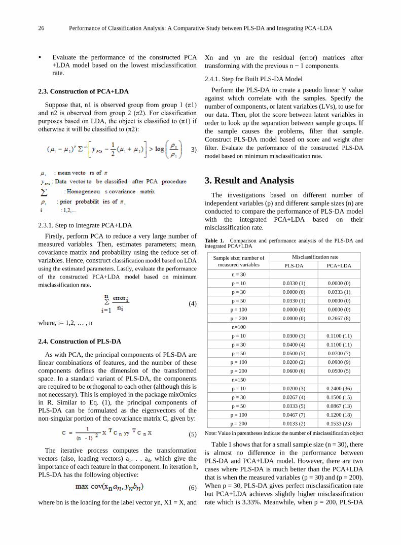
26 Performance of Classification Analysis: A Comparative Study between PLS-DA and Integrating PCA+LDA
Evaluate the performance of the constructed PCA +LDA model based on the lowest misclassification rate.
2.3. Construction of PCA+LDA
Suppose that, n1 is observed group from group 1 (π1) and n2 is observed from group 2 (π2). For classification purposes based on LDA, the object is classified to (π1) if otherwise it will be classified to (π2):
3)
2.3.1. Step to Integrate PCA+LDA Firstly, perform PCA to reduce a very large number of
measured variables. Then, estimates parameters; mean, covariance matrix and probability using the reduce set of variables. Hence, construct classification model based on LDA using the estimated parameters. Lastly, evaluate the performance of the constructed PCA+LDA model based on minimum misclassification rate.
(4)
where, i= 1,2, … , n
2.4. Construction of PLS-DA
As with PCA, the principal components of PLS-DA are linear combinations of features, and the number of these components defines the dimension of the transformed space. In a standard variant of PLS-DA, the components are required to be orthogonal to each other (although this is not necessary). This is employed in the package mixOmics in R. Similar to Eq. (1), the principal components of PLS-DA can be formulated as the eigenvectors of the non-singular portion of the covariance matrix C, given by:
(5)
The iterative process computes the transformation vectors (also, loading vectors) a1. . . ad, which give the importance of each feature in that component. In iteration h, PLS-DA has the following objective:
(6)
where bn is the loading for the label vector yn, X1 = X, and
Xn and yn are the residual (error) matrices after transforming with the previous n − 1 components.
2.4.1. Step for Built PLS-DA Model Perform the PLS-DA to create a pseudo linear Y value
against which correlate with the samples. Specify the number of components, or latent variables (LVs), to use for our data. Then, plot the score between latent variables in order to look up the separation between sample groups. If the sample causes the problems, filter that sample. Construct PLS-DA model based on score and weight after filter. Evaluate the performance of the constructed PLS-DA model based on minimum misclassification rate.
3. Result and Analysis The investigations based on different number of
independent variables (p) and different sample sizes (n) are conducted to compare the performance of PLS-DA model with the integrated PCA+LDA based on their misclassification rate.
Table 1. Comparison and performance analysis of the PLS-DA and integrated PCA+LDA
Sample size; number of measured variables
Misclassification rate PLS-DA PCA+LDA
n = 30 p = 10 0.0330 (1) 0.0000 (0) p = 30 0.0000 (0) 0.0333 (1) p = 50 0.0330 (1) 0.0000 (0)
p = 100 0.0000 (0) 0.0000 (0) p = 200 0.0000 (0) 0.2667 (8) n=100 p = 10 0.0300 (3) 0.1100 (11) p = 30 0.0400 (4) 0.1100 (11) p = 50 0.0500 (5) 0.0700 (7)
p = 100 0.0200 (2) 0.0900 (9) p = 200 0.0600 (6) 0.0500 (5) n=150 p = 10 0.0200 (3) 0.2400 (36) p = 30 0.0267 (4) 0.1500 (15) p = 50 0.0333 (5) 0.0867 (13)
p = 100 0.0467 (7) 0.1200 (18) p = 200 0.0133 (2) 0.1533 (23)
Note: Value in parentheses indicate the number of misclassification object
Table 1 shows that for a small sample size (n = 30), there is almost no difference in the performance between PLS-DA and PCA+LDA model. However, there are two cases where PLS-DA is much better than the PCA+LDA that is when the measured variables (p = 30) and (p = 200). When p = 30, PLS-DA gives perfect misclassification rate but PCA+LDA achieves slightly higher misclassification rate which is 3.33%. Meanwhile, when p = 200, PLS-DA

Mathematics and Statistics 7(4A): 24-28, 2019 27
gives perfect misclassification rate while PCA+LDA provides much greater misclassification rate with 26.67%.
For larger sample size (n = 100), the performance of PLS-DA is improved significantly than PCA+LDA for all cases except case of p = 200 where there is 1% difference misclassification rate between PLS-DA and PCA+LDA.
Finally, for large sample size (n = 150), the performance of PLS-DA is greatly improved than PCA+LDA for all cases. The results indicate small misclassification rate under PLS-DA compared to PCA+LDA. In particular, when p = 10, PLS-DA obtains 2.0% misclassification rate while PCA+LDA shows much higher misclassification rate of 24.0%. In other words, PLS-DA has misclassified only 3 out of 150 objects while PCA+LDA misclassified 36 objects for the same condition. These results demonstrated that PLS-DA plays an important role in dealing with a large number of variables. However, there is no significant difference between PLS-DA and PCA+LDA performance for smaller sample size. The discussion of the results based on the relationship between sample size and independent variables can be summarized as follows: For smaller sample size (n = 30). When p gets larger
generally misclassification rate of PLS-DA gets smaller. In fact, PLS-DA performs better than PCA+LDA model, for larger p.
For sample size, (n = 100).PLS-DA performed better than PCA+LDA. In almost all cases, the misclassification rate of PLSDA are less than 6.0% compared to PCA+LDA > 7.0%.
For large sample (n=150), the performance of PLS-DA is consistent and better than PCA+LDA in all cases. Hence, produce better model.
Regardless of the fact that sample size of the performance of PLS-DA is always better than PCA+LDA especially when number of variables (p) is equal to number of sample size (n).
PLS-DA model show better performance for large sample size in most cases.
This finding is consistent with the result of [17], where PLS-DA outperformed PCA+LDA when dealing with large sample size
4. Conclusions and Future Work As the sample size gets larger, the misclassification rate
becomes smaller for the PLS-DA. On the other hand, PCA+LDA are inconsistent. In conclusion, the entire results revealed that PLS-DA highly recommend for a large sample size than PCA+LDA in dimension reduction and classification. PLS-DA can be considered to have a good and reliable technique to be used when dealing with large datasets for classification task. The future work might include the real dataset to make comparison between the performance of PCA+LDA and PLS-DA on large variable dataset.
Acknowledgement The research would like to thank Research and
Industrial Linkage Division UiTM Kedah for financial support to publish this paper.
Appendix str(data1)
X <- (data2[,3:203])
Y <- as.factor(data2$Status)
## if training is perfomed on 4/5th of the original data
samp <- sample(1:2, nrow(X), replace = TRUE)
test <- which(samp == 1) # testing on the first fold
train <- setdiff(1:nrow(X), test)
plsda.train <- plsda(X[train, ], Y[tra VCin], ncomp = 2)
test.predict <- predict(plsda.train, X[test, ], dist =
"max.dist")
Prediction <- test.predict$class$max.dist[, 2]
cbind(Y = as.character(Y[test]), Prediction)
LDA tr <- sample(1:50, 25)
train <- rbind(iris3[tr,,1], iris3[tr,,2], iris3[tr,,3])
test <- rbind(iris3[-tr,,1], iris3[-tr,,2], iris3[-tr,,3])
cl <- factor(c(rep("s",25), rep("c",25), rep("v",25)))
z <- lda(train, cl)
predict(z, test)$class
PCA+LDA Running PCA using covariance matrix:
wdbc.pcov <- princomp(wdbc.data, scores = TRUE)
summary(wdbc.pcov)
Running PCA using correlation matrix:
wdbc.pr <- prcomp(wdbc.data, scale = TRUE, center =
TRUE)
summary(wdbc.pr)
LDA from six PCA extract 6pca
wdbc.pcs <- wdbc.pr$x[,1:6]
wdbc.pcst <- cbind(wdbc.pcs, diagnosis)
head(wdbc.pcst)
28 Performance of Classification Analysis: A Comparative Study between PLS-DA and Integrating PCA+LDA
> Y <- as.factor(data2$dataLabel)
> X <- (data2[,2:102])
> samp <- sample(1:2, nrow(X), replace = TRUE)
> test <- which(samp == 1) # testing on the first fold
> train <- setdiff(1:nrow(X), test)
> pca.train <-pca(X[train,],2,TRUE)
REFERENCES Adeboye, N. O., Fagoyinbo, I. S., & Olatayo, T. O. (2014). [1]
Estimation of the effect of multicollinearity on the standard error for regression coefficients. IOSR Journal of Mathematics, 10(4), 16-20.
Breiman, L. (2017). Classification and regression trees. [2]Routledge.
Cole, S. R., & Hudgens, M. G. (2010). Survival analysis in [3]infectious disease research: describing events in time. AIDS (London, England), 24(16), 2423.
Ghosh, J., & Ghattas, A. E. (2015). Bayesian variable [4]selection under collinearity. The American Statistician, 69(3), 165-173.
Gromski, P. S., Muhamadali, H., Ellis, D. I., Xu, Y., Correa, [5]E., Turner, M. L., & Goodacre, R. (2015). A tutorial review: Metabolomics and partial least squares-discriminant analysis–a marriage of convenience or a shotgun wedding. Analytica chimica acta, 879, 10-23.
He, Y., Feng, S., Deng, X., & Li, X. (2006). Study on [6]lossless discrimination of varieties of yogurt using the Visible/NIR-spectroscopy. Food Research International, 39(6), 645-650.
Keogh, E., & Mueen, A. (2011). Curse of dimensionality. In [7]Encyclopedia of machine learning (pp. 257-258). Springer, Boston, MA.
Kim-Anh Le Cao, Florian Rohart, Ignacio Gonzalez, [8]Sebastien Dejean, Benoit Gautier, and Francois Bartolo. mixOmics: Omics data integration project. R package, version, 2017
Kim, G., Silvapulle, M. J., & Silvapulle, P. (2007). [9]Comparison of semiparametric and parametric methods for estimating copulas. Computational Statistics & Data Analysis, 51(6), 2836-2850.
Loong Chuen Lee, Choong-Yeun Liong and Abdul Aziz [10]Jemain (2018) Partial least squares-discriminant analysis (PLS-DA) for classification of high-dimensional (HD) data: a review of contemporary practice strategies and knowledge gaps. Analyst, 2018,143, 3526-3539
Mario Fordellone, Andrea Bellincontro, and Fabio [11]Mencarelli,(2018), Partial least squares discriminant analysis: A dimensionality reduction method to classify hyperspectral data, arXiv.org > stat > arXiv:1806.09347v1.
Maroco, J., Silva, D., Rodrigues, A., Guerreiro, M., Santana, [12]
I., & de Mendonça, A. (2011). Data mining methods in the prediction of Dementia: A real-data comparison of the accuracy, sensitivity and specificity of linear discriminant analysis, logistic regression, neural networks, support vector machines, classification trees and random forests. BMC research notes, 4(1), 299.
Moncayo, S., Manzoor, S., Navarro-Villoslada, F., & [13]Caceres, J. O. (2015). Evaluation of supervised chemometric methods for sample classification by Laser Induced Breakdown Spectroscopy. Chemometrics and Intelligent Laboratory Systems, 146, 354-364.
Neideen, T., & Brasel, K. (2007). Understanding statistical [14]tests. Journal of surgical education, 64(2), 93-96.
N.A. Rashid, A. H. A.Rahim, I.-N. M. Nasir. S.hussin. A.-R. [15]Ahmad. (2017) Classifying Bankruptcy of Small and Medium Sized Enterprises with Partial Least Square Discriminant Analysis. Proceedings of the International Conference on Computing, Mathematics and Statistics (ICMS), 315-323.
Okwonu, F. Z., & Othman, A. R. (2012). A model [16]classification technique for linear discriminant analysis for two groups. International Journal of Computer Science Issues (IJCSI), 9(3), 125.
Perez, D. R., & Narasimhan, G. (2017). So you think you can [17]PLS-DA. bioRxiv, 207225.
Reimann, C., Filzmoser, P., Garrett, R. G., & Dutter, R. [18](2008). Statistical data analysis explained: applied environmental statistics with R (No. Sirsi) i9780470985816). Chichester: Wiley.
Szymańska, E., Gerretzen, J., Engel, J., Geurts, B., Blanchet, [19]L., & Buydens, L. M. (2015). Chemometrics and qualitative analysis have a vibrant relationship. TrAC Trends in Analytical Chemistry, 69, 34-51.
Wey, A., Connett, J., & Rudser, K. (2015). Combining [20]parametric, semi-parametric, and non-parametric survival models with stacked survival models. Biostatistics, 16(3), 537-549.

Mathematics and Statistics 7(4A): 29-40, 2019 http://www.hrpub.org DOI: 10.13189/ms.2019.070705
Application of ARIMAX Model to Forecast Weekly Cocoa Black Pod Disease Incidence
Ling, A. S. C.1,*, Darmesah, G.2, Chong, K. P.2, Ho, C. M.2
1Malaysian Cocoa Board, Wisma SEDCO, Locked Bag 211, 88999 Kota Kinabalu, Sabah, Malaysia 2Faculty of Science and Natural Resources, Universiti Malaysia Sabah, Jalan UMS, 88400 Kota Kinabalu, Sabah, Malaysia
Received July 1, 2019; Revised September 8, 2019; Accepted September 23, 2019
Copyright©2019 by authors, all rights reserved. Authors agree that this article remains permanently open access under the terms of the Creative Commons Attribution License 4.0 International License
Abstract The losses caused by cocoa black pod disease around the world exceeded $400 million due to inaccurate forecasting of cocoa black pod disease incidence which leads to inappropriate spraying timing. The weekly cocoa black pod disease incidence is affected by external factors, such as climatic variables. In order to overcome this inaccuracy of spraying timing, the forecasting disease incidence should consider the influencing external factors such as temperature, rainfall and relative humidity. The objective of this study is to develop a Autoregressive Integrated Moving Average with external variables (ARIMAX) model which tries to account the effects due to the climatic influencing factors, to forecast the weekly cocoa black pod disease incidence. With respect to performance measures, it is found that the proposed ARIMAX model improves the traditional Autoregressive Integrated Moving Average (ARIMA) model. The results of this forecasting can provide benefits especially for the development of decision support system in determine the right timing of action to be taken in controlling the cocoa black pod disease.
Keywords ARIMAX, Black Pod, Climate, Cocoa, Forecasting
1. IntroductionBlack pod or Phytophthora pod rot is the most
economically important and widespread disease of cocoa, Theobroma cacao L. in Malaysia. The losses due to Phytophthora exceed $400 million worldwide [1]. Among the Phytophthora spesies which attacked the cocoa, Phytophthora palmivora is the most widely distributed in the world and it caused global yield loss of 20-30% and tree deaths of 10% annually [1]. The intensity of black pod disease in cocoa was influenced by numerous climatic
parameters such as rainfall, temperature and high humidity as reported by Thorold [2,3], Dakwa [4], Wood [5] and Mpika [6]. Both rainfall and relative humidity has strong correlation which encourages pathogen sporulation by reproduction of zoospores to infect the cocoa pods while the optimum temperature is propitious to black pod symptom development [2-6]. It is important to quantify the black pod disease fluctuations due to the real effect of climatic parameters. Understanding the effect of the climatic variables on the cocoa black pod incidence can identifying the suitable management options such as fungicide spraying and culture practices to control the disease incidence under projected climate change scenario. The time-fractional partial differential equation was widely used in study the mathematical biology including the description of plant disease epidemic [7] but need the numerical approach to solve the equation. Another approach was developing the time series model especially auto-regressive moving average (ARIMA) described by Box and Jenkins [8] that widely used in forecasting where it used the historical sequences of observations to do the forecasting. In agriculture, ARIMA model used to forecast the annual production of several crop in countries that relied the crop for daily life or economy, for example production of rice [9], wheat [10], coffee [11] and cocoa [12].
As for the disease monitoring program, ARIMA model was used to predict Botrytis cinerea spore concentrations that caused grey mould in Spain and assist in deciding number of treatments needed [13]. In cocoa, it is very useful in forecasting the cocoa black pod incidence to understand the effect of previous incidence on the current incidence. However, ARIMA model along can’t quantify the effect of climate variables on the cocoa black pod disease incidence and help in decision making process. The key problem is how to incorporate the climate information into the forecasting process and subsequently into the decision making process. When an ARIMA model
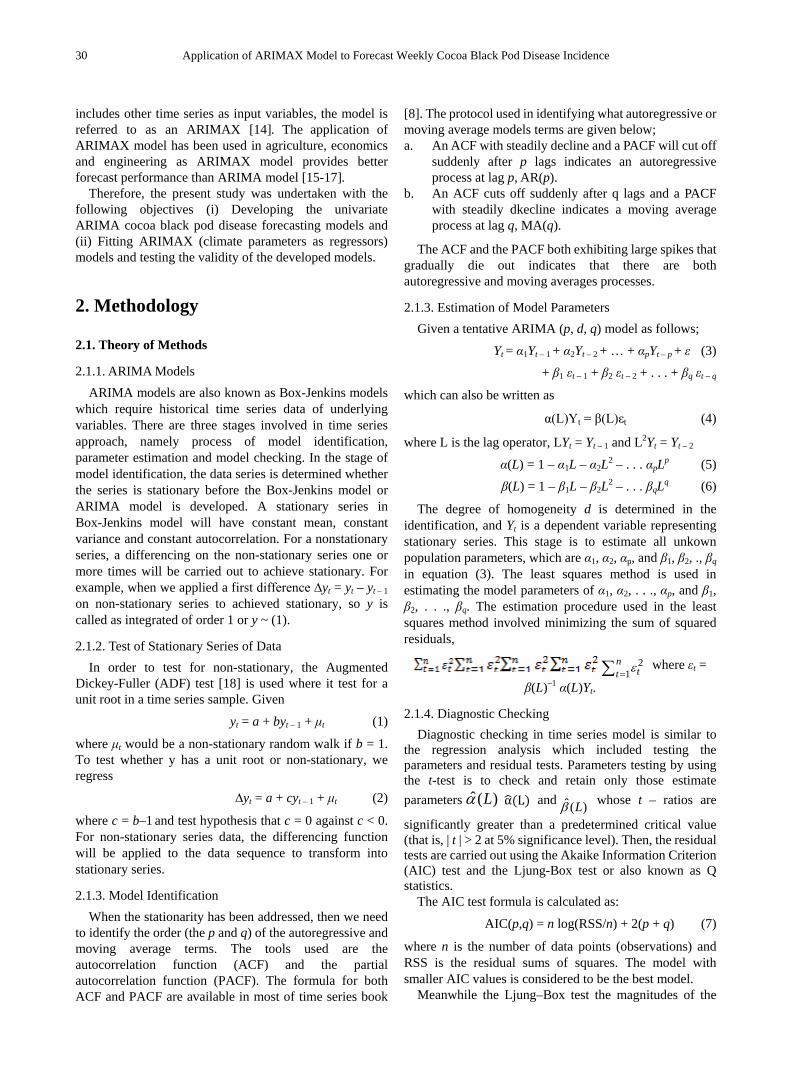
30 Application of ARIMAX Model to Forecast Weekly Cocoa Black Pod Disease Incidence
includes other time series as input variables, the model is referred to as an ARIMAX [14]. The application of ARIMAX model has been used in agriculture, economics and engineering as ARIMAX model provides better forecast performance than ARIMA model [15-17].
Therefore, the present study was undertaken with the following objectives (i) Developing the univariate ARIMA cocoa black pod disease forecasting models and (ii) Fitting ARIMAX (climate parameters as regressors) models and testing the validity of the developed models.
2. Methodology
2.1. Theory of Methods
2.1.1. ARIMA Models ARIMA models are also known as Box-Jenkins models
which require historical time series data of underlying variables. There are three stages involved in time series approach, namely process of model identification, parameter estimation and model checking. In the stage of model identification, the data series is determined whether the series is stationary before the Box-Jenkins model or ARIMA model is developed. A stationary series in Box-Jenkins model will have constant mean, constant variance and constant autocorrelation. For a nonstationary series, a differencing on the non-stationary series one or more times will be carried out to achieve stationary. For example, when we applied a first difference ∆yt = yt – yt – 1 on non-stationary series to achieved stationary, so y is called as integrated of order 1 or y ~ (1).
2.1.2. Test of Stationary Series of Data In order to test for non-stationary, the Augmented
Dickey-Fuller (ADF) test [18] is used where it test for a unit root in a time series sample. Given
yt = a + byt – 1 + μt (1)
where μt would be a non-stationary random walk if b = 1. To test whether y has a unit root or non-stationary, we regress
∆yt = a + cyt – 1 + μt (2)
where c = b–1 and test hypothesis that c = 0 against c < 0. For non-stationary series data, the differencing function will be applied to the data sequence to transform into stationary series.
2.1.3. Model Identification When the stationarity has been addressed, then we need
to identify the order (the p and q) of the autoregressive and moving average terms. The tools used are the autocorrelation function (ACF) and the partial autocorrelation function (PACF). The formula for both ACF and PACF are available in most of time series book
[8]. The protocol used in identifying what autoregressive or moving average models terms are given below; a. An ACF with steadily decline and a PACF will cut off
suddenly after p lags indicates an autoregressive process at lag p, AR(p).
b. An ACF cuts off suddenly after q lags and a PACF with steadily dkecline indicates a moving average process at lag q, MA(q).
The ACF and the PACF both exhibiting large spikes that gradually die out indicates that there are both autoregressive and moving averages processes.
2.1.3. Estimation of Model Parameters Given a tentative ARIMA (p, d, q) model as follows;
Yt = α1Yt – 1 + α2Yt – 2 + … + αpYt – p + ε (3) + β1 εt – 1 + β2 εt – 2 + . . . + βq εt – q
which can also be written as
α(L)Yt = β(L)εt (4)
where L is the lag operator, LYt = Yt – 1 and L2Yt = Yt – 2
α(L) = 1 – α1L – α2L2 – . . . αpLp (5) β(L) = 1 – β1L – β2L2 – . . . βqLq (6)
The degree of homogeneity d is determined in the identification, and Yt is a dependent variable representing stationary series. This stage is to estimate all unkown population parameters, which are α1, α2, αp, and β1, β2, ., βq in equation (3). The least squares method is used in estimating the model parameters of α1, α2, . . ., αp, and β1, β2, . . ., βq. The estimation procedure used in the least squares method involved minimizing the sum of squared residuals,
21
ntt ε=∑ where εt =
β(L)–1 α(L)Yt.
2.1.4. Diagnostic Checking Diagnostic checking in time series model is similar to
the regression analysis which included testing the parameters and residual tests. Parameters testing by using the t-test is to check and retain only those estimate parameters α�(L) and ˆ( )Lβ whose t – ratios are
significantly greater than a predetermined critical value (that is, | t | > 2 at 5% significance level). Then, the residual tests are carried out using the Akaike Information Criterion (AIC) test and the Ljung-Box test or also known as Q statistics.
The AIC test formula is calculated as:
AIC(p,q) = n log(RSS/n) + 2(p + q) (7)
where n is the number of data points (observations) and RSS is the residual sums of squares. The model with smaller AIC values is considered to be the best model.
Meanwhile the Ljung–Box test the magnitudes of the
ˆ ( )Lα

Mathematics and Statistics 7(4A): 29-40, 2019 31
residuals autocorrelation for significance: H0: The data are independently distributed with no serial
correlation Ha: The data are not independently distributed which
they exhibit serial correlation.
The test statistic is:
( )1
22
ˆnk
kQ n n
n kρ
== +
−∑ (8)
where n is the sample size,
2ˆkρ ρ�k2 is the sample autocorrelation at lag k, and h is the number of lags being tested. Under H0, the statistic Q follows a chi-square distribution, χ2 (k – p – q). For significance level α, the critical region for rejection of the hypothesis of randomness is Q > χ2 ( α, k – p – q).
2.1.5. ARIMAX Model An ARIMAX model is viewed as a multiple regression
model with one or more autoregressive (AR) terms and/or one or more moving average (MA) terms. Autoregressive terms for a dependent variable are merely lagged values of that dependent variable that have a statistically significant relationship with its most recent value. Moving average terms is nothing more than residuals (i.e., lagged errors) resulting from previously made estimates. The general ARIMAX models are as follows:
Autogressive model with exogenous variables (ARX):
yt = ϕ(L)yt + βxt + εt (9)
Moving average model with exogenous variables (MAX):
yt = βxt + θ(L)εt (10) Autogressive Moving Average with exogenous
variables model (ARMAX):
ϕ(L)yt = βxt + θ(L)εt (11)
where xt represents exogenous variables, β their coefficients, ϕ(L)yt is an AR model (ϕ1yt – 1 + ϕ2yt – 2 + ϕ3yt – 3 + . . . + ϕpyt – p) and θ(L)εt is the MA model (θ1εt – 1 + θ2εt – 2 + θ3εt – 3 + . . . + θqεt – q).
The approach used in ARIMAX model was based on the steps described by Andrews [19] with flowchart shown in Fig. 1. The approach involved two phases where the first phase deals with a linear regression model and the second phase deals with integration of AR and MA terms into a multiple regression model. In the first phase, the linear regression is used to identify the exogenous variables that are significant. Meanwhile, the second phase deals with iterative searching process to search the order of ARIMA part of the model. When there is large number of exogenous variables to be screened, the stepwise regression process is used in selecting and introducing a new exogenous variable into the ARIMAX model. This is followed by the iteration process of finding newly AR or MA or both terms to re-establish the random pattern of residuals in the ARIMAX models.
2.2. Data Collection and Statistical Analysis
The study is conducted in the cocoa mature areas in the Cocoa Research and Development Madai, Sabah with the coordinates of latitude and longitude as 4o 47’ 10’’ N and 117o 57’ 54” E. The plot’s size of 1 hectare was planted with cocoa clone of PBC 123. The study plot was divided into two treatments, i.e. first treatment was the combination of fungicide, pruning and phytosanitary of diseased pods removed from the field while second treatment was the combination between fungicide and phytosanitary of diseased pods removed from the field. Each treatment has three replications with 30 trees per replication. The random sampling method was used to select 10 trees in each replication for the black pod incidence studied meanwhile the assessment of the black pod incidence was adapted from Ndoumbe-Nkeng [20] and Ngoh Dooh [21] as follows:
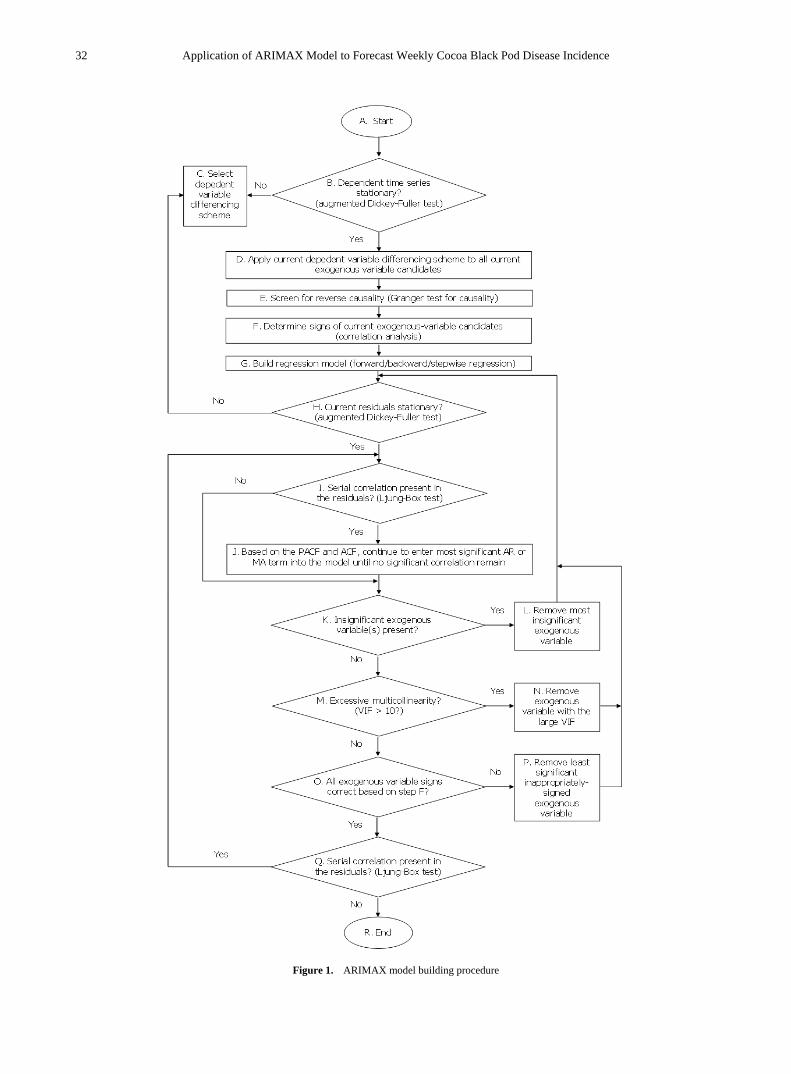
32 Application of ARIMAX Model to Forecast Weekly Cocoa Black Pod Disease Incidence
Figure 1. ARIMAX model building procedure
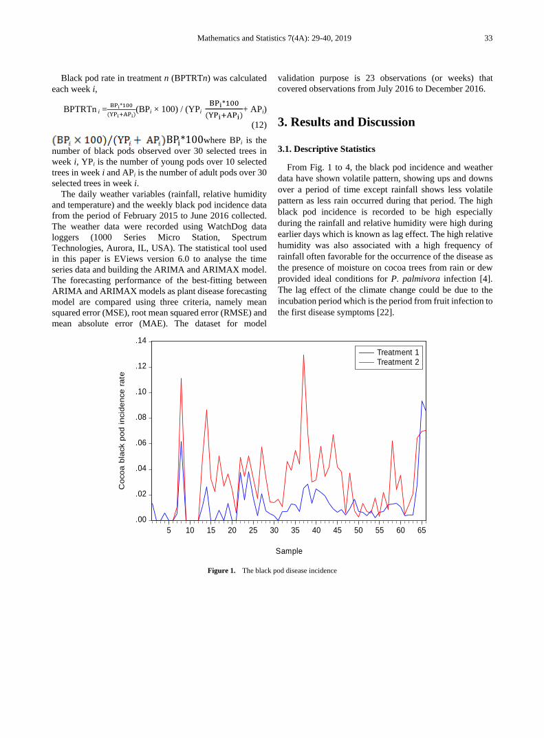
Mathematics and Statistics 7(4A): 29-40, 2019 33
Black pod rate in treatment n (BPTRTn) was calculated each week i,
BPTRTn i =BPi*100
(YPi+APi)(BPi × 100) / (YPi
BPi*100(YPi+APi)
+ APi)
(12)
BPi*100where BPi is the number of black pods observed over 30 selected trees in week i, YPi is the number of young pods over 10 selected trees in week i and APi is the number of adult pods over 30 selected trees in week i.
The daily weather variables (rainfall, relative humidity and temperature) and the weekly black pod incidence data from the period of February 2015 to June 2016 collected. The weather data were recorded using WatchDog data loggers (1000 Series Micro Station, Spectrum Technologies, Aurora, IL, USA). The statistical tool used in this paper is EViews version 6.0 to analyse the time series data and building the ARIMA and ARIMAX model. The forecasting performance of the best-fitting between ARIMA and ARIMAX models as plant disease forecasting model are compared using three criteria, namely mean squared error (MSE), root mean squared error (RMSE) and mean absolute error (MAE). The dataset for model
validation purpose is 23 observations (or weeks) that covered observations from July 2016 to December 2016.
3. Results and Discussion
3.1. Descriptive Statistics
From Fig. 1 to 4, the black pod incidence and weather data have shown volatile pattern, showing ups and downs over a period of time except rainfall shows less volatile pattern as less rain occurred during that period. The high black pod incidence is recorded to be high especially during the rainfall and relative humidity were high during earlier days which is known as lag effect. The high relative humidity was also associated with a high frequency of rainfall often favorable for the occurrence of the disease as the presence of moisture on cocoa trees from rain or dew provided ideal conditions for P. palmivora infection [4]. The lag effect of the climate change could be due to the incubation period which is the period from fruit infection to the first disease symptoms [22].
.00
.02
.04
.06
.08
.10
.12
.14
5 10 15 20 25 30 35 40 45 50 55 60 65
Treatment 1Treatment 2
Coc
oa b
lack
pod
inci
denc
e ra
te
Sample
Figure 1. The black pod disease incidence
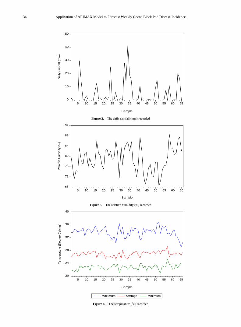
34 Application of ARIMAX Model to Forecast Weekly Cocoa Black Pod Disease Incidence
Figure 2. The daily rainfall (mm) recorded
68
72
76
80
84
88
92
5 10 15 20 25 30 35 40 45 50 55 60 65
Rela
tive
Hum
idity
(%)
Sample
Figure 3. The relative humidity (%) recorded
20
24
28
32
36
40
5 10 15 20 25 30 35 40 45 50 55 60 65
Maximum Average Minimum
Tem
pera
ture
(Deg
ree
Cel
cius
)
Sample
Figure 4. The temperature (oC) recorded
0
10
20
30
40
50
5 10 15 20 25 30 35 40 45 50 55 60 65
Dai
ly ra
infa
ll (m
m)
Sample
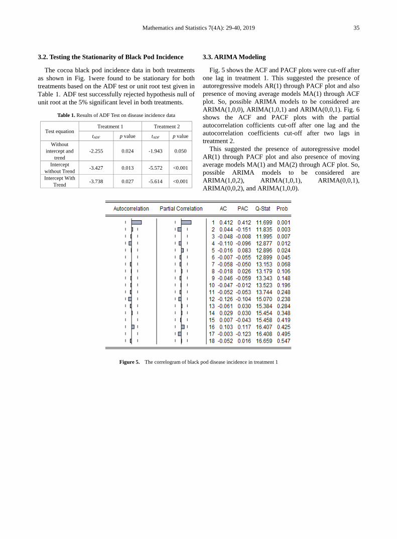
Mathematics and Statistics 7(4A): 29-40, 2019 35
3.2. Testing the Stationarity of Black Pod Incidence
The cocoa black pod incidence data in both treatments as shown in Fig. 1were found to be stationary for both treatments based on the ADF test or unit root test given in Table 1. ADF test successfully rejected hypothesis null of unit root at the 5% significant level in both treatments.
Table 1. Results of ADF Test on disease incidence data
Test equation Treatment 1 Treatment 2
tADF p value tADF p value Without
intercept and trend
-2.255 0.024 -1.943 0.050
Intercept without Trend -3.427 0.013 -5.572 <0.001
Intercept With Trend -3.738 0.027 -5.614 <0.001
3.3. ARIMA Modeling
Fig. 5 shows the ACF and PACF plots were cut-off after one lag in treatment 1. This suggested the presence of autoregressive models AR(1) through PACF plot and also presence of moving average models MA(1) through ACF plot. So, possible ARIMA models to be considered are ARIMA(1,0,0), ARIMA(1,0,1) and ARIMA(0,0,1). Fig. 6 shows the ACF and PACF plots with the partial autocorrelation cofficients cut-off after one lag and the autocorrelation coefficients cut-off after two lags in treatment 2.
This suggested the presence of autoregressive model AR(1) through PACF plot and also presence of moving average models MA(1) and MA(2) through ACF plot. So, possible ARIMA models to be considered are ARIMA(1,0,2), ARIMA(1,0,1), ARIMA(0,0,1), ARIMA(0,0,2), and ARIMA(1,0,0).
Figure 5. The correlogram of black pod disease incidence in treatment 1
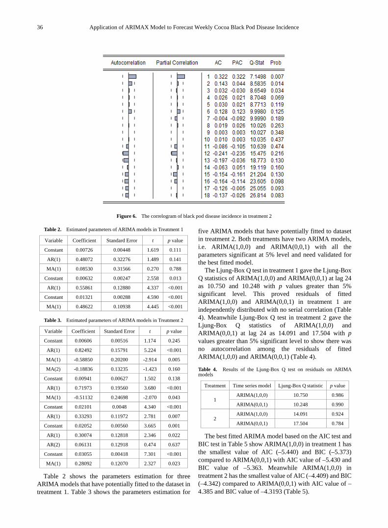
36 Application of ARIMAX Model to Forecast Weekly Cocoa Black Pod Disease Incidence
Figure 6. The correlogram of black pod disease incidence in treatment 2
Table 2. Estimated parameters of ARIMA models in Treatment 1
Variable Coefficient Standard Error t p value
Constant 0.00726 0.00448 1.619 0.111
AR(1) 0.48072 0.32276 1.489 0.141
MA(1) 0.08530 0.31566 0.270 0.788
Constant 0.00632 0.00247 2.558 0.013
AR(1) 0.55861 0.12880 4.337 <0.001
Constant 0.01321 0.00288 4.590 <0.001
MA(1) 0.48622 0.10938 4.445 <0.001
Table 3. Estimated parameters of ARIMA models in Treatment 2
Variable Coefficient Standard Error t p value
Constant 0.00606 0.00516 1.174 0.245
AR(1) 0.82492 0.15791 5.224 <0.001
MA(1) -0.58850 0.20200 -2.914 0.005
MA(2) -0.18836 0.13235 -1.423 0.160
Constant 0.00941 0.00627 1.502 0.138
AR(1) 0.71973 0.19560 3.680 <0.001
MA(1) -0.51132 0.24698 -2.070 0.043
Constant 0.02101 0.0048 4.340 <0.001
AR(1) 0.33293 0.11972 2.781 0.007
Constant 0.02052 0.00560 3.665 0.001
AR(1) 0.30074 0.12818 2.346 0.022
AR(2) 0.06131 0.12918 0.474 0.637
Constant 0.03055 0.00418 7.301 <0.001
MA(1) 0.28092 0.12070 2.327 0.023
Table 2 shows the parameters estimation for three ARIMA models that have potentially fitted to the dataset in treatment 1. Table 3 shows the parameters estimation for
five ARIMA models that have potentially fitted to dataset in treatment 2. Both treatments have two ARIMA models, i.e. ARIMA(1,0,0) and ARIMA(0,0,1) with all the parameters significant at 5% level and need validated for the best fitted model.
The Ljung-Box Q test in treatment 1 gave the Ljung-Box Q statistics of ARIMA(1,0,0) and ARIMA(0,0,1) at lag 24 as 10.750 and 10.248 with p values greater than 5% significant level. This proved residuals of fitted ARIMA(1,0,0) and ARIMA(0,0,1) in treatment 1 are independently distributed with no serial correlation (Table 4). Meanwhile Ljung-Box Q test in treatment 2 gave the Ljung-Box Q statistics of ARIMA(1,0,0) and ARIMA(0,0,1) at lag 24 as 14.091 and 17.504 with p values greater than 5% significant level to show there was no autocorrelation among the residuals of fitted ARIMA(1,0,0) and ARIMA(0,0,1) (Table 4).
Table 4. Results of the Ljung-Box Q test on residuals on ARIMA models
Treatment Time series model Ljung-Box Q statistic p value
1 ARIMA(1,0,0) 10.750 0.986
ARIMA(0,0,1) 10.248 0.990
2 ARIMA(1,0,0) 14.091 0.924
ARIMA(0,0,1) 17.504 0.784
The best fitted ARIMA model based on the AIC test and BIC test in Table 5 show ARIMA(1,0,0) in treatment 1 has the smallest value of AIC (–5.440) and BIC (–5.373) compared to ARIMA(0,0,1) with AIC value of –5.430 and BIC value of –5.363. Meanwhile ARIMA(1,0,0) in treatment 2 has the smallest value of AIC (–4.409) and BIC (–4.342) compared to ARIMA(0,0,1) with AIC value of –4.385 and BIC value of –4.3193 (Table 5).

Mathematics and Statistics 7(4A): 29-40, 2019 37
Table 5. Results of the AIC test and BIC test
Treatment Time series model
AIC value
BIC value Decision
1 ARIMA(1,0,0) –5.440 –5.373 Selected
ARIMA(0,0,1) –5.430 –5.363
2 ARIMA(1,0,0) –4.409 –4.342 Selected
ARIMA(0,0,1) –4.385 –4.319
The selected ARIMA(1,0,0) model for both treatments explained that the forecast cocoa black pod disease incidence at time t was depend on the incidence at time t – 1. This was because the cocoa black pod disease incidence existed in treatments 1 and 2 mostly caused by the environment as study by Guest [23] that showed under favorable condition will caused the sporangia from diseased pod to develop within 48 hours of infection.
3.4. ARIMAX Modeling
The twelve steps given in the flowchart shown in Fig. 1 was used to build the ARIMA model. Part of the tests have been carried out in ARIMA modeling. The pair-wise Granger Causality tests in Table 6 for treatments 1 and 2 showed three null hypotheses of Granger Causality tests being rejected at 5% significant level to indicate one-way causal relationships from the exogenous variables to a dependent variable. The exogenous variables in treatment 1 were the relative humidity at time t (MeanRHt), average temperature at time t (Tmeant) and maximum temperature at time t (Tmaxt). As for treatment 2, the exogenous variables were the total rainfall at time t (TRainFt), average relative humidity at time t (MeanRHt) and maximum temperature at time t (Tmaxt).
Table 6. Granger Causality test involved climate variables
Null Hypothesis p value
Treatment 1
Treatment 2
TRainFt does not granger cause BPTRTt 0.062 0.007
BPTRTt does not granger cause TRainFt 0.346 0.407
MeanRHt does not granger cause BPTRTt 0.050 0.026
BPTRTt does not granger cause MeanRHt 0.944 0.917
Tmeant does not granger cause BPTRTt 0.042 0.702
BPTRT1t does not granger cause Tmeant 0.345 0.578
Tmint does not granger cause BPTRTt 0.474 0.142
BPTRTt does not granger cause Tmint 0.094 0.446
Tmaxt does not granger cause BPTRTt <0.001 0.021
BPTRTt does not granger cause Tmaxt 0.686 0.832
It is important to ensure the exogenous variables have correct correlation sign to the disease incidence. The Spearman correlation analysis in treatment 1 determined four climate variables have correct correlation at 5% significant level (Table 7). The climate variables were the average relative humidity at time t – 6 (MeanRHt–6),
average temperature at time t – 3 (Tmeant–3), maximum temperature at time t (Tmaxt) and t – 2 (Tmaxt–2). There were nine climate variables in treatment 2 have correct correlation at 5% significant level (Table 8). The climate variables were the total rainfall at time t – 4 (TRainFt – 4) and t – 5 (TRainFt–5), average relative humidity at time t – 3 (MeanRHt – 3), t – 4 (MeanRHt–4), t – 5 (MeanRHt–5), t – 6 (MeanRHt–6) and t – 7 (MeanRHt–7), maximum temperature at time t (Tmaxt) and t – 5 (Tmaxt–5).
Table 7. Correlation analysis on climate variables in treatment 1
Climate variable Correlation coefficient p value
MeanRHt – 6 0.293 0.017
Tmeant – 3 0.243 0.050 Tmaxt -0.392 0.001
Tmaxt – 2 -0.256 0.038
Table 8. Correlation analysis on climate variables in treatment 2
Climate variable Correlation coefficient p value
TRainFt – 4 0.265 0.031
TRainFt– 5 0.283 0.021
MeanRHt – 3 0.285 0.020
MeanRHt – 4 0.374 0.002
MeanRHt– 5 0.416 <0.001
MeanRHt – 6 0.438 <0.001
MeanRHt– 7 0.355 0.004
Tmaxt -0.268 0.660
Tmaxt – 5 -0.266 0.069
The stepwise regression that develop a linear regression model between the climate variables and the cocoa black pod disease incidence showed both Tmeant – 3 and Tmaxt variables have significant F values at 5% level in treatment 1 while only MeanRHt – 4 in treatment 2 has significant F values at 5% level (Table 9).
Table 9. Stepwise regression analysis
Variable Parameter Estimate
Standard Error F p
value R
Squared Treatment 1
Constant 0.07897 0.07109 1.23 0.271
0.2892 Tmeant – 3 0.00492 0.00232 4.50 0.038
Tmaxt -0.00588 0.00123 22.93 <0.001
Treatment 2
Constant -0.16575 0.05086 10.62 0.002 0.1892
MeanRHt – 4 0.00245 0.00063 14.94 <0.001
Table 10 shows the residuals from stepwise regression model in treatments1 and 2 rejected the hypothesis null of unit root at the 5% significant level in ADF test. This indicated the residuals from the stepwise regression model in treatments 1 and 2 were stationary.
38 Application of ARIMAX Model to Forecast Weekly Cocoa Black Pod Disease Incidence
Table 10. Results of ADF Test on residuals from stepwise regression
Test equation Treatment 1 Treatment 2
tADF p value tADF p
value Without intercept and
trend 0.656 0.855 -6.120 <0.001
Intercept without Trend -5.317 <0.001 -6.070 <0.001
Intercept With Trend -5.756 <0.001 -6.039 <0.001
Both the Ljung-Box Q statistics in treatments 1 and 2 (Table 11), 12.289 (lag 5) and 4.218 (lag 1) have p value greater than 0.05 which indicated autocorrelation exist in the residuals at 5% significant level. This provides an indication that AR and/or MA terms must be added into the model to remove the serial correlation.
Table 11. Results of the Ljung-Box Q test on residuals from stepwise regression
Treatment Lags Ljung-Box Q statistic p value
1 5 12.289 0.0153
2 1 4.218 0.0400
Table 12 shows the ARIMAX model in treatment 1 was established using the AR(1) term and variable Tmaxt as both were significant at 5% level while ARIMAX model in treatment 2 involved the AR(1) term and variable MeanRHt – 4 as both were significant at 5% level. The sign check on the coefficient of the exogenous variable as given in Table 12 correctly correlated with the disease incidence.
Table 12. Fitted ARIMAX models
Treatment Variable Coefficient Standard Error t p
value
1
Constant 0.14900 0.04316 3.452 0.0010
AR(1) 0.40777 0.12807 3.184 0.0023
Tmaxt -0.00418 0.00126 -3.310 0.0016
2
Constant -0.1563 0.04948 -3.159 0.0024
AR(1) 0.29427 0.11029 2.668 0.0097 MeanRHt
– 4 0.00222 0.00062 3.598 0.0006
The selection of maximum temperature as one of the predictors in ARIMAX model in treatment 1 was due to its treatment applied the pruning as one of its control measure in managing the cocoa black pod disease incidence. The pruning provided good ventilation around and within the cocoa tree which can reduced the relative humidity to less volatile compared to temperature [24]. There were study
proved that the difference in maximum temperature measured outside and inside canopy layers of cocoa trees caused the maximum temperature to be an important factor in effecting the cocoa production and also the disease infection [25-26]. Meanwhile the selection of average relative humidity as one of the predictors in ARIMAX model in the treatments 2 due to the control measure applied to the cocoa trees were free from pruning with fungicide application only. The cocoa tree without pruning have dense canopy and caused little sunshine penetration that will create highly relative humidity to favor the Phytophthora’s inoculums to infect the cocoa pods [5, 27].
3.5. Model Validation
The best cocoa black pod disease forecasting model between ARIMA and ARIMAX model was selected based on its forecasting performance using three criteria, namely mean squared error (MSE), root mean squared error (RMSE) and mean absolute error (MAE). Table 13 shows ARIMAX model in treatment 1 has the lowest values of MSE (i.e. 0.00057), RMSE (i.e. 0.02389) and MAE (i.e. 0.01730) as compared to ARIMA model with MSE value of 0.00061, RMSE value of 0.02467 and MAE value of 0.01773. Meanwhile ARIMAX model in treatment 2 has the lowest values of MSE k(i.e. 0.00955), RMSE (i.e. 0.09773) and MAE (i.e. 0.07765) as compared to ARIMA model with MSE value of 0.01003, RMSE value of 0.10013 and MAE value of 0.08139. This showed ARIMAX model has performed better compared to ARIMA model and therefore, ARIMAX model was selected as the best disease forecasting model in this study. The gap between the actual and ARIMAX predicted values seen to be far especially on sample with higher black pod incidence rates as seen in Fig.7 and Fig.8. The reason probable due to nonlinear effects in cocoa black pod incidence rate and also influencing external factors that not being considered in the study, i.e. duration of pods being exposed to wetness as direct impact to the disease.
Table 13. Actual versus forecasted values
Validation test Treatment 1 Treatment 2
ARIMA ARIMAX ARIMA ARIMAX
MSE 0.00061 0.00057 0.01003 0.00955
RMSE 0.02467 0.02389 0.10013 0.09773
MAE 0.01773 0.01730 0.08139 0.07765

Mathematics and Statistics 7(4A): 29-40, 2019 39
-.06
-.04
-.02
.00
.02
.04
.06 .00
.02
.04
.06
.08
.10
.12
10 20 30 40 50 60 70 80
ResidualActualFitted ARIMAX
Res
idua
l
Sample
Black pod incidence rate
Figure 7. Plot of forecasted value of ARIMAX model in treatment 1
Figure 8. Plot of forecasted value of ARIMAX model in treatment 2
4. Conclusions This study shows that there were an effect of climate
variables to the cocoa black pod incidence. Key findings indicate that maximum temperature and relative humidity have significant correlation with black pod incidence and suggested as indicator in forecasting the cocoa black pod incidence. The results in this paper has found that ARIMA model with climate variables as input series i.e. ARIMAX consistently showed the superiority over ARIMA models in capturing the percent relative deviations pertaining to cocoa black pod incidence forecasts in two different treatment plots. The ARIMAX models performed well with lower error as compared to the ARIMA models. The plant disease forecasting models developed from ARIMAX model able to provide benefits especially for the development of decision support system in determine the right timing of action to be taken in controlling the cocoa
black pod disease.
Acknowledgements The author also would like to thank the Director-General, Malaysian Cocoa Board (MCB) and Director of Upstream Technology Cocoa for permission to publish and reviewing this paper.
REFERENCES [1] International Cocoa Organization, Online available from
http://www.icco.org/about-cocoa/pest-a-diseases.html
[2] C. A. Thorold. The epiphytes of Theobroma cacao in Nigeria in relation to the incidence of black pod disease
-.10
-.05
.00
.05
.10
.15
-.05
.00
.05
.10
.15
.20
.25
10 20 30 40 50 60 70 80
ResidualActualFitted
Res
idua
lBlack pod incidence rate
Sample

40 Application of ARIMAX Model to Forecast Weekly Cocoa Black Pod Disease Incidence
(Phytophthora palmivora), Journal of Ecology, Vol.40, No.1, 125-142, 1952.
[3] C. A. Thorold. Observations on black pod disease (Phytophthora palmivora) of cacao in Nigeria, Transactions of the British Mycological Society, Vol.38, 435-452, 1955.
[4] J. T. Dakwa. The relationship between black pod incidence and the weather in Ghana, Ghana Journal of Agricultural Science, Vol.6, 93-102, 1973.
[5] G. A. R. Wokod. Black pod: Meteorological factors, In: Gregory PH (ed) Phytophthora diseases of cocoa, Longman, London, 1974.
[6] J. Mpika, E. I. Auguste, B. K. Ismael, K. Brou, L. K. Jean, A. Kouassi, A. Z. Nicodeme, A. Severin. Effects of climatic parameters on the expression of the black pod disease on Theobroma cacao in Cote d’Ivoire, Journal of Applied Biosciences, Vol.20, 1183-1193, 2009.
[7] O. A. Arqub, Z. Odibat, M. Al-Smadi. Numerical solutions of time-fractional partial integrodifferential equations of Robin functions types in Hibert space with error bounds and error estimates, International Journal of Numerical Methods for Heat and Fluid Flow, Vol.28, No.4, 828 – 856, 2018.
[8] G. E. P. Box, G. M. Jenkins. Time Series Analysis: Forecasting and Control, Holden-Day, San Francisco, 1976.
[9] M. Hemavathi, K. Prabakaran. ARIMA Model for Forecasting of Area, Production and Productivity of Rice and Its Growth Status in Thanjavur District of Tamil Nadu, India, International Journal of Current Microbiology and Applied Sciences, Vol.7, No.2, 149-156, 2018.
[10] M. Amin, M. Amanullah, A. Akbar. Time series modeling for forecasting wheat production of Pakistan, Journal of Animal and Plant Sciences, Vol.24, No.5, 1444-1451, 2014.
[11] E. Harris, A. R. Abdul-Aziz, R.K. Avuglah. Modeling annual Coffee production in Ghana using ARIMA time series Model, International Journal of Business, Social and Scientific Research, Vol.2, No.7, 175-186, 2012.
[12] S. Ankrah, K. A. Nyantakyi, E. Dadey. Modeling the Causal Effect of World Cocoa Price on Production of Cocoa in Ghana, Universal Journal of Agricultural Research, Vol.2, No.7, 264-271, 2014.
[13] F. J. Rodríguez-Rajo, V. Jato, M. Fernández-González, M. J. Aira. The use of aerobiological methods for forecasting Botrytis spore concentrations in a vineyard. Grana, Vol.49, No.1, 56-65, 2010.
[14] A. Pankratz. Forecasting with Dynamic Regression Models, Wiley-Interscience, New York, 1991.
[15] B. Yogarajah, C. Elankumaran, R. Vigneswaran. Application of ARIMAX Model for Forecasting Paddy Production in Trincomalee District in Sri Lanka, In: 3rd International Symposium, South Eastern University of Sri Lanka, 21-25, 2013.
[16] C. Kongcharoen, T. Kruangpradit. Autoregressive Integrated Moving Average with Explanatory Variable (ARIMAX) Model for Thailand Export, In: 33rd International Symposium on Forecasting, South Korea, South Korea, 1-8, 2013.
[17] H. Cui, X. Peng. Short-Term City Electric Load Forecasting
with Considering Temperature Effects: An Improved ARIMAX Model, Mathematical Problems in Engineering Vol.2015, 2015.
[18] E. Graham, J. R. Thomas, H. S. James. Efficient tests for an autoregressive unit root, Econometrica, Vol.64, No.4, 813-836, 1996.
[19] B. Andrews, M. Dean, R. Swain, C. Cole Building ARIMA and ARIMAX models for predicting long-term disability benefit application rates in the public/private sectors, Society of Actuaries, University of Southern Maine, 2013.
[20] M. Ndoumbe-Nkenga, C. Cilasb, E. Nyemba, S. Nyassea, D. Bieysseb, A. Florib, I. Sachec. Impact of removing diseased pods on cocoa black pod caused by Phytophthora megakarya and on cocoa production in Cameroon, Crop Protection, Vol.23, 415-424, 2004.
[21] J. P. Ngoh Dooh, B. N. Zachée Ambang, W. N. Kuate Tueguem, H. Alain, N. G. Ntsomboh. Development of Cocoa Black Pod Disease (Caused by Phytophthora megakarya) in Cameroon when Treated with Extracts of Thevetia peruviana or Ridomil, International Journal of Current Research in Biosciences and Plant Biology, Vol.2, No.3, 47-59, 2015.
[22] M. Ndoumbè-Nkeng, M. I. B. Efombagn, S. Nyassé, E. Nyemb, I. Sache, C. Cilas Relationships between cocoa Phytophthora pod rot disease and climatic variables in Cameroon, Canadian Journal of Plant Pathology, Vol.3, 309-320, 2009.
[23] D. I. Guest. Black pod: diverse pathogens and the greatest global impact on cocoa yield, Phytopathology, Vol.97, No.12, 1650-1653, 2007.
[24] C. H. Lee. Planting cocoa challenges and reality in Malaysia, Online available from http://www.iipm.com.my/ipicex2014 /docs/2012/oral/PLANTING%20COCOA-%20CHALLENGES %20AND%20REALITY%20IN%20MALAYSIA.pdf.
[25] R. A. C. Miranda, L. C. E. Milde, A. L. Bichara, S. Cornell Daily characterisation of air temperature and relative humidity profiles in a cocoa plantation, Pesquisa Agropecuária Brasileira, Vol.29, 345-353, 1994.
[26] A. J. Daymond, P. Hadley. The effects of temperature and light integral on early vegetative growth and chloroplyll fluorescence of four contrasting genotypes of cacao (Theobroma cacao), Annals of Applied Biology, Vol.145, 257-262, 2004.
[27] J. Flood, D. Guest, K. A. Holmes, P. Keane, B. Padi, E. Sulistyowati. Cocoa under attack, In: J. Flood, R. Murphy (eds) Cocoa futures. Chinchina, CO: CABIFEDERACAFE, 2004.
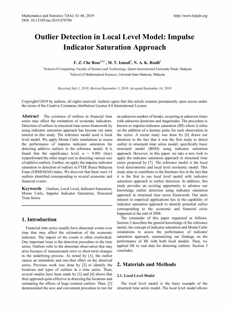
Mathematics and Statistics 7(4A): 41-48, 2019 http://www.hrpub.org DOI: 10.13189/ms.2019.070706
Outlier Detection in Local Level Model: Impulse Indicator Saturation Approach
F. Z. Che Rose1,2,*, M. T. Ismail2, N. A. K. Rosili1
1School of Computing, Faculty of Science and Technology, Quest International University Perak, Malaysia 2School of Mathematical Sciences, Universiti Sains Malaysia, Malaysia
Received July 1, 2019; Revised September 3, 2019; Accepted September 14, 2019
Copyright©2019 by authors, all rights reserved. Authors agree that this article remains permanently open access under the terms of the Creative Commons Attribution License 4.0 International License
Abstract The existence of outliers in financial time series may affect the estimation of economic indicators. Detection of outliers in structural time series framework by using indicator saturation approach has become our main interest in this study. The reference model used is local level model. We apply Monte Carlo simulations to assess the performance of impulse indicator saturation for detecting additive outliers in the reference model. It is found that the significance level, α = 0.001 (tiny) outperformed the other target size in detecting various size of additive outliers. Further, we apply the impulse indicator saturation to detection of outliers in FTSE Bursa Malaysia Emas (FBMEMAS) index. We discover that there were 14 outliers identified corresponding to several economic and financial events.
Keywords Outliers, Local Level, Indicator Saturation, Monte Carlo, Impulse Indicator Saturation, Structural Time Series
1. IntroductionFinancial time series usually have abnormal events over
time that may affect the estimation of the economic indicator. The impact of the events is often overlooked. One important issue is the detection procedure in the time series. Outliers refer to the abnormal observation that may arise because of measurement error or short-term changes in the underlying process. As noted by [1], the outlier causes an immediate and one-shot effect on the observed series. Previous work was done by [2] to identify the locations and types of outliers in a time series. Then, several studies have been made by [3] and [4] shows that their approach quite effective in detecting the locations and estimating the effects of huge isolated outliers. Then, [5] demonstrated the new and convenient procedure to test for
an unknown number of breaks, occurring at unknown times with unknown durations and magnitudes. The procedure is known as impulse-indicator saturation (IIS) where it relies on the addition of a dummy pulse for each observation in the series. A recent study was done by [6] draws our attention to the fact that it was the first study to detect outlier in structural time series model, specifically basic structural model (BSM) using indicator saturation approach. However, in this paper, we take a new look to apply the indicator saturation approach in structural time series proposed by [7]. The reference model is the local level deterministic and local level stochastic model. This study aims to contribute to the literature lies in the fact that it is the first to use local level model with indicator saturation approach to outlier detection. In addition, this study provides an exciting opportunity to advance our knowledge outlier detection using indicator saturation approach in structural time series framework. Our main interest in empirical applications lies in the capability of indicator saturation approach to identify potential outlier corresponding to the economic and financial crisis happened at the end of 2008.
The remainder of this paper organized as follows. Section 2 describes the general knowledge of the reference model, the concept of indicator saturation and Monte Carlo simulations to assess the performance of indicator saturation approach, summarizing our findings on the performance of IIS with both local models. Then, we applied IIS to real data for detecting outliers. Section 3 concludes.
2. Materials and Methods
2.1. Local Level Model
The local level model is the basic example of the structural time series model. The local level model allows
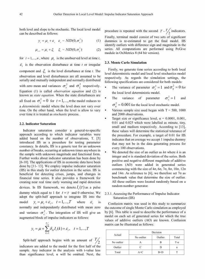
42 Outlier Detection in Local Level Model: Impulse Indicator Saturation Approach
both level and slope to be stochastic. The local level model can be described as follows:
2 ~ (0, )t t t ty NID εµ ε ε σ= + (1)
2
1 ~ (0, )t t t t NID ξµ µ ξ ξ σ+= + (2)
for 1, ...,t n= , where tµ is the unobserved level at time t,
tε is the observation disturbance at time t or irregular
component and tξ is the level disturbance at time t. The observation and level disturbances are all assumed to be serially and mutually independent and normally distributed
with zero mean and variances 2εσ and 2
ξσ respectively. Equation (1) is called observation equation and (2) is known as state equation. When the state disturbances are
all fixed on 2 0ξσ = for 1,...,t n= the model reduces to a deterministic model where the level does not vary over time. On the other hand, when the level is allow to vary over time it is treated as stochastic process.
2.2. Indicator Saturation
Indicator saturation consider a general-to-specific approach according to which indicator variables were added based on the number of observations, T. [5] introduced IIS as a procedure for testing parameter constancy. In details, IIS is a generic test for an unknown number of breaks, occurring at unknown times anywhere in the sample with unknown magnitude and functional form. Further works about indicator saturation has been done by [6-10]. The applications of IIS in economic data have been done by [11- 13]. We employ impulse indicator saturation (IIS) in this study for outlier detection in the series. IIS is beneficial for detecting crises, jumps, and changes in financial time series. It also provides a framework for creating near real time early warning and rapid detection devices. In IIS framework, we denote ( )tI t as a pulsedummy which equal to 1 for t t= and 0 otherwise. We adopt the split-half approach to integrate IIS into the model , 1,...,t t ty t Tµ ε= + = where tε is normally and independently distributed with mean zero and variance 2
εσ . The integration of IIS will give an augmented block of impulse indicators as follows:
2
1( ) , 1,...,
T
t lk t tk
y I k t Tµ δ ε=
= + + =∑
Split-half approach begins with an amount of 2T
indicators are added to the model for the first half of the sample. Any indicator in the analysis with t-value less than significance level, α will be omitted. Next, the
procedure is repeated with the second 2
TT − indicators.
Finally, terminal model consist of two sets of significant dummies is re-estimated to get the final model. IIS identify outliers with difference sign and magnitude in the series. All computations are performed using PcGive module in OxMetrics 8 (64 bit version).
2.3. Monte Carlo Simulation
Firstly, we generate time series according to both local level deterministic model and local level stochastics model respectively. As regards the simulation settings, the following specifications are considered for both models: The variance of parameter 2 1εσ = and 2 0ησ = for
the local level deterministic model. The variance of parameter 2 1εσ = and
2 0.001ησ = for the local level stochastic model. Various sample size used began with T = 500, 1000
and 2000 observations. Target size or significance level, α = 0.0001, 0.001,
0.01 and 0.025 which were labelled as minute, tiny, small and medium respectively. According to [13], these values will determine the statistical tolerance of the procedure. For example, a target of 0.01 for IIS indicates that on average we accept 1 impulse dummy that may not be in the data generating process for every 100 observations.
We denoted the size of an outlier as kσ where k is an integer and σ is standard deviation of the series. Both positive and negative different magnitude of additive outliers (AO) were added in generated series commencing with the size of 4σ, 6σ, 7σ, 8σ, 10σ, 12σ and 14σ. As reference to [6], we therefore set 7σ as benchmark value that determine the size of outlier. All these outliers were located randomly based on a random number generator.
2.3.1. Assessing the Performance of Impulse Indicator Saturation (IIS)
Confusion matrix was used in this study to summarize the outcome of single Monte Carlo simulation as employed by [6]. This table is used to describe the performance of a model on each set of generated series for which the true values of additive outliers (AO) are known. Confusion matrix can be illustrated as follows:
Actual Decision
No outlier Outlier Total
No outlier A B T-n
Outlier C D n
Total A+C B+D T
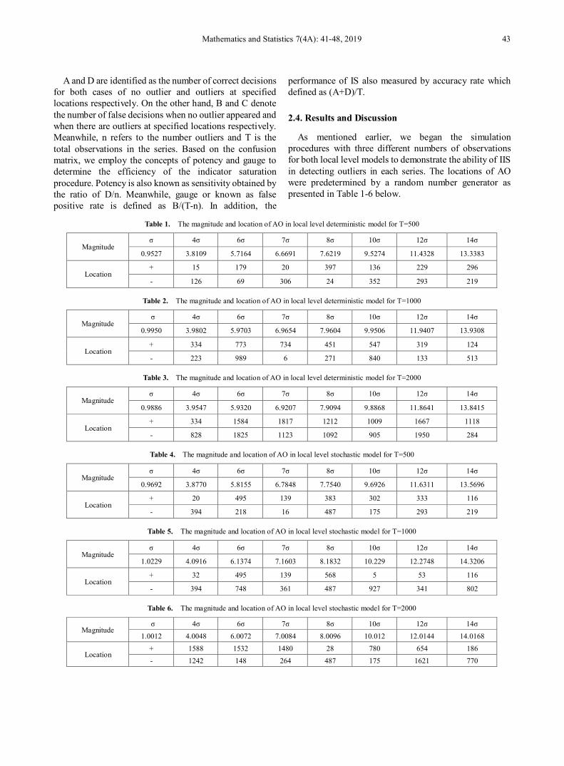
Mathematics and Statistics 7(4A): 41-48, 2019 43
A and D are identified as the number of correct decisions for both cases of no outlier and outliers at specified locations respectively. On the other hand, B and C denote the number of false decisions when no outlier appeared and when there are outliers at specified locations respectively. Meanwhile, n refers to the number outliers and T is the total observations in the series. Based on the confusion matrix, we employ the concepts of potency and gauge to determine the efficiency of the indicator saturation procedure. Potency is also known as sensitivity obtained by the ratio of D/n. Meanwhile, gauge or known as false positive rate is defined as B/(T-n). In addition, the
performance of IS also measured by accuracy rate which defined as (A+D)/T.
2.4. Results and Discussion
As mentioned earlier, we began the simulation procedures with three different numbers of observations for both local level models to demonstrate the ability of IIS in detecting outliers in each series. The locations of AO were predetermined by a random number generator as presented in Table 1-6 below.
Table 1. The magnitude and location of AO in local level deterministic model for T=500
Magnitude σ 4σ 6σ 7σ 8σ 10σ 12σ 14σ
0.9527 3.8109 5.7164 6.6691 7.6219 9.5274 11.4328 13.3383
Location + 15 179 20 397 136 229 296
- 126 69 306 24 352 293 219
Table 2. The magnitude and location of AO in local level deterministic model for T=1000
Magnitude σ 4σ 6σ 7σ 8σ 10σ 12σ 14σ
0.9950 3.9802 5.9703 6.9654 7.9604 9.9506 11.9407 13.9308
Location + 334 773 734 451 547 319 124
- 223 989 6 271 840 133 513
Table 3. The magnitude and location of AO in local level deterministic model for T=2000
Magnitude σ 4σ 6σ 7σ 8σ 10σ 12σ 14σ
0.9886 3.9547 5.9320 6.9207 7.9094 9.8868 11.8641 13.8415
Location + 334 1584 1817 1212 1009 1667 1118
- 828 1825 1123 1092 905 1950 284
Table 4. The magnitude and location of AO in local level stochastic model for T=500
Magnitude σ 4σ 6σ 7σ 8σ 10σ 12σ 14σ
0.9692 3.8770 5.8155 6.7848 7.7540 9.6926 11.6311 13.5696
Location + 20 495 139 383 302 333 116
- 394 218 16 487 175 293 219
Table 5. The magnitude and location of AO in local level stochastic model for T=1000
Magnitude σ 4σ 6σ 7σ 8σ 10σ 12σ 14σ
1.0229 4.0916 6.1374 7.1603 8.1832 10.229 12.2748 14.3206
Location + 32 495 139 568 5 53 116
- 394 748 361 487 927 341 802
Table 6. The magnitude and location of AO in local level stochastic model for T=2000
Magnitude σ 4σ 6σ 7σ 8σ 10σ 12σ 14σ
1.0012 4.0048 6.0072 7.0084 8.0096 10.012 12.0144 14.0168
Location + 1588 1532 1480 28 780 654 186 - 1242 148 264 487 175 1621 770
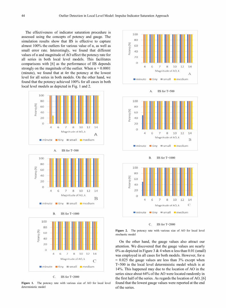
44 Outlier Detection in Local Level Model: Impulse Indicator Saturation Approach
The effectiveness of indicator saturation procedure is assessed using the concepts of potency and gauge. The simulation results show that IIS is effective to capture almost 100% the outliers for various value of α, as well as small error rate. Interestingly, we found that different values of α and magnitude of AO affect the potency rate for all series in both local level models. This facilitates comparisons with [6] as the performance of IIS depends strongly on the magnitude of the outlier. When α = 0.0001 (minute), we found that at 4σ the potency at the lowest level for all series in both models. On the other hand, we found that the potency achieved 100% for all cases in both local level models as depicted in Fig. 1 and 2.
A. IIS for T=500
B. IIS for T=1000
C. IIS for T=2000
Figure 1. The potency rate with various size of AO for local level deterministic model
A. IIS for T=500
B. IIS for T=1000
C. IIS for T=2000
Figure 2. The potency rate with various size of AO for local level stochastic model
On the other hand, the gauge values also attract our attention. We discovered that the gauge values are nearly 0% as depicted in Figure 3 & 4 when α less than 0.01 (small) was employed in all cases for both models. However, for α = 0.025 the gauge values are less than 3% except when T=500 in the local level deterministic model which is at 14%. This happened may due to the location of AO in the series since about 64% of the AO were located randomly in the first half of the series. As regards the location of AO, [6] found that the lowest gauge values were reported at the end of the series.
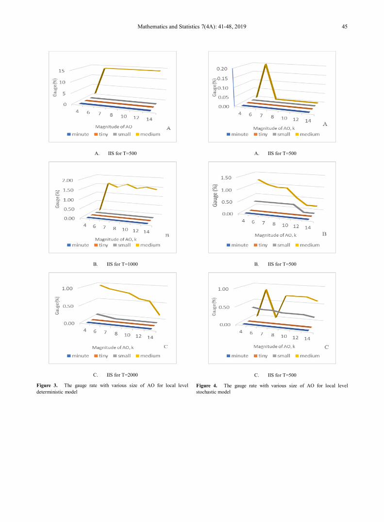
Mathematics and Statistics 7(4A): 41-48, 2019 45
A. IIS for T=500
B. IIS for T=1000
C. IIS for T=2000
Figure 3. The gauge rate with various size of AO for local level deterministic model
A. IIS for T=500
B. IIS for T=500
C. IIS for T=500
Figure 4. The gauge rate with various size of AO for local level stochastic model

46 Outlier Detection in Local Level Model: Impulse Indicator Saturation Approach
In view of accuracy of the model, we found remarkable results when α = 0.001 (tiny) is applied. Overall, the accuracy rate is still above 98% for different values of significance level, α, magnitude and location of AO. As the number of observations, T increase we found that the accuracy rate reduces by 1% when the target size at medium level as depicted in Fig. 5B and 5C.
A. IIS for T=500
B. IIS for T=1000
C. IIS for T=2000 Figure 5. The accuracy rate with various size of AO for local level deterministic model
A. IIS for T=500
B. IIS for T=1000
C. IIS for T=2000
Figure 6. The accuracy rate with various size of AO for local level stochastic model
2.5. Empirical Application
In economic time series, detection of outlier has detrimental effects in signal extraction and forecasting. In this section, we illustrate the application of IIS in identifying the outliers in shariah FTSE Bursa Malaysia Emas index (FBMEMAS) with the local level stochastic model as a reference model. The series consists of daily closing prices with estimation period from September 30,
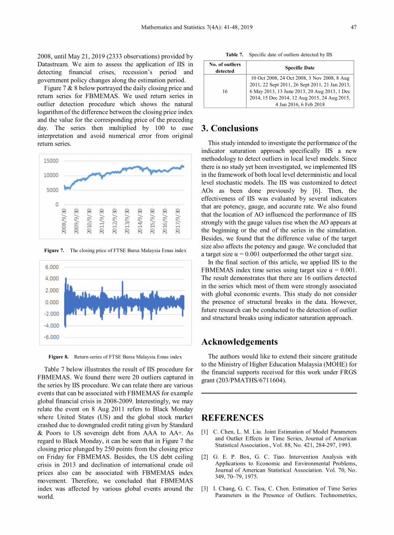
Mathematics and Statistics 7(4A): 41-48, 2019 47
2008, until May 21, 2019 (2333 observations) provided by Datastream. We aim to assess the application of IIS in detecting financial crises, recession’s period and government policy changes along the estimation period.
Figure 7 & 8 below portrayed the daily closing price and return series for FBMEMAS. We used return series in outlier detection procedure which shows the natural logarithm of the difference between the closing price index and the value for the corresponding price of the preceding day. The series then multiplied by 100 to ease interpretation and avoid numerical error from original return series.
Figure 7. The closing price of FTSE Bursa Malaysia Emas index
Figure 8. Return series of FTSE Bursa Malaysia Emas index
Table 7 below illustrates the result of IIS procedure for FBMEMAS. We found there were 20 outliers captured in the series by IIS procedure. We can relate there are various events that can be associated with FBMEMAS for example global financial crisis in 2008-2009. Interestingly, we may relate the event on 8 Aug 2011 refers to Black Monday where United States (US) and the global stock market crashed due to downgraded credit rating given by Standard & Poors to US sovereign debt from AAA to AA+. As regard to Black Monday, it can be seen that in Figure 7 the closing price plunged by 250 points from the closing price on Friday for FBMEMAS. Besides, the US debt ceiling crisis in 2013 and declination of international crude oil prices also can be associated with FBMEMAS index movement. Therefore, we concluded that FBMEMAS index was affected by various global events around the world.
Table 7. Specific date of outliers detected by IIS
No. of outliers detected Specific Date
16
10 Oct 2008, 24 Oct 2008, 3 Nov 2008, 8 Aug 2011, 22 Sept 2011, 26 Sept 2011, 21 Jan 2013, 6 May 2013, 13 June 2013, 20 Aug 2013, 1 Dec 2014, 15 Dec 2014, 12 Aug 2015, 24 Aug 2015,
4 Jan 2016, 6 Feb 2018
3. ConclusionsThis study intended to investigate the performance of the
indicator saturation approach specifically IIS a new methodology to detect outliers in local level models. Since there is no study yet been investigated, we implemented IIS in the framework of both local level deterministic and local level stochastic models. The IIS was customized to detect AOs as been done previously by [6]. Then, the effectiveness of IIS was evaluated by several indicators that are potency, gauge, and accurate rate. We also found that the location of AO influenced the performance of IIS strongly with the gauge values rise when the AO appears at the beginning or the end of the series in the simulation. Besides, we found that the difference value of the target size also affects the potency and gauge. We concluded that a target size α = 0.001 outperformed the other target size.
In the final section of this article, we applied IIS to the FBMEMAS index time series using target size α = 0.001. The result demonstrates that there are 16 outliers detected in the series which most of them were strongly associated with global economic events. This study do not consider the presence of structural breaks in the data. However, future research can be conducted to the detection of outlier and structural breaks using indicator saturation approach.
Acknowledgements The authors would like to extend their sincere gratitude
to the Ministry of Higher Education Malaysia (MOHE) for the financial supports received for this work under FRGS grant (203/PMATHS/6711604).
REFERENCES C. Chen, L. M. Liu. Joint Estimation of Model Parameters [1]
and Outlier Effects in Time Series, Journal of American Statistical Association., Vol. 88, No. 421, 284-297, 1993.
G. E. P. Box, G. C. Tiao. Intervention Analysis with [2]Applications to Economic and Environmental Problems, Journal of American Statistical Association. Vol. 70, No. 349, 70–79, 1975.
I. Chang, G. C. Tioa, C. Chen. Estimation of Time Series [3]Parameters in the Presence of Outliers. Technometrics,

48 Outlier Detection in Local Level Model: Impulse Indicator Saturation Approach
Vol.30, No.2, 193-204, 1988.
R. S. Tsay. Outliers, Level Shifts, and Variance Changes in [4]Time Series, Journal of Forecasting, Vol. 7, No. 1, 1–20, 1988.
D. F. Hendry. An econometric analysis of US food [5]expenditure, 1931-1989 in Methodlogy and tacit knowledge: two experiments in econometrics in econometrics, 341-361, John Wiley and Sons, England, 1999.
M. Marczak, T. Proietti. Outlier detection in structural time [6]series models: The indicator saturation approach, International Journal of Forecasting, Vol. 32, No. 1, 180–202, 2016.
S. Johansen, B. Nielsen. An Analysis of the Indicator [7]Saturation Estimator as a Robust Regression Estimator in The Methodology and Practice of Econometrics: A Festschrift Honour David F. Hendry, 1-36, Oxford University Press, England 2009.
J. L. Castle, J. A. Doornik, D. F. Hendry, and F. Pretis. [8]Detecting Location Shifts by Step-indicator Saturation, Econometrics, Vol. 3, No. 2, 240–264, 2015.
J. A. Doornik, D. F. Hendry, and F. Pretis. Step-indicator [9]saturation, Oxford Economic Department Discussion Paper No. 658, 2013.
C. Santos, D. F. Hendry, and S. Johansen. Automatic [10]selection of indicators in a fully saturated regression. Computational Statistics, Vol. 23, No. 2, 317–335, 2008.
D. F. Hendry, G. E Mizon. Econometric Modelling of Time [11]Series with Outlying Observations, Journal of Time Series Econometrics, Vol. 3. No.1, 2011.
N. R. Ericsson. How biased are U.S. government forecasts of [12]the federal debt?, International Journal of Forecasting, Vol. 33, No. 2, 543–559, 2017.
R. Mariscal, A. Powell. Commodity Price Booms and [13]Breaks: Detection, Magnitude and Implications for Developing Countries, Inter-American Development Bank Working Paper series IDB-WP-444, 2014.
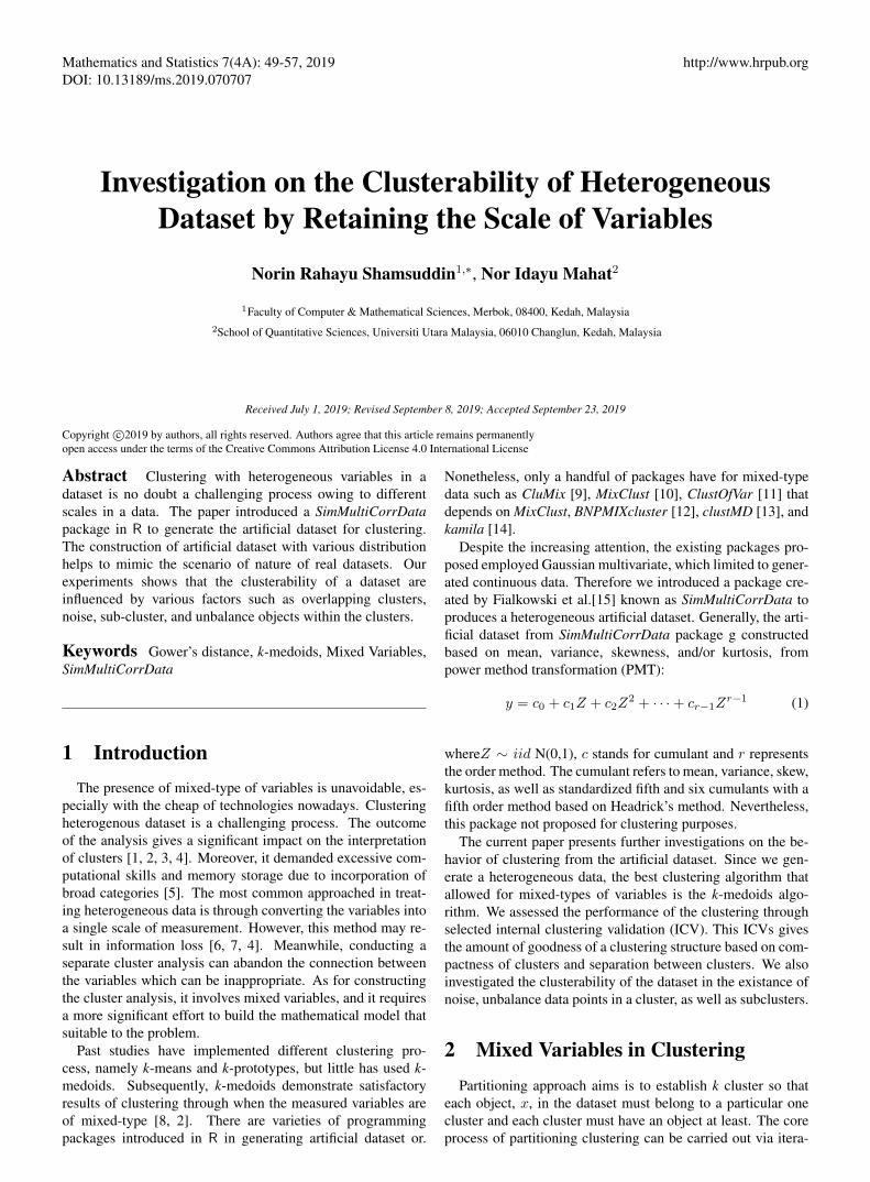
Mathematics and Statistics 7(4A): 49-57, 2019DOI: 10.13189/ms.2019.070707
http://www.hrpub.org
Investigation on the Clusterability of HeterogeneousDataset by Retaining the Scale of Variables
Norin Rahayu Shamsuddin1,∗, Nor Idayu Mahat2
1Faculty of Computer & Mathematical Sciences, Merbok, 08400, Kedah, Malaysia2School of Quantitative Sciences, Universiti Utara Malaysia, 06010 Changlun, Kedah, Malaysia
Received July 1, 2019; Revised September 8, 2019; Accepted September 23, 2019
Copyright c©2019 by authors, all rights reserved. Authors agree that this article remains permanentlyopen access under the terms of the Creative Commons Attribution License 4.0 International License
Abstract Clustering with heterogeneous variables in adataset is no doubt a challenging process owing to differentscales in a data. The paper introduced a SimMultiCorrDatapackage in R to generate the artificial dataset for clustering.The construction of artificial dataset with various distributionhelps to mimic the scenario of nature of real datasets. Ourexperiments shows that the clusterability of a dataset areinfluenced by various factors such as overlapping clusters,noise, sub-cluster, and unbalance objects within the clusters.
Keywords Gower’s distance, k-medoids, Mixed Variables,SimMultiCorrData
1 IntroductionThe presence of mixed-type of variables is unavoidable, es-
pecially with the cheap of technologies nowadays. Clusteringheterogenous dataset is a challenging process. The outcomeof the analysis gives a significant impact on the interpretationof clusters [1, 2, 3, 4]. Moreover, it demanded excessive com-putational skills and memory storage due to incorporation ofbroad categories [5]. The most common approached in treat-ing heterogeneous data is through converting the variables intoa single scale of measurement. However, this method may re-sult in information loss [6, 7, 4]. Meanwhile, conducting aseparate cluster analysis can abandon the connection betweenthe variables which can be inappropriate. As for constructingthe cluster analysis, it involves mixed variables, and it requiresa more significant effort to build the mathematical model thatsuitable to the problem.
Past studies have implemented different clustering pro-cess, namely k-means and k-prototypes, but little has used k-medoids. Subsequently, k-medoids demonstrate satisfactoryresults of clustering through when the measured variables areof mixed-type [8, 2]. There are varieties of programmingpackages introduced in R in generating artificial dataset or.
Nonetheless, only a handful of packages have for mixed-typedata such as CluMix [9], MixClust [10], ClustOfVar [11] thatdepends on MixClust, BNPMIXcluster [12], clustMD [13], andkamila [14].
Despite the increasing attention, the existing packages pro-posed employed Gaussian multivariate, which limited to gener-ated continuous data. Therefore we introduced a package cre-ated by Fialkowski et al.[15] known as SimMultiCorrData toproduces a heterogeneous artificial dataset. Generally, the arti-ficial dataset from SimMultiCorrData package g constructedbased on mean, variance, skewness, and/or kurtosis, frompower method transformation (PMT):
y = c0 + c1Z + c2Z2 + · · ·+ cr−1Z
r−1 (1)
whereZ ∼ iid N(0,1), c stands for cumulant and r representsthe order method. The cumulant refers to mean, variance, skew,kurtosis, as well as standardized fifth and six cumulants with afifth order method based on Headrick’s method. Nevertheless,this package not proposed for clustering purposes.
The current paper presents further investigations on the be-havior of clustering from the artificial dataset. Since we gen-erate a heterogeneous data, the best clustering algorithm thatallowed for mixed-types of variables is the k-medoids algo-rithm. We assessed the performance of the clustering throughselected internal clustering validation (ICV). This ICVs givesthe amount of goodness of a clustering structure based on com-pactness of clusters and separation between clusters. We alsoinvestigated the clusterability of the dataset in the existance ofnoise, unbalance data points in a cluster, as well as subclusters.
2 Mixed Variables in ClusteringPartitioning approach aims is to establish k cluster so that
each object, x, in the dataset must belong to a particular onecluster and each cluster must have an object at least. The coreprocess of partitioning clustering can be carried out via itera-
50 Investigation on the Clusterability of Heterogeneous Dataset by Retaining the Scale of Variables
tion approach to minimize or to maximize an objective func-tion. Typically, researchers tend to minimize the function toobtain a homogeneous cluster. Partitioning around medoids(PAM) [16], k-medoids uses the actual objects in the datasetas the center of the cluster rather than using the means pointswhich known as medoids.
PAM enables multiple measures to be incorporated, such asthe range of Euclidean, Manhattan, and Gower distances. Onthe contrary, only Gower’s distance able to measure the dissim-ilarity of the heterogeneous dataset.
2.1 Gower’s Distance
Assume a dataset with n objects with p variables xij : (i =1, 2, . . . , n; j = 1, 2, . . . , p) where p stands for dimensions ofvariables that comprise of c continuous, o ordinal, b binary orm discrete variables. For ordinal variables with ot levels, thevalue written as 1, 2, . . . , ot. Generally, the difference in valuedenoted in the form of matrix structure attained from dissimi-larity measure from a dataset.
Nonetheless, the distance for continuous variables is moreextensive than the distance for mixed-type of variables [17].Currently, several methods have been suggested to addressthe shortcomings of variation for mixed-type of variables (see[18, 19, 20, 21]). It was found that the most commonly
used measurement to deal with mixed-type of variables is theGower’s similarity measure. Gower introduced it in the 1970swith the features of Euclidean distance [22]. Generally, thesimilarity measure between ith object and kth object,sik, is cal-culated as:
sik =
∑pl=1 wiklsikl∑p
l=1 wikl(2)
where wikl refers to weight. wikl = 0 if objects i and k can-not be compared for variable p = l. For instance, let variablel be the criterion of chest pain after certain exercises. Thus,comparing objects i and k based on variable l would be biasedin one of these two objects that do not show the pain.
Nevertheless, Gower’s suggested a few methods to dismissordinal variables. Since many datasets have ordinal variables,Podani [23] had stretched out Gower’s study by inserting thefunction for ordinal, as given in the following:
sikl = 1, if ril = rkl (3)
where ril and rkl are the ordinal variables for objects i and k,respectively.
If the number of objects share similar rank score for variablep, therefore:
sik = 1− |ril − rkl| − (Til − 1)/2− (Tkl − 1)/2
max{rl} −min{rl} − (Tl,max − 1)/2− (Tl,min − 1)/2(4)
Til refers to the number of n objects in that share similarrank score with object i for variable l, Tkl denotes the numberof objects in n that have the same rank score with object k forvariable l, Tl,max reflects the number of objects with maximumscore rank for variable l, and Tl,min represents the number ofobjects with minimum score rank for variable l. An exten-sion of Gower’s distance proposed by [23] allowed for met-ric or non-metric version. Currently, Gower’s similarity indexhas been widely used to support the vector machine, machinelearning, recognizing the patter, bioinformatics, molecular bi-ology, epidemiology, and other disciplines.
2.2 Internal Clustering Validation (ICV)
The ICV measures (as in [24, 25, 26, 27]) provide better op-tions for researchers to select the most appropriate method forclustering. The validity indices determine the quality of clus-tering, apart from discovering the optimal K. In order to attaineffective evaluation of cluster analysis, understanding the ‘def-inition’ of internal validation is crucial. In addition, internalvalidation is a method to assess the fitness of the structure anddata in clustering as it is based on the distance between theobjects in the cluster as well as between the clusters [28].
Handl and Knowles [29] explained ICV from the stance ofthree aspects; (i) compactness, (ii) connectedness, and (iii) sep-aration. Compactness is considered to attain homogeneouscluster. High homogeneity can lead to overlapping of clus-
ters. Next, connectedness examines the connection of neigh-bouring data points in the similar clusters. Meanwhile, sep-aration examines the degree of partition between the clusters.Additionally, inverse compactness leads to a good quality ofseparation and vice versa. Based on these measurements, mostof the previous studies had conducted clustering by combiningthe measurement of compactness and separation to dismiss thecluster’s density and structure. In fact, compactness and sepa-ration were estimated to be suitable number of clusters K of adataset. The indices of ICV can be discovered in [30, 31, 32].
Intra-cluster compactness and separation were measured us-ing Dunn (D) index [33]. D index shares same range valueswith Davies-Bouldin (DB) index, yet, D index generates maxi-mum value to show compact and well-separated clusters. In ad-dition, DB and D had utilized the ratio-type coefficient withinthe different clusters and also between the different clusterswhich do not display any trends [25]. Meanwhile, the conceptof ΓC is adopted from [34] and designed by [35]. They definedit as average of total distance between objects in a cluster overother clusters. In addition, it also defines the average to thenearest and the furthest distances between the pairs of objectsin the dataset (Table 1). In the C-index, the minimum valuerepresented the good clusters. [36] suggested that Silhouette(S) index should determine the objects that do not belong tocluster and depicts the wellness of the objects in the cluster.Thus, the index will measure the average distance between theobjects within a cluster and the average distance between the
Mathematics and Statistics 7(4A): 49-57, 2019 51
Table 1. Internal cluster validation indices (ICV)
Indices Formula
Davies-Bouldin (DB) DB =1
nc
nc∑i=1
Ri
Ri = maxk=1,...,nc,i6=k
(Rik) i = 1, . . . , nc
Rik =si + sk
dik
dik = d(vi, vk) s =1
‖ci‖∑
d(x, vi)
C-index (ΓC) Cindex =S − Smin
Smax − Smin
Dunn (D) D = min1≤i≤c
(mini+1≤k≤c
(d(ci, ck)
max1≤j≤c diam(cj)
))
Silhouette (S) ASW =1
n
n∑i=1
si si =b(i)−a(i)
max a(i),b(i)
a(i)= average dissimilarity of i to all other objects of A
b(i) = minC 6=A
d(i, C)
d(i,C ) = average dissimilarity of i to all other objects of C
nc = no. of clusters; vi= centre of cluster;‖ci‖ = norm of ci; ci= cluster ; S =sum of distances over all pairs of objects; Smin = sum ofpair with smallest distances if all pairs of objects; Smax= sum of pair largest distances out of all pairs; d(∴,∴) = distance between clusters/centrod of clusters; xi= ith objects.
clusters.
3 Methodology
This package created all variables from standard and normalvariables from an intermediate correlation matrix. The contin-uous mixture variables are drawn from more than one compo-nent distribution. Categorical and count variables are generatedfrom inverse cumulative density function (cdf). As for ordinalvariable, the data generated through a process of discretisingthe standard normal variables at quantiles in conformity to thetargetted marginal distribution. Meanwhile, the count variablescomprise of standard and normal variables of uniform distribu-tion. The continuous mixture variables drawn from more thanone component distribution is describe in term of mixture dis-tribution.
The setting for generating the heterogenous dataset is de-scribed in the following:
(a) count variables were set to derive from one of these threedistributions:
(i) Poisson distribution (λ= 2, 6 and 11),
(ii) negative binomial distribution NB(2, 0.2), and
(iii) negative binomial NB(6, 0.8) distribution.
(b) ordinal variables were derived from two scenarios:
(i) group 1 with three categories (p(x) = 0.35; 0.75; 1),and
(ii) group 2 with four categories (p(x) =0.25; 0.5; 0.8; 1).
(c) the continuous variables were drawn from Gaussian(N(0, 1)), gamma (Γ(α = β = 10)), and chi-square(χ2
4) distributions to have both normal and non-normaldatasets.
From the uniform distribution withU(0.25, 0.7), the correla-tion matrix was obtained and fell within the feasible correlationbounds. The valid corr function for ‘Correlation Method 1’resolute if the matrix is in the boundaries. Subsequently, thevariables were generated using the function of rcorrvar alongwith the addition of error loop to reduce the errors in correla-tion.
Generally, ten parameters along with 300 objects were gen-erated as follows:
(a) five count variables – three variables with different meanvalues for Poisson distribution and two variables for neg-ative binomial with different parameters r and p,
(b) two ordinal variables with two groups of different cate-gories, and
(c) three continuous variables – chi-square, gamma, andGaussian distribution.
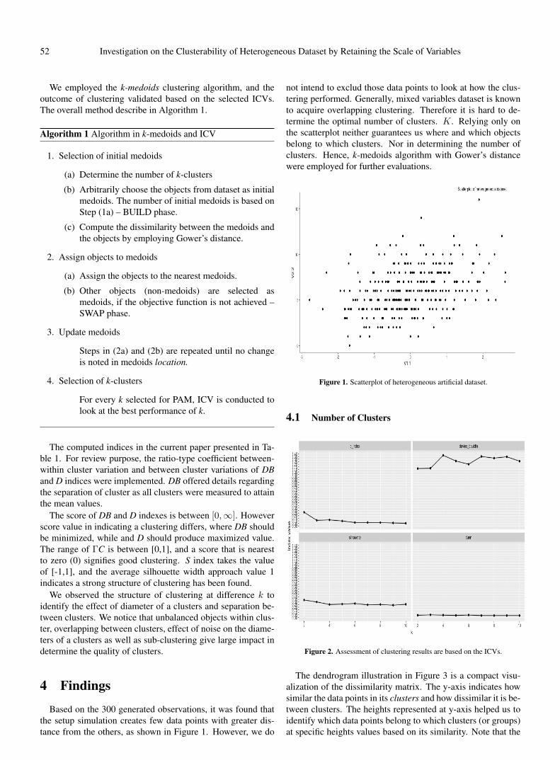
52 Investigation on the Clusterability of Heterogeneous Dataset by Retaining the Scale of Variables
We employed the k-medoids clustering algorithm, and theoutcome of clustering validated based on the selected ICVs.The overall method describe in Algorithm 1.
Algorithm 1 Algorithm in k-medoids and ICV
1. Selection of initial medoids
(a) Determine the number of k-clusters
(b) Arbitrarily choose the objects from dataset as initialmedoids. The number of initial medoids is based onStep (1a) – BUILD phase.
(c) Compute the dissimilarity between the medoids andthe objects by employing Gower’s distance.
2. Assign objects to medoids
(a) Assign the objects to the nearest medoids.
(b) Other objects (non-medoids) are selected asmedoids, if the objective function is not achieved –SWAP phase.
3. Update medoids
Steps in (2a) and (2b) are repeated until no changeis noted in medoids location.
4. Selection of k-clusters
For every k selected for PAM, ICV is conducted tolook at the best performance of k.
The computed indices in the current paper presented in Ta-ble 1. For review purpose, the ratio-type coefficient between-within cluster variation and between cluster variations of DBand D indices were implemented. DB offered details regardingthe separation of cluster as all clusters were measured to attainthe mean values.
The score of DB and D indexes is between [0,∞]. Howeverscore value in indicating a clustering differs, where DB shouldbe minimized, while and D should produce maximized value.The range of ΓC is between [0,1], and a score that is nearestto zero (0) signifies good clustering. S index takes the valueof [-1,1], and the average silhouette width approach value 1indicates a strong structure of clustering has been found.
We observed the structure of clustering at difference k toidentify the effect of diameter of a clusters and separation be-tween clusters. We notice that unbalanced objects within clus-ter, overlapping between clusters, effect of noise on the diame-ters of a clusters as well as sub-clustering give large impact indetermine the quality of clusters.
4 Findings
Based on the 300 generated observations, it was found thatthe setup simulation creates few data points with greater dis-tance from the others, as shown in Figure 1. However, we do
not intend to exclud those data points to look at how the clus-tering performed. Generally, mixed variables dataset is knownto acquire overlapping clustering. Therefore it is hard to de-termine the optimal number of clusters. K. Relying only onthe scatterplot neither guarantees us where and which objectsbelong to which clusters. Nor in determining the number ofclusters. Hence, k-medoids algorithm with Gower’s distancewere employed for further evaluations.
Figure 1. Scatterplot of heterogeneous artificial dataset.
4.1 Number of Clusters
Figure 2. Assessment of clustering results are based on the ICVs.
The dendrogram illustration in Figure 3 is a compact visu-alization of the dissimilarity matrix. The y-axis indicates howsimilar the data points in its clusters and how dissimilar it is be-tween clusters. The heights represented at y-axis helped us toidentify which data points belong to which clusters (or groups)at specific heights values based on its similarity. Note that the

Mathematics and Statistics 7(4A): 49-57, 2019 53
dendrogram illustration does not let us set the K, but may onlyyield an appropriate number of clusters.
Therefore, the assessment of the clustering structure of an al-gorithm is evaluated based on the ICVs values. Looking at Fig-ure 2, it is apparent that DB, ΓC, and S shows a point at which asignificant change in values of the index for k = [2, 10]. How-ever, D index hardly indicates the trend of changes in the indexvalues for the heterogeneous dataset. The indexes values of theDB, D, ΓC, and S are 1.1163, 0.0501, 0.0529 and 0.3381, re-spectively. DB and S indices suggest the construction of clus-ters at K = 2. On the hand, D index suggested the suitableclusters formations be K = 3, while ΓC indicates K = 10 asthe best number of clusters. Judging from the value obtainedand the constraint of the four indexes, the suitable K for thisartificial dataset should be K = 10 since only ΓC index ableto meet its constraints.
4.2 Cluster Strucuture Assessment
Further investigations on the behavior of clusters formationsbased on the selection of K from DB, D, ΓC, and S indexespresented in Figure 4. From this figure, it can be seen that thereis no distinct separation on the formation of clusters for K = 2and K = 3. Interestingly, there occur a pattern of clusters forK = 10 in Figure 4 (c), where it suggested that the numberof clusters for this dataset is equivalent to three. However, itonly can be managed with some conditions. For example, datapoints allocated to cluster 5, 7, and 8 should be classified as oneclass, while data points in cluster 2, 4, and 9 as another class.Hence, a precise clustering formation could have formed.
From the average silhouette width (figure not shows forK =2 andK = 3), overall average silhouette width forK = 2 yield0.28. The average silhouette width of the first cluster is only0.2, while the second cluster recorded an average of 0.45. Theoverall average silhouette width for K = 3, we obtained 0.24,where the average of the first cluster is 0.3, second clusters with0.35 while only 0.4 in the third cluster. In K = 10, the averagesilhouette width obtained is 0.27, and the average value of eachcluster shown in Figure 5.
We observed the structure at difference K to identify the ef-fect of diameter of a cluster and separation between clusters.We notice that unbalanced objects within cluster, overlappingbetween clusters, effect of noise on the diameters of a clustersas well as sub-clustering as shown in Figure 6, give large im-pact in clusterability of this dataset.
5 DiscussionVarious results in the number of clusters obtained from dif-
ferent ICVs. This phenomenon is common for a dataset to havemore than one K that represent good clusters. This is becausean unsupervised clustering makes it more challenging to dis-cover the best K. Nevertheless, careful validation of clustersand discovering the best K as particular indices are sensitiveto the outliers, noise, and even subclusters. A wise selectionof ICV used in a study is essential since the numerator and de-nominator of the indices is much influence on the structure of
the dataset.Halkidi, Batistakis, and Vazirgiannis [25] independent re-
views define that validation assessment performance is the bestwhen clusters are thoroughly compact (well clustered), but per-formance badly in data with mixed variables. Having a mixedtype of variables in clustering may create some discriminationin term of dissimilarity. Bijuraj [37] mentioned that it is moreappropriate if a dataset has a similar of variables.
Intersection, insertion or deletion at certain magnitude ofobjects within a cluster significantly influence the of disper-sion (width) as well as density of a cluster. As the K increase,the intra-cluster compactness tends to decrease an inter-clusterseparation increase simultaneously. k-medoids assigned ob-jects to it nearest medoids. Medoids is based on points ofdataset that represent minimal averaging dissimilarity mea-sures. The concepts similar to the k-means. Due to this ob-jective function, it explained the implication of the factors.
Since this dataset consists of overlapping data points in clus-tering, k-medoids algorithm is not suitable to carry out the clus-ter analysis. It is known that k-medoids algorithmhard cluster-ing, in which each data points should belong to one and onlyone cluster. Therefore other clustering approaches, such asdensity-based method should be employed. The differences inthe decision of appropriate K between ICVs were influencedby various factors that affected the nominator and denominatorof ICVs.
The problems in identifying the appropriate K have createdan interest among researchers in the discipline of clustering.Moreover, it becomes as essential issues as its effects on theperformance of the internal validity of clustering. Few researchworks of this matter have been carried out and reported in [38,39, 40] and few others cited elsewhere.
6 Concluding Remarks
In this paper, we investigate the clusterability of mixed-typesof variables of a dataset through artificial dataset consist ofmixed types of data from various distributions from SimMul-tiCorrData package. This package allows users to choose towork on empirical or theoretical approaches based on one’sobjective in generating simulation dataset. We have conductedboth approaches, and we discovered that the empirical methodis time-consuming, and the correlation matrix always hard toachieve. For this paper, we opt for theory methods using cal
theory function with mixed types of variables. Furthermore,it is happened a simulation dataset from this package generatesome noises and outliers which give benefits to identify the ef-fect on clustering. Since the simulation data not purposely de-veloped for clustering, therefore is unable to measure the levelof overlap between clusters.
We have demonstrated that by‘retaining’ the scale of vari-ables through Gower’s distance, the formation of clusters doesexist. However, we obtained poor results of clustering using k-medoids algorithm. Results from the average silhouette width,it can be said indicated that no substantial structure had beenfound. As for the effect of various factors in clusterability ofdataset, we have performed a weighted clustering approach to
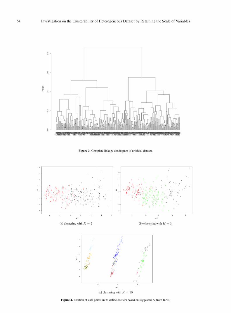
54 Investigation on the Clusterability of Heterogeneous Dataset by Retaining the Scale of Variables
Figure 3. Complete linkage dendogram of artificial dataset.
(a) clustering with K = 2 (b) clustering with K = 3
(c) clustering with K = 10
Figure 4. Position of data points in its define clusters based on suggested K from ICVs.

Mathematics and Statistics 7(4A): 49-57, 2019 55
Figure 5. Silhouettes of a clustering with K = 10 of the artificial dataset.
reduce the overlapping between clusters and assigning the ob-jects to it nearest cluster. We also deleted data points that wereidentified as outliers/noise (results are not display) to obtaineda better clustring results. Yet, there is no improvement in thevalidity scores but further worsen the clustering performance.Besides, the process of clustering mixed-type of variables andretaining their scale throughout the analysis was indeed chal-lenging.
k-medoids
AcknowledgementsThe authors would like to express their gratitude to the editor
and reviewers for their insights to help improving this paper.We would also gratefully acknowledge the financial supportby Universiti Teknologi MARA (UiTM) and the Ministry ofHigher Education (MOHE) Malaysia.
REFERENCES[1] Z. Huang. Extensions to the k-means algorithm for clustering
large data sets with categorical values, Data Mining andKnowledge Discovery, Vol.2, No.3, 283-304, 1998.
[2] C. Hennig, T. F. Liao. How to find an appropriate clusteringfor mixed-type variables with application to socio-economicstratification, Journal of the Royal Statistical Society: Series C(Applied Statistics), Vol.62, No.3, 309-369, 2013.
[3] G. Szepannek. ‘clustMixType’: k-Prototypes clustering formixed variable-type data, R package version 0.1-16, 2017.
[4] A. H. Foss, M. Markatou. kamila: Clustering mixed-type datain R and Hadoop, Journal of Statistical Software, Vol.83, No.1,
44, 2018.
[5] H. Ralambondrainy. A conceptual version of the K-means algo-rithm, Pattern Recognition Letters, Vol.16, No.11, 1147-1157,1995.
[6] W. J. Krzanowski. The location model for mixtures of categori-cal and continuous variables, Journal of Classification, Vol.10,25-49, 1993.
[7] G. Celeux, G. Govaert. Latent class models for categoricaldata,Chapman & Hall/CRC, 2015.
[8] E. C. de Assis,. R. M. C. R. de Souza. A k-medoids clusteringalgorithm for mixed feature-type symbolic data, EEE Interna-tional Conference on Systems, Man and Cybernetics, 527-531,2011.
[9] M. Hummel, D. Edelmann, A. Kopp-Schneider. CluMix: Clus-tering and visualization of mixed-type data”, Comprehensive RArchive Network (CRAN), 2017.
[10] M. Marbac, C. Biernacki, V. Vandewalle. Model-based clus-tering of Gaussian copulas for mixed data, Communications inStatistics-Theory and Methods, Vol.46, No.23, 11635-11656,2017.
[11] M. Chavent, V. Kuentz, B. Liquet, L. Saracco., ClustOfVar: AnR package for the clustering of variables, Journal of StatisticalSoftware, 2011.
[12] C. Carmona, L. Nieto-Barajas, A. Canale. Model-basedapproach for household clustering with mixed scale variables,Advances in Data Analysis and Classification, Vo.13, No.2,559, 2019.
[13] D. McParland, I. C. Gormley. clustMD: Model based clusteringfor mixed data, Comprehensive R Archive Network (CRAN),2017.
[14] A. H. Foss, M. Markatou. kamila: Methods for clusteringmixed-type data. Comprehensive R Archive Network (CRAN),2018.
[15] A. C. Fialkowski,. SimMultiCorrData: Simulation of correlateddata with multiple variable types, Comprehensive R ArchiveNetwork (CRAN), 2017.
[16] L. Kaufman, P. J. Rousseeuw. Clustering by Means of Medoids,Faculty of Mathematics and Informatics, 1987.
[17] A. S. Shirkhorshidi, S. Aghabozorgi, T. Y. Wah. A comparisonstudy on similarity and dissimilarity measures in clusteringcontinuous data, PLoS ONE, Vol.10, No.12, e0144059, 2015

56 Investigation on the Clusterability of Heterogeneous Dataset by Retaining the Scale of Variables
[18] Z.Huang. Clustering Large Data Sets with Mixed Numeric andCategorical Values, Proceedings of the 1st Pacific-Asia Con-ference on Knowledge Discovery and Data Mining,(PAKDD),21-34, 1997, 1997.
[19] M.S. Yang, P. Y. Hwang, D. H. Chen. Fuzzy clustering algo-rithms for mixed feature variables, Fuzzy Sets and Systems,Vol.141, No.2, 301-317, 2004.
[20] A. Ahmad, L. Dey. A k-mean clustering algorithm for mixednumeric and categorical data, Data and Knowledge Engineer-ing, Vol.63, No.2, 503-527, 2007.
[21] J. Ji, T. Bai, C. Zhou, C. Ma, Z. Wang. An improvedk-prototypes clustering algorithm for mixed numeric andcategorical data, Neurocomputing, Vol.120, 590-596, 2013.
[22] J.C. Gower. A general coefficient of similarity and some of itsproperties, Biometrics, Vol.27, No.4, 857-871, 1971.
[23] J. Podani. Extending Gower’s general coefficient of similarityto ordinal characters, Taxon, 331-340, 1999.
[24] R. Tibshirani, G. Walther, T. Hastie. Estimating the number ofclusters in a data set via the gap statistic, Journal of the RoyalStatistical Society: Series B (Statistical Methodology), Vol.63,No.2, 411-423, 2001.
[25] M. Halkidi, Y. Batistakis, M. Vazirgiannis,. Clustering validitychecking methods: Part II, ACM Sigmod Record, Vol.31, No.3,19-27, 2002.
[26] M. Kim, R. S. Ramakrishna. New indices for cluster validityassessment, Pattern Recognition Letters, Vol.26, No.15,2353-2363, 2005.
[27] J. C. Rojas-Thomas, M. Santos, M. Mora. New internal indexfor clustering validation based on graphs, Expert Systems withApplications, Vol.86, No.15, 334-349, 2017.
[28] A. K. Jain, R. C. Dubes. Algorithms for Clustering Data,Prentice Hall, 1988.
[29] J. Handl, J. Knowles. Exploiting the Trade-off - The Benefitsof Multiple Objectives in Data Clustering, In: Coello CoelloC.A., Hernandez Aguirre A., Zitzler E. (eds) EvolutionaryMulti-Criterion Optimization. EMO 2005. Lecture Notes in
Computer Science, Vol. 3410, Springer, Berlin, Heidelberg,547-560, 2005.
[30] B. Desgraupes. clusterCrit: clustering indices. R packageversion 1.2. 3”, Comprehensive R Archive Network (CRAN),2015.
[31] M. Charrad, N. Ghazzali, V. Boiteau, A. Niknafs,. NbClust:An R package for determining the relevant number of clustersin a data set”, Journal of Statistical Software, Vol.61, No.61548-7660, 2014.
[32] M. Hassani, T. Seidl. Internal clustering evaluation of datastreams, Trends and Applications in Knowledge Discovery andData Mining, 198-209, 2015.
[33] D. L. Davies, D. W. Bouldin. A cluster separation measure,IEEE Transactions on Pattern Analysis and Machine Intelli-gence, Vol.2, 36, 1979.
[34] E. C. Dalrymple-Alford. Measurement of clustering in freerecall, Psychological Bulletin, Vol.74, No.1, 32-34, 1970.
[35] L. J. Hubert, J. R. Levin. A general statistical framework forassessing categorical clustering in free recall, PsychologicalBulletin, Vol.83, No.6, 1072, 1976.
[36] P. J. Rousseeuw. Silhouettes: A graphical aid to the interpreta-tion and validation of cluster analysis, Journal of Computationaland Applied Mathematics, Vol.20, 53-65, 1987.
[37] L. V. Bijuraj. Clustering and its Applications, Proceedingsof National Conference on New Horizons in IT-NCNHIT,169-172, 2013.
[38] Y. Liu, Z. Li, H. Xiong, X. Gao, J. Wu. Understanding ofInternal Clustering Validation Measures, Proceeding IEEEInternational Conference of Data Mining, 911-916, 2010.
[39] J. C. Bezdek, N. R. Pal. Some new indexes of cluster validity,Part B (Cybernetics) IEEE Transactions on Systems, Man, andCybernetics, Vol.28, No.3, 301-315, 1998.
[40] S. Saitta, B. Raphael, I. F.C. Smith. A bounded index forcluster validity, Machine Learning and Data Mining in PatternRecognition, Vol.30, 174-187, 2007.
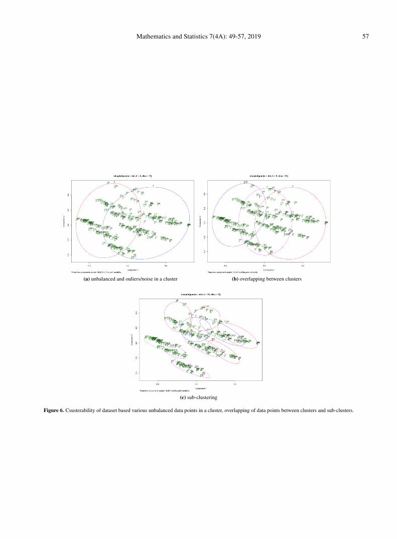
Mathematics and Statistics 7(4A): 49-57, 2019 57
(a) unbalanced and ouliers/noise in a cluster (b) overlapping between clusters
(c) sub-clustering
Figure 6. Csusterability of dataset based various unbalanced data points in a cluster, overlapping of data points between clusters and sub-clusters.

Mathematics and Statistics 7(4A): 58-64, 2019DOI: 10.13189/ms.2019.070708
http://www.hrpub.org
Tree-based Threshold Model for Non-stationary Extremeswith Application to the Air Pollution Index Data
Afif Shihabuddin1, Norhaslinda Ali1,2,∗, Mohd Bakri Adam1,2
1Institute for Mathematical Research, Universiti Putra Malaysia, 43400 UPM Serdang, Selangor, Malaysia2Department of Mathematics, Faculty of Science,Universiti Putra Malaysia, 43400 UPM Serdang, Selangor, Malaysia
Received July 01, 2019; Revised August 22, 2019; August 30, 2019
Copyright c©2019 by authors, all rights reserved. Authors agree that this article remains permanentlyopen access under the terms of the Creative Commons Attribution License 4.0 International License
Abstract Air pollution index (API) is a common tool usedto describe the air quality in the environment. High level ofAPI indicates the greater level of air pollution which will givesbad impact on human health. Statistical model for high levelof API is important for the purpose of forecasting the level ofAPI so that the public can be warned. In this study, extremesof API are modelled using Generalized Pareto Distribution(GPD). Since the values of API are determined by the valueof five pollutants namely sulphur dioxide, nitrogen dioxide,carbon monoxide, ozone and suspended particulate matter,data on API exhibit non-stationarity. Standard method formodelling the non-stationary extremes using GPD is by fixingthe high constant threshold and incorporating the covariatemodel in the GPD parameters for data above the thresholdto account for the non-stationarity. However, high constantthreshold value might be high enough on certain covariate forGPD approximation to be a valid model for extreme values,but not on the other covariates which leads to the violationof the asymptotic basis of GPD model. New method forthe threshold selection in non-stationary extremes modellingusing regression tree is proposed to the API data. Regressiontree is used to partition the API data into a stationary groupwith similar covariate condition. Then, a high threshold valuecan be applied within a group. Study shows that model forextremes of API using tree-based threshold gives a good fitand provides an alternative to the model based on standardmethod.
Keywords Air Pollution Index, Threshold Exceedances,Generalized Pareto Distribution, Non-stationary, RegressionTree, Tree-based Threshold
1 IntroductionAir quality is an important aspect of human life. In
Malaysia, it is monitored and enforced by the Department
of Environment (DOE). Air quality is determined by the AirPollution Index (API) which is updated hourly by DOE. APIvalue is derived from five main pollutants which are groundlevel ozone (O3), nitrogen dioxide (NO2), particulate matter(PM10), carbon monoxide (CO) and sulphur dioxide (SO2).High concentration of these pollutants in the air is harmfulfor everyone and also causing serious health problem. Highconcentration of SO2, NO2 and CO in the air can cause aheart and lungs problem [1]. High level of PM10 is associatedwith haze days which can limit the eyesight and cause therespiratory problem [2]. According to Malaysian AmbientAir Quality Guidelines (MAAQG), API values which above100 are considered unhealthy and could threaten public health.Therefore it is important to understand the behavior of highlevel of API particularly to give health warnings for thepublic. In order to describe the behavior of high level API ata particular area, it is important to identify the distributionswhich best fit the data [3]. Extreme value distribution fromextreme value theory are suitable in modelling such highvalues.
Extreme value theory (EVT) is a branch of statistics whichstudy the stochastic behavior of a process at unusually large orsmall values [3]. Particularly, EVT provides procedures for tailestimation which are scientifically and statistically rational.Two significant results from EVT are first, the asymptoticdistribution of the standardized series of maxima (minima)is shown to converge to the Gumbel, Frechet, or Weibulldistributions. A standard form of these three distributions iscalled the generalized extreme value (GEV) distribution. Thesecond significant result concerns the distribution of excessover a given threshold, where the limiting distribution is ageneralized Pareto distribution (GPD). The application ofEVT is important in various disciplines such as hydrology,meteorology, finance, engineering, insurance and environment.Common applications of EVT include modeling the extremesof heavy rainfall, sea-levels, pollution concentrations andmany more. There are many application of extreme value
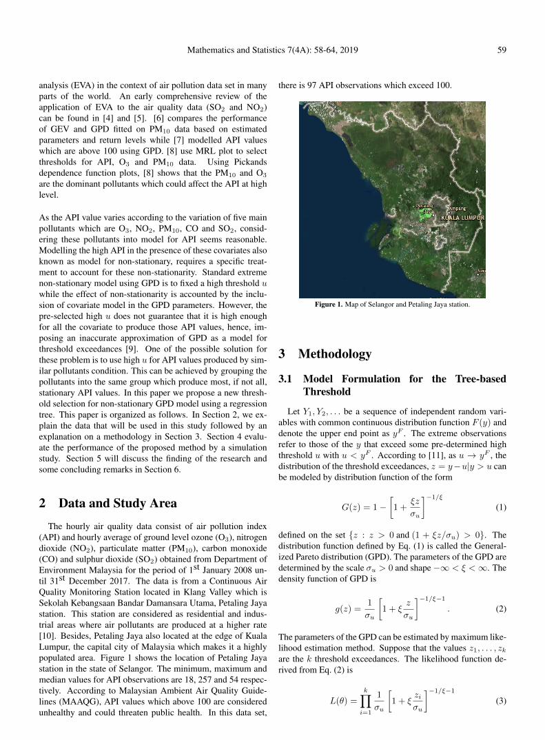
Mathematics and Statistics 7(4A): 58-64, 2019 59
analysis (EVA) in the context of air pollution data set in manyparts of the world. An early comprehensive review of theapplication of EVA to the air quality data (SO2 and NO2)can be found in [4] and [5]. [6] compares the performanceof GEV and GPD fitted on PM10 data based on estimatedparameters and return levels while [7] modelled API valueswhich are above 100 using GPD. [8] use MRL plot to selectthresholds for API, O3 and PM10 data. Using Pickandsdependence function plots, [8] shows that the PM10 and O3
are the dominant pollutants which could affect the API at highlevel.
As the API value varies according to the variation of five mainpollutants which are O3, NO2, PM10, CO and SO2, consid-ering these pollutants into model for API seems reasonable.Modelling the high API in the presence of these covariates alsoknown as model for non-stationary, requires a specific treat-ment to account for these non-stationarity. Standard extremenon-stationary model using GPD is to fixed a high threshold uwhile the effect of non-stationarity is accounted by the inclu-sion of covariate model in the GPD parameters. However, thepre-selected high u does not guarantee that it is high enoughfor all the covariate to produce those API values, hence, im-posing an inaccurate approximation of GPD as a model forthreshold exceedances [9]. One of the possible solution forthese problem is to use high u for API values produced by sim-ilar pollutants condition. This can be achieved by grouping thepollutants into the same group which produce most, if not all,stationary API values. In this paper we propose a new thresh-old selection for non-stationary GPD model using a regressiontree. This paper is organized as follows. In Section 2, we ex-plain the data that will be used in this study followed by anexplanation on a methodology in Section 3. Section 4 evalu-ate the performance of the proposed method by a simulationstudy. Section 5 will discuss the finding of the research andsome concluding remarks in Section 6.
2 Data and Study Area
The hourly air quality data consist of air pollution index(API) and hourly average of ground level ozone (O3), nitrogendioxide (NO2), particulate matter (PM10), carbon monoxide(CO) and sulphur dioxide (SO2) obtained from Department ofEnvironment Malaysia for the period of 1st January 2008 un-til 31st December 2017. The data is from a Continuous AirQuality Monitoring Station located in Klang Valley which isSekolah Kebangsaan Bandar Damansara Utama, Petaling Jayastation. This station are considered as residential and indus-trial areas where air pollutants are produced at a higher rate[10]. Besides, Petaling Jaya also located at the edge of KualaLumpur, the capital city of Malaysia which makes it a highlypopulated area. Figure 1 shows the location of Petaling Jayastation in the state of Selangor. The minimum, maximum andmedian values for API observations are 18, 257 and 54 respec-tively. According to Malaysian Ambient Air Quality Guide-lines (MAAQG), API values which above 100 are consideredunhealthy and could threaten public health. In this data set,
there is 97 API observations which exceed 100.
Figure 1. Map of Selangor and Petaling Jaya station.
3 Methodology
3.1 Model Formulation for the Tree-basedThreshold
Let Y1, Y2, . . . be a sequence of independent random vari-ables with common continuous distribution function F (y) anddenote the upper end point as yF . The extreme observationsrefer to those of the y that exceed some pre-determined highthreshold u with u < yF . According to [11], as u → yF , thedistribution of the threshold exceedances, z = y−u|y > u canbe modeled by distribution function of the form
G(z) = 1−[1 +
ξz
σu
]−1/ξ(1)
defined on the set {z : z > 0 and (1 + ξz/σu) > 0}. Thedistribution function defined by Eq. (1) is called the General-ized Pareto distribution (GPD). The parameters of the GPD aredetermined by the scale σu > 0 and shape−∞ < ξ <∞. Thedensity function of GPD is
g(z) =1
σu
[1 + ξ
z
σu
]−1/ξ−1. (2)
The parameters of the GPD can be estimated by maximum like-lihood estimation method. Suppose that the values z1, . . . , zkare the k threshold exceedances. The likelihood function de-rived from Eq. (2) is
L(θ) =
k∏i=1
1
σu
[1 + ξ
ziσu
]−1/ξ−1(3)
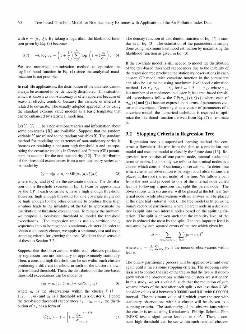
60 Tree-based Threshold Model for Non-stationary Extremes with Application to the Air Pollution Index Data
with θ = (σu, ξ). By taking a logarithm, the likelihood func-tion given by Eq. (3) becomes
`(θ) = −k log σu −(1 +
1
ξ
) k∑i=1
log(1 + ξ
ziσu
). (4)
We use numerical optimization method to optimize thelog-likelihood function in Eq. (4) since the analytical maxi-mization is not possible.
In real-life applications, the distribution of the data sets cannotalways be assumed to be identically distributed. This situationwhich is known as non-stationary is often apparent because ofseasonal effects, trends or because the variable of interest isrelated to covariate. The usually adopted approach is by usingthe standard extreme value models as a basic templates thatcan be enhanced by statistical modeling.
Let Y1, Y2, . . . be a non-stationary series and information aboutsome covariates {X} are available. Suppose that the randomvariable Y are related to the random variables X. The standardmethod for modeling the extremes of non-stationary series isfocuses on retaining a constant high threshold u and incorpo-rating the covariate models in Generalized Pareto (GP) param-eters to account for the non-stationarity [12]. The distributionof the threshold exceedances from a non-stationary series canbe model by
(y − u|y > u) ∼ GP(σu(x), ξ(x)) (5)
where σu(x) and ξ(x) are the covariate models. The distribu-tion of the threshold excesses in Eq. (5) can be approximateby the GP if each covariate x have a high enough threshold.However, high enough threshold for one covariate might notbe high enough for the other covariate to produce those highy values leads to the invalidity of the GP to approximate thedistribution of threshold exceedances. To remedy the problem,we propose a tree-based threshold to model the thresholdexceedances. The regression tree is use to partition the ysequences into m homogeneous stationary clusters. In order toobtain a stationary cluster, we apply a stationary test and use astopping criteria for growing the tree. We defer the discussionof these to Section 3.2.
Suppose that the observations within each clusters producedby regression tree are stationary or approximately stationary.Then, a constant high threshold can be set within each clustersproducing a different threshold in each of the clusters knownas tree-based threshold. Then, the distribution of the tree-basedthreshold exceedances can be model by
(yk − uk|yk > uk) ∼ GP(σuk, ξ) (6)
where yk is the observations within the cluster k (k =1, 2, . . . ,m) and uk is a threshold set in a cluster k. Denotethe tree-based threshold exceedances zk = yk − uk, the distri-bution of zk has a form of
G(zk) = 1−[1 +
ξzkσuk
]−1/ξ+
. (7)
The density function of distribution function of Eq. (7) is sim-ilar as in Eq. (3). The estimation of the parameters is simplydone using maximum likelihood estimation by maximizing thelikelihood function as given in Eq. (3).
If the covariate model is still needed to model the distributionof the tree-based threshold exceedances due to the inability ofthe regression tree produced the stationary observations in eachcluster, GP model with covariate function in the parameterscan also be estimated using maximum likelihood estimationmethod. Let zi1, zi2, . . . , zik for i = 1, 2, . . . , nuk where nukis a number of exceedances in cluster k, be a tree-based thresh-old exceedances follow the GP(σuk
(x), ξ(x)) where each ofσuk
(x) and ξ(x) have an expression in terms of parameters vec-tor and covariates. Denoting β as a vector of parameters of acovariate model, the numerical technique is required to opti-mize the likelihood function derived from Eq. (7) to estimateβ.
3.2 Stopping Criteria in Regression TreeRegression tree is a supervised learning method that con-
struct a flowchart-like tree from the data as a prediction treemodel and uses the model to classify the future data [13]. Re-gression tree consists of one parent node, internal nodes andterminal nodes. In our study, we refer to the terminal nodes as acluster which consist of stationary observations. To determinewhich cluster an observation is belongs to, all observations areplaced at the root (parent node) of the tree. We follow a pathfrom the root and proceed to one of the internal node calledleaf by following a question that split the parent node. Theobservations with yes answer will be placed at the left leaf (in-ternal node) while observations with no answer will be placedat the right leaf (internal node). The tree model is fitted usingbinary recursive partitioning where a parent node in a decisiontree is split into two internal nodes based on the splitting cri-terion. The split is chosen such that the impurity level of thetree is reduced the most by the split. The tree impurity level ismeasured by sum squared errors of the tree which given by
S =∑
c∈leaves(T )
∑i∈c
(yi −mc)2
where mc = 1nc
∑i∈c yi, is the mean of observations within
leaf c.
The binary partitioning process will be applied over and overagain until it meets some stopping criteria. The stopping crite-ria is set to control the size of the tree so that the tree will stop togrow when the observations within the clusters are stationary.In this study, we set a value δ, such that the reduction of sumsquared errors of the tree after each split is not less than δ. Weconsider values of δ between 0.000001 and 0.01 with 0.000001interval. The maximum value of δ which grow the tree withstationary observations within a cluster will be chosen as astopping criteria. The stationarity of the observations withinthe cluster is tested using Kwiatkowski-Phillips-Schmidt-Shin(KPSS) test at significance level α = 0.05. Then, a con-stant high threshold can be set within each resulted clusters.

Mathematics and Statistics 7(4A): 58-64, 2019 61
The threshold is set at qth percentile where q kept similar forall clusters so that the rate of exceedances remain constantthroughout the data set. Since each cluster has different num-ber of observations, the threshold value might differ for eachclusters. In other words, each observation will have their ownthreshold value. These threshold values are arranged accordingto the index of observations producing a varying threshold. Inthis study, the 95th percentile value for threshold are chosen foreach cluster. This percentile value is reasonably sufficient forGPD approximation be a valid limiting distribution for thresh-old exceedances while still keep the number of exceedanceslarge enough for the model estimation [14].
4 Simulation StudyIn this section we will illustrate the efficiency of the tree-
based threshold method over the standard method for mod-elling the non-stationary extremes by a simulation study. Wesimulate random numbers from generalized extreme value dis-tribution using inverse sampling method. Our argument for thechoice of GEV distribution is as follows. If Y1, . . . , Yn is dis-tributed as GEV(µ, σ, ξ), then, it can be shown that the blockmaxima Mn = max(Y1, . . . , Yn) will also GEV(µ∗, σ∗, ξ)with
µ∗ = µ+σ(nξ − 1)
ξand σ∗ = nξσ.
According to [3], if the distribution of a block maxima is GEV,then the excesses of high enough threshold, u can be approxi-mated by GPD with parameter σ and ξ where
σ = σ∗ + ξ(u− µ∗).
Here, parameter ξ is equal to that of the correspondingparameter ξ in GEV distribution.
Covariates model is incorporated in the GEV location parame-ter, µ to induce non-stationarity in the simulated random num-bers. Two covariate models are used which are:
1. µ = µ0 + µ1
(t
n+1
)+ µ2x for linear trend,
2. µ = µ0+µ1 cos(2πtn )−µ2 sin(
2πtn )+µ3x for cyclic trend
where t and n represent time covariate and number of obser-vations respectively. Another covariate x is generated fromstandard normal distribution. Time covariate, t is included tocreate trends in the data sets, while the covariate x representsa random variable which might affect the variable y. The timecovariate is simply an increasing index from 1 until 3653 whichcorresponds to number of days in 10 years. The covariate x issimulated using function rnorm in R statistical software. Weconsider four non-stationary GEV data sets of size n = 3653,each containing either a linear or a cyclic trend in parameter µwith shape parameter ξ = 0.4 and ξ = −0.4. The abbrevia-tion of non-stationary GEV data sets are given in Table 1. Thescale parameter, σ is fixed at 1 for all data sets. The locationparameter µ0, µ1, µ2, µ3 are chosen arbitrarily and given inTable 2.
Table 1. The Abbreviation for simulated non-stationary GEV data sets.
Data set AbbreviationGEV with Linear trend andPositive Shape Parameter GEVLPGEV with Linear trend andNegative Shape Parameter GEVLNGEV with Cyclic trend andPositive Shape Parameter GEVCPGEV with Cyclic trend andNegative Shape Parameter GEVCN
Table 2. Location parameter for simulated data sets.
Data set µ0 µ1 µ2 µ3
GEVLP 1 10 1 -GEVLN 1 10 1 -GEVCP 1 5 5 1GEVCN 1 10 10 1
The tree-based threshold selection method is applied to thesimulated data sets. The excesses of tree-based threshold aremodelled by both stationary and non-stationary GP model. Co-variate models are incorporated in the scale parameter of non-stationary GP model such that the scale parameter is either
σ = exp
{σ0 + σ1
(t
n+ 1
)+ σ2x
}, (8)
or
σ = exp{σ0 + σ1 cos
(2πt
n
)− σ2 sin
(2πt
n
)+ σ3x
}(9)
where Eq. (8) is for data set with linear trend while Eq. (9) isfor data set with a cyclic trend. The performance of the fittedstationary GP and non-stationary GP models are compared us-ing Akaike Information Criterion (AIC) and Bayesian Informa-tion Criterion (BIC). The AIC and BIC values are shown in Ta-ble 3. Table 3 shows that the AIC and BIC values of stationarymodel fitted to the tree-based threshold exceedances for simu-lated data with positive shape parameters are smaller comparedto the non-stationary model. For simulated data with negativeshape parameter, both AIC and BIC show a negative valuesindicates less information loss than a positive values. Com-parison between stationary and non-stationary models showsthat, in overall, the AIC and BIC values are smaller for station-ary than non-stationary therefore favor the stationary model inmodelling the tree-based threshold exceedances. This concludethat regression tree method are able to produce most stationarydata within the cluster, hence simpler model can be fit into thethreshold exceedances.Now we compare the performance of tree-based thresholdmethod using stationary model with the standard method whichis based on a constant high threshold u. For a standard method,value of threshold is fixed at 95th percentile of the simulateddata. Threshold exceedances for standard method are mod-elled using GPD with the covariate models incorporated intothe scale parameter as given in Eq. (8) and Eq. (9). The Root
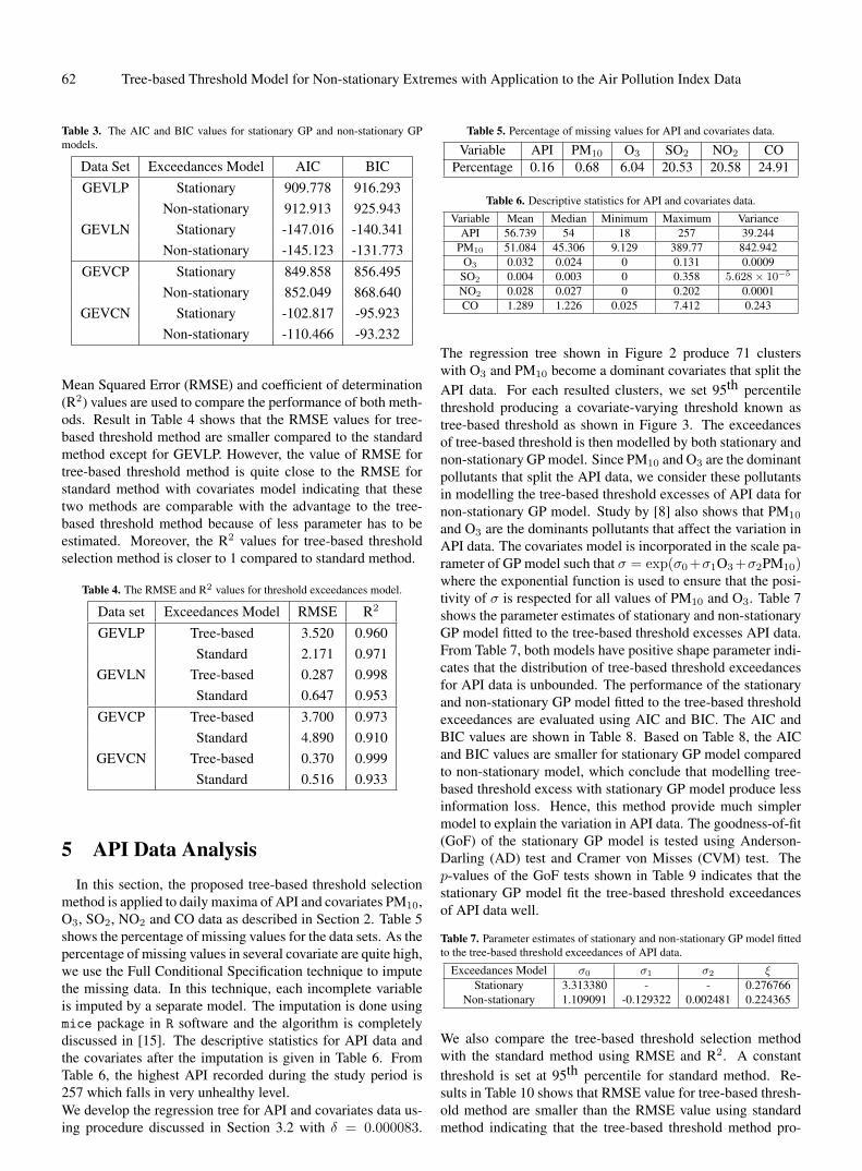
62 Tree-based Threshold Model for Non-stationary Extremes with Application to the Air Pollution Index Data
Table 3. The AIC and BIC values for stationary GP and non-stationary GPmodels.
Data Set Exceedances Model AIC BICGEVLP Stationary 909.778 916.293
Non-stationary 912.913 925.943GEVLN Stationary -147.016 -140.341
Non-stationary -145.123 -131.773GEVCP Stationary 849.858 856.495
Non-stationary 852.049 868.640GEVCN Stationary -102.817 -95.923
Non-stationary -110.466 -93.232
Mean Squared Error (RMSE) and coefficient of determination(R2) values are used to compare the performance of both meth-ods. Result in Table 4 shows that the RMSE values for tree-based threshold method are smaller compared to the standardmethod except for GEVLP. However, the value of RMSE fortree-based threshold method is quite close to the RMSE forstandard method with covariates model indicating that thesetwo methods are comparable with the advantage to the tree-based threshold method because of less parameter has to beestimated. Moreover, the R2 values for tree-based thresholdselection method is closer to 1 compared to standard method.
Table 4. The RMSE and R2 values for threshold exceedances model.
Data set Exceedances Model RMSE R2
GEVLP Tree-based 3.520 0.960Standard 2.171 0.971
GEVLN Tree-based 0.287 0.998Standard 0.647 0.953
GEVCP Tree-based 3.700 0.973Standard 4.890 0.910
GEVCN Tree-based 0.370 0.999Standard 0.516 0.933
5 API Data AnalysisIn this section, the proposed tree-based threshold selection
method is applied to daily maxima of API and covariates PM10,O3, SO2, NO2 and CO data as described in Section 2. Table 5shows the percentage of missing values for the data sets. As thepercentage of missing values in several covariate are quite high,we use the Full Conditional Specification technique to imputethe missing data. In this technique, each incomplete variableis imputed by a separate model. The imputation is done usingmice package in R software and the algorithm is completelydiscussed in [15]. The descriptive statistics for API data andthe covariates after the imputation is given in Table 6. FromTable 6, the highest API recorded during the study period is257 which falls in very unhealthy level.We develop the regression tree for API and covariates data us-ing procedure discussed in Section 3.2 with δ = 0.000083.
Table 5. Percentage of missing values for API and covariates data.
Variable API PM10 O3 SO2 NO2 COPercentage 0.16 0.68 6.04 20.53 20.58 24.91
Table 6. Descriptive statistics for API and covariates data.
Variable Mean Median Minimum Maximum VarianceAPI 56.739 54 18 257 39.244
PM10 51.084 45.306 9.129 389.77 842.942O3 0.032 0.024 0 0.131 0.0009
SO2 0.004 0.003 0 0.358 5.628× 10⁻⁵
NO2 0.028 0.027 0 0.202 0.0001CO 1.289 1.226 0.025 7.412 0.243
The regression tree shown in Figure 2 produce 71 clusterswith O3 and PM10 become a dominant covariates that split theAPI data. For each resulted clusters, we set 95th percentilethreshold producing a covariate-varying threshold known astree-based threshold as shown in Figure 3. The exceedancesof tree-based threshold is then modelled by both stationary andnon-stationary GP model. Since PM10 and O3 are the dominantpollutants that split the API data, we consider these pollutantsin modelling the tree-based threshold excesses of API data fornon-stationary GP model. Study by [8] also shows that PM10
and O3 are the dominants pollutants that affect the variation inAPI data. The covariates model is incorporated in the scale pa-rameter of GP model such that σ = exp(σ0+σ1O3+σ2PM10)where the exponential function is used to ensure that the posi-tivity of σ is respected for all values of PM10 and O3. Table 7shows the parameter estimates of stationary and non-stationaryGP model fitted to the tree-based threshold excesses API data.From Table 7, both models have positive shape parameter indi-cates that the distribution of tree-based threshold exceedancesfor API data is unbounded. The performance of the stationaryand non-stationary GP model fitted to the tree-based thresholdexceedances are evaluated using AIC and BIC. The AIC andBIC values are shown in Table 8. Based on Table 8, the AICand BIC values are smaller for stationary GP model comparedto non-stationary model, which conclude that modelling tree-based threshold excess with stationary GP model produce lessinformation loss. Hence, this method provide much simplermodel to explain the variation in API data. The goodness-of-fit(GoF) of the stationary GP model is tested using Anderson-Darling (AD) test and Cramer von Misses (CVM) test. Thep-values of the GoF tests shown in Table 9 indicates that thestationary GP model fit the tree-based threshold exceedancesof API data well.
Table 7. Parameter estimates of stationary and non-stationary GP model fittedto the tree-based threshold exceedances of API data.
Exceedances Model σ0 σ1 σ2 ξStationary 3.313380 - - 0.276766
Non-stationary 1.109091 -0.129322 0.002481 0.224365
We also compare the tree-based threshold selection methodwith the standard method using RMSE and R2. A constantthreshold is set at 95th percentile for standard method. Re-sults in Table 10 shows that RMSE value for tree-based thresh-old method are smaller than the RMSE value using standardmethod indicating that the tree-based threshold method pro-
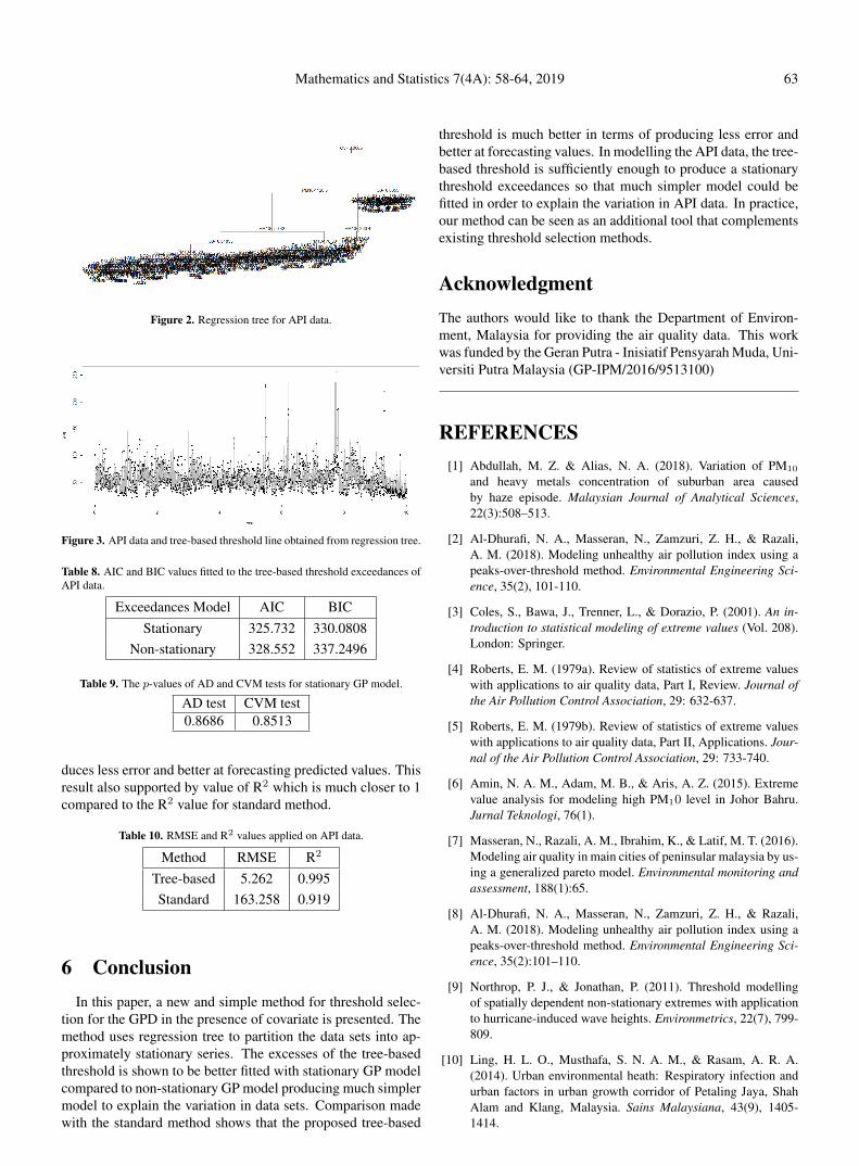
Mathematics and Statistics 7(4A): 58-64, 2019 63
Figure 2. Regression tree for API data.
Figure 3. API data and tree-based threshold line obtained from regression tree.
Table 8. AIC and BIC values fitted to the tree-based threshold exceedances ofAPI data.
Exceedances Model AIC BICStationary 325.732 330.0808
Non-stationary 328.552 337.2496
Table 9. The p-values of AD and CVM tests for stationary GP model.
AD test CVM test0.8686 0.8513
duces less error and better at forecasting predicted values. Thisresult also supported by value of R2 which is much closer to 1compared to the R2 value for standard method.
Table 10. RMSE and R2 values applied on API data.
Method RMSE R2
Tree-based 5.262 0.995Standard 163.258 0.919
6 ConclusionIn this paper, a new and simple method for threshold selec-
tion for the GPD in the presence of covariate is presented. Themethod uses regression tree to partition the data sets into ap-proximately stationary series. The excesses of the tree-basedthreshold is shown to be better fitted with stationary GP modelcompared to non-stationary GP model producing much simplermodel to explain the variation in data sets. Comparison madewith the standard method shows that the proposed tree-based
threshold is much better in terms of producing less error andbetter at forecasting values. In modelling the API data, the tree-based threshold is sufficiently enough to produce a stationarythreshold exceedances so that much simpler model could befitted in order to explain the variation in API data. In practice,our method can be seen as an additional tool that complementsexisting threshold selection methods.
AcknowledgmentThe authors would like to thank the Department of Environ-ment, Malaysia for providing the air quality data. This workwas funded by the Geran Putra - Inisiatif Pensyarah Muda, Uni-versiti Putra Malaysia (GP-IPM/2016/9513100)
REFERENCES[1] Abdullah, M. Z. & Alias, N. A. (2018). Variation of PM10
and heavy metals concentration of suburban area causedby haze episode. Malaysian Journal of Analytical Sciences,22(3):508–513.
[2] Al-Dhurafi, N. A., Masseran, N., Zamzuri, Z. H., & Razali,A. M. (2018). Modeling unhealthy air pollution index using apeaks-over-threshold method. Environmental Engineering Sci-ence, 35(2), 101-110.
[3] Coles, S., Bawa, J., Trenner, L., & Dorazio, P. (2001). An in-troduction to statistical modeling of extreme values (Vol. 208).London: Springer.
[4] Roberts, E. M. (1979a). Review of statistics of extreme valueswith applications to air quality data, Part I, Review. Journal ofthe Air Pollution Control Association, 29: 632-637.
[5] Roberts, E. M. (1979b). Review of statistics of extreme valueswith applications to air quality data, Part II, Applications. Jour-nal of the Air Pollution Control Association, 29: 733-740.
[6] Amin, N. A. M., Adam, M. B., & Aris, A. Z. (2015). Extremevalue analysis for modeling high PM10 level in Johor Bahru.Jurnal Teknologi, 76(1).
[7] Masseran, N., Razali, A. M., Ibrahim, K., & Latif, M. T. (2016).Modeling air quality in main cities of peninsular malaysia by us-ing a generalized pareto model. Environmental monitoring andassessment, 188(1):65.
[8] Al-Dhurafi, N. A., Masseran, N., Zamzuri, Z. H., & Razali,A. M. (2018). Modeling unhealthy air pollution index using apeaks-over-threshold method. Environmental Engineering Sci-ence, 35(2):101–110.
[9] Northrop, P. J., & Jonathan, P. (2011). Threshold modellingof spatially dependent non-stationary extremes with applicationto hurricane-induced wave heights. Environmetrics, 22(7), 799-809.
[10] Ling, H. L. O., Musthafa, S. N. A. M., & Rasam, A. R. A.(2014). Urban environmental heath: Respiratory infection andurban factors in urban growth corridor of Petaling Jaya, ShahAlam and Klang, Malaysia. Sains Malaysiana, 43(9), 1405-1414.

64 Tree-based Threshold Model for Non-stationary Extremes with Application to the Air Pollution Index Data
[11] Pickands III, J. (1975). Statistical inference using extreme orderstatistics. the Annals of Statistics, 3(1), 119-131.
[12] Davison, A. C., & Smith, R. L. (1990). Models for exceedancesover high thresholds. Journal of the Royal Statistical Society:Series B (Methodological), 52(3), 393-425.
[13] Breiman, L., Friedman, J. H., Olshen, R. A. & Stone, C. J.(1984). Classification and Regression Trees. London: Chapmanand Hall.
[14] Eastoe, E. F., & Tawn, J. A. (2009). Modelling non-stationaryextremes with application to surface level ozone. Journal of theRoyal Statistical Society: Series C (Applied Statistics), 58(1),25-45.
[15] Buuren, S. V., & Groothuis-Oudshoorn, K. (2010). mice: Mul-tivariate imputation by chained equations in R. Journal of sta-tistical software, 1-68.

Call for Papers
Mathematics and Statistics is an international peer-reviewed journal that publishes original and high-quality research papers in all areas of mathematics and statistics. As an important academic exchange platform, scientists and researchers can know the most up-to-date academic trends and seek valuable primary sources for reference.
Editorial Board
Manuscripts Submission
Manuscripts to be considered for publication have to be submitted by Online Manuscript Tracking System(http://www.hrpub.org/submission.php). If you are experiencing difficulties during the submission process, please feel free to contact the editor at [email protected].
Contact Us
Horizon Research Publishing 2880 ZANKER RD STE 203SAN JOSE, CA 95134USAEmail: [email protected]
Aims & Scope
Mathematics and Statistics
AlgebraAnalysisApplied MathematicsApproximation TheoryCombinatoricsComputational StatisticsComputing in MathematicsDesign of Experiments
Discrete MathematicsDynamical SystemsGeometry and TopologyStatistical ModellingNumber TheoryNumerical AnalysisProbability TheoryRecreational Mathematics
Dshalalow JewgeniJiafeng LuNadeem-ur RehmanDebaraj SenMauro SpreaficoVeli ShakhmurovAntonio Maria ScarfoneLiang-yun ZhangIlgar JabbarovMohammad Syed PukhtaVadim KryakvinRakhshanda DzhabarzadehSergey SudoplatovBirol AltinAraz AlievFrancisco Gallego LupianezHui ZhangYusif AbilovEvgeny Malekoİmdat İşcanEmanuele GalliganiMahammad Nurmammadov
Florida Inst. of Technology, USAZhejiang Normal University, ChinaAligarh Muslim University, IndiaConcordia University, CanadaUniversity of São Paulo, BrazilOkan University, TurkeyNational Research Council, ItalyNanjing Agricultural University, ChinaGanja state university, AzerbaijanSher-e-Kashmir University, IndiaSouthern Federal University, RussiaNational Academy of Science of Azerbaijan, AzerbaijanSobolev Institute of Mathematics, RussiaGazi University, TurkeyBaku State University, AzerbaijanUniversidad Complutense de Madrid, SpainSt. Jude Children's Research Hospital, USAOdlar Yurdu University, AzerbaijanMagnitogorsk State Technical University, RussiaGiresun University, TurkeyUniversity of Modena and Reggio Emillia, ItalyBaku State University, Azerbaijan