SIL

MATHEMATICAL PROGRAMMING AS AN AID TO ENGINEERINGDESIGN

A user's guide to available MP computer codes and to NELC's capabilitiesin numerically solving MP problems

D. C. McCall Research and Development I1 August 1971

DDC

Reproduc.at by

NATIONAL TECHNICAL AN 7 j IINFORMATION SERVICES-w•ingfiWl, Va. 2 1•151

_C.

_-f B _jU

Apy-rmved for piiblic rloecae"Distribution Unlimited

_ _ __ NAVAL ELECTRONICS LABORATORY CENTERSAN DIEGO, CALIFORNIA 92152

(V

UJNCLASSIFIEDSec'uroy Classification

DOCUMENT CONTROL DATA.- R & DIS. , oy claiisili~stion of titlet. body of abstract enid md wing snnrot~ft n i- for. Ie*ntreed when thie overall report I, classified)

I OR! GINA-.ING A C ThVI v y (Cirpo Palo author) 2.r P R EU IYC ASF C TO

NzvaIL ý rnc Laboratory Center UCASFESaAi Diego, California 921522bGRU

SREPORT TITLE

MATHEMATICAL PROGRAMMING AS AN AID TO ENGINEERING DESIGN

4. DESCRIPTIVE NOTES (Ty'pe of rep,)rt and inclusive dates)

Research and Development July 1968 to March 1970S. AU THOR(S) (First narri. middle initial, lamt namte)

D. C. McCall

4. REPORT DATE 70. TOTAL NO. OF PAGE S ___1b. NO. OF RIEFS

I1I August 1971 132 166&a. CONTRACT OR GRANT NO. 90. ORIGINATOR'S REPORT NUMBER(S)

1778b. PROJECT NO. ZFXX.212.0Ol (NELC Z223)

C. eb. OTHER REPORT NO(Si (Any~ other numbers that may be assignedthis report)

d.

10 DISTRIBUTION STATEMENT

Approved for public release; distribution unlimited.

It. SUPPLEMENTARY NOTES 12. SPONSORING MILITARY ACTIVITY

Director of Navy Laboratories

13. ABSSTRACT

This report is a user's guide to available mathematical programming (MP) computer codesand to NELICs capabilitics in numerically solving MP pr oblems. It defines the general MP problem;lists and evaluates the MP codes operational on the NELC IBM 360/65 computers; and providesguidelines for modifying the MP problem when, in its first form, it is cumbersome; or there is notinformation enough to start comp.jtation; or the available codes do not yield all the neededinformation.

ODD NFOV 1473 (PG )UNCLASSIFIED0102.014-6600 Security ClaS~ification

IUNC! ASS.I F!EDSe urity Classification

14 KEY URD S LINK A LINK 1 LINK C

ROLE WT ROLEI WT ROLE WT

Computer programming

Mathematical programming

DDr FORM 1473 (BACK) UNCLASSIFIED(PAGE 2) Security Classification

PROBLEM

Provide analysis and synthesis of Navy design problems. Specifically,develop a capability at NELC for using mathematical programming (MP) as anaid to engineering design.

RESULTS

1. The overall software capabilities at NELC for numerically solvingvarious types of MP problems - initiated or developed under t0is problem -are discussed in the report proper. Applications of integer programming aregiven in Appendix 1. User's guides and FORTRAN codes f-)r solving someclasses of MP problems are given in Appendix 2.

2. Practical guidelines are given for applying MP methods.

RECOMMENDATIONS

1. Maintain a continued effort to keep the mathematical programmingsoftware current. Monitor research literature for new developments in non-linear programming and integer programming.

2. Conduct ongoing seminars or in-house classes to inform practicingscientists and engineers of the utility of MP.

3. Review Navy engineering design problems for possible applicationof MP techniques.

ADMINISTRATIVE INFORMATION

Work was performed under ZFXX.212.001 (NELC Z223) by theDecision and Control Technology Division. The report covers work donefrom July 1968 to March 1970 and -was approved for publicationII August 1971.

The author thanks W. J. Dejka, Advanced Modular Concepts Division,who, as the initial principal investigator of Z223, set the goals and generaltrends of the project, for assistance and comments on this report; andSan Diego State College Foundation students, Gail Grotke and Dale Klamer,and C. M. Becker, Applications Software Division, for programming assistancein preparing Appendix 2.

.5I

CONTENTS

INTRODUCTION: SCOPE OF REPORT... page 3

THE MATHEMATICAL PROGRAMMING PROBLEM ... 4

MATHEMATICAL PROGRAMMING CAPABILITIES AT NELC... 5Unconstrainedi problems... 5Constrained problems ... 8

DESIGNING WITH MATHEMATICAL PROGRAMMING AS AN AID... 19Formulating a mat" r:'tic~l programming problem ... 19SUMT and constra~nt iransiormation ... 2?Gradient approximation. .. 27Duality in MP ... 33Lagrange multipliers as a design aid ... 43Initial point and scalng. ... 50

SUMMARY... 52

APPENDIX 1: APPLICATIONS OF INTEGER PROGRAMMING TOENGINEERING DESIGN... 53

APPENDiX 2: USER INFORMATION... 59

APPENDIX 3: REFERENCES. . . 123

ILLUSTRATIONS

I Constraint set ... page 52 Examples of convex and nonconvex sets... 123 Disconnected constraint set... 154 Magni .udes of currently solvable MP problems... 185 Dual circuits.. .33

6 Kuhn-Tucker conditions ... 457 Integer constraint set ... 548 Backplane grid... 56

TABLE

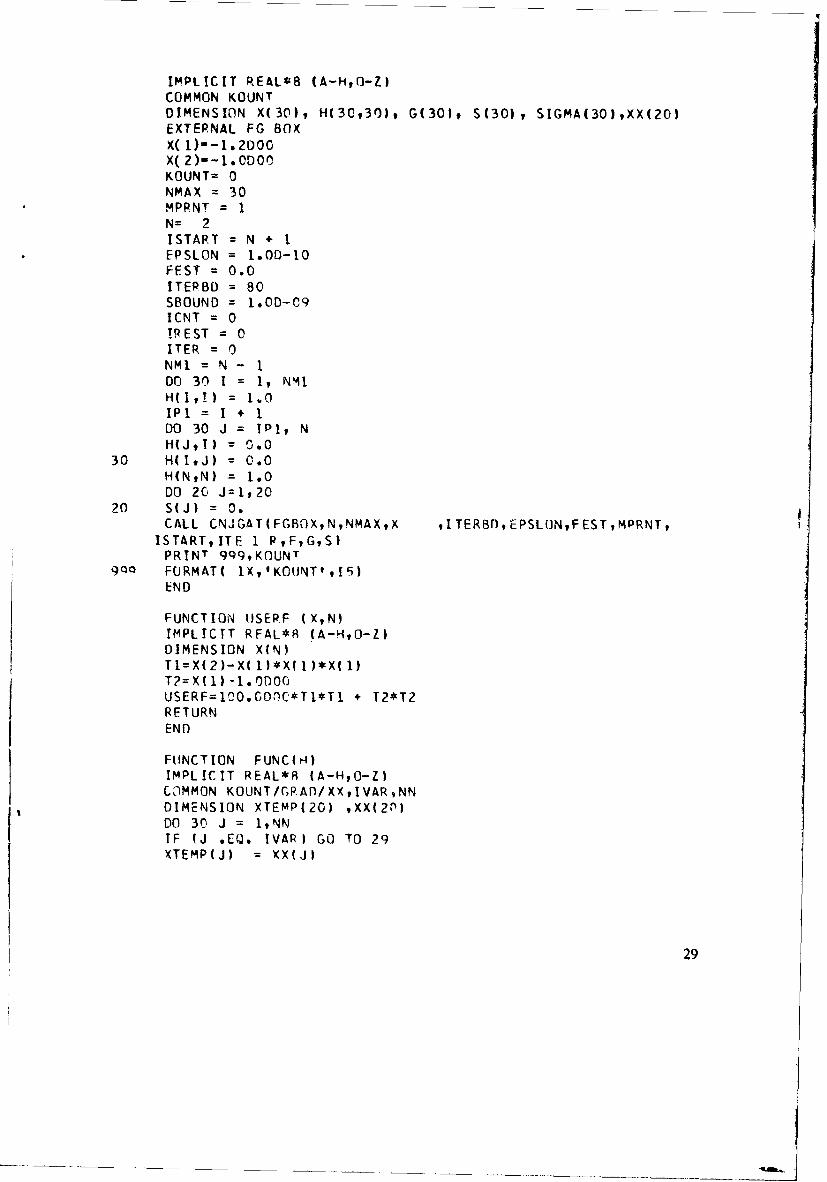
I Listing of FORTRAN code of test problem... 29

2

INTRODUCTION: SCOPE OF REPORT

There are several problems involved in the development of fai!hfulmathematical models of real-world processes. The processes are in generalnonlinear. The modeling equations are frequently incomplete. Conditionsare known only within limits. Often the best approach to these problems isvia mathematical programming (MP). 1-5

MP is a distinct discipline - it exists independently of computer pro-gramming. Prior to the age of the high-speed computer, however, some ofthe original algorithms for the solution of MP problems were too cumbersometo be of real use. The advent of the modern digital computer has made thesolution of many types of MP problems feasible and has stimulated the searchfor better algorithms.

This report is chiefly concerned with solving MP problems - with thecomputational stage of MP. It is intended as a guide for thc usage and appli-cation of available MP c..mputer codes.

THE MATHEMATICAL PROGRAMMING PROBLEM defines thegeneral MP problem.

MATHEMATICAL PROGRAMMING CAPABILITIES AT NELC listsand evaluates the MP codes operational on the NELC IBM 360/65 computer,and will be of interest to the user who has an MP problem in final form, readyto solve. He can choose the appropriate code from the list and obtain thecard deck and user's guide from the NELC program library, Computer SciencesDepartment.

DESIGNING WITH MATHEMATICAL PROGRAMMING AS AN AIDprovides guidelines for modifying the MP problem when, in its first form, itis cumbersome; or when there is not information enough to start computation(for example, an initial feasible point is lacking); or when the available codesdo not yield all the needed information (for example, postoptimal analysis).

i. See APPENDIX 3: REFERENCES.

3

THE MATHEMATICAL PROGRAMMING PROBLEM

The basic problem of MP is to develop an algorithm for finding themiaintum of a scalar-valued function of n real variables that satisfies a set ofauxiliary conditions called constraints. Stated in mathematical terms, theproblem becomes:

Let f(x1 . x.) and gl(xi ..... x.) ..... gm(Xl xnscalar-valued functions of the n variables x 1I...., xn. Then we wish to findvariables which

minimize f(xl, x2, ... , Xn)

subject to

gl(Xl, x2 ... xn)> 0(1

gm (XlI, x2. , Xn) :>t 0

The above problem is known variously as the 'general mathematical program-ming problem,' the 'constrained optimization problem,' and the 'nonlinear pro-gramming problem.' For the sake of convenience, we call it proble.n (1).

in problem (1), f is called the objective or cost function and the gi arecalled the constraints. We also refer to f and gi as the problem functions.We denote the vector (x1, x2 ... , xn) by xT (where T denotes the matrixtranspose) and call the. set of all vectors x which satisfy gi(x) > 0 for all i = 1,

.m, the constraint set or feasible set. The problem is said to be consistentlyposed if the constraint set is nonempty. We note that finding the maximum of

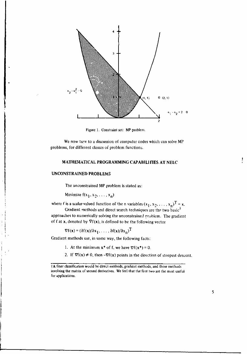
a function f is equivalent to finding the minimum of -f.Consider the following example (fig. 1):

Minimize f(x1 , x2 )= (x1 -2) 2 + 'x 2 -1)2

subject to

gl(xl, x2) = x2 - x!>0 (2)

g2 (x 1, x2 ) =-xI -x2 +2•0

Since f(x 1 , x2 ) is the sum of squares, the minimum oc-.urs at xI = 2, x2 =

However, the point (2,1) is not in the constraint set defined by gl and g2.The obvious (in this example) candidate is the point (1,1), which in thisstraightforward problem is the constrained minimum. As m and n get larger,the problem becomes significantly more difficult to solve.

4

4

3

x2 1

1, 11 a' (2, 1

-x -1x2 +2 0

2

Figure 1. Constraint set: MP problem.

We now turn to a discussion of computer codes which can solve MPproblems, for different classes of problem functions.

MATHEMATICAL PROGRAMMING CAPABILI tIES AT NELC

UNCONSTRAINED PROBLEMS

The unconstrained MP problem is stated as:

Minimize f(x 1,x 2.... , x.)

where f is a scalar-valued function of the n variables (x1, x2, T . .x.Gradient methods and direct search techniques are the two basic"

approaches to numerically solving the unconstrained problem. The gradientof f at x, denoted by Vf(x), is defined to be the following vector

¶Vf(x) = (af(x)/ax . . af(x)/3xn)T

Gradient methods use, in some way, the following facts:

I. At the minimum x* of f, we have Vf(x*) = 0.

2. If Vf(x) * 0, then -Vf(x) points in the direction of steepest descent.

tA finer classification would be direct methods, gradient methods, and those methodsinvolving the matrix of second derivatives. We feel that the first two are the most usefulfor applications.

5

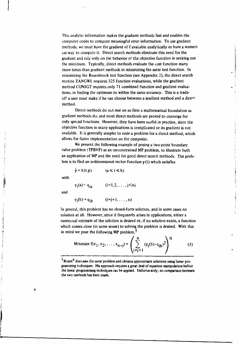
This analytic information makes the gradient methods fast and enables thecomputer codes to compute meaningful error information. To use gradientmethods, we must have the gradient of f avaiable analytically or have a numeri-cal way to compute it. Direct search methods eliminate this need for thegradient and rely only on the behavior of the objective function in seeking outthe minimum. Typically, direct methods evaluate the cost function manymore times than gradient methods in minimizing the same test function. Inminimizing the Rosenbrock test function (see Appendix 2), the direct searchroutine ZANGWL requires 325 function evaluations, while the gradientmethod CONJGT requires only 71 combined function and gradient evalua-tions, in finding the optimum to within the same accuracy. This is a trade-off a user must make if he can choose between a gradient method and a dirertmethod.

Direct methods do not rest on so firm a mathematical foundation asgradient methods do, and most direct methods are proved to converge foronly special functions. However, they have been uhful in practice, since theobjective function in many applications is complicated or its gradient is notavailable. It is generally simpler to code a problem for a direct method, which"allows for faster implementation on the computer.

We present the following example of posing a two-point boundaryvalue problem (TPBVP) as an unconstrained MP problem. to illustrate both

an application of MP and the need for good direct search methods. The prob-lem is to find an n-dimensional vector function y(t) which satisfies

h =(t,y) (a < t < b)

withYi(a) - qia (i= 1,2, . .. , j<n)

and

Yi(b) = qib (i=j+l,. .. , n)

In general, this problem has no closed-form solution, and in some cases nosolution at all. However, since it frequently arises in applications, either anumei ical estimate of the solution is desired or, if no solution exists, a functionwhich comes close (in some sense) to solving the problem is desired. With thisin mind we pose the following MP problem. t

/n '/2

Minimize f(x 1, x2,..., xn-j) = (3)i=j+lI

tRosen6 discisses the same problem and obtains approximate solutions using linear pro-gramming techniques. His approach requires a great deal of equation manipulation beforethe linear programming techniques car, be appiied. Unforturately, no comparison betweenthe two methods has been made.

6

where the numbers yi(b), i=j+ 1,... n are numerically computed as folloss.For a given (xI,..., xn.j), solve the following initial-value problem over the

interval [a,b].

•, = h(t,y) (a < t < b)

wherey(a) = (qla, • qja, x l, • ,Xn-j)

the last n-j components of the solution obtained at t=b of this problem areused in the objective function for yi(b), i=j+ 1 .... n.

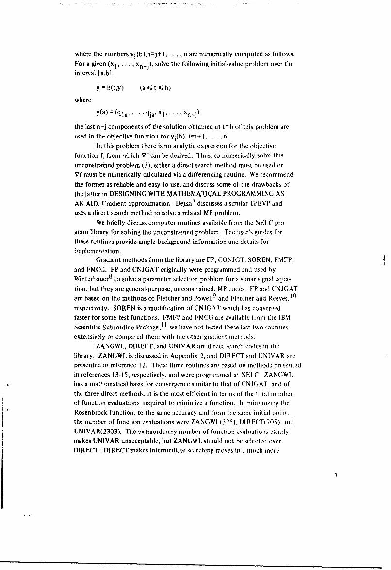
In this problem there is no analytic expression for the objectivefunction f, from which Vf can be derived. Thus, to numerically solve thisunconstrained problem (3), either a direct search method must be used orVf must be numerically calculated via a differencing routine. We recommendthe former as reliable and easy to use, and discuss some of the drawbacks of

the latter in DESIGNING WITH MATHEMATICAL PROGRAMMING ASAN AID, Cradient approximation. Dejka 7 discusses a similar TiBVP anduses a direct search method to solve a related MP problem.

We briefly discuss computer routines available from the NELC pro-gram library for solving the unconstrained problem. The user's guides forthese routines provide ample background information ana details for:.rnplementition.

Gradient methods from the library are FP, CONJGT, SOREN, FMFP,and FMCG. FP and CNJGAT originally were programmed and used byWinterbauer 8 to solve a parameter selection problem for a sonar signal equa-tion, but they are general-purpose, unconstrained, MP codes. FP and CNJGATare based on the methods of Fletcher and Powell 9 and Fletcher and Reeves, 19

respectively. SOREN is a modification of CNJGAT which has convergedfaster for some test functions. FMFP and FMCG are available from the IBMScientific Subroutine Package)!I we have not tested these last two routinesextensively or compared them with the other gradient methods.

ZANGWL, DIRECT, and UNIVAR are direct search codes in thelibrary. ZANGWL is discussed in Appendix 2, and DIRECT and UNIVAR arepresented in reference 12. These three routines are based on methods presentedin references 13-15, respectively, and were programmed at NELC. ZANGWLhas a mat'ematical basis for convergence similar to that of CNJGAT, and oftht three direct methods, it is the most efficient in terms of the toal numberof function evaluations iequired to minimize a function. In minimizing theRosenbrock function, to the same accuracy and from the same initial point,the number of function evaluations were ZANGWL(325), DIRF('T(705), andUNIVAR(2303). The extraordinary number of function evaluations clearlymakes UNIVAR unacceptable, but ZANGWL should not be selected overDIRECT. DIRECT makes intermediate searching moves in a much more

.7

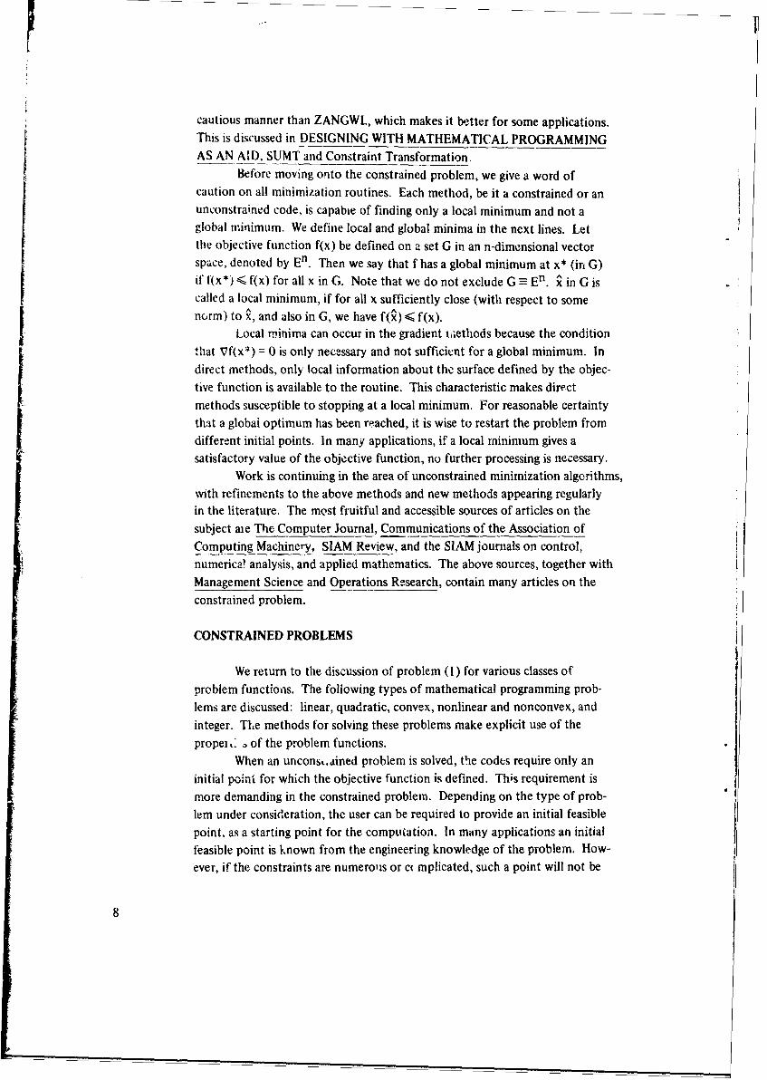
cautious manner than ZANGWL, which makes it better for some applications.

This is discussed in DESIGNING WITH MATHEMATICAL PROGRAMMINGAS AN AID, SUMT and Constraint Transformation.

Before moving onto the constrained problem, we give a word ofcaution on all minimization routines. Each method, be it a constrained or anunconstrained code, is capabie of finding only a local minimum and not a

global minimum. We define local and global minima in the next lines. Letthe objective function f(x) be defined on a set G in an n-dimensional vectorspace, denoted by En. Then we say that f has a global minimum at x* (in G)if f(x*) < f(x) for all x in G. Note that we do not exclude G a En. x in G is

called a local minimum, if for all x sufficiently close (with respect to somenorm) to X, and also in G, we have f(A) < f(x).

Local minima can occur in the gradient ii;ethods because the conditionthat Vf(x*) = 0 is only necessary and not sufficient for a global minimum. In

direct methods, only local information about the surface defined by the objec-tive function is available to the routine. This characteristic makes directmethods susceptible to stopping at a local minimum. For reasonable certaintythat a global optimum has been reached, it is wise to restart the problem fromdifferent initial points. In many applications, if a local minimum gives asatisfactory value of the objective function, no further processing is necessary.

Work is continuing in the area of unconstrained minimization algorithms,with refinements to the above methods and new methods appearing regularlyin the literature. The most fruitful and accessible sources of articles on thesubject aie The Computer Journal, Communications of the Association ofComputing Machinery, SIAM Review, and the SIAM journals on control,numerical analysis, and applied mathematics. The above sources, together withManagement Science and Operations Research, contain many articles on theconstrained problem.

CONSTRAINED PROBLEMS

We return to the discussion of problem (1) for various classes ofproblem functionis. The following types of mathematical programming prob-lems are discussed: linear, quadratic, convex, nonlinear and nonconvex, andinteger. The methods for solving these problems make explicit use of thepropel,. , of the problem functions.

When an uncons,.ained problem is solved, the codes require only aninitial point for which the objective function is defined. This requirement ismore demanding in the constrained problem. Depending on the type of prob-lem under consideration, the user can be required to provide an initial feasiblepoint, as a starting point for the computation. In many applications an initialfeasible point is known from the engineering knowledge of the problem. How-ever, if the constraints are numerous or c' mplicated, such a point will not be

8

obvious and a preliminary step must be taken prior to solving the problem.A method for obtaining an initial feasible point is treated in DESIGNING WITI'MATHEMATICAL PROGRAMMING AS AN AID, Initial Points and Scaling,so we assume that one is at hand in the following discussion.

Each class of constrained MP problem is described, together withcomputer programs which can solve it. Since each routine to be discussed hasan associated user's guide, we confine our remarks to the following points:

I. Is an initial feasible point required?

2. Does the code find a global optimum?3. Can information be saved for possible restarts or postoptimal

analysis?

4. Is the routine easy to use?5. What error messages are given if tWe routine fails to converge?

LINEAR PROGRAMMING (LP)

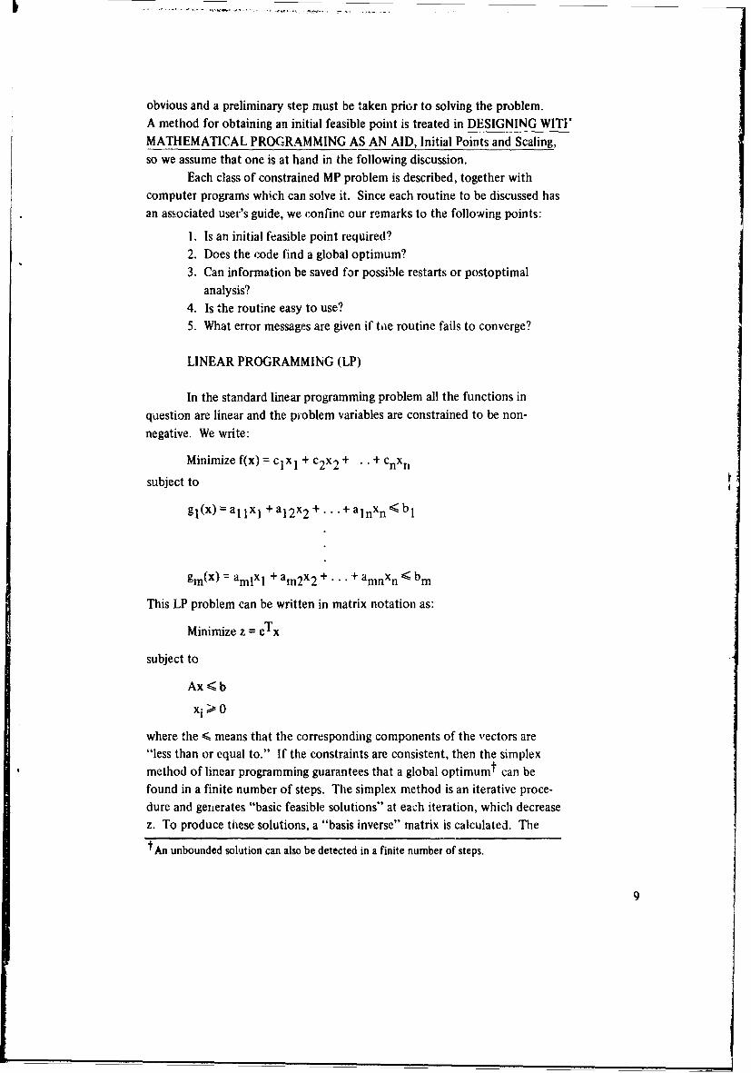
In the standard linear programming problem all the functions inquestion are linear and the problem variables are constrained to be non-negative. We write:

Minimize f(x) = c 1xI + c2 x2 + ... + nXn

subject to

g1(x) = alx, +a 12 x2 +...+ alnxn •<b 1

gi(x) = amlxI + am2X2 +... + amnxn < bm

This LP problem can be written in matrix notation as:

Minimize z = cTx

subject to

Ax < b

where the < means that the corresponding components of the vectors are"less than or equal to." If the constraints are consistent, then the simplexmethod of linear programming guarantees that a global optimumt can befound in a finite number of steps. The simplex method is an iterative proce-dure and generates "basic feasible solutions" at each iteration, which decreasez. To produce these solutions, a "basis inverse" matrix is calculated. The

An unbounded solution can also be detected in a finite number of steps.

9

preceding brief comments serve only to associate the terms "basic feasiblesolution" and "basis inverse" wit•i the simplex method; references 16 and 17treat the simplex method.

The most complete code for rumerically solving the LP problem is theIBM Mathematical Programming System 18 (MPS/360). MPS/360 is based ona modification of the simplex method and will either solve the LP problem orindicate that no solution exists. This code does not require that the problemvariables be nonnegative, and treats upper and lower bounds on the variables

az special constraints. Separable programming problems (a special nonlinear,,P problem) can be solved with this routine. MPS/360 is capable of solvingproblems of up to 4095 constraints and "virtually an unlimited number ofcolumns."' 8 It is currently stored on disk pack NELC05 at the NELC

Computer Center.No initial point is required to begin the computation; however, the

option exists to start the problem from a user-supplied basis inverse. MPS/360has its own control language, which provides a variety of capabilities. Theuser is afforded several postoptimal analysis procedures and can access thecurrent basis inverse for future restarts. This control language is straight-forward to use and provides some looping and branching capability. A varietyof messages are output to the user in the course of computation. They arefully explained in the message manual. 1 9

The chief drawback of this program is the format of the input data.It requires each element of the arrays c,b, and A to have a "row name" and a"column name" for identification. This has proved cumbersome for scientific"and cngineering work. A FORTRAN program, DATAPREP, is available to 1.reduce the data arranged in compact matrix notation to a format acceptableto MPS/360.

In many applications a lineai- programming problem must be solvedrepeatedly as part of a larger problem. The READCOMM 20 facility of MPS/360allows the main program to be used in an iterative fashion as a subroutine. .

READCOMM enables the user to supplement the standard control languagewith FORTRAN procedures; for example, DATA PREP. Rosen 6 and Griffith Iand Stewart2 l have examples of using a linear programming code in an itera-

tive way.Previous large-scale, efficient LP codes were geared to commercial

applications and required a great deal of modification for efficient scientific

and engineering use. The READCOMM facility has made a powerful programeasily available for a wide range of specialized applications.

QUADRATIC PROGRAMMING (QP)

This type of problem is the next order of difficulty. A quadraticcost function is minimized subject to linear constraints:

10

Minimize f(xI, x2, xn)

subject to

a, xl +a 1 2x2 +...+alnxn<bI

(4)

amlxl+am2x2+-.. +amnxn <bm

where f has one of two forms -

f(xI, x2 , . ,xn) =cTx+xTBx (5)

or

f(xI, x2 ... ,xn) IIHx - ell (6)

B and H are n-by-n and k-by-n matrices, respectively, and c and e are n-, andk-dimensional vectors, respectively. The norm of a vector y, denoted by Ily II,is given by

At present only the minimum norm problem (equation 6) can besolved at NLLC. The program which does this is QPHANSON. This routinewas written by R. J. Hanson, of the Jet Propulsion Laboratory, Pasadena, anduses a numerically stablet version of Rosen's22 gradient projection algorithm.The method guarantees that a global bptimum will be found for a consistentproblem. The routine is reported to have worked well on examples from theareas of curve fitting and approximation of solutions to linear integralequations. 23

The routine is described in reference 23, and an NELC user's guide is inpreparation. The code is operational, but it is still unpolished in respect touser-oriented input and output. QPHANSON does not require an initialfeasible point nor does it have an option to accept a good approximation ofthe optimum. The code treats equality constraints and inequality constraintsseparately. It can solve problems of up to 60 constraints (equality and in-equality combined) and 30 variables. No experi:nents have been done todetermine whether this is a hard and fast upper bound on the problem size.

The program suffers. from lack of good error and timing messages. Ifthe routine fails to converge, no messages are given as to the possible cause.Also, no provisions are made to identify inconsistent quadratic programs.The user is on his own with QPHANSON.

tAn algorithm 0 is numerically stable if the errors in the input data are approximatelyequal to the round-off errors generated by the computations of&.

11

If a QP problem occurs with equation (5) as the cost function, and thematrix B is positive-definite or positive-semidefinite,t then Hanson23 presentsa method for transforming this QP problem into a minimum-norm QP prob-lem. This minimum-norm problem is soived with QPHANSON and then an

inverse transformation is made. Presently this must be done by the user.QPHANSON is currently being modified to make this transformationautomatically.

Codes to solve quadratic programs are not as well polished or as highlydeveloped as those for LP. Unless the demand increases for good QP routines,the user will have to write his own code or be content wit.j the experimentalmodels.

CONVEX PROGRAMMING

Before turning to the convex programmir g problem, we make some

preliminary definitions.

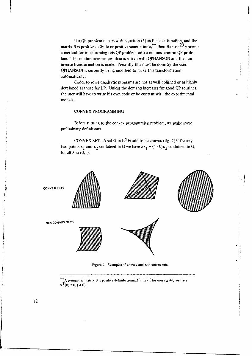
CONVEX SET. A set G in En is said to be convex (fig. 2) if for anytwo points x1 and contained in G we have Xx1 + (1 -,)x 2 contained in G,

for all X in (0,1).

CONVEX SETS

NONCON VEX SETS

Figure 2. Examples of convex and nonconvex sets.

t'A symmetric matrix B is positive-definite (semidefinite) if for every x * 0 we have

xTBx > 0,( 0).

12

CONVEX FUNCTION. A scalar-valued function f defined on a convexset G in En is said to be convex if for any two points x, and x2 in G

f(XxI + (1-W)x 2 ) < Xf(x 1 ) + (1-X f(x 2 )

for all X in (0, ).Linear functions, and the quadratic cost function (equation 6) with B

positive-semidefinite, are examples of convex functions. A theorem of intereststates that if the constraint set of an MP problem is defined by convex functions,then it, too, is convex. More precisely, if gI(x), . . . , gm(x) are convex func-tions, then the set of all x for which gI(x) < 0, .... , gm(x) < 0 holds simul-taneously is a convex set. The constraint sets of linear and quadratic programsare convex.

With these facts in hand we state the convex programming problem.

Minimize f(x)

subject to

gi(x) < 0 (i- I,..., m)

where the functions t and gi are convex functions of x = (xI xn)

great deal of work has been done with convex programming andthe theory 24 can guarantee convergence for some computational methods.Each method is valid for specific requirements on the problem functions. Inthis section we assume that the gradients of all functionm exist and are con-tinuous. The central problem in solving convex programs is not so muchtheoretical difficulty but rather the obtaining of rapid convergence of numeri-cal schemes. Even though some QP problems are convex, it may be moreefficient to use a routine like QPHANSON to so~ve them rather than treatthem as convex programs. Another practical difficulty with convex program-ming is the identification of convex functions. If the function has a complicatedanalytic expression, it can be difficult to classify it as convex. The methodsfor solving convex programs will not in general completely hang-up if the dataare not convex, but the significance of s' :ch results should be judged in1 termsof the user's problem formulation.

The first library routine which solves the convex programming prob-lem is the subroutine CONVEX, which was developed by Hartley andHocking25 at Texas A&M. The routine makes a linear approximation to thefunctions in question and then uses a simplex-like procedure to move to theoptimum. In making the linear approximations, the routine requires a user-supplied subroutine which computes the gradients of the cost function andthe nonlinear constraints.

CONVEX does not require an initial feasible point: however, theoption does exist to start from a given point. In addition, CONVEX produces

13

a current feasible point and a basis inverse at the end of each i .ration forpossible restarts. The format of the input data is straightforward and suitabletV scientific and engineering work; however, care should be exercised in theorganization of the data for any upper and lower bounds on the problemvariables. CONVEX requires that the constraint data be input in threegroups - the upper and lower bounds on the variables, the linear inequalities,and the nonlinear convex constraints. This feature makes it possible to con-veniently solve quadratic programs with convex cost functions. No compari-sons between QPHANSON and CONVEX have been made on solving quadraticprogramming problems.

CONVEX suffers from the lack of good error messages and analysisin the event of an inconsistent problem or any numerical difficulties. Noinvestigation of the numerical stability of the method or of timing or accuracybenchmarks for large problems has been reported. A convex problem with60 corPtraints and 60 variables is the largest which can be solved withoultprogram modifications. Because the linear constraints are treated separately,it is likely that larger problems can be solved if the number of nonlinear con-straints is not too great. Future work should invest-gate this possibility.

The second routine for solving the convex prograroming problem isExperimental SUMT. This method is theoretically convergent for convexdata, but, since it also has provisions for nonconvex programs, we postponediscussion of it until the next section.

There is a special subclass of convex programs for which a globaloptimum can be found with the linear programming code MPS/360. Theseare separable programming problems, which are defined as follows:

n

Minimize z (x-) (7)

j=I

subject ton

Sgij(xj) < bi (i=l 1 .... , mn)

j=l

Note that the objective function and the constraints are sums offunctions of the single variables xj; that is, there are no "cross product" terms.This allows each nonlinear function to be replaced by a polygonal approxima-tion, and reduces problem (7) to a form which can be solved by MPS/360. TheMPS/360 user's manual 18 gives the appropriate details and examples ofsolving separable programming problems. If the separable tunctions areconvex, then MPS/360 will find a global optimum to the approximationproblem. The use of successive approximations causes the global optima ofthe approximation problems to converge to the optimum of the original

14

problem. The method can tolerate some nonconvex functions but may stop

at a local optimum.

This technk ie can also be used for separable convex programs toolarge for CONVEX. tCONVEX may be more efficient if the problem is nottoo large - unfortunately, no experimental evidence is available to aid in

making the selection.)

NONLINEAR, NONCONVEX PROGRAMMING

This last class of MP problems is composed of all the problems whichare not necessarily linear or necessarily convex. In the statement of problem

(I), no requirements were made on the functions in question other than the

assumptions that the objective function would be defined for all feasible x,and the gi would be defined for all x. This statem ,nt of problem (1) is muchtoo general to be of use. To have any hope of oblaining a solution, we must

put some restrictions on the problem functions. The three computer codeswhich we discuss require that the gradients of all thu functions in problem ( I)exist and be continuous. Although these co:,ditions are stringent from a

mathematical point of view,t they do not provide a base for an MP algorithm.The following example illustrates one of the difficulties of nonlinear,

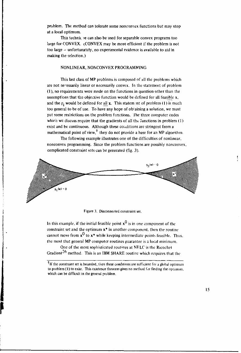
nonconvex programming. Since the problem functions are possibly nonconvex,

complicated constraint sets can be generated (fig. 3).

gl fx) =0 ,

Figure 3. Disconnected constraint set.

In this example, if the initial feasible point x0 is in one component of the

constraint set and the optimum x* in another component, then the routine

cannot move from x0 to x* while keeping intermediate points feasible. Thus.the most that general MP computer routines guarantee is a local minimum.

One of the most sophisticated routines at NELC is the Ricochet

Gradient 2 6 method. This is an IBM SHARE routine which requires that the

"tlf the constraint set is bounded, then these conditions are sufficient for a global optimumto problem (I) to exist. This existence theorem gives no method for finding the optlmum,which can be difficult in the general problem.

II

gradients of both the objective function and the constraints exist and be con-tinuous. The method requires an initial feasible point and begins by movingdown the gradient of the objective function until a constraint is reached. Theprogram "ricochets" and traverses on the objective function surface acrossthe feasibility region to the opposite constraint. A triangle is then constructedwith this Lraverse line as its base and its apex in the direction of the gradientof f. The next step is made along the line from the base to the apex. Themethod terminates either on a small step size or when no ricochet is possible.

The user must supply codes to calculate the cost function and theconstraints and their gradients. An initial feasible point must also be provided.The program has no options for restarts or postoptimal analysis; in such casesthe problem is simply rerun - the known best point is used as initial data.

This routine is capable of producing a tremendous amount of outputinformation. Once the method for controlling this output has been mastered,the user has access to a variety of information, which can be of great use insolving a nonlinear problem. The accompanying user's guide26 providesdetaikd documentation on the code and the underlying method. A supple-mentai user's guide (Appendix 2) reports the results of some test examplesand gives a sample deck setup for output control. This program has provedreliable and, after a bit of experience, easy to use.

A second computer code for the general problem is NELC FESDIR.This pregram is not as sophisticated as the Ricochet Gradient routine, but itcan easily be modified for special applications. The user's guide, completewith results on test examples, appears in Appendix 2.

The final code available for solving the nor~Ainear problem is Experi-mental SUMT, which was written at Research Analysis Ccrporation byG. P. McCormick, et al. 2 7 SUMT is not a production code and is primarilyused as a research tool in MP. The experimental nature does not lessen itsaccuracy, but only its efficiency and speed. The code has modular structure,which allows for easy user modification and adaptation. The user's guide iscomplete with test examples, although some handwritten corrections anddeletions are not too clear. The user has the option of providing an initialpoint himself or allowing the program to find one. The option also exists ofhaving SUMT compute the gradients by a differencing scheme; the code can

also check user-supplied gradients for errors. SUMT provides timing informa-tion and allows for user-controlled output. However, the output can be con-fusing, with the values of different variables appearing under the same headings.The only error message other than incorrectly entered data is a warning duringcomputation that certain estimates indicated the problem functions to benot convex. The theoretical background for SUMT is described in Fiacccand McCormick. 24

In DESIGNING WITH MATHEMATICAL PROGRAMMING AS AN

AID, SUMT and Constraint Transformation, we discuss methods for transforming

16

a constrained problem into a sequence of unconstrained problems (also calledSUMT). This requires more work on the part of the user but can also givehim more control in solving the problem and perhaps more insight as to whatis happening. Irn solving the associated unconstrained problems, the user hasthe option of selecting a direct search method, thereby eliminating the needfor differentiable or, in some problems, continuous functions. Special-purposeMP routines can be closely tailored to fit special applications via thesetechniques.

IN rEGER PROGRAMMING

In addition to the standard linear programming proolem, there areseveral special programs under the heading of integer linear programming(ILP). The problem statement is similar except for constraints placed onthe variables:

Minimize f(x) = cl 1x + c2x2 +. +CnXn

subject to

g, (x) =allx, + al2x2 +..+alnXn < b,

gm(x)= amlxl +am2X2 +" " "+ amnXn •<bm (8)

xi > 0 and xi is an integer.

There are further distinctions within ILP - pure integer, mixed integer, and10,1i. The above problem is a pure integer problem; if xI ... xk are requiredto be integral and xk+1 ..... xn are not necessarily integral, then we have amixed integer problem; and finally if xi can equaJ only zero or one, we have a10,1} ILP. Integer programming is in its infancy, and some methods, althoughthey theoretically exhibit finite convergence, have not been computationallysuccessful. The three ILP routines available at NELC are "Zero-One IntegerProgramming with Heuristics," 28 BBMIP,2 9 and OPTALG. Zero-one andBBMIP are SHARE routines which have been checked out on the 360/65 butnot tested extensively. BBMIP (a mixed integer routine) has been tried on a

series of test problems30 and compared with other routines; however, theother codes are machine-dependent, so the comparison is not meaningful.

OPTALG is a bound and scan pure integer programming code whichhas solved large problems successfully. It was developed at Stanford byF. S. Hillier, 3 1 and is currently operational at NELC. The routine requires 336kof core and a solution to the associated linear programming problem; that is,we simply drop the restriction that xi be an integer. This solution, together

17

with the LP basis matrix and a guess at an initial feasible solution are then usedas data for OPTALG. If the problem is large (a maximum of 61 rows and 61columns), then this data preparation can be tedious if done by hand. Theprocedure has been somewhat automated; the exact details are in the user'sguide (Appendix 2).

The user should be cautious when attempting to solve an ILP with aninteger programming code, since it is possible for a routine to solve some prob-lems and not others, even if they are the same climension and fairly similar.Matching the routine to the problem is still an art. Progress is being made inthis area, but it will be some time before methods are available to solve a generalILP. A selection of engineering applications is presented in Appendix 1.

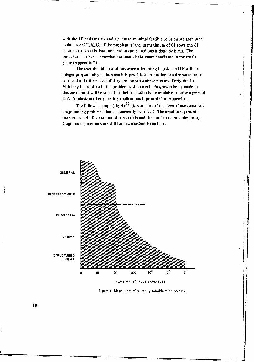
The following graph (fig. 4)32 gives an idea of the sizes of mathematicalprogramming problems that can currently be solved. The abscissa representsthe sum of both the number of constraints and the number of variables; integerprogramming methods are still too inconsistent to include.

GENERAL

DIFFERENTIABLE

QUADRATI./

LINEAR

STRUCTUREDLINEAR

0 0o 10o 1000 164 o5 106

CONSTRAINTS PLUS VARIABLES

Figure 4. Magnitudes of currently solvable MP problems.

18

DESIGNING WITH MATHEMATICAL PROGRAMMING AS AN AID

The engineer can effect a better design in some areas in less time andat lower cost with mathematical programming techniques than with classicalmethods. I1,e key to success is in the word "aid," for, in using the methodseffectively, the engineer must have command of his own field and understandsome basic principles of MP techniques. It is recognized that typically theuser of MP techniques is concerned with obtaining results quickly withoutlengthy excursions into numerical analysis or mathematical programming.Commercial routines - ECAP, 3 3 MATCH, 34 etc. - are geared to such a user;however, blindly accepting the output of such routines can be disastrous. 35

Also, these off-the-shelf routines are procrustean - they generally do not lendthemselves to modification for a special case. General mathematical programmingcomputer codes can be modified for particular requirements. For example, iffilter design by MP techniques is a frequent task, then the computer code canbe modified to incorporate the automatic scaling of variables.

In these remaining sections, we discuss how an engineer would proceedfrom start to finish in using MP as a design aid. We also discuss some specialtopics, such as duality, that do not apply in all iastances, but, if used properly,can save time and money, both in setup analysis and in obtaining a numericalsolution.

FORMULATING A MATHEMATICAL PROGRAMMING PROBLEM

In many design problem statements there is, instead of a single goal, acollection of specifications to be satisfied. This gives the engineer severaldegrees of freedom in formulating an associated MP problem. He has the optionof merely satisfying all the design specifications (this is equivalent to findingan initial feasible point) or of singling out one distinguished requirement andusing it as the objective function. For example, in reference 1, : tunablebandpass filter was to be designed which would satisfy the following (amongother) specifications:

1. At the tuned frequency F, the "insertion loss" of the filter was tobe less than 2 dB.

2. At 10% on either side of F, the "roll off" was to be at least 40 dB.

Either of the above options for formulating an MP problem would have beensatisfactory. The latter method was chosen. The insertion loss of the filterwas selected to be minimized and the roll off requirements were treated as

constraints.To properly formulate an MP problem, the user must explicitly

determine the following:

19

1. The objective (performance, tolerance, etc.) that is to be accom-plished.

2. The mathematical relations that govern the interaction between the

independent design variables.

3. The bounds and limitations on the values of the components thatguarantee a reafizable design.

With this information in hand the designer can select which MP approach touse. However, since care is required in choosing the objective function andproviding a code for its numerical evaluation, we present some general

examples and guidelines.The objective function can be defined as a measure of the merit or the

desirability of a solution to a problem, and its magnitude typically representscost, profit, performance, quality, etc., or a combination cf these. The case of

the single well defined objective function generally poses no problems; it isthe combination of goals which can lead to difficulties. The followingexamples illustrate various treatments of multiple goals.

Suppose that it is desired to minimize both the insertion loss of a net-work denoted by fl (x) and the cost of the components denoted by f2 (x).

Then one formulation of an objective function f would be

Minimize f(x) = f 1 (x) + r*f 2 (x) (9)

whzze r is an appropriately chosen scaling factor.Another possible choice of f would be

Minimize f(x) = -f 2(x)/fl(x) (10)

Note that no scaling factor is required and the dimensions of the objectivefunction are

- cost($)/(unit power loss) = cost($'/(unit power gain) (11)

The next example illustrates treating secondary design goals asconstraints. Suppose that high reliability (f3 (x)) is desired but the primary

goal is a design of minimum costs(f2(x)). A constrained formulation would be

Minimize f2(x) (12)

subject to

-f3(x) + 0' O< 0

where u is a tolerance on reliability (mean time to failure).

A possible numerical pitfall is combining design goals in a haphazard

manner. Suppose we have two performance indicators ul(x) and u2(x), and

we desiie to maximize u I and minimize u2 in the same design. Since maxi-

miring u I is equivalent to minimizing -u I, a possible objective function

20

would be

Minimize f(x) = w2*u2(x) - wI *ul(x) (13)

where the constants wI and w2 are required to make the function dimensionallycorrect. These weights are important, since the magnitudes of -u 1 and u2 atthe optimum x* can be quite different. For example, if -ul (x*) • 0 andu2(x*) r 1000, then the effect of uI is obliterated by u2.

The above discussion of objective functions is intended to be general.Aoki 36 presents many detailed examples of engineering applications togetherwith ample background material.

Some care should be taken in the numerical evaluation of the problemfunctions and their gradients. Coding the functions offers an opportunity forconsiderable analysis ard clever programming. This task is done only once,against the many times that the functions are evaluated during the optimiza-tion. A seemingly innocent equation or a naive way of combining terms canlead to poor numerical results. The objective function can be complicated, anda single e ialuation for a set of parameters can involve:

1. A solution of a system of differential equations

2. Inverting a matrix

3. Table lookups or interpolation

4. All of the above

Gear3 7 and Calahan 38 discuss similar numerical problems and some usefultechniques in applying MP to engineering design. One of the goals of mathe-matics as applied to computer-aided design is to free the applications-orienteduser from the standard numerical worries. For example, the routine should be

able to analyze the problem and choose the best method for integrating asystem of norlinear differential equations. State-of-the-art techniques do notmeet this goal; thus, it is still up to the user to make the proper selection of

numerical methods.Duality is a case in which careful analysis can pay off generously. Full

details with examples are presented in the section on duality, but we presentthis idea here to point out some analysis and numerical considerations. Insome applications of linear programming, problems occur which have a muchlarger number of constraints than variables. To be specific, we may have 50constraints and 10 variables. To obtain a solution to the LP problem posed inti-is way, an LP code would essentially invert a 50-by-50 matrix. Thisinversion can te time-consuming and perhaps inaccurate for such a largematrix. We show in Duality in MP how to cast this problem as a dual linearprogramming problem which would require only a 10-by-10 matrix to be

inverted. Duality is an excellent example of a little analysis saving a greatdeal of time and effort.

21

Suppose that the design problem is clearly stated as an MP problem.

In order to solve the resulting problem, it may be necessary to transform it intoan equivalent MP problem. The possible modifications can occur in the light

of the following questions:

I. Is the necessary computer code available?2. Would duality aid in obtaining numerical results?

3. Is an initial point available?4. Can the derivatives be easily calculated?

5. Would a postoptimal analysis be useful?

6. Can significant benefit be gained by scaling the variables or clever

coding techniques?

It does little good to cast a design problem as an MP problem, if we lack thenumerical means to solve it. Thus, the user should be prepared to transformhis problem into a solvable form or into a more useful f)rm. In the ensuingpages we address ourselves to problem modifications %,hich we found useful

in practice.

SUMT AND CONSTRAINT TRANSFORMATION

The most common mismatch is that of a constrained problem to besolved and a routine for solving only unconstrained problems. The sequentialunconstrained minimization techniques (SUMT) developed by Fiacco andMcCormick 24 transform a constrained MP problem into an equivalent sequence(in terms of having the same solution) of unconstrained problems. The

transformation takes place with the aid of an unconstrained auxiliary function

which has the following form: m

O(x, rk) f(x) + p(rk)>. G(gi(x)) (14)i=l

where rk is a parameter, G(y) is a monotonic function of y that behaves insome well chosen manner at y = 0, and p(r) is a function of r which dependson the choice of G. Typical choices require G(y) > 0 for y > 0 and G(y) = 0for y < 0, or require that G(y) approach - as y approaches 0 through values

less than zero. The first choice of G is usually associated with procedures

that are not concerned with constraint satisfaction except at the solution(exterior methods); and the second choice of G is associated with procedureswhich enforce constraint satisfaction throughout the minimization (interior

methods). The basic idea cf SUMT is the following. Let x* be a solution toproblem I : that is, we assume x* minimizes 1(x), subject to gi(x) < 0 for i= 1,... m. Then under appropriate cot :tions 24 on the problem functions the

following theorem holds.

2w

If xk k=1 is a sequence of points, each of which minimizesO(x, rk) where rk is a sequence of points tending to zero, then we have thelimit xk = x*, or in some cases limit f(xk) = f(x*). So a constrained problemk-i- k-400is replaced by an equivalent sequence (in the sense of having a commonsolution) of unconstrained problems. Common choices for G(y) are -1 /y,(min [y, 01 )l+e, e > 0, and-log (-y) with p(r) = r, l/r, r respectively. For thefirst form of G(y), ,(x, rk) becomes

m0(x, rk) = f(x) + rk I {-l/gi(x) (15)

then ifwe have a feasible point x° and seek to minimize O(x, rk), the term 2: 1/-gi(x)keeps intermediate test points in the constraint set. For, if the routineattempts to leave the feasible set, it must cross the boundary; this causesT I /-gi(x) to approach + -, and, since we are minimizing, the routine auto-matically avoids points which yield large values of O(x, rk). As rk approacheszero, xk is approaching x*, and since xk is used as the initial point to findxk+1, each successive minimization requires fewer iterations. In LagrangeMultipliers as a Design Aid we givc some examples.

Variations of the above techniques can be applied in many situationswhere there is a mismatch between computer code and mathematicalprogramming problem. For example, Rosen's gradient projection method

solves the followinig problem:

Minimize f(x) (16)

Subject to

nnI- aij xj < bi i =1, 2,. .. , m

j=l

Now suppose the MP problem we have on hand has some nonlinear constraintsgi(x) < 0, i = 1. . , as well as some linear ones. We modify the problemas follows:

Minimize fix) - rk I /gi(x) (17)i=l

nsubject to aij xj < bi i= I.. m

"j=I

Thus, we take advantage of a good routine which our problem does notquite fit.

23

Another method which allows us to make use of an unconstrainedcomputer code is a straight constant transformation. Many times in ProblemI the constraints are fairly simple - for example, ai < xi < bi or ci < aixi+ bi < di - and the objective function is very complicated with a Oifficultgradient to compute. The simple nature of the above constraints a.lows ininitial feasible point to be obtained immediately, and the constraini trans-formation keeps the intermediate points feasible. This transformation (aswell as SUMT) allows a direct search method to be used for optimizingcomplicated objective functions. However, as the examples show, there is apoint of diminishing return in trying to transform all the constraints, since,as the constraints become complicated, it can be impossibie to find a wellmannered constraint transformation to do the job.

If we require a < x < b, then the following transformations keep xwithin this range:

b+a (b-a)1. x= +-- siny2 2

2. x = a + (b-a) sin 2yeY

3. x = a + (b-a) - for y unconstrained.ey + e-Y

For one-sided boundaries - that is, a < x - we have:

4. x=a+eY

5. x=a+lyl

6. x=a+y2

The next types of constraints are linear inequalities - for example,d < ax + b < c. However, this is equivalent to a boundary inequality; that is,d-b c-b- <x<- for a > 0.

a aIf we have two linear inequalities in two unknowns, a transformation

is still possible:

a < bilxl + b12 x2 •< c

e <b2 1x + b2 2 x2 f

then let yl bl lxl +b12x2

y= b2 1X + b

then x I (b22YI - b1 2Y-)/D

x2 (b2 1yI -bIIY 2 )/D

24

where D = b22 b 1I - b1 2 b21

then let Y = a + (c-a) sin 2 Zl

Y2 = e + (f-e) sin 2 z2

Thus, we have made x 1, x2 functions of the unrestricted variables z1 , z2 , andthey still satisfy the inequality constraints.

OTHER EXAMPLES

1. Suppose we require 0 < x1 x2 /32

then consider x1

'1 y

2 2yx~2 + Y

x3 Yl + Y2 3

2. This example was presented in Box 3 9

maximizef [9 - (x 1 3)21 x3/27 VY-

subject to 0 < X I

0 •< x 2 •< xl/ V-3

0 x< xI +r3- (x2) < 6

Initial point

x 1 = l,x 2 .5 f= .01336

optimum x1 = 3,x v3 f= 1.0

TRANSFORMATION OF CONSTRAINTS

Yl = X, +Vr- x2

Y2 = x2 - xl/IV-

Then if x2 = xl[V-/\ we have 0 < x, + xI < 6 or x, < 3. This then gives

bounds for the variables yl and y2 "

-XOV- < x2 - X /r/- < 0

-V3 = -3/V-3 < Y 2 < 0. Thus we have

25

-vTy 2•O

This implies

xI = 1/2 (y, -/•'y 2 )

x2 = 1/2 (y1l/V-0 + y 2 )

Thus, we have the unconstrained problem

maximize f(xl(z 1 , z2 ), x2(z1 , z2 ))

where x1 = 1/2 (yl - i•'y 2 )

x2 =1/2 (y I/ N/ + Y2)

y1 = 6 sin 2zI

Y2 = `V3 + 0 sin 2z 2

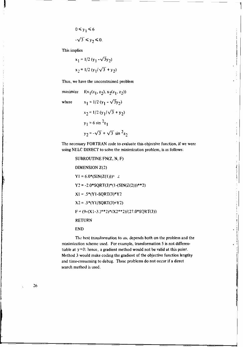
The necessary FORTRAN code to evaluate this objective function, if we wereusing NELC DIRECT to solve the minimization problem, is as follows:

SUBROUTINE FN(Z, N, F)

DIMENSION Z(2)

Y1 = 6.0*(SIN(Z(I)))4

Y2 = -2.0*SQRT(3)*(I-(SIN(Z(2)))**2)

XI =.5*(YI-SQRT(3)*Y2

X2 = .5*(Y 1/SQRT(3)+Y2)

F = (9-(XI-3.)**2)*(X2**2)/(27.0*SQRT(3))

RETURN

END

The best transformation to usL depends both on the problem and theminimization scheme used. For example, transformation 5 is not differen-

tiable at y=0: hence, a gradient method would not be valid at this point.Method 3 would make coding the gradient of the objective function lengthy

and time-consuming to debug. These problems do not occur if a directsearch method is used.

26

GRADIENT APPROXIMATION

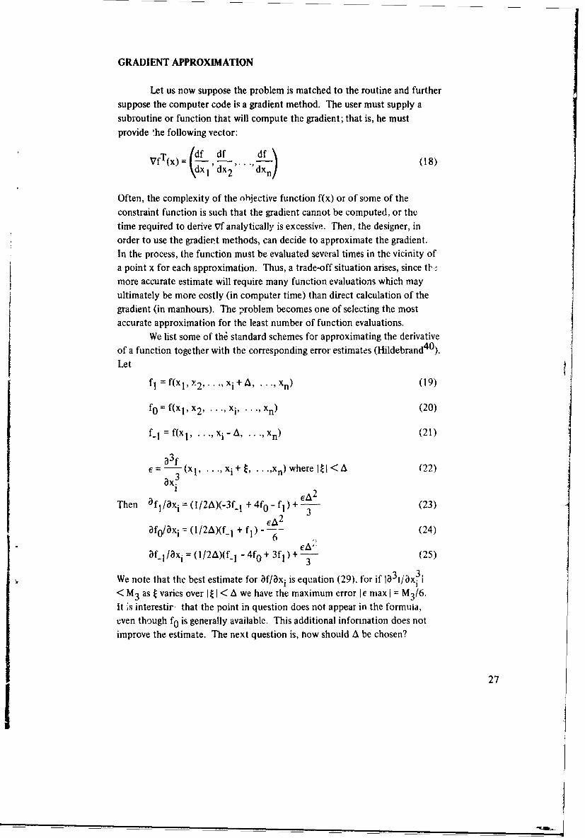
Let us now suppose the problem is matched to the routine and furthersuppose the computer code is a gradient method. The user must supply asubroutine or function that will compute the gradient; that is, he mustprovide the following vector:

T Idf df dfVf(x).. (18)'dx dx2 dxn(

Often, the complexity of the objective function f(x) or of some of theconstraint function is such that the gradient cannot be computed, or the

time required to derive Vf analytically is excessive. Then, the designer, inorder to use the gradient methods, can decide to approximate the gradient.In the process, the function must be evaluated several times in the vicinity ofa point x for each approximation. Thus, a trade-off situation arises, since tl,more accurate estimate will require many function evaluations which mayultimately be more costly (in computer time) than direct calculation of thegradient (in manhours). The problem becomes one of selecting the mostaccurate approximation for the least number of function evaluations.

We list some of th6 standard schemes for approximating the derivativeof a function together with the corresponding error estimates (Hildebrand 4 0).

Let

fl f(x I, Y2 , xi + A, ... ,Xn) (19)

fx f(xl, x2, xi, xn) (20)

f-l f(x, ""I , xi-A, ... ,xn) (21)

a3 f(x 3 xi + .,xn) where IZI < A (22)ax.

i eA 2

Then aflaxi= (l/22A)(-3fl + 4f0 - fl) + (23)

af0/axi = ( OAKf + f ) - 6- (24)

af I1/axi = (Il/2A)(fl - 4f0+ 3f1)+CA (25)1 3

We note that the best estimate for af/axi is equation (29), for if ja3j/3x3I

< M3 as t varies over It I < A we have the maximum error I e max I = M3/6.

It is interestirý that the point in question does not appear in the formula,even though f0 is generally available. This additional inforination does not

improve the estimate. The next question is, now should A be chosen?

27

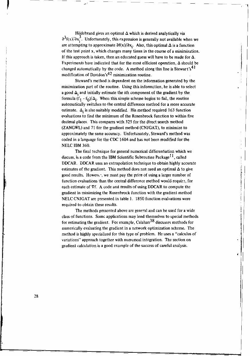
Hildebrand gives an optimal A which is derived analytically via3a3f(x)/,x3 . Unfortunately, this expression is generally not available when we

are attempting to approximate af(x)/axi. Also, this optimal A is a functionof the test point x, which changes many times in the course of a minimization.If this approach is taken, then an educated guess will have to be made for A.Experiments have indicated that for the most efficient operation, A should bechanged automatically by the code. A method along this line is Stewart's 4 1

modification of Davidon's 4 2 minimization routine.

Steward's method is dependent on the information generated by theminimization part of the routine. Using this information, he is able to selecta good Ai and initially estimate the ith component of the gradient by theformula (fl - fo)/Ai. When this simple scheme begins to fail, the routineautomatically switches to the central difference method for a more accurateestimate. Ai is also suitably modified. His method required 163 function

evaluations to find the minimum of the Rosenbrock function to within fivedecimal places. This compares with 325 for the direct search method(ZANGWL) and 71 for the gradient method (CNJGAT), to minimize toapproximately the same accuracy. Unfortunately, Steward's method wascoded in a language for the CDC 1604 and has not been modified for theNELC IBM 360.

The final technique for general numerical differentiation which wediscuss, is a code from the IBM Scientific Subroutine Package1 , calledDDCAR. DDCAR uses an extrapolation technique to obtain highly accurateestimates of the gradient. This method does not need an optimal A to give

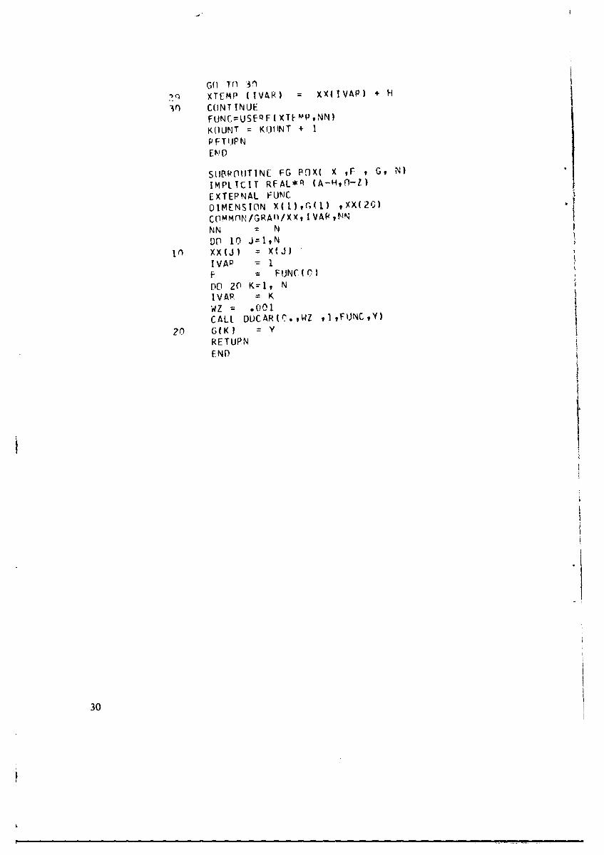
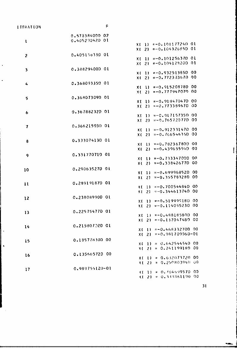
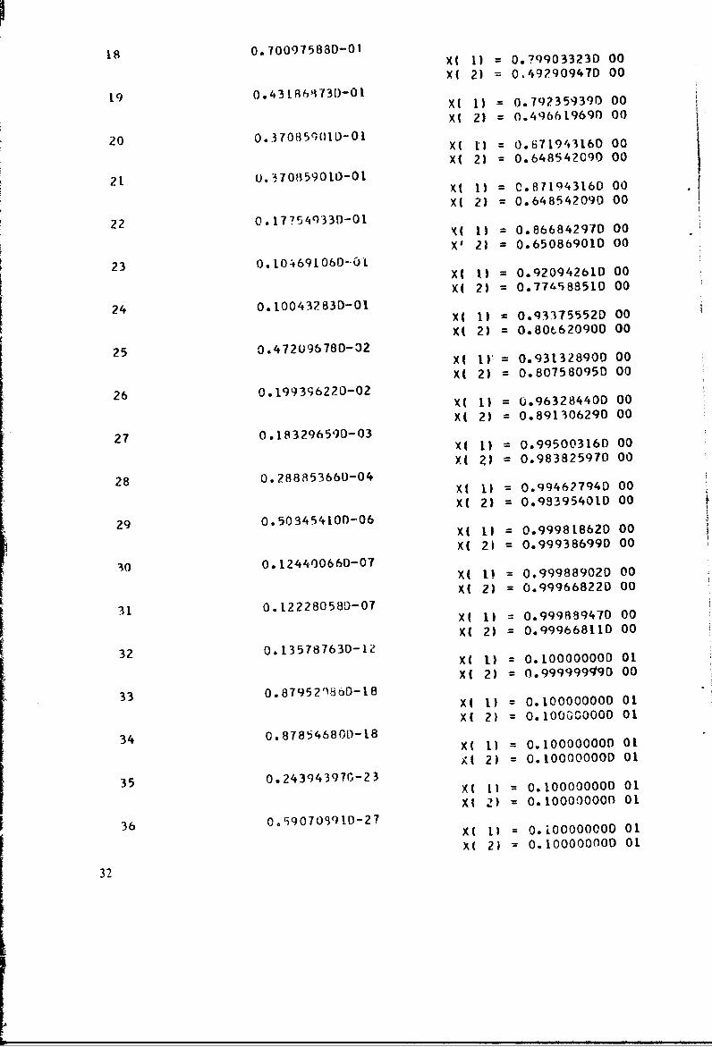
good results. Howevw-, we must pay the price of using a larger number offunction evaluations than the central difference method would require, foreach estimate of Vf. A code and results of using DDCAR to compute thegradient in minimizing the Rosenbrock function with the gradient methodNELC CNJGAT are presented in table 1. 1850 function evaluations wererequired to obtain these results.

The methods presented above are general and can be used for a wideclass of functions. Somc applications may lend themselves to special methodsfor estimating the gradient. For example, Calahan 3 8 discusses methods fornumerically evaluating the gradient in a network optimization scheme. Themethod is highly specialized for this type of problem. He uses a "calculus ofvariations" approach together with numerical integration. The section ongradient calculation is a good example of the success of careful analysis.

28

IMPLICIT REAL*8 (A-HvO-l)COMMON KOUNTD[MENSION X(30)9 H(3C,30)t G(30), S(30), SIGMA(3Oh#XX(20)EXTERNAL FG BOXX( 1)-1.2000X( 2)--l.ODOCKOUNT= 0NMAX 30MPPNT IN= 2ISTART = N +- 1EPSION = 1.00-10FEST = 0.0ITERBO = 80SBOUND = 1.OD-C9ICNT = 0IPEST = 0ITER = 0NMI = N - IDO 30 1 =1, NMIH(I,!) =1.0

IP1 = I + 1DO 30 J = WI, NH(J,T) 0.0

30 H(IJ) 0.0H(NN) =1.0

DO 2C J=192020 S(J) = 0.

CALL CNJGAT(FGBOXN,NMAXtX VITERBfl,E~PSLON,FEST,MPRNT,ISTART, IEF 1 P,F,G,S)PRINT 9q9,KOUNT

9q0 FUJRMAT( IX,@KO(JNT',15)END

FUNCTION IISERF (X,N)IMPLICTT RFAL*8 (A-HO-i)DIMENSION X(N)T1=X(2)-X( 1)*Xfl1)*X( 1)T2=X(1) -1.0000'USERF=l00.GD0C*TL*r1 + T2*T2RETURNEND

FUINCTION FUNC(H)IMPLICIT REAL*8 (A-HO-Z)COMMON KOUNT/fRAD/XXvIVARwNNDIMENSION XTEMP(20) ,XX(2n)DO 30 J = 1,NNIF (J .EQ. IVAR) GO TO 29XTEMP(J) =XX(J)

29

XTEMP (IVAR) = X(VAP) +HV0 CONTINUE

Fk)NC.>USEQ F ( XT[- "VNN)K(1UNT =K01INT +1P F TIJP N

SUBROU.TINE FG POX( x rF , Gt N)

IMPLICIT RFAL*A (A-H,0-Z)EXTEPNAL FUNC

DIMENSION X(fl,G'I) ,xx(2'J)

CommflN/GRAi0/XX, IVAR,t"N

9(1 10 J=1,N10 WXJ X'.J)

IVAP IF =FUNC(G0

DO 20 Krl, NIVAP KWZ = .001

RTU.CALL DL)CAR(C.,WZ ,1,FUNC,Y)

20 G(K? =Y

30

I TFRATION F

0.578384000 02

1 0.4052)0420 01XC 1) =-0.10t177241) 01

X{ 2) =-0.[04326&'5D 01

2 0.40517)6330 01X( 1) =-0.10125631D 01

X( 2) =-0.t04129201) 01

3 0.38829400D 01X( 1) =-0.93251385D 00

X( 2) =-0.7723336?) 004 0.368093350 01

X( 1) =-0.91520878D 00

X( 2) =-0.77794707nF o0

5 0.36807309D 01X( 1) =-0.918470470 00X( 2) =-0.77338967D 00

6 0.36788232D 01X( 1) =-C.91715735f 00X( 2) 1-0.765720770 00

7 0.36621503D 01X( 1) =-0.912331470 00

X( 2) =-0.16654635D O0

8 0.33307413D 01X( 1) =-0.782367800 00

X( 2) =-0.43965594D 00

9 0.33177071D 01X( 11 =-0.733347000 00

X( 2) =-0.33842677D 00

10 0.290635270 O0X( 1) =-0.69996852D 00X( 2) =-0.355783280 00

1i 0.289191870 01X( 1) =-a.700544840 00

X( 2) -,-0.344613740 0012. 0.238089900 01

X( I) =-0.51999ql8D 00X( 2) =-0.114055230 00

13 0.225754710 01XC 1) =-0.48818580D 00

X( 2) =-0.137047480 00

14 0.2158072.2D 01XC I) =-.0.468332700 00X( 2) =-0.98170906D-0i

15 0.13577830D 00X( 1) = 0.642544540 00X( 2) = 0.241199180 00

16 0.135665720 00X ( 1 0.612o73721) 00XC 2) = 0.250803941) 00

17 0.989754120-01X( 1) = 0. 104',09570 00

X( 2) = 0. ill6ll)I') 00

31

18 0.700975880-01XC .) = 0.799033230 00

X( 2) 0,4,92909470 00

19 0.431864730-01

X( 1) = 0.792359390 00

Xt 2) = 0.496619690 00

20 0. 370859010-01X( 1) = 0.671943160 00

X( 2) = 0.648542090 00

21 0. 370EI59010-01XCI I = C.87194316D 00

X( 2) = 0.648542090 00

22 0.17754933D-01X( 1) = 0.866842970 00

X' 2) = 0.650869010 00

23 0.104691060-C0tX 1.) = 0.92094261D 00

X 2) = 0.774588510 00

24 0.10043283D-01X( 1) = 0.q3375552D 00

X1 2) = 0.80t62090D 00

25 0.472096780-32X( 1) = 0.931328900 00

X( 2) = 0.807580950 00

26 0.199396220-02X( 1) = 0.963284400 00

X( 2) = 0.891306290 00

27 0.183296590-03X( 1) = 0.995003160 00

X( Z) = 0.983825970 00

28 0.288853660-04X( 1) = 0.99462794D 00

X( 2) = 0.983954010 00

29 0.503454100-06XC 11 = 0.999818620 00

X( 2) = 0.999386990 00

30 0.12440066D-07X( 1) = 0.999889020 00

X( 2) = 0.999668220 00

31 0.122280589-07XC 1) = 0.999889470 00

XC 2) = 0.99966811D 00

32 0.135787630-UX( 1) = 0.10000000D 01

X( 2) = 0. 9 9 9 9 99q90 00

33 0.87952186D-18Xf 1) = 0.10000000D 01

X( 2) = 0. l OOO0O 01

34 0.878546800-18X( 1) = 0.100000000 O0

A( 2) = O.10000000D 01

35 0 . 2 4 3 94397G-23Xl L) = 0.100000000 01Xl 2) = 0.100000000 01

3b 0.59070990D-27X( 11 = 0.i0000000D 01

X( 2) = 0.100000000 01

32

DUALITY IN MP

In linear programming and certain SUMT methods with convex

functions, the possibility of using duality to gain computational efficiency

should be considered.

Duality occurs in many areas - mathematics, engineering, economics

physics, etc. In a mathematical or engineering context it implies that two

concepts or systems have a specific mathematical relationship. We give an

example from circuit theory before proceeding with duality and MP.

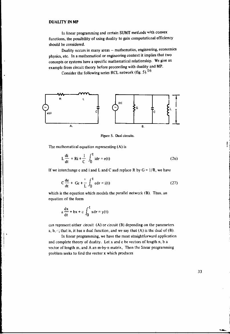
Consider the following series RCL network (fig. 5) 16

"O G Le

feft) 1%C L

A. B

Figure 5. Dual circuits.

The mathematical equation representing (A) is

L-d +Ri+ 1 idr = e(t) (26)

dt C 0

If we interchange e and i and L and C and replace R by G = l/R, we have

de rtC-+ Ge+ edr = i(t) (27)

dt L 0

which is the equation which models the parallel network (B). Thus, anequation of the form

dxa - + bx + c xdr = y(t)

can represent either circuit (A) or circuit (B) depending on the parameters

a, b, '; that is, it has a dual function, and we say that (A) is the dual of (B).

In linear programming, we have the most straightforward applicaticn

and complete theory of duality. Let x and c be vectors of length n, b a

vector of length m, and A an m-by-n matrix, Then the linear programming

problem seeks to find the vector x which produces

33

F

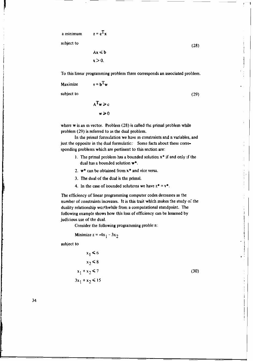
a minimum z = ix

subject to (28)

Ax<b

x>0.

To this linear programming problem there corresponds an associated problem.

Maximize v = bTw

subject to (29)

ATw > c

W0O

where w is an m vector. Problem (28) is called the primal problem while

problem (29) is referred to as the dual problem.In the primal fonnulation we have m constraints and n variables, and

just the opposite in the dual formulatic; Some facts about these corre-sponding problems which are pertinent to this section are:

1. The primal problem, has a bounded solution x* if and only if the

dual has a bounded solution w*.

2. w* can be obtained from x* and vice versa.

3. The dual of the dual is the primal.

4. In the case of bounded solutions we have z* =v*.

The efficiency of linear programming computer codes decreases as the

number of constraints increases. It is this trait which makes the study of theduality relationship worthwhile from a computational standpoint. Thefollowing example shows how this loss of efficiency can be lessened byjudicious use of the dual.

Consider the following programming proble'.n:

Minimize z = -4xI - 3x 2

subject to

xI + x2 < 7 (30)

3xI +x 2 < 15

34

-x2 '< 1

Xl >0,

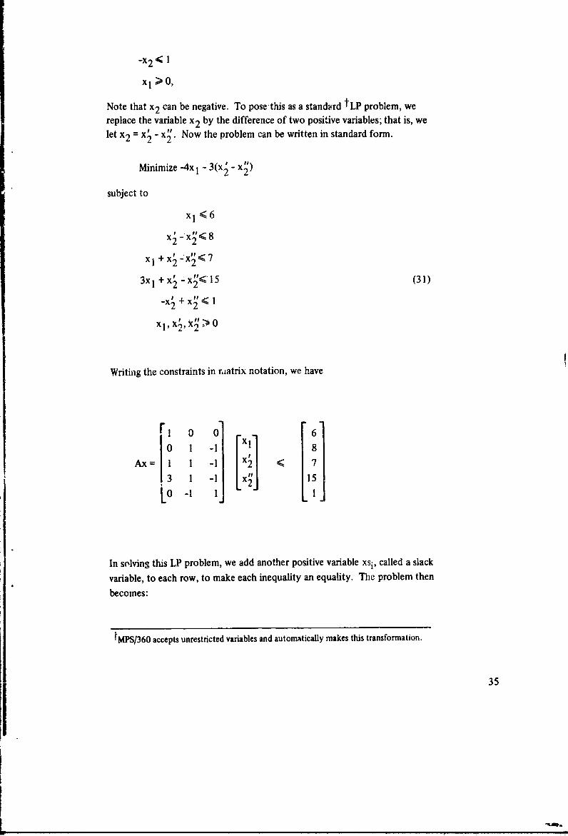
Note that x2 can be negative. To posethis as a standard tLP problem, we

replace the variable x2 by the difference of two positive variables; that is, we

let x2= x2 - x". Now the problem can be written in standard form.

Minimize -4x1- 3(x• - x )

subject to

xI -x<6

x, + x'2-:x2F<7

3xI + x' - x"< 15 (31)2 2,1 + xr l

-x2 + 2 - I

xl1, X"), k• 11 0

Writing the constraints in rmatrix notation, we have

1 0 0 6

0 1 -1 X1 8

Ax = 1 1 -1 x 4 7

13 1 -1 [x2J 15

0 -1 1 1

In solving this LP problem, we add another positive variable xsi, called a slack

variable, to each row, to make each inequality an equality. The problem then

becomes:

tMPS/360 accepts unrestricted variables and automatically makes this transformation.

35

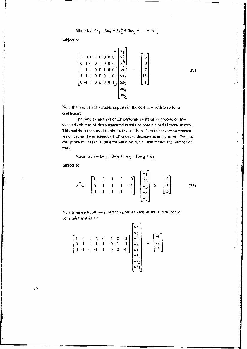
Minimize -4xI - 3xý + 3x' + OxsI +.. + Oxs 5

subject to

xl10010000 x2 6

0 -1 0 1 000 x2 82i

11-1 0 0 1 0 0 xs! 7 (32)3 I-i 0 0 0 1 0 xs2) 15

0-1 1 000 0 I xs3 ..

xs 4

xs5

Note that each slack variable appears in the cost row with zero for a

coefficient.The simplex method of LP performs an iterative process on five

selected columns of this augmented matrix to obtain a basis inverse matrix.This matrix is then used to obtain the solution. It is this inversion processwhich causes the efficiency of LP codes to decrease as m increases. We now

cast problem (31) in its dual formulation, which will reduce the number ofrows.

Maximize v = 6wI + 8w 2 + 7w3 + 15w 4 + w5

subject toW I-w1 4

2 03 1 3V0-ATw = 1 1 1 - w3 -3 (33)

.0 -1 -1 -I 1 w4 3

w5

Now from each row we subtract a positive variable wsi and write the

constraint matrix as:

wsws2

ws 3

36

We now have a formulation similar to problem (33); however, tosolve this problem, it is necessary to "invert" only a 3-by-3 matrix. Eventhough the number of variables is the same, the smaller number of constraintsmakes this formulation more efficient. If we were to solve the dual formu-lation using MPS/360, since the dual of the dual is the primal, the solutionto problem (31) would appear under the DUAL ACTIVITY heading.

There is another form of the primal-dual relationship which has bothformulational and computational advantages; it is the unsymmetric form.

The primal problem can also be stated as: find a column vector x*which

minimizes z = cTx

subject to

Ax = b (34)

x> 0

The original LP problem (28) can be put in this form by adding slack variablesto transform the inequality constraints into equality constraints. Then the

unsymmetric dual to (34) is

Maximize v = bTw

subject to (35)

ATw < c

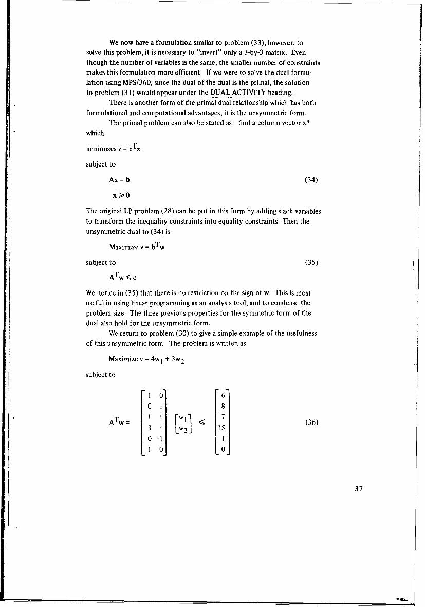
We notice in (35) that there is no restriction on the sign of w. This is mostuseful in using linear programming as an analysis tool, and to condense theproblem size. The three previous properties for the symmetric form of thedual also hold for the unsymmetric form.

We return to problem (30) to give a simple example of the usefulness

of this unsymmetric form. The problem is written as

Maximize v = 4wI + 3w2

subject to

1 01 6

0 1 8

ATw I I [wli < 7 (36)3 1 w2 15is0 -!1 1

-L1 0L 0

37

Note that w2 is unrestricted in sign and that the last row of AT keeps w1

nonnegative. This is the unsymmetric dual formulation of problem (30).Since w2 is unrestricted in sign, to solve this problem via a standard LP code,we should have to replace w2 by w2 w2, us before. But if we consider the

associated primal problem, this requirement disappears; i.e.,

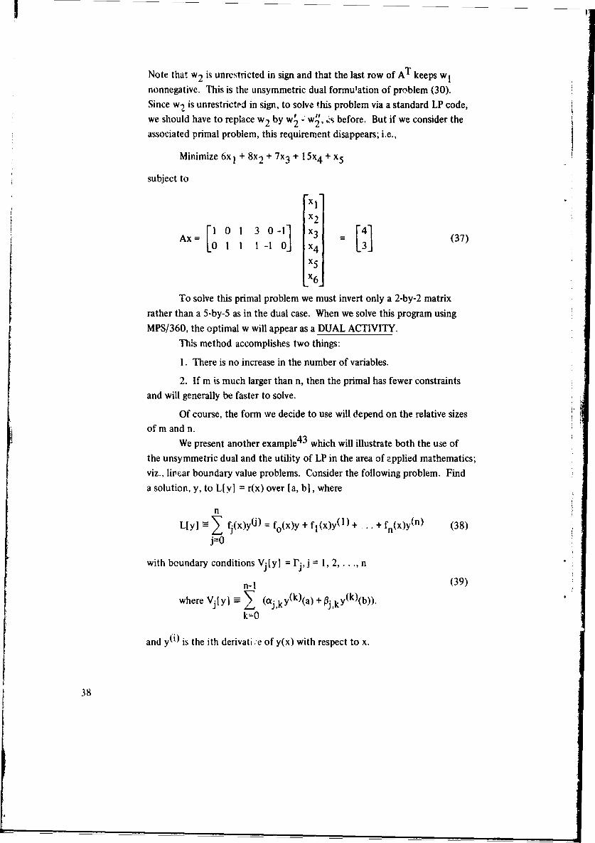
Minimize 6x, + 8x2 + 7x 3 + 15x 4 + x5

subject to

xl

x2

Ax= [1 0 1 30 o] x3 4 (37Ax= 1 1 1 -1l x4 (37

x5_x6.

To solve this primal problem we must invert only a 2-by-2 matrixrather than a 5-by-5 as in the dual case. When we solve this program usingMPS/360, the optimal w will appear as a DUAL ACTIVITY.

This method accomplishes two things:

1. There is no increase in the number of variables.

2. If m is much larger than n, then the primal has fewer constraintsand will generally be faster to solve.

Of course, the form we decide to use will depend on the relative sizesof m and n.

We present another example4 3 which will illustrate both the use ofthe unsymmetric dual and the utility of LP in the area of applied mathematics;viz., lirear boundary value problems. Consider the following problem. Find

a solution, y, to L[yI = r(x) over [a, b], where

nLtyI ---•, fj(x)y(j) fo(x)y + fl(x)y(l) + .. + fn(x)y(n) (38)

j=0

with boundary conditions Vj[yI = j,j= 1,2,. .. , n

n-I (39)

where Vj[yj =3j (j,k y(k)(a) + Pj,ky(k)(b)).k=O

and y(i) is the ith denivati :e of y(x) with respect to x.

38

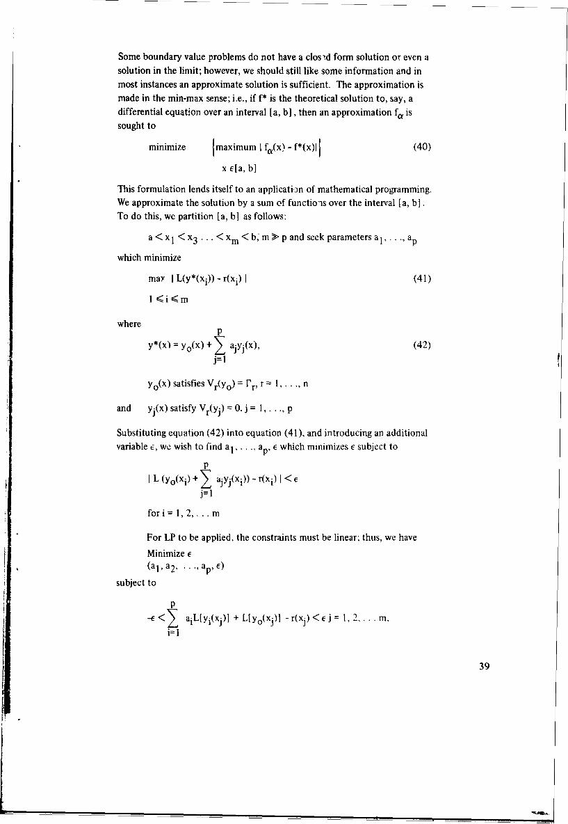
Some boundary value problems do not have a closid form solution or even asolution in the limit; however, we should still like some information and inmost instances an approximate solution is sufficient. The approximation ismade in the min-max sense; i.e., if f* is the theoretical solution to, say, adifferential equation over an interval [a, bI, then an approximation f., issought to

minimize Imaximum I f,(x) - f*(x)lj (40)

x ela, b]

This formulation lends itself to an applicati n of mathematical programming.We approximate the solution by a sum of functions over the interval [a, b].To do this, we partition [a, b] as follows:

a < x, < x3 ... < xm < b,'m i> p and seek parameters a1 ,..., ap

which minimize

may I L(y*(xi)) - r(xi) I (41)

l <i <m

wherep

y*(x) = Yo(X) + I ajyj(x), (42)

j=1

yo(x) satisfies Vr(yo) = rr, r 1, . . n

and yj(x) satisfy Vr(Yj) = 0. j = I., p

Substituting equation (42) into equation (41), and introducing an additionalvariable c, we wish to find a 1. , ap, e which minimizes e subject to

pI L (yo(xi) + ý a•ay(xi)) - r(xi) I <E

j= 1

fori= 1,2,. .. m

"For LP to be applied, the constraints must be linear: thus, we have

Minimize ei-'(a I, a2. , ap, e)

subject to

p

-e <> aiL[yi(xj)I + L[y°(xj)I - r(xj) < E 1, 2.... m,

39

F

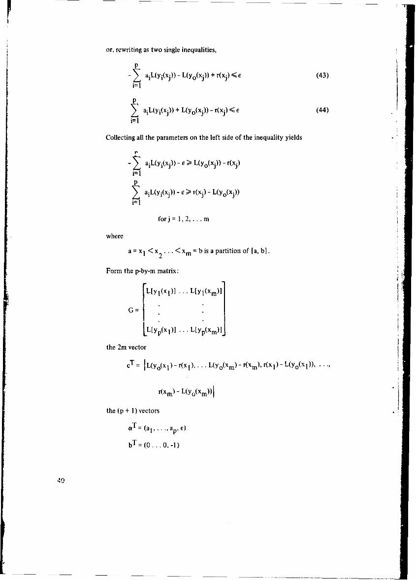
or, rewriting as two single inequalities,

p- • aiL(yi(xj)) - L(Yo(xj)) + r(xj) < e (43)

i=lI

p• aiL(yi(xj)) + L(Yo(xj)) - r(xj) < e (44)

Collecting all the parameters on the left side of the inequality yields

- • aiL(yi(xj)) - e > L(Yo(xj)) - r(xj)i= 1

p> aiL(yi(xj)) - e > r(xj) - L(Yo(xj))i=l1

forj 1,2,...m

where

a x1 < x2 < xm b is a partition of [a, b].

Form the p-by-m matrix:

L[Yl(Xl)] ... L[Yl(Xm)] i

G=

L~yp(X 1)] " L[yp(Xm)]j

the 2m vector

CT= L(yo(x1 ) - r(x 1),... L(yo(xm) - r(xm), r(x 1) - L(yo(xl)), ..

r(xm) - L(Yo(xm))i

the (p + l) vectors

J = (a . ap,e)

bT= (0... 0,-l)

49

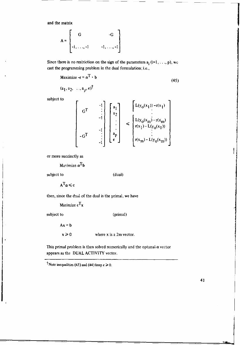
and the matrix

Since there is no restriction on the sign of the parameters ai (i= ,.. .,p), wecast the programming problem in the dual formulation; i.e.,

Maximize -e = aT . b (45)

(a1, a2 , .. , a "

subject to -1 a, L(yo(x 1)) -r(x1)

-GT . aL - r(xm) - L(yo(xm))

or more succinctly as

Maximize ATb

subject to (dual)

ATa < c

then, since the dual of the dual is the primal, we have

Minimize cTx

subject to (primal)

Ax = b

x > 0 where x is a 2m vector.

This primal problem is then solved numerically and the optimal ot vectorappears as the DUAL ACTIVITY vector.

tNote inequalities (43) and (44) keep e > 0.

41

In summary, we basic advantages are as follows: We wish para-

meters ai, 1 . ., ap, which give the best estimate in a min-max sense of the

'solution to the linear boundary value problem. The parameters are

unrestricted in sjia and the number of points m in the interval of solutionis large. To cast this problem as a primal linear programming problem would

have required 2p + I variables, since the ai are unrestricted, and 2m constraints.By first writing the approximation problem as a dual linear programming

problem (45), we need only p + 1 variables; then transforming to the primal

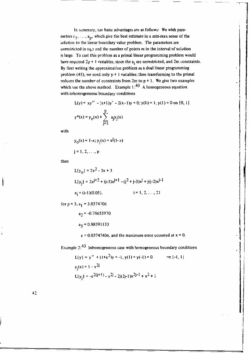
reduces the number of constraints from 2m to p + 1. We give two examples .which use the above method. Example 1:43 A homogeneous equationwith inhomogeneous boundary conditions

L(y) = xy" - 'x+l)y' - 2(x-1)y 0;y((i) 1, y(l) 0 on [0, 11

py*(x) = yo(x) + ' ajyj(x)

j=1

with

Yo(X) = l-x; yj(x) = xAl- x)

j = 1, 2,. .. , p

then

L[yo] 2x 2 -3x+3

L[yj] 2xj+2 + U-3)xj+l -2 + j-3)xj * j(j-2)xJ-I

xi = i1( .5 .i = 1, 2, .. ., 211

fcr p 3, a1 = 3.0374706

a2 = -0.78655970

a3 = 0.88391133

E= 0.03747406, and the maximum error occurred at x = 0.

Example 2:43 Inhomogeneous case with homogeneous boundary conditions

Ljy] = y" +(i+x2)y -l,y(l)=y(-l)= 0 on [-1, 11yj(x) = I _ x2j

]

LIyj] = _x20+1) x2-2j2jlx2-1 + x2 + i

42

I

Letz=x2 , L[yj] -zJ+l - zJ - 2j(2j - )zi-I + z + 1

zi= (i-1)(0.05) i 1, 2,.. ,21

for p = 3, aI = 0.9675, a2 .. a3 = -0.0285

e = 0.0029

The preceding paragraphs have pointed out some of the numericaladvantages of duality. Duality concepts also have application in nonlinear

programming; however, so far these have been limited to SUMI methodsinvolving convex functions. In this case, the duality theory provides a lower

bound on the value of the unconstrained problem to test for convergence; seereference 24. Its use in nonlinear problems is no! widespread.

LAGRANGE MULTIPLIERS AS A DESIGN AID

Another influence on choice of routine or method to solve an MPproblem is postoptimal analysis.

When a constrained optimization problem is solved via sequentialunconstrained minimization techniques (SUMT), additional information is

available to the designer foi a sensitivity analysis; i.e., postoptimal analysis.

Suppose x* is the solution to the following MP problem.

Minimize f(x)

subject to (46)

NA~) < bi, i = 1, 2,. .. , m

The engineer wishes information as to how f(x*) will change if b ischanged a little; i.e., if the design requirements are changed, how wil theperformance be affected? The interesting result is:

af(x*(b))

abi = Xi (47)

where Xi is a generalization of the classic Lagrange multiplier for finding the

extrema with side conditions. The proof of (47) is contained in reference 44.We recall from advanced calculus that an extrema problem with side

conditions was: find the minimum (maximum) of p(x j, x2 . xn) subiect

to q(Xl, .. ., xn) ... - qm(Xl, ... , xn) = 0. To solve this problem we

43

F -T

formed the Lagrangian L(x ... n, ) p(x) + m iqi(x)

then solved the (n+m) system of equations:

aL(x, X) 0

axiqi(x) = 0 i=!. ., m

for (x 1 , xn) with the Ni's being introduced to help find the xi. TheKuhn-Tucker theorem 4 5 allows us to define a meaningful and useful

Lagrangian for inequality constraints.We discuss the Kuhn-Tucker theorem to allow a generalization of

Lagrange multiplier, and then discuss SUMT methods to iflustrate obtaining

ihe Xi's numerically.Rewriting the constraints to problem (46) as gi(x) hi(x) - bi < 0,

we obtain probiern (1):

Minimize f(x)

subject to (48)

gi(x) •< 0 M , ..m

Then the Kuhn-Tucker theorem says essentially the following:

Lc' x* be a solution to the above Problem and assume the boundaryc,. the constraint set has no "c'isps;" then the following conditions hold.

1. There exist multipliers Xi > 0, i 1 .. m such that

Xi gi(x )- 01. i=l1, 2,. .. m

n2 . '*)+ xiV gi(y' 0, '

i=1

The following example illust. Aes the Kuhn-Tu-ker condition:

Minimize f(: j, XI) =fx - 2)2 + (x2 - 1)2

subject to

gl(X 1, Y2) -x2 + x'" <0

g2(x x''2+l +x x2 <0

44.

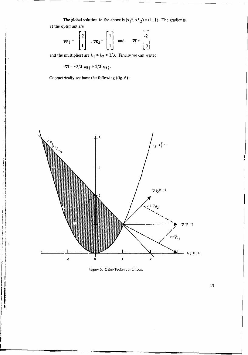
The global solution to the above is (x1*, x* 2 ) (1, 1). The gradients

at the optimum are

Vgl= [ V] '72= ['] and Vf=

and the multipliers are W, = X2 = 2/3. Finally we can write:

-Vf= +2/3 Vg, + 2/3 Vg2 .

Geometrically we have the following (fig. 6):

+

+ x x2- 02 1 1 0I 0

V~g2

2N

, //

/ 2/3Vg1

-0 0

Figure 6. Kahn-Tucker conditions.

45

Now that we have seen a need for knowing the Lagrange multipliers

and have seen the geometrical interpretation, we turn to SUMT and thenumerical calculation of the multipliers. The constrained optimizationproblem is transformed into an unconstrained one through the use of an

auxiliary function, 0(x). 0(x) does one of two things, 0(x) * as x -+ 0 or

0(x) = 0 for x feasible and 0(x) positive for x :nfeasible. The three forms4 4

of 0(x) we discuss are:

m

Barrier: B(x)= - I I/gi(x) (49)i= I

m

Penalty: P(x) (Max (gi(x), 0))l+e (50)i=lI

m

Logarithmic: L(x) -L iog(-gi(x)) (51)

i= I

SUMT works as follows: Using 0(x) = B(x), P(x) or L(x), wetransform the constrained problem into a sequence of unconstrained problems,as. in SUMT and Constraint Transformation.

Minimize D(x, rk) = f(x) + p(rk)o(x) (52)

for rk > 0. Then if x* is the optimum for the constrained problem (48) andx(rk) -= xk, the optimum for problem (52), it can be shown that limi* xk =x*;

k-+oo

i.e., (rk-•0). Thus, we replace the constrained problem by a sequence ofunconstrained problems.

In the barrier and logarithmic cases as gi(x) - 0 - i.e., x attempts to

leave the constraint set - gi(x), must approach 0, and this causes B(x) andL(x) to increase rapidly. Since the routine wishes to minimize D(x, r), and

we have an initial feasible point, intermediate x's are chosen feasible.

In the penalty function approach the test points are allowed to leavethe constraint set; however, when they do so, a positive amount is added tothe objective function. Again, since we ;eek to minimize D(x, r), points are

selected within the constraint set. When 24(.) or L(x) is used, we have an

interior point method; and when P(x) is used, we have an exterior point

method. With each type of 0(x) a slightly different technique is used to

recover the Xi.

46

Barrier Method:

Form the function

D(x, r) = f(x) + rB(x)

m= fix) + r -l/gi(x) (53)

i=lI

for r> 0. Let rk be a monotonic decreasing sequence converging to zero. If

xk minimizes D(x, rk), thenI

0= VxD(xk, rk) = Vf(xk) + rk 2 1 vgi(xk) (54)Vf~~xk + ir l gi2 (Xk) gxk

Letting

x (k)-k (55)2

gi (xk)then the Lagrangian becomes

in m

L(xk, Xk) = f(xk) + X( { gi(xk = f(xk) + rk(56)Sgi(xk)

The multipliers can be computed by equation (55,.

We note if gi(x*) > 0, then Xk 2 (0k)k r approaches G as k • o, sinceg i (Xk)

rk-_+ 0.

rkIf gi(x*) = 0, then by the Kuhn-Tucker theorem Xi>0; thus the limit

gi (xk)must be taken strictly as a quotient.

m

Logarithmic Penalty: Form C(x, r) = f(x) - r log(-gi(x)) (57)

then at the optimum, xk for C(x, rk) we have,

0 = VxC(xk, rk) Vf(Xk) + rk Vgi(xk) (58)

• gi(xk)

47

Now, in a similar argument, let

k(k)X. rk/-gi(xk) (59)

Since (-gi(x*)) > 0 in the feasible set, we have X ,() > 0. Thus, we can form

the Lagrangian as before and equation (59) generates the multipliers.

We next give an example to illustrate this.

Lootsma 3 9 solves the following problem

Minimize f(x) =x -6x3_ 6 x +x 3

subject togl(x)= +x2 2 + x 2 x (<0 (60)

g1•(x)=-x2-xx 2 -x 3 -4 !O<

g4(x) = -x 2 x -4<01 2 3

95(x) = -x2 •< 0

96(x) = -x3 •<0

The optimum is x* = (0,v2,\V-) with gl(x*) = g2 (x*) g4(x*) 0. The

theoretical multipliers are

XI = X'2 =V/2/8, - 0. 1767766

X4 = 11 X3 = X5 = X6 = 0

For rk = 10-6, the numerical multipliers are

Srk 10-6

X(k) = - - = 0.176664I -gl(Xk) 5.66046 10-6

X(k)= rk 10-6 0.150302 -g2(xk) 6.65324 10-6

_ _rk _ 1 0 -6r(k) ____10-6 _ = 10.8687

4 -g4(xk) 9.2007 10-8

xk (9 .2 071 10-8, 1.4121, !.41422)

48

The final example is the Penalty Function method.

Let

C(x, r) = f(x) + I P(x),r

where

mP(x) = (max. (gi(x), 0))l> 0.

i=l

Then at the optimum,

VxC(xk, rk) = 0 which implies Vf(x) + 1 '7 P(x) = 0 (61)r

where VP(x) = + (l+e) [max. (gi(x), 0)] e Vgi(x)

If we let X(k)= (l+e)m .g(x), 0o1

Srk

then X k > 0, since we have an exterior point method.

Thus, (61) becomes Vf(x) + YXiVgi(x) = 0,

and, letting xk denote the optimum for rk, 'A nave

Xi = lim X(k) = li (max gi(xk),01)jk--oo i k--w rk (ax-Ig~k,01)

In this way we can obtain the Xi's.

In solving the Lootsma problem by the penalty method with e = 1, we

obtained the following results for rk .1 * 10-4:

xk = (.144 3 *i0-16, 1.4142, . .. , 1.4141, . .

g1(xk) = .8797110* 10- 6 ; g2(xk) = 0.8797477* 10-6

,4(xk) = 0.388414* 10-14

=(k I+e) 0.879711*10-6 Irk (max. (g 1O = =-.0.1759422r 1.0 *10"5

( k +) .87974779*10•T 1.... (max. (g),0)) 2 0.1759495580

rk 1.0 * 10-5

49

F

(k)= 0+0 (max. (g4 , 0)) =2 j0.388414*1- 4 = 0.7768*10-11 114 rk 10-5

The last four con.itraints of problem (60) were transformed by the followingequation and not included as penalties:

= 2

2"2 = Y

x3 = 5 sin2 (y( 3 )).

When these transformations are used, A(k) cannot be obtained by the above'4

formula.

INITIAL POINT AND SCALING

Two final topics in solution strategy depend a great deil on th"

specific problem: initial point and scaling of variables. If the constraintsare numerous and complicated, then finding an initial feasible point can bean additional pioblem in itself.

Zoutcndijk 4 7 gives a "simple" trick for a transformation which

replaces the original problem by an equivalent problem for which an initial

feasible point can readily be found. Suppose we are given:

Minimize f(x)

subject to

gi(x)•< 0 i= 1,2,. m

a.ad no initial point x0 can be found by inspection oi engineering knowledge

such that gi(x°) •< 0 for i = 1, 2.. m. We now form the following problem:

Minimize f(x) + gt

subject to gi(x) - Pit < 0

P i > 0 i 1 , ? . . . .

where y is a large number, t an additional variable, and pi = I if gi(x 0) > 0and pi = 0 it gi(x°) < 0. If t > max. /gi(x') for all i such that gi(x°) > 0,

then the point (x0 , t) is feasible for the modified problem. In reference 17

Zoutendijk proves that, for p sufficiently large, the modified problem will

so

have the same solution as the original. Note that in the attempt to minimizef(x) + jt, t is driven to zero, but to satisfy the constraints x must besimultaneously chosen feasible (for the original problem). This is the part of

mathematical programming in which the user's previous engineering anddesign experience pays off, since the better the initial point, the faster the

routine will converge.Proper scaling of variables is still an art. Most computer routines ,or

solving mathematical programming problems are designed to follow steepcurved valleys and sharp ridges in locating an optimum. For a one-shotproblem, scaling the variables is not worth the time; however, if a code is tobe written to solve a large class of similar problems, then scaling may beworthwhile in long-term savings of machine time. We give an example,

Pierre48 which transforms a poorly shaped objective function into a "nice"bowl-shaped function which can quickly be minimized. Unfortunately,

scaling is somewhat limited to unconstrained problems; in a constrainedproblem attempting to make the objective function easy to minimize, the

Ecaling might destroy any useful properties the constraints enjoy.

Example:

2 2SIf f(x1, x2 )= x1 +- lxxl2 + lO0x , then f has a narrow valley and

a minimum at x 1 = x2 = 0. To transfc.rm f into a more desirable shape, we

eliminate the cross product 10xlX2 by letting xI = zI - abz 2 and x2 - bz 2 .Then f becomes

f zI + (-2ab + lOb) zlz 2 + (-1Oab 2 + a2 b2 + lOOb2)z1/ 2 i Ob

Letting a = 5 makes (-2ab + 1Ob) = 0 and b = (1/75)12 solves -50b 2 + 100b225b2 =t fh 2

I ; thus, f=zI + z 2 , which is easily minimized by almost anyroutin,.

It is highly recommended, when the variables are bounded or therange of the variable is known, that the variable be normalized. For example,

if the variable xi lies in the range:

Li <• xi < Ui

then an appropriate normalization is given by:

S" 0< Yi < 1.0

where

51

xi - LiYi=Ui - Li

Normalization is particularly useful in direct search algorithms for which wemust arbitrarily choose a step size search increment, A. It can readily beI% of 1.0 (0.01), which allows each variable to be changed proportionally,

or any other realistic choice depending on our knowledge of the problem.In summary, scaling an objective function is generally not practical,

and we must rely on the properties of the algorithms to find the optimum;

however, normalization is recommended wherever possible.

SUMMARY

Mathematical programming is a broad subject with many varied applica-tions. Not all top; -s in MP -.re opplicable to engineering design. We have triedto delineate those areas wh.lh are useful and the corresponding capabilities atNELC. The computer code; described have proved reliable on a wide range ofproblems; however, MP is -an expanding area, and the new algorithms constantlybeing developed could render some of these codes obsolete. The applications-

oriented user should not accept this list as complete or give up if his particularproblem does not match an available routine. Perhaps a literature search willyield the appropriate method. The high-speed digital computer has provided

an impetus to develop algorithms to solve MP problems which previously weretoo large to be handled. It is recommended that a continued effort be main-tained to keep NELC up to date in the area of solving MP problems numerically.Logically, this shouUd be a function of either a Center-wide computer users'group or of CoInputer Sciences Department. Other installations maintain alibrary of computer codes readily available to users; NELC should do the same.

In the applications area, mathlematic'l programming has been a proveddesign tool. In reference 1, it was shown to be applicable to typical NELCproblems. The second part of this report discussed some topics which wereusetul in obtaining actual solutions to design-related MP problems. The tech-niques have been used with routines available at NELC We have tried to showthat NIP can be an aid to the design engineer and not his replaceme'nt. In factto use MP effectively requires that the engineer be skillful in his field and beable to generate an aLcurate mathematical mod'l of his design problem. Wefurtier recommend that a short course or continuing seminar be offered toNhL(" personnel to familiarize them with MP techniques. Such a course wasgiven in-house in the fall of 1968 and was well received.

52

APPENDIX 1: APPLICATIONS OF INTEGER PROGRAMMINGTO ENGINEERING DESIGN

In this appendix we report on the results of a literature search todetern ine feasibility of using integer programming (IP) as a practical designaid in in ongoing NELC task - BAMS (Benchmarks foi Applications of Micro-electronics to Systems). The results were disappointing. Meaningful applica-tions .:re still in the experimental stage, with results limited to relatively smalltest problems. The main hindrance to successful applications is not formula-

tional difficulties, but the lack of reliable computer codes for solving theresulting IP problems. General-purpose IP codes are severely limited in thesize problem they cai solve (a maximum of 60 constraints and 60 variab.es atNELC), anO they are sometimes unreliable. The majority of the applicationsof IP have been in the business world, and many algorithms for solving specialIP problems have been developed; e.g., aircraft crew scheduling and warehouseplacement. These methods rely on the special structure of the IP problemunder consideration and have worked well. If the design engineer is lucky,his IP problem may fit one of these special methods (it is still an art to matchthe computer code to the posed IP problem); otherwise he must rely on thegeneral IF codes. Here, application is ahead of theory.

We give a brief example which illustrates the computational difficultiesof IP, a review of the state of the art of IP as related to BAMS, and finally adetailed example in which IP is used to solve a backboard winng problem.

Most of the IP work has been done in the linear case; i.e.,

Minimize f(x) = c I1x + c2 x2 +. . . + cnXn

subjectto gl(x)=alIxl +a 1 2x 12 +..+alnxln <bl

gm(x) = amIxI + am2x2 + •+ amnxn < bm

xi ; 0 and xi an integer

Thus, the integer linear orogramming (ILP) problem is just the LP problemwith the additional constraint that the solution be integral. Gomory49 hasdeveloped an algoritim. ,,,,,h theoretically solves the above problem in afinite number of steps N- however, N can be a large number and henceimpractical for some problems. Since this area of mathematics is so useful,many methods (some heuristic in nature) for solving special ILP problemshave been reported which work well. One methoC, which appears obvious,is to solve the associated LP problem, then round to the nearest (in somesense) integer-valued vector and use that for the solution. Many times this

53

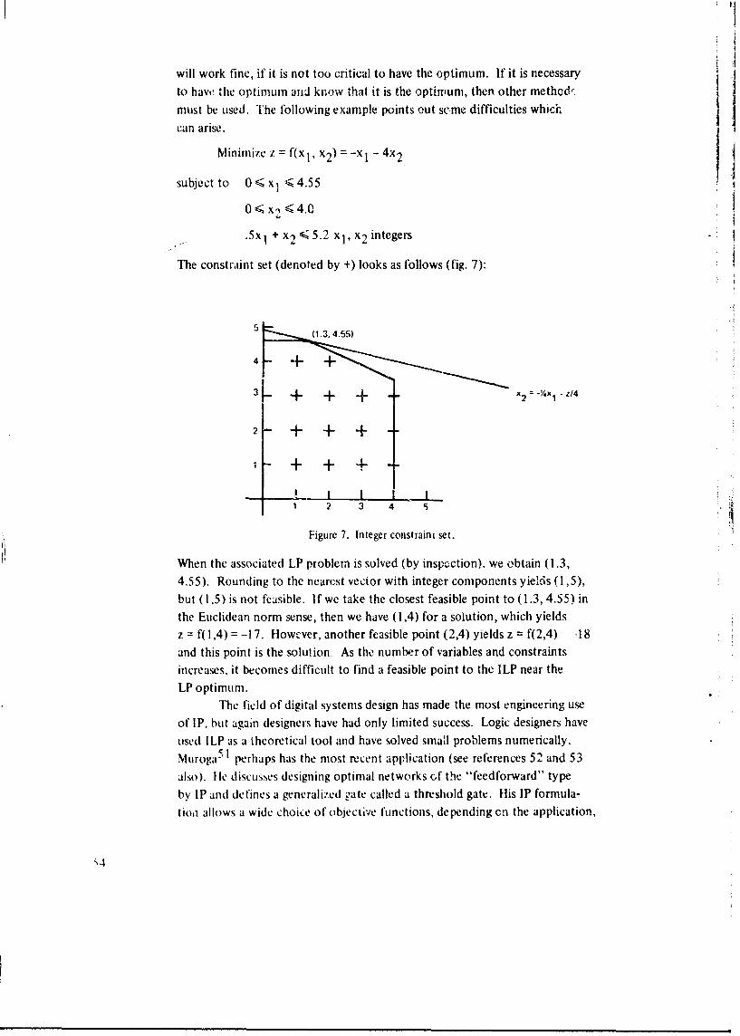
will work fine, if it is not too critical to have the optimum. If it is necessary

to have tie optimum and know that it is the optimrum, then other method'.must be used. The following example points out some difficulties whichcan arise.

Minimize z = f(x 1 , x2) =-xI - 4x2

subject to 0<x1 ,4.55

0< x2< 4.0

.5x 1 + x,•< 5.2 x 1, x2 integers

The constraint set (denoted by +) looks as follows (fig. 7):

5 (1.3. 4.55)

4 ++

3 + +1 + x 2 =-1/X 1- z/4

2 + + +

-+ + +

1 2 3 4 S

Figure 7. Integer constraint set.

When the associated LP problem is solved (by inspcction). we obtain (1.3,4.55). Rounding to the nearest vector with integer components yields (1,5),but (1,5) is not feasible. If we take the closest feasible point to (1.3, 4.55) inthe Euclidean norm sense, then we have (1,4) for a solution, which yields

z = f( 1,4) = -17. Howcver, another feasible point (2,4) yields z = f(2,4) .18and this point is the solution.. As the number of variables and constraintsincreases, it becomes difficult to find a feasible point to the ILP near the

LP optimum.The field of digital systems design has made the most engineering use

of IP. but again designers have had only limited success. Logic designers haveused ILP as a theoretical tool and have solved small problems numerically.Muroga51 perhaps has the most recent application (see references 52 and 53also). lie discusses designing optimal networks of the "feedforward" typeby IP and defines a generalized gate called a threshold gate. His IP formula-

tioa allows a wide choice of objective functions, depending on the application,

.'-.

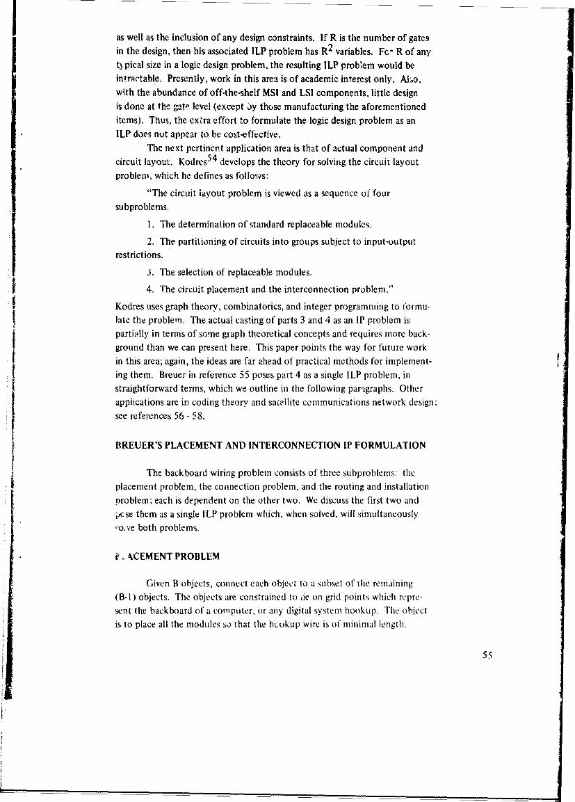
as well as the inclusion of any design constraints. If R is the number of gatesin the design, then his associated ILP problem has R2 variables. Fc- R of anytypical size in a logic design problem, the resulting ILP problem would beintractable. Presently, work in this area is of academic interest only. ALo,with the abundance of off-the-shelf MSI and LSI components, little design

is done at the gateý level (except 3y those manufacturing the aforementioneditems). Thus, the extra effort to formulate the logic design problem as anILP does not appear to be cost-effective.

The next pertinent application area is that of actual component andcircuit layout. Kodres 54 develops the theory for solving the circuit layout

problem, which he defines as follows:

"The circuit layout problem is viewed as a sequence of foursubproblems.

1. The determination of standard replaceable modules.

2. The partitioning of circuits into groups subject to input-outputrestrictions.

3. The selection of replaceable modules.

4. The circuit placement and the interconnection problem."

Kodres uses graph theory, combinatorics, and integer programming to tormu-late the problem. The actual casting of parts 3 and 4 as an IP problem ispartially in terms of some graph theoretical concepts and requires more back-

ground than we can present here. This paper points the way for future workin this area; again, the ideas are far ahead of practical methods for implement-

ing them. Breuer in reference 55 poses part 4 as a single ILP problem, instraightforward terms, which we outline in the following paragraphs. Otherapplications are in coding theory and satellite communications network design:Iisee references 56 - 58.

t BREUER'S PLACEMENT AND INTERCONNECTION IP FORMULATION

The backboard wiring problem consists of three subproblems: theplacement problem, the connection problem, and the routing and installationproblem; each is dependent on the other two. We discuss the first two andSpcse them as a single ILP problem which, when solved, will simultaneously""ove both problems.

P . 4,CEMENT PROBLEM

Given B objects, connect each object to a subset of the remaining(B-I ) objects. The objects are constrained to ,ie o0 grid points which repre-sent the backboard of a computer, or any digital system hookup. The objectis to place all the modules so that the hcukup wire is of minimal length.

55

CONNECTION PROBLEM

Given S fixed objects which are to be made electrically common,connect thte objcts so that the total interconnection length is minimal.

INTEGER PROGRAMMiNG FORMULATION

Given B obj,-cl:s to be placed at the intersections of the rectangulargrid (fig. 8).

m-1

YAXIS . ...

2

0 1 2 n-1ix AXIS

Figure 8. Back plane grid.

Tet xi, i = 0,1,... .n-I be the x coordinate of the ith object

Yi' i = 01, ... . m-1 be the y coordinate of the ith object

and B<mn.The interconnection distance between the ith and jth object is definedto be

dij = [i - xjI + k lyi- yj I

We note that no two objects can occupy the same spot at the same time.Also given is a list of the desired connections. We wish to uniquely positionthe set of B objects at the intersections and determine which objects sbouldbe directly connected together, in a manner such that total interconnectiondistance of those objects, directly connected, is minimal. The hard parts aremaking sure no two objects occupy the same spot and getting a linearrelation for d.

5(,,

The constraint that no two objects lie at the same point requiresthat ifxi = xj, then yi -? yj for i *j; or ifyi = yj, then xi * xj for i *i.

We list the required constraints for the placement problem and thenexplain how they meet the conditions of the problem.

xi-xj •<n 6ij (Al)

xj - xi + I < 110 - 6ij) (A2)

bij _<l i.e. 6ij = 0orlI (A3)

oij •< n 5ij (A4)xi - xj <• c~ii •< xi - xj + n(1 .- bij) (A5)

oýi •< n(l - 5ij) (A6)

x - Xi •< Qji < xj - xi + n ij (A7)

for all i> j,j = 1,2, .... B-IFrom inequalities (AI) and (A2) we find that if xi > xj, then 5 ij I

ii = 0, if xi > xj. Inequalities (A4) - (A7) give a representation for

Ixi - xj I as follows. Since (A4) and (A5) yield 0 < aij = xi - xj < n- i,if xi > xj and oij = 0 otherwise. In a similar fashion 0 <aj i = xj - xi,if xj > xi; thus, we have aij + Uji xi - xil-

Now let n and 0 play analogous roles for y; then Oij + jii= lY - y I.Thus, dij can be stated in terms of these auxiliary variables as

dij = aij + 0tji + k(Oij + 3ji)

Some additional constraints guarantee realizabiliy.

atij + t'ji + k(O3ij + Oji) >• I (A8)

xi< n-1 i=1,2, ... ,B (A9)

yi< rn-I i=1,2 .... B (A10)

Inequality (A8) guarantees that tvo objects do not occupy the same grid inter-

section. All xi and yi are nonnegative integers. Note that the above irequalitiesdo not Jepend on how the objects are connected, but only guarantee thatspecific necessary conditions will be satisfied. Inequalities (AI) through (A10)represent the constraints for the placement problem. We now turn to theproblem of optimally interconnecting the B objects.

Assume that there are C independent circuits where the jth circuit canbe connected in P. different acceptable ways. Let fij(d) be an expression forthe total length of wire in the ith way of connectinC, the jth circuit. Forexample, if the sixth circuit consists of three objects ( 1, 2, 3) and the first

may have only one connection to it, then

f 16 =d21 +d 32 and f2 ,d +d

The two final constraints which relate to the connection problem are:

Vj >, fij(d) + (Iij-. I)Q (Al 1)

and

P.

rij = forj=l...C (A12)i=1

Equation (A 12) implies that each circuit is connected and -,ij is 0 or 1.In (A10)Q = max. fij(d) fr i =1,2, .... Pj;ji= 1,2, ... C. Then the

resulting objective function is

C

min. Z = Vjj.-d Ij=l

The objective function and inequalities (Al) - (Al 1) form the ILP repre-senting the combined placement and connection problem. Although theformulation seenms straightforward, the resulting ILP problem can be large,even for small values of B. Breuer gives the following relations between thenumber of variables I, the number of constraints W, and B for the placementproblem: i.e., constraints (Al) - (AI0).

I(B) =(B/2)(19B-15)

W(B) = B(3B-I)

Thus, for B=5 (which couLd be manually positioned quickly and most likelyoptimally), we have 1(5) = 200, W(5) = 70; for B = 10 (stiil not too large),R(10) = 875, W(10) = 290. These !LP problems are very large and are beyondth, capabilities of today's methods.

It seems that, unless newer formulational techniques are developedwhich lead to smaller IP problems, or the computational capabilities solvingIP increase rapidly, this appioach wili remain a theoretical tool with nopractical applicatiops. The following quote (Glover 59 , p. I ) sums up the

current state of affairs in integer programming: "Since its inception integerGinear programming has. paradoxically, been a source of both promise and

disappointment. Promise because there are manifold and compellingopportunities to- its application; disappointment because it has made onlythe most dubious progress in spite of these opportunities."

APPENDIX 2: USER INFORMATION

H 1 - H20PT 4•LG

CATALOG IDENTIFICATION:

H i - H2OPTALG

PROGRAMMER:

F. S. Hillier, Stanford University, adapted for NELC by D. Klamer,Decision and Control Technology Division.

PURPOSE:

An algorithm for solving the rure integer linear programming problem.n

Maximize x0 cjxj

j=I

subject ton

(i) a ijxj < bj (i=1,2,. ,m)j=l

(ii) xj > (j 1,2. n)

(iii) xj is an integer (j=1, .... n)

RESTRICTIONS AND LIMITATIONS:

The dimensions of the constraint matrix A(,J ) aij have to b.' less than

or equal to 61 X 61; i.e., m < 61 and n •< 61.

LANGUAGE:

FORTRAN IV

COMPUTER CONFIGURATION:Go step REGION = 336kIBM 360/65

METHOD:

An initial noninteger solution must be obtained from the related liicarprogramming problem (i.e., xj is not necessarily ý.i integer) as well as tl,.:resulting basis inverse. To accomplish this, we have chosen the linear p, ugram-ming routine MPS/360. 18 Data are taken directly from MPS/360 and ii pUtdirectly into Hillier's program,31 without user intervention, in one mult stepcomputer run.

The advantage of using this modified version ot Hillier's progran, isthe time saved from obtaining the basis inverse and optimal ,.lhtion : the time

59

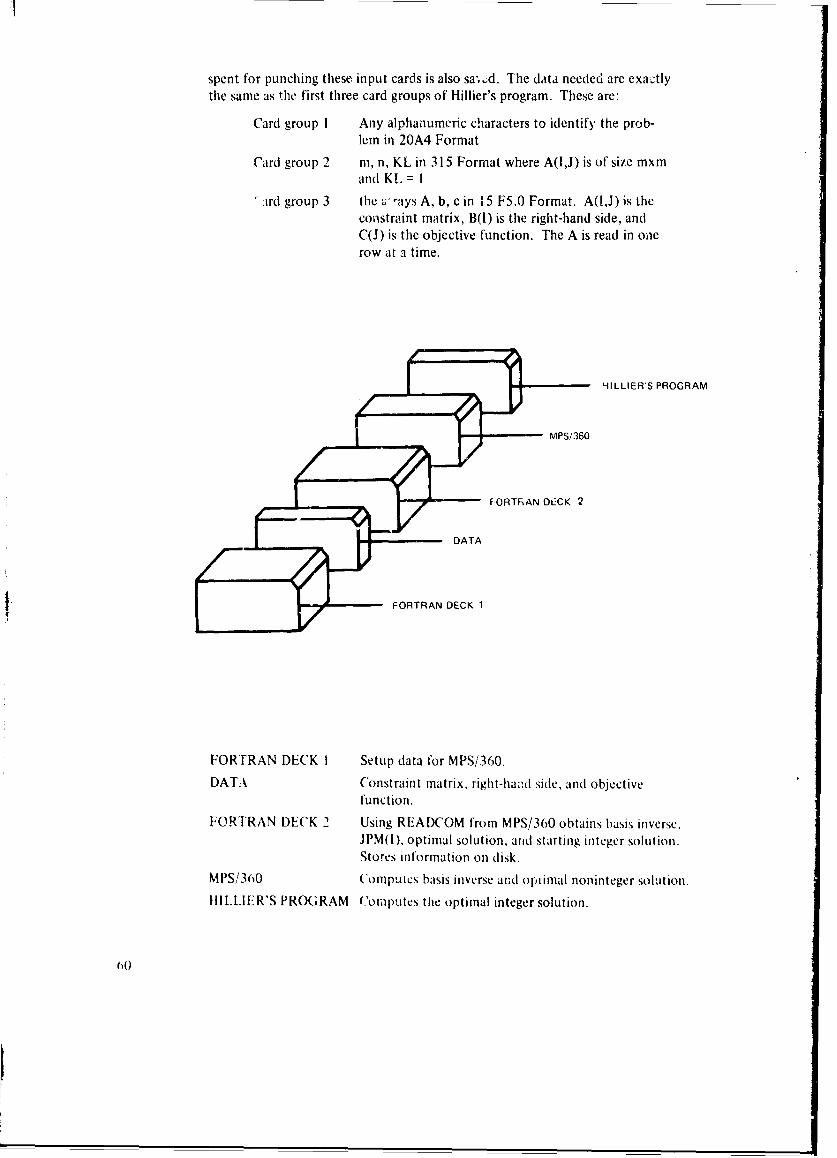
spent for punching these input cards is also sa,;,d. The data needed are exaitlythe same as the first three card groups of Hillier's program. These are:

Card group I Any alphanumeric characters to identify the prob-lem in 20A4 Format

Card group 2 m, n, KL in 315 Format where A(l,J) is of size mxmand KL = I

"ird group 3 the -rays A, b, c in 15 F5.0 Format. A(l,J) is theconstraint matrix, B(l) is the right-hand side, andC(J) is the objective function. The A is read in onerow at a time.

ZHILLIER'S PROGRAM

IJ

MPS/360

FORTRAN DECK 2

DATA

S~FORTRAN DECK 1

FORTRAN DECK I Setup data for MPS/360.

DATA Constraint matrix, right-hanld side, and objectivefunction.

FORTRAN DECK 2 Using READCOM from MPS/360 obtains basis inverse,JPM(I), optimal solution, and starting integer solution.Stores information on disk.

MPS/360 Computes basis inverse and optimal noninteger solution.

HILLIER'S PROGRAM Co, putes the optimal integer solution.

t00

FORTRAN DECK 1

This deck sets up the data for MPS/360, sin'ce (he format for MPS/360is long and cumber3ome. The constraint matrix A(IJ) is normalized, as is theright-hand side B(I); this is done on,' row at a time. The subroutine XPUNCHplaces the data into a disk file in proper forinat for MPS/360, from whichMPS/360 reads the data. A printout is given of the data that are placed ondisk. (Note: This data set is placed into a disk file called FTOIFOO1. Thedata are in normalized form, and, since MPS/360 is designed to find the mini-mum, the 6igns of the cost coefficients (objective function) are changed.)The constraint matrix A(IJ), the right-hand side B(l), and the cost coefficientsC(J) are also stored on the disk file called FT02FOOI.

FORTRAN DECK 2 (DATAHIlL)

This deck is a temporary update that is concatenated onto MPS/360,'inder the name DATAHILL. It uses READCOMM, 20 which is a subroutinedesigned to augment MPS/360 with procedures written in FORTRAN larnguage.DATAHILL retrieves from MPS/360 ti- e basis inverse, the order of the basicvariables, the optimal noninteger souluion, and a sUrting feasible solution tothe integer linear programming problem. These data are then added to thedata from the first FORTRAN deck on the disk file FT02F00I.

The starting feasible solution is a lower bound on the value of theobjective function. To obtain this feasible solution, we have chosen to do thefollowing: If the cost coefficient is positive, round the corresponding variableof the optimal noninteger solution down to the next largest integer. If thecost coefficient is negative, round up to the next smallest integer. (Note:The cost coefficients are placed into the disk file called FT03F001 in thefirst FORTRAN deck and are read by DATAHILL: the constraint matrix andright-hand side are also pased.) This rounded solu, tion is checked for feasibil-ity. If the solution is feasible, then proceed to the next step. If the solutionis not feasible, then try a rounding procedure to satisfy the constraint violated.(User may set the maximum number of iterations or changes in the solution.)In order for Hillier's program to be executed, a feasible integer solution mustbe found; if such a solution is not found, then Hillier's program is skipped andall the data are punched out on cards. This information includes the nam.,constraint matrix A(!, 1), right-hand side B(I ), cost coefficients ('C), the basisinverse, the order oi the balic aria•,les. and the optimal noninteger solution.The user may then supply his own starting integer solution and run the prob-fem directly from LLOAD, using the punched data produced in the last step.(See Part II.)

If a feasible integer solution is obtained and the user wisheC, to haICthe above data also, then ,:itlher of iwo methods mayv be usL .1. First, there

ri

01

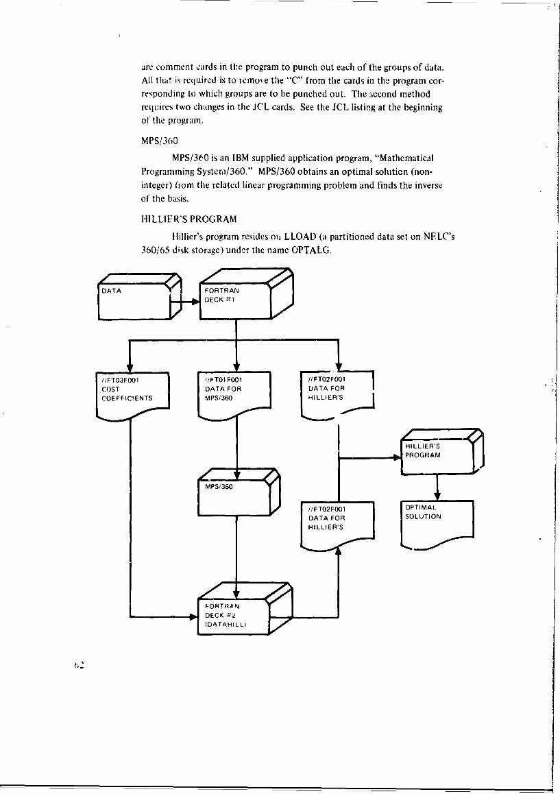
are comment cards in tle program to punch out each of the groups of data.

All that is required is to temove the "C" from the cards in the program cor-

responding to which groups are to be punched out. The second method

requires two changes in the JCL cards. See the JCL listing at the beginning

of the program.

MPS/360

MPS/360 is an IBM supplied application program, "Mathematical

Programming Systeni/360." MPS/360 obtains an optimal solution (non-

integer) from the related linear programming problem and finds the inverse

of the basis.

HILLIER'S PROGRAM

Hillier's program resides oi, LLOAD (a partitioned data set on NELC's

360/65 disk storage) under the name OPTALG.

DATA ORTRAN

tDECK 12

//FTD3FOO1 //FTO1 F001 //FTO2FO0lCOST DATA FOR DATA FOR

COEFFICIENTJS EMPS/360 HILLERS J

IDATAHILL)S

MPS/360

//T2F, OPIA

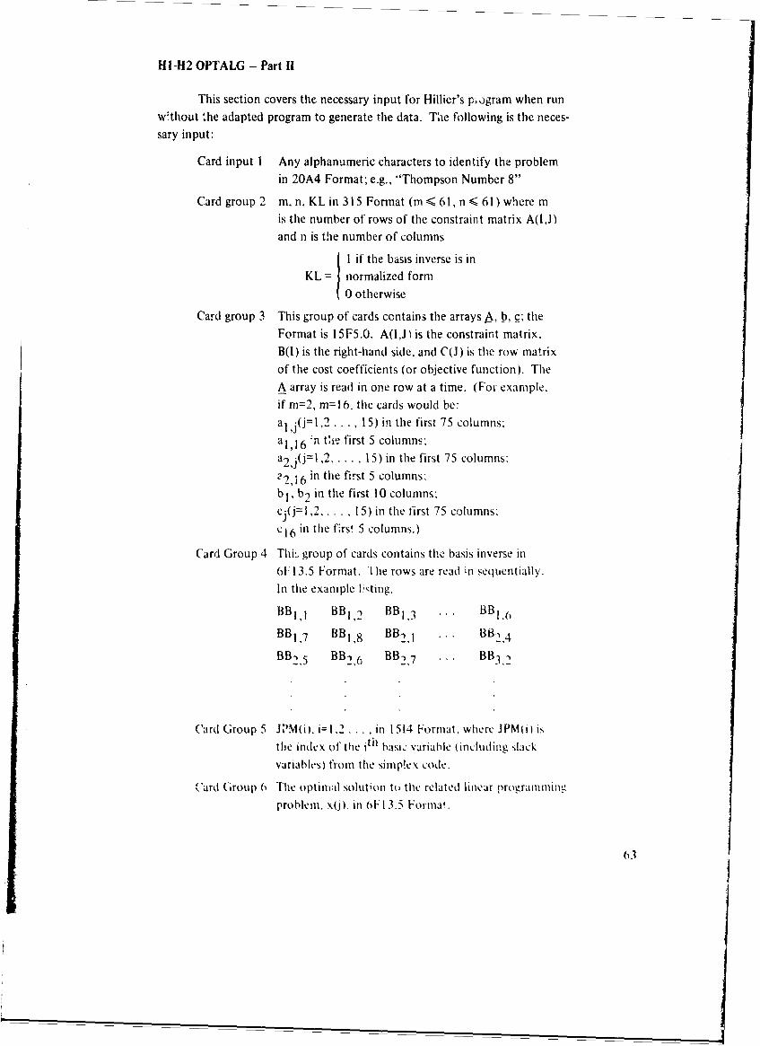
HI-H2 OPTALG - Part 1i

This section covers the necessary input for Hillier's pogram when runw'thout the adapted program to generate the data. The following is the neces-sary input:

Card input I Any alphanumeric characters to identify the problemin 20A4 Format; e.g., "Thompson Number 8"

Card group 2 m, n, KL in 315 Format (m < 61, n < 61) where mis the number of rows of the constraint matrix A(IJ)and n is the number of columns

I if the basis inverse is inKL normalized form

0 otherwise

Card group 3 This group of cards contains the arrays A, b, c, theFormat is 15F5.0. A(I,J' is the constraint matrix,B(1) is the right-hand side, and C(J) is the row matrixof the cost coefficients (or objective function). The

A array is read in one row at a time. (For example,if m=2, m=16, the cards would be:a1 ,j(j=l,2 . . . , 15) in the first 75 columns;

al,16 'n the first 5 columns-a2 ,j(j=l,2 .... 15) in the first 75 columns:22,16 in the first 5 columns;b1 , b2 in the first 10 columns-cj(j=1,2 .... 15) in the first 75 columns:c16 in the firs! 5 columns.)

Card Group 4 Thi group of cards contains the basis inverse in6F 13.5 Format. 'I he rows are read .n sequentially.In the example lH•ting,

BBII BBI,2 BBI13 ... BBI,o

BB 1,7 BB1,8 BB2,1 I ... BB2,4

BB2,5 BB2, 6 BB2, 7 ... BB3 ,2

Card Group 5 JPM(i), i= 1,2 .... in 1514 Format, where JPM(is ithe index of the ith basic variable (including slackvariables) from the simp!ex code.

('ard Group 0 The optim-l solution to tihe related linear programmingproblem, x(j) i (i F13.5 Format.

63

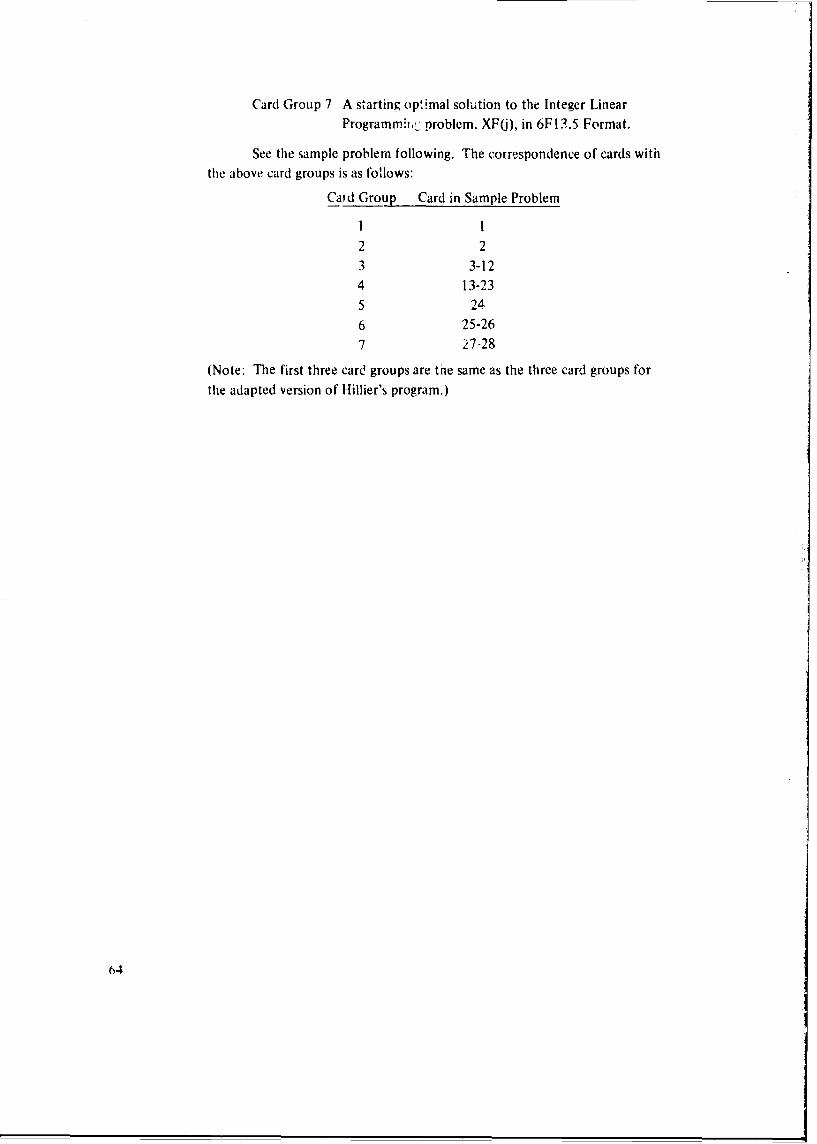
Card Group 7 A starting optimal solution to the Integer LinearProgrammi~w problem, XF(j), in 6F13.5 Format.

See the sample problem following. The correspondence of cards withthe above card groups is as follows:

Caid Group Card in Sample Problem

1 1

2 23 3-124 13-235 24

6 25-267 27-28

(Note: The first three card groups are the same as the three card groups forthe adapted version of Hillier's program.)

64

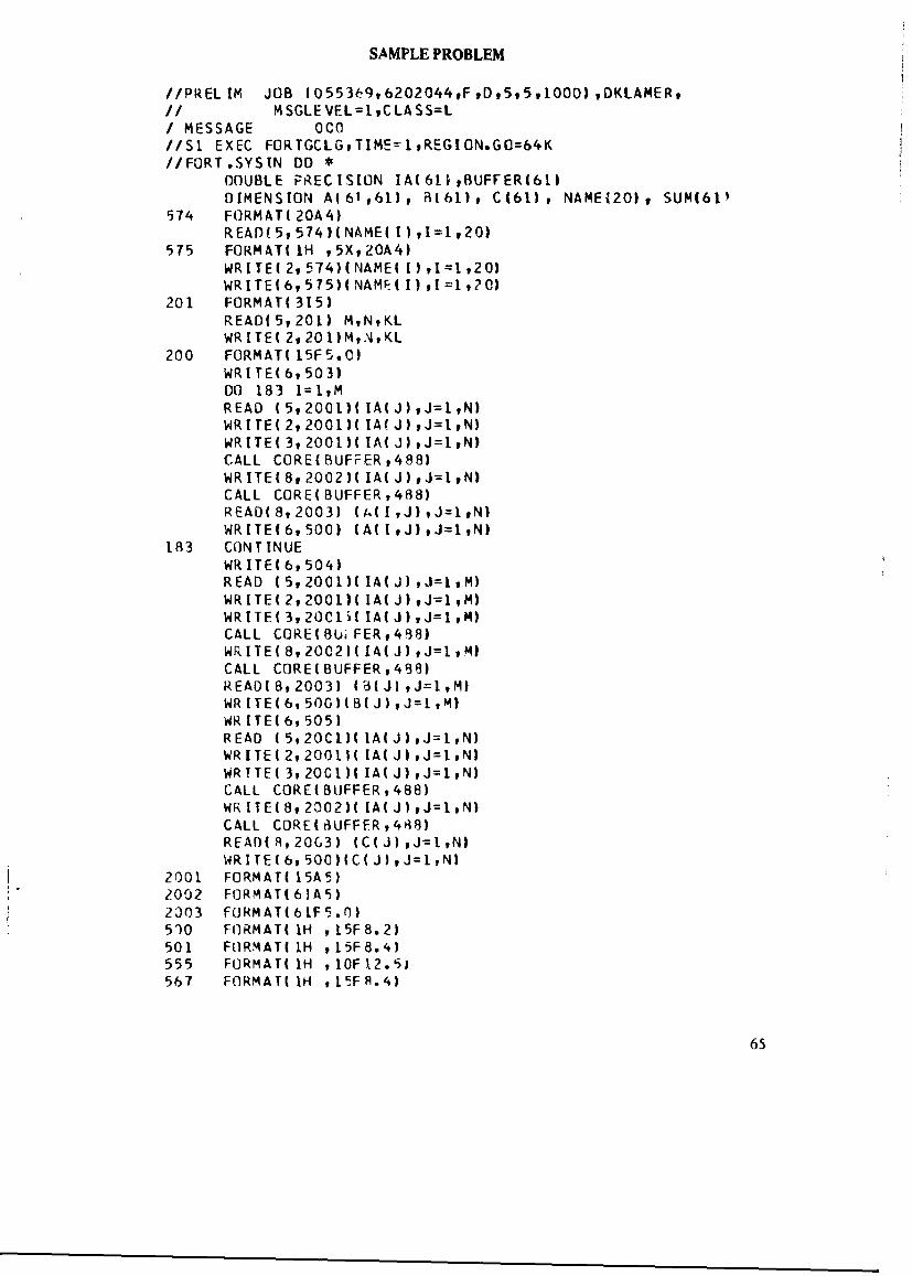
SAMPLE PROBLEM

//PRELIM JOB 10553,49,6202044,FD,5i,5,10O0),DKLAMERvII MSGLEVEL=lCLASS=L

/MESSAGE 000I/SI EXEC FORTGCLG, TIME= 1,REGI ON.GO=64KI/FORT .SYSIN DO*

DOUBLE PR~ECISION IA(6IhvBUFFER(61)DIMENSION A16)161), 8(6111 C(61) , NAMEM2)t SUM(W1

574 FORMAT(20A't)READI 5,574 )( NAMFI I) ,=1, 20)

575 FORMAT( IH , 5X,20A4)WRITEI 2,574)1 NAME( I)i,1=1920)WR ITE 6,9575H1 NAME ( 1) 91 =1, 10)

201 FORMAT(315)READ(5,201) MvNKLWRITE( 29201)M,,NUKL

200 FORMAT 1SF 5.0)WRITEI 6,503)DO 183 1=1,MREAD (5t200l)IIA(J),J=lrN)WR [TEl 2,2001)1 IA J) ,J=1,N)WRITEI 3,2001)H AI J) ,J=1,N)CALL CORE(EBUFFER,4881WRITE(8t2002)( IA(J)#J=1,N)CALL CORE( BUFFER t488)

WRITEI 6,500) (A( ,J) ,J=I,N)183 CONTINUE

WR ITEI 6, 504)READ ( 5, 200 1)HIA( J) ,J= , M)WRITEI 2,2001)1 IAIJ) ,J=1,M)WRITE(3,2OCl(IAIJ)vJ=1,M)CALL CORE( B~i FERt,488)WR[TEI 8,2002)1 141J),J=1,,M)CALL CORE( BUFFER,4838)READI8,2003) (3(J)pJ=1,M)WR [TEl 6,500)181 J) ,J~1,M)WR ITEI 6,505)READ l5v20Cl)11A(J)tJ=1,N)WR ITE 12, 2001)1 [AlJ) , J~1,N)WR!TE 3, 2001)1 IAIJ) ,J=1,N)CALL CORE(BLJFFER,488)WR [TEl 8,2002 )l Al J) ,J=1pN)CALL CORE( 8UFFER,4838)READI.9,2063) (C(J),J=l,N)WRITE 169500)1C(J), J=1 ,N)

2001 FORMAT( 15A5;)2002 FORMATI6)A5)2303 FORMATI61F5.0)510 FORMAT( IH , 15F8.2)501 FORMAT( 1H 15hF8.4)555 FURMAT(I H ,10F12.51

567 FORMAT( IH , 15FR.4)

65

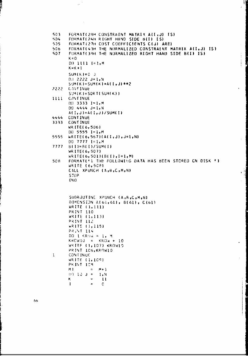
503 FORMAT(2,H CONSTRAINT MATRIX A(IIJ) IS)504 F(RMAT(24H RIGHT HANO SIDE d(l) IS)505 FORMAT(27H COST COEFFICIENTS C(J) ARE)506 FORMAT(43H THE NORMALIZED CONSTRAINT MATRIX A(IJ) IS)507 FORMAT(3qH THE N'RMALIZED RIGHT HAND SIDE B(I) IS)

K=ODO 1111 I=I.,MK=K+1

SUM(IKI= JOI 2222 J=ltNSUM(K )=SUM(K +A( I J)**2

2222 C h)1', T" IN UES ,'M ( K )= SQR T ( SU,1i( K))

1111 CtNTINUEDO 3333 I=IM00 4444 J=1,NA(I,J)=A(IJ)iSUM(1)

4444 CONTINUE

3333 CONTINUEWR ITE( 6,506)DO 5555 I=1,M

5555 WRITE(6,567)(A(I,J),J=1,N)DO 7777 I=1,M

7777 B( I )=B( I )SUM( I)WRITE( 6,507)WR ITE( 6, 50O1 HB(I ),tI=lM)

508 FORMAT(' 1 TH[- FOLLOWII'G DATA HAS BEEN STCRED CN DISK )WRITE (6,5Ce)CALL XPUNCH (A#BCMN)STOPEND

SUBROUTINE XPUNCH (A,BtCtM,N)DIMENSIJN A b,61), 8(61), C(61)WRITE (1,111)PRINT 110wRITE (1,113)PRINT 11 1-1

00 1 KRI.),i = 1, 14

I CONTINUFWRITE ( I,1Cc)PRIk 4T 113Ml = M+II')l 1) J = 1,NK - III = C

66

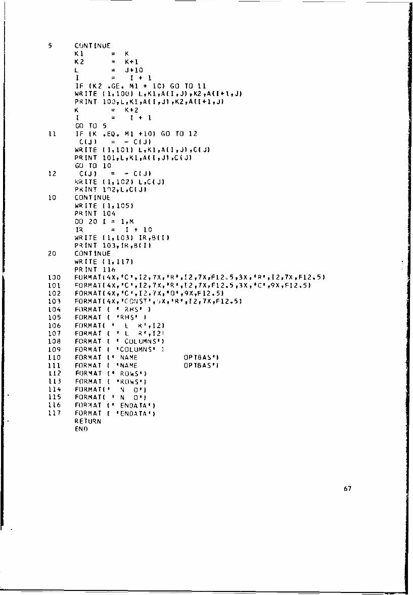
5 CONTINUEKL = KK2 : K+lL = J+1OI I + 1IF (K2 .GE. Ml + IC) GO TO 1IWRITE (,1100) L,K1,A(I,J),K2,A(I+I,J)PRINT 103,L,KlA(IJ),K2tA(I+÷,J)K = K+2I = I +1GO TO 5

11 IF (K .EQ. Ml +10) GO TO 12C(J = - C(J)

WRITE (1,101) L,KI,A(IJ),C(J)PRINT 101,L,KltA(ItJ),C(J)GO TO 10

12 C(J ) - C( J)uJRITE (,1 02) L,C(JJPRINT 1f.29L,C(J)

10 CONTINUEWRITE (1,105)PRINT 104DO 20 1 = 1,MIR = I + 10WRITE (1,103) IRB(1)PRINT 103,IRB(I)

20 CONTINUEWRITE (1,117)PR INT 116

100 FURMAT(4X,'C ',12,7X,'R',12,7X,F12,.5,3XR' ,2,T7X,F12.5)101 FORMAT( 4X, 'C', 12,7X, 'R ,!2,7XF12.5,3X,sCe ,9X,F12.5)102 FORMAT( 4X, 'C', 12, fX, .0' ,9X,F 12.5)103 FORMAT(4X, CONST', ,X,'R,12,7X,F12.5)104 FORMAT ( RHS'105 FORMAT ( 1RHS'106 FORMAT( L R',12)107 FORMAT ( L _ R1,I21108 FORMAT ( ' COLUMNSI)109 FORMAT ( 'COLUMNS' 1110 FORMAT (I NAME OPTBAS')ill FORMAT ( 'NAME OPTBAS')112 FORMAT (' ROWS')113 FORMAT ( 'ROWS')114 FORMAT( ' N 0')115 FORMAT( ' N 01)116 FORM4AT (I ENDATA')117 FORMAT f 'ENDATA')

RETURNEND

67

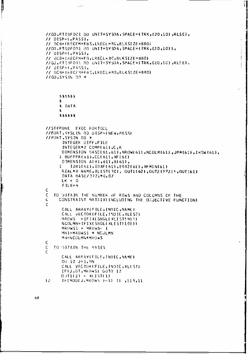
//GO.FTOIFOCI DD) UNIT=SYSO)ASPACE=(TRK,(20,1O),RLSE),// ISP=(tPASS),1/ C$=(RECFM=Fi3S,LkEcL-=8CgB':(SIZE=88O;

I/GO JTO2FGOI 00 UNIT=SVSD~tSPACE=(TRKj(2OlO))lIIDISP=(,PASS)t1/ C3=(RE'CFM=FBLRECL=8C,#3LKSIZE=88O)

//GJ.FTC3F(Yll DDB uNITz-SYSt)A, SPACE=(TRK,I2O410) RLSE)~IL)SP=(,PA';S),// [)C=(kECF,4Fti,LRECL=)30,fPLKSIZE=8'3O)

//CO.SYSIN 01f)*

t DATA

//STEPONE EXEC FO'RTCLL//FORT.SYSLIN DD DISP7-(NEWviPAS.S)f/F9RT.SYSIN Dl( *

INTEGER OIFF,FILEINTEGER*2 COMP( 611 ,CRDIMENSION ý3ASEr(61761),NROW(61),NCOLM(61),JPM(61),II.,fW(61),1 BUFFFR(bl),CC(61) ,XF(61)DIMENSION A(61,61),3(61),I IDX1(61I),ID)XF(61) ,1flX2(6fl ,XFMIN(61.)REAL*8 NAMEXLIST(3O), OUTl(62),OUrZ(3?A2].,0uT!613DATA BASE/372i*0.O/I 1K =0F ILE=4

CC TO JW3TA IN THE NUMBER OIF ROWS AND COLUMNS CF THEL C"ONSTRAINT M4AT.RIX(INCLUDING THE O3JECTIVE FUNCTION)C

CALL ARRAY F ILE, INDIC ,NAME)CALL vECTOR( FILE, INDIC tXLI S.)MROWS =IFIX(SNGL(X!LI5T!9)))NCOLMN-IFIX(S.NGL(XLIST(1O))MI1lWSl = MRotiS- 1MN1=MR()WS1 * NCOLMNMNl=NCOLMN*M'<OWS

CC To C!t3TAIN THE ýISISC

CALL ARRAY(FILE, !NDIC,N44E)00l 10 J=1,MNCALL VECTOR( FILE, INDIC,XLIST)IF(J.GT.MlkU'vS) GOTO 12O'JTl(J) = XLISTM1

12 IF(MOD(J.MROWS )-l) 11 ,115,11

68

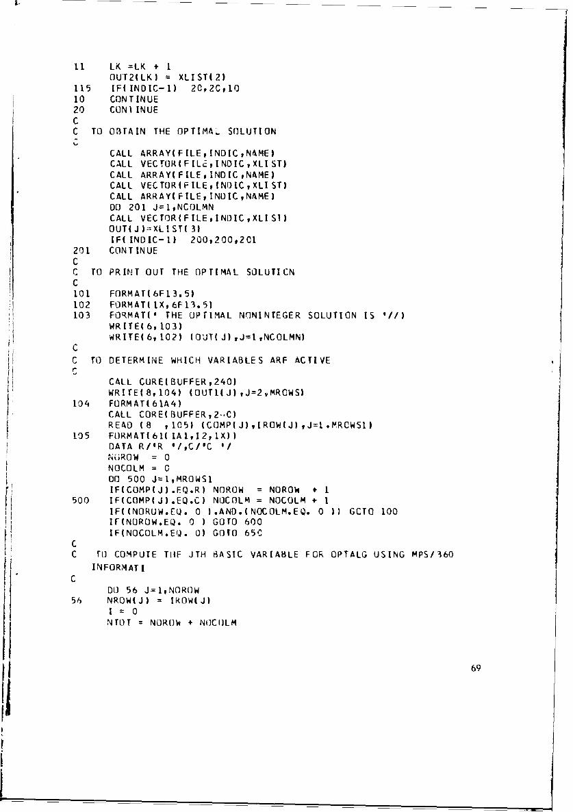
L1 LK =LK + IOUT2(LK) = XLIST(2)

115 IF(INDIC-1) 20,2Ctl10 CONTINUE20 CONI INUECC TO OBTAIN THE OPTIMAL SOLUTIONZ;

CALL ARRAY(FILEINDICNAME)CALL VECTOR(FILE,:INDICXLIST)CALL ARRAY(FILE,INDIC,NAME)CALL VECTOR(FILE,INDIC,XLIST)CALL ARRAY( FILE, INDICNAME)DO 201 J=1,NCOLMNCALL VECTOR(FILEINOICXLISI)OUT(J);XLIST( 3)IF(INDIC-1) 200,200t201

201 CONTINUECC TO PRINT OUT THE OPTIMAL SOLUTICNC101 FORMATW6F13.5)1.02 FORMAT(lX,6F13.5)103 FORMAT(' THE OPFIMAL NONINTEGER SOLUTION IS 'li)

WRITE( 6, 103)WRITE( 6, 102) (OUT(J) hJ=INCOLMN)

C

C TO DETERMINE WHICH VARIABLES ARF ACTIVEr

CALL CORE(BUFFER,240)WRITE( 8,104) (OUTI(J) ,J=2 MRCWS)

104 FORMAT( 61A4)CALL CORE(BUFFER,2,,C)READ (8 ,105) (COMP(J)tIROW(J)tJ=1.MROWSI)

105 FORMAT( 61(1A,12,1X))DATA R/IR '/,C/IC I/N(iROW = 0NOCOLM = 0DO 500 J=1,MROWSIIF(COMP(J).EQ.R) NOROW = NOROW + 1

500 IF(COMP(J).EQ.C) NOCOLM = NOCOLM + IIF[(NORUW.EQ. 0 ).AND.(NOCOLM.EQ. 0 1) GCTO 100IF(NOROW.EQ. 0 ) GOTO 600IF(NOCOLM.EQ. 0) GOTO 650

CC TO) COMPUTE TIIF JTH BASIC VARIABLE FOR OPTALG USING MPS/360

INFORMAT I

CDO 56 J=1,NOROW

56 NROW(J) = IROW(J)I = 0NTOT = NOROW + NOCUILM

69

Ni m-NUROW + I00 57 J=N1,NTOT

I -I+ 157 NCOLMMI = IROW(J)

6010 150CC BASXS INVERSE IS BASI SC600 D0 601 J=I,NOCOLM601 JPM(J) = J

WR ITE 6, 10S)DO 602 I=1,MROWS1

602 WRITE(6pl01) (OUT2(1ItJ-1)*MwROWS1)9,,I=lNCOLPN)!-IRITE(291011 ((UtJT2(I+(J-1J*MROWSI)fJ=1,NCOLPIN),I=1,MRCWS1)

CC IF YOU WANT THE BASIS INVERSE PINCHED OUTC (THERE ARE THREE (3) CARDS FOR THE BASIS INVERSE)C REMOVE THE 'C' FROM THE FOLLOWING CARD*C WRITE(7il0l) ((OUT2(14(J-1)*MROWSI),J=1,NCOLP'N),1I=MRCWSi)C

GUTO 202CC BASIS INVERSE IS IDENTITY MATRIXC650 DO 651 J=1,NOROW

JPM(J) = MROWSI + J651 BASE(J,J) =1.0

WRITHt 6t loci)WRITE(6,101) ((BASE(14J),J=l.MROWS1),I=1,MROWS1)WRITE(2,101) ((BASE(I,J),J=1,MROWS1),=I=,MROWS1)

CC IF YOU WANT THE BASIS INVERSE PUNCHED OUTC (THERE ARE THREE (3) CARDS FOR THE BASIS INVERSE)C REMOVE THE IC' FROM THE FOLLOWING CARD.C WRITE(7,101) ((BASE(IJ),J=1,MROWS1),I=1,MROWS11C

GOTO 202

150 CONTINUEL= 1KL= INORMI1 = NOROW - 1IF(NROW(l)-11) 100,3092-'

30 JPM( 1) = NROW( 1) + NCOLMN -10

L =1+lGOTO 47

22 01FF = NROW( I) - 11D0 46 K=1,DIFFJPM(L) = NCOLM(KL) - 10KL =KL41

L =L41

46 CONTINUEJPM(L ) = NROW(I1) + NCOLMN -10

L= L +147 CONTINUE

70 DO 50 I=1,NORMl

01FF = NROW( 141) - (NROW( 1)+1)IF (DIFF) 10093594C

35 JPM(L f = NROW( 1+l 1) NCOLMN - 10L = L+1GOTO 50

40 D0 45 KzlD[FFJPM(I) = NCOLM(KL) - L0KL =KL+l

L = +145 CONTINUE

JPM(L I = NROW( 1+1) + NCOIMN - 10L = 1+1

50 CONTINUED1FF = 10 + NTOT - NROW(NOROWq)IF(OIFF) 100t5516C

5,5 JPM(NTOT) t!NROW(NOROW) + NCOLMN -10

GOTO 6560 00 65 K=l,DIFF

JPM(L) = NCOLM(KL) - 10KL =KL+l

L = +165 CONTINUECC TO OBiTAIN THE BASIS INVERSE

J1=

J2 =ID0 300 JK=1,NTfl(IF(JPM(JK).GjT.,NCOLMN) BASE(J2,JK) =1.0

IF(JPM(JK).LE.NCOLMN) GOTO 310J2 = J2 + 1GOTO 300

310 DO 311 J=1,MROWS1 UPTJ!= j! ;- 1

311 BA$,-E(JJK.) = OUT2(J1)j300 CONTINUE

WRITE( 6,101) ( (BASE I ,J) ,J=l ,MROWS1) ,I=lMROWSI)WRITE(2,101) ((BASE(I,J),J=lMROWSI),I=1,MROWS1)

CC IF YOU WANT THE BASIS INVERSE PUNCHED OUTC (THERE ARE THREE (3't CARDS FOR THE BASIS INVERSE)C REMOVE THE 1C.' FROM THE FOLLCWING CARD.C WRITEC 7,101) ( (BASE( I ,J) J=1 ,MROWSl) ,1=l ,MROWSl)C20Ž CONTINUE

WRITEt6, 107)WRITE(6,108) (JPM(JK)t JK=1,NTOT)WRITE(2,108) (JPM(JK)t JK=1,NTOT)

C

7'

C IF YOU WANT THE ORDER OF THE ITH BASIC VARIABLE, JPPI(I),

FUNCHED OUTL REMUVE THE 'C' FROM THE FOLLOWING CARD.C WRITE(7,108) (JPM(JK), JK=1,NTOT)C

WRITE(2,101) (UUT(J),J=1,NCOLMN)CC IF YOU WANT THE OPTIMt, ".Ni NTEGER SOLUTICN PUNCHED CUTC REMOVE THE 'C' FROM THE FOLLCWING CARD.C WRITE(7,101) (OUT(J',J=1,NCOLMN)CCC IF YOU WANT TO SUPPLY YOUR OWN FEASIBLE INTEGER SOLUTIONC REMOVE THE IC' FROM THE FOLLOWING CARD.C COTO 151CCC TO OBTAIN THE STARTING INTEGER SOLUTION TG THE ILPC

DO 110 I=1,MROWS1READ( 3,111) (A(I,JlJ=1,NCOLMN)

110 CONTINUEREAD( 3,111) ({(I),I=1,MROkSl)READ(3,111)(CC(J),J=lNCOLMN)

ill FORMAT( 15F5.C)DO 1000 [=1,NCOLMNXF(I) = SNGL(OUT(I)iIF(CC( J)) 1001, I000,1000

1001 IF (XFIL).EQ AINT(XF(I))) GOTO 1000XF(I) = XF(I) + 1.

1000 CONTINUEDO 1020 I=1,NCULMN

1 '20 XF( l) = AINT{XF{I))

ITEST 0 0CC SET THE MAXIMUM NUMBER OF ITERATIONS.C1021 IF(10 -ITEST) lCO,[C22,10221022 ITEST = ITEST + 1CC CHECK TO SEE IF THE POINT IS FEASIBLE.C

DO 1030 I=1,MROWS-SUM = 0.0DO 1025 J=1,NCULMNSUM = SUM + A(1,J) * XF(J)

1025 CONTINUEIF(B(I)-SUM) 1026,1030,1030

1026 ITER = ICC IF POINT IS NOT FEASIBLE, WRITE THE CONSTRAINT VICLATED ANDC THE POINT THAT VIOLATEQ THE CONSTRAINT.

72

CWRITE( 6,1027) 1,B( I), SUM,( XF (I J) ,I J=I NCCLMN)

1027 FORMAT( fOX,lOH B(12,21H) SUM1 15X, 2F12.2 il 14H THE POINT IS /4(15F8.2/)///1/')

GOTO 10351030 CONTINUE

GOTO 11201035 L = 0

Ni = 0CC FIND ALL OF THE NONZERO VALUES OF THE VARIABLES.C IDXI STURES ALL OF THE ZERO VALUED VARIABLES.C IDXF STORES ALL OF THE NON7-RO VALUED VARIABLES.C

DO 1040 J=1,NCOLMNIF( XF(J) ) 1036,1037,1038

1036 XF(J) = 0.01037 L = 1+1

IDXI(L) = JGOTO 1040

1038 NI = NI + 1XFMIN(NI = XF(J)

IDXF(NI) = J1.040 CONTINUE

IF(Lý,LT.I) GOTO 1042CC TACK ON TO THE END OF THE INDES OF THE NONZERO VARIABLES THEC INDEX OF THE ZERO VARIABLES.C

DO 1041 I=1,L1041 IDXF(NI+I) = IDXI(I)CC IF THERE IS AT LEAST ONE NONZERC VARIBALE,C THEN ARRANGE THE NONZERO VARIABLFS FROMC MINIMUM TO MAXIMUM VALUE.C IDX2 IS TilE INDEX OF THE REARRANGED VARIAt3LES.C1042 IF(NI.GT.0) GOTO 1045

DO 1044 I=I,L1044 XFMIN( I )=0.0

GOTO 10461045 CALL SORTI(XFMIN,IDX2,l,NI)1046 IF(NI.EQ.NCOLMN)GOTO 1048

NlPl = NI + IDO 1047 I=NIP1tNCOLMN

1047 I1X2(I) = IDXF(I)CC ROUNDING PROCEDURE.C TAKE THE SMALLEST NONZERO VARIABLE,C IF THE CORRESPONDING CONSTRAINT COEFFICIENTS ISC POSITIVE -- ROUND DOWNC NEGATIVE -- ROUND UP.C

73

1048 DO 1060 KL=ltNCO' MNIV = IDXF( IDX2(KL,)LCK = 0

104Q IF( A(ITERtIV) 1050,1060,10511050 XF( IV) = XF( IV) + 1.0

GOTO 10551051 XF(IV) = XF(IV) - 1.0

IF(XF(IV),LT.O.O) XF(IV) = 0.0

1055 SUM = 0.0DO 1.056 I=1,N(.OLMNSUM = SUM + A(ITER,1) * XF(I)

1056 CONTINUECCC IF THIS DOES NOT STAISFY THE CONSTRAINT,C THEN TAKE THE NEXT SMALLEST VARIABLEC AND REPEAT THE PROCEDURE.CC IF THE CONSTRAINT IS SATISFIED, THEN USE THIS PCINT TOC CHECK ALL OF THE OTHER CONSTRAINTS.CC

IF( B( ITER) - SUM) 1057,1021,10211057 LCK = LCK + 1CC SET THE MAXIMUM NUMBER OF CHANGES FOR ONE VARIABLE FCR ONE

ITERAT ION.C CHANGE THIS IF THERE IS AN OSCILATION BACK AKD FORTH eETWEENC TWO POINTS.C

IF(LCK.LT.1) GOTO 1C4ý-1060 CONTINUE

GOTO 10211100 CONTINUE

WRITEt 6, 1105) ITEST1105 FORMAT(47H NO FEASIBLE STARTING INTEGER SOLUTION HAS BEEN

I 26H FOUND AT THIS POINT AFTER 15,6H TRYS.)GOTO 1150

1120 CONTINUEOBJ = 0.0DO 1122 I=INCOLMN

1122 OBJ = OBJ + XF(I)*CC(l)WRITE{6, 1!251 (XF( I),I=lNCOLMN)

1125 FORMAT(53H A FEASIBLE STARTING INTEGER SOLUTION HAS BEENFOUND. /14(15F8.1/I))

WRITE(6,1126) OBJ1126 FORMAT( 40H THE VALUE OF THE OBJECTIVE FUKCTION IS

/ F12.4 I

WRITE(2,101) (XF(J3,J=1,NCOLMN)CC IF YOU WANT THE OPTIMAL OFEASIBLE' INTEGER SOLUTION PUNC14ED OUT

74

C REMOVE THE 'Cl FROM THF FOLLCWING CARD,C WR I TE(791011 (XF (JA),J=l tNCOLMN)C

GOTO 151100 WRITE(6,106)106 FORMAT(I AN CRROR HAS OCCURED11107 FORMAT(' JPM(I) IN THE ORDER THEY SHOULD OCCCUR AND IS THE

INDEX Of 1 THE ITH BASIC VARIABLE')108 FORMAT(151'i)109 FORMAT(////' THE BASIS PI'VERSE IS 'I1150 CONTINUE

I1 10WRITEIIO,.1151) I

1151 FORMAT(15)151 CONTINUE

WRITE( 10tI 151) I200 RETURN

END

SUBROUTINE SORTI(AIO),II,JJ)DIMENSION A(1)91U(301,IL(30),ID(1)INTEGER Tl,T2M= 1

J=JJDO 1 IS=IJ

1 IDCIS)=IS5 IF( I .GE. J) GOTO 7010 K=I

IJ=(J+I)/2'=A( IJ)T1= [Di IJ)I F(A(1) .LE. T) GOTO 20

AIDIJ)=D( I)

A I )= I101 1)=TIT=AC IJ)

20 L=JIF(A(J) .GE. T) GOTO 40Al IJ )=A( J)[DtIJIJ=ID(J)A(J) =TID(J )= T1T=AI IJ)TI- 101IJ II F( A(I) .LE. TI) GOTO 40Al IJ )=A( I)

A ! )=T

75

T=A( IJ)Tl= ID( IJ)GOTO 40O

30 A(L )=A(K )10(1 )= 10(K)AIK )=TT101K )=T?

40 L=L-1IF( AKL) sGi. T1 GL)TO 40TT=A( L)T 2= [01L)

50 K=K+l[FE A(K) .LTs T) GUTO 5CIF(K .LE. L) GUTO 30IF(L-1 ALE. J-K) GOTO 60IL~i A II U M )LI=KM=M+1GOTO 80

60 1L(M)=KTUIM )=iJ=LM=M4 1GOTO 80

70 M=M-1!F(M .EQ. 0) RETURN

1=IL(M)J= IUEM)

80 [F(J-1 .G-E. 111 M)OTO 10IF II .EQ. I11) GrJTO 5

90 1=1+1IF( I .EQ. J . GOTO 70T=AE 1+1)Tl IDE 1+11IF(A(1) . LE. T) GOTO 90K= 1101K )= ID( I)

100 AEK+1h=A(K)ID(K+lh )=0(K)K=K- 1IF(T LT1. AMK) GOTO 100A(K+1)=T101K +1 )=TiGUTO 90END

//LKED.SYSLIiB DD DSN=LLOAD,OISP=(SHRKEEP)II DO DSN=SYSI..FORTLIRDI SP=SHR

//LKEO.SYSLMOD DO DSN=EMCCAIDI SP=(NEW,PASS) rUNIT=SYSDA,

'76

1/ SPACE=(CYL,(1,1,1O)),PDCB=(DSORG=POtRECFM=USLKSIZE=36251//LKEO.SY.;IN 00 *

INSE2, READCOHMENTRY MAINNAME DATAHILL(R)

//CPC EXEC PGM=COMPILER//STEPLIB DO DISP=(SHRtKEEP~jDSNAME=LLCAO)//SCRATCHI DO UNTSS~DS=NWDLTISAErT~il)//SCRArcH2 DD UNIT=SYSDA"t,DISP=(NEWDELETE)tSPACE..(TRK I~ll))//SCRATCHi3 DO tJNIT=SYSDAPDISP=(NEWDELETE),SPACE=(rRK(Il,l)//SCRATCH4 DD UNIT=SYSDADISP=(NEWDFLFTE),SPACE=(TRK,(,L li//SYSMLCP DD LINIT=SYSDASPACE=(TRK,.(2,1)),DISP=(NEW PASS)//SYSPRINT 01) SYSOUT=A//SYSPUNCH OD SYSOUT 6//SYSIN DD *

PROGRAM ('IND')IN ITIALZMOVE( XOATA, IOPTt3ASI)MOVE( XPBNAME, 'MYFiLE.)MOVE(X)OBJ, '0')MOVE( XRHSv 'CONST')ASSIGN !'COMMFMTI I FT0 4 F0Ol I CofrMl)PREPOUT( 'COMMFMT4CONVERT( 'SUMMARY')BC DOUTSETUP( IPR IMALSOLUT IONrRANCOL ( 'ENTIRE ,I NVERSE 11TRANCOL( *ENTIRE'I)TRANCOL ('FIl-EI,'CO1MFMTIIIENTIREV)SOL UT ION ('F ILE', 'COMkMF MTI'DATAH ILLE XI TPEND

//EXEC E XEC PGM=E XECUTOR CIJND=(C0,NEtCPC) REG[I0N=22 KIT I P'Eý3/ST EPL IB DO DOISP= (SHRpKE EP) jO0SNA ME =LL CAO

1 003 DSN=&MCCALD1SP=(0LDPASSjUNIr=sYSOAI/SCRATCHI DD UNIT=SYSD)ADIS,'=(NFWDELETE),,SPACE=(CYL,(l,1))//StCRATCH2 DO LIN IT=SYSOA,0DUP=(NEWDELETE) tSPACE=(CYL,11.L))f!?ROBFILF ~JO UNIT=SYSDASPACE1(CYL,Cl1iJ),0tISP=1NEWtDELETE)//FTAI OD UNIT=SYSDA,S'OACE=(CYI.,(t,1)) ,O'SP=(NEW,DELETE)//MATRIX ODO UNi&T=SYSDA,SPACE=(CNLf,,1,)),D)ISP=(NEW,OELETE)

77

/SY SMLCP DO UN IT= SY StA)ASNAME=*.C PC -SY SMLC P #D I SP=(OLDODELET F)//YSPRINT Or) SYSOUT=A'/[XEC.FT02F0CI DD0 fSN** SI*GU.F T02F001 #DI SP=( 000i ASS)//EXEC.FT03FOO1 O)0 DSN=*.SL.GtJ.FTO3FQO1,O[SP=(CLDtDELETE)//EX[C.FTfl6FOOI Dn SYSOUT=A//,EXFC.FTO7FOOl 01) SYSOUT=B//EXEC.FTO4FOO1 DO) UNII=SYSD",SPACE=(CYLv(l1,J/ISYSPUNCH DD SYSCJUT=B//EXEC.FT1OFOO1 Dr, UNIT=SYSD)ASPACE=(TRK,(1,1),RLSE)p

I! ISP=(#PASS),//DCI3=(RFCFM=FBStLRECL=80,,BLKSlZE=880)

//SVSIN DO DSN=*.S1.GO.FTO1FO01,D[SP=(OL0,DELETE)//CHKF EXEC FL)RTGCrLGREGION.GO=42KTIME=I.//FURT,,SYSLIN On) DISP=(NEWPPASS1//IFRT.SYSIN DD

REAN(10, bC) I130 F(JRMAT( 15)

IF( I) 20#20,0010 STOP 1020 CONTINUE

STOPEND

/IG(J.FT1OFOOl DO. DSN=*.EXEC.FTLOFOOIDISP=(OLD,DELETE)

//TWO EXEC PGM=OPTALG,COND=(2,LTCHKF.GO),REGIaN=(,336K),T1t'E=2//STEPLIR DO DSN=tIOAO,DISP=SHR//FTC6FOOl DD SYSOUT=A//FTO5FOOJ DO) r)SN=*.SI.GO.FTO2FOO1,DISP=(OLDDELETE)

//SFAIL EXEC [ORTGCLG,COND.FORT=(0,EQCHKF.GOtJ)/1CONO.LKED=U0O,FQ,CHKF.G'O),14,LT,FORTi))

I!CONO.GO=((O,EQ,CHKF.GObt4,tLT,FCRT)d(4,LT,LKEO))I/1REGION.GO=42KTtME~I

/IFORT.SYSIN 00)REAL X( 80)I5 READ(5,i0,END=100) X

10 FORMAT( 80A I)WRITE7,l0) XGOTO 5

t/ooF0F~ P U DSN=*.Sl.GO.FTO2FOO1,ilI)P=(0LODELETE)

78

NELC ZANGWL

CATALOG IDENTIFICATION:

E4 NELC ZANGWL

PROGRAMMERS:

D. C. McCALL, Decision and Control Technology Division, andC. M. BECKER, Applications Software Division

PURPOSE:

To compute the minimum of a function f(x 1 .... , xn), of n real variables

RESTRICTIONS AND LIMITATIONS:

A maximum of 20 variables can be handled.

LANGUAGE:

FORTRAN IV

COMPUTER CONFIGURATION:

IBM 360/65Core storage: 19086 bytes

ENTRY POINTS:

ZANGWL

SUBPROGRAMS AND WHERE REFERENCED:User-supplied programs

FUNC called by ZANGWL, (POWELL)Programmer-supplied programsZGITER cailed by ZANGWLPOWELL called by ZANGWL

USAGE:

CALL ZANGWL (XI, N, EACCUR, QSTEP, ISTOP, LPRINT, !X,I.PUNCH, XOPT, FF)

For a description of parameters see the listing.

INPUT FORMAT:

All input is through the parameter list except when user-supplied s._:cldirections are desired. Then ZANGWL expects N vectors of length N input oncards in 4(FI 5.!0, 5X) Format, where N = n is the number of variables.

OUTPUT:

The output depends on tile print and punch option. See tile listing.

ERROR MESSAGES:

None

79)

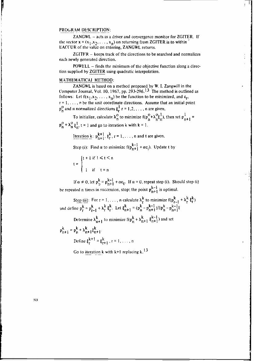
PROGRAM DESCRIPTION:

ZANGWL - acts as a driver and convergence monitor for ZGITER. Ifthe vector x = (x0 ,x2, , . , x.) on returning from ZGITER is to withinEACCUR of the value on entering, ZANGWL returns.

ZGITFR - keeps track of the directions to be searched and normalizeseach newly generated direction.

POWELL - finds the minimum of the objective function along a direc-tion supplied by ZGITER using quadratic interpolation.

MATHEMATICAl METHOD:ZANGWL is based on a method proposed by W. I. Zangwill in the

Computer Journal, Vol. 10, 1967, pp. 293-296.13 The method is outlined asfollows: Let f(x!,x 2 . xn) be the function to be minimized, and Cr,r = 1, . . . , ii be the unit coordinate directions. Assume that an initial point

o and n normalized directions t r = 1,2, .. , n are given.Pn r'

To initialize, calculate X' to minimize f(pn+Xn), then set pnn n n et+ 1P+n n x2 , t = l and go to iteration k with k = 1.

k+l kIteration k: n r = 1 ... n and t are given.

Step (i): Find a to minimize f(Pn+l + aci)" Update t by

t= It if I <-t<n

i it" t = k

If a * 0, let p=p k-nI + act. If a •0, repeat step (i). Should step (i)k-Ibe repeated n times in succession, stop; the point Pn+1 is optimal.

Step (ii): For r = 1, . .. , n calculate Xk to minimize f(p + )k k)k k k k k k pk-I )/kk-land define Pr = +Pr- r Let _n+ -n-

Determine Xk to minimize f n+ ) n+ l ) and setn+l n XniI ~n+lan s

k k+ k kPn+= Pn +n+ In+l

Define rk+l = k . ..r r+ir n

Go to iteration k with k+1 replacing k.0 3

so

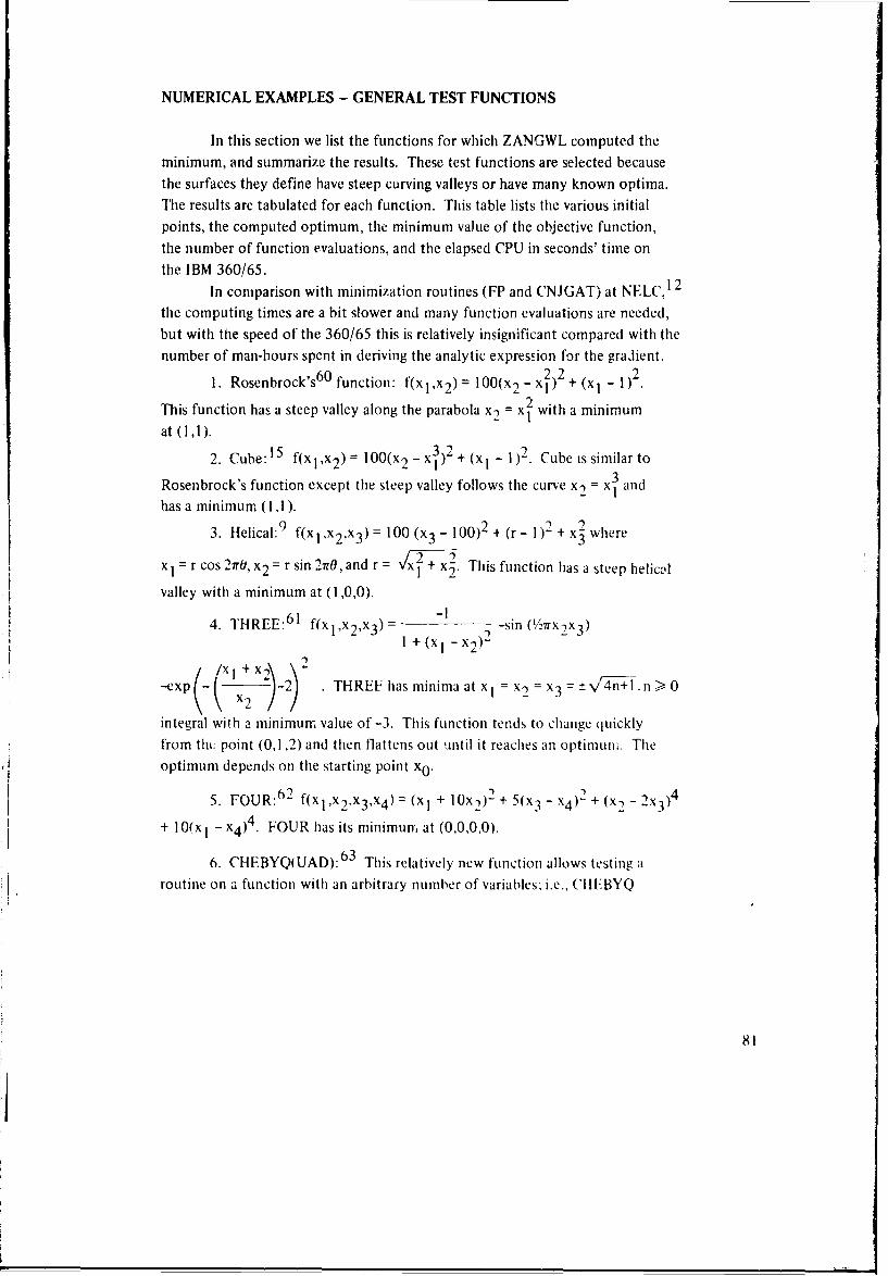
NUMERICAL EXAMPLES - GENERAL TEST FUNCTIONS

In this section we list the functions for which ZANGWL computed theminimum, and summarize the results. These test functions are selected becausethe surfaces they define have steep curving valleys or have many known optima.The results are tabulated for each function. This table lists the various initialpoints, the computed optimum, the minimum value of the objective function,the number of function evaluations, and the elapsed CPU in seconds' time onthe IBM 360/65.

In comparison with minimization routines (FP and CNJGAT) at NELC, 12

the computing times are a bit slower and many function evaluations are needed,but with the speed of the 360/65 this is relatively insignificant compared with thenumber of man-hours spent in deriving the analytic expression for the gradient.

60 2 2 21. Rosenbrock's 6 0 function: f(x 1 ,x2) = 100(x2 - xi) + (x1 - 1).

This function has a steep valley along the parabola x2 = x2 with a minimumat (1,1).

2. Cube: 15 f(x Ix 2 ) = 100(x 2 - x3)2 + (x I - 1 )2. Cube is similar to

Rosenbrock's function except the steep valley follows the curve x2 = x3 andhas a minimum (1,1 ).

3. Helical: 9 f(xl ,x2 ,x3 ) = 100 (x3 - 100)2 + (r- 1)2 + x3 where

= r cos 27W, x2 = r sin 2frO, and r = x1 + x2. This function has a steep helical

valley with a minimum at (1,0,0).

4. THREE: 6 1 f(xl,x 2,x3) = -sin ('/2rx 2x3 )1 + (x - x2 )2

--exp - 2) THREF has minima at xl = x1 = x3 =\4n+ ln Ž0

integral with a minimum value of -3. This function tends to change quicklyfrom tht, point (0,1,2) and then flattens out until it reaches an optimnum. Theoptimum depends on the starting point x0 .

5. FOUR: 6 2 f(xi,x 2 ,x3 ,x4 ) = (xI + 1Ox2)2 + 5(x3 - x4 )2 + (xi - 2x3)4

+ 10(x1 - x4 ) . FOUR has its minimun, at (0,0,0.0).

6. CHEBYQ(UAD): 6 3 This relatively new function allows testing a

routine on a function with an arbitrary number of variables- i.e., CHEBYQ

81

(xI .... xn), where n is a parameter preset by ti. user. For n - 1,2,. . . , 7,9

the minimum value of CHEBYQ is zero; however, for other n the minimizationis still valid.

Briefly, CHEBYQ does the following: Let x = (xI.... , xn) be a vector

(abscissae) whose coordinates are in the range 0 < xi < 1. Then, choosing the

shifted chebyshev polynomial Ti, we define:

- I d nSTi(z)dz - Ti(xj)

j=1n

Then the function f(x) = >. (Ai(x)) 2 has the property that if X is the vectori=l1

of abscissae, then f = 0; otherwise, f > 0. Although contrived, CHEBYQ is a

good example of a complicated objective function that can occur. TheFORTRAN IV listing of CHEBYQ follows.

X2

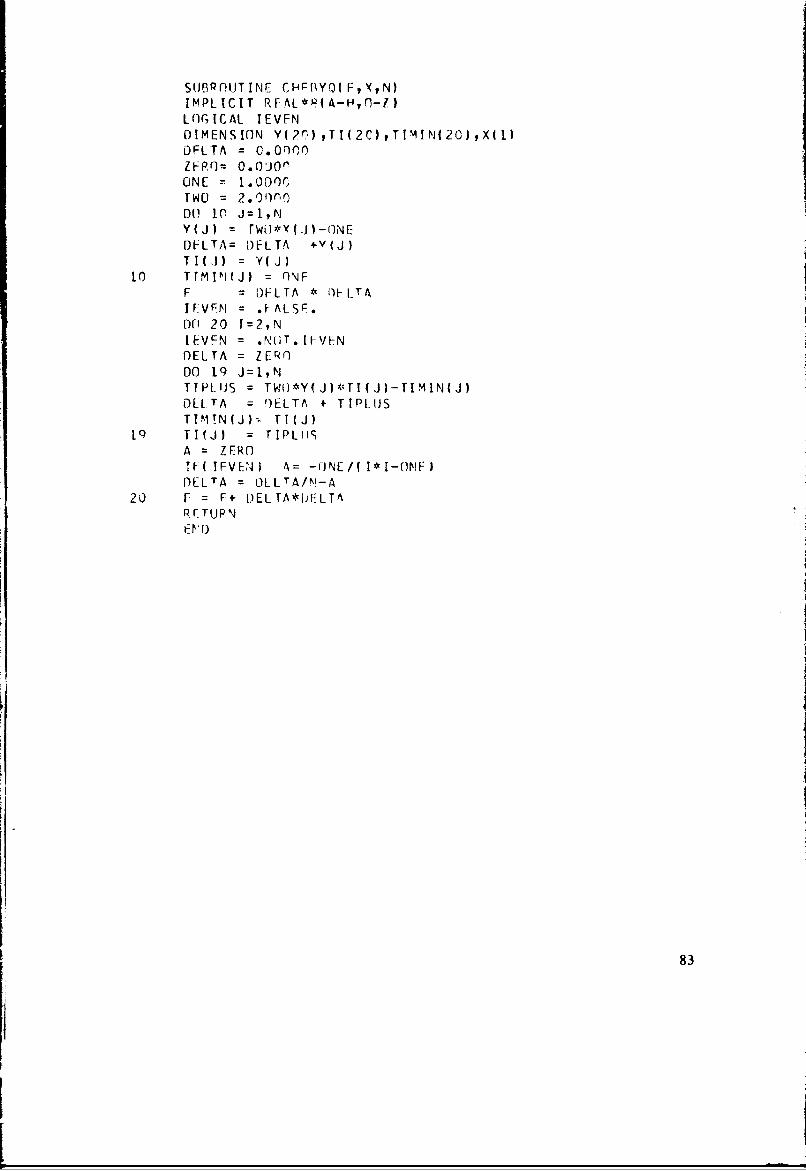
si.JBprIJT INC CHF-BY0( F ,X, N)IMPLICIT RFAL*P( A-H,fl-1)LOGICAL IEVFNDIMENSION Y(2r) ,TI(2C) ,TIMIN(20),X(l)DFLTA = O.ODlOOZFPO= 0.0or'ONE r1.ODOCTWO = 200Dli 10 J=1,N

DFLTA= IDFLTA +V(J)TIH A) = Y(J )

10 TTIMN(J) = liNFF DFLTA ý,f)F LTAIFVFNj .FALSF.DOi 20 1 = 2,N[FVFN = .NUT.*IF-VFNDELTA = ZERO1DO 19 J=l,NT!PLIJS = Ttih)Y( J )*TI( J )- I MIN( JD)ElTA = r)ELTA + TIPLOSTIM!N(Jh- TT(J)

Iq T I JI =TIPLIIS

A =ZERO

I F I FVEN A = -0JNE/ I I -OMFIDELTA O LLTA/N!-A

20 F = F+ L)ELTA*UF:LT'ApRErUP,.F rD

83

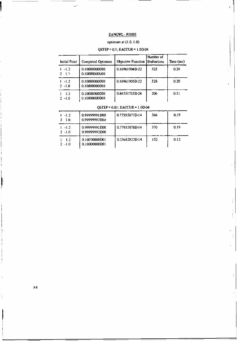
ZANGWL- ROSIE

optimum at (1.0, 1.0)

QSTEP = 0.1; EACCUR = 1.OD-04

Number ofInitial Point Computed Optimum Objective Function Evaluations Time (sec)

1 -1.2 0.100000DOI 0.16961904D-22 325 0.262 L', 0. 100000000DI

I -1.2 0.100000001DOI 0.16961905D-22 328 0.202 -1.0 0.10000000DOI

1 1.2 0.10000000DOI 0.84351733D124 206 0.112 -1.0 0.I1OOOOOOODOI

QSTEP 0.01; EACCUR = 1L.OD-04

1 -1.2 0.99999991 DO0 0.77935877D-14 366 0.192 1.0 0.99999992D00O

1 -1.2 0.99999991D00 0.77935878D-14 370 0.192 -1.0 0.99999992D00

1 1.2 0.10090000)1DO 0.23682822D-14 152 0.122 -1.0 0.10000000D01

84

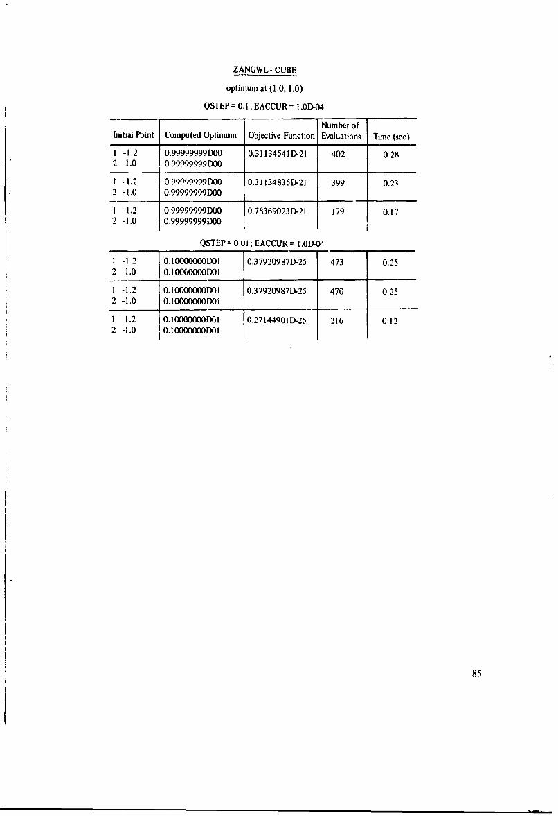
ZANGWL- CUBE

optimum at (1.0, 1.0)

QSTEP = 0.1; EACCUR = 1.OD-04

Number ofInitial Point Computed Optimum Objective Function Evaluations Time (sec)

1 -1.2 0.99999999D00 0.31134541ID-21 402 0.282 1.0 0.99999999D00

1 -1.2 0.99999999D00 0.31134835D-21 399 0.232 -1.0 0.99999999D00

1 1.2 0.99999999D00 0.78369023D-21 179 0.172 -1.0 0.99999999D00

QSTEP 0.01; EACCUR = 1L.OD-04

1 -1.2 0.IOOOOOOODOI 0.37920987D-25 473 0.252 1.0 0.100IOMD01

1 -1.2 0.10000000DO1 0.37920987D-25 470 0.252 -1.0 0.10000000D01

1 1.2 0.10000000DOi 0.27144901 D-25 216 0.122 -1.0 0.10000000DOI

85

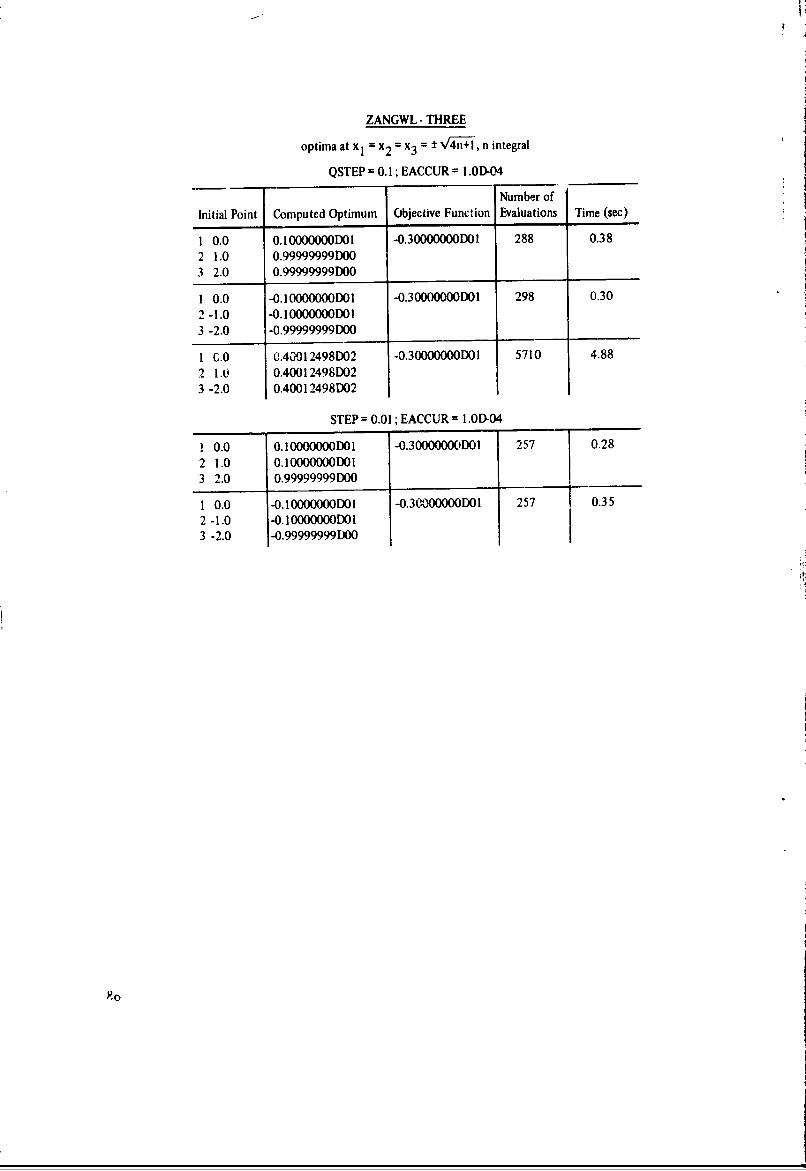
ZANGWL - THREE

optima at X, = =2 ` ±x ~i n integral

QSTEP = 0. 1; EACCUR = .OD-04

Number of

Initial Point Computed Optimum Objective Function Evaluations Time (sec)

1 0.0 0. 1OOOOOOODO I -0.30000000DOI 288 0.382 1.0 O.99999999D003 2.0 0.99999999D00_____ _____

1 0.0 -0.10000000D01 -0.30000000D01 298 0.302-1.0 -0. 10000000DO 13 -2.0 -0.99999999D00

1 C.0 0.40i012498D02 -0.30000000D01 5710 4.882 1.0 0.4001 2498D023 -2.0 0.40012498D02

STEP= 0.01; EACCUR = I.OD.04

1 0.0 0.IOOOOOOODO1 -0.3000000C1D01 257 J 0.282 1.0 0.10000000DOII3 2.0 0.99999999D0030001 5

1 0.0 -O.10000000DO1 3 ý )0 5 0.352-1.0 -0.10000000D013 -2.0 -0.999999991110

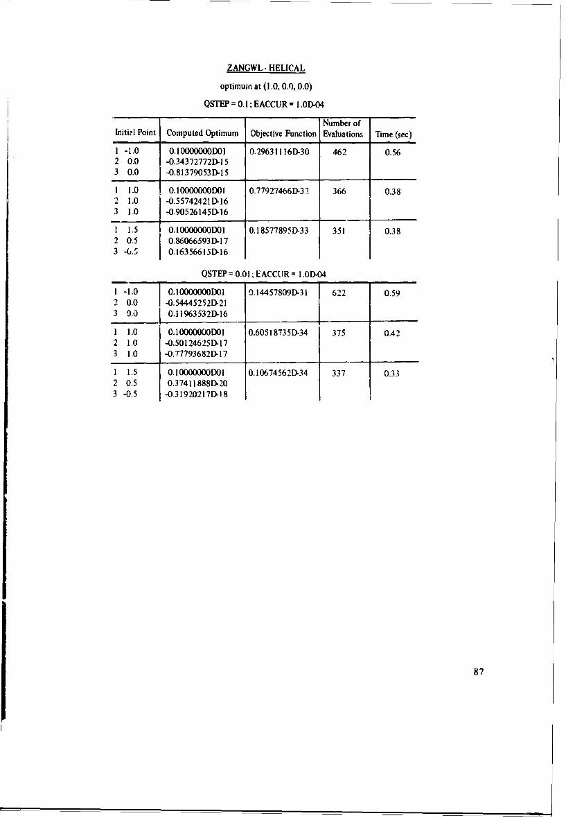
ZANGWL - HELICAL

optimum at (1.0, 0.0, 0.0)

QSTEP = 0.1; EACCUR = 1.OD-04

Number ofInitivl Point Computed Optimum Objective Function Evaluations Time (sec)

1 -1.0 0.1OOOOOOODOI 0.29631116D-30 462 0.562 0.0 -0.34372772D.] 53 0.0 -0.813790531)-I5

1 1.0 O.10000000DOI 0.77927466D-32 366 0.382 1.0 -0.55742421D-163 1.0 -0-90526145D.16

1 1.5 0. 1OOOOOOODOI 0.18577895D-33 351 0.382 0.5 0.86066593D-173 -6.5 0.16356615D-16

QSTEP = 0.01; EACCUR = 1 .01304

1 -1.0 0.IOOOOOOODOI 9.14457809D-31 622 0.592 0.0 -0.54445252D-213 0.0 0.11963532&116

1 1.0 0.10000000DO1 0.60518735D-34 375 0.422 1.0 -0.5012462513-173 1.0 -0.777936821)-17

1 1.5 0.10000000DOI 0.10674562D-34 337 0.332 0.5 0.37411888&-203 -0.5 -0.31920217D-1 8

87

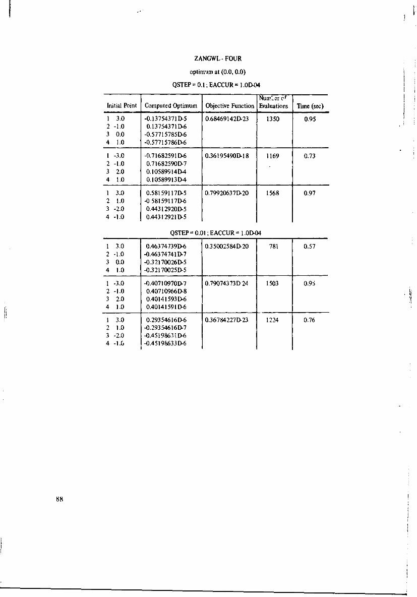
ZANGWL - FOUR

optim-im at (0.0, 0.0)

QSTEP = 0.1; EACCUR = .OD.04

Numi. cr ofInitial Point Computed Optimum Objective Function Evaluations Time (sec)

1 3.0 -0.13754371ID-5 0.6846914213-23 1350 0.952 -1.0 0.13754371ID-63 0.0 -0.57715785D-64 1.0 -0.57715786D-6

1 -3.0 -0.71682591 D-6 0.36195490D-18 1169 0.732 -1.0 0.71682590D-73 2.0 0.10589914D-44 1.0 0.10589913D-4

1 3.0 0.58159117D-5 0.79920637D-20 1568 0.972 1.0 -058159117D-63 -2.0 0.44312920D-54 -1.0 0.44312921DM5

QSTEP 0.01 ; EACCUR = .OD-04

1 3.0 0.463747391)-6 0.35002584D-20 781 0.572 -1.0 -0.46374741D-73 0.0 -0.3217002613-54 1.0 -0.32170025D-5

1 -3.0 -0.40710970D-7 0.79074373D 24 1503 0.952 -1.0 0.4071096613-83 2.0 0.4014159313-64 1.0 0.401415911D-6

1 3.0 0.29354616D-6 0.36784227D-23 1224 0.762 1.0 -0.29354616a.73 -2.0 -0.4519863"D-64 -1.6 -0.45198633D-6

88

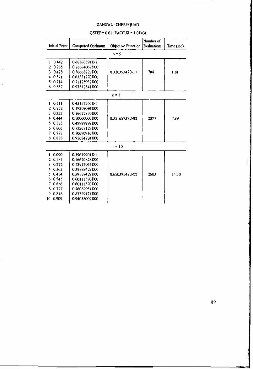
ZANGWL CHEBYQUAD

QSTEP = 0.0 1; EACCUR = 1 OD-04

IiilPitI Copue Opiu Number ofInitial Point Computed Optimum Objective Function Evaluations Time (sec)

n=6

1 0.142 0.66876591D-12 0.285 0.28874067D003 0.428 0.36668229D00 0.32039347D-17 704 1.814 0.571 0.63331770D005 0.714 0.71125932D006 0.857 0.93312341 DO0

n=8

1 0.111 0.43152760D-1

2 0.222 O.19309084D003 0.333 0.26632870D004 0.444 0.50000000D0O 0.35168737D02 209"7 7.995 0.555 jJ.49999999DO06 0.666 0.73367129D007 0.777 0.80690916D008 0.888 0.95684724D00

n=10

1 0.090 0.596199011-12 0.181 0.16670828D003 0.272 0.23917065D004 0.363 0.39888429D005 0.454 0.39888429D00 0.65039548D192 2603 14.306 0.545 0.60111570D007 0.636 0.60111570D008 0.727 0.76082934D009 0.818 0.83329171 D00

10 0.909 0.940380091)00

89

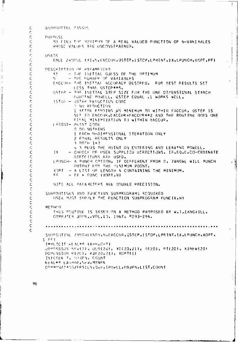
C S'J;AP(I IT TN f.? A\','

r

C 19 F IN;) Tl4r' ',IN IM K111 F A PE AL VALUED FIJNCT! ON OF N-VAkI Ar3LESc oJHr1SE VAL,.hS Al'E UNCONS IPA! NED.

C;ALL I a I IL ()IN,EACCIJIýt.,QSTEPISTCPLPRINTIXLPUNCHXCjPT,FF)

C DE S C4T1)T T PI 0iF PAQAYFY~'i'C x T~iE INITIAL GJFSS OF THE O1PTIMUMMC - N UMtBFP 'IF VARIABLFSCF EACC'Jk- Tp~4 V.\!TTAI ACCURACY DES!PFD. FOR REST RESULTS SET

r I-ESS THAN (ISTEP**5.C ~()5Th-? - TH4F PNITTAL STEP SIZE FOR THE OINE DIVENSICNAL SEARCH

pjWT~ 0OEL.QSTEP EQUAL .1 WORKS WELL.C!S`T;-T - ý).-TI-P QEOIUCTIC~I COO[

c ~ ~ 1 ýTF[R FTIf)INrV AN MINIMUJM TO WITHIN FACCUR, OSTEP ISc SFT TO E.AC,('iJP,,ACCURP=FACCI.'R**2 414D THE ROUT INE DOEFS OJNE

c r-ll/l- M NIM ZAT ON T) W THI EACC U P

C -1 5f) NOTH!NCic I EACH N,-0IMvFNSIrINAL ITERATION OlNLYC 2 F!NA4L kFSULTIS ONLY

c~ nf-IH 1+'c. 4 3 PLUS THE POINT ON ENTERING AND LEAV!NG, POWELL.C ix~ - CHOi!CE rF ''SER SUPPLIEDJ DlRECT!ONS. IF.EQ.0,CO-CRDINATEc -,)IPFCT!IONjs "ARE USED.

c ~ ~ ~ ~ ~ ~ ~ ~ ~ ~~S LON. IC -ADNO('ITOIFDPEETFROM M; ZNIMUM. WILL *PUNCH

c FIRRGA -FUN=C(XNI XOT,14

C T%1,iT ALLTR ISAETP 34 KE' ' A METO PRECSON.E Y~I~~GIL

C CO!MPjTER 10114.,VOL.10), 1967, D293-296.cC

SUI; 0 G-JINL !A"F'.q (NtN,EACC1JR, 'STEP, I STOP, LPR INT, IX t.PUNCHpXOPTv

ImPl- TC IT mF V1-A ( -ý, -

1%,TF rEkE T , 'I-IFN, CrCUNTRtEAL*P LA,i~i)Ptl ,4t-W,-M!NFNCxflin/7- FPIN,-,! L,C)3JFN,LIST,CooNT

90

Ip=OQ = QSTErPC = EACCIJk

LIST = LPMINTItBMCRD= 1,PIJNCHORJ FN--O

IPnW'EL=2EPSILN=1.0O-J.5

C IP=STOP FLAG TFR.4INATING, SIMULTANEOUS RFDUtCTION OF BOTH Q AND EC K-N'JMBER OF CLIPRENT TF PAT IJNC OBJFN=C0RREMIT QIJ4NTýTY OF OBJECTVE FUNCTION FVALUATIONSC OL~t!jC)=IC-TH COMPONFNT (IF ENTER POINT FOR. MITERC NEWUIC)=Ir-TH CONIPCNENT OF INITIAL POINT AND) POINT CCMPIJTEDJ INC ZrI TERC R(!CI=OLC( I.C AT START OF ZG;ITFRC X1(ICID)=IC-TH C0MPflNFNT tIF 10-TH NORMAL!ZED NONCI]ORDINATEC DIRECTI(INC XJ(ICID)=XI(IC,,ID) AT START OF ZGI.'TFRC XItNE'(IC)=Ir-TH COMPfINENT CF (NJ+1J-ST (''Erk-TA')C N!ORMALIZE-0 KONC00krDI NATE DIRECTIONC PT(IC)=IC-TH COMPONr-NT OF MINIMJM POINT OF N-DIMENSIONALC MINIMIZATIONlc 0(!C)=IC-TH Cfl,1PONE~iT OF NfOýMALIZF--) NONCOORDINATE flIQECTIdNk OFC ONF rI-vF',SIClN4L mINIMiIZATIONIC ALPHlA=MINItAUM STEP 1.EN'ITH FOP N-DI'AENSIONAL MINIMIZATIONC LA:"ý3DA=MININ'&W I-TEP LIýNGTH FOR ONE OIMENST()NIýL MAINIMIZATIONC #v!NFNl=O,3JFCT IVE FtJNCT ION MINIMUM' VALUEC ZGFN=C(URRENIT ZG1TIFtr !TERATI0N f03J[CTIVE FUNCTICN VALUEC STFN=(JBJECTTVE FjiJNCTT!ON VALUE AT INITI AL P'JINTC J( MP=F IRST ZGITEP ITFRATIO~N FLAGc o.PJ=rflBJFN kT START (!F- ZGITElRC PT70!F=MAV!,,UAU NFEV AN'q OLD PCINT COMPONENAT 0!FF-ERENCEC10 COiNT INIJF

IF ( P.GT.C Gli T.1 2',I01F I P . rT. r~ TO'-S T FN=F UNC, ( fl%',N!,4 k)FF= STFNIR J F NI=r3J F N + I

GCi Tf 40)3 0 ST F N=F UN C( P T , N

0(R J F N~ =9 PJ F N+ 1

PRINT -.40, N,C,77P14INIT 48ns, L 1ST, Lj\iCreO, !xIF ri.El~ Tl 5r,%Pý,lrT 4.10, ( C.,PT( IC) ,IC-1,NJ)r,tl TO~ 6C

5 , PR1I N T It% C I,( -A) I C 1,tN)6-' 141NIN7 51), STFN

IF r,(-,.C G Tý'] 7'C-,O Tri j

7) Cr;NTINriý

9'

I 1F I IP.G T .0 C TO 0 13 0IF ( I X EQ. 0 O 10 TO c

CC USER SUPPLIES INITIAL NrJNCO(IROINATE DIRECTIONS

k EAD 340, (X I (IC ,1O) 1 C=1 ,N)tII')=I ,N)

CC COmPUTE INITIAL NrfNC10ROI NATE DIRECTIONSC

n DO 12n~ 10=10NOil 110 IC=1,NIF (IC.Er3. 10) Go To 1(1,

10 CONTINUE

C

130 on 140 IC=l.,N140 D( IC )=XI( K , N~

IF ( IP.EQ.n) rL) TO 16CIF: (L IST.FEOJI, GO To 145PRINT 581), ( IC,PT( Ir)IC.=j,Nj)

145 CALL POWELL (NOLnI),LAMH3OA,FF-)DJO 150 IC=1,N

150 OLD( IC)=tOD( IC) +LAMB0)A*D(ICIIF (LIST.EQ.01 rO TO 195PRINJT 59)0, (IC-,OLD(IC,),IC=1,N)

155 CONTINUEGo Tfl 13c

160 IF (LIST.EQ.(ý) C,0 TO 105PRINT 560, (IC,NEW(TC),IC=1,N)

S69 CALL POWELL (N,NEW,r),LAMf3iJA,FF)C

CCOMPUJTE F IRST Pfl TNT

C

1C IF (LIST.tQ.r GO T; 175PJUITPJUP (InnT-,,CI

1792 ~ 4 Ij)

r________________________________________

IT, DO ? C IJ=IpN2OC. k ( I J )=flL NlI J)

or 220 IK=INDO 21.0 IL=] ,r-l

210 XJ(ILIK)=XI(II,TK)220 C(ONT TlIJF

)PRJ =flfiJFNIIF (LIST.",lF. ,}) Ti T 2 ,PPTNT 540t K

C

Y3C, CALl. 7GITLb (.InL)vXI, rAL M , AP TXINNF ,JJ M), []YESFF

24C Z(;FN=FF

C 'MP R / F ki ,,t fln -tn Oi N TS FflIn -,•-0I N1 FNS , INAL M IN it I IIA C HI E VEL 0

PCl IF=IOAB3S( PT (1) -fk1) (f I) Jl)r0 250 IJ=2,,'2

IF (IW4.L[.PTI1TFW 1 0 TO 2 5(CPTDI P = -,N

25C C3NT N1JCIF (fLTI)IF.(;L.F I .!) T C 2? C

IF (K.NE.2) GO TO 2ý,0(i_ BJ FN= O, JKK- =

267)D IF (L!ST.F).,3) rfl TO 27CIF (LIST.Fo 2) (;1 Trl 27CPRINT 430, (IC,R(IC),IC=I,N)PkINT 45S0., (4 ( C, C), XJ( IC ,!C)) ,I=,1 ,N) ,1=)1 , N)P4I ýj 550, KPR [Nr 431, (I IL Li)( C) [IC- I ,N)PRINT 450, ((tC, T II,X!( IC.IC )),IC= T ,N) ,I D-I.N)PRINT 510, ( IC,XINE"( IC I,IC=I,N)PRINT 520, K,.7 CGF 0PtN-INT 4 C, ( IC,PT( IC IC=I ,I)PP Tý!T. 4.¢ ,- ,n K f,fAJFN

IF (PTr)IF ,I T.F ) Ct(J iT 2 ,9C

C TFST F0 - I"- F! I f'CSIIt AL 'IINI'IJ- /T HIFVEo02Tq IF (COT).IT.I-T. N) ja T1 3fl

C - D TM E NI1IrNAL MI \T 4 I JM ACHI E VE1)C

29:) 9 F-N T !UOIUFIF ( 1[,I,1C4OL[ E . I C,) i T! 29nP rGN A hlC, T 1, I XPIJN':H 37C, .,, F

PUNCH 340, (PT( IC), !C=IN)Pill'ICHl 410), IST_ 711 -'CPll),Kt.(ICKI [F ( Vy E,~.' c.F1 TflPUNCh It,, ((Xf(IC, ID),IC=i.,N) ,ID=.,N)

2 C 0.T)N T I NIJ

93

MTNPNI= FFA31c IF (L IS T. LF .I) rO Tf!I 1C

PP I NT 350), M1TNvNPPr'INT J(O ir. ,PT(IC),f=P I.1T '.T 40, r~P,

C, TI-ST Pijk F!NTSH ANI) RESTAR<T IF NOT31~ I r ( 11) . Gr. I STO)P I (ilj Tf 33('

Q= F

K=K+ IJIIMP=JIP*1IP+ 1Ip= !P+I1IPOwvA.= I~ PJWFL* IprjWbLGO0 Tri to

17 RE ITFPArL I)'vT 1 PF CUIPEI) ACCURACY ACHIFVEII32' K=K+l

jIJmp=jI'I!P+ IG(I TP JQ',

33 0 DO 335 J=10133'5 XOP T ( j) =1L 0( J

PR I IT 62CRE TURN

c.340 FORMtAAT (d15 10 , 5 x35C' 1-0 RM AT (-I A03 31-1 AJ~ffT IVE FU(NCTIPON Mi N I MUM VALUE E 19.11 13 ý'0 F(IPMAT I1f Y',2H1g MINIMUM POJ!NM/fBOXvE18.111))37C 10 RM AT 1C1 I, ?X , F1 .. 1 r.,3X 9F 15. 1C )390) F CRý A T tll l18HNAC. CF D)IM OR VAR=, 12,5X, 1610NE DIM START

Q =, E19. 11 1 ,5 X, HAC CUP AC Y =, E I.A. I4CC FO-,RMAT ( PIlC,21HNO. INITIAL Pr)INT/C13,3XIE18.llfl

4 . O-nR MAT ( IiHC,2lRITFPATT0NS I THROUGH ,19,lICH REQUIREDIQ,31H OBJIEC HTIVE FUNCTION I-VALUATIONSI

430 FORMAT(2811 FNT[P IGITEk WITH THE PI)INT,/414 Nn, 33,ý81)431 F-VPmAT( 26H L fAV'E Zr!TER AT THE P1OINT,/4H NL)./113,93X,F18. 11)

44 FrR'AAT ( PiC,3?HACHIEVINGC THIS MINIMUM PEQUIJRED ,19s3611QBJECI~VE F 1UNCTION4 EVALIJAT!ONS AND) 19,1IH ITERATIONS)

45.O FNRmAT ( pir,1'3h1- I. XNTE NO.EL/ ,3,IRB(.T1w(2~~t

4W7') rRF4AT 4JH'v,3?ul-N'. INITIALIZAT/IUNLAEP)EL3,3X,E18.1I)II') FOR~MAT ( I I1 N' H1 3,5X,1 14PUN 3, 2H

94 )1DF=,13,5XAHX AG, 1

sutmn(ITINE 1(1,IT FR ( '110V )PT DI)R,,NC,D IST,G,EXTP A, JSW,11S1~,!FF)IMPLIC;IT PFAL*I8 (A-H,0-1iD I MNS ION DPT(2?',) I flR(20?21 ), C( 20) t G(2 0) IWO2) , TNrW42) ) t FXTR A

F.EAL*R L,NEWINITFr,ER rjj~jrN, fO.j~tTCr)MMIIN/lArJG/E:PSILNO,F,IPLUWEL,O(JF3JFNLISTCOIJNT

CC UINCONSTRAINELD NIOV-D!MENS TONAL mINTM.17 ATION 141THIIT 'JS7Nr NOF V4rIV

C ')SIN(; rGIVEN POINT DPT ANI) GI 1FN !)[kFCTI(JN DIRC NflV2(OIANTITY flF: VAR!ARLFS IN 013JFCTIVE FUNCTIONr, NC=NllMi3[R Of: CAIRRENT COORL)INATF PT PECT JON1C L)PT( 1Ck IC-TH COM0PPONENT (OF OLD PO3INTr NEW( ICk=IC-TH (,rlAPr'NPNr OF NEW POINTc [)IIP(II)I-' COMPONENT OF ! U-T'l Nl0Nf'JORt TtATý E !YiRflAL IL - DIP'ECC FXTP.A(C)=ICT(`,T CO'A¶0(NFNT OF IN4-1)-ST ('EXTRA')

C NICIMALIZh)J NfON~CrI~PfINATF DIRECTION

C f)IST=MINI'\jItAjlf~ STED LFNIGTH ALfJNG CMRlrDINATE )IPFCT1 IN Or.C C.(If )= TO-TH CflN'PrNFNT OF C URRLNT NtIPMALIZEt) COCIkDINATF. DIKFCTIf)Nr 0(0)=I-T!CMPf)NENT OIF 1M1INIMUM P')I NT IN NDV-Nil NIMI 74TlOT1>J,

Cl L=M!NIMIM STEP L FNGTFO IN lJNL DIMONSIONAL 'I NI M IZAInN ALONGc N!flNCflORf)lN-TF IMP'1 rT ION HCl fl(IC )=I-Tll Cf1ThiPflNELNT UF cUjR.?ENr N!ONCU-l1P[)' ATh PF ICTIIINj I N (iNEC nIMEN~S IVNAL '1INI MIZAT IONr Cril\INT=CURF< ENT Till"AL. Cr (71lOPOIN ATF 0IiRFCTrIONS UJSE(.N Iq THolJ CoMPIJT IiC IFXT[\IA' KCfh)l'A 9 :)RECTFIONC JSW=FIRST Zl';ITCP ITFPATION F-LAGc,

C PART ONE:CUUNT = 0

C IF K-i AN") IX ( IN 7ANGW!OLL =C, G) TO OART TWOIF (JSW.GT. 1) Ci) ro 2rNC=rNC4-DO0 10 JK=1,NIDV

C COIMPtJTF (IJQP C-NT C11)PO, INATfI DI PECT ION

20 00 4,) J C =I ,'i!\IF ( JC .[Qý.Nf ) t,(m r 3(1C( JC-,)=.'GO)1 TO] 40

40 CIN T I N iLCC MINI1 I[IF I N ONIF 01 1FNSI iN ALfINO, CUjRFNT CrIO'ýOI NATF IOi'lýC.T I",\,C

IF: (LIST.N\S.4) (-.n ro 45

PPINT 2?(iu (j,O(.!PT(,Jl ),,JC=i,NDV)45 CALL POWEhLL (NFji)V,[)PT,tT,ý)lST,rFF)C TLST FOR ALL C(7tflkI.'VNA'rE I)1 PECTIIINS (IrL0

IF (NCr.NE.N,')Vl fli) Tt,1,

95

Gn T ( 60

c TFSJ T P'l' AINT %1Ii1 STPP LVJ(;H ALONG~ C(NC)

If Vr)AR (I T).;LFSI LN 1 6 TO )Of

IrF C IIUNT. GE %1D V GTIi TO 71-0C (: UN T =C 0UN T* +1(,( Tf! 2')il

r, Mllil1MilPk STFP L rN GTH ALON G C NC) FO0UN1DN70 DfO KC -KI ,N [)V

33 f(Jk)=Df'lPT J" IF FTIIPN

C UPDA TE Ct.','P ',4 ' t DI I NT

I Ft- IC S~ T ,N F4 1

jfýYINT 26,r, 1 CNdJ) ,J(=i ,N[PV)

C PAPT TW~)

C, MINTY~IZE IN F)10 LUT 4NSION IIS! N CflRIFNT P'OI NT ANO CIQPRENTC NINCUf)(lIN/,Tc UIJTCTI(ThJS11C On lA, 8CJD=1,ND\'

001 12() JC=l,NI)V120 HI JCO )UIw( jc, Jr

c TEST Flt 71'14D )ILýF('T ON

plf! 1-A J=) ,')I F (OiA,,.S (M1 .J )*LU * 1.11 -15) T-- 1tI3C

l 0 Cl)N T I NilJET F ( TlI. F . 1)) 1-,( Tr) II F (L IS T . ý, . 4 ',) T 0 15 9P P T NT 2 5 , 1 ri,4 w ( 1,1), I Ij=1 ,Dr)v

15 5 CALLi fl'tWýLt (NDVNlFw PH,L,FF)lo C: Vn 1 711 KJ=I l r) VI-'Q NE v(KJ )=Nft'W( KJ I L*H( K J)

IF (I- IST.NIL .4 ) ;rl Tnl JjO

c CPY011TE OF) S (T;')R) IAT DirECTION

U F ; 1 ')( AcU * 3 )

1O' f N' fi , H LN ýVA 4)AS ('j-Iq( JC)-,l)QTI JO jCDt) 2qr) jc=rt.o1, %

96 l~P (J C '4)V + I =tlWJC ) - PT JC) 1/1) EN13M

C MiNIM! ZE IfN Clý nI MFLNWIfN ALM--, 'F KT At Nf'jCiIORD INAT F I)! RFrT IONDOP ?10 JC=I~flV

210 1-i(Jr.)=.,)Tp (JC,NOlV+I.IF (LIST.NF.4) C(;(] TO1 215PRINT 250, (C K NF0(J(. )iJC.=1NDV)

215 CAL[ PUWl.t-L (Nf.'INEI-lH,LFF)l90 ?10 JC=I,N[)NI

22n DPT (J(, )=N Fi( JC I+L*lH( ,i

IF- (LI1$T.NF.4) r0 TOl ?29~PRINT 26',t (Jt,')PT(JC)1,jC=INIV)

c Cpr'PI.TF MW4CW)flk)INATr DREpCTIONS' FOR~ NEXT TT!iWATT¶]N

225 DO0 24 "' J0 I t ,\Jr'A,

OPn 2jr JC= , ND") 1~ )P ( JC , j r) I u( JC ,Jf)+ I

140, DOl 1 5.) -J JK I r, Vj15" (;ý(JvK)N ,,( -P FTOiRN

6 r0 Ff-P,-ýAT Clilr', 17HN-I, PHWELL LEAVH-/( 13,3X,F 18.o1))F N

IrIC IT RPAL*P(-iO7DIME-?STU)Nj Do('3 Of~) ,(20) , F(4) , VTtNT~rCFP MThJF\, CV-J!NTCf~I/ZWFýINCF I PE,rfl'JF.N, ,LTT,Cu1UNT

C Mj4C01JSrý.MIF<) ONP r !MENSIftNAL MINI MiZAI Innir W!rijT U01tSTN; )kIVTT

c FOP FJ'j[)I'I- HG FLP3W RFAY)PJ4BLE 0 VALIE, SFE :CALAHAN,D. A., CrmpkJTERc At)F-D NE-TW~P(lESIO.rKRWH!L 9gC I0 IN IT IAL P!) I :T V ECTORC S=GTIVFtN DIkFC.TTh1N Vr-CTOR

C IVFN PO,S; FINNr STEP Tý4AT MINPI-4/ES (IFIJEC-TIVE FlJNCT~I'N PO-9STEP*SC (;IVFPI PO,S. F1.Jr 5TFP THAT MINIMIZES 09JLCTIVF FUNCT[C])N(PC+ST[P*C N=UUJANTT TY flF VAk APLFS TN OB~JF(CTIVE fI(JN(-rljNjC, 0= PINTl M STFP I.FhY;-TH ALONG Sc k=r,Eo)MkTP Ir St-P FrS 0ATTC3 '-'w NIN REASINAi9LE STrF n LFNGTI- INC, C.11APIJTjrI, SFT'IF INITIAL TFIRLF PO]INTS

CP=Gt-rVJM[TRIC, 'Qf: IFS C-IJEFFIC lENT FOR FINOING APWJVE RF AS(Oýt3LF STFPC E-PHCAlIRF'3 ACOIP ACY1V 'iF U'! MUM POITN (FACH COM)ýPONENT)

c V=APRAY CF CUJPPI!T fPoINT VALUESc F=AlPPAV rOF CIIPPENT PlITNT Jf3JF3CTIVE FUNCTION VALUFSC liWA.i- *=r JANT I v OF )P J,-Ti Vt: tWICJT ION F VAt hAT1I NSC. NUJM= 0'IANT T, TY Oý .JIJArRATIC INTEPPOLATIU(NS

C CIMPIJ~FTfIPEF STArkTING VALULS A~o THEIR O8J~r JIVE FLJNCT!0Or VALUFSc

A=O.r'1DQO

urL ir10 ZiT)=PO(I)

0O 20l I=l,N'0 ( I P 0( 1+0*S1T

FC,=FIJ.NC( Z N IU H J F- N =O R J F N + I

(F (FQ.LT. FAI Ci TO 'inDO 30 1=1,N

30 Z( I )=P0)( I )-0*St I)FNQ=F-IJNC(t -N)LlbJFNi=OQJI-N+ 1IF (FNi).GE.FMl GU Tn 40-,

f3= -fF P.= F N0I sw=r)GO TOl 60

V (2 =0 . OP f),-V ( 3) =(Ft 1)=FNQ1,

F( 3)=FQGO TO 120

I Sw = 1i

60 CF=1.C'000SUM=1 .'jfW0

70 CF=CF*RS I J M S UM + C F

I F tIS 1. ECU.1I) GO TO (IFC = -r)* S Umrm rn go

10 C=Q*S(JM90 DO 100 1=1,N'

100 ZM =Pr( I)+C*S(1TFC=FINC( t,rN)CIfRJ F- ~h 0 IJ F N +IF (FC.,T.FFUl ril TO 11C

A=PkF A= 1 '3 CF E; F CC,(' TO 70

110 V( I )A

Vt '41=CF( 1 IFA

Ft 3)-FC.

98

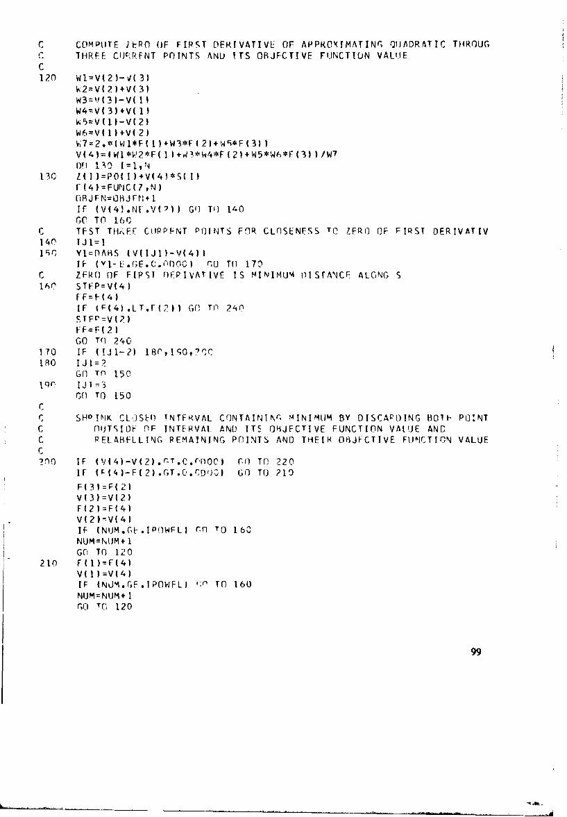
C COM~PUTE2 flRnO (F FIRST DFRTVATIVIL OF APPROI(IMATINr, QUADRATIC TIIROUGCTHREE C'JF:RFNT POINTS ANO ITS OBJECTIVE FUJNCTION VALUE

C120 Wl=V(2)-V( 3)

W2=V(2)+V( 3)W3='J(3)-V( 1)W4=V( 3)+V( 1)

W6=V(I )+V( 2)W7=2.*(Wl*F!1)+W3*F(2)+w9i*F(3))V(4)=(Wl*W2*FC1)+W3*W4*F(2)4-W5*W46*F(31))W71)0 1.30) 1=19,N

13C'ý 111 )=PO( I )V(4)*S( I)f (4)kFUNJC( 7 ,N(lHJFN=0HiJr1+ 1IF (V(4).*N[EV(?)) GO] TO) 140GO. TO 160G

C TEST TWrFF CIIPPFNT POINTS FOR CLOSENESS Tfl ZFRg] OF F IRST DER IVAT IV140 !J1=1

IF (VI-f-. GE. C. ihýOG) rcdi To 170,'c ZFRO OF FIRST fOEPIVATIVE IS MINIMUM1 O)1STANCE. ALONG S160 STFP=V(4)

fF=F~(4)IF (F(4).LT.F(i2)) GBl TO 240SFFP=V(2)F F =F( 2 )Go To 240

1,70 IF (!J1-2) 18f"l,11;0,O'rf

GOj Tn 150190 IJ I= 3

(7,( To 150

C SHPINK CLOSEI) !NTFRVAL CONTAININC 14INIMUM BY DISCAPI)ING BOTI- POINTC flTIO1F nF INTERVAL. AND ITS O'iJFCTIVE FUNCTION VAt!UE ANCC RELABF-LL ING REMAINING POINTS AND THEIN ORJFCTIVE FUNCTION VALUE

?O0 I F v(k/(4 V(2) rT .C .r, C GO1 TO 220,IF (r(4)-F(2).GT.Q.rDDUG3) GO TO 210

Fl 31=F(2)V ( 3=V (2)F(2 )=F(4)V(2)-V(4)IF (NUMi.GI.IPOlWFL) rnf TO60bNUM=INUM+ 1Gn TO 120

210 F(1lkF(4)V (I ) =V (4 )IF (NOM.GF.IPOWFL) ;f TO 160NIJMNUM+ 1r.O TG, 120

2Y, IF (F(4)-F(2 .1 T. .I Gf) Tr! 230

V: 3 -FV ( 4'V(3V=V(4)IF (NNUM.,.[ IPl•'EL.) GO IT) 160

NULJ IJM÷]. I.G(1 T() 120

i Cl F( I)=F(2))V( 1):V(?)

V( 2 1 =V( 4)

IP (NUM.GE.IPf1WFL) G9 TO 160NIJ =IM :hlJ'• 1

GO TO 120

"2 4 CrINTIN 1:RFTIJPN

100

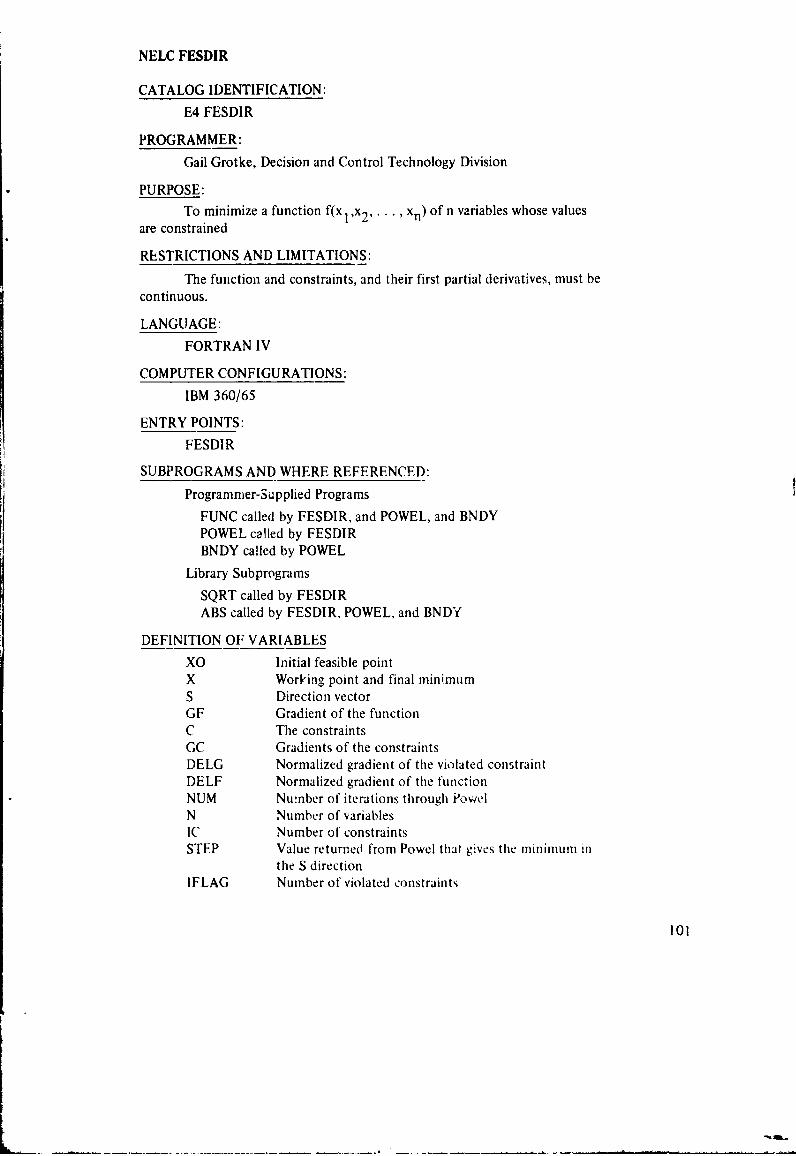
NELC FESDIR

CATALOG IDENTIFICATION:

E4 FESDIR

PROGRAMMER:

Gail Grotke, Decision and Control Technology Division

PURPOSE:

To minimize a function f(x 1 x2, .... xn) of n variables whose valuesare constrained

RESTRICTIONS AND LIMITATIONS:

The function and constraints, and their first partial derivatives, must becontinuous.

LANGUAGE:

FORTRAN IV

COMPUTER CONFIGURATIONS:

IBM 360/65

ENTRY POINTS:

FESDIR

SUBPROGRAMS AND WHERE REFERENCED:

Programmer-Supplied Programs

FUNC called by FESDIR, and POWEL, and BNDYPOWEL called by FESDIRBNDY called by POWEL

Library Subprograms

SQRT called by FESDIRABS called by FESDIR, POWEL, and BNDY

DEFINITION OF VARIABLES

XO Initial feasible pointX Working point and final minimumS Direction vectorGF Gradient of the functionC The constraintsGC Gradients of the constraintsDELG Normalized gradient of the violated constraintDELF Normalized gradient of the functionNUM Number of iterations through PowelN Number of variablesIC Number of constraintsSTEP Value returned from Powel that gives the minimum in

the S directionIFLAG Number of violated constraints

101

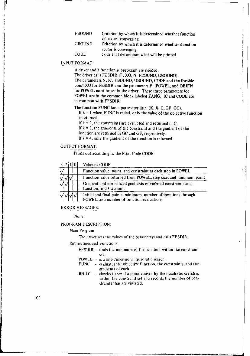
FBOUND Criterion by which it is determined whether functionvalues are converging

GBOUND Criterion by which it is determined whether directionvector is converging

CODE Code that determines what will be printed

INPUT FORMAT:

A driver and a function subprogram are needed.The driver calls FESDIR (F, XO, N, FBCUND, GBOUND)."The parameters N, IC, FBOUND, GBOUND, CODE and the feasiblepoint XO for FESDIR ano the parameters E, IPOWEL, and OBJFNfor POWEL must be set in the driver. These three parameters forPOWEL are in the common block labeled ZANG. IC and CODE arein common with FFSDIR.

The function FUNC has a parameter list: (K, X, C, GF, GC).If k = I when FUNC is called, only the value of the objective functionis returned.if k = 2, the cons-raints are evalhlted and returned in C.If k = 3, the grauents of the constraii~t and the gradient of thefunction are returned in GC and GF, respectively.If k = 4, only the gradient of the function is returned.

OUTPUT FORMAT.

Prints out according to the Print Code CODE

3 2'110 Value of CODE14Function value, noint, and ccrnstraint at each step in POWELFunction value returned from POWEL, step size, and minimum point

&I/ - Gradient and normalized gradiernts of vio'ated constraints andfunction, and their sum

&k/ Initial and final points, minimum, number of iterations throughPOWEL, and number of function evaluations

ERROR MESSAGES:

None

PROGRAM DESCRIPTION:

Main Program

The driver sets the values of the narameters and calls FESDIR.Subroutines and Functions

FESDI R - finds the min.imum of the function within the constraintset.

POWEL - is a one-O'imensional quadratic search.FUNC evaluates the objective function, the constraints, and the

gradients of each.BNDY -- checks to see if a point chosen by the quadratic search is

within the constraint set md records the number of con-straints thaw are violated.

102

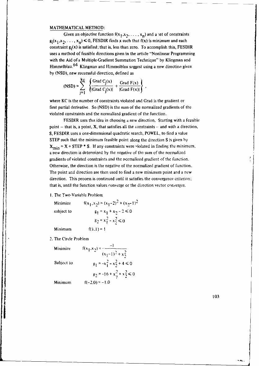
MATHEMATICAL METHOD:

Given an objective function f(xI ,x2 , .... xn) and a ',et of constraintsgi(xl ,x2 , ... , xn) < 0, FESDIR finds x such that f(x) is minimum and eachconstraint gi(x) is satisfied; that is, less than zero. To accomplish this, FESDIR

uses a method of feasible directions given in the article "Nonlinear Programming

with the Aid of a Multiple-Gradient Summation Technique" by Klingman and

Himmelblau. 64 Klingman and Ilimmeiblau suggest using a new directioo givenby (NSD), new successful direction, defined as

kc( Grad Cj(x) Grad Fix)

(NSD) = G Grad + x)j=l Grad Cj(x)l IGrad F(x) '

where KC is the number of constraints violated and Grad is the gradient orfirst partial derivative. So (NSD) is the sum of the normalized gradients of theviolated constraints and the normalized gradient of the function.

FESDIR uses this idea in choosing a new direction. Starting with a feasible

point - that is, a point, X, that satisfies all the constraints - and with a direction,

S, FESDIR uses a one-dimensional quadratic search, POWEL, to find a value

STEP such that the minimum feasible point along the direction S is given by

Xmin = X + STEP * S. If any constraints were violated in finding the minimum,

a new direction is determined by the negative of the sum of the normalized

gradients of violated constraints and the normalized gradient of the function.

Otherwise, the direction is the negative of the normalized gradient of function.

The point and direction are then used to find a new minimum point and a new

direction. This process is continued until it satisfies the convergence criterion;

that is, until the function values converge or the direction vector converges.

1. The Two-Variable Problem

Minimize f(x 1,x 2) = (x 12)2 + (x)- 0)2

subject to g91 = Xl + x2 -2 < 0

g2) = xi- - X3S < 0

Minimum f(il) = I

2. The Circle Problem

Minimize fxI,x(Xl-1)2 + x27

Subject to gl =-xI- x2 + 4 < 0

7-g2) -16+ +Minimum f(- 2,0) = - 1.0

103

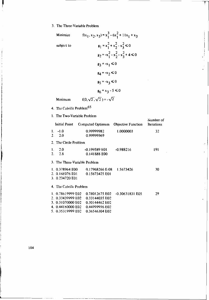
3. The Three-Variable Problem

3 2Miiie f(xl, x2 , x3 )= x1 -6x 1 +lIxI +x 3Minimize 6

subject to gl= x2+ x•-x2_x <0

2 2 292 1-x 2- x-3+40,

93 =-x I < 0

94 =-x2 0

95 = x3 0

96=x3 -5 <0

Minimum f(0, V, V2-) =--2-

4. The Colville Problem 6 5

I. The Two-Variable ProblemNumber of

Initial Point Computed Optimum Objective Function Iterations1. -1.0 0.99999982 1.0000003 32

2. 2.0 0.99999969

2. The Circle Problem

1. 2.0 -0.199589 E01 -0.988216 1912. 2.8 0.141888 E00

3. The Three-Variable Problem

I. 0.378964 E00 0.17968266 E-08 1.5673426 302. 0.16F076 E01 0.15673425 E013. 0.234720 E01

4. The Colville Problem

1. 0.78619999 E02 0.78012675 E02 -0.30631831 E05 292, 0.33439999 E02 0.33144035E02

3. 0.31070000 E02 0.30144462 E024. 0.44180000 E02 0.44999996 E025. 0.35319999 E02 0.36546304E02

104

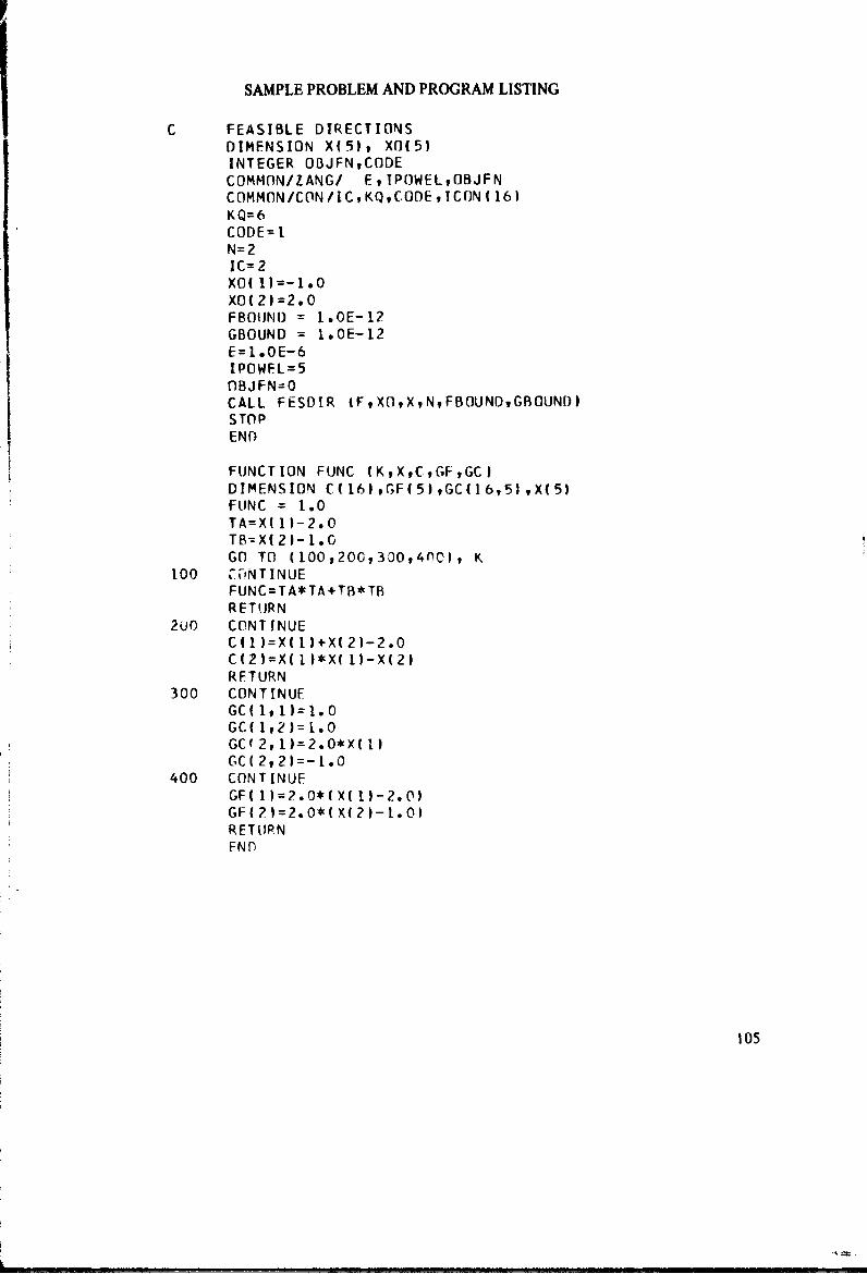
SAMPLE PROBLEM AND PROGRAM LISTING

C FEASIBLE DIRECTIONSDIMENSION X(5), XO(5)INTEGER OBJFN,CODECOMMON/ZANG/ F,1POWELOBJFNCOMMON/C0N/ICKQCOOE,!CUN (16)KQ=6CODE= 1N= 2IC=2XO( 1)=-1.OXO (2 I= 2 *0FBOIIND =1.OE-12GBOUND = 1.0E-12E=1.OE-6IPOWEL=5OBJFN=0CALL FESOIR lFXOqXvNFBOUNDqGBOUND)STOPEND

FUNCTION FUNC (K,XC,GEGC)DIMENSION C( 16) ,GF( 5) ,GC( 16,51 ,X( 5)FLJNC =1.0TA=X( 11-2.0TB=X( 21-1.0GO TO (1O0,2O0,30O,4(n0I, K

100 Cý'NTINUEFUNC=TA*TA+TB*TfBRETURN

2uo CONTINUECl )=X( I )+X( 2)-2.0C(2 )=X( I )*X( 1)-X(2)RETURN

300 CONTINUEGC(I1,11=1.0GC( 1,2)=I.0GC( 2, 1)=2.O*X( I)GC( 2,21=-1.O

400 CONTINUEGF(1)=2.0*(X(l)-2.0)GF ( 2 =2. 0*( X(2)- 1. 0)RETUPRNEND

105

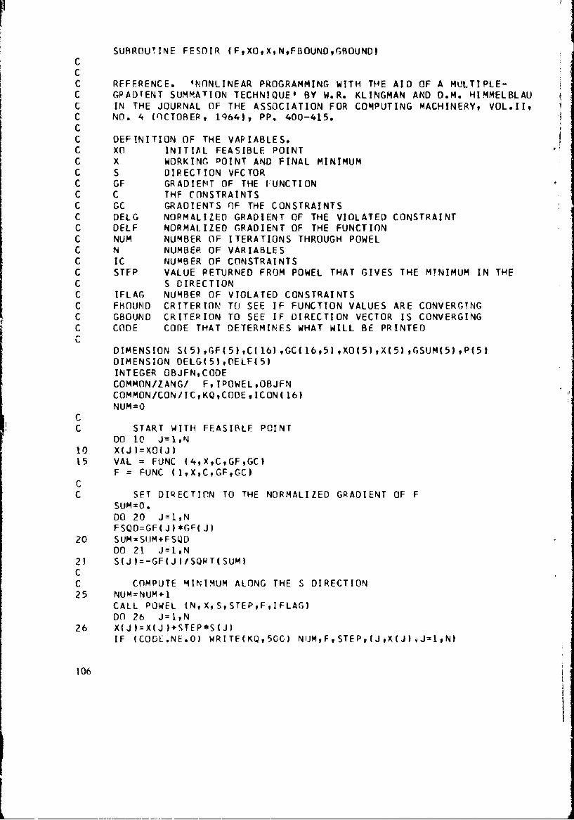
SUBROUTINE FESDIR (F,XO,X,N,FBOUND,?BOUND.

CC

C REFERENCE. 'NONLINEAR PROGRAMMING WITH THE AID OF A MULTIPLE-C GRADVENT SUMMATION TECHNIQUE' BY W.R. KLINGMAN AND D.M. HIMMELBLAUC IN THE JOURNAL OF THE ASSOCIATION FOR COMPUTING MACHINERY, VOL.II,C NO. 4 (OCTOBER, 19641, PP. 400-415.CC DEFINITION OF THE VARIABLES.C XO INITIAL FEASIBLE POINTC X WORKING POINT AND FINAL MINIMUMC S DIRECTION VFCTORC GF GRADIENT OF THE FUNCTIONC C THF CONSTRAINTSC GC GRADIENTS OF THE CONSTRAINTSC DELG NORMALIZED GRADIENT OF THE VIOLATED CONSTRAINTC DELF NORMALIZED GRADIENT OF THE FUNCTIONC NUM NUMBER OF ITERATIONS THROUGH POWELC N NUMBER OF VARIABLESC IC NUMBER OF CONSTRAINTSC STEP VALUE RETURNED FROM POWEL THAT GIVES THE MYNIMUM IN THEC S DIRECTIONC IFLAG NUMBER OF VIOLATED CONSTRAINTSC FIJOUND CRITERION/ TO SEE IF FUNCTION VALUES ARE CONVERGINGC GBOUND CRITERION TO SEE IF DIRECTION VECTOR IS CONVERGINGC CODE CODE THAT DFTERMINES WHAT WILL BE PRINTEDC

DIMENSION S(5),GF(5),C(161,GC(16,51,XO(5),X(5),GSUM(5),P(5)DIMENSION DELG(51,DELF(5)INTEGER OBJFNCODECOMMON/ZANG/ FIPOWELOBJFNCOMMON/CON/ICKQCODE,ICON( 16)NUM=O

CC START WITH FEASIBLE POINT

DO 10 J=1,N10 X(JI=XO(J)15 VAL = FUNC (4,XtC,GFGC)

F = FUNC (1,XCGFGC)CC SET DIRECTION TO THE NORMALIZED GRADIENT OF F

SUM=O.DO 20 J=1,N

FSQD=GF( J) *GF( J)20 SUM=SIMM+FSQD

DO 21 J=1,N2.1 S( J =-GF (JI/SQRT(SUM)

CC COMPUTE MINIMUM ALONG THE S DIRECTION25 NUM=NUM+÷

CALL POWEL (N,X,S,STEPF,IFLAG)DO 26 J=1,N

26 X(Ji =X(J )÷STEP*S (J)IF (CODE.NF.O) WRITF(KQ,500) NUJMF,STEP9(J,X(J) ,J=1,N)

106

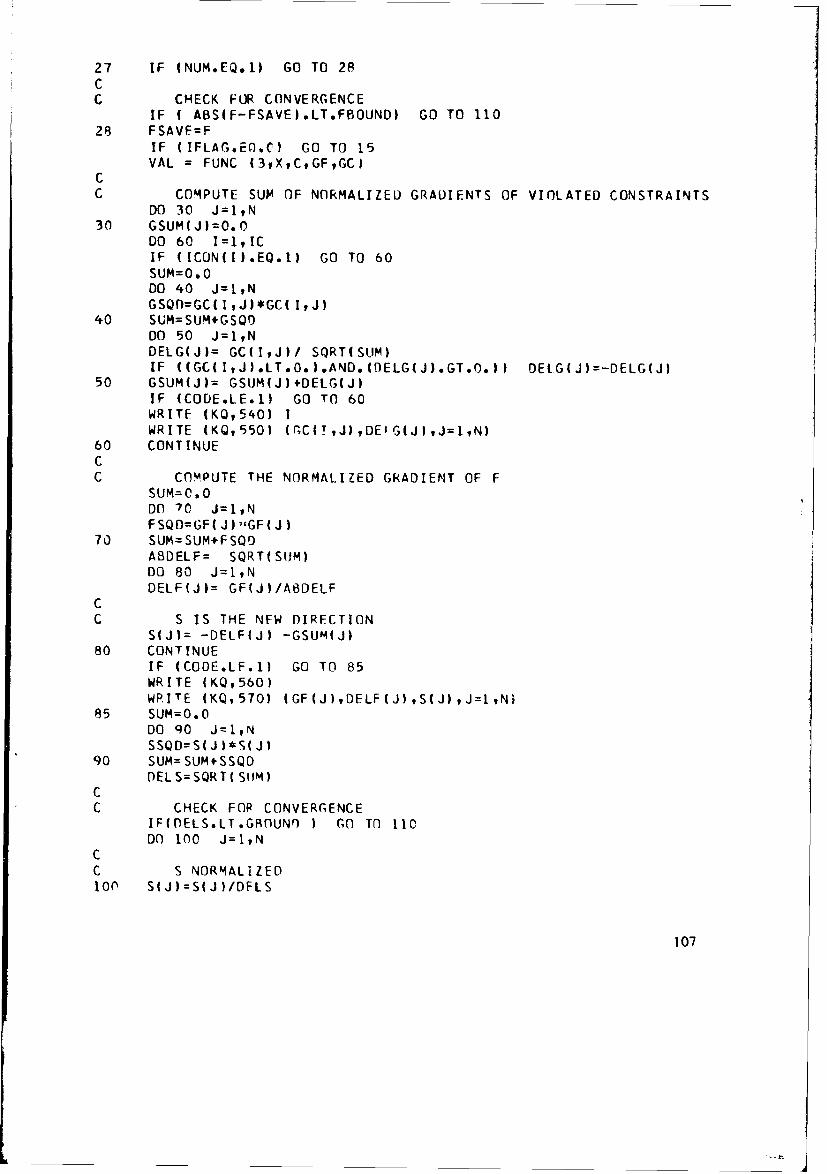
27 IF (NUM.EQ.1) GO TO 2BCC CHECK FOR CONVERGENCE

IF ( ABS(F-FSAVE).LT.FBOUND) GO TO 11028 FSAVF=F

IF (IFLAG.EOC') GO TO 15VAL = FUNC (3tXCGFGC)

CC COMPUTE SUP OF NORMALIZED GRADIENTS OF VIOLATED CONSTRAINTS

DO 30 J=1,N30 GSUM(J)=0.O

DO 60 I=1,ICIF (ICUN(I).EQ.1) GO TO 60SUM=0*0DO 40 J=19NGSQn=GC( I,J)*GC( IJ)

40 SUM=SUM+GSQODO 50 J=1,NDELG(J)= GC(I,,J)/ SQRT(SIJM)IF ((GC(I,J).LT.0.).AND.(DELG(J).GT~o.) I DEL.G(J)='-DELG(J)

50 GSUM(J)= GSUM(J[4-DELG(J)IF 4CODE.LE.11 GO TO 60WRITF (1(0,540) IWRITE (KQ,550) (rC(! ,JI DEI G(Jl9J=1,pN)

60 CONTINUECC COMPUTE THE NORMALIZED GRADIENT OF F

SUM=0.0Do 70 J=1*NFSQD=GF( J) "GF(J)

70 SUM=SUM+FSQDASDELF= SQRT(SOM)00 80 J=1,NDELF(JI= GF(J)/ABDELF

CC S IS THE NEW DIRECTION

S(Jl= -DELF(JI -GSUM(J)80 CONTINUE

IF (COOE.LF.1) GO TO 85WRITE (1(0,560)WRITE (KQ,570) (GF(J),DELF(Jl,S(J) ,J=1,N)'

85 SUM=0.ODO 90 J=1,NSSQD=S(J )*S(J)

90 SUM=SUM+SSQDDEL S=SQRT( SUM)

CC CHECK FOR CONVERGENCE

IF(DELS.LT.GBOUNn GO TO 110DO 100 J1I,N

CC S NORMALIZED100 S(J)=S(J)/DFLS

107

6O TO 25110 WRITE (KQ,510)

DO 120 J=lN

120 WRITE (KQ,520) J,XO(J)hJ,X(J)WRITE (KQ,530) F,NUM,OBJFNRETURN

500 FORMAT (1HO,16,21H RETURNED FROM POWFLLvf,17H FUNCTION VALUE =

lE15.li,/#8H STFP = ,F15.8,/,(3H X(,[2,3H) =,E15.8))

510 FORMAT (lHO, 13HINITIAL POINT,15Xl1HFINAL POINT,//)

520 FORMý~T (4H XOhI2,3H) =,E15.8,5X,2HX(,12t4H) = ,EI5*89/)

530 F9RMAT (54H THE MINIMUM FUNCTION VALUE WITHIN THE CONSTRAINTS IS

1E15.89/,40H THE NUJMBER OF ITERATIONS OF POWELL IS =16,/,

139H THE NUMBER OF FUNCTION EVALUATIONS IS 0616

54C0 FORMAT (11H CONSTRAINT,12,/,9H GRADIENT,17XIOHNORMALIZED)

550 FORMAT (lX,E15.8,1OX,Fl9.8)

560 FORMAT (9H FUNCTION,/,qH GRADIENT,17XlOHNORMALIZEO,16X,3HSUM)370 FORMAT (lXtE15.A,1OX,E15.8q10X,E15.8)

END

SUBROUTINE POWFL (N,POS,STEP,FFYIFLAG)

DIMENSION S(20), P0(201, Z(20), F(4), V(4)', CO(301

INTErGER OBJFNCfMMON/ZANG/ F, IPOWEL,OBJFNSTEP =0.0NUM=OR= 1.5A=0. 0

Go To 54 Q=Q*.l

R= 1.DO 8 I=1,N

$3 poC )=po(lI)+STFP*S( I)

5 CONTINUEF A= FFDO 20 'I=,N

20 Z(Ih:PO(I)+Q*S(I)CALL BNDY (CO,IFLA(;,Z,N)IF (IFLAG.GE.11 GO TO 25

FQ = FUNC (1,ltflGF,G'C)OBJFNUGBJFN+ IIF (FQ.LT.FA) GO TO 50

25 CONTINUFIFLAGI~ilFLAG00 3n~ 1=10

30 Z(lk=PO1(I)0*S(I)CALL. F5NDY (Co(IFLAG,ZN)

IF ( IFLAG.EO.() GO TO 32

IF (STEP.EQ-.OJ GO TO 4

kETURN

32 FNQ = FUNC ( 1,Z,0vGF ,GC

U iJ F N =OB J F N

108

IF(FNQ.GjE.FA.AN0.TFLAGI*EQO) GO TO 40

IF (FNQ.LT.FA) GO TO 35

IF (STEP.EQ.0.1 GO TO 4

DO 33 I=1,N

33 Z( !) = Po( !) + Q*5 (I)CALL BNDY (COIFLAGZN)R ETURN

35 B=-QFB=FNQI SW=0GO TO 6C

40 STFP=-QFF=FNQRETURN

soB0.FB=FOI SW=1

60 CF=1.0SiM1.0

70 CF=CF*RSUM= SUM +CFIF (TISW. EQ. 1) nO TO 80

C=QSUMGO TO 90

80 C=Q*SIJM90 D0 100 1=19N

100 Z(I)=PO(I)+C*S(I)CALL BNDY (COIFLAGZNlIF (IFLAG.EQ.01 GO TO 102

101 STEP=BFF=FBRETURN

10? CONTINUEFC FUNC (1,Z,DCF,GCI

(1PJ F N =08J F N+ 1IF (FC.GT.FB) GO TO 110A=BFA=FBB=CFB=FCGO TO 70

1HO STFP=AFF=FAIF (STEP.EQ.0C-,) 6O TO 4RETtuRNEND

V ~SURROUTINE BINDY (C,!FLAG,X,N)DIMENSION C(l161 tX( 5)INTEGER CODECOMMOINICUNIICKQCOPDF,ICoN(161IFI Ar=O

109

VAL = F'JNC (?,#X,CGF(.;c)F-= FlJNC ( 1,9XvC','F,'rCIF (COfD.NF. 3) 'f TO (I

WPITT (KQ, 50 ) F

WP I TF- (KU, 7(2) (., ~ I

1' On 4r J=I ,ICIF ( Ar3S(C(J) ) LT.1.flE-1'5) C( J C.

IF (((JI.LF.U.(' ) ; Tf 3'?

ICU(N( J )=IF-LAr,=IFLA(;+1IF (C.OU.N[.3) rf T q 4 0

Go Til 4030 1ICO'N ( J14() C(1NT INUE

F6 R MA T :4H' F =,Fl5.P)70 FflR AT (32-l C,1T? 3H5.) = F 5 8

F 0R M A T (11H CflNSTRAP4T,T?,12H IS VIOLATE')

RFTIIPNENn

110:

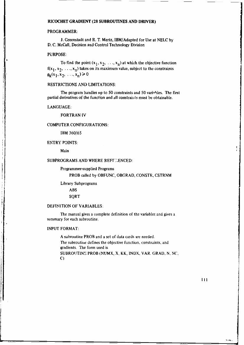
RICOCHET GRADIENT (28 SUBROUTINES AND DRIVER)

PROGRAMMER:

J. Greenstadt and R. T. Mertz, IBM/Adapted for Use at NELC byD. C. McCall, Decision and Control Technology Division

PURPOSE:

To find the point (xl, x2 ... , xn) at which the objective functionf(xl, x2 , ... , xn) takes on its maximum value, subject to the constraints

gk(xl,x2, .... xn)>

RESTRICTIONS AND LIMITATIONS:

The program handles tip to 50 constraints and 50 varinbles. The firstpartial derivatives of the function and all constraiiits must be obtainable.

LANGUAGE:

FORTRAN IV

COMPUTER CONFIGURATIONS:

IBM 360/65

ENTRY POINTS:

Main

SUBPROGRAMS AND WHERE REFE I•ENCED:

Programmer-supplied Programs

PROB called by OBFUNC, OBGRAD, CONSTR, CSTRNM

Library Subprograms

ABS

SQRT

DEFINITION OF VARIABLES:

The manual gives a complete definition of the variables and gives asummary for each subroutine.

INPUT FORMAT:

A subroutine PROB and a set of data cards are needed.The subroutine defines the objective function, constraints, andgradients. The form used isSUBROUTINE PROB (NUMX, X, KK, INDX, VAR. GRAD, N, NC,C)

Ill

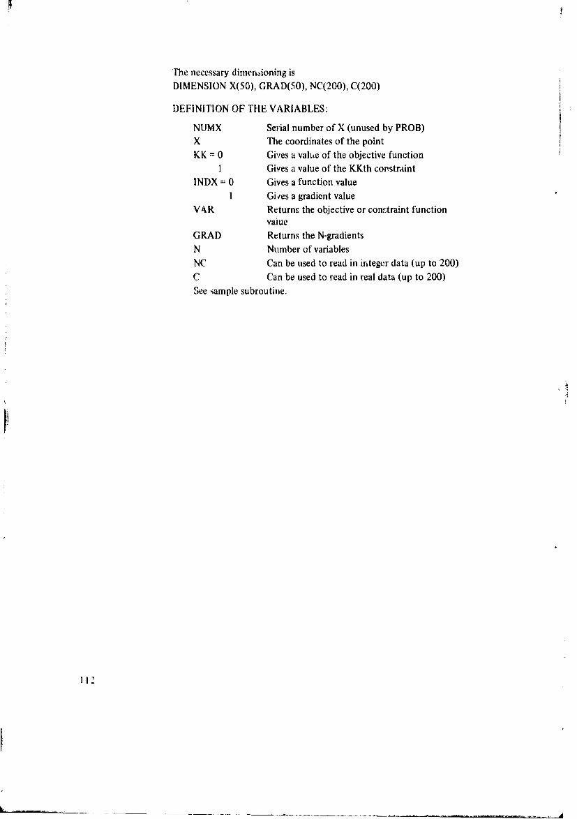
The necessary dimenaioning isDIMENSION X(50), GRAD(50), NC(200), C(200)

DEFINITION OF THE VARIABLES:

NUMX Sefial number of X (unused by PROB)X The coordinates of the pointKK = 0 Gives a valhe of the objective function

I Gives a value of the KKth corstraintINDX = 0 Gives a function value

I Gives a gradient valueVAR Returns the objective or con,,traint function

vaiueGRAD Returns the N-gradientsN Number of variablesNC Can be used to read in integer data (up to 200)C Can be used to read in real data (up to 200)See sample subroutine.

1 12

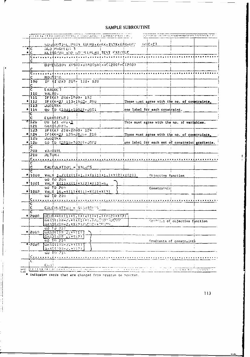
SAMPLE SUBROUTINE

17' J 2 3 13 4~ 3 7f5* 1 3 ,97I0' 3, 3 Th 5 6? 6 6 6 7 7 ?~1 'I7 -7

* C AL% ',i(O .Li 3 I F* C -"j. 1. P LAU TE T ".

C......... 6049

DP18E4j1IO, XNhýl. '•) (b ,N¢,%200) t- (200)

h *1.1100 IF I•)X) 210, ll0 1201C I_ _ _ _ _ _ _ _

110 VAL40• I __

11l 1F(IK) 200,1nUO, 112 1* 112 IF(kK-2) 113,iL, 2PO " _ These .,.ist 4gree with t e no. of constraints,

113 .J o=K* 114 (6U 0 (11 U 1 UOZ)'JGC1 ione label fir each constraint. _

C c I /A D TE1T II

12.{, Du 1 I- This must agree with the no. :f variables.121 (A( (J)•___ utr123 IF(kK) 21U#2000p 124 I f

* 1 IFýK-2.)1 . 210 ',!_These must Agree with t e no. of constraints ,_ _ -| '1

*126 GO * 0 (2'10P,'1AU0, tJG02 one label fir each set if constraint gradlents.

200 VA; VAt.L_ _

210 I,•TRJ I...... ............ q..............................,..... e.4t...S

C CAL ULATI011 - VjL7S _ ,C1 V001 VAt.: J./2() } ([bhjcctive function

* 0 1 VAL. • X ( _)____ _______ ____._(___-__.____'__

(t) o 20" 1- Constraints

* IOU? VAL- 16.-X(1)(Y(1)-X(2)*X(")GO 0 20-1

C .. . .. . r .. . . . . . . . .. . . .. . . .I ..

C CALdUI.AT!: -. ,

C 2 I C

*?(.OON ILEIF:r~0(×{I)+1.)*(ACt)+I.)*f(2),X(2) _______ ____

60 TO }['2U 210 k~1fl1TT7 . 4 ___ _____ __

60 0 21_ -,('radients of constrairtt" P 0o;e 01 .,1, rl ) 1 1-- ,, [ \3,1 ( %x) * Y 1 2 ____"______

C

* indicates cards that are changed from 7prograr, to pcon',ram.

113

The user-supplied data follow the required data. The user's data aredivided into seven classes; preceding each clas'; is a header card with theclass number in the first column. All other data cards must be blank in thefirst column and are read only through column 72.

The sever classes are:

0 Descnption of th;, prcblem

I Setting for the output control switches (See OUTPUT FORMAT)

2 Integer parameters used in the algorithm subroutines

3 Real parameters used in the algorithm subroutines, including the feasiblestarting point

Classes 2 and 3 usually use the same parawiieters from problem to problemexcept for the starting point.

The starting point begins in the 47th entry under Class 3, and is read inwith an E14.8, 3E15.8 format.

4 Siue of the problem. The number of variables A'i columns 2-5; the numberof constraints in L )Iumns 6-10.

5 Integer Parameters for the PROB subroutine - 14, 1515 format

6 Real Parameters for the PROB subrout.ne - E14.8, 3E15.8 format

The readi... in ot data is terminated by two cards with a 9 in column 1. 'ftii• program is to be rni more than once with diffeient data, one card witha 9 in column I is placed between the data for the different problems andtwo 9-cards are u', d to terminate the program.

114

II

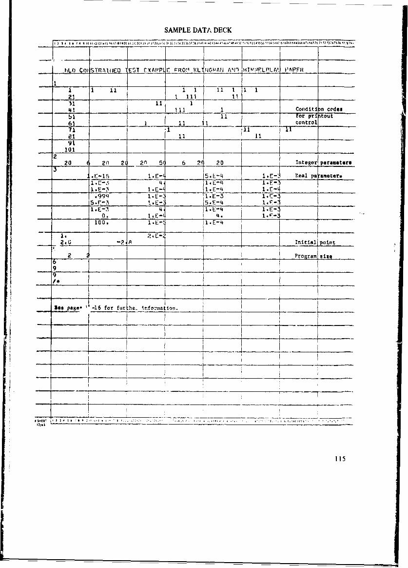
SAMPLE DATA DECK

S hLO C01jST.RAIIED 1EST FXAMPI, F FRO:q KL NGCMAN A,"I H ,TN.AFLPLA.. PAPF14 _ __

711

21 1 11 111 1 i

a1 11 1"4 _ _ __ _____ 1.11 1 ,__ Conditi n ccdeaS1 11 2 for" pri atout

61 I 1 1i 5*E_ _ control __________

71 11 iI1j

dl __E__3 11- -__ _ _ E-4_ __120 20 2 2n5 6 2 20 Integer paramEters

IsI

•_ -I:. j .E- 5IEn4 _ .E-'. Peal pe iameteru___ __ __ -___ __ 1. -I __ _ _ _ .E- 14 __ _ .__ _- __ _

- .9-3 I.E- I.E-3 1.F_-

_ _ _ _ _5. r-.3 i..E-. -_ __ _ _.j.E-4 ____ _.____-

I .E-.I 4 i.E .•-_i_0__ 0. i.E-,, __ __ I.E4 __ _ _ _ _ _ __ _ _ _ _ _

_ - -2 p/ 11E, Initial point

2 Program site

9 _

Be* page. -16 for furlhe, infozm o.__________ _____

1115__ _ _ _ _ _ _ __ _ _ _ _ _I_ __ _ _ _ _ _ _ _

j 2I __ __ _ __ _

115

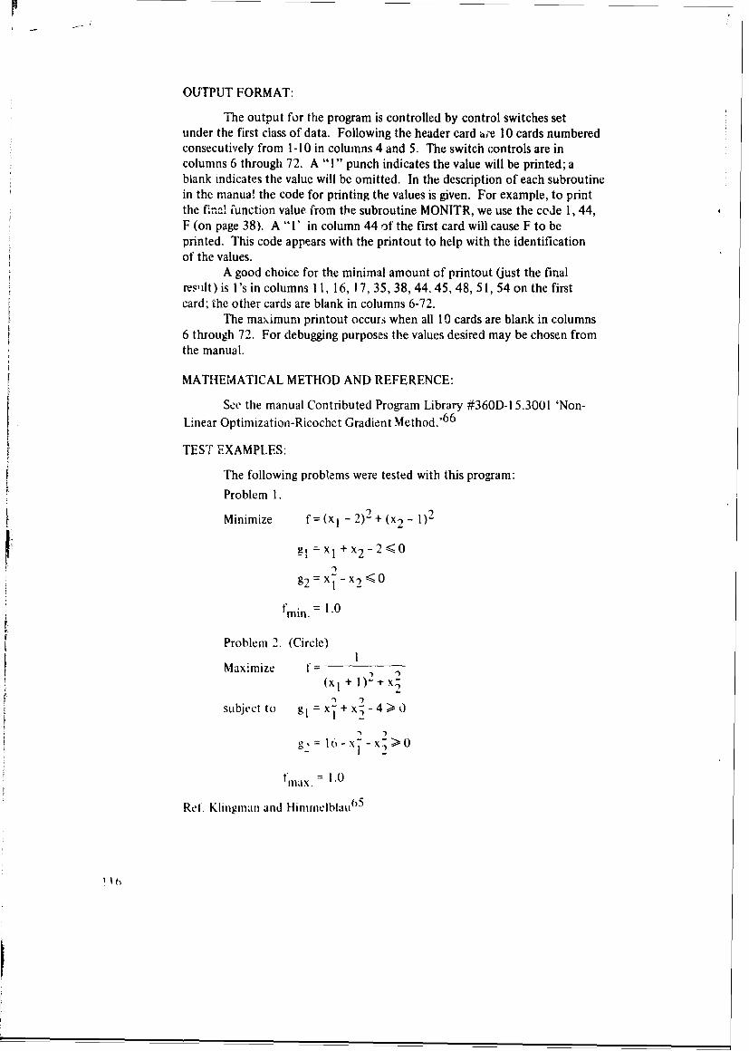
OUTPUT FORMAT:

The output for the program is controlled by control switches setunder the first class of data. Following the header card ire 10 cards numberedconsecutively from 1-10 in columns 4 and 5. The switch controls are incolumns 6 through 72. A "1" punch indicates the value will be printed; ablank indicates the value will be omitted. In the description of each subroutinein the manua! the code for printing the values is given. For example, to printthe fnia function value from the subroutine MONITR, we use the cede 1, 44,F (on page 38). A "I' in column 44 of the first card will cause F to beprinted. This code appears with the printout to help with the identificationof the values.

A good choice for the minimal amount of printout (just the finalresuilt) is l's in columns 11, 16, 17, 35, 38, 44, 45, 48, 51, 54 on the firstcard; ihe other cards are blank in columns 6.-72.

The maximum printout occurs when all 10 cards are blank in columns6 through 72. For debugging purposes th~e values desired may be chosen fromthe manual.

MATHEMATICAL METHOD AND REFERENCE:

See the manual Contributed Program Library #360D-I 5.3001 'Non-Linear Optimization-Ricochet Gradient Method.' 66

TEST EXAMPLES:

The following problems were tested with this program:

Problem 1.

Minimize f= (xi - 2)2 + (x2- 1)2

g1 =xi+x2,-2•O

g2 = xI + x2 - 2 0

fmin. = 1.0

Problem 2. (Circle)

Maximize f__(xI + 1) 2- tx

subject to g, =x- + x- - 4> 01 2,

10X- - X > 01 ~2

fiax. = 1.0

Ref. Klingman and Hiirnrelblau 5

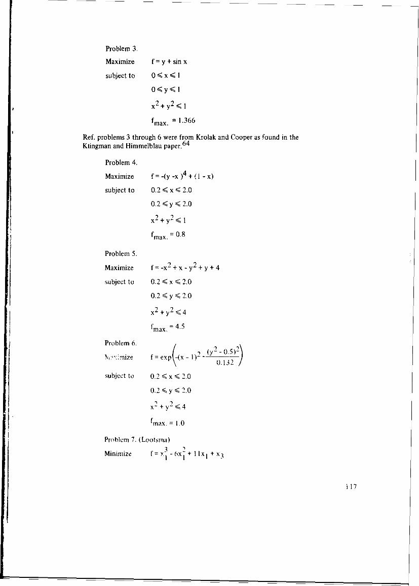
Problem 3.

Maximize f = y + sin x

subject to 0 < x < I

x2 +y 2 lI

fmax. = 1.366

Ref. problems 3 through 6 were from Krolak and Cooper as found in theKlingman and Himmelblau paper. 64

Problem 4.

Maximize f = -(y -x )4 + ( - x)

subject to 0.2 < x < 2.0

0.2 < y < 2.0

x2 +y 2 <I

fmax. = 0.8

Problem 5.

Maximize f = -x2 + x -y2 + y + 4

subject to 0.2 < x < 2.0

0.2 <y •<2.0

x2 + y2 < 4

fmax. = 4.5

Problem 6. /- /

N•,'mize f=exP((x- (y)2 -0"5

subject to 0.2 < x < 2.0

0.2 -y •<2.0

fmax. = 1.0

Problem 7. (Lootsma)

Minimize f = /- 6x + 1lxI +x 3

i17

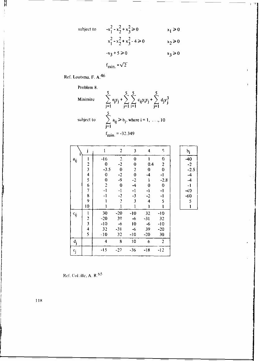
subject to -x2 x x2 +x2 >0 XI>01~ 2 32 2 2x1 -x+3-4 x2 > 0

-x 3 + 5> 0 0

fmrin. =,f

Ref. Lootsma, F. A.4 6

Problem 8.

Minimize + + ýMinmiz •'_., ejyj + _ cijYiYj + • jy

j=l J=l i=l j=!

5subject to aij > bi, where i 1, . ., 10

j=!

fmin. = -32.349

1 2 3 4 S bi

aij 1 -16 2 0 1 0 -402 0 -2 0 0.4 2 -23 -3.5 0 2 0 0 -2.54 0 -2 0 -4 -1 -45 0 -9 -2 1 -2.8 -46 2 0 -4 0 0 -17 -1 -1 -1 -1 -1 -498 -1 -2 -3 -2 -1 -609 1 2 3 4 5 5

10 1 1 1 1 1 1

ci 1 30 -20 -10 32 -102 -20 39 -6 -31 323 -10 -6 10 -6 -104 32 -31 -6 39 -205 -10 32 -10 -20 30

d- 4 8 10 6 2

ei -15 -27 -36 -18 -12

Ref. Col .,ille, A. R.65

1I1

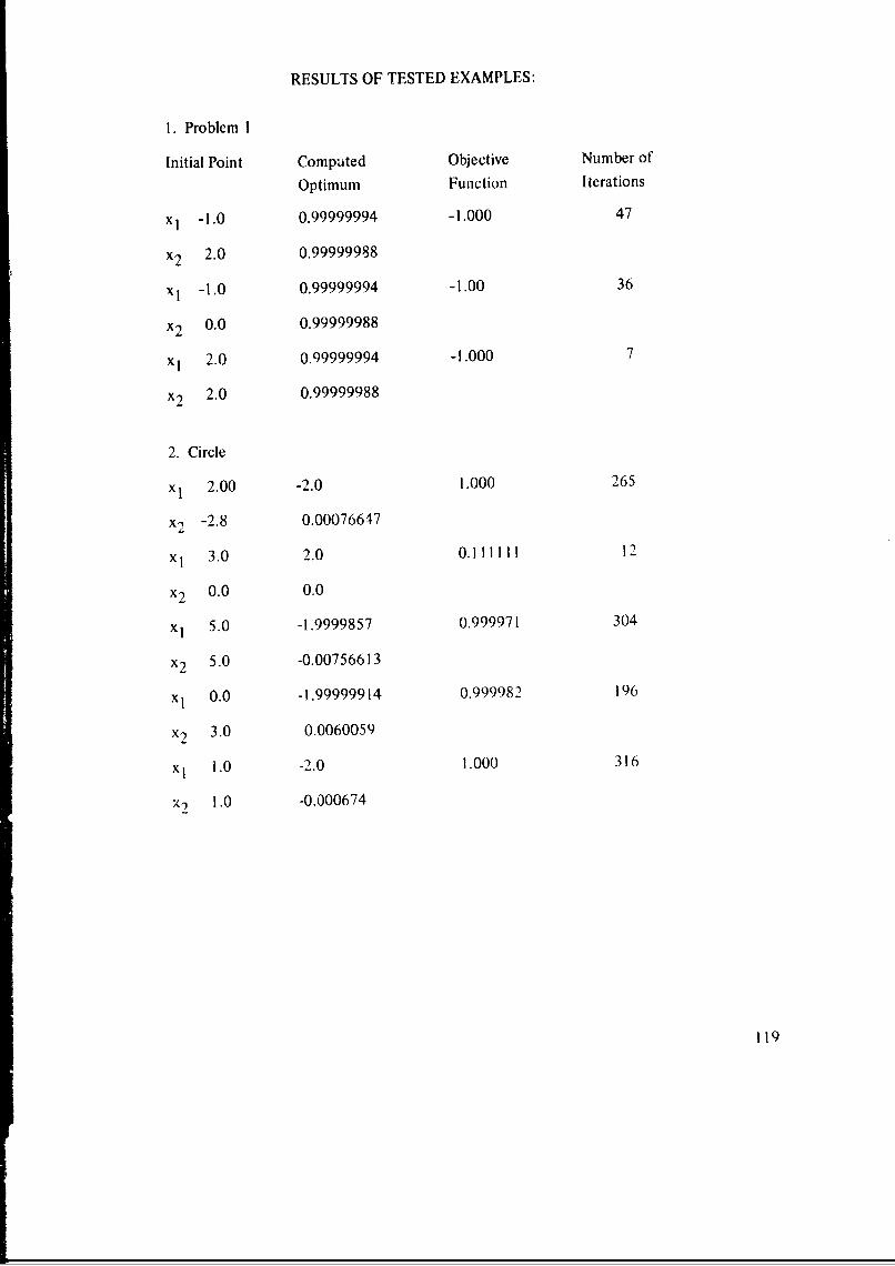
RESULTS OF TESTED EXAMPLES:

1. Problem I

Initial Point Computed Objective Number of

Optimum Function Iterations

x] -1.0 0.99999994 -1.000 47

x2 2.0 0.99999988

xi -1.0 0.99999994 -1.00 36

x2 0.0 0.99999988

xI 2.0 0.99999994 -1.000 7

x2 2.0 0.99999988

2. Circle

x 2.00 -2.0 1.000 265

x2 -2.8 0.00076647

x 3.0 2.0 0.111111 12

x2 0.0 0.0

xI 5.0 -1.9999857 0.999971 304

x2 5.0 -0.00756613

xI 0.0 -1.99999914 0.999982 196

x2 3.0 0.0060059

xI 1.0 -2.0 1.000 316

x-2 1.0 -0.000674

119

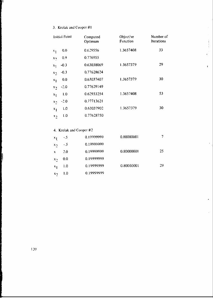
3. Krolak and Cooper #1

hIitial Point Computed Objectfve Number ofOptimum Function Iterations

,1 0.0 0.629556 1.3657408 33

x1 0.9 0.776955

x! -0.3 0.63038069 1.3657379 29

x- -0.3 0.77628624

xI 0.0 0.63037407 1.3657379 30

x- -2.0 0.77629149

xI 1.0 0.62933254 1.3657408 53

x, -2.0 0.77713621

xI 1.0 0.63037902 1.3657379 30

x1 1.0 0.77628750

4. Krolak and Cooper #2

x/ -.5 0.19999999 0.80000001 7

Xi -. 5 0.19999999

x 2.0 0.19999999 0.80000001 25

Xi 0.0 0.19999999

xI 1.0 0.19999999 0.80000001 29

Xi 1.0 0.19999999

120

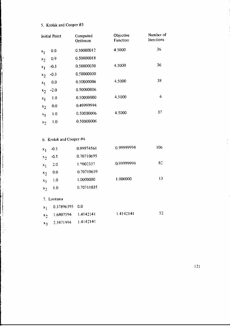
5. Krolak and Cooper #3

Initial Point Computed Objective Number of

Optimum Function Iterations

xI 0.0 0.50000012 4.5000 36

x'2 0.9 0.50000018

x -0.3 0.50000030 4.5000 36

x2 -0.3 0.50000030

x1 0.0 0.50000006 4.5000 38

x2 -2.0 0.50000006

x1 1.0 0.50000000 4.5000 6

x2 0.0 0.49999994

x 1.0 0.50000006 4.5000 37

x') 1.0 0.50000006

6. Krolak and Cooper #4

x -0.5 0.99974561 0.99999994 106

x2 -0.5 0.70710695

x 2.0 1.0002337 0.99999994 82

x 0.0 0.70710659

xI 1.0 1.0000000 1.000000 13

x2 1.0 0.70711035

7. Lootsma

xI 0.37896395 0.0

x2 1.6807594 1.4142141 1.4142141 52

x 2.3471994 1.4142141

121

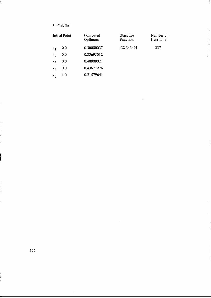
8. Colville I

Initial Point Computed Objective Number of

Optimum Function Iterations

x 1 0.0 0.30000037 -32.343491 337

x2 0.0 0.33695012

x3 0.0 0.40000027

x4 0.0 0.43677974

x5 1.0 0.21579641

I122

APPENDIX 3: REFERENCES

1. Dejka, W. J. and McCall, D. C., "A Study in the Design of a PracticalTunable Bandpass Filter Using Mathematical Programming," p. 267-270 in IEEE Systems Science and Cybernetics Conference, Pittsburgh,1970, Systems For the Seventies; Proceedings [Held] October 14-16,1970, at Pittsburgh, Pennsylvania, Institute of Electrical and ElectronicEngineers, 1970

2. Lasdon, L. S. and Waren, A. D., "Mathematical Programming For OptimalDesign," Electro-Technology, v. 80, p. 53-70, November 1967

3. Calahan, D. A., Computer-Aided Network Design, McGraw-Hill, 1968

4. "Special Issue on Computer-Aided Design," Institute of Electrical andElectronics Engineers. Proceedings, v. 55, No. 11, November 1967

5. Joint Conference on Mathematical and Computer Aids to Design, Anaheim,California, 1969, Digest Record, Institute of Electrical and ElectronicsEngineers, 1969 (IEEE Catalogue No. 69C63-C)

6. Rosen, J. B. and Meyer, R., "Solution of Nonlinear Two-Point BoundingValue Problems by Linear Programming," p. 71-84 in Conference onthe Mathematical Theory of Control, University of SouthernCalifornia, 1967, Mathematical Theory of Control: Proceedings of aConference Held at the University of Southern California, Los Angeles,January 30 - February 1, 1967, Academic Press, 1967

7. Naval Electronics Laboratory Center Technical Document 82, Direct-SearchMethods For the Solution of the Two-Point Boundary Value ProblemtT, PBVP1, by W. J. Dejka, 30 January 1970

8. Naval Electronics Laboratory Center lechnical Note 1417,* ComputerPrograms to Find the Minimum o" a Nonlinear Function of SeveralVariables, by P. S. Winterbauer, 1 August 1968

9. Fletcher, R. and Powell, M. J. D., "A Rapidly Convergent Descent MethodFor Minimization," Computer Journal, v. 6, p. 163-16;, 1963

*NELC technical notes are informal doctnments intended chiefly for use within the ('enter.

123

10. Fletcher, R. and Reeves, C. M., "Function Minimization by Conjugate

Gradients," Computer Journal, v. 7, p. 149-154, 1964

II. IBM Application Program H2-0205-3 System/360 Scientific Subroutine

Package (360A-CM-03X) Version III: Programmer's Manual, 1968

12. Naval Electronics Laboratory Center Technical Note 1628, Two Direct

Search Methods of MNathematical Programming, by D. C. McCall and

C. T. Ogata, 26 January 1970

13. Zangwill, W. I., "Miniinizing, a Function Without Calculating Derivatives,"

Computer Journal, v. 10, p. ,.93-296, 1967

14. Hooke, R. and Jeeves, T. A., "'Direct Search' Solution of Numerical and

Statistical Problems," Association For Computing Machinery. Journal,v. 8, p. 21-229, 1961

15. Leon, A., "'A Comparison Among Eight Ktiown Optimization Procedures,"p. 23-46 in Symposium on Rccent Advances in Optimization Techniques,

Carnegie Institute of Technology, 1965, Edited by T. P. Vogl, Wiley, 1966

16. Hadley, G., Linear Programming, Addison-Wesley, 1962

17. Zoutendijk, G., Methods of Feasible Directions, Elsevier Publishing Company,

1960

18. IBM Application Program H20-0476-1, Mathematical Programming System/

360 (360 \-CO-14X) Version 2, Linear and Separable Programming -

User's Manual, 30 April 1969

19. IBM Application Program H2C-0603-0, Mathematical Programming System,'360 (36,OA-CO- 14X) Message Manual, March 1969

.1 IBM Application Program H20-0372-1, Mathematical Programming System/

300 36•A-CO- 14X) Read Communications Format [READCOMM 1.Program Reference Manual, D)ecember 1968

"21. Griffith, R. F. and Stewart, R. A., "A Nonlinear Programming Technique Forthe Optimization of Continuous Processing Systems," Management Science,v. 7. p. 379-392, July 1 1) 1

124

22. Rosen, J. B., "The Gradient Projection Method For Nonlinear Programming:

Part 1, Linear Coastraints," Society For Industrial and Applied Matherna-

tics. Journal, v. 8, p. 181-217, March 1960

23. California Institute of Technology. .Jet Propulsion Laboratory Techn~calMemorandum 240, Computing Quadratic Programmuing Problems:

Linear Inequality Constraints, by R. J. Hanson, 9 February 1970

24. Fiacco, A. V. and McCormick, G. P., Nonlinear Programming: SequentialUnconstrained Minimization Techniques, Wiley, 1968

25. Hartley, 11. 0. ad Hocking, R. R., "Convex Programming by Tangential

Approximation," Management Sciencce, v. 9, p. 600-612, luly 1963

26. IBM. Contributed Program Library 3601)-15.3.001, No,.-Linzear Optimiza-

tion -- Ricochet Gradient Method, by J. Greenstadt and R. T. Mertz,

October 1967

27. Research Analysi3 Corporation, A User's Manual For Experimental SUMT:

The Computer Program Implementing the Sequential Unconstrained

Minimization Technique For Nonlinear Programming, by G. P. McCormickand others, March 1970

28. IBM. Program Information Department Program 360D-I15.2.011. Zero-One

Integer Linear Programming With Heuristics, by B. D. Holcomb, 1968

29. IBM. Program Information Department Program 3600-15.2.005, Branch

and Bound Mixed Integer Programming BBMIP, hy R. Shareshial,

April 1967

30. Pace Company, Comparison of Integer Programming Algorithms, -yW. J. Mears and G. S. Dawkias, 1-3 May 1968 (Paper presented at the

Joint National Meeting of the Operations Research Society ot Americaani the Institute of Management Sciences, San Fra,,cisco)

31. Stanford University. Operations Research D)eparntmcnit Technical Report 1 I1Bound-and-Scan Algorithm For Pure Integer I incar Progra lifing Willh

General Variables, by F. S. tlillier. 20 May I t)()

125

32. Wolfe, P., "Review of Nonlinear Programming," p. xi-xv in Optimization,

cdited by R. Fletcher, Academic Press, 1969

33. IBM Application Program H20-0147-0, 1620 Electronic Circuit Analysis

Program [ECAPI (I 620-EE-02X); Application Description, n.d.

34. Lee, H. B. and others, "Program Refines Circuit From Rough Design Data,"

Electronics, v. 43, p. 58-65, 23 November 1970

35. University of California, Los Angeles. Department of Engineering,

A Critical Evaluation of the Numerical Significance of Gencral

Circuit Analysis Programs ir. Relation to the Tranisient Problem,

by D. E. Meyerhoff and L. P. McNamee, i.d.

36. Aoki, M., Introduction to Optimization Techniques Fundamentals and

Applications of Nonlinear Programming, Macmillan, 1971

37. Gear, C. W., "The Automatic !,itegration of Large Systems of Ordinary

Differential Equations," p. 27-29 in Joint Conference on Mathemati-

cal and Computer Aids to Design, Anaheim, California, 1969, Digest

Record, Institute of Electrical and Electronics Engineers, 1969

(IEEE Catalogue No. 69C63-C)

38. Cal 'ian, D. A., "Numerical Considerations in the f ransient Analysis andthe Optimal Design of Nonlinear Cihcuits," p. 129-145 in Joint Confer-

ence on Mathematical and Comnputer Aids to Design, Anaheim,

California, 1969, Digest Record, Institute of Electrical and Electronics

Engineers, 1969 (IEEE Catalogue No. 69C63-C)

39. Box, M. J., "A Comparison of Several Current Optimization Methods and

the Use of Transformations in Constrained Problems," Computer

Journal, v. 9, p. 67-77, 1966

40 Hildebrand, F. B., Introduction to I imerical Analysis, McGraw-Hill, 1956

41. Stewart, G. W., HI, "A Modification of Davidon's Minimization Method

to Accept Difference Approximations of Derivatives," Association

For Computing Machinery. Journal, v. 14, p. 72-83, January 1967

126

42. AEC Research Development Report ANL-5990, Revision 2, Variable

Metric Method For Minimization, by W. C. Dav don, February 1966

43. Rabinowitz, P., "Applications of Linear Programming to Numerical

Analysis," S I A M Review (Society For Industrial and Applied

Mathematics), v. 10, p. 128-159, April 1968

44. Zangwill, W. I., Nonlinear Programming: A Unified Approach, Prentice

Hall, 1969

45. Kuhn, H. W. and Tucker, A. W., "Nonlinear Programming," p. 481-492in Berkeley Symposium on Mathematical Statistics and Probability,Proceedings. Second, University of California, 1950, University of

California Press, 1951

46. Lootsma, F. A., "Logarithmic Programming: A Method of SolvingNoalinear Programming Problems," Philips Research Reports, v. 22,

p. 329-344, June 1967

47. Zoutendijk, G., "Nonlinear Programming: A Numerical Survey,"

S I A M Journal on Control (Society For Industrial and Applied

Mathematics), v. 4, p. 194-2 10, February 1966

48. Pierre, D. A., Optimization Theory With Applications, Wiley, 1969

49. Gomory, R. E., "Outline of an Algor.thm For Integer Solutions to

Linear Programs," American Mathematical Society. Bulletin,

v. 64, p. 275-278, September 1958

50. Stanford University. Operations Research Department Technical

Repert 10, Efficient Heuristic Procedures For Integer LinearProgramming With an Interior, by F. S. Hillier, 28 February 1969

51. Illinois. University. Computer Science Department Report 264,1. l Logical Design of an Optimal Network by Integer Linear Pro-

"gramming, Part I, by S. Muroga, 18 July 1968

52. Pyne, 1. B. and McCluskey, E. J., "An Essay on Prime Implicant Tables."

Society For Industrial and Applied Mathematics. Journal, v. 9,

p. 604-631, December 196

k127

53. Breuer, M. A., "Logic Synthesis," p. 146-164 in Joint Conference on

Mathematical and Computer Aids to Design, Anaheim, California,

1969, Digest Record, institute of Electrical and Electronics

Engineers, 1969 (IEEE Catalogue No. 69C63-C)

54. Kodres, U. R., "Logc Circuit Layout," p. 165-191 in Joint Copf`renceon Mathematical and Computer Aids to Design, Anaheim, California,

1969, Digest Record, Institute of Electrical and Electronics Engineers,

1969 (IEEE Catalogue No. 69C63-C)

55. Breuer, M. A., "The Application of Integer Programming in Design Auto-

mation," SHARE Design Automation Workshop, Proceedings, 1966

56. McCluskey, E. J., "Error Correcting Codes: A Linear Programming

Approach," Bell System Technical Journal, v. 38, p. 1485-1512,

November 1959

57. Karp, R. M., "Minimum-Redundancy Coding For the Discrete Noiseless

Channel," Institute of Radio Iýngikeers. Transactions: Information

Theory, v. IT-7, p. 27-38, January 1961

58. Saaty, T. L. and Suzuki, G., "A Nonlinear Programming Model in

Optimum Communication Satellite Use," S I A M Review (Society

For Industrial and Applied Mathematics), v. 7, p. 403-408, July I ' 5

59. Carnegie Institute of Technology ONR Research Memorandum 116,

A Study of the All-Integer Integer Programming Algorithm, by

F. Glover, September 1963

60. Rosenbrock, H. H., "An Automatic Method For Finding the Greatest or

Least Value of a FLUIction," Computer Journal, v. 3, p. 175-184, 1960

61. Powell, M. J. D., "An Efficient Method of Finding the Minimum of a

Function of Several Variables Without Calculating Derivatives,"

Computer Journal, v. 7, p. 155, 1964

62. Powell, M. J. D., "An Iterative Method for Finding Stationary Values of

a Function of Several Variables," Computer Journal, v. 5, p. 147, 1962

128

63. Fletcher, R., "Function Minimization Without Evaluating Derivatives - aReview," Computer Journa!, v. 8, p. 33, 1965

64. Klingman, W. R. and Himmelblau, D. M., "Nonlinear Programming With the

Aid of a Multiple-Gradient Summation Technique," Association For

Computing Machinery. Journal, v. 11, p. 400-415, October 1964

65. IBM Data Processing Division Technical Report No. 320-2949, A Comparative

Study on Nonlinear Programming Ccjes, New York Scientific Center, by

A. R. Colville, ;une 1968

66. Contributed Program Library #360D-I 5.3001, Non-Linear Optimization -Ricochet Gradient Method

REVERSE SIDE BLANK 129