Mathematical development and verification of a non-orthogonal finite volume model for groundwater flow applications

D. Loudyi a, R. A. Falconer a,*, B. Lin a

aHydroenvironmental Research Centre, Cardiff School of Engineering, Cardiff University, Cardiff, CF24 3AA, UK

Abstract The mathematical development of a two-dimensional finite volume model for groundwater flow is described. Based on the hydraulic equations for saturated flow, the model deploys a least-squares gradient reconstruction technique (LSGR) to evaluate the gradient at the control volume face, derived from the application of the finite volume formulation and using a cell-centred structured quadrilateral grid. The model turns to a finite difference model with orthogonal grids. The effects of grid non-orthogonality and skeweness are investigated. The model was verified by comparison with analytical solutions and the results for a finite difference model. The finite volume model was then applied successfully to an aquifer discharging in a section of the River Tawe, and the results were compared with results from MODFLOW and observed hydraulic heads. Results of the numerical model tests and field exercise showed that the use of finite volume method provides modellers with a consistent substitute for the finite difference methods with the same ease of use and an improved flexibility and accuracy in simulating irregular boundary geometries. Keywords: Finite volume; Groundwater flow; Non-orthogonal grid; Finite difference comparison

1. Introduction Most groundwater problems require an accurate simulation of the flow, in particular, the accuracy of the results from solute-transport models rely heavily on the ground-water velocities calculated from flow models. Furthermore, variable-density groundwater models are even more dependent upon the flow simulation since the groundwater velocities are, in turn, affected by the solute concentrations. This requirement has stimulated the development of many numerical models backed up by advanced verification tests. The finite difference technique was one of the first methods to be used for various types of flow problems and its applications have been widely developed. As other numerical solution methods for similar governing equations arising from CFD applications have continuously emerged, (namely the finite element (FE), integrated finite difference (IFD), boundary element (BE) and finite volume (FV) methods), they have been increasingly introduced into groundwater modelling studies. All of these widely used methods have already been discussed in groundwater applications, and some of the corresponding codes have been developed and applied successfully (Table 1).

Table 1. Various codes widely used for simulating groundwater flow problems

The choice of whether to use one method or another is generally a matter of personal preference. Furthermore, there is currently still much research being undertaken on developing better mixed or adaptative methods, that aim to minimize numerical errors and combine the best features of alternative standard numerical approaches [8,9,19,35,38,39]. Finite difference – based models, such as MODFLOW, are generally attractive to practitioners, with this approach providing advantages of ease of meshing the domain, a relatively simple formulation, and the scope for solving the resulting system of discretised equations in a straightforward manner. This numerical method is known to have many strengths, but it also has the shortcoming of its rigidity in conforming to boundary geometries and a corresponding loss of accuracy in predicting hydraulic heads along and near these boundaries [3,47]. The use of a rectangular grid to discretise the problem domain necessitates a stepwise approximation of irregular boundaries and aquifer zoning. Haitjema et al.20 found that an accurate flow field prediction could be obtained in the FD model MODFLOW if the boundary conditions in the groundwater flow regime were represented accurately and with the appropriate cell sizes. In regions with singular velocities (e.g. near corners), or strongly converging or diverging flow, or zones with a contrasting transmissivity level, then a large number of grid cells were required. It should be noted that, given the nature of a finite difference grid, the cell sizes are restrictively dependent upon the number of cells (i.e. rectilinear rows and columns). Barrash et al.5 found that the finite difference formulation underestimated large head gradients that can occur in the vicinity of pumping (or injection) wells. Generally, a detailed representation of the flow field in the vicinity of hydrological features and through irregular hydrogeological units (e.g. discontinuities, or very thin units) requires a relatively small grid spacing. Moreover, the accuracy of contaminant transport models, particularly for advection dominated transport, is particularly conditional upon the use of small cell sizes. Many authors choose to reduce or eliminate the FD limitations by using techniques of mesh refinement [30,41]. However, fine grids can result in long execution times that prohibit the many model runs often needed to understand the system dynamics and calibrate the model. As an alternative to grid refinement for more accurate local modelling, the grid structure can be made more flexible. Among the latest numerical techniques to be developed is the finite volume method, which is based on the integration of the governing equations of fluid flow over a control volume (CV) that can have any shape with rectilinear sides, structured or unstructured and with flow variables associated with a point inside the cell (i.e. the cell-centred FV) or attached to cell vertices (i.e. the cell-vertex FV). The finite volume procedure can be

Code Type of numerical solution References

AQUIFEM-N FE Townley44

BEMLAP BEM Kirkup29

FEMWATER FE Lin et al.31

FTWORK FD Faust et al.16

MODFLOW FD McDonald and Harbaugh34

SUTRA FE-IFD Voss48

considered as a variant of the finite-element method [20], although, from another viewpoint this method constitutes a particular type of finite difference scheme [36]. The most attractive feature of the FV method is that the resulting solution implies integral conservation of quantities such as mass, momentum, and energy over the CVs. Therefore these quantities are conserved over the whole calculation domain, for any number of grid points. In contrast, for the FD method the conservation principle is only generally satisfied for infinitesimal CVs. The FE method does not conserve mass at the local level for certain schemes [10]. Another advantage of the FV method is that the mesh offers greater geometrical flexibility vis-à-vis the FD method and the integrated finite difference method, in the sense that the line joining two grid points does not necessarily have to be perpendicular to a given CV surface. More recently, Zheng44 developed a higher-order finite-volume TVD method, within the code MT3D, for transport simulation. Heberton et al.19 also have developed a finite volume Eulerian-Lagrangian method to solve the transport equation, as used in MOC3D. Both methods, however, are based on the finite difference cell structure and use the FD model MODFLOW to drive their interstitial fluid velocity components. From these perspective, and to overcome the considerable difficulty that the orthogonality condition presents in the representation of the problem domain with well-fitted grid, and with grid generation techniques becoming more complex, a variant of the finite volume approach close to the FD method is suggested herein, where any grid shape may be used, and the simplicity of the mathematical formulation of the FD method is conserved. A finite volume discretisation of the saturated groundwater flow equation on a structured non-orthogonal grid has been developed. As the form of the diffusion term governing the groundwater flow equation is common to a wide range of similar physical processes, such as heat, magnetics, gas dynamics, petroleum reservoir simulation, etc. [21], the main challenge arising from most FV applications is the handling of the cross diffusion term on cell faces. The accuracy of a control volume discretisation depends heavily on the order of approximation of the flux at the cell faces [39] and many methods have been proposed to approximate the gradient along a control volume surface for different CFD applications [9,12,13,22]. A comparison between some of these techniques has been undertaken in Jayantha and Turner22 and Loudyi28. One of these techniques, namely the improved least squares gradient reconstruction (ILSGR) [22] has appeared to be an ideal approach to handle the diffusion term with regard to accuracy and simplicity of the generated matrix equations. In this paper a cell-centred finite volume model of the groundwater equation using ILSGR technique is presented. The method uses a boundary-fitted computational grid to gain flexibility in representing complex boundary geometries and improve on the accuracy of the predictions, based on the premise that the finite volume method has the inherent advantage of being unconditionally mass conservative. To maintain the familiar properties of block-centred finite difference methods, rectangular grids have been replaced by structured quadrilateral cell-centred grids (see Fig. 1). Conformity with the discretisation methods of block-centred finite difference methods has been maintained by using the (i,j) indexing system (see Fig. 1). Three benchmark and analytical tests have been used to verify the refined numerical model and assess the accuracy of this scheme, along with its performances and limitations. The model has also been applied to an

aquifer drained by a reach of the River Tawe, in the UK. The results were compared with observation data and the results from another FD model.

Fig. 1. Space discretisation convention in MODFLOW and its equivalent finite volume discretisation. 2. Governing equations The transient saturated groundwater flow through porous material is governed by the elliptic partial differential equation:

qvthSs . with hKv (1)

where v is the Darcy velocity, LT-1 ; K is the hydraulic conductivity of the porous media, LT-1; h is the hydraulic head, L; Ss is the specific storage coefficient, L-1 ; t is time, T; q is the volumetric flux per unit volume (positive for inflow and negative for outflow),T-1; and xi are the Cartesian co-ordinates, L. Eq.(1) is valid for a two-dimensional (and three-dimensional) flow through an inhomogeneous anisotropic medium, with K representing the second rank tensor of hydraulic conductivity of an anisotropic medium and consisting of four components (nine in 3D) that may vary in space, for the case of an inhomogeneous medium (Bear, 1972[6]). Symbolically, K is written as:

yyyx

xyxx

KKKK

K (2)

where the hydraulic conductivity tensor is symmetric. Hence, in a two-dimensional flow only three distinct components (six in 3D) are needed to define fully the hydraulic conductivity. It has been shown that it is always possible to find two mutually orthogonal directions, called the principal directions of the anisotropic medium, such that these directions may be used to form the coordinate system (Bear, 1979[7]). Therefore, the components jiK , = 0 for all ji and 0, jiK for ji , then Eq. (2) becomes:

KYKXK0

0 (3)

where KX and KY are values of the hydraulic conductivity in the x and y coordinate axes[LT-1] respectively.

1

23

4

5

6

1

2

3 4

5

6

4 5 6 7 Column (j) 1 2 3 4 5 6 7 8

Row (i)

321

8 9

3. Finite volume discretisation Integrating the general differential Eq. (1) over an arbitrary control volume (area in two dimensions) V and applying the Gauss divergence theorem yield:

Vs

VVdV

thSqdVdsnhK ˆ

(3)

where dV is the volume of the considered element, V is the boundary of V, ds is the surface measure on V and n represents the outward normal area vector at the control volume boundary (see Fig. 2). Discretising Eq. (3) on a quadrilateral grid yields:

VthSqVAnhK s

fff

4

1

ˆ)( (4)

where f is a subscript denoting cell faces and Af is the surface vector of a cell face f. One of the main potential problems at this stage is the handling of the diffusion term. The integration of this term over a control volume leads to the necessity to estimate the derivative of h with respect to the face normal. 3.1. Gradient approximation The block-centred finite difference method approximates the gradient on a surface using a two-node backward difference scheme. In Fig. 2a, the gradient of h in the x direction from cell P to cell N is approximated by:

PN

PN

S xx

hh

x

h

NP

(5)

In the y direction the derivative is null as the cells are orthogonal. With the finite volume method, the approximation of the gradient term for a common face presents more complexity as the grid is no longer orthogonal (see Fig. 2b). In fact, the accuracy of a control volume discretisation depends heavily on the order of approximation of the flux at the cell faces [39].

Fig. 2. Two adjacent cell-centred control volumes for: (a) finite difference method, and (b) finite volume method.

Many methods have been proposed to approximate the gradient or fluxes along a control volume surface as the question has arisen from several CFD applications (Morel, 8,12,13,15,27,31,43]. In this model, the higher order gradient approximation technique suggested by Jayantha and Turner22 2003 has been developed furtherand will be termed hereinafter the GWFV model. The method is applicable even for highly anisotropic media, where the K tensor is not necessarily diagonal. This method can be used for any cell shape (e.g. quadrilateral, triangular, polygon). The principle used in this method is to

N P N P

R

F n

decompose the flux, using the vectors u and v in Fig. 3, and then introducing corrections for mesh skewness using the improved least squares gradient reconstruction (ILSGR) technique. B

Fig. 3. Representative control-volume face.

In the first step, and for computational purposes, the term nhK ˆ of Eq. (4) is written

as nKhwh T ˆ and which can be decomposed as follows: uhvhwh ˆ (6)

where the constants α and β depend on the tensor K and the geometry of the CV mesh. The vector v connects adjacent nodes and u is the unit vector along the CV face (Fig. 3). The first term in Eq. (6) is generally approximated using the first order Taylor approximation where PN hhvh . The second term, called the cross-diffusion term, requires evaluation of the gradient of h at the CV face. The accuracy of the estimation of the scalar wh depends primarily on the accuracy order associated with the approximation of the first term (Jyantha 2003a[22]). The ILSGR method maintains a second order spatial accuracy for the approximation of both terms. The method consists of explicitly representing the terms of Eq. (6) by decomposing the vector nKw T ˆ in terms of the vectors v and u . Using the two vector equations nnvuuvv ˆˆ.ˆˆ. and

nnwuuww ˆˆ.ˆˆ. , the following formula can then be obtained:

nv

uuvvnwuuww

ˆˆˆˆˆˆ

(7)

Therefore, the term wh can be expressed as:

uhnvuvnwuwvh

nvnwwh ˆ

ˆˆˆˆ

ˆˆ

(8)

In Eq. 4, the primary term vh. needs to be evaluated at the midpoint F of the CV face instead of point R (see Fig. 3), so that errors due to mesh skewness will be corrected. Using a Taylor series expansion of the function h yields:

Rxhxk

xxhm

kF

k

F0

)(!

1 (9)

and

Rxhxk

xxhm

kF

k

F0

)(!

1 (10)

v

t

P N

A

R

F

ux

nx

where the remainder term R has the Lagrange form. Subtracting Eq. (10) from Eq. (9), and assuming 0 RR , yields:

npPNF hhvh (11)

where

m

kF

kk

np xhxxk2

)(!

1 (12)

and m is the order of the Taylor expansion. In this study, the accuracy will be limited to second order. Thus, the correction term in Eq. (12) becomes:

)(21 22

Fnp xhxx (13)

Substituting Eq. (11) in Eq. (8), yields:

FnpFPNF nvnwuh

nvuvnwuwhh

nvnwnhK )(

ˆˆˆ

ˆˆˆˆ

ˆˆˆ

(14)

When the implicit scheme is used, the scalar term FnhK ˆ in Eq. (4) should be

evaluated at the time step n+1. However, terms uh ˆ. and np at the CV faces in Eq. (14)

are not readily available at the time step n+1. Therefore, they are evaluated at the nth time step. These terms are computed using the ILSGR, where the values h at nodes Nd, connected to point F, are expressed as follows (see Fig. 4):

Fk

d

m

kdF xhx

kxxh

.!

1

0

(15)

When Eq. (15) is written for a chosen number r of nodes Nd, d=1,2,…r, connected to point F, a system of equations is obtained. Therefore, as m = 2, a minimum of six nodes is required. In this study, a stencil of nine cells has been used (see Fig. 4), with the following over-determined system of equations then being obtained (for m=2):

99

29

29

99

22

22

22

22

11

21

21

11

221

......

......

......22

1

221

yxyx

yx

yxyx

yx

yxyx

yx

F

F

F

F

F

F

yx

h

y

h

x

h

y

h

x

hh

2

2

2

2

2

9

2

1

.

.

.

h

h

h

(16)

which can be written as HMX D where M is a matrix of order (9,6). This means that the set of Eq. (16) is over-determined, and thus should be reduced to a linear least-squares problem of the type HMMXM T

DT . Equations related to boundary conditions

have to be carefully inserted into this system. The system is then multiplied by

)(99 kwDiagW and TM to find the components that minimise 2

HMX D in the least

squares sense and with respect to a weighted inner product on Rr. The resulting normal system is given as:

WHMXWMM TD

T (17)

The weight coefficients, wk, are chosen such that 2 kk vw for the numerical

simulations. To solve the system of Eqs. (16), LU decomposition is used to obtain the least square solution vector XD at the mid-point of each cell face and for each time step. Thus, the terms uh ˆ. and np can be evaluated, and the fluxes through the CV face are

calculated using Eq. (13).

Fig. 4. Neighbouring nodes involved in surface flux calculation.

3.2 Approximating the hydraulic conductivity on a control volume face In Eq. (4) the hydraulic conductivity K has also to be evaluated at cell faces. In block-centred finite difference models, this is achieved using arithmetic, harmonic or logarithmic mean of the hydraulic conductivities at the two adjacent cells. In a finite volume discretisation, an equivalent hydraulic conductivity has to be assessed at the face between two adjacent quadrilateral cells that are not necessarily orthogonal. Croft9 proposed the use of a harmonic mean value to describe the variation of such a coefficient between nodes. As the line connecting nodes N and P does not necessarily lay along the normal face f (see Fig. 2(a)), nor does it pass through the centre of the face, then another approximation is made to take into account these types of skewness (i.e. non-orthogonality and non-conjunctionality). In Fig. 2(b) for instance, the hydraulic conductivity along face f can be estimated by using the formula:

N

FN

P

PF

FNPFf

KXxx

KXxx

xxxxKX

and

N

FN

P

PF

FNPFf

KYyy

KYyy

yyyyKY

(17bis)

This approximation yields the same expression as the harmonic mean when the mesh is fully orthogonal. 3.3. Boundary conditions Three types of boundary conditions are used in groundwater flow simulations, namely: the Dirichlet boundary condition; the Neumann boundary condition; and the Cauchy boundary condition. For cells having a face coincident with the domain boundary, information is introduced into the equation to complete the formulation and enabling the

F

equation to be solved. One of the advantages of the cell-centred control volume technique is the ease with which the boundary conditions can be accommodated within the scheme (Turner, 1995). In the new discretisation, the heads at surrounding cells of the stencil are needed to calculate the flux at faces of cells along boundaries (see Fig. 5). Nine point values are required to write the matrix given in Eq. (16). Thus, values at cells that cannot appear at boundaries are replaced with existing adjacent cells (empty circles), and associated vectors are extended only to the centre of the boundary face, as shown with filled circles in Fig. 5.

Fig. 5. Typical boundary control volume and related point values. 3.4. Source Term In Eq. (4), the source term can be written as:

PPP

V

QSVqqdV

where VP is the volume (with unit depth) of node P, and qP is the volumetric flux per unit volume,T-1, accounting for flows into or out of cell P from processes external to the aquifer, such as streams, drains, areal recharge, evaporation, wells and sinks. For most of these physical processes, the source term QSP can generally be linearised (patank) giving:

PPPP hQHQCQS (18) where QSP is the sum of the flows from all external sources affecting the cell P, L3T-1; and QHP and QCP are constants, L2T-1 and L3T-1. 4. Transient term – temporal discretisation In Eq. (4), the transient term is approximated by using the backward-difference scheme as follows:

. 1,

1,

, i,jm

m

mji

mji

S

V

S Vtt

hhSdV

thS

ji

(19)

where the superscript m denotes the old-time step value, Vi,j is the volume of the control volume defined by node (i,j), t is the time step and hP denotes the value of h at the centroid of the cell P. In the model GWFV, the matrix Eq. (13) is solved explicitly. At each time step m+1, the vector XD , that provides the function value and its derivatives at each CV face, is required to compute uh ˆ. and np in Eq. (14) with the vector values being available from

F

the previous time step m. In the GWFV model, as in block-centred finite difference models, only five unknowns exist for each cell at each time step. 5. Formulation of linear equations and solution method Using the indexing system (i,j), the substitution of approximation terms into Eq. (4) gives the finite volume approximation for cell (i,j) as:

ji

mm

mji

mji

jijim

jijim

jim

jiji

mji

mjiji

mji

mjiji

mji

mjiji

Vtthh

SQChQHhhH

hhFhhDhhB

,1

,1

,,,

1,,

1,

1,1,

1,

11,,

1,

11,,

1,

1,1,

(20)

where the coefficients Bi,j, Di,j, Fi,j, and Hi,j depend upon the shape and hydraulic conductivity at cells associated with node (i,j). This equation is common to both finite difference models and the GWFV model where only five nodes of the cross stencil are required (see Fig. 6).

Fig. 6. Five-node stencil and indexing system used in the linear equation.

The flow terms on the left-hand side of Eq. (4) are specified at time t+t, while the transient term, as shown in Eq. (19), is approximated using the difference between the head at time t and the head at the next time step t+t. The model involves expressing the head at the considered cell and its four neighbouring nodes with different coefficients which, for the implicit scheme, yields a matrix that needs to be treated individually. The resulting matrix in the GWFV model, as in block-centred finite difference models, is a symmetric sparse banded matrix with five non-zero diagonals, and has the common form:

BXA

The banded system is always positive definite. Generally, the stability of finite difference methods is satisfied when the interpolation operators are symmetric and positive definite (Hymann and Shashkov, 1999). Therefore, these properties should be sought in the current schemes to guarantee stability. The GWFV model shows similarities in the generated-matrix properties with finite difference methods, and is closer to the ideal criteria of the matrix resulting from discretisation on a quadrilateral grid. The matrix is symmetric, positive definite and diagonally dominant and a specific analysis of the model accuracy is considered further. For the GWFV model, the iterative procedure used to solve the system of algebraic equations is the Strongly Implicit Procedure (SIP). This method has proved to be the best

i,j

i-1,j

i+1,j

i,j-1i,j+1

for large systems (Patank1980) and provides accurate solutions if the proper combination of the solver parameters is chosen. 6. Numerical tests 6.1 Test 1: Numerical error – Sensitivity to mesh size In finite difference models, non-orthogonality is not an issue, but the predictions do depend upon the grid size and time steps (Andersen 1993, Haitjema et al. 2001). In this test the effects of the grid structure, in terms of cell sizes, on the behaviour of numerical error and convergence of the new scheme have been investigated. A test problem similar to the one used by Morel et al. (1992), has been used to demonstrate the accuracy of the new model as a function of the mesh size for ‘random’ meshes. A 10 10 m square area was used to simulate a two-dimensional flow through a porous media. The domain was meshed with a quadrilateral grid of five different levels of discretisation (see Fig. 9). Each mesh was generated from a uniform orthogonal mesh by moving each interior node in a random direction, on a circle of radius equal to 20% of the interior-nodal distance and centred about the original position of the corner. The problem to be solved has the following boundary and internal conditions:

0100

m 1010

m 00

[0,10][0,10]in 0

,y)(xh,y)(

xh

)h(x,

)h(x,

h

with an exact solution of: yyxh ),( . The relative mean-square norm 2L was used to compute the error. The results from simulating this problem for different mesh sizes are given in Table 1. It has to be recalled that these results are dependent on the solver accuracy, which is represented in the SIP solver by the head change criterion for convergence, which was set at 10-4 m. The results from the GWFV model on orthogonal meshes showed similar behaviour and the model showed better results than MODFLOW on the most refined grid. On non-orthogonal meshes, the GWFV model performed well, especially when results were closer to the solver precision criterion. From these model results it can be seen that the error was reduced by a factor of 2 (minimum) each time the mesh spacing was reduced by a similar factor, thereby indicating a second-order accurate method for all grids used. MODFLOW reached its best accuracy level with the mesh resolution 40 40 (see Table 1), whereas the results from the GWFV model were still improving relatively to higher mesh resolution (i.e. mesh 80 80).

(a) (b)

(c) (d)

(e)

Fig. 9. Test 2: Random grids, (a) 5 5; (b) 10 10; (c) 20 20; (d) 40 40; and (e) 80 80.

Model Problem Size (cells) Relative 2L norm Error Ratio

0 2 4 6 8 100

2

4

6

8

10

0 2 4 6 8 100

2

4

6

8

10

0 2 4 6 8 100

2

4

6

8

10

0 2 4 6 8 100

2

4

6

8

10

0 2 4 6 8 100

2

4

6

8

10

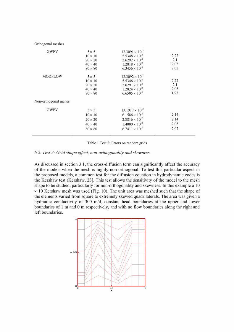
Orthogonal meshes

GWFV 5 5 12.3091 10-2 10 10 5.5348 10-2 2.22 20 20 2.6292 10-2 2.1 40 40 1.2818 10-2 2.05 80 80 6.3456 10-3 2.02

MODFLOW 5 5 12.3092 10-2 10 10 5.5346 10-2 2.22 20 20 2.6291 10-2 2.1 40 40 1.2824 10-2 2.05 80 80 6.6505 10-3 1.93

Non-orthogonal mehes

GWFV 5 5 13.1917 10-2 10 10 6.1586 10-2 2.14 20 20 2.8816 10-2 2.14 40 40 1.4000 10-2 2.05 80 80 6.7411 10-3 2.07

Table 1 Test 2: Errors on random grids

6.2. Test 2: Grid shape effect, non-orthogonality and skewness

As discussed in section 3.1, the cross-diffusion term can significantly affect the accuracy of the models when the mesh is highly non-orthogonal. To test this particular aspect in the proposed models, a common test for the diffusion equation in hydrodynamic codes is the Kershaw test (Kershaw, 23]. This test allows the sensitivity of the model to the mesh shape to be studied, particularly for non-orthogonality and skewness. In this example a 10 10 Kershaw mesh was used (Fig. 10). The unit area was meshed such that the shape of the elements varied from square to extremely skewed quadrilaterals. The area was given a hydraulic conductivity of 300 m/d, constant head boundaries at the upper and lower boundaries of 1 m and 0 m respectively, and with no flow boundaries along the right and left boundaries.

X

Y

0 0.5 10

0.5

1

Fig. 10. The 10 10 Kershaw mesh. The models were then run to determine a steady state head profile across the area. A tool which correctly calculates the heads will show equally spaced isolines parallel to the constrained sides. Therefore, the head results would not have been expected to be a function of the mesh generated or the shape of the elements. The problem was first solved for an orthogonal mesh. The contour plot of the steady state results gave straight lines for both MODFLOW and the GWFV model (see Fig. 11(a)). The analytical solution was linear in y, and the methods reproduced this result exactly, as shown by the straight contour lines. This finding was expected since the method reduced to the standard five-point finite difference method for the case of an orthogonal mesh. For the non-orthogonal mesh, the resulting isolines from the GWFV model (see Fig. 11) were not altered by the distortion of the grid, thereby proving its independence from the mesh shape as these contours were straight. The same simulation was repeated with a 20 20 mesh. The mesh and its corresponding head contours for the steady state results are shown in Fig. 12. (a) --- MODFLOW; ─ Analytic (b) --- GWFV: Non-orth; ─ Analytic

Fig. 11. Isolines on the 10 10 Kershaw mesh for MODFLOW and the GWFV models. The isolines in Fig. 12 remain linear, even though the mesh was more severely skewed. This was particularly true for the GWFV model as it gave less curvature and more accurate contours for both levels of mesh distortion. The GWFV model calculations exhibited linearity of the solution to the level of machine precision.

0.1

0.2

0.3

0.4

0.5

0.6

0.7

0.8

0.9

1

X(m)

Y(m

)

0 0.1 0.2 0.3 0.4 0.5 0.6 0.7 0.8 0.9 10

0.1

0.2

0.3

0.4

0.5

0.6

0.7

0.8

0.9

1

0.1

0.2

0.3

0.4

0.5

0.6

0.7

0.80.8

0.9

1

X(m)

Y(m

)

0 0.1 0.2 0.3 0.4 0.5 0.6 0.7 0.8 0.9 10

0.1

0.2

0.3

0.4

0.5

0.6

0.7

0.8

0.9

1

(a) The mesh (b) --- GWFV: Non-orth; ─ Analytic

Fig. 12. The 20 20 Kershaw grid, (a) the mesh; (b) isolines resulting from the GWFV model. 6.3 Test 3: Permeability-Heterogeneity To test the new equivalent permeability formulation, a simple data set was constructed with variable hydraulic conductivity and incorporating a single extraction well. In a similar structure to Test 1, no flow boundaries were assumed along the borders of the model domain. The well discharged at a constant rate of 1000 m3day-1 from the centre of a confined aquifer of 1000 m × 1000 m. The test runs were performed with uniform isotropy and benchmarked against MODFLOW results. The results for the transient simulation after 20 days with variable hydraulic conductivity are shown in Fig. 13. The left hand side of the simulation area had a conductivity coefficient of 90 m/day and a storage coefficient of 8×10-3 m-1, whereas the right hand side of the domain had values of 900 m/day and 8×10-2 m-1 for the same parameters. The SIP solver was set to run with 20 stress periods, with each period being one day long. It was observed that the new equivalent conductivity expression and that in MODFLOW gave exactly the same results when implemented in the GWFV model and when the grids were orthogonal. However, the MODFLOW results were different from the results for the GWFV model for the non-orthogonal grids (see Fig. 13). Nevertheless, the GWFV model results with the non-orthogonal grid did not differ much from the results obtained using the orthogonal grid.

0.1

0.2

0.3

0.4

0.5

0.6

0.7

0.8

0.9

1

X(m)Y

(m)

0 0.1 0.2 0.3 0.4 0.5 0.6 0.7 0.8 0.9 10

0.1

0.2

0.3

0.4

0.5

0.6

0.7

0.8

0.9

1

X

Y

0 0.5 10

0.5

1

(a) MODFLOW (b) GWFV: Non-orthogonal

Fig. 13. Head drawdown for Test 5 from application of (a) MODFLOW, and

(b) GWFV model on non-orthogonal grids. 7. Application to River Tawe case study (experimental area) The model was then applied to an experimental aquifer, discharging along a section of the River Tawe (Fig. 14). The site is located to the southeast of the town of Clydach in South Wales, UK. It covers an area of approximately 121 hectares, comprising a nickel refinery plant and a landfill area, separated by River Tawe. The refinery effluents were considered to possibly lead to an adverse hydro-environmental impact on the river water quality. The numerical model was set up to give a clear insight into the quantity and direction of the groundwater flow in the vicinity of the site. Substantial amounts of data were available from many reliable sources (e.g. Environment Agency and the Geological Survey of Great Britain) and site investigations and routine monitoring were carried out by the refinery company. For the purpose of comparing the results of the GWFV model, MODFLOW, and the observed hydraulic heads, steady-state calibrated parameters from MODFLOW were used to simulate the same field conditions with the new GWFV model. The non-orthogonal grid was generated using the Tecplot Mesh Generator [1]. The model rectangular area was divided into 50 rows and 50 columns on an algebraic structured mesh. The row direction was chosen to be parallel to the riverbanks and the columns were located in such a way that they fitted the flow direction towards the river (Fig. 15). The quadrilateral cell coordinates were generated using the write mesh file option of Tecplot and then reconverted to a format adapted within the GWFV program input. Another file gave the equivalent cell indices (i, j) for each orthogonal cell from the non-orthogonal generated mesh. This basic file allowed the translation of all the MODFLOW input parameters (e.g. permeability, recharge, boundary conditions, etc.) into a properties file adapted to the GWFV program for the structured non-orthogonal grid.

0.4

0.4

0.5

0.6

0.70.8

2.5

0.4

0.5

0.6

0.7 0.8

11.1

1.61.7

0 200 400 600 800 10000

200

400

600

800

1000

0.4

0.4

0.5

0.5

0.6

0.6

0.7

0.8

0.9 1

1.1

1.5

1.72.4

2.63.5

0 200 400 600 800 10000

200

400

600

800

1000

The GWFV model was then run for the non-orthogonal grid using the same run parameters of the SIP solver as for MODFLOW with a user-defined seed equal to 0.1, five iteration parameters, and a head change criterion for convergence equal to 10-2m.

Fig. 14. Site location plan from Digimap11.

Fig. 15. The non-orthogonal 50 × 50 mesh.

N.T.S

D.J.A.Williams

Social Club

Gen e

ral Off ice s

Car Park

Ga

rages

Contro

l

Lab o

ratory

Medica

l

Ce

ntre

Cantee

n

Wo

rks

Entran

ce

We

ighb

r idge

T ermin al

Building

Gas

Holder

Nickel O xide Silo

Main Warehouse

Hydrogen

Hydrogen

Gas

Holder

Nickel Sulp hide SiloFlu id Bed

Roaster

No rth

Sub -Statio

n

Nickel Extraction Plants

(Kiln L ine 1) (Kiln Lin e 2 )

Pellet

Production

Plant

Pow der Pro duction Plant

Conc.1 R esidue Warehouse

General Stores

Produ ct

R esearch

Central Engineering

W orkshops

Engineering

Of fices

Engineering Wo rkshops

(Civil/Electrical/In struments)

Re

search

Labo

ratory

Sa

fety/T

raining

Off ice

Pellet

Flattening

Mill

Nickel Sulp hate

Plan t

Powder/Sulphate

D espatch Warehou se

Pow der Warehouse

Hydrogen

P urification

Unit

(P .S.A)

CO

G as

H older

Cen tral

Inert

Plant

Inert

G as

Hold er

South

Sub-S

tatio n

In takeSub -station

Stores Annexe

E ffluentPlant

Nickel

C hlorid e

Plant

Chemical Prod ucts

Off ices/W arehouse

Riv

erP

ump

Hou

se

No.1

Butane

Sphere

No.2

Butane

Sphere

Butane Plant

Hydrogen Plant

Proje ct Store/Bui ldin g Sto re

V ehicle RepairWorkshop

Sub

Stat ion

"A"

Canal

Pump

House

( Intake)Acid Storage Tanks

Gaseous

Incinerators

E.S.Precipitators

R.C Stack

Acid Plant

SO Storage2

REFINERY WORKS PLAN

MAIN PLANT IDENTIFICATION

BH23

BH1

TPJ

E

F

D

BH3

BH22BH17

BH21

BH7BH6

BH19

BH20

BH18

BH9

BH13

BH2

U T

BH26BH25

BH5

S

S1

BH8

R

Q

Q1BH24

BH10

P

TPO

BH11

X

BH14

W

V

BH27

TPI1

TPI2 BH4

TPB

TPA

TPC

TPN

TRIAL PITS

BOREHOLES

FIGURE 1. TRIAL PIT, BOREHOLE AND WELL LOCATIONS AT INCO CLYDACH

WELL 1

LANDFILL

WELLS

WELL 2

TPG TPH1

TPKTPL TPM

BHA

BHD

BHC

BHB

ADDITIONAL BOREHOLES

For an orthogonal grid, the GWFV model gave the same results as MODFLOW, with the heads contour map being shown in Fig. 16. For the non-orthogonal mesh, Fig. 17 illustrates the contour map for the heads calculated from the GWFV simulations. From both models, it can be seen that the river is still draining into the one-layer aquifer. However, differences between the heads arose at a few borehole sites. To assess the accuracy and correctness of the two models, a comparison was undertaken with the observed heads for the existing conditions.

Table 2 Root mean squared error results comparison

RMSE (m) Refinery well group River well group Landfill well group All groups

MODFLOW 0.31199 0.50776 0.49619 0.42176

GWFV 0.28770 0.43227 0.49262 0.381931

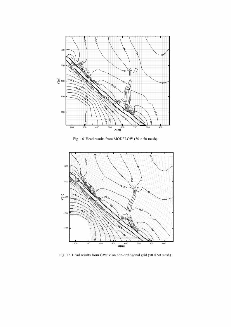
Fig. 16. Head results from MODFLOW (50 × 50 mesh).

Fig. 17. Head results from GWFV on non-orthogonal grid (50 × 50 mesh).

94.5

95

95

95.5

95.5

95.5

96

96

96

96

96.5

96.5

96.5

96.5

96.5

96.5

97

97

97

97

97

97

97

.5

97.5

97

.5

97.5

97.5

97.5 98

98

98

98

98

98

98.5

98.5

98

.5

98

.5

98.5

98

.5

98.5

99

99

99

99.5

99.5100

00

.5

X(m)

Y(m

)

200 300 400 500 600 700 800 900

200

300

400

500

600

95.5

95.5

96

96

96

96 96

.5

96.5

96.5

96.5

96.5

97

97

97

97

97

97

97

.5

97.5

97

.5

97.5

97.5

98

98

98

98

98

98

98

.5

98.598.5

99

99

99

99.5

99.5

10

0

100

X(m)

Y(m

)

200 300 400 500 600 700 800 900

200

300

400

500

600

The observation wells were grouped into three groups to make more distinctive comparisons between the accuracy of the two models. The root mean squared error (RMSE) of all the groups and the overall area is given in Table 2. The basic difference between the models is solely the shape of the mesh used in the GWFV model, and it can be seen that the best improvement in accuracy was observed at the river well group since the cells fitted exactly to the shape the river and the direction of the flow towards the river. Fig. 18 highlights the improved accuracy for this group and Fig. 19 shows the overall features of the steady state calculated vs. observed head around a line of equal potential. The normalised RMSE for MODFLOW was 8.21% on the orthogonal 50 × 50 mesh, whereas the corresponding RMSE for the GWFV model on the 50 × 50 non-orthogonal mesh was 7.15%. This accuracy was only reached by MODFLOW when running the model on a mesh refined by two (i.e. a 100 × 100 mesh). The MODFLOW normalised RMSE was then 7.11%. This clearly highlighted the higher accuracy of the GWFV model relative to MODFLOW, when using a non-orthogonal grid that captured the geometry of the river for this particular site. A lower mesh resolution was needed for

the GWFV model to give the same results as MODFLOW. Fig. 18. Comparison of head results from MODFLOW and the GWFV model

for non-orthogonality with observed heads, for different observations well groups.

Fig. 19. Steady state calculated vs. observed heads on 35 observation boreholes.

8. Conclusions A new non-orthogonal grid finite volume model has been described herein and for application to groundwater flow studies. Accurate results have been obtained from model tests against analytical and benchmarked conditions. The sensitivity of the model to the mesh size was tested using different random mesh resolutions for a simple Laplace equation. The same equation has been used with a 2D Kershaw mesh to examine the effects of the grid non-orthogonality and skewness on the overall performance of the new developed algorithm. Finally, a heterogeneity test has been carried out to check the effectiveness of the selected equivalent permeability formulation. The model has also been applied to a field study, where observed and predicted hydraulic heads have been compared. For this case study, although only a 50×50 mesh was used, the results obtained using the newly developed GWFV model for a non-orthogonal mesh were compared to the results obtained using a 100×100 mesh and MODFLOW simulations. The corresponding comparisons between both models showed a high level of agreement, despite the new model having a coarser grid. In particular, the agreement was closest near the river, which was the main site of concern and where heads at observation boreholes were close to the corresponding predicted heads. Therefore, it was noted that in using a grid that fits closely to the geometrical layout of the river with the

94

95

96

97

98

99

100

101

102

103

94 96 98 100 102 104

Observed heads (m)

Cal

cula

ted

head

s (m

)

GWFV_Nonorthogonal

Line of equal relation

MODFLOW

GWFV model, the reduced use of mesh nodes by up to 50% in comparison with MODFLOW, did not result in any reduced accuracy in the predicted heads. The new model was generated by replacing the finite difference structure of MODFLOW with the finite volume method and using orthogonal and non-orthogonal quadrilateral grids to give improved accuracy. The new model also gave greater flexibility at internal and/or external boundaries. The suite of tests undertaken and outlined herein for the new model are by no means exhaustive, but the results have demonstrated the accuracy of the new model in comparison with the numerical concepts used in finite difference models, such as MODFLOW. In particular, the use of non-orthogonal grids and the new equivalent hydraulic conductivity formulations have been investigated. The comparative analysis of the tests results have shown that in all cases the advantages of the finite volume model were shown to be favourable compared with the finite difference method. The effects of grid non-orthogonality and skewness in the finite volume formulation used in the GWFV model were absorbed and did not affect the accuracy of the method. The parameters associated with the head in each cell in the system equation in the GWFV model (namely Bi,j, Di,j, Fi,j, Hi,j in Eq. (20)) contained few terms in relation to the geometry of the cells. Therefore, the GWFV model proved to be less sensitive to grid non-orthogonality and skewness and more accurate as to heterogeneity and boundary conditions than the comparisons undertaken with the finite difference algorithms. The new model gives broad flexibility for grid shapes in the x and y directions and therefore, when constructing a conceptual model, assumptions related to the geometry of the boundaries could be more realistic and accurate. In conclusion, the test results have indicated that the GWFV model offers a viable alternative to the finite difference solution method. Its use is desirable when accurate simulations of boundary conditions or complex property distributions with a mass balance are required for accurate groundwater flow predictions. References [1] Amtec, 1999. Tecplot Mesh Generator, Version 1.0. User’s Manual. Amtec Engineering, Inc.,

Bellevue, Washington, USA. http://www.tecplot.com [2] Andersen, P.F., 1993. A Manual of Instructional Problems for the U.S.G.S. MODFLOW Model.

EPA/600/R-93/010. [3] Anderson, M.P., Woessner, W.W., 1992. Applied Groundwater Modeling: Simulation of Flow and

Advective Transport. Academic Press, San Diego. [4] Archer, R.A, 2000. Computing Flow and Pressure Transients in Heterogeneous Media Using Boundary

Element Method. PhD thesis, Stanford University. [5] Barrash, W., Dougherty, M.E., 1997. Modeling Axially Symmetric and Nonsymmetric Flow to a Well

with MODFLOW, and Application to Goddard2 Well Test, Boise, Idaho. Ground Water 35 (4), 602-611.

[6] Bear, J., 1972. Dynamics of Fluids in Porous Media. American Elsevier, New York. [7] Bear, J., 1979. Hydraulics of Groundwater. McGraw-Hill, New York, New York. [8] Carrera, J., Melloni, G., 1987. The Simulation of Solute Transport: An Approach Free of Numerical

Dispersion. SAND86-7095, Sandia National. Laboratories, Albuquerque, NM. [9] Celia, M.A., Russell, T.F., Herrera, I., Ewing, R.E., 1990. Eulerian-Lagrangian Localized Adjoint

Method for the Advection-Diffusion Equation. Advances in Water Resources, 13 (4), 187-206.

[10] Chow P, Cross M, Pericleous K. A Natural Extension of the Conventional Finite Volume Method into Polygonal Unstructured Meshes for CFD Application. Applied Mathematical Modelling 1996;20(2):170-183.

[11] Croft, T.N., 1998. Unstructured Mesh-Finite Volume Algorithms for Swirling, Turbulent, Reacting Flows. Ph.D. Thesis, University of Greenwich, UK.

[12] Di Giammarco, P., Todini, E., Lamberti, P., 1996. A Conservative Finite Elements Approach to Overland Flow: the Control Volume Finite Element Formulation. Journal of Hydrology 175 (1-4), 267-291.

[13] Digimap, 2004. University of Edinburgh. http://www.edina.ac.uk/digimap/ [14] Elmahi I, Benkhaldoun F, Vilsmeier R, Gloth O, Patschull A, Hănel D. Finite Volume Simulation of a

Droplet Flame Ignition on Unstructured Meshes. Journal of Computational and Applied Mathematics 1999;103(1):187-205.

[15] Faille, I., 1992. A Control Volume Method to Solve Elliptic Equation on a Two-Dimensional Irregular Mesh. Computer Methods in Applied Mechanics and Engineering, 100, 275-290.

[16] Faust, C.R., Sims, P.N., Spalding, C.P., Andersen, P.F., Lester, B.H., Shupe, M.G., Harrover, A., 1993. FTWORK: Groundwater Flow and Solute Transport in Three Dimensions. In: Documentation Versions 2.8, GeoTrans, Sterling, VA.

[17] Ferguson, W.J., Turner, I.W., 1996. A Control Volume Finite Element Numerical Simulation of the Drying of Spruce. Journal of Computational Physics 125 (1), 59-70.

[18] Ferguson, W.J., 1998. The control volume finite element numerical solution technique applied to creep in softwoods. International Journal of Solids and Structures 35 (13), 1325-1338.

[19] Gottardi, G., Venutelli, M., 1994. One-Dimensional Moving Finite-Element Model of Solute Transport. Ground Water 32 (4), 645-649.

[20] Haitjema, H.M., Kelson, V.A., de Lange, W., 2001. Selecting MODFLOW Cell Sizes for Accurate Flow Fields. Ground Water 39 (6), 931-938.

[21] Heberton, C.I., Russell, T.F., Konikow, L.F., Hornberger, G.Z., 2000. A Three-Dimensional Finite Volume Eulerian-Lagrangian Localized Adjoint Method (ELLAM) for Solute-Transport Modeling. U.S. Geological Survey Water-Resources Investigations Report 00-4087.

[22] Hirsch, C., 1988. Numerical Computation of Internal and External Flows. Volume 1: Fundamentals of numerical discretisation. John Wiley & Sons, Chichester.

[23] Hyman, J.M., Shashkov, M., 1999. Mimetic Discretizations for Maxwell's Equations. Journal of Computational Physics 151 (2), 881-909.

[24] Hyman, J., Morel, J., Shashkov, M., Steinberg, S., 2002. Mimetic Finite Difference Methods for diffusion equations. Computational Geosciences, 6 (3-4), 333-352.

[25] Jayantha, P.A., Turner, I.W., 2001. A Comparison of Gradient Approximations for Use in Finite-Volume Computational Models for two-Dimensional Diffusion Equations. Numerical Heat Transfer, Part B 40 (5), 376-390.

[26] Jayantha, P.A., Turner, I.W., 2003. A Second Order Finite Volume Technique for Simulating Transport in Anisotropic Media. International Journal of Numerical Methods for Heat and Fluid Flow 13 (1), 31-56.

[27] Jayantha, P.A., Turner, I.W., 2005. Second Order Control-Volume Finite-Element Least-Squares Strategy for Simulating Diffusion in Strongly Anisotropic Media. Journal of Computational Mathematics 23 (1), 1-16.

[28] Kershaw, D.S., 1981. Differencing of the Diffusion Equation in Lagrangian Hydrodynamic Codes. Journal of Computational Physics 39, 375-395.

[29] Kirpup, S.M., 1996. Fortran Codes for Computing the Discrete Helmholtz Integral Operators: User Guide. Report MCS-96-06, Department of Mathematics and Computer Sciences, University of Salford, UK.

[30] Leake, S.A., Claar, D.V., 1999. Procedures and Computer Programs for Telescopic Mesh Refinement Using MODFLOW. U.S. Geological Survey Open-File Report 99-238.

[31] Lin, H.C., Richards, D.R., Yeh, G.T., Cheng, H.P., Jones, N.L., 1997. FEMWATER:A Three Dimensional Finite Element Computer Model For Simulating Density Dependent Flow and Transport, in Variably Saturated Media. Report CHL-96-12, US Army Corps of Engineer, Vicksburg, MS.

[32] Liu, F., Jameson, A., 1993. Multigrid Navier-Stokes Calculations for Three-Dimensional Cascades. AIAA Journal 31 (10), 1785-1791.

[33] Loudyi, D., 2005. A 2D Finite Volume Model for Groundwater Flow Simulations: Integrating Non-Orthogonal Grid Capability Into MODFLOW. Ph.D. Thesis, Cardiff University, UK.

[34] McDonald, M.G., Harbaugh, A.W., 1988. A Modular Three-Dimensional Finite-Difference Ground-Water Flow Model. U.S. Geological Survey Techniques of Water-Resources Investigations, Book 6, Chap. A1.

[35] Meerschaert, M.M., Tadjeran, C., 2004. Finite Difference approximations for fractional Advection-Dispersion Flow Equations. Journal of Computational and Applied Mathematics 172 (1), 65-77.

[36] Morel, J.E., Dendy, Jr., Hall, M.L., White, S.W., 1992. A Cell-Centered Lagrangian-Mesh Diffusion Differencing Scheme. Journal of Computational Physics 103 (2), 286-299.

[37] Morel, J.E., Roberts, R.M., Shashkov, M.J., 1998. A Local Support-Operators Diffusion Discretization Scheme for Quadrilateral r-z Meshes. Journal of Computational Physics 144 (1), 17-51.

[38] Neuman, S.P., 1984. Adaptive Eulerian-Lagrangian Finite Element Method for Advection-Dispersion. International Journal for Numerical Methods in Engineering, 20 (2), 321-337.

[39] Osnes, H., Langtangen, H.P., 1998. An Efficient Probabilistic Finite Element Method for Stochastic Groundwater Flow. Advances in Water Resources 22 (2), 185-195.

[40] Patankar, S.V., 1980. Numerical Heat Transfer and Fluid Flow, Hemisphere, Washington, DC. [41] Spitz, F.J., Nicholson, R.S., Daryll, A.P., 2001. A Nested Rediscretization Method to Improve Pathline

Resolution by Eliminating Weak Sinks Representing Wells. Ground Water 39 (5), 778-785. [42] Tannehill, J.C., Anderson, D.A., Pletcher, R.H., 1997. Computational Fluid Mechanics and Heat

Transfer, 2nd ed., Taylor & Francis, London. [43] Theis, C.V., 1935. The Relation Between the Lowering of the Piezometric Surface and the Rate and

Duration of Discharge of a Well Using Groundwater Storage. Trans. Amer. Geophys. Union, 16, 519-524.

[44] Townley, L.R., 1990. AQUIFEM-N: A Multi-layered Finite Element Aquifer Flow Model, User’s Manual and Description. CSIRO Division of Water Resources, Perth, Western Australia.

[45] Turkel, E., 1985. Accuracy of Schemes with Nonuniform Meshes for Compressible Fluid Flows. Applied Numerical Mathematics 2 (6), 529-550.

[46] Turner, I.W., Ferguson, W.J., 1995. An Unstructured Mesh Cell-Centered Control Volume Method for Simulating Heat and Mass Transfer in Porous Media: Application to Softwood Drying, Part I: The isotropic model. Applied Mathematical Modelling, 19 (11), 654-667.

[47] U.S. Environmental Protection Agency (USEPA), 1994. A Technical Guide to Ground-Water Model Selection at Sites Contaminated with Radioactive Substances. EPA/402/R-94/012, Office of Solid Waste and Emergency Response, U.S. Environmental Protection Agency, Washington, D.C.

[48] Voss, C.I., 1984. A Finite Element Simulation Model for Saturated-Unsaturated, Fluid-Density-Dependent Ground-Water Flow with Energy Transport or Chemically-Reactive Single-Species Solute Transport. U.S. Geological Survey Water Resources Investigation Report 84-4369.

[49] Wang, H.F., Anderson, M.P., 1982. Introduction to Ground Water Modeling: Finite Difference and Finite Element Methods. W.H. Freeman, San Francisco, California.

[50] Wasantha Lal, A.M., 1998. Weighted Implicit Finite-Volume Model for Overland Flow. Journal of Hydraulic Engineering 124 (9), 941-950.

[51] Zheng, C., 1990. MT3D, a Modular Three-Dimensional Transport Model for Simulation of Advection, Dispersion, and Chemical Reactions of Contaminants in Groundwater Systems. Report to the Kerr Environmental Research Laboratory, U.S. Environmental Protection Agency, Ada, Oklahoma.