MATH6112 - Abstract Algebra II - The Ohio State University
88
The Ohio State University - MATH6112 - Lecture notes Ivo Terek Couto MATH6112 - Abstract Algebra II Ivo Terek Couto * Lecture notes from the Spring 2019 Abstract Algebra II course taught by professor David Anderson. Everything here was written like a list of topics, following the pace of the lectures and trying to keep the main results bite-sized. Disclaimer: I added a few comments and examples of my own here and there, so I take responsibility for any eventual mistakes you may find here. * [email protected] Page i
-
Upload
khangminh22 -
Category
Documents
-
view
1 -
download
0
Transcript of MATH6112 - Abstract Algebra II - The Ohio State University

The Ohio State University - MATH6112 - Lecture notes Ivo Terek Couto
MATH6112 - Abstract Algebra II
Ivo Terek Couto*
Lecture notes from the Spring 2019 Abstract Algebra II course taught by professorDavid Anderson. Everything here was written like a list of topics, following the paceof the lectures and trying to keep the main results bite-sized.Disclaimer: I added a few comments and examples of my own here and there, so Itake responsibility for any eventual mistakes you may find here.
Page i

The Ohio State University - MATH6112 - Lecture notes Ivo Terek Couto
Contents
Category Theory 1Jan 7th . . . . . . . . . . . . . . . . . . . . . . . . . . . . . . . . . . . . . . . . . . 1Jan 9th . . . . . . . . . . . . . . . . . . . . . . . . . . . . . . . . . . . . . . . . . . 3Jan 11th . . . . . . . . . . . . . . . . . . . . . . . . . . . . . . . . . . . . . . . . . 6Jan 14th . . . . . . . . . . . . . . . . . . . . . . . . . . . . . . . . . . . . . . . . . 10Jan 16th . . . . . . . . . . . . . . . . . . . . . . . . . . . . . . . . . . . . . . . . . 12Jan 18th . . . . . . . . . . . . . . . . . . . . . . . . . . . . . . . . . . . . . . . . . 14Jan 23rd . . . . . . . . . . . . . . . . . . . . . . . . . . . . . . . . . . . . . . . . . 17Jan 25th . . . . . . . . . . . . . . . . . . . . . . . . . . . . . . . . . . . . . . . . . 19Jan 28th . . . . . . . . . . . . . . . . . . . . . . . . . . . . . . . . . . . . . . . . . 23
Homological Algebra (and more Category Theory) 27Feb 1st . . . . . . . . . . . . . . . . . . . . . . . . . . . . . . . . . . . . . . . . . . 27Feb 4th . . . . . . . . . . . . . . . . . . . . . . . . . . . . . . . . . . . . . . . . . 29Feb 6th . . . . . . . . . . . . . . . . . . . . . . . . . . . . . . . . . . . . . . . . . 30Feb 8th . . . . . . . . . . . . . . . . . . . . . . . . . . . . . . . . . . . . . . . . . 33Feb 11th . . . . . . . . . . . . . . . . . . . . . . . . . . . . . . . . . . . . . . . . . 34Feb 13th . . . . . . . . . . . . . . . . . . . . . . . . . . . . . . . . . . . . . . . . . 36Feb 15th . . . . . . . . . . . . . . . . . . . . . . . . . . . . . . . . . . . . . . . . . 38Feb 18th . . . . . . . . . . . . . . . . . . . . . . . . . . . . . . . . . . . . . . . . . 41Feb 22nd . . . . . . . . . . . . . . . . . . . . . . . . . . . . . . . . . . . . . . . . 45Feb 25th . . . . . . . . . . . . . . . . . . . . . . . . . . . . . . . . . . . . . . . . . 48Feb 27th . . . . . . . . . . . . . . . . . . . . . . . . . . . . . . . . . . . . . . . . . 51Mar 1st . . . . . . . . . . . . . . . . . . . . . . . . . . . . . . . . . . . . . . . . . 54
Galois Theory 57Mar 20th . . . . . . . . . . . . . . . . . . . . . . . . . . . . . . . . . . . . . . . . 57Mar 22nd . . . . . . . . . . . . . . . . . . . . . . . . . . . . . . . . . . . . . . . . 59Mar 25th . . . . . . . . . . . . . . . . . . . . . . . . . . . . . . . . . . . . . . . . 63Mar 27th . . . . . . . . . . . . . . . . . . . . . . . . . . . . . . . . . . . . . . . . 65Mar 29th . . . . . . . . . . . . . . . . . . . . . . . . . . . . . . . . . . . . . . . . 67Apr 1st . . . . . . . . . . . . . . . . . . . . . . . . . . . . . . . . . . . . . . . . . 68Apr 3rd . . . . . . . . . . . . . . . . . . . . . . . . . . . . . . . . . . . . . . . . . 70Apr 5th . . . . . . . . . . . . . . . . . . . . . . . . . . . . . . . . . . . . . . . . . 72Apr 8th . . . . . . . . . . . . . . . . . . . . . . . . . . . . . . . . . . . . . . . . . 73Apr 10th . . . . . . . . . . . . . . . . . . . . . . . . . . . . . . . . . . . . . . . . . 75Apr 12th . . . . . . . . . . . . . . . . . . . . . . . . . . . . . . . . . . . . . . . . . 76Apr 15th . . . . . . . . . . . . . . . . . . . . . . . . . . . . . . . . . . . . . . . . . 78Apr 17th . . . . . . . . . . . . . . . . . . . . . . . . . . . . . . . . . . . . . . . . . 79Apr 19th . . . . . . . . . . . . . . . . . . . . . . . . . . . . . . . . . . . . . . . . . 81Apr 22th . . . . . . . . . . . . . . . . . . . . . . . . . . . . . . . . . . . . . . . . . 83
References 86
Page ii

The Ohio State University - MATH6112 - Lecture notes Ivo Terek Couto
Category Theory
Jan 7th
• Historical context: the notion of “category” was introduced in 1945 by Eilenbergand Maclane as a framework for studying “natural transformations”.
• Definition of a category: a category C consists of
(i) a collection (class) Obj(C) of objects;
(ii) for each pair (A, B), a set MorC(A, B) of morphisms (arrows) between A andB, such that if (A, B) 6= (C, D), then MorC(A, B) ∩MorC(C, D) = ∅;
(iii) a composition law
MorC(A, B)×MorC(B, C) 3 ( f , g) 7→ g ◦ f ∈ MorC(A, C)
which is associative and admits identity elements, that is, for every objectA of C there is IdA ∈ MorC(A, A) such that given any object B, we havef ◦ IdA = f for all f ∈ MorC(A, B) and IdA ◦ g = g for all g ∈ MorC(B, A).In terms of diagrams, we mean the following situations:
A A BIdA
f
fand B A A
g
g
IdA .
• Remark on notation: In the above definition, condition (ii) says that MorC(A, B)is completely specified by the source object A and the target object B. Anothercommon notation for MorC(A, B) is HomC(A, B) (“hom” for “homomorphism”).
• Examples:
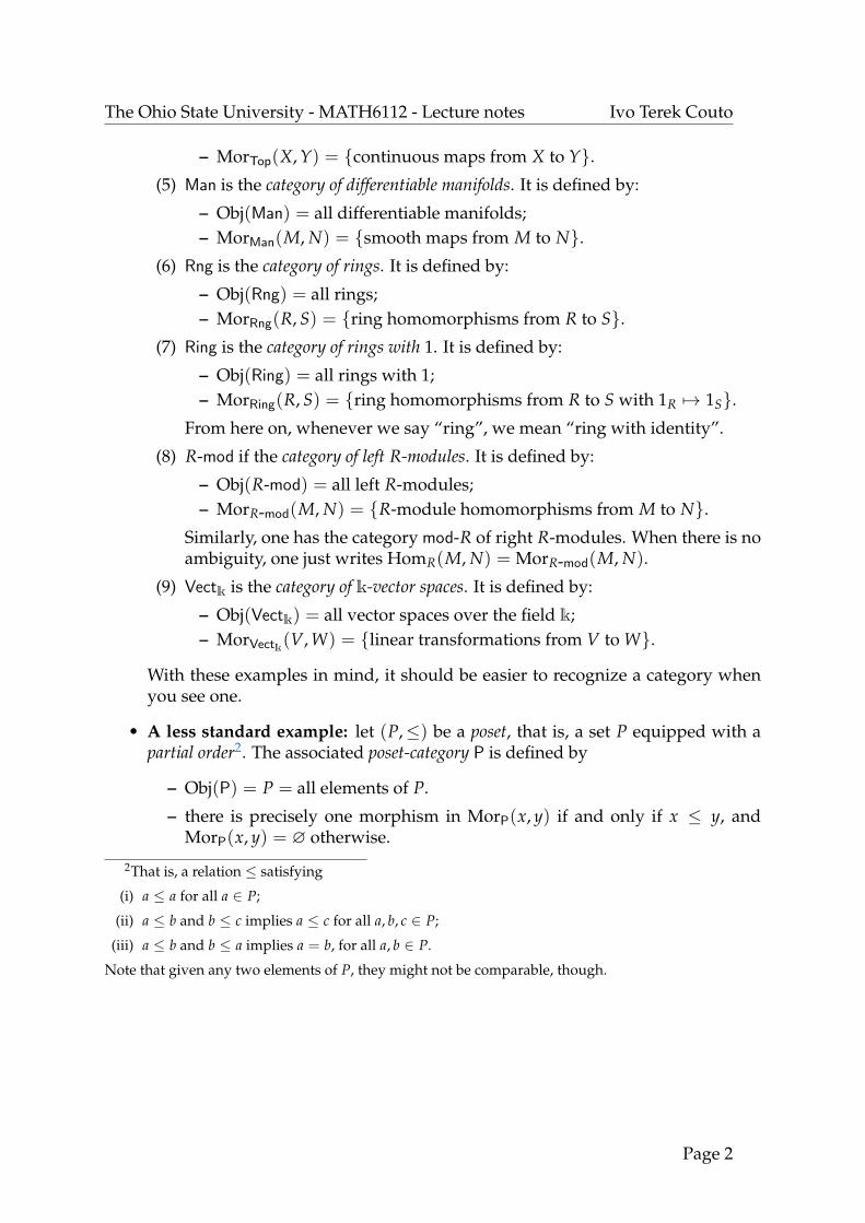
(1) Set is the category of sets (surprise?). It is defined by:
– Obj(Set) = all sets1;– MorSet(A, B) = {functions from A to B}..
(2) Grp is the category of groups. It is defined by:
– Obj(Grp) = all groups;– MorGrp(G, H) = {group homomorphisms from G to H}.
(3) Ab is the category of abelian groups. It is defined by:
– Obj(Ab) = all abelian groups;– MorAb(G, H) = {group homomorphisms from G to H}.
(4) Top is the category of topological spaces. It is defined by:
– Obj(Top) = all topological spaces;
1Note that this is a proper class. This is the reason why in (i) of the definition of a category we donot require Obj(C) being a set.
Page 1
The Ohio State University - MATH6112 - Lecture notes Ivo Terek Couto
– MorTop(X, Y) = {continuous maps from X to Y}.(5) Man is the category of differentiable manifolds. It is defined by:
– Obj(Man) = all differentiable manifolds;– MorMan(M, N) = {smooth maps from M to N}.
(6) Rng is the category of rings. It is defined by:
– Obj(Rng) = all rings;– MorRng(R, S) = {ring homomorphisms from R to S}.
(7) Ring is the category of rings with 1. It is defined by:
– Obj(Ring) = all rings with 1;– MorRing(R, S) = {ring homomorphisms from R to S with 1R 7→ 1S}.
From here on, whenever we say “ring”, we mean “ring with identity”.
(8) R-mod if the category of left R-modules. It is defined by:
– Obj(R-mod) = all left R-modules;– MorR-mod(M, N) = {R-module homomorphisms from M to N}.
Similarly, one has the category mod-R of right R-modules. When there is noambiguity, one just writes HomR(M, N) = MorR-mod(M, N).
(9) Vectk is the category of k-vector spaces. It is defined by:
– Obj(Vectk) = all vector spaces over the field k;– MorVectk(V, W) = {linear transformations from V to W}.
With these examples in mind, it should be easier to recognize a category whenyou see one.
• A less standard example: let (P,≤) be a poset, that is, a set P equipped with apartial order2. The associated poset-category P is defined by
– Obj(P) = P = all elements of P.
– there is precisely one morphism in MorP(x, y) if and only if x ≤ y, andMorP(x, y) = ∅ otherwise.
2That is, a relation ≤ satisfying
(i) a ≤ a for all a ∈ P;
(ii) a ≤ b and b ≤ c implies a ≤ c for all a, b, c ∈ P;
(iii) a ≤ b and b ≤ a implies a = b, for all a, b ∈ P.
Note that given any two elements of P, they might not be comparable, though.
Page 2

The Ohio State University - MATH6112 - Lecture notes Ivo Terek Couto
The usual way to represent posets and poset-categories is via Hasse diagrams:
• •
• •
• •
•
≤ and
• •
• •
• •
•
In the left we have the poset, where the order ≤ increases upwards. In the right,we have the poset-category, where the dashed arrows are the morphism compo-sitions implied by the transitivity of ≤.
Jan 9th
• Open category: If X is a topological space, one may consider the topology of Xpartially ordered by inclusion. The corresponding poset-category is called theopen category of X, and it is denoted by OpenX or Op(X).
• Small categories: A small category is a category C for which Obj(C) is a set. So,for example, Set is not a small category (again – because the collection of all setsis not a set, but a proper class).
• Monoids and its associated categories: Recall that a monoid is a set M equippedwith an associative multiplications, with an identity3. For example, (Z, ·) is amonoid. A monoid M determines a category M with:
– one object ?;
– a morphism ?m−−−→ ? for each element m ∈ M;
– composition of morphisms given by multiplication in M:
? ? ?m
n·m
n
In fact, a sort of converse holds: if a category C has only one object ?, thenMorC(?, ?) is a monoid.
• Isomorphisms: an isomorphism between two objects in a category is a morphismwhich has a two-sided inverse with respect to morphism composition. An iso-morphism from an object to itself is called an automorphism. With this terminol-ogy, one might say things like “an isomorphism of topological spaces is just anhomeomorphism”, etc..
3That is to say, the only difference between a monoid and a group is that elements in a monoid donot necessarily have inverses.
Page 3

The Ohio State University - MATH6112 - Lecture notes Ivo Terek Couto
• Groupoids: Continuing the previous example, we can say that a group G is amonoid for which every element has an inverse. So, the corresponding categoryG has the property that all its morphisms are actually isomorphisms. Also, ifa category C has only one object ? and all morphisms are isomorphisms, thenMorC(?, ?) is a group. In general, a category for which all morphisms are iso-morphisms is called a groupoid. This in particular says that a group is nothingmore than a groupoid with one object.
• Core of a category: If C is a category, we define its core to be the category core(C)with:
– Obj(core(C)) .= Obj(C), and;
– Morcore(C)(A, B) .= { f ∈ MorC(A, B) | f is an isomorphism}.
Then, core(C) is always a groupoid.
• Opposite categories: Given a category C, its opposite category Cop is nothing morethan C with its arrows reversed. To be more precise, we put Obj(Cop)
.= Obj(C),
MorCop(A, B) .= MorC(B, A), and the composition in Cop makes the diagram
MorCop(A, B)×MorCop(B, C) MorCop(A, C)
MorC(C, B)×MorC(B, A) MorC(C, A)
∼=
comp. in Cop
=
comp. in C
commute, where the map ∼= indicated above is the obvious one, ( f , g) 7→ (g, f ).
• Example:
(1) If (G, ·) is a group, the opposite group (Gop, ∗) is the same set Gop = Gequipped with the operation defined by g ∗ h .
= h · g. We then have therelation (Gop) = (G)op between the associated monoid-categories.
(2) If (P,≤) is a poset, the opposite order (Pop,≤op) is defined by Pop .= P and
x ≤op y if and only if y ≤ x. Just like in the previous item, the poset-category associated to Pop is Pop.
So the “op” notation is indeed adequate.
• Subcategories: A subcategory “D ⊆ C” is a category D where Obj(D) ⊆ Obj(C)is a subcolletion (subclass), and for all objects A and B of D, one has the inclu-sion MorD(A, B) ⊆ MorC(A, B). We say that D is a full subcategory of C if actualequality MorD(A, B) = MorC(A, B) holds. For example:
(1) Ab is a full subcategory of Grp.
(2) Grp is not a subcategory of Set, because there can be more than one groupstructure in a given set.
Page 4

The Ohio State University - MATH6112 - Lecture notes Ivo Terek Couto
(3) Rng is not a subcategory of Set for the same reason given for Grp above,however Ring is a subcategory of Rng because if a multiplicative identityexists in a ring, then it is necessarily unique.
• More geometric examples: Man is not a subcategory of Top, because a giventopological space can have more than one smooth structure. In fact, Man is noteven a subcategory of the category TopMan of topological manifolds and contin-uous maps, for the same reason (e.g., consider exotic R4’s).
• Products (and coproducts): the idea is to generalize what we already know forsome basic categories. Many familiar categories have a product. For example:
(1) In Set, the cartesian product A× B = {(a, b) | a ∈ A, b ∈ B}.(2) In Grp, the product group G× H with operation (g, h)(g′, h′) .
= (gg′, hh′).
(3) In Top, the product space X×Y with the product topology4.
We want to axiomatize these notions using categorial terms. Say, in Grp, we have
two projections G1 × G2pri−−−→ Gi, i = 1, 2 (which are homomorphisms, that is
to say, arrows in Grp). Giving a morphism Hf−−→ G1 × G2 is the same as giving
two morphisms Hfi−−→ Gi, i = 1, 2, such that fi = pri ◦ f . The idea is the
following:
G1
H G1 × G2
G2
f
f1
f2
pr1
pr2
With this in mind, we have the following:
Definition: in a category C, a product of two objects A1 and A2 is an object A
together with “projection” morphisms Apri−−−→ Ai, i = 1, 2, such that given
any object B and morphisms Bfi−−→ Ai, i = 1, 2, there is a unique morphism
Bf−−→ A commuting with projections:
A1
B A
A2
∃! f
f1
f2
pr1
pr2
4Some care should be takes with the product of infinite factors, since the box topology and the producttopology are no longer the same.
Page 5
The Ohio State University - MATH6112 - Lecture notes Ivo Terek Couto
It follows from this universal property that any two products of A1 and A2 (if theyexists), are isomorphic, and the isomorphism is compatible with the projectionsin the sense that the following diagram commutes
A A′
A1 A2
pr1 pr2
∃!∼=
pr′1
pr′2
We then say that products are unique up to unique isomorphism (where the isomor-phism is the unique one compatible with projections). For example, in Set wehave MorC(B, A) ∼=bij. MorC(B, A1)×MorC(B, A2). So, for this reason, we writef = ( f1, f2), according to the above notation.
• Remark: in the definition above, motivated by what happened in Grp, one couldask whether anything arises if instead of being given all the fi, we were givenjust f instead. We can trivially define fi
.= pri ◦ f , so there is nothing else to
discuss here.
Jan 11th
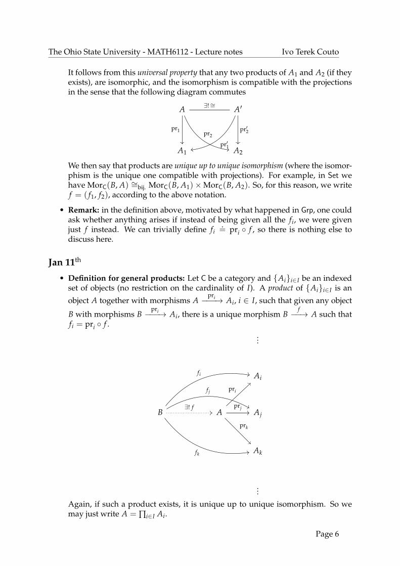
• Definition for general products: Let C be a category and {Ai}i∈I be an indexedset of objects (no restriction on the cardinality of I). A product of {Ai}i∈I is an
object A together with morphisms Apri−−−→ Ai, i ∈ I, such that given any object
B with morphisms Bpri−−−→ Ai, there is a unique morphism B
f−−→ A such thatfi = pri ◦ f .
...
Ai
B A Aj
Ak
...
fi
f j
fk
∃! f
pri
prj
prk
Again, if such a product exists, it is unique up to unique isomorphism. So wemay just write A = ∏i∈I Ai.
Page 6

The Ohio State University - MATH6112 - Lecture notes Ivo Terek Couto
• Examples: Arbitrary products exist in Set. One possible construction is to con-sider
A = {functions α : I →äi∈I
Ai with α(i) ∈ Ai},
where äi∈I Ai =⋃
i∈I{i} × Ai denotes disjoint union, with the projection mapspri : A → Ai given by pri(α)
.= α(i). Arbitrary products also exist in Grp, Ab,
Ring, etc.. Moreover, the notion of product reduces to the following situation inSet: MorC (B, ∏i∈I Ai) ∼= ∏i∈I MorC(B, Ai).
• Maps between products: In a category C with objects A, B, C and D for which
the products A× B and C× D both exist, if we have morphisms Af−−→ C and
Bg−−→ D, we may put them together in a single map A× B
f×g−−−−→ C × D inthe following way: consider the compositions
A× B A CprA f
and A× B B D,prB g
and apply the universal property of C×D to get a unique map f × g making thediagram
A C
A× B C× D
B D
f
f×g
prA
prB prD
prC
g
commute.
• Dual notion to product: Let C be a category and {Ai}i∈I be an indexed set ofobjects. A coproduct of {Ai}i∈I is an object A with morphisms Ai
ρi−−−→ A, i ∈ I,
such that for any object B with morphisms Aifi−−→ B, i ∈ I, there is a unique
morphism Af−−→ B such that fi = f ◦ ρi.
...
Ai
B A Aj
Ak
...
ρi
fi
∃! f ρj
f j
fk
ρk
Page 7
The Ohio State University - MATH6112 - Lecture notes Ivo Terek Couto
Again, coproducts are unique up to unique isomorphism, and so we may writeA = äi∈I Ai. Note how the diagram describing the universal property for co-products is the same as the one describing the universal property for products,but with the arrows reversed. This leads us to the conclusion: products in C arecoproducts in Cop, and coproducts in C are products in Cop.
• Example: Arbitrary coproducts exist in Set: it is just the usual disjoint union. Wethen have, in an arbitrary category C that the notion of coproduct reduces againto Set: MorC(äi∈I Ai, B) ∼= ∏i∈I MorC(Ai, B). Arbitrary coproducts also exist inRing.
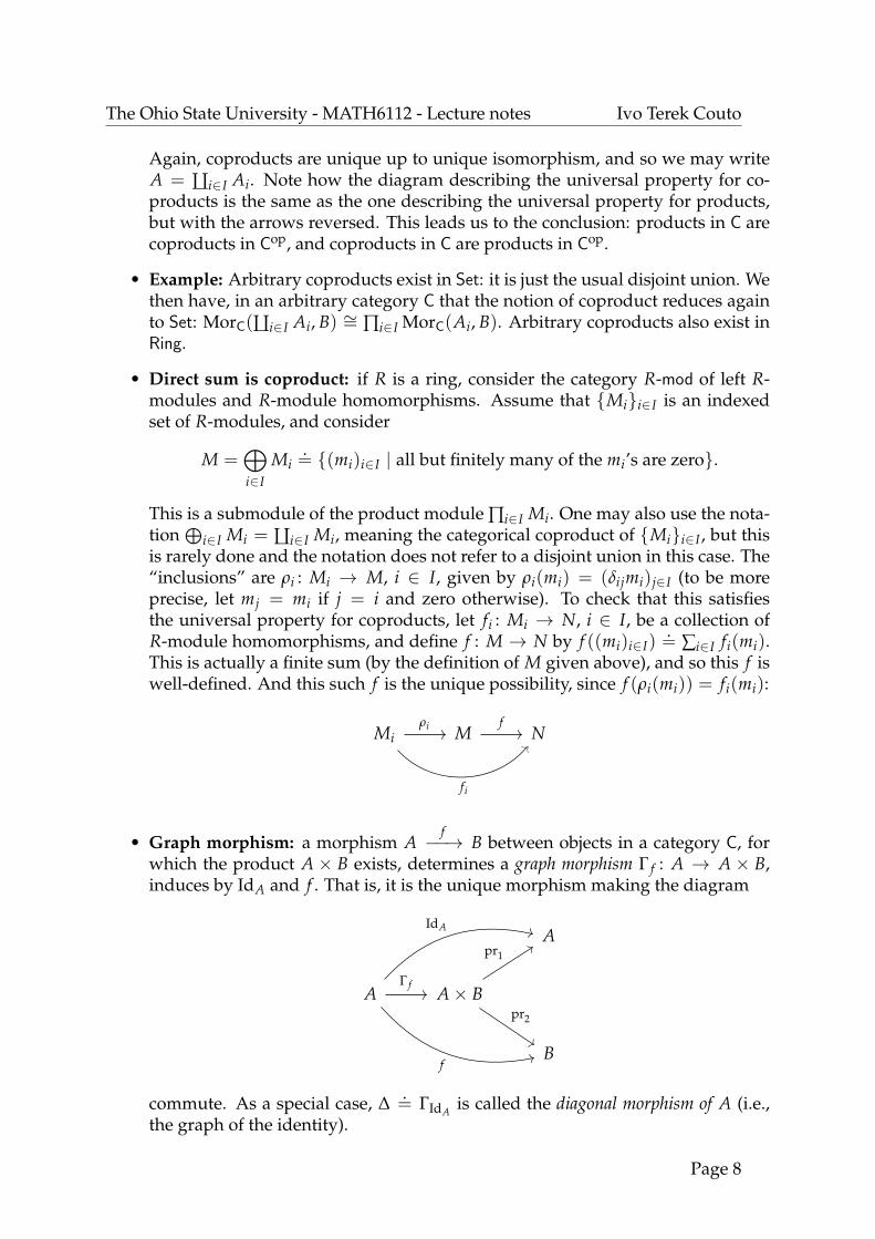
• Direct sum is coproduct: if R is a ring, consider the category R-mod of left R-modules and R-module homomorphisms. Assume that {Mi}i∈I is an indexedset of R-modules, and consider
M =⊕i∈I
Mi.= {(mi)i∈I | all but finitely many of the mi’s are zero}.
This is a submodule of the product module ∏i∈I Mi. One may also use the nota-tion
⊕i∈I Mi = äi∈I Mi, meaning the categorical coproduct of {Mi}i∈I , but this
is rarely done and the notation does not refer to a disjoint union in this case. The“inclusions” are ρi : Mi → M, i ∈ I, given by ρi(mi) = (δijmi)j∈I (to be moreprecise, let mj = mi if j = i and zero otherwise). To check that this satisfiesthe universal property for coproducts, let fi : Mi → N, i ∈ I, be a collection ofR-module homomorphisms, and define f : M → N by f ((mi)i∈I)
.= ∑i∈I fi(mi).
This is actually a finite sum (by the definition of M given above), and so this f iswell-defined. And this such f is the unique possibility, since f (ρi(mi)) = fi(mi):
Mi M Nρi
fi
f
• Graph morphism: a morphism Af−−→ B between objects in a category C, for
which the product A × B exists, determines a graph morphism Γ f : A → A × B,induces by IdA and f . That is, it is the unique morphism making the diagram
A
A A× B
B
Γ f
IdA
f
pr2
pr1
commute. As a special case, ∆ .= ΓIdA is called the diagonal morphism of A (i.e.,
the graph of the identity).
Page 8

The Ohio State University - MATH6112 - Lecture notes Ivo Terek Couto
• Initial and terminal objects: Let C be any category.
– an object I is initial if it admits a unique morphism to every other object:MorC(I, A) has only one element, for every object A.
– an object T is terminal if it receives a unique morphism from every otherobject: MorC(A, T) has only one element, for every object A.
– an object is called a zero object if it is both initial and terminal.
That is to say, initial objects are universal sources and terminal objects are universaltargets. And if they exist, they are unique up to unique isomorphism.
• Examples: in Set, ∅ is initial and singletons are terminal, while in Grp the trivialgroup if both initial and terminal.
• Group objects: Assume C is a category with finite products and a terminal object?. A group object in C is the data (G, ·, ε, ι), where G is an object, and the othersare morphisms
(i) G× G ·−−→ G (multiplication);
(ii) ε : ?→ G (identity);
(iii) ι : G → G (inversion),
satisfying the group axioms in categorical form:
(a) Identity (both left and right):
G ?× G G× G
GIdG
ε×IdG
• andG G× ? G× G
GIdG
IdG×ε
•
(b) Inverses (both left and right):
G G× G G× G
? G
∆ ι×IdG
•ε
andG G× G G× G
? G
∆ IdG×ι
•ε
(c) Associativity:
G× G× G G× G
G× G G
IdGו
•×IdG •
•
Page 9

The Ohio State University - MATH6112 - Lecture notes Ivo Terek Couto
• Remark on abuses of notation: in the above definition there are some abuses ofnotation. For example, both morphisms IdG × • and • × IdG have G × G × G.In fact, all (G × G) × G, G × (G × G) and G × G × G are isomorphic, and tobe completely precise, one should take into account these isomorphisms in thediagrams above. Also, the unnamed maps in (a) are the obvious ones, inducedby the (unique) terminal map G → ? and IdG via the universal property of G×G.
Jan 14th
• Examples:
(1) A group object in Set is a group.
(2) A group object in Grp is an abelian group
(3) A group object in Top is a topological group.
(4) A group object in Man is a Lie group.
• Functors: They are basically “maps between categories”. A (covariant) functorF : C→ D from one category to another is:
(i) an assignment A 7→ F(A) of an object of D for each object of C, and;
(ii) for each morphism Af−−→ B in C, a morphism F(A)
F( f )−−−−→ F(B) in D (thatis, a map MorC(A, B) → MorD(F(A), F(B))), also satisfying the conditions
F(g ◦ f ) = F(g) ◦ F( f ) for any Af−−→ B
g−−→ C, and F(IdA) = IdF(A).
The definition of a contravariant functor is the same, but reversing the arrows in
(ii), that is, Af−−→ B
g−−→ C goes into F(A)F( f )←−−−− F(B)
F(g)←−−−− F(C). So,a contravariant functor C → D is the same as a covariant function Cop → D.However, it is not the same as a covariant function C→ Dop, as condition (ii) willfail.
• Forgetful functors:
(1) Grp→ Mon5 assigns to the group (G, ·) the monoid (G, ·), and assigns to thegroup homomorphism f : G → H, the monoid homomorphism f : G → H.
(2) Mon→ Set, which forgets the monoid structure. That is, maps (M, ·) to theset M, and any monoid homomorphism to its underlying set map.
(3) Man→ Top, which forgets the smooth structure. That is, it maps a differen-tiable manifold to its underlying topological space, and any smooth map toits (underlying?) continuous map.
(4) Top→ Set, which forgets the topology. And so on.5Here, Mon denotes the category of monoids, with monoid homomorphisms.
Page 10

The Ohio State University - MATH6112 - Lecture notes Ivo Terek Couto
• Pre-sheaves: Let X be a topological space. A pre-sheaf of abelian groups over Xis a contravariant functor F : OpenX → Ab with F(∅) = {0}. Similarly, onecan define a pre-sheaf of rings as a contravariant functor F : OpenX → Ring withF(∅) = {0}. Writing explicitly (in the abelian group case, say), this means that
(i) for every open subset U ⊆ X we assign an abelian group F(U), and;
(ii) for any given open sets U ⊆ V ⊆ X, we have a group homomorphismResV,U : F(V) → F(U), suggestively called the restriction, which satisfiesthe conditions ResU,U = IdF(U) and ResV,U ◦ ResW,V = ResW,U, for all opensets U ⊆ V ⊆W ⊆ X.
A pre-sheaf is called a sheaf if it also satisfies the following gluing axiom (whichends up being similar to an universal property): for any given open cover {Ui}i∈Iof X and any collection of elements si ∈ F(Ui) satisfying the conditionResUi,Ui∩Uj(si) = ResUj,Ui∩Uj(sj) for all i, j ∈ I, there is a unique s ∈ F(X) suchthat ResX,Ui(s) = si for all i ∈ I.
• Definition: A functor F : C→ D is:
– faithful, if for all objects A and B of C, the induced map
MorC(A, B)→ MorD(F(A), F(B))
is injective;
– full, if for all objects A and B of C, the induced map
MorC(A, B)→ MorD(F(A), F(B))
is surjective;
– fully faithful if it is full and faithful. That is, if it induces bijections on thehom-sets.
• Examples:
(1) The inclusion of a subcategory is faithful; the inclusion of a full subcategoryis fully faithful;
(2) If (P,≤) is a poset and n ∈ N is a natural number, n can be seen as a poset{1 < 2 < · · · < n}. Then a functor F : n → P between the correspondingposet-categories is a (possibly non-injective) n-chain in (P,≤) (it could haverepeated elements). Fixing this subtlety is not as simple as requiring thefunctor to be faithful or even fully faithful. Consider the following situation:
•
• •
• •
•
≤
• 3
• •
• • 2
• 1
•
• 2, 3 •
• •
• 1
Page 11

The Ohio State University - MATH6112 - Lecture notes Ivo Terek Couto
In the left we have the Hasse diagram for a given poset (P,≤), and the othertwo figures depict two fully faithful functors 3→ P.
(3) If R is a commutative ring and S ⊆ R is multiplicatively closed subset of R,then S−1 : R-mod→ S−1R-mod is a functor taking M to the localized moduleS−1M, and a R-module homomorphism ϕ : M → N to the unique S−1R-linear map S−1(ϕ) : S−1M → S−1N satisfying S−1(ϕ)(m/s) = ϕ(m)/s, forall m ∈ M and s ∈ S. This is not a faithful functor. Say M = N ⊕ R/(s) forsome s ∈ S, and consider both maps
M N M(n, r) n (n, 0)
and IdM : M→ M.
They have the same image in MorS−1R-mod(S−1M, S−1M).
(4) Let Top∗ be the category of pointed topological spaces. The objects are pairs(X, x), where X is a topological space and x ∈ X is a chosen point. A mor-
phism (X, x)f−−→ (Y, y) is a continuous map f : X → Y satisfying also
f (x) = y. Note that this condition can be expressed also in terms of thefollowing commutative diagram:
X Y
{x} {y}
f
Here, the vertical arrows are just inclusions. The fundamental group is a func-tor π1 : Top∗ → Grp, mapping (X, x) to π1(X, x) and a continuous map
(X, x)f−−→ (Y, y) to a group homomorphism f∗ : π1(X, x)→ π1(Y, y). This
functor happens to map terminal objects into terminal objects (indeed, thefundamental group of a one-point space is trivial), but this need not be thecase even if the functor is fully faithful. This is because being fully faithfulis a condition related mainly to morphisms, and one still could have objectsin the target category which are not in the “image” of the functor).
• Isomorphism of categories: If C is a category, the identity functor is 1C doing theobvious: 1C(A)
.= A and 1C( f ) .
= f . Functors can be composed in the obviousway (object-wise). So, a functor F : C → D is an isomorphism of categories if it hasa two-sided inverse G : D → C (that is, satisfying GF = 1C and FG = 1D). Notealso that it follows that an isomorphism of categories actually induces bijectionsbetween Obj(C) and Obj(D), so in particular isomorphic categories must havethe same number of objects. However, this almost never happens, and the bestwe get are uninteresting examples like Ab = Z-mod and (Cop)op = C.
Jan 16th
• Natural transformations: Let F, G : C → D be two (both covariant or both con-travariant) functors between categories. A natural transformation η : F =⇒ G is
Page 12

The Ohio State University - MATH6112 - Lecture notes Ivo Terek Couto
a morphism ηA : F(A) → G(A) in D, for each object A in C, such that given any
morphism Af−−→ B in C, the diagram
F(A) G(A)
F(B) G(B)
F( f )
ηA
G( f )
ηB
commutes.
• Remark: The definition above is uninteresting if one of the functors is covariantand the other contravariant. For example, switching G( f ) in the above diagram,one could try to define ηA as the composition G( f ) ◦ ηB ◦ F( f ), which could be acircular definition also leading to compatibility problems.
• Natural isomorphisms: given a functor F : C → C, the identity transformation1F is the evident thing: (1F)A = IdF(A). Natural transformations can also becomposed at the object level. Then, a natural transformation η : F =⇒ G isa natural isomorphism if each ηA is an isomorphism. One can check that η is anatural isomorphism if and only if there exists an inverse natural transformationη−1 : G =⇒ F such that η−1η = 1F and ηη−1 = 1G.
• Example: Let k be a field and Vectk be the category of k-vector spaces and lineartransformations. The duality functor is D : Vectk → Vectk given by D(V)
.= V∗
and sending ϕ : V → W to D(ϕ) = ϕ∗ : W∗ → V∗ (defined by ϕ∗( f ) = f ◦ ϕ).Note that D is contravariant, so the composition (called the double dual functor)DD is covariant. We have a natural transformation η : 1Vectk =⇒ DD definedby ηV : V → V∗∗, ηV(v) = v∗∗ = evaluation at v. Then we can check naturality,which now has a precise meaning. That is to say, we must check that the diagram
V V∗∗
W W∗∗
f
ηV
f ∗∗
ηW
commutes. This is done as follows: first recall that given ξ ∈ V∗∗ and ψ ∈ W∗,we have f ∗∗(ξ)(ψ) = ξ( f ∗(ψ)). With this in mind, we take ξ = ηV(v) for somev ∈ V and compute
f ∗∗(ηV(v))(ψ) = ηV(v)( f ∗(ψ)) = f ∗(ψ)(v) = ψ( f (v)) = ηW( f (v))(ψ),
as wanted.
• Equivalence of categories: we would like to have a more “relaxed” (and moreuseful) notion of an isomorphism of categories. We say that a functor F : C → D
Page 13

The Ohio State University - MATH6112 - Lecture notes Ivo Terek Couto
is an equivalence of categories if there exist an “inverse” functor G : D → C andnatural isomorphisms GF ∼= 1C and FG ∼= 1D. In this case, we say that C and Dare equivalent categories.
• Remark: Compare this with the situation in Top, where an homotopy equiva-lence is a continuous map which has an inverse up to homotopy. This ends upbeing a particular instance of the definition above.
• Toy example: Consider the category C associated to the multiplicative group(Z/2Z, ·), and the category D depicted below:
A A
1
−1
and A A A′ A′1
−1
a−a
a−1
−a−1
1′
−1′
Note that C and D are not isomorphic (indeed, they do not even have the samenumber of objects), but we claim that they are equivalent. The “inclusion” func-tor F : C → D given by F(A) = A, F(1) = 1, F(−1) = −1 is an equivalence ofcategories. Indeed, the functor G : D→ C given by
G(A) = G(A′) = AG(1) = G(1′) = 1G(−1) = G(−1′) = −1G(a) = G(a−1) = 1G(−a) = G(−a−1) = −1
behaves like a deformation retract. We have that GF = 1C, and FG ∼= 1D via thenatural isomorphism η : 1D =⇒ FG given by ηA = IdA and ηA′ = −a.
Jan 18th
• More definitions of equivalences:
– An equivalence Cop → D is called an anti-equivalence between C and D (thatis, it is given by a contravariant functor C→ D).
– An equivalence C→ C is called an auto-equivalence. For example, the doubledual functor DD is an auto-equivalence of the full subcategory of finite-dimensional vector spaces over a fixed field k.
• Theorem: A functor F : C → D is an equivalence of categories if and only if it isfully faithful and essentially surjective (that is, for every object D of D there is anobject C of C and an isomorphism F(C) ∼= D).
This is generally a very useful criterion for checking whether a given functor isan equivalence of categories, just like one checks if a given function is bijective
Page 14

The Ohio State University - MATH6112 - Lecture notes Ivo Terek Couto
by checking that it is both injective and surjective (instead of always trying toexhibit an inverse function).
Half-proof: Suppose G : D→ C is an inverse for F up to natural isomorphisms.
– F is faithful: assume given two morphisms Af−−→ B and A
g−−→ B withF( f ) = F(g). By GF ∼= 1C, we have that both diagrams
GF(A) A
GF(B) B
∼=
GF( f )=GF(g) f
∼=
and
GF(A) A
GF(B) B
∼=
GF( f )=GF(g) g
∼=
commute, and so f = g (both are equal to the composition of the remainingthree arrows on each diagram).
– F is essentially surjective: now we use the condition FG ∼= 1D. Given anobject D of D, we have that G(D) is now an object in C. Then F
(G(D)
) ∼= D,as wanted.
– F is full: given a morphism F(A)h−−→ F(B), we look for a morphism
Af−−→ B such that F( f ) = h. Define f as the composition:
A GF(A) GF(B) B∼=
f
G(h) ∼=
To see that this indeed works, apply F to get
F(A) FGF(A) FGF(B) F(B)∼=
F( f )
h
FG(h) ∼=
as wanted.
• Example: If R is a ring, let Mat(n, R) ∼= EndR(R⊕n) be the ring of n× n matriceswith entries in R. The categories (of right modules) mod-R and mod-Mat(n, R)are equivalent. To see this, consider the functor F : mod-R → mod-Mat(n, R)given by F(M)
.= M⊕n = M⊕ · · · ⊕M (n times) and F(ϕ) = ϕ⊕n = ϕ⊕ · · · ⊕ ϕ
(n times), for every R-module homomorphism ϕ : M→ N.
We have that F is faithful, since if π : N⊕ → N denotes projection in some fixedfactor, then ϕ⊕ = ψ⊕ readily implies that
ϕ = π ◦ ϕ⊕∣∣∣∣
M⊕{0}⊕(n−1)= π ◦ ψ⊕n
∣∣∣∣M⊕{0}⊕(n−1)
= ψ,
Page 15

The Ohio State University - MATH6112 - Lecture notes Ivo Terek Couto
as wanted.
The verification that F is full and essentially surjective is an exercise.
• The Yoneda Embedding: Fix an object X of C. There is a natural hX : C → Setdefined by
– hX(A).= HomC(X, A);
– hX( f ) : HomC(X, A)→ HomC(X, B), hX( f )(g) .= f ◦ g.
This is called the (covariant) Hom functor. One may also define a contravariantversion hX : C→ Set by
– hX(A).= HomC(A, X);
– hX( f ) .= HomC(B, X)→ HomC(A, X), hX( f )(g) .
= g ◦ f .
This is called the (contravariant) Hom functor. One can also see Hom as a “bifunc-tor” Cop× C→ Grp (here the definition of the product category is the obvious one,no subtleties).
• Universality and representability are synonyms:
– A covariant functor F : C → Set is representable (in C) if there is an object Xin C and a natural isomorphism F ∼= hX = HomC(X, _).
– A contravariant functor F : C→ Set is representable (in C) if there is an objectX in C and a natural isomorphism F ∼= hX = HomC(_, X).
In these cases, we say that F is representable by X.
• Examples: Universal properties are ultimately examples of the previous defini-tions. Let R be a ring, fix two left R-modules A1 and A2 and define a functorFA1,A2 : R-mod → Set by FA1,A2(M) = HomR(A1, M)×HomR(A2, M), and tak-ing a R-module homomorphism f : M→ N to
HomR(A1, M)×HomR(A2, M) HomR(A1, N)×HomR(A2, N)
(ϕ, ψ) ( f ◦ ϕ, f ◦ ψ).
FA1,A2 ( f )
This is covariant, and we have FA1,A2∼= hA1⊕A2 by the universal property of
the direct sum in R-mod (coproduct). Similarly one may define a contravariantversion FA1,A2 by FA1,A2(M) = HomR(M, A1)×HomR(M, A2), with action onmorphisms given by pre-composition this time, as to obtain FA1,A2 ∼= hA1×A2 .Recall also that in this case we have A1 ⊕ A2
∼= A1 × A2.
Page 16

The Ohio State University - MATH6112 - Lecture notes Ivo Terek Couto
Jan 23rd
• Yoneda Lemma: For any functor F : C → Set any any object X of C, there is anatural bijection
{natural transformations hX = HomC(X, _) =⇒ F} η−−−−→∼= F(X)
sending hX α=⇒ F to αX(IdX).
• Remarks: Note that since both HomC(X, X) and F(X) are sets, we have thatαX : HomC(X, X) → F(X) is a function, and so it makes sense to consider itsvalue αX(IdX) in some element of its domain. Moreover, naturality here means
that given any morphism X′f−−→ X, the diagram
{natural transformations HomC(X′, _) =⇒ F} F(X′)
{natural transformations HomC(X, _) =⇒ F} F(X)
ηX′
F( f )
ηX
commutes, where the unlabeled arrow maps HomC(X′, _) α′=⇒ F to the transfor-
mation HomC(X′, _) α=⇒ F given by αY(g) .
= α′Y(g ◦ f ).
• Proof of the Yoneda Lemma: for each morphism Xf−−→ A and each natural
transformation HomC(X, _) α=⇒ F, the diagram
HomC(X, X) F(X)
HomC(X, A) F(A)
αX
hX( f ) F( f )
αA
commutes. This allows us to construct the inverse η−1 in the following way:given x ∈ F(X), we have to define a natural transformation hX =⇒ F. So defineαX(IdX) = x. This actually determines the entire natural map αX, even thoughwe have only defined its value on one element IdX. For example, making A = Xand f = ϕ in the above diagram and noting that hX(ϕ)(IdX) = ϕ, it automati-cally follows that
αX(ϕ) = F(ϕ)(αX(IdX)
)= F(ϕ)(x).
In this sense, naturality “propagates”, allowing us to define αA also for A 6= Xin the same way, setting αA( f ) = F( f )(x).
• Functor categories: Another way to understand the naturality of the Yonedabijection is via functor categories. Given categories C and D, there’s a category
Page 17

The Ohio State University - MATH6112 - Lecture notes Ivo Terek Couto
Fun(C,D) (also denoted DC for clear reasons) with objects being functors C → Dand morphisms being natural transformations F =⇒ G. The Yoneda Lemmathen says that there is a fully faithful “embedding” functor6 Y: Cop → SetC
defined on objects by Y(X) = hX and mapping X → Y to hY =⇒ hX.
Similarly, there is a “dual” functor Y: C → SetC given by Y(X) = hX, mappingX → Y to hX =⇒ hY.
• Consequence: Given a functor F : C → Set, suppose X and X′ are representing
objects (in C) for F, with natural isomorphisms hX η=⇒ F and hX′ η′
=⇒ F. Thereis a unique isomorphism X '−−−→ X′ which is compatible with these transforma-tions. This is because in the hom-level, Y: HomC(X′, X) → HomSetC(h
X, hX′) isa bijection, and the composition (η′)−1 ◦ η can be seen as a morphism hX → hX′
in SetC; consider Y−1((η′)−1 ◦ η)−1.
• Examples:
(1) In any category C with finite products, we have
(A× B)× C) ∼= A× (B× C) ∼= A× B× C
for any objects A, B and C. This is because all of them represent the samefunctor FA,B,C : Cop → Set given by
FA,B,C(D).= HomC(D, A)×HomC(D, B)×HomC(D, C),
acting on morphisms D → D′ by a suitable composition. The moral of thehistory is that if some statement can be proven in Set, then it can be trans-ferred to an arbitrary category C, if one can find convenient representationsfor a convenient functor.
(2) Denote by CRing the category of commutative rings with 1 and ring homo-morphisms which map 1 7→ 1. Let A be a commutative ring, S ⊆ A be amultiplicatively closed subset, and I � A an ideal. Then we have that
S−1AS−1 I
∼=(
SI
)−1(AI
),
because they represent the same functor FA,S,I : CRing→ Set given by
FA,S,I(B) .= {A
g−→ B | g(s) ∈ B× for all s ∈ S and g(x) = 0 for all x ∈ I}
and acting on morphisms via suitable compositions.6The op here only says that Ywill be a contravariant functor from C to SetC.
Page 18
The Ohio State University - MATH6112 - Lecture notes Ivo Terek Couto
Jan 25th
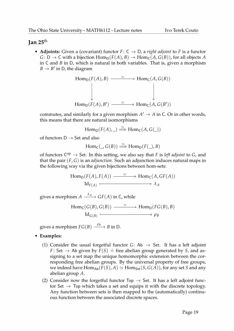
• Adjoints: Given a (covariant) functor F : C → D, a right adjoint to F is a functorG : D → C with a bijection HomD(F(A), B) → HomC(A, G(B)), for all objects Ain C and B in D, which is natural in both variables. That is, given a morphismB→ B′ in D, the diagram
HomD(F(A), B) HomC(A, G(B))
HomD(F(A), B′) HomC(A, G(B′))
'
'
commutes, and similarly for a given morphism A′ → A in C. Or in other words,this means that there are natural isomorphisms
HomD(F(A), _) '=⇒ HomC(A, G(_))
of functors D→ Set and also
HomC(_, G(B)) '=⇒ HomD(F(_), B)
of functors Cop → Set. In this setting, we also say that F is left adjoint to G, andthat the pair (F, G) is an adjunction. Such an adjunction induces natural maps inthe following way via the given bijections between hom-sets:
HomD(F(A), F(A)) HomC(A, GF(A))
IdF(A) λA
'
gives a morphism AλA−−−→ GF(A) in C, while
HomC(G(B), G(B)) HomD(FG(B), B)
IdG(B) ρB
'
gives a morphism FG(B)ρB−−−→ B in D.
• Examples:
(1) Consider the usual forgetful functor G : Ab → Set. It has a left adjointF : Set → Ab given by F(S) .
= free abelian group generated by S, and as-signing to a set map the unique homomorphic extension between the cor-responding free abelian groups. By the universal property of free groups,we indeed have HomAb(F(S), A) ' HomSet(S, G(A)), for any set S and anyabelian group A.
(2) Consider now the forgetful functor Top → Set. It has a left adjoint func-tor Set → Top which takes a set and equips it with the discrete topology.Any function between sets is then mapped to the (automatically) continu-ous function between the associated discrete spaces.
Page 19

The Ohio State University - MATH6112 - Lecture notes Ivo Terek Couto
• Limits (and colimits): The idea is to generalize products and coproducts, respec-tively.
– Definition. Let C be a category. An inverse system is a collection of objects
{Ai}i∈I indexed by a poset I together with morphisms Aiϕij−−−→ Aj when-
ever i ≥ j, such that if i ≥ j ≥ k we have ϕjk ◦ ϕij = ϕik. That is, an inversesystem is a functor Iop → C, sending j → i in I (when j ≤ i) to Ai → Aj.When regarding an inverse system as a functor like this, we set ϕii = IdAiby convention.
– Definition. An (inverse) limit of an inverse system (with the above nota-tion) is an object lim←−I
Ai (also denoted limI Ai) together with morphismspri : lim←−I
Ai → Ai such that:
(i) for all i ≥ j, the diagram
Ai
lim←−IAi
Aj
ϕij
pri
prj
commutes, and;(ii) lim←−I
Ai is universal for condition (i), i.e., given an object B and mor-
phisms Bfi−−→ Ai such that for i ≥ j the diagram
Ai
B
Aj
ϕij
fi
f j
commutes, there is a unique morphism Bf−−→ lim←−I
Ai making the fol-lowing diagram commute:
Ai
B lim←−IAi
Aj
ϕij
fi
f j
∃! f
pri
prj
Page 20

The Ohio State University - MATH6112 - Lecture notes Ivo Terek Couto
• Examples:
(1) Products are indeed particular cases of limits, when {Ai}i∈I is indexed bythe “anti-chain”, that is, the only order relations are i ≤ i for all i ∈ I, andwe have ϕii = IdAi . Moreover, when both lim←−I
Ai and ∏i∈I Ai exist, thereis a canonical morphism lim←−I
Ai → ∏i∈I Ai given by the universal propertyof the product applied to the data lim←−I
Ai → Ai, i ∈ I.
(2) In Ring, consider Ai = Z/piZ, where p is a fixed prime and i = 1, 2, . . .. Wehave maps Z/piZ → Z/pjZ for i ≥ j, and this is an inverse system whoselimit is lim←−NZ/piZ = Zp, the ring of p-adic integers.
• Relation with limits from Calculus: Consider in the real line R a decreasingsequence (xn)n∈N, and assume that it is convergent, to x .
= limn→+∞ xn. Thepoints in the sequence may be seen as objects in the poset-category R associatedto (R,≤). Since for n ≥ m we have xn ≤ xm, this says that we have a uniquemorphism xn
ϕnm−−−−→ xm in R. The compatibility between said morphisms isnothing more than the transitivity of ≤ in R, so we may see the sequence as aninverse system in R. Now we claim that x = lim←−N xn. To wit, we have x ≤ xn
for all n ∈ N and this gives us the projection morphisms xprn−−−→ xn in R. The
diagramxn
x
xm
ϕnm
prn
prm
commutes in R for n ≥ m, again by transitivity of ≤ in R. Now we only have tocheck universality. Assume we’re given an object y ∈ R and morphisms y→ xn,n ∈ N. This just says that y ≤ xn for all n ∈ N, and in particular the diagram
xn
y
xm
ϕnm
automatically commutes for n ≥ m. Since y ≤ xn for all n ∈ N, pass to thelimit (in the usual Calculus sense) to conclude that y ≤ x. This gives us a unique
Page 21

The Ohio State University - MATH6112 - Lecture notes Ivo Terek Couto
morphism y→ x making the diagram
xn
y x
xm
ϕnm
prm
prn
commute for n ≥ m (since then we have the three inequalities y ≤ x ≤ xn,y ≤ x ≤ xm and x ≤ xn ≤ xm). We conclude that
limn→+∞
xn = lim←−N
xn.
• Colimits: Now we state the definitions for the dual notion to inverse systemsand limits.
– Definition. Let C be a category. A direct system is a collection of objects
{Ai}i∈I indexed by a poset I together with morphisms Aiψij−−−→ Aj when-
ever i ≤ j, such that if i ≤ j ≤ k we have ψjk ◦ ψij = ψik. Similar to before,a direct system is a functor I → C, sending i → j in I (when i ≤ j) toAi → Aj. Again, when regarding an inverse system as a functor like this,we set ψii = IdAi .
– Definition. A colimit of a direct system (with the above notation) is an objectlim−→I
Ai (also denoted colimI Ai) together with morphisms ρi : Ai → lim−→IAi
such that:(i) for all i ≤ j, the diagram
Ai
lim−→IAi
Aj
ρi
ψij
ρj
commutes, and;(ii) lim−→I
Ai is universal for condition (i), i.e., given an object B and mor-
phisms Aifi−−→ B such that for i ≤ j the diagram
Ai
B
Aj
fi
ψij
f j
Page 22
The Ohio State University - MATH6112 - Lecture notes Ivo Terek Couto
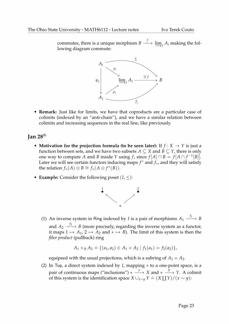
commutes, there is a unique morphism Bf−−→ lim−→I
Ai making the fol-lowing diagram commute:
Ai
lim−→IAi B
Aj
ρi
ψij
fi
∃! f
ρj
f j
• Remark: Just like for limits, we have that coproducts are a particular case ofcolimits (indexed by an “anti-chain”), and we have a similar relation betweencolimits and increasing sequences in the real line, like previously.
Jan 28th
• Motivation for the projection formula (to be seen later): If f : X → Y is just afunction between sets, and we have two subsets A ⊆ X and B ⊆ Y, there is onlyone way to compare A and B inside Y using f , since f [A] ∩ B = f [A ∩ f−1[B]].Later we will see certain functors inducing maps f ∗ and f∗, and they will satisfythe relation f∗(A)⊗ B ∼= f∗(A⊗ f ∗(B)).
• Example: Consider the following poset (I,≤):
1• 2•
∗
(1) An inverse system in Ring indexed by I is a pair of morphisms A1f1−−−→ B
and A2f2−−−→ B (more precisely, regarding the inverse system as a functor,
it maps 1 7→ A1, 2 7→ A2 and ∗ 7→ B). The limit of this system is then thefiber product (pullback) ring
A1 ×B A2.= {(a1, a2) ∈ A1 × A2 | f1(a1) = f2(a2)},
equipeed with the usual projections, which is a subring of A1 × A2.
(2) In Top, a direct system indexed by I, mapping ∗ to a one-point space, is apair of continuous maps (“inclusions”) ∗ x−−→ X and ∗ y−−→ Y. A colimitof this system is the identification space X ∪x∼y Y .
= (X ä Y)/(x ∼ y):
Page 23

The Ohio State University - MATH6112 - Lecture notes Ivo Terek Couto
X xy
YX ∪x∼y Y
Figure 1: Gluing two spaces on a point.
Note that there is no need to restrict ourselves in this example to considering∗ a one-point space (we could glue two spaces along subspaces).
• Remark: We often see the condition that a poset is directed (or filtered): for eachi, j ∈ I there is k ∈ I with i ≤ k and j ≤ k. This condition is not required to definelimits and colimits, but it is useful if it holds. For example, if one replaces I witha subposet J ⊆ I with the property that for every iI there is j ∈ J with i ≤ j,for every system {Ai}i∈I we have lim←−I
Ai∼= lim←−J
Aj and lim−→IAi∼= lim−→J
Aj, whenthese exist.
• Complete/cocomplete categories: A category C is complete (resp. cocomplete) ifall limits (resp. colimits) exist, for all posets I. Sometimes it is required in thisdefinitions that the condition holds only for finite posets. In general, fixed a posetI for which all limits exist, a diagram indexed by I in C is a functor in CIop
, andso we obtain a functor lim←−I
: CIop → C
• Example: Suppose that
A1 A2 · · · and B1 B2 · · ·
are inverse systems of groups. Then lim←−N An and lim←−N Bn always exist. Givingmorphisms An → Bn, n ∈ N, such that the diagram
A1 A2 · · ·
B1 B2 · · ·
commutes is the same as giving a morphism {An}n∈N → {Bn}n∈N in GrpNop
. Wethen obtain a morphism lim←−N An → lim←−N Bn. As a subexample, when the sys-tems are indexed by the antichain (meaning that we do not have the horizontalarrows), we obtain simply a morphism ∏i∈I Ai → ∏i∈I Bi.
Page 24

The Ohio State University - MATH6112 - Lecture notes Ivo Terek Couto
• Monics and epis: In a category C, a morphism Af−−→ B is called a:
– monomorphism (monic) if it is left-cancellable:
T A Bg1
g2
f=⇒ g1 = g2,
or in other words, if f ◦ g1 = f ◦ g2 =⇒ g1 = g2 for every “test” object T.
– epimorphism (epi) if it is right-cancellable:
A B Tf
g1
g2
=⇒ g1 = g2,
or in other words, if g1 ◦ f = g2 ◦ f =⇒ g1 = g2 for every “test” object T.
• Example/Remark: In Set, a map is a monomorphism (resp. epimorphism) if andonly if it is injective (resp. surjective). But this need not be the case even forcategories whose objects are sets with additional structure. For example, Z ↪→ Q
is epi in Ring, Q ↪→ R is epi in Top, etc..
• Equalizers: Let I be the poset • •. A limit over I in a category C is
called an equalizer. More precisely, the equalizer of two morphisms Af1−−→ B and
Af2−−→ B is an object K with a morphism K ε−−→ A such that f1 ◦ ε = f2 ◦ ε,
which is universal among all the morphisms that equalize f and g, that is, forevery morphism T
g−−→ A such that f1 ◦ g = f2 ◦ g, there is a unique morphismT u−−→ K such that ε ◦ u = g. Meaning that the following universal property issatisfied:
T K A B∃! ε
f1
f2
Note that if an equalizer exists, it is automatically monic, in view of the unique-ness of u: to wit, if g1 and g2 are morphisms from T to K with ε ◦ g1 = ε ◦ g2,then the unique morphism completing the above diagram has to be g1, and atthe same time, g2.
• Remarks:
– Reversing the arrows, one may also define the coequalizer of two morphismswith same source and target. Coequalizers, when exist, are automaticallyepimorphisms (since coequalizers in C are the same as equalizers in Cop).
– In the same fashion, one could also define what is the coequalizer of anyfamily of morphisms in C with same source and target.
Page 25

The Ohio State University - MATH6112 - Lecture notes Ivo Terek Couto
• Example: In Ab and Rng, equalizers always exist. Namely, ε will be the inclusionker ( f1 − f2) ↪→ A. This motivates the alternative name “difference kernel” forequalizers as well as the usual choice of letter K. Moreover, wanting to generalizethis to categories where one cannot subtract morphisms motivates more generaldefinitions of kernel, and the definition of an abelian category.
Page 26

The Ohio State University - MATH6112 - Lecture notes Ivo Terek Couto
Homological Algebra (and more Category Theory)
Feb 1st
• Additive categories: The idea here is that an additive category is one whosehom-sets are abelian groups. An abelian category will satisfy additional condi-tions, modeled on Ab or R-mod. More precisely, we have the
Definition: A category A is additive if:
(i) all finite products exist (including the empty product – meaning that A hasa terminal object);
(ii) There is a zero object 0;
(iii) HomA(A, B) is an abelian group, for all objects A and B of A, and the com-positions
HomA(A, B)×HomA(B, C)→ HomA(A, C)
are bilinear.
• Remark: In the above definition, every HomA(A, B) has a “0” morphism, namely,the only arrow making the diagram
A B
0
∃! 0
commute. This morphism must necessarily be the additive identity of HomA(A, B),as the image of the bilinear map
HomA(A, 0)×HomA(0, B) = {(0, 0)} → HomA(A, B)
is just {0}.
• Kernels and cokernels: Let C be a category having a zero object (and hence zero
morphisms between any give two objects of C – all denoted by 0). If Af−−→ B is
a morphism, then:
– a kernel of f is a morphism K k−−→ A such that f ◦ k = 0, and universal forthis property:
T
A B
K
t
0
∃!f
k
0
Page 27

The Ohio State University - MATH6112 - Lecture notes Ivo Terek Couto
– a cokernel of f is a morphism B c−−→ C such that c ◦ f = 0, and universal forthis property:
T
A B
C
f
0
0
t
c
∃!
• Remark: If kernels and cokernels exist, they’re unique up to isomorphism, so oneusually writes K = ker ( f ) and C = coker( f ). Moreover, kernels and cokernelsmay be realized as certain limits and colimits, respectively.
• Additive functors: Let A and B be additive categories. A functor F : A → B iscalled additive if all the induced maps HomA(A, B) → HomB(F(A), F(B)) aregroup homomorphisms.
• Abelian categories: An abelian category is an additive category satisfying the ad-ditional conditions:
(iv) Every morphism has a kernel and a cokernel.(v) Every monic is the kernel of its cokernel; every epi is the cokernel of its
kernel.(vi) Every morphism f factors as f = m ◦ e, where m is monic and e is epic.
• Understanding axiom (v): In Ab, A is the kernel of A ↪→ B � B/A, and given
ker ( f ) ↪→ Af−−→ B, we have B ∼= A/ker ( f ). Here, ker ( f ) measures how far
f is from being injective, while coker( f ) ∼= B/Im( f ) measures for far f is frombeing surjective.
• Propotype: R-mod is an abelian category.
• Counter-example: The full subcategory FreeAb of Ab, of free abelian groups, is
not abelian. For example, Z ·2−−−→ Z has no cokernel in FreeAb, since Z/2Z hastorsion (and it is not an object there).
• Exactness: A sequence Mf−−→ N
g−−→ P in R-mod is exact at N if we haveker ( f ) = Im(g) (as submodules of N). Categorically, the setup is
M N P
M′ ker (g)
f
e
g
m'
k,
which can be adapted to give a definition of exactness in abelian categories. Sim-ilarly, a sequence
· · · Mi−1 Mi Mi+1 · · ·fi−1 fi
Page 28
The Ohio State University - MATH6112 - Lecture notes Ivo Terek Couto
is exact if it is exact at each Mi (i.e., ker ( fi) = Im( fi−1) for all i). A short exactsequence is an exact sequence of the form
0 M′ M M′′ 0.
• Remark: In R-mod:
– 0→ Mf−−→ N is exact if and only if f is injective (monic).
– Mf−−→ N → 0 is exact if and only if f is surjective (epi).
– There is a weaker notion of an “exact category” (due to Quillen), whereexact sequences still make sense.
• Exact functors: Let F : R-mod→ S-mod be an additive functor. Say that F is exactif it preserves all short exact sequences. More precisely, if for every short exactsequence
0 M′ M M′′ 0,
the image-sequence
0 F(M′) F(M) F(M′′) 0
is also exact. Also, F is right-exact (resp. left-exact) if only the sequence
F(M′) F(M) F(M′′) 0
(resp. 0 F(M′) F(M) F(M′′) ) is guaranteed to be exact.In other words, left-exact functors produce left-exact sequences and right-exactfunctors produce right-exact sequences.
Feb 4th
• Remark: If A and B are abelian categories, a left-exact contravariant functorA→ B is the same as a left-exact covariant functor Aop → B.
• Example: For any R-module M, we have that HomR(M, _) is an additive functorR-mod→ Ab, which is left-exact (but not right-exact, in general). The same holdsfor the contravariant version HomR(_, M). Moreover, the same proof shows thatif A is an abelian category and A is any object in A, then the functors HomA(A, _)and HomA(_, A) are left-exact. The modules P for which HomR(P, _) is exact arecalled projective, while the modules Q for which HomR(_, Q) is exact are calledinjective.
• Tensor products: Given vector spaces V and W, V ⊗W is the space spanned by{v⊗w | v ∈ V, w ∈W}, and the elements in this spanning satisfy some algebraicrelations. We want to generalize this idea for modules, giving a characterizationin terms of universal properties. Denote a right R-module M simply by MR anda left R-module N by RN. This leads to the following formal definitions:
Page 29
The Ohio State University - MATH6112 - Lecture notes Ivo Terek Couto
– a balanced product of MR and RN is an abelian group A with a bi-additivemap f : M × N → A satisfying f (mr, n) = f (m, rn) for all m ∈ M, n ∈ Nand r ∈ R.
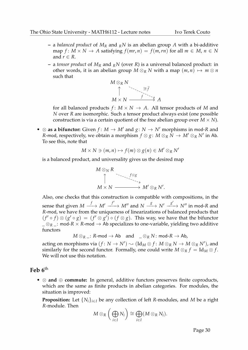
– a tensor product of MR and RN (over R) is a universal balanced product: inother words, it is an abelian group M ⊗R N with a map (m, n) 7→ m ⊗ nsuch that
M⊗R N
M× N A
∃! f
f
for all balanced products f : M × N → A. All tensor products of M andN over R are isomorphic. Such a tensor product always exist (one possibleconstruction is via a certain quotient of the free abelian group over M× N).
• ⊗ as a bifunctor: Given f : M → M′ and g : N → N′ morphisms in mod-R andR-mod, respectively, we obtain a morphism f ⊗ g : M⊗R N → M′ ⊗R N′ in Ab.To see this, note that
M× N 3 (m, n) 7→ f (m)⊗ g(n) ∈ M′ ⊗R N′
is a balanced product, and universality gives us the desired map
M⊗N R
M× N M′ ⊗R N′.
f⊗g
Also, one checks that this construction is compatible with compositions, in the
sense that given Mf−−→ M′
f ′−−−→ M′′ and Ng−−→ N′
g′−−−→ N′′ in mod-R andR-mod, we have from the uniqueness of linearizations of balanced products that( f ′ ◦ f ) ⊗ (g′ ◦ g) = ( f ′ ⊗ g′) ◦ ( f ⊗ g). This way, we have that the bifunctor_⊗R _ : mod-R× R-mod → Ab specializes to one-variable, yielding two additivefunctors
M⊗R _ : R-mod→ Ab and _⊗R N : mod-R→ Ab,
acting on morphisms via ( f : N → N′) ; (IdM ⊗ f : M⊗R N → M⊗R N′), andsimilarly for the second functor. Formally, one could write M⊗R f = IdM ⊗ f .We will not use this notation.
Feb 6th
• ⊗ and ⊕ commute: In general, additive functors preserves finite coproducts,which are the same as finite products in abelian categories. For modules, thesituation is improved:
Proposition: Let {Ni}i∈I be any collection of left R-modules, and M be a rightR-module. Then
M⊗R
(⊕i∈I
Ni
)∼=⊕i∈I
(M⊗R Ni).
Page 30
The Ohio State University - MATH6112 - Lecture notes Ivo Terek Couto
Two proof ideas:
– Show that both objects in Ab represent a same functor Ab → Set; concludeby applying the Yoneda Lemma.
– Combine the universal properties of tensor product and direct sum in dif-ferent orders to obtain the isomorphism and its inverse.
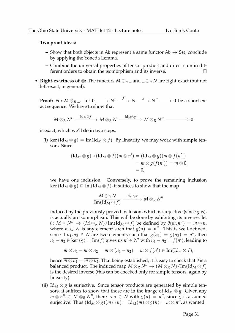
• Right-exactness of ⊗: The functors M⊗R _ and _⊗R N are right-exact (but notleft-exact, in general).
Proof: For M ⊗R _. Let 0 N′ N N′′ 0f g
be a short ex-act sequence. We have to show that
M⊗R N′ M⊗R N M⊗R N′′ 0IdM⊗ f IdM⊗g
is exact, which we’ll do in two steps:
(i) ker (IdM ⊗ g) = Im(IdM ⊗ f ). By linearity, we may work with simple ten-sors. Since
(IdM ⊗ g) ◦ (IdM ⊗ f )(m⊗ n′) = (IdM ⊗ g)(m⊗ f (n′))= m⊗ g( f (n′)) = m⊗ 0= 0,
we have one inclusion. Conversely, to prove the remaining inclusionker (IdM ⊗ g) ⊆ Im(IdM ⊗ f ), it suffices to show that the map
M⊗R NIm(IdM ⊗ f )
IdM⊗g−−−−−→ M⊗R N′′
induced by the previously proved inclusion, which is surjective (since g is),is actually an isomorphism. This will be done by exhibiting its inverse: letθ : M × N′′ → (M ⊗R N)/Im(IdM ⊗ f ) be defined by θ(m, n′′) = m⊗ n,where n ∈ N is any element such that g(n) = n′′. This is well-defined,since if n1, n2 ∈ N are two elements such that g(n1) = g(n2) = n′′, thenn1− n2 ∈ ker (g) = Im( f ) gives us n′ ∈ N′ with n1− n2 = f (n′), leading to
m⊗ n1 −m⊗ n2 = m⊗ (n1 − n2) = m⊗ f (n′) ∈ Im(Idm ⊗ f ),
hence m⊗ n1 = m⊗ n2. That being established, it is easy to check that θ is abalanced product. The induced map M⊗R N′′ → (M⊗R N)/Im(IdM ⊗ f )is the desired inverse (this can be checked only for simple tensors, again bylinearity).
(ii) IdM ⊗ g is surjective. Since tensor products are generated by simple ten-sors, it suffices to show that those are in the image of IdM ⊗ g. Given anym ⊗ n′′ ∈ M ⊗R N′′, there is n ∈ N with g(n) = n′′, since g is assumedsurjective. Thus (IdM ⊗ g)(m⊗ n) = IdM(m)⊗ g(n) = m⊗ n′′, as wanted.
Page 31

The Ohio State University - MATH6112 - Lecture notes Ivo Terek Couto
• Flat modules: In a similar fashion that we mentioned the definition of projectiveand injective modules, we’ll say that a right R-module M is flat if M⊗R _ is exact.And a left R-module N is flat if _⊗R N is exact.
• Bimodules: Let R and S be rings. A (R, S)-bimodule is a left R-module M, whichis also a right S-module, such that the actions of R and S on M are compati-ble, in the sense that (rm)s = r(ms) for all r ∈ R, s ∈ S and m ∈ M. Wemay denote a (R, S)-bimodule simply by RMS. A map f : M1 → M2 between(R, S)-bimodules is called a (R, S)-bimodule homomorphism if it is simultaneouslya left R-module homomorphism and a right S-module homomorphism. The col-lection of (R, S)-bimodule homomorphisms from M1 to M2 is then denoted byHom(R,S)(M1, M2).
• Structures induced by bimodules in ⊗: Consider modules and bimodules MR,RNS and SP. Then M ⊗R N has a natural right S-module structure (defined onsimple tensors by (m⊗ n)s = m⊗ (ns)) and N ⊗S P has a natural left R-modulestructure (defined on simple tensors by r(n ⊗ p) = (rn) ⊗ p). In particular, ifwe’re given RM and R is a subring of S, then S is an (R, R)-bimodule and S⊗R Mis said to be obtained from M by extension of scalars.
• Associativity of ⊗ over bimodules: Consider modules and bimodules MR, RNSand SP. There is a canonical isomorphism (M⊗R N)⊗S P ∼= M⊗R (N ⊗S P).
Proof: Given p ∈ P, the map
M× N 3 (m, n) 7→ m⊗ (n⊗ p) ∈ M⊗R (N ⊗S P)
is a balanced product of M and N over R, and so it induces a map acting onsimple tensors by
M⊗R N 3 m⊗ n 7→ m⊗ (n⊗ p) ∈ M⊗R (N ⊗S P).
Now, letting p vary as well, we obtain a map
(M⊗R N)× P→ M⊗R (N ⊗S P),
that is a balanced product of M⊗R N and P over S, and so induces yet anothermap
(M⊗R N)⊗S P→ M⊗R (N ⊗S P),
which is finally the desired isomorphism. The inverse map is defined similarly.
Page 32
The Ohio State University - MATH6112 - Lecture notes Ivo Terek Couto
Feb 8th
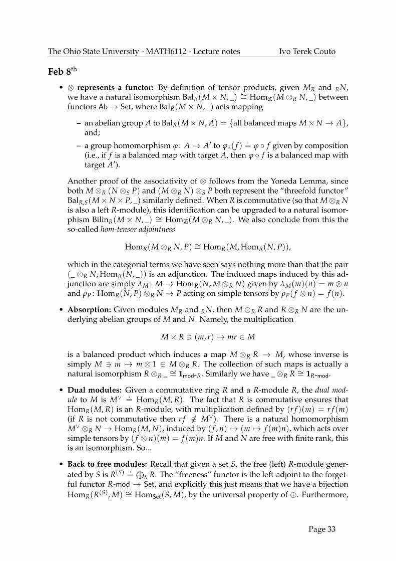
• ⊗ represents a functor: By definition of tensor products, given MR and RN,we have a natural isomorphism BalR(M× N, _) ∼= HomZ(M⊗R N, _) betweenfunctors Ab→ Set, where BalR(M× N, _) acts mapping
– an abelian group A to BalR(M×N, A) = {all balanced maps M×N → A},and;
– a group homomorphism ϕ : A→ A′ to ϕ∗( f ) .= ϕ ◦ f given by composition
(i.e., if f is a balanced map with target A, then ϕ ◦ f is a balanced map withtarget A′).
Another proof of the associativity of ⊗ follows from the Yoneda Lemma, sinceboth M⊗R (N ⊗S P) and (M⊗R N)⊗S P both represent the “threefold functor”BalR,S(M×N× P, _) similarly defined. When R is commutative (so that M⊗R Nis also a left R-module), this identification can be upgraded to a natural isomor-phism BilinR(M × N, _) ∼= HomZ(M ⊗R N, _). We also conclude from this theso-called hom-tensor adjointness
HomR(M⊗R N, P) ∼= HomR(M, HomR(N, P)),
which in the categorial terms we have seen says nothing more than that the pair(_⊗R N, HomR(N, _)) is an adjunction. The induced maps induced by this ad-junction are simply λM : M → HomR(N, M⊗R N) given by λM(m)(n) = m⊗ nand ρP : HomR(N, P)⊗R N → P acting on simple tensors by ρP( f ⊗ n) = f (n).
• Absorption: Given modules MR and RN, then M⊗R R and R⊗R N are the un-derlying abelian groups of M and N. Namely, the multiplication
M× R 3 (m, r) 7→ mr ∈ M
is a balanced product which induces a map M ⊗R R → M, whose inverse issimply M 3 m 7→ m ⊗ 1 ∈ M ⊗R R. The collection of such maps is actually anatural isomorphism R⊗R _ ∼= 1mod-R. Similarly we have _⊗R R ∼= 1R-mod.
• Dual modules: Given a commutative ring R and a R-module R, the dual mod-ule to M is M∨ .
= HomR(M, R). The fact that R is commutative ensures thatHomR(M, R) is an R-module, with multiplication defined by (r f )(m) = r f (m)(if R is not commutative then r f 6∈ M∨). There is a natural homomorphismM∨ ⊗R N → HomR(M, N), induced by ( f , n) 7→ (m 7→ f (m)n), which acts oversimple tensors by ( f ⊗ n)(m) = f (m)n. If M and N are free with finite rank, thisis an isomorphism. So...
• Back to free modules: Recall that given a set S, the free (left) R-module gener-ated by S is R(S) .
=⊕
S R. The “freeness” functor is the left-adjoint to the forget-ful functor R-mod → Set, and explicitly this just means that we have a bijectionHomR(R(S), M) ∼= HomSet(S, M), by the universal property of ⊕. Furthermore,
Page 33

The Ohio State University - MATH6112 - Lecture notes Ivo Terek Couto
R(S) comes with a distinguished set of generators
HomS(R(S), R(S)) HomSet(S, R(S))
IdR(S) (s 7→ xs),
where xs ∈ R(S) has 1 in the s-th position and zeroes elsewhere. We say that{xs | s ∈ S} is a basis for R(S). In general, we say that a left R-module M isfree if M ∼= R(S) for some set S. Up to isomorphism, R(S) depends only on thecardinality |S|. Namely, if |S1| = |S2|, then R(S1) ∼= R(S2), but this does notdiscard the (admittedly bizarre) possibility of having R(S1) ∼= R(S2) even though|S1| 6= |S2|. For example, a ring is said to have IBN (Invariant Basis Number) iffor all non-negative integers n and m, Rn ∼= Rm =⇒ n = m (e.g., non-trivialcommutative rings and Noetherian rings have IBN). Whenever it makes sense,we may say that rank(M) = |S| is the rank of S.
• Every module is a quotient of a free module. That is, given any module M,there is an exact sequence F → M→ 0 with F free.
Proof: Identifying M with its image over M ↪→ R(M), take the unique homo-morphism ϕ : R(M) → M such that ϕ|M = IdM.
Note that the surjection is not, in general, unique.
Feb 11th
• Theorem: Every free R-module F is projective (i.e., HomR(F, _) is exact).
Proof: Since HomR(F, _) is already left-exact (for any module), we just have tocheck that given g : M → M′′ surjective, we also have that the induced maphF(g) : HomR(F, M) → HomR(F, M′′) is also surjective. That is, every map ϕ ∈HomR(F, M) lifts:
F
M M′′ 0
ϕ∃ψ
g
A morphism defined on a free module is (freely) determined by its values in abasis (we have seen that HomR(R(S), N) ∼= HomSet(S, N)). So choose a basisB= (xi)i∈I for F, define B 3 xi 7→ mi ∈ M, where mi is any element in M suchthat g(mi) = ϕ(xi), and consider the unique homomorphism ψ : F → M withψ(xi) = mi for all i ∈ I.
• Splitting: If 0 M′ M F 0f
is exact with F free, thenthe sequence splits. In other words, there is a section σ : F → M with f ◦ σ = IdF:
0 M′ M F 0f
σ
Page 34

The Ohio State University - MATH6112 - Lecture notes Ivo Terek Couto
In particular, this implies that M ∼= F⊕M′.
Proof: This follows from the previous result:
F
M F 0
∃ σ
f
• A list of equivalences: For a R-module P, the following are equivalent:
(i) P is projective (i.e., HomR(P, _) is exact);
(ii) every exact sequence 0→ M′ → M→ P→ 0 splits;
(iii) P has the lifting property:
P
M N 0
∃
(iv) P is a direct summand of a free module.
• Remark: Conditions defined by the exactness of a functor are called acyclic. Forexample, flat modules are the ones acyclic for ⊗.
• Proposition: Any projective module is flat.
Proof steps:
(1) Free modules are flat, because R itself is flat and direct sums of flat modulesare again flat, in view of the natural distributive isomorphismM⊗R
⊕i∈I Ni
∼=⊕
i∈I(M⊗R Ni).
(2) Two modules are flat if and only if their direct sum is – this follows from thenaturality of the isomorphism in (1).
(3) Projective modules are direct summands of free modules – the conclusionfollows from (2).
• Injective modules: just like projective modules are related to freeness, injectivemodules are related to divisibility (a R-module M is divisible if for all a ∈ R, themultiplication map M ·a−−−→ M is surjective). For a R-module Q, the followingare equivalent:
(i) Q is injective (i.e., HomR(_, Q) is exact);
(ii) every exact sequence 0→ Q→ M→ M′′ → 0 splits;
Page 35

The Ohio State University - MATH6112 - Lecture notes Ivo Terek Couto
(iii) Q has the extension property:
Q
0 M′ M
∃
• Theorem: Every R-module embeds in an injective module (just like every R-module is surjected by a projective module7).
Proof steps for R = Z: We have to show that every abelian group embeds in adivisible group.
(1) A free abelian group F ∼= Z(S) embeds into the free Q-vector space FQ withthe same basis.
(2) Any abelian group is a quotient F/K, so it embeds in FQ/K, which is alsodivisible.
(3) Every divisible abelian group is injective (proof uses Zorn’s Lemma, andthe converse is also true).
Feb 13th
• Proof for general R: For any R-module M, HomR(R, M) becomes a R-modulewith operation (r · f )(x) .
= f (xr), which is isomorphic to M itself via
HomR(R, M) 3 f 7→ f (1) ∈ M, with inverse M 3 m 7→ (r 7→ rm) ∈ HomR(R, M).
Also, we have HomR(R, M) ⊆ HomZ(R, M). Now, since we have already veri-fied the result for abelian groups, take Q an injective group with a Z-linear em-bedding ι : M ↪→ Q. By left-exactness of HomZ(R, _), we get a Z-linear em-bedding hR(ι) : HomZ(R, M) ↪→ HomZ(R, Q). Now we claim that the compo-sition of inclusions, HomR(R, M) ↪→ HomZ(R, Q), is actually R-linear and thatHomZ(R, Q) is an injective R-module – this completes the proof.
For R-linearity, let r, x ∈ R and f ∈ HomR(R, M). On one hand, we have
hR(ι)(r · f )(x) = ι ◦ (r · f )(x) = ι((r · f )(x)) = ι( f (xr)),
and on the other hand
(r · hR(ι)( f ))(x) = hR(ι)( f )(xr) = (ι ◦ f )(xr) = ι( f (xr)).
Now, as for injectivity of HomZ(R, Q), take an exact sequence 0 → N′ → N.Then the first line in
HomR(N, HomZ(R, Q)) HomR(N′, HomZ(R, Q)) 0
HomZ(N ⊗Z R, Q) HomZ(N′ ⊗Z R, Q) 0
∼= ∼=
is exact because the second line is, since Q is Z-injective.7Consider being “free” an improvement, which has no analogue in this new contravariant setting.
Page 36

The Ohio State University - MATH6112 - Lecture notes Ivo Terek Couto
• Modern version of Homological Algebra: It was motivated by Algebraic Topol-ogy in the 1940’s, with the Eilerberg-Steenrod axioms, influence by MacLane,etc.. Some precursors were Cayley (“Theory of Elimination”, 1848) and Hilbert(syzygy theorem, 1890), leading to the notion of free resolutions. Also, we hadthe first results about homology and cohomology, such as Hilbert’s theorem 90(on cohomology of Galois groups) and Schur’s theorem (1904) on H2(G, C∗).
• Complexes: Can be defined in an arbitrary abelian category A. We will work onA = R-mod for concreteness. So, a complex of R-modules is a sequence
· · · Ci+1 Ci Ci−1 · · ·di+1 di
where each Ci is an R-module and di : Ci → Ci−1 is a homomorphism of R-modules, such that di ◦ di+1 = 0 for all i. Such a complex is denoted simplyby C•, or (C•, d•) when we need to emphasize the differentials. A morphism ofcomplexes ϕ• : (C•, d•) → (C′•, d′•) is a collection of homomorphism ϕi : Ci → C′isuch that
· · · Ci+1 Ci Ci−1 · · ·
· · · C′i+1 C′i C′i−1 · · ·
di+1
ϕi+1
di
ϕi ϕi−1
d′i+1 d′i
commutes. Composition of these morphisms is defined termwise, the iden-tity morphism is the obvious one, and with this we have defined a categoryComp(R-mod). In general, if A is an abelian category, Comp(A) is also an abeliancategory.
• Prototypical example: Let K be a simplicial complex, we have C• defined by
Ci =⊕
σ is a i-simplex
Zσ,
with differential maps/boundary operators defined by
di(σ) =i
∑j=0
(−1)jσ( j)
extended linearly to Ci, where σ( j) denotes the j-th face of σ.
• Examples:
(1) An R-module M can be regarded as a “one-term” complex, with M placedin the 0-th degree:
· · · 0 M 0 · · ·
Page 37

The Ohio State University - MATH6112 - Lecture notes Ivo Terek Couto
(2) A short exact sequence 0 → M′ → M → M′′ → 0 is a particular “three-term” complex
· · · 0 0 M′ M M′′ 0 0 · · ·
(3) If ϕ• : C• → C′• is a morphism of complexes of R-modules, we may definea complex ker (ϕ•), whose terms are each ker (ϕi). The differentials of C•may be restricted to ker (ϕ•) since the condition ϕi−1 ◦ di = d′i ◦ ϕi says thatdi maps ker (ϕi) inside ker (ϕi−1). Namely, we have
· · · ker (ϕi+1) ker (ϕi) ker (ϕi−1) · · ·di+1 di
In a similar way, one may define a complex coker(ϕ•).
• Constructions:
(1) If (C′•, d′•) and (C′′• , d′′• ) are two complexes of R-modules, we may define thesum (C′• ⊕ C′′• , d•) by
· · · C′i+1 ⊕ C′′i+1 C′i ⊕ C′′i C′i−1 ⊕ C′′i−1 · · ·di+1 di
where di(c′i, c′′i ).= (d′i(c
′i), d′′i (c
′′i )) for all i.
(2) If (C•, d•) is a complex of right R-modules and M is a left R-module, wemay define a complex of abelian groups (C• ⊗R M, d• ⊗ IdM):
· · · Ci+1 ⊗R M Ci ⊗R M Ci−1 ⊗R M · · ·di+1⊗IdM di⊗IdM
Indeed, we have (di⊗ IdM) ◦ (di+1⊗ IdM) = (di ◦ di+1)⊗ IdM = 0⊗ IdM =0. Trying to define the tensor product of two complexes leads to bicomplexes,which are used in the study of spectral sequences. We will not pursue thisfurther in details here.
Feb 15th
• Free resolutions: Since any R-module M is a quotient of a free module, we ob-tain an exact sequence 0 M1 F0 M 0ε with F0 free,and some R-module M1 (namely, ker (ε)). Now, M1 is also a quotient of a free-module, so we also obtain
M2
F1 F0 M 0
M1
d1 ε
Page 38

The Ohio State University - MATH6112 - Lecture notes Ivo Terek Couto
with F1 free. Continue proceeding this way and obtain an exact sequence
. . . M2
· · · F3 F2 F1 F0 M 0
M3 M1
d3 d2 d1 ε
Note that one could stop the process as soon as one of the Mi’s is free, but thereis no guarantee that this might happen – the process may go on forever. So, byconstruction, the complex
· · · F2 F1 F0 M 0d2 d1 ε
is exact and consists of free modules Fi for i ≥ 0. This is called a free resolution ofM, and may be simply denoted by F•
ε−−→ M.
• Remark: Giving a free resolution F•ε−−→ M is the same as giving a morphism
of complexes· · · F2 F1 F0 0
· · · 0 0 M 0,
ε
but here the complexes are no longer exact (for example, the first row is no longerexact at F0). The notation F•
ε−−→ M can be really understood as a morphism ofcomplexes, if we denote again by M the one-term complex defined by M.
• Examples:
(1) If R = k[x, y] and M = k[x, y]/(x, y) ∼= k, then
0 R R⊕ R M 0
y
−x
[x y
]
is a free resolution of M. The matrix notation here means that the first mapis r 7→ (ry,−rx) and the second one is (r1, r2) 7→ r1x + r2y.
(2) R = k[x]/(x2) and M = R/(x2) ∼= k. A free resolution of M is
· · · R R R M 0,·x ·x ·x
which is not finite. In fact, one can show that there is no finite free resolutionfor M.
Page 39
The Ohio State University - MATH6112 - Lecture notes Ivo Terek Couto
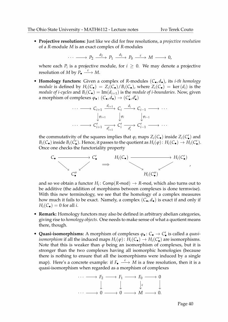
• Projective resolutions: Just like we did for free resolutions, a projective resolutionof a R-module M is an exact complex of R-modules
· · · P2 P1 P0 M 0,d2 d1 ε
where each Pi is a projective module, for i ≥ 0. We may denote a projectiveresolution of M by P•
ε−−→ M.
• Homology functors: Given a complex of R-modules (C•, d•), its i-th homologymodule is defined by Hi(C•) = Zi(C•)/Bi(C•), where Zi(C•) = ker (di) is themodule of i-cycles and Bi(C•) = Im(di+1) is the module of i-boundaries. Now, givena morphism of complexes ϕ• : (C•, d•)→ (C′•, d′•)
· · · Ci+1 Ci Ci−1 · · ·
· · · C′i+1 C′i C′i−1 · · ·
di+1
ϕi+1
di
ϕi ϕi−1
d′i+1 d′i
the commutativity of the squares implies that ϕi maps Zi(C•) inside Zi(C′•) andBi(C•) inside Bi(C′•). Hence, it passes to the quotient as Hi(ϕ) : Hi(C•)→ Hi(C′•).Once one checks the functoriality property
C• C′•
C′′•
=⇒Hi(C•) Hi(C′•)
Hi(C′′• )
,
and so we obtain a functor Hi : Comp(R-mod) → R-mod, which also turns out tobe additive (the addition of morphisms between complexes is done termwise).With this new terminology, we see that the homology of a complex measureshow much it fails to be exact. Namely, a complex (C•, d•) is exact if and only ifHi(C•) = 0 for all i.
• Remark: Homology functors may also be defined in arbitrary abelian categories,giving rise to homology objects. One needs to make sense of what a quotient meansthere, though.
• Quasi-isomorphisms: A morphism of complexes ϕ• : C• → C′• is called a quasi-isomorphism if all the induced maps Hi(ϕ) : Hi(C•)→ Hi(C′•) are isomorphisms.Note that this is weaker than ϕ being an isomorphism of complexes, but it isstronger than the two complexes having all isomorphic homologies (becausethere is nothing to ensure that all the isomorphisms were induced by a singlemap). Here’s a concrete example: if F•
ε−−→ M is a free resolution, then it is aquasi-isomorphism when regarded as a morphism of complexes
· · · F2 F1 F0 0
· · · 0 0 M 0.
ε
Page 40

The Ohio State University - MATH6112 - Lecture notes Ivo Terek Couto
The reason is that all the i-th homologies of the two rows are trivial for i ≥ 1(hence any map induces isomorphisms), while H0(ε) is precisely the usual iso-morphism F0/ker (ε) → M (remember here that Im(d1) = ker (ε)) defined byH0(ε)(x + ker ε) = ε(x). The same holds for projective (or any) resolutions. Andthe converse clearly holds: a quasi-isomorphism between the row complexes de-fines a resolution of M.
Feb 18th
• Remark: Quasi-isomorphisms need not have inverses, e.g.:
0 Z Z 0
0 0 Z/2Z 0.
·2
• Additivity: Since Hi : Comp(R-mod)→ R-mod is an additive functor, it preservesdirect sums. That is to say, Hi(C′• ⊕ C′′• ) ∼= Hi(C′•)⊕ Hi(C′′• ).
• “Dual” notation: One can rename a complex as to obtain a cochain (ascending)complex (C•, d•)
· · · Ci−1 Ci Ci+1 · · ·di−1 di
with di ◦ di−1 = 0. We then have cohomology functors Hi(C•) = Zi(C•)/Bi(C•),where Zi(C•) = ker (di) is the module of i-cocycles and Bi(C•) = Im(di−1) isthe module of i-coboundaries. We’re not effectively dualzing anything here, butjust changing notation, so that functoriality of Hi follows automatically from thefunctoriality of Hi. And Hi is also covariant (not contravariant).
• Two general lemmas: The following results hold in an arbitrary abelian cate-gory:
(a) Snake Lemma: Given the following diagram with exact rows, there is acanonical homomorphism δ : ker ( f ′′)→ coker( f ′) making it commute:
ker ( f ′′)
M′ M M′′ 0
N′ N N′′
coker( f ′)
δf ′ f f ′′
Page 41

The Ohio State University - MATH6112 - Lecture notes Ivo Terek Couto
(b) Five-Lemma: Consider the following commutative diagram with exact rows:
A B C D E
A′ B′ C′ D′ E′
α β γ δ ε
If β and δ are isomorphism, α is epi and ε is monic, then γ is an isomor-phism.
• Sharpening the Five-Lemma:
– β, δ monic, α epi =⇒ γ monic;
– β, δ epi, ε monic =⇒ γ epi.
• Theorem (long exact sequence in homology): Given a short exact sequence
0 C′• C• C′′• 0
of complexes, there is a long exact sequence
· · ·
Hi(C′•) Hi(C•) Hi(C′′• )
Hi−1(C′•) Hi−1(C•) Hi−1(C′′• )
· · ·
δi+1
δi
δi−1
in homology. That is, there are natural homomorphisms δi making the above se-quence exact.Proof: Let’s use the shorthands Z′′i = Zi(C′′• ), etc., and let α and β be the mor-phisms given in the short exact sequence of complexes. We first apply the SnakeLemma to obtain the diagram
Z′′i
0 C′i Ci C′′i 0
0 C′i−1 Ci−1 C′′i−1 0
C′i−1/B′i−1
αi
d′i
βi
di d′′iαi−1 βi−1
Page 42

The Ohio State University - MATH6112 - Lecture notes Ivo Terek Couto
We claim that the “snake morphism” Z′′i → C′i−1/B′i−1 induces the desired mapδi : H′′i → H′i−1. To see that this δi is well-defined, there are two things to check,using the definition of the snake morphism and some diagram chasing. Namely,that the snake morphism maps:
(i) z′′i ∈ Z′′i into H′i−1 = Z′i−1/B′i−1: there is ci ∈ Ci with βi(ci) = z′′i . Then
βi−1(di(ci)) = d′′i (βi(ci)) = d′′i (z′′i ) = 0
says that di(ci) ∈ ker (βi−1) = Im(αi−1). Then take c′i−1 ∈ C′i−1 withαi−1(c′i−1) = di(ci). It suffices now to check that d′i−1(c
′i−1) = 0. Here’s
how to do it: compute
αi−2(d′i−1(c′i−1)) = di−1(αi−1(c′i−1)) = di−1(di(ci)) = 0,
and conclude that d′i−1(c′i−1) = 0 by injectivity of αi−2, and then c′i−1 ∈ Z′i−1.
This step is done because the image of z′′i under the snake morphism isthe projection of c′i−1 in the quotient C′i−1/B′i−1, which now lands insideH′i−1 = Z′i−1/B′i−1.
(ii) b′′i ∈ B′′i to zero in C′i−1/B′i−1 (or in other words, that b′′i is mapped insideB′i−1 before projecting): get ci ∈ Ci with βi(ci) = b′′i . Since B′′i ⊆ Z′′i , thecalculation done in the previous step gives di(ci) ∈ ker (βi−1) = Im(αi−1),and so we may take c′i−1 ∈ C′i−1 with αi−1(c′i−1) = di(ci). We are doneonce we check that c′i−1 ∈ B′i−1. Here’s how to do it: take c′′i+1 ∈ C′′i+1 suchthat d′′i+1(c
′′i+1) = b′′i , and use surjectivity of βi+1 to get ci+1 ∈ Ci+1 with
βi+1(ci+1) = c′′i+1. We now have two elements in Ci, ci and di+1(ci+1). Thencompute
βi(ci − di+1(ci+1)) = βi(ci)− βi(di+1(ci+1))
= b′′i − d′′i+1(βi+1(ci+1))
= b′′i − d′′i+1(c′′i+1)
= b′′i − b′′i = 0,
so that ci − di+1(ci+1) ∈ ker (βi) = Im(αi), and we get an element c′i ∈ C′iwith αi(c′i) = ci − di+1(ci+1). Now, the only reasonable thing left to prove isthat d′i(c
′i) = c′i−1, and for that we use injectivity of αi−1 as follows:
αi−1(c′i−1 − d′i(c′i)) = αi−1(c′i−1)− αi−1(d′i(c
′i))
= di(ci)− di(αi(c′i))= di(ci − αi(c′i))= di(di+1(ci+1))
= 0.
Exactness of the long exact sequence in homology comes directly from theSnake Lemma itself.
Page 43

The Ohio State University - MATH6112 - Lecture notes Ivo Terek Couto
• “Dual” notion again: The same argument says that if
0 C′• C• C
′′• 0
is a short exact sequence of (ascending) complexes, then we have a long exactsequence in cohomology:
· · ·
Hi(C′•) Hi(C•) Hi(C′′• )
Hi+1(C′•) Hi+1(C•) Hi+1(C′′• )
· · ·
δi−1
δi
δi+1
• Naturality: The naturality of the δ-morphisms in those long exact sequencesmeans that if we’re given a morphism
0 C′• C• C′′• 0
0 C′• C• C′′• 0
between two exact sequences of complexes, then the diagram
· · · Hi(C•) Hi(C′′• ) Hi−1(C′•) Hi−1(C•) · · ·
· · · Hi(C•) Hi(C′′• ) Hi−1(C′•) Hi−1(C•) · · ·
δi
δi
commutes. The only square whose commutativity does not follow from functo-riality of Hi is the one indicated in bold – naturality means that this particularsquare does, in fact, commute as well. In other words, H• is a δ-functor (thatis, a collection of functors that transforms a morphism between short exact se-quences of complexes into a natural morphism between the associated long exactsequences).
• Homotopy of complexes: When do two homomorphisms of complexes ϕ andψ induce the same homomorphisms in homology, ϕi = ψi, for all i? Obviouslyif, for example, ϕ = ψ, or equivalently if ϕ− ψ = 0 (subtraction of morphismsis allowed because we are working in an abelian category). Here’s an idea: amorphism C• → C′• induces the zero map between homologies when for each i,
Page 44
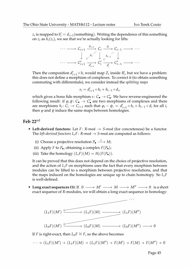
The Ohio State University - MATH6112 - Lecture notes Ivo Terek Couto
zi is mapped to b′i = di+1(something). Writing the dependence of this somethingon zi as hi(zi), we see that we’re actually looking for lifts:
· · · Ci+1 Ci Ci−1 · · ·
· · · C′i+1 C′i C′i−1 · · ·
di+1 di
hi hi−1
d′i+1 d′i
Then the composition d′i+1 ◦ hi would map Zi inside B′i , but we have a problem:this does not define a morphism of complexes. To correct it (to obtain somethingcommuting with differentials), we consider instead the splitting maps
si = d′i+1 ◦ hi + hi−1 ◦ di,
which gives a bona fide morphism s : C• → C′•. We have reverse-engineered thefollowing result: if ϕ, ψ : C• → C′• are two morphisms of complexes and thereare morphisms hi : Ci → Ci+1 such that ϕi − ψi = d′i+1 ◦ hi + hi−1 ◦ di for all i,then ϕ and ψ induce the same maps between homologies.
Feb 22nd
• Left-derived functors: Let F : R-mod → S-mod (for concreteness) be a functor.The left-derived functors LiF : R-mod→ S-mod are computed as follows:
(i) Choose a projective resolution P•ε−−→ M;
(ii) Apply F to P•, obtaining a complex F(P•);(iii) Take the homology (LiF)(M) = Hi(F(P•)).
It can be proved that this does not depend on the choice of projective resolution,and the action of LiF on morphisms uses the fact that every morphism betweenmodules can be lifted to a morphism between projective resolutions, and thatthe maps induced on the homologies are unique up to chain homotopy. So LiFis well-defined.
• Long exact sequences (1): If 0 M′ M M′′ 0 is a shortexact sequence of R-modules, we will obtain a long exact sequence in homology:
· · ·
(L1F)(M′) (L1F)(M) (L1F)(M′′)
(L0F)(M′) (L0F)(M) (L0F)(M′′) 0
If F is right-exact, then L0F ∼= F, so the above becomes
· · · (L1F)(M′) (L1F)(M) (L1F)(M′′) F(M′) F(M) F(M′′) 0
Page 45
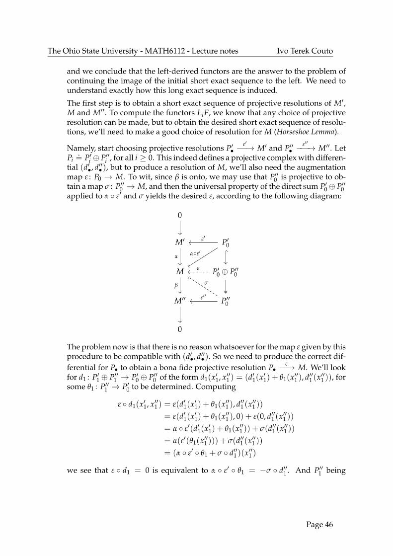
The Ohio State University - MATH6112 - Lecture notes Ivo Terek Couto
and we conclude that the left-derived functors are the answer to the problem ofcontinuing the image of the initial short exact sequence to the left. We need tounderstand exactly how this long exact sequence is induced.
The first step is to obtain a short exact sequence of projective resolutions of M′,M and M′′. To compute the functors LiF, we know that any choice of projectiveresolution can be made, but to obtain the desired short exact sequence of resolu-tions, we’ll need to make a good choice of resolution for M (Horseshoe Lemma).
Namely, start choosing projective resolutions P′•ε′−−→ M′ and P′′•
ε′′−−−→ M′′. LetPi
.= P′i ⊕ P′′i , for all i ≥ 0. This indeed defines a projective complex with differen-
tial (d′•, d′′• ), but to produce a resolution of M, we’ll also need the augmentationmap ε : P0 → M. To wit, since β is onto, we may use that P′′0 is projective to ob-tain a map σ : P′′0 → M, and then the universal property of the direct sum P′0⊕ P′′0applied to α ◦ ε′ and σ yields the desired ε, according to the following diagram:
0
M′ P′0
M P′0 ⊕ P′′0
M′′ P′′0
0
α
ε′
α◦ε′
β
ε
ε′′
σ
The problem now is that there is no reason whatsoever for the map ε given by thisprocedure to be compatible with (d′•, d′′• ). So we need to produce the correct dif-ferential for P• to obtain a bona fide projective resolution P•
ε−−→ M. We’ll lookfor d1 : P′1⊕ P′′1 → P′0⊕ P′′0 of the form d1(x′1, x′′1 ) = (d′1(x′1) + θ1(x′′1 ), d′′1 (x′′1 )), forsome θ1 : P′′1 → P′0 to be determined. Computing
ε ◦ d1(x′1, x′′1 ) = ε(d′1(x′1) + θ1(x′′1 ), d′′1 (x′′1 ))= ε(d′1(x′1) + θ1(x′′1 ), 0) + ε(0, d′′1 (x′′1 ))= α ◦ ε′(d′1(x′1) + θ1(x′′1 )) + σ(d′′1 (x′′1 ))= α(ε′(θ1(x′′1 ))) + σ(d′′1 (x′′1 ))= (α ◦ ε′ ◦ θ1 + σ ◦ d′′1 )(x′′1 )
we see that ε ◦ d1 = 0 is equivalent to α ◦ ε′ ◦ θ1 = −σ ◦ d′′1 . And P′′1 being
Page 46
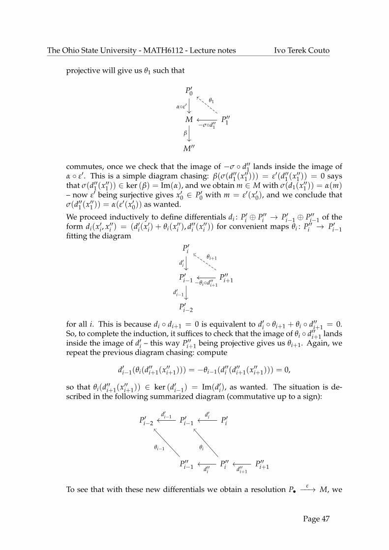
The Ohio State University - MATH6112 - Lecture notes Ivo Terek Couto
projective will give us θ1 such that
P′0
M P′′1
M′′
α◦ε′
β
−σ◦d′′1
θ1
commutes, once we check that the image of −σ ◦ d′′1 lands inside the image ofα ◦ ε′. This is a simple diagram chasing: β(σ(d′′1 (x′′1 ))) = ε′(d′′1 (x′′1 )) = 0 saysthat σ(d′′1 (x′′1 )) ∈ ker (β) = Im(α), and we obtain m ∈ M with σ(d1(x′′1 )) = α(m)– now ε′ being surjective gives x′0 ∈ P′0 with m = ε′(x′0), and we conclude thatσ(d′′1 (x′′1 )) = α(ε′(x′0)) as wanted.
We proceed inductively to define differentials di : P′i ⊕ P′′i → P′i−1 ⊕ P′′i−1 of theform di(x′i, x′′i ) = (d′i(x′i) + θi(x′′i ), d′′i (x′′i )) for convenient maps θi : P′′i → P′i−1fitting the diagram
P′i
P′i−1 P′′i+1
P′i−2
d′i
d′i−1
−θi◦d′′i+1
θi+1
for all i. This is because di ◦ di+1 = 0 is equivalent to d′i ◦ θi+1 + θi ◦ d′′i+1 = 0.So, to complete the induction, it suffices to check that the image of θi ◦ d′′i+1 landsinside the image of d′i – this way P′′i+1 being projective gives us θi+1. Again, werepeat the previous diagram chasing: compute
d′i−1(θi(d′′i+1(x′′i+1))) = −θi−1(d′′i (d′′i+1(x′′i+1))) = 0,
so that θi(d′′i+1(x′′i+1)) ∈ ker (d′i−1) = Im(d′i), as wanted. The situation is de-scribed in the following summarized diagram (commutative up to a sign):
P′i−2 P′i−1 P′i
P′′i−1 P′′i P′′i+1
d′i−1 d′i
θi−1 θi
d′′i d′′i+1
To see that with these new differentials we obtain a resolution P•ε−−→ M, we
Page 47

The Ohio State University - MATH6112 - Lecture notes Ivo Terek Couto
use the long exact sequence in homology induced by the first row in
0 P′• P• P′′• 0
0 M′ M M′′ 0
to obtain · · · �����:0Hi(P′•) Hi(P•) ���
��:0Hi(P′′• ) · · · for all i > 0
– exactness obviously then gives Hi(P•) = 0 as well. Finally, for i = 0, theconclusion H0(P•) ∼= M follows from the Five-Lemma applied to the diagram
0 H0(P′•) H0(P•) H0(P′′• ) 0
0 M′ M M′′ 0.
∼= ∼=
Feb 25th
• Long exact sequences (2): Continuing from where we left off, the next step
would be to check that 0 F(P′•) F(P•) F(P′′• ) 0 is ex-
act. By construction, each step sequence 0 P′i Pi P′′i 0
is split exact. Then the conclusion follows from the general fact that every addi-tive functor preserves short split-exact sequences: the image
0 F(P′i ) F(Pi) F(P′′i ) 0
is also split-exact. Thus, we obtain the long exact sequence for L•F.
• Right-derived functors: Those are defined in a similar way to left-derived func-tors. Assume (for concreteness) that F : R-mod → S-mod is a functor. The right-derived functors of F are defined/computed in the following way:
(i) Choose an injective resolution Mη−−→ Q•, that is an exact (ascending) com-
plex of R-modules
0 M Q0 Q1 Q2 · · ·η d0 d1 d2
where each Qi is an injective module, for i ≥ 0.
(ii) Apply F to Q•, obtaining a complex F(Q•);
(iii) Take the cohomology (RiF)(M).= Hi(F(Q•)).
We have the same results as the ones for left-derived functors, such as indepen-dence of choice of resolution, long exact sequences, etc.. In particular, this isuseful when F is left-exact, so that R0F ∼= F.
Page 48

The Ohio State University - MATH6112 - Lecture notes Ivo Terek Couto
• Remark: If F is contravariant instead, the roles projective/injective are reversed.Namely, we use:
– projective resolutions to define and compute RiF, and;
– injective resolutions to define and compute LiF.
• Ext & Tor: They are the derived functors of HomR(_, N) and M ⊗R _, respec-tively. We will focus on the Ext functor first, and come back to Tor later. Notethat there is a certain initial ambiguity regarding Ext, as it could be computed intwo different ways:
(1) Consider the contravariant functor HomR(_, N) and then computeExti
R(M, N) = Ri(HomR(_, N))(M) using a projective resolution of M, or;
(2) Consider the covariant functor HomR(M, _) and then computeExti
R(M, N) = Ri(HomR(M, _))(N) using an injective resolution of N.
It is a non-trivial fact that both procedures give the same result. Usually, workingwith (1) is easier, so we’ll take this as the definition and denote by Ext the func-tors produced by (2). There is a natural isomorphism Ext ∼= Ext, since both areδ-functors satisfying a certain universal property related to Hom. Note that sincethe hom-functor is left-exact, we automatically have Ext0
R(M, N) = HomR(M, N).
• Ext for projective modules: Given a R-module P, the following are equivalent:
(i) P is projective.
(ii) ExtiR(P, N) = 0 for all i > 0 and all R-modules N.
(iii) Ext1R(P, N) = 0 for all R-modules N.
Proof:
(i) =⇒ (ii) : Assume that P is projective. Then
· · · 0 0 P P 0
is a projective resolution of P. Apply the contravariant functor HomR(_, N)to the projective complex
· · · 0 0 P
to get the ascending complex
HomR(P, N) 0 0 · · ·
Now it is obvious that the cohomologies of this complex are ExtiR(P, N) = 0
for all i > 0.
(ii) =⇒ (iii) : Trivial.
Page 49

The Ohio State University - MATH6112 - Lecture notes Ivo Terek Couto
(iii) =⇒ (i) : Our goal is to prove that HomR(P, _) is exact. If one already hasestablished the natural isomorphism Ext ∼= Ext, one easy proof follows fromjust taking a short exact sequence
0 N′ N N′′ 0
and using the long exact sequence for Ext, which yields
0 Ext0R(P, N′) Ext0
R(P, N) Ext0R(P, N′′) Ext1
R(P, N′) · · ·
Then ExtiR(P, _) = 0 for i ≥ 1 and Ext0
R(P, _) ∼= HomR(P, _) give us that
0 HomR(P, N′) HomR(P, N) HomR(P, N′′) 0
is exact, as wanted. An alternative proof of this implication without usingthe isomorphism Ext ∼= Ext is as follows: take a free presentation
0 N F P 0
of P (i.e., the sequence is exact and F is free). We are done if we provethat the sequence splits, so P is a direct summand of a free module, henceprojective. Apply HomR(_, N) and use the given hypothesis Ext1
R(P, N) = 0to get the exact sequence
0 HomR(P, N) HomR(F, N) HomR(N, N) 0
Since HomR(F, N) → HomR(N, N), there is ρ : F → N which gets mappedto IdN. This ρ is a splitting map.
• Ext and extensions: An extension of an R-module M by another R-module N isan exact sequence 0→ N → E→ M→ 0, for some R-module E. Two extensionsof M by N are called isomorphic if there is a isomorphism E '−−−→ E′ such that
0 N E M 0
0 N E′ M 0
'
commutes. Let E(M, N) be the collection of isomorphism classes of extensions ofM by N. This is natural in both variables. For example, given f : N → N′, thereis E(M, N)→ E(M, N′) given by
0 N E M 0
0 N′ E′ M 0,
f
Page 50

The Ohio State University - MATH6112 - Lecture notes Ivo Terek Couto
where ι : N ↪→ N′ ⊕ E is given by ι(n) = ( f (n),−n) and E′ = (N′ ⊕ E)/ι(N) isthe pushout of the diagram
N E
N′
f
Here, of course, we may regard N as a submodule of E. It has to be shown thatthe bottom row is indeed exact. To wit, let ψ be the arrow E → M, so that we’reeffectively setting N = ker ψ, and also let ψ′ be the arrow E′ → M. The map ψ′
is well-defined since
(n′, e) 7→ ψ(e) and (n′ + f (n), e− n) 7→ ψ(e− n) = ψ(e).
Also, we clearly have ψ′((n, 0) + ι(N)) = ψ(n) = 0. On the other hand, ifψ′((n, e) + ι(N)) = 0, then ψ(e) = 0 says that e ∈ N, allowing:
(n′, e) + ι(N) = (n′ + f (e), e− e) + ι(N) = (n′ + f (e), 0) + ι(N),
which then lies in the image of N′ → E′.
Feb 27th
• The name “extension”: There is a natural isomorphism E(M, N) ∼= Ext1R(M, N).
Proof: Let a class [E] ∈ E(M, N) be represented by the extension
0 N E M 0,
and apply the covariant functor HomR(_, N) to get the long exact sequence
0 HomR(M, N) HomR(E, N) HomR(N, N) Ext1R(M, N) · · ·
Then we can define αM,N : E(M, N) → Ext1R(M, N) by sending [E] to the image
of IdN via the arrow HomR(N, N)→ Ext1R(M, N) in the above sequence. This is
indeed well-defined by the naturality of the long exact sequence in cohomology.
Let’s understand this transformation αM,N more concretely. For this, considera projective presentation 0 K P M 0 of M. ApplyHomR(_, N) to get (the piece of) the sequence
HomR(P, N) HomR(K, N) Ext1R(M, N) 0,
by using that P is projective (and hence ExtiR(P, _) = 0 for i ≥ 1). We obtain that
Ext1R(M, N) ∼=
HomR(K, N)
Im(HomR(P, N)→ HomR(K, N)).
Page 51

The Ohio State University - MATH6112 - Lecture notes Ivo Terek Couto
And in the following diagram, lifts f : P→ E restrict to maps g : K → N:
0
0 N E M 0
P
K
0
f
g
Thus we have obtained an element of HomR(K, N). To eliminate the dependenceon the choice of lift, assume that f ′ : P → E restricts to g′ : K → N. Then thedifference f − f ′ has image in ker (E → M) = N, i.e., f − f ′ ∈ HomR(P, N).This means [ f − f ′] = 0 in the quotient, and we get a well-defined map
E(M, N) 3 [E] 7→ [g] ∈ HomR(K, N)
Im(HomR(P, N)→ HomR(K, N))∼= Ext1
R(M, N).
Up to the last identification ∼=, this is αM,N.
– Surjectivity: given K → N, consider the same projective presentation of Mpreviously given. Let E be the pushout of N and P over K:
N
K E
P
g
f
This produces a class [E] ∈ E(M, N), to be mapped back to [g].– Injectivity: every extension which maps to the same [g] will actually be iso-
morphic to the above pushout.
Checking for naturality is left as an exercise.
• Remarks:
– The extension set E(M, N) is sometimes called the Yoneda-Ext.– The same idea works for higher order ext’s: define En(M, N) as the col-
lection of the equivalence classes of n-extensions of M by N, i.e., exact se-quences
0 N E1 · · · En M 0
We have a natural isomorphism En(M, N) ∼= ExtnR(M, N).
Page 52

The Ohio State University - MATH6112 - Lecture notes Ivo Terek Couto
– Ext1 appears in algebraic topology: the universal coefficients theorem relatedH•(X) and the dual H•(X)∨. In general, for every abelian group A we havethe exact sequences
0 Ext1Z(Hi−1(X;Z), A) Hi(X; A) HomZ(Hi(X;Z), A) 0.
If A = Z and Hi−1(X;Z) is free (or more generally, projective), the above se-quence gives an isomorphism Hi(X;Z) ∼= Hi(X;Z)∨ .
= HomZ(Hi(X;Z),Z).
• Group cohomology: Fix a ring R (usually Z or a field k) and a group G. Wehave the group ring R[G] and the fixed point functor (_)G : R[G]-mod → R-mod,sending:
– an R[G]-module A to AG = {a ∈ A | ga = a for all g ∈ G}, which isisomorphic to HomR[G](R, A), where we regard R as an R[G]-module withtrivial action by elements of G (i.e., gr .
= r for all g ∈ G)8;
– an R[G]-linear map f : A → B to the restriction f G : AG → BG (indeed, thecodomain is correct, since for all a ∈ AG and g ∈ G we have
g f G(a) = g f (a) = f (ga) = f (a) = f G(a)
and hence f G(a) ∈ BG).
Functoriality over morphisms is clear from properties of restrictions. This func-tor is covariant and additive. Let’s also see that it is left-exact. For this, considera short exact sequence
0 A B C 0ϕ ψ
in R[G]-mod. Our goal is to prove that
0 AG BG CGϕG ψG
is exact in R-mod. Clearly the restriction of an injective map is injective andψG ◦ ϕG = (ψ ◦ ϕ)G = 0G = 0, so that the only non-trivial thing to checkhere is one remaining inclusion for exactness at BG. For this, take an elementb ∈ ker (ψG) ⊆ ker (ψ) = Im(ϕ), and take a ∈ A such that b = ϕ(a). We claimthat actually a ∈ AG: to wit, given any g ∈ G we have
ϕ(a− ga) = ϕ(a)− ϕ(ga) = ϕ(a)− gϕ(a) = b− gb = b− b = 0,
and since ϕ is injective it follows that a = ga. Now g ∈ G was arbitrary, andthus a ∈ AG. Note that the same argument fails to prove that ψG is surjective if
8The natural isomorphism here is η : (_)G =⇒ HomR[G](R, _) defined by ηA(a)(r) = ra, for allR[G]-modules A. We have that ηA(a) is R[G]-linear precisely because a ∈ AG. The naturality of η istrivial. The inverse is defined as follows: if ϕ : R → A is R[G]-linear, put a = ϕ(1). Then we actuallyhave a ∈ AG, since for all g ∈ G we have ga = gϕ(1) = ϕ(g1) = ϕ(1) = a, and so we may computeηA(a)(r) = ra = rϕ(1) = ϕ(r) for all r ∈ R.
Page 53
The Ohio State University - MATH6112 - Lecture notes Ivo Terek Couto
ψ is, since given c ∈ CG we may obtain b ∈ B such that ψ(b) = c, but we cannotprove that b ∈ BG – the best we can do here is obtain, for every g ∈ G, an elementag ∈ A such that b− gb = ϕ(ag). This leads to the:
Definition: Let G be a group and R be a ring. The group cohomologies of Gover R are the right-derived functors of (_)G. Since (_)G ∼= HomR[G](R, _), thei-th group cohomology of G with coefficients in a given R[G]-module A is thenHi(G; A) ∼= Exti
R[G](R, A).
Mar 1st
• An explicit description for the case R = Z using complexes: Build a cochaincomplex (C•(G; A), d•) as follows:
– For all n ≥ 0, put Cn(G; A).= {functions Gn = G× · · · × G → A}. Since A
is aZ[G]-module, it is an abelian group, and Cn(G; A) inherits this structure.Note that C0(G; A) = A.
– For all n ≥ 0, define dn : Cn(G; A)→ Cn+1(G; A) by
(dn ϕ)(g0, . . . , gn) = g0ϕ(g1, . . . , gn)+
+n−1
∑i=0
(−1)i+1ϕ(g0, . . . , gi−1, gigi+1, . . . , gn) + (−1)n ϕ(g0, . . . , gn−1).
A standard counting argument gives that dn+1 ◦ dn = 0.
In particular, we have that the zeroth differential d0 : A → C1(G; A) is given by(d0a)(g) = ga − a, so that ker (d0) = AG, while the first differentiald1 : C1(G; A)→ C2(G; A) is given by (d1ϕ)(g0, g1) = g0ϕ(g1)− ϕ(g0g1) + ϕ(g0).Claim: Hn(G; A) ∼= Hn(C•(G; A)).
• Twisted homomorphism: Let G be a group and A be a Z[G]-module. A mapϕ : G → A is called a twisted homomorphism if ϕ(gh) = gϕ(h) + ϕ(g) for allg, h ∈ G. By definition, we have ker (d1) is precisely the collection of twistedhomomorphism from G to A. Moreover, if the action of G on A is trivial (i.e.,A = AG), then twisted homomorphism are just usual homomorphisms.
• Examples:
(1) A = Z is a Z[Z2]-module, with G = Z2 acting trivially. Then we may con-sider the group cohomologies H0(Z2;Z) and H1(Z2;Z). To compute them,just note since the entire Z is fixed we have d0 = 0, from which follows that
H0(Z2;Z) = Z and H1(Z2;Z) ∼= HomZ(Z2;Z) = 0,
by using again that since the action is trivial, twisted homomorphisms arejust homomorphisms.
Page 54

The Ohio State University - MATH6112 - Lecture notes Ivo Terek Couto
(2) Now let G = {1,−1} act multiplicatively on A = Z. Since no element ofZ \ {0} is fixed by G, we have ZG = 0 and so H0(G;Z) = 0. To computeH1(G;Z), we have to understand what are the twisted homomorphismsϕ : {1,−1} → Z. We have that ϕ(1) = ϕ(1 · 1) = 1ϕ(1) + ϕ(1) = 2ϕ(1),and so ϕ(1) = 0. However, the choice of value for ϕ(−1) is arbitrary, since
ϕ(−1) = ϕ(−1 · 1) = −ϕ(1) + ϕ(−1) = ϕ(−1) and0 = ϕ(1) = ϕ((−1)(−1)) = −ϕ(−1) + ϕ(−1) = 0
give us no new information whatsoever. Thus ker (d1) ∼= Z, and for alln ∈ Z we have (d0n)(1) = 0 and (d0n)(−1) = −2n, so that Im(d0) ∼= 2Z(both isomorphisms induced by ϕ 7→ ϕ(−1)). So H1(G;Z) ∼= Z/2Z ∼= Z2.
• Remark: This is also related to other types of cohomology. For example, f G is afinite group acting trivially on A = Z, then H1(G; Z) = H1(BG) = Hn
G(pt),where the latter are the topological cohomology of the classifying space BG(equivariant cohomology). Or if G = Gal(E/F) and A is a G-module, then Hn(G; A)is the so-called Galois cohomology.
• Tor: Recall that given any right R-module M, the functor M⊗R _ : R-mod→ Ab isright-exact, and its left-derived functors are TorR
i (M, _). To compute it, we followthe standard procedure: take a left R-module N, choose a projective resolutionP• → N, form the complex M⊗R P• by
· · · M⊗R P2 M⊗R P1 M⊗R P0 0,
and take the homology TorRi (M, N) = Hi(M⊗R P•). Again by right-exactness of
the tensor functor, we in particular have TorR0 (M, N) = M⊗R N. And if we have
a short exact sequence
0 N′ N N′′ 0
we obtain the long exact sequence
· · · TorR2 (M, N′′)
TorR1 (M, N′) TorR
1 (M, N) TorR1 (M, N′′)
M⊗R N′ M⊗R N M⊗R N′′ 0
• Tor for flat modules: Given a right R-module M, the following are equivalent:
(i) M is flat.
(ii) TorRi (M, N) = 0 for all i > 0 and all left R-modules N.
Page 55

The Ohio State University - MATH6112 - Lecture notes Ivo Terek Couto
(iii) TorR1 (M, N) = 0 for all left R-modules N.
Proof:
(i) =⇒ (ii) : If M is flat, then M ⊗R _ is exact. This means that for every leftR-module N and any projective resolution P• → N, the complex
· · · M⊗R P1 M⊗R P0 M⊗R N 0
is exact, and it follows that TorRi (M, N) = 0 for all i > 0.
(ii) =⇒ (iii) : Trivial.
(iii) =⇒ (i) : Consider a short exact sequence
0 N′ N N′′ 0.
Our goal is to prove that
0 M⊗R N′ M⊗R N M⊗R N′′ 0
is exact. This is precisely the end of the long exact sequence for Tor, sinceTorR
1 (M, N) = 0. We are done.
• Bifunctoriality of Tor: For a left R-module N, one could also define TorRi (_, N)
as the left-derived functors of _ ⊗R N. We again have natural isomorphisms
TorRi (M, N) ∼= Tor
Ri (M, N).
Page 56

The Ohio State University - MATH6112 - Lecture notes Ivo Terek Couto
Galois Theory
Mar 20th
• Theme and History: A natural goal to pursue is to solve polynomial equa-tions. For degree 2 polynomials we have the quadratic formula, while for de-gree 3 polynomials x3 + ax2 + bx + c, which can always be depressed to the sim-pler form x3 + px + q, we have Cardano’s formula (actually due to Tartaglia,∼1540’s). There is also Ferrari’s formula for the degree 4 case. But not for degree5: Abel (1827) and Ruffini (1813) proved that the general quintic cannot be solvedfor radicals. Galois (1832) gave an analysis of this face via symmetries. Why careabout radicals? Again one possible answer is because these illustrate symmetriesof the equation (e.g., complex roots of polynomials with real coefficients come inconjugate pairs).
The idea to discuss this efficiently is to explore correspondences:
field theory←→ group theoryextension fields E/F ←→ Galois groups Gal(E/F)
towers of extensions E ⊇ K ⊇ F ←→ Gal(E/K) ⊆ Gal(E/F) (reverse inclusions)
and more. There is a strong analogy between Galois groups for extension fieldsand fundamental groups (as deck transformations of covering spaces) in Alge-braic Topology.
• Basic Field Theory: We start with some terminology and conventions.
– A field is always commutative.
– The degree of the zero polynomial is −∞.
– A ring where every nonzero element has an inverse is a division ring (orskew-field).
– If E and F are fields with F ⊆ E, we say that F is a subfield of E or, equiv-alently, that E is an extension field of F. We write E/F (since we will neverconsider quotients of fields, this notation won’t cause confusion). Still inthis setup, given elements α1, α2, . . . ∈ E, the field obtained from F by ad-joining these elements if F(α1, α2, . . .) ⊆ E, the smallest subfield of E con-taining F and all the α’s. Do note that the set of adjoined elements need notbe countable.
– The degree of a field extension E/F, denoted by [E : F] (to echo the index ofa subgroup, in group theory), is defined to be dimF E (the dimension of Eas a vector space over F). When [E : F] < +∞, we say that E/F is a finiteextension.
• Example: F = Q, E = Q(√
2) = {a + b√
2 | a, b ∈ Q}. Then [Q(√
2) : Q] = 2because {1,
√2} is a Q-basis for Q(
√2).
• Tower Law: Suppose F ⊆ K ⊆ E are fields. Then [E : F] = [E : K][K : F].
Page 57

The Ohio State University - MATH6112 - Lecture notes Ivo Terek Couto
Proof: Choose bases {ui}i∈I and {vj}j∈J for K/F and E/K, respectively. We willshow that {uivj}(i,j)∈I×J is a basis for E/F. That is spans E over F is clear. Sowe only have to check that it is linearly independent. Indeed, if (aij)(i,j)∈I×J is afamily of elements in F, all but finitely many of them zero, then
∑(i,j)∈I×J
aijuivj = 0 =⇒ ∑j∈J
(∑i∈I
aijui
)vj = 0 =⇒ ∑
i∈Iaijui = 0 =⇒ aij = 0,
for all (i, j) ∈ I × J.
• Algebraic elements: Given a field extension E/F, we say that an element α ∈ E isalgebraic over F is there is a polynomial f (x) ∈ F[x] with f (α) = 0. If all elementsof E are algebraic over F, the extension E/F is called algebraic.
• Minimal polynomials: Given a field extension E/F and α ∈ E algebraic over F,its minimal polynomial (over F) is the monic polynomial f (x) ∈ F[x] with f (α) = 0,having minimal degree.
Claim: the minimal polynomial is completely determined by these conditions,and it is also irreducible in F[x].
Proof: Suppose g(x) ∈ F[x] is another polynomial with g(α) = 0. Then we havedeg g ≥ deg f , and so we may write g(x) = f (x)q(x) + r(x) with polynomialsq(x), r(x) ∈ F[x] and deg r < deg f . If r(x) 6= 0, evaluating at α gives r(α) = 0,contradicting the minimality of deg f . Hence r(x) = 0 and f (x) | g(x). Irre-ducibility follows from 0 = f (α) = f1(α) f2(α) implying f1(α) = 0 or f2(α) = 0,with deg fi < deg f , i = 1, 2.
• Example: Consider the extension R/Q and α =√
3−√
6. Since
α2 = 3−√
6 =⇒ α2 − 3 = −√
6 =⇒ α4 − 6α2 + 9 = 6 =⇒ α4 − 6α2 + 3 = 0,
we consider f (x) ∈ Q[x] given by f (x) = x4 − 6x2 + 3. From Eisenstein’s crite-rion (p = 3), f (x) is irreducible over Q. Thus f (x) is the minimal polynomial ofα over Q.
• Splitting fields: Conversely, given a monic polynomial f (x) ∈ F[x] of degree n,a splitting field of f (x) is an extension E/F so that
f (x) = (x− α1) · · · (x− αn),
with α1, . . . , αn ∈ E, and minimal for this property (so that E = F(α1, . . . , αn)).
• Remark: Above, note that it only makes sense to talk about F(α1, . . . , αn) oncewe already have E, as α1, . . . , αn ∈ E. Any possible dependence on E is implicitin the notation.
• Example: A splitting field for x2 − 2 ∈ Q[x] is Q(√
2), since there we have thefactorization x2 − 2 = (x−
√2)(x +
√2) ∈ Q(
√2)[x].
Page 58

The Ohio State University - MATH6112 - Lecture notes Ivo Terek Couto
• Lemma (Kronecker): Given a field F and f (x) ∈ F[x], there is an extension E/Fso that f (x) has a root in E.
Proof: We may assume that f (x) is irreducible (a root of any factor of f (x) is aroot of f (x)), so that ( f (x)) ⊆ F[x] is a maximal ideal, since F[x] is a PID. ThenE = F[x]/( f (x)) is a field, and α
.= x ∈ E satisfies f (α) = 0 by construction.
• Remark: In the setup of the above Lemma, E = F[α] = {g(α) | g(x) ∈ F[x]},that is, ring-adjunction is the same as field-adjunction. Also, note here that wehave F[α] ∼= F[x]/(m(x)), where m(x) is the (monic) minimal polynomial of α.
• Existence of splitting fields: Given any field F, every monic polynomialf (x) ∈ F[x] has a splitting field.
Proof: Write f (x) = f1(x) · · · fr(x) ∈ F[x] as a product of irreducible monicfactors. If all these factors are linear, we are done. Else, assume (reordering ifnecessary) that deg f1 > 1, and let F1/F be a field extension where f1(x) hasa root (by Kronecker). Now, factor f1(x), . . . , fr(x) over F1[x]. The degrees ofthe new irreducible factors have decreased at least by one, since we may writef1(x) = (x− α1) f1(x), for some α1 ∈ F1 and f1(x) ∈ F1[x]. This means we mayproceed by induction until stopping at a field extension Fk/F for which
f (x) = (x− α1) · · · (x− αn),
with α1, . . . , αn ∈ Fk. This Fk is not necessarily a splitting field for f (x), as it mightbe too big: take E = F(α1, . . . , αn) ⊆ Fk instead.
• Splitting fields are unique up to isomorphism: Let F and F′ be fields andσ : F → F′ be a field isomorphism. If f (x) ∈ F[x] and f ′(x) ∈ F′[x] are poly-nomials with splitting fields E/F and E′/F′ such that the extension of σ to ahomomorphism F[x] → F′[x] maps f (x) to f ′(x), then σ further extends to anisomorphism σ : E→ E′:
E E′
F F′
σ
σ
Observe that such extension need not be unique.
Mar 22nd
• Lemma: Let E/F be a field extension and α ∈ E be algebraic over F, with minimalpolynomial f (x) ∈ F[x]. If E′/F is any field extension, then a field isomorphismσ : F → F′ extends to an embedding F(α) ↪→ E′ if and only if the image g′(x) ofg(x) has a root in E′. In such case, there are #{distinct roots of g′(x) in E′} suchembeddings.
Page 59

The Ohio State University - MATH6112 - Lecture notes Ivo Terek Couto
Proof: If σ extends to σ : F(α) ↪→ E′, then σ still maps 0 to 0 and so we obtaing′(σ(α)) = σ(g(α)) = σ(0) = 0. Conversely, assume that g′(x) has a root α′ ∈ E′.This determines an embedding F(α) ↪→ E′, via composition with the inducedisomorphism that maps α 7→ α′:
F(α) =F[x]
(g(x))F′[x]
(g′(x))= F′[α′] E′.'
Since distinct roots of g′(x) in E′ produce distinct embeddings, we have at leastsuch many embeddings. “At most” such embeddings actually follows from thestart of the argument (any embedding produces a root of g′(x)). This concludesthe count.
E E′
F(α)
F F′σ
• Proof of “uniqueness” of splitting fields: We’ll proceed by induction on thenumber n of roots of f (x) not in F. The base of the induction is the when whereall the roots of f (x) lie on F, in which case E = F and E′ = F′. For the induc-tion step, factor f (x) = f1(x) · · · fr(x) as a product of irreducible polynomialsin F[x]. Then we also have (by applying σ) that f ′(x) = f ′1(x) · · · f ′r(x), wheref ′1(x), . . . , f ′r(x) ∈ F′[x] are irreducible. Reordering if needed, assume deg f1 > 1,and let α1 ∈ E be a root of f1(x). The previous lemma extends σ to an isomor-phism σ1 : F(α1)
'−−−→ F′(α′1) ⊆ E′ (since α′1.= σ(α1) is a root of f ′1(x) in E′).
With this, the number of roots of f (x) not in F(α1) is less than n, and the induc-tion hypothesis kicks in to give us an extension σ : E '−−−→ E′ of σ1 (which isautomatically an isomorphism).
E E′
F(α1) F′(α′1)
F F′
σ
σ1
σ
• Linear independence of characters: If G is a group and F is a field, a character ofG with values in F is a group homomorphism σ : G → F×. Characters σ1, . . . , σnare linearly dependent if there are a1, . . . , an ∈ F, not all of them zero, such that
a1σ1 + · · ·+ anσn = 0 (as maps G → F×)
Page 60

The Ohio State University - MATH6112 - Lecture notes Ivo Terek Couto
The characters are linearly independent otherwise.
Claim: If σ1, . . . , σn : G → F× are distinct characters, they are automatically lin-early independent.
Proof: If n = 1, a single character is linearly independent (to wit, a1σ1 = 0, sochoose any g ∈ G and compute a1σ1(g) = 0; since σ1(g) 6= 0 we have a1 = 0).
Now assume n > 1, that every set with less than n characters of G is linearlyindependent and, by contradiction, that σ1, . . . , σn are linearly dependent. Takea1, . . . , an ∈ F, not all of them zero, such that
a1σ1 + · · ·+ anσn = 0.
The induction hypothesis actually ensures that none of the coefficients ai is zero,so we can rescale the above by dividing by 1/an, obtaining
b1σ1 + · · ·+ bn−1σn−1 + σn = 0,
where bi = ai/an for i = 1, . . . , n− 1. Also, we may take an element x ∈ G withσ1(x) 6= σn(x) (such x exists because σ1 and σn are distinct). Take arbitrary g ∈ G,evaluate the above expression at xg (using that all the σi’s are multiplicative) anddivide through by σn(x) to obtain
0 = σn(x)−1(b1σ1(xg) + · · ·+ bn−1σn−1(xg) + σn(xg))
= b1σ1(x)σn(x)
σ1(g) + · · ·+ bn−1σn−1(x)
σn(x)σn−1(g) + σn(g)
We can use this and the previous expression to eliminate σn, leading to
0 = b1
(1− σ1(x)
σn(x)
)σ1 + · · ·+ bn−1
(1− σn−1(x)
σn(x)
)σn−1.
This bi(1− σi(x)/σn(x)) = 0 for i = 1, . . . , n − 1. Since each ai does not van-ish, the same holds for bi. Then σi(x) = σn(x) for all i = 1, . . . , n − 1, and theparticular equality σ1(x) = σn(x) contradicts our choice of x. We are done.
• Corollary: If E and E′ are fields, and σ1, . . . , σn are given distinct embeddingsE ↪→ E′, then σ1, . . . , σn are linearly independent when regarded as charactersE× → (E′)×.
• Fixed points and subfields: Let E and E′ be fields, and {σ1, . . . , σn} a collectionof embeddings E ↪→ E′. A fixed point for this set is a point a ∈ E such thatσ1(a) = · · · = σn(a). The fixed field is the collection of the fixed points9.
• Main example: If E = E′ and all the σi’s are automorphisms, with σ1 = IdE, thena ∈ E is a fixed point if σi(a) = a for all i.
9This is indeed a field: the only non-trivial verification is that if a is fixed, then so is a−1. If we startwith σ1(a) = · · · = σn(a), inverting everything gives σ1(a)−1 = · · · = σn(a)−1. Since all the σi’s aremultiplicative, it follows that σ1(a−1) = · · · = σn(a−1), as wanted.
Page 61

The Ohio State University - MATH6112 - Lecture notes Ivo Terek Couto
• Theorem: If σ1, . . . , σn : E ↪→ E′ are distinct embeddings and F ⊆ E is the fixedsubfield of {σ1, . . . , σn}, then [E : F] ≥ n.
Proof: If [E : F] = +∞, done. Else, assume by contradiction that {α1, . . . , αr} isa basis for E/F with r < n. Consider the system of equations
σ1(α1)x1 + · · ·+ σn(α1)xn = 0...
σ1(αr)x1 + · · ·+ σn(αr)xn = 0.
Since r < n, this has a non-trivial solution (a1, . . . , an) ∈ Fn. We will use thisto produce a non-trivial dependence relation between the given embeddings,which will gives us the desired contradiction (using that the embeddings are dis-tinct to apply the last corollary). Let α ∈ E be any element, and writeα = c1α1 + · · · + crαr, with c1, . . . , cr ∈ F. Since each ci is a fixed point of{σ1, . . . , σn}, we may multiply the i-th equation of the system above by ci andobtain
σ1(c1α1)a1 + · · ·+ σn(c1α1)an = 0...
σ1(crαr)a1 + · · ·+ σn(crαr)an = 0.
Adding these equations yield
a1σ1(α) + · · ·+ anσn(α) = 0,
and we are done since α ∈ E was arbitrary.
• Corollary/definition: Let E/F be a field extension, and G be the group of auto-morphisms of E fixing F. Then [E : F] ≥ |G|. The group G is called the Galoisgroup of E/F, and it is denoted by Gal(E/F).
• Remark: In the above definition, note that the fixed field of Gal(E/F) might bestrictly bigger than F. This is an important point, and we will come back to thatlater.
• Examples:
(1) Consider the extension Q(√
2)/Q. If ϕ ∈ Gal(Q(√
2)/Q), then
ϕ(a + b√
2) = ϕ(a) + ϕ(b)ϕ(√
2) = a + bϕ(√
2),
so that ϕ is determined by ϕ(√
2). Since 2 = ϕ(2) = ϕ(√
22) = ϕ(
√2)2
gives ϕ(√
2) = ±2 and both the identity and
Q(√
2) 3 a + b√
2 7→ a− b√
2 ∈ Q(√
2)
are automorphisms of Q(√
2) fixing Q, we may conclude that the Galoisgroup of this extension is Gal(Q(
√2)/Q) ∼= Z2. Similarly one can prove
that Gal(Q(i)/Q) ∼= Z2.
Page 62
The Ohio State University - MATH6112 - Lecture notes Ivo Terek Couto
(2) Consider now the extension Q( 3√
2)/Q. Since the minimal polynomial of3√
2 over Q is x3− 2, we conclude that [Q( 3√
2) : Q] = 3 and that {1, 3√
2, 3√
22}is a basis for Q( 3
√2)/Q. Now, if ϕ ∈ Gal(Q( 3
√2)/Q), like before we obtain
ϕ(a + b 3√
2 + c 3√22) = a + bϕ(
3√
2) + cϕ(3√
2)2,
so that ϕ is determined by the value ϕ( 3√
2). Now, ϕ should permute theroots of x3 − 2 in Q( 3
√2). But 3
√2 is the only such root (namely, the other
ones are complex roots), so we conclude that ϕ also fixes 3√
2 and hence ϕ isthe identity. Thus Gal(Q( 3
√2)/Q) is trivial.
Mar 25th
• Normal and separable extensions:
– A field extension E/F is normal whenever any given irreducible polynomialf (x) ∈ F[x] has a root in E, it splits over E. In other words, if there is α1 ∈ Esuch that f (α1) = 0, then f (x) = c(x − α1) · · · (x − αn) for α1, . . . , αn ∈ E(and c necessarily in F, at is is the leading coefficient of a polynomial inF[x]).
– A polynomial f (x) ∈ F[x] is separable if it splits into distinct linear fac-tors over its splitting field E/F. That is, in E[x] we may completely factorf (x) = c(x− α1) · · · (x− αn) with α1, . . . , αn ∈ E pairwise distinct. In otherwords, there exists an extension E/F such that f (x) has n = deg f distinctroots in E.
– Given a field extension E/F, an element α ∈ E is separable (over F) if itsminimal polynomial is separable over F.
– A field extension E/F is separable if every element in E is separable over F.
• Examples:
(1) If p is a prime number, the polynomial xp − a ∈ Fp[x] is not separable if a isnot a p-th power in Fp, since if a = bp, then xp − a = xp − bp = (x− b)p (bythe Freshman’s Dream).
(2) The polynomial xp − t ∈ Fp(t)[x] is not separable. Thus, the extensionFp(t1/p)/Fp(t) is not separable.
• Galois extensions: An algebraic extension E/F is a Galois extension if it is bothnormal and separable.
• Theorem (Artin): Suppose that E/F is a finite extension. The following areequivalent:
(i) E/F is Galois.
(ii) The fixed field of Gal(E/F) is precisely F.
(iii) E is the splitting field of a separable polynomial in F[x].
Page 63

The Ohio State University - MATH6112 - Lecture notes Ivo Terek Couto
In what follows, we will work towards a proof of this theorem.
• Lemma: Let G = {σ1, σ2, . . . , σn} be a finite groups of automorphisms of a fieldE, and let EG be its fixed field. Then [E : EG] = |G|.
Proof: Assume by contradiction that [E : EG] > n and let α1, . . . , αn+1 ∈ E belinearly independent over EG. Consider the homogeneous linear system
σ1(α1) · · · σ1(αn+1)... . . . ...
σn(α1) · · · σn(αn+1)
x1...
xn+1
=
0...
0
.
Take a non-trivial solution (x1, . . . , xn+1) ∈ En+1 of this system. Note that wecannot have all the xi’s in EG, as the equation of the above system correspondingto the identity would read α1x1 + · · · + αn+1xn+1 = 0, contradicting the linearindependence of the αi’s over EG.
With this, be rescaling the solution (the system is homogeneous) and furtherpermuting σ1, . . . , σn, we may assume that
(x1, . . . , xn+1) = (a1, . . . , ar−1, 1, 0, . . . , 0)
with a1, . . . , ar−1 6= 0 and a1 ∈ E \ EG, for some r minimal for these properties.Do note that we could have r = n + 1 here (i.e., the solution we chose couldhave no zeros whatsoever). We will conclude the contradiction argument byproducing another non-trivial solution for the system with less that r non-zeroelements. Our solution satisfies
a1σi(α1) + · · ·+ ar−1σi(αr−1)σi(ar) = 0
for all i = 1, . . . , n. Now, there is k such that σk(a1) 6= a1 (else, a1 ∈ EG). Applyingthis particular σk on the above relation and reindexing all the elements in G (forσk ◦ σi 7→ σi is a bijection), we conclude that
σk(a1)σ1(α1) + · · ·+ σk(ar−1)σi(αr−1) + σi(αr) = 0
for all i = 1, . . . , n. Subtraction yields
(a1 − σk(a1))σi(α1) + · · ·+ (ar−1 − σk(ar−1))σi(αr−1) = 0,
and (a1 − σk(a1), . . . , ar−1 − σk(ar−1), 0, . . . , 0) 6= 0 has less than r non-zero en-tries. We are done.
• Corollary: If G is a finite group of automorphisms of E, then G = Gal(E/EG).
Proof: By definition, G ⊆ Gal(E/EG). The above result says that [E : EG] = |G|,but we also have seen that [E : F] ≥ |Gal(E/EG)|. Thus |G| ≥ |Gal(E/EG)| givesus the remaining inclusion, and we conclude that G = Gal(E/EG) as wanted.
Page 64

The Ohio State University - MATH6112 - Lecture notes Ivo Terek Couto
• Corollary: If G1 and G2 are distinct finite groups of automorphisms of a field E,then EG1 6= EG2 .
Proof: If EG1 = EG2 , the previous corollary would give G1 = G2 = Gal(E/EG1).
Mar 27th
• Proof of Artin’s Theorem: We’ll verify the following three implications:
(i) =⇒ (iii) : Take a basis {α1, . . . , αt} for E/F, and let fi(x) = min(αi, F)(x).Note that each fi(x) is separable, since E/F is a separable extension (in-deed, each αi is a root of a separable polynomial in E[x], which is then di-vided by fi(x), showing that the latter is also separable). Now, eliminatethe repetitions and consider { f1(x), . . . , fr(x)} = { f1(x), . . . , ft(x)}, withf1(x), . . . , fr(x) pairwise distinct, and consider E′ the splitting field of theseparable polynomial f1(x) · · · fr(x) over F (separability here follows fromthe linear independence of the α’s). Since E/F is normal, we have E′ ⊆ E.But since E′ contains the basis {α1, . . . , αt}, we also have E ⊆ E′. ThusE = E′ and we are done.
(iii) =⇒ (ii) : Assume that E is the splitting field of a separable polynomialf (x) ∈ F[x]. If all the roots of f (x) already lie in F, then E = F and wehave that Gal(E/F) = {IdE}. Else, we proceed by induction on the num-ber n ≥ 1 of roots of f (x) outside F, assuming that result is true for allextensions and polynomials with less than n roots outside the base field F.Factor f (x) = f1(x) . . . fr(x) as a product of irreducible factors in F[x]. Lets = deg f1 > 1 (by reordering the factors if needed) and α1 ∈ E be a rootof f1(x), so that [F(α1) : F] = deg f1 (since f1(x) = min(α1, F)(x)). Now,E/F(α1) is a splitting field for f (x) ∈ F(α1)[x], but f (x) has less than nroots outside F(α1). The induction hypothesis gives that the fixed field ofGal(E/F(α1)) is precisely F(α1).To proceed, recall that the roots α1, . . . , αs ∈ E of f1(x) are pairwise distinct,and so we obtain automorphisms σ1, . . . , σs ∈ Gal(E/F) with σi(α1) = αi,for all i (indeed, we have maps F(α1)→ F(αi) which extend to the splittingfields, E → E). Since the fixed field of Gal(E/F) always contains F, we willconclude the proof of this implication by verifying the remaining inclusingdirectly: let β ∈ E be fixed by all of Gal(E/F). Our goal is to prove thatβ ∈ F. Since Gal(E/F) ⊇ Gal(E/F(α1)), we automatically get that
β ∈ EGal(E/F) ⊆ EGal(E/F(α1)) = F(α1),
which allows us to write β = c0 + c1α1 + · · ·+ cs−1αs−11 , for certain coeffi-
cients c0, . . . , cs−1 ∈ F. Applying all of the σi previously considered givesthat
β = σi(β) = c0 + c1αi + · · ·+ cs−1αs−1i , for all i.
Page 65

The Ohio State University - MATH6112 - Lecture notes Ivo Terek Couto
This says that the degree s− 1 polynomial
g(x) = (c0 − β) + c1x + · · ·+ cs−1xs−1 ∈ F(α1)[x]
has s distinct roots α1, . . . , αs. This forces g(x) = 0, so that β = c0 ∈ F, aswanted.
(ii) =⇒ (i) : Assume that the fixed field of Gal(E/F) is precisely F, and writeGal(E/F) = {σ1 = IdE, σ2, . . . , σs} (note that Gal(E/F) is indeed finite, since|Gal(E/F)| ≤ [E : F] < +∞, by assumption). We will prove first that E/Fis separable. Take α = α1 ∈ E, and consider α1, . . . , αr the distinct Galoisconjugates of α, defined by α1 = σ1(α), . . . , αs = σs(α) (i.e., we eliminaterepetitions and consider the Gal(E/F)-orbit of α). The separable polynomial
f (x) = (x− α1) · · · (x− αr)
actually has coefficients in F, since it is invariant under Gal(E/F) (whosefixed field is F, by assumption). If g(x) ∈ F[x] is any polynomial havingg(α1) = 0 also satisfies g(αi) = 0 (apply σi), and so f (x) | g(x). Thisshows that f (x) = min(α, F)(x), and we conclude that E/F is separable,since the element α ∈ E was arbitrary. A similar reasoning as above startingwith irreducible g(x) and a root α1 ∈ E shows that E/F is separable, as Econtains the splitting field of f (x).
• Corollary: Let E/F be a finite and Galois extension. Then for every intermediatefield F ⊆ K ⊆ E, the extension E/K is also Galois.
Proof: By the tower law, E/K is a finite extension, so that Artin’s Theorem ap-plies: E is the splitting field of a separable polynomial in F[x], which is also inK[x]. Then E/K is Galois.
• Galois Theory slogan: If E/F is a finite and Galois extension, then subgroups ofGal(E/F) correspond to intermediate fields F ⊆ K ⊆ E.
• Fundamental Theorem of Galois Theory (finite case): Let E/F be a finite andGalois field extension. Then:
(i) Every intermediate field F ⊆ K ⊆ E is the fixed field of a unique subgroupGK ⊆ Gal(E/F). In other words, the Galois correspondence is a bijection
{subgroups of Gal(E/F)} 3 GK ↔ EGK = K ∈ {intermediate fields of E/F}.
(ii) The following are equivalent:(a) K/F is Galois.(b) K/F is normal.(c) GK �Gal(E/F) (in this case, Gal(K/F) ∼= Gal(E/F)/GK).
(iii) For every intermediate field F ⊆ K ⊆ E, we have
[K : F] = [Gal(E/F) : GK] = |Gal(E/F)/GK| and [E : K] = |GK|.
• Remark: The Galois correspondence is inclusion reversing.
Page 66

The Ohio State University - MATH6112 - Lecture notes Ivo Terek Couto
Mar 29th
• Proof of Fundamental Theorem:
(i) Since distinct subgroups of Gal(E/F) have distinct fixed fields (here we usethat E/F is finite), the map that takes a subgroup H of Gal(E/F) to thefixed subfield EH of E is injective. Said map is also surjective since E/F isGalois: given an intermediate field F ⊆ K ⊆ E, E/K is also Galois and soGal(E/K) 7→ K.
(ii) That (a) is equivalent to (b) is clear (since separability of an extension is anelementwise property). So we’ll show that (b) is equivalent to (c). Start not-ing that embeddings K ↪→ E which fix F correspond to cosets Gal(E/K)/GK(for any σ ∈ Gal(E/K) and τ ∈ GK, we have [στ] = [σ] and soστ(K) = σ(K)).
Also, note that σ(K) = EσGKσ−1. Indeed, if x ∈ K, we directly compute that
στσ−1(σ(x)) = στ(x) = σ(x) for all τ ∈ GK, which shows the inclusionσ(K) ⊆ EσGKσ−1
. On the other hand, if x ∈ EσGKσ−1, we take τ ∈ GK and
write x = σ(τ(σ−1(x))), noting that σ−1(x) ∈ K because τ ∈ GK. Thisproves the remaining inclusion.Thus GK � Gal(E/F) if and only if K = σ(K) for all σ ∈ Gal(E/F). Theproof is concluded once we check that on the other hand, K/F is Galois(hence normal, by (a)) if and only if σ(K) = K for all σ ∈ Gal(E/F). Indeed:
– If a separable polynomial f (x) ∈ F[x] has K as a splitting field, thenf (x) also splits over E, and σ ∈ Gal(E/F) permutes the roots of f (x).So σ(K) = K, because the the roots of f (x) generate K.
– Suppose K/F is not normal and take α ∈ K for which min(α, F)(x) hasa root α′ 6∈ K. There is σ ∈ Gal(E/F) such that σ(α) = α′, and soσ(K) 6= K.
(iii) We have seen that [E : F] = |Gal(E/F)| for finite extensions, and in fact[E : K] = |GK| whenever K = EGK , for any subgroup GK of Gal(E/F). Thefirst formula in the statement follows from the first one by applying thetower law: [E : F] = [E : K][K : F] implies that
[K : F] =[E : F][E : K]
=|Gal(E/F)||GK|
=
∣∣∣∣Gal(E/F)GK
∣∣∣∣ = [Gal(E/F) : GK],
as wanted.
• Terminology: Given subfields K, L of a given field E, their intersection is the sub-field K ∩ L, and their compositum is the smallest subfield K · L containing both Kand L. Note that the compositum is well-defined, since arbitrary intersections of
Page 67

The Ohio State University - MATH6112 - Lecture notes Ivo Terek Couto
subfields of E is again a subfield of E.
K · L
K L
K ∩ L
Similarly, if H, K are subgroups of a group G, we have their intersection H ∩ Kand their compositum H · K – the smalles subgroup of G containing both H andK (do not confuse this with HK = {hk | h ∈ H, k ∈ K}, which is only a subgroupof G if H or K is normal in G). These operations of intersection and compositumturn both the collection of subfields of E and subgroups of G into lattices, orderedby inclusion.
• Corollary: Let E/F be a finite and Galois field extension. If Λ and Λ′ are, respec-tively, the lattices of intermediate subfields of E/F and subgroups of Gal(E/F),then Λ and Λ′ are dual under (F ⊆ K ⊆ E) 7→ (Gal(E/F) ⊇ GK ⊇ {e}). Inparticular, we have GK·K′ = GK ∩ GK′ and GK∩K′ = GK · GK′ .
• Quadratic extensions: Let F be a field with char F 6= 2, and f (x) = x2− a ∈ F[x].If a is not a square in F, then f (x) is irreducible. The splitting field E/F of f (x)is Galois, E = F(β) with β ∈ E satisfying β2 = a, and Gal(E/F) ∼= Z/2Z isgenerated by β 7→ −β.
Conversely, any degree 2 extension of F (again assumed with char F 6= 2) comesby adjoining a square root of β of some element a ∈ F. Indeed, given any ele-ment α ∈ E \ F, {1, α} is a basis for E/F and we consider f (x) = min(α, F)(x).Completing the square gives x2 − a.
Apr 1st
• Remark: If E/F is a finite and Galois extension, and E is the splitting field of apolynomial f (x) ∈ F[x] written as f (x) = (x− α1) · · · (x− αn) in E[x], then theGalois group Gal(E/F) permutes the roots of f (x), which gives us an embeddingGal(E/F) ↪→ Sn.
• Cubic extensions: Let F be a field with char F not equal to 2 or 3 and take apolynomial f (x) = x3 + px + q ∈ F[x] (any degree 3 monic polynomial canbe depressed10 to this form). Assume that f (x) has no roots in F, so that it isirreducible over F. Thus if E/F is the splitting field of f (x), E/F is Galois, since
10If ax3 + bx2 + cx + d is a degree 3 polynomial, char F 6= 3 allows us to substitute x by x + b3a . We
are translating the polynomial to bring the average of the roots to 0. One can think of
avg(
x +b
3a
)= avg(x) + avg
(b
3a
)= − b
3a+
b3a
= 0.
Page 68
The Ohio State University - MATH6112 - Lecture notes Ivo Terek Couto
f (x) is separable ( f ′(x) = 3x2 + p is not the zero polynomial, by char F 6= 3).Now, if α ∈ E is a root of f (x), then F(α)/F is a separable extension of degree 3.But is it normal? Since Gal(E/F) ↪→ S3 and |S3| = 6, we have that [E : F] = 3 or6.
– If [E : F] = 3, then F(α)/F = E/F is Galois and so we have thatGal(F(α)/F) ∼= Z/3Z ∼= A3 ⊆ S3;
– If [E : F] = 6, F(α)/F is not normal and Gal(E/F) ∼= S3.
In general, the discriminant of f (x) distinguishes the two cases. This is a universalpolynomial ∆ in the coefficients of f (x), and it vanishes precisely when f (x) hasmultiple roots. In degrees 2 and 3 we have
– f (x) = ax2 + bx + c =⇒ ∆ = b2 − 4ac;
– f (x) = x3 + px + q =⇒ ∆ = −4p3 − 27q2.
If α1, α2, α3 ∈ E are the roots of f (x), then δ = (α1− α2)(α1− α3)(α2− α3) satisfies∆ = δ2 up to a scalar multiple. Moreover σ(∆) = ∆ and σ(δ) = ±δ for allσ ∈ Gal(E/F). The ± sign gives us information about the extension, accordingto the:
Proposition: Let F be a field and E be the splitting field of a separable polyno-mial f (x) ∈ F[x], so that E/F is Galois and Gal(E/F) ↪→ Sn. The following areequivalent:
(i) Gal(E/F) ⊆ An.
(ii) σ(δ) = δ for all σ ∈ Gal(E/F).
(iii) δ ∈ F.
(iv) ∆ is a square in F.
• Examples:
(1) Consider x3 − a ∈ Q[x], where a is not a cube, so that f (x) is irreducible.Since ∆ = −27a2 is not a square in Q, if we let E be the splitting field ofx3 − a over Q, then Gal(E/Q) = S3. We conclude that if 3
√a 6∈ Q, then
Q( 3√
a)/Q is not normal.
(2) x3 − 3x− 1 ∈ Q[x] is irreducible and ∆ = 81 = 92, so G ∼= A3.
• Finite fields: We will start the discussion with the:
Lemma: Let F be any field, and S ⊆ F× a finite subset which is a multiplicativegroup. Then S is cyclic.
Proof: Let n = |S| and r be the largest order of any element in S. So sr − 1 = 0for all s ∈ S. Since S is abelian, by the structure theorem for finitely generatedabelian groups, we may write S ∼= Cr1 × · · · × Crk=r with r1 | r2 | · · · | rk = r.But then r ≥ n, since xr − 1 has at most r distinct roots. On the other hand, r ≤ nleads us to r = n.
Page 69

The Ohio State University - MATH6112 - Lecture notes Ivo Terek Couto
Corollary: If F is a finite field, F× is cyclic.
• Prime field: Let F be a field and consider the canonical homomorphism
Z 3 nϕ7−→
1 + · · ·+ 1︸ ︷︷ ︸
n times
, if n ≥ 0
−(1 + · · ·+ 1︸ ︷︷ ︸|n| times
), if n < 0∈ F.
This ϕ is always a ring homomorphism, which may or may not be injective.
– If ϕ is injective, the universal property of localizations gives us an embed-ding Q ↪→ F.
– If ϕ is not injective, Z being a PID says that ker ϕ = nZ for some n and weget an embedding Z/nZ ↪→ F. Since F is a field, Z/nZ is a domain, and son = p is a prime number.
The prime field of F is the smallest subfield of F containing the image of ϕ. By theabove, it is always isomorphic to Q (char F = 0) or to Z/pZ for some prime p(char F = p).
• Remark: The prime field of a finite field is Fp for some prime p. Now supposethat |F| = q and E/F is an extension of degree n. So |E| = qn, because E ∼= Fn
as F-vector spaces. Since E× is cyclic, it is generated by a single element α, soE = F(α).
• Corollary: Any finite field F has q = pn elements, for some prime p and n > 0.
Proof: Apply the previous remark for the extension F/Fp.
Apr 3rd
• Corollary: Let F be a field with |F| = q = pn elements, where p, n > 0 and p isprime. Then F is the splitting field of xq − x ∈ Fp[x].
Proof: Since F× is cyclic of order q− 1, every nonzero element of F is a root ofxq−1 − 1. Together with 0, the elements of F are the q distinct roots of xq − x.
• Theorem: Given integers p, n > 0 with p prime, there is a unique field withpn elements, up to isomorphism. It is denoted by Fpn (effectively extending thenotation Fp for prime order fields).
Proof: For existance, split xpn − x. Uniqueness follows because two such fieldsare splitting fields of the same polynomial in Fp.
Page 70

The Ohio State University - MATH6112 - Lecture notes Ivo Terek Couto
• Roots of unity: Let F be a field with char F = p ≥ 0, n > 0 be such that p - n,and f (x) = xn − 1. So f (x) is separable over F (since gcd( f , f ′) = 1). Let E/F bethe splitting field of f (x), obtained by adjoining the nth roots of unity to F (E/Fis then called the nth cyclotomic extension of F). Since f (x) is separable, E/F isGalois. Moreover, the roots {ζ1, . . . , ζn} of f (x) form a subgroup of E×, whichis then cyclic. Say that ζn is a generator of such subgroup. Then ζn is called aprimitive nth root of unity, and E = F(ζn). With this setting, we have the:
Proposition: Gal(F(ζn)/F) is abelian, and if n is also prime, it is cyclic.
Proof: If ζ = ζn is primitive, any σ ∈ Gal(F(ζ)/F) sends ζ to σ(ζ) = ζk for somek. Since {1, ζ, . . . , ζn−1} ∼= Z/nZ, we get an embedding
Gal(F(ζ)/F) Aut(Z/nZ)
(ζ 7→ ζk) (1 7→ k).
Now, Aut(Z/nZ) ∼= (Z/nZ)× is abelian, and so is Gal(F(ζ)/F). If n is alsoprime, then (Z/nZ)× ∼= Cn−1 is cyclic, and the conclusion follows since sub-groups of cyclic groups are cyclic themselves.
• Remark: The above proof also shows that [F(ζ) : F] = |Gal(F(ζ)/F)| ≤ ϕ(n),where ϕ is the Euler totient function, given by
ϕ(n) = |{1 ≤ k ≤ n | gcd(k, n) = 1}|.
Moreover, since ϕ(n) = |Aut(Z/nZ)| and Gal(F(ζ)/F) is a subgroup ofAut(Z/nZ), we have that |Gal(F(ζ)/F)| actually divides ϕ(n).
• Noether’s equations: Let E be a field and G a finite group of automorphisms ofE. Write a set map G 3 σ
χ7−→ ασ ∈ E×. The elements {ασ}σ∈G are said to satisfyNoether’s equations if ασσ(ατ) = αστ, for all σ, τ ∈ G. These equations mean thatχ is a 1-cocycle for the G-module E×, that is, d1 : C1(G, E×) → C2(G, E×) mapsχ to 0. Indeed, the additive expression
(d1χ)(σ, τ) = σ(χ(τ))− χ(στ) + χ(σ) = 0
writes multiplicatively as
(d1χ)(σ, τ) =σ(ατ)ασ
αστ= 1.
The next natural thing to wonder is whether χ vanishes in cohomology. Theanswer is yes.
• Theorem (Speiser): Let E be a field and G a finite group of automorphisms of E.Then {ασ}σ∈G is a solution to Noether’s equations if and only if there is β ∈ E×
such that ασ = β/σ(β), for all σ ∈ G.
• Remark: Speiser’s theorem actually says that every solution to Noether’s equa-tions is a coboundary, with the element β defining the 0-cochain. In other words,the content of this result is that H1(G, E×) is trivial.
Page 71

The Ohio State University - MATH6112 - Lecture notes Ivo Terek Couto
Apr 5th
• Proof of Speiser’s theorem: If the 0-cochain β ∈ E× exists, then we compute
ασσ(ατ) =β
σ(β)σ
(β
τ(β)
)=
β
σ(β)
σ(β)
σ(τ(β))=
β
σ(τ(β))= αστ.
This is nothing more than the statement that every coboundary is a cocycle. Con-versely, assume that {ασ}σ∈G solves Noether’s equations. By linear indepen-dence of the characters, we may fix x ∈ E such that β
.= ∑τ∈G αττ(x) 6= 0. Then
σ(β) = σ
(∑
τ∈Gαττ(x)
)= ∑
τ∈Gσ(ατ)σ(τ(x)),
and soασσ(β) = ∑
τ∈Gασσ(ατ)σ(τ(x)) = ∑
τ∈Gαστσ(τ(x)) = β,
using that τ 7→ στ is a bijection of G.
• Equivalent formulation: Keeping the above notation, regard again a collection{ασ}σ∈G as a map χ : G → E. If ασ ∈ EG for all σ ∈ G, then χ is a character ofG with values in (EG)×. And conversely, any χ : G → (EG)× solves Noether’sequations. The next two corollaries summarize this remark.
• Corollary: Let E/F be a finite and Galois field extension, and χ : Gal(E/F)→ F×
a character. Then, there is β ∈ E× such that χ(σ) = β/σ(β), for all σ ∈ Gal(E/F).Conversely, any β ∈ E× defines such a character, provided β/σ(β) ∈ F for allσ ∈ Gal(E/F).
• Corollary: Let E/F be a finite and Galois field extension, and r be the least com-mon multiple of the orders of all elements in Gal(E/F). Then βr ∈ F for allβ ∈ E× such that β/σ(β) ∈ F (for all σ ∈ Gal(E/F)).
Proof: Since E/F is Galois, it suffices to show that σ(βr) = βr for all σ ∈ Gal(E/F).But
βr
σ(βr)=
(β
σ(β)
)r= χ(σ)r = χ(σr) = χ(IdE) = 1,
as wanted.
• Norm and trace: Let E/F be a finite extension, [E : F] = n. Any α ∈ E definesa F-linear map mα : E → E by mα(x) = αx. The norm of α and the trace of α aredefined as
NE/F(α) = det(mα) and trE/F(α) = tr(mα).
• Examples: These quantities indeed depend on the extension E/F, not only onthe element α.
– NQ/Q(2) = 2, trQ/Q(2) = 2;
Page 72

The Ohio State University - MATH6112 - Lecture notes Ivo Terek Couto
– NQ(√
2)/Q(2) = 2 · 2 = 4, tr
Q(√
2)/Q(2) = 2 + 2 = 4;
– NC/R(a + bi) = a2 + b2, trC/R(a + bi) = 2a.
• Theorem (alternate definition): Let E/F be a finite extension, [E : F] = n. Thereis a unique function N = NE/F : E→ F, called the norm on E/F, satisfying:
(i) character: N(αβ) = N(α)N(β), for all α, β ∈ E.
(ii) homogeneity: N(α) = αn for all α ∈ F.
(iii) simple extensions: if E = F(α) and min(α, F)(x) = xn + c1xn−1 + · · ·+ cn,then N(α) = (−1)ncn.
(iv) transitive: for a tower E ⊇ K ⊇ F, NE/F = NK/F ◦NE/K, as functions E→ F.
Apr 8th
• Proof: First let’s show that there is at most one norm function with properties(i)-(iv). We will do this by taking an arbitrary α ∈ E, and computing NE/F(α)explicitly by using (i)-(iv). Here’s how: consider the tower E ⊇ F(α) ⊇ F andwrite [E : F(α)] = m and [F(α) : F] = k, so that
NE/F(α)(iv)= NF(α)/F ◦NE/F(α)(α)
(ii)= NF(α)/F(α
m)(i)= (NF(α)/F(α))
m (iii)= ((−1)kck)
m,
where min(α, F)(x) = xk + c1xk−1 + · · ·+ ck. With this, we only have to showthat there is at least one norm function with properties (i)-(iv). Of course the map
we’re looking for is just E 3 αN7−→ det(mα) ∈ F. We check:
(i) N(αβ) = det(mαβ) = det(mα ◦mβ) = det(mα)det(mβ) = N(α)N(β).
(ii) If α ∈ F, the matrix representing mα (with respect to any basis of E/F) isαIdn. Thus N(α) = det(αIdn) = αn.
(iii) If min(α, F)(x) = xn + c1xn−1 + · · ·+ cn, we consider the basis (1, α, · · · , αn−1)of E/F and compute
[mα]B =
0 0 · · · 0 −cn
1 0 · · · 0 −cn−1...
... . . . ......
0 0 · · · 0 −c2
0 0 · · · 1 −c1
=⇒ N(α) = det(mα) = (−1)ncn.
The matrix above is called the companion matrix of min(α, F)(x), and thelast equality may be obtained by noting that in the (possible) definitiondet(A) = ∑σ∈Sn ∏n
i=1 ai,σ(i) of a n × n matrix A = (aij)ni,j=1 applied for
A = [mα]B, only one term survives: 1 · 1 · · · 1 · (−cn), with the overall sign(−1)n in the final result coming from the sign of a suitable permutation.
Page 73

The Ohio State University - MATH6112 - Lecture notes Ivo Terek Couto
(iv) We’ll outline the proof strategy, focusing in two special cases. Consider atower E ⊇ K ⊇ F and take α ∈ E. Then either α ∈ K or α 6∈ K.
– If α ∈ K, assume that our tower is F(α, β) ⊇ F(α) ⊇ F, with degrees[F(α, β) : F(α)] = m and [F(α) : F] = n. Then consider the orderedbasis
B= (1, α, . . . , αn−1, β, βα, . . . , βαn−1, . . . , βm−1, βm−1α, . . . , βm−1αn−1)
of F(α, β)/F. So we have the m × m block matrix (whose entries aren× n matrices)
[mα]B =
C f (x) 0 · · · 0
0 C f (x). . . ...
... . . . . . . ...
0 0 · · · C f (x)
,
where C f (x) is the companion matrix of f (x) = min(α, F)(x). So, by thealready verified properties (i)-(iii) we have
NF(α,β)/F(α) = det(C f (x))m = NF(α)/F(α)
m
= NF(α)/F(αm) = NF(α)/F ◦ NF(α,β)/F(α)(α),
as wanted.– If α 6∈ K, we consider the tower F(α, β) ⊇ F(β) ⊇ F instead, and the
same ordered basis B for F(α, β)/F given above. Then
[mα]B =
0 0 · · · −mcn
Idm 0 . . . ...... . . . . . . −mc2
0 · · · Idm −mcn
,
where min(α, F(β))(x) = xn + c1xn−1 + · · ·+ xn and mci is the matrixrepresentation of the multiplication by ci ∈ F(β). Now, we alreadyknow that NF(α,β)/F(β)(α) = (−1)ncn, and so
NF(α,β)/F(α) = det(mα)(∗)= (−1)nm det(mcn)
= (−1)nmNF(β)/F(cn) = NF(β)/F((−1)ncn)
= NF(β)/F(NF(α,β)/F(β)(α)),
as wanted (where the equality in (∗) boils down to linear algebra).
Page 74
The Ohio State University - MATH6112 - Lecture notes Ivo Terek Couto
• Corollary: Suppose that E/F is a finite and Galois field extension. Then we havethat NE/F(α) = ∏σ∈Gal(E/F) σ(α).
Proof: Take α ∈ E and consider the tower E ⊇ F(α) ⊇ F, where [E : F(α)] = m.On one hand, we have that
NE/F(α) = (NF(α)/F(α))m =
(∏ roots of min(α, F)
)m .
On the other hand, since E/F is Galois we may write
∏σ∈Gal(E/F)
σ(α) = ∏[σ]∈Gal(E/F)/GF(α)
∏τ∈[σ]
τ(α) = ∏ στ(α) = ∏σ∈Gal(E/F)/GF(α)
σ(α)m,
where the unlabeled product is taken over τ ∈ GF(α) and distinct cosets [σ], andthe last one is taken by choosing one representative σ for each distinct cosets ofGal(E/F)/GF(α). Since the σ(α) are precisely the roots of min(α, F)(x), we aredone.
Apr 10th
• Remark: We conclude from the previous result that if E/F is a finite and Galoisextension, then NE/F(σ(α)) = NE/F(α) for all σ ∈ Gal(E/F) (although this holdseven under weaker assumptions than being Galois).
• Theorem (Hilbert 90): Suppose that E/F is a cyclic11 extension of degree n. Letα ∈ E and σ be a generator of Gal(E/F). Then NE/F(α) = 1 if and only if there isβ ∈ E× such that α = β/σ(β).
Proof: If such β exists, then
NE/F(α) = NE/F
(β
σ(β)
)=
NE/F(β)
NE/F(σ(β))= 1,
by the previous remark. Conversely, assume that NE/F(α) = 1, and let’s find β.For every i = 1, . . . , n, define αi = ασ(α)σ2(α) · · · σi−1(α). Then αiσ
j(α) = αi+j,provided i + j ≤ n. Else, we have
αiσi(αj) = ασ(α) · · · σi−1(α)σi(α) · · · σi+j−1(α)
= ασ(α) · · · αn−1(α)ασ(α) · · · σi+j−1 (mod n)(α)
= NE/F(α)αi+j−1 (mod n)
= αi+j−1 (mod n).
Thus, σi 7→ αi is a set of elements satisfying Noether’s equations. The soughtelement β is then given by Speiser’s theorem.
11Usually, E/F is an adjective-of-a-group extension means that E/F is Galois and Gal(E/F) is adjective.For example, one may talk about abelian extensions, solvable extensions, nilpotent extensions...
Page 75

The Ohio State University - MATH6112 - Lecture notes Ivo Terek Couto
• Primitive Element Theorem: Let E/F be a finite extension. Then:
(i) E = F(α) for some α ∈ E (called a primitive element) if and only if E/F hasonly finitely many intermediate extensions.
(ii) If E/F is separable, then E = F(α) for some α ∈ E.
Proof:
(i) If F is finite, so is E, then E× is cyclic and E = F(α) for some generator α ofE×. So, we only have to prove the result when F is infinite. Assume that E/Fhas only finitely many intermediate extensions. Fix α, β ∈ E and considerthe family of intermediate fields {F(α + cβ) | c ∈ F}. The assumption saysthat there are distinct c1, c2 ∈ F such that F(α + c1β) = F(α + c2β). Letθi = α + ciβ, for i = 1, 2. Then we have that (in order):
θ2 ∈ F(θ1) =⇒ β =θ1 − θ2
c1 − c2∈ F(θ1) =⇒ α = θ1 − c1β ∈ F(θ1).
Thus F(α, β) = F(θ1). The conclusion follows from induction (more pre-cisely, E is obtained by adjoining finitely many elements to F, and we keepexchanging two of those elements by a single one, until we obtain E = F(θ)for some θ ∈ E)Conversely, assume given E = F(α) for some α ∈ E. We will construct aninjection
{intermediate fields E ⊇ K ⊇ F} ↪→ {divisors g(x) of min(α, F)(x) in F[x]},
which will conclude the proof. So, consider a tower E ⊇ K ⊇ F. We havethat min(α, K)(x) | min(α, F)(x) in K[x], and hence in E[x]. Furthermore,deg min(α, K) = [K(α) : K] = [E : K] (since E = K(α)). Finally, consider K′
to be K(coeffs. of min(α, K)(x)). Then K′ ⊆ K. Also, E = K′(α) = K(α) andmin(α, K)(x) is irreducible over K′, but [E : K] = [E : K′] = deg min(α, F).Hence K = K′. We are done.
(ii) If E/F is finite and separable, write E = F(α1, . . . , αr), where α1, . . . , αr ∈ Eare separable over F. Let E′ be the splitting field of all the minimal polyno-mials min(α1, F)(x), . . . , min(αr, F)(x) over F. Then E′/F is finite and Ga-lois, and so it has only finitely many intermediate fields (namely, in Galoiscorrespondence with the finitely many subgroups of Gal(E′/F)). A fortiori,E/F will also have finitely many intermediate extensions, and the conclu-sion follows from (i).
Apr 12th
• Kummer Theory: Suppose F is a field that contains a primitive nth root of unityζn, where char F - n (in other words, F = F(ζn)). A Kummer field (or Kummerextension) os a splitting field of a polynomial of the form (xn − a1) · · · (xn − ar),where a1, . . . , ar ∈ F.
Page 76

The Ohio State University - MATH6112 - Lecture notes Ivo Terek Couto
• Remark: If F = F(ζn), then we automatically have p = char F - n. Else, write thatp = nm for some integer m and then xn − 1 = (xm − 1)p will not have n distinctroots. Also, it follows that Kummer extensions are Galois: the splitting fieldof (xn − a1) · · · (xn − ar) is the same for the polynomial (xn − b1) · · · (xn − bs),where b1, . . . , bs ∈ F are pairwise distinct and {b1, . . . , bs} = {a1, . . . , ar} (i.e.,remove repetitions) – but the latter is separable.
• Example: Q( 3√
2)/Q is not Kummer (because it is not Galois), but the extensionQ( 3√
2, ζ3)/Q(ζ3) is Kummer.
• Theorem: Let F = F(ζn) be a field containing a primitive nth root of unity ζn,with char F - n.
(i) If E/F is a cyclic extension of degree n, then there is α ∈ E such thatE = F(α) and min(α, F)(x) = xn − a for some a ∈ F.
(ii) Conversely, given a ∈ F and a root α of xn− a (in its splitting field), then theextension F(α)/F is cyclic of degree d for some divisor d | n and αd ∈ F. Inthis case, F(α) is the splitting field of xd − αd.
Proof: Let ζ = ζn be the given primitive nth root of unity.
(i) Assume that Gal(E/F) ∼= Cn is cyclic with a generator σ. We know thatNE/F(ζ) = NE/F(ζ
−1) = ζn = 1. Hilbert 90 gives an element β ∈ E× suchthat ζ−1 = β/σ(β), so that σ(β) = ζβ. Since E/F is Galois and ζ ∈ F,σ fixes ζ and it follows that σi(β) = ζ iβ for i = 1, . . . , n. This means thatβ, ζβ, . . . , ζn−1β are the distinct Galois conjugates of β, and so [F(β) : F] = n.It follows that E = F(β). Moreover, σ(βn) = σ(β)n = (ζβ)n = ζnβn = βn
says that a .= βn ∈ F.
(ii) Suppose that a ∈ F and let α be a root of f (x) = xn − a in some splittingfield E of f (x) over F. Certainly ζ iα is also a root of f (x) for i = 1, . . . , n.Then
f (x) = (x− α)(x− ζα) · · · (x− ζn−1α)
splits over F(α), so E = F(α) and F(α)/F is Galois. Let σ ∈ Gal(F(α)/F).Then σ(α) = ζ iα for some i, since σ permutes the roots of f (x). This givesus an embedding
Gal(F(α)/F) {nth roots of unity} ∼= Cn
σ ζ i
Since subgroups of cyclic groups are again cyclic, we conclude thatGal(F(α)/F) ∼= Cd for some divisor d | n, and the generator σ is mappedto a dth root of unity ω. So σ(αd) = σ(α)d = (ωα)d = ωdαd = αd says thatαd ∈ F.
Page 77

The Ohio State University - MATH6112 - Lecture notes Ivo Terek Couto
• Theorem: A finite extension E/F is Kummer if and only if all of the followingconditions hold:
(i) E/F is Galois.
(ii) Gal(E/F) is abelian (hence isomorphic to a product Cd1 × · · · × Cdr , whered1 | · · · | dr).
(iii) F contains a primitive dth root of unity, where d = dr is also the least com-mon multiple of the orders of the elements in Gal(E/F).
Apr 15th
• Proof: Let’s work on the two implications separately:
=⇒ : Assume that E/F is Kummer. Let’s check that the stated conditions aresatisfied.
(i) Done before.(ii) Assume that F = F(ζn) contains nth roots of unity, and that E splits
(xn − a1) · · · (xn − ar), for a1, . . . , ar ∈ F pairwise distinct. Call thosefactors fi(x), and proceed by induction: if E1 splits f1(x) and E2 splitsf2(x), . . . , fr(x), then E = E1 · E2, E1 ∩ E2 = F, and both E1/F andE2/F are normal. So Gal(E/F) = Gal(E/E1)×Gal(E/E2). By induc-tion, Gal(E/E1) ∼= Gal(E/F)/Gal(E/E2) ∼= Gal(E2/F) is a product ofcyclic groups, while Gal(E/E2) ∼= Gal(E/F)/Gal(E/E1) ∼= Gal(E1/F)is cyclic.
(iii) By (ii), Gal(E/F) ∼= Cd1 × · · · × Cdr , with d1 | · · · | dr. Now taked = lcm(d1, . . . , dr) = dr. By the cyclic case and induction, we havethat di | n for all i. Hence d | n, so ζn ∈ F implies ζd ∈ F.
⇐= : We start with a general remark about groups and fields: if G is any groupof the form Cd1 × · · · × Cdr , d1 | · · · | dr, with d = dr = lcm(d1, . . . , dr) andF if any field such that �d ⊆ F× (here �d denotes the dth roots of unity),then G ∼= X, where X = {characters χ : G → �d ⊆ F×}. Indeed, picka generator σi for each factor Cdi and ζdi ∈ �d a di-th root of unity. Thendefine χi : G → F× by χi(σi) = ζdi and χi(σj) = 1 if i 6= j. This defines thedesired isomorphism12 G 3 σi 7−→ χi ∈ X. With this, we assume again theconditions of the theorem, and set G = Gal(E/F). What we need to proceedis the following:
Lemma. Consider A = {α ∈ E× | αd ∈ F×}. Then
AF×
'−−−−−→ Ad
(F×)d∼= Gal(E/F) ∼= X.
Note that A is a subgroup of E×.12One should think ofX as the dual space to G, with the χi being the dual basis to σi
Page 78
The Ohio State University - MATH6112 - Lecture notes Ivo Terek Couto
Proof: The map A/F× 3 [α] 7→ [αd] ∈ Ad/(F×)d is well-defined and sur-jective. As for injectivity, assume that [αd] = [1]. Our goal is to show thatα ∈ F×. Note that αd = ad for some a ∈ F. In other words, α solvesxd − ad = 0. This means that the other solutions of this equation are ζdα,ζ2
dα, . . . , ζd−1d α. But since a is also a solution, this means that a = ζk
dα forsome 0 ≤ k ≤ d− 1. Then α = ζd−k
d a ∈ F. This establishes the first isomor-phism stated above. As the next step, we check that A/F× ∼= X: for anyα ∈ A we have (
α
σ(α)
)d=
αd
σ(αd)=
αd
αd = 1,
so by Speiser’s theorem and Hilbert 90, σ 7→ α/σ(α) defines a characterG → �d ⊆ F× and, conversely, any character G → �d arises this way. More-over, such a character is trivial precisely when α/σ(α) = 1 for all σ, whichis the same as saying that α ∈ F×. That is, AG = F×. Thus A/F× ∼= X, aswanted.
With this lemma in place, write A/F× = {α1F×, . . . , αtF×}, where eachαi ∈ A is a root of xd − ai for some ai ∈ F×. Then ζdai, . . . , ζd−1
d ai are alsoroots of xd − ai, and we see that xd − ai and xd − aj have distinct roots ifi 6= j, which means that (xd − a1) · · · (xd − at) splits over E. The conclusionwill follow once we check that E = F(α1, . . . , αt). So assume not, take anon-trivial σ ∈ Gal(E/F) fixing F(α1, . . . , αt), and also take χ ∈ X such thatχ(σ) 6= 1. Write χ(σ) = α/σ(α) 6= 1 for some α. Then αd ∈ F says thatα ∈ A, hence α ∈ F(α1, . . . , αt). But σ fixes F(α1, . . . , αt) and σ(α) 6= α, acontradiction.
Apr 17th
• Lemma (transitivity): Let E ⊇ K ⊇ F be a tower of fields such that K/F and E/Kare algebraic extensions. Then so is E/F.
Proof: Let α ∈ E, and take p(x) ∈ K[x] with p(α) = 0. Each coefficient ci ∈ K ofp(x) is algebraic over F. So α is algebraic over the finite extension F({ci}, α)/F.Since every finite extension is algebraic13, we are done.
• Corollary: Let E/F be any field extension. If α, β ∈ E are algebraic (resp. separa-ble), then so are α + β, αβ and α− β.
Proof: Take α, β ∈ E, and consider the tower F(α, β) ⊇ F(α) ⊇ F. Since β isalgebraic over F, it is algebraic over F(α), and so F(α, β)/F(α) is algebraic. Simi-larly, since α is algebraic over F, F(α)/F is algebraic. By transitivity, F(α, β)/F isalgebraic, and the conclusion follows since α + β, α− β, αβ ∈ F(α, β).
13Every element of a finite extension is a root of its own minimal polynomial over the base field.
Page 79
The Ohio State University - MATH6112 - Lecture notes Ivo Terek Couto
Now, for the separable analogue, one can reason as follows: if α and β are sepa-rable, then F(α)/F and F(β)/F are separable. So F(α, β) is separable.
• Algebraic and separable closures: Let K ⊆ E be fields. The algebraic closure(resp. separable closure) of K in E is the set of elements in E which are algebraic(resp. separable) over K. These closures are fields, by the previous corollary.
• Algebraically closed fields: A field k ⊆ E is algebraically closed in E (resp. sepa-rably closed in E) if it equals its own algebraic (resp. separable) closure in E. Wesay that k is algebraically closed (resp. separably closed) if it is algebraically (resp.separably) closed in every extension.
Equivalently, k is algebraically (resp. separably) closed if and only if every (sep-arable) nonconstant polynomial in k[x] has a root in k.
• Theorem: Let k be a field. There exists an algebraically closed extension K/k (i.e.,K is algebraically closed).
Proof: Let S = {x f | f (x) ∈ k[x], deg f ≥ 1} and consider the (very big) poly-nomial ring k[S]. Take also the ideal a = { f (x f ) | f (x) ∈ k[x], deg f ≥ 1}.Modding out a would ensure that all polynomials f (x) will gain a root x f , butk[S]/a might not be a field (if a is not maximal). We know that every non-trivialideal is contained in a maximal ideal. So we need to verify the:
Claim: a ( k[S]. Indeed, if 1 ∈ a, write 1 = ∑i gi(x) fi(x fi), for some co-efficients gi(x) ∈ k[S] (finite combination). Since we have only finitely manygi(x)’s, there are only finitely many variables x1, . . . , xN of S (corresponding tof1(x), . . . , fN(x)) appearing in the last combination. This means that for all i wehave gi(x) ∈ k[x1, . . . , xN]. Now find a finite extension F/k where f1(x), . . . , fN(x)have roots α1, . . . , αN ∈ F, and consider the homomorphism k[S] → F fixing kand sending xi = x fi to αi, and the remaining x f ’s to zero. Then we have thatfi(xi) 7→ fi(αi) = 0, and these relations applied to the expression given for 1become 1 = 0, a contradiction.
With this set in place, we may consider the maximal ideal m ⊆ k[S] containinga. Now the quotient E1 = k[S]/m is a field, having roots x f ∈ E1 for everynonconstant polynomial in k[x]. But this might not be algebraically closed. So werepeat the process and find another extension E2/E1 for which every nonconstantpolynomial in E1[x] has a root in E2. Proceed and get an ascending chain of fieldsk ⊆ E1 ⊆ E2 ⊆ · · · . Put K =
⋃n≥1 En. This is clearly a field, and it is algebraically
closed: any f (x) ∈ K[x] is in En[x] for large enough n, and so it has a root inEn+1 ⊆ K.
• Corollary: Let k be a field. There is an algebraic extension k/k which is alge-braically closed. Such an extension is called an algebraic closure of k.
Proof: Let K/k be an algebraically closed extension of k and k ⊆ K be the alge-braic closure of k in K. Then k is algebraically closed: any element of K which isalgebraic over k already lies in k, since it is algebraic over k (by transitivity).
Page 80

The Ohio State University - MATH6112 - Lecture notes Ivo Terek Couto
• Remark: Algebraic closures are unique up to isomorphism (but there are un-countable many isomorphisms). Assume k and k
′ are algebraic closures of a fieldk. By Zorn’s Lemma, we get an embedding k ↪→ k
′ (by extending embeddings offinite extensions F/k into k
′ further and further). So k ⊆ k ⊆ k′, but k contains all
elements of k′ which are algebraic over k, so k = k′.
• Separable closure: Let k be a field and k/k an algebraic closure of k. Let ksep ⊆ kbe the separable closure of k in k. Then ksep is separably closed, and it is called aseparable closure of k.
• Galois extensions (infinite case): A field extension K/k is Galois if it is normal,separable, and algebraic. By transitivity, it follows also in this setup that if wehave a tower k ⊆ L ⊆ K and K/k is Galois, then so is K/L.
• Lemma: Let K/k be a Galois extension, and consider a tower K ⊇ L ⊇ k. Thenevery embedding L ↪→ K which restricts to the identity on k extends to an iso-morphism K '−−−→ K.
Apr 19th
• Proof of lemma: Use the finite extension lemma and Zorn’s Lemma to produce
an embedding Kσ↪→ K extending L
σ↪→ K. Surjectivity of such extension is not
automatic as in the finite case. So, take an element α ∈ K with minimal polyno-mial f (x) ∈ k[x]. Since f (x) splits into distinct factors in K, it also splits in σ(K).Now α is one of the deg f roots of σ( f ) = f . Thus α ∈ σ(K), as wanted.
• Corollary: Let K/k be a Galois extension, and consider a tower K ⊇ L ⊇ k. Ifσ(L) = L for every σ ∈ Gal(K/k), then L/k is Galois.
Proof: It suffices to show that L/k is normal, as algebraicity and separability areelementwise conditions. Let f (x) ∈ k[x] be irreducible, with a root α ∈ L. Thenf (x) has n = deg f distinct roots in K, say α1 = α, . . . , αn, and for each one wehave the diagram
K K
k(α) k(αi)
k
σ
'
showing that αi ∈ L for all i.
• A quick review on point-set topology: Let X be a topological space. A basis forX is a collection Bof subsets of X such that:
(i)⋃B= X;
Page 81
The Ohio State University - MATH6112 - Lecture notes Ivo Terek Couto
(ii) Given B, B′ ∈ B and x ∈ B ∩ B′, there is B′′ ∈ Bwith x ∈ B′′ ⊆ B ∩ B′.
(iii) Every open subset of X is the union of elements in B.
Conversely, given a set X and a collection B of subsets of X, one can define atopology on X by taking the open sets to be unions of elements in B.
Lemma. Let G be a topological group and Be a local basis of open neighborhoods of theidentity (that is, every neighborhood of the identity contains some element of Be). Then:
(i) For B, B′ ∈ Be, there is B′′ ∈ Be such that B′′ ⊆ B ∩ B′.
(ii) For B ∈ Be, there is B′ ∈ Be such that B′B′ ⊆ B.
(iii) For B ∈ Be, there is B′ ∈ Be such that B′ ⊆ B−1.
(iv) For B ∈ Be and g ∈ G, there is B′ ∈ Be such that B′ ⊆ gBg−1
(v) For any g ∈ G, Bg = gBe is a local basis of open neighborhoods of g.
And conversely, given Be satisfying (i) to (iv), there is a unique topology on G satisfyingalso (v).
Proof: Condition (i) is trivial. Conditions (ii), (iii) and (iv) follow from the con-tinuity of the multiplication, inversion and conjugation. Condition (v) followsfrom translations being homeomorphisms. The converse follows from declaring{g ·Be | g ∈ G} as a basis for the topology.
• Theorem: Let K/k be any field extension. For any finite subset S ⊆ K, con-sider GS = {σ ∈ Gal(K/k) | σ(s) = s for all s ∈ S}. Then Gal(K/k) has aunique structure of topological group for which {GS | S ⊆ K is finite} is a lo-cal basis of open neighborhood of the identity. Furthermore, in this topology,Ne = {GS | S ⊆ K is finite and G · S = S} is a base of open normal neighborhoodsof the identity. This is called the Krull topology on Gal(K/k), and when K = ksep,Gal(ksep/k) is called the absolute Galois group of k.
Proof: It suffices to show that {GS | S ⊆ K is finite} satisfies conditions (i) to(iv) from the above lemma. Indeed, given finite subsets S and S′ of K and anyσ ∈ Gal(K/k), we have:
(i) GS∪S′ = GS ∩ GS′ .
(ii) GSGS = GS.
(iii) G−1S = GS.
(iv) σGSσ−1 = Gσ·S (which implies that if σ · S = S for all σ ∈ Gal(K/k), thenGS is normal in Gal(K/k)).
• Remark: In the previous theorem, one could also replace GS for the setGL = {σ ∈ Gal(K/k) | σ(x) = x for all x ∈ L}, where K ⊇ L ⊇ k and L/kis a finite extension.
Page 82
The Ohio State University - MATH6112 - Lecture notes Ivo Terek Couto
• Facts:
(i) ksep/k is the largest algebraic Galois extension of k, i.e., if K/k is any Galoisextension, there is an embedding K ↪→ ksep which restricts to the identityon k.
(ii) For finite extensions, the Krull topology in the Galois group is the discretetopology.
• Proposition: Let K ⊇ E ⊇ k be a tower of fields with K/k Galois and E/k finiteand Galois. Then the map
Gal(K/k) 3 σ 7→ σ∣∣E ∈ Gal(E/k),
which is well-defined by normality of E/k, is a continuous surjection.
Proof: Denote by π the above map. Any σ ∈ Gal(E/k) is an embedding E ↪→ Kwhich restricts to the identity on k, and so it extends to an isomorphism K → K.This shows that π is surjective. As for continuity, since the topology on Gal(E/k)is discrete, it suffice to show that the fibers of π are surjective. But since we’redealing with topological groups, it suffices to show that the kernel of π (the fiberof the identity) is open. Consider the finite set S ⊆ E generating E over k (i.e.,E = k(S)). Then Gal(K/E) = GS is open and normal.
Apr 22th
• Profinite groups: We’ll say that a group G is profinite if it is isomorphic to aninverse limit lim←−I
Gi of finite groups.
• Profinite topology: Let G be a profinite group. Then G has a natural topologicalgroup structure which makes it compact, Hausdorff and totally disconnected(that is, the connected subspaces of G are precisely the singletons).
Proof: Applying the universal property of inverse limits, we get an embeddingG ∼= lim←−I
Gi ↪→ ∏i∈I . Each Gi has the discrete topology, so ∏i∈I Gi is Hausdorff,and compact (Tychonoff theorem). So G, equipped with the subspace topology,is Hausdorff. Since the embedding is closed, G is closed and hence compact. Asfor G being totally disconnected, we recall two general properties of topologicalgroups14:
(i) any open subgroup is closed;
(ii) any closed subgroup of finite index is open.
14Proof:
(i) Let H ≤ G be open, and take g ∈ G \ H. There is a neighborhood U of e with U ⊆ H. ThengU ⊆ G \ H, and H is closed.
(ii) If [G : H] = n < +∞, write G/H = {H, g2H, . . . , gn H} and a disjoint union G = H ∪ ⋃ni=2 gi H.
Then G \ H =⋃n
i=2 gi H is a finite union of closed sets (by (i)), hence closed. Thus H is open.
Page 83
The Ohio State University - MATH6112 - Lecture notes Ivo Terek Couto
Then let Ni = p−1i (e) be the kernel of the projection pi : G → Gi. Then by the
above facts, each Ni is clopen and⋂
i∈I Ni = {e}, which says that the largestconnected subspace of G containing e ∈ G is {e} itself. By homogeneity, thesame holds for all points in G (since translations are homeomorphisms).
• Proposition: Let K/k be a Galois extension. Then Gal(K/k) ∼= lim←−Gal(E/k),where the inverse limit is taken over all finite Galois extensions E/k with E ⊆ K.It follows that the Krull topology on Gal(K/k) is compact, Hausdorff and totallydisconnected.
Proof: Let’s show, in fact, that Gal(K/k) ∼= lim←−SGal(K/k)/GS, where the in-
verse limit is taken over all Gal(K/k)-stable finite subsets S of K (this is clearlyisomorphic to the original inverse limit in the statement of the proposition). So,let’s organize the argument in steps:
– For a Gal(K/k)-stable finite subset S of K, the stabilizer GS is the kernel ofthe action map Gal(K/k) → Sym(S). So GS is a finite index open normalsubgroup of Gal(K/k).
– Every finite subset S of K is contained in a Gal(K/k)-stable finite subset S′ ofK: since every α ∈ K is algebraic, the Gal(K/k)-orbit of α is finite, consistingprecisely of the roots of min(α, k)(x). Thus if we take S′ to be the union ofthe orbits of the elements in S, S′ is finite and Gal(K/k)-stable.
– The map Gal(K/k)→ ∏S Gal(K/k)/GS (where the product is taken over allGal(K/k)-stable finite subsets S of K) is injective: if σ ∈ Gal(K/k) is not theidentity, it moves some α ∈ K \ k. This means that if S is a Gal(K/k)-stablefinite subset of K containing α, then σ is not mapped to the trivial elementin this particular factor Gal(K/k)/GS. So the kernel of the map in questionis trivial.
– Since S′ ⊆ S implies GS ⊆ GS′ for any two finite subsets of K, we ob-tain maps Gal(K/k)/GS → Gal(K/k)/GS′ . Thus, ordering the collection ofGal(K/k)-stable finite subsets of K by inclusion, we turn {Gal(K/k)/GS}Sinto an inverse system, whose limit is Gal(K/k).
The conclusion now follows because the Krull topology (generated by the stabi-lizers GS) is the profinite topology, as it is the coarsest (homogeneous) topologymaking all the projections Gal(K/k)→ Gal(K/k)/GS continuous.
• Lemma: Let K/k be a Galois extension. Then KGal(K/k) = k.
Proof: Any α ∈ K lies in some finite Galois intermediate extension E/k of K/k,so the conclusion follows from the finite version of this result. Namely, take somefinite set S spanning E, so that Gal(K/k) → Gal(K/k)/GE = Gal(K/k)/GS andEGal(E/k) = k.
• Lemma: Let K/k be a Galois extension. Then:
Page 84
The Ohio State University - MATH6112 - Lecture notes Ivo Terek Couto
(i) For any intermediate K ⊇ L ⊇ k, we have that K/L is Galois, Gal(K/L) isclosed in Gal(K/k), and KGal(K/L) = L.
(ii) For any subgroup H ≤ Gal(K/k), Gal(K/KH) = H is the closure of H inGal(K/k).
Proof:
(i) We had already seen that K/L is Galois. Now, for any finite subset S of L,GS is an open subgroup of Gal(K/k). Hence it is also closed, and with thisGal(K/L) =
⋂{GS | S ⊆ L is finite} is closed. Also, KGal(K/L) = L by theprevious lemma.
(ii) We have that Gal(K/KH) ⊇ H and Gal(K/KH) is closed, so we necessarilyhave that Gal(K/KH) ⊇ H. For the reverse inclusion, we argue as follows:take σ ∈ G \ H. Then {σ · GS | S is finite and Gal(K/k)-stable} is a localbasis of open neighborhoods of σ, meaning that for some such S, we haveσ · GS ⊆ G \ H. In other words, we obtain a finite Gal(K/k)-stable set Ssuch that (σ · GS) ∩ H = ∅.Thus S corresponds to some finite Galois extension E/k (e.g., E = k(S)).Now, the restriction map Gal(K/k)→ Gal(K/k)/GS itself restricts to a mapH → H/(H ∩ GS). So σ
∣∣E 6∈ H/(H ∩ GS), meaning that σ
∣∣E moves some
element in the fixed field of H/(H ∩ GS). Hence σ moves some element ofKH, showing that σ 6∈ Gal(K/KH).
• Fundamental Theorem of Galois Theory (infinite case): Let K/k be a Galoisextension. Then:
(i) There is an inclusion-reversing bijection
{closed subgroups H ≤ G} ↔ {intermediate fields k ⊆ KH ⊆ K}.
(ii) A closed subgroup H ≤ Gal(K/k) is open if and only if [KH : K] is finite, inwhich case we have [KH : K] = [Gal(K/k) : H].
(iii) If H ≤ Gal(K/k) is a closed subgroup corresponding to an intermediatefield K ⊇ L ⊇ k, the conjugate σHσ−1 corresponds to σ(L) ⊆ K.
(iv) A subgroup H ≤ Gal(K/k) is normal if and only if the corresponding inter-mediate field k ⊆ L ⊆ K has L/k Galois. In this case, we have the isomor-phism Gal(K/k)/H ∼= Gal(L/k).
Page 85
The Ohio State University - MATH6112 - Lecture notes Ivo Terek Couto
References
[1] Artin, E., Galois Theory, Notre Dame Mathematica Lectures Number 2, 1942.
[2] Jacobson, N., Basic Algebra II, Dover Books on Mathematics, 2012.
[3] Lang, S., Algebra, Springer-Verlag (Graduate Texts in Mathematics), 2002.
[4] Weibel, C. A., An introduction to homological algebra, Cambridge University Press,1994.
Page 86