Math for Engineering & Technology II - OpenStax CNX
377
Math for Engineering & Technology II Collection edited by: Ali Alavi Content authors: OpenStax and OpenStax Calculus Online: <https://legacy.cnx.org/content/col31997/1.5> This selection and arrangement of content as a collection is copyrighted by Ali Alavi. Creative Commons Attribution License 4.0 http://creativecommons.org/licenses/by/4.0/ Collection structure revised: 2020/08/24 PDF Generated: 2020/08/24 08:52:15 For copyright and attribution information for the modules contained in this collection, see the "Attributions" section at the end of the collection. 1
-
Upload
khangminh22 -
Category
Documents
-
view
4 -
download
0
Transcript of Math for Engineering & Technology II - OpenStax CNX

Math for Engineering &Technology IICollection edited by: Ali AlaviContent authors: OpenStax and OpenStax CalculusOnline: <https://legacy.cnx.org/content/col31997/1.5>This selection and arrangement of content as a collection is copyrighted by Ali Alavi.Creative Commons Attribution License 4.0 http://creativecommons.org/licenses/by/4.0/Collection structure revised: 2020/08/24PDF Generated: 2020/08/24 08:52:15For copyright and attribution information for the modules contained in this collection, see the "Attributions"section at the end of the collection.
1

2
This OpenStax book is available for free at https://legacy.cnx.org/content/col31997/1.5

Table of ContentsChapter 1: Functions and Graphs . . . . . . . . . . . . . . . . . . . . . . . . . . . . . . . . . . . . 5
1.1 Trigonometric Functions . . . . . . . . . . . . . . . . . . . . . . . . . . . . . . . . . . . . . 51.2 Inverse Functions . . . . . . . . . . . . . . . . . . . . . . . . . . . . . . . . . . . . . . . 211.3 Exponential and Logarithmic Functions . . . . . . . . . . . . . . . . . . . . . . . . . . . . 39
Chapter 2: Limits . . . . . . . . . . . . . . . . . . . . . . . . . . . . . . . . . . . . . . . . . . . . 652.1 Derivatives of Trigonometric Functions . . . . . . . . . . . . . . . . . . . . . . . . . . . . 652.2 Derivatives of Inverse Functions . . . . . . . . . . . . . . . . . . . . . . . . . . . . . . . . 762.3 Derivatives of Exponential and Logarithmic Functions . . . . . . . . . . . . . . . . . . . . . 87
Chapter 3: Integration . . . . . . . . . . . . . . . . . . . . . . . . . . . . . . . . . . . . . . . . . 1073.1 Antiderivatives . . . . . . . . . . . . . . . . . . . . . . . . . . . . . . . . . . . . . . . . . 1073.2 Integrals Involving Exponential and Logarithmic Functions . . . . . . . . . . . . . . . . . . 1253.3 Integrals Resulting in Inverse Trigonometric Functions . . . . . . . . . . . . . . . . . . . . 138
Chapter 4: Applications of Integration . . . . . . . . . . . . . . . . . . . . . . . . . . . . . . . . 1514.1 Determining Volumes by Slicing . . . . . . . . . . . . . . . . . . . . . . . . . . . . . . . . 1514.2 Volumes of Revolution: Cylindrical Shells . . . . . . . . . . . . . . . . . . . . . . . . . . . 1714.3 Moments and Centers of Mass . . . . . . . . . . . . . . . . . . . . . . . . . . . . . . . . 1864.4 Integrals, Exponential Functions, and Logarithms . . . . . . . . . . . . . . . . . . . . . . . 2054.5 Exponential Growth and Decay . . . . . . . . . . . . . . . . . . . . . . . . . . . . . . . . 218
Chapter 5: Techniques of Integration . . . . . . . . . . . . . . . . . . . . . . . . . . . . . . . . . 2315.1 Integration by Parts . . . . . . . . . . . . . . . . . . . . . . . . . . . . . . . . . . . . . . 2315.2 Trigonometric Integrals . . . . . . . . . . . . . . . . . . . . . . . . . . . . . . . . . . . . . 2435.3 Trigonometric Substitution . . . . . . . . . . . . . . . . . . . . . . . . . . . . . . . . . . . 2555.4 Partial Fractions . . . . . . . . . . . . . . . . . . . . . . . . . . . . . . . . . . . . . . . . 2685.5 Other Strategies for Integration . . . . . . . . . . . . . . . . . . . . . . . . . . . . . . . . 2815.6 Numerical Integration . . . . . . . . . . . . . . . . . . . . . . . . . . . . . . . . . . . . . 2875.7 Improper Integrals . . . . . . . . . . . . . . . . . . . . . . . . . . . . . . . . . . . . . . . 301
Chapter 6: Introduction to Differential Equations . . . . . . . . . . . . . . . . . . . . . . . . . . 3236.1 Basics of Differential Equations . . . . . . . . . . . . . . . . . . . . . . . . . . . . . . . . 3236.2 Separable Equations . . . . . . . . . . . . . . . . . . . . . . . . . . . . . . . . . . . . . . 3366.3 First-order Linear Equations . . . . . . . . . . . . . . . . . . . . . . . . . . . . . . . . . . 348
Index . . . . . . . . . . . . . . . . . . . . . . . . . . . . . . . . . . . . . . . . . . . . . . . . . . . 371

This OpenStax book is available for free at https://legacy.cnx.org/content/col31997/1.5
1 | FUNCTIONS ANDGRAPHS1.1 | Trigonometric Functions
Learning Objectives1.1.1 Convert angle measures between degrees and radians.
1.1.2 Recognize the triangular and circular definitions of the basic trigonometric functions.
1.1.3 Write the basic trigonometric identities.
1.1.4 Identify the graphs and periods of the trigonometric functions.
1.1.5 Describe the shift of a sine or cosine graph from the equation of the function.
Trigonometric functions are used to model many phenomena, including sound waves, vibrations of strings, alternatingelectrical current, and the motion of pendulums. In fact, almost any repetitive, or cyclical, motion can be modeled by somecombination of trigonometric functions. In this section, we define the six basic trigonometric functions and look at some ofthe main identities involving these functions.
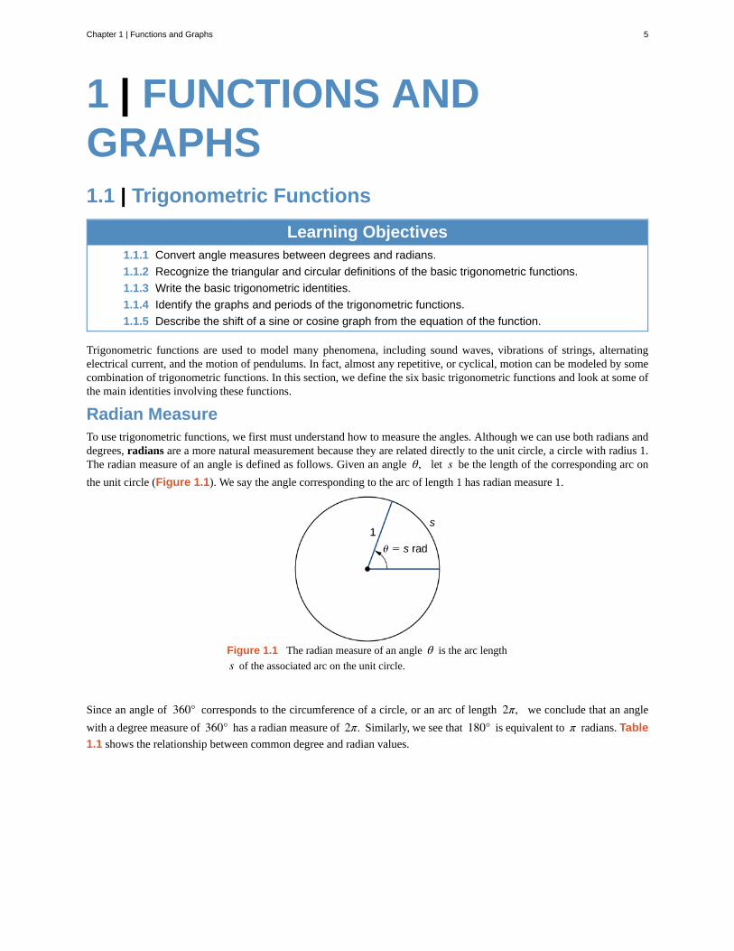
Radian MeasureTo use trigonometric functions, we first must understand how to measure the angles. Although we can use both radians anddegrees, radians are a more natural measurement because they are related directly to the unit circle, a circle with radius 1.The radian measure of an angle is defined as follows. Given an angle θ, let s be the length of the corresponding arc on
the unit circle (Figure 1.1). We say the angle corresponding to the arc of length 1 has radian measure 1.
Figure 1.1 The radian measure of an angle θ is the arc length
s of the associated arc on the unit circle.
Since an angle of 360° corresponds to the circumference of a circle, or an arc of length 2π, we conclude that an angle
with a degree measure of 360° has a radian measure of 2π. Similarly, we see that 180° is equivalent to π radians. Table
1.1 shows the relationship between common degree and radian values.
Chapter 1 | Functions and Graphs 5
1.1
Degrees Radians Degrees Radians
0 0 120 2π/3
30 π/6 135 3π/4
45 π/4 150 5π/6
60 π/3 180 π
90 π/2
Table 1.1 Common Angles Expressed in Degrees andRadians
Example 1.1
Converting between Radians and Degrees
a. Express 225° using radians.
b. Express 5π/3 rad using degrees.
Solution
Use the fact that 180° is equivalent to π radians as a conversion factor: 1 = π rad180° = 180°
π rad.
a. 225° = 225° · π180° = 5π
4 rad
b. 5π3 rad = 5π
3 · 180°π = 300°
Express 210° using radians. Express 11π/6 rad using degrees.
The Six Basic Trigonometric FunctionsTrigonometric functions allow us to use angle measures, in radians or degrees, to find the coordinates of a point on anycircle—not only on a unit circle—or to find an angle given a point on a circle. They also define the relationship among thesides and angles of a triangle.
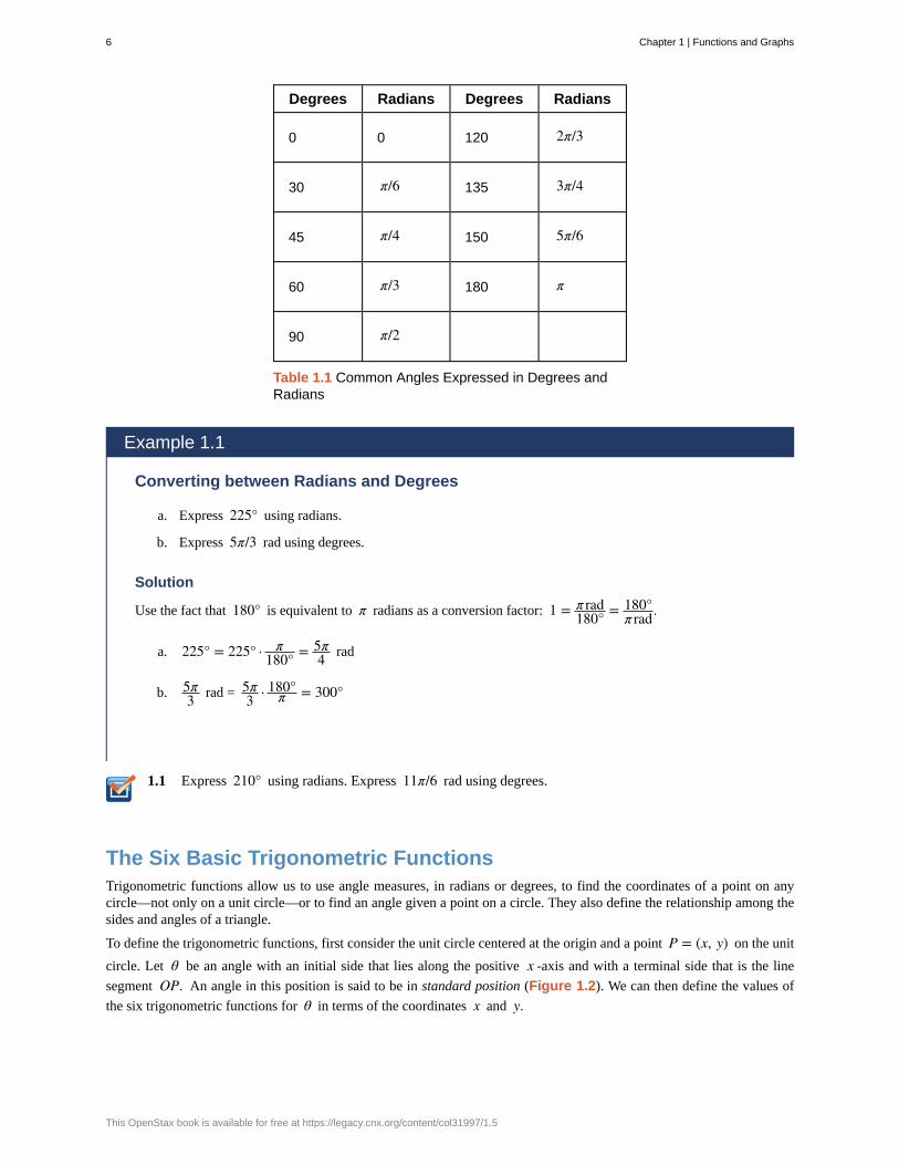
To define the trigonometric functions, first consider the unit circle centered at the origin and a point P = (x, y) on the unit
circle. Let θ be an angle with an initial side that lies along the positive x -axis and with a terminal side that is the line
segment OP. An angle in this position is said to be in standard position (Figure 1.2). We can then define the values of
the six trigonometric functions for θ in terms of the coordinates x and y.
6 Chapter 1 | Functions and Graphs
This OpenStax book is available for free at https://legacy.cnx.org/content/col31997/1.5
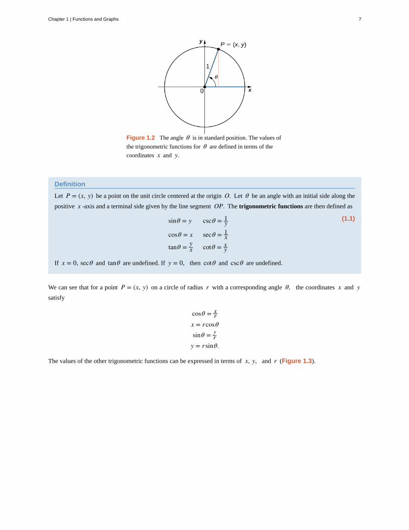
Figure 1.2 The angle θ is in standard position. The values of
the trigonometric functions for θ are defined in terms of the
coordinates x and y.
Definition
Let P = (x, y) be a point on the unit circle centered at the origin O. Let θ be an angle with an initial side along the
positive x -axis and a terminal side given by the line segment OP. The trigonometric functions are then defined as
(1.1)sinθ = y cscθ = 1y
cosθ = x secθ = 1x
tanθ = yx cotθ = x
y
If x = 0, secθ and tanθ are undefined. If y = 0, then cotθ and cscθ are undefined.
We can see that for a point P = (x, y) on a circle of radius r with a corresponding angle θ, the coordinates x and ysatisfy
cosθ = xr
x = rcosθsinθ = y
ry = r sinθ.
The values of the other trigonometric functions can be expressed in terms of x, y, and r (Figure 1.3).
Chapter 1 | Functions and Graphs 7

Figure 1.3 For a point P = (x, y) on a circle of radius r,the coordinates x and y satisfy x = rcosθ and y = r sinθ.
Table 1.2 shows the values of sine and cosine at the major angles in the first quadrant. From this table, we can determinethe values of sine and cosine at the corresponding angles in the other quadrants. The values of the other trigonometricfunctions are calculated easily from the values of sinθ and cosθ.
θ sinθ cosθ
0 0 1
π6
12
32
π4
22
22
π3
32
12
π2 1 0
Table 1.2 Values of sinθand cosθ at Major Angles
θ in the First Quadrant
Example 1.2
Evaluating Trigonometric Functions
Evaluate each of the following expressions.
a. sin⎛⎝2π3⎞⎠
b. cos⎛⎝−5π6⎞⎠
8 Chapter 1 | Functions and Graphs
This OpenStax book is available for free at https://legacy.cnx.org/content/col31997/1.5

c. tan⎛⎝15π4⎞⎠
Solution
a. On the unit circle, the angle θ = 2π3 corresponds to the point
⎛⎝−1
2, 32⎞⎠. Therefore, sin⎛⎝2π3
⎞⎠ = y = 3
2 .
b. An angle θ = − 5π6 corresponds to a revolution in the negative direction, as shown. Therefore,
cos⎛⎝−5π6⎞⎠ = x = − 3
2 .
c. An angle θ = 15π4 = 2π + 7π
4 . Therefore, this angle corresponds to more than one revolution, as shown.
Knowing the fact that an angle of 7π4 corresponds to the point
⎛⎝ 2
2 , − 22⎞⎠, we can conclude that
tan⎛⎝15π4⎞⎠ = y
x = −1.
Chapter 1 | Functions and Graphs 9

1.2 Evaluate cos(3π/4) and sin(−π/6).
As mentioned earlier, the ratios of the side lengths of a right triangle can be expressed in terms of the trigonometric functionsevaluated at either of the acute angles of the triangle. Let θ be one of the acute angles. Let A be the length of the adjacent
leg, O be the length of the opposite leg, and H be the length of the hypotenuse. By inscribing the triangle into a circle of
radius H, as shown in Figure 1.4, we see that A, H, and O satisfy the following relationships with θ:
sinθ = OH cscθ = H
Ocosθ = A
H secθ = HA
tanθ = OA cotθ = A
O
Figure 1.4 By inscribing a right triangle in a circle, we canexpress the ratios of the side lengths in terms of thetrigonometric functions evaluated at θ.
Example 1.3
Constructing a Wooden Ramp
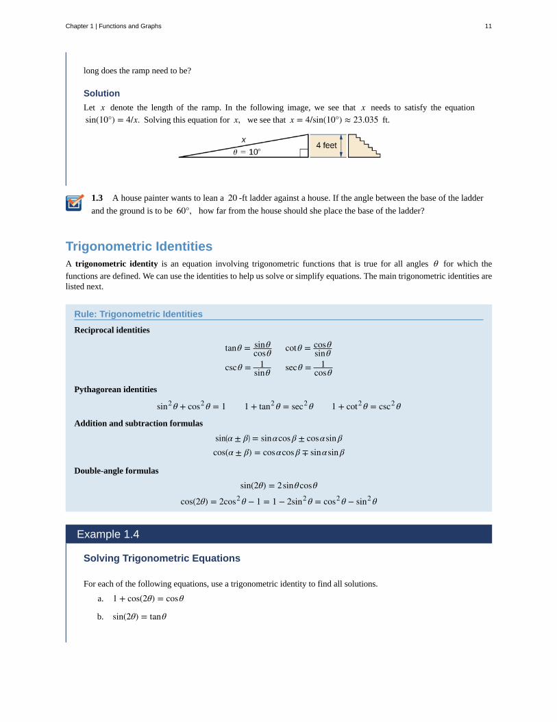
A wooden ramp is to be built with one end on the ground and the other end at the top of a short staircase. If thetop of the staircase is 4 ft from the ground and the angle between the ground and the ramp is to be 10°, how
10 Chapter 1 | Functions and Graphs
This OpenStax book is available for free at https://legacy.cnx.org/content/col31997/1.5
1.3
long does the ramp need to be?
Solution
Let x denote the length of the ramp. In the following image, we see that x needs to satisfy the equation
sin(10°) = 4/x. Solving this equation for x, we see that x = 4/sin(10°) ≈ 23.035 ft.
A house painter wants to lean a 20 -ft ladder against a house. If the angle between the base of the ladder
and the ground is to be 60°, how far from the house should she place the base of the ladder?
Trigonometric IdentitiesA trigonometric identity is an equation involving trigonometric functions that is true for all angles θ for which the
functions are defined. We can use the identities to help us solve or simplify equations. The main trigonometric identities arelisted next.
Rule: Trigonometric Identities
Reciprocal identities
tanθ = sinθcosθ cotθ = cosθ
sinθcscθ = 1
sinθ secθ = 1cosθ
Pythagorean identities
sin2 θ + cos2 θ = 1 1 + tan2 θ = sec2 θ 1 + cot2 θ = csc2 θ
Addition and subtraction formulas
sin⎛⎝α ± β⎞⎠ = sinαcosβ ± cosαsinβcos(α ± β) = cosαcosβ ∓ sinαsinβ
Double-angle formulas
sin(2θ) = 2sinθcosθ
cos(2θ) = 2cos2 θ − 1 = 1 − 2sin2 θ = cos2 θ − sin2 θ
Example 1.4
Solving Trigonometric Equations
For each of the following equations, use a trigonometric identity to find all solutions.
a. 1 + cos(2θ) = cosθ
b. sin(2θ) = tanθ
Chapter 1 | Functions and Graphs 11
Solution
a. Using the double-angle formula for cos(2θ), we see that θ is a solution of
1 + cos(2θ) = cosθ
if and only if
1 + 2cos2 θ − 1 = cosθ,
which is true if and only if
2cos2 θ − cosθ = 0.
To solve this equation, it is important to note that we need to factor the left-hand side and not divide bothsides of the equation by cosθ. The problem with dividing by cosθ is that it is possible that cosθ is
zero. In fact, if we did divide both sides of the equation by cosθ, we would miss some of the solutions
of the original equation. Factoring the left-hand side of the equation, we see that θ is a solution of this
equation if and only if
cosθ(2cosθ − 1) = 0.
Since cosθ = 0 when
θ = π2, π2 ± π, π2 ± 2π,…,
and cosθ = 1/2 when
θ = π3, π3 ± 2π,… or θ = − π
3, − π3 ± 2π,…,
we conclude that the set of solutions to this equation is
θ = π2 + nπ, θ = π
3 + 2nπ, and θ = − π3 + 2nπ, n = 0, ± 1, ± 2,….
b. Using the double-angle formula for sin(2θ) and the reciprocal identity for tan(θ), the equation can be
written as
2sinθcosθ = sinθcosθ .
To solve this equation, we multiply both sides by cosθ to eliminate the denominator, and say that if θsatisfies this equation, then θ satisfies the equation
2sinθcos2 θ − sinθ = 0.
However, we need to be a little careful here. Even if θ satisfies this new equation, it may not satisfy the
original equation because, to satisfy the original equation, we would need to be able to divide both sidesof the equation by cosθ. However, if cosθ = 0, we cannot divide both sides of the equation by cosθ.Therefore, it is possible that we may arrive at extraneous solutions. So, at the end, it is important to checkfor extraneous solutions. Returning to the equation, it is important that we factor sinθ out of both terms
on the left-hand side instead of dividing both sides of the equation by sinθ. Factoring the left-hand side
of the equation, we can rewrite this equation as
sinθ(2cos2 θ − 1) = 0.
12 Chapter 1 | Functions and Graphs
This OpenStax book is available for free at https://legacy.cnx.org/content/col31997/1.5
1.4
1.5
Therefore, the solutions are given by the angles θ such that sinθ = 0 or cos2 θ = 1/2. The solutions
of the first equation are θ = 0, ± π, ± 2π,…. The solutions of the second equation are
θ = π/4, (π/4) ± (π/2), (π/4) ± π,…. After checking for extraneous solutions, the set of solutions to the
equation is
θ = nπ and θ = π4 + nπ
2 , n = 0, ± 1, ± 2,….
Find all solutions to the equation cos(2θ) = sinθ.
Example 1.5
Proving a Trigonometric Identity
Prove the trigonometric identity 1 + tan2 θ = sec2 θ.
Solution
We start with the identity
sin2 θ + cos2 θ = 1.
Dividing both sides of this equation by cos2 θ, we obtain
sin2 θcos2 θ
+ 1 = 1cos2 θ
.
Since sinθ/cosθ = tanθ and 1/cosθ = secθ, we conclude that
tan2 θ + 1 = sec2 θ.
Prove the trigonometric identity 1 + cot2 θ = csc2 θ.
Graphs and Periods of the Trigonometric FunctionsWe have seen that as we travel around the unit circle, the values of the trigonometric functions repeat. We can see thispattern in the graphs of the functions. Let P = (x, y) be a point on the unit circle and let θ be the corresponding angle
. Since the angle θ and θ + 2π correspond to the same point P, the values of the trigonometric functions at θ and
at θ + 2π are the same. Consequently, the trigonometric functions are periodic functions. The period of a function f is
defined to be the smallest positive value p such that f (x + p) = f (x) for all values x in the domain of f . The sine,
cosine, secant, and cosecant functions have a period of 2π. Since the tangent and cotangent functions repeat on an interval
of length π, their period is π (Figure 1.5).
Chapter 1 | Functions and Graphs 13
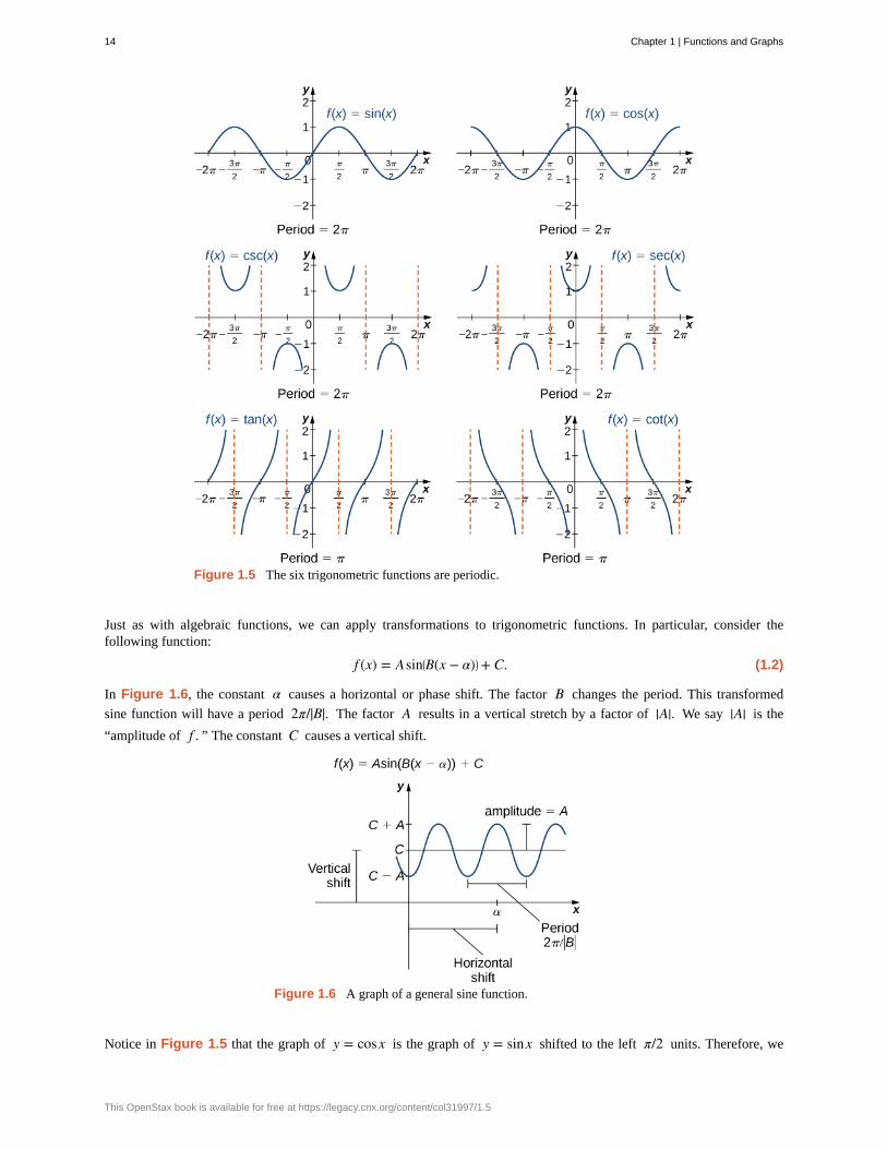
Figure 1.5 The six trigonometric functions are periodic.
Just as with algebraic functions, we can apply transformations to trigonometric functions. In particular, consider thefollowing function:
(1.2)f (x) = Asin⎛⎝B(x − α)⎞⎠+ C.
In Figure 1.6, the constant α causes a horizontal or phase shift. The factor B changes the period. This transformed
sine function will have a period 2π/|B|. The factor A results in a vertical stretch by a factor of |A|. We say |A| is the
“amplitude of f . ” The constant C causes a vertical shift.
Figure 1.6 A graph of a general sine function.
Notice in Figure 1.5 that the graph of y = cosx is the graph of y = sinx shifted to the left π/2 units. Therefore, we
14 Chapter 1 | Functions and Graphs
This OpenStax book is available for free at https://legacy.cnx.org/content/col31997/1.5
can write cosx = sin(x + π/2). Similarly, we can view the graph of y = sinx as the graph of y = cosx shifted right π/2units, and state that sinx = cos(x − π/2).
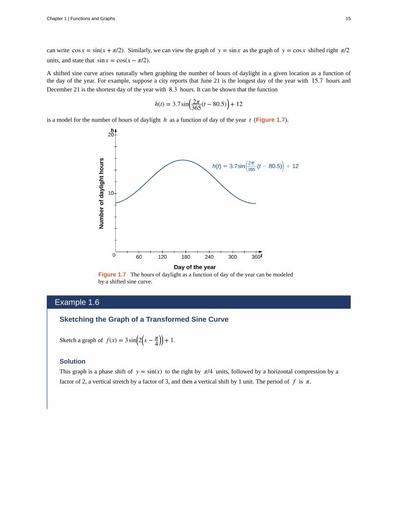
A shifted sine curve arises naturally when graphing the number of hours of daylight in a given location as a function ofthe day of the year. For example, suppose a city reports that June 21 is the longest day of the year with 15.7 hours and
December 21 is the shortest day of the year with 8.3 hours. It can be shown that the function
h(t) = 3.7sin⎛⎝ 2π365(t − 80.5)⎞⎠+ 12
is a model for the number of hours of daylight h as a function of day of the year t (Figure 1.7).
Figure 1.7 The hours of daylight as a function of day of the year can be modeledby a shifted sine curve.
Example 1.6
Sketching the Graph of a Transformed Sine Curve
Sketch a graph of f (x) = 3sin⎛⎝2⎛⎝x − π
4⎞⎠⎞⎠+ 1.
Solution
This graph is a phase shift of y = sin(x) to the right by π/4 units, followed by a horizontal compression by a
factor of 2, a vertical stretch by a factor of 3, and then a vertical shift by 1 unit. The period of f is π.
Chapter 1 | Functions and Graphs 15
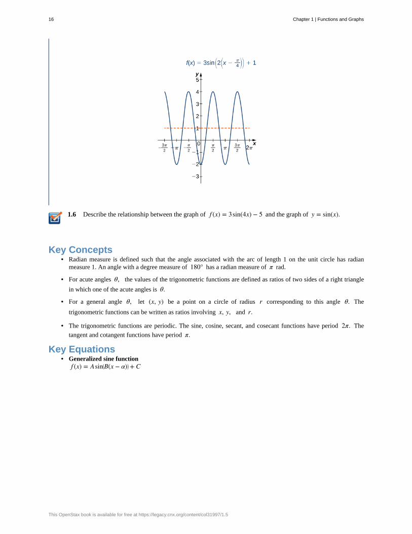
1.6 Describe the relationship between the graph of f (x) = 3sin(4x) − 5 and the graph of y = sin(x).
Key Concepts• Radian measure is defined such that the angle associated with the arc of length 1 on the unit circle has radian
measure 1. An angle with a degree measure of 180° has a radian measure of π rad.
• For acute angles θ, the values of the trigonometric functions are defined as ratios of two sides of a right triangle
in which one of the acute angles is θ.
• For a general angle θ, let (x, y) be a point on a circle of radius r corresponding to this angle θ. The
trigonometric functions can be written as ratios involving x, y, and r.
• The trigonometric functions are periodic. The sine, cosine, secant, and cosecant functions have period 2π. The
tangent and cotangent functions have period π.
Key Equations• Generalized sine function
f (x) = Asin⎛⎝B(x − α)⎞⎠+ C
16 Chapter 1 | Functions and Graphs
This OpenStax book is available for free at https://legacy.cnx.org/content/col31997/1.5

1.1 EXERCISESFor the following exercises, convert each angle in degreesto radians. Write the answer as a multiple of π.
1. 240°
2. 15°
3. −60°
4. −225°
5. 330°
For the following exercises, convert each angle in radiansto degrees.
6. π2 rad
7. 7π6 rad
8. 11π2 rad
9. −3π rad
10. 5π12 rad
Evaluate the following functional values.
11. cos⎛⎝4π3⎞⎠
12. tan⎛⎝19π4⎞⎠
13. sin⎛⎝−3π4⎞⎠
14. sec⎛⎝π6⎞⎠
15. sin⎛⎝ π12⎞⎠
16. cos⎛⎝5π12⎞⎠
For the following exercises, consider triangle ABC, a righttriangle with a right angle at C. a. Find the missing side ofthe triangle. b. Find the six trigonometric function valuesfor the angle at A. Where necessary, round to one decimalplace.
17. a = 4, c = 7
18. a = 21, c = 29
19. a = 85.3, b = 125.5
20. b = 40, c = 41
21. a = 84, b = 13
22. b = 28, c = 35
For the following exercises, P is a point on the unit circle.
a. Find the (exact) missing coordinate value of each pointand b. find the values of the six trigonometric functions forthe angle θ with a terminal side that passes through point
P. Rationalize denominators.
23. P⎛⎝ 725, y⎞⎠, y > 0
24. P⎛⎝−1517 , y⎞⎠, y < 0
25. P⎛⎝x, 73⎞⎠, x < 0
26. P⎛⎝x, − 154⎞⎠, x > 0
For the following exercises, simplify each expression bywriting it in terms of sines and cosines, then simplify. Thefinal answer does not have to be in terms of sine and cosineonly.
27. tan2 x + sinxcscx
28. secxsinxcotx
29. tan2 xsec2 x
30. secx − cosx
31. (1 + tanθ)2 − 2tanθ
Chapter 1 | Functions and Graphs 17
32. sinx(cscx − sinx)
33. cos tsin t + sin t
1 + cos t
34. 1 + tan2α1 + cot2α
For the following exercises, verify that each equation is anidentity.
35. tanθcotθcscθ = sinθ
36. sec2 θtanθ = secθcscθ
37. sin tcsc t + cos t
sec t = 1
38. sinxcosx + 1 + cosx − 1
sinx = 0
39. cotγ + tanγ = secγcscγ
40. sin2 β + tan2 β + cos2 β = sec2 β
41. 11 − sinα + 1
1 + sinα = 2sec2α
42. tanθ − cotθsinθcosθ = sec2 θ − csc2 θ
For the following exercises, solve the trigonometricequations on the interval 0 ≤ θ < 2π.
43. 2sinθ − 1 = 0
44. 1 + cosθ = 12
45. 2tan2 θ = 2
46. 4sin2 θ − 2 = 0
47. 3cotθ + 1 = 0
48. 3secθ − 2 3 = 0
49. 2cosθsinθ = sinθ
50. csc2 θ + 2cscθ + 1 = 0
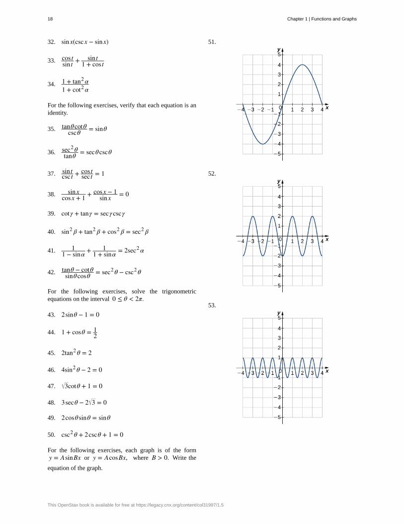
For the following exercises, each graph is of the formy = AsinBx or y = AcosBx, where B > 0. Write the
equation of the graph.
51.
52.
53.
18 Chapter 1 | Functions and Graphs
This OpenStax book is available for free at https://legacy.cnx.org/content/col31997/1.5
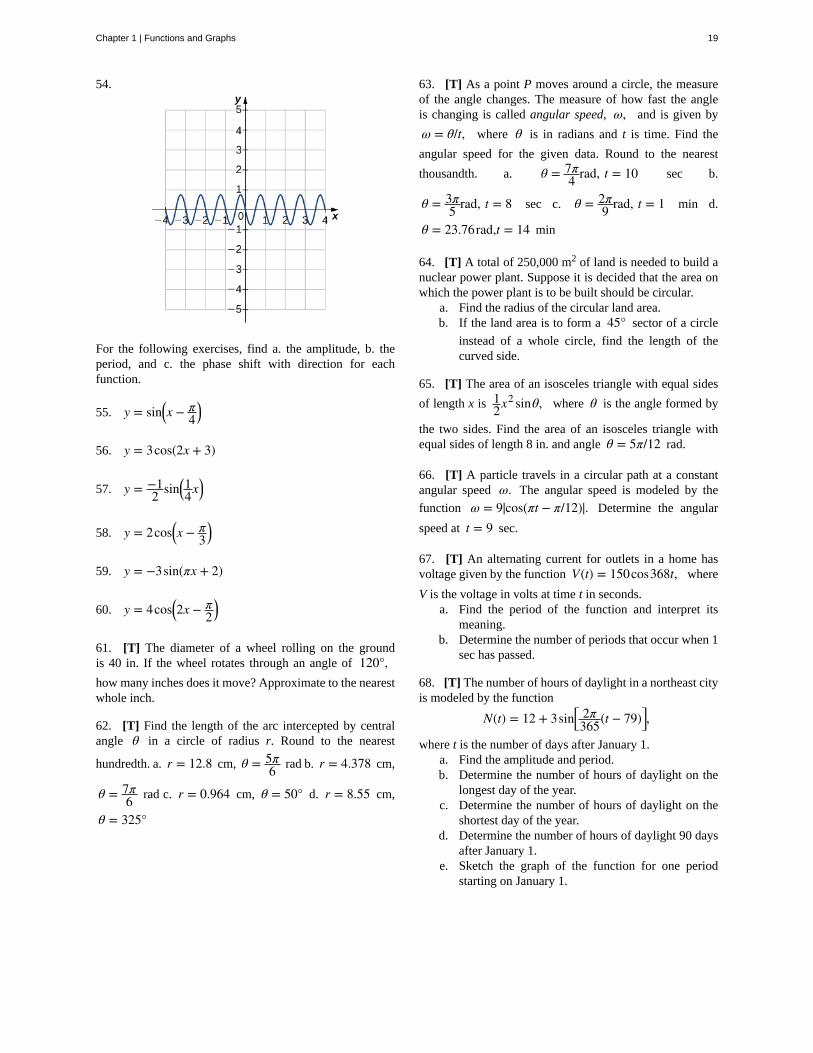
54.
For the following exercises, find a. the amplitude, b. theperiod, and c. the phase shift with direction for eachfunction.
55. y = sin⎛⎝x − π4⎞⎠
56. y = 3cos(2x + 3)
57. y = −12 sin⎛⎝14x
⎞⎠
58. y = 2cos⎛⎝x − π3⎞⎠
59. y = −3sin(πx + 2)
60. y = 4cos⎛⎝2x − π2⎞⎠
61. [T] The diameter of a wheel rolling on the groundis 40 in. If the wheel rotates through an angle of 120°,how many inches does it move? Approximate to the nearestwhole inch.
62. [T] Find the length of the arc intercepted by centralangle θ in a circle of radius r. Round to the nearest
hundredth. a. r = 12.8 cm, θ = 5π6 rad b. r = 4.378 cm,
θ = 7π6 rad c. r = 0.964 cm, θ = 50° d. r = 8.55 cm,
θ = 325°
63. [T] As a point P moves around a circle, the measureof the angle changes. The measure of how fast the angleis changing is called angular speed, ω, and is given by
ω = θ/t, where θ is in radians and t is time. Find the
angular speed for the given data. Round to the nearest
thousandth. a. θ = 7π4 rad, t = 10 sec b.
θ = 3π5 rad, t = 8 sec c. θ = 2π
9 rad, t = 1 min d.
θ = 23.76rad,t = 14 min
64. [T] A total of 250,000 m2 of land is needed to build anuclear power plant. Suppose it is decided that the area onwhich the power plant is to be built should be circular.
a. Find the radius of the circular land area.b. If the land area is to form a 45° sector of a circle
instead of a whole circle, find the length of thecurved side.
65. [T] The area of an isosceles triangle with equal sides
of length x is 12x
2 sinθ, where θ is the angle formed by
the two sides. Find the area of an isosceles triangle withequal sides of length 8 in. and angle θ = 5π/12 rad.
66. [T] A particle travels in a circular path at a constantangular speed ω. The angular speed is modeled by the
function ω = 9|cos(πt − π/12)|. Determine the angular
speed at t = 9 sec.
67. [T] An alternating current for outlets in a home hasvoltage given by the function V(t) = 150cos368t, where
V is the voltage in volts at time t in seconds.a. Find the period of the function and interpret its
meaning.b. Determine the number of periods that occur when 1
sec has passed.
68. [T] The number of hours of daylight in a northeast cityis modeled by the function
N(t) = 12 + 3sin⎡⎣ 2π365(t − 79)⎤⎦,
where t is the number of days after January 1.a. Find the amplitude and period.b. Determine the number of hours of daylight on the
longest day of the year.c. Determine the number of hours of daylight on the
shortest day of the year.d. Determine the number of hours of daylight 90 days
after January 1.e. Sketch the graph of the function for one period
starting on January 1.
Chapter 1 | Functions and Graphs 19
69. [T] Suppose that T = 50 + 10sin⎡⎣ π12(t − 8)⎤⎦ is a
mathematical model of the temperature (in degreesFahrenheit) at t hours after midnight on a certain day of theweek.
a. Determine the amplitude and period.b. Find the temperature 7 hours after midnight.c. At what time does T = 60°?d. Sketch the graph of T over 0 ≤ t ≤ 24.
70. [T] The function H(t) = 8sin⎛⎝π6 t⎞⎠ models the height
H (in feet) of the tide t hours after midnight. Assume thatt = 0 is midnight.
a. Find the amplitude and period.b. Graph the function over one period.c. What is the height of the tide at 4:30 a.m.?
20 Chapter 1 | Functions and Graphs
This OpenStax book is available for free at https://legacy.cnx.org/content/col31997/1.5
1.2 | Inverse Functions
Learning Objectives1.2.1 Determine the conditions for when a function has an inverse.
1.2.2 Use the horizontal line test to recognize when a function is one-to-one.
1.2.3 Find the inverse of a given function.
1.2.4 Draw the graph of an inverse function.
1.2.5 Evaluate inverse trigonometric functions.
An inverse function reverses the operation done by a particular function. In other words, whatever a function does, theinverse function undoes it. In this section, we define an inverse function formally and state the necessary conditions for aninverse function to exist. We examine how to find an inverse function and study the relationship between the graph of afunction and the graph of its inverse. Then we apply these ideas to define and discuss properties of the inverse trigonometricfunctions.
Existence of an Inverse FunctionWe begin with an example. Given a function f and an output y = f (x), we are often interested in finding what
value or values x were mapped to y by f . For example, consider the function f (x) = x3 + 4. Since any output
y = x3 + 4, we can solve this equation for x to find that the input is x = y − 43 . This equation defines x as a function
of y. Denoting this function as f −1, and writing x = f −1 (y) = y − 43 , we see that for any x in the domain of
f , f −1 ⎛⎝ f (x)⎞⎠ = f −1 ⎛⎝x3 + 4⎞⎠ = x. Thus, this new function, f −1, “undid” what the original function f did. A function
with this property is called the inverse function of the original function.
Definition
Given a function f with domain D and range R, its inverse function (if it exists) is the function f −1 with domain
R and range D such that f −1 (y) = x if f (x) = y. In other words, for a function f and its inverse f −1,
(1.3)f −1 ⎛⎝ f (x)⎞⎠ = x for all x in D, and f ⎛⎝ f −1 (y)⎞⎠ = y for all y in R.
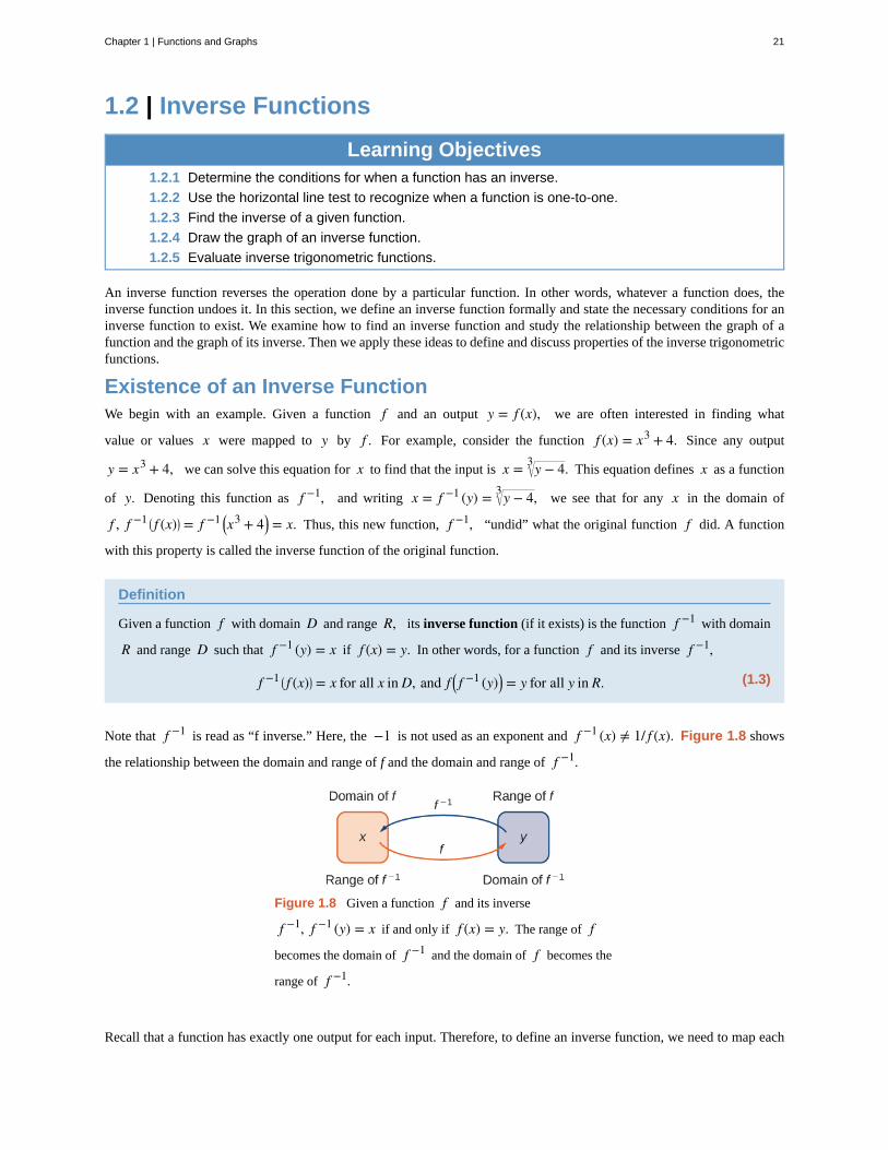
Note that f −1 is read as “f inverse.” Here, the −1 is not used as an exponent and f −1 (x) ≠ 1/ f (x). Figure 1.8 shows
the relationship between the domain and range of f and the domain and range of f −1.
Figure 1.8 Given a function f and its inverse
f −1, f −1 (y) = x if and only if f (x) = y. The range of f
becomes the domain of f −1 and the domain of f becomes the
range of f −1.
Recall that a function has exactly one output for each input. Therefore, to define an inverse function, we need to map each
Chapter 1 | Functions and Graphs 21

input to exactly one output. For example, let’s try to find the inverse function for f (x) = x2. Solving the equation y = x2
for x, we arrive at the equation x = ± y. This equation does not describe x as a function of y because there are two
solutions to this equation for every y > 0. The problem with trying to find an inverse function for f (x) = x2 is that two
inputs are sent to the same output for each output y > 0. The function f (x) = x3 + 4 discussed earlier did not have this
problem. For that function, each input was sent to a different output. A function that sends each input to a different outputis called a one-to-one function.
Definition
We say a f is a one-to-one function if f (x1) ≠ f (x2) when x1 ≠ x2.
One way to determine whether a function is one-to-one is by looking at its graph. If a function is one-to-one, then no twoinputs can be sent to the same output. Therefore, if we draw a horizontal line anywhere in the xy -plane, according to the
horizontal line test, it cannot intersect the graph more than once. We note that the horizontal line test is different fromthe vertical line test. The vertical line test determines whether a graph is the graph of a function. The horizontal line testdetermines whether a function is one-to-one (Figure 1.9).
Rule: Horizontal Line Test
A function f is one-to-one if and only if every horizontal line intersects the graph of f no more than once.
Figure 1.9 (a) The function f (x) = x2 is not one-to-one
because it fails the horizontal line test. (b) The function
f (x) = x3 is one-to-one because it passes the horizontal line
test.
Example 1.7
Determining Whether a Function Is One-to-One
For each of the following functions, use the horizontal line test to determine whether it is one-to-one.
22 Chapter 1 | Functions and Graphs
This OpenStax book is available for free at https://legacy.cnx.org/content/col31997/1.5

a.
b.
Solution
a. Since the horizontal line y = n for any integer n ≥ 0 intersects the graph more than once, this function
is not one-to-one.
Chapter 1 | Functions and Graphs 23
1.7
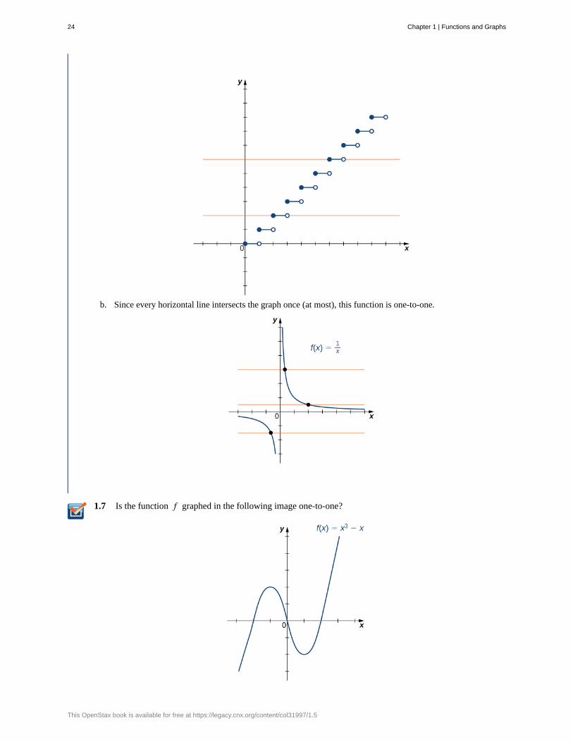
b. Since every horizontal line intersects the graph once (at most), this function is one-to-one.
Is the function f graphed in the following image one-to-one?
24 Chapter 1 | Functions and Graphs
This OpenStax book is available for free at https://legacy.cnx.org/content/col31997/1.5
Finding a Function’s InverseWe can now consider one-to-one functions and show how to find their inverses. Recall that a function maps elements inthe domain of f to elements in the range of f . The inverse function maps each element from the range of f back to its
corresponding element from the domain of f . Therefore, to find the inverse function of a one-to-one function f , given
any y in the range of f , we need to determine which x in the domain of f satisfies f (x) = y. Since f is one-to-one,
there is exactly one such value x. We can find that value x by solving the equation f (x) = y for x. Doing so, we are
able to write x as a function of y where the domain of this function is the range of f and the range of this new function
is the domain of f . Consequently, this function is the inverse of f , and we write x = f −1(y). Since we typically use the
variable x to denote the independent variable and y to denote the dependent variable, we often interchange the roles of x
and y, and write y = f −1(x). Representing the inverse function in this way is also helpful later when we graph a function
f and its inverse f −1 on the same axes.
Problem-Solving Strategy: Finding an Inverse Function
1. Solve the equation y = f (x) for x.
2. Interchange the variables x and y and write y = f −1(x).
Example 1.8
Finding an Inverse Function
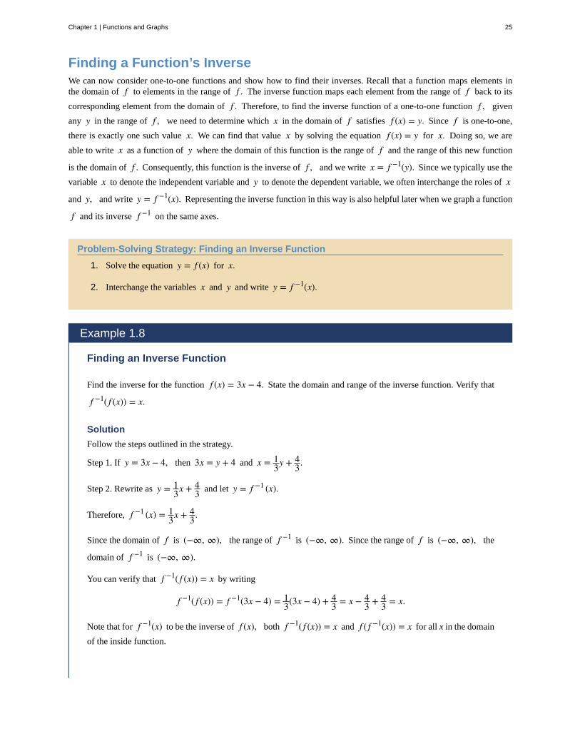
Find the inverse for the function f (x) = 3x − 4. State the domain and range of the inverse function. Verify that
f −1( f (x)) = x.
Solution
Follow the steps outlined in the strategy.
Step 1. If y = 3x − 4, then 3x = y + 4 and x = 13y + 4
3.
Step 2. Rewrite as y = 13x + 4
3 and let y = f −1 (x).
Therefore, f −1 (x) = 13x + 4
3.
Since the domain of f is (−∞, ∞), the range of f −1 is (−∞, ∞). Since the range of f is (−∞, ∞), the
domain of f −1 is (−∞, ∞).
You can verify that f −1( f (x)) = x by writing
f −1( f (x)) = f −1(3x − 4) = 13(3x − 4) + 4
3 = x − 43 + 4
3 = x.
Note that for f −1(x) to be the inverse of f (x), both f −1( f (x)) = x and f ( f −1(x)) = x for all x in the domain
of the inside function.
Chapter 1 | Functions and Graphs 25
1.8 Find the inverse of the function f (x) = 3x/(x − 2). State the domain and range of the inverse function.
Graphing Inverse Functions
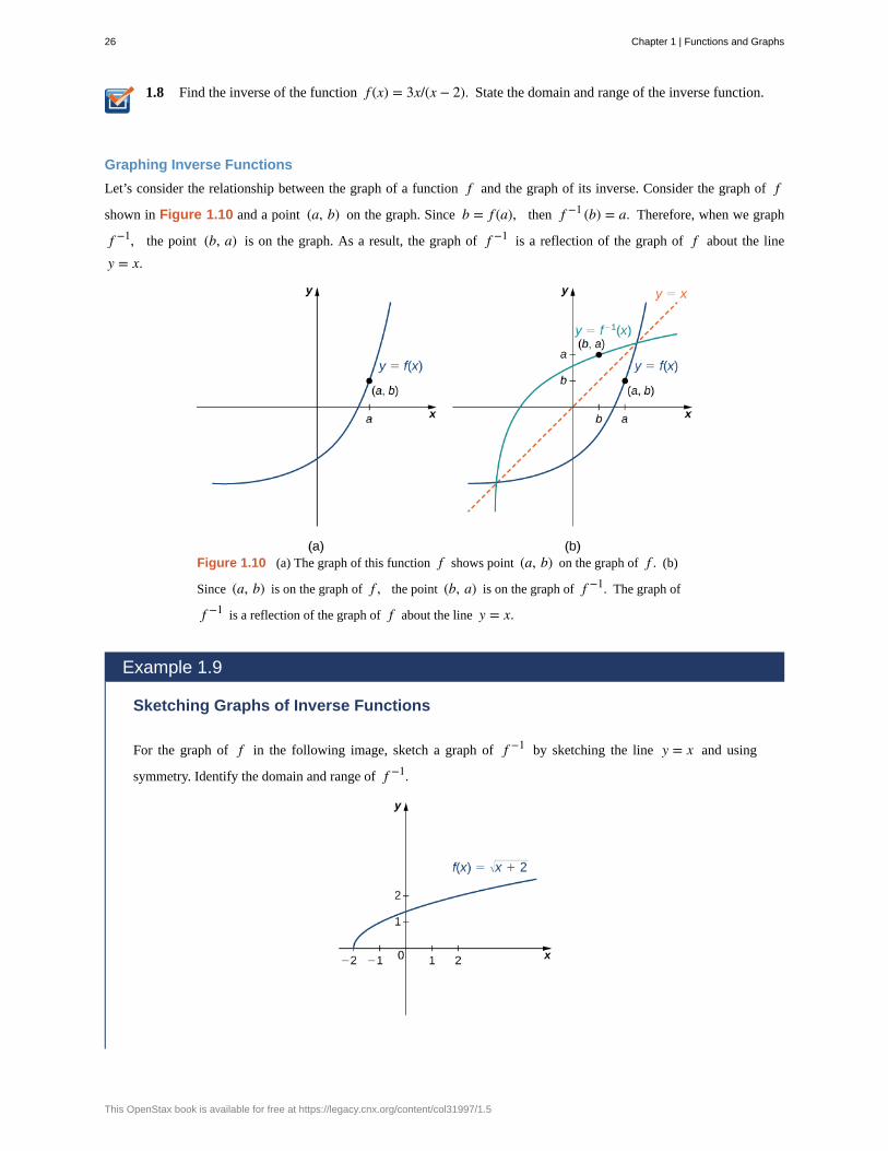
Let’s consider the relationship between the graph of a function f and the graph of its inverse. Consider the graph of f
shown in Figure 1.10 and a point (a, b) on the graph. Since b = f (a), then f −1 (b) = a. Therefore, when we graph
f −1, the point (b, a) is on the graph. As a result, the graph of f −1 is a reflection of the graph of f about the line
y = x.
Figure 1.10 (a) The graph of this function f shows point (a, b) on the graph of f . (b)
Since (a, b) is on the graph of f , the point (b, a) is on the graph of f −1. The graph of
f −1 is a reflection of the graph of f about the line y = x.
Example 1.9
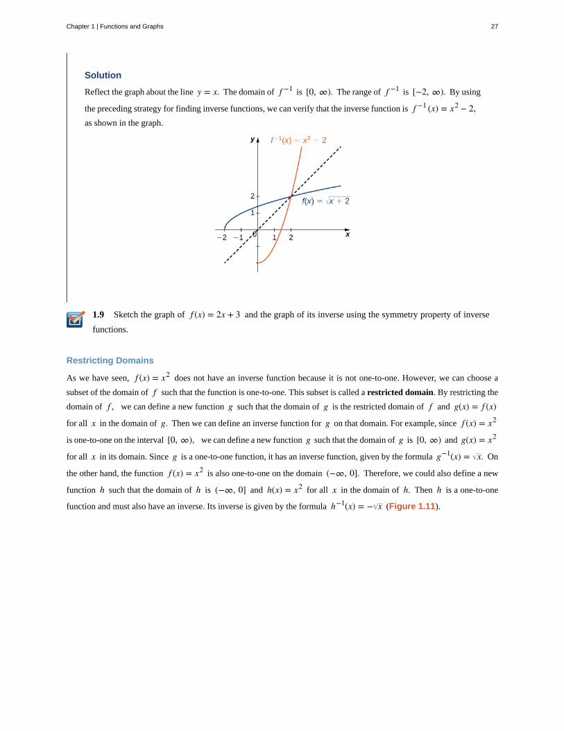
Sketching Graphs of Inverse Functions
For the graph of f in the following image, sketch a graph of f −1 by sketching the line y = x and using
symmetry. Identify the domain and range of f −1.
26 Chapter 1 | Functions and Graphs
This OpenStax book is available for free at https://legacy.cnx.org/content/col31997/1.5
1.9
Solution
Reflect the graph about the line y = x. The domain of f −1 is [0, ∞). The range of f −1 is [−2, ∞). By using
the preceding strategy for finding inverse functions, we can verify that the inverse function is f −1 (x) = x2 − 2,as shown in the graph.
Sketch the graph of f (x) = 2x + 3 and the graph of its inverse using the symmetry property of inverse
functions.
Restricting Domains
As we have seen, f (x) = x2 does not have an inverse function because it is not one-to-one. However, we can choose a
subset of the domain of f such that the function is one-to-one. This subset is called a restricted domain. By restricting the
domain of f , we can define a new function g such that the domain of g is the restricted domain of f and g(x) = f (x)
for all x in the domain of g. Then we can define an inverse function for g on that domain. For example, since f (x) = x2
is one-to-one on the interval [0, ∞), we can define a new function g such that the domain of g is [0, ∞) and g(x) = x2
for all x in its domain. Since g is a one-to-one function, it has an inverse function, given by the formula g−1(x) = x. On
the other hand, the function f (x) = x2 is also one-to-one on the domain (−∞, 0]. Therefore, we could also define a new
function h such that the domain of h is (−∞, 0] and h(x) = x2 for all x in the domain of h. Then h is a one-to-one
function and must also have an inverse. Its inverse is given by the formula h−1(x) = − x (Figure 1.11).
Chapter 1 | Functions and Graphs 27
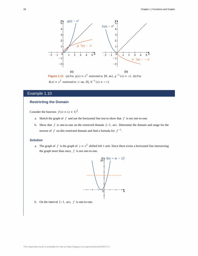
Figure 1.11 (a) For g(x) = x2 restricted to [0, ∞), g−1 (x) = x. (b) For
h(x) = x2 restricted to (−∞, 0], h−1 (x) = − x.
Example 1.10
Restricting the Domain
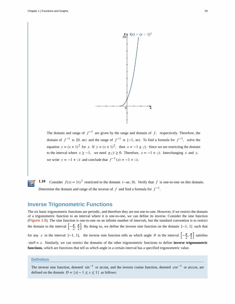
Consider the function f (x) = (x + 1)2.
a. Sketch the graph of f and use the horizontal line test to show that f is not one-to-one.
b. Show that f is one-to-one on the restricted domain [−1, ∞). Determine the domain and range for the
inverse of f on this restricted domain and find a formula for f −1.
Solution
a. The graph of f is the graph of y = x2 shifted left 1 unit. Since there exists a horizontal line intersecting
the graph more than once, f is not one-to-one.
b. On the interval [−1, ∞), f is one-to-one.
28 Chapter 1 | Functions and Graphs
This OpenStax book is available for free at https://legacy.cnx.org/content/col31997/1.5
1.10
The domain and range of f −1 are given by the range and domain of f , respectively. Therefore, the
domain of f −1 is [0, ∞) and the range of f −1 is [−1, ∞). To find a formula for f −1, solve the
equation y = (x + 1)2 for x. If y = (x + 1)2, then x = −1 ± y. Since we are restricting the domain
to the interval where x ≥ −1, we need ± y ≥ 0. Therefore, x = −1 + y. Interchanging x and y,
we write y = −1 + x and conclude that f −1 (x) = −1 + x.
Consider f (x) = 1/x2 restricted to the domain (−∞, 0). Verify that f is one-to-one on this domain.
Determine the domain and range of the inverse of f and find a formula for f −1.
Inverse Trigonometric FunctionsThe six basic trigonometric functions are periodic, and therefore they are not one-to-one. However, if we restrict the domainof a trigonometric function to an interval where it is one-to-one, we can define its inverse. Consider the sine function(Figure 1.5). The sine function is one-to-one on an infinite number of intervals, but the standard convention is to restrict
the domain to the interval⎡⎣−π
2, π2⎤⎦. By doing so, we define the inverse sine function on the domain [−1, 1] such that
for any x in the interval [−1, 1], the inverse sine function tells us which angle θ in the interval⎡⎣−π
2, π2⎤⎦ satisfies
sinθ = x. Similarly, we can restrict the domains of the other trigonometric functions to define inverse trigonometric
functions, which are functions that tell us which angle in a certain interval has a specified trigonometric value.
Definition
The inverse sine function, denoted sin−1 or arcsin, and the inverse cosine function, denoted cos−1 or arccos, are
defined on the domain D = {x| − 1 ≤ x ≤ 1} as follows:
Chapter 1 | Functions and Graphs 29

(1.4)sin−1 (x) = y if and only if sin(y) = x and − π2 ≤ y ≤ π
2;
cos−1 (x) = y if and only if cos(y) = x and 0 ≤ y ≤ π.
The inverse tangent function, denoted tan−1 or arctan, and inverse cotangent function, denoted cot−1 or arccot, are
defined on the domain D = {x| − ∞ < x < ∞} as follows:
(1.5)tan−1 (x) = y if and only if tan(y) = x and − π2 < y < π
2;
cot−1 (x) = y if and only if cot(y) = x and 0 < y < π.
The inverse cosecant function, denoted csc−1 or arccsc, and inverse secant function, denoted sec−1 or arcsec, are
defined on the domain D = {x||x| ≥ 1} as follows:
(1.6)csc−1 (x) = y if and only if csc(y) = x and − π2 ≤ y ≤ π
2, y ≠ 0;
sec−1 (x) = y if and only if sec(y) = x and 0 ≤ y ≤ π, y ≠ π/2.
To graph the inverse trigonometric functions, we use the graphs of the trigonometric functions restricted to the domainsdefined earlier and reflect the graphs about the line y = x (Figure 1.12).
Figure 1.12 The graph of each of the inverse trigonometric functions is a reflection about the line y = x of
the corresponding restricted trigonometric function.
Go to the following site (http://www.openstax.org/l/20_inversefun) for more comparisons of functionsand their inverses.
30 Chapter 1 | Functions and Graphs
This OpenStax book is available for free at https://legacy.cnx.org/content/col31997/1.5

When evaluating an inverse trigonometric function, the output is an angle. For example, to evaluate cos−1 ⎛⎝12⎞⎠, we need to
find an angle θ such that cosθ = 12. Clearly, many angles have this property. However, given the definition of cos−1, we
need the angle θ that not only solves this equation, but also lies in the interval [0, π]. We conclude that cos−1 ⎛⎝12⎞⎠ = π
3.
We now consider a composition of a trigonometric function and its inverse. For example, consider the two expressions
sin⎛⎝sin−1 ⎛⎝ 22⎞⎠⎞⎠ and sin−1(sin(π)). For the first one, we simplify as follows:
sin⎛⎝sin−1 ⎛⎝ 22⎞⎠⎞⎠ = sin⎛⎝π4
⎞⎠ = 2
2 .
For the second one, we have
sin−1 ⎛⎝sin(π)⎞⎠ = sin−1 (0) = 0.
The inverse function is supposed to “undo” the original function, so why isn’t sin−1 ⎛⎝sin(π)⎞⎠ = π ? Recalling our definition
of inverse functions, a function f and its inverse f −1 satisfy the conditions f ⎛⎝ f −1 (y)⎞⎠ = y for all y in the domain of
f −1 and f −1 ⎛⎝ f (x)⎞⎠ = x for all x in the domain of f , so what happened here? The issue is that the inverse sine function,
sin−1, is the inverse of the restricted sine function defined on the domain⎡⎣−π
2, π2⎤⎦. Therefore, for x in the interval
⎡⎣−π
2, π2⎤⎦, it is true that sin−1 (sinx) = x. However, for values of x outside this interval, the equation does not hold, even
though sin−1(sinx) is defined for all real numbers x.
What about sin(sin−1 y)? Does that have a similar issue? The answer is no. Since the domain of sin−1 is the interval
[−1, 1], we conclude that sin(sin−1 y) = y if −1 ≤ y ≤ 1 and the expression is not defined for other values of y. To
summarize,
sin(sin−1 y) = y if −1 ≤ y ≤ 1
and
sin−1 (sinx) = x if − π2 ≤ x ≤ π
2.
Similarly, for the cosine function,
cos(cos−1 y) = y if −1 ≤ y ≤ 1
and
cos−1 (cosx) = x if 0 ≤ x ≤ π.
Similar properties hold for the other trigonometric functions and their inverses.
Example 1.11
Evaluating Expressions Involving Inverse Trigonometric Functions
Evaluate each of the following expressions.
a. sin−1 ⎛⎝− 32⎞⎠
b. tan⎛⎝tan−1 ⎛⎝− 13⎞⎠⎞⎠
Chapter 1 | Functions and Graphs 31
c. cos−1 ⎛⎝cos⎛⎝5π4⎞⎠⎞⎠
d. sin−1 ⎛⎝cos⎛⎝2π3⎞⎠⎞⎠
Solution
a. Evaluating sin−1 ⎛⎝− 3/2⎞⎠ is equivalent to finding the angle θ such that sinθ = − 3/2 and
−π/2 ≤ θ ≤ π/2. The angle θ = −π/3 satisfies these two conditions. Therefore,
sin−1 ⎛⎝− 3/2⎞⎠ = −π/3.
b. First we use the fact that tan−1 ⎛⎝−1/ 3⎞⎠ = −π/6. Then tan(π/6) = −1/ 3. Therefore,
tan⎛⎝tan−1 ⎛⎝−1/ 3⎞⎠⎞⎠ = −1/ 3.
c. To evaluate cos−1 ⎛⎝cos(5π/4)⎞⎠, first use the fact that cos(5π/4) = − 2/2. Then we need to find the
angle θ such that cos(θ) = − 2/2 and 0 ≤ θ ≤ π. Since 3π/4 satisfies both these conditions, we have
cos⎛⎝cos−1 (5π/4)⎞⎠ = cos⎛⎝cos−1 ⎛⎝− 2/2⎞⎠⎞⎠ = 3π/4.
d. Since cos(2π/3) = −1/2, we need to evaluate sin−1 (−1/2). That is, we need to find the angle θ such
that sin(θ) = −1/2 and −π/2 ≤ θ ≤ π/2. Since −π/6 satisfies both these conditions, we can conclude
that sin−1 (cos(2π/3)) = sin−1 (−1/2) = −π/6.
32 Chapter 1 | Functions and Graphs
This OpenStax book is available for free at https://legacy.cnx.org/content/col31997/1.5

The Maximum Value of a Function
In many areas of science, engineering, and mathematics, it is useful to know the maximum value a function can obtain,even if we don’t know its exact value at a given instant. For instance, if we have a function describing the strengthof a roof beam, we would want to know the maximum weight the beam can support without breaking. If we have afunction that describes the speed of a train, we would want to know its maximum speed before it jumps off the rails.Safe design often depends on knowing maximum values.
This project describes a simple example of a function with a maximum value that depends on two equation coefficients.We will see that maximum values can depend on several factors other than the independent variable x.
1. Consider the graph in Figure 1.13 of the function y = sinx + cosx. Describe its overall shape. Is it periodic?
How do you know?
Figure 1.13 The graph of y = sinx + cosx.
Using a graphing calculator or other graphing device, estimate the x - and y -values of the maximum point for
the graph (the first such point where x > 0). It may be helpful to express the x -value as a multiple of π.
2. Now consider other graphs of the form y = Asinx + Bcosx for various values of A and B. Sketch the graph
when A = 2 and B = 1, and find the x - and y-values for the maximum point. (Remember to express the x-value
as a multiple of π, if possible.) Has it moved?
3. Repeat for A = 1, B = 2. Is there any relationship to what you found in part (2)?
4. Complete the following table, adding a few choices of your own for A and B:
Chapter 1 | Functions and Graphs 33
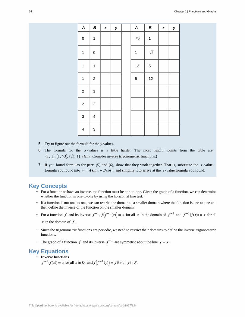
A B x y A B x y
0 1 3 1
1 0 1 3
1 1 12 5
1 2 5 12
2 1
2 2
3 4
4 3
5. Try to figure out the formula for the y-values.
6. The formula for the x -values is a little harder. The most helpful points from the table are
(1, 1), ⎛⎝1, 3⎞⎠, ⎛⎝ 3, 1⎞⎠. (Hint: Consider inverse trigonometric functions.)
7. If you found formulas for parts (5) and (6), show that they work together. That is, substitute the x -value
formula you found into y = Asinx + Bcosx and simplify it to arrive at the y -value formula you found.
Key Concepts• For a function to have an inverse, the function must be one-to-one. Given the graph of a function, we can determine
whether the function is one-to-one by using the horizontal line test.
• If a function is not one-to-one, we can restrict the domain to a smaller domain where the function is one-to-one andthen define the inverse of the function on the smaller domain.
• For a function f and its inverse f −1, f ⎛⎝ f −1 (x)⎞⎠ = x for all x in the domain of f −1 and f −1 ⎛⎝ f (x)⎞⎠ = x for all
x in the domain of f .
• Since the trigonometric functions are periodic, we need to restrict their domains to define the inverse trigonometricfunctions.
• The graph of a function f and its inverse f −1 are symmetric about the line y = x.
Key Equations• Inverse functions
f −1 ⎛⎝ f (x)⎞⎠ = x for all x in D, and f ⎛⎝ f −1 (y)⎞⎠ = y for all y in R.
34 Chapter 1 | Functions and Graphs
This OpenStax book is available for free at https://legacy.cnx.org/content/col31997/1.5

1.2 EXERCISESFor the following exercises, use the horizontal line test todetermine whether each of the given graphs is one-to-one.
71.
72.
73.
74.
75.
76.
For the following exercises, a. find the inverse function,and b. find the domain and range of the inverse function.
77. f (x) = x2 − 4, x ≥ 0
78. f (x) = x − 43
79. f (x) = x3 + 1
80. f (x) = (x − 1)2, x ≤ 1
Chapter 1 | Functions and Graphs 35

81. f (x) = x − 1
82. f (x) = 1x + 2
For the following exercises, use the graph of f to sketch
the graph of its inverse function.
83.
84.
85.
86.
For the following exercises, use composition to determinewhich pairs of functions are inverses.
87. f (x) = 8x, g(x) = x8
88. f (x) = 8x + 3, g(x) = x − 38
89. f (x) = 5x − 7, g(x) = x + 57
90. f (x) = 23x + 2, g(x) = 3
2x + 3
91. f (x) = 1x − 1, x ≠ 1, g(x) = 1
x + 1, x ≠ 0
92. f (x) = x3 + 1, g(x) = (x − 1)1/3
93.
f (x) = x2 + 2x + 1, x ≥ −1, g(x) = −1 + x, x ≥ 0
94.
f (x) = 4 − x2, 0 ≤ x ≤ 2, g(x) = 4 − x2, 0 ≤ x ≤ 2
For the following exercises, evaluate the functions. Givethe exact value.
95. tan−1 ⎛⎝ 33⎞⎠
96. cos−1 ⎛⎝− 22⎞⎠
97. cot−1 (1)
98. sin−1 (−1)
99. cos−1 ⎛⎝ 32⎞⎠
36 Chapter 1 | Functions and Graphs
This OpenStax book is available for free at https://legacy.cnx.org/content/col31997/1.5
100. cos⎛⎝tan−1 ⎛⎝ 3⎞⎠⎞⎠
101. sin⎛⎝cos−1 ⎛⎝ 22⎞⎠⎞⎠
102. sin−1 ⎛⎝sin⎛⎝π3⎞⎠⎞⎠
103. tan−1 ⎛⎝tan⎛⎝−π6⎞⎠⎞⎠
104. The function C = T(F) = (5/9)(F − 32) converts
degrees Fahrenheit to degrees Celsius.
a. Find the inverse function F = T−1(C)b. What is the inverse function used for?
105. [T] The velocity V (in centimeters per second) ofblood in an artery at a distance x cm from the center ofthe artery can be modeled by the function
V = f (x) = 500(0.04 − x2) for 0 ≤ x ≤ 0.2.
a. Find x = f −1(V).b. Interpret what the inverse function is used for.c. Find the distance from the center of an artery with
a velocity of 15 cm/sec, 10 cm/sec, and 5 cm/sec.
106. A function that converts dress sizes in the UnitedStates to those in Europe is given by D(x) = 2x + 24.
a. Find the European dress sizes that correspond tosizes 6, 8, 10, and 12 in the United States.
b. Find the function that converts European dresssizes to U.S. dress sizes.
c. Use part b. to find the dress sizes in the UnitedStates that correspond to 46, 52, 62, and 70.
107. [T] The cost to remove a toxin from a lake ismodeled by the function C(p) = 75p/(85 − p), where
C is the cost (in thousands of dollars) and p is the amount
of toxin in a small lake (measured in parts per billion[ppb]). This model is valid only when the amount of toxinis less than 85 ppb.
a. Find the cost to remove 25 ppb, 40 ppb, and 50 ppbof the toxin from the lake.
b. Find the inverse function. c. Use part b. todetermine how much of the toxin is removed for$50,000.
108. [T] A race car is accelerating at a velocity given
by v(t) = 254 t + 54, where v is the velocity (in feet per
second) at time t.a. Find the velocity of the car at 10 sec.b. Find the inverse function.c. Use part b. to determine how long it takes for the
car to reach a speed of 150 ft/sec.
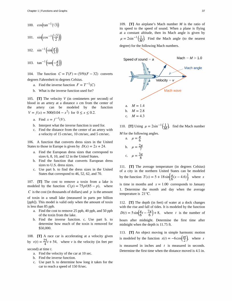
109. [T] An airplane’s Mach number M is the ratio ofits speed to the speed of sound. When a plane is flyingat a constant altitude, then its Mach angle is given by
μ = 2sin−1 ⎛⎝ 1M⎞⎠. Find the Mach angle (to the nearest
degree) for the following Mach numbers.
a. M = 1.4b. M = 2.8c. M = 4.3
110. [T] Using μ = 2sin−1 ⎛⎝ 1M⎞⎠, find the Mach number
M for the following angles.a. μ = π
6
b. μ = 2π7
c. μ = 3π8
111. [T] The average temperature (in degrees Celsius)of a city in the northern United States can be modeled
by the function T(x) = 5 + 18sin⎡⎣π6(x − 4.6)⎤⎦, where x
is time in months and x = 1.00 corresponds to January
1. Determine the month and day when the averagetemperature is 21°C.
112. [T] The depth (in feet) of water at a dock changeswith the rise and fall of tides. It is modeled by the function
D(t) = 5sin⎛⎝π6 t − 7π6⎞⎠+ 8, where t is the number of
hours after midnight. Determine the first time aftermidnight when the depth is 11.75 ft.
113. [T] An object moving in simple harmonic motion
is modeled by the function s(t) = −6cos⎛⎝πt2⎞⎠, where s
is measured in inches and t is measured in seconds.
Determine the first time when the distance moved is 4.5 in.
Chapter 1 | Functions and Graphs 37

114. [T] A local art gallery has a portrait 3 ft in heightthat is hung 2.5 ft above the eye level of an average person.The viewing angle θ can be modeled by the function
θ = tan−1 5.5x − tan−1 2.5
x , where x is the distance (in
feet) from the portrait. Find the viewing angle when aperson is 4 ft from the portrait.
115. [T] Use a calculator to evaluate tan−1 (tan(2.1)) and
cos−1 (cos(2.1)). Explain the results of each.
116. [T] Use a calculator to evaluate sin(sin−1(−2)) and
tan(tan−1(−2)). Explain the results of each.
38 Chapter 1 | Functions and Graphs
This OpenStax book is available for free at https://legacy.cnx.org/content/col31997/1.5

1.3 | Exponential and Logarithmic Functions
Learning Objectives1.3.1 Identify the form of an exponential function.
1.3.2 Explain the difference between the graphs of xb and bx.1.3.3 Recognize the significance of the number e.1.3.4 Identify the form of a logarithmic function.
1.3.5 Explain the relationship between exponential and logarithmic functions.
1.3.6 Describe how to calculate a logarithm to a different base.
1.3.7 Identify the hyperbolic functions, their graphs, and basic identities.
In this section we examine exponential and logarithmic functions. We use the properties of these functions to solveequations involving exponential or logarithmic terms, and we study the meaning and importance of the number e. We also
define hyperbolic and inverse hyperbolic functions, which involve combinations of exponential and logarithmic functions.(Note that we present alternative definitions of exponential and logarithmic functions in the chapter Applicationsof Integrations (https://legacy.cnx.org/content/m53638/latest/) , and prove that the functions have the sameproperties with either definition.)
Exponential FunctionsExponential functions arise in many applications. One common example is population growth.
For example, if a population starts with P0 individuals and then grows at an annual rate of 2%, its population after 1 year
is
P(1) = P0 + 0.02P0 = P0(1 + 0.02) = P0(1.02).
Its population after 2 years is
P(2) = P(1) + 0.02P(1) = P(1)(1.02) = P0 (1.02)2.
In general, its population after t years is
P(t) = P0 (1.02)t,
which is an exponential function. More generally, any function of the form f (x) = bx, where b > 0, b ≠ 1, is an
exponential function with base b and exponent x. Exponential functions have constant bases and variable exponents. Note
that a function of the form f (x) = xb for some constant b is not an exponential function but a power function.
To see the difference between an exponential function and a power function, we compare the functions y = x2 and y = 2x.
In Table 1.3, we see that both 2x and x2 approach infinity as x → ∞. Eventually, however, 2x becomes larger than x2
and grows more rapidly as x → ∞. In the opposite direction, as x → −∞, x2 → ∞, whereas 2x → 0. The line y = 0is a horizontal asymptote for y = 2x.
Chapter 1 | Functions and Graphs 39

x −3 −2 −1 0 1 2 3 4 5 6
x2 9 4 1 0 1 4 9 16 25 36
2x 1/8 1/4 1/2 1 2 4 8 16 32 64
Table 1.3 Values of x2 and 2x
In Figure 1.14, we graph both y = x2 and y = 2x to show how the graphs differ.
Figure 1.14 Both 2x and x2 approach infinity as x → ∞,
but 2x grows more rapidly than x2. As
x → −∞, x2 → ∞, whereas 2x → 0.
Evaluating Exponential Functions
Recall the properties of exponents: If x is a positive integer, then we define bx = b · b ⋯ b (with x factors of b). If x
is a negative integer, then x = −y for some positive integer y, and we define bx = b−y = 1/by. Also, b0 is defined
to be 1. If x is a rational number, then x = p/q, where p and q are integers and bx = b p/q = b pq. For example,
93/2 = 93 = 27. However, how is bx defined if x is an irrational number? For example, what do we mean by 2 2?This is too complex a question for us to answer fully right now; however, we can make an approximation. In Table 1.4, welist some rational numbers approaching 2, and the values of 2x for each rational number x are presented as well. We
claim that if we choose rational numbers x getting closer and closer to 2, the values of 2x get closer and closer to some
number L. We define that number L to be 2 2.
40 Chapter 1 | Functions and Graphs
This OpenStax book is available for free at https://legacy.cnx.org/content/col31997/1.5

1.11
x 1.4 1.41 1.414 1.4142 1.41421 1.414213
2x 2.639 2.65737 2.66475 2.665119 2.665138 2.665143
Table 1.4 Values of 2x for a List of Rational Numbers Approximating 2
Example 1.12
Bacterial Growth
Suppose a particular population of bacteria is known to double in size every 4 hours. If a culture starts with
1000 bacteria, the number of bacteria after 4 hours is n(4) = 1000 · 2. The number of bacteria after 8 hours is
n(8) = n(4) · 2 = 1000 · 22. In general, the number of bacteria after 4m hours is n(4m) = 1000 · 2m. Letting
t = 4m, we see that the number of bacteria after t hours is n(t) = 1000 · 2t/4. Find the number of bacteria
after 6 hours, 10 hours, and 24 hours.
Solution
The number of bacteria after 6 hours is given by n(6) = 1000 · 26/4 ≈ 2828 bacteria. The number of bacteria
after 10 hours is given by n(10) = 1000 · 210/4 ≈ 5657 bacteria. The number of bacteria after 24 hours is
given by n(24) = 1000 · 26 = 64,000 bacteria.
Given the exponential function f (x) = 100 · 3x/2, evaluate f (4) and f (10).
Go to World Population Balance (http://www.openstax.org/l/20_exponengrow) for another example ofexponential population growth.
Graphing Exponential Functions
For any base b > 0, b ≠ 1, the exponential function f (x) = bx is defined for all real numbers x and bx > 0. Therefore,
the domain of f (x) = bx is (−∞, ∞) and the range is (0, ∞). To graph bx, we note that for b > 1, bx is increasing
on (−∞, ∞) and bx → ∞ as x → ∞, whereas bx → 0 as x → −∞. On the other hand, if 0 < b < 1, f (x) = bx is
decreasing on (−∞, ∞) and bx → 0 as x → ∞ whereas bx → ∞ as x → −∞ (Figure 1.15).
Chapter 1 | Functions and Graphs 41

Figure 1.15 If b > 1, then bx is increasing on (−∞, ∞).If 0 < b < 1, then bx is decreasing on (−∞, ∞).
Visit this site (http://www.openstax.org/l/20_inverse) for more exploration of the graphs of exponentialfunctions.
Note that exponential functions satisfy the general laws of exponents. To remind you of these laws, we state them as rules.
Rule: Laws of Exponents
For any constants a > 0, b > 0, and for all x and y,
1. bx · by = bx + y
2. bxby
= bx − y
3. (bx)y = bxy
4. (ab)x = ax bx
5. axbx
= ⎛⎝ab⎞⎠x
Example 1.13
Using the Laws of Exponents
Use the laws of exponents to simplify each of the following expressions.
a.⎛⎝2x2/3⎞⎠
3
⎛⎝4x−1/3⎞⎠
2
b.⎛⎝x3 y−1⎞⎠
2
⎛⎝xy2⎞⎠
−2
Solution
a. We can simplify as follows:
42 Chapter 1 | Functions and Graphs
This OpenStax book is available for free at https://legacy.cnx.org/content/col31997/1.5
1.12
⎛⎝2x2/3⎞⎠
3
⎛⎝4x−1/3⎞⎠
2 =23 ⎛⎝x2/3⎞⎠
3
42 ⎛⎝x−1/3⎞⎠2 = 8x2
16x−2/3 = x2 x2/3
2 = x8/3
2 .
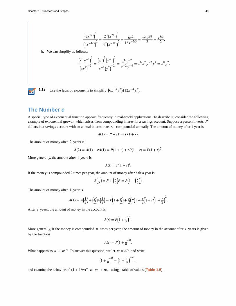
b. We can simplify as follows:
⎛⎝x3 y−1⎞⎠
2
⎛⎝xy2⎞⎠
−2 =⎛⎝x3⎞⎠
2 ⎛⎝y−1⎞⎠
2
x−2 ⎛⎝y2⎞⎠−2 = x6 y−2
x−2 y−4 = x6 x2 y−2 y4 = x8 y2.
Use the laws of exponents to simplify ⎛⎝6x−3 y2⎞⎠/⎛⎝12x−4 y5⎞⎠.
The Number eA special type of exponential function appears frequently in real-world applications. To describe it, consider the followingexample of exponential growth, which arises from compounding interest in a savings account. Suppose a person invests Pdollars in a savings account with an annual interest rate r, compounded annually. The amount of money after 1 year is
A(1) = P + rP = P(1 + r).
The amount of money after 2 years is
A(2) = A(1) + rA(1) = P(1 + r) + rP(1 + r) = P(1 + r)2.
More generally, the amount after t years is
A(t) = P(1 + r)t.
If the money is compounded 2 times per year, the amount of money after half a year is
A⎛⎝12⎞⎠ = P + ⎛⎝r2
⎞⎠P = P⎛⎝1 + ⎛⎝r2
⎞⎠⎞⎠.
The amount of money after 1 year is
A(1) = A⎛⎝12⎞⎠+⎛⎝r2⎞⎠A⎛⎝12⎞⎠ = P⎛⎝1 + r
2⎞⎠+ r
2⎛⎝P⎛⎝1 + r
2⎞⎠⎞⎠ = P⎛⎝1 + r
2⎞⎠2.
After t years, the amount of money in the account is
A(t) = P⎛⎝1 + r2⎞⎠2t
.
More generally, if the money is compounded n times per year, the amount of money in the account after t years is given
by the function
A(t) = P⎛⎝1 + rn⎞⎠nt
.
What happens as n → ∞? To answer this question, we let m = n/r and write
⎛⎝1 + r
n⎞⎠nt
= ⎛⎝1 + 1m⎞⎠mrt
,
and examine the behavior of (1 + 1/m)m as m → ∞, using a table of values (Table 1.5).
Chapter 1 | Functions and Graphs 43

m 10 100 1000 10,000 100,000 1,000,000
⎛⎝1 + 1
m⎞⎠m
2.5937 2.7048 2.71692 2.71815 2.718268 2.718280
Table 1.5 Values of ⎛⎝1 + 1m⎞⎠m
as m → ∞
Looking at this table, it appears that (1 + 1/m)m is approaching a number between 2.7 and 2.8 as m → ∞. In fact,
(1 + 1/m)m does approach some number as m → ∞. We call this number e . To six decimal places of accuracy,
e ≈ 2.718282.
The letter e was first used to represent this number by the Swiss mathematician Leonhard Euler during the 1720s. Although
Euler did not discover the number, he showed many important connections between e and logarithmic functions. We still
use the notation e today to honor Euler’s work because it appears in many areas of mathematics and because we can use it
in many practical applications.
Returning to our savings account example, we can conclude that if a person puts P dollars in an account at an annual
interest rate r, compounded continuously, then A(t) = Pert. This function may be familiar. Since functions involving
base e arise often in applications, we call the function f (x) = ex the natural exponential function. Not only is this
function interesting because of the definition of the number e, but also, as discussed next, its graph has an important
property.
Since e > 1, we know ex is increasing on (−∞, ∞). In Figure 1.16, we show a graph of f (x) = ex along with a
tangent line to the graph of at x = 0. We give a precise definition of tangent line in the next chapter; but, informally, we
say a tangent line to a graph of f at x = a is a line that passes through the point ⎛⎝a, f (a)⎞⎠ and has the same “slope” as
f at that point . The function f (x) = ex is the only exponential function bx with tangent line at x = 0 that has a slope
of 1. As we see later in the text, having this property makes the natural exponential function the most simple exponentialfunction to use in many instances.
Figure 1.16 The graph of f (x) = ex has a tangent line with
slope 1 at x = 0.
Example 1.14
Compounding Interest
Suppose $500 is invested in an account at an annual interest rate of r = 5.5%, compounded continuously.
a. Let t denote the number of years after the initial investment and A(t) denote the amount of money in
the account at time t. Find a formula for A(t).
44 Chapter 1 | Functions and Graphs
This OpenStax book is available for free at https://legacy.cnx.org/content/col31997/1.5
1.13
b. Find the amount of money in the account after 10 years and after 20 years.
Solution
a. If P dollars are invested in an account at an annual interest rate r, compounded continuously, then
A(t) = Pert. Here P = $500 and r = 0.055. Therefore, A(t) = 500e0.055t.
b. After 10 years, the amount of money in the account is
A(10) = 500e0.055 · 10 = 500e0.55 ≈ $866.63.
After 20 years, the amount of money in the account is
A(20) = 500e0.055 · 20 = 500e1.1 ≈ $1, 502.08.
If $750 is invested in an account at an annual interest rate of 4%, compounded continuously, find a
formula for the amount of money in the account after t years. Find the amount of money after 30 years.
Logarithmic FunctionsUsing our understanding of exponential functions, we can discuss their inverses, which are the logarithmic functions. Thesecome in handy when we need to consider any phenomenon that varies over a wide range of values, such as pH in chemistryor decibels in sound levels.
The exponential function f (x) = bx is one-to-one, with domain (−∞, ∞) and range (0, ∞). Therefore, it has an inverse
function, called the logarithmic function with base b. For any b > 0, b ≠ 1, the logarithmic function with base b,
denoted logb, has domain (0, ∞) and range (−∞, ∞), and satisfies
logb (x) = y if and only if by = x.
For example,
log2(8) = 3 since 23 = 8,
log10⎛⎝ 1100⎞⎠ = −2 since 10−2 = 1
102 = 1100,
logb(1) = 0 since b0 = 1 for any base b > 0.
Furthermore, since y = logb(x) and y = bx are inverse functions,
logb (bx) = x and blogb (x)
= x.
The most commonly used logarithmic function is the function loge. Since this function uses natural e as its base, it is
called the natural logarithm. Here we use the notation ln(x) or lnx to mean loge (x). For example,
ln(e) = loge (e) = 1, ln⎛⎝e3⎞⎠ = loge⎛⎝e3⎞⎠ = 3, ln(1) = loge (1) = 0.
Since the functions f (x) = ex and g(x) = ln(x) are inverses of each other,
ln(ex) = x and elnx = x,
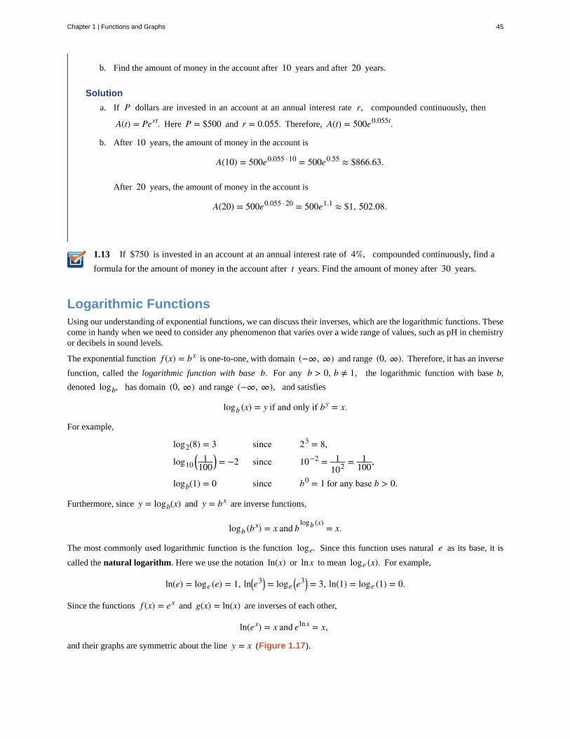
and their graphs are symmetric about the line y = x (Figure 1.17).
Chapter 1 | Functions and Graphs 45
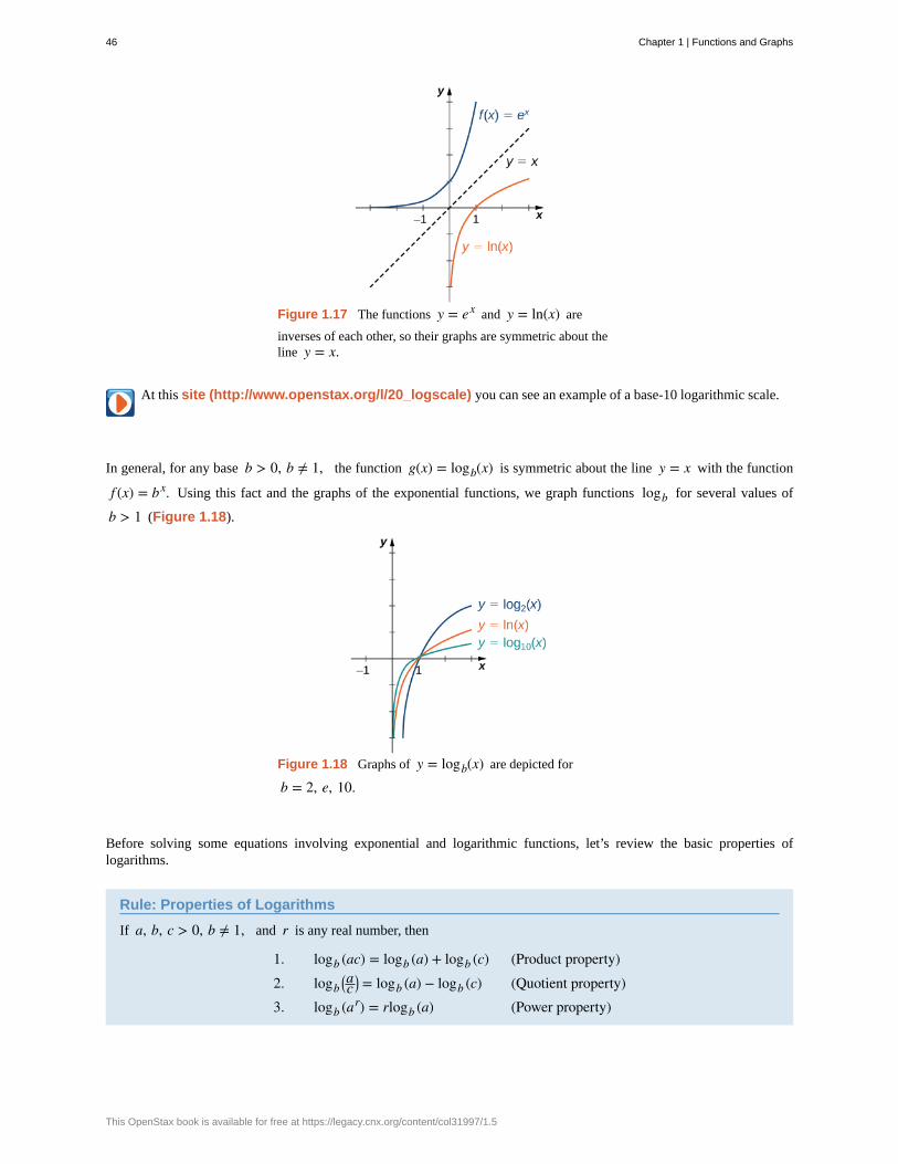
Figure 1.17 The functions y = ex and y = ln(x) are
inverses of each other, so their graphs are symmetric about theline y = x.
At this site (http://www.openstax.org/l/20_logscale) you can see an example of a base-10 logarithmic scale.
In general, for any base b > 0, b ≠ 1, the function g(x) = logb(x) is symmetric about the line y = x with the function
f (x) = bx. Using this fact and the graphs of the exponential functions, we graph functions logb for several values of
b > 1 (Figure 1.18).
Figure 1.18 Graphs of y = logb(x) are depicted for
b = 2, e, 10.
Before solving some equations involving exponential and logarithmic functions, let’s review the basic properties oflogarithms.
Rule: Properties of Logarithms
If a, b, c > 0, b ≠ 1, and r is any real number, then
1. logb (ac) = logb (a) + logb (c) (Product property)2. logb
⎛⎝ac⎞⎠ = logb (a) − logb (c) (Quotient property)
3. logb (ar) = rlogb (a) (Power property)
46 Chapter 1 | Functions and Graphs
This OpenStax book is available for free at https://legacy.cnx.org/content/col31997/1.5

1.14
Example 1.15
Solving Equations Involving Exponential Functions
Solve each of the following equations for x.
a. 5x = 2
b. ex + 6e−x = 5
Solution
a. Applying the natural logarithm function to both sides of the equation, we have
ln5x = ln2.
Using the power property of logarithms,
x ln5 = ln2.
Therefore, x = ln2/ln5.
b. Multiplying both sides of the equation by ex, we arrive at the equation
e2x + 6 = 5ex.
Rewriting this equation as
e2x − 5ex + 6 = 0,
we can then rewrite it as a quadratic equation in ex :
(ex)2 − 5(ex) + 6 = 0.
Now we can solve the quadratic equation. Factoring this equation, we obtain
(ex − 3)(ex − 2) = 0.
Therefore, the solutions satisfy ex = 3 and ex = 2. Taking the natural logarithm of both sides gives us
the solutions x = ln3, ln2.
Solve e2x /(3 + e2x) = 1/2.
Example 1.16
Solving Equations Involving Logarithmic Functions
Solve each of the following equations for x.
a. ln⎛⎝1x⎞⎠ = 4
Chapter 1 | Functions and Graphs 47

1.15
b. log10 x + log10 x = 2
c. ln(2x) − 3ln⎛⎝x2⎞⎠ = 0
Solution
a. By the definition of the natural logarithm function,
ln⎛⎝1x⎞⎠ = 4 if and only if e4 = 1
x .
Therefore, the solution is x = 1/e4.
b. Using the product and power properties of logarithmic functions, rewrite the left-hand side of the equationas
log10 x + log10 x = log10 x x = log10 x3/2 = 3
2log10 x.
Therefore, the equation can be rewritten as
32log10 x = 2 or log10 x = 4
3.
The solution is x = 104/3 = 10 103 .
c. Using the power property of logarithmic functions, we can rewrite the equation as ln(2x) − ln⎛⎝x6⎞⎠ = 0.
Using the quotient property, this becomes
ln⎛⎝ 2x5⎞⎠ = 0.
Therefore, 2/x5 = 1, which implies x = 25 . We should then check for any extraneous solutions.
Solve ln⎛⎝x3⎞⎠− 4ln(x) = 1.
When evaluating a logarithmic function with a calculator, you may have noticed that the only options are log10 or log,
called the common logarithm, or ln, which is the natural logarithm. However, exponential functions and logarithm functionscan be expressed in terms of any desired base b. If you need to use a calculator to evaluate an expression with a different
base, you can apply the change-of-base formulas first. Using this change of base, we typically write a given exponential orlogarithmic function in terms of the natural exponential and natural logarithmic functions.
Rule: Change-of-Base Formulas
Let a > 0, b > 0, and a ≠ 1, b ≠ 1.
1. ax = bxlogba for any real number x.
If b = e, this equation reduces to ax = exloge a = ex lna.
2. loga x = logb xlogba
for any real number x > 0.
48 Chapter 1 | Functions and Graphs
This OpenStax book is available for free at https://legacy.cnx.org/content/col31997/1.5
1.16
If b = e, this equation reduces to loga x = lnxlna.
Proof
For the first change-of-base formula, we begin by making use of the power property of logarithmic functions. We know thatfor any base b > 0, b ≠ 1, logb(a
x) = xlogba. Therefore,
blogb(ax)
= bxlogba.
In addition, we know that bx and logb(x) are inverse functions. Therefore,
blogb(ax)
= ax.
Combining these last two equalities, we conclude that ax = bxlogba.
To prove the second property, we show that
(logba) · (loga x) = logb x.
Let u = logba, v = loga x, and w = logb x. We will show that u · v = w. By the definition of logarithmic functions, we
know that bu = a, av = x, and bw = x. From the previous equations, we see that
buv = (bu)v = av = x = bw.
Therefore, buv = bw. Since exponential functions are one-to-one, we can conclude that u · v = w.
□
Example 1.17
Changing Bases
Use a calculating utility to evaluate log3 7 with the change-of-base formula presented earlier.
Solution
Use the second equation with a = 3 and e = 3:
log3 7 = ln7ln3 ≈ 1.77124.
Use the change-of-base formula and a calculating utility to evaluate log4 6.
Example 1.18
Chapter Opener: The Richter Scale for Earthquakes
Chapter 1 | Functions and Graphs 49
1.17
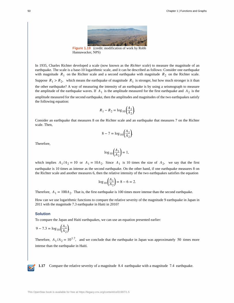
Figure 1.19 (credit: modification of work by RobbHannawacker, NPS)
In 1935, Charles Richter developed a scale (now known as the Richter scale) to measure the magnitude of anearthquake. The scale is a base-10 logarithmic scale, and it can be described as follows: Consider one earthquakewith magnitude R1 on the Richter scale and a second earthquake with magnitude R2 on the Richter scale.
Suppose R1 > R2, which means the earthquake of magnitude R1 is stronger, but how much stronger is it than
the other earthquake? A way of measuring the intensity of an earthquake is by using a seismograph to measurethe amplitude of the earthquake waves. If A1 is the amplitude measured for the first earthquake and A2 is the
amplitude measured for the second earthquake, then the amplitudes and magnitudes of the two earthquakes satisfythe following equation:
R1 − R2 = log10⎛⎝A1A2
⎞⎠.
Consider an earthquake that measures 8 on the Richter scale and an earthquake that measures 7 on the Richterscale. Then,
8 − 7 = log10⎛⎝A1A2
⎞⎠.
Therefore,
log10⎛⎝A1A2
⎞⎠ = 1,
which implies A1 /A2 = 10 or A1 = 10A2. Since A1 is 10 times the size of A2, we say that the first
earthquake is 10 times as intense as the second earthquake. On the other hand, if one earthquake measures 8 onthe Richter scale and another measures 6, then the relative intensity of the two earthquakes satisfies the equation
log10⎛⎝A1A2
⎞⎠ = 8 − 6 = 2.
Therefore, A1 = 100A2. That is, the first earthquake is 100 times more intense than the second earthquake.
How can we use logarithmic functions to compare the relative severity of the magnitude 9 earthquake in Japan in2011 with the magnitude 7.3 earthquake in Haiti in 2010?
Solution
To compare the Japan and Haiti earthquakes, we can use an equation presented earlier:
9 − 7.3 = log10⎛⎝A1A2
⎞⎠.
Therefore, A1 /A2 = 101.7, and we conclude that the earthquake in Japan was approximately 50 times more
intense than the earthquake in Haiti.
Compare the relative severity of a magnitude 8.4 earthquake with a magnitude 7.4 earthquake.
50 Chapter 1 | Functions and Graphs
This OpenStax book is available for free at https://legacy.cnx.org/content/col31997/1.5
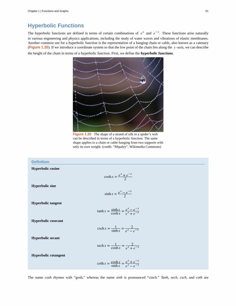
Hyperbolic FunctionsThe hyperbolic functions are defined in terms of certain combinations of ex and e−x. These functions arise naturally
in various engineering and physics applications, including the study of water waves and vibrations of elastic membranes.Another common use for a hyperbolic function is the representation of a hanging chain or cable, also known as a catenary(Figure 1.20). If we introduce a coordinate system so that the low point of the chain lies along the y -axis, we can describe
the height of the chain in terms of a hyperbolic function. First, we define the hyperbolic functions.
Figure 1.20 The shape of a strand of silk in a spider’s webcan be described in terms of a hyperbolic function. The sameshape applies to a chain or cable hanging from two supports withonly its own weight. (credit: “Mtpaley”, Wikimedia Commons)
Definition
Hyperbolic cosine
coshx = ex + e−x
2
Hyperbolic sine
sinhx = ex − e−x
2
Hyperbolic tangent
tanhx = sinhxcoshx = ex − e−x
ex + e−x
Hyperbolic cosecant
csch x = 1sinhx = 2
ex − e−x
Hyperbolic secant
sech x = 1coshx = 2
ex + e−x
Hyperbolic cotangent
cothx = coshxsinhx = ex + e−x
ex − e−x
The name cosh rhymes with “gosh,” whereas the name sinh is pronounced “cinch.” Tanh, sech, csch, and coth are
Chapter 1 | Functions and Graphs 51
pronounced “tanch,” “seech,” “coseech,” and “cotanch,” respectively.
Using the definition of cosh(x) and principles of physics, it can be shown that the height of a hanging chain, such as the
one in Figure 1.20, can be described by the function h(x) = acosh(x/a) + c for certain constants a and c.
But why are these functions called hyperbolic functions? To answer this question, consider the quantity cosh2 t − sinh2 t.Using the definition of cosh and sinh, we see that
cosh2 t − sinh2 t = e2t + 2 + e−2t
4 − e2t − 2 + e−2t
4 = 1.
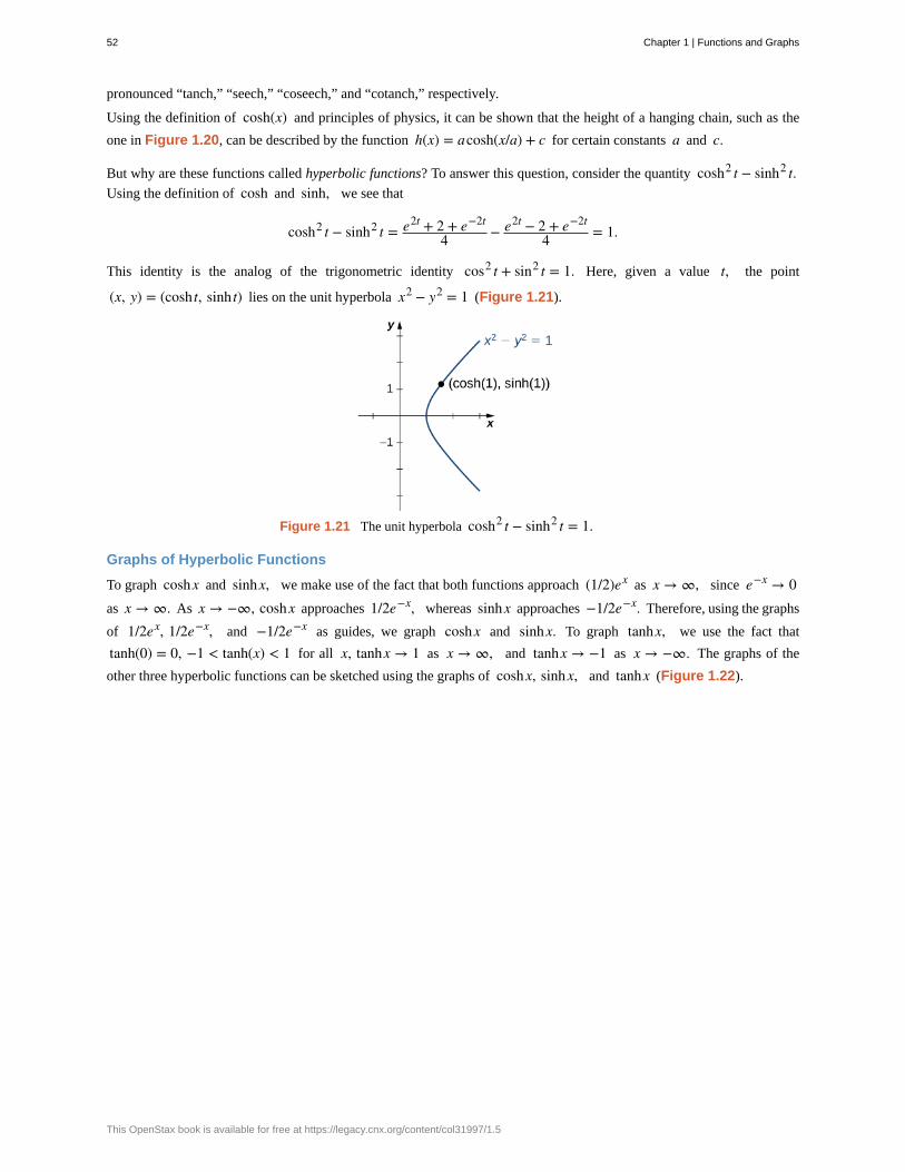
This identity is the analog of the trigonometric identity cos2 t + sin2 t = 1. Here, given a value t, the point
(x, y) = (cosh t, sinh t) lies on the unit hyperbola x2 − y2 = 1 (Figure 1.21).
Figure 1.21 The unit hyperbola cosh2 t − sinh2 t = 1.
Graphs of Hyperbolic Functions
To graph coshx and sinhx, we make use of the fact that both functions approach (1/2)ex as x → ∞, since e−x → 0as x → ∞. As x → −∞, coshx approaches 1/2e−x, whereas sinhx approaches −1/2e−x. Therefore, using the graphs
of 1/2ex, 1/2e−x, and −1/2e−x as guides, we graph coshx and sinhx. To graph tanhx, we use the fact that
tanh(0) = 0, −1 < tanh(x) < 1 for all x, tanhx → 1 as x → ∞, and tanhx → −1 as x → −∞. The graphs of the
other three hyperbolic functions can be sketched using the graphs of coshx, sinhx, and tanhx (Figure 1.22).
52 Chapter 1 | Functions and Graphs
This OpenStax book is available for free at https://legacy.cnx.org/content/col31997/1.5
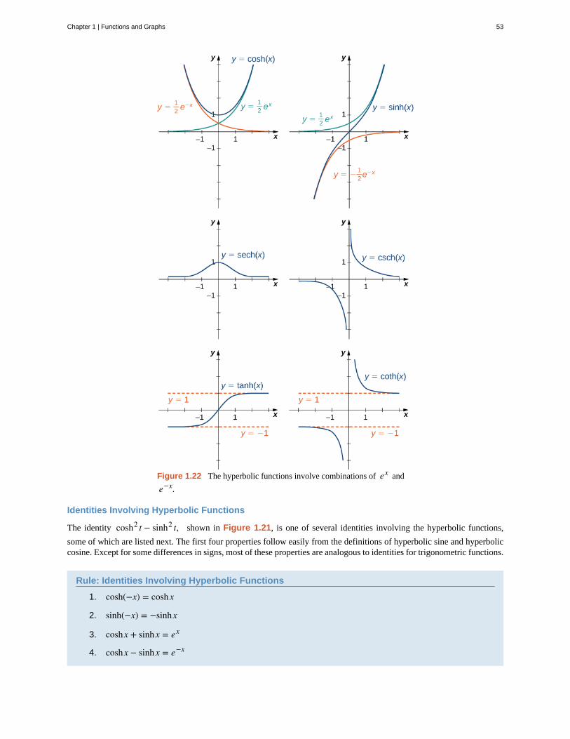
Figure 1.22 The hyperbolic functions involve combinations of ex and
e−x.
Identities Involving Hyperbolic Functions
The identity cosh2 t − sinh2 t, shown in Figure 1.21, is one of several identities involving the hyperbolic functions,
some of which are listed next. The first four properties follow easily from the definitions of hyperbolic sine and hyperboliccosine. Except for some differences in signs, most of these properties are analogous to identities for trigonometric functions.
Rule: Identities Involving Hyperbolic Functions
1. cosh(−x) = coshx
2. sinh(−x) = −sinhx
3. coshx + sinhx = ex
4. coshx − sinhx = e−x
Chapter 1 | Functions and Graphs 53
1.18
5. cosh2 x − sinh2 x = 1
6. 1 − tanh2 x = sech2 x
7. coth2 x − 1 = csch2 x
8. sinh(x ± y) = sinhxcoshy ± coshxsinhy
9. cosh(x ± y) = coshxcoshy ± sinhxsinhy
Example 1.19
Evaluating Hyperbolic Functions
a. Simplify sinh(5lnx).
b. If sinhx = 3/4, find the values of the remaining five hyperbolic functions.
Solution
a. Using the definition of the sinh function, we write
sinh(5lnx) = e5lnx − e−5lnx
2 = eln⎛⎝x5⎞⎠− e
ln⎛⎝x−5⎞⎠2 = x5 − x−5
2 .
b. Using the identity cosh2 x − sinh2 x = 1, we see that
cosh2 x = 1 + ⎛⎝34⎞⎠2
= 2516.
Since coshx ≥ 1 for all x, we must have coshx = 5/4. Then, using the definitions for the other
hyperbolic functions, we conclude that tanhx = 3/5, csch x = 4/3, sech x = 4/5, and cothx = 5/3.
Simplify cosh(2lnx).
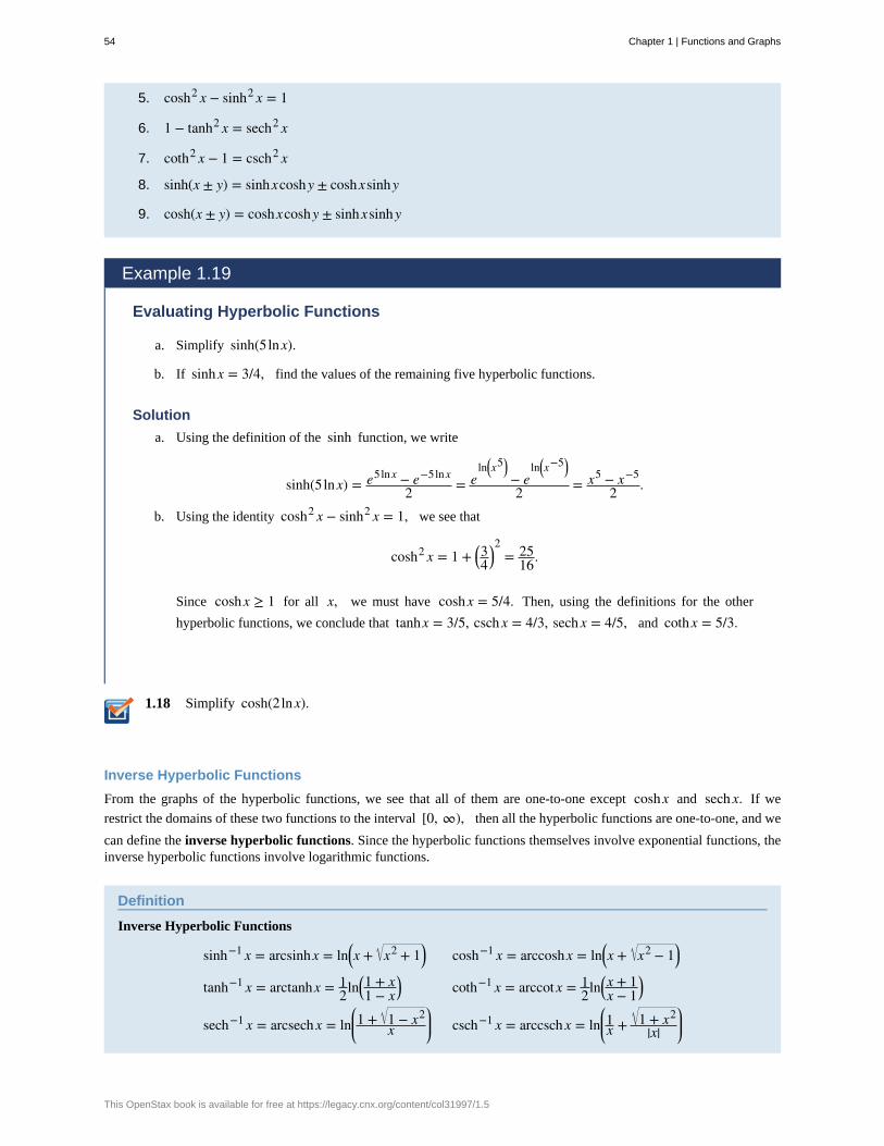
Inverse Hyperbolic Functions
From the graphs of the hyperbolic functions, we see that all of them are one-to-one except coshx and sech x. If we
restrict the domains of these two functions to the interval [0, ∞), then all the hyperbolic functions are one-to-one, and we
can define the inverse hyperbolic functions. Since the hyperbolic functions themselves involve exponential functions, theinverse hyperbolic functions involve logarithmic functions.
Definition
Inverse Hyperbolic Functions
sinh−1 x = arcsinhx = ln⎛⎝x + x2 + 1⎞⎠ cosh−1 x = arccoshx = ln⎛⎝x + x2 − 1⎞⎠tanh−1 x = arctanhx = 1
2ln⎛⎝1 + x1 − x⎞⎠ coth−1 x = arccotx = 1
2ln⎛⎝x + 1x − 1⎞⎠
sech−1 x = arcsech x = ln⎛⎝⎜1 + 1 − x2
x⎞⎠⎟ csch−1 x = arccsch x = ln
⎛⎝⎜1x + 1 + x2
|x|⎞⎠⎟
54 Chapter 1 | Functions and Graphs
This OpenStax book is available for free at https://legacy.cnx.org/content/col31997/1.5
1.19
Let’s look at how to derive the first equation. The others follow similarly. Suppose y = sinh−1 x. Then, x = sinhy and,
by the definition of the hyperbolic sine function, x = ey − e−y
2 . Therefore,
ey − 2x − e−y = 0.
Multiplying this equation by ey, we obtain
e2y − 2xey − 1 = 0.
This can be solved like a quadratic equation, with the solution
ey = 2x ± 4x2 + 42 = x ± x2 + 1.
Since ey > 0, the only solution is the one with the positive sign. Applying the natural logarithm to both sides of the
equation, we conclude that
y = ln⎛⎝x + x2 + 1⎞⎠.
Example 1.20
Evaluating Inverse Hyperbolic Functions
Evaluate each of the following expressions.
sinh−1 (2)
tanh−1(1/4)
Solution
sinh−1 (2) = ln⎛⎝2 + 22 + 1⎞⎠ = ln⎛⎝2 + 5⎞⎠ ≈ 1.4436
tanh−1(1/4) = 12ln⎛⎝1 + 1/4
1 − 1/4⎞⎠ = 1
2ln⎛⎝5/43/4⎞⎠ = 1
2ln⎛⎝53⎞⎠ ≈ 0.2554
Evaluate tanh−1(1/2).
Key Concepts• The exponential function y = bx is increasing if b > 1 and decreasing if 0 < b < 1. Its domain is (−∞, ∞)
and its range is (0, ∞).
• The logarithmic function y = logb(x) is the inverse of y = bx. Its domain is (0, ∞) and its range is (−∞, ∞).
• The natural exponential function is y = ex and the natural logarithmic function is y = lnx = loge x.
• Given an exponential function or logarithmic function in base a, we can make a change of base to convert this
function to any base b > 0, b ≠ 1. We typically convert to base e.
• The hyperbolic functions involve combinations of the exponential functions ex and e−x. As a result, the inverse
hyperbolic functions involve the natural logarithm.
Chapter 1 | Functions and Graphs 55

1.3 EXERCISESFor the following exercises, evaluate the given exponentialfunctions as indicated, accurate to two significant digitsafter the decimal.
117. f (x) = 5x a. x = 3 b. x = 12 c. x = 2
118. f (x) = (0.3)x a. x = −1 b. x = 4 c. x = −1.5
119. f (x) = 10x a. x = −2 b. x = 4 c. x = 53
120. f (x) = ex a. x = 2 b. x = −3.2 c. x = π
For the following exercises, match the exponential equationto the correct graph.
a. y = 4−x
b. y = 3x − 1
c. y = 2x + 1
d. y = ⎛⎝12⎞⎠x
+ 2
e. y = −3−x
f. y = 1 − 5x
121.
122.
123.
56 Chapter 1 | Functions and Graphs
This OpenStax book is available for free at https://legacy.cnx.org/content/col31997/1.5

124.
125.
126.
For the following exercises, sketch the graph of theexponential function. Determine the domain, range, andhorizontal asymptote.
127. f (x) = ex + 2
128. f (x) = −2x
129. f (x) = 3x + 1
130. f (x) = 4x − 1
131. f (x) = 1 − 2−x
132. f (x) = 5x + 1 + 2
133. f (x) = e−x − 1
For the following exercises, write the equation inequivalent exponential form.
134. log3 81 = 4
135. log8 2 = 13
136. log5 1 = 0
137. log5 25 = 2
138. log0.1 = −1
139. ln⎛⎝ 1e3⎞⎠ = −3
140. log9 3 = 0.5
141. ln1 = 0
For the following exercises, write the equation inequivalent logarithmic form.
142. 23 = 8
143. 4−2 = 116
144. 102 = 100
145. 90 = 1
146. ⎛⎝13⎞⎠
3= 1
27
Chapter 1 | Functions and Graphs 57
147. 643 = 4
148. ex = y
149. 9y = 150
150. b3 = 45
151. 4−3/2 = 0.125
For the following exercises, sketch the graph of thelogarithmic function. Determine the domain, range, andvertical asymptote.
152. f (x) = 3 + lnx
153. f (x) = ln(x − 1)
154. f (x) = ln(−x)
155. f (x) = 1 − lnx
156. f (x) = logx − 1
157. f (x) = ln(x + 1)
For the following exercises, use properties of logarithms towrite the expressions as a sum, difference, and/or productof logarithms.
158. logx4 y
159. log39a3
b
160. lna b3
161. log5 125xy3
162. log4xy3
64
163. ln⎛⎝⎜ 6e3
⎞⎠⎟
For the following exercises, solve the exponential equationexactly.
164. 5x = 125
165. e3x − 15 = 0
166. 8x = 4
167. 4x + 1 − 32 = 0
168. 3x/14 = 110
169. 10x = 7.21
170. 4 · 23x − 20 = 0
171. 73x − 2 = 11
For the following exercises, solve the logarithmic equationexactly, if possible.
172. log3 x = 0
173. log5 x = −2
174. log4 (x + 5) = 0
175. log(2x − 7) = 0
176. ln x + 3 = 2
177. log6 (x + 9) + log6 x = 2
178. log4 (x + 2) − log4 (x − 1) = 0
179. lnx + ln(x − 2) = ln4
For the following exercises, use the change-of-baseformula and either base 10 or base e to evaluate the givenexpressions. Answer in exact form and in approximateform, rounding to four decimal places.
180. log5 47
181. log7 82
182. log6 103
183. log0.5 211
184. log2π
185. log0.2 0.452
186. Rewrite the following expressions in terms ofexponentials and simplify. a. 2cosh(lnx) b.
cosh4x + sinh4x c. cosh2x − sinh2x d.
ln(coshx + sinhx) + ln(coshx − sinhx)
58 Chapter 1 | Functions and Graphs
This OpenStax book is available for free at https://legacy.cnx.org/content/col31997/1.5
187. [T] The number of bacteria N in a culture after t days
can be modeled by the function N(t) = 1300 · (2)t/4. Find
the number of bacteria present after 15 days.
188. [T] The demand D (in millions of barrels) for oilin an oil-rich country is given by the function
D(p) = 150 · (2.7)−0.25p, where p is the price (in dollars)
of a barrel of oil. Find the amount of oil demanded (to thenearest million barrels) when the price is between $15 and$20.
189. [T] The amount A of a $100,000 investment payingcontinuously and compounded for t years is given by
A(t) = 100,000 · e0.055t. Find the amount A accumulated
in 5 years.
190. [T] An investment is compounded monthly,quarterly, or yearly and is given by the function
A = P⎛⎝1 + jn⎞⎠nt
, where A is the value of the investment
at time t, P is the initial principle that was invested, jis the annual interest rate, and n is the number of time
the interest is compounded per year. Given a yearly interestrate of 3.5% and an initial principle of $100,000, find theamount A accumulated in 5 years for interest that is
compounded a. daily, b., monthly, c. quarterly, and d.yearly.
191. [T] The concentration of hydrogen ions in a
substance is denoted by ⎡⎣H+ ⎤⎦, measured in moles per
liter. The pH of a substance is defined by the logarithmic
function pH = −log⎡⎣H+ ⎤⎦. This function is used to
measure the acidity of a substance. The pH of water is 7. Asubstance with a pH less than 7 is an acid, whereas one thathas a pH of more than 7 is a base.
a. Find the pH of the following substances. Roundanswers to one digit.
b. Determine whether the substance is an acid or abase.
i. Eggs: ⎡⎣H+ ⎤⎦ = 1.6 × 10⁻⁸ mol/L
ii. Beer: ⎡⎣H+ ⎤⎦ = 3.16 × 10⁻³ mol/L
iii. Tomato Juice: ⎡⎣H+ ⎤⎦ = 7.94 × 10⁻⁵ mol/L
192. [T] Iodine-131 is a radioactive substance that decays
according to the function Q(t) = Q0 · e−0.08664t, where
Q0 is the initial quantity of a sample of the substance and t
is in days. Determine how long it takes (to the nearest day)for 95% of a quantity to decay.
193. [T] According to the World Bank, at the end of2013 ( t = 0 ) the U.S. population was 316 million and
was increasing according to the following model:
P(t) = 316e0.0074t, where P is measured in millions of
people and t is measured in years after 2013.a. Based on this model, what will be the population of
the United States in 2020?b. Determine when the U.S. population will be twice
what it is in 2013.
194. [T] The amount A accumulated after 1000 dollars isinvested for t years at an interest rate of 4% is modeled bythe function A(t) = 1000(1.04)t.
a. Find the amount accumulated after 5 years and 10years.
b. Determine how long it takes for the originalinvestment to triple.
195. [T] A bacterial colony grown in a lab is known todouble in number in 12 hours. Suppose, initially, there are1000 bacteria present.
a. Use the exponential function Q = Q0 ekt to
determine the value k, which is the growth rate of
the bacteria. Round to four decimal places.b. Determine approximately how long it takes for
200,000 bacteria to grow.
196. [T] The rabbit population on a game reserve doublesevery 6 months. Suppose there were 120 rabbits initially.
a. Use the exponential function P = P0at to
determine the growth rate constant a. Round to
four decimal places.b. Use the function in part a. to determine
approximately how long it takes for the rabbitpopulation to reach 3500.
197. [T] The 1906 earthquake in San Francisco had amagnitude of 8.3 on the Richter scale. At the same time,in Japan, an earthquake with magnitude 4.9 caused onlyminor damage. Approximately how much more energy wasreleased by the San Francisco earthquake than by theJapanese earthquake?
Chapter 1 | Functions and Graphs 59
Chapter Review ExercisesTrue or False? Justify your answer with a proof or a counterexample.
Exercise 1.198
A function is always one-to-one.
Exercise 1.199
f ∘g = g ∘ f , assuming f and g are functions.
SolutionFalse
Exercise 1.200
A relation that passes the horizontal and vertical line tests is a one-to-one function.
Exercise 1.201
A relation passing the horizontal line test is a function.
SolutionFalse
For the following problems, state the domain and range of the given functions:
f = x2 + 2x − 3, g = ln(x − 5), h = 1x + 4
Exercise 1.202
h
Exercise 1.203
g
SolutionDomain: x > 5, range: all real numbers
Exercise 1.204
h ∘ f
Exercise 1.205
g ∘ f
SolutionDomain: x > 2 and x < − 4, range: all real numbers
Find the degree, y-intercept, and zeros for the following polynomial functions.
Exercise 1.206
f (x) = 2x2 + 9x − 5
Exercise 1.207
f (x) = x3 + 2x2 − 2x
Solution
60 Chapter 1 | Functions and Graphs
This OpenStax book is available for free at https://legacy.cnx.org/content/col31997/1.5
Degree of 3, y -intercept: 0, zeros: 0, 3 − 1, −1 − 3
Simplify the following trigonometric expressions.
Exercise 1.208
tan2 xsec2 x
+ cos2 x
Exercise 1.209
cos2 x - sin2 x
Solution
cos2 x – sin2 x = cos2x or = 1 – 2sin2 x2 or = 2cos2 x – 1
2
Solve the following trigonometric equations on the interval θ = [−2π, 2π] exactly.
Exercise 1.210
6cos2 x − 3 = 0
Exercise 1.211
sec2 x − 2secx + 1 = 0
Solution0, ± 2π
Solve the following logarithmic equations.
Exercise 1.212
5x = 16
Exercise 1.213
log2(x + 4) = 3
Solution4
Are the following functions one-to-one over their domain of existence? Does the function have an inverse? If so, find the
inverse f −1(x) of the function. Justify your answer.
Exercise 1.214
f (x) = x2 + 2x + 1
Exercise 1.215
f (x) = 1x
Solution
One-to-one; yes, the function has an inverse; inverse: f −1(x) = 1y
For the following problems, determine the largest domain on which the function is one-to-one and find the inverse on thatdomain.
Chapter 1 | Functions and Graphs 61
Exercise 1.216
f (x) = 9 − x
Exercise 1.217
f (x) = x2 + 3x + 4
Solution
x ≥ − 32, f −1(x) = − 3
2 + 12 4y − 7
Exercise 1.218
A car is racing along a circular track with diameter of 1 mi. A trainer standing in the center of the circle marks his progressevery 5 sec. After 5 sec, the trainer has to turn 55° to keep up with the car. How fast is the car traveling?
For the following problems, consider a restaurant owner who wants to sell T-shirts advertising his brand. He recalls thatthere is a fixed cost and variable cost, although he does not remember the values. He does know that the T-shirt printingcompany charges $440 for 20 shirts and $1000 for 100 shirts.
Exercise 1.219
a. Find the equation C = f (x) that describes the total cost as a function of number of shirts and b. determine how many
shirts he must sell to break even if he sells the shirts for $10 each.
Solutiona. C(x) = 300 + 7x b. 100 shirts
Exercise 1.220
a. Find the inverse function x = f −1(C) and describe the meaning of this function. b. Determine how many shirts the
owner can buy if he has $8000 to spend.
For the following problems, consider the population of Ocean City, New Jersey, which is cyclical by season.
Exercise 1.221
The population can be modeled by P(t) = 82.5 − 67.5cos⎡⎣(π/6)t⎤⎦, where t is time in months (t = 0 represents January
1) and P is population (in thousands). During a year, in what intervals is the population less than 20,000? During what
intervals is the population more than 140,000?
SolutionThe population is less than 20,000 from December 8 through January 23 and more than 140,000 from May 29 throughAugust 2
Exercise 1.222
In reality, the overall population is most likely increasing or decreasing throughout each year. Let’s reformulate the modelas P(t) = 82.5 − 67.5cos⎡⎣(π/6)t⎤⎦+ t, where t is time in months ( t = 0 represents January 1) and P is population (in
thousands). When is the first time the population reaches 200,000?
For the following problems, consider radioactive dating. A human skeleton is found in an archeological dig. Carbondating is implemented to determine how old the skeleton is by using the equation y = ert, where y is the percentage
of radiocarbon still present in the material, t is the number of years passed, and r = −0.0001210 is the decay rate of
radiocarbon.
Exercise 1.223
If the skeleton is expected to be 2000 years old, what percentage of radiocarbon should be present?
Solution
62 Chapter 1 | Functions and Graphs
This OpenStax book is available for free at https://legacy.cnx.org/content/col31997/1.5
78.51%
Exercise 1.224
Find the inverse of the carbon-dating equation. What does it mean? If there is 25% radiocarbon, how old is the skeleton?
Chapter 1 | Functions and Graphs 63

base
exponent
horizontal line test
hyperbolic functions
inverse function
inverse hyperbolic functions
inverse trigonometric functions
natural exponential function
natural logarithm
number e
one-to-one function
periodic function
radians
restricted domain
trigonometric functions
trigonometric identity
CHAPTER 1 REVIEW
KEY TERMSthe number b in the exponential function f (x) = bx and the logarithmic function f (x) = logb x
the value x in the expression bx
a function f is one-to-one if and only if every horizontal line intersects the graph of f , at most,
once
the functions denoted sinh, cosh, tanh, csch, sech, and coth, which involve certain
combinations of ex and e−x
for a function f , the inverse function f −1 satisfies f −1 (y) = x if f (x) = y
the inverses of the hyperbolic functions where cosh and sech are restricted to the
domain [0, ∞); each of these functions can be expressed in terms of a composition of the natural logarithm function
and an algebraic function
the inverses of the trigonometric functions are defined on restricted domains wherethey are one-to-one functions
the function f (x) = ex
the function lnx = loge x
as m gets larger, the quantity (1 + (1/m)m gets closer to some real number; we define that real number to be
e; the value of e is approximately 2.718282
a function f is one-to-one if f (x1) ≠ f (x2) if x1 ≠ x2
a function is periodic if it has a repeating pattern as the values of x move from left to right
for a circular arc of length s on a circle of radius 1, the radian measure of the associated angle θ is s
a subset of the domain of a function f
functions of an angle defined as ratios of the lengths of the sides of a right triangle
an equation involving trigonometric functions that is true for all angles θ for which the
functions in the equation are defined
64 Chapter 1 | Functions and Graphs
This OpenStax book is available for free at https://legacy.cnx.org/content/col31997/1.5
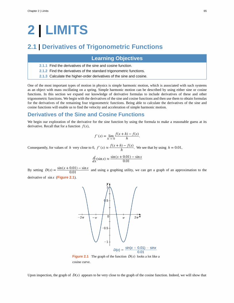
2 | LIMITS2.1 | Derivatives of Trigonometric Functions
Learning Objectives2.1.1 Find the derivatives of the sine and cosine function.
2.1.2 Find the derivatives of the standard trigonometric functions.
2.1.3 Calculate the higher-order derivatives of the sine and cosine.
One of the most important types of motion in physics is simple harmonic motion, which is associated with such systemsas an object with mass oscillating on a spring. Simple harmonic motion can be described by using either sine or cosinefunctions. In this section we expand our knowledge of derivative formulas to include derivatives of these and othertrigonometric functions. We begin with the derivatives of the sine and cosine functions and then use them to obtain formulasfor the derivatives of the remaining four trigonometric functions. Being able to calculate the derivatives of the sine andcosine functions will enable us to find the velocity and acceleration of simple harmonic motion.
Derivatives of the Sine and Cosine FunctionsWe begin our exploration of the derivative for the sine function by using the formula to make a reasonable guess at itsderivative. Recall that for a function f (x),
f ′ (x) = limh → 0
f (x + h) − f (x)h .
Consequently, for values of h very close to 0, f ′ (x) ≈ f (x + h) − f (x)h . We see that by using h = 0.01,
ddx(sinx) ≈ sin(x + 0.01) − sinx
0.01
By setting D(x) = sin(x + 0.01) − sinx0.01 and using a graphing utility, we can get a graph of an approximation to the
derivative of sinx (Figure 2.1).
Figure 2.1 The graph of the function D(x) looks a lot like a
cosine curve.
Upon inspection, the graph of D(x) appears to be very close to the graph of the cosine function. Indeed, we will show that
Chapter 2 | Limits 65
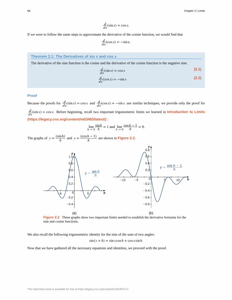
ddx(sinx) = cosx.
If we were to follow the same steps to approximate the derivative of the cosine function, we would find that
ddx(cosx) = −sinx.
Theorem 2.1: The Derivatives of sin x and cos x
The derivative of the sine function is the cosine and the derivative of the cosine function is the negative sine.
(2.1)ddx(sinx) = cosx
(2.2)ddx(cosx) = −sinx
Proof
Because the proofs for ddx(sinx) = cosx and d
dx(cosx) = −sinx use similar techniques, we provide only the proof for
ddx(sinx) = cosx. Before beginning, recall two important trigonometric limits we learned in Introduction to Limits
(https://legacy.cnx.org/content/m53483/latest/) :
limh → 0
sinhh = 1 and lim
h → 0cosh − 1
h = 0.
The graphs of y = (sinh)h and y = (cosh − 1)
h are shown in Figure 2.2.
Figure 2.2 These graphs show two important limits needed to establish the derivative formulas for thesine and cosine functions.
We also recall the following trigonometric identity for the sine of the sum of two angles:
sin(x + h) = sinxcosh + cosxsinh.
Now that we have gathered all the necessary equations and identities, we proceed with the proof.
66 Chapter 2 | Limits
This OpenStax book is available for free at https://legacy.cnx.org/content/col31997/1.5
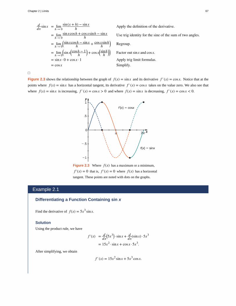
ddx sinx = lim
h → 0sin(x + h) − sinx
h Apply the definition of the derivative.
= limh → 0
sinxcosh + cosxsinh − sinxh Use trig identity for the sine of the sum of two angles.
= limh → 0⎛⎝sinxcosh − sinx
h + cosxsinhh
⎞⎠ Regroup.
= limh → 0⎛⎝sinx⎛⎝cosh − 1
h⎞⎠+ cosx⎛⎝sinh
h⎞⎠⎞⎠ Factor out sinx and cosx.
= sinx · 0 + cosx · 1 Apply trig limit formulas.= cosx Simplify.
□
Figure 2.3 shows the relationship between the graph of f (x) = sinx and its derivative f ′ (x) = cosx. Notice that at the
points where f (x) = sinx has a horizontal tangent, its derivative f ′ (x) = cosx takes on the value zero. We also see that
where f (x) = sinx is increasing, f ′ (x) = cosx > 0 and where f (x) = sinx is decreasing, f ′ (x) = cosx < 0.
Figure 2.3 Where f (x) has a maximum or a minimum,
f ′(x) = 0 that is, f ′(x) = 0 where f (x) has a horizontal
tangent. These points are noted with dots on the graphs.
Example 2.1
Differentiating a Function Containing sin x
Find the derivative of f (x) = 5x3 sinx.
Solution
Using the product rule, we have
f ′(x) = ddx⎛⎝5x3⎞⎠ · sinx + d
dx(sinx) · 5x3
= 15x2 · sinx + cosx · 5x3.
After simplifying, we obtain
f ′ (x) = 15x2 sinx + 5x3 cosx.
Chapter 2 | Limits 67

2.1
2.2
2.3
Find the derivative of f (x) = sinxcosx.
Example 2.2
Finding the Derivative of a Function Containing cos x
Find the derivative of g(x) = cosx4x2 .
Solution
By applying the quotient rule, we have
g′ (x) = (−sinx)4x2 − 8x(cosx)⎛⎝4x2⎞⎠
2 .
Simplifying, we obtain
g′ (x) = −4x2 sinx − 8xcosx16x4
= −xsinx − 2cosx4x3 .
Find the derivative of f (x) = xcosx.
Example 2.3
An Application to Velocity
A particle moves along a coordinate axis in such a way that its position at time t is given by s(t) = 2sin t − tfor 0 ≤ t ≤ 2π. At what times is the particle at rest?
Solution
To determine when the particle is at rest, set s′ (t) = v(t) = 0. Begin by finding s′ (t). We obtain
s′ (t) = 2cos t − 1,
so we must solve
2cos t − 1 = 0 for 0 ≤ t ≤ 2π.
The solutions to this equation are t = π3 and t = 5π
3 . Thus the particle is at rest at times t = π3 and t = 5π
3 .
A particle moves along a coordinate axis. Its position at time t is given by s(t) = 3t + 2cos t for
0 ≤ t ≤ 2π. At what times is the particle at rest?
68 Chapter 2 | Limits
This OpenStax book is available for free at https://legacy.cnx.org/content/col31997/1.5
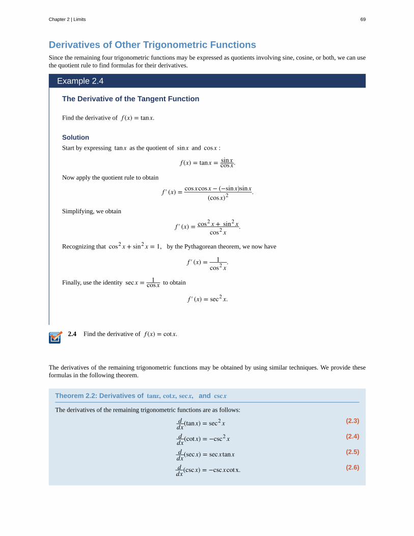
2.4
Derivatives of Other Trigonometric FunctionsSince the remaining four trigonometric functions may be expressed as quotients involving sine, cosine, or both, we can usethe quotient rule to find formulas for their derivatives.
Example 2.4
The Derivative of the Tangent Function
Find the derivative of f (x) = tanx.
Solution
Start by expressing tanx as the quotient of sinx and cosx :
f (x) = tanx = sinxcosx.
Now apply the quotient rule to obtain
f ′ (x) = cosxcosx − (−sinx)sinx(cosx)2 .
Simplifying, we obtain
f ′ (x) = cos2 x + sin2 xcos2 x
.
Recognizing that cos2 x + sin2 x = 1, by the Pythagorean theorem, we now have
f ′ (x) = 1cos2 x
.
Finally, use the identity secx = 1cosx to obtain
f ′ (x) = sec2 x.
Find the derivative of f (x) = cotx.
The derivatives of the remaining trigonometric functions may be obtained by using similar techniques. We provide theseformulas in the following theorem.
Theorem 2.2: Derivatives of tanx, cotx, secx, and cscx
The derivatives of the remaining trigonometric functions are as follows:
(2.3)ddx(tanx) = sec2 x
(2.4)ddx(cotx) = −csc2 x
(2.5)ddx(secx) = secx tanx
(2.6)ddx(cscx) = −cscxcotx.
Chapter 2 | Limits 69

2.5
Example 2.5
Finding the Equation of a Tangent Line
Find the equation of a line tangent to the graph of f (x) = cotx at x = π4.
Solution
To find the equation of the tangent line, we need a point and a slope at that point. To find the point, compute
f ⎛⎝π4⎞⎠ = cot π4 = 1.
Thus the tangent line passes through the point ⎛⎝π4, 1⎞⎠. Next, find the slope by finding the derivative of
f (x) = cotx and evaluating it at π4:
f ′ (x) = −csc2 x and f ′ ⎛⎝π4⎞⎠ = −csc2 ⎛⎝π4
⎞⎠ = −2.
Using the point-slope equation of the line, we obtain
y − 1 = −2⎛⎝x − π4⎞⎠
or equivalently,
y = −2x + 1 + π2.
Example 2.6
Finding the Derivative of Trigonometric Functions
Find the derivative of f (x) = cscx + x tanx.
Solution
To find this derivative, we must use both the sum rule and the product rule. Using the sum rule, we find
f ′ (x) = ddx(cscx) + d
dx(x tanx).
In the first term, ddx(cscx) = −cscxcotx, and by applying the product rule to the second term we obtain
ddx(x tanx) = (1)(tanx) + (sec2 x)(x).
Therefore, we have
f ′ (x) = −cscxcotx + tanx + xsec2 x.
Find the derivative of f (x) = 2tanx − 3cotx.
70 Chapter 2 | Limits
This OpenStax book is available for free at https://legacy.cnx.org/content/col31997/1.5
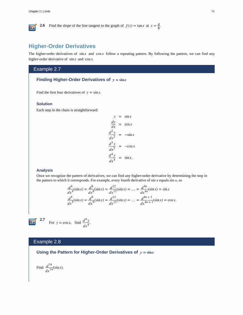
2.6
2.7
Find the slope of the line tangent to the graph of f (x) = tanx at x = π6.
Higher-Order DerivativesThe higher-order derivatives of sinx and cosx follow a repeating pattern. By following the pattern, we can find any
higher-order derivative of sinx and cosx.
Example 2.7
Finding Higher-Order Derivatives of y = sinx
Find the first four derivatives of y = sinx.
Solution
Each step in the chain is straightforward:
y = sinxdydx = cosx
d2 ydx2 = −sinx
d3 ydx3 = −cosx
d4 ydx4 = sinx.
AnalysisOnce we recognize the pattern of derivatives, we can find any higher-order derivative by determining the step inthe pattern to which it corresponds. For example, every fourth derivative of sin x equals sin x, so
d4
dx4(sinx) = d8
dx8(sinx) = d12
dx12(sinx) = … = d4n
dx4n(sinx) = sinx
d5
dx5(sinx) = d9
dx9(sinx) = d13
dx13(sinx) = … = d4n + 1
dx4n + 1(sinx) = cosx.
For y = cosx, findd4 ydx4 .
Example 2.8
Using the Pattern for Higher-Order Derivatives of y = sinx
Find d74
dx74(sinx).
Chapter 2 | Limits 71
2.8
2.9
Solution
We can see right away that for the 74th derivative of sinx, 74 = 4(18) + 2, so
d74
dx74(sinx) = d72 + 2
dx72 + 2(sinx) = d2
dx2(sinx) = −sinx.
For y = sinx, find d59
dx59(sinx).
Example 2.9
An Application to Acceleration
A particle moves along a coordinate axis in such a way that its position at time t is given by s(t) = 2 − sin t.Find v(π/4) and a(π/4). Compare these values and decide whether the particle is speeding up or slowing down.
Solution
First find v(t) = s′ (t):
v(t) = s′ (t) = −cos t.
Thus,
v⎛⎝π4⎞⎠ = − 1
2.
Next, find a(t) = v′(t). Thus, a(t) = v′ (t) = sin t and we have
a⎛⎝π4⎞⎠ = 1
2.
Since v⎛⎝π4⎞⎠ = − 1
2< 0 and a⎛⎝π4
⎞⎠ = 1
2> 0, we see that velocity and acceleration are acting in opposite
directions; that is, the object is being accelerated in the direction opposite to the direction in which it is travelling.Consequently, the particle is slowing down.
A block attached to a spring is moving vertically. Its position at time t is given by s(t) = 2sin t. Find
v⎛⎝5π6⎞⎠ and a⎛⎝5π6
⎞⎠. Compare these values and decide whether the block is speeding up or slowing down.
Key Concepts• We can find the derivatives of sin x and cos x by using the definition of derivative and the limit formulas found
earlier. The results are
ddx sinx = cosx d
dx cosx = −sinx.
• With these two formulas, we can determine the derivatives of all six basic trigonometric functions.
72 Chapter 2 | Limits
This OpenStax book is available for free at https://legacy.cnx.org/content/col31997/1.5
Key Equations• Derivative of sine function
ddx(sinx) = cosx
• Derivative of cosine functionddx(cosx) = −sinx
• Derivative of tangent functionddx(tanx) = sec2 x
• Derivative of cotangent functionddx(cotx) = −csc2 x
• Derivative of secant functionddx(secx) = secx tanx
• Derivative of cosecant functionddx(cscx) = −cscxcotx
Chapter 2 | Limits 73

2.1 EXERCISES
For the following exercises, finddydx for the given
functions.
1. y = x2 − secx + 1
2. y = 3cscx + 5x
3. y = x2 cotx
4. y = x − x3 sinx
5. y = secxx
6. y = sinx tanx
7. y = (x + cosx)(1 − sinx)
8. y = tanx1 − secx
9. y = 1 − cotx1 + cotx
10. y = cosx(1 + cscx)
For the following exercises, find the equation of the tangentline to each of the given functions at the indicated valuesof x. Then use a calculator to graph both the function and
the tangent line to ensure the equation for the tangent lineis correct.
11. [T] f (x) = −sinx, x = 0
12. [T] f (x) = cscx, x = π2
13. [T] f (x) = 1 + cosx, x = 3π2
14. [T] f (x) = secx, x = π4
15. [T] f (x) = x2 − tanx, x = 0
16. [T] f (x) = 5cotx, x = π4
For the following exercises, findd2 ydx2 for the given
functions.
17. y = xsinx − cosx
18. y = sinxcosx
19. y = x − 12 sinx
20. y = 1x + tanx
21. y = 2cscx
22. y = sec2 x
23. Find all x values on the graph of
f (x) = −3sinxcosx where the tangent line is horizontal.
24. Find all x values on the graph of f (x) = x − 2cosxfor 0 < x < 2π where the tangent line has slope 2.
25. Let f (x) = cotx. Determine the points on the graph
of f for 0 < x < 2π where the tangent line(s) is (are)
parallel to the line y = −2x.
26. [T] A mass on a spring bounces up and down in simpleharmonic motion, modeled by the function s(t) = −6cos twhere s is measured in inches and t is measured in
seconds. Find the rate at which the spring is oscillating att = 5 s.
27. Let the position of a swinging pendulum in simpleharmonic motion be given by s(t) = acos t + bsin t where
a and b are constants, t measures time in seconds, and
s measures position in centimeters. If the position is 0 cm
and the velocity is 3 cm/s when t = 0 , find the values of
a and b .
28. After a diver jumps off a diving board, the edge of theboard oscillates with position given by s(t) = −5cos t cm
at t seconds after the jump.
a. Sketch one period of the position function fort ≥ 0.
b. Find the velocity function.c. Sketch one period of the velocity function for
t ≥ 0.d. Determine the times when the velocity is 0 over one
period.e. Find the acceleration function.f. Sketch one period of the acceleration function for
t ≥ 0.
74 Chapter 2 | Limits
This OpenStax book is available for free at https://legacy.cnx.org/content/col31997/1.5
29. The number of hamburgers sold at a fast-foodrestaurant in Pasadena, California, is given byy = 10 + 5sinx where y is the number of hamburgers
sold and x represents the number of hours after the
restaurant opened at 11 a.m. until 11 p.m., when the storecloses. Find y′ and determine the intervals where the
number of burgers being sold is increasing.
30. [T] The amount of rainfall per month in Phoenix,Arizona, can be approximated by y(t) = 0.5 + 0.3cos t,where t is months since January. Find y′ and use a
calculator to determine the intervals where the amount ofrain falling is decreasing.
For the following exercises, use the quotient rule to derivethe given equations.
31. ddx(cotx) = −csc2 x
32. ddx(secx) = secx tanx
33. ddx(cscx) = −cscxcotx
34. Use the definition of derivative and the identitycos(x + h) = cosxcosh − sinxsinh to prove that
d(cosx)dx = −sinx.
For the following exercises, find the requested higher-orderderivative for the given functions.
35.d3 ydx3 of y = 3cosx
36.d2 ydx2 of y = 3sinx + x2 cosx
37.d4 ydx4 of y = 5cosx
38.d2 ydx2 of y = secx + cotx
39.d3 ydx3 of y = x10 − secx
Chapter 2 | Limits 75
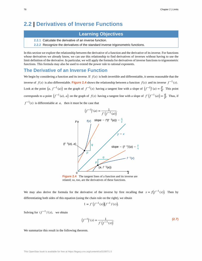
2.2 | Derivatives of Inverse Functions
Learning Objectives2.2.1 Calculate the derivative of an inverse function.
2.2.2 Recognize the derivatives of the standard inverse trigonometric functions.
In this section we explore the relationship between the derivative of a function and the derivative of its inverse. For functionswhose derivatives we already know, we can use this relationship to find derivatives of inverses without having to use thelimit definition of the derivative. In particular, we will apply the formula for derivatives of inverse functions to trigonometricfunctions. This formula may also be used to extend the power rule to rational exponents.
The Derivative of an Inverse FunctionWe begin by considering a function and its inverse. If f (x) is both invertible and differentiable, it seems reasonable that the
inverse of f (x) is also differentiable. Figure 2.4 shows the relationship between a function f (x) and its inverse f −1 (x).
Look at the point ⎛⎝a, f −1 (a)⎞⎠ on the graph of f −1(x) having a tangent line with a slope of ⎛⎝ f −1⎞⎠′ (a) = pq . This point
corresponds to a point ⎛⎝ f −1 (a), a⎞⎠ on the graph of f (x) having a tangent line with a slope of f ′ ⎛⎝ f −1 (a)⎞⎠ = qp. Thus, if
f −1(x) is differentiable at a, then it must be the case that
⎛⎝ f −1⎞⎠′ (a) = 1
f ′ ⎛⎝ f −1 (a)⎞⎠.
Figure 2.4 The tangent lines of a function and its inverse arerelated; so, too, are the derivatives of these functions.
We may also derive the formula for the derivative of the inverse by first recalling that x = f ⎛⎝ f −1 (x)⎞⎠. Then by
differentiating both sides of this equation (using the chain rule on the right), we obtain
1 = f ′ ⎛⎝ f −1 (x)⎞⎠⎛⎝ f −1 )′(x)⎞⎠.
Solving for ( f −1 )′(x), we obtain
(2.7)⎛⎝ f −1⎞⎠′ (x) = 1
f ′ ⎛⎝ f −1 (x)⎞⎠.
We summarize this result in the following theorem.
76 Chapter 2 | Limits
This OpenStax book is available for free at https://legacy.cnx.org/content/col31997/1.5

2.10
Theorem 2.3: Inverse Function Theorem
Let f (x) be a function that is both invertible and differentiable. Let y = f −1 (x) be the inverse of f (x). For all x
satisfying f ′ ⎛⎝ f −1 (x)⎞⎠ ≠ 0,
dydx = d
dx⎛⎝ f −1(x)⎞⎠ = ⎛⎝ f −1⎞⎠′ (x) = 1
f ′ ⎛⎝ f −1 (x)⎞⎠.
Alternatively, if y = g(x) is the inverse of f (x), then
g '(x) = 1f ′ ⎛⎝g(x)⎞⎠
.
Example 2.10
Applying the Inverse Function Theorem
Use the inverse function theorem to find the derivative of g(x) = x + 2x . Compare the resulting derivative to that
obtained by differentiating the function directly.
Solution
The inverse of g(x) = x + 2x is f (x) = 2
x − 1. Since g′ (x) = 1f ′ ⎛⎝g(x)⎞⎠
, begin by finding f ′ (x). Thus,
f ′ (x) = −2(x − 1)2 and f ′ ⎛⎝g(x)⎞⎠ = −2
⎛⎝g(x) − 1⎞⎠2
= −2⎛⎝x + 2
x − 1⎞⎠2 = − x2
2 .
Finally,
g′ (x) = 1f ′ ⎛⎝g(x)⎞⎠
= − 2x2.
We can verify that this is the correct derivative by applying the quotient rule to g(x) to obtain
g′ (x) = − 2x2.
Use the inverse function theorem to find the derivative of g(x) = 1x + 2. Compare the result obtained
by differentiating g(x) directly.
Example 2.11
Applying the Inverse Function Theorem
Use the inverse function theorem to find the derivative of g(x) = x3 .
Chapter 2 | Limits 77

2.11
Solution
The function g(x) = x3 is the inverse of the function f (x) = x3. Since g′ (x) = 1f ′ ⎛⎝g(x)⎞⎠
, begin by finding
f ′ (x). Thus,
f ′ (x) = 3x2 and f ′ ⎛⎝g(x)⎞⎠ = 3⎛⎝ x3 ⎞⎠2
= 3x2/3.
Finally,
g′ (x) = 13x2/3 = 1
3x−2/3.
Find the derivative of g(x) = x5 by applying the inverse function theorem.
From the previous example, we see that we can use the inverse function theorem to extend the power rule to exponents of
the form 1n, where n is a positive integer. This extension will ultimately allow us to differentiate xq, where q is any
rational number.
Theorem 2.4: Extending the Power Rule to Rational Exponents
The power rule may be extended to rational exponents. That is, if n is a positive integer, then
(2.8)ddx⎛⎝x1/n⎞⎠ = 1
nx(1/n) − 1.
Also, if n is a positive integer and m is an arbitrary integer, then
(2.9)ddx⎛⎝xm/n⎞⎠ = m
n x(m/n) − 1.
Proof
The function g(x) = x1/n is the inverse of the function f (x) = xn. Since g′ (x) = 1f ′ ⎛⎝g(x)⎞⎠
, begin by finding f ′ (x).
Thus,
f ′ (x) = nxn − 1 and f ′ ⎛⎝g(x)⎞⎠ = n(x1/n)n − 1 = nx(n − 1)/n.
Finally,
g′ (x) = 1nx(n − 1)/n = 1
nx(1 − n)/n = 1
nx(1/n) − 1.
To differentiate xm/n we must rewrite it as ⎛⎝x1/n⎞⎠m
and apply the chain rule. Thus,
ddx⎛⎝xm/n⎞⎠ = d
dx⎛⎝⎛⎝x1/n⎞⎠
m⎞⎠ = m⎛⎝x1/n⎞⎠
m − 1· 1nx
(1/n) − 1 = mn x
(m/n) − 1.
□
78 Chapter 2 | Limits
This OpenStax book is available for free at https://legacy.cnx.org/content/col31997/1.5
2.12
Example 2.12
Applying the Power Rule to a Rational Power
Find the equation of the line tangent to the graph of y = x2/3 at x = 8.
Solution
First finddydx and evaluate it at x = 8. Since
dydx = 2
3x−1/3 and dy
dx |x = 8= 1
3
the slope of the tangent line to the graph at x = 8 is 13.
Substituting x = 8 into the original function, we obtain y = 4. Thus, the tangent line passes through the point
(8, 4). Substituting into the point-slope formula for a line, we obtain the tangent line
y = 13x + 4
3.
Find the derivative of s(t) = 2t + 1.
Derivatives of Inverse Trigonometric FunctionsWe now turn our attention to finding derivatives of inverse trigonometric functions. These derivatives will prove invaluablein the study of integration later in this text. The derivatives of inverse trigonometric functions are quite surprising in thattheir derivatives are actually algebraic functions. Previously, derivatives of algebraic functions have proven to be algebraicfunctions and derivatives of trigonometric functions have been shown to be trigonometric functions. Here, for the first time,we see that the derivative of a function need not be of the same type as the original function.
Example 2.13
Derivative of the Inverse Sine Function
Use the inverse function theorem to find the derivative of g(x) = sin−1 x.
Solution
Since for x in the interval⎡⎣−π
2, π2⎤⎦, f (x) = sinx is the inverse of g(x) = sin−1 x, begin by finding f ′(x).
Since
f ′ (x) = cosx and f ′ ⎛⎝g(x)⎞⎠ = cos ⎛⎝sin−1 x⎞⎠ = 1 − x2,
we see that
g′ (x) = ddx⎛⎝sin−1 x⎞⎠ = 1
f ′ ⎛⎝g(x)⎞⎠= 1
1 − x2.
Chapter 2 | Limits 79
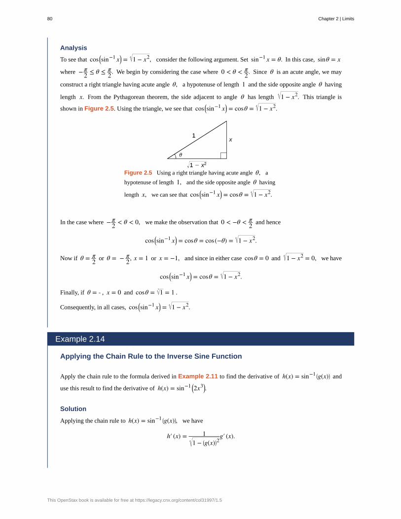
Analysis
To see that cos ⎛⎝sin−1 x⎞⎠ = 1 − x2, consider the following argument. Set sin−1 x = θ. In this case, sinθ = x
where −π2 ≤ θ ≤ π
2. We begin by considering the case where 0 < θ < π2. Since θ is an acute angle, we may
construct a right triangle having acute angle θ, a hypotenuse of length 1 and the side opposite angle θ having
length x. From the Pythagorean theorem, the side adjacent to angle θ has length 1 − x2. This triangle is
shown in Figure 2.5. Using the triangle, we see that cos ⎛⎝sin−1 x⎞⎠ = cosθ = 1 − x2.
Figure 2.5 Using a right triangle having acute angle θ, a
hypotenuse of length 1, and the side opposite angle θ having
length x, we can see that cos ⎛⎝sin−1 x⎞⎠ = cosθ = 1 − x2.
In the case where −π2 < θ < 0, we make the observation that 0 < −θ < π
2 and hence
cos ⎛⎝sin−1 x⎞⎠ = cosθ = cos(−θ) = 1 − x2.
Now if θ = π2 or θ = − π
2, x = 1 or x = −1, and since in either case cosθ = 0 and 1 − x2 = 0, we have
cos ⎛⎝sin−1 x⎞⎠ = cosθ = 1 − x2.
Finally, if θ = - , x = 0 and cosθ = 1- = 1 .
Consequently, in all cases, cos ⎛⎝sin−1 x⎞⎠ = 1 − x2.
Example 2.14
Applying the Chain Rule to the Inverse Sine Function
Apply the chain rule to the formula derived in Example 2.11 to find the derivative of h(x) = sin−1 ⎛⎝g(x)⎞⎠ and
use this result to find the derivative of h(x) = sin−1 ⎛⎝2x3⎞⎠.
Solution
Applying the chain rule to h(x) = sin−1 ⎛⎝g(x)⎞⎠, we have
h′ (x) = 11 − ⎛
⎝g(x)⎞⎠2g′ (x).
80 Chapter 2 | Limits
This OpenStax book is available for free at https://legacy.cnx.org/content/col31997/1.5

2.13
Now let g(x) = 2x3, so g′ (x) = 6x2. Substituting into the previous result, we obtain
h′ (x) = 11 − 4x6
· 6x2
= 6x2
1 − 4x6.
Use the inverse function theorem to find the derivative of g(x) = tan−1 x.
The derivatives of the remaining inverse trigonometric functions may also be found by using the inverse function theorem.These formulas are provided in the following theorem.
Theorem 2.5: Derivatives of Inverse Trigonometric Functions
(2.10)ddx sin−1 x = 1
1 − (x)2
(2.11)ddx cos−1 x = −1
1 − (x)2
(2.12)ddx tan−1 x = 1
1 + (x)2
(2.13)ddxcot−1 x = −1
1 + (x)2
(2.14)ddx sec−1 x = 1
|x| (x)2 − 1(2.15)d
dx csc−1 x = −1|x| (x)2 − 1
Example 2.15
Applying Differentiation Formulas to an Inverse Tangent Function
Find the derivative of f (x) = tan−1 ⎛⎝x2⎞⎠.
Solution
Let g(x) = x2, so g′ (x) = 2x. Substituting into Equation 2.12, we obtain
f ′ (x) = 1
1 + ⎛⎝x2⎞⎠2 · (2x).
Simplifying, we have
Chapter 2 | Limits 81
2.14
2.15
f ′ (x) = 2x1 + x4.
Example 2.16
Applying Differentiation Formulas to an Inverse Sine Function
Find the derivative of h(x) = x2 sin−1 x.
Solution
By applying the product rule, we have
h′ (x) = 2xsin−1 x + 11 − x2
· x2.
Find the derivative of h(x) = cos−1 (3x − 1).
Example 2.17
Applying the Inverse Tangent Function
The position of a particle at time t is given by s(t) = tan−1 ⎛⎝1t⎞⎠ for t ≥ 1
2. Find the velocity of the particle at
time t = 1.
Solution
Begin by differentiating s(t) in order to find v(t). Thus,
v(t) = s′ (t) = 11 + ⎛⎝1t
⎞⎠2 · −1
t2.
Simplifying, we have
v(t) = − 1t2 + 1
.
Thus, v(1) = − 12.
Find the equation of the line tangent to the graph of f (x) = sin−1 x at x = 0.
82 Chapter 2 | Limits
This OpenStax book is available for free at https://legacy.cnx.org/content/col31997/1.5

Key Concepts• The inverse function theorem allows us to compute derivatives of inverse functions without using the limit
definition of the derivative.
• We can use the inverse function theorem to develop differentiation formulas for the inverse trigonometric functions.
Key Equations• Inverse function theorem⎛⎝ f −1⎞⎠′ (x) = 1
f ′ ⎛⎝ f −1 (x)⎞⎠whenever f ′ ⎛⎝ f −1 (x)⎞⎠ ≠ 0 and f (x) is differentiable.
• Power rule with rational exponentsddx⎛⎝xm/n⎞⎠ = m
n x(m/n) − 1.
• Derivative of inverse sine functionddx sin−1 x = 1
1 − (x)2
• Derivative of inverse cosine functionddx cos−1 x = −1
1 − (x)2
• Derivative of inverse tangent functionddx tan−1 x = 1
1 + (x)2
• Derivative of inverse cotangent functionddx cot−1 x = −1
1 + (x)2
• Derivative of inverse secant functionddx sec−1 x = 1
|x| (x)2 − 1
• Derivative of inverse cosecant functionddx csc−1 x = −1
|x| (x)2 − 1
Chapter 2 | Limits 83
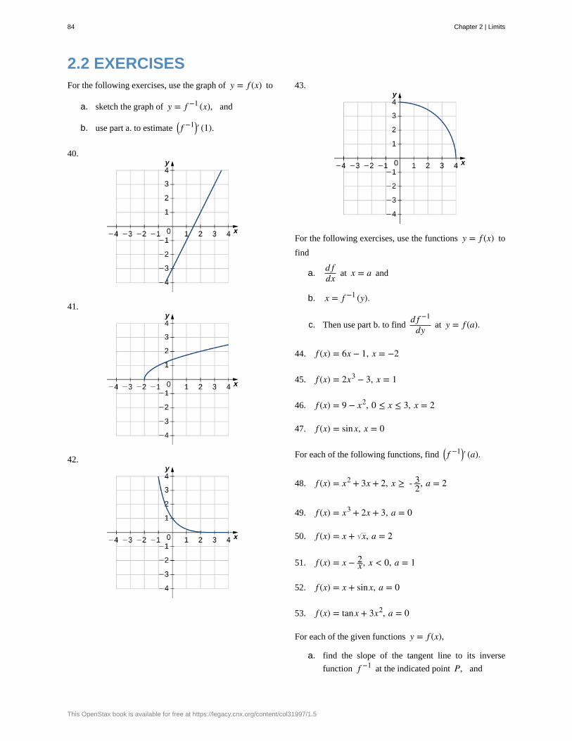
2.2 EXERCISESFor the following exercises, use the graph of y = f (x) to
a. sketch the graph of y = f −1 (x), and
b. use part a. to estimate ⎛⎝ f −1⎞⎠′ (1).
40.
41.
42.
43.
For the following exercises, use the functions y = f (x) to
find
a.d fdx at x = a and
b. x = f −1 (y).
c. Then use part b. to findd f −1
dy at y = f (a).
44. f (x) = 6x − 1, x = −2
45. f (x) = 2x3 − 3, x = 1
46. f (x) = 9 − x2, 0 ≤ x ≤ 3, x = 2
47. f (x) = sinx, x = 0
For each of the following functions, find ⎛⎝ f −1⎞⎠′ (a).
48. f (x) = x2 + 3x + 2, x ≥ - 32, a = 2
49. f (x) = x3 + 2x + 3, a = 0
50. f (x) = x + x, a = 2
51. f (x) = x − 2x , x < 0, a = 1
52. f (x) = x + sinx, a = 0
53. f (x) = tanx + 3x2, a = 0
For each of the given functions y = f (x),
a. find the slope of the tangent line to its inverse
function f −1 at the indicated point P, and
84 Chapter 2 | Limits
This OpenStax book is available for free at https://legacy.cnx.org/content/col31997/1.5
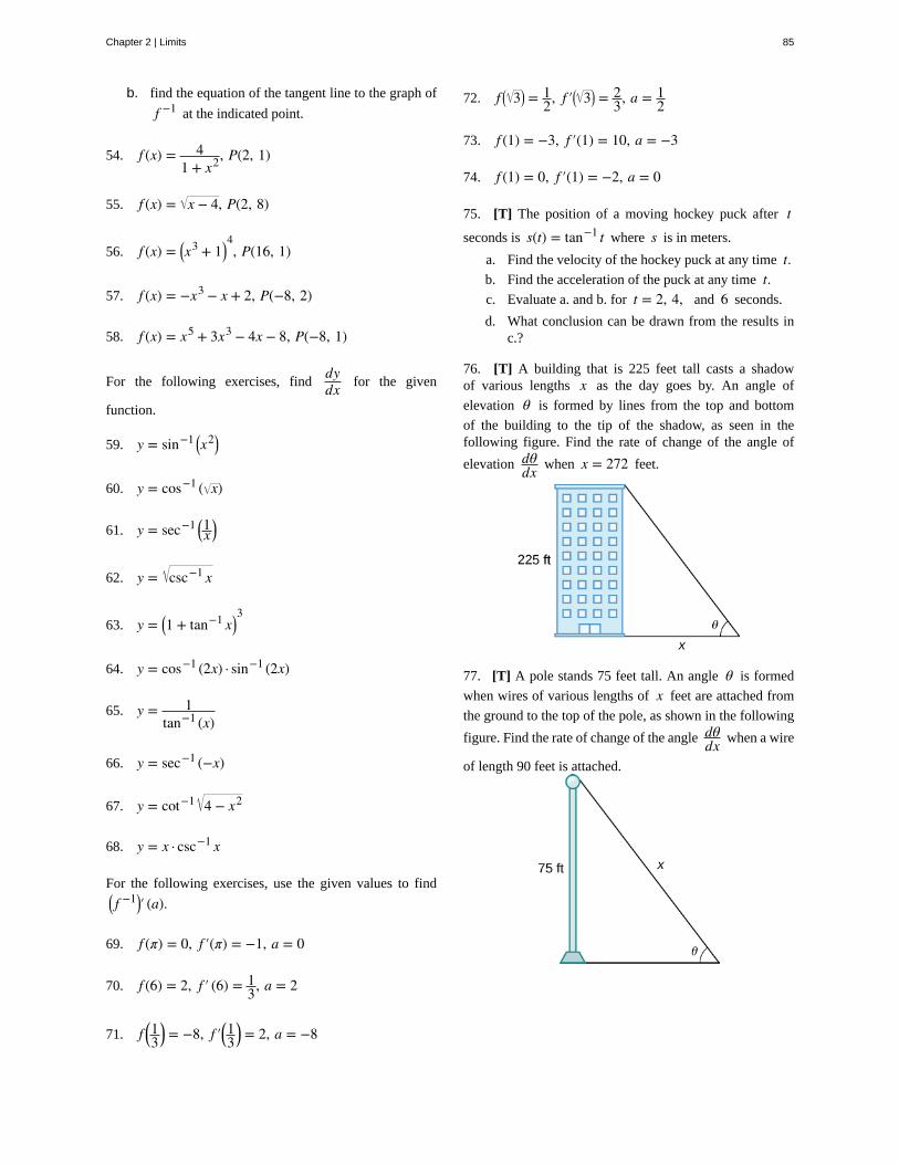
b. find the equation of the tangent line to the graph of
f −1 at the indicated point.
54. f (x) = 41 + x2, P(2, 1)
55. f (x) = x − 4, P(2, 8)
56. f (x) = ⎛⎝x3 + 1⎞⎠4, P(16, 1)
57. f (x) = −x3 − x + 2, P(−8, 2)
58. f (x) = x5 + 3x3 − 4x − 8, P(−8, 1)
For the following exercises, finddydx for the given
function.
59. y = sin−1 ⎛⎝x2⎞⎠
60. y = cos−1 ( x)
61. y = sec−1 ⎛⎝1x⎞⎠
62. y = csc−1 x
63. y = ⎛⎝1 + tan−1 x⎞⎠3
64. y = cos−1 (2x) · sin−1 (2x)
65. y = 1tan−1 (x)
66. y = sec−1 (−x)
67. y = cot−1 4 − x2
68. y = x · csc−1 x
For the following exercises, use the given values to find⎛⎝ f −1⎞⎠′ (a).
69. f (π) = 0, f ′(π) = −1, a = 0
70. f (6) = 2, f ′ (6) = 13, a = 2
71. f ⎛⎝13⎞⎠ = −8, f ′⎛⎝13
⎞⎠ = 2, a = −8
72. f ⎛⎝ 3⎞⎠ = 12, f ′⎛⎝ 3⎞⎠ = 2
3, a = 12
73. f (1) = −3, f ′(1) = 10, a = −3
74. f (1) = 0, f ′(1) = −2, a = 0
75. [T] The position of a moving hockey puck after tseconds is s(t) = tan−1 t where s is in meters.
a. Find the velocity of the hockey puck at any time t.b. Find the acceleration of the puck at any time t.c. Evaluate a. and b. for t = 2, 4, and 6 seconds.
d. What conclusion can be drawn from the results inc.?
76. [T] A building that is 225 feet tall casts a shadowof various lengths x as the day goes by. An angle of
elevation θ is formed by lines from the top and bottom
of the building to the tip of the shadow, as seen in thefollowing figure. Find the rate of change of the angle of
elevation dθdx when x = 272 feet.
77. [T] A pole stands 75 feet tall. An angle θ is formed
when wires of various lengths of x feet are attached from
the ground to the top of the pole, as shown in the following
figure. Find the rate of change of the angle dθdx when a wire
of length 90 feet is attached.
Chapter 2 | Limits 85
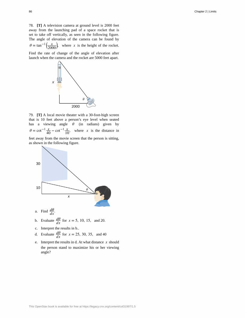
78. [T] A television camera at ground level is 2000 feetaway from the launching pad of a space rocket that isset to take off vertically, as seen in the following figure.The angle of elevation of the camera can be found by
θ = tan−1 ⎛⎝ x2000⎞⎠, where x is the height of the rocket.
Find the rate of change of the angle of elevation afterlaunch when the camera and the rocket are 5000 feet apart.
79. [T] A local movie theater with a 30-foot-high screenthat is 10 feet above a person’s eye level when seatedhas a viewing angle θ (in radians) given by
θ = cot−1 x40 − cot−1 x
10, where x is the distance in
feet away from the movie screen that the person is sitting,as shown in the following figure.
a. Find dθdx .
b. Evaluate dθdx for x = 5, 10, 15, and 20.
c. Interpret the results in b..
d. Evaluate dθdx for x = 25, 30, 35, and 40
e. Interpret the results in d. At what distance x should
the person stand to maximize his or her viewingangle?
86 Chapter 2 | Limits
This OpenStax book is available for free at https://legacy.cnx.org/content/col31997/1.5
2.3 | Derivatives of Exponential and Logarithmic
Functions
Learning Objectives2.3.1 Find the derivative of exponential functions.
2.3.2 Find the derivative of logarithmic functions.
2.3.3 Use logarithmic differentiation to determine the derivative of a function.
So far, we have learned how to differentiate a variety of functions, including trigonometric, inverse, and implicit functions.In this section, we explore derivatives of exponential and logarithmic functions. As we discussed in Introduction toFunctions and Graphs (https://legacy.cnx.org/content/m53472/latest/) , exponential functions play an importantrole in modeling population growth and the decay of radioactive materials. Logarithmic functions can help rescale largequantities and are particularly helpful for rewriting complicated expressions.
Derivative of the Exponential FunctionJust as when we found the derivatives of other functions, we can find the derivatives of exponential and logarithmicfunctions using formulas. As we develop these formulas, we need to make certain basic assumptions. The proofs that theseassumptions hold are beyond the scope of this course.
First of all, we begin with the assumption that the function B(x) = bx, b > 0, is defined for every real number and is
continuous. In previous courses, the values of exponential functions for all rational numbers were defined—beginningwith the definition of bn, where n is a positive integer—as the product of b multiplied by itself n times. Later,
we defined b0 = 1, b−n = 1bn
, for a positive integer n, and bs/t = ( bt )s for positive integers s and t. These
definitions leave open the question of the value of br where r is an arbitrary real number. By assuming the continuity of
B(x) = bx, b > 0, we may interpret br as limx → rbx where the values of x as we take the limit are rational. For example,
we may view 4π as the number satisfying
43 < 4π < 44, 43.1 < 4π < 43.2, 43.14 < 4π < 43.15,43.141 < 4π < 43.142, 43.1415 < 4π < 43.1416 ,….
As we see in the following table, 4π ≈ 77.88.
Chapter 2 | Limits 87
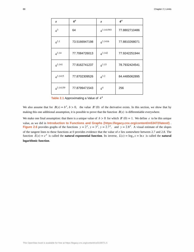
x 4x x 4x
43 64 43.141593 77.8802710486
43.1 73.5166947198 43.1416 77.8810268071
43.14 77.7084726013 43.142 77.9242251944
43.141 77.8162741237 43.15 78.7932424541
43.1415 77.8702309526 43.2 84.4485062895
43.14159 77.8799471543 44 256
Table 2.1 Approximating a Value of 4π
We also assume that for B(x) = bx, b > 0, the value B′ (0) of the derivative exists. In this section, we show that by
making this one additional assumption, it is possible to prove that the function B(x) is differentiable everywhere.
We make one final assumption: that there is a unique value of b > 0 for which B′ (0) = 1. We define e to be this unique
value, as we did in Introduction to Functions and Graphs (https://legacy.cnx.org/content/m53472/latest/) .Figure 2.6 provides graphs of the functions y = 2x, y = 3x, y = 2.7x, and y = 2.8x. A visual estimate of the slopes
of the tangent lines to these functions at 0 provides evidence that the value of e lies somewhere between 2.7 and 2.8. Thefunction E(x) = ex is called the natural exponential function. Its inverse, L(x) = loge x = lnx is called the natural
logarithmic function.
88 Chapter 2 | Limits
This OpenStax book is available for free at https://legacy.cnx.org/content/col31997/1.5
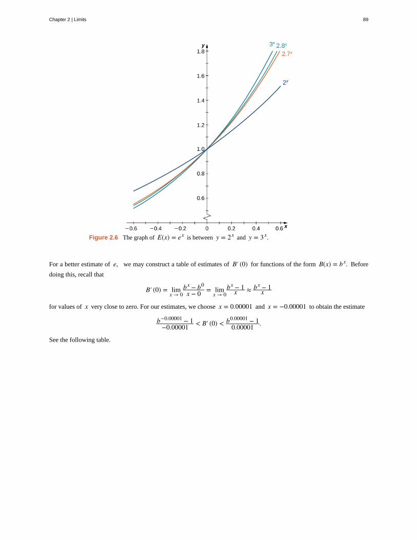
Figure 2.6 The graph of E(x) = ex is between y = 2x and y = 3x.
For a better estimate of e, we may construct a table of estimates of B′ (0) for functions of the form B(x) = bx. Before
doing this, recall that
B′ (0) = limx → 0
bx − b0
x − 0 = limx → 0
bx − 1x ≈ bx − 1
x
for values of x very close to zero. For our estimates, we choose x = 0.00001 and x = −0.00001 to obtain the estimate
b−0.00001 − 1−0.00001 < B′ (0) < b0.00001 − 1
0.00001 .
See the following table.
Chapter 2 | Limits 89

b b−0.00001−1−0.00001 < B′ (0) < b0.00001−1
0.00001b b−0.00001−1
−0.00001 < B′ (0) < b0.00001−10.00001
2 0.693145 < B′ (0) < 0.69315 2.7183 1.000002 < B′ (0) < 1.000012
2.7 0.993247 < B′ (0) < 0.993257 2.719 1.000259 < B′ (0) < 1.000269
2.71 0.996944 < B′ (0) < 0.996954 2.72 1.000627 < B′ (0) < 1.000637
2.718 0.999891 < B′ (0) < 0.999901 2.8 1.029614 < B′ (0) < 1.029625
2.7182 0.999965 < B′ (0) < 0.999975 3 1.098606 < B′ (0) < 1.098618
Table 2.2 Estimating a Value of e
The evidence from the table suggests that 2.7182 < e < 2.7183.
The graph of E(x) = ex together with the line y = x + 1 are shown in Figure 2.7. This line is tangent to the graph of
E(x) = ex at x = 0.
Figure 2.7 The tangent line to E(x) = ex at x = 0 has
slope 1.
Now that we have laid out our basic assumptions, we begin our investigation by exploring the derivative ofB(x) = bx, b > 0. Recall that we have assumed that B′ (0) exists. By applying the limit definition to the derivative we
conclude that
(2.16)B′ (0) = lim
h → 0b0 + h − b0
h = limh → 0
bh − 1h .
Turning to B′ (x), we obtain the following.
90 Chapter 2 | Limits
This OpenStax book is available for free at https://legacy.cnx.org/content/col31997/1.5
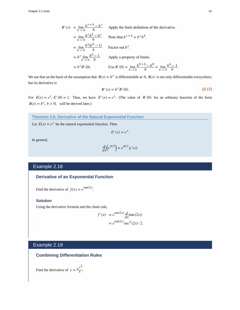
B′ (x) = limh → 0
bx + h − bxh Apply the limit definition of the derivative.
= limh → 0
bx bh − bxh Note that bx + h = bx bh.
= limh → 0
bx(bh − 1)h Factor out bx.
= bx limh → 0
bh − 1h Apply a property of limits.
= bxB′ (0) Use B′ (0) = limh → 0
b0 + h − b0
h = limh → 0
bh − 1h .
We see that on the basis of the assumption that B(x) = bx is differentiable at 0, B(x) is not only differentiable everywhere,
but its derivative is
(2.17)B′ (x) = bxB′ (0).
For E(x) = ex, E′ (0) = 1. Thus, we have E′ (x) = ex. (The value of B′ (0) for an arbitrary function of the form
B(x) = bx, b > 0, will be derived later.)
Theorem 2.6: Derivative of the Natural Exponential Function
Let E(x) = ex be the natural exponential function. Then
E′ (x) = ex.
In general,
ddx⎛⎝e
g(x)⎞⎠ = eg(x)g′ (x).
Example 2.18
Derivative of an Exponential Function
Find the derivative of f (x) = etan(2x).
Solution
Using the derivative formula and the chain rule,
f ′ (x) = etan(2x) ddx⎛⎝tan(2x)⎞⎠
= etan(2x) sec2 (2x) · 2.
Example 2.19
Combining Differentiation Rules
Find the derivative of y = ex2
x .
Chapter 2 | Limits 91

2.16
2.17
Solution
Use the derivative of the natural exponential function, the quotient rule, and the chain rule.
y′ =
⎛⎝ex
2· 2⎞⎠x · x − 1 · ex
2
x2 Apply the quotient rule.
=ex
2 ⎛⎝2x2 − 1⎞⎠x2 Simplify.
Find the derivative of h(x) = xe2x.
Example 2.20
Applying the Natural Exponential Function
A colony of mosquitoes has an initial population of 1000. After t days, the population is given by
A(t) = 1000e0.3t. Show that the ratio of the rate of change of the population, A′ (t), to the population, A(t) is
constant.
Solution
First find A′ (t). By using the chain rule, we have A′ (t) = 300e0.3t. Thus, the ratio of the rate of change of the
population to the population is given by
A′ (t) = 300e0.3t
1000e0.3t = 0.3.
The ratio of the rate of change of the population to the population is the constant 0.3.
If A(t) = 1000e0.3t describes the mosquito population after t days, as in the preceding example, what
is the rate of change of A(t) after 4 days?
Derivative of the Logarithmic FunctionNow that we have the derivative of the natural exponential function, we can use implicit differentiation to find the derivativeof its inverse, the natural logarithmic function.
Theorem 2.7: The Derivative of the Natural Logarithmic Function
If x > 0 and y = lnx, then
(2.18)dydx = 1
x .
More generally, let g(x) be a differentiable function. For all values of x for which g′ (x) > 0, the derivative of
92 Chapter 2 | Limits
This OpenStax book is available for free at https://legacy.cnx.org/content/col31997/1.5

h(x) = ln ⎛⎝g(x)⎞⎠ is given by
(2.19)h′ (x) = 1g(x)g′ (x).
Proof
If x > 0 and y = lnx, then ey = x. Differentiating both sides of this equation results in the equation
ey dydx = 1.
Solving fordydx yields
dydx = 1
ey.
Finally, we substitute x = ey to obtain
dydx = 1
x .
We may also derive this result by applying the inverse function theorem, as follows. Since y = g(x) = lnx is the inverse
of f (x) = ex, by applying the inverse function theorem we have
dydx = 1
f ′ ⎛⎝g(x)⎞⎠= 1
elnx = 1x .
Using this result and applying the chain rule to h(x) = ln ⎛⎝g(x)⎞⎠ yields
h′ (x) = 1g(x)g′ (x).
□
The graph of y = lnx and its derivativedydx = 1
x are shown in Figure 2.8.
Figure 2.8 The function y = lnx is increasing on
(0, +∞). Its derivative y′ = 1x is greater than zero on
(0, +∞).
Example 2.21
Taking a Derivative of a Natural Logarithm
Chapter 2 | Limits 93
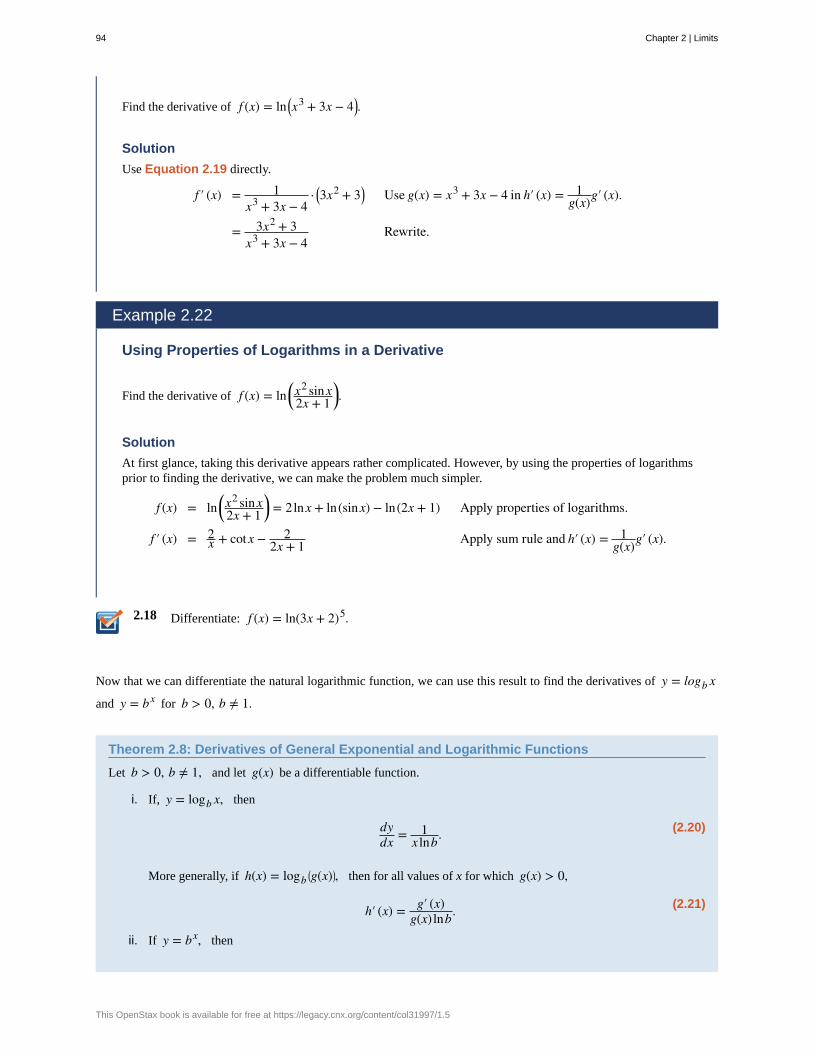
2.18
Find the derivative of f (x) = ln ⎛⎝x3 + 3x − 4⎞⎠.
Solution
Use Equation 2.19 directly.
f ′ (x) = 1x3 + 3x − 4
· ⎛⎝3x2 + 3⎞⎠ Use g(x) = x3 + 3x − 4 in h′ (x) = 1g(x)g′ (x).
= 3x2 + 3x3 + 3x − 4
Rewrite.
Example 2.22
Using Properties of Logarithms in a Derivative
Find the derivative of f (x) = ln⎛⎝x2 sinx
2x + 1⎞⎠.
Solution
At first glance, taking this derivative appears rather complicated. However, by using the properties of logarithmsprior to finding the derivative, we can make the problem much simpler.
f (x) = ln⎛⎝x2 sinx
2x + 1⎞⎠ = 2lnx + ln(sinx) − ln(2x + 1) Apply properties of logarithms.
f ′ (x) = 2x + cotx − 2
2x + 1 Apply sum rule and h′ (x) = 1g(x)g′ (x).
Differentiate: f (x) = ln(3x + 2)5.
Now that we can differentiate the natural logarithmic function, we can use this result to find the derivatives of y = logb x
and y = bx for b > 0, b ≠ 1.
Theorem 2.8: Derivatives of General Exponential and Logarithmic Functions
Let b > 0, b ≠ 1, and let g(x) be a differentiable function.
i. If, y = logb x, then
(2.20)dydx = 1
x lnb.
More generally, if h(x) = logb⎛⎝g(x)⎞⎠, then for all values of x for which g(x) > 0,
(2.21)h′ (x) = g′ (x)g(x) lnb.
ii. If y = bx, then
94 Chapter 2 | Limits
This OpenStax book is available for free at https://legacy.cnx.org/content/col31997/1.5

(2.22)dydx = bx lnb.
More generally, if h(x) = bg(x), then
(2.23)h′ (x) = bg(x)g′(x) lnb.
Proof
If y = logb x, then by = x. It follows that ln(by) = ln x. Thus y ln b = ln x. Solving for y, we have y = lnxlnb.
Differentiating and keeping in mind that lnb is a constant, we see that
dydx = 1
x lnb.
The derivative in Equation 2.21 now follows from the chain rule.
If y = bx, then ln y = x lnb. Using implicit differentiation, again keeping in mind that lnb is constant, it follows that
1ydydx = lnb. Solving for
dydx and substituting y = bx, we see that
dydx = y lnb = bx lnb.
The more general derivative (Equation 2.23) follows from the chain rule.
□
Example 2.23
Applying Derivative Formulas
Find the derivative of h(x) = 3x
3x + 2.
Solution
Use the quotient rule and Derivatives of General Exponential and Logarithmic Functions.
h′ (x) = 3x ln3(3x + 2) − 3x ln3(3x)(3x + 2)2 Apply the quotient rule.
= 2 · 3x ln3(3x + 2)2 Simplify.
Example 2.24
Finding the Slope of a Tangent Line
Find the slope of the line tangent to the graph of y = log2 (3x + 1) at x = 1.
Solution
Chapter 2 | Limits 95

2.19
To find the slope, we must evaluatedydx at x = 1. Using Equation 2.21, we see that
dydx = 3
(3x + 1)ln2.
By evaluating the derivative at x = 1, we see that the tangent line has slope
dydx |x = 1
= 34ln2 = 3
ln16.
Find the slope for the line tangent to y = 3x at x = 2.
Logarithmic DifferentiationAt this point, we can take derivatives of functions of the form y = ⎛
⎝g(x)⎞⎠n for certain values of n, as well as functions
of the form y = bg(x), where b > 0 and b ≠ 1. Unfortunately, we still do not know the derivatives of functions such as
y = xx or y = xπ. These functions require a technique called logarithmic differentiation, which allows us to differentiate
any function of the form h(x) = g(x) f (x). It can also be used to convert a very complex differentiation problem into a
simpler one, such as finding the derivative of y = x 2x + 1ex sin3 x
. We outline this technique in the following problem-solving
strategy.
Problem-Solving Strategy: Using Logarithmic Differentiation
1. To differentiate y = h(x) using logarithmic differentiation, take the natural logarithm of both sides of the
equation to obtain ln y = ln ⎛⎝h(x)⎞⎠.
2. Use properties of logarithms to expand ln ⎛⎝h(x)⎞⎠ as much as possible.
3. Differentiate both sides of the equation. On the left we will have 1ydydx.
4. Multiply both sides of the equation by y to solve fordydx.
5. Replace y by h(x).
Example 2.25
Using Logarithmic Differentiation
Find the derivative of y = ⎛⎝2x4 + 1⎞⎠tanx
.
96 Chapter 2 | Limits
This OpenStax book is available for free at https://legacy.cnx.org/content/col31997/1.5

Solution
Use logarithmic differentiation to find this derivative.
lny = ln⎛⎝2x4 + 1⎞⎠tanx
Step 1. Take the natural logarithm of both sides.
lny = tanx ln ⎛⎝2x4 + 1⎞⎠ Step 2. Expand using properties of logarithms.
1ydydx = sec2 x ln ⎛⎝2x4 + 1⎞⎠+ 8x3
2x4 + 1· tanx
Step 3. Differentiate both sides. Use theproduct rule on the right.
dydx = y · ⎛⎝sec2 x ln ⎛⎝2x4 + 1⎞⎠+ 8x3
2x4 + 1· tanx⎞⎠ Step 4. Multiply by y on both sides.
dydx = ⎛
⎝2x4 + 1⎞⎠tanx⎛⎝sec2 x ln ⎛⎝2x4 + 1⎞⎠+ 8x3
2x4 + 1· tanx⎞⎠ Step 5. Substitute y = ⎛⎝2x4 + 1⎞⎠
tanx.
Example 2.26
Using Logarithmic Differentiation
Find the derivative of y = x 2x + 1ex sin3 x
.
Solution
This problem really makes use of the properties of logarithms and the differentiation rules given in this chapter.
lny = ln x 2x + 1ex sin3 x
Step 1. Take the natural logarithm of both sides.
lny = lnx + 12 ln(2x + 1) − x lne − 3lnsinx Step 2. Expand using properties of logarithms.
1ydydx = 1
x + 12x + 1 − 1 − 3cosx
sinx Step 3. Differentiate both sides.
dydx = y⎛⎝1x + 1
2x + 1 − 1 − 3cotx⎞⎠ Step 4. Multiply by y on both sides.
dydx = x 2x + 1
ex sin3 x⎛⎝1x + 1
2x + 1 − 1 − 3cotx⎞⎠ Step 5. Substitute y = x 2x + 1ex sin3 x
.
Example 2.27
Extending the Power Rule
Find the derivative of y = xr where r is an arbitrary real number.
Solution
The process is the same as in Example 2.26, though with fewer complications.
Chapter 2 | Limits 97

2.20
2.21
lny = lnxr Step 1. Take the natural logarithm of both sides.lny = r lnx Step 2. Expand using properties of logarithms.
1ydydx = r1
x Step 3. Differentiate both sides.
dydx = yrx Step 4. Multiply by y on both sides.
dydx = xr rx Step 5. Substitute y = xr.
dydx = rxr − 1 Simplify.
Use logarithmic differentiation to find the derivative of y = xx.
Find the derivative of y = (tanx)π.
Key Concepts• On the basis of the assumption that the exponential function y = bx, b > 0 is continuous everywhere and
differentiable at 0, this function is differentiable everywhere and there is a formula for its derivative.
• We can use a formula to find the derivative of y = lnx, and the relationship logb x = lnxlnb allows us to extend
our differentiation formulas to include logarithms with arbitrary bases.
• Logarithmic differentiation allows us to differentiate functions of the form y = g(x) f (x)or very complex functions
by taking the natural logarithm of both sides and exploiting the properties of logarithms before differentiating.
Key Equations• Derivative of the natural exponential function
ddx⎛⎝e
g(x)⎞⎠ = eg(x)g′ (x)
• Derivative of the natural logarithmic functionddx⎛⎝lng(x)⎞⎠ = 1
g(x)g′ (x)
• Derivative of the general exponential functionddx⎛⎝b
g(x)⎞⎠ = bg(x)g′ (x) lnb
• Derivative of the general logarithmic function
ddx⎛⎝logbg(x)⎞⎠ = g′ (x)
g(x) lnb
98 Chapter 2 | Limits
This OpenStax book is available for free at https://legacy.cnx.org/content/col31997/1.5

2.3 EXERCISESFor the following exercises, find f ′ (x) for each function.
80. f (x) = x2 ex
81. f (x) = e−xx
82. f (x) = ex3 lnx
83. f (x) = e2x + 2x
84. f (x) = ex − e−x
ex + e−x
85. f (x) = 10x
ln10
86. f (x) = 24x + 4x2
87. f (x) = 3sin3x
88. f (x) = xπ · π x
89. f (x) = ln ⎛⎝4x3 + x⎞⎠
90. f (x) = ln 5x − 7
91. f (x) = x2 ln9x
92. f (x) = log(secx)
93. f (x) = log7⎛⎝6x4 + 3⎞⎠
5
94. f (x) = 2x · log3 7x2 − 4
For the following exercises, use logarithmic differentiation
to finddydx.
95. y = x x
96. y = (sin2x)4x
97. y = (lnx)lnx
98. y = xlog2 x
99. y = ⎛⎝x2 − 1⎞⎠lnx
100. y = xcotx
101. y = x + 11
x2 − 43
102. y = x−1/2 ⎛⎝x2 + 3⎞⎠2/3
(3x − 4)4
103. [T] Find an equation of the tangent line to the graph
of f (x) = 4xe⎛⎝x2 − 1⎞⎠
at the point where x = −1. Graph
both the function and the tangent line.
104. [T] Find the equation of the line that is normal to thegraph of f (x) = x · 5x at the point where x = 1. Graph
both the function and the normal line.
105. [T] Find the equation of the tangent line to the graph
of x3 − x lny + y3 = 2x + 5 at the point where x = 2.
(Hint: Use implicit differentiation to finddydx.) Graph both
the curve and the tangent line.
106. Consider the function y = x1/x for x > 0.a. Determine the points on the graph where the
tangent line is horizontal.b. Determine the points on the graph where y′ > 0
and those where y′ < 0.
Chapter 2 | Limits 99
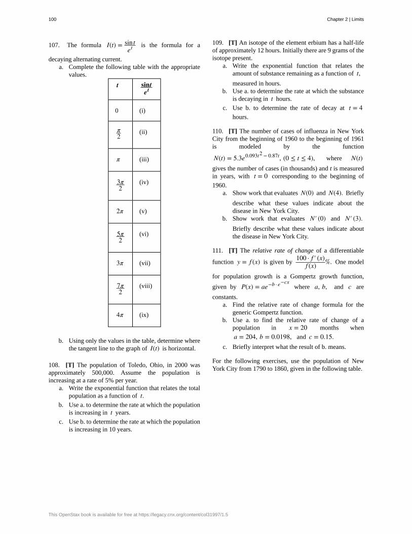
107. The formula I(t) = sin tet
is the formula for a
decaying alternating current.a. Complete the following table with the appropriate
values.
t sintet
0 (i)
π2
(ii)
π (iii)
3π2
(iv)
2π (v)
5π2
(vi)
3π (vii)
7π2
(viii)
4π (ix)
b. Using only the values in the table, determine wherethe tangent line to the graph of I(t) is horizontal.
108. [T] The population of Toledo, Ohio, in 2000 wasapproximately 500,000. Assume the population isincreasing at a rate of 5% per year.
a. Write the exponential function that relates the totalpopulation as a function of t.
b. Use a. to determine the rate at which the populationis increasing in t years.
c. Use b. to determine the rate at which the populationis increasing in 10 years.
109. [T] An isotope of the element erbium has a half-lifeof approximately 12 hours. Initially there are 9 grams of theisotope present.
a. Write the exponential function that relates theamount of substance remaining as a function of t,measured in hours.
b. Use a. to determine the rate at which the substanceis decaying in t hours.
c. Use b. to determine the rate of decay at t = 4hours.
110. [T] The number of cases of influenza in New YorkCity from the beginning of 1960 to the beginning of 1961is modeled by the function
N(t) = 5.3e0.093t2 − 0.87t, (0 ≤ t ≤ 4), where N(t)gives the number of cases (in thousands) and t is measuredin years, with t = 0 corresponding to the beginning of
1960.a. Show work that evaluates N(0) and N(4). Briefly
describe what these values indicate about thedisease in New York City.
b. Show work that evaluates N′ (0) and N′ (3).Briefly describe what these values indicate aboutthe disease in New York City.
111. [T] The relative rate of change of a differentiable
function y = f (x) is given by100 · f ′ (x)
f (x) %. One model
for population growth is a Gompertz growth function,
given by P(x) = ae−b · e−cxwhere a, b, and c are
constants.a. Find the relative rate of change formula for the
generic Gompertz function.b. Use a. to find the relative rate of change of a
population in x = 20 months when
a = 204, b = 0.0198, and c = 0.15.c. Briefly interpret what the result of b. means.
For the following exercises, use the population of NewYork City from 1790 to 1860, given in the following table.
100 Chapter 2 | Limits
This OpenStax book is available for free at https://legacy.cnx.org/content/col31997/1.5
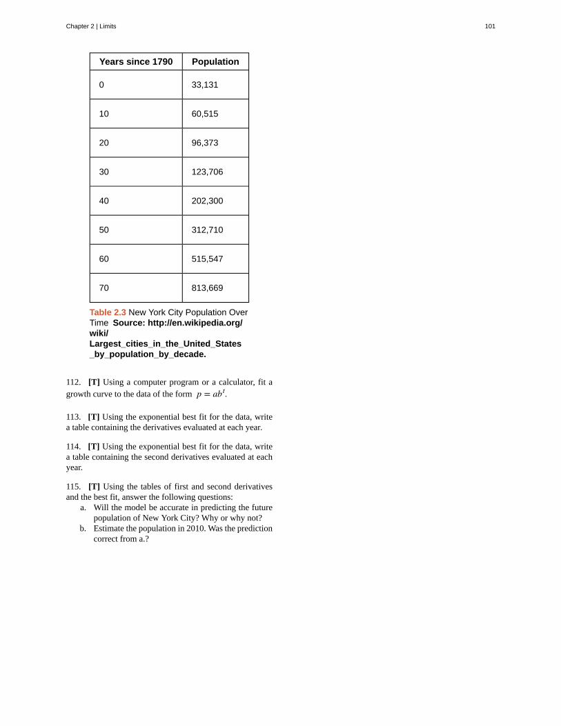
Years since 1790 Population
0 33,131
10 60,515
20 96,373
30 123,706
40 202,300
50 312,710
60 515,547
70 813,669
Table 2.3 New York City Population OverTime Source: http://en.wikipedia.org/wiki/Largest_cities_in_the_United_States_by_population_by_decade.
112. [T] Using a computer program or a calculator, fit agrowth curve to the data of the form p = abt.
113. [T] Using the exponential best fit for the data, writea table containing the derivatives evaluated at each year.
114. [T] Using the exponential best fit for the data, writea table containing the second derivatives evaluated at eachyear.
115. [T] Using the tables of first and second derivativesand the best fit, answer the following questions:
a. Will the model be accurate in predicting the futurepopulation of New York City? Why or why not?
b. Estimate the population in 2010. Was the predictioncorrect from a.?
Chapter 2 | Limits 101

Chapter Review ExercisesTrue or False? Justify the answer with a proof or a counterexample.
Exercise 2.116
Every function has a derivative.
SolutionFalse.
Exercise 2.117
A continuous function has a continuous derivative.
Exercise 2.118
A continuous function has a derivative.
SolutionFalse
Exercise 2.119
If a function is differentiable, it is continuous.
Use the limit definition of the derivative to exactly evaluate the derivative.
Exercise 2.120
f (x) = x + 4
Solution1
2 x + 4
Exercise 2.121
f (x) = 3x
Find the derivatives of the following functions.
Exercise 2.122
f (x) = 3x3 − 4x2
Solution
9x2 + 8x3
Exercise 2.123
f (x) = ⎛⎝4 − x2⎞⎠3
Exercise 2.124
f (x) = esinx
Solution
esinx cosx
102 Chapter 2 | Limits
This OpenStax book is available for free at https://legacy.cnx.org/content/col31997/1.5
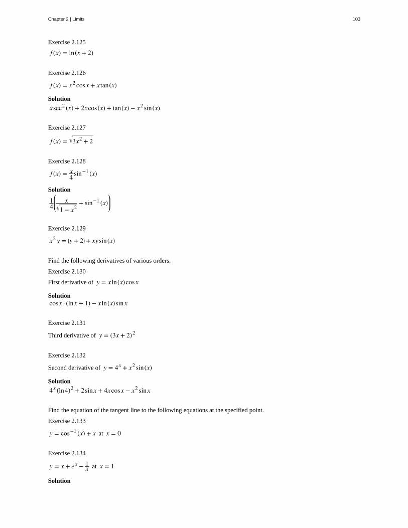
Exercise 2.125
f (x) = ln(x + 2)
Exercise 2.126
f (x) = x2 cosx + x tan(x)
Solution
xsec2 (x) + 2xcos(x) + tan(x) − x2 sin(x)
Exercise 2.127
f (x) = 3x2 + 2
Exercise 2.128
f (x) = x4 sin−1 (x)
Solution
14⎛⎝⎜ x
1 − x2+ sin−1 (x)
⎞⎠⎟
Exercise 2.129
x2 y = ⎛⎝y + 2⎞⎠+ xysin(x)
Find the following derivatives of various orders.
Exercise 2.130
First derivative of y = x ln(x)cosx
Solutioncosx · (lnx + 1) − x ln(x)sinx
Exercise 2.131
Third derivative of y = (3x + 2)2
Exercise 2.132
Second derivative of y = 4x + x2 sin(x)
Solution
4x (ln4)2 + 2sinx + 4xcosx − x2 sinx
Find the equation of the tangent line to the following equations at the specified point.
Exercise 2.133
y = cos−1 (x) + x at x = 0
Exercise 2.134
y = x + ex − 1x at x = 1
Solution
Chapter 2 | Limits 103
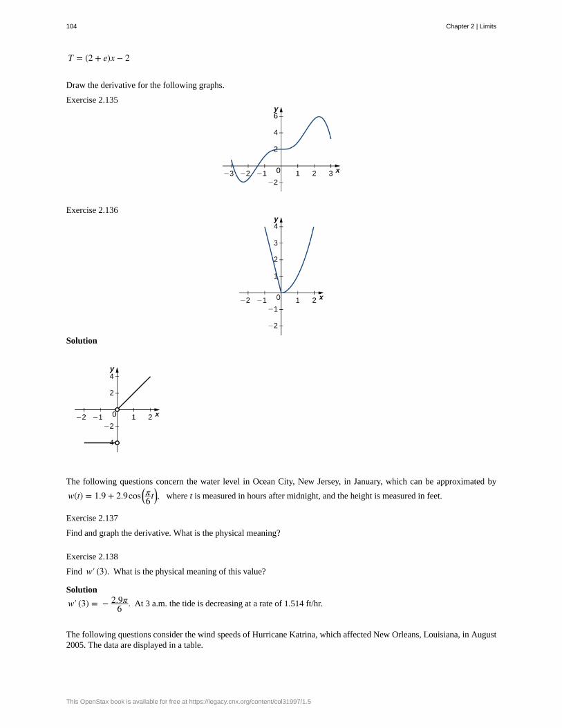
T = (2 + e)x − 2
Draw the derivative for the following graphs.
Exercise 2.135
Exercise 2.136
Solution
The following questions concern the water level in Ocean City, New Jersey, in January, which can be approximated by
w(t) = 1.9 + 2.9cos⎛⎝π6 t⎞⎠, where t is measured in hours after midnight, and the height is measured in feet.
Exercise 2.137
Find and graph the derivative. What is the physical meaning?
Exercise 2.138
Find w′ (3). What is the physical meaning of this value?
Solution
w′ (3) = − 2.9π6 . At 3 a.m. the tide is decreasing at a rate of 1.514 ft/hr.
The following questions consider the wind speeds of Hurricane Katrina, which affected New Orleans, Louisiana, in August2005. The data are displayed in a table.
104 Chapter 2 | Limits
This OpenStax book is available for free at https://legacy.cnx.org/content/col31997/1.5

Hours after Midnight, August 26 Wind Speed (mph)
1 45
5 75
11 100
29 115
49 145
58 175
73 155
81 125
85 95
107 35
Table 2.4 Wind Speeds of Hurricane Katrina Source:http://news.nationalgeographic.com/news/2005/09/0914_050914_katrina_timeline.html.
Exercise 2.139
Using the table, estimate the derivative of the wind speed at hour 39. What is the physical meaning?
Exercise 2.140
Estimate the derivative of the wind speed at hour 83. What is the physical meaning?
Solution−7.5. The wind speed is decreasing at a rate of 7.5 mph/hr
Chapter 2 | Limits 105

logarithmic differentiation
CHAPTER 2 REVIEW
KEY TERMSis a technique that allows us to differentiate a function by first taking the natural logarithm
of both sides of an equation, applying properties of logarithms to simplify the equation, and differentiating implicitly
106 Chapter 2 | Limits
This OpenStax book is available for free at https://legacy.cnx.org/content/col31997/1.5
3 | INTEGRATION3.1 | Antiderivatives
Learning Objectives3.1.1 Find the general antiderivative of a given function.
3.1.2 Explain the terms and notation used for an indefinite integral.
3.1.3 State the power rule for integrals.
3.1.4 Use antidifferentiation to solve simple initial-value problems.
At this point, we have seen how to calculate derivatives of many functions and have been introduced to a variety of theirapplications. We now ask a question that turns this process around: Given a function f , how do we find a function with
the derivative f and why would we be interested in such a function?
We answer the first part of this question by defining antiderivatives. The antiderivative of a function f is a function
with a derivative f . Why are we interested in antiderivatives? The need for antiderivatives arises in many situations,
and we look at various examples throughout the remainder of the text. Here we examine one specific example thatinvolves rectilinear motion. In our examination in Derivatives (https://legacy.cnx.org/content/m53494/latest/) ofrectilinear motion, we showed that given a position function s(t) of an object, then its velocity function v(t) is the
derivative of s(t) —that is, v(t) = s′ (t). Furthermore, the acceleration a(t) is the derivative of the velocity v(t) —that
is, a(t) = v′ (t) = s″(t). Now suppose we are given an acceleration function a, but not the velocity function v or the
position function s. Since a(t) = v′ (t), determining the velocity function requires us to find an antiderivative of the
acceleration function. Then, since v(t) = s′ (t), determining the position function requires us to find an antiderivative of
the velocity function. Rectilinear motion is just one case in which the need for antiderivatives arises. We will see many moreexamples throughout the remainder of the text. For now, let’s look at the terminology and notation for antiderivatives, anddetermine the antiderivatives for several types of functions. We examine various techniques for finding antiderivatives ofmore complicated functions later in the text (Introduction to Techniques of Integration (https://legacy.cnx.org/content/m53654/latest/) ).
The Reverse of DifferentiationAt this point, we know how to find derivatives of various functions. We now ask the opposite question. Given a functionf , how can we find a function with derivative f ? If we can find a function F with derivative f , we call F an
antiderivative of f .
Definition
A function F is an antiderivative of the function f if
F′ (x) = f (x)
for all x in the domain of f .
Consider the function f (x) = 2x. Knowing the power rule of differentiation, we conclude that F(x) = x2 is an
antiderivative of f since F′ (x) = 2x. Are there any other antiderivatives of f ? Yes; since the derivative of any constant
C is zero, x2 + C is also an antiderivative of 2x. Therefore, x2 + 5 and x2 − 2 are also antiderivatives. Are there any
others that are not of the form x2 + C for some constant C? The answer is no. From Corollary 2 of the Mean Value
Theorem, we know that if F and G are differentiable functions such that F′ (x) = G′ (x), then F(x) − G(x) = C for
Chapter 3 | Integration 107
some constant C. This fact leads to the following important theorem.
Theorem 3.1: General Form of an Antiderivative
Let F be an antiderivative of f over an interval I. Then,
i. for each constant C, the function F(x) + C is also an antiderivative of f over I;
ii. if G is an antiderivative of f over I, there is a constant C for which G(x) = F(x) + C over I.
In other words, the most general form of the antiderivative of f over I is F(x) + C.
We use this fact and our knowledge of derivatives to find all the antiderivatives for several functions.
Example 3.1
Finding Antiderivatives
For each of the following functions, find all antiderivatives.
a. f (x) = 3x2
b. f (x) = 1x
c. f (x) = cosx
d. f (x) = ex
Solution
a. Because
ddx⎛⎝x3⎞⎠ = 3x2
then F(x) = x3 is an antiderivative of 3x2. Therefore, every antiderivative of 3x2 is of the form
x3 + C for some constant C, and every function of the form x3 + C is an antiderivative of 3x2.
b. Let f (x) = ln|x|. For x > 0, f (x) = ln(x) and
ddx(lnx) = 1
x .
For x < 0, f (x) = ln(−x) and
ddx⎛⎝ln(−x)⎞⎠ = − 1
−x = 1x .
Therefore,
ddx(ln|x|) = 1
x .
Thus, F(x) = ln|x| is an antiderivative of 1x . Therefore, every antiderivative of 1
x is of the form
108 Chapter 3 | Integration
This OpenStax book is available for free at https://legacy.cnx.org/content/col31997/1.5

3.1
ln|x| + C for some constant C and every function of the form ln|x| + C is an antiderivative of 1x .
c. We have
ddx(sinx) = cosx,
so F(x) = sinx is an antiderivative of cosx. Therefore, every antiderivative of cosx is of the form
sinx + C for some constant C and every function of the form sinx + C is an antiderivative of cosx.
d. Since
ddx(ex) = ex,
then F(x) = ex is an antiderivative of ex. Therefore, every antiderivative of ex is of the form ex + Cfor some constant C and every function of the form ex + C is an antiderivative of ex.
Find all antiderivatives of f (x) = sinx.
Indefinite IntegralsWe now look at the formal notation used to represent antiderivatives and examine some of their properties. These properties
allow us to find antiderivatives of more complicated functions. Given a function f , we use the notation f ′ (x) ord fdx
to denote the derivative of f . Here we introduce notation for antiderivatives. If F is an antiderivative of f , we say that
F(x) + C is the most general antiderivative of f and write
∫ f (x)dx = F(x) + C.
The symbol ∫ is called an integral sign, and ∫ f (x)dx is called the indefinite integral of f .
Definition
Given a function f , the indefinite integral of f , denoted
∫ f (x)dx,
is the most general antiderivative of f . If F is an antiderivative of f , then
∫ f (x)dx = F(x) + C.
The expression f (x) is called the integrand and the variable x is the variable of integration.
Given the terminology introduced in this definition, the act of finding the antiderivatives of a function f is usually referred
to as integrating f .
For a function f and an antiderivative F, the functions F(x) + C, where C is any real number, is often referred to as
Chapter 3 | Integration 109
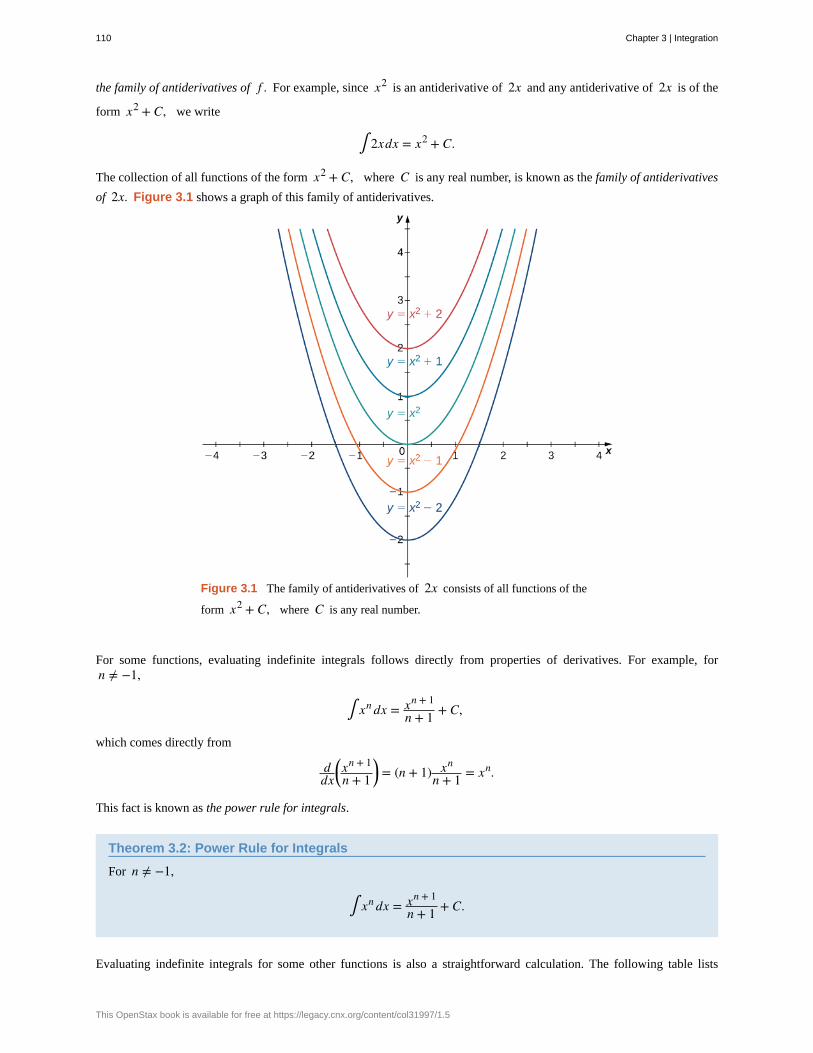
the family of antiderivatives of f . For example, since x2 is an antiderivative of 2x and any antiderivative of 2x is of the
form x2 + C, we write
∫ 2xdx = x2 + C.
The collection of all functions of the form x2 + C, where C is any real number, is known as the family of antiderivatives
of 2x. Figure 3.1 shows a graph of this family of antiderivatives.
Figure 3.1 The family of antiderivatives of 2x consists of all functions of the
form x2 + C, where C is any real number.
For some functions, evaluating indefinite integrals follows directly from properties of derivatives. For example, forn ≠ −1,
∫ xndx = xn + 1
n + 1 + C,
which comes directly from
ddx⎛⎝x
n + 1
n + 1⎞⎠ = (n + 1) xn
n + 1 = xn.
This fact is known as the power rule for integrals.
Theorem 3.2: Power Rule for Integrals
For n ≠ −1,
∫ xndx = xn + 1
n + 1 + C.
Evaluating indefinite integrals for some other functions is also a straightforward calculation. The following table lists
110 Chapter 3 | Integration
This OpenStax book is available for free at https://legacy.cnx.org/content/col31997/1.5
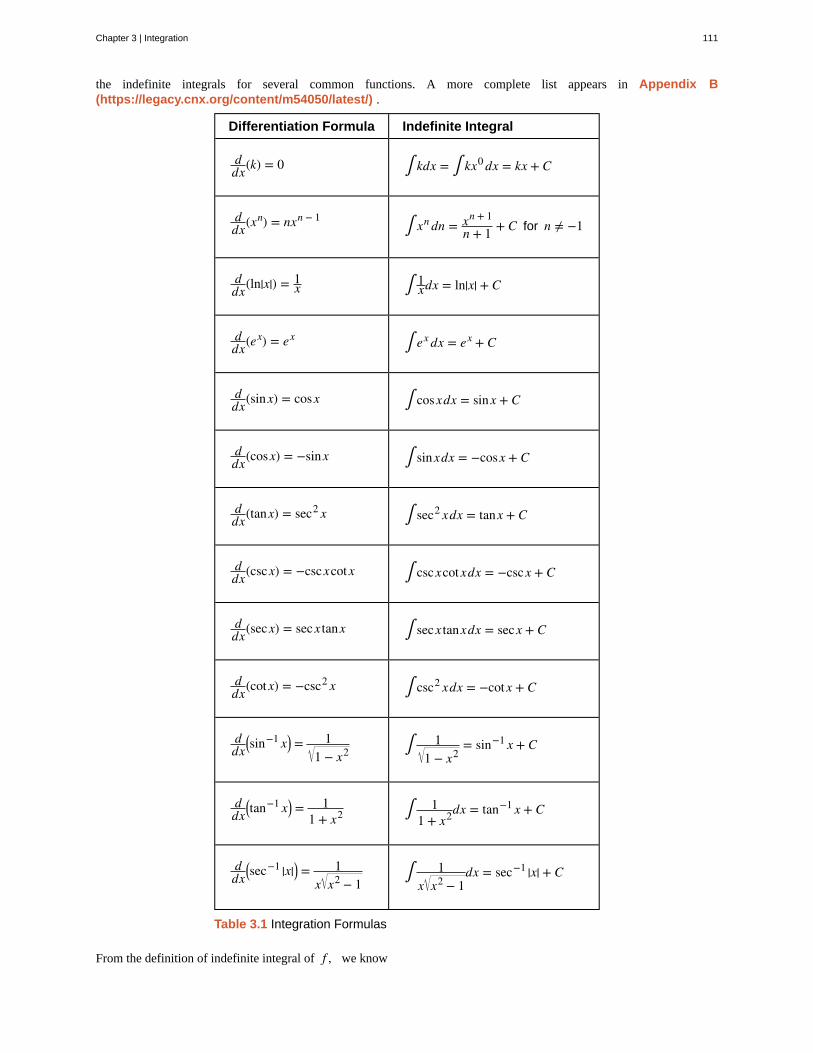
the indefinite integrals for several common functions. A more complete list appears in Appendix B(https://legacy.cnx.org/content/m54050/latest/) .
Differentiation Formula Indefinite Integral
ddx(k) = 0 ∫ kdx = ∫ kx0dx = kx + C
ddx(xn) = nxn − 1 ∫ xndn = xn + 1
n + 1 + C for n ≠ −1
ddx(ln|x|) = 1
x ∫ 1xdx = ln|x| + C
ddx(ex) = ex ∫ ex dx = ex + C
ddx(sinx) = cosx ∫ cosxdx = sinx + C
ddx(cosx) = −sinx ∫ sinxdx = −cosx + C
ddx(tanx) = sec2 x ∫ sec2 xdx = tanx + C
ddx(cscx) = −cscxcotx ∫ cscxcotxdx = −cscx + C
ddx(secx) = secx tanx ∫ secx tanxdx = secx + C
ddx(cotx) = −csc2 x ∫ csc2 xdx = −cotx + C
ddx⎛⎝sin−1 x⎞⎠ = 1
1 − x2 ∫ 11 − x2
= sin−1 x + C
ddx⎛⎝tan−1 x⎞⎠ = 1
1 + x2 ∫ 11 + x2dx = tan−1 x + C
ddx⎛⎝sec−1 |x|⎞⎠ = 1
x x2 − 1∫ 1x x2 − 1
dx = sec−1 |x| + C
Table 3.1 Integration Formulas
From the definition of indefinite integral of f , we know
Chapter 3 | Integration 111

∫ f (x)dx = F(x) + C
if and only if F is an antiderivative of f . Therefore, when claiming that
∫ f (x)dx = F(x) + C
it is important to check whether this statement is correct by verifying that F′ (x) = f (x).
Example 3.2
Verifying an Indefinite Integral
Each of the following statements is of the form ∫ f (x)dx = F(x) + C. Verify that each statement is correct by
showing that F′ (x) = f (x).
a. ∫ (x + ex)dx = x2
2 + ex + C
b. ∫ xex dx = xex − ex + C
Solution
a. Since
ddx⎛⎝x
2
2 + ex + C⎞⎠ = x + ex,
the statement
∫ (x + ex)dx = x2
2 + ex + C
is correct.
Note that we are verifying an indefinite integral for a sum. Furthermore, x2
2 and ex are antiderivatives
of x and ex, respectively, and the sum of the antiderivatives is an antiderivative of the sum. We discuss
this fact again later in this section.
b. Using the product rule, we see that
ddx(xex − ex + C) = ex + xex − ex = xex.
Therefore, the statement
∫ xex dx = xex − ex + C
is correct.Note that we are verifying an indefinite integral for a product. The antiderivative xex − ex is not
a product of the antiderivatives. Furthermore, the product of antiderivatives, x2 ex /2 is not an
antiderivative of xex since
ddx⎛⎝x
2 ex2⎞⎠ = xex + x2 ex
2 ≠ xex.
112 Chapter 3 | Integration
This OpenStax book is available for free at https://legacy.cnx.org/content/col31997/1.5
3.2
In general, the product of antiderivatives is not an antiderivative of a product.
Verify that ∫ xcosxdx = xsinx + cosx + C.
In Table 3.1, we listed the indefinite integrals for many elementary functions. Let’s now turn our attention to evaluatingindefinite integrals for more complicated functions. For example, consider finding an antiderivative of a sum f + g.
In Example 3.2a. we showed that an antiderivative of the sum x + ex is given by the sum⎛⎝x
2
2⎞⎠+ ex —that is, an
antiderivative of a sum is given by a sum of antiderivatives. This result was not specific to this example. In general, if Fand G are antiderivatives of any functions f and g, respectively, then
ddx(F(x) + G(x)) = F′ (x) + G′ (x) = f (x) + g(x).
Therefore, F(x) + G(x) is an antiderivative of f (x) + g(x) and we have
∫ ⎛⎝ f (x) + g(x)⎞⎠dx = F(x) + G(x) + C.
Similarly,
∫ ⎛⎝ f (x) − g(x)⎞⎠dx = F(x) − G(x) + C.
In addition, consider the task of finding an antiderivative of k f (x), where k is any real number. Since
ddx⎛⎝k f (x)⎞⎠ = k d
dxF(x) = k f ′ (x)
for any real number k, we conclude that
∫ k f (x)dx = kF(x) + C.
These properties are summarized next.
Theorem 3.3: Properties of Indefinite Integrals
Let F and G be antiderivatives of f and g, respectively, and let k be any real number.
Sums and Differences
∫ ⎛⎝ f (x)±g(x)⎞⎠dx = F(x)±G(x) + C
Constant Multiples
∫ k f (x)dx = kF(x) + C
From this theorem, we can evaluate any integral involving a sum, difference, or constant multiple of functions withantiderivatives that are known. Evaluating integrals involving products, quotients, or compositions is more complicated (seeExample 3.2b. for an example involving an antiderivative of a product.) We look at and address integrals involving thesemore complicated functions in Introduction to Integration (https://legacy.cnx.org/content/m53623/latest/) . Inthe next example, we examine how to use this theorem to calculate the indefinite integrals of several functions.
Chapter 3 | Integration 113
Example 3.3
Evaluating Indefinite Integrals
Evaluate each of the following indefinite integrals:
a. ∫ ⎛⎝5x3 − 7x2 + 3x + 4⎞⎠dx
b. ∫ x2 + 4 x3x dx
c. ∫ 41 + x2dx
d. ∫ tanxcosxdx
Solution
a. Using Properties of Indefinite Integrals, we can integrate each of the four terms in the integrandseparately. We obtain
∫ ⎛⎝5x3 − 7x2 + 3x + 4⎞⎠dx = ∫ 5x3dx − ∫ 7x2dx + ∫ 3xdx + ∫ 4dx.
From the second part of Properties of Indefinite Integrals, each coefficient can be written in front ofthe integral sign, which gives
∫ 5x3dx − ∫ 7x2dx + ∫ 3xdx + ∫ 4dx = 5∫ x3dx − 7∫ x2dx + 3∫ xdx + 4∫ 1dx.
Using the power rule for integrals, we conclude that
∫ ⎛⎝5x3 − 7x2 + 3x + 4⎞⎠dx = 54x
4 − 73x
3 + 32x
2 + 4x + C.
b. Rewrite the integrand as
x2 + 4 x3x = x2
x + 4 x3x = 0.
Then, to evaluate the integral, integrate each of these terms separately. Using the power rule, we have
∫ ⎛⎝x + 4x2/3⎞⎠dx = ∫ xdx + 4∫ x−2/3dx
= 12x
2 + 4 1⎛⎝−2
3⎞⎠+ 1
x(−2/3) + 1 + C
= 12x
2 + 12x1/3 + C.
c. Using Properties of Indefinite Integrals, write the integral as
4∫ 11 + x2dx.
Then, use the fact that tan−1 (x) is an antiderivative of 1⎛⎝1 + x2⎞⎠
to conclude that
∫ 41 + x2dx = 4tan−1 (x) + C.
d. Rewrite the integrand as
114 Chapter 3 | Integration
This OpenStax book is available for free at https://legacy.cnx.org/content/col31997/1.5

3.3
tanxcosx = sinxcosx cosx = sinx.
Therefore,
∫ tanxcosx = ∫ sinx = −cosx + C.
Evaluate ∫ ⎛⎝4x3 − 5x2 + x − 7⎞⎠dx.
Initial-Value ProblemsWe look at techniques for integrating a large variety of functions involving products, quotients, and compositions later inthe text. Here we turn to one common use for antiderivatives that arises often in many applications: solving differentialequations.
A differential equation is an equation that relates an unknown function and one or more of its derivatives. The equation
(3.1)dydx = f (x)
is a simple example of a differential equation. Solving this equation means finding a function y with a derivative f .Therefore, the solutions of Equation 3.1 are the antiderivatives of f . If F is one antiderivative of f , every function of
the form y = F(x) + C is a solution of that differential equation. For example, the solutions of
dydx = 6x2
are given by
y = ∫ 6x2dx = 2x3 + C.
Sometimes we are interested in determining whether a particular solution curve passes through a certain point (x0, y0)—that is, y(x0) = y0. The problem of finding a function y that satisfies a differential equation
(3.2)dydx = f (x)
with the additional condition
(3.3)y(x0) = y0
is an example of an initial-value problem. The condition y(x0) = y0 is known as an initial condition. For example,
looking for a function y that satisfies the differential equation
dydx = 6x2
and the initial condition
y(1) = 5
is an example of an initial-value problem. Since the solutions of the differential equation are y = 2x3 + C, to find a
function y that also satisfies the initial condition, we need to find C such that y(1) = 2(1)3 + C = 5. From this equation,
we see that C = 3, and we conclude that y = 2x3 + 3 is the solution of this initial-value problem as shown in the
Chapter 3 | Integration 115
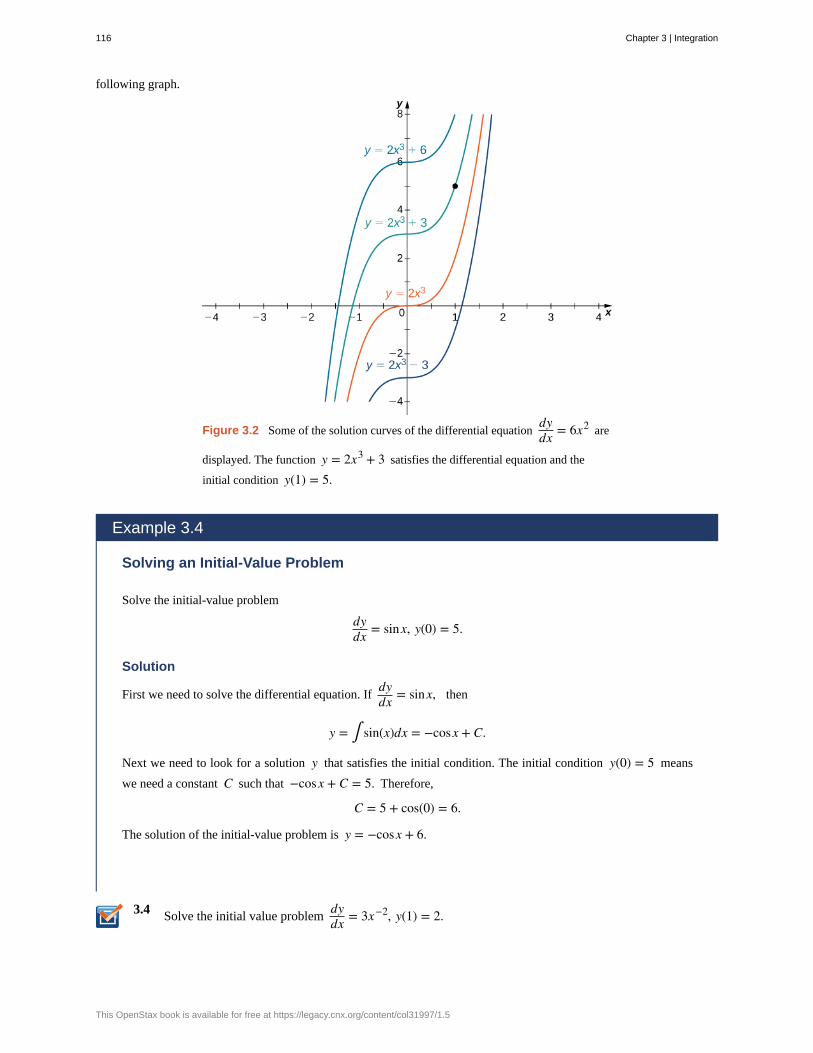
3.4
following graph.
Figure 3.2 Some of the solution curves of the differential equationdydx = 6x2 are
displayed. The function y = 2x3 + 3 satisfies the differential equation and the
initial condition y(1) = 5.
Example 3.4
Solving an Initial-Value Problem
Solve the initial-value problem
dydx = sinx, y(0) = 5.
Solution
First we need to solve the differential equation. Ifdydx = sinx, then
y = ∫ sin(x)dx = −cosx + C.
Next we need to look for a solution y that satisfies the initial condition. The initial condition y(0) = 5 means
we need a constant C such that −cosx + C = 5. Therefore,
C = 5 + cos(0) = 6.
The solution of the initial-value problem is y = −cosx + 6.
Solve the initial value problemdydx = 3x−2, y(1) = 2.
116 Chapter 3 | Integration
This OpenStax book is available for free at https://legacy.cnx.org/content/col31997/1.5

Initial-value problems arise in many applications. Next we consider a problem in which a driver applies the brakes in a car.We are interested in how long it takes for the car to stop. Recall that the velocity function v(t) is the derivative of a position
function s(t), and the acceleration a(t) is the derivative of the velocity function. In earlier examples in the text, we could
calculate the velocity from the position and then compute the acceleration from the velocity. In the next example we workthe other way around. Given an acceleration function, we calculate the velocity function. We then use the velocity functionto determine the position function.
Example 3.5
Decelerating Car
A car is traveling at the rate of 88 ft/sec (60 mph) when the brakes are applied. The car begins decelerating at a
constant rate of 15 ft/sec2.
a. How many seconds elapse before the car stops?
b. How far does the car travel during that time?
Solution
a. First we introduce variables for this problem. Let t be the time (in seconds) after the brakes are first
applied. Let a(t) be the acceleration of the car (in feet per seconds squared) at time t. Let v(t) be the
velocity of the car (in feet per second) at time t. Let s(t) be the car’s position (in feet) beyond the point
where the brakes are applied at time t.The car is traveling at a rate of 88 ft/sec. Therefore, the initial velocity is v(0) = 88 ft/sec. Since the car
is decelerating, the acceleration is
a(t) = −15 ft/s2.
The acceleration is the derivative of the velocity,
v′ (t) = −15.
Therefore, we have an initial-value problem to solve:
v′ (t) = −15, v(0) = 88.
Integrating, we find that
v(t) = −15t + C.
Since v(0) = 88, C = 88. Thus, the velocity function is
v(t) = −15t + 88.
To find how long it takes for the car to stop, we need to find the time t such that the velocity is zero.
Solving −15t + 88 = 0, we obtain t = 8815 sec.
b. To find how far the car travels during this time, we need to find the position of the car after 8815 sec. We
know the velocity v(t) is the derivative of the position s(t). Consider the initial position to be s(0) = 0.Therefore, we need to solve the initial-value problem
s′ (t) = −15t + 88, s(0) = 0.
Chapter 3 | Integration 117

3.5
Integrating, we have
s(t) = − 152 t2 + 88t + C.
Since s(0) = 0, the constant is C = 0. Therefore, the position function is
s(t) = − 152 t2 + 88t.
After t = 8815 sec, the position is s⎛⎝88
15⎞⎠ ≈ 258.133 ft.
Suppose the car is traveling at the rate of 44 ft/sec. How long does it take for the car to stop? How far
will the car travel?
Key Concepts• If F is an antiderivative of f , then every antiderivative of f is of the form F(x) + C for some constant C.
• Solving the initial-value problem
dydx = f (x), y(x0) = y0
requires us first to find the set of antiderivatives of f and then to look for the particular antiderivative that also
satisfies the initial condition.
118 Chapter 3 | Integration
This OpenStax book is available for free at https://legacy.cnx.org/content/col31997/1.5
3.1 EXERCISESFor the following exercises, show that F(x) are
antiderivatives of f (x).
1. F(x) = 5x3 + 2x2 + 3x + 1, f (x) = 15x2 + 4x + 3
2. F(x) = x2 + 4x + 1, f (x) = 2x + 4
3. F(x) = x2 ex, f (x) = ex ⎛⎝x2 + 2x⎞⎠
4. F(x) = cosx, f (x) = −sinx
5. F(x) = ex, f (x) = ex
For the following exercises, find the antiderivative of thefunction.
6. f (x) = 1x2 + x
7. f (x) = ex − 3x2 + sinx
8. f (x) = ex + 3x − x2
9. f (x) = x − 1 + 4sin(2x)
For the following exercises, find the antiderivative F(x) of
each function f (x).
10. f (x) = 5x4 + 4x5
11. f (x) = x + 12x2
12. f (x) = 1x
13. f (x) = ( x)3
14. f (x) = x1/3 + (2x)1/3
15. f (x) = x1/3
x2/3
16. f (x) = 2sin(x) + sin(2x)
17. f (x) = sec2 (x) + 1
18. f (x) = sinxcosx
19. f (x) = sin2 (x)cos(x)
20. f (x) = 0
21. f (x) = 12csc2 (x) + 1
x2
22. f (x) = cscxcotx + 3x
23. f (x) = 4cscxcotx − secx tanx
24. f (x) = 8secx(secx − 4tanx)
25. f (x) = 12e
−4x + sinx
For the following exercises, evaluate the integral.
26. ∫ (−1)dx
27. ∫ sinxdx
28. ∫ (4x + x)dx
29. ∫ 3x2 + 2x2 dx
30. ∫ (secx tanx + 4x)dx
31. ∫ ⎛⎝4 x + x4 ⎞⎠dx
32. ∫ ⎛⎝x−1/3 − x2/3⎞⎠dx
33. ∫ 14x3 + 2x + 1x3 dx
34. ∫ (ex + e−x)dx
For the following exercises, solve the initial value problem.
35. f ′ (x) = x−3, f (1) = 1
36. f ′ (x) = x + x2, f (0) = 2
37. f ′ (x) = cosx + sec2 (x), f ⎛⎝π4⎞⎠ = 2 + 2
2
38. f ′ (x) = x3 − 8x2 + 16x + 1, f (0) = 0
Chapter 3 | Integration 119

39. f ′ (x) = 2x2 − x2
2 , f (1) = 0
For the following exercises, find two possible functions fgiven the second- or third-order derivatives.
40. f ″(x) = x2 + 2
41. f ″(x) = e−x
42. f ″(x) = 1 + x
43. f‴(x) = cosx
44. f‴(x) = 8e−2x − sinx
45. A car is being driven at a rate of 40 mph when the
brakes are applied. The car decelerates at a constant rate of10 ft/sec2. How long before the car stops?
46. In the preceding problem, calculate how far the cartravels in the time it takes to stop.
47. You are merging onto the freeway, accelerating at aconstant rate of 12 ft/sec2. How long does it take you to
reach merging speed at 60 mph?
48. Based on the previous problem, how far does the cartravel to reach merging speed?
49. A car company wants to ensure its newest model canstop in 8 sec when traveling at 75 mph. If we assume
constant deceleration, find the value of deceleration thataccomplishes this.
50. A car company wants to ensure its newest model canstop in less than 450 ft when traveling at 60 mph. If we
assume constant deceleration, find the value of decelerationthat accomplishes this.
For the following exercises, find the antiderivative of thefunction, assuming F(0) = 0.
51. [T] f (x) = x2 + 2
52. [T] f (x) = 4x − x
53. [T] f (x) = sinx + 2x
54. [T] f (x) = ex
55. [T] f (x) = 1(x + 1)2
56. [T] f (x) = e−2x + 3x2
For the following exercises, determine whether thestatement is true or false. Either prove it is true or find acounterexample if it is false.
57. If f (x) is the antiderivative of v(x), then 2 f (x) is
the antiderivative of 2v(x).
58. If f (x) is the antiderivative of v(x), then f (2x) is
the antiderivative of v(2x).
59. If f (x) is the antiderivative of v(x), then f (x) + 1is the antiderivative of v(x) + 1.
60. If f (x) is the antiderivative of v(x), then ⎛⎝ f (x)⎞⎠2 is
the antiderivative of (v(x))2.
120 Chapter 3 | Integration
This OpenStax book is available for free at https://legacy.cnx.org/content/col31997/1.5

Chapter Review ExercisesTrue or False? Justify your answer with a proof or a counterexample. Assume that f (x) is continuous and differentiable
unless stated otherwise.
Exercise 3.61
If f (−1) = −6 and f (1) = 2, then there exists at least one point x ∈ [−1, 1] such that f ′ (x) = 4.
SolutionTrue, by Mean Value Theorem
Exercise 3.62
If f ′ (c) = 0, there is a maximum or minimum at x = c.
Exercise 3.63
There is a function such that f (x) < 0, f ′ (x) > 0, and f ″(x) < 0. (A graphical “proof” is acceptable for this answer.)
SolutionTrue
Exercise 3.64
There is a function such that there is both an inflection point and a critical point for some value x = a.
Exercise 3.65
Given the graph of f ′, determine where f is increasing or decreasing.
SolutionIncreasing: (−2, 0) ∪ (4, ∞), decreasing: (−∞, −2) ∪ (0, 4)
Exercise 3.66
The graph of f is given below. Draw f ′.
Exercise 3.67
Chapter 3 | Integration 121
Find the linear approximation L(x) to y = x2 + tan(πx) near x = 14.
Solution
L(x) = 1716 + 1
2(1 + 4π)⎛⎝x − 14⎞⎠
Exercise 3.68
Find the differential of y = x2 − 5x − 6 and evaluate for x = 2 with dx = 0.1.
Find the critical points and the local and absolute extrema of the following functions on the given interval.
Exercise 3.69
f (x) = x + sin2 (x) over [0, π]
Solution
Critical point: x = 3π4 , absolute minimum: x = 0, absolute maximum: x = π
Exercise 3.70
f (x) = 3x4 − 4x3 − 12x2 + 6 over [−3, 3]
Determine over which intervals the following functions are increasing, decreasing, concave up, and concave down.
Exercise 3.71
x(t) = 3t4 − 8t3 − 18t2
Solution
Increasing: (−1, 0) ∪ (3, ∞), decreasing: (−∞, −1) ∪ (0, 3), concave up: ⎛⎝−∞, 13⎛⎝2 − 13⎞⎠
⎞⎠ ∪ ⎛⎝13
⎛⎝2 + 13⎞⎠, ∞⎞⎠,
concave down: ⎛⎝13⎛⎝2 − 13⎞⎠, 1
3⎛⎝2 + 13⎞⎠
⎞⎠
Exercise 3.72
y = x + sin(πx)
Exercise 3.73
g(x) = x − x
Solution
Increasing: ⎛⎝14, ∞⎞⎠, decreasing: ⎛⎝0, 14⎞⎠, concave up: (0, ∞), concave down: nowhere
Exercise 3.74
f (θ) = sin(3θ)
Evaluate the following limits.
Exercise 3.75
limx → ∞3x x2 + 1
x4 − 1
Solution3
122 Chapter 3 | Integration
This OpenStax book is available for free at https://legacy.cnx.org/content/col31997/1.5
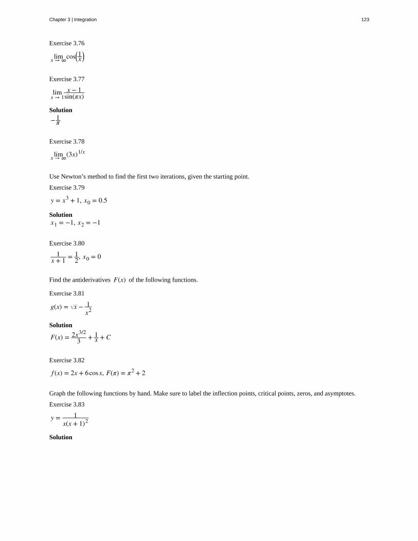
Exercise 3.76
limx → ∞cos⎛⎝1x⎞⎠
Exercise 3.77
limx → 1
x − 1sin(πx)
Solution
− 1π
Exercise 3.78
limx → ∞(3x)1/x
Use Newton’s method to find the first two iterations, given the starting point.
Exercise 3.79
y = x3 + 1, x0 = 0.5
Solutionx1 = −1, x2 = −1
Exercise 3.80
1x + 1 = 1
2, x0 = 0
Find the antiderivatives F(x) of the following functions.
Exercise 3.81
g(x) = x − 1x2
Solution
F(x) = 2x3/2
3 + 1x + C
Exercise 3.82
f (x) = 2x + 6cosx, F(π) = π2 + 2
Graph the following functions by hand. Make sure to label the inflection points, critical points, zeros, and asymptotes.
Exercise 3.83
y = 1x(x + 1)2
Solution
Chapter 3 | Integration 123
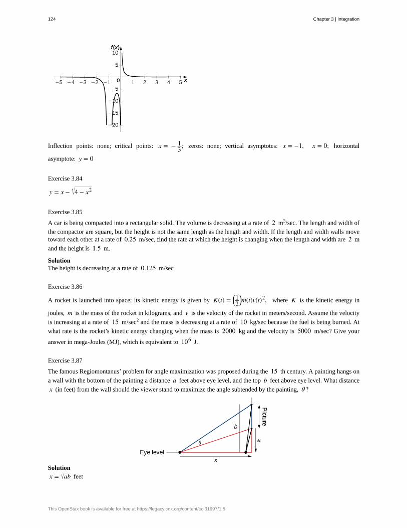
Inflection points: none; critical points: x = − 13; zeros: none; vertical asymptotes: x = −1, x = 0; horizontal
asymptote: y = 0
Exercise 3.84
y = x − 4 − x2
Exercise 3.85
A car is being compacted into a rectangular solid. The volume is decreasing at a rate of 2 m3/sec. The length and width of
the compactor are square, but the height is not the same length as the length and width. If the length and width walls movetoward each other at a rate of 0.25 m/sec, find the rate at which the height is changing when the length and width are 2 m
and the height is 1.5 m.
SolutionThe height is decreasing at a rate of 0.125 m/sec
Exercise 3.86
A rocket is launched into space; its kinetic energy is given by K(t) = ⎛⎝12⎞⎠m(t)v(t)2, where K is the kinetic energy in
joules, m is the mass of the rocket in kilograms, and v is the velocity of the rocket in meters/second. Assume the velocity
is increasing at a rate of 15 m/sec2 and the mass is decreasing at a rate of 10 kg/sec because the fuel is being burned. At
what rate is the rocket’s kinetic energy changing when the mass is 2000 kg and the velocity is 5000 m/sec? Give your
answer in mega-Joules (MJ), which is equivalent to 106 J.
Exercise 3.87
The famous Regiomontanus’ problem for angle maximization was proposed during the 15 th century. A painting hangs on
a wall with the bottom of the painting a distance a feet above eye level, and the top b feet above eye level. What distance
x (in feet) from the wall should the viewer stand to maximize the angle subtended by the painting, θ?
Solutionx = ab feet
124 Chapter 3 | Integration
This OpenStax book is available for free at https://legacy.cnx.org/content/col31997/1.5
3.6
Exercise 3.88
An airline sells tickets from Tokyo to Detroit for $1200. There are 500 seats available and a typical flight books 350seats. For every $10 decrease in price, the airline observes an additional five seats sold. What should the fare be to
maximize profit? How many passengers would be onboard?
3.2 | Integrals Involving Exponential and Logarithmic
Functions
Learning Objectives3.2.1 Integrate functions involving exponential functions.
3.2.2 Integrate functions involving logarithmic functions.
Exponential and logarithmic functions are used to model population growth, cell growth, and financial growth, as well asdepreciation, radioactive decay, and resource consumption, to name only a few applications. In this section, we exploreintegration involving exponential and logarithmic functions.
Integrals of Exponential FunctionsThe exponential function is perhaps the most efficient function in terms of the operations of calculus. The exponentialfunction, y = ex, is its own derivative and its own integral.
Rule: Integrals of Exponential Functions
Exponential functions can be integrated using the following formulas.
(3.4)∫ ex dx = ex + C
∫ ax dx = axlna + C
Example 3.6
Finding an Antiderivative of an Exponential Function
Find the antiderivative of the exponential function e−x.
Solution
Use substitution, setting u = −x, and then du = −1dx. Multiply the du equation by −1, so you now have
−du = dx. Then,
∫ e−xdx = −∫ eudu
= −eu + C= −e−x + C.
Find the antiderivative of the function using substitution: x2 e−2x3.
A common mistake when dealing with exponential expressions is treating the exponent on e the same way we treat
Chapter 3 | Integration 125
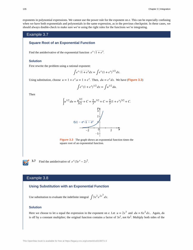
3.7
exponents in polynomial expressions. We cannot use the power rule for the exponent on e. This can be especially confusingwhen we have both exponentials and polynomials in the same expression, as in the previous checkpoint. In these cases, weshould always double-check to make sure we’re using the right rules for the functions we’re integrating.
Example 3.7
Square Root of an Exponential Function
Find the antiderivative of the exponential function ex 1 + ex.
Solution
First rewrite the problem using a rational exponent:
∫ ex 1 + exdx = ∫ ex (1 + ex)1/2dx.
Using substitution, choose u = 1 + ex.u = 1 + ex. Then, du = ex dx. We have (Figure 3.3)
∫ ex (1 + ex)1/2dx = ∫ u1/2du.
Then
⌠⌡u
1/2du = u3/2
3/2 + C = 23u
3/2 + C = 23(1 + ex)3/2 + C.
Figure 3.3 The graph shows an exponential function times thesquare root of an exponential function.
Find the antiderivative of ex (3ex − 2)2.
Example 3.8
Using Substitution with an Exponential Function
Use substitution to evaluate the indefinite integral ∫ 3x2 e2x3dx.
Solution
Here we choose to let u equal the expression in the exponent on e. Let u = 2x3 and du = 6x2dx.. Again, du
is off by a constant multiplier; the original function contains a factor of 3x2, not 6x2. Multiply both sides of the
126 Chapter 3 | Integration
This OpenStax book is available for free at https://legacy.cnx.org/content/col31997/1.5

3.8
equation by 12 so that the integrand in u equals the integrand in x. Thus,
∫ 3x2 e2x3dx = 1
2∫ eudu.
Integrate the expression in u and then substitute the original expression in x back into the u integral:
12∫ eudu = 1
2eu + C = 1
2e2x3
+ C.
Evaluate the indefinite integral ∫ 2x3 ex4dx.
As mentioned at the beginning of this section, exponential functions are used in many real-life applications. The number e isoften associated with compounded or accelerating growth, as we have seen in earlier sections about the derivative. Althoughthe derivative represents a rate of change or a growth rate, the integral represents the total change or the total growth. Let’slook at an example in which integration of an exponential function solves a common business application.
A price–demand function tells us the relationship between the quantity of a product demanded and the price of the product.In general, price decreases as quantity demanded increases. The marginal price–demand function is the derivative of theprice–demand function and it tells us how fast the price changes at a given level of production. These functions are used inbusiness to determine the price–elasticity of demand, and to help companies determine whether changing production levelswould be profitable.
Example 3.9
Finding a Price–Demand Equation
Find the price–demand equation for a particular brand of toothpaste at a supermarket chain when the demand is50 tubes per week at $2.35 per tube, given that the marginal price—demand function, p′ (x), for x number of
tubes per week, is given as
p '(x) = −0.015e−0.01x.
If the supermarket chain sells 100 tubes per week, what price should it set?
Solution
To find the price–demand equation, integrate the marginal price–demand function. First find the antiderivative,then look at the particulars. Thus,
p(x) = ∫ −0.015e−0.01x dx
= −0.015∫ e−0.01xdx.
Using substitution, let u = −0.01x and du = −0.01dx. Then, divide both sides of the du equation by −0.01.
This gives
Chapter 3 | Integration 127
−0.015−0.01 ∫ eudu = 1.5∫ eudu
= 1.5eu + C= 1.5e−0.01x + C.
The next step is to solve for C. We know that when the price is $2.35 per tube, the demand is 50 tubes per week.This means
p(50) = 1.5e−0.01(50) + C
= 2.35.
Now, just solve for C:
C = 2.35 − 1.5e−0.5
= 2.35 − 0.91= 1.44.
Thus,
p(x) = 1.5e−0.01x + 1.44.
If the supermarket sells 100 tubes of toothpaste per week, the price would be
p(100) = 1.5e−0.01(100) + 1.44 = 1.5e−1 + 1.44 ≈ 1.99.
The supermarket should charge $1.99 per tube if it is selling 100 tubes per week.
Example 3.10
Evaluating a Definite Integral Involving an Exponential Function
Evaluate the definite integral ∫1
2e1 − x dx.
Solution
Again, substitution is the method to use. Let u = 1 − x, so du = −1dx or −du = dx. Then
∫ e1 − x dx = −∫ eudu. Next, change the limits of integration. Using the equation u = 1 − x, we have
u = 1 − (1) = 0u = 1 − (2) = −1.
The integral then becomes
128 Chapter 3 | Integration
This OpenStax book is available for free at https://legacy.cnx.org/content/col31997/1.5
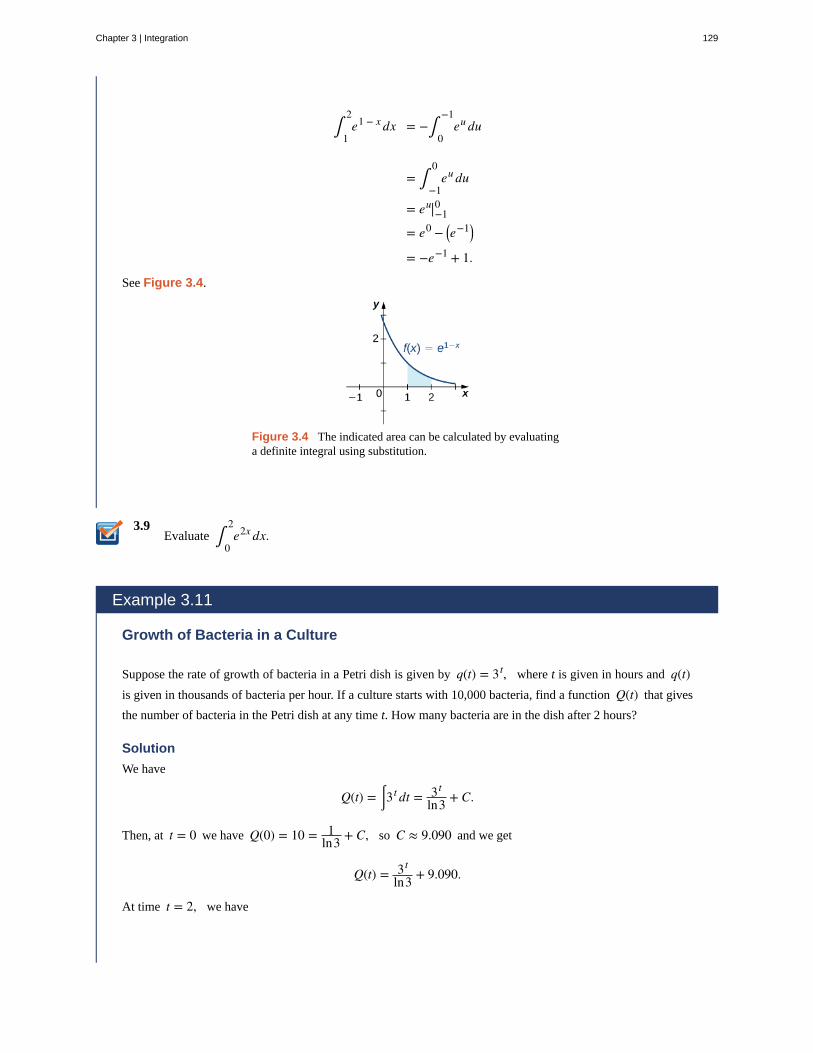
3.9
∫1
2e1 − x dx = −∫
0
−1eudu
= ∫−1
0eudu
= eu|−10
= e0 − ⎛⎝e−1⎞⎠= −e−1 + 1.
See Figure 3.4.
Figure 3.4 The indicated area can be calculated by evaluatinga definite integral using substitution.
Evaluate ∫0
2e2x dx.
Example 3.11
Growth of Bacteria in a Culture
Suppose the rate of growth of bacteria in a Petri dish is given by q(t) = 3t, where t is given in hours and q(t)is given in thousands of bacteria per hour. If a culture starts with 10,000 bacteria, find a function Q(t) that gives
the number of bacteria in the Petri dish at any time t. How many bacteria are in the dish after 2 hours?
Solution
We have
Q(t) = ⌠⌡3t dt = 3t
ln3 + C.
Then, at t = 0 we have Q(0) = 10 = 1ln3 + C, so C ≈ 9.090 and we get
Q(t) = 3t
ln3 + 9.090.
At time t = 2, we have
Chapter 3 | Integration 129

3.10
3.11
Q(2) = 32
ln3 + 9.090
= 17.282.
After 2 hours, there are 17,282 bacteria in the dish.
From Example 3.11, suppose the bacteria grow at a rate of q(t) = 2t. Assume the culture still starts
with 10,000 bacteria. Find Q(t). How many bacteria are in the dish after 3 hours?
Example 3.12
Fruit Fly Population Growth
Suppose a population of fruit flies increases at a rate of g(t) = 2e0.02t, in flies per day. If the initial population
of fruit flies is 100 flies, how many flies are in the population after 10 days?
Solution
Let G(t) represent the number of flies in the population at time t. Applying the net change theorem, we have
G(10) = G(0) + ∫0
102e0.02t dt
= 100 + ⎡⎣ 20.02e
0.02t⎤⎦|010
= 100 + ⎡⎣100e0.02t⎤⎦|010
= 100 + 100e0.2 − 100≈ 122.
There are 122 flies in the population after 10 days.
Suppose the rate of growth of the fly population is given by g(t) = e0.01t, and the initial fly population
is 100 flies. How many flies are in the population after 15 days?
Example 3.13
Evaluating a Definite Integral Using Substitution
Evaluate the definite integral using substitution: ⌠⌡1
2e1/x
x2 dx.
130 Chapter 3 | Integration
This OpenStax book is available for free at https://legacy.cnx.org/content/col31997/1.5
3.12
Solution
This problem requires some rewriting to simplify applying the properties. First, rewrite the exponent on e as apower of x, then bring the x2 in the denominator up to the numerator using a negative exponent. We have
⌠⌡1
2e1/x
x2 dx = ∫1
2ex
−1x−2dx.
Let u = x−1, the exponent on e. Then
du = −x−2dx−du = x−2dx.
Bringing the negative sign outside the integral sign, the problem now reads
−∫ eudu.
Next, change the limits of integration:
u = (1)−1 = 1u = (2)−1 = 1
2.
Notice that now the limits begin with the larger number, meaning we must multiply by −1 and interchange thelimits. Thus,
−∫1
1/2eudu = ∫
1/2
1eudu
= eu |1/21
= e − e1/2
= e − e.
Evaluate the definite integral using substitution: ⌠⌡1
21x3e
4x−2dx.
Integrals Involving Logarithmic FunctionsIntegrating functions of the form f (x) = x−1 result in the absolute value of the natural log function, as shown in the
following rule. Integral formulas for other logarithmic functions, such as f (x) = lnx and f (x) = loga x, are also included
in the rule.
Rule: Integration Formulas Involving Logarithmic Functions
The following formulas can be used to evaluate integrals involving logarithmic functions.
Chapter 3 | Integration 131

3.13
(3.5)∫ x−1dx = ln|x| + C
∫ lnx dx = x lnx − x + C = x(lnx − 1) + C
∫ logax dx = xlna(lnx − 1) + C
Example 3.14
Finding an Antiderivative Involving ln x
Find the antiderivative of the function 3x − 10.
Solution
First factor the 3 outside the integral symbol. Then use the u−1 rule. Thus,
⌠⌡
3x − 10dx = 3⌠⌡
1x − 10dx
= 3∫ duu
= 3ln|u| + C= 3ln|x − 10| + C, x ≠ 10.
See Figure 3.5.
Figure 3.5 The domain of this function is x ≠ 10.
Find the antiderivative of 1x + 2.
Example 3.15
Finding an Antiderivative of a Rational Function
Find the antiderivative of 2x3 + 3xx4 + 3x2 .
132 Chapter 3 | Integration
This OpenStax book is available for free at https://legacy.cnx.org/content/col31997/1.5
3.14
Solution
This can be rewritten as ⌠⌡⎛⎝2x3 + 3x⎞⎠
⎛⎝x4 + 3x2⎞⎠
−1dx. Use substitution. Let u = x4 + 3x2, then
du = 4x3 + 6x. Alter du by factoring out the 2. Thus,
du = ⎛⎝4x3 + 6x⎞⎠dx
= 2⎛⎝2x3 + 3x⎞⎠dx12 du = ⎛
⎝2x3 + 3x⎞⎠dx.
Rewrite the integrand in u:
⌠⌡⎛⎝2x3 + 3x⎞⎠
⎛⎝x4 + 3x2⎞⎠
−1dx = 1
2∫ u−1du.
Then we have
12∫ u−1du = 1
2ln|u| + C
= 12ln|x4 + 3x2| + C.
Example 3.16
Finding an Antiderivative of a Logarithmic Function
Find the antiderivative of the log function log2 x.
Solution
Follow the format in the formula listed in the rule on integration formulas involving logarithmic functions. Basedon this format, we have
∫ log2 xdx = xln2(lnx − 1) + C.
Find the antiderivative of log3 x.
Example 3.17 is a definite integral of a trigonometric function. With trigonometric functions, we often have to apply atrigonometric property or an identity before we can move forward. Finding the right form of the integrand is usually the keyto a smooth integration.
Example 3.17
Evaluating a Definite Integral
Chapter 3 | Integration 133
Find the definite integral of ⌠⌡0
π/2sinx
1 + cosxdx.
Solution
We need substitution to evaluate this problem. Let u = 1 + cosx, , so du = −sinx dx. Rewrite the integral in
terms of u, changing the limits of integration as well. Thus,
u = 1 + cos(0) = 2u = 1 + cos⎛⎝π2
⎞⎠ = 1.
Then
⌠⌡0
π/2sinx
1 + cosx = −∫2
1u−1du
= ∫1
2u−1du
= ln|u||12= [ln2 − ln1]= ln2.
Key Concepts• Exponential and logarithmic functions arise in many real-world applications, especially those involving growth and
decay.
• Substitution is often used to evaluate integrals involving exponential functions or logarithms.
Key Equations• Integrals of Exponential Functions
∫ ex dx = ex + C
⌠⌡a
x dx = axlna + C
• Integration Formulas Involving Logarithmic Functions
∫ x−1dx = ln|x| + C
∫ lnx dx = x lnx − x + C = x(lnx − 1) + C
∫ loga x dx = xlna(lnx − 1) + C
134 Chapter 3 | Integration
This OpenStax book is available for free at https://legacy.cnx.org/content/col31997/1.5
3.2 EXERCISESIn the following exercises, compute each indefiniteintegral.
89. ∫ e2xdx
90. ∫ e−3xdx
91. ∫ 2xdx
92. ∫ 3−xdx
93. ⌠⌡12xdx
94. ∫ 2xdx
95. ⌠⌡1x2dx
96. ∫ 1xdx
In the following exercises, find each indefinite integral byusing appropriate substitutions.
97. ∫ lnxx dx
98. ⌠⌡dx
x(lnx)2
99. ⌠⌡dxx lnx (x > 1)
100. ⌠⌡dx
x lnx ln(lnx)
101. ∫ tanθ dθ
102. ∫ cosx − xsinxxcosx dx
103. ⌠⌡ln(sinx)
tanx dx
104. ∫ ln(cosx)tanxdx
105. ∫ xe−x2dx
106. ∫ x2e−x3dx
107. ∫ esinx cosxdx
108. ∫ etanxsec2 xdx
109. ∫ elnx dxx
110. ⌠⌡eln(1 − t)
1 − t dt
In the following exercises, verify by differentiation that
∫ lnx dx = x(lnx − 1) + C, then use appropriate
changes of variables to compute the integral.
111. ∫ x lnxdx
(Hint: ⌠⌡x lnxdx = 12⌠⌡xln⎛⎝x2⎞⎠dx; x>0)
112. ∫ x2ln2 x dx
113. ⌠⌡lnxx2 dx (Hint: Set u = 1
x .)
114. ∫ lnxx dx (Hint: Set u = x.)
115. Write an integral to express the area under the graph
of y = 1t from t = 1 to ex and evaluate the integral.
116. Write an integral to express the area under the graphof y = et between t = 0 and t = lnx, and evaluate the
integral.
In the following exercises, use appropriate substitutionsto express the trigonometric integrals in terms ofcompositions with logarithms.
117. ∫ tan(2x)dx
118. ⌠⌡sin(3x) − cos(3x)sin(3x) + cos(3x)dx
119. ⌠⌡xsin⎛⎝x2⎞⎠cos⎛⎝x2⎞⎠
dx
Chapter 3 | Integration 135

120. ∫ xcsc⎛⎝x2⎞⎠dx
121. ∫ ln(cosx)tanx dx
122. ∫ ln(cscx)cotxdx
123. ⌠⌡ex − e−x
ex + e−xdx
In the following exercises, evaluate the definite integral.
124. ⌠⌡1
21 + 2x + x2
3x + 3x2 + x3dx
125. ∫0
π/4tanx dx
126. ⌠⌡0
π/3sinx − cosxsinx + cosxdx
127. ∫π/6
π/2cscxdx
128. ∫π/4
π/3cotxdx
In the following exercises, integrate using the indicatedsubstitution.
129. ∫ xx − 100dx; u = x − 100
130. ⌠⌡y − 1y + 1dy; u = y + 1
131. ⌠⌡1 − x2
3x − x3dx; u = 3x − x3
132. ⌠⌡sinx + cosxsinx − cosxdx; u = sinx − cosx
133. ∫ e2x 1 − e2xdx; u = e2x
134. ⌠⌡ln(x) 1 − (lnx)2x dx; u = lnx
In the following exercises, does the right-endpointapproximation overestimate or underestimate the exactarea? Calculate the right endpoint estimate R50 and solvefor the exact area.
135. [T] y = ex over [0, 1]
136. [T] y = e−x over [0, 1]
137. [T] y = ln(x) over [1, 2]
138. [T] y = x + 1x2 + 2x + 6
over [0, 1]
139. [T] y = 2x over [−1, 0]
140. [T] y = −2−x over [0, 1]
In the following exercises, f (x) ≥ 0 for a ≤ x ≤ b. Find
the area under the graph of f (x) between the given values
a and b by integrating.
141. f (x) = log10 (x)x ; a = 10, b = 100
142. f (x) = log2 (x)x ; a = 32, b = 64
143. f (x) = 2−x; a = 1, b = 2
144. f (x) = 2−x; a = 3, b = 4
145. Find the area under the graph of the function
f (x) = xe−x2between x = 0 and x = 5.
146. Compute the integral of f (x) = xe−x2and find the
smallest value of N such that the area under the graph
f (x) = xe−x2between x = N and x = N + 1 is, at
most, 0.01.
147. Find the limit, as N tends to infinity, of the area under
the graph of f (x) = xe−x2between x = 0 and x = 5.
148. Show that ∫a
bdtt = ∫
1/b
1/adtt when 0 < a ≤ b.
149. Suppose that f (x) > 0 for all x and that f and g are
differentiable. Use the identity f g = eg ln fand the chain
rule to find the derivative of f g.
150. Use the previous exercise to find the antiderivative of
h(x) = xx (1 + lnx) and evaluate ∫2
3xx (1 + lnx)dx.
136 Chapter 3 | Integration
This OpenStax book is available for free at https://legacy.cnx.org/content/col31997/1.5
151. Show that if c > 0, then the integral of 1/x from
ac to bc (0 < a < b) is the same as the integral of 1/xfrom a to b.
The following exercises are intended to derive thefundamental properties of the natural log starting from the
definition ln(x) = ∫1
xdtt , using properties of the definite
integral and making no further assumptions.
152. Use the identity ln(x) = ∫1
xdtt to derive the identity
ln⎛⎝1x⎞⎠ = −lnx.
153. Use a change of variable in the integral ∫1
xy1t dt to
show that lnxy = lnx + lny for x, y > 0.
154. Use the identity lnx = ∫1
xdtx to show that ln(x)
is an increasing function of x on [0, ∞), and use the
previous exercises to show that the range of ln(x) is
(−∞, ∞). Without any further assumptions, conclude that
ln(x) has an inverse function defined on (−∞, ∞).
155. Pretend, for the moment, that we do not know thatex is the inverse function of ln(x), but keep in mind
that ln(x) has an inverse function defined on (−∞, ∞).Call it E. Use the identity lnxy = lnx + lny to deduce that
E(a + b) = E(a)E(b) for any real numbers a, b.
156. Pretend, for the moment, that we do not know thatex is the inverse function of lnx, but keep in mind that
lnx has an inverse function defined on (−∞, ∞). Call it
E. Show that E '(t) = E(t).
157. The sine integral, defined as S(x) = ∫0
xsin tt dt is
an important quantity in engineering. Although it does nothave a simple closed formula, it is possible to estimateits behavior for large x. Show that for
k ≥ 1, |S(2πk) − S⎛⎝2π(k + 1)⎞⎠| ≤ 1k(2k + 1)π .
(Hint: sin(t + π) = −sin t)
158. [T] The normal distribution in probability is given
by p(x) = 1σ 2π
e−(x − μ)2 /2σ2, where σ is the standard
deviation and μ is the average. The standard normaldistribution in probability, ps, corresponds to
μ = 0 and σ = 1. Compute the right endpoint estimates
R10 and R100 of ⌠⌡−1
112π
e−x2/2dx.
159. [T] Compute the right endpoint estimates
R50 and R100 of ⌠⌡−3
51
2 2πe−(x − 1)2 /8.
Chapter 3 | Integration 137

3.3 | Integrals Resulting in Inverse Trigonometric
Functions
Learning Objectives3.3.1 Integrate functions resulting in inverse trigonometric functions
In this section we focus on integrals that result in inverse trigonometric functions. We have worked with these functionsbefore. Recall from Functions and Graphs (https://legacy.cnx.org/content/m53472/latest/) that trigonometricfunctions are not one-to-one unless the domains are restricted. When working with inverses of trigonometric functions, wealways need to be careful to take these restrictions into account. Also in Derivatives (https://legacy.cnx.org/content/m53494/latest/) , we developed formulas for derivatives of inverse trigonometric functions. The formulas developed theregive rise directly to integration formulas involving inverse trigonometric functions.
Integrals that Result in Inverse Sine FunctionsLet us begin this last section of the chapter with the three formulas. Along with these formulas, we use substitution toevaluate the integrals. We prove the formula for the inverse sine integral.
Rule: Integration Formulas Resulting in Inverse Trigonometric Functions
The following integration formulas yield inverse trigonometric functions:
1.
(3.6)⌠⌡
dua2 − u2
= sin−1 u|a| + C
2.
(3.7)⌠⌡
dua2 + u2 = 1
a tan−1 ua + C
3.
(3.8)⌠⌡
duu u2 − a2
= 1|a| sec−1 u
|a| + C
Proof
Let y = sin−1 xa. Then asiny = x. Now let’s use implicit differentiation. We obtain
ddx
⎛⎝asiny⎞⎠ = d
dx (x)
acosy dydx = 1
dydx = 1
acosy.
For −π2 ≤ y ≤ π
2, cosy ≥ 0. Thus, applying the Pythagorean identity sin2 y + cos2 y = 1, we have
cosy = 1 – sin2 y. This gives
138 Chapter 3 | Integration
This OpenStax book is available for free at https://legacy.cnx.org/content/col31997/1.5

3.15
1acosy = 1
a 1 − sin2 y
= 1a2 − a2 sin2 y
= 1a2 − x2
.
Then for −a ≤ x ≤ a, and generalizing to u, we have
⌠⌡
1a2 − u2
du = sin−1⎛⎝ua⎞⎠+ C.
□
Example 3.18
Evaluating a Definite Integral Using Inverse Trigonometric Functions
Evaluate the definite integral ⌠⌡0
12
dx1 − x2
.
Solution
We can go directly to the formula for the antiderivative in the rule on integration formulas resulting in inversetrigonometric functions, and then evaluate the definite integral. We have
⌠⌡0
12
dx1 − x2
= sin−1 x|012
= sin−1 12 − sin−1 0
= π6 − 0
= π6.
Find the antiderivative of ⌠⌡dx
1 − 16x2.
Example 3.19
Finding an Antiderivative Involving an Inverse Trigonometric Function
Evaluate the integral ⌠⌡dx
4 − 9x2.
Chapter 3 | Integration 139
3.16
Solution
Substitute u = 3x. Then du = 3dx and we have
⌠⌡
dx4 − 9x2
= 13⌠⌡
du4 − u2
.
Applying the formula with a = 2, we obtain
⌠⌡
dx4 − 9x2
= 13⌠⌡
du4 − u2
= 13sin−1 ⎛⎝u2
⎞⎠+ C
= 13sin−1 ⎛⎝3x2
⎞⎠+ C.
Find the indefinite integral using an inverse trigonometric function and substitution for ⌠⌡dx
9 − x2.
Example 3.20
Evaluating a Definite Integral
Evaluate the definite integral ⌠⌡0
3/2du
1 − u2.
Solution
The format of the problem matches the inverse sine formula. Thus,
⌠⌡0
3/2du
1 − u2= sin−1u|0
3/2
= ⎡⎣sin−1 ⎛⎝ 32⎞⎠⎤⎦− ⎡⎣sin−1 (0)⎤⎦
= π3.
Integrals Resulting in Other Inverse Trigonometric FunctionsThere are six inverse trigonometric functions. However, only three integration formulas are noted in the rule on integrationformulas resulting in inverse trigonometric functions because the remaining three are negative versions of the ones we use.The only difference is whether the integrand is positive or negative. Rather than memorizing three more formulas, if theintegrand is negative, simply factor out −1 and evaluate the integral using one of the formulas already provided. To closethis section, we examine one more formula: the integral resulting in the inverse tangent function.
140 Chapter 3 | Integration
This OpenStax book is available for free at https://legacy.cnx.org/content/col31997/1.5
3.17
3.18
Example 3.21
Finding an Antiderivative Involving the Inverse Tangent Function
Find an antiderivative of ⌠⌡1
1 + 4x2dx.
Solution
Comparing this problem with the formulas stated in the rule on integration formulas resulting in inverse
trigonometric functions, the integrand looks similar to the formula for tan−1u + C. So we use substitution,
letting u = 2x, then du = 2dx and 1/2du = dx. Then, we have
12⌠⌡
11 + u2du = 1
2tan−1u + C = 12tan−1 (2x) + C.
Use substitution to find the antiderivative ⌠⌡dx
25 + 4x2.
Example 3.22
Applying the Integration Formulas
Find the antiderivative of ⌠⌡1
9 + x2dx.
Solution
Apply the formula with a = 3. Then,
⌠⌡
dx9 + x2 = 1
3tan−1 ⎛⎝x3⎞⎠+ C.
Find the antiderivative of ⌠⌡dx
16 + x2.
Example 3.23
Evaluating a Definite Integral
Evaluate the definite integral ⌠⌡ 3/3
3dx
1 + x2.
Chapter 3 | Integration 141
3.19
Solution
Use the formula for the inverse tangent. We have
⌠⌡ 3/3
3dx
1 + x2 = tan−1 x| 3/3
3
= ⎡⎣tan−1 ⎛⎝ 3⎞⎠⎤⎦−⎡⎣tan−1 ⎛⎝ 3
3⎞⎠⎤⎦
= π6.
Evaluate the definite integral ⌠⌡0
2dx
4 + x2.
Key Concepts• Formulas for derivatives of inverse trigonometric functions developed in Derivatives of Exponential and
Logarithmic Functions lead directly to integration formulas involving inverse trigonometric functions.
• Use the formulas listed in the rule on integration formulas resulting in inverse trigonometric functions to match upthe correct format and make alterations as necessary to solve the problem.
• Substitution is often required to put the integrand in the correct form.
Key Equations• Integrals That Produce Inverse Trigonometric Functions
⌠⌡
dua2 − u2
= sin−1 ⎛⎝ua⎞⎠+ C
⌠⌡
dua2 + u2 = 1
a tan−1 ⎛⎝ua⎞⎠+ C
⌠⌡
duu u2 − a2
= 1asec−1 ⎛⎝ua
⎞⎠+ C
142 Chapter 3 | Integration
This OpenStax book is available for free at https://legacy.cnx.org/content/col31997/1.5
3.3 EXERCISESIn the following exercises, evaluate each integral in termsof an inverse trigonometric function.
160. ⌠⌡0
3/2dx
1 − x2
161. ⌠⌡−1/2
1/2dx
1 − x2
162. ⌠⌡ 3
1dx
1 - x2
163. ⌠⌡1/ 3
3dx
1 + x2
164. ⌠⌡1
2dx
|x| x2 − 1
165. ⌠⌡1
2/ 3dx
|x| x2 − 1
In the following exercises, find each indefinite integral,using appropriate substitutions.
166. ⌠⌡dx
9 − x2
167. ⌠⌡dx
1 − 16x2
168. ⌠⌡dx
9 + x2
169. ⌠⌡dx
25 + 16x2
170. ⌠⌡dx
|x| x2 − 9
171. ⌠⌡dx
|x| 4x2 − 16
172. Explain the relationship
−cos−1 t + C = ⌠⌡dt
1 − t2= sin−1 t + C. Is it true, in
general, that cos−1 t = −sin−1 t?
173. Explain the relationship
sec−1 t + C = ⌠⌡dt
|t| t2 − 1= −csc−1 t + C. Is it true, in
general, that sec−1 t = −csc−1 t?
174. Explain what is wrong with the following integral:
⌠⌡1
2dt
1 − t2.
175. Explain what is wrong with the following integral:
⌠⌡−1
1dt
|t| t2 − 1.
In the following exercises, solve for the antiderivative ∫ f
of f with C = 0, then use a calculator to graph f and
the antiderivative over the given interval ⎡⎣a, b⎤⎦. Identify a
value of C such that adding C to the antiderivative recovers
the definite integral F(x) = ∫a
xf (t)dt.
176. [T] ⌠⌡1
9 − x2dx over [−3, 3]
177. [T] ⌠⌡9
9 + x2dx over ⎡⎣−6, 6⎤⎦
178. [T] ⌠⌡cosx
4 + sin2 xdx over ⎡
⎣−6, 6⎤⎦
179. [T] ⌠⌡ex
1 + e2xdx over ⎡⎣−6, 6⎤⎦
In the following exercises, compute the antiderivative usingappropriate substitutions.
180. ⌠⌡sin−1 tdt
1 − t2
181. ⌠⌡dt
sin−1 t 1 − t2
Chapter 3 | Integration 143

182. ⌠⌡tan−1 (2t)1 + 4t2
dt
183. ⌠⌡ttan−1 ⎛⎝t2
⎞⎠
1 + t4dt
184. ⌠⌡sec−1 ⎛⎝ t2
⎞⎠
|t| t2 − 4dt
185. ⌠⌡tsec−1 ⎛⎝t2
⎞⎠
t2 t4 − 1dt
In the following exercises, use a calculator to graph the
antiderivative ∫ f with C = 0 over the given interval
⎡⎣a, b⎤⎦. Approximate a value of C, if possible, such that
adding C to the antiderivative gives the same value as the
definite integral F(x) = ∫a
xf (t)dt.
186. [T] ⌠⌡1
x x2 − 4dx over ⎡
⎣2, 6⎤⎦
187. [T] ⌠⌡1
(2x + 2) xdx over ⎡⎣0, 6⎤⎦
188. [T] ⌠⌡(sinx + xcosx)
1 + x2 sin2 xdx over ⎡
⎣−6, 6⎤⎦
189. [T] ⌠⌡2e−2x
1 − e−4xdx over [0, 2]
190. [T] ⌠⌡1
x + xln2 xover [0, 2]
191. [T] ⌠⌡sin−1 x1 − x2
over [−1, 1]
In the following exercises, compute each integral usingappropriate substitutions.
192. ⌠⌡et
1 − e2tdt
193. ⌠⌡et
1 + e2tdt
194. ⌠⌡dt
t 1 − ln2 t
195. ⌠⌡dt
t⎛⎝1 + ln2 t⎞⎠
196. ⌠⌡cos−1 (2t)
1 − 4t2dt
197. ⌠⌡et cos−1 ⎛⎝et⎞⎠
1 − e2tdt
In the following exercises, compute each definite integral.
198. ⌠⌡0
1/2tan⎛⎝sin−1 t⎞⎠
1 − t2dt
199. ⌠⌡1/4
1/2tan⎛⎝cos−1 t⎞⎠
1 − t2dt
200. ⌠⌡0
1/2sin⎛⎝tan−1 t⎞⎠
1 + t2dt
201. ⌠⌡0
1/2cos⎛⎝tan−1 t⎞⎠
1 + t2dt
202. For A > 0, compute I(A) = ⌠⌡−A
Adt
1 + t2and
evaluate lima → ∞I(A), the area under the graph of 11 + t2
on [−∞, ∞].
203. For 1 < B < ∞, compute I(B) = ⌠⌡1
Bdt
t t2 − 1and
evaluate limB → ∞
I(B), the area under the graph of
1t t2 − 1
over [1, ∞).
204. Use the substitution u = 2 cotx and the identity
1 + cot2 x = csc2 x to evaluate ⌠⌡dx
1 + cos2 x. (Hint:
Multiply the top and bottom of the integrand by csc2 x.)
144 Chapter 3 | Integration
This OpenStax book is available for free at https://legacy.cnx.org/content/col31997/1.5
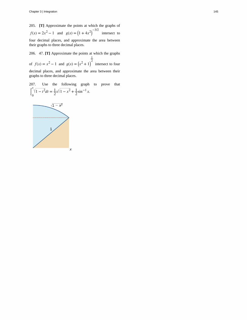
205. [T] Approximate the points at which the graphs of
f (x) = 2x2 − 1 and g(x) = ⎛⎝1 + 4x2⎞⎠−3/2
intersect to
four decimal places, and approximate the area betweentheir graphs to three decimal places.
206. 47. [T] Approximate the points at which the graphs
of f (x) = x2 − 1 and g(x) = ⎛⎝x2 + 1⎞⎠
12
intersect to four
decimal places, and approximate the area between theirgraphs to three decimal places.
207. Use the following graph to prove that
⌠⌡0
x1 − t2dt = 1
2x 1 − x2 + 12sin−1 x.
Chapter 3 | Integration 145
Chapter Review ExercisesTrue or False. Justify your answer with a proof or a counterexample. Assume all functions f and g are continuous over
their domains.
Exercise 3.208
If f (x) > 0, f ′ (x) > 0 for all x, then the right-hand rule underestimates the integral ∫a
bf (x). Use a graph to justify
your answer.
SolutionFalse
Exercise 3.209
∫a
bf (x)2dx = ∫
a
bf (x)dx∫
a
bf (x)dx
Exercise 3.210
If f (x) ≤ g(x) for all x ∈ ⎡⎣a, b⎤⎦, then ∫
a
bf (x) ≤ ∫
a
bg(x).
SolutionTrue
Exercise 3.211
All continuous functions have an antiderivative.
Evaluate the Riemann sums L4 and R4 for the following functions over the specified interval. Compare your answer with
the exact answer, when possible, or use a calculator to determine the answer.
Exercise 3.212
y = 3x2 − 2x + 1 over [−1, 1]
SolutionL4 = 5.25, R4 = 3.25, exact answer: 4
Exercise 3.213
y = ln⎛⎝x2 + 1⎞⎠ over [0, e]
Exercise 3.214
y = x2 sinx over [0, π]
SolutionL4 = 5.364, R4 = 5.364, exact answer: 5.870
Exercise 3.215
y = x + 1x over [1, 4]
Evaluate the following integrals.
Exercise 3.216
146 Chapter 3 | Integration
This OpenStax book is available for free at https://legacy.cnx.org/content/col31997/1.5
∫−1
1 ⎛⎝x3 − 2x2 + 4x⎞⎠dx
Solution
−43
Exercise 3.217
⌠⌡0
43t
1 + 6t2dt
Exercise 3.218
∫π/3
π/22sec(2θ)tan(2θ)dθ
Solution1
Exercise 3.219
∫0
π/4ecos2 xsinxcosxdx
Find the antiderivative.
Exercise 3.220
⌠⌡
dx(x + 4)3
Solution
− 12(x + 4)2 + C
Exercise 3.221
∫ x ln⎛⎝x2⎞⎠dx
Exercise 3.222
⌠⌡
4x2
1 − x6dx
Solution43sin−1 ⎛⎝x3⎞⎠+ C
Exercise 3.223
⌠⌡
e2x
1 + e4xdx
Find the derivative.
Exercise 3.224
Chapter 3 | Integration 147

ddt⌠⌡0
tsinx1 + x2
dx
Solutionsin t1 + t2
Exercise 3.225
ddx∫1
x34 − t2dt
Exercise 3.226
ddx∫1
ln(x)⎛⎝4t + et⎞⎠dt
Solution
4lnxx + 1
Exercise 3.227
ddx∫0
cosxet
2dt
The following problems consider the historic average cost per gigabyte of RAM on a computer.
Year 5-Year Change ($)
1980 0
1985 −5,468,750
1990 −755,495
1995 −73,005
2000 −29,768
2005 −918
2010 −177
Exercise 3.228
If the average cost per gigabyte of RAM in 2010 is $12, find the average cost per gigabyte of RAM in 1980.
Solution$6,328,113
Exercise 3.229
148 Chapter 3 | Integration
This OpenStax book is available for free at https://legacy.cnx.org/content/col31997/1.5
The average cost per gigabyte of RAM can be approximated by the function C(t) = 8, 500, 000(0.65)t, where t is
measured in years since 1980, and C is cost in US$. Find the average cost per gigabyte of RAM for 1980 to 2010.
Exercise 3.230
Find the average cost of 1GB RAM for 2005 to 2010.
Solution$73.36
Exercise 3.231
The velocity of a bullet from a rifle can be approximated by v(t) = 6400t2 − 6505t + 2686, where t is seconds after the
shot and v is the velocity measured in feet per second. This equation only models the velocity for the first half-second after
the shot: 0 ≤ t ≤ 0.5. What is the total distance the bullet travels in 0.5 sec?
Exercise 3.232
What is the average velocity of the bullet for the first half-second?
Solution19117
12 ft/sec, or 1593 ft/sec
Chapter 3 | Integration 149
antiderivative
indefinite integral
initial value problem
CHAPTER 3 REVIEW
KEY TERMSa function F such that F′ (x) = f (x) for all x in the domain of f is an antiderivative of f
the most general antiderivative of f (x) is the indefinite integral of f ; we use the notation
∫ f (x)dx to denote the indefinite integral of f
a problem that requires finding a function y that satisfies the differential equationdydx = f (x)
together with the initial condition y(x0) = y0
150 Chapter 3 | Integration
This OpenStax book is available for free at https://legacy.cnx.org/content/col31997/1.5

4 | APPLICATIONS OFINTEGRATION4.1 | Determining Volumes by Slicing
Learning Objectives4.1.1 Determine the volume of a solid by integrating a cross-section (the slicing method).
4.1.2 Find the volume of a solid of revolution using the disk method.
4.1.3 Find the volume of a solid of revolution with a cavity using the washer method.
In the preceding section, we used definite integrals to find the area between two curves. In this section, we use definiteintegrals to find volumes of three-dimensional solids. We consider three approaches—slicing, disks, and washers—forfinding these volumes, depending on the characteristics of the solid.
Volume and the Slicing MethodJust as area is the numerical measure of a two-dimensional region, volume is the numerical measure of a three-dimensionalsolid. Most of us have computed volumes of solids by using basic geometric formulas. The volume of a rectangular solid,for example, can be computed by multiplying length, width, and height: V = lwh. The formulas for the volume of a sphere⎛⎝V = 4
3πr3⎞⎠, a cone ⎛⎝V = 1
3πr2h⎞⎠, and a pyramid ⎛⎝V = 1
3Ah⎞⎠ have also been introduced. Although some of these
formulas were derived using geometry alone, all these formulas can be obtained by using integration.
We can also calculate the volume of a cylinder. Although most of us think of a cylinder as having a circular base, such asa soup can or a metal rod, in mathematics the word cylinder has a more general meaning. To discuss cylinders in this moregeneral context, we first need to define some vocabulary.
We define the cross-section of a solid to be the intersection of a plane with the solid. A cylinder is defined as any solidthat can be generated by translating a plane region along a line perpendicular to the region, called the axis of the cylinder.Thus, all cross-sections perpendicular to the axis of a cylinder are identical. The solid shown in Figure 4.1 is an exampleof a cylinder with a noncircular base. To calculate the volume of a cylinder, then, we simply multiply the area of the cross-
section by the height of the cylinder: V = A · h. In the case of a right circular cylinder (soup can), this becomes V = πr2h.
Figure 4.1 Each cross-section of a particular cylinder is identical to the others.
Chapter 4 | Applications of Integration 151
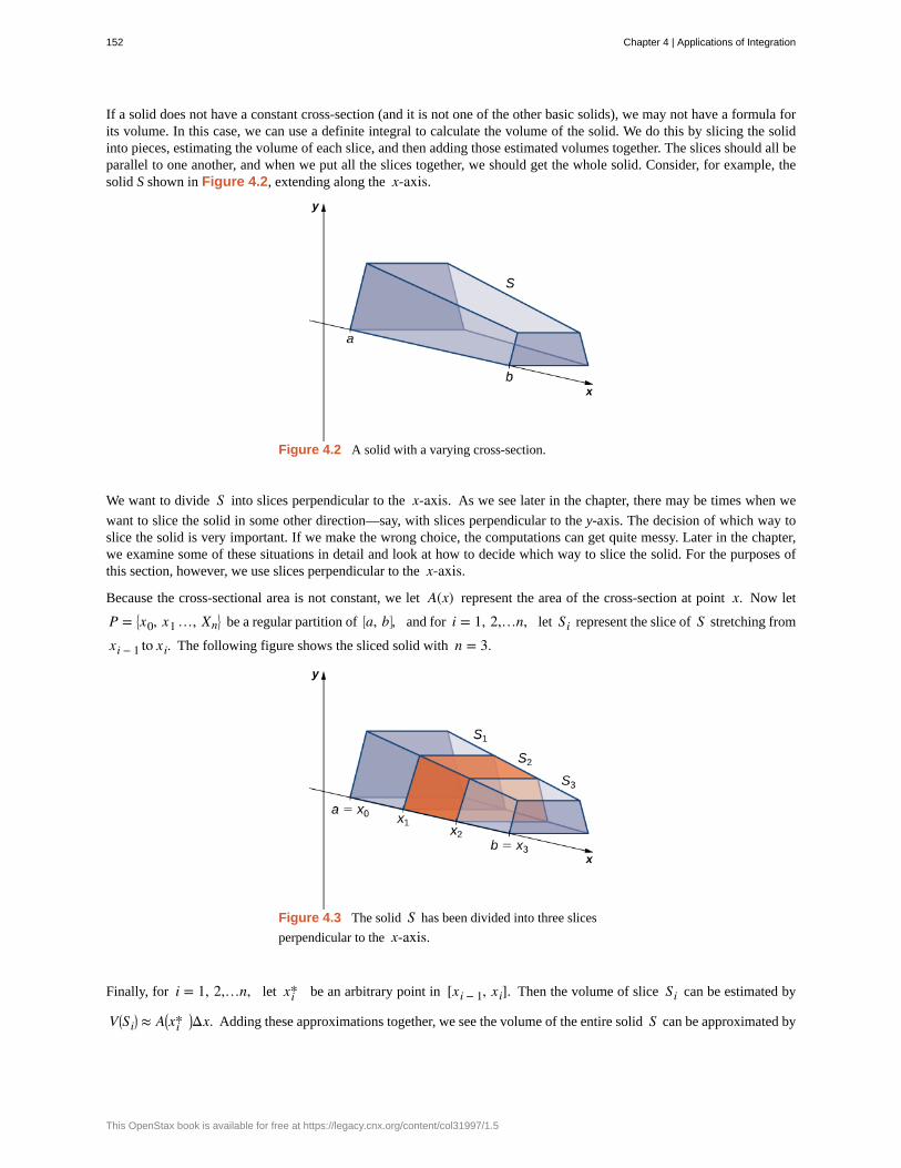
If a solid does not have a constant cross-section (and it is not one of the other basic solids), we may not have a formula forits volume. In this case, we can use a definite integral to calculate the volume of the solid. We do this by slicing the solidinto pieces, estimating the volume of each slice, and then adding those estimated volumes together. The slices should all beparallel to one another, and when we put all the slices together, we should get the whole solid. Consider, for example, thesolid S shown in Figure 4.2, extending along the x-axis.
Figure 4.2 A solid with a varying cross-section.
We want to divide S into slices perpendicular to the x-axis. As we see later in the chapter, there may be times when we
want to slice the solid in some other direction—say, with slices perpendicular to the y-axis. The decision of which way toslice the solid is very important. If we make the wrong choice, the computations can get quite messy. Later in the chapter,we examine some of these situations in detail and look at how to decide which way to slice the solid. For the purposes ofthis section, however, we use slices perpendicular to the x-axis.
Because the cross-sectional area is not constant, we let A(x) represent the area of the cross-section at point x. Now let
P = ⎧⎩⎨x0, x1 …, Xn
⎫⎭⎬ be a regular partition of ⎡⎣a, b⎤⎦, and for i = 1, 2,…n, let Si represent the slice of S stretching from
xi − 1 to xi. The following figure shows the sliced solid with n = 3.
Figure 4.3 The solid S has been divided into three slices
perpendicular to the x-axis.
Finally, for i = 1, 2,…n, let xi* be an arbitrary point in [xi − 1, xi]. Then the volume of slice Si can be estimated by
V ⎛⎝Si⎞⎠ ≈ A⎛⎝xi*
⎞⎠Δx. Adding these approximations together, we see the volume of the entire solid S can be approximated by
152 Chapter 4 | Applications of Integration
This OpenStax book is available for free at https://legacy.cnx.org/content/col31997/1.5

V(S) ≈ ∑i = 1
nA⎛⎝xi*
⎞⎠Δx.
By now, we can recognize this as a Riemann sum, and our next step is to take the limit as n → ∞. Then we have
V(S) = limn → ∞ ∑i = 1
nA⎛⎝xi*
⎞⎠Δx = ∫
a
bA(x)dx.
The technique we have just described is called the slicing method. To apply it, we use the following strategy.
Problem-Solving Strategy: Finding Volumes by the Slicing Method
1. Examine the solid and determine the shape of a cross-section of the solid. It is often helpful to draw a pictureif one is not provided.
2. Determine a formula for the area of the cross-section.
3. Integrate the area formula over the appropriate interval to get the volume.
Recall that in this section, we assume the slices are perpendicular to the x-axis. Therefore, the area formula is in terms of
x and the limits of integration lie on the x-axis. However, the problem-solving strategy shown here is valid regardless of
how we choose to slice the solid.
Example 4.1
Deriving the Formula for the Volume of a Pyramid
We know from geometry that the formula for the volume of a pyramid is V = 13Ah. If the pyramid has a square
base, this becomes V = 13a
2h, where a denotes the length of one side of the base. We are going to use the
slicing method to derive this formula.
Solution
We want to apply the slicing method to a pyramid with a square base. To set up the integral, consider the pyramidshown in Figure 4.4, oriented along the x-axis.
Figure 4.4 (a) A pyramid with a square base is oriented along the x-axis. (b) A two-dimensional view of thepyramid is seen from the side.
Chapter 4 | Applications of Integration 153
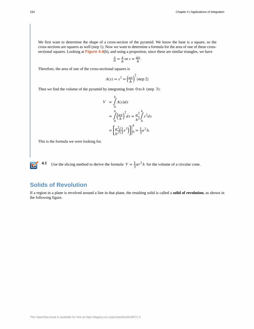
4.1
We first want to determine the shape of a cross-section of the pyramid. We know the base is a square, so thecross-sections are squares as well (step 1). Now we want to determine a formula for the area of one of these cross-sectional squares. Looking at Figure 4.4(b), and using a proportion, since these are similar triangles, we have
sa = x
h or s = axh .
Therefore, the area of one of the cross-sectional squares is
A(x) = s2 = ⎛⎝axh⎞⎠
2⎛⎝step 2⎞⎠.
Then we find the volume of the pyramid by integrating from 0 to h (step 3):
V = ∫0
hA(x)dx
= ∫0
h ⎛⎝axh⎞⎠
2dx = a2
h2∫0
hx2dx
= ⎡⎣a2
h2⎛⎝13x
3⎞⎠⎤⎦ |0h = 1
3a2h.
This is the formula we were looking for.
Use the slicing method to derive the formula V = 13πr
2h for the volume of a circular cone.
Solids of RevolutionIf a region in a plane is revolved around a line in that plane, the resulting solid is called a solid of revolution, as shown inthe following figure.
154 Chapter 4 | Applications of Integration
This OpenStax book is available for free at https://legacy.cnx.org/content/col31997/1.5
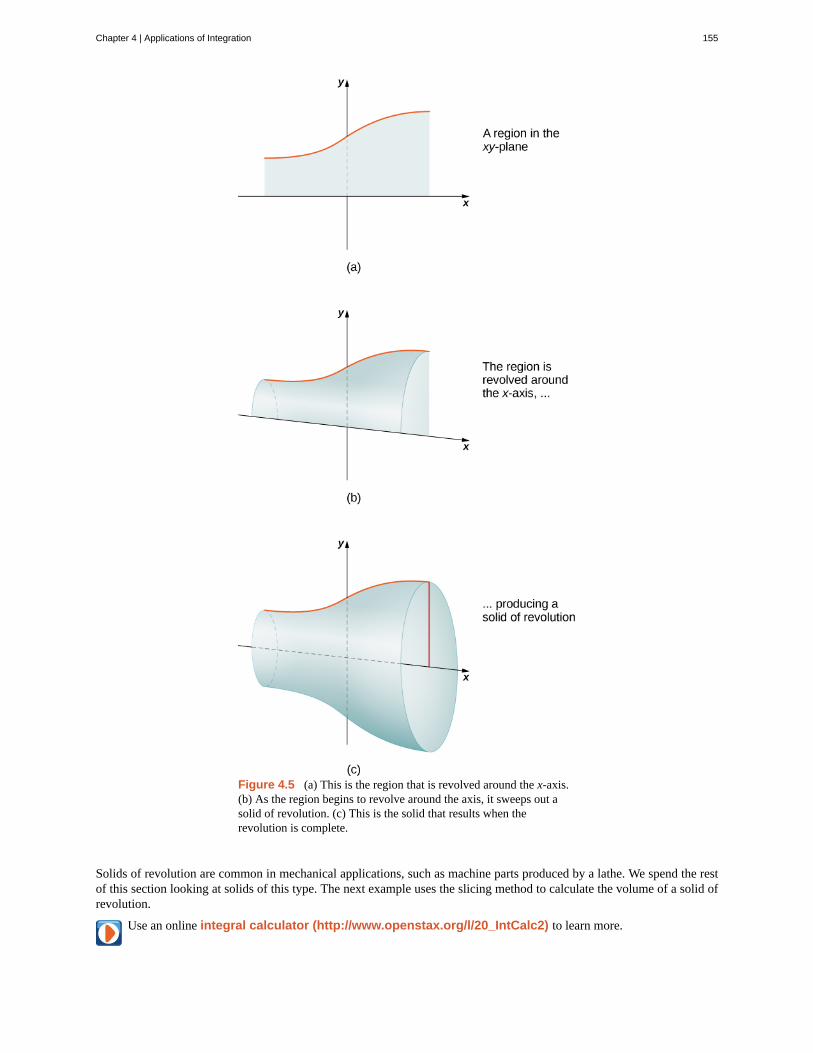
Figure 4.5 (a) This is the region that is revolved around the x-axis.(b) As the region begins to revolve around the axis, it sweeps out asolid of revolution. (c) This is the solid that results when therevolution is complete.
Solids of revolution are common in mechanical applications, such as machine parts produced by a lathe. We spend the restof this section looking at solids of this type. The next example uses the slicing method to calculate the volume of a solid ofrevolution.
Use an online integral calculator (http://www.openstax.org/l/20_IntCalc2) to learn more.
Chapter 4 | Applications of Integration 155

Example 4.2
Using the Slicing Method to find the Volume of a Solid of Revolution
Use the slicing method to find the volume of the solid of revolution bounded by the graphs of
f (x) = x2 − 4x + 5, x = 1, and x = 4, and rotated about the x-axis.
Solution
Using the problem-solving strategy, we first sketch the graph of the quadratic function over the interval [1, 4] as
shown in the following figure.
Figure 4.6 A region used to produce a solid of revolution.
Next, revolve the region around the x-axis, as shown in the following figure.
Figure 4.7 Two views, (a) and (b), of the solid of revolution produced by revolving the regionin Figure 4.6 about the x-axis.
156 Chapter 4 | Applications of Integration
This OpenStax book is available for free at https://legacy.cnx.org/content/col31997/1.5
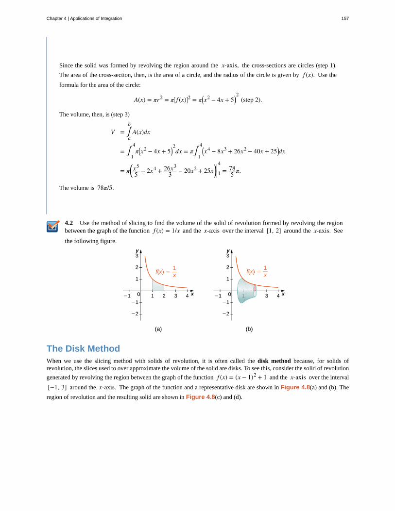
4.2
Since the solid was formed by revolving the region around the x-axis, the cross-sections are circles (step 1).
The area of the cross-section, then, is the area of a circle, and the radius of the circle is given by f (x). Use the
formula for the area of the circle:
A(x) = πr2 = π⎡⎣ f (x)⎤⎦2 = π⎛⎝x2 − 4x + 5⎞⎠2
(step 2).
The volume, then, is (step 3)
V = ∫a
bA(x)dx
= ∫1
4π⎛⎝x2 − 4x + 5⎞⎠
2dx = π∫
1
4⎛⎝x4 − 8x3 + 26x2 − 40x + 25⎞⎠dx
= π⎛⎝x5
5 − 2x4 + 26x3
3 − 20x2 + 25x⎞⎠|14 = 785 π.
The volume is 78π/5.
Use the method of slicing to find the volume of the solid of revolution formed by revolving the regionbetween the graph of the function f (x) = 1/x and the x-axis over the interval [1, 2] around the x-axis. See
the following figure.
The Disk MethodWhen we use the slicing method with solids of revolution, it is often called the disk method because, for solids ofrevolution, the slices used to over approximate the volume of the solid are disks. To see this, consider the solid of revolution
generated by revolving the region between the graph of the function f (x) = (x − 1)2 + 1 and the x-axis over the interval
[−1, 3] around the x-axis. The graph of the function and a representative disk are shown in Figure 4.8(a) and (b). The
region of revolution and the resulting solid are shown in Figure 4.8(c) and (d).
Chapter 4 | Applications of Integration 157

Figure 4.8 (a) A thin rectangle for approximating the area under a curve. (b) A representative disk formed byrevolving the rectangle about the x-axis. (c) The region under the curve is revolved about the x-axis, resulting in
(d) the solid of revolution.
We already used the formal Riemann sum development of the volume formula when we developed the slicing method. Weknow that
V = ∫a
bA(x)dx.
The only difference with the disk method is that we know the formula for the cross-sectional area ahead of time; it is thearea of a circle. This gives the following rule.
Rule: The Disk Method
Let f (x) be continuous and nonnegative. Define R as the region bounded above by the graph of f (x), below by the
158 Chapter 4 | Applications of Integration
This OpenStax book is available for free at https://legacy.cnx.org/content/col31997/1.5
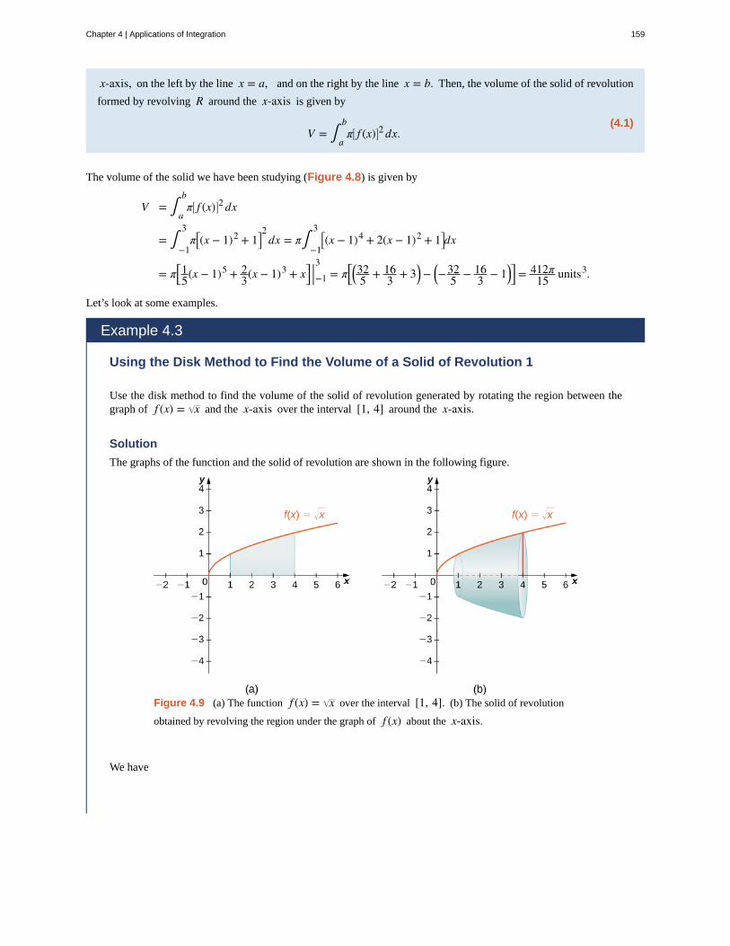
x-axis, on the left by the line x = a, and on the right by the line x = b. Then, the volume of the solid of revolution
formed by revolving R around the x-axis is given by
(4.1)V = ∫
a
bπ⎡⎣ f (x)⎤⎦2dx.
The volume of the solid we have been studying (Figure 4.8) is given by
V = ∫a
bπ⎡⎣ f (x)⎤⎦2dx
= ∫−1
3π⎡⎣(x − 1)2 + 1⎤⎦
2dx = π∫
−1
3 ⎡⎣(x − 1)4 + 2(x − 1)2 + 1⎤⎦dx
= π⎡⎣15(x − 1)5 + 23(x − 1)3 + x⎤⎦ |−1
3= π⎡⎣⎛⎝32
5 + 163 + 3⎞⎠−
⎛⎝−32
5 − 163 − 1⎞⎠
⎤⎦ = 412π
15 units3.
Let’s look at some examples.
Example 4.3
Using the Disk Method to Find the Volume of a Solid of Revolution 1
Use the disk method to find the volume of the solid of revolution generated by rotating the region between thegraph of f (x) = x and the x-axis over the interval [1, 4] around the x-axis.
Solution
The graphs of the function and the solid of revolution are shown in the following figure.
Figure 4.9 (a) The function f (x) = x over the interval [1, 4]. (b) The solid of revolution
obtained by revolving the region under the graph of f (x) about the x-axis.
We have
Chapter 4 | Applications of Integration 159
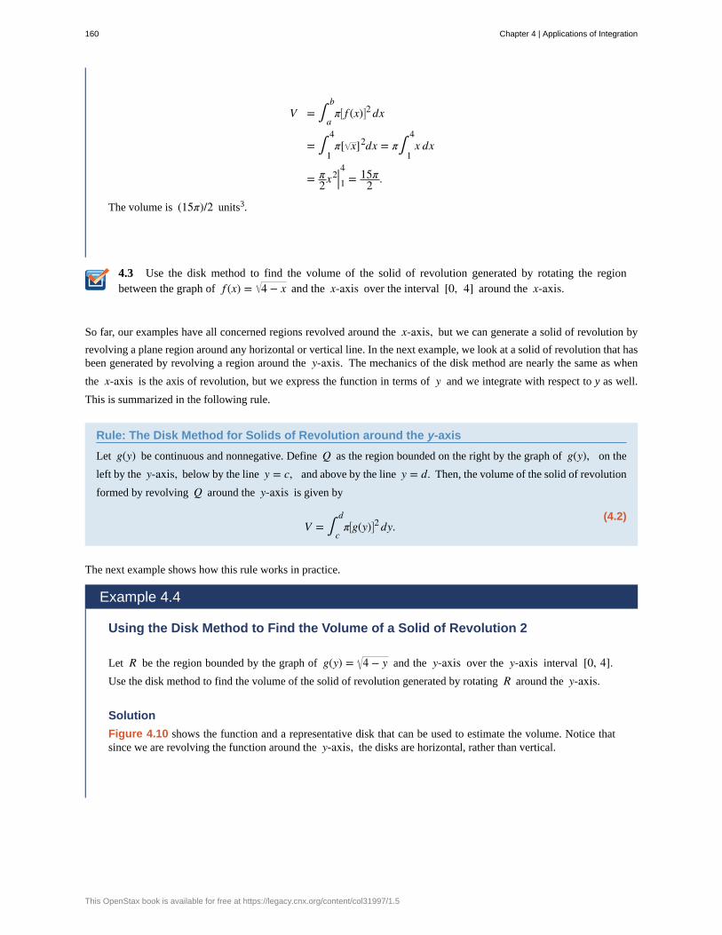
4.3
V = ∫a
bπ⎡⎣ f (x)⎤⎦2dx
= ∫1
4π[ x]2dx = π∫
1
4x dx
= π2x
2|14 = 15π2 .
The volume is (15π)/2 units3.
Use the disk method to find the volume of the solid of revolution generated by rotating the regionbetween the graph of f (x) = 4 − x and the x-axis over the interval [0, 4] around the x-axis.
So far, our examples have all concerned regions revolved around the x-axis, but we can generate a solid of revolution by
revolving a plane region around any horizontal or vertical line. In the next example, we look at a solid of revolution that hasbeen generated by revolving a region around the y-axis. The mechanics of the disk method are nearly the same as when
the x-axis is the axis of revolution, but we express the function in terms of y and we integrate with respect to y as well.
This is summarized in the following rule.
Rule: The Disk Method for Solids of Revolution around the y-axis
Let g(y) be continuous and nonnegative. Define Q as the region bounded on the right by the graph of g(y), on the
left by the y-axis, below by the line y = c, and above by the line y = d. Then, the volume of the solid of revolution
formed by revolving Q around the y-axis is given by
(4.2)V = ∫
c
dπ⎡⎣g(y)⎤⎦2dy.
The next example shows how this rule works in practice.
Example 4.4
Using the Disk Method to Find the Volume of a Solid of Revolution 2
Let R be the region bounded by the graph of g(y) = 4 − y and the y-axis over the y-axis interval [0, 4].Use the disk method to find the volume of the solid of revolution generated by rotating R around the y-axis.
Solution
Figure 4.10 shows the function and a representative disk that can be used to estimate the volume. Notice thatsince we are revolving the function around the y-axis, the disks are horizontal, rather than vertical.
160 Chapter 4 | Applications of Integration
This OpenStax book is available for free at https://legacy.cnx.org/content/col31997/1.5

Figure 4.10 (a) Shown is a thin rectangle between the curve of the function g(y) = 4 − yand the y-axis. (b) The rectangle forms a representative disk after revolution around the y-axis.
The region to be revolved and the full solid of revolution are depicted in the following figure.
Figure 4.11 (a) The region to the left of the function g(y) = 4 − y over the y-axis interval
[0, 4]. (b) The solid of revolution formed by revolving the region about the y-axis.
To find the volume, we integrate with respect to y. We obtain
V = ∫c
dπ⎡⎣g(y)⎤⎦2dy
= ∫0
4π⎡⎣ 4 − y⎤⎦2dy = π∫
0
4⎛⎝4 − y⎞⎠dy
= π⎡⎣⎢4y − y2
2⎤⎦⎥ |04 = 8π.
Chapter 4 | Applications of Integration 161
4.4
The volume is 8π units3.
Use the disk method to find the volume of the solid of revolution generated by rotating the regionbetween the graph of g(y) = y and the y-axis over the interval [1, 4] around the y-axis.
The Washer MethodSome solids of revolution have cavities in the middle; they are not solid all the way to the axis of revolution. Sometimes,this is just a result of the way the region of revolution is shaped with respect to the axis of revolution. In other cases, cavitiesarise when the region of revolution is defined as the region between the graphs of two functions. A third way this can happenis when an axis of revolution other than the x-axis or y-axis is selected.
When the solid of revolution has a cavity in the middle, the slices used to approximate the volume are not disks, but washers(disks with holes in the center). For example, consider the region bounded above by the graph of the function f (x) = xand below by the graph of the function g(x) = 1 over the interval [1, 4]. When this region is revolved around the x-axis,the result is a solid with a cavity in the middle, and the slices are washers. The graph of the function and a representativewasher are shown in Figure 4.12(a) and (b). The region of revolution and the resulting solid are shown in Figure 4.12(c)and (d).
162 Chapter 4 | Applications of Integration
This OpenStax book is available for free at https://legacy.cnx.org/content/col31997/1.5
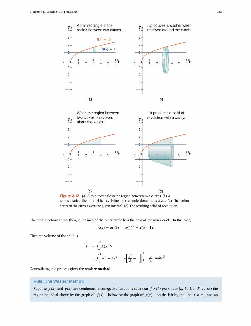
Figure 4.12 (a) A thin rectangle in the region between two curves. (b) Arepresentative disk formed by revolving the rectangle about the x-axis. (c) The region
between the curves over the given interval. (d) The resulting solid of revolution.
The cross-sectional area, then, is the area of the outer circle less the area of the inner circle. In this case,
A(x) = π( x)2 − π(1)2 = π(x − 1).
Then the volume of the solid is
V = ∫a
bA(x)dx
= ∫1
4π(x − 1)dx = π⎡⎣x
2
2 − x⎤⎦ |14 = 92π units3.
Generalizing this process gives the washer method.
Rule: The Washer Method
Suppose f (x) and g(x) are continuous, nonnegative functions such that f (x) ≥ g(x) over ⎡⎣a, b⎤⎦. Let R denote the
region bounded above by the graph of f (x), below by the graph of g(x), on the left by the line x = a, and on
Chapter 4 | Applications of Integration 163
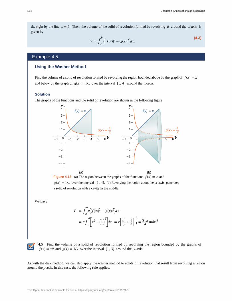
4.5
the right by the line x = b. Then, the volume of the solid of revolution formed by revolving R around the x-axis is
given by
(4.3)V = ∫
a
bπ⎡⎣⎛⎝ f (x)⎞⎠2 − ⎛
⎝g(x)⎞⎠2⎤⎦dx.
Example 4.5
Using the Washer Method
Find the volume of a solid of revolution formed by revolving the region bounded above by the graph of f (x) = xand below by the graph of g(x) = 1/x over the interval [1, 4] around the x-axis.
Solution
The graphs of the functions and the solid of revolution are shown in the following figure.
Figure 4.13 (a) The region between the graphs of the functions f (x) = x and
g(x) = 1/x over the interval [1, 4]. (b) Revolving the region about the x-axis generates
a solid of revolution with a cavity in the middle.
We have
V = ∫a
bπ⎡⎣⎛⎝ f (x)⎞⎠2 − ⎛
⎝g(x)⎞⎠2⎤⎦dx
= π∫1
4⎡⎣x2 − ⎛⎝1x
⎞⎠2⎤⎦dx = π⎡⎣x
3
3 + 1x⎤⎦ |14 = 81π
4 units3.
Find the volume of a solid of revolution formed by revolving the region bounded by the graphs off (x) = x and g(x) = 1/x over the interval [1, 3] around the x-axis.
As with the disk method, we can also apply the washer method to solids of revolution that result from revolving a regionaround the y-axis. In this case, the following rule applies.
164 Chapter 4 | Applications of Integration
This OpenStax book is available for free at https://legacy.cnx.org/content/col31997/1.5
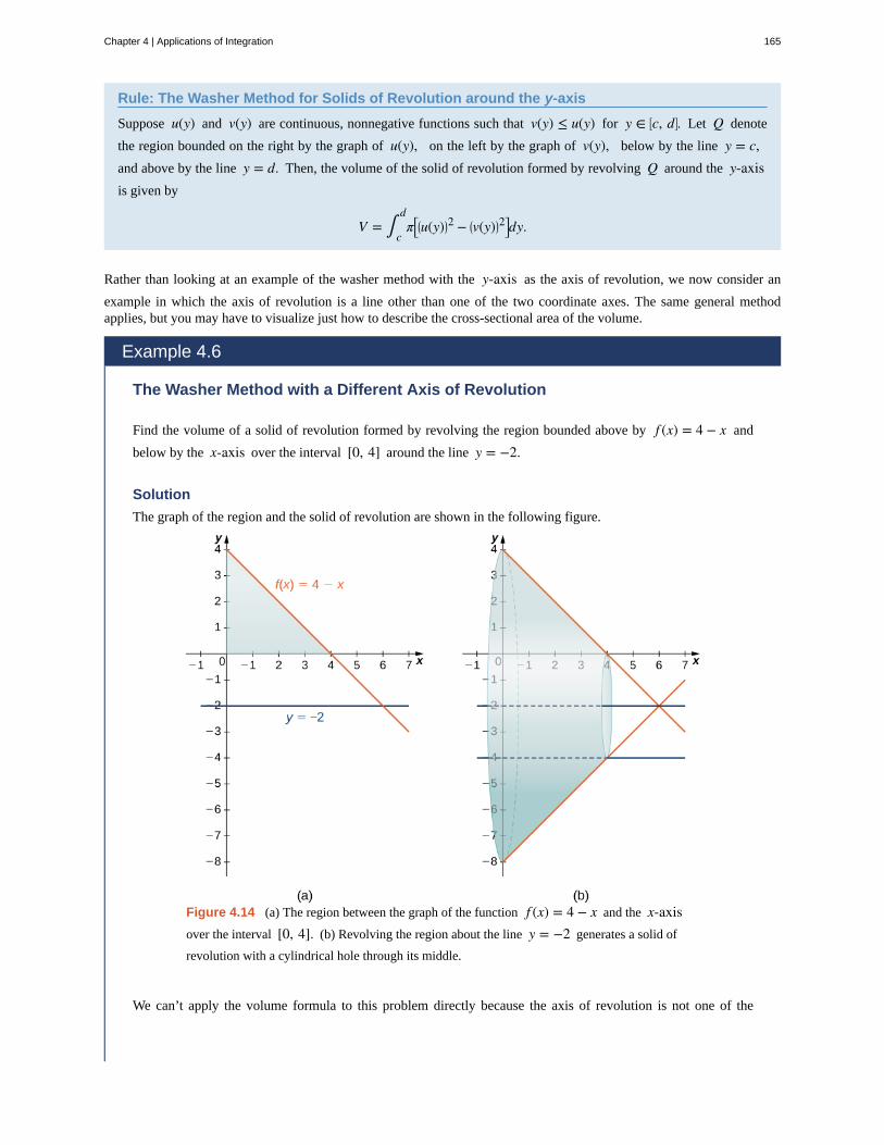
Rule: The Washer Method for Solids of Revolution around the y-axis
Suppose u(y) and v(y) are continuous, nonnegative functions such that v(y) ≤ u(y) for y ∈ ⎡⎣c, d⎤⎦. Let Q denote
the region bounded on the right by the graph of u(y), on the left by the graph of v(y), below by the line y = c,and above by the line y = d. Then, the volume of the solid of revolution formed by revolving Q around the y-axisis given by
V = ∫c
dπ⎡⎣⎛⎝u(y)⎞⎠2 − ⎛
⎝v(y)⎞⎠2⎤⎦dy.
Rather than looking at an example of the washer method with the y-axis as the axis of revolution, we now consider an
example in which the axis of revolution is a line other than one of the two coordinate axes. The same general methodapplies, but you may have to visualize just how to describe the cross-sectional area of the volume.
Example 4.6
The Washer Method with a Different Axis of Revolution
Find the volume of a solid of revolution formed by revolving the region bounded above by f (x) = 4 − x and
below by the x-axis over the interval [0, 4] around the line y = −2.
Solution
The graph of the region and the solid of revolution are shown in the following figure.
Figure 4.14 (a) The region between the graph of the function f (x) = 4 − x and the x-axisover the interval [0, 4]. (b) Revolving the region about the line y = −2 generates a solid of
revolution with a cylindrical hole through its middle.
We can’t apply the volume formula to this problem directly because the axis of revolution is not one of the
Chapter 4 | Applications of Integration 165
4.6
coordinate axes. However, we still know that the area of the cross-section is the area of the outer circle less thearea of the inner circle. Looking at the graph of the function, we see the radius of the outer circle is given byf (x) + 2, which simplifies to
f (x) + 2 = (4 − x) + 2 = 6 − x.
The radius of the inner circle is g(x) = 2. Therefore, we have
V = ∫0
4π⎡⎣(6 − x)2 − (2)2⎤⎦dx
= π∫0
4⎛⎝x2 − 12x + 32⎞⎠dx = π⎡⎣x
3
3 − 6x2 + 32x⎤⎦ |04 = 160π3 units3.
Find the volume of a solid of revolution formed by revolving the region bounded above by the graph off (x) = x + 2 and below by the x-axis over the interval [0, 3] around the line y = −1.
Key Concepts• Definite integrals can be used to find the volumes of solids. Using the slicing method, we can find a volume by
integrating the cross-sectional area.
• For solids of revolution, the volume slices are often disks and the cross-sections are circles. The method of disksinvolves applying the method of slicing in the particular case in which the cross-sections are circles, and using theformula for the area of a circle.
• If a solid of revolution has a cavity in the center, the volume slices are washers. With the method of washers, thearea of the inner circle is subtracted from the area of the outer circle before integrating.
Key Equations• Disk Method along the x-axis
V = ∫a
bπ⎡⎣ f (x)⎤⎦2dx
• Disk Method along the y-axis
V = ∫c
dπ⎡⎣g(y)⎤⎦2dy
• Washer Method
V = ∫a
bπ⎡⎣⎛⎝ f (x)⎞⎠2 − ⎛
⎝g(x)⎞⎠2⎤⎦dx
166 Chapter 4 | Applications of Integration
This OpenStax book is available for free at https://legacy.cnx.org/content/col31997/1.5

4.1 EXERCISES1. Derive the formula for the volume of a sphere using theslicing method.
2. Use the slicing method to derive the formula for thevolume of a cone.
3. Use the slicing method to derive the formula for thevolume of a tetrahedron with side length a.
4. Use the disk method to derive the formula for thevolume of a trapezoidal cylinder.
5. Explain when you would use the disk method versus thewasher method. When are they interchangeable?
For the following exercises, draw a typical slice and findthe volume using the slicing method for the given volume.
6. A pyramid with height 6 units and square base of side 2units, as pictured here.
7. A pyramid with height 4 units and a rectangular basewith length 2 units and width 3 units, as pictured here.
8. A tetrahedron with a base side of 4 units, as seen here.
9. A pyramid with height 5 units, and an isoscelestriangular base with lengths of 6 units and 8 units, as seenhere.
10. A cone of radius r and height h has a smaller cone of
radius r/2 and height h/2 removed from the top, as seen
here. The resulting solid is called a frustum.
For the following exercises, draw an outline of the solid andfind the volume using the slicing method.
11. The base is a circle of radius a. The slices
perpendicular to the base are squares.
12. The base is a triangle with vertices (0, 0), (1, 0),and (0, 1). Slices perpendicular to the x-axis are
semicircles.
13. The base is the region under the parabola y = 1 − x2
in the first quadrant. Slices perpendicular to the xy-planeare squares.
14. The base is the region under the parabola y = 1 − x2
and above the x-axis. Slices perpendicular to the y-axisare squares.
Chapter 4 | Applications of Integration 167
15. The base is the region enclosed by y = x2 and
y = 9. Slices perpendicular to the x-axis are right isosceles
triangles. The intersection of one of these slices and thebase is the leg of the triangle.
16. The base is the area between y = x and y = x2.Slices perpendicular to the x-axis are semicircles.
For the following exercises, draw the region bounded bythe curves. Then, use the disk method to find the volumewhen the region is rotated around the x-axis.
17. x + y = 8, x = 0, and y = 0
18. y = 2x2, x = 0, x = 4, and y = 0
19. y = ex + 1, x = 0, x = 1, and y = 0
20. y = x4, x = 0, and y = 1
21. y = x, x = 0, x = 4, and y = 0
22. y = sin x, y = cos x, and x = 0
23. y = 1x , x = 2, and y = 3
24. x2 − y2 = 9 and x + y = 9, y = 0 and x = 0
For the following exercises, draw the region bounded bythe curves. Then, find the volume when the region isrotated around the y-axis.
25. y = 4 − 12x, x = 0, and y = 0
26. y = 2x3, x = 0, x = 1, and y = 0
27. y = 3x2, x = 0, and y = 3
28. y = 4 − x2, y = 0, and x = 0
29. y = 1x + 1
, x = 0, and x = 3
30. x = sec(y) and y = π4, y = 0 and x = 0
31. y = 1x + 1, x = 0, and x = 2
32. y = 4 − x, y = x, and x = 0
For the following exercises, draw the region bounded bythe curves. Then, find the volume when the region is
rotated around the x-axis.
33. y = x + 2, y = x + 6, x = 0, and x = 5
34. y = x2 and y = x + 2
35. x2 = y3 and x3 = y2
36. y = 4 − x2 and y = 2 − x
37. [T] y = cos x, y = e−x, x = 0, and x = 1.2927
38. y = x and y = x2
39. y = sin x, y = 5 sin x, x = 0 and x = π
40. y = 1 + x2 and y = 4 − x2
For the following exercises, draw the region bounded bythe curves. Then, use the washer method to find the volumewhen the region is revolved around the y-axis.
41. y = x, x = 4, and y = 0
42. y = x + 2, y = 2x − 1, and x = 0
43. y = x3 and y = x3
44. x = e2y, x = y2, y = 0, and y = ln(2)
45. x = 9 − y2, x = e−y, y = 0, and y = 3
168 Chapter 4 | Applications of Integration
This OpenStax book is available for free at https://legacy.cnx.org/content/col31997/1.5

46. Yogurt containers can be shaped like frustums. Rotate
the line y = 1mx around the y-axis to find the volume
between y = a and y = b.
47. Rotate the ellipse ⎛⎝x2 /a2⎞⎠+⎛⎝y2 /b2⎞⎠ = 1 around the
x-axis to approximate the volume of a football, as seenhere.
48. Rotate the ellipse ⎛⎝x2 /a2⎞⎠+⎛⎝y2 /b2⎞⎠ = 1 around the
y-axis to approximate the volume of a football.
49. A better approximation of the volume of a footballis given by the solid that comes from rotating y = sin xaround the x-axis from x = 0 to x = π. What is the
volume of this football approximation, as seen here?
50. What is the volume of the Bundt cake that comesfrom rotating y = sin x around the y-axis from x = 0 to
x = π ?
For the following exercises, find the volume of the soliddescribed.
Chapter 4 | Applications of Integration 169
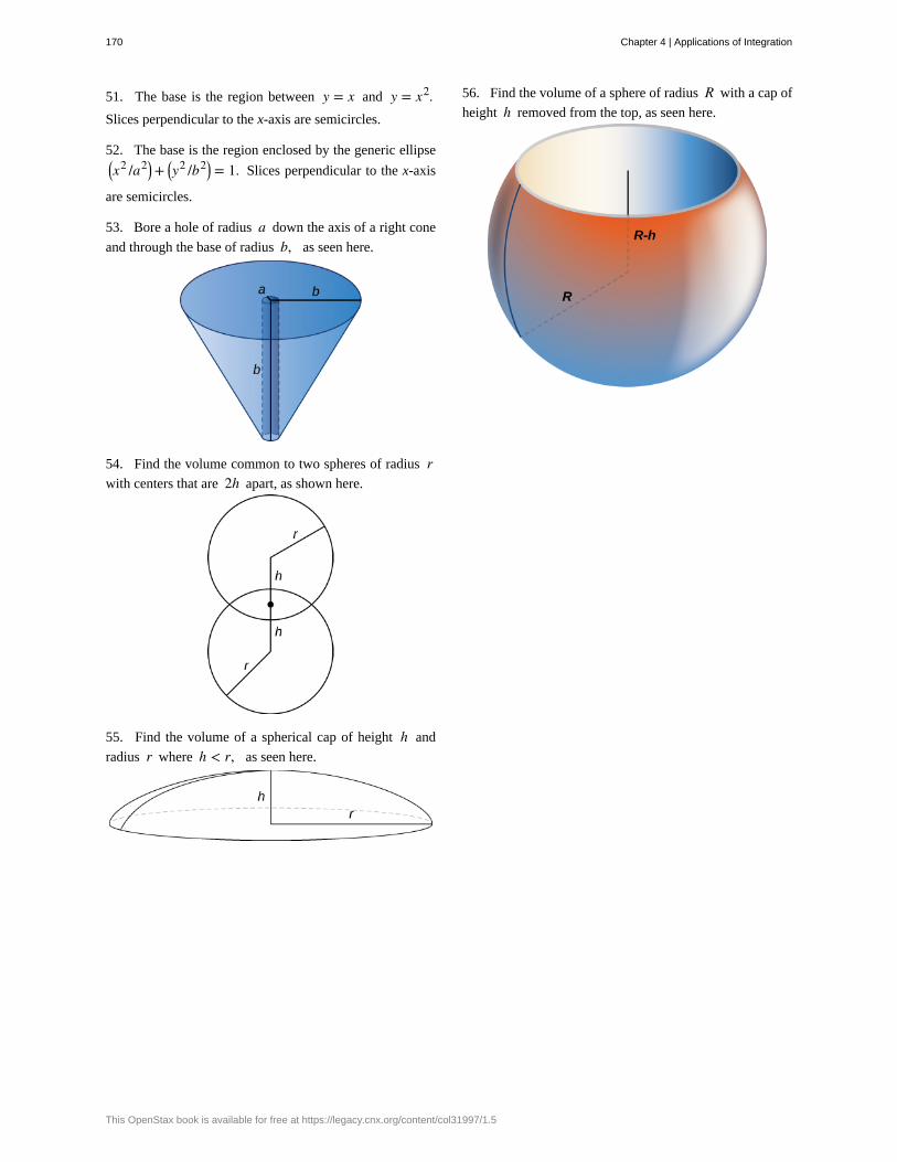
51. The base is the region between y = x and y = x2.Slices perpendicular to the x-axis are semicircles.
52. The base is the region enclosed by the generic ellipse⎛⎝x2 /a2⎞⎠+
⎛⎝y2 /b2⎞⎠ = 1. Slices perpendicular to the x-axis
are semicircles.
53. Bore a hole of radius a down the axis of a right cone
and through the base of radius b, as seen here.
54. Find the volume common to two spheres of radius rwith centers that are 2h apart, as shown here.
55. Find the volume of a spherical cap of height h and
radius r where h < r, as seen here.
56. Find the volume of a sphere of radius R with a cap of
height h removed from the top, as seen here.
170 Chapter 4 | Applications of Integration
This OpenStax book is available for free at https://legacy.cnx.org/content/col31997/1.5
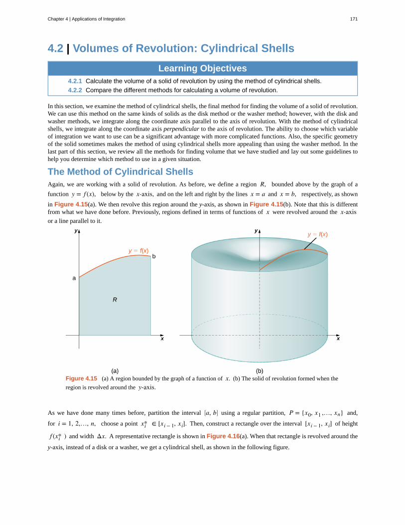
4.2 | Volumes of Revolution: Cylindrical Shells
Learning Objectives4.2.1 Calculate the volume of a solid of revolution by using the method of cylindrical shells.
4.2.2 Compare the different methods for calculating a volume of revolution.
In this section, we examine the method of cylindrical shells, the final method for finding the volume of a solid of revolution.We can use this method on the same kinds of solids as the disk method or the washer method; however, with the disk andwasher methods, we integrate along the coordinate axis parallel to the axis of revolution. With the method of cylindricalshells, we integrate along the coordinate axis perpendicular to the axis of revolution. The ability to choose which variableof integration we want to use can be a significant advantage with more complicated functions. Also, the specific geometryof the solid sometimes makes the method of using cylindrical shells more appealing than using the washer method. In thelast part of this section, we review all the methods for finding volume that we have studied and lay out some guidelines tohelp you determine which method to use in a given situation.
The Method of Cylindrical ShellsAgain, we are working with a solid of revolution. As before, we define a region R, bounded above by the graph of a
function y = f (x), below by the x-axis, and on the left and right by the lines x = a and x = b, respectively, as shown
in Figure 4.15(a). We then revolve this region around the y-axis, as shown in Figure 4.15(b). Note that this is differentfrom what we have done before. Previously, regions defined in terms of functions of x were revolved around the x-axisor a line parallel to it.
Figure 4.15 (a) A region bounded by the graph of a function of x. (b) The solid of revolution formed when the
region is revolved around the y-axis.
As we have done many times before, partition the interval ⎡⎣a, b⎤⎦ using a regular partition, P = {x0, x1 ,…, xn} and,
for i = 1, 2,…, n, choose a point xi* ∈ [xi − 1, xi]. Then, construct a rectangle over the interval [xi − 1, xi] of height
f (xi* ) and width Δx. A representative rectangle is shown in Figure 4.16(a). When that rectangle is revolved around the
y-axis, instead of a disk or a washer, we get a cylindrical shell, as shown in the following figure.
Chapter 4 | Applications of Integration 171
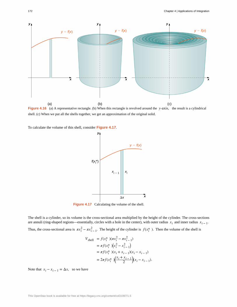
Figure 4.16 (a) A representative rectangle. (b) When this rectangle is revolved around the y-axis, the result is a cylindrical
shell. (c) When we put all the shells together, we get an approximation of the original solid.
To calculate the volume of this shell, consider Figure 4.17.
Figure 4.17 Calculating the volume of the shell.
The shell is a cylinder, so its volume is the cross-sectional area multiplied by the height of the cylinder. The cross-sectionsare annuli (ring-shaped regions—essentially, circles with a hole in the center), with outer radius xi and inner radius xi − 1.
Thus, the cross-sectional area is πxi2 − πxi − 1
2 . The height of the cylinder is f (xi* ). Then the volume of the shell is
Vshell = f (xi* )(πxi2 − πxi − 1
2 )
= π f (xi* )⎛⎝xi2 − xi − 1
2 ⎞⎠
= π f (xi* )(xi + xi − 1)(xi − xi − 1)
= 2π f (xi* )⎛⎝xi + xi − 1
2⎞⎠(xi − xi − 1).
Note that xi − xi − 1 = Δx, so we have
172 Chapter 4 | Applications of Integration
This OpenStax book is available for free at https://legacy.cnx.org/content/col31997/1.5

Vshell = 2π f (xi* )⎛⎝xi + xi − 1
2⎞⎠Δx.
Furthermore,xi + xi − 1
2 is both the midpoint of the interval [xi − 1, xi] and the average radius of the shell, and we can
approximate this by xi* . We then have
Vshell ≈ 2π f (xi* )xi* Δx.
Another way to think of this is to think of making a vertical cut in the shell and then opening it up to form a flat plate(Figure 4.18).
Figure 4.18 (a) Make a vertical cut in a representative shell. (b) Open the shell up to form a flat plate.
In reality, the outer radius of the shell is greater than the inner radius, and hence the back edge of the plate would be slightlylonger than the front edge of the plate. However, we can approximate the flattened shell by a flat plate of height f (xi* ),
width 2πxi* , and thickness Δx (Figure 4.18). The volume of the shell, then, is approximately the volume of the flat
plate. Multiplying the height, width, and depth of the plate, we get
Vshell ≈ f (xi* )⎛⎝2πxi*⎞⎠Δx,
which is the same formula we had before.
To calculate the volume of the entire solid, we then add the volumes of all the shells and obtain
V ≈ ∑i = 1
n⎛⎝2πxi* f (xi* )Δx⎞⎠.
Here we have another Riemann sum, this time for the function 2πx f (x). Taking the limit as n → ∞ gives us
V = limn → ∞ ∑i = 1
n⎛⎝2πxi* f (xi* )Δx⎞⎠ = ∫
a
b⎛⎝2πx f (x)⎞⎠dx.
This leads to the following rule for the method of cylindrical shells.
Rule: The Method of Cylindrical Shells
Let f (x) be continuous and nonnegative. Define R as the region bounded above by the graph of f (x), below by the
x-axis, on the left by the line x = a, and on the right by the line x = b. Then the volume of the solid of revolution
Chapter 4 | Applications of Integration 173
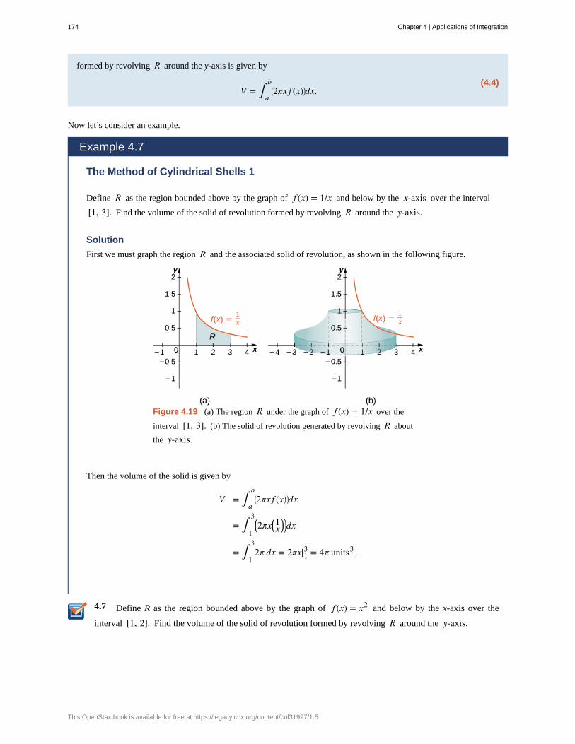
4.7
formed by revolving R around the y-axis is given by
(4.4)V = ∫
a
b⎛⎝2πx f (x)⎞⎠dx.
Now let’s consider an example.
Example 4.7
The Method of Cylindrical Shells 1
Define R as the region bounded above by the graph of f (x) = 1/x and below by the x-axis over the interval
[1, 3]. Find the volume of the solid of revolution formed by revolving R around the y-axis.
Solution
First we must graph the region R and the associated solid of revolution, as shown in the following figure.
Figure 4.19 (a) The region R under the graph of f (x) = 1/x over the
interval [1, 3]. (b) The solid of revolution generated by revolving R about
the y-axis.
Then the volume of the solid is given by
V = ∫a
b⎛⎝2πx f (x)⎞⎠dx
= ∫1
3⎛⎝2πx⎛⎝1x⎞⎠⎞⎠dx
= ∫1
32π dx = 2πx|13 = 4π units3 .
Define R as the region bounded above by the graph of f (x) = x2 and below by the x-axis over the
interval [1, 2]. Find the volume of the solid of revolution formed by revolving R around the y-axis.
174 Chapter 4 | Applications of Integration
This OpenStax book is available for free at https://legacy.cnx.org/content/col31997/1.5
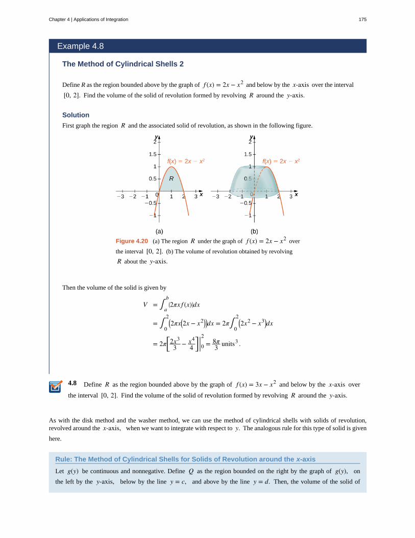
4.8
Example 4.8
The Method of Cylindrical Shells 2
Define R as the region bounded above by the graph of f (x) = 2x − x2 and below by the x-axis over the interval
[0, 2]. Find the volume of the solid of revolution formed by revolving R around the y-axis.
Solution
First graph the region R and the associated solid of revolution, as shown in the following figure.
Figure 4.20 (a) The region R under the graph of f (x) = 2x − x2 over
the interval [0, 2]. (b) The volume of revolution obtained by revolving
R about the y-axis.
Then the volume of the solid is given by
V = ∫a
b⎛⎝2πx f (x)⎞⎠dx
= ∫0
2⎛⎝2πx
⎛⎝2x − x2⎞⎠
⎞⎠dx = 2π∫
0
2⎛⎝2x2 − x3⎞⎠dx
= 2π⎡⎣2x3
3 − x4
4⎤⎦ |02 = 8π
3 units3 .
Define R as the region bounded above by the graph of f (x) = 3x − x2 and below by the x-axis over
the interval [0, 2]. Find the volume of the solid of revolution formed by revolving R around the y-axis.
As with the disk method and the washer method, we can use the method of cylindrical shells with solids of revolution,revolved around the x-axis, when we want to integrate with respect to y. The analogous rule for this type of solid is given
here.
Rule: The Method of Cylindrical Shells for Solids of Revolution around the x-axis
Let g(y) be continuous and nonnegative. Define Q as the region bounded on the right by the graph of g(y), on
the left by the y-axis, below by the line y = c, and above by the line y = d. Then, the volume of the solid of
Chapter 4 | Applications of Integration 175

4.9
revolution formed by revolving Q around the x-axis is given by
V = ∫c
d⎛⎝2πyg(y)⎞⎠dy.
Example 4.9
The Method of Cylindrical Shells for a Solid Revolved around the x-axis
Define Q as the region bounded on the right by the graph of g(y) = 2 y and on the left by the y-axis for
y ∈ [0, 4]. Find the volume of the solid of revolution formed by revolving Q around the x-axis.
Solution
First, we need to graph the region Q and the associated solid of revolution, as shown in the following figure.
Figure 4.21 (a) The region Q to the left of the function g(y) over the interval
[0, 4]. (b) The solid of revolution generated by revolving Q around the x-axis.
Label the shaded region Q. Then the volume of the solid is given by
V = ∫c
d⎛⎝2πyg(y)⎞⎠dy
= ∫0
4⎛⎝2πy⎛⎝2 y⎞⎠⎞⎠dy = 4π∫
0
4y3/2dy
= 4π⎡⎣⎢2y
5/2
5⎤⎦⎥ |04 = 256π
5 units3 .
Define Q as the region bounded on the right by the graph of g(y) = 3/y and on the left by the y-axis for
y ∈ [1, 3]. Find the volume of the solid of revolution formed by revolving Q around the x-axis.
176 Chapter 4 | Applications of Integration
This OpenStax book is available for free at https://legacy.cnx.org/content/col31997/1.5

For the next example, we look at a solid of revolution for which the graph of a function is revolved around a line other thanone of the two coordinate axes. To set this up, we need to revisit the development of the method of cylindrical shells. Recallthat we found the volume of one of the shells to be given by
Vshell = f (xi* )(πxi2 − πxi − 1
2 )
= π f (xi* )⎛⎝xi2 − xi − 1
2 ⎞⎠
= π f (xi* )(xi + xi − 1)(xi − xi − 1)
= 2π f (xi* )⎛⎝xi + xi − 1
2⎞⎠(xi − xi − 1).
This was based on a shell with an outer radius of xi and an inner radius of xi − 1. If, however, we rotate the region around
a line other than the y-axis, we have a different outer and inner radius. Suppose, for example, that we rotate the region
around the line x = −k, where k is some positive constant. Then, the outer radius of the shell is xi + k and the inner
radius of the shell is xi − 1 + k. Substituting these terms into the expression for volume, we see that when a plane region is
rotated around the line x = −k, the volume of a shell is given by
Vshell = 2π f (xi* )⎛⎝⎛⎝xi + k⎞⎠+ ⎛⎝xi − 1 + k⎞⎠
2⎞⎠⎛⎝⎛⎝xi + k⎞⎠− ⎛⎝xi − 1 + k⎞⎠⎞⎠
= 2π f (xi* )⎛⎝⎛⎝xi + xi − 2
2⎞⎠+ k⎞⎠Δx.
As before, we notice thatxi + xi − 1
2 is the midpoint of the interval [xi − 1, xi] and can be approximated by xi* . Then,
the approximate volume of the shell is
Vshell ≈ 2π⎛⎝xi* + k⎞⎠ f (xi* )Δx.
The remainder of the development proceeds as before, and we see that
V = ∫a
b⎛⎝2π(x + k) f (x)⎞⎠dx.
We could also rotate the region around other horizontal or vertical lines, such as a vertical line in the right half plane. Ineach case, the volume formula must be adjusted accordingly. Specifically, the x-term in the integral must be replaced with
an expression representing the radius of a shell. To see how this works, consider the following example.
Example 4.10
A Region of Revolution Revolved around a Line
Define R as the region bounded above by the graph of f (x) = x and below by the x-axis over the interval
[1, 2]. Find the volume of the solid of revolution formed by revolving R around the line x = −1.
Solution
First, graph the region R and the associated solid of revolution, as shown in the following figure.
Chapter 4 | Applications of Integration 177
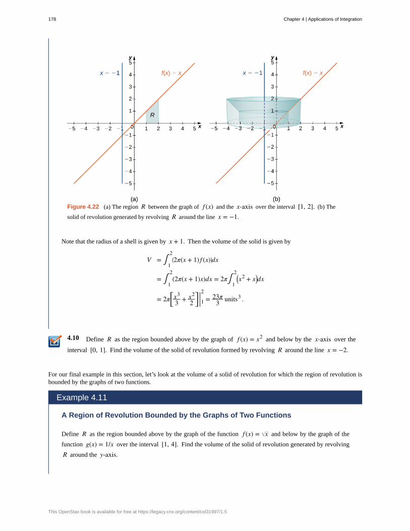
4.10
Figure 4.22 (a) The region R between the graph of f (x) and the x-axis over the interval [1, 2]. (b) The
solid of revolution generated by revolving R around the line x = −1.
Note that the radius of a shell is given by x + 1. Then the volume of the solid is given by
V = ∫1
2⎛⎝2π(x + 1) f (x)⎞⎠dx
= ∫1
2(2π(x + 1)x)dx = 2π∫
1
2⎛⎝x2 + x⎞⎠dx
= 2π⎡⎣x3
3 + x2
2⎤⎦ |12 = 23π
3 units3 .
Define R as the region bounded above by the graph of f (x) = x2 and below by the x-axis over the
interval [0, 1]. Find the volume of the solid of revolution formed by revolving R around the line x = −2.
For our final example in this section, let’s look at the volume of a solid of revolution for which the region of revolution isbounded by the graphs of two functions.
Example 4.11
A Region of Revolution Bounded by the Graphs of Two Functions
Define R as the region bounded above by the graph of the function f (x) = x and below by the graph of the
function g(x) = 1/x over the interval [1, 4]. Find the volume of the solid of revolution generated by revolving
R around the y-axis.
178 Chapter 4 | Applications of Integration
This OpenStax book is available for free at https://legacy.cnx.org/content/col31997/1.5
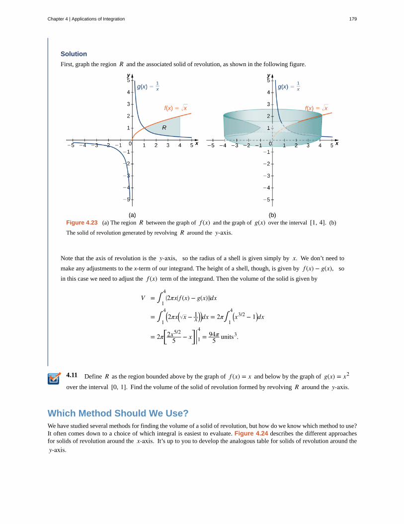
4.11
Solution
First, graph the region R and the associated solid of revolution, as shown in the following figure.
Figure 4.23 (a) The region R between the graph of f (x) and the graph of g(x) over the interval [1, 4]. (b)
The solid of revolution generated by revolving R around the y-axis.
Note that the axis of revolution is the y-axis, so the radius of a shell is given simply by x. We don’t need to
make any adjustments to the x-term of our integrand. The height of a shell, though, is given by f (x) − g(x), so
in this case we need to adjust the f (x) term of the integrand. Then the volume of the solid is given by
V = ∫1
4⎛⎝2πx⎛⎝ f (x) − g(x)⎞⎠⎞⎠dx
= ∫1
4⎛⎝2πx⎛⎝ x − 1
x⎞⎠⎞⎠dx = 2π∫
1
4⎛⎝x3/2 − 1⎞⎠dx
= 2π⎡⎣2x5/2
5 − x⎤⎦ |14 = 94π5 units3.
Define R as the region bounded above by the graph of f (x) = x and below by the graph of g(x) = x2
over the interval [0, 1]. Find the volume of the solid of revolution formed by revolving R around the y-axis.
Which Method Should We Use?We have studied several methods for finding the volume of a solid of revolution, but how do we know which method to use?It often comes down to a choice of which integral is easiest to evaluate. Figure 4.24 describes the different approachesfor solids of revolution around the x-axis. It’s up to you to develop the analogous table for solids of revolution around the
y-axis.
Chapter 4 | Applications of Integration 179
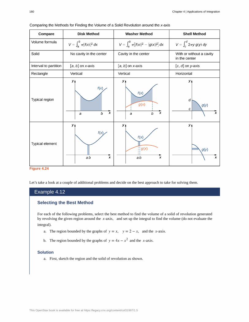
Figure 4.24
Let’s take a look at a couple of additional problems and decide on the best approach to take for solving them.
Example 4.12
Selecting the Best Method
For each of the following problems, select the best method to find the volume of a solid of revolution generatedby revolving the given region around the x-axis, and set up the integral to find the volume (do not evaluate the
integral).
a. The region bounded by the graphs of y = x, y = 2 − x, and the x-axis.
b. The region bounded by the graphs of y = 4x − x2 and the x-axis.
Solution
a. First, sketch the region and the solid of revolution as shown.
180 Chapter 4 | Applications of Integration
This OpenStax book is available for free at https://legacy.cnx.org/content/col31997/1.5
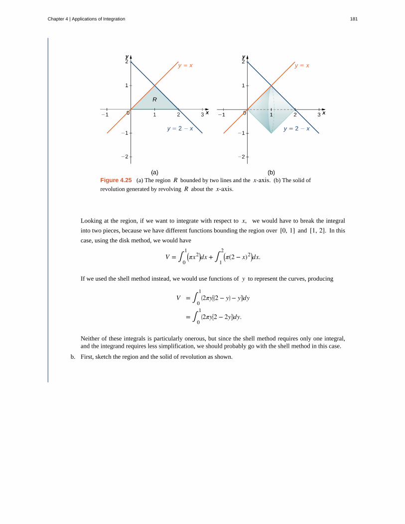
Figure 4.25 (a) The region R bounded by two lines and the x-axis. (b) The solid of
revolution generated by revolving R about the x-axis.
Looking at the region, if we want to integrate with respect to x, we would have to break the integral
into two pieces, because we have different functions bounding the region over [0, 1] and [1, 2]. In this
case, using the disk method, we would have
V = ∫0
1⎛⎝πx2⎞⎠dx + ∫
1
2⎛⎝π(2 − x)2⎞⎠dx.
If we used the shell method instead, we would use functions of y to represent the curves, producing
V = ∫0
1⎛⎝2πy⎡⎣⎛⎝2 − y⎞⎠− y⎤⎦⎞⎠dy
= ∫0
1⎛⎝2πy⎡⎣2 − 2y⎤⎦⎞⎠dy.
Neither of these integrals is particularly onerous, but since the shell method requires only one integral,and the integrand requires less simplification, we should probably go with the shell method in this case.
b. First, sketch the region and the solid of revolution as shown.
Chapter 4 | Applications of Integration 181
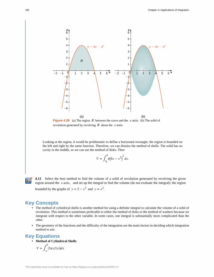
4.12
Figure 4.26 (a) The region R between the curve and the x-axis. (b) The solid of
revolution generated by revolving R about the x-axis.
Looking at the region, it would be problematic to define a horizontal rectangle; the region is bounded onthe left and right by the same function. Therefore, we can dismiss the method of shells. The solid has nocavity in the middle, so we can use the method of disks. Then
V = ∫0
4π⎛⎝4x − x2⎞⎠
2dx.
Select the best method to find the volume of a solid of revolution generated by revolving the givenregion around the x-axis, and set up the integral to find the volume (do not evaluate the integral): the region
bounded by the graphs of y = 2 − x2 and y = x2.
Key Concepts• The method of cylindrical shells is another method for using a definite integral to calculate the volume of a solid of
revolution. This method is sometimes preferable to either the method of disks or the method of washers because weintegrate with respect to the other variable. In some cases, one integral is substantially more complicated than theother.
• The geometry of the functions and the difficulty of the integration are the main factors in deciding which integrationmethod to use.
Key Equations• Method of Cylindrical Shells
V = ∫a
b⎛⎝2πx f (x)⎞⎠dx
182 Chapter 4 | Applications of Integration
This OpenStax book is available for free at https://legacy.cnx.org/content/col31997/1.5
4.2 EXERCISESFor the following exercises, find the volume generatedwhen the region between the two curves is rotated aroundthe given axis. Use both the shell method and the washermethod. Use technology to graph the functions and draw atypical slice by hand.
57. [T] Bounded by the curves y = 3x, x = 0, and
y = 3 rotated around the y-axis.
58. [T] Bounded by the curvesy = 3x, y = 0, and x = 3 rotated around the y-axis.
59. [T] Bounded by the curvesy = 3x, y = 0, and y = 3 rotated around the x-axis.
60. [T] Bounded by the curvesy = 3x, y = 0, and x = 3 rotated around the x-axis.
61. [T] Bounded by the curves
y = 2x3, y = 0, and x = 2 rotated around the y-axis.
62. [T] Bounded by the curves
y = 2x3, y = 0, and x = 2 rotated around the x-axis.
For the following exercises, use shells to find the volumesof the given solids. Note that the rotated regions lie betweenthe curve and the x-axis and are rotated around the
y-axis.
63. y = 1 − x2, x = 0, and x = 1
64. y = 5x3, x = 0, and x = 1
65. y = 1x , x = 1, and x = 100
66. y = 1 − x2, x = 0, and x = 1
67. y = 11 + x2, x = 0, and x = 3
68. y = sinx2, x = 0, and x = π
69. y = 11 − x2
, x = 0, and x = 12
70. y = x, x = 0, and x = 1
71. y = ⎛⎝1 + x2⎞⎠3, x = 0, and x = 1
72. y = 5x3 − 2x4, x = 0, and x = 2
For the following exercises, use shells to find the volumegenerated by rotating the regions between the given curveand y = 0 around the x-axis.
73. y = 1 − x2, x = 0, x = 1 and the x-axis
74. y = x2, x = 0, x = 2 and the x-axis
75. y = x3
2 , x = 0, x = 2, and the x-axis
76. y = 2x2, x = 1, x = 2, and the x-axis
77. x = 11 + y2, x = 1
5, and y = 0
78. x = 1 + y2y , y = 1, y = 4, and the y-axis
79. x = cos y, y = 0, and y = π
80. x = y3 - 2y2, x = 0, x = 9, and the y-axis
81. x = y + 1, x = 1, x = 3, and the x-axis
82. x = 27y3 and x = 3y4
For the following exercises, find the volume generatedwhen the region between the curves is rotated around thegiven axis.
83. y = 3 − x, y = 0, x = 0, and x = 2 rotated around
the y-axis.
84. y = x3, x = 0, and y = 8 rotated around the
y-axis.
85. y = x2, y = x, rotated around the y-axis.
86. y = x, y = 0, and x = 1 rotated around the line
x = 2.
87. y = 14 − x, x = 1, and x = 2 rotated around the line
x = 4.
88. y = x and y = x2 rotated around the y-axis.
89. y = x and y = x2 rotated around the line x = 2.
Chapter 4 | Applications of Integration 183
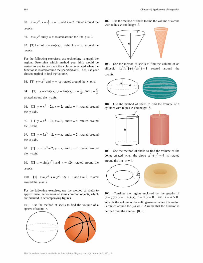
90. x = y3, x = 1y , x = 1, and x = 2 rotated around the
x-axis.
91. x = y2 and y = x rotated around the line y = 2.
92. [T] Left of x = sin(πy), right of y = x, around the
y-axis.
For the following exercises, use technology to graph theregion. Determine which method you think would beeasiest to use to calculate the volume generated when thefunction is rotated around the specified axis. Then, use yourchosen method to find the volume.
93. [T] y = x2 and y = 4x rotated around the y-axis.
94. [T] y = cos(πx), y = sin(πx), x = 14, and x = 5
4rotated around the y-axis.
95. [T] y = x2 − 2x, x = 2, and x = 4 rotated around
the y-axis.
96. [T] y = x2 − 2x, x = 2, and x = 4 rotated around
the x-axis.
97. [T] y = 3x3 − 2, y = x, and x = 2 rotated around
the x-axis.
98. [T] y = 3x3 − 2, y = x, and x = 2 rotated around
the y-axis.
99. [T] x = sin⎛⎝πy2⎞⎠ and x = 2y rotated around the
x-axis.
100. [T] x = y2, x = y2 − 2y + 1, and x = 2 rotated
around the y-axis.
For the following exercises, use the method of shells toapproximate the volumes of some common objects, whichare pictured in accompanying figures.
101. Use the method of shells to find the volume of asphere of radius r.
102. Use the method of shells to find the volume of a conewith radius r and height h.
103. Use the method of shells to find the volume of an
ellipsoid ⎛⎝x2/a2⎞⎠+
⎛⎝y2/b2⎞⎠ = 1 rotated around the
x-axis.
104. Use the method of shells to find the volume of acylinder with radius r and height h.
105. Use the method of shells to find the volume of the
donut created when the circle x2 + y2 = 4 is rotated
around the line x = 4.
106. Consider the region enclosed by the graphs ofy = f (x), y = 1 + f (x), x = 0, y = 0, and x = a > 0.What is the volume of the solid generated when this regionis rotated around the y-axis? Assume that the function is
defined over the interval [0, a].
184 Chapter 4 | Applications of Integration
This OpenStax book is available for free at https://legacy.cnx.org/content/col31997/1.5

107. Consider the function y = f (x), which decreases
from f (0) = b to f (1) = 0. Set up the integrals for
determining the volume, using both the shell method andthe disk method, of the solid generated when this region,with x = 0 and y = 0, is rotated around the y-axis.Prove that both methods approximate the same volume.Which method is easier to apply? (Hint: Since f (x) is one-
to-one, there exists an inverse f −1(y).)
Chapter 4 | Applications of Integration 185
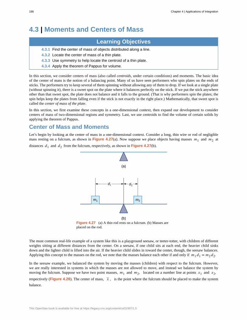
4.3 | Moments and Centers of Mass
Learning Objectives4.3.1 Find the center of mass of objects distributed along a line.
4.3.2 Locate the center of mass of a thin plate.
4.3.3 Use symmetry to help locate the centroid of a thin plate.
4.3.4 Apply the theorem of Pappus for volume.
In this section, we consider centers of mass (also called centroids, under certain conditions) and moments. The basic ideaof the center of mass is the notion of a balancing point. Many of us have seen performers who spin plates on the ends ofsticks. The performers try to keep several of them spinning without allowing any of them to drop. If we look at a single plate(without spinning it), there is a sweet spot on the plate where it balances perfectly on the stick. If we put the stick anywhereother than that sweet spot, the plate does not balance and it falls to the ground. (That is why performers spin the plates; thespin helps keep the plates from falling even if the stick is not exactly in the right place.) Mathematically, that sweet spot iscalled the center of mass of the plate.
In this section, we first examine these concepts in a one-dimensional context, then expand our development to considercenters of mass of two-dimensional regions and symmetry. Last, we use centroids to find the volume of certain solids byapplying the theorem of Pappus.
Center of Mass and MomentsLet’s begin by looking at the center of mass in a one-dimensional context. Consider a long, thin wire or rod of negligiblemass resting on a fulcrum, as shown in Figure 4.27(a). Now suppose we place objects having masses m1 and m2 at
distances d1 and d2 from the fulcrum, respectively, as shown in Figure 4.27(b).
Figure 4.27 (a) A thin rod rests on a fulcrum. (b) Masses areplaced on the rod.
The most common real-life example of a system like this is a playground seesaw, or teeter-totter, with children of differentweights sitting at different distances from the center. On a seesaw, if one child sits at each end, the heavier child sinksdown and the lighter child is lifted into the air. If the heavier child slides in toward the center, though, the seesaw balances.Applying this concept to the masses on the rod, we note that the masses balance each other if and only if m1d1 = m2d2.
In the seesaw example, we balanced the system by moving the masses (children) with respect to the fulcrum. However,we are really interested in systems in which the masses are not allowed to move, and instead we balance the system bymoving the fulcrum. Suppose we have two point masses, m1 and m2, located on a number line at points x1 and x2,respectively (Figure 4.28). The center of mass, x– , is the point where the fulcrum should be placed to make the system
balance.
186 Chapter 4 | Applications of Integration
This OpenStax book is available for free at https://legacy.cnx.org/content/col31997/1.5
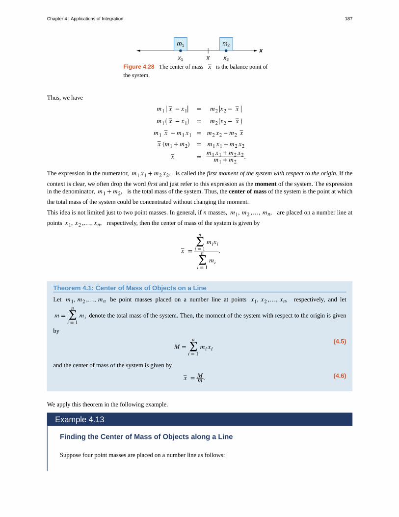
Figure 4.28 The center of mass x– is the balance point of
the system.
Thus, we have
m1 | x– − x1| = m2 |x2 − x– |m1⎛⎝ x– − x1
⎞⎠ = m2
⎛⎝x2 − x– ⎞⎠
m1 x– − m1 x1 = m2 x2 − m2 x–
x– (m1 + m2) = m1 x1 + m2 x2
x– = m1 x1 + m2 x2m1 + m2
.
The expression in the numerator, m1 x1 + m2 x2, is called the first moment of the system with respect to the origin. If the
context is clear, we often drop the word first and just refer to this expression as the moment of the system. The expressionin the denominator, m1 + m2, is the total mass of the system. Thus, the center of mass of the system is the point at which
the total mass of the system could be concentrated without changing the moment.
This idea is not limited just to two point masses. In general, if n masses, m1, m2 ,…, mn, are placed on a number line at
points x1, x2 ,…, xn, respectively, then the center of mass of the system is given by
x– =∑i = 1
nmixi
∑i = 1
nmi
.
Theorem 4.1: Center of Mass of Objects on a Line
Let m1, m2 ,…, mn be point masses placed on a number line at points x1, x2 ,…, xn, respectively, and let
m = ∑i = 1
nmi denote the total mass of the system. Then, the moment of the system with respect to the origin is given
by
(4.5)M = ∑
i = 1
nmi xi
and the center of mass of the system is given by
(4.6)x– = Mm .
We apply this theorem in the following example.
Example 4.13
Finding the Center of Mass of Objects along a Line
Suppose four point masses are placed on a number line as follows:
Chapter 4 | Applications of Integration 187

4.13
m1 = 30 kg, placed at x1 = −2 m m2 = 5 kg, placed at x2 = 3 m
m3 = 10 kg, placed at x3 = 6 m m4 = 15 kg, placed at x4 = −3 m.
Find the moment of the system with respect to the origin and find the center of mass of the system.
Solution
First, we need to calculate the moment of the system:
M = ∑i = 1
4mixi
= −60 + 15 + 60 − 45 = −30.
Now, to find the center of mass, we need the total mass of the system:
m = ∑i = 1
4mi
= 30 + 5 + 10 + 15 = 60 kg.
Then we have
x– = Mm = −30
60 = − 12.
The center of mass is located 1/2 m to the left of the origin.
Suppose four point masses are placed on a number line as follows:
m1 = 12 kg, placed at x1 = −4 m m2 = 12 kg, placed at x2 = 4 m
m3 = 30 kg, placed at x3 = 2 m m4 = 6 kg, placed at x4 = −6 m.
Find the moment of the system with respect to the origin and find the center of mass of the system.
We can generalize this concept to find the center of mass of a system of point masses in a plane. Let m1 be a point
mass located at point (x1, y1) in the plane. Then the moment Mx of the mass with respect to the x-axis is given by
Mx = m1 y1. Similarly, the moment My with respect to the y-axis is given by My = m1 x1. Notice that the x-coordinate
of the point is used to calculate the moment with respect to the y-axis, and vice versa. The reason is that the x-coordinategives the distance from the point mass to the y-axis, and the y-coordinate gives the distance to the x-axis (see the followingfigure).
Figure 4.29 Point mass m1 is located at point (x1, y1) in
the plane.
If we have several point masses in the xy-plane, we can use the moments with respect to the x- and y-axes to calculate the
188 Chapter 4 | Applications of Integration
This OpenStax book is available for free at https://legacy.cnx.org/content/col31997/1.5
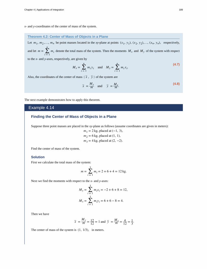
x- and y-coordinates of the center of mass of the system.
Theorem 4.2: Center of Mass of Objects in a Plane
Let m1, m2 ,…, mn be point masses located in the xy-plane at points (x1, y1), (x2, y2),…, (xn, yn), respectively,
and let m = ∑i = 1
nmi denote the total mass of the system. Then the moments Mx and My of the system with respect
to the x- and y-axes, respectively, are given by
(4.7)Mx = ∑
i = 1
nmi yi and My = ∑
i = 1
nmi xi.
Also, the coordinates of the center of mass ⎛⎝ x– , y– ⎞⎠ of the system are
(4.8)x– =Mym and y– = Mx
m .
The next example demonstrates how to apply this theorem.
Example 4.14
Finding the Center of Mass of Objects in a Plane
Suppose three point masses are placed in the xy-plane as follows (assume coordinates are given in meters):
m1 = 2 kg, placed at (−1, 3),m2 = 6 kg, placed at (1, 1),m3 = 4 kg, placed at (2, −2).
Find the center of mass of the system.
Solution
First we calculate the total mass of the system:
m = ∑i = 1
3mi = 2 + 6 + 4 = 12 kg.
Next we find the moments with respect to the x- and y-axes:
My = ∑i = 1
3mixi = −2 + 6 + 8 = 12,
Mx = ∑i = 1
3miyi = 6 + 6 − 8 = 4.
Then we have
x– =Mym = 12
12 = 1 and y– = Mxm = 4
12 = 13.
The center of mass of the system is (1, 1/3), in meters.
Chapter 4 | Applications of Integration 189
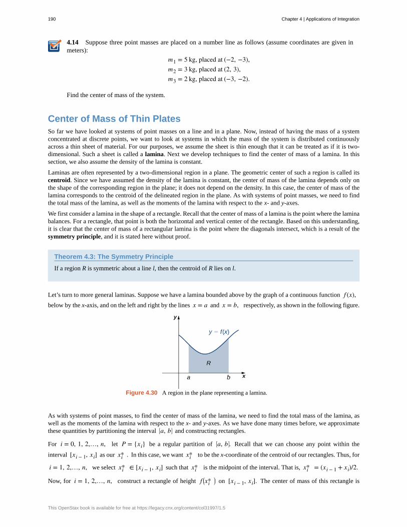
4.14 Suppose three point masses are placed on a number line as follows (assume coordinates are given inmeters):
m1 = 5 kg, placed at (−2, −3),m2 = 3 kg, placed at (2, 3),m3 = 2 kg, placed at (−3, −2).
Find the center of mass of the system.
Center of Mass of Thin PlatesSo far we have looked at systems of point masses on a line and in a plane. Now, instead of having the mass of a systemconcentrated at discrete points, we want to look at systems in which the mass of the system is distributed continuouslyacross a thin sheet of material. For our purposes, we assume the sheet is thin enough that it can be treated as if it is two-dimensional. Such a sheet is called a lamina. Next we develop techniques to find the center of mass of a lamina. In thissection, we also assume the density of the lamina is constant.
Laminas are often represented by a two-dimensional region in a plane. The geometric center of such a region is called itscentroid. Since we have assumed the density of the lamina is constant, the center of mass of the lamina depends only onthe shape of the corresponding region in the plane; it does not depend on the density. In this case, the center of mass of thelamina corresponds to the centroid of the delineated region in the plane. As with systems of point masses, we need to findthe total mass of the lamina, as well as the moments of the lamina with respect to the x- and y-axes.
We first consider a lamina in the shape of a rectangle. Recall that the center of mass of a lamina is the point where the laminabalances. For a rectangle, that point is both the horizontal and vertical center of the rectangle. Based on this understanding,it is clear that the center of mass of a rectangular lamina is the point where the diagonals intersect, which is a result of thesymmetry principle, and it is stated here without proof.
Theorem 4.3: The Symmetry Principle
If a region R is symmetric about a line l, then the centroid of R lies on l.
Let’s turn to more general laminas. Suppose we have a lamina bounded above by the graph of a continuous function f (x),below by the x-axis, and on the left and right by the lines x = a and x = b, respectively, as shown in the following figure.
Figure 4.30 A region in the plane representing a lamina.
As with systems of point masses, to find the center of mass of the lamina, we need to find the total mass of the lamina, aswell as the moments of the lamina with respect to the x- and y-axes. As we have done many times before, we approximatethese quantities by partitioning the interval ⎡⎣a, b⎤⎦ and constructing rectangles.
For i = 0, 1, 2,…, n, let P = {xi} be a regular partition of ⎡⎣a, b⎤⎦. Recall that we can choose any point within the
interval [xi − 1, xi] as our xi* . In this case, we want xi* to be the x-coordinate of the centroid of our rectangles. Thus, for
i = 1, 2,…, n, we select xi* ∈ [xi − 1, xi] such that xi* is the midpoint of the interval. That is, xi* = (xi − 1 + xi)/2.
Now, for i = 1, 2,…, n, construct a rectangle of height f ⎛⎝xi*⎞⎠ on [xi − 1, xi]. The center of mass of this rectangle is
190 Chapter 4 | Applications of Integration
This OpenStax book is available for free at https://legacy.cnx.org/content/col31997/1.5

⎛⎝xi* , ⎛⎝ f (xi* )⎞⎠/2⎞⎠, as shown in the following figure.
Figure 4.31 A representative rectangle of the lamina.
Next, we need to find the total mass of the rectangle. Let ρ represent the density of the lamina (note that ρ is a constant).
In this case, ρ is expressed in terms of mass per unit area. Thus, to find the total mass of the rectangle, we multiply the area
of the rectangle by ρ. Then, the mass of the rectangle is given by ρ f (xi* )Δx.
To get the approximate mass of the lamina, we add the masses of all the rectangles to get
m ≈ ∑i = 1
nρ f (xi* )Δx.
This is a Riemann sum. Taking the limit as n → ∞ gives the exact mass of the lamina:
m = limn → ∞ ∑i = 1
nρ f (xi* )Δx = ρ∫
a
bf (x)dx.
Next, we calculate the moment of the lamina with respect to the x-axis. Returning to the representative rectangle, recall its
center of mass is ⎛⎝xi* , ⎛⎝ f (xi* )⎞⎠/2⎞⎠. Recall also that treating the rectangle as if it is a point mass located at the center of
mass does not change the moment. Thus, the moment of the rectangle with respect to the x-axis is given by the mass ofthe rectangle, ρ f (xi* )Δx, multiplied by the distance from the center of mass to the x-axis: ⎛⎝ f (xi* )⎞⎠/2. Therefore, the
moment with respect to the x-axis of the rectangle is ρ⎛⎝⎡⎣ f (xi* )⎤⎦2/2⎞⎠Δx. Adding the moments of the rectangles and taking
the limit of the resulting Riemann sum, we see that the moment of the lamina with respect to the x-axis is
Mx = limn → ∞ ∑i = 1
nρ⎡⎣ f (xi* )⎤⎦2
2 Δx = ρ∫a
b ⎡⎣ f (x)⎤⎦2
2 dx.
We derive the moment with respect to the y-axis similarly, noting that the distance from the center of mass of the rectangleto the y-axis is xi* . Then the moment of the lamina with respect to the y-axis is given by
My = limn → ∞ ∑i = 1
nρxi* f (xi* )Δx = ρ∫
a
bx f (x)dx.
We find the coordinates of the center of mass by dividing the moments by the total mass to givex– = My/m and y– = Mx/m. If we look closely at the expressions for Mx, My, and m, we notice that the constant ρ
cancels out when x– and y– are calculated.
We summarize these findings in the following theorem.
Theorem 4.4: Center of Mass of a Thin Plate in the xy-Plane
Let R denote a region bounded above by the graph of a continuous function f (x), below by the x-axis, and on the left
Chapter 4 | Applications of Integration 191

and right by the lines x = a and x = b, respectively. Let ρ denote the density of the associated lamina. Then we
can make the following statements:
i. The mass of the lamina is
(4.9)m = ρ∫
a
bf (x)dx.
ii. The moments Mx and My of the lamina with respect to the x- and y-axes, respectively, are
(4.10)Mx = ρ∫
a
b ⎡⎣ f (x)⎤⎦2
2 dx and My = ρ∫a
bx f (x)dx.
iii. The coordinates of the center of mass ⎛⎝ x– , y– ⎞⎠ are
(4.11)x– =Mym and y– = Mx
m .
In the next example, we use this theorem to find the center of mass of a lamina.
Example 4.15
Finding the Center of Mass of a Lamina
Let R be the region bounded above by the graph of the function f (x) = x and below by the x-axis over the
interval [0, 4]. Find the centroid of the region.
Solution
The region is depicted in the following figure.
Figure 4.32 Finding the center of mass of a lamina.
Since we are only asked for the centroid of the region, rather than the mass or moments of the associatedlamina, we know the density constant ρ cancels out of the calculations eventually. Therefore, for the sake of
convenience, let’s assume ρ = 1.
First, we need to calculate the total mass:
m = ρ∫a
bf (x)dx = ∫
0
4x dx
= 23x
3/2|04 = 23[8 − 0] = 16
3 .
192 Chapter 4 | Applications of Integration
This OpenStax book is available for free at https://legacy.cnx.org/content/col31997/1.5

4.15
Next, we compute the moments:
Mx = ρ∫a
b ⎡⎣ f (x)⎤⎦2
2 dx
= ∫0
4x2dx = 1
4x2|04 = 4
and
My = ρ∫a
bx f (x)dx
= ∫0
4x xdx = ∫
0
4x3/2dx
= 25x
5/2|04 = 25[32 − 0] = 64
5 .
Thus, we have
x– =Mym = 64/5
16/3 = 645 · 3
16 = 125 and y– = Mx
m = 416/3 = 4 · 3
16 = 34.
The centroid of the region is (12/5, 3/4).
Let R be the region bounded above by the graph of the function f (x) = x2 and below by the x-axis over
the interval [0, 2]. Find the centroid of the region.
We can adapt this approach to find centroids of more complex regions as well. Suppose our region is bounded above by thegraph of a continuous function f (x), as before, but now, instead of having the lower bound for the region be the x-axis,
suppose the region is bounded below by the graph of a second continuous function, g(x), as shown in the following figure.
Figure 4.33 A region between two functions.
Again, we partition the interval ⎡⎣a, b⎤⎦ and construct rectangles. A representative rectangle is shown in the following figure.
Chapter 4 | Applications of Integration 193

Figure 4.34 A representative rectangle of the region betweentwo functions.
Note that the centroid of this rectangle is ⎛⎝xi* , ⎛⎝ f (xi* ) + g(xi* )⎞⎠/2⎞⎠. We won’t go through all the details of the Riemann
sum development, but let’s look at some of the key steps. In the development of the formulas for the mass of the laminaand the moment with respect to the y-axis, the height of each rectangle is given by f (xi* ) − g(xi* ), which leads to the
expression f (x) − g(x) in the integrands.
In the development of the formula for the moment with respect to the x-axis, the moment of each rectangle is foundby multiplying the area of the rectangle, ρ⎡⎣ f (xi* ) − g(xi* )⎤⎦Δx, by the distance of the centroid from the x-axis,
⎛⎝ f (xi* ) + g(xi* )⎞⎠/2, which gives ρ(1/2)⎧⎩⎨
⎡⎣ f (xi* )⎤⎦2 − ⎡⎣g(xi* )⎤⎦2
⎫⎭⎬Δx. Summarizing these findings, we arrive at the
following theorem.
Theorem 4.5: Center of Mass of a Lamina Bounded by Two Functions
Let R denote a region bounded above by the graph of a continuous function f (x), below by the graph of the
continuous function g(x), and on the left and right by the lines x = a and x = b, respectively. Let ρ denote the
density of the associated lamina. Then we can make the following statements:
i. The mass of the lamina is
(4.12)m = ρ∫
a
b⎡⎣ f (x) − g(x)⎤⎦dx.
ii. The moments Mx and My of the lamina with respect to the x- and y-axes, respectively, are
(4.13)Mx = ρ∫
a
b12⎛⎝⎡⎣ f (x)⎤⎦2 − ⎡
⎣g(x)⎤⎦2⎞⎠dx and My = ρ∫a
bx⎡⎣ f (x) − g(x)⎤⎦dx.
iii. The coordinates of the center of mass ⎛⎝ x– , y– ⎞⎠ are
(4.14)x– =Mym and y– = Mx
m .
We illustrate this theorem in the following example.
Example 4.16
Finding the Centroid of a Region Bounded by Two Functions
Let R be the region bounded above by the graph of the function f (x) = 1 − x2 and below by the graph of the
function g(x) = x − 1. Find the centroid of the region.
194 Chapter 4 | Applications of Integration
This OpenStax book is available for free at https://legacy.cnx.org/content/col31997/1.5

Solution
The region is depicted in the following figure.
Figure 4.35 Finding the centroid of a region between twocurves.
The graphs of the functions intersect at (−2, −3) and (1, 0), so we integrate from −2 to 1. Once again, for the
sake of convenience, assume ρ = 1.
First, we need to calculate the total mass:
m = ρ∫a
b⎡⎣ f (x) − g(x)⎤⎦dx
= ∫−2
1 ⎡⎣1 − x2 − (x − 1)⎤⎦dx = ∫
−2
1(2 − x2 − x)dx
= ⎡⎣2x − 13x
3 − 12x
2⎤⎦ |−21
= ⎡⎣2 − 13 − 1
2⎤⎦−⎡⎣−4 + 8
3 − 2⎤⎦ = 92.
Next, we compute the moments:
Mx = ρ∫a
b12⎛⎝⎡⎣ f (x)⎤⎦2 − ⎡
⎣g(x)⎤⎦2⎞⎠dx
= 12∫
−2
1 ⎛⎝⎛⎝1 − x2⎞⎠
2− (x − 1)2⎞⎠dx = 1
2∫−2
1 ⎛⎝x4 − 3x2 + 2x⎞⎠dx
= 12⎡⎣x
5
5 − x3 + x2⎤⎦ |−2
1= − 27
10
and
My = ρ∫a
bx⎡⎣ f (x) − g(x)⎤⎦dx
= ∫−2
1x⎡⎣(1 − x2) − (x − 1)⎤⎦dx = ∫
−2
1x⎡⎣2 − x2 − x⎤⎦dx
= ∫−2
1 ⎛⎝2x − x4 − x2⎞⎠dx
= ⎡⎣x2 − x5
5 − x3
3⎤⎦ |−2
1= − 9
4.
Therefore, we have
Chapter 4 | Applications of Integration 195

4.16
x– =Mym = − 9
4 · 29 = − 1
2 and y– = Mxm = − 27
10 · 29 = − 3
5.
The centroid of the region is ⎛⎝−(1/2), −(3/5)⎞⎠.
Let R be the region bounded above by the graph of the function f (x) = 6 − x2 and below by the graph
of the function g(x) = 3 − 2x. Find the centroid of the region.
The Symmetry PrincipleWe stated the symmetry principle earlier, when we were looking at the centroid of a rectangle. The symmetry principle canbe a great help when finding centroids of regions that are symmetric. Consider the following example.
Example 4.17
Finding the Centroid of a Symmetric Region
Let R be the region bounded above by the graph of the function f (x) = 4 − x2 and below by the x-axis. Find the
centroid of the region.
Solution
The region is depicted in the following figure.
Figure 4.36 We can use the symmetry principle to help findthe centroid of a symmetric region.
The region is symmetric with respect to the y-axis. Therefore, the x-coordinate of the centroid is zero. We needonly calculate y– . Once again, for the sake of convenience, assume ρ = 1.
First, we calculate the total mass:
196 Chapter 4 | Applications of Integration
This OpenStax book is available for free at https://legacy.cnx.org/content/col31997/1.5
4.17
m = ρ∫a
bf (x)dx
= ∫−2
2 ⎛⎝4 − x2⎞⎠dx
= ⎡⎣4x − x3
3⎤⎦ |−2
2= 32
3 .
Next, we calculate the moments. We only need Mx :
Mx = ρ∫a
b ⎡⎣ f (x)⎤⎦2
2 dx
= 12∫
−2
2 ⎡⎣4 − x2⎤⎦
2dx = 1
2∫−2
2 ⎛⎝16 − 8x2 + x4⎞⎠dx
= 12⎡⎣x
5
5 − 8x3
3 + 16x⎤⎦ |−2
2= 256
15 .
Then we have
y– = Mxm = 256
15 · 332 = 8
5.
The centroid of the region is (0, 8/5).
Let R be the region bounded above by the graph of the function f (x) = 1 − x2 and below by x-axis.
Find the centroid of the region.
Chapter 4 | Applications of Integration 197

The Grand Canyon Skywalk
The Grand Canyon Skywalk opened to the public on March 28, 2007. This engineering marvel is a horseshoe-shapedobservation platform suspended 4000 ft above the Colorado River on the West Rim of the Grand Canyon. Its crystal-clear glass floor allows stunning views of the canyon below (see the following figure).
Figure 4.37 The Grand Canyon Skywalk offers magnificent views of the canyon. (credit: 10da_ralta, WikimediaCommons)
The Skywalk is a cantilever design, meaning that the observation platform extends over the rim of the canyon, with novisible means of support below it. Despite the lack of visible support posts or struts, cantilever structures are engineeredto be very stable and the Skywalk is no exception. The observation platform is attached firmly to support posts thatextend 46 ft down into bedrock. The structure was built to withstand 100-mph winds and an 8.0-magnitude earthquakewithin 50 mi, and is capable of supporting more than 70,000,000 lb.
One factor affecting the stability of the Skywalk is the center of gravity of the structure. We are going to calculatethe center of gravity of the Skywalk, and examine how the center of gravity changes when tourists walk out onto theobservation platform.
The observation platform is U-shaped. The legs of the U are 10 ft wide and begin on land, under the visitors’ center,48 ft from the edge of the canyon. The platform extends 70 ft over the edge of the canyon.
To calculate the center of mass of the structure, we treat it as a lamina and use a two-dimensional region in the xy-planeto represent the platform. We begin by dividing the region into three subregions so we can consider each subregion
198 Chapter 4 | Applications of Integration
This OpenStax book is available for free at https://legacy.cnx.org/content/col31997/1.5
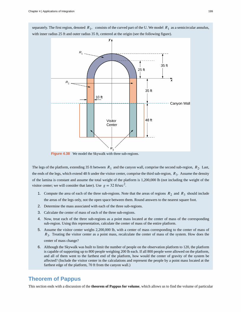
separately. The first region, denoted R1, consists of the curved part of the U. We model R1 as a semicircular annulus,
with inner radius 25 ft and outer radius 35 ft, centered at the origin (see the following figure).
Figure 4.38 We model the Skywalk with three sub-regions.
The legs of the platform, extending 35 ft between R1 and the canyon wall, comprise the second sub-region, R2. Last,
the ends of the legs, which extend 48 ft under the visitor center, comprise the third sub-region, R3. Assume the density
of the lamina is constant and assume the total weight of the platform is 1,200,000 lb (not including the weight of the
visitor center; we will consider that later). Use g = 32 ft/sec2.
1. Compute the area of each of the three sub-regions. Note that the areas of regions R2 and R3 should include
the areas of the legs only, not the open space between them. Round answers to the nearest square foot.
2. Determine the mass associated with each of the three sub-regions.
3. Calculate the center of mass of each of the three sub-regions.
4. Now, treat each of the three sub-regions as a point mass located at the center of mass of the correspondingsub-region. Using this representation, calculate the center of mass of the entire platform.
5. Assume the visitor center weighs 2,200,000 lb, with a center of mass corresponding to the center of mass ofR3. Treating the visitor center as a point mass, recalculate the center of mass of the system. How does the
center of mass change?
6. Although the Skywalk was built to limit the number of people on the observation platform to 120, the platformis capable of supporting up to 800 people weighing 200 lb each. If all 800 people were allowed on the platform,and all of them went to the farthest end of the platform, how would the center of gravity of the system beaffected? (Include the visitor center in the calculations and represent the people by a point mass located at thefarthest edge of the platform, 70 ft from the canyon wall.)
Theorem of PappusThis section ends with a discussion of the theorem of Pappus for volume, which allows us to find the volume of particular
Chapter 4 | Applications of Integration 199
kinds of solids by using the centroid. (There is also a theorem of Pappus for surface area, but it is much less useful than thetheorem for volume.)
Theorem 4.6: Theorem of Pappus for Volume
Let R be a region in the plane and let l be a line in the plane that does not intersect R. Then the volume of the solid ofrevolution formed by revolving R around l is equal to the area of R multiplied by the distance d traveled by the centroidof R.
Proof
We can prove the case when the region is bounded above by the graph of a function f (x) and below by the graph of a
function g(x) over an interval ⎡⎣a, b⎤⎦, and for which the axis of revolution is the y-axis. In this case, the area of the region is
A = ∫a
b⎡⎣ f (x) − g(x)⎤⎦dx. Since the axis of rotation is the y-axis, the distance traveled by the centroid of the region depends
only on the x-coordinate of the centroid, x– , which is
x– =Mym ,
where
m = ρ∫a
b⎡⎣ f (x) − g(x)⎤⎦dx and My = ρ∫
a
bx⎡⎣ f (x) − g(x)⎤⎦dx.
Then,
d = 2πρ∫
a
bx⎡⎣ f (x) − g(x)⎤⎦dx
ρ∫a
b⎡⎣ f (x) − g(x)⎤⎦dx
and thus
d · A = 2π∫a
bx⎡⎣ f (x) − g(x)⎤⎦dx.
However, using the method of cylindrical shells, we have
V = 2π∫a
bx⎡⎣ f (x) − g(x)⎤⎦dx.
So,
V = d · A
and the proof is complete.
□
Example 4.18
Using the Theorem of Pappus for Volume
Let R be a circle of radius 2 centered at (4, 0). Use the theorem of Pappus for volume to find the volume of the
torus generated by revolving R around the y-axis.
200 Chapter 4 | Applications of Integration
This OpenStax book is available for free at https://legacy.cnx.org/content/col31997/1.5
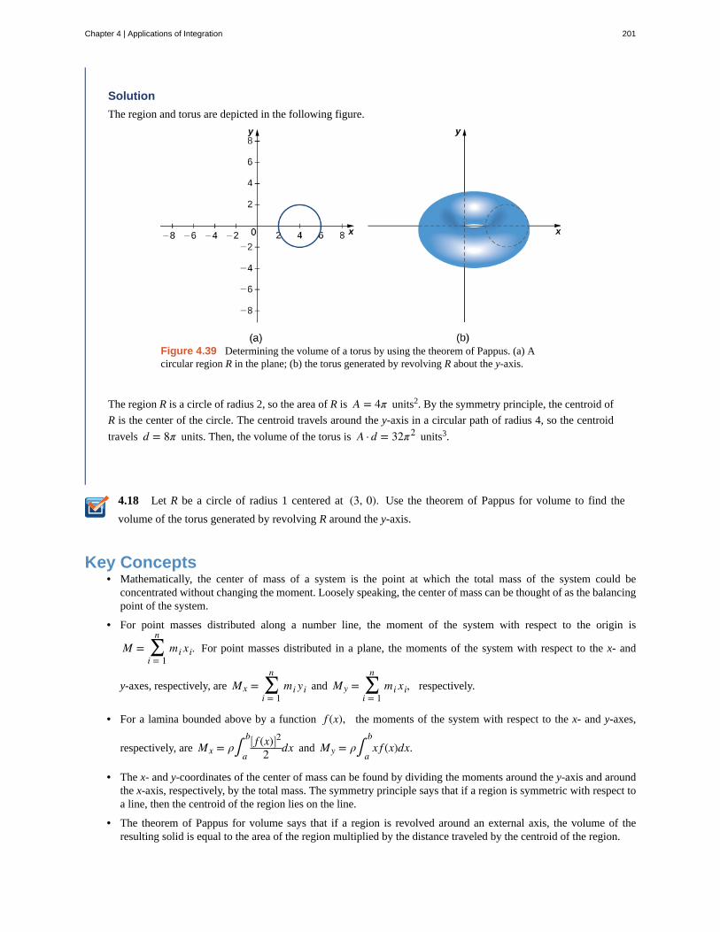
4.18
Solution
The region and torus are depicted in the following figure.
Figure 4.39 Determining the volume of a torus by using the theorem of Pappus. (a) Acircular region R in the plane; (b) the torus generated by revolving R about the y-axis.
The region R is a circle of radius 2, so the area of R is A = 4π units2. By the symmetry principle, the centroid of
R is the center of the circle. The centroid travels around the y-axis in a circular path of radius 4, so the centroid
travels d = 8π units. Then, the volume of the torus is A · d = 32π2 units3.
Let R be a circle of radius 1 centered at (3, 0). Use the theorem of Pappus for volume to find the
volume of the torus generated by revolving R around the y-axis.
Key Concepts• Mathematically, the center of mass of a system is the point at which the total mass of the system could be
concentrated without changing the moment. Loosely speaking, the center of mass can be thought of as the balancingpoint of the system.
• For point masses distributed along a number line, the moment of the system with respect to the origin is
M = ∑i = 1
nmi xi. For point masses distributed in a plane, the moments of the system with respect to the x- and
y-axes, respectively, are Mx = ∑i = 1
nmi yi and My = ∑
i = 1
nmi xi, respectively.
• For a lamina bounded above by a function f (x), the moments of the system with respect to the x- and y-axes,
respectively, are Mx = ρ∫a
b ⎡⎣ f (x)⎤⎦2
2 dx and My = ρ∫a
bx f (x)dx.
• The x- and y-coordinates of the center of mass can be found by dividing the moments around the y-axis and aroundthe x-axis, respectively, by the total mass. The symmetry principle says that if a region is symmetric with respect toa line, then the centroid of the region lies on the line.
• The theorem of Pappus for volume says that if a region is revolved around an external axis, the volume of theresulting solid is equal to the area of the region multiplied by the distance traveled by the centroid of the region.
Chapter 4 | Applications of Integration 201
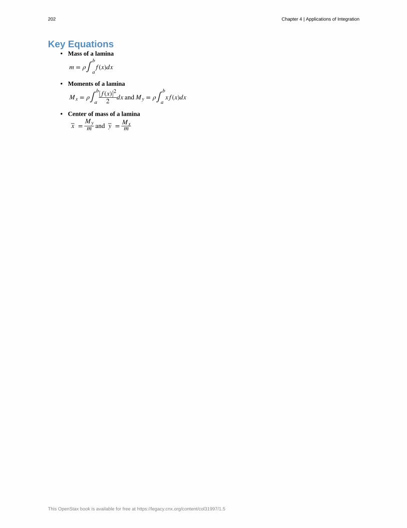
Key Equations• Mass of a lamina
m = ρ∫a
bf (x)dx
• Moments of a lamina
Mx = ρ∫a
b ⎡⎣ f (x)⎤⎦2
2 dx and My = ρ∫a
bx f (x)dx
• Center of mass of a lamina
x– =Mym and y– = Mx
m
202 Chapter 4 | Applications of Integration
This OpenStax book is available for free at https://legacy.cnx.org/content/col31997/1.5

4.3 EXERCISESFor the following exercises, calculate the center of mass forthe collection of masses given.
108. m1 = 2 at x1 = 1 and m2 = 4 at x2 = 2
109. m1 = 1 at x1 = −1 and m2 = 3 at x2 = 2
110. m = 3 at x = 0, 1, 2, 6
111. Unit masses at (x, y) = (1, 0), (0, 1), (1, 1)
112. m1 = 1 at (1, 0) and m2 = 4 at (0, 1)
113. m1 = 1 at (1, 0) and m2 = 3 at (2, 2)
For the following exercises, compute the center of massx– .
114. ρ = 1 for x ∈ (−1, 3)
115. ρ = x2 for x ∈ (0, L)
116. ρ = 1 for x ∈ (0, 1) and ρ = 2 for x ∈ (1, 2)
117. ρ = sin x for x ∈ (0, π)
118. ρ = cos x for x ∈ ⎛⎝0, π2⎞⎠
119. ρ = ex for x ∈ (0, 2)
120. ρ = x3 + xe−x for x ∈ (0, 1)
121. ρ = x sin x for x ∈ (0, π)
122. ρ = x for x ∈ (1, 4)
123. ρ = ln x for x ∈ (1, e)
For the following exercises, compute the center of mass⎛⎝ x– , y– ⎞⎠. Use symmetry to help locate the center of mass
whenever possible.
124. ρ = 7 in the square 0 ≤ x ≤ 1, 0 ≤ y ≤ 1
125. ρ = 3 in the triangle with vertices (0, 0), (a, 0),and (0, b)
126. ρ = 2 for the region bounded by y = cos(x),
y = −cos(x), x = − π2, and x = π
2
For the following exercises, use a calculator to draw theregion, then compute the center of mass ⎛
⎝ x– , y– ⎞⎠. Use
symmetry to help locate the center of mass wheneverpossible.
127. [T] The region bounded by y = cos(2x),
x = − π4, and x = π
4
128. [T] The region between y = 2x2, y = 0, x = 0,and x = 1
129. [T] The region between y = 54x
2 and y = 5
130. [T] Region between y = x, y = ln(x), x = 1,and x = 4
131. [T] The region bounded by y = 0, x2
4 + y2
9 = 1
132. [T] The region bounded by y = 0, x = 0, and
x2
4 + y2
9 = 1
133. [T] The region bounded by y = x2 and y = x4 in
the first quadrant
For the following exercises, use the theorem of Pappus todetermine the volume of the shape.
134. Rotating y = mx around the x -axis between x = 0and x = 1
135. Rotating y = mx around the y -axis between x = 0and x = 1
136. A general cone created by rotating a triangle withvertices (0, 0), (a, 0), and (0, b) around the y -axis.
Does your answer agree with the volume of a cone?
137. A general cylinder created by rotating a rectanglewith vertices (0, 0), (a, 0), (0, b), and (a, b) around
the y -axis. Does your answer agree with the volume of a
cylinder?
138. A sphere created by rotating a semicircle with radiusa around the y -axis. Does your answer agree with the
volume of a sphere?
For the following exercises, use a calculator to draw theregion enclosed by the curve. Find the area M and the
Chapter 4 | Applications of Integration 203
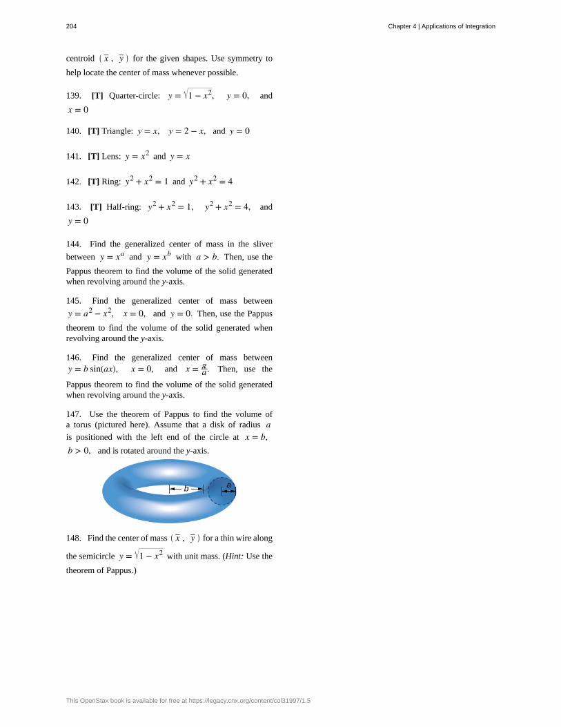
centroid ⎛⎝ x– , y– ⎞⎠ for the given shapes. Use symmetry to
help locate the center of mass whenever possible.
139. [T] Quarter-circle: y = 1 − x2, y = 0, and
x = 0
140. [T] Triangle: y = x, y = 2 − x, and y = 0
141. [T] Lens: y = x2 and y = x
142. [T] Ring: y2 + x2 = 1 and y2 + x2 = 4
143. [T] Half-ring: y2 + x2 = 1, y2 + x2 = 4, and
y = 0
144. Find the generalized center of mass in the sliver
between y = xa and y = xb with a > b. Then, use the
Pappus theorem to find the volume of the solid generatedwhen revolving around the y-axis.
145. Find the generalized center of mass between
y = a2 − x2, x = 0, and y = 0. Then, use the Pappus
theorem to find the volume of the solid generated whenrevolving around the y-axis.
146. Find the generalized center of mass betweeny = b sin(ax), x = 0, and x = π
a . Then, use the
Pappus theorem to find the volume of the solid generatedwhen revolving around the y-axis.
147. Use the theorem of Pappus to find the volume ofa torus (pictured here). Assume that a disk of radius ais positioned with the left end of the circle at x = b,b > 0, and is rotated around the y-axis.
148. Find the center of mass ⎛⎝ x– , y– ⎞⎠ for a thin wire along
the semicircle y = 1 − x2 with unit mass. (Hint: Use the
theorem of Pappus.)
204 Chapter 4 | Applications of Integration
This OpenStax book is available for free at https://legacy.cnx.org/content/col31997/1.5

4.4 | Integrals, Exponential Functions, and Logarithms
Learning Objectives4.4.1 Write the definition of the natural logarithm as an integral.
4.4.2 Recognize the derivative of the natural logarithm.
4.4.3 Integrate functions involving the natural logarithmic function.
4.4.4 Define the number e through an integral.
4.4.5 Recognize the derivative and integral of the exponential function.
4.4.6 Prove properties of logarithms and exponential functions using integrals.
4.4.7 Express general logarithmic and exponential functions in terms of natural logarithms andexponentials.
We already examined exponential functions and logarithms in earlier chapters. However, we glossed over some key detailsin the previous discussions. For example, we did not study how to treat exponential functions with exponents that areirrational. The definition of the number e is another area where the previous development was somewhat incomplete. Wenow have the tools to deal with these concepts in a more mathematically rigorous way, and we do so in this section.
For purposes of this section, assume we have not yet defined the natural logarithm, the number e, or any of the integrationand differentiation formulas associated with these functions. By the end of the section, we will have studied these conceptsin a mathematically rigorous way (and we will see they are consistent with the concepts we learned earlier).
We begin the section by defining the natural logarithm in terms of an integral. This definition forms the foundation forthe section. From this definition, we derive differentiation formulas, define the number e, and expand these concepts to
logarithms and exponential functions of any base.
The Natural Logarithm as an IntegralRecall the power rule for integrals:
∫ xndx = xn + 1
n + 1 + C, n ≠ −1.
Clearly, this does not work when n = −1, as it would force us to divide by zero. So, what do we do with ∫ 1xdx? Recall
from the Fundamental Theorem of Calculus that ∫1
x1t dt is an antiderivative of 1/x. Therefore, we can make the following
definition.
Definition
For x > 0, define the natural logarithm function by
(4.15)ln x = ∫
1
x1t dt.
For x > 1, this is just the area under the curve y = 1/t from 1 to x. For x < 1, we have ∫1
x1t dt = −∫
x
11t dt, so in
this case it is the negative of the area under the curve from x to 1 (see the following figure).
Chapter 4 | Applications of Integration 205
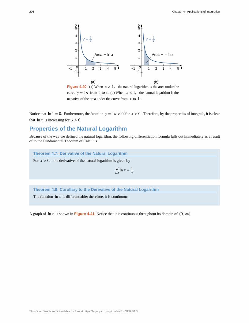
Figure 4.40 (a) When x > 1, the natural logarithm is the area under the
curve y = 1/t from 1 to x. (b) When x < 1, the natural logarithm is the
negative of the area under the curve from x to 1.
Notice that ln 1 = 0. Furthermore, the function y = 1/t > 0 for x > 0. Therefore, by the properties of integrals, it is clear
that ln x is increasing for x > 0.
Properties of the Natural LogarithmBecause of the way we defined the natural logarithm, the following differentiation formula falls out immediately as a resultof to the Fundamental Theorem of Calculus.
Theorem 4.7: Derivative of the Natural Logarithm
For x > 0, the derivative of the natural logarithm is given by
ddxln x = 1
x .
Theorem 4.8: Corollary to the Derivative of the Natural Logarithm
The function ln x is differentiable; therefore, it is continuous.
A graph of ln x is shown in Figure 4.41. Notice that it is continuous throughout its domain of (0, ∞).
206 Chapter 4 | Applications of Integration
This OpenStax book is available for free at https://legacy.cnx.org/content/col31997/1.5
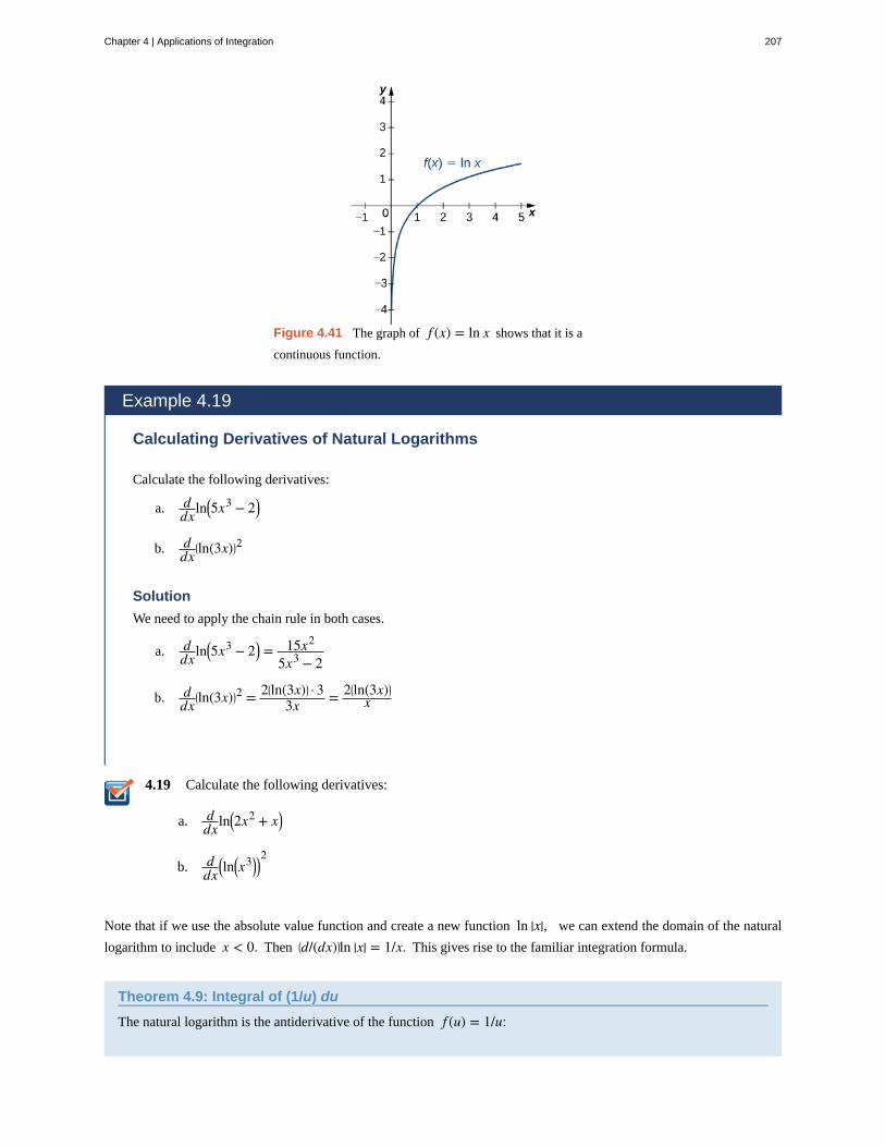
4.19
Figure 4.41 The graph of f (x) = ln x shows that it is a
continuous function.
Example 4.19
Calculating Derivatives of Natural Logarithms
Calculate the following derivatives:
a. ddxln⎛⎝5x3 − 2⎞⎠
b. ddx⎛⎝ln(3x)⎞⎠2
Solution
We need to apply the chain rule in both cases.
a. ddxln⎛⎝5x3 − 2⎞⎠ = 15x2
5x3 − 2
b. ddx⎛⎝ln(3x)⎞⎠2 = 2⎛⎝ln(3x)⎞⎠ · 3
3x = 2⎛⎝ln(3x)⎞⎠x
Calculate the following derivatives:
a. ddxln⎛⎝2x2 + x⎞⎠
b. ddx⎛⎝ln⎛⎝x3⎞⎠⎞⎠2
Note that if we use the absolute value function and create a new function ln |x|, we can extend the domain of the natural
logarithm to include x < 0. Then ⎛⎝d/(dx)⎞⎠ln |x| = 1/x. This gives rise to the familiar integration formula.
Theorem 4.9: Integral of (1/u) du
The natural logarithm is the antiderivative of the function f (u) = 1/u:
Chapter 4 | Applications of Integration 207
4.20
∫ 1udu = ln |u| + C.
Example 4.20
Calculating Integrals Involving Natural Logarithms
Calculate the integral ∫ xx2 + 4
dx.
Solution
Using u -substitution, let u = x2 + 4. Then du = 2x dx and we have
∫ xx2 + 4
dx = 12∫ 1
udu = 12ln |u| + C = 1
2ln |x2 + 4| + C = 12ln⎛⎝x2 + 4⎞⎠+ C.
Calculate the integral ∫ x2
x3 + 6dx.
Although we have called our function a “logarithm,” we have not actually proved that any of the properties of logarithmshold for this function. We do so here.
Theorem 4.10: Properties of the Natural Logarithm
If a, b > 0 and r is a rational number, then
i. ln 1 = 0
ii. ln(ab) = ln a + ln b
iii. ln⎛⎝ab⎞⎠ = ln a − ln b
iv. ln(ar) = r ln a
Proof
i. By definition, ln 1 = ∫1
11t dt = 0.
ii. We have
() ln(ab) = ∫1
ab1t dt = ∫
1
a1t dt + ∫
a
ab1t dt.
Use u-substitution on the last integral in this expression. Let u = t/a. Then du = (1/a)dt. Furthermore, when
t = a, u = 1, and when t = ab, u = b. So we get
() ln(ab) = ∫1
a1t dt + ∫
a
ab1t dt = ∫
1
a1t dt + ∫
a
abat · 1
adt = ∫1
a1t dt + ∫
1
b1udu = ln a + ln b.
208 Chapter 4 | Applications of Integration
This OpenStax book is available for free at https://legacy.cnx.org/content/col31997/1.5
4.21
iv. Note that
() ddxln(xr) = rxr − 1
xr= r
x.
Furthermore,
() ddx(r ln x) = r
x.
Since the derivatives of these two functions are the same, by the Fundamental Theorem of Calculus, they must differ by aconstant. So we have
() ln(xr) = r ln x + C
for some constant C. Taking x = 1, we get
()ln(1r) = r ln(1) + C
0 = r(0) + CC = 0.
Thus ln(xr) = r ln x and the proof is complete. Note that we can extend this property to irrational values of r later in this
section.Part iii. follows from parts ii. and iv. and the proof is left to you.
□
Example 4.21
Using Properties of Logarithms
Use properties of logarithms to simplify the following expression into a single logarithm:
ln 9 − 2 ln 3 + ln⎛⎝13⎞⎠.
Solution
We have
ln 9 − 2 ln 3 + ln⎛⎝13⎞⎠ = ln⎛⎝32⎞⎠− 2 ln 3 + ln⎛⎝3−1⎞⎠ = 2 ln 3 − 2 ln 3 − ln 3 = −ln 3.
Use properties of logarithms to simplify the following expression into a single logarithm:
ln 8 − ln 2 − ln⎛⎝14⎞⎠.
Defining the Number eNow that we have the natural logarithm defined, we can use that function to define the number e.
Definition
The number e is defined to be the real number such that
ln e = 1.
Chapter 4 | Applications of Integration 209
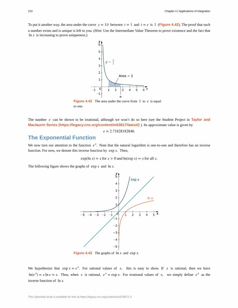
To put it another way, the area under the curve y = 1/t between t = 1 and t = e is 1 (Figure 4.42). The proof that such
a number exists and is unique is left to you. (Hint: Use the Intermediate Value Theorem to prove existence and the fact thatln x is increasing to prove uniqueness.)
Figure 4.42 The area under the curve from 1 to e is equal
to one.
The number e can be shown to be irrational, although we won’t do so here (see the Student Project in Taylor and
Maclaurin Series (https://legacy.cnx.org/content/m53817/latest/) ). Its approximate value is given by
e ≈ 2.71828182846.
The Exponential FunctionWe now turn our attention to the function ex. Note that the natural logarithm is one-to-one and therefore has an inverse
function. For now, we denote this inverse function by exp x. Then,
exp(ln x) = x for x > 0 and ln(exp x) = x for all x.
The following figure shows the graphs of exp x and ln x.
Figure 4.43 The graphs of ln x and exp x.
We hypothesize that exp x = ex. For rational values of x, this is easy to show. If x is rational, then we have
ln(ex) = x ln e = x. Thus, when x is rational, ex = exp x. For irrational values of x, we simply define ex as the
inverse function of ln x.
210 Chapter 4 | Applications of Integration
This OpenStax book is available for free at https://legacy.cnx.org/content/col31997/1.5
Definition
For any real number x, define y = ex to be the number for which
(4.16)ln y = ln(ex) = x.
Then we have ex = exp(x) for all x, and thus
(4.17)eln x = x for x > 0 and ln(ex) = x
for all x.
Properties of the Exponential FunctionSince the exponential function was defined in terms of an inverse function, and not in terms of a power of e, we must
verify that the usual laws of exponents hold for the function ex.
Theorem 4.11: Properties of the Exponential Function
If p and q are any real numbers and r is a rational number, then
i. e p eq = e p + q
ii. e peq
= e p − q
iii. (e p)r = e pr
Proof
Note that if p and q are rational, the properties hold. However, if p or q are irrational, we must apply the inverse
function definition of ex and verify the properties. Only the first property is verified here; the other two are left to you. We
have
ln(e p eq) = ln(e p) + ln(eq) = p + q = ln⎛⎝ep + q⎞⎠.
Since ln x is one-to-one, then
e p eq = e p + q.
□
As with part iv. of the logarithm properties, we can extend property iii. to irrational values of r, and we do so by the end
of the section.
We also want to verify the differentiation formula for the function y = ex. To do this, we need to use implicit
differentiation. Let y = ex. Then
ln y = xddxln y = d
dxx
1ydydx = 1
dydx = y.
Thus, we see
Chapter 4 | Applications of Integration 211

4.22
ddxe
x = ex
as desired, which leads immediately to the integration formula
∫ ex dx = ex + C.
We apply these formulas in the following examples.
Example 4.22
Using Properties of Exponential Functions
Evaluate the following derivatives:
a. ddte
3t et2
b. ddxe
3x2
Solution
We apply the chain rule as necessary.
a. ddte
3t et2
= ddte
3t + t2 = e3t + t2 (3 + 2t)
b. ddxe
3x2= e3x2
6x
Evaluate the following derivatives:
a. ddx⎛⎝⎜ex
2
e5x
⎞⎠⎟
b. ddt⎛⎝e2t⎞⎠
3
Example 4.23
Using Properties of Exponential Functions
Evaluate the following integral: ∫ 2xe−x2dx.
Solution
Using u -substitution, let u = −x2. Then du = −2x dx, and we have
∫ 2xe−x2dx = −∫ eudu = −eu + C = −e−x2
+ C.
212 Chapter 4 | Applications of Integration
This OpenStax book is available for free at https://legacy.cnx.org/content/col31997/1.5
4.23 Evaluate the following integral: ∫ 4e3xdx.
General Logarithmic and Exponential FunctionsWe close this section by looking at exponential functions and logarithms with bases other than e. Exponential functions
are functions of the form f (x) = ax. Note that unless a = e, we still do not have a mathematically rigorous definition
of these functions for irrational exponents. Let’s rectify that here by defining the function f (x) = ax in terms of the
exponential function ex. We then examine logarithms with bases other than e as inverse functions of exponential
functions.
Definition
For any a > 0, and for any real number x, define y = ax as follows:
y = ax = ex ln a.
Now ax is defined rigorously for all values of x. This definition also allows us to generalize property iv. of logarithms and
property iii. of exponential functions to apply to both rational and irrational values of r. It is straightforward to show that
properties of exponents hold for general exponential functions defined in this way.
Let’s now apply this definition to calculate a differentiation formula for ax. We have
ddxa
x = ddxe
x ln a = ex ln a ln a = ax ln a.
The corresponding integration formula follows immediately.
Theorem 4.12: Derivatives and Integrals Involving General Exponential Functions
Let a > 0. Then,
ddxa
x = ax ln a
and
∫ ax dx = 1ln aa
x + C.
If a ≠ 1, then the function ax is one-to-one and has a well-defined inverse. Its inverse is denoted by loga x. Then,
y = loga x if and only if x = ay.
Note that general logarithm functions can be written in terms of the natural logarithm. Let y = loga x. Then, x = ay.Taking the natural logarithm of both sides of this second equation, we get
ln x = ln(ay)ln x = y ln a
y = ln xln a
log x = ln xln a.
Thus, we see that all logarithmic functions are constant multiples of one another. Next, we use this formula to find adifferentiation formula for a logarithm with base a. Again, let y = loga x. Then,
Chapter 4 | Applications of Integration 213
4.24
dydx = d
dx⎛⎝loga x⎞⎠
= ddx⎛⎝ln xln a⎞⎠
= ⎛⎝ 1ln a⎞⎠ ddx(ln x)
= 1ln a · 1
x
= 1x ln a.
Theorem 4.13: Derivatives of General Logarithm Functions
Let a > 0. Then,
ddxloga x = 1
x ln a.
Example 4.24
Calculating Derivatives of General Exponential and Logarithm Functions
Evaluate the following derivatives:
a. ddt⎛⎝4t · 2t2⎞⎠
b. ddxlog8
⎛⎝7x2 + 4⎞⎠
Solution
We need to apply the chain rule as necessary.
a. ddt⎛⎝4t · 2t2⎞⎠ = d
dt⎛⎝22t · 2t2⎞⎠ = d
dt⎛⎝22t + t2⎞⎠ = 22t + t2 ln(2)(2 + 2t)
b. ddxlog8
⎛⎝7x2 + 4⎞⎠ = 1
⎛⎝7x2 + 4⎞⎠(ln 8)
(14x)
Evaluate the following derivatives:
a. ddt 4t4
b. ddxlog3
⎛⎝ x2 + 1⎞⎠
Example 4.25
Integrating General Exponential Functions
214 Chapter 4 | Applications of Integration
This OpenStax book is available for free at https://legacy.cnx.org/content/col31997/1.5

4.25
Evaluate the following integral: ∫ 323xdx.
Solution
Use u-substitution and let u = −3x. Then du = −3dx and we have
∫ 323xdx = ∫ 3 · 2−3xdx = −∫ 2udu = − 1
ln 22u + C = − 1ln 22−3x + C.
Evaluate the following integral: ∫ x2 2x3dx.
Key Concepts• The earlier treatment of logarithms and exponential functions did not define the functions precisely and formally.
This section develops the concepts in a mathematically rigorous way.
• The cornerstone of the development is the definition of the natural logarithm in terms of an integral.
• The function ex is then defined as the inverse of the natural logarithm.
• General exponential functions are defined in terms of ex, and the corresponding inverse functions are general
logarithms.
• Familiar properties of logarithms and exponents still hold in this more rigorous context.
Key Equations• Natural logarithm function
• ln x = ∫1
x1t dt Z
• Exponential function y = ex
• ln y = ln(ex) = x Z
Chapter 4 | Applications of Integration 215

4.4 EXERCISES
For the following exercises, find the derivativedydx.
149. y = ln(2x)
150. y = ln(2x + 1)
151. y = 1ln x
For the following exercises, find the indefinite integral.
152. ∫ dt3t
153. ∫ dx1 + x
For the following exercises, find the derivative dy/dx.(You can use a calculator to plot the function and thederivative to confirm that it is correct.)
154. [T] y = ln(x)x
155. [T] y = x ln(x)
156. [T] y = log10 x
157. [T] y = ln(sin x)
158. [T] y = ln(ln x)
159. [T] y = 7 ln(4x)
160. [T] y = ln⎛⎝(4x)7⎞⎠
161. [T] y = ln(tan x)
162. [T] y = ln(tan(3x))
163. [T] y = ln⎛⎝cos2 x⎞⎠
For the following exercises, find the definite or indefiniteintegral.
164. ∫0
1dx
3 + x
165. ∫0
1dt
3 + 2t
166. ∫0
2x dxx2 + 1
167. ∫0
2x3dxx2 + 1
168. ∫2
edx
x ln x
169. ∫2
edx
x (ln x)2
170. ∫ cos x dxsin x
171. ∫0
π/4tan x dx
172. ∫ cot(3x)dx
173. ∫ (ln x)2dxx
For the following exercises, compute dy/dx by
differentiating ln y.
174. y = x2 + 1
175. y = x2 + 1 x2 − 1
176. y = esin x
177. y = x−1/x
178. y = e(ex)
179. y = xe
180. y = x(ex)
181. y = x x3 x6
182. y = x−1/ln x
183. y = e−ln x
For the following exercises, evaluate by any method.
216 Chapter 4 | Applications of Integration
This OpenStax book is available for free at https://legacy.cnx.org/content/col31997/1.5
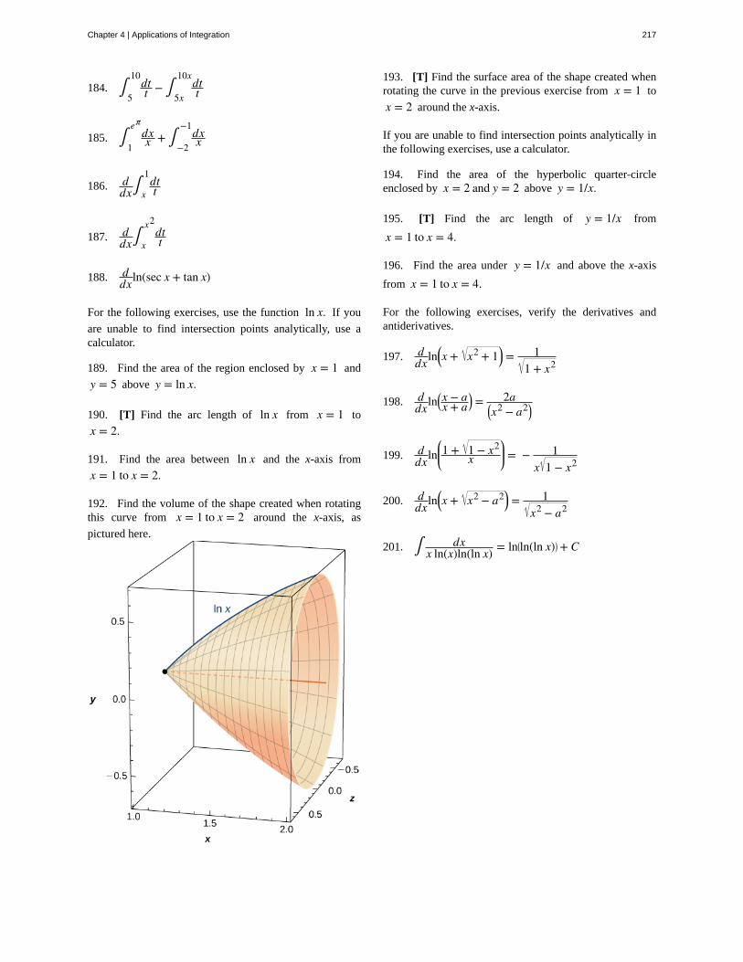
184. ∫5
10dtt − ∫
5x
10xdtt
185. ∫1
eπdxx + ∫
−2
−1dxx
186. ddx∫x
1dtt
187. ddx∫x
x2dtt
188. ddxln(sec x + tan x)
For the following exercises, use the function ln x. If you
are unable to find intersection points analytically, use acalculator.
189. Find the area of the region enclosed by x = 1 and
y = 5 above y = ln x.
190. [T] Find the arc length of ln x from x = 1 to
x = 2.
191. Find the area between ln x and the x-axis from
x = 1 to x = 2.
192. Find the volume of the shape created when rotatingthis curve from x = 1 to x = 2 around the x-axis, as
pictured here.
193. [T] Find the surface area of the shape created whenrotating the curve in the previous exercise from x = 1 to
x = 2 around the x-axis.
If you are unable to find intersection points analytically inthe following exercises, use a calculator.
194. Find the area of the hyperbolic quarter-circleenclosed by x = 2 and y = 2 above y = 1/x.
195. [T] Find the arc length of y = 1/x from
x = 1 to x = 4.
196. Find the area under y = 1/x and above the x-axis
from x = 1 to x = 4.
For the following exercises, verify the derivatives andantiderivatives.
197. ddxln⎛⎝x + x2 + 1⎞⎠ = 1
1 + x2
198. ddxln⎛⎝x − a
x + a⎞⎠ = 2a⎛⎝x2 − a2⎞⎠
199. ddxln⎛⎝⎜1 + 1 − x2
x⎞⎠⎟ = − 1
x 1 − x2
200. ddxln⎛⎝x + x2 − a2⎞⎠ = 1
x2 − a2
201. ∫ dxx ln(x)ln(ln x) = ln⎛⎝ln(ln x)⎞⎠+ C
Chapter 4 | Applications of Integration 217
4.5 | Exponential Growth and Decay
Learning Objectives4.5.1 Use the exponential growth model in applications, including population growth andcompound interest.
4.5.2 Explain the concept of doubling time.
4.5.3 Use the exponential decay model in applications, including radioactive decay and Newton’slaw of cooling.
4.5.4 Explain the concept of half-life.
One of the most prevalent applications of exponential functions involves growth and decay models. Exponential growthand decay show up in a host of natural applications. From population growth and continuously compounded interest toradioactive decay and Newton’s law of cooling, exponential functions are ubiquitous in nature. In this section, we examineexponential growth and decay in the context of some of these applications.
Exponential Growth Model
Many systems exhibit exponential growth. These systems follow a model of the form y = y0 ekt, where y0 represents
the initial state of the system and k is a positive constant, called the growth constant. Notice that in an exponential growth
model, we have
(4.18)y′ = ky0 ekt = ky.
That is, the rate of growth is proportional to the current function value. This is a key feature of exponential growth.Equation 4.18 involves derivatives and is called a differential equation. We learn more about differential equations inIntroduction to Differential Equations (https://legacy.cnx.org/content/m53696/latest/) .
Rule: Exponential Growth Model
Systems that exhibit exponential growth increase according to the mathematical model
y = y0 ekt,
where y0 represents the initial state of the system and k > 0 is a constant, called the growth constant.
Population growth is a common example of exponential growth. Consider a population of bacteria, for instance. It seemsplausible that the rate of population growth would be proportional to the size of the population. After all, the more bacteriathere are to reproduce, the faster the population grows. Figure 4.44 and Table 4.1 represent the growth of a populationof bacteria with an initial population of 200 bacteria and a growth constant of 0.02. Notice that after only 2 hours (120minutes), the population is 10 times its original size!
218 Chapter 4 | Applications of Integration
This OpenStax book is available for free at https://legacy.cnx.org/content/col31997/1.5
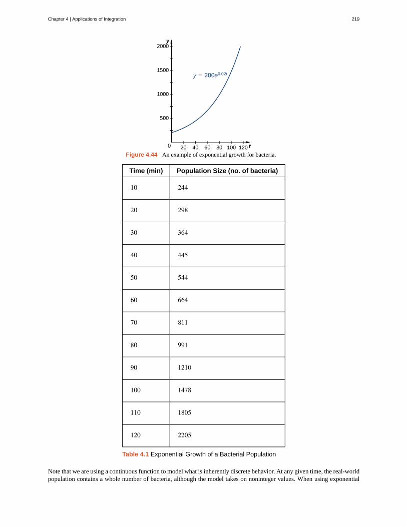
Figure 4.44 An example of exponential growth for bacteria.
Time (min) Population Size (no. of bacteria)
10 244
20 298
30 364
40 445
50 544
60 664
70 811
80 991
90 1210
100 1478
110 1805
120 2205
Table 4.1 Exponential Growth of a Bacterial Population
Note that we are using a continuous function to model what is inherently discrete behavior. At any given time, the real-worldpopulation contains a whole number of bacteria, although the model takes on noninteger values. When using exponential
Chapter 4 | Applications of Integration 219
4.26
growth models, we must always be careful to interpret the function values in the context of the phenomenon we aremodeling.
Example 4.26
Population Growth
Consider the population of bacteria described earlier. This population grows according to the function
f (t) = 200e0.02t, where t is measured in minutes. How many bacteria are present in the population after 5hours (300 minutes)? When does the population reach 100,000 bacteria?
Solution
We have f (t) = 200e0.02t. Then
f (300) = 200e0.02(300) ≈ 80,686.
There are 80,686 bacteria in the population after 5 hours.
To find when the population reaches 100,000 bacteria, we solve the equation
100,000 = 200e0.02t
500 = e0.02t
ln 500 = 0.02tt = ln 500
0.02 ≈ 310.73.
The population reaches 100,000 bacteria after 310.73 minutes.
Consider a population of bacteria that grows according to the function f (t) = 500e0.05t, where t is
measured in minutes. How many bacteria are present in the population after 4 hours? When does the populationreach 100 million bacteria?
Let’s now turn our attention to a financial application: compound interest. Interest that is not compounded is called simpleinterest. Simple interest is paid once, at the end of the specified time period (usually 1 year). So, if we put $1000 in a
savings account earning 2% simple interest per year, then at the end of the year we have
1000(1 + 0.02) = $1020.
Compound interest is paid multiple times per year, depending on the compounding period. Therefore, if the bankcompounds the interest every 6 months, it credits half of the year’s interest to the account after 6 months. During the
second half of the year, the account earns interest not only on the initial $1000, but also on the interest earned during the
first half of the year. Mathematically speaking, at the end of the year, we have
1000⎛⎝1 + 0.022⎞⎠2
= $1020.10.
Similarly, if the interest is compounded every 4 months, we have
1000⎛⎝1 + 0.023⎞⎠
3= $1020.13,
and if the interest is compounded daily (365 times per year), we have $1020.20. If we extend this concept, so that the
interest is compounded continuously, after t years we have
220 Chapter 4 | Applications of Integration
This OpenStax book is available for free at https://legacy.cnx.org/content/col31997/1.5
4.27
1000 limn → ∞⎛⎝1 + 0.02
n⎞⎠nt
.
Now let’s manipulate this expression so that we have an exponential growth function. Recall that the number e can be
expressed as a limit:
e = limm → ∞⎛⎝1 + 1
m⎞⎠m
.
Based on this, we want the expression inside the parentheses to have the form (1 + 1/m). Let n = 0.02m. Note that as
n → ∞, m → ∞ as well. Then we get
1000 limn → ∞⎛⎝1 + 0.02
n⎞⎠nt
= 1000 limm → ∞⎛⎝1 + 0.02
0.02m⎞⎠
0.02mt= 1000⎡⎣ limm → ∞
⎛⎝1 + 1
m⎞⎠m⎤⎦
0.02t.
We recognize the limit inside the brackets as the number e. So, the balance in our bank account after t years is given by
1000e0.02t. Generalizing this concept, we see that if a bank account with an initial balance of $P earns interest at a rate
of r%, compounded continuously, then the balance of the account after t years is
Balance = Pert.
Example 4.27
Compound Interest
A 25-year-old student is offered an opportunity to invest some money in a retirement account that pays 5%annual interest compounded continuously. How much does the student need to invest today to have $1 million
when she retires at age 65? What if she could earn 6% annual interest compounded continuously instead?
Solution
We have
1,000,000 = Pe0.05(40)
P = 135,335.28.
She must invest $135,335.28 at 5% interest.
If, instead, she is able to earn 6%, then the equation becomes
1,000,000 = Pe0.06(40)
P = 90,717.95.
In this case, she needs to invest only $90,717.95. This is roughly two-thirds the amount she needs to invest at
5%. The fact that the interest is compounded continuously greatly magnifies the effect of the 1% increase in
interest rate.
Suppose instead of investing at age 25 , the student waits until age 35. How much would she have to
invest at 5%? At 6%?
If a quantity grows exponentially, the time it takes for the quantity to double remains constant. In other words, it takes thesame amount of time for a population of bacteria to grow from 100 to 200 bacteria as it does to grow from 10,000 to
20,000 bacteria. This time is called the doubling time. To calculate the doubling time, we want to know when the quantity
reaches twice its original size. So we have
Chapter 4 | Applications of Integration 221
4.28
2y0 = y0 ekt
2 = ektln 2 = kt
t = ln 2k .
Definition
If a quantity grows exponentially, the doubling time is the amount of time it takes the quantity to double. It is givenby
Doubling time = ln 2k .
Example 4.28
Using the Doubling Time
Assume a population of fish grows exponentially. A pond is stocked initially with 500 fish. After 6 months,
there are 1000 fish in the pond. The owner will allow his friends and neighbors to fish on his pond after the fish
population reaches 10,000. When will the owner’s friends be allowed to fish?
Solution
We know it takes the population of fish 6 months to double in size. So, if t represents time in months,
by the doubling-time formula, we have 6 = (ln 2)/k. Then, k = (ln 2)/6. Thus, the population is given by
y = 500e⎛⎝(ln 2)/6⎞⎠t. To figure out when the population reaches 10,000 fish, we must solve the following
equation:
10,000 = 500e(ln 2/6)t
20 = e(ln 2/6)t
ln 20 = ⎛⎝ln 2
6⎞⎠t
t = 6(ln 20)ln 2 ≈ 25.93.
The owner’s friends have to wait 25.93 months (a little more than 2 years) to fish in the pond.
Suppose it takes 9 months for the fish population in Example 4.28 to reach 1000 fish. Under these
circumstances, how long do the owner’s friends have to wait?
Exponential Decay ModelExponential functions can also be used to model populations that shrink (from disease, for example), or chemicalcompounds that break down over time. We say that such systems exhibit exponential decay, rather than exponential growth.The model is nearly the same, except there is a negative sign in the exponent. Thus, for some positive constant k, we have
y = y0 e−kt.
As with exponential growth, there is a differential equation associated with exponential decay. We have
y′ = −ky0 e−kt = −ky.
222 Chapter 4 | Applications of Integration
This OpenStax book is available for free at https://legacy.cnx.org/content/col31997/1.5
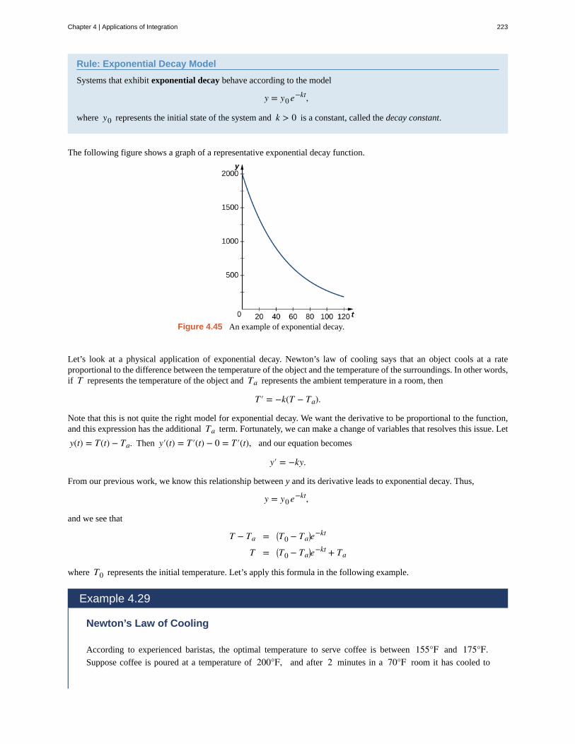
Rule: Exponential Decay Model
Systems that exhibit exponential decay behave according to the model
y = y0 e−kt,
where y0 represents the initial state of the system and k > 0 is a constant, called the decay constant.
The following figure shows a graph of a representative exponential decay function.
Figure 4.45 An example of exponential decay.
Let’s look at a physical application of exponential decay. Newton’s law of cooling says that an object cools at a rateproportional to the difference between the temperature of the object and the temperature of the surroundings. In other words,if T represents the temperature of the object and Ta represents the ambient temperature in a room, then
T′ = −k(T − Ta).
Note that this is not quite the right model for exponential decay. We want the derivative to be proportional to the function,and this expression has the additional Ta term. Fortunately, we can make a change of variables that resolves this issue. Let
y(t) = T(t) − Ta. Then y′(t) = T′(t) − 0 = T′(t), and our equation becomes
y′ = −ky.
From our previous work, we know this relationship between y and its derivative leads to exponential decay. Thus,
y = y0 e−kt,
and we see that
T − Ta = ⎛⎝T0 − Ta⎞⎠e−kt
T = ⎛⎝T0 − Ta⎞⎠e−kt + Ta
where T0 represents the initial temperature. Let’s apply this formula in the following example.
Example 4.29
Newton’s Law of Cooling
According to experienced baristas, the optimal temperature to serve coffee is between 155°F and 175°F.Suppose coffee is poured at a temperature of 200°F, and after 2 minutes in a 70°F room it has cooled to
Chapter 4 | Applications of Integration 223
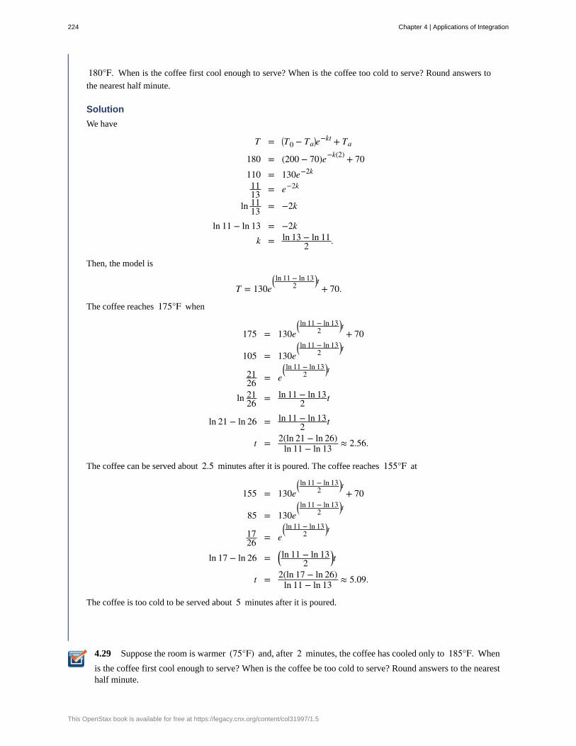
4.29
180°F. When is the coffee first cool enough to serve? When is the coffee too cold to serve? Round answers to
the nearest half minute.
Solution
We have
T = ⎛⎝T0 − Ta⎞⎠e−kt + Ta
180 = (200 − 70)e−k(2) + 70110 = 130e−2k
1113 = e−2k
ln 1113 = −2k
ln 11 − ln 13 = −2kk = ln 13 − ln 11
2 .
Then, the model is
T = 130e⎛⎝ln 11 − ln 13
2⎞⎠t + 70.
The coffee reaches 175°F when
175 = 130e⎛⎝ln 11 − ln 13
2⎞⎠t + 70
105 = 130e⎛⎝ln 11 − ln 13
2⎞⎠t
2126 = e
⎛⎝ln 11 − ln 13
2⎞⎠t
ln 2126 = ln 11 − ln 13
2 t
ln 21 − ln 26 = ln 11 − ln 132 t
t = 2(ln 21 − ln 26)ln 11 − ln 13 ≈ 2.56.
The coffee can be served about 2.5 minutes after it is poured. The coffee reaches 155°F at
155 = 130e⎛⎝ln 11 − ln 13
2⎞⎠t + 70
85 = 130e⎛⎝ln 11 − ln 13
2⎞⎠t
1726 = e
⎛⎝ln 11 − ln 13
2⎞⎠t
ln 17 − ln 26 = ⎛⎝ln 11 − ln 13
2⎞⎠t
t = 2(ln 17 − ln 26)ln 11 − ln 13 ≈ 5.09.
The coffee is too cold to be served about 5 minutes after it is poured.
Suppose the room is warmer (75°F) and, after 2 minutes, the coffee has cooled only to 185°F. When
is the coffee first cool enough to serve? When is the coffee be too cold to serve? Round answers to the nearesthalf minute.
224 Chapter 4 | Applications of Integration
This OpenStax book is available for free at https://legacy.cnx.org/content/col31997/1.5
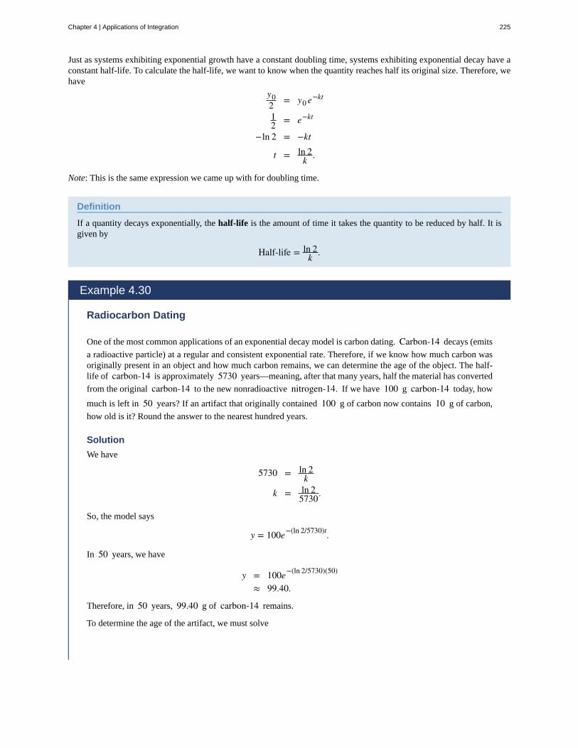
Just as systems exhibiting exponential growth have a constant doubling time, systems exhibiting exponential decay have aconstant half-life. To calculate the half-life, we want to know when the quantity reaches half its original size. Therefore, wehave
y02 = y0 e
−kt
12 = e−kt
−ln 2 = −kt
t = ln 2k .
Note: This is the same expression we came up with for doubling time.
Definition
If a quantity decays exponentially, the half-life is the amount of time it takes the quantity to be reduced by half. It isgiven by
Half-life = ln 2k .
Example 4.30
Radiocarbon Dating
One of the most common applications of an exponential decay model is carbon dating. Carbon-14 decays (emits
a radioactive particle) at a regular and consistent exponential rate. Therefore, if we know how much carbon wasoriginally present in an object and how much carbon remains, we can determine the age of the object. The half-life of carbon-14 is approximately 5730 years—meaning, after that many years, half the material has converted
from the original carbon-14 to the new nonradioactive nitrogen-14. If we have 100 g carbon-14 today, how
much is left in 50 years? If an artifact that originally contained 100 g of carbon now contains 10 g of carbon,
how old is it? Round the answer to the nearest hundred years.
Solution
We have
5730 = ln 2k
k = ln 25730.
So, the model says
y = 100e−(ln 2/5730)t.
In 50 years, we have
y = 100e−(ln 2/5730)(50)
≈ 99.40.
Therefore, in 50 years, 99.40 g of carbon-14 remains.
To determine the age of the artifact, we must solve
Chapter 4 | Applications of Integration 225

4.30
10 = 100e−(ln 2/5730)t
110 = e−(ln 2/5730)t
t ≈ 19035.
The artifact is about 19,000 years old.
If we have 100 g of carbon-14, how much is left after t years? If an artifact that originally contained
100 g of carbon now contains 20g of carbon, how old is it? Round the answer to the nearest hundred years.
Key Concepts• Exponential growth and exponential decay are two of the most common applications of exponential functions.
• Systems that exhibit exponential growth follow a model of the form y = y0 ekt.
• In exponential growth, the rate of growth is proportional to the quantity present. In other words, y′ = ky.
• Systems that exhibit exponential growth have a constant doubling time, which is given by (ln 2)/k.
• Systems that exhibit exponential decay follow a model of the form y = y0 e−kt.
• Systems that exhibit exponential decay have a constant half-life, which is given by (ln 2)/k.
226 Chapter 4 | Applications of Integration
This OpenStax book is available for free at https://legacy.cnx.org/content/col31997/1.5

4.5 EXERCISESTrue or False? If true, prove it. If false, find the true answer.
202. The doubling time for y = ect is ⎛⎝ln (2)⎞⎠/⎛⎝ln (c)⎞⎠.
203. If you invest $500, an annual rate of interest of
3% yields more money in the first year than a 2.5%continuous rate of interest.
204. If you leave a 100°C pot of tea at room temperature
(25°C) and an identical pot in the refrigerator (5°C),with k = 0.02, the tea in the refrigerator reaches a
drinkable temperature (70°C) more than 5 minutes
before the tea at room temperature.
205. If given a half-life of t years, the constant k for
y = ekt is calculated by k = ln (1/2)/t.
For the following exercises, use y = y0 ekt.
206. If a culture of bacteria doubles in 3 hours, how many
hours does it take to multiply by 10?
207. If bacteria increase by a factor of 10 in 10 hours,
how many hours does it take to increase by 100?
208. How old is a skull that contains one-fifth as muchradiocarbon as a modern skull? Note that the half-life ofradiocarbon is 5730 years.
209. If a relic contains 90% as much radiocarbon as
new material, can it have come from the time of Christ(approximately 2000 years ago)? Note that the half-life of
radiocarbon is 5730 years.
210. The population of Cairo grew from 5 million to
10 million in 20 years. Use an exponential model to find
when the population was 8 million.
211. The populations of New York and Los Angeles aregrowing at 1% and 1.4% a year, respectively. Starting
from 8 million (New York) and 6 million (Los Angeles),
when are the populations equal?
212. Suppose the value of $1 in Japanese yen decreases
at 2% per year. Starting from $1 = ¥250, when will
$1 = ¥1?
213. The effect of advertising decays exponentially. If40% of the population remembers a new product after 3days, how long will 20% remember it?
214. If y = 1000 at t = 3 and y = 3000 at t = 4,what was y0 at t = 0?
215. If y = 100 at t = 4 and y = 10 at t = 8, when
does y = 1?
216. If a bank offers annual interest of 7.5% or
continuous interest of 7.25%, which has a better annual
yield?
217. What continuous interest rate has the same yield asan annual rate of 9%?
218. If you deposit $5000 at 8% annual interest, how
many years can you withdraw $500 (starting after the first
year) without running out of money?
219. You are trying to save $50,000 in 20 years for
college tuition for your child. If interest is a continuous10%, how much do you need to invest initially?
220. You are cooling a turkey that was taken out of theoven with an internal temperature of 165°F. After 10minutes of resting the turkey in a 70°F apartment, the
temperature has reached 155°F. What is the temperature
of the turkey 20 minutes after taking it out of the oven?
221. You are trying to thaw some vegetables that areat a temperature of 1°F. To thaw vegetables safely, you
must put them in the refrigerator, which has an ambienttemperature of 44°F. You check on your vegetables 2hours after putting them in the refrigerator to find that theyare now 12°F. Plot the resulting temperature curve and use
it to determine when the vegetables reach 33°F.
222. You are an archaeologist and are given a bone that isclaimed to be from a Tyrannosaurus Rex. You know thesedinosaurs lived during the Cretaceous Era (146 million
years to 65 million years ago), and you find by
radiocarbon dating that there is 0.000001% the amount of
radiocarbon. Is this bone from the Cretaceous?
223. The spent fuel of a nuclear reactor containsplutonium-239, which has a half-life of 24,000 years. If 1barrel containing 10 kg of plutonium-239 is sealed, how
many years must pass until only 10g of plutonium-239 is
left?
For the next set of exercises, use the following table, whichfeatures the world population by decade.
Chapter 4 | Applications of Integration 227
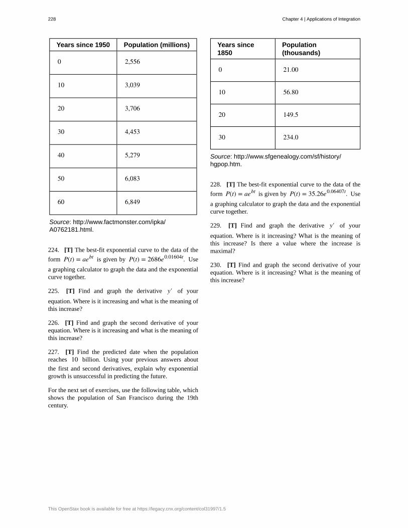
Years since 1950 Population (millions)
0 2,556
10 3,039
20 3,706
30 4,453
40 5,279
50 6,083
60 6,849
Source: http://www.factmonster.com/ipka/A0762181.html.
224. [T] The best-fit exponential curve to the data of the
form P(t) = aebt is given by P(t) = 2686e0.01604t. Use
a graphing calculator to graph the data and the exponentialcurve together.
225. [T] Find and graph the derivative y′ of your
equation. Where is it increasing and what is the meaning ofthis increase?
226. [T] Find and graph the second derivative of yourequation. Where is it increasing and what is the meaning ofthis increase?
227. [T] Find the predicted date when the populationreaches 10 billion. Using your previous answers about
the first and second derivatives, explain why exponentialgrowth is unsuccessful in predicting the future.
For the next set of exercises, use the following table, whichshows the population of San Francisco during the 19thcentury.
Years since1850
Population(thousands)
0 21.00
10 56.80
20 149.5
30 234.0
Source: http://www.sfgenealogy.com/sf/history/hgpop.htm.
228. [T] The best-fit exponential curve to the data of the
form P(t) = aebt is given by P(t) = 35.26e0.06407t. Use
a graphing calculator to graph the data and the exponentialcurve together.
229. [T] Find and graph the derivative y′ of your
equation. Where is it increasing? What is the meaning ofthis increase? Is there a value where the increase ismaximal?
230. [T] Find and graph the second derivative of yourequation. Where is it increasing? What is the meaning ofthis increase?
228 Chapter 4 | Applications of Integration
This OpenStax book is available for free at https://legacy.cnx.org/content/col31997/1.5

center of mass
centroid
cross-section
disk method
doubling time
exponential decay
exponential growth
half-life
lamina
method of cylindrical shells
moment
slicing method
solid of revolution
symmetry principle
theorem of Pappus for volume
washer method
CHAPTER 4 REVIEW
KEY TERMSthe point at which the total mass of the system could be concentrated without changing the moment
the centroid of a region is the geometric center of the region; laminas are often represented by regions in theplane; if the lamina has a constant density, the center of mass of the lamina depends only on the shape of thecorresponding planar region; in this case, the center of mass of the lamina corresponds to the centroid of therepresentative region
the intersection of a plane and a solid object
a special case of the slicing method used with solids of revolution when the slices are disks
if a quantity grows exponentially, the doubling time is the amount of time it takes the quantity to double,and is given by (ln 2)/k
systems that exhibit exponential decay follow a model of the form y = y0 e−kt
systems that exhibit exponential growth follow a model of the form y = y0 ekt
if a quantity decays exponentially, the half-life is the amount of time it takes the quantity to be reduced by half. Itis given by (ln 2)/k
a thin sheet of material; laminas are thin enough that, for mathematical purposes, they can be treated as if they aretwo-dimensional
a method of calculating the volume of a solid of revolution by dividing the solid intonested cylindrical shells; this method is different from the methods of disks or washers in that we integrate withrespect to the opposite variable
if n masses are arranged on a number line, the moment of the system with respect to the origin is given by
M = ∑i = 1
nmi xi; if, instead, we consider a region in the plane, bounded above by a function f (x) over an interval
⎡⎣a, b⎤⎦, then the moments of the region with respect to the x- and y-axes are given by Mx = ρ∫
a
b ⎡⎣ f (x)⎤⎦2
2 dx and
My = ρ∫a
bx f (x)dx, respectively
a method of calculating the volume of a solid that involves cutting the solid into pieces, estimating thevolume of each piece, then adding these estimates to arrive at an estimate of the total volume; as the number of slicesgoes to infinity, this estimate becomes an integral that gives the exact value of the volume
a solid generated by revolving a region in a plane around a line in that plane
the symmetry principle states that if a region R is symmetric about a line l, then the centroid of Rlies on l
this theorem states that the volume of a solid of revolution formed by revolving aregion around an external axis is equal to the area of the region multiplied by the distance traveled by the centroid ofthe region
a special case of the slicing method used with solids of revolution when the slices are washers
Chapter 4 | Applications of Integration 229

230 Chapter 4 | Applications of Integration
This OpenStax book is available for free at https://legacy.cnx.org/content/col31997/1.5

5 | TECHNIQUES OFINTEGRATION5.1 | Integration by Parts
Learning Objectives5.1.1 Recognize when to use integration by parts.
5.1.2 Use the integration-by-parts formula to solve integration problems.
5.1.3 Use the integration-by-parts formula for definite integrals.
By now we have a fairly thorough procedure for how to evaluate many basic integrals. However, although we can integrate
∫ xsin(x2)dx by using the substitution, u = x2, something as simple looking as ∫ xsinx dx defies us. Many students
want to know whether there is a product rule for integration. There isn’t, but there is a technique based on the product rulefor differentiation that allows us to exchange one integral for another. We call this technique integration by parts.
The Integration-by-Parts FormulaIf, h(x) = f (x)g(x), then by using the product rule, we obtain h′(x) = f ′(x)g(x) + g′(x) f (x). Although at first it may
seem counterproductive, let’s now integrate both sides of this equation: ∫ h′(x)dx = ∫ ⎛⎝g(x) f ′(x) + f (x)g′(x)⎞⎠dx.
This gives us
h(x) = f (x)g(x) = ∫ g(x) f ′(x)dx + ∫ f (x)g′(x)dx.
Now we solve for ∫ f (x)g′(x)dx :
∫ f (x)g′(x)dx = f (x)g(x) − ∫ g(x) f ′(x)dx.
By making the substitutions u = f (x) and v = g(x), which in turn make du = f ′(x)dx and dv = g′(x)dx, we have the
more compact form
∫ u dv = uv − ∫ v du.
Theorem 5.1: Integration by Parts
Let u = f (x) and v = g(x) be functions with continuous derivatives. Then, the integration-by-parts formula for the
integral involving these two functions is:
(5.1)∫ u dv = uv − ∫ v du.
The advantage of using the integration-by-parts formula is that we can use it to exchange one integral for another, possiblyeasier, integral. The following example illustrates its use.
Example 5.1
Chapter 5 | Techniques of Integration 231

Using Integration by Parts
Use integration by parts with u = x and dv = sinx dx to evaluate ∫ xsinx dx.
Solution
By choosing u = x, we have du = 1dx. Since dv = sinx dx, we get v = ∫ sinx dx = −cosx. It is handy to
keep track of these values as follows:
u = x dv = sinx dx
du = 1dx v = ∫ sinx dx = −cosx.
Applying the integration-by-parts formula results in
∫ xsinx dx = (x)(−cosx) − ∫ (−cosx)(1dx) Substitute.
= −xcosx + ∫ cosx dx Simplify.
= −xcosx + sinx + C. Use ∫ cosx dx = sinx + C.
AnalysisAt this point, there are probably a few items that need clarification. First of all, you may be curious aboutwhat would have happened if we had chosen u = sinx and dv = x. If we had done so, then we would
have du = cosxdx and v = 12x
2. Thus, after applying integration by parts, we have
∫ xsinx dx = 12x
2 sinx − ∫ 12x
2 cosx dx. Unfortunately, with the new integral, we are in no better position
than before. It is important to keep in mind that when we apply integration by parts, we may need to try severalchoices for u and dv before finding a choice that works.
Second, you may wonder why, when we find v = ∫ sinx dx = −cosx, we do not use v = −cosx + K. To see
that it makes no difference, we can rework the problem using v = −cosx + K:
∫ xsinx dx = (x)(−cosx + K) − ∫ (−cosx + K)(1dx)
= −xcosx + Kx + ∫ cosx dx − ∫ Kdx= −xcosx + Kx + sinx − Kx + C= −xcosx + sinx + C.
As you can see, it makes no difference in the final solution.
Last, we can check to make sure that our antiderivative is correct by differentiating −xcosx + sinx + C:
ddx(−xcosx + sinx + C) = (−1)cosx + (−x)(−sinx) + cosx
= xsinx.
Therefore, the antiderivative checks out.
Watch this video (http://www.openstax.org/l/20_intbyparts1) and visit this website(http://www.openstax.org/l/20_intbyparts2) for examples of integration by parts.
232 Chapter 5 | Techniques of Integration
This OpenStax book is available for free at https://legacy.cnx.org/content/col31997/1.5
5.1 Evaluate ∫ xe2x dx using the integration-by-parts formula with u = x and dv = e2x dx.
The natural question to ask at this point is: How do we know how to choose u and dv? Sometimes it is a matter of trial
and error; however, the acronym LIATE can often help to take some of the guesswork out of our choices. This acronymstands for Logarithmic Functions, Inverse Trigonometric Functions, Algebraic Functions, Trigonometric Functions, andExponential Functions. This mnemonic serves as an aid in determining an appropriate choice for u.
The type of function in the integral that appears first in the list should be our first choice of u. For example, if an integral
contains a logarithmic function and an algebraic function, we should choose u to be the logarithmic function, because L
comes before A in LIATE. The integral in Example 5.1 has a trigonometric function (sinx) and an algebraic function
(x). Because A comes before T in LIATE, we chose u to be the algebraic function. When we have chosen u, dv is
selected to be the remaining part of the function to be integrated, together with dx.
Why does this mnemonic work? Remember that whatever we pick to be dv must be something we can integrate. Since we
do not have integration formulas that allow us to integrate simple logarithmic functions and inverse trigonometric functions,it makes sense that they should not be chosen as values for dv. Consequently, they should be at the head of the list as
choices for u. Thus, we put LI at the beginning of the mnemonic. (We could just as easily have started with IL, since
these two types of functions won’t appear together in an integration-by-parts problem.) The exponential and trigonometricfunctions are at the end of our list because they are fairly easy to integrate and make good choices for dv. Thus, we have
TE at the end of our mnemonic. (We could just as easily have used ET at the end, since when these types of functions appeartogether it usually doesn’t really matter which one is u and which one is dv.) Algebraic functions are generally easy both
to integrate and to differentiate, and they come in the middle of the mnemonic.
Example 5.2
Using Integration by Parts
Evaluate ∫ lnxx3 dx.
Solution
Begin by rewriting the integral:
∫ lnxx3 dx = ∫ x−3 lnx dx.
Since this integral contains the algebraic function x−3 and the logarithmic function lnx, choose u = lnx,
since L comes before A in LIATE. After we have chosen u = lnx, we must choose dv = x−3dx.
Next, since u = lnx, we have du = 1xdx. Also, v = ∫ x−3dx = − 1
2x−2. Summarizing,
u = lnx dv = x−3dx
du = 1xdx v = ∫ x−3dx = − 1
2x−2.
Substituting into the integration-by-parts formula (Equation 5.1) gives
Chapter 5 | Techniques of Integration 233

5.2
∫ lnxx3 dx = ∫ x−3 lnx dx = ⎛⎝lnx)(− 1
2x−2⎞⎠− ∫ ⎛⎝− 1
2x−2⎞⎠(1
xdx)
= − 12x
−2 lnx + ∫ 12x
−3dx Simplify.
= − 12x
−2 lnx − 14x
−2 + C Integrate.
= − 12x2lnx − 1
4x2 + C. Rewrite with positive integers.
Evaluate ∫ x lnx dx.
In some cases, as in the next two examples, it may be necessary to apply integration by parts more than once.
Example 5.3
Applying Integration by Parts More Than Once
Evaluate ∫ x2 e3x dx.
Solution
Using LIATE, choose u = x2 and dv = e3x dx. Thus, du = 2x dx and v = ∫ e3x dx = ⎛⎝13⎞⎠e3x. Therefore,
u = x2 dv = e3x dx
du = 2x dx v = ∫ e3x dx = 13e
3x.
Substituting into Equation 5.1 produces
∫ x2 e3x dx = 13x
2 e3x − ∫ 23xe
3x dx.
We still cannot integrate ∫ 23xe
3x dx directly, but the integral now has a lower power on x. We can evaluate this
new integral by using integration by parts again. To do this, choose u = x and dv = 23e
3x dx. Thus, du = dx
and v = ∫ ⎛⎝23⎞⎠e3x dx = ⎛⎝29
⎞⎠e3x. Now we have
u = x dv = 23e
3x dx
du = dx v = ∫ 23e
3x dx = 29e
3x.
Substituting back into the previous equation yields
∫ x2 e3x dx = 13x
2 e3x − ⎛⎝29xe3x − ∫ 2
9e3x dx⎞⎠.
After evaluating the last integral and simplifying, we obtain
234 Chapter 5 | Techniques of Integration
This OpenStax book is available for free at https://legacy.cnx.org/content/col31997/1.5
∫ x2 e3x dx = 13x
2 e3x − 29xe
3x + 227e
3x + C.
Example 5.4
Applying Integration by Parts When LIATE Doesn’t Quite Work
Evaluate ∫ t3 et2dt.
Solution
If we use a strict interpretation of the mnemonic LIATE to make our choice of u, we end up with u = t3 and
dv = et2dt. Unfortunately, this choice won’t work because we are unable to evaluate ∫ et
2dt. However, since
we can evaluate ∫ tet2dx, we can try choosing u = t2 and dv = tet
2dt. With these choices we have
u = t2 dv = tet2dt
du = 2t dt v = ∫ tet2dt = 1
2et2.
Thus, we obtain
∫ t3 et2dt = 1
2t2 et
2− ∫ 1
2et2 2tdt
= 12t
2 et2
− 12e
t2 + C.
Example 5.5
Applying Integration by Parts More Than Once
Evaluate ∫ sin(lnx)dx.
Solution
This integral appears to have only one function—namely, sin(lnx) —however, we can always use the constant
function 1 as the other function. In this example, let’s choose u = sin(lnx) and dv = 1dx. (The decision to
use u = sin(lnx) is easy. We can’t choose dv = sin(lnx)dx because if we could integrate it, we wouldn’t be
using integration by parts in the first place!) Consequently, du = (1/x)cos(lnx)dx and v = ∫ 1dx = x. After
applying integration by parts to the integral and simplifying, we have
∫ sin(lnx)dx = xsin(lnx) − ∫ cos(lnx)dx.
Chapter 5 | Techniques of Integration 235

5.3
Unfortunately, this process leaves us with a new integral that is very similar to the original. However, let’s seewhat happens when we apply integration by parts again. This time let’s choose u = cos(lnx) and dv = 1dx,
making du = −(1/x)sin(lnx)dx and v = ∫ 1dx = x. Substituting, we have
∫ sin(lnx)dx = xsin(lnx) − ⎛⎝xcos(lnx) — ∫ − sin(lnx)dx⎞⎠.
After simplifying, we obtain
∫ sin(lnx)dx = xsin(lnx) − xcos(lnx) − ∫ sin(lnx)dx.
The last integral is now the same as the original. It may seem that we have simply gone in a circle, but now we
can actually evaluate the integral. To see how to do this more clearly, substitute I = ∫ sin(lnx)dx. Thus, the
equation becomes
I = xsin(lnx) − xcos(lnx) − I.
First, add I to both sides of the equation to obtain
2I = xsin(lnx) − xcos(lnx).
Next, divide by 2:
I = 12xsin(lnx) − 1
2xcos(lnx).
Substituting I = ∫ sin(lnx)dx again, we have
∫ sin(lnx)dx = 12xsin(lnx) − 1
2xcos(lnx).
From this we see that (1/2)xsin(lnx) − (1/2)xcos(lnx) is an antiderivative of sin(lnx)dx. For the most general
antiderivative, add +C:
∫ sin(lnx)dx = 12xsin(lnx) − 1
2xcos(lnx) + C.
AnalysisIf this method feels a little strange at first, we can check the answer by differentiation:
ddx⎛⎝12xsin(lnx) − 1
2xcos(lnx)⎞⎠= 1
2(sin(lnx)) + cos(lnx) · 1x · 1
2x − ⎛⎝12cos(lnx) − sin(lnx) · 1x · 1
2x⎞⎠
= sin(lnx).
Evaluate ∫ x2 sinx dx.
Integration by Parts for Definite IntegralsNow that we have used integration by parts successfully to evaluate indefinite integrals, we turn our attention to definiteintegrals. The integration technique is really the same, only we add a step to evaluate the integral at the upper and lowerlimits of integration.
236 Chapter 5 | Techniques of Integration
This OpenStax book is available for free at https://legacy.cnx.org/content/col31997/1.5
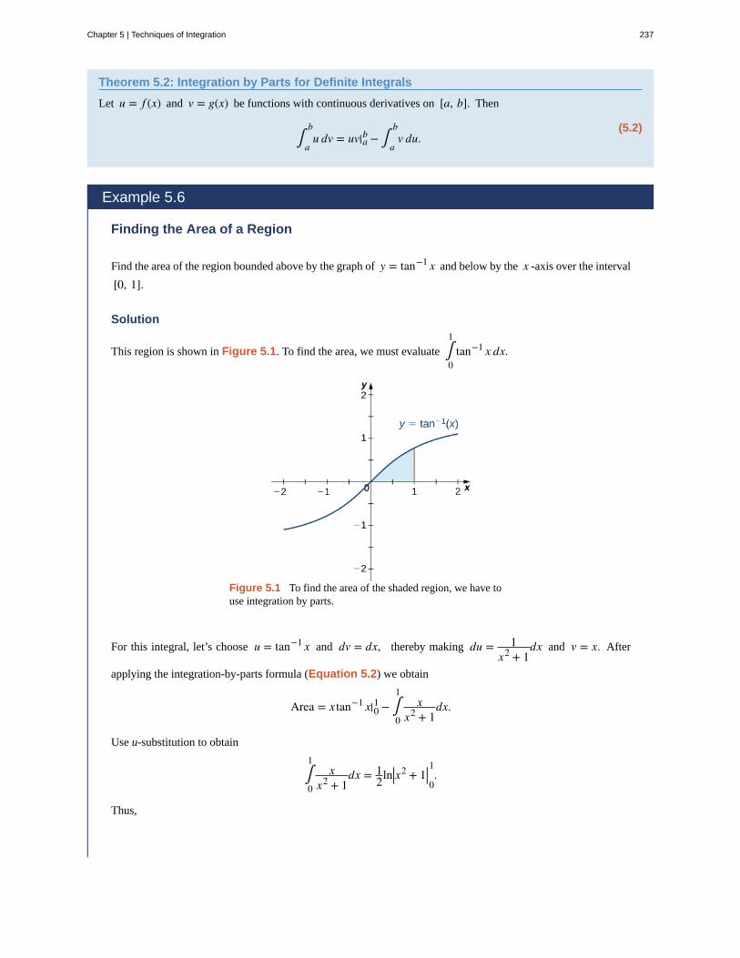
Theorem 5.2: Integration by Parts for Definite Integrals
Let u = f (x) and v = g(x) be functions with continuous derivatives on [a, b]. Then
(5.2)∫a
bu dv = uv|ab − ∫
a
bv du.
Example 5.6
Finding the Area of a Region
Find the area of the region bounded above by the graph of y = tan−1 x and below by the x -axis over the interval
[0, 1].
Solution
This region is shown in Figure 5.1. To find the area, we must evaluate ∫0
1tan−1 x dx.
Figure 5.1 To find the area of the shaded region, we have touse integration by parts.
For this integral, let’s choose u = tan−1 x and dv = dx, thereby making du = 1x2 + 1
dx and v = x. After
applying the integration-by-parts formula (Equation 5.2) we obtain
Area = x tan−1 x|01 − ∫
0
1x
x2 + 1dx.
Use u-substitution to obtain
∫0
1x
x2 + 1dx = 1
2ln|x2 + 1|01.
Thus,
Chapter 5 | Techniques of Integration 237
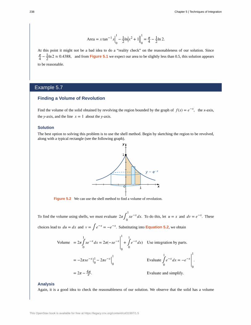
Area = x tan−1 x|01
− 12ln|x2 + 1||0
1= π
4 − 12ln 2.
At this point it might not be a bad idea to do a “reality check” on the reasonableness of our solution. Sinceπ4 − 1
2ln2 ≈ 0.4388, and from Figure 5.1 we expect our area to be slightly less than 0.5, this solution appears
to be reasonable.
Example 5.7
Finding a Volume of Revolution
Find the volume of the solid obtained by revolving the region bounded by the graph of f (x) = e−x, the x-axis,
the y-axis, and the line x = 1 about the y-axis.
Solution
The best option to solving this problem is to use the shell method. Begin by sketching the region to be revolved,along with a typical rectangle (see the following graph).
Figure 5.2 We can use the shell method to find a volume of revolution.
To find the volume using shells, we must evaluate 2π∫0
1xe−x dx. To do this, let u = x and dv = e−x. These
choices lead to du = dx and v = ∫ e−x = −e−x. Substituting into Equation 5.2, we obtain
Volume = 2π∫0
1xe−x dx = 2π(−xe−x |0
1
+ ∫0
1e−x dx) Use integration by parts.
= −2πxe−x |01 − 2πe−x |0
1Evaluate ∫
0
1e−x dx = −e−x |0
1
.
= 2π − 4πe . Evaluate and simplify.
AnalysisAgain, it is a good idea to check the reasonableness of our solution. We observe that the solid has a volume
238 Chapter 5 | Techniques of Integration
This OpenStax book is available for free at https://legacy.cnx.org/content/col31997/1.5
5.4
slightly less than that of a cylinder of radius 1 and height of 1/e added to the volume of a cone of base radius
1 and height of 1 − 1e . Consequently, the solid should have a volume a bit less than
π(1)2 1e + ⎛⎝π3
⎞⎠(1)2 ⎛⎝1 − 1
e⎞⎠ = 2π
3e + π3 ≈ 1.8177.
Since 2π − 4πe ≈ 1.6603, we see that our calculated volume is reasonable.
Evaluate ∫0
π/2xcosx dx.
Key Concepts• The integration-by-parts formula allows the exchange of one integral for another, possibly easier, integral.
• Integration by parts applies to both definite and indefinite integrals.
Key Equations• Integration by parts formula
∫ u dv = uv − ∫ v du
• Integration by parts for definite integrals
∫a
bu dv = uv|ab − ∫
a
bv du
Chapter 5 | Techniques of Integration 239
5.1 EXERCISESIn using the technique of integration by parts, you mustcarefully choose which expression is u. For each of thefollowing problems, use the guidelines in this section tochoose u. Do not evaluate the integrals.
1. ∫ x3 e2x dx
2. ∫ x3 ln(x)dx
3. ∫ y3 cosydy
4. ∫ x2 arctanx dx
5. ∫ e3x sin(2x)dx
Find the integral by using the simplest method. Not allproblems require integration by parts.
6. ∫ vsinvdv
7. ∫ lnx dx (Hint: ∫ lnx dx is equivalent to
∫ 1 · ln(x)dx.)
8. ∫ xcosx dx
9. ∫ tan−1 x dx
10. ∫ x2ex dx
11. ∫ xsin(2x)dx
12. ∫ xe4x dx
13. ∫ xe−x dx
14. ∫ xcos3x dx
15. ∫ x2cosx dx
16. ∫ x lnx dx
17. ∫ ln(2x + 1)dx
18. ∫ x2 e4xdx
19. ∫ ex sinx dx
20. ∫ ex cosx dx
21. ∫ xe−x2dx
22. ∫ x2 e−x dx
23. ∫ sin(ln(2x))dx
24. ∫ cos(lnx)dx
25. ∫ (lnx)2dx
26. ∫ ln(x2)dx
27. ∫ x2 lnx dx
28. ∫ sin−1 x dx
29. ∫ cos−1(2x)dx
30. ∫ xarctanx dx
31. ∫ x2 sinx dx
32. ∫ x3 cosx dx
33. ∫ x3 sinx dx
34. ∫ x3 ex dx
35. ∫ xsec−1 x dx
36. ∫ xsec2 x dx
37. ∫ xcoshx dx
240 Chapter 5 | Techniques of Integration
This OpenStax book is available for free at https://legacy.cnx.org/content/col31997/1.5

Compute the definite integrals. Use a graphing utility toconfirm your answers.
38. ∫1/e
1lnx dx
39. ∫0
1xe−2x dx (Express the answer in exact form.)
40. ∫0
1e x dx(let u = x)
41. ∫1
eln(x2)dx
42. ∫0
πxcosx dx
43. ∫−π
πxsinx dx (Express the answer in exact form.)
44. ∫0
3ln(x2 + 1)dx (Express the answer in exact form.)
45. ∫0
π/2x2 sinx dx (Express the answer in exact form.)
46. ∫0
1x5x dx (Express the answer using five significant
digits.)
47. Evaluate ∫ cosx ln(sinx)dx
Derive the following formulas using the technique ofintegration by parts. Assume that n is a positive integer.These formulas are called reduction formulas because theexponent in the x term has been reduced by one in eachcase. The second integral is simpler than the originalintegral.
48. ∫ xn ex dx = xn ex − n∫ xn − 1 ex dx
49. ∫ xn cosx dx = xn sinx − n∫ xn − 1 sinx dx
50. ∫ xn sinx dx = ______
51. Integrate ∫ 2x 2x − 3dx using two methods:
a. Using parts, letting dv = 2x − 3dxb. Substitution, letting u = 2x − 3
State whether you would use integration by parts to
evaluate the integral. If so, identify u and dv. If not,describe the technique used to perform the integrationwithout actually doing the problem.
52. ∫ x lnx dx
53. ∫ ln2 xx dx
54. ∫ xex dx
55. ∫ xex2 − 3dx
56. ∫ x2 sinx dx
57. ∫ x2 sin(3x3 + 2)dx
Sketch the region bounded above by the curve, the x-axis,and x = 1, and find the area of the region. Provide the
exact form or round answers to the number of placesindicated.
58. y = 2xe−x (Approximate answer to four decimal
places.)
59. y = e−x sin(πx) (Approximate answer to five
decimal places.)
Find the volume generated by rotating the region boundedby the given curves about the specified line. Express theanswers in exact form or approximate to the number ofdecimal places indicated.
60. y = sinx, y = 0, x = 2π, x = 3π about the y-axis
(Express the answer in exact form.)
61. y = e−x y = 0, x = −1x = 0; about x = 1(Express the answer in exact form.)
62. A particle moving along a straight line has a velocity
of v(t) = t2 e−t after t sec. How far does it travel in the
first 2 sec? (Assume the units are in feet and express theanswer in exact form.)
63. Find the area under the graph of y = sec3 x from
x = 0to x = 1. (Round the answer to two significant
digits.)
64. Find the area between y = (x − 2)ex and the x-axis
from x = 2 to x = 5. (Express the answer in exact form.)
Chapter 5 | Techniques of Integration 241
65. Find the area of the region enclosed by the curve
y = xcosx and the x-axis for 11π2 ≤ x ≤ 13π
2 . (Express
the answer in exact form.)
66. Find the volume of the solid generated by revolvingthe region bounded by the curve y = lnx, the x-axis,
and the vertical line x = e2 about the x-axis. (Express the
answer in exact form.)
67. Find the volume of the solid generated by revolvingthe region bounded by the curve y = 4cosx and the
x-axis, π2 ≤ x ≤ 3π
2 , about the x-axis. (Express the
answer in exact form.)
68. Find the volume of the solid generated by revolvingthe region in the first quadrant bounded by y = ex and
the x-axis, from x = 0 to x = ln(7), about the y-axis.
(Express the answer in exact form.)
242 Chapter 5 | Techniques of Integration
This OpenStax book is available for free at https://legacy.cnx.org/content/col31997/1.5

5.5
5.2 | Trigonometric Integrals
Learning Objectives5.2.1 Solve integration problems involving products and powers of sinx and cosx.5.2.2 Solve integration problems involving products and powers of tanx and secx.5.2.3 Use reduction formulas to solve trigonometric integrals.
In this section we look at how to integrate a variety of products of trigonometric functions. These integrals are calledtrigonometric integrals. They are an important part of the integration technique called trigonometric substitution, which isfeatured in Trigonometric Substitution. This technique allows us to convert algebraic expressions that we may not beable to integrate into expressions involving trigonometric functions, which we may be able to integrate using the techniquesdescribed in this section. In addition, these types of integrals appear frequently when we study polar, cylindrical, andspherical coordinate systems later. Let’s begin our study with products of sinx and cosx.
Integrating Products and Powers of sinx and cosxA key idea behind the strategy used to integrate combinations of products and powers of sinx and cosx involves rewriting
these expressions as sums and differences of integrals of the form ∫ sin j xcosx dx or ∫ cos j xsinx dx. After rewriting
these integrals, we evaluate them using u-substitution. Before describing the general process in detail, let’s take a look atthe following examples.
Example 5.8
Integrating ∫cos j xsinxdx
Evaluate ∫ cos3 xsinx dx.
Solution
Use u -substitution and let u = cosx. In this case, du = −sinx dx. Thus,
∫ cos3 xsinx dx = −∫ u3 du
= − 14u
4 + C
= − 14cos4 x + C.
Evaluate ∫ sin4 xcosx dx.
Example 5.9
A Preliminary Example: Integrating ∫cos j xsinkxdx Where k is Odd
Chapter 5 | Techniques of Integration 243
5.6
Evaluate ∫ cos2 xsin3 x dx.
Solution
To convert this integral to integrals of the form ∫ cos j xsinx dx, rewrite sin3 x = sin2 xsinx and make the
substitution sin2 x = 1 − cos2 x. Thus,
∫ cos2 xsin3 x dx = ∫ cos2 x(1 − cos2 x)sinx dx Let u = cosx; then du = −sinx dx.
= −∫ u2 ⎛⎝1 − u2⎞⎠du
= ∫ ⎛⎝u4 − u2⎞⎠du
= 15u
5 − 13u
3 + C
= 15cos5 x − 1
3cos3 x + C.
Evaluate ∫ cos3 xsin2 x dx.
In the next example, we see the strategy that must be applied when there are only even powers of sinx and cosx. For
integrals of this type, the identities
sin2 x = 12 − 1
2cos(2x) = 1 − cos(2x)2
and
cos2 x = 12 + 1
2cos(2x) = 1 + cos(2x)2
are invaluable. These identities are sometimes known as power-reducing identities and they may be derived from the
double-angle identity cos(2x) = cos2 x − sin2 x and the Pythagorean identity cos2 x + sin2 x = 1.
Example 5.10
Integrating an Even Power of sinx
Evaluate ∫ sin2 x dx.
Solution
To evaluate this integral, let’s use the trigonometric identity sin2 x = 12 − 1
2cos(2x). Thus,
∫ sin2 x dx = ∫ ⎛⎝12 − 12cos(2x)⎞⎠dx
= 12x − 1
4sin(2x) + C.
244 Chapter 5 | Techniques of Integration
This OpenStax book is available for free at https://legacy.cnx.org/content/col31997/1.5
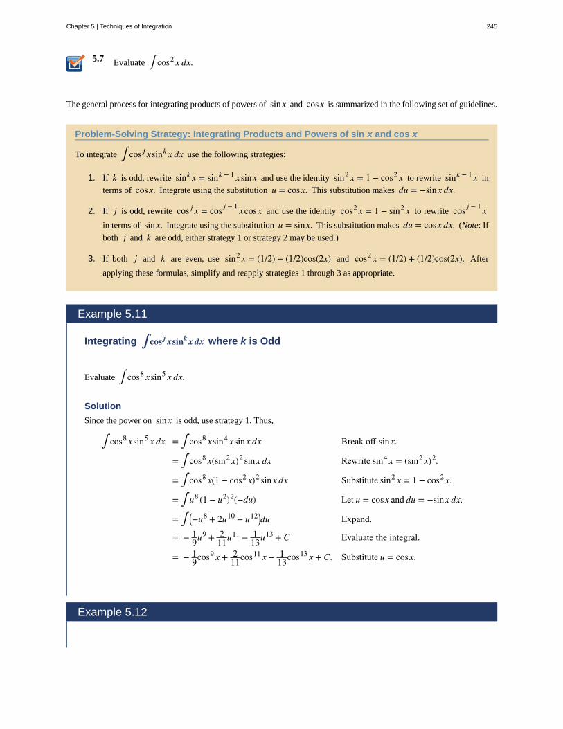
5.7 Evaluate ∫ cos2 x dx.
The general process for integrating products of powers of sinx and cosx is summarized in the following set of guidelines.
Problem-Solving Strategy: Integrating Products and Powers of sin x and cos x
To integrate ∫ cos j xsink x dx use the following strategies:
1. If k is odd, rewrite sink x = sink − 1 xsinx and use the identity sin2 x = 1 − cos2 x to rewrite sink − 1 x in
terms of cosx. Integrate using the substitution u = cosx. This substitution makes du = −sinx dx.
2. If j is odd, rewrite cos j x = cos j − 1 xcosx and use the identity cos2 x = 1 − sin2 x to rewrite cos j − 1 xin terms of sinx. Integrate using the substitution u = sinx. This substitution makes du = cosx dx. (Note: If
both j and k are odd, either strategy 1 or strategy 2 may be used.)
3. If both j and k are even, use sin2 x = (1/2) − (1/2)cos(2x) and cos2 x = (1/2) + (1/2)cos(2x). After
applying these formulas, simplify and reapply strategies 1 through 3 as appropriate.
Example 5.11
Integrating ∫cos j xsinkxdx where k is Odd
Evaluate ∫ cos8 xsin5 x dx.
Solution
Since the power on sinx is odd, use strategy 1. Thus,
∫ cos8 xsin5 x dx = ∫ cos8 xsin4 xsinx dx Break off sinx.
= ∫ cos8 x(sin2 x)2 sinx dx Rewrite sin4 x = (sin2 x)2.
= ∫ cos8 x(1 − cos2 x)2 sinx dx Substitute sin2 x = 1 − cos2 x.
= ∫ u8 (1 − u2)2(−du) Let u = cosx and du = −sinx dx.
= ∫ ⎛⎝−u8 + 2u10 − u12⎞⎠du Expand.
= − 19u
9 + 211u
11 − 113u
13 + C Evaluate the integral.
= − 19cos9 x + 2
11cos11 x − 113cos13 x + C. Substitute u = cosx.
Example 5.12
Chapter 5 | Techniques of Integration 245
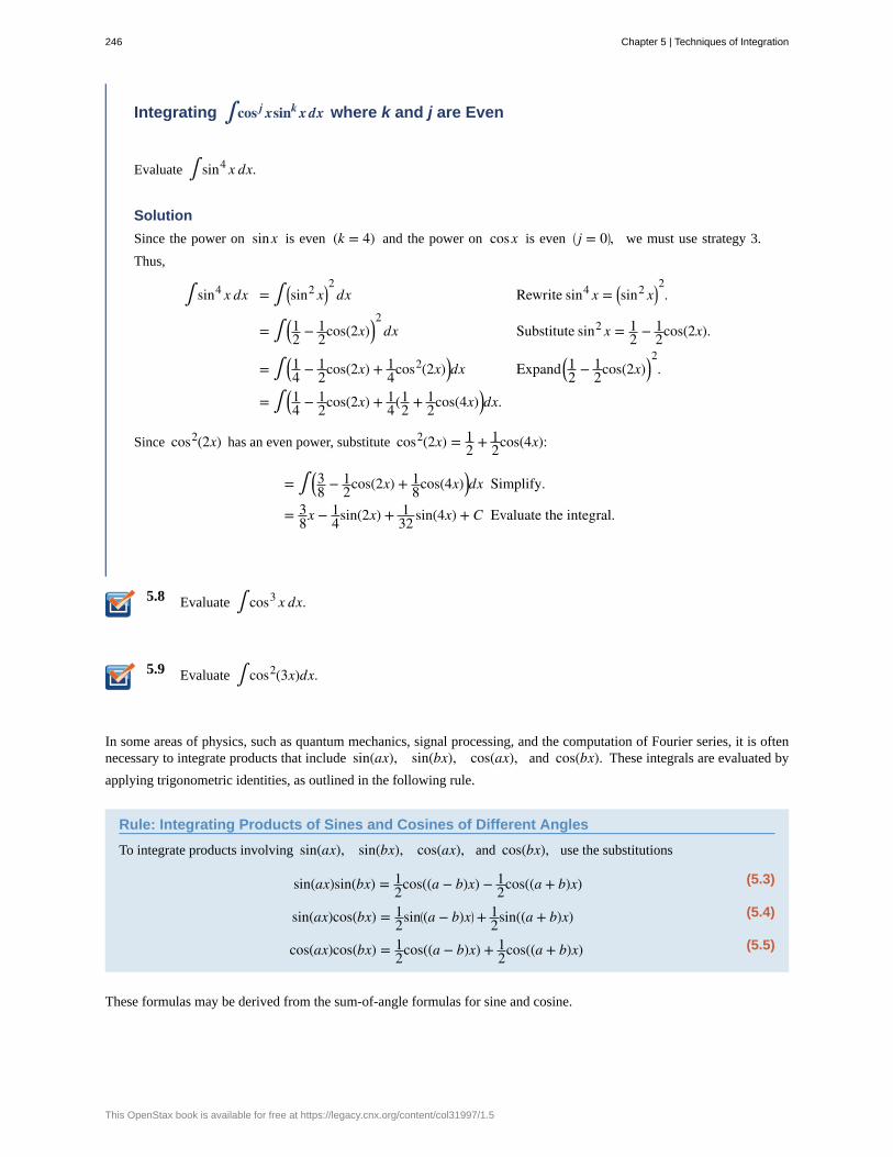
5.8
5.9
Integrating ∫cos j xsinkxdx where k and j are Even
Evaluate ∫ sin4 x dx.
Solution
Since the power on sinx is even (k = 4) and the power on cosx is even ⎛⎝ j = 0⎞⎠, we must use strategy 3.
Thus,
∫ sin4 x dx = ∫ ⎛⎝sin2 x⎞⎠2dx Rewrite sin4 x = ⎛⎝sin2 x⎞⎠
2.
= ∫ ⎛⎝12 − 12cos(2x)⎞⎠
2dx Substitute sin2 x = 1
2 − 12cos(2x).
= ∫ ⎛⎝14 − 12cos(2x) + 1
4cos2(2x)⎞⎠dx Expand⎛⎝12 − 12cos(2x)⎞⎠
2.
= ∫ ⎛⎝14 − 12cos(2x) + 1
4(12 + 1
2cos(4x)⎞⎠dx.
Since cos2(2x) has an even power, substitute cos2(2x) = 12 + 1
2cos(4x):
= ∫ ⎛⎝38 − 12cos(2x) + 1
8cos(4x)⎞⎠dx Simplify.
= 38x − 1
4sin(2x) + 132 sin(4x) + C Evaluate the integral.
Evaluate ∫ cos3 x dx.
Evaluate ∫ cos2(3x)dx.
In some areas of physics, such as quantum mechanics, signal processing, and the computation of Fourier series, it is oftennecessary to integrate products that include sin(ax), sin(bx), cos(ax), and cos(bx). These integrals are evaluated by
applying trigonometric identities, as outlined in the following rule.
Rule: Integrating Products of Sines and Cosines of Different Angles
To integrate products involving sin(ax), sin(bx), cos(ax), and cos(bx), use the substitutions
(5.3)sin(ax)sin(bx) = 12cos((a − b)x) − 1
2cos((a + b)x)
(5.4)sin(ax)cos(bx) = 12sin⎛⎝(a − b)x⎞⎠+ 1
2sin((a + b)x)
(5.5)cos(ax)cos(bx) = 12cos((a − b)x) + 1
2cos((a + b)x)
These formulas may be derived from the sum-of-angle formulas for sine and cosine.
246 Chapter 5 | Techniques of Integration
This OpenStax book is available for free at https://legacy.cnx.org/content/col31997/1.5
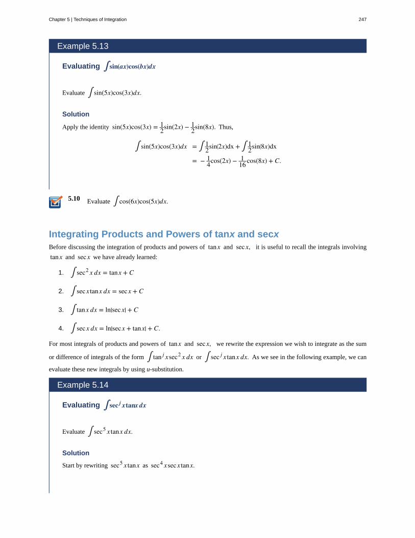
5.10
Example 5.13
Evaluating ∫ sin(ax)cos(bx)dx
Evaluate ∫ sin(5x)cos(3x)dx.
Solution
Apply the identity sin(5x)cos(3x) = 12sin(2x) − 1
2sin(8x). Thus,
∫ sin(5x)cos(3x)dx = ∫ 12sin⎛⎝2x)dx + ∫ 1
2sin⎛⎝8x)dx
= − 14cos(2x) − 1
16 cos(8x) + C.
Evaluate ∫ cos(6x)cos(5x)dx.
Integrating Products and Powers of tanx and secxBefore discussing the integration of products and powers of tanx and secx, it is useful to recall the integrals involving
tanx and secx we have already learned:
1. ∫ sec2 x dx = tanx + C
2. ∫ secx tanx dx = secx + C
3. ∫ tanx dx = ln|secx| + C
4. ∫ secx dx = ln|secx + tanx| + C.
For most integrals of products and powers of tanx and secx, we rewrite the expression we wish to integrate as the sum
or difference of integrals of the form ∫ tan j xsec2 x dx or ∫ sec j x tanx dx. As we see in the following example, we can
evaluate these new integrals by using u-substitution.
Example 5.14
Evaluating ∫ sec j xtanxdx
Evaluate ∫ sec5 x tanx dx.
Solution
Start by rewriting sec5 x tanx as sec4 xsecx tanx.
Chapter 5 | Techniques of Integration 247
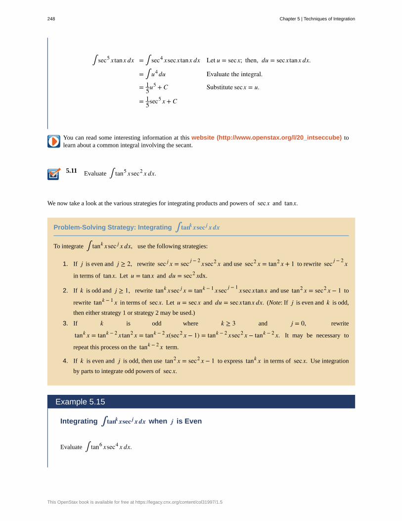
5.11
∫ sec5 x tanx dx = ∫ sec4 xsecx tanx dx Let u = secx; then, du = secx tanx dx.
= ∫ u4du Evaluate the integral.
= 15u
5 + C Substitute secx = u.
= 15sec5 x + C
You can read some interesting information at this website (http://www.openstax.org/l/20_intseccube) tolearn about a common integral involving the secant.
Evaluate ∫ tan5 xsec2 x dx.
We now take a look at the various strategies for integrating products and powers of secx and tanx.
Problem-Solving Strategy: Integrating ∫ tankxsec j xdx
To integrate ∫ tank xsec j x dx, use the following strategies:
1. If j is even and j ≥ 2, rewrite sec j x = sec j − 2 xsec2 x and use sec2 x = tan2 x + 1 to rewrite sec j − 2 x
in terms of tanx. Let u = tanx and du = sec2 xdx.
2. If k is odd and j ≥ 1, rewrite tank xsec j x = tank − 1 xsec j − 1 xsecx tanx and use tan2 x = sec2 x − 1 to
rewrite tank − 1 x in terms of secx. Let u = secx and du = secx tanx dx. (Note: If j is even and k is odd,
then either strategy 1 or strategy 2 may be used.)
3. If k is odd where k ≥ 3 and j = 0, rewrite
tank x = tank − 2 x tan2 x = tank − 2 x(sec2 x − 1) = tank − 2 xsec2 x − tank − 2 x. It may be necessary to
repeat this process on the tank − 2 x term.
4. If k is even and j is odd, then use tan2 x = sec2 x − 1 to express tank x in terms of secx. Use integration
by parts to integrate odd powers of secx.
Example 5.15
Integrating ∫ tankxsec j xdx when j is Even
Evaluate ∫ tan6 xsec4 x dx.
248 Chapter 5 | Techniques of Integration
This OpenStax book is available for free at https://legacy.cnx.org/content/col31997/1.5
Solution
Since the power on secx is even, rewrite sec4 x = sec2 xsec2 x and use sec2 x = tan2 x + 1 to rewrite the first
sec2 x in terms of tanx. Thus,
∫ tan6 xsec4 x dx = ∫ tan6 x⎛⎝tan2 x + 1⎞⎠sec2 x dx Let u = tanx and du = sec2 xdx.
= ∫ u6 ⎛⎝u2 + 1⎞⎠du Expand.
= ∫ (u8 + u6)du Evaluate the integral.
= 19u
9 + 17u
7 + C Substitute tanx = u.
= 19tan9 x + 1
7tan7 x + C.
Example 5.16
Integrating ∫ tankxsec j xdx when k is Odd
Evaluate ∫ tan5 xsec3 x dx.
Solution
Since the power on tanx is odd, begin by rewriting tan5 xsec3 x = tan4 xsec2 xsecx tanx. Thus,
tan5 xsec3 x = tan4 xsec2 xsecx tanx. Write tan4 x = (tan2 x)2.
∫ tan5 xsec3 x dx = ∫ (tan2 x)2 sec2 xsecx tanx dx Use tan2 x = sec2 x − 1.
= ∫ (sec2 x − 1)2 sec2 xsecx tanx dx Let u = secx and du = secx tanx dx.
= ∫ (u2 − 1)2u2du Expand.
= ∫ ⎛⎝u6 − 2u4 + u2⎞⎠du Integrate.
= 17u
7 − 25u
5 + 13u
3 + C Substitute secx = u.
= 17sec7 x − 2
5sec5 x + 13sec3 x + C.
Example 5.17
Integrating ∫ tankxdx where k is Odd and k ≥ 3
Evaluate ∫ tan3 x dx.
Chapter 5 | Techniques of Integration 249
5.12
Solution
Begin by rewriting tan3 x = tanx tan2 x = tanx⎛⎝sec2 x − 1⎞⎠ = tanxsec2 x − tanx. Thus,
∫ tan3 x dx = ∫ ⎛⎝tanxsec2 x − tanx⎞⎠dx
= ∫ tanxsec2 x dx − ∫ tanx dx
= 12tan2 x − ln|secx| + C.
For the first integral, use the substitution u = tanx. For the second integral, use the formula.
Example 5.18
Integrating ∫ sec3 xdx
Integrate ∫ sec3 x dx.
Solution
This integral requires integration by parts. To begin, let u = secx and dv = sec2 xdx. These choices make
du = secx tanx and v = tanx. Thus,
∫ sec3 x dx = secx tanx − ∫ tanxsecx tanx dx
= secx tanx − ∫ tan2 xsecx dx Simplify.
= secx tanx − ∫ ⎛⎝sec2 x − 1⎞⎠secx dx Substitute tan2 x = sec2 x − 1.
= secx tanx + ∫ secx dx − ∫ sec3 x dx Rewrite.
= secx tanx + ln|secx + tanx| − ∫ sec3 x dx. Evaluate∫ secx dx.
We now have
∫ sec3 x dx = secx tanx + ln|secx + tanx| − ∫ sec3 x dx.
Since the integral ∫ sec3 x dx has reappeared on the right-hand side, we can solve for ∫ sec3 x dx by adding it
to both sides. In doing so, we obtain
2∫ sec3 x dx = secx tanx + ln|secx + tanx|.
Dividing by 2, we arrive at
∫ sec3 x dx = 12secx tanx + 1
2ln|secx + tanx| + C.
Evaluate ∫ tan3 xsec7 x dx.
250 Chapter 5 | Techniques of Integration
This OpenStax book is available for free at https://legacy.cnx.org/content/col31997/1.5
Reduction Formulas
Evaluating ∫ secn x dx for values of n where n is odd requires integration by parts. In addition, we must also know
the value of ∫ secn − 2 x dx to evaluate ∫ secn x dx. The evaluation of ∫ tann x dx also requires being able to integrate
∫ tann − 2 x dx. To make the process easier, we can derive and apply the following power reduction formulas. These
rules allow us to replace the integral of a power of secx or tanx with the integral of a lower power of secx or tanx.
Rule: Reduction Formulas for ∫ secnxdx and ∫ tannxdx
(5.6)∫ secn x dx = 1n − 1secn − 2 x tanx + n − 2
n − 1∫ secn − 2 x dx
(5.7)∫ tann x dx = 1n − 1tann − 1 x − ∫ tann − 2 x dx
The first power reduction rule may be verified by applying integration by parts. The second may be verified byfollowing the strategy outlined for integrating odd powers of tanx.
Example 5.19
Revisiting ∫ sec3 xdx
Apply a reduction formula to evaluate ∫ sec3 x dx.
Solution
By applying the first reduction formula, we obtain
∫ sec3 x dx = 12secx tanx + 1
2∫ secx dx
= 12secx tanx + 1
2ln|secx + tanx| + C.
Example 5.20
Using a Reduction Formula
Evaluate ∫ tan4 x dx.
Solution
Applying the reduction formula for ∫ tan4 x dx we have
Chapter 5 | Techniques of Integration 251

5.13
∫ tan4 x dx = 13tan3 x − ∫ tan2 x dx
= 13tan3 x − (tanx − ∫ tan0 x dx) Apply the reduction formula to∫ tan2 x dx.
= 13tan3 x − tanx + ∫ 1 dx Simplify.
= 13tan3 x − tanx + x + C. Evaluate∫ 1dx.
Apply the reduction formula to ∫ sec5 x dx.
Key Concepts• Integrals of trigonometric functions can be evaluated by the use of various strategies. These strategies include
1. Applying trigonometric identities to rewrite the integral so that it may be evaluated by u-substitution
2. Using integration by parts
3. Applying trigonometric identities to rewrite products of sines and cosines with different arguments as thesum of individual sine and cosine functions
4. Applying reduction formulas
Key EquationsTo integrate products involving sin(ax), sin(bx), cos(ax), and cos(bx), use the substitutions.
• Sine Products
sin(ax)sin(bx) = 12cos((a − b)x) − 1
2cos((a + b)x)
• Sine and Cosine Products
sin(ax)cos(bx) = 12sin⎛⎝(a − b)x⎞⎠+ 1
2sin((a + b)x)
• Cosine Products
cos(ax)cos(bx) = 12cos((a − b)x) + 1
2cos((a + b)x)
• Power Reduction Formula
∫ secn x dx = 1n − 1secn − 1 x + n − 2
n − 1∫ secn − 2 x dx
• Power Reduction Formula
∫ tann x dx = 1n − 1tann − 1 x − ∫ tann − 2 x dx
252 Chapter 5 | Techniques of Integration
This OpenStax book is available for free at https://legacy.cnx.org/content/col31997/1.5

5.2 EXERCISESFill in the blank to make a true statement.
69. sin2 x + _______ = 1
70. sec2 x − 1 = _______
Use an identity to reduce the power of the trigonometricfunction to a trigonometric function raised to the firstpower.
71. sin2 x = _______
72. cos2 x = _______
Evaluate each of the following integrals by u-substitution.
73. ∫ sin3 xcosx dx
74. ∫ cosxsinx dx
75. ∫ tan5(2x)sec2(2x)dx
76. ∫ sin7(2x)cos(2x)dx
77. ∫ tan⎛⎝x2⎞⎠sec2 ⎛⎝x2
⎞⎠dx
78. ∫ tan2 xsec2 x dx
Compute the following integrals using the guidelines forintegrating powers of trigonometric functions. Use a CASto check the solutions. (Note: Some of the problems may bedone using techniques of integration learned previously.)
79. ∫ sin3 x dx
80. ∫ cos3 x dx
81. ∫ sinxcosx dx
82. ∫ cos5 x dx
83. ∫ sin5 xcos2 x dx
84. ∫ sin3 xcos3 x dx
85. ∫ sinxcosx dx
86. ∫ sinxcos3 x dx
87. ∫ secx tanx dx
88. ∫ tan(5x)dx
89. ∫ tan2 xsecx dx
90. ∫ tanxsec3 x dx
91. ∫ sec4 x dx
92. ∫ cotx dx
93. ∫ cscx dx
94. ∫ tan3 xsecxdx
For the following exercises, find a general formula for theintegrals.
95. ∫ sin2axcosax dx
96. ∫ sinaxcosax dx.
Use the double-angle formulas to evaluate the followingintegrals.
97. ∫0
πsin2 x dx
98. ∫0
πsin4 x dx
99. ∫ cos2 3x dx
100. ∫ sin2 xcos2 x dx
101. ∫ sin2 x dx + ∫ cos2 x dx
102. ∫ sin2 xcos2(2x)dx
Chapter 5 | Techniques of Integration 253

For the following exercises, evaluate the definite integrals.Express answers in exact form whenever possible.
103. ∫0
2πcosxsin2x dx
104. ∫0
πsin3xsin5x dx
105. ∫0
πcos(99x)sin(101x)dx
106. ∫−π
πcos2(3x)dx
107. ∫0
2πsinxsin(2x)sin(3x)dx
108. ∫0
4πcos(x/2)sin(x/2)dx
109. ∫π/6
π/3cos3 x
sinxdx (Round this answer to three decimal
places.)
110. ∫−π/3
π/3sec2 x − 1dx
111. ∫0
π/21 − cos(2x)dx
112. Find the area of the region bounded by the graphs of
the equations y = sinx, y = sin3 x, x = 0, and x = π2.
113. Find the area of the region bounded by the graphsof the equations
y = cos2 x, y = sin2 x, x = − π4, and x = π
4.
114. A particle moves in a straight line with the velocity
function v(t) = sin(ωt)cos2 (ωt). Find its position
function x = f (t) if f (0) = 0.
115. Find the average value of the function
f (x) = sin2 xcos3 x over the interval [−π, π].
For the following exercises, solve the differentialequations.
116.dydx = sin2 x. The curve passes through point
(0, 0).
117.dydθ = sin4 (πθ)
118. Find the length of the curvey = ln(cscx), π4 ≤ x ≤ π
2.
119. Find the length of the curvey = ln(sinx), π3 ≤ x ≤ π
2.
120. Find the volume generated by revolving the curvey = cos(3x) about the x-axis, 0 ≤ x ≤ π
36.
For the following exercises, use this information: The innerproduct of two functions f and g over [a, b] is defined
by f (x) · g(x) = ⟨ f , g ⟩ = ∫a
bf · gdx. Two distinct
functions f and g are said to be orthogonal if⟨ f , g ⟩ = 0.
121. Show that {sin(2x), cos(3x)} are orthogonal over
the interval [−π, π].
122. Evaluate ∫−π
πsin(mx)cos(nx)dx.
123. Integrate y′ = tanxsec4 x.
For each pair of integrals, determine which one is moredifficult to evaluate. Explain your reasoning.
124. ∫ sin456 xcosx dx or ∫ sin2 xcos2 x dx
125. ∫ tan350 xsec2 x dx or ∫ tan350 xsecx dx
254 Chapter 5 | Techniques of Integration
This OpenStax book is available for free at https://legacy.cnx.org/content/col31997/1.5
5.3 | Trigonometric Substitution
Learning Objectives5.3.1 Solve integration problems involving the square root of a sum or difference of two squares.
In this section, we explore integrals containing expressions of the form a2 − x2, a2 + x2, and x2 − a2, where the
values of a are positive. We have already encountered and evaluated integrals containing some expressions of this type, but
many still remain inaccessible. The technique of trigonometric substitution comes in very handy when evaluating theseintegrals. This technique uses substitution to rewrite these integrals as trigonometric integrals.
Integrals Involving a2− x2
Before developing a general strategy for integrals containing a2 − x2, consider the integral ∫ 9 − x2dx. This integral
cannot be evaluated using any of the techniques we have discussed so far. However, if we make the substitutionx = 3sinθ, we have dx = 3cosθdθ. After substituting into the integral, we have
∫ 9 − x2dx = ∫ 9 − (3sinθ)23cosθdθ.
After simplifying, we have
∫ 9 − x2dx = ∫ 9 1 − sin2 θcosθdθ.
Letting 1 − sin2 θ = cos2 θ, we now have
∫ 9 − x2dx = ∫ 9 cos2 θcosθdθ.
Assuming that cosθ ≥ 0, we have
∫ 9 − x2dx = ∫ 9cos2 θdθ.
At this point, we can evaluate the integral using the techniques developed for integrating powers and products oftrigonometric functions. Before completing this example, let’s take a look at the general theory behind this idea.
To evaluate integrals involving a2 − x2, we make the substitution x = asinθ and dx = acosθ. To see that this
actually makes sense, consider the following argument: The domain of a2 − x2 is [−a, a]. Thus, −a ≤ x ≤ a.Consequently, −1 ≤ x
a ≤ 1. Since the range of sinx over ⎡⎣−(π/2), π/2⎤⎦ is [−1, 1], there is a unique angle θ satisfying
−(π/2) ≤ θ ≤ π/2 so that sinθ = x/a, or equivalently, so that x = asinθ. If we substitute x = asinθ into a2 − x2,we get
a2 − x2 = a2 − (asinθ)2 Let x = asinθ where − π2 ≤ θ ≤ π
2. Simplify.
= a2 − a2 sin2 θ Factor out a2.= a2(1 − sin2 θ) Substitute 1 − sin2 x = cos2 x.
= a2 cos2 θ Take the square root.= |acosθ|= acosθ.
Since cosθ ≥ 0 on −π2 ≤ θ ≤ π
2 and a > 0, |acosθ| = acosθ. We can see, from this discussion, that by making the
substitution x = asinθ, we are able to convert an integral involving a radical into an integral involving trigonometric
functions. After we evaluate the integral, we can convert the solution back to an expression involving x. To see how to
Chapter 5 | Techniques of Integration 255

do this, let’s begin by assuming that 0 < x < a. In this case, 0 < θ < π2. Since sinθ = x
a, we can draw the reference
triangle in Figure 5.3 to assist in expressing the values of cosθ, tanθ, and the remaining trigonometric functions in
terms of x. It can be shown that this triangle actually produces the correct values of the trigonometric functions evaluated
at θ for all θ satisfying −π2 ≤ θ ≤ π
2. It is useful to observe that the expression a2 − x2 actually appears as the length
of one side of the triangle. Last, should θ appear by itself, we use θ = sin−1 ⎛⎝xa⎞⎠.
Figure 5.3 A reference triangle can help express thetrigonometric functions evaluated at θ in terms of x.
The essential part of this discussion is summarized in the following problem-solving strategy.
Problem-Solving Strategy: Integrating Expressions Involving a2− x2
1. It is a good idea to make sure the integral cannot be evaluated easily in another way. For example, although
this method can be applied to integrals of the form ∫ 1a2 − x2
dx, ∫ xa2 − x2
dx, and ∫ x a2 − x2dx,
they can each be integrated directly either by formula or by a simple u-substitution.
2. Make the substitution x = asinθ and dx = acosθdθ. Note: This substitution yields a2 − x2 = acosθ.
3. Simplify the expression.
4. Evaluate the integral using techniques from the section on trigonometric integrals.
5. Use the reference triangle from Figure 5.3 to rewrite the result in terms of x. You may also need to use some
trigonometric identities and the relationship θ = sin−1 ⎛⎝xa⎞⎠.
The following example demonstrates the application of this problem-solving strategy.
Example 5.21
Integrating an Expression Involving a2− x2
Evaluate ∫ 9 − x2dx.
Solution
Begin by making the substitutions x = 3sinθ and dx = 3cosθdθ. Since sinθ = x3, we can construct the
reference triangle shown in the following figure.
256 Chapter 5 | Techniques of Integration
This OpenStax book is available for free at https://legacy.cnx.org/content/col31997/1.5
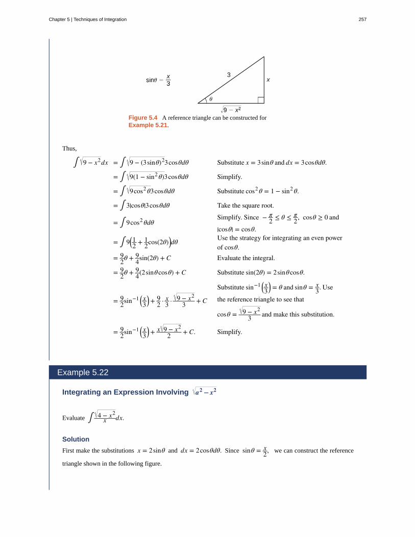
Figure 5.4 A reference triangle can be constructed forExample 5.21.
Thus,
∫ 9 − x2dx = ∫ 9 − (3sinθ)23cosθdθ Substitute x = 3sinθ and dx = 3cosθdθ.
= ∫ 9(1 − sin2 θ)3cosθdθ Simplify.
= ∫ 9cos2 θ3cosθdθ Substitute cos2 θ = 1 − sin2 θ.
= ∫ 3|cosθ|3cosθdθ Take the square root.
= ∫ 9cos2 θdθSimplify. Since − π
2 ≤ θ ≤ π2, cosθ ≥ 0 and
|cosθ| = cosθ.
= ∫ 9⎛⎝12 + 12cos(2θ)⎞⎠dθ
Use the strategy for integrating an even powerof cosθ.
= 92θ + 9
4sin(2θ) + C Evaluate the integral.
= 92θ + 9
4(2sinθcosθ) + C Substitute sin(2θ) = 2sinθcosθ.
= 92sin−1 ⎛⎝x3
⎞⎠+ 9
2 · x3 · 9 − x2
3 + C
Substitute sin−1 ⎛⎝x3⎞⎠ = θ and sinθ = x
3. Use
the reference triangle to see that
cosθ = 9 − x2
3 and make this substitution.
= 92sin−1 ⎛⎝x3
⎞⎠+ x 9 − x2
2 + C. Simplify.
Example 5.22
Integrating an Expression Involving a2− x2
Evaluate ∫ 4 − x2x dx.
Solution
First make the substitutions x = 2sinθ and dx = 2cosθdθ. Since sinθ = x2, we can construct the reference
triangle shown in the following figure.
Chapter 5 | Techniques of Integration 257
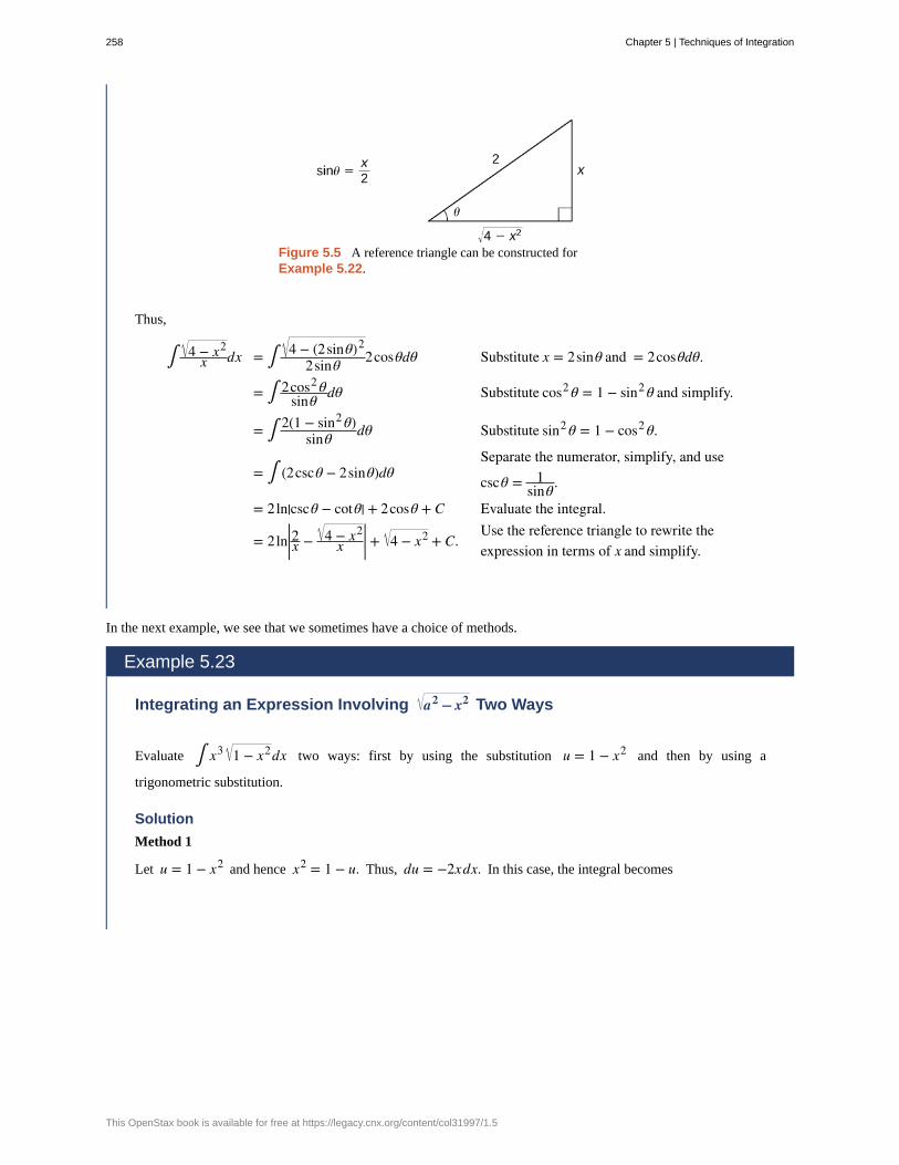
Figure 5.5 A reference triangle can be constructed forExample 5.22.
Thus,
∫ 4 − x2x dx = ∫ 4 − (2sinθ)2
2sinθ 2cosθdθ Substitute x = 2sinθ and = 2cosθdθ.
= ∫ 2cos2 θsinθ dθ Substitute cos2 θ = 1 − sin2 θ and simplify.
= ∫ 2(1 − sin2 θ)sinθ dθ Substitute sin2 θ = 1 − cos2 θ.
= ∫ (2cscθ − 2sinθ)dθSeparate the numerator, simplify, and use
cscθ = 1sinθ .
= 2ln|cscθ − cotθ| + 2cosθ + C Evaluate the integral.
= 2ln|2x − 4 − x2x | + 4 − x2 + C.
Use the reference triangle to rewrite theexpression in terms of x and simplify.
In the next example, we see that we sometimes have a choice of methods.
Example 5.23
Integrating an Expression Involving a2− x2 Two Ways
Evaluate ∫ x3 1 − x2dx two ways: first by using the substitution u = 1 − x2 and then by using a
trigonometric substitution.
Solution
Method 1
Let u = 1 − x2 and hence x2 = 1 − u. Thus, du = −2xdx. In this case, the integral becomes
258 Chapter 5 | Techniques of Integration
This OpenStax book is available for free at https://legacy.cnx.org/content/col31997/1.5
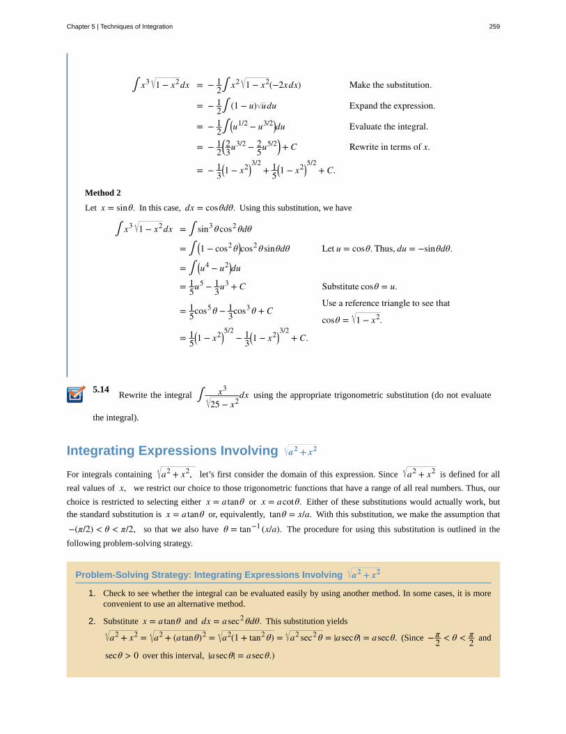
5.14
∫ x3 1 − x2dx = − 12∫ x2 1 − x2(−2xdx) Make the substitution.
= − 12∫ (1 − u) udu Expand the expression.
= − 12∫ ⎛⎝u1/2 − u3/2⎞⎠du Evaluate the integral.
= − 12⎛⎝23u
3/2 − 25u
5/2⎞⎠+ C Rewrite in terms of x.
= − 13⎛⎝1 − x2⎞⎠
3/2+ 1
5⎛⎝1 − x2⎞⎠
5/2+ C.
Method 2
Let x = sinθ. In this case, dx = cosθdθ. Using this substitution, we have
∫ x3 1 − x2dx = ∫ sin3 θcos2 θdθ
= ∫ ⎛⎝1 − cos2 θ⎞⎠cos2 θsinθdθ Let u = cosθ. Thus, du = −sinθdθ.
= ∫ ⎛⎝u4 − u2⎞⎠du
= 15u
5 − 13u
3 + C Substitute cosθ = u.
= 15cos5 θ − 1
3cos3 θ + CUse a reference triangle to see that
cosθ = 1 − x2.
= 15⎛⎝1 − x2⎞⎠
5/2− 1
3⎛⎝1 − x2⎞⎠
3/2+ C.
Rewrite the integral ∫ x3
25 − x2dx using the appropriate trigonometric substitution (do not evaluate
the integral).
Integrating Expressions Involving a2+ x2
For integrals containing a2 + x2, let’s first consider the domain of this expression. Since a2 + x2 is defined for all
real values of x, we restrict our choice to those trigonometric functions that have a range of all real numbers. Thus, our
choice is restricted to selecting either x = a tanθ or x = acotθ. Either of these substitutions would actually work, but
the standard substitution is x = a tanθ or, equivalently, tanθ = x/a. With this substitution, we make the assumption that
−(π/2) < θ < π/2, so that we also have θ = tan−1 (x/a). The procedure for using this substitution is outlined in the
following problem-solving strategy.
Problem-Solving Strategy: Integrating Expressions Involving a2+ x2
1. Check to see whether the integral can be evaluated easily by using another method. In some cases, it is moreconvenient to use an alternative method.
2. Substitute x = a tanθ and dx = asec2 θdθ. This substitution yields
a2 + x2 = a2 + (a tanθ)2 = a2(1 + tan2 θ) = a2 sec2 θ = |asecθ| = asecθ. (Since −π2 < θ < π
2 and
secθ > 0 over this interval, |asecθ| = asecθ.)
Chapter 5 | Techniques of Integration 259
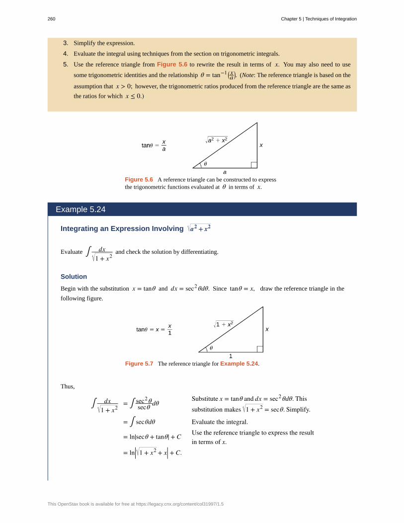
3. Simplify the expression.
4. Evaluate the integral using techniques from the section on trigonometric integrals.
5. Use the reference triangle from Figure 5.6 to rewrite the result in terms of x. You may also need to use
some trigonometric identities and the relationship θ = tan−1 ⎛⎝xa⎞⎠. (Note: The reference triangle is based on the
assumption that x > 0; however, the trigonometric ratios produced from the reference triangle are the same as
the ratios for which x ≤ 0.)
Figure 5.6 A reference triangle can be constructed to expressthe trigonometric functions evaluated at θ in terms of x.
Example 5.24
Integrating an Expression Involving a2+ x2
Evaluate ∫ dx1 + x2
and check the solution by differentiating.
Solution
Begin with the substitution x = tanθ and dx = sec2 θdθ. Since tanθ = x, draw the reference triangle in the
following figure.
Figure 5.7 The reference triangle for Example 5.24.
Thus,
∫ dx1 + x2
= ∫ sec2 θsecθ dθ
Substitute x = tanθ and dx = sec2 θdθ. Thissubstitution makes 1 + x2 = secθ. Simplify.
= ∫ secθdθ Evaluate the integral.
= ln|secθ + tanθ| + C Use the reference triangle to express the resultin terms of x.
= ln| 1 + x2 + x| + C.
260 Chapter 5 | Techniques of Integration
This OpenStax book is available for free at https://legacy.cnx.org/content/col31997/1.5
To check the solution, differentiate:
ddx⎛⎝ln| 1 + x2 + x|⎞⎠ = 1
1 + x2 + x·⎛⎝⎜ x
1 + x2+ 1⎞⎠⎟
= 11 + x2 + x
· x + 1 + x2
1 + x2
= 11 + x2
.
Since 1 + x2 + x > 0 for all values of x, we could rewrite ln| 1 + x2 + x| + C = ln⎛⎝ 1 + x2 + x⎞⎠+ C, if
desired.
Example 5.25
Evaluating ∫ dx1 + x2
Using a Different Substitution
Use the substitution x = sinhθ to evaluate ∫ dx1 + x2
.
Solution
Because sinhθ has a range of all real numbers, and 1 + sinh2 θ = cosh2 θ, we may also use the substitution
x = sinhθ to evaluate this integral. In this case, dx = coshθdθ. Consequently,
∫ dx1 + x2
= ∫ coshθ1 + sinh2 θ
dθSubstitute x = sinhθ and dx = coshθdθ.Substitute 1 + sinh2 θ = cosh2 θ.
= ∫ coshθcosh2 θ
dθ cosh2 θ = |coshθ|
= ∫ coshθ|coshθ|dθ |coshθ| = coshθ since coshθ > 0 for all θ.
= ∫ coshθcoshθdθ Simplify.
= ∫ 1dθ Evaluate the integral.
= θ + C Since x = sinhθ, we know θ = sinh−1 x.= sinh−1 x + C.
AnalysisThis answer looks quite different from the answer obtained using the substitution x = tanθ. To see that the
solutions are the same, set y = sinh−1 x. Thus, sinhy = x. From this equation we obtain:
ey − e−y
2 = x.
After multiplying both sides by 2ey and rewriting, this equation becomes:
Chapter 5 | Techniques of Integration 261
e2y − 2xey − 1 = 0.
Use the quadratic equation to solve for ey :
ey = 2x ± 4x2 + 42 .
Simplifying, we have:
ey = x ± x2 + 1.
Since x − x2 + 1 < 0, it must be the case that ey = x + x2 + 1. Thus,
y = ln⎛⎝x + x2 + 1⎞⎠.
Last, we obtain
sinh−1 x = ln⎛⎝x + x2 + 1⎞⎠.
After we make the final observation that, since x + x2 + 1 > 0,
ln⎛⎝x + x2 + 1⎞⎠ = ln| 1 + x2 + x|,we see that the two different methods produced equivalent solutions.
Example 5.26
Finding an Arc Length
Find the length of the curve y = x2 over the interval [0, 12].
Solution
Becausedydx = 2x, the arc length is given by
∫0
1/21 + (2x)2dx = ∫
0
1/21 + 4x2dx.
To evaluate this integral, use the substitution x = 12tanθ and dx = 1
2sec2 θdθ. We also need to change the limits
of integration. If x = 0, then θ = 0 and if x = 12, then θ = π
4. Thus,
262 Chapter 5 | Techniques of Integration
This OpenStax book is available for free at https://legacy.cnx.org/content/col31997/1.5

5.15
∫0
1/21 + 4x2dx = ∫
0
π/41 + tan2 θ1
2sec2 θdθ
After substitution,
1 + 4x2 = tanθ. Substitute1 + tan2 θ = sec2 θ and simplify.
= 12∫
0
π/4sec3 θdθ
We derived this integral in theprevious section.
= 12⎛⎝12secθ tanθ + ln|secθ + tanθ|⎞⎠|0π/4
Evaluate and simplify.
= 14( 2 + ln( 2 + 1)).
Rewrite ∫ x3 x2 + 4dx by using a substitution involving tanθ.
Integrating Expressions Involving x2− a2
The domain of the expression x2 − a2 is (−∞, −a] ∪ [a, +∞). Thus, either x ≤ −a or x ≥ a. Hence, xa ≤ − 1
or xa ≥ 1. Since these intervals correspond to the range of secθ on the set
⎡⎣0, π2⎞⎠ ∪ ⎛⎝π2, π⎤⎦, it makes sense to use the
substitution secθ = xa or, equivalently, x = asecθ, where 0 ≤ θ < π
2 or π2 < θ ≤ π. The corresponding substitution
for dx is dx = asecθ tanθdθ. The procedure for using this substitution is outlined in the following problem-solving
strategy.
Problem-Solving Strategy: Integrals Involving x2− a2
1. Check to see whether the integral cannot be evaluated using another method. If so, we may wish to considerapplying an alternative technique.
2. Substitute x = asecθ and dx = asecθ tanθdθ. This substitution yields
x2 − a2 = (asecθ)2 − a2 = a2(sec2 θ – 1) = a2 tan2 θ = |a tanθ|.
For x ≥ a, |a tanθ| = a tanθ and for x ≤ − a, |a tanθ| = −a tanθ.
3. Simplify the expression.
4. Evaluate the integral using techniques from the section on trigonometric integrals.
5. Use the reference triangles from Figure 5.8 to rewrite the result in terms of x. You may also need to use some
trigonometric identities and the relationship θ = sec−1 ⎛⎝xa⎞⎠. (Note: We need both reference triangles, since the
values of some of the trigonometric ratios are different depending on whether x ≥ a or x ≤ −a.)
Chapter 5 | Techniques of Integration 263

Figure 5.8 Use the appropriate reference triangle to express the trigonometric functions evaluated at θ in terms of x.
Example 5.27
Finding the Area of a Region
Find the area of the region between the graph of f (x) = x2 − 9 and the x-axis over the interval [3, 5].
Solution
First, sketch a rough graph of the region described in the problem, as shown in the following figure.
Figure 5.9 Calculating the area of the shaded region requiresevaluating an integral with a trigonometric substitution.
We can see that the area is A = ∫3
5x2 − 9dx. To evaluate this definite integral, substitute x = 3secθ and
dx = 3secθ tanθdθ. We must also change the limits of integration. If x = 3, then 3 = 3secθ and hence
θ = 0. If x = 5, then θ = sec−1 ⎛⎝53⎞⎠. After making these substitutions and simplifying, we have
264 Chapter 5 | Techniques of Integration
This OpenStax book is available for free at https://legacy.cnx.org/content/col31997/1.5
5.16
Area = ∫3
5x2 − 9dx
= ∫0
sec−1 (5/3)9tan2 θsecθdθ Use tan2 θ = 1 − sec2 θ.
= ∫0
sec−1 (5/3)9(sec2 θ − 1)secθdθ Expand.
= ∫0
sec−1 (5/3)9(sec3 θ − secθ)dθ Evaluate the integral.
= ⎛⎝92ln|secθ + tanθ| + 92secθ tanθ⎞⎠− 9ln|secθ + tanθ||0sec−1 (5/3)
Simplify.
= 92secθ tanθ − 9
2ln|secθ + tanθ||0sec−1 (5/3) Evaluate. Use sec⎛⎝sec−1 53⎞⎠ = 5
3and tan⎛⎝sec−1 5
3⎞⎠ = 4
3.
= 92 · 5
3 · 43 − 9
2ln|53 + 43| − ⎛⎝92 · 1 · 0 − 9
2ln|1 + 0|⎞⎠= 10 − 9
2ln3.
Evaluate ∫ dxx2 − 4
. Assume that x > 2.
Key Concepts• For integrals involving a2 − x2, use the substitution x = asinθ and dx = acosθdθ.
• For integrals involving a2 + x2, use the substitution x = a tanθ and dx = asec2 θdθ.
• For integrals involving x2 − a2, substitute x = asecθ and dx = asecθ tanθdθ.
Chapter 5 | Techniques of Integration 265
5.3 EXERCISESSimplify the following expressions by writing each oneusing a single trigonometric function.
126. 4 − 4sin2 θ
127. 9sec2 θ − 9
128. a2 + a2 tan2 θ
129. a2 + a2 sinh2 θ
130. 16cosh2 θ − 16
Use the technique of completing the square to express eachtrinomial as the square of a binomial or the square of abinomial plus a constant.
131. 4x2 − 4x + 1
132. 2x2 − 8x + 3
133. −x2 − 2x + 4
Integrate using the method of trigonometric substitution.Express the final answer in terms of the variable.
134. ∫ dx4 − x2
135. ∫ dxx2 − a2
136. ∫ 4 − x2dx
137. ∫ dx1 + 9x2
138. ∫ x2dx1 − x2
139. ∫ dxx2 1 − x2
140. ∫ dx(1 + x2)2
141. ∫ x2 + 9dx
142. ∫ x2 − 25x dx
143. ∫ θ3dθ9 − θ2
144. ∫ dxx6 − x2
145. ∫ x6 − x8dx
146. ∫ dx⎛⎝1 + x2⎞⎠
3/2
147. ∫ dx⎛⎝x2 − 9⎞⎠
3/2
148. ∫ 1 + x2dxx
149. ∫ x2dxx2 − 1
150. ∫ x2dxx2 + 4
151. ∫ dxx2 x2 + 1
152. ∫ x2dx1 + x2
153. ∫−1
1(1 − x2)3/2dx
In the following exercises, use the substitutionsx = sinhθ, coshθ, or tanhθ. Express the final answers
in terms of the variable x.
154. ∫ dxx2 − 1
155. ∫ dxx 1 − x2
156. ∫ x2 − 1dx
157. ∫ x2 − 1x2 dx
266 Chapter 5 | Techniques of Integration
This OpenStax book is available for free at https://legacy.cnx.org/content/col31997/1.5
158. ∫ dx1 − x2
159. ∫ 1 + x2
x2 dx
Use the technique of completing the square to evaluate thefollowing integrals.
160. ∫ 1x2 − 6x
dx
161. ∫ 1x2 + 2x + 1
dx
162. ∫ 1−x2 + 2x + 8
dx
163. ∫ 1−x2 + 10x
dx
164. ∫ 1x2 + 4x − 12
dx
165. Evaluate the integral without using calculus:
∫−3
39 − x2dx.
166. Find the area enclosed by the ellipse x2
4 + y2
9 = 1.
167. Evaluate the integral ∫ dx1 − x2
using two different
substitutions. First, let x = cosθ and evaluate using
trigonometric substitution. Second, let x = sinθ and use
trigonometric substitution. Are the answers the same?
168. Evaluate the integral ∫ dxx x2 − 1
using the
substitution x = secθ. Next, evaluate the same integral
using the substitution x = cscθ. Show that the results are
equivalent.
169. Evaluate the integral ∫ xx2 + 1
dx using the form
∫ 1udu. Next, evaluate the same integral using x = tanθ.
Are the results the same?
170. State the method of integration you would use to
evaluate the integral ∫ x x2 + 1dx. Why did you choose
this method?
171. State the method of integration you would use to
evaluate the integral ∫ x2 x2 − 1dx. Why did you
choose this method?
172. Evaluate ∫−1
1xdxx2 + 1
173. Find the length of the arc of the curve over thespecified interval: y = lnx, [1, 5]. Round the answer to
three decimal places.
174. Find the surface area of the solid generated byrevolving the region bounded by the graphs of
y = x2, y = 0, x = 0, and x = 2 about the x-axis.
(Round the answer to three decimal places).
175. The region bounded by the graph of f (x) = 11 + x2
and the x-axis between x = 0 and x = 1 is revolved about
the x-axis. Find the volume of the solid that is generated.
Solve the initial-value problem for y as a function of x.
176. ⎛⎝x2 + 36⎞⎠dydx = 1, y(6) = 0
177. ⎛⎝64 − x2⎞⎠dydx = 1, y(0) = 3
178. Find the area bounded by
y = 264 − 4x2
, x = 0, y = 0, and x = 2.
179. An oil storage tank can be described as the volumegenerated by revolving the area bounded by
y = 1664 + x2
, x = 0, y = 0, x = 2 about the x-axis. Find
the volume of the tank (in cubic meters).
180. During each cycle, the velocity v (in feet per second)
of a robotic welding device is given by v = 2t − 144 + t2
,
where t is time in seconds. Find the expression for thedisplacement s (in feet) as a function of t if s = 0 when
t = 0.
181. Find the length of the curve y = 16 − x2 between
x = 0 and x = 2.
Chapter 5 | Techniques of Integration 267

5.4 | Partial Fractions
Learning Objectives5.4.1 Integrate a rational function using the method of partial fractions.
5.4.2 Recognize simple linear factors in a rational function.
5.4.3 Recognize repeated linear factors in a rational function.
5.4.4 Recognize quadratic factors in a rational function.
We have seen some techniques that allow us to integrate specific rational functions. For example, we know that
∫ duu = ln|u| + C and ∫ du
u2 + a2 = 1atan−1 ⎛⎝ua
⎞⎠+ C.
However, we do not yet have a technique that allows us to tackle arbitrary quotients of this type. Thus, it is not immediately
obvious how to go about evaluating ∫ 3xx2 − x − 2
dx. However, we know from material previously developed that
∫ ⎛⎝ 1x + 1 + 2
x − 2⎞⎠dx = ln|x + 1| + 2ln|x − 2| + C.
In fact, by getting a common denominator, we see that
1x + 1 + 2
x − 2 = 3xx2 − x − 2
.
Consequently,
∫ 3xx2 − x − 2
dx = ∫ ⎛⎝ 1x + 1 + 2
x − 2⎞⎠dx.
In this section, we examine the method of partial fraction decomposition, which allows us to decompose rational functionsinto sums of simpler, more easily integrated rational functions. Using this method, we can rewrite an expression such as:
3xx2 − x − 2
as an expression such as 1x + 1 + 2
x − 2.
The key to the method of partial fraction decomposition is being able to anticipate the form that the decomposition of arational function will take. As we shall see, this form is both predictable and highly dependent on the factorization of thedenominator of the rational function. It is also extremely important to keep in mind that partial fraction decomposition
can be applied to a rational functionP(x)Q(x) only if deg(P(x)) < deg⎛⎝Q(x)⎞⎠. In the case when deg(P(x)) ≥ deg⎛⎝Q(x)⎞⎠, we
must first perform long division to rewrite the quotientP(x)Q(x) in the form A(x) + R(x)
Q(x), where deg(R(x)) < deg⎛⎝Q(x)⎞⎠.
We then do a partial fraction decomposition onR(x)Q(x). The following example, although not requiring partial fraction
decomposition, illustrates our approach to integrals of rational functions of the form ∫ P(x)Q(x)dx, where
deg(P(x)) ≥ deg⎛⎝Q(x)⎞⎠.
Example 5.28
Integrating ∫ P(x)Q(x)dx, where deg(P(x)) ≥ deg⎛⎝Q(x)⎞⎠
Evaluate ∫ x2 + 3x + 5x + 1 dx.
268 Chapter 5 | Techniques of Integration
This OpenStax book is available for free at https://legacy.cnx.org/content/col31997/1.5
5.17
Solution
Since deg⎛⎝x2 + 3x + 5⎞⎠ ≥ deg(x + 1), we perform long division to obtain
x2 + 3x + 5x + 1 = x + 2 + 3
x + 1.
Thus,
∫ x2 + 3x + 5x + 1 dx = ∫ ⎛⎝x + 2 + 3
x + 1⎞⎠dx
= 12x
2 + 2x + 3ln|x + 1| + C.
Visit this website (http://www.openstax.org/l/20_polylongdiv) for a review of long division ofpolynomials.
Evaluate ∫ x − 3x + 2dx.
To integrate ∫ P(x)Q(x)dx, where deg(P(x)) < deg⎛⎝Q(x)⎞⎠, we must begin by factoring Q(x).
Nonrepeated Linear FactorsIf Q(x) can be factored as ⎛⎝a1 x + b1
⎞⎠⎛⎝a2 x + b2
⎞⎠…⎛
⎝an x + bn⎞⎠, where each linear factor is distinct, then it is possible to
find constants A1, A2 ,… An satisfying
P(x)Q(x) = A1
a1 x + b1+ A2a2 x + b2
+ ⋯ + Anan x + bn
.
The proof that such constants exist is beyond the scope of this course.
In this next example, we see how to use partial fractions to integrate a rational function of this type.
Example 5.29
Partial Fractions with Nonrepeated Linear Factors
Evaluate ∫ 3x + 2x3 − x2 − 2x
dx.
Solution
Since deg(3x + 2) < deg⎛⎝x3 − x2 − 2x⎞⎠, we begin by factoring the denominator of 3x + 2x3 − x2 − 2x
. We can see
that x3 − x2 − 2x = x(x − 2)(x + 1). Thus, there are constants A, B, and C satisfying
3x + 2x(x − 2)(x + 1) = A
x + Bx − 2 + C
x + 1.
Chapter 5 | Techniques of Integration 269
(5.8)
We must now find these constants. To do so, we begin by getting a common denominator on the right. Thus,
3x + 2x(x − 2)(x + 1) = A(x − 2)(x + 1) + Bx(x + 1) + Cx(x − 2)
x(x − 2)(x + 1) .
Now, we set the numerators equal to each other, obtaining
3x + 2 = A(x − 2)(x + 1) + Bx(x + 1) + Cx(x − 2).
There are two different strategies for finding the coefficients A, B, and C. We refer to these as the method of
equating coefficients and the method of strategic substitution.
Rule: Method of Equating Coefficients
Rewrite Equation 5.8 in the form
3x + 2 = (A + B + C)x2 + (−A + B − 2C)x + (−2A).
Equating coefficients produces the system of equations
A + B + C = 0−A + B − 2C = 3
−2A = 2.
To solve this system, we first observe that −2A = 2 ⇒ A = −1. Substituting this value into the first two
equations gives us the system
B + C = 1B − 2C = 2.
Multiplying the second equation by −1 and adding the resulting equation to the first produces
−3C = 1,
which in turn implies that C = − 13. Substituting this value into the equation B + C = 1 yields B = 4
3.
Thus, solving these equations yields A = −1, B = 43, and C = − 1
3.
It is important to note that the system produced by this method is consistent if and only if we have set up thedecomposition correctly. If the system is inconsistent, there is an error in our decomposition.
Rule: Method of Strategic Substitution
The method of strategic substitution is based on the assumption that we have set up the decompositioncorrectly. If the decomposition is set up correctly, then there must be values of A, B, and C that satisfy
Equation 5.8 for all values of x. That is, this equation must be true for any value of x we care to substitute
into it. Therefore, by choosing values of x carefully and substituting them into the equation, we may find
A, B, and C easily. For example, if we substitute x = 0, the equation reduces to 2 = A(−2)(1).Solving for A yields A = −1. Next, by substituting x = 2, the equation reduces to 8 = B(2)(3),or equivalently B = 4/3. Last, we substitute x = −1 into the equation and obtain −1 = C(−1)(−3).
Solving, we have C = − 13.
It is important to keep in mind that if we attempt to use this method with a decomposition that has not been
270 Chapter 5 | Techniques of Integration
This OpenStax book is available for free at https://legacy.cnx.org/content/col31997/1.5

set up correctly, we are still able to find values for the constants, but these constants are meaningless. If wedo opt to use the method of strategic substitution, then it is a good idea to check the result by recombiningthe terms algebraically.
Now that we have the values of A, B, and C, we rewrite the original integral:
∫ 3x + 2x3 − x2 − 2x
dx = ∫ ⎛⎝− 1x + 4
3 · 1(x − 2) − 1
3 · 1(x + 1)
⎞⎠dx.
Evaluating the integral gives us
∫ 3x + 2x3 − x2 − 2x
dx = −ln|x| + 43ln|x − 2| − 1
3ln|x + 1| + C.
In the next example, we integrate a rational function in which the degree of the numerator is not less than the degree of thedenominator.
Example 5.30
Dividing before Applying Partial Fractions
Evaluate ∫ x2 + 3x + 1x2 − 4
dx.
Solution
Since degree(x2 + 3x + 1) ≥ degree(x2 − 4), we must perform long division of polynomials. This results in
x2 + 3x + 1x2 − 4
= 1 + 3x + 5x2 − 4
.
Next, we perform partial fraction decomposition on 3x + 5x2 − 4
= 3x + 5(x + 2)(x − 2). We have
3x + 5(x − 2)(x + 2) = A
x − 2 + Bx + 2.
Thus,
3x + 5 = A(x + 2) + B(x − 2).
Solving for A and B using either method, we obtain A = 11/4 and B = 1/4.
Rewriting the original integral, we have
∫ x2 + 3x + 1x2 − 4
dx = ∫ ⎛⎝1 + 114 · 1
x − 2 + 14 · 1
x + 2⎞⎠dx.
Evaluating the integral produces
∫ x2 + 3x + 1x2 − 4
dx = x + 114 ln|x − 2| + 1
4ln|x + 2| + C.
Chapter 5 | Techniques of Integration 271
5.18
As we see in the next example, it may be possible to apply the technique of partial fraction decomposition to a nonrationalfunction. The trick is to convert the nonrational function to a rational function through a substitution.
Example 5.31
Applying Partial Fractions after a Substitution
Evaluate ∫ cosxsin2 x − sinx
dx.
Solution
Let’s begin by letting u = sinx. Consequently, du = cosxdx. After making these substitutions, we have
∫ cosxsin2 x − sinx
dx = ∫ duu2 − u
= ∫ duu(u − 1).
Applying partial fraction decomposition to 1/u(u − 1) gives 1u(u − 1) = − 1
u + 1u − 1.
Thus,
∫ cosxsin2 x − sinx
dx = −ln|u| + ln|u − 1| + C
= −ln|sinx| + ln|sinx − 1| + C.
Evaluate ∫ x + 1(x + 3)(x − 2)dx.
Repeated Linear FactorsFor some applications, we need to integrate rational expressions that have denominators with repeated linear factors—thatis, rational functions with at least one factor of the form (ax + b)n, where n is a positive integer greater than or equal to
2. If the denominator contains the repeated linear factor (ax + b)n, then the decomposition must contain
A1ax + b + A2
(ax + b)2 + ⋯ + An(ax + b)n
.
As we see in our next example, the basic technique used for solving for the coefficients is the same, but it requires morealgebra to determine the numerators of the partial fractions.
Example 5.32
Partial Fractions with Repeated Linear Factors
Evaluate ∫ x − 2(2x − 1)2(x − 1)
dx.
Solution
We have degree(x − 2) < degree⎛⎝(2x − 1)2 (x − 1)⎞⎠, so we can proceed with the decomposition. Since
272 Chapter 5 | Techniques of Integration
This OpenStax book is available for free at https://legacy.cnx.org/content/col31997/1.5

(5.9)
5.19
(2x − 1)2 is a repeated linear factor, include A2x − 1 + B
(2x − 1)2 in the decomposition. Thus,
x − 2(2x − 1)2(x − 1)
= A2x − 1 + B
(2x − 1)2 + Cx − 1.
After getting a common denominator and equating the numerators, we have
x − 2 = A(2x − 1)(x − 1) + B(x − 1) + C(2x − 1)2.
We then use the method of equating coefficients to find the values of A, B, and C.
x − 2 = (2A + 4C)x2 + (−3A + B − 4C)x + (A − B + C).
Equating coefficients yields 2A + 4C = 0, −3A + B − 4C = 1, and A − B + C = −2. Solving this system
yields A = 2, B = 3, and C = −1.
Alternatively, we can use the method of strategic substitution. In this case, substituting x = 1 and x = 1/2 into
Equation 5.9 easily produces the values B = 3 and C = −1. At this point, it may seem that we have run out
of good choices for x, however, since we already have values for B and C, we can substitute in these values
and choose any value for x not previously used. The value x = 0 is a good option. In this case, we obtain the
equation −2 = A(−1)(−1) + 3(−1) + (−1)(−1)2 or, equivalently, A = 2.
Now that we have the values for A, B, and C, we rewrite the original integral and evaluate it:
∫ x − 2(2x − 1)2(x − 1)
dx = ∫⎛⎝⎜ 22x − 1 + 3
(2x − 1)2 − 1x − 1⎞⎠⎟dx
= ln|2x − 1| − 32(2x − 1) − ln|x − 1| + C.
Set up the partial fraction decomposition for ∫ x + 2(x + 3)3 (x − 4)2dx. (Do not solve for the coefficients
or complete the integration.)
The General MethodNow that we are beginning to get the idea of how the technique of partial fraction decomposition works, let’s outline thebasic method in the following problem-solving strategy.
Problem-Solving Strategy: Partial Fraction Decomposition
To decompose the rational function P(x)/Q(x), use the following steps:
1. Make sure that degree(P(x)) < degree(Q(x)). If not, perform long division of polynomials.
2. Factor Q(x) into the product of linear and irreducible quadratic factors. An irreducible quadratic is a quadratic
that has no real zeros.
3. Assuming that deg(P(x)) < deg(Q(x)), the factors of Q(x) determine the form of the decomposition of
P(x)/Q(x).
a. If Q(x) can be factored as ⎛⎝a1 x + b1⎞⎠⎛⎝a2 x + b2
⎞⎠…⎛
⎝an x + bn⎞⎠, where each linear factor is distinct,
Chapter 5 | Techniques of Integration 273
then it is possible to find constants A1, A2, ...An satisfying
P(x)Q(x) = A1
a1 x + b1+ A2a2 x + b2
+ ⋯ + Anan x + bn
.
b. If Q(x) contains the repeated linear factor (ax + b)n, then the decomposition must contain
A1ax + b + A2
(ax + b)2 + ⋯ + An(ax + b)n
.
c. For each irreducible quadratic factor ax2 + bx + c that Q(x) contains, the decomposition must
include
Ax + Bax2 + bx + c
.
d. For each repeated irreducible quadratic factor ⎛⎝ax2 + bx + c⎞⎠n, the decomposition must include
A1 x + B1ax2 + bx + c
+ A2 x + B2(ax2 + bx + c)2 + ⋯ + An x + Bn
(ax2 + bx + c)n.
e. After the appropriate decomposition is determined, solve for the constants.
f. Last, rewrite the integral in its decomposed form and evaluate it using previously developed techniquesor integration formulas.
Simple Quadratic FactorsNow let’s look at integrating a rational expression in which the denominator contains an irreducible quadratic factor. Recall
that the quadratic ax2 + bx + c is irreducible if ax2 + bx + c = 0 has no real zeros—that is, if b2 − 4ac < 0.
Example 5.33
Rational Expressions with an Irreducible Quadratic Factor
Evaluate ∫ 2x − 3x3 + x
dx.
Solution
Since deg(2x − 3) < deg(x3 + x), factor the denominator and proceed with partial fraction decomposition.
Since x3 + x = x(x2 + 1) contains the irreducible quadratic factor x2 + 1, include Ax + Bx2 + 1
as part of the
decomposition, along with Cx for the linear term x. Thus, the decomposition has the form
2x − 3x(x2 + 1)
= Ax + Bx2 + 1
+ Cx .
After getting a common denominator and equating the numerators, we obtain the equation
2x − 3 = (Ax + B)x + C⎛⎝x2 + 1⎞⎠.
Solving for A, B, and C, we get A = 3, B = 2, and C = −3.
Thus,
274 Chapter 5 | Techniques of Integration
This OpenStax book is available for free at https://legacy.cnx.org/content/col31997/1.5
2x − 3x3 + x
= 3x + 2x2 + 1
− 3x .
Substituting back into the integral, we obtain
∫ 2x − 3x3 + x
dx = ∫ ⎛⎝3x + 2x2 + 1
− 3x⎞⎠dx
= 3∫ xx2 + 1
dx + 2∫ 1x2 + 1
dx − 3∫ 1xdx Split up the integral.
= 32ln|x2 + 1| + 2tan−1 x − 3ln|x| + C. Evaluate each integral.
Note: We may rewrite ln|x2 + 1| = ln(x2 + 1), if we wish to do so, since x2 + 1 > 0.
Example 5.34
Partial Fractions with an Irreducible Quadratic Factor
Evaluate ∫ dxx3 − 8
.
Solution
We can start by factoring x3 − 8 = (x − 2)(x2 + 2x + 4). We see that the quadratic factor x2 + 2x + 4 is
irreducible since 22 − 4(1)(4) = −12 < 0. Using the decomposition described in the problem-solving strategy,
we get
1(x − 2)(x2 + 2x + 4)
= Ax − 2 + Bx + C
x2 + 2x + 4.
After obtaining a common denominator and equating the numerators, this becomes
1 = A⎛⎝x2 + 2x + 4⎞⎠+ (Bx + C)(x − 2).
Applying either method, we get A = 112, B = − 1
12, and C = − 13.
Rewriting ∫ dxx3 − 8
, we have
∫ dxx3 − 8
= 112∫ 1
x − 2dx − 112∫ x + 4
x2 + 2x + 4dx.
We can see that
∫ 1x − 2dx = ln|x − 2| + C, but ∫ x + 4
x2 + 2x + 4dx requires a bit more effort. Let’s begin by completing the
square on x2 + 2x + 4 to obtain
x2 + 2x + 4 = (x + 1)2 + 3.
Chapter 5 | Techniques of Integration 275

By letting u = x + 1 and consequently du = dx, we see that
∫ x + 4x2 + 2x + 4
dx = ∫ x + 4(x + 1)2 + 3
dx Complete the square on thedenominator.
= ∫ u + 3u2 + 3
du Substitute u = x + 1, x = u − 1,and du = dx.
= ∫ uu2 + 3
du + ∫ 3u2 + 3
du Split the numerator apart.
= 12ln|u2 + 3| + 3
3tan−1 u
3+ C Evaluate each integral.
= 12ln|x2 + 2x + 4| + 3tan−1 ⎛⎝x + 1
3⎞⎠+ C. Rewrite in terms of x and
simplify.
Substituting back into the original integral and simplifying gives
∫ dxx3 − 8
= 112ln|x − 2| − 1
24ln|x2 + 2x + 4| − 312tan−1 ⎛⎝x + 1
3⎞⎠+ C.
Here again, we can drop the absolute value if we wish to do so, since x2 + 2x + 4 > 0 for all x.
Example 5.35
Finding a Volume
Find the volume of the solid of revolution obtained by revolving the region enclosed by the graph of
f (x) = x2
⎛⎝x2 + 1⎞⎠
2 and the x-axis over the interval [0, 1] about the y-axis.
Solution
Let’s begin by sketching the region to be revolved (see Figure 5.10). From the sketch, we see that the shellmethod is a good choice for solving this problem.
Figure 5.10 We can use the shell method to find the volumeof revolution obtained by revolving the region shown about they-axis.
276 Chapter 5 | Techniques of Integration
This OpenStax book is available for free at https://legacy.cnx.org/content/col31997/1.5

5.20
The volume is given by
V = 2π∫0
1x · x2
⎛⎝x2 + 1⎞⎠
2dx = 2π∫0
1x3
(x2 + 1)2dx.
Since deg⎛⎝⎛⎝x2 + 1⎞⎠2⎞⎠ = 4 > 3 = deg(x3), we can proceed with partial fraction decomposition. Note that
(x2 + 1)2 is a repeated irreducible quadratic. Using the decomposition described in the problem-solving strategy,
we get
x3
(x2 + 1)2 = Ax + Bx2 + 1
+ Cx + D(x2 + 1)2.
Finding a common denominator and equating the numerators gives
x3 = (Ax + B)⎛⎝x2 + 1⎞⎠+ Cx + D.
Solving, we obtain A = 1, B = 0, C = −1, and D = 0. Substituting back into the integral, we have
V = 2π∫0
1x3
(x2 + 1)2dx
= 2π∫0
1 ⎛⎝⎜ xx2 + 1
− x(x2 + 1)2
⎞⎠⎟dx
= 2π⎛⎝12ln(x2 + 1) + 12 · 1
x2 + 1⎞⎠|01
= π⎛⎝ln2 − 12⎞⎠.
Set up the partial fraction decomposition for ∫ x2 + 3x + 1(x + 2)(x − 3)2 (x2 + 4)2dx.
Key Concepts• Partial fraction decomposition is a technique used to break down a rational function into a sum of simple rational
functions that can be integrated using previously learned techniques.
• When applying partial fraction decomposition, we must make sure that the degree of the numerator is lessthan the degree of the denominator. If not, we need to perform long division before attempting partial fractiondecomposition.
• The form the decomposition takes depends on the type of factors in the denominator. The types of factorsinclude nonrepeated linear factors, repeated linear factors, nonrepeated irreducible quadratic factors, and repeatedirreducible quadratic factors.
Chapter 5 | Techniques of Integration 277
5.4 EXERCISESExpress the rational function as a sum or difference of twosimpler rational expressions.
182. 1(x − 3)(x − 2)
183. x2 + 1x(x + 1)(x + 2)
184. 1x3 − x
185. 3x + 1x2
186. 3x2
x2 + 1(Hint: Use long division first.)
187. 2x4
x2 − 2x
188. 1(x − 1)(x2 + 1)
189. 1x2(x − 1)
190. xx2 − 4
191. 1x(x − 1)(x − 2)(x − 3)
192. 1x4 − 1
= 1(x + 1)(x − 1)⎛⎝x2 + 1⎞⎠
193. 3x2
x3 − 1= 3x2
(x − 1)(x2 + x + 1)
194. 2x(x + 2)2
195. 3x4 + x3 + 20x2 + 3x + 31
(x + 1)⎛⎝x2 + 4⎞⎠2
Use the method of partial fractions to evaluate each of thefollowing integrals.
196. ∫ dx(x − 3)(x − 2)
197. ∫ 3xx2 + 2x − 8
dx
198. ∫ dxx3 − x
199. ∫ xx2 − 4
dx
200. ∫ dxx(x − 1)(x − 2)(x − 3)
201. ∫ 2x2 + 4x + 22x2 + 2x + 10
dx
202. ∫ dxx2 − 5x + 6
203. ∫ 2 − xx2 + x
dx
204. ∫ 2x2 − x − 6
dx
205. ∫ dxx3 − 2x2 − 4x + 8
206. ∫ dxx4 − 10x2 + 9
Evaluate the following integrals, which have irreduciblequadratic factors.
207. ∫ 2(x − 4)⎛⎝x2 + 2x + 6⎞⎠
dx
208. ∫ x2
x3 − x2 + 4x − 4dx
209. ∫ x3 + 6x2 + 3x + 6x3 + 2x2 dx
210. ∫ x
(x − 1)⎛⎝x2 + 2x + 2⎞⎠2dx
Use the method of partial fractions to evaluate thefollowing integrals.
211. ∫ 3x + 4⎛⎝x2 + 4⎞⎠(3 − x)
dx
212. ∫ 2(x + 2)2(2 − x)
dx
278 Chapter 5 | Techniques of Integration
This OpenStax book is available for free at https://legacy.cnx.org/content/col31997/1.5
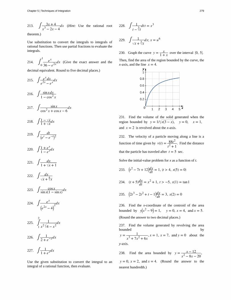
213. ∫ 3x + 4x3 − 2x − 4
dx (Hint: Use the rational root
theorem.)
Use substitution to convert the integrals to integrals ofrational functions. Then use partial fractions to evaluate theintegrals.
214. ∫0
1ex
36 − e2xdx (Give the exact answer and the
decimal equivalent. Round to five decimal places.)
215. ∫ ex dxe2x − ex
dx
216. ∫ sinxdx1 − cos2 x
217. ∫ sinxcos2 x + cosx − 6
dx
218. ∫ 1 − x1 + xdx
219. ∫ dt⎛⎝et − e−t⎞⎠2
220. ∫ 1 + ex1 − ex
dx
221. ∫ dx1 + x + 1
222. ∫ dxx + x4
223. ∫ cosxsinx(1 − sinx)dx
224. ∫ ex⎛⎝e2x − 4⎞⎠
2dx
225. ∫1
21
x2 4 − x2dx
226. ∫ 12 + e−xdx
227. ∫ 11 + ex
dx
Use the given substitution to convert the integral to anintegral of a rational function, then evaluate.
228. ∫ 1t − t3 dt t = x3
229. ∫ 1x + x3 dx; x = u6
230. Graph the curve y = x1 + x over the interval ⎡⎣0, 5⎤⎦.
Then, find the area of the region bounded by the curve, thex-axis, and the line x = 4.
231. Find the volume of the solid generated when theregion bounded by y = 1/ x(3 − x), y = 0, x = 1,and x = 2 is revolved about the x-axis.
232. The velocity of a particle moving along a line is a
function of time given by v(t) = 88t2t2 + 1
. Find the distance
that the particle has traveled after t = 5 sec.
Solve the initial-value problem for x as a function of t.
233. ⎛⎝t2 − 7t + 12⎞⎠dxdt = 1, ⎛⎝t > 4, x(5) = 0⎞⎠
234. (t + 5)dxdt = x2 + 1, t > −5, x(1) = tan1
235. ⎛⎝2t3 − 2t2 + t − 1⎞⎠dxdt = 3, x(2) = 0
236. Find the x-coordinate of the centroid of the area
bounded by y⎛⎝x2 − 9⎞⎠ = 1, y = 0, x = 4, and x = 5.
(Round the answer to two decimal places.)
237. Find the volume generated by revolving the areabounded by
y = 1x3 + 7x2 + 6x
, x = 1, x = 7, and y = 0 about the
y-axis.
238. Find the area bounded by y = x − 12x2 − 8x − 20
,
y = 0, x = 2, and x = 4. (Round the answer to the
nearest hundredth.)
Chapter 5 | Techniques of Integration 279
239. Evaluate the integral ∫ dxx3 + 1
.
For the following problems, use the substitutions
tan⎛⎝x2⎞⎠ = t, dx = 2
1 + t2dt, sinx = 2t
1 + t2, and
cosx = 1 − t2
1 + t2.
240. ∫ dx3 − 5sinx
241. Find the area under the curve y = 11 + sinx between
x = 0 and x = π. (Assume the dimensions are in inches.)
242. Given tan⎛⎝x2⎞⎠ = t, derive the formulas
dx = 21 + t2
dt, sinx = 2t1 + t2
, and cosx = 1 − t2
1 + t2.
243. Evaluate ∫ x − 83
x dx.
280 Chapter 5 | Techniques of Integration
This OpenStax book is available for free at https://legacy.cnx.org/content/col31997/1.5

5.5 | Other Strategies for Integration
Learning Objectives5.5.1 Use a table of integrals to solve integration problems.
5.5.2 Use a computer algebra system (CAS) to solve integration problems.
In addition to the techniques of integration we have already seen, several other tools are widely available to assist with theprocess of integration. Among these tools are integration tables, which are readily available in many books, including theappendices to this one. Also widely available are computer algebra systems (CAS), which are found on calculators and inmany campus computer labs, and are free online.
Tables of IntegralsIntegration tables, if used in the right manner, can be a handy way either to evaluate or check an integral quickly. Keep inmind that when using a table to check an answer, it is possible for two completely correct solutions to look very different.For example, in Trigonometric Substitution, we found that, by using the substitution x = tanθ, we can arrive at
∫ dx1 + x2
= ln⎛⎝x + x2 + 1⎞⎠+ C.
However, using x = sinhθ, we obtained a different solution—namely,
∫ dx1 + x2
= sinh−1 x + C.
We later showed algebraically that the two solutions are equivalent. That is, we showed that sinh−1 x = ln⎛⎝x + x2 + 1⎞⎠.In this case, the two antiderivatives that we found were actually equal. This need not be the case. However, as long as thedifference in the two antiderivatives is a constant, they are equivalent.
Example 5.36
Using a Formula from a Table to Evaluate an Integral
Use the table formula
∫ a2 − u2
u2 du = − a2 − u2u − sin−1 u
a + C
to evaluate ∫ 16 − e2x
exdx.
Solution
If we look at integration tables, we see that several formulas contain expressions of the form a2 − u2. This
expression is actually similar to 16 − e2x, where a = 4 and u = ex. Keep in mind that we must also have
du = ex dx. Multiplying the numerator and the denominator of the given integral by ex should help to put this
integral in a useful form. Thus, we now have
∫ 16 − e2x
exdx = ∫ 16 − e2x
e2x ex dx.
Chapter 5 | Techniques of Integration 281
Substituting u = ex and du = ex dx produces ∫ a2 − u2
u2 du. From the integration table (#88 in Appendix
A (https://legacy.cnx.org/content/m54049/latest/) ),
∫ a2 − u2
u2 du = − a2 − u2u − sin−1 u
a + C.
Thus,
∫ 16 − e2x
exdx = ∫ 16 − e2x
e2x ex dx Substitute u = ex and du = ex dx.
= ∫ 42 − u2
u2 du Apply the formula using a = 4.
= − 42 − u2u − sin−1 u
4 + C Substitute u = ex.
= − 16 − e2xu − sin−1 ⎛⎝e
x
4⎞⎠+ C.
Computer Algebra SystemsIf available, a CAS is a faster alternative to a table for solving an integration problem. Many such systems are widelyavailable and are, in general, quite easy to use.
Example 5.37
Using a Computer Algebra System to Evaluate an Integral
Use a computer algebra system to evaluate ∫ dxx2 − 4
. Compare this result with ln| x2 − 42 + x
2| + C, a result
we might have obtained if we had used trigonometric substitution.
Solution
Using Wolfram Alpha, we obtain
∫ dxx2 − 4
= ln| x2 − 4 + x| + C.
Notice that
ln| x2 − 42 + x
2| + C = ln| x2 − 4 + x2 | + C = ln| x2 − 4 + x| − ln2 + C.
Since these two antiderivatives differ by only a constant, the solutions are equivalent. We could have alsodemonstrated that each of these antiderivatives is correct by differentiating them.
You can access an integral calculator (http://www.openstax.org/l/20_intcalc) for more examples.
282 Chapter 5 | Techniques of Integration
This OpenStax book is available for free at https://legacy.cnx.org/content/col31997/1.5

5.21
Example 5.38
Using a CAS to Evaluate an Integral
Evaluate ∫ sin3 xdx using a CAS. Compare the result to 13cos3 x − cosx + C, the result we might have
obtained using the technique for integrating odd powers of sinx discussed earlier in this chapter.
Solution
Using Wolfram Alpha, we obtain
∫ sin3 xdx = 112(cos(3x) − 9cosx) + C.
This looks quite different from 13cos3 x − cosx + C. To see that these antiderivatives are equivalent, we can
make use of a few trigonometric identities:
112(cos(3x) − 9cosx) = 1
12(cos(x + 2x) − 9cosx)
= 112(cos(x)cos(2x) − sin(x)sin(2x) − 9cosx)
= 112(cosx⎛⎝2cos2 x − 1⎞⎠− sinx(2sinxcosx) − 9cosx)
= 112(2cos x − cosx − 2cosx⎛⎝1 − cos2 x⎞⎠− 9cosx)
= 112(4cos x − 12cosx)
= 13cos x − cosx.
Thus, the two antiderivatives are identical.
We may also use a CAS to compare the graphs of the two functions, as shown in the following figure.
Figure 5.11 The graphs of y = 13cos3 x − cosx and
y = 112(cos(3x) − 9cosx) are identical.
Use a CAS to evaluate ∫ dxx2 + 4
.
Chapter 5 | Techniques of Integration 283

Key Concepts• An integration table may be used to evaluate indefinite integrals.
• A CAS (or computer algebra system) may be used to evaluate indefinite integrals.
• It may require some effort to reconcile equivalent solutions obtained using different methods.
284 Chapter 5 | Techniques of Integration
This OpenStax book is available for free at https://legacy.cnx.org/content/col31997/1.5

5.5 EXERCISESUse a table of integrals to evaluate the following integrals.
244. ∫0
4x
1 + 2xdx
245. ∫ x + 3x2 + 2x + 2
dx
246. ∫ x3 1 + 2x2dx
247. ∫ 1x2 + 6x
dx
248. ∫ xx + 1dx
249. ∫ x · 2x2dx
250. ∫ 14x2 + 25
dx
251. ∫ dy4 − y2
252. ∫ sin3(2x)cos(2x)dx
253. ∫ csc(2w)cot(2w)dw
254. ∫ 2ydy
255. ∫0
13xdxx2 + 8
256. ∫−1/4
1/4sec2(πx)tan(πx)dx
257. ∫0
π/2tan2 ⎛⎝x2
⎞⎠dx
258. ∫ cos3 xdx
259. ∫ tan5 (3x)dx
260. ∫ sin2 ycos3 ydy
Use a CAS to evaluate the following integrals. Tables can
also be used to verify the answers.
261. [T] ∫ dw1 + sec⎛⎝w2
⎞⎠
262. [T] ∫ dw1 − cos(7w)
263. [T] ∫0
tdt
4cos t + 3sin t
264. [T] ∫ x2 − 93x dx
265. [T] ∫ dxx1/2 + x1/3
266. [T] ∫ dxx x − 1
267. [T] ∫ x3 sinxdx
268. [T] ∫ x x4 − 9dx
269. [T] ∫ x1 + e−x2dx
270. [T] ∫ 3 − 5x2x dx
271. [T] ∫ dxx x − 1
272. [T] ∫ ex cos−1(ex)dx
Use a calculator or CAS to evaluate the following integrals.
273. [T] ∫0
π/4cos(2x)dx
274. [T] ∫0
1x · e−x2
dx
275. [T] ∫0
82x
x2 + 36dx
276. [T] ∫0
2/ 31
4 + 9x2dx
Chapter 5 | Techniques of Integration 285
277. [T] ∫ dxx2 + 4x + 13
278. [T] ∫ dx1 + sinx
Use tables to evaluate the integrals. You may need tocomplete the square or change variables to put the integralinto a form given in the table.
279. ∫ dxx2 + 2x + 10
280. ∫ dxx2 − 6x
281. ∫ ex
e2x − 4dx
282. ∫ cosxsin2 x + 2sinx
dx
283. ∫ arctan⎛⎝x3⎞⎠x4 dx
284. ∫ ln|x|arcsin(ln|x|)x dx
Use tables to perform the integration.
285. ∫ dxx2 + 16
286. ∫ 3x2x + 7dx
287. ∫ dx1 − cos(4x)
288. ∫ dx4x + 1
289. Find the area bounded by
y⎛⎝4 + 25x2⎞⎠ = 5, x = 0, y = 0, and x = 4. Use a table of
integrals or a CAS.
290. The region bounded between the curve
y = 11 + cosx
, 0.3 ≤ x ≤ 1.1, and the x-axis is
revolved about the x-axis to generate a solid. Use a table ofintegrals to find the volume of the solid generated. (Roundthe answer to two decimal places.)
291. Use substitution and a table of integrals to find thearea of the surface generated by revolving the curvey = ex, 0 ≤ x ≤ 3, about the x-axis. (Round the answer
to two decimal places.)
292. [T] Use an integral table and a calculator to findthe area of the surface generated by revolving the curve
y = x2
2 , 0 ≤ x ≤ 1, about the x-axis. (Round the answer
to two decimal places.)
293. [T] Use a CAS or tables to find the area of the surfacegenerated by revolving the curve y = cosx, 0 ≤ x ≤ π
2,
about the x-axis. (Round the answer to two decimalplaces.)
294. Find the length of the curve y = x2
4 over [0, 8].
295. Find the length of the curve y = ex over ⎡⎣0, ln(2)⎤⎦.
296. Find the area of the surface formed by revolvingthe graph of y = 2 x over the interval [0, 9] about the
x-axis.
297. Find the average value of the function
f (x) = 1x2 + 1
over the interval [−3, 3].
298. Approximate the arc length of the curve y = tan(πx)
over the interval⎡⎣0, 1
4⎤⎦. (Round the answer to three
decimal places.)
286 Chapter 5 | Techniques of Integration
This OpenStax book is available for free at https://legacy.cnx.org/content/col31997/1.5
5.6 | Numerical Integration
Learning Objectives5.6.1 Approximate the value of a definite integral by using the midpoint and trapezoidal rules.
5.6.2 Determine the absolute and relative error in using a numerical integration technique.
5.6.3 Estimate the absolute and relative error using an error-bound formula.
5.6.4 Recognize when the midpoint and trapezoidal rules over- or underestimate the true valueof an integral.
5.6.5 Use Simpson’s rule to approximate the value of a definite integral to a given accuracy.
The antiderivatives of many functions either cannot be expressed or cannot be expressed easily in closed form (that is,in terms of known functions). Consequently, rather than evaluate definite integrals of these functions directly, we resortto various techniques of numerical integration to approximate their values. In this section we explore several of thesetechniques. In addition, we examine the process of estimating the error in using these techniques.
The Midpoint RuleEarlier in this text we defined the definite integral of a function over an interval as the limit of Riemann sums. In general,
any Riemann sum of a function f (x) over an interval [a, b] may be viewed as an estimate of ∫a
bf (x)dx. Recall that a
Riemann sum of a function f (x) over an interval [a, b] is obtained by selecting a partition
P = {x0, x1, x2 ,…, xn}, where a = x0 < x1 < x2 < ⋯ < xn = b
and a set
S = ⎧⎩⎨x1* , x2* ,…, xn*
⎫⎭⎬, where xi − 1 ≤ xi* ≤ xi for all i.
The Riemann sum corresponding to the partition P and the set S is given by ∑i = 1
nf (xi* )Δxi, where Δxi = xi − xi − 1,
the length of the ith subinterval.
The midpoint rule for estimating a definite integral uses a Riemann sum with subintervals of equal width and the midpoints,mi, of each subinterval in place of xi* . Formally, we state a theorem regarding the convergence of the midpoint rule as
follows.
Theorem 5.3: The Midpoint Rule
Assume that f (x) is continuous on ⎡⎣a, b⎤⎦. Let n be a positive integer and Δx = b − a
n . If ⎡⎣a, b⎤⎦ is divided into n
subintervals, each of length Δx, and mi is the midpoint of the ith subinterval, set
(5.10)Mn = ∑
i = 1
nf (mi)Δx.
Then limn → ∞Mn = ∫a
bf (x)dx.
As we can see in Figure 5.12, if f (x) ≥ 0 over [a, b], then ∑i = 1
nf (mi)Δx corresponds to the sum of the areas of
rectangles approximating the area between the graph of f (x) and the x-axis over ⎡⎣a, b⎤⎦. The graph shows the rectangles
corresponding to M4 for a nonnegative function over a closed interval [a, b].
Chapter 5 | Techniques of Integration 287

Figure 5.12 The midpoint rule approximates the area betweenthe graph of f (x) and the x-axis by summing the areas of
rectangles with midpoints that are points on f (x).
Example 5.39
Using the Midpoint Rule with M4
Use the midpoint rule to estimate ∫0
1x2dx using four subintervals. Compare the result with the actual value of
this integral.
Solution
Each subinterval has length Δx = 1 − 04 = 1
4. Therefore, the subintervals consist of
⎡⎣0, 1
4⎤⎦,⎡⎣14, 1
2⎤⎦,⎡⎣12, 3
4⎤⎦, and ⎡⎣34, 1⎤⎦.
The midpoints of these subintervals are⎧⎩⎨18, 3
8, 58, 7
8⎫⎭⎬. Thus,
M4 = 14 f ⎛⎝18⎞⎠+ 1
4 f ⎛⎝38⎞⎠+ 1
4 f ⎛⎝58⎞⎠+ 1
4 f ⎛⎝78⎞⎠ = 1
4 · 164 + 1
4 · 964 + 1
4 · 2564 + 1
4 · 2164 = 21
64.
Since
∫0
1x2dx = 1
3 and |13 − 2164| = 1
192 ≈ 0.0052,
we see that the midpoint rule produces an estimate that is somewhat close to the actual value of the definiteintegral.
Example 5.40
Using the Midpoint Rule with M6
Use M6 to estimate the length of the curve y = 12x
2 on [1, 4].
288 Chapter 5 | Techniques of Integration
This OpenStax book is available for free at https://legacy.cnx.org/content/col31997/1.5

5.22
Solution
The length of y = 12x
2 on [1, 4] is
∫1
41 + ⎛⎝
dydx⎞⎠
2dx.
Sincedydx = x, this integral becomes ∫
1
41 + x2dx.
If [1, 4] is divided into six subintervals, then each subinterval has length Δx = 4 − 16 = 1
2 and the midpoints
of the subintervals are⎧⎩⎨54, 7
4, 94, 11
4 , 134 , 15
4⎫⎭⎬. If we set f (x) = 1 + x2,
M6 = 12 f ⎛⎝54⎞⎠+ 1
2 f ⎛⎝74⎞⎠+ 1
2 f ⎛⎝94⎞⎠+ 1
2 f ⎛⎝114⎞⎠+ 1
2 f ⎛⎝134⎞⎠+ 1
2 f ⎛⎝154⎞⎠
≈ 12(1.6008 + 2.0156 + 2.4622 + 2.9262 + 3.4004 + 3.8810) = 8.1431.
Use the midpoint rule with n = 2 to estimate ∫1
21xdx.
The Trapezoidal RuleWe can also approximate the value of a definite integral by using trapezoids rather than rectangles. In Figure 5.13, the areabeneath the curve is approximated by trapezoids rather than by rectangles.
Figure 5.13 Trapezoids may be used to approximate the areaunder a curve, hence approximating the definite integral.
The trapezoidal rule for estimating definite integrals uses trapezoids rather than rectangles to approximate the area undera curve. To gain insight into the final form of the rule, consider the trapezoids shown in Figure 5.13. We assume that thelength of each subinterval is given by Δx. First, recall that the area of a trapezoid with a height of h and bases of length
b1 and b2 is given by Area = 12h(b1 + b2). We see that the first trapezoid has a height Δx and parallel bases of length
f (x0) and f (x1). Thus, the area of the first trapezoid in Figure 5.13 is
12Δx( f (x0) + f (x1)).
The areas of the remaining three trapezoids are
Chapter 5 | Techniques of Integration 289

12Δx( f (x1) + f (x2)), 1
2Δx( f (x2) + f (x3)), and 12Δx( f (x3) + f (x4)).
Consequently,
∫a
bf (x)dx ≈ 1
2Δx( f (x0) + f (x1)) + 12Δx( f (x1) + f (x2)) + 1
2Δx( f (x2) + f (x3)) + 12Δx( f (x3) + f (x4)).
After taking out a common factor of 12Δx and combining like terms, we have
∫a
bf (x)dx ≈ 1
2Δx⎛⎝ f (x0) + 2 f (x1) + 2 f (x2) + 2 f (x3) + f (x4)⎞⎠.
Generalizing, we formally state the following rule.
Theorem 5.4: The Trapezoidal Rule
Assume that f (x) is continuous over ⎡⎣a, b⎤⎦. Let n be a positive integer and Δx = b − a
n . Let ⎡⎣a, b⎤⎦ be divided into
n subintervals, each of length Δx, with endpoints at P = ⎧⎩⎨x0, x1, x2 …, xn
⎫⎭⎬. Set
(5.11)Tn = 12Δx⎛⎝ f (x0) + 2 f (x1) + 2 f (x2) + ⋯ + 2 f (xn − 1) + f (xn)⎞⎠.
Then, limn → +∞
Tn = ∫a
bf (x)dx.
Before continuing, let’s make a few observations about the trapezoidal rule. First of all, it is useful to note that
Tn = 12(Ln + Rn) where Ln = ∑
i = 1
nf (xi − 1)Δx and Rn = ∑
i = 1
nf (xi)Δx.
That is, Ln and Rn approximate the integral using the left-hand and right-hand endpoints of each subinterval, respectively.
In addition, a careful examination of Figure 5.14 leads us to make the following observations about using the trapezoidalrules and midpoint rules to estimate the definite integral of a nonnegative function. The trapezoidal rule tends tooverestimate the value of a definite integral systematically over intervals where the function is concave up and tounderestimate the value of a definite integral systematically over intervals where the function is concave down. On the otherhand, the midpoint rule tends to average out these errors somewhat by partially overestimating and partially underestimatingthe value of the definite integral over these same types of intervals. This leads us to hypothesize that, in general, themidpoint rule tends to be more accurate than the trapezoidal rule.
Figure 5.14 The trapezoidal rule tends to be less accurate than the midpoint rule.
290 Chapter 5 | Techniques of Integration
This OpenStax book is available for free at https://legacy.cnx.org/content/col31997/1.5
5.23
Example 5.41
Using the Trapezoidal Rule
Use the trapezoidal rule to estimate ∫0
1x2dx using four subintervals.
Solution
The endpoints of the subintervals consist of elements of the set P =⎧⎩⎨0, 1
4, 12, 3
4, 1⎫⎭⎬ and Δx = 1 − 0
4 = 14.
Thus,
∫0
1x2dx ≈ 1
2 · 14⎛⎝ f (0) + 2 f ⎛⎝14
⎞⎠+ 2 f ⎛⎝12
⎞⎠+ 2 f ⎛⎝34
⎞⎠+ f (1)⎞⎠
= 18⎛⎝0 + 2 · 1
16 + 2 · 14 + 2 · 9
16 + 1⎞⎠= 11
32.
Use the trapezoidal rule with n = 2 to estimate ∫1
21xdx.
Absolute and Relative ErrorAn important aspect of using these numerical approximation rules consists of calculating the error in using them forestimating the value of a definite integral. We first need to define absolute error and relative error.
Definition
If B is our estimate of some quantity having an actual value of A, then the absolute error is given by |A − B|. The
relative error is the error as a percentage of the absolute value and is given by |A − BA | = |A − B
A | · 100%.
Example 5.42
Calculating Error in the Midpoint Rule
Calculate the absolute and relative error in the estimate of ∫0
1x2dx using the midpoint rule, found in Example
5.39.
Solution
The calculated value is ∫0
1x2dx = 1
3 and our estimate from the example is M4 = 2164. Thus, the absolute error
is given by |⎛⎝13⎞⎠− ⎛⎝2164⎞⎠| = 1
192 ≈ 0.0052. The relative error is
Chapter 5 | Techniques of Integration 291
5.24
1/1921/3 = 1
64 ≈ 0.015625 ≈ 1.6%.
Example 5.43
Calculating Error in the Trapezoidal Rule
Calculate the absolute and relative error in the estimate of ∫0
1x2dx using the trapezoidal rule, found in
Example 5.41.
Solution
The calculated value is ∫0
1x2dx = 1
3 and our estimate from the example is T4 = 1132. Thus, the absolute error
is given by |13 − 1132| = 1
96 ≈ 0.0104. The relative error is given by
1/961/3 = 0.03125 ≈ 3.1%.
In an earlier checkpoint, we estimated ∫1
21xdx to be 24
35 using T2. The actual value of this integral is
ln2. Using 2435 ≈ 0.6857 and ln2 ≈ 0.6931, calculate the absolute error and the relative error.
In the two previous examples, we were able to compare our estimate of an integral with the actual value of the integral;however, we do not typically have this luxury. In general, if we are approximating an integral, we are doing so because wecannot compute the exact value of the integral itself easily. Therefore, it is often helpful to be able to determine an upperbound for the error in an approximation of an integral. The following theorem provides error bounds for the midpoint andtrapezoidal rules. The theorem is stated without proof.
Theorem 5.5: Error Bounds for the Midpoint and Trapezoidal Rules
Let f (x) be a continuous function over ⎡⎣a, b⎤⎦, having a second derivative f ″(x) over this interval. If M is the
maximum value of | f ″(x)| over [a, b], then the upper bounds for the error in using Mn and Tn to estimate
∫a
bf (x)dx are
(5.12)Error in Mn ≤ M(b − a)3
24n2
and
(5.13)Error in Tn ≤ M(b − a)3
12n2 .
292 Chapter 5 | Techniques of Integration
This OpenStax book is available for free at https://legacy.cnx.org/content/col31997/1.5
5.25
We can use these bounds to determine the value of n necessary to guarantee that the error in an estimate is less than a
specified value.
Example 5.44
Determining the Number of Intervals to Use
What value of n should be used to guarantee that an estimate of ∫0
1ex
2dx is accurate to within 0.01 if we use
the midpoint rule?
Solution
We begin by determining the value of M, the maximum value of | f ″(x)| over [0, 1] for f (x) = ex2. Since
f ′ (x) = 2xex2, we have
f ″ (x) = 2ex2
+ 4x2 ex2.
Thus,
| f ″(x)| = 2ex2 ⎛⎝1 + 2x2⎞⎠ ≤ 2 · e · 3 = 6e.
From the error-bound Equation 5.12, we have
Error in Mn ≤ M(b − a)3
24n2 ≤ 6e(1 − 0)3
24n2 = 6e24n2.
Now we solve the following inequality for n:
6e24n2 ≤ 0.01.
Thus, n ≥ 600e24 ≈ 8.24. Since n must be an integer satisfying this inequality, a choice of n = 9 would
guarantee that |∫0
1ex
2dx − Mn| < 0.01.
AnalysisWe might have been tempted to round 8.24 down and choose n = 8, but this would be incorrect because we
must have an integer greater than or equal to 8.24. We need to keep in mind that the error estimates provide an
upper bound only for the error. The actual estimate may, in fact, be a much better approximation than is indicatedby the error bound.
Use Equation 5.13 to find an upper bound for the error in using M4 to estimate ∫0
1x2dx.
Simpson’s RuleWith the midpoint rule, we estimated areas of regions under curves by using rectangles. In a sense, we approximated thecurve with piecewise constant functions. With the trapezoidal rule, we approximated the curve by using piecewise linearfunctions. What if we were, instead, to approximate a curve using piecewise quadratic functions? With Simpson’s rule,we do just this. We partition the interval into an even number of subintervals, each of equal width. Over the first pair
Chapter 5 | Techniques of Integration 293
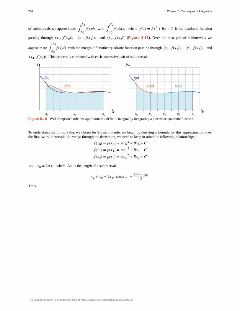
of subintervals we approximate ∫x0
x2f (x)dx with ∫
x0
x2p(x)dx, where p(x) = Ax2 + Bx + C is the quadratic function
passing through (x0, f (x0)), (x1, f (x1)), and (x2, f (x2)) (Figure 5.15). Over the next pair of subintervals we
approximate ∫x2
x4f (x)dx with the integral of another quadratic function passing through (x2, f (x2)), (x3, f (x3)), and
(x4, f (x4)). This process is continued with each successive pair of subintervals.
Figure 5.15 With Simpson’s rule, we approximate a definite integral by integrating a piecewise quadratic function.
To understand the formula that we obtain for Simpson’s rule, we begin by deriving a formula for this approximation overthe first two subintervals. As we go through the derivation, we need to keep in mind the following relationships:
f (x0) = p(x0) = Ax02 + Bx0 + C
f (x1) = p(x1) = Ax12 + Bx1 + C
f (x2) = p(x2) = Ax22 + Bx2 + C
x2 − x0 = 2Δx, where Δx is the length of a subinterval.
x2 + x0 = 2x1, since x1 = (x2 + x0)2 .
Thus,
294 Chapter 5 | Techniques of Integration
This OpenStax book is available for free at https://legacy.cnx.org/content/col31997/1.5
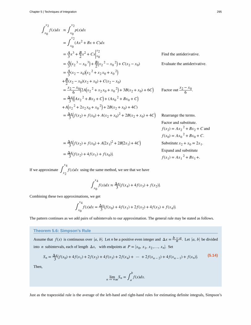
∫x0
x2f (x)dx ≈ ∫
x0
x2p(x)dx
= ∫x0
x2(Ax2 + Bx + C)dx
= A3 x
3 + B2 x
2 + Cx|x2x0
Find the antiderivative.
= A3⎛⎝x2
3 − x03⎞⎠+ B
2⎛⎝x2
2 − x02⎞⎠+ C(x2 − x0) Evaluate the antiderivative.
= A3 (x2 − x0)⎛⎝x2
2 + x2 x0 + x02⎞⎠
+B2 (x2 − x0)(x2 + x0) + C(x2 − x0)
= x2 − x06
⎛⎝2A⎛⎝x2
2 + x2 x0 + x02⎞⎠+ 3B(x2 + x0) + 6C⎞⎠ Factor out x2 − x0
6 .
= Δx3⎛⎝⎛⎝Ax2
2 + Bx2 + C⎞⎠+ (Ax02 + Bx0 + C⎞⎠
+A⎛⎝x22 + 2x2 x0 + x0
2⎞⎠+ 2B(x2 + x0) + 4C)
= Δx3⎛⎝ f (x2) + f (x0) + A(x2 + x0)2 + 2B(x2 + x0) + 4C⎞⎠ Rearrange the terms.
Factor and substitute.f (x2) = Ax2
2 + Bx2 + C and
f (x0) = Ax02 + Bx0 + C.
= Δx3⎛⎝ f (x2) + f (x0) + A⎛⎝2x1
⎞⎠2 + 2B⎛⎝2x1
⎞⎠+ 4C⎞⎠ Substitute x2 + x0 = 2x1.
= Δx3⎛⎝ f (x2) + 4 f (x1) + f (x0)⎞⎠.
Expand and substitute
f (x1) = Ax12 + Bx1 +.
If we approximate ∫x2
x4f (x)dx using the same method, we see that we have
∫x0
x4f (x)dx ≈ Δx
3⎛⎝ f (x4) + 4 f (x3) + f (x2)⎞⎠.
Combining these two approximations, we get
∫x0
x4f (x)dx = Δx
3⎛⎝ f (x0) + 4 f (x1) + 2 f (x2) + 4 f (x3) + f (x4)⎞⎠.
The pattern continues as we add pairs of subintervals to our approximation. The general rule may be stated as follows.
Theorem 5.6: Simpson’s Rule
Assume that f (x) is continuous over ⎡⎣a, b⎤⎦. Let n be a positive even integer and Δx = b − a
n . Let ⎡⎣a, b⎤⎦ be divided
into n subintervals, each of length Δx, with endpoints at P = ⎧⎩⎨x0, x1, x2 ,…, xn
⎫⎭⎬. Set
(5.14)Sn = Δx3⎛⎝ f (x0) + 4 f (x1) + 2 f (x2) + 4 f (x3) + 2 f (x4) + ⋯ + 2 f (xn − 2) + 4 f (xn − 1) + f (xn)⎞⎠.
Then,
limn → +∞
Sn = ∫a
bf (x)dx.
Just as the trapezoidal rule is the average of the left-hand and right-hand rules for estimating definite integrals, Simpson’s
Chapter 5 | Techniques of Integration 295
rule may be obtained from the midpoint and trapezoidal rules by using a weighted average. It can be shown that
S2n = ⎛⎝23⎞⎠Mn + ⎛⎝13
⎞⎠Tn.
It is also possible to put a bound on the error when using Simpson’s rule to approximate a definite integral. The bound inthe error is given by the following rule:
Rule: Error Bound for Simpson’s Rule
Let f (x) be a continuous function over [a, b] having a fourth derivative, f (4)(x), over this interval. If M is the
maximum value of | f (4)(x)| over [a, b], then the upper bound for the error in using Sn to estimate ∫a
bf (x)dx is
given by
(5.15)Error in Sn ≤ M(b − a)5
180n4 .
Example 5.45
Applying Simpson’s Rule 1
Use S2 to approximate ∫0
1x3dx. Estimate a bound for the error in S2.
Solution
Since [0, 1] is divided into two intervals, each subinterval has length Δx = 1 − 02 = 1
2. The endpoints of these
subintervals are⎧⎩⎨0, 1
2, 1⎫⎭⎬. If we set f (x) = x3, then
S4 = 13 · 1
2⎛⎝ f (0) + 4 f ⎛⎝12
⎞⎠+ f (1)⎞⎠ = 1
6⎛⎝0 + 4 · 1
8 + 1⎞⎠ = 14. Since f (4) (x) = 0 and consequently M = 0, we
see that
Error in S2 ≤ 0(1)5
180 ⋅ 24 = 0.
This bound indicates that the value obtained through Simpson’s rule is exact. A quick check will verify that, in
fact, ∫0
1x3dx = 1
4.
Example 5.46
Applying Simpson’s Rule 2
Use S6 to estimate the length of the curve y = 12x
2 over [1, 4].
Solution
296 Chapter 5 | Techniques of Integration
This OpenStax book is available for free at https://legacy.cnx.org/content/col31997/1.5

5.26
The length of y = 12x
2 over [1, 4] is ∫1
41 + x2dx. If we divide [1, 4] into six subintervals, then each
subinterval has length Δx = 4 − 16 = 1
2, and the endpoints of the subintervals are⎧⎩⎨1, 3
2, 2, 52, 3, 7
2, 4⎫⎭⎬.
Setting f (x) = 1 + x2,
S6 = 13 · 1
2⎛⎝ f (1) + 4 f ⎛⎝32
⎞⎠+ 2 f (2) + 4 f ⎛⎝52
⎞⎠+ 2 f (3) + 4 f ⎛⎝72
⎞⎠+ f (4)⎞⎠.
After substituting, we have
S6 = 16(1.4142 + 4 · 1.80278 + 2 · 2.23607 + 4 · 2.69258 + 2 · 3.16228 + 4 · 3.64005 + 4.12311)
≈ 8.14594.
Use S2 to estimate ∫1
21xdx.
Key Concepts• We can use numerical integration to estimate the values of definite integrals when a closed form of the integral is
difficult to find or when an approximate value only of the definite integral is needed.
• The most commonly used techniques for numerical integration are the midpoint rule, trapezoidal rule, andSimpson’s rule.
• The midpoint rule approximates the definite integral using rectangular regions whereas the trapezoidal ruleapproximates the definite integral using trapezoidal approximations.
• Simpson’s rule approximates the definite integral by first approximating the original function using piecewisequadratic functions.
Key Equations• Midpoint rule
Mn = ∑i = 1
nf (mi)Δx
• Trapezoidal rule
Tn = 12Δx⎛⎝ f (x0) + 2 f (x1) + 2 f (x2) + ⋯ + 2 f (xn − 1) + f (xn)⎞⎠
• Simpson’s rule
Sn = Δx3⎛⎝ f (x0) + 4 f (x1) + 2 f (x2) + 4 f (x3) + 2 f (x4) + 4 f (x5) + ⋯ + 2 f (xn − 2) + 4 f (xn − 1) + f (xn)⎞⎠
• Error bound for midpoint rule
Error in Mn ≤ M(b − a)3
24n2
• Error bound for trapezoidal rule
Error in Tn ≤ M(b − a)3
12n2
• Error bound for Simpson’s rule
Error in Sn ≤ M(b − a)5
180n4
Chapter 5 | Techniques of Integration 297
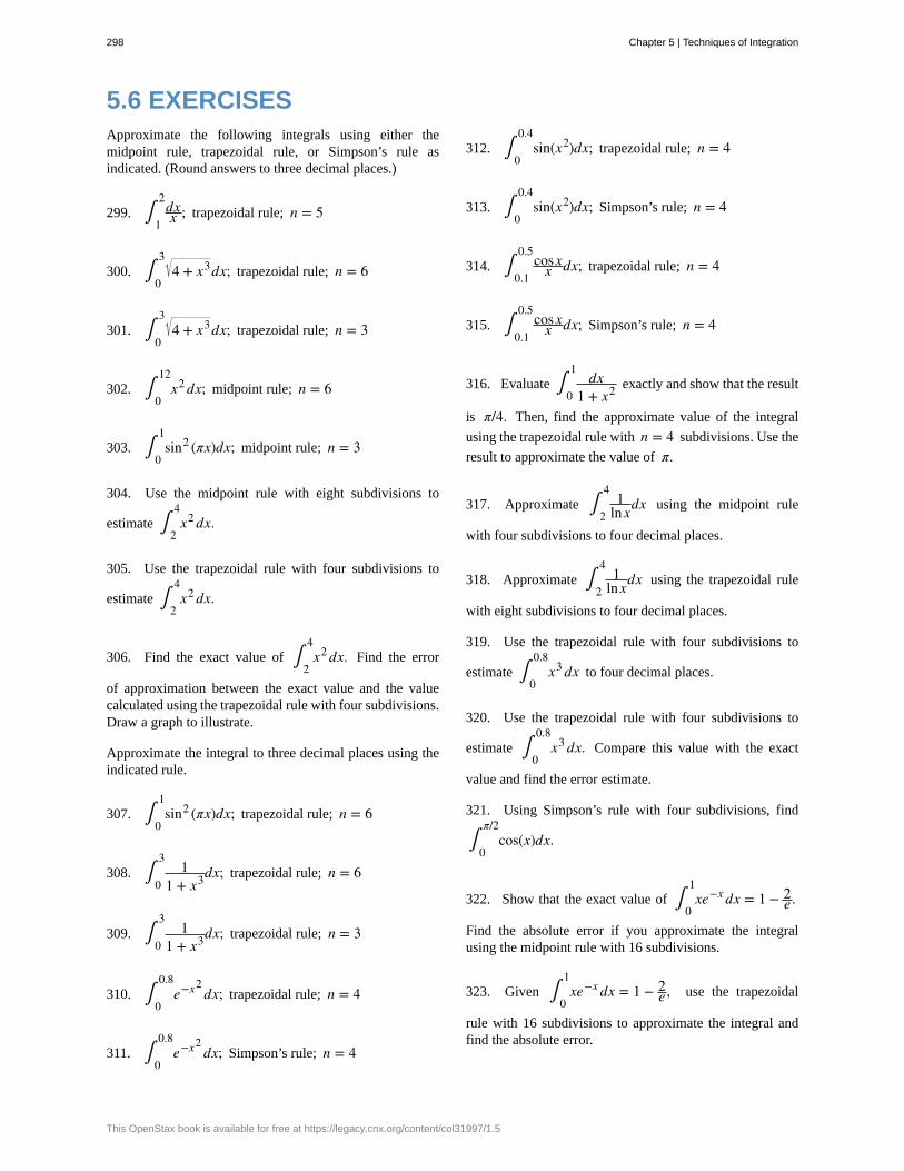
5.6 EXERCISESApproximate the following integrals using either themidpoint rule, trapezoidal rule, or Simpson’s rule asindicated. (Round answers to three decimal places.)
299. ∫1
2dxx ; trapezoidal rule; n = 5
300. ∫0
34 + x3dx; trapezoidal rule; n = 6
301. ∫0
34 + x3dx; trapezoidal rule; n = 3
302. ∫0
12x2dx; midpoint rule; n = 6
303. ∫0
1sin2 (πx)dx; midpoint rule; n = 3
304. Use the midpoint rule with eight subdivisions to
estimate ∫2
4x2dx.
305. Use the trapezoidal rule with four subdivisions to
estimate ∫2
4x2dx.
306. Find the exact value of ∫2
4x2dx. Find the error
of approximation between the exact value and the valuecalculated using the trapezoidal rule with four subdivisions.Draw a graph to illustrate.
Approximate the integral to three decimal places using theindicated rule.
307. ∫0
1sin2 (πx)dx; trapezoidal rule; n = 6
308. ∫0
31
1 + x3dx; trapezoidal rule; n = 6
309. ∫0
31
1 + x3dx; trapezoidal rule; n = 3
310. ∫0
0.8e−x2
dx; trapezoidal rule; n = 4
311. ∫0
0.8e−x2
dx; Simpson’s rule; n = 4
312. ∫0
0.4sin(x2)dx; trapezoidal rule; n = 4
313. ∫0
0.4sin(x2)dx; Simpson’s rule; n = 4
314. ∫0.1
0.5cosxx dx; trapezoidal rule; n = 4
315. ∫0.1
0.5cosxx dx; Simpson’s rule; n = 4
316. Evaluate ∫0
1dx
1 + x2 exactly and show that the result
is π/4. Then, find the approximate value of the integral
using the trapezoidal rule with n = 4 subdivisions. Use the
result to approximate the value of π.
317. Approximate ∫2
41
lnxdx using the midpoint rule
with four subdivisions to four decimal places.
318. Approximate ∫2
41
lnxdx using the trapezoidal rule
with eight subdivisions to four decimal places.
319. Use the trapezoidal rule with four subdivisions to
estimate ∫0
0.8x3dx to four decimal places.
320. Use the trapezoidal rule with four subdivisions to
estimate ∫0
0.8x3dx. Compare this value with the exact
value and find the error estimate.
321. Using Simpson’s rule with four subdivisions, find
∫0
π/2cos(x)dx.
322. Show that the exact value of ∫0
1xe−x dx = 1 − 2
e .
Find the absolute error if you approximate the integralusing the midpoint rule with 16 subdivisions.
323. Given ∫0
1xe−x dx = 1 − 2
e , use the trapezoidal
rule with 16 subdivisions to approximate the integral andfind the absolute error.
298 Chapter 5 | Techniques of Integration
This OpenStax book is available for free at https://legacy.cnx.org/content/col31997/1.5
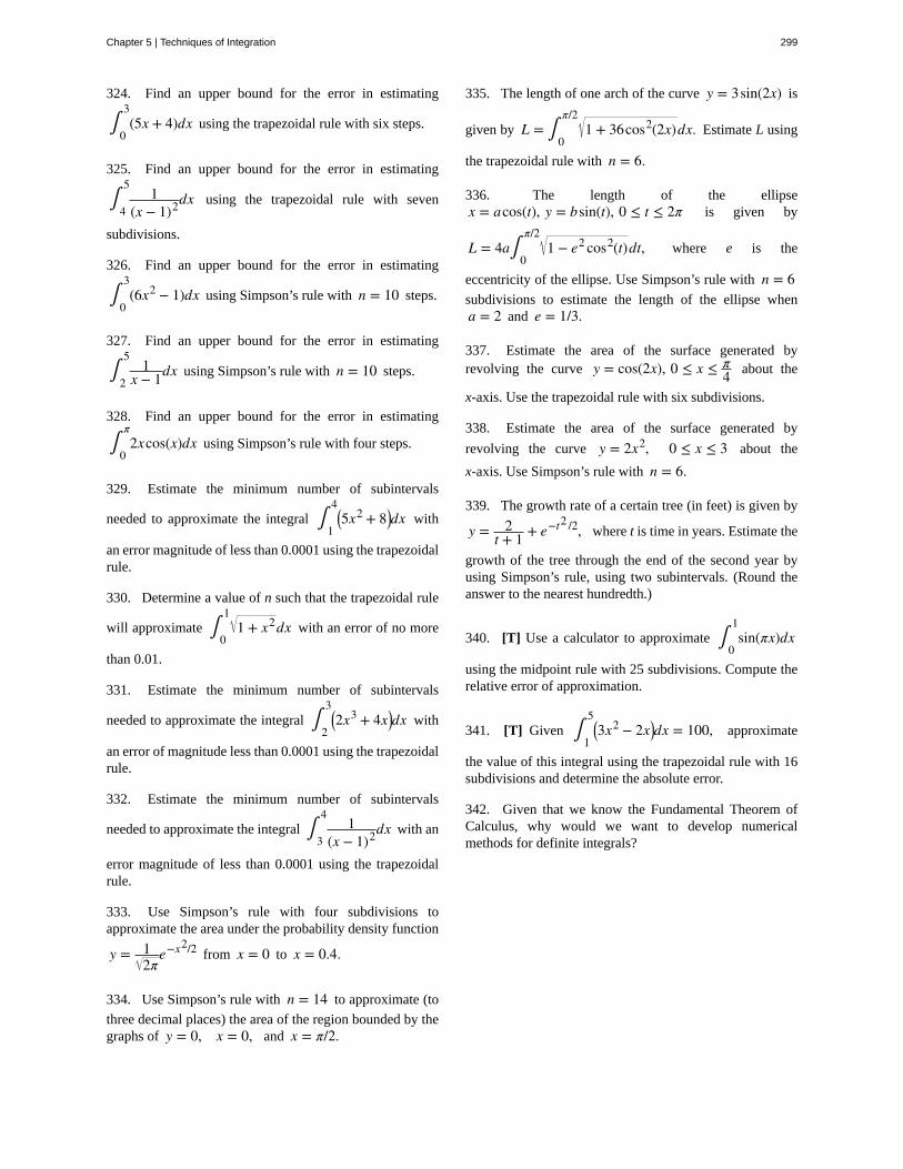
324. Find an upper bound for the error in estimating
∫0
3(5x + 4)dx using the trapezoidal rule with six steps.
325. Find an upper bound for the error in estimating
∫4
51
(x − 1)2dx using the trapezoidal rule with seven
subdivisions.
326. Find an upper bound for the error in estimating
∫0
3(6x2 − 1)dx using Simpson’s rule with n = 10 steps.
327. Find an upper bound for the error in estimating
∫2
51
x − 1dx using Simpson’s rule with n = 10 steps.
328. Find an upper bound for the error in estimating
∫0
π2xcos(x)dx using Simpson’s rule with four steps.
329. Estimate the minimum number of subintervals
needed to approximate the integral ∫1
4⎛⎝5x2 + 8⎞⎠dx with
an error magnitude of less than 0.0001 using the trapezoidalrule.
330. Determine a value of n such that the trapezoidal rule
will approximate ∫0
11 + x2dx with an error of no more
than 0.01.
331. Estimate the minimum number of subintervals
needed to approximate the integral ∫2
3⎛⎝2x3 + 4x⎞⎠dx with
an error of magnitude less than 0.0001 using the trapezoidalrule.
332. Estimate the minimum number of subintervals
needed to approximate the integral ∫3
41
(x − 1)2dx with an
error magnitude of less than 0.0001 using the trapezoidalrule.
333. Use Simpson’s rule with four subdivisions toapproximate the area under the probability density function
y = 12π
e−x2/2 from x = 0 to x = 0.4.
334. Use Simpson’s rule with n = 14 to approximate (to
three decimal places) the area of the region bounded by thegraphs of y = 0, x = 0, and x = π/2.
335. The length of one arch of the curve y = 3sin(2x) is
given by L = ∫0
π/21 + 36cos2(2x)dx. Estimate L using
the trapezoidal rule with n = 6.
336. The length of the ellipsex = acos(t), y = bsin(t), 0 ≤ t ≤ 2π is given by
L = 4a∫0
π/21 − e2 cos2(t)dt, where e is the
eccentricity of the ellipse. Use Simpson’s rule with n = 6subdivisions to estimate the length of the ellipse whena = 2 and e = 1/3.
337. Estimate the area of the surface generated byrevolving the curve y = cos(2x), 0 ≤ x ≤ π
4 about the
x-axis. Use the trapezoidal rule with six subdivisions.
338. Estimate the area of the surface generated by
revolving the curve y = 2x2, 0 ≤ x ≤ 3 about the
x-axis. Use Simpson’s rule with n = 6.
339. The growth rate of a certain tree (in feet) is given by
y = 2t + 1 + e−t2 /2, where t is time in years. Estimate the
growth of the tree through the end of the second year byusing Simpson’s rule, using two subintervals. (Round theanswer to the nearest hundredth.)
340. [T] Use a calculator to approximate ∫0
1sin(πx)dx
using the midpoint rule with 25 subdivisions. Compute therelative error of approximation.
341. [T] Given ∫1
5⎛⎝3x2 − 2x⎞⎠dx = 100, approximate
the value of this integral using the trapezoidal rule with 16subdivisions and determine the absolute error.
342. Given that we know the Fundamental Theorem ofCalculus, why would we want to develop numericalmethods for definite integrals?
Chapter 5 | Techniques of Integration 299
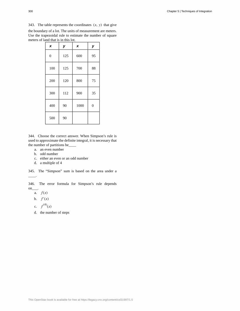
343. The table represents the coordinates (x, y) that give
the boundary of a lot. The units of measurement are meters.Use the trapezoidal rule to estimate the number of squaremeters of land that is in this lot.
x y x y
0 125 600 95
100 125 700 88
200 120 800 75
300 112 900 35
400 90 1000 0
500 90
344. Choose the correct answer. When Simpson’s rule isused to approximate the definite integral, it is necessary thatthe number of partitions be____
a. an even numberb. odd numberc. either an even or an odd numberd. a multiple of 4
345. The “Simpson” sum is based on the area under a____.
346. The error formula for Simpson’s rule dependson___.
a. f (x)b. f ′(x)
c. f (4)(x)d. the number of steps
300 Chapter 5 | Techniques of Integration
This OpenStax book is available for free at https://legacy.cnx.org/content/col31997/1.5

5.7 | Improper Integrals
Learning Objectives5.7.1 Evaluate an integral over an infinite interval.
5.7.2 Evaluate an integral over a closed interval with an infinite discontinuity within the interval.
5.7.3 Use the comparison theorem to determine whether a definite integral is convergent.
Is the area between the graph of f (x) = 1x and the x-axis over the interval [1, +∞) finite or infinite? If this same region
is revolved about the x-axis, is the volume finite or infinite? Surprisingly, the area of the region described is infinite, but thevolume of the solid obtained by revolving this region about the x-axis is finite.
In this section, we define integrals over an infinite interval as well as integrals of functions containing a discontinuity onthe interval. Integrals of these types are called improper integrals. We examine several techniques for evaluating improperintegrals, all of which involve taking limits.
Integrating over an Infinite Interval
How should we go about defining an integral of the type ∫a
+∞f (x)dx? We can integrate ∫
a
tf (x)dx for any value of
t, so it is reasonable to look at the behavior of this integral as we substitute larger values of t. Figure 5.16 shows that
∫a
tf (x)dx may be interpreted as area for various values of t. In other words, we may define an improper integral as a
limit, taken as one of the limits of integration increases or decreases without bound.
Figure 5.16 To integrate a function over an infinite interval, we consider the limit of the integral as the upper limit increaseswithout bound.
Definition
1. Let f (x) be continuous over an interval of the form [a, +∞). Then
(5.16)∫a
+∞f (x)dx = lim
t → +∞∫a
tf (x)dx,
provided this limit exists.
2. Let f (x) be continuous over an interval of the form (−∞, b]. Then
(5.17)∫−∞
bf (x)dx = lim
t → −∞∫t
bf (x)dx,
provided this limit exists.In each case, if the limit exists, then the improper integral is said to converge. If the limit does not exist, thenthe improper integral is said to diverge.
3. Let f (x) be continuous over (−∞, +∞). Then
Chapter 5 | Techniques of Integration 301
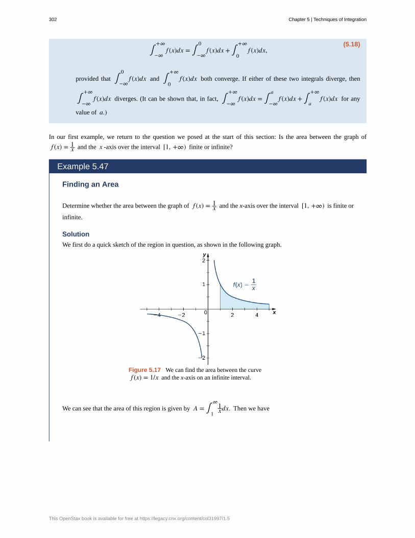
(5.18)∫−∞
+∞f (x)dx = ∫
−∞
0f (x)dx + ∫
0
+∞f (x)dx,
provided that ∫−∞
0f (x)dx and ∫
0
+∞f (x)dx both converge. If either of these two integrals diverge, then
∫−∞
+∞f (x)dx diverges. (It can be shown that, in fact, ∫
−∞
+∞f (x)dx = ∫
−∞
af (x)dx + ∫
a
+∞f (x)dx for any
value of a.)
In our first example, we return to the question we posed at the start of this section: Is the area between the graph of
f (x) = 1x and the x -axis over the interval [1, +∞) finite or infinite?
Example 5.47
Finding an Area
Determine whether the area between the graph of f (x) = 1x and the x-axis over the interval [1, +∞) is finite or
infinite.
Solution
We first do a quick sketch of the region in question, as shown in the following graph.
Figure 5.17 We can find the area between the curvef (x) = 1/x and the x-axis on an infinite interval.
We can see that the area of this region is given by A = ∫1
∞1xdx. Then we have
302 Chapter 5 | Techniques of Integration
This OpenStax book is available for free at https://legacy.cnx.org/content/col31997/1.5

A = ∫1
∞1xdx
= limt → +∞
∫1
t1xdx Rewrite the improper integral as a limit.
= limt → +∞
ln|x||1t Find the antiderivative.
= limt → +∞
(ln|t| − ln1) Evaluate the antiderivative.
= +∞. Evaluate the limit.
Since the improper integral diverges to +∞, the area of the region is infinite.
Example 5.48
Finding a Volume
Find the volume of the solid obtained by revolving the region bounded by the graph of f (x) = 1x and the x-axis
over the interval [1, +∞) about the x -axis.
Solution
The solid is shown in Figure 5.18. Using the disk method, we see that the volume V is
V = π∫1
+∞1x2dx.
Figure 5.18 The solid of revolution can be generated by rotating an infinite area about thex-axis.
Then we have
Chapter 5 | Techniques of Integration 303

V = π∫1
+∞1x2dx
= π limt → +∞
∫1
t1x2dx Rewrite as a limit.
= π limt → +∞
− 1x |1t Find the antiderivative.
= π limt → +∞
⎛⎝− 1
t + 1⎞⎠ Evaluate the antiderivative.= π.
The improper integral converges to π. Therefore, the volume of the solid of revolution is π.
In conclusion, although the area of the region between the x-axis and the graph of f (x) = 1/x over the interval [1, +∞)is infinite, the volume of the solid generated by revolving this region about the x-axis is finite. The solid generated is knownas Gabriel’s Horn.
Visit this website (http://www.openstax.org/l/20_GabrielsHorn) to read more about Gabriel’s Horn.
Example 5.49
Chapter Opener: Traffic Accidents in a City
Figure 5.19 (credit: modification of work by DavidMcKelvey, Flickr)
In the chapter opener, we stated the following problem: Suppose that at a busy intersection, traffic accidents occurat an average rate of one every three months. After residents complained, changes were made to the traffic lightsat the intersection. It has now been eight months since the changes were made and there have been no accidents.Were the changes effective or is the 8-month interval without an accident a result of chance?
Probability theory tells us that if the average time between events is k, the probability that X, the time between
events, is between a and b is given by
P(a ≤ x ≤ b) = ∫a
bf (x)dx where f (x) =
⎧⎩⎨ 0 if x < 0ke−kx if x ≥ 0
.
Thus, if accidents are occurring at a rate of one every 3 months, then the probability that X, the time between
accidents, is between a and b is given by
304 Chapter 5 | Techniques of Integration
This OpenStax book is available for free at https://legacy.cnx.org/content/col31997/1.5
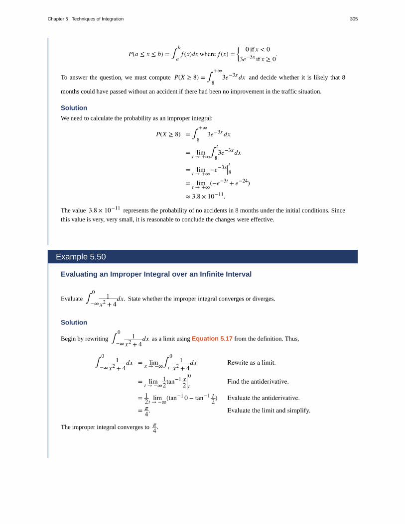
P(a ≤ x ≤ b) = ∫a
bf (x)dx where f (x) =
⎧⎩⎨ 0 if x < 03e−3x if x ≥ 0
.
To answer the question, we must compute P(X ≥ 8) = ∫8
+∞3e−3x dx and decide whether it is likely that 8
months could have passed without an accident if there had been no improvement in the traffic situation.
Solution
We need to calculate the probability as an improper integral:
P(X ≥ 8) = ∫8
+∞3e−3x dx
= limt → +∞
∫8
t3e−3x dx
= limt → +∞
−e−3x|8t= lim
t → +∞(−e−3t + e−24)
≈ 3.8 × 10⁻¹¹.
The value 3.8 × 10⁻¹¹ represents the probability of no accidents in 8 months under the initial conditions. Since
this value is very, very small, it is reasonable to conclude the changes were effective.
Example 5.50
Evaluating an Improper Integral over an Infinite Interval
Evaluate ∫−∞
01
x2 + 4dx. State whether the improper integral converges or diverges.
Solution
Begin by rewriting ∫−∞
01
x2 + 4dx as a limit using Equation 5.17 from the definition. Thus,
∫−∞
01
x2 + 4dx = limx → −∞∫
t
01
x2 + 4dx Rewrite as a limit.
= limt → −∞
12tan−1 x
2|t0 Find the antiderivative.
= 12 limt → −∞
(tan−1 0 − tan−1 t2) Evaluate the antiderivative.
= π4. Evaluate the limit and simplify.
The improper integral converges to π4.
Chapter 5 | Techniques of Integration 305
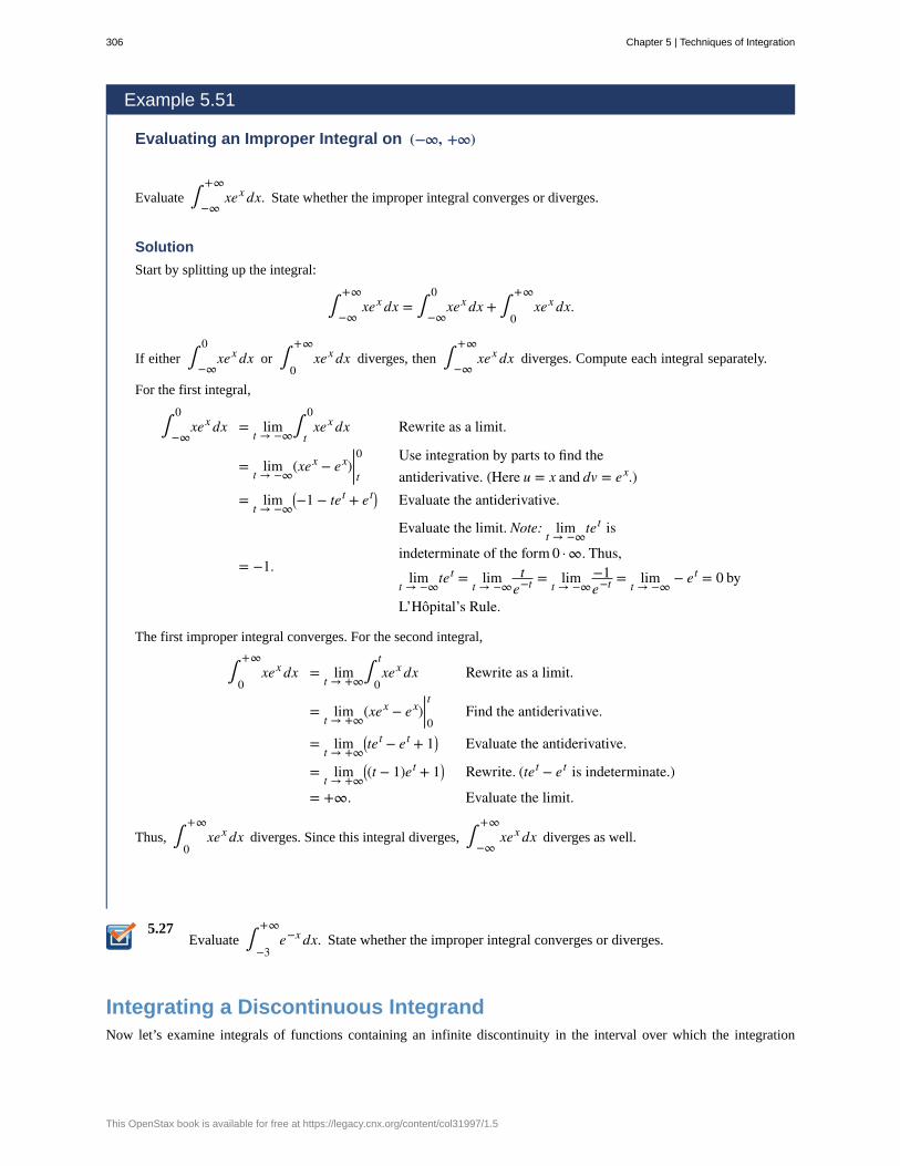
5.27
Example 5.51
Evaluating an Improper Integral on (−∞, +∞)
Evaluate ∫−∞
+∞xex dx. State whether the improper integral converges or diverges.
Solution
Start by splitting up the integral:
∫−∞
+∞xex dx = ∫
−∞
0xex dx + ∫
0
+∞xex dx.
If either ∫−∞
0xex dx or ∫
0
+∞xex dx diverges, then ∫
−∞
+∞xex dx diverges. Compute each integral separately.
For the first integral,
∫−∞
0xex dx = lim
t → −∞∫t
0xex dx Rewrite as a limit.
= limt → −∞
(xex − ex)|t0 Use integration by parts to find theantiderivative. (Here u = x and dv = ex.)
= limt → −∞
⎛⎝−1 − tet + et⎞⎠ Evaluate the antiderivative.
= −1.
Evaluate the limit. Note: limt → −∞
tet is
indeterminate of the form 0 · ∞. Thus,
limt → −∞
tet = limt → −∞
te−t = lim
t → −∞−1e−t = lim
t → −∞− et = 0 by
L’Hôpital’s Rule.
The first improper integral converges. For the second integral,
∫0
+∞xex dx = lim
t → +∞∫
0
txex dx Rewrite as a limit.
= limt → +∞
(xex − ex)|0t Find the antiderivative.
= limt → +∞
⎛⎝tet − et + 1⎞⎠ Evaluate the antiderivative.
= limt → +∞
⎛⎝(t − 1)et + 1⎞⎠ Rewrite. (tet − et is indeterminate.)
= +∞. Evaluate the limit.
Thus, ∫0
+∞xex dx diverges. Since this integral diverges, ∫
−∞
+∞xex dx diverges as well.
Evaluate ∫−3
+∞e−x dx. State whether the improper integral converges or diverges.
Integrating a Discontinuous IntegrandNow let’s examine integrals of functions containing an infinite discontinuity in the interval over which the integration
306 Chapter 5 | Techniques of Integration
This OpenStax book is available for free at https://legacy.cnx.org/content/col31997/1.5
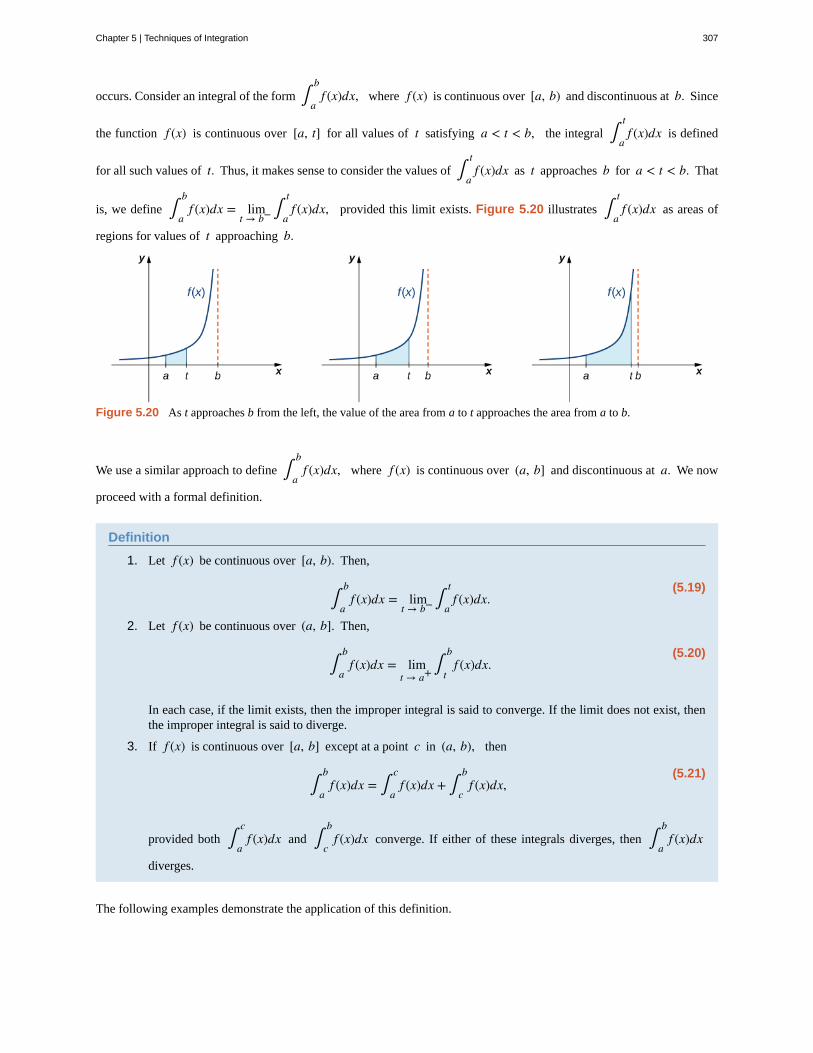
occurs. Consider an integral of the form ∫a
bf (x)dx, where f (x) is continuous over [a, b) and discontinuous at b. Since
the function f (x) is continuous over [a, t] for all values of t satisfying a < t < b, the integral ∫a
tf (x)dx is defined
for all such values of t. Thus, it makes sense to consider the values of ∫a
tf (x)dx as t approaches b for a < t < b. That
is, we define ∫a
bf (x)dx = lim
t → b− ∫a
tf (x)dx, provided this limit exists. Figure 5.20 illustrates ∫
a
tf (x)dx as areas of
regions for values of t approaching b.
Figure 5.20 As t approaches b from the left, the value of the area from a to t approaches the area from a to b.
We use a similar approach to define ∫a
bf (x)dx, where f (x) is continuous over (a, b] and discontinuous at a. We now
proceed with a formal definition.
Definition
1. Let f (x) be continuous over [a, b). Then,
(5.19)∫a
bf (x)dx = lim
t → b− ∫a
tf (x)dx.
2. Let f (x) be continuous over (a, b]. Then,
(5.20)∫a
bf (x)dx = lim
t → a+∫t
bf (x)dx.
In each case, if the limit exists, then the improper integral is said to converge. If the limit does not exist, thenthe improper integral is said to diverge.
3. If f (x) is continuous over [a, b] except at a point c in (a, b), then
(5.21)∫a
bf (x)dx = ∫
a
cf (x)dx + ∫
c
bf (x)dx,
provided both ∫a
cf (x)dx and ∫
c
bf (x)dx converge. If either of these integrals diverges, then ∫
a
bf (x)dx
diverges.
The following examples demonstrate the application of this definition.
Chapter 5 | Techniques of Integration 307
Example 5.52
Integrating a Discontinuous Integrand
Evaluate ∫0
41
4 − xdx, if possible. State whether the integral converges or diverges.
Solution
The function f (x) = 14 − x
is continuous over [0, 4) and discontinuous at 4. Using Equation 5.19 from the
definition, rewrite ∫0
41
4 − xdx as a limit:
∫0
41
4 − xdx = lim
t → 4− ∫0
t1
4 − xdx Rewrite as a limit.
= limt → 4−
⎛⎝−2 4 − x⎞⎠|0t Find the antiderivative.
= limt → 4−
⎛⎝−2 4 − t + 4⎞⎠ Evaluate the antiderivative.
= 4. Evaluate the limit.
The improper integral converges.
Example 5.53
Integrating a Discontinuous Integrand
Evaluate ∫0
2x lnxdx. State whether the integral converges or diverges.
Solution
Since f (x) = x lnx is continuous over (0, 2] and is discontinuous at zero, we can rewrite the integral in limit
form using Equation 5.20:
∫0
2x lnxdx = lim
t → 0+∫t
2x lnxdx Rewrite as a limit.
= limt → 0+
⎛⎝12x
2 lnx − 14x
2⎞⎠|t2 Evaluate ∫ x lnxdx using integration by partswith u = lnx and dv = xdx.
= limt → 0+
⎛⎝2ln2 − 1 − 1
2t2 ln t + 1
4t2⎞⎠. Evaluate the antiderivative.
= 2ln2 − 1.Evaluate the limit. lim
t → 0+t2 ln t is indeterminate.
To evaluate it, rewrite as a quotient and applyL’Hôpital’s rule.
The improper integral converges.
308 Chapter 5 | Techniques of Integration
This OpenStax book is available for free at https://legacy.cnx.org/content/col31997/1.5

5.28
Example 5.54
Integrating a Discontinuous Integrand
Evaluate ∫−1
11x3dx. State whether the improper integral converges or diverges.
Solution
Since f (x) = 1/x3 is discontinuous at zero, using Equation 5.21, we can write
∫−1
11x3dx = ∫
−1
01x3dx + ∫
0
11x3dx.
If either of the two integrals diverges, then the original integral diverges. Begin with ∫−1
01x3dx :
∫−1
01x3dx = lim
t → 0− ∫−1
t1x3dx Rewrite as a limit.
= limt → 0−⎛⎝− 1
2x2⎞⎠|−1
tFind the antiderivative.
= limt → 0−⎛⎝− 1
2t2+ 1
2⎞⎠ Evaluate the antiderivative.
= +–∞. Evaluate the limit.
Therefore, ∫−1
01x3dx diverges. Since ∫
−1
01x3dx diverges, ∫
−1
11x3dx diverges.
Evaluate ∫0
21xdx. State whether the integral converges or diverges.
A Comparison TheoremIt is not always easy or even possible to evaluate an improper integral directly; however, by comparing it with anothercarefully chosen integral, it may be possible to determine its convergence or divergence. To see this, consider twocontinuous functions f (x) and g(x) satisfying 0 ≤ f (x) ≤ g(x) for x ≥ a (Figure 5.21). In this case, we may view
integrals of these functions over intervals of the form [a, t] as areas, so we have the relationship
0 ≤ ∫a
tf (x)dx ≤ ∫
a
tg(x)dx for t ≥ a.
Chapter 5 | Techniques of Integration 309
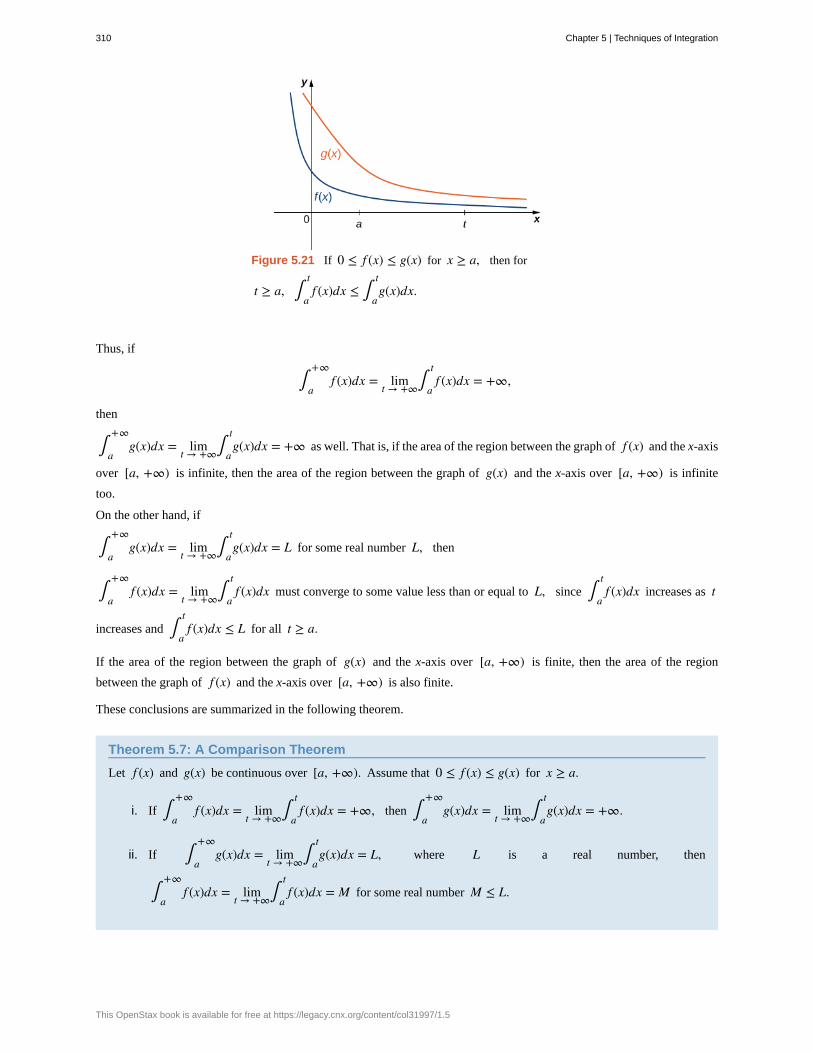
Figure 5.21 If 0 ≤ f (x) ≤ g(x) for x ≥ a, then for
t ≥ a, ∫a
tf (x)dx ≤ ∫
a
tg(x)dx.
Thus, if
∫a
+∞f (x)dx = lim
t → +∞∫a
tf (x)dx = +∞,
then
∫a
+∞g(x)dx = lim
t → +∞∫a
tg(x)dx = +∞ as well. That is, if the area of the region between the graph of f (x) and the x-axis
over [a, +∞) is infinite, then the area of the region between the graph of g(x) and the x-axis over [a, +∞) is infinite
too.
On the other hand, if
∫a
+∞g(x)dx = lim
t → +∞∫a
tg(x)dx = L for some real number L, then
∫a
+∞f (x)dx = lim
t → +∞∫a
tf (x)dx must converge to some value less than or equal to L, since ∫
a
tf (x)dx increases as t
increases and ∫a
tf (x)dx ≤ L for all t ≥ a.
If the area of the region between the graph of g(x) and the x-axis over [a, +∞) is finite, then the area of the region
between the graph of f (x) and the x-axis over [a, +∞) is also finite.
These conclusions are summarized in the following theorem.
Theorem 5.7: A Comparison Theorem
Let f (x) and g(x) be continuous over [a, +∞). Assume that 0 ≤ f (x) ≤ g(x) for x ≥ a.
i. If ∫a
+∞f (x)dx = lim
t → +∞∫a
tf (x)dx = +∞, then ∫
a
+∞g(x)dx = lim
t → +∞∫a
tg(x)dx = +∞.
ii. If ∫a
+∞g(x)dx = lim
t → +∞∫a
tg(x)dx = L, where L is a real number, then
∫a
+∞f (x)dx = lim
t → +∞∫a
tf (x)dx = M for some real number M ≤ L.
310 Chapter 5 | Techniques of Integration
This OpenStax book is available for free at https://legacy.cnx.org/content/col31997/1.5
5.29
Example 5.55
Applying the Comparison Theorem
Use a comparison to show that ∫1
+∞1xex
dx converges.
Solution
We can see that
0 ≤ 1xex
≤ 1ex
= e−x,
so if ∫1
+∞e−x dx converges, then so does ∫
1
+∞1xex
dx. To evaluate ∫1
+∞e−x dx, first rewrite it as a limit:
∫1
+∞e−xdx = lim
t → +∞∫
1
te−x dx
= limt → +∞
(−e−x)| t1= lim
t → +∞⎛⎝−e−t + e–1⎞⎠
= e–1.
Since ∫1
+∞e−x dx converges, so does ∫
1
+∞1xex
dx.
Example 5.56
Applying the Comparison Theorem
Use the comparison theorem to show that ∫1
+∞1x p
dx diverges for all p < 1.
Solution
For p < 1, 1/x ≤ 1/(x p) over [1, +∞). In Example 5.47, we showed that ∫1
+∞1xdx = +∞. Therefore,
∫1
+∞1x p
dx diverges for all p < 1.
Use a comparison to show that ∫e
+∞lnxx dx diverges.
Chapter 5 | Techniques of Integration 311

Laplace Transforms
In the last few chapters, we have looked at several ways to use integration for solving real-world problems. For thisnext project, we are going to explore a more advanced application of integration: integral transforms. Specifically, wedescribe the Laplace transform and some of its properties. The Laplace transform is used in engineering and physics tosimplify the computations needed to solve some problems. It takes functions expressed in terms of time and transformsthem to functions expressed in terms of frequency. It turns out that, in many cases, the computations needed to solveproblems in the frequency domain are much simpler than those required in the time domain.
The Laplace transform is defined in terms of an integral as
L⎧⎩⎨ f (t)⎫⎭⎬ = F(s) = ∫0
∞e−st f (t)dt.
Note that the input to a Laplace transform is a function of time, f (t), and the output is a function of frequency, F(s).
Although many real-world examples require the use of complex numbers (involving the imaginary number i = −1),in this project we limit ourselves to functions of real numbers.
Let’s start with a simple example. Here we calculate the Laplace transform of f (t) = t . We have
L{t} = ∫0
∞te−st dt.
This is an improper integral, so we express it in terms of a limit, which gives
L{t} = ∫0
∞te−st dt = limz → ∞∫
0
zte−st dt.
Now we use integration by parts to evaluate the integral. Note that we are integrating with respect to t, so we treat thevariable s as a constant. We have
u = t dv = e−st dtdu = dt v = −1
se−st.
Then we obtain
limz → ∞∫0
zte−st dt = limz → ∞
⎡⎣⎡⎣− t
se−st⎤⎦|0z + 1
s∫0
ze−st dt⎤⎦
= limz → ∞⎡⎣⎡⎣− z
se−sz + 0
se−0s⎤⎦+ 1
s∫0
ze−st dt⎤⎦
= limz → ∞⎡⎣⎡⎣− z
se−sz + 0⎤⎦− 1
s⎡⎣e
−sts⎤⎦|0z⎤⎦
= limz → ∞⎡⎣⎡⎣− z
se−sz⎤⎦− 1
s2⎡⎣e−sz − 1⎤⎦
⎤⎦
= limz → ∞⎡⎣− z
sesz⎤⎦− limz → ∞
⎡⎣ 1s2 esz⎤⎦+ limz → ∞
1s2
= 0 − 0 + 1s2
= 1s2.
1. Calculate the Laplace transform of f (t) = 1.
312 Chapter 5 | Techniques of Integration
This OpenStax book is available for free at https://legacy.cnx.org/content/col31997/1.5
2. Calculate the Laplace transform of f (t) = e−3t.
3. Calculate the Laplace transform of f (t) = t2. (Note, you will have to integrate by parts twice.)
Laplace transforms are often used to solve differential equations. Differential equations are not covered indetail until later in this book; but, for now, let’s look at the relationship between the Laplace transform of afunction and the Laplace transform of its derivative.Let’s start with the definition of the Laplace transform. We have
L⎧⎩⎨ f (t)⎫⎭⎬ = ∫0
∞e−st f (t)dt = limz → ∞∫
0
ze−st f (t)dt.
4. Use integration by parts to evaluate limz → ∞∫0
ze−st f (t)dt. (Let u = f (t) and dv = e−st dt.)
After integrating by parts and evaluating the limit, you should see that
L⎧⎩⎨ f (t)⎫⎭⎬ = f (0)s + 1
s⎡⎣L⎧⎩⎨ f ′(t)⎫⎭⎬⎤⎦.
Then,
L⎧⎩⎨ f ′(t)⎫⎭⎬ = sL⎧⎩⎨ f (t)⎫⎭⎬ − f (0).
Thus, differentiation in the time domain simplifies to multiplication by s in the frequency domain.The final thing we look at in this project is how the Laplace transforms of f (t) and its antiderivative are
related. Let g(t) = ∫0
tf (u)du. Then,
L⎧⎩⎨g(t)⎫⎭⎬ = ∫0
∞e−st g(t)dt = limz → ∞∫
0
ze−st g(t)dt.
5. Use integration by parts to evaluate limz → ∞∫0
ze−st g(t)dt. (Let u = g(t) and dv = e−st dt. Note, by the way,
that we have defined g(t), du = f (t)dt.)As you might expect, you should see that
L⎧⎩⎨g(t)⎫⎭⎬ = 1s · L⎧⎩⎨ f (t)⎫⎭⎬.
Integration in the time domain simplifies to division by s in the frequency domain.
Key Concepts• Integrals of functions over infinite intervals are defined in terms of limits.
• Integrals of functions over an interval for which the function has a discontinuity at an endpoint may be defined interms of limits.
• The convergence or divergence of an improper integral may be determined by comparing it with the value of animproper integral for which the convergence or divergence is known.
Key Equations• Improper integrals
∫a
+∞f (x)dx = lim
t → +∞∫a
tf (x)dx
∫−∞
bf (x)dx = lim
t → −∞∫t
bf (x)dx
∫−∞
+∞f (x)dx = ∫
−∞
0f (x)dx + ∫
0
+∞f (x)dx
Chapter 5 | Techniques of Integration 313

5.7 EXERCISESEvaluate the following integrals. If the integral is notconvergent, answer “divergent.”
347. ∫2
4dx
(x − 3)2
348. ∫0
∞1
4 + x2dx
349. ∫0
21
4 − x2dx
350. ∫1
∞1
x lnxdx
351. ∫1
∞xe−x dx
352. ∫−∞
∞x
x2 + 1dx
353. Without integrating, determine whether the integral
∫1
∞1
x3 + 1dx converges or diverges by comparing the
function f (x) = 1x3 + 1
with g(x) = 1x3
.
354. Without integrating, determine whether the integral
∫1
∞1
x + 1dx converges or diverges.
Determine whether the improper integrals converge ordiverge. If possible, determine the value of the integrals thatconverge.
355. ∫0
∞e−x cosxdx
356. ∫1
∞lnxx dx
357. ∫0
1lnxx dx
358. ∫0
1lnxdx
359. ∫−∞
∞1
x2 + 1dx
360. ∫1
5dxx − 1
361. ∫−2
2dx
(1 + x)2
362. ∫0
∞e−x dx
363. ∫0
∞sinxdx
364. ∫−∞
∞ex
1 + e2xdx
365. ∫0
1dxx3
366. ∫0
2dxx3
367. ∫−1
2dxx3
368. ∫0
1dx
1 − x2
369. ∫0
31
x − 1dx
370. ∫1
∞5x3dx
371. ∫3
55
(x − 4)2dx
Determine the convergence of each of the followingintegrals by comparison with the given integral. If theintegral converges, find the number to which it converges.
372. ∫1
∞dx
x2 + 4x; compare with ∫
1
∞dxx2 .
373. ∫1
∞dxx + 1; compare with ∫
1
∞dx2 x.
Evaluate the integrals. If the integral diverges, answer“diverges.”
314 Chapter 5 | Techniques of Integration
This OpenStax book is available for free at https://legacy.cnx.org/content/col31997/1.5
374. ∫1
∞dxxe
375. ∫0
1dxxπ
376. ∫0
1dx
1 − x
377. ∫0
1dx
1 − x
378. ∫−∞
0dx
x2 + 1
379. ∫−1
1dx
1 − x2
380. ∫0
1lnxx dx
381. ∫0
eln(x)dx
382. ∫0
∞xe−x dx
383. ∫−∞
∞x
⎛⎝x2 + 1⎞⎠
2dx
384. ∫0
∞e−x dx
Evaluate the improper integrals. Each of these integralshas an infinite discontinuity either at an endpoint or at aninterior point of the interval.
385. ∫0
9dx
9 − x
386. ∫−27
1dxx2/3
387. ∫0
3dx
9 − x2
388. ∫6
24dt
t t2 − 36
389. ∫0
4x ln(4x)dx
390. ∫0
3x
9 − x2dx
391. Evaluate ∫.5
1dx
1 − x2. (Be careful!) (Express your
answer using three decimal places.)
392. Evaluate ∫1
4dx
x2 − 1. (Express the answer in exact
form.)
393. Evaluate ∫2
∞dx
(x2 − 1)3/2.
394. Find the area of the region in the first quadrant
between the curve y = e−6x and the x-axis.
395. Find the area of the region bounded by the curve
y = 7x2, the x-axis, and on the left by x = 1.
396. Find the area under the curve y = 1(x + 1)3/2,
bounded on the left by x = 3.
397. Find the area under y = 51 + x2 in the first
quadrant.
398. Find the volume of the solid generated by revolving
about the x-axis the region under the curve y = 3x from
x = 1 to x = ∞.
399. Find the volume of the solid generated by revolving
about the y-axis the region under the curve y = 6e−2x in
the first quadrant.
400. Find the volume of the solid generated by revolvingabout the x-axis the area under the curve y = 3e−x in the
first quadrant.
The Laplace transform of a continuous function over the
interval [0, ∞) is defined by F(s) = ∫0
∞e−sx f (x)dx
(see the Student Project). This definition is used to solvesome important initial-value problems in differentialequations, as discussed later. The domain of F is the setof all real numbers s such that the improper integralconverges. Find the Laplace transform F of each of thefollowing functions and give the domain of F.
Chapter 5 | Techniques of Integration 315

401. f (x) = 1
402. f (x) = x
403. f (x) = cos(2x)
404. f (x) = eax
405. Use the formula for arc length to show that the
circumference of the circle x2 + y2 = 1 is 2π.
A non-negative function is a probability density function if
it satisfies the following definition: ∫−∞
∞f (t)dt = 1. The
probability that a random variable x lies between a and b is
given by P(a ≤ x ≤ b) = ∫a
bf (t)dt.
406. Show that f (x) =⎧⎩⎨ 0if x < 07e−7x if x ≥ 0
is a probability
density function.
407. Find the probability that x is between 0 and 0.3. (Usethe function defined in the preceding problem.) Use four-place decimal accuracy.
316 Chapter 5 | Techniques of Integration
This OpenStax book is available for free at https://legacy.cnx.org/content/col31997/1.5

Chapter Review ExercisesFor the following exercises, determine whether the statement is true or false. Justify your answer with a proof or acounterexample.
Exercise 5.408
∫ ex sin(x)dx cannot be integrated by parts.
Exercise 5.409
∫ 1x4 + 1
dx cannot be integrated using partial fractions.
SolutionFalse
Exercise 5.410
In numerical integration, increasing the number of points decreases the error.
Exercise 5.411
Integration by parts can always yield the integral.
SolutionFalse
For the following exercises, evaluate the integral using the specified method.
Exercise 5.412
∫ x2 sin(4x)dx using integration by parts
Exercise 5.413
∫ 1x2 x2 + 16
dx using trigonometric substitution
Solution
− x2 + 1616x + C
Exercise 5.414
∫ x ln(x)dx using integration by parts
Exercise 5.415
∫ 3xx3 + 2x2 − 5x − 6
dx using partial fractions
Solution110⎛⎝4ln(2 − x) + 5ln(x + 1) − 9ln(x + 3)⎞⎠+ C
Exercise 5.416
∫ x5
⎛⎝4x2 + 4⎞⎠
5/2dx using trigonometric substitution
Chapter 5 | Techniques of Integration 317

Exercise 5.417
∫ 4 − sin2(x)sin2(x)
cos(x)dx using a table of integrals or a CAS
Solution
− 4 − sin2(x)sin(x) − x
2 + C
For the following exercises, integrate using whatever method you choose.
Exercise 5.418
∫ sin2(x)cos2(x)dx
Exercise 5.419
∫ x3 x2 + 2dx
Solution
115⎛⎝x2 + 2⎞⎠
3/2 ⎛⎝3x2 − 4⎞⎠+ C
Exercise 5.420
∫ 3x2 + 1x4 − 2x3 − x2 + 2x
dx
Exercise 5.421
∫ 1x4 + 4
dx
Solution
116ln⎛⎝x
2 + 2x + 2x2 − 2x + 2
⎞⎠− 1
8tan−1 (1 − x) + 18tan−1 (x + 1) + C
Exercise 5.422
∫ 3 + 16x4
x4 dx
For the following exercises, approximate the integrals using the midpoint rule, trapezoidal rule, and Simpson’s rule usingfour subintervals, rounding to three decimals.
Exercise 5.423
[T] ∫1
2x5 + 2dx
SolutionM4 = 3.312, T4 = 3.354, S4 = 3.326
Exercise 5.424
[T] ∫0
πe−sin(x2)dx
318 Chapter 5 | Techniques of Integration
This OpenStax book is available for free at https://legacy.cnx.org/content/col31997/1.5
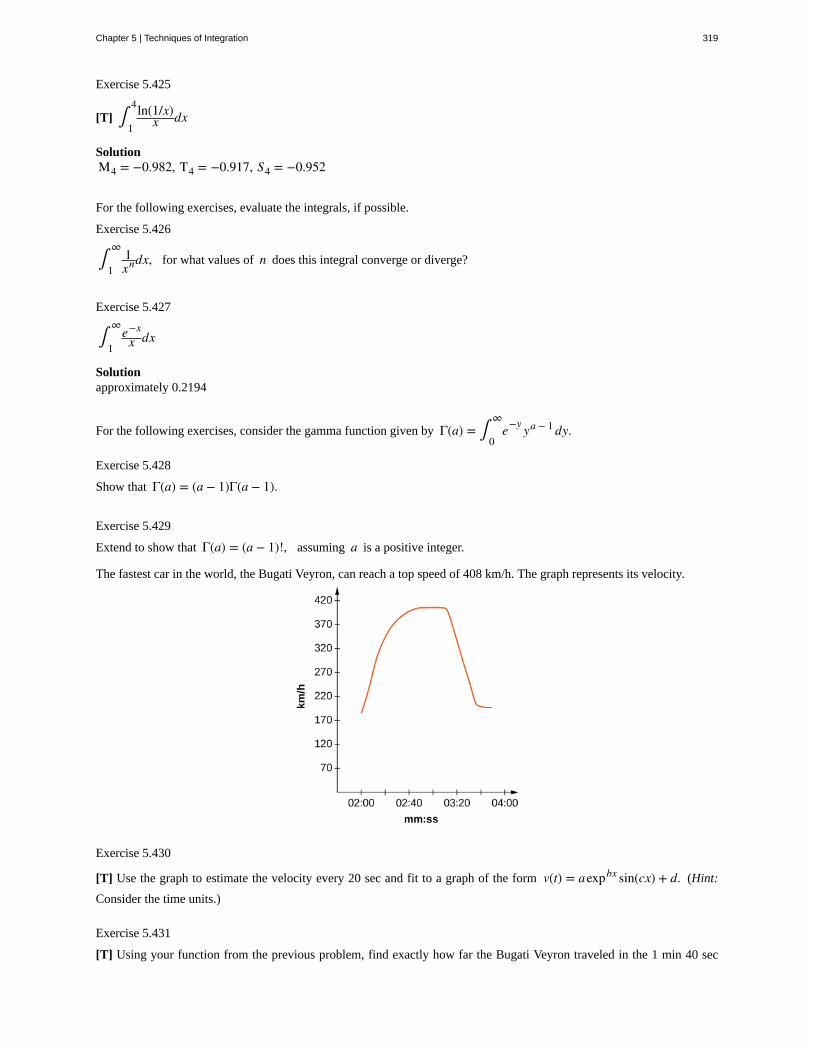
Exercise 5.425
[T] ∫1
4ln(1/x)x dx
SolutionM4 = −0.982, T4 = −0.917, S4 = −0.952
For the following exercises, evaluate the integrals, if possible.
Exercise 5.426
∫1
∞1xndx, for what values of n does this integral converge or diverge?
Exercise 5.427
∫1
∞e−xx dx
Solutionapproximately 0.2194
For the following exercises, consider the gamma function given by Γ(a) = ∫0
∞e−y ya − 1dy.
Exercise 5.428
Show that Γ(a) = (a − 1)Γ(a − 1).
Exercise 5.429
Extend to show that Γ(a) = (a − 1)!, assuming a is a positive integer.
The fastest car in the world, the Bugati Veyron, can reach a top speed of 408 km/h. The graph represents its velocity.
Exercise 5.430
[T] Use the graph to estimate the velocity every 20 sec and fit to a graph of the form v(t) = aexpbx sin(cx) + d. (Hint:
Consider the time units.)
Exercise 5.431
[T] Using your function from the previous problem, find exactly how far the Bugati Veyron traveled in the 1 min 40 sec
Chapter 5 | Techniques of Integration 319

included in the graph.
SolutionAnswers may vary. Ex: 9.405 km
320 Chapter 5 | Techniques of Integration
This OpenStax book is available for free at https://legacy.cnx.org/content/col31997/1.5
absolute error
computer algebra system (CAS)
improper integral
integration by parts
integration table
midpoint rule
numerical integration
partial fraction decomposition
power reduction formula
relative error
Simpson’s rule
trigonometric integral
trigonometric substitution
CHAPTER 5 REVIEW
KEY TERMSif B is an estimate of some quantity having an actual value of A, then the absolute error is given by
|A − B|
technology used to perform many mathematical tasks, including integration
an integral over an infinite interval or an integral of a function containing an infinite discontinuity onthe interval; an improper integral is defined in terms of a limit. The improper integral converges if this limit is a finitereal number; otherwise, the improper integral diverges
a technique of integration that allows the exchange of one integral for another using the formula
∫ u dv = uv − ∫ v du
a table that lists integration formulas
a rule that uses a Riemann sum of the form Mn = ∑i = 1
nf (mi)Δx, where mi is the midpoint of the ith
subinterval to approximate ∫a
bf (x)dx
the variety of numerical methods used to estimate the value of a definite integral, including themidpoint rule, trapezoidal rule, and Simpson’s rule
a technique used to break down a rational function into the sum of simple rationalfunctions
a rule that allows an integral of a power of a trigonometric function to be exchanged for anintegral involving a lower power
error as a percentage of the absolute value, given by |A − BA | = |A − B
A | · 100%
a rule that approximates ∫a
bf (x)dx using the integrals of a piecewise quadratic function. The
approximation Sn to ∫a
bf (x)dx is given by Sn = Δx
3⎛⎝f (x0) + 4 f (x1) + 2 f (x2) + 4 f (x3) + 2 f (x4) + 4 f (x5)
+ ⋯ + 2 f (xn − 2) + 4 f (xn − 1) + f (xn)⎞⎠
trapezoidal rule a rule that approximates ∫a
bf (x)dx using trapezoids
an integral involving powers and products of trigonometric functions
an integration technique that converts an algebraic integral containing expressions of the
form a2 − x2, a2 + x2, or x2 − a2 into a trigonometric integral
Chapter 5 | Techniques of Integration 321

322 Chapter 5 | Techniques of Integration
This OpenStax book is available for free at https://legacy.cnx.org/content/col31997/1.5
6 | INTRODUCTION TODIFFERENTIAL EQUATIONS6.1 | Basics of Differential Equations
Learning Objectives6.1.1 Identify the order of a differential equation.
6.1.2 Explain what is meant by a solution to a differential equation.
6.1.3 Distinguish between the general solution and a particular solution of a differential equation.
6.1.4 Identify an initial-value problem.
6.1.5 Identify whether a given function is a solution to a differential equation or an initial-valueproblem.
Calculus is the mathematics of change, and rates of change are expressed by derivatives. Thus, one of the most commonways to use calculus is to set up an equation containing an unknown function y = f (x) and its derivative, known as
a differential equation. Solving such equations often provides information about how quantities change and frequentlyprovides insight into how and why the changes occur.
Techniques for solving differential equations can take many different forms, including direct solution, use of graphs, orcomputer calculations. We introduce the main ideas in this chapter and describe them in a little more detail later in thecourse. In this section we study what differential equations are, how to verify their solutions, some methods that are usedfor solving them, and some examples of common and useful equations.
General Differential EquationsConsider the equation y′ = 3x2, which is an example of a differential equation because it includes a derivative. There is a
relationship between the variables x and y: y is an unknown function of x. Furthermore, the left-hand side of the equation
is the derivative of y. Therefore we can interpret this equation as follows: Start with some function y = f (x) and take its
derivative. The answer must be equal to 3x2. What function has a derivative that is equal to 3x2? One such function is
y = x3, so this function is considered a solution to a differential equation.
Definition
A differential equation is an equation involving an unknown function y = f (x) and one or more of its derivatives.
A solution to a differential equation is a function y = f (x) that satisfies the differential equation when f and its
derivatives are substituted into the equation.
Go to this website (http://www.openstax.org/l/20_Differential) to explore more on this topic.
Some examples of differential equations and their solutions appear in Table 6.1.
Chapter 6 | Introduction to Differential Equations 323

6.1
Equation Solution
y′ = 2x y = x2
y′ + 3y = 6x + 11 y = e−3x + 2x + 3
y′′ − 3y′ + 2y = 24e−2x y = 3ex − 4e2x + 2e−2x
Table 6.1 Examples of Differential Equations and TheirSolutions
Note that a solution to a differential equation is not necessarily unique, primarily because the derivative of a constant is
zero. For example, y = x2 + 4 is also a solution to the first differential equation in Table 6.1. We will return to this idea a
little bit later in this section. For now, let’s focus on what it means for a function to be a solution to a differential equation.
Example 6.1
Verifying Solutions of Differential Equations
Verify that the function y = e−3x + 2x + 3 is a solution to the differential equation y′ + 3y = 6x + 11.
Solution
To verify the solution, we first calculate y′ using the chain rule for derivatives. This gives y′ = −3e−3x + 2.Next we substitute y and y′ into the left-hand side of the differential equation:
(−3e−2x + 2) + 3(e−2x + 2x + 3).
The resulting expression can be simplified by first distributing to eliminate the parentheses, giving
−3e−2x + 2 + 3e−2x + 6x + 9.
Combining like terms leads to the expression 6x + 11, which is equal to the right-hand side of the differential
equation. This result verifies that y = e−3x + 2x + 3 is a solution of the differential equation.
Verify that y = 2e3x − 2x − 2 is a solution to the differential equation y′ − 3y = 6x + 4.
It is convenient to define characteristics of differential equations that make it easier to talk about them and categorize them.The most basic characteristic of a differential equation is its order.
Definition
The order of a differential equation is the highest order of any derivative of the unknown function that appears in theequation.
324 Chapter 6 | Introduction to Differential Equations
This OpenStax book is available for free at https://legacy.cnx.org/content/col31997/1.5
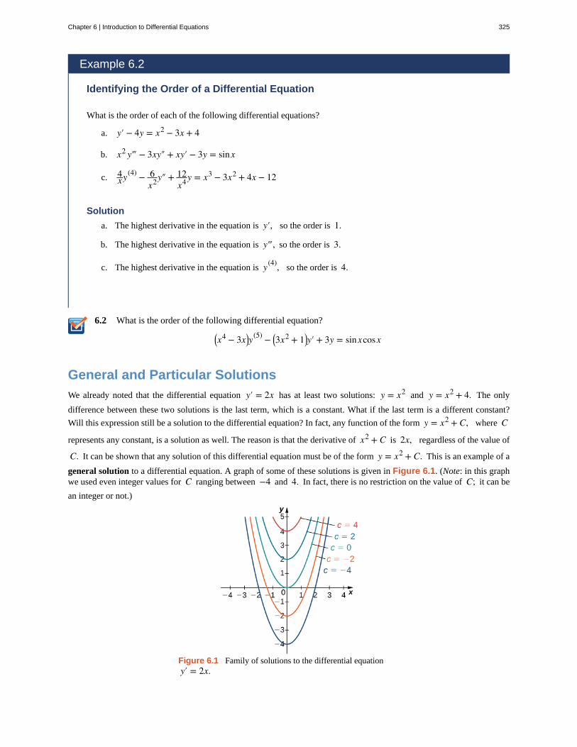
6.2
Example 6.2
Identifying the Order of a Differential Equation
What is the order of each of the following differential equations?
a. y′ − 4y = x2 − 3x + 4
b. x2 y‴ − 3xy″ + xy′ − 3y = sinx
c. 4xy
(4) − 6x2y″ + 12
x4y = x3 − 3x2 + 4x − 12
Solution
a. The highest derivative in the equation is y′, so the order is 1.
b. The highest derivative in the equation is y‴, so the order is 3.
c. The highest derivative in the equation is y(4), so the order is 4.
What is the order of the following differential equation?
⎛⎝x4 − 3x⎞⎠y
(5) − ⎛⎝3x2 + 1⎞⎠y′ + 3y = sinxcosx
General and Particular SolutionsWe already noted that the differential equation y′ = 2x has at least two solutions: y = x2 and y = x2 + 4. The only
difference between these two solutions is the last term, which is a constant. What if the last term is a different constant?
Will this expression still be a solution to the differential equation? In fact, any function of the form y = x2 + C, where C
represents any constant, is a solution as well. The reason is that the derivative of x2 + C is 2x, regardless of the value of
C. It can be shown that any solution of this differential equation must be of the form y = x2 + C. This is an example of a
general solution to a differential equation. A graph of some of these solutions is given in Figure 6.1. (Note: in this graphwe used even integer values for C ranging between −4 and 4. In fact, there is no restriction on the value of C; it can be
an integer or not.)
Figure 6.1 Family of solutions to the differential equationy′ = 2x.
Chapter 6 | Introduction to Differential Equations 325
6.3
In this example, we are free to choose any solution we wish; for example, y = x2 − 3 is a member of the family of solutions
to this differential equation. This is called a particular solution to the differential equation. A particular solution can oftenbe uniquely identified if we are given additional information about the problem.
Example 6.3
Finding a Particular Solution
Find the particular solution to the differential equation y′ = 2x passing through the point (2, 7).
Solution
Any function of the form y = x2 + C is a solution to this differential equation. To determine the value of C,we substitute the values x = 2 and y = 7 into this equation and solve for C:
y = x2 + C
7 = 22 + C = 4 + CC = 3.
Therefore the particular solution passing through the point (2, 7) is y = x2 + 3.
Find the particular solution to the differential equation
y′ = 4x + 3
passing through the point (1, 7), given that y = 2x2 + 3x + C is a general solution to the differential
equation.
Initial-Value ProblemsUsually a given differential equation has an infinite number of solutions, so it is natural to ask which one we want to use.To choose one solution, more information is needed. Some specific information that can be useful is an initial value, whichis an ordered pair that is used to find a particular solution.
A differential equation together with one or more initial values is called an initial-value problem. The general rule isthat the number of initial values needed for an initial-value problem is equal to the order of the differential equation. Forexample, if we have the differential equation y′ = 2x, then y(3) = 7 is an initial value, and when taken together, these
equations form an initial-value problem. The differential equation y″ − 3y′ + 2y = 4ex is second order, so we need two
initial values. With initial-value problems of order greater than one, the same value should be used for the independentvariable. An example of initial values for this second-order equation would be y(0) = 2 and y′(0) = −1. These two initial
values together with the differential equation form an initial-value problem. These problems are so named because often theindependent variable in the unknown function is t, which represents time. Thus, a value of t = 0 represents the beginning
of the problem.
Example 6.4
Verifying a Solution to an Initial-Value Problem
326 Chapter 6 | Introduction to Differential Equations
This OpenStax book is available for free at https://legacy.cnx.org/content/col31997/1.5
6.4
Verify that the function y = 2e−2t + et is a solution to the initial-value problem
y′ + 2y = 3et, y(0) = 3.
Solution
For a function to satisfy an initial-value problem, it must satisfy both the differential equation and the initialcondition. To show that y satisfies the differential equation, we start by calculating y′. This gives
y′ = −4e−2t + et. Next we substitute both y and y′ into the left-hand side of the differential equation and
simplify:
y′ + 2y = ⎛⎝−4e−2t + et⎞⎠+ 2⎛⎝2e−2t + et⎞⎠= −4e−2t + et + 4e−2t + 2et
= 3et.
This is equal to the right-hand side of the differential equation, so y = 2e−2t + et solves the differential equation.
Next we calculate y(0):
y(0) = 2e−2(0) + e0
= 2 + 1= 3.
This result verifies the initial value. Therefore the given function satisfies the initial-value problem.
Verify that y = 3e2t + 4sin t is a solution to the initial-value problem
y′ − 2y = 4cos t − 8sin t, y(0) = 3.
In Example 6.4, the initial-value problem consisted of two parts. The first part was the differential equationy′ + 2y = 3ex, and the second part was the initial value y(0) = 3. These two equations together formed the initial-value
problem.
The same is true in general. An initial-value problem will consists of two parts: the differential equation and the initialcondition. The differential equation has a family of solutions, and the initial condition determines the value of C. The
family of solutions to the differential equation in Example 6.4 is given by y = 2e−2t + Cet. This family of solutions is
shown in Figure 6.2, with the particular solution y = 2e−2t + et labeled.
Chapter 6 | Introduction to Differential Equations 327
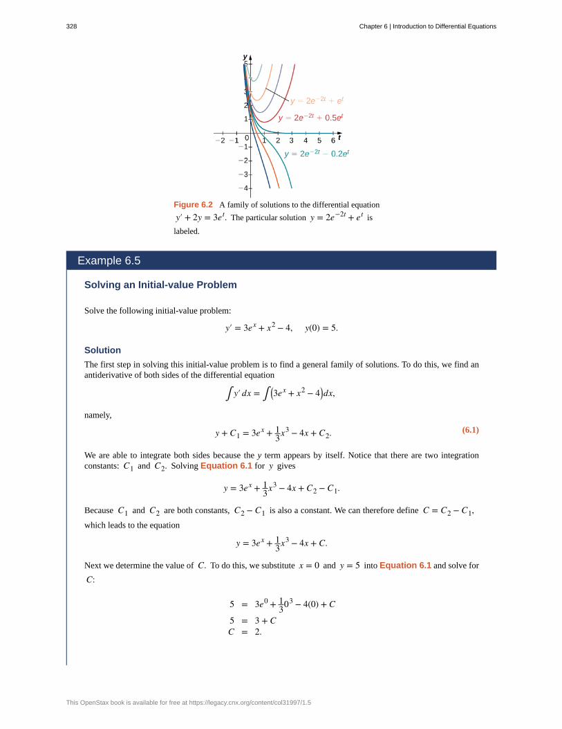
(6.1)
Figure 6.2 A family of solutions to the differential equation
y′ + 2y = 3et. The particular solution y = 2e−2t + et is
labeled.
Example 6.5
Solving an Initial-value Problem
Solve the following initial-value problem:
y′ = 3ex + x2 − 4, y(0) = 5.
Solution
The first step in solving this initial-value problem is to find a general family of solutions. To do this, we find anantiderivative of both sides of the differential equation
∫ y′dx = ∫ ⎛⎝3ex + x2 − 4⎞⎠dx,
namely,
y + C1 = 3ex + 13x
3 − 4x + C2.
We are able to integrate both sides because the y term appears by itself. Notice that there are two integrationconstants: C1 and C2. Solving Equation 6.1 for y gives
y = 3ex + 13x
3 − 4x + C2 − C1.
Because C1 and C2 are both constants, C2 − C1 is also a constant. We can therefore define C = C2 − C1,which leads to the equation
y = 3ex + 13x
3 − 4x + C.
Next we determine the value of C. To do this, we substitute x = 0 and y = 5 into Equation 6.1 and solve for
C:
5 = 3e0 + 1303 − 4(0) + C
5 = 3 + CC = 2.
328 Chapter 6 | Introduction to Differential Equations
This OpenStax book is available for free at https://legacy.cnx.org/content/col31997/1.5
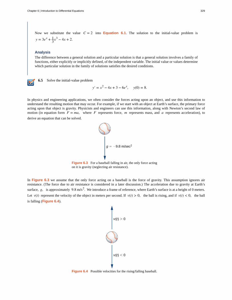
6.5
Now we substitute the value C = 2 into Equation 6.1. The solution to the initial-value problem is
y = 3ex + 13x
3 − 4x + 2.
AnalysisThe difference between a general solution and a particular solution is that a general solution involves a family offunctions, either explicitly or implicitly defined, of the independent variable. The initial value or values determinewhich particular solution in the family of solutions satisfies the desired conditions.
Solve the initial-value problem
y′ = x2 − 4x + 3 − 6ex, y(0) = 8.
In physics and engineering applications, we often consider the forces acting upon an object, and use this information tounderstand the resulting motion that may occur. For example, if we start with an object at Earth’s surface, the primary forceacting upon that object is gravity. Physicists and engineers can use this information, along with Newton’s second law ofmotion (in equation form F = ma, where F represents force, m represents mass, and a represents acceleration), to
derive an equation that can be solved.
Figure 6.3 For a baseball falling in air, the only force actingon it is gravity (neglecting air resistance).
In Figure 6.3 we assume that the only force acting on a baseball is the force of gravity. This assumption ignores airresistance. (The force due to air resistance is considered in a later discussion.) The acceleration due to gravity at Earth’s
surface, g, is approximately 9.8 m/s2. We introduce a frame of reference, where Earth’s surface is at a height of 0 meters.
Let v(t) represent the velocity of the object in meters per second. If v(t) > 0, the ball is rising, and if v(t) < 0, the ball
is falling (Figure 6.4).
Figure 6.4 Possible velocities for the rising/falling baseball.
Chapter 6 | Introduction to Differential Equations 329
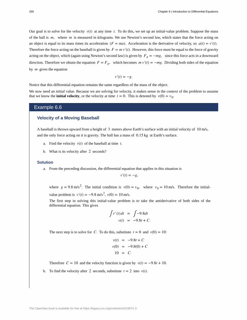
Our goal is to solve for the velocity v(t) at any time t. To do this, we set up an initial-value problem. Suppose the mass
of the ball is m, where m is measured in kilograms. We use Newton’s second law, which states that the force acting on
an object is equal to its mass times its acceleration (F = ma). Acceleration is the derivative of velocity, so a(t) = v′(t).Therefore the force acting on the baseball is given by F = m v′(t). However, this force must be equal to the force of gravity
acting on the object, which (again using Newton’s second law) is given by Fg = −mg, since this force acts in a downward
direction. Therefore we obtain the equation F = Fg, which becomes m v′(t) = −mg. Dividing both sides of the equation
by m gives the equation
v′(t) = −g.
Notice that this differential equation remains the same regardless of the mass of the object.
We now need an initial value. Because we are solving for velocity, it makes sense in the context of the problem to assumethat we know the initial velocity, or the velocity at time t = 0. This is denoted by v(0) = v0.
Example 6.6
Velocity of a Moving Baseball
A baseball is thrown upward from a height of 3 meters above Earth’s surface with an initial velocity of 10 m/s,and the only force acting on it is gravity. The ball has a mass of 0.15 kg at Earth’s surface.
a. Find the velocity v(t) of the baseball at time t.
b. What is its velocity after 2 seconds?
Solution
a. From the preceding discussion, the differential equation that applies in this situation is
v′(t) = −g,
where g = 9.8 m/s2. The initial condition is v(0) = v0, where v0 = 10 m/s. Therefore the initial-
value problem is v′(t) = −9.8 m/s2, v(0) = 10 m/s.The first step in solving this initial-value problem is to take the antiderivative of both sides of thedifferential equation. This gives
∫ v′ (t)dt = ∫ −9.8dt
v(t) = −9.8t + C.
The next step is to solve for C. To do this, substitute t = 0 and v(0) = 10:
v(t) = −9.8t + Cv(0) = −9.8(0) + C
10 = C.
Therefore C = 10 and the velocity function is given by v(t) = −9.8t + 10.
b. To find the velocity after 2 seconds, substitute t = 2 into v(t).
330 Chapter 6 | Introduction to Differential Equations
This OpenStax book is available for free at https://legacy.cnx.org/content/col31997/1.5

6.6
v(t) = −9.8t + 10v(2) = −9.8(2) + 10v(2) = −9.6.
The units of velocity are meters per second. Since the answer is negative, the object is falling at a speedof 9.6 m/s.
Suppose a rock falls from rest from a height of 100 meters and the only force acting on it is gravity. Find
an equation for the velocity v(t) as a function of time, measured in meters per second.
A natural question to ask after solving this type of problem is how high the object will be above Earth’s surface at a givenpoint in time. Let s(t) denote the height above Earth’s surface of the object, measured in meters. Because velocity is the
derivative of position (in this case height), this assumption gives the equation s′ (t) = v(t). An initial value is necessary;
in this case the initial height of the object works well. Let the initial height be given by the equation s(0) = s0. Together
these assumptions give the initial-value problem
s′ (t) = v(t), s(0) = s0.
If the velocity function is known, then it is possible to solve for the position function as well.
Example 6.7
Height of a Moving Baseball
A baseball is thrown upward from a height of 3 meters above Earth’s surface with an initial velocity of 10 m/s,and the only force acting on it is gravity. The ball has a mass of 0.15 kilogram at Earth’s surface.
a. Find the position s(t) of the baseball at time t.
b. What is its height after 2 seconds?
Solution
a. We already know the velocity function for this problem is v(t) = −9.8t + 10. The initial height of the
baseball is 3 meters, so s0 = 3. Therefore the initial-value problem for this example is
To solve the initial-value problem, we first find the antiderivatives:
∫ s′ (t)dt = ∫ −9.8t + 10dt
s(t) = −4.9t2 + 10t + C.
Next we substitute t = 0 and solve for C:
s(t) = −4.9t2 + 10t + C
s(0) = −4.9(0)2 + 10(0) + C3 = C.
Chapter 6 | Introduction to Differential Equations 331
Therefore the position function is s(t) = −4.9t2 + 10t + 3.
b. The height of the baseball after 2 s is given by s(2):
s(2) = −4.9(2)2 + 10(2) + 3= −4.9(4) + 23= 3.4.
Therefore the baseball is 3.4 meters above Earth’s surface after 2 seconds. It is worth noting that the
mass of the ball cancelled out completely in the process of solving the problem.
Key Concepts• A differential equation is an equation involving a function y = f (x) and one or more of its derivatives. A solution
is a function y = f (x) that satisfies the differential equation when f and its derivatives are substituted into the
equation.
• The order of a differential equation is the highest order of any derivative of the unknown function that appears inthe equation.
• A differential equation coupled with an initial value is called an initial-value problem. To solve an initial-valueproblem, first find the general solution to the differential equation, then determine the value of the constant. Initial-value problems have many applications in science and engineering.
332 Chapter 6 | Introduction to Differential Equations
This OpenStax book is available for free at https://legacy.cnx.org/content/col31997/1.5
6.1 EXERCISESDetermine the order of the following differential equations.
1. y′ + y = 3y2
2. (y′)2 = y′ + 2y
3. y‴ + y″y′ = 3x2
4. y′ = y″ + 3t2
5.dydt = t
6.dydx + d2 y
dx2 = 3x4
7.⎛⎝dydt⎞⎠
2+ 8dydt + 3y = 4t
Verify that the following functions are solutions to thegiven differential equation.
8. y = x3
3 solves y′ = x2
9. y = 2e−x + x − 1 solves y′ = x − y
10. y = e3x − ex2 solves y′ = 3y + ex
11. y = 11 − x solves y′ = y2
12. y = ex2/2 solves y′ = xy
13. y = 4 + lnx solves xy′ = 1
14. y = 3 − x + x lnx solves y′ = lnx
15. y = 2ex − x − 1 solves y′ = y + x
16. y = ex + sinx2 − cosx
2 solves y′ = cosx + y
17. y = πe−cosx solves y′ = ysinx
Verify the following general solutions and find theparticular solution.
18. Find the particular solution to the differential equation
y′ = 4x2 that passes through (−3, −30), given that
y = C + 4x3
3 is a general solution.
19. Find the particular solution to the differential equation
y′ = 3x3 that passes through (1, 4.75), given that
y = C + 3x4
4 is a general solution.
20. Find the particular solution to the differential equation
y′ = 3x2 y that passes through (0, 12), given that
y = Cex3
is a general solution.
21. Find the particular solution to the differential equation
y′ = 2xy that passes through ⎛⎝0, 1
2⎞⎠, given that
y = Cex2
is a general solution.
22. Find the particular solution to the differential equation
y′ = ⎛⎝2xy⎞⎠2 that passes through ⎛⎝1, − 1
2⎞⎠, given that
y = − 3C + 4x3 is a general solution.
23. Find the particular solution to the differential equation
y′ x2 = y that passes through ⎛⎝1, 2
e⎞⎠, given that
y = Ce−1/x is a general solution.
24. Find the particular solution to the differential equation
8dxdt = −2cos(2t) − cos(4t) that passes through (π, π),
given that x = C − 18sin(2t) − 1
32sin(4t) is a general
solution.
25. Find the particular solution to the differential equationdudt = tanu that passes through ⎛⎝1, π2
⎞⎠, given that
u = sin−1 ⎛⎝eC + t⎞⎠ is a general solution.
26. Find the particular solution to the differential equationdydt = e(t + y)
that passes through (1, 0), given that
y = −ln(C − et) is a general solution.
27. Find the particular solution to the differential equation
y′(1 − x2) = 1 + y that passes through (0, −2), given
that y = C x + 11 − x
− 1 is a general solution.
Chapter 6 | Introduction to Differential Equations 333

For the following problems, find the general solution to thedifferential equation.
28. y′ = 3x + ex
29. y′ = lnx + tanx
30. y′ = sinxecosx
31. y′ = 4x
32. y′ = sin−1 (2x)
33. y′ = 2t t2 + 16
34. x′ = coth t + ln t + 3t2
35. x′ = t 4 + t
36. y′ = y
37. y′ = yx
Solve the following initial-value problems starting fromy(t = 0) = 1 and y(t = 0) = −1. Draw both solutions on
the same graph.
38.dydt = 2t
39.dydt = −t
40.dydt = 2y
41.dydt = −y
42.dydt = 2
Solve the following initial-value problems starting fromy0 = 10. At what time does y increase to 100 or drop to
1?
43.dydt = 4t
44.dydt = 4y
45.dydt = −2y
46.dydt = e4t
47.dydt = e−4t
Recall that a family of solutions includes solutions to adifferential equation that differ by a constant. For thefollowing problems, use your calculator to graph a familyof solutions to the given differential equation. Use initialconditions from y(t = 0) = −10 to y(t = 0) = 10increasing by 2. Is there some critical point where the
behavior of the solution begins to change?
48. [T] y′ = y(x)
49. [T] xy′ = y
50. [T] y′ = t3
51. [T] y′ = x + y (Hint: y = Cex − x − 1 is the
general solution)
52. [T] y′ = x lnx + sinx
53. Find the general solution to describe the velocity of aball of mass 1 lb that is thrown upward at a rate a ft/sec.
54. In the preceding problem, if the initial velocity of theball thrown into the air is a = 25 ft/s, write the particular
solution to the velocity of the ball. Solve to find the timewhen the ball hits the ground.
55. You throw two objects with differing masses m1 and
m2 upward into the air with the same initial velocity a ft/
s. What is the difference in their velocity after 1 second?
56. [T] You throw a ball of mass 1 kilogram upward
with a velocity of a = 25 m/s on Mars, where the force
of gravity is g = −3.711 m/s2. Use your calculator to
approximate how much longer the ball is in the air onMars.
57. [T] For the previous problem, use your calculator toapproximate how much higher the ball went on Mars.
58. [T] A car on the freeway accelerates according toa = 15cos(πt), where t is measured in hours. Set up
and solve the differential equation to determine the velocityof the car if it has an initial speed of 51 mph. After 40minutes of driving, what is the driver’s velocity?
334 Chapter 6 | Introduction to Differential Equations
This OpenStax book is available for free at https://legacy.cnx.org/content/col31997/1.5
59. [T] For the car in the preceding problem, find theexpression for the distance the car has traveled in time t,assuming an initial distance of 0. How long does it take
the car to travel 100 miles? Round your answer to hours
and minutes.
60. [T] For the previous problem, find the total distancetraveled in the first hour.
61. Substitute y = Be3t into y′ − y = 8e3t to find a
particular solution.
62. Substitute y = acos(2t) + bsin(2t) into
y′ + y = 4sin(2t) to find a particular solution.
63. Substitute y = a + bt + ct2 into y′ + y = 1 + t2 to
find a particular solution.
64. Substitute y = aet cos t + bet sin t into
y′ = 2et cos t to find a particular solution.
65. Solve y′ = ekt with the initial condition y(0) = 0and solve y′ = 1 with the same initial condition. As kapproaches 0, what do you notice?
Chapter 6 | Introduction to Differential Equations 335
6.2 | Separable Equations
Learning Objectives6.2.1 Use separation of variables to solve a differential equation.
6.2.2 Solve applications using separation of variables.
We now examine a solution technique for finding exact solutions to a class of differential equations known as separabledifferential equations. These equations are common in a wide variety of disciplines, including physics, chemistry, andengineering. We illustrate a few applications at the end of the section.
Separation of VariablesWe start with a definition and some examples.
Definition
A separable differential equation is any equation that can be written in the form
(6.2)y′ = f (x)g(y).
The term ‘separable’ refers to the fact that the right-hand side of the equation can be separated into a function of x times a
function of y. Examples of separable differential equations include
y′ = ⎛⎝x2 − 4⎞⎠⎛⎝3y + 2⎞⎠
y′ = 6x2 + 4x
y′ = secy + tanyy′ = xy + 3x − 2y − 6.
The second equation is separable with f (x) = 6x2 + 4x and g(y) = 1, the third equation is separable with f (x) = 1 and
g(y) = secy + tany, and the right-hand side of the fourth equation can be factored as (x + 3)⎛⎝y − 2⎞⎠, so it is separable
as well. The third equation is also called an autonomous differential equation because the right-hand side of the equationis a function of y alone. If a differential equation is separable, then it is possible to solve the equation using the method of
separation of variables.
Problem-Solving Strategy: Separation of Variables
1. Check for any values of y that make g(y) = 0. These correspond to constant solutions.
2. Rewrite the differential equation in the formdyg(y) = f (x)dx.
3. Integrate both sides of the equation.
4. Solve the resulting equation for y if possible.
5. If an initial condition exists, substitute the appropriate values for x and y into the equation and solve for the
constant.
Note that Step 4. states “Solve the resulting equation for y if possible.” It is not always possible to obtain y as an
explicit function of x. Quite often we have to be satisfied with finding y as an implicit function of x.
336 Chapter 6 | Introduction to Differential Equations
This OpenStax book is available for free at https://legacy.cnx.org/content/col31997/1.5
Example 6.8
Using Separation of Variables
Find a general solution to the differential equation y′ = ⎛⎝x2 − 4⎞⎠⎛⎝3y + 2⎞⎠ using the method of separation of
variables.
Solution
Follow the five-step method of separation of variables.
1. In this example, f (x) = x2 − 4 and g(y) = 3y + 2. Setting g(y) = 0 gives y = − 23 as a constant
solution.
2. Rewrite the differential equation in the form
dy3y + 2 = (x2 − 4)dx.
3. Integrate both sides of the equation:
⌠⌡
dy3y + 2 = ∫ ⎛⎝x2 − 4⎞⎠dx.
Let u = 3y + 2. Then du = 3dydxdx, so the equation becomes
13∫ 1
udu = 13x
3 − 4x + C
13 ln|u| = 1
3x3 − 4x + C
13 ln|3y + 2| = 1
3x3 − 4x + C.
4. To solve this equation for y, first multiply both sides of the equation by 3.
ln|3y + 2| = x3 − 12x + 3C
Now we use some logic in dealing with the constant C. Since C represents an arbitrary constant, 3Calso represents an arbitrary constant. If we call the second arbitrary constant C1, the equation becomes
ln|3y + 2| = x3 − 12x + C1.
Now exponentiate both sides of the equation (i.e., make each side of the equation the exponent for thebase e).
eln|3y + 2| = ex3 − 12x + C1
|3y + 2| = eC1 ex
3 − 12x
Again define a new constant C2 = ec1 (note that C2 > 0):
|3y + 2| = C2 ex3 − 12x.
Chapter 6 | Introduction to Differential Equations 337
6.7
(6.3)
This corresponds to two separate equations: 3y + 2 = C2 ex3 − 12x and 3y + 2 = −C2 e
x3 − 12x.
The solution to either equation can be written in the form y = −2 ± C2 ex3 − 12x
3 .
Since C2 > 0, it does not matter whether we use plus or minus, so the constant can actually have either
sign. Furthermore, the subscript on the constant C is entirely arbitrary, and can be dropped. Therefore
the solution can be written as
y = −2 + Cex3 − 12x
3 .
5. No initial condition is imposed, so we are finished.
Use the method of separation of variables to find a general solution to the differential equationy′ = 2xy + 3y − 4x − 6.
Example 6.9
Solving an Initial-Value Problem
Using the method of separation of variables, solve the initial-value problem
y′ = (2x + 3)(y2 − 4), y(0) = 1.
Solution
Follow the five-step method of separation of variables.
1. In this example, f (x) = 2x + 3 and g(y) = y2 − 4. Setting g(y) = 0 gives y = ± 2 as constant
solutions.
2. Divide both sides of the equation by y2 − 4 and multiply by dx. This gives the equation
dyy2 − 4
= (2x + 3)dx.
3. Next integrate both sides:
⌠⌡
1y2 − 4
dy = ∫ (2x + 3)dx.
To evaluate the left-hand side, use the method of partial fraction decomposition. This leads to the identity
1y2 − 4
= 14⎛⎝ 1y − 2 − 1
y + 2⎞⎠.
Then Equation 6.3 becomes
338 Chapter 6 | Introduction to Differential Equations
This OpenStax book is available for free at https://legacy.cnx.org/content/col31997/1.5
14⌠⌡⎛⎝ 1y − 2 − 1
y + 2⎞⎠dy = ∫ (2x + 3)dx
14⎛⎝ln|y − 2| − ln|y + 2|⎞⎠ = x2 + 3x + C.
Multiplying both sides of this equation by 4 and replacing 4C with C1 gives
ln|y − 2| − ln|y + 2| = 4x2 + 12x + C1
ln|y − 2y + 2| = 4x2 + 12x + C1.
4. It is possible to solve this equation for y. First exponentiate both sides of the equation and define
C2 = eC1 :
|y − 2y + 2| = C2 e
4x2 + 12x.
Next we can remove the absolute value and let C2 be either positive or negative. Then multiply both
sides by y + 2.
y − 2 = C2⎛⎝y + 2⎞⎠e4x2 + 12x
y − 2 = C2 ye4x2 + 12x + 2C2 e
4x2 + 12x.
Now collect all terms involving y on one side of the equation, and solve for y:
y − C2 ye4x2 + 12x = 2 + 2C2 e
4x2 + 12x
y(1 − C2 e4x2 + 12x) = 2 + 2C2 e
4x2 + 12x
y = 2 + 2C2 e4x2 + 12x
1 − C2 e4x2 + 12x
.
5. To determine the value of C2, substitute x = 0 and y = −1 into the general solution. Alternatively,
we can put the same values into an earlier equation, namely the equationy − 2y + 2 = C2 e
4x2 + 12. This is
much easier to solve for C2 :
y − 2y + 2 = C2 e
4x2 + 12x
−1 − 2−1 + 2 = C2 e
4(0)2 + 12(0)
C2 = −3.
Therefore the solution to the initial-value problem is
y = 2 − 6e4x2 + 12x
1 + 3e4x2 + 12x.
Chapter 6 | Introduction to Differential Equations 339
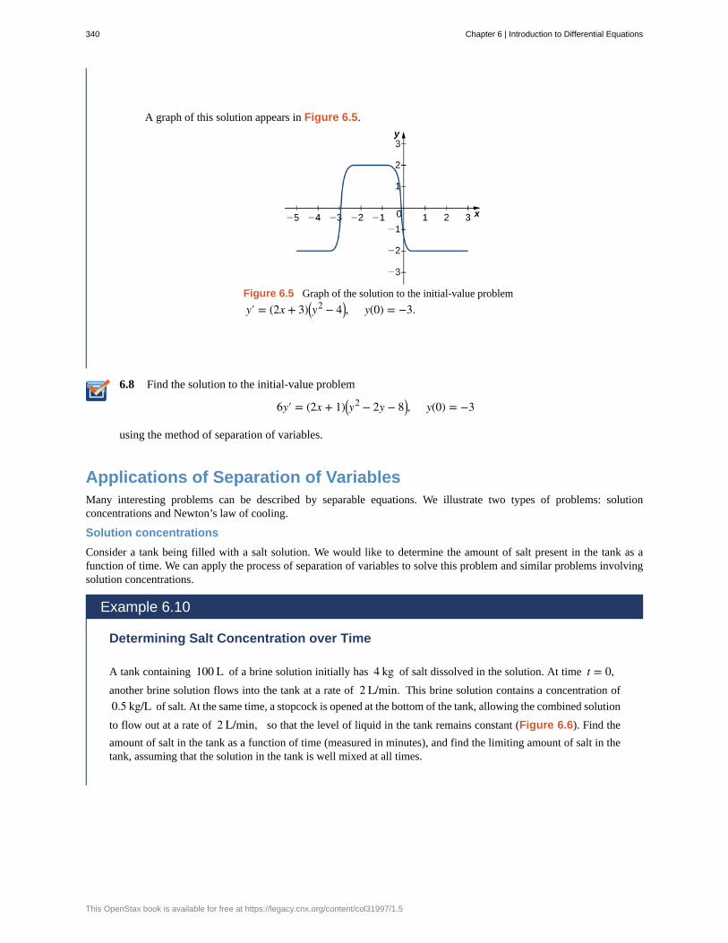
6.8
A graph of this solution appears in Figure 6.5.
Figure 6.5 Graph of the solution to the initial-value problem
y′ = (2x + 3)⎛⎝y2 − 4⎞⎠, y(0) = −3.
Find the solution to the initial-value problem
6y′ = (2x + 1)⎛⎝y2 − 2y − 8⎞⎠, y(0) = −3
using the method of separation of variables.
Applications of Separation of VariablesMany interesting problems can be described by separable equations. We illustrate two types of problems: solutionconcentrations and Newton’s law of cooling.
Solution concentrations
Consider a tank being filled with a salt solution. We would like to determine the amount of salt present in the tank as afunction of time. We can apply the process of separation of variables to solve this problem and similar problems involvingsolution concentrations.
Example 6.10
Determining Salt Concentration over Time
A tank containing 100 L of a brine solution initially has 4 kg of salt dissolved in the solution. At time t = 0,another brine solution flows into the tank at a rate of 2 L/min. This brine solution contains a concentration of
0.5 kg/L of salt. At the same time, a stopcock is opened at the bottom of the tank, allowing the combined solution
to flow out at a rate of 2 L/min, so that the level of liquid in the tank remains constant (Figure 6.6). Find the
amount of salt in the tank as a function of time (measured in minutes), and find the limiting amount of salt in thetank, assuming that the solution in the tank is well mixed at all times.
340 Chapter 6 | Introduction to Differential Equations
This OpenStax book is available for free at https://legacy.cnx.org/content/col31997/1.5

(6.4)
Figure 6.6 A brine tank with an initial amount of salt solutionaccepts an input flow and delivers an output flow. How does theamount of salt change with time?
Solution
First we define a function u(t) that represents the amount of salt in kilograms in the tank as a function of time.
Then dudt represents the rate at which the amount of salt in the tank changes as a function of time. Also, u(0)
represents the amount of salt in the tank at time t = 0, which is 4 kilograms.
The general setup for the differential equation we will solve is of the form
dudt = INFLOW RATE − OUTFLOW RATE.
INFLOW RATE represents the rate at which salt enters the tank, and OUTFLOW RATE represents the rate atwhich salt leaves the tank. Because solution enters the tank at a rate of 2 L/min, and each liter of solution
contains 0.5 kilogram of salt, every minute 2(0.5) = 1 kilogram of salt enters the tank. Therefore INFLOW
RATE = 1.
To calculate the rate at which salt leaves the tank, we need the concentration of salt in the tank at any point intime. Since the actual amount of salt varies over time, so does the concentration of salt. However, the volume ofthe solution remains fixed at 100 liters. The number of kilograms of salt in the tank at time t is equal to u(t).
Thus, the concentration of salt is u(t)100 kg/L, and the solution leaves the tank at a rate of 2 L/min. Therefore
salt leaves the tank at a rate of u(t)100 · 2 = u(t)
50 kg/min, and OUTFLOW RATE is equal to u(t)50 . Therefore the
differential equation becomes dudt = 1 − u
50, and the initial condition is u(0) = 4. The initial-value problem to
be solved is
dudt = 1 − u
50, u(0) = 4.
The differential equation is a separable equation, so we can apply the five-step strategy for solution.
Step 1. Setting 1 − u50 = 0 gives u = 50 as a constant solution. Since the initial amount of salt in the tank is 4
kilograms, this solution does not apply.
Step 2. Rewrite the equation as
dudt = 50 − u
50 .
Chapter 6 | Introduction to Differential Equations 341
6.9
Then multiply both sides by dt and divide both sides by 50 − u:
du50 − u = dt
50.
Step 3. Integrate both sides:
⌠⌡
du50 − u = ⌠
⌡dt50
−ln|50 − u| = t50 + C.
Step 4. Solve for u(t):
ln|50 − u| = − t50 − C
eln|50 − u| = e−(t/50) − C
|50 − u| = C1 e−t/50.
Eliminate the absolute value by allowing the constant to be either positive or negative:
50 − u = C1 e−t/50.
Finally, solve for u(t):
u(t) = 50 − C1 e−t/50.
Step 5. Solve for C1 :
u(0) = 50 − C1 e−0/50
4 = 50 − C1C1 = 46.
The solution to the initial value problem is u(t) = 50 − 46e−t/50. To find the limiting amount of salt in the tank,
take the limit as t approaches infinity:
limt → ∞
u(t) = 50 − 46e−t/50
= 50 − 46(0)= 50.
Note that this was the constant solution to the differential equation. If the initial amount of salt in the tank is 50kilograms, then it remains constant. If it starts at less than 50 kilograms, then it approaches 50 kilograms overtime.
A tank contains 3 kilograms of salt dissolved in 75 liters of water. A salt solution of 0.4 kg salt/L is
pumped into the tank at a rate of 6 L/min and is drained at the same rate. Solve for the salt concentration at
time t. Assume the tank is well mixed at all times.
Newton’s law of cooling
Newton’s law of cooling states that the rate of change of an object’s temperature is proportional to the difference betweenits own temperature and the ambient temperature (i.e., the temperature of its surroundings). If we let T(t) represent
the temperature of an object as a function of time, then dTdt represents the rate at which that temperature changes. The
342 Chapter 6 | Introduction to Differential Equations
This OpenStax book is available for free at https://legacy.cnx.org/content/col31997/1.5

temperature of the object’s surroundings can be represented by Ts. Then Newton’s law of cooling can be written in the
form
dTdt = k⎛⎝T(t) − Ts⎞⎠
or simply
(6.5)dTdt = k(T − Ts).
The temperature of the object at the beginning of any experiment is the initial value for the initial-value problem. We callthis temperature T0. Therefore the initial-value problem that needs to be solved takes the form
(6.6)dTdt = k(T − Ts), T(0) = T0,
where k is a constant that needs to be either given or determined in the context of the problem. We use these equations in
Example 6.11.
Example 6.11
Waiting for a Pizza to Cool
A pizza is removed from the oven after baking thoroughly, and the temperature of the pizza when it comes out ofthe oven is 350°F. The temperature of the kitchen is 75°F, and after 5 minutes the temperature of the pizza
is 340°F. We would like to wait until the temperature of the pizza reaches 300°F before cutting and serving it
(Figure 6.7). How much longer will we have to wait?
Figure 6.7 From Newton’s law of cooling, if the pizza cools10°F in 5 minutes, how long before it cools to 300°F?
Solution
The ambient temperature (surrounding temperature) is 75°F, so Ts = 75. The temperature of the pizza when
it comes out of the oven is 350°F, which is the initial temperature (i.e., initial value), so T0 = 350. Therefore
Equation 6.3 becomes
dTdt = k(T − 75), T(0) = 350.
To solve the differential equation, we use the five-step technique for solving separable equations.
1. Setting the right-hand side equal to zero gives T = 75 as a constant solution. Since the pizza starts at
350°F, this is not the solution we are seeking.
2. Rewrite the differential equation by multiplying both sides by dt and dividing both sides by T − 75:
Chapter 6 | Introduction to Differential Equations 343

dTT − 75 = kdt.
3. Integrate both sides:
⌠⌡
dTT − 75 = ∫ kdt
ln|T − 75| = kt + C.4. Solve for T by first exponentiating both sides:
eln|T − 75| = ekt + C
|T − 75| = C1 ekt
T − 75 = C1 ekt
T(t) = 75 + C1 ekt.
5. Solve for C1 by using the initial condition T(0) = 350:
T(t) = 75 + C1 ekt
T(0) = 75 + C1 ek(0)
350 = 75 + C1C1 = 275.
Therefore the solution to the initial-value problem is
T(t) = 75 + 275ekt.
To determine the value of k, we need to use the fact that after 5 minutes the temperature of the pizza
is 340°F. Therefore T(5) = 340. Substituting this information into the solution to the initial-value
problem, we have
T(t) = 75 + 275ekt
T(5) = 340 = 75 + 275e5k
265 = 275e5k
e5k = 5355
lne5k = ln⎛⎝5355⎞⎠
5k = ln⎛⎝5355⎞⎠
k = 15 ln⎛⎝53
55⎞⎠ ≈ − 0.007408.
So now we have T(t) = 75 + 275e−0.007048t. When is the temperature 300°F? Solving for t, we find
344 Chapter 6 | Introduction to Differential Equations
This OpenStax book is available for free at https://legacy.cnx.org/content/col31997/1.5
6.10
T(t) = 75 + 275e−0.007048t
300 = 75 + 275e−0.007048t
225 = 275e−0.007048t
e−0.007048t = 911
lne−0.007048t = ln 911
−0.007048t = ln 911
t = − 10.007048 ln 9
11 ≈ 28.5.
Therefore we need to wait an additional 23.5 minutes (after the temperature of the pizza reached
340°F). That should be just enough time to finish this calculation.
A cake is removed from the oven after baking thoroughly, and the temperature of the cake when itcomes out of the oven is 450°F. The temperature of the kitchen is 70°F, and after 10 minutes the
temperature of the cake is 430°F.
a. Write the appropriate initial-value problem to describe this situation.
b. Solve the initial-value problem for T(t).
c. How long will it take until the temperature of the cake is within 5°F of room temperature?
Key Concepts• A separable differential equation is any equation that can be written in the form y′ = f (x)g(y).
• The method of separation of variables is used to find the general solution to a separable differential equation.
Key Equations• Separable differential equation
y′ = f (x)g(y)
• Solution concentrationdudt = INFLOW RATE − OUTFLOW RATE
• Newton’s law of coolingdTdt = k(T − Ts)
Chapter 6 | Introduction to Differential Equations 345
6.2 EXERCISESSolve the following initial-value problems with the initialcondition y0 = 0 and graph the solution.
66.dydt = y + 1
67.dydt = y − 1
68.dydt = y + 1
69.dydt = −y − 1
Find the general solution to the differential equation.
70. x2 y′ = (x + 1)y
71. y′ = tan(y)x
72. y′ = 2xy2
73.dydt = ycos(3t + 2)
74. 2xdydx = y2
75. y′ = ey x2
76. (1 + x)y′ = (x + 2)⎛⎝y − 1⎞⎠
77. dxdt = 3t2 ⎛⎝x2 + 4⎞⎠
78. tdydt = 1 − y2
79. y′ = ex ey
Find the solution to the initial-value problem.
80. y′ = ey − x, y(0) = 0
81. y′ = y2(x + 1), y(0) = 2
82.dydx = y3 xex
2, y(0) = 1
83.dydt = y2 ex sin(3x), y(0) = 1
84. y′ = xsech2 y
, y(0) = 0
85. y′ = 2xy(1 + 2y), y(0) = −1
86. dxdt = ln(t) 1 − x2, x(1) = 0
87. y′ = 3x2(y2 + 4), y(0) = 0
88. y′ = ey5x, y(0) = ln(ln(5))
89. y′ = −2x tan(y), y(0) = π2
For the following problems, use a software program or yourcalculator to generate the directional fields. Solve explicitlyand draw solution curves for several initial conditions. Arethere some critical initial conditions that change thebehavior of the solution?
90. [T] y′ = 1 − 2y
91. [T] y′ = y2 x3
92. [T] y′ = y3 ex
93. [T] y′ = ey
94. [T] y′ = y ln(x)
95. Most drugs in the bloodstream decay according to theequation y′ = cy, where y is the concentration of the
drug in the bloodstream. If the half-life of a drug is 2hours, what fraction of the initial dose remains after 6hours?
96. A drug is administered intravenously to a patient ata rate r mg/h and is cleared from the body at a rate
proportional to the amount of drug still present in the body,d Set up and solve the differential equation, assuming
there is no drug initially present in the body.
97. [T] How often should a drug be taken if its dose is3 mg, it is cleared at a rate c = 0.1 mg/h, and 1 mg is
required to be in the bloodstream at all times?
98. A tank contains 1 kilogram of salt dissolved in 100liters of water. A salt solution of 0.1 kg salt/L is pumped
into the tank at a rate of 2 L/min and is drained at the same
rate. Solve for the salt concentration at time t. Assume the
tank is well mixed.
346 Chapter 6 | Introduction to Differential Equations
This OpenStax book is available for free at https://legacy.cnx.org/content/col31997/1.5

99. A tank containing 10 kilograms of salt dissolved in
1000 liters of water has two salt solutions pumped in. The
first solution of 0.2 kg salt/L is pumped in at a rate of
20 L/min and the second solution of 0.05 kg salt/L is
pumped in at a rate of 5 L/min. The tank drains at 25L/min. Assume the tank is well mixed. Solve for the saltconcentration at time t.
100. [T] For the preceding problem, find how much salt isin the tank 1 hour after the process begins.
101. Torricelli’s law states that for a water tank with ahole in the bottom that has a cross-section of A and with
a height of water h above the bottom of the tank, the
rate of change of volume of water flowing from the tankis proportional to the square root of the height of water,
according to dVdt = −A 2gh, where g is the acceleration
due to gravity. Note that dVdt = Adhdt . Solve the resulting
initial-value problem for the height of the water, assuminga tank with a hole of radius 2 ft. The initial height of water
is 100 ft.
102. For the preceding problem, determine how long ittakes the tank to drain.
For the following problems, use Newton’s law of cooling.
103. The liquid base of an ice cream has an initialtemperature of 200°F before it is placed in a freezer with
a constant temperature of 0°F. After 1 hour, the
temperature of the ice-cream base has decreased to 140°F.Formulate and solve the initial-value problem to determinethe temperature of the ice cream.
104. [T] The liquid base of an ice cream has an initialtemperature of 210°F before it is placed in a freezer with
a constant temperature of 20°F. After 2 hours, the
temperature of the ice-cream base has decreased to 170°F.At what time will the ice cream be ready to eat? (Assume30°F is the optimal eating temperature.)
105. [T] You are organizing an ice cream social. Theoutside temperature is 80°F and the ice cream is at 10°F.After 10 minutes, the ice cream temperature has risen by
10°F. How much longer can you wait before the ice cream
melts at 40°F?
106. You have a cup of coffee at temperature 70°C and
the ambient temperature in the room is 20°C. Assuming
a cooling rate k of 0.125, write and solve the differential
equation to describe the temperature of the coffee withrespect to time.
107. [T] You have a cup of coffee at temperature 70°Cthat you put outside, where the ambient temperature is0°C. After 5 minutes, how much colder is the coffee?
108. You have a cup of coffee at temperature 70°C and
you immediately pour in 1 part milk to 5 parts coffee.
The milk is initially at temperature 1°C. Write and solve
the differential equation that governs the temperature ofthis coffee.
109. You have a cup of coffee at temperature 70°C,which you let cool 10 minutes before you pour in the same
amount of milk at 1°C as in the preceding problem. How
does the temperature compare to the previous cup after 10minutes?
110. Solve the generic problem y′ = ay + b with initial
condition y(0) = c.
111. Prove the basic continual compounded interestequation. Assuming an initial deposit of P0 and an interest
rate of r, set up and solve an equation for continually
compounded interest.
112. Assume an initial nutrient amount of I kilograms
in a tank with L liters. Assume a concentration of c kg/
L being pumped in at a rate of r L/min. The tank is well
mixed and is drained at a rate of r L/min. Find the equation
describing the amount of nutrient in the tank.
113. Leaves accumulate on the forest floor at a rate of2 g/cm2/yr and also decompose at a rate of 90% per
year. Write a differential equation governing the number ofgrams of leaf litter per square centimeter of forest floor,assuming at time 0 there is no leaf litter on the ground.
Does this amount approach a steady value? What is thatvalue?
114. Leaves accumulate on the forest floor at a rate of 4g/cm2/yr. These leaves decompose at a rate of 10% per
year. Write a differential equation governing the number ofgrams of leaf litter per square centimeter of forest floor.Does this amount approach a steady value? What is thatvalue?
Chapter 6 | Introduction to Differential Equations 347
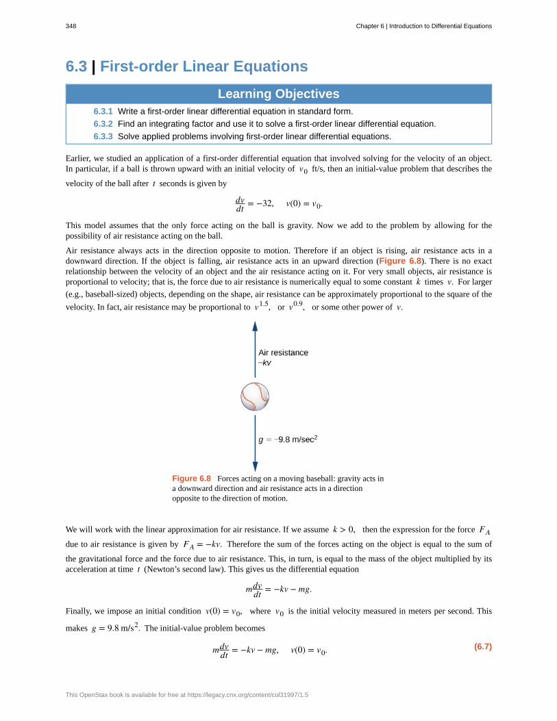
6.3 | First-order Linear Equations
Learning Objectives6.3.1 Write a first-order linear differential equation in standard form.
6.3.2 Find an integrating factor and use it to solve a first-order linear differential equation.
6.3.3 Solve applied problems involving first-order linear differential equations.
Earlier, we studied an application of a first-order differential equation that involved solving for the velocity of an object.In particular, if a ball is thrown upward with an initial velocity of v0 ft/s, then an initial-value problem that describes the
velocity of the ball after t seconds is given by
dvdt = −32, v(0) = v0.
This model assumes that the only force acting on the ball is gravity. Now we add to the problem by allowing for thepossibility of air resistance acting on the ball.
Air resistance always acts in the direction opposite to motion. Therefore if an object is rising, air resistance acts in adownward direction. If the object is falling, air resistance acts in an upward direction (Figure 6.8). There is no exactrelationship between the velocity of an object and the air resistance acting on it. For very small objects, air resistance isproportional to velocity; that is, the force due to air resistance is numerically equal to some constant k times v. For larger
(e.g., baseball-sized) objects, depending on the shape, air resistance can be approximately proportional to the square of the
velocity. In fact, air resistance may be proportional to v1.5, or v0.9, or some other power of v.
Figure 6.8 Forces acting on a moving baseball: gravity acts ina downward direction and air resistance acts in a directionopposite to the direction of motion.
We will work with the linear approximation for air resistance. If we assume k > 0, then the expression for the force FA
due to air resistance is given by FA = −kv. Therefore the sum of the forces acting on the object is equal to the sum of
the gravitational force and the force due to air resistance. This, in turn, is equal to the mass of the object multiplied by itsacceleration at time t (Newton’s second law). This gives us the differential equation
mdvdt = −kv − mg.
Finally, we impose an initial condition v(0) = v0, where v0 is the initial velocity measured in meters per second. This
makes g = 9.8 m/s2. The initial-value problem becomes
(6.7)mdvdt = −kv − mg, v(0) = v0.
348 Chapter 6 | Introduction to Differential Equations
This OpenStax book is available for free at https://legacy.cnx.org/content/col31997/1.5
The differential equation in this initial-value problem is an example of a first-order linear differential equation. (Recall thata differential equation is first-order if the highest-order derivative that appears in the equation is 1.) In this section, we
study first-order linear equations and examine a method for finding a general solution to these types of equations, as well assolving initial-value problems involving them.
Definition
A first-order differential equation is linear if it can be written in the form
(6.8)a(x)y′ + b(x)y = c(x),
where a(x), b(x), and c(x) are arbitrary functions of x.
Remember that the unknown function y depends on the variable x; that is, x is the independent variable and y is the
dependent variable. Some examples of first-order linear differential equations are
⎛⎝3x2 − 4⎞⎠y′ + (x − 3)y = sinx
(sinx)y′ − (cosx)y = cotx
4xy′ + (3lnx)y = x3 − 4x.
Examples of first-order nonlinear differential equations include
⎛⎝y′⎞⎠4 − ⎛
⎝y′⎞⎠3 = (3x − 2)⎛⎝y + 4⎞⎠4y′ + 3y3 = 4x − 5
⎛⎝y′⎞⎠2 = siny + cosx.
These equations are nonlinear because of terms like ⎛⎝y′⎞⎠4, y3, etc. Due to these terms, it is impossible to put these
equations into the same form as Equation 6.8.
Standard FormConsider the differential equation
⎛⎝3x2 − 4⎞⎠y′ + (x − 3)y = sinx.
Our main goal in this section is to derive a solution method for equations of this form. It is useful to have the coefficient of
y′ be equal to 1. To make this happen, we divide both sides by 3x2 − 4.
y′ + ⎛⎝ x − 33x2 − 4
⎞⎠y = sinx
3x2 − 4
This is called the standard form of the differential equation. We will use it later when finding the solution to a generalfirst-order linear differential equation. Returning to Equation 6.8, we can divide both sides of the equation by a(x). This
leads to the equation
(6.9)y′ + b(x)a(x)y = c(x)
a(x).
Now define p(x) = b(x)a(x) and q(x) = c(x)
a(x). Then Equation 6.8 becomes
(6.10)y′ + p(x)y = q(x).
We can write any first-order linear differential equation in this form, and this is referred to as the standard form for a first-order linear differential equation.
Chapter 6 | Introduction to Differential Equations 349
(6.11)
6.11
Example 6.12
Writing First-Order Linear Equations in Standard Form
Put each of the following first-order linear differential equations into standard form. Identify p(x) and q(x) for
each equation.
a. y′ = 3x − 4y
b.3xy′
4y − 3 = 2 (here x ≠ 0)
c. y = 3y′ − 4x2 + 5
Solution
a. Add 4y to both sides:
y′ + 4y = 3x.
In this equation, p(x) = 4 and q(x) = 3x.
b. Multiply both sides by 4y − 3, then subtract 8y from each side:
3xy′4y − 3 = 2
3xy′ = 2⎛⎝4y − 3⎞⎠3xy′ = 8y − 6
3xy′ − 8y = −6.
Finally, divide both sides by 3x to make the coefficient of y′ equal to 1:
y′ − 83xy = − 2
3x.
This is allowable because in the original statement of this problem we assumed that x ≠ 0. (If x = 0then the original equation becomes 0 = 2, which is clearly a false statement.)
In this equation, p(x) = − 83x and q(x) = − 2
3x.
c. Subtract y from each side and add 4x2 − 5:
3y′ − y = 4x2 − 5.
Next divide both sides by 3:
y′ − 13y = 4
3x2 − 5
3.
In this equation, p(x) = − 13 and q(x) = 4
3x2 − 5
3.
Put the equation(x + 3)y′
2x − 3y − 4 = 5 into standard form and identify p(x) and q(x).
350 Chapter 6 | Introduction to Differential Equations
This OpenStax book is available for free at https://legacy.cnx.org/content/col31997/1.5
Integrating FactorsWe now develop a solution technique for any first-order linear differential equation. We start with the standard form of afirst-order linear differential equation:
(6.12)y′ + p(x)y = q(x).
The first term on the left-hand side of Equation 6.9 is the derivative of the unknown function, and the second term isthe product of a known function with the unknown function. This is somewhat reminiscent of the product rule from theDifferentiation Rules (https://legacy.cnx.org/content/m53575/latest/) section. If we multiply Equation 6.10 bya yet-to-be-determined function μ(x), then the equation becomes
(6.13)μ(x)y′ + μ(x)p(x)y = μ(x)q(x).
The left-hand side Equation 6.12 can be matched perfectly to the product rule:
ddx⎡⎣ f (x)g(x)⎤⎦ = f ′ (x)g(x) + f (x)g′ (x).
Matching term by term gives y = f (x), g(x) = μ(x), and g′ (x) = μ(x)p(x). Taking the derivative of g(x) = μ(x) and
setting it equal to the right-hand side of g′ (x) = μ(x)p(x) leads to
μ′ (x) = μ(x)p(x).
This is a first-order, separable differential equation for μ(x). We know p(x) because it appears in the differential equation
we are solving. Separating variables and integrating yields
μ′ (x)μ(x) = p(x)
⌠⌡μ′ (x)μ(x) dx = ∫ p(x)dx
ln|μ(x)| = ∫ p(x)dx + C
eln|μ(x)| = e∫ p(x)dx + C
|μ(x)| = C1 e∫ p(x)dx
μ(x) = C2 e∫ p(x)dx
.
Here C2 can be an arbitrary (positive or negative) constant. This leads to a general method for solving a first-order linear
differential equation. We first multiply both sides of Equation 6.10 by the integrating factor μ(x). This gives
(6.14)μ(x)y′ + μ(x)p(x)y = μ(x)q(x).
The left-hand side of Equation 6.13 can be rewritten as ddx⎛⎝μ(x)y⎞⎠.
(6.15)ddx⎛⎝μ(x)y⎞⎠ = μ(x)q(x).
Next integrate both sides of Equation 6.14 with respect to x.
(6.16)⌠⌡ddx⎛⎝μ(x)y⎞⎠dx = ∫ μ(x)q(x)dx
μ(x)y = ∫ μ(x)q(x)dx.
Divide both sides of Equation 6.15 by μ(x):
(6.17)y = 1μ(x)⎡⎣∫ μ(x)q(x)dx + C⎤⎦.
Since μ(x) was previously calculated, we are now finished. An important note about the integrating constant C: It may
Chapter 6 | Introduction to Differential Equations 351
seem that we are inconsistent in the usage of the integrating constant. However, the integral involving p(x) is necessary in
order to find an integrating factor for Equation 6.9. Only one integrating factor is needed in order to solve the equation;therefore, it is safe to assign a value for C for this integral. We chose C = 0. When calculating the integral inside the
brackets in Equation 6.15, it is necessary to keep our options open for the value of the integrating constant, because ourgoal is to find a general family of solutions to Equation 6.9. This integrating factor guarantees just that.
Problem-Solving Strategy: Solving a First-order Linear Differential Equation
1. Put the equation into standard form and identify p(x) and q(x).
2. Calculate the integrating factor μ(x) = e∫ p(x)dx
.
3. Multiply both sides of the differential equation by μ(x).
4. Integrate both sides of the equation obtained in step 3, and divide both sides by μ(x).
5. If there is an initial condition, determine the value of C.
Example 6.13
Solving a First-order Linear Equation
Find a general solution for the differential equation xy′ + 3y = 4x2 − 3x. Assume x > 0.
Solution
1. To put this differential equation into standard form, divide both sides by x:
y′ + 3xy = 4x − 3.
Therefore p(x) = 3x and q(x) = 4x − 3.
2. The integrating factor is μ(x) = e∫ (3/x)dx
= e3lnx = x3.
3. Multiplying both sides of the differential equation by μ(x) gives us
x3 y′ + x3 ⎛⎝3x⎞⎠y = x3 (4x − 3)
x3 y′ + 3x2 y = 4x4 − 3x3
ddx⎛⎝x3 y⎞⎠ = 4x4 − 3x3.
4. Integrate both sides of the equation.
⌠⌡ddx⎛⎝x3 y⎞⎠dx = ∫ 4x4 − 3x3dx
x3 y = 4x5
5 − 3x4
4 + C
y = 4x2
5 − 3x4 + Cx−3.
5. There is no initial value, so the problem is complete.
Analysis
352 Chapter 6 | Introduction to Differential Equations
This OpenStax book is available for free at https://legacy.cnx.org/content/col31997/1.5

6.12
You may have noticed the condition that was imposed on the differential equation; namely, x > 0. For any
nonzero value of C, the general solution is not defined at x = 0. Furthermore, when x < 0, the integrating
factor changes. The integrating factor is given by Equation 6.13 as f (x) = e∫ p(x)dx
. For this p(x) we get
e∫ p(x)dx =
e∫ (3/x)dx
= e3ln|x| = |x|3,
since x < 0. The behavior of the general solution changes at x = 0 largely due to the fact that p(x) is not
defined there.
Find the general solution to the differential equation (x − 2)y′ + y = 3x2 + 2x. Assume x > 2.
Now we use the same strategy to find the solution to an initial-value problem.
Example 6.14
A First-order Linear Initial-Value Problem
Solve the initial-value problem
y′ + 3y = 2x − 1, y(0) = 3.
Solution
1. This differential equation is already in standard form with p(x) = 3 and q(x) = 2x − 1.
2. The integrating factor is μ(x) = e∫ 3dx
= e3x.
3. Multiplying both sides of the differential equation by μ(x) gives
e3x y′ + 3e3x y = (2x − 1)e3x
ddx⎡⎣ye3x⎤⎦ = (2x − 1)e3x.
Integrate both sides of the equation:
⌠⌡ddx⎡⎣ye3x⎤⎦dx = ∫ (2x − 1)e3x dx
ye3x = e3x
3 (2x − 1) − ⌠⌡23e
3x dx
ye3x = e3x (2x − 1)3 − 2e3x
9 + C
y = 2x − 13 − 2
9 + Ce−3x
y = 2x3 − 5
9 + Ce−3x.
4. Now substitute x = 0 and y = 3 into the general solution and solve for C:
Chapter 6 | Introduction to Differential Equations 353
6.13
y = 23x − 5
9 + Ce−3x
3 = 23(0) − 5
9 + Ce−3(0)
3 = −59 + C
C = 329 .
Therefore the solution to the initial-value problem is
y = 23x − 5
9 + 329 e−3x.
Solve the initial-value problem y′ − 2y = 4x + 3 y(0) = −2.
Applications of First-order Linear Differential EquationsWe look at two different applications of first-order linear differential equations. The first involves air resistance as it relatesto objects that are rising or falling; the second involves an electrical circuit. Other applications are numerous, but most aresolved in a similar fashion.
Free fall with air resistance
We discussed air resistance at the beginning of this section. The next example shows how to apply this concept for a ball invertical motion. Other factors can affect the force of air resistance, such as the size and shape of the object, but we ignorethem here.
Example 6.15
A Ball with Air Resistance
A racquetball is hit straight upward with an initial velocity of 2 m/s. The mass of a racquetball is approximately
0.0427 kg. Air resistance acts on the ball with a force numerically equal to 0.5v, where v represents the
velocity of the ball at time t.
a. Find the velocity of the ball as a function of time.
b. How long does it take for the ball to reach its maximum height?
c. If the ball is hit from an initial height of 1 meter, how high will it reach?
Solution
a. The mass m = 0.0427 kg, k = 0.5, and g = 9.8 m/s2. The initial velocity is v0 = 2 m/s. Therefore
the initial-value problem is
0.0427dvdt = −0.5v − 0.0427(9.8), v0 = 2.
Dividing the differential equation by 0.0427 gives
354 Chapter 6 | Introduction to Differential Equations
This OpenStax book is available for free at https://legacy.cnx.org/content/col31997/1.5
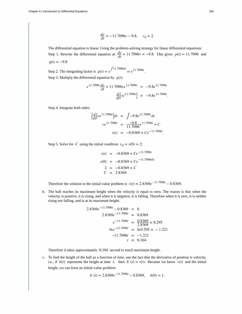
dvdt = −11.7096v − 9.8, v0 = 2.
The differential equation is linear. Using the problem-solving strategy for linear differential equations:
Step 1. Rewrite the differential equation as dvdt + 11.7096v = −9.8. This gives p(t) = 11.7096 and
q(t) = −9.8
Step 2. The integrating factor is μ(t) = e∫ 11.7096dt
= e11.7096t.Step 3. Multiply the differential equation by μ(t):
e11.7096t dvdt + 11.7096ve11.7096t = −9.8e11.7096t
ddt⎡⎣ve11.7096t⎤⎦ = −9.8e11.7096t.
Step 4. Integrate both sides:
⌠⌡ddt⎡⎣ve11.7096t⎤⎦dt = ∫ −9.8e11.7096t dt
ve11.7096t = −9.811.7096e
11.7096t + C
v(t) = −0.8369 + Ce−11.7096t.
Step 5. Solve for C using the initial condition v0 = v(0) = 2:
v(t) = −0.8369 + Ce−11.7096t
v(0) = −0.8369 + Ce−11.7096(0)
2 = −0.8369 + CC = 2.8369.
Therefore the solution to the initial-value problem is v(t) = 2.8369e−11.7096t − 0.8369.
b. The ball reaches its maximum height when the velocity is equal to zero. The reason is that when thevelocity is positive, it is rising, and when it is negative, it is falling. Therefore when it is zero, it is neitherrising nor falling, and is at its maximum height:
2.8369e−11.7096t − 0.8369 = 02.8369e−11.7096t = 0.8369
e−11.7096t = 0.83692.8369 ≈ 0.295
lne−11.7096t = ln0.295 ≈ − 1.221−11.7096t = −1.221
t ≈ 0.104.
Therefore it takes approximately 0.104 second to reach maximum height.
c. To find the height of the ball as a function of time, use the fact that the derivative of position is velocity,i.e., if h(t) represents the height at time t, then h′ (t) = v(t). Because we know v(t) and the initial
height, we can form an initial-value problem:
h′ (t) = 2.8369e−11.7096t − 0.8369, h(0) = 1.
Chapter 6 | Introduction to Differential Equations 355
6.14
Integrating both sides of the differential equation with respect to t gives
∫ h′ (t)dt = ∫ 2.8369e−11.7096t − 0.8369dt
h(t) = − 2.836911.7096e
−11.7096t − 0.8369t + C
h(t) = −0.2423e−11.7096t − 0.8369t + C.
Solve for C by using the initial condition:
h(t) = −0.2423e−11.7096t − 0.8369t + C
h(0) = −0.2423e−11.7096(0) − 0.8369(0) + C1 = −0.2423 + CC = 1.2423.
Therefore
h(t) = −0.2423e−11.7096t − 0.8369t + 1.2423.
After 0.104 second, the height is given by
h(0.2) = −0.2423e−11.7096t − 0.8369t + 1.2423 ≈ 1.0836 meter.
The weight of a penny is 2.5 grams (United States Mint, “Coin Specifications,” accessed April 9, 2015,
http://www.usmint.gov/about_the_mint/?action=coin_specifications), and the upper observation deck of theEmpire State Building is 369 meters above the street. Since the penny is a small and relatively smooth object,
air resistance acting on the penny is actually quite small. We assume the air resistance is numerically equal to0.0025v. Furthermore, the penny is dropped with no initial velocity imparted to it.
a. Set up an initial-value problem that represents the falling penny.
b. Solve the problem for v(t).
c. What is the terminal velocity of the penny (i.e., calculate the limit of the velocity as t approaches
infinity)?
Electrical Circuits
A source of electromotive force (e.g., a battery or generator) produces a flow of current in a closed circuit, and this currentproduces a voltage drop across each resistor, inductor, and capacitor in the circuit. Kirchhoff’s Loop Rule states that the sumof the voltage drops across resistors, inductors, and capacitors is equal to the total electromotive force in a closed circuit.We have the following three results:
1. The voltage drop across a resistor is given by
ER = Ri,
where R is a constant of proportionality called the resistance, and i is the current.
2. The voltage drop across an inductor is given by
EL = Li′,
356 Chapter 6 | Introduction to Differential Equations
This OpenStax book is available for free at https://legacy.cnx.org/content/col31997/1.5
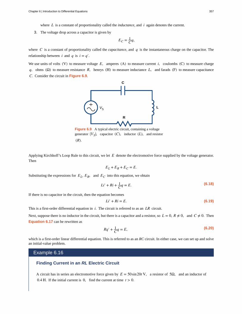
where L is a constant of proportionality called the inductance, and i again denotes the current.
3. The voltage drop across a capacitor is given by
EC = 1Cq,
where C is a constant of proportionality called the capacitance, and q is the instantaneous charge on the capacitor. The
relationship between i and q is i = q′.
We use units of volts (V) to measure voltage E, amperes (A) to measure current i, coulombs (C) to measure charge
q, ohms (Ω) to measure resistance R, henrys (H) to measure inductance L, and farads (F) to measure capacitance
C. Consider the circuit in Figure 6.9.
Figure 6.9 A typical electric circuit, containing a voltagegenerator ⎛⎝VS
⎞⎠, capacitor (C), inductor (L), and resistor
(R).
Applying Kirchhoff’s Loop Rule to this circuit, we let E denote the electromotive force supplied by the voltage generator.
Then
EL + ER + EC = E.
Substituting the expressions for EL, ER, and EC into this equation, we obtain
(6.18)Li′ + Ri + 1Cq = E.
If there is no capacitor in the circuit, then the equation becomes
(6.19)Li′ + Ri = E.
This is a first-order differential equation in i. The circuit is referred to as an LR circuit.
Next, suppose there is no inductor in the circuit, but there is a capacitor and a resistor, so L = 0, R ≠ 0, and C ≠ 0. Then
Equation 6.17 can be rewritten as
(6.20)Rq′ + 1Cq = E,
which is a first-order linear differential equation. This is referred to as an RC circuit. In either case, we can set up and solvean initial-value problem.
Example 6.16
Finding Current in an RL Electric Circuit
A circuit has in series an electromotive force given by E = 50sin20t V, a resistor of 5Ω, and an inductor of
0.4 H. If the initial current is 0, find the current at time t > 0.
Chapter 6 | Introduction to Differential Equations 357

Solution
We have a resistor and an inductor in the circuit, so we use Equation 6.18. The voltage drop across the resistor isgiven by ER = Ri = 5i. The voltage drop across the inductor is given by EL = Li′ = 0.4i′. The electromotive
force becomes the right-hand side of Equation 6.18. Therefore Equation 6.18 becomes
0.4i′ + 5i = 50sin20t.
Dividing both sides by 0.4 gives the equation
i′ + 12.5i = 125sin20t.
Since the initial current is 0, this result gives an initial condition of i(0) = 0. We can solve this initial-value
problem using the five-step strategy for solving first-order differential equations.
Step 1. Rewrite the differential equation as i′ + 12.5i = 125sin20t. This gives p(t) = 12.5 and
q(t) = 125sin20t.
Step 2. The integrating factor is μ(t) = e∫ 12.5dt
= e12.5t.
Step 3. Multiply the differential equation by μ(t):
e12.5t i′ + 12.5e12.5t i = 125e12.5t sin20tddt⎡⎣ie12.5t⎤⎦ = 125e12.5t sin20t.
Step 4. Integrate both sides:
⌠⌡ddt⎡⎣ie12.5t⎤⎦dt = ∫ 125e12.5t sin20t dt
ie12.5t = ⎛⎝250sin20t − 400cos20t
89⎞⎠e12.5t + C
i(t) = 250sin20t − 400cos20t89 + Ce−12.5t.
Step 5. Solve for C using the initial condition v(0) = 2:
i(t) = 250sin20t − 400cos20t89 + Ce−12.5t
i(0) = 250sin20(0) − 400cos20(0)89 + Ce−12.5(0)
0 = −40089 + C
C = 40089 .
Therefore the solution to the initial-value problem is
i(t) = 250sin20t − 400cos20t + 400e−12.5t
89 = 250sin20t − 400cos20t89 + 400e−12.5t
89 .
The first term can be rewritten as a single cosine function. First, multiply and divide by 2502 + 4002 = 50 89:
250sin20t − 400cos20t89 = 50 89
89⎛⎝250sin20t − 400cos20t
50 89⎞⎠
= − 50 8989⎛⎝8cos20t
89− 5sin20t
89⎞⎠.
Next, define φ to be an acute angle such that cosφ = 889
. Then sinφ = 589
and
358 Chapter 6 | Introduction to Differential Equations
This OpenStax book is available for free at https://legacy.cnx.org/content/col31997/1.5
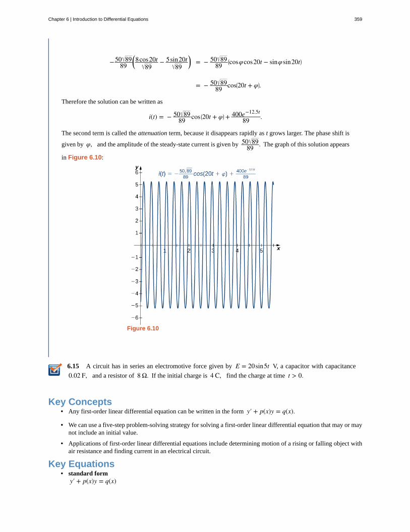
6.15
−50 8989⎛⎝8cos20t
89− 5sin20t
89⎞⎠ = − 50 89
89⎛⎝cosφcos20t − sinφsin20t⎞⎠
= − 50 8989 cos⎛⎝20t + φ⎞⎠.
Therefore the solution can be written as
i(t) = − 50 8989 cos ⎛⎝20t + φ⎞⎠+ 400e−12.5t
89 .
The second term is called the attenuation term, because it disappears rapidly as t grows larger. The phase shift is
given by φ, and the amplitude of the steady-state current is given by 50 8989 . The graph of this solution appears
in Figure 6.10:
Figure 6.10
A circuit has in series an electromotive force given by E = 20sin5t V, a capacitor with capacitance
0.02 F, and a resistor of 8 Ω. If the initial charge is 4 C, find the charge at time t > 0.
Key Concepts• Any first-order linear differential equation can be written in the form y′ + p(x)y = q(x).
• We can use a five-step problem-solving strategy for solving a first-order linear differential equation that may or maynot include an initial value.
• Applications of first-order linear differential equations include determining motion of a rising or falling object withair resistance and finding current in an electrical circuit.
Key Equations• standard form
y′ + p(x)y = q(x)
Chapter 6 | Introduction to Differential Equations 359

• integrating factor
μ(x) = e∫ p(x)dx
360 Chapter 6 | Introduction to Differential Equations
This OpenStax book is available for free at https://legacy.cnx.org/content/col31997/1.5
6.3 EXERCISESAre the following differential equations linear? Explainyour reasoning.
115.dydx = x2 y + sinx
116.dydt = ty
117.dydt + y2 = x
118. y′ = x3 + ex
119. y′ = y + ey
Write the following first-order differential equations instandard form.
120. y′ = x3 y + sinx
121. y′ + 3y − lnx = 0
122. −xy′ = (3x + 2)y + xex
123.dydt = 4y + ty + tan t
124.dydt = yx(x + 1)
What are the integrating factors for the followingdifferential equations?
125. y′ = xy + 3
126. y′ + ex y = sinx
127. y′ = x ln(x)y + 3x
128.dydx = tanh(x)y + 1
129.dydt + 3ty = et y
Solve the following differential equations by usingintegrating factors.
130. y′ = 3y + 2
131. y′ = 2y − x2
132. xy′ = 3y − 6x2
133. (x + 2)y′ = 3x + y
134. y′ = 3x + xy
135. xy′ = x + y
136. sin(x)y′ = y + 2x
137. y′ = y + ex
138. xy′ = 3y + x2
139. y′ + lnx = yx
Solve the following differential equations. Use yourcalculator to draw a family of solutions. Are there certaininitial conditions that change the behavior of the solution?
140. [T] (x + 2)y′ = 2y − 1
141. [T] y′ = 3et/3 − 2y
142. [T] xy′ + y2 = sin(3t)
143. [T] xy′ = 2cosxx − 3y
144. [T] (x + 1)y′ = 3y + x2 + 2x + 1
145. [T] sin(x)y′ + cos(x)y = 2x
146. [T] x2 + 1y′ = y + 2
147. [T] x3 y′ + 2x2 y = x + 1
Solve the following initial-value problems by usingintegrating factors.
148. y′ + y = x, y(0) = 3
149. y′ = y + 2x2, y(0) = 0
150. xy′ = y − 3x3, y(1) = 0
151. x2 y′ = xy − lnx, y(1) = 1
152. ⎛⎝1 + x2⎞⎠y′ = y − 1, y(0) = 0
153. xy′ = y + 2x lnx, y(1) = 5
Chapter 6 | Introduction to Differential Equations 361

154. (2 + x)y′ = y + 2 + x, y(0) = 0
155. y′ = xy + 2xex, y(0) = 2
156. xy′ = y + 2x, y(0) = 1
157. y′ = 2y + xex, y(0) = −1
158. A falling object of mass m can reach terminal
velocity when the drag force is proportional to its velocity,with proportionality constant k. Set up the differential
equation and solve for the velocity given an initial velocityof 0.
159. Using your expression from the preceding problem,what is the terminal velocity? (Hint: Examine the limitingbehavior; does the velocity approach a value?)
160. [T] Using your equation for terminal velocity, solvefor the distance fallen. How long does it take to fall 5000meters if the mass is 100 kilograms, the acceleration due
to gravity is 9.8 m/s2 and the proportionality constant is
4?
161. A more accurate way to describe terminal velocity isthat the drag force is proportional to the square of velocity,with a proportionality constant k. Set up the differential
equation and solve for the velocity.
162. Using your expression from the preceding problem,what is the terminal velocity? (Hint: Examine the limitingbehavior: Does the velocity approach a value?)
163. [T] Using your equation for terminal velocity, solvefor the distance fallen. How long does it take to fall 5000meters if the mass is 100 kilograms, the acceleration due
to gravity is 9.8 m/s2 and the proportionality constant
is 4? Does it take more or less time than your initial
estimate?
For the following problems, determine how parameter aaffects the solution.
164. Solve the generic equation y′ = ax + y. How does
varying a change the behavior?
165. Solve the generic equation y′ = ax + y. How does
varying a change the behavior?
166. Solve the generic equation y′ = ax + xy. How does
varying a change the behavior?
167. Solve the generic equation y′ = x + axy. How does
varying a change the behavior?
168. Solve y′ − y = ekt with the initial condition
y(0) = 0. As k approaches 1, what happens to your
formula?
362 Chapter 6 | Introduction to Differential Equations
This OpenStax book is available for free at https://legacy.cnx.org/content/col31997/1.5
Chapter Review ExercisesTrue or False? Justify your answer with a proof or a counterexample.
Exercise 6.169
The differential equation y′ = 3x2 y − cos(x)y″ is linear.
Exercise 6.170
The differential equation y′ = x − y is separable.
SolutionF
Exercise 6.171
You can explicitly solve all first-order differential equations by separation or by the method of integrating factors.
Exercise 6.172
You can determine the behavior of all first-order differential equations using directional fields or Euler’s method.
SolutionT
For the following problems, find the general solution to the differential equations.
Exercise 6.173
y′ = x2 + 3ex − 2x
Exercise 6.174
y′ = 2x + cos−1 x
Solution
y(x) = 2x
ln(2) + xcos−1 x − 1 − x2 + C
Exercise 6.175
y′ = y⎛⎝x2 + 1⎞⎠
Exercise 6.176
y′ = e−y sinx
Solutiony(x) = ln(C − cosx)
Exercise 6.177
y′ = 3x − 2y
Exercise 6.178
y′ = y lny
Solution
y(x) = eeC + x
Chapter 6 | Introduction to Differential Equations 363
For the following problems, find the solution to the initial value problem.
Exercise 6.179
y′ = 8x − lnx − 3x4, y(1) = 5
Exercise 6.180
y′ = 3x − cosx + 2, y(0) = 4
Solution
y(x) = 4 + 32x
2 + 2x − sinx
Exercise 6.181
xy′ = y(x − 2), y(1) = 3
Exercise 6.182
y′ = 3y2 (x + cosx), y(0) = −2
Solution
y(x) = − 21 + 3⎛⎝x2 + 2sinx⎞⎠
Exercise 6.183
(x − 1)y′ = y − 2, y(0) = 0
Exercise 6.184
y′ = 3y − x + 6x2, y(0) = −1
Solution
y(x) = −2x2 − 2x − 13 − 2
3e3x
For the following problems, draw the directional field associated with the differential equation, then solve the differentialequation. Draw a sample solution on the directional field.
Exercise 6.185
y′ = 2y − y2
Exercise 6.186
y′ = 1x + lnx − y, for x > 0
Solution
364 Chapter 6 | Introduction to Differential Equations
This OpenStax book is available for free at https://legacy.cnx.org/content/col31997/1.5

y(x) = Ce−x + lnx
For the following problems, use Euler’s Method with n = 5 steps over the interval t = [0, 1]. Then solve the initial-value
problem exactly. How close is your Euler’s Method estimate?
Exercise 6.187
y′ = −4yx, y(0) = 1
Exercise 6.188
y′ = 3x − 2y, y(0) = 0
Solution
Euler: 0.6939, exact solution: y(x) = 3x − e−2x
2 + ln(3)
For the following problems, set up and solve the differential equations.
Exercise 6.189
A car drives along a freeway, accelerating according to a = 5sin(πt), where t represents time in minutes. Find the
velocity at any time t, assuming the car starts with an initial speed of 60 mph.
Exercise 6.190
You throw a ball of mass 2 kilograms into the air with an upward velocity of 8 m/s. Find exactly the time the ball will
remain in the air, assuming that gravity is given by g = 9.8 m/s2.
Solution4049 second
Exercise 6.191
You drop a ball with a mass of 5 kilograms out an airplane window at a height of 5000 m. How long does it take for the
ball to reach the ground?
Chapter 6 | Introduction to Differential Equations 365

Exercise 6.192
You drop the same ball of mass 5 kilograms out of the same airplane window at the same height, except this time you
assume a drag force proportional to the ball’s velocity, using a proportionality constant of 3 and the ball reaches terminal
velocity. Solve for the distance fallen as a function of time. How long does it take the ball to reach the ground?
Solution
x(t) = 5000 + 2459 − 49
3 t − 2459 e−5/3t, t = 307.8 seconds
Exercise 6.193
A drug is administered to a patient every 24 hours and is cleared at a rate proportional to the amount of drug left in the
body, with proportionality constant 0.2. If the patient needs a baseline level of 5 mg to be in the bloodstream at all times,
how large should the dose be?
Exercise 6.194
A 1000 -liter tank contains pure water and a solution of 0.2 kg salt/L is pumped into the tank at a rate of 1 L/min and is
drained at the same rate. Solve for total amount of salt in the tank at time t.
Solution
T(t) = 200⎛⎝1 − e−t/1000⎞⎠
Exercise 6.195
You boil water to make tea. When you pour the water into your teapot, the temperature is 100°C. After 5 minutes in your
15°C room, the temperature of the tea is 85°C. Solve the equation to determine the temperatures of the tea at time t.How long must you wait until the tea is at a drinkable temperature (72°C)?
Exercise 6.196
The human population (in thousands) of Nevada in 1950 was roughly 160. If the carrying capacity is estimated at
10 million individuals, and assuming a growth rate of 2% per year, develop a logistic growth model and solve for the
population in Nevada at any time (use 1950 as time = 0). What population does your model predict for 2000? How close
is your prediction to the true value of 1,998,257?
Solution
P(t) = 1600000e0.02t
9840 + 160e0.02t
Exercise 6.197
Repeat the previous problem but use Gompertz growth model. Which is more accurate?
366 Chapter 6 | Introduction to Differential Equations
This OpenStax book is available for free at https://legacy.cnx.org/content/col31997/1.5
autonomous differential equation
differential equation
general solution (or family of solutions)
initial value(s)
initial velocity
initial-value problem
integrating factor
linear
order of a differential equation
particular solution
separable differential equation
separation of variables
solution to a differential equation
standard form
CHAPTER 6 REVIEW
KEY TERMSan equation in which the right-hand side is a function of y alone
an equation involving a function y = y(x) and one or more of its derivatives
the entire set of solutions to a given differential equation
a value or set of values that a solution of a differential equation satisfies for a fixed value of theindependent variable
the velocity at time t = 0
a differential equation together with an initial value or values
any function f (x) that is multiplied on both sides of a differential equation to make the side
involving the unknown function equal to the derivative of a product of two functions
description of a first-order differential equation that can be written in the form a(x)y′ + b(x)y = c(x)
the highest order of any derivative of the unknown function that appears in theequation
member of a family of solutions to a differential equation that satisfies a particular initial condition
any equation that can be written in the form y′ = f (x)g(y)
a method used to solve a separable differential equation
a function y = f (x) that satisfies a given differential equation
the form of a first-order linear differential equation obtained by writing the differential equation in theform y′ + p(x)y = q(x)
Chapter 6 | Introduction to Differential Equations 367

368 Chapter 6 | Introduction to Differential Equations
This OpenStax book is available for free at https://legacy.cnx.org/content/col31997/1.5

ANSWER KEYChapter 1
Chapter 2
Chapter 3
Chapter 4
Chapter 5
Chapter 6
Answer Key 369

370 Answer Key
This OpenStax book is available for free at https://legacy.cnx.org/content/col31997/1.5
INDEXAabsolute error, 291, 321air resistance, 348algebraic function, 233antiderivative, 107, 150autonomous differentialequation, 336, 367
Bbase, 39, 64
Ccarbon dating, 225center of mass, 187, 229centroid, 190, 229common logarithm, 48compound interest, 220compounding interest, 43computer algebra system(CAS), 321computer algebra systems(CAS), 281cross-section, 151, 229
Ddifferential equation, 323, 367disk method, 157, 229doubling time, 222, 229drugs in the bloodstream, 346
Eearthquake, 50exponent, 39, 64exponential decay, 223, 229exponential growth, 218, 229
Ffruit flies, 130
GGabriel’s Horn, 304general solution, 325general solution (or family ofsolutions), 367growth of bacteria, 129
Hhalf-life, 225, 229horizontal line test, 22, 64hyperbolic functions, 51, 64
Iimproper integral, 301, 321indefinite integral, 109, 150indefinite integrals, 236initial value, 326
initial value problem, 150initial value(s), 367initial velocity, 330, 367initial-value problem, 115, 326,367integrating factor, 351, 367integration by parts, 231, 321integration table, 321integration tables, 281inverse function, 21, 64inverse hyperbolic functions, 54,64inverse trigonometric functions,29, 64
Llamina, 190, 229Laplace transform, 312, 315linear, 349, 367logarithmic differentiation, 96,106logarithmic function, 233
Mmethod of cylindrical shells, 229method of cylindrical shells.,173method of equating coefficients,270method of strategic substitution,270midpoint rule, 287, 321moment, 187, 229
Nnatural exponential function, 44,64, 88natural logarithm, 45, 64natural logarithmic function, 88Newton’s law of cooling, 223,342Newton’s second law of motion,329number e, 64number e , 44
numerical integration, 287, 321
Oone-to-one function, 22, 64order of a differential equation,324, 367
Ppartial fraction decomposition,268, 321
particular solution, 326, 367periodic function, 64periodic functions., 13population growth, 39Population growth, 218power reduction formula, 321power reduction formulas, 251power-reducing identities, 244price–demand function, 127probability, 304probability density function, 316
Rradians, 5, 64rational functions, 268RC circuit, 357Regiomontanus’ problem, 124relative error, 291, 321restricted domain, 27, 64Richter scale, 50Riemann sums, 287
Sseparable differential equation,336, 367separation of variables, 336,367simple interest, 220Simpson’s rule, 293, 321slicing method, 153, 229solid of revolution, 154, 229solution concentrations, 340solution to a differentialequation, 323, 367standard form, 349, 367symmetry principle, 190, 229
Ttheorem of Pappus for volume,199, 229traffic accidents, 304trapezoidal rule, 289trigonometric functions, 7, 64trigonometric identity, 11, 64trigonometric integral, 321trigonometric integrals, 243trigonometric substitution, 255,321
Wwasher method, 163, 229
Index 371

372 Index
This OpenStax book is available for free at https://legacy.cnx.org/content/col31997/1.5
ATTRIBUTIONSCollection: Math for Engineering & Technology IIEdited by: Ali AlaviURL: https://legacy.cnx.org/content/col31997/1.5/Copyright: Ali AlaviLicense: http://creativecommons.org/licenses/by/4.0/
Module: Trigonometric FunctionsBy: OpenStaxURL: https://legacy.cnx.org/content/m53479/1.7/Copyright: Rice UniversityLicense: http://creativecommons.org/licenses/by-nc-sa/4.0/
Module: Inverse FunctionsBy: OpenStaxURL: https://legacy.cnx.org/content/m53480/1.9/Copyright: Rice UniversityLicense: http://creativecommons.org/licenses/by-nc-sa/4.0/
Module: Exponential and Logarithmic FunctionsBy: OpenStaxURL: https://legacy.cnx.org/content/m53481/1.15/Copyright: Rice UniversityLicense: http://creativecommons.org/licenses/by-nc-sa/4.0/
Module: Derivatives of Trigonometric FunctionsBy: OpenStaxURL: https://legacy.cnx.org/content/m53578/1.10/Copyright: Rice UniversityLicense: http://creativecommons.org/licenses/by-nc-sa/4.0/
Module: Derivatives of Inverse FunctionsBy: OpenStaxURL: https://legacy.cnx.org/content/m53584/1.10/Copyright: Rice UniversityLicense: http://creativecommons.org/licenses/by-nc-sa/4.0/
Module: Derivatives of Exponential and Logarithmic FunctionsBy: OpenStaxURL: https://legacy.cnx.org/content/m53586/1.10/Copyright: Rice UniversityLicense: http://creativecommons.org/licenses/by-nc-sa/4.0/
Module: AntiderivativesBy: OpenStaxURL: https://legacy.cnx.org/content/m53621/1.8/Copyright: Rice UniversityLicense: http://creativecommons.org/licenses/by-nc-sa/4.0/
Module: Integrals Involving Exponential and Logarithmic FunctionsBy: OpenStaxURL: https://legacy.cnx.org/content/m53635/1.8/Copyright: Rice UniversityLicense: http://creativecommons.org/licenses/by-nc-sa/4.0/
Module: Integrals Resulting in Inverse Trigonometric FunctionsBy: OpenStaxURL: https://legacy.cnx.org/content/m53636/1.13/
Index 373

Copyright: Rice UniversityLicense: http://creativecommons.org/licenses/by-nc-sa/4.0/
Module: Determining Volumes by SlicingBy: OpenStaxURL: https://legacy.cnx.org/content/m53642/1.8/Copyright: Rice UniversityLicense: http://creativecommons.org/licenses/by-nc-sa/4.0/
Module: Volumes of Revolution: Cylindrical ShellsBy: OpenStaxURL: https://legacy.cnx.org/content/m53643/1.10/Copyright: Rice UniversityLicense: http://creativecommons.org/licenses/by-nc-sa/4.0/
Module: Moments and Centers of MassBy: OpenStaxURL: https://legacy.cnx.org/content/m53649/1.9/Copyright: Rice UniversityLicense: http://creativecommons.org/licenses/by-nc-sa/4.0/
Module: Integrals, Exponential Functions, and LogarithmsBy: OpenStaxURL: https://legacy.cnx.org/content/m53650/1.9/Copyright: Rice UniversityLicense: http://creativecommons.org/licenses/by-nc-sa/4.0/
Module: Exponential Growth and DecayBy: OpenStaxURL: https://legacy.cnx.org/content/m53651/1.10/Copyright: Rice UniversityLicense: http://creativecommons.org/licenses/by-nc-sa/4.0/
Module: Integration by PartsBy: OpenStaxURL: https://legacy.cnx.org/content/m53656/1.6/Copyright: Rice UniversityLicense: http://creativecommons.org/licenses/by-nc-sa/4.0/
Module: Trigonometric IntegralsBy: OpenStax Calculus and OpenStaxURL: https://legacy.cnx.org/content/m53657/1.8/Copyright: OpenStax Calculus and Rice UniversityLicense: http://creativecommons.org/licenses/by-nc-sa/4.0/
Module: Trigonometric SubstitutionBy: OpenStaxURL: https://legacy.cnx.org/content/m53659/1.9/Copyright: Rice UniversityLicense: http://creativecommons.org/licenses/by-nc-sa/4.0/
Module: Partial FractionsBy: OpenStaxURL: https://legacy.cnx.org/content/m53681/1.6/Copyright: Rice UniversityLicense: http://creativecommons.org/licenses/by-nc-sa/4.0/
Module: Other Strategies for IntegrationBy: OpenStaxURL: https://legacy.cnx.org/content/m53684/1.5/
374 Index
This OpenStax book is available for free at https://legacy.cnx.org/content/col31997/1.5
Copyright: Rice UniversityLicense: http://creativecommons.org/licenses/by-nc-sa/4.0/
Module: Numerical IntegrationBy: OpenStaxURL: https://legacy.cnx.org/content/m53685/1.8/Copyright: Rice UniversityLicense: http://creativecommons.org/licenses/by-nc-sa/4.0/
Module: Improper IntegralsBy: OpenStaxURL: https://legacy.cnx.org/content/m53686/1.9/Copyright: Rice UniversityLicense: http://creativecommons.org/licenses/by-nc-sa/4.0/
Module: Basics of Differential EquationsBy: OpenStaxURL: https://legacy.cnx.org/content/m53697/1.6/Copyright: Rice UniversityLicense: http://creativecommons.org/licenses/by-nc-sa/4.0/
Module: Separable EquationsBy: OpenStaxURL: https://legacy.cnx.org/content/m53704/1.7/Copyright: Rice UniversityLicense: http://creativecommons.org/licenses/by-nc-sa/4.0/
Module: First-order Linear EquationsBy: OpenStaxURL: https://legacy.cnx.org/content/m53713/1.6/Copyright: Rice UniversityLicense: http://creativecommons.org/licenses/by-nc-sa/4.0/
Index 375

376 Index
This OpenStax book is available for free at https://legacy.cnx.org/content/col31997/1.5
ABOUT CONNEXIONSSince 1999, Connexions has been pioneering a global system where anyone can create course materials and make them fullyaccessible and easily reusable free of charge. We are a Web-based authoring, teaching and learning environment open to anyoneinterested in education, including students, teachers, professors and lifelong learners. We connect ideas and facilitate educationalcommunities. Connexions's modular, interactive courses are in use worldwide by universities, community colleges, K-12 schools,distance learners, and lifelong learners. Connexions materials are in many languages, including English, Spanish, Chinese,Japanese, Italian, Vietnamese, French, Portuguese, and Thai.
Index 377