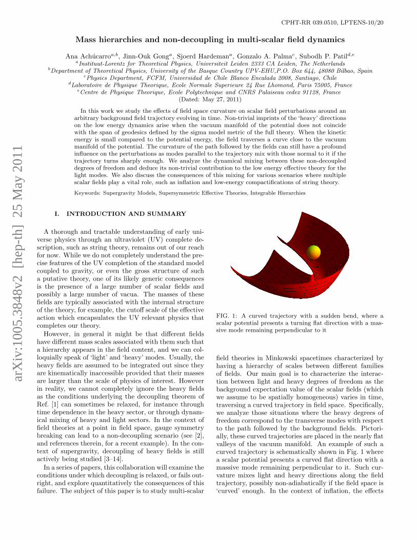
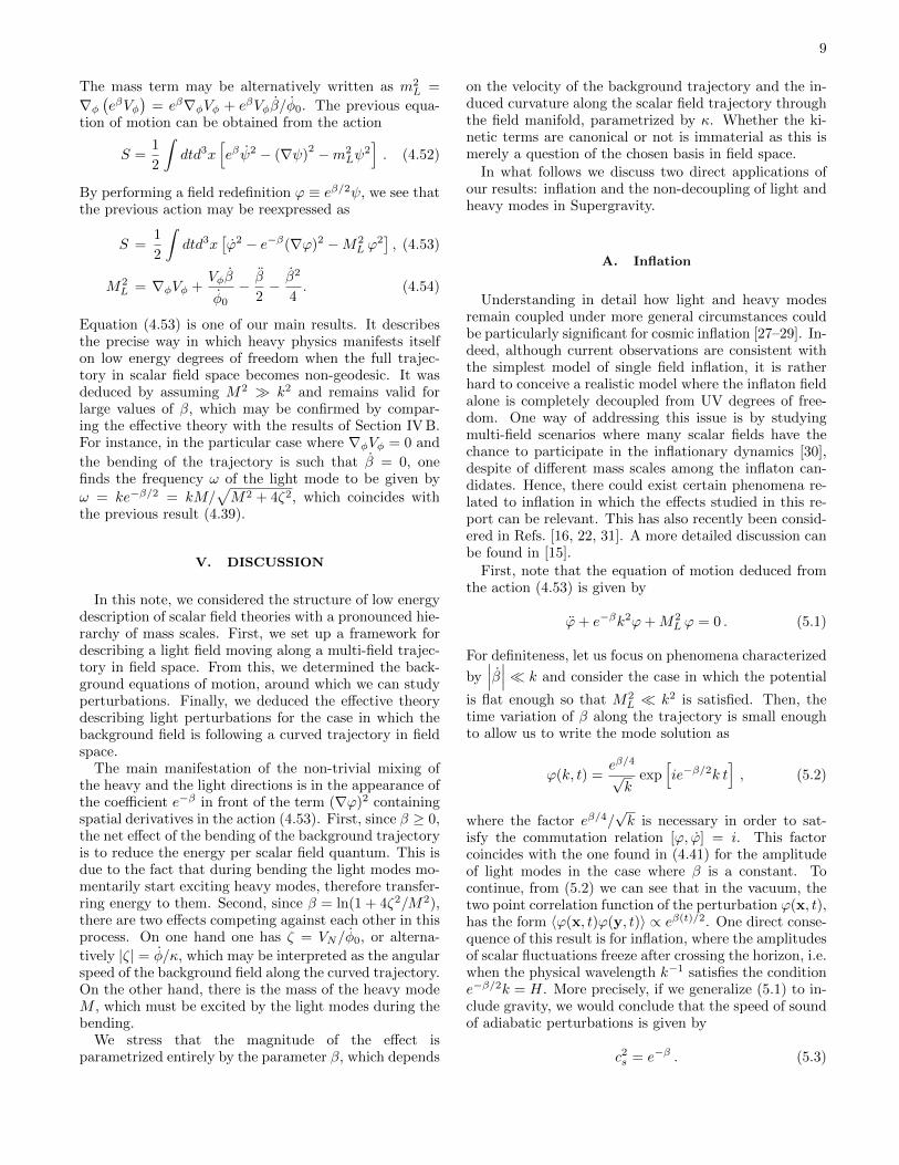
CPHT-RR 039.0510, LPTENS-10/20

Mass hierarchies and non-decoupling in multi-scalar field dynamics

Ana Achucarroa,b, Jinn-Ouk Gonga, Sjoerd Hardemana, Gonzalo A. Palmac, Subodh P. Patild,eaInstituut-Lorentz for Theoretical Physics, Universiteit Leiden 2333 CA Leiden, The Netherlands

bDepartment of Theoretical Physics, University of the Basque Country UPV-EHU,P.O. Box 644, 48080 Bilbao, SpaincPhysics Department, FCFM, Universidad de Chile Blanco Encalada 2008, Santiago, Chile

dLaboratoire de Physique Theorique, Ecole Normale Superieure 24 Rue Lhomond, Paris 75005, FranceeCentre de Physique Theorique, Ecole Polytechnique and CNRS Palaiseau cedex 91128, France

(Dated: May 27, 2011)

In this work we study the effects of field space curvature on scalar field perturbations around anarbitrary background field trajectory evolving in time. Non-trivial imprints of the ‘heavy’ directionson the low energy dynamics arise when the vacuum manifold of the potential does not coincidewith the span of geodesics defined by the sigma model metric of the full theory. When the kineticenergy is small compared to the potential energy, the field traverses a curve close to the vacuummanifold of the potential. The curvature of the path followed by the fields can still have a profoundinfluence on the perturbations as modes parallel to the trajectory mix with those normal to it if thetrajectory turns sharply enough. We analyze the dynamical mixing between these non-decoupleddegrees of freedom and deduce its non-trivial contribution to the low energy effective theory for thelight modes. We also discuss the consequences of this mixing for various scenarios where multiplescalar fields play a vital role, such as inflation and low-energy compactifications of string theory.

Keywords: Supergravity Models, Supersymmetric Effective Theories, Integrable Hierarchies

I. INTRODUCTION AND SUMMARY

A thorough and tractable understanding of early uni-verse physics through an ultraviolet (UV) complete de-scription, such as string theory, remains out of our reachfor now. While we do not completely understand the pre-cise features of the UV completion of the standard modelcoupled to gravity, or even the gross structure of sucha putative theory, one of its likely generic consequencesis the presence of a large number of scalar fields andpossibly a large number of vacua. The masses of thesefields are typically associated with the internal structureof the theory, for example, the cutoff scale of the effectiveaction which encapsulates the UV relevant physics thatcompletes our theory.

However, in general it might be that different fieldshave different mass scales associated with them such thata hierarchy appears in the field content, and we can col-loquially speak of ‘light’ and ‘heavy’ modes. Usually, theheavy fields are assumed to be integrated out since theyare kinematically inaccessible provided that their massesare larger than the scale of physics of interest. Howeverin reality, we cannot completely ignore the heavy fieldsas the conditions underlying the decoupling theorem ofRef. [1] can sometimes be relaxed, for instance throughtime dependence in the heavy sector, or through dynam-ical mixing of heavy and light sectors. In the context offield theories at a point in field space, gauge symmetrybreaking can lead to a non-decoupling scenario (see [2],and references therein, for a recent example). In the con-text of supergravity, decoupling of heavy fields is stillactively being studied [3–14].

In a series of papers, this collaboration will examine theconditions under which decoupling is relaxed, or fails out-right, and explore quantitatively the consequences of thisfailure. The subject of this paper is to study multi-scalar

FIG. 1: A curved trajectory with a sudden bend, where ascalar potential presents a turning flat direction with a mas-sive mode remaining perpendicular to it

field theories in Minkowski spacetimes characterized byhaving a hierarchy of scales between different familiesof fields. Our main goal is to characterize the interac-tion between light and heavy degrees of freedom as thebackground expectation value of the scalar fields (whichwe assume to be spatially homogeneous) varies in time,traversing a curved trajectory in field space. Specifically,we analyze those situations where the heavy degrees offreedom correspond to the transverse modes with respectto the path followed by the background fields. Pictori-ally, these curved trajectories are placed in the nearly flatvalleys of the vacuum manifold. An example of such acurved trajectory is schematically shown in Fig. 1 wherea scalar potential presents a curved flat direction with amassive mode remaining perpendicular to it. Such cur-vature mixes light and heavy directions along the fieldtrajectory, possibly non-adiabatically if the field space is‘curved’ enough. In the context of inflation, the effects

arX

iv:1

005.

3848

v2 [

hep-

th]

25

May

201

1

2

studied in this work lead to potentially observable effectsin the spectrum of primordial perturbations (see [15] andreferences therein).

In the case of two-field models, we will show that when-ever the trajectory makes a turn in field space such thatthe light direction is interchanged by a heavy direction(and vice versa), the low energy effective action describ-ing the dynamics of the light degrees of freedom gener-ically picks up a non-trivial correction, hereby parame-terized by β and given by

β = ln

(1 +

4φ20

κ2M2H

), (1.1)

where φ0 is the velocity of the background scalar field, κis the radius of curvature characterizing the bending ofthe trajectory in field space, and MH is the characteristicmass scale of the heavy modes. We emphasize that thebending is measured with respect to the geodesics of thesigma model metric, whether or not it is canonical; noticethat κ represents a distance measured in the geometricalspace of scalar fields, and therefore it has units of mass.

More precisely, at low energies (k �MH) the equationof motion describing the scalar field fluctuation parallelto the trajectory of background fields is found to be

ϕ− e−β∇2ϕ+M2L ϕ = 0 , (1.2)

with∇2 ≡ δij∂i∂j being the spatial Laplacian: see (4.53).Thus the kinetic energy term is modified by a factor ofe−β in front of the spatial gradient term, in agreementwith [16]. In the context of inflation, this can give rise tosizable effects that may be observable in the next gener-ation of the cosmic microwave background observations.For example, for inflation in supergravity models, themasses of heavy degrees of freedom during inflation aretypically of order MH = O(H), with H being the Hub-ble parameter during inflation. This leads to the naiveexpectation

eβ ∼ 1 + εM2

Pl

κ2, (1.3)

where ε ≡ −H/H2 = (φ0/H)2/(2M2Pl) is the so-called

slow-roll parameter. Then, if the bending of the trajec-tory is such that the radius of curvature κ becomes muchsmaller than MPl one then is led to eβ � 1. Such a situa-tion implies strong modifications on the scale dependenceof inflaton fluctuations, contributing non-trivial featuresto the power spectrum well within the threshold of detec-tion. The full analysis valid for inflationary cosmology is,however, more involved than the naive arguments aboveas it requires a detailed account of gravity and carefultreatments of the multi-field dynamics at horizon cross-ing. For this reason, in the present note we study thebasic features of the effects of the heavy-light field in-teractions during turns of the scalar field trajectory in aMinkowski background, and leave the study of inflation-ary de Sitter case for a separate paper [15]. We stress

here that the perspective that follows from our analysisis that the only relevant criteria for the effects we un-cover (such as the modified speed of sound for the per-turbations) is that our system deviates sufficiently froma geodesic trajectory [33].

Our formalism, and its application to inflation [15]builds upon previous work [17–20] that we extend to beable to account for the effects coming from very sharpturns and also prolonged turns in which the true groundstate deviates significantly from its single-field approx-imation. By disregarding the effects of gravity, we areable to describe in detail the evolution of the quantummodes in some idealized settings (e.g. turns at a constantrate). We also extend recent results by [16, 21], that werecover in the right limits. In particular, we are able toclarify the relevance or otherwise of non-canonical kineticterms, in particular with respect to a reduced speed ofsound in the effective low energy theory (see also [22]).We expect our results to be relevant for any phenomenawhere the variation of vacuum expectation values plays asignificant role, such us inflation, phase transitions, soli-ton interactions and soliton-radiation scattering.

In the remainder of this paper, we will first elabo-rate on the general framework and study the backgroundequations of motion in Section II. In Section III, we willstudy the theory of perturbations and the quantizationaround a general field trajectory. In Section IV, we willapply the theory to the case of a large hierarchy betweenlight and heavy degrees of freedom that span a curvedfield space trajectory. To conclude, we will discuss someapplications in Section V, in particular regarding infla-tion and the decoupling of heavy modes in supergrav-ity. Some calculational details are provided in the ap-pendices.

II. GEOMETRY OF MULTI-SCALAR FIELDMODELS

We are interested in multi-scalar field theories admit-ting a low energy effective action consisting of at mosttwo space-time derivatives. Examples of such theoriesare low energy compactifications of string theory and su-pergravity models, where the number of scalar degreesof freedom (often referred to as moduli) can be consider-ably large. For an arbitrary number ntot of scalar fieldsin a Minkowski background, the effective action of sucha theory may be written in the form

S = −∫d4x

[1

2γab∂

µφa∂µφb + V (φ)

], (2.1)

where φa, with a = 1, · · ·ntot, is a set of scalar fieldsand γab = γab(φ) is an arbitrary symmetric matrix re-stricted to be positive definite. Any contribution to thisaction containing higher space-time derivatives will besuppressed by some cutoff energy scale Λ, which we as-sume to be much larger than the energy scale of our inter-est. In low energy string compactifications, such a scale

3

Λ corresponds to the compactification scale, which maybe close to MPl. However, as mentioned before, we donot consider coupling this theory to gravity, saving thisfor a separate report [15].

In order to study the dynamics of the present systemit is useful to think of γab as a metric tensor of some ab-stract scalar manifold M of dimension ntot. This allowsus to consider the definition of several standard geometri-cal quantities related toM. For instance, the Christoffelconnections are given by

Γabc =1

2γad (∂bγdc + ∂cγbd − ∂dγbc) , (2.2)

where γab is the inverse metric satisfying γacγcb = δab,and ∂a denotes a partial derivative with respect to φa.This allows us to define covariant derivatives in the usualway as ∇aXb ≡ ∂aXb − ΓcabXc. Also, we may define theassociated Riemann tensor as

Rabcd ≡ ∂cΓabd − ∂dΓabc + ΓaceΓedb − ΓadeΓ

ecb . (2.3)

as well as the Ricci tensor Rab = Rcacb and the Ricciscalar R = γabRab. We should keep in mind that, typ-ically, there will be an energy scale ΛM associated withthe curvature of M, fixing the typical mass scale of theRicci scalar as R ∼ Λ−2

M . In many concrete situationsthe scale ΛM corresponds precisely to the aforementionedcutoff scale Λ. For example, in N = 1 supergravity real-izations of string compactifications, one typically findsthat the Ricci scalar of the Kahler manifold satisfiesR ∼M−2

Pl [23, 24]. In the following, we assume Λ ∼ ΛMand do not distinguish them.

Given these geometric quantities, we can write thebackground equation of motion of the homogeneous back-ground fields φa0 = φa0(t) from the action (2.1). If

φ0aφa0 6= 0, one may think of φa0(t) as the coordinates

parametrizing a trajectory inM, where t is the parame-ter on the curve describing the expectation value of thescalar fields. Before proceeding with a detailed analysisof these trajectories, let us emphazise that these trajec-tories may or may not be the geodesics of M, with thedetails depending on the specific form of the scalar po-tential V (φ) and the geometry ofM. Varying the action(2.1) with respect to φa, the equations of motion of φa

are then found to be

D

dtφa0 + V a = 0 , (2.4)

where we have introduced the notation DXa ≡ dXa +ΓabcX

bdφc0 and V a ≡ γab∂bV . Given a certain scalar man-ifoldM and a scalar potential V , these equations can besolved to obtain the trajectory in M traversed by thebackground scalar fields. It is convenient to define therate of variation of the scalar fields φ0 along the trajec-tory as

φ20 ≡ γabφa0φb0 . (2.5)

Since γab is positive definite, φ20 is always greater than or

equal to zero. Without loss of generality, in what follows

we assume that φ(t) > 0 for all t. Then the unit tangentvector T a to the trajectory is defined as

T a ≡ φa0

φ0

, (2.6)

and if the trajectory is curved we can define one of thenormal vectors to be

Na ≡ sN (t)

(γbc

DT b

dt

DT c

dt

)−1/2DT a

dt, (2.7)

where sN (t) = ±1 denotes the orientation of Na withrespect to the vector DT a/dt. That is, if sN (t) = +1then Na is pointing in the same direction as DT a/dt,whereas if sN (t) = −1 then Na is pointing in the oppo-site direction. Due to the presence of the square root, itis clear that Na is only well defined at intervals whereDT a/dt 6= 0. However, since DT a/dt may become zeroat finite values of t, we allow sN (t) to flip signs each timethis happens in such a way that both Na and DT a/dtremain a continuous function of t. This implies that thesign of sN may be chosen conventionally at some initialtime ti, but from then on it is subject to the equations ofmotion respected by the background [34]. As we shall seelater, in the particular case whereM is two dimensional,the presence of sN (t) in (2.7) is sufficient for Na to havea fixed orientation with respect to T a (either left-handedor right-handed).

After some formal manipulations, we can deduce κ,the radius of curvature of the trajectory followed by thevacuum expectation value φa0(t), as

1

κ=|VN |φ2

0

, (2.8)

where VN ≡ NaVa. Details of how (2.8) is derived can

be found in Appendix A. Notice that for φ0 6= 0, the onlyway of having VN = 0 is by following a straight curve forwhich there is no geodesic deviation, DT a/dt = 0. Thisresult follows the basic intuition that, during a turn inthe trajectory, the scalar fields will shift from the min-imum of the potential VN = 0 along the perpendiculardirection Na. Trajectories for which VN = 0 are in factgeodesics, and therefore the parameter κ is a useful mea-sure of the geodesic deviation caused by the potential V .On dimensional grounds, we should expect κ−1 ∼ Λ−1

M ,as the intrinsic curvature of the manifold M is the resultof the embedding in a yet higher energy completion, andthis likely bestows this manifold with a similar extrinsiccurvature scale. This extrinsic curvature is then neces-sarily the minimal extrinsic curvature for any trajectoryon M . Yet, much more curved trajectories are perfectlypossible [35] and we therefore allow a wider range of val-ues for κ.

4

III. PERTURBATION THEORY AND ITSQUANTIZATION

We now study the evolution of the scalar field fluctu-ations around the background time-dependent solutionexamined in the previous section. We extend the formal-ism of [18–20] to be able to deal with regimes of fast andor continuous turns. As we shall see, the radius of cur-vature κ couples the perturbations parallel and normalto the motion of the background fields. Let us start bywriting φa including perturbations δφa(t,x) ≡ ϕa(t,x)as

φa(t,x) = φa0(t) + ϕa(t,x) , (3.1)

where φa0(t) corresponds to the exact solution to the ho-mogeneous equation of motion (2.4). Starting from theaction (2.1), one finds the equations of motion for ϕa as

D2ϕa

dt2−∇2ϕa + Cabϕ

b = 0 , (3.2)

where

Cab = ∇bV a − φ20RacdbT cT d . (3.3)

It is convenient to rewrite these equations in terms of anew set of perturbations orthogonal to each other. Forthis we define a complete set of vielbeins eIa and workwith redefined fields

vI = eIaϕa . (3.4)

An example of a possible choice for these vielbeins is aset{eIa}

with Ta and Na among its elements [17], but wedo not consider this choice until later. Recall that thevielbeins satisfy the basic relations δIJe

IaeJb = γab and

γabeIaeJb = δIJ , which lead to

eIaD

dteaJ = −eaJ

D

dteIa , (3.5)

eaID

dteIb = −eIb

D

dteaI . (3.6)

In (3.4) the ϕa are vectors with respect to the covariantderivative D/dt, while the fields vI are scalars. Then, itis easy to show that

vI = eIaDϕa

dt− ZIJvJ , (3.7)

vI = eIaD2ϕa

dt2− 2ZIJ v

J −(ZIKZ

KJ + ZIJ

)vJ , (3.8)

where we have introduced the antisymmetric matrix ZIJas

ZIJ = eIaD

dteaJ . (3.9)

Notice that ZIJ =(eIa∂be

aJ + eIaΓabce

cJ

)φb0 = ω I

b J φb0,

where ω Ib J are the usual spin connections for non-

coordinate basis, therefore ZIJ can be used to define acovariant derivative acting on the vI -fields as

DdtvI ≡ vI + ZIJv

J . (3.10)

From (3.7) and (3.8), we can see that this new covariantderivative is related to the original covariant derivativeas

DdtvI = eIa

D

dtϕa , (3.11)

D2

dt2vI = eIa

D2

dt2ϕa . (3.12)

One can verify that this derivative is compatible with theKronecker delta in the sense that DδIJ/dt = 0. Then,it is easy to show that the equation of motion (3.2) interms of the new perturbations vI becomes

D2

dt2vI −∇2vI + CIJv

J = 0 , (3.13)

where CIJ ≡ eIaebJCab.

A. Canonical frame

In introducing the vielbeins in the previous section, wehave not specified any alignment of the moving frame. Infact, given an arbitrary frame eIa, it is always possible tofind a ‘canonical’ frame where the scalar field perturba-tions acquire canonical kinetic terms in the action. Tofind it, let us introduce a new set of fields uI defined fromthe original ones vI in the following way:

vI(t) = RIJ(t, t0)uJ(t) . (3.14)

Here, RIJ(t, t0) is a matrix satisfying the first order dif-ferential equation

d

dtRIJ = −ZIKRKJ , (3.15)

with the boundary condition RIJ(t0, t0) = δIJ . By defin-ing a new matrix SIJ to be the inverse of RIJ , namelySIKR

KJ = RIKS

KJ = δIJ , it is not difficult to see that

SIJ satisfies

d

dtS JI = −ZJKS K

I , (3.16)

where we used the fact that Z is antisymmetric in its in-dices ZIJ = −ZJI . Since both solutions to (3.15) and(3.16) are unique, the previous equation tells us thatSIJ = RJI . Thus, S corresponds to RT , the transposeof R. This means that for a fixed time t, RIJ(t, t0) isan element of the orthogonal group O(ntot), the group ofmatrices R satisfying RRT = 1. The solution of (3.15) iswell known, and may be symbolically written as

R(t, t0) = 1 +

∞∑n=1

(−1)n

n!

∫ t

t0

T [Z(t1) · · ·Z(tn)] dnt

= T exp

[−∫ t

t0

dtZ(t)

], (3.17)

5

where T stands for the time ordering symbol. That is:T[Z(t1)Z(t2) · · ·Z(tn)] corresponds to the product of nmatrices Z(ti) for which t1 ≥ t2 ≥ · · · ≥ tn. Comingback to the uI -fields, it is possible to see now that, byvirtue of (3.15) one has

DvI

dt= RIJ

duJ

dt, (3.18)

D2vI

dt2= RIJ

d2uJ

dt2. (3.19)

Inserting these relations back into the equation of motion(3.13), we obtain the equation of motion for the uI -fieldsas

d2uI

dt2−∇2uI +

[RT (t)C R(t)

]IJuJ = 0 . (3.20)

This equation of motion can be derived from an action

S =1

2

∫d4x{uI uI −∇uI · ∇uI

−[RT (t)CR(t)

]IJuIuJ

}. (3.21)

Thus, we see that the uI -fields correspond to the canon-ical fields in the usual sense. To finish, let us notice thatby construction, at the initial time t0, the canonical fieldsuI and the original fields vI coincide, uI(t0) = vI(t0).Obviously, it is always possible to redefine a new set ofcanonical fields by performing an orthogonal transforma-tion.

B. Quantization of the system

Having the canonical frame at hand, we may now quan-tize the system in the usual way. Starting from the ac-tion (3.21), the canonical momentum conjugate to uI isgiven by ΠI

u = duI/dt. To quantize the system, we thendemand this pair to satisfy the canonical commutationrelations [

uI(x, t),ΠJu(y, t)

]= iδIJδ(3)(x− y) , (3.22)

with all other commutators vanishing. With the help ofthe R transformation introduced in (3.14), we can definecommutation relations which are valid in an arbitrarymoving frame. More precisely, we are free to define anew canonical pair vI and ΠI

v given by

vI = RIJuJ , (3.23)

ΠIv ≡

DdtvI = RIJ(t, t0)ΠJ

u . (3.24)

This pair is found to satisfy similar commutation rela-tions [19][

vI(x, t),ΠJv (y, t)

]= iδIJδ(3)(x− y) . (3.25)

It is in fact possible to obtain an explicit expression forvI(x, t) in terms of creation and annihilation operators.For this, let us write vI(x, t) as a sum of Fourier modes

vI(x, t) =1

(2π)3/2

∑α

∫d3k[eik·x vIα(k, t) aα(k)

+e−ik·x vI∗α (k, t) a†α(k)], (3.26)

where we have anticipated the need of expressing vI(x, t)as a linear combination of ntot time-independent creationand annihilation operators a†α(k) and aα(k) respectively,with α = 1, · · · , ntot. These operators are required tosatisfy the usual commutation relations[

aα(k), a†β(k′)]

= δαβδ(3)(k− k′) , (3.27)

otherwise zero. Since the operators a†α(k), for different α,are taken to be linearly independent, the time-dependentcoefficients vIα(k, t) in (3.26) must satisfy ntot indepen-dent equations (one for each value of α) given by

D2

dt2vIα(t, k) + k2vIα(k, t) + CIJv

Jα(k, t) = 0 , (3.28)

which follows from (3.13). Of course, there must existntot independent solutions vIα(k, t) to this equation.

For definiteness, at a given initial time t = t0 we are allowed to choose each mode to satisfy the following orthogonalinitial conditions

vI1 =

10...0

v1(k), vI2 =

01...0

v2(k), · · · vIntot=

00...1

vntot(k), (3.29)

and initial momenta

DvI1dt

=

10...0

π1(k),DvI2dt

=

01...0

π2(k), · · ·DvIntot

dt=

00...1

πntot(k), (3.30)

6

where each unit vector refers to a direction in the tan-gent space labelled by the I-index, and vα(k) and πα(k)are the factors defining the amplitude of the initial con-ditions. Since the operator D/dt = ∂/∂t + Z mixes dif-ferent directions in the vI -field space and since in generalthe time-dependent matrix CIJ is non-diagonal, then themode solutions vIα(k, t) satisfying the initial conditions(3.29) and (3.30) will not necessarily remain pointing inthe same direction nor will they remain orthogonal atan arbitrary time t 6= t0. Therefore, each mode solutionlabelled by α will provide a linearly independent vectorwhich is allowed to vary its direction in the field spacelabelled by the I-index, which is why one needs to dis-tinguish between the two set of indices. In other wordsthe I-index labels the system of coupled oscillators whilethe α-index labels the modes.

In Appendix B we show that it is always possibleto choose initial conditions for vIα(k, t) and DvIα(k, t)/dtsuch that the commutation relations (3.25) are ensured.The choice of the initial conditions in (3.29) and (3.30) isa convenient one, as it is not difficult to verify that withthis choice and the requirement on vα(k) and πα(k) suchthat

vα(k)π∗α(k)− v∗α(k)πα(k) = i, (3.31)

and the commutation relations (3.25) are automaticallysatisfied for all times. We should emphazise howeverthat, as discussed in the appendix, this is not the uniquechoice for initial conditions. In general, any choice satis-fying conditions (B.14) and (B.15) deduced and discussedin Appendix B will do just fine.

IV. DYNAMICS IN THE PRESENCE OF MASSHIERARCHIES

The main quantity determining the dynamics of thepresent system is the scalar potential V (φ). Since weare interested in studying the dynamics of multi-scalarfield theories in Minkowski space-time, we will assumethat it is positive definite, V (φ) ≥ 0. From the potentialone can define the mass matrix M2

ab associated to thescalar fluctuations around a given vacuum expectationvalue 〈φa〉 = φa0 as

M2ab(φ0) ≡ ∇a∇bV

∣∣φ=φ0

. (4.1)

In general this definition renders a non-diagonal massmatrix, yet it is always possible to find a ‘local’ frame inwhich it becomes diagonal, where the entries are givenby the eigenvalues m2

a. Now, we take into account theexistence of hierarchies among different families of scalarfields, and specifically consider two families, herein re-ferred to as heavy and light fields which are characterizedby

m2H � m2

L . (4.2)

In the particular case where the vacuum expectationvalue of the scalar fields remains constant φa0 = 0, itis well understood that the heavy fields can be systemat-ically integrated out, providing corrections of O(k2/m2

H)with k being the energy scale of interest to the low en-ergy effective Lagrangian describing the remaining lightdegrees of freedom [1]. If however the vacuum expecta-tion value φa0 is allowed to vary with time, new effectsstart occurring which can be significant at low energies.Naively speaking, given the mass matrix (4.1) one wouldsay that a hierarchy between the directions T a and Na

is present if

T aT bM2ab ∼ m2

L , (4.3)

NaN bM2ab ∼ m2

H . (4.4)

However, the flatness of the potential along the T a direc-tion is rather given by the following condition

T a∇a(T b∇bV ) ∼ m2L. (4.5)

After recalling the definitions (2.7) and (2.8) and using

the geometrical identity T a∇a = φ−1D/dt along the tra-jectory, we arrive to the more refined requirements

T aT bM2ab −

V 2N

φ2∼ m2

L , (4.6)

NaN bM2ab ∼ m2

H . (4.7)

We therefore focus on scalar potentials V (φ) for whicha hierarchy of the type (4.6) and (4.7) is present. SinceM2ab is in general non-diagonal, for consistency we take

T aN bM2ab to be at most of O(mLmH). Such trajectories

are generic in the following sense: for arbitrary initialconditions, the background field φa0 typically will startevolving to the minimum of the potential V (φ) by firstquickly minimizing the heavy directions. Then the lightmodes evolve to their minimum much more slowly.

We will continue the present analysis systematically bysplitting the potential into two parts,

V (φ) = V∗(φ) + δV (φ) . (4.8)

Here, V∗(φ) ≥ 0 is the zeroth-order positive definite po-tential characterized by containing exactly flat directions,and δV (φ) is a correction which breaks this flatness. Sucha type of splitting happens, for instance, in the modulisector of many low energy string compactifications, whereV∗ appear as a consequence of fluxes [25] and δV (φ) ar-guably from non-perturbative effects [26].

By construction, V∗(φ) contains all the information re-garding the heavy directions. Therefore, the mass ma-trix M2

∗ ab obtained out of V∗(φ) presents eigenvalueswhich are either zero or O(m2

H), and the light massesappear only after including the correction δV (φ). Wethus require the second derivatives of δV (φ) to be atmost O(m2

L). It should be clear that such a splitting isnot unique, as it is always possible to redefine both con-tributions while keeping the property M2

∗ ab ∼ m2H . In

7

Appendix C we study in detail the dynamics offered bythe zeroth order contribution V∗(φ) to the potential andshow how the effects of geodesic deviations take placeon the evolution of background fields for slow turns. Inwhat follows we use these criteria to disentangle lightand heavy physics, leading us to an effective descriptionof this class of system at low energy.

A. Two-field models

For theories with two scalar fields we can always choosethe set of vielbeins eIa to consists in the following pair:

ea1 = eaT = T a, (4.9)

ea2 = eaN = Na. (4.10)

This is in fact allowed by the presence of sN (t) in defi-nition (2.7). A concrete choice for T a and Na with theproperties implied by (2.7) is given by

T a =1

φ0

(φ1, φ2

), (4.11)

Na =1

φ0√γ

(−γ22φ

2 − γ12φ1, γ11φ

1 + γ21φ2), (4.12)

where γ = γ11γ22−γ12γ21 is the determinant of γab. Withthis choice we can write vT ≡ Taϕa and vN ≡ Naϕa from(3.4), which denote the perturbations parallel and normalto the background trajectory, respectively. In the casewhere M is two-dimensional, these mutually orthogonalvectors are enough to span all of space. Therefore, thetwo unit vectors satisfy the relations

DT a

dt= − ζ Na , (4.13)

DNa

dt= ζ T a , (4.14)

where we have defined the useful parameter:

ζ ≡ VN

φ0

. (4.15)

From eq. (2.8) we also have |ζ| = φ0/κ. In terms of theformalism of the previous sections, we may write ZTN =−ZNT = ζ. Further, the entries of the symmetric tensorCIJ = eaIe

bJCab defined in (3.13) are given by

CTT = T aT b∇aVb , (4.16)

CTN = T aN b∇aVb , (4.17)

CNN = NaN b∇aVb +φ2

0

2R , (4.18)

where R = γabRcacb = 2RTNTN is the Ricci scalar.[36]Then, by noticing that T aT b∇aVb = T a∇a

(T bVb

)−(

T a∇aT b)Vb and using the fact T a∇a ≡ ∇φ = φ−1

0 D/dt,we may rewrite

CTT = ∇φVφ + ζ2 , (4.19)

CTN = ζ − 2Vφκ

. (4.20)

The remaining component CNN cannot be deduced inthis way, as it depends on the second variation of Vaway from the trajectory. From our discussion regard-ing equations (4.6) and (4.7), we demand ∇φVφ ∼ m2

Land CNN ∼ m2

H such that m2L � m2

H .Inserting the previous expressions back into (3.13), the

set of equations of motion for the pair of perturbationsvT and vN is found to be

�vT − 2ζvN − 2ζvN −∇φVφvT + 2VφκvN = 0, (4.21)

�vN + 2ζvT −M2vN + 2VφκvT = 0, (4.22)

where � = −∂2t +∇2 and M2 = CNN −ζ2. It is interest-

ing to see that the contribution ζ2 to (4.19) has cancelledout in the equations of motion. The rotation matrix RIJconnecting the perturbations vI with the canonical coun-terparts uI is easily found to be

RIJ =

(cos θ(t) − sin θ(t)sin θ(t) cos θ(t)

), (4.23)

θ(t) =

∫t

dt′ ζ(t′) . (4.24)

The convenience of staying in the frame where eaT = T a

and eaN = Na is that the matrix CIJ has elements witha well defined physical meaning.

B. An exact analytic solution : Constant radius ofcurvature

To gain some insight into the dynamics behind theseequations, let us consider the particular case where Vφ =T aVa = 0 and ∇φVφ = 0. This is the situation in whichthe background solution consists of a trajectory in fieldspace crossing an exactly flat valley within the landscape.As Vφ = 0 requires φ0 = 0, we see that φ0 becomesa constant of motion. Additionally, let us assume thatthe radius of curvature κ remains constant, and that themass matrix M2 = CNN−ζ2 is also constant [37]. Underthese conditions ζ is a constant and one has CTT = ζ2

and CTN = 0. Then, the equations of motion for theperturbations become

vT −∇2vT + 2ζvN = 0 , (4.25)

vN −∇2vN − 2ζvT +M2vN = 0 . (4.26)

We can solve and quantize these perturbations by fol-lowing the procedure described in Section III. First, themode solutions vIα(k) must satisfy

vTα + 2ζvNα + k2vTα = 0 , (4.27)

vNα − 2ζvTα +(M2 + k2

)vNα = 0 . (4.28)

To obtain the mode solutions let us try the ansatz

vTα (k, t) = vTα (k)e−iωαt, (4.29)

vNα (k, t) = vNα (k)e−iωαt, (4.30)

8

where ωα ≥ 0 (α = 1, 2) corresponds to a set of frequen-cies to be deduced shortly. Notice that the associatedoperators a†α(k) and aα(k) create and annihilate quantacharacterized by the frequency ωα and momentum k. Be-fore proceeding, it is already clear that due to the masshierarchy we will obtain a hierarchy for the frequencies.This frequency hierarchy precisely dictates what is meantby heavy and light, and therefore the fields vT and vN

associated to directions of the trajectory in field spaceare combinations of both light and heavy modes. Withthe former ansatz, the equations of motion take the form(

k2 − ω2α

)vTα (k)− 2iωαζv

Nα (k) = 0 , (4.31)(

M2 + k2 − ω2α

)vNα (k) + 2iωαζv

Tα (k) = 0 . (4.32)

Combining them one finds the equation determining thevalues of ωα as(

k2 − ω2α

) (M2 + k2 − ω2

α

)= 4ζ2ω2

α . (4.33)

The solutions to this equation are

ω2± =

1

2

[ (M2 + 2k2 + 4ζ2

)±√

(M2 + 2k2 + 4ζ2)2 − 4k2 (M2 + k2)

]. (4.34)

On the other hand, the coefficients vTα (k) and vNα (k) mustbe such that relations (B.1) and (B.2) are satisfied. Afterstraightforward algebra, it is possible to show that thesecoefficients are given by

|vT−(k)|2 =

(ω2

+ − k2)ω−

2k2(ω2

+ − ω2−) , (4.35)

|vN− (k)|2 =

(ω2

+ −M2 − k2)ω−

2 (M2 + k2)(ω2

+ − ω2−) , (4.36)

|vT+(k)|2 =

(k2 − ω2

−)ω+

2k2(ω2

+ − ω2−) , (4.37)

|vN+ (k)|2 =

(M2 + k2 − ω2

−)ω+

2 (M2 + k2)(ω2

+ − ω2−) . (4.38)

In the low energy regime k2 �M2 we can in fact expandall the relevant quantities in powers of k2. One finds, upto leading order in k2/M2,

ω2− = k2

(1− 4ζ2

M2 + 4ζ2

), (4.39)

ω2+ = M2 + 4ζ2 + k2

(1 +

4ζ2

M2 + 4ζ2

), (4.40)

|vT−(k)|2 =M

2k√M2 + 4ζ2

, (4.41)

|vN− (k)|2 =2ζ2k

M(M2 + 4ζ2)3/2, (4.42)

|vT+(k)|2 =2ζ2

(M2 + 4ζ2)3/2, (4.43)

|vN+ (k)|2 =1

2√M2 + 4ζ2

. (4.44)

Thus we see that in the particular case where ζ = 0 atall times (a straight trajectory) one has |vN− (k)|2 = 0

and |vT+(k)|2 = 0 and one recovers the standard results

describing the quantization of a massless scalar field vT−and a massive scalar field vN+ of mass M . Observe that inthis case it was not necessary to choose eqs. (3.29), (3.30)and (3.31) as initial conditions to ensure the quantizationof the system. Note also that the results hold regardlessof whether the sigma model metric is canonical or not.

C. The general case: low energy effective theory inthe presence of a very heavy mode

Although in general it is not possible to solve (4.21)and (4.22) analytically, we may integrate the heavy modeto deduce a reliable low energy effective theory describingthe light degree of freedom parallel to the trajectory aslong as k � M . In the example of the previous section,heavy and light modes were identified with the set of fre-quencies ω+ and ω−, and found to be closely related tothe respective directions N and T in field space. Follow-ing that guideline, here we adopt the notation α = L,Hand focus on the light mode vIL, which here we expressas

vIL →(vTLvNL

)≡(ψχ

), (4.45)

where χ is a contribution satisfying |χ| � M2|χ|, thatis, its time variation is much slower than the time scaleM−1 characterizing the heavy mode. Then, inserting(4.45) back into the second equation of motion (4.22)and keeping the leading term in χ, we obtain the result

χ =2ζ

M2ψ + 2

VφM2κ

ψ . (4.46)

Of course, we have to verify that |χ| � M2|χ| is a goodansatz for the solution. Inserting (4.46) back into thefirst equation of motion (4.21) we obtain

ψ + 4d

dt

(ζ2

M2ψ

)+(k2 +m2

L

)ψ = 0 , (4.47)

m2L = ∇φ

[(1 +

4ζ2

M2

)Vφ

]. (4.48)

Simple inspection of this equation shows that indeed|χ| �M2|χ| is satisfied. Additionally, from (4.46) noticethat the vector (4.45) is pointing almost entirely towardsthe direction (1, 0), which corresponds to the directionparallel to the motion of the background field. To dealwith the previous equation we define

eβ = 1 + 4ζ2/M2. (4.49)

Then, we may write

eβ(ψ + βψ

)+(k2 +m2

L

)ψ = 0 , (4.50)

m2L = ∇φ

(eβVφ

). (4.51)

9

The mass term may be alternatively written as m2L =

∇φ(eβVφ

)= eβ∇φVφ + eβVφβ/φ0. The previous equa-

tion of motion can be obtained from the action

S =1

2

∫dtd3x

[eβψ2 − (∇ψ)

2 −m2Lψ

2]. (4.52)

By performing a field redefinition ϕ ≡ eβ/2ψ, we see thatthe previous action may be reexpressed as

S =1

2

∫dtd3x

[ϕ2 − e−β(∇ϕ)2 −M2

L ϕ2], (4.53)

M2L = ∇φVφ +

Vφβ

φ0

− β

2− β2

4. (4.54)

Equation (4.53) is one of our main results. It describesthe precise way in which heavy physics manifests itselfon low energy degrees of freedom when the full trajec-tory in scalar field space becomes non-geodesic. It wasdeduced by assuming M2 � k2 and remains valid forlarge values of β, which may be confirmed by compar-ing the effective theory with the results of Section IV B.For instance, in the particular case where ∇φVφ = 0 and

the bending of the trajectory is such that β = 0, onefinds the frequency ω of the light mode to be given by

ω = ke−β/2 = kM/√M2 + 4ζ2, which coincides with

the previous result (4.39).

V. DISCUSSION

In this note, we considered the structure of low energydescription of scalar field theories with a pronounced hie-rarchy of mass scales. First, we set up a framework fordescribing a light field moving along a multi-field trajec-tory in field space. From this, we determined the back-ground equations of motion, around which we can studyperturbations. Finally, we deduced the effective theorydescribing light perturbations for the case in which thebackground field is following a curved trajectory in fieldspace.

The main manifestation of the non-trivial mixing ofthe heavy and the light directions is in the appearance ofthe coefficient e−β in front of the term (∇ϕ)2 containingspatial derivatives in the action (4.53). First, since β ≥ 0,the net effect of the bending of the background trajectoryis to reduce the energy per scalar field quantum. This isdue to the fact that during bending the light modes mo-mentarily start exciting heavy modes, therefore transfer-ring energy to them. Second, since β = ln(1 + 4ζ2/M2),there are two effects competing against each other in thisprocess. On one hand one has ζ = VN/φ0, or alterna-

tively |ζ| = φ/κ, which may be interpreted as the angularspeed of the background field along the curved trajectory.On the other hand, there is the mass of the heavy modeM , which must be excited by the light modes during thebending.

We stress that the magnitude of the effect isparametrized entirely by the parameter β, which depends

on the velocity of the background trajectory and the in-duced curvature along the scalar field trajectory throughthe field manifold, parametrized by κ. Whether the ki-netic terms are canonical or not is immaterial as this ismerely a question of the chosen basis in field space.

In what follows we discuss two direct applications ofour results: inflation and the non-decoupling of light andheavy modes in Supergravity.

A. Inflation

Understanding in detail how light and heavy modesremain coupled under more general circumstances couldbe particularly significant for cosmic inflation [27–29]. In-deed, although current observations are consistent withthe simplest model of single field inflation, it is ratherhard to conceive a realistic model where the inflaton fieldalone is completely decoupled from UV degrees of free-dom. One way of addressing this issue is by studyingmulti-field scenarios where many scalar fields have thechance to participate in the inflationary dynamics [30],despite of different mass scales among the inflaton can-didates. Hence, there could exist certain phenomena re-lated to inflation in which the effects studied in this re-port can be relevant. This has also recently been consid-ered in Refs. [16, 22, 31]. A more detailed discussion canbe found in [15].

First, note that the equation of motion deduced fromthe action (4.53) is given by

ϕ+ e−βk2ϕ+M2L ϕ = 0 . (5.1)

For definiteness, let us focus on phenomena characterized

by∣∣∣β∣∣∣ � k and consider the case in which the potential

is flat enough so that M2L � k2 is satisfied. Then, the

time variation of β along the trajectory is small enoughto allow us to write the mode solution as

ϕ(k, t) =eβ/4√k

exp[ie−β/2k t

], (5.2)

where the factor eβ/4/√k is necessary in order to sat-

isfy the commutation relation [ϕ, ϕ] = i. This factorcoincides with the one found in (4.41) for the amplitudeof light modes in the case where β is a constant. Tocontinue, from (5.2) we can see that in the vacuum, thetwo point correlation function of the perturbation ϕ(x, t),has the form 〈ϕ(x, t)ϕ(y, t)〉 ∝ eβ(t)/2. One direct conse-quence of this result is for inflation, where the amplitudesof scalar fluctuations freeze after crossing the horizon, i.e.when the physical wavelength k−1 satisfies the conditione−β/2k = H. More precisely, if we generalize (5.1) to in-clude gravity, we would conclude that the speed of soundof adiabatic perturbations is given by

c2s = e−β . (5.3)

10

Such an effect is known to produce sizable levels of non-Gaussianities [32]. Additionally it modifies the powerspectrum as

P (k) ' eβ(k)/2P∗(k) , (5.4)

where P∗(k) is the conventional power spectrum P∗(k) ∝kns−1 deduced in single field slow-roll inflation, and β(k)is the value of β(t) at the time t when the mode k crossesthe horizon [38]. Certainly the more interesting case cor-responds to a varying β, and since β can be large, suchan effect may be sizable and observable in the near fu-ture. In many scalar field theories, such as supergravity,the masses of heavy degrees of freedom during inflationare typically of order M ∼ H, leading to the relation

eβ ∼ 1 + 4εM2

Pl

κ2. (5.5)

If the bending is such that κ�MPl (a feasible situation)one then could obtains effects as large as β ∼ 1. In thecase where a turn of the trajectory happens during a fewe-folds, one then should be able to observe features inthe power spectrum of O(1), particularly by modifyingthe running of the spectral index as dns/d ln k, whichotherwise would be of O(ε2). A detailed computation ofthis effect can be found in [15], where the interactionbetween light an heavy modes during horizon crossing isexamined more closely (see also [22]).

B. Decoupling of light and heavy modes insupergravity

Our results can be also used to assess when a low en-ergy effective theory, deduced from a multi-scalar fieldtheory containing both heavy directions and light direc-tions, is accurate enough. As discussed in full detail inAppendix C, whenever the background fields are evolv-ing (as in inflation) the only way of having a vanishing β-parameter is for a trajectory to correspond to a geodesic

in the full scalar field manifold M. It is clear that theonly way of achieving this is by having some propertyrelating the shape of the potential V (φ) with the geom-etry of M. In the particular case of supergravity sucha property is known to exist, and therefore one shouldexpect supergravity theories rendering low energy effec-tive theories for which β vanishes exactly. To be moreprecise, in N = 1 supergravity the scalar field potentialis given by

V = eG(γabGaGb − 3

), (5.6)

where γab is the inverse of the Kahler metric γab = ∂a∂bGdeduced out of the generalized Kahler potential G, whichis a real function of the chiral scalar fields φa, Ga = ∂aGand Gb = ∂bG. Now, consider a supergravity theory inwhich a set of massive chiral fields φH satisfy the condi-tion

GH = 0 , (5.7)along a given hypersurface S inM parametrized only bythe light fields L. This means that a surface S is definedby f(H, H) = 0 rather that by a function f(H, H, L, L) =0 [5] (see also [8]). Then it is possible to verify thatthe scalar fluctuations φL parallel to S are decoupledfrom the fields φH , rendering β = 0. To appreciate this,observe first that at any point on the surface S the Kahlermetric γab is diagonal between the two sectors. Indeed,since GH = 0 holds at any point in the surface, thenit must be independent of arbitrary displacements δφL

along S. This implies that

∂LGH = γHL = 0 on S. (5.8)

This condition automatically ensures that in the absenceof a scalar field potential, the trajectory along S will be ageodesic. It remains then to verify that the potential doesnot imply quadratic couplings between both sectors, andtherefore leaves these geodesic trajectories unmodified.Consider the first and second derivatives of the potential

∇aV = eG(Ga +Gb∇aGb

)+ V Ga , (5.9)

∇a∇bV = eG(γab +∇aGc∇bGc−RabcdGcGd

)+GaVb +GbVa + (γab −GaGb)V , (5.10)

∇a∇bV = eG(

2∇aGb +Gc∇a∇bGc)

+GaVb +GbVa + (∇aGb −GaGb)V . (5.11)

Since γHL = 0 and GH = 0, from (5.9) one immediatelyobtains VH = 0 in S. It is not difficult to notice thatalso ∇LVH = ∇LVH = ∇LVH = ∇LVH = 0 which alsohinge on γHL = 0 and GH = 0. All of these results puttogether imply that the heavy sector will not affect thelight sector as long as the background trajectory remains

on the geodesically generated surface S. Conversely, de-viations from the condition GH = 0, or a surface S withH 6= const., will produce interactions leading to the ap-pearance of the coupling β studied in the present work. Aparticularly interesting example is Ref. [11], where O(ε)couplings between heavy and light fields in the superpo-

11

tential result in suppressed, O(ε2) terms in the effectiveaction for the light fields. This result was obtained byexpanding about a particular H = const. configurationwhich, for constant light background fields, only devi-ates at O(ε) from the true solution to the equations ofmotion. But along an arbitrary background L(t) the de-viation will exceed O(ε) for displacements ∆L/κ > ε (due

to the ΓHLLL2 term in the H equation of motion), and the

corrections to the effective action discussed in this paperbecome dominant.

Acknowledgements

We would like to thank Koenraad Schalm and Ted vander Aalst for discussion and comments. This work issupported by the NWO under the VIDI and VICI pro-grams (AA,JG,SH,GAP), by Conicyt under the FondecytInitiation Research Project 11090279 (GAP), by fundsfrom CEFIPRA/IFCPAR (SP) and by project CPANCSD2007-D004 (AA). SP wishes to thank the theorygroup at Leiden University and the ISCAP at ColumbiaUniversity for hospitalities during preparation of themanuscript.

Appendix A: Geometric identities

In this appendix, we derive some additional useful ge-ometric identities. As before, we study a system charac-terized by a manifold M of dimension ntot with metricγab. The Christoffel connections are given by

Γabc =1

2γad (∂bγdc + ∂cγbd − ∂dγbc) , (A.1)

with ∂a the partial derivatives with respect to φa. Fromthis, we define the covariant derivatives ∇aXb ≡ ∂aXb −ΓcabXc. Then, the Riemann tensor is

Rabcd ≡ ∂cΓabd − ∂dΓabc + ΓaceΓedb − ΓAdeΓ

ecb , (A.2)

which can be used to define Rab = Rcacb and R =γabRab.

If φ 6= 0 we define vectors parallel and orthogonal tothe field trajectory φ0 as before,

T a ≡ φa0

φ0

, (A.3)

Na ≡ sN (t)

(γbc

DT b

dt

DT c

dt

)−1/2DT a

dt, (A.4)

where sN (t) is defined in the way explained in Section II.With the help of the equation of motion (2.4) we canthen show that

DT a

dt= − φ0

φ0

T a − 1

φ0

V a , (A.5)

which, projected along T a and Na, leads to two indepen-dent equations of motion

φ0 + Vφ = 0 , (A.6)

DT a

dt= −VN

φ0

Na . (A.7)

From this, we can characterize the time variation ofNa. Taking a total time derivative to (2.4) we obtain

1

φ0

D2φa0dt2

= −∇φV a , (A.8)

where ∇φ ≡ T a∇a is the covariant derivative along thetrajectory. Using the definition of T a, the previous ex-pression can be used to compute

D2T a

dt2= (∇φVφ)T a −∇φV a −

VφVN

φ20

Na . (A.9)

Then, by further recalling the definition (A.4) of Na andinserting it on the left hand side of the previous expres-sion, one arrives to

DNa

dt=VN

φ0

T a +φ0

VNP ab∇φVb , (A.10)

where we have defined the projector tensor P ab ≡ γab −T aT b−NaN b along the space orthogonal to the subspacespanned by the unit vectors T a and Na. Observe that inthe particular case of two-field models ntot = 2, one hasγab = TaTb + NaNb and therefore P ab = 0. The radiusof curvature κ of the trajectory followed by the vacuumstate in the scalar manifold M is defined as

1

φ0

DT a

dt=DT a

dφ= sN (t)

Na

κ, (A.11)

Finally, using (A.7), we can deduce (eq. 2.8)

1

κ=|VN |φ2

0

. (A.12)

Appendix B: Initial conditions for perturbations

In this appendix we study the conditions that the ntot

mode solutions vIα(k, t) defined in (3.26) must satisfy tobe compatible with the commutation relations (3.25). Wefind that the conditions on the vIα(k, t) are

∑α

[vIαDvJ∗αdt− Dv

Jα

dtvI∗α

]= iδIJ , (B.1)∑

α

[vIαv

J∗α − vJαvI∗α

]= 0 , (B.2)

∑α

[DvIαdt

DvJ∗αdt− Dv

Jα

dt

DvI∗αdt

]= 0 . (B.3)

12

To show that these relations can be imposed at any giventime t we proceed as follows. First, let us define thefollowing matrices:

AIJ = i∑α

[vIαv

J∗α − vJαvI∗α

], (B.4)

BIJ = i∑α

[DvIαdt

DvJ∗αdt− Dv

Jα

dt

DvI∗αdt

], (B.5)

EIJ = i∑α

[vIαDvJ∗αdt− Dv

Jα

dtvI∗α

]. (B.6)

It is possible to show that they satisfy the following prop-erties:

AIJ = AIJ∗ = −AJI , (B.7)

BIJ = BIJ∗ = −BJI , (B.8)

EIJ = EIJ∗ . (B.9)

That is, all of them are real, and AIJ and BIJ are anti-symmetric. Due to these properties it is possible to ap-preciate that AIJ and BIJ consist of ntot(ntot−1)/2 inde-pendent real components each. On the other hand, EIJ

consists of n2tot independent real components. Therefore,

In order to fix the values of all of them we need to specify2n2

tot−ntot independent quantities. They also satisfy thefollowing equations of motion:

DdtAIJ = EIJ − EJI , (B.10)

DdtBIJ = CIKE

KJ − CJKEKI , (B.11)

DdtEIJ = BIJ +AIK

(k2δJK + C J

K

). (B.12)

Taking the trace to the last equation, we obtain that thetrace E ≡ EII satisfies

dE

dt= 0 , (B.13)

and therefore E is a constant of motion of the system.Furthermore, observe that the configuration

EIJ =EδIJ

ntot, (B.14)

AIJ = BIJ = 0 , (B.15)

for which conditions (B.1) to (B.3) are satisfied corre-sponds to a fixed point of the set of equations (B.10) to(B.12). That is, they automatically satisfy DAIJ/dt =DBIJ/dt = DEIJ/dt = 0. Therefore, it remains to ver-ify whether there exist sufficient independent degrees offreedom in order to satisfy the initial conditions EIJ =EδIJ/ntot and AIJ = BIJ = 0 at a given initial time t0.As a matter of fact, we have exactly the right numberof degrees of freedom. As we have already noticed thereexists ntot independent solutions vIα(t, k) to the equa-tions of motion. To fix each solution vIα(t, k) we there-fore need to specify 2n2

tot independent quantities, corre-sponding to the addition of n2

tot components vIα(t0) and

n2tot momenta Dviα(t0)/dt. However we must notice that

the overall phase of each solution viα(t, k) plays no roll insatisfying the initial values for AIJ , BIJ and EIJ . Wetherefore have precisely 2n2

tot − ntot free parameters toset EIJ = EδIJ/ntot and AIJ = BIJ = 0. Of course, thevalue of the trace E is part of this freedom, and we arefree to set it in such a way that E/ntot = 1.

Appendix C: Zeroth-order theory of the backgroundfields

In this appendix we study in detail the dynamics of-fered by the tree level potential V (φ) = V∗(φ) discussedin Section IV. We shall focus only on potentials V forwhich the Hessian Vab is positive definite. Let us for amoment independently consider solutions to the equation

V a = 0 . (C.1)

In general, these will correspond to a set of fieldsparametrizing a surface S in M. The fields lying onthis surface correspond to exactly flat directions of thepotential V . Let us express this surface by means of thefollowing parametrization

φa∗ = φa∗(χα) , (C.2)

where α = 1, · · ·nS , with nS the number of flat directionsof the potential. Then

Va [φ∗(χ)] = 0 (C.3)

for any χ. Clearly, nS is the dimension of the surface.We may now define the induced metric on the surface bymaking use of the pullbacks Xa

α ≡ ∂αφa∗ in the followingway

gαβ = XaαX

bβγab . (C.4)

Let us for a moment disregard the degrees of freedomperpendicular to this surface and consider only those ly-ing on S. This corresponds to truncate the theory byconsidering only the fields χα. The theory for such fieldswould be deduced from the action

S = −1

2

∫d4x gαβ∂µχ

α∂µχβ , (C.5)

and the equations of motion would be given by

D

dtχα =

d2χα

dt2+ Γαβγ

dχβ

dt

dχγ

dt= 0 , (C.6)

where

Γαβγ =1

2gαδ (∂βgδγ + ∂γgβδ − ∂δgβγ) (C.7)

is the connection deduced out of the induced metric gαβ .

The relation between Γαβγ and Γabc is given by

Γαβγ = X αa

(Xb

βXcγΓabc +Xa

βγ

), (C.8)

13

where Xaβγ ≡ ∂γX

aβ . It is convenient here to de-

fine Maβγ ≡ Xb

βXcγΓabc + Xa

βγ . Then, one has Γαβγ =X αa Ma

βγ . Let us review under what conditions the pre-vious truncation is consistent. For this, let us recall howmuch a solution to (C.6) deviates from the equation ofmotion of the full theory given by (2.4). By differen-tiating with respect to time the solution (C.2) with χα

satisfying (C.6) we find

D

dtφa∗(χ) = Xa

αχα +Ma

αβχαχβ , (C.9)

or alternatively:

D

dtφa∗(χ) =

(Maαβ −Xa

γXγb M b

αβ

)χαχβ . (C.10)

It is useful to define Qaαβ ≡ P abMbαβ , where P ab ≡ δab −

XaγX

γb is the projector along the space perpendicular

to the surface. Qaαβ transforms as a tensor:

Qaαβ = ∂αXaβ + ΓabαX

bβ − ΓγαβX

aγ = DαX

aβ , (C.11)

where Γabα ≡ ΓabcXcα. The previous notation is consistent

as Xaα transforms homogeneously under reparametriza-

tions of φ and χ. Thus, finally we are left with

D

dtφa∗(χ) = Qaαβχ

αχβ . (C.12)

Therefore, since V a(φ∗) = 0 by definition, if Qaαβχαχβ is

non-vanishing along the trajectory followed by χα, thenφa∗ does not satisfy the equations of motion for φa in thefull theory. In fact, we are interested in an arbitrary so-lution χα = χα(t) of (C.6), thus in general, either χα = 0or Qaαβ = 0. The first case corresponds to a stationarysolution, where the background is not evolving. The sec-ond case Qaαβ = 0 is more interesting, as it correspondsto the case in which S is geodesically generated. To ap-preciate this, notice first that if Qaαβ = 0 then φa∗ = φa∗(t)satisfies the equation of a geodesic. In second place, it ispossible to deduce the following identity

Raαβγ ≡ P abXcαX

dβX

eγRBcde

= P ab(DβQ

bγα −DγQ

bβα

). (C.13)

Thus, if Qaαβ = 0 then arbitrary vectors, which are tan-gent to S, will not generate a component normal to Safter being transported around an arbitrary loop in S.Finally, one also has the general relation

Rαβγδ = X αa Xb

βXcγX

dδRabcd

+(QaβδγabQ

bσγg

σα −QaβγγabQbσδgσα), (C.14)

meaning that if Qaαβ = 0 one has that the Riemann ten-

sor Rαβγδ characterizing S coincides with the induced

Riemann tensor X αa Xb

βXcγX

dδRabcd to the surface.

It is rather clear that whenever the surface S is notgeodesically generated, the solution φA = φA(χ) is not

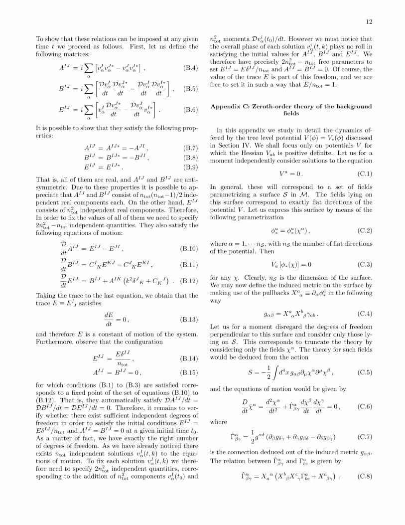
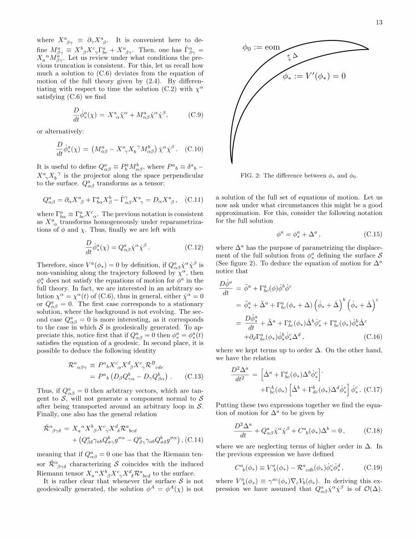
FIG. 2: The difference between φ∗ and φ0.

a solution of the full set of equations of motion. Let usnow ask under what circumstances this might be a goodapproximation. For this, consider the following notationfor the full solution

φa = φa∗ + ∆a , (C.15)

where ∆a has the purpose of parametrizing the displace-ment of the full solution from φa∗ defining the surface S(See figure 2). To deduce the equation of motion for ∆a

notice that

Dφa

dt= φa + Γabc(φ)φbφc

= φa∗ + ∆a + Γabc(φ∗ + ∆)(φ∗ + ∆

)b (φ∗ + ∆

)c=Dφa∗dt

+ ∆a + Γabc(φ∗)∆bφc∗ + Γabc(φ∗)φ

b∗∆

c

+∂dΓabc(φ∗)φ

b∗φc∗∆

d , (C.16)

where we kept terms up to order ∆. On the other hand,we have the relation

D2∆a

dt2=[∆a + Γabc(φ∗)∆

bφc∗

]˙

+ΓAbc(φ∗)[∆b + Γbde(φ∗)∆

dφe∗

]φc∗ . (C.17)

Putting these two expressions together we find the equa-tion of motion for ∆a to be given by

D2∆a

dt+Qaαβχ

αχβ + Cab(φ∗)∆b = 0 , (C.18)

where we are neglecting terms of higher order in ∆. Inthe previous expression we have defined

Cab(φ∗) ≡ V ab(φ∗)−Racdb(φ∗)φc∗φd∗ , (C.19)

where V ab(φ∗) ≡ γac(φ∗)∇cVb(φ∗). In deriving this ex-pression we have assumed that Qaαβχ

αχβ is of O(∆).

14

This is correct since we need to demand ∆ = 0 for theparticular case Qaαβχ

αχβ = 0. That is to say, we arestrictly interested in the inhomogeneous solution of theprevious equation (we shall later address the issue re-garding perturbations). Notice that the effective massCab contains a contribution from the Riemann tensor.

However, the direction given by φa∗ continues to be a flat

direction since Racdb(φ∗)φc∗φd∗φb∗ = 0. In other words,

Cab(φ∗)φb∗ = 0 . (C.20)

Additionally, notice that Cab is symmetric. To proceed,let us define a few more quantities. First, the tangentvector to the trajectory defined by φ∗(t) on the surfaceis given by

T a∗ =φa∗

φ∗, (C.21)

where φ2∗ = γabφ

a∗φ

b∗. In fact, notice that

T a∗ = XaαT

α∗ , (C.22)

Tα∗ =χα

φ∗, (C.23)

φ2∗ = gαβχ

αχβ . (C.24)

It is a simple matter to show that

DT a∗dt

= φ∗QaαβT

α∗ T

β∗ , (C.25)

φ∗ = 0 . (C.26)

It follows that Na∗ ∝ QaαβT

α∗ T

β∗ . It should be clear that

T b∗Vab(φ∗) = 0, as T a∗ is by definition along the flat di-

rections of the potential. It is useful to consider the def-inition of the radius of curvature κ∗ parametrizing thedeviation of the trajectory in S with respect to geodesicsin M. The radius of curvature κ∗ comes defined as

DT a∗dφ∗

= sN (t)Na∗κ∗

, (C.27)

and therefore one has

1

κ∗= |N∗aQaαβTα∗ T β∗ | =

√γabQaαβT

α∗ T

β∗ QbγδT

γ∗ T δ∗ .

(C.28)Notice that this quantity depends only on geometricalobjects, as it should. Coming back to (C.18), we maynow write

D2∆a

dt2− sN (t)φ2

∗Na∗ κ−1∗ + Cab(φ∗)∆

b = 0 . (C.29)

At this point one may argue that there are no good rea-sons to consider κ−1

∗ to be a small parameter. In fact,typically, for theories incorporating modular fields, κmaybe of O(1) in Planck unit or even smaller. Since φ∗ isconstant, it is convenient to parametrize the trajectorywith φ∗. We can in fact write

D∆a

dt= φ∗

D∆a

dφ∗, (C.30)

D2∆a

dt2= φ2

∗D2∆a

dφ2∗. (C.31)

We can therefore reexpress the equation of motion for ∆a

in terms of the proper parameter φ∗ along the curve

D2∆a

dφ2∗

+1

φ2∗Cab(φ∗)∆

b = sN (φ∗)Na∗ κ−1∗ , (C.32)

where now sN (φ∗) denotes the sign of Na∗ relative to

DT a∗ /dφ∗ but expressed as a function of φ∗ instead oftime. To gain experience with this equation, consider thefollowing situation. Suppose we have a trajectory in fieldspace characterized by a constant curvature κ and suchthat CabN

b = M2Na with M2 > 0 a constant. Thatis, Na is an eigenvector of Cab. Under such conditions,using the results of Section II we find that

D2Na∗

dφ2∗

= −Na∗κ2∗. (C.33)

Then, we can see that ∆a = ∆Na with ∆ constant is asolution of the equation, with

∆ =φ2∗κ∗

(M2 − φ2

∗κ2∗

)−1

. (C.34)

If M2 � φ2∗/κ

2∗, which corresponds to the case in which

the energy scale of the low energy dynamics is muchsmaller than the energy scale associated to the heavyfields, we simply have

∆ ' φ2∗

M2κ∗, (C.35)

This is the typical deviation from the true minimumof the potential if the surface of this minimum is notgeodesic. To be more general, let us focus on a class ofbackground trajectories in which

D∆a

dφ∗∼ O

(∆

κ∗

). (C.36)

This is a very reasonable situation to look into (our previ-ous example is a particular case of this) as it correspondto those cases in which the main scale encoding the geo-metrical effects in the trajectory is its curvature. Then,if the non-vanishing eigenvalues of Cab are much larger

than φ2∗/κ

2 we can neglect the first term in (C.32) andwrite

Cab(φ∗)∆b ' φ2

∗Na

κ∗. (C.37)

Thus more generally ∆ ' φ2∗/(M

2κ∗) is indeed a goodmeasure of the deviation from the true minimum. Noticethat in the case of a system with two scalar fields this isprecisely the case.

15

[1] T. Appelquist and J. Carazzone, Infrared Singularitiesand Massive Fields, Phys. Rev. D11 (1975) 2856.

[2] R. S. Chivukula, N. D. Christensen, and E. H. Sim-mons, Low-Energy Effective Theory, Unitarity, and Non-Decoupling Behavior in a Model with Heavy Higgs-Triplet Fields, Phys. Rev. D77 (2008) 035001, [arXiv:0712.0546].

[3] K. Choi, A. Falkowski, H. P. Nilles, M. Olechowski, andS. Pokorski, Stability of flux compactifications and thepattern of supersymmetry breaking, JHEP 11 (2004) 076,[ hep-th/0411066].

[4] S. P. de Alwis, On integrating out heavy fields insusy theories, Phys. Lett. B628 (2005) 183–187, [ hep-th/0506267].

[5] S. P. de Alwis, Effective potentials for light moduli, Phys.Lett. B626 (2005) 223–229, [ hep-th/0506266].

[6] P. Binetruy, G. Dvali, R. Kallosh, and A. Van Proeyen,Fayet-iliopoulos terms in supergravity and cosmology,Class. Quant. Grav. 21 (2004) 3137–3170, [ hep-th/0402046].

[7] A. Achucarro, K. Sousa, F-term uplifting and moduli sta-bilization consistent with Kahler invariance, JHEP 0803(2008) 002. [ arXiv:0712.3460].

[8] A. Achucarro, S. Hardeman, and K. Sousa, Con-sistent Decoupling of Heavy Scalars and Moduli inN=1 Supergravity, Phys. Rev. D78 (2008) 101901, [arXiv:0806.4364].

[9] A. Achucarro, S. Hardeman, K. Sousa, F-term uplift-ing and the supersymmetric integration of heavy moduli,JHEP 0811 (2008) 003. [ arXiv:0809.1441].

[10] I. Ben-Dayan, R. Brustein, and S. P. de Alwis, Modelsof Modular Inflation and Their Phenomenological Con-sequences, JCAP 0807 (2008) 011, [ arXiv:0802.3160].

[11] D. Gallego and M. Serone, An Effective Description of theLandscape - I, JHEP 01 (2009) 056, [ arXiv:0812.0369].

[12] L. Brizi, M. Gomez-Reino, and C. A. Scrucca, Glob-ally and locally supersymmetric effective theories forlight fields, Nucl. Phys. B820 (2009) 193–212, [arXiv:0904.0370].

[13] D. Gallego, M. Serone, An Effective Description ofthe Landscape - II, JHEP 0906 (2009) 057. [[arXiv:0904.2537].

[14] D. Gallego, On the Effective Description of Large VolumeCompactifications, [ [arXiv:1103.5469].

[15] A. Achucarro, J. O. Gong, S. Hardeman, G. A. Palmaand S. P. Patil, Features of heavy physics in theCMB power spectrum, JCAP 1101 (2011) 030. [[arXiv:1010.3693].

[16] A. J. Tolley and M. Wyman, The Gelaton Scenario:Equilateral non-Gaussianity from multi-field dynamics,Phys. Rev. D81 (2010) 043502, [ arXiv:0910.1853].

[17] C. Gordon, D. Wands, B. A. Bassett and R. Maartens,Adiabatic and entropy perturbations from inflation, Phys.Rev. D 63, 023506 (2001) [arXiv:astro-ph/0009131].

[18] S. Groot Nibbelink and B. J. W. van Tent, Density per-turbations arising from multiple field slow roll inflation,arXiv:hep-ph/0011325.

[19] S. Groot Nibbelink and B. J. W. van Tent, Scalar per-turbations during multiple field slow-roll inflation, Class.Quant. Grav. 19, 613 (2002) [arXiv:hep-ph/0107272].

[20] H. P. Nilles, M. Peloso and L. Sorbo, Coupled fields in

external background with application to nonthermal pro-duction of gravitinos, JHEP 0104, 004 (2001) [arXiv:hep-th/0103202].

[21] X. Chen and Y. Wang, Large non-Gaussianities withIntermediate Shapes from Quasi-Single Field Inflation,Phys. Rev. D 81, 063511 (2010) [arXiv:0909.0496 [astro-ph.CO]].

[22] S. Cremonini, Z. Lalak, K. Turzynski, “Strongly CoupledPerturbations in Two-Field Inflationary Models,” JCAP1103, 016 (2011). [arXiv:1010.3021 [hep-th]].

[23] M. Gomez-Reino and C. A. Scrucca, Constraints for theexistence of flat and stable non- supersymmetric vacua insupergravity, JHEP 09 (2006) 008, [ hep-th/0606273].

[24] L. Covi et. al., de Sitter vacua in no-scale supergravitiesand Calabi-Yau string models, JHEP 06 (2008) 057, [arXiv:0804.1073].

[25] S. B. Giddings, S. Kachru, and J. Polchinski, Hierarchiesfrom fluxes in string compactifications, Phys. Rev. D66(2002) 106006, [ hep-th/0105097].

[26] S. Kachru, R. Kallosh, A. Linde, and S. P. Trivedi, De sit-ter vacua in string theory, Phys. Rev. D68 (2003) 046005,[ hep-th/0301240].

[27] A. H. Guth, The Inflationary Universe: A Possible So-lution to the Horizon and Flatness Problems, Phys. Rev.D23 (1981) 347–356.

[28] A. Albrecht and P. J. Steinhardt, Cosmology for GrandUnified Theories with Radiatively Induced SymmetryBreaking, Phys. Rev. Lett. 48 (1982) 1220–1223.

[29] A. D. Linde, A New Inflationary Universe Scenario: APossible Solution of the Horizon, Flatness, Homogeneity,Isotropy and Primordial Monopole Problems, Phys. Lett.B108 (1982) 389–393.

[30] A. A. Starobinsky, Multicomponent de Sitter (Inflation-ary) Stages and the Generation of Perturbations, JETPLett. 42 (1985) 152–155.

[31] X. Chen and Y. Wang, Quasi-Single Field Inflationand Non-Gaussianities, JCAP 1004 (2010) 027, [arXiv:0911.3380].

[32] M. Alishahiha, E. Silverstein, and D. Tong, DBI in thesky, Phys. Rev. D70 (2004) 123505, [ hep-th/0404084].

[33] In [16] [22], related effects were uncovered that werespecifically induced by non-canonical kinetic terms. Ourperspective is that the latter is more readily thought ofas having been induced by non-geodesic trajectories infield space. Certainly any metric on field space can bebrought into canonical form by a suitable field redefini-tion at the expense of introducing complicated derivativeinteractions at higher orders. Therefore the criteria mustbe more general than simply considering non-canonicalkinetic terms (to induce for example, a reduced speed ofsound for the scalar field perturbations).

[34] We are assuming here that the background solutionsφa = φa

0(t) are analytic functions of time, and thereforewe disregard any situation where this procedure cannotbe performed.

[35] For example the degenerate minima offered by theSU(2)×U(1) invariant potential, used to break the elec-troweak symmetry of the standard model, have a radiusof curvature of order κ ∼ MH � MPl, where MH is theHiggs mass.

[36] Since M is two dimensional, RTNTN = R/2 is the only

16

non-vanishing component of the Riemann tensor.[37] Notice that in the particular case where M is flat and

with a trivial topology, these conditions would corre-spond to an exact circular curve, such as the one thatwould happen at the bottom of the ‘Mexican hat’ poten-

tial.[38] In the constant curvature case κ = const., β(κ) is con-

stant as well and we find an overall modulation of thepower spectrum compatible with Ref. [31].