MARKET RECOGNITION OF DIFFERENCES IN EARNINGS PERSISTENCE: UK EVIDENCE

Journal of Business Finance d Accounfing, 19(4), June 1992, 0306 686X $2.50

MARKET RECOGNITION OF DIFFERENCES IN EARNINGS PERSISTENCE: UK EVIDENCE

J. O’HANLON, s. POON AND R.A. YAANSAH’

INTRODUCTION

Much empirical work at the interface between Accounting and Finance involves the observation of the impact of earnings announcements on share prices. Results of such work have been used, for example, to draw inferences about the usefulness of earnings or to compare the relative usefulness of a number of different earnings constructs. Such work typically involves the comparison of a series of scaled earnings changes/surprises with a matching series of abnormal returns. Such tests of association do not typically take account of the possibility that, since companies differ from each other in the extent to which they (and their competitors) can protect new sources of earnings from competi- tion, there may exist cross-sectional variation in the extent to which earnings changedsurprises are likely to persist.

It could be argued that the use of earnings surprise as the earnings signal, rather than earnings surprise adjusted to reflect the extent to which the surprise is likely to persist, results in the omission of an important explanatory variable in the earnings surprise/abnormal return relationship. Indeed, a US study by Kormendi and Lipe (1987) showed that cross-sectional variation in the magnitude of market reaction to announcements of companies’ unexpected earnings (or earnings surprise) can partly be explained by measures, based on time series models, of the extent to which current earnings surprises change expectations about future earnings. These measures have been termed earnings pnsistmce measures. The Kormendi and Lipe finding was consistent with those of other studies which showed that market reaction to current earnings surprises was partly explained by contemporaneous revisions in expectations of future earnings. The misspecification suggested by the Kormendi and Lipe and other studies may have been partly responsible for the notoriously low R2s reported in studies of the cross-sectional relationship between returns and earnings. (See Lev, 1989, for a review of earnings research.) The crucial importance of the concept of earnings persistence to professional and academic accountants can

*The first and second authors are from Lancaster University, and the third author is from the University of Saskatchewan. They wish to thank IBES Inc. which, as part of a broad academic programme to encourage earnings expectations research, made available its database of consensus analysts’ forecasts; thanks also to Lynne Irvine who assisted in the processing of the IBES data and to Joyce Entwistle for data collection. The helpful comments of Laurence Copeland, Ken Peasnell, Stephen Taylor and the anonymous referee on earlier drafts of this paper are gratefully acknowledged. Any remaining errors are the authors’ own.

625

626 O’HANLON, POON AND YAANSAH

partly be gauged from recent debate in the UK about the treatment of extraordinary and exceptional items which has arisen as a result of proposed changes to the presentation of the profit and loss account.

In the present study, UK data is used to examine the issue of whether adjustment of earnings surprise to reflect cross-sectional variation in earnings persistence increases the strength of the relationship between earnings surprise and abnormal return. To our knowledge, this issue is addressed in the UK context for the first time in our study. Our study differs from the Kormendi and Lipe study in that analysts’ forecasts from the IBES service,’ rather than lorecasts from time series models, are used as estimates of expected earnings. Also, in estimating earnings persistence, we allow both the earnings capitalisation rate and the class of time series model, which characterises the earnings generating process, to vary from company to company. It is hoped that these refinements may reduce the ‘errors in variables’ problems inherent in studies of this type.

The remainder of this paper is structured as follows. The next section briefly reviews previous related studies. The third section discusses the relationship between earnings surprises and share price changes, and describes the model for the conversion of information from time series models of earnings into earnings persistence measures. The fourth section describes the criteria for the inclusion of companies in the study. The fifth section describes the tests which we carry out in order to seek evidence as to whether the persistence measures described in the third section help to explain the relationship between abnormal return and earnings surprise. In the final section we summarise the findings and provide some conclusions to the study.

PREVIOUS STUDIES

Lev (1989), in an extensive review of earnings research, points to the very low R 2 s (typically less than 10 per cent) reported by studies which have sought to measure the strength of cross-sectional association between stock market (abnormal) returns and (unexpected) earnings. Studies which have reported, at the individual security level, a low R 2 between stock market return and earnings change/surprise include Beaver, Lambert and Morse (1 980) and Bowen, Burgstahler and Daley (1987). Possible causes of the low R2s include problems in measuring expected earnings and normal returns, the use of exces- sively short experimental windows and low ‘quality of earnings’. Another recent suggestion is that there is a misspecification of the relationship between earnings changes/surprises and abnormal returns inherent in any methodology that tests the association between earnings changes/surprises and abnormal returns without allowing for cross-sectional differences in the extent to which current changedsurprises are likely to persist. If the price reaction to an earnings surprise results from a revision in the present value of current and expected

DIFFERENCES IN EARNINGS PERSISTENCE 62 7

future earnings, it would be wrong to take the earnings surprise to be the signal to which the market can be expected to react. Perhaps the right signal to use in such tests is the earnings surprise adjusted by a cross-sectionally varying measure of the extent to which the surprise is likely to persist. A number of papers have addressed this last issue by testing whether cross-sectional variation in the share price response to an earnings surprise depends upon cross-sectional variation in earnings persistence* as well as the earnings surprise itself.

Brown, Foster and Noreen (1985), using annual earnings data, showed that the market reaction to a current earnings surprise was partly conditioned by the extent to which expectations concerning future earnings underwent a change which coincided with the earnings surprise. Cornell and Landsman (1989) found similar results using quarterly data. Kormendi and Lipe (1987) formulated earnings expectations based on a time series model and also used a time series model to estimate the present value of the change in expected future earnings resulting from a $1 current earnings surprise. This latter measure was described as a measure of earnings persistence. Similar use of time series models to estimate the extent to which changes in a series are persistent also appears in the economics literature (e.g. Flavin, 1981; and Mills, 1991). Kormendi and Lipe found that their persistence measure was positively related to the dollar stock price change occasioned by a $1 earnings surprise. This finding suggested that the information contained in the time series process generating earnings was important in describing the relationship between changes in earnings and abnormal returns. Collins and Kothari (1989) also found that the magnitude of market reaction to earnings surprise (or the earnings response coefficient) was positively related to earnings persistence as estimated from a time series model. A potential problem with both the Kormendi and Lipe study and the Collins and Kothari study is that both used a single class of time series model to estimate the persistence measure for each company in their sample. One might argue that the assumption of a uniform class of earnings generating model is too strong to be realistic in practice.

Other factors have been found to cause variation in the earnings response coefficient. For example, Collins and Kothari (1989) found a negative relationship between the earnings response coefficient and systematic risk. This finding is consistent with that of Dhaliwal and Reynolds (1990) who also found a negative relationship between the earnings response coefficient and the debt- equity ratio. Kallapur (1991) found that earnings response coefficients were positively related to dividend payout ratios.

STOCK RETURNS, EARNINGS SURPRISES AND PERSISTENCE MEASURES

At time 0 - A, an instant before the time 0 cash flow is known, the value of a share ( Vo-a) can be represented as the present value of expected future cash flows:


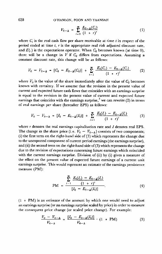
where C, is the real cash flow per share receivable at time t in respect of the period ended at time t, Y is the appropriate real risk adjusted discount rate, and E ( . ) is the expectations operator. When CO becomes known (at time 0), there will be a change in V if Co differs from expectations. Assuming a constant discount rate, this change will be as follows:

where Vo is the value of the share immediately after the value of CO becomes known with certainty. If we assume that the revision in the present value of current and expected future cash flows that coincides with an earnings surprise is equal to the revision in the present value of current and expected future earnings that coincides with the earnings ~urpr i se ,~ we can rewrite (2) in terms of real earnings per share (hereafter EPS) as follows:

where 7 denotes the real earnings capitalisation rate and I denotes real EPS. The change in the share price (i.e. VO - V O - A ) consists of two components; (i) the first term on the right-hand side of (3) which represents the change due to the unexpected component of current period earnings (the earnings surprise), and (ii) the second term on the right-hand side of(3) which represents the change due to the revision of expectations concerning future earnings which coincided with the current earnings surprise. Division of (ii) by (i) gives a measure of the effect on the present value of expected future earnings of a current unit earnings surprise. This would represent an estimate of the earnings persistence measure (PM):

(1 + PM) is an estimate of the amount by which one would need to adjust an earnings surprise (or an earnings surprise scaled by price) in order to measure the consequent price change (or scaled price change). For example:

DIFFERENCES IN EARNINGS PERSISTENCE 629

where the term on the left-hand side is the proportional price change that results from the effect of the earnings surprise on the present value of current and expected future earnings.

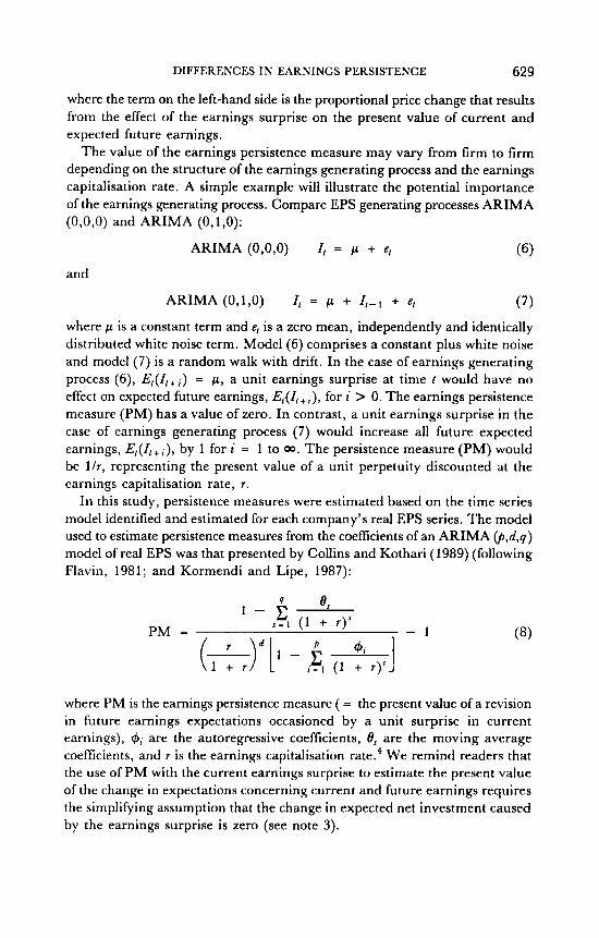
The value of the earnings persistence measure may vary from firm to firm depending on the structure of the earnings generating process and the earnings capitalisation rate. A simple example will illustrate the potential importance of the earnings generating process. Compare EPS generating processes ARIMA (O,O,O) and ARIMA (O,l,O):

and

ARIMA (0,1,0) I, = p + + e, (7) where p is a constant term and e, is a zero mean, independently and identically distributed white noise term. Model (6) comprises a constant plus white noise and model (7) is a random walk with drift. In the case of earnings generating process (6 ) , E,(Z,+;) = p, a unit earnings surprise at time t would have no effect on expected future earnings, E,(Z,+i), for i > 0. The earnings persistence measure (PM) has a value of zero. In contrast, a unit earnings surprise in the case of earnings generating process (7) would increase all future expected earnings, E,(Z, + i), by 1 for i = 1 to 00. The persistence measure (PM) would be l / r , representing the present value of a unit perpetuity discounted at the earnings capitalisation rate, Y.

In this study, persistence measures were estimated based on the time series model identified and estimated for each company’s real EPS series. The model used to estimate persistence measures from the coefficients of an ARIMA (p,d,q) model of real EPS was that presented by Collins and Kothari (1989) (following Flavin, 1981; and Kormendi and Lipe, 1987):

1 - i 8, , = I (1 + r y

PM = - 1 (8) (+[1 - 4 . ]

l + r i = l (1 + r ) l

where PM is the earnings persistence measure ( = the present value of a revision in future earnings expectations occasioned by a unit surprise in current earnings), t # ~ ~ are the autoregressive coefficients, 8, are the moving average coefficients, and Y is the earnings capitalisation rate.4 We remind readers that the use of PM with the current earnings surprise to estimate the present value of the change in expectations concerning current and future earnings requires the simplifying assumption that the change in expected net investment caused by the earnings surprise is zero (see note 3).

630 O’HANLON. POON AND YAANSAH

CRITERIA FOR INCLUSION IN OUR SAMPLE

The sample used in our study consists of 188 UK companies. It comprised all those companies which met the following conditions:

(i) The company had to have a complete EPS series in Datastream for accounting periods ended in each of the years 1968 to 1988, both inclusive. We recognise that this criterion excludes non-surviving firms but do not feel that this is a serious defect in this context. Whilst it may be that the extent to which earnings changes are persistent varies between distressed and non-distressed firms and, consequently, a survivorship biased sample might prevent us from estimating an earnings persistence measure for the whole population of companies, we do not feel that the exclusion of failed firms interferes with our attempt to observe the market’s differentiation between differing levels of earnings persistence.

(ii) The company had to have both analysts’ forecast EPS and actual EPS, for the accounting period ended in 1988, in the June 1990 version of IBES database record.

EMPIRICAL TESTS AND RESULTS

If market reaction to earnings surprise is conditioned by the degree of persistence in earnings changes, then the abnormal return occasioned by an earnings surprise ought to be more strongly related to (1 + PM) times the scaled earnings surprise (ES) than to ES alone. In this section, we compare the correlation between abnormal return and ES with that between abnormal return and ES(1 + PM) in order to establish whether in the UK market there is any evidence of market recognition of differences in earnings persistence.

Computation of Earnings Surprise and Abnormal Return Measures

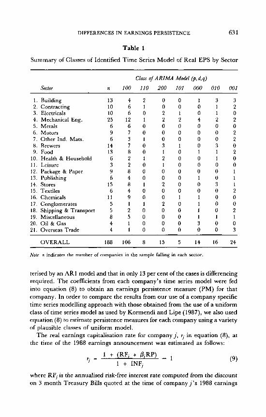
For each of the 188 UK companies included in the sample, EPS values were collected from Datastream for the period from 1968 to 1988 inclusive. In order to maintain comparability with the earnings construct used in the Kormendi and Lipe (1987) study, our EPS series was deflated by the UK Retail Price Index (RPI) to produce a real EPS ~ e r i e s . ~ Using the real EPS series of each company, a company specific ARIMA model was identified and estimated to represent the company’s real EPS generating process. The model identification process involved the examination of correllograms and, when a number of possible classes of model suggested themselves, comparison of the standard deviations of the residual terms and t-ratios of the coefficient estimates of the candidate models. Table 1 summarises the classes of identified model by industrial sector for the 188 companies in our sample. Here, one notes that the real EPS series of 56 per cent of the companies in our sample are charac-


Table 1

Summary of Classes of Identified Time Series Model of Real EPS by Sector

Class o j A RIMA Model (p, d, q)

Sector n 100 110 200 101 000 010 001

1 . Building 13 4 2 0 0 1 3 3 2. Contracting 10 6 1 0 0 0 1 2 3. Electricals 10 6 0 2 1 0 1 0 4. Mechanical Eng. 25 12 1 2 2 4 2 2 5. Metals 6 6 0 0 0 0 0 0 6 . Motors 9 7 0 0 0 0 0 2 7. Other Ind. Mats. 6 3 1 0 0 0 0 2 8. Brewers 14 7 0 3 1 0 3 0 9. Food 13 8 0 1 0 1 1 2

10. Health & Household 6 2 1 2 0 0 1 0 11. Leisure 3 2 0 1 0 0 0 0 12. Package & Paper 9 8 0 0 0 0 0 1 13. Publishing 6 4 0 0 0 1 0 1 14. Stores 15 8 1 2 0 0 3 1 15. Textiles 6 4 0 0 0 0 0 2 16. Chemicals 11 9 0 0 1 1 0 0 17. Conglomerates 5 1 1 2 0 1 0 0 18. Shipping & Transport 5 2 0 0 0 1 0 2 19. Miscellaneous 8 5 0 0 0 1 1 1 20. Oil & Gas 4 1 0 0 0 3 0 0 2 1. Overseas Trade 4 1 0 0 0 0 0 3

~~

OVERALL 188 106 8 15 5 14 16 24 ~~ ~~ ~

Nofe n indicates the number of companies in the sample falling in each sector.

terised by an AR1 model and that in only 13 per cent of the cases is differencing required. The coefficients from each company’s time series model were fed into equation (8) to obtain an earnings persistence measure (PM) for that company. In order to compare the results from our use of a company specific time series modelling approach with those obtained from the use of a uniform class of time series model as used by Kormendi and Lipe (1987), we also used equation (8) to estimate persistence measures for each company using a variety of plausible classes of uniform model.

The real earnings capitalisation rate for companyj, 9 in equation (8), at the time of the 1988 earnings announcement was estimated as follows:

- 1 1 + (RF, + 0;RP)

T . = J 1 + INF, (9)

where RFj is the annualised risk-free interest rate computed from the discount on 3 month Treasury Bills quoted at the time of company j ’ s 1988 earnings


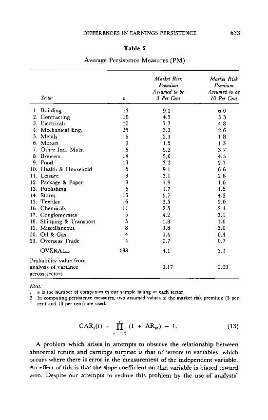
announcement, pj is the beta of company j as at the earnings announcement date, INF, is the annual rate of increase in the UK Retail Price Index for the year prior to company j ’ s 1988 earnings announcement,6 and R P is the market risk premium. In this study, our estimate of oj is the beta of company j as reported by the London Business School’s Risk Measurement Service at the quarter prior to the 1988 earnings announcement.’ Two assumed values for the market risk premium were used: R P = 5 per cent and RP = 10 per cent.’ Table 2 gives details of the average earnings persistence measures by industrial sector for each of the two assumptions made about the value of RP. Note here that an analysis of variance test suggests that earnings persistence varies from sector to sector.

For each company, a scaled earnings surprise measure (ES) was computed as follows:

where II is the EPS of company j for the accounting year ended in 1988, F q is the mean EPS forecastg for company j as at the IBES run date immediately prior to the corresponding earnings announcement, and q is the price of company j ’ s shares one week prior to the corresponding earnings announcement. Both the actual EPS and the forecast EPS for use in (10) were obtained from IBES. Share prices were obtained from Datastream, adjustments being made where necessary to ensure that q was stated on a comparable basis to I, and F 4 .

The earnings surprise measures were adjusted as follows to reflect cross- sectional differences in persistence:

= (1 + PMj)ESj. Zj - FZ;)(l + PMj) AES, = ( 4

For each company, an abnormal return was computed for the day of the 1988 earnings announcement and for each of the five weekdays before and after the announcement (eleven weekdays in all). We define the abnormal return of company j on day t (ARj,) as follows:’o

ARj, = Rjt - ( r f i + (W - rfi)Pj) (12) where Rj, is the total return on company j ’ s shares on day t , r f i is the (daily) risk-free rate observed on day t , nn, is the return observed on the Financial Times All Share Total Returns Index on day t , and Pj is the beta for company j as reported by the London Business School’s Risk Measurement Service at the quarter prior to day t .

For t = - 5 to 5 (indicating the number of days relative to the earnings announcement date), multiplicative cumulative abnormal return measures (CARj(t)) were also computed for each company:


Table 2

Average Persistence Measures (PM)

Sector

Market Risk Market Risk Premium Premium

Assumed to be Assumed to be n 5 Per Cent 10 Per Cent

1. 2. 3. 4. 5. 6. 7.

9. 10. 11. 12. 13. 14. 15. 16. 17.

19. 20. 21.

a.

l a .

Building Contracting Electricals Mechanical Eng. Metals Motors Other Ind. Mats. Brewers Food Health & Household Leisure Package & Paper Publishing Stores Textiles Chemicals Conglomerates Shipping & Transport Miscellaneous Oil & Gas Overseas Trade

OVERALL

Probability value from analysis of variance across sectors

13 10 10 25 6 9 6

14 13 6 3 9 6

15 6

11 5 5

4 4

a

i aa

9.2 4.3 7.7 3.3 2.1 1.5 5.2 5.6 3.2 9.1 2 . 1 1.9 1.7 5.7 2.5 2.5 4.2 1 .a 3.8 0.4 0.7

4.1

6.0 3.3

2.6

1.3 3.7 4.5 2.7 6.6

1.6 1.5 4.3 2.0 2.1 3.1 1.6 3.0 0.4 0.7

3.1

4.8

1 .a

2.8

0.17 0.09

Notes: 1 2

n is the number of companies in our sample falling in each sector. In computing persistence measures, two assumed values of the market risk premium (5 per cent and 10 per cent) are used.

I

CAR;(t) = n (1 + ARju) - 1. (13) u = - 5

A problem which arises in attempts to observe the relationship between abnormal return and earnings surprise is that of ‘errors in variables’ which occurs where there is error in the measurement of the independent variable. An effect of this is that the slope coeficient on that variable is biased toward zero. Despite our attempts to reduce this problem by the use of analysts’


forecasts, the use of company specific classes of time series model and the use of company specific estimates of earnings capitalisation rates, such a problem can be expected to persist in our study, both in the case of the relationship between abnormal return and ES and in the case of the relationship between abnormal return and AES. The understatement of the strength of the relationship is likely to be greater in the latter case because AES, as well as containing an estimate of earnings surprise, contains an estimate of earnings persistence. A further problem potentially arises in that estimates of beta are used both in estimating the abnormal return and in estimating AES, and the possibility thus exists that errors in the beta estimates might induce spurious correlation between the two variables. However, it must be noted that, whilst an error in estimation of beta would always result in an error of opposite sign in the estimate of abnormal return, the sign of the resultant error in the estimate of AES would depend upon the sign of the unadjusted forecast error. The results obtained when we compute both abnormal return and AES using the assumption that beta = 1 for all companies are almost identical to those obtained when company specific betas are used in both variables, and this suggests that our results are not sensitive to the estimates of beta used.

Abnormal Stock Return and Earnings Surprise

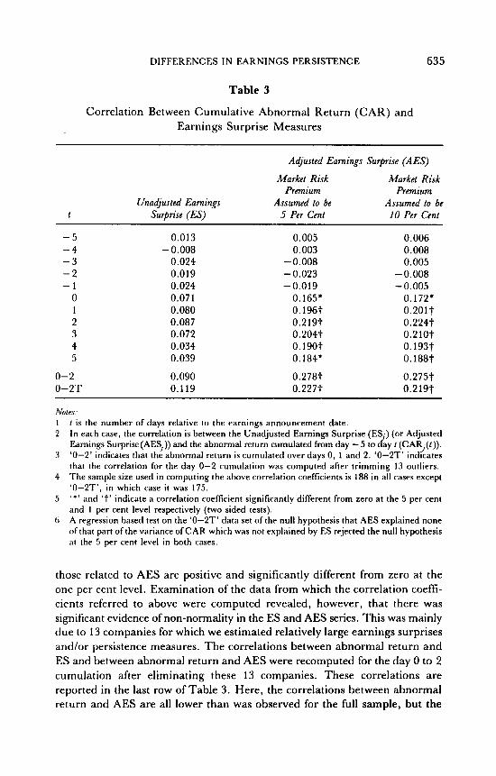
Table 3 reports the cross-sectional correlation coefficients between the cumulative abnormal returns (CAR) cumulated from five days before the earnings announcement day to each day up to the fifth day after the announcement, and both (i) the unadjusted earnings surprise measure (ES) as in equation (lo), and (ii) the adjusted earnings surprise measure (AES) as in equation (1 1). There are two versions of AES, each corresponding to a different assumption concerning the market risk premium.

The results in Table 3 show that for ES and for each of the two AES measures, the correlation coefficients are insignificantly different from zero for all days prior to the earnings announcement date t = 0. On day 0 there is, in each case, a noticeable rise. There are then smaller rises over the next two days. The strength of the earningsheturn relationship is in line with most of the results reported in the various studies reviewed by Lev (1989). One striking feature of the results reported in Table 3 is that the rise is far more marked in the case of AES than in the case of ES. All of the correlation coefficients from day 0 to day 5 are positive and significantly different from zero for all measures of AES, whilst none of those for ES is significantly different from zero.

We also report, in the penultimate row of Table 3, the correlation coefficients between the earnings surprise measures and the abnormal return that cumulated during days 0, 1 and 2. This is the period during which the correlations between cumulative abnormal return and earnings surprise continued to rise after the earnings announcement. As with the results reported above, the correlation coefficient related to ES, whilst positive, is not statistically significant, whereas


Table 3

Correlation Between Cumulative Abnormal Return (CAR) and Earnings Surprise Measures

Adjusted Earnings Surprise (AES)

Market Risk Market Risk Premium Premium

Unadjusted Earnings Assumed to be Assumed to be 1 Surprise (ES) 5 Per Cent 10 Per Cent

-5 -4 -3 -2 - 1

0 1 2 3 4 5

0-2 0-2T

0.013

0.024 0.019 0.024 0.071

-0.008

0. oao 0.087 0.072 0.034 0.039

0.090 0.119

0.005 0.003

-0.008 -0.023 -0.019

0.165’ 0.196t 0.2197 0.2047 0.1907 0.184’

0.2787 0.2277

0.006

0.005 0.008

-0.008 -0.005

0.172; 0.2017 0.2247 0.210t 0.193t 0. i aa t 0.275t 0.2197

Notes: 1 2

3

4

5

0

t is the number of days relative to the earnings announcement date. In each case, the correlation is between the Unadjusted Earnings Surprise (ES ) (or Adjusted Earnings Surprise(AESJ)) and the abnormal return cumulated from day - 5 to day f (CAR (f)). ‘0-2’ indicates that the abnormal return is cumulated over days 0, 1 and 2. ‘0-2T’ indicates that the correlation for the day 0-2 cumulation was computed after trimming 13 outliers. The sample size used in computing the above correlation coefficients is 188 in all cases except ‘0-ZT’, in which case it was 175. ‘ * ’ and ‘t’ indicate a correlation coefficient significantly different from zero at the 5 per cent and 1 per cent level respectively (two sided tests). A regression based test on the ‘0-2T’ data set of the null hypothesis that AES explained none of that part of the variance of CAR which was not explained by ES rejected the null hypothesis at the 5 per cent level in both cases.

.J

those related to AES are positive and significantly different from zero at the one per cent level. Examination of the data from which the correlation coeff- cients referred to above were computed revealed, however, that there was significant evidence of non-normality in the ES and AES series. This was mainly due to 13 companies for which we estimated relatively large earnings surprises and/or persistence measures. The correlations between abnormal return and ES and between abnormal return and AES were recomputed for the day 0 to 2 cumulation after eliminating these 13 companies. These correlations are reported in the last row of Table 3. Here, the correlations between abnormal return and AES are all lower than was observed for the full sample, but the

636 O'HANLON, POON AND YAANSAH

pattern observed above remains: the correlations for AES are higher than that for ES. A regression based test on this reduced data set of the null hypothesis that AES explained none of that part of the variance of CAR which was not explained by ES rejected the null hypothesis at the five per cent level in both cases (RP = 5 per cent and R P = 10 per cent)."

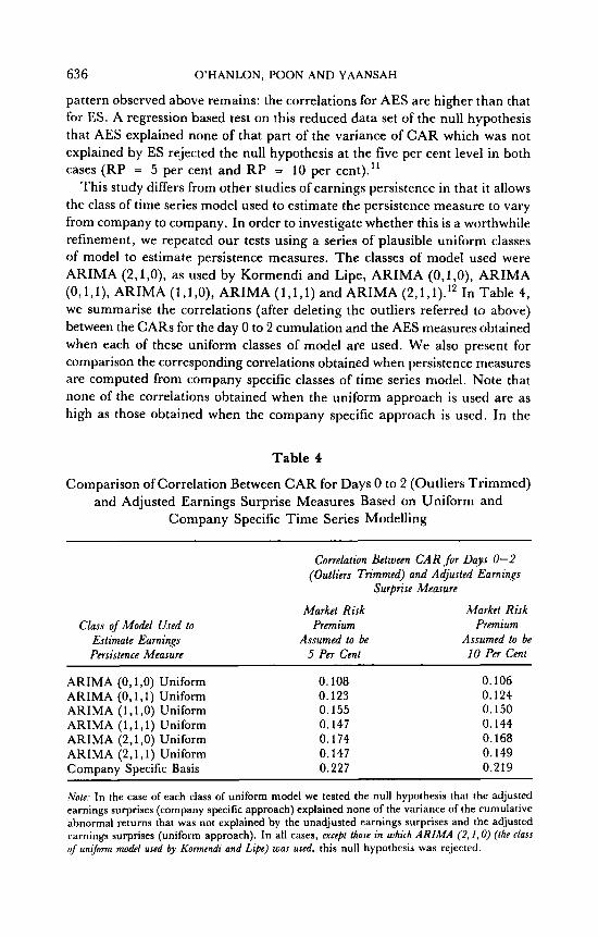
This study differs from other studies of earnings persistence in that it allows the class of time series model used to estimate the persistence measure to vary from company to company. In order to investigate whether this is a worthwhile refinement, we repeated our tests using a series of plausible uniform classes of model to estimate persistence measures. The classes of model used were ARIMA (2,1,0), as used by Kormendi and Lipe, ARIMA (O,l,O), ARIMA (0, 1 , l) , ARIMA (1,l ,O), ARIMA ( l , l , 1 ) and ARIMA (2,1, l).I2 In Table 4, we summarise the correlations (after deleting the outliers referred to above) between the CARS for the day 0 to 2 cumulation and the AES measures obtained when each of these uniform classes of model are used. We also present for comparison the corresponding correlations obtained when persistence measures are computed from company specific classes of time series model. Note that none of the correlations obtained when the uniform approach is used are as high as those obtained when the company specific approach is used. In the

Table 4

Comparison of Correlation Between CAR for Days 0 to 2 (Outliers Trimmed) and Adjusted Earnings Surprise Measures Based on Uniform and

Company Specific Time Series Modelling

Class of Model Used to Estimate Earnings Persistence Measure

Correlation Between C A R for Days 0-2 (Outliers Trimmed) and Adjusted Earnings

Surprise Measure

Market Risk Premium

Assumed to be 5 Per Cent

Market Risk Premium

Assumed to be 10 Per Cent

ARIMA (O,l,O) Uniform 0.108 0.106 ARIMA (0, l ,1) Uniform 0.123 0.124 ARIMA (1,1,0) Uniform 0.155 0.150 ARIMA (1,1,1) Uniform 0.147 0.144 ARIMA (2,1,0) Uniform 0.174 0.168 ARIMA (2,1,1) Uniform 0.147 0.149 Company Specific Basis 0.227 0.219

No&; In the case of each class of uniform model we tested the null hypothesis that the adjusted earnings surprises (company specific approach) explained none of the variance of the cumulative abnormal returns that was not explained by the unadjusted earnings surprises and the adjusted carnings surprises (uniform approach). In all cases, except fhose in which ARIMA (2, I , 0) (ihe class of unijorm model used by Kormendi and Lipe) was used. this null hypothesis was rejected.


case of each uniform class of model we tested the null hypothesis that the AES (company specific approach) explained none of the variance of the cumulative abnormal returns that was not explained by the ES and AES (uniform approach). In all cases, except those in which ARIMA (2,1,0) was used, this null hypothesis was rejected. Thus, although there is some evidence here that persistence measures based on company specific classes of model are more appropriate than those based on uniform classes of model, it seems that in the case of real EPS the ‘best’ of the uniform approaches (ARIMA (2,1,0) as used by Kormendi and Lipe) is not significantly outperformed by the company specific approach. It could be argued that this class of uniform model might be expected to perform relatively well compared to less complex classes of uniform model, since its use involves a greater degree of encompassing over-specification.

CONCLUSION

In this study, using data in respect of accounting periods ended in 1988 for 188 UK companies, we find evidence in support of the view that market reaction to earnings surprise depends on the extent to which the impact of unexpected earnings changes can, according to the time series model describing the earnings process, be expected to persist. Our findings lend support to the view that studies which have not accounted for cross-sectionally varying earnings persistence may have understated the degree of cross-sectional association between abnormal return and earnings surpriselchange. The results of the study suggest that company specific earnings modelling may be a better basis for estimating persistence measures than the use of a uniform class of earnings model but, when the ‘best’ uniform approach is used, the evidence for this is weak.

It must be recognised that, despite our use of a company specific modelling approach, the estimation of persistence measures by the use of univariate time series methods applied to 21 year series of ‘bottom line’ EPS numbers represents a relatively crude approach. Potential problems derive from the need to assume that the EPS series had not been affected by structural change and from the use of a relatively small number of data points to estimate the models. It is hoped that the latter point may be capable of rectification in later studies as longer machine readable earnings series become available and through the use of interim earnings numbers. Also, our analysis is based on the ‘bottom line’ earnings numbers which exclude value relevant items such as extraordinary items and transfers to reserves. Furthermore, it must be recognised that the ‘bottom line’ earnings number is the difference between several large numbers, each of which might be drawn from series with different generating processes and different levels of persistence.

Also, it must be pointed out that studies of the effect of earnings persistence on the strength of the market reaction to earnings changes/surprises, whilst


acknowledging that it is the effect of earnings changes on future expected dividends that is the variable of importance, typically assume that share price changes are driven by changes in the present value of earnings. As was observed earlier, this is tantamount to assuming that all of the changes in expected future earnings are going to be paid out as dividends as they occur. Whilst this simplifying assumption may be justified on the grounds that it enables researchers to focus on the specific issue of earnings persistence, the related issue of cross-sectional and time series variation in payout expectations could also be fruitfully incorporated into this type of work.

Given that the market appears to take notice of persistence in reacting to earnings surprises, it is tempting to suggest that the concept of earnings persistence could provide a useful basis to guide accounting regulators in their deliberations on the treatment of extraordinary items and other related issues. The traditional accounting models used to deal with extraordinary items could be represented as a crude method of accounting for earnings persistence in which the earnings stream is split into two components, one of which (extraordinary items) has a persistence value of zero and one of which (other components of earnings) has a positive but undefined and cross-sectionally constant persistence value. Recognition of the need to replace this sort of dichotomous approach by one that explicitly recognises that persistence can have more than two values would be a great step forward, both for regulators grappling with the problems of extraordinary items and related issues and for academics seeking to explain the abnormal return/earnings surprise relationship.

NOTES

1 IBES, abbreviation for the Institutional Brokers Estimate System, is a database of consensus analyst forecasts of earnings per share. Intn alia, the service provides, at monthly intervals, the mean of analysts’ forecasts of earnings per share in respect of the accounting period end for which results are next to be announced.

2 That is, the effect of a unit earnings surprise on the present value of expected future earnings. 3 This assumption would hold true if all earnings are expected to be paid out as dividends as

they occur (i.e. if there is expected to be zero net investment). It would also hold if, less restrictively, the change in expected net investment caused by the earnings changdsurprise were zero. (See Kormendi and Lipe, 1987, p. 328, for discussion of this assumption.)

4 A derivation of this expression may be obtained on request from the authors. 5 No attempt was made to construct inflation adjusted earnings series using, for example, current

cost accounting. The construction of the series merely involved the deflation of the annual earnings series by the Retail Price Index.

6 By using the inflation rate of the previous year as though it were the estimate of expected inflation for the future, we are effectively assuming that inflation follows a random walk.

7 Persistence measures were also computed on the assumption that beta = 1 for all companies. The results from the use of this approach were very similar to those obtained when we allowed beta to vary and are not reported.

8 The evidence suggests that the realised market risk premium over the last 60 years or so has averaged about 9 per cent per annum (Risk Measurement Service (October-December 1988)). Here we use an assumed value of RP = 10 per cent and, in order to ensure that our results are not sensitive to the assumption made about the value of the market risk premium, we also use an assumed value of R P = 5 per cent.


9 The average number of estimates used in computing the mean forecasts was about 11. 10 Abnormal returns were also computed using market adjusted RNmS (i.e. assuming that beta = 1

for all companies). The results from the use of this approach were very similar to those obtained when we allowed beta to vary and are not reported.

11 We recognise here that AES and ES are correlated and that this test would not enable us to carry out significance tests on the individual regression coefficients of AES and ES. Here, however, we are only concerned with testing the significance of the increase in R 2 that results from adding AES to the model which already contains ES.

12 Although Table 1 indicates that ARIMA (1,0,0) is the most common company specific class of model, this is not a plausible uniform class of model because i t cannot be used in the cases of those companies of which the real EPS series is not stationary.

REFERENCES

Beaver, W., R . Lamben and D. Morse (1980), ‘The Information Content of Security Prices’, Journal of Accounfing and Economics (1980), pp. 3-28.

Bowen, R., D. Burgstahler and L. Daley (1987), ‘The Incremental Information Content of Accrual versus Cash Flows’, Accounting Review (1987), pp. 723-747.

Brown, P., G. Foster and E. Noreen (1985), Sccuriy Analysl Multi-ycar Earnings Forccarfs and fhe Capihl Market (American Accounting Association, 1985).

Brown, L., R. Hagerman, P. Griffin and M. Zmijewski (1987), ‘Security Analyst Superiority Relative to Univariate Time Series Models in Forecasting Quarterly Earnings’, Journol of Accounfing and Economics (1987), pp. 61-87.

Collins, D. and S. Kothari (1989), ‘An Analysis of Intertemporal and Cross-sectional Determinants of Earnings Response Coefficients’, Journal ofAccounting and Economics (1989), pp. 143-181.

Cornell, B. and W. Landsman (1989), ‘Security Price Response to Quarterly Earnings Announce- ments and Analysts’ Forecast Revisions’, Accounting Reuiew (1989), pp. 680-692.

Dhaliwal, D. and S. Reynolds (1990), ‘A Cross-sectional Analysis of the Relationship Between Changes in Firm Earnings and Stock Returns’ (University of Arizona, 1990).

Flavin, M. (1981). ‘The Adjustment of Consumption to Changing Expectations About Future Income’, Journal of Polificd Economy (1981), pp. 974-1009.

Kallapur, S . (1991), ‘Dividend Payout Ratios as Determinants of Earnings Response Coefficients: A Test of the Free Cash Flow Theory’ (University of Arizona, 1991).

Kormendi, R. and R. Lipe (1987), ‘Earnings Innovations, Earnings Persistence and Stock Returns’, Journal of Business (1987), pp. 323-345.

Lev, B. (1989), ‘On the Usefulness of Earnings and Earnings Research: Lessons and Directions from Two Decades of Empirical Research’, Journal ofAccounfing Research (1989), pp. 153-192.

Mills, T . (1991). ‘Are Fluctuations in UK Output Transitory or Permanent?’ The Manchcster School of Economic and Social Studies (1991), pp. 1-11.

O’Brien, P. (1988), ‘Analysts’ Forecasts as Earnings Expectations’, J o u d ofdccounfing and Economics (1988), pp. 53-83.

Risk Measurement Service (1988), London Business School (October-December 1988).

MARKET RECOGNITION OF DIFFERENCES IN EARNINGS PERSISTENCE: UK EVIDENCE

Documents

Transcript of MARKET RECOGNITION OF DIFFERENCES IN EARNINGS PERSISTENCE: UK EVIDENCE