Market Integration in the US Beef supply Chain: A Threshold Cointegration approach

Market Integration in the US Beef supply Chain: A Threshold

Cointegration approach

Kedir Nesha Turi

Department of Agricultural and Consumer Economics, University of

Illinois at Champaign-Urbana

1. Introduction

Beef industry is the largest single industry within U.S.

agriculture, generating between $34 and $37 billion per year in

2006-2008 and accounting for 20% of the annual total market value

of agricultural products sold in the U.S. (USDA, 2009). The

industry is part of a vertically-related meat marketing and

distribution channel. Beef packers purchase live cattle from

cattle feedlots (upstream) and sell processed beef to wholesalers

and retailers (downstream). The upstream can be classified into

three distinct production tiers. According to Boyabath et al.

(2010) the three production tiers are cow/calf operations,

stocker and backgrounding operations, and feedlot operations.

1

The industry has under gone significant structural change in the

last decades. The upstream of the supply chain, the majority of

cattle operations are relatively small in scale. In 2007, many of

the cattle operations are small; some 77% of beef cow operations

have fewer than 50 head of cattle (USDA, 2009). Feedlots (where

beef cattle are fed an energy-intense grain diet before

slaughter) can reach much larger sizes; 40% of inventory is

contained in operations with more than 32,000 head (USDA, 2009).

In the same tier, the majority of feedlot operations have fewer

than 1,000 head of cattle. In general, beef cattle and feedlot

operations all have grown larger over the last 10 years, with

sharp declines most evident in the number of dairy operators.

Four meat packers slaughter and process more than 80% of thefed

cattle marketed in the United States (USDA, 2009).

The aforementioned market concentration and implied presence of

market power can potentially influence the degree and dynamics of

price transmission, leading to differential price effects on

different stages of the chain. Additionally, differing market

operation dynamics under competitive and noncompetitive market

2

conditions can have welfare implications with respect to the

efficiency and equity of the marketing system.

On the downstream side, there is a concern about the impacts of

increasing retail grocery store concentration on marketing

margins and farm-level prices (Marsh, 2004). Live cattle

producers argue that retail consolidation translates into market

power or collusive behavior and results in wider red meat

marketing margins. The margin for packers-retail is increasing

while the margin for live cattle-packers is declining. The wider

margins may result in lower live cattle and hog prices because of

a lack of offsetting market power at those levels (Cotterill,

1999; Schrimper, 2001).

The purpose of this paper is to investigate market efficiency and

coordination of vertically integrated US beef industry at

different stage. Specifically, this research analyzes price

cointegration using live cattle, packers and retail prices.

Cointegration is used as a tool to assess market efficiency and

can analyze both perfect and imperfect market conditions.

3

Cointegration of prices in distinct markets is an indication of

price transmission and market integration. Previous research on

efficiency of beef industry employed similar methodology. Except

Goodwin and Holt((1999), however, they assume symmetric short

term adjustment among the prices. Goodwin and Holt (1999) use

weekly data from 1981 to 1997 to test for nonlinearity of

cointegration relationship. They found no linear relationship and

estimated threshold cointegration. We extend Goodwin and Holt

(1999) works in two ways: first, we use monthly data from January

1980 to December 2010 and second, we employing various recent

developments in threshold cointegration methodology. We estimate

linear cointegration where nonlinearty is rejected and threshold

cointegration where nonlinearity is the case.

2. Conceptual Framework

2.1. Price transmission and market power in vertically

integrated market

Degree to which market shocks are transmitted through the

marketing chain is an important indicator of the market

4

efficiency. Vertical price linkages are often considered to be

reflection of the underlying structure, conduct, and performance

of the industry. In competitive markets, increases or decreases

in input prices are likely to be transmitted as proportionate

changes in marginal costs and aconsequently prices change. Price

transmission is widely explored. For example:Brorsen et al, 1985;

Wohlgenant 2001, 1985; Kinnucan and Forker, 1987; Shroeter and

Azzam, 1991; Goodwin and Holt, 1999; von Cramon-Taubadel, 1998;

Goodwin and Harper, 2000; Ben-Kaabia, et al., 2002. The

literature regarding price transmission has not converged yet.

The studies are vary in choice among possible analysis methods,

the assumptions made, the goods analyzed, time frequencies, time

periods and model specification (Frey and Manera, 2007).

Consequently, it is difficult to draw conclusions on which to

base policy decisions (Vavra and Goodwin, 2005).

Price transmission, which is shocks at one level of the market

are realized at other market levels, is considered as a crucial

indicator of the exercise of market power by participating agents

at different level. The link between price transmission and

5

market power has been explored by many prominent authors. For

example: Gardner, 1975; Cowling and Waterson, 1979; McCorriston

et al., 2001; Sexton et al., 2003; Lloyd et al., 2006. However,

Goodwin (2006) finds gap in his review of the topic. In most

articles there is a gap between the theoretical model and the

empirical application, as some of the marketing margin

determinants are unobservable. In meat and livestock markets,

this issue has been of particular interest in light of the

considerable consolidation and concentration of the industry by

packers and processors. Koontz and Garcia (1997) found evidence

of market power among beef meat packers though differs by

geographic regions and the extent is small.

2.2. Asymmetric Price Transmission

Peltzman (2000) argues that asymmetric price transmission is

prevalent in the majority of producer and consumer markets.

Economic theory offers a limited number of justifications for

price asymmetries. Peltzman (2000) articulate that if standard

economic theory that does not account for this situation must be

6

incorrect. Focusing on vertical price transmission, very few

justifications offered by economic theory market. Among these

justifications market power (non-competitive market) is the most

convincing argument.

Under the competitive markets and firm’s profit maximizing

behavior firms forced to adjust their prices to new cost

conditions immediately and presumably symmetrically (Manera and

Frey, 2007). This hold when frictions and imperfections are

absent. In the presence of this friction and imperfections,

output prices respond more quickly to input price increases than

they do to decreases. Manera and Frey (2007) outline the scenario

when tacit collusion in oligopolistic markets is a concern.

Accordingly, when prices rise, each firm is quick to increase its

selling price in order to signal its competitors that it is

adhering to the tacit agreement; when wholesale prices fall, it

is slow in adjusting its price because it does not want to run

the risk of sending a signal that it is cutting its margins and

breaking away from the agreement. Blinder (1994) and Blinder et

7

al. (1998) are among empirical literature that fall to this line

of assertion.

However, in most empirical work this conclusion is presented

without rigorous theoretical underpinning (Jochen Meyer and

Stephan von Cramon-Taubadel, 2004). The direction of impact of

market power on asymmetric price transmission is not determined

ex-ante in most cases. For instance, Ward (1982)argue that

oligopolistic market power can lead to negative asymmetric price

transmission if oligopolists are reluctant to risk losing market

share by increasing output prices.Similarly in the case of firms

facing a kinked demand curve oligopolistic market power can

result in negative asymmetry (Bailey &Brorsen, 1989). That is, if

a firm believes that no competitor will match a price increase

but all will match a price cut, negative asymmetry will result.

Otherwise if the firm presumed that all firms will match an

increase but none will match a price cut, positive asymmetry will

result.

8

Another explanation is the case where asymmetric price

transmission arises due to adjustment costs. In the case of price

changes, adjustment costs are also called menu costs which

originally developed by originally proposed by Barro (1972). Here

a change in nominal prices induces costs(for example, the

reprinting of price lists or catalogues and the costs of

informing market partners). Levy et al. (1997) and Dutta et al.

(1999) provide recent quantifications of menu costs in US retail

markets. For the US beef market, Bailey &Brorsen (1989) show that

packers, unlike feedlots, face significant fixed costs. In the

short run, margins may thus be reduced in an attempt to keep a

plant operating at or near capacity. Therefore, as a result of

competition between different packers, farm prices may be bid up

more quickly than they are bid down (negative adjustment). In

contrast to Bailey &Brorsen, Peltzman (2000) makes a case for

positive adjustment, arguing that it is easier for a firm to

reduce inputs in the case of an output reduction than it is to

recruit new inputs to increase output. This recruitment of inputs

will lead to search costs and price premia in increasing phases.

9

Ward (1982) suggests that retailers of perishable products might

hesitate to raise prices for fear of reduced sales leading to

spoilage. This would lead to negative APT. Many empirical

studies have found evidence that supports asymmetric farm-retail

price transmission for various fresh agricultural products

including dairy (Kinnucan and Forker ,1987; Frigon, Doyon and

Romain,1999; and Carman and Sexton, 2005), peanuts (Zhang,

Fletcher, and Carley, 1995), and citrus (Pick, Karrenbrock, and

Carman, 1999). Powers and Powers (2001) found that the price

transmission from farm to retail for California-Arizona lettuce

is not asymmetric in the magnitude or frequency of price changes.

Furthermore, less plausible economic justificationsgiven for

asymmetry pricetransmission includes: inventory management

strategies (Reagan and Weitzman, 1982), accounting methods such

as FIFO (Balke et al., 1998),and market agents expectation of

government intervention in case of price movements (Kinnucan and

Forker ,1987). Form of government intervention, often in the form

of floor prices, is quite common, especially in agriculture.

10

The often suggested, the main shortcoming of empirical asymmetric

price transmission studies based only on price data is the lack

of empirical tests to explain any imperfections found (Goodwin,

2006). However, since in most empirical analysis different

structural stories may be consistent with the results obtained,

an understanding of the fundamental structure of the markets

under consideration is essential for a proper interpretation of

the results (Goodwin, 2006). Analyzing beef market, Goodwin and

Holt (1999) argued that the adjustments to exogenous shocks at

various levels of the market may be nonlinear as well as

asymmetric. They estimated a full vector error correction (VEC)

model of monthly beef price relationships at the farm, wholesale,

and retail levels. Their results were consistent with causality

running from farm to wholesale to retail levels. They also found

evidence of statistically significant thresholds and asymmetries

in price adjustments.

3. Threshold Vector Error Correction Model (TVECM)

The standard cointegration relationship, specifically vector

error correction model (VECM),assumes linear relationship.11

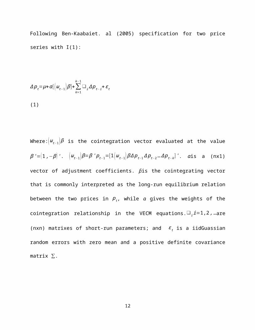
Following Ben-Kaabaiet. al (2005) specification for two price

series with I(1):

∆pt=μ+α[ (ωt−1 )β]+∑k=1

k−1❑i∆pt−i+ϵt

(1)

Where:(ωt−1 )β is the cointegration vector evaluated at the value

β'=(1,−β )'. (ωt−1 )β=β'pt−1=[1 (ωt−1)β∆pt−1∆pt−2…∆pt−k]'. αis a (nx1)

vector of adjustment coefficients. βis the cointegrating vector

that is commonly interpreted as the long-run equilibrium relation

between the two prices in pt, while α gives the weights of the

cointegration relationship in the VECM equations.❑ii=1,2,…are

(nxn) matrixes of short-run parameters; and ϵt is a iidGuassian

random errors with zero mean and a positive definite covariance

matrix .∑

12

However, the standard error correction model has drawn criticism

for two drawbacks. The first criticism is that it assumes

symmetric adjustment to long-run equilibrium regardless of the

sign of the shock. Granger and Lee (1989) tried to solve the

issue by introducing a non-symmetric error-correction model. The

design is simply to segment the ECM term to positive and negative

deviation. The non-symmetric error correction model was further

developed by Enders and Granger (1998), who argued that standard

unit root tests are misspecified if adjustment is asymmetric.

Consequently,Enders and Granger (1998)tabulated new critical

values for unit root tests.The second criticism against the

conventional error correction model is that after a shock it

assumes instant adjustment towards the equilibrium and hence does

not consider, for example, possible transaction costs.Balke and

Fomby (1997)pointed that the movement towards thelong-run

equilibrium is not linear.That is the adjustment need not to

occur instantaneously but only once the deviations exceed some

critical threshold, allowing thus the presence of an inaction, or

no-arbitrage band (Stigler, 2011). Rather adjustments towards the

long-runequilibrium occur only when deviations from the long-run

13

equilibrium exceed acertain threshold.Small deviation from

equilibrium is characterized by a random walk (i.e. a lack of

cointegration).Balke and Fomby (1997) introduced threshold

cointegration method as solution to combine non-linearity and

cointegration.

Lo and Zivot (2001) extendedtheBalke and Fomby

(1997)’sunivariatecointegrationproperty in bivariate settingwith

a known cointegratingvector. Hansen and Seo (2002) improvedBalke

and Fomby(1997) model by estimating the cointegratingvectorand

the threshold parametersimultaneously. In this paper, a three-

regime threshold vectorerror correction model (TVECM3) with one

cointegrating vector and twothreshold parameters is

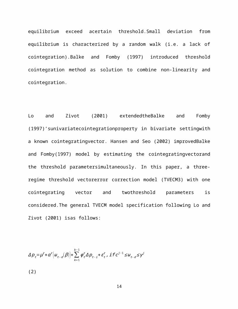
considered.The general TVECM model specification following Lo and

Zivot (2001) isas follows:

∆pt=μr+αr (ωt−d(β))+∑

k=1

k−1φtr∆pt−i+εt

r,ifcj−1≤ωt−d≤γj

(2)

14

Where:r=1,2,3 is regime number;i=1,…,k; k is lag length , d is

delay variable and d<k; (ωt−d ) is error correction term (residual

of the cointegration); γis the parameter of the threshold that

separates the regimes( j=1,2 in our case).

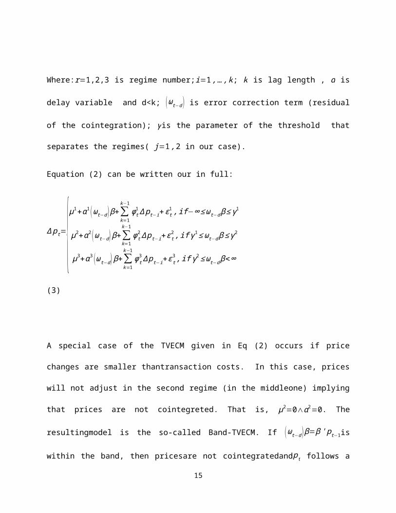
Equation (2) can be written our in full:

∆pt={μ1+α1 (ωt−d )β+∑

k=1

k−1φt1∆pt−i+εt1,if−∞≤ωt−dβ≤γ1

μ2+α2 (ωt−d)β+∑k=1

k−1

φt2∆pt−i+εt

2,ifγ1≤ωt−dβ≤γ2

μ3+α3 (ωt−d)β+∑k=1

k−1φt3∆pt−i+εt

3,ifγ2≤ωt−dβ<∞

(3)

A special case of the TVECM given in Eq (2) occurs if price

changes are smaller thantransaction costs. In this case, prices

will not adjust in the second regime (in the middleone) implying

that prices are not cointegreted. That is, μ2=0∧α2=0. The

resultingmodel is the so-called Band-TVECM. If (ωt−d )β=β'pt−1is

within the band, then pricesare not cointegratedandpt follows a

15

VAR (k) without a drift. However, in the outer bandseconomic

forces push prices moving together implying cointegration with

different adjustmentcoefficients.If(ωt−d )β<γ1∨(ωt−d)β>γ2, then the

cointegrating vector reverts tothe regime-specific mean with an

adjustment coefficient. ρ1∨ρ3.While∆pt adjusts to thelong-run

equilibrium with a speed of adjustment vectorα1∨α3. Where the the

adjustment coefficients,ρr, calculated as:

ρj=1+β'αj=1+[1−β2 ][α1

j

α2j]=1+α1

j−β2α2j

In testing for linearity, Balke and Fomby (1997) advocate two

step approach, first testing for cointegration and then for

threshold effect if there is evidence of cointegtaion. However,

this method may suffer of low power when true model contain

threshold effect and first step is tested based on linear

specification(Stigler, 2011). An alternative methodology by

Hansen and Seo (2002) assumes both threshold parameterγ and

cointegrating vector βare unknown and estimated from the data.

Hansen and Seo (2002) proposed a supLM test statistic of linear

16

VECM against a threshold VECM with two regimes when the true

cointegrating vector is unknown.The test is TVECM against the

null hypothesis of linear VECM. The distribution from SupLM test

cannot be tabulated due to presence of nuisance parameters and

hence the authors suggest two bootstrap approaches, with either

fixed regressor or a residual bootstrap(Stigler, 2011).Further,

Seo (2006) developed Sup-Wald test to test for null hypothesis of

no cointegration against Threshold cointegration based on TVECM

model. The test is based on three regimes where the middle

regime not taken in to account, since it does not adjust. The

Sup-Wald test does not depend on nuisance parameter and critical

values can be calculated via bootstrap method.

4. Data

The data used in this analysis is obtained at three level of beef

industry. The price received by live cattle, price received by

feed lot, price received by slaughters and packers (whole sale

price) andpiece received by retail stores (retail price) are used

for analysis. The national price for live cattle is cash price

which was obtained from CME database. This is nominal price. For

17

wholesale price, however, USDA (ERS) calculated equivalent value

starting with retail price and reassembling the parts. The

pricesseries span years from January 1980 to December 2010. This

period is where the consumption of meat declined because of

health concerns. The time-series data is monthly, not seasonally

adjusted, and all price series were converted into their natural

logarithms before analysis. We have total of 492 data point for

each series. Summary of the data is also provided as appnedex.

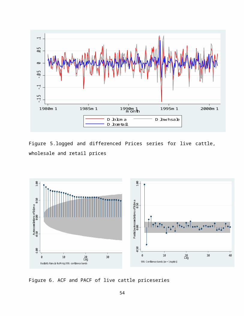
Visual inspection of graphs shows thatthe three price series are

non-stationary (Figure 1 to 3).. The ACF and PCF of this prices

also confirms the same (Figure 4 to 6). For beef across price

stages and changes in co-movement over time (Figure 1 to 3). We

will formally test for stationarity in the next section.

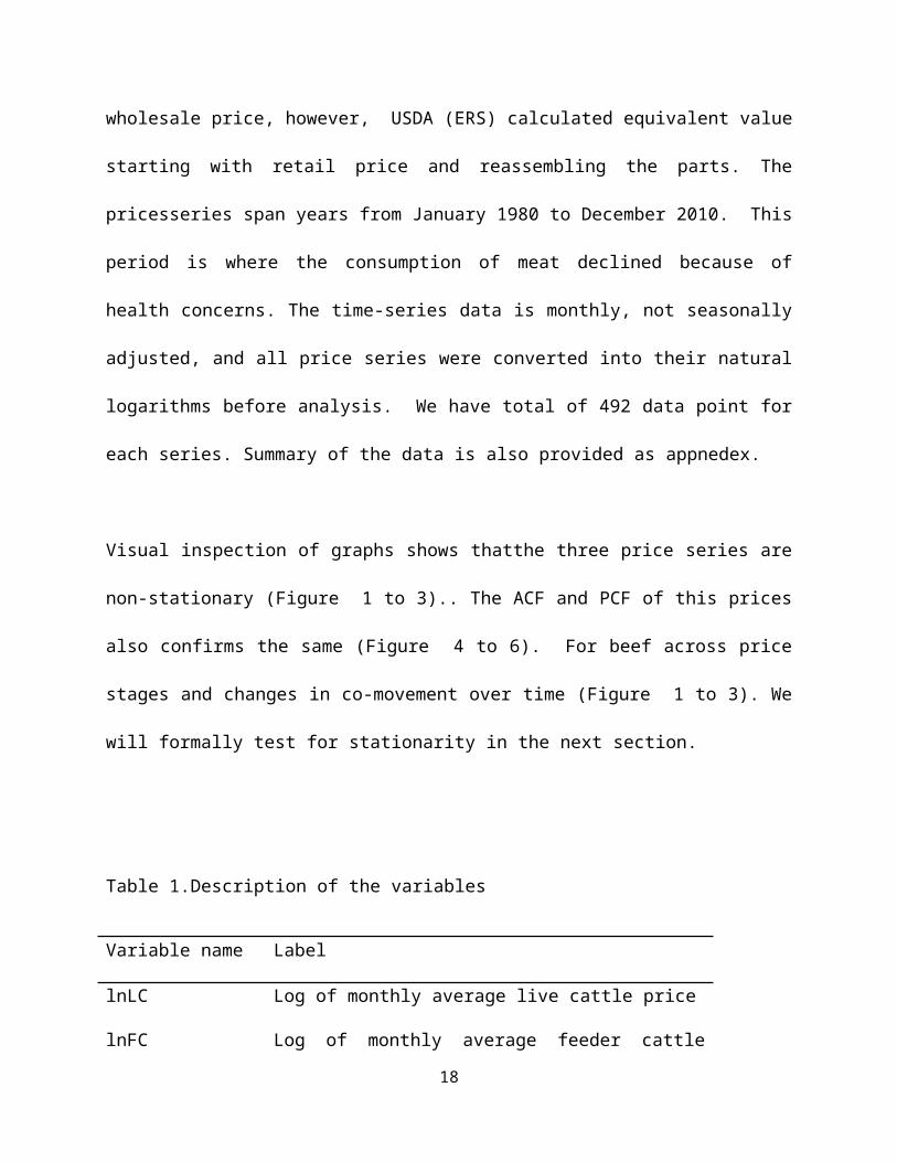
Table 1.Description of the variables

Variable name Label

lnLC Log of monthly average live cattle price

lnFC Log of monthly average feeder cattle

18

price

lnwhsale Log of monthly average meat packers

(whole sellers) price value

lnretail Log of monthly meat retailers price

value

5. Empirical Estimation and Result

5.1. Testing for unit root

Three beef channel price series were test for unit root. We

start with standard Augmented Dickey fuller test first. However,

literature argues that in the presence of a structural break, the

standard ADF tests are biased towards the non-rejection of the

null hypothesis. Thus, we employ Zivot and Andrews (1992) test

which account for one unknown structural break. This endogenous

structural break test is a sequential test which utilizes the

full sample and uses a different dummy variable for each possible

break date. A break date is chosen where the evidence is least

favorable for null hypothesis that says the series has the unit

root.

19

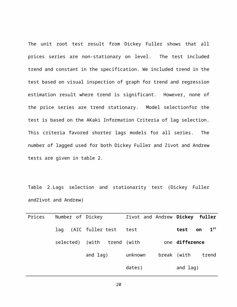
The unit root test result from Dickey Fuller shows that all

prices series are non-stationary on level. The test included

trend and constant in the specification. We included trend in the

test based on visual inspection of graph for trend and regression

estimation result where trend is significant. However, none of

the price series are trend stationary. Model selectionfor the

test is based on the AKaki Information Criteria of lag selection.

This criteria favored shorter lags models for all series. The

number of lagged used for both Dickey Fuller and Zivot and Andrew

tests are given in table 2.

Table 2.Lags selection and stationarity test (Dickey Fuller

andZivot and Andrew)

Prices Number of

lag (AIC

selected)

Dickey

fuller test

(with trend

and lag)

Zivot and Andrew

test

(with one

unknown break

dates)

Dickey fuller

test on 1st

difference

(with trend

and lag)

20

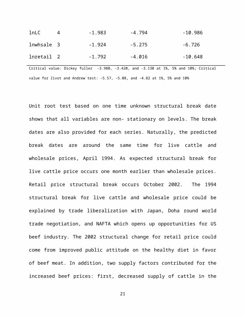
lnLC 4 -1.983 -4.794 -10.986

lnwhsale 3 -1.924 -5.275 -6.726

lnretail 2 -1.792 -4.016 -10.648

Critical value: Dickey fuller -3.980, -3.420, and -3.130 at 1%, 5% and 10%; Critical

value for Zivot and Andrew test: -5.57, -5.08, and -4.82 at 1%, 5% and 10%

Unit root test based on one time unknown structural break date

shows that all variables are non- stationary on levels. The break

dates are also provided for each series. Naturally, the predicted

break dates are around the same time for live cattle and

wholesale prices, April 1994. As expected structural break for

live cattle price occurs one month earlier than wholesale prices.

Retail price structural break occurs October 2002. The 1994

structural break for live cattle and wholesale price could be

explained by trade liberalization with Japan, Doha round world

trade negotiation, and NAFTA which opens up opportunities for US

beef industry. The 2002 structural change for retail price could

come from improved public attitude on the healthy diet in favor

of beef meat. In addition, two supply factors contributed for the

increased beef prices: first, decreased supply of cattle in the

21

United States due to bad weather and second, the U.S.

government’s ban on Canadian beef and cattle after the BSE

outbreak in Canada (USDA/ERS).

5.2. Cointegration Analysis

The unit root test above, both with and without structural break

consideration, establishes that all price series have unit root.

On the other hand the differenced series are stationary, that is,

the series are cointegrated of order one I(1). Therefore, we

proceed with analysis cointegration relationship between the

series at different stage of the beef supply chain. First we

analyze linear cointegration relationships, with and without

unknown structural break consideration. Then we will test for

linearity (threshold cointegration) both for cointegrated and non

cointegrated relationships. The analysis is conducted both on

bivariate (pair) relationship and multivariate relationship in

the chain.

22

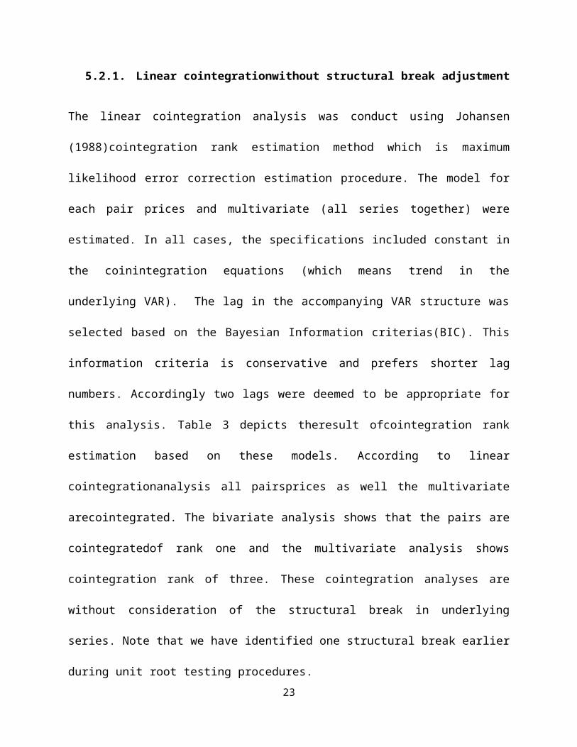
5.2.1. Linear cointegrationwithout structural break adjustment

The linear cointegration analysis was conduct using Johansen

(1988)cointegration rank estimation method which is maximum

likelihood error correction estimation procedure. The model for

each pair prices and multivariate (all series together) were

estimated. In all cases, the specifications included constant in

the coinintegration equations (which means trend in the

underlying VAR). The lag in the accompanying VAR structure was

selected based on the Bayesian Information criterias(BIC). This

information criteria is conservative and prefers shorter lag

numbers. Accordingly two lags were deemed to be appropriate for

this analysis. Table 3 depicts theresult ofcointegration rank

estimation based on these models. According to linear

cointegrationanalysis all pairsprices as well the multivariate

arecointegrated. The bivariate analysis shows that the pairs are

cointegratedof rank one and the multivariate analysis shows

cointegration rank of three. These cointegration analyses are

without consideration of the structural break in underlying

series. Note that we have identified one structural break earlier

during unit root testing procedures. 23

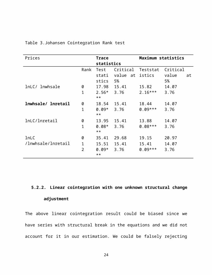
Table 3.Johansen Cointegration Rank test

Prices Tracestatistics

Maximum statistics

Rank Teststatistics

Criticalvalue at5%

Teststatistics

Criticalvalue at5%

lnLC/ lnwhsale 0 17.98 15.41 15.82 14.071 2.56*

**3.76 2.16*** 3.76

lnwhsale/ lnretail 0 18.54 15.41 18.44 14.071 0.09*

**3.76 0.09*** 3.76

lnLC/lnretail 0 13.95 15.41 13.88 14.071 0.08*

**3.76 0.08*** 3.76

lnLC/lnwhsale/lnretail

0 35.41 29.68 19.15 20.971 15.51 15.41 15.41 14.072 0.09*

**3.76 0.09*** 3.76

5.2.2. Linear cointegration with one unknown structural change

adjustment

The above linear cointegration result could be biased since we

have series with structural break in the equations and we did not

account for it in our estimation. We could be falsely rejecting

24

the null hypothesis that no cointegration between the series

where some or all of the underlying series behave like an AR(1)

process with a structural break(Pfaff, 2008). Thus, if the

presence of changes distorts the inference in the univariate

frameworkwe may expect similar effects in the multivariate

framework when testing for the numberofcointegration relations.

This expectation is further supported by evidence from

smallsample studies conducted by Gregory & Hansen (1996) and

Gregory, Nason& Watt(1996) who have found that breaks in the

cointegration relation reduces the power ofsingle-equation

cointegration tests. We follow procedure developed by Lutkepohl,

Saikkonen, and Trenkler (2004) for estimating a VECM in which the

structural shift is a simple shift in level of the process. In

this procedure the structural break date is estimated

endogenously first and the VECM estimation is adjusted

accordingly.

According to this estimation most of the bivariate cointegration

do reject the null hypothesis that no cointegration between the

pair of series (table 4). The cointegration rank betwwen live

cattle and wholesale prices is marginally significant, that is,25

it is significant at 10% significance level. Compared to

estimation without structural break adjustment, the cointegration

relationship between live cattle price and whole sale price

becomes week. It reverts to full rank at 1 and 5% significance

level where both series are stationary by themselves. However,

since the initial stationarity test (using both Dickey Fuller and

Zivot and Andrew test)shows that both series are non-stationary

we trust the 10% significance level result. The cointegration

rank between live cattle and retail and wholesale and retail are

both significant at 5% significance level. The multivariate

equations arecointegratedof rank two at 1% significance level.

The multivariate case is similar result with estimation without

structural break adjustment.

Looking at bivariate relationship may exposes the hidden price

transmission friction which may not be observed when multivariate

model is estimated. Price transmission between sequential stages

of the channel which is hindered either by oligopoly or monopsony

power of one of the agentscannot be observed in multivariate

model. This hindrance is eased depending on the direction of

impact of the two forces on the price transmission in the channel26

(Weldegebriel, 2004). This looks the case for wholesale and live

cattle prices where packers have market power.

Table 4.Linear cointegration rank estimation with endogenous

structural change adjustment

Rank Trace

statistic

s

Critical

value at 5%

lnLC/ lnwhsale 0 43.32 15.83

1 9.32* 6.79

lnLC/lnretail 0 38.72 15.83

1 6.49** 6.79

lnwhsale/ lnretail 0 50.87 15.83

1 6.50** 6.79

lnLC/llnwhsale/lnretail 0 79.84 28.45

1 35.04 15.83

2 3.72*** 6.79

27

5.3. Testing for Linear vs nonlinear cointegration

Once the cointegrationvs no cointegrationrelationshipestablished,

we need test whether the equilibrium price adjustment follow

symmetric (linear) or asymmetric (nonlinear) process for those

cointegrated price relationships. We follow Hansen &Seo (2002)

supLM test where the cointegrating value is estimated from the

linear VECM and then, conditional on this value, the LM test is

run for a range of different threshold values. The maximum of

those LM test values is reported.The null hypothesis for this

test is that the adjustment to equilibrium is linear.

Unfortunately, the current methodology limits this test to be

performed only under bivariate relationship. However, based on

Weldegebriel (2004) theoretical work, breaking down the

relationship into bivariate can help us to clearly see where the

inefficiencies in the market lie. According to this test live

28

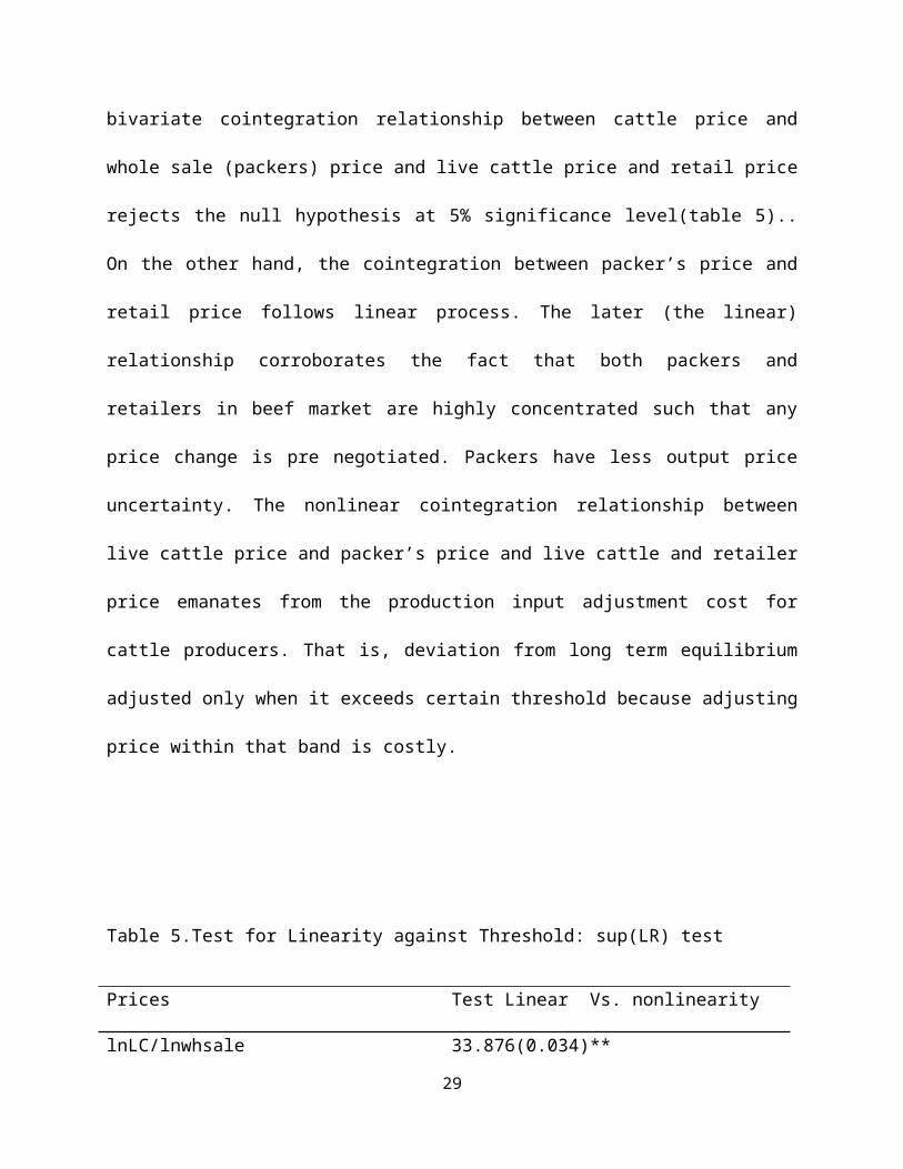
bivariate cointegration relationship between cattle price and

whole sale (packers) price and live cattle price and retail price

rejects the null hypothesis at 5% significance level(table 5)..

On the other hand, the cointegration between packer’s price and

retail price follows linear process. The later (the linear)

relationship corroborates the fact that both packers and

retailers in beef market are highly concentrated such that any

price change is pre negotiated. Packers have less output price

uncertainty. The nonlinear cointegration relationship between

live cattle price and packer’s price and live cattle and retailer

price emanates from the production input adjustment cost for

cattle producers. That is, deviation from long term equilibrium

adjusted only when it exceeds certain threshold because adjusting

price within that band is costly.

Table 5.Test for Linearity against Threshold: sup(LR) test

Prices Test Linear Vs. nonlinearity

lnLC/lnwhsale 33.876(0.034)**

29

lnLC/ lnretail 33.618(0.044)**

lnwhsale/lnretial 11.004(0.356)

Numbers in parenthesis are p-values

5.4. Vector error correction

In this section we estimated the error correction model based on

the models selected in the previous sections. First we estimate

VEC for pair of prices and multivariate prices. Then, we estimate

threshold Vector error correction model for those prices that

found to have nonlinear relationship.

5.4.1. Linear Vector Error correction model Estimation

Based on the cointegration rank test in previous section, we now

proceed toward estimation of the vector error correction model.

The lag selection for the underlying VAR model is based more

conservative on Information Criteria (BIC). As the prices series

displays upward trend we included constant in the error

30

correction term (ECT) which means trend in the cointegrating

equation. For comparison reason we present linear cointegration

estimation result for those bivariate prices that exhibits

nonlinear cointegration.

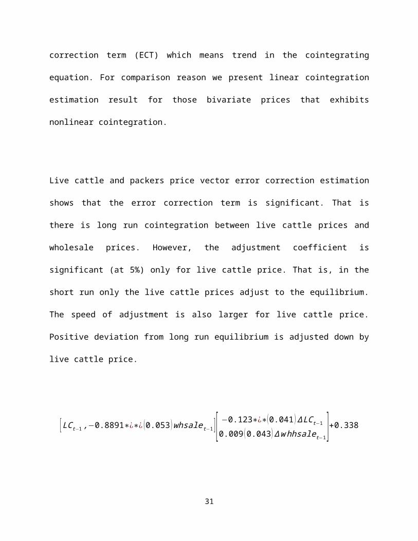
Live cattle and packers price vector error correction estimation

shows that the error correction term is significant. That is

there is long run cointegration between live cattle prices and

wholesale prices. However, the adjustment coefficient is

significant (at 5%) only for live cattle price. That is, in the

short run only the live cattle prices adjust to the equilibrium.

The speed of adjustment is also larger for live cattle price.

Positive deviation from long run equilibrium is adjusted down by

live cattle price.

[LCt−1,−0.8891∗¿∗¿ (0.053 )whsalet−1 ][ −0.123∗¿∗(0.041 )∆LCt−1

0.009 (0.043)∆whhsalet−1]+0.338

31

Wholesale and retail price vector error correction estimation

result below depicts that the error correction term is

significant at 1% significance level. The adjustment coefficient

for both wholesale price and retail price is significant at 1%

significance level. When the cointeration relationship deviates

up (positive) from lung run equilibrium it is corrected down by

whole sale price. On other side, when it deviates down (negative)

it is adjusted up by retail price. That is, whole sale price

corrects for positive deviation while retail price corrects for

negative deviation. The speed of adjustment is higher for

positive deviation. This shows that, the two agents in the

channel work together. This should be the case since both packers

and retailer are concentrated. The packer can exercise oligopoly

power and the retailer can exercise monopsony power which

balances each other. Thus, agents forced towork together than

exercising their power.

[whsalet−1−0.617∗¿∗¿ (0.042 )retailt−1 ] [−0.147∗¿∗(0.029 )∆whhsalet−1

0.029∗¿∗(0.010 )∆retailT−1 ]−1.66932

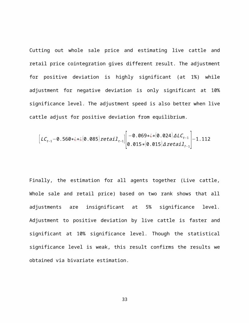
Cutting out whole sale price and estimating live cattle and

retail price cointegration gives different result. The adjustment

for positive deviation is highly significant (at 1%) while

adjustment for negative deviation is only significant at 10%

significance level. The adjustment speed is also better when live

cattle adjust for positive deviation from equilibrium.

[LCt−1−0.560∗¿∗¿ (0.085 )retailt−1 ] [ −0.069∗¿∗(0.024 )∆LCt−1

0.015∗(0.015 )∆retailT−1]−1.112

Finally, the estimation for all agents together (Live cattle,

Whole sale and retail price) based on two rank shows that all

adjustments are insignificant at 5% significance level.

Adjustment to positive deviation by live cattle is faster and

significant at 10% significance level. Though the statistical

significance level is weak, this result confirms the results we

obtained via bivariate estimation.

33

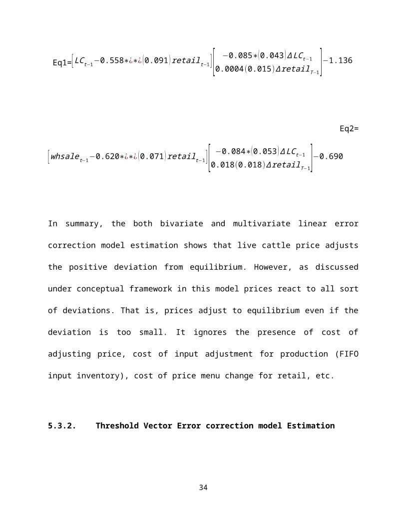
Eq1=[LCt−1−0.558∗¿∗¿ (0.091 )retailt−1 ] [ −0.085∗(0.043 )∆LCt−1

0.0004(0.015)∆retailT−1]−1.136

Eq2=

[whsalet−1−0.620∗¿∗¿ (0.071 )retailt−1 ] [ −0.084∗(0.053 )∆LCt−1

0.018(0.018)∆retailT−1]−0.690

In summary, the both bivariate and multivariate linear error

correction model estimation shows that live cattle price adjusts

the positive deviation from equilibrium. However, as discussed

under conceptual framework in this model prices react to all sort

of deviations. That is, prices adjust to equilibrium even if the

deviation is too small. It ignores the presence of cost of

adjusting price, cost of input adjustment for production (FIFO

input inventory), cost of price menu change for retail, etc.

5.3.2. Threshold Vector Error correction model Estimation

34

Threshold cointegration extends the usual linear cointegration to

cases where the adjustment towards long-run equilibrium does not

occur after each small deviation but more realistically only when

the deviations exceed some critical thresholds.Thus it account

for transaction costs, other institutional market interventions

and asymmetries in price transmission.In previous section, we

have already tested for possibility of threshold cointegration

instead of linear cointegration. We have found two of the

bivariate relationship to be threshold cointegrated. Here, we

estimate and present the threshold vector error correction model

(TVECM) result for those two bivariate price series.

We implement Hansen and Seo (2002) three regime TVEM estimation

technique. The three regime model makes much more economic sense

that there should be a buffer zone before the adjustment to

equilibrium is triggered. The lag selection for VAR was based on

AIC and BIC. Both AIC and BIC favored two lags. As the case with

linear VECM, two lag and trend was included in the regression

which common for all regimes. Trims of 2% (minimum number of

35

observation to be included in each regime) were set for

regression. The number of bootstrap replication used to estimate

the p values is 500 and the number of grid (threshold points to

be estimated) is also 300. The number of bootstrap replication is

higher than what the authors used in their original paper. We

just wanted to assure robustness of our estimate.

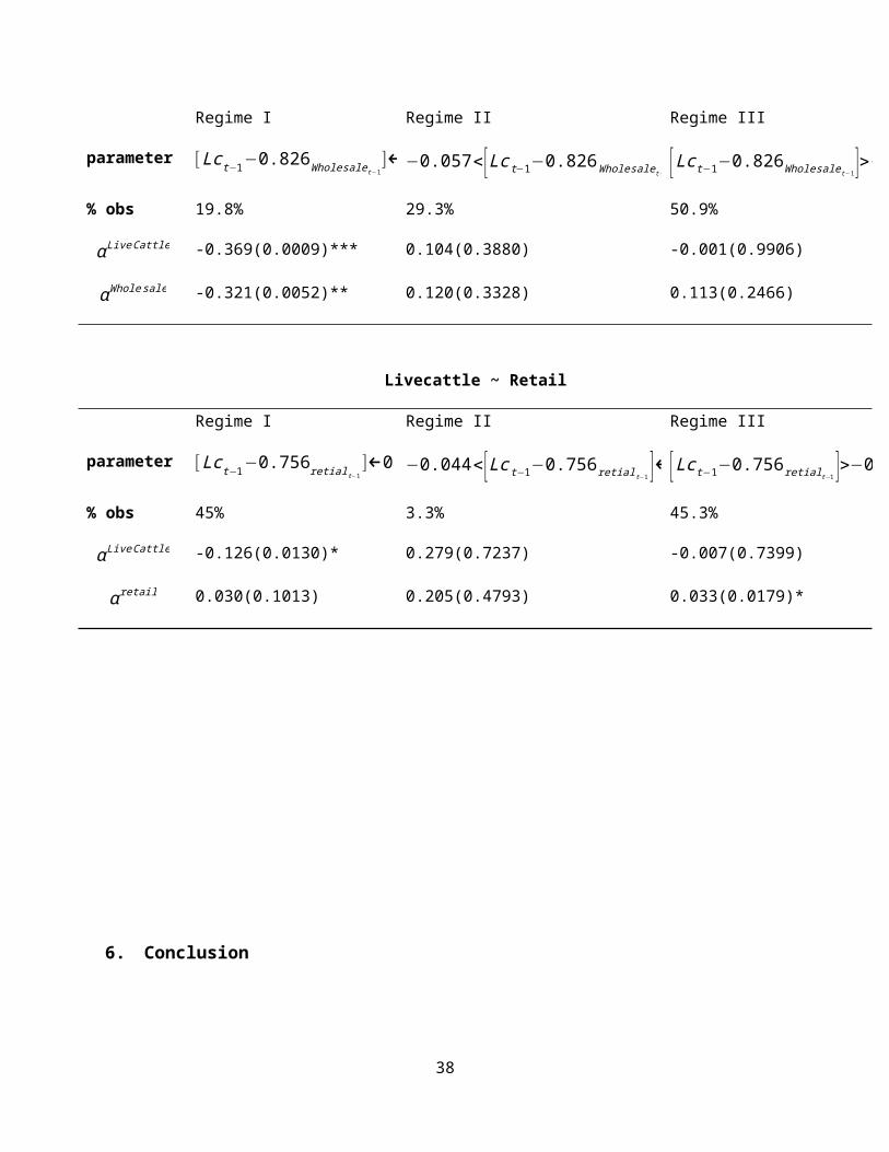
Table 6 depicts the result of the TVECM estimation. For

estimation of cointegration between live cattle and whole sale

price, the two thresholds value are 4.9% and 1.5% of the

equilibrium price. Decrease in live cattle price 4.9% below lung

run equilibrium moves the equilibrium process to regime one,

which calls for adjustment. If live cattle price increase 1.5%

above the long run equilibrium, then, the system moves to regime

there which calls for different adjustment pattern. Prices

adjustment process won’t be triggered within band (between 4.9%

decrease and 1.5% increases from equilibrium prices). The

adjustment process is significant in regime one. The speed of

adjustment is also faster. Note that even though its adjustment

36

coefficients are not statistically significant, regime three

contains majority (50.9%) of the observation.

For live cattle and retail price threshold cointegration the

observation is almost equally divided between regime one and

regime three. The middle regime has extremely low observation.

The two thresholds that drive the system between regime one and

three are 4.4 % and 3.6% decreases (increase) in price of live

cattle from equilibrium. The adjustment coefficients are

significant (at 10%) for negative adjustment and positive

adjustment in regime one and three respectively. Positive

deviation is adjusted by live cattle price in regime one while

negative deviation in regime three is adjusted by retail price.

The speed of adjustment is faster for positive deviation than

negative deviation.

Table 6. TVECM model estimates

Live cattle ~ whole sale

37

Regime I Regime II Regime III

parameter [Lct−1−0.826Wholesalet−1]←0.049−0.057<[Lct−1−0.826Wholesalet−1 ]←0.015[Lct−1−0.826Wholesalet−1]>−0.015

% obs 19.8% 29.3% 50.9%

αLiveCattle -0.369(0.0009)*** 0.104(0.3880) -0.001(0.9906)

αWholesale -0.321(0.0052)** 0.120(0.3328) 0.113(0.2466)

Livecattle ~ Retail

Regime I Regime II Regime III

parameter [Lct−1−0.756retialt−1]←0.044−0.044<[Lct−1−0.756retialt−1 ]←0.036[Lct−1−0.756retialt−1 ]>−0.036

% obs 45% 3.3% 45.3%

αLiveCattle -0.126(0.0130)* 0.279(0.7237) -0.007(0.7399)

αretail 0.030(0.1013) 0.205(0.4793) 0.033(0.0179)*

6. Conclusion

38

The purpose of this research is to assess the integration, and

thus the efficiency of the beef industry. Towards this goal, we

tested the presence of long run cointegration between the price

series. The price series considered in this analysis are live

cattle price, wholesale price and retail price. We tested and

estimated both linear and nonlinear (where linearity is rejected)

relationships between these price series. Accordingly, the both

bivariate and multivariate linear error correction model

estimation shows that live cattle price adjusts the positive

deviation from equilibrium. This result reflects the structure of

the industry where meat slaughters and packers are concentrated.

On the other hand, slaughters and packers and retailers prices

adjust to each other. Since both Packers and retailers have

market power, it is not surprising that this giants work together

in collaboration.

However, as discussed under conceptual framework in this model

prices react to all sort of deviations. That is, prices adjust to

equilibrium even if the deviation is too small. It ignores the

39

presence of cost of adjusting price, cost of input adjustment for

production (FIFO input inventory), cost of price menu change for

retail, etc. Therefore, we estimated TVECM model for live cattle

and wholesale prices and for live cattle retail prices.

Accordingly we find that live cattle and whole sale prices adjust

when the deviation crosses two thresholds value, 4.9% and 1.5%

below and above the equilibrium price, respectively. The both

adjustment coefficients are significant at the lower regime but

level of significant and the speed of adjustment is greater for

live cattle price. Though asymmetric, the basic result is

similar to the linear model. For live cattle and retail prices,

the two thresholds value that drive the system between regime one

and three are 4.4 % and 3.6% (decreases and increase in price of

live cattle from equilibrium respectively). The adjustment

coefficients are significant (at 10%) for live cattle and retail

prices in regime one and three, respectively.

Generally, the price transmission is unidirectional especially at

the upper tier of the market channel. The price the price

40

fluctuation transmitted from live cattle to wholesale but not

vice versa. This result is similar to finding by Goodwin and Holt

(1999). Whole sale and packers work together, that they negotiate

the price beforehand. The slaughter/ packer have price certainty

when it buys fed cattle as input. This is not the case at the

upper level of the channel. This has an implication for the

margin of the upper level agents in the beef industry.

41

References

Abdulai, A. (2002): Using threshold cointegration to estimate

asymmetric price transmission

in the Swiss pork market, Applied Economics, Vol. 34, pp. 679-687.

Azzam, A. M. (1997). Measuring Market Power and Cost-Efficiency

Effects of Industrial Concentration, Journal of Industrial Economics,

45(4), 377–86.

Bailey, D. V. and B. W. Brorsen (1989). Price Asymmetry in

Spatial Fed Cattle Markets, Western Journal of Agricultural Economics

14:246-52.

Balke, N.S. and Fomby, T.S. (1997).Threshold

Cointegration.International Economic Review 38: 627-645.

Balke, N.S., Brown, S.P.A. and Yücel, M.K. (1998). Crude oil and

gasoline prices: An asymmetric relationship? Federal Reserve Bank of

Dallas, Economic Review, First Quarter: 2-11.

42

Barro, R. J. (1972). A theory of monopolistic price adjustment,

Review of Economic Studies 39: 17-26.

Ben-Kaabai, M., Gill, JM., Boshnjaku, L. (2002): Price

transmission asymmetries in the Spanish lamb sector. Paper presented

at the X. Congress of European Association of Agricultural Economists, 28-31 August,

Zaragoza, Spain.

Bernhard Pfaff, Analysis of Integrated and Cointegrated Time

Series with R, Springer New York, 2008.

Blinder, A. S. (1994), “On sticky prices: Academic theories meet

the real world”, in Mankiw,

N.G. (ed.), Monetary Policy, Chicago and London, The University of

Chicago Press.

Blinder, Alan S., E. R. D. Canetti, D. E. Lebow, and J. B. Rudd

(1998). Asking About Prices: A New Approach to Understanding

Price Stickiness , Russell Sag e Foundation, New York.43

Brorsen, B. Wade, Jean-Paul Chavas, and Warren R. Grant (1985).A

Dynamic Analysis of Prices in the U.S. Rice Marketing Channel" J.

Bus.& Econ. Stat., 4:362-369.

Carman, H.F. (1998). California Milk Marketing Margins, Journal

of Food Distribution Research November, 1-6.

Carman, H.F. and R.J. Sexton (2005). A Supermarket Fluid Milk

Pricing Practices in the Western United States, Agribusiness 21:

509-530.

Cotterill, R. W. "Continuing Concentration in the U.S.: Strategic

Challenges to an Unstable Status Quo, Res. Rep. No. 48, Food

Marketing Policy Center, University of Connecticut, August 1999.

Cowling, K and Waterson, M. (1979).Price-Cost Margins and Market

Structure.Economica43: 267-274.

Dawson, P.J. and Tiffin, R. (2000): Structural breaks,

cointegration and the farm-retail price spread for lamb, Applied

Economics 32:1281-1286.

44

Dimitri, C., A. Tegene, and P.R. Kaufman (2003). U.S. Fresh

Produce Markets: Marketing Channels, Trade Practices, and Retail

Pricing Behavior, U.S. Department of Agriculture, Economic

Research Service, Agricultural Economic Report No. 825,

September.

Frey, G. and M. Manera (2007). Econometric models of asymmetric

price transmission. Journal of Economic Surveys 21(2):349-415.

Frigon, M., Doyon, M. and Romain, R. (1999). Asymmetry in Farm-

Retail Price Transmission in the Northeastern Fluid Milk Market,

University of Connecticut, Food Marketing Policy Center, Research

Report No. 45.

Gardner, B.L. (1975). The farm-retail price spread in a

competitive food industry, American Journal of Agricultural Economics

57:399-409.

Goodwin, B.K. (2006). Spatial and Vertical Price Transmission in

Meat markets. Paper presented at the Workshop on Market

45

Integration and Vertical and Spatial Price Transmission in

Agricultural Markets. University of Kentucky, USA, April.

Goodwin, Barry, and Matthew Holt, (1999).Price Transmission and

Asymmetric Adjustment in the U.S. Beef Sector.American Journal of

Agricultural Economics 81.

Gregory, A.W., Hansen B.E. (1996). Residual based tests for

cointegration in models with regime shifts, Journal of Econometrics

70:99-126.

Gregory, A.W., Nason, J.M., Watt, D. (1996). Testing for

structural breaks in cointegrated relationship, Journal of

Econometrics 71:321-341.

Hansen, B. and Seo, B. (2002). Testing for two-regime threshold

cointegration in vector error-correction models, Journal of

Econometrics, 110, pages 293 – 318.

46

Kinnucan, H.W. and O.D. Forker (1987). Asymmetry in Farm-Retail

Price Transmission for Major Dairy Products, American Journal of

Agricultural Economics 69: 285-292.

Koontz, S., & Garcia, P. (1997). Meat-packer conduct in fed

cattle pricing: Multiple-market oligopsony power, Journal of

Agricultural and Resource Economics 22: 78–86.

Levy, Daniel, M. Bergen, S. Dutta, and R. Venable (1997). The

Magnitude of Menu Costs: Direct Evidence from Large U.S.

Supermarket Chains, Quarterly Journal of Economics 112: 791–825.

Lloyd, T. A., McCorriston, S., Morgan, C. W., and Rayner, A. J.,

(2006). Food Scares, Market Power and Price Transmission: The UK

BSE Crisis. European Review of Agricultural Economics 33(2): 119-147.

Lo, C. and Zivot, E. (2001). Threshold Cointegration and

Nonlinear Adjustments to the Law

of One Price. Macroeconomic Dynamics 5: 533-576.

47

Lutkepohl, H., Saikkonen, P. and Trenkler, C. (2004). Testing for

the Cointegrating Rank of a VAR Process with Level Shift at

Unknown Time, Econometrica, Vol. 72, No. 2, 647–662.

McCorriston, S., Morgan, C.W. and A.J. Rayner (2001): Price

transmission: The interaction between market power and returns to

scale, European Review of Agricultural Economics 28:143-159.

Marsh, J., and G. Brester (2004). Wholesale -Retail Margin

behavior in Pork and Beef, Journal of Agricultural and Resource

Economics, 29, 45–64.

Meyer J, von Cramon-Taubadel S. (2004). Asymmetric Price

Transmission: A survey. J. Agric. Econ. 55 (3): 581-611.

Peltzman S. (2000). Prices rise faster than they fall. The Journal

of Political Economy, 108, pp. 466–502.

Pick, D.H., J. Karrenbrock, and H.F. Carman (1990). Price

Asymmetry and Marketing Margin Behavior: an Example for

California B Arizona Citrus, Agribusiness 6: 75-84.

48

Powers, E.T. and N.J. Powers (2001) “The Size and Frequency of

Price Changes: Evidence from Grocery Stores,” Review of Industrial

Organization 18: 397-416.

Reagan, Patricia B., and Martin L. Weitzman (1982). Asymmetries

in Price and Quantity Adjustments by the Competitive Firm, Journal

of Economic Theory 27: 410-420.

Schrimper, R. A. Economics ofAgricultura1 Markets. Englewood

Cliffs, NJ: Prentice-Hall, Inc., 2001.

Schroeder, Ted C. and Barry K. Goodwin (1990). Regional Fed

Cattle Price Dynamics, West. Ournalof Agricultural Economics 15:111-122.

Schroeter, John and A. Azzam (1991). Marketing Margins, Market

Power, and Price Uncertainiy, Amer. .lAgr. Econ.73 : 990-999.

Seo, M. (2006), Bootstrap testing for the null of no

cointegration in a threshold vector error correction model,

Journal of Econometrics 134:129–150.

49

Von Cramon-Taubadel S. (1998). Estimating asymmetric price

transmission with the error correction representation: an

application to the German pork market.European Review of Agricultural

Economics, 25, pp. 1–18.

Ward, R.W. (1982). Asymmetry in Retail, Wholesale and Shipping

Point Pricing for Fresh Vegetable.American Journal of Agricultural

Economics 64: 205-212.

Weldegebriel, H. T., (2004). Imperfect Price Transmission: Is

Market Power Really to Blame? Journal of Agricultural Economics 55: 101-

114.

Wohlgenant,M., and J. Mullen (1987). Modeling the Farm-Retail

Price Spread for Beef, Western Journal of Agricultural Economics 12(2),

115–125.

50

Vara, P. and B.K. Goodwin (2005).Analysis price transmission

along the food chain, OECD Foord Agriculture and Fisheries

Working Papers, No. 3.

Zhang, P., S.M. Fletcher, and D.H. Carley (1995). Peanut Price

Transmission Asymmetry in Peanut Butter, Agribusiness 11: 13-20.

Zivot, E. and D. Andrews, (1992). Further evidence of great

crash, the oil price shock and unit root hypothesis, Journal of

Business and Economic Statistics 10: 251-270.

Appendix 51

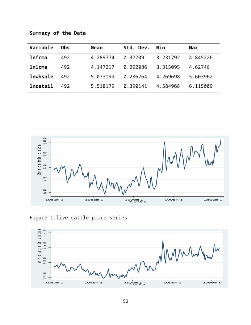
Summary of the Data

Variable Obs Mean Std. Dev. Min Max

lnfcma 492 4.289774 0.37709 3.231792 4.845226lnlcma 492 4.147217 0.292086 3.315095 4.62746lnwhsale 492 5.073199 0.286764 4.269698 5.603962lnretail 492 5.518179 0.390141 4.584968 6.115009

6070

8090

100

livec

attle

pric

e

1980m 1 1985m 1 1990m 1 1995m 1 2000m 1M onths

Figure 1.live cattle price series

150

200

250

300

whole

sale

value

1980m 1 1985m 1 1990m 1 1995m 1 2000m 1M onths

52

Figure 2.whole sale price (value) series

250

300

350

400

450

reta

il valu

e

1980m 1 1985m 1 1990m 1 1995m 1 2000m 1M onths

Figure 3. Retail price (value) series

44.5

55.5

6

1980m 1 1985m 1 1990m 1 1995m 1 2000m 1m onth

lnlcm a lnwhsalelnretail

Figure 4.logged Pricesseries for live cattle, wholesale and

retail prices

53

-.15

-.1-.0

50

.05

.1

1980m 1 1985m 1 1990m 1 1995m 1 2000m 1m onth

D.lnlcm a D.lnwhsaleD.lnretail

Figure 5.logged and differenced Prices series for live cattle,

wholesale and retail prices

-1.00

-0.50

0.00

0.50

1.00

Autocorrelations of lnlcm

a

0 10 20 30 40LagBartlett's form ula for M A(q) 95% confidence bands

-0.50

0.00

0.50

1.00

Partial autocorrelations of lnlcm

a

0 10 20 30 40Lag95% Confidence bands [se = 1/sqrt(n)]

Figure 6. ACF and PACF of live cattle priceseries

54

-1.00

-0.50

0.00

0.50

1.00

Autocorrelation

s of ln

whsale


-0.50

0.00

0.50

1.00

Partial autocorrelation

s of ln

whsale


Figure 7. ACF and PACF wholesale price series

-1.00

-0.50

0.00

0.50

1.00

Autoco

rrelat

ions o

f lnretail


-0.50

0.00

0.50

1.00

Partial

autoco

rrelat

ions o

f lnretail


Figure 8. ACF and PACF retail price series

55

-0.40

-0.20

0.00

0.20

0.40

Autocorrelations of D.lnlcm

a


-0.40

-0.20

0.00

0.20

0.40

Partial autocorrelations of D.lnlcm

a


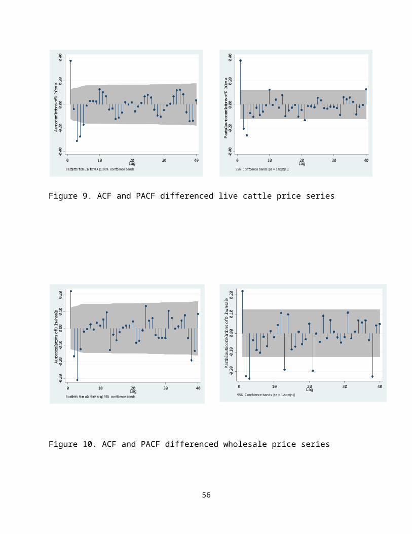
Figure 9. ACF and PACF differenced live cattle price series

-0.30

-0.20

-0.10

0.00

0.10

0.20

Autocorrelation

s of D

.lnwh

sale


-0.20

-0.10

0.00

0.10

0.20

Partial autocorre

lation

s of D

.lnwh

sale


Figure 10. ACF and PACF differenced wholesale price series

56

-0.20

-0.10

0.00

0.10

0.20

Autocorrelations of D.lnretail


-0.20

-0.10

0.00

0.10

0.20

Partial autocorrelations of D.lnretail


Figure 11. ACF and PACF differenced retial price series

-.5

0

.5

1

1.5

-.5

0

.5

1

1.5

-.5

0

.5

1

1.5

0 10 20 30 0 10 20 30 0 10 20 30

lnlc, lnlc lnlc, lnretail lnlc, lnwhsale

lnretail, lnlc lnretail, lnretail lnretail, lnwhsale

lnwhsale, lnlc lnwhsale, lnretail lnwhsale, lnwhsale

M onthsG raphs: im pulse variable and response variable

Figure 12.Impulse response functionbased on VEC estimation

57

050

100

150

200

250

1980m 1 1985m 1 1990m 1 1995m 1 2000m 1m onth

m argin_fc_lc m argin_wh_fcm argin_rtl_wh

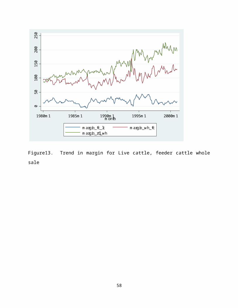
Figure13. Trend in margin for Live cattle, feeder cattle whole

sale

58

Market Integration in the US Beef supply Chain: A Threshold Cointegration approach

Documents

Transcript of Market Integration in the US Beef supply Chain: A Threshold Cointegration approach