DISCUSSION PAPER SERIES

Available online at: www.cepr.org/pubs/dps/DP3450.asp and http://ssrn.com/abstract_id=325366

www.ssrn.com/xxx/xxx/xxx

No. 3450

MARKET AND TECHNICALRISK IN R&D

Heiko Gerlach, Thomas Roendeand Konrad O Stahl

INDUSTRIAL ORGANIZATION

ISSN 0265-8003

MARKET AND TECHNICALRISK IN R&D

Heiko Gerlach, CERAS-ENPCThomas Roende, Universität Mannheim and CEPRKonrad O Stahl, Universität Mannheim and CEPR

Discussion Paper No. 3450July 2002

Centre for Economic Policy Research90–98 Goswell Rd, London EC1V 7RR, UK

Tel: (44 20) 7878 2900, Fax: (44 20) 7878 2999Email: cepr@cepr.org, Website: www.cepr.org

This Discussion Paper is issued under the auspices of the Centre’s researchprogramme in INDUSTRIAL ORGANIZATION. Any opinions expressed hereare those of the author(s) and not those of the Centre for Economic PolicyResearch. Research disseminated by CEPR may include views on policy, butthe Centre itself takes no institutional policy positions.

The Centre for Economic Policy Research was established in 1983 as aprivate educational charity, to promote independent analysis and publicdiscussion of open economies and the relations among them. It is pluralistand non-partisan, bringing economic research to bear on the analysis ofmedium- and long-run policy questions. Institutional (core) finance for theCentre has been provided through major grants from the Economic andSocial Research Council, under which an ESRC Resource Centre operateswithin CEPR; the Esmée Fairbairn Charitable Trust; and the Bank ofEngland. These organizations do not give prior review to the Centre’spublications, nor do they necessarily endorse the views expressed therein.

These Discussion Papers often represent preliminary or incomplete work,circulated to encourage discussion and comment. Citation and use of such apaper should take account of its provisional character.

Copyright: Heiko Gerlach, Thomas Roende and Konrad O Stahl

CEPR Discussion Paper No. 3450

July 2002

ABSTRACT

Market and Technical Risk in R&D*

We endogenize the market risk (at given technical risk) in firms’ R&Ddecisions by introducing stochastic R&D in the Hotelling model. It is shownthat if the technical risk is sufficiently high, the market risk remains low even iffirms pursue similar projects. This leads firms to focus on the most valuablemarket segment. We then also endogenize technical risk by allowing firms tochoose their R&D technology. In equilibrium, firms either pursue similar(different) R&D projects with risky (safe) technologies or they choose thesame project but apply different R&D technologies. We show that R&Dspillovers lead to more differentiated R&D efforts and patent protection to less.Project coordination within a RJV implies more differentiation, and may, ormay not be welfare-improving.

JEL Classification: D81, L13 and O32Keywords: market risk, R&D project choice and technical risk

Heiko A. GerlachCERAS-ENPC28, Rue des Saints-Peres75343 Paris Cedex 07FRANCETel: (33 1) 44 58 28 81Fax: (33 1) 44 58 28 80Email: heiko.gerlach@enpc.fr

For further Discussion Papers by this author see:www.cepr.org/pubs/new-dps/dplist.asp?authorid=139965

Thomas RoendeDepartment of EconomicsUniversität MannheimD-68131 MannheimGERMANYTel: (49 621) 181 1871Fax: (49 621) 181 1874Email: roende@econ.uni-mannheim.de

For further Discussion Papers by this author see:www.cepr.org/pubs/new-dps/dplist.asp?authorid=146667

Konrad O StahlDepartment of EconomicsUniversität MannheimD-68131 MannheimGERMANYTel: (49 621) 181 1875Fax: (49 621) 181 1874Email: konrad@econ.uni-mannheim.de

For further Discussion Papers by this author see:www.cepr.org/pubs/new-dps/dplist.asp?authorid=103825

* We wish to thank Gilles Duranton, Martin Hellwig, Patrick Rey, andconference and seminar participants at University Bocconi, CERAS (Paris),IAE (Barcelona), INSEAD (Fontainebleau), and University of Mannheim foruseful comments. We gratefully acknowledge financial support from theDeutsche Forschungsgemeinschaft (grant SPP 199, Sta 169/9-3) and theEuropean Commission under the TMR network ‘The Evolution of MarketStructure in Network Industries’ (FMRX-CT98-0203). This Paper is producedas part of a CEPR Research Network on The Evolution of Market Structure inNetwork Industries, funded by the European Commission under the Trainingand Mobility of Researchers Programme (Contract No ERBFMRX-CT98-0203).

Submitted 20 June 2002

1 Introduction

It is reported from the pharmaceutical industry that the next ten years

could yield an astonishing 4000 to 5000 different types of new drugs due to

new research techniques. Nevertheless, according to the Financial Times,

the top 50 companies in that industry concentrate over 70 per cent of their

R&D expenditure in as few as 20 so-called blockbuster drugs.1,2 In this pa-

per we study the strategic forces that lead firms in R&D intensive industries

to concentrate in such profitable market segments, and thereby forego op-

portunities in less competitive niche segments. We argue that the focus on

blockbuster innovations stems from the stochasticity inherent in R&D ac-

tivities. That stochasticity is particularly important in the pharmaceutical

industry: only one or two compounds out of 10,000 evaluated ever get as far

as getting a licence.3

In the business literature on R&D portfolio theory, it is common to

distinguish between two dimensions of risks. Technical risk referring to the

probability that a development project eventually turns into a marketable

product, andmarket risk referring to the probability of meeting a competitor

in a targeted market segment once the product is developed. Analytically, a

firm’s market risk consists of two elements: the probability that a competitor

develops a product (which is in fact the technical risk taken by him), and the

probability that this product is in a similar market segment. We show that if

the technical risk of the firms in an industry is sufficiently high, the market

risk remains low even if the firms are pursuing similar projects, and this

leads firms to focus on the most valuable market segment. The notions of

market and technical risks are useful for analyzing R&D choices. Yet these

risks should be considered as endogenous. To the best of our knowledge,

ours is the first attempt to endogenize both of these risk dimensions in one

model.

Towards motivating our approach by a more specific example, consider

the ongoing race to bring a new type of cancer treatment to the market.

1see The Financial Times, January 3, 1998, page 18 (London Edition).2This is confirmed in a more recent report by Ansell and Sparker (1999). In the report,

R&D in the pharmaceutical industry is divided into 14 therapeutic areas. On average,the top 50 firms are active in 5 of the 6 most popular therapeutic areas, but in less than2 of the remaining 8 areas. Furthermore, 96 percent of the 50 biggest pharmaceuticalcompanies concentrate on research in cardiovascular treatment.

3BBC News Online, Nov 21, 2000: ”Drugs - a high-risk business” (available athttp://news.bbc.co.uk).

1

The drugs, EGFR inhibitors, do not cure cancer, but stop cancer cells from

growing and spreading to other parts of the body.4 Three drugs have made

it to the final trial phase and are potentially valuable weapons in the bat-

tle against cancer. Interestingly, the firms involved have chosen different

drug designs. AstraZeneca and OSI Pharmaceuticals have developed drugs

(Iressa and Tarceva, respectively) that are more convenient to use than Im-

Clone Systems’ Erbitux, as they can be taken in pill-form instead of being

injected. This is likely to make them the first choice for patients with lung

cancer, the most common cancer form (indeed, AstraZeneca and OSI Phar-

maceuticals are primarily targeting this group in their trials). Erbitux, on

the other hand, is less likely to cause diarrhea as a side effect, which makes

it more suitable against colon cancer, a considerably less valuable market

segment. This example is supposed to highlight two points: First, product

differentiation matters; here, products differ by side effects. Second, there is

a tendency for firms to agglomerate in the most profitable market segment;

here, that for the treatment of lung cancer.

We now sketch our modelling approach to analyze strategic behavior

in such a market. Towards replicating the choice between market risks,

we use Hotelling’s (1929) product differentiation framework. For identi-

cal known product qualities and quadratic transportation costs, we know

from d’Aspremont et al. (1979) that duopolists always choose to offer niche

products at the opposite end of the market. In the above terminology, firms

minimize their market risk. We amend the Hotelling framework and allow

for technical risk by assuming that market entry depends on the stochastic

outcome of firms’ R&D activities. In our benchmark model with exogenous

and symmetric R&D success probabilities, we show that this may lead to

clustering around, or in the center of the market. From a welfare point of

view, the duopolists excessively concentrate (disperse) if innovation proba-

bilities are low (high).

In the second part of the paper, we take the analysis one step further and

endogenize the technical risk as well. In addition to the choice of the market

segment, firms can now also select a R&D technology: they can adopt either

a safe project yielding a low-quality product; or a risky technology yielding,

if successful, a high quality one. We show that this leads to a feedback

4For more information about EGFR inhibitors and the firms involved in the marketsee: The Scientist, April 1, 2002: ”Closing in on Multiple Cancer Targets” (available athttp://www.the-scientist.com); Reuters Health Information, October 18, 2001: ” ”SmartBomb” Drugs Offer Hope in Cancer Battle” (available at http://www.cancerpage.com).

2

loop between the two dimensions of risks. More technical risk leads to more

clustering, and this endogenous increase in market risk makes risky projects

more profitable. Three types of equilibria may emerge. Either firms cluster

and both adopt the risky R&D technology, or one firm does so whilst the

other chooses the safe technology; or the firms maximally differentiate and

both adopt the safe technology.

A couple of straightforward extensions of the benchmark model yield fur-

ther interesting insights. In contrast to standard reasoning, R&D spillovers

exercise in our model a centrifugal force on the location equilibrium. The

reason is that spillovers increase the probability that firms end up in a

duopoly. By contrast, patent protection fosters monopolistic outcomes and

therefore constitutes an additional agglomerative force. Finally, we intro-

duce research joint ventures in a particular and, in our view, interesting way,

by allowing firms to coordinate the location of their R&D effort. Relative

to uncoordinated location decisions, this leads firms to cluster less, which

may, or may not contribute to welfare. While, as we will argue in detail

in the concluding section of our paper, the elements of strategic behavior

are in principle difficult to observe, the outcomes sketched above for the

pharmaceutical industry are certainly in consonance with our analytic ones.

The related theoretical literature is rich in papers on clustering in prod-

uct space. Our work is most closely related to Harter (1993). Like us,

Harter introduces R&D into the Hotelling model. However, he only de-

rives sufficient conditions for a clustering equilibrium to arise, whence in

our benchmark model, we are able to fully characterize and evaluate all

equilibrium outcomes. Furthermore, we extend our model to cover a num-

ber of issues not addressed by him. Most importantly, we analyze the effects

of an endogenous choice of R&D technology. We also discuss the effects of

spillovers, patent protection, and research joint ventures.

Bester (1998) and Vettas (1999) look at a situation where firms signal the

quality of their products to imperfectly informed consumers, and show how

this might lead to agglomeration. The authors use a Hotelling set-up, with

horizontal product as well as vertical quality differentiation. In our model,

consumers can perfectly observe the quality of the products, so signalling

does not play a role. The effects leading to agglomeration in our model are

thus quite different from those demonstrated by these authors.

Within a two dimensional Hotelling framework, Neven and Thisse (1993)

and Irmen and Thisse (1998) demonstrate clustering effects in one of two

3

dimensions of product differentiation, where one is vertical and the other

horizontal, and both are horizontal, respectively. Their central point is on

sufficient conditions under which (maximal) product differentiation in one

dimension suffices for firms to agglomerate in the centre of the market in

another dimension.

There are also models on R&D portfolio choices by authors such as Bhat-

tacharya and Mokherjee (1986), Dasgupta and Maskin (1987), and more re-

cently Cabral (2002). The R&D technologies considered in these papers are

more general than the one we use. However, these authors do not consider

product differentiation, which is our main focus. An exception is Cardon

and Sasaki (1998) who consider a simple, binary choice of product charac-

teristics in a patent race. In Cardon and Sasaki, the incentive to choose the

same characteristics stems from patent protection. Our basic argument does

not rely on patent protection, but we show that such protection reinforces

the tendency towards clustering.

The decision to make products compatible in a network industry resem-

bles the choice of agglomerating in product space, as the products become

closer substitutes. Our work is therefore related to an early paper by Katz

and Shapiro (1986) who consider compatibility choices when technological

progress is stochastic. However, making the products closer substitutes leads

to opposite effects in the two models. In our model, it makes product mar-

ket competition tougher whereas it softens competition in Katz and Shapiro,

because firms do not compete in building up a customer base.

The remainder of the paper is organized as follows: In the next section,

we present our benchmark model. We determine and characterize the price

equilibrium, and the location equilibrium and welfare outcomes. In Section

3, we endogenize R&D decisions by allowing firms to choose the riskiness of

their R&D project. In section 4, we consider a number of smaller extensions.

The concluding section serves to summarize our results and to comment on

their empirical verifiability. Proofs are relegated to the appendix.

2 The Benchmark Model

We employ the standard Hotelling (1929) duopoly model in the version

of d’Aspremont et al. (1979). The market area is described by the unit

interval M = [0, 1]. There is a unit mass of consumers with locations that

are uniformly distributed on M. Two firms i = A,B are potentially active

4

in this market at locations of supply denoted a, b ∈ M , a ≤ b. Consumersbuy at most one unit of the product and incur quadratic distance costs of

overcoming space. Thus a consumer located at y derives net utility

UA(a, qA, pA, y) = qA − pA − t(a− y)2

when buying good A and a corresponding utility when buying B. qi and pi

are the quality and the price of firm i’s product, respectively. t > 0 reflects

the degree of consumer heterogeneity or horizontal product differentiation.

All variables are common knowledge.

Firms costlessly invest in R&D.5 If firm i0s project succeeds, it sells aproduct of quality qi, i = A,B. In the benchmark model, firms succeed with

the probability ρ and produce the same quality if successful, qA = qB = q.

Thus, firms face the same technical risk. The firms’ success probabilities are

uncorrelated. Firms have no fall-back quality. If the project is unsuccessful,

the firm remains inactively in the market.6

As to the timing, firms first simultaneously choose their locations (a, b),

which together with ρ determine the market risk.7 Then the outcomes of

their R&D are realized. Finally, firms set prices simultaneously, consumers

buy one of the available products, and profits are realized.

2.1 Price Equilibrium for given qualities and locations

Depending on the outcome of the R&D process after the location is fixed,

the typical firm may produce and sell a product at positive quality, or it may

remain inactive if unsuccessful. If successful, it may either be a monopolist

or a duopolist, depending on the success or failure of its competitor.

In the present stage, the firms’ locations and product qualities are known

and taken as given when they set their prices. It is entirely standard to derive

the monopoly and the duopoly prices, so we short cut our presentation. For

future reference to be used in the extensions, we calculate equilibrium prices

and profits allowing for quality differences between the firms’ products.

5Introducing a small fixed cost of R&D would not change the results.6Thus, we think of a situation where firms active in other markets explore the possibil-

ity, via engaging in R&D, of becoming active in the market under scrutiny. The possibilityof a fall-back product if R&D fails is discussed in section 4.4.

7In a duopoly model, the concept of market risk is easy to define for independentproducts. It is the product of the probability that the competitor targets the same productand the probability that its R&D is successful. Once products are substitutes, it is lessobvious how to define market risk as it depends on how close substitutes products are.Here, we will simply refer to market risk as being higher if for given technical risks productsare closer substitutes.

5

2.1.1 Monopoly Pricing

Let without loss of generality only firm A located at a ≤ 12 succeed in

developing a product of quality qA. The then monopolist maximizes its

profits, pDM(qA, a, p). Under the assumption qA ≥ 3t used henceforth, themonopolist covers the market by charging the price pMA = qA − t(1 − a)2.Since under this assumption all consumers are served, the monopoly profit

ΠM(qA, a) is equivalent to the monopoly price.

2.1.2 Duopoly Pricing

Here both firms conduct successful R&D, resulting in qualities qA and qB, re-

spectively. By our assumption, the market is covered. The firms’ Bertrand-

Nash equilibrium prices are given in Lemma 1.

Lemma 1 (i) For qA − qB < −t(b− a)(2 + a+ b), firm B is the only firm

with positive market share. The unique price equilibrium is

pDA(a, b, qA, qB) = 0 and pDB(a, b, qA, qB) = qB − qA − t(b2 − a2). (1)

(ii) For −t(b− a)(2+ a+ b) < qA− qB < t(b− a)(4− a− b), the firms sharethe market. The unique price equilibrium is

pDA(a, b, qA, qB) =1

3(qA − qB + t(b− a)(2 + a+ b)) and (2)

pDB(a, b, qA, qB) =1

3(qB − qA + t(b− a)(4− a− b)).

(iii) For qA − qB > t(b− a)(4− a− b), firm A is the only firm with positive

market share. The unique price equilibrium is

pDA(a, b, qA, qB) = qA − qB − t(b− a)(2− a− b) and pDB(a, b, qA, qB) = 0.(3)

The proof is entirely standard. Not unexpectedly, Lemma 1 demon-

strates that if there are substantial quality differences relative to the trans-

portation cost t, the low quality firm is driven out of the market by the high

quality one. Using Lemma 1, we can derive the equilibrium profits. In case

(i) where firm A is inactive, the profits are given as

ΠDB(a, b, qA, qB) = qB − qA − t(b2 − a2) and ΠDA(a, b, qA, qB) = 0. (4)

6

Similarly, if firm B is inactive as in case (iii), the profits are

ΠDA(a, b, qA, qB) = qA − qB − t(b− a)(2− a− b) and ΠDB(a, b, qA, qB) = 0.(5)

Finally, in the case where the firms share the market, they earn profits

ΠDA(a, b, qA, qB) =(qA − qB + t(b− a)(2 + a+ b))2

18t(b− a) and (6)

ΠDB(a, b, qA, qB) =(qB − qA + t(b− a)(4− a− b))2

18t(b− a) .

This completes the analysis of price competition in the market place.

2.2 Location under Stochastic R&D Outcomes

2.2.1 The Equilibrium

The firms’ location decisions are taken before the outcomes of their R&D

efforts become known. Each of the firms innovates with probability ρ. Ex-

pected profits are

E(ΠA(a, b, qA, qB, ρ)) = ρ(ρΠDA(a, b, q, q) + (1− ρ)ΠM(q, a)) and

E(ΠB(a, b, qA, qB, ρ)) = ρ(ρΠDB(a, b, q, q) + (1− ρ)ΠM(q, b)).

Using pMi and equation (4)-(6), we obtain the first order condition for firm

A when choosing its location a. It can be shown that firm A’s problem is

concave, so solving the first-order condition, we find the optimal location of

firm A as a function of the location of firm B. The equilibrium is derived

formally in Proposition 1.

Proposition 1 Consider the choice of location in the first stage of the game.

i) For ρ ≤ 23 , the unique equilibrium locations are a∗ = b∗ = 1

2 .

ii) For 23 < ρ ≤ 1, the unique equilibrium locations for a ≤ b are

a∗ =Max½0,1

2− Γ

¾and b∗ = 1− a∗,

where Γ≡ 3(3ρ−2)4(3−2ρ) .

The equilibrium outcome can be interpreted in terms of the well-known

trade off between the demand and the competition effect. The former pro-

vides incentives to move to the center of the market, and the latter away

7

from it. d’Aspremont et al. (1979) show that if both firms are active with

certainty, the competition effect dominates, so firms locate as far as possible

from each other. However, in our model, the firms foresee that if they enter

the market, they will only meet an active competitor with probability ρ.

This weakens the competition effect but not the demand effect, as a firm

benefits from a central location as an ex-post monopolist. Therefore, firms

tend to cluster more in equilibrium.

They locate in the center of the market if the technical risk is high, so the

probability of ending up in a duopoly situation is low. If the technical risk is

low, the duopoly outcome becomes so likely that the competition effect starts

to dominate and firms fragment in equilibrium. In that sense, an increase

(decrease) in technical risk leads to an endogenous decrease (increase) in

market risk. As in d’Aspremont et al., that outcome does not depend on t.

2.2.2 Welfare

Is there too much, or too little clustering in equilibrium, as compared to

the locational choice of a surplus maximizing social planner? The following

two observations greatly simplify the calculation of the latter. First, as the

market is covered by assumption, we do not need to worry about how many

consumers buy the product. Second, as consumers exercise unit demand,

there is no deadweight loss due to monopoly pricing. Therefore, the wel-

fare optimal locations are simply those that minimize consumers’ expected

transportation costs.

Proposition 2 The welfare maximizing locations are:

aW =1

2− Ω and bW =

1

2+Ω where Ω ≡ ρ

4 (2− ρ).

Ex-post, that is, after the R&D outcomes are realized, the optimal loca-

tions depend on whether there are one or two firms active in the market.

The monopolist’s welfare maximizing location is 1/2, and the duopolists’

ones are a = 14 and b =

34 , respectively. What does this imply for the firms’

ex-ante welfare maximizing locations, i.e., before the outcomes of the R&D

efforts are revealed? Let ρ, the probability that a firm innovates, become

very small. Then, if there is any innovation, the innovator will tend to be a

monopolist, resulting in an optimal location close to 12 . As ρ increases, the

probability that a duopoly arises increases. Therefore, the distance between

the welfare maximizing locations increases up to 12 for ρ = 1 .

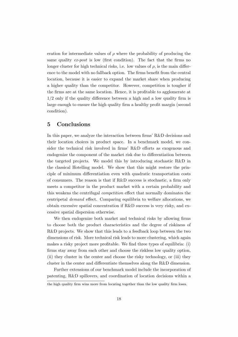
8

ρ

1

a*

32

13120 1

b*

aW

bW

21

Figure 1: Equilibrium and welfare maximising locations at varying technicalrisk.

Comparing Proposition 1 and Proposition 2, we obtain immediately

Corollary 1 There exists a unique value eρ = 3/2−p15/28 ≈ 0.7681 suchthat

i) ρ < eρ implies a∗ < aW (b∗ > bW )ii) ρ > eρ implies a∗ > aW (b∗ < bW ).

Figure 1 illustrates the relationship between welfare maximizing (dashed)

and equilibrium (solid) locations as a function of the exogenous technical

risk, ρ. There is excessive product clustering for low ρ (i.e. high technical

risk) and excessive dispersion for high ρ. From a welfare point of view, firms

disregard the surplus of infra-marginal consumers. It is easy to check that,

ex post, consumer surplus is maximized if the monopolist is located at one

end of the line and if duopolists are completely clustered in the center. Thus,

ex ante, if the technical risk is high (low) and a monopoly (duopoly) outcome

is more likely, the firms’ marginal incentives to cluster are too strong (weak)

from a social point of view.

9

3 Endogenous Risk-Taking in R&D

In the previous section, the firms’ technical risk was assumed to be exoge-

nous and symmetric. In the following we endogenize it and allow it to be

asymmetric by considering firms to costlessly follow alternatively a ’safe’

research path (’S ’), or a risky and innovative path (’R’). Following the safe

path, the firm develops with certainty a product of quality q and thereby

minimizes its own technical risk. Instead, following the risky path, it devel-

ops with probability ρ a product of higher quality q +∆. The outcomes of

risky R&D efforts are again uncorrelated. In order to keep the model man-

ageable, we assume that the firms can only follow one of the paths. Hence,

if a firm tries to develop the high quality product but fails, it cannot switch

to the low risk strategy, and thus must stay inactive ex-post.

The firms simultaneously choose their location and R&D strategies. We

already have determined the equilibrium prices for given location and qual-

ities, so we only have to look for a Nash-equilibrium jointly in locations and

R&D choices. We denote firm A’s strategy by sA = (a, zA), where a is the

location and zA ∈ S,R is the R&D project. Firm B’s strategy is denoted

in the same manner.

We find the equilibrium of the game in two steps. First, we determine

the reaction functions in location and the equilibrium locations for given

R&D technologies. Afterwards, we determine the equilibrium of the overall

game where R&D technologies and locations are chosen simultaneously.

If both firms choose the safe strategy, we know from d’Aspremont et al.

that their equilibrium locations are at the opposite ends of the Hotelling

line. Proposition 1 specifies the equilibrium locations conditional upon both

firms choosing the risky R&D path. However, if one firm chooses the safe

technology and the other the risky one, the reaction functions are highly

non-linear. Towards solving the model in closed form we need to assume

that ρ ≤ 23 ≡ ρ. This excludes technologies that are successful with a very

high probability. Hence we concentrate our analysis on sufficiently risky

R&D projects, which are anyway the more interesting ones in the present

context. In the next lemma, we specify the best location that a firm with

the risky technology would choose given the other firm’s location and (safe)

technology.

Lemma 2 Consider a candidate equilibrium, in which one firm, say, A

chooses the safe technology and locates at a ≤ 12 while B chooses the risky

10

one. Then, firm B’s optimal location is

b∗ =½a if ∆ ≥ (1− a)(6 + a− 3√3 + 2a)t1 if ∆ < (1− a)(6 + a− 3√3 + 2a)t.

The best response for the safe technology firm is given by

Lemma 3 Consider a candidate equilibrium, in which one firm (say, A)

chooses the safe technology while the other (B) chooses the risky one. Then,

firm A’s optimal location is 1/2.

The optimal locations of the two firms are substantially different for

asymmetric R&D choices. The reaction function of the high quality firm

exhibits an interesting discontinuity. For low quality improvements, it be-

haves as ’soft’ as possible, and goes to the end of the line to enjoy some local

monopoly power. However, once a certain threshold level of ∆ is reached, it

chooses the opposite strategy and behaves as ’tough’ as possible. It locates

then at the same place as the low quality firm, which is the most profitable

way of driving the competitor out of the market. The firm with the safe

technology earns much higher profits when it is alone in the market. There-

fore, it chooses the location that maximizes the monopoly profits for all

locations of the (potential) high quality competitor.

The next lemma summarizes the two possible candidate equilibria when

firms have asymmetric R&D technologies.

Lemma 4 The unique candidate equilibrium, in which one firm (say, A)

chooses the safe technology while the other (B) chooses the risky one is

(12 , S), (1, R) if ∆ ≤ t4 , and (12 , S), (12 , R) otherwise.

We are now in the position to solve for the equilibria of the full game.

For given technology choices, we have identified four candidate equilibria.

These equilibria qualify as an equilibrium of the overall game if no firm

has an incentive to switch unilaterally its technology (and optimally adjusts

its location). Denote the possible equilibria by sA, sB where the twoentries refer to firm A’s and firm B’s strategies, respectively. For notational

convenience, define the following threshold values

∆∗1(ρ, t) ≡25t

144ρ, ∆∗2(ρ, t) ≡Min

t

2ρ, 3t(

1√ρ− 1) and

∆∗3(ρ, t) ≡(1− ρ)(4q − t)

4ρ.

11

Proposition 3 There exist three different types of Nash equilibria of the

game:

i) (12 , R), (12 , R) is the unique equilibrium if and only if ∆ ≥ ∆∗3(ρ, t).ii) (12 , S), (12 , R) and (12 , R), (12 , S) are equilibria if and only if ∆∗1(ρ, t) ≤∆ ≤ ∆∗3(ρ, t).iii) (0, S), (1, S) is an equilibrium if and only if ∆ ≤ ∆∗2(ρ, t).

2/3

(1/2,R),(1/2,R)

and

0

*1∆

*2∆

*3∆

(1/2,S),(1/2,R)

(0,S),(1,S)(0,S),(1,S)

(1/2,S), (1/2,R)

∆

ρ

t)32(3 −

4/t

Figure 2: Equilibrium Strategies in ρ−∆ Space

Figure 2 summarizes the equilibrium outcomes. With low values of both

∆ and ρ, the expected return on the risky technology is so low that the

firms prefer choosing the safe technology, in which case the firms locate as

far as possible from each other. However, if the innovation step is larger

than ∆∗2(ρ, t), firms have an incentive to switch unilaterally to the riskytechnology and differentiate maximally (minimally) for ∆ ≤ (≥)3(2−√3)t.By contrast, if both ∆ and ρ exhibit high values, the risky technology has a

high expected return and is chosen by both firms. The probability of being

monopolist in the market is sufficiently high that a firm only deviates to the

safe technology (and staying at 1/2) if ∆ ≤ ∆∗3(ρ, t). Most interestingly, forintermediate values of ∆ and ρ, we find equilibria where the firms choose

different technologies and locate in the center of the market. The firm with

12

the safe technology does not deviate to the risky technology (with optimal

location at 1/2) as long as ∆ ≤ ∆∗3(ρ, t). The optimal deviation of thefirm with the risky technology should be accompanied by a relocation to

the end of the line. This is not beneficial for all ∆ ≥ ∆∗1(ρ, t). Finally, notethat for ∆ ≤ t/4, the fourth candidate equilibrium (1/2, S), (1, R) is notan equilibrium of the overall game since the risky technology firm always

deviates to the safe technology.

From this it follows that there is a non-empty subset of the parame-

ter space consisting of ∆∗1(ρ, t) ≤ ∆ ≤ ∆∗3(ρ, t) with two possible equilibria:(0, S), (1, S) and (1/2, S), (1/2, R). This multiplicity is due to the inher-ent interdependence between risk-taking and clustering. The more technical

risk there is in the market (it suffices that one firm is taking the risk), the

stronger is the incentive to cluster in the most profitable segment. And the

closer both firms’ R&D projects are, the more it pays to take risk, as a low

quality competitor is easier to drive out of the market. This feedback loop

leads to the coexistence of an equilibrium with niche projects and safe re-

search paths and an equilibrium where firms cluster and one is taking a risky

research path. It is easy to check that there is no ranking of these two equi-

libria in terms of firms’ profits since the firm with the safe technology in the

center prefers the clustering equilibrium (1/2, S), (1/2, R) while the firmwith the risky technology prefers the dispersion equilibrium (0, S), (1, S).However, industry profits are higher in the clustering equilibrium.

These results provide an interesting link to the literature on multi-

dimensional horizontal differentiation. Here, it has been shown (e.g. by

Irmen and Thisse, 1998) that firms tend to differentiate maximally in one

dimension and minimally in all other. This is similar to what happens in our

model for low and intermediate values of∆ and ρ. For low values, firms differ

maximally in locations but choose the same R&D strategy, whilst for inter-

mediate values, locational differentiation is minimal but the R&D strategies

differ. Yet this cannot happen for high values: Since consumers are willing

to pay more for higher quality, both firms differentiate minimally in space,

and prefer the risky technology as it has a high expected pay-off.

The risk-return trade-off in R&D has also been studied by Dasgupta

and Maskin (1987) and Bhattacharya and Mookherjee (1986), among oth-

ers. They used general risk-return functions. However, to make the analysis

tractable, the authors restrict their attention to symmetric R&D choices by

the firms in the industry. In a less general model, we demonstrate that im-

13

posing symmetry might be quite restrictive. Indeed, our results suggest that

firms have incentives to differentiate themselves along the R&D dimension

in order to relax expected competition.

The following corollary looks at the equilibrium outcome under a spe-

cific subset of the risky innovation technologies, namely all mean-preserving

spreads of the safe innovation technology.

Corollary 2 If the firms can choose between two technologies with the same

mean but a different spread, i.e. q = ρ(q +∆), the equilibrium outcome is

(12 , R), (12 , R).

Hence, if the risky innovation is a mean-preserving spread of the safe

innovation, the possibility of ending up as a monopolist with the high quality

product is so attractive that no firm wishes to pursue the safe R&D strategy.

Unfortunately, extending the welfare evaluation does not lead to results

as clear cut as those illustrated in the benchmark model. Referring to Propo-

sition 3, there is a ∆W1 (ρ, t) < ∆∗1(ρ, t) and a ∆

W2 (ρ, t) > ∆

∗2(ρ, t) such that

below ∆W1 (ρ, t) and above ∆W2 (ρ, t), firms both adopt the safe and the risky

technology, respectively, which are the welfare maximizing R&D technol-

ogy choices. However, below ∆W1 (ρ, t) the firms excessively differentiate in

product space, and above ∆W2 (ρ, t) they excessively concentrate. In the

regime between ∆W1 (ρ, t) and ∆W2 (ρ, t), the firms should optimally cluster

in the middle and choose different R&D technologies. Thus, the interval

(∆∗2(ρ, t),∆∗3(ρ, t)) contains welfare maximizing equilibrium allocations. Be-low this, one of the firms adopts too safe a technology and products are

excessively differentiated. Above this, firms choose the welfare maximiz-

ing location in the middle, but one of the firms chooses too risky a R&D

technology.8

4 Other Extensions

4.1 Patent Protection and Technological Spillovers

As discussed earlier, our model most appropriately reflects a situation in

which the firms think of introducing a brand new type of product and cre-

ating a new market. Products of this type, such as a first effective drug

against a disease, are often protected by patent laws. It is thus interesting

8The complete welfare analysis is contained in Gerlach et al. (2002)

14

to know how the above results are affected by patent protection. We assume

that patents introduce an element of ’winner-takes-all’ into the pay-offs. In

particular, if both firms are successful in R&D, there is a probability λ that

one of the firms will be granted a patent that excludes the other firm from

the market. The firms are equally likely to be the lucky one awarded the

patent.9 The expected profits of firm A (and firm B symmetrically) are:

ρ2(1− λ)ΠDA(a, b) + ρ2λΠMA (a)/2 + ρ(1− ρ)ΠMA (a).

Proposition 4 summarizes the analysis of this modified game with patent

protection.

Proposition 4 Patent protection leads to (weakly) less dispersed locations.

The intuition behind this result is straightforward: Patent protection

makes it more likely that the firms end up in a monopoly. This weakens

the competition effect even more (and with it, the market risk), with the

demand effect again unaffected. Thus, clustering becomes more attractive.

Following the same logic, it is clear that any force preventing the monopoly

outcome to arise increases dispersion incentives. The most prominent ex-

ample is technological spillovers. In the literature, spillovers are typically

considered a centripetal force in models with product differentiation (e.g.,

Duranton, 2000; Mai and Peng, 1985). It thus seems worth highlighting the

effect of spillovers on firms’ locations in our framework.

Assume that if one of the firms innovates, but the other one does not,

the unsuccessful firm receives a spillover that allows it to become active with

probability σ.10

Proposition 5 Technological spillovers lead to (weakly) more dispersed lo-

cations.

The formal argument is analogous to the patent protection one. Spillovers

decrease both firms’ technical risk and increase the market risk. Clustering

9Under a ’first-to-file’ patent system, one could imagine a sequential structure wherethe firms were equally likely to file the patent first. λ would be the probability that thefirm holding the patent would win a patent infringement case.10Such spillovers may occur due to the use of common suppliers or to employees switch-

ing job or talking informally; see Mansfield (1985).

15

becomes less attractive.11 The model thus provides an interesting contrast-

ing view to the standard argument suggesting that knowledge spillovers lead

to clustering in R&D intensive industries.

Finally, notice that positive or negative correlation in R&D outcomes

would have an effect similar to spillovers and patent protection, respec-

tively.12 Hence, a positive correlation between R&D outcomes would lead

to less agglomeration in equilibrium compared to the benchmark model, and

negative correlation to more agglomeration.

4.2 Research Joint Venture

Returning to the benchmark model, we assume that the firms, by forming

a research joint venture (RJV), can coordinate their choice of location, but

then compete in prices.13 Calculating the locations that maximize the joint

expected profits of firms yields

Proposition 6 Consider a situation in which firms coordinate their loca-

tion choices but compete in prices.

i) For ρ ≤ 12 , the unique equilibrium locations are aRJV = bRJV = 1

2 .

ii) For 12 < ρ ≤ 1, the unique equilibrium locations for a ≤ b are

aRJV =Max

½0,1

2−Ψ

¾and bRJV = 1− arjv where Ψ≡ 2ρ− 1

2(1− ρ).

iii) An RJV is welfare improving for ρ ∈ (12 , 2 −√2) and welfare reducing

for ρ ∈ (2−√2, 1213).

In this semi-collusive arrangement, firms internalize the loss incurred by

the competitor as they move closer together in product space. Consequently,

firms always locate (weakly) further from each when they collude in loca-

tions. This explains why a RJV may be welfare improving for low values

of ρ where firms are clustering too much in the non-collusive equilibrium.

11Actually, while the reduction in the rival’s technical risk fosters differentiation, thereduction in a firm’s own technical risk has no effect on project choice since this decisionis taken conditional upon success in development.12Yet the effects are not identical. Take the case of spillovers. With spillovers, the fact

that a firm fails to innovate does not contain information about the other firm’s likelihoodof failing, as it would if projects were positively correlated. A positive correlation in R&Doutcomes might occur for exogenous reasons (for example, the most promising researchpath is evident to participants in the industry) or might be a strategic choice as in Cardonand Sasaki (1998).13The idea that firms collude in R&D through a research joint venture goes back to

Kamien et al. (1992).

16

For large values of ρ, on the other hand, there is too much dispersion in

equilibrium and a RJV exacerbates this tendency. Observe that this result

is in sharp contrast to results a la Kamien et al. (1992), according to which

RJV’s always welfare dominate less co-operative equilibrium outcomes.

4.3 Endogenous Costly R&D Intensity

As a third extension, consider now the continuous choice of R&D intensity.

Instead of choosing the risk profile of the R&D activities, firms decide on the

technical risk by investing in the probability of success, ρi, for an innovation

of given size q.14 For quadratic R&D costs, 12γρi2, we find a symmetric

equilibrium where firms choose the same R&D intensity, i.e. ρA = ρB =

ρ. This corresponds to the equilibrium in the benchmark model, since,

for a given equilibrium ρ, the location is as described in Proposition 1.

However, the crucial parameter is now γ. If γ is high, R&D is relatively

costly. Therefore, the firms choose ρ low and locate together at the center

of the line. On the other hand, if γ is low, the firms choose ρ high and locate

away from each other. However, unlike the benchmark model, there is the

possibility of asymmetric equilibria.15

4.4 A Fallback Product

In the benchmark model, we have assumed that a firm can not enter the

market if its R&D efforts fail. We interpret this as a situation where the

firms open a new market. We have considered a variation of the benchmark

model with a fallback product. It is not possible to solve the model with

continuous location choice. Assuming instead that the firms can locate either

at the center or at the ends of the line, the firms agglomerate at the center

of the market if ρ is neither close to 0 nor to 1 and the quality improvement

resulting from successful R&D is sufficiently high.

The firms prefer to locate as far as possible from each other if the prod-

ucts ex-post are of the same quality.16 Therefore, there can only be agglom-

14Ideally, one would include both R&D intensity and risk choice in the same model.Unfortunately, this analysis is not tractable in our set-up.15The general analysis of asymmetric equilibria is difficult because of the functional

forms involved. We have, however, been able to find sufficient conditions for the existenceof an asymmetric equilibrium where one firm locates at 1/2 and invests a lot in R&Dwhereas the other firm locates at the end of the line and invests little in R&D.16Of course, a low quality firm would prefer to locate as far as possible from a high

quality firm ex-post. However, ex-ante the firms are equally likely to be the high and thelow quality firm. Agglomeration may thus be profitable from an ex-ante point of view if

17

eration for intermediate values of ρ where the probability of producing the

same quality ex-post is low (first condition). The fact that the firms no

longer cluster for high technical risks, i.e. low values of ρ, is the main differ-

ence to the model with no fallback option. The firms benefit from the central

location, because it is easier to expand the market share when producing

a higher quality than the competitor. However, competition is tougher if

the firms are at the same location. Hence, it is profitable to agglomerate at

1/2 only if the quality difference between a high and a low quality firm is

large enough to ensure the high quality firm a healthy profit margin (second

condition).

5 Conclusions

In this paper, we analyze the interaction between firms’ R&D decisions and

their location choices in product space. In a benchmark model, we con-

sider the technical risk involved in firms’ R&D efforts as exogenous and

endogenize the component of the market risk due to differentiation between

the targeted projects. We model this by introducing stochastic R&D in

the classical Hotelling model. We show that this might restore the prin-

ciple of minimum differentiation even with quadratic transportation costs

of consumers. The reason is that if R&D success is stochastic, a firm only

meets a competitor in the product market with a certain probability and

this weakens the centrifugal competition effect that normally dominates the

centripetal demand effect. Comparing equilibria to welfare allocations, we

obtain excessive spatial concentration if R&D success is very risky, and ex-

cessive spatial dispersion otherwise.

We then endogenize both market and technical risks by allowing firms

to choose both the product characteristics and the degree of riskiness of

R&D projects. We show that this leads to a feedback loop between the two

dimensions of risk. More technical risk leads to more clustering, which again

makes a risky project more profitable. We find three types of equilibria: (i)

firms stay away from each other and choose the riskless low quality option,

(ii) they cluster in the center and choose the risky technology, or (iii) they

cluster in the center and differentiate themselves along the R&D dimension.

Further extensions of our benchmark model include the incorporation of

patenting, R&D spillovers, and coordination of location decisions within a

the high quality firm wins more from locating together than the low quality firm loses.

18

research joint venture. Patent protection leads one firm to win at the cost

of the other, which decreases the competitive pressure and increases cluster-

ing. In sharp contrast to extant arguments, spillovers align the firms’ R&D

successes and lead to more dispersion. Finally, allowing firms to coordinate

their object of R&D efforts within a research joint venture brings them to

differentiate more than in the uncoordinated equilibrium. Unexpectedly,

this may lessen welfare rather than contribute to it.

As usual, some interesting issues must be left for future work. In partic-

ular, we have only shown how patents affect the targeted product varieties

through the strategic interaction of firms. It would be interesting to analyze

socially optimal patent design (in particular, patent length and breadth)

taking into account the effect on the variety in the market.

It remains to comment on the observability of our results. The object of

R&D is proprietary information to the firm. Before its outcome is revealed,

it becomes known, at best, to its competitor(s). Most certainly it never

surfaces in any publicly available statistics. In these statistics, only the

outcomes of research surface, and in many R&D prone areas with heavy

patenting, only the patented ones. Therefore, the strategic choices analyzed

in our model are very hard to observe by outsiders. Yet we are convinced

that we have modeled important aspects involved in firms’ R&D choices.

This conviction is reaffirmed by informal conversations with insiders into

the pharmaceutical industry. After all, the outcome related data reported

in the introduction of this paper are certainly not in conflict with our results.

19

References

[1] Ansell, J. and K. Sparkes, 1999, R&D Portfolio Analysis: Therapeutic

Focus of the Top 50 Pharmaceutical Companies, Decision Resources,

Inc.

[2] d’Aspremont, C., Gabszewicz, J. J., and J.-F. Thisse, 1979, ”On

Hotelling’s Stability in Competition,” Econometrica, 47, 1145-1150.

[3] Bester, H., 1998, ”Quality uncertainty mitigates product differentia-

tion,” Rand Journal of Economics, 29, 828-844.

[4] Bhattacharya, S. and D. Mookherjee, 1986, ”Portfolio choice in research

and development,” Rand Journal of Economics, 17, 594-606.

[5] Cabral, L., 2002, ”Football, Sailing and R&D: Dynamic Competition

with Strategic Choice of Variance and Covariance,” mimeo.

[6] Cardon, J.H. and D. Sasaki, 1998, ”Preemptive search and R&D clus-

tering,” Rand Journal of Economics, 29, 324-338.

[7] Dasgupta, P. and E. Maskin, 1987, ”The Simple Economics of Research

Portfolios,” The Economic Journal, 97, 581-595.

[8] Duranton, G., 2000, ”Cumulative Investment and Spillovers in the For-

mation of Technological Landscapes,” Journal of Industrial Economics,

48, 205-13.

[9] Gerlach, H., T. Rønde and K. Stahl, 2002, ”Market and

Technical Risk”, University of Mannheim, mimeo (available at

http://www.vwl.uni-mannheim.de/stahl/!/pps/papers roende.php3 ).

[10] Harter, J. F. R., 1991, ”Differentiated Products with R&D,” Journal

of Industrial Economics, 41, 9-28.

[11] Hotelling, H, 1929, ”Stability in Competition,” The Economic Journal,

39, 41-57.

[12] Irmen, A. and J.-F. Thisse, 1998, ”Competition in Multi-Characteristic

Spaces: Hotelling was almost Right,” Journal of Economic Theory, 78,

76-102.

[13] Kamien, M., E. Mueller, and I. Zang, 1992, ”Research Joint Ventures

and R&D Cartels,” American Economic Review, 82, 1293-1306

20

[14] Katz, M. L. and C. Shapiro, 1986, ”Product Compatibility Choice in

a Market with Technological Progress,” in D.J. Morris, P. J. N. Sin-

clair, M. D. E. Slater and J. S. Vickers, eds., Strategic Behaviour and

Industrial Competition, New York: Oxford University Press, 146-165.

[15] Mai, C.-C. and S.-K. Peng, 1985, ”Cooperation vs. Competition in a

Spatial Model,” Regional Science and Urban Economics, 29, 463-472.

[16] Mansfield, E., 1985, ”How Rapidly Does New Industrial Technology

Leak Out?,” Journal of Industrial Economics, 34, 217-23.

[17] Neven, D. and J.F.Thisse, 1990, ”On Quality and Variety Competi-

tion”, in: Gabszewicz, J.J., Richard, R.F., and L. Wolsey, Games,

Econometrics, and Optimization. Contributions in the Honour of

Jacques Dreze, Amsterdam: North Holland, 175-199.

[18] Vettas, N., 1999, ”Location as a Signal of Quality”, CEPR Discussion

Paper Series (Industrial Organization), No. 2165.

21

A Proof of Proposition 1

Assume for now that b ≥ 12 . We verify later that this is satisfied in equilib-

rium. The reaction function of firm i, which indicates the optimal location

as a response to the competitor’s location j, is denoted Ri(j, ρ), i = A,B

and j = a, b. The expected profits of firm A as a function of (a, b) are given

as:

E(ΠA(.)) =

ρ³ρ t(b−a)(2+a+b)

2

18 + (1− ρ)(q − t(1− a)2)´for a < 1

2 ,

ρ³ρ t(b−a)(2+a+b)

2

18 + (1− ρ)(q − t(a)2)´for b ≥ a ≥ 1

2 ,

ρ³ρ t(a−b)(4−a−b)

2

18 + (1− ρ)(q − t(a)2)´for 1 ≥ a > b.

(7)

From (7), we derive the following two results: 1) any location a ≤ 1 st. a > bis dominated by the location 1 − a, 2) ∂E(ΠA(a,b,q,q,ρ)

∂a < 0 for b ≥ a ≥ 12 .

These results imply that RA(b, ρ) ∈ [0, 12 ]. We have

∂E(ΠA)

∂a=

ρt

18

¡36(1− a)− (40 + 3a2 − 2a(14− b)− b2)ρ¢ for a ≤ 1

2. (8)

As ∂2E(ΠA(a,b,q,q,ρ))∂a2

= −ρ(18 − (14 − b − 3a)ρ)t < 0, solving the first ordercondition finds the optimal location. From (8), and using b ≥ 1

2 , we obtain

the following reaction function of firm A, RA(b, ρ) =

12 for ρ ≤ 2

312 for

23 < ρ ≤ 72

107 and12 + 3

√3ρ−2√ρ ≤ b

13ρ

³−18 + (14− b)ρ+√X

´for 23 < ρ ≤ 72

107 and12 ≤ b < 1

2 + 3√3ρ−2√ρ

13ρ

³−18 + (14− b)ρ+√X

´for 72

107 < ρ ≤ 4853

13ρ

³−18 + (14− b)ρ+√X

´for4853 < ρ ≤ 12

13 and 2q10− 9

ρ < b

0 for 4853 < ρ ≤ 1213 and 2

q10− 9

ρ ≥ b0 for ρ > 12

13

where X ≡ 324 − 36(11 − b)ρ + 4(19 − (7 − b)b)ρ2. It can be verified thatRA(b, ρ) ≤ 1

2 .

Deriving the reaction function of firm B in the same way as above, and

22

using a ≤ 12 , we obtain RB(a, ρ) =

12 for ρ ≤ 2

312 for

23 < ρ ≤ 72

107 and12 − 3

√3ρ−2√ρ ≥ a

13ρ

³18− (10 + a)ρ− 1

2

√Y´for 23 < ρ ≤ 72

107 and12 ≥ a > 1

2 − 3√3ρ−2√ρ

13ρ

³18− (10 + a)ρ− 1

2

√Y´for 72

107 < ρ ≤ 4853

13ρ

³18− (10 + a)ρ− 1

2

√Y´for4853 < ρ ≤ 12

13 and a ≤ 1− 2q10− 9

ρ

0 for 4853 < ρ ≤ 1213 and

12 ≥ a > 1− 2

q10− 9

ρ

0 for ρ > 1213

where Y ≡ (36−2(10+a)r)2−12(16−a2)r. It can be verified that RB(a, ρ) ≥12 , so the initial assumption b ≥ 1

2 is satisfied.

The candidate equilibrium locations, as a function of ρ, are found by

solving the system of equations: RA(b∗, ρ) = a∗ and RB(a∗, ρ) = b∗. It can

be shown that the equilibrium locations described in the proposition are the

only candidate locations satisfying a∗ ∈ [0, 12 ] and b∗ ∈ [12 , 1]. Finally noticethat for b ≤ 1

2 , the resulting equilibrium is identical but with the roles of

firm A and B switched. The equilibrium is thus unique modulo symmetry.

¥

B Proof of Proposition 2

Total welfare in a monopoly where a firm offers a product of quality q at

location a, 0 ≤ a ≤ 1 is given by

WM ≡1Z0

(q − t(y − a)2)dy = q − t2+ at(1− a).

In a duopoly with firms located at a and b, welfare is

WD ≡2+a+b

6Z0

(q − t(a− y)2)dy +1Z

2+a+b6

(q − t(b− y)2)dy

= q − t3+ bt(1− b) + t

36(b− a)(2 + a+ b)(5b+ 5a− 2).

Expected welfare in the economy, EW (a, b), is then defined as

EW (a, b) ≡ ρ2WD + ρ(1− ρ)WM(a) + (1− ρ)ρWM(b).

23

Taking the first derivatives of this function with respect to the locations a

and b yields the following two necessary conditions:¡4− a (16 + 15 a)− 10 a b+ 5 b2¢ ρ2 t

36+ (1− 2 a) (1− ρ) ρq = 0

and

(32− 56 b+ 5 (a+ b) (−a+ 3 b)) ρ2 t36

+ (1− 2 b) (1− ρ) ρq = 0.

Since ∂EW (a, b)/∂a2 < 0 and ∂EW (a, b)/∂a2∂EW (a, b)/∂b2−(∂EW (a, b)/∂a∂b)2 >0, these conditions are also sufficient. Thus, solving the two first order con-

ditions above for (a, b) yields the welfare maximizing locations given in the

proposition. ¥

C Proof of Lemma 2

If firmB innovates, it drives firm A out the market iff. t(b−a)(2+a+b)−∆ ≤0. Therefore, there exists b such that Firm A stays in the market iff. b ≥ b.b is given by

b ≡Minn1,−1 +

p(1 + a)2t+∆/

√to

Using equation (6), the expected profits of firm B can be written as:

E(ΠB ((a, S), (b,R))) =

(ρ(∆− t(b2 − a2)) for b ≤ bρ (t(b−a)(4−a−b)+∆)

2

18t(b−a) for b > b.

Let b ≤ b. Then, ∂E(ΠB(·, ·))/∂b < (>)0 for b > (<)a. Hence, there is a

local maximum at b = a.

Let b > b. Then,

∂E(ΠB((1

2, S), (b,R)))/∂b = −ρ(∆− (b− a)(4 + a− 3b)t)(∆+ (b− a)(4− a− b)t)

18(b− a)2 .

This expression is negative if ∆ > (b−a)(4+a− 3b)t. It can be shown that∆− (b− a)(4 + a− 3b)t is decreasing in b. We have thus two cases to dealwith. First, if ∆ ≥ 4/3t, ∂E(ΠB(a,S),(b,R)))

∂b < 0 for all a and b ≥ b. Using theresult for b ≤ b, we have that the optimal location is b∗ = a.

Consider now ∆ < 43 t. Solving ∆ = (b− a)(4 + a− 3b)t for b, we obtain

bL ≡ 2(1+a)3 − 1

3√t

p(2− a)2t− 3∆ and bH ≡ 2

3+13√t

p(2− a)2t− 3∆. It can

24

be shown that bH > b for the parameters considered and that bH ≤ 1 for∆ ≥(1 − a2)t. Thus there exists an interval [MaxbL, b,MinbH , 1] ⊆ [b, 1]for which ∂E(ΠB((a,S),(b,R)))

∂b ≥ 0. It follows that there is a local maximumat b = MinbH , 1. Again using the result for b ≤ b, there are two localmaxima that we need to compare to find the optimal location, b = a and

b =MinbH , 1.Consider first (1 − a2)t ≤ ∆ < 4

3t where bH < 1. Straightforward

calculations show that E(ΠB((a, S), (a,R))) − E(ΠB((a, S), (bH , R))) ≥ 0

iff. Φ(t, a,∆) ≥ 0 where

Φ(t, a,∆) ≡ ∆− 8(((2− a)2t− 3∆)3/2 + (2− a)√t((2− a)2t+ 9∆))

243√t

.

Φ(t, a,∆) is positive for all∆ ≥ t128

¡−107− 784a− 128a2 + 3(17 + 32a)3/2¢.Calculations show that (1−a2)t ≥ t

128

¡−107− 784a− 128a2 + 3(17 + 32a)3/2¢.Therefore, E(ΠB((a, S), (a,R))) − E(ΠB((a, S), (bH , R))) ≥ 0 for all (1 −a2)t ≤ ∆ < 4

3 t, so b∗ = a. Consider now (1− a2)t > ∆. Here, we have that

E(ΠB((a, S), (a,R))) − E(ΠB((a, S), (1, R))) ≥ 0 iff. ∆ ≥ (1 − a)(6 + a −3√3 + 2a)t where (1− a2)t ≥ (1− a)(6 + a− 3√3 + 2a)t. Proof follows. ¥

D Proof of Lemma 3

From Lemma 1 it follows that firm A is driven out the market when firm B

innovates iff. t(b− a)(2 + a+ b)−∆ ≤ 0. Therefore, there exists an a suchthat firm A stays in the market with firm B innovating iff. a ≤ a. a is givenby

a ≡Maxn0,−1 +

p(1 + b)2 −∆/t

o.

Using equation (5)-(6), the profit function of firmA isE(ΠA((a, S), (b,R))) =(ρ (t(b−a)(2+a+b)−∆)

2

18t(b−a) + (1− ρ)(qL − t(Maxa, 1− a)2) for a ≤ a(1− ρ)(q − t(Maxa, 1− a)2) for a > a.

If a = 0, ∂E(ΠA((a, S), (b,R)))/∂a > (<)0 for a < (>)1/2. It follows

that the optimal location is a∗ = 12 .

If 0 < a ≤ 12 , E(ΠA((a, S), (b,R))) is increasing for

12 ≥ a > a and

decreasing for a > 12 . We now look at a ≤ a. Maximizing the profits wrt. a

yields ∂E(ΠA)∂a =

1

18

Ã−2 (∆) ρ+ (∆)2ρ

(a− b)2t −¡36 (−1 + a) + ¡40 + 3a2 + 2a (−14 + b)− b2¢ ρ¢ t! .

25

We have that

∂2E(ΠA((a, S), (b,R)))

∂a∂b=

ρ

9

Ã(b− a)t− (∆)2

(b− a)3t

!.

From this follows that ∂2E(ΠA((a,S),(b,R)))∂a∂b ≤ (>) 0 for b ≤ (>)a+

q∆t . Hence,

b = a+q

∆t is the b that minimizes

∂2E(ΠA((a,S),(b,R)))∂a∂b . It follows that

∂E(ΠA((a, S), (b,R)))

∂a≥

∂E(ΠA((a, S), (a+q

∆t , R)))

∂a=2t

9(9(1− a)− (5− a)(2− a)ρ)

This expression is decreasing in a. Hence, for all a ≤ a ≤ 12 we have

∂E(ΠA((a, S), (b,R)))

∂a>

∂E(ΠA((12 , S), (

12 +

q∆t , R)))

∂a= t(1− 3

2ρ).

From ρ ≤ 23 it then follows that

∂E(ΠA((a,S),(b,R))∂a > 0 for all a ≤ a. The

optimal location is thus a∗ = 12 .

Finally, if a > 12 it follows from the argument above that

∂E(ΠA((a,S),(b,R)))∂a ≥

0 for a ≤ 12 . Consider now

12 < a ≤ a < b. Here, the first order condition is

given as ∂E(ΠA((a,S),(b,R))∂a =

ρ(∆− t(b− a)(2 + a+ b)t)(∆+ t(b− a)(2 + 3a− b)t)18(b− a)2 + (−2(1− ρ)at) < 0.

As above,∂ΠDA ((a,S),(1,R))

∂a < 0 for a < a ≤ b. Hence, a∗ = 12 . ¥

E Proof of Proposition 3

We denote by E(Πi(sA, sB)), firm i’s expected profit as a function of the

two firms’ strategies.

Part i) Consider the strategy choice (12 , R), (12 , R). We know from

Proposition 1 that if both firms choose the risky technology, the unique

equilibrium locations are a = b = 12 . Therefore, we only need to check for de-

viations involving the safe technology. It follows from Lemma 3 that the op-

timal deviation for firm A (B, respectively) would be to the strategy (12 , S).

Therefore, that strategy choice is an equilibrium iff. E(ΠA((12 , R), (

12 , R))) ≥

E(ΠA((12 , S), (

12 , R))), which reduces to equation ∆ ≥ ∆∗3(ρ, t).

26

Part ii) It follows from Lemma 4 that the strategy choice (12 , S), (12 , R)(the analysis for (12 , R), (12 , S) is analogous) is the unique candidate equi-librium for asymmetric technology choices and ∆ > t

4 . Thus, we only need

to consider deviations to a different technology. Proposition 1 implies that

the optimal deviation for firm A is (12 , R), while it follows from d’Asprement

et al. that the optimal deviation for firm B is (1, S). Hence, no devia-

tion takes place iff. E(ΠA((12 , S), (

12 , R))) ≥ E(ΠA((

12 , R), (

12 , R))) and if

E(ΠB((12 , S), (

12 , R))) ≥ E(ΠB((

12 , S), (1, S))), which reduce to ∆

∗1(ρ, t) ≤

∆ ≤ ∆∗3(ρ, t). Now consider ∆ ≤ t4 , where the candidate equilibrium is

(12 , S), (1, R). From d’Asprement et al. we know that the best deviation

for firm B is (1, S). Firm B deviates if and only if ∆ ≤ 5t4 (

1√ρ − 1) which

always holds for ρ ≤ 23 and ∆ ≤ t

4 . Thus, there exists no equilibrium with

asymmetric R&D choices for ∆ ≤ t4 .

Part iii) Consider the strategy choices (0, S), (1, S). From d’Asprementet al. it follows that this is the only candidate equilibrium given the tech-

nology choice. Suppose that firm B (or, alternatively, A) would choose the

technology R. From Lemma 2, it follows that the best deviation is (0, R)

if ∆ ≥ 3(2 − √3)t. Therefore, the strategy choices constitute an equilib-rium iff. ΠDA((0, S), (1, S)) ≥ ΠDA((0, S), (0, R)), which reduces to ∆ ≤ t

2ρ .

Consider now ∆ ≤ 3(2 − √3)t where the optimal deviation is (1, R). Forthese parameters, (0, S), (1, S) is an equilibrium iff. ΠDA((0, S), (1, S)) ≥ΠDA((0, S), (1, R))⇔ ∆ ≤ 3t( 1√ρ − 1). Taken together, we get ∆ ≤ ∆∗2(ρ, t).¥

F Proof of Corollary 2

Using q = ρ(q + ∆), we can express the quality difference as ∆ = 1−ρρ q,

which is strictly greater than (1−ρ)(4q−t)4ρ . It follows from Proposition 3 that

the unique equilibrium under Assumption 2 is (12 , R), (12 , R). ¥

G Proof of Proposition 4 and 5

We prove that patent protection is leading to more clustering. In the follow-

ing we need that∂ΠDA (.)

∂a < 0,∂ΠMA (.)

∂a > 0 (for a ≤ 12),

∂2ΠDA (.)

(∂a)2= − t(4+3a+b)9 <

0 and∂2ΠMA (.)

(∂a)2= −2t < 0. The first order condition for firm A is given by

ρ2(1− λ)∂ΠDA(.)

∂a+ (ρ− ρ2 +

1

2ρ2λ)

∂ΠMA (.)

∂a= 0.

27

Note that the two first terms are strictly decreasing in a. Thus, if an interior

solution exists, it is unique. Moreover, note that any increase in λ leads to

an increase of the absolute value of the two first terms. But this implies

that the optimal a increases with λ, i.e. the reaction function of A shifts

(weakly) upwards for any b and (symmetrically and with omitted proof) the

reaction function of B shifts downwards for any a. It follows that in the new

equilibrium firms are (weakly) more clustered.

With the same line of reasoning, we now show that spillovers are a cen-

trifugal force. The expected profits of firm A, E[ΠA(.)] are

ρ2ΠDA(.) + ρ(1− ρ)(1− σ)ΠMA (.) + 2ρ(1− ρ)ΠDA(.)

and the resulting first order condition is

ρ2∂ΠDA(.)

∂a+ ρ(1− ρ)((1− σ)

∂ΠMA (.)

∂a+ 2σ

∂ΠDA(.)

∂a) = 0.

With the same arguments as above, increasing σ decreases the whole expres-

sion which implies that spillovers lead to equilibria with more differentiated

products. ¥

28