MAPPING SOIL SALINITY USING COLLOCATED COKRIGING IN BAHARIYA OASIS, EGYPT

Kh. M. Darwish, M. M. Kotb, R. Ali

Soils & Water Use Dept., National Research Centre (NRC), El-Tahrir ST., Dokki, Cairo, Egypt kdarwish@hotmail.com

KEY WORDS: Soil Salinity, Spatial Variability, Cokriging Algorithm, Colocated Cokriging ABSTRACT:

The mapping of saline soils is the first task before any reclamation effort can be conducted. Soil salinity is determined, traditionally, by soil sampling and laboratory analysis. Recently, it became possible to complement these hard data with soft secondary data made available using field sensors like electrode probes or satellite images. Estimating spatial variability of soil salinity is an important issue in precision agriculture.

In this study, cokriging was applied to estimate and identify the spatial variability of soil salinity with ECe measurements in 200 km2 agricultural fields in the north and south Bahariya oasis. In cokriging, more densely sampled secondary data from the ETM satellite image source were incorporated to improve the estimation of the electrical conductivity (ECe). The estimated spatial distributions of ECe using cokriging with various reduced data sets were compared with the extensive salinity measurements in the large field. The results suggest that sampling cost can be dramatically reduced and estimation can be significantly improved using cokriging. Compared with the kriging results using only primary data set of ECe, cokriging with reduced data sets of ECe improves the estimations greatly by reducing mean squared error and kriging variance up to 70% and increasing correlation of estimates and measurements about 25%. Relative improvements in map accuracy were highest (25% to 38%) in regression colocated cokriging approach, which also performed better than ordinary kriging method that utilized only one ancillary variable. The relative gain from incorporating remote sensing secondary information increased with decreasing sampling density. The results of these models allow to interpolate and classify salinity on a more realistic and continuous scale.

1. INTROIDUCTION Soil salinity limits food production in many countries of

the world. There are mainly two kinds of soil salinity: naturally occurring dryland salinity and human-induced salinity caused by the low quality of water. In both cases the development of plants and soil organisms are limited leading to low yields. In Bahariya oasis, where more than 10% of the land is affected by salt, groundwater and inadequate drainage conditions are the major causes of salinization. Generally, the classical soil survey methods of field sampling, laboratory analysis and interpolation of these field data for mapping, especially in large areas is relatively expensive and time consuming. Remote sensed data might be a useful tool to overcome these problems. Dwivedi (1992) used Landsat MSS and TM data for more detailed mapping and monitoring of the salt affected soils in the frame of the reconnaissance soil map of India. Also, De Dapper and Goossens (1996) indicated the development of GIS and remote sensing for monitoring and predication of soil salinity in the Desert-Delta fringes of Egypt.

Conventionally (Soil and Plant Analysis Council, 1992) soil salinity is determined by laboratory analysis (electrical conductivity of the saturated soil paste extract ECe). This procedure is expensive and timeconsuming, and provides an incomplete view of the extent of soil salinity. An alternative to laboratory analysis is to assess soil salinity in the field by determining the apparent electrical conductivity (ECa). This can be done using sensors such as the four-electrode probes (Rhoades and van Schilfgaarde, 1976) or by electromagnetic induction instruments (McNeil, 1980). This procedure is

cheaper and less time-consuming and enabling a more intensive survey of the study area. Creating maps typically involves sampling, measuring the variable of interest, 2 and estimating values at unsampled locations through some form of interpolation, plain regression, data aggregation, or other prediction techniques (McBratney et al., 2003).

Geostatistics offers a collection of deterministic and statistical tools aimed at understanding and modeling spatial variability. Hybrid geostatistical procedures that account for environmental correlation have become increasingly popular in recent years because they allow utilizing secondary information that is often available at finer spatial resolution than the sampled values of a primary target variable. If the correlation between primary and secondary variables is significant, hybrid techniques generally result in more accurate local predictions than ordinary kriging or other univariate predictors (Goovaerts, 1999; McBratney et al., 2000; Odeh et al., 1994; Triantafilis et al., 2001).

Cokriging is the extension of kriging to more than one variable. It is most likely to be beneficial where the primary variable is under sampled with respect to the secondary variable(s) that are assumed to be correlated with the primary variable. In some applications there are only a few measurements of the attribute of interest; the resultant predicated maps have poor resolution and the corresponding uncertainty may be very large. In such situation it is critical to account for secondary, indirect information that may be more densely sampled (Goovaerts, 1997).

In this way, colocated cokriging is as reduced form of full cokriging. It requires only knowledge of the semivariogram of

the primary variable and the cross-variogram between the primary and secondary variable (Curran & Atkinson, 1997). Furthermore, the combination of geostatistics and remote sensing techniques has been used before to study and assess the magnitude and extent of spatial variability in soil salinity (Lesch et al., 1995; Christakos & Li, 1998.; Darwish, 1998).

This study aims to map soil salinity in the northern and southern part of Bahariya oasis using geostatistical techniques, integrating a limited data set of soil salinity measurements (ECe) as a primary variable with ETM satellite image as a secondary data source. The result of this methodology will be qualified using the cross validation method.

2. MATERIAL AND METHODS 2.1. Study site description

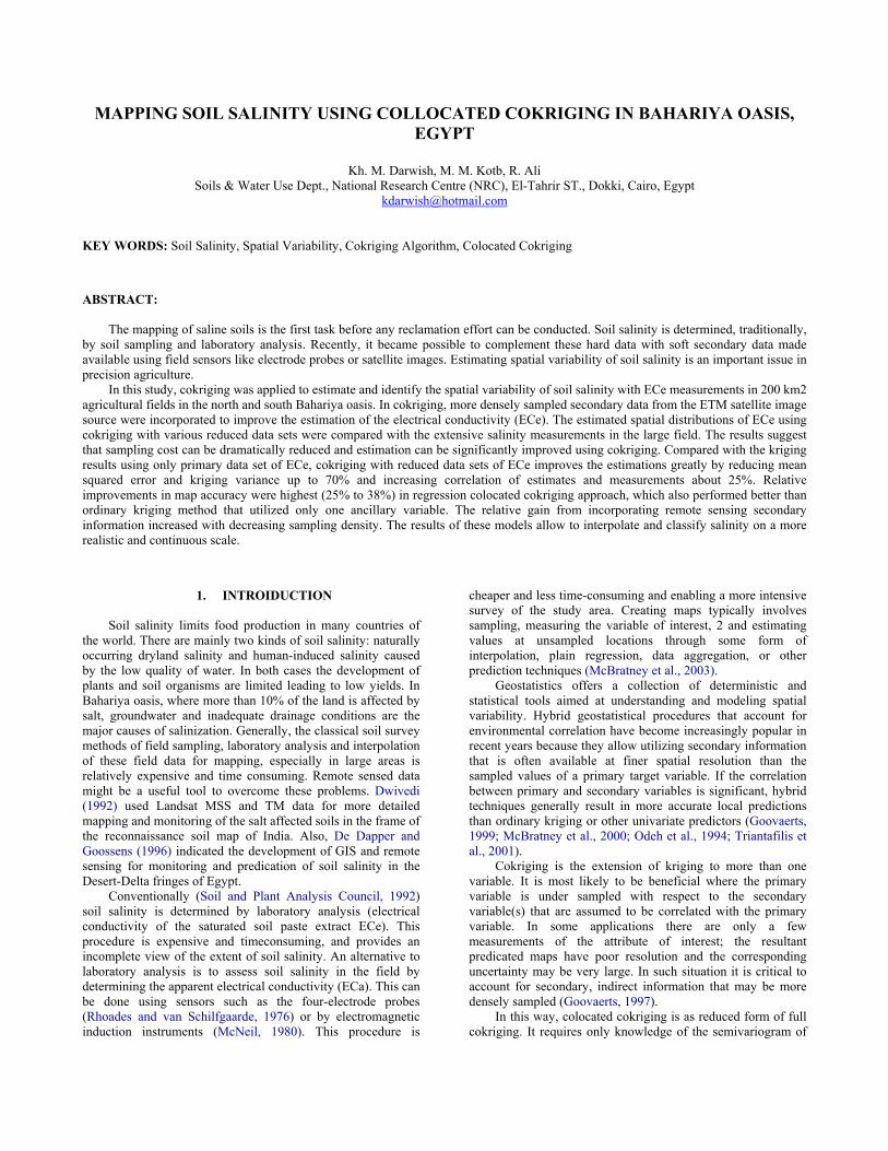
Bahariya depression is located nearly in the middle of the Western desert of Egypt and comprising a total area of approximately 2250 km2 (Fig.1). The area falls under the arid condition as the total rainfall is (3-6) mm/year. Springs and wells are the main two groundwater resources for irrigation and civic purposes (Salem, 1987). In Bahariya, it is found that the main unsuitability criteria eliminating more extend of cultivation areas is the excess of salts. In this research, two study areas were selected. One is in the north of Bahariya covering an area of about 118.3km2 and the second is covering partly the southern part of it with an area of 77.5km2 (Fig.2). 2.2. Data description

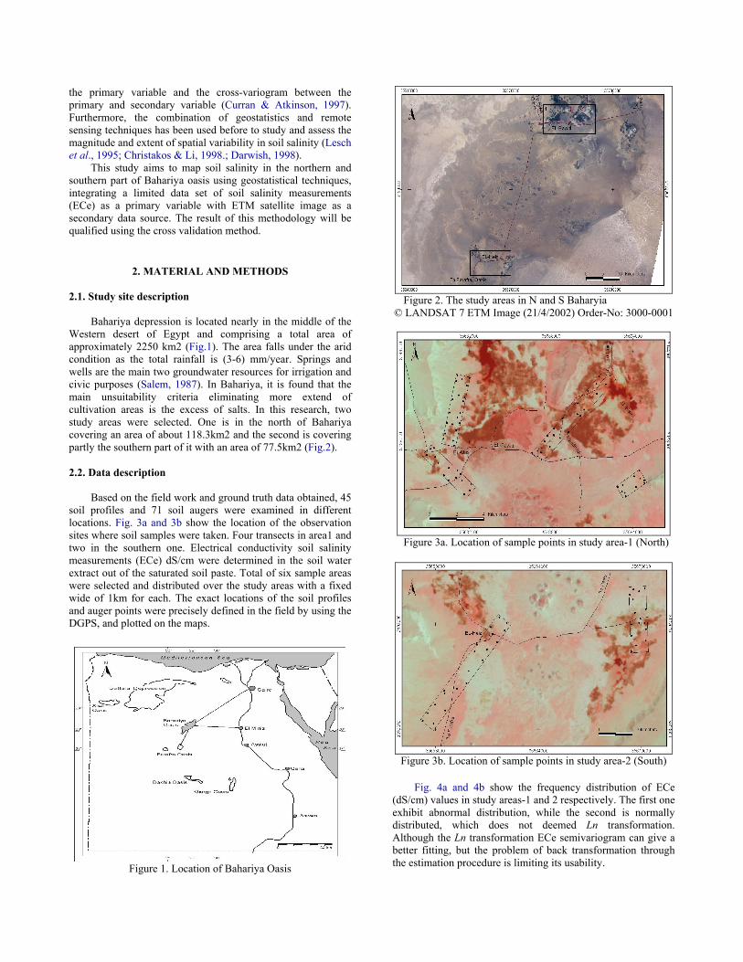
Based on the field work and ground truth data obtained, 45 soil profiles and 71 soil augers were examined in different locations. Fig. 3a and 3b show the location of the observation sites where soil samples were taken. Four transects in area1 and two in the southern one. Electrical conductivity soil salinity measurements (ECe) dS/cm were determined in the soil water extract out of the saturated soil paste. Total of six sample areas were selected and distributed over the study areas with a fixed wide of 1km for each. The exact locations of the soil profiles and auger points were precisely defined in the field by using the DGPS, and plotted on the maps.

Figure 1. Location of Bahariya Oasis

Figure 2. The study areas in N and S Baharyia © LANDSAT 7 ETM Image (21/4/2002) Order-No: 3000-0001

Figure 3a. Location of sample points in study area-1 (North)

Figure 3b. Location of sample points in study area-2 (South)

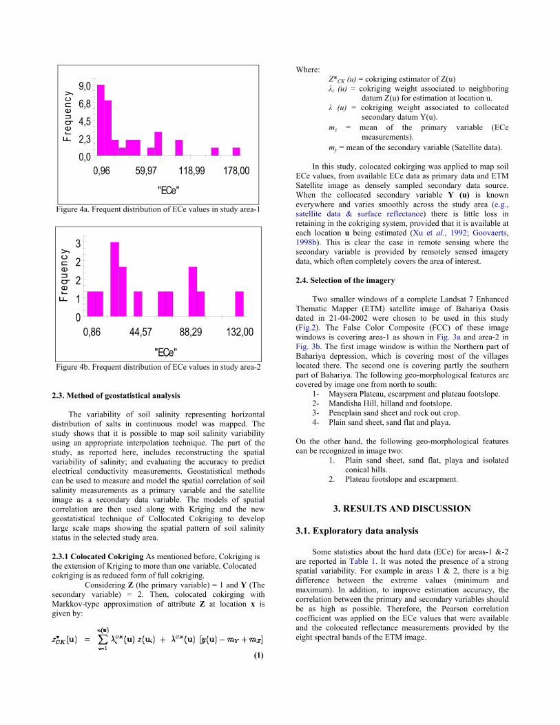
Fig. 4a and 4b show the frequency distribution of ECe (dS/cm) values in study areas-1 and 2 respectively. The first one exhibit abnormal distribution, while the second is normally distributed, which does not deemed Ln transformation. Although the Ln transformation ECe semivariogram can give a better fitting, but the problem of back transformation through the estimation procedure is limiting its usability.

0,0 2,3 4,5 6,8 9,0

0,96 59,97 118,99 178,00

Freq

uenc

y

"ECe"

Figure 4a. Frequent distribution of ECe values in study area-1

0 1 2 2 3

0,86 44,57 88,29 132,00

Freq

uenc

y

"ECe" Figure 4b. Frequent distribution of ECe values in study area-2

2.3. Method of geostatistical analysis

The variability of soil salinity representing horizontal distribution of salts in continuous model was mapped. The study shows that it is possible to map soil salinity variability using an appropriate interpolation technique. The part of the study, as reported here, includes reconstructing the spatial variability of salinity; and evaluating the accuracy to predict electrical conductivity measurements. Geostatistical methods can be used to measure and model the spatial correlation of soil salinity measurements as a primary variable and the satellite image as a secondary data variable. The models of spatial correlation are then used along with Kriging and the new geostatistical technique of Collocated Cokriging to develop large scale maps showing the spatial pattern of soil salinity status in the selected study area. 2.3.1 Colocated Cokriging As mentioned before, Cokriging is the extension of Kriging to more than one variable. Colocated cokriging is as reduced form of full cokriging.

Considering Z (the primary variable) = 1 and Y (The secondary variable) = 2. Then, colocated cokirging with Markkov-type approximation of attribute Z at location x is given by:

(1)

Where: Z*CK (u) = cokriging estimator of Z(u) λi (u) = cokriging weight associated to neighboring

datum Z(u) for estimation at location u. λ (u) = cokriging weight associated to collocated

secondary datum Y(u). mz = mean of the primary variable (ECe

measurements). my = mean of the secondary variable (Satellite data).

In this study, colocated cokirging was applied to map soil

ECe values, from available ECe data as primary data and ETM Satellite image as densely sampled secondary data source. When the collocated secondary variable Y (u) is known everywhere and varies smoothly across the study area (e.g., satellite data & surface reflectance) there is little loss in retaining in the cokriging system, provided that it is available at each location u being estimated (Xu et al., 1992; Goovaerts, 1998b). This is clear the case in remote sensing where the secondary variable is provided by remotely sensed imagery data, which often completely covers the area of interest. 2.4. Selection of the imagery

Two smaller windows of a complete Landsat 7 Enhanced Thematic Mapper (ETM) satellite image of Bahariya Oasis dated in 21-04-2002 were chosen to be used in this study (Fig.2). The False Color Composite (FCC) of these image windows is covering area-1 as shown in Fig. 3a and area-2 in Fig. 3b. The first image window is within the Northern part of Bahariya depression, which is covering most of the villages located there. The second one is covering partly the southern part of Bahariya. The following geo-morphological features are covered by image one from north to south:

1- Maysera Plateau, escarpment and plateau footslope. 2- Mandisha Hill, hilland and footslope. 3- Peneplain sand sheet and rock out crop. 4- Plain sand sheet, sand flat and playa.

On the other hand, the following geo-morphological features can be recognized in image two:

1. Plain sand sheet, sand flat, playa and isolated conical hills.

2. Plateau footslope and escarpment.

3. RESULTS AND DISCUSSION 3.1. Exploratory data analysis

Some statistics about the hard data (ECe) for areas-1 &-2 are reported in Table 1. It was noted the presence of a strong spatial variability. For example in areas 1 & 2, there is a big difference between the extreme values (minimum and maximum). In addition, to improve estimation accuracy, the correlation between the primary and secondary variables should be as high as possible. Therefore, the Pearson correlation coefficient was applied on the ECe values that were available and the colocated reflectance measurements provided by the eight spectral bands of the ETM image.

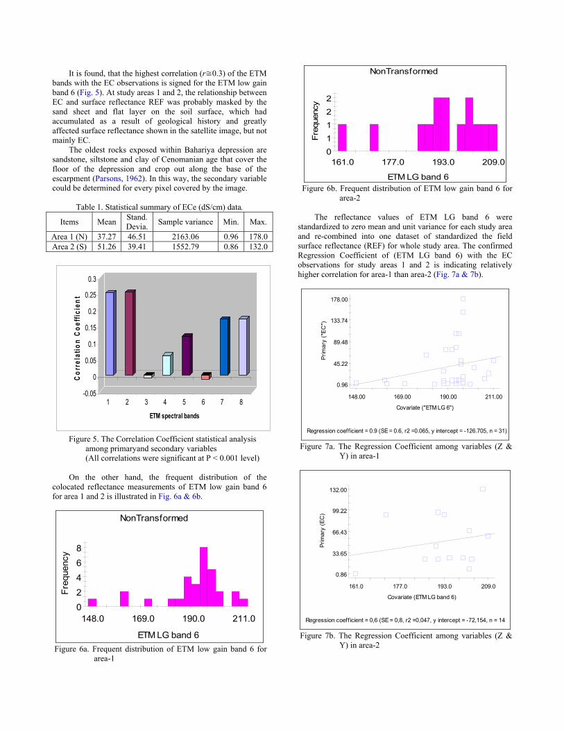
It is found, that the highest correlation (r≅0.3) of the ETM bands with the EC observations is signed for the ETM low gain band 6 (Fig. 5). At study areas 1 and 2, the relationship between EC and surface reflectance REF was probably masked by the sand sheet and flat layer on the soil surface, which had accumulated as a result of geological history and greatly affected surface reflectance shown in the satellite image, but not mainly EC.

The oldest rocks exposed within Bahariya depression are sandstone, siltstone and clay of Cenomanian age that cover the floor of the depression and crop out along the base of the escarpment (Parsons, 1962). In this way, the secondary variable could be determined for every pixel covered by the image.

Table 1. Statistical summary of ECe (dS/cm) data.

Items Mean Stand. Devia. Sample variance Min. Max.

Area 1 (N) 37.27 46.51 2163.06 0.96 178.0 Area 2 (S) 51.26 39.41 1552.79 0.86 132.0

-0.05

0

0.05

0.1

0.15

0.2

0.25

0.3

Cor

rela

tion

Coe

ffici

ent

1 2 3 4 5 6 7 8

ETM spectral bands

Figure 5. The Correlation Coefficient statistical analysis

among primaryand secondary variables (All correlations were significant at P < 0.001 level)

On the other hand, the frequent distribution of the

colocated reflectance measurements of ETM low gain band 6 for area 1 and 2 is illustrated in Fig. 6a & 6b.

0 2 4 6 8

148.0 169.0 190.0 211.0

Freq

uenc

y

ETM LG band 6

NonTransformed

Figure 6a. Frequent distribution of ETM low gain band 6 for

area-1

0 1 1 2 2

161.0 177.0 193.0 209.0

Freq

uenc

y

ETM LG band 6

NonTransformed

Figure 6b. Frequent distribution of ETM low gain band 6 for

area-2

The reflectance values of ETM LG band 6 were standardized to zero mean and unit variance for each study area and re-combined into one dataset of standardized the field surface reflectance (REF) for whole study area. The confirmed Regression Coefficient of (ETM LG band 6) with the EC observations for study areas 1 and 2 is indicating relatively higher correlation for area-1 than area-2 (Fig. 7a & 7b).

0.96

45.22

89.48

133.74

178.00

148.00 169.00 190.00 211.00

Prim

ary

("EC

")

Covariate ("ETM LG 6")

Regression coefficient = 0.9 (SE = 0.6, r2 =0.065, y intercept = -126.705, n = 31) Figure 7a. The Regression Coefficient among variables (Z &

Y) in area-1

0.86

33.65

66.43

99.22

132.00

161.0 177.0 193.0 209.0

Prim

ary

(EC

)

Covariate (ETM LG band 6)

Regression coeff icient = 0,6 (SE = 0,8, r2 =0,047, y intercept = -72,154, n = 14 Figure 7b. The Regression Coefficient among variables (Z &

Y) in area-2

3.2. Structure analysis

It is necessary to analyze the spatial variability of the data above by semivariance function. Fig. 8a and 8b illustrate the semivariance value of primary variable (ECe) of study areas 1 & 2. The sill of EC in areas 1 & 2 are 2620.0m and 1845.0m and their correlation lag range 3710.0m and 1120.0m respectively.

0

1451

2902

4353

5805

0.0 2596.0 5192.0 7788.0

Sem

ivar

ianc

e

Separation Distance (h) m Figure 8a. Isotropic variogram (spherical model) of ECe

(dS/cm) in area-1

0

870

1741

2611

3482

0.0 2257.7 4515.3 6773.0

Sem

ivar

ianc

e

Separation Distance (h) m Figure 8b. Isotropic variogram (spherical model) of ECe

(dS/cm) in area-2

The variogram shows a relative nugget effect of 11.7% for study area-1 and 10.0% for area-2, which cloud be calculated through this ratio [(C0/(C0 + C)) x 100] between nugget variance and sill. The nugget effect looks more significant in study area-2 than area-1, which causes by random factors. On the other hand, as Cokriging is a multivariate extension of kriging, when the secondary variable is known everywhere and varies smoothly across the study area (e.g., colocated reflectance measurements provided by ETM low gain band 6) there is little loss in retaining in the cokriging system. The secondary variable provides information only about the primary trend at location u.

In order to apply a colocated cokriging method a cross-semivariance analysis must be performed prior to cokriging, where CZY(ui - u) is the cross covariance between primary and secondary variables at locations ui and u, respectively.

Again, the common practice consists of estimating and modeling the (cross) semivariogram, then retrieving the (cross) covariance. Fig. 9a and 9b show the experimental semivariogram of the secondary variable ETM LG band6 and cross semivariogram with the primary one (ECe point observations) for study area-1, computed as:

(2)

0.0

131.6

263.1

394.7

0.0 2596.0 5192.0 7788.0

Sem

ivar

ianc

e

Separation Distance (h) m

"ETM LG 6": Isotropic Variogram

Figure 9a. The semivariogram of secondary variable for study

area-1

-34.

698.

1431.

2163.

0.0 2596.0 5192.0 7788.0

Sem

ivar

ianc

e

Separation Distance (h) m

"EC" x "ETM LG 6": Isotropic Cross Variogram

Figure 9b. The cross-variogram of primary and secondary

variables for area-1

The sampling interval can be determined based on the semivariograms. In Fig. 9a & 9b, an exponential model of isotropic variogram was fitted for the secondary variable (ETM LG 6) using an iterative procedure developed by Goulard (1989). The cross-variogram between the primary and secondary data sets is modeled (here a small nugget effect 11.6m and a spherical model with sill 232.2m and range 3400.0m), indicating that the intensive sampling scheme used resolved most of the spatial variation.

Nevertheless, Fig. 10a & 10b illustrate the experimental semivariograms of the secondary variable (ETM LG 6) and the cross-variogram in study area-2. At area-2, the isotropic varigram of (ETM LG 6) shows a spherical model with a sill of 164.7m and a fitted range of 1150.0m, which probably reflected gradual differences in EC due to elevation. The cross-variogram between the primary and secondary data sets in area-2 modeled linearly with sill of 0.1m and range of 0.75m. Although in study area-2, EC was less significantly correlated with the secondary variable compare with area-1, only a small portion of the variation in EC can be explained by variation in elevation.

Generally, cross-variograms largely confirmed the findings of the simple correlation analysis, showing (i) more spatial correlation between EC and ETM LG 6 at area-1, and (ii) declining spatial correlation between EC and ETM LG 6 at area-2 (Fig. 10b). This proves the existence of correlation between spatial variability of the soil salinity data, which belongs to nugget effect.

0.0

150.0

300.0

450.0

0.0 2257.7 4515.3 6773.0

Sem

ivar

ianc

e

Separation Distance (h) m

"ETM LG 6" Isotropic Variogram

Figure 10a. The semivariogram of secondary variable for study

area-2

-1251.75

-550.61

150.52

851.66

1552.79

0.00 2257.67 4515.33 6773.00

Sem

ivar

ianc

e

Separation Distance (h) m

"EC" x "ETM LG 6" : Isotropic Cross Variogram

Figure 10b. The cross-variogram of primary and secondary

variables for area-2

3.3. Colocated Cokriging of EC point observations with ETM as secondary data source

The colocated cokriging interpolated maps cover study areas 1 and 2 is shown in Fig. 11a & 12a. The ordinary

cokriging algorithm was applied to interpolate the EC data using GS+ program.

As a result of using search neighborhood area as indicated in the cross-variograms of area-1 and area-2, quite lots of areas were closed to the primary observation points and this give high effect of the secondary data. Closer to primary observation points this effect is more screened by the available primary data and this significantly improved the accuracy of colocated EC maps. However, the visual interpretation of the EC colocated map of area-1 in relation to the DEM (digital Elevation Model) grid image of each area give a good impression that the estimation of salinity values is logical, taken into consideration the location from the salt effected soils (playa), the relatively lower elevation units (depressions) and the position in landscape in the oasis (Fig. 11b).

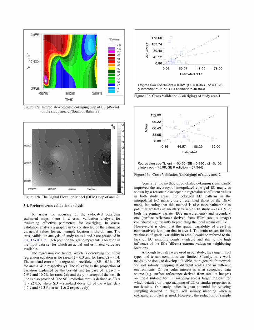
On the other hand, the relatively high ECe (dS/cm) values that are pronounced and presented as connected counter lines are expressing the areas where low elevation and much salinity features are available. This is clear presented for area-2 in Fig. 12b. This quite validating the estimated interpolated cokriged maps obtained. Obviously, there is a visually better resolution of spatial detail in the EC colocated cokriging interpolated maps.

35679444 35687159 35694874"m east"

3134583

3138434

3142286"m

nor

th"

"EC"

> 164> 151> 139> 126> 114> 102> 89> 77> 64> 52> 39> 27> 15> 2> -10

Figure 11a. Interpolate-colocated cokriging map of EC (dS/cm) of the study area-1 (North of Bahariya)

35680000 35684000 35688000 35692000

3136000

3138000

3140000

3142000

92

96

100

104

108

112

116

120

124

128

132

136

140

144

Playa

Playa

Depression

Figure 11b. The Digital Elevation Model (DEM) map of area-1

35657997 35663986 35669976"m east"

3097399

3100634

3103869"m

nor

th"

"EC south area"

> 119> 110> 102> 93> 85> 77> 68> 60> 51> 43> 34> 26> 18> 9> 1

Figure 12a. Interpolate-colocated cokriging map of EC (dS/cm) of the study area-2 (South of Bahariya)

35658000 35661000 35664000 35667000

3098000

3100000

3102000

94

98

102

106

110

114

118

122

126

130

134

138

142

Playa

Figure 12b. The Digital Elevation Model (DEM) map of area-2 3.4. Perform cross validation analysis

To assess the accuracy of the colocated cokriging estimated maps, there is a cross validation analysis for evaluating effective parameters for cokriging. In cross-validation analysis a graph can be constructed of the estimated vs. actual values for each sample location in the domain. The cross validation analysis of study areas 1 and 2 are presented in Fig. 13a & 13b. Each point on the graph represents a location in the input data set for which an actual and estimated value are available.

The regression coefficient, which is describing the linear regression equation is for (area-1) = 0.3 and for (area-2) = -0.4. The standard error of the regression coefficient (SE = 0.36, 0.39 for area-1 & 2 respectively). The r2 value is the proportion of variation explained by the best-fit line (in case of (area-1) = 2.6% and 10.2% for (area-2)); and the y-intercept of the best-fit line is also provided. The SE Prediction term is defined as SD x (1 - r2)0.5, where SD = standard deviation of the actual data (45.9 and 37.3 for areas-1 & 2 respectively).

0.96

45.22 89.48

133.74 178.00

0.96 59.97 118.99 178.00

Actu

al "E

C"

Estimated "EC"

Regression coefficient = 0.321 (SE = 0.363 , r2 =0.026,y intercept = 26.72, SE Prediction = 45.893)

Figure 13a. Cross Validation (CoKriging) of study area-1

0.86

33.65

66.43

99.22 132.00

0.86 44.57 88.29 132.00Ac

tual

Estimated

Regression coeff icient = -0.455 (SE = 0.390 , r2 =0.102,y intercept = 75.99, SE Prediction = 37.344)

Figure 13b. Cross Validation (CoKriging) of study area-2

Generally, the method of colokated cokriging significantly improved the accuracy of interpolated cokriged EC maps, as shown by a reasonable acceptable regression coefficient values in both study areas. For cokriged EC, patterns in the interpolated EC maps closely resembled those of the DEM maps, indicating that this method is also more vulnerable to potential artifacts in ancillary variables. In study areas 1 & 2, both the primary variate (ECe measurements) and secondary one (surface reflectance derived from ETM satellite image) contributed significantly to predicting the local means of ECe. However, it is clear that the spatial variability of area-2 is comparatively less than that in area-1. The main reason for this weakness of spatial variability in area-2 could be referred to the lack of EC sampling points available and still to the high influence of the ECe (dS/cm) extreme values on neighboring locations.

Although two sites were used in our study, the range in soil types and terrain conditions was limited. Clearly, more work needs to be done, to develop a flexible, more generic framework for soil salinity mapping at different scales and in different environments. Of particular interest is what secondary data source (e.g. surface reflectance derived from satellite images) are most suitable for EC mapping across larger regions, for which detailed on-thego mapping of EC or similar properties is not feasible. Our study indicates great potential for reducing sampling demand in digital soil salinity mapping when a cokriging approach is used. However, the reduction of sample

size tested here (Fig. 13a & 13b) was somewhat arbitrary. Better procedures are needed for optimizing sampling with regard to covering the variation in primary and secondary variables in both feature and geographic spaces, including situations where little prior information about the target variable is available.

3. CONCLUSION The spatial distribution maps drawn based on cokriging

explain clearly the spatial variability of soil salinity in north and south study areas of Bahariya oasis. Collocated cokriging uses spatially correlated secondary information increased the quality of maps of soil salinity (ECe measurements) as compared to ordinary kriging. Apparent EC cokriged with surface reflectance derived from satellite images performed best in terms of increasing map accuracy. In this method, relative improvements in map accuracy over ordinary kriging method ranged from 19% to 38% at the two study areas and there was little loss of accuracy when sampling intensity was reduced by half as shown in area-2. The ETM LG band 6 secondary data source is considered valuable one for detailed mapping of EC at the field scale, whereas the relative value of terrain attributes varied geographically.

Indeed, there are different original factors have influenced the final output of the cokriging logarithm technique. Those factors can be related to the issues of sampling, the spatial distribution of the soil salinity measurements in the space, the total number of the observation points and the variability of the ECe data set obtained. In addition, most secondary information (i.e. satellite image data) contains uncertainties that may mask relationships with EC values, or other soil properties of interest. Furthermore, relying on a single secondary attribute is risky because (i) the variable chosen may not be related to the primary variable of interest and (ii) field artifacts or errors in the secondary information could cause significant errors in the EC prediction.

Improving those factors especially in the south study area-2, would play an important role for receiving more accurate results out of this interpolation method. At the end of the whole procedure, it is still manage successfully to use the obtained interpolated EC salinity maps. To reduce uncertainties, we recommend using independently measured, multivariate secondary information in estimating spatial variability of soil salinity approach.

REFRENCES Christakos, G. & Li, X., 1998. Bayesian maximum entropy analysis and mapping: a farewell to kriging estimators. Mathematical Geology 30, 435–462. Curran P. J. & Atkinson P. M., 1997. Geostatistics and remote sensing. In Press. Progress in Physical Geography. Darwish, Kh. M., 1998. Integrating soil salinity data with satellite image using geostatistics. M.Sc. Thesis, 1998. Faculty of Agricultural and Applied Biological Sciences, Gent University, Gent, Belgium.

De Dapper, M. & Goossens, R. 1996. Modeling and monitoring of soil salinity and water logging hazards in the Desert-Delta fringes of Egypt based on Geomorphology, Remote Sensing and GIS. 12 Dwivedi, R. S., 1992. Monitoring and the study of the effect of image scale on delineation of salt affected soils in the Indo-Gangentic plains. Intern. Journal of Remote Sensing, 13: 1527-1536. Goovaerts, P., 1997. Geostatistics for Natural Resources Evaluation, Oxford University Press, London. Goovaerts, P., 1998b. Ordinary cokriging revisited, Math. Geol., 30(1), pp. 21-42. Goovaerts, P., 1999. Geostatistics in soil science: state-of-the-art and perspectives. Geoderma 89, 1 –45. Goulard, M., 1989. Inference in a coregionalization model. In: M. Armstrong, Ed. Geostatistics, Kluwer, Dordrecht, pp. 397-408. Lesch, S. M., Strauss, D. J. And Rhoades, J. D. 1995. Spatial predication of soil salinity using electromagnetic induction techniques. 1. Statistical predication models: A comparison of multiple linear regression and cokriging. Water Resour. Res. 31, 373-386. McBratney, A.B., Odeh, I.O.A., Bishop, T.F.A., Dunbar, M.S., Shatar, T.M., 2000. An overview of pedometric techniques for use in soil survey. Geoderma 97, 293– 327. McBratney, A.B., Mendonca Santos, M.L., Minasny, B., 2003. On digital soil mapping. Geoderma 117, 3– 52. McNeil, J.D., 1980. Electromagnetic Terrain Conductivity Measurement at Low Induction Numbers: Technical Note TN-6. GEONICS Limited, Ontario, Canada (15 pp.). Odeh, I.O.A., McBratney, A.B., Chittleborough, D.J., 1994. Spatial prediction of soil properties from landform attributes derived from a digital elevation model. Geoderma 63, 197–214. Parsons, R.M., 1962. Bahariya and Farafra areas (New Valley Project, Western Desert of Egypt), Final Report. Egyptian General Desert Development Organization, U.A.R. Rhoades, J.D., van Schilfgaarde, J., 1976. An electrical conductivity probe for determining soil salinity. Soil Science Society of America Journal 40, 647– 651. Salem, M.Z., 1987. Pedological characteristics of Bahariya Oasis soils. Ph.D. Thesis, Fac. of Agric. Ain Shams, Univ., Egypt. Soil and Plant Analysis Council, 1992. Handbook on Reference Methods for Soil Analysis. Georgia University Station, Athens, Georgia. Triantafilis, J., Huckel, A.I., Odeh, I.O.A., 2001. Comparison of statistical prediction methods for estimating fieldscale clay

content using different combinations of ancillary variables. Soil Sci. 166, 415–427. Xu, W., T.T. Tran, R.M. Srivastava and A.G. Journel, 1992. Integrating seismic data in reservoir modeling: the collocated cokriging alternative, Society of Petroleum Engineers, paper no. 24,742.