Neural Networks 22 (2009) 1257–1270

Contents lists available at ScienceDirect

Neural Networks

journal homepage: www.elsevier.com/locate/neunet

2009 Special Issue

Mapping broadband electrocorticographic recordings to two-dimensional handtrajectories in humansMotor control featuresAysegul Gunduz a,∗, Justin C. Sanchez b, Paul R. Carney b, Jose C. Principe aa Computational NeuroEngineering Laboratory, Department of Electrical and Computer Engineering, United Statesb Department of Pediatrics, Division of Neurology University of Florida, Gainesville, FL 32611, United States

a r t i c l e i n f o

Article history:Received 30 September 2008Received in revised form 25 June 2009Accepted 27 June 2009

Keywords:Brain–machine interfacesHuman neuroprosthesisElectrocorticographyMotor controlNeural decoding

a b s t r a c t

Brain–machine interfaces (BMIs) aim to translate the motor intent of locked-in patients intoneuroprosthetic control commands. Electrocorticographical (ECoG) signals provide promising neuralinputs to BMIs as shown in recent studies. In this paper, we utilize a broadband spectrum above thefast gamma ranges and systematically study the role of spectral resolution, in which the broadband ispartitioned, on the reconstruction of the patients’ hand trajectories. Traditionally, the power of ECoGrhythms (<200–300 Hz) has been computed in short duration bins and instantaneously and linearlymapped to cursor trajectories. Neither time embedding, nor nonlinear mappings have been previouslyimplemented in ECoG neuroprosthesis. Herein, mapping of neural modulations to goal-oriented motorbehavior is achieved via linear adaptive filters with embedded memory depths and as a noveltythrough echo state networks (ESNs), which provide nonlinear mappings without compromising trainingcomplexity or increasing the number of model parameters, with up to 85% correlation. Reconstructedhand trajectories are analyzed through spatial, spectral and temporal sensitivities. The superiority ofnonlinear mappings in the cases of low spectral resolution and abundance of interictal activity isdiscussed.

© 2009 Elsevier Ltd. All rights reserved.

1. Introduction

Collected through subdural electrode grids, ECoG signals are thecumulative sum of dendritic activity and postsynaptic potentialsfrom synchronized sources with finer spatial resolution and highersignal-to-noise ratios compared to EEG recordings (Leuthardt,Schalk, Moran, & Ojemann, 2006). Most importantly, ECoG signalsyield much broader spectra since the electrode grids are belowthe skull and scalp media which act as lowpass filters in EEGrecording techniques (Nunez & Srinivasan, 2005). However, thisadvantage of ECoG over EEG has not been exploited in previousECoG BMI studies as the clinical recording systems employedwere designed for the collection of EEG at low sampling rates(<1 kHz). Unlike the implantation of intracortical microelectrodearrays, which are restricted to limited cases in human subjects

∗ Corresponding address: Computational NeuroEngineering Laboratory, Depart-ment of Electrical and Computer Engineering, P.O. Box 116130, Building #33, CenterDrive, Room NEB 486, Gainesville, FL, 32611, United States. Tel.: +1 352 392 2682;fax: +1 352 392 0044.E-mail addresses: aysegul@cnel.ufl.edu (A. Gunduz), jcs77@ufl.edu

(J.C. Sanchez), carnepr@peds.ufl.edu (P.R. Carney), principe@cnel.ufl.edu(J.C. Principe).

0893-6080/$ – see front matter© 2009 Elsevier Ltd. All rights reserved.doi:10.1016/j.neunet.2009.06.036

(Donoghue, Nurmikko, Black, & Hochberg, 2007; Hochberg et al.,2006; Kennedy, Kirby, Moore, King, & Mallory, 2004), ECoGhas been used extensively in the localization and resection ofepileptogenic focus of humans for decades (Leuthardt et al., 2006).Electrocorticography (ECoG) provides an intermediate level of

brain activity between intracortical and scalp (EEG) recordings, andits potential as a BMI input signal has been demonstrated throughhand movement classification (Chin et al., 2007), hand directionclassification (Mehring et al., 2004), and one-dimensional handtrajectory prediction (Felton, Wilson, Williams, & Garell, 2007;Leuthardt, Schalk, Wolpaw, Ojemann, & Moran, 2004). ECoG BMIsthat decode two-dimensional hand trajectories have not emergeduntil recently due to the many clinical and signal processing(feature extraction and translation) challenges involved. ECoGis the spatiotemporal smoothed sum of dendritic activity frommillions of neurons over a pial surface of 1–1.5 cm2 (Freeman,2006) and thus many of the feature extraction issues arise fromthe fact that motor encoding with ECoG is not as straightforwardas firing rates of single unit activities.Since ECoG signals represent a diverse set of cortical rhythms,

spectral analysis is typically the first level method used to derivecontrol signals for a neuroprosthesis. For the reconstruction ofmovement trajectories there are still many unknown aspects

1258 A. Gunduz et al. / Neural Networks 22 (2009) 1257–1270

of which bands in the available ECoG spectrum are the mostrelevant for control. Schalk et al. (2007) studiedmovement-relatedspectral changes in seven frequency bands from 8 Hz to 190 Hz,and amplitude changes in moving averages in raw ECoG in 333ms windows (yielding a total of 8 features per 64 channels)and mapped linearly to two-dimensional trajectories with nofurther memory depth. The correlation coefficients between thekinematics and the model outputs for in five cross-validation foldswere between [0.50, 0.81] (with a median of 0.71) and [0.18, 0.80](with a median of median 0.51) for the subject with the highestperformance. The sensitive areas were found to be the motorand pre-motor cortices (Brodmann areas 4 and 6). Pistohl, Ball,Schulze-Bonhage, Aertsen, and Mehring (2008) lowpass filteredECoG signals whichwere already recorded at low sampling rates of256 Hz or 1024 Hz with 0.75 s windows of Savitsky–Golay filters.The smoothed signals from all channels formed the measurementvector at time (t − τ) and the hand kinematics at time t formedthe state vector to be used in a Kalman filter (the optimal value ofτ was found empirically to be 125 ms). Across all trials correlationcoefficients of 0.40±0.1 were attained with two patients that hadcoverage over the motor area. In neither of these two-dimensionalstudies is the broadband characteristics of ECoG utilized beyondthe fast gamma range, nor have nonlinear translation functionshave been employed. Moreover, time embedding is only facilitatedby the window sizes in which the feature vectors are computed.However, in animal studies memory depths up to 1 s into the pasthave been utilized (Carmena et al., 2003; Wessberg et al., 2000).In previous studies, we had utilized the broader spectra of

ECoG over EEG and shown presence of motor features in ECoGrecordings from patients tracing two-dimensional trajectories upto 6 kHz through reconstructed trajectories in coarse spectralranges (1–60 Hz, 60–100 Hz, 100–300 Hz, 300 Hz–6 kHz) (Gun-duz, Ozturk, Sanchez, & Principe, 2007; Sanchez, Gunduz, Car-ney, & Principe, 2008), as well as in exploratory studies with finerspectral decomposition (Gunduz, Sanchez, Carney, & Principe, inpreparation). The results of these studies indicated that there isa sophisticated performance relationship between the total spec-tral bandwidth, resolution of spectral decomposition used for ex-tracting control features, and the choice of decoding model (linearor nonlinear) for translating features into control commands. ForBMIs high-dimensional multiple-input–multiple-output (MIMO)systems are common and one must balance the number of modelparameters and the optimization of the projection from neural ac-tivity to behavior. Utilizing broad spectra and embedding moretime samples undoubtedly increases the number of model pa-rameters. In this paper, we empirically investigate the optimalECoG spectral ranges and spectral resolution (number of spectralbands and their bandwidths) and translation topologies for re-constructing two-dimensional hand trajectories. Our overall goalis to find modulations in the minimal configuration of spectralbands, memory depths on the feature extraction end and the sim-plest model architectures that could be implemented for real-timeapplications.Optimal spectral resolution in the broad spectrum and optimal

memory depths are found empirically by adaptive linear modelssuch as Wiener filters (Haykin, 2001), normalized least meansquares (Haykin, 2001) and gamma filters (Principe, Vries, &Oliveira, 1993) with tap delay lines (TDLs). These three types oflinear filter provide a simple analytic solution, online feasibilitywhile compensating for system nonstationarities and decreasednumber of model parameters without compromising memorydepth, respectively. Although linear filters have well established,in low-complexity training methodologies, the reconstructedtrajectories may be suboptimal since the output is limited tomappings in the input space and the intrinsic neurophysiologicalmapping of control features to motor behavior may involve

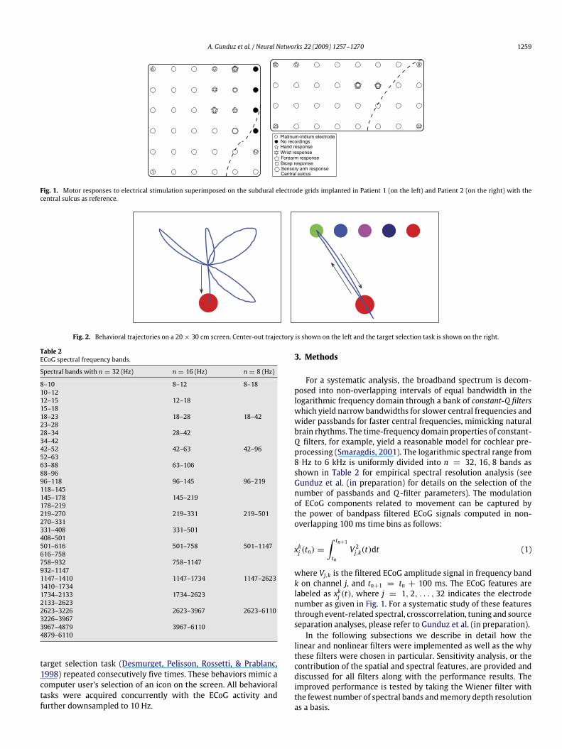
Table 1Motor response to electrical stimulation of subdural grids.

Patient 1 Patient 2

Right hand 22, 28 Right hand 2,3Right wrist 23, 24, 30 Right arm 14, 15Right forearm 22, 30Right bicep 29Right sensory arm 27

nonlinear translations (Gunduz et al., 2007). Again in ourpreliminary studies with low spectral resolution, we reportedhigher performance results in reconstruction of two-dimensionaltrajectories with nonlinear projections (Gunduz et al., 2007).Therefore, herein, we also study modeling hand movementsfrom spectral ECoG features using artificial neural networks,specifically echo state networks (ESNs) (Jaeger, 2001) and leakyecho state networks (Rao et al., 2005). These neural networkswere chosen over time-delay neural networks (TDNNs) dueto the reduced number of parameters by embedding memorythrough recurrencies. Moreover, ESNs have training complexitiesequivalent toWiener filters which do not require backpropagationthrough time. Performance of the linear and nonlinear filters arecompared based on reconstructionmetrics, spectral resolution andpresence of interictal artifacts.

2. Materials

The subjects volunteering in the behavioral experiments werebeing monitored for the treatment of intractable complex partialepilepsy at Shands Hospital at the University of Florida. Patient1 was implanted with a 6 × 6 subdural grid and Patient 2 wasimplanted with a 4×8 grid, both over left fronto-temporal regionscovering the PMd, M1, PP motor cortices. The grids consisted ofa 1.5 mm thick silastic sheet embedded with platinum-iridiumelectrodes of 4 mm diameter, 2.3 mm diameter exposed surfaceand 1 cm center-to-center distances. Electrical stimulation ofthe subdural grids (Uematsu et al., 1992) further guided thelocalization of the primary motor cortex (for further details seeSanchez et al. (2008)). Motor responses from the stimulation,using the enumeration convention in Fig. 1 are provided inTable 1. Both patients executed the tasks with their right hands.The experimental paradigms were approved by the University ofFlorida Institutional Review Board.1For our behavioral experiments, a separate 32 channel system2

capable of recording ECoG at a sampling rate of 12 kHz and 16 bitsof resolution was set up due to the limited bandwidth of thesystem available in the clinic for epilepsy monitoring. The desiredbehavioral trajectories were generated by a desktop computerrunning Matlab v7 which communicated with a bank of DSPs(Tucker–Davis Pentusa base-station) processing the amplifiedECoG signals. The desired trajectories were sent to a secondcomputer monitor placed in front of the patients. Behavioraltrajectory recordings were also stored with a shared time clock onthe Pentusa system. (For further details on the signal acquisitionsystem please refer to Gunduz et al. (in preparation).)Patients were asked to trace a predefined cursor trajectory

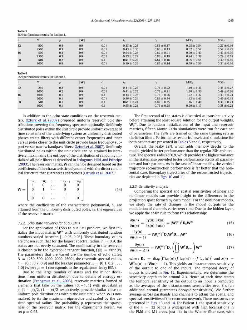
presented on an LCD screen with an active area of 20 ×30 cm with their right index finger. Snapshots of the screen asobserved by the patients during experimentation are presentedin Fig. 2. The paradigm consists of a center-out cursor controltask (Georgopoulus, Kalaska, Caminiti, & Massey, 1982) and a

1 http://irb.ufl.edu/.2 Activity from electrodes 33–36 of the implanted 6 × 6 grids of Patient 1 werenot recorded.

A. Gunduz et al. / Neural Networks 22 (2009) 1257–1270 1259

Fig. 1. Motor responses to electrical stimulation superimposed on the subdural electrode grids implanted in Patient 1 (on the left) and Patient 2 (on the right) with thecentral sulcus as reference.

Fig. 2. Behavioral trajectories on a 20× 30 cm screen. Center-out trajectory is shown on the left and the target selection task is shown on the right.

Table 2ECoG spectral frequency bands.

Spectral bands with n = 32 (Hz) n = 16 (Hz) n = 8 (Hz)

8–10 8–12 8–1810–1212–15 12–1815–1818–23 18–28 18–4223–2828–34 28–4234–4242–52 42–63 42–9652–6363–88 63–10688–9696–118 96–145 96–219118–145145–178 145–219178–219219–270 219–331 219–501270–331331–408 331–501408–501501–616 501–758 501–1147616–758758–932 758–1147932–11471147–1410 1147–1734 1147–26231410–17341734–2133 1734–26232133–26232623–3226 2623–3967 2623–61103226–39673967–4879 3967–61104879–6110

target selection task (Desmurget, Pelisson, Rossetti, & Prablanc,1998) repeated consecutively five times. These behaviors mimic acomputer user’s selection of an icon on the screen. All behavioraltasks were acquired concurrently with the ECoG activity andfurther downsampled to 10 Hz.

3. Methods

For a systematic analysis, the broadband spectrum is decom-posed into non-overlapping intervals of equal bandwidth in thelogarithmic frequency domain through a bank of constant-Q filterswhich yield narrow bandwidths for slower central frequencies andwider passbands for faster central frequencies, mimicking naturalbrain rhythms. The time-frequency domain properties of constant-Q filters, for example, yield a reasonable model for cochlear pre-processing (Smaragdis, 2001). The logarithmic spectral range from8 Hz to 6 kHz is uniformly divided into n = 32, 16, 8 bands asshown in Table 2 for empirical spectral resolution analysis (seeGunduz et al. (in preparation) for details on the selection of thenumber of passbands and Q -filter parameters). The modulationof ECoG components related to movement can be captured bythe power of bandpass filtered ECoG signals computed in non-overlapping 100 ms time bins as follows:

xkj (tn) =∫ tn+1

tnV 2j,k(t)dt (1)

where Vj,k is the filtered ECoG amplitude signal in frequency bandk on channel j, and tn+1 = tn + 100 ms. The ECoG features arelabeled as xkj (t), where j = 1, 2, . . . , 32 indicates the electrodenumber as given in Fig. 1. For a systematic study of these featuresthrough event-related spectral, crosscorrelation, tuning and sourceseparation analyses, please refer to Gunduz et al. (in preparation).In the following subsections we describe in detail how the

linear and nonlinear filters were implemented as well as the whythese filters were chosen in particular. Sensitivity analysis, or thecontribution of the spatial and spectral features, are provided anddiscussed for all filters along with the performance results. Theimproved performance is tested by taking the Wiener filter withthe fewest number of spectral bands andmemory depth resolutionas a basis.

1260 A. Gunduz et al. / Neural Networks 22 (2009) 1257–1270

3.1. Linear mapping

We design linear models to map the extracted features fromECoG recordings to the position of the cursor on the screen whichthe patients are tracing with their right index fingers. The desiredsignals, donated by dX (t) and dY (t), are the horizontal (x-axis) andvertical (y-axis) positions of the cursor (and thus the position of theright index finger of the patient) on the 20×30 cmdisplaywith theorigin of the coordinate system at the center of the screen. Finally,the model outputs are given by yX (t) and yY (t).With adaptive linear filters the hand/cursor position at any

given time is modeled through a function of the short-term historyof the ECoG signal. Such a dynamical model requires a systemwithsufficientmemory for a proper functionalmapping from the neuralmodulations to the motor output. With the addition of tap delaylines (TDLs) at each channel, the number of filter parameters (thesize of the weight matrix) becomes the product of the number ofchannels, M = 32, the number of output dimensions, C = 2, andthe memory depth of the TDL, L, which is determined empirically.The TDL outputs are translated into the cursor coordinate systemby means of the weight matrix, w, and linear combiners. Thisoperation is mathematically described below:

yc(t) =n∑k=1

L−1∑i=0

M∑j=1

xkj (t − i)wkc(i, j)+ b

kc (2)

where c denotes one of the two output dimensions (horizontal,X- or vertical, Y-), wkc(i, j) is the (i, j)th entry of the weight matrixmapping activity in the kth band to the cth dimension and bkc is theestimation bias of the model which can be dropped if the inputsand desired signal are centered around their mean (Kim et al.,2006).First, we employ a Wiener filter with ridge regression (Kim,

2005). The Wiener–Hopf equation (Haykin, 2001) is the analyticalsolution for minimization of the mean-squared error:

wc = (R+ δI)−1 · Pc (3)

where Pc is the L × 1 crosscorrelation vector between the ECoGactivity and the trajectory in the cth dimension and R is theautocorrelation matrix of all ECoG activity, composed of L × Lcorrelation matrices between each feature (channel power in acertain band) with the autocorrelation matrices of the individualfeatures aligned at the diagonal in blocks and is not necessarilysymmetric. Hence, with inadequate data lengths or noisy data,R may be estimated poorly and be close to singular with veryhigh condition numbers (highly correlated input channels mayespecially cause the weight matrix to have an artificially largevariance). δ is the ridge regression regularization term whichconditions the inverse and is equivalent to solving a constrainedleast squares, i.e. minimizing theMSEwith the constraint: ‖w‖2 ≤ρ. Practically, δ is selected by a desirable value for the input signal-to-noise ratio (SNR) estimated by:

SNR ≈tr[R]δ. (4)

We set the desired SNR to 30 dB and empirically compute the traceof the covariance matrix and determine δ (Kim, 2005).The Wiener filter provides the optimal analytic solution for

stationary systems, however, the brain is a nonstationary dynamicsystem that generates different neural responses to the samestimulus. Normalized least mean squares (NLMS) is an onlinegradient descent algorithm which minimizes the instantaneoussquared error, e2(n), at a rate normalized by the power in the input

u(t) y(t)z–1μ

1–μ

Σ

Fig. 3. The leaky integrator.

G(z)

w0

G(z)

Σ

Σ

+d(n)

y(n)

e(n)

–

x0(n)x(n)

w1

x1(n)G(z)

xk–1(n)

wK–1

xk(n)

wK

Fig. 4. Block diagram representation of a general linear filter. The gamma filter isimplemented by substituting the leaky integrator in the transfer functions, G(z).Note that G(z) = z−1 reduces the structure to a tap-delay-line.

tap vector in order to contend with this problem (Haykin, 2001).The weight updates are formalized as:

w(n+ 1) = w(n)+η

M∑j=1

∥∥xj(n)∥∥2 + γ e(n)x(n) (5)

where xj(n) =[xj(n) xj(n− 1) · · · xj(n− L+ 1)

]is the

input tap vector at channel j and η is the learning rate or step sizewhich adjusts the speed of convergence of the algorithm. γ is asmall constant which prevents divergence in case of very smallinput signals.As in the case with Wiener filters, the NLMS weights can have

high variance due to correlated input channels. NLMS with weightdecay aims to lower weight variance by placing an upper boundon the sum of weight magnitudes. The gradient descent updateequation for the weights then becomes:

w(n+ 1) = w(n)+η

M∑j=1

∥∥xj(n)∥∥2 + γ e(n)x(n)− δw(n). (6)

All threemodels thus far, are finite impulse response filters andtheir memory depths are coupled to the filter orders. For example,for L taps, M channels, n bands, and C output dimensions wouldrequire L×M×n×C parameters. The final linear filter we adopt isthe gamma filter which decouples memory depth from filter orderwith restricted feedback (Principe et al., 1993). In other words,equal memory depths can be achieved with fewer model weightsthrough leaky integrators depicted in Fig. 3 with the followingtransfer function:

G(z) =µ

z − (1− µ)(7)

where (1−µ) is the gain in the feedback loop. The memory depthof a gamma filter is DK = K

µ(i.e. can be adjusted by varyingµ). The

system equations for the variable shown in 4 are as follows:

Y (z) =K∑k=0

wkXk(z) (8)

Xk(z) = G(z)Xk−1(z), k = 1, 2, . . . , KX0(z) = X(z), k = 1, 2, . . . , K

A. Gunduz et al. / Neural Networks 22 (2009) 1257–1270 1261

Table 3Filter performance comparisons for Patient 1.

n Filter L # of param. rX rY MSEX MSEY

32 Wiener 8 8192 0.49± 0.15 0.86± 0.11 0.94± 0.64 0.36± 0.18NLMS 14 14336 (+1) 0.55± 0.21 0.87± 0.17 0.83± 0.50 0.34± 0.20Weight decay 14 14336 (+3) 0.45± 0.19 0.87± 0.14 0.85± 0.56 0.36± 0.15Gamma 8 8192 (+1) 0.33± 0.29 0.81± 0.22 0.82± 0.46 0.31± 0.16

16 Wiener 14 7168 0.55± 0.21 0.87± 0.17 0.83± 0.50 0.34± 0.20NLMS 25 12800 (+1) 0.64± 0.19 0.82± 0.25 0.81± 0.43 0.34± 0.24Weight decay 25 12800 (+3) 0.63± 0.21 0.80± 0.29 0.87± 0.59 0.36± 0.23Gamma 8 4096 (+1) 0.37± 0.31 0.81± 0.23 0.82± 0.38 0.34± 0.18

8 Wiener 8 2048 0.52± 0.25 0.87± 0.18 0.84± 0.58 0.36± 0.23NLMS 8 2048 (+1) 0.52± 0.25 0.86± 0.18 0.86± 0.59 0.35± 0.26Weight decay 8 2048 (+3) 0.44± 0.23 0.87± 0.21 0.90± 0.64 0.39± 0.22Gamma 8 2048 (+1) 0.37± 0.22 0.80± 0.27 0.84± 0.47 0.35± 0.23

Table 4Filter performance comparisons for Patient 2.

n Filter L # of param. rX rY MSEX MSEY

32 Wiener 8 8192 0.40± 0.21 0.65± 0.21 1.09± 1.12 0.67± 0.27NLMS 14 14336 (+1) 0.52± 0.20 0.77± 0.16 1.07± 0.94 0.63± 0.30Weight decay 14 14336 (+3) 0.53± 0.21 0.77± 0.16 1.05± 0.95 0.66± 0.29Gamma 8 8192 (+1) 0.54± 0.31 0.76± 0.25 1.15± 1.27 0.59± 0.22

16 Wiener 14 7168 0.47± 0.22 0.78± 0.15 1.08± 0.99 0.64± 0.26NLMS 14 7168 (+1) 0.51± 0.22 0.77± 0.16 1.07± 0.92 0.58± 0.26Weight decay 14 7168(+3) 0.58± 0.23 0.77± 0.19 1.01± 0.95 0.67± 0.26Gamma 8 4096 (+1) 0.54± 0.31 0.76± 0.25 1.15± 1.27 0.59± 0.22

8 Wiener 8 2048 0.56± 0.21 0.76± 0.28 0.98± 1.01 0.65± 0.22NLMS 25 6400 (+1) 0.52± 0.22 0.71± 0.24 0.99± 0.93 0.63± 0.23Weight decay 25 6400 (+3) 0.53± 0.22 0.71± 0.23 0.98± 0.98 0.59± 0.26Gamma 8 2048 (+1) 0.59± 0.27 0.72± 0.26 0.95± 1.16 0.55± 0.24

which yield the following system transfer function:

H(z) =Y (z)X(z)

=

K∑k=0

wk (G(z))k . (9)

The system is stable when the pole lies inside the unit circle, i.e. for0 < µ < 2. For µ = 1 the system reduces to a tap delay line.For µ < 1 additional memory depth is supplied for low frequencycomponents at the expense of thehigh frequency components. Thiswould be desirable in our filter design as the hand trajectories os-cillate at low frequencies (refer to Gunduz et al. (in preparation)).

3.1.1. Comparison of linear filtersPatient 1 performed five trials of center-out task followed by

target selection in 3.87 min from which the first three trials isused for training and the remaining trials are used for testing themodels. Patient 2 performed four trials in 4.65 min of which thefirst 3.5 min were used in model training. The performance of themodels are quantified in each dimension (horizontal and vertical)by Pearson’s r which indicates the degree of linear dependencebetween the reconstructed and the actual hand trajectories, andby the normalized mean squared error (MSE). Both of the abovemeasures are computed over non-overlappingwindows of 20 s andthemean and standard deviations of thesemeasures on the test setare reported as the performance statistics.Over four choices of linear filters, three choices of spectral

resolution and memory depths varying from 800 ms to 2.5 s,t-tests with comparison to the lowest order Wiener filter3 did notstatistically identify the best combination, i.e. the performanceswere found to be statistically equivalent, attributable to highstandard deviations in the performance metrics. For each filter the

3 A Wiener filter of order L = 8 in n = 8 spectral bands is the simplest linearfilter design.

performance results with the bestmean value and lowest standarddeviation are reported in Tables 3 and 4. The output trajectories ofthe Wiener filters in Tables 3 and 4 are plotted in Figs. 5 and 6, forPatients 1 and 2, respectively.

3.1.2. Sensitivity analysisGiven the wide spectrum of ECoG used in these studies and the

fine resolution of the decomposition, we seek to determine theranking of the important electrode locations and spectral bandsin terms of their contribution to behavior. To quantify the mostimportant control signals, a sensitivity analysis was performed(Sanchez, Carmena, Lebedev, Nicolelis, & Harris, 2003). Themagni-tude of weights corresponding to channels and spectral bands canbe used as a sensitivity measure since the outputs are directly re-lated to the input taps through the weight function if themodelingerror is sufficiently small and is mathematically defined as:

Skj =12L

∑c=X,Y

L−1∑i=0

|wkc(i, j)|. (10)

We further average the sensitivities across frequency bands (overk) to attain spatial sensitivity and across electrode grids (over j) toattain spectral sensitivity. These measures are presented in Figs. 7and 8 for Patients 1 and 2, respectively. The spatial sensitivity ofthe n = 32 bands is widespread with high localizations in the PMdand M1 areas. Three of Patient 1’s M1 electrodes for which hand,wrist, forearm and bicep responses to electrical stimulation wereobserved are revealed to have high sensitivities.With Patient 2, theM1 electrode for which a hand response was observed is identifiedas sensitive.

3.2. Nonlinear mapping

ECoG is the sum of dendritic activity of many sources pro-pagated to the subdural surface, those modulating the motor

1262 A. Gunduz et al. / Neural Networks 22 (2009) 1257–1270

5 cm

5 sec

Xpos

5 cm

5 sec

5 cm

5 sec

Ypos

Xpos

Ypos

Xpos

Ypos

a

b

c

Fig. 5. Reconstructed trajectories from Wiener filters for Patient 1 (in blue)projected on the cursor trajectories (in red) with (a) n = 32, (b) n = 16, (c) n = 8bands. (For interpretation of the references to colour in this figure legend, the readeris referred to the web version of this article.)

behavior and extraneous activity, as well as acquisition noise.Therefore, with linear modeling, reconstructed trajectories arerestricted to be a combination of the motor control features andirrelevant activity riding on them.With nonlinear translations, thenoise within ECoG BMI features and themotor control features canbe projected into different areas of the output space.Time delay neural networks (TDNNs), the most common neural

architecture for dynamicalmodeling, have been used in BMI exper-iments (Kim, 2005) and offer a nonlinear mapping through hiddenprocessing elements. However, the number of parameters of themodel scales the high dimensional input and thus creates prob-lems with model generalization. Moreover, the size of the trainingdata required for good approximation increases with the numberof parameters. To overcome the problem of model order, recurrent

5 cm

5 sec

5 cm

5 sec

5 cm

5 sec

Xpos

Ypos

Xpos

Ypos

Xpos

Ypos

a

b

c

Fig. 6. Reconstructed trajectories from Wiener filters for Patient 2 (in blue)projected on the cursor trajectories (in red) with (a) n = 32, (b) n = 16, (c) n = 8bands. (For interpretation of the references to colour in this figure legend, the readeris referred to the web version of this article.)

neural networks (RNNs) have been implemented in BMIs (Sanchezet al., submitted for publication) as they employ only current datasamples and defer the memory structure to the hidden, recur-rent layer instead of time-embedding. Various algorithms, suchas backpropagation through time and real-time recurrent learning(Williams& Zipser, 1989), have been proposed to train RNNs; how-ever, these algorithms suffer from computational complexity, re-sulting in slow training and possibly instability (Haykin, 1998). Forreal-time clinical applications, models of low order that are easy totrain with low memory requirements are desirable.

3.2.1. Echo state networksFor BMIs, the best compromise of training, computational

complexity, nonlinearity, and dynamics can be achieved by

A. Gunduz et al. / Neural Networks 22 (2009) 1257–1270 1263

Temporal

Ant

erio

r

Temporal

Ant

erio

r

Temporal

Ant

erio

r

101 102 1030

Spe

ctra

l Sen

sitiv

ity

Frequency (Hz)

10–2

Spe

ctra

l Sen

sitiv

ity

Spe

ctra

l Sen

sitiv

ity

0

0.1

0.2

0.3

0.4

0.5

0.6

0.7

0.8

0.9

1

0.1

0.2

0.3

0.4

0.5

0.6

0.7

0.8

0.1

0.2

0.3

0.4

0.5

0.6

0.7

0.8

101 102 103

Frequency (Hz)

101 102 103

Frequency (Hz)

a b

c d

e f

Fig. 7. Spatial and spectral sensitivities of Patient 1with L = 8 orderWiener filters. (a) Spatial contribution of 32 channels across n = 32 passbands, (b) Spectral sensitivitiesof n = 32 passbands across the electrode grid. (c)–(d) Sensitivities for n = 16 passbands. (e)–(f) Sensitivities for n = 8 passbands. The central sulcus is shown on the gridswith the white dotted line.

echo state networks (ESNs). ESNs are recurrent network (RNN)paradigms which address the difficulties with RNN training(Ozturk, Xu, & Principe, 2007). ESNs possess a large recurrenttopology of nonlinear processing elements (PEs) which constitutesa ‘‘reservoir of rich dynamics’’ (Jaeger & Haas, 2004) and containinformation about the history of input and output patterns whenproperly dimensioned (Jaeger, 2001). The outputs of these internalPEs (the echo states) are fed to a memoryless but adaptivereadout network, which is generally linear, to produce the networkoutput. The advantageous property of ESN is that only the linearmemoryless readout is trained with a Wiener filter, whereasthe recurrent topology W has fixed connection weights. Thisreduces the training complexity to simple linear regression whilepreserving the recurrent topology. Moreover, by integrating leakyneurons in the ESN structure, the memory depth of the system isincreased without increasing filter orders (Gunduz et al., 2007).Fig. 9 depicts an ESN withM input channels, N internal PEs and

C = 2 output units. The input units, internal PEs, and output unitsat time n are donated by u(n) =

[u1(n) u2(n) · · · uM(n)

],

x(n) =[x1(n) x2(n) · · · xN(n)

], and y(n) =

[yX (n) yY (n)

],

respectively. The weights are given by an N × M matrix Win=

(winij ) for connections between the input and the states, by anN×Nmatrix W = (wij) for connections between the PEs, by an L × NmatrixWout

= (woutij ) for connections from PEs to the output units,by an N × L matrix Wback

= (wbackij ) for the connections thatproject back from the output to the internal PEs, by an L×MmatrixWinout for connections from input units to output units, and by anL× LmatrixWoutout for connections between output units (Jaeger,2001). The activation of the internal PEs is updated according to:

x(n) = f (Winu(n)+Wx(n− 1)+Wbacky(n− 1)) (11)where f = (f1, f2, . . . , fN) are the internal unit’s activationfunctions.Alternatively, each PE can be implementedwith a leaky integra-

tor neuron with leakage parameterµ, decay rate α and the follow-ing update equation:x(n) = (1− µα)x(n)+ µf (Winu(n)+Wx(n− 1)

+WbackyC (n− 1)). (12)The leaky neuron implementation utilizes the gamma delay opera-tor in the recurrencies and is particularly useful when larger mem-ory depths are required. Herein, for the sake of simplicityWback is

1264 A. Gunduz et al. / Neural Networks 22 (2009) 1257–1270

Spe

ctra

l Sen

sitiv

ity101 102 103

Spe

ctra

l Sen

sitiv

ity

Frequency (Hz)

Spe

ctra

l Sen

sitiv

ity

Ant

erio

r

Temporal

0.5

0.45

0.4

0.35

0.3

0.25

0.2

0.15

0.1

Ant

erio

r

Temporal

Ant

erio

r

Temporal

0.95

1

0.85

0.9

0.8

0.75

0.7

0.65

0.6

0.55

0.85

0.9

0.8

0.75

0.7

0.65

0.6

0.55

101 102 103

Frequency (Hz)

Frequency (Hz)101 102 103

a b

c d

e f

Fig. 8. Spatial and spectral sensitivities of Patient 2with L = 8 orderWiener filters. (a) Spatial contribution of 32 channels across n = 32 passbands, (b) Spectral sensitivitiesof n = 32 passbands across the electrode grid. (c)–(d) Sensitivities for n = 16 passbands. (e)–(f) Sensitivities for n = 8 passbands. The central sulcus is shown on the gridswith the white dotted line.

set to zero for both architectures. The output from the readout net-work is computed according to:

yC (n) = f out(WoutC x(n)+Winoutu(n)+Woutouty(n− 1)) (13)

where f out = (f out1 , f out2 , . . . , f outN ) are the output unit’s nonlin-ear functions. Generally, the feedback loops fromoutput-to-outputand output-to-input are not connected and the readout is chosento be linear (i.e. f out is identity), in which case the optimal outputweight matrix,Wout

C , can computed using the Wiener solution.Two basic reservoir properties have to be satisfied: the input

forgetting and state forgetting properties which state that thereservoir must asymptotically forget the input history and theinitial state, respectively. It has been shown in Jaeger (2001) thatthese two conditions are equivalent and both can be satisfiedthrough the echo state condition of the spectral radius4 of thereservoir weight matrix being less than unity, i.e. ‖W‖ < 1.This condition states that the dynamics of the ESN is uniquelycontrolled by the recent input values and the effect of initial states

4 The spectral radius of a matrix is the largest magnitude of its eigenvalues.

Linear MapperWin

Winout Wback

Wback

Wout

Woutout

W

yY

yX

dY

d

Fig. 9. Block diagram of an Echo state network.

vanishes. For the leaky neuron case, it is required that ‖µW+ (1−µα)W‖ be less than unity (Jaeger & Haas, 2004).

A. Gunduz et al. / Neural Networks 22 (2009) 1257–1270 1265

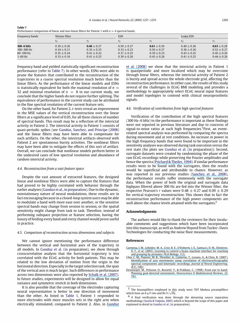
Table 5ESN performance results for Patient 1.

n N µ ‖W‖ c rX rY MSEX MSEY

32 500 0.4 0.9 0.01 0.33± 0.25 0.85± 0.17 0.98± 0.54 0.27± 0.162500 0.3 0.9 0.01 0.43± 0.30 0.85± 0.13 0.92± 0.57 0.57± 0.29

16 500 0.3 0.9 0.01 0.54± 0.28 0.82± 0.21 0.90± 0.43 0.43± 0.362500 0.3 0.9 0.01 0.53± 0.22 0.83± 0.19 0.84± 0.39 0.28± 0.18

8 500 0.2 0.9 0.1 0.51± 0.26 0.85± 0.18 0.95± 0.55 0.30± 0.161000 0.8 0.9 0.01 0.39± 0.29 0.85± 0.14 0.99± 0.59 0.31± 0.16

Table 6ESN performance results for Patient 2.

n N µ ‖W‖ c rX rY MSEX MSEY

32 250 0.2 0.9 0.01 0.41± 0.28 0.74± 0.22 1.19± 1.36 0.48± 0.271000 0.2 0.9 0.01 0.41± 0.25 0.71± 0.21 1.20± 1.30 0.48± 0.26

16 1000 0.1 0.9 0.1 0.44± 0.28 0.75± 0.26 1.22± 1.37 0.43± 0.242000 0.1 0.9 0.01 0.56± 0.24 0.81± 0.24 1.12± 1.42 0.46± 0.18

8 500 0.1 0.9 0.1 0.61± 0.28 0.80± 0.25 1.16± 1.40 0.35± 0.231000 0.1 0.9 0.1 0.55± 0.28 0.76± 0.28 0.99± 1.17 0.38± 0.22

In addition to the echo state conditions on the reservoir ma-trix, Ozturk et al. (2007) proposed uniform reservoir pole dis-tributions covering the frequency spectrum optimally. Uniformlydistributedpoleswithin the unit circle provide uniformcoverage oftime constants of the underlying system as uniformly distributedphases create filters with different center frequencies and innerversus poles closer to the unit circle provide large frequency sup-port versus narrowbandpass filters (Ozturk et al., 2007). Uniformlydistributed poles within the unit circle can be attained by itera-tively maximizing the entropy of the distribution of randomly ini-tialized all-pole filters as described in Erdogmus, Hild, and Principe(2003). The reservoir matrix,W can then be designed based on thecoefficients of the characteristic polynomial with the direct canon-ical structure that guarantees sparseness (Ozturk et al., 2007):

W =

−a1 −a2 · · · −aN−1 −aN1 0 · · · 0 00 1 · · · 0 0· · · · · · · · · · · · · · ·

0 0 · · · 1 0

(14)

where the coefficients of the characteristic polynomial, ai, areattained from the uniformly distributed poles, i.e. the eigenvaluesof the reservoir matrix.

3.2.2. Echo state networks for ECoG BMIsFor the application of ESNs to our BMI problem, we first ini-

tialize the input matrix Win with uniformly distributed randomnumbers scaled between [−0.05, 0.05]. These boundary valuesare chosen such that for the largest spectral radius, r = 0.9, thestates are not overly saturated. The nonlinearity in the reservoiris chosen to be the hyperbolic tangent function, f (x) = tanh(x).The parameters that are varied are the number of echo states,N = {250, 500, 1000, 2000, 2500}, the reservoir spectral radius,r = {0.5, 0.7, 0.9} and the leakage parameter µ = {0.1, 0.2, . . . ,1.0} (where µ = 1 corresponds to the regular/non-leaky ESN).Due to the large number of states and the minor devia-

tions from uniform distribution due to details of entropy es-timation (Erdogmus et al., 2003), reservoir matrices formed ofelements that take on the values {0,−1, 1} with probabilitiesp, (1 − p)/2, (1 − p)/2 respectively, provide similar close-to-uniform pole distributions within the unit circle when W is nor-malized by its the maximum eigenvalue and scaled by the de-sired spectral radius. The probability p represents the sparse-ness of the reservoir matrix. For the experiments herein, weset p = 0.95.

The first second of the states is discarded as transient activitybefore attaining the least square solution for the output weights,WoutC . Due to random initializations of the input and reservoir

matrices, fifteen Monte Carlo simulations were run for each setof parameters. The ESNs are trained on the same training sets asthe linear filters. Performance results from selected simulations forboth patients are presented in Tables 5 and 6, respectively.Overall, the leaky ESN, which adds memory depths to the

model, yielded better performance than the regular ESN architec-ture. The spectral radius of 0.9,which provides the highest variancein the states, also provided better performance across all parame-ters and both patients. As in the case of linear models, the verticaltrajectory reconstruction performance is far better that the hori-zontal case. Exemplary trajectories of the reconstructed trajecto-ries are depicted in Figs. 10 and 11.

3.2.3. Sensitivity analysisComparing the spectral and spatial sensitivities of linear and

nonlinear models can provide insight to the differences in theprojection space formed by each model. For the nonlinear models,we study the rate of changes in the model outputs as themodulation of channels varies over time. Due to the hidden layer,we apply the chain rule to form this relationship:

∂y(n)∂u(n)

=∂y(n)∂x(n)

∂x(n)∂u(n)

= (WoutC )

TDnWin (15)

∂y(n)∂u(n− 1)

= (WoutC )

TDnWTDn−1Win (16)

∂y(n)∂u(n−∆n)

= (WoutC )

TDn

(∆n∏i=1

WTDn−i

)Win (17)

where Dn = diag[f ′(z1(n)) f ′(z2(n)) · · · f ′(zN(n))

]and z(n) =

Winu(n) + Wx(n − 1). This yields an instantaneous sensitivityof the output to one of the inputs. The temporal decay ofinputs is plotted in Fig. 12. Experimentally, we determine thesensitivity depth to be around 2 s. Hence at each time stampthe temporal sensitivity of the output to an input is computedas the averages of the instantaneous sensitivities over 3 s (anadditional second guarantees decayed sensitivities). We furtheraverage across passbands and channels to attain the spatial andspectral sensitivities of the recurrent network. These measures arepresented in Figs. 13 and 14. For Patient 1, the spatial sensitivityof the n = 32 bands is widespread with high localizations inthe PMd and M1 areas. Just like in the Wiener filter case, with

1266 A. Gunduz et al. / Neural Networks 22 (2009) 1257–1270

Xpos

Ypos

Xpos

Ypos

Xpos

Ypos

5 sec

5 sec

5 sec

a

b

c

Fig. 10. Reconstructed trajectories from Wiener filters for Patient 1 (in blue)projected on the cursor trajectories (in red) with (a) n = 32, (b) n = 16, (c) n = 8bands with N = 500 states. (For interpretation of the references to colour in thisfigure legend, the reader is referred to the web version of this article.)

a lower number of bands, we have narrower spatial sensitivities.Moreover, the spatial sensitivities of the ESNs and Wiener filteroverlap. In the case of spectral sensitivities, ESNs and the Wienerfilters identify the same spectral ranges as the most sensitive.Similar observations can bemadewith Patient 2. Spatial sensitivityis widespread in the case n = 32 with high positive and negativesensitivities overlappingwith those of theWiener filter. Areaswithhigh spatial sensitivities become narrower with n = 16, 8 bands.Finally, the same sensitive spectral ranges as the Wiener filter arecaptured.

5 sec

Xpos

Ypos

5 sec

5 sec

Xpos

Ypos

Xpos

Ypos

a

b

c

Fig. 11. Reconstructed trajectories from ESNs for Patient 2 (in blue) projected onthe cursor trajectories (in red) with (a) n = 32, (b) n = 16, (c) n = 8 bands withN = 1000 states. (For interpretation of the references to colour in this figure legend,the reader is referred to the web version of this article.)

4. Discussion

In this study we showed the feasibility of reconstructing oftwo-dimensional hand trajectories with high resolution broad-band ECoG via linear and nonlinear models with embedded mem-ory depths. Three avenues for are explored for maximal decodingperformance. First,we varied how finelywedivided the ECoG spec-trum. Second, we vary how much memory, or time embedding,is employed by the decoding models. Third, we provided a com-parison on linear and nonlinear decoding models. Overall, this pa-

A. Gunduz et al. / Neural Networks 22 (2009) 1257–1270 1267

0 1 2 30

1

Δ (sec)

Tem

pora

l sen

sitiv

ity

VerticalHorizontal

Fig. 12. Sensitivity at time t for channel 1 of Patient 1 with n = 32 bands as afunction of∆.

per presents a systematic analysis of the bounds on the requiredcomplexity of ECoG decoders and provides much needed studieson ECoG spectral range, spectral decomposition and nonlinear BMIprojections.The following subsections summarize our findings, mainly

the spectral and spatial contributions and present comparison ofreconstruction performance across trajectory axes and patients,

as well as an insight to how the significance of the results wereverified.

4.1. Spectral resolution of broadband ECoG features

Spectral sensitivity analyses demonstrate the presence ofmotorcontrol features in ECoG up to 6 kHz in Fig. 7(d)–(f). Hence, ECoGsignal acquisition systems should utilize higher sampling ratesthan those clinically used for EEG. Extracting features in this vastinput space, however, has to be systematically facilitated, whicharises the question of resolution in the spectral decomposition.We reconstructed trajectories from features at three different lev-els of spectral resolution. As there were no significant differencesin performance, we can conclude that the lowest resolution levelat which the well-known neurophysiological rhythms are main-tained (n = 8) is the optimal resolution as itminimizes the numberof parameters involved in the models. Furthermore, well knownneural rhythms over the motor cortex (such as mu, beta, gamma,fast gamma) are captured within one passband with n = 8 bandswhich were otherwise split with higher resolution. This supports

Temporal

Ant

erio

r

Temporal

Ant

erio

r

Temporal

Ant

erio

r

101 102 103

Spe

ctra

l Sen

sitiv

ity

Frequency (Hz)

Spe

ctra

l Sen

sitiv

ityS

pect

ral S

ensi

tivity

0.1

0.2

0.3

0.4

0.5

0.6

0.7

0.8

0.1

0.2

0.3

0.4

0.5

0.6

0.7

0.8

0.1

0.2

0.3

0.4

0.5

0.6

0.7

0.8

101 102 103

Frequency (Hz)

101 102 103

Frequency (Hz)

a b

c d

e f

Fig. 13. Spatial and spectral sensitivities of ESNs with N = 500 states for Patient 1. (a) Spatial contribution of 32 channels across n = 32 passbands, (b) Spectral sensitivitiesof n = 32 passbands across the electrode grid. (c)–(d) Sensitivities for n = 16 passbands. (e)–(f) Sensitivities for n = 8 passbands. The central sulcus is shown on the gridswith the white dotted line.

1268 A. Gunduz et al. / Neural Networks 22 (2009) 1257–1270

Spe

ctra

l Sen

sitiv

ity101 102 103

Spe

ctra

l Sen

sitiv

ity

Frequency (Hz)

Spe

ctra

l Sen

sitiv

ity

Ant

erio

r

Temporal

0.8

1

0.6

0.4

0.2

0

–0.2

–0.4

–0.6

–0.8

–1

Ant

erio

r

Temporal

Ant

erio

r

Temporal

101 102 103

Frequency (Hz)

Frequency (Hz)101 102 103

a b

c d

e f

0.8

1

0.6

0.4

0.2

0

–0.2

–0.4

–0.6

–0.8

–1

0.8

1

0.6

0.4

0.2

0

–0.2

–0.4

–0.6

–0.8

Fig. 14. Spatial and spectral sensitivities of ESNswithN = 1000 states for Patient 2. (a) Spatial contribution of 32 channels across n = 32 passbands, (b) Spectral sensitivitiesof n = 32 passbands across the electrode grid. (c)–(d) Sensitivities for n = 16 passbands. (e)–(f) Sensitivities for n = 8 passbands. The central sulcus is shown on the gridswith the white dotted line.

the empirical finding that n = 8 Q -bands yield the optimal spec-tral resolution for the decomposition of the broadband spectrumbetween 8 Hz–6 kHz. Further merging these bands, leads to de-teriorated reconstruction performances as previously reported inSanchez et al. (2008).Again from Fig. 7(d)–(f), we observe that when the number of

spectral bands were reduced from 32 to 16 and then to 8, contri-butions from some of the passbands are lost. However, these lossesare compensated by putting more emphasis on the important spa-tiotemporal features that were preserved. This can explain thenarrower spatial sensitivity localizations in Fig. 7(a)–(c). Similarobservations are made with the nonlinear spectral sensitivities,with fewer bands, we have narrower spatial sensitivities (seeFig. 13).

4.2. Spatial contributions of broadband ECoG

The most sensitive channels identified with linear sensitivityanalysis not only capture the electrodes over the responsiveelectrodes, but they are also in accord with those found to behighly correlated to behavior, extracted through source separation

and that are directionally tuned to trajectories in Gunduz et al.(in preparation). For Patient 1, the nonlinear spatial sensitivity ofthe n = 32 bands is widespread with high localizations in thePMd and M1 areas. Moreover, the spatial sensitivities of ESNs andWiener filter overlap (Figs. 7 and 13). Similar observations can bemade with Patient 2. Spatial sensitivity is widespread in the casen = 32 with high positive and negative sensitivities overlappingwith those of the Wiener filter (8 and 14). However, we must notethat the nonlinear sensitivities are initialization dependent andslightly alter from one simulation to the other.

4.3. Nonlinear mapping through ESNs

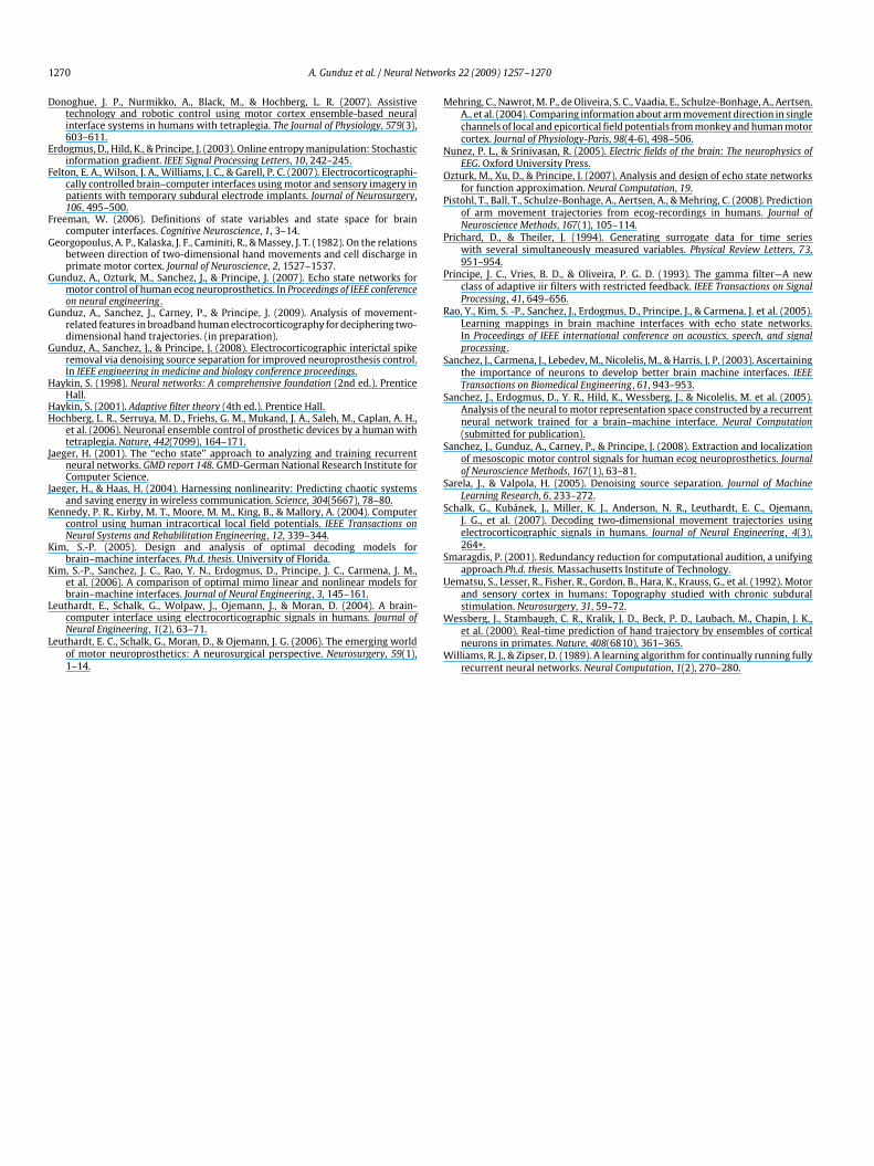
For Patient 1, the nonlinear recurrent architecture has notprovided a statistically significance over the linear methods. Thismay be due to the fact that itwas possible to find a projection to thelow dimensional trajectories from the very high dimensional inputspace. However, in a previous study (Gunduz et al., 2007) in whichwe had coarsely divided the broadband spectrum into four bandsbetween: 1–60 Hz, 60–100 Hz, 100–300 Hz and 300 Hz–6 kHz,the ESNs were able to identify the sensitive portions of the highest

A. Gunduz et al. / Neural Networks 22 (2009) 1257–1270 1269

Table 7Performance comparison of linear and non-linear filters for Patient 1 with n = 4 spectral bands.

Frequency bands Wiener filter ESN Leaky ESNrX rY rX rY rX rY

300–6 kHz 0.39± 0.26 0.48± 0.27 0.50± 0.27 0.61± 0.29 0.49± 0.26 0.63± 0.28100–300 Hz 0.34± 0.21 0.35± 0.25 0.33± 0.22 0.50± 0.27 0.36± 0.26 0.52± 0.2760–100 Hz 0.35± 0.24 0.41± 0.22 0.37± 0.25 0.39± 0.23 0.43± 0.25 0.45± 0.261–60 Hz 0.33± 0.16 0.41± 0.25 0.39± 0.26 0.43± 0.26 0.41± 0.25 0.44± 0.26

frequency band and yielded statistically significant reconstructionperformance (refer to Table 7). In other words, ESNs were able toprune the features that contributed to the reconstruction of thetrajectories in a coarse spectral resolution much better than thelinear filters. As the performance of the linear models and ESNsis statistically equivalent for both the maximal resolution of n =32 and minimal resolution of n = 8 in our current study, weconclude that the higher bands do not require further splitting. Theequivalence of performance in the current study can be attributedto the fine spectral resolution of the current feature sets.On the other hand, for Patient 2, t-tests reveal an improvement

in the MSE values of the vertical reconstruction over the linearfilters at a significance level of 0.05, for all three choices of numberof spectral bands. This result may be a reflection of the interictalactivity in Patient 2. The interictal activity in Patient 1 consists ofquasi-periodic spikes (see Gunduz, Sanchez, and Principe (2008)and the linear filters may have been able to compensate forsuch artifacts. On the other, the interictal artifacts observed withPatient 2 are spontaneous bursty activities. The nonlinear filtersmay have been able to mitigate the effects of this sort of artifact.Overall, we can conclude that nonlinear models perform better inthe undesired cases of low spectral resolution and abundance ofrandom interictal activity.

4.4. Reconstruction from a vast feature space

Despite the vast amount of extracted features, the designedlinear and nonlinear filters were able to capture the features thathad proved to be highly correlated with behavior through theearlier analyses (Gunduz et al., in preparation). Due to the dynamic,nonstationary nature of neural modulations, these results are infact encouraging because in a closed-loop systemusersmaybe ableto modulate a band with more ease over another, or the sensitivespectral bands may change from session to session, or the spatialsensitivity might change from task to task. Therefore, instead ofperforming subspace projection or feature selection, having theluxury of feeding every band and every channelwould prove usefulin practice.

4.5. Comparison of reconstruction across dimensions and subjects

We cannot ignore mentioning the performance differencebetween the vertical and horizontal axes of the trajectory inall models. In Gunduz et al. (in preparation), we show throughcrosscorrelation analysis that the horizontal trajectory is lesscorrelated with the ECoG activity for both patients. This may berelated to the low deviation of motion from the origin in thehorizontal direction. Especially in the target selection task, the spanof the vertical axis is much larger. Such differences in performanceacross two dimensions were also reported by Schalk et al. (2007).In future studies, experiments will be designed to allow for equalvariance and symmetric stretch in both dimensions.It is also possible that the coverage of the electrodes capturing

neural representation is better in one direction of movementthan the other. As listed in Table 1, Patient 1 responded tomore electrodes with more muscles sets in the right arm whenelectrically stimulated, compared to Patient 2. Also, in Gunduz

et al. (2008) we show that the interictal activity in Patient 1is quasiperiodic and more localized which may be overcomethrough linear filters, whereas the interictal activity of Patient 2is bursty and spread across the whole electrode grid, affecting thereconstruction performance. In either case, the results of this studyseveral of the challenges in ECoG BMI modeling and provides amethodology to appropriately select ECoG neural input featuresand model topologies to contend with clinical neuroprostheticsignals.

4.6. Verification of contribution from high spectral features

Verification of the contribution of the high spectral features(300 Hz–6 kHz) to the performance is important as these findingswere not reported in previous literature and due to concerns ofsignal-to-noise ratios at such high frequencies.5First, an event-related spectral analysis was performed by comparing the spectraduring movement and at rest conditions. An increase in power inthe high frequency bands that were found to be important in thesensitivity analyses was observed during task execution versus therest state (for plots see Gunduz et al. (in preparation)). Second,surrogate datasets were created by randomizing the phase of theraw ECoG recordings while preserving the Fourier amplitudes andhence the spectra (Prichard& Theiler, 1994). If similar performanceresults were to be found with the surrogates, then the resultswould be superficial and attributable to chance. However, aswas reported in our previous studies (Sanchez et al., 2008),the performance results suffer immensely with the surrogatedata. When the power of both the original and surrogate datahighpass filtered above 300 Hz are fed into the Wiener filter, therespective Pearson’s r values were 0.48 ± 0.27 and 0.09 ± 0.29for vertical trajectory reconstruction. This shows that in fact thereconstruction performance of the high power components arewell above the chance levels attained with the surrogates.6

Acknowledgments

The authors would like to thank the reviewers for their invalu-able comments and suggestions which have been incorporatedinto thismanuscript, as well as AndrewHoyord from Tucker–DavisTechnologies for conducting the noise floor measurements.

References

Carmena, J. M., Lebedev, M. A., Crist, R. E., O’Doherty, J. E., Santucci, D. M., Dimitrov,D. F., et al. (2003). Learning to control a brain–machine interface for reachingand grasping by primates. PLoS Biology, 1(2).

Chin, C. M., Popovic, M. R., Thrasher, A., Cameron, T., Lozano, A., & Chen, R. (2007).Identification of arm movements using correlation of electrocorticographicspectral components and kinematic recordings. Journal of Neural Engineering ,4(2), 146+.

Desmurget, M., Pelisson, D., Rossetti, Y., & Prablanc, C. (1998). From eye to hand:Planning goal-directed movements. Neuroscience & Biobehavioral Reviews, 22,761.

5 The bioamplifiers employed in this study were TDT Medusa preamplifierswhich have an 6 µV rms and 8n V/

√Hz.

6 A final verification was done through the denoising source separationmethodology (Sarela & Valpola, 2005) which is beyond the scope of this paper andexplained in detail in Gunduz et al. (in preparation).

1270 A. Gunduz et al. / Neural Networks 22 (2009) 1257–1270

Donoghue, J. P., Nurmikko, A., Black, M., & Hochberg, L. R. (2007). Assistivetechnology and robotic control using motor cortex ensemble-based neuralinterface systems in humans with tetraplegia. The Journal of Physiology, 579(3),603–611.

Erdogmus, D., Hild, K., & Principe, J. (2003). Online entropymanipulation: Stochasticinformation gradient. IEEE Signal Processing Letters, 10, 242–245.

Felton, E. A., Wilson, J. A., Williams, J. C., & Garell, P. C. (2007). Electrocorticographi-cally controlled brain–computer interfaces usingmotor and sensory imagery inpatients with temporary subdural electrode implants. Journal of Neurosurgery,106, 495–500.

Freeman, W. (2006). Definitions of state variables and state space for braincomputer interfaces. Cognitive Neuroscience, 1, 3–14.

Georgopoulus, A. P., Kalaska, J. F., Caminiti, R., &Massey, J. T. (1982). On the relationsbetween direction of two-dimensional hand movements and cell discharge inprimate motor cortex. Journal of Neuroscience, 2, 1527–1537.

Gunduz, A., Ozturk, M., Sanchez, J., & Principe, J. (2007). Echo state networks formotor control of human ecog neuroprosthetics. In Proceedings of IEEE conferenceon neural engineering .

Gunduz, A., Sanchez, J., Carney, P., & Principe, J. (2009). Analysis of movement-related features in broadbandhumanelectrocorticography for deciphering two-dimensional hand trajectories. (in preparation).

Gunduz, A., Sanchez, J., & Principe, J. (2008). Electrocorticographic interictal spikeremoval via denoising source separation for improved neuroprosthesis control.In IEEE engineering in medicine and biology conference proceedings.

Haykin, S. (1998). Neural networks: A comprehensive foundation (2nd ed.). PrenticeHall.

Haykin, S. (2001). Adaptive filter theory (4th ed.). Prentice Hall.Hochberg, L. R., Serruya, M. D., Friehs, G. M., Mukand, J. A., Saleh, M., Caplan, A. H.,et al. (2006). Neuronal ensemble control of prosthetic devices by a human withtetraplegia. Nature, 442(7099), 164–171.

Jaeger, H. (2001). The ‘‘echo state’’ approach to analyzing and training recurrentneural networks. GMD report 148. GMD-German National Research Institute forComputer Science.

Jaeger, H., & Haas, H. (2004). Harnessing nonlinearity: Predicting chaotic systemsand saving energy in wireless communication. Science, 304(5667), 78–80.

Kennedy, P. R., Kirby, M. T., Moore, M. M., King, B., & Mallory, A. (2004). Computercontrol using human intracortical local field potentials. IEEE Transactions onNeural Systems and Rehabilitation Engineering , 12, 339–344.

Kim, S.-P. (2005). Design and analysis of optimal decoding models forbrain–machine interfaces. Ph.d. thesis. University of Florida.

Kim, S.-P., Sanchez, J. C., Rao, Y. N., Erdogmus, D., Principe, J. C., Carmena, J. M.,et al. (2006). A comparison of optimal mimo linear and nonlinear models forbrain–machine interfaces. Journal of Neural Engineering , 3, 145–161.

Leuthardt, E., Schalk, G., Wolpaw, J., Ojemann, J., & Moran, D. (2004). A brain-computer interface using electrocorticographic signals in humans. Journal ofNeural Engineering , 1(2), 63–71.

Leuthardt, E. C., Schalk, G., Moran, D., & Ojemann, J. G. (2006). The emerging worldof motor neuroprosthetics: A neurosurgical perspective. Neurosurgery, 59(1),1–14.

Mehring, C., Nawrot,M. P., de Oliveira, S. C., Vaadia, E., Schulze-Bonhage, A., Aertsen,A., et al. (2004). Comparing information about armmovement direction in singlechannels of local and epicortical field potentials frommonkey andhumanmotorcortex. Journal of Physiology-Paris, 98(4-6), 498–506.

Nunez, P. L., & Srinivasan, R. (2005). Electric fields of the brain: The neurophysics ofEEG. Oxford University Press.

Ozturk, M., Xu, D., & Principe, J. (2007). Analysis and design of echo state networksfor function approximation. Neural Computation, 19.

Pistohl, T., Ball, T., Schulze-Bonhage, A., Aertsen, A., &Mehring, C. (2008). Predictionof arm movement trajectories from ecog-recordings in humans. Journal ofNeuroscience Methods, 167(1), 105–114.

Prichard, D., & Theiler, J. (1994). Generating surrogate data for time serieswith several simultaneously measured variables. Physical Review Letters, 73,951–954.

Principe, J. C., Vries, B. D., & Oliveira, P. G. D. (1993). The gamma filter—A newclass of adaptive iir filters with restricted feedback. IEEE Transactions on SignalProcessing , 41, 649–656.

Rao, Y., Kim, S. -P., Sanchez, J., Erdogmus, D., Principe, J., & Carmena, J. et al. (2005).Learning mappings in brain machine interfaces with echo state networks.In Proceedings of IEEE international conference on acoustics, speech, and signalprocessing .

Sanchez, J., Carmena, J., Lebedev, M., Nicolelis, M., & Harris, J. P. (2003). Ascertainingthe importance of neurons to develop better brain machine interfaces. IEEETransactions on Biomedical Engineering , 61, 943–953.

Sanchez, J., Erdogmus, D., Y. R., Hild, K., Wessberg, J., & Nicolelis, M. et al. (2005).Analysis of the neural tomotor representation space constructed by a recurrentneural network trained for a brain–machine interface. Neural Computation(submitted for publication).

Sanchez, J., Gunduz, A., Carney, P., & Principe, J. (2008). Extraction and localizationof mesoscopic motor control signals for human ecog neuroprosthetics. Journalof Neuroscience Methods, 167(1), 63–81.

Sarela, J., & Valpola, H. (2005). Denoising source separation. Journal of MachineLearning Research, 6, 233–272.

Schalk, G., Kubánek, J., Miller, K. J., Anderson, N. R., Leuthardt, E. C., Ojemann,J. G., et al. (2007). Decoding two-dimensional movement trajectories usingelectrocorticographic signals in humans. Journal of Neural Engineering , 4(3),264+.

Smaragdis, P. (2001). Redundancy reduction for computational audition, a unifyingapproach.Ph.d. thesis.Massachusetts Institute of Technology.

Uematsu, S., Lesser, R., Fisher, R., Gordon, B., Hara, K., Krauss, G., et al. (1992). Motorand sensory cortex in humans: Topography studied with chronic subduralstimulation. Neurosurgery, 31, 59–72.

Wessberg, J., Stambaugh, C. R., Kralik, J. D., Beck, P. D., Laubach, M., Chapin, J. K.,et al. (2000). Real-time prediction of hand trajectory by ensembles of corticalneurons in primates. Nature, 408(6810), 361–365.

Williams, R. J., & Zipser, D. (1989). A learning algorithm for continually running fullyrecurrent neural networks. Neural Computation, 1(2), 270–280.