Engineering Applications of Artificial Intelligence 17 (2004) 83–96

ARTICLE IN PRESS

*Correspondi

297-279.

E-mail addre

0952-1976/$ - see

doi:10.1016/j.eng

Manufacturing quality control by means of a Fuzzy ART networktrained on natural process data

Massimo Pacellaa,*, Quirico Semerarob, Alfredo Anglania

aDipartimento di Ingegneria dell’Innovazione, Universit "a degli Studi di Lecce, Via per Monteroni, Lecce 73100, ItalybDipartimento di Meccanica, Politecnico di Milano, Via Bonardi, Milano 20133, Italy

Received 25 October 2002; received in revised form 24 November 2003; accepted 24 November 2003

Abstract

In order to produce products with constant quality, manufacturing systems need to be monitored for any unnatural deviations in

the state of the process. Control charts have an important role in solving quality control problems; nevertheless, their effectiveness is

strictly dependent on statistical assumptions that in real industrial applications are frequently violated. In contrast, neural networks

can elaborate huge amounts of noisy data in real time, requiring no hypothesis on statistical distribution of monitored

measurements. This important feature makes neural networks potential tools that can be used to improve data analysis in

manufacturing quality control applications. In this paper, a neural network system, which is based on an unsupervised training

phase, is presented for quality control. In particular, the adaptive resonance theory (ART) has been investigated in order to

implement a model-free quality control system, which can be exploited for recognising changes in the state of a manufacturing

process. The aim of this research is to analyse the performances of ART neural network under the assumption that predictable

unnatural patterns are not available. To such aim, a simplified Fuzzy ART neural algorithm is firstly discussed, and then studied by

means of extensive Monte Carlo simulation.

r 2004 Elsevier Ltd. All rights reserved.

Keywords: Manufacturing quality control; Fuzzy ART neural network; Monte Carlo simulation

1. Introduction

Statistical process control (SPC) is a methodologybased on several techniques, which is aimed atmonitoring manufacturing process output measure-ments. Control charts are the most widely applied SPCtools used to reveal unnatural variations of monitoredmeasurements, as well as to locate their assignablecauses. To use a control chart, samples of the output arecollected during manufacturing process, and samplestatistics are then plotted on the chart. If the process isin a natural state, the sample statistics are expected toplot within specific control limits. On the other hand, if aspecial cause of variation is present, the sample statisticsare likely to plot outside the predefined control limits.When an unnatural variation is signalled by controlchart, operators search for the special cause and make

ng author. Tel.: +39-0832-297-253; fax: +39-0832-

ss: massimo.pacella@unile.it (M. Pacella).

front matter r 2004 Elsevier Ltd. All rights reserved.

appai.2003.11.005

necessary corrections and adjustments to bring theprocess back to the natural state.Nowadays, with the widespread exploitation of auto-

mated production and inspection in several manufactur-ing environments, the tasks of SPC traditionallyperformed by quality practitioners have to be automated.Hence, computer-based algorithms need to be developedto implement, or at least help quality practitioners tocarry out, the various quality control tasks automatically.Neural networks are promising and effective analysistools and, in the last decade, they have been widely usedin quality control (Zorriassantine and Tannock, 1998).What makes neural networks popular is their ability tolearn from experience and to handle uncertain andcomplex information in a competitive and qualitydemanding environment. Notably, neural networks aresuitable for quality control because of their capacity forhandling noisy measurements requiring no assumptionabout statistical distribution of the monitored data.Several researchers have investigated applications of

neural networks for manufacturing quality control.

ARTICLE IN PRESSM. Pacella et al. / Engineering Applications of Artificial Intelligence 17 (2004) 83–9684

Pugh (1991) proposed the first reported neural networkfor quality control. The multi-layer perceptron (MLP)network, trained by means of the supervised back-propagation (BP) learning algorithm (Bishop, 1995), hasbeen used to detect mean shifts. Guo and Dooley (1992),and Smith (1994) trained an MLP BP network foridentifying positive shifts in both mean and variance.Cheng (1995) later, trained an MLP BP neural networkfor identifying positive/negative shifts and upward/downward trends of the process mean as well. Guhand Tannock (1999) developed an MLP BP neuralnetwork approach for concurrent unnatural patternrecognition. Cook et al. (2001) discussed the develop-ment of an MLP BP neural network to identify changesin the variance of serially correlated process parameters.The MLP BP network has been exploited successfully

in pattern recognition, but the slowness in training stillposes some inconveniences for practical applications.Indeed, the convergence of the BP algorithm requires ahuge number of iterations, as well as an adequatenumber of training examples. Therefore, other feed-forward neural networks for quality control have beenproposed in the literature. For example, Cook and Chiu(1998), in order to recognise mean shifts in auto-correlated manufacturing process parameters, proposeda radial basis function (RBF) neural network system.A shared feature of the most diffused neural methods

for quality control is the exploitation of supervisedtraining algorithms. The use of these techniques is basedon the hypothesis that user knows in advance the groupof unnatural patterns that must be discovered by neuralnetwork. A prior knowledge of pattern shapes isessential for generating training data that mimic theactual unnatural outcomes. However, in real industrialcases, unnatural process outcomes cannot be manifestedby the appearance of predictable patterns, thus math-ematical models are not readily available or they cannotbe formulated.The present paper proposes a different neural net-

work approach for process monitoring, when noprevious knowledge on the distribution of unnaturaldata is available. The proposed approach is based on theadaptive resonance theory (ART) neural network that iscapable of fast, stable and cumulative learning.The ART network is a neural algorithm, which is used

to cluster arbitrary data into groups with similarfeatures. Al-Ghanim (1997) presented an ART1 neuralnetwork (the binary version of the ART algorithm) as ameans to distinguish natural from unnatural variationsin the outcomes of a generic manufacturing process. Theauthor proposed to train the ART1 network using a setof natural data patterns produced by the monitoredprocess. During the training phase, the network clustersnatural patterns of data into groups with similarfeatures, and when it is confronted by a new input, itproduces a response that indicates which cluster the

pattern belongs to (if any). Therefore, the neuralnetwork is not intended to indicate the type of unnaturalpattern detected in process outputs. It provides anindication that a structural change in process outputshas occurred when input pattern does not fit to any ofthe learned natural categories.The use of a neural system that monitors process

outputs without a prior knowledge of unnaturalpatterns is appealing in real industrial applications.Indeed, only knowledge of the natural behaviour of theprocess is required in order to train the neural network.Furthermore, the neural network can operate in aplastic mode (i.e. a continuous and cumulative trainingmode) as long as new patterns are presented to it.The remainder of this paper is structured as follows.

The ART is presented in Section 2. The reference testcase is illustrated in Section 3. The proposed FuzzyART neural system and the training/testing algorithmsare discussed in Section 4 and 5, respectively. Then,simulation methodology and experimental results areboth provided in Section 6. Finally, the last section givesconclusions and discusses some directions for furtherresearch.

2. The adaptive resonance theory

ART was introduced as a theory of human cognitiveinformation processing. This theory has led to anevolving series of neural network models for unsuper-vised and supervised category learning. These models,including ART1, ART2, ARTMAP, Fuzzy ART, andFuzzy ARTMAP, are capable of learning stablerecognition categories in response to arbitrary inputsequences (Pao, 1989; Hagan et al., 1996).ART1 can stably learn to categorise binary inputs and

ART2 can learn to categorise analog patterns presentedin an arbitrary order. ARTMAP can rapidly self-organise stable categorical mappings between m-dimen-sional input vectors and n-dimensional output vectors.Fuzzy ART, which incorporate computations fromfuzzy set theory into the ART1 neural network, iscapable of fast stable learning of recognition categoriesin response to arbitrary sequences of either analog orbinary input patterns (Huang et al., 1995; Georgiopou-los et al., 1996, 1999). Fuzzy ARTMAP, the combina-tion of ARTMAP with Fuzzy ART, can rapidly learnstable categorical mappings between analog input andoutput vectors.

2.1. The ART algorithm

ART is composed of two major subsystems, theattentional and the orienting subsystem. While in theattentional subsystem familiar patterns are processed,the orienting subsystem resets the neural activity

ARTICLE IN PRESSM. Pacella et al. / Engineering Applications of Artificial Intelligence 17 (2004) 83–96 85

whenever an unfamiliar pattern is presented as input.Two layers of nodes, namely F1 (called the comparisonlayer) and F2 (called the recognition layer) which arefully connected by both bottom-up and top-downweights, compose the attentional subsystem. The bot-tom-up and top-down weights between F1 and F2 canbe updated adaptively in response to input patterns.While the comparison layer (F1) acts as a feature

detector that receives external input, the recognitionlayer (F2) acts as a category classifier that receivesinternal patterns. The application of a single inputvector leads to a neural activity that produces a patternin both layers F1 and F2. These patterns remain in thenetwork only during the application of current input.The orienting subsystem is responsible for generating areset signal to F2 when the bottom-up input pattern andthe top-down template mismatch according to avigilance criterion. This reset signal, if sent, will stopthe neural activity of the recognition layer, and duringtraining the network adapts its structure by immediatelystoring the novelty in additional nodes of the layer F2. Ifthe reset signal is not sent, the formerly coded patternassociated with the category node that represents thebest match to current input, will be modified to includethe input features. The vigilance criterion depends onthe vigilance parameter. The choice of high values forthe vigilance parameter implies that only a slightmismatch will be tolerated before a reset signal isemitted. In contrast, small values of vigilance imply thatlarge mismatches will be tolerated.

2.2. Fuzzy ART

Using one of the unsupervised ART networks ratherthan the simpler competitive learning system, importantstability properties of the network can be exploited(Haykin, 1999). Indeed, unlike competitive learning,when new patterns are produced by the monitoredprocess, ART networks can continue to learn (withoutforgetting past learning) and incorporate new informa-tion. ART1, ART2 and Fuzzy ART are examples ofunsupervised ART methods, which are capable oflearning in both off-line (batch) and on-line (incremen-tal) training modes. Dissimilarities among input pat-terns are only considered in their measurement space forclustering (unsupervised training). After clustering thisspace, each of their clusters is given by a weight vector(the template).ART1 only tolerates binary (‘0’ or ‘1’ coded) numbers

within an input vector. ART2 and Fuzzy ART canprocess any real number, scaled to the continuous rangebetween 0 and 1. The differences between ART2 andART1 reflect the modifications needed to accommodatepatterns with continuous-valued components. The F1field of ART2 is more complex because continuous-valued input vectors may be arbitrarily close together.

The F1 field in ART2 includes a combination ofnormalisation and noise suppression, in addition tothe comparison of the bottom-up and top-down signalsneeded for the reset mechanism.Fuzzy ART is the most recent adaptive resonance

framework that provides a unified architecture for bothbinary and continuous value inputs. Fuzzy ARToperations reduce to ART1 (which accepts only binaryvectors) as a special case. The generalisation of learningboth analog and binary input patterns is achieved byreplacing the appearance of the logical AND intersec-tion operator (

T) in ART1 by the MIN operator (4) of

fuzzy set theory.By incorporation from fuzzy set theory into ART1,

Fuzzy ART does not require a binary representation ofinput patterns to be clustered; however, it possesses thesame desirable properties as ART1 and a simplerarchitecture than that of ART2. There are twoimportant differences between ART2 and Fuzzy ART.

* The first is in their measures of dissimilarity betweeninput patterns and templates: Fuzzy ART uses thecity-block distance metric (or Manhattan distance,which derives from the MIN operator of the fuzzy settheory) rather than the Euclidean norm distance as inthe ART2. Each category of Fuzzy ART is repre-sented by the simplest statistics about its data: theminimum and the maximum in each dimension,which are learned to conjointly minimise predictiveerror and maximise predictive generalization. Ahyper-rectangle represents the range of acceptablecategory vectors. Multiplications are not required forweight adaptations and the algorithm can performwell with few digits of weight precision. On the otherhand, the ART2 architecture requires highly complexreset and choice functions, which are based onEuclidean norm.

* The second is in the way they pre-process their data(normalisation of input patterns). For ART2 thenormalisation of input patterns is obtained bydividing each vector by its Euclidean norm. Hence,ART2 is able to achieve good categorisation of inputpatters only if they are all normalised to a constantcommon length. However, such normalisation candestroy valuable amplitude information that, instead,is necessary for quality monitoring. In order to savesuch information, Fuzzy ART uses complement

coding, which transforms every M-dimensional inputvector into a 2M-dimensional vector, as normal-isation pre-processing. With complement coding,Fuzzy ART is able to achieve good categorizationof input patters even if input vectors have not thesame norm.

An additional desirable property of Fuzzy ART isthat, due to the simple nature of its architecture,responses of the neural network to input patterns are

ARTICLE IN PRESSM. Pacella et al. / Engineering Applications of Artificial Intelligence 17 (2004) 83–9686

easily explained, in contrast to other models, where ingeneral, it is more difficult to explain why an inputpattern produces a specific output. Significant insighthas been gained in the past by attributing a geometricalinterpretation to the Fuzzy ART categories, andrecently, novel geometric concepts have been introducedin the original framework. Detailed properties oflearning for Fuzzy ART can be found in Huang et al.(1995), Georgiopoulos et al. (1996, 1999), Anagnosto-poulos and Georgiopoulos (2002).Because of its algorithmic simplicity, and of the

several properties that facilitate the implementation ofthe neural network, Fuzzy ART neural network hasbeen exploited in this paper for analog pattern clusteringin quality monitoring applications.

3. The reference manufacturing process model

In order to investigate Fuzzy ART performances forquality control applications, a generic manufacturingprocess has been synthetically reproduced by means of acomputer program. The code is based on the pseudo-random number generator provided by the MATLABs

software environment (Vattulainen et al., 1995).The running of a control chart, as well as of a neural

network algorithm, can be considered a periodicallyrepetitive statistical test. At each time t; a specificsubset of the past output data is used to evaluate thestate of the process. The null hypothesis H0 and thealternative hypothesis H1 of the test can be formulatedas follows:

* H0: the process is in a natural state.* H1: the process is not in a natural state.

As with every statistical test, errors of Type I andType II can occur. They can be formulated as follows:

* Error of Type I: Some action is taken although theprocess is under control (false alarm).

* Error of Type II: No action is taken although theprocess is out of control.

The focus of this research is on processes with a singlequality parameter of interest. Let fYtg be the randomsequence of the observed quality characteristic, wheret=1, 2,y denotes a discrete time index or part number.The random time series fYtg has been simulated bymeans of a probabilistic model. A process in a naturalstate is realistically modelled by a system in which theoutput is the sum of a constant nominal mean (i.e. theprocess target m), added to a random natural variationcomponent. This random component, which models thenatural process variability, is a time series of normally,independently and identically distributed (NIID) valueswith mean zero and common standard deviation s:Without loss of generality, it is assumed that m ¼ 0 and

s ¼ 1 (a standardisation of the monitored measure-ments can be implemented otherwise). This model givesa close approximation to many types of practicalmanufacturing processes. In situations where theseassumptions are violated, a power transformationtechnique can be implemented in order to reduceanomalies such as non-normality and heteroscedasticityof the monitored measurements.On the other hand, when the process starts drifting

from the natural state, a form of a special disturbancesignal overlaps the series of process output measure-ments. This special disturbance signal is usually referredto as the unnatural pattern.Thus, let fZtg be the time series of the natural process

data, and let fStg be the time series of the specialdisturbance signal. The statistical test can be formulatedas follows:

ZtBNIIDð0; 1Þ;

H0 : Yt ¼ Zt;

H1 : Yt ¼ Zt þ St: ð1Þ

In order to simulate the process in an unnatural state,the mean shift will be used as unnatural pattern in thereference test case (Montgomery, 2000). The primarypossible causes for the mean shift may result from theintroduction of new machines, workers, or methods.Other possible reasons include the minor failures of amachine part or changes in the skill level of theoperators. Assuming j the amplitude of the shift andt the instant of shifting, then a shift pattern can bemodelled as follows:

St ¼0 tot

j tXt

(8t ¼ 1; 2;y : ð2Þ

A quality control system is designed in order toperform binary discrimination between natural andunnatural classes of data. Two performance measuresare used.

* The first is the ability to model the common causes ofvariation without creating Type I errors (i.e. falsealarms), which indicate that the process is out ofcontrol when it is in fact not. This property isexperimentally measured by reporting the mean ofType I errors (i.e. the sample mean of the alarmsignals) occurring in process data only having naturalsources of variation. This value is a consistent pointestimator of the parameter a ¼ PfH1jH0g i.e. theexpected probability that the control system signalsan alarm when the process is in the natural state.

* The second is the ability to detect unnatural patternsin process output data. This property is measuredexperimentally by reporting the mean of Type IIerrors (i.e. the non-alarm signals) when a specialdisturbance has been introduced in process data. Thisvalue is a consistent point estimator of the parameter

ARTICLE IN PRESSM. Pacella et al. / Engineering Applications of Artificial Intelligence 17 (2004) 83–96 87

b ¼ PfH0jH1g; i.e. the expected probability that thecontrol system signals no alarm although the processis actually out of control. Generally, the objective ofany quality control system is to detect changes of theprocess parameters as fast as possible (a small Type IIerror rate), without too many false alarms (a smallType I error rate).

4. Outline of the proposed Fuzzy ART system

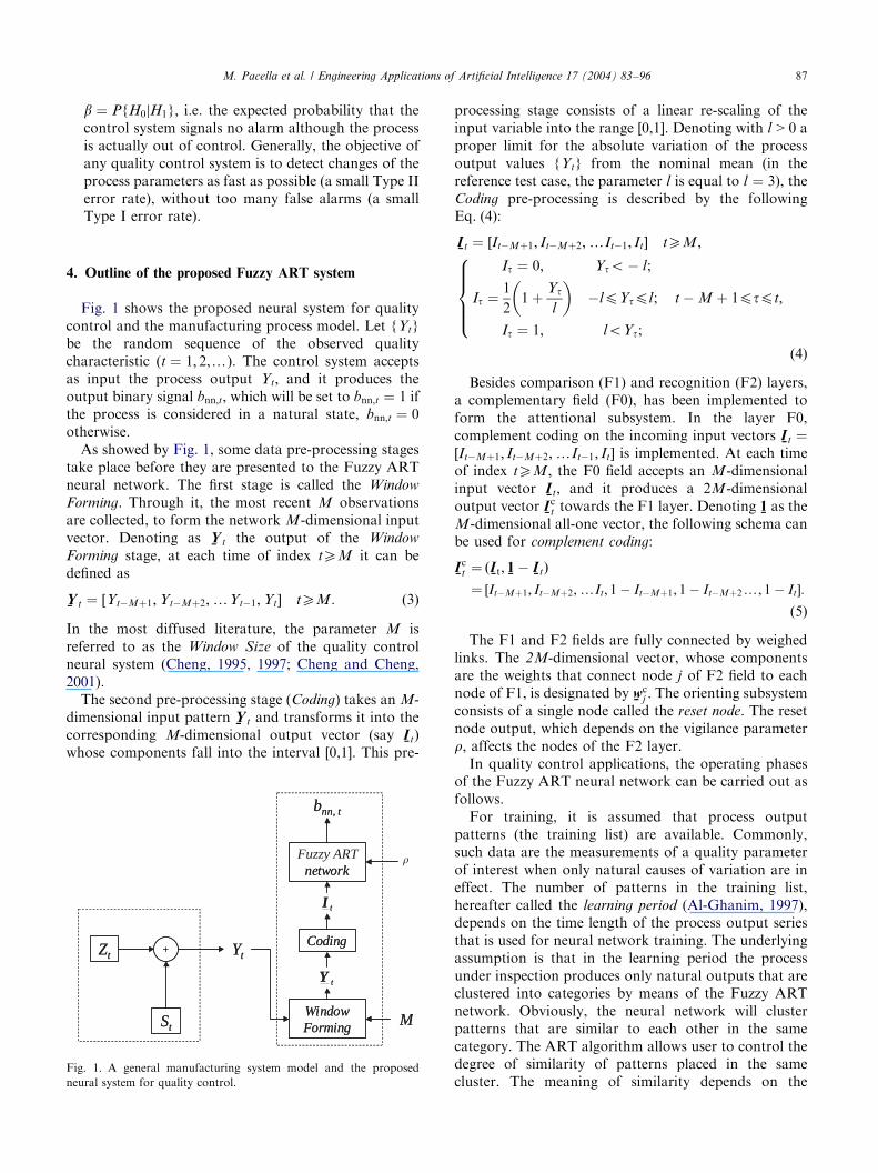
Fig. 1 shows the proposed neural system for qualitycontrol and the manufacturing process model. Let fYtgbe the random sequence of the observed qualitycharacteristic (t ¼ 1; 2,y). The control system acceptsas input the process output Yt; and it produces theoutput binary signal bnn;t; which will be set to bnn;t ¼ 1 ifthe process is considered in a natural state, bnn;t ¼ 0otherwise.As showed by Fig. 1, some data pre-processing stages

take place before they are presented to the Fuzzy ARTneural network. The first stage is called the Window

Forming. Through it, the most recent M observationsare collected, to form the network M-dimensional inputvector. Denoting as

%Y t the output of the Window

Forming stage, at each time of index tXM it can bedefined as

%Y t ¼ ½YtMþ1;YtMþ2;yYt1;Yt� tXM: ð3Þ

In the most diffused literature, the parameter M isreferred to as the Window Size of the quality controlneural system (Cheng, 1995, 1997; Cheng and Cheng,2001).The second pre-processing stage (Coding) takes an M-

dimensional input pattern%Y t and transforms it into the

corresponding M-dimensional output vector (say%I t)

whose components fall into the interval [0,1]. This pre-

Zt

St

+ YtCoding

WindowForming

network

bnn, t

M

tY

tI

Zt

St

+ YtCoding

WindowForming

Fuzzy ARTnetwork

bnn, t

M

tY

tI

�

Fig. 1. A general manufacturing system model and the proposed

neural system for quality control.

processing stage consists of a linear re-scaling of theinput variable into the range [0,1]. Denoting with l > 0 aproper limit for the absolute variation of the processoutput values fYtg from the nominal mean (in thereference test case, the parameter l is equal to l ¼ 3), theCoding pre-processing is described by the followingEq. (4):

%I t ¼ ½ItMþ1; ItMþ2;yIt1; It� tXM;

It ¼ 0; Yto l;

It ¼1

21þ

Yt

l

� �lpYtpl;

It ¼ 1; loYt;

8>>><>>>:

t M þ 1ptpt;

ð4Þ

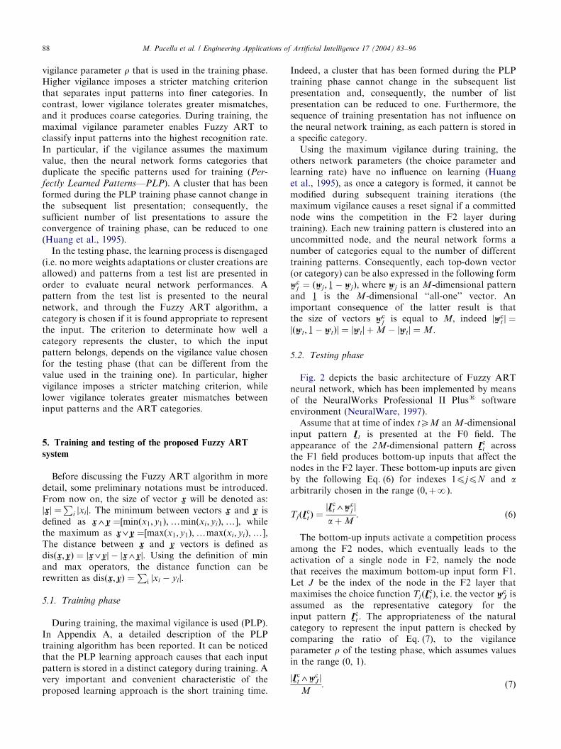
Besides comparison (F1) and recognition (F2) layers,a complementary field (F0), has been implemented toform the attentional subsystem. In the layer F0,complement coding on the incoming input vectors

%I t ¼

½ItMþ1; ItMþ2;yIt1; It� is implemented. At each timeof index tXM ; the F0 field accepts an M-dimensionalinput vector

%I t; and it produces a 2M-dimensional

output vector%I ct towards the F1 layer. Denoting %

1 as theM-dimensional all-one vector, the following schema canbe used for complement coding:

%I ct ¼ ð

%I t;

%1

%I tÞ

¼ ½ItMþ1; ItMþ2;yIt; 1 ItMþ1; 1 ItMþ2y; 1 It�:

ð5Þ

The F1 and F2 fields are fully connected by weighedlinks. The 2M-dimensional vector, whose componentsare the weights that connect node j of F2 field to eachnode of F1, is designated by

%wc

j : The orienting subsystemconsists of a single node called the reset node. The resetnode output, which depends on the vigilance parameterr; affects the nodes of the F2 layer.In quality control applications, the operating phases

of the Fuzzy ART neural network can be carried out asfollows.For training, it is assumed that process output

patterns (the training list) are available. Commonly,such data are the measurements of a quality parameterof interest when only natural causes of variation are ineffect. The number of patterns in the training list,hereafter called the learning period (Al-Ghanim, 1997),depends on the time length of the process output seriesthat is used for neural network training. The underlyingassumption is that in the learning period the processunder inspection produces only natural outputs that areclustered into categories by means of the Fuzzy ARTnetwork. Obviously, the neural network will clusterpatterns that are similar to each other in the samecategory. The ART algorithm allows user to control thedegree of similarity of patterns placed in the samecluster. The meaning of similarity depends on the

ARTICLE IN PRESSM. Pacella et al. / Engineering Applications of Artificial Intelligence 17 (2004) 83–9688

vigilance parameter r that is used in the training phase.Higher vigilance imposes a stricter matching criterionthat separates input patterns into finer categories. Incontrast, lower vigilance tolerates greater mismatches,and it produces coarse categories. During training, themaximal vigilance parameter enables Fuzzy ART toclassify input patterns into the highest recognition rate.In particular, if the vigilance assumes the maximumvalue, then the neural network forms categories thatduplicate the specific patterns used for training (Per-

fectly Learned Patterns—PLP). A cluster that has beenformed during the PLP training phase cannot change inthe subsequent list presentation; consequently, thesufficient number of list presentations to assure theconvergence of training phase, can be reduced to one(Huang et al., 1995).In the testing phase, the learning process is disengaged

(i.e. no more weights adaptations or cluster creations areallowed) and patterns from a test list are presented inorder to evaluate neural network performances. Apattern from the test list is presented to the neuralnetwork, and through the Fuzzy ART algorithm, acategory is chosen if it is found appropriate to representthe input. The criterion to determinate how well acategory represents the cluster, to which the inputpattern belongs, depends on the vigilance value chosenfor the testing phase (that can be different from thevalue used in the training one). In particular, highervigilance imposes a stricter matching criterion, whilelower vigilance tolerates greater mismatches betweeninput patterns and the ART categories.

5. Training and testing of the proposed Fuzzy ART

system

Before discussing the Fuzzy ART algorithm in moredetail, some preliminary notations must be introduced.From now on, the size of vector

%x will be denoted as:

j%xj ¼

Pi jxi j: The minimum between vectors

%x and

%y is

defined as%x4

%y ¼½minðx1; y1Þ;yminðxi; yiÞ;y�; while

the maximum as%x3

%y ¼½maxðx1; y1Þ;ymaxðxi; yiÞ;y�;

The distance between%x and

%y vectors is defined as

disð%x;

%yÞ ¼ j

%x3

%yj j

%x4

%yj: Using the definition of min

and max operators, the distance function can berewritten as disð

%x;

%yÞ ¼

Pi jxi yij:

5.1. Training phase

During training, the maximal vigilance is used (PLP).In Appendix A, a detailed description of the PLPtraining algorithm has been reported. It can be noticedthat the PLP learning approach causes that each inputpattern is stored in a distinct category during training. Avery important and convenient characteristic of theproposed learning approach is the short training time.

Indeed, a cluster that has been formed during the PLPtraining phase cannot change in the subsequent listpresentation and, consequently, the number of listpresentation can be reduced to one. Furthermore, thesequence of training presentation has not influence onthe neural network training, as each pattern is stored ina specific category.Using the maximum vigilance during training, the

others network parameters (the choice parameter andlearning rate) have no influence on learning (Huanget al., 1995), as once a category is formed, it cannot bemodified during subsequent training iterations (themaximum vigilance causes a reset signal if a committednode wins the competition in the F2 layer duringtraining). Each new training pattern is clustered into anuncommitted node, and the neural network forms anumber of categories equal to the number of differenttraining patterns. Consequently, each top-down vector(or category) can be also expressed in the following form

%wc

j ¼ ð%wj ;

%1

%wjÞ; where

%wj is an M-dimensional pattern

and%1 is the M-dimensional ‘‘all-one’’ vector. An

important consequence of the latter result is thatthe size of vectors

%wc

j is equal to M, indeed j%wc

t j ¼jð%wt;

%1

%wtÞj ¼ j

%wtj þ M j

%wtj ¼ M:

5.2. Testing phase

Fig. 2 depicts the basic architecture of Fuzzy ARTneural network, which has been implemented by meansof the NeuralWorks Professional II Pluss softwareenvironment (NeuralWare, 1997).Assume that at time of index tXM an M-dimensional

input pattern%I t is presented at the F0 field. The

appearance of the 2M-dimensional pattern%I ct across

the F1 field produces bottom-up inputs that affect thenodes in the F2 layer. These bottom-up inputs are givenby the following Eq. (6) for indexes 1pjpN and aarbitrarily chosen in the range ð0;þNÞ:

Tjð%I ct Þ ¼

j%I ct4%

wcj j

aþ M: ð6Þ

The bottom-up inputs activate a competition processamong the F2 nodes, which eventually leads to theactivation of a single node in F2, namely the nodethat receives the maximum bottom-up input form F1.Let J be the index of the node in the F2 layer thatmaximises the choice function Tjð

%I ct Þ; i.e. the vector %

wcJ is

assumed as the representative category for theinput pattern

%I ct : The appropriateness of the natural

category to represent the input pattern is checked bycomparing the ratio of Eq. (7), to the vigilanceparameter r of the testing phase, which assumes valuesin the range (0, 1).

j%I ct4%

wcJ j

M: ð7Þ

ARTICLE IN PRESS

ctI

( )ttct I1II = ,

( )M

T

cj

ct

tj +

=

wII

cJ

ct wI

tI

tnnb ,

cJ

ct wI

cJw

cJ

ct wI

0F

1F

2F Reset( )JChoice

Match

Coding

Complement

AttentionalSubsystem

OrientingSubsystem

ctI

( )ttct I1II = ,

( )M

T

cj

ct

tj +

=

wII

cJ

ct wI

tI

tnnb ,

cJ

ct wI

cJw

cJ

ct wI

0F

1F

2F Reset( )JChoice

Match

ing

t

AttentionalSubsystem

OrientingSubsystem

ctI

ttct I1I −= ,

( )M

T

cj

ct

tj +

∧=

α

wII

≥∧ M.�cJ

ct wI

tI

tnnb ,

cJ

ct wI ∧

cJw

cJ

ct wI ∧1F

2F s t( )i

�

Fig. 2. The proposed Fuzzy ART neural network for manufacturing

quality control.

M. Pacella et al. / Engineering Applications of Artificial Intelligence 17 (2004) 83–96 89

If such ratio is not less than the vigilance parameter r;then the output is set to bnn;t ¼ 1 (natural input),otherwise, the algorithm produces the output bnn;t ¼ 0(unnatural input). Since it results that

j%I ct4%

wcJ j ¼ jð

%I t;

%1

%I tÞ4ð

%wJ ;

%1

%wJ Þj

¼ j½%I t4

%wJ ; ð

%1

%I tÞ4ð

%1

%wJÞj;

j%I ct4%

wcJ j ¼ j½

%I t4

%wJ ;

%1 ð

%I t3

%wJ Þ�j

¼ j%I t4

%wJ j þ M j

%I t3

%wJ j;

j%I ct4%

wcJ j ¼M disð

%I t;

%wJÞ:

It may be noted that the node J; whose top-downweight vector

%wc

J ¼ ð%wJ ;

%1

%wJÞ maximises the choice

function (6), is also that node which minimises thedistance disð

%I t;

%wJ Þ: Thus, an input pattern is classified as

natural if the following condition (8) is passed:

j%I ct4%

wcJ j

MXr3disð

%I t;

%wJÞpMð1 rÞ: ð8Þ

6. Experiment and analysis

Three parameters can affect the performances of theproposed neural system for quality control.

1. The vigilance parameter r of testing phase, it can takevalues in the range (0,1).

2. The window size M; it can take values in {1, 2, 3,y},i.e. any non-zero integer.

3. The training period d; i.e. the number of trainingpatterns.

In order to estimate their effects on the systemperformances, which are measured in terms of bothType I error and Type II error rates, a completeexperimental design was used (Montgomery, 1997). Forsimplicity, each of the three factors was evaluated bymeans two proper levels (high and low), thus eightexperimental scenarios was analysed.Both a number of 15 training data sets and of

15 different testing data sets were produced by meansof Monte Carlo simulation. To make this randomgeneration different for all data sets, a different seedof the MATLABs pseudo-random generator wasspecified for each distinct training or testing series.Simulation replications were obtained combiningeach training data set to all the testing sets. Thus,a number of 15� 15=225 different replications, foreach of the eight experimental scenarios, wereobtained.Each training data set included a number of d M-

dimensional vectors, while testing data sets were formedby means of 10000 M-dimensional vectors. Trainingdata sets, as well as testing data sets, used to estimateType I errors, were simulated by means of the normaldistribution function (mean m ¼ 0 and standard devia-tion s ¼ 1). On the other hand, the testing data sets usedto estimate Type II errors, were simulated through ashift pattern (Eq. (2)) of 1.5 units of standard deviation(j ¼ 1:5), and starting point in the fifth observation(t ¼ 5).Before presenting simulation results, let us elaborate

on the experiment model in more detail. The relation-ship between the Type I error and the networkparameters can be formulated as follows.

aðr;M ; dÞ ¼ f ðr;M; dÞ þ eðr;M; dÞ; ð9Þ

where the function f ðr;M ; dÞ is the expected Type Ierror level for the parameter combination ðr;M ; dÞ; andaðr;M ; dÞ is the actual simulation measure. The actualmeasure is affected by an error eðr;M; dÞ that can beconsidered as an occurrence of a random variable withmean zero. Three sources of variability can affect therandom error eðr;M ; dÞ: the training set, the testing setand the interaction between them. The effect of trainingdata set on the actual measure aðr;M ; dÞ is designatedas elðr;M ; dÞ; while the effect of testing data setis designated as etðr;M; dÞ: Therefore, denotingeltðr;M; dÞ the effect of the interaction between thetwo factors, Eq. (9) can be rewritten as follows:

aðr;M ; dÞ ¼ f ðr;M ; dÞ þ elðr;M; dÞ

þ etðr;M ; dÞ þ eltðr;M ; dÞ: ð10Þ

ARTICLE IN PRESS

dMrho

100010

025100.

900.

85

1.00

0.75

0.50

0.25

0.00

Fig. 3. Type I main effect plot. Simulation results based on 225

replications of 10,000 trials for each of the eight scenarios. The

horizontal line represents the mean value of the Type I error.

M. Pacella et al. / Engineering Applications of Artificial Intelligence 17 (2004) 83–9690

Denoting with symbols s2l ðr;M; dÞ; s2t ðr;M ; dÞ;s2ltðr;M ; dÞ the variance values of random componentselðr;M; dÞ; etðr;M ; dÞ and eltðr;M ; dÞ; respectively, thenthe variance of aðr;M; dÞ can be rewritten ass2aðr;M; dÞ ¼ s2l ðr;M ; dÞ þ s2t ðr;M; dÞ þ s2ltðr;M ; dÞ: Asimilar model can be formulated for the Type II error,so the following Eq. (11) can be used in this case:

bðr;M ; dÞ ¼ gðr;M ; dÞ þ eLðr;M; dÞ

þ eT ðr;M ; dÞ þ eLT ðr;M ; dÞ: ð11Þ

That implies s2bðr;M ; dÞ ¼ s2Lðr;M; dÞ þ s2T ðr;M ; dÞ þs2LT ðr;M; dÞ:

6.1. Analysis

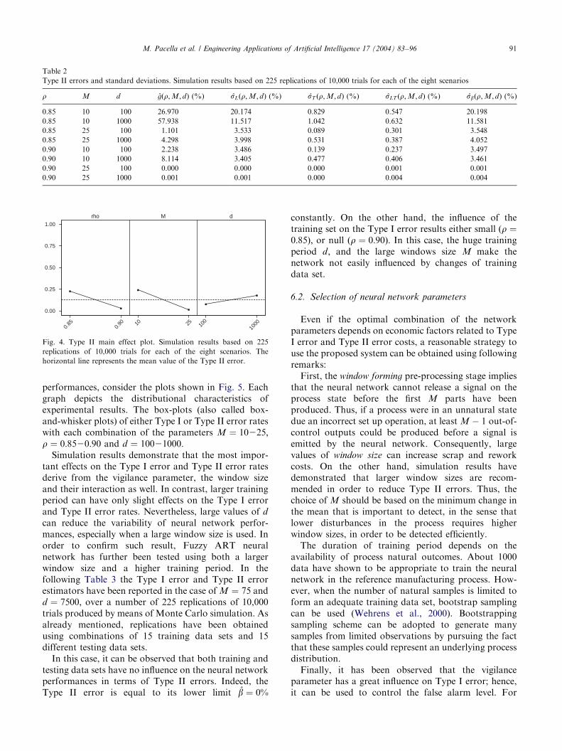
As already mentioned, to find out how the threeparameters ðr;M ; dÞ influence network performances,both the Type I and Type II error rates have beenestimated in eight scenarios. Two window sizes ðM ¼10225Þ; two levels of the vigilance parameter ðr ¼0:8520:90Þ and two learning periods ðd ¼ 10021000Þ;have been used. The resulting Type I error rates havebeen presented in Table 1.Following Fig. 3 shows the main-effect plots for each

experimental factor.It results that as the vigilance parameter increases,

the Type I error rate increases too. Similarly, a higherwindow size causes the Type I error to increase. Incontrast, a long training period produces a smallerType I error. It can be noticed that variations of thevigilance parameter and of the window size can haveconsiderable effects on Type I errors, while changes ofthe training period have only slight influence on thefalse alarm rate. Moreover, the Analysis of Variance(ANOVA—Montgomery, 1997) of the simulation results,underlines that there is considerable interaction betweenthe vigilance parameter r and the window size M ; interms of their effects on Type I errors.The eight standard-deviation point estimators

#saðr;M; dÞ of Table 1 measure the spread of perfor-mances around the false alarm point-estimators#fðr;M; dÞ: It results that changes in the training dataset, as well as in the testing data set, have not important

Table 1

Type I errors and standard deviations. Simulation results based on 225 repl

r M d #fðr;M; dÞ (%) #slðr;M; dÞ (%)

0.85 10 100 1.100 0.197

0.85 10 1000 0.027 0.004

0.85 25 100 7.656 2.293

0.85 25 1000 0.337 0.031

0.90 10 100 42.276 3.773

0.90 10 1000 7.661 0.189

0.90 25 100 97.906 1.090

0.90 25 1000 84.036 1.781

effects on Type I errors. Nevertheless, it can be noticedthat short learning period ðd ¼ 100Þ can cause higherinfluence of the training data set on the false alarm ratepresented by the neural system.Type II errors are reported in following Table 2, while

the main effect plots are depicted in Fig. 4.In this case, it can be deduced that as the vigilance

parameter increases, the Type II error decreases.Similarly, a larger window size causes the decrease ofType II error, while a longer training period producesslightly higher Type II error. By comparing plots ofFigs. 3 and 4, it appears that the effects of the threeparameters on the Type II error are smaller than thosepresented on Type I error. As for Type I error measures,the Analysis of Variance shows that there is significantinteraction between the vigilance parameter and windowsize in terms of Type II error as well.Results of Table 2 reveal that changes of training/

testing data set can have valuable effects on Type IIerrors. Moreover, it can be observed that the variability,which is due to changes of training set, is higher thanthat obtained varying the testing set. In other words, itappears that the spread of the neural network perfor-mances in terms of Type II error mainly depends on thetraining data set rather than on the choice of the testingdata set.To analyse in more detail the experimental results,

and how the vigilance parameter r affects network

ications of 10,000 trials for each of the eight scenarios

#stðr;M; dÞ (%) #sltðr;M; dÞ (%) #saðr;M; dÞ (%)

0.187 0.136 0.304

0.017 0.018 0.025

0.898 0.509 2.515

0.134 0.084 0.161

1.191 0.671 4.013

0.662 0.292 0.748

0.187 0.319 1.151

1.018 0.604 2.138

ARTICLE IN PRESS

Table 2

Type II errors and standard deviations. Simulation results based on 225 replications of 10,000 trials for each of the eight scenarios

r M d #gðr;M; dÞ (%) #sLðr;M; dÞ (%) #sT ðr;M; dÞ (%) #sLT ðr;M; dÞ (%) #sbðr;M; dÞ (%)

0.85 10 100 26.970 20.174 0.829 0.547 20.198

0.85 10 1000 57.938 11.517 1.042 0.632 11.581

0.85 25 100 1.101 3.533 0.089 0.301 3.548

0.85 25 1000 4.298 3.998 0.531 0.387 4.052

0.90 10 100 2.238 3.486 0.139 0.237 3.497

0.90 10 1000 8.114 3.405 0.477 0.406 3.461

0.90 25 100 0.000 0.000 0.000 0.001 0.001

0.90 25 1000 0.001 0.001 0.000 0.004 0.004

dMrho

100010

025100.

900.

85

1.00

0.75

0.50

0.25

0.00

Fig. 4. Type II main effect plot. Simulation results based on 225

replications of 10,000 trials for each of the eight scenarios. The

horizontal line represents the mean value of the Type II error.

M. Pacella et al. / Engineering Applications of Artificial Intelligence 17 (2004) 83–96 91

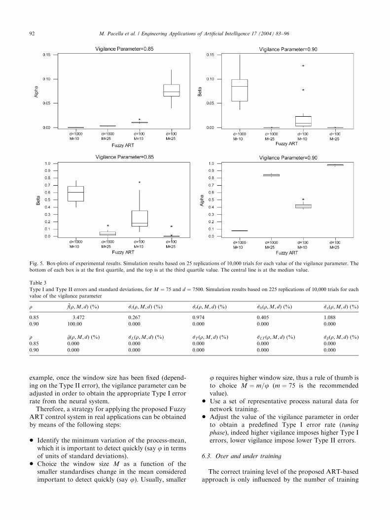
performances, consider the plots shown in Fig. 5. Eachgraph depicts the distributional characteristics ofexperimental results. The box-plots (also called box-and-whisker plots) of either Type I or Type II error rateswith each combination of the parameters M ¼ 10225;r ¼ 0:8520:90 and d ¼ 10021000:Simulation results demonstrate that the most impor-

tant effects on the Type I error and Type II error ratesderive from the vigilance parameter, the window sizeand their interaction as well. In contrast, larger trainingperiod can have only slight effects on the Type I errorand Type II error rates. Nevertheless, large values of d

can reduce the variability of neural network perfor-mances, especially when a large window size is used. Inorder to confirm such result, Fuzzy ART neuralnetwork has further been tested using both a largerwindow size and a higher training period. In thefollowing Table 3 the Type I error and Type II errorestimators have been reported in the case of M ¼ 75 andd ¼ 7500; over a number of 225 replications of 10,000trials produced by means of Monte Carlo simulation. Asalready mentioned, replications have been obtainedusing combinations of 15 training data sets and 15different testing data sets.In this case, it can be observed that both training and

testing data sets have no influence on the neural networkperformances in terms of Type II errors. Indeed, theType II error is equal to its lower limit #b ¼ 0%

constantly. On the other hand, the influence of thetraining set on the Type I error results either small ðr ¼0:85Þ; or null ðr ¼ 0:90Þ: In this case, the huge trainingperiod d; and the large windows size M make thenetwork not easily influenced by changes of trainingdata set.

6.2. Selection of neural network parameters

Even if the optimal combination of the networkparameters depends on economic factors related to TypeI error and Type II error costs, a reasonable strategy touse the proposed system can be obtained using followingremarks:First, the window forming pre-processing stage implies

that the neural network cannot release a signal on theprocess state before the first M parts have beenproduced. Thus, if a process were in an unnatural statedue an incorrect set up operation, at least M 1 out-of-control outputs could be produced before a signal isemitted by the neural network. Consequently, largevalues of window size can increase scrap and reworkcosts. On the other hand, simulation results havedemonstrated that larger window sizes are recom-mended in order to reduce Type II errors. Thus, thechoice of M should be based on the minimum change inthe mean that is important to detect, in the sense thatlower disturbances in the process requires higherwindow sizes, in order to be detected efficiently.The duration of training period depends on the

availability of process natural outcomes. About 1000data have shown to be appropriate to train the neuralnetwork in the reference manufacturing process. How-ever, when the number of natural samples is limited toform an adequate training data set, bootstrap samplingcan be used (Wehrens et al., 2000). Bootstrappingsampling scheme can be adopted to generate manysamples from limited observations by pursuing the factthat these samples could represent an underlying processdistribution.Finally, it has been observed that the vigilance

parameter has a great influence on Type I error; hence,it can be used to control the false alarm level. For

ARTICLE IN PRESS

Fig. 5. Box-plots of experimental results. Simulation results based on 25 replications of 10,000 trials for each value of the vigilance parameter. The

bottom of each box is at the first quartile, and the top is at the third quartile value. The central line is at the median value.

Table 3

Type I and Type II errors and standard deviations, for M ¼ 75 and d ¼ 7500: Simulation results based on 225 replications of 10,000 trials for each

value of the vigilance parameter

r #fðr;M; dÞ (%) #slðr;M; dÞ (%) #stðr;M; dÞ (%) #sltðr;M; dÞ (%) #saðr;M; dÞ (%)

0.85 3.472 0.267 0.974 0.405 1.088

0.90 100.00 0.000 0.000 0.000 0.000

r #gðr;M; dÞ (%) #sLðr;M; dÞ (%) #sT ðr;M; dÞ (%) #sLT ðr;M; dÞ (%) #sbðr;M; dÞ (%)

0.85 0.000 0.000 0.000 0.000 0.000

0.90 0.000 0.000 0.000 0.000 0.000

M. Pacella et al. / Engineering Applications of Artificial Intelligence 17 (2004) 83–9692

example, once the window size has been fixed (depend-ing on the Type II error), the vigilance parameter can beadjusted in order to obtain the appropriate Type I errorrate from the neural system.Therefore, a strategy for applying the proposed Fuzzy

ART control system in real applications can be obtainedby means of the following steps:

* Identify the minimum variation of the process-mean,which it is important to detect quickly (say j in termsof units of standard deviations).

* Choice the window size M as a function of thesmaller standardises change in the mean consideredimportant to detect quickly (say j). Usually, smaller

j requires higher window size, thus a rule of thumb isto choice M ¼ m=j (m ¼ 75 is the recommendedvalue).

* Use a set of representative process natural data fornetwork training.

* Adjust the value of the vigilance parameter in orderto obtain a predefined Type I error rate (tuning

phase), indeed higher vigilance imposes higher Type Ierrors, lower vigilance impose lower Type II errors.

6.3. Over and under training

The correct training level of the proposed ART-basedapproach is only influenced by the number of training

ARTICLE IN PRESS

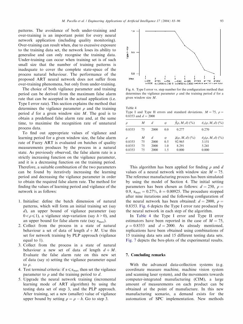
Fig. 6. Type I error vs. step number for the configuration method that

determines the vigilance parameter r and the training period d for a

given window size M:

Table 4

Type I and Type II errors and standard deviations. M ¼ 75; r ¼0:8353 and d ¼ 2000

r M d j #fðr;M; dÞ (%) #saðr;M; dÞ (%)

0.8353 75 2000 0.0 0.277 0.270

r M d j #gðr;M; dÞ (%) #sbðr;M; dÞ (%)

0.8353 75 2000 0.5 92.965 3.151

0.8353 75 2000 1.0 8.291 5.241

0.8353 75 2000 1.5 0.000 0.000

M. Pacella et al. / Engineering Applications of Artificial Intelligence 17 (2004) 83–96 93

patterns. The avoidance of both under-training andover-training is an important point for every neuralnetwork application (including quality monitoring).Over-training can result when, due to excessive exposureto the training data set, the network loses its ability togeneralise and can only recognise the training data.Under-training can occur when training set is of suchsmall size that the number of training patterns isinadequate to cover the complete state-space of theprocess natural behaviour. The performance of theproposed ART neural network does not suffer fromover-training phenomena, but only from under-training.The choice of both vigilance parameter and training

period can be derived from the maximum false alarmrate that can be accepted in the actual application (i.e.Type I error rate). This section explains the method thatdetermines the vigilance parameter r and the trainingperiod d for a given window size M: The goal is toobtain a predefined false alarm rate and, at the sametime, to maximise the recognition rate of unnaturalprocess data.To find out appropriate values of vigilance and

learning period for a given window size, the false alarmrate of Fuzzy ART is evaluated on batches of qualitymeasurements produces by the process in a naturalstate. As previously observed, the false alarm rate is astrictly increasing function on the vigilance parameter,and it is a decreasing function on the training period.Therefore, a suitable combination of the two parameterscan be found by iteratively increasing the learningperiod and decreasing the vigilance parameter in orderto obtain the required false alarm rate. The method forfinding the values of learning period and vigilance of thenetwork is as follows:

1. Initialise: define the batch dimension of naturalpatterns, which will form an initial training set (sayd), an upper bound of vigilance parameter (say0orp1), a vigilance step-variation (say h > 0), andan upper bound for false alarm rate (say amax).

2. Collect from the process in a state of naturalbehaviour a set of data of length d þ M : Use thisset for network training by PLP approach (vigilanceequal to 1).

3. Collect from the process in a state of naturalbehaviour a new set of data of length d þ M :Evaluate the false alarm rate on this new setof data (say a) setting the vigilance parameter equalto r:

4. Test terminal criteria: if apamax then set the vigilanceparameter to r and the training period to d:

5. Upgrade the neural network training (incrementallearning mode of ART algorithm) by using thetesting data set of step 3, and the PLP approach.After training, set a new (smaller) value of vigilanceupper bound by setting r ¼ r h: Go to step 3.

This algorithm has been applied for finding r and d

values of a neural network with window size M ¼ 75:The reference manufacturing process has been simulatedby using the model of Section 4. The initial settingparameters has been chosen as follows: d ¼ 250; r ¼0:9; amax ¼ 0:27%; h ¼ 0:00925: The procedure stoppedafter nine iterations and the following configuration ofthe neural network has been obtained: d ¼ 2000; r ¼0:8353: Fig. 6 depicts the Type I error rate produced bythe neural network in each step of the algorithm.In Table 4 the Type I error and Type II error

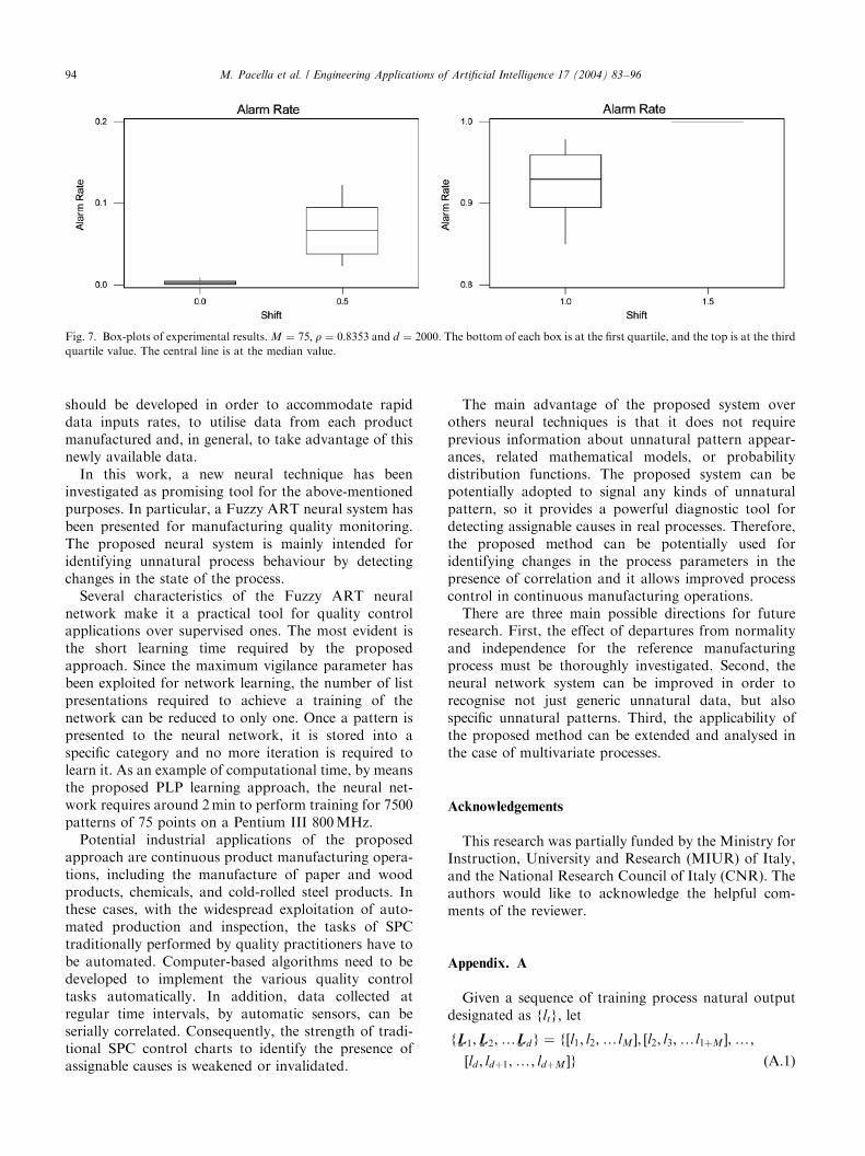
estimators have been reported in the case of M ¼ 75;r ¼ 0:8353 and d ¼ 2000: As already mentioned,replications have been obtained using combinations of15 training data sets and 15 different testing data sets.Fig. 7 depicts the box-plots of the experimental results.

7. Concluding remarks

With the advanced data-collection systems (e.g.coordinate measure machine, machine vision systemand scanning laser system), and the movements towardscomputer-integrated manufacturing (CIM), a largeamount of measurements on each product can beobtained at the point of manufacture. In this newmanufacturing scenario, a demand exists for theautomation of SPC implementation. New methods

ARTICLE IN PRESS

Fig. 7. Box-plots of experimental results. M ¼ 75; r ¼ 0:8353 and d ¼ 2000: The bottom of each box is at the first quartile, and the top is at the third

quartile value. The central line is at the median value.

M. Pacella et al. / Engineering Applications of Artificial Intelligence 17 (2004) 83–9694

should be developed in order to accommodate rapiddata inputs rates, to utilise data from each productmanufactured and, in general, to take advantage of thisnewly available data.In this work, a new neural technique has been

investigated as promising tool for the above-mentionedpurposes. In particular, a Fuzzy ART neural system hasbeen presented for manufacturing quality monitoring.The proposed neural system is mainly intended foridentifying unnatural process behaviour by detectingchanges in the state of the process.Several characteristics of the Fuzzy ART neural

network make it a practical tool for quality controlapplications over supervised ones. The most evident isthe short learning time required by the proposedapproach. Since the maximum vigilance parameter hasbeen exploited for network learning, the number of listpresentations required to achieve a training of thenetwork can be reduced to only one. Once a pattern ispresented to the neural network, it is stored into aspecific category and no more iteration is required tolearn it. As an example of computational time, by meansthe proposed PLP learning approach, the neural net-work requires around 2min to perform training for 7500patterns of 75 points on a Pentium III 800MHz.Potential industrial applications of the proposed

approach are continuous product manufacturing opera-tions, including the manufacture of paper and woodproducts, chemicals, and cold-rolled steel products. Inthese cases, with the widespread exploitation of auto-mated production and inspection, the tasks of SPCtraditionally performed by quality practitioners have tobe automated. Computer-based algorithms need to bedeveloped to implement the various quality controltasks automatically. In addition, data collected atregular time intervals, by automatic sensors, can beserially correlated. Consequently, the strength of tradi-tional SPC control charts to identify the presence ofassignable causes is weakened or invalidated.

The main advantage of the proposed system overothers neural techniques is that it does not requireprevious information about unnatural pattern appear-ances, related mathematical models, or probabilitydistribution functions. The proposed system can bepotentially adopted to signal any kinds of unnaturalpattern, so it provides a powerful diagnostic tool fordetecting assignable causes in real processes. Therefore,the proposed method can be potentially used foridentifying changes in the process parameters in thepresence of correlation and it allows improved processcontrol in continuous manufacturing operations.There are three main possible directions for future

research. First, the effect of departures from normalityand independence for the reference manufacturingprocess must be thoroughly investigated. Second, theneural network system can be improved in order torecognise not just generic unnatural data, but alsospecific unnatural patterns. Third, the applicability ofthe proposed method can be extended and analysed inthe case of multivariate processes.

Acknowledgements

This research was partially funded by the Ministry forInstruction, University and Research (MIUR) of Italy,and the National Research Council of Italy (CNR). Theauthors would like to acknowledge the helpful com-ments of the reviewer.

Appendix. A

Given a sequence of training process natural outputdesignated as fltg; let

f%L1;

%L2;y

%Ldg ¼ f½l1; l2;ylM �; ½l2; l3;yl1þM �;y;

½ld ; ldþ1;y; ldþM �g ðA:1Þ

ARTICLE IN PRESSM. Pacella et al. / Engineering Applications of Artificial Intelligence 17 (2004) 83–96 95

be the sequence of the M-dimensional trainingvectors, which result from the window coding stage.Denoting by d (the learning period) the number ofthe M-dimensional training patterns, let fI1; %

I2;y%Idg

be the series of M-dimensional training vectors thatresult from the Coding stage, and let f

%I c1; %

I c2;y%I cdg be

the 2M-dimensional training vectors that resultfrom the complement coding stage at the F0 layer. Thefollowing algorithm describes the systematic implemen-tation of the PLP learning approach for Fuzzy ARTtraining.

1. Initialise the vigilance parameter to r ¼ 1 andthe number of committed nodes in F2 to N ¼ 0(a committed node in F2 is a node that hascoded at least one input pattern; during thetraining phase, Fuzzy ART operates over all of thecommitted nodes along with a single uncommittednode).

2. Choose the nth input pattern ð%I cnÞ from the training

list (1pnpd).3. Calculate the bottom-up inputs to the N þ 1 nodes in

F2 due to the presentation of the nth input pattern.When calculating bottom-up inputs consider allthe committed nodes and the uncommitted node.These bottom-up inputs are calculated according tothe following Eq. (A.2) where 1pjpN þ 1 and a (thechoice parameter) is arbitrarily chosen in the rangeð0;þNÞ:

Tjð%I cnÞ ¼

M

aþ 2Mif j is the uncommited node;

j%I cn4%

wcj j

aþ j%wc

j jif j is a commited node:

8>>><>>>:

ðA:2Þ

4. Chose the node in F2 that receives the maximumbottom-up input from F1. Assume that this node hasindex J: Check to see whether this node satisfies thevigilance criterion of Eq. (A.3).

j%I cn4%

wcJ j ¼ M ðA:3Þ

Three cases are now distinguished.* If node J is the uncommitted node, it satisfies the

vigilance criterion since%wc

J ¼ ½1; 1;y1� )j%I cn4%

wcJ j ¼ j

%I cnj ¼ M: In this case, increase the

parameter N by one: this way a new uncommittednode in F2 is introduced, and its initial weightvector is chosen to be the ‘‘all-ones’’ vector. Go tostep 5.

* If node J is a committed node, and the top-downweight vector is equal to

%wc

J ¼%I cn; then the

vigilance criterion is satisfied since%wc

J ¼%I cn )

j%I cn4%

I cnj ¼ j%I cnj ¼ M: Go to step 5.

* Otherwise, exclude the node J by setting TJð%I cnÞ ¼

1; and go to the beginning of Step 3.

5. The top-down weight vector of node J is set equal to

%wc

J ¼%I cn: If %

I cn is the last input pattern in the traininglist ðn ¼ dÞ then the learning process is consideredcompleted. Otherwise, go to Step 2 to present thenext in sequence input pattern by increasing the indexn by one.

References

Al-Ghanim, A., 1997. An unsupervised learning neural algorithm for

identifying process behavior on control charts and a comparison

with supervised learning approaches. Computers and Industrial

Engineering 32 (3), 627–639.

Anagnostopoulos, G.C., Georgiopoulos, M., 2002. Category regions

as a new geometrical concept in Fuzzy-ART and Fuzzy-ARTMAP.

Neural Networks 15, 1205–1221.

Bishop, C.M., 1995. Neural Networks for Pattern Recognition. Oxford

University Press, Inc., Oxford.

Cheng, C.S., 1995. A multi-layer neural network model for detecting

changes in the process mean. Computers and Industrial Engineer-

ing 28 (1), 51–61.

Cheng, C.S., 1997. A neural network approach for the analysis of

control chart patterns. International Journal of Production

Research 35 (3), 667–697.

Cheng, C.S., Cheng, S.S., 2001. A neural network-based procedure for

the monitoring of the exponential mean. Computers and Industrial

Engineering 40, 309–321.

Cook, D.F., Chiu, C.C., 1998. Using radial basis function neural

networks to recognize shifts in correlated manufacturing process

parameters. IIE Transactions 30, 227–234.

Cook, D.F., Zobel, C.W., Nottingham, Q.J., 2001. Utilization of

neural networks for the recognition of variance shifts in correlated

manufacturing process parameters. International Journal of

Production Research 39 (17), 3881–3887.

Georgiopoulos, M., Fernlund, H., Bebis, G., Heileman, G.L.,

1996. Order of search in Fuzzy ART and Fuzzy ARTMAP:

effect of the choice parameter. Neural Networks 9 (9),

1541–1559.

Georgiopoulos, M., Dagher, I., Heileman, G.L., Bebis, G., 1999.

Properties of learning of a fuzzy ART variant. Neural Networks

12, 837–850.

Guo, Y., Dooley, K.J., 1992. Identification of changes structure in

statistical process control. International Journal of Production

Research 30 (7), 1655–1669.

Guh, R.S., Tannock, J.D.T., 1999. Recognition of control

chart concurrent patterns using a neural network ap-

proach. International Journal of Production Research 37 (8),

1743–1765.

Hagan, M.T., Demuth, H.B., Beale, M., 1996. Neural Network

Design. PWS, Boston, MA.

Haykin, S., 1999. Neural Networks: A Comprehensive Foundation,

third ed. Prentice-Hall, Englewood Cliffs, NJ.

Huang, J., Georgiopoulos, M., Heileman, J.L., 1995. Fuzzy ART

proprieties. Neural Networks 8 (2), 203–213.

Montgomery, D.C., 1997. Design and Analysis of Experiments, fifth

ed. Wiley, New York.

Montgomery, D.C., 2000. Introduction to Statistical Quality Control,

fourth ed. Wiley, New York.

NeuralWare Inc., 1997. NeuralWorks Professional II Plus Reference

Guide. Pittsburgh, PA, USA.

Pao, Y.H., 1989. Adaptive Pattern Recognition and Neural Networks.

Addison-Wesley, Reading, MA.

Pugh, G.A., 1991. A comparison of neural networks to SPC charts.

Computers and Industrial Engineering 21, 253–255.

ARTICLE IN PRESSM. Pacella et al. / Engineering Applications of Artificial Intelligence 17 (2004) 83–9696

Smith, A.E., 1994. X-bar and R control chart interpretation using

neural computing. International Journal of Production Research

32 (2), 309–320.

Vattulainen, I., Kankaala, K., Saarinen, J., Ala-Nissila, T., 1995. A

comparative study of some pseudorandom number generators.

Computer Physics Communications 86, 209–226.

Wehrens, R., Putter, H., Buydens, L.M.C., 2000. The bootstrap:

a tutorial. Chemometrics and intelligent laboratory systems 54,

35–42.

Zorriassantine, F., Tannock, J.D.T., 1998. A review of neural

networks for statistical process control. Journal of Intelligent

Manufacturing 9, 209–224.