MANIPUR UNIVERSITY

Department of Mathematics, Manipur University, Canchipur

MANIPUR UNIVERSITY

Learning Outcomes-based Curriculum Framework

(LOCF)

Semester Scheme with Multiple Entry and Exit Options for Under Graduate Course

Syllabus for Mathematics

(I, II, III & IV Semesters)

2022-23 onwards

of 38


of 38

Table of Contents

Contents Page Number

1. Proceedings of LOCF meeting 3

2. Programme Outcomes 4

3. Assessment 4

4. Course Structure Draft A 5

5. Semester-wise Distribution of Course 6

6. Contents of Courses for B A/ B Sc degree Model B 8

7. Discipline Specific Core Courses

Semester I i. MMC-101 :Calculus

10

ii MMC-102 : Algebra 12

Semester II

i. MMC-203 : Real Analysis 13

ii. MMC-204 : Differential Equations 15

Semester III

i. MMC-305 : Theory of Real Functions 16

ii. MMC-306 : Group Theory 18

iii. MMC-307 : Multivariate Calculus 19

Semester IV

i. MMC-408 : Partial Differential Equations 21

ii. MMC-409 : Riemann Integral 23

iii. MMC-410 : Numerical Analysis 25

8. Skill Enhancement Paper

Semester I

i. MMSE-101 A : LaTeX 28

ii. MMSE-101 B : Computational Mathematics Laboratory 29

Semester II

i. MMSE-202 A : Python Programming 31

ii. MMSE-202 B : Computer Algebra Systems and Related Software 34

9. Generic Elective Course

Semester III

i. MMGE-301 : Quantitative Aptitude 36

Semester IV

i. MMGE-402 : Basic Tools of Mathematics 37


of 38


of 38

Syllabus for Bachelor of Science/Arts in Mathematics

Name of the Degree /Program: Bachelor of Science/ Bachelor of Arts

Discipline Course: Mathematics

Starting year of implementation: 2022-2023 Programme Outcomes (PO): By the end of the program the students will be able to gain the following skills.

PO1

Disciplinary knowledge: Bachelor degree in Mathematics is the culmination of in-depth

knowledge of Algebra, Calculus, geometry, Real analysis, Differential equations and several

other branches of pure and applied mathematics, This also leads to study of relevant areas such

as computer science and other disciplines.

PO2

Communication Skills: Ability to communicate the various mathematical concepts effectively

using variety of examples mostly having real life applications and their geometric

visualization. The skills and knowledge gained in this programme will lead to the proficiency

in analytical reasoning which can be used to express thoughts and views in mathematically or

logically correct statements.

PO3

Critical thinking and analytical reasoning: The students undergoing this programme acquire

the ability of critical thinking and logical reasoning and will apply in formulating or

generalizing specific hypothesis, conclusion. The learner will be able to recognize and

distinguish the various aspects of real life problems.

PO4

Problem solving: The Mathematical knowledge gained by the student through this programme

develops an ability to solve the problems, identify and define appropriate computing

requirements for its solutions. This programme will enhance the overall development.

PO5

Research related skills: After the completion of this programme, the student will develop the

capability of inquiring about appropriate questions relating to the Mathematical concepts,

arguments. He/she will be able to define problems, formulate hypothesis, proofs, write the

results obtained clearly.

PO6 Information/ digital literacy: The completion of this programme will enable the learner to use

appropriate softwares to solve the system of algebraic and differential equations.

PO7

Self-directed learning: The student after the completion of the programme will be able to

work independently, make an in-depth search of various areas of Mathematics and resources

for self learning in order to enhance knowledge in mathematics.

PO8

Moral and ethical awareness / reasoning: The student after the completion of the course will

develop an ability to identify unethical behaviour such as fabrication, falsification or

misinterpretation of data and adopting objectives, unbiased and truthful actions in all aspects of

life in general and Mathematical studies in particular.

PO9

Lifelong learning: This programme provides self directed learning and lifelong learning skills.

With these skills, the learner will be able to think independently, improve personal

development.

Assessment Weightage for the Assessments (in percentage)

Type of Course Formative Assessment(I.A) Summative Assessment (S.A)

Theory 30% 70%

Practical 30% 70%

Projects 30% 70%

Experimental Learning (Internship etc.)


of 38

Course Structure (Draft) Model A

(A) Bachelor’s Certificate in Mathematics (Level 5)

Semester

Discipline

specific Core

(DSC)

Discipline

Specific

Elective

(DSE)

Generic Elective

Course (GEC),

(To be selected

from GEC

listings of other

disciplines) (Credit)

Ability

Enhancement

Compulsory

Courses

(AECC)

Skill Enhancement

Course (SEC) Select

any one among A/B

Value Addition

Courses (VAC)

(To be selected

from VAC

listings of other

disciplines). (Credits)

Semester

Credit

I

MMC-101 (6) AECC-101 (4)

English/MIL MMSE-101 A/B (4) VAC-101 (2)

24 MMC-102 (6) VAC-102 (2)

II

MMC-203 (6) AECC-202 (4)

Environmental

Science

MMSE-202 A/B (4)

VAC-203 (2)

24 MMC-204(6) VAC-204 (2)

Award of Certificate in Mathematics (after 1stYear : minimum 46 (four six) Credits)

(B) Bachelor’s Diploma in Mathematics (Level 6)

Semester

Discipline

specific

Core (DSC)

Discipline

Specific

Elective

(DSE)

Generic

Elective

Course

(GEC), (Credit)

Ability

Enhancement

Compulsory

Courses

(AECC)

Skill

Enhancement

Course

(SEC)

Value

Addition

Courses

(VAC) (Credits)

Semester

Credit

III

MMC-305 (6)

MMGE-301 (6)

VAC-305 (2)

26 MMC-306 (6)

MMC-307 (6)

IV

MMC-408 (6)

MMGE-402 (6)

VAC-406 (2)

26 MMC-409 (6)

MMC-410 (6)

Award of Diploma in Mathematics (after 2nd Year: minimum 96 (nine six) Credits)

(C) Bachelor’s Degree in Mathematics (Level 7)

Semester

Discipline

specific Core

(DSC)

Discipline

Specific

Elective

(DSE)

Generic Elective

Course (GEC),

(Credit)

Ability

Enhancement

Compulsory

Courses (AECC)

Skill

Enhancement

Value

Addition

Courses

(VAC) (Credits)

Semester

Credit

V MMC-511 (6)

MME-501 (6) MMGE-503(6)

VAC-507 (2) 26 MMC-512 (6)

VI MMC-613 (6)

MME-602 (6) MMGE-604(6)

VAC-608 (2) 26 MMC-614 (6)

Award of BSc degree in Mathematics (after 3rd Year: minimum 140 (one four zero) Credits)

(D) Bachelor’s (Hons) Degree (Level 8)

Semester

Discipline

specific Core

(DSC)

Discipline

Specific Elective

(DSE)

Generic Elective

Course (GEC),

(Credit)

Ability

Enhancement

Compulsory

Courses (AECC)

Skill

Enhancement

Course (SEC)

Value

Addition

Courses

(VAC) (Credits)

Semester

Credit

VII MMC-715 (6)

MME-703 (6) MMGE-705 (6)

24 MMC-716 (6)

VIII MMC-817 (6) MME-804 (6)

/Research projects MMGE-806(6)

24

MMC-818 (6)

Award of B A/ B Sc degree with honours in Mathematics on completion of course equal to a

minimum of 182 (one eight two) credits.


of 38

Bachelor of Science or Bachelor of Arts with Mathematics as Major & BA/BSc (Hons) Mathematics.

Course Structure (Draft)

SEMESTER-WISE DISTRIBUTION OF COURSES

A. Discipline Specific Core (DSC) Courses:

All the courses have 6 credits with 4 credits of theory (4 hours per week) and 2 credits of practical (4

hours per week) OR 5 (FIVE) credits of theory and 1(ONE) credit of tutorial

Sl.No. CC Paper Code Semester Course Name

1. MMC-101 I Calculus

2. MMC-102 I Algebra

3. MMC-203 II Real Analysis

4. MMC-204 II Differential Equations

5. MMC-305 III Theory of Real Functions

6. MMC-306 III Group Theory

7. MMC-307 III Multivariate Calculus

8. MMC-408 IV Partial Differential Equations

9. MMC-409 IV Riemann Integration

10. MMC-410 IV Numerical Analysis

11. MMC-511 V Metric Spaces

12. MMC-512 V Mechanics

13. MMC-613 VI Complex Analysis

14. MMC-614 VI Ring Theory and Linear Algebra

15. MMC-715 VII Abstract Algebra

16. MMC-716 VII Advanced Real Analysis

17. MMC-817 VIII Topology

18. MMC-818 VIII Ordinary Differential Equations

B. Discipline Specific Electives (DSE):

All the courses have 6 credits with 4 credits of theory and 2 credits of practical or 5 credits of theory and

1 credit of tutorials.

Sl. No. DSE Paper

Code Semester DSE Name

1. MME-501 V Integral Transform/Mathematical Modelling/Advanced Group Theory

2.

MME-602

VI

Special Theory of Relativity & Tensor/Linear

Programming and its applications/Probability Theory

and Statistics

3. MME-703 VII Advanced Complex Analysis/Graph Theory/Fixed point theory

4. MME-804 VIII Advanced Partial Differential Equations/Functional Analysis/Cryptology/Research Projects


of 38

C. Skill Enhancement Courses (SEC):

All courses have 4 credits with 2 credits of theory and 2 credits of Practical/Tutorials/Projects and Field

Work to be decided by the College.

Sl No. DSE Paper Code Semester SEC Name

1. MMSE-101 A I LaTeX

2. MMSE-101 B I Computational Mathematics Laboratory

3. MMSE-202 A II Python Programming

4. MMSE-202 B II Computer Algebra Systems and Related Software

D. Ability Enhancement Compulsory Courses:

All the courses have 4 credits including Theory/Practicals/Projects.

Sl No. AECC Paper Code Semester AECC Name

1. AECC-101 I English/MIL

2. AECC-202 II Environmental Science

E. Value Addition Courses:

Sl.No VAC Paper Code Semester VAC Name

1. VAC-101 I Yoga

2. VAC-102 I Sports

3. VAC-203 II Culture

4. VAC-204 II Health Care

5. VAC-305 III NCC

6. VAC-406 IV Ethics

7. VAC-507 V NSS

8. VAC-608 VI History of Science

F. Generic Elective Courses:

All the courses have 6 credits with 4 credits of theory and 2 credits of practicals. These courses are meant

for students of other departments/disciplines or 5 credits of theory and 1 credit of tutorials.

Sl.No. GECPaperCode Semester GEC Name

1. MMGE-301 III Quantitative Aptitude

2. MMGE-402 IV Basic Tools of Mathematics

3. MMGE-503 V Recreational Mathematics

4. MMGE-604 VI Discrete Mathematics

5. MMGE-705 VII Analytical Geometry and Theory of Equations

6. MMGE-806 VIII Numerical methods with practical


of 38

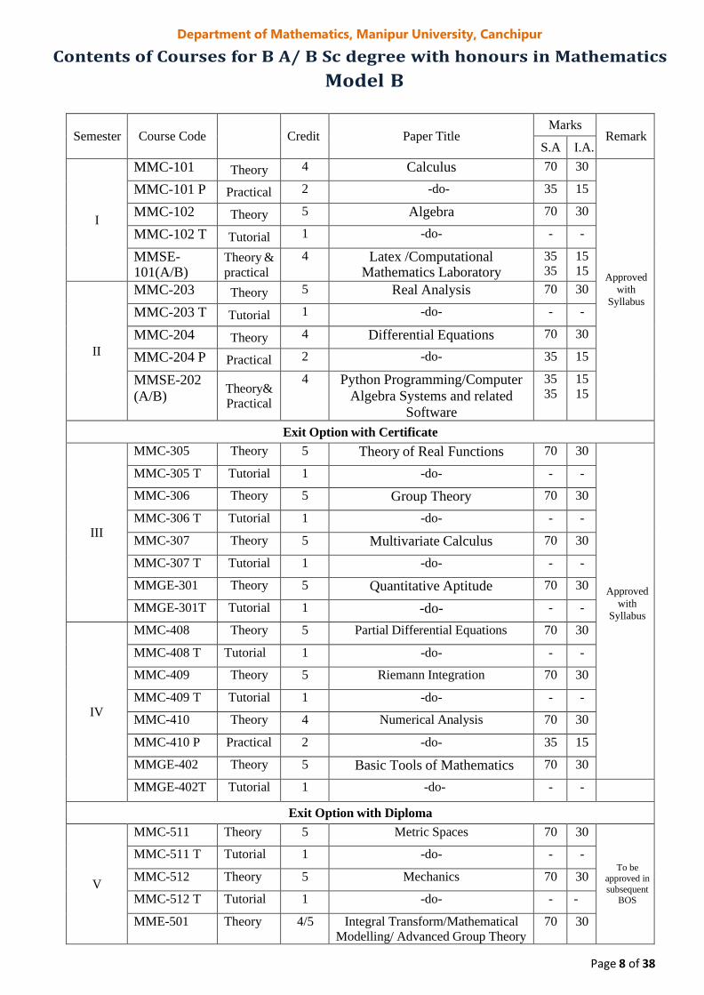
Contents of Courses for B A/ B Sc degree with honours in Mathematics

Model B

Semester

Course Code

Credit

Paper Title Marks

Remark S.A I.A.

I

MMC-101 Theory 4 Calculus 70 30

Approved

with

Syllabus

MMC-101 P Practical 2 -do- 35 15

MMC-102 Theory 5 Algebra 70 30

MMC-102 T Tutorial 1 -do- - -

MMSE- 101(A/B)

Theory &

practical

4 Latex /Computational Mathematics Laboratory

35 35

15 15

II

MMC-203 Theory 5 Real Analysis 70 30


MMC-204 Theory 4 Differential Equations 70 30


MMSE-202

(A/B) Theory&

Practical

4 Python Programming/Computer

Algebra Systems and related

Software

35

35

15

15

Exit Option with Certificate

III

MMC-305 Theory 5 Theory of Real Functions 70 30

Approved

with

Syllabus


MMC-306 Theory 5 Group Theory 70 30


MMC-307 Theory 5 Multivariate Calculus 70 30


MMGE-301 Theory 5 Quantitative Aptitude 70 30

MMGE-301T Tutorial 1 -do- - -

IV

MMC-408 Theory 5 Partial Differential Equations 70 30


MMC-409 Theory 5 Riemann Integration 70 30


MMC-410 Theory 4 Numerical Analysis 70 30


MMGE-402 Theory 5 Basic Tools of Mathematics 70 30

MMGE-402T Tutorial 1 -do- - -

Exit Option with Diploma

V

MMC-511 Theory 5 Metric Spaces 70 30

To be

approved in

subsequent BOS


MMC-512 Theory 5 Mechanics 70 30


MME-501 Theory 4/5 Integral Transform/Mathematical

Modelling/ Advanced Group Theory

70 30


of 38

MME-501 P/T Practical/

Tutorial

2/1 -do- 35/ -

15 /-

MMGE-503 Theory 5 Recreational Mathematics 70 30

MMGE-503 T Tutorial 1 -do- - -

VI

MMC-613 Theory 5 Complex Analysis 70 30


MMC-614 Theory 5 Ring Theory and Linear Algebra 70 30


MME-602 Theory 4/5 Special Theory of Relativity &

Tensor/Linear Programming and its

applications/Probability Theory and Statistics

70 30

MME-602 P/T Practical/

Tutorial

2/1 -do- 35 -

15 -

MMGE-604 Theory 5 Discrete Mathematics 70 30


Exit Option with Bachelor of Arts, B.A./Bachelor of Science, B.Sc.

VII

MMC-715 Theory 5 Abstract Algebra 70 30

To be

approved in subsequent

BOS


MMC-716 Theory 5 Advanced Real Analysis 70 30


MME-703 Theory 5 Advanced Complex Analysis/Graph

Theory/ Fixed Point Theory

70 30

MME-703 T Tutorial 1 -do- - -

MMGE-705 Theory Analytic Geometry and Theory of Equations

70 30


VIII

MMC-817 Theory 5 Topology 70 30

MMC-817 T Tutorial 1 Topology - -

MMC-818 Theory 5 Ordinary Differential Equations 70 30


MME-804 Theory 5/6 Advanced Partial Differential

Equations/Functional Analysis/

Cryptology/RESEARCH

PROJECTS

70 30

MME-804 Tutorial 1/0 -do- - -

MMGE-806 Theory 4 Numerical Methods with practical 70 30

MMGE-806 P Practical 2 -do- 35 15

Award of Bachelor of Arts / Science (BA/BSc) Honours in Mathematics


of 38

Discipline Specific Core Courses Semester I

MMC-101 : Calculus

Total Marks: 150 (Theory: 70, Internal Assessment: 30 and Practical: 50)

Workload: 4 Lectures (per week), 4 Practicals (per week)

Duration: 14 Weeks (56 Hrs. Theory + 56 Hrs. Practical) Examination: 3 Hrs.

Course Objectives: The primary objective of this course is to introduce the basic tools of calculus and

geometric properties of different conic sections which are helpful in understanding their applications in

planetary motion, design of telescope and to the real-world problems. Also, to carry out the hand on

sessions in computer lab to have a deep conceptual understanding of the above tools to widen the horizon

of students’ self-experience.

Course Learning Outcomes: After completion of the course, a student will be able to:

i) sketch curves in a plane in the different coordinate systems of reference.

ii) understand the Calculus of vector valued functions.

iii) apply calculus to develop basic principles of planetary motions.

Unit 1: Derivatives for Curve sketching (35 marks, 5 weeks)

First and second derivative tests for Extreme Values of Functions, Concavity and Curve Sketching,

Limits to infinity and infinite limits, Indeterminate Forms and L’Hôpital’s Rule, Asymptotes, Higher

order derivatives, Leibniz rule.

Unit 2: Curve tracing in polar Coordinates (30 marks, 4 weeks)

Parametric representation of curves, Polar Coordinates, Tracing of curves in Polar Coordinates, Graphing

Polar Coordinate Equations, Areas and Lengths in Polar Coordinates, Classification of conics in Polar

Coordinates.

Unit 3: Vector Calculus and its applications (35 marks, 5 weeks)

Vector valued functions and their graphs, Limits and continuity of vector functions, Differentiation and

integration of vector functions, Projectile motion, Unit tangent, Normal and binormal vectors, Curvature,

Kepler’s Second Law (Equal Area Law).

References:

1. Thomas, Jr. George B., Weir, Maurice D., & Hass, Joel (2014). Thomas’ Calculus (13thed.) Pearson

Education, Delhi. Indian Reprint 2017.

2. B. C. Das, B. N. Mukherjee. Differential Calculus (55th Edition), U.N. Dhur & Sons Private Ltd.,

Kolkata (2015).


of 38

𝑥 𝑥

Practical / Lab work to be performed in Computer Lab.

List of the practicals to be done using Mathematica /MATLAB /Maple /Scilab/Maxima etc.

(i). Plotting the graphs of the following functions:

ax, [x] (greatest integer function),√𝑎𝑥 + 𝑏, |ax+b|, c ± |ax+b|,

𝑥±𝑛 1

, 𝑥𝑛 (n∈Z), |𝑥|, sin (1 𝑥

), xsin (1 ), and 𝑒 1

𝑥 , for x ≠ 0

𝑒𝑎𝑥 +𝑏 , log (ax+b), 1/(ax+b),, sin (ax+b), cos (ax+b),

| sin (ax+b)|, | cos (ax+b)|.

Observe and discuss the effect of changes in the real constants a, b and c on the graphs.

(ii). Plotting the graphs of polynomial of degree 4 and 5, and their first and secondderivatives, and analysis of

these graphs in context of the concepts covered in Unit 1.

(iii). Sketching parametric curves..

(iv). Tracing of conic in Cartesian coordinates.

(v). Graph of hyperbolic functions.

(vi). Computation of limit, Differentiation, Integration and sketching of vector-valued functions.

(vii). Complex numbers and their representations, Operations like addition, Multiplication, Division,

Modulus, Graphical representation of polar form.

Teaching plan (Theory of MMC 101 Calculus):

Week 1: First and second derivative tests for Extreme Values of Functions; [1] Chapter 4 (Section 4.3).

Week 2: Concavity and Curve Sketching;[1] Chapter 4 (Section 4.4).

Week 3: Limits to infinity and infinite limits;[1] Chapter 2 (Section 2.6).

Week 4: Indeterminate forms and L’ Hospital’s Rule;[1] Chapter 4 (Section 4.5), Asymptotes; [1]

Chapter 2 (Section 2.6).

Week 5: Higher order derivatives; [1] Chapter 3 (Section 3.7), Leibniz rule; [1] Chapter 3 (Section 3.11).

Week 6: Parametric representation of curves; [1] Chapter 11 (Section 11.1 and 11.2),

Week 7: Polar Coordinates, Tracing of curves in Polar Coordinates;[1] Chapter 11 (Section 11.3).

Week 8: Graphing Polar Coordinates Equations;[1] Chapter 11 (Section 11.4), Areas and Lengths in

Polar Coordinates;[1] Chapter 11 (Section 11.5).

Week 9: Classification of Conics in Polar Coordinates;[1] Chapter 11 (Section 11.6 and 11.7).

Week 10: Vector valued functions and their graphs, Limits and Continuity of vector functions;[1]


Week 11: Differentiation and integration of vector functions;[1] Chapter 13 (Section 13.1).

Week 12: Projectile motion;[1] Chapter 13 (Section 13.2), Unit tangent;[1] Chapter 13 (Section 13.3).

Week 13:Normal and binormal vectors;[1] Chapter 13 (Section 13.3).

Week 14: Curvature; [1] Chapter 13 (Section 13.4 and 13.5), Kepler’s Second Law (Equal Area Law);

[1] Chapter 13 (Section 13.6).

±


of 38

MMC-102 : Algebra

Total Marks: 100 (Theory: 70, Internal Assessment: 30)

Workload: 5 Lectures (per week), 1 Tutorial (per week)

Duration: 14 Weeks (70 Hrs.) Examination: 3 Hrs.

Course Objectives: The primary objective of this course is to introduce the basic tools of theory of

equations, complex numbers, number theory and matrices to understand their linkage to the real-world

problems.

Course Learning Outcomes: After completion of the course, a student will be able to

i) Employ De Moivre’s theorem in a number of applications to solve numerical problems;

ii) Apply Euclid’s algorithm and backwards substitution to find greatest common divisor;

iii) Recognize consistent and inconsistent systems of linear equations by using rank.

Unit 1: Theory of Equations (35 marks, 5 weeks)

Polynomial functions, Division algorithm, Synthetic division, Remainder Theorem, Factor Theorem,

Polynomial equations, Relation between roots and Co-efficients of a polynomial equation, Symmetric

function of the roots of an equation, sum of powers of the roots, Solution of cubic and biquadratic

equations, De Moivre’s Theorem for integer and fractional indices.

Unit2: Relation, functions and Basic Number Theory (35 marks, 5 weeks)

Binary relations, Partial order relation, Equivalence relations, Functions, Inverses and composition, One

to one correspondence and Cardinality of a set, Division Algorithm, Divisibility and the Euclidean

Algorithm, Prime Numbers, Congruences and applications, Principles of Mathematical induction.

Unit 3: Matrices (30 marks, 4 weeks)

Rank of a matrix, Rank and elementary operations, Row reduction and echelon forms, System of linear

equations, Solution of the matrix equation AX=B, Solution sets of linear systems, linear independence,

Eigenvectors and Eigen values, The Characteristic equation and Cayley- Hamilton Theorem.

References:

1. Goodaire, Edgar G & Parmentor, Michael M (2005); Discrete Mathematics with Graph Theory (3rd

Ed.) Pearson Education Pvt. Ltd., Indian Reprint 2015

2. MK Singal, Asha Rani Singal, (2020); Algebra (31st Ed) R Chand &Co, New Delhi.

3. Chandrika Prasad, (1963). Text Book on Algebra and Theory of Equations Pothishala Pvt. Ltd.

Additional Readings:

1. Kolman, Bernard, & Hill, David R. (2001). Introductory Linear Algebra with Applications (7th ed.).

Pearson Education, Delhi. First Indian Reprint 2003.

2. Lay, David C., Lay, Steven R., & McDonald, Judi J. (2016). Linear Algebra and its Applications (5th

ed.). Pearson Education.

3. Andrilli, Stephen, & Hecker, David (2016). Elementary Linear Algebra (5th ed.). Academic Press,

Elsevier India Private Limited.

4. Burton, David M. (2007). Elementary Number Theory (7th ed.). Tata Mc-Graw Hill Edition, Indian

Reprint.


of 38

Teaching plan (Theory of MMC 102 Algebra):

Week 1: Polynomial functions, Division Algorithm, Synthetic division; [2] Chapter 3 (Section 3.2, 3.3 &3.4).

Week 2: Remainder Theorem, Factor Theorem;[1] Chapter 4 (Section 4.1),

Week 3: Polynomial equations, Relations between roots and Co-efficients of a polynomial equation; [2] Chapter 3

(Section 3.6 &3.7).

Week 4: Symmetric functions of the roots of an equation, Sum of the powers of the roots; [2] Chapter 3 (Section

3.10 &3.10), Solutions of cubic and biquadratic equations; [3]Chapter 13(Section 13.2, 13.3, 13.6, 13.7)

Week 5: De Moivre’s Theorem for integer and fractional indices; [2] Chapter 4 (Section 4.1).

Week 6: Binary relations, Partial order relation, Equivalence relations; [1] Chapter 2 (Section 2.3 &2.4).

Week 7: Functions, Domain, Range, One-One, Onto, Inverses and composition, One to One correspondence and

Cardinality of a set; [1] Chapter 3 (Section 3.1, 3.2 &3.3).

Week 8: Division Algorithm, Divisibility and The Euclidean Algorithm;[1] Chapter 4 (Section 4.2).

Week 9: Prime Numbers, Congruences and applications; [1] Chapter 4 (Section 4.3 & 4.4).

Week 10: Principle of Mathematical Induction; [1] Chapter 5 (Section 5.1).

Week 11: Rank of a matrix, Rank and elementary operations; [2] Chapter 6 (Section 6.2 & 6.3).

Week 12: System of linear equations, Solution of the matrix equation AX=B; [2] Chapter 7 (Section 7.2 &7.3)

Week 13: Solution sets of linear systems, linear independence; [2] Chapter 6 (Section 6.4), Eigenvectors and Eigen

values; [2] Chapter 8 (Section 8.2).

Week 14: The Characteristic equation and Cayley-Hamilton Theorem; [2] Chapter 8 (Section 8.4).

Semester II

MMC-203 : Real Analysis


Workload: 5 Lectures (per week), 1 Tutorial (per week per student)


Course Objectives: The course will develop a deep and rigorous understanding of real line and of

defining terms to prove the results about convergence and divergence of sequences and series of real

numbers. These concepts has vide range of applications in real life scenario.

Course Learning Outcomes: This course will enable the students to:

i) Understand many properties of the real line R and learn to define sequence in terms of functions from

to a subset of R.

ii) Recognize bounded, convergent, divergent, Cauchy and monotonic sequences and to calculate their

limit superior, limit inferior, and the limit of a bounded sequence.

iii) Apply the ratio, root, alternating series and limit comparison tests for convergence and absolute

convergence of an infinite series of real numbers.

Unit 1: Real Number System Rand its properties (30 Marks, 4 Weeks )

Algebraic and order properties of R, Absolute value of a real number; Bounded above and bounded below

sets, Supremum and infimum of a nonempty subset of R, the completeness property of R, Archimedean

property, Density of rational numbers in R; Definition and types of intervals, Nested intervals property;

Neighbourhood of a point in R, Open and closed sets in R.


of 38

Unit 2: Sequences in R (35 Marks, 5 Weeks )

Convergent sequence, Limit of a sequence, Bounded sequence, Limit theorems, Monotone sequences,

Monotone convergence theorem, Subsequences, Bolzano-Weierstrass theorem for sequences, Limit

superior and limit inferior for bounded sequence, Cauchy sequence, Cauchy’s convergence criterion.

Unit 3: Infinite Series (35 Marks, 5 Weeks)

Convergence and divergence of infinite series of real numbers, Necessary condition forconvergence,

Cauchy criterion for convergence; Tests for convergence of positive term series: Integral test, Basic

comparison test, Limit comparison test, D’Alembert’s ratio test, Cauchy’s nth root test; Alternating series,

Leibniz test, Absolute and conditional convergence.

References:

1. Bartle, Robert G., &Sherbert, Donald R. (2015). Introduction to Real Analysis(4th ed.). Wiley India

Edition. New Delhi.

2. Ross, Kenneth A. (2013). Elementary Analysis: The theory of calculus (2nd ed.).Undergraduate Texts

in Mathematics, Springer.Indian Reprint.

3. Denlinger, Charles G. (2011). Elements of Real Analysis.Jones and Bartlett India Pvt.Ltd. Student

Edition.Reprinted 2015.


1. Bilodeau, Gerald G., Thie, Paul R., & Keough, G. E. (2010). An Introduction toAnalysis (2nd ed.).

Jones and Bartlett India Pvt. Ltd. Student Edition. Reprinted 2015.

2. Thomson, Brian S., Bruckner, Andrew. M., & Bruckner, Judith B. (2001).ElementaryReal Analysis.

Prentice Hall.

Teaching Plan (Theory of MMC-203: Real Analysis):

Weeks 1 and 2: Algebraic and order properties of R. Absolute value of a real number; Bounded above and

bounded below sets, Supremum and infimum of a nonempty subset of R. [1] Chapter 2 [Sections 2.1, 2.2 (2.2.1 to 2.2.6), and 2.3 (2.3.1 to 2.3.5)]

Weeks 3 and 4: The completeness property of R, Archimedean property, Density of rational numbersinR;

Definition and types of intervals, Nested intervals property; Neighborhood of a point in ,Openand closed

sets in R. [1] Chapter 2 [Sections 2.3 (2.3.6), 2.4 (2.4.3 to 2.4.9), and 2.5 up to Theorem 2.5.3] [1] Chapter 11 [Section 11.1 (11.1.1 to 11.1.3)]

Weeks 5 and 6:Convergentsequence,Sequences and their limits, Bounded sequence, Limit theorems.

[1] Chapter 3 (Sections 3.1 and 3.2)

Week 7: Monotone sequences, Monotone convergence theorem and applications.

[1] Chapter 3 (Section 3.3)

Week 8: Subsequences and statement of the Bolzano-Weierstrasstheorem,Limit superior and limitinferior for

bounded sequence of real numbers with illustrations only. [1] Chapter 3 [Section 3.4 (3.4.1 to 3.4.12), except 3.4.4, 3.4.7, 3.4.9 and 3.4.11]

Week 9: Cauchy sequences of real numbers and Cauchy’s convergence criterion.

[1] Chapter 3 [Section 3.5 (3.5.1 to 3.5.6)]

Week 10: Convergence and divergence of infinite series, Sequence of partial sums of infinite series,Necessary

condition for convergence, Cauchy criterion for convergence of series.



of 38

Weeks 11 and 12: Tests for convergence of positive term series: Integral test statement and convergence of p-

series, Basic comparison test, Limit comparison test with applications, D’Alembert’s ratio test and

Cauchy’s nth root test.

[3] Chapter 8 (Section 8.2 up to 8.2.19)

Weeks 13 and 14: Alternating series, Leibniz test, Absolute and conditional convergence.

[3] Chapter 8[Section 8.3 (8.3.1 to 8.3.7)]

MMC-204 : Differential Equations




Course Objectives: The main objectives of this course are to introduce the students to the exciting world

of Differential Equations, Mathematical Modeling and their applications.

Course Learning Outcomes: The course will enable the students to:

i) Formulate Differential Equations for various Mathematical models.

ii) Solve first order non-linear differential equation and linear differential equations of higher order using

various techniques.

iii) Apply these techniques to solve and analyze various mathematical models.

Unit 1: Differential Equations and Mathematical Modeling (35 marks, 5 weeks)

Differential equations and mathematical models, Order and degree of a differential equations, Integrals as

general and particular solutions, Exact differential equations and integrating factors of first order

differential equations, Separable Equations, Homogeneous Equations, Reduction to homogeneous

equations, Linear equations and Bernoulli Equation, Clairaut’s Equation, Existence and Uniqueness of

solution of initial and boundary value problems of first order ODE, singular solution of first order ODE.

Unit 2: Second and higher order differential Equations (35 marks, 5 weeks)

General solution of homogeneous equation of second order, Principle of superposition for a homogeneous

equation, Wronskian, its properties and applications, Linear homogeneous and non- homogeneous

equations of higher order with constant coefficients, Euler’s equation, Method of undetermined

coefficients, Method of variation of parameters, Applications of second order differential equations to

mechanical vibration.

Unit 3: Analysis of Mathematical Models (30 marks, 4 weeks)

Application of first order differential equations to acceleration-velocity model, Growth and Decay model.

Introduction to compartmental models, Lake pollution model (with case study of Lake Burley Griffin),

Drug Assimilation models, population models (with limited growth, exponential growth) Epidemic

models.

References:

1. Barnes, Belinda &Fulford, Glenn R. (2015). Mathematical Modelling with Case Studies, Using Maple

and MATLAB (3rd ed.). CRC Press, Taylor & Francis Group.

2. Edwards, C. Henry, Penney, David E., & Calvis, David T. (2015). Differential Equation and Boundary

Value Problems: Computing and Modeling (5th ed.). Pearson Education.

3. Ross, Shepley L. (2004). Differential Equations (3rd ed.). John Wiley & Sons. India.


of 38

Practical /Lab work to be performed in a Computer Lab:

Modelling of the following problems using Free and Open Source Software (FOSS) tools

(Maxima/Python/Mathematica/MATLAB/Maple/Scilab etc.)

1. Solving of Linear equations and Bernoulli Equation, Clairaut’s Equations.

2. Plotting of second and third order respective solution for a family of differential equations

3. Growth and decay model(exponential cases only)

4. (a) Lake pollution model(with constant/seasonal flow and pollution concentration)

(b) Limited growth of population

5. (a) Predatory-prey model

(b) Epidemic model of influenza (basic epidemic model, contagious for life, disease with carriers)

Teaching plan (Theory of MMC-204 : Differential Equations)

Week 1: Differential equations and mathematical models; [2] Chapter 1 (Section 1.1), Order and degree

of a differential equations; [3] Chapter 1 (Section 1.1)

Week 2: Integrals as general and particular solutions; [2] Chapter 1 (Section 1.2), Exact differential

equations and integrating factors of first order differential equations; [3] Chapter 2 (Section 2.1)

Week 3: Separable equations, Homogeneous equations, Reduction to homogeneous equations; [3]


Week 4: Linear equations and Bernoulli equation Clairaut’s equation ; [3] Chapter 2 (Section 2.3)

Week 5: Existence and Uniqueness of solution of initial and boundary value problems of first order ODE;

singular solution of the first order ODE [3] Chapter 1 (Section 1.3),

Week 6& 7: General solution of homogeneous equation of second order, Principle of superposition for a

homogeneous equation, Wronskian, its properties and applications; [2] Chapter 3 (Section 3.1).

Week8: Linear homogeneous and non-homogeneous equations of higher order with constant coefficients,

Euler’s equation; [2] Chapter 3 (Section 3.3).

Week 9: Method of undetermined coefficients, Method of variation of parameters; [2] Chapter 3 (Section

3.5).

Week 10: Applications of second order differential equations to mechanical vibration; [2] Chapter 3

(Section 3.6).

Week 11& 12: Application of first order differential equations to acceleration-velocity model; [2]

Chapter 2 (Section 2.3), Growth and Decay model; [1] Chapter 2 (Section 2.2).

Week 13:Introduction to compartmental models; [1] Chapter 2 (Section 2.1), Lake pollution model (with

case study of Lake Burley Griffin); [1] Chapter 2 (Section 2.5 & 2.6), Drug Assimilation models; [1]


Week 14:Population models (with limited growth, exponential growth) Epidemic models; [2] Chapter 2

(Section 2.1) or [1] Chapter 3 (Section 3.1)

Semester III MMC-305 : Theory of Real Functions


Workload: 5 Lectures (per week), 1 Tutorial (per week per student)


Course Objectives: It is a basic course on the study of real valued functions that would develop an

analytical ability to have a more matured perspective of the key concepts of calculus, namely, limits,

continuity, differentiability and their applications.


of 38

Course Learning Outcomes: This course will enable the students to learn:

i) A rigorous approach of the concept of limit of a function.

ii) About continuity and uniform continuity of functions defined on intervals.

iii) The geometrical properties of continuous functions on closed and bounded intervals.

iv) The applications of mean value theorem and Taylor’s theorem.

Unit 1: Limits of Functions (20 Marks, 3 Weeks)

Limits of functions (− approach), Sequential criterion for limits, Divergence criteria, Limit theorems,

One-sided limits, Infinite limits and limits at infinity.

Unit 2: Continuous Functions and their Properties (35 Marks, 5 Weeks)

Continuous functions, Sequential criterion for continuity and discontinuity, Algebra of continuous

functions, Properties of continuous functions on closed and bounded intervals ; Uniform continuity, Non-

uniform continuity criteria, Uniform continuity theorem.

Unit 3: Derivability and its Applications (45 Marks, 6 Weeks)

Differentiability of a function, Algebra of differentiable functions, Carathéodory’s theorem and chain

rule; Relative extrema, Interior extremum theorem, Rolle’s theorem, Mean- value theorem and its

applications, Intermediate value property of derivatives - Darboux’s theorem, Taylor polynomial,

Taylor’s theorem with Lagrange form of remainder, Application of Taylor’s theorem in error estimation;

Relative extrema, and to establish a criterion for convexity ; Taylor’s series expansions of 𝑒𝑥 , sin x and

cosx

Reference:

1. Bartle, Robert G., &Sherbert, Donald R. (2015). Introduction to Real Analysis (4thed.).Wiley India

Edition. New Delhi.


1. Ghorpade, Sudhir R. &Limaye, B. V. (2006). A Course in Calculus and Real Analysis.Undergraduate

Texts in Mathematics, Springer (SIE).First Indian reprint.

2. Mattuck, Arthur. (1999). Introduction to Analysis, Prentice Hall.

3. Ross, Kenneth A. (2013). Elementary Analysis: The theory of calculus (2nd ed.).Undergraduate Texts

in Mathematics, Springer.Indian Reprint.

Teaching Plan (MMC 305: Theory of Real Functions):

Week 1: Definition of the limit, Sequential criterion for limits, Divergence criteria.

[1]Chapter 4 (Section 4.1).

Week 2: Algebra of limits of functions with illustrations andexamples,Squeeze theorem.

[1]Chapter 4 (Section 4.2).

Week 3: Definition and illustration of the concepts of one-sided limits, Infinite limits and limits at

infinity.



of 38

Weeks 4 and 5: Definitions of continuity at a point and on a set, Sequential criterion for continuity,

Algebra of continuous functions, Composition of continuous functions.

[1] Sections 5.1 and 5.2.

Weeks 6 and 7: Various properties of continuous functions defined on an interval, viz., Boundedness

theorem, Maximum-minimum theorem, Statement of the location of roots theorem, Intermediate value

theorem and the preservation of intervals theorem.


Week 8: Definition of uniform continuity, Illustration of non-uniform continuity criteria, Uniform

continuity theorem.

[1] Chapter 5 [Section 5.4 (5.4.1 to 5.4.3)].

Weeks 9 and 10: Differentiability of a function, Algebra of differentiable functions, Carathéodory’s

theorem and chain rule.

[1] Chapter 6 [Section 6.1 (6.1.1 to 6.1.7)].

Weeks 11 and 12: Relative extrema, Interior extremum theorem,Rolle’s theorem, Mean value theorem

and its applications, Intermediate value property of derivatives -Darboux’s theorem.

[1] Section 6.2.

Weeks 13 and 14: Taylor polynomial, Taylor’s theorem and its applications, Taylor’s series expansions

of of𝑒𝑥 , sin x and cosx .

[1] Chapter 6 [Sections 6.4(6.4.1 to 6.4.6)], and Chapter 9 (Example 9.4.14, Page 286).

MMC-306 : Group Theory




Course Objectives: The objective of the course is to introduce the fundamental theory of groups and

their homomorphisms. Symmetric groups and group of symmetries are also studied in detail. Fermat’s

Little theorem as a consequence of the Lagrange’s theorem on finite groups.

Course Learning Outcomes: After completion of the course, a student will be able to

i) understand the basic concepts of groups and links with symmetric figures;

ii) learn concepts of normal subgroups, cosets and quotient groups;

iii) learn the concepts of group homomorphisms and isomorphisms.

Unit 1: Groups and elementary properties (35 Marks, 5 Weeks)

Symmetries of a Square, Dihedral groups, Definition and examples of groups including permutation

groups and quaternion groups, cycle notation of permutations, properties of permutations, Elementary

properties of groups, Permutations, Even and odd permutations.

Unit 2: Subgroups (35 Marks, 5 Weeks)

Subgroups and examples of subgroups, Centralizer, Normalizer, Center of a group, Cosets of a Group,

Lagrange’s theorem and consequences including Fermat’s Little theorem, cyclic groups, Classification of

subgroups of cyclic groups, Normal subgroups, Quotient Groups, alternating groups.


of 38

Unit 3: Group Homomorphisms (30 Marks, 4 Weeks)

Group homomorphisms, Properties of homomorphisms, Group isomorphisms, Properties of

isomorphisms, First, Second and Third isomorphism theorems for groups, Cayley’s theorem

Reference

1. Gallian, Joseph. A. (2013). Contemporary Abstract Algebra (8th ed.). Cengage Learning India Private

Limited, Delhi. Fourth impression, 2015.

2. I.N. Herstein,(2006).Topics in Algebra (2ndEdn).Wiley India Pvt. Ltd.

Additional Reading:

1. V.K. Khanna, SK Bhambri (2017). A course in Abstract Algebra (5thEdn).Vikas Pub. House Pvt. Ltd.

2. Rotman, Joseph J. (1995). An Introduction to The Theory of Groups (4th ed.). Springer Verlag, NY.

Teaching Plan (MMC-306 : Group Theory):

Week 1: Symmetries of a square, Dihedral groups, Definition and examples of groups including

permutation groups and quaternion groups (illustration through matrices). [1] Chapter 1.

Week 2: Definition and examples of groups, Elementary properties of groups. [1] Chapter 2.

Week 3: Subgroups and examples of subgroups, Centralizer, Normalizer, Center of a Group, Product of

two subgroups. [1] Chapter 3.

Weeks 4 and 5: Properties of cyclic groups. Classification of subgroups of cyclic groups. [1] Chapter 4

Weeks 6 and 7: Cycle notation for permutations, Properties of permutations, Even and odd permutations,

[1] Chapter 5 (up to Page 110).

Weeks 8 and 9: Properties of cosets, Lagrange’s theorem and consequences including Fermat’s Little

theorem. [1] Chapter 7 (up to Example 6, Page 150).

Week 10: Normal subgroups, Factor groups, Cauchy’s theorem for finite abelian groups. [1] Chapters 9

(Theorem 9.1, 9.2, 9.3 and 9.5, and Examples 1 to 12), Alternating group, [1] Chapter 5 (up to Page 110).

Weeks 11 and 12: Group homomorphisms, Properties of homomorphisms, Group isomorphisms,

Cayley’s theorem. [1] Chapter 10 (Theorems 10.1 and 10.2, Examples 1 to 11). [1] Chapter 6 (Theorem

6.1, and Examples 1 to 8).

Weeks 13 and 14: Properties of isomorphisms, First, Second and Third isomorphism theorems. [1]

Chapter 6 (Theorems 6.2 and 6.3), Chapter 10 (Theorems 10.3, 10.4, Examples 12 to 14, and Exercises 41

and 42 for second and third isomorphism theorems for groups).

MMC-307 : Multivariate Calculus



Duration: 14 Weeks (70 Hrs. Theory) Examination: 3 Hrs.

Course Objectives: To understand the extension of the studies of single variable differential and integral

calculus to functions of two or more independent variables. Also, the emphasis will be on the use of

Computer Algebra Systems by which these concepts may be analyzed and visualized to have a better

understanding.


of 38

Course Learning Outcomes: This course will enable the students to learn:

i) The conceptual variations when advancing in calculus from one variable to multivariable discussions.

ii) Inter-relationship amongst the line integral, double and triple integral formulations.

iii) Applications of multi variable calculus tools in physics, economics, optimization, and understanding

the architecture of curves and surfaces in plane and space etc.

Unit 1: Calculus of Functions of Several Variables and Properties of Vector Field- (40 Marks, 6

weeks)

Functions of several variables, Level curves and surfaces, Limits and continuity, Partial differentiation,

Higher order partial derivative, Tangent planes, Total differential and differentiability, Chain rule,

Directional derivatives, The gradient, Maximal and normal property of the gradient, Tangent planes and

normal lines, Extrema of functions of two variables, Method of Lagrange multipliers, Constrained

optimization problems; Definition of vector field, Divergence and curl.

Unit 2: Double and Triple Integrals – (30 Marks, 4 Weeks)

Double integration over rectangular and nonrectangular regions, Double integrals in polar co-ordinates,

Triple integral over a parallelepiped and solid regions, Volume by triple integrals, triple integration in

cylindrical and spherical coordinates, Jacobians (Without Proof), Change of variables in double and triple

integrals.

Unit 3: Green's, Stokes' and Gauss Divergence Theorem – (30 Marks, 4 Weeks)

Line integrals, Applications of line integrals: Mass and Work, Fundamental theorem for line integrals,

Conservative vector fields, Green's theorem, Area as a line integral; Surface integrals, Stokes' theorem,

The Gauss divergence theorem.

References:

1. Strauss, Monty J., Bradley, Gerald L., & Smith, Karl J. (2007). Calculus (3rd ed.). Dorling Kindersley

(India) Pvt. Ltd. (Pearson Education). Delhi. Indian Reprint 2011.

2. Marsden, J. E., Tromba, A., & Weinstein, A. (2004). Basic Multivariable Calculus. Springer

(SIE).First Indian Reprint.

Teaching Plan (MMC-307 : Multivariate Calculus):

Week 1: Definition of functions of several variables, Graphs of functions of two variables-Level curves

and surfaces, limits and continuity of functions of two variables.

[1] Chapter 11(Sections 11.1 and 11.2)

Week 2: Partial differentiation, and partial derivative as slope and rate, Higher order partial derivatives,

Tangent Planes, incremental approximation, Total differential.

[1] Chater 11 (Sections 11.3 and 11.4)

Week 3: Differentiability, Chain rule for one parameter, Two and three independent parameters.

[1] Chapter 11 (Section 11.4 and 11.5)

Week 4: Directional derivatives, The gradient, Maximal and normal property of the gradient, Tangent

planes and normal lines.


Week 5: First and second partial derivative tests for relative extrema of functions of two variables, and

absolute extrema of continuous functions.


of 38

[1] Chapter 11(section 11.7 (upto page 605))

Week 6: Lagrange multipliers method for optimization problems with one constraint, Definition of vector

field, Divergence and curl.

[1] Chapter 11 [Section 11.8 (pages 610-614) Chapter 13 (section 13.1)

Week 7: Double integration over rectangular and nonrectangular regions.

[1] Chapter 12(Sections 12.3 and 12.4)

Week 8: Double integrals in polar coordinates, and triple integral over a parallelopiped.


Week 9: Triple integral over solid regions, Volume by triple integral, and triple integration in cylindrical

coordinates.

[1] chapter 12 (Sections 12.4 and 12.5)

Week 10: Triple integration in spherical coordinates, Jacobian (Without Proof), Change of variables in

double and triple integrals.

[1] Chapter 12(Sections 12.7 and 12.8 upto page 849)

Week 11: Line integrals and its properties, applications of line integrals: mass and work.


Week 12: Fundamental theorem for line integrals, Conservative vector fields and path independence.


Week 13: Green’s theorem for simply connected region, area as a line integral, Definition of surface

integrals.


Week 14: Stokes’ theorem and the divergence theorem.


Semester IV

MMC-408 : Partial Differential Equations



Duration: 14 Weeks (70 Hrs. Theory ) Examination: 3 Hrs.

Course Objectives: The main objectives of this course are to teach students to form and solve partial

differential equations and use them in solving some physical problems.

Course Learning Outcomes: The course will enable the students to

i. Formulate, classify and transform partial differential equations into canonical form

ii. Solve linear and non-linear partial differential equations using various methods: and apply

these methods in solving some physical problems.

Unit 1. First order PDE and Methods of Characteristics (30 Marks, 4 Weeks)

Definitions & Basic concepts, Formation of PDE, classification and geometrical interpretation of first

order partial differential equations (PDE), Method of characteristics and general solution of first order

PDE, Lagrange and Charpit method, Cauchy’s problems for first order PDE, Canonical form of first order

PDE, Method of separation of variables for first order PDE


of 38

Unit 2. Classification of second order Linear PDE an Wave equations (35 Marks, 5 Weeks)

Classification of second order PDE, Reduction to canonical forms, Equations with constant coefficients,

General solutions, Cauchy’s Problem for second order PDE, Mathematical Modeling of vibrating string,

vibrating membrane, Homogeneous wave equation, Initial boundary value problems, Non-homogenous

boundary conditions, Finite string with fixed ends, Non- homogeneous wave equation.

Unit 3. Methods of separation of Variables (35 Marks, 5 Weeks)

Methods of separation of Variables for second order PDE, vibrating string problems, Existence and

uniqueness of solution of vibrating string problems, Heat conduction problem, Existence and uniqueness

of solution of Heat conduction problems, General solution of higher order PDE with constant coefficient,

Non- homogeneous Problems.

References:

1. Myint-U, Tyn and Debnath, Lokenath. (2007). Linear Partial Differential Equation for Scientists and

Engineers (4thed). Springer, Third Indian Reprint.


1. Sneddon, I. N. (2006). Elements of Partial Differential Equations, Dover Publications.Indian Reprint.

2. Stavroulakis, Ioannis P &Tersian, Stepan A. (2004). Partial Differential Equations: An Introduction

with Mathematica and MAPLE (2nd ed.). World Scientific.

Teaching Plan (Theory of MMC-408 : Partial Differential Equations):

Week 1: Introduction, Classification, Construction of first order partial differential equations (PDE).

[1] Chapter 2 (Sections 2.1 to 2.3)

Week 2: Method of characteristics and general solution of first order PDE.


Week 3: Canonical form of first order PDE, Method of separation of variables for first order PDE.


Week 4: The vibrating string, Vibrating membrane, Gravitational potential, Conservation laws.

[1] Chapter 3 (Sections 3.1 to 3.3, 3.5, and 3.6)

Weeks 5 and 6: Reduction to canonical forms, Equations with constant coefficients, General solution.


Weeks 7 and 8: The Cauchy problem for second order PDE, Homogeneous wave equation.

[1] Chapter 5 (Sections 5.1, 5.3, and 5.4)

Weeks 9 and 10: Initial boundary value problem, Non-homogeneous boundary conditions, Finite string with fixed

ends, Non – homogeneous wave equation, Goursat problem.

[1] Chapter 5 (Sections 5.5 to 5.7, and 5.9)

Weeks 11 and 12: Method of separation of variables for second order PDE, Vibrating string problem.


Weeks 13 and 14: Existence (omit proof) and uniqueness of vibrating string problem. Heat conduction problem.

Existence (omit proof) and uniqueness of the solution of heat conduction problem. Non – homogeneous

problem.

[1] Chapter 7 (Sections 7.4 to 7.6, and 7.8)


of 38

MMC-409 : Riemann Integration

Total Marks: 100 (Theory: 70 and Internal Assessment: 30)



Course Objectives: To understand the integration of bounded functions on a closed and bounded interval

and its extension to the cases where either the interval of integration is infinite, or the integrand has

infinite limits at a finite number of points on the interval of integration. The sequence and series of real

valued functions, and an important class of series of functions (i.e., power series).

Course Learning Outcomes: The course will enable the students to learn about:

i) Some of the families and properties of Riemann integrable functions, and the applications of the

fundamental theorems of integration.

ii) Beta and Gamma functions and their properties.

iii) The valid situations for the inter-changeability of differentiability and integrability within finite sum,

and approximation of transcendental functions in terms of power series.

Unit 1: Riemann Integration (35 Marks, 5 Weeks)

Definition of Riemann integration,(Algebraic and order properties of Riemann Integrals) Boundedness

theorem, Riemann integrability, Cauchy’s criterion, Squeeze Theorem, Riemann integrability of step,

continuous, and monotone functions, Additivity theorem, Fundamental theorems (First and Second

forms), substitution theorem, Lebesgue’s integrability criteria, composition theorem, product theorem,

Integration by parts, Darboux sums, Darboux integrals, Darboux integrability criteria, equivalence of

Riemann integral and Darboux integral.

Unit 2: Sequence and Series of Functions (35 Marks, 5 Weeks)

Pointwise and uniform convergence of sequence of functions, Theorem on the continuity of the limit

function of a sequence of functions, Theorems on the interchange of the limit and derivative, and the

interchange of the limit and integrability of a sequence of functions. Point-wise and uniform convergence

of series of functions, Theorems on the continuity, Derivability and integrability of the sum function of a

series of functions, Cauchy criterion and the Weierstrass M-Test for uniform convergence.

Unit 3: Improper Integral and Power Series (30 Marks, 4 weeks)

Improper integrals of Type-I, Type-II and mixed type, Convergence of Beta and Gamma functions, and

their properties.

Definition of a power series, Radius of convergence, Absolute convergence (Cauchy-Hadamard theorem),

Uniform convergence, Differentiation and integration of power series, Abel's Theorem.

References:

1. Bartle, Robert G., &Sherbert, Donald R. (2015). Introduction to Real Analysis (4th ed.). Wiley India

Edition. Delhi.

2. Denlinger, Charles G. (2011). Elements of Real Analysis.Jones and Bartlett (Student Edition).First

Indian Edition.Reprinted 2015.


of 38

3. Ghorpade, Sudhir R. &Limaye, B. V. (2006). A Course in Calculus and Real Analysis.Undergraduate

Texts in Mathematics, Springer (SIE).First Indian reprint.

4. Ross, Kenneth A. (2013). Elementary Analysis: The Theory of Calculus (2nd ed.). Undergraduate Texts

in Mathematics, Springer.

Teaching Plan (MMC-409: Riemann Integration):

Week 1: Definition of Riemann integration.

[1] Chapter 7 [Section (7.1.1 to 7.1.4)]

Week 2: Some properties of Riemann integral, Boundedness theorem,

[1] Chapter 7 [Section (7.1.5 to 7.1.7), Exercises of section 7 (1, 2, 7, 8)]

Week 3: Riemann integrable function, Cauchy criterion, Squeeze theorem, Riemann integrability of step,

continuous, and monotone functions, additive theorem


Week 4:Fundamental theorems (First and Second forms), substitution theorem, Lebesgue’sintegrability

criteria, product theorem, Integration by parts


Week 5: Darbouxsums,Darboux integrals, Darbouxintegrability criteria, equivalence of

Riemann integral and Darboux integral.


Week 6: Definitions and examples of pointwise and uniformly convergent sequence of functions.


Week 7: Motivation for uniform convergence by giving examples. Theorem on the continuity of the limit function

of a sequence of functions.


Week 8: The statement of the theorem on the interchange of the limit function and derivative, and its illustration

with the help of examples. The interchange of the limit function and integrability of a sequence of functions.

[1] Chapter 8 [Section 8.2 (Theorems 8.2.3, and 8.2.4)]

Week 9: Pointwise and uniform convergence of series of functions, Theorems on the continuity, derivability and

integrability of the sum function of a series of functions.


Week 10: Cauchy criterion for the uniform convergence of series of functions, and the Weierstrass M-Test for

uniform convergence.


Week 11: Improper integrals of Type-I, Type-II and mixed type.


Week 12: Convergence of Beta and Gamma functions, and their properties.

[3] Pages 405 - 408

Week 13: Definition of a power series, Radius of convergence, Absolute and uniform convergence of a power

series.

[4] Chapter 4 (Section 23)

Week 14: Differentiation and integration of power series, Statement of Abel's Theorem and its illustration with the

help of examples.

[4] Chapter 4 [Section 26 (26.1 to 26.6)]


of 38

MMC-410 : Numerical Analysis

Total Marks: 150 (Theory: 70 + Internal Assessment: 30 + Practical: 50)

Workload: 4 Lectures (per week), 4 Periods practical (per week )

Duration: 14 Weeks (56 Hrs. Theory + 56 Hrs. practical) Examination: 3 Hrs.

Course Objectives: To comprehend various computational techniques to find approximate value for possible

root(s) of non-algebraic equations, to find the approximate solutions of system of linear equations and

ordinary differential equations. Also, the use of Computer Algebra System (CAS) by which the numerical

problems can be solved both numerically and analytically, and to enhance the problem solving skills.

Course Learning Outcomes: The course will enable the students to learn the following:

i) Some numerical methods to find the zeroes of nonlinear functions of a single variable and solution of a

system of linear equations, up to a certain given level of precision.

ii) Interpolation techniques to compute the values for a tabulated function at points not in the table.

iii) Applications of numerical differentiation and integration to convert differential equations into difference

equations for numerical solutions.

Unit 1: Methods for solving Algebraic and Transcendental Equations(30 Marks, 4 weeks)

Rate of Convergence, Methods of iteration, Bisection method, Newton-Raphson method, Fixed point

iteration method, Solution of systems of linear algebraic equations using Gauss elimination and Gauss-

Seidel method.

Unit 2: Interpolation(35 Marks, 5 weeks)

Finite difference, relation between the operators, ordinary and divided differences, Newton’s forward and

Backward interpolation formulae, Newton’s divided difference formulae and their properties, Lagrange,

Hermite and Spline interpolation, Least square polynomial approximation.

Unit 3: Numerical Differentiation and Integration(35 Marks, 5 weeks)

First order and higher order approximation for first derivative, Approximation for second derivative.

Numerical integration by Newton-Cotes formula, Trapezoidal rule, Simpson’s rule and its error analysis.

Methods to solve ODE’s, Picard’s method, Euler’s and Euler’s modified method and Runge-Kutta

methods of 2nd and 4th order.

Solution of boundary value problems of ordinary differential equations using Finite Difference method.

References:

1. Bradie, Brian. (2006). A Friendly Introduction to Numerical Analysis. Pearson Education, India. Dorling

Kindersley (India) Pvt. Ltd. Third impression 2011.


of 38


1. Jain, M. K., Iyengar, S. R. K., & Jain, R. K. (2012). Numerical Methods for Scientific and Engineering

Computation. (6th ed.). New Age International Publisher, India, 2016.

2. Gerald, C. F., & Wheatley, P. O. (2008). Applied Numerical Analysis (7th ed.). Pearson Education. India.

Practical / Lab work to be performed in Computer Lab: Use of computer algebra software (CAS), for

example Mathematica/MATLAB/Maple/ Maxima/Scilab etc., for developing the following numerical

programs:

1. Bisection method

2. Newton−Raphson method

3. Secant method

4. Regula−Falsi method

5. LU decomposition method

6. Gauss−Jacobi method

7. Gauss−Seidel method

8. Lagrange interpolation

9. Newton interpolation

10. Trapezoidal rule

11. Simpson's rule

12. Euler’s method

13. Second order Runge−Kutta methods.

Note: For any of the CAS: Mathematica /MATLAB/ Maple/Maxima/Scilab etc., data typessimple data

types, floating data types, character data types, arithmetic operators and operator precedence, variables

and constant declarations, expressions, input/output, relational operators, logical operators and logical

expressions, control statements and loop statements, Arrays should be introduced to the students.

Teaching Plan (Theory of MMC 410 : Numerical Analysis):

Week 1: Algorithms, Convergence, Order of convergence and examples. [1] Chapter 1 (Sections 1.1 and

1.2).

Week 2: Bisection method, False position method and their convergence analysis, Stopping condition and

algorithms. [1] Chapter 2 (Sections 2.1 and 2.2).

Week 3: Fixed point iteration method, its order of convergence and stopping condition. [1] Chapter 2

(Section 2.3).

Week 4: Newton's method, Secant method, their order of convergence and convergence analysis. [1]

Chapter 2 (Sections 2.4 and 2.5). Department of Mathematics, University of Delhi 49

Week 5: Examples to understand partial and scaled partial pivoting. LU decomposition. [1] Chapter 3

(Sections 3.2, and 3.5 up to Example 3.15).

Weeks 6 and 7: Application of LU decomposition to solve system of linear equations. Gauss−Jacobi

method, Gauss−Seidel. [1] Chapter 3 (Sections 3.5 and 3.8).

Week 8: Lagrange interpolation: Linear and higher order interpolation, and error in it. [1] Chapter 5

(Section 5.1).

Weeks 9 and 10: Divided difference and Newton interpolation, Piecewise linear interpolation. [1]

Chapter 5 (Sections 5.3 and 5.5).

Weeks 11 and 12: First and higher order approximation for first derivative and error in the

approximation. Second order forward, Backward and central difference approximations for second

derivative, Richardson extrapolation method [1] Chapter 6 (Sections 6.2 and 6.3).


of 38

Week 13: Numerical integration: Trapezoidal rule, Simpson's rule and its error analysis. [1] Chapter 6

(Section 6.4).

Week 14: Euler’s method to solve ODE’s, Second order Runge−Kutta methods: Modified Euler’s

method, Heun’s method and optimal RK2 method. [1] Chapter 7 (Section 7.2 up to Page 562 and Section

7.4, Pages 582-585).


of 38

Skill Enhancement Paper

Semester I MMSE-101 A : LaTeX


Workload: 2 Lectures (per week), 4 Practicals (per week per student)


Course Objectives: The purpose of this course is to acquaint students with the latest typesetting skills,

which shall enable them to prepare high quality typesetting, beamer presentation and webpages.

Course Learning Outcomes: After studying this course the student will be able to:

i) Typeset mathematical formulas, use nested list, tabular & array environments.

ii) Create or import graphics.

iii) Use beamer to create presentation .

Unit 1: Getting Started with LaTeX (15 marks, 4 weeks)

Introduction to TeX and LaTeX, Typesetting a simple document, Adding basic information to a document,

Environments, Footnotes, Sectioning and displayed material.

Unit 2: Mathematical Typesetting with LaTeX (20 marks, 6 weeks)

Accents and symbols, Mathematical Typesetting (Elementary and Advanced): Subscript/ Superscript,

Fractions, Roots, Ellipsis, Mathematical Symbols, Arrays, Delimiters, Multiline formulas, Spacing and

changing style in math mode.

Unit 3: Graphics and Beamer Presentation in LaTeX (15 marks, 4 weeks)

Graphics in LaTeX, Simple pictures using PS Tricks, Plotting of functions, Beamer presentation.

References:

1. Bindner, Donald & Erickson, Martin. (2011). A Student’s Guide to the Study, Practice, and Tools

of Modern Mathematics.CRC Press, Taylor & Francis Group, LLC.

2. Lamport, Leslie (1994). LaTeX: A Document Preparation System, User’s Guide and Reference Manual

(2nd ed.). Pearson Education.Indian Reprint.

Practical/Lab work to be performed in Computer Lab.

Practicals:

[1] Chapter 9 (Exercises 4 to 10), Chapter 10 (Exercises 1 to 4 and 6 to 9),

Chapter 11 (Exercises 1, 3, 4, and 5), and Chapter 15 (Exercises 5, 6 and 8 to 11).

Teaching Plan (Theory of MMSE-101A: LaTeX):

Weeks 1 to 3: Introduction to TeX and LaTeX, Typesetting a simple document, Adding basic information to a

document, Environments, Footnotes, Sectioning and displayed material.

[1] Chapter 9 (9.1 to 9.5)

[2] Chapter 2 (2.1 to 2.5)


of 38

Weeks 4 to 7: Accents of symbols, Mathematical typesetting (elementary and advanced): subscript/superscript,

Fractions, Roots, Ellipsis, Mathematical symbols, Arrays, Delimiters, Multiline formulas, Spacing and

changing style in math mode.

[1] Chapter 9 (9.6 and 9.7)

[2] Chapter 3 (3.1 to 3.3)

Weeks 8 to 10: Graphics in LaTeX, Simple pictures using PS Tricks, Plotting of functions.


[1] Chapter 10 (10.1 to 10.3)

[2] Chapter 7 (7.1 and 7.2)

Weeks 11 to 14: Beamer presentation.


MMSE-101 B : Computational Mathematics Laboratory




Course Objective: This course is designed to introduce the student to the basics of power point

presentations and working with spread sheets. Also the students of mathematics will have the chance to

gain essential skills involving computational mathematics software called mathematica.

Course Learning Outcomes: On successful completion of the course, students will be able to

i). Develop, manage power point presentations while preparing for presentations in seminars with

additional skills such as inserting pictures, objects, multimedia etc.

ii). Work out with excel files with skill of preparing charts to represent the information found in daily life

situations.

iii). Use mathematica software to plot the graph of various functions.

Unit-1: PowerPoint Presentation (10 marks, 3 weeks)

Navigate the PowerPoint interface, creating new presentation from scratch – or by using beautiful

templets, Add text, Pictures, Sound, Movies and Charts. Designing slides using themes, colours and

special effects, Animate objects on slides, work with Master slides to make presentation easy.

Unit -2: Spreadsheets (15 marks, 4 weeks)

Examine spreadsheet concepts and explore the Microsoft Office Excel environment, Create, Open and

View a workbook. Save and print workbooks. Enter and Edit data. Modify a worksheet and workbook.

Work with cell references. Learn to use functions and formulas. Create and edit charts and Graphics.

Filter and sort table data. Work with pivot tables and charts. Import and Export data.

Unit -3: Mathematica (25 marks, 7 weeks)

Getting Acquainted with the notation and convention, the Kernel and the Front End, Built- functions.

Basic operations, Assignment and Replacement. Logical Relations, Sum and Products, Loops.

Two Dimensional Graphics – plotting functions of a single variable, Additional Graphics Commands,

Animations.


of 38

Three Dimensional Graphics – plotting functions of two variables, Special three dimensional plots.

Equation(s) solving commands, Matrix operations – vectors and matrices operations, eigenvalues and

eigenvectors, trace, adjoint, inverse, diagonalization etc.

References:

1. Binder, Donald & Erickson, Martin (2011). A student’s guide to the Study, Practice, and Tools of

Modern Mathematics. CRC Press, Taylor & Francis Group, LLC.

2. Hillier and Hillier (2003). Introduction to Management Science: A Modeling and Case Studies

Approach with Spreadsheet, Second Edition, McGraw-Hill.

3. Eugene Don, Ph. D., Schaum’s Outlines Mathematica, Mc-Graw Hill (2009).

List of Practical to be performed at the Laboratory:

a) PowerPoint Presentation:

1. Change the fonts, colour of text on a slide

2. Add bullets or numbers to text

3. Format text as superscript or subscript

4. Insert a picture that is save on your local drive or an internal server

5. Insert a picture from the web

6. Insert shapes in your slide

b) Spreadsheet:

1. Format, enhance, and insert formulas in spreadsheet.

2. Move data within and between workbooks.

3. Maintain a workbook and create a chart in a spreadsheet.

4. Create, modify and manage a database table and query.

5. Create relationships between tables in a database.

6. Import and export data among word processing software, a spreadsheet and a database.

7. Merge data in a database with a word processing document.

c) Mathematica:

1. In an expression containing x, y, z replace all x, y, z by 𝑥2, 𝑦2and 𝑧2.

2. Find the sum of i) 1 + 1 + 1 + ⋯ + 1

, ii) 1 + 1 + 1 + ⋯ 𝑡𝑜∞

2 3 100 22 32

3. solve the equation i) 𝑥3 − 𝑥 + 1 = 0 for 𝑥, ii) Solve: 𝑥 − 𝑦 = 1, 𝑥2 − 𝑥𝑦 + 𝑦2 = 10

4. Plot the graph of sin 𝑥 and cos 𝑥 together, where −𝜋 ≤ 𝑥 ≤ 𝜋

6. Plot the graph of the function sin 𝜋𝑥 sin 𝜋𝑦, where −1 ≤ 𝑥 ≤ 1 and −1 ≤ 𝑦 ≤ 1


of 38

Skill Enhancement Paper

Semester II

MMSE-202A: Python Programming




Course Objective: This course is designed to introduce the student to the basics of programming using

Python. The course covers the topics essential for developing well documented modular programs using

different instructions and built-in data structures available in Python.

Course Learning Outcomes: On successful completion of the course, students will be able to

1. Develop, document, and debug modular python programs to solve computational problems.

2. Select a suitable programming construct and data structure for a situation.

3. Use built-in strings, lists, sets, tuples and dictionary in applications.

4. Define classes and use them in applications.

5. Use files for I/O operations.

Unit 1Introduction to Programming using Python (20 marks, 6 weeks)

Structure of a Python Program, Functions, Interpreter shell, Indentation. Identifiers and keywords,

Literals, Strings, Basic operators (Arithmetic operator, Relational operator, Logical or Boolean operator,

Assignment Operator, Bit wise operator). Building blocks of Python: Standard libraries in Python, notion

of class, object and method.

Unit 2 Creating Python Programs (15 marks, 4 weeks)

Input and Output Statements, Control statements:-branching, looping, Exit function, break, continue and

pass, mutable and immutable structures. Testing and debugging a program.

Unit 3 Visualization using 2D and 3D graphics and data structures (15 marks, 4 weeks)

Visualization using graphical objects like Point, Line, Histogram, Sine and Cosine Curve, 3D objects,

Built-in data structures: Strings, lists, Sets, Tuples and Dictionary and associated operations. Basic

searching and sorting methods using iteration and recursion.

References:

1. Downey, A.B., (2015),Think Python–How to think like a Computer Scientist, 3rd edition. O’Reilly

Media.

2. Taneja, S. &Kumar,N., (2017),Python Programming-A Modular Approach. Pearson Education.


of 38

Additional Reading:

1. Brown, M. C. (2001).The Complete Reference : Python, McGraw Hill Education.

2. Dromey, R. G. (2006),How to Solve it by Computer, Pearson Education.

3. Guttag, J.V.(2016),Introduction to computation and programming using Python. MIT Press.

4. Liang,Y.D. (2013),Introduction to programming using Python. Pearson Education.

Practical

1. Execution of expressions involving arithmetic, relational, logical, and bitwise operators in the shell

window of Python IDLE.

2. Write a Python function to produce the outputs such as:

a)

*

* * *

* * * * *

* * *

*

(b)

1

232

34543

4567654

567898765

3. Write a Python program to illustrate the various functions of the “Math”module.

4. Write a function that takes the lengths of three sides:side1, side2 and side3 of the triangle as the input

from the user using input function and return the area of the triangle as the output. Also, assert that

sum of the length of any two sides is greater than the third side.

5. Consider a showroom of electronic products, where there are various salesmen. Each salesman is

given a commission of 5%, depending on the sales made per month. In case the sale done is less than

50000, then the sales man is not given any commission. Write a function to calculate total sales of a

salesman in a month, commission and remarks forthe salesman. Sales done by each salesman per

week is to be provided as input. Assign remarks according to the following criteria:

Excellent: Sales >=80000

Good: Sales>=60000 and <80000

Average: Sales>=40000 and <60000

Work Hard: Sales <40000

6. Write a Python function that takes a number as an input from the user and computes its factorial.

7. Write a Python function to return nth terms of Fibonacci sequence

8. Write a function that takes a number with two or more digits as an input and finds its reverse and

computes the sum of its digits.

9. Write a function that takes two numbers as input parameters and returns their least common multiple

and highest common factor.

10. Write a function that takes a number as an input and determine whether it is prime or not.


of 38

11. Write a function that finds the sum of then terms of the following series:

a) 1 – x2 /2! +x4 /4! –x6 /6! +… xn /n!

b) 1 +x2 /2! +x4 /4! +x6 /6! +… xn /n!

12. Write a Python function that takes two strings as an input from the user and counts the number of

matching characters in the given pair of strings.

13. Write a Python function that takes a string as an input from the user and displays itsreverse.

14. Write a Python function that takes a string as an input from the user and determines whether it is

palindrome or not.

15. Write a Python function to calculate the sum and product of two compatible matrices

16. Write a function that takes a list of numbers as input from the user and produces the corresponding

cumulative list where each element in the list present at index i is the sum of elements at index j <=i.

17. Write a function that takes n as an input and creates a list of n lists such that ith list contains first five

multiples of i.

18. Write a function that takes a sentence as input from the user and calculates the frequency of each

letter. Use a variable of dictionary type to maintain the count.

19. Write a Python function that takes a dictionary of word:meaning pairs as an input from the user and

creates an inverted dictionary of the form meaning:list-of-words.

20. Usage of Python debugger tool-pydband Python Tutor.

21. Implementation of Linear and binary search techniques

22. Implementation of selection sort, insertion sort, and bubble sort techniques

23. Write a menu-driven program to create mathematical 3D objects Curve, Sphere, Cone, Arrow, Ring,

and Cylinder.

24. Write a program that makes use of a function to accept a list of n integers and displays a histogram.

25. Write a program that makes use of a function to display sine, cosine, polynomial and exponential

curves.

26. Write a program that makes use of a function to plot a graph of people with pulse rate p vs. height h.

The values of p and hare to be entered by the user.

27. Write a function that reads a file file1 and displays the number of words and the number of vowels in

the file.

28. Write a Python function that copies the content of one file to another.

29. Write a function that reads a file file1 and copies only alternative lines to another file file2.

Alternative lines copied should be the odd numbered lines.

Teaching Plan (MMSE-202 A Python Programming )

Week 1: Python Programming: An Introduction Structure of a Python program, understanding Python

interpreter/Python shell, indentation. Atoms, identifiers and keywords, literals, Python strings, arithmetic

operator, relational operator, logical or Boolean operator, bit wise operators.

Week 2: Variables and Functions Python standard libraries such as sys and math. Variables and assignment

statements.Built-in functions such as input and print.

Week 3-4: Control Structures if conditional statement and for loop, While loop, break, continue, and pass

statement, else statement. Infinite loop

Week 5: Functions Function definition and call, default parameter values, keyword arguments, assert statement

Week 6: Strings and Lists Strings-slicing, membership, and built-in functions on strings Lists- list operations.

Week 7:. Mutable object Lists- built-in functions, list comprehension, passing list as arguments, copying list

objects.

Week 8: Sets, tuples, and dictionary- associated operations and built-in functions.

Week 9: Testing and Debugging Determining test cases, use of python debugger tool- pydb for debugging

Week 10: Searching and Sorting Linear search, binary search, selection sort, insertion sort, and bubble sort


of 38

Week 11: Python 2D and 3D Graphics Visualization using graphical objects like point, line, histogram, sine and

cosine curve, 3D objects

Week 12: File Handling Reading and writing text and structured files.

Week 13: Errors and Exceptions Types of errors and exceptions, and exception handling

Week 14: Classes Notion of class, object, and method.

MMSE-202 B: Computer Algebra Systems and Related Software




Course Objectives: This course aims at familiarizing students with the usage of computer algebra

systems (/Mathematica/MATLAB/Maxima/Maple) and the statistical software R. The basic emphasis is

on plotting and working with matrices using CAS. Data entry and summary commands will be studied in

R. Graphical representation of data shall also be explored.


i) Use CAS as a calculator, for plotting functions, animations and various applications of matrices.

ii) Understand the use of the software R for entry, summary calculation, pictorial representation of data

and exploring relationship between data.

iii) Analyze, test, and interpret technical arguments on the basis of geometry.

Unit 1: Introduction to CAS and Applications (15 marks, 4 weeks)

Computer Algebra System (CAS), Use of a CAS as a calculator, Computing and plotting functions in 2D,

Plotting functions of two variables using Plot3D and Contour Plot, Plotting parametric curves surfaces,

Customizing plots, Animating plots, Producing tables of values, working with piecewise defined

functions, Combining graphics.

Unit 2: Working with Matrices (15 marks, 4 weeks)

Simple programming in a CAS, Working with matrices, Performing Gauss elimination, operations

(transpose, determinant, inverse), Minors and cofactors, Working with large matrices, Solving system of

linear equations, Rank and nullity of a matrix, Eigen value, eigenvector and diagonalization.

Unit 3: R - The Statistical Programming Language (20 marks, 6 weeks)

R as a calculator, Explore data and relationships in R. Reading and getting data into R: Combine and

scan commands, Types and structure of data items with their properties. Manipulating vectors, Data

frames, Matrices and lists. Viewing objects within objects. Constructing data objects and conversions,

Summary commands: Summary statistics for vectors, Data frames, Matrices and lists. Summary tables.

Stem and leaf plot, Histograms. Plotting in R: Box-whisker plots, Scatter plots, Pairs plots, Line charts,

Pie charts, Cleveland dot charts and bar charts. Copy and save graphics to other applications.


of 38

References:

1. Bindner, Donald & Erickson, Martin. (2011). A Student’s Guide to the Study, Practice, and Tools of

Modern Mathematics.CRC Press, Taylor & Francis Group, LLC.

2. Torrence, Bruce F., &Torrence, Eve A. (2009). The Student’s Introduction to Mathematica®: A

Handbook for Precalculus, Calculus, and Linear Algebra (2nd ed.). Cambridge University Press.

3. Gardener, M. (2012). Beginning R: The Statistical Programming Language, Wiley.

Note: Theoretical and Practical demonstration should be carried out only in one of the CAS:

Mathematica/MATLAB/Maxima/Scilab or any other.

Practical/Lab work to be performed in Computer Lab.

Practicals:

[1] Chapter 12 (Exercises 1 to 4 and 8 to 12), Chapter 14 (Exercises 1 to 3)

[2] Chapter 3 [Exercises 3.2 (1 and 2), 3.3 (1, 2 and 4), 3.4 (1 and 2), 3.5 (1 to 4), 3.6 (2 and 3)].

[2] Chapter 6 (Exercises 6.2 and 6.3).

[2] Chapter 7 [Exercises 7.1 (1), 7.2, 7.3 (2), 7.4 (1) and 7.6].

Note: Relevant exercises of [3] Chapters 2 to 5 and 7 (The practical may be done on the database to be

downloaded from http://data.gov.in/).

Teaching Plan (Theory of MMSE-202B: Computer Algebra Systems and Related Software):

Weeks 1 to 3: Computer Algebra System (CAS), Use of a CAS as a calculator, Computing and plotting

functions in 2D, Producing tables of values, Working with piecewise defined functions, Combining

graphics. Simple programming in a CAS. [1] Chapter 12 (Sections 12.1 to 12.5). [2] Chapter 1, and

Chapter 3 (Sections 3.1 to 3.6 and 3.8).

Weeks 4 and 5: Plotting functions of two variables using Plot3D and contour plot, Plotting parametric

curves surfaces, Customizing plots, Animating plots. [2] Chapter 6 (Sections 6.2 and 6.3). Weeks 6 to 8:

Working with matrices, Performing Gauss elimination, Operations (Transpose, Determinant, Inverse),

Minors and cofactors, Working with large matrices, Solving system of linear equations, Rank and nullity

of a matrix, Eigenvalue, Eigenvector and diagonalization. [2] Chapter 7 (Sections 7.1 to 7.8).

Weeks 9 to 11: R as a calculator, Explore data and relationships in R. Reading and getting data into R:

Combine and scan commands, Types and structure of data items with their properties. Manipulating

vectors, Data frames, Matrices and lists. Viewing objects within objects. Constructing data objects and

conversions. [1] Chapter 14 (Sections 14.1 to 14.4). [3] Chapter 2, and Chapter 3.Weeks 12 to 14:

Summary commands: Summary statistics for vectors, Data frames, Matrices and lists. Summary tables.

Stem and leaf plot, histograms. Plotting in R: Box-whisker plots, Scatter plots, Pairs plots, Line charts,

Pie charts, Cleveland dot charts and Bar charts. Copy and save graphics to

http://data.gov.in/


of 38

Generic Elective (GE) Course -Mathematics

Semester-III

MMGE-301: QUANTITATIVE APTITUDE


Workload: 5 Lectures, 1 Tutorial (per week) Credits: 6 (5+1)


Course Objectives: The main aim of this course is to gain knowledge of elementary ideas about

arithmetic abilities which one finds in daily life. It will help the students from any background to get

acquainted with this knowledge and get prepared for any competitive examinations.


i) gain sufficient ideas of mental and arithmetic abilities.

ii) handle mental/quantitative aptitude test questions with great ease.

iii) acquire the skill of solving problems of daily life quickly.

Unit-1: Arithmetic Ability I (30 marks, 4 weeks)

Chain Rule –Time and Work – Pipes and Cisterns

Time and Distance – Problems on Trains – Boats and Streams

Unit-2: Arithmetic Ability II (30 marks, 4 weeks)

Simple Interest – Compound Interest – Stocks and Shares. (Chapters 17, 18 & 19)

Clocks – Area (Chapters 24, 25)

Unit-3: Arithmetic Ability III (40 marks, 6 weeks)

Volume and Surface Area. (Chapters 28)

Permutations and Combinations. (Chapters 30 & 31)

Text Book:

1. Scope and treatment as in “Quantitative Aptitude”, S. Chand and Company Ltd. Ram Nagar, New

Delhi (2007).

Teaching plan (Theory of MMGE- 301: Quantitative Aptitude):

Week 1& 2:Chain Rule –Time and Work – Pipes and Cisterns,[1] Chapters 14, 15 & 16.

Week 3 &4 :Time and Distance – Problems on Trains – Boats and Streams [1] Chapters 21, 22 & 29.

Week 5 &6:Simple Interest – Compound Interest – Stocks and Shares. [1]Chapters 17, 18 & 19.

Week 7 & 8:Clocks – Area [1] Chapters 24, 25.

Week 9:Volume and Surface Area. [1] Chapter 28.

Week 10 to 14:Permutations and Combinations. [1] Chapters 30 & 31.


of 38

Semester-IV

MMGE-402 : BASIC TOOLS OF MATHEMATICS


Workload: 5 Lectures, 1 Tutorial (per week) Credits: 6 (5+1)


Course Objectives: The objective of the course is to introduce the concept geometry, vectors algebraic

ideas like various forms of mean, progression, polynomial will be taught to the students. The concept of

differential calculus and probability will help the students in understanding their respective core courses

with great comfort.

Course learning Outcomes: After studying this course, the student may understand

1. The basic concepts of Geometry and Vectors Analysis.

2. Some topics of Algebra and Differential Calculus.

3. Application of partial differentiation in daily life problems.

4. Properties and methods of Integration, solving of definite and indefinite integrals.

5. Basic ideas of probability such as probability distribution, expectations, Binomial Distribution,

Poisson distribution, etc.

UNIT-1: Geometry and Vectors: (40 marks, 6 weeks)

Geometry

Three Dimensional space, Rectangular Cartesian Coordinates, Polar Coordinates, Cylindrical

Coordinates, Spherical coordinates. Change of origin, Section of a line joining two given points.

Vectors

Addition of two or more vectors, Negative of a vector, , Subtraction of two vectors, Multiplication of a

vector by a scalar, Vector equations, Collinear vectors, Position vector of a point, Section formula of a

point, Linear combination of a set of vectors, Coordinates of two and three dimensional vectors.

Product of two or three vectors.

UNIT-2: Algebra and Calculus (40 marks, 6 weeks)

Algebra

Geometric Mean, Arithmetic Mean, Harmonic Mean and related Inequalities, Arithmetic and Geometric

Progression, Polynomial, Equation, Linear Equation, Quadratic Equation, Roots and Coefficients,

Fundamental Theorem of Algebra, Binomial Theorem, Permutation, and Combination, Mathematical

Induction, Determinants, Matrices, Solution of equations by matrix method.

Differential Calculus

Mappings, Inverse Mapping and Composite Mappings.

Limit, Continuity, Differentiation, Maxima and Minima, Tangent and normal, Partial Differentiation.


of 38

Integral Calculus

Definition, Properties, Methods of Integration, Definite integrals, Infinite Integrals.

UNIT-3: Probability (20 marks, 2 weeks)

Probability

Definition, Random variable (discrete and continuous), Probability Distribution (mass function, density

function, distribution function), Expectations, Some Standard Probability Distributions (Distributions :

Binomial, Poisson, Negative Binomial, Geometric, Hypergeometric, Normal, Exponent, Uniform,

Gamma, Beta, etc.)

Recommended books

1. B.S.Vatssa: Discrete Mathematics ch.1, 2e, Wishwa Prakashan (A Division of Wiley Eastern Ltd.)

2. Chandrika Prasad: Algebra and Theory of Equations, Pothisala Pvt. Ltd.

3. Das and Mukherjee: Differential Calculus, UN Dhur & Sons Pvt. Ltd.

4. Das and Mukherjee: Integral Calculus, UN Dhur & Sons Pvt. Ltd.

5. Ghosh & Maity: Vector Analysis, New Central Book Agency, Kolkata

6. S.C. Gupta and V.K. Kapoor: Fundamentals of Mathematical Statistics, Sultan Chand & Sons.

7. Chakraborty & Ghosh: Analytical Geometry and Vector Analysis, UN. Dhur & Sons, Kolkata

8. Chakraborty & Ghosh: Advanced Analytical Geometry , UN. Dhur & Sons, Kolkata

MANIPUR UNIVERSITY

Documents

Transcript of MANIPUR UNIVERSITY