Managing future oil revenues in Ghana - An assessment of alternative allocation options

Clemens Breisinger, Xinshen Diao, Rainer Schweickert, Manfred Wiebelt

No. 1518 | May 2009

Kiel Institute for the World Economy, Düsternbrooker Weg 120, 24105 Kiel, Germany

Kiel Working Paper 1518 | May 2009

Managing future oil revenues in Ghana

An assessment of alternative allocation options

Clemens Breisinger, Xinshen Diao, Rainer Schweickert, and Manfred Wiebelt Abstract: Contemporary policy debates on the macroeconomics of resource booms often concentrate on the short-run Dutch disease effects of public expenditure ignoring the possible long-term effects of alternative revenue-allocation options and the supply-side impact of royalty-financed public investments. In a simple model applied here, the government decides the level and timing of spending out of resource rents. This model also considers productivity spillovers over time, which may exhibit a sector bias toward domestic production or exports. A dynamic computable general equilibrium model is used to simulate the effect of temporary oil revenue inflows to Ghana. The simulations show that beyond the short-run Dutch disease effects, the relationship between windfall profits, growth and households’ welfare is less straightforward than what the simple model of the "resource curse" suggests. The CGE model results suggest that designing a rule to smoothing in and out of oil revenues between productivity enhancing investments and an oil fund is crucial to achieving both shared growth and macroeconomic stability.

Keywords: oil fund, public expenditures, growth, productivity spillovers, Ghana, CGE analysis

JEL classification: H4, O5

Clemens Breisinger/Xinshen Diao Rainer Schweickert/Manfred Wiebelt International Food Policy Research Institute Kiel Institute for the World Economy Washington, D.C., USA 24100 Kiel, Germany Phone: +1/202/862-4638/-8113 Phone: +49/431/8814-494/-211 Email: c.breisinger@cgiar.org E-mail: rainer.schweickert@ifw-kiel.de x.diao@cgiar.org manfred.wiebelt@ifw-kiel.de

____________________________________

The responsibility for the contents of the working papers rests with the author, not the Institute. Since working papers are of a preliminary nature, it may be useful to contact the author of a particular working paper about results or caveats before referring to, or quoting, a paper. Any comments on working papers should be sent directly to the author. Coverphoto: uni_com on photocase.com

1

1. Introduction

Ghana has become a rising star and is one of the recent success stories in Africa. The discovery of offshore oil has further raised the prospects of the country to become a frontrunner in African development. However, experiences from other African countries like Nigeria and Zambia show that properly managing resource windfalls remains a challenge for many developing countries. Wrong strategies to allocating and using resource incomes can harm the process of economic development instead of accelerating growth.

Proponents of a “conservative” strategy therefore argue that government spending of mineral windfalls often leads to Dutch disease effects, where exchange rate appreciation and competition for domestic resources causes a reduction in the competitiveness of non-oil sectors, and corruption further undermines effective spending (Auty 1990; Eifert et al., 2002; Gelb and Turner, 2007). Moreover, notoriously volatile world oil prices and the physical limitations of mineral resources underline the importance of a sound revenue management strategy. From this perspective, oil windfalls can help achieving a balanced budget, a reduction in foreign debts and create savings for the time when oil resources deplete (e.g. the Norwegian model).

Advocates of a “big push” strategy argue that developing countries often run fiscal and trade deficits in development periods of rapid economic growth. Revenues from newly found oil resources therefore provide an opportunity to increase government investment to support growth. In fact, public investments that facilitate private-sector led growth has been identified as an important component for many countries that rapidly transitioned from low to middle income country status (Breisinger and Diao, 2009). In countries like Indonesia and Chile, public investments in agriculture and rural development financed by oil revenues have played important supporting role in the countries’ transformation.

However, cross-country empirical evidence suggests that the impact of resources critically depends on initial conditions, especially on the strength of institutions and human capital (Gelb and Grassman, 2008). Compared with other African countries where oil or other natural resources were found in the past, current conditions in Ghana seem favorable to avoid the typical resource curse as a consequence of implementing a growth-inducing spending strategy. First, Ghana possesses experiences and has learnt lessons in managing resource windfalls. Gold and cocoa have been the most important export commodities throughout the country’s entire modern history. After the structural adjustment program implemented in the mid-1980s, the country has eventually reached macroeconomic stability. and these favorable macroeconomic conditions, together with other pro-growth and pro-poor strategies, have led the country to achieve steady growth and rapid poverty reduction over the past 20 years. Second, politically, Ghana has become a stable democratic state, which has been demonstrated in peaceful transitions of power in two consecutive free and fair elections in 2000 and 2008. Third, the governance indicators reported by the World Bank show that Ghana has been steadily improving her governance situation and in 2007 the country ranked ahead of regional averages of Asia, Latin America and Africa in most important governance indicators, such as government effectiveness, regulatory quality and control of corruption

2

(Kaufmann et al. 2008). Finally, the country has large economic potential for further growth acceleration, especially through a green revolution type of growth in the agricultural sector (Breisinger et al., 2008).

Harnessing these opportunities and turning the oil windfalls into an opportunity to accelerate economic transformation requires a strategy that balances current government spending and savings. In this paper, we therefore develop a dynamic computable general equilibrium (DCGE) model to assess alternative options of oil revenue allocation by analyzing trade-offs between different spending and saving scenarios. The DCGE model includes different types of public spending and a possible oil fund. We draw information from IMF’s current account, government balance and interest payments projections to calibrate the model’s baseline (2009 to 2030). We then use oil revenue projections of the IMF and ISSER (a local think tank) to assess the trade-offs between macroeconomic stability and productivity enhancing public investments. As two extreme cases, we consider a scenario in which the government spends all oil revenues it receives annually vs. a scenario in which the government saves all oil revenues by creating an oil fund and only spends the interest earned from the fund. We also suggest an allocation rule which allows smoothing in and out of oil with parameters adjusting saving and spending.

The rest of the paper is organized as follows. Section 2 discusses new challenges in the era of oil for the Ghanaian economy in terms of balancing growth acceleration and macroeconomic stability. Section 3 introduces the dynamic CGE model developed for this study, and Section 4 presents the allocation of oil revenues and the potential impact of this allocation together with the model simulation results. Section 5 summarizes and concludes.

2. A new era of oil in Ghana: new challenges for growth and macro stability

Newly found oil resources along the coast of Ghana provide new opportunities to further accelerating growth and achieving economic transformation. The total reserves of the Jubilee oil field are estimated at between 500-1,500 million barrels and the potential for future government revenues is estimated at around 1-1.5 billion annually. Given that oil revenues will therefore add around 30 percent to government income and constitute between 6-9 percent of GDP, potential to accelerate economy-wide growth using oil revenues clearly exists. Yet, several challenges remain.

First, the country aims at becoming a middle income country by 2015 and achieving this development goal will require annual growth rates of around 7 percent over the next 10 years (NDPC 2005, Breisinger et al. 2009). This growth requirement is higher than the growth rates that the country has achieved in recent years. The large share of agriculture in GDP (about 40 percent), the high share of agriculture-related processing in manufacturing (about 60 percent), and the high share of the population working in agriculture (about 70 percent) indicate that without a green revolution type of agricultural growth as a main driver, Ghana is unlikely to achieve such rapid growth (Breisinger et al., 2009)

Second, the pattern of current growth reveals certain weaknesses in promoting private investments, generating more employment opportunities, and economic diversification. The

3

distribution of growth benefits has also started to show certain warning signs as income growth in lagging Northern regions does not match with fast growth in the coastal regions (Aryeetey and Kanbur, 2008).

Third, lessons from other countries and from Ghana’s own history show that maintaining macroeconomic stability is crucial for sustainable growth (BoG, 2007; BoG 2008). In the past, inefficient public expenditure schemes, overvalued exchange rates, trade protection and an oversized public sector have long held Ghana back to transform its economy before the structural adjustment program in the mid-1980s (Agyeman Duah, et al., 2008). While Ghana has also benefited from the HIPC debt relief in 2002 to restore macroeconomic balance (IMF, 2008), new debt has started to accumulate recently because of rapidly increasing fiscal deficits. The fiscal deficit was about three percent of GDP in 2005, yet it is expected to reach more than 10 percent in 2009 (IMF, 2008). In the same report, the IMF estimates that public debt will reach more than 50 percent of GDP in 2009, and other sources’ estimations are even higher (EIU, 2008). Osei and Domfe (2008) argue that the food and energy crisis has caused part of the additional spending. Other sources emphasize the sharp increase in recurrent spending (especially from the wage bills of civil servants) and the stagnation of the share of investment in spending, (EIU, 2009). While this paper does not specifically look at the issue rising recurrent spending and possible public expenditure reform scenarios, we do emphasize the importance of productivity enhancing investments in our scenarios and implicitly assume that recurrent spending does not increase from oil revenues.

While the relationship between growth, fiscal deficits and debt accumulation is an endogenous dynamic process, increased debt does put more pressure on required growth to sustain a stable debt to GDP ratio. As illustrated in table 1, a higher debt to GDP ratio requires higher GDP growth rates given a certain level of fiscal deficit. Generally speaking, the higher the fiscal deficit is proportional to GDP, the higher the required GDP growth has to be in order to stabilize the debt to GDP ratio. For example, stabilizing the public debt to GDP ratio at 65, and when the share of fiscal deficit in GDP rises from 3.0 to 5.0 percent, requires an annual GDP growth increase from 4.6 percent to 7.7 percent. If the fiscal deficits reach 9 percent of GDP, an annual growth rate of 13.8 percent is required to maintain the debt to GDP ratio at 65. On the other hand, if growth stagnates, debt starts to accumulate rapidly with high fiscal deficits. For example, with a fiscal deficit of 3 percent of GDP, and GDP growth of 4.0 percent annually, the debt to GDP ratio will increase from 65 to 75. This discussion implies that oil revenues may allow a country to “afford” a high debt to GDP ratio (Osei and Domfe, 2008). However, in case of a lack of growth acceleration induced by increased public investment financed by the oil revenues, debt will continue to accumulate rapidly. It can therefore be expected that striking the right balance between growth and macroeconomic stability will continue to be a challenge even with oil revenues.

4

Table 1: Endogenous relationship between fiscal deficits, debt to GDP ratio, and GDP growth

Required annual growth rate in GDP (%)

Ratio of fiscal deficit to GDP If debt to GDP ratio is 65 If debt to GDP ratio is 75

3.0 4.6 4.0 5.0 7.7 6.7 7.0 10.8 9.3 9.0 13.8 12.0

Source: calculated by authors

3. Modeling alternative oil revenue allocation options

The ability to capture synergies, trade-offs and linkages between macroeconomic balances and the sector and household level have made general equilibrium models an important tool to analyze the impacts of resource booms. We therefore developed a recursive dynamic general equilibrium (DCGE) model to assess the impacts of windfalls from oil revenues and their structural impact on the Ghanaian economy over the period of 20 years. While this model does not attempt to make precise predictions about the future development of the Ghanaian economy, it does measure the trade-offs between alternative options of saving and spending of oil revenues.

The DCGE model is constructed consistently with the neoclassical general equilibrium theory. The theoretical background and the analytical framework of CGE models have been well documented in Dervis, de Melo and Robinson (1982), while the detailed mathematical presentation of a static CGE model is described in Lofgren et al. (2002). A dynamic CGE model from which our Ghana model is developed can be found in Thurlow (2004). The Ghana DCGE model is an economy-wide, multi-sectoral model that solves simultaneously and endogenously for both quantities and prices of a series of economic variables.

On the supply side, the model defines specific production functions for each economic activity. Assumptions that are made before calibrating the model to the data include constant returns to scale technology with constant elasticity of substitution (CES) between primary inputs. This is a necessary assumption for the model to reach a general equilibrium solution. For the substitution between primary and intermediate inputs in the production functions we assume a Leontief technology.

The demand side of the CGE model is dominated by a series of consumer demand functions. This demand system is derived from well-defined utility functions. In our model, the consumer demand functions are solved from a Stone-Geary type of utility function in which the income elasticity departures from one (which is a typical assumption in a Cobb-Douglas type of utility function), and hence, the marginal budget share of each good consumed differs from its respective average budget share. Similar to other general equilibrium models, consumers’ income that enters the demand system is an endogenous

5

variable in our model. Income generated from the primary factors employed in the production process is the dominated income source for consumers, while the model also considers incomes coming from abroad (as remittance received) or the government (as direct transfers).

The DCGE model explicitly models the relationship between supply and demand, which determines the equilibrium prices in domestic markets. To capture the linkages between the domestic and international markets, the model assumes price-sensitive substitution (imperfect substitution) between foreign goods and domestic production.1 While the linkages between demand and supply through changes in income (an endogenous variable) and productivity (often an exogenous variable) are the most important general equilibrium interactions in an economy-wide model, production linkages also occur across sectors through the intermediate demand and competition for primary factors employed in production sectors.

The model has a neoclassical closure in which total domestic investment is determined by the sum of private, public (budget surplus), and foreign savings (current account deficit), net of public savings abroad in the Natural Resource Funds. Public investment is assumed to be a fixed proportion of overall domestic investment, while private investment is constrained by total savings net of public investment, where household savings propensities are exogenous. This rule, broadly consistent with conditions in developing countries where unrationed access to world capital markets is virtually zero and domestic private saving is relatively interest inelastic, means that any shortfall of government savings relative to the cost of government capital formation, net of exogenous foreign savings, directly crowds out private investment (and any excess of government savings directly crowds in private investment).

The model has a simple recursively dynamic structure. Each solution run tracks the economy over the period 2007 to 2028, in which each period is also corresponding to a fiscal year. While public and private capital stocks are fixed within each year, they accumulate over time. Capital accumulation is affected both by savings (particularly for private capital accumulation) and government decisions in the allocation of public funds. Investment (and hence capital accumulation) is also affected by the foreign inflow of capital, in which new oil revenues become an important component in the simulations. Distribution of increased capital across sector is determined by the relative return to sector capital and such returns are the endogenous variables in a general equilibrium model. Specifically, the accumulation of sectoral capital stock is defined as follows:

(1) Ki,t = Ki,t-j(1-μi) + ΔKi,t-j

where Ki,t is the capital stock, μi the rate of depreciation that is sector specific, and t-j measures the gestation lag on investment. In the simulations presented below, the default setting is j=1, although the effects of assuming that public investment augments the stock of infrastructure capital only with a longer lag may also be examined. 1 Appendix Table 1 provides selected indicators on the export orientation of individual sectors and

the import dependence of domestic demand, together with information on sectoral production and employment structure.

6

The model also considers the effects of public investment on productivity as an externality factor resulting from public investment in infrastructure. Public investment is assumed to generate a Hicks-neutral improvement in total factor productivities. Specifically, the shift parameter in the production function, Ai, changes corresponding to the accumulation of public capital, i.e.

(2) As,t = As · Πg{(Kgt/Kg

0)/(Qs,t/Qs,0)}ρsg

where g denotes a set of public capital stocks generally defined over infrastructure, health and education, Kg and Qs are the public capital stocks and sectoral output levels under the simulation experiment, and Kg

0 and Qs,0 are the correspondingly defined public capital stocks and output levels in the base period. The terms ρsg measures the extent of the spillovers. If ρsg = 0, there is no spillover from public investment in infrastructure, health and education. The higher ρsg the higher are spillover effect.

4. Impacts of alternative oil revenue allocation options

We use this model to assess the medium and long term impacts of four alternative oil revenue allocation options. This section first describes the scenarios in more detail and then discusses the core results and sensitivity results.

Scenarios

The DCGE model is first applied to a scenario (the base-run) in which the sectoral level growth rate is consistent with the growth trends observed in recent years between (2001 and 2007). Newly found oil is not considered in this scenario. Along this business as usual growth path, Ghana’s economy will continue to grow at an annual rate of 5.6 percent until 2027. We assume that the main impact from oil will occur through an increase in foreign exchange revenues to the government given that the local content of setting up and running the oil operations are highly technology-, capital- and skill intensive,

We then develop four policy scenarios in which oil revenue as part of new foreign inflows going to the government account is equivalent to 8.5 percent of GDP in 2007 (the base year in the model).2 This projection of oil revenues is based on Osei and Domge from ISSER (2008), which is summarized in Table 2.

Total oil revenues are then modelled either as foreign inflows to finance increased public investment (scenario 1) or as savings into the Oil Fund (scenario 2). Interests earned from such savings are used to finance public investments in scenario 2. Scenarios 3-4 examine the combination of these two extreme cases, in which only part of the royalties is saved in the oil fund following different allocation rules.

2 We adopt the – from the current perspective - more optimistic view that oil prices will average 80

$US per barrel over the simulation period. However, assuming a lower oil price would not change the qualitative results of the paper.

7

Table 2: Projection of oil production and revenues

2010 2015 2020 2025 2030Barrels per day (in 1,000) 120 250 250 250 250Barrels per year (365 days) 43,800 91,250 91,250 91,250 91,250 Oil value (per day, in 1,000) 60 $US per barrel 7,200 15,000 15,000 15,000 15,000 80 $US per barrel 9,600 20,000 20,000 20,000 20,000 Oil value (annual, in 1,000) 60 $US per barrel 2,628,000 900,000 900,000 900,000 900,000 80 $US per barrel 3,504,000 7,300,000 7,300,000 7,300,000 7,300,000 Gov. revenue per day (in 1,000 cedi) 60 $US per barrel 2,750 5,730 5,730 5,730 5,730 80 $US per barrel 3,667 7,640 7,640 7,640 7,640 Gov. revenue annual (in 1,000 cedi) 60 $US per barrel 1,003,896 1,343,800 1,343,800 1,343,800 1,343,800 80 $US per barrel 1,338,528 2,788,600 2,788,600 2,788,600 2,788,600

Source: Osei and Domfe (2008)

Designs of the above four scenarios are based on some other countries’ practices. In order to guards against destabilizing impacts of swings in public expenditure, certain fiscal rules have proved useful to anchoring long term fiscal policy, and to ensure that windfall revenues are saved as a cushion against future adverse shocks. The most well known example for successful fiscal rules is Norway (Larsen, 2006), where spending effects are controlled by the government shielding the economy through fiscal discipline and investments abroad. Accumulating oil revenues in an oil fund would allow supporting the fiscal budget by a moderate but permanent income stream stemming from interest on these assets. Saving at least part of the oil revenues would therefore provide some support to the budget while, at the same time, moderating real appreciation and building up assets for buffering future shocks to foreign exchange inflows and / or fiscal revenues. Accordingly, the Government of Ghana has proposed to adopt some form of establishing a permanent income fund. However, the details of this plan on what proportion to save and what proportion to spend do not yet seem to be determined and the public consultation process has remained limited.

To help understanding the design of the scenarios, we first provide a simple model to formalize the allocation between government savings and spending, assuming that the government follows a fiscal rule to allocate oil revenues either to the fiscal budget or into an oil fund (see Adam et al., 2008):

8

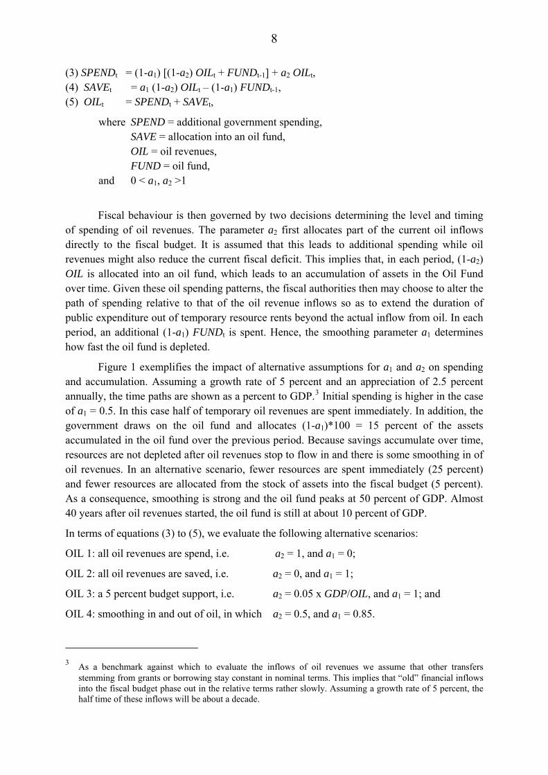
(3) SPENDt = (1-a1) [(1-a2) OILt + FUNDt-1] + a2 OILt, (4) SAVEt = a1 (1-a2) OILt – (1-a1) FUNDt-1, (5) OILt = SPENDt + SAVEt,

where SPEND = additional government spending, SAVE = allocation into an oil fund, OIL = oil revenues, FUND = oil fund, and 0 < a1, a2 >1

Fiscal behaviour is then governed by two decisions determining the level and timing of spending of oil revenues. The parameter a2 first allocates part of the current oil inflows directly to the fiscal budget. It is assumed that this leads to additional spending while oil revenues might also reduce the current fiscal deficit. This implies that, in each period, (1-a2) OIL is allocated into an oil fund, which leads to an accumulation of assets in the Oil Fund over time. Given these oil spending patterns, the fiscal authorities then may choose to alter the path of spending relative to that of the oil revenue inflows so as to extend the duration of public expenditure out of temporary resource rents beyond the actual inflow from oil. In each period, an additional (1-a1) FUNDt is spent. Hence, the smoothing parameter a1 determines how fast the oil fund is depleted.

Figure 1 exemplifies the impact of alternative assumptions for a1 and a2 on spending and accumulation. Assuming a growth rate of 5 percent and an appreciation of 2.5 percent annually, the time paths are shown as a percent to GDP.3 Initial spending is higher in the case of a1 = 0.5. In this case half of temporary oil revenues are spent immediately. In addition, the government draws on the oil fund and allocates (1-a1)*100 = 15 percent of the assets accumulated in the oil fund over the previous period. Because savings accumulate over time, resources are not depleted after oil revenues stop to flow in and there is some smoothing in of oil revenues. In an alternative scenario, fewer resources are spent immediately (25 percent) and fewer resources are allocated from the stock of assets into the fiscal budget (5 percent). As a consequence, smoothing is strong and the oil fund peaks at 50 percent of GDP. Almost 40 years after oil revenues started, the oil fund is still at about 10 percent of GDP.

In terms of equations (3) to (5), we evaluate the following alternative scenarios:

OIL 1: all oil revenues are spend, i.e. a2 = 1, and a1 = 0;

OIL 2: all oil revenues are saved, i.e. a2 = 0, and a1 = 1;

OIL 3: a 5 percent budget support, i.e. a2 = 0.05 x GDP/OIL, and a1 = 1; and

OIL 4: smoothing in and out of oil, in which a2 = 0.5, and a1 = 0.85.

3 As a benchmark against which to evaluate the inflows of oil revenues we assume that other transfers

stemming from grants or borrowing stay constant in nominal terms. This implies that “old” financial inflows into the fiscal budget phase out in the relative terms rather slowly. Assuming a growth rate of 5 percent, the half time of these inflows will be about a decade.

9

Figure 1: Additional Spending and Asset Accumulation (Deviation from Benchmark; percent of GDP)

A. Additional Spending

0123456789

1 3 5 7 9 11 13 15 17 19 21 23 25 27 29 31 33 35 37 39 41

Spend 0.5 / 0.85 Spend 0.25 / 0.95 B. Asset Accumulation

0

10

20

30

40

50

60

1 2 3 4 5 6 7 8 9 10 11 12 13 14 15 16 17 18 19 20 21 22 23 24 25 26 27 28 29 30 31 32 33 34 35 36 37 38 39 40 41

Oil Fund 0.5 / 0.85 Oil Fund 0.25 / 0.95

These four scenarios are designed to measure the direct and indirect effects of oil revenues that stem from additional public spending or savings, while the spillover effects of public investments on productivity growth in the economy are ignored. Thus, we develop two additional sets of scenarios to evaluate the joint effect of an increase in oil revenues that leads to productivity growth. In scenarios 1a-4a the productivity spillover effects are assumed to occur in the export-oriented sectors, while in scenarios 1b-4b such spillover effects are assumed to occur in the domestic sectors. Given that there is very little empirical consensus on the size of the productivity effects of infrastructure investments in developing economies, we assume a value of 0.5 for the spillover parameter in equation (2), i.e. ρsg = 0.50 in both cases. This value is comparably higher than the values estimated in Hulten (1996) who studies the relationship of infrastructure capital and economic growth. This higher value reflects in part the expectation of a higher marginal product of public capital for countries with a severely depleted capital stock and in part the likelihood that the contemporary marginal productivity of public infrastructure expenditure in Ghana may be higher than the historical point estimates suggest.

10

For each scenario, the average annual changes for selected variables over three periods (2007-09, 2007-13, and 2007-2027) are reported. To simplify the presentation, we only report a small number of key aggregate variables in tables: the real exchange rate, total and sectoral exports, real GDP, total and government fixed investment, and real consumption of rural and urban households. At given constant income-tax rates and given savings rates the changes in real consumption reflect changes in real disposable income.

OIL1 - A “spend all” strategy fosters growth, yet leads to Dutch disease effects and hurts rural households

In scenario 1, the primary impact of oil revenues is an increase in public investment that leads to a higher level of real GDP both in the short and medium runs compared to the baseline. The real exchange rate appreciates only modestly in the short run, which is mainly due to the assumed high adjustment flexibility in foreign trade and domestic factor markets. However, increases in investment demand induce significant changes in the terms-of-trade and a sizable contraction in exports in favour of higher production of domestic goods.

These Dutch-Disease effects weaken over time, yet the effect of relative price changes on the cost of capital goods persists. This implies that although these changes moderate over time, the initial decline in export performance does not reverse drastically and hence initial welfare gains increase only slightly in the long run.

Finally, while total income increases in real terms from the base run, the gains are not distributed equally across household groups. While income levels of urban households increase, rural household incomes fall in the short run and do not change in the long run. The main reason for these increasing disparities between rural and urban households is demand-side effects. Additional government investment is primarily spent on capital goods and construction, raising the prices for these mainly urban sectors. Moreover, the backward linkages from these urban industrial sectors to the agricultural sectors, from which many rural households earn their income from, seem to be weak. In addition, the agricultural export sector is hurt by the exchange rate appreciation, which exacerbates the negative effects for rural households. As later results show, these demand effects may be largely offset when the oil revenues are used productively but may re-emerge and increase when relative price effects turn against agriculture.

OIL2 - A “save all and invest interest only” strategy has very limited growth effects

In scenarios 2-4, all or part of the oil revenues are saved into the oil fund (as foreign assets) and only interests earned from the fund is used to finance investment. In scenario 2, a moderate but permanent income stream stemming from interest earnings finances additional investment of only 1.7 and 1.4 percentage points in the short and long run respectively. Thus, there is now fairly less cumulative growth in GDP both in the short and long term and a marked reduction in total investment compared to scenario 1. As a consequence, relative price changes are less pronounced in the short run but increase over time with increasing income

11

from interest. Total exports decline in the short-run but increase in the long-run, compared with the baseline. However, the changes are significantly smaller than in scenario 1.

Table 3: Impacts of oil revenue inflows on selected economic variables in the model simulations, without consideration of productivity spillovers from public investment (percentage point changes compared to BASE run growth rates)

Experiment Period BASE OIL1 OIL2 OIL3 OIL4

Spending Saving Budget Support Smoothing

Exchange rate to T=2009 0 to T=2013 -0.1 -0.2 0 -0.1 -0.2 to T=2027 -0.2 -0.2 -0.1 -0.1 -0.2 Exports to T=2009 5.7 to T=2013 5.9 -4.6 -0.7 -1.9 -3.5 to T=2027 7.1 1.1 0.3 0.7 1

Agriculture to T=2009 7.5 to T=2013 6.6 -5.3 -0.7 -2.5 -3.9 to T=2027 3.3 -3.3 -1.7 -2.7 -3.1 Mining to T=2009 4.3 to T=2013 5.9 -4.3 -0.9 -1.7 -3.5 to T=2027 9.9 2.1 0.9 1.5 1.9 Services to T=2009 4.2

to T=2013 3.9 -3 -0.5 -1.4 -2.2 to T=2027 2.9 -1.3 -0.7 -1.1 -1.2 Real GDP to T=2009 4.6 to T=2013 4.8 0.6 0.1 0.3 0.4 to T=2027 5.4 0.7 0.4 0.6 0.7 Investment to T=2009 6.1 to T=2013 6.2 9 1.7 4.4 7.1 to T=2027 6.8 2.1 1.4 2 2.1

Government investment to T=2009 6.3 to T=2013 6.4 16.8 17 16.9 16.9 to T=2027 7.1 3.4 3.6 3.6 3.5 Real income

Rural to T=2009 3.9 to T=2013 3.9 -0.4 0 -0.2 -0.3 to T=2027 4.1 0 0 0 0 Urban to T=2009 5.2

to T=2013 5.4 0.8 0.1 0.4 0.6 to T=2027 6 0.5 0.3 0.4 0.5 Real wage to T=2009 1.9

to T=2013 2.2 1.2 0.1 0.5 0.9 to T=2027 2.8 0.8 0.4 0.6 0.7

12

While the short and long run effects on household incomes are significantly smaller than in scenario 1, savings to create the oil fund at least avoid the short run reduction of rural households’ income. In the long run, rural households’ income is not affected by the decision to either spend or save oil revenues.

OIL3 - Supporting the budget with oil revenues stabilizes the debt ratio, yet only modestly accelerates growth due to Dutch disease effects

While scenarios 1 and 2 represent two extreme cases of oil revenue allocation, scenarios 3 and 4 consider a strategy where the government decides to save only part of oil revenues in the oil fund. In the case of scenario 3, it is assumed that starting with the influx of oil revenues in year 2010, an oil revenue equivalent to 5 percent of GDP is retained to support the public budget. Compared to scenario 2, this allocation rule results in both increasing savings in the oil fund and increasing investment until 2013. As expected an increase in investment demand results in a worsening of the terms of trade in the short term with the above mentioned consequences. After 2013, with stagnant oil revenues but increasing GDP, savings into the oil fund decrease steadily. However, increasing interest revenues from the oil fund still allows for an increase of investment and GDP growth over the whole simulation period, which compares to scenario 1 but with less short-run adjustment cost for rural households.

OIL4 - In the long run, smoothing in and out of oil balances growth, distribution, and stability targets

The allocation rule in scenario 4 implies that savings in the oil fund increases with rising oil revenues while it decreases with rising savings stocks. Thus, given the parameterization indicated above, savings in the oil fund increase between 2010-2013 while they decrease thereafter until 2027. The long run macroeconomic, sectoral, and distributional outcomes are comparable with scenario 1, in which all oil revenues are immediately invested as they emerge. However, compared to spending oil revenues immediately (scenario 2), saving part of revenues into the oil fund has the advantage of interest income after the oil boom. In addition, the short run adjustment costs with respect to exports and rural incomes are significantly lower than in the spending scenario.

Robustness Check - Productivity improvements due to investments accelerate growth and can offset Dutch disease effects

In scenarios 1a-4a and 1b-4b, public investment raises the productivity in the economy. The absence of productivity increases in domestic production (in 1a-4a) leads to a stronger appreciation of the real exchange rate compared to previous scenarios 1 – 4 (see Appendix Table 2). Hence, although the export performance of traditional cash crops and services is significantly stronger because of the productivity bias, mining exports are hit relatively hard, with no productivity effect. When the productivity gain is biased towards production of domestic goods (in 1b-4b), outcomes are markedly different (see Appendix Table 3). The bias

13

in production (which increases the supply of non-tradables and import substitutes) partly offsets the demand effects of the increased foreign exchange inflows so that the initial real exchange rate appreciation is reversed even in the short run. Yet, the effects on exports are symmetrical with those in scenarios 1 to 4; cash crop exports are hit even harder while services exports are less affected and mining exports recover less than in earlier experiments. Overall export performance is weaker with a domestic bias than with an export bias. The domestic-biased supply response also leads to a larger improvement in the long-run fiscal balance, reflecting favourable relative price movements as well as the effects of higher growth and investment than in either the case without productivity effects or export-biased forms of productivity growth.

The most striking difference between scenarios 1a-4a and 1b-4b is the effect on household disposable real income. Compared to the case of no productivity effects, productivity effects induced by public investment lead to higher real income growth for both household groups. However, the income gain is spread somewhat differently across household groups, with rural households benefitting less than urban households when productivity effects are biased towards domestic production. This contrasts sharply with the export-biased supply response, which generates a lower aggregate real income gain in the long run but one that is disproportionately skewed in favour of rural households.

Comparing Strategies - The oil fund will provide revenues long after oil resources will be depleted

Figure 2 summarizes the difference in oil-related revenues between a situation with and without an oil fund. We compare the simulation results with the base run and show the deviations in terms of real GDP adjusted for interest income from the oil fund on the basis of an interest rate constant at 5 percent. This comparison shows that the loss in terms of income between scenario 1 and scenarios 2 or 3 is modest. For scenario 2, GDP plus interest is about 1.5 (1.2) percent lower in 2013 (2027), indicating that the gap closes over time. For scenario 3, in which oil revenue worth about 5 percent of GDP is allocated to each year’s fiscal budget, the gap is even smaller and accounts for only 0.2 percent in 2027. For scenario 4, in which oil revenues are smoothed over time according to two parameters for current spending and for drawing out of the oil fund, the GDP figures adjusted for additional interest income are even larger than in scenario 1. Given that the oil fund allows the country to continue to enjoy the income generated from oil even after the end of the oil era, this scenario suggests that it is an option that might be the best for growth and stability in the long run.

14

Figure 2: GDP plus Interest on Oil Fund, Deviation from Base (percent of GDP)

0

2

4

6

8

10

12

14

Oil1 Oil2 Oil3 Oil4

2027 2013 Source: Calculated from Appendix Table 4

5. Spending vs. saving oil revenues – concluding remarks

This paper has examined the potential trade-offs between spending and saving oil revenues for growth and stability in Ghana. We found that in the scenario in which all oil revenues are spent as they occur, the GDP effect is largest in the short-run. However, this short term advantage declines over time. Over the long-run the differences between spending and saving are relatively small as interest earned from the oil fund can be used to finance investments in the long run. In other words, a big push strategy might be less promising as would be expected at the first glance. In addition, model results suggest that typical Dutch disease effect of the oil boom negatively affect export agriculture and rural households. In all scenarios, agriculture and rural areas either get hurt or tend to have smaller positive effects relative to the non-agricultural sectors and urban areas. Smoothing in oil revenue allocations into the fiscal budget by saving part of the inflow in an oil fund is not only preferable for growth and stability, but also for equality, since the negative short-run effects on agriculture are significantly moderated. In addition, using oil revenues to increase agricultural productivity and raise competitiveness has the potential to offset the negative impacts from the Dutch disease.

The model captures the positive effect of an oil fund for macro stability in the long run, yet this effect might be underestimated. Establishing an oil fund implies the accumulation of assets, which can be used in the post oil era after 2027. For example, in the extreme case of scenario 2 in which all oil revenues are saved, the size of the oil fund will be equivalent to the level of GDP by 2027 (assuming average oil prices of $US 80/barrel). Income from interests

15

earned from this fund will be about 4.85 percent of GDP (assuming a 5 percent interest rate). Even with the more moderate accumulation in scenarios 3 and 4 incomes generated from the oil fund would still be considerable, amounting to about 2.3 and 0.7 percent of GDP, respectively. Hence, with an oil fund, oil revenues will make substantial contribution to government revenues in the long run (see Appendix Table 4).

The creation of an oil fund can also help to smooth global commodity price shocks. It is therefore especially important for countries like Ghana with high vulnerability to world market price volatility for both imports and exports to consider the creation of foreign exchange reserves in an oil fund. The current global financial and economic crisis and the associated extreme volatility in the world oil prices underlines how establishing an oil fund could help the country to copy with future oil shocks. While we did not consider this additional positive effect in this paper, the model used can easily be adapted for such type of analysis in the future.

Oil revenues and the establishment of an oil fund will require improved government capacity in managing the macroeconomic policies. Moreover, oil revenues are likely to challenge the country’s government in addressing inefficiencies and corruption often associated with resource rents. Even if an oil fund is created, clear rules are needed on how to handle future revenues from interest and the allocation of spending. Scenario 4 provides an example how such a rule that considers a good balance between spending and reserving is good for stability, growth and equality. Our results also emphasize the importance of spending a considerable amount of oil revenue soon for productivity enhancing investment, especially in rural areas and in the agricultural sector. At the same time, saving a certain amount of oil revenues is critical for smoothing the macroeconomic impact and creating a buffer for future world commodity price shocks.

More concrete allocation plans can be assessed once they are disclosed by the government. In March president Atta Mills had announced a full public disclosure of all oil contracts in an attempt to increase transparency in the sector.

16

References Adam, C., S. O’Connell, E. Buffie, and C. Pattillo (2008). Monetary Policy Rules for

Managing Aid Surges in Africa. UNU-WIDER Research Paper 2008.77. Helsinki.

Agyeman Duah, I., W. Soyinka, and C. Kelly (2008). An Economic History of Ghana: Reflections on a Half-Century of Challenges and Progress. Ayebia Clarke Publishing Ltd.

Aryeetey, E., and R. Kanbur (2008). Ghana’s Economy at Half Century: An Overview of Stability, Growth & Poverty. In: Aryeetey, E. and R. Kanbur (eds.). The Economy of Ghana: Analytical Perspectives on Stability, Growth & Poverty, James Currey, Woodbridge, Suffolk.

Auty, R.M. (1990). Resource-based Industrialization: Sowing the Oil in 8 Developing Countries. Clarendon Press, Oxford.

Bank of Ghana (2007). A Framework for the Management of Oil Resources in Ghana – Issues and Proposals. Bank of Ghana Policy Briefing Paper, Bank of Ghana, Accra, December 12, 2007.

Bank of Ghana (2008). Fiscal Rules and Fiscal Discipline – What can Ghana Learn from Country Experiences. Bank of Ghana Policy Briefing Paper, Bank of Ghana, Accra, January 2008.

Breisinger C., X. Diao, J. Thurlow, and R. Al Hassan (2008). Agriculture for Development in Ghana. New Opportunities and Challenges. IFPRI Discussion Paper 784, International Food Policy Research Institute, Washington D.C.

Breisinger, C., X. Diao, and J. Thurlow (2009). Modeling Growth Options and Structural Change to Reach Middle Income Country Status: The Case of Ghana. Economic Modeling 26: 514–525:

Breisinger, C., and X. Diao (2009). Economic Transformation in Theory and Practice: What are the Messages for Africa? Current Politics and Economics of Africa, Vol. 1, Issue 3/4. Nova Science Publishers.

Dervis, K., J. de Melo, S. Robinson (1982). General Equilibrium Models for Development Policy. Cambridge University Press, New York.

Eifert, B., A. Gelb and N. Tallroth (2002). The Political Economy of Fiscal Policies and Economic Management in Oil Exporting Countries. World Bank Policy Research Paper 2899. Washington D.C.

EIU (2009). Country Report Ghana, Economist Intelligence Unit, London.

17

Gelb A., and G. Turner (2007). Confronting the Resource Curse. Lessons of Experience for African Oil Producers. World Bank, Washington D.C.

Gelb, A., and S. Grassman (2008). Confronting the Oil Curse. Draft Paper for AFD/EUDN Conference, November 12, 2008

Hulten, C. (1996). Infrastructure Capital and Economic Growth: How Well You Use It May Be More Important than How Much You Have. NBER Working Paper 5847. National Bureau of Economic Research, Cambridge, Mass.

IMF (2008). Ghana – Country Report No. 08/344. Washington, D.C.

Kaufmann D., A. Kraay, and M. Mastruzzi (2008). Governance Matters VII. Governance Indicators for 1996-2007. World Bank Policy Research Working Paper 4280. The World Bank. Washington D.C.

Larsen, E.R. (2006). Escaping the Resource Curse and the Dutch Disease? When and Why Norway Caught Up with and Forged ahead of its Neighbours. The American Journal of Economics and Sociology 65 (3): 605 – 640.

Lofgren, H., R.L. Harris, and S. Robinson (2002). A Standard Computable General Equilibrium (CGE) Model in GAMS. Microcomputers in Policy Research 5, International Food Policy Research Institute, Washington, D.C.

NDPC (2005). Growth and Poverty Reduction Strategy (GPRS II) 2006-2009. National Development Planning Commission, Accra. Ghana.

Osei, R.D., and G. Domfe (2008). Oil Production in Ghana: Implications for Economic Development. Institute of Statistical Social and Economic Research, University of Ghana, ARI 104/2008. Accra.

Thurlow, J. (2004). A Dynamic Computable General Equilibrium (CGE) Model for South Africa: Extending the Static IFPRI Model. TIPS. Working Paper 1-2004. Pretoria.

World Bank (2008). Ghana – Country Brief. 30th October 2008. Washington, D.C.

18

Appendix Table 1: Economic structure in the base year, Ghana, 2007

Sector VAshr PRDshr EMPshr EXPshr EXP-

OUTshr IMPshr IMP-

DEMshr

Domestic agriculture 23.5 19.5 15.8 6.6 11.3 Export agriculture 9.9 8.2 8.1 42.2 79.6 Mining 8.7 7.3 4.3 44.3 96.2 Manufacturing 10.0 14.7 13.0 76.9 63.1 Industry 4.1 9.1 3.2 16.4 34.8 Construction 10.6 7.8 11.2 Private Services 20.2 25.8 26.4 13.5 8.3 Public Services 13.0 7.5 18.1 TOTAL-2 100.0 100.0 100.0 100.0 15.7 100.0 27.8 Total agriculture 33.3 27.8 23.8 42.2 23.6 6.6 10.5 Total non-agriculture 66.7 72.2 76.2 57.8 12.7 93.4 32.3 TOTAL 100.0 100.0 100.0 100.0 15.7 100.0 27.8

VAshr: Sector share of total value added PRDshr: Sector share of total production EMPshr: Sector share of total labor income EXPshr: Sector share of total export revenues EXP-OUT-shr: Share of exports in output IMPshr: Sector share of total imports IMP-DEM-shr: Share of imports in sectoral absorption

19

Appendix Table 2: Impacts of oil revenue inflows on selected economic variables in the

model simulations, with consideration of productivity spillovers from public investment in export sectors (percentage point changes compared to BASE run growth rates)

Experiment Period BASE OIL1 OIL2 OIL3 OIL4

Spending Saving Budget Support Smoothing

Exchange rate to T=2009 0 0.1 to T=2013 -0.1 -0.5 0 -0.2 -0.3 to T=2027 -0.2 -0.1 -0.1 -0.1 -0.1 Exports to T=2009 5.7 -0.2 to T=2013 5.9 -1.5 -0.7 -0.7 -1.3 to T=2027 7.1 0.9 -0.2 0.4 0.7

Agriculture to T=2009 7.5 -1.6 to T=2013 6.6 -1.8 -0.9 -1.2 -1.6 to T=2027 3.3 2.9 2.5 2.7 2.8 Mining to T=2009 4.3 0.9 to T=2013 5.9 -1.2 -0.5 -0.5 -1.1 to T=2027 9.9 -0.1 -1.4 -0.7 -0.2 Services to T=2009 4.2 0.7

to T=2013 3.9 -1.9 -0.6 -0.2 -1.3 to T=2027 2.9 2.6 0.3 2.4 2.5 Real GDP to T=2009 4.6 0 to T=2013 4.8 1.2 0.1 0.6 0.9 to T=2027 5.4 0.9 0.3 0.7 0.8 Investment to T=2009 6.1 0 to T=2013 6.2 9.1 1.7 4.8 7.2 to T=2027 6.8 2.3 1.4 2.1 2.3

Government investment to T=2009 6.3 0.1 to T=2013 6.4 16.9 17 16.9 16.9 to T=2027 7.1 3.5 3.7 3.7 3.6 Real income

Rural to T=2009 3.9 0 to T=2013 3.9 0.4 0 0.2 0.3 to T=2027 4.1 0.5 0.1 0.4 0.5 Urban to T=2009 5.2 0

to T=2013 5.4 1.3 0.1 0.6 0.9 to T=2027 6 0.4 0 0.3 0.4 Real wage to T=2009 1.9 0

to T=2013 2.2 1.8 0.1 0.8 1.3 to T=2027 2.4 1.4 0.8 1.2 1.4

20

Appendix Table 3: Impacts of oil revenue inflows on selected economic variables in the

model simulations, with consideration of productivity spillovers from public investment in domestic sectors (percentage point changes compared to BASE run growth rates)

Experiment Period BASE OIL1 OIL2 OIL3 OIL4

Spending Saving Budget Support Smoothing

Exchange rate to T=2009 0 0 to T=2013 -0.1 0 0.1 0.1 0.1 to T=2027 -0.2 0 0 0 0 Exports to T=2009 5.7 -0.1 to T=2013 5.9 -5.1 -0.8 -2.2 -3.9 to T=2027 7.1 0.8 0.1 0.4 0.7

Agriculture to T=2009 7.5 0.1 to T=2013 6.6 -5.8 -0.8 -2.7 -4.2 to T=2027 3.3 -3.5 -1.9 -2.9 -3.4 Mining to T=2009 4.3 -0.1 to T=2013 5.9 -5.2 -1.1 -2.1 -4.2 to T=2027 9.9 1.7 0.6 1.1 1.6 Services to T=2009 4.2 0.1

to T=2013 3.9 -2.7 -0.3 -1.2 -2 to T=2027 2.9 -1.2 -0.6 -0.9 -1.1 Real GDP to T=2009 4.6 0.1 to T=2013 4.8 0.9 0.1 0.5 0.7 to T=2027 5.4 1 0.6 0.8 1 Investment to T=2009 6.1 0 to T=2013 6.2 9 1.7 4.7 7.1 to T=2027 6.8 1.1 1.5 2.1 2.2

Government investment to T=2009 6.3 0.1 to T=2013 6.4 17.1 17.1 17.1 17.2 to T=2027 7.1 3.7 4 3.9 3.8 Real income

Rural to T=2009 3.9 0 to T=2013 3.9 -0.1 0 0 -0.1 to T=2027 4.1 0.3 0.2 0.2 0.3 Urban to T=2009 5.2 0.1

to T=2013 5.4 1.1 0.2 0.6 0.8 to T=2027 6 0.9 0.5 0.7 0.8 Real wage to T=2009 1.9 0.3

to T=2013 2.2 1.7 0.2 0.8 1.2 to T=2027 2.8 1.2 0.7 1 1.2

21

Appendix Table 4: Growth s. accumulation - Deviation of GDP and oil fund from BASE

run (100 mil. Cedis in constant 2007 prices) 2010 2011 2012 2013 2014 2021 2027

GDP Oil1 1.69 3.30 5.73 7.94 10.31 32.73 63.25Oil2 0.15 0.34 0.65 1.10 1.69 11.01 30.16Oil3 1.16 1.93 2.87 3.99 5.30 21.28 49.18Oil4 1.06 2.18 3.93 5.70 7.71 29.02 59.93

Oil Fund Oil1 0.00 0.00 0.00 0.00 0.00 0.00 0.00Oil2 6.95 23.53 47.04 74.86 102.75 297.95 465.27Oil3 2.49 9.96 23.94 41.79 59.23 165.74 228.30Oil4 2.95 9.56 18.12 27.22 34.99 64.90 73.69

GDP+Interest Oil1 1.69 3.30 5.73 7.94 10.31 32.73 63.25Oil2 0.50 1.52 3.00 4.84 6.83 25.91 53.42Oil3 1.28 2.43 4.07 6.08 8.26 29.57 60.60Oil4 1.21 2.66 4.84 7.06 9.46 32.27 63.61