management - DSpace at Global College International
1001
-
Upload
khangminh22 -
Category
Documents
-
view
0 -
download
0
Transcript of management - DSpace at Global College International

MANAGEMENTS t a t i s t i c s
f o r
Richard I. Levin Masood H. SiddiquiThe University of Jaipuria Institute of North Carolina at Chapel Hill Management, Lucknow
David S. Rubin Sanjay RastogiThe University of Indian Institute ofNorth Carolina at Chapel Hill Foreign Trade, New Delhi
EIGHTH EDITION

ISBN 978-93-325-8118-0
Copyright © 2017 Pearson India Education Services Pvt. Ltd
Published by Pearson India Education Services Pvt. Ltd, CIN: U72200TN2005PTC057128, formerly known as TutorVista Global Pvt. Ltd, licensee of Pearson Education in South Asia.
No part of this eBook may be used or reproduced in any manner whatsoever without thepublisher’s prior written consent.
This eBook may or may not include all assets that were part of the print version. The publisherreserves the right to remove any material in this eBook at any time.
eISBN
Head Office: A-8 (A), 7th Floor, Knowledge Boulevard, Sector 62, Noida 201 309,Uttar Pradesh, India.
Registered Office: 4th Floor, Software Block, Elnet Software City, TS 140, Block 2 & 9,Rajiv Gandhi Salai, Taramani, Chennai 600 113, Tamil Nadu, India.Fax: 080-30461003, Phone: 080-30461060www.pearson.co.in, Email: [email protected]
Contents
Preface xi
CHAPTER 1 Introduction 1
1.1 Why Should I Take This Course and Who Uses Statistics Anyhow? 2
1.2 History 3
1.3 Subdivisions Within Statistics 4
1.4 A Simple and Easy-to-Understand Approach 4
1.5 Features That Make Learning Easier 5
1.6 Surya Bank—Case Study 6
CHAPTER 2 Grouping and Displaying Data to Convey Meaning: Tables and Graphs 13
2.1 How Can We Arrange Data? 14
2.2 Examples of Raw Data 17
2.3 Arranging Data Using the Data Array and the Frequency Distribution 18
2.4 Constructing a Frequency Distribution 27
2.5 Graphing Frequency Distributions 38 Statistics at Work 58 Chapter Review 59 Flow Chart: Arranging Data to Convey Meaning 72
CHAPTER 3 Measures of Central Tendency and Dispersion in Frequency Distributions 73
3.1 Summary Statistics 74
3.2 A Measure of Central Tendency: The Arithmetic Mean 77

iv Contents
3.3 A Second Measure of Central Tendency: The Weighted Mean 87
3.4 A Third Measure of Central Tendency: The Geometric Mean 92
3.5 A Fourth Measure of Central Tendency: The Median 96
3.6 A Final Measure of Central Tendency: The Mode 104
3.7 Dispersion: Why It is Important? 111
3.8 Ranges: Useful Measures of Dispersion 113
3.9 Dispersion: Average Deviation Measures 119
SPSS 136 Statistics at Work 140 Chapter Review 141 Flow Charts: Measures of Central Tendency and Dispersion 151
CHAPTER 4 Probability I: Introductory Ideas 153
4.1 Probability: The Study of Odds and Ends 154
4.2 Basic Terminology in Probability 155
4.3 Three Types of Probability 157
4.4 Probability Rules 164
4.5 Probabilities Under Conditions of Statistical Independence 170
4.6 Probabilities Under Conditions of Statistical Dependence 179
4.7 Revising Prior Estimates of Probabilities: Bayes’ Theorem 188 Statistics at Work 196 Chapter Review 197 Flow Chart: Probability I: Introductory Ideas 206
CHAPTER 5 Probability Distributions 207
5.1 What is a Probability Distribution? 208
5.2 Random Variables 212
5.3 Use of Expected Value in Decision Making 218
5.4 The Binomial Distribution 222
5.5 The Poisson Distribution 230
Contents v
5.6 The Normal Distribution: A Distribution of a Continuous Random Variable 238
5.7 Choosing the Correct Probability Distribution 254 Statistics at Work 255 Chapter Review 256 Flow Chart: Probability Distribution 264
CHAPTER 6 Sampling and Sampling Distributions 267
6.1 Introduction to Sampling 268
6.2 Random Sampling 271
6.3 Non-random Sampling 279
6.4 Design of Experiments 282
6.5 Introduction to Sampling Distributions 286
6.6 Sampling Distributions in More Detail 289
6.7 An Operational Consideration in Sampling: The Relationship Between Sample Size and Standard Error 302
Statistics at Work 308 Chapter Review 309 Flow Chart: Sampling and Sampling Distributions 314
CHAPTER 7 Estimation 315
7.1 Introduction 316
7.2 Point Estimates 319
7.3 Interval Estimates: Basic Concepts 324
7.5 Calculating Interval Estimates of the Mean from Large Samples 332
7.6 Calculating Interval Estimates of the Proportion from Large Samples 336
7.7 Interval Estimates Using the t Distribution 341
7.8 Determining the Sample Size in Estimation 351 Statistics at Work 357 Chapter Review 358 Flow Chart: Estimation 363
vi Contents
CHAPTER 8 Testing Hypotheses: One-sample Tests 365
8.1 Introduction 366
8.2 Concepts Basic to the Hypothesis-testing Procedure 367
8.3 Testing Hypotheses 371
8.4 Hypothesis Testing of Means When the Population
8.5 Measuring the Power of a Hypothesis Test 388
8.6 Hypothesis Testing of Proportions: Large Samples 391
8.7 Hypothesis Testing of Means When the Population
Statistics at Work 404 Chapter Review 404 Flow Chart: One-Sample Tests of Hypotheses 410
CHAPTER 9 Testing Hypotheses: Two-sample Tests 411
9.1 Hypothesis Testing for Differences Between Means and Proportions 412
9.2 Tests for Differences Between Means: Large Sample Sizes 414
9.3 Tests for Differences Between Means: Small Sample Sizes 420
9.4 Testing Differences Between Means with Dependent Samples 431
9.5 Tests for Differences Between Proportions: Large Sample Sizes 441
9.6 Prob Values: Another Way to Look at Testing Hypotheses 450 Statistics at Work 455 Chapter Review 456 Flow Chart: Two-Sample Tests of Hypotheses 463
CHAPTER 10 Quality and Quality Control 465
10.1 Introduction 466
10.2 Statistical Process Control 468
10.3 x Charts: Control Charts for Process Means 470
10.4 R Charts: Control Charts for Process Variability 481
10.5 p Charts: Control Charts for Attributes 487
Contents vii
10.6 Total Quality Management 494
10.7 Acceptance Sampling 500 Statistics at Work 508 Chapter Review 509 Flow Chart: Quality and Quality Control 515
CHAPTER 11 Chi-Square and Analysis of Variance 517
11.1 Introduction 518
11.2 Chi-Square as a Test of Independence 519
11.3 Chi-Square as a Test of Goodness of Fit: Testing the Appropriateness of a Distribution 534
11.4 Analysis of Variance 542
11.5 Inferences About a Population Variance 568
11.6 Inferences About Two Population Variances 576 Statistics at Work 583 Chapter Review 584 Flow Chart: Chi-Square and Analysis of Variance 594
CHAPTER 12 Simple Regression and Correlation 595
12.1 Introduction 596
12.2 Estimation Using the Regression Line 603
12.3 Correlation Analysis 629
12.4 Making Inferences About Population Parameters 643
12.5 Using Regression and Correlation Analyses: Limitations, Errors, and Caveats 650
Statistics at Work 653 Chapter Review 653 Flow Chart: Regression and Correlation 662
CHAPTER 13 Multiple Regression and Modeling 663
13.1 Multiple Regression and Correlation Analysis 664
13.2 Finding the Multiple-Regression Equation 665
13.3 The Computer and Multiple Regression 674
viii Contents
13.4 Making Inferences About Population Parameters 684
13.5 Modeling Techniques 703 Statistics at Work 719 Chapter Review 720 Flow Chart: Multiple Regression and Modeling 731
CHAPTER 14 Nonparametric Methods 733
14.1 Introduction to Nonparametric Statistics 734
14.2 The Sign Test for Paired Data 736
14.3 Rank Sum Tests: The Mann–Whitney U Test
14.4 The One-sample Runs Test 758
14.5 Rank Correlation 767
Statistics at Work 786 Chapter Review 787 Flow Chart: Nonparametric Methods 800
CHAPTER 15 Time Series and Forecasting 803
15.1 Introduction 804
15.2 Variations in Time Series 804
15.3 Trend Analysis 806
15.4 Cyclical Variation 818
15.5 Seasonal Variation 824
15.6 Irregular Variation 833
15.7 A Problem Involving All Four Components of a Time Series 834
15.8 Time-Series Analysis in Forecasting 844 Statistics at Work 844 Chapter Review 846 Flow Chart: Time Series 853
Contents ix
CHAPTER 16 Index Numbers 855
16.2 Unweighted Aggregates Index 860
16.3 Weighted Aggregates Index 865
16.4 Average of Relatives Methods 874
16.5 Quantity and Value Indices 881
16.6 Issues in Constructing and Using Index Numbers 886 Statistics at Work 887 Chapter Review 888 Flow Chart: Index Numbers 896
CHAPTER 17 Decision Theory 897
17.1 The Decision Environment 898
17.3 Using Continuous Distributions: Marginal Analysis 908
17.4 Utility as a Decision Criterion 917
17.5 Helping Decision Makers Supply the Right Probabilities 921
17.6 Decision-Tree Analysis 925 Statistics at Work 938 Chapter Review 939
Appendix Tables 949
Bibliography 973
Index 977

This page is intentionally left blank

Preface
An Opportunity for New IdeasWriting a new edition of our textbook is an exciting time. In the two years that it takes to complete it, we
professors who review the manuscript, our students here at the University of North Carolina at Chapel Hill always have a lot of good ideas for change, and our team at Prentice Hall organizes the whole pro-cess and provides a very high level of professional input. Even though this is the eighth edition of our book, our original goal of writing the most teacher- and student-friendly textbook in business statistics still drives our thoughts and our writing in this revision.
What Has Made This Book Different through Various Editions?Our philosophy about what a good business statistics textbook ought to be hasn’t changed since the day
always strived to produce a textbook that met these four goals:
We think a beginning business statistics textbook ought to be intuitive and easy to learn from. In explaining statistical concepts, we begin with what students already know from their life experi-ence and we enlarge on this knowledge by using intuitive ideas. Common sense, real-world ideas, references, patient explanations, multiple examples, and intuitive approaches all make it easier for students to learn.
We believe a beginning business statistics textbook ought to cover all of the topics any teacher might wish to build into a two-semester or a two-quarter course. Not every teacher will cover every topic in our book, but we offer the most complete set of topics for the consideration of anyone who teaches this course.
We do not believe that using complex mathematical notation enhances the teaching of business statistics and our own experience suggests that it may even make learning more dif cult. Complex mathematical notation belongs in advanced courses in mathematics and statistics (and we do use it there), but not here. This is a book that will make and keep you comfortable even if you didn’t get an A in college algebra.
We believe that a beginning business statistics textbook ought to have a strong real-world focus. Students ought to see in the book what they see in their world every day. The approach we use, the ex-ercises we have chosen for this edition, and the continuing focus on using statistics to solve business problems all make this book very relevant. We use a large number of real-world problems, and our
xii Preface
explanations tend to be anecdotal, using terms and references that students read in the newspapers, see on TV, and view on their computer monitors. As our own use of statistics in our consulting practices has increased, so have the references to how and why it works in our textbook. This book is about actual managerial situations, which many of the students who use this book will face in a few years.
New Features in This Edition to Make Teaching and Learning EasierEach of our editions and the supplements that accompanied them contained a complete set of pedagogi-cal aids to make teaching business statistics more effective and learning it less painful. With each revi-sion, we added new ideas, new tools, and new helpful approaches. This edition begins its own set of new features. Here is a quick preview of the twelve major changes in the eighth edition:
End-of-section exercises have been divided into three subsets: Basic Concepts, Applications, and Self-Check Exercises. The Basic Concepts are those exercises without scenarios, Applications have scenarios, and the Self-Check Exercises have worked-out solutions right in the section.
The set of Self-Check Exercises referenced above is found at the end of each chapter section except the introductory section. Complete Worked-Out Answers to each of these can be found at the end of the applications exercises in that section of the chapter.
Hints and Assumptions are short discussions that come at the end of each section in the book, just before the end-of-section exercises. These review important assumptions and tell why we made them, they give students useful hints for working the exercises that follow, and they warn students
The number of real-world examples at the end-of-chapter Review and Application Exercises have been doubled, and many of the exercises from the previous edition have been updated. The content
Most of the hypothesis tests in Chapters 8 and 9 are done using the standardized scale. The scenarios for a quarter of the exercises in this edition have been rewritten. Over a hundred new exercises appear in this edition. All of the large, multipage data sets have been moved to the data disk, which is available with this book. The material on exploratory data analysis The design of this edition has been completely changed to represent the state of the art in easy-to-
follow pedagogy. Instructions are provided to handle the data using computer software such as MS Excel and SPSS. A Comprehensive Case “Surya Bank Pvt. Ltd.” has been added along with the live data. The ques-
tions related to this case has been put at the end of each chapter in order to bring more clarity in Statistical Applications in real-life scenarios.
Successful Features Retained from Previous EditionsIn the time between editions, we listen and learn from teachers who are using our book. The many adopters of our last edition reinforced our feeling that these time-tested features should also be a part of the new edition:
Chapter learning objectives are prominently displayed in the chapter opening. The more than 1,500 on-page notes highlight important material for students.

Preface xiii
Each chapter begins with a real-world problem, in which a manager must make a decision. Later in the chapter, we discuss and solve this problem as part of the teaching process.
Each chapter has a section entitled review of Terms Introduced in the chapter. An annotated review of all Equations Introduced is a part of every chapter. Each chapter has a comprehensive Chapter Concepts Test using multiple pedagogies. A ow chart (with numbered page citations) in Chapters 2–16 organizes the material and makes it
easier for students to develop a logical, sequential approach to problem solving. Our Statistics at Work sections in each chapter allow students to think conceptually about business
statistics without getting bogged down with data. This learning aid is based on the continuing story of the “Loveland Computer Company” and the experiences of its employees as they bring more and more statistical applications to the management of their business.
Teaching Supplements to the Eighth EditionThe following supplements to the text represent the most comprehensive, classroom-tested set of sup-plementary teaching aids available in business statistics books today. Together they provide a powerful instructor-focused package.
An Instructor’s Solutions Manual containing worked-out solutions to all of the exercises in the book. A comprehensive online Test Bank Questions. A complete set of Instructor Lecture Notes, developed in Microsoft Powerpoint.
It Takes a Lot of People to Make a BookOur part in the process of creating a new edition is to present ideas that we believe work in the class-room. The Prentice Hall team takes these ideas and makes them into a book. Of course, it isn’t that easy.
in St. Paul. Tom is like a movie director; he makes sure everybody plays his or her part and that the entire process moves forward on schedule. Tom guides the project from the day we begin to discuss a
-
day-to-day activities that must all be completed before a book is produced. Together they move the rough manuscript pages through the editing and printing process, see that printed pages from the compositor reach us, keep us on schedule as we correct and return proofs, work with the bindery and the art folks, and do about a thousand other important things we never get to see but appreciate immensely.
A very helpful group of teachers reviewed the manuscript for the eighth edition and took the time to make very useful suggestions. We are happy to report that we incorporated most of them. This process
are grateful. The reviewers for this edition were Richard P. Behr, Broome Community College; Ronald L. Coccari, Cleveland State University; V. Reddy Dondeti, Norfolk State University; Mark Haggerty, Clarion University; Robert W. Hull, Western Illinois University; James R. Schmidt, University of Nebraska-Lincoln; and Edward J. Willies.
We use statistical tables in the book that were originally prepared by other folks, and we are grateful to the literary executor of the late Sir Ronald Fisher, F.R.S., to Dr Frank Yates, F.R.S., and to Longman

Group, Ltd., London, for pemrission to reprint tables from their book Statistical Tables for Biological, Agricultural and Medical Research, sixth edition, 1974.
Dr David O. Robinson of the Hass School of Business, Berkeley University, contributed a number of real-world exercises, produced many of the problem scenario changes, and as usual, persuaded us that it would be considerably less fun to revise a book without him.
these very important, hard-working folks, we are grateful. We are glad it is done and now we look forward to hearing from you with your comments about how
well it works in your classroom. Thank you for all your help.
Richard I. LevinDavid S. Rubin
I want to express my heartfelt and sincere gratitude towards my mother, Late Mrs Ishrat Sultana, my wife, Uzma, my son Ashar, family members, and friends. I also want to express my sincere thanks to my statistics teachers, colleagues, and Jaipuria Institute of Management, Lucknow, for their help and support in completion of this task.
Masood H. Siddiqui
I owe a great deal to my teachers and colleagues from different management institutes for their sup-port, encouragement, and suggestions. Sincere thanks to my student, Ashish Awasthi, for helping me in
preparing the manuscript. Finally, I would like to express my gratitude to my parents, special thanks to my wife, Subha, and my kids, Sujay and Sumedha, for their love, understanding, and constant support.
Sanjay Rastogi
xiv Preface

LEARNING OBJECTIVES
1After reading this chapter, you can understand:
CHAPTER CONTENTS
To examine who really uses statistics and how statistics is used
To provide a very short history of the use of statistics
1.1 Why should I Take This Course and Who Uses Statistics Anyhow? 2
1.2 History 31.3 Subdivisions within Statistics 4
To present a quick review of the special features of this book that were designed to make learning statistics easier for you
1.4 A Simple and Easy-to-Understand Approach 4
1.5 Features That Make Learning Easier 51.6 Surya Bank—Case Study 6
Introduction
2 Statistics for Management
1.1 WHY SHOULD I TAKE THIS COURSE AND WHO USES STATISTICS ANYHOW?
before the election, television, radio, and newspaper broadcasts inform us that “a poll conducted by XYZ Opinion Research shows that the Democratic (or Republican) candidate has the support of 54 percent of voters with a margin of error of plus or minus 3 percent.” What does this statement mean? What is meant by the term margin of error? Who has actually done the polling? How many people did they interview and how many should they have interviewed to make this assertion? Can we rely on the truth of what they reported? Polling is a big business and many companies conduct polls for political candidates, new products, and even TV shows. If you have an ambition to become president, run a company, or even star in a TV show, you need to know something about statistics and statisticians.
It’s the last play of the game and the Giants are behind by 4 points; they have the ball on the Chargers’ 20-yard line. The Chargers’ defensive coordinator calls time and goes over to the sidelines to speak to
or try a running play. His statistical assistant quickly consults his computer and points out that in the last 50 similar situations, the Giants have passed the ball 35 times. He also points out to the Chargers’ coach that two-thirds of these passes have been short passes, right over center. The Chargers’ coach instructs his defensive coordinator to expect the short pass over center. The ball is snapped, the Giants’ quarterback does exactly what was predicted and there is a double-team Charger effort there to break up the pass. Statistics suggested the right defense.
80 percent of clinical trials, with only a 2 percent incidence of undesirable side effects. Prostate cancer is the second largest medical killer of men and there is no present cure. The Director of Research must
in the clinical tests and those in the general population using the drug. There are statistical methods that can provide her a basis for making this important decision.
The Community Bank has learned from hard experience that there are four factors that go a long way in determining whether a borrower will repay his loan on time or will allow it to go into default. These factors are (1) the number of years at the present address, (2) the number of years in the present job, (3) whether the applicant owns his own home, and (4) whether the applicant has a checking or savings account with the Community Bank. Unfortunately, the bank doesn’t know the individual effect of each of these four factors
(both those who were granted a loan and those who were turned down) and knows, too, how each granted loan turned out. Sarah Smith applies for a loan. She has lived at her present address 4 years, owns her own home, has been in her current job only 3 months, and is not a Community Bank depositor. Using statistics, the bank can calculate the chance that Sarah will repay her loan on time if it is granted.
The word statistics means different things to different folks. To a football fan, statistics are rushing,
that the Giants will throw the short pass over center. To the manager of a power station, statistics are the amounts of pollution being released into the atmosphere. To the Food and Drug Administrator in our third example, statistics is the likely percentage of undesirable effects in the general population using the new prostate drug. To the Community Bank in the fourth example, statistics is the chance that Sarah

Introduction 3
will repay her loan on time. To the student taking this course, statistics are the grades on your quizzes
Each of these people is using the word correctly, yet each person uses it in a different way. All of them are using statistics to help them make decisions; you about your grade in this course, and the
-tistics is important and how to use it in your personal and professional life is the purpose of this book.
Benjamin Disraeli once said, “There are three kinds of lies: lies, damned lies, and statistics.” This rather severe castigation of statistics, made so many years ago, has come to be a rather apt description of many of the statistical deceptions we encounter in our everyday lives. Darrell Huff, in an enjoyable little book, How to Lie with Statistics, noted that “the crooks already know these tricks; honest men must learn them in self-defense.” One goal of this book is to review some of the common ways sta-tistics are used incorrectly.
1.2 HISTORYThe word statistik comes from the Italian word statista (meaning
a professor at Marlborough and Göttingen. Dr. E. A. W. Zimmer-man introduced the word statistics into England. Its use was popularized by Sir John Sinclair in his work Statistical Account of Scotland 1791–1799. Long before the eighteenth century, however, people had been recording and using data.
Old Testament contains several accounts of census taking. Govern-ments of ancient Babylonia, Egypt, and Rome gathered detailed records of populations and resources. In the Middle Ages, governments began to register the ownership of land. In A.D.the ninth century, he completed a statistical enumeration of the serfs attached to the land. About 1086, William the Conqueror ordered the writing of the Domesday Book, a record of the ownership, extent,
Because of Henry VII’s fear of the plague, England began to register its dead in 1532. About this same time, French law required the clergy to register baptisms, deaths, and marriages. During an out-break of the plague in the late 1500s, the English government started publishing weekly death statistics. This practice continued, and by 1632, these Bills of Mortality listed births and deaths by sex. In 1662, Captain John Graunt used 30 years of these Bills to make predictions about the number of people who would die from various diseases and the propor-tions of male and female births that could be expected. Summarized in his work Natural and Political Observations . . . Made upon the Bills of Mortality, Graunt’s study was a pioneer effort in statistical analysis. For his achievement in using past records to predict future events, Graunt was made a member of the original Royal Society.
The history of the development of statistical theory and practice is a lengthy one. We have only begun to
How to lie with statistics
Origin of the word
Early government records
An early prediction from
statistics

4 Statistics for Management
1.3 SUBDIVISIONS WITHIN STATISTICSManagers apply some statistical technique to virtually every branch of public and private enterprise. These techniques are so diverse that statisticians commonly separate them into two broad categories: descriptive statistics and inferential statistics. Some examples will help us understand the difference between the two.
Suppose a professor computes an average grade for one history class. Because statistics describe the performance of that one class but do not make a generalization about several classes, we can say that the professor is using descriptive statistics. Graphs, tables, and charts that display data so that they are easier to understand are all examples of descriptive statistics.
Now suppose that the history professor decides to use the av-erage grade achieved by one history class to estimate the average grade achieved in all ten sections of the same history course. The process of estimating this average grade would be a problem in inferential statistics. Statisticians also refer to this category as statistical inference. Obviously, any conclusion the professor makes about the ten sections of the course is based on a generalization that goes far beyond the data for the original his-tory class; the generalization may not be completely valid, so the professor must state how likely it is to be true. Similarly, statistical inference involves generalizations and statements about the probability of their validity.
The methods and techniques of statistical inference can also be used in a branch of statistics called decision theory. Knowledge of decision theory is very helpful for managers because it is used to make decisions under conditions of uncertainty when, for example, a manufacturer of stereo sets cannot specify precisely the demand for its products or when the chairperson of the English department at your school must schedule faculty teaching assignments without knowing precisely the student enrollment for next fall.
1.4 A SIMPLE AND EASY-TO-UNDERSTAND APPROACHThis book is designed to help you get the feel of statistics: what it is, how and when to apply statistical techniques to decision-making situations, and how to interpret the results you get. Because we are not writing for professional statisticians, our writing is tailored to the backgrounds and needs of college students, who probably accept the fact that statistics can be of considerable help to them in their future occupations but are probably apprehensive about studying the subject.
We discard mathematical proofs in favor of intuitive ones. You will be guided through the learning process by reminders of what you already know, by examples with which you can identify, and by a step-by-step process instead of statements such as “it can be shown” or “it therefore follows.”
As you thumb through this book and compare it with other basic business statistics textbooks, you will notice a minimum of math-ematical notation. In the past, the complexity of the notation has intimidated many students, who got lost in the symbols even though they were motivated and intellectually capable of understanding the ideas. Each symbol and formula that is used is explained in detail, not only at the point at which it is introduced, but also in a section at the end of the chapter.
Descriptive statistics
Inferential statistics
Decision theory
For students, not statisticians
Symbols are simple and
explained

Introduction 5
school algebra course, you have enough background to understand everything in this book. Nothing beyond basic algebra is assumed or used. Our goals are for you to be comfortable as you learn and for you to get a good intuitive grasp of statistical concepts and techniques. As a future manager, you will need to know when statistics can help
expert to handle the details.The problems used to introduce material in the chapters, the ex-
ercises at the end of each section in the chapter, and the chapter review exercises are drawn from a wide variety of situations you are already familiar with or are likely to confront quite soon. You will see problems involving all facets
and production. In addition, you will encounter managers in the public sphere coping with problems in public education, social services, the environment, consumer advocacy, and health systems.
In each problem situation, a manager is trying to use statistics creatively and productively. Helping you become comfortable doing exactly that is our goal.
1.5 FEATURES THAT MAKE LEARNING EASIER
particular role in helping you study and understand statistics, and if we spend a few minutes here dis-cussing the most effective way to use some of these aids, you will not only learn more effectively, but will gain a greater understanding of how statistics is used to make managerial decisions.
Margin Notes Each of the more than 1,500 margin notes highlights the material in a paragraph or
meaning of what the text is explaining.
Application Exercises The Chapter Review Exercises include Application Exercises that come directly from real business/economic situations. Many of these are from the business press; others come from government publications. This feature will give you practice in setting up and solving problems that are faced every day by business professionals. In this edition, the number of Application Exercises has been doubled.
Review of Terms Each chapter ends with a glossary of every new term introduced in that chapter.
through a chapter, use the glossary to reinforce your understanding of what the terms mean. Doing
the chapter means.
Equation Review Every equation introduced in a chapter is found in this section. All of them are
book is a very effective way to make sure you understand what each equation means and how it is used.
No math beyond simple
algebra is required
Text problem cover a wide
variety of situations
6 Statistics for Management
Chapter Concepts Test Using these tests is a good way to see how well you understand the chapter material. As a part of your study, be sure to take these tests and then compare your answers with those in the back of the book. Doing this will point out areas in which you need more work, especially before quiz time.
Statistics at Work In this set of cases, an employee of Loveland Computers applies statistics to
in these cases. As you read each of these cases, focus on what the problem is and what statistical
good appreciation for identifying problems and matching solution methods with problems, without being bogged down by numbers.
Flow Chart approach to applying statistical methods to problems. Using them helps you understand where you begin, how you proceed, and where you wind up; if you get good at using them, you will not get lost in some of the more complex word problems instructors are fond of putting on tests.
From the Textbook to the Real World Each of these will take you no more than 2 or 3 minutes to read, but doing so will show you how the concepts developed in this book are used to solve real-world problems. As you study each chapter, be sure to review the “From the Textbook to the Real World” example; see what the problem is, how statistics solves it, and what the solution adds in value. These situations also generate good classroom discussion questions.
This feature is new with this edition of the book. The exercises at the end of each section are divided into three categories: basic concepts to get started on, application exercises to show how statistics is used, and self-check exercises with worked-out answers to allow you to test yourself.
Self-Check Exercises with Worked-Out Answers A new feature in this edition. At the beginning of most sets of exercises, there are one or two self-check exercises for you to test yourself. The worked-out answers to these self-check exercises appear at the end of the exercise set.
Hints and Assumptions New with this edition, these provide help, direction, and things to avoid before you begin work on the exercises at the end of each section. Spending a minute reading these saves lots of time, frustration, and mistakes in working the exercises.
1.6 SURYA BANK—CASE STUDY
a group of ambitious and enterprising Entrepreneurs. Over the period of time, the Bank with its untiring customer services has earned a lot of trust and goodwill of its customers. The staff and the management of the bank had focused their attention on the customers from the very inceptions of the bank. It is the practice of the bank that its staff members would go out to meet the customers of various walks of life and enquire about their banking requirements on the regular basis. It was due to the bank’s strong belief in the need for innovation, delivering the best service and demonstrating responsibility that had helped the bank in growing from strength to strength.
and urban areas.
Introduction 7
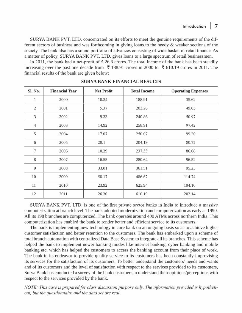
SURYA BANK PVT. LTD. concentrated on its efforts to meet the genuine requirements of the dif-ferent sectors of business and was forthcoming in giving loans to the needy & weaker sections of the
a matter of policy, SURYA BANK PVT. LTD. gives loans to a large spectrum of retail businessmen. ` 26.3 crores. The total income of the bank has been steadily
increasing over the past one decade from ` 188.91 crores in 2000 to ` 610.19 crores in 2011. The
SURYA BANK FINANCIAL RESULTS
Sl. No. Financial Year Total Income Operating Expenses
1 2000 10.24 188.91 35.62
2 2001 203.28 49.03
3 2002 9.33 240.86
4 2003 14.92 258.91
5 2004 99.20
6 2005 204.19
2006 10.39 86.68
8 16.55 280.64 96.52
9 2008 33.01 361.51 95.23
10 2009
11 2010 23.92 625.94 194.10
12 2011 26.30 610.19 202.14
computerization at branch level. The bank adopted modernization and computerization as early as 1990. All its 198 branches are computerized. The bank operates around 400 ATMs across northern India. This
The bank is implementing new technology in core bank on an ongoing basis so as to achieve higher customer satisfaction and better retention to the customers. The bank has embarked upon a scheme of total branch automation with centralized Data Base System to integrate all its branches. This scheme has helped the bank to implement newer banking modes like internet banking, cyber banking and mobile banking etc, which has helped the customers to access the banking account from their place of work. The bank in its endeavor to provide quality service to its customers has been constantly improvising its services for the satisfaction of its customers. To better understand the customers’ needs and wants and of its customers and the level of satisfaction with respect to the services provided to its customers, Surya Bank has conducted a survey of the bank customers to understand their opinions/perceptions with respect to the services provided by the bank.
NOTE: This case is prepared for class discussion purpose only. The information provided is hypotheti-cal, but the questionnaire and the data set are real.

8 Statistics for Management
Questionnaire
Q. 1 Do You have an account in any bank, If yes name of the bank
………………………………………………………
……………………………………………………….Q. 2 Which type of account do you have, Saving
Current Both
Q. 3 For how long have had the bank account < 1 year 2-3 year 3-5 year 5-10 year >10 year
Q. 4 Rank the following modes in terms of the extent to which they helped you know about e-banking services on scale 1 to 4
Least important Slightly important Important Most important
(a) Advertisement
(b) Bank Employee
(c) Personal enquiry
(d) Friends or relative
Q. 5 How frequently do you use e-banking Daily 2-3 times in a week Every week Fort nightly Monthly Once in a six month Never
Q. 6 Rate the add-on services which are available in your e-banking account on scale 1 to 5
Highly unavailable Available Moderate Available
Highly available
(a) Seeking product & rate information(b) Calculate loan payment information(c) Balance inquiry(d) Inter account transfers(e) Lodge complaints(f) To get general information(g) Pay bills(h) Get in touch with bank

Introduction 9
Q. 7 Rate the importance of the following e-banking facilities while selecting a bank on the scale 1 to 4
Least important
Slightly important If important
Most important
(a) Speed of transaction
(b) Reliability
(c) Ease of use
(d) Transparency
(e)
(f) Congestion
(g) Lower amount transactions are not possible
(h) Add on services and schemes
(i) Information retrieval
(j) Ease of contact
(k) Safety
(l) Privacy
(m) Accessibility
Q. 8 Rate the level of satisfaction of the following e-banking facilities of your bank on the scale 1 to 4
Highly
(a) Speed of transaction(b) Reliability(c) Ease of use(d) Transparency(e)(f) Congestion(g) Lower amount transactions
are not possible(h) Add on services and schemes(i) Information retrieval(j) Ease of contact(k) Safety(l) Privacy(m) Accessibility

10 Statistics for Management
Q. 9 Rate the level of satisfaction with e-services provided by your bank
Q. 10e-banking
Daily Monthly
Once in a six month Every week Nightly never
Q. 11 Rate the following problems you have faced frequently using e-banking.
Least faced Slightly faced Faced Fegularly faced
(a) Feel it is unsecured mode of transaction
(b) Misuse of information
(c) Slow transaction
(d) No availability of server
(e) Not a techno savvy
(f) Increasingly expensive and time consuming
(g) Low direct customer connection
Q. 12 How promptly your problems have been solved Instantly Within a week
Within a month
Q. 13 Rate the following statements for e-banking facility according to your agreement level on
Strongly disagree Disagree Neutral Agree
Strongly agree
(a) It saves a person’s time
(b) Private banks are better than public banks
(c)banks so they have an edge over the public banks
(Continued)

Introduction 11
Strongly disagree Disagree Neutral Agree
Strongly agree
(d) Information provided by us is misused
(e) It is good because we can access our bank account from anywhere in the world
(f) It makes money transfer easy and quick
(g) It is an important criterion to choose a bank to open an account
(h) Limited use of this is due to lack of awareness
(i) Complaint handling through e-banking is better by private banks than public banks
(j) Banks provides incentives to use it
(k) This leads to lack of personal touch
(l) People do not use e-banking because of extra charge
Q. 14 Age in years
>60 years
Q. 15 Gender Male
Female
Q. 16 Marital Status Single Married
Q. 17 Education Intermediate
Graduate
Postgraduate
Professional course
Q. 18 Profession Student
Employed in private sector
Employed in Govt sector
Professional
Self employed
House wife
12 Statistics for Management
Q. 19 Monthly Personal Income in INR
<10,000
>50,000
Our own work experience has brought us into contact with thousands of situations where statistics helped deci-sion makers. We participated personally in formulating and applying many of those solutions. It was stimulating, challenging, and, in the end, very rewarding as we saw sensible application of these ideas produce value for organizations. Although very few of you will likely end up as statistical analysts, we believe very strongly that you can learn, develop, and have fun studying statistics, and that’s why we wrote this book. Good luck!
The authors’ goals
LEARNING OBJECTIVES
2After reading this chapter, you can understand:
CHAPTER CONTENTS
To show the difference between samples and populations
To convert raw data to useful information To construct and use data arrays To construct and use frequency distributions
2.1 How Can We Arrange Data? 142.2 Examples of Raw Data 172.3 Arranging Data Using the Data Array
and the Frequency Distribution 182.4 Constructing a Frequency
Distribution 272.5 Graphing Frequency Distributions 38
To graph frequency distributions with histograms, polygons, and ogives
To use frequency distributions to make decisions
Statistics at Work 58 Terms Introduced in Chapter 2 59 Equations Introduced in Chapter 2 60 Review and Application Exercises 60 Flow Chart: Arranging Data to Convey
Meaning 72
Grouping and Displaying Data to Convey Meaning: Tables and Graphs
14 Statistics for Management
The production manager of the Dalmon Carpet Company is responsible for the output of over 500 carpet looms. So that he does not have to measure the daily output (in yards) of each loom, he
samples the output from 30 looms each day and draws a conclusion as to the average carpet production of the entire 500 looms. The table below shows the yards produced by each of the 30 looms in yester-day’s sample. These production amounts are the raw data from which the production manager can draw conclusions about the entire population of looms yesterday.
16.2 15.4 16.0 16.6 15.9 15.8 16.0 16.8 16.9 16.815.7 16.4 15.2 15.8 15.9 16.1 15.6 15.9 15.6 16.016.4 15.8 15.7 16.2 15.6 15.9 16.3 16.3 16.0 16.3
YARDS PRODUCED YESTERDAY BY EACH OF 30 CARPET LOOMS
Using the methods introduced in this chapter, we can help the production manager draw the right conclusion.
Data are collections of any number of related observations. We can collect the number of telephones that several workers install on a given day or that one worker installs per day over a period of several days, and we can call the results our data. A collection of data is called a data set, and a single observation a data point.
2.1 HOW CAN WE ARRANGE DATA?For data to be useful, our observations must be organized so that we can pick out patterns and come to logical conclusions. This chapter introduces the techniques of arranging data in tabular and graphical forms. Chapter 3 shows how to use numbers to describe data.
Collecting DataStatisticians select their observations so that all relevant groups are represented in the data. To determine the potential market for a new product, for example, analysts might study 100 consumers in a certain geographical area. Analysts must be certain that this group contains people representing variables such as income level, race, education, and neighborhood.
Data can come from actual observations or from records that are kept for normal purposes. For billing purposes and doctors’ reports, a hospital, for example, will record the number of patients using the X-ray facilities. But this information can also be organized to pro-duce data that statisticians can describe and interpret.
Data can assist decision makers in educated guesses about the causes and therefore the probable effects of certain characteristics in given situations. Also, knowledge of trends from past experience can enable concerned citizens to be aware of potential outcomes and to plan in advance. Our marketing survey may reveal that the product is preferred by African-American homemakers of suburban communities, average incomes, and average education. This product’s advertising copy should address this target audience. If hospital records show that more patients used the X-ray facilities in June than in January, the hospital personnel
Some definitions
Represent all groups
Find data by observation or
from records
Use data about the past to
make decisions about the
future
Grouping and Displaying Data to Convey Meaning: Tables and Graphs 15
division should determine whether this was accidental to this year or an indication of a trend, and per-haps it should adjust its hiring and vacation practices accordingly.
When data are arranged in compact, usable forms, decision makers can take reliable information from the environment and use it to make intelligent decisions. Today, computers allow statisticians to collect enormous volumes of observations and compress them instantly into tables, graphs, and num-bers. These are all compact, usable forms, but are they reliable? Remember that the data that come out of a computer are only as accurate as the data that go in. As computer programmers say, “GIGO,” or “Garbage In, Garbage Out.” Managers must be very careful to be sure that the data they are using are based on correct assumptions and interpretations. Before relying on any interpreted data, from a com-puter or not, test the data by asking these questions:
1. Where did the data come from? Is the source biased—that is, is it likely to have an interest in supplying data points that will lead to one conclusion rather than another?
2. Do the data support or contradict other evidence we have? 3. Is evidence missing that might cause us to come to a different conclusion? 4. How many observations do we have? Do they represent all the groups we wish to study? 5. Is the conclusion logical? Have we made conclusions that the data do not support?
Study your answers to these questions. Are the data worth using? Or should we wait and collect more information before acting? If the hospital was caught short-handed because it hired too few nurses to
copy only toward African-American suburban home makers when it could have tripled its sales by
available data would have helped managers make better decisions.The effect of incomplete or biased data can be illustrated with
this example. A national association of truck lines claimed in an advertisement that “75 percent of everything you use travels by truck.” This might lead us to believe that cars, railroads, airplanes, ships, and other forms of transpor-tation carry only 25 percent of what we use. Reaching such a conclusion is easy but not enlightening. Missing from the trucking assertion is the question of double counting. What did they do when some-thing was carried to your city by rail and delivered to your house by truck? How were packages treated if they went by airmail and then by truck? When the double-counting issue (a very complex one to treat) is resolved, it turns out that trucks carry a much lower proportion of the goods you use than truckers claimed. Although trucks are involved in delivering a relatively high proportion of what you use, rail-roads and ships still carry more goods for more total miles.
Difference between Samples and PopulationsStatisticians gather data from a sample. They use this informa-tion to make inferences about the population that the sample represents. Thus, a population is a whole, and a sample is a fraction or segment of that whole.
We will study samples in order to be able to describe popu-lations. Our hospital may study a small, representative group of X-ray records rather than examining each record for the last 50 years. The Gallup Poll may interview a sample of only 2,500 adult Americans in order to predict the opinion of all adults living in the United States.
Tests for data
Double-counting example
Sample and population defined
Function of samples

16 Statistics for Management
Studying samples is easier than studying the whole population; it costs less and takes less time. Often, testing an airplane part for strength destroys the part; thus, testing fewer parts is desirable. Sometimes testing involves human risk; thus, use of sampling reduces that risk to an acceptable level. Finally, it has been proven that examining an entire population still allows defective items to be accepted; thus, sampling, in some instances, can raise the quality level. If you’re wondering how that can be so, think of how tired and inattentive you might get if you had to look at thousands and thousands of items passing before you.
A population is a collection of all the elements we are studying
this population so that it is clear whether an element is a member of the population. The population for our marketing study may be all women within a 15-mile radius of center-city Cincinnati who have annual family incomes between $20,000 and $45,000 and have completed at least 11 years of school. A woman living in downtown Cincinnati with a family income of $25,000 and a college degree would be a part of this population. A woman living in San Francisco, or with a family income of $7,000, or with 5 years of schooling would not qualify as a member of this population.
A sample is a collection of some, but not all, of the elements of the population. The population of our marketing survey is all
crumbs of crust is a sample of pie, but it is not a representative sample because the proportions of the ingredients are not the same in the sample as they are in the whole.
A representative sample contains the relevant characteristics of the population in the same propor-tions as they are included in that population. If our population of women is one-third African-American, then a sample of the population that is representative in terms of race will also be one-third African-
Finding a Meaningful Pattern in the DataThere are many ways to sort data. We can simply collect them and keep them in order. Or if the observations are measured in numbers, we can list the data points from lowest to highest in numerical value. But if the data are skilled workers (such as carpenters, masons, and ironworkers) at construction sites, or the different types of automobiles manufactured by all automakers,
must present the data points in alphabetical order or by some other organizing principle. One useful way to organize data is to divide them into similar categories or classes and then count the number of observa-tions that fall into each category. This method produces a frequency distribution and is discussed later in this chapter.
The purpose of organizing data is to enable us to see quickly some of the characteristics of the data we have collected. We look for things such as the range (the largest and smallest values), apparent patterns, what values the data may tend to group around, what values appear most often, and so on. The more information of this kind that we can learn from our sample, the better we can understand the population from which it came, and the better we can make decisions.
Advantages of samples
Function of populations
Need for a representative
sample
Data come in a variety of
forms
Why should we arrange data?
Grouping and Displaying Data to Convey Meaning: Tables and Graphs 17
EXERCISES 2.1
Applications2-1 When asked what they would use if they were marooned on an island with only one choice for
a pain reliever, more doctors chose Bayer than Tylenol, Bufferin, or Advil. Is this conclusion drawn from a sample or a population?
2-2 Is this conclusion drawn from a sample or a population?
2-3
would be implemented immediately to ensure that the defects would not appear again. Comment
2-4 “Germany will remain ever divided” stated Walter Ulbricht after construction of the Berlin Wall in 1961. However, toward the end of 1969, the communists of East Germany began allowing free travel between the east and west, and twenty years after that, the wall was completely destroyed. Give some reasons for Ulbricht’s incorrect prediction.
2-5 on page 15.
2.2 EXAMPLES OF RAW DATAInformation before it is arranged and analyzed is called raw data. It is “raw” because it is unprocessed by statistical methods.
The carpet-loom data in the chapter-opening problem was one example of raw data. Consider a second. Suppose that the admis-sions staff of a university, concerned with the success of the students it selects for admission, wishes to compare the students’ college per-formances with other achievements, such as high school grades, test scores, and extracurricular activi-ties. Rather than study every student from every year, the staff can draw a sample of the population of all the students in a given time period and study only that group to conclude what characteristics appear to predict success. For example, the staff can compare high school grades with college grade-point aver-ages (GPAs) for students in the sample. The staff can assign each grade a numerical value. Then it can add the grades and divide by the total number of grades to get an average for each student. Table 2-1 shows a sample of these raw data in tabular form: 20 pairs of average grades in high school and college.
Problem facing admissions
staff
TABLE 2-1 HIGH SCHOOL AND COLLEGE GRADE-POINT AVERAGES OF 20 COLLEGE SENIORS
H.S. College H.S. College H.S. College H.S. College
3.6 2.5 3.5 3.6 3.4 3.6 2.2 2.8
2.6 2.7 3.5 3.8 2.9 3.0 3.4 3.4
2.7 2.2 2.2 3.5 3.9 4.0 3.6 3.0
3.7 3.2 3.9 3.7 3.2 3.5 2.6 1.9
4.0 3.8 4.0 3.9 2.1 2.5 2.4 3.2
18 Statistics for Management
EXERCISES 2.2
Applications2-6 Look at the data in Table 2-1. Why do these data need further arranging? Can you form any
conclusions from the data as they exist now?2-7 The marketing manager of a large company receives a report each month on the sales activity
of one of the company’s products. The report is a listing of the sales of the product by state during the previous month. Is this an example of raw data?
2-8 The production manager in a large company receives a report each month from the quality control section. The report gives the reject rate for the production line (the number of rejects per 100 units produced), the machine causing the greatest number of rejects, and the average cost of repairing the rejected units. Is this an example of raw data?
2.3 ARRANGING DATA USING THE DATA ARRAY AND THE FREQUENCY DISTRIBUTION
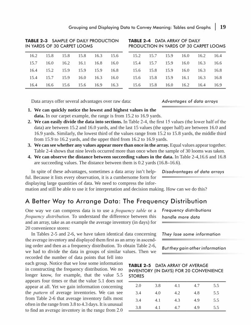
The data array is one of the simplest ways to present data. It arranges values in ascending or descending order. Table 2-3 repeats the carpet data from our chapter-opening problem, and Table 2-4 rearranges these numbers in a data array in ascending order.
Data array defined
Data are not necessarily information, and having more data doesn’t necessarily produce better decisions. The goal is to summarize and present data in useful ways to support prompt and effec-tive decisions. The reason we have to organize data is to see whether there are patterns in them, patterns such as the largest and smallest values, and what value the data seem to cluster around. If the data are from a sample, we assume that they fairly represent the population from which they were drawn. All good statisticians (and users of data) recognize that using biased or incomplete data leads to poor decisions.
HINTS & ASSUMPTIONS
TABLE 2-2 POUNDS OF PRESSURE PER SQUARE INCH THAT CONCRETE CAN WITHSTAND
2500.2 2497.8 2496.9 2500.8 2491.6 2503.7 2501.3 2500.0
2500.8 2502.5 2503.2 2496.9 2495.3 2497.1 2499.7 2505.0
2490.5 2504.1 2508.2 2500.8 2502.2 2508.1 2493.8 2497.8
2499.2 2498.3 2496.7 2490.4 2493.4 2500.7 2502.0 2502.5
2506.4 2499.9 2508.4 2502.3 2491.3 2509.5 2498.4 2498.1
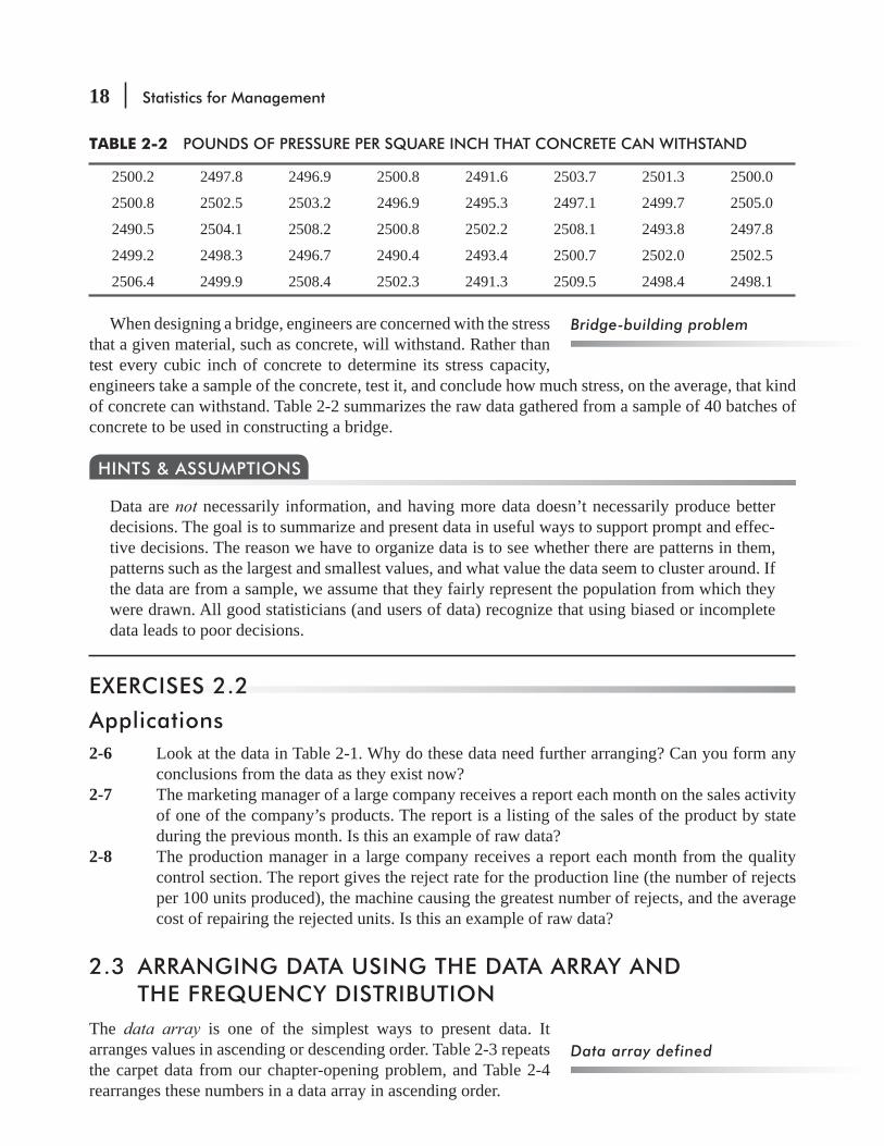
When designing a bridge, engineers are concerned with the stress that a given material, such as concrete, will withstand. Rather than test every cubic inch of concrete to determine its stress capacity, engineers take a sample of the concrete, test it, and conclude how much stress, on the average, that kind of concrete can withstand. Table 2-2 summarizes the raw data gathered from a sample of 40 batches of concrete to be used in constructing a bridge.
Bridge-building problem
Grouping and Displaying Data to Convey Meaning: Tables and Graphs 19
Data arrays offer several advantages over raw data:
1. We can quickly notice the lowest and highest values in the data. In our carpet example, the range is from 15.2 to 16.9 yards.
2. We can easily divide the data into sections.data) are between 15.2 and 16.0 yards, and the last 15 values (the upper half) are between 16.0 and 16.9 yards. Similarly, the lowest third of the values range from 15.2 to 15.8 yards, the middle third from 15.9 to 16.2 yards, and the upper third from 16.2 to 16.9 yards.
3. We can see whether any values appear more than once in the array. Equal values appear together. Table 2-4 shows that nine levels occurred more than once when the sample of 30 looms was taken.
4. We can observe the distance between succeeding values in the data. In Table 2-4,16.6 and 16.8 are succeeding values. The distance between them is 0.2 yards (16.8–16.6).
In spite of these advantages, sometimes a data array isn’t help-ful. Because it lists every observation, it is a cumbersome form for displaying large quantities of data. We need to compress the infor-mation and still be able to use it for interpretation and decision making. How can we do this?
A Better Way to Arrange Data: The Frequency DistributionOne way we can compress data is to use a frequency table or a frequency distribution. To understand the difference between this and an array, take as an example the average inventory (in days) for 20 convenience stores:
In Tables 2-5 and 2-6, we have taken identical data concerning -
ing order and then as a frequency distribution. To obtain Table 2-6, we had to divide the data in groups of similar values. Then we recorded the number of data points that fell into each group. Notice that we lose some information in constructing the frequency distribution. We no longer know, for example, that the value 5.5 appears four times or that the value 5.1 does not appear at all. Yet we gain information concerning the pattern of average inventories. We can see from Table 2-6 that average inventory falls most often in the range from 3.8 to 4.3 days. It is unusual
Advantages of data arrays
Disadvantages of data arrays
Frequency distributions
handle more data
They lose some information
But they gain other information
TABLE 2-3 SAMPLE OF DAILY PRODUCTION IN YARDS OF 30 CARPET LOOMS
16.2 15.8 15.8 15.8 16.3 15.6
15.7 16.0 16.2 16.1 16.8 16.0
16.4 15.2 15.9 15.9 15.9 16.8
15.4 15.7 15.9 16.0 16.3 16.0
16.4 16.6 15.6 15.6 16.9 16.3
TABLE 2-4 DATA ARRAY OF DAILY PRODUCTION IN YARDS OF 30 CARPET LOOMS
15.2 15.7 15.9 16.0 16.2 16.4
15.4 15.7 15.9 16.0 16.3 16.6
15.6 15.8 15.9 16.0 16.3 16.8
15.6 15.8 15.9 16.1 16.3 16.8
15.6 15.8 16.0 16.2 16.4 16.9
TABLE 2-5 DATA ARRAY OF AVERAGE INVENTORY (IN DAYS) FOR 20 CONVENIENCE STORES
2.0 3.8 4.1 4.7 5.5
3.4 4.0 4.2 4.8 5.5
3.4 4.1 4.3 4.9 5.5
3.8 4.1 4.7 4.9 5.5

20 Statistics for Management
to 2.5 days or from 2.6 to 3.1 days. Inventories in the ranges of 4.4 to 4.9 days and 5.0 to 5.5 days are
detail but offer us new insights into patterns of data.A frequency distribution is a table that organizes data into
classes, that is, into groups of values describing one characteristic of the data. The average inventory is one characteristic of the 20 convenience stores. In Table 2-5, this characteristic has 11 different values. But these same data could be divided into any number of classes. Table 2-6, for example, uses 6. We could compress the data even further and use only 2 classes: less than 3.8 and greater than or equal to 3.8. Or we could increase the number of classes by using smaller intervals, as we have done in Table 2-7.
A frequency distribution shows the number of observations from the data set that fall into each of the classes. If you can determine the frequency with which values occur in each class of a data set, you can construct a frequency distribution.
Characteristics of Relative Frequency DistributionsSo far, we have expressed the frequency with which values occur in each class as the total number of data points that fall within that class. We can also express the frequency of each value as a fraction or a percentage of the total number of observations. The frequency of an average inventory of 4.4 to 4.9 days, for example, is 5 in Table 2-6 but 0.25 in Table 2-8. To get this value of 0.25, we divided the frequency for that class (5) by the total number of observations in the data set (20). The answer can be expressed as a fraction (5
20) a decimal (0.25), or a percentage (25 percent). A relative frequency distribution presents frequencies in terms of fractions or percentages.
Notice in Table 2-8 that the sum of all the relative frequencies equals 1.00, or 100 percent. This is true because a relative fre-quency distribution pairs each class with its appropriate fraction or percentage of the total data. Therefore, the classes in any relative or simple frequency distribution are all-inclusive.
Function of classes in a
frequency distribution
Why is it called a frequency
distribution?
Relative frequency
distribution defined
Classes are all-inclusive
They are mutually exclusive
Class (Group of Similar Values of
Data Points)
Frequency (Number of Observationsin Each Class)
2.0 to 2.5 1
2.6 to 3.1 0
3.2 to 3.7 2
3.8 to 4.3 8
4.4 to 4.9 5
5.0 to 5.5 4
TABLE 2-6 FREQUENCY DISTRIBUTION OF AVERAGE INVENTORY (IN DAYS) FOR 20 CONVENIENCE STORES (6 CLASSES)
Class Frequency Class Frequency
2.0 to 2.2 1 3.8 to 4.0 3
2.3 to 2.5 0 4.1 to 4.3 5
2.6 to 2.8 0 4.4 to 4.6 0
2.9 to 3.1 0 4.7 to 4.9 5
3.2 to 3.4 2 5.0 to 5.2 0
3.5 to 3.7 0 5.3 to 5.5 4
TABLE 2-7 FREQUENCY DISTRIBUTION OF AVERAGE INVENTORY (IN DAYS) FOR 20 CONVENIENCE STORES (12 CLASSES)

Grouping and Displaying Data to Convey Meaning: Tables and Graphs 21
that the classes in Table 2-8 are mutually exclusive; that is, no data point falls into more than one cate-gory. Table 2-9 illustrates this concept by comparing mutually exclusive classes with ones that overlap. In frequency distributions, there are no overlapping classes.
Up to this point, our classes have consisted of numbers and have described some quantitative attribute of the items sampled. We can also classify information according to qualitative charac-teristics, such as race, religion, and gender, which do not fall naturally into numerical categories. Like classes of quantitative attributes, these classes must be all-inclusive and mutually exclusive. Table 2-10 shows how to construct both simple and relative frequency distributions using the qualitative attribute of occupations.
Classes of qualitative data
Class Frequency Relative Frequency: Fraction of Observations in Each Class
2.0 to 2.5 1 0.05
2.6 to 3.1 0 0.00
3.2 to 3.7 2 0.10
3.8 to 4.3 8 0.40
4.4 to 4.9 5 0.25
5.0 to 5.5 4 0.20
20 1.00 (sum of the relative frequencies of all classes)
TABLE 2-8 RELATIVE FREQUENCY DISTRIBUTION OF AVERAGE INVENTORY (IN DAYS) FOR 20 CONVENIENCE STORES
TABLE 2-9 MUTUALLY EXCLUSIVE AND OVERLAPPING CLASSES
Mutually exclusive 1 to 4 5 to 8 9 to 12 13 to 16
Not mutually exclusive 1 to 4 3 to 6 5 to 8 7 to 10
Occupational ClassFrequency Distribution
(1)Relative Frequency Distribution
(1) ÷ 100
Actor 5 0.05Banker 8 0.08Businessperson 22 0.22Chemist 7 0.07Doctor 10 0.10Insurance representative 6 0.06Journalist 2 0.02Lawyer 14 0.14Teacher 9 0.09Other 17 0.17
100 1.00
TABLE 2-10 OCCUPATIONS OF SAMPLE OF 100 GRADUATES OF CENTRAL COLLEGE

22 Statistics for Management
Although Table 2-10 does not list every occupation held by the graduates of Central College, it is still all-inclusive. Why? The class
-ated categories. We will use a word like this when-
-sibilities. For example, if our characteristic can occur in any month of the year, a complete list would include 12 categories. But if we wish to list only the 8 months from January through August, we can use the term other to account for our obser-vations during the 4 months of September, October, November, and December. Although our
is all-inclusive. This “other” is called an open-ended class when it allows either the upper or the
to be limitless. The last class in Table 2-11 (“72 and older”) is open-ended.
-tive or qualitative and either discrete or continu-ous. Discrete classes are separate entities that do not progress from one class to the next without a break. Such classes as the number of children in each family, the number of trucks owned by moving companies, and the occupa-tions of Central College graduates are discrete. Discrete data are data that can take on only a limited
something in between. The closing price of AT&T stock can be 3912 or 39 7
8 (but not 39.43), or your basketball team can win by 5 or 27 points (but not by 17.6 points).
Continuous data do progress from one class to the next without a break. They involve numerical measurement such as the weights of cans of tomatoes, the pounds of pressure on concrete, or the high school GPAs of college seniors. Continuous data can be expressed in either fractions or whole numbers.
There are many ways to present data. Constructing a data array in either descending or ascending order is a good place to start. Showing how many times a value appears by using a frequency distribution is even more effective, and converting these frequencies to decimals (which we call relative frequencies) can help even more. Hint: We should remember that discrete variables are things that can be counted but continuous variables are things that appear at some point on a scale.
HINTS & ASSUMPTIONS
EXERCISES 2.3
Self-Check ExercisesSC 2-1 Here are the ages of 50 members of a country social service program:
Open-ended classes for lists
that are not exhaustive
Discrete classes
Continuous classes
Class: Age (1)
Frequency (2)
Relative Frequency (2) ÷ 89,592
Birth to 7 8,873 0.09908 to 15 9,246 0.1032
16 to 23 12,060 0.134624 to 31 11,949 0.133432 to 39 9,853 0.110040 to 47 8,439 0.094248 to 55 8,267 0.092356 to 63 7,430 0.082964 to 71 7,283 0.0813
72 and older 6,192 0.069189,592 1.0000
TABLE 2-11 AGES OF BUNDER COUNTY RESIDENTS

Grouping and Displaying Data to Convey Meaning: Tables and Graphs 23
83 51 66 61 82 65 54 56 92 6065 87 68 64 51 70 75 66 74 6844 55 78 69 98 67 82 77 79 6238 88 76 99 84 47 60 42 66 7491 71 83 80 68 65 51 56 73 55
Use these data to construct relative frequency distributions using 7 equal intervals and 13 equal intervals. State policies on social service programs require that approximately 50 percent of the program participants be older than 50.(a) Is the program in compliance with the policy?(b) Does your 13-interval relative frequency distribution help you answer part (a) better than
your 7-interval distribution?(c) Suppose the Director of Social Services wanted to know the proportion of program par-
ticipants between 45 and 50 years old. Could you estimate the answer for her better with a 7- or a 13-interval relative frequency distribution?
SC 2-2 Using the data in Table 2-1 on page 17, arrange the data in an array from highest to lowest high school GPA. Now arrange the data in an array from highest to lowest college GPA. What can you conclude from the two arrays that you could not from the original data?
Applications2-9 Transmission Fix-It stores recorded the number of service tickets submitted by each of its
20 stores last month as follows:
823 648 321 634 752
669 427 555 904 586
722 360 468 847 641
217 588 349 308 766
manager who generates more than 725 service actions a month. Arrange these data in a data array and indicate how many stores are not breaking even and how many are to get bonuses.
2-10 what she calls a “store watch list,” that is, a list of the stores whose service activity is low
whose service activity is between 550 and 650 service actions a month. How many stores should be on that list based on last month’s activity?
2-11 The number of hours taken by transmission mechanics to remove, repair, and replace trans-missions in one of the Transmission Fix-It stores one day last week is recorded as follows:
4.3 2.7 3.8 2.2 3.4
3.1 4.5 2.6 5.5 3.2
6.6 2.0 4.4 2.1 3.3
6.3 6.7 5.9 4.1 3.7

24 Statistics for Management
Construct a frequency distribution with intervals of 1.0 hour from these data. What conclusions can you reach about the productivity of mechanics from this distribution? If Transmission Fix-It management believes that more than 6.0 hours is evidence of unsatisfactory perfor-mance, does it have a major or minor problem with performance in this particular store?
2-12 The Orange County Transportation Commission is concerned about the speed motorists are driving on a section of the main highway. Here are the speeds of 45 motorists:
15 32 45 46 42 39 68 47 1831 48 49 56 52 39 48 69 6144 42 38 52 55 58 62 58 4856 58 48 47 52 37 64 29 5538 29 62 49 69 18 61 55 49
Use these data to construct relative frequency distributions using 5 equal intervals and 11 equal intervals. The U.S. Department of Transportation reports that, nationally, no more than 10 percent of the motorists exceed 55 mph.(a) Do Orange County motorists follow the U.S. DOT’s report about national driving patterns?(b) Which distribution did you use to answer part (a)?(c) The U.S. DOT has determined that the safest speed for this highway is more than 36 but
less than 59 mph. What proportion of the motorists drive within this range? Which distri-bution helped you answer this question?
2-13 Arrange the data in Table 2-2 on page 18 in an array from highest to lowest.(a) Suppose that state law requires bridge concrete to withstand at least 2,500 lb/sq in. How
many samples would fail this test?(b) How many samples could withstand a pressure of at least 2,497 lb/sq in. but could not
withstand a pressure greater than 2,504 lb/sq in.?(c) As you examine the array, you should notice that some samples can withstand identical
amounts of pressure. List these pressures and the number of samples that can withstand each amount.
2-14 A recent study concerning the habits of U.S. cable television consumers produced the follow-ing data:
Number of Channels PurchasedNumber of Hours Spent
Watching Television per Week25 1418 1642 1296 628 1343 1639 929 717 1984 476 822 13
104 6
Arrange the data in an array. What conclusion(s) can you draw from these data?

Grouping and Displaying Data to Convey Meaning: Tables and Graphs 25
2-15 The Environmental Protection Agency took water samples from 12 different rivers and streams that feed into Lake Erie. These samples were tested in the EPA laboratory and rated as to the amount of solid pollution suspended in each sample. The results of the testing are given in the following table:
Sample 1 2 3 4 5 6Pollution Rating (ppm) 37.2 51.7 68.4 54.2 49.9 33.4Sample 7 8 9 10 11 12Pollution Rating (ppm) 39.8 52.7 60.0 46.1 38.5 49.1
(a) Arrange the data into an array from highest to lowest.(b) Determine the number of samples having a pollution content between 30.0 and 39.9, 40.0
and 49.9, 50.0 and 59.9, and 60.0 and 69.9. (c) If 45.0 is the number used by the EPA to indicate excessive pollution, how many samples
would be rated as having excessive pollution? (d) What is the largest distance between any two consecutive samples?
2-16 Suppose that the admissions staff mentioned in the discussion of Table 2-1 on page 17 wishes to examine the relationship between a student’s differential on the college SAT examination (the difference between actual and expected score based on the student’s high school GPA) and the spread between the student’s high school and college GPA (the difference between the college and high school GPA). The admissions staff will use the following data:
H.S. GPA College GPA SAT Score H.S. GPA College GPA SAT Score3.6 2.5 1,100 3.4 3.6 1,1802.6 2.7 940 2.9 3.0 1,0102.7 2.2 950 3.9 4.0 1,3303.7 3.2 1,160 3.2 3.5 1,1504.0 3.8 1,340 2.1 2.5 9403.5 3.6 1,180 2.2 2.8 9603.5 3.8 1,250 3.4 3.4 1,1702.2 3.5 1,040 3.6 3.0 1,1003.9 3.7 1,310 2.6 1.9 8604.0 3.9 1,330 2.4 3.2 1,070
In addition, the admissions staff has received the following information from the Educational Testing Service:
H.S. GPA Avg. SAT Score H.S. GPA Avg. SAT Score4.0 1,340 2.9 1,0203.9 1,310 2.8 1,0003.8 1,280 2.7 9803.7 1,250 2.6 9603.6 1,220 2.5 9403.5 1,190 2.4 9203.4 1,160 2.3 9103.3 1,130 2.2 9003.2 1,100 2.1 8803.1 1,070 2.0 8603.0 1,040

26 Statistics for Management
(a) Arrange these data into an array of spreads from highest to lowest. (Consider an increase in college GPA over high school GPA as positive and a decrease in college GPA below high school GPA as negative.) Include with each spread the appropriate SAT differential. (Consider an SAT score below expected as negative and above expected as positive.)
(b) What is the most common spread?(c) For this spread in part (b), what is the most common SAT differential?(d) From the analysis you have done, what do you conclude?
Worked-Out Answers to Self-Check Exercises
SC 2-1 7 Intervals 13 Intervals
ClassRelative
Frequency ClassRelative
Frequency ClassRelative
Frequency
30–39 0.02 35–39 0.02 70–74 0.10
40–49 0.06 40–44 0.04 75–79 0.10
50–59 0.16 45–49 0.02 80–84 0.12
60–69 0.32 50–54 0.08 85–89 0.04
70–79 0.20 55–59 0.08 90–94 0.04
80–89 0.16 60–64 0.10 95–99 0.04
90–99 0.08 65–69 0.22 1.00
1.00
(a) As can be seen from either distribution, about 90 percent of the participants are older than 50, so the program is not in compliance.
(b) In this case, both are equally easy to use.(c) The 13-interval distribution gives a better estimate because it has a class for 45–49,
whereas the 7-interval distribution lumps together all observations between 40 and 49.SC 2-2 Data array by high school GPA:
High School GPA College GPA High School GPA College GPA
4.0 3.9 3.4 3.4
4.0 3.8 3.2 3.5
3.9 4.0 2.9 3.0
3.9 3.7 2.7 2.2
3.7 3.2 2.6 2.7
3.6 3.0 2.6 1.9
3.6 2.5 2.4 3.2
3.5 3.8 2.2 3.5
3.5 3.6 2.2 2.8
3.4 3.6 2.1 2.5
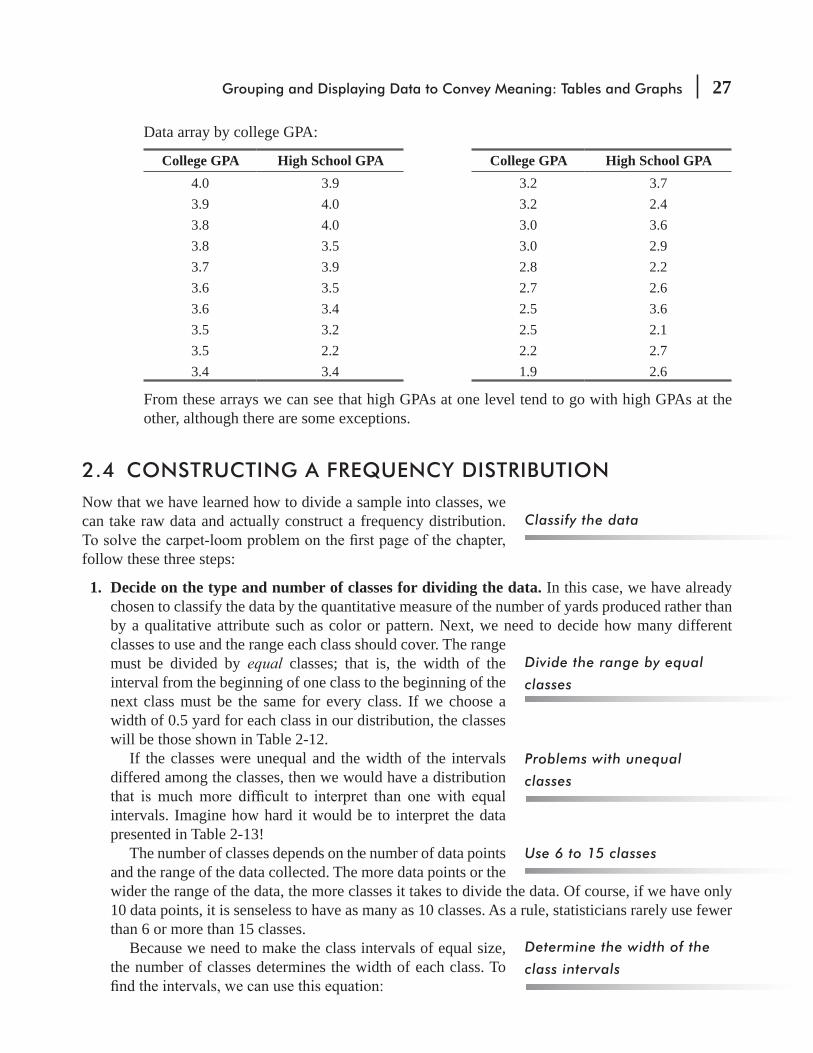
Grouping and Displaying Data to Convey Meaning: Tables and Graphs 27
Data array by college GPA:
College GPA High School GPA College GPA High School GPA4.0 3.9 3.2 3.73.9 4.0 3.2 2.43.8 4.0 3.0 3.63.8 3.5 3.0 2.93.7 3.9 2.8 2.23.6 3.5 2.7 2.63.6 3.4 2.5 3.63.5 3.2 2.5 2.13.5 2.2 2.2 2.73.4 3.4 1.9 2.6
From these arrays we can see that high GPAs at one level tend to go with high GPAs at the other, although there are some exceptions.
2.4 CONSTRUCTING A FREQUENCY DISTRIBUTIONNow that we have learned how to divide a sample into classes, we can take raw data and actually construct a frequency distribution.
follow these three steps:
1. Decide on the type and number of classes for dividing the data. In this case, we have already chosen to classify the data by the quantitative measure of the number of yards produced rather than by a qualitative attribute such as color or pattern. Next, we need to decide how many different classes to use and the range each class should cover. The range must be divided by equal classes; that is, the width of the interval from the beginning of one class to the beginning of the next class must be the same for every class. If we choose a width of 0.5 yard for each class in our distribution, the classes will be those shown in Table 2-12.
If the classes were unequal and the width of the intervals differed among the classes, then we would have a distribution
intervals. Imagine how hard it would be to interpret the data presented in Table 2-13!
The number of classes depends on the number of data points and the range of the data collected. The more data points or the wider the range of the data, the more classes it takes to divide the data. Of course, if we have only 10 data points, it is senseless to have as many as 10 classes. As a rule, statisticians rarely use fewer than 6 or more than 15 classes.
Because we need to make the class intervals of equal size, the number of classes determines the width of each class. To
Classify the data
Divide the range by equal
classes
Problems with unequal
classes
Use 6 to 15 classes
Determine the width of the
class intervals
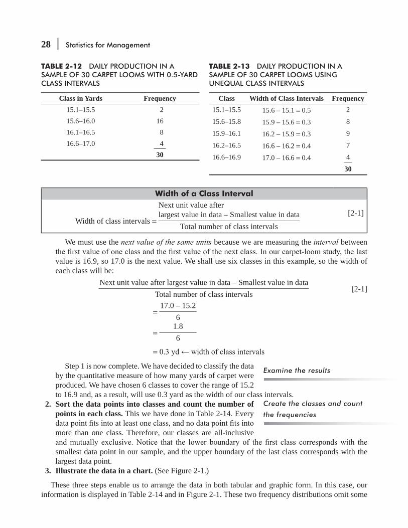
28 Statistics for Management
Width of a Class Interval
Width of class intervals =
Next unit value afterlargest value in data – Smallest value in data
Total number of class intervals
[2-1]
We must use the next value of the same units because we are measuring the interval between
value is 16.9, so 17.0 is the next value. We shall use six classes in this example, so the width of each class will be:
Next unit value after largest value in data – Smallest value in data
Total number of class intervals [2-1]
= 17.0 – 15.2
6
= 1.86
=
Step 1 is now complete. We have decided to classify the data by the quantitative measure of how many yards of carpet were produced. We have chosen 6 classes to cover the range of 15.2 to 16.9 and, as a result, will use 0.3 yard as the width of our class intervals.
2. Sort the data points into classes and count the number of points in each class. This we have done in Table 2-14. Every
more than one class. Therefore, our classes are all-inclusive
smallest data point in our sample, and the upper boundary of the last class corresponds with the largest data point.
3. Illustrate the data in a chart. (See Figure 2-1.)
These three steps enable us to arrange the data in both tabular and graphic form. In this case, our information is displayed in Table 2-14 and in Figure 2-1. These two frequency distributions omit some
Examine the results
Create the classes and count
the frequencies
Class in Yards Frequency15.1–15.5 215.6–16.0 1616.1–16.5 816.6–17.0 4
30
TABLE 2-12 DAILY PRODUCTION IN A SAMPLE OF 30 CARPET LOOMS WITH 0.5-YARD CLASS INTERVALS
Class Width of Class Intervals Frequency15.1–15.5 15.6 – 15.1 = 0.5 2
15.6–15.8 15.9 – 15.6 = 0.3 8
15.9–16.1 16.2 – 15.9 = 0.3 9
16.2–16.5 16.6 – 16.2 = 0.4 7
16.6–16.9 17.0 – 16.6 = 0.4 4
30
TABLE 2-13 DAILY PRODUCTION IN A SAMPLE OF 30 CARPET LOOMS USING UNEQUAL CLASS INTERVALS
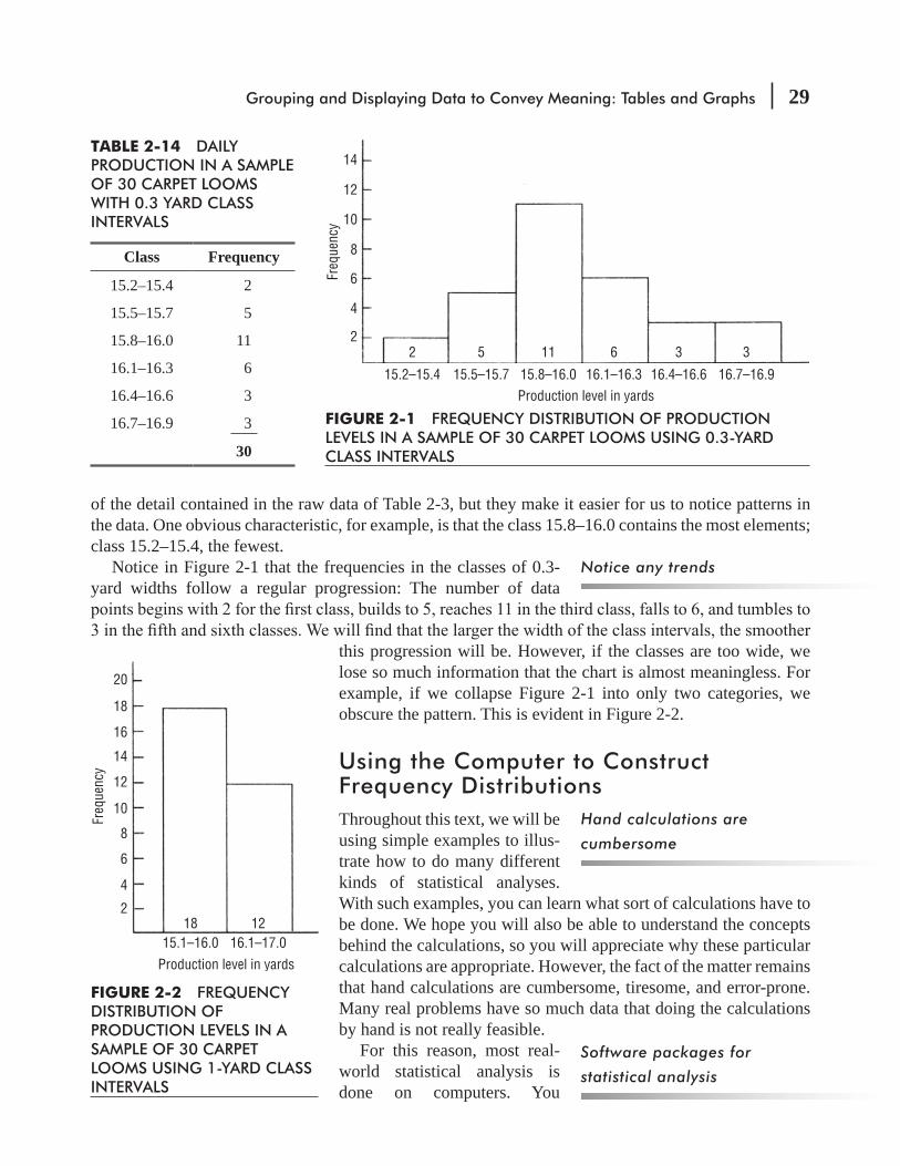
Grouping and Displaying Data to Convey Meaning: Tables and Graphs 29
of the detail contained in the raw data of Table 2-3, but they make it easier for us to notice patterns in the data. One obvious characteristic, for example, is that the class 15.8–16.0 contains the most elements; class 15.2–15.4, the fewest.
Notice in Figure 2-1 that the frequencies in the classes of 0.3-yard widths follow a regular progression: The number of data
this progression will be. However, if the classes are too wide, we lose so much information that the chart is almost meaningless. For example, if we collapse Figure 2-1 into only two categories, we obscure the pattern. This is evident in Figure 2-2.
Using the Computer to Construct Frequency DistributionsThroughout this text, we will be using simple examples to illus-trate how to do many different kinds of statistical analyses. With such examples, you can learn what sort of calculations have to be done. We hope you will also be able to understand the concepts behind the calculations, so you will appreciate why these particular calculations are appropriate. However, the fact of the matter remains that hand calculations are cumbersome, tiresome, and error-prone. Many real problems have so much data that doing the calculations by hand is not really feasible.
For this reason, most real-world statistical analysis is done on computers. You
Notice any trends
Hand calculations are
cumbersome
Software packages for
statistical analysis
Class Frequency
15.2–15.4 2
15.5–15.7 5
15.8–16.0 11
16.1–16.3 6
16.4–16.6 3
16.7–16.9 3
30
TABLE 2-14 DAILY PRODUCTION IN A SAMPLE OF 30 CARPET LOOMS WITH 0.3 YARD CLASS INTERVALS
14
12
10
8
6
4
2
15.2–15.4 15.5–15.7 15.8–16.0 16.1–16.3 16.4–16.6 16.7–16.9
3361152Fr
eque
ncy
Production level in yards
FIGURE 2-1 FREQUENCY DISTRIBUTION OF PRODUCTION LEVELS IN A SAMPLE OF 30 CARPET LOOMS USING 0.3-YARD CLASS INTERVALS
20
18
16
14
12
10
8
6
4
218 12
Freq
uenc
y
15.1–16.0 16.1–17.0Production level in yards
FIGURE 2-2 FREQUENCY DISTRIBUTION OF PRODUCTION LEVELS IN A SAMPLE OF 30 CARPET LOOMS USING 1-YARD CLASS INTERVALS
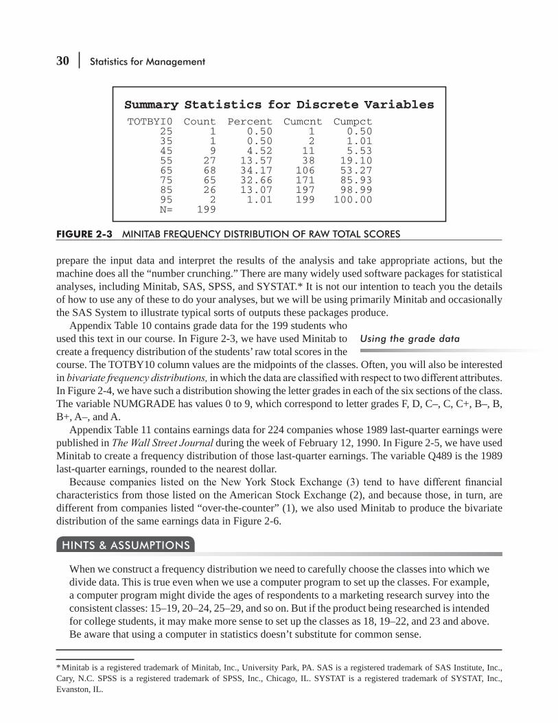
30 Statistics for Management
prepare the input data and interpret the results of the analysis and take appropriate actions, but the machine does all the “number crunching.” There are many widely used software packages for statistical analyses, including Minitab, SAS, SPSS, and SYSTAT.* It is not our intention to teach you the details of how to use any of these to do your analyses, but we will be using primarily Minitab and occasionally the SAS System to illustrate typical sorts of outputs these packages produce.
Appendix Table 10 contains grade data for the 199 students who used this text in our course. In Figure 2-3, we have used Minitab to create a frequency distribution of the students’ raw total scores in the course. The TOTBY10 column values are the midpoints of the classes. Often, you will also be interested in bivariate frequency distributions,In Figure 2-4, we have such a distribution showing the letter grades in each of the six sections of the class. The variable NUMGRADE has values 0 to 9, which correspond to letter grades F, D, C–, C, C+, B–, B, B+, A–, and A.
Appendix Table 11 contains earnings data for 224 companies whose 1989 last-quarter earnings were published in The Wall Street Journal during the week of February 12, 1990. In Figure 2-5, we have used Minitab to create a frequency distribution of those last-quarter earnings. The variable Q489 is the 1989 last-quarter earnings, rounded to the nearest dollar.
characteristics from those listed on the American Stock Exchange (2), and because those, in turn, are different from companies listed “over-the-counter” (1), we also used Minitab to produce the bivariate distribution of the same earnings data in Figure 2-6.
When we construct a frequency distribution we need to carefully choose the classes into which we divide data. This is true even when we use a computer program to set up the classes. For example, a computer program might divide the ages of respondents to a marketing research survey into the consistent classes: 15–19, 20–24, 25–29, and so on. But if the product being researched is intended for college students, it may make more sense to set up the classes as 18, 19–22, and 23 and above. Be aware that using a computer in statistics doesn’t substitute for common sense.
HINTS & ASSUMPTIONS
* Minitab is a registered trademark of Minitab, Inc., University Park, PA. SAS is a registered trademark of SAS Institute, Inc., Cary, N.C. SPSS is a registered trademark of SPSS, Inc., Chicago, IL. SYSTAT is a registered trademark of SYSTAT, Inc., Evanston, IL.
Using the grade data
FIGURE 2-3 MINITAB FREQUENCY DISTRIBUTION OF RAW TOTAL SCORES
Summary Statistics for Discrete Variables TOTBYI0 Count Percent Cumcnt Cumpct 25 1 0.50 1 0.50 35 1 0.50 2 1.01 45 9 4.52 11 5.53 55 27 13.57 38 19.10 65 68 34.17 106 53.27 75 65 32.66 171 85.93 85 26 13.07 197 98.99 95 2 1.01 199 100.00 N= 199

Grouping and Displaying Data to Convey Meaning: Tables and Graphs 31
FIGURE 2-5 MINITAB FREQUENCY DISTRIBUTION OF 1989 LAST-QUARTER EARNINGS
Summary Statistics for Discrete Variables
Q489 Count Percent Cumcnt Cumpct -5 1 0.45 1 0.45 -4 2 0.89 3 1.34 -2 1 0.45 4 1.79 -1 9 4.02 13 5.80 0 164 73.21 177 79.02 1 43 19.20 220 98.21 2 2 0.89 222 99.11 5 2 0.89 224 100.00 N= 224
FIGURE 2-4 MINITAB BIVARIATE FREQUENCY DISTRIBUTION SHOWING GRADES IN EACH SECTION
Tabulated Statistics
ROWS: NUMGRADE COLUMNS: SECTION
1 2 3 4 5 6 ALL
0 2 3 0 1 3 2 11 1.01 1.51 -- 0.50 1.51 1.01 5.53
1 3 6 5 2 4 6 26 1.51 3.02 2.51 1.01 2.01 3.02 13.07
2 2 2 1 2 7 4 18 1.01 1.01 0.50 1.01 3.52 2.01 9.05
3 9 11 3 9 6 6 44 4.52 5.53 1.51 4.52 3.02 3.02 22.11
4 3 6 10 6 7 2 34 1.51 3.02 5.03 3.02 3.52 1.01 17.09
5 1 5 5 1 0 3 15 0.50 2.51 2.51 0.50 -- 1.51 7.54
6 2 5 3 2 2 3 17 1.01 2.51 1.51 1.01 1.01 1.51 8.54
7 1 1 1 2 1 1 7 0.50 0.50 0.50 1.01 0.50 0.50 3.52
8 2 2 8 1 3 0 16 1.01 1.01 4.02 0.50 1.51 -- 8.04
9 2 5 1 0 3 0 11 1.01 2.51 0.50 -- 1.51 -- 5.53
ALL 27 46 37 26 36 27 199 13.57 23.12 18.59 13.07 18.09 13.57 100.00
CELL CONTENTS -- COUNT % OP TBL
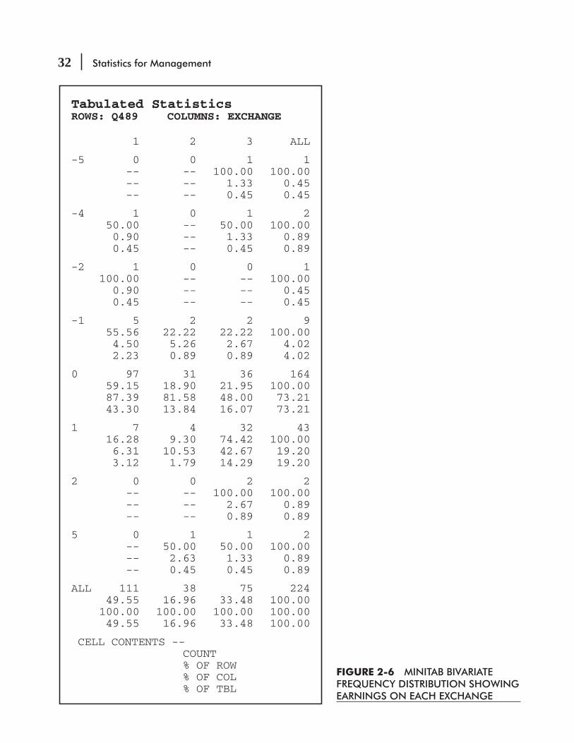
32 Statistics for Management
FIGURE 2-6 MINITAB BIVARIATE FREQUENCY DISTRIBUTION SHOWING EARNINGS ON EACH EXCHANGE
Tabulated StatisticsROWS: Q489 COLUMNS: EXCHANGE
1 2 3 ALL
-5 0 0 1 1 -- -- 100.00 100.00 -- -- 1.33 0.45 -- -- 0.45 0.45
-4 1 0 1 2 50.00 -- 50.00 100.00 0.90 -- 1.33 0.89 0.45 -- 0.45 0.89
-2 1 0 0 1 100.00 -- -- 100.00 0.90 -- -- 0.45 0.45 -- -- 0.45
-1 5 2 2 9 55.56 22.22 22.22 100.00 4.50 5.26 2.67 4.02 2.23 0.89 0.89 4.02
0 97 31 36 164 59.15 18.90 21.95 100.00 87.39 81.58 48.00 73.21 43.30 13.84 16.07 73.21
1 7 4 32 43 16.28 9.30 74.42 100.00 6.31 10.53 42.67 19.20 3.12 1.79 14.29 19.20
2 0 0 2 2 -- -- 100.00 100.00 -- -- 2.67 0.89 -- -- 0.89 0.89
5 0 1 1 2 -- 50.00 50.00 100.00 -- 2.63 1.33 0.89 -- 0.45 0.45 0.89
ALL 111 38 75 224 49.55 16.96 33.48 100.00 100.00 100.00 100.00 100.00 49.55 16.96 33.48 100.00
CELL CONTENTS -- COUNT % OF ROW % OF COL % OF TBL
Grouping and Displaying Data to Convey Meaning: Tables and Graphs 33
EXERCISES 2.4
Self-Check ExercisesSC 2-3 High Performance Bicycle Products Company in Chapel Hill, North Carolina, sampled its
shipping records for a certain day with these results:
Time from Receipt of Order to Delivery (in Days) 4 12 8 14 11 6 7 13 13 1111 20 5 19 10 15 24 7 19 6
Construct a frequency distribution for these data and a relative frequency distribution. Use intervals of 6 days.(a) What statement can you make about the effectiveness of order processing from the
frequency distribution?(b) If the company wants to ensure that half of its deliveries are made in 10 or fewer days, can
you determine from the frequency distribution whether they have reached this goal?(c) What does having a relative frequency distribution permit you to do with the data that is
SC 2-4 Mr. Frank, a safety engineer for the Mars Point Nuclear Power Generating Station, has charted the peak reactor temperature each day for the past year and has prepared the following frequency distribution:
Temperatures in °C FrequencyBelow 500 4501–510 7511–520 32521–530 59530–540 82550–560 65561–570 33571–580 28580–590 27591–600 23
Total 360
Applications2-17 Universal Burger is concerned about product waste, so they sampled their burger waste record
from the past year with the following results:
Number of Burgers Discarded During a Shift 2 16 4 12 19 29 24 7 1922 14 8 24 31 18 20 16 6

34 Statistics for Management
Construct a frequency distribution for these data and a relative frequency distribution. Use intervals of 5 burgers.(a) One of Universal Burger’s goals is for at least 75 percent of shifts to have no more than
16 burgers wasted. Can you determine from the frequency distribution whether this goal has been achieved?
(b) What percentage of shifts have waste of 21 or fewer burgers? Which distribution did you use to determine your answer?
2-18 Refer to Table 2-2 on page 18 and construct a relative frequency distribution using intervals of 4.0 lb/sq in. What do you conclude from this distribution?
2-19 The Bureau of Labor Statistics has sampled 30 communities nationwide and compiled prices
the Consumer Price Index (CPI) has changed during August. The percentage changes in prices for the 30 communities are as follows:
0.7 0.4 –0.3 0.2 –0.1 0.1 0.3 0.7 0.0 –0.4
0.1 0.5 0.2 0.3 1.0 –0.3 0.0 0.2 0.5 0.1
–0.5 –0.3 0.1 0.5 0.4 0.0 0.2 0.3 0.5 0.4
(a) Arrange the data in an array from lowest to highest.(b) Using the following four equal-sized classes, create a frequency distribution: –0.5 to –0.2,
–0.1 to 0.2, 0.3 to 0.6, and 0.7 to 1.0.(c) How many communities had prices that either did not change or that increased less than
1.0 percent?(d) Are these data discrete or continuous?
2-20 Sarah Anne Rapp, the president of Baggit, Inc., has just obtained some raw data from a mar-keting survey that her company recently conducted. The survey was taken to determine the effectiveness of the new company slogan, “When you’ve given up on the rest, Baggit!” To determine the effect of the slogan on the sales of Luncheon Baggits, 20 people were asked how many boxes of Luncheon Baggits per month they bought before and after the slogan was used in the advertising campaign. The results were as follows:
Before/After Before/After Before/After Before/After
4 3 2 1 5 6 8 10
4 6 6 9 2 7 1 3
1 5 6 7 6 8 4 3
3 7 5 8 8 4 5 7
5 5 3 6 3 5 2 2
(a) Create both frequency and relative frequency distributions for the “Before” responses, using as classes 1–2, 3–4, 5–6, 7–8, and 9–10.
(b) Work part (a) for the “After” responses.(c) Give the most basic reason why it makes sense to use the same classes for both the
“Before” and “After” responses.(d) For each pair of “Before/After” responses, subtract the “Before” response from the
“After” response to get the number that we will call “Change” (example: 3 – 4 = –1), and

Grouping and Displaying Data to Convey Meaning: Tables and Graphs 35
create frequency and relative frequency distributions for “Change” using classes –5 to –4, –3 to –2, –1 to 0, 1 to 2, 3 to 4, and 5 to 6.
(e) Based on your analysis, state whether the new slogan has helped sales, and give one or two reasons to support your conclusion.
2-21 Here are the ages of 30 people who bought video recorders at Symphony Music Shop last week:
26 37 40 18 14 45 32 68 31 3720 32 15 27 46 44 62 58 30 4222 26 44 41 34 55 50 63 29 22
(a) From looking at the data just as they are, what conclusions can you come to quickly about Symphony’s market?
anything more about Symphony’s market?2-22 Use the data from Exercise 2-21.
-clude anything more about Symphony’s market?
(b) Now construct a relative frequency distribution to go with the 5-category open-ended
its marketing? Why?2-23 John Lyon, owner of Fowler’s Food Store in Chapel Hill, North Carolina, has arranged his
customers’ purchase amounts last week into this frequency distribution:
$ Spent Frequency $ Spent Frequency $ Spent Frequency
0.00–0.99 50 16.00–18.99 1,150 34.00–36.99 610
1.00–3.99 240 19.00–21.99 980 37.00–39.99 420
4.00–6.99 300 22.00–24.99 830 40.00–42.99 280
7.00–9.99 460 25.00–27.99 780 43.00–45.99 100
10.00–12.99 900 28.00–30.99 760 46.00–48.99 90
13.00–15.99 1,050 31.00–33.99 720
him simplify the data he has without losing too much of their value?2-24 Here are the midpoints of the intervals for a distribution representing minutes it took the mem-
bers of a university track team to complete a 5-mile cross-country run.
25 35 45
(a) Would you say that the team coach can get enough information from these midpoints to help the team?
(b) If your answer to part (a) is “no,” how many intervals do seem appropriate?2-25 Barney Mason has been examining the amount of daily french fry waste (in pounds) for the
past 6 months at Universal Burger and has created the following frequency distribution:
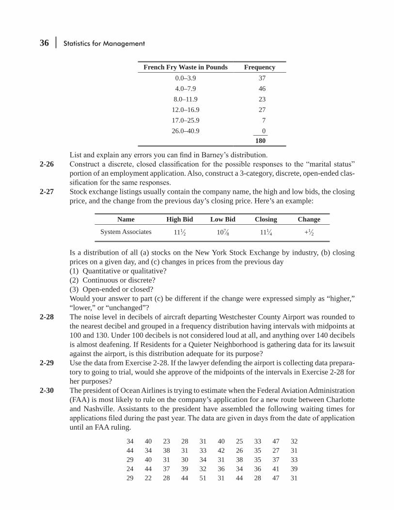
36 Statistics for Management
French Fry Waste in Pounds Frequency0.0–3.94.0–7.98.0–11.9
12.0–16.917.0–25.926.0–40.9
374623277
0180
2-26 portion of an employment application. Also, construct a 3-category, discrete, open-ended clas-
2-27 Stock exchange listings usually contain the company name, the high and low bids, the closing price, and the change from the previous day’s closing price. Here’s an example:
Name High Bid Low Bid Closing Change
System Associates 1112 107
8 1114 +1
2
Is a distribution of all (a) stocks on the New York Stock Exchange by industry, (b) closing prices on a given day, and (c) changes in prices from the previous day(1) Quantitative or qualitative?(2) Continuous or discrete?(3) Open-ended or closed?Would your answer to part (c) be different if the change were expressed simply as “higher,” “lower,” or “unchanged”?
2-28 The noise level in decibels of aircraft departing Westchester County Airport was rounded to the nearest decibel and grouped in a frequency distribution having intervals with midpoints at 100 and 130. Under 100 decibels is not considered loud at all, and anything over 140 decibels is almost deafening. If Residents for a Quieter Neighborhood is gathering data for its lawsuit against the airport, is this distribution adequate for its purpose?
2-29 Use the data from Exercise 2-28. If the lawyer defending the airport is collecting data prepara-tory to going to trial, would she approve of the midpoints of the intervals in Exercise 2-28 for her purposes?
2-30 The president of Ocean Airlines is trying to estimate when the Federal Aviation Administration (FAA) is most likely to rule on the company’s application for a new route between Charlotte and Nashville. Assistants to the president have assembled the following waiting times for
until an FAA ruling.
34 40 23 28 31 40 25 33 47 3244 34 38 31 33 42 26 35 27 3129 40 31 30 34 31 38 35 37 3324 44 37 39 32 36 34 36 41 3929 22 28 44 51 31 44 28 47 31

Grouping and Displaying Data to Convey Meaning: Tables and Graphs 37
(a) Construct a frequency distribution using 10 closed intervals, equally spaced. Which inter-val contains the most data points?
(b) Construct a frequency distribution using 5 closed intervals, equally spaced. Which inter-val contains the most data points?
(c) If the president of Ocean Airlines had a relative frequency distribution for either (a) or (b), would that help him estimate the answer he needs?
2-31 For the purpose of performance evaluation and quota adjustment, Ralph Williams monitored the auto sales of his 40 salespeople. Over a 1-month period, they sold the following number of cars:
7 8 5 10 9 10 5 12 8 610 11 6 5 10 11 10 5 9 138 12 8 8 10 15 7 6 8 85 6 9 7 14 8 7 5 5 14
(a) Based on frequency, what would be the desired class marks (midpoints of the intervals)?(b) Construct a frequency and relative frequency distribution having as many of these marks
as possible. Make your intervals evenly spaced and at least two cars wide.(c) If sales fewer than seven cars a month is considered unacceptable performance, which
of the two answers, (a) or (b), helps you more in identifying the unsatisfactory group of salespeople?
2-32 of its stores. Their marketing-research director suggests that keeping better records for each store is the key to preventing stockouts. Don Martin, director of store operations, collects data
(c) Are the data qualitative or quantitative?(d) What would you suggest Martin do to generate better data for market-research purposes?
2-33 Doug Atkinson is the owner and ticket collector for a ferry that transports people and cars from Long Island to Connecticut. Doug has data indicating the number of people, as well as the number of cars, that have ridden the ferry during the past 2 months. For example,
JULY 3 NUMBER OF PEOPLE, 173 NUMBER OF CARS, 32
might be a typical daily entry for Doug. Doug has set up six equally spaced classes to record the daily number of people, and the class marks are 84.5, 104.5, 124.5, 144.5, 164.5, and 184.5. Doug’s six equally spaced classes for the daily number of cars have class marks of 26.5, 34.5, 42.5, 50.5, 58.5, and 66.5. (The class marks are the midpoints of the intervals.)(a) What are the upper and lower boundaries of the classes for the number of people?(b) What are the upper and lower boundaries of the classes for the number of cars?
Worked-Out Answers to Self-Check ExercisesSC 2-3 Class 1–6 7–12 13–18 19–24 25–30
Frequency 4 8 4 3 1Relative Frequency 0.20 0.40 0.20 0.15 0.05
38 Statistics for Management
(a) Assuming that the shop is open 6 days a week, we see that fully 80 percent of the orders
(b) We can tell only that between 20 percent and 60 percent of the deliveries are made in 10 or fewer days, so the distribution does not generate enough information to determine whether the goal has been met.
(c) A relative frequency distribution lets us present frequencies as fractions or percentages.SC 2-4 The distribution is not all-inclusive. The data point 500°C is left out, along with the points
between 541°C and 549°C, inclusive. In addition, the distribution is closed on the high end, which eliminates all data points above 600°C. These omissions might explain the fact that the total number of observations is only 360, rather than 365 as might be expected for a data set compiled over one year. (Note: It is not absolutely necessary that the distribution be open-ended on the high end, especially if no data points were recorded above 600°C. However, for completeness, the distribution should be continuous over the range selected, even though
exclusive. Two points, 530°C and 580°C, are contained in more than one interval. When creat-
2.5 GRAPHING FREQUENCY DISTRIBUTIONSFigures 2-1 and 2-2 (on page 29) are previews of what we are going to discuss now: how to present frequency distributions graphically. Graphs give data in a two-dimensional picture. On the horizontal axis, we can show the values of the variable (the characteristic we are measuring), such as the carpet output in yards. On the vertical axis, we mark the frequencies of the classes shown on the horizontal axis. Thus, the height of the boxes in Figure 2-1 measures the number of observations in each of the classes marked on the horizontal axis. Graphs of frequency distributions and relative frequency distributions are useful because they emphasize and clarify patterns that are not so readily discernible in tables. They attract a reader’s attention to patterns in the data. Graphs can also help us do problems concerning frequency distributions. They will enable us to estimate some values at a glance and will provide us with a pictorial check on the accuracy of our solutions.
HistogramsFigures 2-1 and 2-2 (page 29) are two examples of histograms. A histogram is a series of rectangles, each proportional in width to the range of values within a class and proportional in height to the number of items falling in the class. If the classes we use in the frequency distribution are of equal width, then the vertical bars in the histogram are also of equal width. The height of the bar for each class corresponds to the number of items in the class. As a result, the area contained in each rectangle (width times height) is the same percentage of the area of all the rectangles as the frequency of that class is to all the observations made.
A histogram that uses the relative frequency of data points in each of the classes rather than the actual number of points is called a relative frequency histogram. The relative frequency histogram has the same shape as an absolute frequency histogram made from the same data set. This is true because in both, the relative size of each rectangle is the frequency of that class compared to the total number of observations.
Identifying the horizontal and
vertical axes
Function of graphs
Histograms described
Function of a relative
frequency histogram
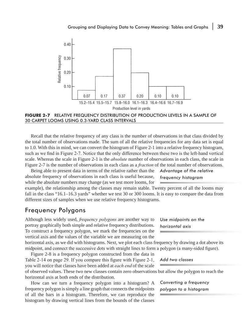
Grouping and Displaying Data to Convey Meaning: Tables and Graphs 39
Recall that the relative frequency of any class is the number of observations in that class divided by the total number of observations made. The sum of all the relative frequencies for any data set is equal to 1.0. With this in mind, we can convert the histogram of Figure 2-1 into a relative frequency histogram,
scale. Whereas the scale in Figure 2-1 is the absolute number of observations in each class, the scale in Figure 2-7 is the number of observations in each class as a fraction of the total number of observations.
Being able to present data in terms of the relative rather than the absolute frequency of observations in each class is useful because, while the absolute numbers may change (as we test more looms, for example), the relationship among the classes may remain stable. Twenty percent of all the looms may fall in the class “16.1–16.3 yards” whether we test 30 or 300 looms. It is easy to compare the data from different sizes of samples when we use relative frequency histograms.
Frequency PolygonsAlthough less widely used, frequency polygons are another way to portray graphically both simple and relative frequency distributions. To construct a frequency polygon, we mark the frequencies on the vertical axis and the values of the variable we are measuring on the horizontal axis, as we did with histograms. Next, we plot each class frequency by drawing a dot above its
Figure 2-8 is a frequency polygon constructed from the data in
you will notice that classes have been added at each end of the scale of observed values. These two new classes contain zero observations but allow the polygon to reach the horizontal axis at both ends of the distribution.
How can we turn a frequency polygon into a histogram? A frequency polygon is simply a line graph that connects the midpoints of all the bars in a histogram. Therefore, we can reproduce the histogram by drawing vertical lines from the bounds of the classes
Advantage of the relative
frequency histogram
Use midpoints on the
horizontal axis
Add two classes
Converting a frequency
polygon to a histogram
0.40
0.30
0.20
0.10
Rela
tive
frequ
ency
15.2–15.4 15.5–15.7 15.8–16.0 16.1–16.3 16.4–16.6 16.7–16.9Production level in yards
0.07 0.17 0.37 0.20 0.10 0.10
FIGURE 2-7 RELATIVE FREQUENCY DISTRIBUTION OF PRODUCTION LEVELS IN A SAMPLE OF 30 CARPET LOOMS USING 0.3-YARD CLASS INTERVALS

40 Statistics for Management
(as marked on the horizontal axis) and connecting them with horizontal lines at the heights of the polygon at each midpoint. We have done this with dotted lines in Figure 2-9.
A frequency polygon that uses the relative frequency of data points in each of the classes rather than the actual number of points is called a relative frequency polygon. The relative frequency polygon has the same shape as the frequency polygon made from the same data set but a different scale of values on the vertical axis. Rather than the absolute number of observations, the scale is the number of observa-tions in each class as a fraction of the total number of observations.
Histograms and frequency polygons are similar. Why do we need both? The advantages of histograms are 1. The rectangle clearly shows each separate class in the distribution. 2. The area of each rectangle, relative to all the other rectangles, shows the proportion of the total
number of observations that occur in that class.Frequency polygons, however, have certain advantages, too.
1. The frequency polygon is simpler than its histogram counterpart. 2. It sketches an outline of the data pattern more clearly. 3. The polygon becomes increasingly smooth and curvelike as we increase the number of classes and
the number of observations.
Constructing a relative
frequency polygon
Advantages of histograms
Advantages of polygons
FIGURE 2-8 FREQUENCY POLYGON OF PRODUCTION LEVELS IN A SAMPLE OF 30 CARPET LOOMS USING 0.3-YARD CLASS INTERVALS
14
12
10
8
6
4
2
15.0 15.3 15.6 15.9 16.2 16.5 16.8 17.1
Freq
uenc
y
Production level in yards
FIGURE 2-9 HISTOGRAM DRAWN FROM THE POINTS OF THE FREQUENCY POLYGON IN FIGURE 2-8
14
12
10
8
6
4
2
15.0 15.3 15.6 15.9 16.2 16.5 16.8 17.1
Freq
uenc
y
Production level in yards
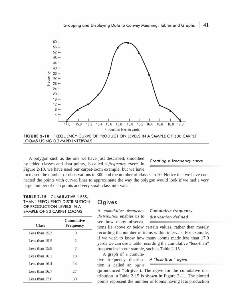
Grouping and Displaying Data to Convey Meaning: Tables and Graphs 41
A polygon such as the one we have just described, smoothed by added classes and data points, is called a frequency curve. In Figure 2-10, we have used our carpet-loom example, but we have increased the number of observations to 300 and the number of classes to 10. Notice that we have con-nected the points with curved lines to approximate the way the polygon would look if we had a very large number of data points and very small class intervals.
OgivesA cumulative frequency distribution enables us to see how many observa-tions lie above or below certain values, rather than merely recording the number of items within intervals. For example, if we wish to know how many looms made less than 17.0 yards we can use a table recording the cumulative “less-than” frequencies in our sample, such as Table 2-15.
A graph of a cumula-tive frequency distribu-tion is called an ogive (pronounced “oh-jive”). The ogive for the cumulative dis-tribution in Table 2-15 is shown in Figure 2-11. The plotted points represent the number of looms having less production
Creating a frequency curve
Cumulative frequency
distribution defined
A “less-than” ogive
60565248444036322824201612
84
14.8 15.0 15.2 15.4 15.6 15.8 16.0 16.2 16.4 16.6 16.8 17.0
Freq
uenc
y
Production level in yards
FIGURE 2-10 FREQUENCY CURVE OF PRODUCTION LEVELS IN A SAMPLE OF 300 CARPET LOOMS USING 0.2-YARD INTERVALS
ClassCumulative Frequency
Less than 15.2 0
Less than 15.5 2
Less than 15.8 7
Less than 16.1 18
Less than 16.4 24
Less than 16.7 27
Less than 17.0 30
TABLE 2-15 CUMULATIVE “LESS-THAN” FREQUENCY DISTRIBUTION OF PRODUCTION LEVELS IN A SAMPLE OF 30 CARPET LOOMS
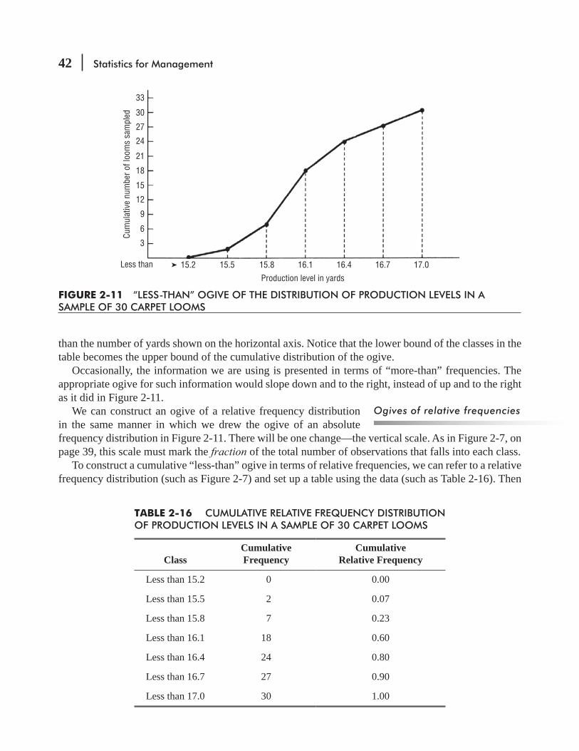
42 Statistics for Management
than the number of yards shown on the horizontal axis. Notice that the lower bound of the classes in the table becomes the upper bound of the cumulative distribution of the ogive.
Occasionally, the information we are using is presented in terms of “more-than” frequencies. The appropriate ogive for such information would slope down and to the right, instead of up and to the right as it did in Figure 2-11.
We can construct an ogive of a relative frequency distribution in the same manner in which we drew the ogive of an absolute frequency distribution in Figure 2-11. There will be one change—the vertical scale. As in Figure 2-7, on page 39, this scale must mark the fraction of the total number of observations that falls into each class.
To construct a cumulative “less-than” ogive in terms of relative frequencies, we can refer to a relative frequency distribution (such as Figure 2-7) and set up a table using the data (such as Table 2-16). Then
Ogives of relative frequencies
33
30
27
24
21
18
15
12
9
6
3
15.2 15.5 15.8 16.1 16.4 16.7 17.0
Cum
ulat
ive
num
ber o
f loo
ms
sam
pled
Production level in yards
Less than
FIGURE 2-11 “LESS-THAN” OGIVE OF THE DISTRIBUTION OF PRODUCTION LEVELS IN A SAMPLE OF 30 CARPET LOOMS
ClassCumulative Frequency
Cumulative Relative Frequency
Less than 15.2 0 0.00
Less than 15.5 2 0.07
Less than 15.8 7 0.23
Less than 16.1 18 0.60
Less than 16.4 24 0.80
Less than 16.7 27 0.90
Less than 17.0 30 1.00
TABLE 2-16 CUMULATIVE RELATIVE FREQUENCY DISTRIBUTION OF PRODUCTION LEVELS IN A SAMPLE OF 30 CARPET LOOMS

Grouping and Displaying Data to Convey Meaning: Tables and Graphs 43
equivalent except for the left-hand vertical axis.Suppose we now draw a line perpendicular to the vertical axis
at the 0.50 mark to intersect our ogive. (We have done this in Figure 2-13.) In this way, we can read an approximate value of 16.0 for the production level in the
construct frequency distributions. From frequency distributions, we can construct cumulative frequency distributions. From these, we can graph an ogive. And from this ogive, we can approximate the values we had in the data array. However, we cannot normally recover the exact original data from any of the graphic representations we have discussed.
Approximating the data array
1.00
0.90
0.80
0.70
0.60
0.50
0.40
0.30
0.20
0.10
15.2 15.5 15.8 16.1 16.4 16.7 17.0
Cum
ulat
ive
rela
tive
frequ
ency
Production level in yards
Less than
FIGURE 2-12 “LESS-THAN” OGIVE OF THE DISTRIBUTION OF PRODUCTION LEVELS IN A SAMPLE OF 30 CARPET LOOMS USING RELATIVE FREQUENCIES
1.00
Approximate value of 15th loom = 16.0
0.90
0.80
0.70
0.60
0.50
0.40
0.30
0.20
0.10
15.2 15.5 15.8 16.1 16.4 16.7 17.0
Cum
ulat
ive
rela
tive
frequ
ency
Production level in yards
Less than
FIGURE 2-13 “LESS-THAN” OGIVE OF THE DISTRIBUTION OF THE PRODUCTION LEVELS IN A SAMPLE OF 30 CARPET LOOMS, INDICATING THE APPROXIMATE MIDDLE VALUE IN THE ORIGINAL DATA ARRAY

44 Statistics for Management
Using Statistical Packages to Graph Frequency Distribution:
Histogram
Above data is sample of daily production in meters of 30 carpet looms and the desired mid values for creating histogram.
For histogram go to DATA>DATA ANALYISYS >HISTOGARAM>DEFINE INPUT RANGE, BIN RANGE (mid values)> SELECT CHART OUTPUT>OK.
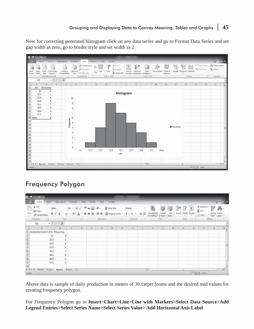
Grouping and Displaying Data to Convey Meaning: Tables and Graphs 45
Now for correcting generated histogram click on any data series and go to Format Data Series and set gap width as zero, go to border style and set width as 2.
Frequency Polygon
Above data is sample of daily production in meters of 30 carpet looms and the desired mid values for creating frequency polygon.
For Frequency Polygon go to Insert>Chart>Line>Line with Markers>Select Data Source>Add Legend Entries>Select Series Name>Select Series Value> Add Horizontal Axis Label

46 Statistics for Management
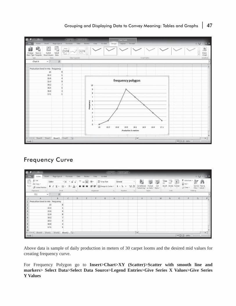
Grouping and Displaying Data to Convey Meaning: Tables and Graphs 47
Frequency Curve
Above data is sample of daily production in meters of 30 carpet looms and the desired mid values for creating frequency curve.
For Frequency Polygon go to Insert>Chart>XY (Scatter)>Scatter with smooth line and markers> Select Data>Select Data Source>Legend Entries>Give Series X Values>Give Series Y Values

48 Statistics for Management

Grouping and Displaying Data to Convey Meaning: Tables and Graphs 49
Bar ChartBelow data is sample unit wise production in meters of 30 carpet looms for creating bar chart.
For Bar chart go to Insert>Chart>Column>Clustered Column>Select Data>Add Legend Entries> Add Horizontal Axis Label

50 Statistics for Management

Grouping and Displaying Data to Convey Meaning: Tables and Graphs 51
Pie ChartBelow data is sample weekday production in meters of 30 carpet looms for creating pie chart.
For Pie Chart go to Insert>Chart>Pie>Pie in 3D>Select Data>Add Legend Entries>Add Horizontal Axis Label

52 Statistics for Management
Whoever said “a picture is worth a thousand words” understood intuitively what we have been covering in this section. Using graphic methods to display data gives us a quick sense of patterns and trends and what portion of our data is above or below a certain value. Warning: Some publica-tions print graphic displays of data (histograms) in a way that is confusing by using a vertical axis that doesn’t go all the way to zero. Be aware when you see one of these that small differences have been made to look too large, and that the pattern you are seeing is misleading.
HINTS & ASSUMPTIONS
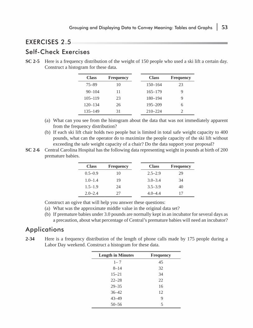
Grouping and Displaying Data to Convey Meaning: Tables and Graphs 53
EXERCISES 2.5
Self-Check ExercisesSC 2-5 Here is a frequency distribution of the weight of 150 people who used a ski lift a certain day.
Construct a histogram for these data.
Class Frequency Class Frequency75–89 10 150–164 23
90–104 11 165–179 9105–119 23 180–194 9120–134 26 195–209 6135–149 31 210–224 2
(a) What can you see from the histogram about the data that was not immediately apparent from the frequency distribution?
(b) If each ski lift chair holds two people but is limited in total safe weight capacity to 400 pounds, what can the operator do to maximize the people capacity of the ski lift without exceeding the safe weight capacity of a chair? Do the data support your proposal?
SC 2-6 Central Carolina Hospital has the following data representing weight in pounds at birth of 200 premature babies.
Class Frequency Class Frequency0.5–0.9 10 2.5–2.9 291.0–1.4 19 3.0–3.4 341.5–1.9 24 3.5–3.9 402.0–2.4 27 4.0–4.4 17
Construct an ogive that will help you answer these questions:(a) What was the approximate middle value in the original data set?(b) If premature babies under 3.0 pounds are normally kept in an incubator for several days as
a precaution, about what percentage of Central’s premature babies will need an incubator?
Applications2-34 Here is a frequency distribution of the length of phone calls made by 175 people during a
Labor Day weekend. Construct a histogram for these data.
Length in Minutes Frequency 1– 7 45 8–14 3215–21 3422–28 2229–35 1636–42 1243–49 950–56 5

54 Statistics for Management
(a) Describe the general shape of the histogram. Does there appear to be a pattern?(b) Suppose all the people were making their calls from a room that had 10 different phones,
and each person knew which time class the call would belong to. Suggest an ordering so that all calls can be completed as fast as possible.
(c) Does the order affect the length of time to complete all calls?2-35 Golden Acres is a homeowners’ association that operates a trailer park outside Orlando,
Florida, where retirees keep their winter homes. In addition to lot rents, a monthly facility fee of $12 is charged for social activities at the clubhouse. One board member has noted that many of the older residents never attend the clubhouse functions, and has proposed waiving the fee for association members over age 60. A survey of 25 residents reported the following ages:
66 65 96 80 7193 66 96 75 6169 61 51 84 5873 77 89 69 9257 56 55 78 96
Construct an ogive that will help you answer these questions:(a) Roughly what proportion of residents would be eligible for no fee?(b) Approximately what fee would the board have to charge to the remaining (fee-paying)
residents to cover the same total cost of running the clubhouse?2-36
even catch on his boats is 5,000 pounds per trip. Here are data on a sample of catches on 20
6,500 6,700 3,400 3,600 2,0007,000 5,600 4,500 8,000 5,0004,600 8,100 6,500 9,000 4,2004,800 7,000 7,500 6,000 5,400
Construct an ogive that will help you answer these questions:(a) Roughly what proportion of the trips breaks even for Homer?(b) What is the approximate middle value in the data array for Homer’s boats?(c) What catch do Homer's boats exceed 80 percent of the time?
2-37 The Massachusetts Friends of Fish has the following data representing pollutants (in parts per million) at 150 sites in the state:
Pollutants (in ppm) Frequency Pollutants (in ppm) Frequency
5.0– 8.9 14 25.0–28.9 16
9.0–12.9 16 29.0–32.9 9
13.0–16.9 28 33.0–36.9 7
17.0–20.9 36 37.0–40.9 4
21.0–24.9 20
Construct an ogive that will help you answer the following questions:(a) Below what value (approximately) do the lowest one-fourth of these observations fall?(b) If the Friends of Fish heavily monitor all sites with more than 30 ppm of pollutants, what
percentage of sites will be heavily monitored?
Grouping and Displaying Data to Convey Meaning: Tables and Graphs 55
2-38 Before constructing a dam on the Colorado River, the U.S. Army Corps of Engineers per-
results of the testing were used to construct the following frequency distribution:
River Flow (Thousands of Gallons per Minute) Frequency1,001–1,050 71,051–1,100 211,101–1,150 321,151–1,200 491,201–1,250 581,251–1,300 411,301–1,350 271,351–1,400 11
Total 246
(a) Use the data given in the table to construct a “more-than” cumulative frequency distribution and ogive.
(b) Use the data given in the table to construct a “less-than” cumulative frequency distribution and ogive.
of gallons per minute.2-39 -
ment programs attractive to senior citizens. She knew that if potential customers could obtain a certain level of return, they would be willing to risk an investment, but below a certain level, they would be reluctant. From a group of 50 subjects, she obtained the following data regard-ing the various levels of return required for each subject to invest $1,000:
Indifference Point Frequency Indifference Point Frequency$70–74 2 $ 90– 94 11 75–79 5 95– 99 3 80–84 10 100–104 3 85–89 14 105–109 2
(a) Construct both “more-than” and “less-than” cumulative relative frequency distributions.(b) Graph the 2 distributions in part (a) into relative frequency ogives.
2-40 50 days. The data, to the nearest tenth of a minute, are given below.
20.8 22.8 21.9 22.0 20.7 20.9 25.0 22.2 22.8 20.125.3 20.7 22.5 21.2 23.8 23.3 20.9 22.9 23.5 19.523.7 20.3 23.6 19.0 25.1 25.0 19.5 24.1 24.2 21.821.3 21.5 23.1 19.9 24.2 24.1 19.8 23.9 22.8 23.919.7 24.2 23.8 20.7 23.8 24.3 21.1 20.9 21.6 22.7
(a) Arrange the data in an array from lowest to highest.(b) Construct a frequency distribution and a “less-than” cumulative frequency distribution
from the data, using intervals of 0.8 minute.

56 Statistics for Management
(c) Construct a frequency polygon from the data.(d) Construct a “less-than” ogive from the data.(e) From your ogive, estimate what percentage of the time the front page can be set in less
than 24 minutes.2-41 Chien-Ling Lee owns a CD store specializing in spoken-word recordings. Lee has 35 months
of gross sales data, arranged as a frequency distribution.
Monthly Sales Frequency Monthly Sales Frequency$10,000–12,499 2 $20,000–22,499 612,500–14,999 4 22,500–24,999 815,000–17,499 7 25,000–27,499 217,500–19,999 5 27,500–29,999 1
(a) Construct a relative frequency distribution.(b) Construct, on the same graph, a relative frequency histogram and a relative frequency
polygon.2-42 The National Association of Real Estate Sellers has collected these data on a sample of 130
salespeople representing their total commission earnings annually:
Earnings Frequency$ 5,000 or less 5$ 5,001–$10,000 9$10,001–$15,000 11$15,001–$20,000 33$20,001–$30,000 37$30,001–$40,000 19$40,001–$50,000 9Over $50,000 7
Construct an ogive that will help you answer these questions.(a) About what proportion of the salespeople earns more than $25,000?(b) About what does the “middle” salesperson in the sample earn?(c) Approximately how much could a real estate salesperson whose performance was about
25 percent from the top expect to earn annually?2-43
have received tickets for illegally parked cars to come in and make their case to an administra--
ing frequency distribution for the time spent on each appeal:
Minutes Spent on Appeal Frequency Minutes Spent on Appeal FrequencyLess than 2 30 8–9 70
2–3 40 10–11 504–5 40 12–13 506–7 90 14–15 30
400

Grouping and Displaying Data to Convey Meaning: Tables and Graphs 57
(a) Construct a “less-than” cumulative frequency distribution.(b) Construct an ogive based on part (a).(c) The town administrator will consider streamlining the paperwork for the appeal process if
more than 50 percent of appeals take longer than 4 minutes. What is the percentage taking more than 4 minutes? What is the approximate time for the 200th (midpoint) appeal?
Worked-Out Answers to Self-Check Exercises
SC 2-5 323028262422201816141210
86420
82.5 97.5 112.5 127.5 142.5 157.5 172.5 187.5 202.5 217.5
Freq
uenc
y
Weight (pounds)
(a) The lower tail of the distribution is fatter (has more observations in it) than the upper tail.(b) Because there are so few people who weigh 180 pounds or more, the operator can afford
to pair each person who appears to be heavy with a lighter person. This can be done with-out greatly delaying any individual’s turn at the lift.
C 2-6 Class
Cumulative Relative Frequency Class
Cumulative Relative Frequency
0.5–0.9 0.050 2.5–2.9 0.5451.0–1.4 0.145 3.0–3.4 0.7151.5–1.9 0.265 3.5–3.9 0.9152.0–2.4 0.400 4.0–4.4 1.000
10.90.80.70.60.50.40.30.20.1
00.5 1 1.5 2 2.5 3 4 4.53.5
Cum
ulat
ive
rela
tive
frequ
ency
Weight (pounds)
(a) The middle value was about 2.8 pounds.(b) About 55 percent will need incubators.
58 Statistics for Management
STATISTICS AT WORK
Loveland ComputersCase 2: Arranging Data New Year’s Day 1995, found Lee Azko staring out the window, watching a light dusting of snow fall on the Denver suburbs. Lee had graduated early from the University of Colorado, one semester short of the usual 4 years, thanks to a handful of advanced placement credits from high school. Lee was both excited and apprehensive that the next day would be the start of a serious job search for a well-trained business major, with little experience in the real world.
Contemplation of the future was interrupted by a phone call from Lee’s uncle. ‘‘I was going to call
things have come up in the business, and it looks as if I need someone to crunch some numbers in a hurry. Why don’t you drive up tomorrow and I’ll tell you what I have in mind.’’
Lee knew that Uncle Walter’s company, Loveland Computers, had been growing by leaps and bounds. Walter Azko had developed the computer company from a strange background. Unlike Lee, Walter
had traveled extensively in the Far East with his parents, so it was only natural that he would begin an importing business while still a student at Boulder. He imported just about anything that could be sold cheaply and that would appeal to students: furniture, gifts, household utensils, and some clothing.
On one buying trip to Taiwan in the early 1980s, Walter was offered some personal computers. Looking back, they were awful. Not much memory and no hard drive, but they were dirt cheap and Walter soon sold them to “tekkies” at the university. The computer business grew, and within 2 years, Walter sold his retail importing business and concentrated solely on importing and selling computers.
much cheaper than in Boulder. From this location, he could market directly to students at the Universities at Boulder, Fort Collins, and Greeley. About an hour north of Denver’s Stapleton International Airport, Loveland was a convenient site for imports coming by airfreight and a good place to recruit part-time workers. The name Loveland Computers seemed a natural.
his car. Walter made every sale on price alone and word-of-mouth referrals supplemented a few ads placed in the college newspapers. Because he sold directly to students and enthusiasts, it seemed that he was the only game in town. Walter’s niche seemed to be an altogether different market from the one being reached by the industry giants. At the top end of the market for PCs, IBM was using expensive retail distribution, targeting the business market. And Apple was defending its high-price strategy with easy ‘‘point-and-click” graphical computing that couldn’t be matched by IBM-compatible machines.
Azko began reading computer magazines and found he wasn’t the only box shop (the industry name for a company that shipped boxes of computers to users with little or no additional service). One or two other companies had found cheap overseas suppliers and they were pursuing a mail-order strategy. Walter thought customers would be reluctant to buy such an expensive—and novel—piece of equip-ment sight unseen, but the arrival of a new shipment of computers with preinstalled hard disk drives gave him the motivation to run a few ads of his own.
So Loveland Computers joined the ranks of the national mail-order box shops, and by 1988, the company was one of the two dozen companies in this market. The mail-order companies together shared about the same percentage of the market as ‘‘Big Blue’’ (IBM) was maintaining: about 20 percent. But the market for PCs was huge and growing rapidly. By 1993, Loveland Computers regularly booked
sales. Uncle Walter had become a rich man.

Grouping and Displaying Data to Convey Meaning: Tables and Graphs 59
Along the way, Walter Azko realized that to give customers exactly what they wanted, there were advantages in assembling computers at his ever-expanding Loveland facility. He never saw himself as a manufacturer—just an assembler of premade parts such as drive controllers and power supplies. With his contacts with overseas manufacturers, Walter was able to hunt around for the best prices, so Loveland Computers’ costs remained low.
Gratia Delaguardia. Gratia knew hardware: She had completed several development projects for Storage Technology. In only a few years at Loveland Computers, she built a development staff of more than two dozen and was rewarded with a partnership in the business.
Loveland Computers had a few setbacks due to misjudging demand. Walter Azko was always opti-mistic about sales so inventory of components was often much greater than needed. Once or twice there were embarrassing ‘‘write-downs,’’ such as when a shipment of power supplies turned out to be useless because they produced too little current for Loveland’s latest model. Gratia Delaguardia had concluded
market would be like from one month to the next.After a sleepless night, Lee Azko met with Loveland Computers’ founder and president. ‘‘Come and
sit over here by the window—you can see my new Mercedes 500 SL sports car,’’ Walter Azko said, wel-coming his young visitor. ‘‘Let me tell you my problem. You know that things move pretty fast around here. Seems like each model lasts about 6 months and then we replace it with something fancier. Up to
getting some attention from folks on Wall Street. We may be doing a ‘private placement’—that’s where we’d raise money for expansion from one or two well-heeled investors or banks—and then, later on, we might want to take the company public. Thing is, they want to know a whole lot about our sales growth: how much is coming from which products and so on. They want to know how long each model lasts, what we should project for next year. Now, of course, I have monthly sales reports going back almost to the beginning. The good news is, it’s all on disk. The bad news is, we kept changing our formats so
reports. Your job is to organize it all so it makes sense when these city slickers come to town in their corporate jet.’’
‘‘When would I start, Uncle?’’ asked Lee Azko, quite taken aback by the task ahead.
due in next Monday.’’Lee made a mental note to cancel a ski trip planned for the weekend and pulled out a notepad and
started to sketch out a plan.Study Questions:
sales and income? What format will present the company’s rapid growth most clearly in a 45-minute business presentation?
CHAPTER REVIEW
Terms Introduced in Chapter 2Continuous Data Data that may progress from one class to the next without a break and may be expressed by either whole numbers or fractions.Cumulative Frequency Distribution A tabular display of data showing how many observations lie above, or below, certain values.

60 Statistics for Management
Data A collection of any number of related observations on one or more variables.Data Array The arrangement of raw data by observations in either ascending or descending order.Data Point A single observation from a data set.Data Set A collection of data.Discrete Classes Data that do not progress from one class to the next without a break; that is, where classes represent distinct categories or counts and may be represented by whole numbers.Frequency Curve A frequency polygon smoothed by adding classes and data points to a data set.Frequency Distribution An organized display of data that shows the number of observations from the data set that falls into each of a set of mutually exclusive and collectively exhaustive classes.Frequency Polygon A line graph connecting the midpoints of each class in a data set, plotted at a height corresponding to the frequency of the class.Histogram A graph of a data set, composed of a series of rectangles, each proportional in width to the range of values in a class and proportional in height to the number of items falling in the class, or the fraction of items in the class.Ogive A graph of a cumulative frequency distribution.Open-Ended Class scheme to be limitless.Population A collection of all the elements we are studying and about which we are trying to draw conclusions.Raw Data Information before it is arranged or analyzed by statistical methods.Relative Frequency Distribution The display of a data set that shows the fraction or percentage of the total data set that falls into each of a set of mutually exclusive and collectively exhaustive classes.Representative Sample A sample that contains the relevant characteristics of the population in the same proportions as they are included in that population.Sample A collection of some, but not all, of the elements of the population under study, used to describe the population.
Equations Introduced in Chapter 2
2-1 Width of class intervals =
Next unit value afterlargest value in data – Smallest value in data
Total number of class intervals p. 28
To arrange raw data, decide the number of classes into which you will divide the data (nor-mally between 6 and 15), and then use Equation 2-1 to determine the width of class intervals of equal size. This formula uses the next value of the same units because it measures the inter-
Review and Application Exercises2-44 The following set of raw data gives income and education level for a sample of individuals.
Would rearranging the data help us to draw some conclusions? Rearrange the data in a way that makes them more meaningful.
Grouping and Displaying Data to Convey Meaning: Tables and Graphs 61
Income Education Income Education Income Education$17,000 High school $ 21,200 B.S. $17,200 2 years college
20,800 B.S. 28,000 B.S. 19,600 B.A.27,000 M.A. 30,200 High school 36,200 M.S.70,000 M.D. 22,400 2 years college 14,400 1 year college29,000 Ph.D. 100,000 M.D. 18,400 2 years college14,400 10th grade 76,000 Law degree 34,400 B.A.19,000 High school 44,000 Ph.D. 26,000 High school23,200 M.A. 17,600 11th grade 52,000 Law degree30,400 High school 25,800 High school 64,000 Ph.D.25,600 B.A. 20,200 1 year college 32,800 B.S.
2-45 All 50 states send the following information to the Department of Labor: the average num-
absentees for each state. Is this an example of raw data? Explain.2.46 The Nebraska Department of Agriculture has these data representing weekly growth (in
inches) on samples of newly planted spring corn:
0.4 1.9 1.5 0.9 0.3 1.6 0.4 1.5 1.2 0.80.9 0.7 0.9 0.7 0.9 1.5 0.5 1.5 1.7 1.8
(a) Arrange the data in an array from highest to lowest.(b) Construct a relative frequency distribution using intervals of 0.25.(c) From what you have done so far, what conclusions can you come to about growth in this
sample?(d) Construct an ogive that will help you determine what proportion of the corn grew at more
than 1.0 inch a week.(e) What was the approximate weekly growth rate of the middle item in the data array?
2-47 The National Safety Council randomly sampled the tread depth of 60 right front tires on pas-senger vehicles stopped at a rest area on an interstate highway. From its data, it constructed the following frequency distribution:
Tread Depth (Inches) Frequency Tread Depth (Inches) Frequency
16 __ 32 (new tire) 5 4 __ 32 – 6 __ 32 7
13 __ 32 – 15 __ 32 10 1 __ 32 – 3 __ 32 4
10 __ 32 – 12 __ 32 20 0 __ 32 bald 2
7 __ 32 – 9 __ 32 12
(a) Approximately what was the tread depth of the thirtieth tire in the data array?(b) If a tread depth less than 7 __ 32 inch is considered dangerous, approximately what proportion
of the tires on the road are unsafe?2-48 The High Point Fastener Company produces 15 basic items. The company keeps records
on the number of each item produced per month in order to examine the relative production
62 Statistics for Management
levels. Records show the following numbers of each item were produced by the company for the last month of 20 operating days:
9,897 10,052 10,028 9,722 9,90810,098 10,587 9,872 9,956 9,92810,123 10,507 9,910 9,992 10,237
Construct an ogive that will help you answer these questions.(a) On how many of its items did production exceed the break-even point of 10,000 units?(b) What production level did 75 percent of its items exceed that month?(c) What production level did 90 percent of its items exceed that month?
2-49 The administrator of a hospital has ordered a study of the amount of time a patient must wait before being treated by emergency room personnel. The following data were collected during a typical day:
Waiting Time (Minutes)12 16 21 20 24 3 11 17 29 1826 4 7 14 25 1 27 15 16 5
(a) Arrange the data in an array from lowest to highest. What comment can you make about patient waiting time from your data array?
(b) Now construct a frequency distribution using 6 classes. What additional interpretation can you give to the data from the frequency distribution?
(c) From an ogive, state how long 75 percent of the patients should expect to wait based on these data.
2-50 Of what additional value is a relative frequency distribution once you have already constructed a frequency distribution?
2-51 Below are the weights of an entire population of 100 NFL football players.
226 198 210 233 222 175 215 191 201 175264 204 193 244 180 185 190 216 178 190174 183 201 238 232 257 236 222 213 207233 205 180 267 236 186 192 245 218 193189 180 175 184 234 234 180 252 201 187155 175 196 172 248 198 226 185 180 175217 190 212 198 212 228 184 219 196 212220 213 191 170 258 192 194 180 243 230180 135 243 180 209 202 242 259 238 227207 218 230 224 228 188 210 205 197 169
10 elements.(b) Are the two samples equally representative of the population? If not, which sample is
more representative, and why?(c) Under what conditions would the sample of the largest 10 elements be as representative
2-52 In the population under study, there are 2,000 women and 8,000 men. If we are to select a sample of 250 individuals from this population, how many should be women to make our sample considered strictly representative?

Grouping and Displaying Data to Convey Meaning: Tables and Graphs 63
2-53 as well as the rate itself. Recently, the unemployment rate was 6.8 percent. The department reported the following educational categories:
Level of Education Relative Frequency
(% of Those Unemployed)Did not complete high school 35%Received high school diploma 31Attended college but did not receive a degree 16Received a college degree 9Attended graduate school but did not receive a degree 6Received a graduate degree 3 Total 100%
Using these data, construct a relative frequency histogram.2-54 Using the relative frequency distribution given in Exercise 2-63, construct a relative frequency
histogram and polygon. For the purposes of the present exercise, assume that the upper limit of the last class is $51.00.
2-55 Consider the following information about March 1992 nonfarm employment (in thousands of
Alabama 1,639.0 Nebraska 730.6Alaska 235.5 Nevada 638.4Arizona 1,510.0 New Hampshire 466.5Arkansas 951.1 New Jersey 3,390.7California 12,324.3 New Mexico 583.3Colorado 1,552.7 New York 7,666.4Connecticut 1,510.6 North Carolina 3,068.3Delaware 335.2 North Dakota 271.0District of Columbia 667.0 Ohio 4,709.9Florida 5,322.8 Oklahoma 1,196.9Georgia 2,927.1 Oregon 1,245.6Hawaii 546.3 Pennsylvania 4,992.1Idaho 400.4 Rhode Island 413.2Illinois 5,146.2 South Carolina 1,494.6Indiana 2,496.3 South Dakota 295.6Iowa 1,229.2 Tennessee 2,178.6Kansas 1,108.3 Texas 7,209.7Kentucky 1,474.8 Utah 752.2Louisiana 1,617.5 244.8Maine 500.0 2,792.4Maryland 2,037.3 Washington 2,165.8Massachusetts 2,751.6 622.1Michigan 3,828.9 Wisconsin 2,272.1Minnesota 2,117.1 Wyoming 198.0Mississippi 940.9 Puerto Rico 842.4Missouri 2,275.9 42.4Montana 299.3Source: Sharon R. Cohany, “Employment Data,” ‘Monthly Labor Review 115(6), (June 1992): 80–82.
64 Statistics for Management
(a) Arrange the data into 10 equal-width, mutually exclusive classes.(b) Determine the frequency and relative frequency within each class.(c) Are these data discrete or continuous?(d) Construct a “less-than” cumulative frequency distribution and ogive for the relative
frequency distribution in part (b).(e) Based on the ogive constructed in part (d), what proportion of states have nonfarm
employment greater than 3 million?2-56 Using the frequency distribution given in Exercise 2-57 for miles per day of jogging, construct
an ogive that will help you estimate what proportion of the joggers are averaging 4.0 miles or fewer daily.
2-57 A sports psychologist studying the effect of jogging on college students’ grades collected data from a group of college joggers. Along with some other variables, he recorded the average number of miles run per day. He compiled his results into the following distribution:
Miles per Day Frequency1.00–1.39 321.40–1.79 431.80–2.19 812.20–2.59 1222.60–2.99 1313.00–3.39 1303.40–3.79 1113.80–4.19 954.20–4.59 824.60–4.99 47
5.00 and up 53927
(a) Construct an ogive that will tell you approximately how many miles a day the middle jogger runs.
(b) From the ogive you constructed in part (a), approximately what proportion of college joggers run at least 3.0 miles a day?
2-58 A behavioral researcher studying the success of college students in their careers conducts interviews with 100 Ivy League undergraduates, half men and half women, as the basis for the study. Comment on the adequacy of this survey.
2-59 If the following age groups are included in the proportions indicated, how many of each age group should be included in a sample of 3,000 people to make the sample representative?
Age Group Relative Proportion in Population12–17 0.1718–23 0.3124–29 0.2730–35 0.2136+ 0.04
Grouping and Displaying Data to Convey Meaning: Tables and Graphs 65
2-60 State University has three campuses, each with its own business school. Last year, State’s business professors published numerous articles in prestigious professional journals, and the board of regents counted these articles as a measure of the productivity of each department.
Journal Number
Number of Publications Campus
Journal Number
Number of Publications Campus
9 3 North 14 20 South12 6 North 10 18 South3 12 South 3 12 West
15 8 West 5 6 North2 9 West 7 5 North5 15 South 7 15 West1 2 North 6 2 North
15 5 West 2 3 West12 3 North 9 1 North11 4 North 11 8 North7 9 North 14 10 West6 10 West 8 17 South
(a) Construct a frequency distribution and a relative frequency distribution by journal.(b) Construct a frequency distribution and a relative frequency distribution by university
branch.(c) Construct a frequency distribution and a relative frequency distribution by number of
publications (using intervals of 3).
2-61 A reporter wants to know how the cost of compliance with the Americans with Disabilities Act (ADA) has affected national hiring practices and sends out a form letter to 2,000 businesses
2-62 With each appliance that Central Electric produces, the company includes a warranty card for the purchaser. In addition to validating the warranty and furnishing the company with the purchaser’s name and address, the card also asks for certain other information that is used for marketing studies. For each of the numbered blanks on the card, determine the most likely characteristics of the categories that would be used by the company to record the informa-tion. In particular, would they be (1) quantitative or qualitative, (2) continuous or discrete,
Name Marital Status
Address Where was appliance purchased?
Why was appliance purchased?
City State
Zip Code
Age Yearly Income1 2 5
4
3

66 Statistics for Management
2-63 The following relative frequency distribution resulted from a study of the dollar amounts spent per visit by customers at a supermarket:
Amount Spent Relative Frequency$ 0–$ 5.99 1%
6.00–$10.99 311.00–$15.99 416.00–$20.99 621.00–$25.99 726.00–$30.99 931.00–$35.99 1136.00–$40.99 1941.00–$45.99 3246,00 and above 8
Total 100%
Determine the class marks (midpoints) for each of the intervals. 2-64 The following responses were given by two groups of hospital patients, one receiving a new
treatment, the other receiving a standard treatment for an illness. The question asked was, ‘‘What degree of discomfort are you experiencing?’’
Group 1 Group 2
Mild Moderate Severe Moderate Mild SevereNone Severe Mild Severe None ModerateModerate Mild Mild Mild Moderate ModerateMild Moderate None Moderate Mild SevereModerate Mild Mild Severe Moderate ModerateNone Moderate Severe Severe Mild Moderate
Suggest a better way to display these data. Explain why it is better. 2-65
ratings based on total units produced, percentages of rejects, and total hours worked. Is this an example of raw data? Why or why not? If not, what would the raw data be in this situation?
2-66 The head of a large business department wanted to classify the specialties of its 67 members. He asked Peter Wilson, a Ph.D. candidate, to get the information from the faculty members’ publications. Peter compiled the following:
Specialty Faculty Members PublishingAccounting only 1Marketing only 5Statistics only 4Finance only 2Accounting and marketing 7
(continued)

Grouping and Displaying Data to Convey Meaning: Tables and Graphs 67
Specialty Faculty Members PublishingAccounting and statistics 6
389
Statistics and marketing 21No publications 1
67
Construct a relative frequency distribution for the types of specialties. (Hint: The catego-ries of your distribution will be mutually exclusive, but any individual may fall into several categories.)
2-67 Lesley Niles, a summer intern at the Internet Financial Services Corporation, has been asked to investigate the low participation rates in the company’s 401(k) investment program. Niles read an article in The Wall Street Journal commenting on families’ second wage-earner income
-tives eligible to participate. None of the executives reported a spouse with second income over $35,000 and many families had no second income. To examine the situation, Niles decides to construct both frequency and relative frequency distributions.(a) Develop a continuous, closed distribution with $5,000 intervals.(b) Develop a continuous distribution open at both ends, with 6 categories. You may relax the requirement for $5,000 intervals for the open-ended categories.
2-68 The Kawahondi Computer Company compiled data regarding the number of interviews required for each of its 40 salespeople to make a sale. Following are a frequency distribution and a relative frequency distribution of the number of interviews required per salesperson per sale. Fill in the missing data.
Number of Interviews (Classes) Frequency Relative Frequency
0–10 ? 0.075
11–20 1 ?
21–30 4 ?
31–40 ? ?
41–50 2 ?
51–60 ? 0.175
61–70 ? 0.225
71–80 5 ?
81–90 ? 0.000
91–100 ? 0.025
? ?

68 Statistics for Management
2-69 A. T. Cline, the mine superintendent of the Grover Coal Co., has recorded the amount of time per workshift that Section Crew #3 shuts down its machinery for on-the-spot adjustments, repairs, and moving. Here are the records for the crew’s last 35 shifts:
60 72 126 110 91 115 11280 66 101 75 93 129 105
113 121 93 87 119 111 97102 116 114 107 113 119 100110 99 139 108 128 84 99
(a) Arrange the data in an array from highest to lowest.(b) If Cline believes that a typical amount of downtime per shift is 108 minutes, how many of
Crew #3’s last 35 shifts exceeded this limit? How many were under the limit?(c) Construct a relative frequency distribution with 10-minute intervals.(d) Does your frequency distribution indicate that Cline should be concerned?
2-70 Cline has obtained information on Section Crew #3’s coal production per shift for the same 35-shift period discussed in Exercise 2-69. The values are in tons of coal mined per shift:
356 331 299 391 364 317 386360 281 360 402 411 390 362311 357 300 375 427 370 383322 380 353 371 400 379 380369 393 377 389 430 340 368
(a) Construct a relative frequency distribution with six equal intervals.(b) If Cline considers 330 to 380 tons per shift to be an expected range of output, how many
of the crew’s shifts produced less than expected? How many did better than expected?(c) Does this information affect the conclusions you reached from the preceding problem on
equipment downtime?2-71
supplier caught the eye of a clerk. Suboleski sent 25 of the bolts to a testing lab to determine the force necessary to break each of the bolts. In thousands of pounds of force, the results are as follows:
147.8 137.4 125.2 141.1 145.7119.9 133.3 142.3 138.7 125.7142.0 130.8 129.8 141.2 134.9125.0 128.9 142.0 118.6 133.0151.1 125.7 126.3 140.9 138.2
(a) Arrange the data into an array from highest to lowest.(b) What proportion of the bolts withstood at least 120,000 pounds of force? What proportion
withstood at least 150,000 pounds?(c) If Suboleski knows that these bolts when installed on aircraft are subjected to up to
140,000 pounds of force, what proportion of the sample bolts would have failed in use? What should Suboleski recommend the company do about continuing to order from the new supplier?

Grouping and Displaying Data to Convey Meaning: Tables and Graphs 69
2-72 The telephone system used by PHM, a mail-order company, keeps track of how many custom-
year to prepare the following frequency distribution:
Frequency Frequency0.00–2.50% 3 12.51–15.00% 42.51–5.00% 7 17.51–20.00% 35.00–7.50% 13 20.01–22.51% 27.51–10.00% 10 22.51–25.50% 210.00–12.50% 6 25.51 or greater 2
52 Total number of weeks
2-73 Hanna Equipment Co. sells process equipment to agricultural companies in developing coun-
records. Karl Slayden has just been hired to help rebuild the company. He has found sales records for the last 2 months:
Country # of Sales Country # of Sales Country # of Sales 1 3 7 4 13 1 2 1 8 9 14 1 3 1 9 5 15 5 4 8 10 1 16 6 5 3 11 3 17 6 6 5 12 7 18 219 2 23 1 27 120 1 24 7 28 521 1 25 322 2 26 1
(a) Arrange the sales data in an array from highest to lowest.(b) Construct two relative frequency distributions of number of sales, one with 3 classes and one
with 9 classes. Compare the two. If Slayden knows nothing about Hanna’s sales patterns, think about the conclusions he might draw from each about country-to-country sales variability.
2-74 Jeanne Moreno is analyzing the waiting times for cars passing through a large expressway toll plaza that is severely clogged and accident-prone in the morning. Information was collected on the number of minutes that 3,000 consecutive drivers waited in line at the toll gates:
Minutes of Waiting Frequency Minutes of Waiting Frequencyless than 1 75 9–10.99 709
1–2.99 183 11–12.99 5393–4.99 294 13–14.99 1645–6.99 350 15–16.99 1067–8.99 580

70 Statistics for Management
(a) Construct a “less-than” cumulative frequency and cumulative relative frequency distribution.(b) Construct an ogive based on part (a). What percentage of the drivers had to wait more than
4 minutes in line? 8 minutes?2-75 Maribor Cement Company of Montevideo, Uruguay, hired Delbert Olsen, an American manu-
facturing consultant, to help design and install various production reporting systems for its concrete roof tile factory. For example, today Maribor made 7,000 tiles and had a breakage rate during production of 2 percent. To measure daily tile output and breakage rate, Olsen has set up equally spaced classes for each. The class marks (midpoints of the class intervals) for daily tile output are 4,900, 5,500, 6,100, 6,700, 7,300, and 7,900. The class marks for breakage rates are 0.70, 2.10, 3.50, 4.90, 6.30, and 7.70.(a) What are the upper and lower boundaries of the classes for the daily tile output?(b) What are the upper and lower boundaries of the classes for the breakage rate?
2-76 BMT, Inc., manufactures performance equipment for cars used in various types of racing. It has gathered the following information on the number of models of engines in different size categories used in the racing market it serves:
Class (Engine Size in Cubic Inches)
Frequency (# of Models)
101–150 1151–200 7201–250 7251–300 8301–350 17351–400 16401–450 15451–500 7
Construct a cumulative relative frequency distribution that will help you answer these questions:(a) Seventy percent of the engine models available are larger than about what size?(b) What was the approximate middle value in the original data set?(c) If BMT has designed a fuel-injection system that can be used on racing engines up to 400
cubic inches, about what percentage of the engine models available will not be able to use BMT’s system?
2-77 A business group is supporting the addition of a light-rail shuttle in the central business district and has two competing bids with different numbers of seats in each car. They arrange a fact-
number of passengers per car:
Number of Passengers Frequency1–10 2011–20 1821–30 1131–40 841–50 351–60 1

Grouping and Displaying Data to Convey Meaning: Tables and Graphs 71
(a) One bid proposes light-rail cars with 30 seats and 10 standees. What percentage of the total observations are more than 30 and less than 41 passengers?
(b) The business group members have been told that street cars with fewer than 11 passengers are uneconomical to operate and more than 30 passengers lead to poor customer satisfac-tion. What proportion of trips would be economical and satisfying?
2-78 Refer to the toll plaza problem in Exercise 2-74. Jeanne Moreno’s employer, the state Department of Transportation, recently worked with a nearby complex of steel mills, with 5,000 employees, to modify the complex’s shift changeover schedule so that shift changes do not coincide with the morning rush hour. Moreno wants an initial comparison to see whether waiting times at the toll plaza appear to have dropped. Here are the waiting times observed for 3,000 consecutive drivers after the mill schedule change:
Minutes of Waiting Frequencyless than 1 177 1– 2.99 238 3– 4.99 578 5– 6.99 800 7– 8.99 713 9–10.99 32611–12.99 15913–14.99 915–16.99 0
3,000
(a) Construct a ‘‘less-than’’ cumulative frequency and cumulative relative frequency distribution.(b) Construct an ogive based on part (a). What percentage of the drivers had to wait more than
4 minutes in line? 8 minutes?(c) Compare your results with your answers to Exercise 2-74. Is there an obvious difference
in waiting times?
Questions on Running Case: SURYA Bank Pvt. Ltd.
1. Construct a pie chart showing the distribution of type of bank account held by the people in the banks. (Question 2)
2. Construct a bar chart showing the frequency of usage of e-banking by the customers. (Question 5) 3. Construct a bar chart comparing the level of satisfaction with e-services across the different age group of
customers. (Question 9 vs Question 14) 4. Draw an appropriate chart depicting the problems faced in e-banking and the promptness with which they
are solved. (Question 10 vs Question 12) 5. Draw an appropriate diagram to study the gap in the expected and observed e-banking services provided by
the banks to their customers. (Question 7 & 8)
@
CASE
@

72 Statistics for Management
Flow Chart: Arranging Data to Convey Meaning
START
Collect raw data
Organize raw datainto an array
Should databe condensed and
simplified?
No
No
Yes
Yes
Do you wanta graphic display?
p.18
Prepare frequencydistribution by groupingarrayed data into classes
Prapare graphic presentationof frequency distribution:
histogrampolygonogive
STOP
p.38p.39p.41
LEARNING OBJECTIVES
3Measures of Central Tendency and Dispersion in Frequency Distributions
After reading this chapter, you can understand:
CHAPTER CONTENTS
To use summary statistics to describe collections of data
To use the mean, median, and mode to describe how data “bunch up”
To use the range, variance, and standard deviation to describe how data “spread out”
3.1 Summary Statistics 743.2 A Measure of Central Tendency:
The Arithmetic Mean 773.3 A Second Measure of Central Tendency:
The Weighted Mean 873.4 A Third Measure of Central Tendency:
The Geometric Mean 923.5 A Fourth Measure of Central Tendency:
The Median 963.6 A Final Measure of Central Tendency:
The Mode 1043.7 Dispersion: Why It Is Important 1113.8 Ranges: Useful Measures of
Dispersion 1133.9 Dispersion: Average Deviation
Measures 119
To examine computer-based exploratory data analysis to see other useful ways to summarize data
Statistics at Work 140 Terms Introduced in Chapter 3 141 Equations Introduced in Chapter 3 142 Review and Application Exercises 145 Flow Charts: Measures of Central Tendency
and Dispersion 151
Measures of Central Tendency and Dispersion in Frequency Distributions
of Variation 132
3.11 Descriptive Statistics Using Msexcel & SPSS 136
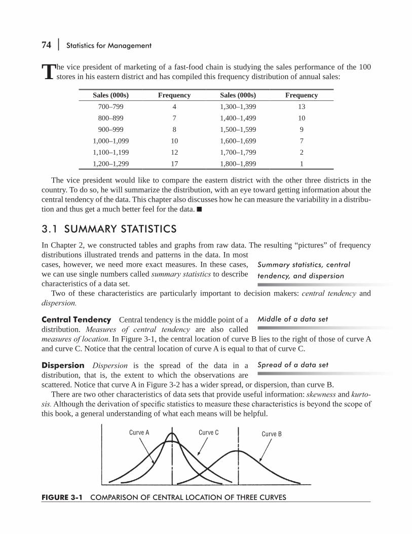
74 Statistics for Management
The vice president of marketing of a fast-food chain is studying the sales performance of the 100 stores in his eastern district and has compiled this frequency distribution of annual sales:
Sales (000s) Frequency Sales (000s) Frequency700–799 4 1,300–1,399 13800–899 7 1,400–1,499 10900–999 8 1,500–1,599 9
1,000–1,099 10 1,600–1,699 71,100–1,199 12 1,700–1,799 21,200–1,299 17 1,800–1,899 1
The vice president would like to compare the eastern district with the other three districts in the country. To do so, he will summarize the distribution, with an eye toward getting information about the central tendency of the data. This chapter also discusses how he can measure the variability in a distribu-tion and thus get a much better feel for the data.
3.1 SUMMARY STATISTICSIn Chapter 2, we constructed tables and graphs from raw data. The resulting “pictures” of frequency distributions illustrated trends and patterns in the data. In most cases, however, we need more exact measures. In these cases, we can use single numbers called summary statistics to describe characteristics of a data set.
Two of these characteristics are particularly important to decision makers: central tendency and dispersion.
Central Tendency Central tendency is the middle point of a distribution. Measures of central tendency are also called measures of location. In Figure 3-1, the central location of curve B lies to the right of those of curve A and curve C. Notice that the central location of curve A is equal to that of curve C.
Dispersion Dispersion is the spread of the data in a distribution, that is, the extent to which the observations are scattered. Notice that curve A in Figure 3-2 has a wider spread, or dispersion, than curve B.
There are two other characteristics of data sets that provide useful information: skewness and kurto-sis.this book, a general understanding of what each means will be helpful.
Curve A Curve C Curve B
FIGURE 3-1 COMPARISON OF CENTRAL LOCATION OF THREE CURVES
Summary statistics, central
tendency, and dispersion
Middle of a data set
Spread of a data set
Measures of Central Tendency and Dispersion in Frequency Distributions 75
Curve A Curve B
FIGURE 3-2 COMPARISON OF DISPERSION OF TWO CURVES
Skewness Curves representing the data points in the data set may be either symmetrical or skewed. Symmetrical curves, like the one in Figure 3-3, are such that a vertical line drawn from the center of the curve to the horizontal axis divides the area of the curve into two equal parts. Each part is the mirror image of the other.
Curves A and B in Figure 3-4 are skewed curves. They are skewed because values in their frequency distributions are con-centrated at either the low end or the high end of the measuring scale on the horizontal axis. The values are not equally distributed. Curve A is skewed to the right (or positively skewed) because it tails off toward the high end of the scale. Curve B is just the opposite. It is skewed to the left (negatively skewed) because it tails off toward the low end of the scale.
Curve A might represent the frequency distribution of the number of days’ supply on hand in the wholesale fruit business. The curve would be skewed to the right, with many values at the low end and few at the high, because the inventory must turn over rapidly. Similarly, curve B could represent the frequency of the number of days a real-estate broker requires to sell a house. It would be skewed to the left, with many values at the high end and few at the low, because the inventory of houses turns over very slowly.
FIGURE 3-3 SYMMETRICAL CURVE
Curve A:skewed right
Curve B:skewed left
FIGURE 3-4 COMPARISON OF TWO SKEWED CURVES
Symmetry of a data set
Skewness of a data set

76 Statistics for Management
Curve A Curve B
FIGURE 3-5 TWO CURVES WITH THE SAME CENTRAL LOCATION BUT DIFFERENT KURTOSIS
Kurtosis When we measure the kurtosis of a distribution, we are measuring its peakedness. In Figure 3-5, for example, curves A and B differ only in that one is more peaked than the other. They have the same central location and dispersion, and both are symmetrical. Statisticians say that the two curves have different degrees of kurtosis.
EXERCISES 3.1
Basic Concepts3-1 Draw three curves, all symmetrical but with different dispersions.3-2 Draw three curves, all symmetrical and with the same dispersion, but with the following cen-
tral locations:(a) 0.0 (b) 1.0 (c) –1.0
3-3 Draw a curve that would be a good representation of the grades on a statistics test in a poorly prepared class and another or a well-prepared class.
3-4 For the following distributions, indicate which distribution(a) Has the larger average value.(b) Is more likely to produce a small value than a large value.(c) Is the better representation of the distribution of ages at a rock concert.(d) Is the better representation of the distribution of the times patients have to wait at a
A B
For the next two distributions, indicate which distribution, if any(e) Has values more evenly distributed across the range of possible values.(f) Is more likely to produce a value near 0.(g) Has a greater likelihood of producing positive values than negative values.
AB
0
Peakedness of a data set
Measures of Central Tendency and Dispersion in Frequency Distributions 77
3-5 If the following two curves represent the distribution of scores for a group of students on two
A B
3.2 A MEASURE OF CENTRAL TENDENCY: THE ARITHMETIC MEAN
Most of the time when we refer to the “average” of something, we are talking about its arithmetic mean. This is true in cases such as the average winter temperature in New York City, the average life of a
Table 3-1 presents data describing the number of days the gen-erators at a power station on Lake Ico are out of service owing to
by the number of observations:
Arithmetic mean 7 23 4 8 2 12 6 13 9 4
10=
+ + + + + + + + +
88
10=
= 8.8 days
power plant manager has a reasonable single measure of the behavior of all her generators.
Conventional SymbolsTo write equations for these measures of frequency distribu-tions, we need to learn the mathematical notations used by stat-isticians. A sample of a population consists of n observations (a lowercase n) with a mean of x (read x-bar). Remember that the measures we compute for a sample are called statistics.
The notation is different when we are computing measures for the entire population, that is, for the group containing every element we are describing. The mean of a population is sym-bolized by μ, which is the Greek letter mu. The number of
The arithmetic mean
Characteristics of a sample are
called statistics
Characteristics of a population
are called parameters
TABLE 3-1 DOWNTIME OF GENERATORS AT LAKE ICO STATION
GENERATOR 1 2 3 4 5 6 7 8 9 10
DAYS OUT OF SERVICE 7 23 4 8 2 12 6 13 9 4

78 Statistics for Management
elements in a population is denoted by the capital italic letter N. Generally in statistics, we use italicized Roman letters to symbolize sample information and Greek letters to symbolize population information.
Calculating the Mean from Ungrouped DataIn the example, the average of 8.8 days would be μ (the popula-tion mean) if the 10 generators are the entire population. It would be x (the sample mean) if the 10 generators are a sample drawn from a larger population of generators. To write the formulas for these two means, we combine our mathematical symbols and the steps we used to determine the arithmetic mean. If we add the values of the observations and divide this sum by the number of observations, we will get
Population Arithmetic Mean
x
Nμ =
∑
Sum of values of all observations
Number of elements in the population
[3-1]
and
Sample Arithmetic Mean
xx
n=
∑
Sum of values of all observations
Number of elements in the sample
[3-2]
Because μ is the population arithmetic mean, we use N to indicate that we divide by the number of observations or elements in the population. Similarly, x is the sample arithmetic mean and n is the number of observations in the sample. The Greek letter sigma, ∑, indicates that all the values of x are summed together.
Another example: Table 3-2 lists the per-centile increase in SAT verbal scores shown by seven different students taking an SAT prepara-tory course.
Finding the population and
sample means
TABLE 3-2 SAT VERBAL SCORES
STUDENT 1 2 3 4 5 6 7INCREASE 9 7 7 6 4 4 2

Measures of Central Tendency and Dispersion in Frequency Distributions 79
We compute the mean of this sample of seven students as follows:
xx
n=
∑ [3-2]
9 7 7 6 4 4 2
7=
+ + + + + +
39
7=
= 5.6 points per student ← ⎯⎯⎯ Sample mean
Notice that to calculate this mean, we added every observation. Statisticians call this kind of data ungrouped data. The computa-
suppose we are dealing with the weights of 5,000 head of cattle and prefer not to add each of our data points separately. Or suppose we have access to only the frequency distribution of the data, not to every individual observation. In these cases, we will need a different way to calculate the arithmetic mean.
Calculating the Mean from Grouped DataA frequency distribution consists of data that are grouped by classes. Each value of an observation falls somewhere in one of the classes. Unlike the SAT example, we do not know the sepa-rate values of every observation. Suppose we have a frequency distribution (illustrated in Table 3-3) of average monthly checking-account balances of 600 customers at a branch bank. From the information in this table, we can easily compute an estimate of the value of the mean of these grouped data. It is an estimate because we do not use all 600 data points in the sample. Had we used the original, ungrouped data, we could have calculated the actual value of the mean, but only by averaging the 600 separate values. For ease of calcula-tion, we must give up accuracy.
the midpoint of each class. To make midpoints come out in whole
class becomes 25.00, rather than 24.995. Then we multiply each midpoint by the frequency of observa-tions in that class, sum all these results, and divide the sum by the total number of observations in the sample. The formula looks like this:
Sample Arithmetic Mean of Grouped Data
xf x
n
( )=
∑ × [3-3]
where
x = sample mean ∑ = symbol meaning “the sum of”
Dealing with ungrouped data
Dealing with grouped data
Estimating the mean
Calculating the mean
80 Statistics for Management
f = frequency (number of observations) in each class x = midpoint for each class in the sample n = number of observations in the sample
Table 3-4 illustrates how to calculate the arithmetic mean from our grouped data, using Equation 3-3.
TABLE 3-3 AVERAGE MONTHLY BALANCE OF 600 CUSTOMERS
Class (Dollars) Frequency0–49.99 78
50.00–99.99 123100.00–149.99 187150.00–199.99 82200.00–249.99 51250.00–299.99 47300.00–349.99 13350.00–399.99 9400.00–449.99 6450.00–499.99 4
600
TABLE 3-4 CALCULATION OF ARITHMETIC SAMPLE MEAN FROM GROUPED DATA IN TABLE 3-3
Class (Dollars)(1)
Midpoint (x)(2)
Frequency (f)(3)
f ¥ x(3) ¥ (2)
0–49.99 25.00 × 78 = 1,950
50.00–99.99 75.00 × 123 = 9,225
100.00–149.99 125.00 × 187 = 23,375
150.00–199.99 175.00 × 82 = 14,350
200.00–249.99 225.00 × 51 = 11,475
250.00–299.99 275.00 × 47 = 12,925
300.00–349.00 325.00 × 13 = 4,225
350.00–399.99 375.00 × 9 = 3,375
400.00–449.99 425.00 × 6 = 2,550
450.00–499.99 475.00 × 4 = 1,900
f = n = 600 85,350 f × x)
xf x
n
( )=
∑ × [3-3]
85,350
600=
= 142.25 ← ⎯⎯⎯ Sample mean (dollars)
Measures of Central Tendency and Dispersion in Frequency Distributions 81
In our sample of 600 customers, the average monthly check-ing-account balance is $142.25. This is our approximation from the frequency distribution. Notice that because we did not know every data point in the sample, we assumed that every value in a class was equal to its midpoint. Our results, then, can only approximate the actual average monthly balance.
CodingIn situations where a computer is not available and we have to do the arithmetic by hand, we can further simplify our calculation of the mean from grouped data. Using a technique called coding, we eliminate the problem of large or inconvenient midpoints. Instead of using the actual midpoints to perform our calculations, we can assign small-value consecutive inte-gers (whole numbers) called codes to each of the midpoints. The integer zero can be assigned anywhere, but to keep the integers small, we will assign zero to the midpoint in the middle (or the one nearest to the middle) of the frequency distribution. Then we can assign negative integers to values smaller than that midpoint and positive integers to those larger, as follows:
Class 1–5 6–10 11–15 16–20 21–25 26–30 31–35 36–40 41–45Code (u) –4 –3 –2 –1 0 1 2 3 4
x0
Symbolically, statisticians use x0 to represent the midpoint that is assigned the code 0, and u for the coded midpoint. The following formula is used to determine the sample mean using codes:
Sample Arithmetic Mean of Grouped Data Using Codes
x x wu f
n
( )0= +
∑ × [3-4]
where
x = mean of sample x0 = value of the midpoint assigned the code 0 w = numerical width of the class interval u = code assigned to each class f = frequency or number of observations in each class n = total number of observations in the sample
Keep in mind that (u × f) simply means that we (1) multiply u by f for every class in the frequency
the sample mean of the annual snowfall (in inches) over 20 years in Harlan, Kentucky.
Assigning codes to the
midpoints
Calculating the mean from
grouped data using codes
We make an assumption
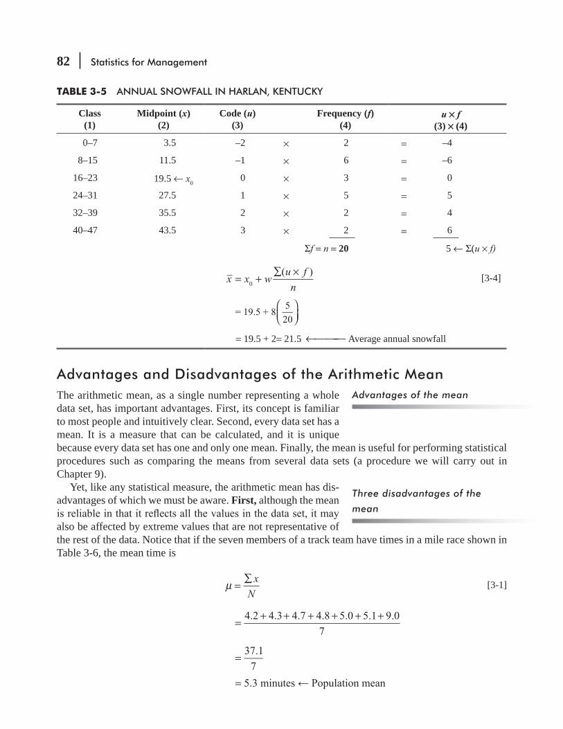
82 Statistics for Management
TABLE 3-5 ANNUAL SNOWFALL IN HARLAN, KENTUCKY
Class(1)
Midpoint (x)(2)
Code (u)(3)
Frequency (f)(4)
u ¥ f(3) ¥ (4)
0–7 3.5 –2 × 2 = –4
8–15 11.5 –1 × 6 = –6
16–23 19.5 ← x00 × 3 = 0
24–31 27.5 1 × 5 = 5
32–39 35.5 2 × 2 = 4
40–47 43.5 3 × 2 = 6
Σf = n = 20 5 ← Σ(u × f)
x x wu f
n
( )0= +
∑ × [3-4]
= 19.5 + 85
20
⎛⎝⎜
⎞⎠⎟
= 19.5 + 2= 21.5 ← ⎯⎯⎯ Average annual snowfall
Advantages and Disadvantages of the Arithmetic MeanThe arithmetic mean, as a single number representing a whole data set, has important advantages. First, its concept is familiar to most people and intuitively clear. Second, every data set has a mean. It is a measure that can be calculated, and it is unique because every data set has one and only one mean. Finally, the mean is useful for performing statistical procedures such as comparing the means from several data sets (a procedure we will carry out in Chapter 9).
Yet, like any statistical measure, the arithmetic mean has dis-advantages of which we must be aware. First, although the mean
also be affected by extreme values that are not representative of the rest of the data. Notice that if the seven members of a track team have times in a mile race shown in Table 3-6, the mean time is
x
Nμ =
∑ [3-1]
4.2 4.3 4.7 4.8 5.0 5.1 9.0
7=
+ + + + + +
37.1
7=
=
Advantages of the mean
Three disadvantages of the
mean

Measures of Central Tendency and Dispersion in Frequency Distributions 83
members, however, and exclude the 9.0 value, the answer is about 4.7 minutes. The one extreme value of 9.0 distorts the value we get for the mean. It would be more representative to calculate the mean without including such an extreme value.
A second problem with the mean is the same one we encountered with our 600 checking-account balances: It is tedious to compute the mean because we do use every data point in our calculation (unless, of course, we take the short-cut method of using grouped data to approximate the mean).
The third disadvantage is that we are unable to compute the mean for a data set that has open-ended classes at either the high or low end of the scale. Suppose the data in Table 3-6 had been arranged in the frequency distribution shown in Table 3-7. We could not compute a mean value for these data because of the open-ended class of “5.4 and above.” We have no way of knowing whether the value is 5.4, near 5.4, or far above 5.4.
The mean (or average) can be an excellent measure of central tendency (how data group around the middle point of a distribution). But unless the mean is truly representative of the data from which it was computed, we are violating an important assumption. Warning: If there are very high or very low values in the data that don’t look like most of the data, the mean is not representative. Fortunately there are measures that can be calculated that don’t suffer from this shortcoming. A helpful hint in choosing which one of these to compute is to look at the data points.
HINTS & ASSUMPTIONS
EXERCISES 3.2
Self-Check ExercisesSC 3-1 The frequency distribution below represents the weights in pounds of a sample of packages
carried last month by a small airfreight company.
Class Frequency Class Frequency
10.0–10.9 1 15.0–15.9 11
11.0–11.9 4 16.0–16.9 8
12.0–12.9 6 17.0–17.9 7
13.0–13.9 8 18.0–18.9 6
14.0–14.9 12 19.0–19.9 2
TABLE 3-6 TIMES FOR TRACK-TEAM MEMBERS IN A 1-MILE RACE
MEMBER 1 2 3 4 5 6 7TIME IN MINUTES
4.2 4.3 4.7 4.8 5.0 5.1 9.0
TABLE 3-7 TIMES FOR TRACK-TEAM MEMBERS IN A 1-MILE RACE
CLASS IN MINUTES
4.2– 4.5 4.6– 4.9 5.0–5.3 5.4 and above
FREQUENCY 2 2 2 1
84 Statistics for Management
(a) Compute the sample mean using Equation 3-3.(b) Compute the sample mean using the coding method (Equation 3-4) with 0 assigned to the
fourth class.(c) Repeat part (b) with 0 assigned to the sixth class.(d) Explain why your answers in parts (b) and (c) are the same.
SC 3-2 Davis Furniture Company has a revolving credit agreement with the First National Bank. The loan showed the following ending monthly balances last year:
Jan. $121,300 Apr. $72,800 July $58,700 Oct. $52,800Feb. $112,300 May $72,800 Aug. $61,100 Nov. $49,200Mar. $72,800 June $57,300 Sept. $50,400 Dec. $46,100
The company is eligible for a reduced rate of interest if its average monthly balance is over
Applications3-6 Child-Care Community Nursery is eligible for a county social services grant as long as the
average age of its children stays below 9. If these data represent the ages of all the children
8 5 9 10 9 12 7 12 13 7 8
3-7 Child-Care Community Nursery can continue to be supported by the county social services
is below $12,500. The family incomes of the attending children are
$14,500 $15,600 $12,500 $8,600 $7,800$6,500 $5,900 $10,200 $8,800 $14,300 $13,900
(a) (b) If the answer to part (a) is no, by how much must the average family income fall for it to
(c) If the answer to part (a) is yes, by how much can average family income rise and Child-
3-8 These data represent the ages of patients admitted to a small hospital on February 28, 1996:
85 75 66 43 4088 80 56 56 6789 83 65 53 7587 83 52 44 48
(a) Construct a frequency distribution with classes 40–49, 50–59, etc.(b) Compute the sample mean from the frequency distribution.(c) Compute the sample mean from the raw data.(d) Compare parts (b) and (c) and comment on your answer.
Measures of Central Tendency and Dispersion in Frequency Distributions 85
3-9 The frequency distribution below represents the time in seconds needed to serve a sample of customers by cashiers at BullsEye Discount Store in December 1996.
Time (in seconds) Frequency20–29 630–39 1640–49 2150–59 2960–69 2570–79 2280–89 1190–99 7
100–109 4110–119 0120–129 2
(a) Compute the sample mean using Equation 3-3.(b) Compute the sample mean using the coding method (Equation 3-4) with 0 assigned to the
70–79 class.3-10 The owner of Pets ‘R Us is interested in building a new store. The owner will build if the aver-
monthly average for the year is at least 285. The data for 1995 are as follows:
Jan. Feb. Mar. Apr. May June July Aug. Sept. Oct. Nov. Dec.234 216 195 400 315 274 302 291 275 300 375 450
3-11 the accuracy of the machine’s volume setting, 18 trial bottles were run. The resulting volumes (in ounces) for the trials were as follows:
3.02 2.89 2.92 2.84 2.90 2.97 2.95 2.94 2.933.01 2.97 2.95 2.90 2.94 2.96 2.99 2.99 2.97
3-12 The production manager of Hinton Press is determining the average time needed to photo-graph one printing plate. Using a stopwatch and observing the platemakers, he collects the following times (in seconds)
20.4 20.0 22.2 23.8 21.3 25.1 21.2 22.9 28.2 24.322.0 24.7 25.7 24.9 22.7 24.4 24.3 23.6 23.2 21.0
An average per-plate time of less than 23.0 seconds indicates satisfactory productivity. Should
86 Statistics for Management
3-13 National Tire Company holds reserve funds in short-term marketable securities. The ending daily balance (in millions) of the marketable securities account for 2 weeks is shown below:
Week 1 $1.973 $1.970 $1.972 $1.975 $1.976Week 2 1.969 1.892 1.893 1.887 1.895
What was the average (mean) amount invested in marketable securities during(a) (b) (c) (d) An average balance over the 2 weeks of more than $1.970 million would qualify National
(e) If the answer to part (c) is less than $1.970 million, by how much would the last day’s
(f) If the answer to part (c) is more than $1,970 million, how much could the company treasurer
3-14 M. T. Smith travels the eastern United States as a sales representative for a textbook publisher. She is paid on a commission basis related to volume. Her quarterly earnings over the last 3 years are given below.
1st Quarter 2nd Quarter 3rd Quarter 4th QuarterYear 1 $10,000 $ 5,000 $25,000 $15,000Year 2 20,000 10,000 20,000 10,000Year 3 30,000 15,000 45,000 50,000
(a) Calculate separately M. T.’s average earnings in each of the four quarters.(b) Calculate separately M. T.’s average quarterly earnings in each of the 3 years.(c) Show that the mean of the four numbers you found in part (a) is equal to the mean of the three
numbers you found in part (b). Furthermore, show that both these numbers equal the mean of all 12 numbers in the data table. (This is M. T.’s average quarterly income over 3 years.)
3-15 Lillian Tyson has been the chairperson of the county library committee for 10 years. She con-tends that during her tenure she has managed the book-mobile repair budget better than her predecessor did. Here are data for bookmobile repair for 15 years:
Year Town Budget Year Town Budget Year Town Budget1992 $30,000 1987 $24,000 1982 $30,0001991 28,000 1986 19,000 1981 20,0001990 25,000 1985 21,000 1980 15,0001989 27,000 1984 22,000 1979 10,0001988 26,000 1983 24,000 1978 9,000
(a) Calculate the average annual budget for the last 5 years (1988–1992).(b) (c) Calculate the average annual budget for the 5 years before she was elected (1978–1982).(d) Based on the answers you found for parts (a), (b), and (c), do you think that there has
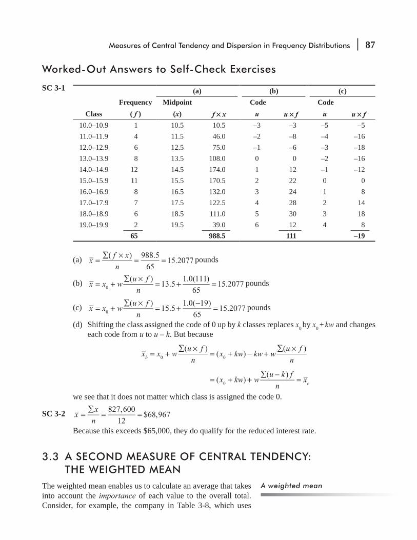
Measures of Central Tendency and Dispersion in Frequency Distributions 87
Worked-Out Answers to Self-Check Exercises
SC 3-1 (a) (b) (c)Frequency Midpoint Code Code
Class ( f ) (x) f ¥ x u u ¥ f u u ¥ f10.0–10.9 1 10.5 10.5 –3 –3 –5 –511.0–11.9 4 11.5 46.0 –2 –8 –4 –1612.0–12.9 6 12.5 75.0 –1 –6 –3 –1813.0–13.9 8 13.5 108.0 0 0 –2 –1614.0–14.9 12 14.5 174.0 1 12 –1 –1215.0–15.9 11 15.5 170.5 2 22 0 016.0–16.9 8 16.5 132.0 3 24 1 817.0–17.9 7 17.5 122.5 4 28 2 1418.0–18.9 6 18.5 111.0 5 30 3 1819.0–19.9 2 19.5 39.0 6 12 4 8
65 988.5 111 –19
(a) xf x
n
( ) 988.5
6515.2077=
∑ ×= = pounds
(b) x x wu f
n
( )13.5
1.0(111)
6515.20770= +
∑ ×= + = pounds
(c) x x wu f
n
( )15.5
1.0( 19)
6515.20770= +
∑ ×= +
−= pounds
(d) Shifting the class assigned the code of 0 up by k classes replaces x0 by x0 + kw and changes each code from u to u – k. But because
x x wu f
nx kw kw w
u f
n
( )( )
( )b 0 0= +
∑ ×= + − +
∑ ×
x kw wu k f
nx( )
( )c0= + +
∑ −=
we see that it does not matter which class is assigned the code 0.
SC 3-2 xx
n
827,600
12$68,967=
∑= =
Because this exceeds $65,000, they do qualify for the reduced interest rate.
3.3 A SECOND MEASURE OF CENTRAL TENDENCY: THE WEIGHTED MEAN
The weighted mean enables us to calculate an average that takes into account the importance of each value to the overall total. Consider, for example, the company in Table 3-8, which uses
A weighted mean

88 Statistics for Management
three grades of labor—unskilled, semiskilled, and skilled—to produce two end products. The company wants to know the average cost of labor per hour for each of the products.
A simple arithmetic average of the labor wage rates would be
xx
n=
∑ [3-2]
$5 $7 $9
3=
+ +
$21
3=
= $7.00/hour
Using this average rate, we would compute the labor cost of one unit of product 1 to be $7(1 + 2 + 5) = $56 and of one unit of prod-uct 2 to be $7(4 + 3 + 3) = $70. But these answers are incorrect.
To be correct, the answers must take into account that differ-ent amounts of each grade of labor are used. We can determine the correct answers in the following manner. For product 1, the total labor cost per unit is ($5 × 1) + ($7 × 2) + ($9 × 5) = $64, and, since there are 8 hours of labor input, the average labor cost per hour is $64/8 = $8.00 per hour. For product 2, the total labor cost per unit is ($5 × 4) + ($7 × 3) + ($9 × 3) = $68, for an average labor cost per hour of $68/10, or $6.80 per hour.
Another way to calculate the correct average cost per hour for the two products is to take a weighted average of the cost of the three grades of labor. To do this, we weight the hourly wage for each grade by its proportion of the total labor required to produce the product. One unit of product 1, for example, requires 8 hours of labor. Unskilled labor uses 1
8 of this time, semiskilled labor uses 28 of this time, and skilled labor
requires 58 of this time. If we use these fractions as our weights, then one hour of labor for product
1 costs an average of
1
8$5
2
8$7
5
8$9 $8.00 /×
⎛⎝⎜
⎞⎠⎟
+ ×⎛⎝⎜
⎞⎠⎟
+ ×⎛⎝⎜
⎞⎠⎟
= hour
Similarly, a unit of product 2 requires 10 labor hours, of which 410 is used for unskilled labor, 3
10 for semiskilled labor, and 3
10 for skilled labor. By using these fractions as weights, one hour of labor for product 2 costs
In this case, the arithmetic
mean is incorrect
The correct answer is the
weighted mean
TABLE 3-8 LABOR INPUT IN MANUFACTURING PROCESS
Labor Hours per Unit of OutputGrade of Labor Hourly Wage (x) Product 1 Product 2
Unskilled $5.00 1 4Semiskilled 7.00 2 3Skilled 9.00 5 3

Measures of Central Tendency and Dispersion in Frequency Distributions 89
4
10$5
3
10$7
3
10$9 $6.80 /×
⎛⎝⎜
⎞⎠⎟
+ ×⎛⎝⎜
⎞⎠⎟
+ ×⎛⎝⎜
⎞⎠⎟
= hour
Thus, we see that the weighted averages give the correct values for the average hourly labor costs of the two products because they take into account that different amounts of each grade of labor are used in the products.
Symbolically, the formula for calculating the weighted average is
Weight Mean
xw x
w
( )w =
∑ ×∑
[3-5]
where
xw = symbol for the weighted mean*
w = weight assigned to each observation ( 18 , 2
8 , and 58 , for product 1 and 4
10, 310, and 3
10, for product 2 in our example)
w × x) = sum of the weight of each element times that element w = sum of all of the weights
xw x
w
( )w =
∑ ×∑
[3-5]
18
$528
$758
$9
18
28
58
=×
⎛⎝⎜
⎞⎠⎟
+ ×⎛⎝⎜
⎞⎠⎟
+ ×⎛⎝⎜
⎞⎠⎟
+ +
$8
1=
= $8.00/hour
Notice that Equation 3-5 states more formally something we have done previously. When we calculated the arithmetic mean from grouped data (page 79), we actually found a weighted mean, using the midpoints for the x values and the frequencies of each class as the weights. We divided this answer by the sum of all the frequencies, which is the same as dividing by the sum of all the weights.
In like manner, any mean computed from all the values in a data set according to Equation 3-1 or 3-2 is really a weighted average of the components of the data set. What those components are, of course, determines what the mean measures. In a factory, for example, we could determine the weighted mean
*The symbol xw is read x-bar sub w. The lowercase w is called a subscript and is a reminder that this is not an ordinary mean but one that is weighted according to the relative importance of the values of x.
The arithmetic mean of grouped
data: the weighted mean
Calculating the weighted mean
90 Statistics for Management
of all the wages (skilled, semiskilled, and unskilled) or of the wages of men workers, women workers, or union and nonunion members.
Distinguish between distinct values and individual observations in a data set, since several obser-vations can have the same value. If values occur with different frequencies, the arithmetic mean of the values (as opposed to the arithmetic mean of the observations) may not be an accurate measure of central tendency. In such cases, we need to use the weighted mean of the values. If you are using an average value to make a decision, ask how it was calculated. If the values in the sample do not appear with the same frequency, insist on a weighted mean as the correct basis for your decision.
HINTS & ASSUMPTIONS
EXERCISES 3.3
Self-Check ExercisesSC 3-3 Dave’s Giveaway Store advertises, “If our average prices are not equal or lower than everyone
else’s, you get it free.” One of Dave’s customers came into the store one day and threw on the counter bills of sale for six items she bought from a competitor for an average price less than Dave’s. The items cost
$1.29 $2.97 $3.49 $5.00 $7.50 $10.95
Dave’s prices for the same six items are $1.35, $2.89, $3.19, $4.98, $7.59 and $11.50. Dave told the customer, “My ad refers to a weighted average price of these items. Our average is lower because our sales of these items have been:”
7 9 12 8 6 3
SC 3-4 Bennett Distribution Company, a subsidiary of a major appliance manufacturer, is forecasting regional sales for next year. The Atlantic branch, with current yearly sales of $193.8 million, is expected to achieve a sales growth of 7.25 percent; the Midwest branch, with current sales of
million, is expected to increase sales by 7.15 percent. What is the average rate of sales growth
Applications3-16
students. The homework average will count for 20 percent of a student’s grade; the midterm,
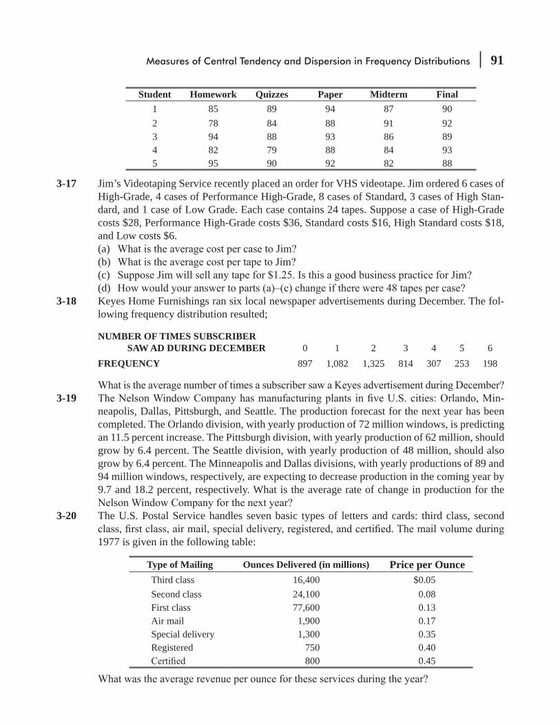
Measures of Central Tendency and Dispersion in Frequency Distributions 91
Student Homework Quizzes Paper Midterm Final1 85 89 94 87 902 78 84 88 91 923 94 88 93 86 894 82 79 88 84 935 95 90 92 82 88
3-17 Jim’s Videotaping Service recently placed an order for VHS videotape. Jim ordered 6 cases of High-Grade, 4 cases of Performance High-Grade, 8 cases of Standard, 3 cases of High Stan-dard, and 1 case of Low Grade. Each case contains 24 tapes. Suppose a case of High-Grade costs $28, Performance High-Grade costs $36, Standard costs $16, High Standard costs $18, and Low costs $6.(a) (b) (c) (d)
3-18 Keyes Home Furnishings ran six local newspaper advertisements during December. The fol-lowing frequency distribution resulted;
NUMBER OF TIMES SUBSCRIBER SAW AD DURING DECEMBER 0 1 2 3 4 5 6FREQUENCY 897 1,082 1,325 814 307 253 198
3-19 -neapolis, Dallas, Pittsburgh, and Seattle. The production forecast for the next year has been completed. The Orlando division, with yearly production of 72 million windows, is predicting an 11.5 percent increase. The Pittsburgh division, with yearly production of 62 million, should grow by 6.4 percent. The Seattle division, with yearly production of 48 million, should also grow by 6.4 percent. The Minneapolis and Dallas divisions, with yearly productions of 89 and 94 million windows, respectively, are expecting to decrease production in the coming year by 9.7 and 18.2 percent, respectively. What is the average rate of change in production for the
3-20 The U.S. Postal Service handles seven basic types of letters and cards: third class, second
1977 is given in the following table:
Type of Mailing Ounces Delivered (in millions) Price per OunceThird class 16,400 $0.05Second class 24,100 0.08First class 77,600 0.13Air mail 1,900 0.17Special delivery 1,300 0.35Registered 750 0.40
800 0.45

92 Statistics for Management
3-21 -
rates charged to consulting clients for the work of each of these professional categories are
hours billed last year in each category: 8,000, 14,000, 24,000, and 35,000. If Matthews, Young is trying to come up with an average billing rate for estimating client charges for next year,
Worked-Out Answers to Self-Check ExercisesSC 3-3 With unweighted averages, we get
xx
n
31.20
6$5.20c =
∑= = at the competition
= =x31.50
6$5.25D
at Dave’s
With weighted averages, we get
xw x
w
( )c =
∑ ×∑
7(1.29) 9(2.97) 12(3.49) 8(5.00) 6(7.50) 3(10.95)
7 9 12 8 6 3=
+ + + + ++ + + + +
195.49
45$4.344= = at the competition
=+ + + + +
+ + + + +x
7(1.35) 9(2.89) 12(3.19) 8(4.98) 6(7.59) 3(11.50)
7 9 12 8 6 3D
193.62
45$4.303= = at Dave’s
Although Dave is technically correct, the word average in popular usage is equivalent to unweighted average in technical usage, and the typical customer will surely be angry with Dave’s assertion (whether he or she understands the technical point or not).
SC 3-4 xw x
w
( ) 193.8(7.25) 79.3(8.20) 57.5(7.15)
193.8 79.3 57.5w =∑ ×
∑=
+ ++ +
2466.435
330.67.46%= =
3.4 A THIRD MEASURE OF CENTRAL TENDENCY: THE GEOMETRIC MEAN
Sometimes when we are dealing with quantities that change over a period of time, we need to know an average rate of change, such as an average growth rate over a period of several years. In
Finding the growth rate: The
geometric mean
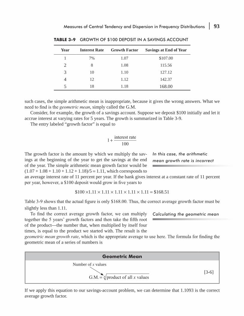
Measures of Central Tendency and Dispersion in Frequency Distributions 93
such cases, the simple arithmetic mean is inappropriate, because it gives the wrong answers. What we geometric mean, simply called the G.M.
Consider, for example, the growth of a savings account. Suppose we deposit $100 initially and let it accrue interest at varying rates for 5 years. The growth is summarized in Table 3-9.
The entry labeled “growth factor” is equal to
1interest rate
100+
The growth factor is the amount by which we multiply the sav-ings at the beginning of the year to get the savings at the end of the year. The simple arithmetic mean growth factor would be (1.07 + 1.08 + 1.10 + 1.12 + 1.18)/5 = 1.11, which corresponds to an average interest rate of 11 percent per year. If the bank gives interest at a constant rate of 11 percent
$100 ×1.11 × 1.11 × 1.11 × 1.11 × 1.11 = $168.51
slightly less than 1.11.
of the product—the number that, when multiplied by itself four times, is equal to the product we started with. The result is the geometric mean growth rategeometric mean of a series of numbers is
Geometric Mean
Number of x values
xG.M. product of all valuesn=[3-6]
If we apply this equation to our savings-account problem, we can determine that 1.1093 is the correct average growth factor.
In this case, the arithmetic
mean growth rate is incorrect
Calculating the geometric mean
TABLE 3-9 GROWTH OF $100 DEPOSIT IN A SAVINGS ACCOUNT
Year Interest Rate Growth Factor Savings at End of Year
1 7% 1.07 $107.00
2 8 1.08 115.56
3 10 1.10 127.12
4 12 1.12 142.37
5 18 1.18 168.00

94 Statistics for Management
G.M. xproduct of all valuesn= [3-6]
1.07 1.08 1.10 1.12 1.185= × × × ×
1.6799655== 1.1093 ← ⎯⎯⎯ Average growth factor (the geometric
mean of the 5 growth factors)
Notice that the correct average interest rate of 10.93 percent per year obtained with the geometric mean is very close to the incorrect average rate of 11 percent obtained with the arithme-tic mean. This happens because the interest rates are relatively small. Be careful however, not to be tempted to use the arithmetic mean instead of the more compli-cated geometric mean. The following example demonstrates why.
250, 300, and 400 percent, which correspond to growth factors of 2, 3, 3.5, 4, and 5. (We’ve calculated these growth factors just as we did in Table 3-9.)
In 5 years, an initial deposit of $100 would grow to $100 × 2 × 3 × 3.5 × 4 × 5 = $42,000. The arith-metic mean growth factor is (2 + 3 + 3.5 + 4 + 5)/5, or 3.5. This corresponds to an average interest rate of 250 percent. Yet if the banks actually gave interest at a constant rate of 250 percent per year, then $100 would grow to $52,521.88 in 5 years:
$100 × 3.5 × 3.5 × 3.5 × 3.5 × 3.5 = $52,521.88.
This answer exceeds the actual $42,000 by more than $10,500, a sizable error.
growth factor:
G.M. xproduct of all valuesn= [3-6]
2 3 3.5 4 55= × × × ×
4205== 3.347 ← ⎯⎯⎯ Average growth factor
This growth factor corresponds to an average interest rate of 235 percent per year. In this case, the use of the appropriate mean does
-tion calculations. In certain situations, answers using the arithmetic mean and the geometric mean will not be too far apart, but even a small difference can generate a poor decision. A good working hint is to use the geometric mean whenever you are calculating the average percentage change in
whether it’s a geometric mean and be warned that if it’s not, you are dealing with an incorrect value.
HINTS & ASSUMPTIONS
Warning: use the appropriate
mean

Measures of Central Tendency and Dispersion in Frequency Distributions 95
EXERCISES 3.4
Self-Check ExercisesSC 3-5
follows. Calculate the average percentage increase in bad-debt expense over this time period. If this rate continues, estimate the percentage increase in bad debts for 1997, relative to 1995.
1989 1990 1991 1992 1993 1994 19950.11 0.09 0.075 0.08 0.095 0.108 0.120
SC 3-6 Realistic Stereo Shops marks up its merchandise 35 percent above the cost of its latest addi-tions to stock. Until 4 months ago, the Dynamic 400-S VHS recorder had been $300. During the last 4 months Realistic has received 4 monthly shipments of this recorder at these unit costs: $275, $250, $240, and $225. At what average rate per month has Realistic’s retail price
Applications3-22 Hayes Textiles has shown the following percentage increase in net worth over the last 5 years:
1992 1993 1994 1995 19965% 10.5% 9.0% 6.0% 7.5%
3-23 MacroSwift, the U.S.-based computer software giant, has posted an increase in net worth dur-ing 7 of the last 9 years. Calculate the average percentage change in net worth over this time period. Assuming similar conditions in the years to come, estimate the percentage change for 1998, relative to 1996.
1988 1989 1990 1991 1992 1993 1994 1995 1996
0.11 0.09 0.07 0.08 –0.04 0.14 0.11 –0.03 0.06
3-24 The Birch Company, a manufacturer of electrical circuit boards, has manufactured the follow-ing number of units over the past 5 years:
1992 1993 1994 1995 1996
12,500 13,250 14,310 15,741 17,630
Calculate the average percentage increase in units produced over this time period, and use this to estimate production for 1999.
3-25 Bob Headen is calculating the average growth factor for his stereo store over the last 6 years. Using a geometric mean, he comes up with an answer of 1.24. Individual growth factors for
3-26 Over a 3-week period, a store owner purchased $120 worth of acrylic sheeting for new display
second, $1.10; and the third, $1.15. What was the average weekly rate of increase in the price

96 Statistics for Management
3-27 Lisa’s Quick Stop has been attracting customers by selling milk at a price 2 percent below that of the main grocery store in town. Given below are Lisa’s prices for a gallon of milk for a
Week 1 Week 2 Week 3 Week 4 Week 5 Week 6 Week 7 Week 8
$2.30 $2.42 $2.36 $2.49 $2.24 $2.36 $2.42 $2.49
3-28 Industrial Suppliers, Inc., keeps records on the cost of processing a purchase order. Over the last 5 years, this cost has been $55.00, $58.00, $61.00, $65.00, and $66.00. What has Indus-
3-29 A sociologist has been studying the yearly changes in the number of convicts assigned to the largest correctional facility in the state. His data are expressed in terms of the percentage increase in the number of prisoners (a negative number indicates a percentage decrease). The sociologist’s most recent data are as follows:
1991 1992 1993 1994 1995 1996–4% 5% 10% 3% 6% –5%
(a) Calculate the average percentage increase using only the 1992–1995 data.(b) Rework part (a) using the data from all 6 years.(c) A new penal code was passed in 1990. Previously, the prison population grew at a rate of
Worked-Out Answers to Self-Check Exercises
SC 3-5 G.M. 1.11(1.09)(1.075)(1.08)(1.095)(1.108)(1.12) 1.908769992 1.096757 7= = =
The average increase is 9.675 percent per year. The estimate for bad debt expenses in 1997 is (1.09675)2 – 1 = .2029, i.e., 20.29 percent higher than in 1995.
SC 3-6 The monthly growth factors are 275/300 = 0.9167, 250/275 = 0.9091, 240/250 = 0.9600, and 225/240 = 0.9375, so
G.M. = 0.9167(0.9091)(0.9600)(0.9375) 0.7500 0.9306 1 0.06944 4= = = −
The price has been decreasing at an average rate of 6.94 percent per month.
3.5 A FOURTH MEASURE OF CENTRAL TENDENCY: THE MEDIAN
The median is a measure of central tendency different from any of the means we have discussed so far. The median is a single value from the data set that measures the central item in the data. This single item is the middlemost or most central item in the set of numbers. Half of the items lie above this point, and the other half lie below it.
Median defined
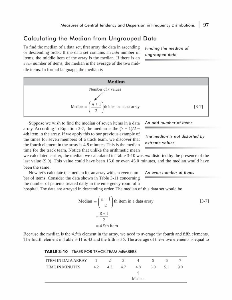
Measures of Central Tendency and Dispersion in Frequency Distributions 97
Calculating the Median from Ungrouped Data
or descending order. If the data set contains an odd number of items, the middle item of the array is the median. If there is an even number of items, the median is the average of the two mid-dle items. In formal language, the median is
Median
Number of x values
n=
+ 1
2
⎛⎝⎜
⎞⎠⎟
Median th item in a data array [3-7]
array. According to Equation 3-7, the median is the (7 + 1)/2 = 4th item in the array. If we apply this to our previous example of the times for seven members of a track team, we discover that the fourth element in the array is 4.8 minutes. This is the median time for the track team. Notice that unlike the arithmetic mean we calculated earlier, the median we calculated in Table 3-10 was not distorted by the presence of the last value (9.0). This value could have been 15.0 or even 45.0 minutes, and the median would have been the same!
Now let’s calculate the median for an array with an even num-ber of items. Consider the data shown in Table 3-11 concerning the number of patients treated daily in the emergency room of a hospital. The data are arrayed in descending order. The median of this data set would be
Median n=
+ 1
2
⎛⎝⎜
⎞⎠⎟
th item in a data array [3-7]
8 1
2=
+
= 4.5th item
Finding the median of
ungrouped data
An odd number of items
The median is not distorted by
extreme values
An even number of items
TABLE 3-10 TIMES FOR TRACK-TEAM MEMBERS
ITEM IN DATA ARRAY 1 2 3 4 5 6 7TIME IN MINUTES 4.2 4.3 4.7 4.8 5.0 5.1 9.0
↑Median

98 Statistics for Management
(43 + 35)/2, or 39. Therefore, 39 is the median number of patients treated in the emergency room per day during the 8-day period.
Calculating the Median from Grouped DataOften, we have access to data only after they have been grouped in a frequency distribution. For example, we do not know every observation that led to the construction of Table 3-12, the data on 600 bank customers originally introduced earlier. Instead, we have 10 class intervals and a record of the frequencies with which the observations appear in each of the intervals.
Nevertheless, we can compute the median checking-account balance of these 600 customers by determining which of the 10 class intervals contains the median. To do this, we must add the frequencies in the fre-quency column in Table 3-12 until we reach the (n + 1)/2th item. Because there are 600 accounts, the value for (n + l)/2 is 300.5 (the average of the
the class intervals containing the 300th and 301st
two classes is only 78 + 123 = 201. But when we moved to the third class interval, 187 elements are added to 201, for a total of 388. Therefore, the 300th and 301st observations must be located in this third class (the interval from $100.00 to $149.99).The median class for this data set contains 187 items. If we assume that these 187 items begin at $100.00 and are evenly spaced over the entire class interval from $100.00 to $149.99, then we can
items. First, we determine that the 300th item is the 99th element in the median class:
= 99
Finding the median of grouped
data
Locate the median class
TABLE 3-11 PATIENTS TREATED IN EMERGENCY ROOM ON 8 CONSECUTIVE DAYS
ITEM IN DATA ARRAY 1 2 3 4 5 6 7 8
NUMBER OF PATIENTS 86 52 49 43 35 31 30 11
↑Median of 39
TABLE 3-12 AVERAGE MONTHLY BALANCES FOR 600 CUSTOMERS
Class in Dollars Frequency
0–49.99 78
50.00– 99.99 123
100.00–149.99 187 Median class
150.00–199.99 82
200.00–249.99 51
250.00–299.99 47
300.00–349.99 13
350.00–399.99 9
400.00–449.99 6
450.00–499.99 2
600
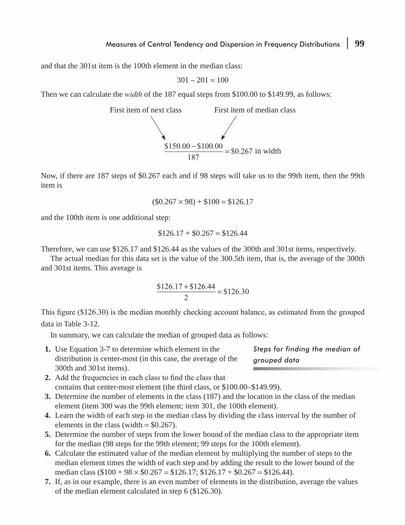
Measures of Central Tendency and Dispersion in Frequency Distributions 99
and that the 301st item is the 100th element in the median class:
301 – 201 = 100
Then we can calculate the width of the 187 equal steps from $100.00 to $149.99, as follows:
in width$150.00 $100.00
187$0.267
−=
First item of median classFirst item of next class
Now, if there are 187 steps of $0.267 each and if 98 steps will take us to the 99th item, then the 99th item is
($0.267 × 98) + $100 = $126.17
and the 100th item is one additional step:
$126.17 + $0.267 = $126.44
Therefore, we can use $126.17 and $126.44 as the values of the 300th and 301st items, respectively.The actual median for this data set is the value of the 300.5th item, that is, the average of the 300th
and 301st items. This average is
$126.17 $126.44
2$126.30
+=
data in Table 3-12.In summary, we can calculate the median of grouped data as follows:
1. Use Equation 3-7 to determine which element in the distribution is center-most (in this case, the average of the 300th and 301st items).
2. contains that center-most element (the third class, or $100.00–$149.99).
3. Determine the number of elements in the class (187) and the location in the class of the median element (item 300 was the 99th element; item 301, the 100th element).
4. Learn the width of each step in the median class by dividing the class interval by the number of elements in the class (width = $0.267).
5. Determine the number of steps from the lower bound of the median class to the appropriate item for the median (98 steps for the 99th element; 99 steps for the 100th element).
6. Calculate the estimated value of the median element by multiplying the number of steps to the median element times the width of each step and by adding the result to the lower bound of the median class ($100 + 98 × $0.267 = $126.17; $126.17 + $0.267 = $126.44).
7. If, as in our example, there is an even number of elements in the distribution, average the values of the median element calculated in step 6 ($126.30).
Steps for finding the median of
grouped data

100 Statistics for Management
To shorten this procedure, statisticians use an equation to deter-mine the median of grouped data. For a sample, this equation would be
Sample Median of Grouped Data
m =n F
fw L
( 1) / 2 ( 1)
mm
+ − +⎛
⎝⎜⎞
⎠⎟+� [3-8]
where
�m = sample median n = total number of items in the distribution F = sum of all the class frequencies up to, but not including, the median class fm = frequency of the median class w = class-interval width Lm = lower limit of the median-class interval
If we use Equation 3-8 to compute the median of our sample of checking-account balances, then n = 600, F = 201, fm = 187, w = $50, and Lm = $100.
mn F
fw L
( 1) / 2 ( 1)
mm=
+ − +⎛
⎝⎜⎞
⎠⎟+ [3-8]
601/ 2 202
187$50 $100=
−⎛⎝⎜
⎞⎠⎟
+
98.5
187$50 $100=
⎛⎝⎜
⎞⎠⎟
+
= (0.527)($50) + $100= $126.35
The slight difference between this answer and our answer calculated the long way is due to rounding.
Advantages and Disadvantages of the MedianThe median has several advantages over the mean. The most important, demonstrated in our track-team example in Table 3-10, is that extreme values do not affect the median as strongly as they do the mean. The median is easy to understand and can be calculated from any kind of data—even for grouped data with open-ended classes such as the frequency distribution in Table 3-7—unless the median falls in an open-ended class.
must be rated according to sharpness of the image. We can array the results from best to worst: extremely
Advantages of the median
An easier method

Measures of Central Tendency and Dispersion in Frequency Distributions 101
or the third rating (sharp).The median has some disadvantages as well. Certain statisti-
cal procedures that use the median are more complex than those that use the mean. Also, because the median is the value at the average position, we must array the data before we can perform any calculations. This is time consum-ing for any data set with a large number of elements. Therefore, if we want to use a sample statistic as an estimate of a population parameter, the mean is easier to use than the median. Chapter 7 will discuss estimation in detail.
In using the median, there is good news and bad news. The good news is that it is fairly quick to calculate and it avoids the effect of very large and very small values. The bad news is that you do give up some accuracy by choosing a single value to represent a distribution. With the values 2, 4, 5, 40, 100, 213, and 347, the median is 40, which has no apparent relationship to any of the other values in the distribution. Warning: Before you do any calculating, take a commonsense look at the data themselves. If the distribution looks unusual, just about anything you calculate from it will have shortcomings.
HINTS & ASSUMPTIONS
EXERCISES 3.5
Self-CheckSC 3-7 Swifty Markets compares prices charged for identical items in all of its food stores. Here are
the prices charged by each store for a pound of bacon last week:
$1.08 0.98 1.09 1.24 1.33 1.14 1.55 1.08 1.22 1.05
(a) Calculate the median price per pound.(b) Calculate the mean price per pound.(c)
SC 3-8 For the following frequency distribution, determine(a) The median class.(b) The number of the item that represents the median.(c) The width of the equal steps in the median class.(d) The estimated value of the median for these data.
Class Frequency Class Frequency100–149.5 12 300–349.5 72150–199.5 14 350–399.5 63200–249.5 27 400–449.5 36250–299.5 58 450–499.5 18
Disadvantages of the median
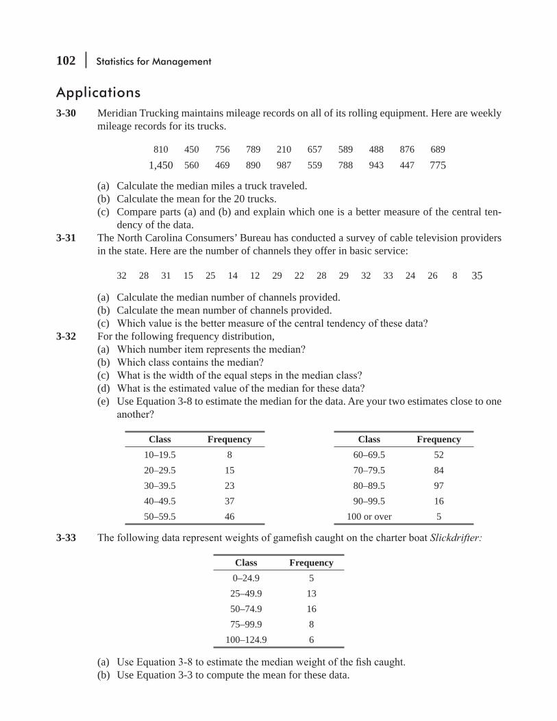
102 Statistics for Management
Applications3-30 Meridian Trucking maintains mileage records on all of its rolling equipment. Here are weekly
mileage records for its trucks.
810 450 756 789 210 657 589 488 876 689
1,450 560 469 890 987 559 788 943 447 775
(a) Calculate the median miles a truck traveled.(b) Calculate the mean for the 20 trucks.(c) Compare parts (a) and (b) and explain which one is a better measure of the central ten-
dency of the data.3-31 The North Carolina Consumers’ Bureau has conducted a survey of cable television providers
in the state. Here are the number of channels they offer in basic service:
32 28 31 15 25 14 12 29 22 28 29 32 33 24 26 8 35
(a) Calculate the median number of channels provided.(b) Calculate the mean number of channels provided.(c)
3-32 For the following frequency distribution,(a) (b) (c) (d) (e) Use Equation 3-8 to estimate the median for the data. Are your two estimates close to one
Class Frequency Class Frequency10–19.5 8 60–69.5 5220–29.5 15 70–79.5 8430–39.5 23 80–89.5 9740–49.5 37 90–99.5 1650–59.5 46 100 or over 5
3-33 Slickdrifter:
Class Frequency0–24.9 5
25–49.9 1350–74.9 1675–99.9 8
100–124.9 6
(a) (b) Use Equation 3-3 to compute the mean for these data.

Measures of Central Tendency and Dispersion in Frequency Distributions 103
(c) Compare parts (a) and (b) and comment on which is the better measure of the central tendency of these data.
3-34 The Chicago Transit Authority thinks that excessive speed on its buses increases maintenance cost. It believes that a reasonable median time from O’Hare Airport to John Hancock Center is about 30 minutes. From the following sample data (in minutes) can you help them determine
17 32 21 22
29 19 29 34
33 22 28 33
52 29 43 39
44 34 30 41
3-35 Mark Merritt, manager of Quality Upholstery Company, is researching the amount of material -
ture styles and sizes. Merritt gathers the following data (in yards) from the jobs completed last week. Calculate the median yardage used on a job last week.
5¼ 6¼ 6 9¼ 9½ 10½6 6¼ 8 9½ 10¼
5½ 6½ 8¼ 10¼5¾ 7 8½ 10½
6 7½ 9 9¼ 10
If there are 150 jobs scheduled in the next 3 weeks, use the median to predict how many yards of material will be required.
3-36 If insurance claims for automobile accidents follow the distribution given, determine the median using the method outlined on page 94. Verify that you get the same answer using Equation 3-8.
Amount of Claim ($) Frequency Amount of Claim ($) Frequency
less than 250 52 750–999.99 1,776
250–499.99 337 1,000 and above 1,492
500–749.99 1,066
3-37 A researcher obtained the following answers to a statement on an evaluation survey: strongly disagree, disagree, mildly disagree, agree somewhat, agree, strongly agree. Of the six answers,
Worked-Out Answers to Self-Check ExercisesSC 3-7
0.98 1.05 1.08 1.08 1.09 1.14 1.22 1.24 1.33 1.55
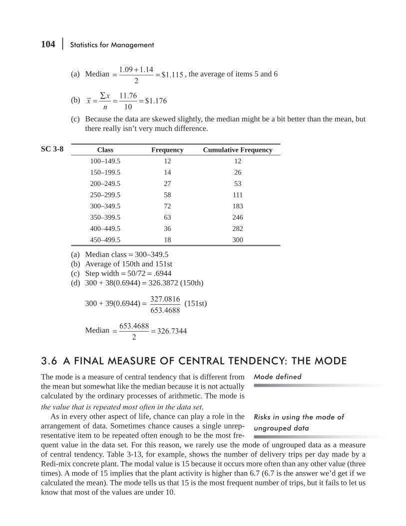
104 Statistics for Management
(a) Median 1.09 1.14
2$1.115=
+= , the average of items 5 and 6
(b) xx
n
11.76
10$1.176=
∑= =
(c) Because the data are skewed slightly, the median might be a bit better than the mean, but there really isn’t very much difference.
SC 3-8 Class Frequency Cumulative Frequency100–149.5 12 12150–199.5 14 26200–249.5 27 53250–299.5 58 111300–349.5 72 183350–399.5 63 246400–449.5 36 282450–499.5 18 300
(a) Median class = 300–349.5 (b) Average of 150th and 151st(c) Step width = 50/72 = .6944(d) 300 + 38(0.6944) = 326.3872 (150th)
300 + 39(0.6944) = 327.0816
653.4688 (151st)
Median 653.4688
2326.7344= =
3.6 A FINAL MEASURE OF CENTRAL TENDENCY: THE MODEThe mode is a measure of central tendency that is different from the mean but somewhat like the median because it is not actually calculated by the ordinary processes of arithmetic. The mode is the value that is repeated most often in the data set.
As in every other aspect of life, chance can play a role in the arrangement of data. Sometimes chance causes a single unrep-resentative item to be repeated often enough to be the most fre-quent value in the data set. For this reason, we rarely use the mode of ungrouped data as a measure of central tendency. Table 3-13, for example, shows the number of delivery trips per day made by a Redi-mix concrete plant. The modal value is 15 because it occurs more often than any other value (three times). A mode of 15 implies that the plant activity is higher than 6.7 (6.7 is the answer we’d get if we calculated the mean). The mode tells us that 15 is the most frequent number of trips, but it fails to let us know that most of the values are under 10.
Mode defined
Risks in using the mode of
ungrouped data
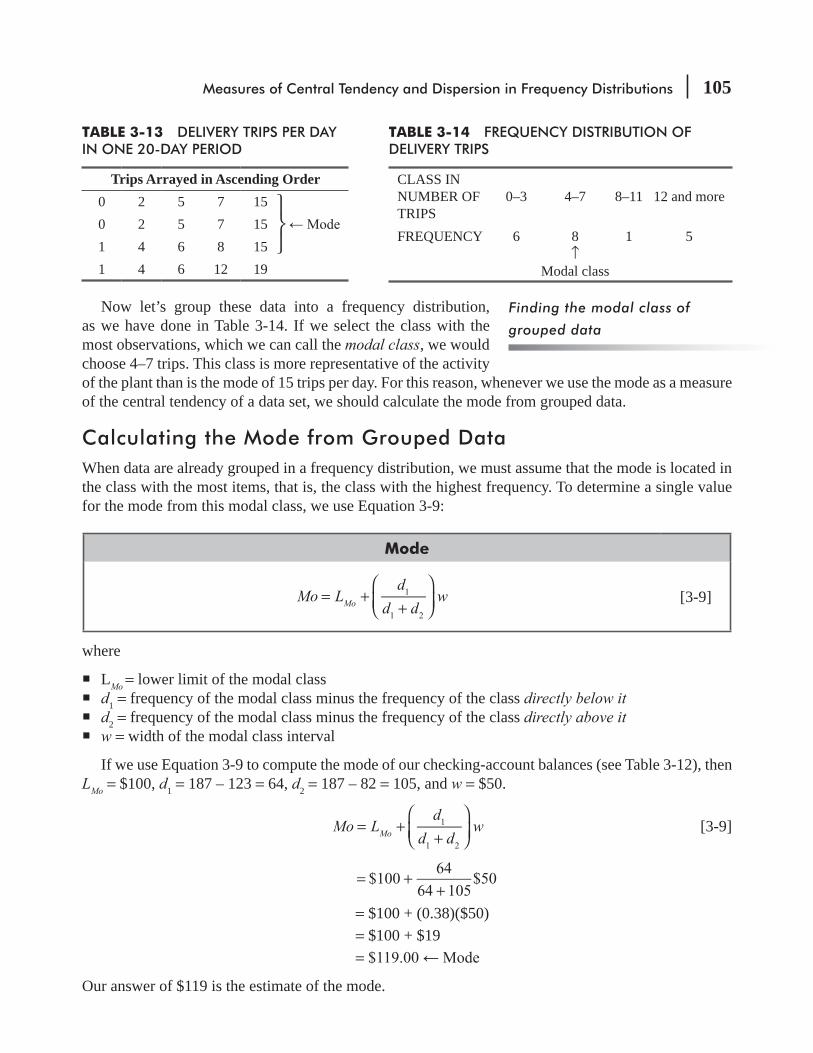
Measures of Central Tendency and Dispersion in Frequency Distributions 105
TABLE 3-13 DELIVERY TRIPS PER DAY IN ONE 20-DAY PERIOD
Trips Arrayed in Ascending Order0 2 5 7 150 2 5 7 151 4 6 8 151 4 6 12 19
TABLE 3-14 FREQUENCY DISTRIBUTION OF DELIVERY TRIPS
CLASS IN NUMBER OF TRIPS
0–3 4–7 8–11 12 and more
FREQUENCY 6 8 1 5↑
Modal class
Now let’s group these data into a frequency distribution, as we have done in Table 3-14. If we select the class with the most observations, which we can call the modal class, we would choose 4–7 trips. This class is more representative of the activity of the plant than is the mode of 15 trips per day. For this reason, whenever we use the mode as a measure of the central tendency of a data set, we should calculate the mode from grouped data.
Calculating the Mode from Grouped DataWhen data are already grouped in a frequency distribution, we must assume that the mode is located in the class with the most items, that is, the class with the highest frequency. To determine a single value for the mode from this modal class, we use Equation 3-9:
Mode
Mo Ld
d dwMo
1
1 2
= ++
⎛
⎝⎜⎞
⎠⎟[3-9]
where
LMo = lower limit of the modal class d1 = frequency of the modal class minus the frequency of the class directly below it d2 = frequency of the modal class minus the frequency of the class directly above it w = width of the modal class interval
If we use Equation 3-9 to compute the mode of our checking-account balances (see Table 3-12), then LMo = $100, d1 = 187 – 123 = 64, d2 = 187 – 82 = 105, and w = $50.
Mo Ld
d dwMo
1
1 2
= ++
⎛
⎝⎜⎞
⎠⎟ [3-9]
$10064
64 105$50= +
+= $100 + (0.38)($50)= $100 + $19=
Our answer of $119 is the estimate of the mode.
Finding the modal class of
grouped data
⎫⎬⎭
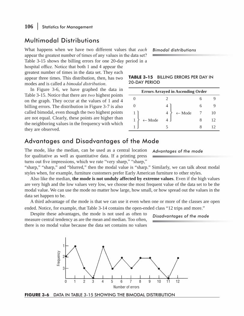
106 Statistics for Management
Multimodal DistributionsWhat happens when we have two different values that each
Table 3-15 shows the billing errors for one 20-day period in a
greatest number of times in the data set. They each appear three times. This distribution, then, has two modes and is called a bimodal distribution.
In Figure 3-6, we have graphed the data in Table 3-15. Notice that there are two highest points on the graph. They occur at the values of 1 and 4 billing errors. The distribution in Figure 3-7 is also called bimodal, even though the two highest points are not equal. Clearly, these points are higher than the neighboring values in the frequency with which they are observed.
Advantages and Disadvantages of the ModeThe mode, like the median, can be used as a central location for qualitative as well as quantitative data. If a printing press
“sharp,” “sharp,” and “blurred,” then the modal value is “sharp.” Similarly, we can talk about modal styles when, for example, furniture customers prefer Early American furniture to other styles.
Also like the median, the mode is not unduly affected by extreme values. Even if the high values are very high and the low values very low, we choose the most frequent value of the data set to be the modal value. We can use the mode no matter how large, how small, or how spread out the values in the data set happen to be.
A third advantage of the mode is that we can use it even when one or more of the classes are open ended. Notice, for example, that Table 3-14 contains the open-ended class “12 trips and more.”
Despite these advantages, the mode is not used as often to measure central tendency as are the mean and median. Too often, there is no modal value because the data set contains no values
Bimodal distributions
TABLE 3-15 BILLING ERRORS PER DAY IN 20-DAY PERIOD
Errors Arrayed in Ascending Order
0 2 6 9
0 4 6 9
1 4 ← Mode 7 10
1 ← Mode 4 8 121 5 8 12
⎫⎬⎭
⎫⎬⎭
1
2
3
0 1 2 3 4 5 6 7 8 9 10 11 12
Freq
uenc
y
Number of errors
FIGURE 3-6 DATA IN TABLE 3-15 SHOWING THE BIMODAL DISTRIBUTION
Advantages of the mode
Disadvantages of the mode

Measures of Central Tendency and Dispersion in Frequency Distributions 107
Mode
Mode
FIGURE 3-7 BIMODAL DISTRIBUTION WITH TWO UNEQUAL MODES
that occur more than once. Other times, every value is the mode, because every value occurs the same number of times. Clearly, the mode is a useless measure in these cases. Another disadvantage is that
Comparing the Mean, Median, and ModeWhen we work statistical problems, we must decide whether to use the mean, the median, or the mode as the measure of central tendency. Symmetrical distributions that contain only one mode always have the same value for the mean, the median, and the mode. In these cases, we need not choose the measure of central tendency because the choice has been made for us.
In a positively skewed distribution (one skewed to the right), as illustrated in Figure 3-8(a), the mode is at the highest point of the distribution, the median is to the right of that, and the mean is to the right of both the median and mode.
In a negatively skewed distribution (one skewed to the left), as illustrated in Figure 3-8(b), the mode is still at the highest point of the distribution, the median is to the left of that, and the mean is to the left of both the median and mode.
Mode MeanMedian
Mode MeanMedian
(a) (b)
FIGURE 3-8 POSITIVELY (A) AND NEGATIVELY (B) SKEWED DISTRIBUTIONS, ILLUSTRATING RELATIVE POSITIONS OF MEAN, MEDIAN, AND MODE.
Mean, median, and mode
are identical in a symmetrical
distribution
108 Statistics for Management
When the population is skewed negatively or positively, the median is often the best measure of location because it is always between the mean and the mode. The median is not as highly
the mode, nor is it pulled by extreme values as is the mean.Otherwise, there are no universal guidelines for applying the mean, median, or mode as the measure
of central tendency for different populations. Each case must be judged independently, according to the guidelines we have discussed.
Hint: In trying to decide on the uses of the various means, the median, and the mode, think about practical situations in which each of them would make more sense. If you are averaging a small group of factory wages fairly near each other, the arithmetic mean is very accurate and fast. If there are 500 new houses in a development all within $10,000 of each other in value, then the
interest requires the geometric mean if you want accuracy. A common-sense example: Although it’s true that the average family has 1.65 children, automobile designers will make better decisions by using the modal value of 2.0 kids.
HINTS & ASSUMPTIONS
EXERCISES 3.6
Self-Check ExercisesSC 3-9 Here are the ages in years of the cars worked on by the Village Autohaus last week:
5 6 3 6 11 7 9 10 2 4 10 6 2 1 5
(a) Compute the mode for this data set.(b) Compute the mean of the data set.(c) Compare parts (a) and (b) and comment on which is the better measure of the central
tendency of the data.SC 3-10 The ages of a sample of the students attending Sandhills Community College this semester
are:
19 17 15 20 23 41 33 21 18 2018 33 32 29 24 19 18 20 17 2255 19 22 25 28 30 44 19 20 39
(a) Construct a frequency distribution with intervals 15–19, 20–24, 25–29, 30–34, and 35 and older.
(b) Estimate the modal value using Equation 3-9.(c) Now compute the mean of the raw data.(d) Compare your answers in parts (b) and (c) and comment on which of the two is the better
measure of the central tendency of these data and why.
The median may be the best
location measure in skewed
distributions
Measures of Central Tendency and Dispersion in Frequency Distributions 109
Applications3-38 A librarian polled 20 different people as they left the library and asked them how many books
they checked out. Here are the responses:
1 0 2 2 3 4 2 1 2 0 2 2 3 1 0 7 3 5 4 2
(a) Compute the mode for this data set.(b) Compute the mean for this data set.(c) Graph the data by plotting frequency versus number checked out. Is the mean or the mode
3-39 The ages of residents of Twin Lakes Retirement Village have this frequency distribution:
Class Frequency47–51.9 4
52–56.9 9
57–61.9 13
62–66.9 42
67–71.9 39
72–76.9 20
77–81.9 9
Estimate the modal value of the distribution using Equation 3-9.3-40
(a) Hair Color Black Brunette Redhead BlondeFrequency 11 24 6 18
(b) Blood Type AB O A BFrequency 4 12 35 16
(c) Day of Birth Mon. Tues. Wed. Thurs. Fri. Sat. Sun.Frequency 22 10 32 17 13 32 14
3-41 The numbers of apartments in 27 apartment complexes in Cary, North Carolina, are given below.
91 79 66 98 127 139 154 147 192 88 97 92 87 142 127 184 145 162 95 89 86 98 145 129 149 158 241
(a) Construct a frequency distribution using intervals 66–87, 88–109,..., 220–241.(b) Estimate the modal value using Equation 3-9.(c) Compute the mean of the raw data.(d) Compare your, answers in parts (b) and (c) and comment on which of the two is the better
measure of central tendency of these data and why.3-42 Estimate the mode for the distribution given in Exercise 3-36.

110 Statistics for Management
3-43 The number of solar heating systems available to the public is quite large, and their heat-storage capacities are quite vaired. Here is a distribution of heat-storage capacity (in days) of 28 systems that were tested recently by University Laboratories, Inc.:
Days Frequency0–0.99 21–1.99 42–2.99 63–3.99 74–4.99 55–5.99 36–6.99 1
University Laboratories, Inc., knows that its report on the tests will be widely circulated and used as the basis for tax legislation on solar-heat allowances. It therefore wants the measures
(a) Compute the mean for these data.(b) Compute the mode for these data.(c) Compute the median for these data.
test data and justify your choice.3-44
Summer Earnings Number of Students$ 0–499 231
500–999 3041,000–1,499 4001,500–1,999 2962,000–2,499 1232,500–2,999 68
3,000 or more 23
(a) Find the modal class for Ed’s data.
(c) If student aid is restricted to those whose summer earnings were at least 10 percent lower
Worked-Out Answers to Self-Check ExercisesSC 3-9 (a) Mode = 6
(b) xx
n
87
155.8=
Σ= =
(c) Because the modal frequency is only 3 and because the data are reasonably symmetric, the mean is the better measure of central tendency.

Measures of Central Tendency and Dispersion in Frequency Distributions 111
SC 3-10 (a) Class 15–19 20–24 25–29 30–34Frequency 10 9 3 4 4
(b) Mo Ld
d dw 15
10
10 15 19.55Mo
1
1 2
= ++
= ++
⎛⎝⎜
⎞⎠⎟
=
(c) xx
n
760
3025.33=
Σ= =
(d) Because this distribution is very skewed, the mode is a better measure of central tendency.
3.7 DISPERSION: WHY IT IS IMPORTANTEarly in this chapter, in Figure 3-2, we illustrated two sets of data with the same central location but with one more spread out than the other. This is true of the three distributions in Figure 3-9. The mean of all three curves is the same, but curve A has less spread (or variability) than curve B, and curve B has less variability than curve C. If we measure only the mean of these three distributions, we will miss an important difference among the three curves. Likewise for any data, the mean, the median, and the mode tell us only part of what we need to know about the char-acteristics of the data. To increase our understanding of the pattern of the data, we must also measure its dispersion—its spread, or variability.
Why is the dispersion of the distribution such an important First, it gives us
additional information that enables us to judge the reliability of our measure of the central tendency. If data are widely dis-persed, such as those in curve C in Figure 3-9, the central location is less representative of the data as a whole than it would be for data more closely centered around the mean, as in curve A. Second, because there are problems peculiar to widely dispersed data, we must be able to recognize that data are widely dispersed before we can tackle those problems. Third, we may wish to compare disper-sions of various samples. If a wide spread of values away from the center is undesirable or presents an unacceptable risk, we need to be able to recognize and avoid choosing the distributions with the greatest dispersion.
Curve A
Curve B
Curve C
Mean of A, B, C
FIGURE 3-9 THREE CURVES WITH THE SAME MEAN BUT DIFFERENT VARIABILITIES
Need to measure dispersion or
variability
Uses of dispersion measures
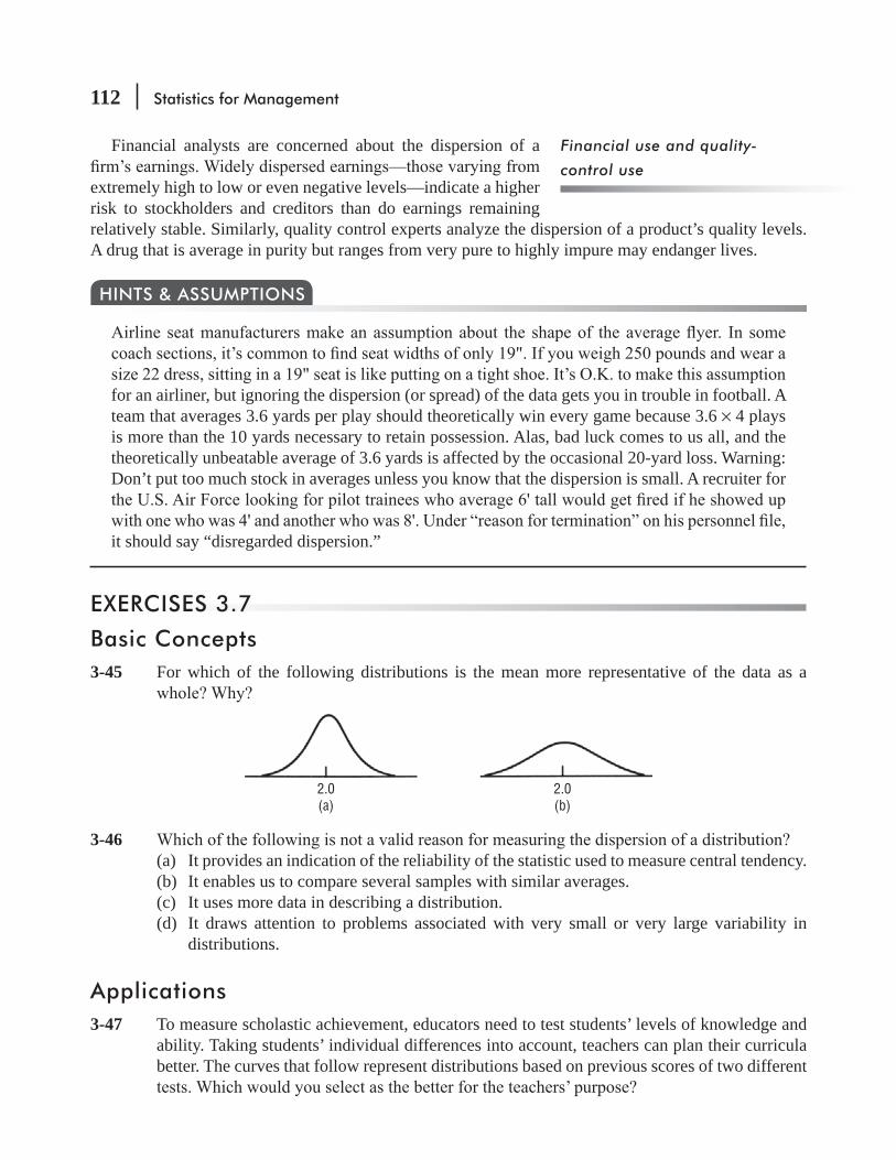
112 Statistics for Management
Financial analysts are concerned about the dispersion of a
extremely high to low or even negative levels—indicate a higher risk to stockholders and creditors than do earnings remaining relatively stable. Similarly, quality control experts analyze the dispersion of a product’s quality levels. A drug that is average in purity but ranges from very pure to highly impure may endanger lives.
for an airliner, but ignoring the dispersion (or spread) of the data gets you in trouble in football. A team that averages 3.6 yards per play should theoretically win every game because 3.6 × 4 plays is more than the 10 yards necessary to retain possession. Alas, bad luck comes to us all, and the theoretically unbeatable average of 3.6 yards is affected by the occasional 20-yard loss. Warning: Don’t put too much stock in averages unless you know that the dispersion is small. A recruiter for
it should say “disregarded dispersion.”
HINTS & ASSUMPTIONS
EXERCISES 3.7
Basic Concepts3-45 For which of the following distributions is the mean more representative of the data as a
2.0(a)
2.0(b)
3-46 (a) It provides an indication of the reliability of the statistic used to measure central tendency.(b) It enables us to compare several samples with similar averages.(c) It uses more data in describing a distribution.(d) It draws attention to problems associated with very small or very large variability in
distributions.
Applications3-47 To measure scholastic achievement, educators need to test students’ levels of knowledge and
ability. Taking students’ individual differences into account, teachers can plan their curricula better. The curves that follow represent distributions based on previous scores of two different
Financial use and quality-
control use

Measures of Central Tendency and Dispersion in Frequency Distributions 113
A B
3-48 -butions of delivery time for the two methods, based on past records. From available evidence,
2.0(a)
2.0(b)
3-49 Of the 3 curves shown in Figure 3-9, choose one that would best describe the distribution of values for the ages of the following groups: members of Congress, newly elected members of the House of Representatives, and the chairpersons of major congressional committees. In making your choices, disregard the common mean of the curves in Figure 3-9 and consider
3-50 How do you think the concept of variability might apply to an investigation that the
3-51 Choose which of the three curves shown in Figure 3-9 best describes the distribution of the following characteristics of various groups. Make your choices only on the basis of the vari-
(a) The number of points scored by each player in a professional basketball league during an 80-game season.
(b) The salary of each of 100 people working at roughly equivalent jobs in the federal government.(c) The grade-point average of each of the 15,000 students at a major state university.(d) The salary of each of 100 people working at roughly equivalent jobs in a private corporation.(e) The grade-point average of each student at a major state university who has been accepted
for graduate school.(f) The percentage of shots made by each player in a professional basketball league during an
80-game season.
3.8 RANGES: USEFUL MEASURES OF DISPERSIONDispersion may be measured in terms of· the difference between two values selected from the data set. In this section, we shall study three of these so-called distance measures: the range, the interfractile range, and the interquartile range.
RangeThe range is the difference between the highest and lowest observed values. In equation form, we can say
Three distance measures
Defining and computing the
range

114 Statistics for Management
Range
Range =value of highest
observationvalue of lowest
observation− [3-10]
Using this equation, we compare the ranges of annual payments from Blue Cross–Blue Shield received by the two hospitals illustrated in Table 3-16.
The range of annual payments to Cumberland is $1,883,000 – $863,000 = $1,020,000. For Valley Falls, the range is $690,000 – $490,000 = $200,000.
-ness as a measure of dispersion is limited. The range considers only the highest and lowest values of a distribution and fails to take account of any other observation in the data set. As a result, it ignores the nature of the variation
only two values, the range is likely to change drastically from one sample to the next in a given popu-lation, even though the values that fall between the highest and lowest values may be quite similar. Keep in mind, too, that open-ended distributions have no range because no “highest” or “lowest” value exists in the open-ended class.
Interfractile RangeIn a frequency distribution, a given fraction or proportion of the data lie at or below a fractile. The median, for example, is the 0.5 fractile, because half the data set is less than or equal to this value. You will notice that fractiles are similar to percentages. In any distribution, 25 percent of the data lie at or below the 0.25 fractile; likewise, 25 percent of the data lie at or below the 25th percentile. The interfractile range is a measure of the spread between two fractiles in a frequency distribution, that is, the dif-ference between the values of the two fractiles.
thirds of Cumberland’s receipts from Blue Cross–Blue Shield. We begin by dividing the observations into thirds, as we have done in Table 3-17. Each third contains four
TABLE 3-16 ANNUAL PAYMENTS FROM BLUE CROSS–BLUE SHIELD (000S OMITTED)
CUMBERLAND 863 903 957 1,041 1,138 1,2041,354 1,624 1,698 1,745 1,802 1,883
VALLEY FALLS 490 540 560 570 590 600 610 620 630 660 670 690
Characteristics of the range
Fractiles
Meaning of the interfractile
range
Calculating the interfractile
range

Measures of Central Tendency and Dispersion in Frequency Distributions 115
the second third.Fractiles have special names, depending on the number of
equal parts into which they divide the data. Fractiles that divide the data into 10 equal parts are called deciles. Quartiles divide the data into four equal parts. Percentiles divide the data into 100 equal parts.
Interquartile RangeThe interquartile range measures approximately how far from the median we must go on either side before we can include one-half the values of the data set. To compute this range, we divide our data into four parts, each of which contains 25 per-cent of the items in the distribution. The quartiles are then the highest values in each of these four parts, and the interquartile range
Interquartile Range
Interquartile range = Q3 – Q1 [3-11]
of the four quartiles need not be the same.In Figure 3-11, another illustration of quartiles, the quartiles divide the area under the distribution
into four equal parts, each containing 25 percent of the area.
Interquartile range
14
of items 14
of items
Lowestobservation
Highestobservation
1st quartile 3rd quartile2nd quartile(median)
Q1 Q2 Q3
FIGURE 3-10 INTERQUARTILE RANGE
Special fractiles: deciles,
quartiles, and percentiles
Computing the interquartile
range
TABLE 3-17 BLUE CROSS–BLUE SHIELD ANNUAL PAYMENTS TO CUMBERLAND HOSPITAL (000S OMITTED)
First Third Second Third Last Third863 1,138 1,698903 1,204 1,745957 1,354 1,802
1,883
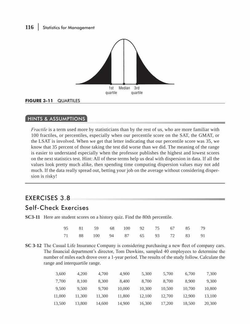
116 Statistics for Management
1stquartile
3rdquartile
Median
FIGURE 3-11 QUARTILES
Fractile is a term used more by statisticians than by the rest of us, who are more familiar with 100 fractiles, or percentiles, especially when our percentile score on the SAT, the GMAT, or the LSAT is involved. When we get that letter indicating that our percentile score was 35, we know that 35 percent of those taking the test did worse than we did. The meaning of the range is easier to understand especially when the professor publishes the highest and lowest scores on the next statistics test. Hint: All of these terms help us deal with dispersion in data. If all the values look pretty much alike, then spending time computing dispersion values may not add much. If the data really spread out, betting your job on the average without considering disper-sion is risky!
HINTS & ASSUMPTIONS
EXERCISES 3.8
Self-Check ExercisesSC3-11 Here are student scores on a history quiz. Find the 80th percentile.
95 81 59 68 100 92 75 67 85 79
71 88 100 94 87 65 93 72 83 91
SC 3-12
number of miles each drove over a 1-year period. The results of the study follow. Calculate the range and interquartile range.
3,600 4,200 4,700 4,900 5,300 5,700 6,700 7,300
7,700 8,100 8,300 8,400 8,700 8,700 8,900 9,300
9,500 9,500 9,700 10,000 10,300 10,500 10,700 10,800
11,000 11,300 11,300 11,800 12,100 12,700 12,900 13,100
13,500 13,800 14,600 14,900 16,300 17,200 18,500 20,300
Measures of Central Tendency and Dispersion in Frequency Distributions 117
Basic Concepts3-52 For the following data, compute the interquartile range.
99 75 84 61 33 45 66 97 69 5572 91 74 93 54 76 52 91 77 68
3-53 For the sample that follows, compute the(a) Range.(b) Interfractile range between the 20th and 80th percentiles.(c) Interquartile range.
2,549 3,897 3,661 2,697 2,200 3,812 2,228 3,891 2,668 2,2683,692 2,145 2,653 3,249 2,841 3,469 3,268 2,598 3,842 3,362
Applications3-54 Here are the high temperature readings during June 1995 in Phoenix, Arizona. Find the 70th
percentile.
84 86 78 69 94 95 94 98 89 87 88 89 92 99 10294 92 96 89 88 87 88 84 82 88 94 97 99 102 105
3-55 These are the total fares (in dollars) collected Tuesday by the 20 taxis belonging to City Transit, Ltd.
147 95 93 127 143 101 123 83 135 129185 92 115 126 157 93 133 51 125 132
Compute the range of these data and comment on whether you think it is a useful measure of dispersion.
3-56 Redi-Mix Incorporated kept the following record of time (to the nearest 100th of a minute) its truck waited at the job to unload. Calculate the range and the interquartile range.
0.10 0.45 0.50 0.32 0.89 1.20 0.53 0.67 0.58 0.480.23 0.77 0.12 0.66 0.59 0.95 1.10 0.83 0.69 0.51
3-57 Warlington Appliances has developed a new combination blender-crock-pot. In a market-ing demonstration, a price survey determined that most of those sampled would be willing to pay around $60, with a surprisingly small interquartile range of $14.00. In an attempt to replicate the results, the demonstration and accompanying survey were repeated. The mar-
52 35 48 46 43 40 61 49 57 58 65 4672 69 38 37 55 52 50 31 41 60 45 4155 38 51 49 46 43 64 52 60 61 68 4969 66 35 34 52 49 47 28 38 57 42 38

118 Statistics for Management
3-58 MacroSwift has decided to develop a new software program designed for CEOs and other high-level executives. MacroSwift did not want to develop a program that required too much hard-drive space, so they polled 36 executives to determine the amount of available space on their PCs. The results are given below in megabytes.
6.3 6.7 7.9 8.4 9.7 10.6 12.4 19.4 29.1 42.6
59.8 97.6 100.4 120.6 135.5 148.6 178.6 200.1 229.6 284.6
305.6 315.6 325.9 347.5 358.6 397.8 405.6 415.9 427.8 428.6
439.5 440.9 472.3 475.9 477.2 502.6
Calculate the range and interquartile range.3-59 The New Mexico State Highway Department is charged with maintaining all state roads in
good condition. One measure of condition is the number of cracks present in each 100 feet of roadway. From the department’s yearly sample, the following data were obtained:
4 7 8 9 9 10 11 12 12 13
13 13 13 14 14 14 15 15 16 16
16 16 16 17 17 17 18 18 19 19
Calculate the interfractile ranges between the 20th, 40th, 60th, and 80th percentiles.3-60 Ted Nichol is a statistical analyst who reports directly to the highest levels of management at
then RESEARCH!” Ted has just received some disturbing data: the monthly dollar volume of research contracts that the company has won for the past year. Ideally, these monthly numbers
dollars) follow:
253 104 633 57 500 201
43 380 467 162 220 302
Calculate the following:(a) The interfractile range between the second and eighth deciles.(b) The median, Ql, and Q3.(c) The interquartile range.
Worked-Out Answers to Self-Check ExercisesSC 3-11 First we arrange the data in increasing order:
59 65 67 68 71 72 75 79 81 83
85 87 88 91 92 93 94 95 100 100
The 16th of these (or 93) is the 80th percentile.SC 3-12 Range = 20,300 – 3,600 = 16,700 miles
Interquartile range = Q3 – Q1 = 12,700 – 8,100 = 4,600 miles

Measures of Central Tendency and Dispersion in Frequency Distributions 119
3.9 DISPERSION: AVERAGE DEVIATION MEASURES The most comprehensive descriptions of dispersion are those that deal with the average deviation from some measure of central tendency. Two of these measures are important to our study of statistics: the variance and the standard deviation. Both of these tell us an average distance of any observation in the data set from the mean of the distribution.
Population VarianceEvery population has a variance, which is symbolized by σ 2 (sigma squared). To calculate the population variance, we divide the sum of the squared distances between the mean and each item in the population by the total number of items in the population. By squaring each distance, we make each number positive and, at the same time, assign more weight to the larger deviations (deviation is the distance between the mean and a value).
The formula for calculating the variance is
Population Variance
x
N
x
N
( )22 2
2σ μ μ=Σ −
=Σ
− [3-12]
where
σ 2 = population variance x = item or observation μ = population mean N = total number of items in the population = sum of all the values (x – μ)2 or all the values x2
In Equation 3-12, the middle expression x
N
( )2μΣ − σ 2 The last expression, x
N
22μΣ
− ,
is mathematically must actu-ally compute the value of σ 2, since it frees us from calculating the deviations from the mean. However, when the x values are large and the x – μ values are small, it may be more convenient to use the middle
expression, x
N
( )2μΣ − , to compute σ 2. Before we can use this formula in an example, we need to discuss
an important problem concerning the variance. In solving that problem, we will learn what the standard deviation is and how to calculate it. Then we can return to the variance itself.
Earlier, when we calculated the range, the answers were expressed in the same units as the data. (In our examples, the units were “thousands of dollars of pay-ments.”) For the variance, however, the units are the squares of the units of the data—for example, “squared dollars” or “dollars squared.” Squared dollars or dollars squared are not intuitively
Two measures of average
deviation
Variance
Formula for the variance of a
population
Units in which the variance is
expressed cause a problem

120 Statistics for Management
compute a useful measure of deviation, one that does not give us a problem with units of measure and thus is less confusing. This measure is called the standard deviation, and it is the square root of the variance. The square root of 100 dollars squared is 10 dollars because we take the square root of both the value and the units in which it is measured. The standard deviation, then, is in units that are the same as the original data.
Population Standard DeviationThe population standard deviation, or σ, is simply the square root of the population variance. Because the variance is the average of the squared distances of the observations from the mean, the standard deviation is the square root of the average of the squared distances of the observations from the mean. While the variance is expressed in the square of the units used in the data, the standard deviation is in the same units as those used in the data. The formula for the standard deviation is
Population Standard Deviation
x
N
x
N
( )22 2
2σ σ μ μ= =Σ −
=Σ
− [3-13]
x = observation μ = population mean N = total number of elements in the population = sum of all the values (x – μ,)2, or all the values x2
σ = population standard deviation σ 2 = population variance
The square root of a positive number may be either positive or negative because a2 = (–a)2. When taking the square root of the variance to calculate the standard deviation, however, statisti-cians consider only the positive square root.
To calculate either the variance or the standard deviation, we construct a table, using every element
test each vial to determine its purity, our data might look like Table 3-18. In Table 3-19, we show how to use these data to compute the mean (0.166 = 2.49/15, the column (1) sum divided by N), the deviation of each value from the mean (column 3), the square of the deviation of each value from the mean (column 4), and the sum of the squared deviations. From this, we can compute the variance, which is 0.0034 percent squared. (Table 3-19 also computes σ 2 using the
second half of Equation 3-12, x
N
22μ=
Σ− . Note
Relationship of standard
deviation to the variance
Use the positive square root
Computing the standard
deviation
TABLE 3-18 RESULTS OF PURITY TEST ON COMPOUNDS
Observed Percentage Impurity0.04 0.14 0.17 0.19 0.22
0.06 0.14 0.17 0.21 0.24
0.12 0.15 0.18 0.21 0.25
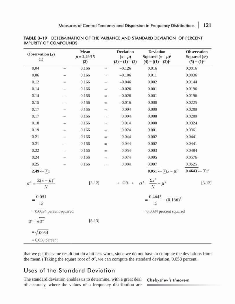
Measures of Central Tendency and Dispersion in Frequency Distributions 121
that we get the same result but do a bit less work, since we do not have to compute the deviations from the mean.) Taking the square root of σ 2, we can compute the standard deviation, 0.058 percent.
Uses of the Standard DeviationThe standard deviation enables us to determine, with a great deal of accuracy, where the values of a frequency distribution are
Chebyshev’s theorem
TABLE 3-19 DETERMINATION OF THE VARIANCE AND STANDARD DEVIATION OF PERCENT IMPURITY OF COMPOUNDS
Observation (x) (1)
Mean m = 2.49/15
(2)
Deviation (x – m)
(3) = (1) – (2)
Deviation Squared (x – m)2 (4) = [(1) – (2)]2
Observation Squared (x2)
(5) = (1)2
0.04 – 0.166 = –0.126 0.016 0.0016
0.06 – 0.166 = –0.106 0.011 0.0036
0.12 – 0.166 = –0.046 0.002 0.0144
0.14 – 0.166 = –0.026 0.001 0.0196
0.14 – 0.166 = –0.026 0.001 0.0196
0.15 – 0.166 = –0.016 0.000 0.0225
0.17 – 0.166 = 0.004 0.000 0.0289
0.17 – 0.166 = 0.004 0.000 0.0289
0.18 – 0.166 = 0.014 0.000 0.0324
0.19 – 0.166 = 0.024 0.001 0.0361
0.21 – 0.166 = 0.044 0.002 0.0441
0.21 – 0.166 = 0.044 0.002 0.0441
0.22 – 0.166 = 0.054 0.003 0.0484
0.24 – 0.166 = 0.074 0.005 0.0576
0.25 – 0.166 = 0.084 0.007 0.0625
2.49 ← x 0.051 ← x − μ)2 0.4643 x2
x
N
( )22
σ μ=
Σ − [3-12] x
N2
22σ μ =
Σ− [3-12]
0.051
15=
0.4643
15(0.166)2= −
= 0.0034 percent squared = 0.0034 percent squared
2σ σ= [3-13]
= .0034
= 0.058 percent

122 Statistics for Management
located in relation to the mean. We can do this according to a theorem devised by the Russian mathema-tician P. L. Chebyshev (1821–1894). Chebyshev’s theorem says that no matter what the shape of the distribution, at least 75 percent of the values will fall within ±2 standard deviations from the mean of the distribution, and at least 89 percent of the values will lie within ±3 standard deviations from the mean.
under a symmetrical, bell-shaped curve such as the one in Figure 3-12. In these cases, we can say that:
1. About 68 percent of the values in the population will fall within ± 1 standard deviation from the mean.
2. About 95 percent of the values will lie within ±2 standard deviations from the mean. 3. About 99 percent of the values will be in an interval ranging from 3 standard deviations below the
mean to 3 standard deviations above the mean.
In the light of Chebyshev’s theorem, let’s analyze the data in Table 3-19. There, the mean impurity of the 15 vials of com-pound is 0.166 percent, and the standard deviation is 0.058 per-cent. Chebyshev’s theorem tells us that at least 75 percent of the values (at least 11 of our 15 items) are between 0.166 – 2(0.058) = 0.050 and 0.166 + 2(0.058) = 0.282. In fact, 93 percent of the values (14 of the 15 values) are actually in that interval. Notice that the distribution is reasonably symmetrical and that 93 percent is close to the theoretical 95 percent for an interval of plus and minus 2 standard devia-tions from the mean of a bell-shaped curve.
The standard deviation is also useful in describing how far individual items in a distribution depart from the mean of the distribution. A measure called the standard score gives us the number of standard deviations a particular observation lies below or above the mean. If we let x symbol-ize the observation, the standard score computed from population data is
Standard Score
Population standard score x μσ
=− [3-14]
Using Chebyshev’s theorem
Concept of the standard score
99%
95%
68%
μ − 3σ μ − 2σ μ + 2σ μ + 3σμ − σ μ + σμ
FIGURE 3-12 LOCATION OF OBSERVATIONS AROUND THE MEAN OF A BELL-SHAPED FREQUENCY DISTRIBUTION
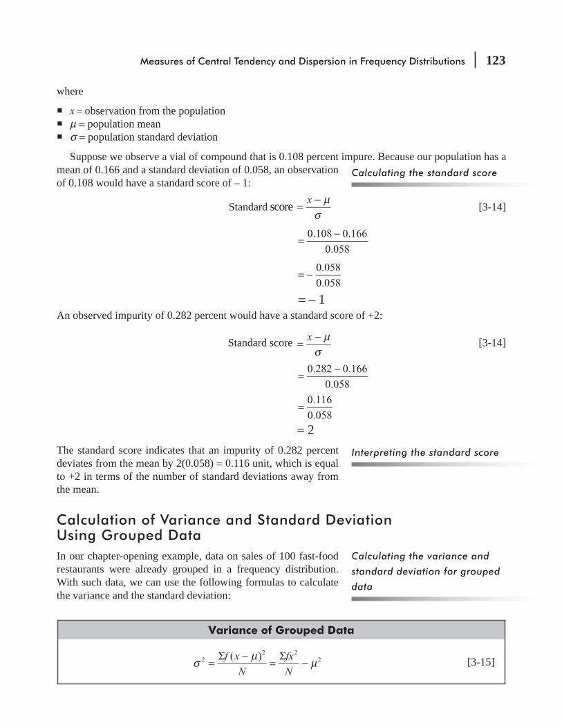
Measures of Central Tendency and Dispersion in Frequency Distributions 123
where
x = observation from the population μ = population mean σ = population standard deviation
Suppose we observe a vial of compound that is 0.108 percent impure. Because our population has a mean of 0.166 and a standard deviation of 0.058, an observation of 0.108 would have a standard score of – 1:
Standard score x μσ
=−
[3-14]
0.108 0.166
0.058=
−
0.058
0.058= −
= – 1An observed impurity of 0.282 percent would have a standard score of +2:
Standard score x μσ
=− [3-14]
0.282 0.166
0.058=
−
0.116
0.058=
= 2The standard score indicates that an impurity of 0.282 percent deviates from the mean by 2(0.058) = 0.116 unit, which is equal to +2 in terms of the number of standard deviations away from the mean.
Calculation of Variance and Standard Deviation Using Grouped DataIn our chapter-opening example, data on sales of 100 fast-food restaurants were already grouped in a frequency distribution. With such data, we can use the following formulas to calculate the variance and the standard deviation:
Variance of Grouped Data
f x
N
fx
N
( )22 2
2σ μ μ=Σ −
=Σ
− [3-15]
Calculating the standard score
Interpreting the standard score
Calculating the variance and
standard deviation for grouped
data
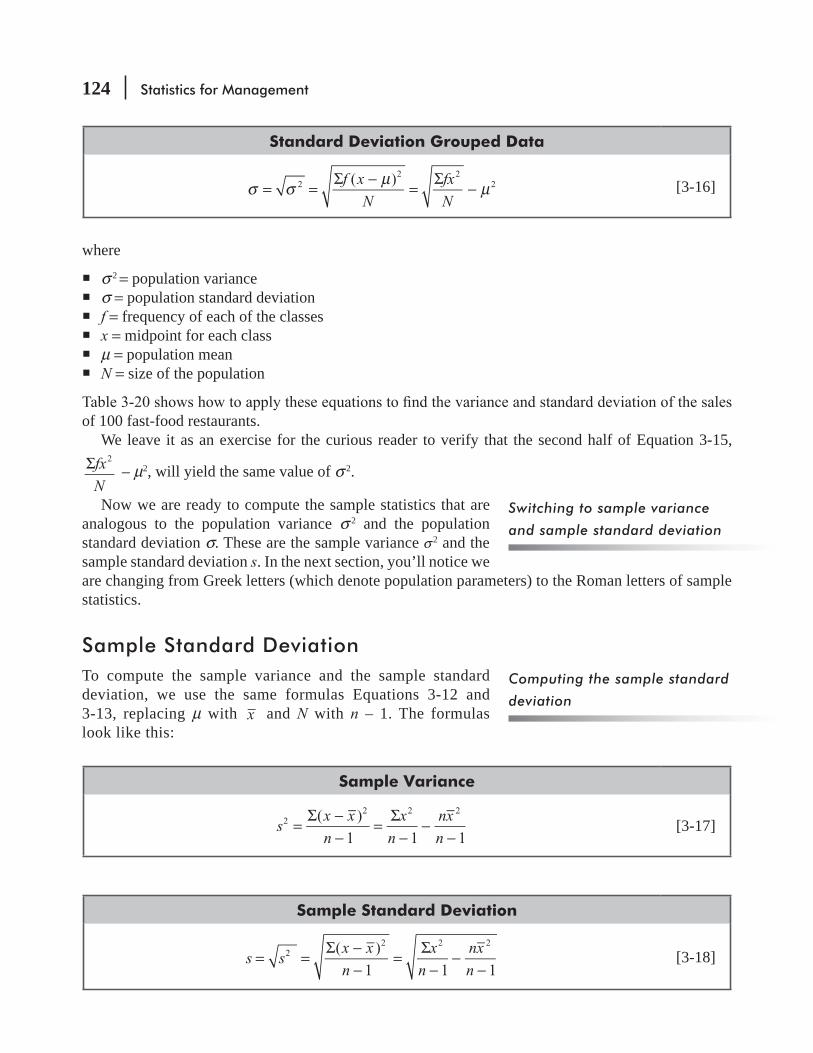
124 Statistics for Management
Standard Deviation Grouped Data
f x
N
fx
N
( )22 2
2σ σ μ μ= =Σ −
=Σ
− [3-16]
where
σ 2 = population variance σ = population standard deviation f = frequency of each of the classes x = midpoint for each class μ = population mean = size of the population
of 100 fast-food restaurants.We leave it as an exercise for the curious reader to verify that the second half of Equation 3-15,
fx
N
2Σ – μ2, will yield the same value of σ 2.
Now we are ready to compute the sample statistics that are analogous to the population variance σ 2 and the population standard deviation σ. These are the sample variance σ 2 and the sample standard deviation s. In the next section, you’ll notice we are changing from Greek letters (which denote population parameters) to the Roman letters of sample statistics.
Sample Standard DeviationTo compute the sample variance and the sample standard deviation, we use the same formulas Equations 3-12 and 3-13, replacing μ with x and N with n – 1. The formulas look like this:
Sample Variance
sx x
n
x
n
nx
n
( )
1 1 12
2 2 2
=Σ −
−=
Σ−
−−
[3-17]
Sample Standard Deviation
s sx x
n
x
n
nx
n
( )
1 1 12
2 2 2
= =Σ −
−=
Σ−
−−
[3-18]
Switching to sample variance
and sample standard deviation
Computing the sample standard
deviation
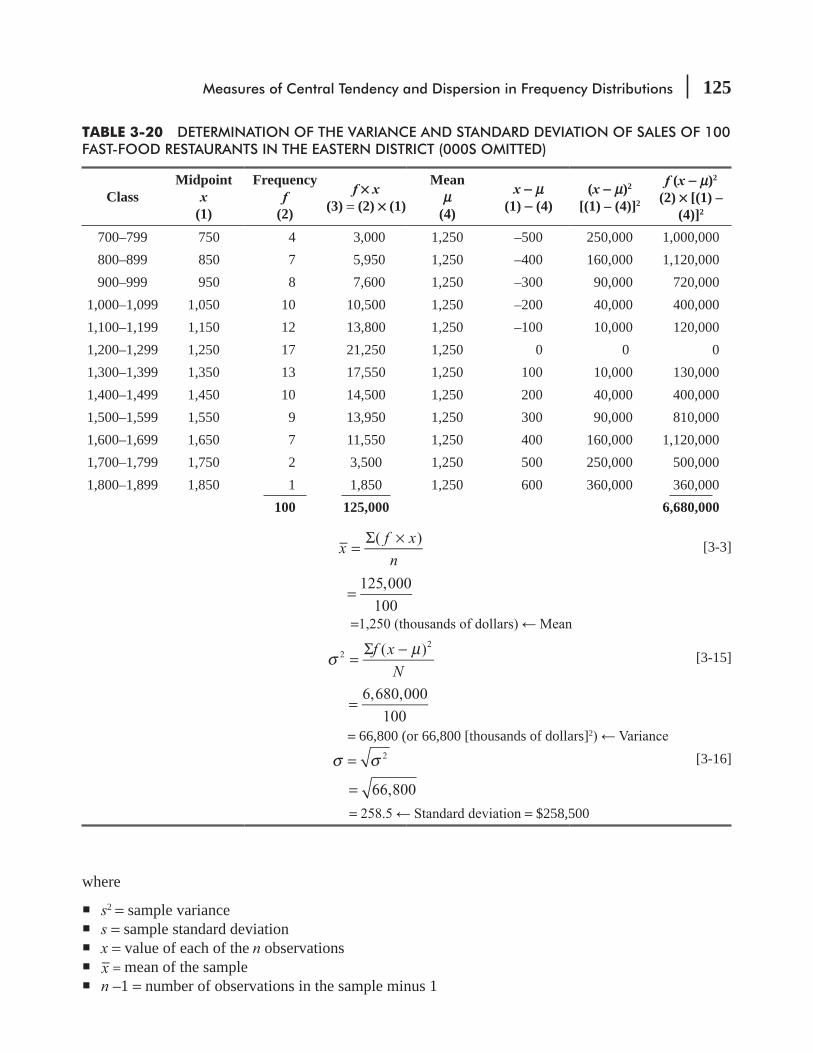
Measures of Central Tendency and Dispersion in Frequency Distributions 125
where
s2 = sample variance s = sample standard deviation x = value of each of the n observations x = mean of the sample n –1 = number of observations in the sample minus 1
TABLE 3-20 DETERMINATION OF THE VARIANCE AND STANDARD DEVIATION OF SALES OF 100 FAST-FOOD RESTAURANTS IN THE EASTERN DISTRICT (000S OMITTED)
ClassMidpoint
x (1)
Frequency f
(2)
f ¥ x (3) = (2) ¥ (1)
Mean m
(4)
x - m (1) - (4)
(x - m)2 [(1) – (4)]2
f (x - m)2 (2) ¥ [(1) –
(4)]2
700–799 750 4 3,000 1,250 –500 250,000 1,000,000800–899 850 7 5,950 1,250 –400 160,000 1,120,000900–999 950 8 7,600 1,250 –300 90,000 720,000
1,000–1,099 1,050 10 10,500 1,250 –200 40,000 400,0001,100–1,199 1,150 12 13,800 1,250 –100 10,000 120,0001,200–1,299 1,250 17 21,250 1,250 0 0 01,300–1,399 1,350 13 17,550 1,250 100 10,000 130,0001,400–1,499 1,450 10 14,500 1,250 200 40,000 400,0001,500–1,599 1,550 9 13,950 1,250 300 90,000 810,0001,600–1,699 1,650 7 11,550 1,250 400 160,000 1,120,0001,700–1,799 1,750 2 3,500 1,250 500 250,000 500,0001,800–1,899 1,850 1 1,850 1,250 600 360,000 360,000
100 125,000 6,680,000
xf x
n
( )=
Σ × [3-3]
125,000
100=
=
f x
N
( )22
σ μ=
Σ − [3-15]
6,680,000
100=
= 66,800 (or 66,800 [thousands of dollars]2
2σ σ= [3-16]
66,800== = $258,500

126 Statistics for Management
Why do we use n – 1 as the denominator instead of n Statisticians can prove that if we take many samples from a given
s2) for each sample, and average each of these together, then this average tends not to equal the population variance, σ 2, unless we use n – 1 as the denominator. In Chapter 7, we shall learn the statistical explanation of why this is true.
and the sample standard deviation of the annual Blue Cross–Blue Shield payments to Cumberland Hospital in Table 3-21; note that both halves of Equation 3-17 yield the same result.
Calculating sample variance
and standard deviation for
hospital data
Use of n – 1 as the denominator
TABLE 3-21 DETERMINATION OF THE SAMPLE VARIANCE AND STANDARD DEVIATION OF ANNUAL BLUE CROSS–BLUE SHIELD PAYMENTS TO CUMBERLAND HOSPITAL (000S OMITTED)
Observation (x) (1)
Mean (x_)
(2)
x - x_
(1) - (2)(x - x
_)2
[(1) – (2)]2x2
(1)2
863 1,351 –488 238,144 744,769 903 1,351 –448 200,704 815,409 957 1,351 –394 155,236 915,8491,041 1,351 –310 96,100 1,083,6811,138 1,351 –213 45,369 1,295,0441,204 1,351 –147 21,609 1,449,6161,354 1,351 3 9 1,833,3161,624 1,351 273 74,529 2,637,3761,698 1,351 347 120,409 2,883,2041,745 1,351 394 155,236 3,045,0251,802 1,351 451 203,401 3,247,2041,883 1,351 532 283,024 3,545,689
x - x_)2 x2
s
x x
n
( )
12
2
=Σ −
−[3-17]
1,593,770
11=
= 144,888 (or 144,888 [thousands of dollars]2
s s2=
OR 144,888=
=
s
x
n
nx
n1 12
2 2
=Σ
−−
−
23,496,182
11
12(1,351)
11
2
= −
1,593,770
11=
=144,888
[3-18]
[3-17]
⎧⎨⎩
⎧⎨⎩

Measures of Central Tendency and Dispersion in Frequency Distributions 127
Just as we used the population standard deviation to derive population standard scores, we may also use the sample devia-tion to compute sample standard scores. These sample standard scores tell us how many standard deviations a particular sample observation lies below or above the sample mean. The appropriate formula is
Standard Score of an Item in a Sample
Sample standard score x x
s=
− [3-19]
where
x = observation from the sample x = sample mean s = sample standard deviation
In the example we just did, we see that the observation 863 corresponds to a standard score of –1.28:
Sample standard score x x
s=
− [3-19]
863 1,351
380.64=
−
488
380.64=
−
= –1.28
This section has demonstrated why the standard deviation is the measure of dispersion used most often. We can use it to compare distributions and to compute standard scores, an important element of statistical inference to be discussed later. Like the variance, the standard deviation takes into account every observation in the data set. But the standard deviation has some disadvantages, too. It is not as easy to calculate as the range, and it cannot be computed from open-ended distributions. In addition, extreme values in the data set distort the value of the standard deviation, although to a lesser extent than they do the range.
We assume when we calculate and use the standard deviation that there are not too many very large or very small values in the data set because we know that the standard deviation uses every value, and such extreme values will distort the answer. Hint: Forgetting whether to use N or n – 1 as the denominator for samples and populations can be avoided by associating the smaller value (n – 1) with the smaller set (the sample).
HINTS & ASSUMPTIONS
Computing sample standard
Scores

128 Statistics for Management
EXERCISES 3.9
Self-Check ExercisesSC 3-13 Talent, Ltd., a Hollywood casting company, is selecting a group of extras for a movie. The
interviewed are
50 56 55 49 52 57 56 57 56 5954 55 61 60 51 59 62 52 54 49
The director of the movie wants men whose ages are fairly tightly grouped around 55 years. Being a statistics buff of sorts, the director suggests that a standard deviation of 3 years would
SC 3-14 In an attempt to estimate potential future demand, the National Motor Company did a study asking married couples how many cars the average energy-minded family should own in 1998. For each couple, National averaged the husband’s and wife’s responses to get the overall couple response. The answers were then tabulated:
Number of cars 0 0.5 1.0 1.5 2.0 2.5Frequency 2 14 23 7 4 2
(a) Calculate the variance and the standard deviation.(b) Since the distribution is roughly bell-shaped, how many of the observations should theo-
Applications3-61 The head chef of The Flying Taco has just received two dozen tomatoes from her supplier,
but she isn’t ready to accept them. She knows from the invoice that the average weight of a tomato is 7.5 ounces, but she insists that all be of uniform weight. She will accept them only if the average weight is 7.5 ounces and the standard deviation is less than 0.5 ounce. Here are the weights of the tomatoes
6.3 7.2 7.3 8.1 7.8 6.8 7.5 7.8 7.2 7.5 8.1 8.28.0 7.4 7.6 7.7 7.6 7.4 7.5 8.4 7.4 7.6 6.2 7.4
3-62 a Miami manufacturer:
17 21 18 27 17 21 20 22 18 23
The company production manager feels that a standard deviation of more than three boats a day indicates unacceptable production-rate variations. Should she be concerned about plant-
3-63 A set of 60 observations has a mean of 66.8, a variance of 12.60, and an unknown distribution shape.(a) Between what values should at least 75 percent of the observations fall, according to
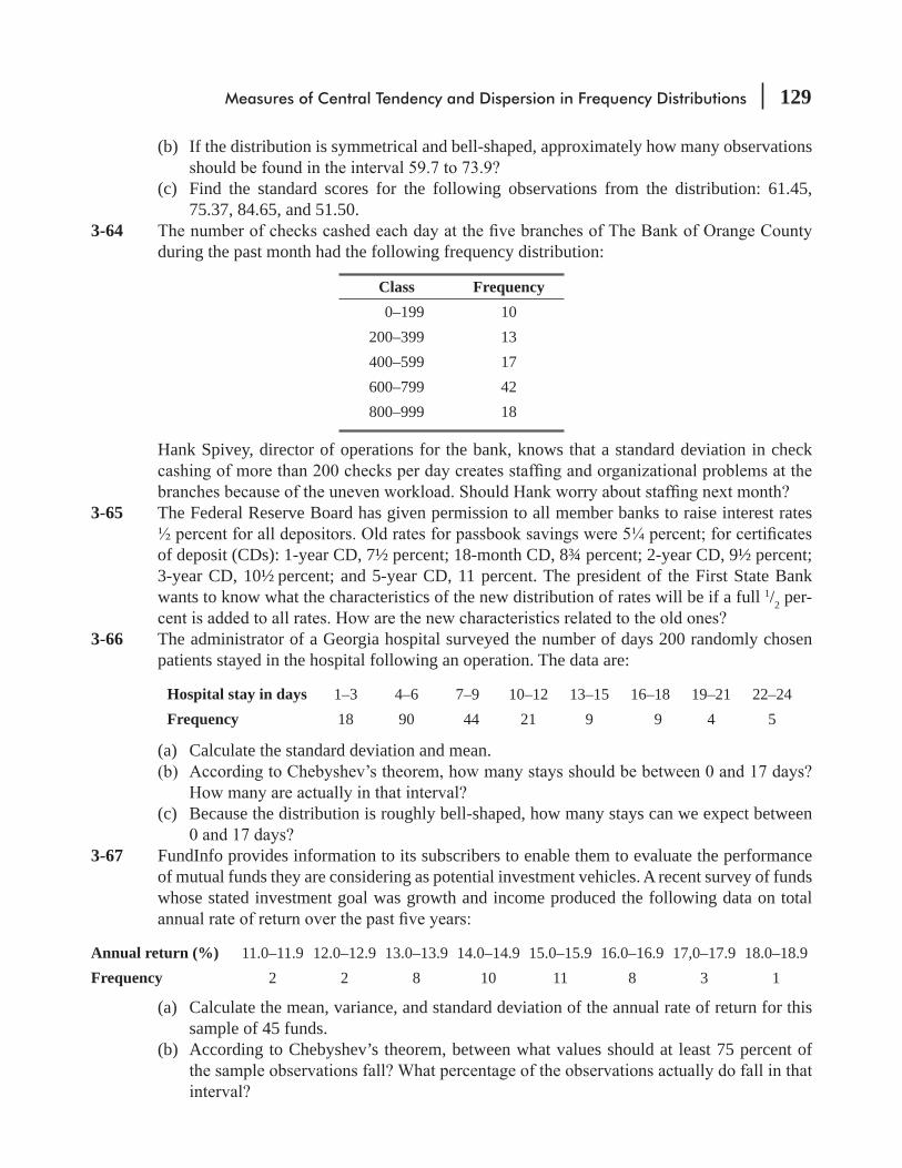
Measures of Central Tendency and Dispersion in Frequency Distributions 129
(b) If the distribution is symmetrical and bell-shaped, approximately how many observations
(c) Find the standard scores for the following observations from the distribution: 61.45, 75.37, 84.65, and 51.50.
3-64 during the past month had the following frequency distribution:
Class Frequency 0–199 10200–399 13400–599 17600–799 42800–999 18
Hank Spivey, director of operations for the bank, knows that a standard deviation in check
3-65 The Federal Reserve Board has given permission to all member banks to raise interest rates
of deposit (CDs): 1-year CD, 7½ percent; 18-month CD, 8¾ percent; 2-year CD, 9½ percent; 3-year CD, 10½ percent; and 5-year CD, 11 percent. The president of the First State Bank wants to know what the characteristics of the new distribution of rates will be if a full 1/2 per-
3-66 The administrator of a Georgia hospital surveyed the number of days 200 randomly chosen patients stayed in the hospital following an operation. The data are:
Hospital stay in days 1–3 4–6 7–9 10–12 13–15 16–18 19–21 22–24Frequency 18 90 44 21 9 9 4 5
(a) Calculate the standard deviation and mean.
(c) Because the distribution is roughly bell-shaped, how many stays can we expect between
3-67 FundInfo provides information to its subscribers to enable them to evaluate the performance of mutual funds they are considering as potential investment vehicles. A recent survey of funds whose stated investment goal was growth and income produced the following data on total
Annual return (%) 11.0–11.9 12.0–12.9 13.0–13.9 14.0–14.9 15.0–15.9 16.0–16.9 17,0–17.9 18.0–18.9Frequency 2 2 8 10 11 8 3 1
(a) Calculate the mean, variance, and standard deviation of the annual rate of return for this sample of 45 funds.
(b) According to Chebyshev’s theorem, between what values should at least 75 percent of
130 Statistics for Management
(c) Because the distribution is roughly bell-shaped, between what values would you expect to
3-68 Nell Berman, owner of the Earthbred Bakery, said that the average weekly production level of her company was 11,398 loaves, and the variance was 49,729. If the data used to compute the results were collected for 32 weeks, during how many weeks was the production level below
3-69
was $3,760, and the standard deviation was $622. In Durham, N.C., the average increase was $850, and the standard deviation was $95. Three employees were interviewed. The Washing-ton employee received a raise of $1,100; the New York employee, a raise of $3,200; and the Durham employee, a raise of $500. Which of the three had the smallest raise in relation to the
3-70 American Foods heavily markets three different products nationally. One of the underlying objectives of each of the product’s advertisements is to make consumers recognize that Ameri-can Foods makes the product. To measure how well each ad implants recognition, a group of consumers was asked to identify as quickly as possible the company responsible for a long
a standard deviation of 0.004 second. The second had an average latency of 2.8 seconds, and a standard deviation of 0.006 second. The third had an average latency of 3.7 seconds, and a standard deviation of 0.09 second. One particular subject had the following latencies: 2.495
3-71 Sid Levinson is a doctor who specializes in the knowledge and effective use of pain-killing -
nel to employ, he has begun to keep track of the number of patients he sees each week. Each
patients. Sid has reason to believe that the number of routine patients per week would look like a bell-shaped curve if he had enough data. (This is not true of seriously ill patients.) However,
Seriously ill patients 33 50 22 27 48
Routine patients 34 31 37 36 27
(a) Calculate the mean and variance for the number of seriously ill patients per week. Use -
bers of seriously ill patients per week should fall.(b) Calculate the mean, variance, and standard deviation for the number of routine patients
per week. Within what boundaries should the “middle 68 percent” of these weekly num-
3-72 The superintendent of any local school district has two major problems: A tough job dealing
-trict 18, is no exception. He has learned the value of understanding all numbers in any budget

Measures of Central Tendency and Dispersion in Frequency Distributions 131
and being able to use them to his advantage. This year, the school board has proposed a media research budget of $350,000. From past experience, Tom knows that actual spending always exceeds the budget proposal, and the amount by which it exceeds the proposal has a mean of $40,000 and variance of 100,000,000 dollars squared. Tom learned about Chebyshev’s theo-
the actual expenditure would fall 75 percent of the time in years when the budget proposal is
3-73 Bea Reele, a well-known clinical psychologist, keeps very accurate data on all her patients. From these data, she has developed four categories within which to place all her patients: child, young adult, adult, and elderly. For each category, she has computed the mean IQ and the variance of IQs within that category. These numbers are given in the following table. If on a certain day Bea saw four patients (one from each category), and the IQs of those patients were as follows: child, 90; young adult, 92; adult, 100; elderly, 98; then which of the patients
Category Mean IQ IQ VarianceChild 110 81
Young adult 90 64
Adult 95 49
Elderly 90 121
Worked-Out Answers to Self-Check Exercises
SC 3-13
x x – x– (x –x–)2 x x – x– (x –x –)2
50 –5.2 27.04 54 –1.2 1.44
56 0.8 0.64 55 –0.2 0.04
55 –0.2 0.04 61 5.8 33.64
49 –6.2 38.44 60 4.8 23.04
52 –3.2 10.24 51 –4.2 17.64
57 1.8 3.24 59 3.8 14.44
56 0.8 0.64 62 6.8 46.24
57 1.8 3.24 52 –3.2 10.24
56 0.8 0.64 54 –1.2 1.44
59 3.8 14.44 49 –6.2 38.44
1,104 285.20
xx
n
1,104
20=
Σ= = 55.2 years, which is close to the desired 55 years
sx x
n
( )
1
285.20
19
2
=Σ −
−= = 3.874 years, which shows more variability than desired
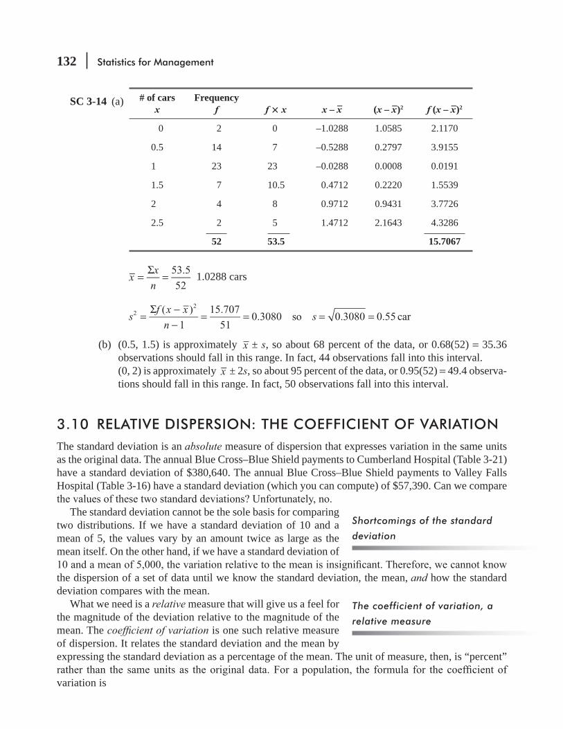
132 Statistics for Management
SC 3-14 (a) # of cars x
Frequency f f ¥ x x – x– (x – x–)2 f (x – x–)2
0 2 0 –1.0288 1.0585 2.1170
0.5 14 7 –0.5288 0.2797 3.9155
1 23 23 –0.0288 0.0008 0.0191
1.5 7 10.5 0.4712 0.2220 1.5539
2 4 8 0.9712 0.9431 3.7726
2.5 2 5 1.4712 2.1643 4.3286
52 53.5 15.7067
xx
n
53.5
52=
Σ= 1.0288 cars
sf x x
ns
( )
1
15.707
510.3080 so 0.3080 0.55 car2
2
=Σ −
−= = = =
(b) (0.5, 1.5) is approximately x ± s, so about 68 percent of the data, or 0.68(52) = 35.36 observations should fall in this range. In fact, 44 observations fall into this interval.
(0, 2) is approximately x ± 2s, so about 95 percent of the data, or 0.95(52) = 49.4 observa-tions should fall in this range. In fact, 50 observations fall into this interval.
3.10 RELATIVE DISPERSION: THE COEFFICIENT OF VARIATIONThe standard deviation is an absolute measure of dispersion that expresses variation in the same units as the original data. The annual Blue Cross–Blue Shield payments to Cumberland Hospital (Table 3-21) have a standard deviation of $380,640. The annual Blue Cross–Blue Shield payments to Valley Falls Hospital (Table 3-16) have a standard deviation (which you can compute) of $57,390. Can we compare
The standard deviation cannot be the sole basis for comparing two distributions. If we have a standard deviation of 10 and a mean of 5, the values vary by an amount twice as large as the mean itself. On the other hand, if we have a standard deviation of
the dispersion of a set of data until we know the standard deviation, the mean, and how the standard deviation compares with the mean.
What we need is a relative measure that will give us a feel for the magnitude of the deviation relative to the magnitude of the mean. The coef cient of variation is one such relative measure of dispersion. It relates the standard deviation and the mean by expressing the standard deviation as a percentage of the mean. The unit of measure, then, is “percent”
variation is
Shortcomings of the standard
deviation
The coefficient of variation, a
relative measure
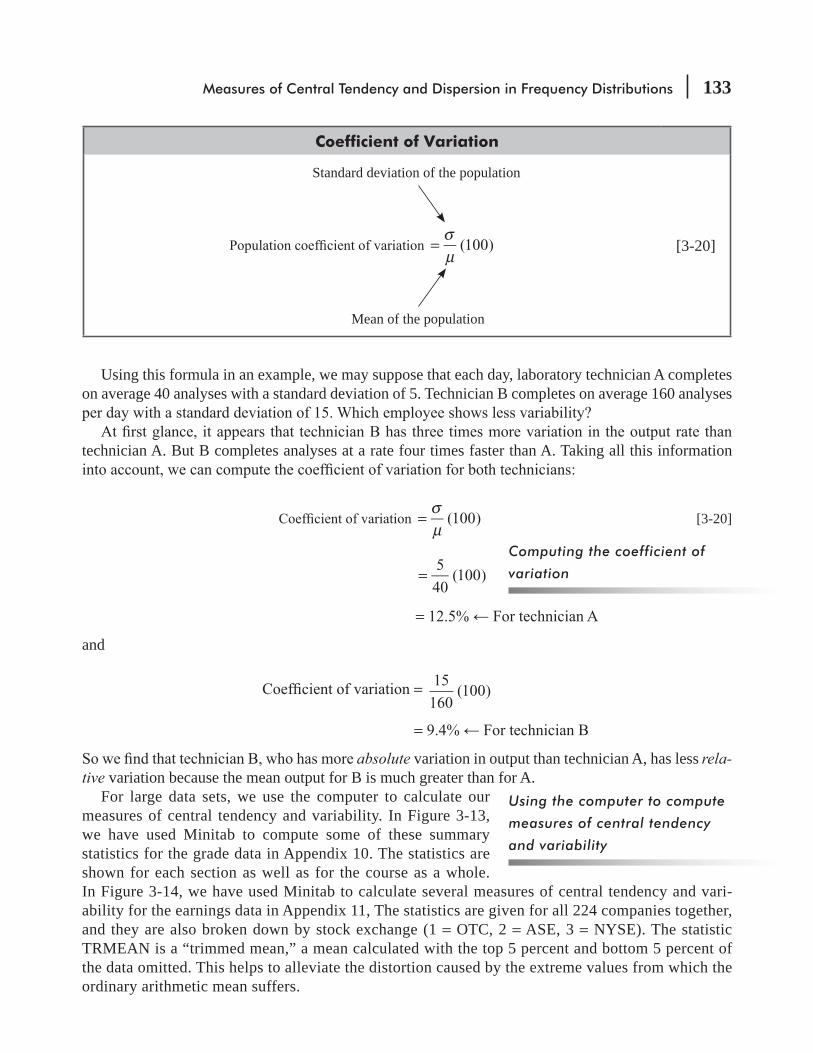
Measures of Central Tendency and Dispersion in Frequency Distributions 133
Coefficient of Variation
(100)σμ
=
Standard deviation of the population
Mean of the population
[3-20]
Using this formula in an example, we may suppose that each day, laboratory technician A completes on average 40 analyses with a standard deviation of 5. Technician B completes on average 160 analyses
technician A. But B completes analyses at a rate four times faster than A. Taking all this information
(100)σμ
= [3-20]
5
40(100)=
=
and
= 15
160(100)
=
absolute variation in output than technician A, has less rela-tive variation because the mean output for B is much greater than for A.
For large data sets, we use the computer to calculate our measures of central tendency and variability. In Figure 3-13, we have used Minitab to compute some of these summary statistics for the grade data in Appendix 10. The statistics are shown for each section as well as for the course as a whole. In Figure 3-14, we have used Minitab to calculate several measures of central tendency and vari-ability for the earnings data in Appendix 11, The statistics are given for all 224 companies together, and they are also broken down by stock exchange (1 = OTC, 2 = ASE, 3 = NYSE). The statistic TRMEAN is a “trimmed mean,” a mean calculated with the top 5 percent and bottom 5 percent of the data omitted. This helps to alleviate the distortion caused by the extreme values from which the ordinary arithmetic mean suffers.
Computing the coefficient of
variation
Using the computer to compute
measures of central tendency
and variability
134 Statistics for Management
-pare overweight men with overweight women. Suppose a group of men and women are all 20 pounds overweight. The 20 pounds is not a good measure of the excessive weight. Average weight for men is about 160 pounds, and average weight for women is about 120 pounds. Using a simple ratio, we can see that the women are 20/120, or about 16.7 percent overweight but the men are
-plex than our simple ratio example, the concept is the same: We use it to compare the amount of variation in data groups that have different means. Warning: Don’t compare the dispersion in data sets by using their standard deviations unless their means are close to each other.
HINTS & ASSUMPTIONS
EXERCISES 3.10
Self-Check ExercisesSC 3-15 Bassart Electronics is considering employing one of two training programs. Two groups were
trained for the same task. Group 1 was trained by program A; group 2, by program B. For the -
ance of 68.09. In the second group, the average was 19.75 hours and the variance was 71.14.
SC 3-16 Southeastern Stereos, a wholesaler, was contemplating becoming the supplier to three retail-ers, but inventory shortages have forced Southeastern to select only one. Southeastern’s credit manager is evaluating the credit record of these three retailers. Over the past 5 years, these retailers’ accounts receivable have been outstanding for the following average number of days. The credit manager feels that consistency, in addition to lowest average, is important. Based
Lee 62.2 61.8 63.4 63.0 61.7Forrest 62.5 61.9 62.8 63.0 60.7Davis 62.0 61.9 63.0 63.9 61.5
Applications3-74 The weights of the Baltimore Bullets professional football team have a mean of 224 pounds
with a standard deviation of 18 pounds, while the mean weight and standard deviation of their Sunday opponent, the Chicago Trailblazers, are 195 and 12, respectively. Which team exhibits
3-75 The university has decided to test three new kinds of lightbulbs. They have three identical rooms to use in the experiment. Bulb 1 has an average life-time of 1,470 hours and a variance of 156. Bulb 2 has an average lifetime of 1,400 hours and a variance of 81. Bulb 3 has an av-erage lifetime of 1,350 hours and a standard deviation of 6 hours. Rank the bulbs in terms of
3-76 Students’ ages in the regular daytime M.B.A. program and the evening program of Central University are described by these two samples:
Regular M.B.A. 23 29 27 22 24 21 25 26 27 24Evening M.B.A. 27 34 30 29 28 30 34 35 28 29

Measures of Central Tendency and Dispersion in Frequency Distributions 135
If homogeneity of the class is a positive factor in learning, use a measure of relative variability to suggest which of the two groups will be easier to teach.
3-77 There are a number of possible measures of sales performance, including how consistent a salesperson is in meeting established sales goals. The data that follow represent the percentage of goal met by each of three salespeople over the last 5 years.
Patricia 88 68 89 92 103John 76 88 90 86 79Frank 104 88 118 88 123
(b) Comment on the adequacy of using a measure of consistency along with percentage of sales goal met to evaluate sales performance.
3-78 The board of directors of Gothic Products is considering acquiring one of two companies and is closely examining the management of each company in regard to their inclinations toward
28.0 percent and a standard deviation of 5.3 percent. The second company’s returns on invest-ments had an average of 37.8 percent and a standard deviation of 4.8 percent. If we consider risk to be associated with greater relative dispersion, which of these two companies has pur-
3-79 A drug company that supplies hospitals with premeasured doses of certain medications uses different machines for medications requiring different dosage amounts. One machine, de-signed to produce doses of 100 cc, has as its mean dose 100 cc, and a standard deviation of 5.2 cc. Another machine produces premeasured amounts of 180 cc of medication and has a standard deviation of 8.6 cc. Which machine has the lower accuracy from the standpoint of
3-80 HumanPower, the temporary employment agency, has tested many people’s data entry skills. Infotech needs a data entry person, and the person needs to be not only quick but also consis-tent. HumanPower pulls the speed records for 4 employees with the data given below in terms of number of correct entries per minute. Which employee is best for Infotech based on relative
John 63 66 68 62 69 72Jeff 68 67 66 67 69Mary 62 79 75 59 72 84Tammy 64 68 58 57 59
3-81 Wyatt Seed Company sells three grades of Early White Sugar corn seed, distinguished ac-cording to the consistency of germination of the seeds. The state seed testing laboratory has a sample of each grade of seed and its test results on the number of seeds that germinated out of packages of 100 are as follows:
Grade I (Regular) 88 91 92 89 79Grade II (Extra) 87 92 88 90 92Grade III (Super) 90 89 79 93 88
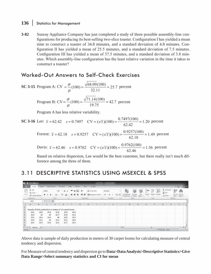
136 Statistics for Management
3-82 Sunray Appliance Company has just completed a study of three possible assembly-line con-
time to construct a toaster of 34.8 minutes, and a standard deviation of 4.8 minutes. Con-
-
Worked-Out Answers to Self-Check Exercises
SC 3-15 Program A: CV (100)68.09(100)
32.1125.7
σμ
= = = percent
Program B: CV (100)71.14(100)
19.7542.7
σμ
= = = percent
Program A has less relative variability.
SC 3-16 Lee: x s s x62.42 0.7497 CV ( / )(100)0.7497(100)
62.421.20= = = = = percent
Forrest: x s s x62.18 0.9257 CV ( / )(100)0.9257(100)
62.181.49= = = = = percent
Davis: x s s x62.46 0.9762 CV ( / )(100)0.9762(100)
62.461.56= = = = = percent
Based on relative dispersion, Lee would be the best customer, but there really isn’t much dif-ference among the three of them.
3.11 DESCRIPTIVE STATISTICS USING MSEXCEL & SPSS
Above data is sample of daily production in meters of 30 carpet looms for calculating measure of central tendency and dispersion.
For Measure of central tendency and dispersion go to Data>Data Analysis>Descriptive Statistics>Give Data Range>Select summary statistics and CI for mean
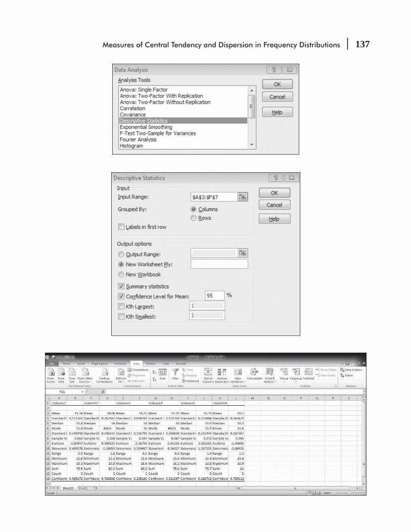
Measures of Central Tendency and Dispersion in Frequency Distributions 137

138 Statistics for Management
For calculating measure of central tendency and dispersion in SPSS 16.0 Go to Analyze>Descriptive Statistics>Frequencies>In statistics select desired measure of central tendency and measure of dispersion.
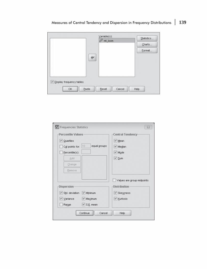
Measures of Central Tendency and Dispersion in Frequency Distributions 139
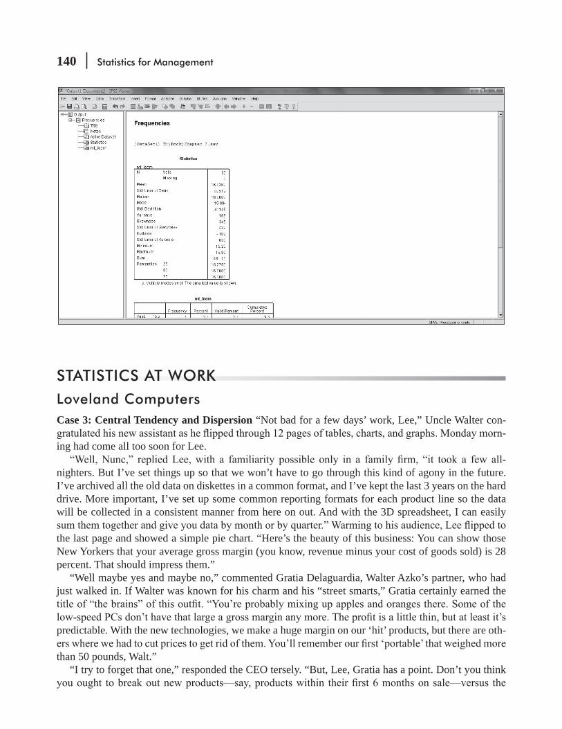
140 Statistics for Management
STATISTICS AT WORK
Loveland ComputersCase 3: Central Tendency and Dispersion “Not bad for a few days’ work, Lee,” Uncle Walter con-
-ing had come all too soon for Lee.
nighters. But I’ve set things up so that we won’t have to go through this kind of agony in the future. I’ve archived all the old data on diskettes in a common format, and I’ve kept the last 3 years on the hard drive. More important, I’ve set up some common reporting formats for each product line so the data will be collected in a consistent manner from here on out. And with the 3D spreadsheet, I can easily
the last page and showed a simple pie chart. “Here’s the beauty of this business: You can show those New Yorkers that your average gross margin (you know, revenue minus your cost of goods sold) is 28 percent. That should impress them.”
“Well maybe yes and maybe no,” commented Gratia Delaguardia, Walter Azko’s partner, who had just walked in. If Walter was known for his charm and his “street smarts,” Gratia certainly earned the
predictable. With the new technologies, we make a huge margin on our ‘hit’ products, but there are oth-
than 50 pounds, Walt.”“I try to forget that one,” responded the CEO tersely. “But, Lee, Gratia has a point. Don’t you think

Measures of Central Tendency and Dispersion in Frequency Distributions 141
established lines. See if the gross margins look different and whether they’re all over the place like Gratia says. I’m off to the airport to pick up the investment folks. See what you can whip up by the time I get back.”
Study Questions: The spreadsheet program Lee is using has many built-in statistical functions. -
CHAPTER REVIEW
Terms Introduced in Chapter 3Bimodal Distribution A distribution of data points in which two values occur more frequently than the rest of the values in the data set.Boxplot A graphical EDA technique used to highlight the center and extremes of a data set.Chebyshev’s Theorem No matter what the shape of a distribution, at least 75 percent of the values in the population will fall within 2 standard deviations of the mean and at least 89 percent will fall within 3 standard deviations.Coding A method of calculating the mean for grouped data by recoding values of class midpoints to more simple values.
A relative measure of dispersion, comparable across distributions, that expresses the standard deviation as a percentage of the mean.Deciles Fractiles that divide the data into 10 equal parts.Dispersion The spread or variability in a set of data.Distance Measure A measure of dispersion in terms of the difference between two values in the data set.Exploratory Data Analysis (EDA) Methods for analyzing data that require very few prior assumptions.Fractile In a frequency distribution, the location of a value at or above a given fraction of the data.Geometric Mean A measure of central tendency used to measure the average rate of change or growth for some quantity, computed by taking the nth root of the product of n values representing change.Interfractile Range A measure of the spread between two fractiles in a distribution, that is, the differ-ence between the values of two fractiles.Interquartile Range -ence indicates the range of the middle half of the data set.Kurtosis The degree of peakedness of a distribution of points.Mean A central tendency measure representing the arithmetic average of a set of observations.Measure of Central Tendency A measure indicating the value to be expected of a typical or middle data point.Measure of Dispersion A measure describing how the observations in a data set are scattered or spread out.Median The middle point of a data set, a measure of location that divides the data set into halves.Median Class The class in a frequency distribution that contains the median value for a data set.Mode The value most often repeated in the data set. It is represented by the highest point in the distribu-tion curve of a data set.Parameters Numerical values that describe the characteristics of a whole population, commonly rep-resented by Greek letters.
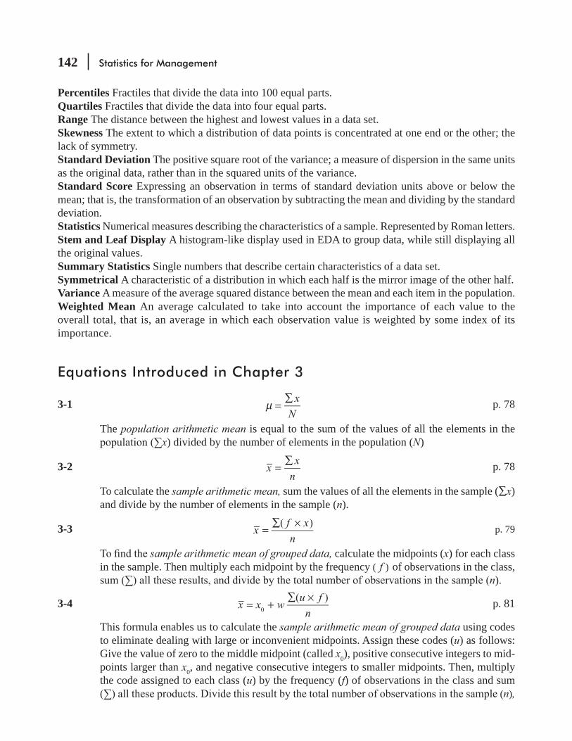
142 Statistics for Management
Percentiles Fractiles that divide the data into 100 equal parts.Quartiles Fractiles that divide the data into four equal parts.Range The distance between the highest and lowest values in a data set.Skewness The extent to which a distribution of data points is concentrated at one end or the other; the lack of symmetry.Standard Deviation The positive square root of the variance; a measure of dispersion in the same units as the original data, rather than in the squared units of the variance.Standard Score Expressing an observation in terms of standard deviation units above or below the mean; that is, the transformation of an observation by subtracting the mean and dividing by the standard deviation.Statistics Numerical measures describing the characteristics of a sample. Represented by Roman letters.Stem and Leaf Display A histogram-like display used in EDA to group data, while still displaying all the original values.Summary Statistics Single numbers that describe certain characteristics of a data set.Symmetrical A characteristic of a distribution in which each half is the mirror image of the other half.Variance A measure of the average squared distance between the mean and each item in the population.Weighted Mean An average calculated to take into account the importance of each value to the overall total, that is, an average in which each observation value is weighted by some index of its importance.
Equations Introduced in Chapter 3
3-1 x
Nμ =
∑ p. 78
The population arithmetic mean is equal to the sum of the values of all the elements in the x) divided by the number of elements in the population (N)
3-2 =∑
xx
n p. 78
To calculate the sample arithmetic mean, sum the values of all the elements in the sample (∑x) and divide by the number of elements in the sample (n).
3-3 xf x
n
( )=
∑ × p. 79
sample arithmetic mean of grouped data, calculate the midpoints (x) for each class in the sample. Then multiply each midpoint by the frequency ( f ) of observations in the class,
n).
3-4 x x wu f
n
( )0= +
∑ × p. 81
This formula enables us to calculate the sample arithmetic mean of grouped data using codes to eliminate dealing with large or inconvenient midpoints. Assign these codes (u) as follows: Give the value of zero to the middle midpoint (called x0), positive consecutive integers to mid-points larger than x0, and negative consecutive integers to smaller midpoints. Then, multiply the code assigned to each class (u) by the frequency (f) of observations in the class and sum
(n),
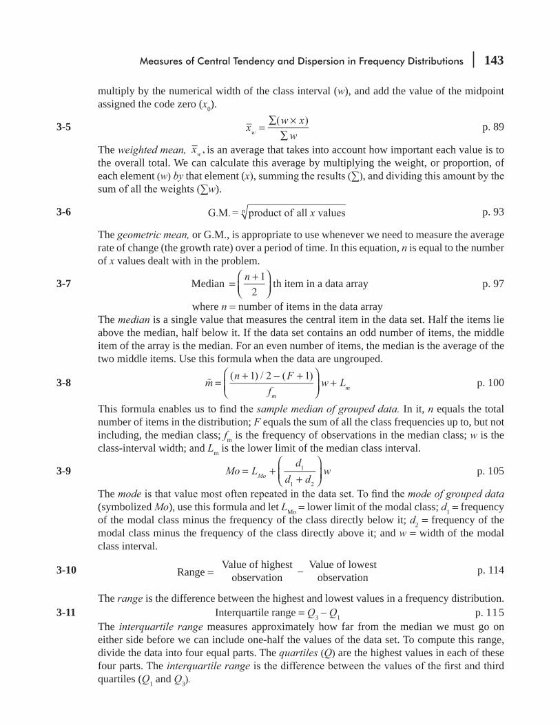
Measures of Central Tendency and Dispersion in Frequency Distributions 143
multiply by the numerical width of the class interval (w), and add the value of the midpoint assigned the code zero (x0).
3-5 xw x
w
( )w =
∑ ×∑
p. 89
The weighted mean, x ,w is an average that takes into account how important each value is to the overall total. We can calculate this average by multiplying the weight, or proportion, of each element (w) by that element (x
w).
3-6 xG.M. = product of all valuesn p. 93
The geometric mean, or G.M., is appropriate to use whenever we need to measure the average rate of change (the growth rate) over a period of time. In this equation, n is equal to the number of x values dealt with in the problem.
3-7 Median n 1
2=
+⎛⎝⎜
⎞⎠⎟
th item in a data array p. 97
where n = number of items in the data arrayThe median is a single value that measures the central item in the data set. Half the items lie above the median, half below it. If the data set contains an odd number of items, the middle item of the array is the median. For an even number of items, the median is the average of the two middle items. Use this formula when the data are ungrouped.
3-8 =+ − +⎛
⎝⎜⎞
⎠⎟+m
n F
fw L
( 1) / 2 ( 1)
mm p. 100
sample median of grouped data. In it, n equals the total number of items in the distribution; F equals the sum of all the class frequencies up to, but not including, the median class; fm is the frequency of observations in the median class; w is the class-interval width; and Lm is the lower limit of the median class interval.
3-9 Mo Ld
d dwMo
1
1 2
= ++
⎛
⎝⎜⎞
⎠⎟ p. 105
The mode mode of grouped data (symbolized Mo), use this formula and let LMo = lower limit of the modal class; d1 = frequency of the modal class minus the frequency of the class directly below it; d2 = frequency of the modal class minus the frequency of the class directly above it; and w = width of the modal class interval.
3-10 Value of highestobservationRange = – Value of lowest
observation p. 114
The range is the difference between the highest and lowest values in a frequency distribution.3-11 Interquartile range = Q3 – Q1 p. 115
The interquartile range measures approximately how far from the median we must go on either side before we can include one-half the values of the data set. To compute this range, divide the data into four equal parts. The quartiles (Q) are the highest values in each of these four parts. The interquartile rangequartiles (Q1 and Q3).

144 Statistics for Management
3-12 x
N
x
N
( )22 2
2σ μ μ=Σ −
=Σ
− p. 119
This formula enables us to calculate the population variance, a measure of the average squared distance between the mean and each item in the population. The middle expression, x
N
( )2μΣ − , is
σ2. The last expression, x
N,
22μΣ
−
but is often much more convenient to use because it frees us from calculating the deviations from the mean.
3-13 x
N
x
N
( )22 2
2σ σ μ μ= =Σ −
=Σ
− p. 120
The population standard deviation, σ, is the square root of the population variance. It is a more useful parameter than the variance because it is expressed in the same units as the data (whereas the units of the variance are the squares of the units of the data). The standard devia-tion is always the positive square root of the variance.
3-14 Population standard score x μσ
=− p. 122
The standard score of an observation is the number of standard deviations the observation lies below or above the mean of the distribution. The standard score enables us to make com-parisons between distribution items that differ in order of magnitude or in the units used. Use
population.
3-15 f x
N
fx
N
( )22 2
2σ μ μ=Σ −
=Σ
− p. 123
This formula in either form enables us to calculate the variance of data already grouped in a frequency distribution. Here, f represents the frequency of the class and x represents the midpoint.
3-16 f x
N
fx
N
( )22 2
2σ σ μ μ= =Σ −
=Σ
− p. 124
Take the square root of the variance and you have the standard deviation using grouped data.
3-17 sx x
n
x
n
nx
n
( )
1 1 12
2 2 2
=Σ −
−=
Σ−
−−
p. 124
To compute the sample variance, use the same formula as Equation 3-12, replacing μ with x and N with n – 1. Chapter 7 contains an explanation of why we use n – 1 rather than n to calculate the sample variance.
3-18 s sx x
n
x
n
nx
n
( )
1 1 12
2 2 2
= =Σ −
−=
Σ−
−−
p. 124
The sample standard deviation is the square root of the sample variance. It is similar to Equa-tion 3-13, except that μ is replaced by the sample mean x and N is changed to n – 1
3-19 Sample standard score x x
s=
− p. 127
sample.

Measures of Central Tendency and Dispersion in Frequency Distributions 145
3-20 (100)σμ
= p. 133
The coef cient of variation is a relative measure of dispersion that enables us to compare two distributions. It relates the standard deviation and the mean by expressing the standard devia-tion as a percentage of the mean.
Review and Application Exercises3-83 The weights and measures department of a state agriculture department measured the amount
of granola sold in 4-ounce packets and recorded the following data:
4.01 4.00 4.02 4.02 4.03 4.00 3.98 3.99 3.99 4.01
3.99 3.98 3.97 4.00 4.02 4.01 4.02 4.00 4.01 3.99
If the sample is typical of all granola snacks marketed by this manufacturer, what is the range
3-84 How would you react to this statement from a football fan: “The Rockland Raiders average 3.6
have four plays to get it, they can’t miss if they just stick to their ground game.”3-85 How would you reply to the following statement: “Variability is not an important factor be-
cause even though the outcome is more uncertain, you still have an equal chance of falling either above or below the median. Therefore, on average, the outcome will be the same.”
3-86 Following are three general sections of one year’s defense budget, each of which was allocated the same amount of funding by Congress:
(b) Aircraft maintenance.(c) Food purchases (total).Considering the distribution of possible outcomes for the funds actually spent in each of these areas, match each section to one of the curves in Figure 3-9. Support your answers.
3-87
Mean Test Strength (lb) Standard DeviationMaster 40 Exact value unknown, but estimated to be quite largeSuper 30 Exact value unknown, but estimated to be quite small
3-88 The VP of sales for Vanguard Products has been studying records regarding the performances of his sales reps. He has noticed that in the last 2 years, the average level of sales per sales rep has remained the same, while the distribution of the sales levels has widened. Salespeople’s
the previous 2-year periods for which he has records. What conclusions might be drawn from
3-89 New cars sold in December at eight Ford dealers within 50 miles of Canton, Ohio, can be described by this data set:
200 156 231 222 96 289 126 308
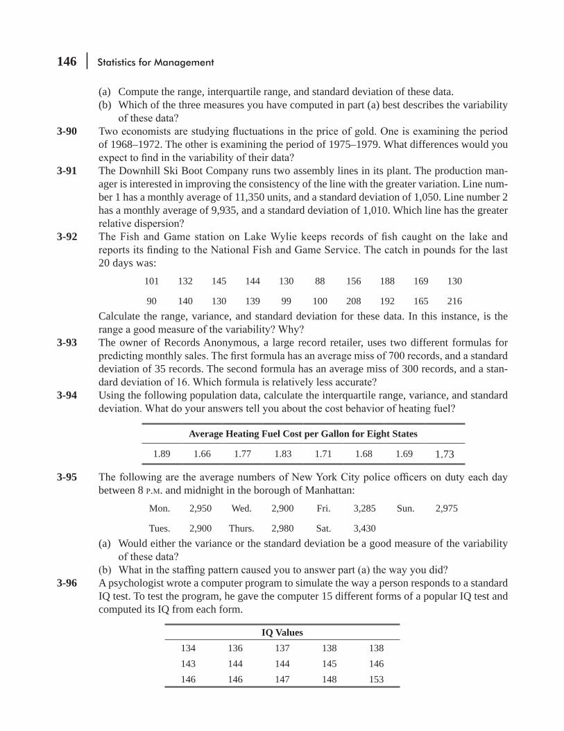
146 Statistics for Management
(a) Compute the range, interquartile range, and standard deviation of these data.(b) Which of the three measures you have computed in part (a) best describes the variability
3-90 of 1968–1972. The other is examining the period of 1975–1979. What differences would you
3-91 The Downhill Ski Boot Company runs two assembly lines in its plant. The production man-ager is interested in improving the consistency of the line with the greater variation. Line num-ber 1 has a monthly average of 11,350 units, and a standard deviation of 1,050. Line number 2 has a monthly average of 9,935, and a standard deviation of 1,010. Which line has the greater
3-92
20 days was:101 132 145 144 130 88 156 188 169 130
90 140 130 139 99 100 208 192 165 216Calculate the range, variance, and standard deviation for these data. In this instance, is the
3-93 The owner of Records Anonymous, a large record retailer, uses two different formulas for
deviation of 35 records. The second formula has an average miss of 300 records, and a stan-
3-94 Using the following population data, calculate the interquartile range, variance, and standard
Average Heating Fuel Cost per Gallon for Eight States
1.89 1.66 1.77 1.83 1.71 1.68 1.69 1.73
3-95 between 8 P.M. and midnight in the borough of Manhattan:
Mon. 2,950 Wed. 2,900 Fri. 3,285 Sun. 2,975
Tues. 2,900 Thurs. 2,980 Sat. 3,430(a) Would either the variance or the standard deviation be a good measure of the variability
3-96 A psychologist wrote a computer program to simulate the way a person responds to a standard IQ test. To test the program, he gave the computer 15 different forms of a popular IQ test and computed its IQ from each form.
IQ Values134 136 137 138 138143 144 144 145 146146 146 147 148 153
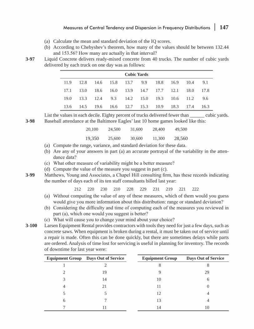
Measures of Central Tendency and Dispersion in Frequency Distributions 147
(a) Calculate the mean and standard deviation of the IQ scores.(b) According to Chebyshev’s theorem, how many of the values should be between 132.44
3-97 Liquid Concrete delivers ready-mixed concrete from 40 trucks. The number of cubic yards delivered by each truck on one day was as follows:
Cubic Yards
11.9 12.8 14.6 15.8 13.7 9.9 18.8 16.9 10.4 9.1
17.1 13.0 18.6 16.0 13.9 14.7 17.7 12.1 18.0 17.8
19.0 13.3 12.4 9.3 14.2 15.0 19.3 10.6 11.2 9.6
13.6 14.5 19.6 16.6 12.7 15.3 10.9 18.3 17.4 16.3
List the values in each decile. Eighty percent of trucks delivered fewer than ______ cubic yards.3-98 Baseball attendance at the Baltimore Eagles’ last 10 home games looked like this:
20,100 24,500 31,600 28,400 49,500
19,350 25,600 30,600 11,300 28,560(a) Compute the range, variance, and standard deviation for these data.(b) Are any of your answers in part (a) an accurate portrayal of the variability in the atten-
(d) Compute the value of the measure you suggest in part (c).3-99
the number of days each of its ten staff consultants billed last year:212 220 230 210 228 229 231 219 221 222
(a) Without computing the value of any of these measures, which of them would you guess
3-100 Larsen Equipment Rental provides contractors with tools they need for just a few days, such as concrete saws. When equipment is broken during a rental, it must be taken out of service until a repair is made. Often this can be done quickly, but there are sometimes delays while parts are ordered. Analysis of time lost for servicing is useful in planning for inventory. The records of downtime for last year were:
Equipment Group Days Out of Service Equipment Group Days Out of Service1 2 8 82 19 9 293 14 10 64 21 11 05 5 12 46 7 13 47 11 14 10
148 Statistics for Management
3-101 Larsen (see Exercise 3-102) has just gotten the following additional information:
Equipment Group Pieces of Machinery Equipment Group Pieces of Machinery
1 1 8 5
2 3 9 8
3 1 10 2
4 4 11 2
5 2 12 6
6 1 13 1
7 1 14 1
3-102 Compare and contrast the central position and skewness of the distributions of the readership volume in numbers of readers per issue for all nationally distributed(a) Monthly magazines.(b) Weekly news magazines.(c) Monthly medical journals.
3-103 Compare and contrast the central tendency and skewness of the distributions of the amount of taxes paid (in dollars) for all
percent.(b) Individuals paying state income taxes in North Carolina, where the top tax bracket is 7
percent.(c) Individuals paying airport taxes (contained in the price of the airplane ticket) at JFK In-
ternational Airport in New York City.3-104 Allison Barrett does statistical analyses for an automobile racing team. Here are the fuel con-
4.77 6.11 6.11 5.05 5.99 4.91 5.27 6.01
5.75 4.89 6.05 5.22 6.02 5.24 6.11 5.02
(a) Calculate the median fuel consumption.(b) Calculate the mean fuel consumption.
(d) Which of the three measures of central tendency is best for Allison to use when she orders
Measures of Central Tendency and Dispersion in Frequency Distributions 149
3-105 Claire Chavez, an Internal Revenue Service analyst, has been asked to describe the “aver-age” American taxpayer in terms of gross annual income. She has summary data grouping taxpayers into different income classes. Which measure of central tendency should she
3-106 -ber of bulbs in each can vary depending on the varieties included. The number of bulbs in each of 20 bags sampled were:
21 33 37 56 47
36 23 26 33 37
25 33 32 47 34
26 37 37 43 45
(b) Based on your answer, what can you conclude about the shape of the distribution of num-
3-107 An engineer tested nine samples of each of three designs of a certain bearing for a new electri-cal winch. The following data are the number of hours it took for each bearing to fail when the winch motor was run continuously at maximum output, with a load on the winch equivalent to 1.9 times the intended capacity.
Design
A B C16 18 31
16 27 16
53 23 42
15 21 20
31 22 18
17 26 17
14 39 16
30 17 15
20 28 19
(a) Calculate the mean and median for each group.
3-108 Table Spice Co. is installing a screener in one stage of its new processing plant to separate leaves, dirt, and insect parts from a certain expensive spice seed that it receives in bulk from
The smaller mesh will remove more debris but also will remove more seeds. The larger mesh will pass debris and remove fewer seeds. Table Spice has the following information from a sample of pieces of debris.

150 Statistics for Management
Debris Size(in millimeters) Frequency
1.0 or less 121.01–1.5 1291.51–2.0 1862.01–2.5 2752.51–3.0 3413.01–3.5 4223.51–4.0 6,2874.01–4.5 8,1634.51–5.0 6,2125.01–5.5 2,416
more than 5.5 1,019
(b) Which screen would you use based on part (a) if you wanted to remove at least half of the
3-109 The following is the average amount of money each major airline operator spend per passen-ger on baggage handling:
Airlines Amount ( in Rs ’00)Katar Airlines 3.17Lusiana Airlines 6.00Go-Deigo Airlines 2.41Splice Jet 7.93Indiana Airlines 5.90East-West Airlines 1.76India Konnect Airlines 0.98Ethos Airlines 6.77Air Malaya 7.15
-age it should consider for planning purpose and
Questions on Running Case: SURYA Bank Pvt. Ltd.
1. creating the customer awareness about e-banking. Compare the results of the different modes of creating awareness (Q4).
2. 3. Which facility has the highest variability (Q7). 4. Comment on the average satisfaction level of the customers with the e-services provided by their banks. Also
@
CASE
@
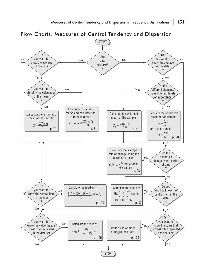
Measures of Central Tendency and Dispersion in Frequency Distributions 151
Flow Charts: Measures of Central Tendency and Dispersion
Calculate the median:
p. 97
2⎛⎜⎝
⎛⎜⎝
n + 1 ththe item in
the data array
START
Aredata
grouped?
Doyou want to
know the averageof the data
?
Doyou want to
know the averageof the data
?
Doyou want to
simplify the calculationof the mean
?
Doyou want to
know the central itemin the data
?
Doyou want to
know the value theat ismost often repeated
in the data set?
Do thedifferent elements
have different levelsof importance
?
No
No
NoNo
Yes
Yes
No
Yes
Yes
Yes
No
No No
No
Yes
Yes
Do thequantities
change over a periodof time
?
Do youwant to know thecentral item in the
data?
Yes
Yes
No
Calculate the arithmeticmean of the sample:
x n= Σ(f × x)
p. 79
Calculate the weightedmean of the sample:
xw Σw= Σ(w × x)
p. 89
Use coding of classmarks and calculate the
arithmetic mean:
x = x0 + w nΣ(u × f )
p. 81
Calculate the arithmeticmean of population:
p. 78
N= Σx
or of the sample:
xN
= Σx
Calculate the averagerate of change using the
geometric mean:
p. 93
G.M. = product of allx values
n
Doyou want to
know the value thatis most often repeated
in the data set?
YesLimited use of modeof ungrouped data
p. 105p. 105
p. 100
Calculate the median:
fm
⎛⎜⎝
⎛⎜⎝
(n + 1)/2 –(F + 1) w + Lm
Calculate the mode:d1
d1 + d2
⎛⎜⎝
⎛⎜⎝w Lmo +
μ
STOP
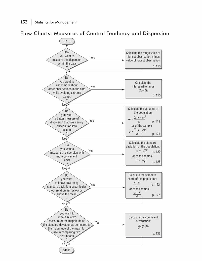
152 Statistics for Management
Flow Charts: Measures of Central Tendency and DispersionSTART
STOP
Doyou want to
measure the dispersionwithin the data
?
Doyou want to
know more aboutother observations in the data
while avoiding extremevalues
?
Doyou want
a better measure ofdispersion that takes every
observation intoaccount
?
YesCalculate the range value ofhighest observation minusvalue of lowest observation
p. 113
Yes
Yes
No
No
No
p. 115
Calculate theinterquartile range
Q3 – Q1
p. 119
p. 124
Calculate the variance ofthe population:
or of the sample
σ2 = ∑(x − μ)2
N
s2 = ∑(x − x )2
n − 1
Doyou want a
measure of dispersion withmore convenient
units?
Doyou want
to know how manystandard deviations a particular
observation lies below orabove the mean
?
Do you want to
know a relativemeasure of the magnitude of
the standard deviation as compared tothe magnitude of the mean for
use in comparing twodistribtions
?
Yes
Yes
Yes
No
No
Calculate the coefficientof variation:
p. 133
Calculate the standarddeviation of the population:
or of the sample:p. 120
p. 125
σ = σ2
s = s2
Calculate the standardscore of the population:
or of the sample:p. 122
p. 127
x − σ
x − xs
(100)σμ
μ

LEARNING OBJECTIVES
4After reading this chapter, you can understand:
CHAPTER CONTENTS
To examine the use of probability theory in decision making
To explain the different ways probabilities arise To develop rules for calculating different kinds
of probabilities
4.1 Probability: The Study of Odds and Ends 154
4.2 Basic Terminology in Probability 1554.3 Three Types of Probability 1574.4 Probability Rules 1644.5 Probabilities under Conditions of
Statistical Independence 1704.6 Probabilities under Conditions of
Statistical Dependence 1794.7 Revising Prior Estimates of Probabilities:
Bayes’ Theorem 188
To use probabilities to take new information
theorem
Statistics at Work 196 Terms Introduced in Chapter 4 197 Equations Introduced in Chapter 4 198 Review and Application Exercises 199 Flow Chart: Probability I: Introductory
Ideas 206
Probability I: Introductory Ideas
154 Statistics for Management
Gamblers have used odds to make bets during most of recorded history. But it wasn’t until the seventeenth century that French nobleman Antoine Gombauld (1607–1684) sought a
mathematical basis for success at the dice tables. He asked French mathematician Blaise Pascal (1623–1662), “What are the odds of rolling two sixes at least once in twenty-four rolls of a pair of dice?” Pascal solved the problem, having become as interested in the idea of probabilities as was Gombauld. They shared their ideas with the famous mathematician Pierre de Fermat (1601–1665),
do know that their curiosity and research introduced many of the concepts we shall study in this chapter and the next.
4.1 PROBABILITY: THE STUDY OF ODDS AND ENDSJacob Bernoulli (1654–1705), Abraham de Moivre (1667–1754), the Reverend Thomas Bayes (1702–1761), and Joseph Lagrange (1736–1813) developed probability formulas and techniques. In the
Probability theory was successfully applied at the gambling tables and, more relevant to our study, eventually to social and economic problems. The insurance industry, which emerged in the nineteenth century, required precise knowledge about the risk of loss in order to calculate premiums. Within 50 years, many learning centers were studying probability as a tool for understanding social phenomena. Today, the mathematical theory of probability is the basis for statistical applications in both social and decision-making research.
Probability is a part of our everyday lives. In personal and man-agerial decisions, we face uncertainty and use probability theory whether or not we admit the use of something so sophisticated. When we hear a weather forecast of a 70 percent chance of rain, we change our plans from a picnic to a pool game. Playing bridge, we make some probability estimate
must wonder about the chances that sales will reach or exceed a certain level, and the buyer who stocks up on skateboards considers the probability of the life of this particular fad. Before Muhammad Ali’s
odds I’m still the greatest when it’s over.” And when you begin to study for the inevitable quiz attached to the use of this book, you may ask yourself, “What are the chances the professor will ask us to recall something about the history of probability theory?”
We live in a world in which we are unable to forecast the future with complete certainty. Our need to cope with uncertainty leads us to the study and use of probability theory. In many instances, we, as concerned citizens, will have some knowledge about the possible outcomes of a decision. By organiz-ing this information and considering it systematically, we will be able to recognize our assumptions, communicate our reasoning to others, and make a sounder decision than we could by using a shot-in-the-dark approach.
Early probability theorists
Need for probability theory
Examples of the use of
probability theory
Probability I: Introductory Ideas 155
EXERCISES 4.1
Applications4-1 The insurance industry uses probability theory to calculate premium rates, but life insurers
know for certain that every policyholder is going to die. Does this mean that probability theory does not apply to the life insurance business? Explain.
4-2 “Use of this product may be hazardous to your health. This product contains saccharin, which has been determined to cause cancer in laboratory animals.” How might probability theory have played a part in this statement?
4-3 Is there really any such thing as an “uncalculated risk”? Explain.4-4 A well-known soft drink company decides to alter the formula of its oldest and most popular
product. How might probability theory be involved in such a decision?
4.2 BASIC TERMINOLOGY IN PROBABILITYIn our day-to-day life involving decision-making problems, we encounter two broad types of problems. These problems can be categorized into two types of models: Deterministic Models and Random or Probabilistic Models. Deterministic Models cover those situations, where everything related to the situation is known with certainty to the decision-maker, when decision is to be made. Whereas in Probabilistic Models, the totality of the outcomes is known but it can not be certain, which particular outcome will appear. So, there is always some uncertainty involved in decision-making.
In Deterministic Models, frequency distribution or descriptive statistics measures are used to arrive at a decision. Similarly, in random situations, probability and probability distributions are used to make
In general, probability is the chance something will happen. Probabilities are expressed as fractions (1
6, 12, 8
9) or as decimals (0.167, 0.500, 0.889) between zero and 1. Assigning a probability of zero means that something can never happen; a probability of 1 indicates that something will always happen.
In probability theory, an event is one or more of the possible outcomes of doing something. If we toss a coin, getting a tail would be an event, and getting a head would be another event. Similarly, if we are drawing from a deck of cards, selecting the ace of spades would be an event. An example of an event closer to your life, perhaps, is being picked from a class of 100 students to answer a question. When we hear the frightening predic-
The activity that produces such an event is referred to in prob-ability theory as an experiment. Using this formal language, we could ask the question, “In a coin-toss experiment, what is the prob-ability of the event head?” And, of course, if it is a fair coin with an equal chance of coming down on either side (and no chance of landing on its edge), we would answer “1
2” or “0.5.” The set of all possible outcomes of an experiment is called the sample space for the experiment. In the coin-toss experiment, the sample space is
S = {head, tail}
In the card-drawing experiment, the sample space has 52 members: ace of hearts, deuce of hearts, and so on.
An event
An experiment

156 Statistics for Management
Most of us are less excited about coins or cards than we are interested in questions such as “What are -
view?” In short, we are concerned with the chances that an event will happen.Events are said to be mutually exclusive if one and only one of
them can take place at a time. Consider again our example of the coin. We have two possible outcomes, heads and tails. On any toss, either heads or tails may turn up, but not both. As a result, the events heads and tails on a single toss are said to be mutually exclusive. Similarly, you will either pass or fail this course or, before the course is over, you may drop it without a grade. Only one of those three outcomes can happen; they are said to be mutually exclusive events. The crucial question to ask in deciding whether events are really mutually exclusive is, “Can two or more of these events occur at one time?” If the answer is yes, the events are not mutually exclusive.
When a list of the possible events that can result from an experi-ment includes every possible outcome, the list is said to be collec-tively exhaustive. In our coin example, the list “head and tail” is collectively exhaustive (unless, of course, the coin stands on its edge when we toss it). In the US presidential campaign, the list of outcomes “Democratic candidate and Republican candidate” is not a collectively exhaustive list of outcomes, because an independent candidate or the candidate of another party could conceivably win.
Let us consider a situation, total number of possible outcomes related to the situation is “N”, out of them “m” are the number of outcomes where the desired event “E” has occurred. So, “N-m” is the number of outcomes where the desired event has not occurred.
Odds in favor of happening of E = m : N-mOdds against the happening of E = N-m : m
This concept is related to the concept of Probability as:Probability of happening of the event E = m/N
Ex: A cricket match is to be played between two teams CX Club and TE Club. A cricket analyst has predicated that the odds in favor of CX Club winning the match are 4:3. This prediction is based upon the historical records and upon the current strengths and weaknesses of the two teams. So, if a cricket fan is interested in knowing the chances that CX will win the match, then the desired chances would be 4
7.
EXERCISES 4.2
Self-Check ExercisesSC 4-1 Give a collectively exhaustive list of the possible outcomes of tossing two dice.SC 4-2 Give the probability for each of the following totals in the rolling of two dice: 1, 2, 5, 6, 7, 10,
and 11.
Basic Concepts4-5 Which of the following are pairs of mutually exclusive events in the drawing of one card from
a standard deck of 52?(a) A heart and a queen.(b) A club and a red card.
Mutually exclusive events
A collectively exhaustive list
Odd in favor and against

Probability I: Introductory Ideas 157
(c) An even number and a spade.(d) An ace and an even number.Which of the following are mutually exclusive outcomes in the rolling of two dice?(a) A total of 5 points and a 5 on one die.(b) A total of 7 points and an even number of points on both dice.(c) A total of 8 points and an odd number of points on both dice.(d) A total of 9 points and a 2 on one die.(e) A total of 10 points and a 4 on one die.
Applications4-6 Consider a stack of nine cards, all spades, numbered 2 through 10, and a die. Give a collec-
tively exhaustive list of the possible outcomes of rolling the die and picking one card. How many elements are there in the sample space?
4-7 Consider the stack of cards and the die discussed in Exercise 4-6. Give the probability for each of the following totals in the sum of the roll of the die and the value of the card drawn:
2 3 8 9 12 14 16
4-8 Dheer’s leading supporter said “chances are good” that Dheer will defeat the single opponent facing him in the election.(a) What are the “events” that could take place with regard to the election?(b) Is your list collectively exhaustive? Are the events in your list mutually exclusive?(c) Disregarding the supporter’s comments and knowing no additional information, what
probabilities would you assign to each of your events?
Worked-Out Answers to Self-Check ExercisesSC 4-1 (Die 1, Die 2)
(1,1) (1,2) (1,3) (1,4) (1,5) (1,6)(2,1) (2,2) (2,3) (2,4) (2,5) (2,6)(3,1) (3,2) (3,3) (3,4) (3,5) (3,6)(4,1) (4,2) (4,3) (4,4) (4,5) (4,6)(5,1) (5,2) (5,3) (5,4) (5,5) (5,6)(6,1) (6,2) (6,3) (6,4) (6,5) (6,6)
SC 4-2 P(1) = 0/36, P(2) = 1/36, P(5) = 4/36, P(6) = 5/36, P(7) = 6/36, P(10) = 3/36, P(11) = 2/36.
4.3 THREE TYPES OF PROBABILITYThere are three basic ways of classifying probability. These three represent rather different conceptual approaches to the study of probability theory; in fact, experts disagree about which approach is the
1. Classical approach 2. Relative frequency approach 3.

158 Statistics for Management
Classical ProbabilityClassical probability
Probability of an Event
Probability of an event = number of outcomes where the event occurs
total number of possible outcomes[4-1]
It must be emphasized that in order for Eq. 4-1 to be valid, each of the possible outcomes must be
us, but we can use it to write our coin-toss and dice-rolling examples in symbolic form. First, we would state the question, “What is the probability of getting a head on one toss?” as
P(Head)
Then, using formal terms, we get
P(Head) = 1
1 + 1
= 0.5 or 12
And for the dice-rolling example:
P(5) = 1
1 + 1 + 1 + 1 + 1 + 1
= 16
Classical probability is often called a priori probability because if we keep using orderly examples such as fair coins, unbiased dice, and standard decks of cards, we can state the answer in advance (a priori) without tossing a coin, rolling a die, or drawing a card. We do not have to perform experiments to make our probability statements about fair coins, standard card decks, and unbiased dice. Instead, we can make statements based on logi-cal reasoning before any experiments take place.
probability. So, if those assumptions are included then the complete :
ratio of number of outcomes where the event occurs (favorable out-comes) to the total number of possible outcomes, provided these outcomes are equally likely (the chances of happening of all outcomes are equal), exhaustive (the total-
in non-happening of others). If these assumptions related to the outcomes are not followed, then this approach can not be applied in determining the probability.
This approach to probability is useful when we deal with card games, dice games, coin tosses, and the like, but has serious problems when we try to apply it to the less orderly decision problems we encounter in management. The classical approach to probability assumes a world that does not exist. It assumes away situations that are very unlikely but that could conceivably happen. Such occurrences as
Classical probability defined
Number of outcomes of one toss where the event occurs (in this case, the number hat will produce a head)
Total number of possible outcomes of one toss (a head or a tail)
Total number of possible outcomes of one roll of the die (getting a 1, a 2, a 3, a 4, a 5, or a 6)
Number of outcomes of one roll of the die that will produce a 5
A priori probability
Shortcomings of the classical
approach
Probability I: Introductory Ideas 159a coin landing on its edge, your classroom burning down during a discussion of probabilities, and your eating pizza while on a business trip at the North Pole are all extremely unlikely but not impossible. Nevertheless, the classical approach assumes them all away. Classical probability also assumes a kind of symmetry about the world, and that assumption can get us into trouble. Real-life situations, disor-
Relative Frequency of OccurrenceSuppose we begin asking ourselves complex questions such as, “What is the probability that I will live to be 85?” or “What are the chances that I will blow one of my stereo speakers if I turn my 200-watt
advance, without experimentation, what these probabilities are. Other approaches may be more useful.In the 1800s, British statisticians, interested in a theoretical
foundation for calculating risk of losses in life insurance and com-
collected on births and deaths. Today, this approach is called the relative frequency of occurrence. It
1. The observed relative frequency of an event in a very large number of trials, or 2. The proportion of times that an event occurs in the long run when conditions are stable.
This method uses the relative frequencies of past occurrences as probabilities. We determine how often something has happened
happen again in the future. Let us look at an example. Suppose an insurance company knows from past actuarial data that of all males 40 years old, about 60 out of every 100,000 will die within a 1-year period. Using this method, the company estimates the probability of death for that age group as
60100,000
, or 0.0006
A second characteristic of probabilities established by the relative frequency of occurrence method can be shown by tossing one of our fair coins 300 times. Figure 4-1 illustrates the outcomes of these 300
seemed to stabilize and approach 0.5 as the number of tosses increased. In statistical language, we would say that the relative frequency becomes stable as the number of tosses becomes large (if we are tossing the coin under uniform conditions). Thus, when we use the relative frequency approach to establish
course, this improved accuracy is not free; although more tosses of our coin will produce a more accurate probability of heads occurring, we must bear the time and the cost of additional observations.
S -quency of the desired outcome is “f ”. Then relative frequency of the outcome is “ f N”. The limiting value
Probability redefined
Using the relative frequency
of occurrence approach
More trials, greater accuracy
A limitation of relative
frequency
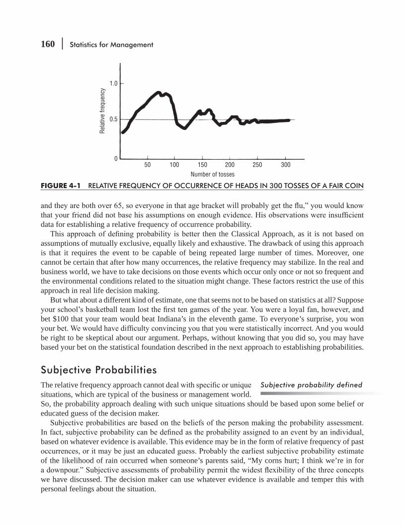
160 Statistics for Management
data for establishing a relative frequency of occurrence probability.then the Classical Approach, as it is not based on
assumptions of mutually exclusive, equally likely and exhaustive. The drawback of using this approach is that it requires the event to be capable of being repeated large number of times. Moreover, one cannot be certain that after how many occurrences, the relative frequency may stabilize. In the real and business world, we have to take decisions on those events which occur only once or not so frequent and the environmental conditions related to the situation might change. These factors restrict the use of this approach in real life decision making.
But what about a different kind of estimate, one that seems not to be based on statistics at all? Suppose
bet $100 that your team would beat Indiana’s in the eleventh game. To everyone’s surprise, you won
be right to be skeptical about our argument. Perhaps, without knowing that you did so, you may have based your bet on the statistical foundation described in the next approach to establishing probabilities.
Subjective ProbabilitiesThe relative frequency approach cannosituations, which are typical of the business or management world. So, the probability approach dealing with such unique situations should be based upon some belief or educated guess of the decision maker.
based on whatever evidence is available. This evidence may be in the form of relative frequency of past
of the likelihood of rain occurred when someone’s parents said, “My corns hurt; I think we’re in for
we have discussed. The decision maker can use whatever evidence is available and temper this with personal feelings about the situation.
Subjective probability defined
1.0
0.5
0
Rela
tive
frequ
ency
Number of tosses50 100 150 200 250 300
FIGURE 4-1 RELATIVE FREQUENCY OF OCCURRENCE OF HEADS IN 300 TOSSES OF A FAIR COIN

Probability I: Introductory Ideas 161
narrowed your choice to three people. Each has an attractive appearance, a high level of energy, abound--
lenges. What are the chances each will relate to clients successfully? Answering this question and
Here is one more illustration of this kind of probability
of a nuclear power plant on a site where there is some evidence of
location?” The fact that there is no relative frequency of occurrence evidence of previous accidents at
-ations, rather than with a long series of identical situations, decision makers at this level make consider-
book The Foundation of Mathematics and Other Logical Essays. The concept was further developed by Bernard Koopman, Richard Good, and Leonard Savage, names that appeared regularly in advanced
-
people who made opposing bets on the outcome of the Indiana basketball game would understand quite well what he meant.
Warning: In classical probability problems, be sure to check whether the situation is “with replacement” after each draw or “without replacement.” The chance of drawing an ace from a
452, or about .077. If you draw one and it is replaced, the odds of
drawing an ace on the second draw are the same, 452. However, without replacement, the odds
change to 451 not an ace, or to 3
51 was an ace. In assigning
for the same event; that’s the result of experience and time (we often call this combination “wisdom”). In assigning probabilities using the relative frequency of occurrence method, be sure you have observed an adequate number of outcomes. Just because red hasn’t come up in 9 spins of the roulette wheel, you shouldn’t bet next semester’s tuition on black this spin!
HINTS & ASSUMPTIONS
EXERCISES 4.3
Self-Check ExercisesSC 4-3 The leader of MP Fiber Plant, Siddharth,
be presented to management. To get an idea of worker support for the package, he randomly polls the two largest groups of workers at his plant, the machinists (M) and the inspectors (I). He polls 30 of each group with the following results:
Using the subjective approach
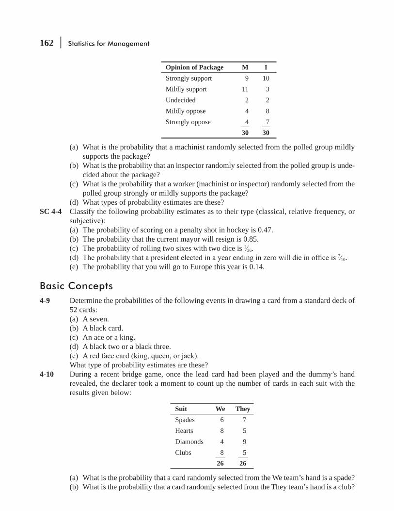
162 Statistics for Management
Opinion of Package M IStrongly support 9 10Mildly support 11 3Undecided 2 2Mildly oppose 4 8Strongly oppose 4 7
30 30
(a) What is the probability that a machinist randomly selected from the polled group mildly supports the package?
(b) What is the probability that an inspector randomly selected from the polled group is unde-cided about the package?
(c) What is the probability that a worker (machinist or inspector) randomly selected from the polled group strongly or mildly supports the package?
(d) What types of probability estimates are these?SC 4-4 Classify the following probability estimates as to their type (classical, relative frequency, or
(a) The probability of scoring on a penalty shot in hockey is 0.47.(b) The probability that the current mayor will resign is 0.85.(c) The probability of rolling two sixes with two dice is 1 36.
710.
(e) The probability that you will go to Europe this year is 0.14.
Basic Concepts4-9 Determine the probabilities of the following events in drawing a card from a standard deck of
52 cards:(a) A seven.(b) A black card.(c) An ace or a king.(d) A black two or a black three.
What type of probability estimates are these?4-10 During a recent bridge game, once the lead card had been played and the dummy’s hand
revealed, the declarer took a moment to count up the number of cards in each suit with the results given below:
Suit We TheySpades 6 7Hearts 8 5Diamonds 4 9Clubs 8 5
26 26
(a) What is the probability that a card randomly selected from the We team’s hand is a spade?(b) What is the probability that a card randomly selected from the They team’s hand is a club?
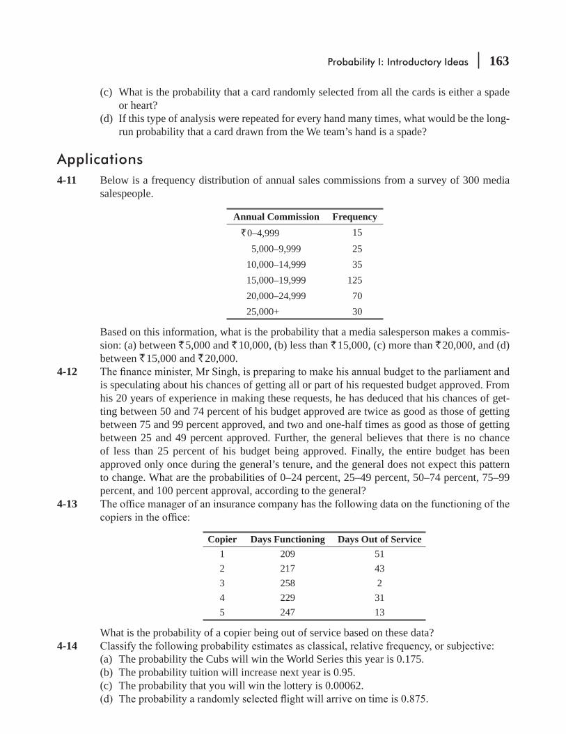
Probability I: Introductory Ideas 163
(c) What is the probability that a card randomly selected from all the cards is either a spade or heart?
(d) If this type of analysis were repeated for every hand many times, what would be the long-run probability that a card drawn from the We team’s hand is a spade?
Applications4-11 Below is a frequency distribution of annual sales commissions from a survey of 300 media
salespeople.
Annual Commission Frequency
` 0–4,999 15
5,000–9,999 2510,000–14,999 3515,000–19,999 12520,000–24,999 7025,000+ 30
Based on this information, what is the probability that a media salesperson makes a commis-sion: (a) between ` 5,000 and ` 10,000, (b) less than ` 15,000, (c) more than ` 20,000, and (d) between ` 15,000 and ` 20,000.
4-12 is speculating about his chances of getting all or part of his requested budget approved. From his 20 years of experience in making these requests, he has deduced that his chances of get-ting between 50 and 74 percent of his budget approved are twice as good as those of getting between 75 and 99 percent approved, and two and one-half times as good as those of getting between 25 and 49 percent approved. Further, the general believes that there is no chance of less than 25 percent of his budget being approved. Finally, the entire budget has been approved only once during the general’s tenure, and the general does not expect this pattern to change. What are the probabilities of 0–24 percent, 25–49 percent, 50–74 percent, 75–99 percent, and 100 percent approval, according to the general?
4-13
Copier Days Functioning Days Out of Service1 209 512 217 433 258 24 229 315 247 13
What is the probability of a copier being out of service based on these data?4-14
(a) The probability the Cubs will win the World Series this year is 0.175.(b) The probability tuition will increase next year is 0.95.(c) The probability that you will win the lottery is 0.00062.
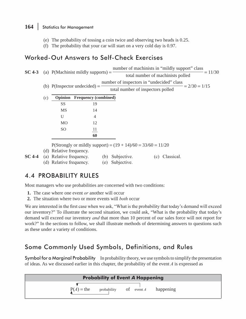
164 Statistics for Management
(e) The probability of tossing a coin twice and observing two heads is 0.25.(f) The probability that your car will start on a very cold day is 0.97.
Worked-Out Answers to Self-Check Exercises
SC 4-3 (a) P(Machinist mildly supports) = number of machinists in “mildly support” class
total number of machinists polled = 11/30
(b) P(Inspector undecided) = number of inspectors in “undecided” class
total number of inspectors polled = 2/30 = 1/15
(c) Opinion Frequency (combined)SS 19MS 14U 4MO 12SO 11
60
P(Strongly or mildly support) = (19 + 14)/60 = 33/60 = 11/20(d) Relative frequency.
SC 4-4
4.4 PROBABILITY RULESMost managers who use probabilities are concerned with two conditions: 1. The case where one event or another will occur 2. The situation where two or more events will both occur
our inventory?” To illustrate the second situation, we could ask, “What is the probability that today’s demand will exceed our inventory and that more than 10 percent of our sales force will not report for work?” In the sections to follow, we shall illustrate methods of determining answers to questions such as these under a variety of conditions.
Some Commonly Used Symbols, Definitions, and Rules
Symbol for a Marginal Probability In probability theory, we use symbols to simplify the presentation of ideas. As we discussed earlier in this chapter, the probability of the event A is expressed as
Probability of Event A Happening
P(A) = the probability of event A happening

Probability I: Introductory Ideas 165
A single probability means that only one event can take place. It is called a marginal or unconditional probability. To illustrate, let us suppose that 50 members of a school class drew tickets to see which student would get a free trip to the National Rock Festival. Any one of the students could calculate his or her chances of winning as:
P(Winning) = 150
= 0.02
In this case, a student’s chance is 1 in 50 because we are certain that the possible events are mutually exclusive, that is, only one student can win at a time.
There is a nice diagrammatic way to illustrate this example and other probability concepts. We use a pictorial representation called a Venn diagram, after the nineteenth-century English mathemati-cian John Venn. In these diagrams, the entire sample space is represented by a rectangle, and events are represented by parts of the rectangle. If two events are mutually exclusive, their parts of the rectangle will not overlap each other, as shown in Figure 4-2(a). If two events are not mutually exclusive, their parts of the rectangle will overlap, as in Figure 4-2(b).
Because probabilities behave a lot like areas, we shall let the rectangle have an area of 1 (because the probability of something happening is 1). Then the probability of an event is the area of its part of the rectangle. Figure 4-2(c) illustrates this for the National Rock Festival example. There the rectangle is divided into 50 equal, nonoverlapping parts.
Addition Rule of Probabilistic Events If two events are not mutually exclusive, it is possible for both events to occur. In these
the probability of drawing either an ace or a heart from a deck of cards? Obviously, the events ace and heart can occur together because we could draw the ace of hearts.
counting, that is, we have to reduce the probability of drawing either an ace or a heart by the chance that we could draw both of them together. As a result, the correct equation for the probability of one or more of two events that are not mutually exclusive is
Marginal or unconditional
probability
Venn diagrams
Area of anysquare is .02 (1/50)
Two mutuallyexclusive events
(a)
Two nonexclusiveevents
(b)
A B A B
National rockfestival example
(c)
FIGURE 4-2 SOME VENN DIAGRAMS
Probability of one or more
events not mutually exclusive

166 Statistics for Management
Addition Rule of Probabilistic Events
P(A or B) = P(A) + P(B) – P(AB)
Probability of A happening
Probability of A or B happening when A and B are not mutually exclusive
Probability of A and B happening together
Probability of B happening
[4-2]
A Venn diagram illustrating Equation 4-2 is given in Figure 4-3. There, the event A or B is outlined with a heavy line. The event A and B is the cross-hatched wedge in the middle. If we add the areas of circles A and B, we double count the area of the wedge, and so we must subtract it to make sure it is counted only once.
Using Equation 4-2 to determine the probability of drawing either an ace or a heart, we can calculate:
P(Ace or Heart) = P(Ace) + P(Heart) – P(Ace and Heart)
= 452
+ 1352
– 152
= 1652
or 413
1. male age 302. male 323. female 454. female 205. male 40
This group decides to elect a spokesperson by drawing a name from a hat. Our question is, “What is the probability the spokesperson will be either female or over 35?” Using Equation 4-2, we can set up the solution to our question like this:
P(Female or Over 35) = P(Female) + P(Over 35) – P(Female and Over 35)
= 25
+ 25
– 15
= 35
requirements of being either female or over 35.
Addition Rule for Mutually Exclusive Events Often, however, we are interested in the probability that one thing or another will occur. If these two events are mutually exclusive, we can express this probability using the addition rule for mutually exclusive events. This rule is expressed symbolically as
Probability of one or more
mutually exclusive events
FIGURE 4-3 VENN DIAGRAM FOR THE ADDITION RULE FOR TWO EVENTS NOT MUTUALLY EXCLUSIVE
A or B A and B
A B

Probability I: Introductory Ideas 167
P(A or B) = the probability of either A or B happening
and is calculated as follows:
Probability of Either A or B Happening
P(A or B) = P(A) + P(B) [4-3]
This addition rule is illustrated by the Venn diagram in Figure 4-4, where we note that the area in the two circles together (denoting the event A or B) is the sum of the areas of the circle denoting the event A and the circle denoting the event B.
Now to use this formula in an example. Five equally capable students are
Hafsa, John, Harleen, and Prakash. If our question is, “What is the probability that John will be the candidate?” we can use Equation 4-1 and give the answer.
P(John) = 15
= 0.02However, if we ask, “What is the probability that either John or Harleen will be the candidate?” we would use Equation 4-3:
P(John or Harleen) = P(John) + P(Harleen)
= 15
+ 15
= 25
= 0.4
Let’s calculate the probability of two or more events happening once more. Table 4-1 contains data on the sizes of families in a certain town. We are interested in the question, “What is the probability that
children)?” Using Equation 4-3, we can calculate the answer as
P(4, 5, 6 or more) = P(4) + P(5) + P(6 or more) = 0.15 + 0.10 + 0.05= 0.30
There is an important special case of Equation 4-3. For any event A, either A happens or it doesn’t. So the events A and not A are exclusive and exhaustive. Applying Equation 4-3 yields the result
P(A) + P(not A) = 1or, equivalently,
P(A) = 1 – P(not A)
A special case of Equation 4-3
A B
P(A or B) = P(A) + P(B)
FIGURE 4-4 VENN DIAGRAM FOR THE ADDITION RULE FOR MUTUALLY EXCLUSIVE EVENTS

168 Statistics for Management
is most easily obtained by subtracting from 1 the probability of the family’s having six or more children, and thus is seen to be 0.95.
TABLE 4.1 FAMILY-SIZE DATA
NUMBER OF CHILDREN 0 1 2 3 4 5 6 or morePROPORTION OF FAMILIES 0.05 0.10 0.30 0.25 0.15 0.10 0.05
John Venn’s diagrams are a useful way to avoid errors when you apply the addition rule for events that are and are not mutually exclusive. The most common error here is double counting. Hint: In applying the addition rule for mutually exclusive events, we’re looking for a probability of one event or another and overlap is not a problem. However, with non–mutually exclusive events, both can occur together and we need to reduce our probability by the chance that they could. Thus, we subtract the overlap or cross-hatched area in the Venn diagram to get the correct value.
HINTS & ASSUMPTIONS
EXERCISES 4.4
Self-Check ExercisesSC 4-5 From the following Venn diagram, which indicates the number of outcomes of an experiment
corresponding to each event and the number of outcomes that do not correspond to either event, give the probabilities indicated.
A BP(A) =P(B) =P(A or B) =
23
8 6 13
Total outcomes = 50
SC 4-6 Samreen, an owner of a big business house, is considering to purchase one of the two pumping stations. The cost of purchase of both is same but the main concern is chances of failure of the pumping stations under consideration. Each station is susceptible to two kinds of failure: pump failure and leakage. When either (or both) occur, the station must be shut down. The data at hand indicate that the following probabilities prevail:
Station P(Pump Failure) P(Leakage) P(Both)1 0.07 0.10 02 0.09 0.12 0.06
Recommend, which pumping station, should be purchased by Samreen. Justify your answer.
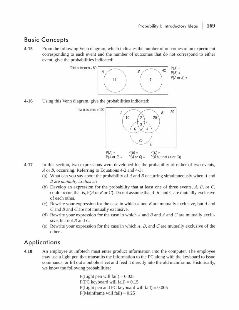
Probability I: Introductory Ideas 169
Basic Concepts4-15 From the following Venn diagram, which indicates the number of outcomes of an experiment
corresponding to each event and the number of outcomes that do not correspond to either event, give the probabilities indicated:
A BP(A) =P(B) =P(A or B) =
42
11 7
Total outcomes = 50
4-16 Using this Venn diagram, give the probabilities indicated:
A B
C
P(A) =P(A or B) =
P(B) =P(A or C) =
P(C) =P(B but not (A or C))
10 2
36 4
25
2030Total outcomes = 100
4-17 In this section, two expressions were developed for the probability of either of two events, A or B, occurring. Referring to Equations 4-2 and 4-3:(a) What can you say about the probability of A and B occurring simultaneously when A and
B are mutually exclusive?(b) Develop an expression for the probability that at least one of three events, A, B, or C,
could occur, that is, P(A or B or C). Do not assume that A, B, and C are mutually exclusive of each other.
(c) Rewrite your expression for the case in which A and B are mutually exclusive, but A and C and B and C are not mutually exclusive.
(d) Rewrite your expression for the case in which A and B and A and C are mutually exclu-sive, but not B and C.
(e) Rewrite your expression for the case in which A, B, and C are mutually exclusive of the others.
Applications4.18 An employee at Infotech must enter product information into the computer. The employee
may use a light pen that transmits the information to the PC along with the keyboard to issue
we know the following probabilities:
P(Light pen will fail) = 0.025P(PC keyboard will fail) = 0.15P(Light pen and PC keyboard will fail) = 0.005P(Mainframe will fail) = 0.25

170 Statistics for Management
Data can be entered into the PC only if both the light pen and keyboard are functioning.(a) What is the probability that the employee can use the PC to enter data?(b) What is the probability that either the PC fails or the mainframe fails? Assume they cannot
both fail at the same time.4-19 The HAL Corporation wishes to improve the resistance of its personal computer to disk-drive
and keyboard failures. At present, the design of the computer is such that disk-drive failures occur only one-third as often as keyboard failures. The probability of simultaneous disk-drive and keyboard failures is 0.05. If the computer is 80 percent resistant to disk-drive and/or key-board failure, how low must the disk-drive failure probability be?
4-20 The Herr–McFee Company, which produces nuclear fuel rods, must X-ray and inspect each rod before shipping. Karen Wood, an inspector, has noted that for every 1,000 fuel
probability?
Worked-Out Answers to Self-Check ExercisesSC 4-5 P(A) = 14/50 = 0.28 P(B) = 19/50 = 0.38
P(A or B) = 1450
+ 1950
– 650
= 0.54
SC 4-6 P(Failure) = P(Pump failure or leakage)Station 1: 0.07 + 0.1 – 0 = 0.17 Station 2: 0.09 + 0.12 – 0.06 = 0.15Thus, Station 1 has the higher probability of being shut down. So, Station 2 should be taken over by Samreen.
4.5 PROBABILITIES UNDER CONDITIONS OF STATISTICAL INDEPENDENCE
not have an effect on the outcome of the second event. That is, the events may be either dependent or independent. In this section, we examine events that are statistically independent: The occurrence of one event has no effect on the probability of the occurrence of any other event. There are three types of probabilities under statistical independence:
1. Marginal 2. Joint 3. Conditional
Marginal Probabilities under Statistical IndependenceAs we explained previously, a marginal or unconditional probabil-ity is the simple probability of the occurrence of an event. In a fair coin toss, P(H) = 0.5, and P(T) = 0.5; that is, the probability of heads equals 0.5 and the probability of tails equals 0.5. This is true for every toss, no matter how many tosses have been made or what their outcomes have been. Every toss stands alone and is in no way connected
Independence defined
Marginal probability of
independent events

Probability I: Introductory Ideas 171
with any other toss. Thus, the outcome of each toss of a fair coin is an event that is statistically indepen-dent of the outcomes of every other toss of the coin.
Imagine that we have a biased or unfair coin that has been altered in such a way that heads occurs 0.90 of the time and tails 0.10 of the time. On each individual toss, P(H) = 0.90, and P(T) = 0.10. The outcome of any particular toss is completely unrelated to the outcomes of the tosses that may precede or follow it. The outcomes of several tosses of this coin are statistically independent events too, even though the coin is biased.
Joint Probabilities under Statistical IndependenceThe probability of two or more independent events occurring together or in succession is the product of their marginal probabili-ties. Mathematically, this is stated (for two events):
Joint Probability of Two Independent Events
P(AB) = P(A) × P(B) [4-4]
where
P(AB) = probability of events A and B occurring together or in succession; this is known as a joint probability
P(A) = marginal probability of event A occurring P(B) = marginal probability of event B occurring
In terms of the fair coin example, the probability of heads on two
we shall call H1) times the probability of heads on the second toss (H2). That is, P(H1H2) = P(H1) × P(H2). We have shown that the events are statistically independent, because the probability of any outcome is not affected by any preceding outcome. Therefore, the probability of heads on any toss is 0.5, and P(H1H2) = 0.5 × 0.5 = 0.25. Thus, the probability of heads on two successive tosses is 0.25.
Likewise, the probability of getting three heads on three successive tosses is P(H1H2H3) = 0.5 × 0.5 × 0.5 = 0.125.
Assume next that we are going to toss an unfair coin that has P(H) = 0.8 and P(T) = 0.2. The events (outcomes) are independent, because the probabilities of all tosses are exactly the same—the individual tosses are completely separate and in no way affected by any other toss or outcome. Suppose our ques-tion is, “What is the probability of getting three heads on three successive tosses?” We use Equation 4-4 and discover that:
P(H1H2H3) = P(H1) × P(H2) × P(H3) = 0.8 × 0.8 × 0.8 = 0.512
Now let us ask the probability of getting three tails on three successive tosses:
P(T1T2T3) = P(T1) × P(T2) × P(T3) = 0.2 × 0.2 × 0.2 = 0.008
Note that these two probabilities do not add up to 1 because the events H1H2H3 and T1T2T3 do not constitute a collectively exhaustive list. They are mutually exclusive, because if one occurs, the other cannot.
Multiplication rule for joint,
independent events
The fair coin example

172 Statistics for Management
We can make the probabilities of events even more explicit using a probability tree. Figure 4-5 is a probability tree showing the possible outcomes and their respective probabilities for one toss of a fair coin.
For toss 1, we have two possible outcomes, heads and tails, each with a probability of 0.5. Assume that the outcome of toss 1 is heads. We toss again. The second toss has two possible outcomes, heads and tails, each with a probability of 0.5. In Figure 4-6, we add these two branches of the tree.
Next we consider the possibility that the outcome of toss 1 is tails. Then the second toss must stem from the lower branch repre-senting toss 1. Thus, in Figure 4-7, we add two more branches to the tree. Notice that on two tosses, we have four possible outcomes: H1H2, H1T2, TlH2, and T1T2 (remember the subscripts indicate the toss number, so that T2, for example, means tails on toss 2). Thus, after two tosses, we may arrive at any one of four possible points. Because we are going to toss three times, we must add more branches to the tree.
now ready to begin adding branches for the third toss. As before, the two possible outcomes are heads and tails, each with a probability
manner. The completed probability tree is shown in Figure 4-9. Notice that both heads and tails have a
following it.
One toss, two possible
outcomes
Two tosses, four possible
outcomes
Three tosses, eight possible
outcomes
Toss 1 Toss 2
P(H) = 0.5
P(H) = 0.5
P(T ) = 0.5
P(T ) = 0.5
0.25
0.25
0.5
0.5
FIGURE 4-6 PROBABILITY TREE OF A PARTIAL SECOND TOSS
Toss 1 Toss 2
P(H) = 0.5
P(H) = 0.5
P(H) = 0.5P(T ) = 0.5
P(T ) = 0.5
P(T ) = 0.5
0.25
0.25
0.25
0.25
0.5
0.5
FIGURE 4-7 PROBABILITY TREE OF TWO TOSSES
Toss 1
P(H) = 0.5
P(T ) = 0.5
0.5
0.5
FIGURE 4-5 PROBABILITY TREE OF ONE TOSS
Constructing a probability tree
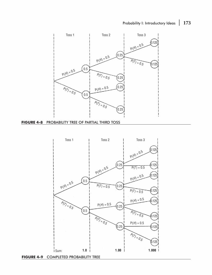
Probability I: Introductory Ideas 173
Toss 1 Toss 2 Toss 3
P(H) = 0.5
P(H) = 0.5
P(H) = 0.5
P(H) = 0.5P(T ) = 0.5
P(T ) = 0.5
P(T ) = 0.5
P(T ) = 0.5
0.125
0.125
0.25
0.25
0.25
0.25
0.5
0.5
FIGURE 4-8 PROBABILITY TREE OF PARTIAL THIRD TOSS
Toss 1 Toss 2 Toss 3
P(H) = 0.5
P(H) = 0.5
P(H) = 0.5
P(H) = 0.5P(H) = 0.5
P(H) = 0.5
P(T ) = 0.5
P(T ) = 0.5
P(T ) = 0.5
P(T ) = 0.5
P(T ) = 0.5P(T ) = 0.5
P(T ) = 0.5
0.125
0.125
0.125
0.125
0.125
0.125
0.125
0.125
Sum: 1.0 1.00 1.000
P(H) = 0.5
0.25
0.25
0.25
0.25
0.5
0.5
FIGURE 4-9 COMPLETED PROBABILITY TREE

174 Statistics for Management
TABLE 4-2 LISTS OF OUTCOMES
1 Toss 2 Tosses 3 TossesPossible Outcomes Probability Possible Outcomes Probability Possible Outcomes Probability
H1 0.5 H1H2 0.25 H1H2H3 0.125T1 0.5 H1T2 0.25 H1H2T3 0.125
1.0 T1H2 0.25 H1T2H3 0.125T1T2 0.25 T1H2H3 0.125
1.00 T1H2T3 0.125The sum ofthe probabilities of allthe possible outcomesmust always equal 1
T1T2H3 0.125T1T2T3 0.125
0.1251.000
Suppose we are going to toss a fair coin and want to know the probability that all three tosses will result in heads. Expressing the problem symbolically, we want to know P(H1H2H3). -ability of independent events, we know that
P(H1H2H3) = P(H1) × P(H2) × P(H3) = 0.5 × 0.5 × 0.5 = 0.125
We could have read this answer from the probability tree in Figure 4-9 by following the branches giving H1H2H3.
Try solving these problems using the probability tree in Figure 4-9.
Example 1 What is the probability of getting tails, heads, tails in that order on three successive tosses of a fair coin?
Solution P(T1H2T3) = P(T1) × P(H2) × P(T3) = 0.125. Following the prescribed path on the probability tree will give us the same answer.
Example 2 What is the probability of getting tails, tails, heads in that order on three successive tosses of a fair coin?
Solution the third toss, we arrive at the probability of 0.125. Thus, P(T1T2H3) = 0.125.
It is important to notice that the probability of arriving at a given point by a given route is not the same as the probability of, say, heads on the third toss. P(H1T2H3) = 0.125, but P(H3) =a case of joint probabilityand heads on the third. The latter, by contrast, is simply the marginal probability of getting heads on a particular toss, in this instance toss 3.
Notice that the sum of the probabilities of all the possible outcomes for each toss is 1. This results from the fact that we have mutually exclusive and collectively exhaustive lists of outcomes. These are given in Table 4-2.
Outcomes in a particular order
All tosses are independent
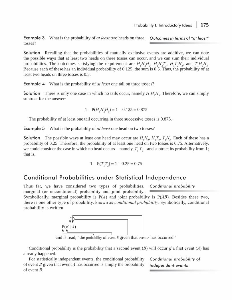
Probability I: Introductory Ideas 175
Example 3 What is the probability of at least two heads on three tosses?
Solution Recalling that the probabilities of mutually exclusive events are additive, we can note the possible ways that at least two heads on three tosses can occur, and we can sum their individual probabilities. The outcomes satisfying the requirement are H1H2H3, H1H2T3, H1T2H3, and T1H2H3. Because each of these has an individual probability of 0.125, the sum is 0.5. Thus, the probability of at least two heads on three tosses is 0.5.
Example 4 What is the probability of at least one tail on three tosses?
Solution There is only one case in which no tails occur, namely H1H2H3. Therefore, we can simply subtract for the answer:
1 – P(H1H2H3) = 1 – 0.125 = 0.875
The probability of at least one tail occurring in three successive tosses is 0.875.
Example 5 What is the probability of at least one head on two tosses?
Solution The possible ways at least one head may occur are H1H2, H1T2, T1H2. Each of these has a probability of 0.25. Therefore, the probability of at least one head on two tosses is 0.75. Alternatively, we could consider the case in which no head occurs—namely, T1 T2—and subtract its probability from 1; that is,
1 – P(T1T2) = 1 – 0.25 = 0.75
Conditional Probabilities under Statistical IndependenceThus far, we have considered two types of probabilities,
Symbolically, marginal probability is P(A AB). Besides these two, there is one other type of probability, known as conditional probability. Symbolically, conditional probability is written
P(B | A)
and is read, “the probability of event B given that event A has occurred.”
Conditional probability is the probability that a second event (B) will occur if A) has already happened.
For statistically independent events, the conditional probability of event B given that event A has occurred is simply the probability of event B:
Conditional probability
Conditional probability of
independent events
Outcomes in terms of “at least”
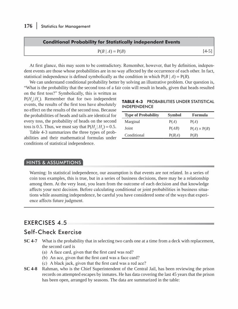
176 Statistics for Management
Conditional Probability for Statistically independent Events
P(B | A) = P(B) [4-5]
-dent events are those whose probabilities are in no way affected by the occurrence of each other. In fact,
B | A) = P(B).We can understand conditional probability better by solving an illustrative problem. Our question is,
“What is the probability that the second toss of a fair coin will result in heads, given that heads resulted
P(H2 | H1). Remember that for two independent
no effect on the results of the second toss. Because the probabilities of heads and tails are identical for every toss, the probability of heads on the second toss is 0.5. Thus, we must say that P(H2 | H1) = 0.5.
Table 4-3 summarizes the three types of prob-abilities and their mathematical formulas under conditions of statistical independence.
Warning: In statistical independence, our assumption is that events are not related. In a series of coin toss examples, this is true, but in a series of business decisions, there may be a relationship among them. At the very least, you learn from the outcome of each decision and that knowledge
-tions while assuming independence, be careful you have considered some of the ways that experi-
HINTS & ASSUMPTIONS
EXERCISES 4.5
Self-Check ExerciseSC 4-7 What is the probability that in selecting two cards one at a time from a deck with replacement,
the second card is
SC 4-8 Rahman, who is the Chief Superintendent of the Central Jail, has been reviewing the prison records on attempted escapes by inmates. He has data covering the last 45 years that the prison has been open, arranged by seasons. The data are summarized in the table:
TABLE 4-3 PROBABILITIES UNDER STATISTICAL INDEPENDENCE
Type of Probability Symbol FormulaMarginal P(A) P(A)Joint P(AB) P(A) × P(B)Conditional P(B|A) P(B)

Probability I: Introductory Ideas 177
Attempted Escapes Winter Spring Summer Fall 0 3 2 1 0 1–5 15 10 11 12 6–10 15 12 11 1611–15 5 8 7 716–20 3 4 6 521–25 2 4 5 3
More than 25 2 5 4 245 45 45 45
(a) What is the probability that in a year selected at random, the number of escapes was between 16 and 20 during the winter?
(b) What is the probability that more than 10 escapes were attempted during a randomly cho-sen summer season?
(c) What is the probability that between 11 and 20 escapes were attempted during a randomly chosen season? (Hint: Group the data together.)
Basic Concepts4-21 What is the probability that a couple’s second child will be
4-22 In rolling two dice, what is the probability of rolling
4-23 A bag contains 32 marbles: 4 are red, 9 are black, 12 are blue, 6 are yellow, and 1 is purple. Marbles are drawn one at a time with replacement. What is the probability that
4-24 George, Richard, Paul, and John play the following game. Each man takes one of four balls numbered 1 through 4 from an urn. The man who draws ball 4 loses. The other three return their balls to the urn and draw again. Now the one who draws ball 3 loses. The other two return their balls to the urn and draw again. The man who draws ball 1 wins the game.
(b) What is the probability that Paul wins the game?
Applications4-25 The health department routinely conducts two independent inspections of each restaurant,
with the restaurant passing only if both inspectors pass it. Inspector A is very experienced, and, hence, passes only 2 percent of restaurants that actually do have health code violations.
178 Statistics for Management
Inspector B is less experienced and passes 7 percent of restaurants with violations. What is the probability that(a) Inspector A passes a restaurant, given that inspector B has found a violation?(b) Inspector B passes a restaurant with a violation, given that inspector A passes it?(c) A restaurant with a violation is passed by the health department?
4-26
order?
order are less than 1 in 5,000,000. Is this statement true?4-27 Sridharan is preparing a report that his employer, the Titre Corporation, will eventually deliver
to the Ministry of Small and Medium Enterprises (MSME). First, the report must be approved by Sridharan’s group leader, department head, and division chief (in that order). Sridharan knows from experience that the three managers act independently. Further, he knows that his group leader approves 85 percent of his reports, his department head approves 80 percent of the reports written by Sridharan that reach him, and his division chief approves 82 percent of Sridharan’s work.
MSME?
leader and department head, but is not approved by his division chief?4-28 A grocery store is reviewing its restocking policies and has analyzed the number of half-liter
Morning Afternoon Evening0–19 3 8 2
20–39 3 4 340–59 12 6 460–79 4 9 980–99 5 3 6
100 or more 3 0 630 30 30
(a) What is the probability that on a randomly selected day the number of cartons of orange
(b) What is the probability that 39 or fewer cartons were sold during a randomly selected afternoon?
(c) What is the probability that either 0–19 or 100 or more cartons were sold in a randomly selected morning?
4-29
installed four billboards on a highway outside of town, and he knows from experience the probabilities that each will be noticed by a randomly chosen motorist. The probability of the
noticed is 0.82, the third has a probability of 0.87 of being noticed, and the probability of the fourth sign’s being noticed is 0.9. Assuming that the event that a motorist notices any

Probability I: Introductory Ideas 179
particular billboard is independent of whether or not he notices the others, what is the prob-ability that(a) All four billboards will be noticed by a randomly chosen motorist?
(c) Exactly one of the billboards will be noticed?(d) None of the billboards will be noticed?(e) The third and fourth billboards won’t be noticed?
Worked-Out Answers to Self-Check ExercisesSC 4-7 (a) P(Face2 | Red1) = 12/52 = 3/13
(b) P(Ace2 | Face1) = 4/52 = 1/132 | Red ace1) = 2/52 = 1 /26
SC 4-8 (a) 3/45 = 1/15(b) (7 + 6 + 5 + 4)/45 = 22/45(c) (8 + 12 + 13 + 12)/180 = 45/180 = 1/4
4.6 PROBABILITIES UNDER CONDITIONS OF STATISTICAL DEPENDENCE
Statistical dependence exists when the probability of some event is dependent on or affected by the occurrence of some other event. Just as with independent events, the types of probabilities under statistical dependence are
1. Conditional 2. Joint 3. Marginal
Conditional Probabilities under Statistical Dependence-
best illustrated by using conditional probabilities as a basis.Assume that we have one box containing 10 balls distributed as
follows:
Three are colored and dotted. One is colored and striped. Two are gray and dotted. Four are gray and striped.
The probability of drawing any one ball from this box is 0.1, since there are 10 balls, each with equal probability of being drawn. The discussion of the following examples will be facilitated by reference to Table 4-4 and to Figure 4-10, which shows the contents of the box in diagram form.
Example 1 Suppose someone draws a colored ball from the box. What is the probability that it is dotted? What is the probability it is striped?
Dependence defined
Examples of conditional
probability of dependent events

180 Statistics for Management
Solution This question can be expressed symbolically as P(D | C), or “What is the conditional probability that this ball is dotted, given that it is colored?”
We have been told that the ball that was drawn is colored. Therefore, to calculate the probability that the ball is dotted, we will ignore all the gray balls and concern ourselves with the colored balls only. In diagram form, we consider only what is shown in Figure 4-11.
From the statement of the problem, we know that there are four colored balls, three of which are dotted and one of which is striped.
striped. To do so, we divide the number of balls in each category by the total number of colored balls:
P(D|C) = 35
= 0.75
P(S|C) = 14
= 0.25
1.00
In other words, three-fourths of the colored balls are dotted and one-fourth of the colored balls are striped. Thus, the probability of dotted, given that the ball is colored, is 0.75. Likewise, the probability of striped, given that the ball is colored, is 0.25.
Now we can see how our reasoning will enable us to develop the formula for conditional probability are statistically dependent
by observing that the color of the balls determines the probabilities that they are either striped or dotted. For example, a gray ball is more likely to be striped than a colored ball is. Since color affects the prob-ability of striped or dotted, these two events are dependent.
To calculate the probability of dotted given colored, P(D|C), we divided the probability of colored and dotted balls (3 out of 10, or 0.3) by the probability of colored balls (4 out of 10, or 0.4):
P(D|C) = P(DC)P(C)
COLOR AND CONFIGURATION OF 10 BALLS
Event Probability of Event 1 0.1
colored and dotted 2 0.1 3 0.1 4 0.1 } colored and striped 5 0.1
gray and dotted 6 0.1 7 0.1
gray and striped 8 0.1 9 0.110 0.1
⎫⎬⎭
⎫⎬⎭
⎫⎬⎭
Gray
Colored
3 balls are colored and dotted
2 balls are gray and dotted
4 balls are gray and striped
1 ball is colored and striped
FIGURE 4-10 CONTENTS OF THE BOX
FIGURE 4-11 PROBABILITY OF DOTTED AND STRIPED, GIVEN COLORED
Colored
3 balls are colored and dotted
1 ball is colored and striped
Probability I: Introductory Ideas 181
Expressed as a general formula using the letters A and B to represent the two events, the equation is
Conditional Probability for Statistically Dependent Events
P(B | A) = P(BA)P(A)
[4-6]
This is the formula for conditional probability under statistical dependence.
Example 2 Continuing with our example of the colored and gray balls, let’s answer the questions, “What is P(D|G)?” and “What is P(S|G)?”
Solution
P(D|G) = P(DG)P(G)
= 0.20.6
= 13
P(S |G) = P(SG)P(G)
= 0.40.6
= 23
1.0
The problem is shown diagrammatically in Figure 4-12. The total probability of gray is 0.6 (6 out of 10 balls). To determine the probability that the ball
(which we know is gray) will be dotted, we divide the probability of gray and dotted (0.2) by the prob-ability of gray (0.6), or 0.2/0.6 = 1/3. Similarly, to determine the probability that the ball will be striped, we divide the probability of gray and striped (0.4) by the probability of gray (0.6), or 0.4/0.6 = 2/3.
Example 3 Calculate P(G|D) and P(C|D).
Solution Figure 4-13 shows the contents of the box arranged according to the striped or dotted markings on the balls. Because we have been told that the ball that was drawn is dotted, we can disregard striped and consider only dotted.
Now see Figure 4-14, showing the probabilities of colored and gray, given dotted. Notice that the relative proportions of the two are 0.4 to 0.6. The calculations used to arrive at these proportions were
Gray
2 balls are gray and dottedeach with a probability of 0.1
4 balls are gray and stripedeach with a probability of 0.1
FIGURE 4-12 PROBABILITY OF DOTTED AND STRIPED, GIVEN GRAY
Striped Dotted
P(CS ) = 0.1P(GD ) = 0.2
P(CD ) = 0.3P(GS ) = 0.4
FIGURE 4-13 CONTENTS OF THE BOX ARRANGED BY CONFIGURATION, STRIPED AND DOTTED
182 Statistics for Management
P(G|D) = P(GD)P(D)
= 0.20.5
= 0.4
P(C|D) = P(CD)P(D)
= 0.30.5
= 0.6
1.0
Example 4 Calculate P(C|S) and P(G|S).
Solution
P(C|S) = P(CS)P(S)
= 0.10.5
= 0.2
P(G|S) = P(GS)P(S)
= 0.40.5
= 0.8
1.0
Joint Probabilities under Statistical DependenceWe have shown that the formula for conditional probability under con-ditions of statistical dependence is
P(B | A) =
P(BA)P(A)
[4-6]
If we solve this for P(BA) by cross multiplication, we have the formula for joint probability under condi-tions of statistical dependence:
Joint Probability for Statistically Dependent Events
P(BA) = P(B | A) × P(A)*
Joint probability of events B and A happening together or in succession
Probability that event A will happen
Probability of event B given that event A has happened
[4-7]
Notice that this formula is not P(BA) = P(B) × P(A), as it would be under conditions of statistical independence.
Converting the general formula P(BA) = P(B | A) × P(A) to our example and to the terms of colored, gray, dotted, and striped, we have P(CD) = P(C | D) × P(D), or P(CD) = 0.6 × 0.5 = 0.3. Here, 0.6 is the
FIGURE 4-14 PROBABILITY OF COLORED AND GRAY, GIVEN DOTTED
Dotted
P(G⏐D ) = 0.4
P(C⏐D ) = 0.6
A and B, you could also use the formula P(BA) = P(AB) = P(A | B) × P(B). This is because BA = AB.

Probability I: Introductory Ideas 183
probability of colored, given dotted (computed in Example 3 above) and 0.5 is the probability of dotted (also computed in Example 3).
P(CD) =Three balls out of 10 are colored and dotted.
-ner and can also be substantiated by reference to Table 4-4.
P(CS) = P(C|S) × P(S) = 0.2 × 0.5 = 0.1
P(GD) = P(G|D) × P(D) = 0.4 × 0.5 = 0.2
P(GS) = P(G|S) × P(S) = 0.8 × 0.5 = 0.4
Marginal Probabilities under Statistical DependenceMarginal probabilities under statistical dependence are computed by summing up the probabilities of all
occurred:P(C) = P(CD) + P(CS) = 0.3 + 0.1 = 0.4
Similarly, the marginal probability of the event gray can be computed by summing the probabilities
P(G) = P(GD) + P(GS) = 0.2 + 0.4 = 0.6
In like manner, we can compute the marginal probability of the event dotted by summing the prob-
P(D) = P(CD) + P(GD) = 0.3 + 0.2 = 0.5
-
P(S) = P(CS) + P(GS) = 0.1 + 0.4 = 0.5
These four marginal probabilities, P(C) = 0.4, P(G) = 0.6, P(D) = 0.5, and P(S) =by inspection of Table 4-4 on page 180.
-ditions of statistical dependence. Table 4-5 provides a résumé of our development of probabilities under both statistical independence and statistical dependence.
Example Department of Social Welfare has recently carried out a socio-economic survey of a village. The information collected is related to the gender of the respondent and level of education (graduation). 1000 respondents were surveyed. The results are presented in the following table:
Gender Undergraduate Graduate TotalMale 150 450 600Female 150 250 400Total 300 700 1000
Several examples

184 Statistics for Management
A respondent has been selected randomly, what are the chances that -
(a) The respondent will be Undergraduate (U)-
P (U) = 300/1000 = 0.3(b) The respondent will be Graduate (G),
P (G) = 700/1000 = 0.7
(c) The respondent will be Female (F),
P (F) = 400/1000 = 0.4
These are the examples of Unconditional Probability. They are termed as unconditional because no condition is imposed on any event.
(d) The respondent will be Male-Graduate (MG)
P (Male & Graduate) = P (MG) = 450/1000 = 0.45
(e) The respondent will be Undergraduate-Female (UF)
P (Undergraduate and Female) = P (UF) = 150/1000 = 0.15
The above two cases (d) and (e) are examples of Joint Probability.
(f) A randomly selected Female will be Graduate (G/F):
Here a condition has been imposed that randomly selected respondent has been Female. So, this is an
under the condition that the respondent should be Female. Hence consideration should be from a total of 400 (Female respondents only)
So, Probability of the respondent being Graduate, given Female-
P (G/F) = 250/400 = 0.625
TABLE 4-5 PROBABILITIES UNDER STATISTICAL INDEPENDENCE AND DEPENDENCE
Type of Probability Symbol
Formula under Statistical Independence
Formula under Statistical Dependence
Marginal P(A) P(A) Sum of the probabilities of the A occurs
Joint P(AB) P(A) × P(B) P(A|B) × P(B)or P(BA) P(B) × P(A) P(B|A) × P(A)
Conditional P(B|A) P(B) P(BA)P(A)
or P(A|B) P(A) P(AB)P(B)

Probability I: Introductory Ideas 185
The above concept can also be explained as under:
Probability of the respondent being Female,
P (F) = 400/1000 = 0.40
Probability of Female-Graduate
P (Graduate & Female) = P (GF) = 250/1000 = 0.25
So,
P (G/F) = P (G and F) / P (F) = 0.25/0.40 = 0.625
(g) A randomly selected Undergraduate will be Male (M/U)):
Probability of the respondent being Male, given Undergraduate,
P (M/U) = 150/300 = 0.50
Alternatively,
Probability of the respondent being Undergraduate,
P (U) = 300/1000 = 0.30
Probability of the respondent being Male-Undergraduate-
P (Male & Undergraduate) = P (MU) = 150/1000 = 0.15
So,
P (M/U) = P (M and U) / P (U) = 0.15/0.30 = 0.50
given that and both … and: P(A|B) is “the probability that A will occur given that B has occurred” and P(AB) is “the probability that both A and B will occur.” And the marginal probability P(A) is the “probability that A will occur, whether or not B happens.”
HINTS & ASSUMPTIONS
EXERCISES 4.6
Self-Check ExercisesSC 4-9 According to a survey, the probability that a family owns two cars if its annual income is
greater than `6,00,000 is 0.75. Of the households surveyed, 60 percent had incomes over `6,00,000 and 52 percent had two cars. What is the probability that a family has two cars and an income over `6,00,000 a year?
186 Statistics for Management
SC 4-10 Friendly’s Department Store has been the target of many shoplifters during the past month, but owing to increased security precautions, 250 shoplifters have been caught. Each shoplifter’s
are summarized in the table.
Sex First-Time Offender Repeat OffenderMale 60 70Female 44 76
104 146
(a) The probability that the shoplifter is male.
(c) The probability that the shoplifter is female, given that the shoplifter is a repeat offender.
(e) The probability that the shoplifter is both male and a repeat offender.
Basic Concepts4-30 Two events, A and B, are statistically dependent. If P(A) = 0.39, P(B) = 0.21, and P(A or B) = 0.47,
(a) Neither A nor B will occur.(b) Both A and B will occur.(c) B will occur, given that A has occurred.(d) A will occur, given that B has occurred.
4-31 Given that P(A) = 3/14, P(B) = 1/6, P(C) = 1/3, P(AC) = 1/7, and P(B|C) = -lowing probabilities: P(A|C), P(C|A), P(BC), P(C|B).
4-32 Assume that for two events A and B, P(A) = 0.65, P(B) = 0.80, P(A|B) = P(A), and P(B|A) = 0.85. Is this a consistent assignment of probabilities? Explain.
Applications4-33 At a soup kitchen, a social worker gathers the following data. Of those visiting the kitchen,
59 percent are men, 32 percent are alcoholics, and 21 percent are male alcoholics. What is the probability that a random male visitor to the kitchen is an alcoholic?
4-34 During a study of auto accidents, the Highway Safety Council found that 60 percent of all accidents occur at night, 52 percent are alcohol-related, and 37 percent occur at night and are alcohol-related.(a) What is the probability that an accident was alcohol-related, given that it occurred at
night?(b) What is the probability that an accident occurred at night, given that it was alcohol-related?
4-35 If a hurricane forms in the eastern half of the Bay of Bengal, there is a 76 percent chance that it will strike the western coast of Maharashtra. From data gathered over the past 50 years, it has been determined that the probability of a hurricane’s occurring in this area in any given year is 0.85. What is the probability that a hurricane will occur in the eastern Bay of Bengal and strike Maharashtra this year?

Probability I: Introductory Ideas 187
4-36 is a new operating system. The company has asked an engineer for an evaluation of the oper-ating system. Suppose the probability of a favorable evaluation is 0.65. If the probability the company will upgrade its system given a favorable evaluation is 0.85, what is the probability that the company will upgrade and receive a favorable evaluation?
4-37 The university’s library has been randomly surveying patrons over the last month to see who -
data for 350 people are given below. Assume a patron uses only one service per visit.
Patron Reference Periodicals BooksUndergraduate 44 26 72Graduate 24 61 20Faculty 16 69 18
84 156 110
Find the probability that a randomly chosen patron(a) Is a graduate student.(b) Visited the periodicals section, given the patron is a graduate student.(c) Is a faculty member, given a reference section visit.(d) Is an undergraduate who visited the book section.
4-38 about the likelihood of strikes by some of his employees. He has learned that the probability of a strike by his pilots is 0.75 and the probability of a strike by his drivers is 0.65. Further, he knows that if the drivers strike, there is a 90 percent chance that the pilots will strike in sympathy.(a) What is the probability of both groups’ striking?(b) If the pilots strike, what is the probability that the drivers will strike in sympathy?
4-39 National Horticulture Board has been entrusted with the responsibility of sending good qual-ity mangoes to overseas. For this purpose, an inspection is conducted on 10,000 boxes of man-goes from Malihabad and Hyderabad for exports. The inspection of boxes gave the following information:-
Damaged Fruit Overripe FruitMalihabad 6000 200 840Hyderabad 4000 365 295
(a) What are the chances that a selected box will contain damaged or overripe fruit?(b) A randomly selected box contains overripe fruit, what is the probability that it has came
from Hyderabad?4-40 Fragnance Soaps Pvt Ltd is a leading soap manufacturing company in India. “Active” is a
wellthis brand. The marketing research responses are as shown in the following table:
188 Statistics for Management
Prefer Ahmedabad Gwalior Raipur Lucknow55 40 80 75
No 40 30 20 90No Opinion 5 10 20 35
If a customer is selected at random, what is the probability?(a) That he or she prefers active?(b) The consumer prefers Active and is from Ahmadabad?(c) The consumer prefers Active given he is from Lucknow?(d) That he is from Raipur and has no opinion?
Worked-Out Answers to Self-Check ExercisesSC 4-9 Let I = income > $35,000 C = 2 cars.
P(C and I ) = P(C|I)P(I) = (0.75)(0.6) = 0.45SC 4-10 M/W = shoplifter is male/female; F/R =
(a) P(M) = (60 + 70)/250 = 0.520(b) P(F|M) = P(F and M)/P(M) = (60/250)/(130/250) = 0.462(c) P(W|R) = P(W and R)/P(R) = (76/250)/(146/250) = 0.521(d) P(W|F) = P(W and F)/P(F) = (44/250)/(104/250) = 0.423(e) P(M and R) = 70/250 = 0.280
4.7 REVISING PRIOR ESTIMATES OF PROBABILITIES: BAYES’ THEOREM
At the beginning of the baseball season, the fans of last year’s pennant winner thought their team had a
fans realized that they must alter their prior probabilities of winning.
her prior probabilities and order a different color combination or have a sale.In both these cases, certain probabilities were altered after the
people involved got additional information. The new probabilities are known as revised, or posterior, probabilities. Because probabili-ties can be revised as more information is gained, probability theory is of great value in managerial decision making.
The origin of the concept of obtaining posterior probabilities with limited information is attributable to the Reverend Thomas Bayes (1702–1761), and the basic formula for conditional probabil-ity under dependence
P(B|A) =
P(BA)P(A)
[4-6]
is called Bayes’ Theorem.
Posterior probabilities defined
Bayes’ theorem

Probability I: Introductory Ideas 189
Bayes, an Englishman, was a Presbyterian minister and a competent mathematician. He pondered how he might prove the existence of God by examining whatever evidence the world about him pro-vided. Attempting to show “that the Principal End of the Divine Providence . . . is the Happiness of His Creatures,” the Reverend Bayes used mathematics to study God. Unfortunately, the theological implica-
work during his lifetime. Nevertheless, his work outlived him, and modern decision theory is often called Bayesian decision theory in his honor.
Bayes’ theorem offers a powerful statistical method of evaluat-ing new information and revising our prior estimates (based upon limited information only) of the probability that things are in one state or another. If correctly used, it makes it unnecessary to gather masses of data over long periods of time in order to make good decisions based on probabilities.
Calculating Posterior Probabilities
have equal numbers of two types of deformed (biased or weighted) dice in a bowl. On half of them, ace (or one dot) comes up 40 per-cent of the time; therefore P(ace) = 0.4. On the other half, ace comes up 70 percent of the time; P(ace) = 0.7. Let us call the former type 1 and the latter type 2. One die is drawn, rolled once, and comes up ace. What is the probability that it is a type 1 die? Knowing the bowl contains the same number of both types of dice, we might incorrectly answer that the probability is one-half; but we can do better than this. To answer the question correctly, we set up Table 4-6.
The sum of the probabilities of the elementary events (drawing either a type 1 or a type 2 die) is 1.0 because there are only two types of dice. The probability of each type is 0.5. The two types constitute a mutually exclusive and collectively exhaustive list.
The sum of the P(ace | elementary event) column does notrepresent the conditional probabilities of getting an ace, given type 1 and type 2 dice, respectively.
× 0.5 = 0.20), × 0.5 =
-ability was obtained by using the formula
P(AB) = P(A|B) × P(B) [4-7]
Value of Bayes’ theorem
Finding a new posterior
estimate
Revising probabilities based
on one outcome
TABLE 4-6 FINDING THE MARGINAL PROBABILITY OF GETTING AN ACE
Elementary EventProbability of
Elementary EventP(Ace|
Elementary Event)P(Ace,
Elementary Event)*Type 1 0.5 0.4 0.4 × 0.5 = 0.20Type 2 0.5 0.7 0.7 × 0.5 = 0.35
1.0 P(ace) = 0.55
(AB,in this table, and they could be confusing.

190 Statistics for Management
-ability under statistical dependence:
P(B|A) = P(BA)P(A)
[4-6]
Converting to our problem, we have
P(type 1|ace) = P(type 1, ace)
P(ace)
or
P(type 1|ace) = 0.200.55
= 0.364
Thus, the probability that we have drawn a type 1 die is 0.364.Let us compute the probability that the die is type 2:
P(type 2|ace) P(type 2, ace)
P(ace) =
0.350.55
= 0.636
What have we accomplished with one additional piece of infor-mation made available to us? What inferences have we been able to draw from one roll of the die? Before we rolled this die, the best we could say was that there is a 0.5 chance it is a type 1 die and a 0.5 chance it is a type 2 die. However, after rolling the die, we have been able to alter, or revise, our prior probability estimate. Our new posterior estimate is that there is a higher probability (0.636) that the die we have in our hand is a type 2 than that it is a type 1 (only 0.364).
Posterior Probabilities with More Information
characteristics (whether it is type 1 or type 2). In this case, we can obtain additional information by rolling the die again. (Obtaining more information in most decision-making situations, of course, is more complicated and time-consuming.) Assume that the same die is rolled a second time and again comes up ace. What is the further revised probability that the die is type 1? To determine this answer, see Table 4-7.
Conclusion after one roll
Finding a new posterior
estimate with more
information
TABLE 4-7 FINDING THE MARGINAL PROBABILITY OF TWO ACES ON TWO SUCCESSIVE ROLLS
Elementary Event
Probability of Elementary Event
P(Ace| Elementary Event)
P(2Aces| Elementary Event)
P(2 Aces, Elementary Event)
Type 1 0.5 0.4 0.16 0.16 × 0.5 = 0.080Type 2 0.5 0.7 0.49 0.49 × 0.5 = 0.245
1.0 P(2 aces) = 0.325

Probability I: Introductory Ideas 191
We have one new column in this table. P(2 aces | elementary event). This column gives the joint probability of two aces on two successive rolls if the die is type 1 and if it is type 2: P(2 aces | type 1) = 0.4 × 0.4 = 0.16, and P(2 aces | type 2) = 0.7 × 0.7 = -abilities of two aces on two successive rolls and the elementary events (type 1 and type 2). That is, P(2 aces, type 1) is equal to P(2 aces | type 1) times the probability of type 1, or 0.16 × 0.5 = 0.080, and P(2 aces, type 2) is equal to P(2 aces | type 2) times the probability of type 2, or 0.49 × 0.5 = 0.245. The sum of these (0.325) is the marginal probability of two aces on two successive rolls.
We are now ready to compute the probability that the die we have drawn is type 1, given an ace on each of two successive rolls. Using the same general formula as before, we convert to
P(type 1|2 aces) = P(type 1, 2 aces)
P(2 aces) =
0.0800.325
= 0.246
Similarly,
P(type 2|2 aces) = P(type 2, 2 aces)
P(2 aces) =
0.2450.325
= 0.754
was a probability of 0.5 that it was type 1 and a probability of 0.5 that it was type 2. In other words, there was a 50–50 chance that it was either type 1 or type 2. After rolling the die once and getting an ace, we revised these original probabilities to the following:
Probability that it is type 1, given that an ace was rolled = 0.364
Probability that it is type 2, given that an ace was rolled = 0.636
After the second roll (another ace), we revised the probabilities again:
Probability that it is type 1, given that two aces were rolled = 0.246
Probability that it is type 2, given that two aces were rolled = 0.754
We have thus changed the original probabilities from 0.5 for each type to 0.246 for type 1 and 0.754 for type 2. This means that if a die turns up ace on two successive rolls, we can now assign a probability of 0.754 that it is type 2.
In both these experiments, we gained new information free of charge. We were able to roll the die twice, observe its behavior, and draw inferences from the behavior without any monetary cost. Obviously, there are few situations in which this is true, and managers must not only understand how to use new information to revise prior probabilities, but also be able to determine how much that infor-mation is worth to them before the fact. In many cases, the value of the information obtained may be considerably less than its cost.
A Problem with Three Pieces of InformationConsider the problem of a Little League baseball team that has been using an automatic pitching machine. If the machine is correctly
of the time. If it is incorrectly set up, it will pitch strikes only 35 percent of the time. Past experience indicates that 75 percent of the setups of the machine are correctly done. After the machine has been set up at batting practice one day,
Example of posterior
probability based on three
trials
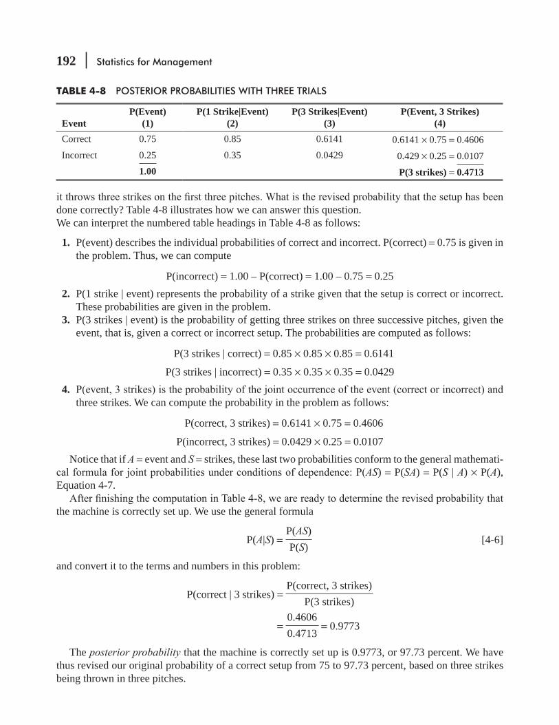
192 Statistics for Management
TABLE 4-8 POSTERIOR PROBABILITIES WITH THREE TRIALS
EventP(Event)
(1)P(1 Strike|Event)
(2)P(3 Strikes|Event)
(3)P(Event, 3 Strikes)
(4)Correct 0.75 0.85 0.6141 0.6141 × 0.75 = 0.4606Incorrect 0.25 0.35 0.0429 0.429 × 0.25 = 0.0107
1.00 P(3 strikes) = 0.4713
done correctly? Table 4-8 illustrates how we can answer this question.We can interpret the numbered table headings in Table 4-8 as follows:
1. P(event) describes the individual probabilities of correct and incorrect. P(correct) = 0.75 is given in the problem. Thus, we can compute
P(incorrect) = 1.00 – P(correct) = 1.00 – 0.75 = 0.25 2. P(1 strike | event) represents the probability of a strike given that the setup is correct or incorrect.
These probabilities are given in the problem. 3. P(3 strikes | event) is the probability of getting three strikes on three successive pitches, given the
event, that is, given a correct or incorrect setup. The probabilities are computed as follows:
P(3 strikes | correct) = 0.85 × 0.85 × 0.85 = 0.6141
P(3 strikes | incorrect) = 0.35 × 0.35 × 0.35 = 0.0429 4.
three strikes. We can compute the probability in the problem as follows:
P(correct, 3 strikes) = 0.6141 × 0.75 = 0.4606
P(incorrect, 3 strikes) = 0.0429 × 0.25 = 0.0107Notice that if A = event and S = strikes, these last two probabilities conform to the general mathemati-
AS) = P(SA) = P(S | A) × P(A), Equation 4-7.
the machine is correctly set up. We use the general formula
P(A|S) = P(AS)P(S)
[4-6]
and convert it to the terms and numbers in this problem:
P(correct | 3 strikes) = P(correct, 3 strikes)
P(3 strikes)
= 0.46060.4713
= 0.9773
The posterior probability that the machine is correctly set up is 0.9773, or 97.73 percent. We have thus revised our original probability of a correct setup from 75 to 97.73 percent, based on three strikes being thrown in three pitches.

Probability I: Introductory Ideas 193
Posterior Probabilities with Inconsistent OutcomesIn each of our problems so far, the behavior of the experiment was consistent: the die came up ace on two successive rolls, and the
most situations, we would expect a less consistent distribution of outcomes. In the case of the pitching
it was with a set of perfectly consistent outcomes. Using the notation S = strike and B = ball, we have solved this example in Table 4-9.
Posteriori Probabilities under Bayes Theorem has an application utility, they provided revised estimates of priori probabilities (chances) to the decision maker using the additional information presented. This helps in more effective decision-making. So estimates of the probability, based on historical information, are revised using additional information.
Bayes’ theorem is a formal procedure that lets decision makers combine classical probability theory with their best intuitive sense about what is likely to happen. Warning: The real value of Bayes’ theorem is not in the algebra, but rather in the ability of informed managers to make good
the process. Intuition used to make guesses about things that are already statistically well-described is misdirected.
HINTS & ASSUMPTIONS
EXERCISES 4.7
Self-Check ExercisesSC 4-11 Given: The probabilities of three events, A, B, and C, occurring are P(A) = 0.35, P(B) = 0.45, and
P(C) = 0.2. Assuming that A, B, or C has occurred, the probabilities of another event, X, occur-ring are P(X | A) = 0.8, P(X | B) = 0.65, and P(X | C) = 0.3. Find P(A | X), P(B | X), and P(C | X).
An example with inconsistent
outcomes
TABLE 4-9 POSTERIOR PROBABILITIES WITH INCONSISTENT OUTCOMES
Event P (Event) P (S|Event) P(SBSSS|Event) P(Event, SBSSS)Correct 0.75 0.85 0.85 × 0.15 × 0.85 × 0.85 × 0.85 = 0.07830 0.07830 × 0.75 = 0.05873Incorrect 0.25
1.000.35 0.35 × 0.65 × 0.35 × 0.35 × 0.35 = 0.00975 0.00975 × 0.25 = 0.00244
P(SBSSS) = 0.06117
P(correct setup|SBSSS) = P(correct setup, SBSSS)
P(SBSSS)
= 0.058730.06117
= 0.9601
194 Statistics for Management
SC 4-12 A doctor has decided to prescribe two new drugs to 200 heart patients as follows: 50 get drug A, 50 get drug B, and 100 get both. The 200 patients were chosen so that each had an 80 per-cent chance of having a heart attack if given neither drug. Drug A reduces the probability of a heart attack by 35 percent, drug B reduces the probability by 20 percent, and the two drugs, when taken together, work independently. If a randomly selected patient in the program has a heart attack, what is the probability that the patient was given both drugs?
Basic Concept4-41 -
comes: A, B, and C. The second has two possible, mutually exclusive outcomes: X and Y. We know P(A) = 0.2 and P(B) = 0.65. We also know the following conditional probabilities if the result of the second experiment is X: P(X | A) = 0.75, P(X | B) = 0.60, and P(X|C) = 0.40. Find P(A | X), P(B | X), and P(C | X). What is the probability that the result of the second experi-ment is Y?
Applications4-42 Amit Singh, a credit manager at the National Bank, knows that the company uses three meth-
ods to encourage collection of delinquent accounts. From past collection records, he learns that 70 percent of the accounts are called on personally, 20 percent are phoned, and 10 percent are sent a letter. The probabilities of collecting an overdue amount from an account with the three
due account. What is the probability that this account(a) Was called on personally?(b) Received a phone call?(c) Received a letter?
4-43 A public-interest group was planning to make a court challenge to auto insurance rates in one of three cities: New Delhi, Mumbai, or Chennai. The probability that it would choose New Delhi was 0.40; Mumbai, 0.35; and Chennai, 0.25. The group also knew that it had a 60 per-cent chance of a favorable ruling if it chose Mumbai, 45 percent if it chose New Delhi, and 35 percent if it chose Chennai. If the group did receive a favorable ruling, which city did it most likely choose?
4-44 EconOcon is planning its company picnic. The only thing that will cancel the picnic is a thunderstorm. The Weather Service has predicted dry conditions with probability 0.2, moist conditions with probability 0.45, and wet conditions with probability 0.35. If the probability of a thunderstorm given dry conditions is 0.3, given moist conditions is 0.6, and given wet conditions is 0.8, what is the probability of a thunderstorm? If we know the picnic was indeed canceled, what is the probability moist conditions were in effect?
4-45 An independent research group has been studying the chances that an accident at a nuclear power plant will result in radiation leakage. The group considers that the only possible types
a radiation leak would occur 20 percent of the time; if there were a mechanical failure, a

Probability I: Introductory Ideas 195
radiation leak would occur 50 percent of the time; and if there were a human error, a radiation leak would occur 10 percent of the time. Its studies have also shown that the probability of
A mechanical failure and a radiation leak occurring together is 0.0015. A human error and a radiation leak occurring together is 0.0012.
failure, and human error?(c) What is the probability of a radiation leak?
4-46 A physical therapist of a national football team knows that the team will play 40 percent of its -
grass?4-47 The physical therapist from Exercise 4-45 is also interested in studying the relationship
-marized in the following table:
Offensive Line
Defensive Line
Offensive Defensive
45 56 24 20
32 38 11 9
4-48 Namit Kapoor, marketing director for Alpha Motion Pictures, believes that the studio’s upcoming release has a 60 percent chance of being a hit, a 25 percent chance of being a
scale of 1 to 10, 10 being best. From his long experience in the industry, Namit Kapoor knows that 60 percent of the time, a hit picture will receive a rating of 7 or higher; 30 percent of the time, it will receive a rating of 4, 5, or 6; and 10 percent of the time, it will receive a rating of 3 or lower. For a moderately successful picture, the respective probabilities are 0.30, 0.45, and
a hit?
are independent of each other)?

196 Statistics for Management
Worked-Out Answers to Self-Check Exercises
SC 4-11 Event P(Event) P(X | Event) P(X and Event) P(Event | X)A 0.35 0.80 0.2800 0.2800/0.6325 = 0.4427B 0.45 0.65 0.2925 0.2925/0.6325 = 0.4625C 0.20 0.30 0.0600 0.0600/0.6325 = 0.0949
P(X) = 0.6325
Thus, P(A|X) = 0.4427, P(B|X) = 0.4625, and P(C|X) = 0.0949.SC 4-12 H = heart attack.
Event P(Event) P(H | Event) P(H and Event) P(Event | H)A 0.25 (0.8)(0.65) = 0.520 0.130 0.130/0.498 = 0.2610B 0.25 (0.8)(0.80) = 0.640 0.160 0.160/0.498 = 0.3213
A&B 0.50 (0.8)(0.65)(0.80) = 0.416 0.208 0.208/0.498 = 0.4177
P(X) = 0.498
Thus, P(A&B | H) = 0.4177.
STATISTICS AT WORK
Loveland ComputersCase 4: Probability “Aren’t you going to congratulate me, Uncle Walter?” Lee Azko asked the CEO of Loveland Computers as they waved goodbye to their new-found investment bankers who were
because you’re trying to guess what will happen in the future, not what did happen in the past. Get in the car and I’ll explain.
Now that still works for some of the low-end products, but the higher-end stuff needs to be customized, so we run an assembly line here. Now I won’t call it a factory, because there isn’t a single thing that we ‘make’ here. We buy the cases from one place, the hard drives from somewhere else, and so on. Then
“Not a bad question, but here’s the reason we can’t do that. In this game, price is very important. And if you load a machine with something that a customer is never going to use—for example, going to the expense of adding a very large hard drive to a machine that’s going to be used in a local area network,
schedule. This should give you some experience with real decision making.”Nancy Rainwater had worked for Loveland Computers for 5 years. Although Nancy was short on book
learning, growing up on a farm nearby, she had learned some important practical skills about managing

Probability I: Introductory Ideas 197
a workforce and getting work done on time. Her rise through the ranks to Production Supervisor had been rapid. Nancy explained her problem to Lee as follows.
“We have to decide whether to close the production line on Martin Luther King Day on the 20th of
Mr. Azko, won’t make it a paid vacation. But he might be open to closing the production line and letting people take the day off without pay if we can put in enough work days by the end of the month to meet our target production.”
typical day and divide that into the production target and see how many workdays you’ll need,” replied
“Well, I’ve already got that far. Not counting today, there are 19 workdays left until the end of the month, and I’ll need 17 days to complete the target production.”
“So let the workers take Martin Luther King Day off,” Lee concluded.
people call in sick—and believe me that happens when there’s a ‘bug’ going around—I have to close the line for the day. I have records going back for a couple of years since I’ve been supervisor, and on an average winter day, there’s a 1 in 30 chance that we’ll have to close the line because of too many sick calls.
“And there’s always a chance that we’ll get a bad snowstorm—maybe even two—between now and the end of the month. Two years ago, two of the staff were in a terrible car wreck, trying to come to work on a day when the weather was real bad. So the company lawyer has told us to have a very tight ‘snow day’ policy. If the roads are dangerous, we close the line and lose that day’s production. I’m not allowed to schedule weekend work to make up—that costs us time-and-a-half on wages and costs get out of line.
“I’d feel a lot better about closing the line for the holiday if I could be reasonably certain that we’d get in enough workdays by the end of the month. But I guess you don’t have a crystal ball.”
“Well, not a crystal ball, exactly. But I do have some ideas,” Lee said, walking back toward the
back toward Nancy Rainwater, “What’s your
Study Questions: What was Lee sketching on the notepad? What type of calculation will Lee make
“reasonably certain” means to meet the required production goal “75 percent of the time” or “99 percent of the time”?
CHAPTER REVIEW
Terms Introduced in Chapter 4A Priori Probability Probability estimate made prior to receiving new information.Bayes’ Theorem The formula for conditional probability under statistical dependence.Classical Probability The number of outcomes favorable to the occurrence of an event divided by the total number of possible outcomes.Collectively Exhaustive Events A list of events that represents all the possible outcomes of an experiment.

198 Statistics for Management
Conditional Probability The probability of one event occurring, given that another event has occurred.Event One or more of the possible outcomes of doing something, or one of the possible outcomes from conducting an experiment.Experiment The activity that results in, or produces, an event.Joint Probability The probability of two events occurring together or in succession.Marginal Probability The unconditional probability of one event occurring; the probability of a single event.Mutually Exclusive Events Events that cannot happen together.Posterior Probability A probability that has been revised after additional information was obtained.Probability The chance that something will happen.Probability Tree A graphical representation showing the possible outcomes of a series of experiments and their respective probabilities.Relative Frequency of Occurrence The proportion of times that an event occurs in the long run when conditions are stable, or the observed relative frequency of an event in a very large number of trials.Sample Space The set of all possible outcomes of an experiment.Statistical Dependence The condition when the probability of some event is dependent on, or affected by, the occurrence of some other event.Statistical Independence The condition when the occurrence of one event has no effect on the prob-ability of occurrence of another event.
Probabilities based on the personal beliefs of the person making the prob-ability estimate.Venn Diagram A pictorial representation of probability concepts in which the sample space is repre-sented as a rectangle and the events in the sample space as portions of that rectangle.
Equations Introduced in Chapter 4
4-1 Probability of an event = number of outcomes where the event occurs
total number of possible outcomes p. 158
classical probability that an event will occur.
P(A) = probability of event A happening p. 164
A single probability refers to the probability of one particular event occurring, and it is called marginal probability.
P(A or B) = probability of either A or B happening p. 167This notation represents the probability that one event or the other will occur.
4-2 P(A or B) = P(A) + P(B) – P(AB) p. 166
The addition rule for events that are not mutually exclusive shows that the probability of A or B happening when A and B are not mutually exclusive is equal to the probability of event A
Probability I: Introductory Ideas 199
happening plus the probability of event B happening minus the probability of A and B happen-ing together, symbolized P(AB).
4-3 P(A or B) = P(A) + P(B) p. 167
The probability of either A or B happening when A and B are mutually exclusive equals the sum of the probability of event A happening and the probability of event B happening. This is the addition ride for mutually exclusive events.
4-4 P(AB) = P(A) × P(B) p. 171 where
P(AB) = A and B occurring together or in succession P(A) = marginal probability of event A happening P(B) = marginal probability of event B happening
The joint probability of two or more independent events occurring together or in succession is the product of their marginal probabilities.
P(B | A) = probability of event B, given that event A has happened p. 175This notation shows conditional probability, the probability that a second event (B) will occur
( A ) has already happened.
4-5 P(B | A) = P(B) p. 176For statistically independent events, the conditional probability of event B, given that event A has occurred, is simply the probability of event B. Independent events are those whose prob-abilities are in no way affected by the occurrence of each other.
4-6 P(B|A) = P(BA)P(A)
and
P(A|B) = P(AB)P(B)
p. 181
For statistically dependent events, the conditional probability of event B, given that event A A and B divided by the marginal prob-
ability of event A.4-7 P(AB) = P(A|B) × P(B)
and P(BA) = P(B | A) × P(A) p. 182
Under conditions of statistical dependence, the joint probability of events A and B happening together or in succession is equal to the probability of event A, given that event B has already happened, multiplied by the probability that event B will happen.
Review and Application Exercises4-49 Life insurance premiums are higher for older people, but auto insurance premiums are gener-
ally higher for younger people. What does this suggest about the risks and probabilities associ-ated with these two areas of the insurance business?
200 Statistics for Management
4-50 “The chance of rain today is 80 percent.” Which of the following best explains this statement?(a) It will rain 80 percent of the day today.(b) It will rain in 80 percent of the area to which this forecast applies today.(c) In the past, weather conditions of this sort have produced rain in this area 80 percent of
the time.4-51 “There is a 0.25 probability that a restaurant in India will go out of business this year.” When
researchers make such statements, how have they arrived at their conclusions?4-52 Using probability theory, explain the success of gambling and poker establishments.4-53 Studies have shown that the chance of a new car being a “lemon” (one with multiple warranty
problems) is greater for cars manufactured on Mondays and Fridays. Most consumers don’t know on which day their car was manufactured. Assuming a 5-day production week, for a consumer taking a car at random from a dealer’s lot,(a) What is the chance of getting a car made on a Monday?(b) What is the chance of getting a car made on Monday or Friday?(c) What is the chance of getting a car made on Tuesday through Thursday?(d) What type of probability estimates are these?
4-54 T. S. Khan, an engineer for Super Jet Aircraft, disagrees with his supervisor about the likeli-hood of landing-gear failure on the company’s new airliner. Isaac contends that the probabil-ity of landing-gear failure is 0.12, while his supervisor maintains that the probability is only 0.03. The two agree that if the landing gear fails, the airplane will crash with probability 0.55.
crashes.
4-55 Which of the following pairs of events are mutually exclusive?
its work force by 50 percent.(b) A man is older than his uncle, and he is younger than his cousins.(c) A baseball team loses its last game of the year, and it wins the World Series.(d) A bank manager discovers that a teller has been embezzling, and she promotes the same
teller.4-56
additional patrol units in each of two neighborhoods. She knows that on any given day dur-
northern neighborhood were 0.478 and 0.602, respectively, and that the corresponding prob-
crimes occur independently of each other and likewise that crimes in the two neighborhoods are independent of each other.(a) What is the probability that no crime of either type is committed in the northern neighbor-
hood on a given day?(b) What is the probability that a crime of either type is committed in the southern neighbor-
hood on a given day?(c) What is the probability that no crime of either type is committed in either neighborhood
on a given day?
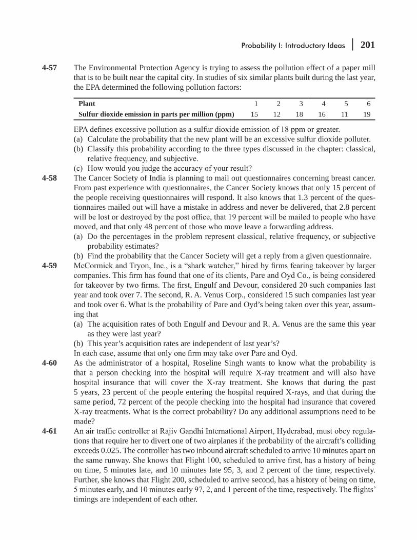
Probability I: Introductory Ideas 201
4-57 The Environmental Protection Agency is trying to assess the pollution effect of a paper mill that is to be built near the capital city. In studies of six similar plants built during the last year, the EPA determined the following pollution factors:
Plant 1 2 3 4 5 6Sulfur dioxide emission in parts per million (ppm) 15 12 18 16 11 19
(a) Calculate the probability that the new plant will be an excessive sulfur dioxide polluter.(b) Classify this probability according to the three types discussed in the chapter: classical,
4-58 The Cancer Society of India is planning to mail out questionnaires concerning breast cancer. From past experience with questionnaires, the Cancer Society knows that only 15 percent of the people receiving questionnaires will respond. It also knows that 1.3 percent of the ques-tionnaires mailed out will have a mistake in address and never be delivered, that 2.8 percent
moved, and that only 48 percent of those who move leave a forwarding address.
probability estimates?(b) Find the probability that the Cancer Society will get a reply from a given questionnaire.
4-59
year and took over 7. The second, R. A. Venus Corp., considered 15 such companies last year and took over 6. What is the probability of Pare and Oyd’s being taken over this year, assum-ing that(a) The acquisition rates of both Engulf and Devour and R. A. Venus are the same this year
as they were last year?(b) This year’s acquisition rates are independent of last year’s?
4-60 As the administrator of a hospital, Roseline Singh wants to know what the probability is that a person checking into the hospital will require X-ray treatment and will also have hospital insurance that will cover the X-ray treatment. She knows that during the past 5 years, 23 percent of the people entering the hospital required X-rays, and that during the same period, 72 percent of the people checking into the hospital had insurance that covered X-ray treatments. What is the correct probability? Do any additional assumptions need to be made?
4-61 -tions that require her to divert one of two airplanes if the probability of the aircraft’s colliding exceeds 0.025. The controller has two inbound aircraft scheduled to arrive 10 minutes apart on
on time, 5 minutes late, and 10 minutes late 95, 3, and 2 percent of the time, respectively. Further, she knows that Flight 200, scheduled to arrive second, has a history of being on time,
timings are independent of each other.

202 Statistics for Management
(a) Must the controller divert one of the planes, based on this information?
one of the airplanes?
one of the airplanes?4-62 In a staff meeting called to address the problem of returned checks at the supermarket where
to the customer. Overall, 10 percent of customers ask for cash back at the end of their transac-tion with the store. For 1,000 customer visits, how many transactions will involve:
(b) Cash back to the customer?
4-63 Which of the following pairs of events are statistically independent?(a) The times until failure of a calculator and of a second calculator marketed by a different
(b) The life-spans of the current U.S. and Russian presidents.(c) The amounts of settlements in asbestos poisoning cases in Dhanbad and Kishan Garh.(d) The takeover of a company and a rise in the price of its stock.(e) The frequency of organ donation in a community and the predominant religious orienta-
tion of that community.4-64 Raman Singh, supervisor of customer relations for GLF Airlines, is studying his company’s
International in New Delhi. In the last year, 7, 8, and 5 percent of the passengers on the
25 percent of the late-night GLF passengers at Indira Gandhi International take the London,
was scheduled to be on the
4-65 An electronics manufacturer is considering expansion of its plant in the next 4 years. The deci-sion depends on the increased production that will occur if either government or consumer
company also believes that both these events will not happen in the same year. The planning director has obtained the following estimates: The probability of consumer sales increasing by 50 percent within 1, 2, 3, and 4 years is
0.05, 0.08, 0.12, and 0.16, respectively.
0.08, 0.15, 0.25, and 0.32, respectively.What is the probability that the plant will expand(a) Within the next year (in year 1)?(b) Between 1 and 2 years from now (in year 2)?(c) Between 2 and 3 years from now (in year 3)?

Probability I: Introductory Ideas 203
(d) Between 3 and 4 years from now (in year 4)?(e) At all in the next 4 years (assume at most one expansion)?
4-66 Cartoonist R. Pran sends his comics to his publisher via Union Postal Delivery. UPD uses rail and truck transportation in Mr. Pran part of the country. In UPD’s 20 years of operation, only 2 percent of the packages carried by rail and only 3.5 percent of the packages carried by truck have been lost. Mr. Pran calls the claims manager to inform him that a package contain-ing a week of comics has been lost. If UPD sends 60 percent of the packages in that area by rail, which mode of transportation was more likely used to carry the lost comics? How does the solution change if UPD loses only 2 percent of its packages, regardless of the mode of transportation?
4-67 Determine the probability that(a) Both engines on a small airplane fail, given that each engine fails with probability 0.05
and that an engine is twice as likely to fail when it is the only engine working.(b) An automobile is recalled for brake failure and has steering problems, given that 15 per-
cent of that model were recalled for brake failure and 2 percent had steering problems.
4-68 are local. The chances of selling a home on each showing are 0.075 and 0.053 for out-of-town
“It’s a deal!” was the agent more likely to have conducted a showing for an out-of-town or local client?
4-69 A local Member of Parliament knows he will soon vote on a controversial bill. To learn his constituents’ attitudes about the bill, he met with groups in three cities in his state. An aide
Opinion CitySitapur Lucknow Kanpur
Strongly oppose 2 2 4Slightly oppose 2 4 3Neutral 3 3 5Slightly support 2 3 2Strongly support 6 3 1Total 15 15 15
(a) What is the probability that someone from Sitapur is neutral about the bill? Strongly opposed?
(b) What is the probability that someone in the three city groups strongly supports the bill?(c) What is the probability that someone from the Lucknow or Kanpur groups is neutral or
slightly opposed?4-70 Marcia Lerner will graduate in 3 months with a master’s degree in business administration.
result of any given on-campus interview is about 0.07 and is statistically independent from interview to interview.
interviews?

204 Statistics for Management
(b) If she has three interviews per month, what is the probability that she will have at least one
4-71 BMT, Inc., is trying to decide which of two oil pumps to use in its new race car engine. One pump produces 75 pounds of pressure and the other 100. BMT knows the following probabili-ties associated with the pumps:
Probability of Engine Failure Due toSeized Bearings Ruptured Head Gasket
Pump A 0.08 0.03Pump B 0.02 0.11
(a) If seized bearings and ruptured head gaskets are mutually exclusive, which pump should BMT use?
(b) If BMT devises a greatly improved “rupture-proof” head gasket, should it change its decision?
4-72 attacked in the popular press for distributing an allegedly unsafe vaccine. The vaccine protects against a virulent contagious disease that has a 0.04 probability of killing an infected person.
A researcher has told her the following: The probability of any unvaccinated individual acquiring the disease is 0.30. Once vaccinated, the probability of acquiring the disease through normal means is zero. However, 2 percent of vaccinated people will show symptoms of the disease, and 3 percent of that group will die from it. Of people who are vaccinated and show no symptoms from the vaccination, 0.05 percent will die. Irick must draw some conclusions from these data for a staff meeting in 1 hour and a news conference later in the day.(a) If a person is vaccinated, what is the probability of dying from the vaccine? If he was not
vaccinated, what is the probability of dying?(b) What is the probability of a randomly selected person dying from either the vaccine or the
normally contracted disease?4-73
paper closer to distribution time, thus giving the editorial staff more leeway for last-minute changes. She has the option of running the presses at “normal” speed or at 110 percent of normal—“fast” speed. She estimates that they will run at the higher speed 60 percent of the time. The roll of paper (the newsprint “web”) is twice as likely to tear at the higher speed, which would mean temporarily stopping the presses,(a) If the web on a randomly selected printing run has a probability of 0.112 of tearing, what
is the probability that the web will not tear at normal speed?(b) If the probability of tearing on fast speed is 0.20, what is the probability that a randomly
selected torn web occurred on normal speed?4-74 Refer to Exercise 4-73. The supervisor has noted that the web tore during each of the last four
runs and that the speed of the press was not changed during these four runs. If the probabilities of tearing at fast and slow speeds were 0.14 and 0.07, respectively, what is the revised prob-ability that the press was operating at fast speed during the last four runs?
Probability I: Introductory Ideas 205
4-75 A restaurant is experiencing discontentment among its customers. Historically it is known that there are three factors responsible for discontent amongst the customers viz. food quality, services quality, and interior décor. By conducting an analysis, it assesses the probabilities of discontentment with the three factors as 0.40, 0.35 and 0.25, respectively. By conducting a survey among customers, it also evaluates the probabilities of a customer going away discon-tented on account of these factors as 0.6, 0.8 and 0.5, respectively. The restaurant manager knows that a customer is discontented, what is the probability that it is due to service quality?
4-76 An economist believes that the chances of the Indian Rupee appreciating during period of high economic growth is 0.70, during moderate economic growth the chances of appreciation is 0.40, and during low economic growth it is 0.20. During any given time period the probability of high and moderate economic growth is 0.30 and 0.50 respectively. According to the RBI report the Rupee has been appreciating during the present period. What is the probability that the economy is experiencing a period of low economic growth?
Questions on Running Case: Academic Performance
In the MBA-I Trimester of a college, XML Management School, there are 50 students. Their academic performance
provide in Disk (Case_Academic Performance-Data.xls)
Answer the following questions:
1. If a student is randomly selected, what are the chances that she will be a male? 2. What is the probability that a randomly selected student has taken commerce stream in graduation? 3. What is the probability that a randomly selected student will be female and have taken professional stream in
graduation? 4. What is the probability that a randomly selected female student has taken science stream in graduation? 5. What is the probability that a randomly selected arts student will be male? 6. What is the probability that a randomly selected student have secured at least 75% marks both in XII and
graduation? 7. What is the probability that a randomly selected student has obtained less than 70% marks in XII provided
he/she has more than 80% marks in X? 8. What is the probability that a randomly selected female student have secured more than 80 percentile in CAT
if she has above 75% marks in graduation? 9. Are the events ‘being male’ and ‘having science stream in graduation’ independent?10. A randomly selected student is found to be female, what are the chances that she has her CAT percentile in
between 75 and 90?11. A randomly selected student has got less than 65% marks in graduation, which event has more probability
that the student would be a male or female?
@
CASE
@

206 Statistics for Management
Flow Chart: Probability I: Introductory Ideas
START
Areevents mutually
exclusive?
No
No
Yes
Areevents statistically
independent?
p.167
Addition rule:P (A or B) = P(A) + P(B)
p.170
The marginal probabilityof event A
occurring is P(A)
p.171
The joint probability oftwo events occurring
together or in successionis
P(AB) = P(A) x P(B)
p.176
The conditional probabilityof one event occurringgiven that another has
already occurred isP(B⏐A) = P(B)
This is knownas Bayes’Theorem
p.183
The marginal probabilityof event A occurring is the sum
of the probabilities of alljoint events in which
A occurs
p.182
The joint probability oftwo events occurring
together or in succession isP(BA) = P(B⏐A) x P(A)
p.189
Determine posteriorprobabilities withBayes Theorem
p.181
The conditional probabilityof one event occurring given
that another has alreadyoccurred is
p.166
Addition rule:P (A or B)
= P(A) + P(B) – P(AB)
STOP
P(BA)
P(A)P(B⏐A) =
LEARNING OBJECTIVES
5After reading this chapter, you can understand:
CHAPTER CONTENTS
To introduce the probability distributions most commonly used in decision making
To use the concept of expected value to make decisions
5.1 What is a Probability Distribution? 2085.2 Random Variables 2125.3 Use of Expected Value in Decision
Making 2185.4 The Binomial Distribution 2225.5 The Poisson Distribution 2305.6 The Normal Distribution: A Distribution of
a Continuous Random Variable 2385.7 Choosing the Correct Probability
Distribution 254
To show which probability distribution to use
To understand the limitations of each of the probability distributions you use
Statistics at Work 255 Terms Introduced in Chapter 5 256 Equations Introduced in Chapter 5 257 Review and Application Exercises 258 Flow Chart: Probability Distribution 264
Probability Distributions

208 Statistics for Management
Mtoothpaste pumps to within 0.1 ounce of the desired level 80 percent of the time. A visitor to the
we cannot make an exact forecast, the ideas about probability distributions discussed in this chapter enable us to give a pretty good answer to the question.
5.1 WHAT IS A PROBABILITY DISTRIBUTION?In Chapter 2, we described frequency distributions as a useful way of summarizing variations in observed data. We prepared frequency distributions by listing all the possible outcomes of an experi-ment and then indicating the observed frequency of each possible outcome. Probability distributions are related to frequency distributions. In fact, we can think of a probability distribution as a theoretical frequency distribu-tion. Now, what does that mean? A theoretical frequency distri-bution is a probability distribution that describes how outcomes are expected to vary. Because these distributions deal with expec-tations, they are useful models in making inferences and decisions under conditions of uncertainty. Probability distribution is related to random experiments just like frequency distribution to determinis-tic experiments. Frequency distribution expresses distribution of frequencies over different values of the concerned variables while probability distribution expresses distribution of probability values over dif-ferent values of concerned random variable. Frequency distribution is related to certainty in outcome while probability distribution to uncertainty. In later chapters, we will discuss the methods we use under these conditions.
Examples of Probability Distributions
the idea of a fair coin, which we introduced in Chapter 4. Suppose we toss a fair coin twice. Table 5-1 illustrates the possible out-comes from this two-toss experiment.
Now suppose that we are interested in formulating a probability distribution of the number of tails that could possibly result when we toss the coin twice. We would begin by noting any outcome that did not contain a tail. With a fair coin, that is only the third outcome in Table 5-1: H, H. Then we would note
Probability distributions and
frequency distribution
Experiment using a fair coin
TABLE 5-1 POSSIBLE OUTCOMES FROM TWO TOSSES OF A FAIR COIN
First Toss
Second Toss
Number of Tails on Two Tosses
Probability of the Four Possible Outcomes
T T 2 0.5 × 0.5 = 0.25T H 1 0.5 × 0.5 = 0.25H H 0 0.5 × 0.5 = 0.25H T 1 0.5 × 0.5 = 0.25
1.00
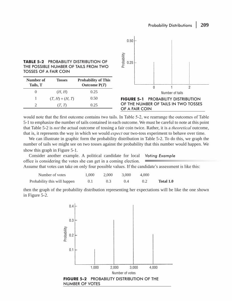
Probability Distributions 209
5-1 to emphasize the number of tails contained in each outcome. We must be careful to note at this point that Table 5-2 is not the actual outcome of tossing a fair coin twice. Rather, it is a theoretical outcome, that is, it represents the way in which we would expect our two-toss experiment to behave over time.
We can illustrate in graphic form the probability distribution in Table 5-2. To do this, we graph the number of tails we might see on two tosses against the probability that this number would happen. We show this graph in Figure 5-1.
Consider another example. A political candidate for local
Number of votes 1,000 2,000 3,000 4,000Probability this will happen 0.1 0.3 0.4 0.2 Total 1.0
then the graph of the probability distribution representing her expectations will be like the one shown in Figure 5-2.
Voting Example
TABLE 5-2 PROBABILITY DISTRIBUTION OF THE POSSIBLE NUMBER OF TAILS FROM TWO TOSSES OF A FAIR COIN
Number of Tails, T
Tosses Probability of This Outcome P(T)
0 (H, H) 0.251 (T, H) + (H, T) 0.50
2 (T, T) 0.25FIGURE 5-1 PROBABILITY DISTRIBUTION OF THE NUMBER OF TAILS IN TWO TOSSES OF A FAIR COIN
0.50
0.25
Prob
abili
ty
Number of tails0 1 2
FIGURE 5-2 PROBABILITY DISTRIBUTION OF THE NUMBER OF VOTES
0.4
0.3
0.2
0.1
Prob
abili
ty
Number of votes1,000 2,000 3,000 4,000

210 Statistics for Management
Before we move on to other aspects of probability distribu-tions, we should point out that a frequency distribution is a listing of the observed frequencies of all the outcomes of an experiment that actually occurred when the experiment was done, whereas a probability distribution is a listing of the probabilities of all the possible outcomes that could result if the experiment were done. Also, as we can see in the two examples we presented in Figures 5-1 and 5-2, probability distributions can be based on theoretical considerations (the tosses of a coin) or on a subjective assessment of the likelihood
Insurance company actuaries determine insurance premiums, for example, by using long years of experi-ence with death rates to establish probabilities of dying among various age groups.
Conditions for Probability Distribution[X, p(X)] is said to constitute a probability distribution if:
1. X is a random variable 2. p(x) > = 0 3. Σp(x) = 1.
Types of Probability Distributions discrete or con-
tinuous. In a discrete probability distribution, the variable under consideration is restricted to take only a limited number of values, which can be listed. An example of
about the coming election. There, votes could take on only four possible values (1,000, 2,000, 3,000, or 4,000). Similarly, the probability that you were born in a given month is also discrete because there are only 12 possible values (the 12 months of the year).
In a continuous probability distribution, on the other hand, the variable under consideration is allowed to take on any value within a given range, so we cannot list all the possible values.
expect quite a continuous range of parts per million (ppm), all the way from very low levels in clear mountain streams to extremely high levels in polluted streams. In fact, it would be quite normal for the
this variable (ppm) a continuous distribution. Continuous distributions are convenient ways to represent discrete distributions that have many possible outcomes, all very close to each other.
EXERCISES 5.1
Basic Concepts5-1 Based on the following graph of a probability distribution, construct the corresponding
table.
Discrete probability distributions
Continuous probability
distributions
Difference between frequency
distributions and probability
distributions

Probability Distributions 211
1 2 3 4 5 6 7 8 9 10
0.6
0.5
0.4
0.3
0.2
0.1
5-2 In the last chapter, we looked at the possible outcomes of tossing two dice, and we calculated some probabilities associated with various outcomes. Construct a table and a graph of the probability distribution representing the outcomes (in terms of total numbers of dots showing on both dice) for this experiment.
5-3 Which of the following statements regarding probability distributions are correct?(a) A probability distribution provides information about the long-run or expected frequency
of each outcome of an experiment.(b) The graph of a probability distribution has the possible outcomes of an experiment marked
on the horizontal axis.(c) A probability distribution lists the probabilities that each outcome is random.(d) A probability distribution is always constructed from a set of observed frequencies like a
frequency distribution.(e) A probability distribution may be based on subjective estimates of the likelihood of
certain outcomes.
Applications5-4 Southport Autos offers a variety of luxury options on its cars. Because of the 6- to 8-week
waiting period for customer orders, Padmanabha Pillai, the dealer, stocks his cars with a
needs immediately, is worried because of an industrywide shortage of cars with V-8 engines. Padmanabha offers the following luxury combinations:
1. V-8 engine electric sun roof halogen headlights 2. Leather interior power door locks stereo cassette deck 3. Halogen headlights V-8 engine leather interior 4. Stereo cassette deck V-8 engine power door locks He thinks that combinations 2, 3, and 4 have an equal chance of being ordered, but that com-
bination 1 is twice as likely to be ordered as any of these.(a) What is the probability that any one customer ordering a luxury car will order one with a
V-8 engine?(b) Assume that two customers order luxury cars. Construct a table showing the probability
distribution of the number of V-8 engines ordered.

212 Statistics for Management
5-5
-tion is going to buy only enough Auto King cars to replace half of its 500 cars. Finally, there
Construct a table and draw a graph of the probability distribution of sales of Auto Kings to the Secretariat administration.
5.2 RANDOM VARIABLESA variable is random if it takes on different values as a result of the outcomes of a random experiment. A random variable can be either discrete or continuous. If a random variable is allowed to take on only a limited number of values, which can be listed, it is a discrete random variable. On the other hand, if it is allowed to assume any value within a given range, it is a continuous random variable.
You can think of a random variable as a value or magnitude that changes from occurrence to occurrence in no predictable sequence. A breast cancer screening clinic, for example, has no way of knowing exactly how many women will be screened on
are the numerical values corresponding to each possible outcome of the random experiment. If past daily records of the clinic indicate that the values of the random variable range from 100 to 115 patients daily, the random variable is a discrete random variable.
Table 5-3 illustrates the number of times each level has been reached during the last 100 days. Note that the table gives a frequency distribution. To the extent that we believe that the experience of the past 100 days has been typical, we can use
distribution. We have accomplished this in Table 5-4 by normalizing the observed frequency distribution (in this case, dividing each value in the right-hand column of Table 5-3 by 100, the total number of
random variable provides a probability for each possible value and that these probabilities must sum to 1. Table 5-4 shows that both these requirements have been met. Furthermore, both Table 5-4 and Figure 5-3 give us information about the long-run frequency of occurrence of daily patient screenings
The Expected Value of a Random VariableSuppose you toss a coin 10 times and get 7 heads, like this:
Heads Tails Total7 3 10
5 tails. So now you have, in all, 22 heads and 8 tails out of 30 tosses.
Random variable defined
Example of discrete random
variables
Creating a probability
distribution

Probability Distributions 213
TABLE 5-3 NUMBER OF WOMEN SCREENED DAILY DURING 100 DAYS
Number Screened
Number of Days This Level Was Observed
100 1101 2102 3103 5104 6105 7106 9107 10108 12109 11110 9111 8112 6113 5114 4115 2
100
TABLE 5-4 PROBABILITY DISTRIBUTION FOR NUMBER OF WOMEN SCREENED
Number Screened (Value of the Random Variable)
Probability That the Random Variable Will Take on This Value
100 0.01101 0.02102 0.03103 0.05104 0.06105 0.07106 0.09107 0.10108 0.12109 0.11110 0.09111 0.08112 0.06113 0.05114 0.04115 0.02
1.00
FIGURE 5-3 PROBABILITY DISTRIBUTION FOR THE DISCRETE RANDOM VARIABLE “DAILY NUMBER SCREENED”
0.120.110.100.090.080.070.060.050.040.030.020.01
Prob
abili
ty
Daily number of women screened100 101 102 103 104 105 106 107 108 109 110 111 112 113 114 115
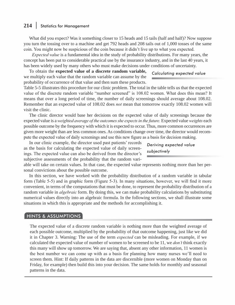
214 Statistics for Management
What did you expect? Was it something closer to 15 heads and 15 tails (half and half)? Now suppose you turn the tossing over to a machine and get 792 heads and 208 tails out of 1,000 tosses of the same
Expected value is a fundamental idea in the study of probability distributions. For many years, the concept has been put to considerable practical use by the insurance industry, and in the last 40 years, it has been widely used by many others who must make decisions under conditions of uncertainty.
To obtain the expected value of a discrete random variable, we multiply each value that the random variable can assume by the probability of occurrence of that value and then sum these products. Table 5-5 illustrates this procedure for our clinic problem. The total in the table tells us that the expected
means that over a long period of time, the number of daily screenings should average about 108.02. Remember that an expected value of 108.02 does not mean that tomorrow exactly 108.02 women will visit the clinic.
The clinic director would base her decisions on the expected value of daily screenings because the expected value is a weighted average of the outcomes she expects in the future. Expected value weights each possible outcome by the frequency with which it is expected to occur. Thus, more common occurrences are given more weight than are less common ones. As conditions change over time, the director would recom-
as the basis for calculating the expected value of daily screen-
subjective assessments of the probability that the random vari-able will take on certain values. In that case, the expected value represents nothing more than her per-sonal convictions about the possible outcome.
In this section, we have worked with the probability distribution of a random variable in tabular
convenient, in terms of the computations that must be done, to represent the probability distribution of a random variable in algebraic form. By doing this, we can make probability calculations by substituting numerical values directly into an algebraic formula. In the following sections, we shall illustrate some situations in which this is appropriate and the methods for accomplishing it.
The expected value of a discrete random variable is nothing more than the weighted average of each possible outcome, multiplied by the probability of that outcome happening, just like we did it in Chapter 3. Warning: The use of the term expected can be misleading. For example, if we calculated the expected value of number of women to be screened to be 11, we don’t think exactly this many will show up tomorrow. We are saying that, absent any other information, 11 women is
screen them. Hint: If daily patterns in the data are discernible (more women on Monday than on Friday, for example) then build this into your decision. The same holds for monthly and seasonal patterns in the data.
HINTS & ASSUMPTIONS
Calculating expected value
Deriving expected value
subjectively
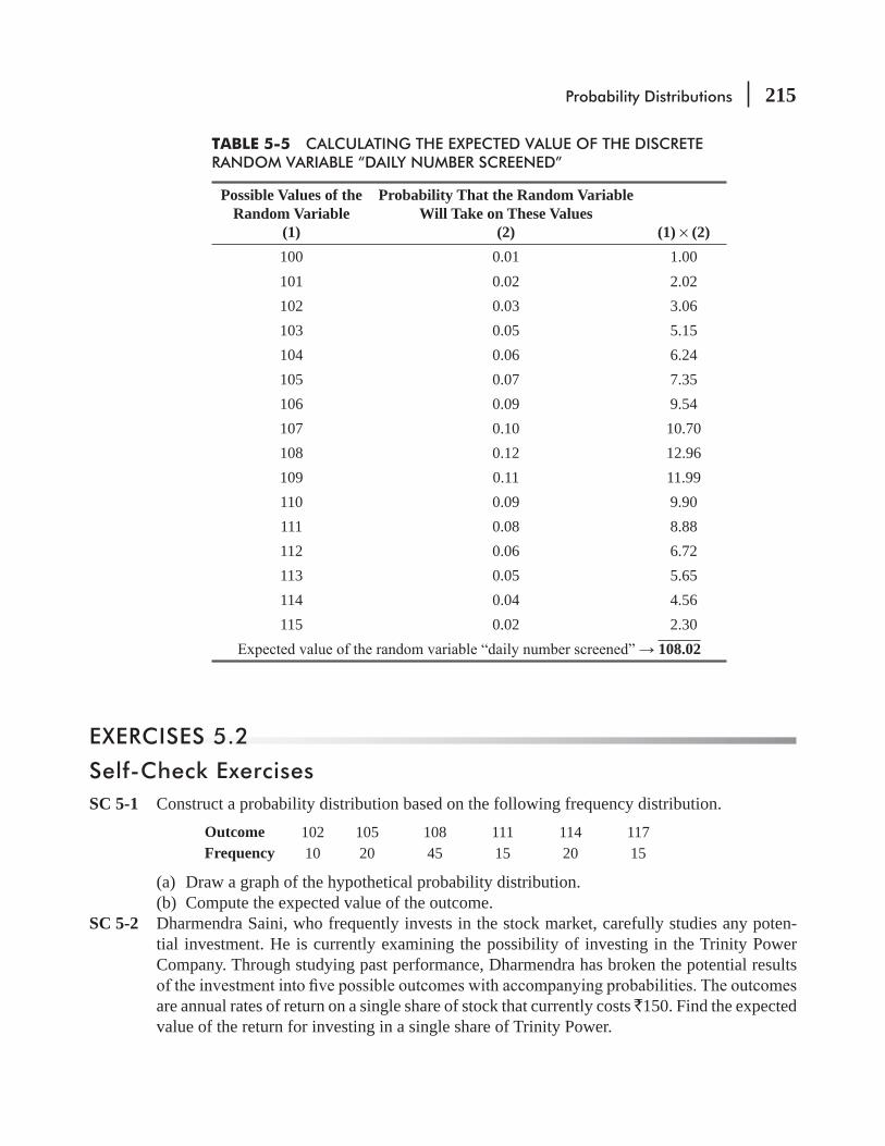
Probability Distributions 215
TABLE 5-5 CALCULATING THE EXPECTED VALUE OF THE DISCRETE RANDOM VARIABLE “DAILY NUMBER SCREENED”
Possible Values of the Random Variable
(1)
Probability That the Random Variable Will Take on These Values
(2) (1) × (2)100 0.01 1.00101 0.02 2.02102 0.03 3.06103 0.05 5.15104 0.06 6.24105 0.07 7.35106 0.09 9.54107 0.10 10.70108 0.12 12.96109 0.11 11.99110 0.09 9.90111 0.08 8.88112 0.06 6.72113 0.05 5.65114 0.04 4.56115 0.02 2.30
108.02
EXERCISES 5.2
Self-Check ExercisesSC 5-1 Construct a probability distribution based on the following frequency distribution.
Outcome 102 105 108 111 114 117Frequency 10 20 45 15 20 15
(a) Draw a graph of the hypothetical probability distribution.(b) Compute the expected value of the outcome.
SC 5-2 Dharmendra Saini, who frequently invests in the stock market, carefully studies any poten-tial investment. He is currently examining the possibility of investing in the Trinity Power Company. Through studying past performance, Dharmendra has broken the potential results
are annual rates of return on a single share of stock that currently costs 150. Find the expected value of the return for investing in a single share of Trinity Power.
216 Statistics for Management
Return on investment (`) 0.00 10.00 15.00 25.00 50.00Probability 0.20 0.25 0.30 0.15 0.10
If Dharmendra purchases stock whenever the expected rate of return exceeds 10 percent, will he purchase the stock, according to these data?
Basic Concepts5-6 Construct a probability distribution based on the following frequency distribution:
Outcome 2 4 6 8 10 12 15Frequency 24 22 16 12 7 3 1
(a) Draw a graph of the hypothetical probability distribution.(b) Compute the expected value of the outcome.
5-7 From the following graph of a probability distribution(a) Construct a table of the probability distribution.(b) Find the expected value of the random variable.
8,000 9,000 10,000 11,000 12,000 13,000
0.4
0.3
0.2
0.1
Applications5-8
After talking to friends and reading reports, Bill believes the following maintenance expenses
Expense 0 50 100 150 200 250 300Probability 0.35 0.25 0.15 0.10 0.08 0.05 0.02
warranty?
5-9 -
ous intersection of State Highway SH-4 and State Highway SH-7. Toward this end, Raj has collected data on accidents at the intersection:
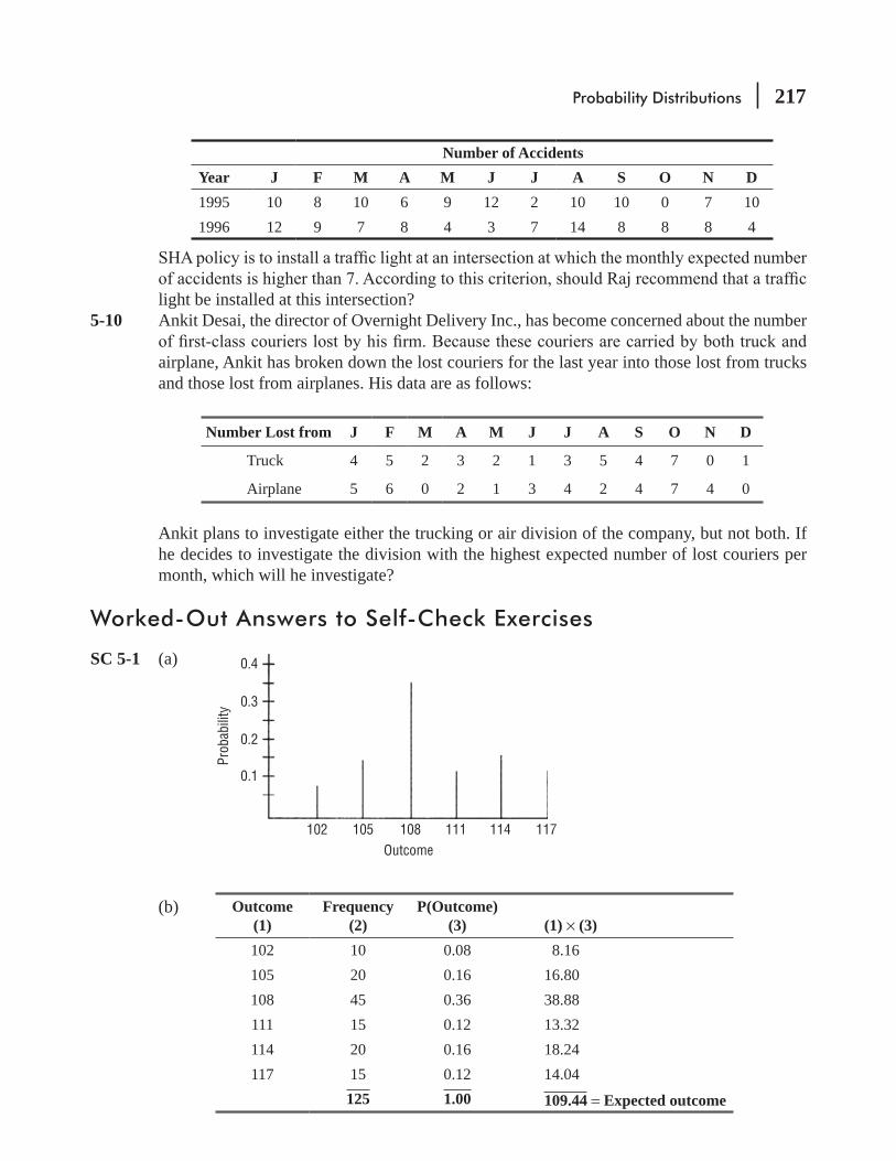
Probability Distributions 217
Number of AccidentsYear J F M A M J J A S O N D1995 10 8 10 6 9 12 2 10 10 0 7 101996 12 9 7 8 4 3 7 14 8 8 8 4
light be installed at this intersection?5-10 Ankit Desai, the director of Overnight Delivery Inc., has become concerned about the number
airplane, Ankit has broken down the lost couriers for the last year into those lost from trucks and those lost from airplanes. His data are as follows:
Number Lost from J F M A M J J A S O N D
Truck 4 5 2 3 2 1 3 5 4 7 0 1
Airplane 5 6 0 2 1 3 4 2 4 7 4 0
Ankit plans to investigate either the trucking or air division of the company, but not both. If he decides to investigate the division with the highest expected number of lost couriers per month, which will he investigate?
Worked-Out Answers to Self-Check Exercises
SC 5-1 (a)
102 105 108 111 114 117Outcome
Prob
abili
ty
0.4
0.3
0.2
0.1
(b) Outcome (1)
Frequency (2)
P(Outcome) (3)
(1) × (3)
102 10 0.08 8.16105 20 0.16 16.80108 45 0.36 38.88111 15 0.12 13.32114 20 0.16 18.24117 15 0.12 14.04
125 1.00 109.44 = Expected outcome

218 Statistics for Management
SC 5-2 Return (1)
P(Return) (2)
(1) × (2)
0 0.20 0.0010 0.25 2.5015 0.30 4.5025 0.15 3.7550 0.10 5.00
1.00 15.75 = Expected return
Dharmendra will purchase the stock because the expected return of `15.75 is greater than 10 percent of the `150 purchase price.
5.3 USE OF EXPECTED VALUE IN DECISION MAKINGIn the preceding section, we calculated the expected value of a random variable and noted that it can
makers combine the probabilities that a random variable will take on certain values with the monetary gain or loss that results when it does take on those values. Doing just this enables them to make intel-ligent decisions under uncertain conditions.
Combining Probabilities and Monetary ValuesLet us look at the case of a fruit and vegetable wholesaler who sells strawberries. This product has a very limited useful life. If not sold
but her analysis of past records has produced the information in Table 5-6.
Types of Losses DefinedTwo types of losses are incurred by the wholesaler: (1) obsoles-cence losses, caused by stocking too much fruit on any one day
opportunity losses, caused by being out of strawberries any time that custom-ers call for them. (Customers will not wait beyond the day a case is requested.)
Wholesaler problem
Obsolescence and opportunity
losses
TABLE 5-6 SALES DURING 100 DAYS
Daily Sales Number of Days Sold Probability of Each Number Being Sold10 15 0.1511 20 0.2012 40 0.4013 25 0.25
100 1.00
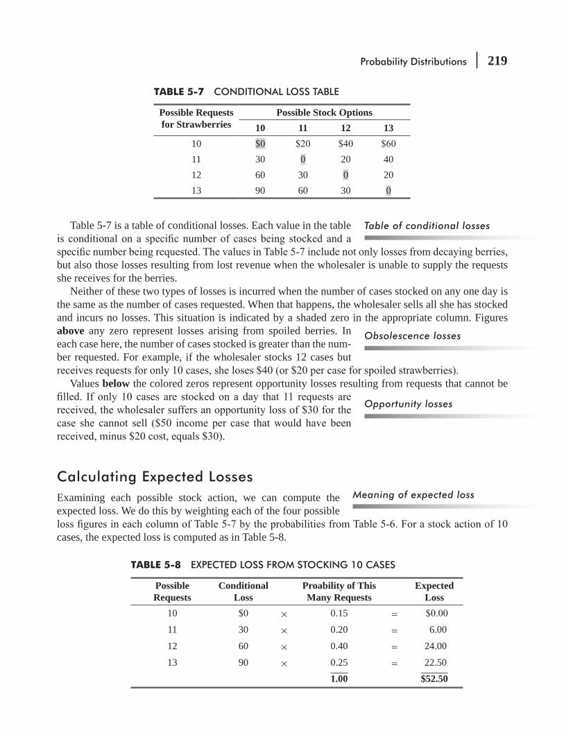
Probability Distributions 219
Table of conditional lossesTable 5-7 is a table of conditional losses. Each value in the table
but also those losses resulting from lost revenue when the wholesaler is unable to supply the requests she receives for the berries.
Neither of these two types of losses is incurred when the number of cases stocked on any one day is the same as the number of cases requested. When that happens, the wholesaler sells all she has stocked and incurs no losses. This situation is indicated by a shaded zero in the appropriate column. Figures above any zero represent losses arising from spoiled berries. In each case here, the number of cases stocked is greater than the num-ber requested. For example, if the wholesaler stocks 12 cases but
Values below the colored zeros represent opportunity losses resulting from requests that cannot be
.
Calculating Expected LossesExamining each possible stock action, we can compute the expected loss. We do this by weighting each of the four possible
cases, the expected loss is computed as in Table 5-8.
Obsolescence losses
Opportunity losses
Meaning of expected loss
TABLE 5-7 CONDITIONAL LOSS TABLE
Possible Requests for Strawberries
Possible Stock Options10 11 12 13
1011 30 0 20 4012 60 30 0 2013 90 60 30 0
TABLE 5-8 EXPECTED LOSS FROM STOCKING 10 CASES
Possible Requests
Conditional Loss
Proability of This Many Requests
Expected Loss
10 × 0.15 =11 30 × 0.20 = 6.00
12 60 × 0.40 = 24.00
13 90 × 0.25 = 22.50
1.00 $52.50

220 Statistics for Management
The conditional losses in Table 5-8 are taken from the second column of Table 5-7 for a stock action of 10 cases. The fourth column total in Table 5-8 shows us that if 10 cases are stocked each day, over a
tomorrow’s
Tables 5-9 through 5-11 show the computations of the expected loss resulting from decisions to stock 11, 12, and 13 cases, respectively. The optimal stock action is the one that will minimize expected losses. This action calls for the stocking of 12 cases each day, at which point the expected
approach, that is, maximizing expected gainminimizing expected loss. The answer, 12 cases, would have been the same.
In our brief treatment of expected value, we have made quite a few assumptions. To name only two,
nothing one day later. Both these assumptions reduce the value of the answer we got. In Chapter 17, you
Optimal solution
TABLE 5-9 EXPECTED LOSS FROM STOCKING 11 CASES
Possible Requests
Conditional Loss
Probability of This Many Requests
Expected Loss
10 × 0.15 =11 0 × 0.20 = 0.00
12 30 × 0.40 = 12.00
13 60 × 0.25 = 15.00
1.00 $30.00
TABLE 5-10 EXPECTED LOSS FROM STOCKING 12 CASES
Possible Requests
Conditional Loss
Probability of This Many Requests
Expected Loss
10 × 0.15 =11 20 × 0.20 = 4.0012 0 × 0.40 = 0.0013 30 × 0.25 = 7.50
1.00 $17.50
TABLE 5.11 EXPECTED LOSS FROM STOCKING 13 CASES
Possible Requests
Conditional Loss
Probability of This Many Requests
Expected Loss
10 × 0.15 =11 40 × 0.20 = 8.0012 20 × 0.40 = 8.0013 0 × 0.25 = 0.00
1.00 $25.00
Probability Distributions 221
will again encounter expected-value decision making, but there we will develop the ideas as a part of statistical decision theory (a broader use of statistical methods to make decisions), and we shall devote an entire chapter to expanding the basic ideas we have developed at this point.
This is unrealistic in the real world and we did it here only to make the explanation easier. Any manager facing this problem in her job would know that demand might be as low as zero on a given day (weather, holidays) and as high as perhaps 50 cases on another day. Hint: With demand ranging
HINTS & ASSUMPTIONS
EXERCISES 5.3
Self-Check ExerciseSC 5-3
-zas per night. These pizzas take so long to prepare, however, that Mario prepares all of them in advance and stores them in the refrigerator. Because the ingredients go bad within one day, Mario always throws out any unsold pizzas at the end of each evening. The cost of preparing
-
stock each night in order to minimize expected loss if the number of pizzas ordered has the following probability distribution?
Number of pizzas demanded 1 2 3 4Probability 0.40 0.30 0.20 0.10
Applications5-11 The management of National Sports Stadium is trying to decide how many tickets to print for
an upcoming hockey match. Each ticket costs ` 5 to print and sells for ` 25. Any ticket unsold at the end of the game must be discarded. Based on the past records of such hockey matches occurring on this ground, the management of the National Sports Stadium has estimated the following probability distribution for the ticket sales:
Tickets sold 25,000 40,000 55,000 70,000Probability 0.10 0.30 0.45 0.15
So, based on the above information related to four categories of ticket-sales, what suggestions would you give to the management with respect to the number of tickets to be printed for the next match?
5-12 Airport Rent-a-Car (ARC) is a locally operated business in competition with several major
one day and will return it to the airport. For ` 35, the company will rent a small economy car
222 Statistics for Management
-ning to buy number of small cars from the manufacturer at a reduced price of ` 6,300. The big question is how many to buy. Company executives have decided the following distribution of demands per day for the service:
Number of cars rented 13 14 15 16 17 18Probability 0.08 0.15 0.22 0.25 0.21 0.09
The company intends to offer the plan 6 days a week (312 days per year) and anticipates that its variable cost per car per day will be `2.50. After the end of one year, the company expects to sell the cars and recapture 50 percent of the original cost. Disregarding the time value of money and any noncash expenses, use the expected-loss method to determine the optimal number of cars for ARC to buy.
Worked-Out Answer to Self-Check ExerciseSC 5-3 Loss Table
Pizzas Demanded 1 2 3 4
Probability 0.4 0.3 0.2 0.1Pizzas Stocked Expected Loss
1 0 10 20 30 10.0
2 7 0 10 203 14 7 0 10 8.74 21 14 7 0 14.0
5.4 THE BINOMIAL DISTRIBUTIONOne widely used probability distribution of a discrete random variable is the binomial distribution. It describes a variety of processes of interest to managers. The binomial distribu-tion describes discrete, not continuous, data, resulting from an experiment known as a Bernoulli process, after the seventeenth-century Swiss mathematician Jacob
of such tosses can be represented by the binomial probability distribution. The success or failure of interviewees on an aptitude test may also be described by a Bernoulli process. On the other hand, the
scale of hours and would not qualify as a binomial distribution.
Use of the Bernoulli Process
coin as an example of a Bernoulli process. We can describe this process as follows:
The binomial distribution and
Bernoulli processes
Bernoulli process described

Probability Distributions 223
1. Each trial (each toss, in this case) has only two possible outcomes: heads or tails, yes or no, success or failure.
2. The probability of the outcome of any trial (toss) remains xed over time. With a fair coin, the probability of heads remains 0.5 each toss regardless of the number of times the coin is tossed.
3. The trials are statistically independentof any other toss.
Each Bernoulli process has its own characteristic probability. Take the situation in which historically seven-tenths of all peo-ple who applied for a certain type of job passed the job test. We would say that the characteristic probability here is 0.7, but we could describe our testing results as Bernoulli only if we felt certain that the proportion of those passing the test (0.7) remained constant over time. The other characteristics of the Bernoulli process would also have to be met, of course. Each test would have only two outcomes (success or failure), and the results of each test would have to be statistically independent.
In more formal language, the symbol p represents the probability of a success (in our example, 0.7), and the symbol q (q = 1 – p), the probability of a failure (0.3). To represent a certain number of successes, we will use the symbol r, and to symbolize the total number of trials, we use the symbol n.is begun.
Using this language in a simple problem, we can calculate the chances of getting exactly two heads (in any order) on three tosses of a fair coin. Symbolically, we express the values as follows:
p = characteristic probability or probability of success = 0.5 q = 1 – p = probability of failure = 0.5 r = number of successes desired = 2 n = number of trials undertaken = 3
We can solve the problem by using the binomial formula:
Binomial Formula
Probability of r successes in n trials = n
r n rp q
!
!( )r n r
−− [5-1]
Although this formula may look somewhat complicated, it can be used quite easily. The symbol ! means factorial, which is computed as follows: 3! means 3 × 2 × 1, or 6. To calculate 5!, we multiply 5 × 4 × 3 × 2 × 1 = -lem, we discover
Probability of 2 successes in 3 trials = 3!
2!(3 2)!(0.5) (0.5)2 1
−
=3 2 1
(2 1)(1 1)(0.5) (0.5)2× ×
× ×
=6
2(0.25)(0.5) = 0.375
Thus, there is a 0.375 probability of getting two heads on three tosses of a fair coin.
Characteristic probability
defined
Binomial Formula
224 Statistics for Management
-abilities for the toothpaste pump problem we introduced at the beginning of this chapter. Recall that his-
p = 0.8q = 0.2r = 3n = 6
and then use the binomial formula as follows:
Probability of r successes in n trials = n
r n rp q
!
! !r n r
( )−− [5-1]
= 6 5 4 3 2 1
(3 2 1)(3 2 1)(0.8) (0.2)3 3× × × × ×
× × × ×
= 720
6 6(0.512)(0.008)
× = (20)(0.512)(0.008) = 0.08192
Of course, we could have solved these two problems using the probability trees we developed in Chapter 4, but for larger prob-lems, trees become quite cumbersome. In fact, using the binomial formula (Equation 5-1) is no easy task when we have to compute the value of something like 19 factorial. For this reason, binomial probability tables have been developed, and we shall use them shortly.
Using the Binomial TablesEarlier we recognized that it is tedious to calculate probabilities using the binomial formula when n is a large number. Fortunately, we can use Appendix Table 3 to determine binomial probabilities quickly.
To illustrate the use of the binomial tables, consider this problem. What is the probability that 8 of the 15 registered Democrats on Prince Street will fail to vote in the coming primary if the probability of any
First, we represent the elements in this problem in binomial distribution notation:
n = 15 number of registered Democratsp = r = 8 number of individuals who will fail to vote
table corresponding to n = 15. Because the probability of an indi-
r = 8 row, where we read the answer 0.0348. This is the probability of eight registered voters not voting.
Binomial tables are available
Solving problems using the
binomial tables
How to use the binomial tables

Probability Distributions 225
-ing? We would have looked under the 0.30 column and added up the probabilities there from 8 to the bottom of the column like this:
8 0.0348 9 0.011610 0.003011 0.000612 0.000113 0.0000
0.0501
The answer is that there is a 0.0501 probability of eight or more registered voters not voting. fewer than eight non-voters. Again,
we would have begun with the 0.30 column, but this time we would add the probabilities from 0 (the top of the n = 15 column) down to 7 (the highest value less than 8), like this:
0 0.0047
1 0.0305
2 0.0916
3 0.1700
4 0.2186
5 0.2061
6 0.1472
7 0.0811
0.9498
The answer is that there is a 0.9498 probability of fewer than eight nonvoters.Because r (the number of nonvoters) is either 8 or more, or else fewer than 8, it must be true that
P(r ≥ 8) + P(r < 8) = 1
But according to the values we just calculated,
P(r ≥ 8) + P(r < 8) = 0.0501 + 0.9498 = 0.9999
The slight difference between 1 and 0.9999 is due to rounding errors resulting from the fact that the binomial table gives the probabilities to only 4 decimal places of accuracy.
to 0.50. How do you solve problems with probabilities larger than 0.5? Simply go back through the binomial tables and look this time at the probability values at the bottoms 0.50 through 0.99.

226 Statistics for Management
Measures of Central Tendency and Dispersion for the Binomial DistributionEarlier in this chapter, we encountered the concept of the expected value or mean of a probability distribution. The binomial distribution has an expected value or mean (μ) and a standard deviation (σ), and we should be able to compute both these statistical measures. Intuitively, we can reason that if a certain machine produces good parts with a p = 0.5, then, over time, the mean of the distribution of the number of good parts in the out-put would be 0.5 times the total output. If there is a 0.5 chance of tossing a head with a fair coin, over a large number of tosses, the mean of the binomial distribution of the number of heads would be 0.5 times the total number of tosses.
Symbolically, we can represent the mean of a binomial distribution as
Mean of a Binomial Distribution
μ = np [5-2]
where
n = number of trials p = probability of success
And we can calculate the standard deviation of a binomial distribution by using the formula
Standard Deviation of a Binomial Distribution
σ = npq [5-3]
where n = number of trials p = probability of success q = probability of failure = 1 – p
To see how to use Equations 5-2 and 5-3, take the case of a packaging machine that produces 20 percent defective packages. If we take a random sample of 10 packages, we can compute the mean and the standard deviation of the binomial distribution of that process like this:
μ = np [5-2] = (10)(0.2) = 2 ← Mean
σ = npq [5-3]
= (10)(0.2)(0.8)
1.6= = 1.265 ← Standard deviation
Computing the mean and the
standard deviation
The mean
The standard deviation
Probability Distributions 227
The important thing to note that standard deviation of the binomial distribution must always be less than that of its mean.
Meeting the Conditions for Using the Bernoulli ProcessWe need to be careful in the use of the binomial probability to make certain that the three conditions necessary for a Bernoulli process introduced earlier are met, particularly conditions 2 and 3. Condition 2 requires the probability of the outcome of any trial
-
beyond a reasonable point, the proportion of acceptable parts produced by the machine will be altered and condition 2 for the use of the binomial distribution may be violated. This problem is not present in a coin-toss experiment, but it is an integral consideration in all real applications of the binomial prob-ability distribution.
Condition 3 requires that the trials of a Bernoulli process be statistically independent, that is, the out-come of one trial cannot affect in any way the outcome of any other trial. Here, too, we can encounter some problems in real applications. Consider an interviewing process in which high-potential candi-
-dates in a row, he may not view the sixth with complete impartiality. The trials, therefore, might not be statistically independent.
Warning: One of the requirements for using a Bernoulli process is that the probability of the
automatic machine making parts will experience some wear as the number of parts increases and this will affect the probability of producing acceptable parts. Still another condition for its use is that the trials (manufacture of parts in our machine example) be independent. This too is a condition that is hard to meet. If our machine produces a long series of bad parts, this could affect the position (or sharpness) of the metal-cutting tool in the machine. Here, as in every other
experience and intuition to know when a Bernoulli process is appropriate.
HINTS & ASSUMPTIONS
EXERCISES 5.4
Self-Check ExercisesSC 5-4 For a binomial distribution with n = 12 and p =
(a) P(r = 8).(b) P(r > 4).(c) P(r ≤ 10).
Problems in applying the
binomial distribution to real-life
situations

228 Statistics for Management
SC 5-5 Find the mean and standard deviation of the following binomial distributions:(a) n = 16, p = 0.40.(b) n = 10, p = 0.75.(c) n = 22, p = 0.15.(d) n = 350, p = 0.90.(e) n = 78, p = 0.05.
SC 5-6 The latest nationwide political poll indicates that for Indians who are randomly selected, the probability that they are with alliance ABC is 0.55, the probability that they are with alliance PQR is 0.30, and the probability that they are with alliance XYZ is 0.15. Assuming that these probabilities are accurate, answer the following questions pertaining to a randomly chosen group of 10 Indians. (a) What is the probability that four are with alliance PQR?(b) What is the probability that none are with alliance ABC?(c) What is the probability that two are with alliance XYZ?(d) What is the probability that at least eight are with alliance PQR?
Basic Concepts5-13 For a binomial distribution with n = 7 and p =
(a) P(r = 5).(b) P(r > 2).(c) P(r < 8).(d) P(r ≥ 4).
5-14 For a binomial distribution with n = 15 and p =(a) P(r = 6).(b) P(r ≥ 11).(c) P(r ≤ 4).
5-15 Find the mean and standard deviation of the following binomial distributions:(a) n = 15, p = 0.20.(b) n = 8, p = 0.42.(c) n = 72, p = 0.06.(d) n = 29, p = 0.49.(e) n = 642, p = 0.21.
5-16 For n = 8 trials, compute the probability that r ≥ 1 for each of the following values of p:(a) p = 0.1.(b) p = 0.3.(c) p = 0.6.(d) p = 0.4.
Applications5-17 Harley Davidson, director of quality control for the Kyoto Motor company, is conducting
his monthly spot check of automatic transmissions. In this procedure, 10 transmissions are removed from the pool of components and are checked for manufacturing defects. Historically,
Probability Distributions 229
in different transmissions.)
(b) What is the probability that none of the selected transmissions has any manufacturing
5-18 Diane Bruns is the mayor of a large city. Lately, she has become concerned about the pos-sibility that large numbers of people who are drawing unemployment checks are secretly
category, but Ms. Bruns is not convinced. She asks one of her aides to conduct a quiet inves-
individuals investigated have jobs? -
tigated individuals have jobs? 5-19 A recent study of how IT professionals spend their leisure time surveyed workers employed
more than 5 years. They determined the probability an employee has 2 weeks of vaca-tion time to be 0.45, 1 week of vacation time to be 0.10, and 3 or more weeks to be 0.20. Suppose 20 workers are selected at random. Answer the following questions without Appendix Table 3.(a) What is the probability that 8 have 2 weeks of vacation time?(b) What is the probability that only one worker has 1 week of vacation time?(c) What is the probability that at most 2 of the workers have 3 or more weeks of vacation
time?(d) What is the probability that at least 2 workers have 1 week of vacation time?
5-20 Nagendra Kumar is in charge of the electronics section of a large department store. He has noticed that the probability that a customer who is just browsing will buy something is 0.3. Suppose that 15 customers browse in the electronics section each hour. Use Appendix Table 3 in the back of the book to answer the following questions:(a) What is the probability that at least one browsing customer will buy something during a
(b) What is the probability that at least four browsing customers will buy something during a
hour?(d) What is the probability that no more than four browsing customers will buy something
Worked-Out Answers to Self-Check ExercisesSC 5-4 Binomial (n = 12, p = 0.45).
(a) P(r = 8) = 0.0762(b) P(r > 4) = 1 – P(r ≤ 4) = 1 – (0.0008 + 0.0075 + 0.0339 + 0.0923 + 0.1700) = 0.6955(c) P(r ≤ 10) = 1 – P(r ≥ 11) = 1 – (0.0010 + 0.0001) = 0.9989
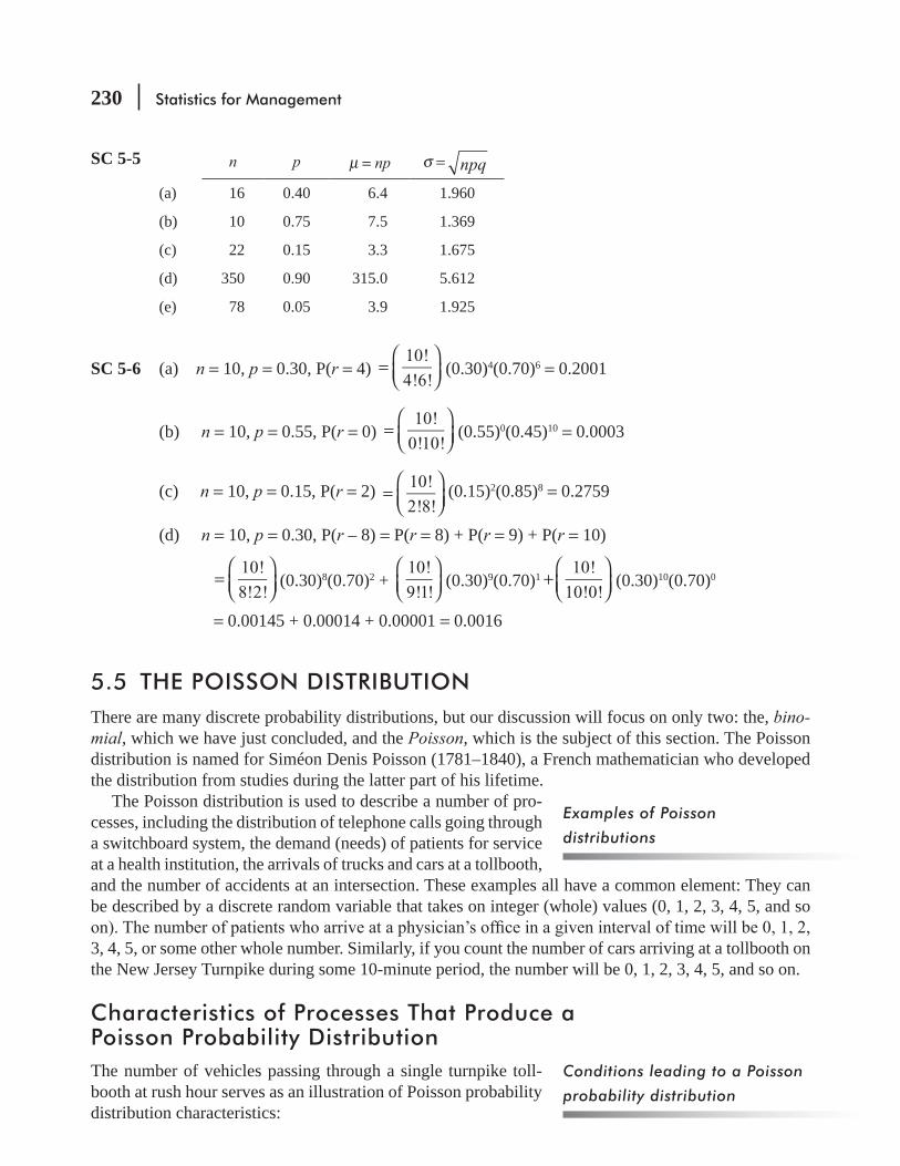
230 Statistics for Management
SC 5-5
n p μ = np σ = npq
(a) 16 0.40 6.4 1.960
(b) 10 0.75 7.5 1.369
(c) 22 0.15 3.3 1.675
(d) 350 0.90 315.0 5.612
(e) 78 0.05 3.9 1.925
SC 5-6 (a) n = 10, p = 0.30, P(r = 4) 10!
4!6!=
⎛⎝⎜
⎞⎠⎟
(0.30)4(0.70)6 = 0.2001
(b) n = 10, p = 0.55, P(r = 0) 10!
0!10!=
⎛⎝⎜
⎞⎠⎟
(0.55)0(0.45)10 = 0.0003
(c) n = 10, p = 0.15, P(r = 2) 10!
2!8!=
⎛⎝⎜
⎞⎠⎟
(0.15)2(0.85)8 = 0.2759
(d) n = 10, p = 0.30, P(r – 8) = P(r = 8) + P(r = 9) + P(r = 10)
10!
8!2!=
⎛⎝⎜
⎞⎠⎟
(0.30)8(0.70)2 + 10!
9!1!
⎛⎝⎜
⎞⎠⎟
(0.30)9(0.70)110!
10!0!+
⎛⎝⎜
⎞⎠⎟
(0.30)10(0.70)0
= 0.00145 + 0.00014 + 0.00001 = 0.0016
5.5 THE POISSON DISTRIBUTIONThere are many discrete probability distributions, but our discussion will focus on only two: the, bino-mial, which we have just concluded, and the Poisson, which is the subject of this section. The Poisson distribution is named for Siméon Denis Poisson (1781–1840), a French mathematician who developed the distribution from studies during the latter part of his lifetime.
The Poisson distribution is used to describe a number of pro-cesses, including the distribution of telephone calls going through a switchboard system, the demand (needs) of patients for service at a health institution, the arrivals of trucks and cars at a tollbooth, and the number of accidents at an intersection. These examples all have a common element: They can be described by a discrete random variable that takes on integer (whole) values (0, 1, 2, 3, 4, 5, and so
3, 4, 5, or some other whole number. Similarly, if you count the number of cars arriving at a tollbooth on the New Jersey Turnpike during some 10-minute period, the number will be 0, 1, 2, 3, 4, 5, and so on.
Characteristics of Processes That Produce a Poisson Probability DistributionThe number of vehicles passing through a single turnpike toll-booth at rush hour serves as an illustration of Poisson probability distribution characteristics:
Examples of Poisson
distributions
Conditions leading to a Poisson
probability distribution
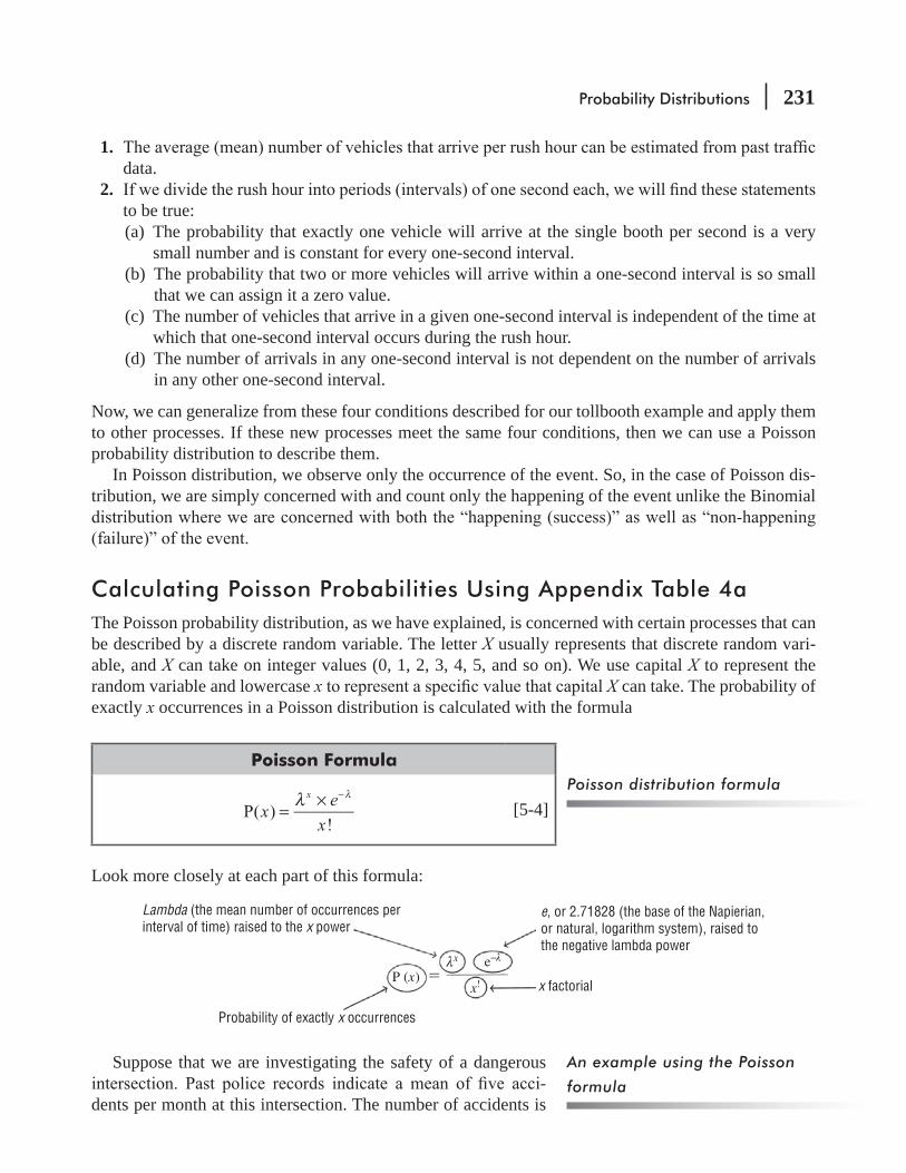
Probability Distributions 231
1. data.
2. to be true:(a) The probability that exactly one vehicle will arrive at the single booth per second is a very
small number and is constant for every one-second interval.(b) The probability that two or more vehicles will arrive within a one-second interval is so small
that we can assign it a zero value. (c) The number of vehicles that arrive in a given one-second interval is independent of the time at
which that one-second interval occurs during the rush hour.(d) The number of arrivals in any one-second interval is not dependent on the number of arrivals
in any other one-second interval.
Now, we can generalize from these four conditions described for our tollbooth example and apply them to other processes. If these new processes meet the same four conditions, then we can use a Poisson probability distribution to describe them.
In Poisson distribution, we observe only the occurrence of the event. So, in the case of Poisson dis-tribution, we are simply concerned with and count only the happening of the event unlike the Binomial
Calculating Poisson Probabilities Using Appendix Table 4aThe Poisson probability distribution, as we have explained, is concerned with certain processes that can be described by a discrete random variable. The letter X usually represents that discrete random vari-able, and X can take on integer values (0, 1, 2, 3, 4, 5, and so on). We use capital X to represent the random variable and lowercase x X can take. The probability of exactly x occurrences in a Poisson distribution is calculated with the formula
Poisson Formula
xe
xP( )
!
xλ=
× λ−
[5-4]
Look more closely at each part of this formula:
Lambda (the mean number of occurrences perinterval of time) raised to the x power
Probability of exactly x occurrences
e, or 2.71828 (the base of the Napierian,or natural, logarithm system), raised tothe negative lambda power
x factorialP (x)
e−λ
x!
λx
Suppose that we are investigating the safety of a dangerous -
dents per month at this intersection. The number of accidents is
Poisson distribution formula
An example using the Poisson
formula
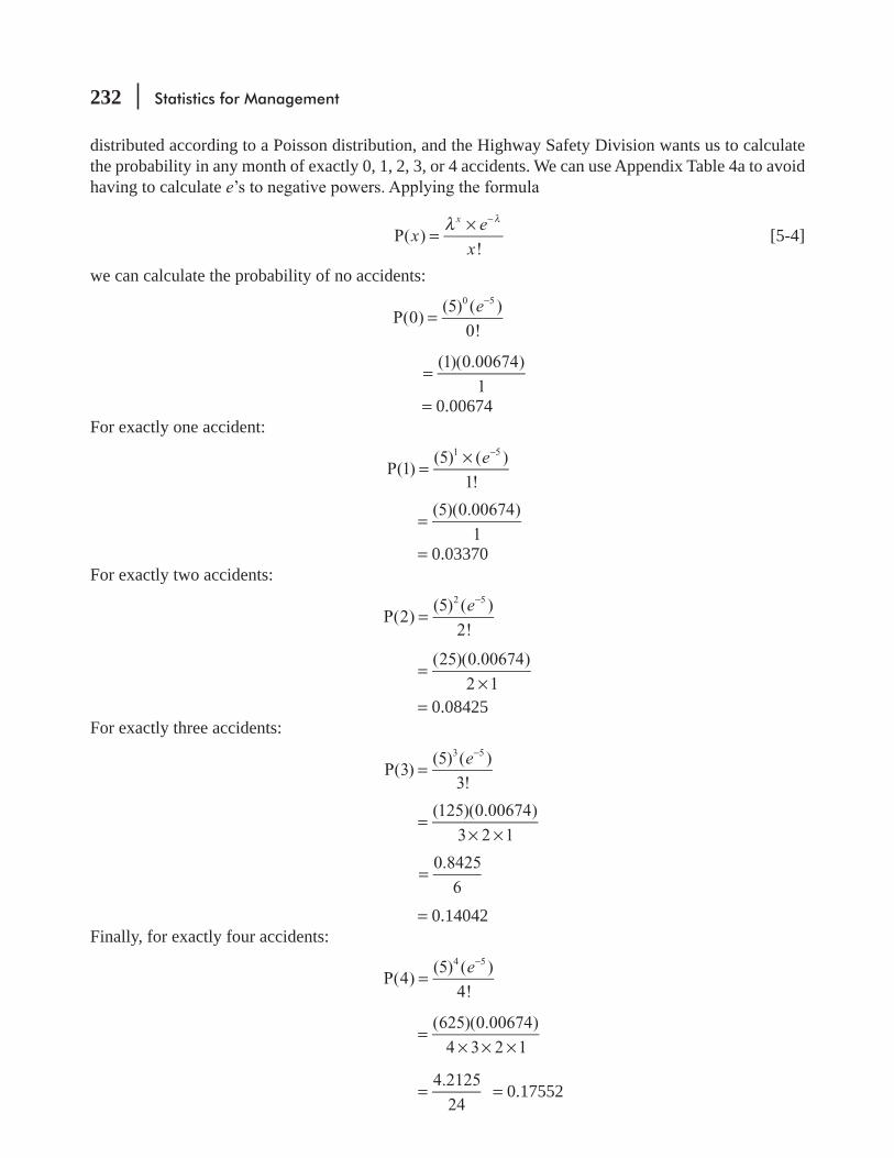
232 Statistics for Management
distributed according to a Poisson distribution, and the Highway Safety Division wants us to calculate the probability in any month of exactly 0, 1, 2, 3, or 4 accidents. We can use Appendix Table 4a to avoid having to calculate e
xe
xP( )
!
xλ=
× λ−
[5-4]
we can calculate the probability of no accidents:
eP(0)
(5) ( )
0!
0 5
=−
(1)(0.00674)
1=
= 0.00674For exactly one accident:
eP(1)
(5) ( )
1!
1 5
=× −
(5)(0.00674)
1=
= 0.03370For exactly two accidents:
eP(2)
(5) ( )
2!
2 5
=−
(25)(0.00674)
2 1=
× = 0.08425
For exactly three accidents:
eP(3)
(5) ( )
3!
3 5
=−
(125)(0.00674)
3 2 1=
× ×
0.8425
6=
= 0.14042Finally, for exactly four accidents:
eP(4)
(5) ( )
4!
4 5
=−
(625)(0.00674)
4 3 2 1=
× × ×
4.2125
24=
= 0.17552
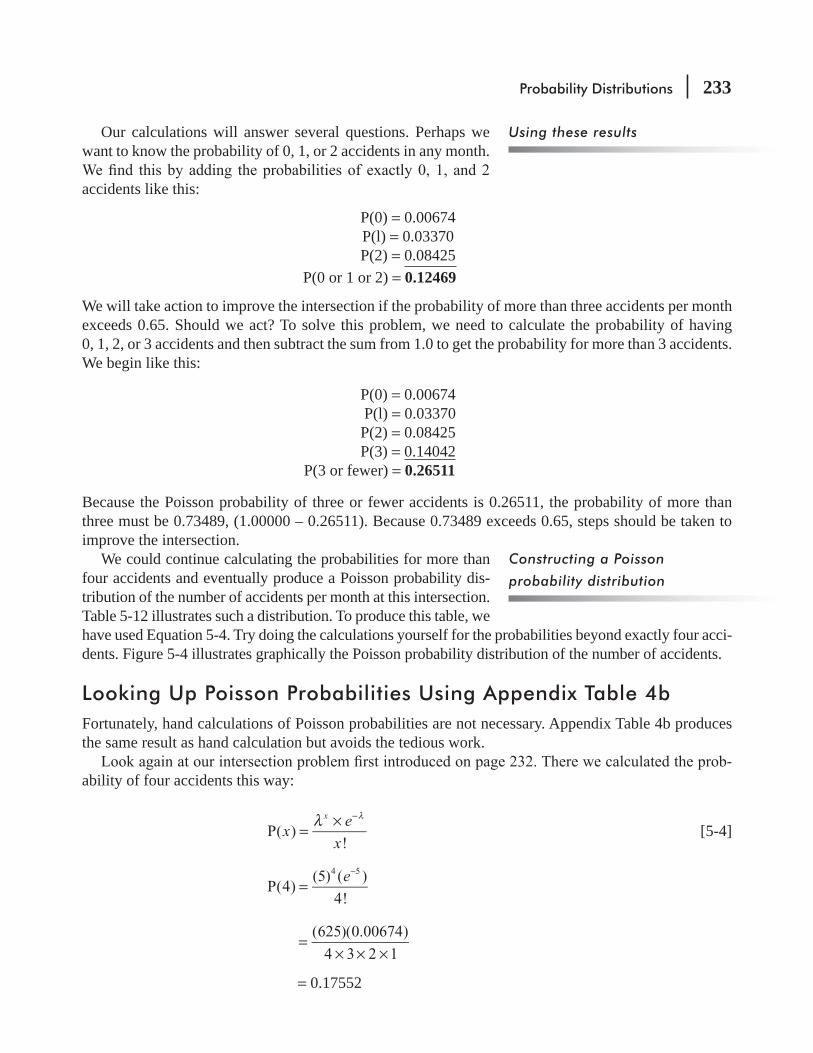
Probability Distributions 233
Using these resultsOur calculations will answer several questions. Perhaps we want to know the probability of 0, 1, or 2 accidents in any month.
accidents like this:
P(0) = 0.00674P(l) = 0.03370P(2) = 0.08425
P(0 or 1 or 2) = 0.12469
We will take action to improve the intersection if the probability of more than three accidents per month exceeds 0.65. Should we act? To solve this problem, we need to calculate the probability of having 0, 1, 2, or 3 accidents and then subtract the sum from 1.0 to get the probability for more than 3 accidents. We begin like this:
P(0) = 0.00674 P(l) = 0.03370P(2) = 0.08425P(3) = 0.14042
P(3 or fewer) = 0.26511
Because the Poisson probability of three or fewer accidents is 0.26511, the probability of more than three must be 0.73489, (1.00000 – 0.26511). Because 0.73489 exceeds 0.65, steps should be taken to improve the intersection.
We could continue calculating the probabilities for more than four accidents and eventually produce a Poisson probability dis-tribution of the number of accidents per month at this intersection. Table 5-12 illustrates such a distribution. To produce this table, we have used Equation 5-4. Try doing the calculations yourself for the probabilities beyond exactly four acci-dents. Figure 5-4 illustrates graphically the Poisson probability distribution of the number of accidents.
Looking Up Poisson Probabilities Using Appendix Table 4bFortunately, hand calculations of Poisson probabilities are not necessary. Appendix Table 4b produces the same result as hand calculation but avoids the tedious work.
-ability of four accidents this way:
xe
xP( )
!
xλ=
× λ−
[5-4]
eP(4)
(5) ( )
4!
4 5
=−
(625)(0.00674)
4 3 2 1=
× × ×
= 0.17552
Constructing a Poisson
probability distribution

234 Statistics for Management
TABLE 5-12 POISSON PROBABILITY DISTRIBUTION OF ACCIDENTS PER MONTH
x = Number of Accidents
P(x) = Probability of Exactly That Number
0 0.006741 0.033702 0.084253 0.140424 0.175525 0.175526 0.146277 0.104488 0.065309 0.03628
10 0.0181411 0.00824
0.9948612 or more
1.00000
FIGURE 5-4 POISSON PROBABILITY DISTRIBUTION OF THE NUMBER OF ACCIDENTS
0.18
0.16
0.14
0.12
0.10
0.08
0.06
0.04
0.02
Prob
abili
ty
Number of accidents0 1 2 3 4 5 6 7 8 9 10 11 ≥12
To use Appendix Table 4b all we need to know are the values for x and , in this instance 4 and 5, respectively. Now look in Appendix
233, we calculated the Poisson probability of 0, 1, or 2 accidents as being 0.12469. Finding this same result using Appendix
Using Appendix Table 4b to look
up Poisson probabilities

Probability Distributions 235
Table 4b requires that we again look for the column headed 5, then come down that column, and add up
0.0067 (Probability of 0 accidents)0.0337 (Probability of 1 accident)0.0842 (Probability of 2 accidents)0.1246 (Probability of 0, 1, or 2 accidents)
Once again, the slight differences in the two answers are due to rounding errors.
Poisson Distribution as an Approximation of the Binomial DistributionSometimes, if we wish to avoid the tedious job of calculating binomial probability distributions, we can use the Poisson instead. The Poisson distribution can be a reasonable approxima-tion of the binomial, but only under certain conditions. These conditions occur when n is large and p is small, that is, when the number of trials is large and the binomial probability of success is small. The rule most often used by statisticians is that the Poisson is a good approximation of the binomial when n is greater than or equal to 20 and p is less than or equal to 0.05. In cases that meet these conditions, we can substitute the mean of the binomial distribution (np) in place of the mean of the Poisson distribution ( ) so that the formula becomes
Poisson Probability Distribution as an Approximation of the Binomial
xnp e
xP( )
( )
!
x np
=× −
[5-5]
Let us use both the binomial probability formula (5-1) and the Poisson approximation formula (5-5) on the same problem to determine the extent to which the Poisson is a good approxima-tion of the binomial. Say that we have a hospital with 20 kidney dialysis machines and that the chance of any one of them malfunctioning during any day is 0.02. What is the probability that exactly three machines will be out of service on the same day? Table 5-13 shows the answers to this question. As we can see, the difference between the two probability distributions is slight (only about a 10 percent error, in this example).
Poisson distribution should be used when the occurrence of the event is rare so that we are con-cerned with only the happening (success) of the event and count that only. Further, the Poisson distribution is a good approximation of the binomial distribution, but we qualify our assumption by requiring n to be greater than or equal to 20 and p to be less than or equal to 0.05.
HINTS & ASSUMPTIONS
Using a modification of the
Poisson formula to approximate
binomial probabilities
Comparing the Poisson and
binomial formulas
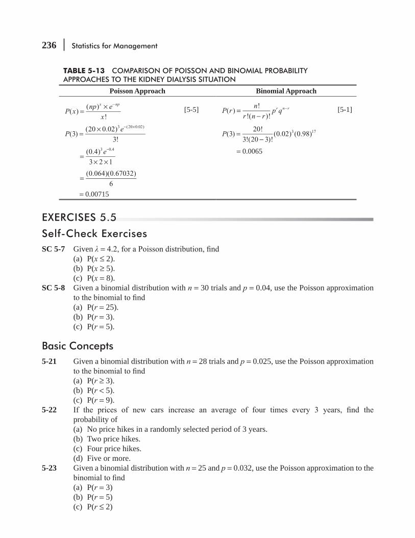
236 Statistics for Management
EXERCISES 5.5
Self-Check ExercisesSC 5-7 Given =
(a) P(x ≤ 2).(b) P(x ≥ 5).(c) P(x = 8).
SC 5-8 Given a binomial distribution with n = 30 trials and p = 0.04, use the Poisson approximation
(a) P(r = 25).(b) P(r = 3).(c) P(r = 5).
Basic Concepts5-21 Given a binomial distribution with n = 28 trials and p = 0.025, use the Poisson approximation
(a) P(r ≥ 3).(b) P(r < 5).(c) P(r = 9).
5-22 probability of(a) No price hikes in a randomly selected period of 3 years.(b) Two price hikes.(c) Four price hikes.(d) Five or more.
5-23 Given a binomial distribution with n = 25 and p = 0.032, use the Poisson approximation to the
(a) P(r = 3)(b) P(r = 5)(c) P(r ≤ 2)
TABLE 5-13 COMPARISON OF POISSON AND BINOMIAL PROBABILITY APPROACHES TO THE KIDNEY DIALYSIS SITUATION
Poisson Approach Binomial Approach
P xnp e
x( )
( )
!
x np
=× −
[5-5]
Pe
(3)(20 0.02)
3!
3 (20 0.02)
=× − ×
e(0.4)
3 2 1
3 0.4
=× ×
−
(0.064)(0.67032)
6=
= 0.00715
P rn
r n rp q( )
!
!( )!r n r=
−−
[5-1]
P(3)20!
3!(20 3)!(0.02) (0.98)3 17=
−
= 0.0065

Probability Distributions 237
5-24 Given =(a) P(x ≤ 3)(b) P(x ≥ 2)(c) P(x = 6)(d) P(1 ≤ x ≤ 4)
Applications5-25 Concert pianist Donna Prima has become quite upset at the number of coughs occurring in
the audience just before she begins to play. On her latest tour, Donna estimates that on aver-age eight coughs occur just before the start of her performance. Ms. Prima has sworn to her
play. What is the probability that she will play tonight?5-26 In Lucknow Railway Station, recently there was a complaint about the accidents on its eleva-
tors and the resulting injuries, especially among the elderly people. According to the past
allocated unless the chances of more than three accidents on elevators in any week exceed 75 percent. Will the funds be allocated?
5-27 Southwestern Electronics has developed a new calculator that performs a series of func-tions not yet performed by any other calculator. The marketing department is planning to demonstrate this calculator to a group of potential customers, but it is worried about some initial problems, which have resulted in 4 percent of the new calculators developing math-ematical inconsistencies. The marketing VP is planning on randomly selecting a group of calculators for this demonstration and is worried about the chances of selecting a calculator that could start malfunctioning. He believes that whether or not a calculator malfunctions is a Bernoulli process, and he is convinced that the probability of a malfunction is really about 0.04.(a) Assuming that the VP selects exactly 50 calculators to use in the demonstration, and using
the Poisson distribution as an approximation of the binomial, what is the chance of getting at least three calculators that malfunction?
(b) No calculators malfunctioning?5-28 The District Family Court handles various kinds of disputes, but most are marital disputes. In
fact, 96 percent of the disputes handled by the Family Court are of a marital nature.(a) What is the probability that, out of 80 disputes handled by the Family Court, exactly seven
are nonmarital?(b) None are nonmarital?
5-29
238 Statistics for Management
Worked-Out Answers to Self-Check ExercisesSC 5-7 = 4.2, e–4.2 = 0.0150.
(a) P(x ≤ 2) = P(x = 0) + P(x = 1) + P(x = 2)
e e e(4.2)
0!
(4.2)
1!
(4.2)
2!
0 4.2 1 4.2 2 4.2
= + +− − −
= 0.0150 + 0.0630 + 0.1323 = 0.2103(b) P(x ≥ 5) = 1 – P(x ≤ 4) = 1 – P(x = 4) – P(x = 3) – P(x ≤ 2)
e e1
(4.2)
4!
(4.2)
3!0.2103
4 4.2 3 4.2
= − − −− −
= 1 – 0.1944 – 0.1852 – 0.2103 = 0.4101
(c) xe
P( 8)(4.2)
8!0.0360
8 4.2
= = =−
SC 5-8 Binomial, n = 30, p = λ = np = e–1.2 = 0.30119.
(a) re
P( 25)(1.2)
25!0.0000
25 1.2
= = =−
(b) re
P( 3)(1.2)
3!0.0867
3 1.2
= = =−
(c) re
P( 5)(1.2)
5!0.0062
5 1.2
= = =−
5.6 THE NORMAL DISTRIBUTION: A DISTRIBUTION OF A CONTINUOUS RANDOM VARIABLESo far in this chapter, we have been concerned with discrete probability distributions. In this section, we shall turn to cases in which the variable can take on any value within a given range and in which the probability distribution is continuous.
A very important continuous probability distribution is the normal distribution. Several mathemati-cians were instrumental in its development, including the eighteenth-century mathematician– astronomer Karl Gauss. In honor of his work, the normal probability distribution is often called the Gaussian distribution.
There are two basic reasons why the normal distribution occu-pies such a prominent place in statistics. First, it has some proper-ties that make it applicable to a great many situations in which it is necessary to make inferences by taking samples. In Chapter 6,
-
human characteristics (weights, heights, and IQs), outputs from physical processes (dimensions and yields), and other measures of interest to managers in both the public and private sectors.
Continuous distribution defined
Importance of the normal
distribution

Probability Distributions 239
Characteristics of the Normal Probability DistributionLook for a moment at Figure 5-5. This diagram suggests several important features of a normal prob-ability distribution:
1. 2. The mean of a normally distributed population lies at the center of its normal curve. 3. Because of the symmetry of the normal probability distribution, the median and the mode of the
same value. 4.
axis. (Graphically, of course, this is impossible to show.)
Most real-life populations do not extend forever in both direc-tions, but for such populations the normal distribution is a conve-nient approximation. There is no single normal curve, but rather
-ability distribution, we need only two parameters: the mean (μ) and the standard deviation (σ ). In Table 5-14, each of the populations is described only by its mean and its standard deviation, and each has a particular normal curve.
Figure 5-6 shows three normal probability distributions, each of which has the same mean but
Significance of the two
parameters that describe a
normal distribution
FIGURE 5-5 FREQUENCY CURVE FOR THE NORMAL PROBABILITY DISTRIBUTION
MeanMedianMode
Normal probability distributionis symmetrical around a verticalline erected at the mean
Right-hand tail extendsindefinitely but neverreaches the horizontalaxis
Left-hand tail extendsindefinitely but neverreaches the horizontalaxis
TABLE 5-14 DIFFERENT NORMAL PROBABILITY DISTRIBUTIONS
Nature of the Population Its Mean Its Standard DeviationAnnual earnings of employees at one plant
Length of standard 8′ building lumber 8′ 0.05″Air pollution in one community 2,500 particles per million 750 particles per millionPer capita income in a single developing countryViolent crimes per year in a given city 8,000 900

240 Statistics for Management
a different mean.Finally, Figure 5-8 shows three different normal probability distributions, each with a different mean
and a different standard deviation. The normal probability distributions illustrated in Figures 5-6, 5-7,
FIGURE 5-6 NORMAL PROBABILITY DISTRIBUTIONS WITH IDENTICAL MEANS BUT DIFFERENT STANDARD DEVIATIONS
Curve A has a very smallstandard deviation
Curve B has a largerstandard deviation
Curve C has a very largestandard deviation
μ = 50
σ = 10
σ = 5
σ = 1
FIGURE 5-7 NORMAL PROBABILITY DISTRIBUTION WITH DIFFERENT MEANS BUT THE SAME STANDARD DEVIATION
Curve A has thesmallest mean
Curve C has thelargest mean
Curve B has a mean betweencurve A and curve C
μ = 15 μ = 25 μ = 35
σ = 5 σ = 5 σ = 5
FIGURE 5-8 THREE NORMAL PROBABILITY DISTRIBUTIONS, EACH WITH A DIFFERENT MEAN AND A DIFFERENT STANDARD DEVIATION
Curve A has a smallmean and a smallstandard deviation
Curve B has a largermean and a largerstandard deviation
Curve C has a very largemean and a very largestandard deviation
σ = 1σ = 3
σ = 10
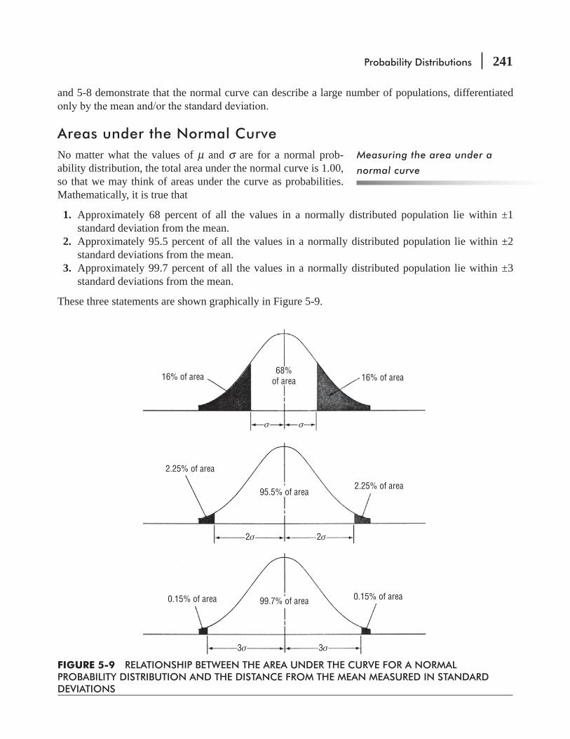
Probability Distributions 241
and 5-8 demonstrate that the normal curve can describe a large number of populations, differentiated
Areas under the Normal CurveNo matter what the values of μ and σ are for a normal prob-ability distribution, the total area under the normal curve is 1.00, so that we may think of areas under the curve as probabilities. Mathematically, it is true that
1. Approximately 68 percent of all the values in a normally distributed population lie within ±1 standard deviation from the mean.
2. Approximately 95.5 percent of all the values in a normally distributed population lie within ±2 standard deviations from the mean.
3. Approximately 99.7 percent of all the values in a normally distributed population lie within ±3 standard deviations from the mean.
These three statements are shown graphically in Figure 5-9.
Measuring the area under a
normal curve
σ σ
16% of area 16% of area
2.25% of area
0.15% of area0.15% of area
2.25% of area
95.5% of area
99.7% of area
68%of area
2σ 2σ
3σ 3σ
FIGURE 5-9 RELATIONSHIP BETWEEN THE AREA UNDER THE CURVE FOR A NORMAL PROBABILITY DISTRIBUTION AND THE DISTANCE FROM THE MEAN MEASURED IN STANDARD DEVIATIONS

242 Statistics for Management
Figure 5-9 shows three different ways of measuring the area under the normal curve. However, very few of the applications we shall make of the normal probability distribution involve intervals of exactly 1, 2, or 3 standard deviations (plus and minus) from the mean. What should we do about all these other cases? Fortunately, we can refer to statistical tables constructed for precisely these situations. They indicate portions of the area under the normal curve that are contained within any number of standard deviations (plus and minus) from the mean.
It is not possible or necessary to have a different table for every possible normal curve. Instead, we can use a table of the standard normal probability distribution (a normal distribution with (μ = 0 and σ =this table, we can determine the area, or probability, that the normally distributed random variable will
We can better understand the concept of the standard normal probability distribution by examining the special relationship of the standard deviation to the normal curve. Look at Figure 5-10. Here we have illustrated two normal probability distributions, each with a different mean and a different standard deviation. Both area a and area b, the shaded areas under the curves, contain the same proportion of the
the mean and one standard deviation to the right of the mean. All intervals containing the same number of standard deviations from the mean will contain the same proportion of the total area under the curve for any normal probability distribution. This makes possible the use of only one standard normal prob-ability distribution table.
is represented by colored areas in Figure 5-10. In Figure 5-9, we saw that an interval of one standard deviation (plus and minus) from the mean contained about 68 percent of the total area under the curve. In Figure 5-10, however, we are interested only in the area between the mean and 1 standard deviation to the right of the mean (plus, not plus and minus). This area must be half of 68 percent, or 34 percent, for both distributions.
One more example will reinforce our point. Look at the two normal probability distributions in Figure 5-11. Each of these has a different mean and a different standard deviation. The colored area under both curves, however, contains the same proportion of the total area under the curve. Why? Because both colored areas fall within 2 standard deviations (plus and minus) from the mean. Two
Standard normal probability
distribution
Finding the percentage of the
total area under the curve
FIGURE 5-10 TWO INTERVALS, EACH ONE STANDARD DEVIATION TO THE RIGHT OF THE MEAN
μ = 100σ = 35
σ = 35 σ = 30
μ = 60σ = 30
Distribution A
60 90100 135
Area a Area b
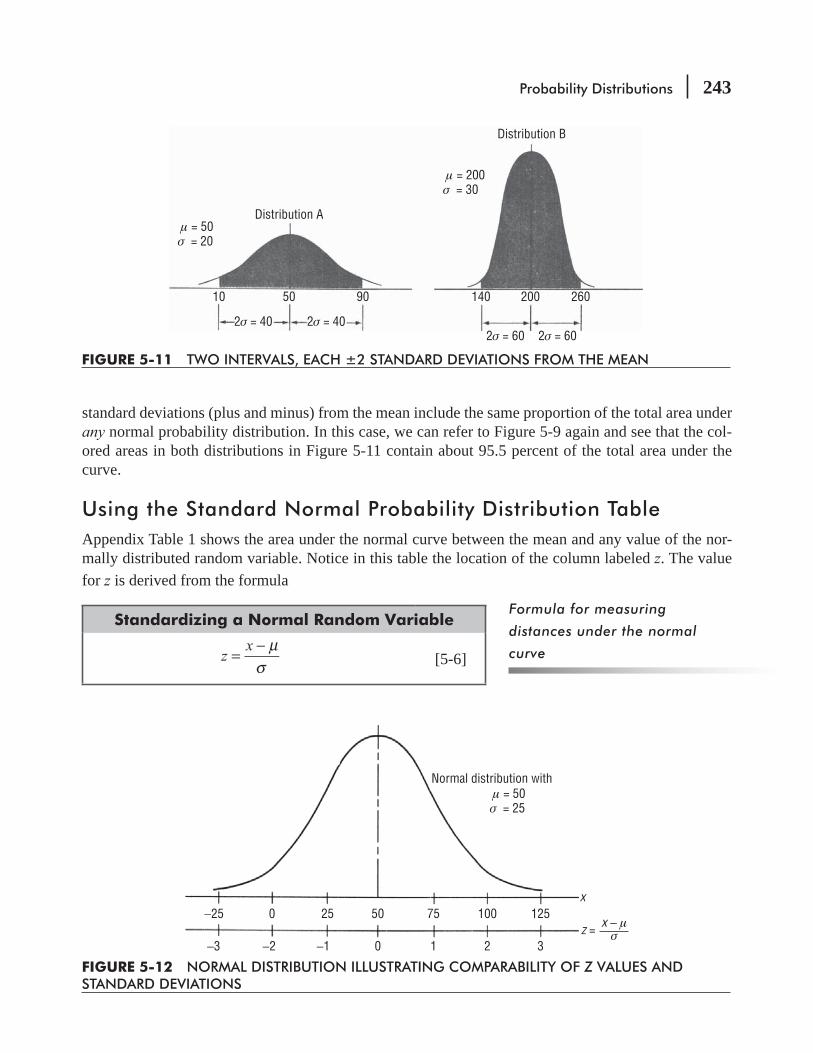
Probability Distributions 243
standard deviations (plus and minus) from the mean include the same proportion of the total area under any normal probability distribution. In this case, we can refer to Figure 5-9 again and see that the col-ored areas in both distributions in Figure 5-11 contain about 95.5 percent of the total area under the curve.
Using the Standard Normal Probability Distribution TableAppendix Table 1 shows the area under the normal curve between the mean and any value of the nor-mally distributed random variable. Notice in this table the location of the column labeled z. The value for z is derived from the formula
Standardizing a Normal Random Variable
zx μ
σ=
−[5-6]
Formula for measuring
distances under the normal
curve
FIGURE 5-11 TWO INTERVALS, EACH ±2 STANDARD DEVIATIONS FROM THE MEAN
2σ = 40 2σ = 402σ = 60 2σ = 60
μ = 200σ = 30
μ = 50σ = 20
Distribution A
Distribution B
10 140 200 26050 90
FIGURE 5-12 NORMAL DISTRIBUTION ILLUSTRATING COMPARABILITY OF Z VALUES AND STANDARD DEVIATIONS
μ = 50σ = 25
Normal distribution with
x
x − μz =−25 0 25 50 75 100 125
−3 −2 −1 0 1 2 3σ
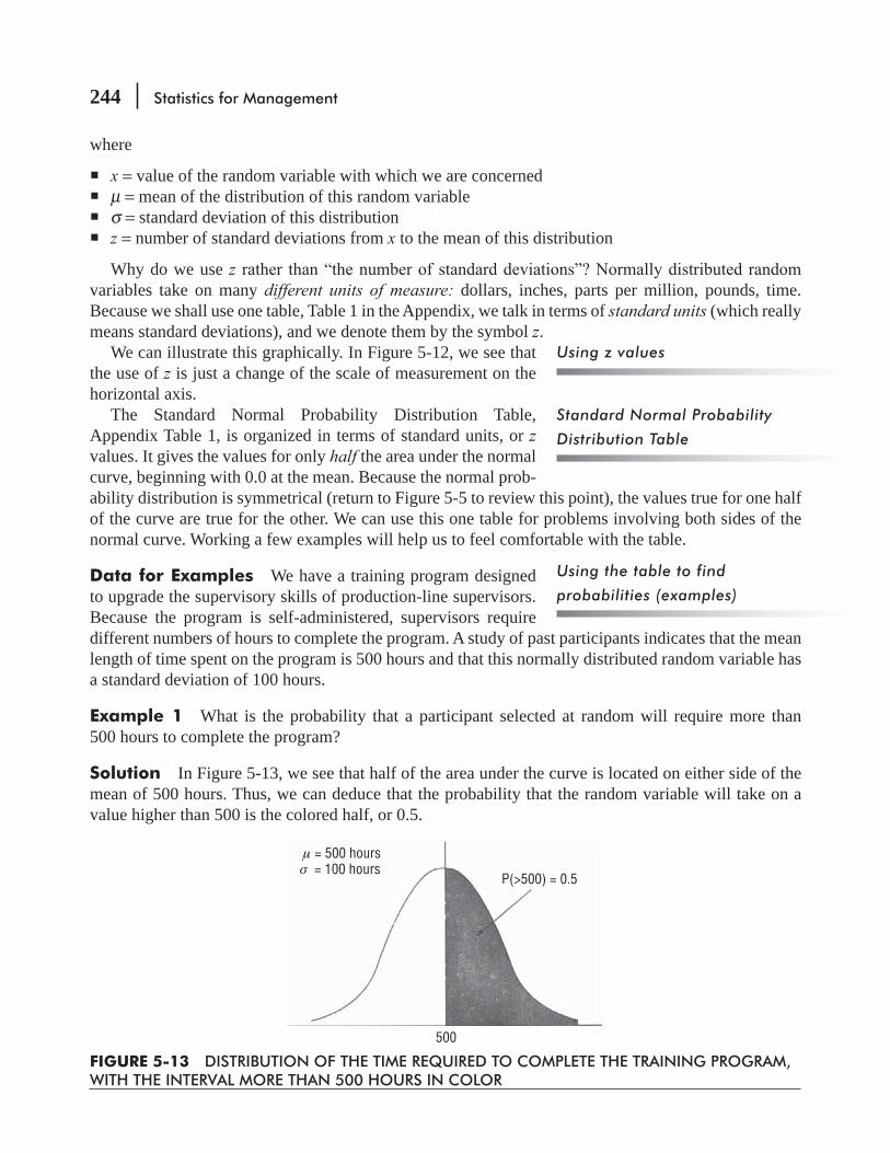
244 Statistics for Management
where
x = value of the random variable with which we are concerned μ = mean of the distribution of this random variable σ = standard deviation of this distribution z = number of standard deviations from x to the mean of this distribution
Why do we use zvariables take on many different units of measure: dollars, inches, parts per million, pounds, time. Because we shall use one table, Table 1 in the Appendix, we talk in terms of standard units (which really means standard deviations), and we denote them by the symbol z.
We can illustrate this graphically. In Figure 5-12, we see that the use of z is just a change of the scale of measurement on the horizontal axis.
The Standard Normal Probability Distribution Table, Appendix Table 1, is organized in terms of standard units, or z values. It gives the values for only half the area under the normal curve, beginning with 0.0 at the mean. Because the normal prob-ability distribution is symmetrical (return to Figure 5-5 to review this point), the values true for one half of the curve are true for the other. We can use this one table for problems involving both sides of the normal curve. Working a few examples will help us to feel comfortable with the table.
Data for Examples We have a training program designed to upgrade the supervisory skills of production-line supervisors. Because the program is self-administered, supervisors require different numbers of hours to complete the program. A study of past participants indicates that the mean length of time spent on the program is 500 hours and that this normally distributed random variable has a standard deviation of 100 hours.
Example 1 What is the probability that a participant selected at random will require more than 500 hours to complete the program?
Solution In Figure 5-13, we see that half of the area under the curve is located on either side of the mean of 500 hours. Thus, we can deduce that the probability that the random variable will take on a value higher than 500 is the colored half, or 0.5.
Using z values
Standard Normal Probability
Distribution Table
Using the table to find
probabilities (examples)
FIGURE 5-13 DISTRIBUTION OF THE TIME REQUIRED TO COMPLETE THE TRAINING PROGRAM, WITH THE INTERVAL MORE THAN 500 HOURS IN COLOR
μ = 500 hoursσ = 100 hours
P(>500) = 0.5
500

Probability Distributions 245
Example 2 What is the probability that a candidate selected at random will take between 500 and 650 hours to complete the training program?
Solution We have shown this situation graphically in Figure 5-14. The probability that will answer this question is represented by the colored area between the mean (500 hours) and the x value in which we are interested (650 hours). Using Equation 5-6, we get a z value of
zx μ
σ=
− [5-6]
650 500
100=
−
150
100=
= 1.5 standard deviations
If we look up z = -didate selected at random would require between 500 and 650 hours to complete the training program is slightly higher than 0.4.
Example 3 What is the probability that a candidate selected at random will take more than 700 hours to complete the program?
Solution This situation is different from our previous examples. Look at Figure 5-15. We are
can begin by using Equation 5-6:
zx μ
σ=
− [5-6]
700 500
100=
−
200
100=
= 2 standard deviations
FIGURE 5-14 DISTRIBUTION OF THE TIME REQUIRED TO COMPLETE THE TRAINING PROGRAM, WITH THE INTERVAL 500 TO 650 HOURS IN COLOR
μ = 500 hoursσ = 100 hours
P(500 to 650) = 0.4332
500 650
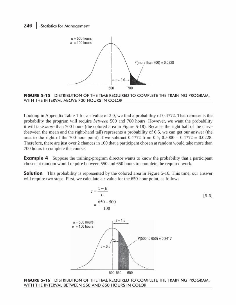
246 Statistics for Management
Looking in Appendix Table 1 for a zprobability the program will require between 500 and 700 hours. However, we want the probability it will take more than 700 hours (the colored area in Figure 5-18). Because the right half of the curve (between the mean and the right-hand tail) represents a probability of 0.5, we can get our answer (the
= 0.0228. Therefore, there are just over 2 chances in 100 that a participant chosen at random would take more than 700 hours to complete the course.
Example 4 Suppose the training-program director wants to know the probability that a participant chosen at random would require between 550 and 650 hours to complete the required work.
Solution This probability is represented by the colored area in Figure 5-16. This time, our answer will require two steps. First, we calculate a z value for the 650-hour point, as follows:
zx μ
σ=
−
[5-6]650 500
100=
−
FIGURE 5-15 DISTRIBUTION OF THE TIME REQUIRED TO COMPLETE THE TRAINING PROGRAM, WITH THE INTERVAL ABOVE 700 HOURS IN COLOR
μ = 500 hoursσ = 100 hours
P(more than 700) = 0.0228
500 700
z = 2.0
FIGURE 5-16 DISTRIBUTION OF THE TIME REQUIRED TO COMPLETE THE TRAINING PROGRAM, WITH THE INTERVAL BETWEEN 550 AND 650 HOURS IN COLOR
μ = 500 hoursσ = 100 hours
P(500 to 650) = 0.2417
500 550 650
z = 1.5
z = 0.5

Probability Distributions 247
150
100=
= 1.5 standard deviations
When we look up a z of 1.5 in Appendix Table 1, we see a probability value of 0.4332 (the probability that the random variable will fall between the mean and 650 hours). Now for step 2. We calculate a z value for our 550-hour point like this:
zx μ
σ=
− [5-6]
550 500
100=
−
50
100=
= 0.5 standard deviation
In Appendix Table 1, the z value of 0.5 has a probability of 0.1915 (the chance that the random variable will fall between the mean and 550 hours). To answer our question, we must subtract as follows:
0.4332 (Probability that the random variable will lie between the mean and 650 hours)– 0.1915 (Probability that the random variable will lie between the mean and 550 hours) 0.2417 ← (Probability that the random variable will lie between 550 and 650 hours)
Thus, the chance of a candidate selected at random taking between 550 and 650 hours to complete the program is a bit less than 1 in 4.
Example 5 What is the probability that a candidate selected at random will require fewer than 580 hours to complete the program?
Solution This situation is illustrated in Figure 5-17. Using Equation 5-6 to get the appropriate z value for 580 hours, we have
zx μ
σ=
− [5-6]
FIGURE 5-17 DISTRIBUTION OF THE TIME REQUIRED TO COMPLETE THE TRAINING PROGRAM, WITH THE INTERVAL LESS THAN 580 HOURS IN COLOR
μ = 500 hoursσ = 100 hours
P(less than 580) = 0.7881
500 580
z = 0.8

248 Statistics for Management
580 500
100=
−
80
100=
= 0.8 standard deviation
Looking in Appendix Table 1 for a zthe random variable will lie between the mean and 580 hours. We must add to this the probability that the random variable will be between the left-hand tail and the mean. Because the distribution is sym-
then, we add the two probabilities:
0.2881 (Probability that the random variable will lie between the mean and 580 hours)+0.5000 (Probability that the random variable will lie between the left-hand tail and the mean) 0.7881 ← (Probability that the random variable will lie between the left-hand tail and 580 hours)
Thus, the chances of a candidate requiring less than 580 hours to complete the programme slightly higher than 75 percent.
Example 6 What is the probability that a candidate chosen at random will take between 420 and 570 hours to complete the program?
Solution Figure 5-18 illustrates the interval in question, from 420 to 570 hours. Again, the solution requires two steps. First, we calculate a z value for the 570-hour point:
zx μ
σ=
− [5-6]
570 500
100=
−
70
100=
= 0.7 standard deviation
FIGURE 5-18 DISTRIBUTION OF THE TIME REQUIRED TO COMPLETE THE TRAINING PROGRAM, WITH THE INTERVAL BETWEEN 420 AND 570 HOURS IN COLOR
μ = 500 hoursσ = 100 hours
P(420 to 570) = 0.5461
420 500 570
z = 0.7
z = 0.8
Probability Distributions 249
We look up the zcalculate the z value for the 420-hour point:
zx μ
σ=
− [5-6]
420 500
100=
−
80
100=
−
= –0.8 standard deviation
Because the distribution is symmetrical, we can disregard the sign and look for a z value of 0.8. The prob-ability associated with this z
0.2580 (Probability that the random variable will lie between the mean and 570 hours)+0.2881 (Probability that the random variable will lie between the mean and 420 hours) 0.5461 ←(Probability that the random variable will lie between 420 and 570 hours)
Shortcomings of the Normal Probability DistributionEarlier in this section, we noted that the tails of the normal distri-bution approach but never touch the horizontal axis. This implies that there is some probability (although it may be very small) that the random variable can take on enormous values. It is possible for the right-hand tail of a normal curve
that such a person exists. (A weight of one ton or more would lie about 50 standard deviations to the right of the mean and would have a probability that began with 250 zeros to the right of the decimal point!) We do not lose much accuracy by ignoring values far out in the tails. But in exchange for the convenience of using this theoretical model, we must accept the fact that it can assign impos-sible empirical values.
The Normal Distribution as an Approximation of the Binomial DistributionAlthough the normal distribution is continuous, it is interesting to note that it can sometimes be used to approximate discrete dis-tributions. To see how we can use it to approximate the binomial distribution, suppose we would like to know the probability of
-ability, as follows:
P(r = 5, 6, 7 or 8) = P(r = 5) + P(r = 6) + P(r = 7) + P(r = 8)= 0.2461 + 0.2051 + 0.1172 + 0.0439= 0.6123
Theory and practice
Sometimes the normal is used to
approximate the binomial
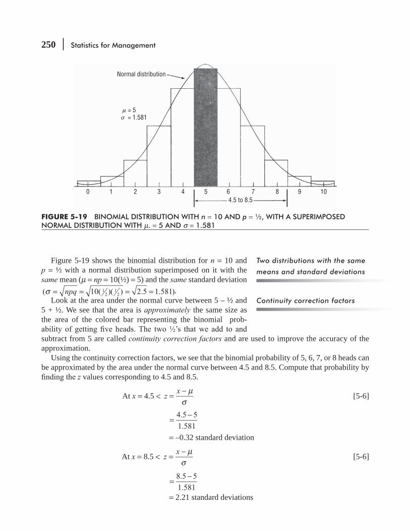
250 Statistics for Management
Figure 5-19 shows the binomial distribution for n = 10 and p = ½ with a normal distribution superimposed on it with the same mean (μ = np = 10(½) = 5) and the same standard deviation
npq( 10( )( ) 2.5 1.581)12
12σ = = = = .
Look at the area under the normal curve between 5 – ½ and 5 + ½. We see that the area is approximately the same size as the area of the colored bar representing the binomial prob-
subtract from 5 are called continuity correction factors and are used to improve the accuracy of the approximation.
Using the continuity correction factors, we see that the binomial probability of 5, 6, 7, or 8 heads can be approximated by the area under the normal curve between 4.5 and 8.5. Compute that probability by
z values corresponding to 4.5 and 8.5.
At x = 4.5 < zx μ
σ=
− [5-6]
4.5 5
1.581=
−
= –0.32 standard deviation
At x = 8.5 < zx μ
σ=
− [5-6]
8.5 5
1.581=
−
= 2.21 standard deviations
Two distributions with the same
means and standard deviations
Continuity correction factors
FIGURE 5-19 BINOMIAL DISTRIBUTION WITH n = 10 AND p = ½, WITH A SUPERIMPOSED NORMAL DISTRIBUTION WITH μ. = 5 AND σ = 1.581
μ = 5σ = 1.581
Normal distribution
0 1 2 3 4 5 6 7 8 9 104.5 to 8.5

Probability Distributions 251
0.1255 (Probability that z will be between –0.32 and 0 (and, correspondingly, that x will be between 4.5 and 5))
+0.4864 (Probability that z will be between 0 and 2.21 (and, correspondingly, that x will be between 5 and 8.5))
0.6119 (Probability that x will be between 4.5 and 8.5)
Comparing the binomial probability of 0.6123 (Appendix Table 3) with this normal approximation of 0.6119, we see that the error in the approximation is less than .1 percent.
The normal approximation to the binomial distribution is very convenient because it enables us to solve the problem without extensive tables of the binomial distribu-tion. (You might note that Appendix Table 3, which gives binomial probabilities for values of n up to 20, is already 9 pages long.) We should note that some care needs to be taken in using this approximation, but it is quite good whenever both np and nq are at least 5.
Warning: The normal distribution is the probability distribution most often used in statistics. Statisticians fear that too often, the data being analyzed are not well-described by a normal dis-
calculating probabilities using the normal distribution tend to do better when they actually sketch the distribution in question, indicate the mean and standard deviation, and then show the limits of the random variable in question (we use color but pencil shading is just as good). Visualizing the situation this way makes decisions easier (and answers more accurate).
HINTS & ASSUMPTIONS
EXERCISES 5.6
Self-Check ExercisesSC 5-9 Use the normal approximation to compute the binomial probabilities in parts (a)–(d) below:
(a) n = 30, p = 0.35, between 10 and 15 successes, inclusive.(b) n = 42, p = 0.62, 30 or more successes.(c) n = 15, p = 0.40, at most 7 successes.(d) n = 51, p = 0.42, between 17 and 25 successes, inclusive.
SC 5-10 Parminder Singh is the supervisor for the Krishna Hydroelectric Dam. He knows that the
-ity that the turbines will generate at peak rate today?
The error in estimating is slight
Care must be taken
252 Statistics for Management
Basic Concepts5-30 Given that a random variable, X, has a normal distribution with mean 6.4 and standard devia-
(a) P(4.0 < x < 5.0).(b) P(x > 2.0).(c) P(x < 7.2).(d) P((x < 3.0) or (x > 9.0)).
5-31 Given that a random variable, X, has a binomial distribution with n = 50 trials and p = 0.25,
(a) P(x > 10).(b) P(x < 18).(c) P(x > 21).(d) P(9 < x < 14).
5-32 In a normal distribution with a standard deviation of 5.0, the probability that an observation selected at random exceeds 21 is 0.14.(a) Find the mean of the distribution.(b) Find the value below which 4 percent of the values in the distribution lie.
5-33 Use the normal approximation to compute the binomial probabilities in parts (a)–(e) below.(a) n = 35, p = 0.15, between 7 and 10 successes inclusive.(b) n = 29, p = 0.25, at least 9 successes.(c) n = 84, p = 0.42, at most 40 successes.(d) n = 63, p = 0.11,10 or more successes.(e) n = 18, p = 0.67, between 9 and 12 successes inclusive.
Applications5-34 The manager of a small postal substation is trying to quantify the variation in the weekly
demand for mailing tubes. She has decided to assume that this demand is normally distributed. She knows that on average 100 tubes are purchased weekly and that 90 percent of the time, weekly demand is below 115.(a) What is the standard deviation of this distribution?(b) The manager wants to stock enough mailing tubes each week so that the probability of
running out of tubes is no higher than 0.05. What is the lowest such stock level?5-35 The Gilbert Machinery Company has received a big order to produce electric motors for a
stock of steel rods in inventory with a mean diameter of 5.07′′ and a standard deviation of 0.07′′
5-36 The manager of a Spiffy Lube auto lubrication shop is trying to revise his policy on order-ing grease gun cartridges. Currently, he orders 110 cartridges per week, but he runs out of cartridges 1 out of every 4 weeks. He knows that, on average, the shop uses 95 cartridges per week. He is also willing to assume that demand for cartridges is normally distributed.(a) What is the standard deviation of this distribution?(b) If the manager wants to order enough cartridges so that his probability of running out
during any week is no greater than 0.2, how many cartridges should he order per week?

Probability Distributions 253
5-37 -
ing his stock requirements for fatigue caps. Based on experience, Sgt. Peter has decided that hat size among recruits varies in such a way that it can be approximated by a normal distribu-tion with a mean of 7″. Recently, though, he has revised his estimate of the standard deviation from 0.75 to 0.875. Present stock policy is to have on hand hats in every size (increments of
″) from 6 ¼″ to 7 ¾″
(a) The old estimate of the standard deviation.(b) The new estimate of the standard deviation.
5-38 Anushree Saxena, VP of personnel for the Standard Insurance Company, has developed a new training program that is entirely self-paced. New employees work various stages at their own
-
is only 67 percent of that earned upon completion of the program. In the last several years, average completion time of the program was 44 days, and the standard deviation was 12 days.
(c) Fewer than 25 or more than 60 days?5-39 On the basis of past experience, automobile inspectors in Mumbai have noticed that
5 percent of all cars coming in for their annual inspection fail to pass. Using the normal
to enter the city inspection station will fail the inspection.5-40 Maurine Lewis, an editor for a large publishing company, calculates that it requires 11 months
standard deviation of 2.4 months. She believes that the normal distribution well describes the distribution of publication times. Out of 19 books she will handle this year, approximately how many will complete the process in less than a year?
5-41 objectives: It wants to build doors as small as possible to save on material costs, but to pre-serve its good reputation with the public, it feels obligated to manufacture doors that are tall enough for 95 percent of the adult population in the country to pass through without stooping. In order to determine the height at which to manufacture doors, Nobb is willing to assume that the height of adults in the country is normally distributed with mean 73 inches and standard
Worked-Out Answers to Self-Check ExercisesSC 5-9
(a) μ = np = 30(0.35) = 10.5 npq 30(0.35)(0.65) 2.612σ = = =
r zP(10 15) P
9.5 10.5
2.612
15.5 10.5
2.612≤ ≤ =
−≤ ≤
−⎛⎝⎜
⎞⎠⎟
= P(–0.38 ≤ z ≤ 1.91) = 0.1480 + 0.4719 = 0.6199
254 Statistics for Management
(b) μ = np = 42(0.62) = 26.04 npq 42(0.62)(0.38) 3.146σ = = =
r z zP( 30) P
29.5 26.04
3.146P( 1.10) 0.5 0.3643 0.1357≥ = ≥
−⎛⎝⎜
⎞⎠⎟
= ≥ = − =
(c) μ = np = 15(0.40) = 6 npq 15(0.40)(0.60) 1.895σ = = =
r z zP( 7) P
7.5 6
1.897P( 0.79) 0.5 0.2852 0.7852≤ = ≤
−⎛⎝⎜
⎞⎠⎟
= ≤ = + =
(d) μ = np = 51(0.42) = 21.42 npq 51(0.42)(0.58) 3.525σ = = =
r zP(17 25) P
16.5 21.42
3.525
25.5 21.42
3.525≤ ≤ =
−≤ ≤
−⎛⎝⎜
⎞⎠⎟
P(–1.40 ≤ z ≤ 1.16) = 0.4192 + 0.3770 = 0.7962
SC 5-10 For today, μ = 850,000, σ = 200,000
x z zP( 1,000,000) P1,000,000 850,000
200,000P( 0.75)≥ = ≥
−⎛⎝⎜
⎞⎠⎟
= ≥
= 0.5 – 0.2734 = 0.2266
5.7 CHOOSING THE CORRECT PROBABILITY DISTRIBUTIONIf we plan to use a probability to describe a situation, we must be careful to choose the right one. We need to be certain that we are not using the Poisson probability distribution when it is the binomial that more nearly describes the situation we are studying. Remember that the binomial distribution is applied
the Poisson distribution applies when each trial is independent. But although the probabilities in a
The results are not limited to two mutually exclusive outcomes. Under some conditions, the Poisson dis-tribution can be used as an approximation of the binomial, but not always. All the assumptions that form the basis of a distribution must be met if our use of that distribution is to produce meaningful results.
Even though the normal probability distribution is the only continuous distribution we have dis-cussed in this chapter, we should realize that there are other useful continuous distributions. In the
t, χ2, and F. Each of these is of interest to decision makers who solve problems using statistics.
EXERCISES 5.75-42 Which probability distribution is most likely the appropriate one to use for the following vari-
ables: binomial, Poisson, or normal?(a) The life span of a female born in 1977.(b) The number of autos passing through a tollbooth.(c) The number of defective radios in a lot of 100.(d) The water level in a reservoir.
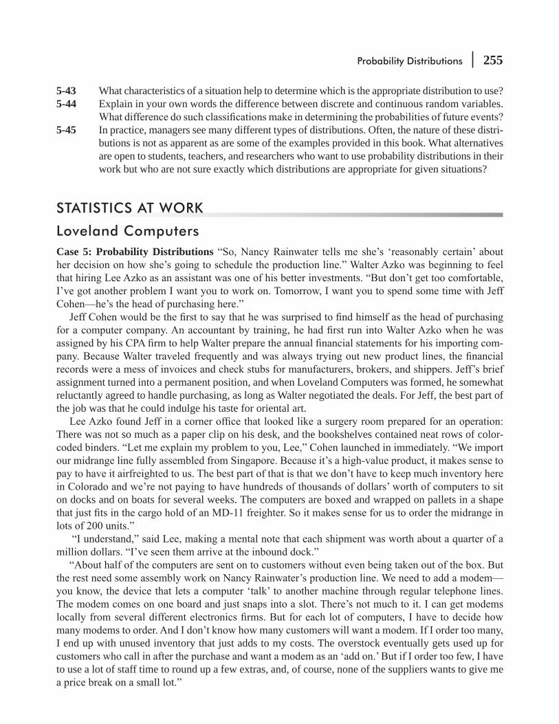
Probability Distributions 255
5-43 What characteristics of a situation help to determine which is the appropriate distribution to use?5-44 Explain in your own words the difference between discrete and continuous random variables.
5-45 In practice, managers see many different types of distributions. Often, the nature of these distri-butions is not as apparent as are some of the examples provided in this book. What alternatives are open to students, teachers, and researchers who want to use probability distributions in their work but who are not sure exactly which distributions are appropriate for given situations?
STATISTICS AT WORK
Loveland ComputersCase 5: Probability Distributions
-
assignment turned into a permanent position, and when Loveland Computers was formed, he somewhat reluctantly agreed to handle purchasing, as long as Walter negotiated the deals. For Jeff, the best part of the job was that he could indulge his taste for oriental art.
There was not so much as a paper clip on his desk, and the bookshelves contained neat rows of color-
on docks and on boats for several weeks. The computers are boxed and wrapped on pallets in a shape
I end up with unused inventory that just adds to my costs. The overstock eventually gets used up for
to use a lot of staff time to round up a few extras, and, of course, none of the suppliers wants to give me
256 Statistics for Management
average number of modems per lot has stayed the same over the last few years, the actual number requested by customers on any single lot jumps around a bit. Take a look at
for me to end up with too few modems in stock when a shipment of midranges comes through the pro-duction line than to have too many. So I suppose I tend to order above the average. It just seems that
”
Study Questions:
CHAPTER REVIEW
Terms Introduced in Chapter 5Bernoulli Process A process in which each trial has only two possible outcomes, the probability of the
Binomial Distribution A discrete distribution describing the results of an experiment known as a Bernoulli process.Continuity Correction Factor Corrections used to improvement the accuracy of the approximation of a binomial distribution by a normal distribution.Continuous Probability Distribution A probability distribution in which the variable is allowed to take on any value within a given range.Continuous Random Variable A random variable allowed to take on any value within a given range.Discrete Probability Distribution A probability distribution in which the variable is allowed to take on only a limited number of values, which can be listed.Discrete Random Variable A random variable that is allowed to take on only a limited number of values, which can be listed.Expected Value A weighted average of the outcomes of an experiment.Expected Value of a Random Variable The sum of the products of each value of the random variable
Normal Distribution A distribution of a continuous random variable with a single-peaked, bell-shaped curve. The mean lies at the center of the distribution, and the curve is symmetrical around a vertical line
Poisson Distribution A discrete distribution in which the probability of the occurrence of an event within a very small time period is a very small number, the probability that two or more such events will occur within the same time interval is effectively 0, and the probability of the occurrence of the event within one time period is independent of where that time period is.Probability Distribution A list of the outcomes of an experiment with the probabilities we would expect to see associated with these outcomes.
Probability Distributions 257
Random Variable A variable that takes on different values as a result of the outcomes of a random experiment.Standard Normal Probability Distribution A normal probability distribution, with mean μ = 0 and standard deviation σ = 1.
Equations Introduced in Chapter 55-1 Probability of r successes in n trials n
r n rp q
!
!( )!r n r=
−− p. 223
where r = number of successes desired n = number of trials undertaken p = probability of success (characteristic probability) q = probability of failure (q = 1 – p)
This binomial formula enables us to calculate algebraically the probability of r successes. We can apply it to any Bernoulli process, where each trial has only two possible outcomes (a suc-cess or a failure), the probability of success remains the same trial after trial, and the trials are statistically independent.
5-2 μ = np p. 226 The mean of a binomial distribution is equal to the number of trials multiplied by the
probability of success.
5-3 npqσ = p. 226 The standard deviation of a binomial distribution is equal to the square root of the product
of the number of trials, the probability of a success, and the probability of a failure (found by taking q = 1 – p).
5-4 xe
xP( )
!
xλ=
× λ−
p. 231
This formula enables us to calculate the probability of a discrete random variable occurring in a Poisson distribution. The formula states that the probability of exactly x occurrences is equal to λ, or lambda (the mean number of occurrences per interval of time in a Poisson distribution), raised to the xth power and multiplied by e, or 2.71828 (the base of the natural logarithm system), raised to the negative lambda power, and the product divided by x facto-rial. Appendix Tables 4a and 4b can be used for computing Poisson probabilities.
5-5 xnp e
xP( )
( )
!
x np
=× −
p. 235
If we substitute in Equation 5-4 the mean of the binomial distribution (np) in place of the mean of the Poisson distribution (λ), we can use the Poisson probability distribution as a reasonable approximation of the binomial. The approximation is good when n is greater than or equal to 20 and p is less than or equal to 0.05.
5-6 zx= − μ
σ p. 243

258 Statistics for Management
where x = value of the random variable with which we are concerned μ = mean of the distribution of this random variable σ = standard deviation of this distribution z = number of standard deviations from x to the mean of this distribution
Once we have derived z using this formula, we can use the Standard Normal Probability Distribution Table (which gives the values for areas under half the normal curve, beginning with 0.0 at the mean) and determine the probability that the random variable with which we are concerned is within that distance from the mean of this distribution.
Review and Application Exercises5-46 In the past 20 years, on average, only 3 percent of all checks written to the Life Insurance
Limited (LIL) have bounced. This month, the LIL received 200 checks. What is the probabil-ity that(a) Exactly 10 of these checks bounced?(b) Exactly 5 of these checks bounced?
5-47 An inspector for the Department of Agriculture is about to visit a large vegetable-packing company. She knows that, on average, 2 percent of all packets of vegetables inspected by the
be closed for at least 1 month. Out of curiosity, she wants to compute the probability that this company will be shut down as a result of her inspection. Should she assume her inspection of
5-48 students as summer interns to help the agency prepare court cases. The agency is under a budget and wishes to keep its costs at a minimum. However, hiring student interns is less costly than hiring full-time employees. Accordingly, the agency wishes to hire the maximum
research a case. The interns turn their work over to staff attorneys, who prosecute the cases in the fall when the circuit court convenes. The legal staff coordinator has to place his budget request in June of the preceding summer for the number of positions he wishes to maintain. It is therefore impossible for him to know with certainty how many cases will be researched in the following summer. The data from preceding summers are as follows:
Year 1987 1988 1989 1990 1991Number of cases 6 4 8 7 5Year 1992 1993 1994 1995 1996Number of cases 6 4 5 4 5
Using these data as his probability distribution for the number of cases, the legal staff coordi-nator wishes to hire enough interns to research the expected number of cases that will arise. How many intern positions should be requested in the budget?
Probability Distributions 259
5-49 Label the following probability distributions as discrete or continuous:
(a) (b) (c)
5-50 situations: binomial, Poisson, or normal?(a) 112 trials, probability of success 0.06.(b) 15 trials, probability of success 0.4.(c) 650 trials, probability of success 0.02.(d) 59 trials, probability of success 0.1.
5-51 The French bread made at Anmol Bread Company costs ` 400 per dozen to produce. Fresh bread sells at a premium, 800 per dozen, but it has a short shelf life. If Anmol Bread Company bakes more bread than its customers demand on any given day, the leftover day-old bread goes for croutons in local restaurants at a discounted ` 350 per dozen. Conversely, producing less bread than customers demand leads to lost sales. Anmol Bread Company bakes its French bread in batches of 350 dozen. The daily demand for bread is a random variable, taking the
bake each morning?5-52
In his upcoming speech to the BWA board of directors, Mr. Dunfey wants to include the
will be more than 10 minutes early or late?5-53 The City Bank of Durham has recently begun a new credit program. Customers meeting
certain credit requirements can obtain a credit card accepted by participating area merchants that carries a discount. Past numbers show that 25 percent of all applicants for this card are rejected. Given that credit acceptance or rejection is a Bernoulli process, out of 15 applicants, what is the probability that(a) Exactly four will be rejected?(b) Exactly eight?(c) Fewer than three?
5-54 -
Bangalore training center is 15, what is the probability that(a) Fewer than 6 will have to repeat the course?(b) Exactly 10 will pass the course?(c) More than 12 will pass the course?

260 Statistics for Management
5-55
advance. On the basis of 5 years of data, the following probability distribution for the com-
Amount of wool (kg) 2,500 3,500 4,500 5,500Probability 0.30 0.45 0.20 0.05
From these data, the raw-materials purchaser computed the expected number of pounds
years before. Extrapolating, she observed that the company will be lucky if its weekly demand averages 2,500 this year.(a) What was the expected weekly demand for wool based on the distribution from past data?(b) If each pound of wool generates ` 5 in revenue and costs ` 4 to purchase, ship, and han-
5-56
full-length leather coats to order. These coats cost her ` 100 each and will sell for ` 200 each. Any coats left over at the end of the season will have to be sold at a 20 percent discount in
demand for the coats has the following probability distribution:
Number of coats demanded 8 10 12 14 16Probability 0.10 0.20 0.25 0.30 0.15
She also knows that any leftover coats can be sold at discount.
(b) How would the answer to part (a) change if the leftover coats were sold at a 40 percent discount?
5-57 The Executive Camera Company provides full expenses for its sales force. When attempting -
ures to estimate gas, tire, and repair expenses. Distances driven average 5,650 miles a month,
subsequent budget to be adequately high and, therefore, does not want to use any of the data
drove 5,500 miles or more?5-58 Mission Bank is considering changing the day for scheduled maintenance for the automatic
teller machine (ATM) in the lobby. The average number of people using it between 8 and 9 A.M. is 30, except on Fridays, when the average is 45. The management decision must bal-
inconvenienced customers)?
Probability Distributions 261
(b) Taking the data for all days together, the relative probability of inconveniencing 45 cus-tomers is quite small. Should the manager expect many inconvenienced customers if the maintenance day is changed to Friday?
5-59 -agency motor pool was considering two different models. Both were 4-door, 4-cylinder cars with comparable service warranties. The decision was to choose the automobile that achieved the best mileage per gallon. The state had done some tests of its own, which produced the fol-lowing results for the two automobiles in question:
Average MPG Standard DeviationAutomobile A 42 4Automobile B 38 7
The purchasing agent was uncomfortable with the standard deviations, so she set her own decision criterion for the car that would be more likely to get more than 45 miles per gallon.
which car should she choose?
less than 39 mpg, which car should she buy?5-60 In its third year, attendance in the Liberty Football League averaged 16,050 fans per game,
and had a standard deviation of 2,500.(a) According to these data, what is the probability that the number of fans at any given
game was greater than 20,000?(b) Fewer than 10,000?(c) Between 14,000 and 17,500?
5-61 The city mayor, wants to do something to reduce the number of accidents in the town involv-ing motorists and bicyclists. Currently, the probability distribution of the number of such accidents per week is as follows:
Number of accidents 0 1 2 3 4 5Probability 0.05 0.10 0.20 0.40 0.15 0.10
or he can expand the number of bike lanes in the town. The respective revised probability distributions for the two options are as follows:
Number of accidents 0 1 2 3 4 5Probability (lights) 0.10 0.20 0.30 0.25 0.10 0.05Probability (lanes) 0.20 0.20 0.20 0.30 0.05 0.05
262 Statistics for Management
Which plan should the mayor approve if he wants to produce the largest possible reduction in(a) Expected number of accidents per week?(b) Probability of more than three accidents per week?(c) Probability of three or more accidents per week?
5-62 discount. Leases are normally distributed, with a mean of 24 months and a standard deviation of 7.5 months.(a) What is the probability that a copier will still be on lease after 28 months?(b) What is the probability that a copier will be returned within one year?
5-63 Shekhar Baradoli supervises the packaging of college textbooks for Newsome-Cluett Publishers. He knows that the number of cardboard boxes he will need depends partly on the size of the books. All Newsome-Cluett books use the same size paper but may have differing numbers of pages. After pulling shipment records for the last 5 years, Baradoli derived the following set of probabilities:
# of pages 100 300 500 700 900 1100Probability 0.05 0.10 0.25 0.25 0.20 0.15
(a) If Baradoli bases his box purchase on an expected length of 600 pages, will he have enough boxes?
(b) If all 700-page books are edited down to 500 pages, what expected number of pages should he use?
5-64
previous years:
Roses sold 15,000 20,000 25,000 30,000Probability 0.10 0.30 0.40 0.20
5-65 A certain business school has 400 students in its MBA program. One hundred sixteen of the
students are married. Without using Appendix Table 3, determine(a) The probability that exactly 2 of 3 randomly selected students are married.(b) The probability that exactly 4 of 13 students chosen at random are married.
5-66 Raj Chaudhary wants to borrow ` 7,50,000 from his bank for a new tractor for his farm. The
does tell Raj that over the years, the bank has received about 1460 loan applications per year and that the probability of approval was, on average, about 0.8.(a) Raj is curious about the average and standard deviation of the number of loans approved

Probability Distributions 263
are 1,327 applications per year with an approval probability of 0.77. What are the mean and standard deviation now?
5-67 --
(a) If Raj is right, what is the probability that exactly 6 of the next 10 applications will be approved?
(b) What is the probability that more than 3 will be approved?(c) What is the probability that more than 2 but fewer than 6 will be approved?
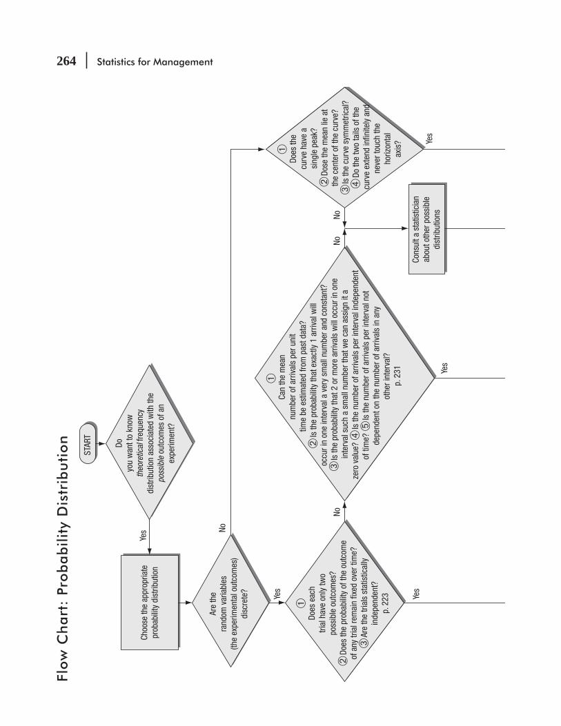
264 Statistics for Management
STAR
T
Doyo
u w
ant t
o kn
owthe
oretic
al fre
quen
cydi
strib
utio
n as
soci
ated
with
the
poss
ible o
utco
mes
of a
nex
perim
ent?
Are
the
rand
om v
aria
bles
(the
expe
rimen
tal o
utco
mes
)di
scre
te?
Choo
se th
e ap
prop
riate
prob
abili
ty d
istri
butio
nYe
s No
NoNo
No
Yes
Yes
Yes
Yes
➀Do
es e
ach
trial
hav
e on
ly tw
opo
ssib
le o
utco
mes
?➁
Does
the
prob
abili
ty o
f the
out
com
eof
any
tria
l rem
ain
fixed
ove
r tim
e?➂
Are
the
trial
s st
atis
tical
lyin
depe
nden
t?p.
223
➀
Does
the
curv
e ha
ve a
si
ngle
pea
k?➁
Dose
the
mea
n lie
at
the
cent
er o
f the
cur
ve?
➂Is
the
curv
e sy
mm
etric
al?
➃Do
the
two
tails
of t
he
curv
e ex
tend
infin
itely
and
ne
ver t
ouch
the
horiz
onta
lax
is?
➀Ca
n th
e m
ean
num
ber o
f arr
ival
s pe
r uni
t tim
e be
est
imat
ed fr
om p
ast d
ata?
➁
Is th
e pr
obab
ility
that
exa
ctly
1 a
rriv
al w
ill
occu
r in
one
inte
rval
a v
ery
smal
l num
ber a
nd c
onst
ant?
➂
Is th
e pr
obab
ility
that
2 o
r mor
e ar
rival
s w
ill o
ccur
in o
ne
inte
rval
suc
h a
smal
l num
ber t
hat w
e ca
n as
sign
it a
ze
ro v
alue
? ➃
Is th
e nu
mbe
r of a
rriv
als
per i
nter
val i
ndep
ende
nt
of ti
me?
➄Is
the
num
ber o
f arr
ival
s pe
r int
erva
l not
de
pend
ent o
n th
e nu
mbe
r of a
rriv
als
in a
ny
othe
r int
erva
l? p
. 231
Cons
ult a
sta
tistic
ian
abou
t oth
er p
ossi
ble
dist
ribut
ions
Flo
w C
ha
rt:
Pro
ba
bilit
y D
istr
ibu
tio
n

Probability Distributions 265
Is n
≥ 20
and
p ≤ .0
5?
Is np
≥ 5
and n
q ≤ 5
?
Yes
Yes
STOP
STOP
Use
the
bino
mia
ldi
strib
utio
n an
d fo
rmul
a:Pr
obab
ility
of r
succ
esse
s in
n tri
als
=
pr qn–
rr !(
n × r)!
n! p.
223
Use
the
norm
al d
istri
butio
nan
d th
e st
anda
rd n
orm
alpr
obab
ility
dis
tribu
tion
tabl
e w
ith
p. 2
43
Use
the
Pois
son
dist
ribut
ion
and
form
ula
Prob
abili
ty o
f xoc
curr
ence
s =
x!p.
231
λx × e
–λ
You
may
use
the
Pois
son
dist
ribut
ion
as a
nap
prox
imat
ion
of th
ebi
nom
ial d
istri
butio
n:
p. 2
35P(
x) =
x!(np
)x × e
–np
You
may
use
the
norm
aldi
strib
utio
n as
an
appr
oxim
atio
n of
the
bino
mia
l dis
tribu
tion
with
p. 2
50
μ = np
and
σ =
npq
z =
σX × μ

This page is intentionally left blank

LEARNING OBJECTIVES
6After reading this chapter, you can understand:
CHAPTER CONTENTS
To take a sample from an entire population and use it to describe the population
To make sure the samples you do take are an accurate representation of the population from which they came
To introduce the concepts of sampling distributions
6.1 Introduction to Sampling 2686.2 Random Sampling 2716.3 Non-Random Sampling 2796.4 Design of Experiments 2826.5 Introduction to Sampling
Distributions 2866.6 Sampling Distributions in More
Detail 2896.7 An Operational Consideration in
Sampling: The Relationship between Sample Size and Standard Error 302
To understand the trade-offs between the cost of taking larger samples and the additional accuracy this gives to decisions made from them
To introduce experimental design: sampling procedures to gather the most information for the least cost
Statistics at Work 308 Terms Introduced in Chapter 6 309 Equations Introduced in Chapter 6 311 Review and Application Exercises 311 Flow Chart: Sampling and Sampling
Distributions 314
Sampling and Sampling Distributions
268 Statistics for Management
Although there are over 200 million TV viewers in the United States and somewhat over half that many TV sets, only about 1,000 of those sets are sampled to determine what programs Americans
watch. Why select only about 1,000 sets out of 100 million? Because time and the average cost of an interview prohibit the rating companies from trying to reach millions of people. And since polls are rea-sonably accurate, interviewing everybody is unnecessary. In this chapter, we examine questions such as these: How many people should be interviewed? How should they be selected? How do we know when
6.1 INTRODUCTION TO SAMPLINGShoppers often sample a small piece of cheese before purchasing any. They decide from one piece what the larger chunk will taste like. A chemist does the same thing when he takes a sample of alcohol from a still, determines that it is 90 proof, and infers that all the alcohol in the still is 90 proof. If the chemist tests all the alcohol or the shoppers taste all the cheese, there will be none to sell. Testing all of the product often destroys it and is unnecessary. To determine the characteristics of the whole, we have to sample only a portion.
Suppose that, as the personnel director of a large bank, you need to write a report describing all the
locating all these thousands of people. They are not easily accessible as a group—many have died, moved from the community, left the country, or acquired a new name by marriage. How do you write the report? The best idea is to locate a representative sample and interview them in order to generalize about the entire group.
Time is also a factor when managers need information quickly in order to adjust an operation or change a policy. Consider an automatic machine that sorts thousands of pieces of mail daily. Why wait for an entire day’s output to check whether the machine is working accurately (whether the population characteristics -vals, and if necessary, the machine can be adjusted right away.
Sometimes it is possible and practical to examine every per-son or item in the population we wish to describe. We call this a complete enumeration, or census. We use sampling when it is not possible to count or measure every item in the population.
Statisticians use the word population to refer not only to people but to all items that have been chosen for study. In the cases we have just mentioned, the populations are all the cheese in the chunk, all the whiskey in the vat, all the employees of the large bank who voluntarily left in the last 10 years, and all mail sorted by the automatic machine since the previous sample check. Statisticians use the word sample to describe a portion chosen from the population. Sample is not just a portion (subset) of the population but a “representative subset” of the population that is expected to exhibit the properties of the entire population.
Statistics and ParametersMathematically, we can describe samples and populations by using measures such as the mean, median, mode, and standard deviation, which we introduced in Chapter 3. When these terms
Reasons for sampling
Census or sample
Examples of populations and
samples
Function of statistics and
parameters
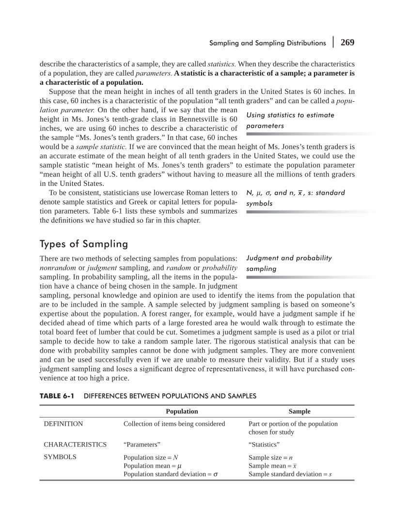
Sampling and Sampling Distributions 269
describe the characteristics of a sample, they are called statistics. When they describe the characteristics of a population, they are called parameters. A statistic is a characteristic of a sample; a parameter is a characteristic of a population.
Suppose that the mean height in inches of all tenth graders in the United States is 60 inches. In this case, 60 inches is a characteristic of the population “all tenth graders” and can be called a popu-lation parameter. On the other hand, if we say that the mean height in Ms. Jones’s tenth-grade class in Bennetsville is 60 inches, we are using 60 inches to describe a characteristic of the sample “Ms. Jones’s tenth graders.” In that case, 60 inches would be a sample statistic. If we are convinced that the mean height of Ms. Jones’s tenth graders is an accurate estimate of the mean height of all tenth graders in the United States, we could use the sample statistic “mean height of Ms. Jones’s tenth graders” to estimate the population parameter “mean height of all U.S. tenth graders” without having to measure all the millions of tenth graders in the United States.
To be consistent, statisticians use lowercase Roman letters to denote sample statistics and Greek or capital letters for popula-tion parameters. Table 6-1 lists these symbols and summarizes
Types of SamplingThere are two methods of selecting samples from populations: nonrandom or judgment sampling, and random or probability sampling. In probability sampling, all the items in the popula-tion have a chance of being chosen in the sample. In judgment sampling, personal knowledge and opinion are used to identify the items from the population that are to be included in the sample. A sample selected by judgment sampling is based on someone’s expertise about the population. A forest ranger, for example, would have a judgment sample if he decided ahead of time which parts of a large forested area he would walk through to estimate the total board feet of lumber that could be cut. Sometimes a judgment sample is used as a pilot or trial sample to decide how to take a random sample later. The rigorous statistical analysis that can be done with probability samples cannot be done with judgment samples. They are more convenient and can be used successfully even if we are unable to measure their validity. But if a study uses
-venience at too high a price.
Using statistics to estimate
parameters
N, μ, s, and n, x , s: standard
symbols
Judgment and probability
sampling
TABLE 6-1 DIFFERENCES BETWEEN POPULATIONS AND SAMPLES
Population Sample
DEFINITION Collection of items being considered Part or portion of the population chosen for study
CHARACTERISTICS “Parameters” “Statistics”
SYMBOLS Population size = NPopulation mean = μPopulation standard deviation = σ
Sample size = nSample mean = x–Sample standard deviation = s

270 Statistics for Management
Biased SamplesThe US Congress is debating some gun control laws. You are asked to conduct an opinion survey. Because hunters are the ones that are most affected by the gun control laws, you went to a hunting lodge and interviewed the members there. Then you reported that in a survey done by you, about 97 percent of the respondents were in favor of repealing all gun control laws.
A week later, the Congress took up another bill: “Should working pregnant women be given a maternity leave of one year with full pay to take care of newborn babies?” Because this issue
-viewed several working women of child-bearing age. Again you reported that in a survey done by you, about 93 percent of the respondents were in favor of the one-year maternity leave with full pay.
In both of these situations you picked a biased sample by choosing people who would have very strong feelings on one side of the issue. How can we be sure that pollsters we listen to and read about don’t make the same mistake you did? The answer is that unless the pollsters have a strong reputation for statistically accurate polling, we can’t. However, we can be alert to the risks we take when we don’t ask for more information or do more research into their competence.
EXERCISES 6.1
Basic Concepts6-1 What is the major drawback of judgment sampling?6-2 Are judgment sampling and probability sampling necessarily mutually exclusive? Explain.6-3 List the advantages of sampling over complete enumeration, or census.6-4 What are some disadvantages of probability sampling versus judgment sampling?
Applications6-5 Farlington Savings and Loan is considering a merger with Sentry Bank, but needs shareholder
approval before the merger can be accomplished. At its annual meeting, to which all sharehold-ers are invited, the president of FS&L asks the shareholders whether they approve of the deal.
6-6 Jean Mason, who was hired by Former Industries to determine employee attitudes toward the
Mason’s study was based on statistical sampling, and from the beginning data, it was clear (or so Jean thought) that the employees were favoring a unionized shop. Jean’s report was shrugged off with the comment, ‘‘This is no good. Nobody can make statements about em-ployee sentiments when she talks to only a little over 15 percent of our employees. Everyone knows you have to check 50 percent to have any idea of what the outcome of the union vote will be. We didn’t hire you to make guesses.” Is there any defense for Jean’s position?
6-7 A consumer protection organization is conducting a census of people who were injured by a particular brand of space heater. Each victim is asked questions about the behavior of the heater just before its malfunction; this information generally is available only from the victim, because the heater in question tends to incinerate itself upon malfunction. Early in the census, it is discovered that several of the victims were elderly and have died. Is any census of the victims now possible? Explain.
couple of biased polls
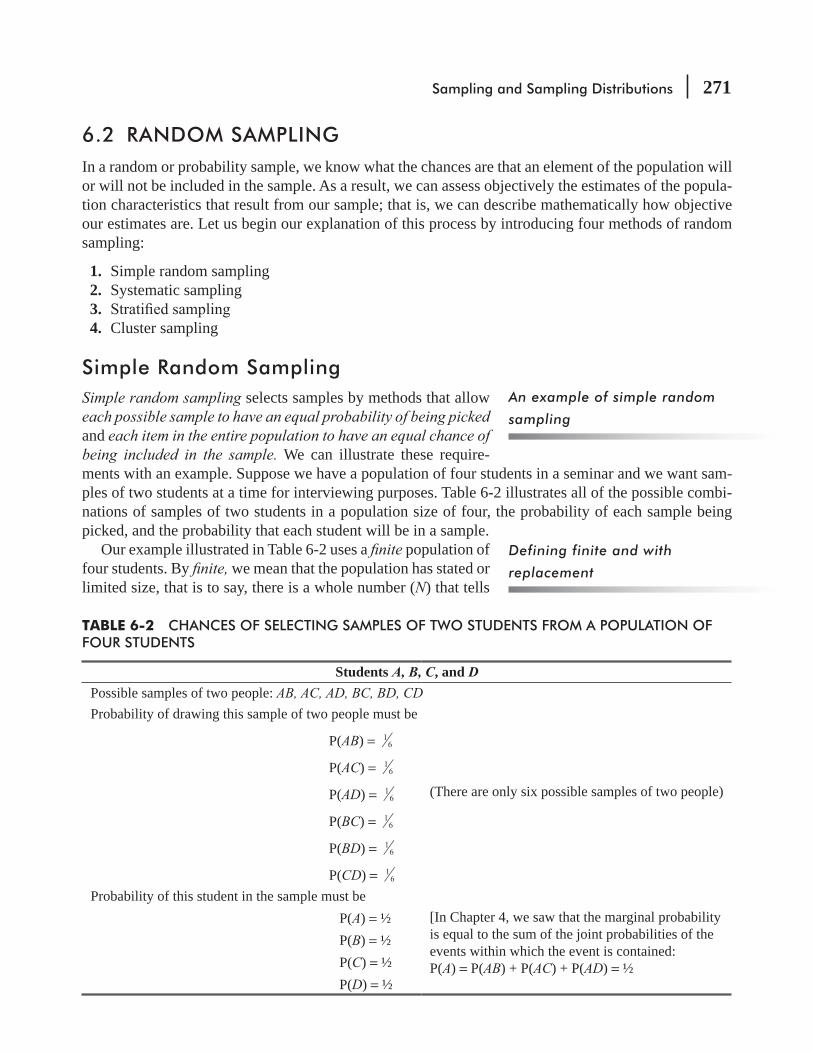
Sampling and Sampling Distributions 271
6.2 RANDOM SAMPLINGIn a random or probability sample, we know what the chances are that an element of the population will or will not be included in the sample. As a result, we can assess objectively the estimates of the popula-tion characteristics that result from our sample; that is, we can describe mathematically how objective our estimates are. Let us begin our explanation of this process by introducing four methods of random sampling:
1. Simple random sampling 2. Systematic sampling 3. 4. Cluster sampling
Simple Random SamplingSimple random sampling selects samples by methods that allow each possible sample to have an equal probability of being picked and each item in the entire population to have an equal chance of being included in the sample. We can illustrate these require-ments with an example. Suppose we have a population of four students in a seminar and we want sam-ples of two students at a time for interviewing purposes. Table 6-2 illustrates all of the possible combi-nations of samples of two students in a population size of four, the probability of each sample being picked, and the probability that each student will be in a sample.
Our example illustrated in Table 6-2 uses a nite population of four students. By nite, we mean that the population has stated or limited size, that is to say, there is a whole number (N) that tells
An example of simple random
sampling
Defining finite and with
replacement
TABLE 6-2 CHANCES OF SELECTING SAMPLES OF TWO STUDENTS FROM A POPULATION OF FOUR STUDENTS
Students A, B, C, and DPossible samples of two people: AB, AC, AD, BC, BD, CDProbability of drawing this sample of two people must be
P(AB) = 16
P(AC) = 16
P(AD) = 16
(There are only six possible samples of two people)
P(BC) = 16
P(BD) = 16
P(CD) = 16
Probability of this student in the sample must beP(A) = ½ [In Chapter 4, we saw that the marginal probability
is equal to the sum of the joint probabilities of the events within which the event is contained:P(A) = P(AB) + P(AC) + P(AD) = ½
P(B) = ½P(C) = ½P(D) = ½
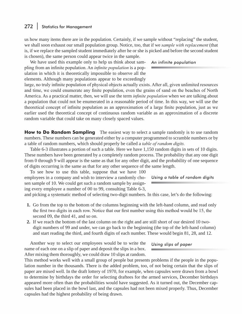
272 Statistics for Management
us how many items there are in the population. Certainly, if we sample without “replacing” the student, we shall soon exhaust our small population group. Notice, too, that if we sample with replacement (that is, if we replace the sampled student immediately after he or she is picked and before the second student is chosen), the same person could appear twice in the sample.
We have used this example only to help us think about sam- in nite population is a pop-
ulation in which it is theoretically impossible to observe all the elements. Although many populations appear to be exceedingly
America. As a practical matter, then, we will use the term in nite population when we are talking about a population that could not be enumerated in a reasonable period of time. In this way, we will use the
earlier used the theoretical concept of continuous random variable as an approximation of a discrete random variable that could take on many closely spaced values.
How to Do Random Sampling The easiest way to select a sample randomly is to use random numbers. These numbers can be generated either by a computer programmed to scramble numbers or by a table of random numbers, which should properly be called a table of random digits.
Table 6-3 illustrates a portion of such a table. Here we have 1,150 random digits in sets of 10 digits. These numbers have been generated by a completely random process. The probability that any one digit from 0 through 9 will appear is the same as that for any other digit, and the probability of one sequence of digits occurring is the same as that for any other sequence of the same length.
To see how to use this table, suppose that we have 100 employees in a company and wish to interview a randomly cho-sen sample of 10. We could get such a random sample by assign-ing every employee a number of 00 to 99, consulting Table 6-3, and picking a systematic method of selecting two-digit numbers. In this case, let’s do the following:
1. Go from the top to the bottom of the columns beginning with the left-hand column, and read only
second 09, the third 41, and so on. 2. If we reach the bottom of the last column on the right and are still short of our desired 10 two-
digit numbers of 99 and under, we can go back to the beginning (the top of the left-hand column) and start reading the third, and fourth digits of each number. These would begin 81, 28, and 12.
Another way to select our employees would be to write the name of each one on a slip of paper and deposit the slips in a box. After mixing them thoroughly, we could draw 10 slips at random. This method works well with a small group of people but presents problems if the people in the popu-lation number in the thousands. There is the added problem, too, of not being certain that the slips of paper are mixed well. In the draft lottery of 1970, for example, when capsules were drawn from a bowl to determine by birthdays the order for selecting draftees for the armed services, December birthdays appeared more often than the probabilities would have suggested. As it turned out, the December cap-sules had been placed in the bowl last, and the capsules had not been mixed properly. Thus, December capsules had the highest probability of being drawn.
An infinite population
Using a table of random digits
Using slips of paper
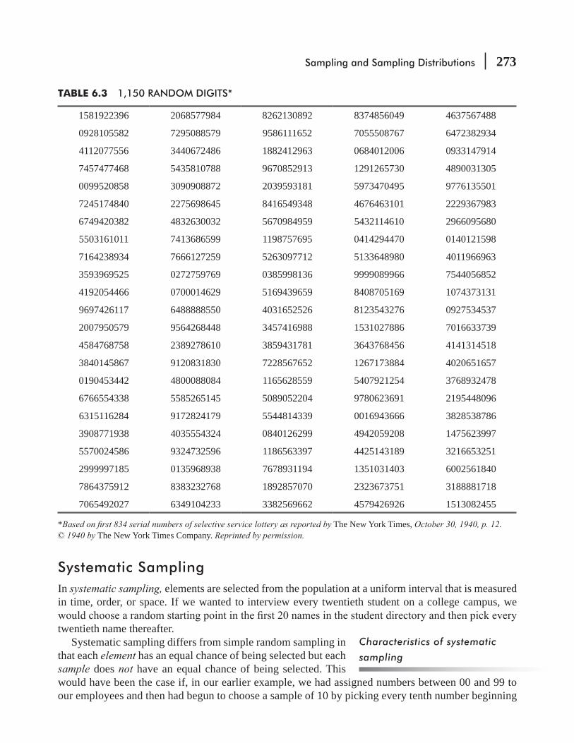
Sampling and Sampling Distributions 273
Systematic SamplingIn systematic sampling, elements are selected from the population at a uniform interval that is measured in time, order, or space. If we wanted to interview every twentieth student on a college campus, we
twentieth name thereafter.Systematic sampling differs from simple random sampling in
that each element has an equal chance of being selected but each sample does not have an equal chance of being selected. This would have been the case if, in our earlier example, we had assigned numbers between 00 and 99 to our employees and then had begun to choose a sample of 10 by picking every tenth number beginning
Characteristics of systematic
sampling
TABLE 6.3 1,150 RANDOM DIGITS*
1581922396 2068577984 8262130892 8374856049 4637567488
0928105582 7295088579 9586111652 7055508767 6472382934
4112077556 3440672486 1882412963 0684012006 0933147914
7457477468 5435810788 9670852913 1291265730 4890031305
0099520858 3090908872 2039593181 5973470495 9776135501
7245174840 2275698645 8416549348 4676463101 2229367983
6749420382 4832630032 5670984959 5432114610 2966095680
5503161011 7413686599 1198757695 0414294470 0140121598
7164238934 7666127259 5263097712 5133648980 4011966963
3593969525 0272759769 0385998136 9999089966 7544056852
4192054466 0700014629 5169439659 8408705169 1074373131
9697426117 6488888550 4031652526 8123543276 0927534537
2007950579 9564268448 3457416988 1531027886 7016633739
4584768758 2389278610 3859431781 3643768456 4141314518
3840145867 9120831830 7228567652 1267173884 4020651657
0190453442 4800088084 1165628559 5407921254 3768932478
6766554338 5585265145 5089052204 9780623691 2195448096
6315116284 9172824179 5544814339 0016943666 3828538786
3908771938 4035554324 0840126299 4942059208 1475623997
5570024586 9324732596 1186563397 4425143189 3216653251
2999997185 0135968938 7678931194 1351031403 6002561840
7864375912 8383232768 1892857070 2323673751 3188881718
7065492027 6349104233 3382569662 4579426926 1513082455
*Based on rst 834 serial numbers of selective service lottery as reported by The New York Times, October 30, 1940, p. 12. 1940 by The New York Times Company. Reprinted by permission.

274 Statistics for Management
1, 11, 21, 31, and so forth. Employees numbered 2, 3, 4, and 5 would have had no chance of being selected together.
In systematic sampling, there is the problem of introducing an error into the sample process. Suppose we were sampling paper waste produced by households, and we decided to sample 100 households every Monday. Chances are high that our sample would not be representative, because Monday’s trash would very likely include the Sunday newspaper. Thus, the amount of waste would be biased upward by our choice of this sampling procedure. So, if the population contains some periodic variation and the sampling interval coincides with periodicity then sample would be badly affected.
Systematic sampling has advantages, too, however. Even though systematic sampling may be inap-propriate when the elements lie in a sequential pattern, this method may require less time and sometimes results in lower costs than the simple random-sample method.
Stratified SamplingTo use strati ed sampling, we divide the population into rela-tively homogeneous groups, called strata. Then we use one of two approaches. Either we select at random from each stratum a
that stratum in the population as a whole or we draw an equal number of elements from each stratum and give weight to the results according to the stratum’s proportion of total population. With either approach,
already divided into groups of different sizes and we wish to acknowledge this fact. Suppose that a physician’s patients are divided into four groups according to age,
how many hours his patients sleep. To obtain an esti-mate of this characteristic of the population, he could take a random sample from each of the four age groups and give weight to the samples according to the percent-age of patients in that group. This would be an example
Cluster SamplingIn cluster sampling, we divide the population into groups, or clusters, and then select a random sample of these clusters. We assume that these individual clusters are representative of the population as a whole. If a market research team is attempting to determine by sampling the average number of televi-sion sets per household in a large city, they could use a city map to divide the territory into blocks and then choose a certain number of blocks (clusters) for interviewing. Every household in each of these blocks would be interviewed. A well-designed cluster sampling procedure can produce a more precise sample at considerably less cost than that of simple random sampling.
Shortcomings of systematic
sampling
Two ways to take stratified
samples
When to use stratified sampling
TABLE 6-4 COMPOSITION OF PATIENTS BY AGE
Age Group Percentage of TotalBirth–19 years20–39 years40–59 years60 years and older
30402010
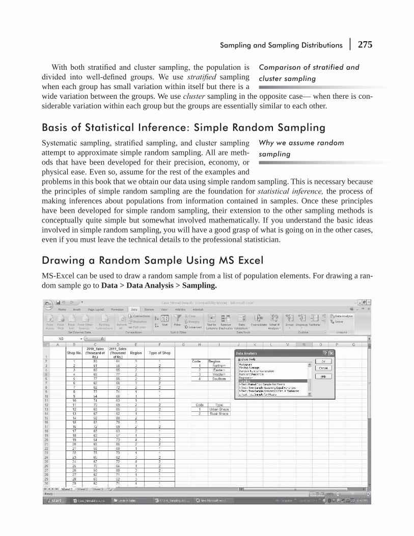
Sampling and Sampling Distributions 275
strati ed sampling when each group has small variation within itself but there is a wide variation between the groups. We use cluster sampling in the opposite case— when there is con-siderable variation within each group but the groups are essentially similar to each other.
Basis of Statistical Inference: Simple Random Sampling
attempt to approximate simple random sampling. All are meth-ods that have been developed for their precision, economy, or physical ease. Even so, assume for the rest of the examples and problems in this book that we obtain our data using simple random sampling. This is necessary because the principles of simple random sampling are the foundation for statistical inference, the process of making inferences about populations from information contained in samples. Once these principles have been developed for simple random sampling, their extension to the other sampling methods is conceptually quite simple but somewhat involved mathematically. If you understand the basic ideas involved in simple random sampling, you will have a good grasp of what is going on in the other cases, even if you must leave the technical details to the professional statistician.
Drawing a Random Sample Using MS ExcelMS-Excel can be used to draw a random sample from a list of population elements. For drawing a ran-dom sample go to Data > Data Analysis > Sampling.
Why we assume random
sampling
Comparison of stratified and
cluster sampling

276 Statistics for Management
When the Sampling dialogue-box opens, enter the range of population elements into Input Range, check Random option button under Sampling Method and enter desired sample-size. Pressing OK will give you the desired random sample.
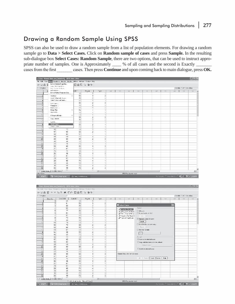
Sampling and Sampling Distributions 277
Drawing a Random Sample Using SPSSSPSS can also be used to draw a random sample from a list of population elements. For drawing a random sample go to Data > Select Cases. Click on Random sample of cases and press Sample. In the resulting sub-dialogue box Select Cases: Random Sample, there are two options, that can be used to instruct appro-priate number of samples. One is Approximately ____ % of all cases and the second is Exactly _______
Continue and upon comimg back to main dialogue, press OK.

278 Statistics for Management
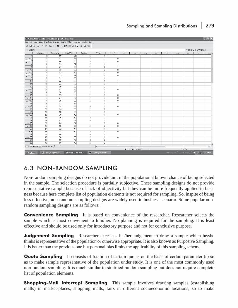
Sampling and Sampling Distributions 279
6.3 NON-RANDOM SAMPLINGNon-random sampling designs do not provide unit in the population a known chance of being selected in the sample. The selection procedure is partially subjective. These sampling designs do not provide representative sample because of lack of objectivity but they can be more frequently applied in busi-ness because here complete list of population elements is not required for sampling. So, inspite of being less effective, non-random sampling designs are widely used in business scenario. Some popular non-random sampling designs are as follows:
Convenience Sampling It is based on convenience of the researcher. Researcher selects the sample which is most convenient to him/her. No planning is required for the sampling. It is least effective and should be used only for introductory purpose and not for conclusive purpose.
Judgement Sampling Researcher excesises his/her judgement to draw a sample which he/she thinks is representative of the population or otherwise appropriate. It is also known as Purposive Sampling. It is better than the previous one but personal bias limits the applicability of this sampling scheme.
Quota Sampling as to make sample representative of the population under study. It is one of the most commonly used
list of population elements.
Shopping-Mall Intercept Sampling This sample involves drawing samples (establishing malls) in market-places, shopping malls, fairs in different socioeconomic locations, so to make
280 Statistics for Management
sample representative of the population. This scheme is very popular because of convenience and representativeness.
Snowball Sampling Here, initial respondents are selected randomly then additional respondents are selected by their referrals and so on. This scheme is also known as Multiplicity Sampling. It is useful for rare population.
Warning: Even when precautions are taken, many so-called random samples are still not ran-dom. When you try to take a random sample of mall shoppers, you get a biased sample because many people are not willing to take the time to stop to talk to the interviewer. Nowadays, when telephone pollers try to take a random sample, often they don’t get through to people with call-screening devices on their phones. There are ways to counter these problems in random sam-
wants to face.
HINTS & ASSUMPTIONS
EXERCISES 6.2
Self-Check ExercisesSC 6-1 If we have a population of 10,000 and we wish to sample 20 randomly, use the random digits
table (Table 6-3) to select 20 individuals from the 10,000. List the numbers of the elements selected, based on the random digits table.
SC 6-2 A parliamentary study on the issue of self-rule for the District of Chandigarh involved sur-veying 2,000 people from the population of the city regarding their opinions on a number of issues related to self-rule. Chandigarh is a city in which many neighborhoods are poor and many neighborhoods are rich, with very few neighborhoods falling between the extremes. The researchers who were administering the survey had reasons to believe that the opinions expressed on the various questions would be highly dependent on income. Which method was
Basic Concepts6-8 In the examples below, probability distributions for three natural subgroups of a larger popula-
(a) (b)
6-9 We wish to sample 15 pages from this textbook. Use the random digits table (Table 6-3) to select 15 pages at random and count the number of words in italics on each page. Report your results.
Sampling and Sampling Distributions 281
6-10 Using a calendar, systematically sample every eighteenth day of the year, beginning with January 6.
6-11 A population is made up of groups that have wide variation within each group but little varia-tion from group to group. The appropriate type of sampling for this population is
(b) Systematic.(c) Cluster.(d) Judgment.
6-12 Consult Table 6-3. What is the probability that a 4 will appear as the leftmost digit in each set of 10 digits? That a 7 will appear? 2? How many times would you expect to see each of these digits in the leftmost position? How many times is each found in that position? Can you explain any differences in the number found and the number expected?
Applications6-13 The local cable television company is planning to add one channel to its basic service. There
There are about 20,000 subscribers, and the company knows that 35 percent of these are col-lege students, 45 percent are white-collar workers, 15 percent are blue-collar workers, and 5 percent are other. However, the company believes there is much variation within these groups.
or cluster sampling?6-14
centers. The organization has devised a scheme for random sampling of houses, and plans to conduct the poll on weekdays from noon to 5 P.M. Will this scheme produce a random sample?
6-15 Mohan Adhikari, public relations manager for Piedmont Power and Light, has implemented an institutional advertising campaign to promote energy consciousness among its custom-ers. Adhikari, anxious to know whether the campaign has been effective, plans to conduct a telephone survey of area residents. He plans to look in the telephone book and select random numbers with addresses that correspond to the company’s service area. Will Adhikari’s sample be a random one?
6-16 At the India Government Mints in Mumbai, 10 machines stamp out ` 10 coins in lots of 50. These lots are arranged sequentially on a single conveyor belt, which passes an inspection station. An inspector decides to use systematic sampling in inspecting the ` 10 coins and is
` 10 coins. Which is better? Why?
6-17 The state occupational safety board has decided to do a study of work-related accidents within the state, to examine some of the variables involved in the accidents, such as the type of job, the cause of the accident, the extent of the injury, the time of day, and whether the employer was negligent. It has been decided that 250 of the 2,500 work-related accidents reported last
Marsha Gulley, a department employee, has proposed that the study use a systematic sampling
sampling be appropriate here? Explain.
282 Statistics for Management
Worked-Out Answers to Self-Check ExercisesSC 6-1 Starting at the top of the third column and choosing the last 4 digits of the numbers in that
column gives the following sample (reading across rows):
892 1652 2963 2913 3181 9348 49597695 7712 8136 9659 2526 6988 17817652 8559 2204 4339 6299 3397
SC 6-2 -similar groups, which probably have smaller variation within each group than between groups.
6.4 DESIGN OF EXPERIMENTSWe encountered the term experiment in Chapter 4, “Probability
event as one or more of the possible outcomes of doing something, and an experiment as an activity that would produce such events. In a coin-toss experiment, the possible events are heads and tails.
Planning ExperimentsIf we are to conduct experiments that produce meaningful results in the form of usable conclusions, the way in which these experi-ments are designed is of the utmost importance. Sections 6.1 and 6.2 discussed ways of ensuring that random sampling was indeed being done. The way in which sampling is conducted is only a part of the total design of an experiment. In fact, the design of experiments is itself the subject of quite a number of books, some of them rather formidable in both scope and volume.
Phases of Experimental DesignTo get a better feel for the complexity of experimental design without actually getting involved with the complex details, take an example from the many that confront us every day, and follow that example through from beginning to end.
The statement is made that a Crankmaster battery will start your car’s engine better than Battery X. Crankmaster might design its experiment in the following way.
Objective This is our beginning point. Crankmaster wants to test its battery against the leading competitor. Although it is possible to design an experiment that would test the two batteries on several characteristics (life, size, cranking power, weight, and cost, to name but a few), Crankmaster has decided to limit this experiment to cranking power.
Events and experiments
revisited
Sampling is only one part
A claim is made
Objectives are set

Sampling and Sampling Distributions 283
What Is to Be Measured This is often called the response variable. If Crankmaster is to design an experiment that compares
how cranking power is to be measured. Again, there are quite a few ways in which this can be done. For example, Crankmaster could measure the time it took for the batteries to run down completely while cranking engines, the total number of engine starts it took to run down the batteries, or the number of months in use that the two batteries could be expected to last. Crankmaster decides that the response variable in its experiment will be the time it takes for batteries to run down completely while cranking engines.
How Large a Sample Size Crankmaster wants to be sure that it chooses a sample size large enough to support claims it makes for its battery, without fear of being challenged; however, it knows that the more batteries it tests, the higher the cost of conducting the experiment. As we shall point out in Section 6 of this chapter, there is a diminishing return in sampling; and although sampling
a sample size that is too expensive to contend with, Crankmaster decides that comparing 10 batteries
Conducting the Experiment Crankmaster must be careful to conduct its experiment under controlled conditions; that is, it has to be sure that it is measuring cranking power, and that the other variables (such as temperature, age of engine, and condition of battery cables, to name only a few) are held as nearly constant as practicable. In an effort to accomplish just this, Crankmaster’s statistical group uses new cars of the same make and model, conducts the tests at the same outside air temperature, and is careful to be quite precise in measuring the time variable. Crankmaster gathers experimental data on the performance of the 20 batteries in this manner.
Analyzing the Data Data on the 20 individual battery tests are subjected to hypothesis testing in the same way that we shall see in Chapter 9, “Testing Hypotheses: Two-Sample
of its battery and that of its competitor. It turns out that the difference between the mean cranking life of Crankmaster’s battery and that of its competitor isthis experiment into its advertising.
Reacting to Experimental ClaimsHow should we, as consumers, react to Crankmaster’s new battery-life claims in its latest advertising? Should we conclude from the tests it has run that the Crankmaster battery is superior to the competitive battery? If we stop for a moment to consider the nature of the experiment, we may not be so quick to come to such a conclusion.
How do we know that the ages and conditions of the cars’ engines in the experiment were identical? And are we absolutely
How many to test
Experimental conditions are
kept constant
Data are analyzed
How should the consumer
react?
Are we sure?
The response variable is
selected
284 Statistics for Management
sure that the battery’s cables were identical in size and resistance to current? And what about air temper-atures during the tests: Were they the same? These are the normal kinds of questions that we should ask.
How should we react to the statement, if it is made, that “we subjected the experimental results to extensive statistical testing”? The answer to that will have to wait until Chapter 9, where we can deter-mine whether such a difference in battery lives is too large to be attributed to chance. At this point, we, as consumers, need to be appropriately skeptical.
Other Options OpenOf course, Crankmaster would have had the same concerns we did, and in all likelihood would not -tising claims solely on the basis of the experimental design we have just described. One possible course of action to avoid criti-cism is to ensure that all variables except the one being measured have indeed been controlled. Despite the care taken to produce such controlled conditions, it turns out that these overcontrolled experiments do not really solve our problem. Normally, instead of investing resources in attempts to eliminate exper-imental variations, we choose a completely different route. The next few paragraphs show how we can accomplish this.
Factorial ExperimentsIn the Crankmaster situation, we had two batteries (let’s refer to them now as A and B) and three test conditions that were of some concern to us: temperature, age of the engine, and condition of the battery cable. Let’s introduce the notion of factorial experi-ments by using this notation:
H = hot temperature N = new engine G = good cable
C = cold temperature O = old engine W = worn cable
temperature conditions and, for that matter, more than two cat-egories for engine condition and battery-cable condition. But it’s
Now, because there are two batteries, two temperature possibilities, two engine condition possibili-ties, and two battery-cable possibilities, there are 2 × 2 × 2 × 2 = 16 possible combinations of factors. If we wanted to write these sixteen possibilities down, they would look like Table 6-5.
Having set up all the possible combinations of factors involved in this experiment, we could now conduct the 16 tests in the table, if we did this, we would have conducted a complete facto-rial experiment, because each of the two levels of each of the four factors would have been used once with each possible combination of other levels of other factors. Designing the experiment this way would permit us to use techniques we shall introduce in Chapter 11, “Chi-Square and Analysis of Variance,” to test the effect of each of the factors.
We need to point out, before we leave this section, that in an actual experiment we would hardly conduct the tests in the order in which they appear in the table. They were arranged in that
Another route for Crankmaster
Handling all test conditions at
the same time
How many combinations?
Randomizing
Levels and factors to be
handled

Sampling and Sampling Distributions 285
order to facilitate your counting the combinations and determining that all possible combinations were indeed represented. In actual practice, we would randomize the order of the tests, perhaps by putting 16 numbers in a hat and drawing out the order of the experiment in that simple manner.
Being More Efficient in Experimental DesignAs you saw from our four-factor experiment, 16 tests were required to compare all levels with all factors. If we were to
temperature, four measures of engine condition, and three measures of battery-cable condition, it would take 2 × 5 × 4 × 3 = 120 tests for a complete factorial experiment.
Fortunately, statisticians have been able to help us reduce the number of tests in cases like this. To illustrate how this works, look at a consumer-products company that wants to test market a new tooth-paste in four different cities with four different kinds of packages and with four different advertising programs. In such a case, a complete factorial experiment would take 4 × 4 × 4 = 64 tests. However, if we do some clever planning, we can actually do it with far fewer tests—16, to be precise.Let’s use the notation:
A = City 1 I = Package 1 1 = Ad program 1
B = City 2 II = Package 2 2 = Ad program 2
C = City 3 III = Package 3 3 = Ad program 3
D = City 4 IV = Package 4 4 = Ad program 4
A bit of efficiency
TABLE 6-5 SIXTEEN POSSIBLE COMBINATIONS OF FACTORS FOR BATTERY TEST
Test Battery Temperature Engine Condition Cable Condition 1 A H N G 2 A H N W 3 A H O G 4 A H O W 5 A C N G 6 A C N W 7 A C O G 8 A C O W 9 B H N G10 B H N W11 B H O G12 B H O W13 B C N G14 B C N W15 B C O G16 B C O W

286 Statistics for Management
Now we arrange the cities, packages, and advertising pro-grams in a design called a Latin square (Figure 6-1).
In the experimental design represented by the Latin square, we would need only 16 tests instead of 64 as originally calculated. Each combination of city, package, and advertising program would be represented in the 16 tests. The actual statistical analy-sis of the data obtained from such a Latin square experimental design would require a form of analysis of variance a bit beyond the scope of this book.
6.5 INTRODUCTION TO SAMPLING DISTRIBUTIONSIn Chapter 3, we introduced methods by which we can use sam-ple data to calculate statistics such as the mean and the standard deviation. So far in this chapter, we have examined how samples can be taken from populations. If we apply what we have learned and take several samples from a population, the statistics we would compute for each sample need not be the same and most probably would vary from sample to sample.
Suppose our samples each consist of ten 25-year-old women
according to our usage). By computing the mean height and stan-dard deviation of that height for each of these samples, we would quickly see that the mean of each sample and the standard deviation of each sample would be different. A probability distribution of all the possible means of the samples is a distribution of the sample means. Statisticians call this a sampling distribution of the mean.
We could also have a sampling distribution of a proportion. Assume that we have determined the proportion of beetle-infested pine trees in samples of 100 trees taken from a very large forest. We have taken a large number of those 100-item samples. If we plot a probability distribution of the possible pro-portions of infested trees in all these samples, we would see a distribution of the sample proportions. In statistics, this is called a sampling distribution of the proportion. (Notice that the term proportion refers
distribution of sample statistic values, obtained from all possible samples.
Describing Sampling DistributionsAny probability distribution (and, therefore, any sampling distribution) can be partially described by its mean and standard deviation. Table 6-6 illustrates several populations. Beside each, we have indicated the sample taken from that population, the sample statistic we have measured, and the sampling distri-bution that would be associated with that statistic.
the sampling distribution of the mean can be partially described by its mean and standard deviation. The sampling distribution of the median in the second example can be partially described by the mean and standard deviation of the distribution of the medians. And in the third, the sampling distribution of the proportion can be partially described by the mean and standard deviation of the distribution of the proportions.
The statistical analysis
Statistics differ among samples
from the same population
Sampling distribution defined
Advertising program
1
I
II
III
IV
2 3 4
Pack
age
City
C B D A
B C A D
D A B C
A D C B
FIGURE 6-1 A LATIN SQUARE
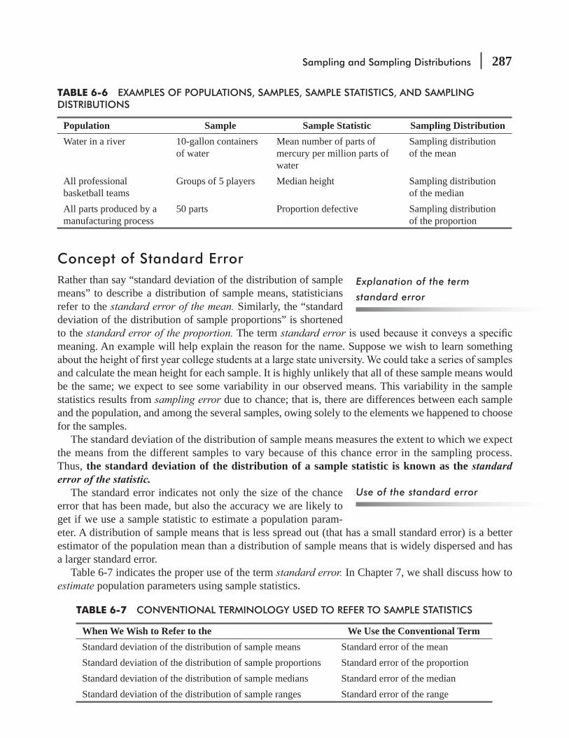
Sampling and Sampling Distributions 287
Concept of Standard ErrorRather than say “standard deviation of the distribution of sample means” to describe a distribution of sample means, statisticians refer to the standard error of the mean. Similarly, the “standard deviation of the distribution of sample proportions” is shortened to the standard error of the proportion. The term standard errormeaning. An example will help explain the reason for the name. Suppose we wish to learn something
and calculate the mean height for each sample. It is highly unlikely that all of these sample means would be the same; we expect to see some variability in our observed means. This variability in the sample statistics results from sampling error due to chance; that is, there are differences between each sample and the population, and among the several samples, owing solely to the elements we happened to choose for the samples.
The standard deviation of the distribution of sample means measures the extent to which we expect the means from the different samples to vary because of this chance error in the sampling process. Thus, the standard deviation of the distribution of a sample statistic is known as the standard error of the statistic.
The standard error indicates not only the size of the chance error that has been made, but also the accuracy we are likely to get if we use a sample statistic to estimate a population param-eter. A distribution of sample means that is less spread out (that has a small standard error) is a better estimator of the population mean than a distribution of sample means that is widely dispersed and has a larger standard error.
Table 6-7 indicates the proper use of the term standard error. In Chapter 7, we shall discuss how to estimate population parameters using sample statistics.
Explanation of the term
standard error
Use of the standard error
TABLE 6-6 EXAMPLES OF POPULATIONS, SAMPLES, SAMPLE STATISTICS, AND SAMPLING DISTRIBUTIONS
Population Sample Sample Statistic Sampling DistributionWater in a river 10-gallon containers
of waterMean number of parts of mercury per million parts of water
Sampling distribution of the mean
All professional basketball teams
Groups of 5 players Median height Sampling distribution of the median
All parts produced by a manufacturing process
50 parts Proportion defective Sampling distribution of the proportion
TABLE 6-7 CONVENTIONAL TERMINOLOGY USED TO REFER TO SAMPLE STATISTICS
When We Wish to Refer to the We Use the Conventional TermStandard deviation of the distribution of sample means Standard error of the meanStandard deviation of the distribution of sample proportions Standard error of the proportionStandard deviation of the distribution of sample medians Standard error of the medianStandard deviation of the distribution of sample ranges Standard error of the range

288 Statistics for Management
Understanding sampling distributions allows statisticians to take samples that are both meaning-ful and cost-effective. Because large samples are very expensive to gather, decision makers should always aim for the smallest sample that gives reliable results. In describing distributions, statisti-cians have their own shorthand, and when they use the term standard error to describe a distribu-tion, they are referring to the distribution’s standard deviation. Instead of saying “the standard deviation of the distribution of sample means” they say “the standard error of the mean.” Hint: The standard error indicates how spread-out (dispersed) the means of the samples are. Warning: Although the standard error of the mean and the population standard deviation are related to each other, as we shall soon see, it is important to remember that they are not the same thing.
HINTS & ASSUMPTIONS
EXERCISES 6.3
Self-Check ExercisesSC 6-3 -
and found the sample mean to be 130. The quality control manager assumed the sample must not be representative. Is the conclusion correct?
SC 6-4 The president of the American Dental Association wants to determine the average number of
-ings per day to the ADA. These numbers are computed and submitted to the president. Has he been given a sample from the population of patients or from some other distribution?
Basic Concepts6-18 Suppose you are sampling from a population with a mean of 2.15. What sample size will
guarantee that(a) The sample mean is 2.15?(b) The standard error of the mean is zero?
6-19 The term error, in standard error of the mean, refers to what type of error?
Applications6-20 You recently purchased a box of raisin bran and measured the number of raisins. The company
claims that the number of raisins per box is 2.0 cups on average, with a standard deviation of 0.2 cup. Your box contained only 1.9 cups. Could the company’s claim be correct?
6-21 A woman working for Nielsen ratings service interviews passersby on a New Delhi street and records each subject’s estimate of average time spent viewing prime-time television per night. These interviews continue for 20 days, and at the end of each day, the interviewer computes the mean time spent viewing among all those interviewed during the day. At the conclusion of all interviews, she constructs a frequency distribution for these daily means. Is this a sampling distribution of the mean? Explain.

Sampling and Sampling Distributions 289
6-22 Rehana Ali, a marketing analyst for the Star Cola Company (SCC), wants to assess the damage done to SCC’s sales by the appearance of a new competitor. Accordingly, she has
appearance. Rehana has graphed the corresponding frequency distributions as follows:
4
8
12
16
20
24
28
Freq
uenc
y
4
8
12
16
20
24
28
Freq
uenc
y
1 2 3 4 5 6Thousands of cartons sold/week
1 2 3 4 5 6Thousands of cartons sold/week
Before After
Based on these graphs, what has been the effect of the competitor’s appearance on average weekly sales?
6-23 randomly selected 50 regional managers to survey customers. Each manager randomly selects 5 supervisors to randomly survey 30 customers. The surveys are conducted and results are computed and sent to the CEO. What type of distribution did the sample come from?
Worked-Out Answers to Self-Check ExercisesSC 6-3 No. The mean of a sample usually does not exactly equal the population mean because of
sampling error.SC 6-4
single patients, so it is a sample from the sampling distribution of the mean of samples of size 50 drawn from the patient population. It is not a sample from the patient population.
6.6 SAMPLING DISTRIBUTIONS IN MORE DETAILIn Section 6.4, we introduced the idea of a sampling distribution. We examined the reasons why sam-pling from a population and developing a distribution of these sample statistics would produce a sam-pling distribution, and we introduced the concept of standard error. Now we will study these concepts further, so that we will not only be able to understand them conceptually, but also be able to handle them computationally.
Conceptual Basis for Sampling DistributionsFigure 6-2 will help us examine sampling distributions without delving too deeply into statistical theory. We have divided this
Deriving the sampling
distribution of the mean

290 Statistics for Management
illustration into three parts. Figure 6-2(a) illustrates a population distribution. Assume that this popula-
operating hours before a screen becomes clogged. The distribution of operating hours has a mean m. (mu) and a standard deviation s (sigma).
Suppose that somehow we are able to take all the possible samples of 10 screens from the population distribution (actually, there would be far too many for us to consider). Next we would calculate the mean and the standard deviation for each one of these samples, as represented in Figure 6-2(b). As a result, each sample would have its own mean, x (x bar), and its own standard deviation, s. All the individual
The population distribution:
The sample frequency distribution:
The sampling distribution of the mean:
This distribution is the distributionof the operating hours of all thefilter screens. It has:
μ = the mean of this distribution
σ = the standard deviation of this distribution
These only represent the enormousnumber of sample distributions possible.Each sample distribution is a discretedistribution and has:
= its own mean, called “x bar”x
= its own standard deviation
x x x x
This distribution is the distributionof all the sample means and has:
= mean of the sampling distribution of the means, called “mu sub x bar”
= standard error of the mean (standard deviation of the sampling distribution of the mean), called “sigma sub x bar”
μx
μx
σx
sNow, if we were able to take the means from all thesample distributions and produce a distribution ofthese sample means, it would look like this:
If somehow we were able to take all the possible samplesof a given size from this population distribution, theywould be represented graphically by these four samplesbelow. Although we have shown only four such samples,there would actually be an enormous number of them.
μ
(a)
(b)
(c)
FIGURE 6-2 CONCEPTUAL POPULATION DISTRIBUTION, SAMPLE DISTRIBUTIONS, AND SAMPLING DISTRIBUTION

Sampling and Sampling Distributions 291
sample means would not be the same as the population mean. They would tend to be near the population mean, but only rarely would they be exactly that value.
As a last step, we would produce a distribution of all the means from every sample that could be taken. This distribution, called the sampling distribution of the mean, is illustrated in Figure 6-2(c). This distribution of the sample means (the sam-pling distribution) would have its own mean, μx
(mu sub x bar), and its own standard deviation, or standard error, σ x (sigma sub x bar).
In statistical terminology, the sampling distribution we would obtain by taking all the samples of a given size is a theoretical sampling distribution. Figure 6-2(c) describes such an example. In practice, the size and character of most populations prohibit decision makers from taking all the possible samples from a population distribution. Fortunately, statis-ticians have developed formulas for estimating the characteristics of these theoretical sampling distribu-tions, making it unnecessary for us to collect large numbers of samples. In most cases, decision makers take only one sample from the population, calculate statistics for that sample, and from those statistics infer something about the parameters of the entire population. We shall illustrate this shortly.
In each example of sampling distributions in the remainder of this chapter, we shall use the sampling distribution of the mean. We could study the sampling distributions of the median, range, or proportion, but we will stay with the mean for the continuity it will add to the explanation. Once you develop an understanding of how to deal compu-tationally with the sampling distribution of the mean, you will be able to apply it to the distribution of any other sample statistic.
Sampling from Normal PopulationsSuppose we draw samples from a normally distributed popula-tion with a mean of 100 and standard deviation of 25, and that we
101, and so on. Obviously, there is just as much chance for the sample mean to be above the population mean of 100 as there is for it to be below 100. Because we are averagingand very small values up. We would reason that we would get less spread among the sample means than we would among the individual items in the original population. That is the same as saying that the standard error of the mean, or standard deviation of the sampling distribution of the mean, would be less than the standard deviation of the individual items in the population. Figure 6-3 illustrates this point graphically.
Now suppose we increase our sample size from 5 to 20. This would not change the standard devia-tion of the items in the original population. But with samples of 20, we have increased the effect of averaging in each sample and would expect even less dispersion among the sample means. Figure 6-4 illustrates this point.
The sampling distribution of a mean of a sample taken from a normally distributed population demonstrates the important properties summarized in Table 6-8. An example will further
The sampling distribution of
the mean
Function of theoretical sampling
distributions
Why we use the sampling
distribution of the mean
Sampling distribution of the
mean from normally distributed
populations
Properties of the sampling
distribution of the mean

292 Statistics for Management
Sampling distributionof the mean withsamples of 5 (n = 5).σx is less than 25.
Sampling distribution of the meanwith samples of 20 (n = 20).σx is much less than 25.
Distribution of the items inthe population. σ = 25.
μ100
FIGURE 6-4 RELATIONSHIP BETWEEN THE POPULATION DISTRIBUTION AND SAMPLING DISTRIBUTION OF THE MEAN WITH INCREASING n’s
TABLE 6-8 PROPERTIES OF THE SAMPLING DISTRIBUTION OF THE MEAN WHEN THE POPULATION IS NORMALLY DISTRIBUTED
Property Illustrated Symbolically
The sampling distribution has a mean equal to the population mean μ μ=x
The sampling distribution has a standard deviation (a standard error) equal to the population standard deviation divided by the square root of the sample size
σ σ=
nx
Sampling distribution of themean with samples of 5 (n = 5).σx is less than 25.
Distribution of the itemsin the population. σ =25.
μ100
FIGURE 6-3 RELATIONSHIP BETWEEN THE POPULATION DISTRIBUTION AND THE SAMPLING DISTRIBUTION OF THE MEAN FOR A NORMAL POPULATION
illustrate these properties. A bank calculates that its individual savings accounts are normally distrib-uted with a mean of $2,000 and a standard deviation of $600. If the bank takes a random sample of 100 accounts, what is the probability that the sample mean will lie between $1,900 and $2,050? This is
error of the mean. In this case, we shall use the equation for the standard error of the mean designed for s):
Sampling and Sampling Distributions 293
Standard Error of the Mean for Infinite Populations
σ σ=
nx
Standard error of the mean [6-1]
where
σ = population standard deviation n = sample size
Applying this to our example, we get$600
100σ =x
$600
10=
=
Next, we need to use the table of z values (Appendix Table 1) and Equation 5-6, which enables us to use the Standard Normal Probability Distribution Table. With these, we can determine the probability that the sample mean will lie between $1,900 and $2,050.
μσ
=−
zx [5-6]
Equation 5-6 tells us that to convert any normal random variable to a standard normal random vari-able, we must subtract the mean of the variable being standardized and divide by the standard error (the standard deviation of that variable). Thus, in this particular case. Equation 5-6 becomes
Standardizing the Sample Mean
zx
x
μσ
=−
Sample mean Population mean
Standard error of the mean =
n
σ
[6-2]
Now we are ready to compute the two z values as follows:For x = $1,900:
μσ
=−
zx
x [6-2]
$1,900 $2,000
$60=
−
100
60= −
1.67= − ← Standard deviations from the mean of a stan-dard normal probability distribution
Finding the standard error
of the mean for infinite
populations
Converting the sample mean to
a z value

294 Statistics for Management
For x = $2,050
zx
x
μσ
=−
[6-2]
$2,050 $2,000
$60=
−
50
60=
= Standard deviation from the mean of a standard normal probability distribution
Appendix Table 1 gives us an area of 0.4525 corresponding to a z value of –1.67, and it gives an area of .2967 for a z value of .83. If we add these two together, we get 0.7492 as the total probability that the sample mean will lie between $1,900 and $2,050. We have shown this problem graphically in Figure 6-5.
Sampling from Nonnormal PopulationsIn the preceding section, we concluded that when the population is normally distributed, the sampling distribution of the mean is also normal. Yet decision makers must deal with many populations that are not normally distributed. How does the sampling distribution of the mean react when the population from which the samples are drawn is not normal? An illustration will help us answer this question.
involved, the population is too small to be approximated by a normal distribution. We’ll take all of the possible samples of the owners in groups of three, compute the sample means ( ),x list them, and compute the mean of the sampling distribution ( ).μx We have done this in Table 6-10. These calculations show that even in a case in which the population is not normally distributed, ,μx the mean of the sampling distribution, is still equal to the population mean, m.
The mean of the sampling
distribution of the mean equals
the population mean
Area between themean and a z of–1.67 = 0.4525
Area between themean and a z of0.83 = 0.2967
Total shadedarea = 0.7492
$1,900 $2,050μ
FIGURE 6-5 PROBABILITY OF SAMPLE MEAN LYING BETWEEN $1,900 AND $2,050

Sampling and Sampling Distributions 295
TABLE 6-9 EXPERIENCE OF FIVE MOTORCYCLE OWNERS WITH LIFE OF TIRES
OWNER Carl Debbie Elizabeth Frank GeorgeTIRE LIFE (MONTHS) 3 3 7 9 14 Total: 36 months
Mean = 36
5 = 7.2 months
-cycle owners, a distribution that is anything, but normal in shape. In Figure 6-6(b), we show the sam-pling distribution of the mean for a sample size of three, taking the information from Table 6-10. Notice the difference between the probability distributions in Figures 6-6(a) and 6-6(b). In Figure 6-6(b), the distribution looks a little more like the bell shape of the normal distribution.
TABLES 6-10 CALCULATION OF SAMPLE MEAN TIRE LIFE WITH n = 3
Samples of Three Sample Data (Tire Lives) Sample Mean
EFG* 7 + 9 + 14 10DFG 3 + 9 + 14DEG 3 + 7 + 14 8DEF 3 + 7 + 9CFG 3 + 9 + 14 CEG 3 + 7 + 14 8CEF 3 + 7 + 9CDF 3 + 3 + 9 5CDE 3 + 3 + 7CDG 3 + 3 + 14
72 months
72
10μ =x
= 7.2 months
3
Tire life in months Tire life in months
6 9 12 15 2 4 6 8 10
Prob
abili
ty
Prob
abili
ty
(a) Population distribution (b) Sampling distribution of the mean
FIGURE 6-6 POPULATION DISTRIBUTION AND SAMPLING DISTRIBUTION OF THE MEAN TIRE LIFE
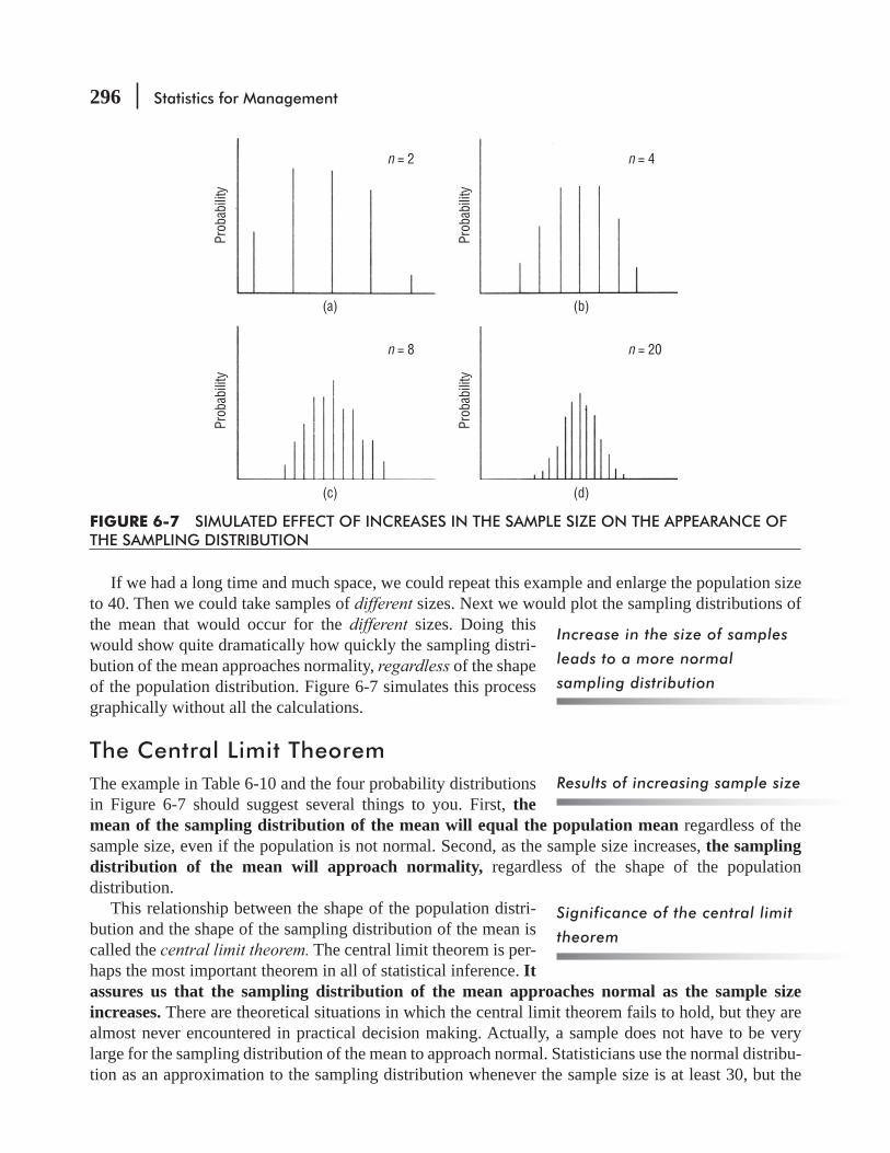
296 Statistics for Management
If we had a long time and much space, we could repeat this example and enlarge the population size to 40. Then we could take samples of different sizes. Next we would plot the sampling distributions of the mean that would occur for the different sizes. Doing this would show quite dramatically how quickly the sampling distri-bution of the mean approaches normality, regardless of the shape of the population distribution. Figure 6-7 simulates this process graphically without all the calculations.
The Central Limit TheoremThe example in Table 6-10 and the four probability distributions in Figure 6-7 should suggest several things to you. First, the mean of the sampling distribution of the mean will equal the population mean regardless of the sample size, even if the population is not normal. Second, as the sample size increases, the sampling distribution of the mean will approach normality, regardless of the shape of the population distribution.
This relationship between the shape of the population distri-bution and the shape of the sampling distribution of the mean is called the central limit theorem. The central limit theorem is per-haps the most important theorem in all of statistical inference. It assures us that the sampling distribution of the mean approaches normal as the sample size increases. There are theoretical situations in which the central limit theorem fails to hold, but they are almost never encountered in practical decision making. Actually, a sample does not have to be very large for the sampling distribution of the mean to approach normal. Statisticians use the normal distribu-tion as an approximation to the sampling distribution whenever the sample size is at least 30, but the
Increase in the size of samples
leads to a more normal
sampling distribution
Results of increasing sample size
Significance of the central limit
theorem
Prob
abili
ty
Prob
abili
ty
Prob
abili
ty
Prob
abili
ty
(a) (b)
(c) (d)
n = 2 n = 4
n = 8 n = 20
FIGURE 6-7 SIMULATED EFFECT OF INCREASES IN THE SAMPLE SIZE ON THE APPEARANCE OF THE SAMPLING DISTRIBUTION

Sampling and Sampling Distributions 297
sampling distribution of the mean can be nearly normal with samples of even half that size. -cance of the central limit theorem is that it permits us to use sample statistics to make inferences about population parameters without knowing anything about the shape of the frequency distri-bution of that population other than what we can get from the sample. Putting this ability to work is the subject of much of the material in the subsequent chapters of this book.
Let’s illustrate the use of the central limit theorem. The dis-
experience is skewed negatively, as shown in Figure 6-8(a). This distribution has a mean of $19,000 and a standard deviation of $2,000. If we draw a random sample of 30 tellers, what is the probability that their earnings will average more than $19,750 annually? In Figure 6-8(b), we show the sampling distribution of the mean that would result, and we have colored the area representing “earnings over $19,750.”
as follows
σ σ=
nx [6-1]
$2,000
30=
$2,000
5.477=
=
Because we are dealing with a sampling distribution, we must now use Equation 6-2 and the Standard Normal Probability Distribution (Appendix Table 1).
For x = $19,750:
μ
σ=
−z
x
x
[6-2]
$19,750 $19,000
$365.16=
−
Using the central limit theorem
(a) (b)
σ = $2,000
μ = $19,000 $19,000 $19,750
0.5000 0.4798
μx
σx = $365.16
2.05σx
FIGURE 6-8 POPULATION DISTRIBUTION AND SAMPLING DISTRIBUTION FOR BANK TELLERS’ EARNINGS
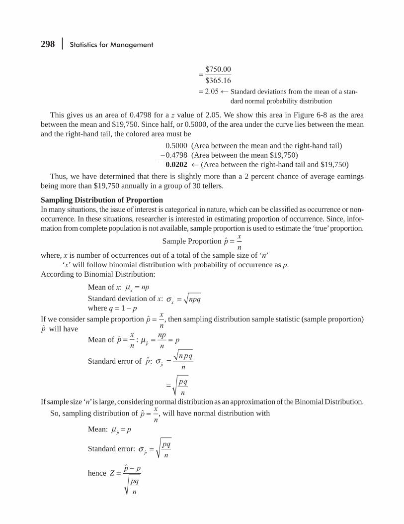
298 Statistics for Management
$750.00
$365.16=
= Standard deviations from the mean of a stan-dard normal probability distribution
This gives us an area of 0.4798 for a z value of 2.05. We show this area in Figure 6-8 as the area between the mean and $19,750. Since half, or 0.5000, of the area under the curve lies between the mean and the right-hand tail, the colored area must be 0.5000 (Area between the mean and the right-hand tail) – 0.4798 (Area between the mean $19,750) 0.0202 ← (Area between the right-hand tail and $19,750)
Thus, we have determined that there is slightly more than a 2 percent chance of average earnings being more than $19,750 annually in a group of 30 tellers.
Sampling Distribution of Proportion
occurrence. In these situations, researcher is interested in estimating proportion of occurrence. Since, infor-mation from complete population is not available, sample proportion is used to estimate the ‘true’ proportion.
Sample Proportion ˆ =px
nwhere, x is number of occurrences out of a total of the sample size of ‘n’ ‘x’ will follow binomial distribution with probability of occurrence as p.According to Binomial Distribution:
Mean of x: μ = npx
Standard deviation of x: σ = npqxwhere q = 1 – p
If we consider sample proportion ˆ =px
n, then sampling distribution sample statistic (sample proportion)
p will have Mean of ˆ =p
x
n: ˆμ = =
np
npp
Standard error of p: ˆσ =n pq
np
= pq
nIf sample size ‘n’ is large, considering normal distribution as an approximation of the Binomial Distribution.
So, sampling distribution of ˆ =px
n, will have normal distribution with
Mean: μ p = p
Standard error: σ =ˆ
pq
np
hence =−ˆ
Zp p
pqn
Sampling and Sampling Distributions 299
The central limit theorem is one of the most powerful concepts in statistics. What it really says is that the distribution of sample means tends to be a normal distribution. This is true regardless of the shape of the population distribution from which the samples were taken. Hint: Go back and look at Figures 6-6 and 6-7 on pages 295–296. Watch again how fast the distribution of sample means taken from the clearly nonnormal population in Figure 6-6 begins to look like a normal distribution in Figure 6-7 once we start to increase the sample size. And it really doesn’t make any difference what the distribution of the population looks like; this will always happen. We could
to understand the proof.
HINTS & ASSUMPTIONS
EXERCISES 6.4
Self-Check ExercisesSC 6-5 In a sample of 25 observations from a normal distribution with mean 98.6 and standard devia-
tion 17.2(a) What is P(92 < x < 102)?(b) Find the corresponding probability given a sample of 36.
SC 6-6 Mary Bartel, an auditor for a large credit card company, knows that, on average, the monthly balance of any given customer is $112, and the standard deviation is $56. If Mary audits 50 randomly selected accounts, what is the probability that the sample average monthly bal-ance is(a) Below $100?(b) Between $100 and $130?
Basic Concepts6-24 In a sample of 16 observations from a normal distribution with a mean of 150 and a variance
of 256, what is(a) P( x < 160)?(b) P( x > 142)?
(c) P( x < 160).(d) P( x > 142).
6-25 In a sample of 19 observations from a normal distribution with mean 18 and standard devia-tion 4.8(a) What is P(16 < x < 20)?(b) What is P(16 ≤ x ≤ 20)?(c) Suppose the sample size is 48. What is the new probability in part (a)?
6-26 In a normal distribution with mean 56 and standard deviation 21, how large a sample must be taken so that there will be at least a 90 percent chance that its mean is greater than 52?
6-27 In a normal distribution with mean 375 and standard deviation 48, how large a sample must be taken so that the probability will be at least 0.95 that the sample mean falls between 370 and 380?
300 Statistics for Management
Applications6-28 An astronomer at the Mount Palomar Observatory notes that during the Geminid meteor
shower, an average of 50 meteors appears each hour, with a variance of 9 meteors squared. The Geminid meteor shower will occur next week.(a) If the astronomer watches the shower for 4 hours, what is the probability that at least
48 meteors per hour will appear?(b) If the astronomer watches for an additional hour, will this probability rise or fall? Why?
6-29 Robertson Employment Service customarily gives standard intelligence and aptitude tests -
eral years and has found that the distribution of scores is not normal, but is skewed to the left with a mean of 86 and a standard deviation of 16. What is the probability that in a sample of 75 applicants who take the test, the mean score will be less than 84 or greater than 90?
6-30 prevent machine malfunctions from disrupting the process. One particular monitor has an average life of 4,300 hours and a standard deviation of 730 hours. In addition to the primary
In the case of malfunction of one of the monitors, another will automatically take over in its place. The operating life of each monitor is independent of the others.(a) What is the probability that a given set of monitors will last at least 13,000 hours?(b) At most 12,630 hours?
6-31 A recent study by the EPA has determined that the amount of contaminants in Nainital lakes (in parts per million) is normally distributed with mean 64 ppm and variance 17.6. Suppose 35 lakes are randomly selected and sampled. What is the probability that the sample average amount of contaminants is(a) Above 72 ppm?(b) Between 64 and 72 ppm?(c) Exactly 64 ppm?(d) Above 94 ppm?(e) If, in our sample, we found x = -
6-32 Calvin Ensor, president of General Telephone Corp., is upset at the number of telephones produced by GTC that have faulty receivers. On average, 110 telephones per day are being returned because of this problem, and the standard deviation is 64. Mr. Ensor has decided that unless he can be at least 80 percent certain that, on average, no more than 120 phones per day will be returned during the next 48 days, he will order the process overhauled. Will the over-haul be ordered?
6-33 Clara Voyant, whose job is predicting the future for her venture capital company, has just received the statistics describing her company’s performance on 1,800 investments last year.
from each of the 1,800 investments from last year, Clara was able to make some accurate pre-
probability that the sample mean of last year’s investments

Sampling and Sampling Distributions 301
(a ) Exceeded $7,700.(b) Was less than $7,400.(c) Was greater than $7,275, but less than $7,650.
6-34 -perience, he knows that the yield from each individual acre is normally distributed with mean 120 bushels and standard deviation 12 bushels. Help Farmer Braun plan for his next year’s
(a) The expected mean of the yields from Farmer Braun’s 60 acres of wheat.(b) The standard deviation of the sample mean of the yields from Farmer Braun’s 60 acres.(c) The probability that the mean yield per acre will exceed 123.8 bushels.(d) The probability that the mean yield per acre will fall between 117 and 122 bushels.
6-35 A ferry carries 25 passengers. The weight of each passenger has a normal distribution with mean 168 pounds and variance 361 pounds squared. Safety regulations state that for this par-ticular ferry, the total weight of passengers on the boat should not exceed 4,250 pounds more
(a) The probability that the total weight of passengers on the ferry will exceed 4,250 pounds.(b) The 95th percentile of the distribution of the total weight of passengers on the ferry.Is the ferry complying with safety regulations?
Worked-Out Answers to Self-Check Exercises
SC 6-5 (a) n = 25 μ = 98.6 σ = 17.2 / 17.2/ 25 3.44σ σ= = =nx
P(92 < x < 102) = P 92 98.6
3.44
102 98.6
3.44
μσ
−<
−<
−⎛
⎝⎜⎞
⎠⎟x
x
= P(–1.92 < z < 0.99) = 0.4726 + 0.3389 = 0.8115
(b) n = 36 / 17.2/ 36 2.87σ σ= = =nx
P(92 < x < 102) = P 92 98.6
2.87
102 98.6
2.87
μσ
−<
−<
−⎛
⎝⎜⎞
⎠⎟x
x
= P(–2.30 < z < 1.18) = 0.4893 + 0.3810 = 0.8703SC 6-6 The sample size of 50 is large enough to use the central limit theorem.
μ = 112 σ = 56 n = 50 / 56/ 50 7.920σ σ= = =nx
(a) P( x < 100) = P 100 112
7.920P( 1.52) 0.5 0.4357 0.0643
μσ−
<−⎛
⎝⎜⎞
⎠⎟= < − = − =
xz
x
(b) P(100 < x < 130) = P 100 112
7.920
130 112
7.920
μσ
−<
−<
−⎛
⎝⎜⎞
⎠⎟x
x
= P(–1.52 < z < 2.27) = 0.4357 + 0.4884 + 0.9241
302 Statistics for Management
6.7 AN OPERATIONAL CONSIDERATION IN SAMPLING: THE RELATIONSHIP BETWEEN SAMPLE SIZE AND STANDARD ERRORWe saw earlier in this chapter that the standard error, σ x is a mea-sure of dispersion of the sample means around the population mean. If the dispersion decreases (if σ x becomes smaller), then the values taken by the sample mean tend to cluster more closely around μ. Conversely, if the disper-sion increases (if σ x becomes larger), the values taken by the sample mean tend to cluster less closely around μ. We can think of this relationship this way: As the standard error decreases, the value of any sample mean will probably be closer to the value of the population mean. Statisticians describe this phenomenon in another way: As the standard error decreases, the precision with which the sample mean can be used to estimate the population mean increases.
If we refer to Equation 6-1, we can see that as n increases, σ x decreases. This happens because in Equation 6-1 a larger denominator on the right side would produce smaller σ x on the left side. Two examples will show this relationship; both assume the same population standard deviation s of 100.
σ σ=
nx [6-1]
When n = 10:
100
10σ =x
100
3.162=
= Standard error of the mean
And when n = 100:
100
100σ =x
100
10=
= Standard error of the mean
What have we shown? As we increased our sample size from 10 to 100 (a tenfold increase), the standard error dropped from 31.63 to 10, which is only about one-third of its former value. Our examples show that, because σ x varies inversely with the square root of n, there is diminishing return in sampling.
the cost. A statistician would say, “The increased precision is not worth the additional sampling cost.’’ In a statistical sense, it seldom pays to take excessively large samples. Managers should always assess both the worth and the cost of the additional precision they will obtain from a larger sample before they commit resources to take it.
Precision of the sample mean
Increasing the sample size:
Diminishing returns

Sampling and Sampling Distributions 303
The Finite Population MultiplierTo this point in our discussion of sampling distributions, we have used Equation 6-1 to calculate the standard error of the mean:
σ σ=
nx [6-1]
before the next item is chosen, so that the same item can possibly be chosen more than once). If you will refer back to page 293, where we introduced Equation 6-1, you will recall our parenthesized note, which
purpose of this section.
that is, of stated or limited size. Examples of these include the employees in a given company, the clients of a city social-
when the population is nite, and we sample without replacements is
Standard Error of the Mean for Finite Populations
1σ σ
= ×−−n
N n
Nx [6-3]
where
N = size of the population n = size of the sample
This new term on the right-hand side, which we multiply by our original standard error, is called the nite population multiplier:
Finite Population Multiplier
Finite population multiplier =1
−−
N n
N[6-4]
A few examples will help us become familiar with interpreting and using Equation 6-3. Suppose we are interested in a population of 20 textile companies of the same size, all of which are experiencing excessive labor turnover. Our study indicates that the standard deviation of the distribution of annual
to compute the standard error of the mean, we would use Equation 6-3 as follows:
Modifying Equation 6-1
Finding the standard error of
the mean for finite populations

304 Statistics for Management
1
σ σ= ×
−−n
N n
Nx [6-3]
75
5
20 5
20 1= ×
−−
= (33.54)(0.888) =
In cases in which the population is very large in relation to the
and has little effect on the calculation of the standard error. Say that we have a population of 1,000 items and that we have taken a
Finite population multiplier = 1
−−
N n
N [6-4]
1,000 20
1,000 1=
−−
0.981== 0.99
Using this multiplier of 0.99 would have little effect on the calculation of the standard error of the mean.This last example shows that when we sample a small fraction
of the entire population (that is, when the population size N is very large relative to the sample size ntakes on a value close to 1.0. Statisticians refer to the fraction n/N as the sampling fraction, because it is the fraction of the population N that is contained in the sample.
well use the same formula for both, namely, Equation 6-1: / .ˆσ σ= nx
The generally accepted rule is: When the sampling fraction is
When we use Equation 6-1, s is constant, and so the measure of sampling precision, σ x depends only on the sample size n and not on the proportion of the population sampled. That is, to make σ x smaller, it is necessary only to make n larger. Thus, it turns out that it is the absolute size of the sample that determines sampling precision, not the fraction of the population sampled.
Standard Error of the Proportion for Finite Populations
Sampling distribution of =px
n will be normal distribution with
Sometimes the finite population
multiplier is close to 1
Sampling fraction defined
Sample size determines
sampling precision
Sampling and Sampling Distributions 305
Mean μ =ˆ pp
Standard error σ = ×−− 1ˆ
pq
n
N n
Np.
Although the law of diminishing return
items will decrease the standard error (the standard deviation of the distribution of sample means), the increased precision may not be worth the cost. Hint: Look again at Equation 6-1 on page 293. Because n is in the denominator, when we increase it (take larger samples) the standard error (sx) decreases. Now look at page 302. When we increased the sample size from 10 to 100 (a tenfold increase) the standard error fell only from 31.63 to 10 (about a two-thirds decrease). Maybe it wasn’t smart to spend so much money increasing the sample size to get this result. That’s exactly why statisticians (and smart managers) focus on the concept of the “right” sample size. Another
of this would be the number of TV households in the United States.
HINTS & ASSUMPTIONS
Sample size determinationDetermination of appropriate sample size depends upon two criteria-
Degree of precision or extent of the permissible error (e) − α).
Estimating Population Mean,Sample mean = x
Population mean = me = ( x – m)
( )
/
μσ
=−
αZx
n
/σ=αZ
e
nσ
= αe Zn
σ=
⋅⎛
⎝⎜⎞
⎠⎟α
2
nZ
e
Estimating Population Proportion,Sample proportion = p
Population proportion = P.
= −( )e p P

306 Statistics for Management
=−−
=−α
( )
(1 ) (1 )Z
p P
P Pn
e
P Pn
= ×−
α
(1 )e Z
P P
n
Taking max. value of P(1 – P) = 1
4
= .25
=×α 0.252
2n
Z
e
EXERCISES 6.5
Self-Check ExercisesSC 6-7 From a population of 125 items with a mean of 105 and a standard deviation of 17, 64 items
were chosen.(a) What is the standard error of the mean?(b) What is the P(107.5 < x < 109)?
SC 6-8 Alisha, researcher for the Brown Beans Coffee Corporation, is interested in determining the rate of coffee usage per household in India. She believes that yearly consumption per house-hold is normally distributed with an unknown mean μ and a standard deviation of about 1.25 pounds.(a) If Alisha takes a sample of 36 households and records their consumption of coffee for one
year, what is the probability that the sample mean is within one-half pound of the popula-tion mean?
(b) How large a sample must she take in order to be 98 percent certain that the sample mean is within one-half pound of the population mean?
Basic Concepts6-36 From a population of 75 items with a mean of 364 and a variance of 18, 32 items were ran-
domly selected without replacement.(a) What is the standard error of the mean?(b) What is the P(363 < x < 366)?(c) What would your answer to part (a) be if we sampled with replacement?
6-37 Given a population of size N = 80 with a mean of 22 and a standard deviation of 3.2, what is the probability that a sample of 25 will have a mean between 21 and 23.5?
6-38 For a population of size N =standard error of the mean for the following sample sizes:(a) n = 16(b) n = 25(c) n = 49
Sampling and Sampling Distributions 307
Applications6-39 Tread-On-Us has designed a new tire, and they don’t know what the average amount of tread
life is going to be. They do know that tread life is normally distributed with a standard devia-tion of 216.4 miles.(a) If the company samples 800 tires and records their tread life, what is the probability the
sample mean is between the true mean and 300 miles over the true mean?(b) How large a sample must be taken to be 95 percent sure the sample mean will be within
100 miles of the true mean?6-40 An underwater salvage team is preparing to explore a site in the Indian Ocean. From the his-
torical records, the team expects these wrecks to generate an average of ` 2,25,000 in revenue when explored, and a standard deviation of `skeptical, and has stated that if exploration expenses of 2.1 million are not recouped from the
the exploration continues past nine wrecks?6-41 An X-ray technician is taking readings from her machine to ensure that it adheres to fed-
eral safety guidelines. She knows that the standard deviation of the amount of radiation emitted by the machine is 150 millirems, but she wants to take readings until the standard error of the sampling distribution is no higher than 25 millirems. How many readings should she take?
6-42 Davis Aircraft Co. is developing a new wing de-icer system, which it has installed on 30 commercial airliners. The system is designed so that the percentage of ice removed is nor-mally distributed with mean 96 and standard deviation 7. The FAA will do a spot check of six of the airplanes with the new system, and will approve the system if at least 98 percent of the ice is removed on average. What is the probability that the system receives FAA approval?
6-43 Food Place, a chain of 145 supermarkets, has been bought out by a larger nationwide
that Food Place will be a consistent moneymaker. The larger chain has decided to look at the
deviation of $1,200. If the Food Place management is correct, what is the probability that the sample mean for the 36 stores will fall within $200 of the actual mean?
6-44 In a study of reading habits among management students, it is desired to estimate average time spent by management students reading in library per week. From the past experience it is known that population standard deviation of the reading time is 90 minutes. How large a sample would be required, if the researcher wants to be able to assert with 95%
an hour?6-45 Indian Oil Company has recently launched a public relation campaign to persuade its sub-
scribers to reduce the wasteful use of the fuel. The Company’s marketing research director
the sample proportion.

308 Statistics for Management
6-46 An automobile insurance company wants to estimate from a sample study what proportion
total number of the policy holders is 6000. How large a sample is required to be able to assert
sample would differ from true proportion by at most 4 percent?
Worked-Out Answers to Self-Check ExercisesSC 6-7 N = 125 μ = 105 s = 17 n = 64
(a) 1
17
8
61
1241.4904σ σ
= ×−−
= × =n
N n
Nx
(b) (107.5 109) P107.5 105
1.4904
109 105
1.4904
μσ
< < =−
<−
<−⎛
⎝⎜⎞
⎠⎟x
x
x
= P(1.68 < z < 2.68) = 0.4963 – 0.4535 = 0.0428SC 6-8 (a) σ = 1.25 n = 36 / 1.25/ 36 0.2083σ σ= = =nx
P ( 0.5 0.5) P0.5
0.2083
0.5
0.2083μ μ μ
σ− ≤ ≤ + =
−≤
−≤
⎛
⎝⎜⎞
⎠⎟x
x
x
P( 2.4 2.4) 0.4918 0.4918 0.9836= − ≤ ≤ = + =z
(b) 0.98 P( 0.5 0.5) P0.5
1.25/
0.5
1.25/μ μ= − ≤ ≤ + =
−≤ ≤
⎛⎝⎜
⎞⎠⎟
xn
zn
P( 2.33 2.33)= − ≤ ≤z
Hence, 2.330.5
1.25/0.4= =
nn and n = (2.33/0.4)2 = 33.93.
She should sample at least 34 households.
STATISTICS AT WORK
Loveland ComputersCase 6: Samplings and Sampling Distributions After less than a week on the job as an administra-tive assistant to Loveland Computers’ CEO, Lee Azko was feeling almost overwhelmed with the range of projects that seemed to demand attention. But, there was no use denying, it sure felt good to put into practice some of the techniques that had been taught in school. And the next day on the job brought a new set of challenges.
“I guess those folks in production must like you,” Walter Azko greeted Lee by the coffee machine. “I hope you’re all done with purchasing because production has a quality control problem it needs help with. Go and see Nancy Rainwater again.”
Lee went down to the assembly line but was greeted by an unfamiliar face. Tyronza Wilson intro-duced himself. “Nancy said you’d be down. I’m in charge of checking the components we use when we
Sampling and Sampling Distributions 309
assemble high-end computers for customers. For most of the components, the suppliers are so reliable that we just assume they’re going to work. In the very rare case there’s a failure, we catch it at the end of the line, where we run the computers overnight on a test program to ‘burn them in.’ That means, we don’t want to be surprised by a part that fails when it’s been on the job for only a few hours.
“Recently, we’ve been having a problem with the 3-gigabyte hard drives. You know, everyone used to be happy with one or two gigabytes of storage, but new programs with fancy graphics eat up a great deal of disk space and many of the customers are specifying the large drive for their computers. To move large amounts of data, access time becomes very important—that’s a measure of the average time that it takes to retrieve a standard amount of data from a hard drive. Because access-time performance is
-
have to completely rebuild the computer with a new drive and drive controller. That’s a lot of expensive rework that we should avoid.
“But it’d be even more expensive to test every one of them at the beginning of the process—the only way I can measure the access time of each drive is to hook it up to a computer and run a diagnostic program. All told, that takes the best part of a quarter of an hour. I don’t have the staff or the machines to test every one, and it’s rather pointless because the vast majority of them will pass inspection.
“There’s more demand than supply for the high-capacity hard drives right now, so we’ve been buy-ing them all over the place. As a result, there seem to be ‘good shipments’ and ‘bad shipments.’ If the average access time of a shipment is too long, we return them to the supplier and reject their invoice. That saves us paying for something we can’t use, but if I reject too many shipments, it leaves us short of disk drives to complete our orders.
“Obviously we need some kind of sampling scheme here—we need to measure the access time on a sample of each shipment and then make our decision about the lot. But I’m not sure how many we should test.”
“Well, I think you have a good handle on the situation,” said Lee, taking out a notepad. “Let me begin by asking you a few questions.”
Study Questions:the choice of scheme? What questions should Lee have for Tyronza?
CHAPTER REVIEW
Terms Introduced in Chapter 6Census The measurement or examination of every element in the population.Central Limit Theorem A result assuring that the sampling distribution of the mean approaches nor-mality as the sample size increases, regardless of the shape of the population distribution from which the sample is selected.Clusters Within a population, groups that are essentially similar to each other, although the groups themselves have wide internal variation.Cluster Sampling A method of random sampling in which the population is divided into groups, or clusters of elements, and then a random sample of these clusters is selected.Factorial Experiment An experiment in which each factor involved is used once with each other factor. In a complete factorial experiment, every level of each factor is used with each level of every other factor.Finite Population A population having a stated or limited size.
310 Statistics for Management
Finite Population Multiplier A factor used to correct the standard error of the mean for studying a
A population in which it is theoretically impossible to observe all the elements.Judgment Sampling A method of selecting a sample from a population in which personal knowledge or expertise is used to identify the items from the population that are to be included in the sample.Latin Squareexperiment.Parameters Values that describe the characteristics of a population.Precision The degree of accuracy with which the sample mean can estimate the population mean, as revealed by the standard error of the mean.Random or Probability Sampling A method of selecting a sample from a population in which all the items in the population have an equal chance of being chosen in the sample.Sample A portion of the elements in a population chosen for direct examination or measurement.Sampling Distribution of the Mean A probability distribution of all the possible means of samples of a given size, n, from a population.Sampling Distribution of a Statistic For a given population, a probability distribution of all the pos-sible values a statistic may take on for a given sample size.Sampling Error Error or variation among sample statistics due to chance, that is, differences between each sample and the population, and among several samples, which are due solely to the elements we happen to choose for the sample.Sampling Fraction The fraction or proportion of the population contained in a sample.Sampling with Replacement A sampling procedure in which sampled items are returned to the popu-lation after being picked, so that some members of the population can appear in the sample more than once.Sampling without Replacement A sampling procedure in which sampled items are not returned to the population after being picked, so that no member of the population can appear in the sample more than once.Simple Random Sampling Methods of selecting samples that allow each possible sample an equal probability of being picked and each item in the entire population an equal chance of being included in the sample.Standard Error The standard deviation of the sampling distribution of a statistic.Standard Error of the Mean The standard deviation of the sampling distribution of the mean; a mea-sure of the extent to which we expect the means from different samples to vary from the population mean, owing to the chance error in the sampling process.Statistical Inference The process of making inferences about populations from information contained in samples.Statistics Measures describing the characteristics of a sample.Strata Groups within a population formed in such a way that each group is relatively homogeneous, but wider variability exists among the separate groups.
A method of random sampling in which the population is divided into homoge-neous groups, or strata, and elements within each stratum are selected at random according to one of two
that stratum in the population, or (2) equal numbers of elements are drawn from each stratum, and the results are weighted according to the stratum’s proportion of the total population. Systematic Sampling A method of sampling in which elements to be sampled are selected from the population at a uniform interval that is measured in time, order, or space.
Sampling and Sampling Distributions 311
Equations Introduced in Chapter 6
6-1 σ σ=
nx p. 293
is, when the elements of the population cannot be enumerated in a reasonable period of time, or when we sample with replacement. This equation states that the sampling distribution has a standard deviation, which we also call a standard error, equal to the population standard devia-tion divided by the square root of the sample size.
6-2 μ
σ=
−z
x
x
p. 293
sample mean x from the population mean μ, when we divide the difference by the standard error of the mean .σ x Once we have derived a z value, we can use the Standard Normal Prob-ability Distribution Table and compute the probability that the sample mean will be that dis-tance from the population mean. Because of the central limit theorem, we can use this formula for nonnormal distributions if the sample size is at least 30.
6-3 1
σ σ= ×
−−n
N n
Nx p. 303
where
N = size of the population n = size of the sample
standard error of the mean when the population is nite, that is, of stated or limited size, and the sampling is done without replacement.
6-4 Finite population multiplier =1
−−
N n
N p. 303
In Equation 6-3, the term ( ) / ( 1),− −N n N which we multiply by the standard error from Equation (6-1), is called the nite population multiplier. When the population is small in rela-
error. Any decrease in the standard error increases the precision with which the sample mean can be used to estimate the population mean.
Review and Application Exercises6-47
feelings toward the development’s recreation facilities and the improvements they would like to see implemented. The development includes residents of various ages and income levels,
312 Statistics for Management
but a large proportion are middle-class residents between the ages of 30 and 50. As yet, Shreedhar is unsure whether there are differences among age groups or income levels in their
6-48 -lems with the company and what improvements are needed. To assess the opinions of the 37 departments, management is considering a sampling plan. It has been recommended to the personnel director that management adopt a cluster sampling plan. Management would choose six departments and interview all the employees. Upon collecting and assessing the data gath-ered from these employees, the company could then make changes and plan for areas of job improvement. Is a cluster sampling plan appropriate in this situation?
6-49 By reviewing sales since opening 6 months ago, a restaurant owner found that the average bill for a couple was $26, and the standard deviation was $5.65. How large would a sample of customers have to be for the probability to be at least 95.44 percent that the mean cost per meal for the sample would fall between $25 and $27?
6-50 Devesh Mehta, president of Mehta Garments Ltd., wants to offer videotaped courses for em-ployees during the lunch hour, and wants to get some idea of the courses that employees
5 minutes, listing his or her preferences among the possible courses. The ballots, which cost very little to print, will be distributed with paychecks, and the results will be tabulated by the as yet unreassigned clerical staff of a recently dissolved group within the company. Devesh plans to poll all employees. Are there any reasons to poll a sample of the employees rather than the entire population?
6-51 A drug manufacturer knows that for a certain antibiotic, the average number of doses ordered for a patient is 20. Steve Simmons, a salesman for the company, after looking at one day’s prescription orders for the drug in his territory, announced that the sample mean for this drug should be lower. He said, “For any sample, the mean should be lower, since the sampling mean always understates the population mean because of sample variation.” Is there any truth to what Simmons said?
6-52 Several weeks later at a sales meeting, Steve Simmons again demonstrated his expertise in statistics. He had drawn a graph and presented it to the group, saying, “This is a sampling distribution of means. It is a normal curve and represents a distribution of all observations in each possible sample combination.” Is Simmons right? Explain.
6-53 Low-Cal Foods Company uses estimates of the level of activity for various market segments to determine the nutritional composition of its diet food products. Low-Cal is considering the introduction of a liquid diet food for older women, since this segment has special weight problems not met by the competitor’s diet foods. To determine the desired calorie content of this new product, Dr. Nell Watson, researcher for the company, conducted tests on a sample of women to determine calorie consumption per day. Her results showed that the average num-ber of calories expended per day for older women is 1,328 and the standard deviation is 275.
it costs $16 for every woman in the sample, should Watson reduce her standard error?6-54 The Custom Department of India routinely checks all passengers arriving from foreign countries
as they enter India. The department reports that the number of people per day found to be carry-
Sampling and Sampling Distributions 313
ing contraband material as they enter India through Indira Gandhi International Airport in New
the airport, the average number of passengers found carrying contraband will exceed 50?6-55 HAL Corporation manufactures large computer systems and has always prided itself on the
reliability of its System 666 central processing units. In fact, past experience has shown that the monthly downtime of System 666 CPUs averages 41 minutes, and has a standard devia-tion of 8 minutes. The computer center at a large state university maintains an installation built around six System 666 CPUs. James Kitchen, the director of the computer center, feels that a satisfactory level of service is provided to the university community if the average downtime of the six CPUs is less than 50 minutes per month. In any given month, what is the probability
6-56 Members of the Organization for Consumer Action send more than 250 volunteers a day all over the state to increase support for a consumer protection bill that is currently before
resident in the hope that the resident will sign a petition to be given to the state legislature. The number of signatures a volunteer obtains for the petition each day averages 5.8 and has a standard deviation of 0.8. What is the probability a sample of 20 volunteers will result in an average between 5.5 and 6.2 signatures per day?
6-57 Jill Johnson, product manager for Southern Electric’s smoke alarm, is concerned over recent complaints from consumer groups about the short life of the device. She has decided to gather evidence to counteract the complaints by testing a sample of the alarms. For the test, it costs $4 per unit in the sample. Precision is desirable for presenting persuasive statistical evidence
= $5,249/ .σ x If Johnson wants to increase her sample
deviation is 265.6-58 Seventy data clerks at the Department of Motor Vehicles make an average of 18 errors per day,
clerks per day. What is the probability that the average number of errors in a group of 15 clerks checked on one day is(a) Fewer than 15.5?(b) Greater than 20?

314 Statistics for Management
Flow Chart: Sampling and Sampling Distributions
The central limit theorem permits inferencesabout populations without knowledge ofthe shape of the frequency distribution of
the population other than what we get fromthe sample; the sampling distribution of the
mean will approach normality as samplesize increases
Use sampling and samplingdistributions to make
inferences about a populationwithout counting or measuring
every item in the population
Isexpertise about the
population used to selectthe sample
?
Yes
Yes
Yes
Yes
Yes Yes
Yes
Yes
No
No
No
No
No No
No
No
This isjudgmentsampling
This is random sampling: all items in the populationhave a chance of being chosen in the sample
Use simple randomsampling employinga table of random
digits
p. 272
Doyou want each
possible sample tohave an equal probability of being
picked and each item in the populationto have an equal chance of
being included in thesample
?
Doyou want each
item to have an equalchance of being selected but
each sample not to have an equalchance of being
selected?
p. 273
Usesystematicsampling
Use clustersampling
p. 274
Is thepopulation already
divided into groups witheach group having wide variation
within itself and you wish to guaranteethat every item in the population
has a chance of beingselected
?
Is thepopulation
already divided intogroups with each group having
small variation within itself and you wishto guarantee that every item in the
population has a chanceof being selected
?
p. 274
Usestratifiedsampling
START
STOP
p. 303
The sampling distributionof x, the sample mean, has
mx– = mσx– = σ ×n
N–n N–1 p. 292
The sampling distributionof x, the sample mean, has
mx– = mσx– = σ
n
Is thepopulation
infinite?
Is thepopulation normally
distributed ?Is n > 30 ? Consuit a statistician
To make probabilitystatements about x–, use
the standard normaldistribution, with
z = x– – mx–
σx–p. 297

LEARNING OBJECTIVES
7After reading this chapter, you can understand:
CHAPTER CONTENTS
To learn how to estimate certain characteristics of a population from samples
To learn the strengths and shortcomings of point estimates and interval estimates
To calculate how accurate our estimates really are
7.1 Introduction 3167.2 Point Estimates 3197.3 Interval Estimates: Basic Concepts 324
Intervals 3297.5 Calculating Interval Estimates of the Mean
from Large Samples 3327.6 Calculating Interval Estimates of the
Proportion from Large Samples 3367.7 Interval Estimates Using the
t Distribution 3417.8 Determining the Sample Size in
Estimation 351
To learn how to use the t distribution to make interval estimates in some cases when the normal distribution cannot be used
To calculate the sample size required for any desired level of precision in estimation
Statistics at Work 357 Terms Introduced in Chapter 7 358 Equations Introduced in Chapter 7 358 Review and Application Exercises 359 Flow Chart: Estimation 363
Estimation

316 Statistics for Management
As part of the budgeting process for next year, the manager of the Far Point electric generating plant must estimate the coal he will need for this year. Last year, the plant almost ran out, so he is
reluctant to budget for that same amount again. The plant manager, however, does feel that past usage data will help him estimate the number of tons of coal to order. A random sample of 10 plant operating weeks chosen over the last 5 years yielded a mean usage of 11,400 tons a week, and a sample standard deviation of 700 tons a week. With the data he has and the methods we shall discuss in this chapter, the plant manager can make a sensible estimate of the amount to order this year, including some idea of the accuracy of the estimate he has made.
7.1 INTRODUCTIONEveryone makes estimates. When you are ready to cross a street, you estimate the speed of any car that is approaching, the distance between you and that car, and your own speed. Having made these quick estimates, you decide whether to wait, walk, or run.
All managers must make quick estimates too. The outcome of these estimates can affect their organizations as seriously as the outcome of your decision as to whether to cross the street. University department heads make estimates of next fall’s enrollment in statistics. Credit managers estimate whether a purchaser will eventually pay his bills. Prospective home buyers make estimates concerning the behavior of interest rates in the mortgage market. All. these people make estimates
resemblance to the outcome.Managers use estimates because in all but the most trivial decisions, they must make rational deci-
sions without complete information and with a great deal of uncertainty about what the future will bring. As educated citizens and professionals, you will be able to make more useful estimates by applying the techniques described in this and subsequent chapters.
The material on probability theory covered in Chapters 4, 5, and 6 forms the foundation for statistical inference, the branch of statistics concerned with using probability concepts to deal with uncertainty in decision making. Statistical inference is based on estimation, which we shall introduce in this chapter, and hypothesis testing, which is the subject of Chapters 8, 9, and 10. In both estimation and hypothesis testing, we shall be making inferences about characteristics of populations from information contained in samples.
How do managers use sample statistics to estimate population parameters? The department head attempts to estimate enroll-ments next fall from current enrollments in the same courses. The credit manager attempts to estimate the creditworthiness of prospective customers from a sample of their past payment habits. The home buyer attempts to estimate the future course of interest rates by observing the current behavior of those rates. In each case, somebody is trying to infer something about a population from information taken from a sample.
This chapter introduces methods that enable us to estimate with reasonable accuracy the population proportion (the pro-portion of the population that possesses a given characteristic) and the population mean. To calculate the exact proportion or the exact mean would be an impos-sible goal. Even so, we will be able to make an estimate, make a statement about the error that
Reasons for estimates
Making statistical inferences
Using samples
Estimating population
parameters

Estimation 317
will probably accompany this estimate, and implement some controls to avoid as much of the error as possible. As decision makers, we will be forced at times to rely on blind hunches. Yet in other situations, in which information is available and we apply statistical concepts, we can do better than that.
Types of EstimatesWe can make two types of estimates about a population: a point estimate and an interval estimate. A point estimate is a single number that is used to estimate an unknown population parameter.
250 pounds,” you have made a point estimate. A department head would make a point estimate if she
or wrong. If you are told only that her point estimate of enroll-ment is wrong, you do not know how wrong it is, and you cannot be certain of the estimate’s reliability. If you learn that it is off by only 10 students, you would accept 350 students as a good estimate of future enrollment. But if the estimate is off by 90 students, you would reject it as an estimate of future enroll-ment. Therefore, a point estimate is much more useful if it is accompanied by an estimate of the error that might be involved.
An interval estimate is a range of values used to estimate a population parameter. It indicates the error in two ways: by the extent of its range and by the probability of the true population parameter lying within that
-ment in this course in the fall will be between 330 and 380 and that it is very likely that the exact enrollment will fall within this interval.” She has a better idea of the reliability of her estimate. If
sections, then on the basis of her estimate, she can now cancel one of those sections and offer an elective instead.
Estimator and EstimatesAny sample statistic that is used to estimate a population param-eter is called an estimator, that is, an estimator is a sample sta-tistic used to estimate a population parameter. The sample mean x can be an estimator of the popula-tion mean μ, and the sample proportion can be used as an estimator of the population proportion. We can also use the sample range as an estimator of the population range.
estimator, we call that value an estimate. In other words, an esti-. We form an estimate by taking a sample and computing
the value taken by our estimator in that sample. Suppose that we calculate the mean odometer reading -
illustrates several populations, population parameters, estimators, and estimates.
Point estimate defined
Shortcoming of point estimates
Interval estimate defined
Estimator defined
Estimate defined
318 Statistics for Management
Criteria of a Good EstimatorSome statistics are better estimators than others. Fortunately, we can evaluate the quality of a statistic as an estimator by using four criteria:
1. Unbiasedness. This is a desirable property for a good estimator to have. The term unbiasedness refers to the fact that a sample mean is an unbiased estimator of a population mean because the mean of the sampling distribution of sample means taken from the same population is equal to the population mean itself. We can say that a statistic is an unbiased estimator if, on average, it tends to assume values that are above the population parameter being estimated as frequently and to the same extent as it tends to assume values that are below the population parameter being estimated.
2. Ef ciency refers to the size of the standard error of the statistic. If we compare two statistics from a sample of the same
the smaller standard error, or standard deviation of the sampling distribution. Suppose we choose a sample of a given size and must decide whether to use the sample mean or the sample median to
say that the sample mean is a more ef cient estimator of the population mean because its standard error is smaller. It makes sense that an estimator with a smaller standard error (with less variation) will have more chance of producing an estimate nearer to the population parameter under consideration.
3. A statistic is a consistent estimator of a population parameter if as the sample size increases, it becomes almost certain that the value of the statistic comes very close to the value of the population parameter. If an estimator is consistent, it becomes more reliable with large samples. Thus, if you are wondering whether to increase the sample size to get more information about a
will waste time and money by taking larger samples. 4. An estimator is suf cient if it makes so much use of the information in the sample that
no other estimator could extract from the sample additional information about the population parameter being estimated.
We present these criteria here to make you aware of the care that statisticians must use in picking an estimator.
Qualities of a good estimator
TABLE 7-1 POPULATIONS, POPULATION PARAMETERS, ESTIMATORS, AND ESTIMATES
Population in Which We Are Interested
Population Parameter We Wish to Estimate
Sample Statistic We Will Use as an Estimator Estimate We Make
Employees in a furniture factory
Mean turnover per year Mean turnover for a period of 1 month
8.9% turnover per year
Applicants for Town Manager of Chapel Hill
Mean formal education (years)
Mean formal education of 17.9 years of formal education
Teenagers in a given community
Proportion who have criminal records
Poportion of a sample of 50 teenagers who have criminal records
0.02, or 2%, have criminal records
Estimation 319
A given sample statistic is not always the best estimator of its analogous population parameter. Consider a symmetrically dis-tributed population in which the values of the median and the mean coincide. In this instance, the sample mean would be an unbiased estimator of population median. Also, the sample mean would be a consistent estimator of the population median because, as the sample size increases, the value of the sample mean would tend to come very close to the population median. And the sample mean would be a more ef cient estimator of the population median than the sample median itself because in large samples, the sample mean has a smaller standard error than the sample median. At the same time, the sample median in a symmetrically distributed population would be an unbiased and consistent estimator of the population mean but not the most ef cient estimator because in large samples, its standard error is larger than that of the sample mean.
EXERCISES 7.17-1 What two basic tools are used in making statistical inferences?7-2 Why do decision makers often measure samples rather than entire populations? What is the
disadvantage?7-3 Explain a shortcoming that occurs in a point estimate but not in an interval estimate. What
measure is included with an interval estimate to compensate for this?7-4 What is an estimator? How does an estimate differ from an estimator?7-5 7-6 What role does consistency play in determining sample size?
7.2 POINT ESTIMATESThe sample mean x is the best estimator of the population mean μ
can be approximated by the normal distribution.If we know the sampling distribution of x,we can make state-
ments about any estimate we may make from sampling informa-tion. Let’s look at a medical-supplies company that produces disposable hypodermic syringes. Each syringe is wrapped in a sterile package and then jumble-packed in a large corrugated carton. Jumble packing causes the cartons to contain differing numbers of syringes. Because the syringes are sold on a per unit basis, the company needs an estimate of the number of syringes per carton for billing purposes. We have taken a sample of 35 cartons at random and recorded the number of syringes in each carton. Table 7-2 illustrates our results. Using the results of Chapter 3, we can obtain the sample mean x -ing the sum of all our results, ∑x, and dividing this total by n, the number of cartons we have sampled:
x = ∑xn [3-2]
Using this equation to solve our problem, we get
x = 3,570
35
= 102 syringes
Using the sample mean to
estimate the population mean
Finding the sample mean
Finding the best estimator
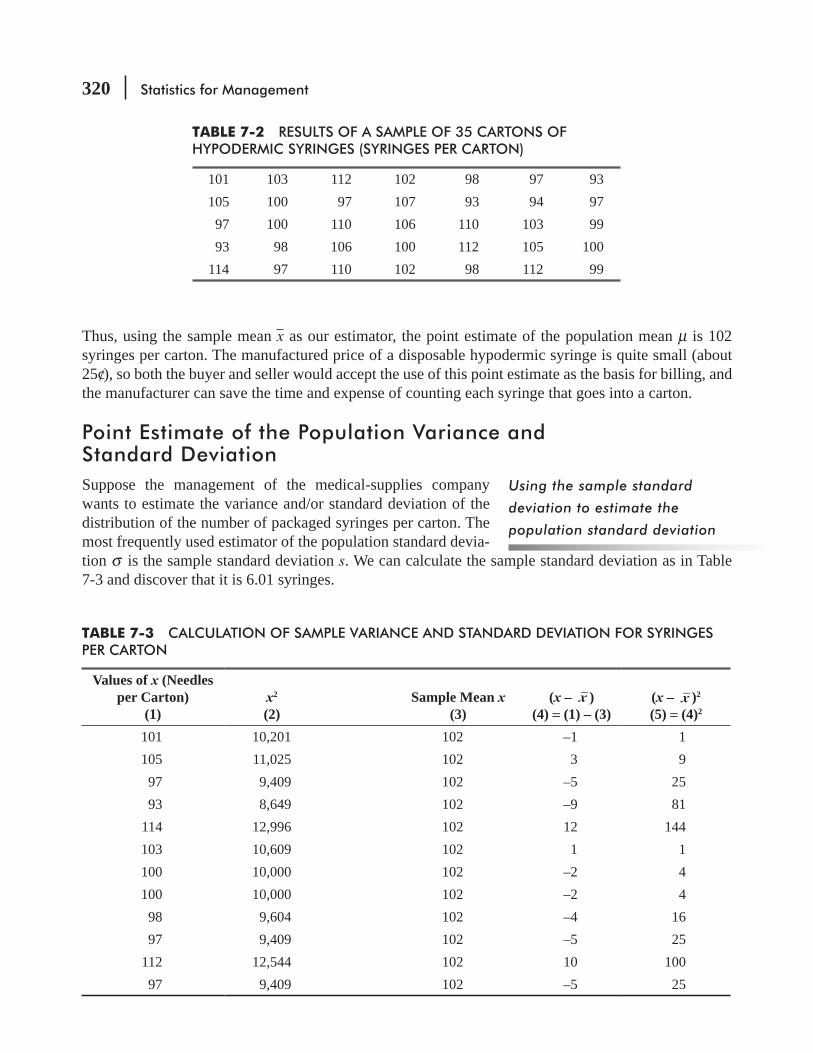
320 Statistics for Management
Thus, using the sample mean x as our estimator, the point estimate of the population mean μ is 102 syringes per carton. The manufactured price of a disposable hypodermic syringe is quite small (about 25c/), so both the buyer and seller would accept the use of this point estimate as the basis for billing, and the manufacturer can save the time and expense of counting each syringe that goes into a carton.
Point Estimate of the Population Variance and Standard DeviationSuppose the management of the medical-supplies company wants to estimate the variance and/or standard deviation of the distribution of the number of packaged syringes per carton. The most frequently used estimator of the population standard devia-tion σ is the sample standard deviation s. We can calculate the sample standard deviation as in Table 7-3 and discover that it is 6.01 syringes.
Using the sample standard
deviation to estimate the
population standard deviation
TABLE 7-2 RESULTS OF A SAMPLE OF 35 CARTONS OF HYPODERMIC SYRINGES (SYRINGES PER CARTON)
101 103 112 102 98 97 93105 100 97 107 93 94 97 97 100 110 106 110 103 99 93 98 106 100 112 105 100114 97 110 102 98 112 99
TABLE 7-3 CALCULATION OF SAMPLE VARIANCE AND STANDARD DEVIATION FOR SYRINGES PER CARTON
Values of x (Needles per Carton)
(1)x2 (2)
Sample Mean x (3)
(x – x ) (4) = (1) – (3)
(x – x )2 (5) = (4)2
101 10,201 102 –1 1105 11,025 102 3 997 9,409 102 –5 2593 8,649 102 –9 81
114 12,996 102 12 144103 10,609 102 1 1100 10,000 102 –2 4100 10,000 102 –2 498 9,604 102 –4 1697 9,409 102 –5 25
112 12,544 102 10 10097 9,409 102 –5 25

Estimation 321
110 12,100 102 8 64106 11,236 102 4 16110 12,100 102 8 64102 10,404 102 0 0107 11,449 102 5 25106 11,236 102 4 16100 10,000 102 –2 4102 10,404 102 0 098 9,604 102 –4 1693 8,649 102 –9 81
110 12,100 102 8 64112 12,544 102 10 10098 9,604 102 –4 1697 9,409 102 –5 2594 8,836 102 –8 64
103 10,609 102 1 1105 11,025 102 3 9112 12,544 102 10 10093 8,649 102 –9 8197 9,409 102 –5 2599 9,801 102 –3 9
100 10,000 102 –2 499 9,801 102 –3 9
3,570 365,368 Sum of all the squared differences
Σ(x – x )2 1,228
[3-17] 1 1
22 2
=Σ
−−
−s
x
n
nx
n
365,368
34
35(102)
34
2
= −
1,228
34=
= 36.12
Sum of the squared differences divided by 34, the number of items in the sample – 1 (sample variance)
( )
136.12
2Σ −−
→x x
n
[3-18] 2=s s
36.12= = 6.01 syringes
Sample standard deviation s ( )
16.01syringes
2Σ −−
→x x
n
TABLE 7-3 CALCULATION OF SAMPLE VARIANCE AND STANDARD DEVIATION FOR SYRINGES PER CARTON (Contd.)

322 Statistics for Management
If, instead of considering
sx x
n
( )
12
2
=∑ −
− [3-17]
as our sample variance, we had considered
s
x x
n
( )22
=∑ −
the result would have some biasbe too low. Using a divisor of n – 1 gives us an unbiased estimator of σ 2. Thus, we will use s2
in Equation 3-17) and s σ 2 and σ .
Point Estimate of the Population ProportionThe proportion of units that have a particular characteristic in a given population is symbolized p. If we know the proportion of units in a sample that have that same characteristic (symbolized p), we can use this p as an estimator of p. It can be shown that p has all the desirable properties we discussed earlier; it is unbi-
Continuing our example of the manufacturer of medical supplies, we shall try to estimate the popu-lation proportion from the sample proportion. Suppose management wishes to estimate the number of cartons that will arrive damaged, owing to poor handling in shipment after the cartons leave the factory. We can check a sample of 50 cartons from their shipping point to the arrival at their destination and
cartons in the sample is 0.08, we would say that
p = 0.08 ← Sample proportion damaged
Because the sample proportion p is a convenient estimator of the population proportion p, we can esti-mate that the proportion of damaged cartons in the population will also be 0.08.
-
lunch here either, and when we give up counting everything, we lose some accuracy. Managers would like to know the accuracy that is achieved when we sample, and using the ideas in this chapter, we can tell them. Hint: Determining the best sample size is not just a statistical deci-sion. Statisticians can tell you how the standard error behaves as you increase or decrease the sample size, and market researchers can tell you what the cost of taking more or larger samples will be. But it’s you who must use your judgment to combine these two inputs to make a sound managerial decision.
HINTS & ASSUMPTIONS
Why is n – 1 the divisor?
Using the sample proportion
to estimate the population
proportion
Estimation 323
EXERCISES 7.2
Self-Check ExercisesSC 7-1 The National Stadium is considering expanding its seating capacity and needs to know both
the average number of people who attend events there and the variability in this number. The following are the attendances (in thousands) at nine randomly selected sporting events. Find point estimates of the mean and the variance of the population from which the sample was drawn
8.8 14.0 21.3 7.9 12.5 20.6 16.3 14.1 13.0
SC 7-2 The Pizza Distribution Authority (PDA) has developed quite a business in Mumbai by deliv-ering pizza orders promptly. PDA guarantees that its pizzas will be delivered in 30 minutes or less from the time the order was placed, and if the delivery is late, the pizza is free. The time
15.3 29.5 30.0 10.1 30.0 19.610.8 12.2 14.8 30.0 22.1 18.3
(a) Find the mean for the sample.(b) From what population was this sample drawn?(c) Can this sample be used to estimate the average time that it takes for PDA to deliver a
pizza? Explain.
Applications7-7 Joe Jackson, a meteorologist for local television station WDUL, would like to report the aver-
age rainfall for today on this evening’s newscast. The following are the rainfall measurements (in inches) for today’s date for 16 randomly chosen past years. Determine the sample mean rainfall.
0.47 0.27 0.13 0.54 0.00 0.08 0.75 0.060.00 1.05 0.34 0.26 0.17 0.42 0.50 0.86
7-8 The National Bank of India is trying to determine the number of tellers available during the lunch rush on Fridays. The bank has collected data on the number of people who entered the bank during the last 3 months on Friday from 11 A.M. to 1 P.Mestimates of the mean and standard deviation of the population from which the sample was drawn.
242 275 289 306 342 385 279 245 269 305 294 328
7-9 Electric Pizza was considering national distribution of its regionally successful product and in ten thousand
rupees) from its 30 current distributors are listed. Treating them as (a) a sample and (b) a population, compute the standard deviation.
7.3 5.8 4.5 8.5 5.2 4.12.8 3.8 6.5 3.4 9.8 6.5
324 Statistics for Management
6.7 7.7 5.8 6.8 8.0 3.96.9 3.7 6.6 7.5 8.7 6.92.1 5.0 7.5 5.8 6.4 5.2
7-10 In a sample of 400 textile workers, 184 expressed extreme dissatisfaction regarding a pro-spective plan to modify working conditions. Because this dissatisfaction was strong enough to allow management to interpret plan reaction as being highly negative, they were curious about the proportion of total workers harboring this sentiment. Give a point estimate of this proportion.
7-11 The Friends of the Psychics network charges $3 per minute to learn the secrets that can turn
company. Thus, a 2 minute 10 second call costs $9. Below is a list of 15 randomly selected charges.
3 9 15 21 42 30 6 9 6 15 21 24 32 9 12
(a) Find the mean of the sample.(b) Find a point estimate of the variance of the population.(c) Can this sample be used to estimate the average length of a call? If so, what is your
estimate? If not, what can we estimate using this sample?
Worked-Out Answers to Self-Check ExercisesSC 7-1 ∑x2 = 2003.65 ∑x = 128.5 n = 9
xx
n
128.5
914.2778=
∑= =
thousands of people
sn
x nx1
1( )
2003.65 9(14.2778)
82 2 2
2
=−
∑ − =−
= 21.119 (1,000s of people)2
SC 7-2 (a) x x
n
242.7
1220.225=
∑= = minutes.
(c) No, it cannot. Because every delivery time over 30 minutes is recorded as 30 minutes, use of these will consistently underestimate the average of the delivery time.
7.3 INTERVAL ESTIMATES: BASIC CONCEPTSThe purpose of gathering samples is to learn more about a population. We can compute this information from the sample data as either point estimates, which we have just discussed, or as interval estimates, the subject of the rest of this chapter. An interval estimate describes a range of values within which
Suppose the marketing research director needs an estimate of the average life in months of car batteries his company manufac-tures. We select a random sample of 200 batteries, record the car owners’ names and addresses as listed
Start with the point estimate

Estimation 325
200 users has a mean battery life of 36 months. If we use the point estimate of the sample mean x as the best estimator of the population mean μ, we would report that the mean life of the company’s batteries is 36 months.
But the director also asks for a statement about the uncertainty that will be likely to accompany this estimate, that is, a statement about the range within which the unknown population mean is
the standard error of the mean.We learned from Chapter 6 that if we select and plot a large number of sample means from a popu-
lation, the distribution of these means will approximate a normal curve. Furthermore, the mean of the
can apply the central limit theorem, as we have done graphically in Figure 7-1. To measure the spread, or dispersion, in our distribution of sample means, we can use the following formula* and calculate the standard error of the mean:
n
σσ x =
Standard error of the mean Standard deviation of the population [6-1]
Suppose we have already estimated the standard devi-ation of the population of the batteries and reported that it is 10 months. Using this standard deviation and
standard error of the mean:
nxσ σ
=
[6-1]
10
200=
10
14.14=
= 0.707 month ←
We could now report to the director that our estimate of the life of the company’s batteries is 36 months, and the standard error that accompanies this estimate is 0.707. In other words, the actual mean life for all the batteries may lie somewhere in the interval estimate of 35.293 to 36.707
chance that the actual life will lie in this interval or in other intervals of different widths that we might choose, ±2σ (2 × 0.707), ±3σ (3 × 0.707), and so on.
Finding the likely error of this
estimate
Making an interval estimate
FIGURE 7-1 SAMPLING DISTRIBUTION OF THE MEAN FOR SAMPLES OF 200 BATTERIES
μ = 36 monthsn = 200
μ = 36
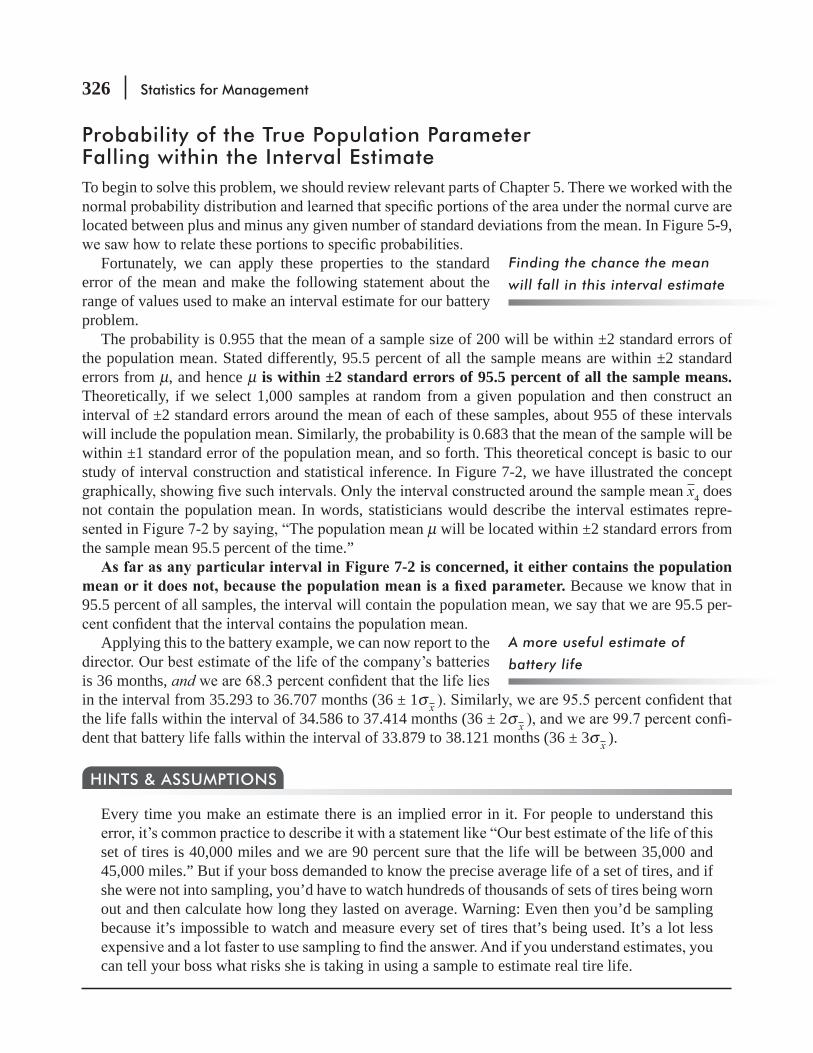
326 Statistics for Management
Probability of the True Population Parameter Falling within the Interval EstimateTo begin to solve this problem, we should review relevant parts of Chapter 5. There we worked with the
located between plus and minus any given number of standard deviations from the mean. In Figure 5-9,
Fortunately, we can apply these properties to the standard error of the mean and make the following statement about the range of values used to make an interval estimate for our battery problem.
The probability is 0.955 that the mean of a sample size of 200 will be within ±2 standard errors of the population mean. Stated differently, 95.5 percent of all the sample means are within ±2 standard errors from μ, and hence μ is within ±2 standard errors of 95.5 percent of all the sample means. Theoretically, if we select 1,000 samples at random from a given population and then construct an interval of ±2 standard errors around the mean of each of these samples, about 955 of these intervals will include the population mean. Similarly, the probability is 0.683 that the mean of the sample will be within ±1 standard error of the population mean, and so forth. This theoretical concept is basic to our study of interval construction and statistical inference. In Figure 7-2, we have illustrated the concept
x4 does not contain the population mean. In words, statisticians would describe the interval estimates repre-
μ will be located within ±2 standard errors from the sample mean 95.5 percent of the time.”
7-2 is concerned, it either contains the population Because we know that in
95.5 percent of all samples, the interval will contain the population mean, we say that we are 95.5 per-
Applying this to the battery example, we can now report to the
is 36 months, andin the interval from 35.293 to 36.707 months (36 ± 1σ x
the life falls within the interval of 34.586 to 37.414 months (36 ± 2σ x -dent that battery life falls within the interval of 33.879 to 38.121 months (36 ± 3σ x ).
Every time you make an estimate there is an implied error in it. For people to understand this
set of tires is 40,000 miles and we are 90 percent sure that the life will be between 35,000 and 45,000 miles.” But if your boss demanded to know the precise average life of a set of tires, and if she were not into sampling, you’d have to watch hundreds of thousands of sets of tires being worn out and then calculate how long they lasted on average. Warning: Even then you’d be sampling because it’s impossible to watch and measure every set of tires that’s being used. It’s a lot less
can tell your boss what risks she is taking in using a sample to estimate real tire life.
HINTS & ASSUMPTIONS
Finding the chance the mean
will fall in this interval estimate
A more useful estimate of
battery life

Estimation 327
EXERCISES 7.3
Self-Check ExercisesSC 7-3 For a population with a known variance of 185, a sample of 64 individuals leads to 217 as an
estimate of the mean.(a) Find the standard error of the mean.(b) Establish an interval estimate that should include the population mean 68.3 percent of the
time.SC 7-4 Eunice Gunterwal is a frugal undergraduate at State U, who is interested in purchasing a used
car. She randomly selected 125 want ads and found that the average price of a car in this sample was $3,250. Eunice knows that the standard deviation of used-car prices in this city is $615.(a) Establish an interval estimate for the average price of a car so that Eunice can be 68.3
percent certain that the population mean lies within this interval.(b) Establish an interval estimate for the average price of a car so that Miss Gunterwal can be
95.5 percent certain that the population mean lies within this interval.
Basic Concepts7-12 From a population known to have a standard deviation of 1.4, a sample of 60 individuals is
taken. The mean for this sample is found to be 6.2.
FIGURE 7-2 A NUMBER OF INTERVALS CONSTRUCTED AROUND SAMPLE MEANS; ALL EXCEPT ONE INCLUDE THE POPULATION MEAN
interval forsample 5
μ –2σx– μ +2σx–
± 2σx
interval forsample 4
± 2σx
interval forsample 3
± 2σx
interval forsample 2
± 2σx
interval forsample 1
± 2σx
x5
x4
x3
x2
x1 x3 x2 x4
x1
μ
95.5%of the means
328 Statistics for Management
(a) Find the standard error of the mean.(b) Establish an interval estimate around the sample mean, using one standard error of
the mean.7-13 From a population with known standard deviation of 1.65, a sample of 32 items resulted in
34.8 as an estimate of the mean.(a) Find the standard error of the mean.(b) Compute an interval estimate that should include the population mean 99.7 percent of
the time.
Applications7-14 The Central University is conducting a study on the average weight of the many bricks that
make up the university’s walkways. Workers are sent to dig up and weigh a sample of 421 bricks and the average brick weight of this sample was 14.2 lb. It is a well-known fact that the standard deviation of brick weight is 0.8 lb.(a) Find the standard error of the mean.(b) What is the interval around the sample mean that will include the population mean
95.5 percent of the time?7-15 -
mating the quantity of food to be prepared each evening, he decided to determine the mean number of customers served each night. He selected a sample of 30 nights, which resulted in a mean of 71. The population standard deviation has been established as 3.76.(a) Give an interval estimate that has a 68.3 percent probability of including the population
mean.(b) Give an interval estimate that has a 99.7 percent chance of including the population mean.
7-16 toll gates and is considering altering the toll-collection procedure if such alteration would be cost-effective. She randomly sampled 75 hours to determine the rate of violation. The result-ing average violations per hour was 7. If the population standard deviation is known to be 0.9, estimate an interval that has a 95.5 percent chance of containing the true mean.
7-17 Gwen Taylor, apartment manager for WillowWood Apartments, wants to inform potential renters about how much electricity they can expect to use during August. She randomly selects 61 residents and discovers their average electricity usage in August to be 894 kilowatt hours (kwh). Gwen believes the variance in usage is about 131 (kwh)2.(a) Establish an interval estimate for the average August electricity usage so Gwen can be
68.3 percent certain the true population mean lies within this interval.(b) Repeat part (a) with a 99.7 percent certainty.(c) If the price per kwh is $0.12, within what interval can Gwen be 68.3 percent certain that
the average August cost for electricity will lie?
Worked-Out Answers to Self-Check Exercises
SC 7-3 1852σ = 185 13.60σ = = n = 64 x 217=
(a) n/ 13.60/ 64 1.70xσ σ= = =(b) x 217 1.70 (215.3, 218.7)xσ± = ± =

Estimation 329
SC 7-4 615σ = n 125= x 3,250= n/ 615/ 125 55.01xσ σ= = =(a) x 3,250 55.01 ($3,194.99, $3,305.01)xσ± = ± =(b) x 2 3,250 2(55.01) 3,250 110.02xσ+ = ± = ± = ($3,139.98, $3,360.02)
7.4 INTERVAL ESTIMATES AND CONFIDENCE INTERVALS
Table 1, for example, ±1.64 standard errors includes about 90 percent of the area under the curve; it includes 0.4495 of the area on either side of the mean in a normal distribution. Similarly, ±2.58 standard errors includes about 99 percent of the area, or 49.51 percent on each side of the mean.
interval estimate is called the confidence level. This prob-ability indicates how confident we are that the interval esti-mate will include the population parameter. A higher probability means more confidence. In esti-mation, the most commonly used confidence levels are 90 percent, 95 percent, and 99 percent, but we are free to apply any confidence level. In Figure 7-2, for example, we used a 95.5 percent confidence level.
The is the range of the estimate we are making. If we report that we are
x ± 1.64 σ x , where
x + 1.64σ x =x – 1.64σ x =
Thus, con dence limits x + 1.64σ x is called the upper con dence limit (UCL) and x – 1.64σ x , is the lower con dence limit (LCL).
Relationship between Confidence Level and Confidence Interval-
-vals are not precise; they give very fuzzy estimates.
Consider an appliance store customer who inquires about the delivery of a new washing machine. In Table 7-4 are several of the questions the customer might ask and the likely responses. This table
the case with a one-year delivery, the estimate may have very little real value, even though the store
Confidence level defined
330 Statistics for Management
Using Sampling and Confidence Interval EstimationIn our discussion of the basic concepts of interval estimation, particularly in Figure 7-2, we described samples being drawn repeatedly from a given population in order to estimate a popu-lation parameter. We also mentioned selecting a large number of sample means from a population. In
Based on just one sample, we estimate the population parameter. We must be careful, then, about inter-preting the results of such a process.
within 30 and 42 months.” This statement does not mean that the chance is 0.95 that the mean life of all our batteries falls within the interval established from this one sample. Instead, it means
for each of these samples, then in about 95 percent of these cases, the population mean will lie within that interval.
you want more of one, you have to take less of the other. Hint: To understand this important rela-tionship, go back to Table 7-4. If you want the estimate of the time of delivery to be perfectly
you within an hour.” You can’t have both at the same time.
HINTS & ASSUMPTIONS
Estimating from only one
sample
TABLE 7-4 ILLUSTRATION OF THE RELATIONSHIP BETWEEN CONFIDENCE LEVEL AND CONFIDENCE INTERVAL
Customer’s Question Store Manager’s Response Level IntervalWill I get my washing machine within 1 year?
I am absolutely certain of that. Better than 99% 1 year
Will you deliver the washing machine within 1 month?
I am almost positive it will be delivered this month.
At least 95% 1 month
Will you deliver the washing machine within 1 week?
I am pretty certain it will go out within this week.
About 80% 1 week
Will I get my washing machine tomorrow?
I am not certain we can get it to you then.
About 40% 1 day
Will my washing machine get home before I do?
There is little chance it will beat you home.
Near 1% 1 hour
Estimation 331
EXERCISES 7.4
Self-Check ExerciseSC 7-5
interval for these levels in terms of x and σ x.(a) 54 percent.(b) 75 percent.(c) 94 percent.(d) 98 percent.
Basic Concepts7-18 7-19 7-20 -
dence interval in terms of the sample mean, x, and the standard error, σ x.7-21 In what way may an estimate be less meaningful because of
7-22 Suppose a sample of 50 is taken from a population with standard deviation 27 and that the sample mean is 86.(a) Establish an interval estimate for the population mean that is 95.5 percent certain to
include the true population mean.(b) Suppose, instead, that the sample size was 5,000. Establish an interval for the population
mean that is 95.5 percent certain to include the true population mean.(c) Why might estimate (a) be preferred to estimate (b)? Why might (b) be preferred to (a)?
7-23
Applications7-24 Habib Iqbal, who is the owner of Habib’s Barbershop, has built quite a reputation among the
residents of Kanpur. As each customer enters his barbershop, Habib yells out the number of min-utes that the customer can expect to wait before getting his haircut. The only statistician in town, after being frustrated by Habib’s inaccurate point estimates, has determined that the actual wait-ing time for any customer is normally distributed with mean equal to Habib’s estimate in minutes and standard deviation equal to 5 minutes divided by the customer’s position in the waiting line. Help Habib’s customers develop 95 percent probability intervals for the following situations·(a) The customer is second in line and Steve’s estimate is 25 minutes.(b) The customer is third in line and Steve’s estimate is 15 minutes.
Worked-Out Answers to Self-Check ExerciseSC 7-5 (a) x 0.74 .xσ± (b) x 1.15 .xσ± (c) x 1.88 .xσ± (d) x 2.33 .xσ±

332 Statistics for Management
7.5 CALCULATING INTERVAL ESTIMATES OF THE MEAN FROM LARGE SAMPLES
A large automotive-parts wholesaler needs an estimate of the mean life it can expect from windshield wiper blades under typi-cal driving conditions. Already, management has determined that the standard deviation of the population life is 6 months. Suppose we select a simple random sample of 100 wiper blades, collect data on their useful lives, and obtain these results:
n = 100 ← Sample sizex = 21 months ← Sample meanσ = 6 months ← Population standard deviation
Because the wholesaler uses tens of thousands of these wiper
30, so the central limit theorem allows us to use the normal distribution as our sampling distribution even if the population isn’t normal. We calculate the standard error of the mean by using Equation 6-1:
nxσ σ
=
[6-1]
6 months
100=
6
10=
= 0.6 month ←
the area on either side of the mean of the sampling distribution, we can search in the body of Appendix Table 1 for the 0.475 value. We discover that 0.475 of the area under the normal curve is contained between the mean and a point 1.96 standard errors to the right of the mean. Therefore, we know that (2)(0.475) = 0.95 of the area is located between plus and minus 1.96
x 1.96 xσ+ ← x 1.96 xσ+ ←
Then we substitute numerical values into these two expressions:.
x 1.96 xσ+ = 21 months + 1.96(0.6 month)= 21 + 1.18 months= 22.18 months ←
x 1.96 xσ+ = 21 months – 1.96(0.6 month)= 21 – 1.18 months= 19.82 months ←
Finding a 95 percent confidence
interval
Population standard deviation is
known
Calculating confidence limits

Estimation 333
Our conclusionWe can now report that we estimate the mean life of the popula-tion of wiper blades to be between 19.82 and 22.18 months with
When the Population Standard Deviation Is UnknownA more complex interval estimate problem comes from a social-service agency in a local government. It is interested in estimating the mean annual income of 700 families living in a four-square-
n = 50 ← Sample sizex = $11,800 ← Sample means = $950 ← Sample standard deviation
The agency asks us to calculate an interval estimate of the mean annual income of all 700 families so that
so once again the central limit theorem enables us to use the normal distribution as the sampling distribution.Notice that one part of this problem differs from our previ-
ous examples: we do not know the population standard deviation, and so we will use the sample standard deviation to estimate the population standard deviation:
Estimate of the Population Standard Deviation
sx x
nˆ
( )
1
2
σ = =∑ −
−Estimate of the population standard deviation [7-1]
The value $950.00 is our estimate of the standard deviation of the population. We can also symbolize this estimated value by ˆ ,σ which is called sigma hat.
and because our sample is more than 5 percent of the population, we will use the formula for deriving
n
N n
N 1xσ σ= ×
−−
[6-3]
But because we are calculating the standard error of the mean using an estimate of the standard deviation of the population, we must rewrite this equation so that it is correct symbolically:
Estimated Standard Error of the Mean of a Finite Population
n
N n
Nˆ
ˆ
1xσ σ= ×
−−
Symbol that indicates an estimated value
Estimate of the population standard deviation
[7-2]
Finding a 90 percent confidence
interval
Estimating the population
standard deviation
Estimating the standard error of
the mean
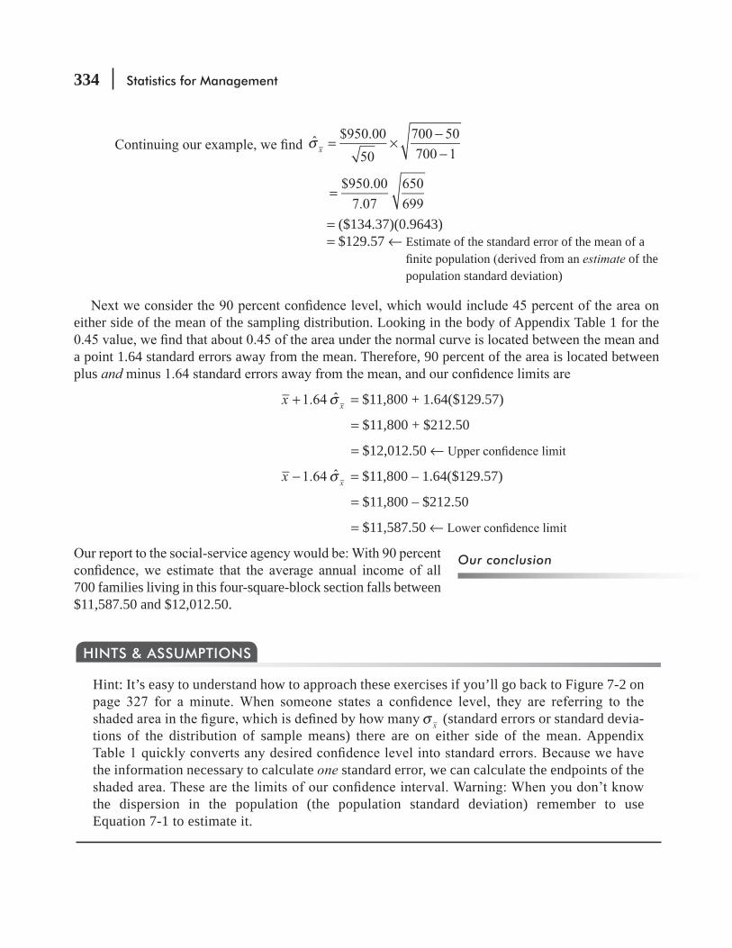
334 Statistics for Management
ˆ$950.00
50
700 50
700 1xσ = ×−−
$950.00
7.07
650
699=
= ($134.37)(0.9643) = $129.57 ← Estimate of the standard error of the mean of a
estimate of the population standard deviation)
either side of the mean of the sampling distribution. Looking in the body of Appendix Table 1 for the
a point 1.64 standard errors away from the mean. Therefore, 90 percent of the area is located between plus and
x 1.64 ˆxσ+ = $11,800 + 1.64($129.57)
= $11,800 + $212.50
= $12,012.50 ←
x 1.64 ˆxσ− = $11,800 – 1.64($129.57)
= $11,800 – $212.50
= $11,587.50 ←
700 families living in this four-square-block section falls between $11,587.50 and $12,012.50.
Hint: It’s easy to understand how to approach these exercises if you’ll go back to Figure 7-2 on
xσ (standard errors or standard devia-tions of the distribution of sample means) there are on either side of the mean. Appendix
the information necessary to calculate one standard error, we can calculate the endpoints of the
the dispersion in the population (the population standard deviation) remember to use Equation 7-1 to estimate it.
HINTS & ASSUMPTIONS
Our conclusion
Estimation 335
EXERCISES 7.5
Self-Check ExercisesSC 7-6 From a population of 540, a sample of 60 individuals is taken. From this sample, the mean is
found to be 6.2 and the standard deviation 1.368.(a) Find the estimated standard error of the mean.
SC 7-7 In an automotive safety test conducted by the New Delhi Highway Safety Research Center, the average tire pressure in a sample of 62 tires was found to be 24 pounds per square inch, and the standard deviation was 2.1 pounds per square inch.(a) What is the estimated population standard deviation for this population? (There are about
a million cars registered in New Delhi.)(b) Calculate the estimated standard error of the mean.
Basic Concepts7-25 The manager of Cardinal Electric’s lightbulb division must estimate the average number of
hours that a lightbulb made by each lightbulb machine will last. A sample of 40 lightbulbs was selected from machine A and the average burning time was 1,416 hours. The standard devia-tion of burning time is known to be 30 hours.(a) Compute the standard error of the mean.
7-26 Upon collecting a sample of 250 from a population with known standard deviation of 13.7, the mean is found to be 112.4.
Applications7-27 The Westview High School nurse is interested in knowing the average height of seniors at
this school, but she does not have enough time to examine the records of all 430 seniors. She
deviation to be 2.3 inches.(a) Find the estimated standard error of the mean.
7-28 page dissertation. Jon has typed his paper himself and is interested in knowing the average number of typographical errors per page, but does not want to read the whole paper. Knowing a little bit about business statistics, Jon selected 40 pages at random to read and found that the average number of typos per page was 4.3 and the sample standard deviation was 1.2 typos per page.(a) Calculate the estimated standard error of the mean.
per page in his paper.

336 Statistics for Management
7-29 The New Delhi Cable Television authority conducted a test to determine the amount of time people spend watching television per week. The NCTA surveyed 84 subscribers and found the average number of hours watched per week to be 11.6 hours and the standard deviation to be 1.8 hours.(a) What is the estimated population standard deviation for this population? (There are about
95,000 people with cable television in New Delhi.)(b) Calculate the estimated standard error of the mean.
New Delhi.7-30 Samuel Singh is a broker on the Bombay Stock Exchange who is curious about the amount
of time between the placement and execution of a market order. Samuel sampled 45 orders and found that the mean time to execution was 24.3 minutes and the standard deviation was
to execution.7-31 Neelesh Pant is the production manager for Citrus Groves Inc., located just north of Ranikhet,
Uttarakhand. Neelesh is concerned that the last 3 years’ late freezes have damaged the 2,500 orange trees that Citrus Groves owns. In order to determine the extent of damage to the trees, Neelesh has sampled the number of oranges produced per tree for 42 trees and found that the average production was 525 oranges per tree and the standard deviation was 30 oranges per tree.(a) Estimate the population standard deviation from the sample standard deviation.
(d) If the mean orange output per tree was 600 oranges 5 years ago, what can Neelesh say about the possible existence of damage now?
Worked-Out Answers to Self-Check ExercisesSC 7-6 σ = 1.368 N = 540 n = 60 x = 6.2
(a) n
N n
Nˆ
ˆ
1
1.368
60
540 60
540 10.167xσ σ
= ×−−
= ×−−
=
(b) x ± 2.05 ˆxσ = 6.2 ± 2.05(0.167) = 6.2 ± 0.342 = (5.86, 6.54)
SC 7-7 s = 2.1 n = 62 x = 24(a) σ = s = 2.1 psi
(b) nˆ ˆ / 2.1/ 62 0.267xσ σ= = = psi
(c) x ± 1.96 ˆxσ = 24 ± 1.96(0.267) = 24 ± 0.523 = (23.48, 24.52) psi
7.6 CALCULATING INTERVAL ESTIMATES OF THE PROPORTION FROM LARGE SAMPLES
Statisticians often use a sample to estimate a proportion of occur-rences in a population. For example, the government estimates by a sampling procedure the unemployment rate, or the proportion of unemployed people, in the U.S. workforce.
Review of the binomial
distribution
Estimation 337
In Chapter 5, we introduced the binomial distribution, a distribution of discrete, not continuous, data. Also, we presented the two formulas for deriving the mean and the standard deviation of the binomial distribution:
μ = np [5-2]
npqσ = [5-3]where
n = number of trials p = probability of success q = 1 – p = probability of a failure
intervals to estimate a population proportion.Because the computation of binomial probabilities is so
tedious (recall that the probability of r successes in n trials is [n!/r!(n – r)!][prqn–r]), using the binomial distribution to form interval estimates of a population proportion is a complex propo-sition. Fortunately, as the sample size increases, the binomial can be approximated by an appropriate normal distribution, which we can use to approximate the sampling distribution. Statisticians recom-mend that in estimation, n be large enough for both np and nq to be at least 5 when you use the normal distribution as a substitute for the binomial.
Symbolically, let’s express the proportion of successes in a sample by p (pronounced p bar). Then modify Equation 5-2, so that we can use it to derive the mean of the sampling distribution of the proportion of successes. In words, μ = np shows that the mean of the binomial distribution is equal to the product of the number of trials, n, and the probability of success, p; that is, np equals the mean number of successes. To change this number of successes to the proportion of successes, we divide np by n and get p alone. The mean in the left-hand side of the equation becomes μp, or the mean of the sampling distribution of the proportion of successes.
Mean of the Sampling Distribution of the Proportion
μp = p [7-3]
Similarly, we can modify the formula for the standard devia-tion of the binomial distribution, npq, which measures the standard deviation in the number of successes. To change the number of successes to the proportion of successes, we divide
npq by n and get pq n/ . In statistical terms, the standard deviation for the proportion of suc-cesses in a sample is symbolized and is called the standard error of the proportion.
Standard Error of the Proportion
σ p = pq
nStandard error of the proportion [7-4]
Shortcomings of the binomial
distribution
Finding the mean of the sample
proportion
Finding the standard deviation
of the sample proportion

338 Statistics for Management
We can illustrate how to use these formulas if we estimate for a very large organization what propor-
n = 75 ← Sample sizep = 0.4 ← Sample proportion in favorq = 0.6 ← Sample proportion not in favor
-tains the true population proportion.
But what are p and q for the population? We can estimate the population parameters by substituting the corresponding sample statistics p and q (p bar and q bar) in the formula for the standard error of the proportion.* Doing this, we get:
Estimated Standard Error of the Proportion
σ p = pq
n
Symbol indicating that the standard error of the proportion estimated
Sample statistics
← Estimated standard error of the proportion
(0.4)(0.6)
75
0.0032
0.057
=
==
[7-5]
Now we can provide the estimate management needs by using the same procedure we have used previously. A 99 percent
side of the mean in the sampling distribution. The body of Appendix Table 1 tells us that 0.495 of the area under the normal curve is located between the mean and a point 2.58 standard errors from the mean. Thus, 99 percent of the area is contained between plus and minus 2.58 standard errors from the mean.
p + 2.58 σp = 0.4 + 2.58(0.057)
= 0.4 + 0.147 = 0.547 ←
p – 2.58 σp = 0.4 – 2.58(0.057)
= 0.4 – 0.147 = 0.253 ←
Estimating a population
proportion
Computing the confidence limits

Estimation 339
Our conclusionThus, we estimate from our sample of 75 employees that with
population of employees who wish to establish their own retire-ment plans lies between 0.253 and 0.547.
The same assumptions, hints, and warnings we stated on page 334 apply here as well. The only difference is that now, since we’re dealing with a proportion, the binomial distribution is the cor-rect sampling distribution to use. Hint: Remember from Chapter 5 that as long as n is large enough to make both np and nq at least 5, we can use the normal distribution to approximate the binomial. If that is the case, we proceed exactly as we did with interval estimates of the mean. Warning: Since the exact standard error of the proportion depends on the unknown population proportion ( p) , remember to estimate p by p and use p in Equation 7-5 to estimate the standard error of the proportion.
HINTS & ASSUMPTIONS
EXERCISES 7.6
Self-Check ExercisesSC 7-8 When a sample of 70 retail executives was surveyed regarding the poor November perfor-
mance of the retail industry, 66 percent believed that decreased sales were due to unseason-ably warm temperatures, resulting in consumers’ delaying purchase of cold-weather items.(a) Estimate the standard error of the proportion of retail executives who blame warm weather
for low sales.-
dence level.SC 7-9 Dr. Benjamin Shockley, a noted social psychologist, surveyed 150 top executives and found
that 42 percent of them were unable to add fractions correctly.(a) Estimate the standard error of the proportion.
cannot correctly add fractions.
Applications7-32 Pascal, Inc., a computer store that buys wholesale, untested computer chips, is considering
switching to another supplier who would provide tested and guaranteed chips for a higher price. In order to determine whether this is a cost-effective plan, Pascal must determine the proportion of faulty chips that the current supplier provides. A sample of 200 chips was tested and of these, 5 percent were found to be defective.(a) Estimate the standard error of the proportion of defective chips.

340 Statistics for Management
7-33 General Cinema sampled 55 people who viewed GhostHunter 8 and asked them whether they
second time.
7-34 The product manager for the new lemon-lime Clear ’n Light dessert topping was worried about both the product’s poor performance and her future with Clear ’n Light. Concerned that her marketing strategy had not properly identified the attributes of the product, she sampled 1,500 consumers and learned that 956 thought that the product was a floor wax.(a) Estimate the standard error of the proportion of people holding this severe misconception
about the dessert topping.
7-35 Michael Gordon, a professional basketball player, shot 200 foul shots and made 174 of them.(a) Estimate the standard error of the proportion of all foul shots Michael makes.
makes.7-36 SnackMore recently surveyed 95 shoppers and found 80 percent of them purchase SnackMore
fat-free brownies monthly.(a) Estimate the standard error of the proportion.
the brownies monthly.7-37 The owner of the Home Loan Company randomly surveyed 150 of the company’s 3,000
accounts and determined that 60 percent were in excellent standing.
(b) Based on part (a), what kind of interval estimate might you give for the absolute number -
dence level?7-38 For a year and a half, sales have been falling consistently in all 1,500 franchises of a fast-food
Worked-Out Answers to Self-Check ExercisesSC 7-8 n = 70 p 0.66=
(a) p q
nˆ
0.66(0.34)
700.0566pσ = = =
(b) p 1.96 ˆxσ± = 0.66 ± 1.96(0.0566) = 0.66 ± 0.111 = (0.549, 0.771)
SC 7-9 n = 150 p 0.42=
(a) p q
nˆ
0.42(0.58)
1500.0403pσ = = =
(b) p 2.58 ˆpσ± = 0.42 ± 2.58(0.0403) = 0.42 ± 0.104 = (0.316, 0.524)
Estimation 341
7.7 INTERVAL ESTIMATES USING THE t DISTRIBUTIONIn our three examples so far, the sample sizes were all larger than 30. We sampled 100 wind-shield wiper blades, 50 families living in a four-square-block section of a community, and 75 employees of a very large organization. Each time, the normal distribution was the appropriate sampling distribution to use
However, this is not always the case. How can we handle esti-mates where the normal distribution is not the appropriate sam-pling distribution, that is, when we are estimating the population standard deviation and the sample size is 30 or less? For example, in our chapter-opening problem of coal usage, we had data from only 10 weeks. Fortunately, another distribution exists that is appropriate in these cases. It is called the t distribution.
Early theoretical work on t distributions was done by a man named W. S. Gosset in the early 1900s. Gosset was employed by the Guinness Brewery in Dublin, Ireland, which did not permit
Student and published under that name. Consequently, the t distribution is commonly called Student’s t distribu-tion, or simply Student’s distribution.
Because it is used when the sample size is 30 or less, statisti-cians often associate the t distribution with small sample statis-tics. This is misleading, because the size of the sample is only one of the conditions that lead us to use the t distribution. The second condition is that the population standard deviation must be unknown. Use of the distribution for estimating is required whenever
using the
Characteristics of the t DistributionWithout deriving the t distribution mathematically, we can gain an intuitive understanding of the relationship between the t dis-tribution and the normal distribution. Both are symmetrical. In general, the t t distribution for every possible sample size. Even so, as the sample size gets larger, the shape of the t distribution
of more than 30, the t distribution is so close to the normal distribution that we will use the normal to approximate the t.
Figure 7-3 compares one normal distribution with two t distributions of different sample sizes. This t distributions. A distribution is lower at the mean and higher at
the tails than a normal distribution. t distribution has propor-tionally more of its area in its tails than the normal does. This is the reason why it will be necessary to go farther out from the mean of a t distribution to include the same area under the curve. Interval widths from t distributions are, therefore, wider than those based on the normal distribution.
Degrees of FreedomWe said earlier that there is a separate t distribution for each sam-
Sometimes the normal
distribution is not appropriate
Background of the t distribution
Conditions for using the
t distribution
t distribution compared to
normal distribution
Degrees of freedom defined
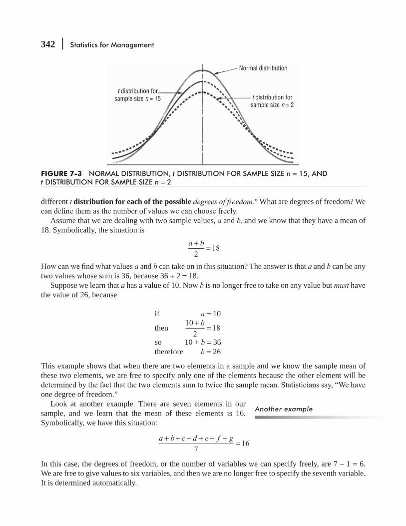
342 Statistics for Management
different t distribution for each of the possible degrees of freedom.” What are degrees of freedom? We
Assume that we are dealing with two sample values, a and b, and we know that they have a mean of 18. Symbolically, the situation is
a b
218
+=
a and b can take on in this situation? The answer is that a and b can be any two values whose sum is 36, because 36 ÷ 2 = 18.
Suppose we learn that a has a value of 10. Now b is no longer free to take on any value but must have the value of 26, because
if a = 10
then b10
218
+=
so 10 + b = 36therefore b = 26
This example shows that when there are two elements in a sample and we know the sample mean of these two elements, we are free to specify only one of the elements because the other element will be
one degree of freedom.”Look at another example. There are seven elements in our
sample, and we learn that the mean of these elements is 16. Symbolically, we have this situation:
a b c d e f g
716
+ + + + + +=
In this case, the degrees of freedom, or the number of variables we can specify freely, are 7 – 1 = 6. We are free to give values to six variables, and then we are no longer free to specify the seventh variable. It is determined automatically.
Another example
FIGURE 7-3 NORMAL DISTRIBUTION, t DISTRIBUTION FOR SAMPLE SIZE n = 15, AND t DISTRIBUTION FOR SAMPLE SIZE n = 2
t distribution forsample size n = 15 t distribution for
sample size n = 2
Normal distribution
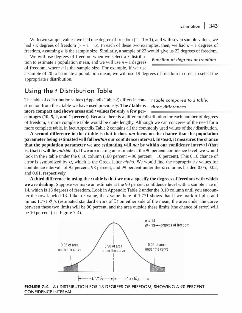
Estimation 343
With two sample values, we had one degree of freedom (2 – 1 = 1), and with seven sample values, we had six degrees of freedom (7 – 1 = 6). In each of these two examples, then, we had n – 1 degrees of freedom, assuming n is the sample size. Similarly, a sample of 23 would give us 22 degrees of freedom.
We will use degrees of freedom when we select a t distribu-tion to estimate a population mean, and we will use n – 1 degrees of freedom, where n is the sample size. For example, if we use a sample of 20 to estimate a population mean, we will use 19 degrees of freedom in order to select the appropriate t distribution.
Using the t Distribution TableThe table of t distribution values (Appendix Table 2) differs in con-struction from the z table we have used previously. The table is more compact and shows areas and values for -centages (10, 5, 2, and 1 percent). Because there is a different t distribution for each number of degrees of freedom, a more complete table would be quite lengthy. Although we can conceive of the need for a more complete table, in fact Appendix Table 2 contains all the commonly used values of the t distribution.
A second difference in the table is that it does focus on the chance that the population parameter being estimated will fall that the population parameter we are estimating will is, that it will lie it).look in the t table under the 0.10 column (100 percent – 90 percent = 10 percent). This 0.10 chance of error is symbolized by α, which is the Greek letter alpha. t values for
α columns headed 0.05, 0.02, and 0.01, respectively.
A third difference in using the we are dealing.14, which is 13 degrees of freedom. Look in Appendix Table 2 under the 0.10 column until you encoun-ter the row labeled 13. Like a z value, the t value there of 1.771 shows that if we mark off plus and minus 1.771 σ x’s (estimated standard errors of x ) on either side of the mean, the area under the curve between these two limits will be 90 percent, and the area outside these limits (the chance of error) will be 10 percent (see Figure 7-4).
Function of degrees of freedom
t table compared to z table:
three differences
0.05 of areaunder the curve
degrees of freedomn = 14df = 13
0.90 of areaunder the curve
0.05 of areaunder the curve
–1.771σx^ +1.771σx
^
FIGURE 7-4 A t DISTRIBUTION FOR 13 DEGREES OF FREEDOM, SHOWING A 90 PERCENT CONFIDENCE INTERVAL

344 Statistics for Management
Recall that in our chapter-opening problem, the generating plant manager wanted to estimate the coal needed for this year, and he took a sample by measuring coal usage for 10 weeks. The sample data are
n = 10 weeks ← Sample sizedf = 9 ← Degrees of freedom x = 11,400 tons ← Sample mean s = 700 tons Sample standard deviation
The plant manager wants an interval estimate of the mean
the mean consumption falls within that interval. This problem requires the use of a
estimate the population standard deviation with the sample standard deviation; thus
sσ = [7-1]= 700 tons
Using this estimate of the population standard deviation, we can estimate the standard error of the
10 weeks is less than 5 percent of the 5 years (260 weeks) for which data are available):
Estimated Standard Error of the Mean of an Infinite Population
nˆ
ˆxσ σ
= [7-6]
ˆ700
10xσ =
700
3.162=
= 221.38 tons ← Estimated standard error of the mean of an
Now we look in Appendix Table 2 down the 0.05 column (100 percent – 95 percent = 5 percent) until we encounter the row for 9 degrees of freedom (10 – 1 = 9). There we see the t value 2.262 and can set
x + 2.2626 σx = 11,400 tons + 2.262(221.38 tons)
= 11,400 + 500.76 = 11,901 tons ←
x – 2.262 σx = 11,400 tons – 2.262(221.38 tons)
= 11,400 – 500.76 = 10,899 tons ←
Using the t table to compute
confidence limits
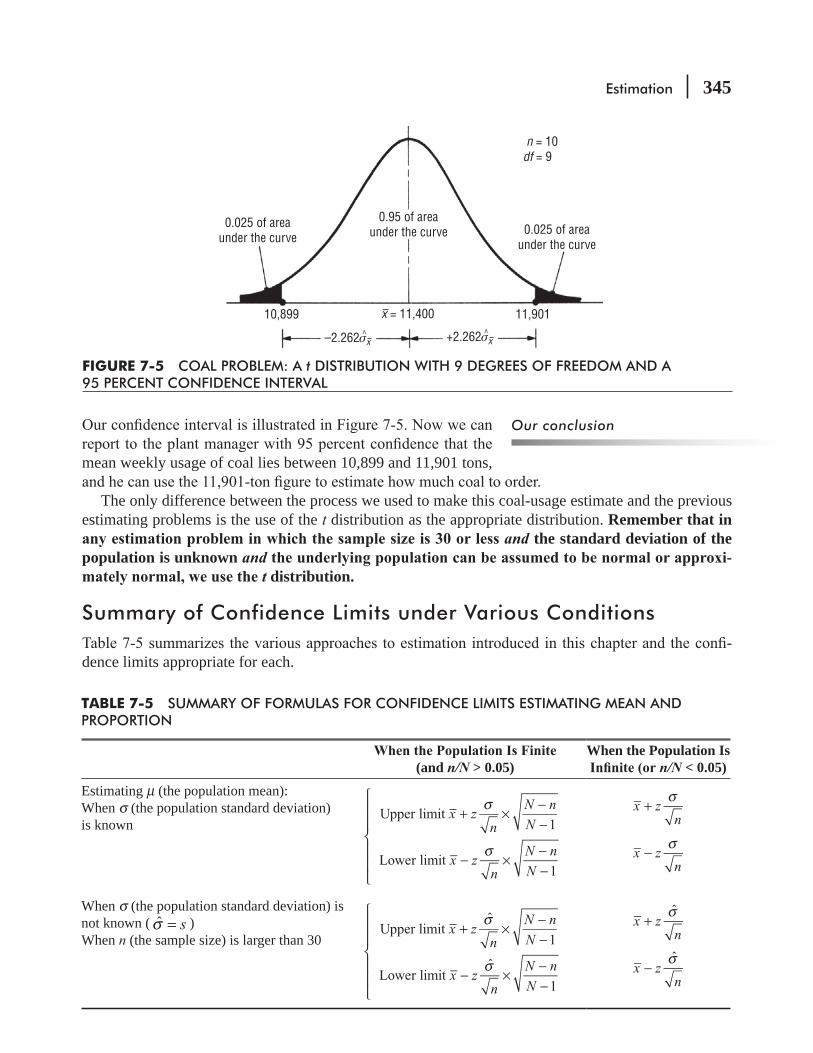
Estimation 345
Our conclusion
mean weekly usage of coal lies between 10,899 and 11,901 tons,
The only difference between the process we used to make this coal-usage estimate and the previous estimating problems is the use of the t distribution as the appropriate distribution. Remember that in
the standard deviation of the population is unknown -
distribution.
Summary of Confidence Limits under Various Conditions-
dence limits appropriate for each.
FIGURE 7-5 COAL PROBLEM: A t DISTRIBUTION WITH 9 DEGREES OF FREEDOM AND A 95 PERCENT CONFIDENCE INTERVAL
0.025 of areaunder the curve
0.025 of areaunder the curve
0.95 of areaunder the curve
n = 10df = 9
10,899 11,901x = 11,400
–2.262σx^ +2.262σx
^
TABLE 7-5 SUMMARY OF FORMULAS FOR CONFIDENCE LIMITS ESTIMATING MEAN AND PROPORTION
(and n/N > 0.05)
When the Population Is n/N < 0.05)
Estimating μ (the population mean):When σ (the population standard deviation) is known
x zn
N n
N
x zn
N n
N
Upper limit1
Lower limit1
σ
σ
+ ×−−
− ×−−
⎧
⎨
⎪⎪
⎩
⎪⎪
x zn
σ+
x zn
σ−
When σ (the population standard deviation) is not known ( sσ = )When n (the sample size) is larger than 30
x zn
N n
N
x zn
N n
N
Upper limitˆ
1
Lower limitˆ
1
σ
σ
+ ×−−
− ×−−
⎧
⎨
⎪⎪
⎩
⎪⎪
x zn
σ+
x zn
σ−
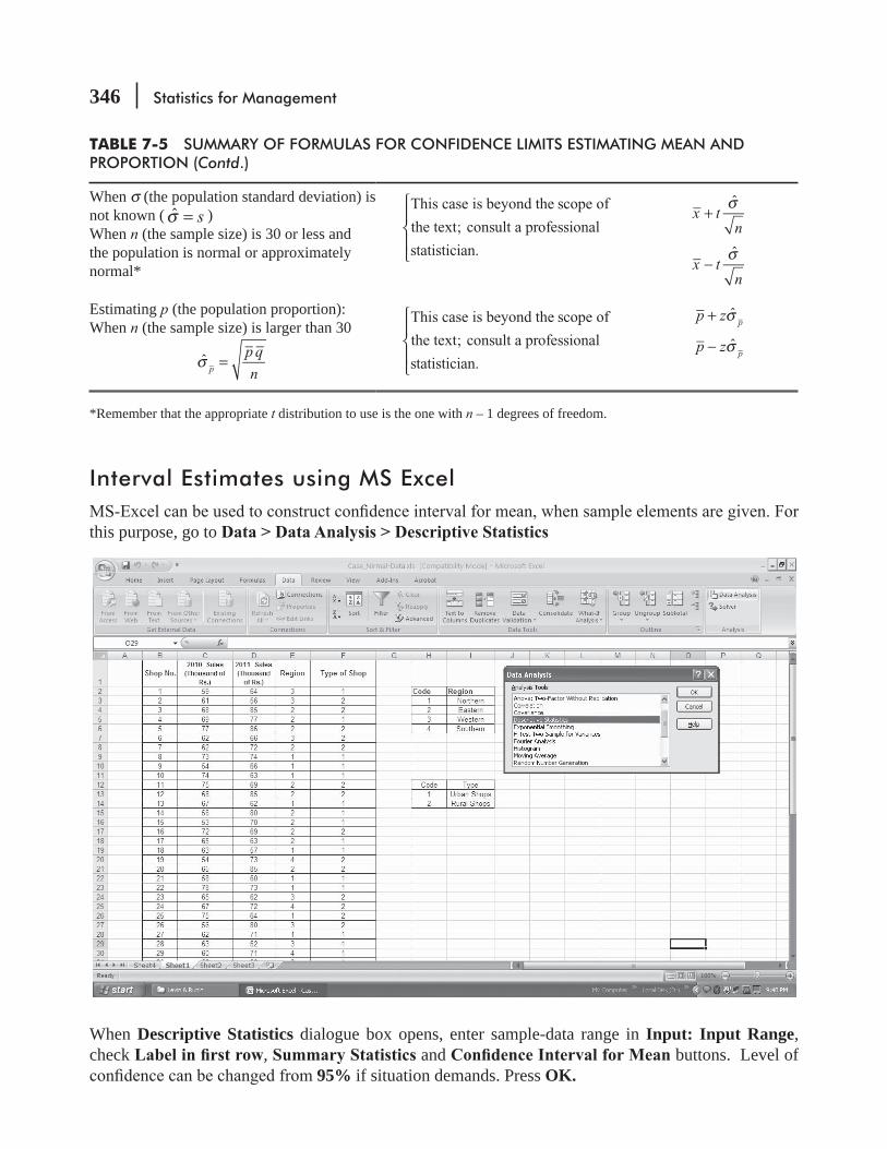
346 Statistics for Management
Interval Estimates using MS Excel
this purpose, go to
When Descriptive Statistics dialogue box opens, enter sample-data range in Input: Input Range, check , and buttons. Level of
95% if situation demands. Press OK.
When σ (the population standard deviation) is not known ( sσ = )When n (the sample size) is 30 or less and the population is normal or approximately normal*
This case is beyond the scope of
the text; consult a professional
statistician.
⎧
⎨⎪
⎩⎪
x tn
σ+
x tn
σ−
Estimating p (the population proportion):When n (the sample size) is larger than 30
p q
nˆ
pσ =
This case is beyond the scope of
the text; consult a professional
statistician.
⎧
⎨⎪
⎩⎪
p z ˆpσ+
p z ˆpσ−
*Remember that the appropriate t distribution to use is the one with n – 1 degrees of freedom.
TABLE 7-5 SUMMARY OF FORMULAS FOR CONFIDENCE LIMITS ESTIMATING MEAN AND PROPORTION (Contd.)
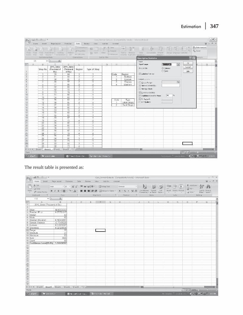
Estimation 347
The result table is presented as:
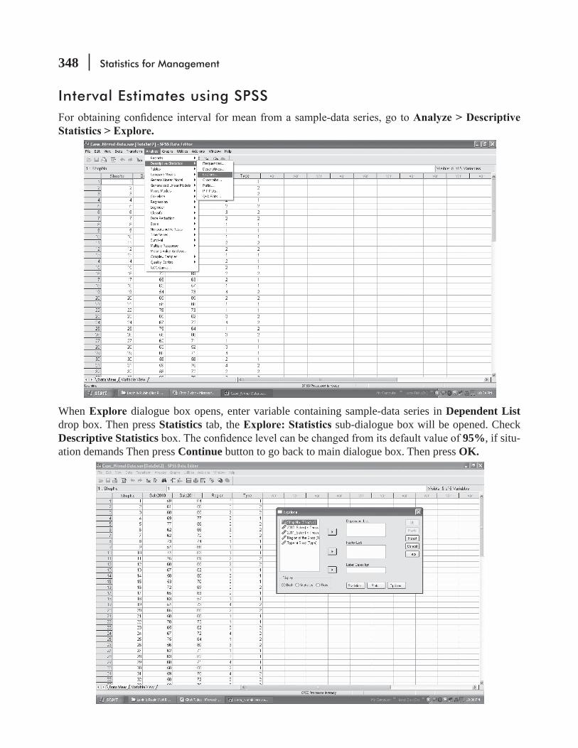
348 Statistics for Management
Interval Estimates using SPSS
When dialogue box opens, enter variable containing sample-data series in Dependent List drop box. Then press Statistics tab, the sub-dialogue box will be opened. Check Descriptive Statistics 95%, if situ-ation demands Then press Continue button to go back to main dialogue box. Then press OK.

Estimation 349
The concept of degrees of freedomof choices you have. If you have peanut butter and cheese in your refrigerator, you can choose either a peanut butter or a cheese sandwich (unless you like peanut butter and cheese sandwiches).
zero degrees of freedom.” That is, if you want lunch, you have no choices left; it’s peanut butter or starve. Warning: Although the t distribution is associated with small-sample statistics, remem-ber that a sample size of less than 30 is only one of the conditions for its use. The others are that the population standard deviation is not known and the population is normally or approximately normally distributed.
HINTS & ASSUMPTIONS
EXERCISES 7.7
Self-Check ExercisesSC 7-10 t values for con-
(a) n = 28; 95 percent.(b) n = 8; 98 percent.(c) n = 13; 90 percent.

350 Statistics for Management
(d) n = 10; 95 percent.(e) n = 25; 99 percent.(f) n = 10; 99 percent.
SC 7-11 Seven homemakers were randomly sampled, and it was determined that the distances they walked in their housework had an average of 39.2 miles per week and a sample standard
mean.
Basic Concepts7-39 t values for con-
(a) n = 15; 90 percent.(b) n = 6; 95 percent.(c) n = 19; 99 percent.(d) n = 25; 98 percent.(e) n = 10; 99 percent.(f) n = 41; 90 percent.
7-40 Given the following sample sizes and t
(a) n = 27; t = ±2.056.(b) n = 5; t = ±2.132.(c) n = 18; t = ±2.898.
7-41 A sample of 12 had a mean of 62 and a standard deviation of 10. Construct a 95 percent con-
7-42 distribution:
75.3 76.4 83.2 91.0 80.1 77.5 84.8 81.0
(a) Find the sample mean.(b) Estimate the population standard deviation.
Applications7-43 Twelve bank tellers were randomly sampled and it was determined they made an average of
3.6 errors per day with a sample standard deviation of 0.42 error. Construct a 90 percent con-
the number of errors bank tellers make? 7-44 The director of River-Sports Security, Donna Singh, has ordered an investigation of the large
number of boating accidents that have occurred in the state in recent summers. Acting on her instructions, her aide, Ranjan Rao, has randomly selected 9 summer months within the last few years and has compiled data on the number of boating accidents that occurred during each of these months. The mean number of boating accidents to occur in these 9 months was 31, and the stan-dard deviation in this sample was 9 boating accidents per month. Ranjan was told to construct a
he was in such an accident himself recently, so you will have to do this for him.
Estimation 351
Worked-Out Answers to Self-Check ExercisesSC 7-10 (a) 2.052.
(b) 2.998.(c) 1.782.(d) 2.262.(e) 2.797.(f) 3.250.
SC 7-11 s = 3.2 n = 7 x = 39.2 s nˆ / 3.2/ 7 1.2095xσ = = =
x t ˆ 39.2 2.447(1.2095) 39.2 2.9596xσ± = ± = ± = (36.240, 42.160) miles
7.8 DETERMINING THE SAMPLE SIZE IN ESTIMATIONIn all our discussions so far, we have used for sample size the symbol nNow we need to know how to determine what number to use. How large should the sample be? If it is too small, we may fail to achieve the objective of our analysis. But if it is too large, we waste resources when we gather the sample.
Some sampling error will arise because we have not studied the whole population. Whenever we sample, we always miss some helpful information about the population. If we want a high level of precision (that is, if we want to be quite sure of our estimate), we have to sample enough of the population to provide the required information. Sampling error is controlled by selecting a sample that is adequate in size. In general, the more precision you want, the larger the sample you will need to take. Let us examine some methods that are useful in determining what sample size is necessary for any
Sample Size for Estimating a MeanSuppose a university is performing a survey of the annual earnings of last year’s graduates from its busi-ness school. It knows from past experience that the standard deviation of the annual earnings of the entire population (1,000) of these graduates is about $1,500. How large a sample size should the univer-sity take in order to estimate the mean annual earnings of last year’s class within $500 and at a
Exactly what is this problem asking? The university is going to take a sample of some size, determine the mean of the sam-ple, x, and use it as a point estimate of the population mean. It wants to be 95 percent certain that the true mean annual earnings of last year’s class is not more than $500 above or below the point estimate. Row a in Table 7-6 summarizes in symbolic terms how the
What sample size is adequate?
Two ways to express a
confidence limit
TABLE 7-6 COMPARISON OF TWO WAYS OF EXPRESSING THE SAME CONFIDENCE LIMITS
a. x – $500 a. x + $500b. x – σ x b. x + σ x

352 Statistics for Management
b shows symbolically how we normally express
can see thatzσ x = $500
Thus, the university is actually saying that it wants zσ x to be equal to $500. If we look in Appendix z
If zσ x = $500and z = 1.96then 1.96σ x = $500
and $500
1.96σ =x
= $255 ← Standard error of the meanRemember that the formula for the standard error is Equation 6-1:
σ σ=
nx ← Population standard deviation [6-1]
Using Equation 6-1, we can substitute our known population standard deviation value of $1,500 and our calculated standard error value of $255 and solve for n:
σ σ=
nx
[6-1]
$255$1,500
=n
( )($255) $1,500=n
$1,500
$255=n
n = 5.882; now square both sides n =
Therefore, because n must be greater than or equal to 34.6, the university should take a sample of 35 business-school graduates to get the precision it wants in estimating the class’s mean annual earnings.
In this example, we knew the standard deviation of the popu-lation, but in many cases, the standard deviation of the popula-tion is not available. Remember, too, that we have not yet taken the sample, and we are trying to decide how large to make it. We
If we have a notion about the range of the population, we can use that to get a crude but workable estimate.
Finding an adequate sample
size
Estimating the standard
deviation from the range

Estimation 353
there is a $4.00 difference between the highest and lowest wage rates. We know that plus and minus 3 standard deviations include 99.7 percent of all the area under the normal curve, that is, plus 3 standard deviations and minus 3 standard deviations include almost all of the distribution. To symbolize this rela-tionship, we have constructed Figure 7-6, in which $4.00 (the range) equals 6 standard deviations (plus 3 and minus 3). Thus, a rough estimate of the population standard deviation would be
6 σ = $4.00
ˆ$4.00
6σ =
Estimate of the population standard deviation → σ = $0.667
mean the difference between getting a working idea of the required sample size and knowing nothing about that sample size.
Sample Size for Estimating a ProportionThe procedures for determining sample sizes for estimating a population proportion are similar to those for estimating a population mean. Suppose we wish to poll students at a large state university. We want to determine what proportion of them is in favor of a new grading system. We would like a sample size that will enable us to be 90 percent certain of estimating the true proportion of the population of 40,000 students that is in favor of the new system within plus and minus 0.02.
z value for a 90 percent
0.02, so we can symbolize the step-by-step process like this:
z pσ = 0.02and z = 1.64then 1.64 pσ = 0.02
FIGURE 7-6 APPROXIMATE RELATIONSHIP BETWEEN THE RANGE AND THE POPULATION STANDARD DEVIATION
–3σ +3σRange ($4.00)
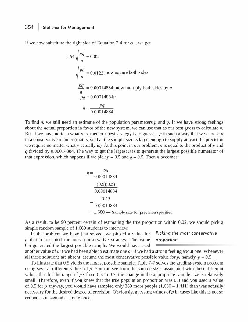
354 Statistics for Management
If we now substitute the right side of Equation 7-4 for pσ , we get
1.64 0.02=pq
n
0.0122;=pq
nnow square both sides
pq
n = 0.00014884; now multiply both sides by n
pq = 0.00014884n
0.00014884=n
pq
n, we still need an estimate of the population parameters p and q. If we have strong feelings about the actual proportion in favor of the new system, we can use that as our best guess to calculate n. But if we have no idea what p is, then our best strategy is to guess at p in such a way that we choose n in a conservative manner (that is, so that the sample size is large enough to supply at least the precision we require no matter what p actually is). At this point in our problem, n is equal to the product of p and q divided by 0.00014884. The way to get the largest n is to generate the largest possible numerator of that expression, which happens if we pick p = 0.5 and q = 0.5. Then n becomes:
0.00014884=n
pq
(0.5)(0.5)
0.00014884=
0.25
0.00014884=
= 1,680 ←
As a result, to be 90 percent certain of estimating the true proportion within 0.02, we should pick a simple random sample of 1,680 students to interview.
In the problem we have just solved, we picked a value for p that represented the most conservative strategy. The value 0.5 generated the largest possible sample. We would have used another value of p if we had been able to estimate one or if we had a strong feeling about one. Whenever all these solutions are absent, assume the most conservative possible value for p, namely, p = 0.5.
To illustrate that 0.5 yields the largest possible sample, Table 7-7 solves the grading-system problem using several different values of p. You can see from the sample sizes associated with these different values that for the range of p’s from 0.3 to 0.7, the change in the appropriate sample size is relatively small. Therefore, even if you knew that the true population proportion was 0.3 and you used a value of 0.5 for p anyway, you would have sampled only 269 more people (1,680 – 1,411) than was actually
p in cases like this is not so
Picking the most conservative
proportion
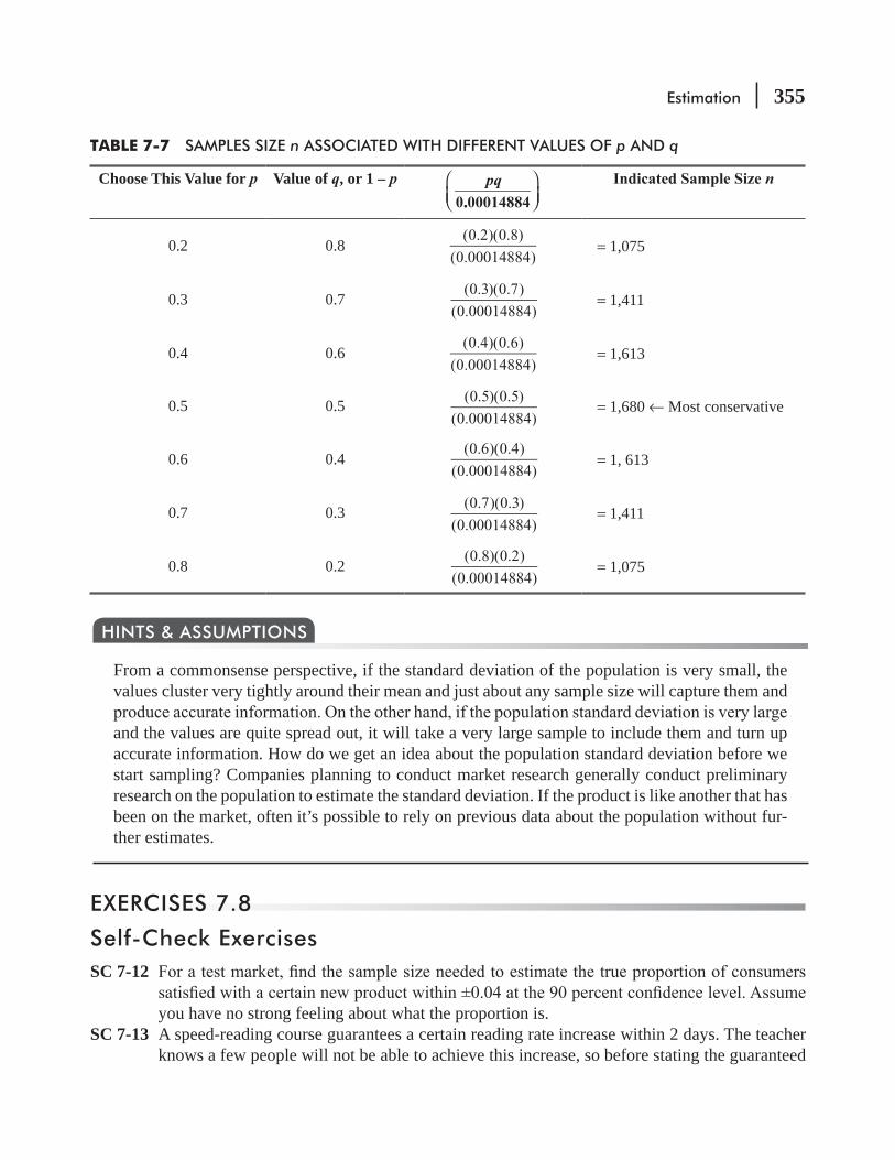
Estimation 355
From a commonsense perspective, if the standard deviation of the population is very small, the values cluster very tightly around their mean and just about any sample size will capture them and
and the values are quite spread out, it will take a very large sample to include them and turn up accurate information. How do we get an idea about the population standard deviation before we start sampling? Companies planning to conduct market research generally conduct preliminary research on the population to estimate the standard deviation. If the product is like another that has been on the market, often it’s possible to rely on previous data about the population without fur-ther estimates.
HINTS & ASSUMPTIONS
EXERCISES 7.8
Self-Check ExercisesSC 7-12
you have no strong feeling about what the proportion is.SC 7-13 A speed-reading course guarantees a certain reading rate increase within 2 days. The teacher
knows a few people will not be able to achieve this increase, so before stating the guaranteed
TABLE 7-7 SAMPLES SIZE n ASSOCIATED WITH DIFFERENT VALUES OF p AND q
Choose This Value for p Value of q, or 1 – p..0 00014884
⎛⎝⎜
⎞⎠⎟
pq n
0.2 0.8(0.2)(0.8)
(0.00014884)= 1,075
0.3 0.7(0.3)(0.7)
(0.00014884)= 1,411
0.4 0.6(0.4)(0.6)
(0.00014884)= 1,613
0.5 0.5 (0.5)(0.5)
(0.00014884)= 1,680 ← Most conservative
0.6 0.4(0.6)(0.4)
(0.00014884)= 1, 613
0.7 0.3 (0.7)(0.3)
(0.00014884)= 1,411
0.8 0.2(0.8)(0.2)
(0.00014884)= 1,075

356 Statistics for Management
-dent that the percentage has been estimated to within ±5 percent of the true value. What is the most conservative sample size needed for this problem?
Basic Concepts7-45
7-46 We have strong indications that the proportion is around 0.7. Find the sample size needed to
7-47 Given a population with a standard deviation of 8.6, what size sample is needed to estimate
Applications7-48
people who are in favor of the proposal. Find the sample size needed to estimate the true -
ings about what the proportion is. How would your sample size change if you believe about 75 percent of the people favor the proposal? How would it change if only about 25 percent favor the proposal?
7-49 -edly detrimental effects on health caused by its manufacturing process. A social scientist has advanced a theory that the employees who die from natural causes exhibit remarkable consis-tency in their life-span: The upper and lower limits of their life-spans differ by no more than
7-50 Food Tiger, a local grocery store, sells generic garbage bags and has received quite a few complaints about the strength of these bags. It seems that the generic bags are weaker than the
of purchasing, is interested in determining the average maximum weight that can be put into one of the generic bags without its breaking. If the standard deviation of garbage breaking weight is 1.2 lb, determine the number of bags that must be tested in order for Mr. Tiger to be
7-51 The university is considering raising tuition to improve school facilities, and they want to determine what percentage of students favor the increase. The university needs to be 90 per-
large a sample is needed to guarantee this accuracy regardless of the true percentage?7-52 A local store that specializes in candles and clocks, Wicks and Ticks, is interested in obtaining
an interval estimate for the mean number of customers that enter the store daily. The owners are reasonably sure that the actual standard deviation of the daily number of customers is 15
only eight customers.

Estimation 357
Worked-Out Answers to Self-Check ExercisesSC 7-12 Assume p = q = 0.5.
0.04 1.64 1.640.5 (0.5)
= =pq
n n so 1.64(0.5)
0.04
2
=⎛⎝⎜
⎞⎠⎟
n = 420.25 i.e. n ≥ 421.
SC 7-13 Assume p = q = 0.5.
0.05 2.33 2.330.5 (0.5)
= =pq
n n so 2.33(0.5)
0.05
2
=⎛⎝⎜
⎞⎠⎟
n = 542.89 i.e. n ≥ 543.
So take a sample of at least 543 records of prior students.
STATISTICS AT WORK
Loveland ComputersCase 7: Estimation -
next assignment introduced Lee to another of Loveland Computers’ departments and the no-nonsense approach of its head, Margot Derby.
-
actual PCs that people use in their homes and businesses. When we started out, we left it up to the customers to seek out software. Sometimes, they bought directly from the companies that wrote the
every suburban mall has at least one store that sells computer programs.
didn’t want to guess which one would be the ‘hit’ product and end up with a lot of useless inventory on our hands. But the game changed. After some shakeout in software, two or three clear leaders emerged
bundle some software with the computers for certain promotions.
give them a very competitive price for the software, and preloading turns out to be an important product feature that many people are shopping for. So I’m taking another look at software, to see if we shouldn’t change our strategy and do more in that line. To get some idea of the market, I had a summer intern call up 500 customers who’d owned Loveland machines for about a year. And we asked them how much
from our spreadsheet program. Those investment bankers from New York took a look at a draft of my marketing plan for software; when they were down here last week, they asked me how sure I could be that the results of that telephone survey were accurate.

358 Statistics for Management
of all the surveys and when they’re right and wrong? I only have this one set of results. I don’t see how I can answer their question.”
out right now.” What distribution will Lee assume for the telephone poll results, and which statisti-
margin of error for Margot? Is Lee likely to recom-mend a larger sample?
CHAPTER REVIEW
Terms Introduced in Chapter 7 A range of values that has some designated probability of including the true
population parameter value. The probability that statisticians associate with an interval estimate of a popula-
parameter.
Consistent Estimator An estimator that yields values more closely approaching the population parameter as the sample size increases.
The number of values in a sample we can specify freely once we know some-thing about that sample.
An estimator with a smaller standard error than some other estimator of the popu-
EstimateEstimator A sample statistic used to estimate a population parameter.Interval Estimate A range of values to estimate an unknown population parameter.Point Estimate A single number used to estimate an unknown population parameter.Student’s Distribution A family of probability distributions distinguished by their individual degrees of freedom, similar in form to the normal distribution, and used when the population standard deviation is unknown and the sample size is relatively small (n ≤ 30).
An estimator that uses all the information available in the data concerning a parameter.Unbiased Estimator An estimator of a population parameter that, on the average, assumes values above the population parameter as often, and to the same extent, as it tends to assume values below the population parameter.
Equations Introduced in Chapter 7
7-1 sx x
nˆ
( )
1
2
σ = ×∑ −
− p. 333
This formula indicates that the sample standard deviation can be used to estimate the popula-tion standard deviation.

Estimation 359
7-2 ˆˆ
1σ σ
= ×−−n
N n
N p. 333
This formula enables us to derive an estimated standard error of the mean of a nite popula-tion from an estimate of the population standard deviation. The symbol ˆ, called a hat, indi-
population.7-3 μ
p = p p. 337
Use this formula to derive the mean of the sampling distribution of the proportion of suc-cesses. The right-hand side, p, is equal to (n × p)/n, where the numerator is the expected number of successes in n trials and the denominator is the number of trials. Symbolically, the proportion of successes in a sample is written p and is pronounced p bar.
7-4 σ =pq
np p. 337
To get the standard error of the proportion, take the square root of the product of the prob-abilities of success and failure divided by the number of trials.
7-5 σ =p q
np p. 338
This is the formula to use to derive an estimated standard error of the proportion when the population proportion is unknown and you are forced to use p and q, the sample proportions of successes and failures.
7-6 ˆˆ
σ σ=
nx p. 344
This formula enables us to derive an estimated standard error of the mean of an in nite popu-lation from an estimate of the population standard deviation. It is exactly like Equation 7-2
Review and Application Exercises7-53 From a sample of 42 gasoline stations statewide, the average price of a gallon of unleaded gas was
found to be $1.12 and the standard deviation was $0.04 per gallon. Within what interval can we be
7-54 What are the advantages of using an interval estimate over a point estimate?7-55 Why is the size of a statistic’s standard error important in its use as an estimator? To which
characteristic of estimator does this relate?7-56 Suzanne Jones, head registrar for the university system, needs to know what proportion of
students have grade-point averages below 2.0. How many students’ grades should be looked
7-57 --
tages of each of these interval estimates?7-58 The posted speed limit on the Cross-Bronx Expressway is 55 mph. Congestion results in much
slower actual speeds. A random sample of 57 vehicles clocked speeds with an average of 23.2 mph and a standard deviation of 0.3 mph.
360 Statistics for Management
(a) Estimate the standard deviation of the population.(b) Estimate the standard error of the mean for this population.
7-59 Based on knowledge about the desirable qualities of estimators, for what reasons might x be
7-60 has been considering various courses of action. In an effort to understand the catalysts of
0.032 nd the associated standard deviation is 0.0130.
given day that a crew has returned from the mainland.
7-61 -veys, it is known that the standard deviation of the number of hours of television watched in a
number of hours of television watched per week per household in India. Accuracy is important,
of hours falls within ±0.3 hour of the national average. Conservatively, what sample size should
7-62 John Bull has just purchased a computer program that claims to pick stocks that will increase
test this program in order to be 98 percent certain that the percentage of stocks that do in fact go up in the next week will be within ±0.05 of the sample proportion?
7-63 Gotchya runs a laser-tag entertainment center where adults and teenagers rent equipment and engage in mock combat. The facility is always used to capacity on weekends. The three own-ers want to assess the effectiveness of a new advertising campaign aimed at increasing week-night usage. The number of paying patrons on twenty-seven randomly selected weeknights
patrons on a weeknight.
61 57 53 60 64 57 54 58 6359 50 60 60 57 58 62 63 6061 54 50 54 61 51 53 62 57
7-64 Their accountants have told the owners of Gotchya, the laser-tag entertainment center
break even on a weeknight. The partners are willing to continue to operate on weeknights if they can be at least 95 percent certain that they will break even at least half the time.
weeknights on which Gotchya will break even. Should Gotchya continue to stay open on weeknights? Explain.
7-65 In evaluating the effectiveness of a national prison rehabilitation program, a survey of 52 of a prison’s 900 inmates found that 35 percent were repeat offenders.
Estimation 361
(a) Estimate the standard error of the proportion of repeat offenders.
the inmates of this prison.7-66
calculated the mean number of passengers per kilometer to be 4.1. From previous studies, the population standard deviation is known to be 1.2 passengers per kilometer.
meter for the population.7-67 The Internal Revenue Service sampled 200 tax returns recently and found that the sample
average income tax refund amounted to $425.39 and the sample standard deviation was $107.10.(a) Estimate the population mean tax refund and standard deviation.(b) Using the estimates of part (a), construct an interval in which the population mean is
95 percent certain to fall.7-68 The Physicians Care Group operates a number of walk-in clinics. Patient charts indicate the
time that a patient arrived at the clinic and the time that the patient was actually seen by a phy--
week’s workload and calculates an average wait time of 15.2 minutes. A previous large-scale study of waiting time over several clinics had a standard deviation of 2.5 minutes. Construct
(a) 90 percent.(b) 99 percent.
7-69 -
tion standard deviation to be 1.4 milligrams of chlorine per liter. The latest samples averaged 4.6 milligrams of chlorine per liter.(a) Find the standard error of the mean.(b) Establish the interval around 5.2, the population mean, that will include the sample mean
with a probability of 68.3 percent.7-70 Ellen Harris, an industrial engineer, was accumulating normal times for various tasks on a
labor-intensive assembly process. This process included 300 separate job stations, each per-forming the same assembly tasks. She sampled seven stations and obtained the following assembly times for each station: 1.9, 2.5, 2.9, 1.3, 2.6, 2.8, and 3.0 minutes.(a) Calculate the mean assembly time and the corresponding standard deviation for the
sample.(b) Estimate the population standard deviation.
7-71 High Fashion Marketing is considering reintroducing paisley ties. In order to avoid a fashion
of the 90 interviewed, 79 believed that paisley ties were fashionable and were interested in
7-72 The Department of Transportation has mandated that the average speed of cars on interstate high-ways must be no more than 67 miles per hour in order for state highway departments to retain

362 Statistics for Management
their federal funding. North Carolina troopers, in unmarked cars, clocked a sample of 186 cars and found that the average speed was 66.3 miles per hour and the standard deviation was 0.6 mph.(a) Find the standard error of the mean.(b) What is the interval around the sample mean that would contain the population mean
95.5 percent of the time?(c) Can North Carolina truthfully report that the true mean speed on its highways is 67 mph
7-73 Dheeraj Pillai, owner of the Aurora Restaurant, is considering purchasing new furniture. To help him decide on the amount he can afford to invest in tables and chairs, he wishes to deter-mine the average revenue per customer. The checks for 9 randomly sampled customers had
interval for the size of the average check per customer.7-74 John Deer, a horticulturist at Northern Carrboro State University, knows that a certain strain
90 percent, how many 1-acre samples must be taken in order to estimate the average produc-tion per acre to within ±5 bushels per acre?
7-75 Nirmal Pvt. Limited is a FMCG company, selling a range of products. It has 1150 sales outlets. A sample of 60 sales outlets was chosen, using random sampling for the purpose of sales analysis. The sample consists of sales outlets from rural and urban areas belonging
related to annual sales has been was collected from them in the month of December 2010. This process has been repeated in December 2011. In the meanwhile, in 2010 a comprehensive sales-promotion program was launched to augment the sales. The information is presented in
following questions.separately.
Compare the results and comment.
Rural Shops” separately. Compare the results and comment.
(e) Point estimate of the standard deviation of 2011 sale.
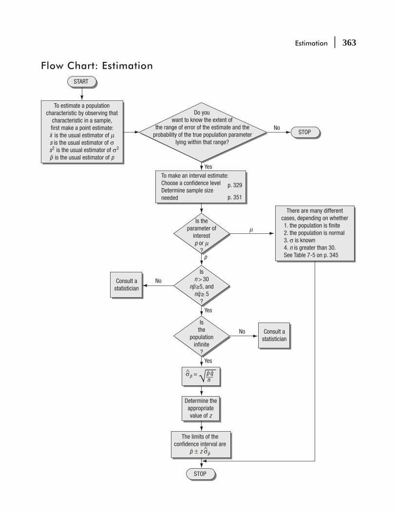
Estimation 363
No
No
No
Yes
Yes
Yes
To make an interval estimate:Choose a confidence levelDetermine sample sizeneeded
p. 329
p. 351
m
p
Is theparameter of
interestp or m
?
Isn > 30
np ≥5, andnq ≥ 5
?
Isthe
populationinfinite
?
STOP
Do youwant to know the extent of
the range of error of the estimate and the probability of the true population parameter
lying within that range?
To estimate a populationcharacteristic by observing that
characteristic in a sample,first make a point estimate:x is the usual estimator of ms is the usual estimator of σ
s2 is the usual estimator of σ2
p is the usual estimator of p
There are many differentcases, depending on whether1. the population is finite2. the population is normal3. σ is known4. n is greater than 30.See Table 7-5 on p. 345
Consult astatistician
STOP
START
Determine theappropriatevalue of z
Consult astatistician
σ∧ p =
√⎯p qn⎯
The limits of theconfidence interval are
p ± z σ∧ p
Flow Chart: Estimation

This page is intentionally left blank
LEARNING OBJECTIVES
8After reading this chapter, you can understand:
CHAPTER CONTENTS
To learn how to use samples to decide whether a population possesses a particular characteristic
To determine how unlikely it is that an observed sample could have come from a hypothesized population
To understand the two types of errors possible when testing hypotheses
8.1 Introduction 366
8.2 Concepts Basic to the Hypothesis-Testing Procedure 367
8.3 Testing Hypotheses 371
8.4 Hypothesis Testing of Means When the Population Standard Deviation is Known 379
8.5 Measuring the Power of a Hypothesis Test 388
To learn when to use one-tailed tests and when to use two-tailed tests
hypotheses
To understand how and when to use the normal and t distributions for testing hypotheses about population means and proportions
8.6 Hypothesis Testing of Proportions: Large Samples 391
8.7 Hypothesis Testing of Means When the Population Standard Deviation is not Known 397
Statistics at Work 404 Terms Introduced in Chapter 8 404 Review and Application Exercises 405 Flow Chart: One-Sample Tests
of Hypotheses 410
Testing Hypotheses: One-sample Tests
366 Statistics for Management
Tapproximately 10,000 sheets of 0.04-inch-thick aluminum. The aluminum sheets cannot be appreciably thicker than 0.04 inch because the structure could not support the additional weight. Nor can the sheets be appreciably thinner than 0.04 inch because the strength of the roof would be inadequate. Because of this restriction on thickness, Parkhill carefully checks the aluminum sheets from its supplier. Of course, Parkhill does not want to measure each sheet, so it randomly samples 100. The sheets in the sample have a mean thickness of 0.0408 inch. From past experience with this supplier, Parkhill believes that these sheets come from a thickness population with a standard deviation of 0.004 inch. On the basis of these
statistics to estimate population parameters. Now, to solve problems like Parkhill’s, we shall learn how to use characteristics of samples to test an assumption we have about the population from which that sample came. Our test for Parkhill, later in the chapter, may lead Parkhill to accept the shipment or it may indicate that Parkhill should reject the aluminum sheets sent by the supplier because they do not
8.1 INTRODUCTIONHypothesis testing begins with an assumption, called a hypothesis, that we make about a population parameter. Then we collect sample data, produce sample statistics, and use this information to decide how likely it is that our hypothesized population parameter is correct. Say that we assume a certain value for a population mean. To test the validity of our assumption, we gather sample data and determine the difference between the hypoth-
-cant. The smaller the difference, the greater the likelihood that our hypothesized value for the mean is correct. The larger the difference, the smaller the likelihood.
Unfortunately, the difference between the hypothesized population parameter and the actual statistic is more often neither so large that we automatically reject our hypothesis nor so small that we just as
are the exception, not the rule.Suppose a manager of a large shopping mall tells us that the
How can we test the validity of her hypothesis? Using the sampling sample of her employees. If we
did this and the sample statistic came out to be 95 percent, we would readily accept the manager’s state-ment. However, if the sample statistic were 46 percent, we would reject her assumption as untrue. We can interpret both these outcomes, 95 percent and 46 percent, using our common sense.
88 percent. This value is relatively close to 90 percent, but is it close enough for us to accept the manager’s hypothesis? Whether we accept or reject the manager’s hypothesis, we cannot be abso-lutely certain that our decision is correct; therefore, we will have to learn to deal with uncertainty in our decision making. We cannot accept or reject a hypothesis about a population parameter simply by intuition. Instead, we need to learn how to decide objectively, on the basis of sample information, whether to accept or reject a hunch.
Function of hypothesis testing
When to accept or reject the
hypothesis
The basic problem is dealing
with uncertainty

Testing Hypotheses: One-sample Tests 367
Making Big JumpsCollege students often see ads for learning aids. One very popular such aid is a combination outline, study guide, and question set for various courses. Advertisements about such items often claim better examination scores with less study-ing time. Suppose a study guide for a basic statistics course is available through an organization that produces such guides for 50 different courses. If this study guide for basic statistics has been tested (and
raise grades and lower study time.” Of course, this assertion is quite true, but only as it applies to the
kind of results for the other 49 guides.
removing crabgrass from your lawn and may assert that the
procedures were, in fact, used during the tests, such claims still involve big jumps. Suppose that the test plot was in Florida and your lawn problems are in Utah. Differences in rainfall, soil fertility, airborne pollutants, temperature, dormancy hours and germination conditions may vary widely between these two locations. Claiming results for a statistically valid test under a completely different set of test conditions is invalid. One such test cannot measure effectiveness under a wide variety of environmental conditions.
EXERCISES 8.18-1 Why must we be required to deal with uncertainty in our decisions, even when using statistical
techniques?8-2 Theoretically speaking, how might one go about testing the hypothesis that a coin is fair? That
a die is fair?8-3 Is it possible that a false hypothesis will be accepted? How would you explain this?8-4 Describe the hypothesis-testing process.8-5 How would you explain a large difference between a hypothesized population parameter and
a sample statistic if, in fact, the hypothesis is true?
8.2 CONCEPTS BASIC TO THE HYPOTHESIS-TESTING PROCEDURE
Before we introduce the formal statistical terms and procedures, we’ll work our chapter-opening sports-complex problem all the
that they will be unsatisfactory if they are too thick or too thin. The contractor takes a sample of 100 sheets and determines that the sample mean thickness is 0.0408 inch. On the basis of past experience, he knows that the population standard deviation is 0.004 inch. Does this sample evidence indicate that the batch of 10,000 sheets of aluminum is suitable for constructing the roof of the new sports complex?
If we assume that the true mean thickness is 0.04 inch, and we know that the population standard deviation is 0.004 inch, how likely is it that we would get a sample mean of 0.0408 or more from that population? In other words, if
Projecting too far
Different test conditions
Sports-complex problem
Formulating the hypothesis

368 Statistics for Management
the true mean is 0.04 inch and the standard deviation is 0.004 inch, what are the chances of getting a sample mean that differs from 0.04 inch by 0.0008 (= 0.0408 – 0.04) inch or more?
These questions show that to determine whether the population mean is actually 0.04 inch, we must calculate the probability that a random sample with a mean of 0.0408 inch will be selected from a population with a μ of 0.04 inch and a σ of 0.004 inch. This probability will indicate whether it is reasonable to observe a sample like this if the population mean is actually 0.04 inch. If this probability is far too low, we must conclude that the aluminum company’s statement is false and that the mean thickness of the aluminum sheets is not 0.04 inch.
Let’s answer the question illustrated in Figure 8-1: If the hypothesized population mean is 0.04 inch and the population standard deviation is 0.004 inch, what are the chances of getting a sample mean (0.0408 inch) that differs from 0.04 inch by 0.0008 inch? First, we calculate the standard error of the mean from the population standard deviation:
nxσ σ
=
0.004 in.
100=
= 0.004 in.
10
= 0.0004 in. [6-1 ]
Next we use Equation 6-2 to discover that the mean of our sample (0.0408 inch) lies 2 standard errors to the right of the hypothesized population mean:
zx
x
μσ
=−
0.0408 0.04
0.0004=
−
= 2 ← Standard errors of the mean [6-2]
Using Appendix Table 1, we learn that 4.5 percent is the total chance of our sample mean differing from the population mean by 2 or more standard errors; that is, the chance that the sample mean would be 0.0408 inch or larger or 0.0392 inch or smaller is only 4.5 per-cent (P(z = 2(0.5 – 0.4772) = 0.0456, or about 4.5 percent). With this low a chance, Parkhill could conclude that a population with a true mean of 0.04 inch would not be likely to produce a sample like this. The project supervisor would reject the aluminum company’s statement about the mean thickness of the sheets.
In this case, the difference between the sample mean and the hypothesized population mean is too large, and the chance that the population would produce such a random sample is far too low. Why this probability of 4.5 percent is too low, or wrong, is a judgment for decision makers to make. Certain situations demand that decision makers be very sure about the characteristics of the items being
Calculating the standard
error of the mean
Interpreting the probability
associated with this difference
The decision maker’s role in
formulating hypotheses
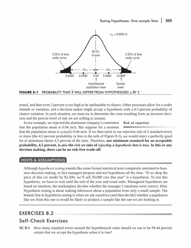
Testing Hypotheses: One-sample Tests 369
tested, and then even 2 percent is too high to be attributable to chance. Other processes allow for a wider latitude or variation, and a decision maker might accept a hypothesis with a 4.5 percent probability of chance variation. In each situation, we must try to determine the costs resulting from an incorrect deci-sion and the precise level of risk we are willing to assume.
In our example, we rejected the aluminum company’s contention that the population mean is 0.04 inch. But suppose for a moment that the population mean is actually 0.04 inch. If we then stuck to our rejection rule of 2 standard errors or more (the 4.5 percent probability or less in the tails of Figure 8-1), we would reject a perfectly good lot of aluminum sheets 4.5 percent of the time. Therefore, our minimum standard for an acceptable probability, 4.5 percent, is also the risk we take of rejecting a hypothesis that is true. In this or any decision making, there can be no risk-free trade-off.
Although hypothesis testing sounds like some formal statistical term completely unrelated to busi-
price of this car model by $1,500, we’ll sell 50,000 cars this year” is a hypothesis. To test this hypothesis, we have to wait until the end of the year and count sales. Managerial hypotheses are based on intuition; the marketplace decides whether the manager’s intuitions were correct. Hint: Hypothesis testing is about making inferences about a population from only a small sample. The bottom line in hypothesis testing is when we ask ourselves (and then decide) whether a population like we think this one is would be likely to produce a sample like the one we are looking at.
HINTS & ASSUMPTIONS
EXERCISES 8.2
Self-Check ExercisesSC 8-1 How many standard errors around the hypothesized value should we use to be 99.44 percent
certain that we accept the hypothesis when it is true?
Risk of rejection
2.25% of areaunder curve
Hypothesizedpopulation mean
0.0392" 0.0396" 0.04" 0.0404" 0.0408"
Samplemean
2.25% of areaunder curve
95.5%of area
σx− = 0.0004 in.
+2σx−−2σx−
FIGURE 8-1 PROBABILITY THAT X WILL DIFFER FROM HYPOTHESIZED μ BY 2
370 Statistics for Management
SC 8-2 An automobile manufacturer claims that a particular model gets 28 miles to the gallon. The
sample mean to be 26.8 miles per gallon. From previous studies, the population standard devia-tion is known to be 5 miles per gallon. Could we reasonably expect (within 2 standard errors) that we could select such a sample if indeed the population mean is actually 28 miles per gallon?
Basic Concepts8-6 What do we mean when we reject a hypothesis on the basis of a sample?8-7 Explain why there is no single standard level of probability used to reject or accept in hypoth-
esis testing.8-8 If we reject a hypothesized value because it differs from a sample statistic by more than 1.75
standard errors, what is the probability that we have rejected a hypothesis that is in fact true?8-9 How many standard errors around the hypothesized value should we use to be 98 percent
certain that we accept the hypothesis when it is true?
Applications8-10 Sports and media magnate Ned Sterner is interested in purchasing the Atlanta Stalwarts if he
-age attendance would have to be about 28,500 fans per game to make the purchase attractive
reported in Sporting Reviews that average attendance at these games was 26,100. A study he commissioned the last time he purchased a team showed that the population standard devia-tion for attendance at similar events had been quite stable for the past 10 years at about 6,000 fans. Using 2 standard errors as the decision criterion, should Ned purchase the Stalwarts? Can you think of any reason(s) why your conclusion might not be valid?
8-11 Computing World has asserted that the amount of time owners of personal computers spend on their machines averages 23.9 hours per week and has a standard deviation of 12.6 hours per week. A random sampling of 81 of its subscribers revealed a sample mean usage of 27.2 hours per week. On the basis of this sample, is it reasonable to conclude (using 2 standard errors as the decision criterion) that Computing World’s subscribers are different from average personal computer owners?
8-12 A grocery store has specially packaged oranges and has claimed a bag of oranges will yield 2.5 quarts of juice. After randomly selecting 42 bags, a stacker found the average juice pro-duction per bag to be 2.2 quarts. Historically, we know the population standard deviation is 0.2 quart. Using this sample and a decision criterion of 2.5 standard errors, could we conclude the store’s claims are correct?
Worked-Out Answers to Self-Check ExercisesSC 8-1 To leave a probability of 1 – 0.9944 = 0.0056 in the tails, the absolute value of z must be
greater than or equal to 2.77, so the interval should be ± 2.77 standard errors about the hypoth-esized value.
SC 8-2 σ = 5 n = 49 x = 26.8 μ = 28μ ± 2 xσ = μ ± 2σ n =28 ± 2(5) 49 = 28 ± 1.429 = (26.571, 29.429)Because x = 26.8 > 26.57, it is not unreasonable to see such sample results if μ really is 28 mpg.
Testing Hypotheses: One-sample Tests 371
8.3 TESTING HYPOTHESESIn hypothesis testing, we must state the assumed or hypothesized value of the population parameter before we begin sampling. The assumption we wish to test is called the null hypothesis and is symbolized H0
Suppose we want to test the hypothesis that the population mean is equal to 500. We would symbol-
H0: μ = 500
The term null hypothesis arises from earlier agricultural and medi-cal applications of statistics. In order to test the effectiveness of a new fertilizer or drug, the tested hypothesis (the null hypothesis) was that it had no effect, that is, there was no difference between treated and untreated samples.
If we use a hypothesized value of a population mean in a problem, we would represent it symbolically as
H0μ
If our sample results fail to support the null hypothesis, we must conclude that something else is true. Whenever we reject the hypothesis, the conclusion we do accept is called the alternative hypothesis and is symbolized H1 (“H sub-one”)· For the null hypothesis
H0: μ = 200
we will consider three possible alternative hypotheses:
H1: μ ← not equal to 200”
H1: μ > 200 ← greater than 200”
H1: μ < 200 ← less than 200”
Interpreting the Significance LevelThe purpose of hypothesis testing is not to question the com-puted value of the sample statistic but to make a judgment about the difference between that sample statistic and a hypothesized population parameter. The next step after stating the null and alternative hypotheses, then, is to decide what criterion to use for deciding whether to accept or reject the null hypothesis.
In our sports-complex example, we decided that a difference observed between the sample mean x and the hypothesized population mean H0
μ had only a 4.5 percent, or 0.045, chance of occurring. Therefore, we rejected the null hypothesis that the population mean was 0.04 inch (H0: μ = 0.04 inch). In statistical terms, the value 0.045 is called the signi cance level.
This means that we will reject the null hypothesis if the difference between the sample statistic and the hypothesized population
Making a formal statement of
the null hypothesis
Why is it called the null
hypothesis?
Making a formal statement of
the alternate hypothesis
Goal of hypothesis testing
Function of the significance
level

372 Statistics for Management
in every 100 samples when the hypothesized population parameter is correct. If we assume the
is outside certain limits.of sample means that fell within
Figure 8-2 illustrates how to interpret a 5 percent level of
located in each tail. From Appendix Table 1, we can determine that 95 percent of all the area under the curve is included in an interval extending 1.96
xσ on either side of
observed value of the sample statistic and the hypothesized value of the population parameter. In the
Figure 8-3 examines this same example in a different way. Here, the 0.95 of the area under the curve is where we would accept the null hypothesis. The two colored parts under the curve, representing a total of 5 percent of the area, are the regions where we would reject the null hypothesis.
A word of caution is appropriate here. Even if our sample statistic in Figure 8-3 does fall in the nonshaded region (the region that makes up 95 percent of the area under the curve), this does not prove that our null hypothesis (H0) is true; it simply does not provide statistical evidence to reject it. Why? Because the only way in which the hypothesis can be accepted with certainty is for us to know the population parameter; unfortunately, this is not possible. Therefore, whenever we say that we accept the null hypothesis, we actually mean that there is not
Use of the term accept, instead of do not reject, has become standard. It means simply that when sample data do not cause us to reject a null hypothesis, we behave as if that hypothesis is true.
Area where no significant
difference exists
Also called the area where
we accept the null hypothesis
Hypotheses are accepted, not
proved
Region where there is no significantdifference between the sample statisticand the hypothesized population parameter
0.025 of area 0.025 of area0.95 of area
In these 2 regions, there is a significant differencebetween the sample statistic and the hypothesizedpopulation parameter
μH0 −1.96σx− μH0
+1.96σx−
μH0
FIGURE 8-2 REGIONS OF SIGNIFICANT DIFFERENCE AND OF NO SIGNIFICANT DIFFERENCE AT A 5 PERCENT LEVEL OF SIGNIFICANCE

Testing Hypotheses: One-sample Tests 373
Selecting a Significance Level
-cance is used. Published research results often test hypotheses at the
any -
the risk we assume of rejecting a null hypothesis when it is true. use for testing a hypothesis, the higher the probability of rejecting a null hypothesis when it is true.
Examining this concept, we refer to Figure 8-4. Here we have illustrated a hypothesis test at three dif-
mean x on each distribution. In parts a and b, we would accept the null hypothesis that the population mean is equal to the hypothesized value. But notice that in part c, we would reject this same null hypoth-
when it is not true but, at the same time, often reject it when it is true.
Type I and Type II Errors
illustrated in Figure 8-4. Rejecting a null hypothesis when it is true is called a Type I error, and its probability (which, as we have seen,
α (alpha). Alternatively, accepting a null hypoth-esis when it is false is called a Type II error, and its probability is symbolized β (beta). There is a trade-off between these two errors: The probability of making one type of error can be reduced only if we are willing to increase the probability of making the other type of error. Notice in part c. Figure 8-4, that our acceptance region is quite small (0.50 of the area under the curve). With an acceptance region this small, we will rarely accept a null hypothesis when it is not true, but as a cost of being this sure, we will
Trade-offs when choosing a
significance level
Type I and Type II errors
defined
We would accept the null hypothesis if thesample statistic falls in this region (wewould no reject H0)
We would reject the null hypothesis if the samplestatistic falls in this regions
0.025 of area 0.025 of area0.95 of area
μH0
μH0 −1.96σx− μH0
−1.96σx−
FIGURE 8-3 A 5 PERCENT LEVEL OF SIGNIFICANCE, WITH ACCEPTANCE AND REJECTION REGIONS DESIGNATED
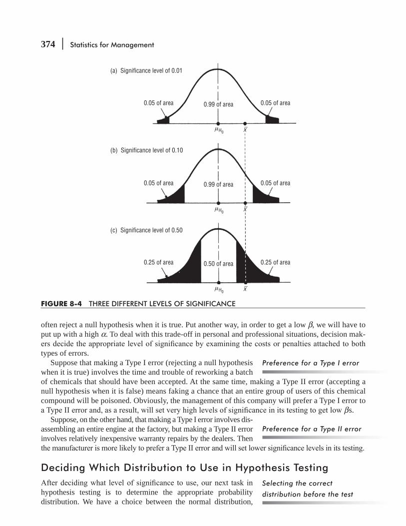
374 Statistics for Management
often reject a null hypothesis when it is true. Put another way, in order to get a low β, we will have to put up with a high α. To deal with this trade-off in personal and professional situations, decision mak-
types of errors.Suppose that making a Type I error (rejecting a null hypothesis
when it is true) involves the time and trouble of reworking a batch of chemicals that should have been accepted. At the same time, making a Type II error (accepting a null hypothesis when it is false) means faking a chance that an entire group of users of this chemical compound will be poisoned. Obviously, the management of this company will prefer a Type I error to
βs.Suppose, on the other hand, that making a Type I error involves dis-
assembling an entire engine at the factory, but making a Type II error involves relatively inexpensive warranty repairs by the dealers. Then
Deciding Which Distribution to Use in Hypothesis Testing
hypothesis testing is to determine the appropriate probability distribution. We have a choice between the normal distribution,
Preference for a Type I error
Preference for a Type II error
Selecting the correct
distribution before the test
(a) Significance level of 0.01
(b) Significance level of 0.10
(c) Significance level of 0.50
0.05 of area 0.99 of area 0.05 of area
0.05 of area 0.99 of area 0.05 of area
0.25 of area 0.50 of area 0.25 of area
μH0
μH0
x−
x−
μH0 x−
FIGURE 8-4 THREE DIFFERENT LEVELS OF SIGNIFICANCE
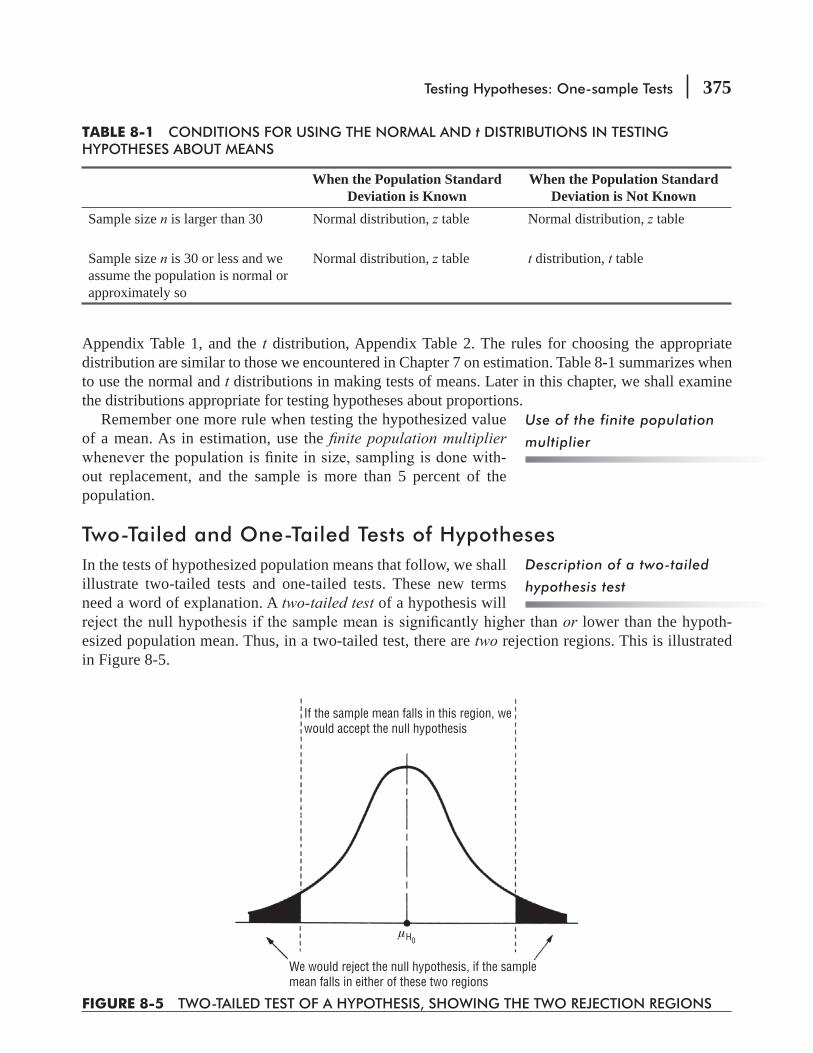
Testing Hypotheses: One-sample Tests 375
Appendix Table 1, and the t distribution, Appendix Table 2. The rules for choosing the appropriate distribution are similar to those we encountered in Chapter 7 on estimation. Table 8-1 summarizes when to use the normal and t distributions in making tests of means. Later in this chapter, we shall examine the distributions appropriate for testing hypotheses about proportions.
Remember one more rule when testing the hypothesized value of a mean. As in estimation, use the nite population multiplier
-out replacement, and the sample is more than 5 percent of the population.
Two-Tailed and One-Tailed Tests of HypothesesIn the tests of hypothesized population means that follow, we shall illustrate two-tailed tests and one-tailed tests. These new terms need a word of explanation. A two-tailed test of a hypothesis will
or lower than the hypoth-esized population mean. Thus, in a two-tailed test, there are two rejection regions. This is illustrated in Figure 8-5.
Use of the finite population
multiplier
Description of a two-tailed
hypothesis test
FIGURE 8-5 TWO-TAILED TEST OF A HYPOTHESIS, SHOWING THE TWO REJECTION REGIONS
If the sample mean falls in this region, wewould accept the null hypothesis
We would reject the null hypothesis, if the samplemean falls in either of these two regions
μH0
TABLE 8-1 CONDITIONS FOR USING THE NORMAL AND t DISTRIBUTIONS IN TESTING HYPOTHESES ABOUT MEANS
When the Population Standard Deviation is Known
When the Population Standard Deviation is Not Known
Sample size n is larger than 30 Normal distribution, z table Normal distribution, z table
Sample size n is 30 or less and we assume the population is normal or approximately so
Normal distribution, z table t distribution, t table

376 Statistics for Management
A two-tailed test is appropriate when the null hypothesis is μ = H0μ ( H0
μand the alternative hypothesis is .H0
μ μ≠ Assume that a manufacturer of lightbulbs wants to produce bulbs with a mean life of H0
μ μ≠ = 1,000 hours. If the lifetime is shorter, he will lose customers to his
be excessively thick. In order to see whether his production process is working properly, he takes a sample of the output to test the hypothesis H0: μ = -cantly from 1,000 hours in either direction, the appropriate alternative hypothesis is H1: μhe uses a two-tailed test. That is, he rejects the null hypothesis if the mean life of bulbs in the sample is either too far above 1,000 hours or too far below 1,000 hours.
However, there are situations in which a two-tailed test is not appropriate, and we must use a one-tailed test. Consider the case of a wholesaler that buys lightbulbs from the manufacturer discussed earlier. The wholesaler buys bulbs in large lots and does not want to accept a lot of bulbs unless their mean life is at least 1,000 hours. As each shipment arrives, the whole-saler tests a sample to decide whether it should accept the shipment. The company will reject the ship-ment only il it feels that the mean life is below 1,000 hours. If it feels that the bulbs are better than expected (with a mean life above 1,000 hours), it certainly will not reject the shipment because the longer life comes at no extra cost. So the wholesaler’s hypotheses are H0: μ = 1,000 hours and H1: μ < 1,000 hours. It rejects H0 below 1,000
left-tailed, test (or a lower-tailed test).In general, a left-tailed (lower-tailed) test is used if the hypotheses
are H0: μ = H0
μ and H1: μ < H0
μ . In such a situation, it is sample evi-
the null hypothesis in favor of the alternative hypothesis. Stated differently, the rejection region is in the lower tail (left tail) of the distribution of the sample mean, and that is why we call this a lower-tailed test.
A left-tailed test is one of the two kinds of one-tailed tests. As you have probably guessed by now, the other kind of one-tailed test
Sometimes a one-tailed test is
appropriate
Left-tailed tests
Right-tailed tests
If the sample mean falls in thisregion, we would accept the nullhypothesis
If the sample meanfalls in this region, wewould reject the nullhypothesis
1,000 hours
FIGURE 8-6 LEFT-TAILED TEST (A LOWER-TAILED TEST) WITH THE REJECTION REGION ON THE LEFT SIDE (LOWER SIDE)
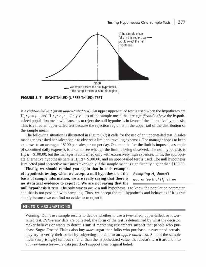
Testing Hypotheses: One-sample Tests 377
is a right-tailed test (or an upper-tailed test). An upper upper-tailed test is used when the hypotheses are H0 : μ =
H0μ and H1 : μ >
H0μ . Only values of the sample mean that are signi cantly above the hypoth-
esized population mean will cause us to reject the null hypothesis in favor of the alternative hypothesis. This is called an upper-tailed test because the rejection region is in the upper tail of the distribution of the sample mean.
The following situation is illustrated in Figure 8-7; it calls for the use of an upper-tailed test. A sales manager has asked her salespeople to observe a limit on traveling expenses. The manager hopes to keep expenses to an average of $100 per salesperson per day. One month after the limit is imposed, a sample of submitted daily expenses is taken to see whether the limit is being observed. The null hypothesis is H0: μ = $100.00, but the manager is concerned only with excessively high expenses. Thus, the appropri-ate alternative hypothesis here is H1: μ > $100.00, and an upper-tailed test is used. The null hypothesis
Finally, we should remind you again that in each example of hypothesis testing, when we accept a null hypothesis on the basis of sample information, we are really saying that there is no statistical evidence to reject it. We are not saying that the null hypothesis is true. The only way to prove a null hypothesis is to know the population parameter, and that is not possible with sampling. Thus, we accept the null hypothesis and behave as if it is true
Warning: Don’t use sample results to decide whether to use a two-tailed, upper-tailed, or lower-tailed test. Before any data are collected, the form of the test is determined by what the decision maker believes or wants to detect. Hint: If marketing researchers suspect that people who pur-chase Sugar Frosted Flakes also buy more sugar than folks who purchase unsweetened cereals, they try to verify their belief by subjecting the data to an upper-tailed test. Should the sample mean (surprisingly) turn out smaller than the hypothesized value, that doesn’t turn it around into a lower-tailed test—the data just don’t support their original belief.
HINTS & ASSUMPTIONS
Accepting H0 doesn’t
guarantee that H0 is true
We would accept the null hypothesis,if the sample mean falls in this region
If the sample meanfalls in this region, wewould reject the nullhypothesis
$100
FIGURE 8-7 RIGHT-TAILED (UPPER-TAILED) TEST

378 Statistics for Management
EXERCISES 8.3
Self-Check ExercisesSC 8-3 For the following cases, specify which probability distribution to use in a hypothesis test:
(a) H0: μ = 27, H1: μ x = 33, σ = 4, n = 25.(b) H0: μ = 98.6, H1: μ > 98.6, x = 99.1, σ = 1.5, n = 50.(c) H0: μ = 3.5, H1: μ < 3.5, x = 2.8, σ = 0.6, n = 18.(d) H0: μ = 382, H1: μ x = 363, σ = 68, n = 12.(e) H0: μ = 57, H1: μ > 57, x = 65, σ = 12, n = 42.
SC 8-4 Martha Inman, a highway safety engineer, decides to test the load-bearing capacity of a bridge that is 20 years old. Considerable data are available from similar tests on the same type of bridge. Which is appropriate, a one-tailed or a two-tailed test? If the minimum load-bearing capacity of this bridge must be 10 tons, what are the null and alternative hypotheses?
Basic Concepts8-13 Formulate null and alternative hypotheses to test whether the mean annual snowfall in Buffalo,
New York, exceeds 45 inches.8-14 Describe what the null and alternative hypotheses typically represent in the hypothesis-testing
process.8-15 signi cance level.8-16 8-17 In a trial, the null hypothesis is that an individual is innocent of a certain crime. Would the
legal system prefer to commit a Type I or a Type II error with this hypothesis?8-18 8-19 If our goal is to accept a null hypothesis that μ = 36.5 with 96 percent certainty when it’s true,
and our sample size is 50, diagram the acceptance and rejection regions for the following alternative hypotheses:(a) μ(b) μ > 36.5.(c) μ < 36.5.
8-20 For the following cases, specify which probability distribution, to use in a hypothesis test:(a) H0: μ = 15, H1: μ x = 14.8, σ = 3.0, n = 35.(b) H0: μ = 9.9, H1: μ x = 10.6, σ = 2.3, n = 16.(c) H0: μ = 42, H1: μ > 42, x = 44, σ = 4.0, n = 10.(d) H0: μ = 148, H1: μ > 148, x = 152, σ = 16.4, n = 29.(e) H0: μ = 8.6, H1: μ < 8.6, x = 8.5, σ = 0.15, n = 24.
8-21 Your null hypothesis is that the battery for a heart pacemaker has an average life of 300 days, with the alternative hypothesis being that the battery life is more than 300 days. You are the quality control engineer for the battery manufacturer.(a) Would you rather make a Type I or a Type II error?
8-22 Under what conditions is it appropriate to use a one-tailed test? A two-tailed test?8-23 If you have decided that a one-tailed test is the appropriate test to use, how do you decide
whether it should be a lower-tailed test or an uppertailed test?

Testing Hypotheses: One-sample Tests 379
Applications8-24
year. Now they want to determine whether the average monthly energy usage has decreased. Should they perform a one- or two-tailed test? If their previous average monthly energy usage was 3,124 kilowatt hours, what are the null and alternative hypotheses?
8-25 Dr. Ross Darrow believes that nicotine in cigarettes causes cigarette smokers to have higher daytime heart rates on average than do nonsmokers. He also believes that smokers crave the nicotine in cigarettes rather than just smoking for the physical satisfaction of the act and, accordingly, that the average smoker will smoke more cigarettes per day if he or she switches from a brand with a high nicotine content to one with a low level of nicotine.(a) Suppose Ross knows that nonsmokers have an average daytime heart rate of 78 beats per
(b) For the past 3 months, he has been observing a sample of 48 individuals who smoke an average of 15 high-nicotine cigarettes per day. He has just switched them to a brand with a low nicotine content. State null and alternative hypotheses for testing his second belief.
Worked-Out Answers to Self-Cheek ExercisesSC 8-3 (a) t with 24 df. (b) Normal. (c) t with l7 df.
(d) Normal. (e) t with 41 df (so we use the normal table).SC 8-4 The engineer would be interested in whether a bridge of this age could withstand minimum
load-bearing capacities necessary for safety purposes. She therefore wants its capacity to be abovetailed test) would be used. The hypotheses are
H0: μ = 10 tons H1: μ > 10 tons
8.4 HYPOTHESIS TESTING OF MEANS WHEN THE POPULATION STANDARD DEVIATION IS KNOWN
Two-Tailed Tests of Means: Testing in the Scale of the Original VariableA manufacturer supplies the rear axles for U.S. Postal Service mail trucks. These axles must be able to withstand 80,000 pounds per square inch in stress tests, but an excessively strong axle raises production
4,000 pounds per square inch. The manufacturer selects a sample of 100 axles from production, tests
symbolically, the data in this case are
H0μ = 80,000
σ = 4,000 n = 100 x = 79,600
Setting up the problem
symbolically
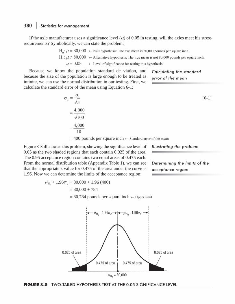
380 Statistics for Management
α) of 0.05 in testing, will the axles meet his stress requirements? Symbolically, we can state the problem: H0: μ = 80,000 H1: μ a = 0.05
Because we know the population standard de viation, and because the size of the population is large enough to be treated as
calculate the standard error of the mean using Equation 6-1:
xσ n
σ= [6-1]
4,000
100=
4,000
10=
= 400 pounds per square inch
0.05 as the two shaded regions that each contain 0.025 of the area. The 0.95 acceptance region contains two equal areas of 0.475 each. From the normal distribution table (Appendix Table 1), we can see that the appropriate z value for 0.475 of the area under the curve is 1.96. Now we can determine the limits of the acceptance region:
H0μ + 1.96 xσ = 80,000 + 1.96 (400)
= 80,000 + 784 = 80,784 pounds per square inch
Calculating the standard
error of the mean
Illustrating the problem
Determining the limits of the
acceptance region
FIGURE 8-8 TWO-TAILED HYPOTHESIS TEST AT THE 0.05 SIGNIFICANCE LEVEL
0.025 of area 0.025 of area
0.475 of area 0.475 of area
μH0 = 80,000
μH0 −1.96σx− μH0
−1.96σx−

Testing Hypotheses: One-sample Tests 381
and
H0μ – 1.96 xσ = 80,000 – 1.96(400)
= 80,000 – 784 = 79,216 pounds per square inch Lower limit
(80,784 and 79,216) and the sample mean (79,600), and illustrated them in Figure 8-9 in the scale of the original variable (pounds per square inch). In a moment, we’ll
Obviously, the sample mean lies within the acceptance region; the manufacturer should accept the null
observed mean of the sample axles. On the basis of this sample, the manufacturer should accept the production run as meeting the stress requirements.
Hypothesis Testing Using the Standardized ScaleIn the hypothesis test we just completed, two numbers were needed to make our decision: an observed value computed from the sample, and a critical value and rejection regions. Let’s look carefully at how we obtained that critical value: After establishing our
α = 0.05, we looked in Appendix Table 1—the standard normal probability distri-z values that left 0.025 of probability in each tail of the distribution.
Recall our discussion of standardizing normal variables in Chapter 5 (pp. 253–259): Instead of mea-suring the variable in its original units, the standardized variable z tells how many standard deviations above (z > 0) or below (z < 0) the mean our observation falls. So there are two different scales of mea-surement we are using, the original scale, or raw scale, and the standardized scale. Figure 8-10 repeats Figure 8-9, but includes both scales. Notice that our sample mean of 79,600 pounds is given on the raw scale, but that the critical z values of ±1.96 are given on the standardized scale. Because these two
Interpreting the results
FIGURE 8-9 TWO-TAILED HYPOTHESIS TEST AT THE 0.05 SIGNIFICANCE LEVEL, SHOWING THE ACCEPTANCE REGION AND THE SAMPLE MEAN
79,216 80,784
Sample mean of79,600 poundsper square inch
μH0 = 80,000
Acceptance regionAccept H0 if the sample value is in this
region
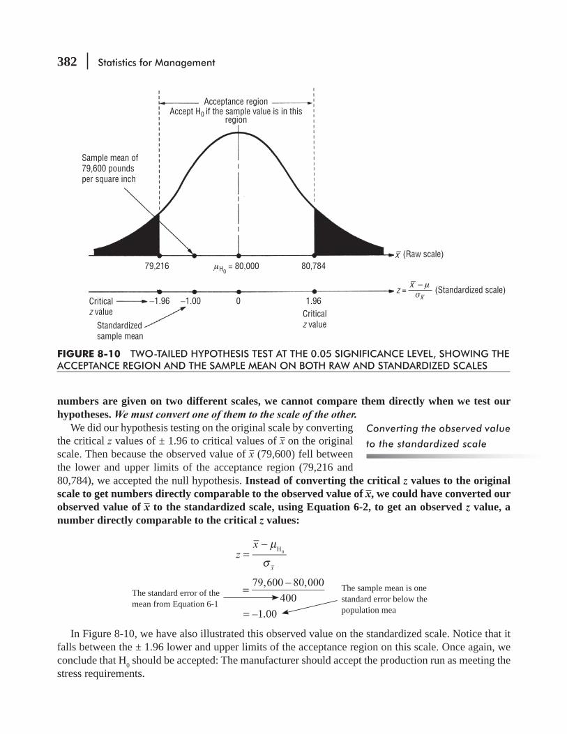
382 Statistics for Management
numbers are given on two different scales, we cannot compare them directly when we test our hypotheses. We must convert one of them to the scale of the other.
We did our hypothesis testing on the original scale by converting the critical z values of ± 1.96 to critical values of x on the original scale. Then because the observed value of x (79,600) fell between the lower and upper limits of the acceptance region (79,216 and 80,784), we accepted the null hypothesis. Instead of converting the critical z values to the original scale to get numbers directly comparable to the observed value of x, we could have converted our observed value of x to the standardized scale, using Equation 6-2, to get an observed z value, a number directly comparable to the critical z values:
zx
x
H0μ
σ=
−
79,600 80,000
400=
−
= –1.00
In Figure 8-10, we have also illustrated this observed value on the standardized scale. Notice that it falls between the ± 1.96 lower and upper limits of the acceptance region on this scale. Once again, we conclude that H0 should be accepted: The manufacturer should accept the production run as meeting the stress requirements.
Converting the observed value
to the standardized scale
The standard error of the mean from Equation 6-1
The sample mean is one standard error below the population mea
−1.96 1.96−1.00 0
Acceptance regionAccept H0 if the sample value is in this
region
Sample mean of79,600 poundsper square inch
Standardizedsample mean
(Standardized scale)
(Raw scale)
Criticalz value Critical
z value
79,216 80,784μH0 = 80,000
x−
x− − μσx−
z =
FIGURE 8-10 TWO-TAILED HYPOTHESIS TEST AT THE 0.05 SIGNIFICANCE LEVEL, SHOWING THE ACCEPTANCE REGION AND THE SAMPLE MEAN ON BOTH RAW AND STANDARDIZED SCALES

Testing Hypotheses: One-sample Tests 383
What is the difference between the two methods we have just
of measurement) differently in each method. However, the two methods will always lead to the same conclusions. Some people are more comfortable using the scale of the original variable; others prefer to use the standardized scale we just explained. The output from most computer statistical packages uses the standardized scale. For the remainder of this chapter and in Chapter 9, we’ll test hypotheses using the standardized scale. Our suggestion: Use the method that’s more comfortable for you.
The Five-Step Process for Hypothesis Testing Using the Standardized Scale
-out Chapter 9 to test hypotheses.
One-Tailed Test of MeansFor a one-tailed test of a mean, suppose a hospital uses large quantities of packaged doses of a particular drug. The individual dose of this drug is 100 cubic centimeters (100 cc). The action of the drug is such
-duce the desired medical effect, and they interfere with patient treatment. The hospital has purchased this drug from the same manufacturer for a number of years and knows that the population standard deviation is 2 cc. The hospital inspects 50 doses of this drug at random from a very large shipment and
H0μ = 100
σ = 2 n = 50 x = 99.75
How do the two methods
differ?
TABLE 8-2 SUMMARY OF THE FIVE-STEP PROCESS
Step Action1 Decide whether this is a two-tailed or a one-tailed test. State your hypotheses. Select a level of
2 Decide which distribution (t or z critical value(s) for the
3 Calculate the standard error of the sample statistic. Use the standard error to convert the observed value of the sample statistic to a standardized value.
4 Sketch the distribution and mark the position of the standardized sample value and the critical value(s) for the test.
5 Compare the value of the standardized sample statistic with the critical value(s) for this test and interpret the result.

384 Statistics for Management
To begin, we can state the problem symbolically:
H0: μ = 100 Null hypothesis: The mean of the shipment’s dosages is 100 cc
H1: μ < 100 Alternative hypothesis: The mean is less than 100 cc
α = 0.10
Because we know the population standard deviation, and n is larger than 30, we can use the normal distribution. From Appendix Table 1, we can determine that the value of z for 40 percent of the area under the curve is 1.28, so the critical value for our lower-tailed test is –1.28.
The hospital wishes to know whether the actual dosages are 100 cc or whether, in fact, the dosages are too small. The hospital must determine that the dosages are more than a certain amount, or it must reject the shipment. This is a left-tailed test, which we have shown graphically in Figure 8-11. Notice
consists of 40 percent on the left side of the distribution plus the entire right side (50 percent), for a total area of 90 percent.
Now we can calculate the standard error of the mean, using the known population standard deviation and Equation 6-1 (because the
xσ = n
σ [6-1]
= 2
50
= 2
7.07
= 0.2829 cc
Step 1: State your hypotheses,
type of test, and significance
level
Step 2: Choose the
appropriate distribution and
find the critical value
Step 3: Compute the standard
error and standardize the
sample statistic
Critical valuez = −1.28
0.10 of area
0.40 of area
0
0.50 of area
z
FIGURE 8-11 LEFT-TAILED HYPOTHESIS TEST AT THE 0.10 SIGNIFICANCE LEVEL
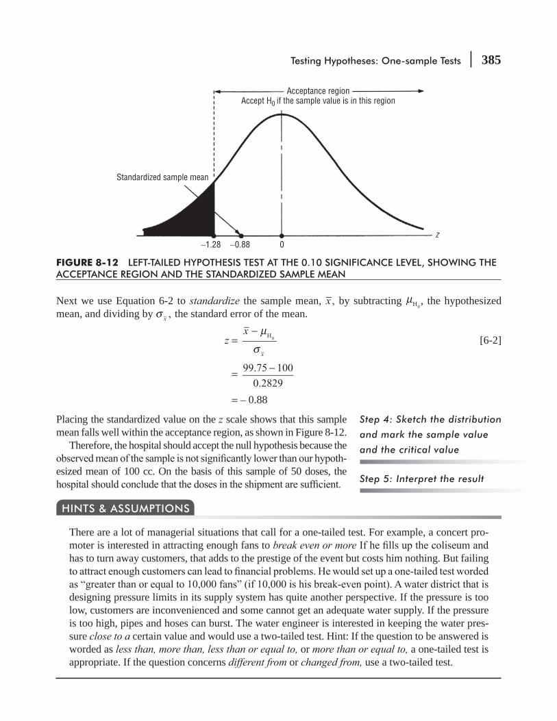
Testing Hypotheses: One-sample Tests 385
Next we use Equation 6-2 to standardize the sample mean, x , by subtracting H0μ , the hypothesized
mean, and dividing by ,xσ the standard error of the mean.
z = x
x
H0μ
σ
− [6-2]
= 99.75 100
0.2829
−
= – 0.88
Placing the standardized value on the z scale shows that this sample mean falls well within the acceptance region, as shown in Figure 8-12.
Therefore, the hospital should accept the null hypothesis because the -
esized mean of 100 cc. On the basis of this sample of 50 doses, the
There are a lot of managerial situations that call for a one-tailed test. For example, a concert pro-moter is interested in attracting enough fans to break even or more has to turn away customers, that adds to the prestige of the event but costs him nothing. But failing
designing pressure limits in its supply system has quite another perspective. If the pressure is too low, customers are inconvenienced and some cannot get an adequate water supply. If the pressure is too high, pipes and hoses can burst. The water engineer is interested in keeping the water pres-sure close to a certain value and would use a two-tailed test. Hint: If the question to be answered is worded as less than, more than, less than or equal to, or more than or equal to, a one-tailed test is appropriate. If the question concerns different from or changed from, use a two-tailed test.
HINTS & ASSUMPTIONS
Step 4: Sketch the distribution
and mark the sample value
and the critical value
Step 5: Interpret the result
−1.28 −0.88 0
Acceptance regionAccept H0 if the sample value is in this region
Standardized sample mean
z
FIGURE 8-12 LEFT-TAILED HYPOTHESIS TEST AT THE 0.10 SIGNIFICANCE LEVEL, SHOWING THE ACCEPTANCE REGION AND THE STANDARDIZED SAMPLE MEAN

386 Statistics for Management
EXERCISES 8.4
Self-Check ExercisesSC 8-5 Hinton Press hypothesizes that the average life of its largest web press is 14,500 hours. They
know that the standard deviation of press life is 2,100 hours. From a sample of 25 presses, the
conclude that the average life of the presses is less than the hypothesized 14,500 hours?SC 8-6 American Theaters knows that a certain hit movie ran an average of 84 days in each city,
and the corresponding standard deviation was 10 days. The manager of the southeastern district was interested in comparing the movie’s popularity in his region with that in all of American’s other theaters. He randomly chose 75 theaters in his region and found that they ran the movie an average of 81.5 days.
the length of the picture’s run between theaters in the southeastern district and all of American’s other theaters.
Applications8-26 Atlas Sporting Goods has implemented a special trade promotion for its propane stove and
feels that the promotion should result in a price change for the consumer. Atlas knows that before the promotion began, the average retail price of the stove was $44.95, and the standard
to believe that the average retail price to the consumer has decreased?8-27 From 1980 until 1985, the mean price/earnings (P/E) ratio of the approximately 1,800 stocks
listed on the New York Stock Exchange was 14.35 and the standard deviation was 9.73. In a sample of 30 randomly chosen NYSE stocks, the mean P/E ratio in 1986 was 11.77. Does this
the mean P/E ratio for NYSE stocks had changed from its earlier value?8-28 -
put of 960 lumens compared to an earlier model that produced only 750 lumens. The com-pany’s data indicate that the standard deviation of light output for this type of bulb is 18.4 lumens. From a sample of 20 new bulbs, the testing committee found an average light output
8-29 Maxwell’s Hot Chocolate is concerned about the effect of the recent year-long coffee adver-tising campaign on hot chocolate sales. The average weekly hot chocolate sales two years ago was 984.7 pounds and the standard deviation was 72.6 pounds. Maxwell’s has randomly selected 30 weeks from the past year and found average sales of 912.1 pounds.(a) State appropriate hypotheses for testing whether hot chocolate sales have decreased.
8-30 $144, and the standard deviation is $52. Joel Freelander has taken a random sample of 121 trades
-cance level, can Joel conclude that his clients’ commissions are higher than the industry average?
Testing Hypotheses: One-sample Tests 387
8-31 Each day, the United States Customs Service has historically intercepted about $28 million in contraband goods being smuggled into the country, with a standard deviation of $16 million per day. On 64 randomly chosen days in 1992, the U.S. Customs Service intercepted an average of
that the Customs Commissioner should be concerned that smuggling has increased above its historic level?
8-32 Before the 1973 oil embargo and subsequent increases in the price of crude oil, gasoline usage in the United States had grown at a seasonally adjusted rate of 0.57 percent per month, with a standard deviation of 0.10 percent per month. In 15 randomly chosen months between 1975 and 1985, gasoline usage grew at an average rate of only 0.33 percent per month. At a 0.01
a result of the embargo and its consequences?8-33 The Bay City Bigleaguers, a semiprofessional baseball team, have the player who led the
league in batting average for many years. For thé past several years, Joe Carver’s batting average has had a mean of .343, and a standard deviation of .018. This year, however, Joe’s average was only .306. Joe is renegotiating his contract for next year, and the salary he will be able to obtain is highly dependent on his ability to convince the team’s owner that his batting
Worked-Out Answers to Self-Check ExercisesSC 8-5 σ = 2,100 n = 25 x = 13,000
H0: μ = 14,500 H1: μ < 14,500 α = 0.01
The lower limit of the acceptance region is z = –2.33, or
x = H0μ – zσ n = 14,500 –
2.33(2,100)
25 = 13,521.4 hours
Because the observed z value x
n
13,000 14,500
2,100 25
H0μ
σ=
−=
−= –3.57 < –233
(or x < 13,521.4), we should reject H0 -esized value.
SC 8-6 σ = 1 0 n = 75 x = 81.5
H0: μ = 84 H1: μ α = 0.01
The limits of the acceptance region are z = ±2.58, or
x = H0μ ± z n 84
2.58(10)
75σ = ± = (81.02, 86.98) days
Because the observed z value x
n
81.5 84
10 75
H0μ
σ=
−=
−= –2.17, it and x are in the acceptance
region, so we do not reject H0from the length of run in other regions.
388 Statistics for Management
8.5 MEASURING THE POWER OF A HYPOTHESIS TESTNow that we have considered two examples of hypothesis testing, a step back is appropriate to discuss what a good hypothesis test should do. Ideally, α and β (the probabilities of Type I and Type II errors) should both be small. Recall that a Type I error occurs when we reject a null hypothesis that is true, and that α
can do about α. A Type II error occurs when we accept a null hypothesis that is false; the probability of a Type II error is β. What can we say about β ?
Suppose the null hypothesis is false. Then managers would like the hypothesis test to reject it all the time. Unfortunately, hypothesis tests cannot be foolproof; sometimes when the null hypothesis is false, a test does not reject it, and thus a Type II error is made. When the null hypothesis is false, μ (the true population mean) does not equal
H0μ (the hypothesized population mean); instead, μ equals some other value. For each possible value of μ for which the alternative hypothesis is true, there is a different probability (β ) of incorrectly accepting the null hypothesis. Of course, we would like this β (the probability of accepting a null hypothesis when it is false) to be as small as possible, or, equivalently, we would like 1 – β (the probability of rejecting a null hypothesis when it is false) to be as large as possible.
Because rejecting a null hypothesis when it is false is exactly what a good test should do, a high value of 1 – β (something near 1.0) means the test is working quite well (it is rejecting the null hypothesis when it is false); a low value of 1 – β (something near 0.0) means that the test is working very poorly (it’s not reject-ing the null hypothesis when it is false). Because the value of 1 – β is the measure of how well the test is working, it is known as the power of the test. If we plot the values of 1 – β for each value of μ for which the alternative hypothesis is true, the resulting curve is known as a power curve.
In part a of Figure 8-13, we reproduce the left-tailed test from Figure 8-11, but now we are looking at the raw scale. In Figure 8-13(b), we show the power curve associated with this test. Computing the values of 1 – βFigure 8-13(b). Recall that with this test we were deciding whether to accept a drug shipment. Our test dictated that we should reject the null hypothesis if the standardized sample mean is less than –1.28, that is, if sample mean dosage is less than 100.00 – 1.28 (0.2829), or 99.64 cc.
Consider point C on the power curve in Figure 8-13(b). The pop-ulation mean dosage is 99.42 cc. Given that the population mean is 99.42 cc, we must compute the probability that the mean of a random sample of 50 doses from this population will be less than 99.64 cc (the point below which we decided to reject the null hypothesis). Now look at Figure 8-13(c). Earlier we computed the standard error of the mean to be 0.2829 cc, so 99.64 cc is (99.64 – 99.42)/0.2829, or 0.78 standard error above 99.42 cc. Using Appendix Table 1, we can see that the probability of observing a sample mean less than 99.64 cc and thus rejecting the null hypothesis is 0.7823, the colored area in Figure 8-13(c). Thus, the power of the test (1 – β ) at μ = 99.42 is 0.7823. This simply means that if μ = 99.42, the probability that this test will reject the null hypothesis when it is false is 0.7823.
Now look at point D in Figure 8-13(b). For this population mean dosage of 99.61 cc, what is the probability that the mean of a random sample of 50 doses from this population will be less than 99.64 cc and thus cause the test to reject the null hypothesis? Look at Figure 8-13(d). Here we see that 99.64 is
What should a good hypothesis
test do?
Meaning of β and 1 – β
Interpreting the values of 1 – β
Computing the values of 1 – β
Interpreting a point on the
power curve

Testing Hypotheses: One-sample Tests 389
(99.64 – 99.61)/0.2829, or 0.11 standard error above 99.61 cc. Using Appendix Table 1 again, we can see that the probability of observing a sample mean less than 99.64 cc and thus rejecting the null hypothesis is 0.5438, the colored area in Figure 8-13(d). Thus, the power of the test (1 – β ) at μ = 99.61 cc is 0.5438.
at μ = 99.80 cc is 0.2843; this is illustrated as the colored area in Figure 8-13(e). The values of 1 – β continue to decrease to the right of point E. How low do they get? As the population mean gets closer and closer to 100.00 cc, the power of the test (1 – β ) must get closer and closer to the probability of rejecting the null hypothesis when the population mean is exactly 100.00 cc. And we know thatof the test—in this case, 0.10. Thus, the curve terminates at point F, which lies at a height of 0.10 directly over the population mean.
What does our power curve in Figure 8-13(b) tell us? Just that as the shipment becomes less satisfactory (as the doses in the shipment become smaller), our test is more powerful (it has a greater probability of recognizing that the shipment is unsatisfactory). It also shows us, however, that because of sampling error, when the dosage is only slightly less than 100.00 cc, the power of the test to recognize this situation is quite low. Thus, if having any dosage below 100.00 cc is completely unsatisfactory, the test we have been discussing would not be appropriate.
Termination point of the
power curve
Interpreting the power curve
FIGURE 8-13 LEFT-TAILED HYPOTHESIS TEST, ASSOCIATED POWER CURVE, AND THREE VALUES OF μ.
(a) (b)
(c) (d) (e)
1.00
C
D
E
F
Power curve (plotof probabilities ofrejecting the nullhypothesis whenthe alternativehypothesis is true)
0.75
0.50
0.25
99.42 cc 99.61 cc
Population mean (μ)
99.80 cc 100.00 cc
Prob
abili
ty o
f rej
ectin
g H 0
α = 0.10
1 − β = 0.7823
1 − β = 0.5438
1 − β = 0.2843
99.64 cc
99.42 99.64 99.61 99.8099.64 99.64
0.78 standarderror
0.11 standarderror
0.57 standarderror
0.7823of area
0.5438of area
0.2843of area
Sample mean (x−)
μH0 = 100,000 cc
μ μ μ
Rejectionregion
Acceptance region
390 Statistics for Management
Of course, we’d always like to use the hypothesis test with the greatest power. But we also know that a certain proportion of the time, all hypothesis tests will fail to reject the null hypothesis when it is false or accept it when it’s true (that’s statistical language that really means that when the test does fail, it will persuade us that things haven’t changed when in fact they have, or persuade us that things have changed when they really haven’t). That’s just the price we pay for using sam-pling in hypothesis testing. The failure of a test to perform perfectly is due to sampling error. The only way to avoid such error is to examine everything in the population and that is either physi-cally impossible or too expensive.
HINTS & ASSUMPTIONS
EXERCISES 8.5
Self-Check ExercisesSC 8-7 See Exercise 8-32. Compute the power of the test for μ = 0.50, 0.45, and 0.40 percent per
month.SC 8-8 In Exercise 8-32, what happens to the power of the test for μ = 0.50, 0.45, and 0.40 percent
Applications8-34 See Exercise 8-31. Compute the power of the test for μ = $28, $29, and $30 million.8-35 See Exercise 8-30. Compute the power of the test for μ = $140, $160, and $175.8-36 In Exercise 8-31, what happens to the power of the test for μ = $28, $29, and $30 million if
8-37 In Exercise 8-30, what happens to the power of the test for μ. = $140, $160, and $175 if the
Worked-Out Answers to Self-Check ExercisesSC 8-7 From Exercise 8-32, we have σ = 0.10, n = 15, H0: μ = 0.57, H1: μ < 0.57. At a = 0.01, the
lower limit of the acceptance region is
n2.33 0.57 2.33(0.10) 15 0.510H0μ σ− = − =
(a) At μ = 0.50, the power of the test is
x z zP( 0.510) P(0.510 0.50
0.10 15P( 0.39)< =
−= < =< 0.5 + 0.1517 = 0.6517
(b) At μ = 0.45, the power of the test is
x z zP( 0.510) P(0.510 0.45
0.10 15P( 2.32)< =
−= < =< 0.5 + 0.4898 = 0.9898
(c) At μ = 0.40, the power of the test is
x z zP( 0.510) P(0.510 0.40
0.10 15P( 4.26)< =
−= < =< 1.0000

Testing Hypotheses: One-sample Tests 391
SC 8-8 At α = 0.04, the lower limit of the acceptance region is
n1.75 0.57 1.75(0.10) 15 0.525H0μ σ− = − =
(a) At μ = 0.50, the power of the test is
x z zP( 0.525) P(0.525 0.50
0.10 15P( 0.97)< = <
−= < = 0.5 + 0.3340 = 0.8340
(b) At μ = 0.45, the power of the test is
x z zP( 0.525) P(0.525 0.45
0.10 15P( 2.90)< = <
−= < = 0.5 + 0.4981 = 0.9981
(c) At μ = 0.40, the power of the test is
x z zP( 0.525) P(0.525 0.40
0.10 15P( 4.84)< = <
−= < = 1.0000
8.6 HYPOTHESIS TESTING OF PROPORTIONS: LARGE SAMPLES
Two-Tailed Tests of ProportionsIn this section, we’ll apply what we have learned about tests con-cerning means to tests for proportions (that is, the proportion of occurrences in a population). But before we apply it, we’ll review the important conclusions we made about proportions in Chapter 7. First, remember that the binomial is the theoretically correct distribution to use in dealing with proportions. As the sample size increases, the binomial distribution approaches the normal in its characteristics, and we can use the normal distribution to approximate the sampling
np and nq each need to be at least 5 before we can use the normal distribution as a substitute for the binomial.
Consider, as an example, a company that is evaluating the promotability of its employees, that is, determining the proportion whose ability, training, and supervisory experience qualify them for pro-motion to the next higher level of management. The human resources director tells the president that
a special committee to assess the promotability of all employees. This committee conducts in-depth
for promotion.
pH0
= 0.8 Hypothesized value of the population proportion of successes (judged promotable, in this case)
qH0
= 0.2 Hypothesized value of the population proportion of failures (judged not promotable) n = 150 Sample size
p = 0.7 Sample proportion of promotables q = 0.3 Sample proportion judged not promotable
hypothesis that 0.8 of the employees are promotable:
H0: p = 0.8 Null hypothesis, 80 percent of the employees are promotable H 1: p ≠ 0.8 Alternative hypothesis. The proportion of promotable employees is not 80 percent α = 0.05
Dealing with proportions
Step 1: State your hypotheses,
type of test, and significance
level
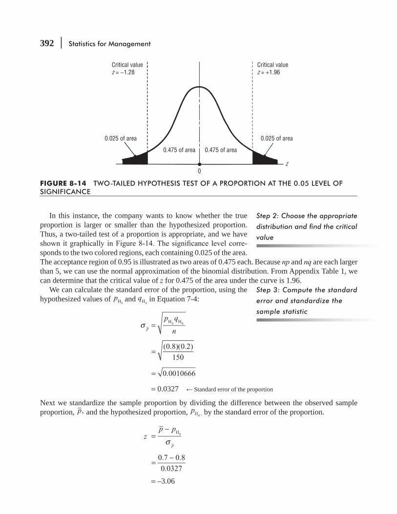
392 Statistics for Management
In this instance, the company wants to know whether the true proportion is larger or smaller than the hypothesized proportion. Thus, a two-tailed test of a proportion is appropriate, and we have
-sponds to the two colored regions, each containing 0.025 of the area. The acceptance region of 0.95 is illustrated as two areas of 0.475 each. Because np and nq are each larger than 5, we can use the normal approximation of the binomial distribution. From Appendix Table 1, we can determine that the critical value of z for 0.475 of the area under the curve is 1.96.
We can calculate the standard error of the proportion, using the hypothesized values of pH0
and qH0 in Equation 7-4:
p q
np
H H0 0σ =
(0.8)(0.2)
150=
0.0010666=
= 0.0327 Standard error of the proportion
Next we standardize the sample proportion by dividing the difference between the observed sample proportion, p, and the hypothesized proportion, pH ,0
by the standard error of the proportion.
z p p
p
H0
σ=
−
0.7 0.8
0.0327=
−
= –3.06
Step 2: Choose the appropriate
value
Step 3: Compute the standard
error and standardize the
sample statistic
FIGURE 8-14 TWO-TAILED HYPOTHESIS TEST OF A PROPORTION AT THE 0.05 LEVEL OF SIGNIFICANCE
Critical valuez = −1.28
Critical valuez = +1.96
0.025 of area 0.025 of area
0.475 of area
0
0.475 of area
z
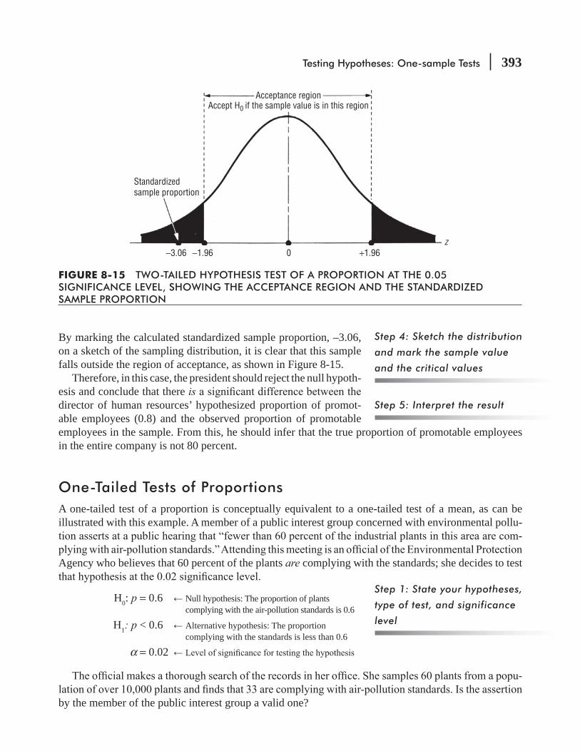
Testing Hypotheses: One-sample Tests 393
By marking the calculated standardized sample proportion, –3.06, on a sketch of the sampling distribution, it is clear that this sample falls outside the region of acceptance, as shown in Figure 8-15.
Therefore, in this case, the president should reject the null hypoth-esis and conclude that there isdirector of human resources’ hypothesized proportion of promot-able employees (0.8) and the observed proportion of promotable employees in the sample. From this, he should infer that the true proportion of promotable employees in the entire company is not 80 percent.
One-Tailed Tests of ProportionsA one-tailed test of a proportion is conceptually equivalent to a one-tailed test of a mean, as can be illustrated with this example. A member of a public interest group concerned with environmental pollu-
-
Agency who believes that 60 percent of the plants are complying with the standards; she decides to test
H0: p = 0.6 Null hypothesis: The proportion of plants complying with the air-pollution standards is 0.6
H1: p < 0.6 Alternative hypothesis: The proportion complying with the standards is less than 0.6
α = 0.02
-
by the member of the public interest group a valid one?
Step 4: Sketch the distribution
and mark the sample value
and the critical values
Step 5: Interpret the result
Step 1: State your hypotheses,
type of test, and significance
level
Acceptance regionAccept H0 if the sample value is in this region
Standardizedsample proportion
−3.06 −1.96 +1.960z
FIGURE 8-15 TWO-TAILED HYPOTHESIS TEST OF A PROPORTION AT THE 0.05 SIGNIFICANCE LEVEL, SHOWING THE ACCEPTANCE REGION AND THE STANDARDIZED SAMPLE PROPORTION
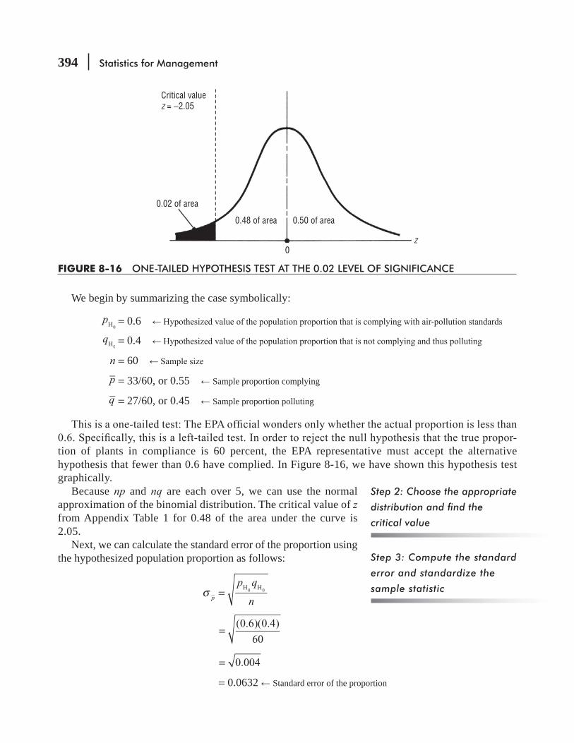
394 Statistics for Management
We begin by summarizing the case symbolically:
pH0 = 0.6
qH0 = 0.4
n = 60
p = 33/60, or 0.55 Sample proportion complying
q = 27/60, or 0.45 Sample proportion polluting
-tion of plants in compliance is 60 percent, the EPA representative must accept the alternative hypothesis that fewer than 0.6 have complied. In Figure 8-16, we have shown this hypothesis test graphically.
Because np and nq are each over 5, we can use the normal approximation of the binomial distribution. The critical value of z from Appendix Table 1 for 0.48 of the area under the curve is 2.05.
Next, we can calculate the standard error of the proportion using the hypothesized population proportion as follows:
p q
np
H H0 0σ =
(0.6)(0.4)
60=
0.004=
= 0.0632 Standard error of the proportion
Step 2: Choose the appropriate
critical value
Step 3: Compute the standard
error and standardize the
sample statistic
Critical valuez = −2.05
0.48 of area
0.02 of area
0.50 of area
0z
FIGURE 8-16 ONE-TAILED HYPOTHESIS TEST AT THE 0.02 LEVEL OF SIGNIFICANCE

Testing Hypotheses: One-sample Tests 395
And we standardize the sample proportion by dividing the difference between the observed sample proportion, p, and the hypothesized proportion, p ,H0
by the standard error of the proportion.
z p p
p
H0
σ=
−
0.55 0.6
0.0632=
−
= –0.79
Figure 8-17 illustrates where the sample proportion lies in relation
the sample proportion lies within the acceptance region. Therefore, -
portion of complying plants is 0.6. Although the observed sample proportion is below 0.6, 0.6; that is, it is not far enough below 0.6 to make us accept the assertion by the member of the public interest group.
Warning: When we’re doing hypothesis tests involving proportions, we use the binomial distribu-tion as the sampling distribution, unless np and nq are both at least 5. In that case, we can use the normal distribution as an approximation of the binomial without worry. Fortunately, in practice,
condition is met. Even when they aren’t, the arithmetic of the binomial distribution and the bino-
HINTS & ASSUMPTIONS
Step 4: Sketch the distribution
and mark the sample value
and the critical value
Step 5: Interpret the result
FIGURE 8-17 ONE-TAILED (LEFT-TAILED) HYPOTHESIS TEST AT THE 0.02 SIGNIFICANCE LEVEL, SHOWING THE ACCEPTANCE REGION AND THE STANDARDIZED SAMPLE PROPORTION
−2.05 −0.79 0
Acceptance regionAccept H0 if the sample value is in this region
Standardizedsample proportion
z

396 Statistics for Management
EXERCISES 8.6
Self-Check ExercisesSC 8-9 A ketchup manufacturer is in the process of deciding whether to produce a new extra-spicy
brand. The company’s marketing-research department used a national telephone survey of 6,000 households and found that the extra-spicy ketchup would be purchased by 335 of them. A much more extensive study made 2 years ago showed that 5 percent of the households
level, should the company
SC 8-10 Steve Cutter sells Big Blade lawn mowers in his hardware store, and he is interested in comparing the reliability of the mowers he sells with the reliability of Big Blade mowers sold nationwide. Steve knows that only 15 percent of all Big Blade mowers sold nationwide
from those sold nationwide?
Applications8-38 Grant, Inc., a manufacturer of women’s dress blouses, knows that its brand is carried in 19 per-
cent of the women’s clothing stores east of the Mississippi River. Grant recently sampled 85 women’s clothing stores on the West Coast and found that 14.12 percent of the stores carried
on the West Coast than it does east of the Mississippi?8-39 From a total of 10,200 loans made by a state employees’ credit union in the most recent 5-year
period, 350 were sampled to determine what proportion was made to women. This sample showed that 39 percent of the loans were made to women employees. A complete census of
level of 0.02, can you conclude that the proportion of loans made to women has changed sig-
8-40 Feronetics specializes in the use of gene-splicing techniques to produce new pharmaceutical compounds. It has recently developed a nasal spray containing interferon, which it believes will limit the transmission of the common cold within families. In the general population, 15.1 percent of all individuals will catch a rhinovirus-caused cold once another family member contracts such a cold. The interferon spray was tested on 180 people, one of whose family members subsequently contracted a rhinovirus-caused cold. Only 17 of the test subjects devel-oped similar colds.
reduces transmission of colds?(b) What should it conclude at α = 0.02?(c) On the basis of these results, do you think Feronetics should be allowed to market the new
spray? Explain.8-41
walk with positive drift.” If this is accurate, then the Dow Jones Industrial Average should show a gain on more than 50 percent of all trading days. If the average increased on 101 of 175 randomly chosen days, what do you think about the suggested theory? Use a 0.01 level of
Testing Hypotheses: One-sample Tests 397
8-42 MacroSwift estimated last year that 35 percent of potential software buyers were planning to wait to purchase the new operating system, Window Panes, until an upgrade had been released. After an advertising campaign to reassure the public, MacroSwift surveyed 3,000
company conclude the proportion of skeptical people has decreased?8-43 Rick Douglas, the new manager of Food Barn, is interested in the percentage of customers who
Worked-Out Answers to Self-Check ExercisesSC 8-9 n = 6,000 p = 335/6,000 = 0.05583
H0: p = 0.05 H1: p > 0.05 α = 0.02The upper limit of the acceptance region is z = 2.05, or
p p zp q
n0.05 2.05
0.05(0.95)
6,0000.05577H
H Ho
o
o= + = + =
Because the observed z value p p
p q n
0.05583 0.05
0.05(0.95) 6,0002.07
H
H H
o
o o
=−
=−
=
> 2.05 (or p > 0.05577), we should reject H0 -cantly greater than the interest of 2 years ago.
SC 8-10 n = 120 p = 22/120 = 0.1833H0: p = 0.15 H 1: p ≠ 0.15 α = 0.02The limits of the acceptance region are z = ±2.33, or
p p zp q
n0.15 2.33
0.15(0.085)
120(0.0741, 0.2259)H
H H
0
0 0= ± = ± =
Because the observed z value p p
p q n
0.1833 0.15
0.15(0.85) 1201.02
H
H H
0
0 0
=−
=−
=
< 2.33 (or p = 0.1833, which is between 0.0741 and 0.2259), we do not reject H0. Steve’s
8.7 HYPOTHESIS TESTING OF MEANS WHEN THE POPULATION STANDARD DEVIATION IS NOT KNOWN
that the difference in size between large and small samples is impor-tant when the population standard deviation σ is unknown and must be estimated from the sample stan-dard deviation. If the sample size n is 30 or less and σ is not known, we should use the t distribution. The appropriate t distribution has n – 1 degrees of freedom. These rules apply to hypothesis testing, too.
When to use the t distribution
398 Statistics for Management
Two-Tailed Tests of Means Using the t DistributionA personnel specialist of a major corporation is recruiting a large number of employees for an overseas
I think the average score on the aptitude test will be around 90.” When management reviews 20 of the
μH0 = 90 Hypothesized value of the population mean
n = 20 Sample size
x = 84 Sample mean
s = 11 Sample standard deviation
H0: μ = 90 Null hypothesis, the true population mean score is 90 H1: μ ≠ 90 Alternative hypothesis, the mean score is not 90
α = 0.10 s
Figure 8-18 illustrates this problem graphically. Because management is interested in knowing whether the true mean score is larger or smaller than the hypothesized score, a two-tailed test 0.10 is shown in Figure 8-18 as the two colored areas, each containing 0.05 of the area under the t distribution. Because the sample size is 20, the appropriate number of degrees of freedom is 19, that is, 20 – 1. Therefore, we look in the t distribution table, Appendix Table 2, under the 0.10 column until we reach the
t, 1.729.Because the population standard deviation is not known, we must estimate it using the sample stan-
dard deviation and Equation 7-1:
σ = s [7-1] = 11
Now we can compute the standard error of the mean. Because we are using σ , an estimate of the population standard deviation, the standard error of the mean will also be an estimate. We can use Equation 7-6, as follows:
σ σ
=n
ˆˆ
x [7-6]
11
20=
11
4.47=
= 2.46 Estimated standard error of the mean
Next we standardize the sample mean, x , by subtracting μH0, the hypothesized mean, and dividing by σ x,
the estimated standard error of the mean. Because our test of hypotheses is based on the t distribution,
Step 1: State your hypotheses,
type of test, and significance
level
Step 2: Choose the
appropriate distribution and
find the critical value
Step 3: Compute the standard
error and standardize the
sample statistic

Testing Hypotheses: One-sample Tests 399
we use t to denote the standardized statistic.
μ
σ=
−t
x
ˆx
Ho
84 90
2.46=
−
= –2.44
Drawing this result on a sketch of the sampling distribution, we see that the sample mean falls outside the acceptance region, as shown in Figure 8-19.
Therefore, management should reject the null hypothesis (the personnel specialist’s assertion that the true mean score of the employees being tested is 90).
Step 4 Sketch the distribution
and mark the sample value
and the critical values
Step 5: Interpret the result
FIGURE 8-18 TWO-TAILED TEST OF HYPOTHESIS AT THE 0.10 LEVEL OF SIGNIFICANCE USING THE t DISTRIBUTION
Critical valuet = −1.729
Critical valuet = +1.729
0.05 of area 0.05 of area
0t
−2.44 −1.729 +1.7290
Standardizedsample mean
t
Acceptance regionAccept H0 if the sample value is in this region
FIGURE 8-19 TWO-TAILED HYPOTHESIS TEST AT THE 0.10 LEVEL OF SIGNIFICANCE, SHOWING THE ACCEPTANCE REGION AND THE STANDARDIZED SAMPLE MEAN
400 Statistics for Management
One-Tailed Tests of Means Using the t DistributionThe procedure for a one-tailed hypothesis test using the t distribu-tion is the same conceptually as for a one-tailed test using the normal distribution and the z table. Performing such one-tailed tests may
area in both tails combined. Thus, they are appropriate to use in a two-tailed test with two rejection regions.
If we use the t distribution for a one-tailed test, we need to deter-t
degrees of freedom, we would look in Appendix Table 2 under the 0.10 column opposite the 12 degrees of freedom row. The answer in this case is 1.782. This is true because the 0.10 column represents 0.10 of the area under the curve contained in both tails combined, so it also represents 0.05 of the area under the curve contained in each of the tails separately.
In the next chapter, we continue our work on hypothesis testing by looking at situations where decisions must be made on the basis of two samples that may or may not come from the same underlying population.
Doing hypothesis tests with the t distribution is no different from doing them with the normal distribution except that we use a different table and we have to supply the number of degrees of freedom. Hint: The number of degrees of freedom in a single-sample test is always one fewer than the sample size. Warning: Use the t distribution whenever the sample size is less than 30, the popu-lation standard deviation is not known, and the population is normal or approximately normal.
HINTS & ASSUMPTIONS
One Sample Test Using SPSS
One difference from the z
tables
Using the t table for one-
tailed tests
Looking ahead
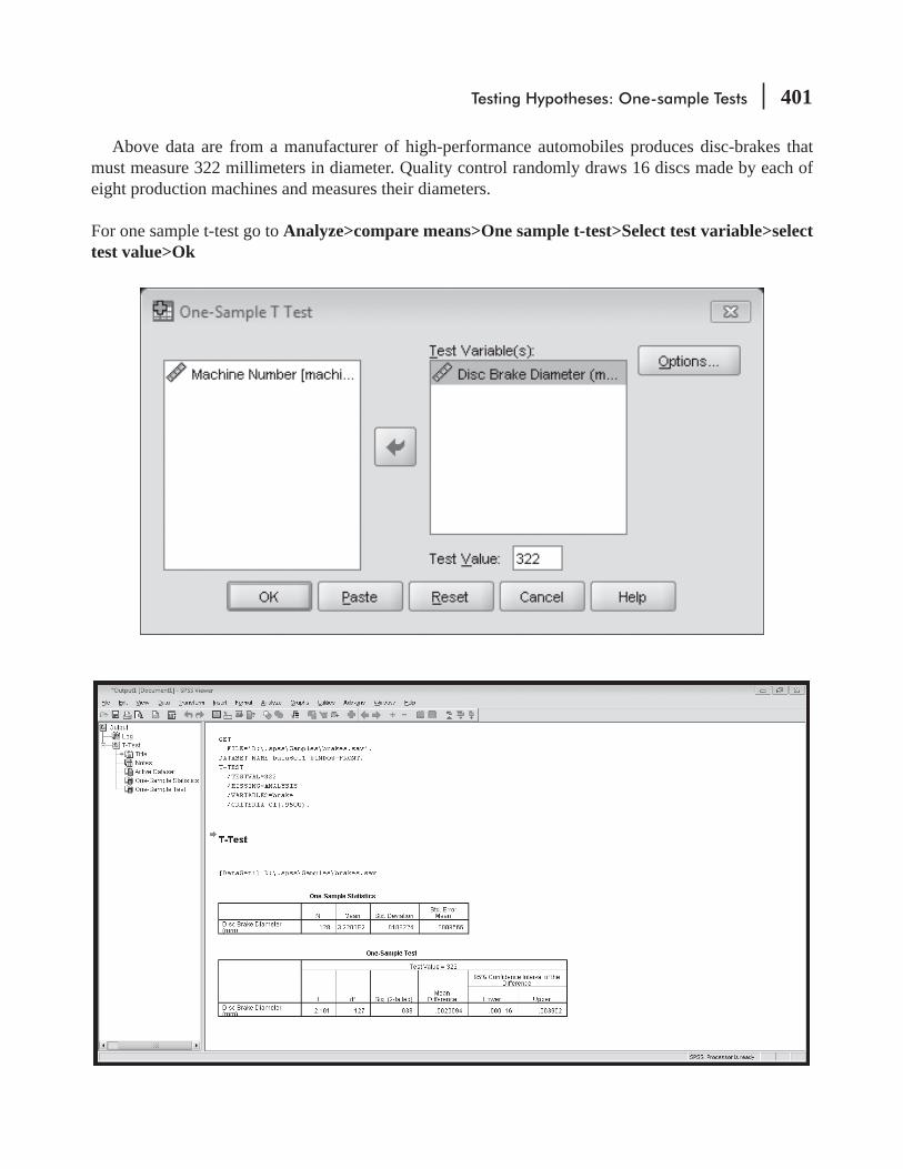
Testing Hypotheses: One-sample Tests 401
Above data are from a manufacturer of high-performance automobiles produces disc-brakes that must measure 322 millimeters in diameter. Quality control randomly draws 16 discs made by each of eight production machines and measures their diameters.
For one sample t-test go to Analyze>compare means>One sample t-test>Select test variable>select test value>Ok

402 Statistics for Management
EXERCISES 8.7
Self-check ExercisesSC 8-11 Given a sample mean of 83, a sample standard deviation of 12.5, and a samplesize of 22, test
the hypothesis that the value of the population mean is 70 against the alternative that it is
SC 8-12 Picosoft, Ltd., a supplier of operating system software for personal computers, was planning
development of a radically new, seventh-generation integrated system. With current earnings of $1.61 a share, Picosoft and its underwriters were contemplating an offering price of $21, or about 13 times earnings. In order to check the appropriateness of this price, they randomly
was 11.6, and the sample standard deviation was 1.3. At α = 0.02, can Picosoft conclude that
different from 13?
Basic Concepts8-44 Given a sample mean of 94.3, a sample standard deviation of 8.4, and a sample size of 6, test
the hypothesis that the value of the population mean is 100 against the alternative hypothesis
8-45 If a sample of 25 observations reveals a sample mean of 52 and a sample variance of 4.2, test the hypothesis that the population mean is 65 against the alternative hypothesis that it is some
Application8-46 Realtor Elaine Snyderman took a random sample of 12 homes in a prestigious suburb of
Chicago and found the average appraised market value to be $780,000, and the standard deviation was $49,000. Test the hypothesis that for all homes in the area, the mean appraised value is $825,000 against the alternative that it is less than $825,000. Use the 0.05 level of
8-47 For a sample of 60 women taken from a population of over 5,000 enrolled in a weight-reducing program at a nationwide chain of health spas, the sample mean diastolic blood
average, did the women enrolled in the program have diastolic blood pressure that exceeds the value of 75?
8-48 The data-processing department at a large life insurance company has installed new color video display terminals to replace the monochrome units it previously used. The 95 opera-tors trained to use the new machines averaged 7.2 hours before achieving a satisfactory level of performance. Their sample variance was 16.2 squared hours. Long experience with operators on the old monochrome terminals showed that they averaged 8.1 hours on the
the supervisor of the department conclude that the new terminals are easier to learn to operate?
8-49 As the bottom fell out of the oil market in early 1986, educators in Texas worried about how the resulting loss of state revenues (estimated to be about $100 million for each $1 decrease
Testing Hypotheses: One-sample Tests 403
in the price of a barrel of oil) would affect their budgets. The state board of education felt the situation would not be critical as long as they could be reasonably certain that the price would stay above $18 per barrel. They surveyed 13 randomly chosen oil economists and asked them to predict how low the price would go before it bottomed out. The 13 predictions average $21.60, and the sample standard deviation was $4.65. At α = 0.01, is the average prediction
Explain.8-50 A television documentary on overeating claimed that Americans are about 10 pounds over-
weight on average. To test this claim, eighteen randomly selected individuals were examined; their average excess weight was found to be 12.4 pounds, and the sample standard deviation
claimed 10-pound value? 8-51 XCO, a multinational manufacturer, uses a batch process to produce widgets. Each batch
of widgets takes 8 hours to produce and has material and labor costs of $8,476. Because of
long as the batches sell for more than $12,500 on average. XCO sampled 16 batches and found 5,040 widgets per batch on average, with a standard deviation of 41.3 widgets. At α = 0.025,
Worked-Out Answers to Self-Check ExercisesSC 8-11 s = 12.5 n = 22 x = 83
H0: μ = 70 H1: μ > 70 α = 0.025
The upper limit of the acceptance region is t = 2.080, or
x t s n 70 2.080(12.5) 22 75.54H0μ= + = + =
Because the observed t value x
s n
83 70
12.5 224.878 2.080
H0μ
=−
=−
= >
(or x > 75.54), we reject H0.
SC 8-12 s = 1.3 n = 7 x = 11.6
H0: μ = 13 H1: μ ≠ 13 α = 0.02
The limits of the acceptance region are t = ±3.143, or
x ts n 13 3.143(1.3) 7 (11.46,14.54)Hoμ= ± = ± =
Because the observed t value x
s n
11.6 13
1.3 72.849 3.143
Hoμ
=−
=−
= − > −
(or x = 11.6, which is between 11.46 and 14.54), we do not reject H0. The average P/E ratio

404 Statistics for Management
STATISTICS AT WORK
Loveland ComputersCase 8: One-Sample Tests of Hypothesesadding a software division,” said Margot Derby, the head of Marketing at Loveland Computers, as she pulled a Wall Street Journaldropping. But, to everyone’s surprise, PC buyers seem to be spending the same in total—they are mak-ing up for the discount price by buying more bells and whistles—and more software.
-ber came in much lower than the amount they quoted in the article. The trouble is I’m not sure which
Maybe they use custom programs they write themselves.”
suggested.
for our telephone sample, but the Journal article only gives us the mean. And I remember enough from my one stat course in college to know that we can’t run a test if we don’t know the population standard deviation.”
Study Questions:reliable population mean. Is Margot right that Lee also needs to know the population standard devia-tion in order to perform a test? What idea is Margot exploring here? How would the idea be stated in hypothesis-testing terms?
CHAPTER REVIEW
Terms Introduced in Chapter 8Alpha (α) The probability of a Type I error.Alternative Hypothesis The conclusion we accept when the data fail to support the null hypothesis.Beta (β) The probability of a Type II error.Critical Value The value of the standard statistic (z or t) beyond which we reject the null hypothesis; the boundary between the acceptance and rejection regions.Hypothesis An assumption or speculation we make about a population parameter.Lower-Tailed Test -esized population value will lead us to reject the null hypothesis.Null Hypothesis The hypothesis, or assumption, about a population parameter we wish to test, usually an assumption of the status quo.
Testing Hypotheses: One-sample Tests 405
One-Tailed Test A hypothesis test in which there is only one rejection region; that is where we are concerned only with whether the observed value deviates from the hypothesized value in one direction.Power Curve A graph of the values of the power of a test for each value of μ, or other population parameter, for which the alternative hypothesis is true.Power of the Hypothesis Test The probability of rejecting the null hypothesis when it is false, that is, a measure of how well the hypothesis test is working.Raw Scale Measurement in the variable’s original units.
A value indicating the percent- age of sample values that is outside certain limits, assuming the null hypothesis is correct, that is, the probability of rejecting the null hypothesis when it is true.Standardized Scale Measurement in standard deviations from the variable’s mean.Two-Tailed Test A hypothesis test in which the null hypothesis is rejected if the sample value is sig-
rejection regions.Type I Error Rejecting a null hypothesis when it is true.Type II Error Accepting a null hypothesis when it is false.Upper-Tailed Test -esized population value will lead us to reject the null hypothesis.
Review and Application Exercises8-52 For the following situations, state appropriate null and alternative hypotheses.
(a) The Census Bureau wants to determine whether the percentage of homeless people in New York City is the same as the national average.
(b) A local hardware store owner wants to determine whether sales of garden supplies are better than usual after a spring promotion.
(c) The Weather Channel wants to know whether average annual snowfall in the 1980s was
sticker.8-53
battery is greater than or equal to 28 months. If scheduling for replacement surgery for the batteries is to be based on this claim, explain to the management of this company the conse-quences of Type I and Type II errors.
8-54 A manufacturer of petite women’s sportswear has hypothesized that the average weight of the women buying its clothing is 110 pounds. The company takes two samples of its customers
-duces a mean weight of 122 pounds. In the test of the company’s hypothesis that the population mean is 110 pounds versus the hypothesis that the mean does not equal 110 pounds, is one of these sample values more likely to lead us to accept the null hypothesis? Why or why not?

406 Statistics for Management
8-55 downtown business districts. Planning for Metro Transportation District has depended on a well-established average of 3.4 passengers per HOV. But a summer intern notes that because many
The intern takes a sample of 23 vehicles going through the HOV lane of a toil plaza and reports a sample mean of 4.3 passengers, and a standard deviation of 1.5 passengers. At the 0.01 level
8-56 In Exercise SC 8-5, what would be the power of the test for μ = 14,000,13,500, and 13,000 if
8-57 On an average day, about 5 percent of the stocks on the New York Stock Exchange set a new high for the year. On Friday, September 18, 1992, the Dow Jones Industrial Average closed at 3,282 on a robust volume of over 136 million shares traded. A random sample of 120 stocks
should we conclude that more stocks than usual set new highs on that day? 8-58 In response to criticism concerning lost mail, the U.S. Postal Service initiated new procedures
to alleviate this problem. The postmaster general had been assured that this change would reduce losses to below the historic loss rate of 0.3 percent. After the new procedures had been in effect for 2 months, the USPS sponsored an investigation in which a total of 8,000 pieces of mail were mailed from various parts of the country. Eighteen of the test pieces failed to reach
the new procedures achieved their goal?8-59 What is the probability that we are rejecting a true null hypothesis when we reject the hypoth-
esized value because(a) The sample statistic differs from it by more than 2.15 standard errors in either direction?(b) The value of the sample statistic is more than 1.6 standard errors above it?(c) The value of the sample statistic is more than 2.33 standard errors below it?
8-60 If we wish to accept the null hypothesis 85 percent of the time when it is correct, within how many standard errors around the hypothesized mean should the sample mean fall, in order to be in the acceptance region? What if we want to be 98 percent certain of accepting the null hypothesis when it is true?
8-61 Federal environmental statutes applying to a particular nuclear power plant specify that recy-cled water must, on average, be no warmer than 84°F (28.9°C) before it can be released into the river beside the plant. From 70 samples, the average temperature of recycled water was found to be 86.3°F (30.2°C). If the population standard deviation is 13.5 Fahrenheit (7.5 Celsius) degrees, should the plant be cited for exceeding the limitations of the statute? State and test appropriate hypotheses at α = 0.05.
8-62
8-63 In 1995, the average 2-week-advance-purchase airfare between Raleigh-Durham, North Carolina, and New York City was $235. The population standard deviation was $68. A1996 survey of 90 randomly chosen travelers between these two cities found that they had paid

Testing Hypotheses: One-sample Tests 407
between 1995 and 1996? What is the largest α at which you would conclude that the observed
8-64 Audio Sounds runs a chain of stores selling stereo systems and components. It has been very successful in many university towns, but it has had some failures. Analysis of its failures has led it to adopt a policy of not opening a store unless it can be reasonably certain that more than 15 percent of the students in town own stereo systems costing $1,100 or more. A survey of 300 of the 2,400 students at a small, liberal arts college in the Midwest has discovered that 57 of them own stereo systems costing at least $1,100. If Audio Sounds is willing to run a 5 percent risk of failure, should it open a store in this town?
8-65 The City of Oakley collects a 1.5 percent transfer tax on closed real estate transactions. In an average week, there are usually 32 closed transactions, with a standard deviation of 2.4. At the
off this year” if a sample of 16 weeks had a mean of 28.25 closed sales?8-66 In 1996, it was estimated that about 72 percent of all U.S. households were cable TV sub-
scribers. Newstime magazine’s editors were sure that their readers subscribed to cable TV at a higher rate than the general population and wanted to use this fact to sell advertising space for premium cable channels. To verify this, they sampled 250 of Newstime’s subscribers and
support the editors’ belief?8-67 A company, recently criticized for not paying women as much as men working in the same
positions, claims that its average salary paid to all employees is $23,500. From a random sample of 29 women in the company, the average salary was calculated to be $23,000. If the population standard deviation is known to be $1,250 for these jobs, determine whether we
fact, the company’s claim is true.8-68 Drive-a-Lemon rents cars that are mechanically sound, but older than those rented by
the large national rent-a-car chains. As a result, it advertises that its rates are consider-ably lower than rates of its larger competitors. An industry survey has established that the
completed transactions at Drive-a-Lemon showed an average total charge of $87.61 and a sample standard deviation of’ $19.48. Verify that at a = 0.025, Drive-a-Lemon’s average
higherthat Drive-a-Lemon’s rates,’ in fact, are not lower than the rates charged by the major national chains? Explain.
8-69 Refer to Exercise 8-26. Compute the power of the test for μ = $41.95, $42.95, and $43.95.8-70 A personnel manager believed that 18 percent of the company’s employees work overtime
every week. If the observed proportion this week is 13 percent in a sample of 250 of the 2,500 employees, can we accept her belief as reasonable or must we conclude that some other value is more appropriate? Use α = 0.05.
8-71 Refer to Exercise SC 8-5. Compute the power of the test for μ = 14,000, 13,500, and 13,000.
8-72 A stockbroker claims that she can predict with 85 percent accuracy whether a stock’s market value will rise or fall during the coming month. As a test, she predicts the outcome of 60 stocks and is correct in 45 of the predictions.
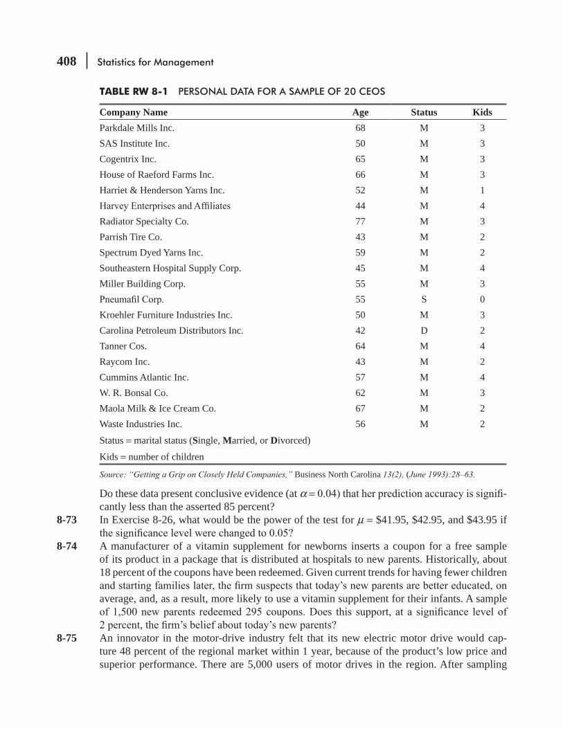
408 Statistics for Management
TABLE RW 8-1 PERSONAL DATA FOR A SAMPLE OF 20 CEOS
Company Name Age Status KidsParkdale Mills Inc. 68 M 3SAS Institute Inc. 50 M 3Cogentrix Inc. 65 M 3House of Raeford Farms Inc. 66 M 3Harriet & Henderson Yarns Inc. 52 M 1
44 M 4Radiator Specialty Co. 77 M 3Parrish Tire Co. 43 M 2Spectrum Dyed Yarns Inc. 59 M 2Southeastern Hospital Supply Corp. 45 M 4Miller Building Corp. 55 M 3
55 S 0Kroehler Furniture Industries Inc. 50 M 3Carolina Petroleum Distributors Inc. 42 D 2Tanner Cos. 64 M 4Raycom Inc. 43 M 2Cummins Atlantic Inc. 57 M 4W. R. Bonsal Co. 62 M 3Maola Milk & Ice Cream Co. 67 M 2Waste Industries Inc. 56 M 2
Status = marital status (Single, Married, or Divorced)
Kids = number of children
Source: “Getting a Grip on Closely Held Companies,” Business North Carolina 13(2), (June 1993):28–63.
Do these data present conclusive evidence (at α = -cantly less than the asserted 85 percent?
8-73 In Exercise 8-26, what would be the power of the test for μ = $41.95, $42.95, and $43.95 if
8-74 A manufacturer of a vitamin supplement for newborns inserts a coupon for a free sample of its product in a package that is distributed at hospitals to new parents. Historically, about 18 percent of the coupons have been redeemed. Given current trends for having fewer children
average, and, as a result, more likely to use a vitamin supplement for their infants. A sample
8-75 An innovator in the motor-drive industry felt that its new electric motor drive would cap-ture 48 percent of the regional market within 1 year, because of the product’s low price and superior performance. There are 5,000 users of motor drives in the region. After sampling

Testing Hypotheses: One-sample Tests 409
10 percent of these users a year later, the company found that 43 percent of them were using the new drives. At α = 0.01, should we conclude that the company failed to reach its market-share goal?
8-76 pay off once in 11.6 turns, with a standard deviation of 2.7 turns. A lawyer believes that the machines at Casino World have been tampered with and observes a payoff once in 12.4 turns, over 36 machines. At α = 0.01, is the lawyer right in concluding that the machines have a lower payoff frequency?
Questions on Running Case: SURYA Bank Pvt. Ltd.
1. their banks. (Question 9)
2. Do the customers on an average agree that the e-banking facilities offered by private sector banks are better than public sector banks? (Question 13b)
3. Do the bank customers in general believe that the information provided by them for using the e-banking services, are misused. (Question 13d)
@
CASE
@
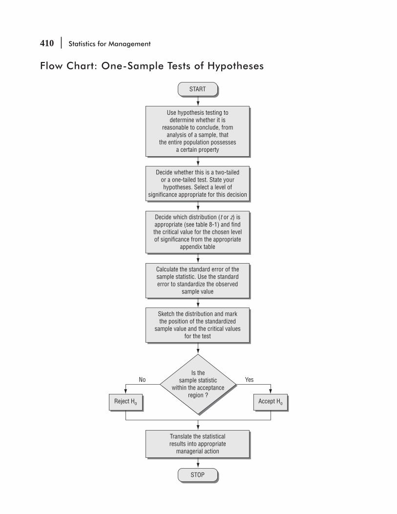
410 Statistics for Management
Flow Chart: One-Sample Tests of Hypotheses
Use hypothesis testing todetermine whether it is
reasonable to conclude, fromanalysis of a sample, that
the entire population possessesa certain property
Decide whether this is a two-tailedor a one-tailed test. State yourhypotheses. Select a level of
significance appropriate for this decision
Decide which distribution (t or z) isappropriate (see table 8-1) and findthe critical value for the chosen levelof significance from the appropriate
appendix table
Calculate the standard error of thesample statistic. Use the standarderror to standardize the observed
sample value
Sketch the distribution and markthe position of the standardized
sample value and the critical valuesfor the test
Translate the statisticalresults into appropriate
managerial action
Reject Ho Accept Ho
START
STOP
YesNoIs the
sample statisticwithin the acceptance
region ?

LEARNING OBJECTIVES
9After reading this chapter, you can understand:
CHAPTER CONTENTS
� To learn how to use samples from two populations to test hypotheses about how the populations are related
� To learn how hypothesis tests for differences between population means take different forms, depending on whether the samples are large or small
� To distinguish between independent and dependent samples when comparing two means
� To learn how to reduce a hypothesis test for the
9.1 Hypothesis Testing for Differences between Means and Proportions 412
9.2 Tests for Differences between Means: Large Sample Sizes 414
9.3 Tests for Differences between Means: Small Sample Sizes 420
9.4 Testing Differences between Means with Dependent Samples 431
9.5 Tests for Differences between Proportions: Large Sample Sizes 441
9.6 Prob Values: Another Way to Look at Testing Hypotheses 450
difference of means from dependent samples to a test about a single mean
� To learn how to test hypotheses that compare the proportions of two populations having some attribute of interest
� To understand how prob values can be used in testing hypotheses
� To get a feel for the kinds of outputs computer statistical packages produce for testing hypotheses
� Statistics at Work 455 � Terms Introduced in Chapter 9 456 � Equations Introduced in Chapter 9 456 � Review and Application Exercises 457 � Flow Chart: Two-Sample Tests of
Hypotheses 463
Testing Hypotheses:Two-sample Tests
4 Statistics for Management
A manufacturer of personal computers has a large number of employees from the local Spanish-speaking community. To improve the productivity of its workforce, it wants to increase the sen-
sitivity of its managers to the needs of this ethnic group. It started by scheduling several informal question-and-answer sessions with leaders of the Spanish-speaking community. Later, it designed a program involving formal classroom contact between its managers and professional psychologists and sociologists. The newer program is much more expensive, and the company president wants to know whether this expenditure has resulted in greater sensitivity. In this chapter, we’ll show you how to test whether these two methods have had essentially the same effects on the managers’ sensitivity or if the expense of the newer program is justified by its improved results.
9.1 HYPOTH ESIS TESTING FOR DIFFERENCES BETWEEN MEANS AND PROPORTIONS
In many decision-making situations, people need to determine whether the parameters of two populations are alike or different. A company may want to test, for example, whether its female employees receive lower salaries than its male employees for the same work. A training director may wish to determine whether the proportion of promotable employees at one government installation is different from that at another. A drag manufacturer may need to know whether a new drug causes one reaction in one group of experimental animals but a different reaction in another group.
Sampling D istribution for the Difference Between Two Population Parameters: Basic ConceptsIn Chapter 6, we introduced the concept of the sampling distribution of the mean as the foundation for the work we would do in estimation and hypothesis testing. For a quick review of the sampling distri-bution of the mean, you may refer to Figure 6-2.
Because we now wish to study two populations, not just one, the sampling distribution of interest is the sampling distribu-tion of the difference between sample means. Figure 9-1 may help us conceptualize this particular sampling distribution. At the top of this figure, we have drawn two populations, identified as Population 1 and Population 2. These two have means of m1 and m2 and standard deviations of s1 and s2, respectively. Beneath each population, we show the sampling distribution of the sample mean for that population. At the bottom of the figure is the sampling distribution of the difference between the sample means.
The two theoretical sampling distributions of the mean in Figure 9-1 are each made up from all pos-sible samples of a given size that can be drawn from the corresponding population distribution. Now,
Comparing two populations
Deriving the sampling
distribution of the difference
between sample means
In each of these examples, decision makers are concerned with the parameters of two populations. In these situations, they are not as interested in the actual value of the parameters as they are in the relation between the values of the two parameters—that is, how these parameters differ. They are concerned about the difference only. Do female employees earn less than male employees for the same work? Is the proportion of promotable employees at one installation different from that at another? Did one group of experimental animals react differently from the other? In this chapter, we shall introduce methods by which these questions can be answered, using hypothesis-testing procedures.

Testing Hypotheses: Two-sample Tests 4
Population 1
Sampling distribution of themean for population 1
Sampling distribution of themean for population 2
Population 2
Standarddeviation = σ1
Standarderror = σx−1
Standarderror σ
Standarderror = σx−2
μ1 μ2
Standarddeviation = σ2
This is the distributionof all possiblevalues of x −1
This is the distribution ofall possible values of x −1 − x −2
This is the distributionof all possiblevalues of x −2
Sampling distribution of thedifference between sample means
μx−2
= μ2μ
x−1 = μ1
μx−1
− x−2
x −1 − x −2
FIGURE 9-1 BASIC CONCEPTS OF POPULATION DISTRIBUTIONS, SAMPLING DISTRIBUTION OF THE MEAN, AND THE SAMPLING DISTRIBUTION OF THE DIFFERENCE BETWEEN SAMPLE MEANS
suppose we take a random sample from the distribution of Population 1 and another random sample from the distribution of Population 2. If we then subtract the two sample means, we get
x x1 2− ← Difference between sample means
This difference will be positive if x1 is larger than x2 and negative if x2 is greater than x1. By con-structing a distribution of all possible sample differences of x x1 2− , we end up with the sampling distribution of the difference between sample means, which is shown at the bottom of Figure 9-1.
The mean of the sampling distribution of the difference between sample means is symbolized
1 2μ −x x and is equal to
,1 2
μ μ−x x which as we saw in Chapter 6, is the same as 1 – 2. If 1 = 2, then
1 2μ μ−x x = 0.
Parameters of this sampling
distribution

4 Statistics for Management
The standard deviation of the distribution of the difference between the sample means is called the standard error of the difference between two means and is calculated using this formula:
Standard Error of the Difference between Two Means
12
1
22
21 2
σσ σ
= +− n nx x
Variance of Population 1
Size of sample from Population 1
Size of sample from Population 2
Variance of Population 2
[9-1]
If the two population standard deviations are not known, we can estimate the standard error of the difference between two means. We can use the same method of estimating the standard error that we have used before by letting sample standard devia-tions estimate the population standard deviations as follows:
σ = s ← Sample standard deviation [7-1]
Therefore, the formula for the estimated standard error of the difference between two means becomes
Estimated Standard Error of the Difference between Two Means
Estimated variance of Population 1
Estimated variance of Population 2
σσ σ
= +− n nx xˆ
ˆ ˆ12
1
22
21 2
[9-2]
As the following sections show, depending on the sample sizes, we shall use different estimates for ˆ1σ
and ˆ2σ in Equation 9-2.
9.2 TESTS FOR DIFFEREN CES BETWEEN MEANS: LARGE SAMPLE SIZES
When both sample sizes are greater than 30, this example illus-trates how to do a two-tailed test of a hypothesis about the differ-ence between two means. A manpower-development statistician is asked to determine whether the hourly wages of semiskilled
How to estimate the standard
error of this sampling
distribution
Step 1: State your hypotheses,
type of test, and significance
level
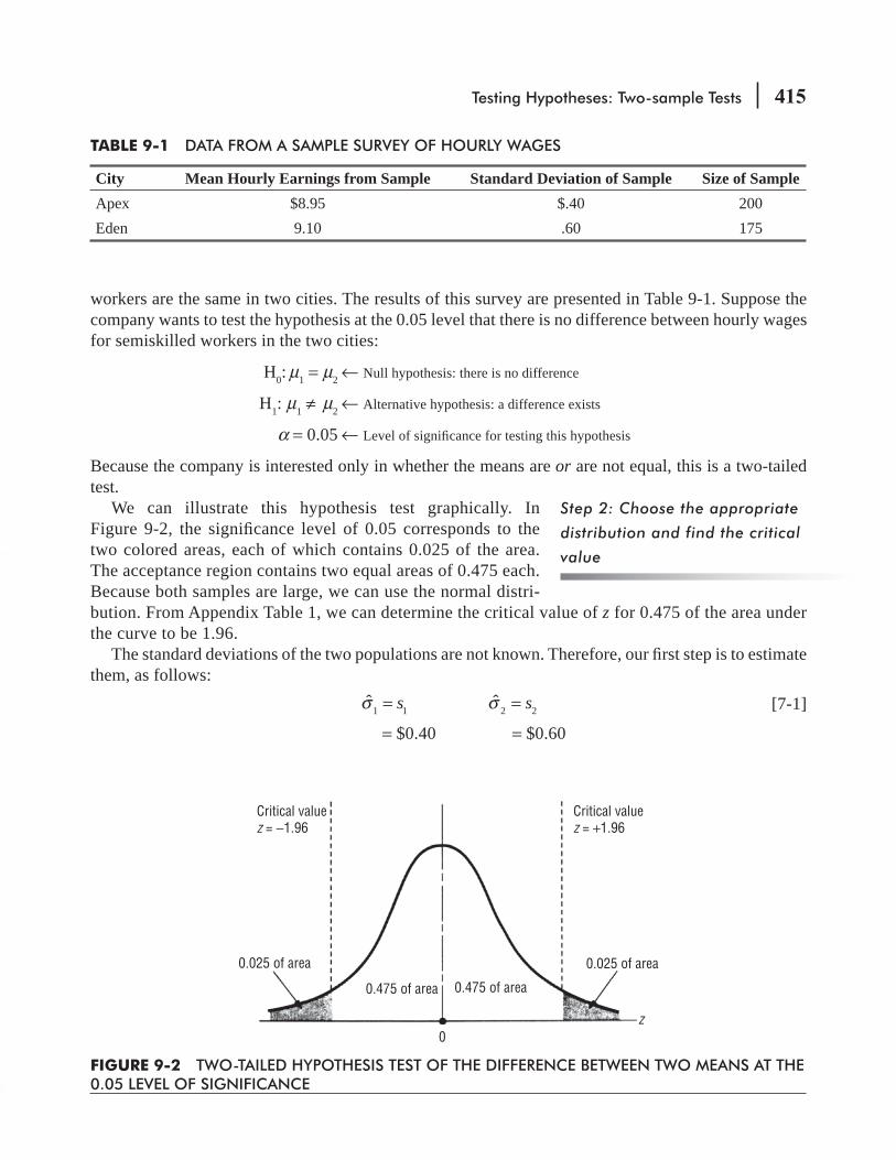
Testing Hypotheses: Two-sample Tests 415
workers are the same in two cities. The results of this survey are presented in Table 9-1. Suppose the company wants to test the hypothesis at the 0.05 level that there is no difference between hourly wages for semiskilled workers in the two cities:
H0: μ1 = μ2 ← Null hypothesis: there is no difference
H1: μ1 ≠ μ2 ← Alternative hypothesis: a difference exists
α = 0.05 ← Level of signi cance for testing this hypothesis
Because the company is interested only in whether the means are or are not equal, this is a two-tailed test.
We can illustrate this hypothesis test graphically. In Figure 9-2, the signi cance level of 0.05 corresponds to the two colored areas, each of which contains 0.025 of the area. The acceptance region contains two equal areas of 0.475 each. Because both samples are large, we can use the normal distri-bution. From Appendix Table 1, we can determine the critical value of z for 0.475 of the area under the curve to be 1.96.
The standard deviations of the two populations are not known. Therefore, our rst step is to estimate them, as follows:
σ σ= =s sˆ ˆ1 1 2 2 [7-1]
= $0.40 = $0.60
Step 2: Choose the appropriate
distribution and find the critical
value
TAB LE 9-1 DAT A FROM A SAMPLE SURVEY OF HOURLY WAGES
City Mean Hourly Earnings from Sample Standard Deviation of Sample Size of SampleApex $8.95 $.40 200Eden 9.10 .60 175
Critical valuez = −1.96
Critical valuez = +1.96
0.025 of area
0.475 of area
z
0.475 of area
0
0.025 of area
FIGURE 9-2 TWO-TAILED HYPOTHESIS TEST OF THE DIFFERENCE BETWEEN TWO MEANS AT THE 0.05 LEVEL OF SIGNIFICANCE

416 Statistics for Management
Now the estimated standard error of the difference between the two means can be determined by
σσ σ
= +− n nx xˆ
ˆ ˆ12
1
22
21 2
[9-2]
(0.40)200
(0.60)175
2 2
= +
0.00286== $0.0 53 Estimated standard error
Next we standardize the difference of sample means, x x .1 2− First, we subtract μ μ−( ) ,1 2 H0 the
hypothesized difference of the population means. Then we divide by σ −x xˆ ,
1 2 the estimated standard
error of the difference between the sample means.
( ) ( )ˆ
1 2 1 2 H0
1 2
μ μ
σ=
− − −
−
zx x
x x
(8.95) (9.10) 00.053
=− −
= –2.83
We mark the standardized difference on a sketch of the sampling distribution and compare with the critical value, as shown in Figure 9-3. It demonstrates that the standardized difference between the two sample means lies outside the acceptance
Step 4: Sketch the distribution
and mark the sample value and
critical values
Step 3: Compute the standard
error and standardize the
sample statistic
Standardizeddifference betweenthe sample means
–2.83 +1.96–1.96 0z
Acceptance regionAccept H0 if the sample value is in this region
FIGURE 9-3 TWO-TAILED HYPOTHESIS TEST OF THE DIFFERENCE BETWEEN TWO MEANS AT THE 0.05 LEVEL OF SIGNIFICANCE, SHOWING THE ACCEPTANCE REGION AND THE STANDARDIZED DIFFERENCE BETWEEN SAMPLE MEANS
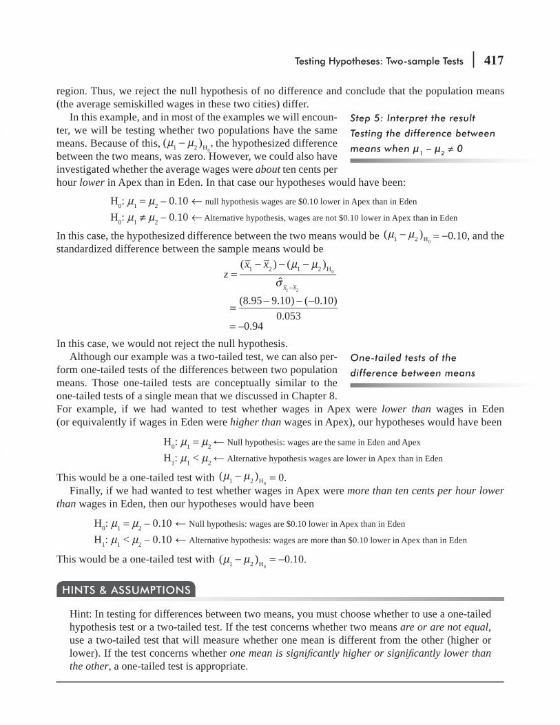
Testing Hypotheses: Two-sample Tests 417
region. Thus, we reject the null hypothesis of no difference and conclude that the population means (the average semiskilled wages in these two cities) differ.
In this example, and in most of the examples we will encoun-ter, we will be testing whether two populations have the same means. Because of this, μ μ−( ) ,1 2 H0
the hypothesized difference between the two means, was zero. However, we could also have investigated whether the average wages were about ten cents per hour lower in Apex than in Eden. In that case our hypotheses would have been:
H0: μ1 = μ2 – 0.10 ← null hypothesis wages are $0.10 lower in Apex than in Eden
H0: μ1 ≠ μ2 – 0.10 ← Alternative hypothesis, wages are not $0.10 lower in Apex than in Eden
In this case, the hypothesized difference between the two means would be μ μ−( )1 2 H0 = −0.10, and the
standardized difference between the sample means would be( ) ( )
ˆ1 2 1 2 H0
1 2
μ μ
σ=
− − −
−
zx x
x x
(8.95 9.10) ( 0.10)0.053
=− − −
= –0.94In this case, we would not reject the null hypothesis.
Although our example was a two-tailed test, we can also per-form one-tailed tests of the differences between two population means. Those one-tailed tests are conceptually similar to the one-tailed tests of a single mean that we discussed in Chapter 8. For example, if we had wanted to test whether wages in Apex were lower than wages in Eden (or equivalently if wages in Eden were higher than wages in Apex), our hypotheses would have been
H0: μ1 = μ2 Null hypothesis: wages are the same in Eden and Apex
H1: μ1 < μ2 Alternative hypothesis wages are lower in Apex than in Eden
This would be a one-tailed test with μ μ−( )1 2 H0= 0.
Finally, if we had wanted to test whether wages in Apex were more than ten cents per hour lower than wages in Eden, then our hypotheses would have been
H0: μ1 = μ2 – 0.10 Null hypothesis: wages are $0.10 lower in Apex than in Eden
H1: μ1 < μ2 – 0.10 Alternative hypothesis: wages are more than $0.10 lower in Apex than in Eden
This would be a one-tailed test with μ μ−( )1 2 H0= −0.10.
Hint: In testing for differences between two means, you must choose whether to use a one-tailed hypothesis test or a two-tailed test. If the test concerns whether two means are or are not equal, use a two-tailed test that will measure whether one mean is different from the other (higher or lower). If the test concerns whether one mean is signi cantly higher or signi cantly lower than the other, a one-tailed test is appropriate.
HINTS & ASSUMPTIONS
Step 5: Interpret the result
Testing the difference between
means when 1 – 2 ≠ 0
One-tailed tests of the
difference between means

418 Statistics for Management
EXERCISES 9.1
Self-Check ExercisesSC 9-1 Two independent samples of observations were collected. For the first sample of 60 elements,
the mean was 86 and the standard deviation 6. The second sample of 75 elements had a mean of 82 and a standard deviation of 9.(a) Compute the estimated standard error of the difference between the two means.
gnisU )b( α = 0.01, test whether the two samples can reasonably be considered to have come from populations with the same mean.
SC 9-2 In 1993, the Financial Accounting Standards Board (FASB) was considering a proposal to require companies to report the potential effect of employees’ stock options on earnings per share (EPS). A random sample of 41 high-technology firms revealed that the new proposal would reduce EPS by an average of 13.8 percent, with a standard deviation of 18.9 percent. A random sample of 35 producers of consumer goods showed that the proposal would reduce EPS by 9.1 percent on average, with a standard deviation of 8.7 percent. On the basis of these samples, is it reasonable to conclude (at α = 0.10) that the FASB proposal will cause a greater reduction in EPS for high-technology firms than for producers of consumer goods?
Basic Concepts9-1 eht roF .det celloc erew selpmas tnednepedni owT first sample of 42 items, the mean was 32.3
and the variance 9. The second sample of 57 items had a mean of 34 and a variance of 16.(a) Compute the estimated standard error of the difference between the two means.
gnisU )b( α = 0.05, test whether there is suffi cient evidence to show the second population has a larger mean.
Applications9-2 Block Enterprises, a manufacturer of chip s for computers, is in the process of deciding
whether to replace its current semiautomated assembly line with a fully automated assembly line. Block has gathered some preliminary test data about hourly chip production, which is summarized in the following table, and it would like to know whether it should upgrade its assembly line. State (and test at α = 0.02) appropriate hypotheses to help Block decide.
x s nSemiautomatic line 198 32 150Automatic line 206 29 200
9-3 Two research laboratories have independently produced drugs that provide relief to arthritis sufferers. The first drug was tested on a group of 90 arthritis sufferers and produced an aver-age of 8.5 hours of relief, and a sample standard deviation of 1.8 hours. The second drug was tested on 80 arthritis sufferers, producing an average of 7.9 hours of relief, and a sample stan-dard deviation of 2.1 hours. At the 0.05 level of significance, does the second drug provide a significantly shorter period of relief?
Testing Hypotheses: Two-sample Tests 419
standard deviation was 0.51 percent. A year earlier, a sample of 38 money-market funds showed an average rate of return of 4.36 percent, and the sample standard deviation was 0.84 percent. Is it reasonable to conclude (at a = 0.05) that money-market interest rates declined during 2015?
9-5
9-6 BullsEye Discount store has always prided itself on customer service. The store hopes that all BullsEye stores are providing the same level of service from region to region, so they have surveyed some customers. In the Southeast region, a random sample of 97 customers yielded an average overall satisfaction rating of 8.8 out of 10 and the sample standard deviation was 0.7. In the Northeast region, a random sample of 84 customers resulted in an average rating of 9.0 and the sample standard deviation was 0.6. Can BullsEye conclude, at a = 0.05, that the levels of customer satisfaction in the two markets are significantly different?
Worked-Out Answers to Self-Check ExercisesSC 9-1 s1 = 6 n1 = 60 x1 = 86 s2 = 9 n2 = 75 x2 = 82
(a) ˆ 3660
8175
1.296x12
1
22
21 2
σ = + = + =−
sn
snx
(b) H0: m1 = m2 H1: m1 ≠ m2 a = 0.01
The limits of the acceptance region are z = ±2.58, or
0 ˆ 2.58(1.296) 3.3441 2 1 2σ− = ± = ± = ±−x x z x x
Because the observed z value ( ) ( )
ˆ1 2 1 2 H0
1 2
μ μ
σ=
− − −
−
x x
x x
(86 82) 01.296
=− − = 3.09 > 2.58 (or x x1 2− = 86 – 82 = 4 > 3.344)
we reject H0. It is reasonable to conclude that the two samples come from different populations.
SC 9-2 Sample 1 (HT firms): s1 = 18.9 n1 = 41 x 13.81 =Sample 2 (CG producers): s2 = 8.7 n2 = 35 x2 = 9.1
Notwithstanding the Equal Remuneration Act, 1976, in 2015 it still appeared that men earned more than women in similar jobs. A random sample of 38 male machine-tool operators found a mean hourly wage of ` 113.8, and the sample standard deviation was ` 18.4. A random sample of 45 female machine-tool operators found their mean wage to be ` 84.2, and the sample standard deviation was ` 13.1. On the basis of these samples, is it reasonable to conclude (at a = 0.01) that the male operators are earning over ` 20 more per hour than the female operators?
9-4 A sample of 32 money-market mutual funds was chosen on January 1, 2016, and the aver-age annual rate of return over the past 30 days was found to be 3.23 percent, and the sample
420 Statistics for Management
H0: μ1 = μ2 H1: μ1 > μ2 α = 0.10
ˆ (18.9)41
(8.7)35
3.298 percent12
1
22
2
2 2
1 2σ = + = + =−
sn
snx x
The upper limit of the acceptance region is z = 1.28, or
0 ˆ 1.28(3.298) 4.221 percent1 2 1 2σ− = + = =−x x z x x
Because the observed z value
( ) ( )ˆ
(13.8 9.1) 03.298
1 2 1 2 H0
1 2
μ μ
σ=
− − −=
− −
−
x x
x x
x x1.43 1.28 (or 4.7 4.221)1 2= > − = >
we reject H0 and conclude that the FASB proposal will cause a signi cantly greater reduction in EPS for high-tech rms.
9.3 TESTS FOR DIFFERENCES BETWEEN MEANS:SMALL SAMPLE SIZES
Wh en the sample sizes are small, there are two technical changes in our procedure for testing the dif-ferences between means. The rst involves the way we compute the estimated standard error of the difference between the two sample means. The second will remind you of what we did in Chapter 8 with small-sample tests of a single mean. Once again we will base our small-sample tests on the t dis-tribution, rather than the normal distribution. To explore the details of these changes, let’s return to our chapter-opening illustration concerning the sensitivity of the managers at a personal-computer manu-facturer to the needs of their Spanish-speaking employees.
Recall that the company has been investigating two education programs for increasing the sensitiv-ity of its managers. The original program consisted of several informal question-and-answer sessions with leaders of the Spanish-speaking community. Over the past few years, a program involving formal classroom contact with professional psychologists and sociologists has been developed. The new pro-gram is considerably more expensive, and the president wants to know at the 0.05 level of signi cance whether this expenditure has resulted in greater sensitivity. Let’s test the following:
H0: μ1 = μ2 Null hypothesis: There is no difference in sensitivity levels achieved by the two programs
H1: μ1 > μ2 Alternative hypothesis. The new program results in higher sensitivity levels
α = 0.05 Level of signi cance for testing this hypothesis
Table 9-2 contains the data resulting from a sample of the managers trained in both programs. Because only limited data are available for the two programs, the population standard deviations are estimated from the data. The sensitivity level is measured as a percentage on a standard psychometric scale.
The company wishes to test whether the sensitivity achieved by the new program is signi cantly higher than that achieved under the older, more informal program. To reject the null hypothesis (a result that the company desires), the observed difference of sample means would need to fall suf ciently high in the right tail of the distribution. Then we would accept the alternative hypothesis that the new pro-gram leads to higher sensitivity levels and that the extra expenditures on this program are justi ed.
Step 1: State your hypotheses,
type of test, and significance
level
Testing Hypotheses: Two-sample Tests 421
Postponing Step 2 until we
know how many degrees of
freedom to use
The second step in our ve-step process for hypothesis test-ing now requires us to choose the appropriate distribution and nd the critical value. Recall from the opening paragraph in this
section that the test will be based on a t distribution, but we don’t yet know which t distribution to use. How many degrees of freedom are there? The answer to this question will be more apparent after we see how to compute the estimated standard error.
Our rst task in performing the test is to calculate the standard error of the difference between the two means. Because the population standard deviations are not known, we must use Equation 9-2.
ˆˆ ˆ
12
1
22
21 2
σσ σ
= +− n nx x [9-2]
In the previous example, where the sample sizes were large (both greater than 30), we used Equation 7-1 and estimated ˆ
12σ by s ,1
2 and ˆ by22
22σ s . Now, with small sample sizes, that procedure is not appropriate.
If we can assume that the unknown population variances are equal (and this assumption can be tested using a method discussed in Section 6 of Chapter 11), we can continue. If we cannot assume that
12
22σ σ= , then the problem is beyond the scope of this text.
Assuming for the moment that 12
22σ σ= , how can we estimate
the common variance σ 2? If we use either s sor12
22 , we get an
unbiased estimator of σ 2, but we don’t use all the information available to us because we ignore one of the samples. Instead we use a weighted average of s sand1
222, and the weights are the numbers of degrees of freedom in each
sample. This weighted average is called a “pooled estimate” of σ 2. It is given by:
Pooled Estimate of σ 2
sn s n s
n n( 1) ( 1)
2p2 1 1
22 2
2
1 2
=− + −
+ −[9-3]
Because we have to use the sample variances to estimate the unknown σ 2, the test will be based on the t distribution. This is just like the test of a single mean from a sample of size n when we did not know σ 2. There we used a t distribution with n – 1 degrees of freedom, because once we knew the sample mean, only n – 1 of the sample observations could be freely speci ed. (You may review the discussion of degrees of freedom on pages 341–342.) Here we
Estimating σ 2 with small sample
sizes
For this test, we have
n1 + n2 – 2 degrees of freedom
TABLE 9-2 DATA FROM SAMPLE OF TWO SENSITIVITY PROGRAMS
Program Sampled
Mean Sensitivity after This Program
Number of Managers Observed
Estimated Standard Deviation of Sensitivity after This
Program
Formal 92% 12 15%
Informal 84 15 19
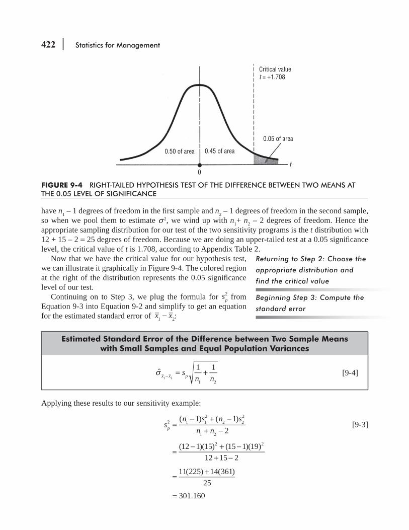
422 Statistics for Management
have n1 – 1 degrees of freedom in the rst sample and n2 – 1 degrees of freedom in the second sample, so when we pool them to estimate σ 2, we wind up with n1+ n2 – 2 degrees of freedom. Hence the appropriate sampling distribution for our test of the two sensitivity programs is the t distribution with 12 + 15 – 2 = 25 degrees of freedom. Because we are doing an upper-tailed test at a 0.05 signi cance level, the critical value of t is 1.708, according to Appendix Table 2.
Now that we have the critical value for our hypothesis test, we can illustrate it graphically in Figure 9-4. The colored region at the right of the distribution represents the 0.05 signi cance level of our test.
Continuing on to Step 3, we plug the formula for sp2 from
Equation 9-3 into Equation 9-2 and simplify to get an equation for the estimated standard error of x x1 2− :
Estimated Standard Error of the Difference between Two Sample Means with Small Samples and Equal Population Variances
σ = +− sn nx x p
ˆ 1 1
1 21 2
[9-4]
Applying these results to our sensitivity example:
sn s n s
n n( 1) ( 1)
2p2 1 1
22 2
2
1 2
=− + −
+ − [9-3]
(12 1)(15) (15 1)(19)12 15 2
2 2
=− + −
+ −
11(225) 14(361)25
=+
= 301.160
Returning to Step 2: Choose the
appropriate distribution and
find the critical value
Beginning Step 3: Compute the
standard error
Critical valuet = +1.708
0.05 of area
0.45 of area0.50 of area
0t
FIGURE 9-4 RIGHT-TAILED HYPOTHESIS TEST OF THE DIFFERENCE BETWEEN TWO MEANS AT THE 0.05 LEVEL OF SIGNIFICANCE
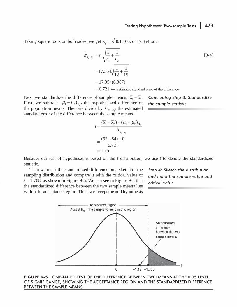
Testing Hypotheses: Two-sample Tests 423
Taking square roots on both sides, we get s 301.160, or 17.354, so :p =
ˆ 1 1
1 21 2
σ = +− sn nx x p [9-4]
17.354 112
115
= +
= 17.354(0.387) = 6.721 Estimated standard error of the difference
Next we standardize the difference of sample means, x x1 2− . First, we subtract ( ) ,1 2 H0
μ μ− the hypothesized difference of the population means. Then we divide by ˆ ,
1 2σ −x x the estimated
standard error of the difference between the sample means.
( ) ( )ˆ
1 2 1 2 H0
1 2
μ μ
σ=
− − −
−
tx x
x x
(92 84) 06.721
=− −
= 1.19Because our test of hypotheses is based on the t distribution, we use t to denote the standardized statistic.
Then we mark the standardized difference on a sketch of the sampling distribution and compare it with the critical value of t = 1.708, as shown in Figure 9-5. We can see in Figure 9-5 that the standardized difference between the two sample means lies within the acceptance region. Thus, we accept the null hypothesis
Concluding Step 3: Standardize
the sample statistic
Step 4: Sketch the distribution
and mark the sample value and
critical value
Acceptance regionAccept H0 if the sample value is in this region
Standardizeddifferencebetween the twosample means
t0 +1.19 +1.708
FIGURE 9-5 ONE-TAILED TEST OF THE DIFFERENCE BETWEEN TWO MEANS AT THE 0.05 LEVEL OF SIGNIFICANCE, SHOWING THE ACCEPTANCE REGION AND THE STANDARDIZED DIFFERENCE BETWEEN THE SAMPLE MEANS
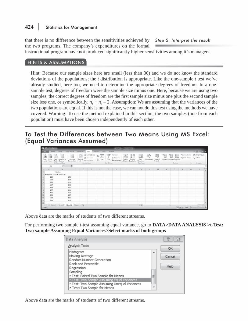
424 Statistics for Management
that there is no difference between the sensitivities achieved by the two programs. The company’s expenditures on the formal instructional program have not produced signi cantly higher sensitivities among it’s managers.
Hint: Because our sample sizes here are small (less than 30) and we do not know the standard deviations of the populations; the t distribution is appropriate. Like the one-sample t test we’ve already studied, here too, we need to determine the appropriate degrees of freedom. In a one-sample test, degrees of freedom were the sample size minus one. Here, because we are using two samples, the correct degrees of freedom are the rst sample size minus one plus the second sample size less one, or symbolically, n1 + n2 – 2. Assumption: We are assuming that the variances of the two populations are equal. If this is not the case, we can not do this test using the methods we have covered. Warning: To use the method explained in this section, the two samples (one from each population) must have been chosen independently of each other.
HINTS & ASSUMPTIONS
To Test the Differences between Two Means Using MS Excel: (Equal Variances Assumed)
Above data are the marks of students of two different streams.
For performing two sample t-test assuming equal variance, go to DATA>DATA ANALYSIS >t-Test: Two sample Assuming Equal Variances>Select marks of both groups
Above data are the marks of students of two different streams.
Step 5: Interpret the result

Testing Hypotheses: Two-sample Tests 425
To Test the Differences between Two Means Using MS Excel: (Unequal Variances Assumed)

426 Statistics for Management
For two sample t-test assuming unequal variance go to DATA>DATA ANALYSIS >t-Test: Two sample Assuming Unequal Variances>Select marks of both groups
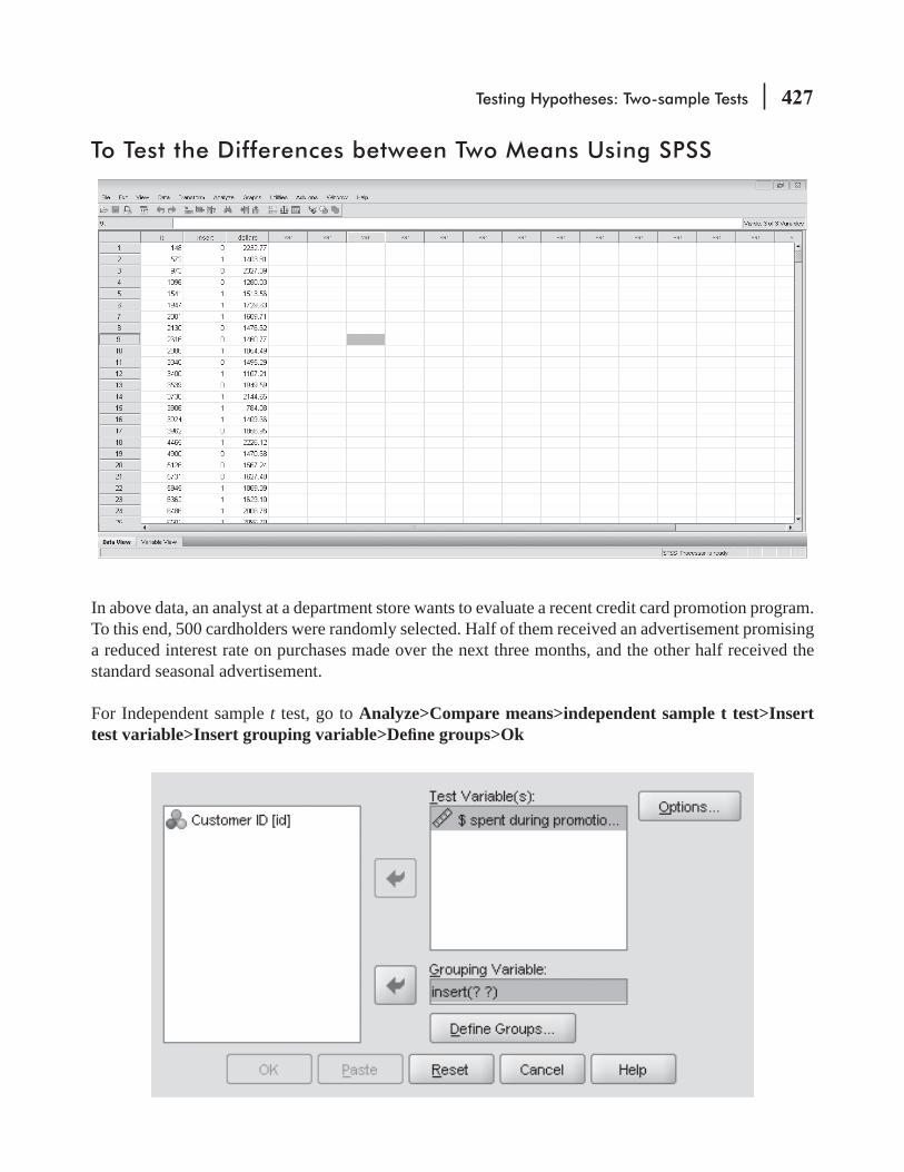
Testing Hypotheses: Two-sample Tests 427
To Test the Differences between Two Means Using SPSS
In above data, an analyst at a department store wants to evaluate a recent credit card promotion program. To this end, 500 cardholders were randomly selected. Half of them received an advertisement promising a reduced interest rate on purchases made over the next three months, and the other half received the standard seasonal advertisement.
For Independent sample t test, go to Analyze>Compare means>independent sample t test>Insert test variable>Insert grouping variable>De ne groups>Ok
428 Statistics for Management
EXERCISES 9.2
Self-Check Exe rcises
SC 9-3 A consumer-research organization routinely selects several car models each year and evalu-ates their fuel efficiency. In this year’s study of two similar subcompact models from two different automakers, the average gas mileage for 12 cars of brand A was 27.2 miles per gal-lon, and the standard deviation was 3.8 mpg. The nine brand B cars that were tested averaged 32.4 mpg, and the standard deviation was 4.3 mpg. At a = 0.01, should it conclude that brand A cars have lower average gas mileage than do brand B cars?
SC 9-4 Connie Rodrigues, the Dean of Students at Midstate College, is wondering about grade dis-tributions at the school. She has heard grumblings that the GPAs in the Business School are about 0.25 lower than those in the College of Arts and Sciences. A quick random sampling produced the following GPAs.
Business: 2.86 2.77 3.18 2.80 3.14 2.87 3.19 3.24 2.91 3.00 2.83
Arts & Sciences: 3.35 3.32 3.36 3.63 3.41 3.37 3.45 3.43 3.44 3.17 3.26 3.18 3.41
Do these data indicate that there is a factual basis for the grumblings? State and test appropri-ate hypotheses at a = 0.02.

Testing Hypotheses: Two-sample Tests 429
9-8 A large stock-brokerage firm wants to determine how successful its new account executives have been at recruiting clients. After completing their training, new account execs spend sev-eral weeks calling prospective clients, trying to get the prospects to open accounts with the firm. The following data give the numbers of new accounts opened in their first 2 weeks by 10 randomly chosen female account execs and by 8 randomly chosen male account execs. At a = 0.05, does it appear that the women are more effective at generating new accounts than the men are?
Number of New AccountsFemale account execs 12 11 14 13 13 14 13 12 14 12Male account execs 13 10 11 12 13 12 10 12
9-9 Because refunds are paid more quickly on tax returns that are filed electronically, the Com-missioner of the Internal Revenue Service was wondering whether refunds due on returns filed by mail were smaller than those due on returns filed electronically. Looking only at returns claiming refunds, a sample of 17 filed by mail had an average refund of $563, and a standard deviation of $378. The average refund on a sample of 13 electronically filed returns was $958, and the sample standard deviation was $619. At a = 0.01, do these data support the commissioner’s speculation?
9-10
Shift Production (in 1,000s)Day 107.5 118.6 124.6 101.6 113.6 119.6 120.6 109.6 105.9Night 115.6 109.4 121.6 128.7 136.6 125.4 121.3 108.6 117.5
Do these data indicate, at a = 0.01, that the night shift is producing more tires per shift?
Greatyear tires currently produces tires at their Chennai plant during two 12-hour shifts. The night-shift employees are planning to ask for a raise because they believe they are producing more tires per shift than the day shift. “Because Greatyear is making more money during the night shift, those employees should also make more money” according to the night-shift spokesman. The Greatyear production supervisor randomly selected some daily production runs from each shift with the results given below (in 1,000s of tires produced).
Applications
9-7 A credit-insurance organization has developed a new high-tech method of training new sales personnel. The company sampled 16 employees who were trained the original way and found average hourly sales to be ` 688 and the standard deviation was ` 32.63. They also sampled11 employees who were trained using the new method and found average daily sales to be` 706 and the standard deviation was ` 24.84. At a = 0.05, can the company conclude that average hourly sales have increased under the new plan?

430 Statistics for Management
Worked-Out An swers to Self-Check ExercisesSC 9-3 sA = 3.8 nA = 12 xA = 27.2 sB = 4.3 nB = 9 xB = 32.1
H0: μA = μB H1: μA < μB α = 0.01
=− + −
+ −=
+=
( 1) ( 1)2
11(3.8) 8(4.3)19
4.0181 mpg2 2 2 2
sn s n s
n npA A B B
A B
The lower limit of the acceptance region is t = −2.539, or
− = − + = − +0 1 1 2.539(4.0181) 112
19
x x tsn nA B p
A B
= –4.499 mpg
Because the observed t value
μ μ=
− − −
+=
− −
+
( ) ( )
1 1(27.2 32.1) 0
4.0181 112
19
H0x x
sn n
A B A B
pA B
= –2.766 < –2.539 (or −x xA B = –4.9 < –4.499), we reject H0. Brand B delivers signi cantly higher mileage than does brand A.
SC 9-4 Sample 1 (Business): sB = 0.176 nB = 11 xB = 2.98Sample 2 (Arts & Sciences): sA = 0.121 nA = 13 xA = 3.368H0: μB – μA = –0.25 H1: μB – μA ≠ –0.25 α = 0.02
=− + −
+ −=
+=
( 1) ( 1)2
10(.176) 12(.121)22
0.14852 2 2 2
sn s n s
n npB B A A
B A
The limits of the acceptance region are t = ±2.508, or
μ μ− = − ± + = −( ) 1 1 0.25H0x x ts
n nB A B A pB A
± + = − −2.508(0.1485) 111
113
( 0.4026, 0.0974)
Because the observed t value
μ μ=
− − −
+
( ) ( )
1 1H0
x x
sn n
B A B A
pB A
=− −
+
(2.980 3.368) 0.25
0.1485 111
113
= –2.268 > –2.508 (or −x xB A = –0.388 > –0.403), we do not reject H0. The Business School GPAs are about .25 below those in the College of Arts & Sciences.

Testing Hypotheses: Two-sample Tests 431
9.4 TESTING DIFFERENCES BETWEEN MEANS WITH DEPENDENT SAMPLES
nesohc erew selpmas ruo ,3.9 dna 2.9 snoitceS ni selpmaxe eht nI independent of each other. In the wage example, the samples were taken from two different cities. In the sensitivity example, samples were taken of those managers who had gone through two different training programs. Sometimes, however, it makes sense to take samples that are not independent of each other. Often the use of such dependent (or paired) samples mrofrep ot su selbane
tnedneped htiW .srotcaf suoenartxe rof lortnoc ot su wolla eseht esuaceb ,sisylana esicerp erom asamples, we still follow the same basic procedure that we have followed in all our hypothesis testing. The basic difference is that in dependent samples, the two samples are related or two observationshave been taken on the same sample members at different points of time.
A health spa has advertised a weight-reducing program and has claimed that the average participant in the program loses more than 17 pounds. A somewhat overweight executive is interested in the program but is skeptical about the claims and asks for some hard evidence. The spa allows him to select randomly the records of 10 participants and record their weights before and after the program. These data are recorded in Table 9-3. Here we have two samples (a before sample and an after sample) that are clearly dependent on each other, because the same 10 people have been observed twice.
The overweight executive wants to test at the 5 percent ificance level the claimed average weight loss of more than ngis
17 pounds. Formally, we may state this problem:
H0: m1 – m2 = 17 Null hypothesis: average weight loss is only 17 pounds
H1: m1 – m2 > 17 Alternative hypothesis: average weight loss exceeds 17 pounds
a = 0.05 Level of significance
What we are really interested in is not the weights before and after, but their differences. Conceptually, what we have is not two samples of before and after weights, but rather one sample of weight losses. If the population of weight losses has a mean ml, we can restate our hypotheses as
H0: ml = 17H1: ml > 17
Figure 9-6 illustrates this problem graphically. Because we want to know whether the mean weight loss exceeds 17 pounds, an upper-tailed test is appropriate. The 0.05 significance level is shown in Figure 9-6 as the colored area under the t distribu-tion. We use the t distribution because the sample size is only 10;
Conditions under which paired
samples aid analysis
Step 1: State your hypotheses, type
of test, and significance level
Conceptual understanding of
differences
Step 2: Choose the appropriate
distribution and find the critical
value
TABLE 9-3 WEIGHTS BEFORE AND AFTER A REDUCING PROGRAM
Before 189 202 220 207 194 177 193 202 208 233After 170 179 203 192 172 161 174 187 186 204

432 Statistics for Management
the appropriate number of degrees of freedom is 9, (10 – 1). Appendix Table 2 gives the critical value of t, 1.833.
We begin by computing the individual losses, their mean, and standard deviation, and proceed exactly as we did when testing hypotheses about a single mean. The computations are done in Table 9-4.
Critical valuet = +1.833
0.05 of area
0.45 of area0.50 of area
0t
FIGURE 9-6 ONE-TAILED HYPOTHESIS TEST AT THE 0.05 LEVEL OF SIGNIFICANCE
Computing the paired differences
TABLE 9-4 FINDING THE MEAN WEIGHT LOSS AND ITS STANDARD DEVIATION
Before After Loss Loss Squared 2
189 170 19 361202 179 23 529220 203 17 289207 192 15 225194 172 22 484177 161 16 256193 174 19 361202 187 15 225208 186 22 484233 204 29
∑x = 197841
∑ x2 = 4,055
=∑x xn
[3-2]
=19710
= 19.7
∑=−
−−1 1
2 2
sx
nnxn
[3-18]
4,0559
10(19.7)9
2
= −
19.34== 4.40
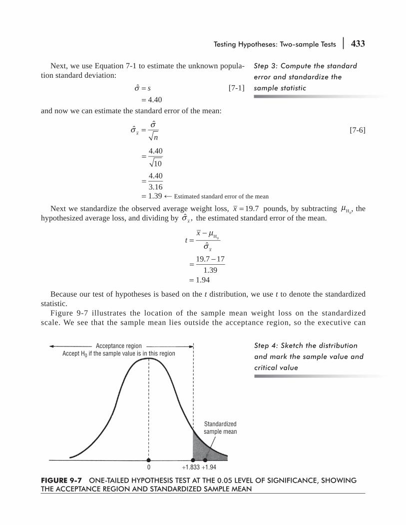
Testing Hypotheses: Two-sample Tests 433
Next, we use Equation 7-1 to estimate the unknown popula-tion standard deviation: σ =ˆ s [7-1]
= 4.40and now we can estimate the standard error of the mean:
σ σ=ˆ ˆ
nx [7-6]
4.4010
=
=4.403.16
= 1.39 Estimated standard error of the mean
Next we standardize the observed average weight loss, = 19.7x pounds, by subtracting μH0, the
hypothesized average loss, and dividing by σ ,x the estimated standard error of the mean.
μ
σ=
−ˆ
H0tx
x
19.7 171.39
=−
= 1.94
Because our test of hypotheses is based on the t distribution, we use t to denote the standardized statistic.
Figure 9-7 illustrates the location of the sample mean weight loss on the standardized scale. We see that the sample mean lies outside the acceptance region, so the executive can
Step 3: Compute the standard
error and standardize the
sample statistic
Step 4: Sketch the distribution
and mark the sample value and
critical value
Acceptance regionAccept H0 if the sample value is in this region
Standardizedsample mean
0 +1.833 +1.94
FIGURE 9-7 ONE-TAILED HYPOTHESIS TEST AT THE 0.05 LEVEL OF SIGNIFICANCE, SHOWING THE ACCEPTANCE REGION AND STANDARDIZED SAMPLE MEAN

434 Statistics for Management
reject the null hypothesis and conclude that the claimed weight loss in the program is legitimate.
Let’s see how this paired difference test differs from a test of the difference of means of two independent samples. Suppose that the data in Table 9-4 represent two independent samples of 10 individuals entering the program and another 10 randomly selected individuals leaving the program. The means and variances of the two samples are given in Table 9-5.
Because the sample sizes are small, we use Equation 9-3 to get a pooled estimate of σ 2 and Equation 9-4 to estimate
1 2σ −x x :
=− + −
+ −s
n s n sn np
( 1) ( 1)2
2 1 12
2 22
1 2
[9-3]
(10 1)(253.61) (10 1)(201.96)10 10 2
=− + −
+ −
=+2282.49 1817.64
18 = 227.79 Estimate of common population variance
σ = +− sn nx x p
ˆ 1 1
1 21 2
[9-4]
227.79 110
110
= +
= 15.09(0.45)= 6.79 Estimate of x x1 2
σ −
The appropriate test is now based on the t distribution with 18 degrees of freedom (10 + 10 – 2). With a signi cance level of 0.05, the critical value of t from Appendix Table 2 is 1.734. The observed differ-ence of the sample means is
x x 202.5 182.81 2− = − = 19.7 pounds
Now when we standardize the difference of the sample means for this independent-samples test, we get
μ μ
σ=
− − −
−
tx x
x x
( ) ( )ˆ
1 2 1 2 H0
1 2
(202.5 182.8) 176.79
=− −
= 0.40
How does the paired difference
test differ?
A pooled estimate of σ 2
TABLE 9-5 BEFORE AND AFTER MEANS AND VARIANCES
Sample Size Mean VarianceBefore 10 202.5 253.61After 10 182.8 201.96
Step 5: Interpret the result

Testing Hypotheses: Two-sample Tests 435
Once again, because our test of hypotheses is based on the t dis-tribution, we use t to denote the standardized statistic. Comparing the standardized difference of the sample means (0.40) with the critical value of t, (1.734), we see that the standardized sample statistic no longer falls outside the acceptance region, so this test will not reject H0.
Why did these two tests give such different results? In the paired sample test, the sample standard deviation of the individ-ual differences was relatively small, so 19.7 pounds was signi -cantly larger than the hypothesized weight loss of 17 pounds. With independent samples, however, the estimated standard deviation of the difference between the means depended on the standard deviations of the before weights and the after weights. Because both of these were relatively large, ˆ ,
1 2σ −x x was also large, and thus 19.7 was not signi cantly larger than
17. The paired sample test controlled this initial and nal variability in weights by looking only at the individual changes in weights. Because of this, it was better able to detect the signi cance of the weight loss.
We conclude this section with two examples showing when to treat two samples of equal size as dependent or independent:
1. An agricultural extension service wishes to determine whether a new hybrid seed corn has a greater yield than an old standard variety. If the service asks 10 farmers to record the yield of an acre planted with the new variety and asks another 10 farmers to record the yield of an acre planted with the old variety, the two samples are independent. However, if it asks 10 farmers to plant one acre with each variety and record the results, then the samples are dependent, and the paired difference test is appropriate. In the latter case, differences due to fertilizer, insecticide, rainfall, and so on, are controlled, because each farmer treats his two acres identically. Thus, any differences in yield can be attributed solely to the variety planted.
2. The director of the secretarial pool at a large legal of ce wants to determine whether typing speed depends on the word-processing software used by a secretary. If she tests seven secretaries using PicosoftWrite and seven using WritePerfect, she should treat her samples as independent. If she tests the same seven secretaries twice (once on each word processor), then the two samples are dependent. In the paired difference test, differences among the secretaries are eliminated as a contributing factor, and the differences in typing speeds can be attributed to the different word processors.
Often in testing differences between means, it makes sense to take samples that are not indepen-dent of each other. For example, if you are measuring the effect of a rust inhibitor on the buildup of rust on metal pipe, you would normally sample the rust on the same pipes before and after applying the inhibitor. Doing that controls for the effects of different locations, heat, and moisture. Because the same pipe is involved twice, the samples are not independent. Hint: If we measure the rust on each pipe before and six months after the application, we have a single sample of the grams of rust that have appeared since the application.
HINTS & ASSUMPTIONS
Explaining differing results
Should we treat samples as
dependent or independent?
With independent samples,
H0 cannot be rejected

436 Statistics for Management
Testing Differences between Means with Dependent Samples (Paired t-test) Using MS Excel
The above data is the weight of a group of people before and after joining a weight reduction program.
For paired t-test, go to DATA>DATA ANALYSIS >t-Test: Paired Two Sample for Means>Select pre and post intervention data

Testing Hypotheses: Two-sample Tests 437
Testing Differences between Means with Dependent Samples (Paired t-test) Using SPSS
Above data is the weight of a group of people before and after joining a weight reduction program.For paired t-test, go to Analyze>compare means>paired sample t-test>Select paired variables>Ok
438 Statistics for Management
EXERCISES 9.3
Self-Check Exercises
SC 9-5 Sherri Welch is a quality control engineer with the windshield wiper manufacturing division of Emsco, Inc. Emsco is currently considering two new synthetic rubbers for its wiper blades, and Sherri was charged with seeing whether blades made with the two new compounds wear equally well. She equipped 12 cars belonging to other Emsco employees with one blade made of each of the two compounds. On cars 1 to 6, the right blade was made of compound A and the left blade was made of compound B; on cars 7 to 12, compound A was used for the left blade. The cars were driven under normal operating conditions until the blades no longer did a satisfactory job of clearing the windshield of rain. The data below give the usable life (in days) of the blades. At a = 0.05, do the two compounds wear equally well?
Car 1 2 3 4 5 6 7 8 9 10 11 12
Left Blade 162 323 220 274 165 271 233 156 238 211 241 154
Right blade 183 347 247 269 189 257 224 178 263 199 263 148
SC 9-6 Nine computer-components dealers in major metropolitan areas were asked for their prices on two similar color inkjet printers. The results of this survey are given below. At a = 0.05, is it reasonable to assert that, on average, the Apson printer is less expensive than the Okay-data printer?

Testing Hypotheses: Two-sample Tests 439
Applications9-11 Jeff Richardson, the receiving clerk for a chemical-products distributor, is faced with the con-
tinuing problem of broken glassware, including test-tubes, petri dishes, and flasks. Jeff has determined some additional shipping precautions that can be undertaken to prevent breakage, and he has asked the Purchasing Director to inform the suppliers of the new measures. Data for 8 suppliers are given below in terms of average number of broken items per shipment. Do the data indicate, at a = 0.05, that the new measures have lowered the average number of broken items?
Supplier 1 2 3 4 5 6 7 8
Before 16 12 18 7 14 19 6 17
After 14 13 12 6 9 15 8 15
9-12 Additives-R-Us has developed an additive to improve fuel efficiency for trucks that pull very heavy loads. They tested the additive by randomly selecting 18 trucks and dividing them into 9 pairs. In each pair, both trucks hauled the same type of load over the same roadway, but only one truck used fuel with the new additive. Different pairs followed different routes and carried different loads. The resulting fuel efficiencies (in miles per gallon) are given below. Do the data indicate, at a = 0.01, that trucks using fuel with the additive achieved significantly better fuel efficiency than trucks using regular fuel?
Pair 1 2 3 4 5 6 7 8 9
Regular 5.7 6.1 5.9 6.2 6.4 5.1 5.9 6.0 5.5
Additive 6.0 6.2 5.8 6.6 6.7 5.3 5.7 6.1 5.9
9-13 Aquarius Health Club has been advertising a rigorous program for body conditioning. The club claims that after 1 month in the program, the average participant should be able to do eight more push-ups in 2 minutes than he or she could do at the start. Does the random sample of 10 program participants given below support the club’s claim? Use the 0.025 level of significance.
Participant 1 2 3 4 5 6 7 8 9 10Before 38 11 34 25 17 38 12 27 32 29After 45 24 41 39 30 44 30 39 40 41
Dealer 1 2 3 4 5 6 7 8 9Apson price $250 319 285 260 305 295 289 309 275Okaydata price $270 325 269 275 289 285 295 325 300
440 Statistics for Management
9-14 Donna Rose is a production supervisor on the disk-drive assembly line at Winchester Tech-nologies. Winchester recently subscribed to an easy listening music service at its factory, hoping that this would relax the workers and lead to greater productivity. Donna is skeptical about this hypothesis and fears the music will be distracting, leading to lower productivity. She sampled weekly production for the same six workers before the music was installed and after it was installed. Her data are given below. At a = 0.02, has the average production changed at all?
Employee 1 2 3 4 5 6
Week without music 219 205 226 198 209 216
Week with music 235 186 240 203 221 205
Worked-Out Answer s to Self-Check ExercisesSC 9-5
Car 1 2 3 4 5 6 7 8 9 10 11 12
Blade A 183 347 247 269 189 257 233 156 238 211 241 154
Blade B 162 323 220 274 165 271 224 178 263 199 263 148
Difference 21 24 27 –5 24 –14 9 –22 –25 12 –22 6
x xn
3512
2.9167=∑
= = days
11
( ) 111
[4397 12(2.9167) ] 390.45, 2222 =−
∑ − = − = =sn
ssnx2x
= 19.76 days
ˆ / 19.76/ 12 5.7042σ = = =s nx days
H :0 μ μ=A B H :1 μ μ≠A B 0.05α =
The limits of the acceptance region are t = ± 2.201, or
0 ˆ 2.201(5.7042) 12.55σ= ± = ± = ±x t x days
Because the observed t value x
ˆ2.9167 0
5.70420.511 2.201H0
μ
σ=
−=
−= <
x
(or x = 2.9167 < 12.55),
we do not reject H0. The two compounds are not significantly different with respect to usable life.
Testing Hypotheses: Two-sample Tests 441
SC 9-6Dealer 1 2 3 4 5 6 7 8 9Apson price 250 319 285 260 305 295 289 309 275Okaydata price 270 325 269 275 289 285 295 325 300Difference 20 6 –16 15 –16 –10 6 16 25
x xn
469
$5.1111=∑
= =
11
( ) 18
(2,190 9(5.1111) ) 244.36, $15.6322222 =−
∑ − = − = = =sn
ssxnx
ˆ / 15.63/ 9 $5.21σ = = =s nx
H :0 0μ μ= A H :1 0μ μ> A 0.05α =
The upper limit of the acceptance region is t = 1.860, or
0 ˆ 1.860(5.21) $9.69σ= + = =x t x
Because the observed t value = ˆ
5.1111 05.21
0.981 1.860H0μ
σ=
−=
−= <
x
x
(or x $5.11 $9.69)= <
we do not reject H0. On average, the Apson inkjet printer is not significantly less expensive than the Okaydata inkjet printer.
9.5 TESTS FOR DIFF ERENCES BETWEEN PROPORTIONS: LARGE SAMPLE SIZES
Suppose you are interested in finding out whether the Republican party is stronger in New York than in California. Or perhaps you would like to know whether women are as likely as men to purchase sports cars. To reach a conclusion in situations like these, you can take samples from each of the two groups in question (voters in New York and California or women and men) and use the sample proportions to test the difference between the two populations.
The big picture here is very similar to what we did in Section 9.2, when we compared two means using independent samples: We standardize the difference between the two sample proportions and base our tests on the normal distribution. The only major difference will be in the way we find an estimate for the standard error of the difference between the two sample proportions. Let’s look at some examples.

442 Statistics for Management
Two-Tailed Tests fo r Differences between ProportionsConsider the case of a pharmaceutical manufacturing company testing two new compounds intended to reduce blood-pressure levels. The compounds are administered to two different sets of laboratory
.slamina In group one, 71 of 100 animals tested respond to drug 1 with lower blood-pressure levels. In group two, 58 of 90 animals tested respond to drug 2 with lower blood-pressure levels. The company wants to test at the 0.05 level whether there is a difference between the efficacies of these two drugs. How should we proceed with this problem?
p1 = 0.71 Sample proportion of successes with drug 1
q1 = 0.29 Sample proportion of failures with drug 1
n1 = 100 Sample size for testing drug 1
p2 = 0.644 Sample proportion of successes with drug 2
q2 = 0.356 Sample proportion of failures with drug 2
n2 = 90 Sample size for testing drug 2
H0: p1 = p2 Null hypothesis: There is no differ-ence between these two drugs
H1: p1 ≠ p2 Alternative hypothesis: There is a difference between them
a = 0.05 Level of significance for testing this hypothesis
Figure 9-8 illustrates this hypothesis test graphically. Because the management of the pharmaceutical company wants to know whether there is a difference between the two compounds, this is a two-tailed test. The significance level of 0.05 corresponds to the colored regions in the figure. Both samples are large enough to justify using the normal distribution to approximate the binomial. From Appendix Table 1, we can determine that the critical value of z for 0.475 of the area under the curve is 1.96.
As in our previous examples, we can begin by calculating the standard deviation of the sampling distribution we are using in our hypothesis test. In this example, the binomial distribution is the correct sampling distribution.
We want to find the standard error of the difference between two proportions; therefore, we should recall the formula for the standard error of the proportion:
σ =pqnp
Step 1: State your hypotheses,
type of test, and significance
level
Step 2: Choose the appropriate
distribution and find the critical
value
Step 3: Compute the standard
error and standardize the
sample statistic
Using this formula and the same form we previously used in Equation 9-1 for the standard error of the difference between two means, we get
]4-7[
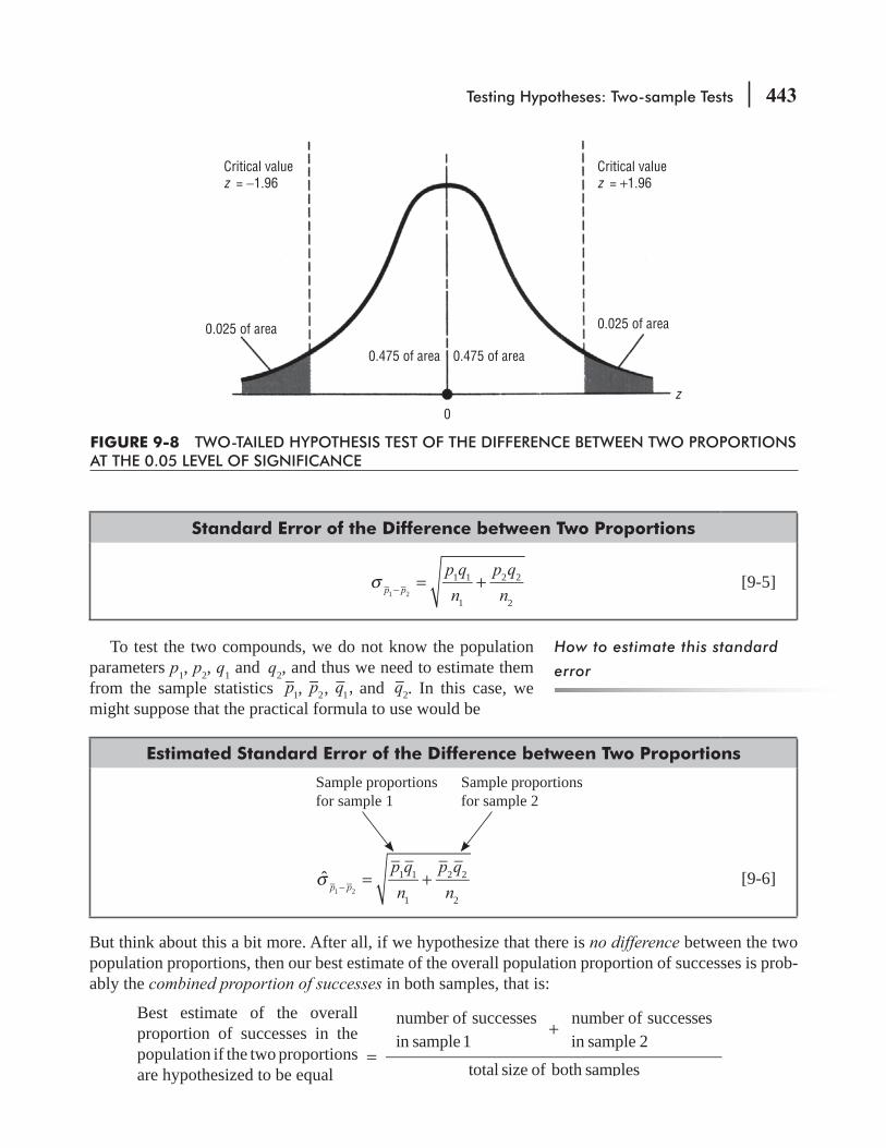
Testing Hypotheses: Two-sample Tests 443
Standard Error of the Difference between Two Proportions
1 1
1
2 2
21 2
σ = +−
p qn
p qnp p [9-5]
To test the two compounds, we do not know the population parameters p1, p2, q1 and q2, and thus we need to estimate them from the sample statistics p1, p2, q ,1 and q2. In this case, we might suppose that the practical formula to use would be
Estimated Standard Error of the Difference between Two Proportions
ˆ 1 1
1
2 2
21 2
σ = +−
p qn
p qnp p
Sample proportions for sample 1
Sample proportions for sample 2
[9-6]
But think about this a bit more. After all, if we hypothesize that there is no difference between the two population proportions, then our best estimate of the overall population proportion of successes is prob-ably the combined proportion of successes in both samples, that is:
Best estimate of the overall proportion of successes in the population if the two proportions are hypothesized to be equal
number of successesin sample 1
number of successesin sample 2
total size of both samples=
+
How to estimate this standard
error
Critical valuez = −1.96
Critical valuez = +1.96
0.025 of area
0.475 of area 0.475 of area
0z
0.025 of area
FIGURE 9-8 TWO-TAILED HYPOTHESIS TEST OF THE DIFFERENCE BETWEEN TWO PROPORTIONS AT THE 0.05 LEVEL OF SIGNIFICANCE
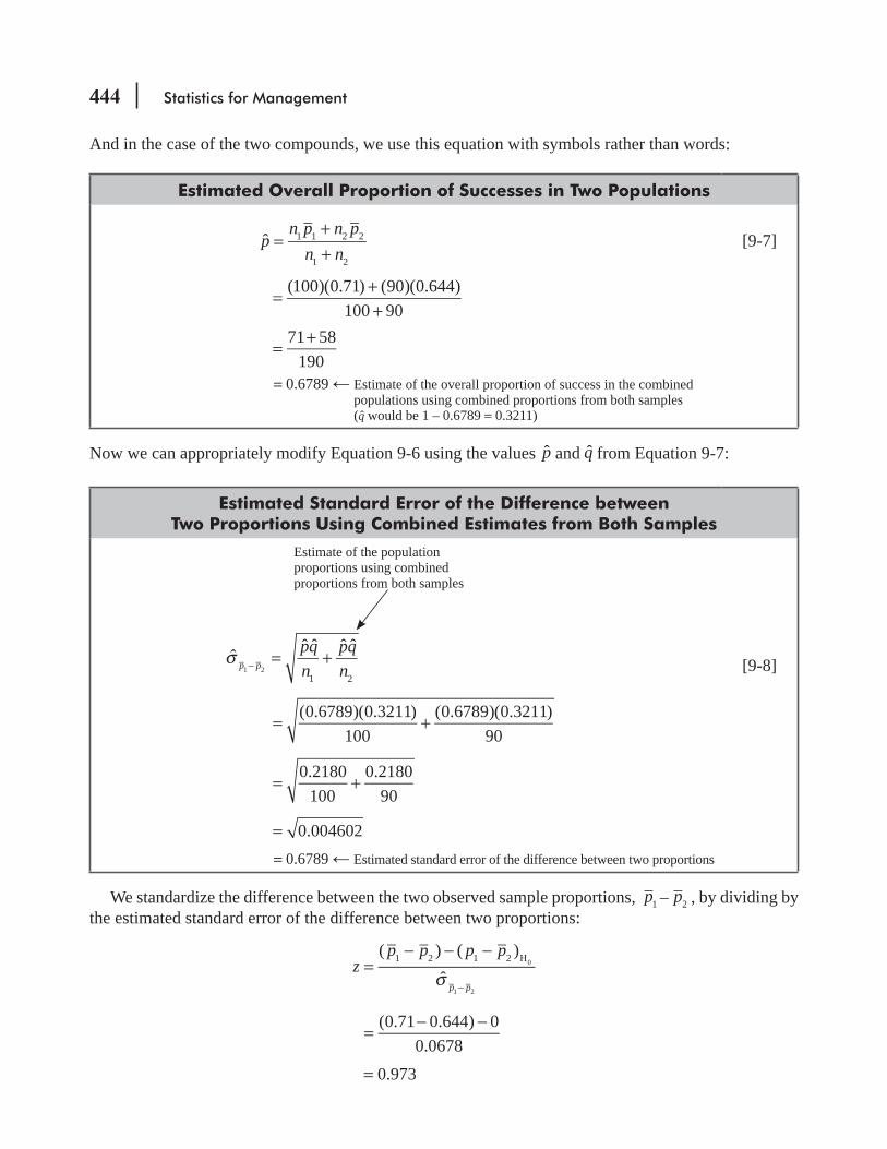
444 Statistics for Management
And in the case of the two compounds, we use this equation with symbols rather than words:
Estimated Overall Pro portion of Successes in Two Populations
pn p n p
n nˆ 1 1 2 2
1 2
=++
(100)(0.71) (90)(0.644)100 90
=++
71 58190
=+
= 0.6789 Estimate of the overall proportion of success in the combined populations using combined proportions from both samples (q would be 1 – 0.6789 = 0.3211)
[9-7]
Now we can appropriately modify Equation 9-6 using the values p and q from Equation 9-7:
Estimated Standard Err or of the Difference betweenTwo Proportions Using Combined Estimates from Both Samples
Estimate of the population proportions using combined proportions from both samples
pqn
pqnp p
ˆ ˆ ˆ ˆ ˆ
1 21 2
σ = +−
(0.6789)(0.3211)100
(0.6789)(0.3211)90
= +
0.2180100
0.218090
= +
0.004602= = 0.6789 Estimated standard error of the difference between two proportions
[9-8]
We standardize the difference between the two observed sample proportions, p1 – p2 , by dividing by the estimated standard error of the difference between two proportions:
zp p p p
p p
( ) ( )ˆ
1 2 1 2 H0
1 2σ
=− − −
−
(0.71 0.644) 00.0678
=− −
= 0.973
Testing Hypotheses: Two-sample Tests 445
Next we plot the standardized value on a sketch of the sampling distribution in Figure 9-9.
We can see in Figure 9-9 that the standardized difference between the two sample proportions lies within the acceptance region. Thus, we accept the null hypothesis and conclude that these two new compounds produce effects on blood pressure that are not signi cantly different.
One-Tailed Tests for Di fferences between ProportionsConceptually, the one-tailed test for the difference between two population proportions is similar to a one-tailed test for the difference between two means. Suppose that for tax purposes, a city govern-ment has been using two methods of listing property. The rst requires the property owner to appear in person before a tax lister, but the second permits the property owner to mail in a tax form. The city manager thinks the personal-appearance method produces far fewer mistakes than the mail-in method. She authorizes an examination of 50 personal-appearance listings and 75 mail-in listings. Ten percent of the personal-appearance forms contain errors; 13.3 percent of the mail-in forms contain them. The results of her sample can be summarized:
p1 = 0.10 Proportion of personal-appearance forms with errors
q1 = 0.90 proportion of personal-appearance forms without errors
n1 = 50 Sample size of personal-appearance forms
p2 = 0.133 Proportion of mail-in forms with errors
q2 = 0.867 Proportion of mail-in forms without errors
n2 = 75 Sample size of mail-in forms
The city manager wants to test at the 0.15 level of signi cance the hypothesis that the personal-appear-ance method produces a lower proportion of errors. What should she do?
Step 5: Interpret the result
Acceptance regionAccept H0 if the sample value is in this region
Standardizeddifference betweenthe two sampleproportions
−1.96 +1.96+0.9730z
FIGURE 9-9 TWO-TAILED HYPOTHESIS TEST OF THE DIFFERENCE BETWEEN TWO PROPORTIONS AT THE 0.05 LEVEL OF SIGNIFICANCE, SHOWING THE ACCEPTANCE REGION AND THE STANDARDIZED DIFFERENCE BETWEEN THE SAMPLE PROPORTIONS
Step 4: Sketch the distribution
and mark the sample value and
critical values
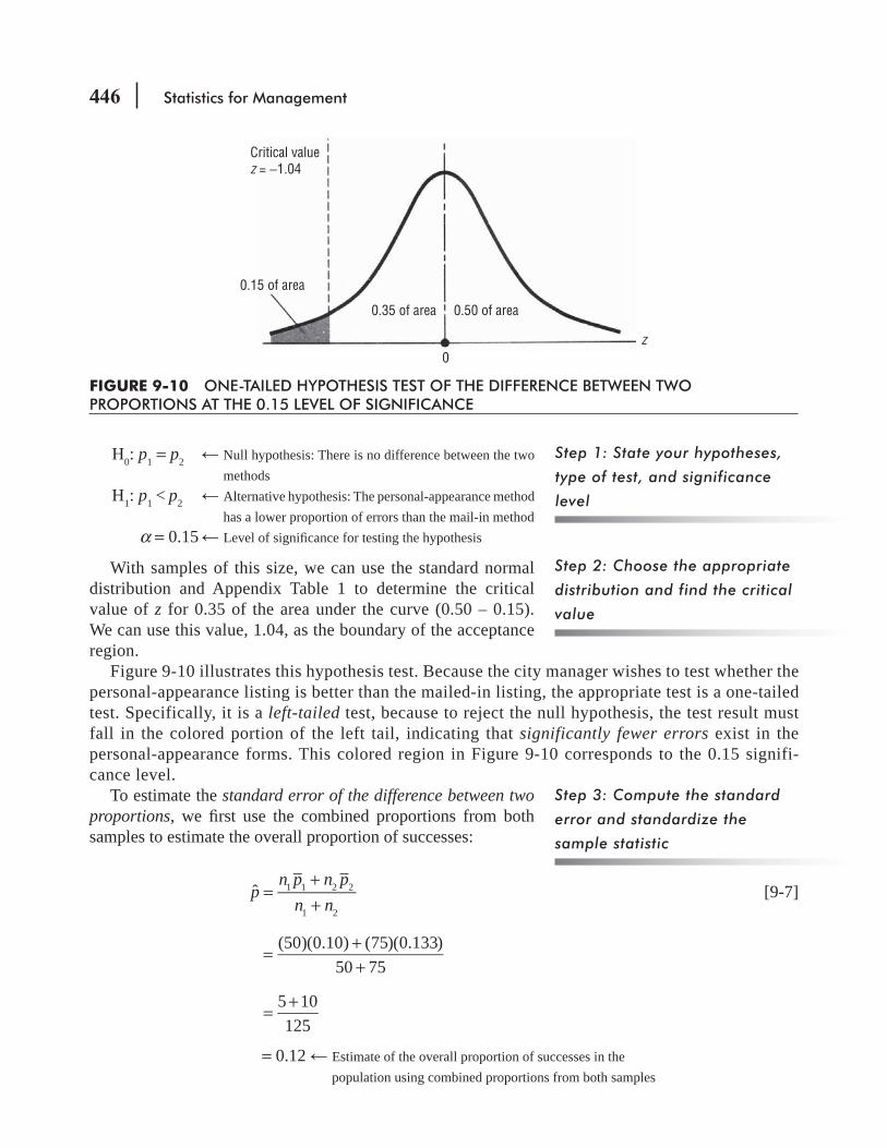
446 Statistics for Management
H0: p1 = p2 Null hypothesis: There is no difference between the two methods
H1: p1 < p2 Alternative hypothesis: The personal-appearance method has a lower proportion of errors than the mail-in method
α = 0.15 Level of signi cance for testing the hypothesis
With samples of this size, we can use the standard normal distribution and Appendix Table 1 to determine the critical value of z for 0.35 of the area under the curve (0.50 – 0.15).We can use this value, 1.04, as the boundary of the acceptance region.
Figure 9-10 illustrates this hypothesis test. Because the city manager wishes to test whether the personal-appearance listing is better than the mailed-in listing, the appropriate test is a one-tailed test. Specifically, it is a left-tailed test, because to reject the null hypothesis, the test result must fall in the colored portion of the left tail, indicating that significantly fewer errors exist in the personal-appearance forms. This colored region in Figure 9-10 corresponds to the 0.15 signifi-cance level.
To estimate the standard error of the difference between two proportions, we rst use the combined proportions from both samples to estimate the overall proportion of successes:
pn p n p
n nˆ 1 1 2 2
1 2
=++
[9-7]
(50)(0.10) (75)(0.133)50 75
=++
5 10125
=+
= 0.12 Estimate of the overall proportion of successes in the population using combined proportions from both samples
Step 2: Choose the appropriate
distribution and find the critical
value
Step 3: Compute the standard
error and standardize the
sample statistic
Step 1: State your hypotheses,
type of test, and significance
level
Critical valuez = −1.04
0.15 of area
0.35 of area 0.50 of area
0z
FIGURE 9-10 ONE-TAILED HYPOTHESIS TEST OF THE DIFFERENCE BETWEEN TWO PROPORTIONS AT THE 0.15 LEVEL OF SIGNIFICANCE
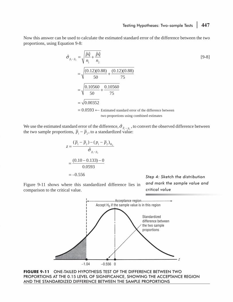
Testing Hypotheses: Two-sample Tests 447
Now this answer can be used to calculate the estimated standard error of the difference between the two proportions, using Equation 9-8:
ˆ ˆ ˆ ˆ ˆ
1 21 2
σ = +−
pqn
pqnp p [9-8]
(0.12)(0.88)50
(0.12)(0.88)75
= +
0.1056050
0.1056075
= +
0.00352== 0.0593 Estimated standard error of the difference between
two proportions using combined estimates
We use the estimated standard error of the difference, ˆ ,1 2
σ −P p to convert the observed difference between the two sample proportions, p p ,1 2− to a standardized value:
( ) ( )ˆ
1 2 1 2 H0
1 2σ
=− − −
−
zp p p p
p p
(0.10 0.133) 00.0593
=− −
= –0.556
Figure 9-11 shows where this standardized difference lies in comparison to the critical value.
Step 4: Sketch the distribution
and mark the sample value and
critical value
Acceptance regionAccept H0 if the sample value is in this region
Standardizeddifference betweenthe two sampleproportions
−1.04 −0.556 0z
FIGURE 9-11 ONE-TAILED HYPOTHESI S TEST OF THE DIFFERENCE BETWEEN TWO PROPORTIONS AT THE 0.15 LEVEL OF SIGNIFICANCE, SHOWING THE ACCEPTANCE REGION AND THE STANDARDIZED DIFFERENCE BETWEEN THE SAMPLE PROPORTIONS
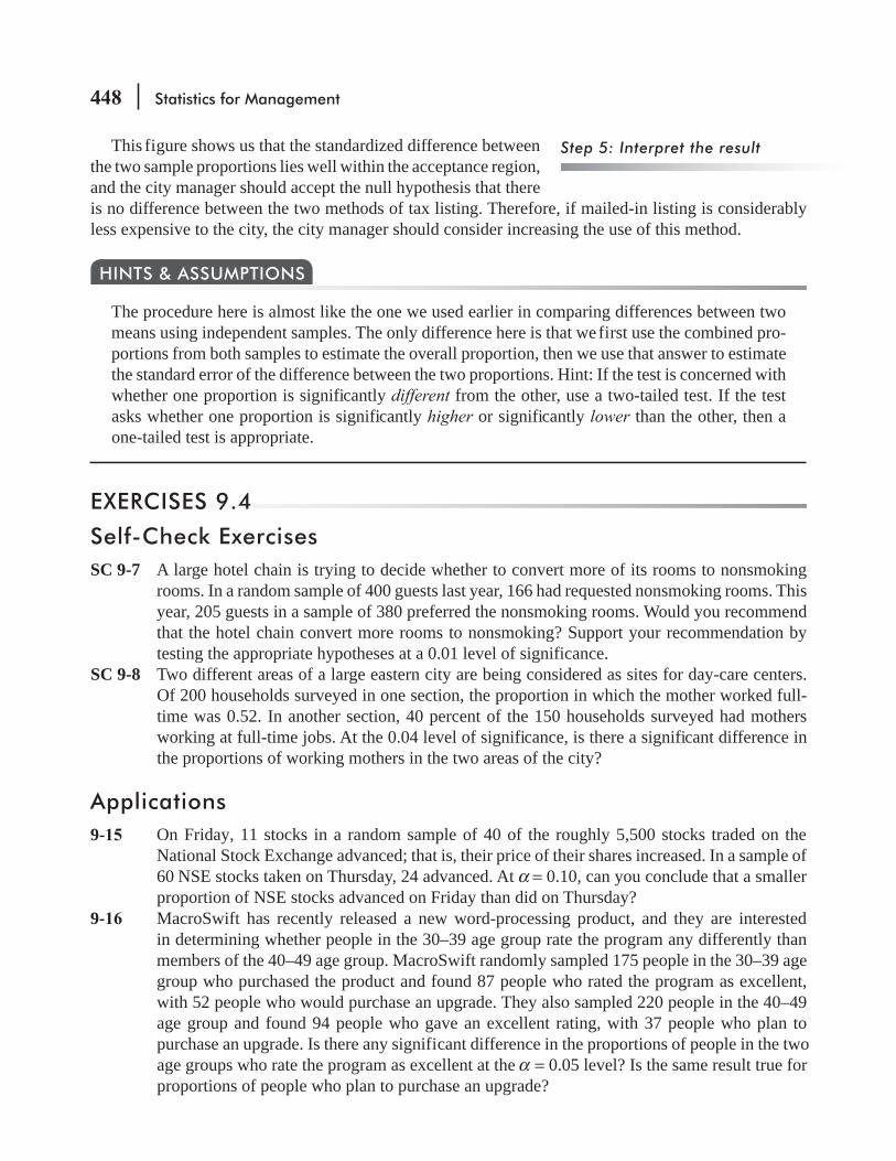
448 Statistics for Management
This figure shows us that the standardized difference between the two sample proportions lies well within the acceptance region, and the city manager should accept the null hypothesis that there
ylbaredisnoc si gnitsil ni-deliam fi ,eroferehT .gnitsil xat fo sdohtem owt eht neewteb ecnereffid on siless expensive to the city, the city manager should consider increasing the use of this method.
The procedure here is almost like the one we used earlier in comparing differences between two means using independent samples. The only difference here is that we first use the combined pro-portions from both samples to estimate the overall proportion, then we use that answer to estimate the standard error of the difference between the two proportions. Hint: If the test is concerned with whether one proportion is signifi cantly different from the other, use a two-tailed test. If the test asks whether one proportion is signifi cantly higher or signifi cantly lower than the other, then a one-tailed test is appropriate.
HINTS & ASSUMPTIONS
EXERCISES 9.4
Self-Check Exerci sesSC 9-7 A large hotel chain is trying to decide whether to convert more of its rooms to nonsmoking
rooms. In a random sample of 400 guests last year, 166 had requested nonsmoking rooms. This year, 205 guests in a sample of 380 preferred the nonsmoking rooms. Would you recommend that the hotel chain convert more rooms to nonsmoking? Support your recommendation by testing the appropriate hypotheses at a 0.01 level of significance.
SC 9-8 Two different areas of a large eastern city are being considered as sites for day-care centers. Of 200 households surveyed in one section, the proportion in which the mother worked full-time was 0.52. In another section, 40 percent of the 150 households surveyed had mothers
ifingis fo level 40.0 eht tA .sboj emit-lluf ta gnikrow cance, is there a signifi cant difference in ?ytic eht fo saera owt eht ni srehtom gnikrow fo snoitroporp eht
Applications9-15
9-16 MacroSwift has recently released a new word-processing product, and they are interested in determining whether people in the 30–39 age group rate the program any differently than members of the 40–49 age group. MacroSwift randomly sampled 175 people in the 30–39 age group who purchased the product and found 87 people who rated the program as excellent, with 52 people who would purchase an upgrade. They also sampled 220 people in the 40–49 age group and found 94 people who gave an excellent rating, with 37 people who plan to purchase an upgrade. Is there any significant difference in the proportions of people in the two age groups who rate the program as excellent at the a = 0.05 level? Is the same result true for proportions of people who plan to purchase an upgrade?
Step 5: Interpret the result
On Friday, 11 stocks in a random sample of 40 of the roughly 5,500 stocks traded on the National Stock Exchange advanced; that is, their price of their shares increased. In a sample of 60 NSE stocks taken on Thursday, 24 advanced. At a = 0.10, can you conclude that a smaller proportion of NSE stocks advanced on Friday than did on Thursday?

Testing Hypotheses: Two-sample Tests 449
9-17 A coal- red power plant is considering two different systems for pollution abatement. The rst system has reduced the emission of pollutants to acceptable levels 68 percent of the time,
as determined from 200 air samples. The second, more expensive system has reduced the emission of pollutants to acceptable levels 76 percent of the time, as determined from 250 air samples. If the expensive system is signi cantly more effective than the inexpensive system in reducing pollutants to acceptable levels, then the management of the power plant will install the expensive system. Which system will be installed if management uses a signi cance level of 0.02 in making its decision?
9-18 A group of clinical physicians is performing tests on patients to determine the effectiveness of a new antihypertensive drug. Patients with high blood pressure were randomly chosen and then randomly assigned to either the control group (which received a well-established anti-hypertensive) or the treatment group (which received the new drug). The doctors noted the percentage of patients whose blood pressure was reduced to a normal level within 1 year. At the 0.01 level of signi cance, test appropriate hypotheses to determine whether the new drug is signi cantly more effective than the older drug in reducing high blood pressure.
Group Proportion That Improved Number of PatientsTreatment 0.45 120Control 0.36 150
9-19 The University Bookstore is facing signi cant competition from off-campus bookstores, and they are considering targeting a speci c class in order to retain student business. The book-store randomly sampled 150 freshmen and 175 sophomores. They found that 46 percent of the freshmen and 40 percent of the sophomores purchase all of their textbooks at the University Bookstore. At α = 0.10, is there a signi cant difference in the proportions of freshman and sophomores who purchase entirely at the University Bookstore?
9-20 In preparation for contract-renewal negotiations, the United Manufacturing Workers surveyed its members to see whether they preferred a large increase in retirement bene ts or a smaller increase in salary. In a group of 1,000 male members who were polled, 743 were in favor of increased retirement bene ts. Of 500 female members surveyed, 405 favored the increase in retirement bene ts.(a) Calculate p.(b) Compute the standard error of the difference between the two proportions.(c) Test the hypothesis that equal proportions of men and women are in favor of increased
retirement bene ts. Use the 0.05 level of signi cance.
Worked-Out Answers to Self-Check ExercisesSC 9-7 n1 = 400 p1 = 0.415 n2 = 380 p2 = 0.5395
p pH :0 1 2= p pH :1 1 2< α = 0.01
pn p n p
n nˆ 400(0.415) 380(0.5395)
400 3800.47571 1 2 2
1 2
=++
=++
=
ˆ ˆ ˆ 1 1 0.4757(0.5243) 1400
1380
0.03581 2
1 2σ = +
⎛
⎝⎜⎞
⎠⎟= +
⎛⎝⎜
⎞⎠⎟
=− pqn np p

450 Statistics for Management
The lower limit of the acceptance region is z = – 2.33, or
0 ˆ 2.33(0.0358) 0.08341 2 1 2σ− = − = − = −−p p z p p
Because the observed z value ˆ
0.415 0.53950.0358
3.481 2
1 2σ
=−
=−
= −−
p p
p p
p p2.33 (or 0.1245 0.0834)1 2< − − = − < − we reject H0. The hotel chain should convert more stseug fo noitroporp eht ni esaercni tnac ifingis a saw ereht esuaceb gnikomsnon ot smoor
requesting these rooms over the last year.
SC 9-8 n1 = 200 p1 = 0.52 n2 = 150 p2 = 0.40
p pH :0 1 2= p pH :1 1 2≠ a = 0.40
pn p n p
n nˆ 200(0.52) 150(0.40)
200 1500.46861 1 2 2
1 2
=++
=++
=
ˆ ˆ ˆ 1 1 0.4686(0.5314) 1200
1150
0.05391 2
1 2σ = +
⎛
⎝⎜⎞
⎠⎟= +
⎛⎝⎜
⎞⎠⎟
=− pqn np p
The limits of the acceptance region are z = ± 2.05, or
0 ˆ 2.05(0.0539) 0.11051 2 1 2σ− = ± = ± = ±−p p z p p
Because the observed z value σ
=−
=−
= >−
ˆ0.52 0.40
0.05392.23 2.051 2
1 2
p p
p p
(or p1 – p2 = 012 > 0.1105),
we reject H0 .yltnac ifingis reffid saera owt eht ni srehtom gnikrow fo snoitroporp ehT .
9.6 PROB VALUES: ANOTHER WAY TO LOOK AT TESTING HYPOTHESES
In all the work we’ve done so far on hypothesis testing, one of the first things we had to do was choose a level of sig ifin cance, a , for the test. It has been traditional to choose a sign ifi cance level of a = 10 percent, 5 percent, 2 percent, or 1 percent, and almost all our examples have been done at these levels. But why use only these few values?
When we discussed Type I and Type II errors on page 3 -3 a no dedneped level ecnac ifingis eht fo eciohc eht taht was ew
trade-off between the costs of each of these two kinds of errors. If the cost of a Type I error (incorrectly rejecting H0) is relatively high, we want to avoid making this kind of error, so we choose a small value of a . On the other hand, if a Type II error (incorrectly accepting H0) is relatively more expensive, we are more willing to make a Type I error, and we choose a high value of a . However, understanding the nature of the trade-off
.level ecnac ifingis a esoohc ot woh su llet t’nseod llits
How do we choose a
significance level?
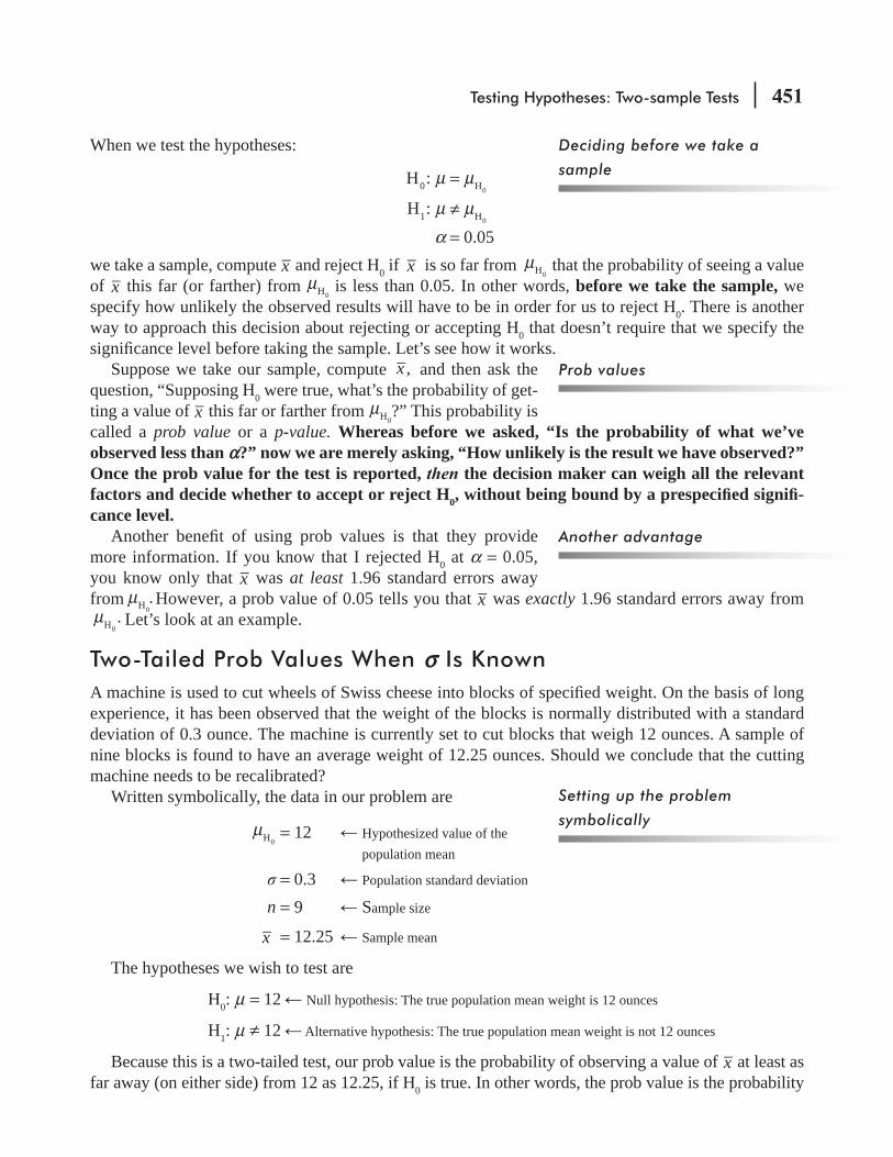
Testing Hypotheses: Two-sample Tests 451
When we test the hypotheses:
H :0 H0μ μ=
H :1 H0μ μ≠
α = 0.05we take a sample, compute x and reject H0 if x is so far from μH0
that the probability of seeing a value of x this far (or farther) from μH0
is less than 0.05. In other words, before we take the sample, we specify how unlikely the observed results will have to be in order for us to reject H0. There is another way to approach this decision about rejecting or accepting H0 that doesn’t require that we specify the signi cance level before taking the sample. Let’s see how it works.
Suppose we take our sample, compute x , and then ask the question, “Supposing H0 were true, what’s the probability of get-ting a value of x this far or farther from μH0
?” This probability is called a prob value or a p-value. Whereas before we asked, “Is the probability of what we’ve observed less than α?” now we are merely asking, “How unlikely is the result we have observed?” Once the prob value for the test is reported, the decision maker can weigh all the relevant factors and decide whether to accept or reject H0, without being bound by a prespeci ed signi -cance level.
Another bene t of using prob values is that they provide more information. If you know that I rejected H0 at α = 0.05, you know only that x was at least 1.96 standard errors away from .H0
μ However, a prob value of 0.05 tells you that x was exactly 1.96 standard errors away from .H0
μ Let’s look at an example.
Two-Tailed Prob Values When σ Is KnownA mach ine is used to cut wheels of Swiss cheese into blocks of speci ed weight. On the basis of long experience, it has been observed that the weight of the blocks is normally distributed with a standard deviation of 0.3 ounce. The machine is currently set to cut blocks that weigh 12 ounces. A sample of nine blocks is found to have an average weight of 12.25 ounces. Should we conclude that the cutting machine needs to be recalibrated?
Written symbolically, the data in our problem are
μH0 = 12 Hypothesized value of the
population mean
= 0.3 Population standard deviation
n = 9 Sample size
x = 12.25 Sample mean
The hypotheses we wish to test are
H0: μ = 12 Null hypothesis: The true population mean weight is 12 ounces
H1: μ ≠ 12 Alternative hypothesis: The true population mean weight is not 12 ounces
Because this is a two-tailed test, our prob value is the probability of observing a value of x at least as far away (on either side) from 12 as 12.25, if H0 is true. In other words, the prob value is the probability
Deciding before we take a
sample
Prob values
Another advantage
Setting up the problem
symbolically
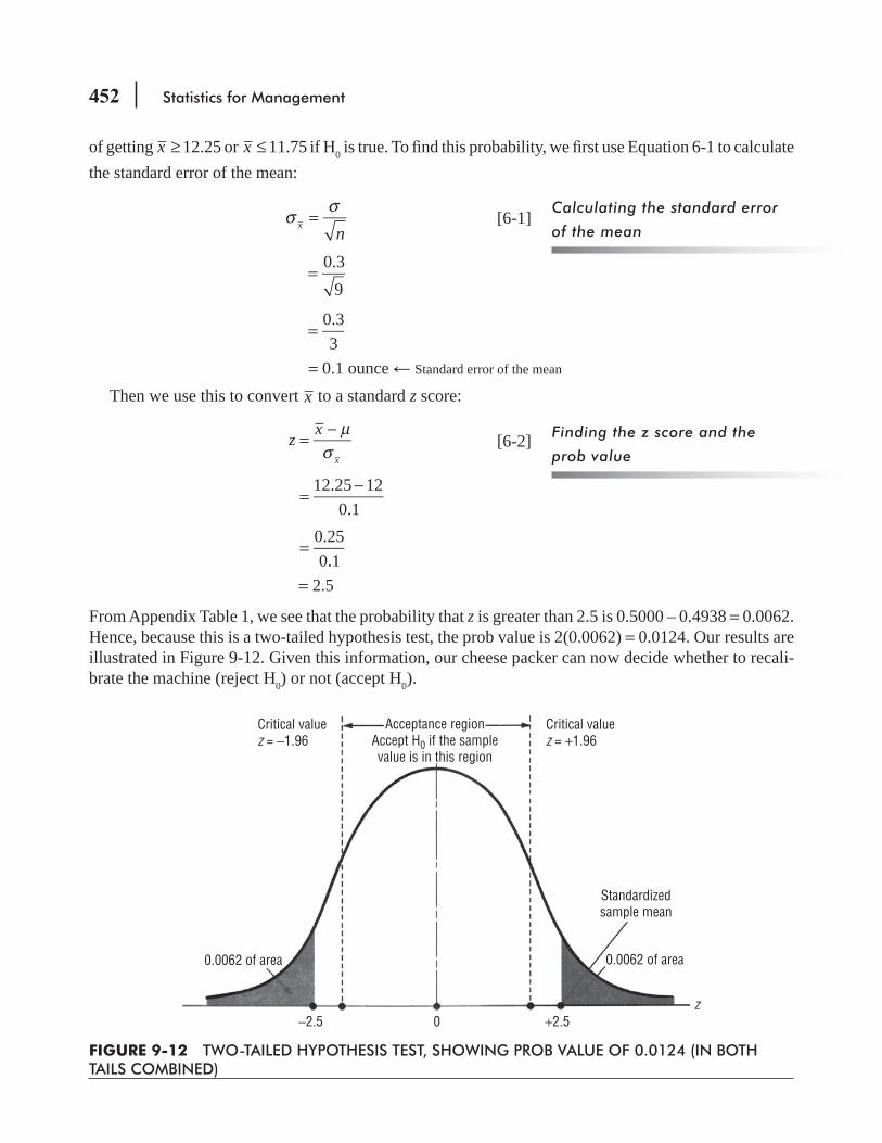
452 Statistics for Management
of getting 12.25 or 11.75≥ ≤x x if H0 is true. To nd this probability, we rst use Equation 6-1 to calculate the standard error of the mean:
σ σ=
nx [6-1]
0.3
9=
0.33
=
= 0.1 ounce Standard error of the mean
Then we use this to convert x to a standard z score:
μ
σ=
−z x
x
[6-2]
12.25 120.1
=−
0.250.1
=
= 2.5
From Appendix Table 1, we see that the probability that z is greater than 2.5 is 0.5000 – 0.4938 = 0.0062. Hence, because this is a two-tailed hypothesis test, the prob value is 2(0.0062) = 0.0124. Our results are illustrated in Figure 9-12. Given this information, our cheese packer can now decide whether to recali-brate the machine (reject H0) or not (accept H0).
Calculating the standard error
of the mean
Finding the z score and the
prob value
Critical valuez = −1.96
Critical valuez = +1.96
Acceptance regionAccept H0 if the samplevalue is in this region
Standardizedsample mean
0.0062 of area0.0062 of area
−2.5 +2.50z
FIGURE 9-12 TWO-TAILED HYPOTHESIS TEST, SHOWING PROB VALUE OF 0.0124 (IN BOTH TAILS COMBINED)

Testing Hypotheses: Two-sample Tests 453
How is this related to what we did before, when we spec ifi ed a sig ifin cance level? If ifingis a cance level of a = 0.05 were adopted, we would reject H0. You can easily see this by looking at Figure 9-12. At a sign ifi cance level of a = 0.05, we reject H0 if x is so far from μH0
that less than 0.05 of the area under the curve is left in the two tails. Because our observed value of x = 12.25 leaves only 0.0124 of the total area in the tails, we would reject H0 at a sign ifi cance level of a = 0.05. (You can also verify this result by noting in Appendix Table 1 that the critical z values for a = 0.05 are ±1.96. Thus, the standardized value of x (2.5) is outside the acceptance region.)
fo level ecnac ifingis a ta taht ees nac ew ,ylralimiS a = 0.01, we would accept H0, because x = 12.25 leaves more than 0.01 of the total area in the tails. (In this case, the critical z values for a = 0.01 would be ±2.58, and now the standardized value of x , 2.5, is inside the acceptance region.) In fact, at any level of a above 0.0124, we would reject H0. Thus, we see that the prob value is precisely the largest
Prob Values under Other ConditionsIn our example, we did a two-tailed hypothesis test using the normal distribution. How would we proceed in other circumstances?
1. If s was known, and we were doing a one-tailed test, we would compute the prob value in exactly the same way except that we would not multiply the probability that we got from Appendix Table 1 by 2, because that table gives one-tailed probabilities directly.
2. If s was not known, we would use the t distribution with n – 1 degrees of freedom and Appendix Table 2. This table gives two-tailed probabilities, but only a few of them, so we can not get exact prob values from it. For example, for a two-tailed test, if μH0
= 50, x = 49.2, s =1.4, and n = 16, we find that
σ σ=ˆ ˆ
nx [7-6]
=1.416
= 0.35
and that x is 2.286 estimated standard errors below H0μ [(49.2 – 50)/0.35= –2.286]. Looking at the
15 degrees of freedom row in Appendix Table 2, we see that 2.286 is between 2.131 (a = 0.05) and 2.602 (a = 0.02). Our prob value is therefore something between 0.02 and 0.05, but we can’t be
.c ificeps eromMost computer statistics packages report exact prob val-
ues, not only for tests about means based on the normal dis-tribution, but for other tests such as chi-square and analysis of variance (which we will discuss in Chapter 11) and tests in the context of linear regression (which we will discuss in Chapters 12 and 13). The discussion we have provided in this section
One-tailed prob values
Using the t distribution
Prob values in other contexts
Relationship between prob
values and significance levels
significance level at which we would accept H0. Prob value (or p-value) is the probability of getting asextreme as or higher than this value, i.e., chances of having that much extreme results. Low p-valuedenotes that chances of having such a extreme result is quite low so it can be said that results are significant.

454 Statistics for Management
will enable you to understand prob values in those contexts too. Although different statistics and distributions will be involved, the ideas are the same.
Prob values and computers eliminate having to look up values from a z or t distribution table, and take the drudgery out of hypothesis testing. Warning: The smaller the prob value, the greater the signi cance of the ndings. Hint: You can avoid confusion here by remembering that a prob value is the chance that the result you have could have occurred by sampling error, thus, smaller prob values mean smaller chances of sampling error and higher signi cance.
HINTS & ASSUMPTIONS
EXERCISES 9.5
Self-Check ExercisesSC 9-9 The Coffee Institute has claimed that more than 40 percent of American adults regularly
have a cup of coffee with breakfast. A random sample of 450 individuals revealed that 200 of them were regular coffee drinkers at breakfast. What is the prob value for a test of hypotheses seeking to show that the Coffee Institute’s claim was correct? (Hint: Test H0: p = 0.4, versus H1: p > 0.4)
SC 9-10 Approximately what is the prob value for the test in Self-Check Exercise 9-3 on page 4 8?
Applications9-21 A car retailer thinks that a 40,000-mile claim for tire life b y the manufacturer is too high. She
carefully records the mileage obtained from a sample of 64 such tires. The mean turns out to be 38,500 miles. The standard deviation of the life of all tires of this type has previously been calculated by the manufacturer to be 7,600 miles. Assuming that the mileage is normally dis-tributed, determine the largest signi cance level at which we would accept the manufacturer’s mileage claim, that is, at which we would not conclude the mileage is signi cantly less than 40,000 miles.
9-22 The North Carolina Department of Transportation has claimed that at most, 18 percent of pas-senger cars exceed 70 mph on Interstate 40 between Raleigh and Durham. A random sample of 300 cars found 48 cars exceeding 70 mph. What is the prob value for a test of hypothesis seeking to show the NCDOT’s claim is correct?
9-23 Kelly’s machine shop uses a machine-controlled metal saw to cut sections of tubing used in pressure-measuring devices. The length of the sections is normally distributed with a standard deviation of 0.06″. Twenty- ve pieces have been cut with the machine set to cut sections 5.00″ long. When these pieces were measured, their mean length was found to be 4.97″. Use prob values to determine whether the machine should be recalibrated because the mean length is signi cantly different from 5.00″?
9-24 SAT Services advertises that 80 percent of the time, its preparatory course will increase an individual’s score on the College Board exams by at least 50 points on the combined verbal and quantitative total score. Lisle Johns, SAT’s marketing director, wants to see whether this is a reasonable claim. He has reviewed the records of 125 students who took the course and found that 94 of them did, indeed, increase their scores by at least
Testing Hypotheses: Two-sample Tests 455
50 points. Use prob values to determine whether SAT’s ads should be changed because the percentage of students whose scores increase by 50 or more points is signifi cantly differ-ent from 80 percent.
9-25 What is the prob value for the test in Exercise 9-2?9-26 What is the prob value for the test in Exercise 9-3?9-27 Approximately what is the prob value for the test in Exercise 9-7?9-28 Approximately what is the prob value for the test in Exercise 9-11?9-29 What is the prob value for the test in Exercise 9-17?9-30 What is the prob value for the test in Exercise 9-20?
Worked-Out Answers to Self-Check ExercisesSC 9-9 n = 450 p = 200/450 = 0.4444
H0: p = H 4. 0 1: p > 0.4The prob value is the probability that ≥ 0.4444,p that is,
zP 0.4444 0.40.4(0.6) /450
P≥−⎛
⎝⎜
⎞
⎠⎟ = ( ≥ 1.92) = 0.5 − 0.4726 = 0.0274z
SC 9-10 From the solution to exercise SC 9-3 on page 430, we have t = –2.766, with 12 + 9 – 2 = 19 degrees of freedom. From the row in Appendix Table 2 for 19 degrees of freedom, we see that –2.766 is between –2.861 (corresponding to a probability of .01/2 = .005 in the lower tail) and –2.539 (corresponding to a probability of .02/2 = .01 in the lower tail). Hence the prob value for our test is between .005 and .01.
KROW T A SCITSITATS
Loveland Compu tersCase 9: Two-Sample Tests of Hypotheses When Lee Azko looked over the results of the telephone survey conducted by the marketing department of Loveland Computers, something was troubling. “Hmm, you wouldn’t still have the data for the ‘Total spent on software’ on computer, would you, Margot?” Lee asked the head of the department.
“Hey, I keep everything,” Margot replied. “It’s in a worksheet file on the computer over there. I had the intern camp out in my offi ce last summer. Why do you need to see the data?”
“Well, give me a minute and I’ll show you,” said Lee, turning on the machine. After a few minutes of muttering over the keyboard, Lee pushed back from the screen. “Thought so! Take a look at that. It looks like there are really two groups of customers here—see how there are two different peaks on this graph?”
“I guess we should have done more than just print out the mean and standard deviation last summer,” said Margot disconsolately. “I guess this means the data are no good.”
“Not necessarily,” said Lee with more optimism. “I’ll bet your ‘big spenders’ are your business yrogetac hcihw wonk ot yaw yna evah t’ndluow uoY .sresu emoh eht si kaep rewol eht dna sremotsuc
the response was in, would you?”

456 Statistics for Management
“Well, we capture that automatically,” Margot said, leaning over and clearing the graph from the screen. “If you look at the rst column, you’ll see that it’s the customer number. All the business cus-tomers have a customer number that begins with a 1 and all the home users have a customer number that begins with a 2.”
“Let me copy this le onto a oppy,” Lee said, opening the briefcase. “I’ll be back this afternoon with the answer.”
: What graph did Lee plot using the worksheet program? What hypothesis is being tested and what is the appropriate statistical test? Is this a one-tailed or a two-tailed problem?
CHAPTER RE VIEW
Terms Intr oduced in Chapter 9Combined Proportion of Successes In comparing two population proportions, the total number of successes in both samples divided by the total size of both samples; used to estimate the proportion of successes common to both populations.Dependent Samples Samples drawn from two populations in such a way that the elements in one sample are matched or paired with the elements in the other sample, in order to allow a more precise analysis by controlling for extraneous factors.Paired Difference Test A hypothesis test of the difference between two population means based on the means of two dependent samples.Paired Samples Another name for dependent samples.Pooled Estimate of σ 2 A weighted average of s1
2 and s22 used to estimate the common variance, σ 2,
when using small samples to test the difference between two population means.Prob Value The largest signi cance level at which we would accept the null hypothesis. It enables us to test hypotheses without rst specifying a value for α.P-value Another name for a prob value.Two-Sample Tests Hypothesis tests based on samples taken from two populations in order to compare their means or proportions.
Equations Introduced in Chapter 9
9-1 12
1
22
21 2
σσ σ
= +− n nx x p. 414
This formula enables us to derive the standard deviation of the distribution of the difference between two sample means, that is, the standard error of the difference between two means. To do this, we take the square root of the sum of Population l’s variance divided by its sample size plus Population 2’s variance divided by its sample size.
9-2 ˆˆ ˆ
12
1
22
21 2
σσ σ
= +− n nx x p. 414
If the two population standard deviations are unknown, we can use this formula to derive the estimated standard error of the difference between two means. We can use this equation after we have used the two sample standard deviations and Equation 7–1 to determine the estimated standard deviations of Population 1 and Population 2, ( σ = s).

Testing Hypotheses: Two-sample Tests 457
9-3 =− + −
+ −s
n s n sn n
( 1) ( 1)2p
2 1 12
2 22
1 2
p. 421
With this formula, we can get a pooled estimate of σ 2. It uses a weighted average of s12 and s ,2
2
where the weights are the numbers of degrees of freedom in each sample. Use of this formula as-sumes that 1
222σ σ= (that the unknown population variances are equal). We use this formula when
testing for the differences between means in situations with small sample sizes (less than 30).
9-4 sn n
ˆ 1 1x x p
1 21 2
σ = +− p. 422
Given the pooled estimate of σ2 obtained from Equation 9-3, we put this value into Equation 9–2 and simplify the expression. This gives us a formula to estimate the standard error of the difference between sample means when we have small samples (less than 30) but equal population variances.
9-5 p qn
p qnp p
1 1
1
2 2
21 2
σ = +− p. 443
This is the formula used to derive the standard error of the difference between two propor-tions. The symbols and p1and p2 represent the proportions of successes in Population 1 and Population 2, respectively, and q1 and q2 are the proportions of failures in Populations 1 and 2, respectively.
9-6 p qn
p qn
ˆp p
1 1
1
2 2
21 2
σ = +− p. 443
If the population parameters p and q are unknown, we can use the sample statistics p and q and this formula to estimate the standard error of the difference between two proportions.
9-7 =++
pn p n p
n nˆ 1 1 2 2
1 2 p. 444
Because the null hypothesis assumes that there is no difference between the two population proportions, it would be more appropriate to modify Equation 9-6 and to use the combined proportions from both samples to estimate the overall proportion of successes in the combined populations. Equation 9-7 combines the proportions from both samples. Note that the value of q is equal to 1 – p.
9-8pqn
pqn
ˆ ˆ ˆ ˆ ˆp p
1 21 2
σ = +− p. 444
Now we can substitute the results of Equation 9-7, both p and q, into Equation 9-6 and get a more correct version of Equation 9-6. This new equation, 9-8, gives us the estimated standard er-ror of the difference between the two proportions using combined estimates from both samples.
Review and Application Exercise s9-31 Clic Pens has tested two types of point-of-purchase displays for its new erasable pen. A shelf
display was placed in a random sample of 40 stores in the test market, and a oor display was placed in 40 other stores in the area. The mean number of pens sold per store in one month

458 Statistics for Management
with the shelf display was 42, and the sample standard deviation was 8. With the floor display, the mean number of pens sold per store in the same month was 45, and the sample standard deviation was 7. At a = 0.02, was there a significant difference between sales with the two types of displays?
9-32 In 2012, a survey of 50 municipal hospitals revealed an average occupancy rate of 73.6 per-cent, and the sample standard deviation was 18.2 percent. Another survey of 75 municipal hospitals in 2015 found an average occupancy rate of 68.9 percent, and the sample standard deviation was 19.7 percent. At a = 0.10, can we conclude that the average occupancy rate changed significantly during the 3 years between surveys?
9-33 General Cereals has just concluded a new advertising campaign for Fruit Crunch, its all-natural breakfast cereal with nuts, grains, and dried fruits. To test the effectiveness of the cam-paign, brand manager Alan Neebe surveyed 11 customers before the campaign and another 11 customers after the campaign. Given are the customers’ reported weekly consumption (in ounces) of Fruit Crunch:
Before 14 5 18 18 30 10 8 26 13 29 24After 23 14 13 29 33 11 12 25 21 26 34
tA )a( a = 0.05, can Alan conclude that the campaign has succeeded in increasing demand for Fruit Crunch?
-orp gnilpmas retteb a tseggus uoy nac ,ngiapmac eht erofeb yevrus laitini s’nalA neviG )b(cedure for him to follow after the campaign?
9-34 Students Against Drunk Driving has targeted seat-belt usage as a positive step to reduce accidents and injuries. Before a major campaign at one high school, 44 percent of 150 drivers entering the school parking lot were using their seat belts. After the seat-belt awareness program, the proportion using seat belts had risen to 52 percent in a sample of 200 vehicles. At a 0.04 significance level, can the students conclude that their campaign was effective?
9-35 Allen Distributing Company hypothesizes that a phone call is more effective than a letter in speeding up collection of slow accounts. Two groups of slow accounts were contacted, one by each method, and the length of time between mailing the letter or making the call and the receipt of payment was recorded:
Method Used Days to CollectionLetter 10 8 9 11 11 14 10Phone call 7 4 5 4 8 6 9
tA )a( a = 0.025, should Allen conclude that slow accounts are collected more quickly with calls than with letters?
(b) Can Allen conclude that slow accounts respond more quickly to calls?
9-36 A buffered aspirin recently lost some of its market share to a new competitor. The competi-tor advertised that its brand enters the bloodstream faster than the buffered aspirin does and,

Testing Hypotheses: Two-sample Tests 459
each medication, the average number of minutes it took to reach each subject’s bloodstream was recorded:
Subject 1 2 3 4 5 6 7 8 9Buffered aspirin 16.5 25.5 23.0 14.5 28.0 10.0 21.5 18.5 15.5Competitor 12.0 20.5 25.0 16.5 24.0 11.5 17.0 15.0 13.0
At a = 0.10, is there any significant difference in the times the two medications take to reach the bloodstream?
9-37 A chemist developing insect repellents wishes to know whether a newly developed formula gives greater protection from insect bites than that given by the leading product on the market. In an experiment, 14 volunteers each had one arm sprayed with the old product and the other sprayed with the new formula. Then each subject placed his arms into two chambers filled with equal numbers of mosquitoes, gnats, and other biting insects. The numbers of bites re-ceived on each arm follow. At a = 0.01, should the chemist conclude that the new formula is, indeed, more effective than the current market leader?
Subject 1 2 3 4 5 6 7 8 9 10 11 12 13 14Old formula 5 2 5 4 3 6 2 4 2 6 5 7 1 3New formula 3 1 5 1 1 4 4 2 5 2 3 3 1 2
9-38 Long Distance Carrier is trying to see the effect of offering “1 month free” with a monthly fixed fee of $10.95, versus an offer of a low monthly fee $8.75 with no free month. To test which might be more attractive to consumers, Long Distance runs a brief market test: 12 phone reps make calls using one approach, and 10 use the other. The following number of customers agreed to switch from their present carrier to LDC:
sehctiwS fo rebmuNreffO1 month free 118 115 122 99 106 125 102 100 92 103 113 129
Low monthly fee 115 126 113 110 135 102 124 137 108 128
Test at a significance level of 10 percent whether there are significant productivity differences with the two offers.
9-39 Is the perceived level of responsibility for an action related to the severity of its consequences? noitpircsed a daer stcejbus eht hcihw ni ytilibisnopser fo yduts a fo sisab eht saw noitseuq tahT
as a result, it relieves pain sooner. The buffered-aspirin company would like to prove that there is no significant difference between the two products and, hence, that the competitor’s claim is false. As a preliminary test, 9 subjects were given buffered aspirin once a day for 3 weeks. For another 3 weeks, the same subjects were given the competitive product. For
460 Statistics for Management
of an accident on an interstate high-way. The consequences, in terms of cost and injury, were described as either very minor or serious. A questionnaire was used to rate the degree of re-sponsibility that the subjects believed should be placed on the main figure in the story. Below are the ratings for both the mild-consequences and the severe-consequences groups. High rat-ings correspond to higher responsibility attributed to the main figure. If a 0.025 significance level was used, did the study conclude that severe consequences lead to a greater attribution of responsibility?
Consequences Degree of ResponsibilityMild 4 5 3 3 4 1 2 6Severe 4 5 4 6 7 8 6 5
9-40 In October 2015, a survey of 120 macroeconomists found 87 who believed that the recession had already ended. A survey of 150 purchasing agents found 89 who believed the recession had ended. At a = 0.10, should you conclude that the purchasing agents were more pessimistic about the economy than the macroeconomists were?
9-41 The MBA program at Piedmont Business School offers Analytic Skills Workshop (ASW) during the summer to help entering students brush up on their accounting, economics, and mathematics. Program Director Andy Bunch wonders whether ASW has been advanta-geous to the students enrolled. He has taken random samples of grade-point averages for students enrolled in ASW over the past 5 years and for students who started the MBA pro-gram without ASW during the same time span. At a = 0.02, have the ASW students gotten significantly higher GPAs? Should Andy advertise that ASW helps student achievement in the MBA program?
x s nASW 3.37 1.13 26Non-ASW 3.15 1.89 35
9-42 Fifty-eight of 2,000 randomly sampled corporations had their 2015 federal income tax returns audited. In another sample of 2,500 corporations, 61 had their 2014 returns audited. Was the fraction of corporate returns audited in 2015 significantly different from the 2014 fraction? Test the appropriate hypotheses at a = 0.01.
9-43 Ellen Singer asserted to one of her colleagues at Triangle Realty that homes in southern Durham County sold for about $15,000 less than similar homes in Chapel Hill. To test this assertion, her colleague randomly chose 10 recent sales in Chapel Hill and matched them with 10 recent sales in southern Durham County in terms of style, size, age, number of rooms, and size of lot. At a = 0.05, do the following data (selling prices in thousands of $) support Ellen’s claim?
Chapel Hill 97.3 108.4 135.7 142.3 151.8 158.5 177.4 183.9 195.2 207.6Durham County 81.5 92.0 115.8 137.8 150.9 149.2 168.2 173.9 175.9 194.4

Testing Hypotheses: Two-sample Tests 461
9-44 TV network executive Terri Black has just received a proposal and a pilot tape for a new show. Empty Nest No Longer is a situation comedy about a middle-aged couple whose two college-graduate offspring cannot find jobs and have returned home. Terri wonders whether the show will appeal to twenty-somethings as well as to an older audience. Figuring that people in her office are reasonably representative of their age group in the population as a whole, she asks them to evaluate the pilot tape on a scale from 0 to 100, and gets the following responses.
ResponseAge20–29 86 74 73 65 82 78 79
30 63 72 68 75 73 80
(a) tA a 0.05 significance level, should Terri conclude the show will be equally attractive to the two age groups?
(b) Independent of your answer to (a), do you think Terry should use the results of her officesurvey to decide how to design an advertising campaign for Empty Nest No Longer? Explain.
9-45 A manufacturer of pet foods was wondering whether cat owners and dog owners reacted dif-ferently to premium pet foods. They commissioned a consumer survey that yielded the follow-ing data.
Pet Owners SurveyedNumber Using Premium Food
Cat 280 152Dog 190 81
Is it reasonable to conclude, at a = 0.02, that cat owners are more likely than dog owners to feed their pets premium food?
9-46 Shivam Kapoor has been offered a transfer from Nagpur to Bangalore, but he is holding out for more money, “because the cost of living there is so much more”. Looking at a grocery receipt and deleting big-ticket items, Shivam came up with 35 items under 100 with a mean of ` 49,standard deviation of ` 21.5 in Nagpur. The HR-manager, who is based in Bangalore, buys39 items, with the same ` 100 limit from a typical grocery store. His mean price is ` 53.5, with standard deviation of ` 19. Is Shivam’s demand justified that the cost of groceries is more in Bangalore than in Nagpur?
9-47 Nirmal Pvt. Limited is a FMCG company, selling a range of products. It has 1150 sales-outlets. A sample of 60 sales-outlets was chosen, using random sampling for the purpose of sales analysis. The sample consists of sales-outlets from rural and urban areas belonging to the four regions of the country as Northern, Eastern, Western and Southern. The informa-tion related to annual sales has been was collected from them in the month of December 2010. This process has been repeated in December 2011. In the meanwhile, in 2010 a com-prehensive sales-promotion program was launched to augment the sales. The information is presented in the data sheet in the DVD (Nirmal Pvt. Ltd DATA). Analyze the data and give answer to the following questions:(a) naC you conclude that there is significant difference between sales of urban outlets and
rural outlets in 2010?
462 Statistics for Management
(b) Does the pattern of differentiation between urban and rural outlets remain the same in 2011 also?
(c) Do the data indicate that there is significant increase in the sales in 2011 as compared to 2010? Comment on the success of the sales-promotion program.
Questions on Running Case: SURYA Bank Pvt. Ltd.
1. Test the hypothesis that the level of satisfaction of the customers with regards to the e-services provided by their banks is same across the gender. (Q9 & Q15)
2. Test the hypothesis that both males and females perceive that private sector banks are better than the public sector banks in terms of the e-banking services provided by them. (Q13b & Q15)
3. Test the hypothesis that irrespective of the marital status of the respondents, people felt that e-banking lacks personal touch. (Q13k & Q16).
@
CASE
@
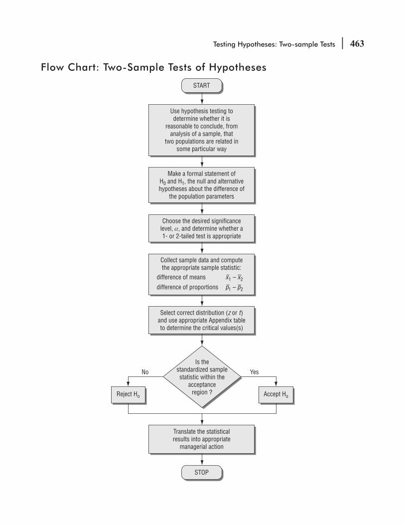
Testing Hypotheses: Two-sample Tests 463
Flow Chart: Two-Sample Tests of Hypotheses
Use hypothesis testing todetermine whether it is
reasonable to conclude, fromanalysis of a sample, that
two populations are related insome particular way
Make a formal statement ofH0 and H1, the null and alternativehypotheses about the difference of
the population parameters
Choose the desired significancelevel, α, and determine whether a1- or 2-tailed test is appropriate
Collect sample data and computethe appropriate sample statistic:
difference of means
Select correct distribution (z or t)and use appropriate Appendix tableto determine the critical values(s)
Translate the statisticalresults into appropriate
managerial action
Reject Ho Accept Ho
START
STOP
YesNo
Is thestandardized samplestatistic within the
acceptanceregion ?
x1 – x2
difference of proportions p1 – p2

This page is intentionally left blank

LEARNING OBJECTIVES
10After reading this chapter, you can understand:
CHAPTER CONTENTS
To examine why the concept of quality—making sure that a product or service is consistent, reliable, and free from errors and defects—is important in decision making
To learn how to use control charts to monitor the output of a process and see whether it is meeting established quality standards
To recognize patterns that indicate that a process is out-of-control
10.1 Introduction 46610.2 Statistical Process Control 46810.3 x Charts: Control Charts for Process
Means 47010.4 R Charts: Control Charts for Process
Variability 48110.5 p Charts: Control Charts for
Attributes 48710.6 Total Quality Management 49410.7 Acceptance Sampling 500
To understand how to construct x, R, and p charts
To introduce basic concepts of Total Quality Management
To learn how acceptance sampling is used to monitor the input to a process to ensure that it meets established quality standards
Statistics at Work 508 Terms Introduced in Chapter 10 509 Equations Introduced in Chapter 10 510 Review and Application Exercises 511 Flow Chart: Quality and Quality Control 515
Quality and Quality Control

466 Statistics for Management
The Durham City Executive for TransCarolina Bank has just established an express teller to handle transactions consisting of a single deposit or withdrawal. She hopes ultimately to be able to com-
plete express transactions in an average of less than 60 seconds. For the moment, however, she wants to be sure that the express line works smoothly and consistently. Once the process is in-control, she can devote her attention to reducing its average time to meet her 60-second goal. For the past month, she has randomly sampled six express transactions each business day:
Day Date Transaction Time (seconds) Day Date Transaction Times (seconds)
M 5/03 63 55 56 53 61 64 M 5/17 57 63 56 64 62 59
T 5/04 60 63 60 65 61 66 T 5/18 66 63 65 59 70 61
W 5/05 57 60 61 65 66 62 W 5/19 63 53 69 60 61 58
Th 5/06 58 64 60 61 57 65 Th 5/20 68 67 59 58 65 59
F 5/07 79 68 65 61 74 71 F 5/21 70 62 66 80 71 76
M 5/10 55 66 62 63 56 52 M 5/24 65 59 60 61 62 65
T 5/11 57 61 58 64 55 63 T 5/25 63 69 58 56 66 61
W 5/12 58 51 61 57 66 59 W 5/26 61 56 62 59 57 55
Th 5/13 65 66 62 68 61 67 Th 5/27 65 57 69 62 58 72
F 5/14 73 66 61 70 72 78 F 5/28 70 60 67 79 75 68
Using the techniques discussed in this chapter, the Durham city executive can determine whether the express-teller line is in-control or out-of-control.
10.1 INTRODUCTIONWe often hear that everyone talks about the weather but no one is prepared to do anything about it. Until recently, the same was true about American business and quality. However, as the relative isolation of national economies has been succeeded by the increasing globalization of commerce, American industry has had to respond to challenges from abroad. One of those challenges was a dedication to quality control and the management of quality in production that came to be epitomized by such Japanese products as automobiles and consumer electronics. In response to this challenge, the philosophy and techniques of quality control and management are becoming widespread in American manufacturing. In addi-tion, the rapidly growing circle of applications of Total Quality Management (known by the acronym TQM) has expanded from manufacturing industries to service industries such as health care and legal services.
In this chapter, you’ll see how simple applications of some of the ideas we’ve already discussed about estimation and hypothesis testing can be used for quality control and improvement. We’ll look at control charts and acceptance sampling, two commonly used quality control techniques. Along
control.
Responding to global challenge
TQM for services as well as for
manufacturing
Quality and Quality Control 467
What Is Quality?When you hear a commercial for a “high-quality automobile,” do you conjure up images of such luxurious options as leather seats and fancy sound systems? Most of us do connect luxury and quality. But expensive leather seats don’t mean very much if the engine won’t start on a cold morning, and the latest noise-reduction technology is hard to appreciate if the tape deck starts chewing up your tapes. These examples show us that it’s important to separate the notion of luxury from our discussion of quality.
In fact, some of the cheapest items in everyday life can have very high quality. Consider the paper used in a copying machine. For little more than a penny a page, you can buy smooth white paper, less than one hundredth of an inch thick and of uniform size. You have come to expect such high quality in copier paper that you don’t examine individual pages before loading it into a copier. You wouldn’t think of measuring the thickness of each page to make sure that it was thin enough not to·jam the copier, but thick enough so that you could print on both sides and not have the two images interfere with each other.
-tion of quality. Things that are of high quality are those that work in the way we expect them to. As quality expert Joseph M. Juran has put it, quality implies tness for use. In this sense, quality means conformance to requirements.
format.
by customers as well as by producers. As you shall see, meeting the needs of customers is central to goods and
services. But in keeping with our notion of conformance to
concepts of consistency, reliability, and lack of errors and defects.
Variability Is the Enemy of QualityWhen a craftsman makes something by hand, there is a continu-ous process of checking, measuring, and reworking. If you’d watched Michelangelo completing a sculpture, you wouldn’t
control is not an issue when you are producing goods and services that are essentially unique. However, when mass production became common during the nineteenth century, it was soon realized that indi-vidual pieces could not be identical—a certain amount of variation is inevitable. But this leads to a
see why variability is the enemy of quality.
Controlling Variability: Inspection vs. PreventionHow should we deal with variability? Think about a stack of two-by-fours in a lumberyard. Most of them will conform to requirements, but some won’t because of twisting and warping as they dried, split-ting when the saw hit a knot, or sundry other causes. One approach to mass production says it’s cheaper to push material through the process and sort out the defects at the end. This leads our lumberyard to
Distinguish between luxury and
quality
Quality means fitness for use
Consistency, reliability, and lack
of defects
Mass production makes quality
an issue
468 Statistics for Management
have an inspector examine two-by-fours as they come out of the drying kiln. Defective pieces go to the scrap heap.
In the early days of mass production, sorting out defects became the chief method of quality control. Armies of white-coated inspec-tors tested goods at the end of a production line and released only some of them to customers. It was widely believed that the cost of a few rejects didn’t amount to much because the marginal cost of each unit was small. But by the late 1970s, people were pointing out that the costs of defects were much higher than supposed. The armies of inspectors had to be paid, and if defective products slipped through, there were warranty costs and loss of customers’ goodwill.
They argued that it is simply cheaper to do things right the zero defects. If your elec-
trical power was 99 percent reliable, you’d spend a lot of time resetting your clocks. A major airline with a 99.9 percent safety record would have several crashes each
expect no less from the producers of all our goods and services.When poorly made parts are passed down a production line, all
quality control inspectors. But it’s expensive to keep inspecting components to make sure they conform to requirements. Imagine how much time would be wasted if you had to examine each piece of paper for defects before loading a copier. This leads to the goal of preventing defects at each stage of manufacturing a product or delivering a service. To accomplish this, the people who make things are given the responsibility to check their work before it is passed on, rather than just
a greater investment of pride in the work they are doing—in this sense, they are more like craftsmen.
EXERCISES 10.1
Basic Concepts10-1 Give an example of a very expensive product that has very low quality.10-2 Give an example of a very inexpensive product that has very high quality.10-3 10-4 What actually makes quality control an issue of concern to management?10-5 What kinds of costs would you gather to perform an “inspection versus prevention” analysis?10-6 zero defects as a concept.
10.2 STATISTICAL PROCESS CONTROLThe key to managing for quality is to believe that excessive variability is not inevitable. When the output of some process is found to be unreliable, not always conforming to requirements, we must carefully examine the process and see how it can be controlled.
In the 1920s, Walter A. Shewhart, a researcher at Bell Labs, created a system for tracking variation and identifying its causes. Shewhart’s system of statistical process control (or SPC) was developed further and championed by his one-time colleague, W. Edwards Deming. For many years, Deming was a prophet without honor in the United States, but when Japan was rebuilding its economy after World
Early quality control: Sorting out
defective finished goods
Zero defects as a goal
Preventing defects and
increasing workers’ pride
Variability is not inevitable.

Quality and Quality Control 469
War II, Japanese managers incorporated Deming’s ideas into their management philosophy. Many American industries, including automobiles and consumer electronics, encountered severe competitive pressures from the Japanese in the late 1970s and 1980s. As a result, the contributions made to quality control by Deming and others were reconsidered by American managers.
Let’s look at some basic ideas of Shewhart’s statistical process control. Consider a production line that makes driveshafts for automobiles. Requirements for well-functioning shafts have been established. We would like to monitor and improve the quality of the shafts we produce. The shafts are made in large quantities on an automatic lathe. If we measured the diameter of each shaft after manu-facture, we would expect to see some variability (perhaps a normal distribution) of the measurements around a mean value. These observed random variations in the measurements could result from varia-tions in the hardness of the steel used for the shafts, power surges affecting the lathe, or even errors in
But imagine what happens as the cutting tool begins to dull. The average diameter will gradually increase unless the lathe is recali-brated. And if the bearings on the lathe wear over time, the cutting edge might move around. Then some shafts would be too large, and some too small. Although the mean diameter might well be the same, the variability in the measurements would increase. It would be important to note such nonrandom (or systematic) variation, to identify its source, and to correct the problem.
From this discussion, you can see that there are two kinds of variation that are observed in the output from most processes, in general, and from our automatic lathe, in particular:
Random variation (sometimes called common, or inherent, variation) Systematic variation (sometimes called assignable, or special cause, variation)
These two kinds of variation call for different managerial responses. Although one of the goals of quality management is constant improvement by the reduction of inherent variation, this cannot ordinarily be accomplished without changing the process. And you should not change the process until you are sure that all
If the process is out-of-control because there is still some special cause variation present, identify and correct the cause of that variation. Then, when the process has been brought in-control, quality can be improved by redesigning the process to reduce its inherent variability.
In the next three sections, we shall look at control charts, devices that Shewhart invented for monitor-ing process outputs to identify when they slip out of control.
There are a lot of catch phrases associated with quality control programs today: “Put Quality First,” “Variation Is the Enemy of Quality,” “Make It Right the First Time,” and “Zero Defects” are only a few. As you read these phrases in the popular press it may seem like a paradox that statistical process control, the topic of this chapter, focuses on variation. Hint: Until we can
variation) we are not able to bring the process into control. Warning: Quality control programs based solely on slogans instead of sound statistical methods do not work.
HINTS & ASSUMPTIONS
Random variation in process
output
Nonrandom variation in the
output
Managerial responses to
inherent and assignable
variation
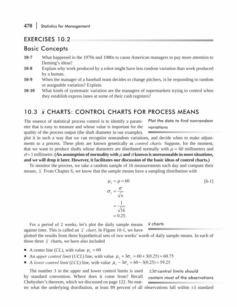
470 Statistics for Management
EXERCISES 10.2
Basic Concepts10-7 What happened in the 1970s and 1980s to cause American managers to pay more attention to
Deming’s ideas?10-8 Explain why work produced by a robot might have less random variation than work produced
by a human.10-9 When the manager of a baseball team decides to change pitchers, is he responding to random
or assignable variation? Explain.10-10 What kinds of systematic variation are the managers of supermarkets trying to control when
they establish express lanes at some of their cash registers?
10.3 x CHARTS: CONTROL CHARTS FOR PROCESS MEANSThe essence of statistical process control is to identify a param-eter that is easy to measure and whose value is important for the quality of the process output (the shaft diameter in our example), plot it in such a way that we can recognize nonrandom variations, and decide when to make adjust-ments to a process. These plots are known genetically as control charts. Suppose, for the moment, that we want to produce shafts whose diameters are distributed normally with μ = 60 millimeters and σ = 1 millimeter. (An assumption of normality with μ and σ known is unreasonable in most situations, and we will drop it later. However, it facilitates our discussion of the basic ideas of control charts.)
To monitor the process, we take a random sample of 16 measurements each day and compute their means, x . From Chapter 6, we know that the sample means have a sampling distribution with
x 60μ μ= = [6-1]
nxσ σ
=
1
16=
= 0.25
For a period of 2 weeks, let’s plot the daily sample means against time. This is called an x chart. In Figure 10-1, we have plotted the results from three hypothetical sets of two weeks’ worth of daily sample means. In each of these three x charts, we have also included
A center line (CL), with value x 60μ = An upper control limit (UCL) line, with value x x3 60 3(0.25) 60.75μ σ+ = + = A lower control limit (LCL) line, with value x x3 60 3(0.25) 59.25μ σ− = − =
The number 3 in the upper and lower control limits is used by standard convention. Where does it come from? Recall Chebyshev’s theorem, which we discussed on page 122. No mat-ter what the underlying distribution, at least 89 percent of all observations fall within ±3 standard
Plot the data to find nonrandom
variations
x charts
3σ± control limits should
contain most of the observations

Quality and Quality Control 471
deviations from the mean. And recall that for normal populations (see Appendix Table 1), over 99.7 percent of all observations fall within that interval.
So, if a process is in-control, essentially all observations should fall within the control limits. Conversely, observations that fall outside those limits suggest that the process is out-of-control, and they warrant further investigation to see if some special cause can be found to explain why they fall outside the limits. With this in mind, let’s look at Figure 10-1.
Basic Interpretation of Control ChartsIn Figure 10-l(a), all observations fall within the control limits, so the process is in-control. In Figure 10-1(b), the second and eighth observations are outliers—they fall outside the control limits. In
out of the ordinary happened on those 2 days. Perhaps the lathe was not recalibrated those mornings, or maybe the regular operator was out sick. An investigation may not turn up anything. After all, even purely random variation will produce outliers 0.3 percent of the time. In such cases, concluding that something has gone awry corresponds to making a Type I error in hypothesis testing. However, because legitimate outliers happen so infrequently, it makes good sense to investigate whenever an outlier is observed.
What should we conclude about Figure 10-l(c)? Even though all 10 observations fall within the control limits, they exhibit anything but random variation. They show a distinct pattern of increase over time. Whenever you see such lack of randomness, you should assume that something systematic is causing it and seek to determine what that assignable cause is. Even though all the observations fall within the control limits, we still say that the process is out-of-control. In this example, the lathe blade was getting duller each day, and the maintenance department had neglected to sharpen it as scheduled.
What sort of patterns should you be looking out for? Among the more commonly noted patterns are
Individual outliers (Figure 10-1(b)). Increasing or decreasing trends (Figure 10-l(c)). These indicate that the process mean may be
drifting. Jumps in the level around which the observations vary (Figure 10-2(a)). These indicate that the
process mean may have shifted. Cycles (Figure 10-2(b)). Such regularly repeating waves above and below the center line could indi-
cate such things as worker fatigue and changeover between work shifts. “Hugging the control limits” (Figure 10-2(c)). Uniformly large deviations from the mean can indi-
cate that two distinct populations are being observed. “Hugging the center line” (Figure 10-2(d)). Uniformly small deviations from the mean indicate that
variability has been reduced from historic levels; this is generally desirable. If it can be maintained, the control limits should be tightened to make sure that this improved quality continues.
x Charts when μ and σ Are Not KnownNow that you understand the basic ideas for interpreting x charts, let’s see how to construct them when μ and σ aren’t known. Recall the express-teller line at TransCarolina Bank, which opened this chapter. Lisa Klein, Durham City Executive for TransCarolina, wants express-teller transactions to be completed
Outliers should be investigated
Patterns in the data points
also indicate out-of-control
processes
Common out-of-control patterns

472 Statistics for Management
60.9(a) Process is in-control
(b) Process is out-of-control: outliers beyond control limits
(c) Process is out-of-control: increasing trend in observations
60.7
60.5
60.3
60.1
59.9
59.7
59.5
59.3
59.11 2 3 4 5 6
Day
Driv
esha
ft di
amet
er (m
m)
60.9
60.7
60.5
60.3
60.1
59.9
59.7
59.5
59.3
59.1
Driv
esha
ft di
amet
er (m
m)
7 8 9 10
1 2 3 4 5 6Day
7 8 9 10
60.9
60.7
60.5
60.3
60.1
59.9
59.7
59.5
59.3
59.1
Driv
esha
ft di
amet
er (m
m)
1 2 3 4 5 6Day
7 8 9 10
FIGURE 10-1 THREE x CHARTS FOR THE DRIVESHAFT PRODUCTION PROCESS
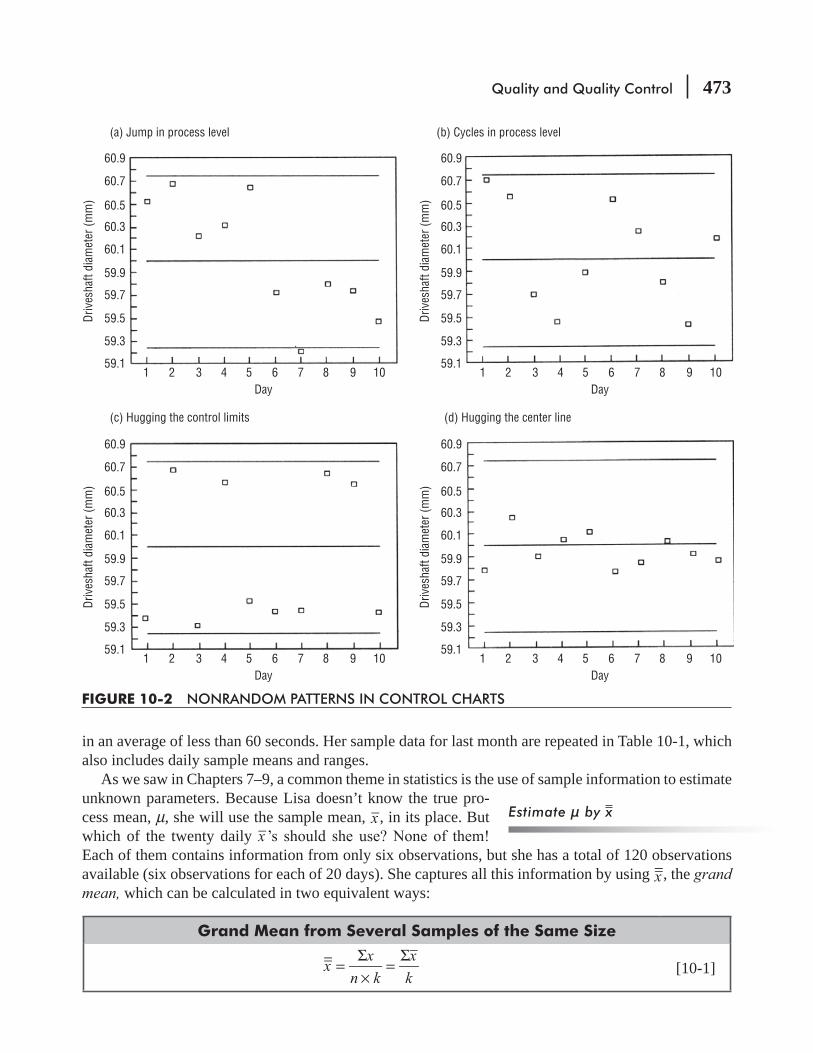
Quality and Quality Control 473
FIGURE 10-2 NONRANDOM PATTERNS IN CONTROL CHARTS
60.9
(a) Jump in process level (b) Cycles in process level
(c) Hugging the control limits (d) Hugging the center line
60.7
60.5
60.3
60.1
59.9
59.7
59.5
59.3
59.11 2 3 4 5 6
Day
Driv
esha
ft di
amet
er (m
m)
7 8 9 10
60.9
60.7
60.5
60.3
60.1
59.9
59.7
59.5
59.3
59.11 2 3 4 5 6
Day
Driv
esha
ft di
amet
er (m
m)
7 8 9 10
60.9
60.7
60.5
60.3
60.1
59.9
59.7
59.5
59.3
59.11 2 3 4 5 6
Day
Driv
esha
ft di
amet
er (m
m)
7 8 9 10
60.9
60.7
60.5
60.3
60.1
59.9
59.7
59.5
59.3
59.11 2 3 4 5 6
Day
Driv
esha
ft di
amet
er (m
m)
7 8 9 10
in an average of less than 60 seconds. Her sample data for last month are repeated in Table 10-1, which also includes daily sample means and ranges.
As we saw in Chapters 7–9, a common theme in statistics is the use of sample information to estimate unknown parameters. Because Lisa doesn’t know the true pro-cess mean, μ, she will use the sample mean, x , in its place. But which of the twenty daily xEach of them contains information from only six observations, but she has a total of 120 observations available (six observations for each of 20 days). She captures all this information by using x , the grand mean, which can be calculated in two equivalent ways:
Grand Mean from Several Samples of the Same Size
xx
n k
x
k=
Σ×
=Σ
[10-1]
Estimate μ by x

474 Statistics for Management
where
x = grand mean ∑x = sum of all observations xΣ = sum of the sample means n = number of observations in each sample k = number of samples taken
In our example, n = 6 and k =
xx
n k
7,561
6(20)63.0=
Σ×
= = or [10-1]
xx
k
1,260.2
2063.0=
Σ= =
Once x has been calculated, its value is used as the center line (CL) in the x chart.
TABLE 10-1 RAW DATA AND DAILY SAMPLE MEANS AND RANGES FOR TRANSCAROLINA BANK EXPRESS-TELLER LINE
Day Date Transaction Times (seconds)Mean
xRange
(R)M 5/03 63 55 56 53 61 64 58.7 11T 5/04 60 63 60 65 61 66 62.5 6W 5/05 57 60 61 65 66 62 61.8 9TH 5/06 58 64 60 61 57 65 60.8 8F 5/07 79 68 65 61 74 71 69.7 18M 5/10 55 66 62 63 56 52 59.0 14T 5/11 57 61 58 64 55 63 59.7 9W 5/12 58 51 61 57 66 59 58.7 15TH 5/13 65 66 62 68 61 67 64.8 7F 5/14 73 66 61 70 72 78 70.0 17M 5/17 57 63 56 64 62 59 60.2 8T 5/18 66 63 65 59 70 61 64.0 11W 5/19 63 53 69 60 61 58 60.7 16TH 5/20 68 67 59 58 65 59 62.7 10F 5/21 70 62 66 80 71 76 70.8 18M 5/24 65 59 60 61 62 65 62.0 6T 5/25 63 69 58 56 66 61 62.2 13W 5/26 61 56 62 59 57 55 58.3 7TH 5/27 65 57 69 62 58 72 63.8 15F 5/28 70 60 67 79 75 68 69.8 19
∑ x = 1,260.2 R = 237
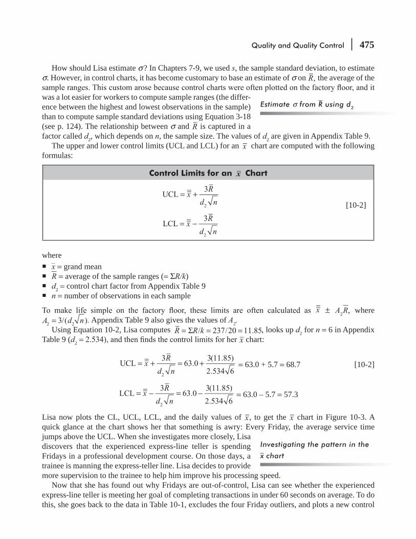
Quality and Quality Control 475
How should Lisa estimate σ ? In Chapters 7-9, we used s, the sample standard deviation, to estimate σ. However, in control charts, it has become customary to base an estimate of σ on R, the average of the
was a lot easier for workers to compute sample ranges (the differ-ence between the highest and lowest observations in the sample) than to compute sample standard deviations using Equation 3-18 (see p. 124). The relationship between σ and R is captured in a factor called d2, which depends on n, the sample size. The values of d2 are given in Appendix Table 9.
The upper and lower control limits (UCL and LCL) for an x chart are computed with the following formulas:
Control Limits for an x Chart
xR
d nUCL
3
2
= +
xR
d nLCL
3
2
= −
[10-2]
where x = grand mean R = average of the sample ranges (= ΣR/k) d2 = control chart factor from Appendix Table 9 n = number of observations in each sample
x ± A2R, where A d n3/( )2 2= . Appendix Table 9 also gives the values of A2.
Using Equation 10-2, Lisa computes R R k/ 237/20 11.85= Σ = = , looks up d2 for n = 6 in Appendix Table 9 (d2 = x chart:
xR
d nUCL
363.0
3(11.85)
2.534 62
= + = + = 63.0 + 5.7 = 68.7 [10-2]
xR
d nLCL
363.0
3(11.85)
2.534 62
= − = − = 63.0 – 5.7 = 57.3
Lisa now plots the CL, UCL, LCL, and the daily values of x , to get the x chart in Figure 10-3. A quick glance at the chart shows her that something is awry: Every Friday, the average service time jumps above the UCL. When she investigates more closely, Lisa discovers that the experienced express-line teller is spending Fridays in a professional development course. On those days, a trainee is manning the express-teller line. Lisa decides to provide more supervision to the trainee to help him improve his processing speed.
Now that she has found out why Fridays are out-of-control, Lisa can see whether the experienced express-line teller is meeting her goal of completing transactions in under 60 seconds on average. To do this, she goes back to the data in Table 10-1, excludes the four Friday outliers, and plots a new control
Estimate σ from R using d2
Investigating the pattern in the
x chart
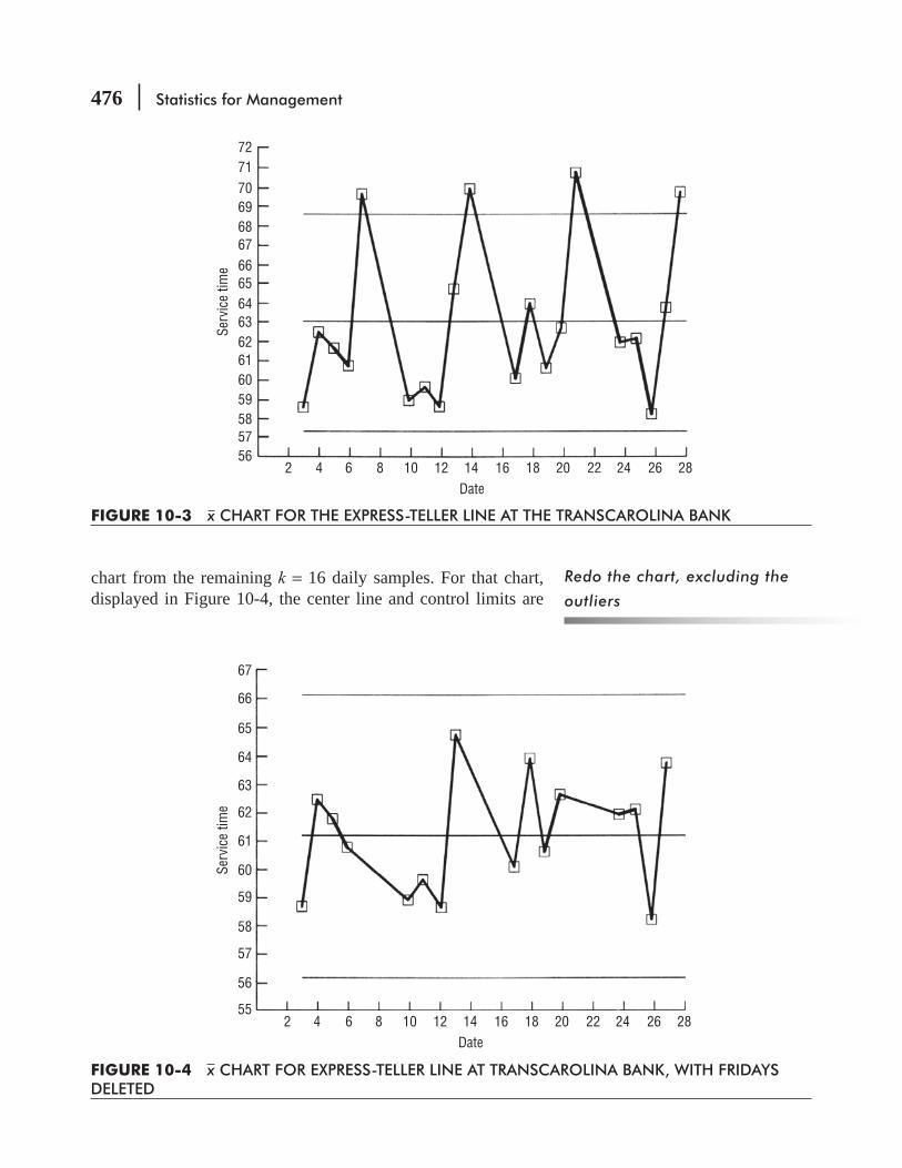
476 Statistics for Management
chart from the remaining k = 16 daily samples. For that chart, displayed in Figure 10-4, the center line and control limits are
Redo the chart, excluding the
outliers
FIGURE 10-3 x CHART FOR THE EXPRESS-TELLER LINE AT THE TRANSCAROLINA BANK
727170696867
Serv
ice
time 66
65646362616059585756
2 4 6 8 10 12 14 16Date
18 20 22 24 26 28
FIGURE 10-4 x CHART FOR EXPRESS-TELLER LINE AT TRANSCAROLINA BANK, WITH FRIDAYS DELETED
67
Serv
ice
time
66
65
64
63
62
61
60
59
58
57
56
552 4 6 8 10 12 14 16
Date18 20 22 24 26 28

Quality and Quality Control 477
given by
xx
n k
5,879
6(16)61.2=
Σ×
= = [10-1]
xR
d nUCL
361.2
3(10.3)
2.534 62
= + = + = 61.2 + 5.0 = 66.2
xR
d nLCL
361.2
3(10.3)
2.534 62
= − = − = 61.2 – 5.0 = 56.2 [10-2]
From Figure 10-4, Lisa sees that the process is in-control. However, with a sample grand mean of 61.2 seconds, even the experienced teller is not yet meeting the under-60-seconds goal. Being in-control does not mean that a process is meeting its goals. In this case, Lisa and the teller will have to work together to analyze the way in which transactions are handled. Perhaps they can redesign procedures to achieve their goal. Or, because the current process is behaving well, they may decide that 61.2 seconds is good enough and not run the risk of spoiling a good system by tinkering with it. This is a managerial decision, not a statistical one. But the statistical analysis has provided Lisa with information she can use in making her managerial decision.
-tion. When, they exist, these patterns focus our attention on something systematic that is causing our problem. Hint: The distribution of the variable we measure in quality control does not have to be normal in order for us to use statistical methods to control the process. As we take successive samples, the use of upper and lower control limits is a very practical example of Chebyshev’s theorem. You will remember that Chebyshev assured us back in Chapter 3 that even when the underlying distribution is not normally distributed, we can still make useful statements about the population from information contained in samples. Warning: The statistical quality control meth-ods we will illustrate in this chapter illuminate problems. From that point on, it takes focused management and effective communication to correct the situation.
HINTS & ASSUMPTIONS
EXERCISES 10.3
Self-Check ExerciseSC 10-1 x chart based on the given
information.(a) n = 9, x = 26.7, R = 5.3.(b) n = 17, x = 138.6, R = 15.1.(c) n = 4, x = 84.2, R = 9.6.(d) n = 22, x = 8.1, R = 7.4.
SC 10-2 Altoona Tire Company sells its ATC-50 tires with a 50,000-mile tread-life warranty. Lorrie Ackerman, a quality control engineer with the company, runs simulated road tests to monitor
Managerial vs. statistical
decisions
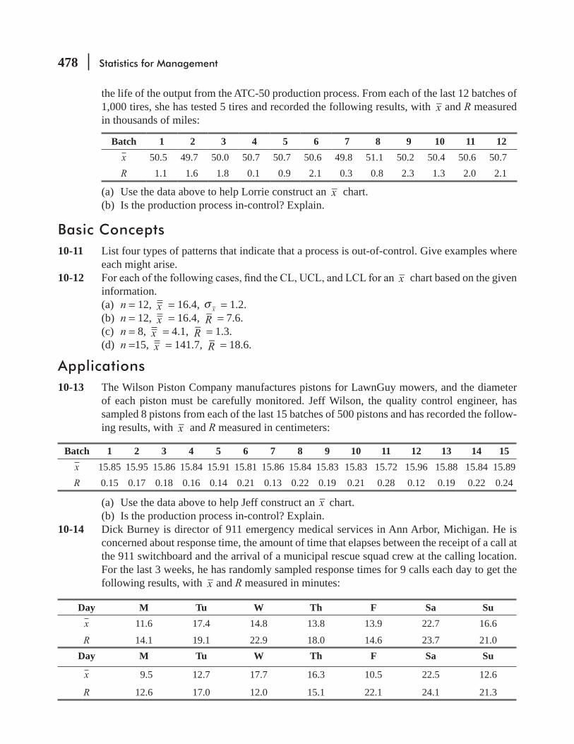
478 Statistics for Management
the life of the output from the ATC-50 production process. From each of the last 12 batches of 1,000 tires, she has tested 5 tires and recorded the following results, with x and R measured in thousands of miles:
Batch 1 2 3 4 5 6 7 8 9 10 11 12x 50.5 49.7 50.0 50.7 50.7 50.6 49.8 51.1 50.2 50.4 50.6 50.7R 1.1 1.6 1.8 0.1 0.9 2.1 0.3 0.8 2.3 1.3 2.0 2.1
(a) Use the data above to help Lorrie construct an x chart.(b) Is the production process in-control? Explain.
Basic Concepts10-11 List four types of patterns that indicate that a process is out-of-control. Give examples where
each might arise.10-12 x chart based on the given
information.(a) n = 12, x = 16.4, xσ = 1.2.(b) n = 12, x = 16.4, R = 7.6.(c) n = 8, x = 4.1, R = 1.3.(d) n =15, x = 141.7, R = 18.6.
Applications10-13 The Wilson Piston Company manufactures pistons for LawnGuy mowers, and the diameter
of each piston must be carefully monitored. Jeff Wilson, the quality control engineer, has sampled 8 pistons from each of the last 15 batches of 500 pistons and has recorded the follow-ing results, with x and R measured in centimeters:
Batch 1 2 3 4 5 6 7 8 9 10 11 12 13 14 15x 15.85 15.95 15.86 15.84 15.91 15.81 15.86 15.84 15.83 15.83 15.72 15.96 15.88 15.84 15.89R 0.15 0.17 0.18 0.16 0.14 0.21 0.13 0.22 0.19 0.21 0.28 0.12 0.19 0.22 0.24
(a) Use the data above to help Jeff construct an x chart.(b) Is the production process in-control? Explain.
10-14 Dick Burney is director of 911 emergency medical services in Ann Arbor, Michigan. He is concerned about response time, the amount of time that elapses between the receipt of a call at the 911 switchboard and the arrival of a municipal rescue squad crew at the calling location. For the last 3 weeks, he has randomly sampled response times for 9 calls each day to get the following results, with x and R measured in minutes:
Day M Tu W Th F Sa Sux 11.6 17.4 14.8 13.8 13.9 22.7 16.6
R 14.1 19.1 22.9 18.0 14.6 23.7 21.0Day M Tu W Th F Sa Su
x 9.5 12.7 17.7 16.3 10.5 22.5 12.6
R 12.6 17.0 12.0 15.1 22.1 24.1 21.3
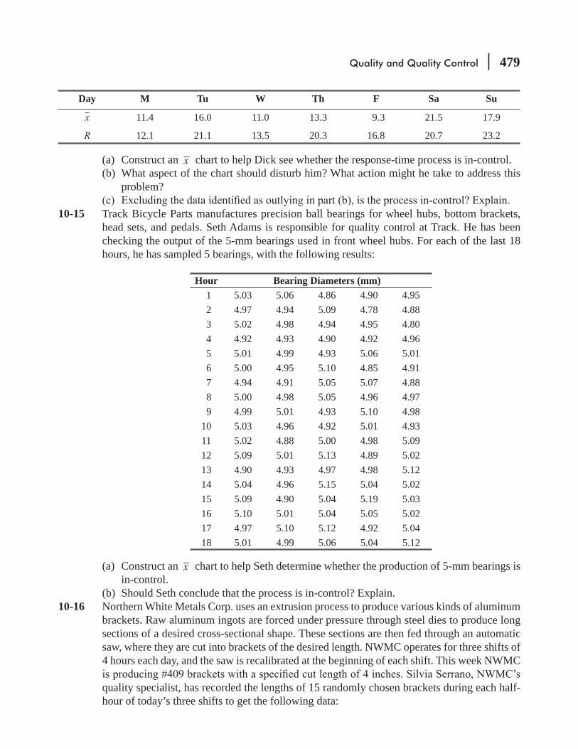
Quality and Quality Control 479
Day M Tu W Th F Sa Su
x 11.4 16.0 11.0 13.3 9.3 21.5 17.9
R 12.1 21.1 13.5 20.3 16.8 20.7 23.2
(a) Construct an x chart to help Dick see whether the response-time process is in-control.(b) What aspect of the chart should disturb him? What action might he take to address this
problem?
10-15 Track Bicycle Parts manufactures precision ball bearings for wheel hubs, bottom brackets, head sets, and pedals. Seth Adams is responsible for quality control at Track. He has been checking the output of the 5-mm bearings used in front wheel hubs. For each of the last 18 hours, he has sampled 5 bearings, with the following results:
Hour Bearing Diameters (mm) 1 5.03 5.06 4.86 4.90 4.95 2 4.97 4.94 5.09 4.78 4.88 3 5.02 4.98 4.94 4.95 4.80 4 4.92 4.93 4.90 4.92 4.96 5 5.01 4.99 4.93 5.06 5.01 6 5.00 4.95 5.10 4.85 4.91 7 4.94 4.91 5.05 5.07 4.88 8 5.00 4.98 5.05 4.96 4.97 9 4.99 5.01 4.93 5.10 4.9810 5.03 4.96 4.92 5.01 4.9311 5.02 4.88 5.00 4.98 5.0912 5.09 5.01 5.13 4.89 5.0213 4.90 4.93 4.97 4.98 5.1214 5.04 4.96 5.15 5.04 5.0215 5.09 4.90 5.04 5.19 5.0316 5.10 5.01 5.04 5.05 5.0217 4.97 5.10 5.12 4.92 5.0418 5.01 4.99 5.06 5.04 5.12
(a) Construct an x chart to help Seth determine whether the production of 5-mm bearings is in-control.
(b) Should Seth conclude that the process is in-control? Explain.10-16 Northern White Metals Corp. uses an extrusion process to produce various kinds of aluminum
brackets. Raw aluminum ingots are forced under pressure through steel dies to produce long sections of a desired cross-sectional shape. These sections are then fed through an automatic saw, where they are cut into brackets of the desired length. NWMC operates for three shifts of 4 hours each day, and the saw is recalibrated at the beginning of each shift. This week NWMC
quality specialist, has recorded the lengths of 15 randomly chosen brackets during each half-hour of today’s three shifts to get the following data:
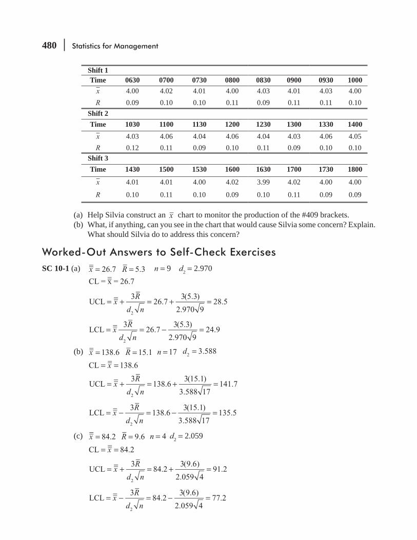
480 Statistics for Management
Shift 1Time 0630 0700 0730 0800 0830 0900 0930 1000
x 4.00 4.02 4.01 4.00 4.03 4.01 4.03 4.00R 0.09 0.10 0.10 0.11 0.09 0.11 0.11 0.10
Shift 2Time 1030 1100 1130 1200 1230 1300 1330 1400
x 4.03 4.06 4.04 4.06 4.04 4.03 4.06 4.05R 0.12 0.11 0.09 0.10 0.11 0.09 0.10 0.10
Shift 3Time 1430 1500 1530 1600 1630 1700 1730 1800
x 4.01 4.01 4.00 4.02 3.99 4.02 4.00 4.00
R 0.10 0.11 0.10 0.09 0.10 0.11 0.09 0.09
(a) Help Silvia construct an x chart to monitor the production of the #409 brackets.(b) What, if anything, can you see in the chart that would cause Silvia some concern? Explain.
What should Silvia do to address this concern?
Worked-Out Answers to Self-Check ExercisesSC 10-1 (a) x 26.7= R 5.3= n = 9 d2 = 2.970
CL = x = 26.7
xR
d nUCL
326.7
3(5.3)
2.970 928.5
2
= + = + =
xR
d nLCL
326.7
3(5.3)
2.970 924.9
2
= = − =
(b) x 138.6= R 15.1= n 17= d 3.5882 =
xCL 138.6= =
xR
d nUCL
3138.6
3(15.1)
3.588 17141.7
2
= + = + =
xR
d nLCL
3138.6
3(15.1)
3.588 17135.5
2
= − = − =
(c) x 84.2= R 9.6= n 4= d2 = 2.059 xCL 84.2= =
xR
d nUCL
384.2
3(9.6)
2.059 491.2
2
= + = + =
xR
d nLCL
384.2
3(9.6)
2.059 477.2
2
= − = − =
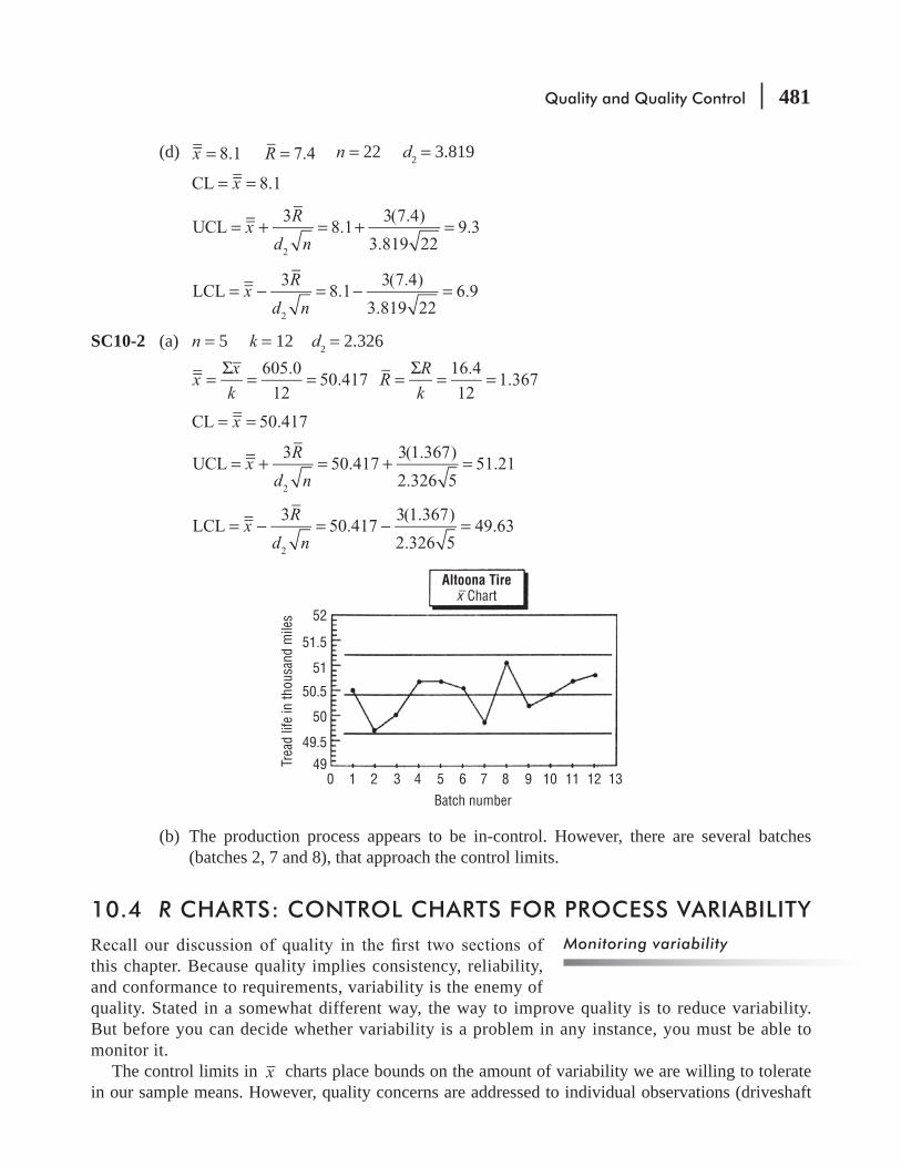
Quality and Quality Control 481
(d) x 8.1= R 7.4= n = 22 d2 = 3.819
xCL 8.1= =
xR
d nUCL
38.1
3(7.4)
3.819 229.3
2
= + = + =
xR
d nLCL
38.1
3(7.4)
3.819 226.9
2
= − = − =
SC10-2 (a) n = 5 k = 12 d2 = 2.326
xx
k
605.0
1250.417=
Σ= = R
R
k
16.4
121.367=
Σ= =
xCL 50.417= =
xR
d nUCL
350.417
3(1.367)
2.326 551.21
2
= + = + =
xR
d nLCL
350.417
3(1.367)
2.326 549.63
2
= − = − =
52
Altoona Tire
51
50
51.5
50.5
49.5
490 1 2 3 4 5 6 7 8 9 10
Batch number
Trea
d lif
e in
thou
sand
mile
s
11 12 13
Chartx−
(b) The production process appears to be in-control. However, there are several batches (batches 2, 7 and 8), that approach the control limits.
10.4 R CHARTS: CONTROL CHARTS FOR PROCESS VARIABILITY
this chapter. Because quality implies consistency, reliability, and conformance to requirements, variability is the enemy of quality. Stated in a somewhat different way, the way to improve quality is to reduce variability. But before you can decide whether variability is a problem in any instance, you must be able to monitor it.
The control limits in x charts place bounds on the amount of variability we are willing to tolerate in our sample means. However, quality concerns are addressed to individual observations (driveshaft
Monitoring variability

482 Statistics for Management
diameters, express-teller-line transaction times, and so on). We saw in Chapter 6 that sample means are less variable than individual observations. More precisely, Equation 6-1 tells us that
n
xσ σ= [6-1]
To monitor the variability in the individual observations, we use another control chart, known as an R chart. In R charts, we plot the values of the sample ranges for each of the samples. The center line for R charts is placed at R. To get the control limits, we need to know something about the sampling distribution of R. In particular, what is its standard deviation, σ R? Although the derivation of the result is beyond the scope of this text, it turns out that
Standard Deviation of the Sampling Distribution of R
dR 3σ σ= [10-3]
where
σ = population standard deviation d3 = another factor depending on n
The values of d3 are also given in Appendix Table 9. Now we can substitute R d/ 2 for σ as we did in Equation 10-2, to compute the control limits for R charts:
Control Limits for an R Chart
Rd R
dR
d
d
Rd R
dR
d
d
UCL3
13
LCL3
13
3
2
3
2
3
2
3
2
= + = +⎛
⎝⎜⎞
⎠⎟
= − = −⎛
⎝⎜⎞
⎠⎟
[10-4]
UCL = RD ,4 where D4 = 1 + 3d3/d2
LCL = RD ,3 where D3 = 1 – 3d3/d2
The values of D3 and D4 can also be found in Appendix Table 9.There is one slight wrinkle in using Equation 10-4. A sample
range is always a nonnegative number (because it is the dif-ference between the largest and smallest observations in the sample). However, when n ≤ 6, the LCL computed by Equation 10-4 will be negative. In these cases, we set the value of LCL to zero. Accordingly, the entries for D3 for n ≤ 6 in Appendix Table 9 are all zeros.
operation is in-control. Returning to the data in Table 10-1, she recalls that R = 11.85. Using this value
Center line for R charts
Control limits for R charts
LCL = 0 if n ≤ 6

Quality and Quality Control 483
R chart in Figure 10-5:
Rd
d
Rd
d
UCL 13
11.85 13(0.848)
2.53423.7
LCL 13
11.85 13(0.848)
2.5340
3
2
3
2
= +⎛
⎝⎜⎞
⎠⎟= +
⎛⎝⎜
⎞⎠⎟
=
= −⎛
⎝⎜⎞
⎠⎟= −
⎛⎝⎜
⎞⎠⎟
= [10-4]
Although Figure 10-5 seems to indicate that the variability in service times on the express-teller line is in-control, Lisa knows that a teller trainee was at work on Fridays (the 7th, 14th, 21st, and 28th of the month). The effect of this can be seen on the R chart, because Fridays have the most variability (the highest sample ranges) during each of the 4 weeks in the sample.
Just as she did when looking at the process mean in Figures 10-3 and 10-4, Lisa now excludes the four Fridays to monitor the variability in service times on the express-teller line when the experienced teller is providing the service. Now R = 10.3, and the control limits are
Rd
d
Rd
d
UCL 13
10.3 13(0.848)
2.53420.6
LCL 13
10.3 13(0.848)
2.5340
3
2
3
2
= +⎛
⎝⎜⎞
⎠⎟= +
⎛⎝⎜
⎞⎠⎟
=
= −⎛
⎝⎜⎞
⎠⎟= −
⎛⎝⎜
⎞⎠⎟
= [10-4]
Noticing a pattern in the R chart
FIGURE 10-5 R CHART FOR EXPRESS-TELLER LINE AT TRANSCAROLINA BANK
26
Serv
ice
time
rang
e
24
22
20
18
16
14
12
10
8
6
4
2
02 4 6 8 10 12 14 16
Date18 20 22 24 26 28

484 Statistics for Management
R chart in Figure 10-6 shows that the experienced teller has service-time variability well in-control. There is nothing evident in the control chart to indicate the presence of any other assignable variation.
Warning: The range we plot in an R chart is only a convenient substitute for the variability of the process we are studying. Its chief advantages are that it is easy to calculate, plot, and understand. But we need to remember from Chapter 3 that the range considers only the highest and lowest values in a distribution and omits all other observations in the data set. Thus, it can ignore the
sample to the next in a given population.
HINTS & ASSUMPTIONS
EXERCISES 10.4
Self-Check ExercisesSC 10-3 R chart based on the given
information.(a) n = 9, x = 26.7, R = 5.3.(b) n = 17, x = 138.6, R = 15.1.
FIGURE 10-6 R CHART FOR EXPRESS-TELLER LINE AT TRANSCAROLINA BANK, WITH FRIDAYS EXCLUDED
Serv
ice
time
rang
e
22
20
18
16
14
12
10
8
6
4
2
02 4 6 8 10 12 14 16
Date18 20 22 24 26 28
Quality and Quality Control 485
(c) n = 4, x = 84.2, R = 9.6.(d) n = 22, x = 8.1, R = 7.4.
SC 10-4 Construct an R chart for the data given in Exercise SC 10-2. Is the variability in the tread life of the ATC-50 in control? Explain.
Basic Concepts10-17 R chart based on the given
information:(a) n = 3, x = 18.4, R = 3.1.(b) n = 19, x = 16.2, R = 6.9.(c) n = 8, x = 141.7, R = 18.2.(d) n = 24, x = 8.6, R = 1.4.(e) R = 6.0, LCL =
Applications10-18 Ray Underhall reproduces antique chairs. His apprentices turn spindles for the chair
backs on manual lathes. The beads on the spindles are to have average diameters of 78-inch at their widest points. Ray monitors the apprentices’ work with control charts.
Which of the following patterns is he likely to see on the R chart for a new apprentice? Explain.
(a) (b)
10-19 Construct an R chart for the data given in Exercise 10-13. Is the variability in the piston diam-eter under control? Explain.
10-20 Consider the emergency medical service data given in Exercise 10-14.(a) Construct an R chart for these data.(b) When he looked at the x chart for these data, Dick Burney noted that the three Saturdays
were outliers. Closer investigation revealed that this happened because the number of calls coming in was higher on Saturdays than on any other day of the week. Does the R chart you constructed in part (a) show any pattern that could be attributed to the same cause? Explain.
(c) Exclude the 3 Saturdays and construct a new R chart. Does this chart exhibit any patterns that Dick should be concerned about? Explain.
486 Statistics for Management
10-21 Construct an R chart for the data given in Exercise 10-15. Are there any patterns in this chart that should concern Seth Adams, or does the variability in the process appear to be in-control? Explain.
10-22 Construct an R chart for the data given in Exercise 10-16. Are there any patterns in this chart that should concern Silvia Serrano, or does the variability in the process appear to be in-control? Explain.
Worked-Out Answers to Self-Check ExercisesSC 10-3 (a) n = 9 R = 5.3 D4 = 1.816 D3 = 0.184
CL = R = 5.3 UCL = RD4 = 5.3(1.816) = 9.62 LCL = RD3 = 5.3(0.184) = 0.98(b) n = 17 R = 15.1 D4 = 1.622 D3 = 0.378 CL = R = 15.1 UCL = RD4 = 15.1(1.622) = 24.49 LCL = RD3 = 15.1(0.378) = 5.71(c) n = 4 R = 9.6 D4 = 2.282 D3 = 0 CL = R = 9.6 UCL = RD4 = 9.6(2.282) = 21.91 LCL = RD3 = 9.6(0) = 0(d) n = 22 R = 7.4 D4 = 1.566 D3 = 0.434 CL = R = 7.4 UCL = RD4 = 7.4(1.566) = 11.59 LCL = RD3 = 7.4(0.434) = 3.21
SC 10-4 n = 5 D4 = 2.114 D3 = 0R = 1.367CL = R = 1.367UCL = RD4 = 1.367(2.114) = 2.89LCL = RD3 = 1.367(0) = 0
3
2.5
2
1.5
1
0.5
00 2 4 6 8 10 12 14
Altoona Tire
Batch number
Trea
d lif
e ra
nge
R Chart
Distinct cycling in the values of R shows that the process is out-of-control.
Quality and Quality Control 487
10.5 p CHARTS: CONTROL CHARTS FOR ATTRIBUTESx charts and R charts are control charts for quantitative variables, which take on numerical values. Quantitative variables are ‘mea-sured (for example, heights, IQs, or speeds) or counted (for example, numbers of employees, phone calls per hour, or points scored in a basketball game). But not all the variables we encounter are quantitative. Variables such as marital status, heads or tails in a coin toss, or winning or losing a basketball game are categorical, or qualitative.
In the area of statistical process control, a qualitative variable that can take on only two values is called an attribute. Recalling, once again, that quality is conformity to requirements, it should not surprise you to learn that the attribute most frequently discussed in SPC is that of conformance or
Consider the case of Golden Guernsey Dairies. Harry Galloway is in charge of the milk bottling operations at GGD, an integrated dairy farm and milk packager near Sheboygan, Wisconsin. (Although cartons have long since replaced milk bottles, Harry still refers to the operations as bottling.) There is some variation in the output from GGD’s bottling machinery, so Harry monitors
long used x charts, based on hourly samples of 100 cartons (taken 10 times each day, from 6 A.M. to 3 P.M.), to monitor the bottling operation, and the process is well under control. The Wisconsin State Department of Agriculture recently instituted a new requirement that not only must half-gallon cartons contain at least 64 ounces on average, but in addition, no more than 3 percent of them can contain less than 63.5 ounces.
The attribute that concerns Harry is whether any particular carton contains at least 63.5 ounces or less than that amount. To monitor the output, he has been keeping a record of the
Agriculture’s 63.5-ounce standard) in his hourly samples for the past week. These data are given in Table 10-2.
cartons (7 days, 10 samples per day, 100 cartons per sample) is
new requirement. A formal test of the hypothesis H0: p = 0.03, against the alternative H1: p > 0.03,
pq
nxσ = [7-4]
0.03(0.97)
7,0000.0020= =
Using this value to convert the observed sample fraction (0.0306) to a standard z score,
0.0306
0.00200.3z
p p
p
μσ
=−
= =
Quantitative and qualitative
variables
Attributes
A standard to be met
The relevant data
Testing whether the standard is
met

488 Statistics for Management
TABLE 10-2 FRACTION OF UNDERFILLED HALF-GALLON CARTONS IN HOURLY SAMPLES AT GOLDEN GUERNSEY DAIRIES
Day Hour Day Hour Sunday 6 0.02 Wednesday (Contd.) 11 0.05
7 0.01 12 0.058 0.03 1 0.049 0.03 2 0.05
10 0.04 3 0.0411 0.02 Thursday 6 0.0112 0.03 7 0.031 0.03 8 0.022 0.03 9 0.023 0.03 10 0.03
Monday 6 0.01 11 0.037 0.01 12 0.038 0.03 1 0.069 0.03 2 0.05
10 0.03 3 0.0511 0.02 Friday 6 0.0212 0.02 7 0.021 0.04 8 0.032 0.03 9 0.033 0.05 10 0.02
Tuesday 6 0.02 11 0.037 0.03 12 0.048 0.02 1 0.049 0.02 2 0.05
10 0.03 3 0.0311 0.02 Saturday 6 0.0112 0.02 7 0.021 0.03 8 0.032 0.05 9 0.023 0.06 10 0.04
Wednesday 6 0.02 11 0.037 0.03 12 0.048 0.01 1 0.059 0.03 2 0.03
10 0.03 3 0.04

Quality and Quality Control 489
is 0.5000 – 0.1179 = 0.3821. With such a large prob value, Harry 0. The fraction of half-
Department of Agriculture’s new standard.However, because he has the overall sample broken down into
k = 70 hourly samples of size n = 100 over the course of the week, there is more information available for Harry to look at. He can plot the hourly sample fractions in a control chart known as a p chart. Because
ppμ = [7-3]
and
pq
npσ = [7-4]
the center line and control limits of p charts are at
Center Line for a p Chart
CL = pμ = p [10-5]
Control Limits for a p Chart
UCL 3 3ppq
np pμ σ= + = +
LCL 3 3ppq
np pμ σ= − = −
[10-6]
If there is a known or targeted value of p, that value should be used in Equations 10-5 and 10-6. However, if no such value of p is available, then you should estimate p by the overall sample fraction
Estimate of p
pp
kj=
∑[10-7]
where
pj = sample fraction in the jth hourly sample k = total number of hourly samples
Recall the slight wrinkle in using Equation 10-4 for the LCL of an R chart: Ranges cannot be negative; so if Equation 10-4 gave an LCL below 0, we replaced it by 0. In the same way, Equation 10-6 can produce a UCL above 1 or an LCL below 0
p charts give more information
Center line and control limits
for p charts
Make sure that LCL ≥ 0 and
ULC ≤ 1
It is met!
490 Statistics for Management
for a p chart. Because p is always between 0 and 1, we will replace a negative LCL by 0 and a UCL above 1 by 1.
Because Harry has a target value of p = p chart:
CL = p = 0.03 [10-5]
UCL 3 0.03 3
0.03(0.97)
1000.081p
pq
n= + = + =
[10-6]
LCL 3 0.03 3
0.03(0.97)
1000.021p
pq
n= − = − = −
Harry corrects the LCL to 0 and then plots the p chart in Figure 10-7.All of the observations on the control chart fall within the
control limits, but there is a, distinct pattern in the chart that
Harry immediately realizes the cause of this pattern. The bottling machinery is cleaned and calibrated each morning and then runs for the entire day. Even though the
Noting a pattern, finding its
cause and taking action to
correct it
Prop
ortio
n un
derf
illed
0.09
0.08
0.07
0.06
0.05
0.04
0.03
0.02
0.01
0.006 10
Sun Mon Tue Wed Thu Fri Sat
2 6 10 2 6 10 2 6 10 2 6 10 2 6 10 2 6 10 2
Day and time
FIGURE 10-7 p CHART FOR BOTTLING MACHINERY AT GOLDEN GUERNSEY DAIRIES
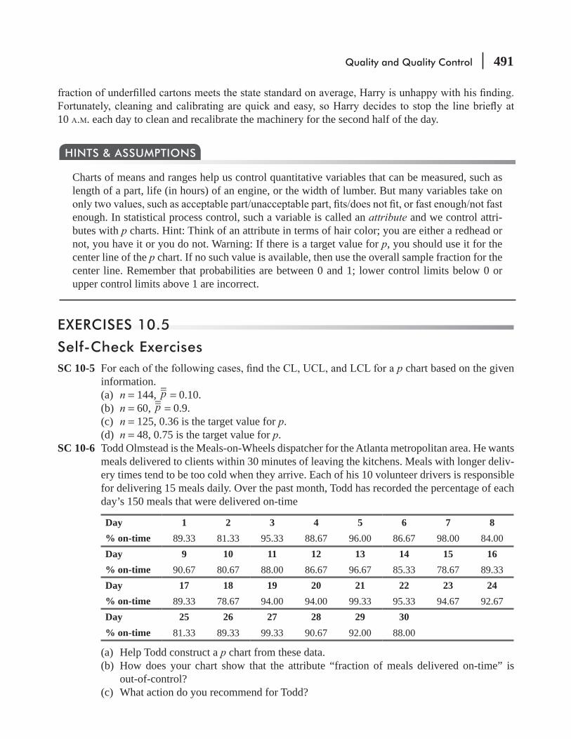
Quality and Quality Control 491
10 A.M. each day to clean and recalibrate the machinery for the second half of the day.
Charts of means and ranges help us control quantitative variables that can be measured, such as length of a part, life (in hours) of an engine, or the width of lumber. But many variables take on
enough. In statistical process control, such a variable is called an attribute and we control attri-butes with p charts. Hint: Think of an attribute in terms of hair color; you are either a redhead or not, you have it or you do not. Warning: If there is a target value for p, you should use it for the center line of the p chart. If no such value is available, then use the overall sample fraction for the center line. Remember that probabilities are between 0 and 1; lower control limits below 0 or upper control limits above 1 are incorrect.
HINTS & ASSUMPTIONS
EXERCISES 10.5
Self-Check ExercisesSC 10-5 p chart based on the given
information.(a) n = 144, p = 0.10.(b) n = 60, p = 0.9.(c) n = 125, 0.36 is the target value for p.(d) n = 48, 0.75 is the target value for p.
SC 10-6 Todd Olmstead is the Meals-on-Wheels dispatcher for the Atlanta metropolitan area. He wants meals delivered to clients within 30 minutes of leaving the kitchens. Meals with longer deliv-ery times tend to be too cold when they arrive. Each of his 10 volunteer drivers is responsible for delivering 15 meals daily. Over the past month, Todd has recorded the percentage of each day’s 150 meals that were delivered on-time
Day 1 2 3 4 5 6 7 8% on-time 89.33 81.33 95.33 88.67 96.00 86.67 98.00 84.00Day 9 10 11 12 13 14 15 16% on-time 90.67 80.67 88.00 86.67 96.67 85.33 78.67 89.33Day 17 18 19 20 21 22 23 24% on-time 89.33 78.67 94.00 94.00 99.33 95.33 94.67 92.67Day 25 26 27 28 29 30% on-time 81.33 89.33 99.33 90.67 92.00 88.00
(a) Help Todd construct a p chart from these data.(b) How does your chart show that the attribute “fraction of meals delivered on-time” is
out-of-control?(c) What action do you recommend for Todd?
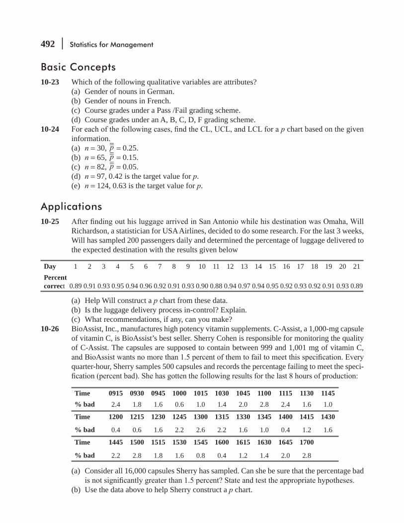
492 Statistics for Management
Basic Concepts10-23 Which of the following qualitative variables are attributes?
(a) Gender of nouns in German.(b) Gender of nouns in French.(c) Course grades under a Pass /Fail grading scheme.(d) Course grades under an A, B, C, D, F grading scheme.
10-24 p chart based on the given information.(a) n = 30, p = 0.25.(b) n = 65, p = 0.15.(c) n = 82, p = 0.05.(d) n = 97, 0.42 is the target value for p.(e) n = 124, 0.63 is the target value for p.
Applications10-25
Richardson, a statistician for USA Airlines, decided to do some research. For the last 3 weeks, Will has sampled 200 passengers daily and determined the percentage of luggage delivered to the expected destination with the results given below
Day 1 2 3 4 5 6 7 8 9 10 11 12 13 14 15 16 17 18 19 20 21Percent correct 0.89 0.91 0.93 0.95 0.94 0.96 0.92 0.91 0.93 0.90 0.88 0.94 0.97 0.94 0.95 0.92 0.93 0.92 0.91 0.93 0.89
(a) Help Will construct a p chart from these data.(b) Is the luggage delivery process in-control? Explain.(c) What recommendations, if any, can you make?
10-26 BioAssist, Inc., manufactures high potency vitamin supplements. C-Assist, a 1,000-mg capsule of vitamin C, is BioAssist’s best seller. Sherry Cohen is responsible for monitoring the quality of C-Assist. The capsules are supposed to contain between 999 and 1,001 mg of vitamin C,
quarter-hour, Sherry samples 500 capsules and records the percentage failing to meet the speci-
Time 0915 0930 0945 1000 1015 1030 1045 1100 1115 1130 1145% bad 2.4 1.8 1.6 0.6 1.0 1.4 2.0 2.8 2.4 1.6 1.0
Time 1200 1215 1230 1245 1300 1315 1330 1345 1400 1415 1430
% bad 0.4 0.6 1.6 2.2 2.6 2.2 1.6 1.0 0.4 1.2 1.6
Time 1445 1500 1515 1530 1545 1600 1615 1630 1645 1700
% bad 2.2 2.8 1.8 1.6 0.8 0.4 1.2 1.4 2.0 2.8
(a) Consider all 16,000 capsules Sherry has sampled. Can she be sure that the percentage bad
(b) Use the data above to help Sherry construct a p chart.

Quality and Quality Control 493
(c) Is there anything in the p chart about which Sherry should worry? If not, why not? If so, what should she do?
10-27 thesis. On each of the last 100 trading days, she has randomly sampled 100 companies listed on the New York Stock Exchange and recorded the fraction whose share prices increased that day. Andie believes that there is a 50–50 chance that any given stock will increase on any given day. Explain how she can use a p chart based on her 100 days’ worth of data to see if her belief is reasonable or not.
10-28
Skies has 240 takeoffs scheduled from this hub. Ross has been concerned about the fraction
that fraction. Use the data for the last 30 week-days to construct a p chart to see whether his new procedures have been successful. What further action, if any, should Ross consider?
Weeks 1 & 2Day M T W Th F M T W Th F# late 26 19 26 22 24 19 19 20 18 18Weeks 3 & 4Day M T W Th F M T W Th F# late 17 9 13 10 12 14 14 13 9 10Weeks 5 & 6Day M T W Th F M T w Th F# late 12 15 14 15 16 18 17 16 18 17
Worked-Out Answers to Self-Check ExercisesSC 10-5 (a) CL = p = 0.10
UCL 3 0.10 3
0.10(0.90)
1440.175p
pq
n= + = + =
LCL 3 0.10 3
0.10(0.90)
1440.025p
pq
n= − = − =
(b) CL 9p= =
ppq
nUCL 3 0.9 3
0.9(0.1)
601.016,= + = + = so the UCL = 1
LCL 3 0.9 3
0.9(0.1)
600.784p
pq
n= − = − =
(c) CL = p = 0.36
UCL 3 0.36 3
0.36(0.64)
1250.489p
pq
n= + = + =

494 Statistics for Management
LCL 3 0.36 3
0.36(0.64)
1250.231p
pq
n= − = − =
(d) CL = p = 0.75
UCL 3 0.75 3
0.75(0.25)
480.938p
pq
n= + = + =
LCL 3 0.75 3
0.75(0.25)
480.563p
pq
n= − = − =
SC 10-6 (a) n = 150 26.94
300.898p
p
k=
∑= =
UCL 3 0.898 3
0.898(0.102)
1500.972p
pq
n= + = + =
ppq
nLCL 3 0.898 3
0.898(0.102)
1500.824= − = − =
100
95
90
85
80
751 3 5 7 9 11 13 15 17
Day sampled
Perc
enta
ge d
eliv
ered
on
time
19 21 23 25 27 29
Meals on Wheelsp Chart
(b) Five of the 30 days sampled had values of “fraction on-time” that were below the lower control limit. (Being above the upper control limit is not worrisome in this context.)
(c) Because the percentage of meals delivered on-time is out-of-control, Todd might investi-gate the reasons behind the 5 days that are out-of-control. It might be a particular driver,
10.6 TOTAL QUALITY MANAGEMENTStatistical Process Control is very useful for continuous pro-
However, many managers feel that their businesses are altogether
Some processes are too
complicated for control charts

Quality and Quality Control 495
too complicated to have their important aspects captured and monitored by control charts. Suppose you were the manager of a regional hub airport and were asked to reduce takeoff delays. Although delays are easy to identify, their causes are harder to pin down. Takeoffs can be delayed by weather, equipment
what things to measure in order to control delays.Total Quality Management (TQM) is a set of approaches
that enable the managers of complex systems to match the
manager can use TQM to reduce delays so that planes match the schedules that their passengers expect. Because so many factors are involved, and because different workers have responsibility
to be successful. In particular, top-level management must provide strong leadership for qual-ity, and workers at all levels must be empowered to identify problems and make changes in the system.
Fishbone Diagrams: Identifying and Grouping CausesThe TQM approach to complex businesses begins with the real-ization that all errors, defects, and problems have causes, and that
and discriminate between things gone right and things gone wrong. In our airport example, some of the planes do leave on time (things gone right). When you look at the late departures (things gone wrong), you can begin to build up a list of causes behind their delays.
Even in complicated systems, causes of problems can be gathered into logical groups. For example, in our airport delays case, some of the late takeoffs are due to problems with the air-craft themselves, others result from baggage handling, and so on. As you collect the various reasons for departure delays into logical groups, it becomes clear that there are cause-and-effect relationships among them. These relationships can be captured pictorially in a cause-and-effect diagram such as Figure 10-8. Such cause-and-effect diagrams are sometimes called Ishikawa diagrams, after their Japanese developer, Kaoru Ishikawa. But, because of their appearance, these diagrams are most often called shbone diagrams.
organizes that list in two major ways. First, it gathers the factors into logical groups. And then, within the groups, it indicates how the various factors feed into one another in cause-and-effect relationships. Because of this, you can see how the complex system hangs together and recognize that many factors may need to be addressed in order to resolve the problems.
-els must be involved if TQM is to be successful. Baggage han-dlers are much more likely than top management or consultants to be able to identify a complete list of baggage problems that contribute to takeoff delays. In addition, because of their familiarity with details of the baggage-handling operation, they are also very likely to be able to suggest ways to improve that operation.
However, unless they are empowered to identify problems and make changes, they are unlikely to be willing to do so.
TQM requires companywide
commitment
Identify what’s right and what’s
wrong
Gather causes into logical
groups
Successful use of TQM involves
personnel at all levels

496 Statistics for Management
Slay the Dragons FirstIn any quality improvement process, as we have seen, there are likely to be a very large number of causes for defects and errors. Looking at all the possible things that can go wrong, even if they
TQM companies distinguish between the vital few and the trivial many. In our airport example, if most of the delays are due to baggage handling, and only one delay a year is attributable to a freak hail storm, it makes good sense to start by looking at ways to improve baggage handling. In TQM parlance, com-panies must in working to improve the quality of their goods or services.
A Pareto chart is a bar graph showing groups of error causes arranged by their frequencies of occurrence. It’s constructed by simply counting data from observations of things gone wrong. The results are usually ordered in a sequence from most common to least common, with a residual “other” category at the end. These charts are named after Vilfredo Pareto (1848–1923), an Italian economist who studied the distribution of wealth. Just as Pareto found that most of the wealth in a society is held by relatively few people, Juran noted that in most complex systems, 80 percent of defects and errors can be attributed to 20 percent of the causes. Looking at the Pareto chart for late departures in Figure 10-9, you can see that about 23 of the delays (45 of 68 observations) were caused by baggage-handling and equipment problems. The airport manager should begin system-improvement efforts by concentrating on these two areas.
Concentrate first on common
causes
Pareto charts
FIGURE 10-8 A FISHBONE DIAGRAM: CAUSE-AND-EFFECT REASONS FOR AIRPORT TAKEOFF DELAYS
Passengers Baggage Flight control
WeatherConnectingConnectingflights flights
Late check-in
VIPs Handlers unavailable Traffic hold
Plane takesoff late
Wrong crewMechanicalFood
Fuel
Cleaners
Service Equipment Crew
scheduled
Late to terminal
Late arrivingin-bound
Here
At d
estin
atio
n
Othe
r flig
hts
Not s
ched
uled
Avio
nics
Engi
nes
Hote
lTr
affic
Out s
ick
Late check-in

Quality and Quality Control 497
Continuous Quality Improvement
to improve the quality of the systems’ goods or services. This can sometimes involve the institution of
baggage handlers or as complex as installing scanners that read bar-coded destination labels on pieces
When TQM efforts are successful, it is not uncommon for the leading cause of errors to drop to zero on the Pareto chart. This means that another cause becomes the “dragon,” and management attention
of problems is known as Continuous Quality Improvement (CQI).
many possible causes of failure. Warning: Unless you use an organized, systematic method to look at all of these causes, you run a high risk of miss-ing something that’s important. Fishbone diagrams and Pareto charts are very effective ways of focusing and guiding your analysis of quality problems so that everything that affects quality is examined, nothing is overlooked, and the most important things get looked at rst. A hint learned from many years of quality control experience is that Total Quality Control programs work only when you have strong top management leadership that involves line employees in the responsibil-ity for controlling their own processes.
HINTS & ASSUMPTIONS
FIGURE 10-9 A PARETO DIAGRAM OF REASONS FOR AIRPORT TAKEOFF DELAYS
30
27
18
9
Baggage Equipment Passengers Service Crew Other
42
8
20
10

498 Statistics for Management
EXERCISES 10.6
Self-Check ExerciseSC 10-7 Northway Computers has just begun a TQM program to manage the quality of the personal com-
puters it assembles. A careful analysis of 25,000 computer systems located the following faults:
Component Number of Faults
CPU 25
Floppy disk drives 106Hard disk drive 237I/O ports 36Keyboard 60Monitor 42Power supply 186RAM memory 30ROM BIOS 7Video adapter 47Other 163
Construct a Pareto chart for Northway. Northway’s President, Ted White, is going to set up a
Basic Concepts10-29 Explain why successful application of TQM requires the participation of employees at all
levels of an organization.10-30
dragon, then you can forget TQM and get on with business as usual.” Comment on Joe’s understanding of TQM.
Applications10-31 The News and Reporter has a long-standing TQM policy, and it is time to analyze this quarter’s
complaints and problems. The following problems have been traced by the quality control engineer:
Problem Department Number of OccurrencesOmitted advertisement 18Incorrect special instructions 37Typographical error in a news story Reporting 14Advertisement in the wrong section 16Incorrectly priced advertisement 8Factual error in news story Reporting 16Late delivery of all papers Printing 3Advertisement placed on incorrect date 6Typographical error in commercial advertisement
Advertising 8
(Continued)
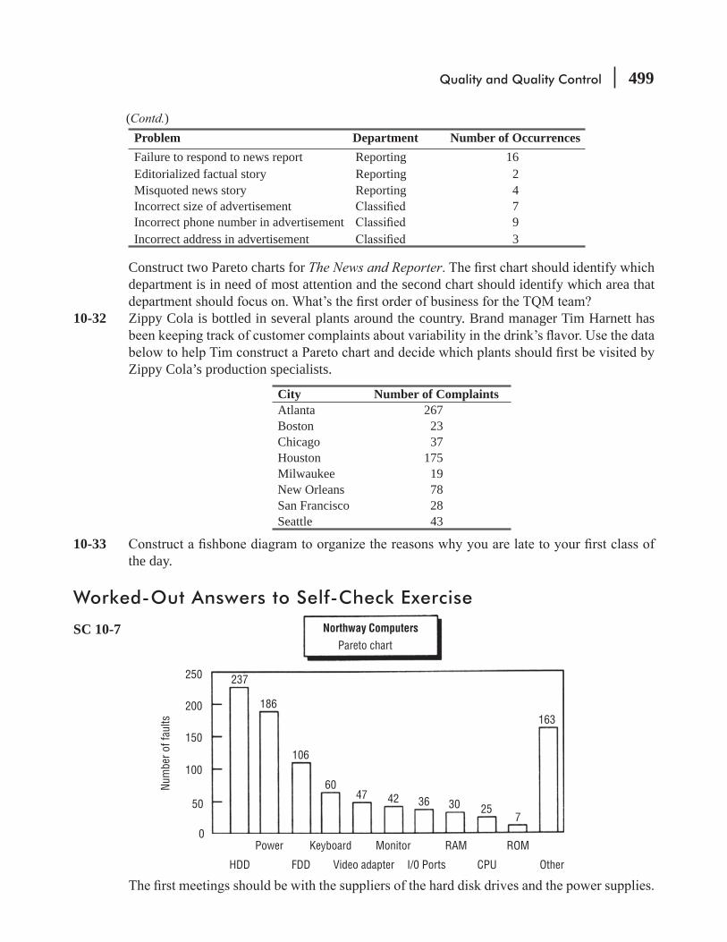
Quality and Quality Control 499
Problem Department Number of OccurrencesFailure to respond to news report Reporting 16Editorialized factual story Reporting 2Misquoted news story Reporting 4Incorrect size of advertisement 7Incorrect phone number in advertisement 9Incorrect address in advertisement 3
Construct two Pareto charts for The News and Reporterdepartment is in need of most attention and the second chart should identify which area that
10-32 Zippy Cola is bottled in several plants around the country. Brand manager Tim Harnett has
Zippy Cola’s production specialists.
City Number of ComplaintsAtlanta 267Boston 23Chicago 37Houston 175Milwaukee 19New Orleans 78San Francisco 28Seattle 43
10-33 the day.
Worked-Out Answers to Self-Check Exercise
SC 10-7
250 237
186
106
6047 42 36 30 25
7
163200
150
100
50
0
Num
ber o
f fau
lts
Power Keyboard Monitor RAM ROM
HDD FDD Video adapter I/0 Ports CPU Other
Northway ComputersPareto chart
(Contd.)

500 Statistics for Management
10.7 ACCEPTANCE SAMPLINGAdoption of TQM techniques implies a goal that the inputs to each stage of an operation should be defect-free because the operations at the preceding stage are under control. But manufacturers often have to accept raw materials and components from suppliers. To be sure that the results of their own operations are of high quality, they must often test inputs to make sure that they conform to requirements. In most production situations, com-plete inspection of an entire batch of input is impractical because of time and cost considerations. Instead, a sample of the batch is inspected, and the decision to accept or reject the entire batch is based on the quality of the sample.
You may feel that reliance on sampling to ensure the quality of inputs is just moving the old-time white-coated inspectors from the end of the production line to the beginning. Many experts in quality engineering would agree with you. The whole process of inspection implies that some materials will be rejected and that amounts to a waste of materials and time. However, acceptance sampling can be an effec-tive way to motivate suppliers to improve the quality of their outputs. In fact, it can even be more effective than inspection of the entire batch. Let’s look more carefully at this apparently paradoxical assertion.
Suppose you inspect an entire batch of components sent to you by a supplier. You sort the individual units into two groups, acceptable and unacceptable. Then you send the latter units back to the supplier for replacements. If only 5 percent of the units are rejected, you have imposed a large cost on yourself and a small cost on the supplier. And to boot, you have saved the supplier the cost of being responsible for the
unsatisfactory units in the sample, and on the basis of the sample send the entire batch back for replace-ment. This imposes a small cost on you and a large cost on the supplier. The supplier may resent the fact that you are sending the acceptable units back along with the unacceptable ones. However, if the supplier values your business, it is ultimately going to take responsibility for ensuring the quality of its output. And if the supplier does not value your business, then you are well served by learning this and seeking another supplier.
The statistical techniques used in acceptance sampling will be familiar to you as applications of the sampling and hypothesis-testing ideas we discussed in Chapters 6, 8 and 9. Much of the original work in acceptance sampling was done in the 1920s and 1930s by Harold F. Dodge and Harry G. Romig, who, like Walter Shewhart, did their research at Bell Labs. They discussed single-sampling and double-sampling schemes:
n, and an acceptance number, c, the maximum number of allow-able pieces with defects. A sample of size n is taken, and the lot is accepted if there are c or fewer defective pieces in the sample, but rejected if the number of defective pieces is greater than c.
Double sampling is more complicated, and depends on four n1, n2, c1, and c2 (> c1), which are used as
follows:First a sample of size n1 is taken. Let b1 (b for bad) be the number of defective pieces in this sample:
If b1 ≤ c1, the lot is accepted. If b1 > c2, the lot is rejected. If c1 < b1 ≤ c2, an additional n2 units are sampled.
Testing inputs for conformance
to requirements
Acceptance sampling can
motivate suppliers to improve
quality
Single sampling
Double sampling
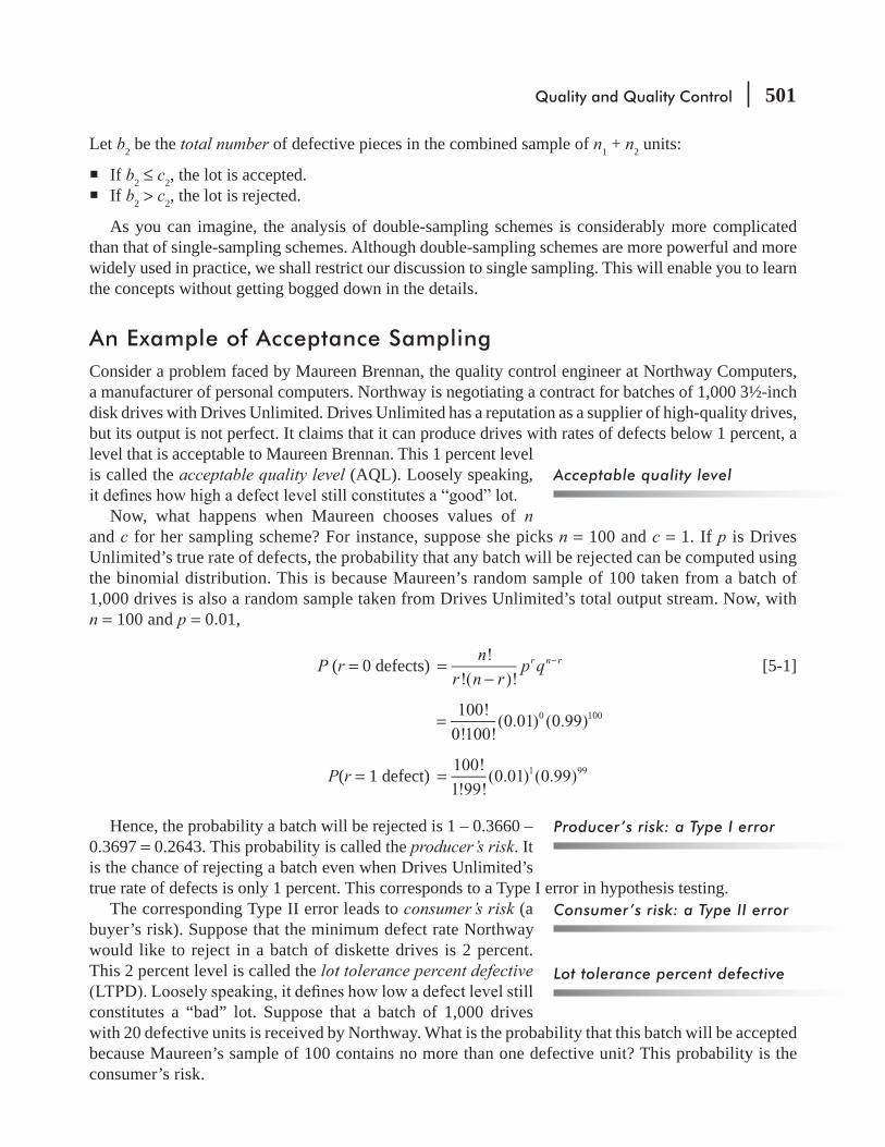
Quality and Quality Control 501
Let b2 be the total number of defective pieces in the combined sample of n1 + n2 units:
If b2 ≤ c2, the lot is accepted. If b2 > c2, the lot is rejected.
As you can imagine, the analysis of double-sampling schemes is considerably more complicated than that of single-sampling schemes. Although double-sampling schemes are more powerful and more widely used in practice, we shall restrict our discussion to single sampling. This will enable you to learn the concepts without getting bogged down in the details.
An Example of Acceptance SamplingConsider a problem faced by Maureen Brennan, the quality control engineer at Northway Computers, a manufacturer of personal computers. Northway is negotiating a contract for batches of 1,000 3½-inch disk drives with Drives Unlimited. Drives Unlimited has a reputation as a supplier of high-quality drives, but its output is not perfect. It claims that it can produce drives with rates of defects below 1 percent, a level that is acceptable to Maureen Brennan. This 1 percent level is called the acceptable quality level (AQL). Loosely speaking,
Now, what happens when Maureen chooses values of n and c for her sampling scheme? For instance, suppose she picks n = 100 and c = 1. If p is Drives Unlimited’s true rate of defects, the probability that any batch will be rejected can be computed using the binomial distribution. This is because Maureen’s random sample of 100 taken from a batch of 1,000 drives is also a random sample taken from Drives Unlimited’s total output stream. Now, with n = 100 and p = 0.01,
P (r = 0 defects) n
r n rp q
!
!( )!r n r=
−− [5-1]
100!
0!100!(0.01) (0.99)0 100=
P(r = 1 defect) 100!
1!99!(0.01) (0.99)1 99=
Hence, the probability a batch will be rejected is 1 – 0.3660 – 0.3697 = 0.2643. This probability is called the producer’s risk. It is the chance of rejecting a batch even when Drives Unlimited’s true rate of defects is only 1 percent. This corresponds to a Type I error in hypothesis testing.
The corresponding Type II error leads to consumer’s risk (a buyer’s risk). Suppose that the minimum defect rate Northway would like to reject in a batch of diskette drives is 2 percent. This 2 percent level is called the lot tolerance percent defective
constitutes a “bad” lot. Suppose that a batch of 1,000 drives with 20 defective units is received by Northway. What is the probability that this batch will be accepted because Maureen’s sample of 100 contains no more than one defective unit? This probability is the consumer’s risk.
Acceptable quality level
Producer’s risk: a Type I error
Consumer’s risk: a Type II error
Lot tolerance percent defective
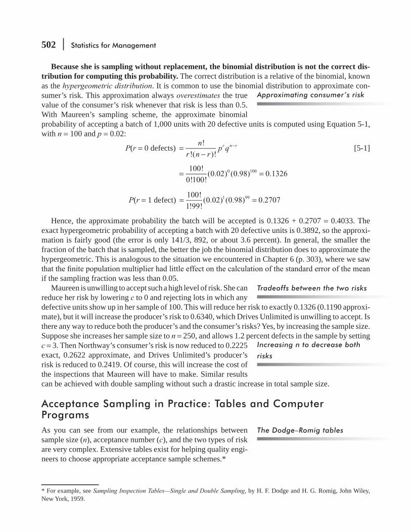
502 Statistics for Management
Because she is sampling without replacement, the binomial distribution is not the correct dis-tribution for computing this probability. The correct distribution is a relative of the binomial, known as the hypergeometric distribution. It is common to use the binomial distribution to approximate con-sumer’s risk. This approximation always overestimates the true value of the consumer’s risk whenever that risk is less than 0.5. With Maureen’s sampling scheme, the approximate binomial probability of accepting a batch of 1,000 units with 20 defective units is computed using Equation 5-1, with n = 100 and p = 0.02:
P(r = 0 defects) !
!( )!
n
r n rp qr n r=
−− [5-1]
100!
0!100!(0.02) (0.98) 0.13260 100= =
P(r = 1 defect) 100!
1!99!(0.02) (0.98) 0.27071 99= =
Hence, the approximate probability the batch will be accepted is 0.1326 + 0.2707 = 0.4033. The exact hypergeometric probability of accepting a batch with 20 defective units is 0.3892, so the approxi-mation is fairly good (the error is only 141/3, 892, or about 3.6 percent). In general, the smaller the fraction of the batch that is sampled, the better the job the binomial distribution does to approximate the hypergeometric. This is analogous to the situation we encountered in Chapter 6 (p. 303), where we saw
if the sampling fraction was less than 0.05.Maureen is unwilling to accept such a high level of risk. She can
reduce her risk by lowering c to 0 and rejecting lots in which any defective units show up in her sample of 100. This will reduce her risk to exactly 0.1326 (0.1190 approxi-mate), but it will increase the producer’s risk to 0.6340, which Drives Unlimited is unwilling to accept. Is there any way to reduce both the producer’s and the consumer’s risks? Yes, by increasing the sample size. Suppose she increases her sample size to n = 250, and allows 1.2 percent defects in the sample by setting c = 3. Then Northway’s consumer’s risk is now reduced to 0.2225 exact, 0.2622 approximate, and Drives Unlimited’s producer’s risk is reduced to 0.2419. Of course, this will increase the cost of the inspections that Maureen will have to make. Similar results can be achieved with double sampling without such a drastic increase in total sample size.
Acceptance Sampling in Practice: Tables and Computer ProgramsAs you can see from our example, the relationships between sample size (n), acceptance number (c), and the two types of risk are very complex. Extensive tables exist for helping quality engi-neers to choose appropriate acceptance sample schemes.*
* For example, see Sampling Inspection Tables—Single and Double Sampling, by H. F. Dodge and H. G. Romig, John Wiley, New York, 1959.
Approximating consumer’s risk
Tradeoffs between the two risks
Increasing n to decrease both
risks
The Dodge–Romig tables
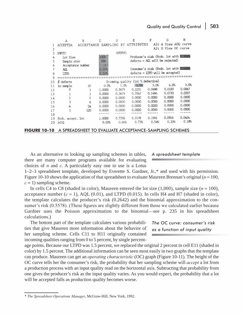
Quality and Quality Control 503
As an alternative to looking up sampling schemes in tables, there are many computer programs available for evaluating choices of n and c. A particularly easy one to use is a Lotus 1–2–3 spreadsheet template, developed by Everette S. Gardner, Jr.,* and used with his permission. Figure 10-10 shows the application of that spreadsheet to evaluate Maureen Brennan’s original (n = 100, c = 1) sampling scheme.
In cells C4 to C8 (shaded in color), Maureen entered the lot size (1,000), sample size (n = 100), acceptance number (c = 1), AQL (0.01), and LTPD (0.015). In cells H4 and H7 (shaded in color), the template calculates the producer’s risk (0.2642) and the binomial approximation to the con-
Gardner uses the Poisson approximation to the binomial—see p. 235 in his spreadsheet calculations.)
The bottom part of the template calculates various probabili-ties that give Maureen more information about the behavior of her sampling scheme. Cells C11 to H11 originally contained incoming qualities ranging from 0 to 5 percent, by single percent-age points. Because our LTPD was 1.5 percent, we replaced the original 2 percent in cell E11 (shaded in color) by 1.5 percent. The additional information can be seen most easily in two graphs that the template can produce. Maureen can get an operating characteristic (OC) graph (Figure 10-11). The height of the OC curve tells her the consumer’s risk, the probability that her sampling scheme will accept a lot from a production process with an input quality read on the horizontal axis. Subtracting that probability from one gives the producer’s risk as the input quality varies. As you would expect, the probability that a lot will be accepted falls as production quality becomes worse.
* The Spreadsheet Operations Manager, McGraw-Hill, New York, 1992.
The OC curve: consumer’s risk
as a function of input quality
FIGURE 10-10 A SPREADSHEET TO EVALUATE ACCEPTANCE-SAMPLING SCHEMES
A spreadsheet template
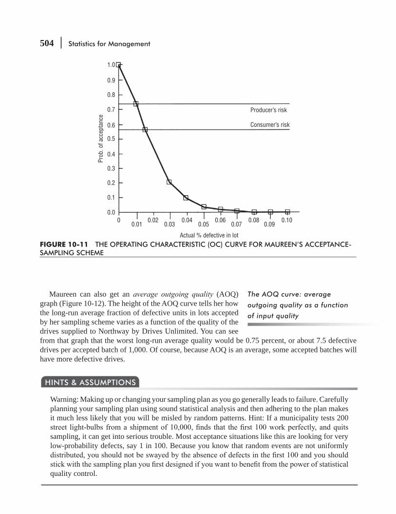
504 Statistics for Management
Maureen can also get an average outgoing quality (AOQ) graph (Figure 10-12). The height of the AOQ curve tells her how the long-run average fraction of defective units in lots accepted by her sampling scheme varies as a function of the quality of the drives supplied to Northway by Drives Unlimited. You can see from that graph that the worst long-run average quality would be 0.75 percent, or about 7.5 defective drives per accepted batch of 1,000. Of course, because AOQ is an average, some accepted batches will have more defective drives.
Warning: Making up or changing your sampling plan as you go generally leads to failure. Carefully planning your sampling plan using sound statistical analysis and then adhering to the plan makes it much less likely that you will be misled by random patterns. Hint: If a municipality tests 200
sampling, it can get into serious trouble. Most acceptance situations like this are looking for very low-probability defects, say 1 in 100. Because you know that random events are not uniformly
quality control.
HINTS & ASSUMPTIONS
FIGURE 10-11 THE OPERATING CHARACTERISTIC (OC) CURVE FOR MAUREEN’S ACCEPTANCE-SAMPLING SCHEME
1.0
0.9
0.8
0.7
0.6
0.5
Producer’s risk
Consumer’s risk
0.4
Prob
. of a
ccep
tanc
e
0.3
0.2
0.1
0.0
Actual % defective in lot
00.01 0.03 0.05 0.07 0.09
0.02 0.04 0.06 0.08 0.10
The AOQ curve: average
outgoing quality as a function
of input quality
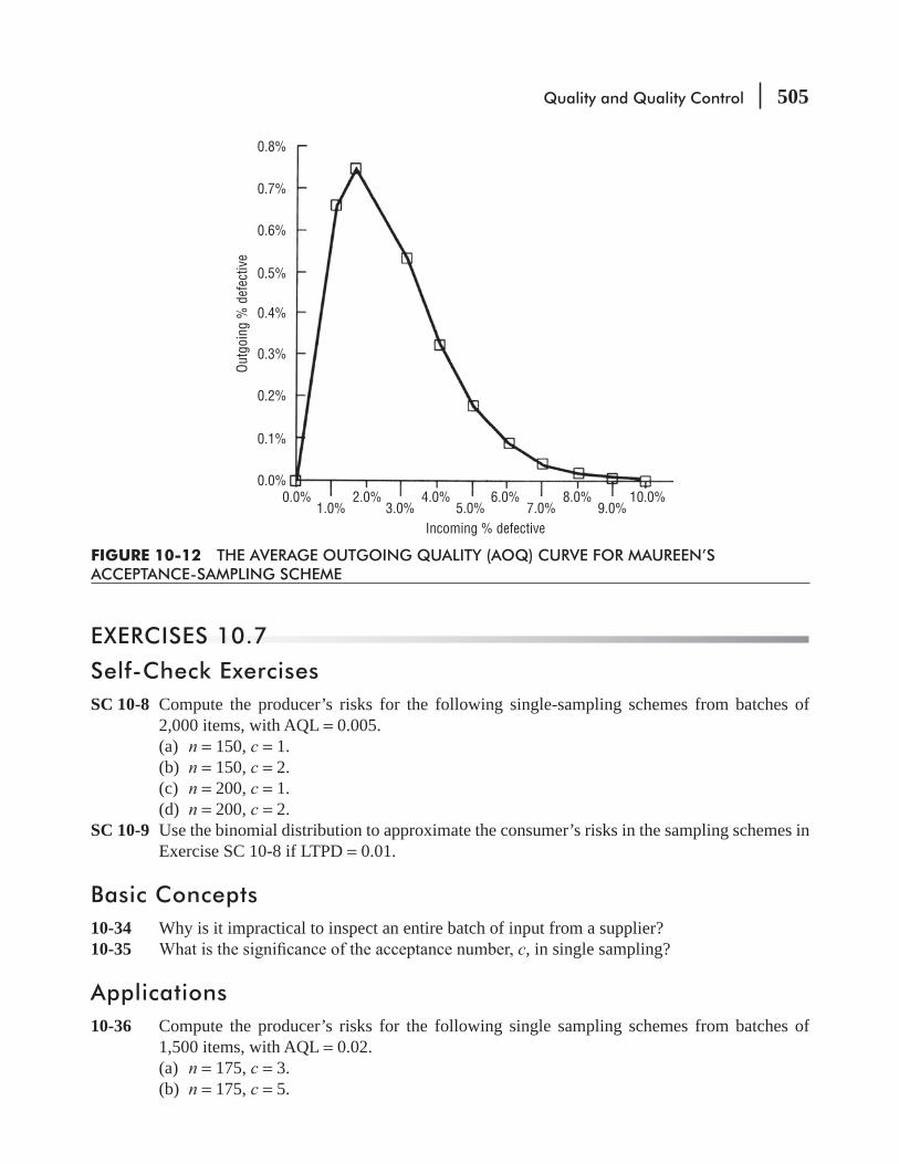
Quality and Quality Control 505
EXERCISES 10.7
Self-Check ExercisesSC 10-8 Compute the producer’s risks for the following single-sampling schemes from batches of
2,000 items, with AQL = 0.005.(a) n = 150, c = 1.(b) n = 150, c = 2.(c) n = 200, c = 1.(d) n = 200, c = 2.
SC 10-9 Use the binomial distribution to approximate the consumer’s risks in the sampling schemes in Exercise SC 10-8 if LTPD = 0.01.
Basic Concepts10-34 Why is it impractical to inspect an entire batch of input from a supplier?10-35 c, in single sampling?
Applications10-36 Compute the producer’s risks for the following single sampling schemes from batches of
1,500 items, with AQL = 0.02.(a) n = 175, c = 3.(b) n = 175, c = 5.
FIGURE 10-12 THE AVERAGE OUTGOING QUALITY (AOQ) CURVE FOR MAUREEN’S ACCEPTANCE-SAMPLING SCHEME
0.8%
0.7%
0.6%
0.5%
0.4%
Outg
oing
% d
efec
tive
0.3%
0.2%
0.1%
0.0%0.0% 2.0% 4.0% 6.0% 8.0% 10.0%
9.0%7.0%5.0%3.0%1.0%Incoming % defective
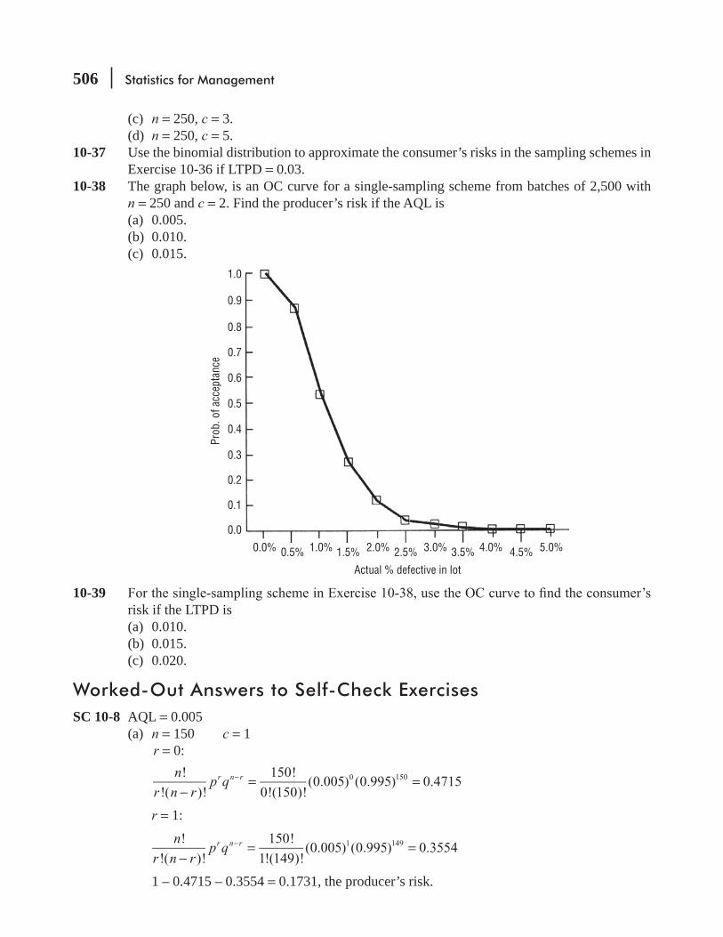
506 Statistics for Management
(c) n = 250, c = 3.(d) n = 250, c = 5.
10-37 Use the binomial distribution to approximate the consumer’s risks in the sampling schemes in Exercise 10-36 if LTPD = 0.03.
10-38 The graph below, is an OC curve for a single-sampling scheme from batches of 2,500 with n = 250 and c = 2. Find the producer’s risk if the AQL is(a) 0.005.(b) 0.010.(c) 0.015.
1.0
0.9
0.8
0.7
0.6
Prob
. of a
ccep
tanc
e
0.5
0.4
0.3
0.2
0.1
0.0
0.0% 0.5% 1.5% 2.5%
Actual % defective in lot
3.5% 4.5%1.0% 2.0% 3.0% 4.0% 5.0%
10-39 risk if the LTPD is(a) 0.010.(b) 0.015.(c) 0.020.
Worked-Out Answers to Self-Check ExercisesSC 10-8 AQL = 0.005
(a) n = 150 c = 1 r = 0:
!
!( )!
150!
0!(150)!(0.005) (0.995) 0.47150 150n
r n rp qr n r
−= =−
r = 1:
!
!( )!
150!
1!(149)!(0.005) (0.995) 0.35541 149n
r n rp qr n r
−= =−
1 – 0.4715 – 0.3554 = 0.1731, the producer’s risk.
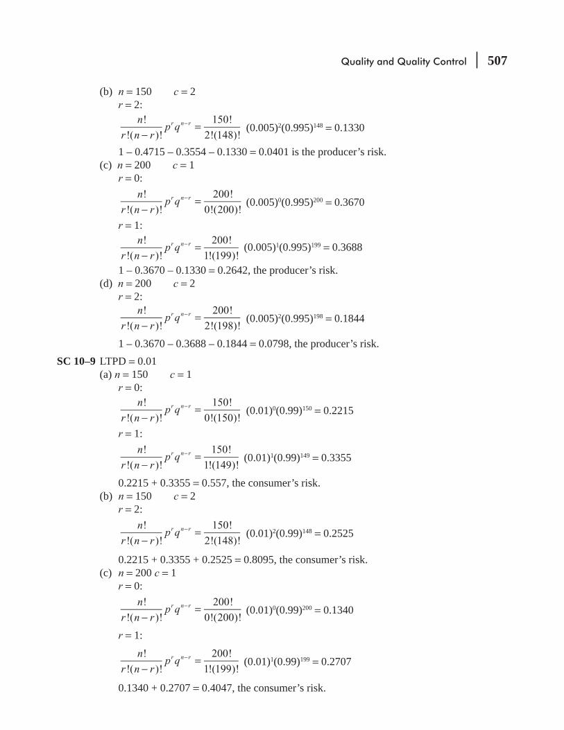
Quality and Quality Control 507
(b) n = 150 c = 2 r = 2:
!
!( )!
150!
2!(148)!
n
r n rp qr n r
−=− (0.005)2(0.995)148 = 0.1330
1 – 0.4715 – 0.3554 – 0.1330 = 0.0401 is the producer’s risk.(c) n = 200 c = 1 r = 0:
!
!( )!
200!
0!(200)!
n
r n rp qr n r
−=− (0.005)0(0.995)200 = 0.3670
r = 1:
n
r n rp q
!
!( )!
200!
1!(199)!r n r
−=− (0.005)1(0.995)199 = 0.3688
1 – 0.3670 – 0.1330 = 0.2642, the producer’s risk.(d) n = 200 c = 2 r = 2:
!
!( )!
200!
2!(198)!
n
r n rp qr n r
−=− (0.005)2(0.995)198 = 0.1844
1 – 0.3670 – 0.3688 – 0.1844 = 0.0798, the producer’s risk.SC 10–9 LTPD = 0.01
(a) n = 150 c = 1 r = 0:
!
!( )!
150!
0!(150)!
n
r n rp qr n r
−=− (0.01)0(0.99)150 = 0.2215
r = 1:
!
!( )!
150!
1!(149)!
n
r n rp qr n r
−=− (0.01)1(0.99)149 = 0.3355
0.2215 + 0.3355 = 0.557, the consumer’s risk.(b) n = 150 c = 2 r = 2:
!
!( )!
150!
2!(148)!
n
r n rp qr n r
−=− (0.01)2(0.99)148 = 0.2525
0.2215 + 0.3355 + 0.2525 = 0.8095, the consumer’s risk.(c) n = 200 c = 1 r = 0:
!
!( )!
200!
0!(200)!
n
r n rp qr n r
−=− (0.01)0(0.99)200 = 0.1340
r = 1:
!
!( )!
200!
1!(199)!
n
r n rp qr n r
−=− (0.01)1(0.99)199 = 0.2707
0.1340 + 0.2707 = 0.4047, the consumer’s risk.

508 Statistics for Management
(d) n = 200 c = 2 r = 2:
!
!( )!
200!
2!(198)!
n
r n rp qr n r
−=− (0.01)2(0.99)198 = 0.2720
0.1340 + 0.2707 + 0.2720 = 0.6767, the consumer’s risk.
STATISTICS AT WORK
Loveland ComputersCase 10: Quality and Quality Control Walter Azko prided himself on his open-door policy, and any
suppliers and better prices.
“Boss, we both went to a seminar put on by the State CPA Association,” Harry began.“So we wanted to talk with you about quality initiatives at Loveland Computers,” added Jeff. The
“I’m not going to pay good money for a bunch of high-priced consultants to come in and preach to us,” Walter greeted their enthusiasm with skepticism. “In any case, I’ve always told you—at this end of the market we compete on price, not on quality. Our customers only care whether a Loveland Computer works and whether we have it in stock when they want to order it. And if it doesn’t work, they just have to ship it back to us and we’ll send them out a new one.”
“Right. And how much is that costing us?” Harry asked.
compared to our volume. You know that.”“Well, after that seminar, I’m sure that we don’t really capture all the costs of a failure,” the control-
ler disputed.“Anyway, we test all the computers overnight at the end of the line before we ship them. What do
you want me to do—run them for a week before we ship them out?” Walter remained unconvinced that thinking about quality could change the way Loveland did business.
“Doesn’t this relate to customer satisfaction?” Lee interjected. “I read where J. D. Power—the com-pany that reports on what automobile customers think about new models—is going to start rating PCs.”
“There’s much more to quality than more testing before we ship things, in fact, if we do things right, I’m convinced we’d need less testing on the production line,” Jeff added. “Let Harry and me buy you lunch and tell you what we learned at the seminar.”
Study Questions: What arguments will Jeff and Harry make against Walter’s assertion that Loveland competes only on price? What are the total costs of replacing a machine that Harry refers to? How does quality relate to customer satisfaction? Why would Loveland need less end-of-the-line testing if it adopted quality control measures? Does it matter whether Walter Azko ends up with a better under-standing of quality by the end of lunch?

Quality and Quality Control 509
CHAPTER REVIEW
Terms Introduced in Chapter 10Acceptable Quality Level (AQL) The average quality level promised by a producer; the maximum number or percentage of defective pieces in a “good” lot.Acceptance Number The maximum number of defective pieces with which a lot will still be accepted.Acceptance Sampling Procedures for deciding whether to accept or reject a batch of input materials based on the quality of a sample taken from that batchAssignable Variation Nonrandom, systematic variability in a process. It usually can be corrected with-out redesigning the entire process.Attributes Qualitative variables with only two categories.Average Outgoing Quality (AOQ) Curve A graph showing how the long-run average fraction of defective units in lots accepted by a sampling scheme varies as a function of the input quality of the lots.Cause-and-Effect Diagram Another name for a sh-bone diagram.Common Variation Random variability inherent in a process. It usually cannot be reduced without re-designing the entire process.Consumer’s Risk The chance that a “bad” lot will be accepted.Continuous Quality Improvement (CQI) problems in TQM.Control Charts A plot of some parameter of interest (such as x, R, or p) over time, used to identify assignable variations and to make adjustments to the process being monitored.Control Limits Upper and lower bounds on control charts. For the process to be in-control, all obser-vations must fall within these limits.Fishbone Diagram A pictorial device for organizing cause-and-effect relationships among the factors causing problems in complex systems.Hypergeometric Distribution The correct distribution for computing consumer’s risk; it is often approximated by the binomial distribution.Inherent Variation Another name for common variation.Ishikawa Diagram Another name for a shbone diagram.Lot Tolerance Percent Defective (LTPD) The minimum number or percentage of defective pieces in a “bad” lot.Operating Characteristic (OC) Curve A graph showing the probability an acceptance-sampling scheme will accept a batch as a function of the input quality of the batch.Outliers Observations falling outside the control limits on a control chart.Out-of-Control A process exhibiting outliers on a control chart, or showing nonrandom patterns even though there are no outliers.p Charts Pareto Chart A bar graph showing groups of error causes arranged by their frequencies of occurrence.Producer’s Risk The chance that a “good” lot will be rejected.Qualitative Variables Variables whose values are categorical rather than numerical.Quality Fitness for use or conformance to requirements.Quantitative Variables Variables with numerical values resulting from measuring or counting.R Charts Control charts for monitoring process variability.Special Cause Variation Another name for assignable variation.Statistical Process Control (SPC) Shewhart’s system of using control charts to track variation and identify its causes.

510 Statistics for Management
Total Quality Management (TQM) A set of approaches that enables the managers of complex sys-
x Chart Control charts for monitoring process means.
Equations Introduced in Chapter 10
10-1 xx
n k
x
k=
∑×
=∑ p. 473
To compute the grand mean x( ) from several (k) samples of the same size (n), either sum all the original observations (Σx) and divide by the total number of observations (n × k), or else sum the means from each of the samples (Σx ) and divide by the number of samples (k). Then use x for the center line (CL) of an x chart.
10-2 xR
d nUCL
3
2
= + p. 475
xR
d nLCL
3
2
= −
To compute the control limits for an x chart, multiply the average sample range (R = ΣR/k) by 3, and then divide by the product of d2 (from Appendix Table 9) and n; the result is then added to and subtracted from x . Alternatively, you can compute these limits as x A R2± , where A2 (= 3/d2 n) can also be found in Appendix Table 9.
10-3 3σ σ= dR
p. 482To get the standard deviation of the sampling distribution of R, multiply the population stan-dard deviation, σ, by d3, another factor that is also given in Appendix Table 9.
10-4 Rd R
dR
d
dUCL
31
33
2
3
2
= + = +⎛
⎝⎜⎞
⎠⎟ p. 482
R
d R
dR
d
dLCL
31
33
2
3
2
= − = −⎛
⎝⎜⎞
⎠⎟
To compute the control limits for an R chart, multiply the average sample range ( R R k/= ∑ ) by 1 ± 3d3/d2. Alternatively, you can compute these limits as
UCL = RD4, where D4 = 1 + 3d3/d2 LCL = RD3, where D3 = 1 – 3d3/d2
Values of D3 and D4 are also given in Appendix Table 9. Because ranges are always nonnega-tive, D3 and the LCL are taken to be 0 when n ≤ 6.
10-5 ppCL μ= = p. 489
10-6 ppq
np pUCL 3 3μ σ= + = + p. 489
LCL 3 3μ σ= − = −p
pq
np p

Quality and Quality Control 511
If there is a known or targeted value of p, that value should be used in Equations 10-5 and 10-6 to get the center line and control limits for a p chart. However, if no such value of p is available, then you should use the overall sample fraction
10-7 pp
kj=
∑ p. 489
where
pj = sample fraction in the jth sample k = total number of samples
Review and Application Exercises10-40
2 percent of its clients audited. As part of a summer internship, Jane Bloch has been asked to see whether this goal is being met on a consistent basis. For each week during a 16-week interval
data follow:
Week Ending 2/25 3/04 3/11 3/18 3/25 4/01 4/08 4/15# Audited 2 1 2 3 5 4 5 6# Week Ending 4/22 4/29 5/06 5/13 5/20 5/27 6/03 6/10# Audited 3 1 1 3 2 2 3 2
test appropriate hypotheses using all 2,000 clients in Jane’s sample.(b) Notwithstanding your result in part (a), construct a p chart based on Jane’s data. Is there
anything evident in the chart that Jane should bring to the attention of the partners in the
10-41 When slaying dragons, should you be concerned with the “trivial many” or the “vital few”? Explain.
10-42 If marital status is coded as “currently married” or “never married,” then marital status is an attribute. However, if it is coded as “single,” “married,” “widowed,” or “divorced,” then it is not an attribute. Explain this apparent inconsistency.
10-43 The amount of time a bank teller needs to process a deposit depends on how many items the customer has. Is this inherent or special cause variation? Explain.
10-44 All checks drafted on accounts at Global Bank are returned to the bank’s check-processing center. There each check is encoded with optically scannable characters that indicate the amount for which it is drawn. The encoded checks are then scanned so that payment can be made and the accounts on which they have been drawn can be debited. Shih-Hsing Liu has been monitoring the encoding operation, and has counted the number of checks processed in 10 randomly chosen 2-minute periods during each hour of the last two 8-hour shifts. She has
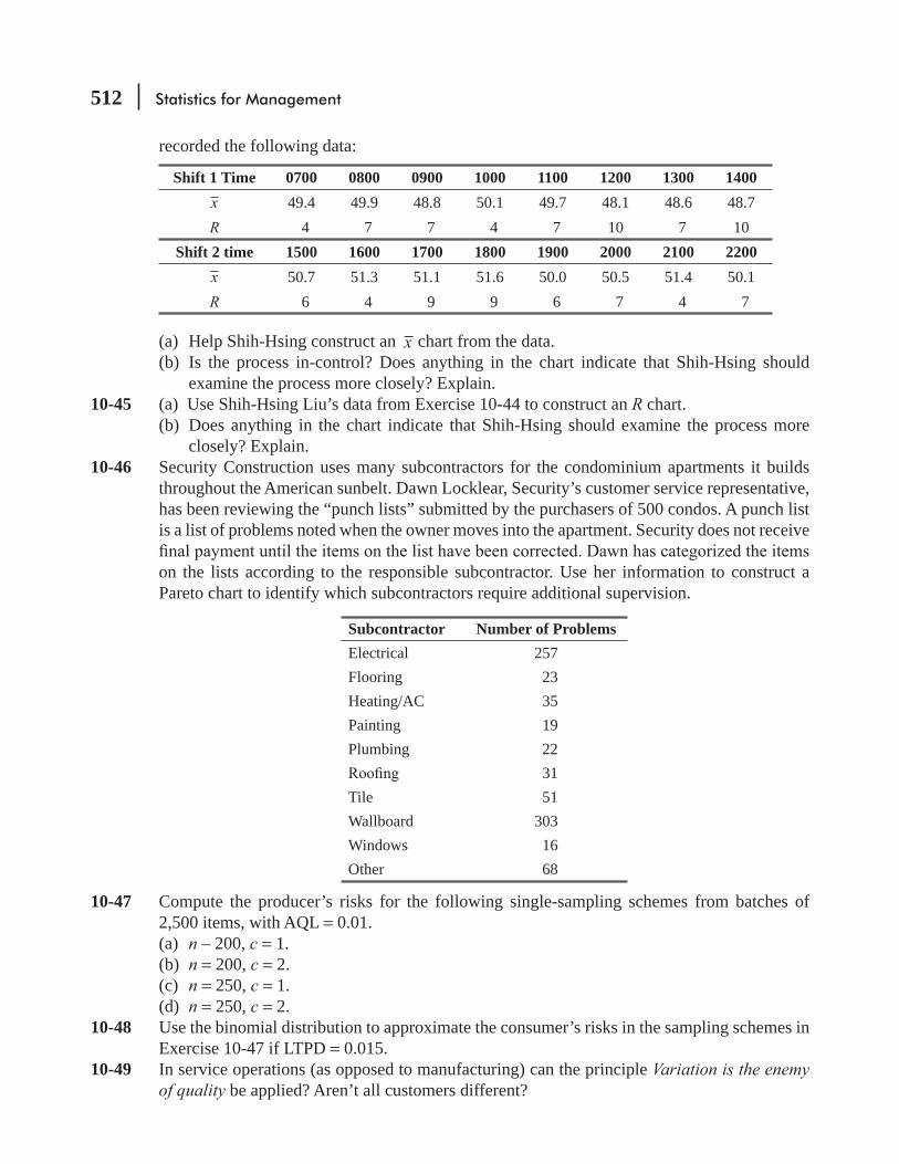
512 Statistics for Management
recorded the following data:
Shift 1 Time 0700 0800 0900 1000 1100 1200 1300 1400x 49.4 49.9 48.8 50.1 49.7 48.1 48.6 48.7R 4 7 7 4 7 10 7 10
Shift 2 time 1500 1600 1700 1800 1900 2000 2100 2200x 50.7 51.3 51.1 51.6 50.0 50.5 51.4 50.1R 6 4 9 9 6 7 4 7
(a) Help Shih-Hsing construct an x chart from the data.(b) Is the process in-control? Does anything in the chart indicate that Shih-Hsing should
examine the process more closely? Explain.10-45 (a) Use Shih-Hsing Liu’s data from Exercise 10-44 to construct an R chart.
(b) Does anything in the chart indicate that Shih-Hsing should examine the process more closely? Explain.
10-46 Security Construction uses many subcontractors for the condominium apartments it builds throughout the American sunbelt. Dawn Locklear, Security’s customer service representative, has been reviewing the “punch lists” submitted by the purchasers of 500 condos. A punch list is a list of problems noted when the owner moves into the apartment. Security does not receive
on the lists according to the responsible subcontractor. Use her information to construct a Pareto chart to identify which subcontractors require additional supervision.
Subcontractor Number of ProblemsElectrical 257Flooring 23Heating/AC 35Painting 19Plumbing 22
31Tile 51Wallboard 303Windows 16Other 68
10-47 Compute the producer’s risks for the following single-sampling schemes from batches of 2,500 items, with AQL = 0.01.(a) n – 200, c = 1.(b) n = 200, c = 2.(c) n = 250, c = 1.(d) n = 250, c = 2.
10-48 Use the binomial distribution to approximate the consumer’s risks in the sampling schemes in Exercise 10-47 if LTPD = 0.015.
10-49 In service operations (as opposed to manufacturing) can the principle Variation is the enemy of quality be applied? Aren’t all customers different?

Quality and Quality Control 513
10-50 Deshawn Jackson is the quality supervisor for Reliance Storage Media, a manufacturer of diskettes for personal computers. The company has been concerned about the quality of their Reliant economy-grade 3½'' diskettes, and has completely revamped the production process. Reliant diskettes consist of a cobalt-enhanced iron-oxide coating deposited on a polyethylene terephthalate substrate. The nominal thickness of the coating is 75.0 microns (0.075 mm), but a deviation of ±3.0 microns is acceptable. The diskettes are manufactured in batches of 2,500. In order to evaluate the new production process, Deshawn has sampled two dozen diskettes from each of the last 20 batches and recorded the following data:
Batch 1 2 3 4 5 6 7 8 9 10
x 75.3 75.0 74.8 75.0 75.3 74.8 74.8 74.9 74.6 74.9
R 3.2 3.3 3.6 3.5 3.8 3.7 3.4 3.3 3.4 3.1
Batch 11 12 13 14 15 16 17 18 19 20
x 75.2 75.1 74.8 74.9 74.9 75.1 75.0 74.9 74.9 75.1
R 3.1 3.0 3.1 2.9 2.8 2.8 2.7 2.9 2.8 2.9
(a) Use the data to construct an x chart.(b) Is the process in-control?(c) Deshawn looks at the x chart and says, “The last 10 batches have means that appear to “be
Should Deshawn be concerned? Explain.10-51 Consider the data Deshawn Jackson collected for Exercise 10-50:
(a) Construct an R chart.(b) Should Deshawn worry about the obvious pattern in the chart? Explain.(c) Is there any relationship between the pattern in the R chart and the one Deshawn noticed
in the x chart? (See Exercise 10-50(c).) Is this good news or bad news for Deshawn? Explain.
10-52 low-cost approach works for most typical situations, but variation in the input can lead to
with special handling, but the results from the automated process are unacceptable. When prints are rejected by customers, Photomatic must reprint by hand—a process that costs
notes that sophisticated light measuring circuitry should produce acceptable print quality with no more than one defect per thousand. Quality engineer B. J. Nighthorse randomly sampled 2,000 prints from each of the last 20 production runs and recorded the following information:
Run 1 2 3 4 5 6 7 8 9 10# Defective 3 1 2 4 4 2 2 3 1 0Run 11 12 13 14 15 16 17 18 19 20# Defective 2 2 1 3 2 2 0 4 2 0
Construct a p chart to see whether the equipment is performing within the manufacturer’s
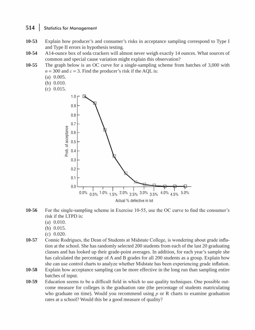
514 Statistics for Management
10-53 Explain how producer’s and consumer’s risks in acceptance sampling correspond to Type I and Type II errors in hypothesis testing.
10-54 A14-ounce box of soda crackers will almost never weigh exactly 14 ounces. What sources of common and special cause variation might explain this observation?
10-55 The graph below is an OC curve for a single-sampling scheme from batches of 3,000 with n = 300 and c = 3. Find the producer’s risk if the AQL is:(a) 0.005.(b) 0.010.(c) 0.015.
1.0
0.9
0.8
0.7
0.6
Prob
. of a
ccep
tanc
e
0.5
0.4
0.3
0.2
0.1
0.00.0% 0.5% 1.5% 2.5%
Actual % defective in lot
3.5% 4.5%1.0% 2.0% 3.0% 4.0% 5.0%
10-56 risk if the LTPD is:(a) 0.010.(b) 0.015.(c) 0.020.
10-57 -tion at the school. She has randomly selected 200 students from each of the last 20 graduating classes and has looked up their grade-point averages. In addition, for each year’s sample she has calculated the percentage of A and B grades for all 200 students as a group. Explain how
10-58 Explain how acceptance sampling can be more effective in the long run than sampling entire batches of input.
10-59 -come measure for colleges is the graduation rate (the percentage of students matriculating who graduate on time). Would you recommend using p or R charts to examine graduation rates at a school? Would this be a good measure of quality?
Quality and Quality Control 515
Flow Chart: Quality and Quality ControlSTART
STOP
Use control charts to monitorthe output of a process
Use TQM techiniques to identifyproblem causes, so the current
process can be improved
Track processmeans with
x chartsp. 470
Track processvariability
with R chartsp. 481
Track processattributes
with p chartsp. 487
Identify and groupcauses with
fishbone diagramsp. 495
Identify the“dragons” withPareto charts
p. 496
Use acceptance sampling tomonitor the input to a process
p. 500

This page is intentionally left blank
LEARNING OBJECTIVES
11After reading this chapter, you can understand:
CHAPTER CONTENTS
To recognize situations requiring the comparison of more than two means or proportions
To introduce the chi-square and F distributions and learn how to use them in statistical inferences
To use the chi-square distribution to see whether -
pendent of each other To use a chi-square test to check whether a
particular collection of data is well described
11.1 Introduction 51811.2 Chi-Square as a Test of Independence 51911.3 Chi-Square as a Test of Goodness of
Fit: Testing the Appropriateness of a Distribution 534
11.4 Analysis of Variance 54211.5 Inferences about a Population Variance 56811.6 Inferences about Two Population
Variances 576
intervals and testing hypotheses about a single population variance
To compare more than two population means using analysis of variance
To use the F distribution to test hypotheses about two population variances
Statistics at Work 583 Terms Introduced in Chapter 11 584 Equations Introduced in Chapter 11 585 Review and Application Exercises 587 Flow Chart: Chi-Square and Analysis
of Variance 594
Chi-Square and Analysis of Variance

518 Statistics for Management
The training director of a company is trying to evaluate three different methods of training new
factory. The second method puts all new employees in a training room separate from the factory, and
16 new employees assigned at random to the three training methods and records their daily production after they complete the programs:
Method 1 15 18 19 22 11Method 2 22 27 18 21 17Method 3 18 24 19 16 22 15
The director wonders whether there are differences in effectiveness among the methods. Using tech-niques learned in this chapter, we can help answer that question.
11.1 INTRODUCTIONIn Chapters 8 and 9, we learned how to test hypotheses using data from either one or two samples. We
hypothesized value. In the two-sample tests, we examined the difference between either two means or
of only two. In this case, the methods for comparing proportions described in Chapter 9 do not apply; we must use the chi-square test,this chapter. Chi-square tests enable us to test whether more than two population proportions can be considered equal.
Actually, chi-square tests allow us to do a lot more than just test for the equality of several propor-tions. If we classify a population into several categories with respect to two attributes (such as age and job performance), we can then use a chi-square test to determine whether the two attributes are indepen-dent of each other.
Managers also encounter situations in which it is useful to test for the equality of more than two population means. Again, we can-not apply the methods introduced in Chapter 9 because they are limited to testing for the equality of only two means. The analysis of variance, discussed in the fourth section of this chapter, will enable us to test whether more than two population means can be considered equal.
It is clear that we will not always be interested in means and proportions. There are many managerial situations where we will be concerned about the variability in a population. Section 11.5 shows
-tion variance. In Section 11.6, we show that hypotheses comparing the variances of two populations can be tested using the F distribution.
EXERCISES 11.111-1 Why do we use a chi-square test?11-2 Why do we use analysis of variance?
Uses of the chi-square test
Function of analysis of
variance
Inferences about population
variances
Chi-Square and Analysis of Variance 519
11-3 In each of the following situations, state whether a chi-square test, analysis of variance, or inference about population variances should be done.(a) We want to see whether the variance in spring temperatures is the same on the east and
west coasts.(b) We want to see whether the average speed on Interstate 95 differs depending on the day
of the week.
or large).(d) Before testing whether μ1 = μ2, we want to test whether the assumption that 1
222σ σ= is
reasonable.11-4 Answer true or false and explain your answers.
(a) After reading this chapter, you should know how to make inferences about two or more population variances.
(b) After reading this chapter, you should know how to make inferences about two or more population means.
(c) After reading this chapter, you should know how to make inferences about two or more population proportions.
11-5 To help remember which distribution or technique is used, complete the following table with
parameter involved. Some cells may not have an entry; others may have more than one pos-sible entry.
Type of Parameter
Number of Parameters Involved μ P
1
2
3 or more
11.2 CHI-SQUARE AS A TEST OF INDEPENDENCEMany times, managers need to know whether the differences they
due to chance. Suppose the campaign manager for a presidential
that 35, 42, and 51 percent, respectively, of the voters surveyed in -
(that is, if the manager concludes that the difference is solely due to chance), then he may decide that the place chosen to make a particular policy-making speech will have no effect on its reception. To run the campaign successfully, then, the manager needs to determine whether location and name recognition are dependent or independent.
Sample differences among
proportions: Significant or
not?
520 Statistics for Management
Contingency TablesSuppose that in four regions, the National Health Care Company samples its hospital employees’ attitudes toward job-performance reviews. Respondents are given a choice between the present method (two reviews a year) and a proposed new method (quarterly reviews). Table 11-1, which illustrates the response to this question from the sample polled, is called a contingency table. A table such as this is made up of rows and columns; rows run horizontally, columns
Table 11-1 is called a 2 × 4 contingency table because it consists of two rows and four columns. We
of columns. The “total” column and the “total” row are not counted as part of the dimensions.
Observed and Expected FrequenciesSuppose we now symbolize the true proportions of the total popula-tion of employees who prefer the present plan as
pN pS Proportion in Southeast who prefer present plan pC Proportion in Central region who prefer present plan pW Proportion in West Coast region who prefer present plan
Using these symbols, we can state the null and alternative hypotheses as follows:
H0: pN = pS = pS = pw ← Null hypothesis
H1: pN , pS , pC , and pW are not all equal ← Alternative hypothesis
If the null hypothesis is true, we can combine the data from the four samples and then estimate the pro-portion of the total workforce (the total population) that prefers the present review method:
68 75 57 79
100 120 90 110=
+ + ++ + +
279
420=
= 0.6643
Describing a contingency
table
Setting up the problem
symbolically
Combined proportion who prefer present method assuming the null hypothesis of no difference is true
TABLE 11-1 SAMPLE RESPONSE CONCERNING REVIEW SCHEDULES FOR NATIONAL HEALTH CARE HOSPITAL EMPLOYEES
Northeast Southeast Central West Coast TotalNumber who prefer present method 68 75 57 79 279Number who prefer new method 32 45 33 31 141Total employees sampled in each region 100 120 90 110 420
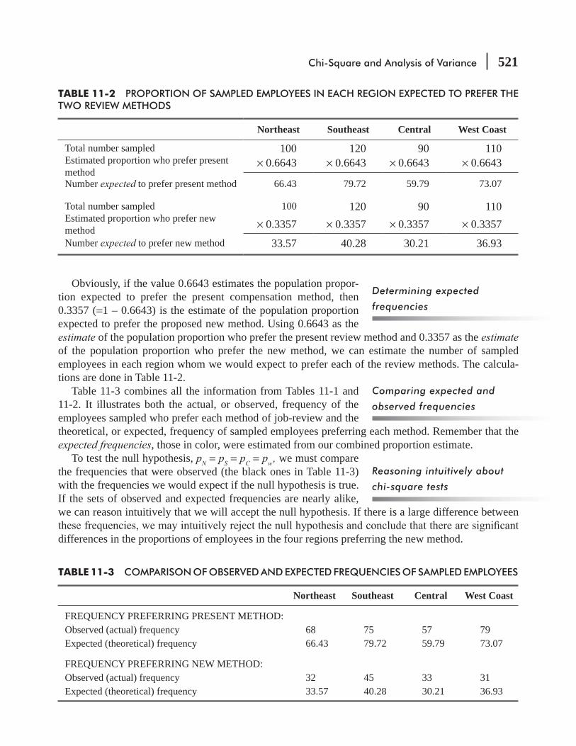
Chi-Square and Analysis of Variance 521
Obviously, if the value 0.6643 estimates the population propor-tion expected to prefer the present compensation method, then 0.3357 (=1 – 0.6643) is the estimate of the population proportion expected to prefer the proposed new method. Using 0.6643 as the estimate of the population proportion who prefer the present review method and 0.3357 as the estimate of the population proportion who prefer the new method, we can estimate the number of sampled employees in each region whom we would expect to prefer each of the review methods. The calcula-tions are done in Table 11-2.
Table 11-3 combines all the information from Tables 11-1 and 11-2. It illustrates both the actual, or observed, frequency of the employees sampled who prefer each method of job-review and the theoretical, or expected, frequency of sampled employees preferring each method. Remember that the expected frequencies, those in color, were estimated from our combined proportion estimate.
To test the null hypothesis, pN = pS = pC = pw , we must compare the frequencies that were observed (the black ones in Table 11-3) with the frequencies we would expect if the null hypothesis is true. If the sets of observed and expected frequencies are nearly alike, we can reason intuitively that we will accept the null hypothesis. If there is a large difference between
differences in the proportions of employees in the four regions preferring the new method.
Determining expected
frequencies
Comparing expected and
observed frequencies
Reasoning intuitively about
chi-square tests
Northeast Southeast Central West Coast
Total number sampledEstimated proportion who prefer present method
100 120 90 110× 0.6643 × 0.6643 × 0.6643 × 0.6643
Number expected to prefer present method 66.43 79.72 59.79 73.07
Total number sampledEstimated proportion who prefer new method
100 120 90 110× 0.3357 × 0.3357 × 0.3357 × 0.3357
Number expected to prefer new method 33.57 40.28 30.21 36.93
TABLE 11-2 PROPORTION OF SAMPLED EMPLOYEES IN EACH REGION EXPECTED TO PREFER THE TWO REVIEW METHODS
Northeast Southeast Central West Coast
FREQUENCY PREFERRING PRESENT METHOD:Observed (actual) frequency 68 75 57 79Expected (theoretical) frequency 66.43 79.72 59.79 73.07
FREQUENCY PREFERRING NEW METHOD:Observed (actual) frequency 32 45 33 31Expected (theoretical) frequency 33.57 40.28 30.21 36.93
TABLE 11-3 COMPARISON OF OBSERVED AND EXPECTED FREQUENCIES OF SAMPLED EMPLOYEES

522 Statistics for Management
The Chi-Square StatisticTo go beyond our intuitive feelings about the observed and expected frequencies, we can use the chi-square statistic, which is calculated this way:
Chi-Square Statistic
f f
f
( )o e
e
22
∑χ =−
An observed frequency An expected frequency
Chi-square Symbol meaning “the sum of”
[11-1]
This formula says that chi-square, or χ2, is the sum we will get if we
1. Subtract fe from fo for each of the eight values in Table 11-3. 2. Square each of the differences. 3. Divide each squared difference by fe. 4. Sum all eight of the answers.
Numerically, the calculations are easy to do using a table such as Table 11-4, which shows the steps.
The answer of 2.764 is the value for chi-square in our prob-lem comparing preferences for review methods. If this value were as large as, say, 20, it would indicate a substantial difference between our observed values and our
Calculating the chi-square
statistic
Interpreting the chi-square
statistic
Step 1 Step 2 Step 3
fo fe fo – fe (fo – fe)2
f f
f
( )o e
e
2−
68 66.43 1.57 2.46 0.037075 79.72 –4.72 22.28 0.279557 59.79 –2.79 7.78 0.130179 73.07 5.93 35.16 0.481232 33.57 –1.57 2.46 0.073345 40.28 4.72 22.28 0.553133 30.21 2.79 7.78 0.257531 36.93 –5.93 35.16 0.9521
2.7638
Step 4 ( )2
∑ −f f
fo e
e
= 2.764 ← χ 2 (chi-square)
TABLE 11-4 CALCULATION OF χ 2 (CHI-SQUARE) STATISTIC FROM DATA IN TABLE 11-3
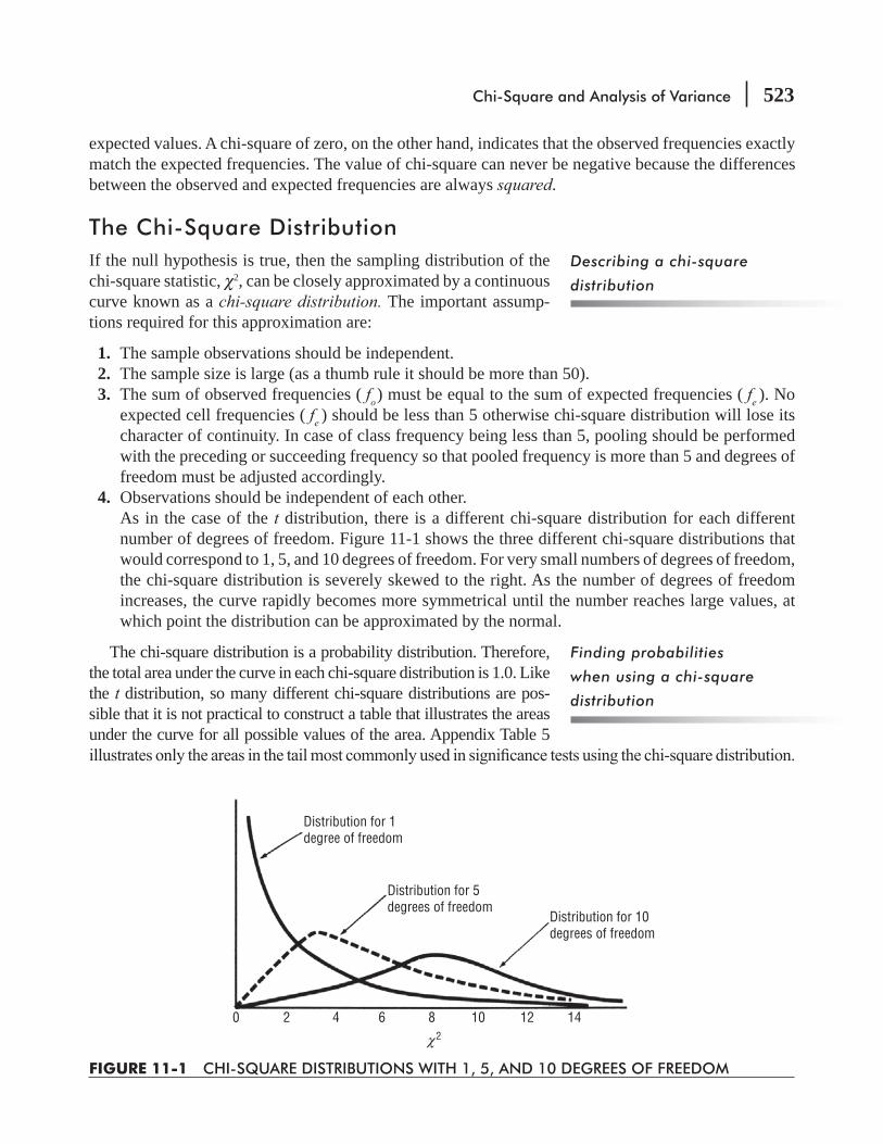
Chi-Square and Analysis of Variance 523
expected values. A chi-square of zero, on the other hand, indicates that the observed frequencies exactly match the expected frequencies. The value of chi-square can never be negative because the differences between the observed and expected frequencies are always squared.
The Chi-Square DistributionIf the null hypothesis is true, then the sampling distribution of the chi-square statistic, χ2, can be closely approximated by a continuous curve known as a chi-square distribution. The important assump-tions required for this approximation are:
1. The sample observations should be independent. 2. The sample size is large (as a thumb rule it should be more than 50). 3. The sum of observed frequencies ( fo ) must be equal to the sum of expected frequencies ( fe ). No
expected cell frequencies ( fe ) should be less than 5 otherwise chi-square distribution will lose its character of continuity. In case of class frequency being less than 5, pooling should be performed with the preceding or succeeding frequency so that pooled frequency is more than 5 and degrees of freedom must be adjusted accordingly.
4. Observations should be independent of each other. As in the case of the t distribution, there is a different chi-square distribution for each different
number of degrees of freedom. Figure 11-1 shows the three different chi-square distributions that would correspond to 1, 5, and 10 degrees of freedom. For very small numbers of degrees of freedom, the chi-square distribution is severely skewed to the right. As the number of degrees of freedom increases, the curve rapidly becomes more symmetrical until the number reaches large values, at which point the distribution can be approximated by the normal.
The chi-square distribution is a probability distribution. Therefore, the total area under the curve in each chi-square distribution is 1.0. Like the t distribution, so many different chi-square distributions are pos-sible that it is not practical to construct a table that illustrates the areas under the curve for all possible values of the area. Appendix Table 5
Describing a chi-square
distribution
Finding probabilities
when using a chi-square
distribution
Distribution for 1degree of freedom
Distribution for 5degrees of freedom
Distribution for 10degrees of freedom
0 2 4 6 8 10 12 14
χ2
FIGURE 11-1 CHI-SQUARE DISTRIBUTIONS WITH 1, 5, AND 10 DEGREES OF FREEDOM

524 Statistics for Management
Determining Degrees of FreedomTo use the chi-square test, we must calculate the number of degrees of freedom in the contingency table by applying Equation 11-2:
Degrees of Freedom in a Chi-Square Test of Independence
Number of degrees of freedom
= (number of rows – l)(number of columns – 1) [11-2]
Let’s examine the appropriateness of this equation. Suppose we have a 3 × 4 contingency table like the one in Figure 11-2. We know the row and column totals that are designated RT1, RT2, RT3, and CT1, CT2, CT3, CT4. As we discussed in Chapter 7, the number of degrees of freedom is equal to the number of values that we can freely specify.
already determined; we are not free to specify it because we know the row total.
denoted this fourth value by a circle. because we already know the
rst two entries in the rst column and the column total; again, we have denoted this entry with a circle. We can apply this same reasoning to the second and third entries in the third row, both of which have been denoted by circles, too.
number of checks in the contingency table in Figure 11-2, you can see that the number of values we are free to specify is 6 (the number of checks). This is equal to 2 × 3, or (the number of rows – 1) times (the number of columns – 1).
This is exactly what we have in Equation 11-2. Table 11-5 illustrates the row-and-column dimensions of three more contingency tables and indicates the appropriate degrees of freedom in each case.
Calculating degrees of
freedom
Column 1
Row 1
Row 2 Row totals
Column totals
Values that can befreely specified
Values that cannotbe freely specified
Row 3
Column 3 Column 4Column 2
CT1 CT2
RT1
RT2
RT3
CT3 CT4
FIGURE 11-2 A 3 × 4 CONTINGENCY TABLE ILLUSTRATING DETERMINATION OF THE NUMBER OF DEGREES OF FREEDOM

Chi-Square and Analysis of Variance 525
Using the Chi-Square TestReturning to our example of job-review preferences of National Health Care hospital employees, we use the chi-square test to determine whether attitude about reviews is independent of geographical region. If the company wants
H0: pN = pS = pC = pW ← Null hypothesis
H1: pN, pS, pC, and pW are not equal ← Alternative hypothesis
α = 0.10 s
Because our contingency table for this problem (Table 11-1) has two rows and four columns, the appropriate number of degrees of freedom is
Number of Degrees of Freedom
Number of rows Number of columns
(r – 1) (c – 1)[11-2]
= (2 – 1)(4 – 1)
= (1)(3)
= 3 ← Degrees of freedom
Figure 11-3 illustrates a chi-square distribution with 3 degrees of
the value of the chi-square statistic, 6.251. We can interpret this to mean that with 3 degrees of freedom, the region to the right of a chi-square value of 6.251 contains 0.10 of the area under the curve. Thus, the acceptance region for the null hypothesis in Figure 11-3 goes from the left tail of the curve to the chi-square value of 6.251.
As we can see from Figure 11-3, the sample chi-square value of 2.764 that we calculated in Table 11-4 falls within the acceptance region. Therefore, we accept the null hypothesis that there is no difference between the attitudes about job interviews in the four geographical regions. In other words, we conclude that attitude about perfor-mance reviews is independent of geography.
Stating the problem symbolically
Calculating degrees of freedom
Illustrating the hypothesis test
Interpreting the results
Contingency Table
Number of Rows (r)
Number of Columns (c) r – 1 c – 1
Degrees of Freedom(r – 1 )(c – 1)
A 3 4 3 – 1 = 2 4 – 1 = 3 (2)(3) = 60B 5 7 5 – 1 = 4 7 – 1 = 6 (4)(6) = 24C 6 9 6 – 1 = 5 9 – 1 = 8 (5)(8) = 40
TABLE 11-5 DETERMINATION OF DEGREES OF FREEDOM IN THREE CONTINGENCY TABLES

526 Statistics for Management
Days in Hospital<5 5-10 >10 Total
Fraction of costs covered by insurance
<25% 40 75 65 18025–50% 30 45 75 150 >50% 40 100 190 330
Total 110 220 330 660
TABLE 11-6 HOSPITAL-STAY DATA CLASSIFIED BY THE TYPE OF INSURANCE COVERAGE AND LENGTH OF STAY
FIGURE 11-3 CHI-SQUARE HYPOTHESIS TEST AT THE 0.10 LEVEL OF SIGNIFICANCE, SHOWING ACCEPTANCE REGION AND SAMPLE CHI-SQUARE VALUE OF 2.764
Acceptance regionAccept the null hypothesis if the
sample value is in this region
Chi-square distributionwith 3 degrees of freedom
Sample chi-squarevalue of 2.764
0.10 of area
2.764 6.251
Contingency Tables with More Than Two RowsMr. George McMahon, president of National General Health Insurance Company, is opposed to national health insurance. He argues that it would be too costly to implement, particularly since the existence of such a system would, among other effects, tend to encourage people to spend more time in hospitals. George believes that lengths of stays in hospitals are dependent on the types of health insurance that people have. He asked Donna McClish, his staff statistician, to check the matter. Donna collected data on a random sample of 660 hospital stays and summarized them in Table 11-6.
Table 11-6 gives observed frequencies in the nine different length-of-stay and type-of-insurance categories (or “cells”) into which we have divided the sample. Donna wishes to test the hypotheses:
H0: length of stay and type of insurance are independent
H1: length of stay depends on type of insurance
α = 0.01 ←
them by looking at the cell that corresponds to stays of less than 5 days and insurance covering less than 25 percent of costs.
Are hospital stay and
insurance coverage
independent?
Stating the hypotheses
Finding expected frequencies
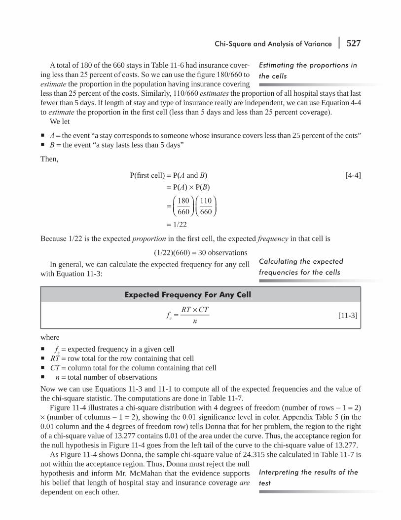
Chi-Square and Analysis of Variance 527
A total of 180 of the 660 stays in Table 11-6 had insurance cover-
estimate the proportion in the population having insurance covering estimates the proportion of all hospital stays that last
fewer than 5 days. If length of stay and type of insurance really are independent, we can use Equation 4-4 to estimate
We let
A = the event “a stay corresponds to someone whose insurance covers less than 25 percent of the cots” B = the event “a stay lasts less than 5 days”
Then,
= P(A and B) [4-4] = P(A) × P(B)
180
660
110
660=
⎛⎝⎜
⎞⎠⎟
⎛⎝⎜
⎞⎠⎟
=
proportion frequency in that cell is
= 30 observationsIn general, we can calculate the expected frequency for any cell
with Equation 11-3:
Expected Frequency For Any Cell
=×
fRT CT
ne [11-3]
where fe = expected frequency in a given cell RT = row total for the row containing that cell CT = column total for the column containing that cell n = total number of observations
Now we can use Equations 11-3 and 11-1 to compute all of the expected frequencies and the value of the chi-square statistic. The computations are done in Table 11-7.
Figure 11-4 illustrates a chi-square distribution with 4 degrees of freedom (number of rows − 1 = 2) × (number of columns – 1 =0.01 column and the 4 degrees of freedom row) tells Donna that for her problem, the region to the right of a chi-square value of 13.277 contains 0.01 of the area under the curve. Thus, the acceptance region for the null hypothesis in Figure 11-4 goes from the left tail of the curve to the chi-square value of 13.277.
As Figure 11-4 shows Donna, the sample chi-square value of 24.315 she calculated in Table 11-7 is not within the acceptance region. Thus, Donna must reject the null hypothesis and inform Mr. McMahan that the evidence supports his belief that length of hospital stay and insurance coverage are dependent on each other.
Calculating the expected
frequencies for the cells
Interpreting the results of the
test
Estimating the proportions in
the cells

528 Statistics for Management
Row Column fo fe = RT CT
n
× fo – fe (fo – fe)2 f f
f
( )o e
e
2−
1 1 40 30 180 110
660
× 10 100 3.333
1 2 75 60 180 220
660
× 15 225 3.750
1 3 65 90 180 330
660
× –25 625 6.944
2 1 30 25 150 110
660
× 5 25 1.000
2 2 45 50 150 220
660
× –5 25 0.500
2 3 75 75 150 330
660
× 0 0 0.000
3 1 40 55 330 110
660
× –15 225 4.091
3 2 100 110 330 220
660
× –10 100 0.909
3 3 190 165 330 330
660
× 25 625 3.788
[11-1] ( )o e
e
2f f
f∑ − = 24.315 ← χ2 (chi-square)
TABLE 11-7 CALCULATION OF EXPECTED FREQUENCIES AND CHI-SQUARE FROM DATA IN TABLE 11-6
FIGURE 11-4 CHI-SQUARE HYPOTHESIS TEST AT THE 0.01 LEVEL OF SIGNIFICANCE, SHOWING ACCEPTANCE REGION AND SAMPLE CHI-SQUARE VALUE OF 24.315
Acceptance regionAccept the null hypothesis if the
sample value is in this regionChi-squaredistribution
0.01 of area
13.277Sample χ2 valueof 24.315

Chi-Square and Analysis of Variance 529
Precautions about Using the Chi-Square TestTo use a chi-square hypothesis test, we must have a sample size large enough to guarantee the similarity between the theoretically correct distribution and our sampling distribution of χ2, the chi-square statistic. When the expected fre-quencies are too small, the value of χ2 will be overestimated and will result in too many rejections of the null hypothesis. To avoid making incorrect inferences from χ2 hypothesis tests, follow the general rule that an expected frequency of less than 5 in one cell of a contingency table is too small to use.* When the table contains more than one cell with an expected frequency of less than 5, we can combine these in order to get an expected frequency of 5 or more. But in doing this, we reduce the number of categories of data and will gain less information from the contingency table.
This rule will enable us to use the chi-square hypothesis test prop-
the quality of the data we feed into it. So far, we have rejected the
- But if the chi-square value
was zero, we should be careful to question whether absolutely no difference exists between observed and expected frequencies. If we have strong feelings that some difference ought to exist, we should examine either the way the data were collected or the manner in which measurements were taken, or both, to be certain that existing differences were not obscured or missed in collecting sample data.
In the 1860s, experiments with the characteristics of peas led the monk Gregor Mendel to propose the existence of genes. Mendel’s experimental results were astoundingly close to those predicted by his theory. A century later, statisticians looked at Mendel’s “pea data,” performed a chi-square test, and concluded that chi-square was too small; that is, Mendel’s reported experimental data were so close to what was expected that they could only conclude that he had fudged the data.
Chi-Square Test Using SPSS
*Statisticians have developed correction factors that, in some cases, allow us to use cells with expected frequencies of less than 5. The derivation and use of these correction factors are beyond the scope of this book.
Use large sample sizes
Use carefully collected data
Mendel’s pea data

530 Statistics for Management
The preceding data are used for chi-square test.In order to determine customer satisfaction rates, a retail company conducted surveys of 582 cus-
tomers at 4 store locations. From the survey results, you found that the quality of customer service was the most important factor to a customer’s overall satisfaction. Given this information, you want to test whether each of the store locations provides a similar and adequate level of customer service.
For χ2 test go to Analyze > Descriptive statistics > Crosstabs > Select rows and columns > Select Chi-square > OK.
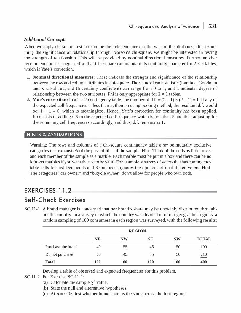
Chi-Square and Analysis of Variance 531
Additional ConceptsWhen we apply chi-square test to examine the independence or otherwise of the attributes, after exam-
’s chi-square, we might be interested in testing the strength of relationship. This will be provided by nominal directional measures. Further, another recommendation is suggested so that Chi-square can maintain its continuity character for 2 × 2 tables, which is Yate’s correction.
1. Nominal directional measures:between the row and column attributes in chi-square. The value of each statistic (Lambda, Goodman
relationship between the two attributes. Phi is only appropriate for 2 × 2 tables. 2. Yate’s correction: In a 2 × 2 contingency table, the number of d.f. = (2 − 1) × (2 − 1) = 1. If any of
the expected cell frequencies is less than 5, then on using pooling method, the resultant d.f. would be: 1 − 1 = 0, which is meaningless. Hence, Yate’s correction for continuity has been applied. It consists of adding 0.5 to the expected cell frequency which is less than 5 and then adjusting for the remaining cell frequencies accordingly, and thus, d.f. remains as 1.
Warning: The rows and columns of a chi-square contingency table must be mutually exclusive categories that exhaust all of the possibilities of the sample. Hint: Think of the cells as little boxes and each member of the sample as a marble. Each marble must be put in a box and there can be no leftover marbles if you want the test to be valid. For example, a survey of voters that has contingency
The categories “car owner” and “bicycle owner” don’t allow for people who own both.
HINTS & ASSUMPTIONS
EXERCISES 11.2
Self-Check ExercisesSC 11-1 A brand manager is concerned that her brand’s share may be unevenly distributed through-
out the country. In a survey in which the country was divided into four geographic regions, a random sampling of 100 consumers in each region was surveyed, with the following results:
REGION
NE NW SE SW TOTAL
Purchase the brand 40 55 45 50 190
Do not purchase 60 45 55 50 210
Total 100 100 100 100 400
Develop a table of observed and expected frequencies for this problem.SC 11-2 For Exercise SC 11-1:
(a) Calculate the sample χ 2 value.(b) State the null and alternative hypotheses.(c) At α = 0.05, test whether brand share is the same across the four regions.
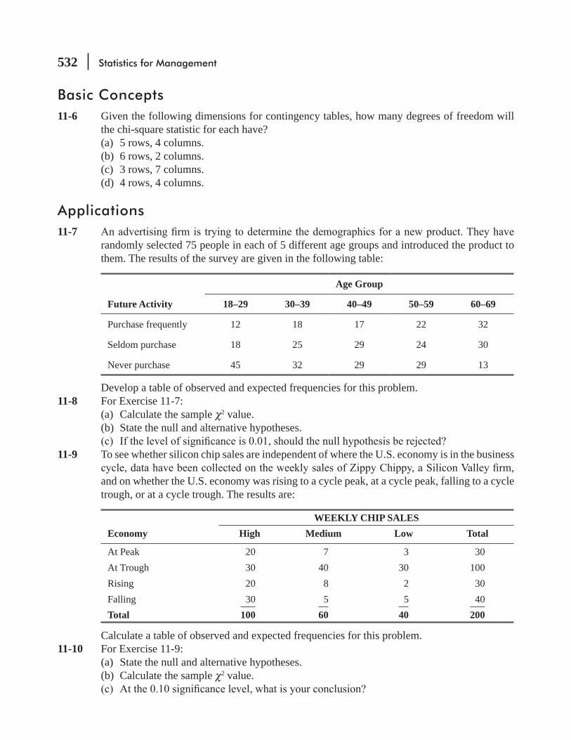
532 Statistics for Management
Basic Concepts11-6 Given the following dimensions for contingency tables, how many degrees of freedom will
the chi-square statistic for each have?(a) 5 rows, 4 columns.(b) 6 rows, 2 columns.(c) 3 rows, 7 columns.(d) 4 rows, 4 columns.
Applications11-7
randomly selected 75 people in each of 5 different age groups and introduced the product to them. The results of the survey are given in the following table:
Age Group
Future Activity 18–29 30–39 40–49 50–59 60–69
Purchase frequently 12 18 17 22 32
Seldom purchase 18 25 29 24 30
Never purchase 45 32 29 29 13
Develop a table of observed and expected frequencies for this problem.11-8 For Exercise 11-7:
(a) Calculate the sample χ2 value.(b) State the null and alternative hypotheses.
11-9 To see whether silicon chip sales are independent of where the U.S. economy is in the business
and on whether the U.S. economy was rising to a cycle peak, at a cycle peak, falling to a cycle trough, or at a cycle trough. The results are:
WEEKLY CHIP SALESEconomy High Medium Low Total
At Peak 20 7 3 30At Trough 30 40 30 100Rising 20 8 2 30Falling 30 5 5 40Total 100 60 40 200
Calculate a table of observed and expected frequencies for this problem.11-10 For Exercise 11-9:
(a) State the null and alternative hypotheses.(b) Calculate the sample χ2 value.
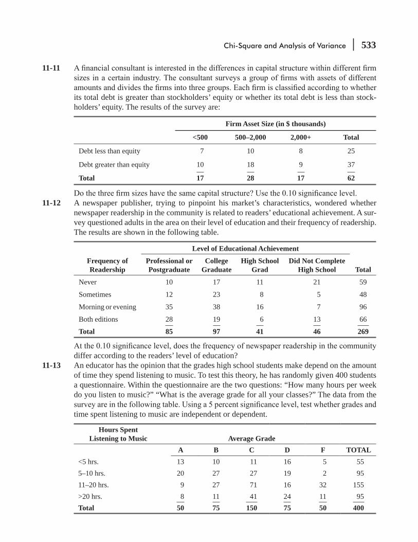
Chi-Square and Analysis of Variance 533
11-11
its total debt is greater than stockholders’ equity or whether its total debt is less than stock-holders’ equity. The results of the survey are:
Firm Asset Size (in $ thousands)
<500 500–2,000 2,000+ Total
Debt less than equity 7 10 8 25
Debt greater than equity 10 18 9 37
Total 17 28 17 62
11-12 A newspaper publisher, trying to pinpoint his market’s characteristics, wondered whether newspaper readership in the community is related to readers’ educational achievement. A sur-vey questioned adults in the area on their level of education and their frequency of readership. The results are shown in the following table.
Level of Educational Achievement
Frequency of Readership
Professional or Postgraduate
College Graduate
High School Grad
Did Not Complete High School Total
Never 10 17 11 21 59
Sometimes 12 23 8 5 48
Morning or evening 35 38 16 7 96
Both editions 28 19 6 13 66
Total 85 97 41 46 269
differ according to the readers’ level of education?11-13 An educator has the opinion that the grades high school students make depend on the amount
of time they spend listening to music. To test this theory, he has randomly given 400 students a questionnaire. Within the questionnaire are the two questions: “How many hours per week do you listen to music?” “What is the average grade for all your classes?” The data from the
time spent listening to music are independent or dependent.
Hours Spent Listening to Music Average Grade
A B C D F TOTAL<5 hrs. 13 10 11 16 5 555–10 hrs. 20 27 27 19 2 9511–20 hrs. 9 27 71 16 32 155>20 hrs. 8 11 41 24 11 95Total 50 75 150 75 50 400
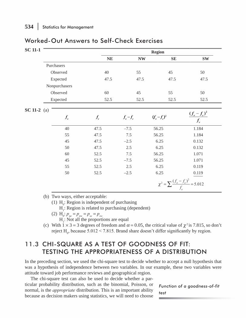
534 Statistics for Management
Worked-Out Answers to Self-Check ExercisesSC 11-1 Region
NE NW SE SWPurchasers Observed 40 55 45 50 Expected 47.5 47.5 47.5 47.5Nonpurchasers Observed 60 45 55 50 Expected 52.5 52.5 52.5 52.5
SC 11-2 (a) fo fe fo – fe (fo – fe )
2f f
f
( )o e
e
2−
40 47.5 –7.5 56.25 1.18455 47.5 7.5 56.25 1.18445 47.5 –2.5 6.25 0.13250 47.5 2.5 6.25 0.13260 52.5 7.5 56.25 1.07145 52.5 –7.5 56.25 1.07155 52.5 2.5 6.25 0.11950 52.5 –2.5 6.25 0.119
( )5.012o e
e
22f f
f∑χ =
−=
(b) Two ways, either acceptable: (1) H0: Region is independent of purchasing H1: Region is related to purchasing (dependent) (2) H0: pne = pnw = pse = psw H1: Not all the proportions are equal(c) With 1 × 3 = 3 degrees of freedom and α = 0.05, the critical value of χ 2 is 7.815, so don’t
reject H0
11.3 CHI-SQUARE AS A TEST OF GOODNESS OF FIT: TESTING THE APPROPRIATENESS OF A DISTRIBUTION
In the preceding section, we used the chi-square test to decide whether to accept a null hypothesis that was a hypothesis of independence between two variables. In our example, these two variables were attitude toward job performance reviews and geographical region.
The chi-square test can also be used to decide whether a par-ticular probability distribution, such as the binomial, Poisson, or normal, is the appropriate distribution. This is an important ability because as decision makers using statistics, we will need to choose
Function of a goodness-of-fit
test
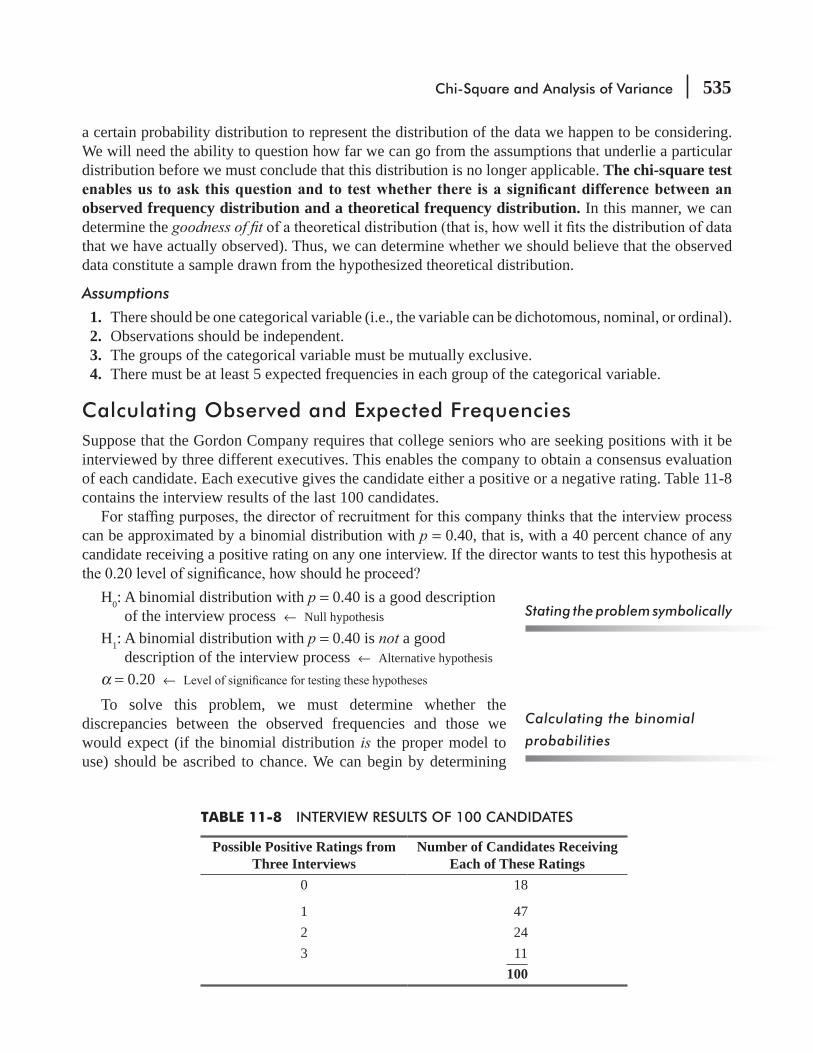
Chi-Square and Analysis of Variance 535
a certain probability distribution to represent the distribution of the data we happen to be considering. We will need the ability to question how far we can go from the assumptions that underlie a particular distribution before we must conclude that this distribution is no longer applicable. The chi-square test
observed frequency distribution and a theoretical frequency distribution. In this manner, we can determine the goodness of tthat we have actually observed). Thus, we can determine whether we should believe that the observed data constitute a sample drawn from the hypothesized theoretical distribution.
Assumptions 1. There should be one categorical variable (i.e., the variable can be dichotomous, nominal, or ordinal). 2. Observations should be independent. 3. The groups of the categorical variable must be mutually exclusive. 4. There must be at least 5 expected frequencies in each group of the categorical variable.
Calculating Observed and Expected FrequenciesSuppose that the Gordon Company requires that college seniors who are seeking positions with it be interviewed by three different executives. This enables the company to obtain a consensus evaluation of each candidate. Each executive gives the candidate either a positive or a negative rating. Table 11-8 contains the interview results of the last 100 candidates.
can be approximated by a binomial distribution with p = 0.40, that is, with a 40 percent chance of any candidate receiving a positive rating on any one interview. If the director wants to test this hypothesis at
H0: A binomial distribution with p = 0.40 is a good description of the interview process ← Null hypothesis
H1: A binomial distribution with p = 0.40 is not a good description of the interview process ← Alternative hypothesis
α = 0.20 ← To solve this problem, we must determine whether the
discrepancies between the observed frequencies and those we would expect (if the binomial distribution is the proper model to use) should be ascribed to chance. We can begin by determining
Stating the problem symbolically
Calculating the binomial
probabilities
Possible Positive Ratings from Three Interviews
Number of Candidates Receiving Each of These Ratings
0 18
1 472 243 11
100
TABLE 11-8 INTERVIEW RESULTS OF 100 CANDIDATES

536 Statistics for Management
what the binomial probabilities would be for this interview situation. For three interviews, we would
column labeled n = 3 and p = 0.40. The results are summarized in Table 11-9.Now we can use the theoretical binomial probabilities of the outcomes to compute the expected frequen-
cies. By comparing these expected frequencies with our observed frequencies using the χ2 test, we can examine the extent of the difference between them. Table 11-10 lists the observed frequencies, the appropri-ate binomial probabilities from Table 11-9, and the expected frequencies for the sample of 100 interviews.
Possible Positive Ratings from Three Interviews
Binomial Probabilities of These Outcomes
0 0.2160
1 0.43202 0.28803 0.0640
1.0000
TABLE 11-9 BINOMIAL PROBABILITIES FOR INTERVIEW PROBLEM
TABLE 11-10 OBSERVED FREQUENCIES, APPROPRIATE BINOMIAL PROBABILITIES, AND EXPECTED FREQUENCIES FOR THE INTERVIEW PROBLEM
Possible Positive Ratings
from Three Interviews
Observed Frequency of Candidates
Receiving These Ratings
Binomial Probability of Possible Outcomes
Number of Candidates Interviewed
Expected Frequency of Candidates
Receiving These Ratings
0 18 0.2160 × 100 = 21.6
1 47 0.4320 × 100 = 43.2
2 24 0.2880 × 100 = 28.8
3 11 0.0640 × 100 = 6.4
100 1.0000 100.0
Calculating the Chi-Square StatisticTo compute the chi-square statistic for this problem, we can use Equation 11-1:
f f
f
( )o e
e
22
∑χ =−
[11-1]
and the format we introduced in Table 11-4. This process is illustrated in Table 11-11.
Determining Degrees of Freedom in a Goodness-of-Fit TestBefore we can calculate the appropriate number of degrees of free-
-ber of classes (symbolized k) for which we have compared the
First, count the number of
classes

Chi-Square and Analysis of Variance 537
observed and expected frequencies. Our interview problem contains four such classes: 0, 1, 2, and 3 positive ratings. Thus, we begin with 4 degrees of freedom. Yet because the four observed frequencies must sum to 100, the total number of observed frequencies we can freely specify is only k – 1, or 3. The fourth is determined because the total of the four has to be 100.
additional restrictions on the calculation of the degrees of freedom.
-quencies. If we have six classes of observed frequencies (k = 6), then we would conclude that we have only k – 1, or 5 degrees of freedom. If, however, we also have to use the sample mean as an estimate of the population mean, we will have to subtract an additional degree of freedom, which leaves us with only 4. And, third, if we have to use the sample standard deviation to esti-mate the population standard deviation, we will have to subtract one more degree of freedom, leaving us with 3. Our general rule in these cases is, (k – 1) rule and then subtract an additional degree of freedom for each population parameter that has to be estimated from the sample data.
In the interview example, we have four classes of observed frequencies. As a result, k = 4, and the appropriate number of degrees of freedom is k – 1, or 3. We are not required to estimate any population parameter, so we need not reduce this number further.
Using the Chi-Square Goodness-of-Fit TestIn the interview problem, the company desires to test the hypothesis
Table 5, then, we must look under the 0.20 column and move down
We can interpret this value as follows: With 3 degrees of freedom, the region to the right of a chi-square value of 4.642 contains 0.20 of the area under the curve.
Figure 11-5 illustrates a chi-square distribution with 3 degrees
that the acceptance region for the null hypothesis (the hypothesis that the sample data came from a binomial distribution with p = 0.4) extends from the left tail to the chi-square value of 4.642. Obviously,
Then, subtract degrees of
freedom lost from estimating
population parameters
Finding the limit of the
acceptance region
Illustrating the problem
Observed Frequency
(fo)
Expected Frequency
(fe) fo – fe (fo – fe)2
( )o e
e
2−f f
f
18 21.6 –3.6 12.96 0.600047 43.2 3.8 14.44 0.334324 28.8 –4.8 23.04 0.800011 6.4 4.6 21.16 3.3063
5.0406
( )o e
e
2
∑ −f f
f = 5.0406 ← χ 2
TABLE 11-11 CALCULATION OF THE 2 STATISTIC FROM THE INTERVIEW DATA LISTED IN TABLE 11-10

538 Statistics for Management
the sample chi-square value of 5.0406 falls outside this accep-tance region. Therefore, we reject the null hypothesis and conclude that the binomial distribution with p = 0.4 fails to provide a good description of our observed frequencies.
can do the calculations. But fewer of them can explain the logic in using the test for this purpose in common-sense terms. Hint: If we have a distribution that we think may be normal, but we’re not sure, we use a known normal distribution to generate the expected values and then using chi-square methods, we see how much difference there is between these expected values and the values we observed in a sample taken from the distribution we think is normal. If the difference is too large, our distribution isn’t normal.
HINTS & ASSUMPTIONS
EXERCISES 11.3
Self-Check ExercisesSC 11-3
a Poisson distribution with λ = 3?
Number of arrivals per hour 0 1 2 3 4 5 or moreNumber of hours 20 57 98 85 78 62
SC 11-4 After years of working at a weighing station for trucks, Jeff Simpson feels that the weight per truck (in thousands of pounds) follows a normal distribution with μ = 71 and σ = 15. In order to test this assumption, Jeff collected the following data one Monday, recording the weight of each truck that entered his station.
Acceptance regionAccept the null hypothesis if the
sample value is in this region
0.20 of area
4.642
Sample chi-squarevalue of 5.0406
FIGURE 11-5 GOODNESS-OF-FIT TEST AT THE 0.20 LEVEL OF SIGNIFICANCE, SHOWING ACCEPTANCE REGION AND SAMPLE CHI-SQUARE VALUE OF 5.0406
Interpreting the results

Chi-Square and Analysis of Variance 539
85 57 60 81 89 63 52 65 77 6489 86 90 60 57 61 95 78 66 9250 56 95 60 82 55 61 81 61 5363 75 50 98 63 77 50 62 79 6976 66 97 67 54 93 70 80 67 73
of interest.) (Hint:
Basic Concepts11-14 Below is an observed frequency distribution. Using a normal distribution with μ = 5 and σ = 1.5,
(a) Find the probability of falling in each class.(b) From part (a), compute the expected frequency of each category.(c) Calculate the chi-square statistic.
by the suggested normal distribution?Observed value of the variable <2.6 2.6–3.79 3.8–4.99 5–6.19 6.2–7.39 ≥7.4Observed frequency 6 30 41 52 12 9
11-15 -bution with λ = 5?
Number of calls per minute 0 1 2 3 4 5 6 7 or moreFrequency of occurrences 4 15 42 60 89 94 52 80
Applications11-16
It is suggested that the variable, sales by Mr. Armstrong, may be described by the binomial distribution, with the probability of selling each account being 0.4. Given the following fre-quency distribution of Armstrong’s number of sales per day, can we conclude that the data do
Number of sales per day 0 1 2 3 4 5Frequency of the number of sales 10 41 60 20 6 3
11-17 The computer coordinator for the business school believes the amount of time a graduate student spends reading and writing e-mail each weekday is normally distributed with mean μ = 14 and standard deviation σ = 5. In order to examine this belief, the coordinator collected data one Wednesday, recording the amount of time in minutes each graduate student spent
-
your hypotheses.) (Hint:8.2 7.4 9.6 12.8 22.4 6.2 8.7 9.7 12.4 10.61.2 18.6 3.3 15.7 18.4 12.4 15.9 19.4 12.8 20.412.3 11.3 10.9 18.4 14.3 16.2 6.7 13.9 18.3 19.214.3 14.9 16.7 11.3 18.4 18.8 20.4 12.4 18.1 20.1

540 Statistics for Management
11-18 In order to plan how much cash to keep on hand in the vault, a bank is interested in seeing whether the average deposit of a customer is normally distributed. A newly hired employee hoping for a raise has collected the following information:
Deposit $0–$999 $1,000–$1,999 $2,000 or moreObserved frequency 20 65 25
(a) Compute the expected frequencies if the data are normally distributed with mean $1,500 and standard deviation $600.
(b) Compute the chi-square statistic.(c) State explicit null and alternative hypotheses.(d) Test your hypotheses at the 0.10 level and state an explicit conclusion.
11-19
so big, it can be assumed that two letters’ chances of being mangled are independent. A sample of 310 people was selected and two test letters were mailed to each of them. The number of people receiving zero, one, or two mangled letters was 260, 40, and 10, respectively. At the
received by people follows a binomial distribution with p = 0.15?11-20 A state lottery commission claims that for a new lottery game, there is a 10 percent chance of
getting a $1 prize, a 5 percent chance of $100, and an 85 percent chance of getting nothing. To test whether this claim is correct, a winner from the last lottery went out and bought 1,000 tickets for the new lottery. He had 87 one-dollar prizes, 48 hundred-dollar prizes, and 865
11-21 Dennis Barry, a hospital administrator, has examined past records from 210 randomly selected 8-hour shifts to determine the frequency with which the hospital treats fractures. The numbers
reasonably believe that the incidence of broken-bone cases follows a Poisson distribution with λ = 2?
11-22 -
pling of 60 days:Number of shifts during which alarms were received 0 1 2 3Number of days 16 27 11 6
(Hint: Combine the last two groups so that all expected frequencies are greater than 5.)
11-23 A diligent statistics student wants to see whether it is reasonable to assume that some sales data have been sampled from a normal population before performing a hypothesis test on the mean sales. She collected some sales data, computed x = 78 and s = 9, and tabulated the data as follows:
Sales level ≤65 66–70 71–75 76–80 81–85 ≥86Number of observations 10 20 40 50 40 40
(a) Is it important for the statistics student to check whether the data are normally distributed? Explain.

Chi-Square and Analysis of Variance 541
(b) State explicit null and alternative hypotheses for checking whether the data are normally distributed.
(c) What is the probability (using a normal distribution with μ = 78 and σ = 9) that sales will be less than or equal to 65.5, between 65.5 and 70.5, between 70.5 and 75.5, between 75.5 and 80.5; between 80.5 and 85.5, and greater than or equal to 85.5?
-mal distribution?
11-24 A supermarket manager is keeping track of the arrival of customers at checkout counters to
periods, there were 22, 74, 115, 95, 94, 80, and 20 periods in which zero, one, two, three,
λ = 3?
Worked-Out Answers to Self-Check ExercisesSC 11-3 H0: Poisson with λ = 3
H1: Something elseTest at α = 0.10, with 6 – 1 = 5 degrees of freedom.
Arrivals/hour 0 1 2 3 4 5+
Poisson prob. 0.0498 0.1494 0.2240 0.2240 0.1680 0.1848
Observed 20 57 98 85 78 62
Expected 19.92 59.76 89.60 89.60 62.20 73.92
f f
f
( )o e
e
2−− 0.000 0.127 0.788 0.236 1.736 1.922
f f
f
( )4.809o e
e
22
∑χ =−
=
With 5 degrees of freedom and α = 0.10, the critical value of χ2 is 9.236, so don’t reject H0, because 4.809 < 9.236. The data are well described by a Poisson distribution with λ = 3.
SC 11-4 5 equiprobable intervals; 0.2 probability for each interval, 50 × 0.2 = 10 trucks expected per interval.z – ∞ – 0.84 – 0.25 0.25 0.84 + ∞
x = 71 + 15z – ∞ 58.40 67.25 74.75 83.60 + ∞
Observed 10 16 3 10 11Expected 10 10 10 10 10
f f
f
( )o e
e
2−0.0 3.6 4.9 0.0 0.1
χ 2 = 8.6

542 Statistics for Management
H0: Truck weights are distributed normally with μ = 71 and σ = 15H1: The weights are distributed differently (either normal with a different μ σ or a non-
normal distribution)
With 5 – 1 = 4 degrees of freedom and α = 0.10, the critical value of χ2 is 7.779, so reject H0, because 8.6 > 7.779. The data are not well described by a normal distribution with μ = 71 and σ = 15. Jeff is wrong.
11.4 ANALYSIS OF VARIANCEEarlier in this chapter, we used the chi-square test to examine the differences among more than two sample proportions and to make inferences about whether such samples are drawn from populations each having the same proportion. In this section, we will learn a technique known as analysis of vari-ance (often abbreviated among more than two sample means. Using analysis of variance, we will be able to make inferences about whether our samples are drawn from populations having the same mean.
Analysis of variance is useful in such situations as comparing
which of four different training methods produces the fastest learn-
half a dozen different business schools. In each of these cases, we would compare the means of more than two samples.
Statement of the ProblemIn the training director’s problem that opened this chapter, she wanted to evaluate three different train-ing methods to determine whether there were any differences in effectiveness.
After completion of the training period, the company’s statisti-cal staff chose 16 new employees assigned at random to the three training methods.* Counting the production output by these 16 trainees, the staff has summarized the data and calculated the mean production of the trainees (see Table 11-12). Now if we wish to determine the grand mean, or x (the mean for the entire group of 16 trainees), we can use one of two methods:
1. 15 18 19 22 11 22 27 18 21 17 18 24 19 16 22 15
16=
+ + + + + + + + + + + + + + +x
304
16=
= 19 ← Grand mean using all data
2. x =
304
16=
= 19 ← Grand mean as a weighted average of the sample means, using the relative sample sizes as the weights
* Although in real practice, 16 trainees would not constitute an adequate statistical sample, we have limited the number here to be able to demonstrate the basic techniques of analysis of variance and to avoid tedious calculations.
Function of analysis of
variance
Situations where we can use
ANOVA
Calculating the grand mean
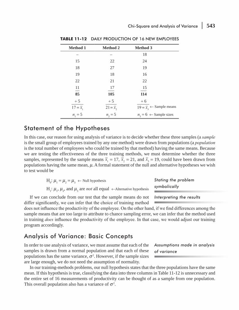
Chi-Square and Analysis of Variance 543
Statement of the HypothesesIn this case, our reason for using analysis of variance is to decide whether these three samples (a sample is the small group of employees trained by any one method) were drawn from populations (a population is the total number of employees who could be trained by that method) having the same means. Because we are testing the effectiveness of the three training methods, we must determine whether the three samples, represented by the sample means 1x = 17, 2x = 21, and 3x = 19, could have been drawn from populations having the same mean, μ. A formal statement of the null and alternative hypotheses we wish to test would be
H0: μ1 = μ2 = μ3 ← Null hypothesis
H1: μ1, μ2, and μ3 are not all equal ←Alternative hypothesis
If we can conclude from our test that the sample means do not
sample means that are too large to attribute to chance sampling error, we can infer that the method used in training doesprogram accordingly.
Analysis of Variance: Basic ConceptsIn order to use analysis of variance, we must assume that each of the samples is drawn from a normal population and that each of these populations has the same variance, σ 2. However, if the sample sizes are large enough, we do not need the assumption of normality.
In our training-methods problems, our null hypothesis states that the three populations have the same mean. If this hypothesis is true, classifying the data into three columns in Table 11-12 is unnecessary and the entire set of 16 measurements of productivity can be thought of as a sample from one population. This overall population also has a variance of σ 2.
Stating the problem
symbolically
Interpreting the results
Assumptions made in analysis
of variance
Method 1 Method 2 Method 3– – 18
15 22 2418 27 1919 18 1622 21 2211 17 1585 105 114
÷ 5 ÷ 5 ÷ 6x17 1= x21 2= x19 3= ← Sample means
n1 = 5 n2 = 5 n3 = 6 ← Sample sizes
TABLE 11-12 DAILY PRODUCTION OF 16 NEW EMPLOYEES
544 Statistics for Management
Analysis of variance is based on a comparison of two different estimates of the variance, σ 2, of our overall population. In this case, we can calculate one of these estimates by examining the vari-ance among the three sample means, which are 17, 21, and 19. The other estimate of the population variance is determined by the variation within the three samples themselves, that is, (15, 18, 19, 22, 11), (22, 27, 18, 21, 17), and (18, 24, 19, 16, 22, 15). Then we compare these two estimates of the popu-lation variance. Because both are estimates of σ 2, they should be approximately equal in value when the null hypothesis is true. If the null hypothesis is not true, these two estimates will differ considerably. The three steps in analysis of variance, then, are
1. Determine one estimate of the population variance from the variance among the sample means.
2. Determine a second estimate of the population variance from the variance within the samples. 3. Compare these two estimates. If they are approximately equal in value, accept the null hypothesis.
In the remainder of this section, we shall learn how to calculate these two estimates of the popula-tion variance, how to compare these two estimates, and how to perform a hypothesis test and interpret the results. As we learn how to do these computations, however, keep in mind that all are based on the above three steps.
Calculating the Variance among the Sample MeansStep 1 in analysis of variance indicates that we must obtain one estimate of the population variance from the variance among the three sample means. In statistical language, this estimate is called the between-column variance.
In Chapter 3, we used Equation 3-17 to calculate the sample variance:
Sample variance sx x
n
( )
12
2
=∑ −
− [3-17]
Now, because we are working with three sample means and a grand mean, let’s substitute x for x, x for x , and k (the number of samples) for n to get a formula for the variance among the sample means:
Variance among the Sample Means
( )
12
2
=∑ −
−s
x x
kx[11-4]
the standard error of the mean as the standard deviation of all pos-sible samples of a given size. The formula to derive the standard error of the mean is Equation 6-1:
nxσ σ
=Standard error of the mean (standard deviation of all possible sample means from a given sample size
Population standard deviation
Square root of the sample size
[6-1]
Steps in analysis of variance
Finding the first estimate of
the population variance
First, find the variance among
sample means
Then, find the population
variance using the variance
among sample means
Chi-Square and Analysis of Variance 545
We can simplify this equation by cross-multiplying the terms and then squaring both sides in order to change the population standard deviation, σ, into the population variance, σ 2:
Population Variance
Standard error squared (this is the variance among the sample means)
nx2 2σ σ= ×
[11-5]
For our training-method problem, we do not have all the information we need to use this equation to σ 2
x2σ . We could, however, calculate the variance among the three
sample means, sx2 , using Equation 11-4. So why not substitute sx
2 for x2σ in Equation 11-5 and calculate
an estimate of the population variance? This will give us
ˆ( )
12 2
2
σ = × =∑ −
−s n
n x x
kx
Equation 6-1, n represents the sample size, but which sample size should we use when the different samples have different sizes? We solve this problem with Equation 11-6, where each ( )2−x xj
is multiplied by its own appropriate nj.
Estimate of Between-Column Variance
First estimate of the population variance
n x x
kˆ
( )
1b
j j2
2
σ =∑ −
−[11-6]
where
ˆ b2σ =
between-column variance) nj = size of the jth sample x j = sample mean of the jth sample x = grand mean k = number of samples
Now we can use Equation 11-6 and the data from Table 11-12 to calculate the between column vari-ance. Table 11-13 shows how to do these calculations.
Calculating the Variance within the SamplesStep 2 in ANOVA requires a second estimate of the population variance based on the variance within the samples. In statistical terms, this can be called the within-column variance. Our
Which sample size to use
Finding the second estimate
of the population variance

546 Statistics for Management
within each of these three samples using Equation 3-17:
Sample variance s x x
n
( )
12
2
=∑ −
− [3-17]
Because we have assumed that the variances of our three populations are the same, we could use any one of the three sample variances ( or or )1
222
32s s s as the second estimate of the population variance.
Statistically, we can get a better estimate of the population variance by using a weighted average of all three sample variances. The general formula for this second estimate of 2 is
Estimate of Within-Column Variance
Second estimate of the population variance
n
n ksˆ
1w
j
Tj
2 2∑σ =−−
⎛
⎝⎜
⎞
⎠⎟ [11-7]
where
ˆ w2σ = our second estimate of the population variance based on the variances within the samples (the
within-column variance) nj = size of the jth sample sj
2 = sample variance of the jth sample k = number of samples nT = ∑nj = total sample size
This formula uses all the information we have at our disposal, not just a portion of it. Had there been seven samples instead of three, we would have taken a weighted average of all seven. The weights used in Equation 11-7 will be explained shortly. Table 11-14 illustrates how to calculate this second estimate of the population variance using the variances within all three of our samples.
Using all the information at
our disposal
n x x −x x x x( )2− n x x( )2−5 17 19 17 – 19 = –2 (–2)2 = 4 5 × 4 = 205 21 19 21 – 19 = 2 (2)2 = 4 5 × 4 = 206 19 19 19 – 19 = 0 (0)2 = 0 6 × 0 = 00
n x x( ) 40j j2∑ − =
n x x
kˆ
( )
1
40
3 1b
j j2
2
σ =∑ −
−=
− [11-6]
40
2=
= 20 Between-column variance
TABLE 11-13 CALCULATION OF THE BETWEEN-COLUMN VARIANCE

Chi-Square and Analysis of Variance 547
TABLE 11-14 CALCULATION OF VARIANCES WITHIN THE SAMPLES AND THE WITHIN-COLUMN VARIANCE
Training Method 1Sample Mean: x = 17
Training Method 2Sample Mean: x = 21
Training Method 3Sample Mean: x = 19
x – x (x – x)2 x – x (x – x)2 x – x (x –x)2
15 – 17 = –2 (–2)2 = 4 22 – 21 = 1 (1)2 = 1 18 – 19 = –1 (–1)2 = 1
18 – 17 = 1 (1)2 = 1 27 – 21 = 6 (6)2 = 36 24 – 19 = 5 (5)2 = 25
19 – 17 = 2 (2)2 = 4 18 – 21 = –3 (–3)2 = 9 19 – 19 = 0 (0)2 = 0
22 – 17 = 5 (5)2 = 25 21 – 21 = 0 (0)2 = 0 16 – 19 = –3 (–3)2 = 9
11 – 17 = –6 (–6)2 = 36 17 – 21 = –4 (–4)2 = 16 22 – 19 = 3 (3)2 = 9
x x = 70( )2∑∑ − x x = 62( )2∑∑ − 15 – 19 = –4 (–4)2 = 16
x x = 60( )2∑∑ −−
x x
n
( )
1
70
5 1
2∑ −−
=−
70
4=
x x
n
( )
1
62
5 1
2∑ −−
=−
62
4=
x x
n
( )
1
60
6 1
2∑ −−
=−
60
5=
Sample variance → s 17.512 = Sample variance → s 15.52
2 = Sample variance → s 12.032 =
And: n
n ksˆ
1j
Tj
2 2∑σ =−
−
⎛
⎝⎜
⎞
⎠⎟ =
192
13=
= 14.769 ←
Second estimate of the population variance based on the variances within the samples (the within-column variance)
The F Hypothesis Test: Computing and Interpreting the F StatisticStep 3 in ANOVA compares these two estimates of the population variance by computing their ratio, called F, as follows:
F
first estimate of the population variancebased on the variance among the sample means
second estimate of the population variance based on the variances within the samples
= [11-8]
If we substitute the statistical shorthand for the numerator and denominator of this ratio, Equation 11-8 becomes
F Statistic
Fbetween - column variance
within - column variance
ˆ
ˆb
w
2
2
σσ
= = [11-9]
Finding the F ratio

548 Statistics for Management
F ratio for the training-method problem with which we have been working:
Fbetween - column variance
within - column variance
ˆ
ˆb
w
2
2
σσ
= = [11-9]
20
14.769=
= 1.354 ← F ratio
Having found this F ratio of 1.354, how can we interpret it? First, examine the denominator, which is based on the variance within the samples. The denominator is a good estimator of σ 2 (the population variance) whether the null hypothesis is true or not. What about the numerator? If the null hypothesis that the three methods of training have equal effects is true, then the numerator, or the variation among the sample means of the three methods, is also a good estimate of σ 2 (the population variance). As a result, the denominator and numerator should be about equal if the null hypothesis is true. The nearer the F ratio comes to 1, then the more we are inclined to accept the null hypothesis. Conversely, as the F ratio becomes larger, we will be more inclined to reject the null hypothesis and accept the alternative (that a difference does exist in the effects of the three training methods).
Shortly, we shall learn a more formal way of deciding when to accept or reject the null hypothesis. But even now, you should understand the basic logic behind the F statistic. When populations are not the same, the between-column variance (which was derived from the variance among the sample means) tends to be larger than the within-column variance (which was derived from the variances within the samples), and the value of F tends to be large. This leads us to reject the null hypothesis.
The F DistributionLike other statistics we have studied, if the null hypothesis is true, then the F statistic has a particular sampling distribution. Like the t and chi-square distributions, this F distribution is actually a whole family of distributions, three of
pair of degrees of freedom, unlike the t and chi-square distributions, which have only one value for the number of degrees of freedom. The
F ratio; the second is the degrees of freedom in the denominator.
As we can see in Figure 11-6, the F F distri-bution depends on the number of degrees of freedom in both the numerator and the denominator of the F ratio. But, in general, the F distribution is skewed to the right and tends to become more symmetrical as the numbers of degrees of freedom in the numerator and denominator increase.
Using the F Distribution: Degrees of FreedomAs we have mentioned, each F distribution has a pair of degrees of freedom, one for the numerator of the F ratio and the other for the denominator. How can we calculate both of these?
First, think about the numerator, the between-column variance. In Table 11-13, we used three values of x x− , one for each sample, to calculate ( ) .2∑ −n x xj j Once we knew two of these −x x val-ues, the third was automatically determined and could not be freely
Interpreting the F ratio
Describing an F distribution
Calculating degrees of
freedom
Finding the numerator
degrees of freedom
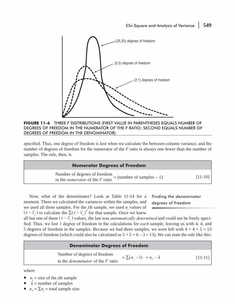
Chi-Square and Analysis of Variance 549
number of degrees of freedom for the numerator of the F ratio is always one fewer than the number of samples. The rule, then, is
Numerator Degrees of Freedom
Number of degrees of freedomin the numerator of the F ratio = (number of samples − 1) [11-10]
Now, what of the denominator? Look at Table 11-14 for a moment. There we calculated the variances within the samples, and we used all three samples. For the jth sample, we used nj values of ( )−x x j to calculate the ( )2∑ −x x j for that sample. Once we knew all but one of these ( )−x x j values, the last was automatically determined and could not be freely speci-
each sample, leaving us with 4, 4, and 5 degrees of freedom in the samples. Because we had three samples, we were left with 4 + 4 + 5 = 13 degrees of freedom (which could also be calculated as 5 + 5 + 6 – 3 = 13). We can state the rule like this:
Denominator Degrees of Freedom
denominator F
Number of degrees of freedom
in the of the ratio( 1)= ∑ − = −n n kj T [11-11]
where nj = size of the jth sample k = number of samples nT = ∑nj = total sample size
Finding the denominator
degrees of freedom
(25,25) degrees of freedom
(5,5) degrees of freedom
(2,1) degrees of freedom
FIGURE 11-6 THREE F DISTRIBUTIONS (FIRST VALUE IN PARENTHESES EQUALS NUMBER OF DEGREES OF FREEDOM IN THE NUMERATOR OF THE F RATIO; SECOND EQUALS NUMBER OF DEGREES OF FREEDOM IN THE DENOMINATOR)

550 Statistics for Management
Now we can see that the weight assigned to 2sj in Equation 11-7 on p. 546 was just its fraction of the total number of degrees of freedom in the denominator of the F ratio.
Using the F TableTo do F hypothesis tests, we shall use an F table in which the columns represent the number of degrees of freedom for the numerator and the rows represent the degrees of freedom for the denominator. Separate
F distribution. Our degrees of freedom are 8 for the numerator and 11 for the denominator. In this instance, we would turn to Appendix Table 6(b). In the body of that table, the appropriate value for 8 and 11 degrees of freedom is 4.74. If our calculated sample value of F exceeds this table value of 4.74, we would reject the null hypothesis. If not, we would accept it.
Testing the HypothesisWe can now test our hypothesis that the three different training methods produce identical results, using the material we have developed to this point. Let’s begin by reviewing how we calcu-lated the F ratio:
F
first estimate of the population variancebased on the variance among the sample means
second estimate of the population variance based on the variances within the samples
= [11-8]
20
14.769=
= 1.354 ← F statistic
Next, calculate the number of degrees of freedom in the numerator of the F ratio, using Equation 11-10 as follows: Number of degrees of freedom in the numerator of the F ratio = (number of samples – 1) [11-10] = 3 – 1 = 2 ← Degrees of freedom in the numerator
And we can calculate the number of degrees of freedom in the denominator of the F ratio by use of Equation 11-11:
Number of degrees of freedom in the denominator of the F ratio ∑(nj – 1) = nj – k [11-11] = (5 – 1) + (5 – 1) + (6 – 1) = 4 + 4 + 5 = 13 ← Degrees of freedom in the denominator
Finding the F statistic and the
degrees of freedom

Chi-Square and Analysis of Variance 551
Finding the limit of the
acceptance region
Suppose the director of training wants to test at the 0.05 level the hypothesis that there are no differences among the three training methods. We can look in Appendix Table 6(a) for 2 degrees of free-
hypothesis test graphically. 3.81 sets the upper limit of the acceptance region. Because the cal-culated sample value for F of 1.354 lies within the acceptance region, we would accept the null hypothesis and conclude that,
three training methods on employee productivity.
Precautions about Using the F TestAs we stated earlier, our sample sizes in this problem are too small for us to be able to draw valid inferences about the effectiveness of the various training methods. We chose small samples so that we could explain the logic of analysis of variance without tedious calculations. In actual practice, our methodology would be the same, but our samples would be larger.
In our example, we have assumed the absence of many factors that might have affected our conclusions. We accepted as given, for example, the fact that all the new employees we sampled had the same demonstrated aptitude for learning, which may or may not be true. We assumed that all the instructors of the three training methods had the same ability to teach and to manage, which may not be true. And we assumed that the company’s statistical staff collected the data on productivity during work periods that were similar in terms of time of day, day of the week, time
to be certain that all these factors are effectively controlled.Finally, notice that we have discussed only one-way, or one-
factor, analysis of variance. Our problem examined the effect of the
Interpreting the results
Use large sample sizes
Control all factors but the
one being tested
A test for one factor only
Sample F value of 1.354
0.05 of area
3.81
Acceptance regionAccept the null hypothesis if the
sample value is in this region
FIGURE 11-7 HYPOTHESIS TEST AT THE 0.05 LEVEL OF SIGNIFICANCE, USING THE F DISTRIBUTION AND SHOWING THE ACCEPTANCE REGION AND THE SAMPLE F VALUE
552 Statistics for Management
type of training method on employee productivity, nothing else. Had we wished to measure the effect of two factors, such as the training program and the age of the employee, we would need the ability to use two-way analysis of variance, a statistical method best saved for more advanced textbooks.
ANOVA: One Way Classification (Shortcut Method)H0: μ1 = μ2 = μ3 ……… = μi ……… μmH1: At least two μi’s are different
Observation Table
Factor Total Mean
A1 x11 x12……xij
……xin1T1 x1
A2 x21 x22……xij
……xin2T2 x2
:. : : :. . . :. :
Ai xi1 xi2……xij
……xiniTi xi
:. : : :. . . :. :
Am xm1 xm2……xmj
……xmn Tm xm
G x
Where
xTi ij
j i
ni
∑==
x
x
ni
ijj i
n
i
i
∑= =
G Ti
i
m
1∑=
= x
n
Tii
m
i
1∑
=∑=
x
i
m
ijj
n
1 1
i
∑ ∑== =
x
ni
m
ijj
n
i
1 1
i
∑ ∑∑
= = =
nN Total Number
of observationsii
m
1∑= =
=
Raw Sum of Square (Raw S.S) = xijj
n
i
m2
11
i
∑∑==
Correction Factor (C.F.) = G
N
2
Total Sum of Squares (T.S.S.) = Raw S.S – C.F.
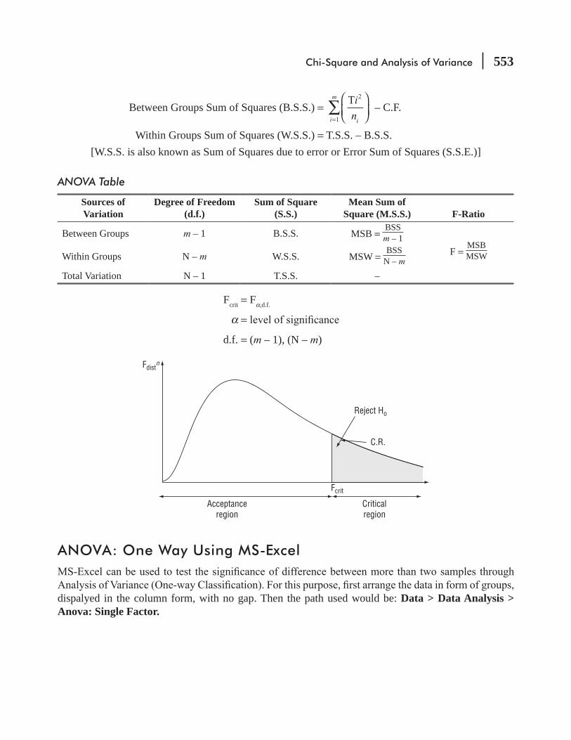
Chi-Square and Analysis of Variance 553
Between Groups Sum of Squares (B.S.S.) = ∑⎛
⎝⎜⎞
⎠⎟=
i
n
T
ii
m 2
1
– C.F.
Within Groups Sum of Squares (W.S.S.) = T.S.S. – B.S.S.[W.S.S. is also known as Sum of Squares due to error or Error Sum of Squares (S.S.E.)]
ANOVA Table
Sources of Variation
Degree of Freedom (d.f.)
Sum of Square (S.S.)
Mean Sum of Square (M.S.S.) F-Ratio
Between Groups m – 1 B.S.S. MSB = BSSm – 1
F = MSBMSWWithin Groups N – m W.S.S. MSW =
BSSN – m
Total Variation N – 1 T.S.S. –
Fcrit = Fα,d.f.
α =
d.f. = (m – 1), (N – m)
Acceptanceregion
Criticalregion
Reject Ho
C.R.
Fcrit
Fdistn
ANOVA: One Way Using MS-Excel
dispalyed in the column form, with no gap. Then the path used would be: Data > Data Analysis > Anova: Single Factor.
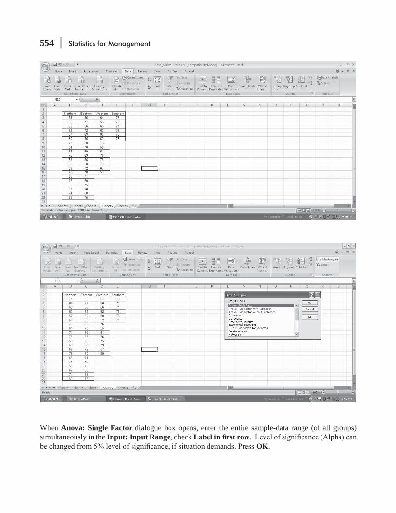
554 Statistics for Management
When Anova: Single Factor dialogue box opens, enter the entire sample-data range (of all groups) simultaneously in the Input: Input Range, check
OK.
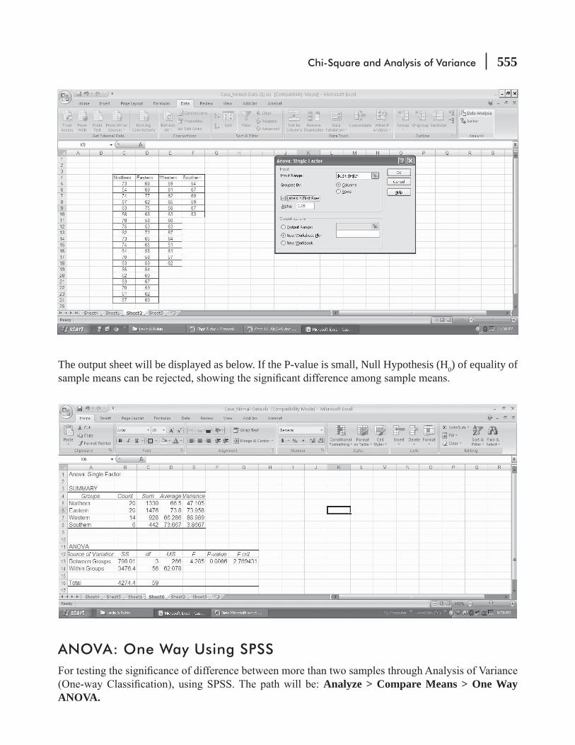
Chi-Square and Analysis of Variance 555
The output sheet will be displayed as below. If the P-value is small, Null Hypothesis (H0) of equality of
ANOVA: One Way Using SPSS
Analyze > Compare Means > One Way ANOVA.
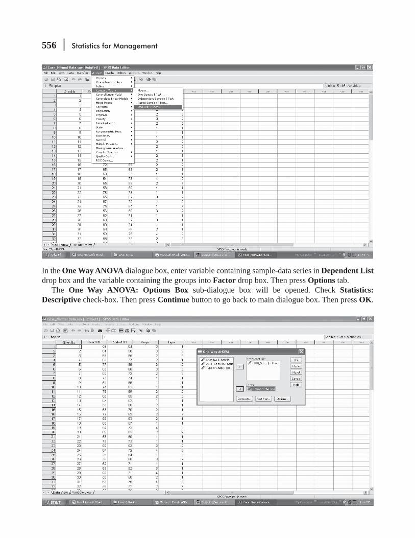
556 Statistics for Management
In the One Way ANOVA dialogue box, enter variable containing sample-data series in Dependent List drop box and the variable containing the groups into Factor drop box. Then press Options tab.
The One Way ANOVA: Options Box sub-dialogue box will be opened. Check Statistics: Descriptive check-box. Then press Continue button to go back to main dialogue box. Then press OK.

Chi-Square and Analysis of Variance 557
The output sheet would be displayed as above. If the Sig. is small, Null Hypothesis (H0) of equality of

558 Statistics for Management
Analysis of Variance (ANOVA): Two Way
Some situations demand that the experiment should be planned in such a manner so as to study the
The two factors are: Factor A and Factor B. The factor A has ‘m
A1, A2,……Ai……Am
Factor B has ‘n
B1, B2,……Bj……Bn
Let xij be the observation under the ith level of Factor A and jth level of the factor B.Here, observations should be so taken that there should be one observation per cell (xij) of the bivari-
ate (Cross Tabulation) table. The corresponding analysis of variance is known as Analysis of Variance
The second option is that the observations should be taken in such a manner that cells of the bivariate table contain more than one observation per cell. This option facilitates the estimation and testing of the interaction effect. Interaction effect is an effect peculiar to the combination (Ai, Bj). If the joint effect of Ai and Bj is different from the sum of the effects due to Ai and Bj taken individually, then the interaction effect is said to be present.
Analysis of Variance (Two Way Classification with One Observation Per Cell) Short-Cut Method
1st Factor (A): H01: α1 = α2 = …… = αi = …… αmH11: At least two α i’s are different.
2nd Factor (B): H02: β1 = β2 = …… = βi = …… βnH12: At least two β j’s are different.
Observation Table
Factor BFactor A B1 B2
……Bj……Bn Total Mean
A1 x11 x12……x1 j
……x1n T1. x1.
A2 x21 x22……x2 j
……x2n T2. x2.
:. : : : :. . . . :. :
Ai xi1 xi2……xij
……xin Ti. xi.
:. : : : :. . . . :. :
Am xm1 xm2……xmj
……xmn Tm. xm.
Total T . 1 T . 2……T . j……T . n G
Mean x . 1 x . 2……x . j……x . n x ..

Chi-Square and Analysis of Variance 559
Where
xT .i ij
j i
n
∑==
xT
n
x
n.
.i
iij
j i
n
∑= = =
xT. j ij
i
m
1∑=
= x
m
x
m.
T.j
jij
i
m
1∑
= = =
xG ij
j
n
i
m
11∑∑=
== x
xG
N N
ijj
n
i
m
11∑∑
= = ==
N = m × n (Total Number of observations)
Raw Sum of Squares (R.S.S.) = xijj
n
i
m2
11∑∑
==
Correction Factor (C.F.) = G
N
2
Total Sum of Square (T.S.S.) = Raw S.S. – C.F.
Sum of Squares due to factor A (SSA) = T
n
.C.F.i
i
m 2
1∑
⎛
⎝⎜
⎞
⎠⎟ −
=
Sum of Squares due to factor B (SSB) = ∑⎛
⎝⎜
⎞
⎠⎟ −
=
T
m
.C.Fj
j
n 2
1
Sum of Squares due to error (SSE) = T.S.S. – S.S.A – S.S.B
ANOVA Table
Sources of VariationDegree of
Freedom (d.f.)Sum of Squares
(S.S.)Mean Sum of
Squares (M.S.S.) F-Ratio
Between the levels of A(due to factor A) (m – 1) SSA MSA =
SSAm – 1
FA = MSAMSE
Between the levels of B(due to factor B) (n – 1) SSB MSB =
SSBn – 1
Error (Residual) (m – 1) × (n – 1) SSE MSE = SSE
(m – 1) × (n – 1) FB = MSBMSE
Total N – 1 TSS –
FA(crit) = Fα,d.f.(A)
d.f.(A) = (m – 1), (m – 1) . (n – 1)Acceptance region
Reject Ho1
FA(crit)
Fdistn
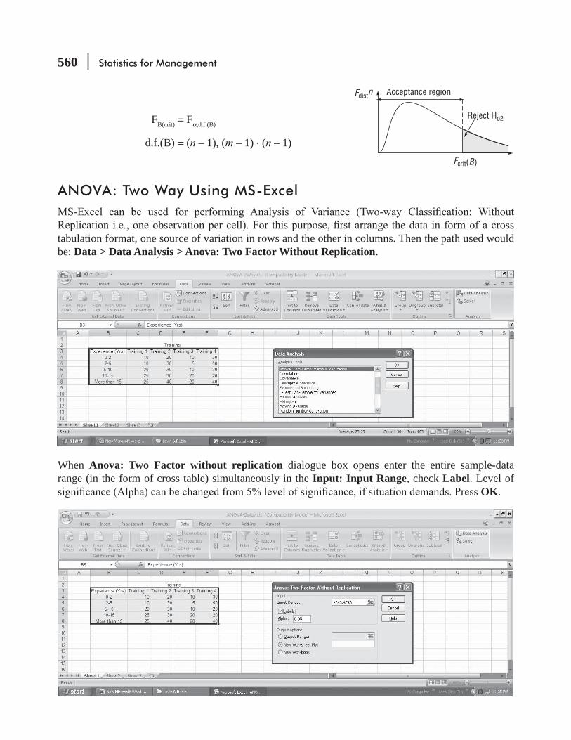
560 Statistics for Management
FB(crit) = Fα,d.f.(B)
d.f.(B) = (n – 1), (m – 1) . (n – 1)
ANOVA: Two Way Using MS-Excel
tabulation format, one source of variation in rows and the other in columns. Then the path used would be: Data > Data Analysis > Anova: Two Factor Without Replication.
When Anova: Two Factor without replication dialogue box opens enter the entire sample-data range (in the form of cross table) simultaneously in the Input: Input Range, check Label. Level of
OK.
Acceptance region
Reject Ho2
Fcrit(B)
Fdistn
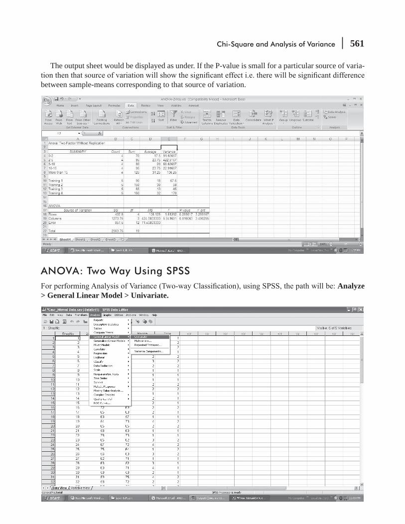
Chi-Square and Analysis of Variance 561
The output sheet would be displayed as under. If the P-value is small for a particular source of varia-
between sample-means corresponding to that source of variation.
ANOVA: Two Way Using SPSS Analyze
> General Linear Model > Univariate.
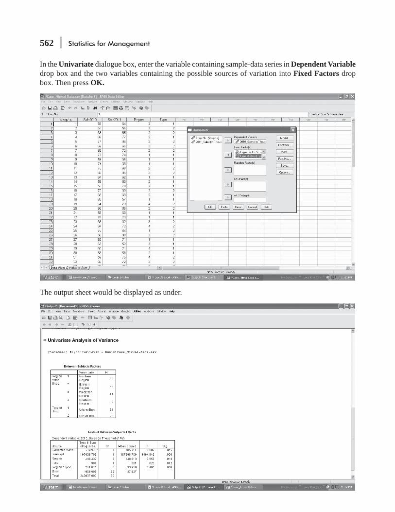
562 Statistics for Management
In the Univariate dialogue box, enter the variable containing sample-data series in Dependent Variable drop box and the two variables containing the possible sources of variation into Fixed Factors drop box. Then press OK.
The output sheet would be displayed as under.

Chi-Square and Analysis of Variance 563
The focus of analysis of variance is to test whether three or more samples have been drawn from populations having the same mean. Analysis of variance is important in research such as the evaluation of new drugs, where we need to examine the effects of dose, frequency of medication, effects of other drugs, and patient differences in a single study. Analysis of variance compares two estimates of the population variance. One estimate comes from the variance among the sample means, the other from the variance within the samples themselves. If they are approximately equal, the chances are high that the samples came from the same population. Warning: It’s vital not to abandon common sense when interpreting results. While it may be true that a study can identify differences in brand preferences for instant coffee that apply to coffee purchases made on weekday mornings, it’s hard to say what a coffee company should do with this information.
HINTS & ASSUMPTIONS
EXERCISES 11.4
Self-Check ExercisesSC 11-5 A study compared the effects of four 1-month point-of-purchase promotions on sales. The unit
low.
Free sample 78 87 81 89 85One-pack gift 94 91 87 90 88Cents off 73 78 69 83 76Refund by mail 79 83 78 69 81
(a) Compute the mean unit sales for each promotion and then determine the grand mean.(b) Estimate the population variance using the between-column variance (Equation 11-6).(c) Estimate the population variance using the within-column variance computed from the
variance within the samples.(d) Calculate the F -
ent effects on sales?SC 11-6 A research company has designed three different systems to clean up oil spills. The following
table contains the results, measured by how much surface area (in square meters) is cleared in 1 hour. The data were found by testing each method in several trials. Are the three systems
System A 55 60 63 56 59 55System B 57 53 64 49 62System C 66 52 61 57
Applications11-25
administered to 25 different people, each with stomach acid considered strong. The results are given in the following table:
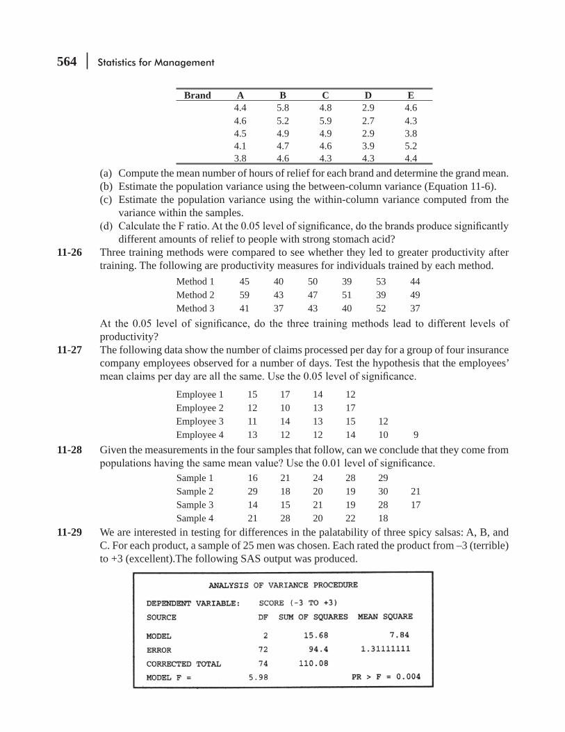
564 Statistics for Management
Brand A B C D E4.4 5.8 4.8 2.9 4.64.6 5.2 5.9 2.7 4.34.5 4.9 4.9 2.9 3.84.1 4.7 4.6 3.9 5.23.8 4.6 4.3 4.3 4.4
(a) Compute the mean number of hours of relief for each brand and determine the grand mean.(b) Estimate the population variance using the between-column variance (Equation 11-6).(c) Estimate the population variance using the within-column variance computed from the
variance within the samples.
different amounts of relief to people with strong stomach acid?11-26 Three training methods were compared to see whether they led to greater productivity after
training. The following are productivity measures for individuals trained by each method.Method 1 45 40 50 39 53 44Method 2 59 43 47 51 39 49Method 3 41 37 43 40 52 37
productivity?11-27 The following data show the number of claims processed per day for a group of four insurance
company employees observed for a number of days. Test the hypothesis that the employees’
Employee 1 15 17 14 12Employee 2 12 10 13 17Employee 3 11 14 13 15 12Employee 4 13 12 12 14 10 9
11-28 Given the measurements in the four samples that follow, can we conclude that they come from
Sample 1 16 21 24 28 29Sample 2 29 18 20 19 30 21Sample 3 14 15 21 19 28 17Sample 4 21 28 20 22 18
11-29 We are interested in testing for differences in the palatability of three spicy salsas: A, B, and C. For each product, a sample of 25 men was chosen. Each rated the product from –3 (terrible) to +3 (excellent).The following SAS output was produced.

Chi-Square and Analysis of Variance 565
(a) State explicit null and alternative hypotheses.(b) Test your hypotheses with the SAS output. Use α = 0.05.(c) State an explicit conclusion.
11-30 The supervisor of security at a large department store would like to know whether the store apprehends relatively more shoplifters during the Christmas holiday season than in the weeks before or after the holiday. He gathered data on the number of shoplifters apprehended in the store during the months of November, December, and January over the past 6 years. The information follows:
Number of Shoplifters
November 43 37 59 55 38 48
December 54 41 48 35 50 49
January 36 28 34 41 30 32
during these 3 months?11-31 An Introduction to Economics course is offered in 3 sections, each with a different instructor.
the average grades given by the instructors? State and test appropriate hypotheses at α = 0.01.
Section 1 Section 2 Section 3
98.4 97.6 94.5
97.6 99.2 92.3
84.7 82.6 92.4
88.5 81.2 82.3
77.6 64.5 62.6
84.3 82.3 68.6
81.6 68.4 92.7
88.4 75.6 82.3
95.1 91.2
90.4 92.6
89.4 87.4
65.6
94.5
99.4
68.7
83.4
11-32 -tered to keep the number of dust particles at a minimum. The Outel Corporation wants to make
have been taken in each room. The “dust score,” on a scale of 1 (low) to 10 (high), was mea-
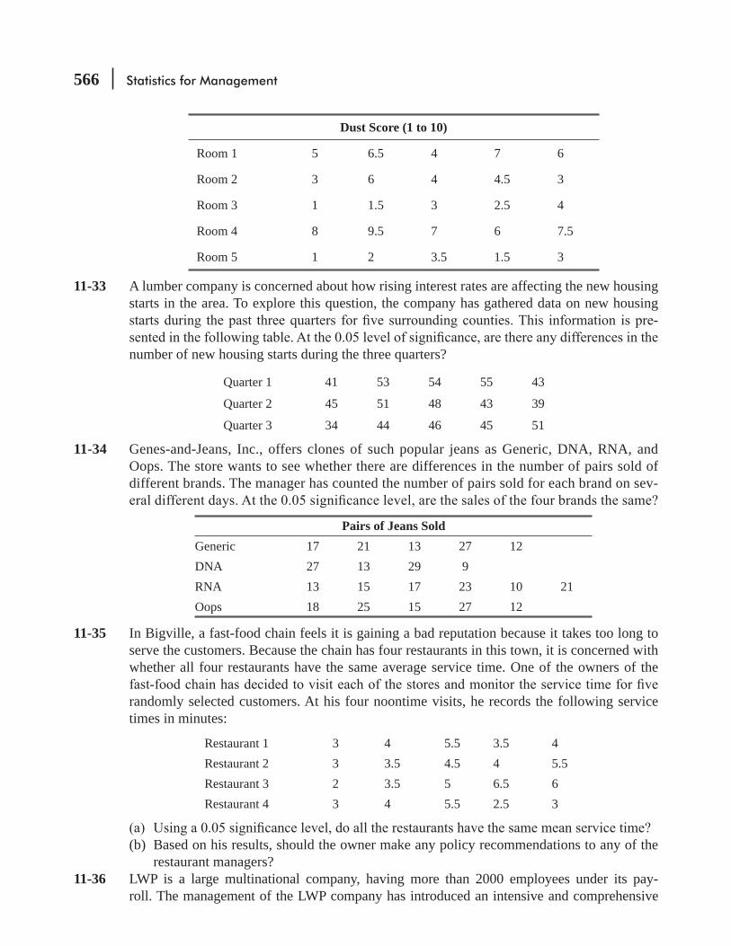
566 Statistics for Management
Dust Score (1 to 10)
Room 1 5 6.5 4 7 6
Room 2 3 6 4 4.5 3
Room 3 1 1.5 3 2.5 4
Room 4 8 9.5 7 6 7.5
Room 5 1 2 3.5 1.5 3
11-33 A lumber company is concerned about how rising interest rates are affecting the new housing starts in the area. To explore this question, the company has gathered data on new housing
-
number of new housing starts during the three quarters?
Quarter 1 41 53 54 55 43
Quarter 2 45 51 48 43 39
Quarter 3 34 44 46 45 51
11-34 Genes-and-Jeans, Inc., offers clones of such popular jeans as Generic, DNA, RNA, and Oops. The store wants to see whether there are differences in the number of pairs sold of different brands. The manager has counted the number of pairs sold for each brand on sev-
Pairs of Jeans SoldGeneric 17 21 13 27 12DNA 27 13 29 9RNA 13 15 17 23 10 21Oops 18 25 15 27 12
11-35 In Bigville, a fast-food chain feels it is gaining a bad reputation because it takes too long to serve the customers. Because the chain has four restaurants in this town, it is concerned with whether all four restaurants have the same average service time. One of the owners of the
randomly selected customers. At his four noontime visits, he records the following service times in minutes:
Restaurant 1 3 4 5.5 3.5 4Restaurant 2 3 3.5 4.5 4 5.5Restaurant 3 2 3.5 5 6.5 6Restaurant 4 3 4 5.5 2.5 3
(b) Based on his results, should the owner make any policy recommendations to any of the restaurant managers?
11-36 LWP is a large multinational company, having more than 2000 employees under its pay-roll. The management of the LWP company has introduced an intensive and comprehensive
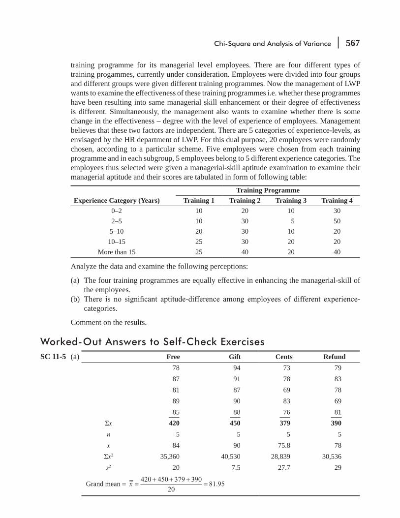
Chi-Square and Analysis of Variance 567
training programme for its managerial level employees. There are four different types of training progammes, currently under consideration. Employees were divided into four groups and different groups were given different training programmes. Now the management of LWP wants to examine the effectiveness of these training programmes i.e. whether these programmes have been resulting into same managerial skill enhancement or their degree of effectiveness is different. Simultaneously, the management also wants to examine whether there is some change in the effectiveness – degree with the level of experience of employees. Management believes that these two factors are independent. There are 5 categories of experience-levels, as envisaged by the HR department of LWP. For this dual purpose, 20 employees were randomly chosen, according to a particular scheme. Five employees were chosen from each training programme and in each subgroup, 5 employees belong to 5 different experience categories. The employees thus selected were given a managerial-skill aptitude examination to examine their managerial aptitude and their scores are tabulated in form of following table:
Training ProgrammeExperience Category (Years) Training 1 Training 2 Training 3 Training 4
0–2 10 20 10 302–5 10 30 5 50
5–10 20 30 10 2010–15 25 30 20 20
More than 15 25 40 20 40
Analyze the data and examine the following perceptions:
(a) The four training programmes are equally effective in enhancing the managerial-skill of the employees.
(b) -categories.
Comment on the results.
Worked-Out Answers to Self-Check ExercisesSC 11-5 (a) Free Gift Cents Refund
78 94 73 7987 91 78 8381 87 69 7889 90 83 6985 88 76 81
x 420 450 379 390n 5 5 5 5x 84 90 75.8 78x2 35,360 40,530 28,839 30,536
s2 20 7.5 27.7 29
Grand mean = x420 450 379 390
2081.95=
+ + +=

568 Statistics for Management
(b) n x x
kˆ
( )
1
5[84 81.95) (90 81.95) (75.8 81.95) (78 81.95) ]
4 1b
j j2
2 2 2 2 2
σ =∑ −
−=
− + − + − + −−
612.15
3204.05= =
(c) ˆ1 4(20 7.5 27.7 29)
20 4
336.8
1621.052 2∑σ =
−−
⎛
⎝⎜
⎞
⎠⎟ =
+ + +−
= =n
n ksw
j
Tj
(d) 204.05
21.059.69= =F
With 3 degrees of freedom in the numerator, 16 degrees of freedom in the denominator, and α = 0.01, the critical value of F is 5.29, so reject H0, because 9.69 > 5.29. The promotions have
SC 11-6 n x s2
System A 6 58 10.4000System B 5 57 38.5000System C 4 59 35.3333
6(58) 5(57) 4(59)
6 5 457.9333=
+ ++ +
=x
ˆ( )
12
2∑σ =−
−n x x
kb
j j
6(58 57.9333) 5(57 57.9333) 4(59 57.9333)
3 1
2 2 2
=− + − + −
−
8.9333
24.4667= =
1 5(10.4) 4(38.5) 3(35.3333)
15 3
312
12262 2σ = ∑
−−
⎛
⎝⎜
⎞
⎠⎟ =
+ +−
= =n
n ksw
j
Tj
ˆ
ˆ4.4667
260.17
2
2
σσ
= = =F w
w
With 2 degrees of freedom in the numerator, 12 degrees of freedom in the denominator, and α = 0.05, the critical value of F is 3.89, so don’t reject H0, because 0.17 < 3.89. The systems
11.5 INFERENCES ABOUT A POPULATION VARIANCE
test hypotheses about one or two population means or proportions. Earlier in this chapter, we used chi-square and F tests to make infer-ences about more than two means or proportions. But we are not
Need to make decisions
about variability in a
population

Chi-Square and Analysis of Variance 569
always interested in means and proportions. In many situations, responsible decision makers have to make inferences about the variability in a population. In order to schedule the labor force at harvest time, a peach grower needs to know not only the mean time to maturity of the peaches, but also their variance around that mean. A sociologist investigating the effect of education on earning power wants to know whether the incomes of college graduates are more variable than those of high school graduates. Precision instruments used in laboratory work must be quite accurate on the average but in addition, repeated measurements should show very little variation. In this section, we shall see how to make infer-ences about a single population variance. The next section looks at problems involving the variances of two populations.
The Distribution of the Sample VarianceIn response to a number of complaints about slow mail delivery, the Postmaster General initiates a pre-liminary investigation. An investigator follows nine letters from New York to Chicago, to estimate the standard deviation in time of delivery. Table 11-15 gives the data and computes ,x s2, and s. As we saw in Chapter 7, we use s to estimate σ.
We can tell the Postmaster General that the population standard deviation, as estimated by the sample standard deviation, is approximately 23 hours. But he also wants to know how accurate that estimate is and what uncertainty is associated with it. In other
σ
Determining the uncertainty
attached to estimates of the
population standard deviation
TABLE 11-15 DELIVERY TIME (IN HOURS) FOR LETTERS GOING BETWEEN NEW YORK AND CHICAGO
Time x x x – x (x – x)2
50 59 –9 8145 59 –14 19627 59 –32 1,02466 59 7 4943 59 –16 25696 59 37 1,36945 59 –14 19690 59 31 96169 59 10 100
x∑ = 531 x x( )2∑ − = 4,232
x =x
n
531
9
∑= [3-2] s =
x x
n
( )
1
4,232
82
2∑ −−
= [3-17]
= 59 hours = 529 hours squared
s s 5292= = [3-18]
= 23 hours

570 Statistics for Management
distribution of s. It is traditional to talk about s2 rather than s, but this will cause us no trouble, because we can always go from s2 and σ 2 to s and σ by taking square roots; we can go in the other direction by squaring.
Chi-Square Statistic for Inferences about One Variance
( 1)22
2χ
σ=
−n s [11-12]
If the population variance is σ 2, then the statistic has a chi-square distribution with n – 1 degrees of freedom. This result is exact if the population is normal, but even for samples from nonnormal popula-
intervals and test hypotheses about σ 2.
Confidence Intervals for the Population Variance
in our mail-delivery problem. Figure 11-8 shows how to begin con-structing this interval.
We locate two points on the χ 2 distribution: 2χu cuts off 0.025 of the area in the upper tail of the distribution, and 2χ L cuts off 0.025 of the area in the lower tail. (For a 99
-dence levels.) The values of 2χ L and u
2χ , can be found in Appendix Table 5. In our mail problem, with 9 – 1 = 8 degrees of freedom, 2χ L = 2.180 and 2χu = 17.535.
Now Equation 11-12 gives χ2 in terms of s2, n, and σ 2. To get a σ2, we solve Equation 11-12 for σ 2:
( 1)22
2σ
χ=
−n s[11-13]
Constructing a confidence
Intervals for a Variance
Upper and lower limits for
the confidence interval
χ2 distribution
χ2L
χ2U
0.025 ofarea 0.025 of area
FIGURE 11-8 CONSTRUCTING A CONFIDENCE INTERVAL FOR σ 2.
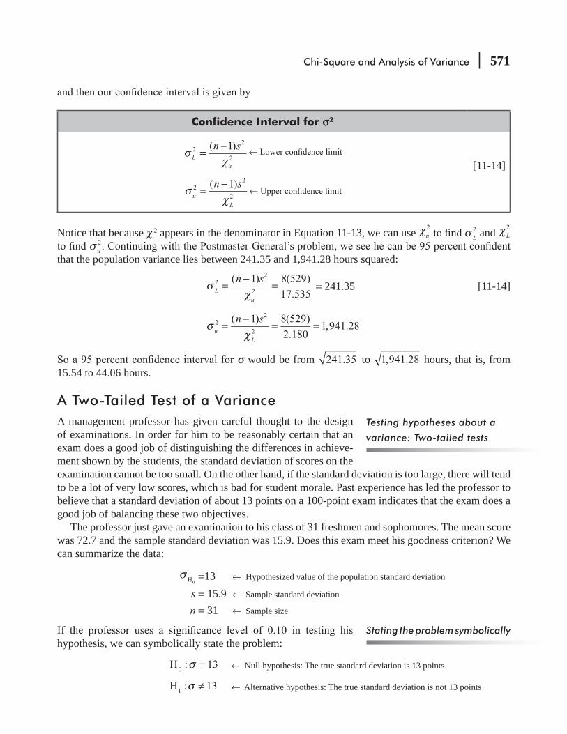
Chi-Square and Analysis of Variance 571
Confidence Interval for s2
σχL
u
n s22
2
1= −( ) ←
( 1)22
2σ
χ=
−n su
L
←
[11-14]
Notice that because χ 2 appears in the denominator in Equation 11-13, we can use 2χu L2σ and 2χ L
u2σ
that the population variance lies between 241.35 and 1,941.28 hours squared:
( 1) 8(529)
17.5352
2
2σ
χ=
−=
n sL
u
= 241.35 [11-14]
( 1) 8(529)
2.1801,941.282
2
2σ
χ=
−= =
n su
L
σ would be from 241.35 to 1,941.28 hours, that is, from 15.54 to 44.06 hours.
A Two-Tailed Test of a VarianceA management professor has given careful thought to the design of examinations. In order for him to be reasonably certain that an exam does a good job of distinguishing the differences in achieve-ment shown by the students, the standard deviation of scores on the examination cannot be too small. On the other hand, if the standard deviation is too large, there will tend to be a lot of very low scores, which is bad for student morale. Past experience has led the professor to believe that a standard deviation of about 13 points on a 100-point exam indicates that the exam does a good job of balancing these two objectives.
The professor just gave an examination to his class of 31 freshmen and sophomores. The mean score was 72.7 and the sample standard deviation was 15.9. Does this exam meet his goodness criterion? We can summarize the data:
H0σ =13 ← Hypothesized value of the population standard deviation
s = 15.9 ← Sample standard deviation
n = 31 ← Sample size
hypothesis, we can symbolically state the problem:
H : 130 σ = ← Null hypothesis: The true standard deviation is 13 points
H : 131 σ ≠ ← Alternative hypothesis: The true standard deviation is not 13 points
Testing hypotheses about a
variance: Two-tailed tests
Stating the problem symbolically
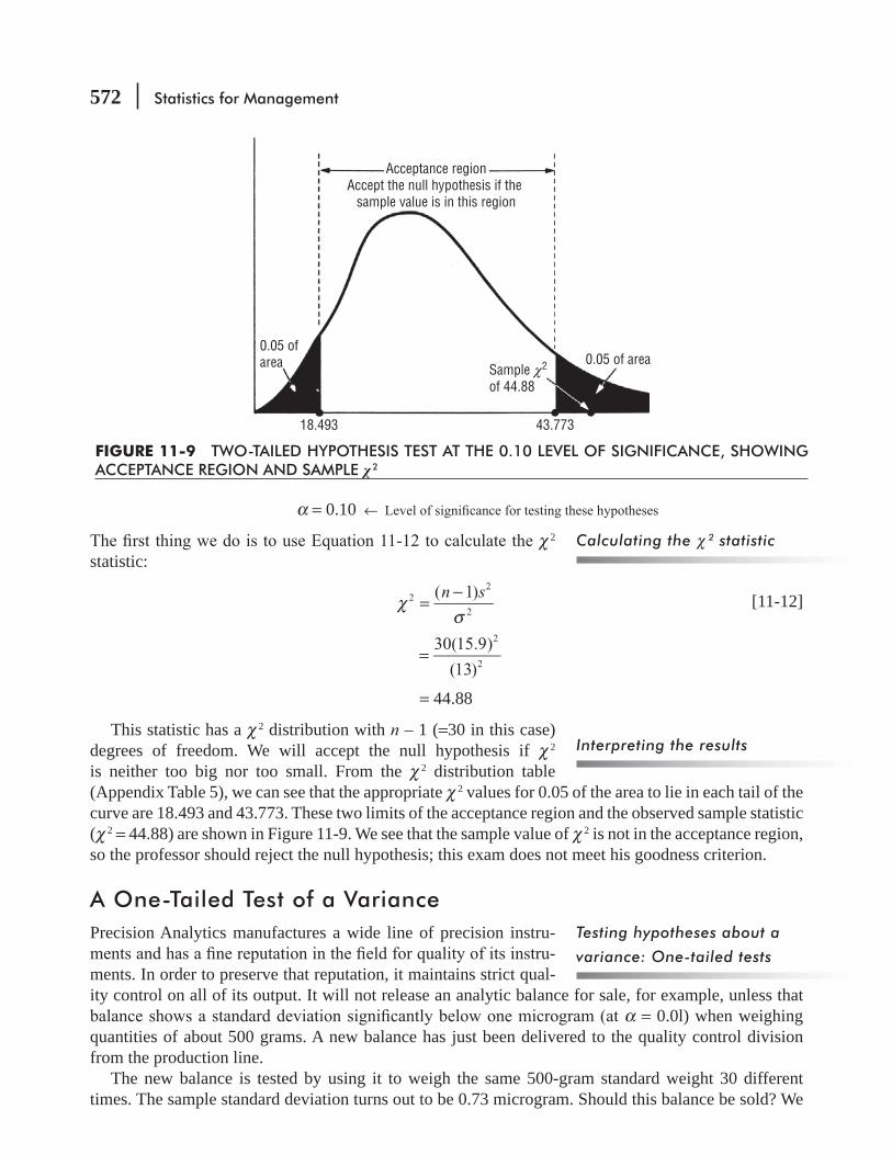
572 Statistics for Management
α = 0.10 ←
χ 2 statistic:
( 1)22
2χ
σ=
−n s [11-12]
30(15.9)
(13)
2
2=
= 44.88
This statistic has a χ 2 distribution with n – 1 (=30 in this case) degrees of freedom. We will accept the null hypothesis if χ 2 is neither too big nor too small. From the χ 2 distribution table (Appendix Table 5), we can see that the appropriate χ 2 values for 0.05 of the area to lie in each tail of the curve are 18.493 and 43.773. These two limits of the acceptance region and the observed sample statistic (χ 2 = 44.88) are shown in Figure 11-9. We see that the sample value of χ 2 is not in the acceptance region, so the professor should reject the null hypothesis; this exam does not meet his goodness criterion.
A One-Tailed Test of a VariancePrecision Analytics manufactures a wide line of precision instru-
-ments. In order to preserve that reputation, it maintains strict qual-ity control on all of its output. It will not release an analytic balance for sale, for example, unless that
α = 0.0l) when weighing quantities of about 500 grams. A new balance has just been delivered to the quality control division from the production line.
The new balance is tested by using it to weigh the same 500-gram standard weight 30 different times. The sample standard deviation turns out to be 0.73 microgram. Should this balance be sold? We
Calculating the χ 2 statistic
Interpreting the results
Testing hypotheses about a
variance: One-tailed tests
Acceptance regionAccept the null hypothesis if the
sample value is in this region
0.05 ofarea Sample χ2
of 44.88
18.493 43.773
0.05 of area
FIGURE 11-9 TWO-TAILED HYPOTHESIS TEST AT THE 0.10 LEVEL OF SIGNIFICANCE, SHOWING ACCEPTANCE REGION AND SAMPLE 2

Chi-Square and Analysis of Variance 573
summarize the data:
H0σ = 1 ← Hypothesized value of the population standard deviation
s = 0.73 ← Sample standard deviation
n = 30 ← Sample size
and state the problem:
H0: σ = 1 ← Null hypothesis: The true standard deviation is 1 microgram
H1: σ < 1 ← Alternative hypothesis. The true standard deviation is less than 1 microgram
α = 0.01 ←
We begin by using Equation 11-12 to calculate the χ 2 statistic:
( 1)22
2χ
σ=
−n s [11-12]
29(0.73)
(1)
2
2=
= 15.45
We will reject the null hypothesis and release the balance for sale
that with 29 degrees of freedom (30 – 1), the value of χ 2 that leaves an area of 0.01 in the lower tail of the curve is 14.256. The acceptance region and the observed value of χ 2 are shown in Figure 11-10. We see that we cannot reject the null hypothesis. The balance will have to be returned to the production line for adjusting.
Stating the problem symbolically
Calculating the χ2 statistic
Interpreting the results
Acceptance regionAccept the null hypothesis if the
sample value is in this region
0.01 ofarea
14.256
Sample χ2
of 15.45
FIGURE 11-10 ONE-TAILED HYPOTHESIS TEST AT THE 0.01 SIGNIFICANCE LEVEL, SHOWING ACCEPTANCE REGION AND SAMPLE χ 2
574 Statistics for Management
Up to this point, we’ve seen how to make inferences about one, two, or several means or propor-tions. But we’re also interested in making inferences about population variability. For one popula-tion, we do this by using the sample variance and the chi-square distribution. Warning: Chi-square tests can be one-tailed or two-tailed. Hint: If the question to be answered is worded less than, more than, less than or equal to, or greater than or equal to, use a one-tailed test. If the question con-cerns different from, or changed from, use a two-tailed test.
HINTS & ASSUMPTIONS
EXERCISES 11.5
Self-Check ExercisesSC 11-7 -
dence interval for the population variance.SC 11-8 A production manager feels that the output rate of experienced employees is surely greater
than that of new employees, but he does not expect the variability in output rates to differ for the two groups. In previous output studies, it has been shown that the average unit output per hour for new employees at this particular type of work is 20 units per hour with a variance of 56 units squared. For a group of 20 employees with 5 years’ experience, the average output for this same type of work is 30 units per hour, with a sample variance of 28 units squared. Does the Variability in output appear to differ at the two experience levels? Test the hypotheses at
Basic Concepts11-37 A sample of 20 observations from a normal distribution has a mean of 37 and a variance of
11-38 The standard deviation of a distribution is hypothesized to be 50. If an observed sample of 30 yields a sample standard deviation of 57, should we reject the null hypothesis that the true
11-39 Given a sample standard deviation of 6.4 from a sample of 15 observations, construct a
Applications11-40 A telescope manufacturer wants its telescopes to have standard deviations in resolution to be
used to focus on an object 500 light-years away 30 times, the sample standard deviation turns out to be 1.46. Should this telescope be sold?(a) State explicit null and alternative hypotheses.(b) Test your hypotheses at the α = 0.01 level.(c) State an explicit conclusion.
11-41 MacroSwift has designed a new operating system that will revolutionize the computing indus-try. The only problem is, the company expects the average amount of time required to learn the software to be 124 hours. Even though this is a long educational time, the company is truly concerned with the variance of the learning time. Preliminary data indicate the variance is 171

Chi-Square and Analysis of Variance 575
hours squared. Recent testing of 25 people found an average learning time of 123 hours and a sample variance of 196.5 hours squared. Do these data indicate the variability in learning time
11-42 A psychologist is aware of studies showing that the variability of attention spans of 5-year-olds can be summarized by σ 2 = 64 minutes squared. She wonders whether the attention span of 6-year-olds is different. A sample of twenty 6-year-olds gives s2 = 28 minutes squared.(a) State explicit null and alternative hypotheses.(b) Test your hypotheses at the α = 0.05 level.(c) State an explicit conclusion.
11-43 In checking its cars for adherence to emissions standards set by the government, an automaker measured emissions of 30 cars. The average number of particles of pollutants emitted was found to be within the required levels, but the sample variance was 50. Find a 90 percent
11-44 A bank is considering ways to reduce the costs associated with passbook savings accounts. The bank has found that the variance in the number of days between account transactions for passbook accounts is 80 days squared. The bank wants to reduce the variance by discouraging the present use of accounts for short-term storage of cash. Therefore, after implementing a new policy that penalizes the customer with a service charge for withdrawals more than once a month, the bank decides to test for a change in the variance of days between account transac-
-
11-45 Sam Bogart, the owner of the Play-It-Again Stereo Company, offers 1-year warranties on all the stereos his company sells. For the 30 stereos that were serviced under the warranty
Sam has decided that unless the true standard deviation is less than $20, he will buy his stereos
level of 0.01. Should he switch wholesalers?
Worked-Out Answers to Self-Check ExercisesSC 11-7
( 1) 8(127)
17.53557.9412
2
2σ
χ=
−= =
n sL
u
( 1) 8(127)
2.180466.0552
2
2σ
χ=
−= =
n su
L
SC 11-8 For testing H0: σ 2 = 56 versus H1: σ 2 ≠ 56 at α = 0.05, the limits of the acceptance region are
χ 2 = 8.907 and χ 2 = 32.852
The observed ( 1) 19(28)
569.5,2
2
2χ
σ=
−= =
n s so we do not reject H0; the variability is not
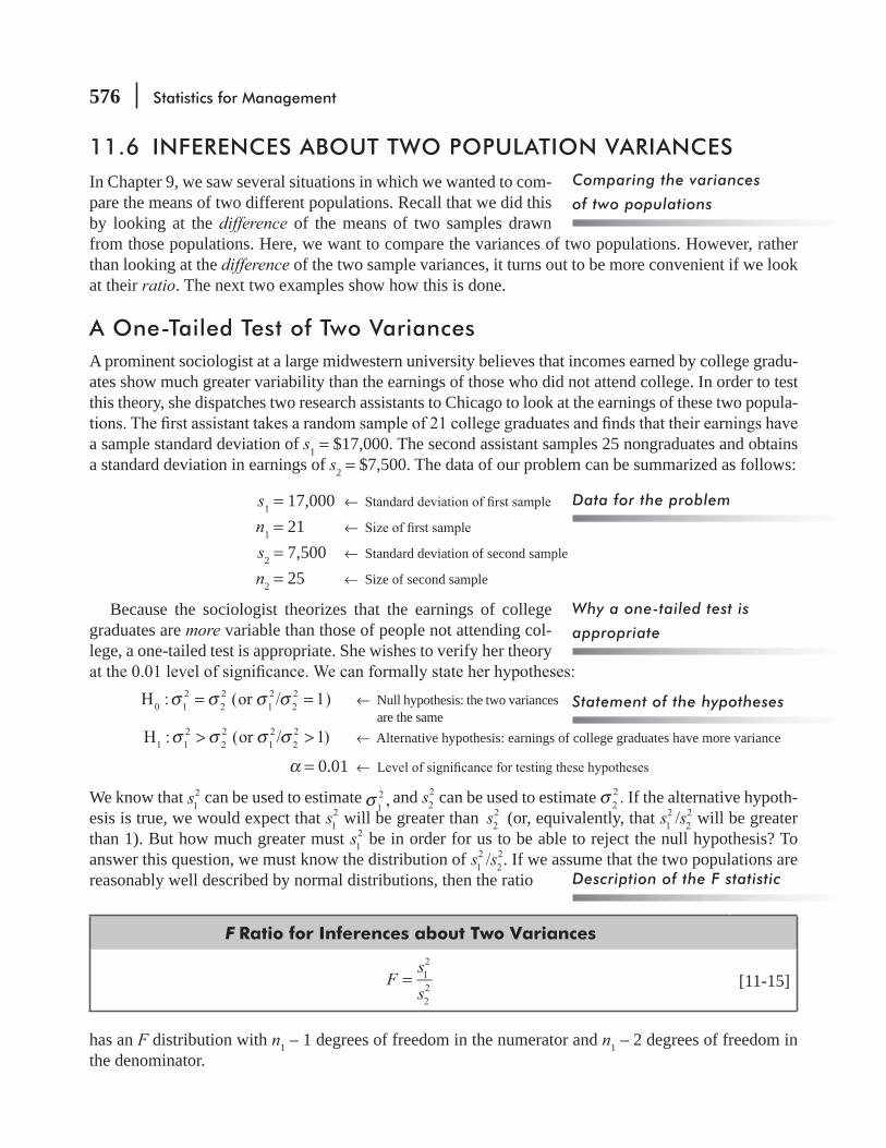
576 Statistics for Management
11.6 INFERENCES ABOUT TWO POPULATION VARIANCESIn Chapter 9, we saw several situations in which we wanted to com-pare the means of two different populations. Recall that we did this by looking at the difference of the means of two samples drawn from those populations. Here, we want to compare the variances of two populations. However, rather than looking at the difference of the two sample variances, it turns out to be more convenient if we look at their ratio. The next two examples show how this is done.
A One-Tailed Test of Two VariancesA prominent sociologist at a large midwestern university believes that incomes earned by college gradu-ates show much greater variability than the earnings of those who did not attend college. In order to test this theory, she dispatches two research assistants to Chicago to look at the earnings of these two popula-
a sample standard deviation of s1 = $17,000. The second assistant samples 25 nongraduates and obtains a standard deviation in earnings of s2 = $7,500. The data of our problem can be summarized as follows:
s1 = 17,000 ←
n1 = 21 ←
s2 = 7,500 ← Standard deviation of second sample
n2 = 25 ← Size of second sample
Because the sociologist theorizes that the earnings of college graduates are more variable than those of people not attending col-lege, a one-tailed test is appropriate. She wishes to verify her theory
H : (or / 1)0 12
22
12
22σ σ σ σ= = ← Null hypothesis: the two variances
are the same H : (or / 1)1 1
222
12
22σ σ σ σ> > ← Alternative hypothesis: earnings of college graduates have more variance
α = 0.01 ←
We know that 12s can be used to estimate ,1
2σ and 22s can be used to estimate .2
2σ If the alternative hypoth-esis is true, we would expect that 1
2s will be greater than 22s (or, equivalently, that /1
222s s will be greater
than 1). But how much greater must 12s be in order for us to be able to reject the null hypothesis? To
answer this question, we must know the distribution of /12
22s s . If we assume that the two populations are
reasonably well described by normal distributions, then the ratio
F Ratio for Inferences about Two Variances
12
22
=Fs
s[11-15]
has an F distribution with n1 – 1 degrees of freedom in the numerator and n1 – 2 degrees of freedom in the denominator.
Comparing the variances
of two populations
Data for the problem
Why a one-tailed test is
appropriate
Statement of the hypotheses
Description of the F statistic

Chi-Square and Analysis of Variance 577
In the earnings problem, we calculate the sample F statistic:
12
22
=Fs
s [11-15]
(17,000)
(7,500)
2
2
=
289,000,000
56,250,000
=
= 5.14
For 20 degrees of freedom (21 – 1) in the numerator and 24 degrees of freedom (25 – 1) in the denominator, Appendix Table 6 tells us that the critical value separating the acceptance and rejection regions is 2.74. Figure 11-11 shows the acceptance region and the observed F statistic of 5.14. Our sociologist rejects the null hypothesis, and the sample data support her theory.
A word of caution about the use of Appendix Table 6 is neces-sary at this point. You will notice that the table gives values of the F statistic that are appropriate only for upper-tailed tests. How can we handle alternative hypotheses of the form 1
222σ σ< (or /1
222σ σ <
1)? This is easily done if we notice that /12
22σ σ < 1 is equivalent to / 1.2
212σ σ > Thus, all we need to do is
calculate the ratio s s/ ,22
12 which also has an F distribution (but with n2 – 1 numerator degrees of freedom
and n1 – 1 denominator degrees of freedom), and then we can use Appendix Table 6. There is another way to say the same thing: Whenever you are doing a one-tailed test of two variances, number the populations so that the alternative hypothesis has the form
H : (or / 1)1 12
22
12
22σ σ σ σ> >
and then proceed as we did in the earnings example.
Interpreting the results
Handling lower-tailed tests in
Appendix Table 6
FIGURE 11-11 ONE-TAILED HYPOTHESIS TEST AT THE 0.01 LEVEL OF SIGNIFICANCE, SHOWING THE ACCEPTANCE REGION AND THE SAMPLE F STATISTIC
Acceptance regionAccept the null hypothesis if the
sample value is in this region
0.01 of areaSampleF statisticof 5.14
2.74

578 Statistics for Management
A Two-Tailed Test of Two VariancesThe procedure for a two-tailed test of two variances is similar to
critical value in the lower tail. This is related to the problem about lower-tailed tests discussed in the last paragraph, and we will resolve it in a similar way.
One criterion in evaluating oral anesthetics for use in general dentistry is the variability in the length of time between injection and complete loss of sensation in the patient. (This is called the effect delay
under the names Oralcaine and Novasthetic. From similarities in the chemical structure of the two compounds, it has been predicted that they should show the same variance in effect delay time. Sample data from tests of the two com-pounds (which controlled other variables such as age and weight) are given in Table 11-16.
The company wants to test at a 2 percent
have the same variance in effect delay time. Symbolically, the hypotheses are
H : (or / 1)0 12
22
12
22σ σ σ σ= = ← Null hypothesis: the two variances are the same
H : (or / 1)1 12
22
12
22σ σ σ σ≠ ≠ ← Alternative hypothesis: the two variances are different
α = 0.02 ←
To test these hypotheses, we again use Equation 11-15:
FS
S12
22
= [11-15]
1,296
784=
= 1.65
This statistic comes from an F distribution with n – 1 degrees of freedom in the numerator (30, in this case) and n2 – 1 degrees of freedom in the denominator (40, in this case). Let us use the notation
F(n, d, α)
to denote that value of F with n numerator degrees of freedom, d denominator degrees of freedom, and an area of α in the upper tail. In our problem, the acceptance region extends from F(30, 40, 0.99) to F(30, 40, 0.01), as illustrated in Figure 11-12.
We can get the value of F(30, 40, 0.01) directly from Appendix Table 6; it is 2.20. However, the value of F(30, 40, 0.99) is not in the table. Now F(30, 40, 0.99) will correspond to a small value of s s/ ,1
222
and hence to a large value of, s s/ ,22
12 which is just the reciprocal of s s/1
222. Given the discussion on p. 577
about lower-tailed tests, we might suspect that
Finding the critical value in a
two-tailed test
Statement of the hypotheses
Calculating the F statistic
Same useful notation for the test
TABLE 11-16 EFFECT DELAY TIMES FOR TWO ANESTHETICS
AnestheticSample Size
(n)
Sample Variance(Seconds Squared)
(s2)Oralcaine 31 1,296Novasthetic 41 784

Chi-Square and Analysis of Variance 579
0.01 ofarea 0.01 of area
F (30, 40, 0.99) F (30, 40, 0.01)
FIGURE 11-12 TWO-TAILED TEST OF HYPOTHESES AT THE 0.02 SIGNIFICANCE LEVEL
Lower-Tail Value of F for Two-Tailed Tests
( , , )1
( , ,1 )α
α=
−F n d
F d n[11-16]
F(30, 40, 0.99):
FF
(30, 40, 0.99)1
(40, 30, 0.01)=
1
2.30=
= 0.43
In Figure 11-13 we have illustrated the acceptance region for this hypothesis test and the observed value of F. We see there that the null hypothesis is accepted, so we conclude that the observed difference in the sample variances of
Interpreting the results
Acceptance regionAccept the null hypothesis if the
sample value is in this region
SampleF statisticof 1.65
0.43 2.20
FIGURE 11-13 TWO-TAILED HYPOTHESIS TEST AT THE 0.02 LEVEL OF SIGNIFICANCE, SHOWING ACCEPTANCE REGION AND THE SAMPLE F STATISTIC
580 Statistics for Management
This section has been about using an F test to compare the variances of two populations by look-ing at the ratio of the variances from two samples. Warning: Appendix Table 6 gives values of F that are appropriate for upper-tailed tests only. Hint: If you want to do a lower-tailed test, be sure to convert it to an upper-tailed test as shown on p. 577. And if you want to do a two-tailed test, use Equation 11-16 to convert an upper-tailed value from the table into the lower-tailed value needed for your test.
HINTS & ASSUMPTIONS
EXERCISES 11.6
Self-Check ExercisesSC 11-9 A quality control supervisor for an automobile manufacturer is concerned with uniformity in
-cantly more variability in the number of defects, then changes have to be made. The supervi-sor has collected the following data:
Number of DefectsAssembly Line A Assembly Line B
Mean 10 11Variance 9 25Sample size 20 16
SC 11-10 Techgene, Inc., is concerned about variability in the number of bacteria produced by different -
duced, then experiments are messed up and some strange things get produced. (The manage-ment of the company gets understandably anxious when the scientists produce strange things.) The following data have been collected:
Number of Bacteria (in thousands)Culture Type A 91 89 83 101 93 98 144 118 108 125 138Culture Type B 62 76 90 75 88 99 110 140 145 130 110
(a) Compute 2sA and .2sB
Basic Concepts11-46 For two populations thought to have the same variance, the following information was found.
A sample of 16 from population 1 exhibited a sample variance of 3.75, and a sample of 10 from population 2 had a variance of 5.38.(a) Calculate the F ratio for the test of equality of variances.(b) Find the critical F
Chi-Square and Analysis of Variance 581
(c) Find the corresponding F value for the lower tail.(d) State the conclusion of your test.
11-47 In our study of comparisons between the means of two groups, it was noted that the most common form of the two-group t-test for the difference between two means assumes that the population variances for the two groups are the same. One experimenter, using a control condition and an experimental condition in his study of drug reaction, wished to verify that this assumption held, that is, that the treatment administered affected only the mean, not the variance of the variable under study. From his data, he calculated the variance of the experi-mental group to be 25.8 and that of the control group to be 20.6. The experimental group had 25 subjects, and the control group had 31. Can he proceed to use the t-test, which assumes equal variances for the two groups? Use α = 0.10.
11-48 From a sample of 25 observations, the estimate of the standard deviation of the population was found to be 15.0. From another sample of 14 observations, the estimate was found to be 9.7. Can we accept the hypothesis that the two samples come from populations with equal variances, or must we conclude that the variance of the second population is smaller? Use the
Applications11-49 Raj, an investor, has narrowed his search for a mutual fund down to the Oppy fund or the
MLPFS fund. Oppy’s rate of return is lower, but seems to be more stable than MLPFS’s. If
standard deviation Raj invest in? Test at the α = 0.05 level.
11-50 An insurance company is interested in the length of hospital-stays for various illnesses. The company has randomly selected 20 patients from hospital A and 25 from hospital B who were treated for the same ailment. The amount of time spent in hospital A had an average of 2.4 days with a standard deviation of 0.6 day. The treatment time in hospital B averaged 2.3 days
-
11-51 Nation’s Broadcasting Company is interested in the number of people who tune in to their hit shows Buddies and Ride to Nowhere; more importantly, the company is very concerned in the variability in the number of people who watch the shows. Advertisers want consistent viewers in hopes that consistent prolonged advertising will help to sell a product. Data are given below (in millions of viewers) for the past few months.
Number of Viewers (in millions)Buddies 57.4 62.6 54.6 52.4 60.5 61.8 71.4 67.5 62.6 58.4Ride to Nowhere 64.5 58.2 39.5 24.7 40.2 41.6 38.4 33.6 34.4 37.8
(a) Compute 2SBUDDIES and S .RIDE2
(b) State explicit hypotheses to determine whether the variability is the same between the two
11-52 The HAL Corporation is about to unveil a new, faster personal computer, PAL, to replace its old model, CAL. Although PAL is faster than CAL on average, PAL’s processing speed seems
582 Statistics for Management
more variable. (Processing speed depends on the program being run, the amount of input, and the amount of output.) Two samples of 25 runs, covering the range of jobs expected, were submitted to PAL and CAL (one sample to each). The results were as follows:
Processing Time(in hundredths of a second)
PAL CALMean 50 75Standard deviation 20 10
CAL’s?11-53 Two brand managers were in disagreement over the issue of whether urban homemakers had
greater variability in grocery shopping patterns than did rural homemakers. To test their con--
makers from rural areas. They found that the variance in days squared between shopping visits for urban homemakers was 14 and the sample variance for the rural homemakers was 3.5.
0.01 level?
11-54 Two competing ice cream stores, Yum-Yum and Goody, both advertise quarter-pound scoops of ice cream. There is some concern about the variability in the serving sizes, so two members of a local consumer group have sampled 25 scoops of Yum-Yum’s ice cream and 11 scoops of Goody’s. Of course, both members now have stomachaches, so you must help them out. Is there a difference in the variance of ice cream weights between Yum-Yum and Goody? The following data have been collected. Test at the 0.10 level.
Scoop Weight(in hundredths of a pound)
Yum-Yum GoodyMean 25 25Variance 16 10
Worked-Out Answers to Self-Check ExercisesSC 11-9 H : B A0
2 2σ σ=
H :12 2σ σ>B A
Observed 25
92.778
2
2= = =F
s
sB
A
(15,19) 2.230.05= =F FCRIT
Thus, we reject H0defects, so some changes have to be made. (Note: We are just checking for uniformity here; the cars could be uniformly bad.)

Chi-Square and Analysis of Variance 583
SC 11-10 (a) 2sA= 423.4 2sB = 755.818
(b) H :02 2σ σ=A B
H :12 2σ σ≠A B
Observed 423.4
755.8180.56
2
2= = =F
s
sB
A
(10,10) 4.850.01 =F
(10,10)1
(10,10, 0.01)
1
4.850.210.99 = = =F
F
Thus, accept H0; management doesn’t have to worry about strange things in the laboratory.
STATISTICS AT WORK
Loveland ComputersCase 11: Chi-Square and Anova Tom Hodges had been supervisor of Loveland Computers’ technical support team for a little over a year. Like many computer suppliers, Loveland contracted with a nationwide service company to provide 1 year of on-site repair. This guarantee was important in inducing customers to buy computers by phone. But Loveland had found that more than 90 percent of customers’ problems could be solved by simply reading the instruction manuals that were packed with each machine, and 95 percent of all problems could be “talked through” if customers were encouraged to call customer service before seeking on-site repair. To save on warranty costs, Loveland had invested heavily in its customer-support center, where as many as 24 staff members would respond to customers’ calls.
The customer-support staff were of two types. Most of the staff did not have much background in
trained internally to run through a routine checklist for common problems. When a customer’s problem -
tion, the call was transferred to a technician. Some of the technicians were full-time employees, but Hodges had found that plenty of part-time help could be found by recruiting students from the local engineering and computer science graduate programs. To suit their class schedule, most were scheduled to work a late shift, beginning at 4 P.M.
-nections. The technicians handled problems such as the incompatibility of some “memory-resident” programs, and how to recover “lost” data.
The heads of several departments were meeting together to plan a strategy for improving telephone support. Loveland’s support rating had slipped from “excellent” to “good” in a recent poll conducted
be of any help.”
obvious. When we call people back who’ve written complaint letters, they say they can never get
584 Statistics for Management
Hodges replied, “On the contrary, Margot. It’s the home users who need to talk with the technicians, so most of those calls come in on the late shift. They come up with these rocket-scientist questions while they’re playing with their machines after work. In any case, the technicians are keeping busy on the late
“Yes, but I‘ll bet that if you look at the average call time, it goes way up in the evening. I think your
the discussion in a more productive direction. “Because no one ever talks to a technician without talking
questions on the day shift or the late shift.”
“1 still think you’re wrong on that. And, by the way, I have a gut feeling that the day of the week makes things different,” added Tom. “We get a lot of technician-level calls early in the week but not toward the weekend.”
Study Questions: In what format should the data be tabulated? Which statistical test might be useful if Lee just focuses on the shift issue (and sets aside the comments about business customers and the day of the week)? And which technique would be most useful for examining the effects of customer type, shift, and day of the week? What might distort the data that Lee asks the customer-support group to collect?
CHAPTER REVIEW
Terms Introduced in Chapter 11Analysis of Variance (ANOVA) A statistical technique used to test the equality of three or more sample means and thus make inferences as to whether the samples come from populations having the same mean.
Between-Column Variance An estimate of the population variance derived from the variance among the sample means.
Chi-Square Distribution A family of probability distributions, differentiated by their degrees of free-dom, used to test a number of different hypotheses about variances, proportions, and distributional
Contingency Table A table having R rows and C columns. Each row corresponds to a level of one variable, each column to a level of another variable. Entries in the body of the table are the frequencies with which each variable combination occurred.
Expected Frequencies The frequencies we would expect to see in a contingency table or frequency distribution if the null hypothesis is true.

Chi-Square and Analysis of Variance 585
F Distribution A family of distributions differentiated by two parameters (df-numerator, df-denomi-nator), used primarily to test hypotheses regarding variances.
F Ratio A ratio used in the analysis of variance, among other tests, to compare the magnitude of two estimates of the population variance to determine whether the two estimates are approximately equal; in ANOVA, the ratio of between-column variance to within-column variance is used.
Goodness-of-Fit Testan observed frequency distribution and a theoretical probability distribution hypothesized to describe the observed distribution.
Grand Mean The mean for the entire group of subjects from all the samples in the experiment.
Test of Independence A statistical test of proportions of frequencies to determine whether member-ship in categories of one variable is different as a function of membership in the categories of a second variable.
Within-Column Variance An estimate of the population variance based on the variances within the k samples, using a weighted average of the k sample variances.
Equations Introduced in Chapter 11
11-1 f f
f
( )e
e
2 02
χ = ∑−
p. 522
This formula says that the chi-square statistic (χ 2) is equal to the sum (Σ) we will get if we1. Subtract the expected frequencies, fe, from the observed frequencies, fo, for each category
of our contingency table.2. Square each of the differences.3. Divide each squared difference by fe.4. Sum all the results of step 3.
11-2 Number of degrees of freedom = (number of rows – 1) (number of columns – 1) p. 524To calculate number of degrees of freedom in a chi-square test of independence, multiply the number of rows (less 1) times the number of columns (less 1).
11-3 fe =×RT CT
n p. 527
With this formula, we can calculate the expected frequency for any cell in a contingency table. RT is the row total for the row containing the cell, CT is the column total for the column con-taining the cell, and n is the total number of observations.
11-4 sx x
kx2
2
1= ∑ −
−( ) p. 544
To calculate the variance among the sample means, use this formula. 11-5 σ σ2 2= ×x n p. 545
The population variance is equal to the product of the square of the standard error of the mean and the sample size.
586 Statistics for Management
11-6 ˆ( )
12
2∑σ =−
−n x x
kb
j j p. 545
One estimate of the population variance (the between-column variance) can be obtained by sx
2 for x2σ in Equation 11-5,
and then by weighting each ( )2−x xj by its own appropriate sample size (nj).
11-7 ˆ1
2 2σ = ∑−−
⎛
⎝⎜
⎞
⎠⎟
n
n ks
w
j
Tj p. 546
A second estimate of the population variance (the within-column variance) can be obtained from this equation. This equation uses a weighted-average of all the sample variances. In this formulation, ,= ∑n nT j the total sample size.
11-8 F
first estimate of the population variancebased on the variance among the sample means
second estimate of the popluation variance based on the variances within the samples
= p. 547
This ratio is the way we can compare the two estimates of the population variance, which we calculated in Equations 11-6 and 11-7. In a hypothesis test based on an F distribution, we are more likely to accept the null hypothesis if this F ratio or F statistic is near to the value of 1. As the F ratio increases, the more likely it is that we will reject the null hypothesis.
11-9 between-columnvariance
within-columnvariance
ˆ
ˆ
2
2
σσ
=
=F b
w
p. 547
This restates Equation 11-8, using statistical shorthand for the numerator and the denominator of the F ratio.
11-10 Number of degrees of freedom in the numerator of the F ratio = (number of samples – 1) p. 549
To do an analysis of variance, we calculate the number of degrees of freedom in the between-column variance (the numerator of the F ratio) by subtracting 1 from the number of samples collected.
11-11 Number of degrees of freedom in the denominator of the F ratio
( 1)= ∑ − = −n n kj T p. 549
We use this equation to calculate the number of degrees of freedom in the denominator of the F ratio. This turns out to be the total sample size, nT , minus the number of samples, k.
11-12 ( 1)22
2χ
σ=
−n s p. 570
With a population variance of σ 2, the χ 2 statistic given by this equation has a chi-square distri-bution with n – 1 degrees of freedom. This result is exact if the population is normal, but even in samples from nonnormal populations, it is often a good approximation.
11-13 ( 1)22
2σ
χ=
−n s p. 570
σ 2, we solve Equation 11–12 for σ 2.
Chi-Square and Analysis of Variance 587
11-14 ( 1)2
2
2σ
χ=
−n sL
u
← p. 571
( 1)2
2
2σ
χ=
−n su
L
←
σ 2. (Notice that because χ 2 appears in the denominator, we use u
2χ u2σ and 2χ L .u
2σ )
11-15 12
22
=Fs
s p. 576
This ratio has an F distribution with n1 – 1 degrees of freedom in the numerator and n2 – 1 degrees of freedom in the denominator. (This assumes that the two populations are reasonably well described by normal distributions.) It is used to test hypotheses about two population variances.
11-16 ( , , )1
( , ,1 )α
α=
−F n d
F d n p. 579
Appendix Table 6 gives values of F for upper-tailed tests only, but this equation enables us to F for lower-tailed and two-tailed tests.
Review and Application Exercises11-55
from the east coast to the west coast. A sample of letters was mailed from the east coast, and the time taken for the letters to arrive at their address on the west coast was recorded. The fol-lowing data were collected:
Mailing Time (in days)2.2 1.7 3.0 2.9 1.9 3.1 4.2 1.5 4.0 2.5
11-56 For the following contingency table, calculate the observed and expected frequencies and the
Attitude Toward Social LegislationOccupation Favor Neutral OpposeBlue-collar 19 16 37White-collar 15 22 46Professional 24 11 32
11-57 Marketers know that tastes differ in various regions of the country. In the rental car business, an industry expert has given the opinion that there are strong regional preferences for size of car and quotes the following data in support of that view:
588 Statistics for Management
Region of CountryPreferred Car Type Northeast Southeast Northwest SouthwestFull-size 105 120 105 70Intermediate 120 100 130 150All other 25 30 15 30
(a) State the appropriate null and alternative hypotheses.
11-58 What probability distribution is used in each of these types of statistical tests?(a) Comparing two population proportions.(b) Value of a single population variance.(c) Comparing three or more population means.(d) Comparing two population means from small, dependent samples.
11-59 What probability distribution is used in each of these types of statistical tests?(a) Comparing the means of two small samples from populations with unknown variances.(b) Comparing two population variances.(c) Value of a single population mean based on large samples.(d) Comparing three or more population proportions.
11-60 their promotion strategy. The marketing manager for Brand C ballpoint pens complains that excessive price-cutting by stores results in the perception of Brand C as an “off brand.” The
price between the brands?
Price (in cents)Brand A Brand B Brand C Brand D
61 52 47 6755 58 52 6357 54 49 6860 55 49 5962 58 57 65
11-61 pass three billboard locations in Newark because the company charges different rates for
during randomly selected 5-minute intervals. The table shows the data gathered. At the 0.05
Billboard 1 30 45 26 44 18 38 42 29
Billboard 2 29 38 36 21 36 18 17 30 32Billboard 3 32 44 40 43 24 28 18
Chi-Square and Analysis of Variance 589
11-62 return on stocks, bonds, and mutual funds. He has taken random samples of each type of investment and has recorded the following data.
Rate of Return (percent)
Stocks 2.0 6.0 2.0 2.1 6.2 2.9
Bonds 4.0 3.1 2.2 5.3 5.9
Mutual funds 3.5 3.1 2.9 6.0
(a) State null and alternative hypotheses.(b) (c) State an explicit conclusion.
11-63 For the following contingency table:(a) Construct a table of observed and expected frequencies.(b) Calculate the chi-square statistic.(c) State the null and alternative hypotheses.(d)
Church Income Level
Attendance Low Middle High
Never 27 48 15
Occasional 25 63 14
Regular 22 74 12
11-64 Quick Logistic Company (QLC) is a national level logistic company. QLC uses three modes of transportation for fetching goods to the desired destinations: Heavy-Duty Trucks, Buses and Medium Capacity Mobile Vans. QLC divides the order received for shipping into two categories: ‘charted’ and ‘contracted’, depending upon the choice of the customers. The dif-ferences between the two categories are the cost of transportation, reliability and the locking period of the couriered goods. ‘Charted’ mode involves higher cost; longer locking period but chances of the safe delivery of the couriered goods is much higher. QLC collected the data regarding frequency of the shipments sent last month. Analyze the data at 10% level of sig-
category of ‘charted’.
Heavy Duty Trucks Mobile Vans BusesCharted 12 13 11Contracted 18 7 4
11-65 Swami Zhami claims to be psychic. He says he can correctly guess the suit (diamonds, clubs, hearts, spades) of a randomly chosen card with probability 0.5. Because the cards are chosen randomly from a big pile, we assume that Zhami’s guesses are independent. On 100 randomly chosen days, Zhami made 10 guesses, and the number of correct guesses was recorded. We want to see whether the number of correct guesses is binomially distributed with n – 10, p = 0.5. The following data have been collected:
590 Statistics for Management
Number of correct guesses per day 0–2 3–5 6–8 9–10Frequency of number of correct guesses 50 47 2 1
(a) State explicit null and alternative hypotheses.(a) Test your hypotheses. Use α = 0.10.(a) If Zhami has no psychic power, then he should have a probability of 0.25 of guessing a
card correctly. (Why?) See whether the number of correct guesses is distributed binomi-ally with n = 10, p = 0.25.
11-66 There has been some sociological evidence that women as a group are more variable than men in their attitudes and beliefs. A large private research organization has conducted a survey of men’s attitudes on a certain issue and found the standard deviation on this attitude scale to be 16 points. A sociologist gave the same scale to a group of 30 women and found that the sample
women do indeed show greater variability on this attitude scale?11-67 Jim Kreeg makes predictions about the number of baskets that will be made by his favorite
basketball team. We are interested in testing whether his errors are normally distributed with mean 0 and variance 16. Using the following data, state explicit null and alternative hypoth-eses and test them at the α = 0.05 level.
Error ≤ − 7 –6 to 0 1 to 6 ≥7Number of predictions 5 45 45 5
11-68 Psychologists have often wondered about the effects of stress and anxiety on test perfor-mance. An aptitude test was given to two randomly chosen groups of 18 college students, one group in a nonstressful situation and the other in a stressful situation. The experimenter expects the stress treatment to increase the variance of scores on the test because he feels some students perform better under stress while others experience adverse reactions to stress. The variances computed for the two groups are s2
1 = 23.9 for the non-stress group and s22 =
test the hypotheses.11-69 In order to determine how women respond to brands of business attire, On the Job, an area
boutique, surveyed groups of realtors, secretaries, entrepreneurs, and account executives about what fashion style they wore most often (A, B, C, D). The following data were collected:
StyleOccupation A B C DRealtor 5 7 6 8Secretary 10 15 12 8Entrepreneur 8 12 21 25Account Executive 12 14 20 25
occupation.11-70 In the development of new drugs for the treatment of anxiety, it is important to check the
drugs’ effects on various motor functions, one of which is driving. The Confab Pharmaceutical

Chi-Square and Analysis of Variance 591
Company is testing four different tranquilizing drugs for their effects on driving skill. Subjects
higher scores. The results of these tests produced the following table:
Drug 1 245 258 239 241
Drug 2 277 276 263 274
Drug 3 215 232 225 247 226
Drug 4 241 253 237 246 240
11-71 been operating three types of aircraft and has collected the following cost data from its 14 planes, expressed as fuel cost (in cents) per available seat mile:
Type A 7.3 8.3 7.6 6.8 8.0
Type B 5.6 7.6 7.2
Type C 7.9 9.5 8.7 8.3 9.4 8.4
plane types in fuel costs? 11-72 -
ent categories of products on Sundays. It is expected that readers will have more free-time to go through these advertisements. Mr. Rahman regularly follows this section in different news papers like Morning Times (MT), News Express (NE) and Voice of Nation (VON). On a par-ticular Sunday, he observed the following numbers of for sale advertisements for Petrol Cars, Diesel Cars and Passenger Vans.
MT NE VONPetrol Cars 27 36 11Diesel Cars 44 22 15Passenger Vans 29 22 24
(a) the three newspapers.
(b) In your conclusion in the part (a) helpful in deciding which newspaper should be followed
11-73 -sultation to business organizations on business solutions and strategic planning. Recently, he
-
Issues” take more time to be resolved after deliberations than issues related to other functions. He has collected relevant data. The following values are the number of weeks spent by different departments to arrive at a acceptable solution, in some of the successful organizations. Mr Sagar.

592 Statistics for Management
Planning Issues Implementation Issues Evaluation Issues
3.5 3.0 1.0
4.8 5.5 2.5
3.0 6.0 2.0
6.5 4.0 1.5
7.5 4.0 1.5
8.0 4.5 6.0
2.0 6.0 3.8
6.0 2.0 4.5
5.5 9.0 0.5
6.5 4.5 2.0
7.0 5.0 3.5
9.0 2.5 1.0
5.0 7.0 2.0
10.0
6.0
11-74 The following
three categories: Marketing Companies, Financial Services Companies and Banking Companies. They are coded as industry code 1, 2 and 3 respectively. Analyze the data and comment which type of industry (Marketing Companies, Financial Services Companies
Company Industry Code P/E Company Industry Code P/E
A 1 21 N 2 17
B 1 12 O 2 15
C 1 23 P 2 21
D 1 15 Q 2 20
E 1 16 R 2 16
F 1 14 S 3 20
G 1 20 T 3 17
H 1 15 U 3 21
I 1 17 V 3 18
J 1 16 W 3 10
K 1 18 X 3 15
L 1 15 Y 3 20
M 2 21 Z 3 13
Chi-Square and Analysis of Variance 593
Questions on Running Case: SURYA Bank Pvt. Ltd.
1. Test the hypothesis that the level of satisfaction of the customers with regards to the e-services provided by their banks is same across different educational groups. (Q9 & Q17)
2. Test the hypothesis that the level of satisfaction of the customers with regards to the e-services provided by their banks is same across different professions. (Q9 & Q18)
3. Test the hypothesis that the level of satisfaction of the customers with regards to the e-services provided by their banks is same across different age groups. (Q9 & Q14)
4. Test the hypothesis that the satisfaction level of the respondent with respect to the e-banking services provided by their bank depends upon the age of the respondent. (Q9 & Q14)
5. Test the hypothesis that the perception of the respondents towards the reliability of the e-banking services provided by their banks dependent upon the profession of the respondents. (Q8b & Q18)
@
CASE
@

594 Statistics for Management
Flow Chart: Chi-Square and Analysis of Variance
To determine whethertwo population
attributesare independent ofeach other, use achi-square test
To determine whether aparticular distribution isconsistent with a given
set of data, use achi-square test
To determine whetherseveral samples comefrom populations with
equal means, useanalysis of variance
(ANOVA)
For inferences aboutthe variance of onepopulation, use the
chi-square distribution,with n –1 degrees
of freedom
For inferences aboutthe variances of twopopulations, use theF distribution withn1 –1 and n2–1 df
Develop a contingencytable and determine
the observed(fo)and expected (fe)
frequencies
Use the data to findthe observed
frequencies (fo) and thehypothesized distribution
to find the expectedfrequencies (fe)
p. 520 p. 520 p. 571
The appropriatenumber of degrees
of freedom (df)is (r – 1) (c – 1)
The appropriate numberof degrees of freedom
(df) is k–1–(# ofparameters estimated
from the data)
Calculate the chi-squarestatistic:
χ2 = Σ(fo– fe)2/ fe
Use appendix Table 5 todetermine the
acceptance region for Ho
Use AppendixTable 6 to
determine theacceptanceregion for Ho
For tests ofhypotheses, use
Appendix Table 5 todetermine the
acceptance regionfor Ho
For tests ofhypotheses, useAppendix Table 6to determine the
acceptanceregion for Ho
The appropriatenumber of numeratordf is k–1 denominator
df is nT–k
Doesthe sample
statistic fall withinthe acceptance
region?
Reject Ho Accept Ho
Translate the statisticalresults into appropriate
managerial actionSTOP
START
No Yes
Determine
1. between-column variance2. within-column variance3. their ratio, F
The point estimate forσ2 is s2. The confidence
interval is
The point estimate forσ1
2/σ22 is s2
1/s22
⎛⎜⎝
⎛⎜⎝
(n –1)s2
χij2
(n –1)s2
χL2
p. 544
p. 545p. 547

LEARNING OBJECTIVES
12After reading this chapter, you can understand:
CHAPTER CONTENTS
To learn how many business decisions depend
two or more variables To use scatter diagrams to visualize the relation-
ship between two variables To use regression analysis to estimate the
relationship between two variables To use the least-squares estimating equation to
predict future values of the dependent variable
12.1 Introduction 59612.2 Estimation Using the Regression
Line 60312.3 Correlation Analysis 62912.4 Making Inferences about Population
Parameters 64312.5 Using Regression and Correlation
Analyses: Limitations, Errors, and Caveats 650
To learn how correlation analysis describes the degree to which two variables are linearly related to each other
as a measure of the strength of the relationship between two variables
To learn limitations of regression and correla-tion analyses and caveats about their use
Statistics at Work 653 Terms Introduced in Chapter 12 653 Equations Introduced in Chapter 12 654 Review and Application Exercises 656 Flow Chart: Regression and Correlation 662
Simple Regression and Correlation
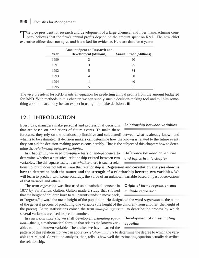
596 Statistics for Management
T -
YearAmount Spent on Research and
Development (Millions)1990 2 201991 3 251992 5 341993 4 301994 11 401995 5 31
-thing about the accuracy he can expect in using it to make decisions.
12.1 INTRODUCTIONEvery day, managers make personal and professional decisions that are based on predictions of future events. To make these forecasts, they rely on the relationship (intuitive and calculated) between what is already known and what is to be estimated. If decision makers can determine how the known is related to the future event, they can aid the decision-making process considerably. That is the subject of this chapter: how to deter-mine the relationship between variables.
In Chapter 11, we used chi-square tests of independence to determine whether a statistical relationship existed between two variables. The chi-square test tells us whether there is such a rela-tionship, but it does not tell us what that relationship is. Regression and correlation analyses show us how to determine both the nature and the strength of a relationship between two variables. We will learn to predict, with some accuracy, the value of an unknown variable based on past observations of that variable and others.
The term regression1877 by Sir Francis Galton. Galton made a study that showed that the height of children born to tall parents tends to move back,
regression as the name of the general process of predicting one variable (the height of the children) from another (the height of the parent). Later, statisticians coined the term multiple regression to describe the process by which several variables are used to predict another.
In regression analysis, we shall develop an estimating equa-tion—that is, a mathematical formula that relates the known vari-ables to the unknown variable. Then, after we have learned the pattern of this relationship, we can apply correlation analysis to determine the degree to which the vari-ables are related. Correlation analysis, then, tells us how well the estimating equation actually describes the relationship.
Relationship between variables
Difference between chi-square
and topics in this chapter
Origin of terms regression and
multiple regression
Development of an estimating
equation
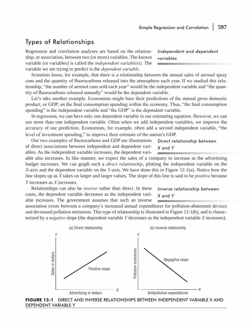
Simple Regression and Correlation 597
Types of RelationshipsRegression and correlation analyses are based on the relation-ship, or association, between two (or more) variables. The known variable (or variables) is called the independent variable(s). The variable we are trying to predict is the dependent variable.
Scientists know, for example, that there is a relationship between the annual sales of aerosol spray -
tionship, “the number of aerosol cans sold each year” would be the independent variable and “the quan-
use more than one independent variable. Often when we add independent variables, we improve the accuracy of our prediction. Economists, for example, often add a second independent variable, “the
of direct associations between independent and dependent vari-ables. As the independent variable increases, the dependent vari-able also increases. In like manner, we expect the sales of a company to increase as the advertising budget increases. We can graph such a direct relationship, plotting the independent variable on the X-axis and the dependent variable on the Y-axis. We have done this in Figure 12-1(a). Notice how the line slopes up as X takes on larger and larger values. The slope of this line is said to be positive because Y increases as X increases.
Relationships can also be inverse rather than direct. In these cases, the dependent variable decreases as the independent vari-able increases. The government assumes that such an inverse
and decreased pollution emissions. This type of relationship is illustrated in Figure 12-1(b), and is charac-terized by a negative slope (the dependent variable Y decreases as the independent variable X increases).
Independent and dependent
variables
Direct relationship between
X and Y
Inverse relationship between
X and Y
(a) Direct relationship (b) Inverse relationship
Negagtive slope
Positive slope
Advertising in dollars
Y Y
X XAntipollution expenditures
Pollu
tion
emis
sion
s
Sale
s in
dol
lars
FIGURE 12-1 DIRECT AND INVERSE RELATIONSHIPS BETWEEN INDEPENDENT VARIABLE X AND DEPENDENT VARIABLE Y
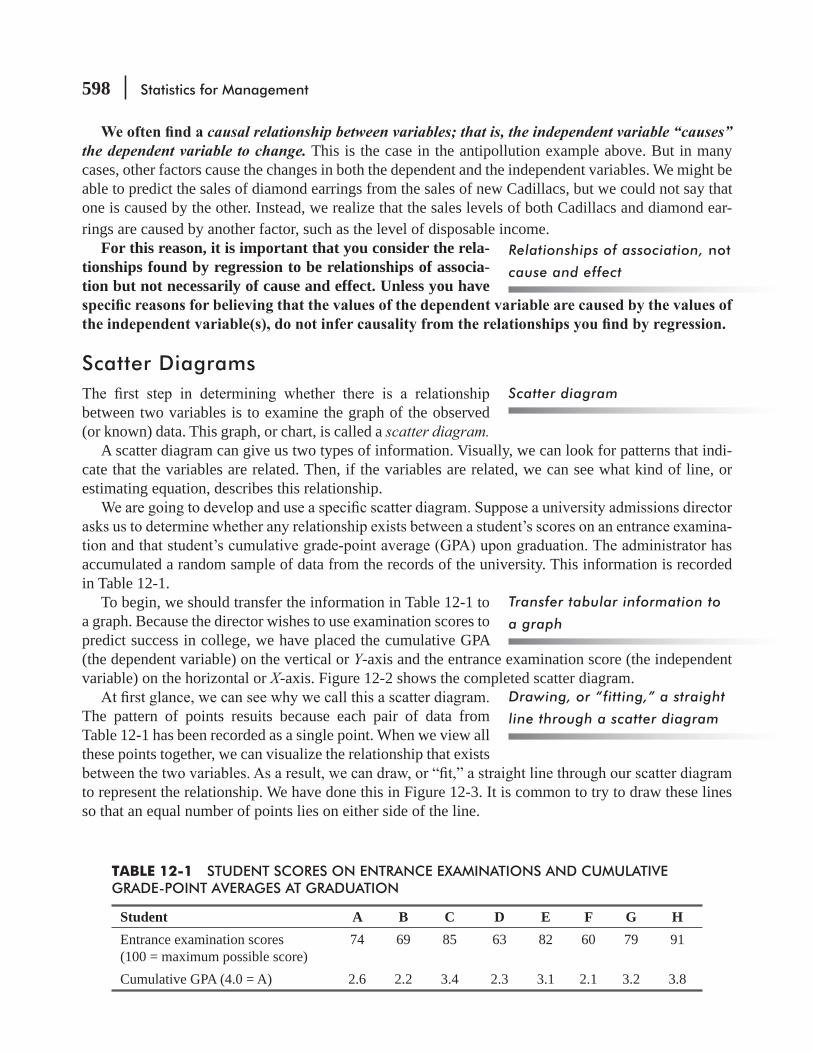
598 Statistics for Management
causal relationship between variables; that is, the independent variable “causes” the dependent variable to change. This is the case in the antipollution example above. But in many cases, other factors cause the changes in both the dependent and the independent variables. We might be able to predict the sales of diamond earrings from the sales of new Cadillacs, but we could not say that one is caused by the other. Instead, we realize that the sales levels of both Cadillacs and diamond ear-rings are caused by another factor, such as the level of disposable income.
For this reason, it is important that you consider the rela-tionships found by regression to be relationships of associa-tion but not necessarily of cause and effect. Unless you have
Scatter Diagrams
between two variables is to examine the graph of the observed (or known) data. This graph, or chart, is called a scatter diagram.
A scatter diagram can give us two types of information. Visually, we can look for patterns that indi-cate that the variables are related. Then, if the variables are related, we can see what kind of line, or estimating equation, describes this relationship.
-
accumulated a random sample of data from the records of the university. This information is recorded in Table 12-1.
To begin, we should transfer the information in Table 12-1 to a graph. Because the director wishes to use examination scores to predict success in college, we have placed the cumulative GPA (the dependent variable) on the vertical or Y-axis and the entrance examination score (the independent variable) on the horizontal or X-axis. Figure 12-2 shows the completed scatter diagram.
The pattern of points resuits because each pair of data from Table 12-1 has been recorded as a single point. When we view all these points together, we can visualize the relationship that exists
to represent the relationship. We have done this in Figure 12-3. It is common to try to draw these lines so that an equal number of points lies on either side of the line.
Relationships of association, not
cause and effect
Scatter diagram
Transfer tabular information to
a graph
Drawing, or “fitting,” a straight
line through a scatter diagram
TABLE 12-1 STUDENT SCORES ON ENTRANCE EXAMINATIONS AND CUMULATIVE GRADE-POINT AVERAGES AT GRADUATION
Student A B C D E F G HEntrance examination scores (100 = maximum possible score)
74 69 85 63 82 60 79 91
Cumulative GPA (4.0 = A) 2.6 2.2 3.4 2.3 3.1 2.1 3.2 3.8
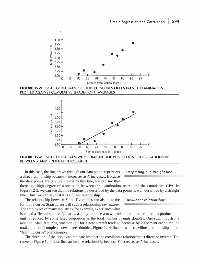
Simple Regression and Correlation 599
FIGURE 12-2 SCATTER DIAGRAM OF STUDENT SCORES ON ENTRANCE EXAMINATIONS PLOTTED AGAINST CUMULATIVE GRADE-POINT AVERAGES
Entrance examination scores50
4.003.753.503.25
3.002.752.502.252.00
Cum
ulat
ive
GPA
55 60 65 70 75 80 85 90 95
Y
X
FIGURE 12-3 SCATTER DIAGRAM WITH STRAIGHT LINE REPRESENTING THE RELATIONSHIP BETWEEN X AND Y “FITTED” THROUGH IT
Entrance examination scores50
4.003.753.503.25
3.002.752.502.252.00
Cum
ulat
ive
GPA
55 60 65 70 75 80 85 90 95
Y
X
In this case, the line drawn through our data points represents a direct relationship because Y increases as X increases. Because the data points are relatively close to this line, we can say that there is a high degree of association between the examination scores and the cumulative GPA. In Figure 12-3, we can see that the relationship described by the data points is well described by a straight line. Thus, we can say that it is a linear relationship.
The relationship between X and Y variables can also take the form of a curve. Statisticians call such a relationship curvilinear. The employees of many industries, for example, experience what is called a “learning curve”; that is, as they produce a new product, the time required to produce one
aviation. Manufacturing time per unit for a new aircraft tends to decrease by 20 percent each time the total number of completed new planes doubles. Figure 12-4 illustrates the curvilinear relationship of this “learning curve” phenomenon.
The direction of the curve can indicate whether the curvilinear relationship is direct or inverse. The curve in Figure 12-4 describes an inverse relationship because Y decreases as X increases.
Curvilinear relationships
Interpreting our straight line

600 Statistics for Management
To review the relationships possible in a scatter diagram, examine the graphs in Figure 12-5. Graphs (a) and (b) show direct and inverse linear relationships. Graphs (c) and (d) are examples of curvilinear relationships that demonstrate direct and inverse associations between vari-ables, respectively. Graph (e) illustrates an inverse linear relationship with a widely scattered pat-tern of points. The wider scattering indicates that there is a lower degree of association between the
FIGURE 12-4 CURVILINEAR RELATIONSHIP BETWEEN NEW-AIRCRAFT CONSTRUCTION TIME AND NUMBER OF UNITS PRODUCED
Number of planes produced0
1000 1,000 hours
800 hours
640 hours
512 hours
750
500
250
Num
ber o
f hou
rs p
er p
lane
5 10 15 20 25 30 35 40 45
Y
X
Review of possible relationships
FIGURE 12-5 POSSIBLE RELATIONSHIPS BETWEEN X AND Y IN SCATTER DIAGRAMS
(a) Direct linear (b) Inverse linear (c) Direct curvilinearY
X
Y
X
Y
X
(d) Inverse curvilinear (f) No relationship(e) Inverse linear withmore scatteringY
X
Y
X
Y
X

Simple Regression and Correlation 601
independent and dependent variables than there is in graph (b). The pattern of points in graph (f) seems to indicate that there is no linear relationship between the two variables; therefore, knowl-edge of the past concerning one variable does not allow us to predict future occurrences of the other.
EXERCISES 12.1
Self-Check ExerciseSC 12-1
related to the mean temperature that day. A random sample of 10 days was used for the study. The following data indicate the number of students absent (ABS) and the mean temperature (TEMP) for each day.
ABS 8 7 5 4 2 3 5 6 8 9TEMP 10 20 25 30 40 45 50 55 59 60
(a) State the dependent (Y) variable and the independent (X) variable.
Basic Concepts12-1 12-2 12-3 12-4 12-5 To what does the term causal relationship12-6 Explain the difference between linear and curvilinear relationships.12-7 Explain why and how we construct a scatter diagram.12-8 12-9 For each of the following scatter diagrams, indicate whether a relationship exists and, if so,
whether it is direct or inverse and linear or curvilinear.
(a) (b) (c)
Applications12-10 A professor is trying to show his students the importance of quizzes even though 90 percent of

602 Statistics for Management
below:
Quiz Average Final Average
59 65
92 8472 7790 8095 7787 8189 8077 8476 8065 6997 8342 4094 7862 6591 90
(a) State the dependent (Y) variable and the independent (X) variable.
12-11
into twelve grades or levels (1 being the lowest grade, 12 the highest) and then randomly
of days that employee had missed over the last 3 years.
Salary ranking 11 10 8 5 9 9 7 3Absences 18 17 29 36 11 26 28 35Salary ranking 11 8 7 2 9 8 6 3Absences 14 20 32 39 16 26 31 40
Construct a scatter diagram for these data and indicate the type of relationship.12-12
statistical relationships between many different variables and the common cold. One of the variables being examined is the use of facial tissues (X) and the number of days that cold symptoms were exhibited (Y) by seven people over a 12-month period. What relationship, if
X 2,000 1,500 500 750 600 900 1,000Y 60 40 10 15 5 25 30
Simple Regression and Correlation 603
Worked-Out Answers to Self-Check ExerciseSC 12-1 (a) We want to see whether absences (ABS) depend on temperature (TEMP).
(b) 10
8
6
4
2
10 20 30 40 50 60 70Temperature
Abse
nces
(c) Curvilinear.(d) Quadratic curve (parabola).(e) When it is very cold and when it is very hot there are many absences. For moderate tem-
peratures, there are not as many absences.
12.2 ESTIMATION USING THE REGRESSION LINEIn the scatter diagrams we have used to this point, the regression lines were put in place by points. In this section, we shall learn how to calculate the regres-sion line somewhat more precisely, using an equation that relates the two variables mathematically.
among more than two variables in the next chapter.The equation for a straight line where the dependent variable
Y is determined by the independent variable X is:
Equation for a Straight Line
Y = a + bXY-intercept
Independent variable
Slope of the line
[12-1]
Using this equation, we can take a given value of X and com-pute the value of Y. The a is called the Y-intercept because its value is the point at which the regression line crosses the Y-axis—that is, the vertical axis. The b in Equation 12-1 is the slope of the line. It represents how much each unit change of the independent vari-able X changes the dependent variable Y. Both a and b are numerical constants because for any given straight line, their values do not change.
Suppose we know that a is 3 and b is 2. Let us determine what Y would be for an X equal to 5. When we substitute the values of
Calculating the regression line
using an equation
Equation for a straight line
Interpreting the equation
Calculating Y from X using the
equation for a straight line
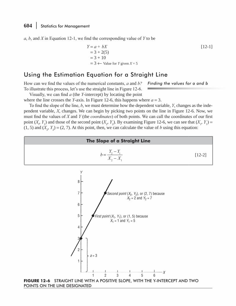
604 Statistics for Management
a, b, and X Y to be
Y = a + bX [12-1] = 3 + 2(5) = 3 + 10 = 3 ← Value for Y given X = 5
Using the Estimation Equation for a Straight Line a and b?
a (the Y-intercept) by locating the point where the line crosses the Y-axis. In Figure 12-6, this happens where a = 3.
b, we must determine how the dependent variable, Y, changes as the inde-pendent variable, X, changes. We can begin by picking two points on the line in Figure 12-6. Now, we
X and Y (the coordinatespoint (Xl, Y1) and those of the second point (X2, Y2). By examining Figure 12-6, we can see that (X1, Y1) = (1, 5) and (X2, Y2) = (2, 7). At this point, then, we can calculate the value of b using this equation:
The Slope of a Straight Line
2 1
2 1
=−−
bY YX X
[12-2]
Finding the values for a and b
FIGURE 12-6 STRAIGHT LINE WITH A POSITIVE SLOPE, WITH THE Y-INTERCEPT AND TWO POINTS ON THE LINE DESIGNATED
8
Second point (X2, Y2), or (2, 7) because X2 = 2 and Y2 = 7
First point (X1, Y1), or (1, 5) because X1 = 1 and Y1 = 5
a = 3
7
6
5
4
3
2
1
1 2 3 4 5 6
Y
X

Simple Regression and Correlation 605
7 5
2 1
=−−
b
2
1
= = 2 ← Slope of the line
In this manner, we can learn the values of the numerical con-stants, a and b, and write the equation for a straight line. The line in Figure 12-6 can be described by Equation 12-1, where a = 3 and b = 2. Thus
Y = a + bX [12-1]
and
Y = 3 + 2X
Using this equation, we can determine the corresponding value of the dependent variable for any value of X Y when X = 7. The answer would be
y = a + bX [12-1] = 3 + 2(7) = 3 + 14 = 17
If you substitute more values for X into the equation, you will notice that Y increases as X increases. Thus, the relationship between the variables is direct and the slope is positive.
Now consider the line in Figure 12-7. We see that it crosses the Y-axis at 6. Therefore, we know that a = 6. If we select the two points where (X1, Y1) = (0, 6) and (X2, Y2) =the line is
2 1
2 1
=−−
bY YX X
[12-2]
3 6
1 0
=−−
3
1
=−
= –3 Notice that when b is negative, the line represents an inverse rela-tionship and the slope is negative (Y decreases as X increases). Now, with the numerical values of a and b determined, we can substitute them into the general equation for a straight line:
Y = a + bX [12-1] = 6 + (–3)X = 6 − 3X
Writing and using the equation
for a straight line
Direct relationship; positive
slope
Inverse relationship; negative
slope

606 Statistics for Management
-able that corresponds to X = 2. Substituting into Equation 12-1, we get
Y = 6 − (3)(2) = 6 − 6 = 0
Thus, when X = 2, Y must equal 0. If we refer to the line in Figure 12-7, we can see that the point (2, 0) does lie on the line.
The Method of Least SquaresNow that we have seen how to determine the equation for a
for a line that is drawn through the middle of a set of points in a -
minimizes the error between the estimated points on the line and the actual observed points that were used to draw it.
Before we proceed, we need to introduce a new symbol. So far, we have used Y to represent the individual values of the observed points measured along the Y-axis. Now we should begin to use Y (Y hat) to symbolize the individual values of the estimated points—that is, the points that lie on the estimating line. Accordingly, we shall write the equation for the estimating line as
Fitting a regression line
mathematically
Introduction of Y
FIGURE 12-7 STRAIGHT LINE WITH A NEGATIVE SLOPE
8
First point (X1, Y1) = (0, 6)
Second point (X2, Y2) = (1, 3)a = 6
7
The point (2,0)
6
5
4
3
2
1
1 2 3 4 5 6
Y
X
Finding Y given X
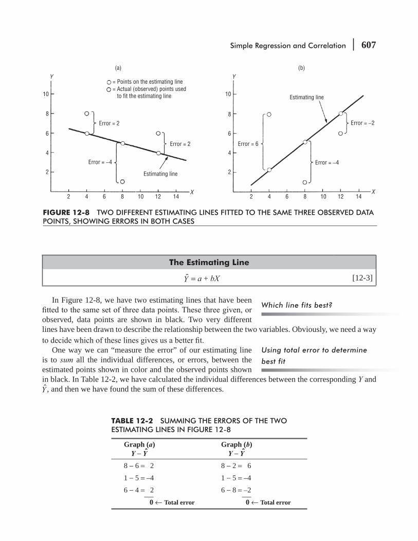
Simple Regression and Correlation 607
The Estimating Line
Y = a + bX [12-3]
In Figure 12-8, we have two estimating lines that have been
observed, data points are shown in black. Two very different lines have been drawn to describe the relationship between the two variables. Obviously, we need a way
One way we can “measure the error” of our estimating line is to sum all the individual differences, or errors, between the estimated points shown in color and the observed points shown in black. In Table 12-2, we have calculated the individual differences between the corresponding Y and Y , and then we have found the sum of these differences.
Which line fits best?
Using total error to determine
best fit
FIGURE 12-8 TWO DIFFERENT ESTIMATING LINES FITTED TO THE SAME THREE OBSERVED DATA POINTS, SHOWING ERRORS IN BOTH CASES
= Points on the estimating line
Estimating line
Error = 6
Error = −4
Error = 2
Error = −4
Estimating line
Error = 2
(a) (b)
Error = −2
= Actual (observed) points used to fit the estimating line10
8
6
4
2
10
8
6
4
2
2 4 6 8 10 12 14 2 4 6 8 10 12 14
Y
X
Y
X
TABLE 12-2 SUMMING THE ERRORS OF THE TWO ESTIMATING LINES IN FIGURE 12-8
Graph (a)Y − Y
Graph (b)Y − Y
8 − 6 = 2 8 − 2 = 6
1 − 5 = –4 1 − 5 = –4
6 − 4 = 2 6 − 8 = –2
0 ← Total error 0 ← Total error
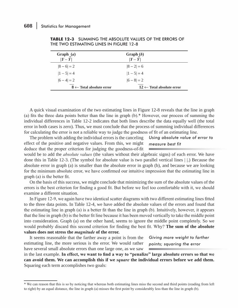
608 Statistics for Management
A quick visual examination of the two estimating lines in Figure 12-8 reveals that the line in graph
individual differences in Table 12-2 indicates that both lines describe the data equally well (the total error in both cases is zero). Thus, we must conclude that the process of summing individual differences
The problem with adding the individual errors is the canceling effect of the positive and negative values. From this, we might
would be to add the absolute values (the values without their algebraic signs) of each error. We have done this in Table 12-3. (The symbol for absolute value is two parallel vertical lines | |.) Because the absolute error in graph (a) is smaller than the absolute error in graph (b), and because we are looking
On the basis of this success, we might conclude that minimizing the sum of the absolute values of the
examine a different situation.
to the three data points. In Table 12-4, we have added the absolute values of the errors and found that
into consideration. Graph (a) on the other hand, seems to ignore the middle point completely. So we The sum of the absolute
values does not stress the magnitude of the error.It seems reasonable that the farther away a point is from the
estimating line, the more serious is the error. We would rather have several small absolute errors than one large one, as we saw in the last example.can avoid them. We can accomplish this if we square the individual errors before we add them. Squaring each term accomplishes two goals:
Using absolute value of error to
measure best fit
Giving more weight to farther
points; squaring the error
TABLE 12-3 SUMMING THE ABSOLUTE VALUES OF THE ERRORS OF THE TWO ESTIMATING LINES IN FIGURE 12-8
Graph (a)|Y − Y |
Graph (b)|Y − Y |
|8 − 6| = 2 |8 − 2| = 6
|1 − 5| = 4 |1 − 5| = 4
|6 − 4| = 2 |6 − 8| = 2
8 ← Total absolute error 12 ← Total absolute error

Simple Regression and Correlation 609
1. 2. It cancels the effect of the positive and negative values (a negative error squared is still positive).
Because we are looking for the estimating line that minimizes the sum of the squares of the errors, we call this the least-squares method.
data and summed the squares in Table 12-5, we can see that, as we thought, the estimating line in graph
Using the criterion of least squares, we can now determine
-ber of estimating lines, how can we tell when we have found the best- tting line
Y-intercept of the best-
Using least squares as a
measure of best fit
Finding the best-fitting least-
squares line mathematically
TABLE 12-4 SUMMING THE ABSOLUTE VALUES OF THE ERRORS OF THE TWO ESTIMATING LINES IN FIGURE 12-9
Graph (a)|Y − Y |
Graph (b)|Y − Y |
|4 − 4| = 0 |4 − 5| = 1
|7 − 3| = 4 |7 − 4| = 3
|2 − 4| = 0 |2 − 3| = 1
4 ← Total absolute error 5 ← Total absolute error
FIGURE 12-9 TWO DIFFERENT ESTIMATING LINES FITTED TO THE SAME THREE OBSERVED DATA POINTS, SHOWING ERRORS IN BOTH CASES
= Points on the estimating line
Estimating line
Estimating lineError = 0
Error = 0
Error = 4Error = 3
(a) (b)
Error = −1 Error = −1
= Actual (observed) points used to fit the estimating line8
6
4
2
8
6
4
2
2 4 6 8 10 2 4 6 8 10
Y Y
X X
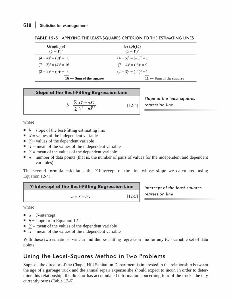
610 Statistics for Management
Slope of the Best-Fitting Regression Line
2 2
XY nXYbX nX
∑ −=∑ −
[12-4]
where
b = X = values of the independent variable Y = values of the dependent variable X = mean of the values of the independent variable Y = mean of the values of the dependent variable n = number of data points (that is, the number of pairs of values for the independent and dependent
variables)
The second formula calculates the Y-intercept of the line whose slope we calculated using Equation 12-4:
Y-Intercept of the Best-Fitting Regression Line
a Y bX= − [12-5]
where
a = Y-intercept b = slope from Equation 12-4 Y = mean of the values of the dependent variable X = mean of the values of the independent variable
points.
Using the Least-Squares Method in Two Problems
the age of a garbage truck and the annual repair expense she should expect to incur. In order to deter-mine this relationship, the director has accumulated information concerning four of the trucks the city currently owns (Table 12-6).
Slope of the least-squares
regression line
Intercept of the least-squares
regression line
TABLE 12-5 APPLYING THE LEAST-SQUARES CRITERION TO THE ESTIMATING LINES
Graph (a)(Y − Y )2
Graph (b)(Y − Y )2
(4 − 4)2 = (0)2 = 0 (4 − 5)2 = (–1)2 = 1
(7 − 3)2 = (4)2 = 16 (7 − 4)2 = ( 3)2 = 9
(2 − 2)2 = (0)2 = 0 (2 − 3)2 = (–1)2 = 1
16 ← Sum of the squares 11 ← Sum of the squares

Simple Regression and Correlation 611
-lem is to organize the data as outlined in Table 12-7. This allows us to substitute directly into Equations 12-4 and 12-5 in order to
YWith the information in Table 12-7, we can now use the equations for the slope (Equation 12-4) and
the Y
b XY xXYX nX2 2=
∑ −∑ −
[12-4]
78 (4)(3)(6)44 (4)(3)
78 3244 36
−=−
68
=
= 0.75 ← The slope of the line
Finding the value of b
Example of the least-squares
method
TABLE 12-6 ANNUAL TRUCK-REPAIR EXPENSES
Truck NumberAge of Truck in
Years (X)Repair Expense During Last
Year in Hundreds of $ (Y)101 5 7102 3 7103 3 6104 1 4
TABLE 12-7 CALCULATION OF INPUTS FOR EQUATIONS 12-4 AND 12-5
Trucks (n = 4)(1)
Age (X )(2)
Repair Expense (Y )(3)
XY(2) × (3)
X 2(2)2
101 5 7 35 25102 3 7 21 9103 3 6 18 9104 1 4 4 1
∑ X = 12 ∑ Y = 24 ∑ XY = 78 ∑ X 2 = 44
=∑X Xn
12
4
=
= 3 ← Mean of the values of the independent variable
=∑Y Yn
24
4
=
= 6 ← Mean of the values of the dependent variable

612 Statistics for Management
And the Y-intercept is
a Y bX= − [12-5] = 6 − (0.75)(3) = 6 − 2.25 = 3.75 ← The Y-intercept
Now, to get the estimating equation that describes the relation-ship between the age of a truck and its annual repair expense, we can substitute the values of a and b in the equation for the estimating line:
Y = a + bX [12-3] = 3.75 + 0.75X
Using this estimating equation (which we could plot as a -
tor can estimate the annual repair expense, given the age of her equipment. For example, if the city has a truck that is 4 years old, the director could use the equation to predict the annual repair expense for this truck as follows:
Y = 3.75 + 0.75(4) = 3.75 + 3
= 6.75 ← Expected annual repair expense of $675.00
Thus, the city might expect to spend about $675 annually in repairs on a 4-year-old truck.Now we can solve the chapter-opening problem concerning
the relationship between money spent on research and develop-
the information for the preceding 6 years. With this, we can determine the regression equation describ-ing the relationship.
Again, we can facilitate the collection of the necessary information if we perform the calculations in a table such as Table 12-9.
Finding the value of a
Determining the estimating
equation
Using the estimating equation
Another example
TABLE 12-8 ANNUAL RELATIONSHIP BETWEEN RESEARCH AND DEVELOPMENT AND PROFITS
Year
Amount of Money Spent on Research and Development ($ Millions)
(X)
(Y)1995 5 31
1994 11 40
1993 4 30
1992 5 34
1991 3 25
1990 2 20

Simple Regression and Correlation 613
a and b for the estimating equation. The value of b is
b XY xXYX nX2 2=
∑ −∑ −
[12-4]
2
1,000 (6)(5)(30)200 (6)(5)
−=−
1,000 900200 150
−=−
10050
=
= 2 ← The slope of the line
And the value for a is
a Y bX= − [12-5] = 30 − (2)(5) = 30 − 10 = 20 ← The Y-intercept
Finding b
Finding a
TABLE 12-9 CALCULATION OF INPUTS FOR EQUATIONS 12-4 AND 12-5
Year (n = 6)
Expenditures for R&D (X )
(Y )
XY
X 2
1995 5 31 155 25
1994 11 40 440 121
1993 4 30 120 16
1992 5 34 170 25
1991 3 25 75 9
1990 2 20 40 4
ÂX = 30 Â Y = 180 Â XY = 1,000 Â X 2 = 200
=∑X Xn
[3-2]
306
=
= 5 ← Mean of the values of the independent variable
=∑Y Yn
[3-2]
1806
=
= 30 ← Mean of the values of the dependent variable
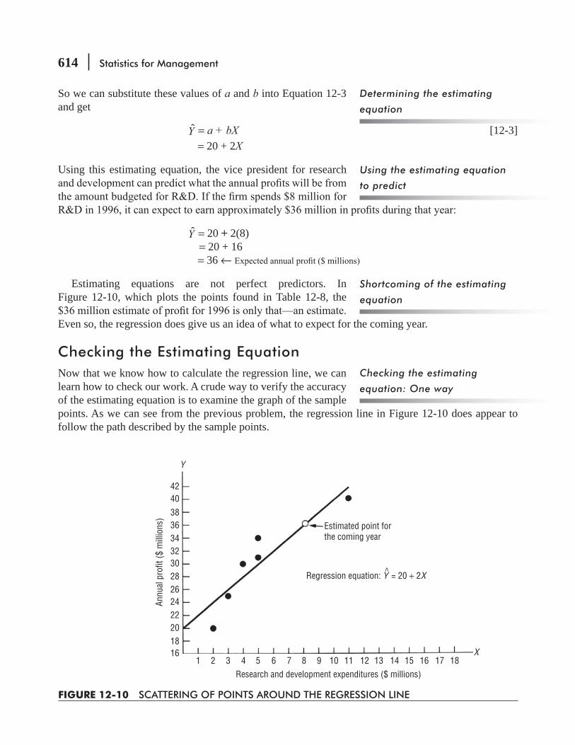
614 Statistics for Management
So we can substitute these values of a and b into Equation 12-3 and get
Y = a + bX [12-3] = 20 + 2X
Using this estimating equation, the vice president for research
Y = 20 + 2(8) = 20 + 16 = 36 ←
Estimating equations are not perfect predictors. In Figure 12-10, which plots the points found in Table 12-8, the
Even so, the regression does give us an idea of what to expect for the coming year.
Checking the Estimating EquationNow that we know how to calculate the regression line, we can learn how to check our work. A crude way to verify the accuracy of the estimating equation is to examine the graph of the sample points. As we can see from the previous problem, the regression line in Figure 12-10 does appear to follow the path described by the sample points.
Using the estimating equation
to predict
Shortcoming of the estimating
equation
Checking the estimating
equation: One way
Determining the estimating
equation
FIGURE 12-10 SCATTERING OF POINTS AROUND THE REGRESSION LINE
4240383634323028262422201816
1 2 3 4 5 6Research and development expenditures ($ millions)
Annu
al p
rofit
($ m
illio
ns)
7 8 9 10
Estimated point forthe coming year
Regression equation: Y = 20 + 2X
11 12 13 14 15 16 17 18X
Y
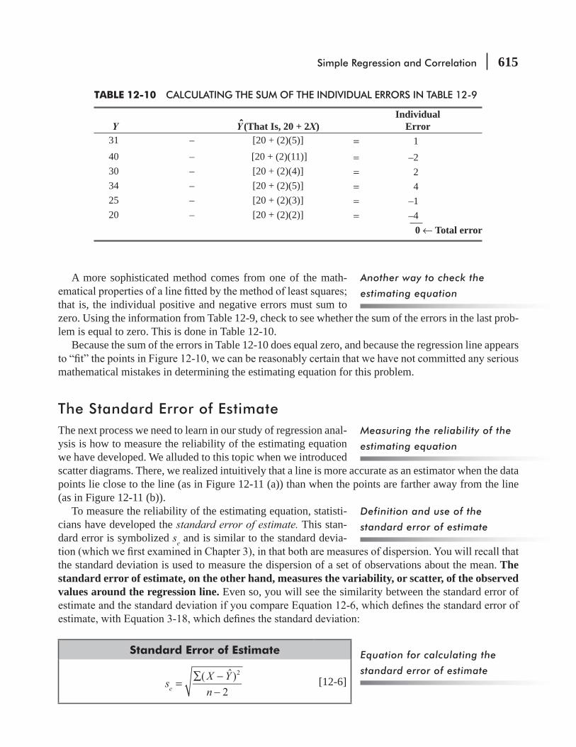
Simple Regression and Correlation 615
A more sophisticated method comes from one of the math-
that is, the individual positive and negative errors must sum to zero. Using the information from Table 12-9, check to see whether the sum of the errors in the last prob-lem is equal to zero. This is done in Table 12-10.
Because the sum of the errors in Table 12-10 does equal zero, and because the regression line appears
mathematical mistakes in determining the estimating equation for this problem.
The Standard Error of EstimateThe next process we need to learn in our study of regression anal-ysis is how to measure the reliability of the estimating equation we have developed. We alluded to this topic when we introduced scatter diagrams. There, we realized intuitively that a line is more accurate as an estimator when the data points lie close to the line (as in Figure 12-11 (a)) than when the points are farther away from the line (as in Figure 12-11 (b)).
To measure the reliability of the estimating equation, statisti-cians have developed the standard error of estimate. This stan-dard error is symbolized se and is similar to the standard devia-
the standard deviation is used to measure the dispersion of a set of observations about the mean. The standard error of estimate, on the other hand, measures the variability, or scatter, of the observed values around the regression line. Even so, you will see the similarity between the standard error of
Standard Error of Estimate
(
ˆ
)
2
2
=∑ −
−s X Y
ne[12-6]
Measuring the reliability of the
estimating equation
Definition and use of the
standard error of estimate
Equation for calculating the
standard error of estimate
Another way to check the
estimating equation
TABLE 12-10 CALCULATING THE SUM OF THE INDIVIDUAL ERRORS IN TABLE 12-9
Y Y (That Is, 20 + 2X)Individual
Error31 – [20 + (2)(5)] = 140 – [20 + (2)(11)] = –230 – [20 + (2)(4)] = 234 – [20 + (2)(5)] = 425 – [20 + (2)(3)] = –120 – [20 + (2)(2)] = –4
0 ← Total error

616 Statistics for Management
where
Y = values of the dependent variable Y = estimated values from the estimating equation that correspond to each Y value n =
Notice that in Equation 12-6, the sum of the squared devia-tions is divided by n − 2, not by n. This happens because we have lost 2 degrees of freedom in estimating the regression line. We can reason that because the values of a and b were obtained from a sample of data points, we lose 2 degrees of freedom when we use these points to estimate the regression line.
of her trucks to the amount of annual repairs. We found the estimating equation in that situation to be
Y = 3.75 + 0.75X
where X is the age of the truck and Y is the estimated amount of annual repairs (in hundreds of dollars).
To calculate sevalue of ∑ (Y − Y )2, that is, the numerator of Equation 12-6. We have done this in Table 12-11, using (3.75 + 0.75X) for Y when-ever it was necessary. Because ∑ (Y − Y )2
standard error of estimate:
(
ˆ
)
2
2
=∑ −
−s X Y
ne [12-6]
1.504 2
=−
0.75=
= 0.866 ← Standard error of estimate of $86.60
n − 2 is the divisor in
Equation 12-6
Calculating the standard error
of estimate
FIGURE 12-11 CONTRASTING DEGREES OF SCATTERING OF DATA POINTS AND THE RESULTING EFFECT ON THE ACCURACY OF THE REGRESSION LINE
(a) This regression line is a more accurate estimator of the relationship between X and Y
(b) This regression line is a less accurate estimator of the relationship between X and Y
Y
X X
Y

Simple Regression and Correlation 617
Using a Short-Cut Method to Calculate the Standard Error of EstimateTo use Equation 12-6, we must do the tedious series of calculations outlined in Table 12-11. For every value of Y, we must compute the corresponding value of Y . Then we must substitute these values into the expression ∑ (Y − Y )2.
Fortunately, we can eliminate some of the steps in this task by using the short cut provided by Equation 12-7, that is:
Short-Cut Method for Finding the Standard Error of Estimate
s Y a Y b XYne 2
2
=∑ − ∑ − ∑
−[12-7]
where
X = values of the independent variable Y = values of the dependent variable a = Y-intercept from Equation 12-5 b = slope of the estimating equation from Equation 12-4 n = number of data points
calculate the slope and the Y-intercept (Table 12-7), we determined every value we need for Equation 12-7 except one: the value of ∑ Y 2. Table 12-12 is a repeat of Table 12-7 with the Y 2 column added.
Now we can refer to Table 12-12 and our previous calculations of a and b in order to calculate se using the short-cut method:
s Y a Y b XYne 2
2
=∑ − ∑ − ∑
− [12-7]
150 (3.75)(24) (0.75)(78)4 2
− −=−
A quicker way to calculate se
TABLE 12-11 CALCULATING THE NUMERATOR OF THE FRACTION IN EQUATION 12-6
X(1)
Y(2)
Y (That is, 3.75 + 0.75X ) (3)
Individual Error (Y − Y )(2) − (3)
(Y − Y )2
[(2) − (3)]2
5 7 3.75 + (0.75)(5) 7 − 7.5 = –0.5 0.25
3 7 3.75 + (0.75)(3) 7 − 6.0 = 1.0 1.00
3 6 3.75 + (0.75)(3) 6 − 6.0 = 0.0 0.00
1 4 3.75 + (0.75)(1) 4 − 4.5 = –0.5 0.25
 (Y − Y )2 = 1.50 ← Sum of squared errors

618 Statistics for Management
150 90 58.52
− −=
0.75= = 0.866 ← Standard error of $86.60
This is the same result as the one we obtained using Equation 12-6, but think of how many steps we saved!
Interpreting the Standard Error of EstimateAs was true of the standard deviation, the larger the standard error of estimate, the greater the scattering (or dispersion) of points around the regression line. Conversely, if se = 0, we expect the estimating equation to be a “perfect” estimator of the dependent variable. In that case, all the data points would lie directly on the regression line, and no points would be scattered around it.
We shall use the standard error of estimate as a tool in the same way that we can use the standard deviation. That is to say, assuming that the observed points are normally distributed
points within ± 1se (or plus and minus 1 standard error of estimate), 95.5 percent of the points within ±2se, and 99.7 percent of the points within ±3se. Figure 12-12 illustrates these “bounds” around the regression line. Another thing to notice in Figure 12-12 is that the standard error of estimate is measured along the Y-axis, rather than perpendicularly from the regression line.
At this point, we should state the assumptions we are making because shortly we shall make some probability statements based
1. The observed values for Y are normally distributed around each estimated value of . 2. The variance of the distributions around each possible value of Y is the same.
If this second assumption were not true, then the standard error at one point on the regression line could differ from the standard error at another point on the line.
Interpreting and using the
standard error of estimate
Using se to form bounds around
the regression line
Assumptions we make in use
of se
TABLE 12-12 CALCULATION OF INPUTS FOR EQUATION 12-7
Trucks (n = 4)(1)
Age X(2)
Repair Expense Y(3)
XY(2) ¥ (3)
X 2(2)2
Y 2(3)2
101 5 7 35 25 49
102 3 7 21 9 49
103 3 6 18 9 36
104 1 4 4 1 16
 X = 12  y = 24  XY = 78  X 2 = 44  X 2 = 150
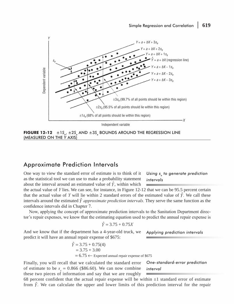
Simple Regression and Correlation 619
Approximate Prediction IntervalsOne way to view the standard error of estimate is to think of it as the statistical tool we can use to make a probability statement about the interval around an estimated value of Y , within which the actual value of Y lies. We can see, for instance, in Figure 12-12 that we can be 95.5 percent certain that the actual value of Y will lie within 2 standard errors of the estimated value of Y . We call these intervals around the estimated Y approximate prediction intervals. They serve the same function as the
-
Y = 3.75 + 0.75XAnd we know that if the department has a 4-year-old truck, we predict it will have an annual repair expense of $675: Y = 3.75 + 0.75(4) = 3.75 + 3.00
= 6.75 ← Expected annual repair expense of $675
Finally, you will recall that we calculated the standard error of estimate to be se = 0.866 ($86.60). We can now combine these two pieces of information and say that we are roughly 68 percent confident that the actual repair expense will be within ±1 standard error of estimate from Y . We can calculate the upper and lower limits of this prediction interval for the repair
Using se to generate prediction
intervals
Applying prediction intervals
One-standard-error prediction
interval
FIGURE 12-12 ±1Se, ±2Se AND ±3Se BOUNDS AROUND THE REGRESSION LINE (MEASURED ON THE Y AXIS)
Y = a + bX + 3se
Y = a + bX + 2se
Y = a + bX + 1se
Y = a + bX − 1se
Y = a + bX − 2se
Y = a + bX − 3se
Y = a + bX (regression line)
±3se (99.7% of all points should lie within this region)
±2se (95.5% of all points should lie within this region)
±1se (68% of all points should lie within this region)
Independent variable
Depe
nden
t var
iabl
e
se
X
Y

620 Statistics for Management
expense as follows: Y + 1se = $675 + (1)($86.60)
= $761.60 ← Upper limit of prediction interval
and Y + 1se = $675 + (1)($86.60)
= $588.40 ← Lower limit of prediction interval
that the actual repair expense will be within ±2 standard errors of estimate from Y ,we would calculate the limits of this new predic-tion interval like this: Y + 2se = $675 + (2)($86.60) = $848.20 ← Upper limit and
Y + 2se = $675 − (2)($86.60) = $501.80 ← Lower limit
Keep in mind that statisticians apply prediction intervals based on the normal distribution (68 percent for 1se, 95.5 percent for 2se, and 99.7 percent for 3se) only to large samples, that is, where n > 30. In this problem, our sample size is too small (n = 4). Thus, our conclusions are inaccurate. But the method we have used nevertheless demonstrates the principle involved in prediction intervals.
If we wish to avoid the inaccuracies caused by the size of the sample, we need to use the t distribution. Recall that the t distri-bution is appropriate when n is less than 30 and the population standard deviation is unknown. We meet both these conditions because n = 4, and se is an estimate rather than the known population standard deviation.
roughly 90 percent certain that the annual truck-repair expense
t distribution table focuses on the prob-ability that the parameter we are estimating will lie outside the prediction interval, we need to look in Appendix Table 2 under the 100% − 90% = 10% value column. Once we locate that column, we look for the row representing 2 degrees of freedom; because n = 4 and because we know we lose 2 degrees of freedom (in estimating the values of a and b), then n − 2 = 2.
t value to be 2.920.Now using this value of t, we can make a more accurate calculation of our prediction interval limits,
as follows:
Y + t(se) = $675 + (2.920)($86.60) = $675 + $252.87 = $927.87 ← Upper limit
Two-standard-error prediction
interval
n is too small to use the normal
distribution
Using the t distribution for
prediction intervals
An example using the
t distribution to calculate
prediction intervals
Simple Regression and Correlation 621
and
Y + t(se) = $675 − (2.920)($86.60)
= $675 − $252.87
= $422.13 ← Lower limit
So the director can be 90 percent certain that the annual repair expense on a 4-year old truck will lie between $422.13 and $927.87.
We stress again that these prediction intervals are only approximate. In fact, statisticians can calcu-late the exact standard error for the prediction sp using this formula:
202 2
1 ( )1p eX Xs s
n X nX−= + +
∑ −
where X0 X at which we want to predict the value of Y.Notice that if we use this formula, sp is different for each value of X0. In particular, if X0 is far from
X , then sp is large because (X0 − X )2 is large. On the other hand, if X0 is close to X and n is mod-erately large (greater than 10), then sp is close to se. This happens because 1/n is small and (X0 − X )2 is small. Therefore, the value under the square-root sign is close to 1, the square root is even closer to 1, and sp is very close to se. This justifies our use of se to compute approximate prediction intervals.
sketch the scatter diagram for those points. This lets you investigate any outlying points because some of the data you have may not represent the problem you are trying to solve. For example, the manager of a restaurant chain near college campuses who wants to examine the hypothesis that
-sity holidays distort an otherwise useful regression. Warning: It is dangerous to pick and choose
should be. In regression analysis, thoughtful selection and consistent use of the best database lead to the most useful estimating equation.
HINTS & ASSUMPTIONS
Simple Linear Regression Using SPSSFor Simple Regression Go to Analyze>Regression>Linear Regression>Choose dependent and independent variables>Select desired statistics
622 Statistics for Management
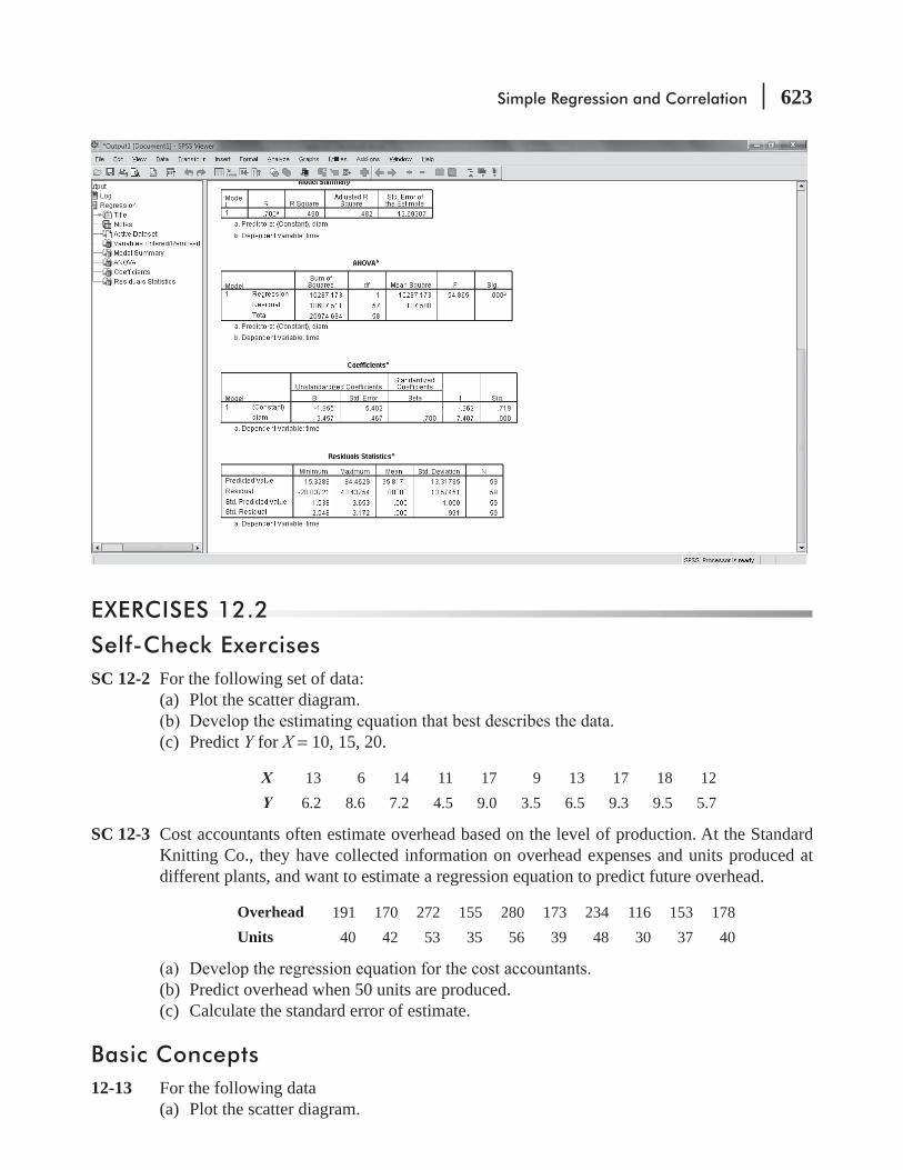
Simple Regression and Correlation 623
EXERCISES 12.2
Self-Check ExercisesSC 12-2 For the following set of data:
(a) Plot the scatter diagram.
(c) Predict Y for X = 10, 15, 20.
X 13 6 14 11 17 9 13 17 18 12Y 6.2 8.6 7.2 4.5 9.0 3.5 6.5 9.3 9.5 5.7
SC 12-3 Cost accountants often estimate overhead based on the level of production. At the Standard Knitting Co., they have collected information on overhead expenses and units produced at different plants, and want to estimate a regression equation to predict future overhead.
Overhead 191 170 272 155 280 173 234 116 153 178Units 40 42 53 35 56 39 48 30 37 40
(b) Predict overhead when 50 units are produced.(c) Calculate the standard error of estimate.
Basic Concepts12-13 For the following data
(a) Plot the scatter diagram.

624 Statistics for Management
(c) Predict Y for X = 6, 13.4, 20.5.X 2.7 4.8 5.6 18.4 19.6 21.5 18.7 14.3Y 16.66 16.92 22.3 71.8 80.88 81.4 77.46 48.7
X 11.6 10.9 18.4 19.7 12.3 6.8 13.8Y 50.48 47.82 71.5 81.26 50.1 39.4 52.8
12-14 Using the data given below(a) Plot the scatter diagram.
(c) Predict Y for X = 5, 6, 7.X 16 6 10 5 12 14Y –4.4 8.0 2.1 8.7 0.1 –2.9
12-15 Given the following set of data:
(b) Compute the standard error of estimate.
dependent variable given that X is 44.X 56 48 42 58 40 39 50Y 45 38.5 34.5 46.1 33.3 32.1 40.4
Applications12-16 Sales of major appliances vary with the new housing market: when new home sales are good,
so are the sales of dishwashers, washing machines, driers, and refrigerators. A trade associa-tion compiled the following historical data (in thousands of units) on major appliance sales and housing starts:
Housing Starts (thousands)
Appliance Sales (thousands)
2.0 5.02.5 5.53.2 6.03.6 7.03.3 7.24.0 7.74.2 8.44.6 9.04.8 9.75.0 10.0
-ing starts (in thousands).
(b) Interpret the slope of the regression line.(c) Compute and interpret the standard error of estimate.
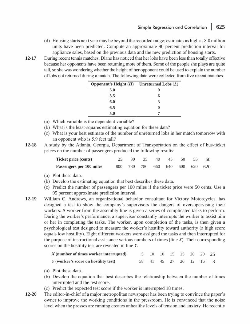
Simple Regression and Correlation 625
units have been predicted. Compute an approximate 90 percent prediction interval for appliance sales, based on the previous data and the new prediction of housing starts.
12-17 because her opponents have been returning more of them. Some of the people she plays are quite tall, so she was wondering whether the height of her opponent could be used to explain the number
Opponent’s Height (H) Unreturned Lobs (L)5.0 95.5 66.0 36.5 05.0 7
(c) What is your best estimate of the number of unreturned lobs in her match tomorrow with
12-18 prices on the number of passengers produced the following results:
Ticket price (cents) 25 30 35 40 45 50 55 60Passengers per 100 miles 800 780 780 660 640 600 620 620
(a) Plot these data.
(c) Predict the number of passengers per 100 miles if the ticket price were 50 cents. Use a 95 percent approximate prediction interval.
12-19 William C. Andrews, an organizational behavior consultant for Victory Motorcycles, has
workers. A worker from the assembly line is given a series of complicated tasks to perform.
or her in completing the tasks. The worker, upon completion of the tasks, is then given a
equals low hostility). Eight different workers were assigned the tasks and then interrupted for the purpose of instructional assistance various numbers of times (line X). Their corresponding scores on the hostility test are revealed in line Y.
X (number of times worker interrupted) 5 10 10 15 15 20 20 25Y (worker’s score on hostility test) 58 41 45 27 26 12 16 3
(a) Plot these data.
interrupted and the test score.(c) Predict the expected test score if the worker is interrupted 18 times.
12-20
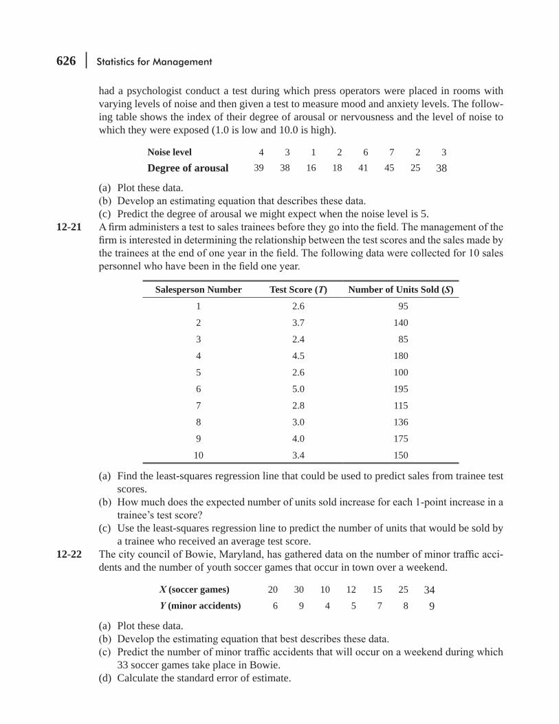
626 Statistics for Management
had a psychologist conduct a test during which press operators were placed in rooms with varying levels of noise and then given a test to measure mood and anxiety levels. The follow-ing table shows the index of their degree of arousal or nervousness and the level of noise to which they were exposed (1.0 is low and 10.0 is high).
Noise level 4 3 1 2 6 7 2 3Degree of arousal 39 38 16 18 41 45 25 38
(a) Plot these data.
(c) Predict the degree of arousal we might expect when the noise level is 5.12-21
Salesperson Number Test Score (T) Number of Units Sold (S)
1 2.6 95
2 3.7 140
3 2.4 85
4 4.5 180
5 2.6 100
6 5.0 195
7 2.8 115
8 3.0 136
9 4.0 175
10 3.4 150
(a) Find the least-squares regression line that could be used to predict sales from trainee test scores.
(c) Use the least-squares regression line to predict the number of units that would be sold by a trainee who received an average test score.
12-22 -dents and the number of youth soccer games that occur in town over a weekend.
X (soccer games) 20 30 10 12 15 25 34Y (minor accidents) 6 9 4 5 7 8 9
(a) Plot these data.
33 soccer games take place in Bowie.(d) Calculate the standard error of estimate.
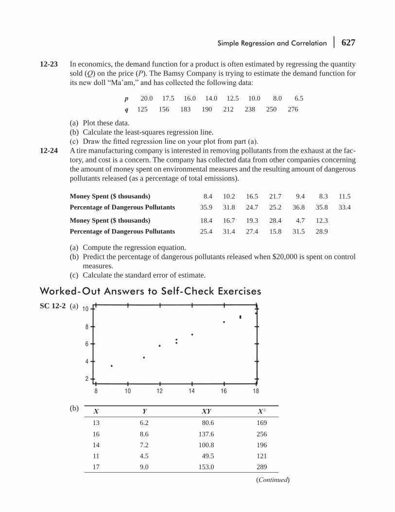
Simple Regression and Correlation 627
12-23 In economics, the demand function for a product is often estimated by regressing the quantity sold (Q) on the price (P). The Bamsy Company is trying to estimate the demand function for
p 20.0 17.5 16.0 14.0 12.5 10.0 8.0 6.5q 125 156 183 190 212 238 250 276
(a) Plot these data.(b) Calculate the least-squares regression line.
12-24 A tire manufacturing company is interested in removing pollutants from the exhaust at the fac-tory, and cost is a concern. The company has collected data from other companies concerning the amount of money spent on environmental measures and the resulting amount of dangerous pollutants released (as a percentage of total emissions).
Money Spent ($ thousands) 8.4 10.2 16.5 21.7 9.4 8.3 11.5Percentage of Dangerous Pollutants 35.9 31.8 24.7 25.2 36.8 35.8 33.4
Money Spent ($ thousands) 18.4 16.7 19.3 28.4 4.7 12.3Percentage of Dangerous Pollutants 25.4 31.4 27.4 15.8 31.5 28.9
(a) Compute the regression equation.(b) Predict the percentage of dangerous pollutants released when $20,000 is spent on control
measures.(c) Calculate the standard error of estimate.
Worked-Out Answers to Self-Check ExercisesSC 12-2 (a) 10
8
6
4
2
8 10 12 14 16 18
(b) X Y XY X 2
13 6.2 80.6 16916 8.6 137.6 25614 7.2 100.8 19611 4.5 49.5 12117 9.0 153.0 289
(Continued)

628 Statistics for Management
X Y XY X 2
9 3.5 31.5 81
13 6.5 84.5 169
17 9.3 158.1 289
18 9.5 171.0 324
12 5.7 68.4 144
∑ X= 140
∑ Y= 70.0 ∑ XY= 1,035.0 ∑ X 2 = 2,038
X 140 / 10 14= = Y 70.0 / 10 7.0= =
b XY nXYX nX2 2=
∑ −∑ −
= 1,035.0 10(14)(7.0)
2,038 10(14)
0.7051
2
−−
=
a Y bX 7.0 (0.7051)(14) 2.8714= − = − = −
Thus, Y = –2.8714 + 0.7051X. If you used a computer regression package to do your computation, you probably got
Y = –2.8718 + 0.7051X.
This slight difference occurs because most computer packages carry their calculations to more than ten decimal places, but we rounded b a. For most practical purposes, this slight difference (i.e., a = –2.8714 instead of –2.8718) is inconsequential.
(c) X = 10, Y = –2.8714 + 0.7051(10) = 4.1796 X = 15, Y = –2.8714 + 0.7051(15) = 7.7051 X = 20, Y = –2.8714 + 0.7051(20) = 11.2306
SC 12-3 In this problem, Y = overhead and X = units produced.
(a) X Y XY X 2 Y 2
40 191 7,640 1,600 36,481
42 170 7,140 1,764 28,900
53 272 14,416 2,809 73,984
35 155 5,425 1,225 24,025
56 280 15,680 3,136 78,400
39 173 6,747 1,521 29,929
48 234 11,232 2,304 54,756
30 116 3,480 900 13,456
37 153 5,661 1,369 23,409
40 178 7,120 1,600 31,684
 X = 420  Y = 1,922  XY = 84,541  X 2 = 18,228  Y 2 = 395,024
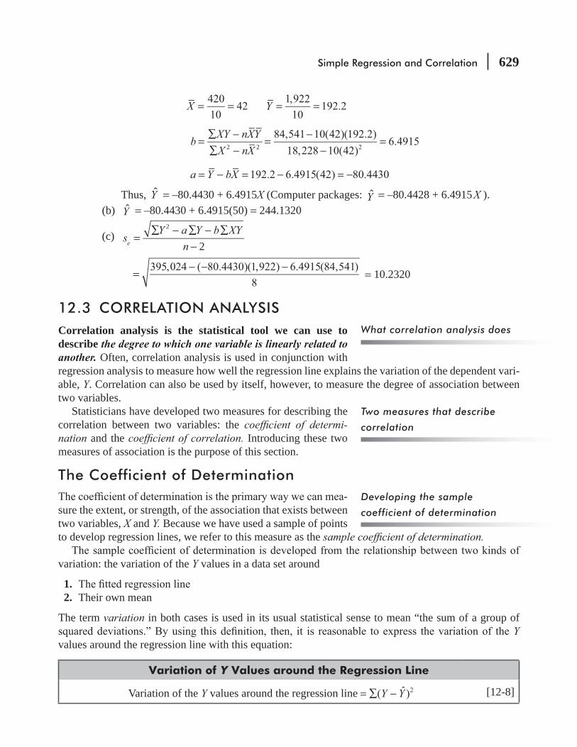
Simple Regression and Correlation 629
X 420
10
42= = Y 1,922
10
192.2= =
b XY nXYX nX2 2=
∑ −∑ −
84,541 10(42)(192.2)
18,228 10(42)
6.4915
2
=−
−=
a Y bX 192.2 6.4915(42) 80.4430= − = − = −
Thus, Y = –80.4430 + 6.4915X (Computer packages: Y = –80.4428 + 6.4915 X ).(b) Y = –80.4430 + 6.4915(50) = 244.1320
(c) sY a Y b XY
n 2e
2
=∑ − ∑ − ∑
−
395,024 ( 80.4430)(1,922) 6.4915(84,541)
8
=− − −
= 10.2320
12.3 CORRELATION ANALYSISCorrelation analysis is the statistical tool we can use to describe the degree to which one variable is linearly related to another. Often, correlation analysis is used in conjunction with regression analysis to measure how well the regression line explains the variation of the dependent vari-able, Y. Correlation can also be used by itself, however, to measure the degree of association between two variables.
Statisticians have developed two measures for describing the correlation between two variables: the coef cient of determi-nation and the coef cient of correlation. Introducing these two measures of association is the purpose of this section.
The Coefficient of Determination-
sure the extent, or strength, of the association that exists between two variables, X and Y. Because we have used a sample of points to develop regression lines, we refer to this measure as the sample coef cient of determination.
variation: the variation of the Y values in a data set around
1. 2. Their own mean
The term variation in both cases is used in its usual statistical sense to mean “the sum of a group of Y
values around the regression line with this equation:
Variation of Y Values around the Regression Line
Variation of the Y values around the regression line Y Y(
ˆ
)
2= ∑ − [12-8]
What correlation analysis does
Two measures that describe
correlation
Developing the sample
coefficient of determination
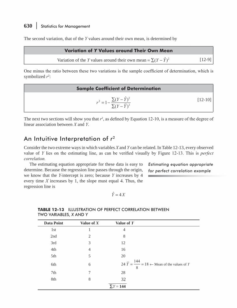
630 Statistics for Management
The second variation, that of the Y values around their own mean, is determined by
Variation of Y Values around Their Own Mean
Variation of the Y values around their own mean Y Y(
ˆ
)
2= ∑ − [12-9]
symbolized r2:
Sample Coefficient of Determination
r Y YY Y
1
(
ˆ
)
( )
2
2
2
= −∑ −∑ −
[12-10]
The next two sections will show you that r2
linear association between X and Y.
An Intuitive Interpretation of r2
Consider the two extreme ways in which variables X and Y can be related. In Table 12-13, every observed value of Y perfect correlation.
The estimating equation appropriate for these data is easy to determine. Because the regression line passes through the origin, we know that the Y-intercept is zero; because Y increases by 4 every time X increases by 1, the slope must equal 4. Thus, the regression line is
Y Xˆ
4=
Estimating equation appropriate
for perfect correlation example
TABLE 12-13 ILLUSTRATION OF PERFECT CORRELATION BETWEEN TWO VARIABLES, X AND Y
Data Point Value of X Value of Y1st 1 42nd 2 83rd 3 124th 4 165th 5 20
6th 6 24 = =Y144
8
18 ← Mean of the values of Y
7th 7 288th 8 32
 Y = 144

Simple Regression and Correlation 631
-tor of the fraction in Equation 12-10:
Variation of the Y values around the regression line Y Y(
ˆ
)
2= ∑ − [12-8]
Because every Y value is on the regression line, the difference between Y and Y is zero in each case
= ∑(0)2
= 0
Variation of the Y values around their own mean Y Y( )
2= Σ − [12-9]( 4 − 18)2 = (–14)2 = 196( 8 − 18)2 = (–10)2 = 100(12 − 18)2 = (– 6)2 = 36(16 − 18)2 = (– 2)2 = 4(20 − 18)2 = ( 2)2 = 4(24 − 18)2 = ( 6)2 = 36(28 − 18)2 = ( 10)2 = 100(32 − 18)2 = ( 14)2 = 196
Y Y672 ( )
2← ∑ −
FIGURE 12-13 PERFECT CORRELATION BETWEEN X AND Y: EVERY DATA POINT LIES ON THE REGRESSION LINE
32
28
24
20
16
12
8
4
00 1 2 3 4 5 6 7 8
X
Y
Y = 4X
Y−
= 18
Determining the sample
coefficient of determination for
the perfect correlation example
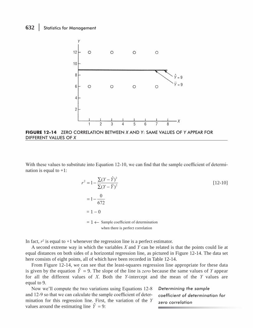
632 Statistics for Management
-nation is equal to +1:
r Y YY Y
1
(
ˆ
)
( )
2
2
2
= −∑ −∑ −
[12-10]
1
0
672
= −
= 1 − 0
= 1 ← when there is perfect correlation
In fact, r2 is equal to +1 whenever the regression line is a perfect estimator.A second extreme way in which the variables X and Y can be related is that the points could lie at
equal distances on both sides of a horizontal regression line, as pictured in Figure 12-14. The data set here consists of eight points, all of which have been recorded in Table 12-14.
From Figure 12-14, we can see that the least-squares regression line appropriate for these data is given by the equation Y = 9. The slope of the line is zero because the same values of Y appear for all the different values of X. Both the Y-intercept and the mean of the Y values are equal to 9.
-mination for this regression line. First, the variation of the Y values around the estimating line Y = 9:
Determining the sample
coefficient of determination for
zero correlation
FIGURE 12-14 ZERO CORRELATION BETWEEN X AND Y: SAME VALUES OF Y APPEAR FOR DIFFERENT VALUES OF X
12
10
8
6
4
2
1 2 3 4 5 6 7 8X
Y
Y = 9
Y−
= 9

Simple Regression and Correlation 633
Variation of the Y values around the regression line Y Y(
ˆ
)
2= ∑ − [12-8]( 6 − 9)2 = (–3)2 = 9(12 − 9)2 = (3)2 = 9( 6 − 9)2 = (–3)2 = 9(12 − 9)2 = (3)2 = 9( 6 − 9)2 = (–3)2 = 9(12 − 9)2 = (3)2 = 9( 6 − 9)2 = (–3)2 = 9(12 − 9)2 = (3)2 = 9 Y Y72 (
ˆ
)
2← ∑ −
Variation of the Y values around their own mean Y Y( )
2= ∑ − [12-9]( 6 − 9)2 = (–3)2 = 9(12 − 9)2 = (3)2 = 9( 6 − 9)2 = (–3)2 = 9(12 − 9)2 = (3)2 = 9( 6 − 9)2 = (–3)2 = 9(12 − 9)2 = (3)2 = 9( 6 − 9)2 = (–3)2 = 9(12 − 9)2 = (3)2 = 9 Y Y72 ( )
2← ∑ −
TABLE 12-14 ILLUSTRATION OF ZERO CORRELATION BETWEEN TWO VARIABLES, X AND Y
Data Point Value of X Value of Y1st 1 62nd 1 123rd 3 64th 3 125th 5 66th 5 127th 7 68th 7 12
∑Y = 72
=Y72
8
= Y
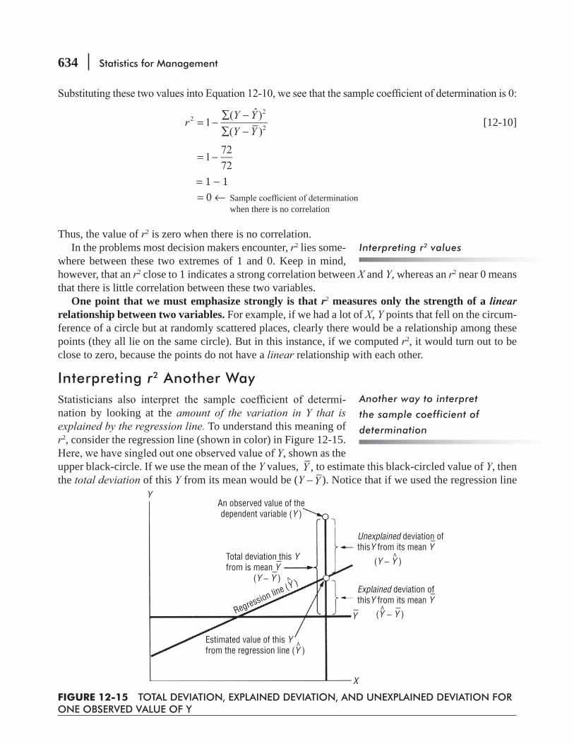
634 Statistics for Management
r Y YY Y
1
(
ˆ
)
( )
2
2
2
= −∑ −∑ −
[12-10]
1
72
72
= −
= 1 − 1= 0 ←
when there is no correlation
Thus, the value of r2 is zero when there is no correlation.In the problems most decision makers encounter, r2 lies some-
where between these two extremes of 1 and 0. Keep in mind, however, that an r2 close to 1 indicates a strong correlation between X and Y, whereas an r2 near 0 means that there is little correlation between these two variables.
One point that we must emphasize strongly is that r2 measures only the strength of a linear relationship between two variables. For example, if we had a lot of X, Y points that fell on the circum-ference of a circle but at randomly scattered places, clearly there would be a relationship among these points (they all lie on the same circle). But in this instance, if we computed r2, it would turn out to be close to zero, because the points do not have a linear relationship with each other.
Interpreting r2 Another Way-
nation by looking at the amount of the variation in Y that is explained by the regression line. To understand this meaning of r2, consider the regression line (shown in color) in Figure 12-15.
Y, shown as the upper black-circle. If we use the mean of the Y values, Y , to estimate this black-circled value of Y, then the total deviation of this Y from its mean would be (Y – Y ). Notice that if we used the regression line
Interpreting r2 values
Another way to interpret
the sample coefficient of
determination
FIGURE 12-15 TOTAL DEVIATION, EXPLAINED DEVIATION, AND UNEXPLAINED DEVIATION FOR ONE OBSERVED VALUE OF Y
An observed value of thedependent variable (Y )
Total deviation this Yfrom is mean Y
−
Estimated value of this Yfrom the regression line (Y )
Unexplained deviation ofthisY from its mean Y
−
Explained deviation ofthisY from its mean Y
−
Regression line (Y ) (Y − Y−
)
(Y − Y−
)
(Y − Y )
Y−
Y
X
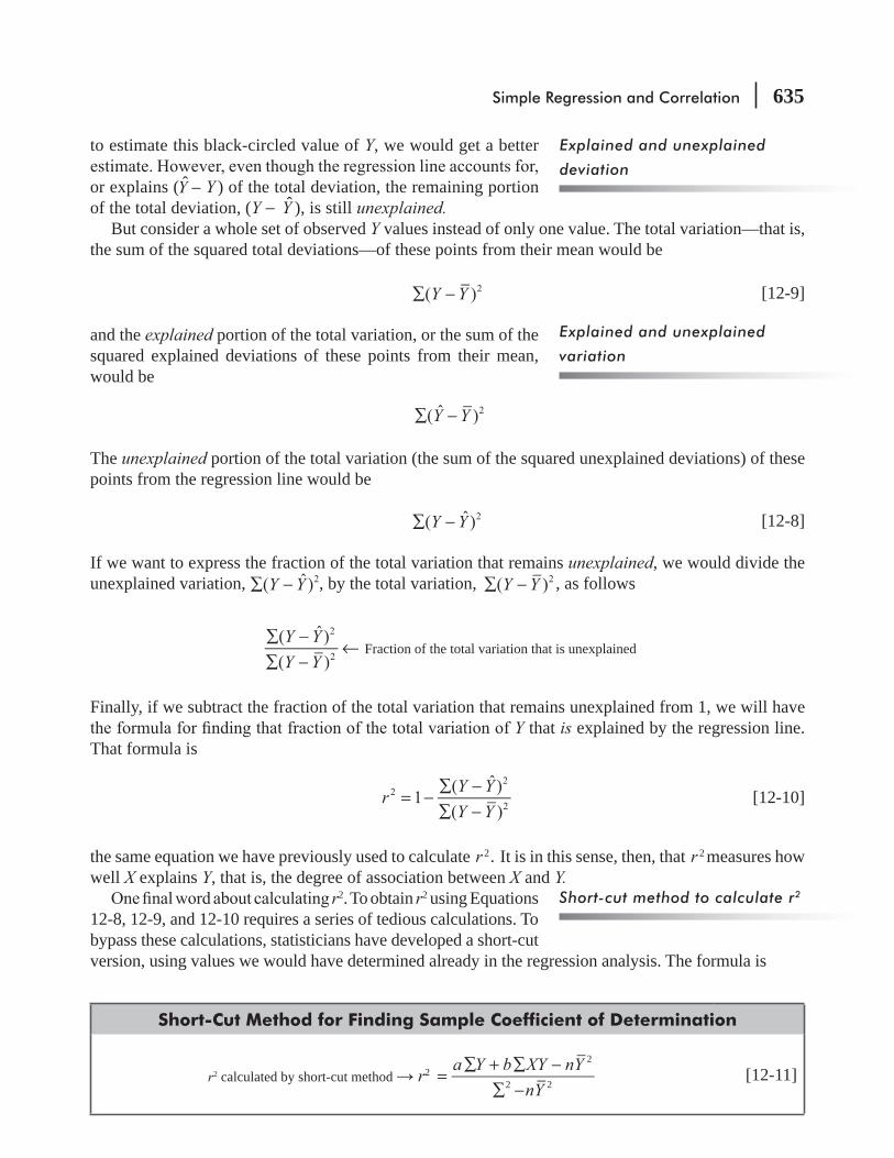
Simple Regression and Correlation 635
to estimate this black-circled value of Y, we would get a better
or explains (Y – Y ) of the total deviation, the remaining portion of the total deviation, (Y − Y ), is still unexplained.
But consider a whole set of observed Y values instead of only one value. The total variation—that is, the sum of the squared total deviations—of these points from their mean would be
Y Y( )
2∑ − [12-9]
and the explained portion of the total variation, or the sum of the squared explained deviations of these points from their mean, would be
Y Y(
ˆ
)
2∑ −
The unexplained portion of the total variation (the sum of the squared unexplained deviations) of these points from the regression line would be
Y Y(
ˆ
)
2∑ − [12-8]
If we want to express the fraction of the total variation that remains unexplained, we would divide the unexplained variation, Y Y(
ˆ
)
2∑ − , by the total variation, Y Y( )
2∑ − , as follows
Y YY Y(
ˆ
)
( )
2
2
∑ −∑ −
← Fraction of the total variation that is unexplained
Finally, if we subtract the fraction of the total variation that remains unexplained from 1, we will have Y that is explained by the regression line.
That formula is
r Y YY Y
1
(
ˆ
)
( )
2
2
2
= −∑ −∑ −
[12-10]
the same equation we have previously used to calculate r 2. It is in this sense, then, that r 2 measures how well X explains Y, that is, the degree of association between X and Y.
r2. To obtain r2 using Equations 12-8, 12-9, and 12-10 requires a series of tedious calculations. To bypass these calculations, statisticians have developed a short-cut version, using values we would have determined already in the regression analysis. The formula is
Short-Cut Method for Finding Sample Coefficient of Determination
r2 calculated by short-cut method r2 a Y b XY nYnY
2
2 2=∑ + ∑ −
∑ −[12-11]
Explained and unexplained
variation
Short-cut method to calculate r2
Explained and unexplained
deviation
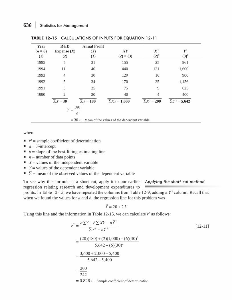
636 Statistics for Management
where
r2 = a = Y-intercept b = n = number of data points X = values of the independent variable Y = values of the dependent variable Y = mean of the observed values of the dependent variable
To see why this formula is a short cut, apply it to our earlier regression relating research and development expenditures to
Y 2 column. Recall that when we found the values for a and b, the regression line for this problem was
Y Xˆ
20 2= +Using this line and the information in Table 12-15, we can calculate r2 as follows:
r a Y b XY nYY nY
22
2 2=∑ + ∑ −
∑ − [12-11]
(20)(180) (2)(1,000) (6)(30)
5,642 (6)(30)
2
2
=+ −
−
3,600 2,000 5,400
5,642 5,400
=+ −
−
200
242
=
= 0.826 ←
Applying the short-cut method
TABLE 12-15 CALCULATIONS OF INPUTS FOR EQUATION 12-11
Year(n = 6)
(1)
R&DExpense (X)
(2)(Y)(3)
XY(2) × (3)
X 2(2)2
Y 2(3)2
1995 5 31 155 25 9611994 11 40 440 121 1,6001993 4 30 120 16 9001992 5 34 170 25 1,1561991 3 25 75 9 6251990 2 20 40 4 400
∑ X = 30 ∑ Y = 180 ∑ XY = 1,000 ∑ X 2 = 200 ∑ Y 2 = 5,642
=Y180
6
= 30 ← Mean of the values of the dependent variable
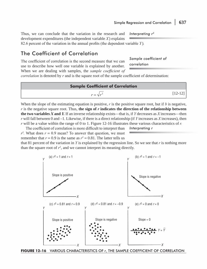
Simple Regression and Correlation 637
Thus, we can conclude that the variation in the research and development expenditures (the independent variable X ) explains
Y ).
The Coefficient of Correlation
use to describe how well one variable is explained by another. When we are dealing with samples, the sample coef cient of correlation is denoted by r
Sample Coefficient of Correlation
r r 2= [12-12]
When the slope of the estimating equation is positive, r is the positive square root, but if b is negative, r is the negative square root. Thus, the sign of r indicates the direction of the relationship between the two variables X and Y. If an inverse relationship exists—that is, if Y decreases as X increases—then r will fall between 0 and –1. Likewise, if there is a direct relationship (if Y increases as X increases), then r will be a value within the range of 0 to 1. Figure 12-16 illustrates these various characteristics of r.
r2. What does r =remember that r = 0.9 is the same as r2 = 0.81. The latter tells us that 81 percent of the variation in Y is explained by the regression line. So we see that r is nothing more than the square root of r2, and we cannot interpret its meaning directly.
Sample coefficient of
correlation
Interpreting r
Interpreting r2
FIGURE 12-16 VARIOUS CHARACTERISTICS OF r, THE SAMPLE COEFFICIENT OF CORRELATION
Slope is positive
Slope is positive
Slope is negative
Slope is negative Slope = 0
Y
Y
X
Y
X
Y
X
X
Y
X
(a) r2 = 1 and r = 1
(c) r2 = 0.81 and r = 0.9 (d) r2 = 0.81 and r = −0.9 (e) r2 = 0 and r = 0
(b) r2 = 1 and r = −1
Y = Y−

638 Statistics for Management
relating research and development expenditures and annual prof-
of determination is r2 =
r r 2= [12-12]
0.826== 0.909 ←
The relation between the two variables is direct and the slope is positive; therefore, the sign for r is positive.
r2 -cient of correlation, r, you should be wary of using all but the highest correlations as the basis for
income, that seems like a fairly strong correlation (0.6 is closer to 1.0 than it is to zero). But when you square 0.6 you see that it accounts for only 0.6 × 0.6 = 0.36 or 36 percent of the variation in the amount of money families spend on movies. If you designed your marketing strategy to appeal
HINTS & ASSUMPTIONS
Simple Correlation Using SPSSFor Correlation go to Analyze>Correlation>Bivariate>Select variables for coorelation
Calculating r for the research
and development problem

Simple Regression and Correlation 639

640 Statistics for Management
Simple Correlation Using MS ExcelFor Correlation go to
Simple Regression and Correlation 641
EXERCISES 12.3
Self-Check ExercisesSC 12-4 Campus Stores has been selling the Believe It or Not: Wonders of Statistics Study Guide for 12
semesters and would like to estimate the relationship between sales and number of sections of elementary statistics taught in each semester. The following data have been collected:
Sales (units) 33 38 24 61 52 45Number of sections 3 7 6 6 10 12
Sales (units) 65 82 29 63 50 79Number of sections 12 13 12 13 14 15
SC 12-5 the data in Exercise SC 12-3.
Basic Concepts12-25
(a) Ability of supervisors and output of their subordinates.
(c) Weight and blood pressure.
12-26 the data in Exercise 12-17.
12-27 for the data in Exercise 12-18.
12-28 the data in Exercise 12-19.
12-29 for the data in Exercise 12-20.
12-30 the data in Exercise 12-21.
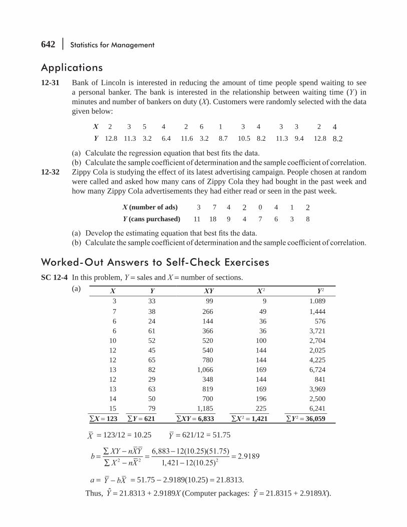
642 Statistics for Management
Applications12-31 Bank of Lincoln is interested in reducing the amount of time people spend waiting to see
a personal banker. The bank is interested in the relationship between waiting time (Y ) in minutes and number of bankers on duty (X). Customers were randomly selected with the data given below:
X 2 3 5 4 2 6 1 3 4 3 3 2 4Y 12.8 11.3 3.2 6.4 11.6 3.2 8.7 10.5 8.2 11.3 9.4 12.8 8.2
12-32 Zippy Cola is studying the effect of its latest advertising campaign. People chosen at random were called and asked how many cans of Zippy Cola they had bought in the past week and how many Zippy Cola advertisements they had either read or seen in the past week.
X (number of ads) 3 7 4 2 0 4 1 2Y (cans purchased) 11 18 9 4 7 6 3 8
Worked-Out Answers to Self-Check ExercisesSC 12-4 In this problem, Y = sales and X = number of sections.
(a)
X Y XY X 2 Y 2
3 33 99 9 1.089 7 38 266 49 1,444 6 24 144 36 576 6 61 366 36 3,72110 52 520 100 2,70412 45 540 144 2,02512 65 780 144 4,22513 82 1,066 169 6,72412 29 348 144 84113 63 819 169 3,96914 50 700 196 2,50015 79 1,185 225 6,241
∑X = 123 ∑Y = 621 ∑XY = 6,833 ∑X 2 = 1,421 ∑Y 2 = 36,059
X = 123/12 = 10.25 Y = 621/12 = 51.75
bXY nXYX nX
6,883 12(10.25)(51.75)
1,421 12(10.25)
2.9189
2 2 2
=∑ −∑ −
=−
−=
a = Y bX− = 51.75 − 2.9189(10.25) = 21.8313.
Thus, Y = 21.8313 + 2.9189X (Computer packages: Y = 21.8315 + 2.9189X).

Simple Regression and Correlation 643
(b) r a Y b XY nYY nY
22
2 2=∑ + ∑ −
∑ −
21.8313(621) 2.9189(6,833) 12(51.75)
36,059 12(51.75)
0.3481
2
2
=+ −
−=
r 0.3481 0.5900= =SC 12-5 From the solution to Exercise SC 12-3 on page 623, we have n = 10, ∑Y = 1,922, Y = 192.2,
∑XY = 84,541, ∑Y 2 = 395,024, a = –80.4430, and b =
r a Y b XY nYY nY
22
2 2=∑ + ∑ −
∑ −
80.4430(1,922) 6.4915(84,541) 10(192.2)
395,024 10(192.2)
2
2
=− + −
−
= 0.9673 r 0.9673 0.9835= =
12.4 MAKING INFERENCES ABOUT POPULATION PARAMETERSSo far, we have used regression and correlation analyses to relate two variables on the basis of sample information. But data from a sample represent only part of the total population. Because of this, we may think of our estimated sample regression line as an estimate of a true but unknown population regression line of the form
Population Regression Line
Y = A + BX [12-13]
explain its annual repair expense. That expense will probably consist of two parts:
1. Regular maintenance that does not depend on the age of the truck: tune-ups, oil changes, and lubrication. This expense is captured in the intercept term A in Equation 12-13.
2. Expenses for repairs due to aging: relining brakes, engine and transmission overhauls, and painting. Such expenses tend to increase with the age of the truck, and they are captured in the BX term of the population regression line Y = A + BX in Equation 12-13.
Of course, all the brakes of all the trucks will not wear out at the same time, and some of the trucks will run for years without engine overhauls. Because of this, the individual data points will
Relationship of sample
regression line and population
regression line
Why data points do not lie
exactly on the regression line
644 Statistics for Management
probably not lie exactly on the population regression line. Some will be above it; some will fall below it. So, instead of satisfying
Y = A + BX [12-13]
the individual data points will satisfy the formula
Population Regression Line with a Random Disturbance
Y = A + BX + e [12-13a]
where e is a random disturbance from the population regression line. On the average, e equals zero because disturbances above the population regression line are canceled out by disturbances below the line. We can denote the standard deviation of these individual disturbances by σ e. The standard error of estimate se, then, is an estimate of σ e, the standard deviation of the disturbance.
Let us look more carefully at Equations 12-13 and 12-13a. Equation 12-13a expresses the individual values of Y (in this case, annual repair expense) in terms of the individual values of X (the age of the truck) and the random disturbance (e). Because disturbances above the population regression line are canceled out by those below the line, we know that the expected value of e is zero, and we see that if we had several trucks of the same age, X, we would expect the average annual repair expense on these trucks to be Y = A + BX. This shows us that the population regression line (Equation 12-13) gives the mean value of Y associated with each value of X.
Because our sample regression line, Y = a + bX (Equation 12-3), estimates the population regression line, Y = A + BX (Equation 12-13), we should be able to use it to make inferences about the population regression line. In this section, then, we shall make inferences about the slope B of the “true” regression equation (the one for the entire popula-tion) that are based on the slope b of the regression equation estimated from a sample of values.
Slope of the Population Regression LineThe regression line is derived from a sample and not from the entire population. As a result, we cannot expect the true regres-sion equation, Y = A + BX (the one for the entire population), to be exactly the same as the equation estimated from the sample observations, or Y = a + bX. Even so, we can use the value of b, the slope we calculate from a sample, to test hypotheses about the value of B, the slope of the regression line for the entire population.
The procedure for testing a hypothesis about B is similar to procedures discussed in Chapters 8 and 9, on hypothesis test-ing. To understand this process, return to the problem that related annual expenditures for research and
b = B to compare with b = 2.
Random disturbance e and its
behavior
Making inferences about B
from b
Difference between true
regression equation and
one estimated from sample
observations
Testing a hypothesis about B

Simple Regression and Correlation 645
Suppose that over an extended past period of time, the slope of the relationship between X and Y was
0: B = 2.1 ← Null hypothesis
1: B ≠ 2.1 ← Alternative hypothesis
In effect, then, we are testing to learn whether current data indi-cate that B has changed from its historical value of 2.1.
B standard error of the regression coef cient. -
b sb. Equation 12-14 presents the mathematical formula for sb:
Standard Error of b
ss
X nXb
e
2 2=
∑ −[12-14]
where sb = se = standard error of estimate X = values of the independent variable X = mean of the values of the independent variable n = number of data points
Once we have calculated sb, we can use Equation 12-15 to stan-
Standardized Value of b
tb B
sbo=
− [12-15]
where b = B
H
0
= actual slope hypothesized for the population sb =
Because the test will be based on the t distribution with n − 2 degrees of freedom, we use t to denote the standardized statistic.
A glance at Table 12-15 on page 636 enables us to calculate the values of ∑X 2 and nX 2. To obtain se, we can take the short-cut method, as follows:
s Y a Y b XYn 2e
2
=∑ − ∑ − ∑
− [12-15]
5,642 (20)(180) (2)(1,000)
6 2
=− −
−
Standard error of the regression
coefficient
Standardizing the regression
coefficient
Calculating se
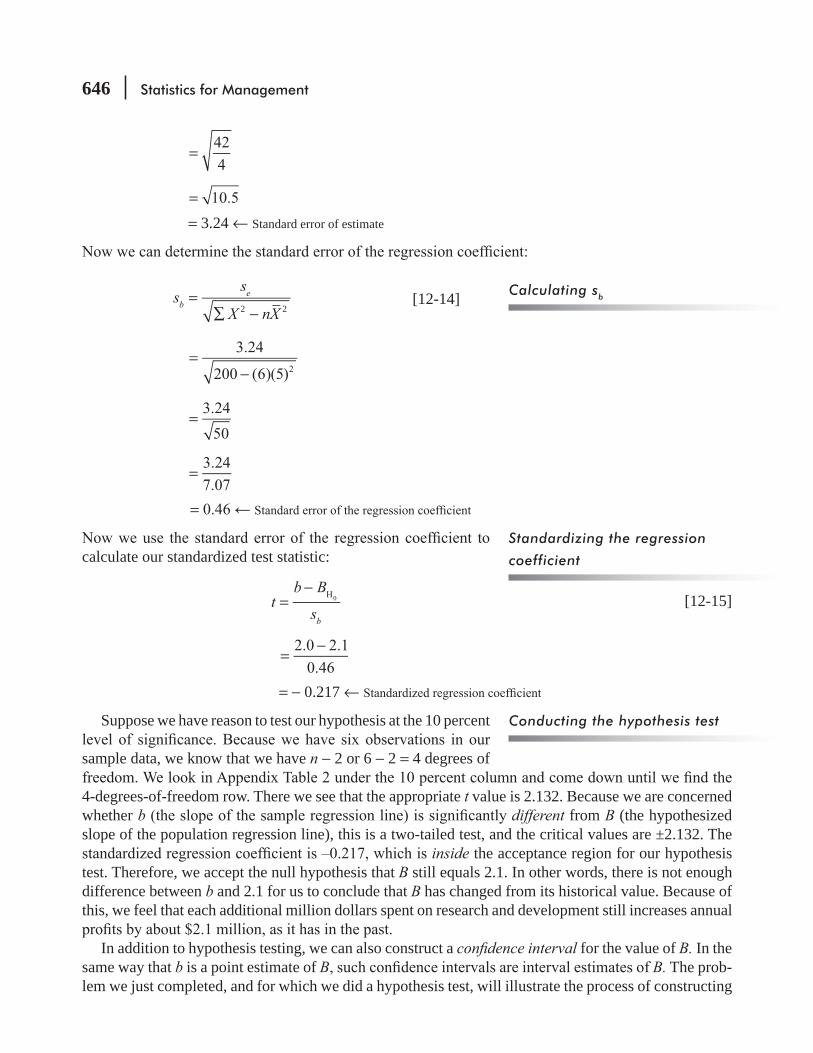
646 Statistics for Management
42
4
=
10.5=
= 3.24 ← Standard error of estimate
ss
X nXb
e
2 2=
∑ −[12-14]
3.24
200 (6)(5)
2
=−
3.24
50
=
3.24
7.07
=
=
calculate our standardized test statistic:
tb B
sb
H
0=−
[12-15]
2.0 2.1
0.46
=−
= − 0.217 ←
Suppose we have reason to test our hypothesis at the 10 percent
sample data, we know that we have n − 2 or 6 − 2 = 4 degrees of
4-degrees-of-freedom row. There we see that the appropriate t value is 2.132. Because we are concerned whether b different from B (the hypothesized slope of the population regression line), this is a two-tailed test, and the critical values are ±2.132. The
inside the acceptance region for our hypothesis test. Therefore, we accept the null hypothesis that B still equals 2.1. In other words, there is not enough difference between b and 2.1 for us to conclude that B has changed from its historical value. Because of this, we feel that each additional million dollars spent on research and development still increases annual
In addition to hypothesis testing, we can also construct a con dence interval for the value of B. In the same way that b is a point estimate of B B. The prob-lem we just completed, and for which we did a hypothesis test, will illustrate the process of constructing
Calculating sb
Standardizing the regression
coefficient
Conducting the hypothesis test
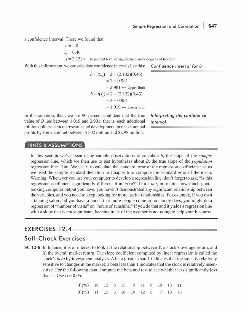
Simple Regression and Correlation 647
b = 2.0 sb = 0.46
t = 2.132 ←
b + t(sb) = 2 + (2.132)(0.46) = 2 + 0.981 = 2.981 ← Upper limit b − t(sb) = 2 − (2.132)(0.46) = 2 − 0.981 = 1.019 ← Lower limit
value of B lies between 1.019 and 2.981; that is, each additional million dollars spent on research and development increases annual
b, the slope of the sample regression line, which we then use to test hypotheses about B, the true slope of the population
sewe used the sample standard deviation in Chapter 6 to compute the standard error of the mean.
not, no matter how much good-
the variables, and you need to keep looking for more useful relationships. For example, if you own a tanning salon and you have a hunch that more people come in on cloudy days, you might do a regression of “number of visits” on “hours of sunshine.” If you do that and it yields a regression line with a slope that is not
HINTS & ASSUMPTIONS
EXERCISES 12.4
Self-Check ExercisesSC 12-6 Y
X beta by investment analysts. A beta greater than 1 indicates that the stock is relatively
sensitive to changes in the market; a beta less than 1 indicates that the stock is relatively insen-
than 1. Use α = 0.05.
Y (%) 10 12 8 15 9 11 8 10 13 11X (%) 11 15 3 18 10 12 6 7 18 13
Confidence interval for B
Interpreting the confidence
interval
648 Statistics for Management
SC 12-7 In a regression problem with a sample size of 17, the slope was found to be 3.73 and the stan-dard error of estimate 28.654. The quantity X nX( )
2 2∑ − = 871.56.
Basic Concepts12-33 In a regression problem with a sample size of 25, the slope was found to be 1.12 and the stan-
dard error of estimate 8.516. The quantity X nX( )
2 2∑ − = 327.52.
Applications12-34
Y ) a bed company earns and the amount spent on advertising (X ). If Fred computes the regression equation, the slope of the line will indicate the amount of
earned from $1 in advertising exceeds $1.50. Compute the slope of the regression equation
Amount of Advertising (X), $ hundreds 3.6 4.8 9.7 12.6 11.5 10.9Y) hundreds 12.13 14.7 22.83 28.4 28.33 27.05
Amount of Advertising (X), $ hundreds 14.6 18.2 3.7 9.8 12.4 16.9Y), hundreds 33.6 40.8 9.4 24.84 30.17 34.7
12-35 the price of gold (X Y). From a data set based on 15 observations, the sample slope was found to be 2.9. If the standard error of the regres-
12-36 For a sample of 25, the slope was found to be 1.685 and the standard error of the regression
12-37 Realtors are often interested in seeing how the appraised value of a home varies according to the size of the home. Some data on area (in thousands of square feet) and appraised value (in thousands of dollars) for a sample of 11 homes follow.
Area 1.1 1.5 1.6 1.6 1.4 1.3 1.1 1.7 1.9 1.5 1.3Value 75 95 110 102 95 87 82 115 122 98 90
(a) Estimate the least-squares regression to predict appraised value from size.= 50 thousands of dollars)
for every additional 1,000 square feet in area. For this sample, does this relationship seem α = 0.10.

Simple Regression and Correlation 649
12-38 In 1969, a government health agency found that in a number of counties, the relationship between smokers and heart-disease fatalities per 100,000 population had a slope of 0.08. A recent study of 18 counties produced a slope of 0.147 and a standard error of the regression
12-39 The local phone company has always assumed that the average number of daily phone calls goes up by 1.5 for each additional person in a household. It has been suggested that people are more talkative than this. A sample of 64 households was taken, and the slope of the regression of Y (average number of daily phone calls) on X (size of household) was computed to be 1.8
calls per additional person are being made than the phone company assumes, using α = 0.05. State explicit hypotheses and an explicit conclusion.
12-40 averages for applicants. One commonly used variable is high school grade-point average. For one college, past data indicated that the slope was 0.85. A recent small study of 20 students found that the sample slope was 0.70 and the standard error of estimate was 0.60. The quantity (∑ 2 − nX 2
Worked-Out Answers to Self-Check Exercises
SC 12-6 X Y XY X 2 Y 2
11 10 110 121 10015 12 180 225 144 3 8 24 9 6418 15 270 324 22510 9 90 100 81
12 11 132 144 121
6 8 48 36 64
7 10 70 49 100
18 13 234 324 169
13 11 143 169 121
 X = 113 ÂY = 107  XY = 1,301  X 2 = 1,501 ÂY 2 = 1,189
X 113
10
11.3= = Y 107
10
10.7= =
b XY nXYX nX
1,301 10(11.3)(10.7)
1,501 10(11.3)
0.4101
2 2 2
=∑ −∑ −
=−
−=

650 Statistics for Management
a = Y bX 10.7 0.4101(11.3) 6.0659− = − = (Computer packages: 6.0660)
s Y a Y b XYn 2e
2
=∑ − ∑ − ∑
−
1,189 6.0659(107) 0.4101(1,301)
8
0.8950=− −
=
(Computer packages: 0.8953)
ss
X nX
0.8950
224.1
0.060be
2 2
=∑ −
= =
0: B = 1: B < 1 α = 0.05
The standardized statistic is tb B
s0.4101 1
0.06
9.83.
b
H
0=−
=−
= − Because the critical value
of t 0. Stock is insensitive to changes in the mar-
SC 12-7 (a) ss
X nX
28.654
871.56
0.9706be
2 2
=∑ −
= =
b ± t(sb)= 3.73 ± 2.602(0.9706) = 3.73 ± 2.53 = (1.20, 6.26).(c) In repeated sampling, 98 out of 100 intervals constructed as above would contain the true,
unknown population slope B. For our single sample, we can say that we are 98 percent B.
12.5 USING REGRESSION AND CORRELATION ANALYSES: LIMITATIONS, ERRORS, AND CAVEATS
Regression and correlation analyses are statistical tools that, -
sions. Unfortunately, they are often misused. As a result, decision makers often make inaccurate forecasts and less-than-desirable
hope that you will avoid them.
Extrapolation beyond the Range of the Observed DataA common mistake is to assume that the estimating line can
can properly use regression analysis to predict the relationship between costs per bed and occupancy levels at various occu-pancy levels. Some administrators, however, incorrectly use the same regression equation to predict the
Misuse of regression and
correlation
Specific limited range over
which regression equation holds

Simple Regression and Correlation 651
regression line. Although one relationship holds over the range of sample points, an entirely different relationship may exist for a different range. As a result, these people make decisions on one set of costs
and capacity constraints). Remember that an estimating equation is valid only over the same range as the one from which the sample was taken initially.
Cause and EffectAnother mistake we can make when we use regression analysis is to assume that a change in one variable is caused by a change in the other variable. As we discussed earlier, regression and correlation analyses can in no way determine cause and effect. If we say that
annual earnings 5 years after graduation, we are not saying that one causes the other. Rather, both may be caused by other factors, such as sociological background, parental attitudes, quality of teachers, effective-ness of the job-interviewing process, and economic status of parents—to name only a few potential factors.
year are caused
expenditures as well as in terms of economic conditions, dollars spent on advertising, and other variables. This can be done by using the multiple-regression techniques, to be discussed in the next chapter.
Using Past Trends to Estimate Future TrendsWe must take care to reappraise the historical data we use to esti-mate the regression equation. Conditions can change and violate one or more of the assumptions on which our regression analysis depends. Earlier in this chapter, we made the point that we assume that the variance of the disturbance e around the mean is constant. In many situations, however, this variance changes from year to year.
Another error that can arise from the use of historical data concerns the dependence of some variables on time. Suppose
between the number of employees and the production volume. If the observations used in the analysis extend back for several years, the resulting regression line may be too steep because it may fail to recognize the effect of changing technology.
Misinterpreting the Coefficients of Correlation and Determination
percentage. If r = 0.6, it is incorrect to state that the regression equation “explains” 60 percent of the total variation in Y. Instead, if r = 0.6, then r2 must be 0.6 × 0.6 = 0.36. Only 36 percent of the total variation is explained by the regression line.
Regression and correlation
analyses do not determine
cause and effect
Conditions change and
invalidate the regression
equation
Values of variables change over
time
Misinterpreting r and r2

652 Statistics for Management
r2 to describe the percentage of the change in the dependent variable that is caused by a change in the independent variable. This is wrong because r2 is a measure only of how well one variable describes another, not of how much of the change in one variable is caused by the other variable.
Finding Relationships When They Do Not Exist
relationship between two variables that, in fact, have no common bond. Even though one variable does not cause a change in the other, they think that there must be some factor common to both
of the number of miles per gallon consumed by eight different cars and the distance from earth to each of the other eight planets. But because there is absolutely no common bond between gas mileage and the distance to other planets, this “relationship” would be meaningless.
In this regard, if one were to run a large number of regressions between many pairs of variables, it would probably be possible to get some rather interesting suggested “relationships.” It might
of beer consumed in the United States, or even between the length of a freight train (in cars) and the weather. But in neither case is there a factor common to both variables; hence, such “relationships” are meaningless. As in most other statistical situations, it takes both knowledge of the inherent limita-tions of the technique that is used and a large dose of common sense to avoid coming to unwarranted conclusions.
Warning: Smart managers ought to be able to reason toward a common-sense connection between two variables even before they run a regression analysis on those variables. But computer regres-sions of large databases sometimes turn up surprising results in terms of unexpected relationships.
should retest these “surprises” on a new sample to see whether the “surprising” relationship con- may have is a data problem, not a breakdown of common
sense.
HINTS & ASSUMPTIONS
EXERCISES 12.512-41 Explain why an estimating equation is valid over only the range of values used for its
development.12-42
correlation.12-43 12-44 Why must we not attribute causality in a relationship even when there is strong correlation
Relationships that have no
common bond
Finding things that do not exist

Simple Regression and Correlation 653
STATISTICS AT WORK
Loveland ComputersCase 12: Simple Regression and Correlation Loveland Computers was running its production line more often to assemble computers from readily available components as the demand for high-end com-
joked that the only part that was unique to Loveland Computers was the plastic base to the keyboard—it was distinguished by the Loveland logo (an outline of the Front Range of the Rocky Mountains, just as
that was the next problem referred to Lee Azko. Nancy Rainwater, the production supervisor, explained her frustrations to Lee.
“When we started assembling this model last summer, the keyboard bases seemed to go together just
break off when the operator tries to snap them together. When that happens, we have to throw out both
lugs measure exactly within specs, and the plastics company that makes them for us did some lab work. They say there is nothing wrong with the plastic they are using.
“I noticed that we had more breakages early in the morning—so 1 wondered whether it just hap-pened because people were being careless on the line. I even wondered if it was because the employees were not properly trained; but the fact is these people are more experienced now than they were last summer—we really have not had much turnover.
defects in the winter. But the warehouse has a couple of heaters, so I am not sure if that is right. And I can hardly walk around with a thermometer and check out the temperature of each set of base parts
Study Questions:
CHAPTER REVIEW
Terms Introduced in Chapter 12
direction of the relationship between two variables, direct or inverse.A measure of the proportion of variation in Y, the dependent variable,
that is explained by the regression line, that is, by YCorrelation Analysis A technique to determine the degree to which variables are linearly related.Curvilinear Relationship An association between two variables that is described by a curved line. Dependent Variable The variable we are trying to predict in regression analysis.Direct Relationship value increases, so does the value of the dependent variable.
654 Statistics for Management
Estimating Equation A mathematical formula that relates the unknown variable to the known vari-ables in regression analysis.Independent Variables The known variable or variables in regression analysis.Inverse Relationship A relationship between two variables in which, as the independent variable increases, the dependent variable decreases.Least-Squares Method the sum of the squared vertical distances from the n points to the line is minimized.Linear Relationship A particular type of association between two variables that can be described mathematically by a straight line.Multiple Regression The statistical process by which several variables are used to predict another variable.Regression The general process of predicting one variable from another by statistical means, using previous data.Regression Line Scatter Diagram A graph of points on a rectangular grid; the X and Y coordinates of each point cor-respond to the two measurements made on some particular sample element, and the pattern of points illustrates the relationship between the two variables.Slope A constant for any given straight line whose value represents how much each unit change of the independent variable changes the dependent variable.Standard Error of Estimate A measure of the reliability of the estimating equation, indicating the variability of the observed points around the regression line, that is, the extent to which observed values differ from their predicted values on the regression line.
A measure of the variability of sample regression coef-
ϒ-Intercept A constant for any given straight line whose value represents the value of the ϒ variable when the X variable has a value of 0.
Equations Introduced in Chapter 1212-1 Y = a + bX p. 603
This is the equation for a straight line, where the dependent variable Y is “determined” by the independent variable X. The a is called the Y-intercept because its value is the point at which the line crosses the Y-axis (the vertical axis). The b is the slope of the line; that is, it tells how much each unit change of the independent variable X changes the dependent variable Y. Both a and b are numerical constants because for any given straight line, their values do not change.
12-2 bY YX X2 1
2 1
=−−
p. 604
To calculate the numerical constant b X and Y X1, Y1) and the second point (X2, Y2). Remember that b is the slope of the line.
12-3 Y = a + bX p. 607 In regression analysis, Y (Y hat) symbolizes the individual Y values of the estimated points,
that is, the points that lie on the estimating line. Accordingly, Equation 12-3 is the equation for the estimating line.
Simple Regression and Correlation 655
12-4 b XY nXYX nX2 2=
∑ −∑ −
p. 610
The equation enables us to calculate the slope of the best- tting regression line for any two-variable set of data points. We introduce two new symbols in this equation, X and Y , which represent the means of the values of the independent variable and the dependent variable, respectively. In addition, this equation contains n, which, in this case, represents the number
12-5 a Y bX= − p. 610
Using this formula, we can compute the Y-intercept of the best- tting regression line for any two-variable set of data points.
12-6 s Y Yn(
ˆ
)
2
e
2
=∑ −
− p. 615
The standard error of estimate, se , measures the variability or scatter of the observed values around the regression line. In effect, it indicates the reliability of the estimating equation. The denominator is n − 2 because we lose 2 degrees of freedom (for the values a and b) in estimat-ing the regression line.
12-7 s Y a Y b XYn 2e
2
=∑ − ∑ − ∑
− p. 617
Because Equation 12-6 requires tedious calculations, statisticians have devised this short-cut method for nding the standard error of estimate. In calculating the values for b and a, we have already calculated every quantity in Equation 12-7 except ∑Y 2, which we can do very easily.
12-8 Variation of the Y values around the regression line = Y Y(
ˆ
)
2∑ − p. 629
The variation of the Y -
how to measure this particular dispersion, which is the unexplained portion of the total varia-tion of the Y values.
12-9 Variation of the Y values around their own mean = Y Y( )
2∑ − p. 630
This formula measures the total variation of a whole set of Y values, that is, the variation of these Y values around their own mean.
12-10 r Y YY Y
1
(
ˆ
)
( )
2
2
2
= −∑ −∑ −
p. 630
The sample coef cient of determination, r2, gives the fraction of the total variation of Y that is explained by the regression line. It is an important measure of the degree of association between X and Y. If the value of r2 is +1, then the regression line is a perfect estimator. If r2 = 0, there is no correlation between X and Y.
12-11 r a Y b XY nYY nY
22
2 2=∑ + ∑ −
∑ − p. 635
This is a short-cut equation for calculating r2
656 Statistics for Management
12-12 r r 2= p. 637 The sample coef cient of correlation is denoted by r and is found by taking the square root of
r2) we can use to describe how well one variable is explained by another. The sign of r is the same as the sign of b; it indicates the direction of the relationship between the two variables X and Y.
12-13 Y = A + BX p. 643 Each population regression line is of the form in Equation 12-13, where A is the Y-intercept
for the population and B is the slope.12-13a Y = A + BX + e p. 644 Because all the individual points in a population do not lie on the population regression line,
the individual data points will satisfy Equation 12-13a, where e is a random disturbance from the population regression line. On the average, e equals zero because disturbances above the population regression line are canceled out by disturbances below it.
12-14 ss
X nXb
e
2 2=
∑ − p. 645
standard error of the regression coef cient, b.
12-15 tb B
sH
b
0=−
p. 645
Once we have calculated sb using Equation 12-14, we can use this equation to standardize the -
ing this standardized value with the critical value(s) from Appendix Table 2.
Review and Application Exercises12-45 A consultant is interested in seeing how accurately a new job-performance index measures what is
important for a corporation. One way to check is to look at the relationship between the job-eval-
about salary (in thousands of dollars) and job-performance index (1–10; 10 is best was collected.
Job-performance index (X) 9 7 8 4 7 5 5 6Salary (Y) 36 25 33 15 28 19 20 22
(b) Calculate the standard error of estimate, se, for these data. r2, for these data.
12-46 The Stork Foundation wishes to show with statistics that, contrary to popular belief, storks do bring babies. Thus, it has collected data on the number of storks and the number of babies (both in thousands) in several large cities in central Europe.
Storks 27 38 13 24 6 19 15Babies 35 46 19 32 15 31 20

Simple Regression and Correlation 657
for these data.
12-47 (Fill in the blanks.) Regression and correlation analyses deal with the ____________________ between variables. Regression analysis, through ____________________ equations, enables us to ____________________ an unknown variable from a set of known variables. The unknown variable is called the ____________________ variable; known variables are called ____________________ variables. The correlation between two variables indicates the ____________________ of the linear relationship between them and thus gives an idea of how well the ____________________ in regression describes the relationship between the variables.
12-48 Exercise 12-14.
12-49 “Nothing succeeds like success” is an old adage in the advertising business. The president of a multiline auto dealership has observed that sales staff who earn the biggest end-of-year bonus are the ones who are most likely to exceed their quota for sales in the following year (and hence earn another bonus).
Last Year’s Bonus ($ thousands) 7.8 6.9 6.7 6.0 6.9 5.2This Year’s Sales Over Quota 64 73 42 49 71 46
Last Year’s Bonus ($ thousands) 6.3 8.4 7.2 10.1 10.8 7.7This Year’s Sales Over Quota 32 88 53 84 85 93
(b) Calculate the standard error of estimate for the relationship.
for a sales staff member who earned a bonus of $9,600 last year.12-50 For each of the following pairs of plots, state which has a higher value of r, the correlation
r.
1.
(a) (b)
(c) (d)
2. 1. 2.
1. 2. 1. 2.
658 Statistics for Management
12-51 An operations manager is interested in predicting costs C (in thousands of dollars) based on the amount of raw material input R (in hundreds of pounds) for a jeans manufacturer. If the
wrong with the production process and the assembly-line machinery should be adjusted. At
an explicit conclusion.
C 10 7 5 6 7 6R 25 20 16 17 19 18
12-52 Exercise 12-13.
12-53 We should not extrapolate to predict values outside the range of data used in constructing the regression line. The reason (choose one):(a) The relationship between the variables may not be the same for different values of the
variables.(b) The independent variable may not have the causal effect on the dependent variable for
these values.
(d) There may be no common bond to explain the relationship.12-54 Economists are often interested in estimating consumption functions. This is done by regress-
ing consumption Y on income X. (For this regression, economists call the slope the marginal propensity to consume.) For a sample of 25 families, a slope of 0.87 and a standard error of
α = 0.05. State explicit hypotheses and an explicit conclusion.
12-55 (a) Indicates whether the slope of the regression line is positive or negative.(b) Measures the strength of association between the two variables more exactly.(c) Can never have an absolute value greater than 1.(d) Measures the percentage of variance explained by the regression line.
12-56 has taken a random sample of starting salaries and college grade-point averages for some recently graduated friends of his. The data follow:
Starting salary ($ thousands) 36 30 30 24 27 33 21 27Grade-point average 4.0 3.0 3.5 2.0 3.0 3.5 2.5 2.5
(a) Plot these data.
(c) Plot the estimating equation on the scatter plot of part (a).12-57 A landlord is interested in seeing whether his apartment rents are typical. Thus, he has taken
a random sample of 11 rents and apartment sizes of similar apartment complexes. The data follow:
Rent 230 190 450 310 218 185 340 245 125 350 280Number of bedrooms 2 1 3 2 2 2 2 1 1 2 2
Simple Regression and Correlation 659
(c) Predict the rent for a two-bedroom apartment.12-58
Burgers of Santa Cruz, California, a small regional chain. The marketing manager is trying to make the case that “you have to spend money to make money.” Spending on billboard
7 months:
Monthly expenditureon billboards (× $1,000) 25 16 42 34 10 21 19
Monthly salesrevenue (× $100,000) 34 14 48 32 26 29 20
(b) Calculate the standard error of estimate for this relationship.(c) For a month with a billboard expenditure of $28,000, develop an approximate 95 percent
12-59 In an FAA study of airline operations, a survey of 18 companies disclosed that the relationship between the number of pilots employed and the number of planes in service has a slope of 4.3. Previous studies indicated that the slope of this relationship was 4.0. If the standard error of
12-60
the offering (in millions of dollars) and the price per share.
Size ($ Millions) Price ($)108.00 12.00
4.40 4.00
3.50 5.00
3.60 6.00
39.00 13.00
68.40 19.00
7.50 8.50
5.50 5.00
375.00 15.00
12.00 6.00
51.00 12.00(Continued)
660 Statistics for Management
66.00 12.00
10.40 6.50
4.00 3.00
-
12-61 A manufacturer of cellular phones is testing two different types of batteries to see how long they last in typical use. Provisional data are in the following table:
Approximate Life(months)
Hours of Daily Use Lithium Alkaline
2.0 3.1 1.3
1.5 4.2 1.6
1.0 5.1 1.8
0.5 6.3 2.2
with lithium batteries and one for alkaline batteries.
hours of daily use, for each battery type. Can the company make any claims about which
12-62 A study has been proposed to investigate the relationship between the birthweight of male babies and their adult height. Using the following data, develop the least-squares estimating
Birthweight Adult Height5 lb, 8 oz7 lb6 lb, 4 oz7 lb, 8 oz8 lb, 2 oz6 lb, 12 oz
12-63 Many college students transfer in the summer before their junior years. To aid in evaluating
transferring. Using the following data:Freshman/sophomore GPA 1.7 3.5 2.3 2.6 3.0 2.8 2.4 1.9 2.0 3.1Junior/senior GPA 2.4 3.7 2.0 2.5 3.2 3.0 2.5 1.8 2.7 3.7
(Contd.)
Simple Regression and Correlation 661
GPAs for students transferring to Piedmont College.-
tion intervals for their junior/senior GPAs fall entirely above 2.0. Will she admit a transfer
12-64along with Boarding-Lodging Expenses rates for different cities. So far MNT is following a uniform rate system for all the cities but there has been a major complaint among the employ-
ready to modify the system by introducing variable rate system as desired by the employees.
accounts department consider both hotel costs and the taxi-rates, or would the hotel costs by
City Hotel Rates (Per Day) Taxi Rates (Per Day)A 3000 550B 2800 400C 1800 200
4500 1000E 3000 700F 2000 300G 2500 450
2700 600I 3600 900J 1900 300
Questions on Running Case: SURYA Bank Pvt. Ltd.
1. Build a regression model to study the impact of reliability of e-banking transactions on the level of satisfaction of customers. {Regress Q9 on 8(b)}. Interpret the results.
2. Study the impact of Bank Site congestion in performing e-transactions on the level of satisfaction of customers. {Regress Q9 on 8(f)}. Interpret the results.
@
CASE
@

662 Statistics for Management
To determine thenature of the linear
relationship betweentwo variables, uselinear regression
Organize the dataand plot a scatter
diagram
Calculate the slope and theY-intercept of the
estimating equation usingthe least squares method:
START
Yes
Yes
No
No
No
No
Yes
Yes
ΣXY – nXY––ΣX 2 – nX 2–⎯⎯⎯⎯
a = Y – bX– –
b =
p. 610
Do you wantto predict valuesof the dependent
variable,Y?
Do youwant an approximateprediction interval
for Y?
p. 630
Use correlation analysis,calculate the sample
coefficient ofdetermination, r2
Σ(Y – Y )2
Σ(Y – Y∧
)2⎯⎯⎯⎯r2 = 1 –
p. 617
Use the standard error ofthe estimate:
p. 645
Use the standard error ofthe regression coefficient:
and the t distribution withn –2 degrees of freedom:
ΣX 2 – nX–2⎯⎯⎯⎯
√⎯⎯⎯⎯sb =
sq
ΣY 2 – aΣY – bΣXYn – 2
√⎯⎯⎯⎯⎯⎯⎯⎯
se = ⎯⎯⎯⎯⎯⎯⎯
Y∧
± tse
p. 645
For confidence intervalsand hypothesis tests, use
sq and t distributionwith n–2 degrees of
freedomSTOP
For point predictions,use the regression line:
Y∧
= a + bX
Do you wantto know the
degree to which one variable islinearly related to
the other?
Doyou want
to make inferencesabout the slope (B ) of the “true”regression equation based onthe value b (the slope of the
fitted regressionequation)
?
–
Flow Chart: Regression and Correlation

LEARNING OBJECTIVES
13After reading this chapter, you can understand:
CHAPTER CONTENTS
To extend the regression techniques of the last chapter to handle more than one explanatory variable for a quantity we are trying to predict
To examine decision-making situations where multiple regression can be used to make predictions
To interpret the output from computer regression packages
13.1 Multiple Regression and Correlation Analysis 664
13.2 Finding the Multiple-Regression Equation 665
13.3 The Computer and Multiple Regression 674
13.4 Making Inferences about Population Parameters 684
13.5 Modeling Techniques 703
To test hypotheses about regressions To use modeling techniques to incorporate quali-
tative variables into regression equations To understand the importance of residuals in
regression analysis
Statistics at Work 719 Terms Introduced in Chapter 13 720 Equations Introduced in Chapter 13 721 Review and Application Exercises 722 Flow Chart: Multiple Regression and
Modeling 731
Multiple Regression and Modeling
664 Statistics for Management
A people charges that this salary structure discriminates against women. Current base salaries for the
Salesmen SaleswomenMonths
EmployedBase Salary
($1,000s)Months
EmployedBase Salary
($1,000s)6 7.5 5 6.2
10 8.6 13 8.712 9.1 15 9.418 10.3 21 9.830 13.0
The director of personnel sees that base salary depends on length of service, but she does not know how to use the data to learn whether it also depends on gender and whether there is discrimination against
13.1 MULTIPLE REGRESSION AND CORRELATION ANALYSISAs we mentioned in Chapter 12, we can use more than one inde-pendent variable to estimate the dependent variable and, in this way, attempt to increase the accuracy of the estimate. This pro-cess is called multiple regression and correlation analysis. It is based on the same assumptions and procedures we have encoun-tered using simple regression.
these two variables. Could we also improve the accuracy of our equation by including in the estimating process the number of salespeople she employs each month? The answer is probably yes. And now, because we want to use both the number of sales agents and the advertising expenditures to predict monthly house sales, we must use multiple, not simple, regression to determine the relationship.
The principal advantage of multiple regression is that it allows us to use more of the information available to us to estimate the dependent variable. Sometimes the correlation between two vari-
-tion. Yet, if we add the data from more independent variables, we may be able to determine an estimat-ing equation that describes the relationship with greater accuracy.
Multiple regression and correlation analysis involve a three-step process such as the one we used in simple regression. In this process, we
1. Describe the multiple-regression equation. 2. Examine the multiple-regression standard error of estimate. 3. Use multiple-correlation analysis to determine how well the regression equation describes the
observed data.
Using more than one
independent variable to
estimate the dependent variable
Advantage of multiple
regression
Steps in multiple regression and
correlation
Multiple Regression and Modeling 665
In addition, in multiple regression, we can look at each individual independent variable and test whether
regression equation for a given set of data and how to analyze the equation we get. Although we shall show how to do multiple regression by hand or on a hand-held calculator, it will quickly become obvious to you that you would not want to do even a modest-size real-life problem by hand. Fortunately, there are available many computer packages for doing multiple regressions and other statistical analyses. These packages do the
estimating equation. dummy
variables, we can even include qualitative factors such as gender in our multiple regression. This tech-nique will enable us to analyze the discrimination problem that opened this chapter. Dummy variables
modeling techniques that can be used in multiple regression to increase the accuracy of our estimating equations.
EXERCISES 13.1
Basic Concepts13-1 Why would we use multiple regression instead of simple regression in estimating a dependent
variable? 13-2 How will dummy variables be used in our study of multiple regression?13-3 To what does the word multiple refer in the phrase multiple regression? 13-4 The owner of a chain of stores would like to predict monthly sales from the size of city in
include the effect of season of the war in the model. Can this be done using the techniques in this chapter?
13-5 Describe the three steps in the process of multiple regression and correlation analysis.13-6 Will the procedures used in multiple regression differ greatly from those we used in simple
regression? Explain.
13.2 FINDING THE MULTIPLE-REGRESSION EQUATION
For convenience, we shall use only two independent variables in the problem we work in this section. Keep in mind, however, that the same sort of technique is, in principle, applicable to any number of independent variables.
The Internal Revenue Service is trying to estimate the monthly amount of unpaid taxes discovered
predictor of the actual unpaid taxes. As a result, the IRS is looking for another factor with which it can improve the estimating equation.
The auditing division does keep a record of the number of hours its computers are used to detect
Computer regression packages
A problem demonstrating
multiple regression

666 Statistics for Management
with a more accurate estimating equation for the unpaid taxes discovered each month? Table 13-1 presents these data for the last 10 months.
In simple regression, X is the symbol used for the values of the independent variable. In multiple regression, we have more than one independent variable. So we shall continue to use X, but we shall add a subscript (for example, X1, X2) to distinguish between the independent variables we are using.
In this problem, we will let Xlaudit labor hours and X2 represent the number of computer hours. The dependent variable, Y, will be the actual unpaid taxes discovered.
Recall that in simple regression, the estimating equation Y = a + bX describes the relationship between the two vari-ables X and Y. In multiple regression, we must extend that equa-tion, adding one term for each new variable. In symbolic form, Equation 13-1 is the formula we can use when we have two independent variables:
Estimating Equation Describing Relationship among Three Variables
Y = a + b1 X1 + b2X2[13-1]
where
Y = estimated value corresponding to the dependent variable a = Y-intercept X1 and X2 = values of the two independent variables b1 and b2 = slopes associated with X1 and X2, respectively
We can visualize the simple estimating equation as a line on a graph; similarly, we can picture a two-variable multiple regression equation as a plane, such as the one shown in Figure 13-1. Here
Appropriate symbols
Defining the variables
Estimating equation for multiple
regression
Visualizing multiple regression
TABLE 13-1 DATA FROM IRS AUDITING RECORDS DURING THE LAST 10 MONTHS
Month
X1Field-Audit Labor Hours
(00’s omitted)
X2Computer Hours
(00’s omitted)
YActual Unpaid Taxes Discovered
(millions of dollars)January 45 16 29February 42 14 24March 44 15 27April 45 13 25May 43 13 26June 46 14 28July 44 16 30August 45 16 28September 44 15 28
43 15 27

Multiple Regression and Modeling 667
we have a three-dimensional shape that possesses depth, length, and width. To get an intuitive feel for this three-dimensional shape, visualize the intersection of the axes, Y, X1, and X2 as one corner of a room.
Figure 13-1 is a graph of 10 sample points and the plane about which these points seem to cluster. Some points lie above the plane and some fall below it—just as points lie above and below the simple regression line.
least-squares criterion and locate the plane that minimizes the sum of the squares of the errors, that is, the distances from the points around the plane to the corresponding points on the plane. We use our data and the following three equations (which statisticians call the “normal equations”) to determine the values of the numeri-cal constants, a, b1, and b2.
Normal Equations
ΣY = na + b1Σ X1 + b2Σ X2Σ X1Y = aΣ X1 + b1Σ X 21 + b2ΣX1X2Σ X2Y = aΣX2 + b1Σ X1X2 + b2Σ X 22
[13-2][13-3][13-4]
Using the least-squares criterion
to fit a regression plane
Observed point
Corresponding pointon the plane
Plane formed throughsample points:
a = Y-intercept
X1
X2
YError
Y = a + b1X1 + b2X2
FIGURE 13-1 MULTIPLE REGRESSION PLANE FOR 10 DATA POINTS

668 Statistics for Management
Solving Equations 13-2, 13-3, and 13-4 for a, b1 and b2
and organize the necessary information, just as we did in simple regression. This we have done for the IRS problem in Table 13-2.
Now, using the information from Table 13-2 in Equations 13-2, 13-3, and 13-4, we get three equations in the three unknown constants (a, b1, and b2 ):
272 = 10a + 441b1 + 147b2
12,005 = 441a + 19,461b1 + 6,485b2
4,013 = 147a + 6,485b1 + 2,173b2
When we solve these three equations simultaneously, we get
a = −13.828b1 = 0.564b2 = 1.099
Substituting these three values into the general two-variable regression equation (Equation 13-1), we
of computer hours, and the unpaid taxes discovered by the auditing division:
Y = a +b1X1 + b2X2 [13-1] = −13.828 + 0.564X1 + 1.099X2
Equation 13-2, 13-3, and 13-4
used to solve for a, b1, and b2
TABLE 13-2 VALUES FOR FITTING LEAST-SQUARES PLANE, WHERE n = 10
Y(1)
X1(2)
X2(3)
X1Y(2) × (1)
X2Y(3) × (1)
X1X2(2) × (3)
X12
(2)2X2
2
(3)2Y2
(1)2
29 45 16 1,305 464 720 2,025 256 84124 42 14 1,008 336 588 1,764 196 57627 44 15 1,188 405 660 1,936 225 72925 45 13 1,125 325 585 2,025 169 62526 43 13 1,118 338 559 1,849 169 67628 46 14 1,288 392 644 2,116 196 78430 44 16 1,320 480 704 1,936 256 90028 45 16 1,260 448 720 2,025 256 78428 44 15 1,232 420 660 1,936 225 78427 43 15 1,161 405 645 1,849 225 729
272 ↑ΣY
441 ↑
Σ X1
147 ↑
Σ X2
12,005 ↑
Σ X1Y
4,013↑
Σ X2Y
6,485 ↑
Σ X1X2
19,461 ↑Σ X1
2
2,173↑
Σ X22
7,428↑
ΣY 2
Y = 27.2
1X = 44.1
2X = 14.7
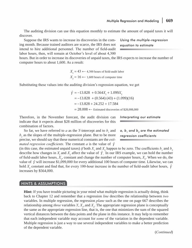
Multiple Regression and Modeling 669
The auditing division can use this equation monthly to estimate the amount of unpaid taxes it will discover.
Suppose the IRS wants to increase its discoveries in the com-ing month. Because trained auditors are scarce, the IRS does not
hours. But in order to increase its discoveries of unpaid taxes, the IRS expects to increase the number of computer hours to about 1,600. As a result:
X1 =X2 = 1,600 hours of computer time
Y = −13.828 + 0.564X1 + 1.099X2
= −13.828 + (0.564) (43) + (1.099)(16) = −13.828 + 24.252 + 17.584 = 28.008 Estimated discoveries of $28,008,000
Therefore, in the November forecast, the audit division can indicate that it expects about $28 million of discoveries for this combination of factors.
So far, we have referred to a as the Y-intercept and to b1 and b2 as the slopes of the multiple-regression plane. But to be more precise, we should say that these numerical constants are the esti-mated regression coef cients. The constant a is the value of Y(in this case, the estimated unpaid taxes) if both X1 and X2 b1 and b2 describe how changes in Xl and X2 affect the value of ˆ.Y In our IRS example, we can hold the number
X1, constant and change the number of computer hours, X2. When we do, the value of Y will increase $1,099,000 for every additional 100 hours of computer time. Likewise, we can hold X2 Yincreases by $564,000.
Hint: If you have trouble picturing in your mind what multiple regression is actually doing, think back to Chapter 12 and remember that a regression line describes the relationship between two variables. In multiple regression, the regression plane such as the one on page 667 describes the relationship among three variables Y, X1, and X2. The appropriate regression plane is conceptually the same as the appropriate regression line, that is, the one that minimizes the sum of the squared vertical distances between the data points and the plane in this instance. It may help to remember that each independent variable may account for some of the variation in the dependent variable. Multiple regression is just a way to use several independent variables to make a better prediction of the dependent variable.
HINTS & ASSUMPTIONS
Using the multiple-regression
equation to estimate
Interpreting our estimate
a, b1 and b2 are the estimated
regression coefficients
(Continued)

670 Statistics for Management
Assumptions: The classical linear regression model (CLRM) makes certain assumptions about the independent variables Xi u, which are very important for the valid interpretation of the regression estimates. The assumptions are:
1. The regression model is linear in parameters, i.e.,
Y = β0 + β1X1 + β2 X2 + u2. The independent variables are assumed to be non random.3. For the given values of Xi , i.e.,
E(ui/Xi) = 04. For the given values of Xi ui is identical, i.e.,
Var(ui/Xi) = σ 2 (Constant)5. For any two values of X, Xi and Xj (i j), the correlation between any two ui and uj (i j) is zero, i.e.,
Cov(ui, uj /Xi, Xj) = 06. There are no exact linear relationships between the independent variables.
EXERCISES 13.2
Self-Check ExercisesSC 13-1 Given the following set of data
(a) Calculate the multiple-regression plane.(b) Predict Y when X1 = 3.0 and X2 = 2.7.
Y X1 X2
25 3.5 5.030 6.7 4.211 1.5 8.522 0.3 1.427 4.6 3.619 2.0 1.3
SC 13-2 The following information has been gathered from a random sample of apartment renters in a city. We are trying to predict rent (in dollars per month) based on the size of the apartment (number of rooms) and the distance from downtown (in miles).
Rent ($)
Number of Rooms
Distance from Downtown
360 2 11,000 6 1
450 3 2525 4 3350 2 10300 1 4

Multiple Regression and Modeling 671
(a) Calculate the least-squares equation that best relates these three variables.(b) If someone is looking for a two-bedroom apartment 2 miles from downtown, what rent
should he expect to pay?
Basic Concepts13-7 Given the following set of data
(a) Calculate the multiple-regression plane.(b) Predict Y when X1 = 10.5 and X2 = 13.6
Y X1 X2
11.4 4.5 13.2
16.6 8.7 18.7
20.5 12.6 19.8
29.4 19.7 25.4
7.6 2.9 22.8
13.8 6.7 17.8
28.5 17.4 14.6
13-8 For the following set of data:(a) Calculate the multiple-regression plane.(b) Predict Y for X1 = 28 and X2 = 10.
Y X1 X2
10 8 4
17 21 9
18 21 11
26 17 20
35 36 13
8 9 28
13-9 Given the following set of data(a) Calculate the multiple-regression plane.(b) Predict Y when X1 = −1 and X2 = 4.
Y X1 X2
6 1 3
10 3 –1
9 2 4
14 –2 7
7 3 2
5 6 –4

672 Statistics for Management
Applications13-10 Sam Spade, owner and general manager of the Campus Stationery Store, is concerned about
the sales behavior of a compact cassette tape recorder sold at the store. He realizes that there are many factors that might help explain sales, but believes that advertising and price are major determinants. Sam has collected the following data:
Sales(units sold)
Advertising(number of ads)
Price($)
33 3 12561 6 11570 10 14082 13 13017 9 14524 6 140
(a) Calculate the least-squares equation to predict sales from advertising and price.(b) If advertising is 7 and price is $132, what sales would you predict?
13-11 A developer of food for pigs would like to determine what relationship exists among the age of a pig when it starts receiving a newly developed food supplement, the initial weight of the pig, and the amount of weight it gains in a 1-week period with the food supplement. The following information is the result of a study of eight piglets:
Piglet Number
X1Initial Weight
(Pounds)
X2Initial Age
(Weeks)
YWeight Gain
1 39 8 7
2 52 6 6
3 49 7 8
4 46 12 10
5 61 9 9
6 35 6 5
7 25 7 3
8 55 4 4
(a) Calculate the least-squares equation that best describes these three variables.(b) How much might we expect a pig to gain in a week with the food supplement if it were
9 weeks old and weighed 48 pounds?13-12 A graduate student trying to purchase a used Neptune car has researched the prices. She
purchase price. Data are given below for 10 cars with the price (Y) in thousands of dollars, year (X1) and miles driven (X2) in thousands.(a) Calculate the least-squares equation that best relates these three variables.(b) The student would like to purchase a 1991 Neptune with about 40,000 miles on it. How
much do you predict she will pay?
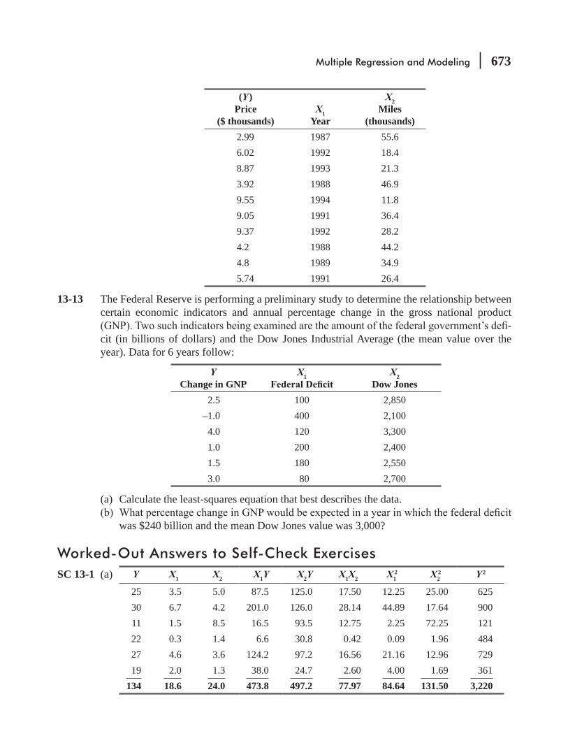
Multiple Regression and Modeling 673
(Y )Price
($ thousands)X1
Year
X2Miles
(thousands)2.99 1987 55.66.02 1992 18.48.87 1993 21.33.92 1988 46.99.55 1994 11.89.05 1991 36.49.37 1992 28.24.2 1988 44.24.8 1989 34.95.74 1991 26.4
13-13 The Federal Reserve is performing a preliminary study to determine the relationship between certain economic indicators and annual percentage change in the gross national product
-cit (in billions of dollars) and the Dow Jones Industrial Average (the mean value over the year). Data for 6 years follow:
YChange in GNP
X1 X2Dow Jones
2.5 100 2,850–1.0 400 2,1004.0 120 3,3001.0 200 2,4001.5 180 2,5503.0 80 2,700
(a) Calculate the least-squares equation that best describes the data.
was $240 billion and the mean Dow Jones value was 3,000?
Worked-Out Answers to Self-Check ExercisesSC 13-1 (a) Y X1 X2 X1Y X2Y X1X2 X1
2 X22 Y 2
25 3.5 5.0 87.5 125.0 17.50 12.25 25.00 62530 6.7 4.2 201.0 126.0 28.14 44.89 17.64 90011 1.5 8.5 16.5 93.5 12.75 2.25 72.25 12122 0.3 1.4 6.6 30.8 0.42 0.09 1.96 48427 4.6 3.6 124.2 97.2 16.56 21.16 12.96 72919 2.0 1.3 38.0 24.7 2.60 4.00 1.69 361
134 18.6 24.0 473.8 497.2 77.97 84.64 131.50 3,220
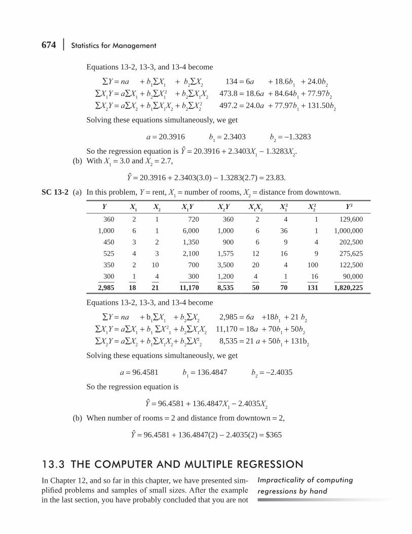
674 Statistics for Management
Equations 13-2, 13-3, and 13-4 become
∑Y = na + b1∑X1 + b2∑X2 134 = 6a + 18.6b1 + 24.0b2
∑X1Y = a∑X1 + b2∑X12 + b2∑X1X2 473.8 = 18.6a + 84.64b1 + 77.97b2
∑X2Y = a∑X2 + b1∑X1X2 + b2∑X22 497.2 = 24.0a + 77.97b1 + 131.50b2
Solving these equations simultaneously, we get
a = 20.3916 b1 = 2.3403 b2 = −1.3283
So the regression equation is Y = 20.3916 + 2.3403X1 − 1.3283X2. (b) With X1 = 3.0 and X2 = 2.7,
Y = 20.3916 + 2.3403(3.0) − 1.3283(2.7) = 23.83.
SC 13-2 (a) In this problem, Y = rent, X1 = number of rooms, X2 = distance from downtown.
Y X1 X2 X1Y X2Y X1X2 X12 X2
2 Y 2
360 2 1 720 360 2 4 1 129,6001,000 6 1 6,000 1,000 6 36 1 1,000,000
450 3 2 1,350 900 6 9 4 202,500525 4 3 2,100 1,575 12 16 9 275,625350 2 10 700 3,500 20 4 100 122,500300 1 4 300 1,200 4 1 16 90,000
2,985 18 21 11,170 8,535 50 70 131 1,820,225
Equations 13-2, 13-3, and 13-4 become
∑Y = na + b1∑X1 + b2∑X2 2,985 = 6a +18b1 + 21 b2
∑X1Y = a∑X1 + b1 ∑X 21 + b2∑X1X2 11,170 = 18a + 70b1 + 50b2
∑X2Y = a∑X2 + b1∑X1X2 + b2∑X22 8,535 = 21 a + 50b1 + 131b2
Solving these equations simultaneously, we get
a = 96.4581 b1 = 136.4847 b2 = −2.4035
So the regression equation is
Y = 96.4581 + 136.4847X1 − 2.4035X2
(b) When number of rooms = 2 and distance from downtown = 2,
Y = 96.4581 + 136.4847(2) − 2.4035(2) = $365
13.3 THE COMPUTER AND MULTIPLE REGRESSIONIn Chapter 12, and so far in this chapter, we have presented sim-
in the last section, you have probably concluded that you are not
Impracticality of computing
regressions by hand

Multiple Regression and Modeling 675
interested in regression if you have to do the computations by hand. In fact, as sample size gets larger and the number of independent variables in the regression increases, it quickly becomes impractical to do the computations even on a hand-held calculator.
As managers, however, we will have to deal with complex problems requiring larger samples and additional independent variables. To assist us in solving these more detailed problems, we will use a computer, which allows us to perform a large number of computations in a very small period of time.
Suppose that we have not one or two independent variables, but rather that we have k of them: X1, X2, ..., Xk. As before, we will let n denote the number of data points we have. The regression equation we are trying to estimate is
Multiple Regression Estimating Equation
Y = a + b1X1 + b2 X2 + … +bk Xk [13-5]
To demonstrate how a computer handles multiple-regression analysis, take our IRS problem from the preceding section. Suppose the auditing division adds to its model the information concerning rewards to informants. The IRS wishes to include this third independent variable, X3, because it feels certain that there is some relationship between these pay-ments and the unpaid taxes discovered. Information for the last 10 months is recorded in Table 13-3.
To solve this problem, the auditing division has used the
not yet know how to interpret the solution provided by Minitab but as we shall see, most of the numbers given in the solution correspond fairly closely to what we have already discussed in the context of simple regression.
Demonstration of multiple
regression using the computer
Using Minitab to solve multiple
regression problems
TABLE 13-3 FACTORS RELATED TO THE DISCOVERY OF UNPAID TAXES
Month
Field-AuditLabor Hours(00’s omitted)
X1
Computer Hours(00’s omitted)
X2
Reward toInformants
(000’s omitted)X3
Actual UnpaidTaxes Discovered
(000,000’s omitted)Y
January 45 16 71 29
February 42 14 70 24
March 44 15 72 27
April 45 13 71 25
May 43 13 75 26
June 46 14 74 28
July 44 16 76 30
August 45 16 69 28
September 44 15 74 28
43 15 73 27

676 Statistics for Management
Minitab Output
dependent variables chosen, Minitab computes the regression
1. The regression equation. From the numbers given in the Coef column, we can read the estimating equation:
Y = a + b1X1 + b2X2 + b3X3 [13-5]
= −45.796 + 0.597X1 + 1.177X2 + 0.405X3
We can interpret this equation in much the same way that we interpreted the two-variable regression equation on page 669.
X1, and the number of computer hours, X2, constant and change the rewards to informants, X3, then the value of Y will increase $405,000 for each additional $ 1,000 paid to informants. Similarly, holding X1 and X3 constant, we see that each additional 100 hours of computer time used will increase Y by $1,177,000. Finally, if X2 and X3 are held constant, we estimate that an
Notice that we have rounded the values provided by the Minitab regression output in Figure 13-2.
$75,000. How much in unpaid taxes do they expect to discover in November? Substituting these values into the estimated regression equation, we get
Y = −45.796 + 0.597X1 + 1.177X2 + 0.405X3
= −45.796 + 0.597(43) + 1.177(15) + 0.405(75) = −45.796 + 25.671 + 17.655 + 30.375
= Estimated discoveries of $27,905,000
So the audit division expects to discover about $28 million in unpaid taxes in November.
Output from the Minitab
program
Finding and interpreting the
regression equation
Regression AnalysisThe regression equation is
DISCOVER = -45.8 + 0.597 AUDIT + 1.18 COMPUTER + 0.405 REWARDSPredictor Coef Stdev t-ratio p
Constant -45.796 4.878 -9.39 0.000
AUDIT 0.59697 0.08112 7.36 0.000
COMPUTER 1.17684 0.08407 14.00 0.000
REWARDS 0.40511 0.04223 9.59 0.000
s = 0.2861 R - sq = 98.3%
FIGURE 13-2 MINITAB OUTPUT FOR IRS REGRESSION
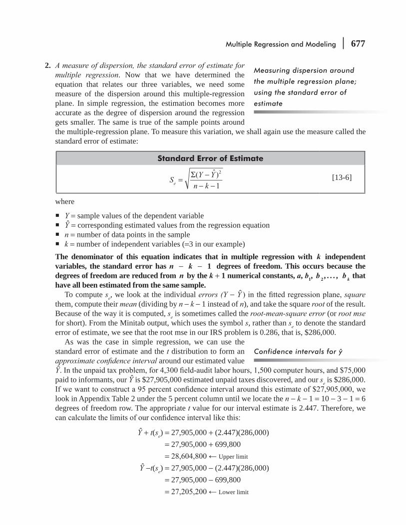
Multiple Regression and Modeling 677
2. A measure of dispersion, the standard error of estimate for multiple regression. Now that we have determined the equation that relates our three variables, we need some measure of the dispersion around this multiple-regression plane. In simple regression, the estimation becomes more accurate as the degree of dispersion around the regression gets smaller. The same is true of the sample points around the multiple-regression plane. To measure this variation, we shall again use the measure called the standard error of estimate:
Standard Error of Estimate
SY Y
n ke =Σ −
− −( ˆ)
1
2[13-6]
where
Y = sample values of the dependent variable Y = corresponding estimated values from the regression equation n = number of data points in the sample k = number of independent variables (=3 in our example)
The denominator of this equation indicates that in multiple regression with k independent variables, the standard error has n − k − 1 degrees of freedom. This occurs because the degrees of freedom are reduced from n by the k + 1 numerical constants, a, b1, b 2, . . . , b k that have all been estimated from the same sample.
To compute se, we look at the individual errors (Y − Y square them, compute their mean (dividing by n − k − 1 instead of n), and take the square root of the result. Because of the way it is computed, se is sometimes called the root-mean-square error (or root mse for short). From the Minitab output, which uses the symbol s, rather than se to denote the standard error of estimate, we see that the root mse in our IRS problem is 0.286, that is, $286,000.
As was the case in simple regression, we can use the standard error of estimate and the t distribution to form an approximate con dence interval around our estimated value Ypaid to informants, our Y is $27,905,000 estimated unpaid taxes discovered, and our se is $286,000.
look in Appendix Table 2 under the 5 percent column until we locate the n − k − 1 = 10 − 3 − 1 = 6 degrees of freedom row. The appropriate t value for our interval estimate is 2.447. Therefore, we
Y + t(se) = 27,905,000 + (2.447)(286,000) = 27,905,000 + 699,800 = Upper limit
Y −t(se) = 27,905,000 − (2.447)(286,000) = 27,905,000 − 699,800 = Lower limit
Measuring dispersion around
the multiple regression plane;
using the standard error of
estimate
Confidence intervals for y

678 Statistics for Management
division can feel certain that the actual discoveries will lie in this large interval from $27,205,200 to $28,604,800. If the
estimating the unpaid taxes discovered. As was true with simple regression, we can use the standard normal distribution, Appendix Table 1, to approximate the t distribution whenever our degrees of freedom (n
Did adding the third independent variable (rewards to informants) make our regression better? Because se measures the dispersion of the data points around the regression plane, smaller values of se should indicate better regressions. For the two-variable regression done earlier in this chapter, se turns out to be 1.076. Because the addition of the third variable reduced se to 0.286, we see that adding the third variable did It is not true in general, however, that adding variables always reduces se.
3. The coef cient of multiple determination. In our discussion of simple correlation analysis, we mea-
r2 Y that is explained by the estimating equation.
Similarly, in multiple correlation, we shall measure the strength of the relationship among three variables using the coef cient of multiple determination, R2, or its square root, R
multiple determination is also the proportion of the total variation of Y that is “explained” by the regression plane.
Notice that the output gives the value of R2 as 98.3 percent. This tells us that 98.3 percent of the total variation in unpaid taxes discovered is explained by the three independent variables. For the two-variable regression done earlier, R2 is only 0.729, so 72.9 percent of the variation is explained
25.4 percent of the variation.We still have not explained the numbers in the columns headed Stdev, t-ratio, and p in
Figure 13-2. These numbers will be used to make inferences about the population regression plane, the topic of Section 13.4.
No one hand-computes regressions anymore; there are too many interesting things to do with your
values of using your computer to do multiple regressions are that you can handle many independent variables, thus working toward a better estimating equation; you can measure whether adding another independent variable really improved your results; and you can quickly see the behavior of R2, which tells you the proportion of the total variation in the dependent variable that is explained by the independent variables. The computer does all the tedious arithmetic quickly, accurately, and without complaints, freeing up your time for the more important work of under-standing the results and using them to make better decisions.
HINTS & ASSUMPTIONS
Interpreting the confidence
interval
Value of additional variables
Using the coefficient of multiple
determination
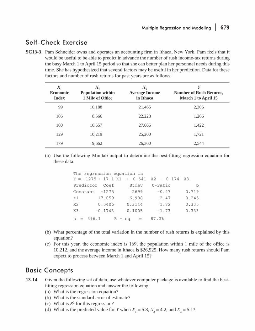
Multiple Regression and Modeling 679
Self-Check ExerciseSC13-3
would be useful to be able to predict in advance the number of rush income-tax returns during the busy March 1 to April 15 period so that she can better plan her personnel needs during this time. She has hypothesized that several factors may be useful in her prediction. Data for these factors and number of rush returns for past years are as follows:
X1Economic
Index
X2Population within
X3Average Income
in Ithaca
YNumber of Rush Returns,
March 1 to April 15
99 10,188 21,465 2,306
106 8,566 22,228 1,266
100 10,557 27,665 1,422
129 10,219 25,200 1,721
179 9,662 26,300 2,544
these data:
The regression equation isY = -1275 + 17.1 X1 + 0.541 X2 - 0.174 X3
Predictor Coef Stdev t-ratio p
Constant -1275 2699 -0.47 0.719
X1 17.059 6.908 2.47 0.245
X2 0.5406 0.3144 1.72 0.335
X3 -0.1743 0.1005 -1.73 0.333
s = 396.1 R - sq = 87.2%
(b) What percentage of the total variation in the number of rush returns is explained by this equation?
10,212, and the average income in Ithaca is $26,925. How many rush returns should Pam expect to process between March 1 and April 15?
Basic Concepts13-14
(a) What is the regression equation?(b) What is the standard error of estimate?(c) What is R2 for this regression?(d) What is the predicted value for Y when X1 = 5.8, X2 = 4.2, and X3 = 5.1?

680 Statistics for Management
Y X1 X2 X3
64.7 3.5 5.3 8.5
80.9 7.4 1.6 2.6
24.6 2.5 6.3 4.5
43.9 3.7 9.4 8.8
77.7 5.5 1.4 3.6
20.6 8.3 9.2 2.5
66.9 6.7 2.5 2.7
34.3 1.2 2.2 1.3
13-15
(a) What is the regression equation?(b) What is the standard error of estimate?(c) What is R2 for this regression?
Y when the values of X1, X2, X3, and X4 are 52.4, 41.6, 35.8, and 3, respectively.
X1 X2 X3 X4 Y
21.4 62.9 21.9 –2 22.8
51.7 40.7 42.9 5 93.7
41.8 81.8 69.8 2 64.9
11.8 41.0 90.9 –4 19.2
71.6 22.6 12.9 8 55.8
91.9 61.5 30.9 1 23.1
Applications13-16 Police stations across the country are interested in predicting the number of arrests they can
-age number of arrests (Yforce (X1), the population of the city in thousands (X2), and the percentage of unemployed people in the city (X3). Data for these factors in 15 cities are presented below.
equation for these data.(b) What percentage of the total variation in the number of arrests (Y) is explained by this
equation?(c) The ChapelBoro police department is trying to predict the number of monthly arrests.
ChapelBoro has a population of 75,000, a police force of 82, and an unemployment per-centage of 10.5 percent. How many arrests do you predict for each month?
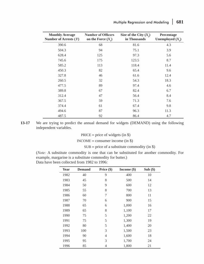
Multiple Regression and Modeling 681
Monthly Average Number of Arrests (Y)
on the Force (X1)
Size of the City (X2) in Thousands
Percentage Unemployed (X3)
390.6 68 81.6 4.3504.3 94 75.1 3.9628.4 125 97.3 5.6745.6 175 123.5 8.7585.2 113 118.4 11.4450.3 82 65.4 9.6327.8 46 61.6 12.4260.5 32 54.3 18.3477.5 89 97.4 4.6389.8 67 82.4 6.7312.4 47 56.4 8.4367.5 59 71.3 7.6374.4 61 67.4 9.8494.6 87 96.3 11.3487.5 92 86.4 4.7
13-17 We are trying to predict the annual demand for widgets (DEMAND) using the following independent variables.
PRICE = price of widgets (in $) = consumer income (in $) SUB = price of a substitute commodity (in $)
(Note: A substitute commodity is one that can be substituted for another commodity. For example, margarine is a substitute commodity for butter.)Data have been collected from 1982 to 1996:
Year Demand Price ($) Income ($) Sub ($)1982 40 9 400 101983 45 8 500 141984 50 9 600 121985 55 8 700 131986 60 7 800 111987 70 6 900 151988 65 6 1,000 161989 65 8 1,100 171990 75 5 1,200 221991 75 5 1,300 191992 80 5 1,400 201993 100 3 1,500 231994 90 4 1,600 181995 95 3 1,700 241996 85 4 1,800 21
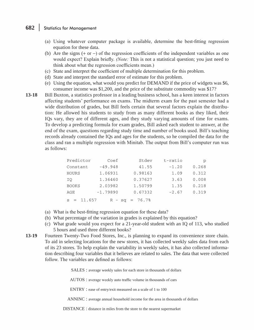
682 Statistics for Management
equation for these data.(b) Are the signs (+ or −
(Note: This is not a statistical question; you just need to
(d) State and interpret the standard error of estimate for this problem.(e) Using the equation, what would you predict for DEMAND if the price of widgets was $6,
consumer income was $1,200, and the price of the substitute commodity was $17?13-18 Bill Buxton, a statistics professor in a leading business school, has a keen interest in factors
wide distribution of grades, but Bill feels certain that several factors explain the distribu-tion: He allowed his students to study from as many different books as they liked, their IQs vary, they are of different ages, and they study varying amounts of time for exams. To develop a predicting formula for exam grades, Bill asked each student to answer, at the
records already contained the IQs and ages for the students, so he compiled the data for the
as follows:
Predictor Coef Stdev t-ratio p
Constant -49.948 41.55 -1.20 0.268
HOURS 1.06931 0.98163 1.09 0.312
IQ 1.36460 0.37627 3.63 0.008
BOOKS 2.03982 1.50799 1.35 0.218
AGE -1.79890 0.67332 -2.67 0.319
s = 11.657 R - sq = 76.7%
(b) What percentage of the variation in grades is explained by this equation?(c) What grade would you expect for a 21-year-old student with an IQ of 113, who studied
5 hours and used three different books?13-19 Fourteen Twenty-Two Food Stores, Inc., is planning to expand its convenience store chain.
To aid in selecting locations for the new stores, it has collected weekly sales data from each of its 23 stores. To help explain the variability in weekly sales, it has also collected informa-tion describing four variables that it believes are related to sales. The data that were collected
SALES : average weekly sales for each store in thousands of dollars
:
ENTRY : ease of entry/exit measured on a scale of 1 to 100
ANNINC : average annual household income for the area in thousands of dollars
DISTANCE : distance in miles from the store to the nearest supermarket
Multiple Regression and Modeling 683
The data were analyzed using Minitab and the output follows:Predictor Coef Stdev t-ratio p
Constant 175.37 92.62 1.89 0.075
AUTOS -0.028 0.315 -0.09 0.929
ENTRY 3.775 1.272 2.97 0.008
ANNINC 1.990 4.510 0.44 0.664
DISTANCE 212.41 28.090 7.56 0.000
s = 85.587 R - sq = 95.8%
(b) What is the standard error of estimate for this equation?(c) What fraction of the variation in sales is explained by this regression?(d) What sales would you predict for a store located in a neighborhood that had an average
annual household income of $20,000, was 2 miles from the nearest supermarket, was on
13-20 Rick Blackburn is thinking about selling his house. In order to decide what price to ask, he has collected data for 12 recent closings. He has recorded sales price (in $l,000s), the number of square feet in the house (in 100s of sq ft.), the number of stories, the number of bathrooms, and the age of the house (in years).
Sales Price Square Feet Stories Bathrooms Age
49.65 8.9 1 1.0 2
67.95 9.5 1 1.0 6
81.15 12.6 2 1.5 11
81.60 12.9 2 1.5 8
91.50 19.0 2 1.0 22
95.25 17.6 1 1.0 17
100.35 20.0 2 1.5 12
104.25 20.6 2 1.5 11
112.65 20.5 1 2.0 9
149.70 25.1 2 2.0 8
160.65 22.7 2 2.0 18
232.50 40.8 3 4.0 12
equation for these data.(b) What is R2 for this equation? What does this number measure?
=18.0 hundreds of square feet), 1 story, 1.5 bath-rooms, and is 6 years old, what sale price can Rick expect?
13-21 -lions of tons of steel it is able to sell each year. Management suspects that the following are
684 Statistics for Management
automakers are planning to produce in that year. Data for 7 years have been collected:
Year
YMillions ofTons Sold
X1
Rate
X2ImportedUndercut
X3Number of
Cars1993 4.2 3.1 3.10 6.21992 3.1 3.9 5.00 5.11991 4.0 7.5 2.20 5.71990 4.7 10.7 4.50 7.11989 4.3 15.5 4.35 6.51988 3.7 13.0 2.60 6.11987 3.5 11.0 3.05 5.9
equation for these data.(b) What percentage of the total variation in the number of millions of tons of steel sold by
Allegheny each year is explained by this equation?
rate is 7.1, American automakers are planning to produce 6.0 million cars, and the average imported price undercut per ton is $3.50?
Worked-Out Answer to Self-Check ExerciseSC 13-3 From the computer output we get the following results:
(a) Y = −1275 + 17.059X1 + 0.5406X2 − 0.1743X3.(b) R2 = 87.2%; 87.2% of the total variation in Y is explained by the model.(c) Y = −1275 + 17.059(169) + 0.5406(10,212) − 0.1743(26,925) = 2,436 rush returns.
13.4 MAKING INFERENCES ABOUT POPULATION PARAMETERSIn Chapter 12, we noted that the sample regression line, Y = a + bX (Equation 12-3), estimates the population regression line, Y = A + BX (Equation 12-13). The reason we could only estimate the popu-
- Y = A + BX + e
(Equation 12-13a) rather than Y = A + BX.Exactly the same sort of thing happens in multiple regression.
Y = a + b1X1 + b2 X2 + … + bk Xk [13-5]
is an estimate of a true but unknown population regression plane of the form
Population Regression Equation
Y = A + B1X1 + B2 X2 + … + Bk Xk[13-7]
Population regression plane

Multiple Regression and Modeling 685
our IRS problem to see why this is so. Not all payments to informants will be equally effective. Some of the computer hours may be used for collecting and organizing data; others may be used for analyzing those data to seek errors and fraud. The success of the computer in discovering unpaid taxes may depend on how much time is devoted to each of these activities. For these and other rea-sons, some of the data points will points be above the regression plane and some will be below it. Instead of satisfying
Y = A + B1X1 + B2 X2 + … + Bk Xk [13-7]
the individual data points will satisfy
Population Regression Plane Plus Random Disturbance
Y = A + B1X1 + B2 X2 + … + Bk Xk + e [13-7a]
The quantity e in Equation 13-7a is a random disturbance, which equals zero on the average. The standard deviation of the individual disturbances is σe, and the standard error of estimate, se, which we looked at in the last section, is an estimate of σe.
Because our sample regression plane, Y = a + b1 X1 + b2 X2 + ... + bk Xk (Equation 13-5), estimates the unknown population regression plane, Y = A + B1X1 + B2X2 + · · · + Bk Xk (Equation 13-7), we should be able to use it to make inferences about the population regression plane. In this section, we shall make inferences about the slopes (B1, B2, ... , Bk) of the “true” regression equation (the one for the entire population) that are based on the slopes (b1 b2, ... , bk) of the regression equation estimated from the sample of data points.
Inferences about an Individual Slope Bi
The regression plane is derived from a sample and not from the entire population. As a result, we cannot expect the true regres-sion equation, Y = A + B1X1 + B2X2 + … + Bk Xk (the one for the entire population), to be exactly the same as the equation esti-mated from the sample observations, = a + b1x1 + b2 X2 + … + bk Xk. Even so, we can use the value of bi one of the slopes we calculate from a sample, to test hypotheses about the value of Bi, one of the slopes of the regression plane for the entire population.
The procedure for testing a hypothesis about Bi is similar to procedures discussed in Chapters 8 and 9 on hypothesis testing.
page 676 we pointed out that b1 = 0.597. B1 to compare with b1= 0.597.
Suppose that over an extended past period of time, the slope of the relationship between Y and X1 was
H0: B1 = 0.400 Null hypothesis
H1: B1 Alternative hypothesis
In effect, then, we are testing to learn whether current data indicate that B1 has changed from its histori-cal value of 0.400.
Random disturbances moves
point off the regression plane
Difference between true
regression equation and
one estimated from sample
observations
Testing a hypothesis about Bi

686 Statistics for Management
B1 standard error of the regression coef cient. Here, the regression
b1, so the standard error of this sb1
.sb1
by hand, but, fortunately, Minitab computes the standard errors of all
From the output, we see that sb1 is 0.0811. (Similarly, if we
want to test a hypothesis about B2, we see that the appropriate standard error to use is sb1
= sb1 on
Standardized Regression Coefficient
0tb B
Si i
bi
=−
[13-8]
where
bi = Bi0
= actual slope hypothesized for the population sbi
=
Why did we use t to denote the standardized statistic? Recall that in simple regression, we used a and b in Equation 12-7 to calculate se, and that se estimated σe, the standard deviation of the disturbances in the data (Equation 12-13a). Then we used se sb, the standard error of the regression
n data points and used them to estimate the two a and b. Then we based our tests on the t distribution with n − 2 degrees of freedom.
Similarly, in multiple regression, we also start out with n data points but we use them to estimate k +1 a, and k slopes, b1, b2, ..., bk13-6 to calculate se, which again estimates σe, the standard deviation of the disturbances in the data (Equation 13-7a). Then se sb1
.
Standard error of the regression
coefficient
Standardizing the regression
coefficient
Regression AnalysisThe regression equation is
DISCOVER = -45.8 + 0.597 AUDIT + 1.18 COMPUTER + 0.405 REWARDSPredictor Coef Stdev t-ratio p
Constant -45.796 4.878 -9.39 0.000
AUDIT 0.59697 0.08112 7.36 0.000
COMPUTER 1.17684 0.08407 14.00 0.000
REWARDS 0.40511 0.04223 9.59 0.000
s = 0.2861 R - sq = 98.3%
FIGURE 13-2 MINITAB OUTPUT FOR IRS REGRESSION

Multiple Regression and Modeling 687
Because of this, we base our hypothesis tests on the t distribution with n − k −1 (=n − (k + 1)) degrees of freedom.
t = 1 10
1
b B
Sb
− [13-8]
= 0.597 0.400
0.081
−
=
Suppose we are interested in testing our hypothesis at the 10
our sample data, and three independent variables, we know that we have n − k − 1 or 10 − 3 − 1 = 6 degrees of freedom. We look in Appendix Table 2 under the 10 percent column and come down until we
t value is 1.943. Because we are concerned whether b1 B1 (the hypothesized slope of the population regression plane), this is a two-tailed test, and the critical values
outside the acceptance region for our hypothesis test. Therefore, we reject the null hypothesis that B1 still equals 0.400. In other words, there is enough difference between b1 and 0.400 for us to conclude that B1 has changed from its histori-
unpaid taxes discovered by $400,000, as it did in the past.In addition to hypothesis testing, we can also construct a con-
dence interval for any one of the values of Bi. In the same way that bi is a point estimate of Bi Bi. To illustrate the
B3 in our IRS problem. The relevant data are
0.405
0.04223
3
==
⎫⎬⎪
⎭⎪
b
Sb
from Figure 13-2
t =
b3 + t ( )3
sb = 0.405 + 2.447(0.0422) = Upper limit
b3 − t ( )3
sb = 0.405 − 2.447(0.0422) = Lower limit
unpaid taxes discovered by some amount between $302,000 and $508,000. We will often be interested in questions of the form: Does Y
really depend on Xi? For example, we could ask whether unpaid taxes discovered really depend on computer hours. This question
Conducting the hypothesis test
Confidence interval for Bi
Is an explanatory variable
significant?

688 Statistics for Management
is often phrased as, “Is Xi Y ?” A bit of thought should convince you that Y depends on Xi (that is, Y varies when Xi varies) if Bi Xi if Bi = 0.
We see that our question leads to hypotheses of the form:
H0: Bi = Null hypothesis: Xi H1: Bi Alternative hypothesis: Xi
We can test these hypotheses using Equation 13-8 just as we did when we tested our hypotheses about whether B1 still equaled 0.400. However, there is an easier way to do this, using the column on the out-put in Figure 13-2 headed “t-ratio.” Look at Equation 13-8 again:
0tb B
Si i
bi
=−
[13-8]
Because our hypothesized value for Biwe shall denote by to, becomes
0tb
Si
bi
=
The value of t0 is called the “observed” or “computed” t value. This is the number that appears in the column headed “t-ratio” in
tc the “critical” t value that we look up in Appendix Table 2. Then, because the test of whether Xi is a
−tc to tc
Test of Whether a Variable Is Significant
– tc to tc [13-9]
where
tc = appropriate t value (with n − k − to = /b si bi
= observed (or computed) t value obtained from computer output
If to falls between −tc and tc, we accept H0 and conclude Xi
0 and conclude that Xi
-covered. From Appendix Table 2, with n − k − 1 = 10 − 3 −1 = 6 degrees of freedom and α = 0.01, we see that tc = 3.707. From Figure 13-2, we see that t0 = 14.00. Because t0 > tc, we conclude that computer hours is t values
t0 = 7.36 and rewards to informants, t0 =
We can also use the column headed “p” to test whether Xi prob
values for the two-tailed test of the hypotheses:
Using computed t values from
the Minitab output
Testing the significance of
computer hours in the IRS
problem

Multiple Regression and Modeling 689
H0:Bi = 0
H1:Bi
Recall from the discussion in Chapter 9 that these prob values are the probabilities that each bi would be as far (or farther) away from zero than the observed value obtained from our regression, if H0 is true. As Figure 13-3 illustrates, we need only compare these prob values with αtest, to determine whether Xi Y.
-able Xi bi different from zero, that is. if t0 is a large positive or a large negative number.
α = 0.01. For each of the three independent variables, p
Inferences about the Regression as a Whole (Using an F Test)Suppose you put a piece of graph paper over a dartboard and randomly tossed a bunch of darts at it. After you took out the darts, you would have something that looked very much like a scatter diagram.
r2. Because the darts were randomly tossed, you would expect to get a low value of r2 because in this case, X Y. However, if you did this many times, occasionally you would observe a high value of r2, just by pure chance.
Given any simple (or multiple) regression, it’s natural to ask whether the value of r2 (or R2) really indicates that the independent variables explain Y, or might have happened just by chance. This question is often phrased, “Is the regres-
Xi was a
Significance of the regression as
a whole
(a) p is greater than α; Xi is not a significant explanatory variable
(b) p is less than α; Xi is not a significant explanatory variable
α/2 of area
−tc −to −to −tcto totc tc
α/2 of area α/2 of area
00
α/2 of area
Acceptance regionAccept the null hypothesis
if the sample value is inthis region
Acceptance regionAccept the null hypothesis
if the sample value is inthis region
FIGURE 13.3 USING “P ” TO SEE WHETHER XI· IS A SIGNIFICANT EXPLANATORY VARIABLE
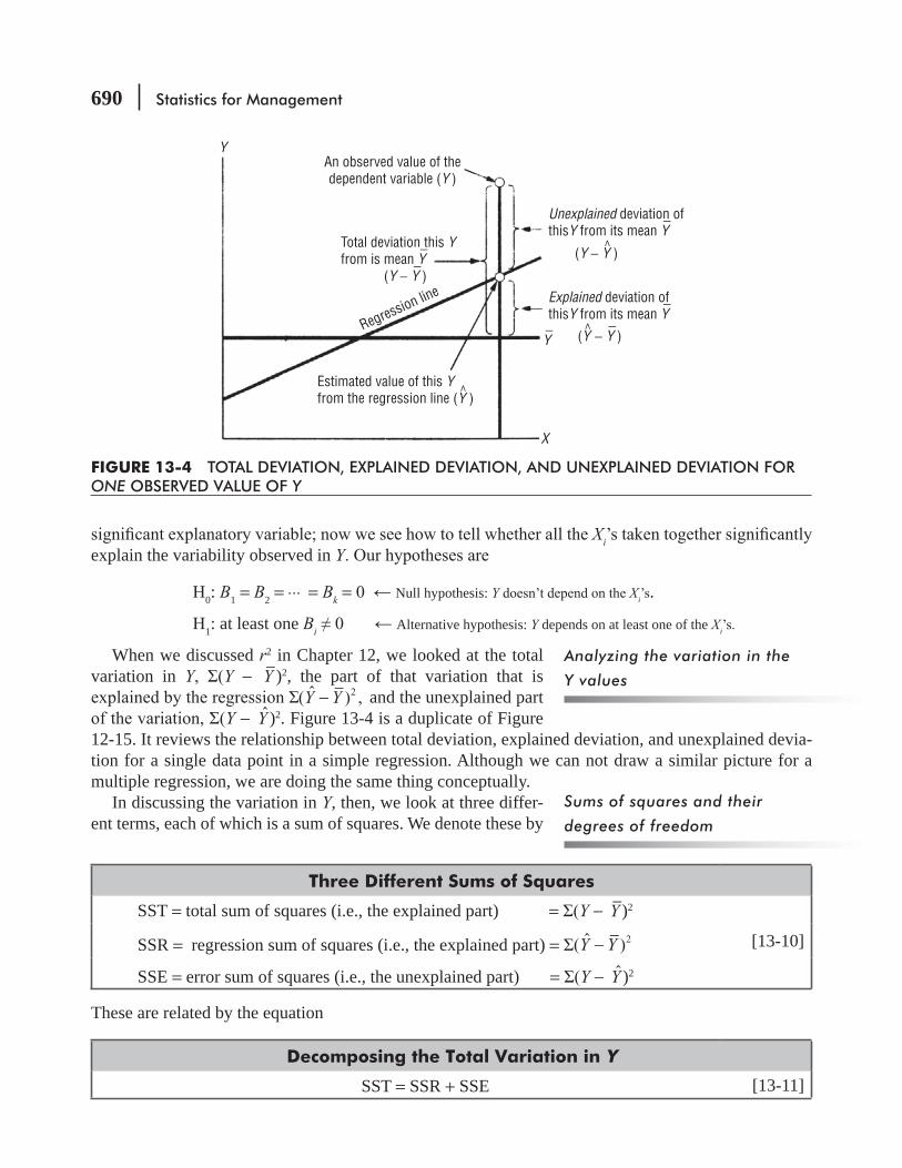
690 Statistics for Management
Xiexplain the variability observed in Y
H0: B1 = B2 = ... = Bk = Null hypothesis: Y Xi .
H1: at least one Bi Alternative hypothesis: Y depends on at least one of the Xi
When we discussed r2 in Chapter 12, we looked at the total variation in Y Y − Y )2, the part of that variation that is
( ˆ ) ,2−Y Y and the unexplained part Y − Y )2. Figure 13-4 is a duplicate of Figure
12-15. It reviews the relationship between total deviation, explained deviation, and unexplained devia-tion for a single data point in a simple regression. Although we can not draw a similar picture for a multiple regression, we are doing the same thing conceptually.
In discussing the variation in Y, then, we look at three differ-ent terms, each of which is a sum of squares. We denote these by
Three Different Sums of Squares
SST = total sum of squares (i.e., the explained part) = Y − Y )2
SSR = regression sum of squares (i.e., the explained part) = ( ˆ )2Y Y− [13-10]
SSE = error sum of squares (i.e., the unexplained part) = Y − Y )2
These are related by the equation
Decomposing the Total Variation in Y
SST = SSR + SSE [13-11]
Analyzing the variation in the
Y values
Sums of squares and their
degrees of freedom
An observed value of thedependent variable (Y )
Total deviation this Yfrom is mean Y
−
Estimated value of this Yfrom the regression line (Y )
Unexplained deviation ofthisY from its mean Y
−
Explained deviation ofthisY from its mean Y
−Regression line
(Y − Y−
)
(Y − Y−
)
(Y − Y )
Y−
Y
X
FIGURE 13-4 TOTAL DEVIATION, EXPLAINED DEVIATION, AND UNEXPLAINED DEVIATION FOR ONE OBSERVED VALUE OF Y
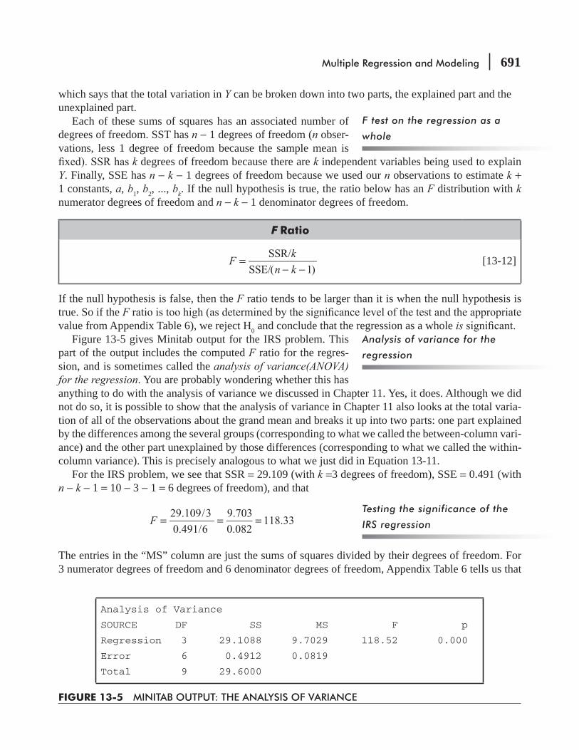
Multiple Regression and Modeling 691
which says that the total variation in Y can be broken down into two parts, the explained part and the unexplained part.
Each of these sums of squares has an associated number of degrees of freedom. SST has n − 1 degrees of freedom (n obser-vations, less 1 degree of freedom because the sample mean is
k degrees of freedom because there are k independent variables being used to explain Y. Finally, SSE has n − k − 1 degrees of freedom because we used our n observations to estimate k + 1 constants, a, b1, b2, ..., bk. If the null hypothesis is true, the ratio below has an F distribution with k numerator degrees of freedom and n − k − 1 denominator degrees of freedom.
F Ratio
SSR/
SSE/( 1)=
− −F
k
n k[13-12]
If the null hypothesis is false, then the F ratio tends to be larger than it is when the null hypothesis is true. So if the Fvalue from Appendix Table 6), we reject H0 and conclude that the regression as a whole is
Figure 13-5 gives Minitab output for the IRS problem. This part of the output includes the computed F ratio for the regres-sion, and is sometimes called the analysis of variance(ANOVA) for the regression. You are probably wondering whether this has anything to do with the analysis of variance we discussed in Chapter 11. Yes, it does. Although we did not do so, it is possible to show that the analysis of variance in Chapter 11 also looks at the total varia-tion of all of the observations about the grand mean and breaks it up into two parts: one part explained by the differences among the several groups (corresponding to what we called the between-column vari-ance) and the other part unexplained by those differences (corresponding to what we called the within-column variance). This is precisely analogous to what we just did in Equation 13-11.
For the IRS problem, we see that SSR = 29.109 (with k =3 degrees of freedom), SSE = 0.491 (with n − k − 1 = 10 − 3 − 1 = 6 degrees of freedom), and that
F29.109/3
0.491/6
9.703
0.082118.33= = =
The entries in the “MS” column are just the sums of squares divided by their degrees of freedom. For 3 numerator degrees of freedom and 6 denominator degrees of freedom, Appendix Table 6 tells us that
F test on the regression as a
whole
Analysis of variance for the
regression
Analysis of Variance
SOURCE DF SS MS F p
Regression 3 29.1088 9.7029 118.52 0.000
Error 6 0.4912 0.0819
Total 9 29.6000
FIGURE 13-5 MINITAB OUTPUT: THE ANALYSIS OF VARIANCE
Testing the significance of the
IRS regression

692 Statistics for Management
α = F
reach the same conclusion by noting that the output tells us that “ p” is 0.000. Because this prob value α = p to do the test without having to use Appendix Table 6 to look up
a critical value of F. This is analogous to the way we used the p values in Figure 13-2 for testing the
Multicollinearity in Multiple Regression
often become less reliable as the degree of correlation between the independent variables increases. If there is a high level of correlation between some of the independent variables, we have a problem that statisticians call multicollinearity.
the number of salespeople employed and their total salaries. Because the values associated with these two independent variables are highly correlated, we need to use only one set of them to make
Y well, even when multicollinearity is present.
to see how it affects the regression. For the past 12 months, the manager of Pizza Shack has been running a series of advertise-ments in the local newspaper. The ads are scheduled and paid for in the month before they appear. Each of the ads contains a two-for-one coupon, which entitles the bearer to receive two Pizza Shack pizzas
Definition and effect of
multicollinearity
An example of multicollinearity
TABLE 13-4 PIZZA SHACK SALES AND ADVERTISING DATA
Month
X1 Number of Ads
Appearing
X2Cost of Ads
Appearing (00s of dollars)
Y Total Pizza Sales (000s of dollars)
May 12 13.9 43.6June 11 12.0 38.0July 9 9.3 30.1Aug. 7 9.7 35.3Sept. 12 12.3 46.4
8 11.4 34.2Nov. 6 9.3 30.2Dec. 13 14.3 40.7Jan. 8 10.2 38.5Feb. 6 8.4 22.6March 8 11.2 37.6April 10 11.1 35.2

Multiple Regression and Modeling 693
while paying for only the more expensive of the two. The manager has collected the data in Table 13-4 and would like to use it to predict pizza sales.
In Figures 13-6 and 13-7, we have given Minitab outputs for the regressions of total sales on number of ads and cost of ads, respectively.
For the regression on number of ads, we see that the observed t value is 3.95. With 10 degrees of α = 0.01, the critical t value (from Appendix Table 2) is found to be
3.169. Because t0 > tc (or, equivalently, because p is less than 0.01), we conclude that the number of ads r2 − 61.0 percent, so that the
number of ads explains about 61 percent of the variation in pizza sales.
Two simple regressions
Regression AnalysisThe regression equation isSALES = 16.9 + 2.08 ADS
Predictor Coef Stdev t-ratio pConstant 16.937 4.982 3.40 0.007ADS 2.0832 0.5271 3.95 0.003
s = 4.206 R - sq = 61.0%
Analysis of Variance
SOURCE DF SS MS F pRegression 1 276.31 276.31 15.62 0.003Error 10 176.88 17.69Total 11 453.19
FIGURE 13-6 MINITAB REGRESSION OF SALES ON NUMBER OF ADS
Regression AnalysisThe regression equation isSALES = 4.17 + 2.87 COST
Predictor Coef Stdev t-ratio pConstant 4.173 7.109 0.59 0.570COST 2.8725 0.6330 4.54 0.000
s = 3.849 R - sq = 67.3%
Analysis of Variance
SOURCE DF SS MS F pRegression 1 305.04 305.04 20.59 0.000Error 10 148.15 14.81Total 11 453.19
FIGURE 13-7 MINITAB REGRESSION OF SALES ON THE COST OF ADS

694 Statistics for Management
For the regression on the cost of ads, the observed t value is 4.54, so that the cost of ads is even more
t value was only 3.95). In this regression, r2 = 67.3 percent, so about 67 percent of the variation in pizza sales is explained by the cost of ads.
themselves, we try to use both of them in a multiple regression. The output is in Figure 13-8.
p is 0.006. R2 = 68.4 percent, so the two variables together explain
about 68 percent of the variation in total sales.However, if we look at the p values for the individual vari-
ables in the multiple regression, we see that even at α = 0.1,
This apparent contradiction is explained once we notice that the number of ads is highly correlated with the cost of ads. In fact, the correlation between these two variables is r = 0.8949, so we have a problem with multicollinearity in our data. You might wonder why these two variables are not perfectly correlated. This is because the cost of an ad varies slightly, depending on where it appears in the newspaper. For instance, in the Sunday paper, ads in the TV section cost more than ads in the news section, and the manager of Pizza Shack has placed Sunday ads in each of these sections on different occasions.
Because X1 and X2 are closely related to each other, in effect they each explain the same part of the variability in Ywe get r2 = r2 = 67.3 percent in the second simple regression, but an R2 of only 68.4 percent in the multiple regression. Adding the number of ads as a second explanatory variable to the cost of ads explains only about 1 percent more of the variation in total sales.
At this point, it is fair to ask, “Which variable is really explaining the variation in total sales in the multiple regres-sion?” The answer is that both are, but we cannot separate out their individual contributions because they are so
-sion have high standard errors, relatively small computed t values, and relatively large prob > |t| values.
How does this multicollinearity affect us? We are still able to make relatively precise pre-dictions when it is present: Note that for the multiple regression (output in Figure 13-8), the standard error of estimate, which determines the width of confidence intervals for predictions, is 3.989. while for the simple regression with the cost of ads as the explanatory variable (output in Figure 13-7), we have se =change if we increase the number of ads by one. The multiple regression says b1 = 0.625 (that is, each ad increases total pizza sales by about $625), but the standard error of this coefficient is 1.12 (that is, about $1,120).
Using both explanatory variables
in a multiple regression
Loss of individual significance
Correlation between two
explanatory variables
Both variables explain the same
thing
Individual contributions can’t be
separated out
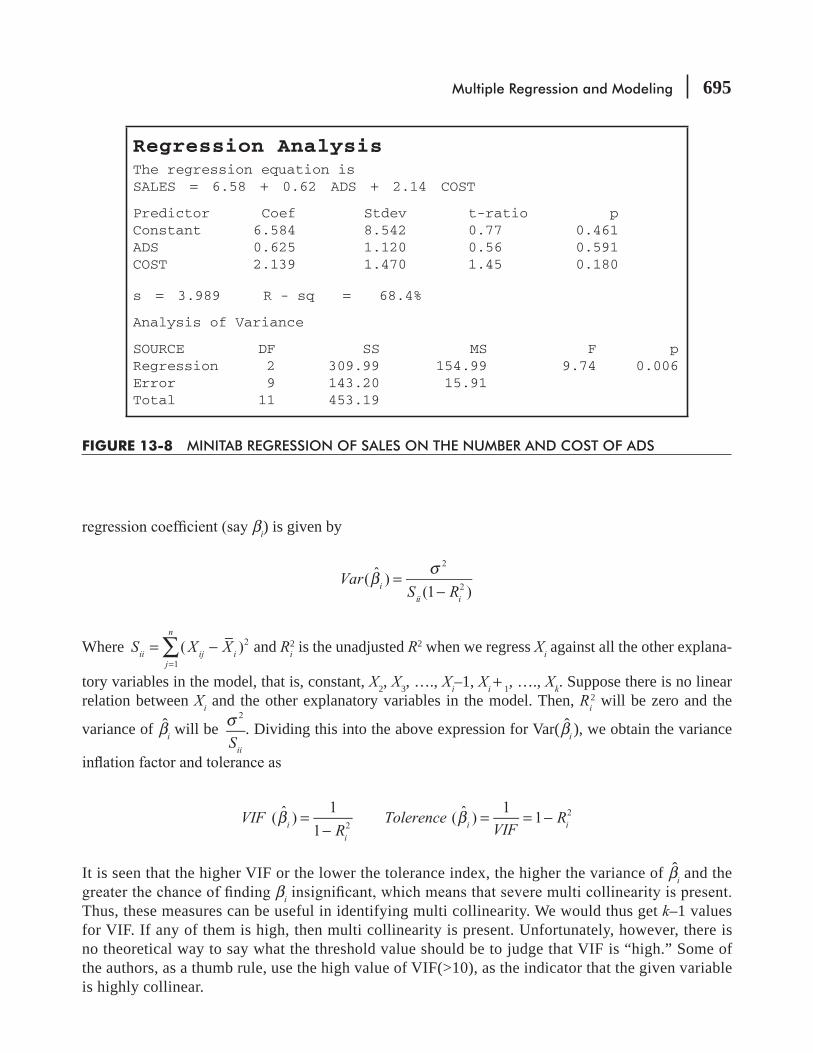
Multiple Regression and Modeling 695
βi) is given by
( ˆ )(1 )
2
2β σ
=−
VarS Ri
ii i
Where ( )2
1∑= −
=
S X Xii ij ij
n
and Ri 2 is the unadjusted R2 when we regress Xi against all the other explana-
tory variables in the model, that is, constant, X2, X3, …., Xi–1, Xi + 1, …., Xk. Suppose there is no linear relation between Xi and the other explanatory variables in the model. Then, Ri
2 will be zero and the
variance of βi will be 2σ
Sii
. Dividing this into the above expression for Var( βi ), we obtain the variance
( ˆ )1
1 ( ˆ )
11
2
2β β=−
= = −VIFR
TolerenceVIF
Ri
i
i i
It is seen that the higher VIF or the lower the tolerance index, the higher the variance of βi and the βi
Thus, these measures can be useful in identifying multi collinearity. We would thus get k–1 values for VIF. If any of them is high, then multi collinearity is present. Unfortunately, however, there is no theoretical way to say what the threshold value should be to judge that VIF is “high.” Some of the authors, as a thumb rule, use the high value of VIF(>10), as the indicator that the given variable is highly collinear.
Regression AnalysisThe regression equation isSALES = 6.58 + 0.62 ADS + 2.14 COST
Predictor Coef Stdev t-ratio pConstant 6.584 8.542 0.77 0.461ADS 0.625 1.120 0.56 0.591COST 2.139 1.470 1.45 0.180
s = 3.989 R - sq = 68.4%
Analysis of Variance
SOURCE DF SS MS F pRegression 2 309.99 154.99 9.74 0.006Error 9 143.20 15.91Total 11 453.19
FIGURE 13-8 MINITAB REGRESSION OF SALES ON THE NUMBER AND COST OF ADS
696 Statistics for Management
Hint: Making inferences about a multiple regression is conceptually just like what we did in
or more independent variables. Warning: Multicollinearity is a problem you have to deal with in multiple regressions, and developing a common-sense understanding of it is necessary. Remember that you can stillpresent, you can’t tell with much precision how much the dependent variable will change if you “jiggle” one of the independent variables. So our aim should be to minimize multicollinearity. Hint: The best multiple regression is one that explains the relationship among the data by account-ing for the largest proportion of the variation in the dependent variable, with the fewest number of independent variables. Warning: Throwing in too many independent variables just because you have a computer is not a great idea.
HINTS & ASSUMPTIONS
Multiple Linear Regression Using SPSS
Above data is used for regression analysis.
An automotive industry group keeps track of the sales for a variety of personal motor vehicles. In an effort to be able to identify over and underperforming models, you want to establish a relationship between vehicle sales and vehicle characteristics.
For linear regression go to Analyze > Regression > Linear > Select dependent and independent variables
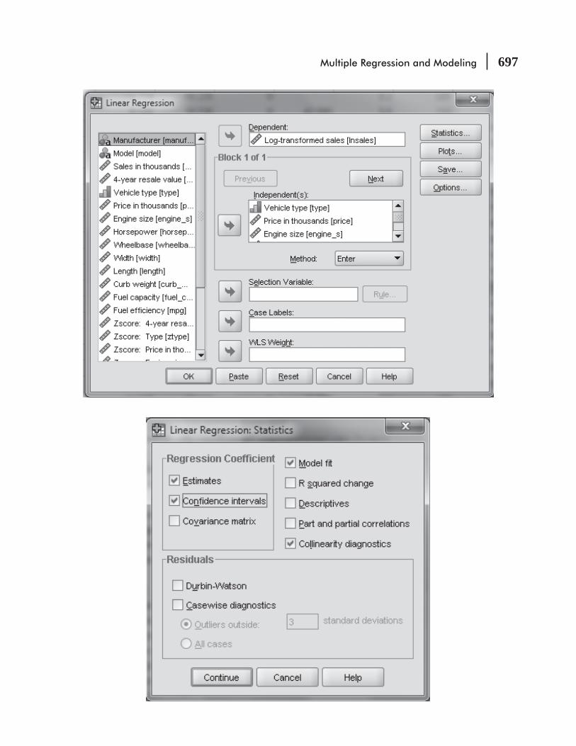
Multiple Regression and Modeling 697
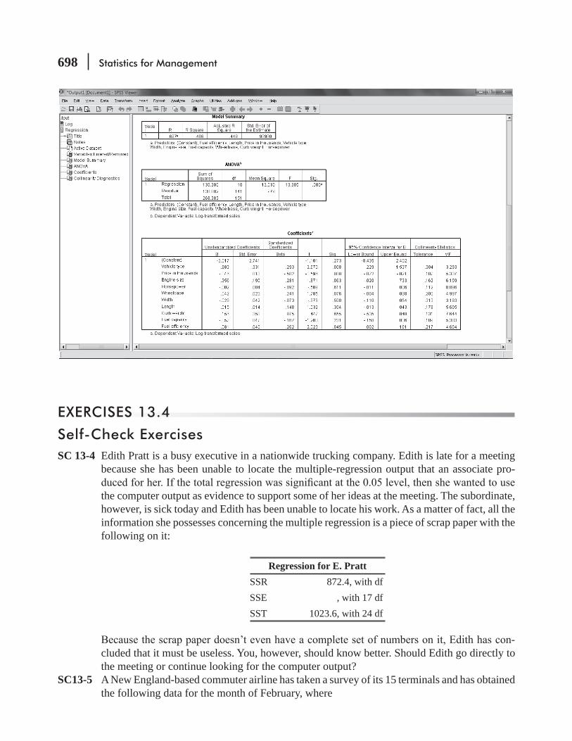
698 Statistics for Management
EXERCISES 13.4
Self-Check ExercisesSC 13-4 Edith Pratt is a busy executive in a nationwide trucking company. Edith is late for a meeting
because she has been unable to locate the multiple-regression output that an associate pro-
the computer output as evidence to support some of her ideas at the meeting. The subordinate, however, is sick today and Edith has been unable to locate his work. As a matter of fact, all the information she possesses concerning the multiple regression is a piece of scrap paper with the following on it:
Regression for E. PrattSSR 872.4, with dfSSE , with 17 dfSST 1023.6, with 24 df
-cluded that it must be useless. You, however, should know better. Should Edith go directly to the meeting or continue looking for the computer output?
SC13-5 A New England-based commuter airline has taken a survey of its 15 terminals and has obtained the following data for the month of February, where

Multiple Regression and Modeling 699
SALES = total revenue based on number of tickets sold (in thousands of dollars)
= amount spent on promoting the airline in the area (in thousands of dollars)
= number of competing airlines at that terminal
FREE =
Sales ($) Promot ($) Comp Free
79.3 2.5 10 3200.1 5.5 8 6163.2 6.0 12 9200.1 7.9 7 16146.0 5.2 8 15177.7 7.6 12 930.9 2.0 12 8
291.9 9.0 5 10160.0 4.0 8 4339.4 9.6 5 16159.6 5.5 11 786.3 3.0 12 6
237.5 6.0 6 10107.2 5.0 10 4155.0 3.5 10 4
airline:
The regression equation isSALES = 172 + 25.9 PROMOT - 13.2 COMP - 3.04 FREE
Predictor Coef Stdev t-ratio pConstant 172.34 51.38 3.35 0.006PROMOT 25.950 4.877 5.32 0.000COST -13.238 3.686 -3.59 0.004FREE -3.041 2.342 -1.30 0.221
-priate hypotheses. Use α = 0.05.
(c) Does an increase in promotions by $1,000 change sales by $28,000, or is the change sig-α = 0.10.
Applications13-22 Mark Lowtown publishes the Mosquito Junction Enquirer
the amount of newsprint needed each day. He has randomly selected 27 days over the past year and recorded the following information:

700 Statistics for Management
=
CLASFIED =
DISPLAY = number of display advertisements
FULLPAGE = number of full-page advertisements
follows.
Predictor Coef Stdev t-ratio pConstant 1072.95 872.43 1.23 0.232CLASFIED 0.251 0.126 1.99 0.060DISPLAY 1.250 0.884 1.41 0.172FULLPAGE 250.66 67.92 3.69 0.001
(a) Mark had always felt that each display advertisement used at least 3 pounds of news-
level?
5 percent level?
(c) Mark sells full-page advertising space to the local merchants for $30 per page. Should he consider adjusting his rates if newsprint costs him 9¢ per pound? Assume other costs are negligible. State explicit hypotheses and an explicit conclusion. (Hint: Holding all else constant, each additional full-page ad uses 250.66 pounds of paper × $0.09 per pound =
should be changed.)13-23 -
atory variables for exam scores? (There were 12 students in the sample.)13-24 Refer to Exercise 13-18. The following additional output was provided by Minitab when Bill
ran the multiple regression:
Analysis of Variance
Regression 4 3134.42 783.60 Error 7 951.25 135.89 Total 11 4085.67
(a) What is the observed value of F? 0.05, what is the appropriate critical value of F to use in deter-
13-25 Refer to Exercise -tory variable for SALES?
13-26 Refer to Exercise 13-19. The following additional output was provided by Minitab when the multiple regression was run:
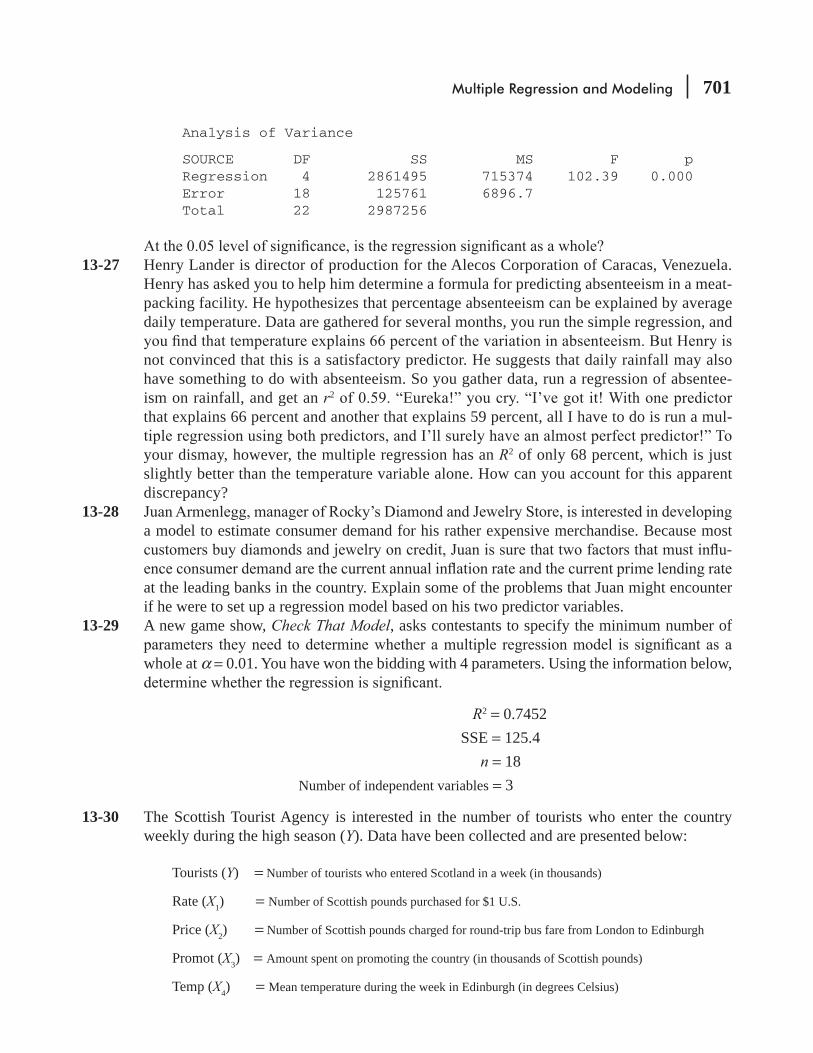
Multiple Regression and Modeling 701
Analysis of Variance
SOURCE DF SS MS F pRegression 4 2861495 715374 102.39 0.000Error 18 125761 6896.7 Total 22 2987256
13-27 Henry Lander is director of production for the Alecos Corporation of Caracas, Venezuela. Henry has asked you to help him determine a formula for predicting absenteeism in a meat-packing facility. He hypothesizes that percentage absenteeism can be explained by average daily temperature. Data are gathered for several months, you run the simple regression, and
not convinced that this is a satisfactory predictor. He suggests that daily rainfall may also have something to do with absenteeism. So you gather data, run a regression of absentee-ism on rainfall, and get an r2
that explains 66 percent and another that explains 59 percent, all I have to do is run a mul-
your dismay, however, the multiple regression has an R2 of only 68 percent, which is just slightly better than the temperature variable alone. How can you account for this apparent discrepancy?
13-28 a model to estimate consumer demand for his rather expensive merchandise. Because most
-
at the leading banks in the country. Explain some of the problems that Juan might encounter if he were to set up a regression model based on his two predictor variables.
13-29 A new game show, Check That Model, asks contestants to specify the minimum number of
whole at α = 0.01. You have won the bidding with 4 parameters. Using the information below,
R2 = 0.7452 SSE = 125.4 n = 18
Number of independent variables = 3
13-30 The Scottish Tourist Agency is interested in the number of tourists who enter the country weekly during the high season (Y). Data have been collected and are presented below:
Tourists (Y) = Number of tourists who entered Scotland in a week (in thousands)
Rate (X1) = Number of Scottish pounds purchased for $1 U.S.
Price (X2) = Number of Scottish pounds charged for round-trip bus fare from London to Edinburgh
Promot (X3) = Amount spent on promoting the country (in thousands of Scottish pounds)
Temp (X4) = Mean temperature during the week in Edinburgh (in degrees Celsius)
702 Statistics for Management
Tourists (Y) Rate (X1) Price (X2) Promot (X3) Temp (X4)6.9 0.61 40 8.7 15.47.1 0.59 40 8.8 15.66.8 0.63 40 8.5 15.47.9 0.61 35 8.6 15.37.6 0.6 35 9.4 15.88.2 0.65 35 9.9 16.28.0 0.58 35 9.8 16.48.4 0.59 35 10.2 16.69.7 0.61 30 11.4 17.49.8 0.62 30 11.6 17.27.2 0.57 40 8.4 17.66.7 0.55 40 8.6 16.4
equation for the tourist agency.-
(c) Does an increase in promotions by one thousand pounds increase the number of tourists
Worked-Out Answers to Self-Check ExercisesSC 13-4 Because SST = SSR + SSE, SSE = SST − SSR = 1,023.6 − 872.4 = 151.2.
Because df SST = df SSR + df SSE, df SSR = df SST − df SSE = 24 − 17 = 7.
Thus, F= /
/ ( 1)
872.4 / 7
151.2 / 1714.01.
SSR k
SSE n k− −= =
FCRIT = F(7,17, .05) = 2.61.Because FOBS > FCRITshould continue looking for the output so she can use it at the meeting.
SC 13-5 From the computer output, we get the following results:(a) � =SALES 172.34 + − − 3.041FREE(b) H0: BFREE = 0 H1: BFREE < 0 α = 0.05 This is a one-tailed test, and the prob-value on the output is for the two-tailed alternative,
H1: BFREE 0. So for our test, the prob-value is 0.221/2 = 0.111 > α = 0.05, so we cannot reject H0increases.
(c) H0: BPROMOT = 28 H1: BPROMOT α = 0.10 The observed t value from the regression results is
( 28) 25.950 28
4.8770.420
b
sPROMOT
bPROMOT
−=
−= −

Multiple Regression and Modeling 703
With 11 degrees of freedom and α = 0.10 in both tails combined, the critical t values for the test are ±1.796, so the observed value is within the acceptance region. We cannot reject H0 -
(d) With 11 degrees of freedom, the tthat interval is
bCOMP ± 1.796sbCOMP = −13.238 ± 1.796(3.686)
= −13.238 ± 6.620 = (–19.858, −6.618)
approximately $6,600 and $19,900 with each additional competing airline.
13.5 MODELING TECHNIQUESGiven a variable we want to explain and a group of potential explanatory variables, there may be several different regression equations we can look at, depending on which explanatory vari-ables we include and how we include them. Each such regression equation is called a model. Modeling techniques are the various ways in which we can include the explanatory variables and check the appro-
at only two of the most commonly used devices.
Qualitative Data and Dummy VariablesIn all the regression examples we have looked at so far, the data have been numerical, or quantitative. But, occasionally, we will be faced with a variable that is categorical, or qualitative. In our chapter-opening problem, the director of personnel wanted to see whether the base salary of a salesperson
For the moment, ignore the length of employment and use the technique developed in Chapter 9 for testing the difference between means of two populations, to see whether men earn
Looking at different models
Reviewing a previous way to
approach the problem
TABLE 13-5 DATA FOR GENDER-DISCRIMINATION PROBLEM
Salesmen Saleswomen
MonthsEmployed
Base Salary($ 1,000s)
MonthsEmployed
Base Salary($1,000s)
6 7.5 5 6.210 8.6 13 8.712 9.1 15 9.418 10.3 21 9.830 13.0
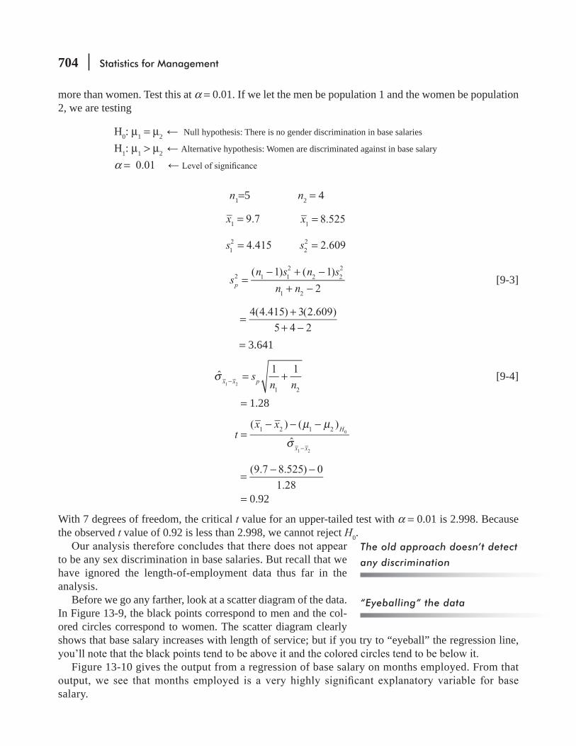
704 Statistics for Management
more than women. Test this at α = 0.01. If we let the men be population 1 and the women be population 2, we are testing
H0: μ1 = μ2 Null hypothesis: There is no gender discrimination in base salaries
H1: μ1 > μ2 Alternative hypothesis: Women are discriminated against in base salary
α =
n1=5 n2 = 4
9.71 =x 8.5251 =x
4.41512 =s 2.6092
2 =s
( 1) ( 1)
22 1 1
22 2
2
1 2
=− + −
+ −s
n s n s
n np [9-3]
4(4.415) 3(2.609)
5 4 2=
++ −
= 3.641
ˆ1 1
1 21 2
σ = +− sn nx x p [9-4]
= 1.28
( ) ( )
ˆ1 2 1 2 0
1 2
tx x H
x x
μ μ
σ=
− − −
−
(9.7 8.525) 0
1.28=
− −
= 0.92
With 7 degrees of freedom, the critical t value for an upper-tailed test with α = 0.01 is 2.998. Because the observed t value of 0.92 is less than 2.998, we cannot reject H0.
to be any sex discrimination in base salaries. But recall that we have ignored the length-of-employment data thus far in the analysis.
Before we go any farther, look at a scatter diagram of the data. In Figure 13-9, the black points correspond to men and the col-ored circles correspond to women. The scatter diagram clearly shows that base salary increases with length of service; but if you try to “eyeball” the regression line,
Figure 13-10 gives the output from a regression of base salary on months employed. From that
salary.
The old approach doesn’t detect
any discrimination
“Eyeballing” the data
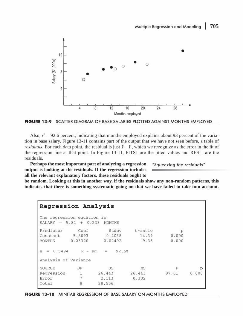
Multiple Regression and Modeling 705
Also, r2 = 92.6 percent, indicating that months employed explains about 93 percent of the varia-tion in base salary. Figure 13-11 contains part of the output that we have not seen before, a table of residuals. For each data point, the residual is just Y– Y
residuals.Perhaps the most important part of analyzing a regression
output is looking at the residuals. If the regression includes all the relevant explanatory factors, these residuals ought to be random. Looking at this in another way, if the residuals show any non-random patterns, this indicates that there is something systematic going on that we have failed to take into account.
“Squeezing the residuals”
12
8
4
4 8 12 16 20 24 28Months employed
Sala
ry ($
1,00
0s)
FIGURE 13-9 SCATTER DIAGRAM OF BASE SALARIES PLOTTED AGAINST MONTHS EMPLOYED
Regression Analysis
The regression equation isSALARY = 5.81 + 0.233 MONTHS
Predictor Coef Stdev t-ratio pConstant 5.8093 0.4038 14.39 0.000MONTHS 0.23320 0.02492 9.36 0.000
s = 0.5494 R - sq = 92.6%
Analysis of Variance
SOURCE DF SS MS F pRegression 1 26.443 26.443 87.61 0.000Error 7 2.113 0.302Total 8 28.556
FIGURE 13-10 MINITAB REGRESSION OF BASE SALARY ON MONTHS EMPLOYED
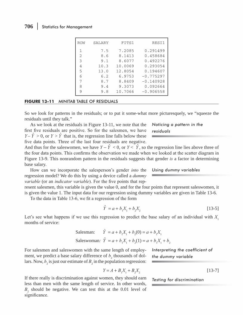
706 Statistics for Management
So we look for patterns in the residuals; or to put it some-what more picturesquely, we “squeeze the residuals until they talk.”
As we look at the residuals in Figure 13-11, we note that the
Y – Y > 0, or Y > Y that is, the regression line falls below these
And thus for the saleswomen, we have Y − Y < 0, or Y < Y , so the regression line lies above three of
Figure 13-9. This nonrandom pattern in the residuals suggests that gender is a factor in determining base salary.
into the regression model? We do this by using a device called a dummy variable (or an indicator variable -resent salesmen, this variable is given the value 0, and for the four points that represent saleswomen, it is given the value 1. The input data for our regression using dummy variables are given in Table 13-6.
Y = a + b1X1 + b2X2 [13-5]
X1 months of service:
Salesman: Y = a + b1X1 + b2(0) = a + b1X1
Saleswoman: Y = a + b1X1 + b2(1) = a + b1X1 + b2
For salesmen and saleswomen with the same length of employ-ment, we predict a base salary difference of b2 thousands of dol-lars. Now, b2 is just our estimate of B2 in the population regression:
Y = A + B1X1 + B2X2 [13-7]If there really is discrimination against women, they should earn less than men with the same length of service. In other words, B2 should be negative. We can test this at the 0.01 level of
Noticing a pattern in the
residuals
Using dummy variables
Interpreting the coefficient of
the dummy variable
Testing for discrimination
ROW SALARY FITS1 RESI1
1 7.5 7.2085 0.291499 2 8.6 8.1413 0.458684 3 9.1 8.6077 0.492276 4 10.3 10.0069 0.293054 5 13.0 12.8054 0.194607 6 6.2 6.9753 -0.775297 7 8.7 8.8409 -0.140928 8 9.4 9.3073 0.092664 9 9.8 10.7066 -0.906558
FIGURE 13-11 MINITAB TABLE OF RESIDUALS

Multiple Regression and Modeling 707
H0: B2 = Null hypothesis: There is no sex discrimination in base salaries
H1: B2 Alternative hypothesis: Women are discriminated against
α =
In order to test these hypotheses, we run a regression on the data in Table 13-6. The results of that regression are given in Figure 13-12.
t distribution with n − k − l = 9 − 2 − l = 6 degrees of freedom. For this lower-tailed test, the criti-cal value from Appendix Table 2 is tc= −3.143. From Figure 13-12,
test is t0 = −3.31. Figure 13-13 illustrates the critical value, − We see
Concluding that discrimination
is present
TABLE 13-6 INPUT DATA FOR GENDER DISCRIMINATION REGRESSION
X1Months Employed
X2Gender
YBase Salary ($1,000s)
6 0 7.510 0 8.6
Men 12 0 9.118 0 10.330 0 13.05 1 6.2
Women 13 1 8.715 1 9.421 1 9.8
Regression Analysis
The regression equation isSALARY = 6.25 + 0.227 MONTHS - 0.789 GENDER
Predictor Coef Stdev t-ratio pConstant 6.2485 0.2915 21.44 0.000MONTHS 0.22707 0.01612 14.09 0.000GENDER -0.7890 0.2384 -3.31 0.016
s = 0.3530 R - sq = 97.4%
Analysis of Variance
SOURCE DF SS MS F pRegression 2 27.808 13.904 111.56 0.000Error 6 0.748 0.125Total 8 28.556
FIGURE 13-12 MINITAB OUTPUT FROM SEX-DISCRIMINATION REGRESSION
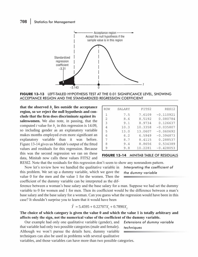
708 Statistics for Management
that the observed b2 lies outside the acceptance region, so we reject the null hypothesis and con-
saleswomen. We also note, in passing, that the computed t value for b1 in this regression is 14.09, so including gender as an explanatory variable
explanatory variable than it was before.
values and residuals for this regression. Because this was the second regression we ran on these data, Minitab now calls these values FITS2 and
this problem. We set up a dummy variable, which we gave the value 0 for the men and the value 1 for the women. Then the
-
base salary and the base salary for a woman. Can you guess what the regression would have been in this
Y = 5.4595 + 0.22707X1 + 0.7890X2
The choice of which category is given the value 0 and which the value 1 is totally arbitrary and
that variable had only two possible categories (male and female).
techniques can also be used in problems with several qualitative variables, and those variables can have more than two possible categories.
Interpreting the coefficient of
the dummy variable
Extensions of dummy variable
techniques
Standardizedregressioncoefficient
−3.31
−3.143 0t
Acceptance regionAccept the null hypothesis if the
sample value is in this region
FIGURE 13-13 LEFT-TAILED HYPOTHESIS TEST AT THE 0.01 SIGNIFICANCE LEVEL, SHOWING ACCEPTANCE REGION AND THE STANDARDIZED REGRESSION COEFFICIENT
ROW SALARY FITS2 RESI2
1 7.5 7.6109 -0.110921 2 8.6 8.5192 0.080784 3 9.1 8.9734 0.126637 4 10.3 10.3358 -0.035807 5 13.0 13.0607 -0.060692 6 6.2 6.5949 -0.394873 7 8.7 8.4115 0.288537 8 9.4 8.8656 0.534389 9 9.8 10.2281 -0.428053
FIGURE 13-14 MINITAB TABLE OF RESIDUALS

Multiple Regression and Modeling 709
Transforming Variables and Fitting CurvesA manufacturer of small electric motors uses an automatic milling machine to produce the slots in the shafts of the motors. A batch of shafts is run and then checked. All shafts in the batch that do not meet required dimensional tolerances are discarded. At the beginning of each new batch, the milling machine is readjusted, because its cut-ter head wears slightly during the production of the batch. The manufacturer is trying to pick an optimal batch size, but in order to do this, he must know how the size of a batch affects the num-ber of defective shafts in the batch. Table 13-7 gives data for a sample of 30 batches, arranged by ascending size of batch.
Figure 13-15 is a scatter diagram for these data. Because there are two batches of size 250 with 34 defective shafts, two of the points in the scatter diagram coincide (this is indicated by a colored data point in Figure 13-15).
We are going to run a regression of number of defective shafts on the batch size. The output from the regression is in Figures 13-16 and 13-17. What does this output tell us? First of all, we note that batch size
TABLE 13-7 NUMBER OF DEFECTIVE SHAFTS PER BATCH
BatchSize
Number Defective
Batch Size
Number Defective
100 5 250 37125 10 250 41125 6 250 34125 7 275 49150 6 300 53150 7 300 54175 17 325 69175 15 350 82200 24 350 81200 21 350 84200 22 375 92225 26 375 96225 29 375 97225 25 400 109250 34 400 112
120
100
80
60
40
20
200 300 4001000Batch size
Num
ber d
efec
tive
FIGURE 13-15 SCATTER DIAGRAM OF DEFECTIVE SHAFTS PLOTTED AGAINST SIZE OF BATCH

710 Statistics for Management
Regression AnalysisThe regression equation isDEFECTS = -47.9 + 0.367 BATCHSIZ
Predictor Coef Stdev t-ratio pConstant -47.901 4.112 -11.65 0.000BATCHSIZ 0.36713 0.01534 23.94 0.000
s = 7.560 R - sq = 95.3%
Analysis of Variance
SOURCE DF SS MS F pRegression 1 32744 32744 572.90 0.000Error 28 1600 54Total 29 34345
FIGURE 13-16 MINITAB OUTPUT FROM REGRESSION OF DEFECTS ON BATCH SIZE
1 5 −11.1875 16.1875 2 10 −2.0093 12.0093 3 6 −2.0093 8.0093 4 7 −2.0093 9.0093 5 6 7.1690 −1.1690 6 7 7.1690 −0.1690 7 17 16.3473 0.6527 8 15 16.3473 −1.3473 9 24 25.5256 −1.5256 10 21 25.5256 −4.5256 11 22 25.5256 −3.5256 12 26 34.7039 −8.7039 13 29 34.7039 −5.7039 14 25 34.7039 −9.7039 15 34 43.8822 −9.8822 16 37 43.8822 −6.8822 17 41 43.8822 −2.8822 18 34 43.8822 −9.8822 19 49 53.0605 −4.0605 20 53 62.2387 −9.2387 21 54 62.2387 −8.2387 22 69 71.4170 −2.4170 23 82 80.5953 1.4047 24 81 80.5953 0.4047 25 84 80.5953 3.4047 26 92 89.7736 2.2264 27 96 89.7736 6.2264 28 97 89.7736 7.2264 29 109 98.9519 10.0481 30 112 98.9519 13.0481
FIGURE 13-17 MINITAB OUTPUT OF RESIDUALS
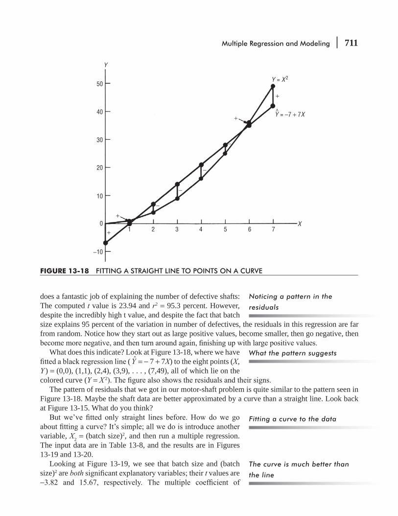
Multiple Regression and Modeling 711
does a fantastic job of explaining the number of defective shafts: The computed t value is 23.94 and r2 = 95.3 percent. However, despite the incredibly high t value, and despite the fact that batch size explains 95 percent of the variation in number of defectives, the residuals in this regression are far from random. Notice how they start out as large positive values, become smaller, then go negative, then
What does this indicate? Look at Figure 13-18, where we have ( Y = − 7 + 7X) to the eight points (X,
Y ) = (0,0), (1,1), (2,4), (3,9), . . . , (7,49), all of which lie on the colored curve (Y = X 2
The pattern of residuals that we got in our motor-shaft problem is quite similar to the pattern seen in Figure 13-18. Maybe the shaft data are better approximated by a curve than a straight line. Look back at Figure 13-15. What do you think?
variable, X2 = (batch size)2, and then run a multiple regression. The input data are in Table 13-8, and the results are in Figures 13-19 and 13-20.
Looking at Figure 13-19, we see that batch size and (batch size)2 are both t values are −
What the pattern suggests
Fitting a curve to the data
−
50
40
30
20
10
0
−10
1 2 3 4 5 6 7+
+
+
+
−
−
−
Y = −7 + 7X
Y = X 2
Y
X
FIGURE 13-18 FITTING A STRAIGHT LINE TO POINTS ON A CURVE
Noticing a pattern in the
residuals
The curve is much better than
the line
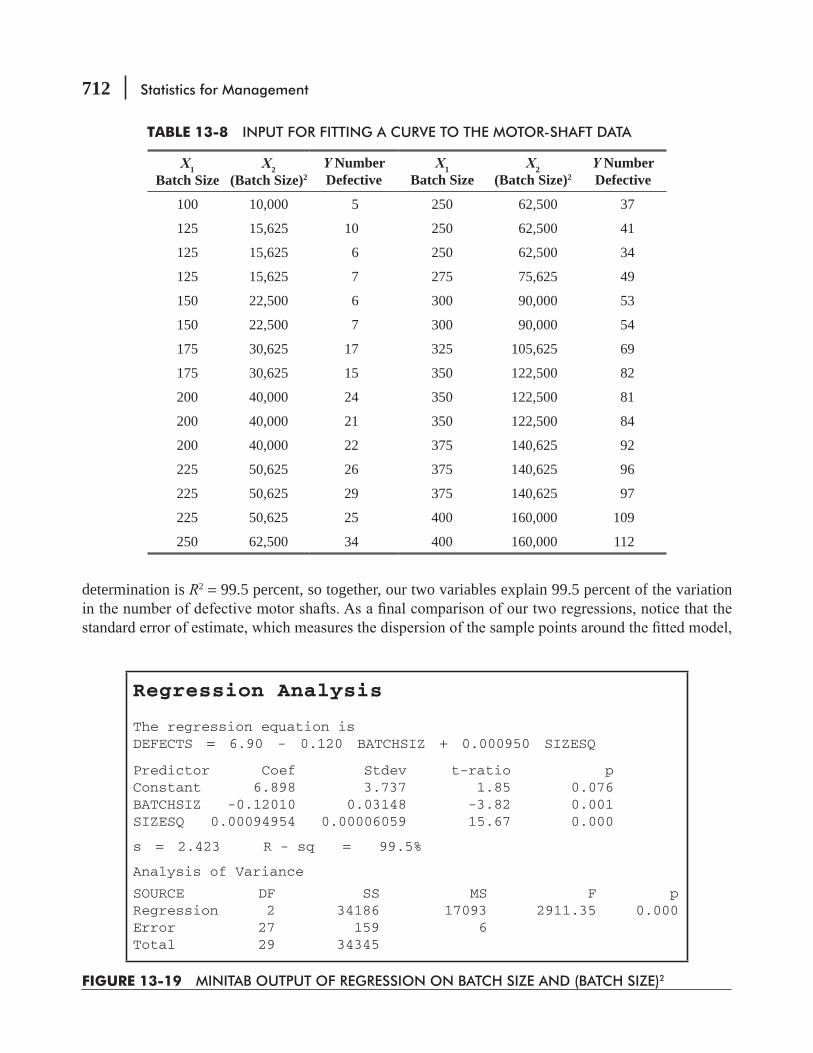
712 Statistics for Management
determination is R2 = 99.5 percent, so together, our two variables explain 99.5 percent of the variation
TABLE 13-8 INPUT FOR FITTING A CURVE TO THE MOTOR-SHAFT DATA
X1Batch Size
X2(Batch Size)2
Y NumberDefective
X1Batch Size
X2(Batch Size)2
Y NumberDefective
100 10,000 5 250 62,500 37
125 15,625 10 250 62,500 41
125 15,625 6 250 62,500 34
125 15,625 7 275 75,625 49
150 22,500 6 300 90,000 53
150 22,500 7 300 90,000 54
175 30,625 17 325 105,625 69
175 30,625 15 350 122,500 82
200 40,000 24 350 122,500 81
200 40,000 21 350 122,500 84
200 40,000 22 375 140,625 92
225 50,625 26 375 140,625 96
225 50,625 29 375 140,625 97
225 50,625 25 400 160,000 109
250 62,500 34 400 160,000 112
Regression Analysis
The regression equation isDEFECTS = 6.90 - 0.120 BATCHSIZ + 0.000950 SIZESQ
Predictor Coef Stdev t-ratio pConstant 6.898 3.737 1.85 0.076BATCHSIZ -0.12010 0.03148 -3.82 0.001SIZESQ 0.00094954 0.00006059 15.67 0.000
s = 2.423 R - sq = 99.5%
Analysis of Variance
SOURCE DF SS MS F pRegression 2 34186 17093 2911.35 0.000Error 27 159 6Total 29 34345
FIGURE 13-19 MINITAB OUTPUT OF REGRESSION ON BATCH SIZE AND (BATCH SIZE)2

Multiple Regression and Modeling 713
is 7.560 for the straight-line model, but only 2.423 for the curved model. The curved model is far superior to the straight-line model, even though the latter explained 95 percent of the variation! And remember, it was the pattern we observed in the residuals for the straight-line model that suggested to us that a curved model would be more appropriate. The residuals for the curved model, shown in Figure 13-20, do not exhibit any pattern.
In our curved model, we got our second variable, (batch size)2, by doing a mathematical transformation -able, batch size. Because we squared a variable, the resulting curved model is known as a second-degree (or quadratic) regression model. There are many other ways in which we can transform variables to get new variables, and most computer regression packages have these transformations built into them. You do not have to compute the transformed variables by hand, as we did in Table 13-8. Computer packages have the capability to compute all sorts of transformations of one or more variables: sums, differences, products, quotients, roots, powers, logarithms, exponentials, trigonometric functions, and many more.
Transforming variables
ROW DEFECTS FITS2 RESI2 1 .5 4.383 0.61728 2 10 6.721 3.27869 3 6 6.721 -0.72131 4 7 6.721 0.27869 5 6 10.247 -4.24682 6 7 10.247 -3.24682 7 17 14.959 2.04074 8 15 14.959 0.04074 9 24 20.859 3.14138 10 21 20.859 0.14138 11 22 20.859 1.14138 12 26 27.945 -1.94491 13 29 27.945 1.05509 14 25 27.945 -2.94491 15 34 36.218 -2.21811 16 37 36.218 0.78189 17 41 36.218 4.78189 18 34 36.218 -2.21811 19 49 45.678 3.32175 20 53 56.325 -3.32530 21 54 56.325 -2.32530 22 69 68.159 0.84072 23 82 81.180 0.81982 24 81 81.180 -0.18018 25 84 81.180 2.81982 26 92 95.388 -3.38800 27 96 95.388 0.61200 28 97 95.388 1.61200 29 109 110.783 -1.78275 30 112 110.783 1.21725
FIGURE 13-20 MINITAB OUTPUT OF RESIDUALS
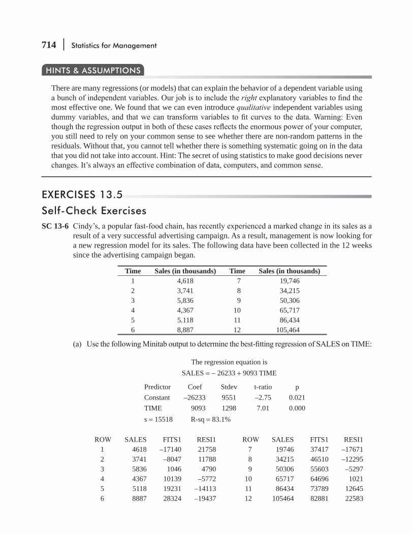
714 Statistics for Management
There are many regressions (or models) that can explain the behavior of a dependent variable using right
most effective one. We found that we can even introduce qualitative independent variables using
you still need to rely on your common sense to see whether there are non-random patterns in the residuals. Without that, you cannot tell whether there is something systematic going on in the data that you did not take into account. Hint: The secret of using statistics to make good decisions never
HINTS & ASSUMPTIONS
EXERCISES 13.5
Self-Check ExercisesSC 13-6
result of a very successful advertising campaign. As a result, management is now looking for a new regression model for its sales. The following data have been collected in the 12 weeks since the advertising campaign began.
Time Sales (in thousands) Time Sales (in thousands)1 4,618 7 19,7462 3,741 8 34,2153 5,836 9 50,3064 4,367 10 65,7175 5.118 11 86,4346 8,887 12 105,464
The regression equation isSALES = − 26233 + 9093 TIME
Predictor Coef Stdev t-ratio pConstant –26233 9551 –2.75 0.021TIME 9093 1298 7.01 0.000s = 15518 R-sq = 83.1%
SALES FITS1 RESI1 SALES FITS1 RESI11 4618 –17140 21758 7 19746 37417 –176712 3741 –8047 11788 8 34215 46510 –122953 5836 1046 4790 9 50306 55603 –52974 4367 10139 –5772 10 65717 64696 10215 5118 19231 –14113 11 86434 73789 126456 8887 28324 –19437 12 105464 82881 22583
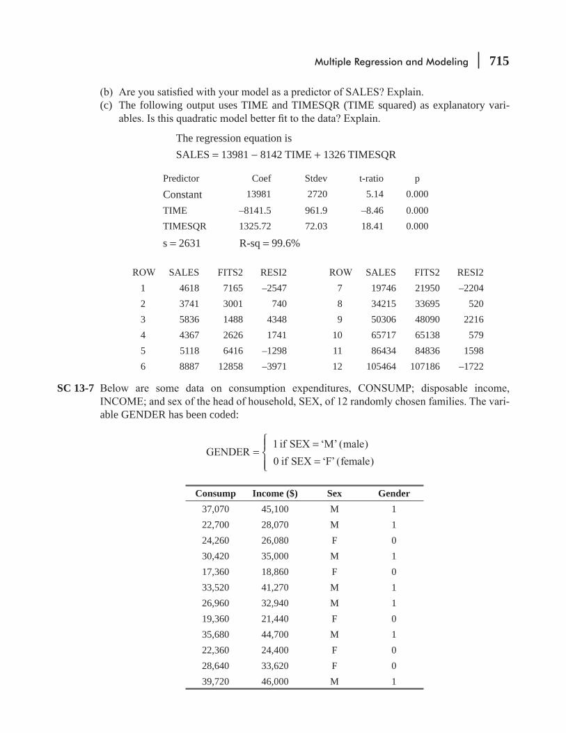
Multiple Regression and Modeling 715
(c) The following output uses TIME and TIMESQR (TIME squared) as explanatory vari-
The regression equation is SALES = 13981 − 8142 TIME + 1326 TIMESQR
Predictor Coef Stdev t-ratio p
Constant 13981 2720 5.14 0.000
TIME –8141.5 961.9 –8.46 0.000TIMESQR 1325.72 72.03 18.41 0.000
s = 2631 R-sq = 99.6%
SALES FITS2 RESI2 SALES FITS2 RESI21 4618 7165 –2547 7 19746 21950 –22042 3741 3001 740 8 34215 33695 5203 5836 1488 4348 9 50306 48090 22164 4367 2626 1741 10 65717 65138 5795 5118 6416 –1298 11 86434 84836 15986 8887 12858 –3971 12 105464 107186 –1722
SC 13-7 -
able GENDER has been coded:
GENDER1 if SEX ‘M’ (male)
0 if SEX ‘F’ (female)=
==
⎧⎨⎪
⎩⎪
Consump Income ($) Sex Gender37,070 45,100 M 122,700 28,070 M 124,260 26,080 F 030,420 35,000 M 117,360 18,860 F 033,520 41,270 M 126,960 32,940 M 119,360 21,440 F 035,680 44,700 M 122,360 24,400 F 028,640 33,620 F 039,720 46,000 M 1
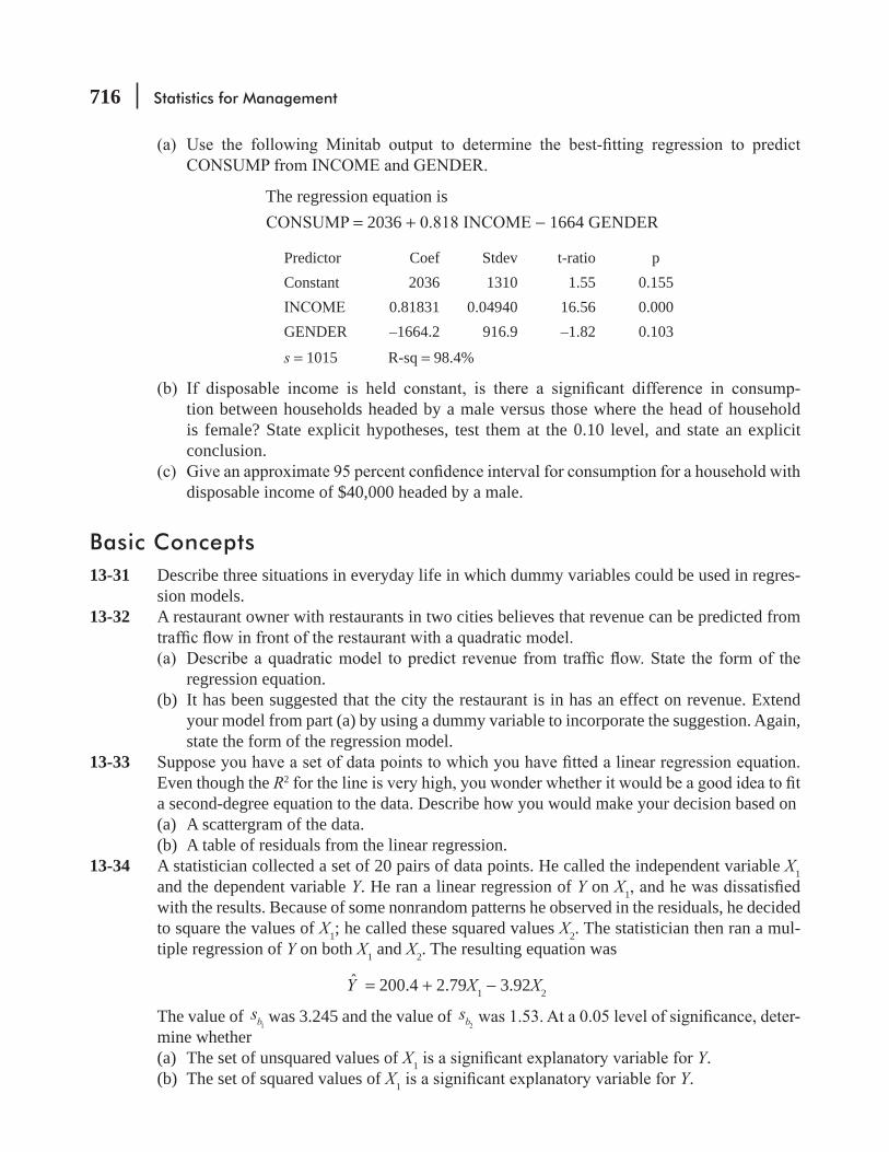
716 Statistics for Management
The regression equation is= 2036 + − 1664 GENDER
Predictor Coef Stdev t-ratio pConstant 2036 1310 1.55 0.155
0.81831 0.04940 16.56 0.000GENDER –1664.2 916.9 –1.82 0.103
s = 1015 R-sq = 98.4%
-tion between households headed by a male versus those where the head of household is female? State explicit hypotheses, test them at the 0.10 level, and state an explicit conclusion.
disposable income of $40,000 headed by a male.
Basic Concepts13-31 Describe three situations in everyday life in which dummy variables could be used in regres-
sion models. 13-32 A restaurant owner with restaurants in two cities believes that revenue can be predicted from
regression equation.(b) It has been suggested that the city the restaurant is in has an effect on revenue. Extend
your model from part (a) by using a dummy variable to incorporate the suggestion. Again, state the form of the regression model.
13-33 Even though the R2
a second-degree equation to the data. Describe how you would make your decision based on(a) A scattergram of the data.(b) A table of residuals from the linear regression.
13-34 A statistician collected a set of 20 pairs of data points. He called the independent variable X1 and the dependent variable Y. He ran a linear regression of Y on X1with the results. Because of some nonrandom patterns he observed in the residuals, he decided to square the values of X1; he called these squared values X2. The statistician then ran a mul-tiple regression of Y on both X1 and X2. The resulting equation was
Y = 200.4 + 2.79X1 − 3.92X2
The value of 1
sb was 3.245 and the value of 2
sb -mine whether(a) The set of unsquared values of X1 Y.(b) The set of squared values of X1 Y.

Multiple Regression and Modeling 717
Applications13-35 Dr. Linda Frazer runs a medical clinic in Philadelphia. She collected data on age, reaction to
penicillin, and systolic blood pressure for 30 patients. She established systolic blood pressure as the dependent variable, age as X1 (independent variable) and reaction to penicillin as X2 (independent variable). Letting 0 stand for a positive reaction to penicillin and 1 stand for a negative reaction, she ran a multiple regression on her desktop personal computer. The pre-dicting equation was
Y = 6.7 + 3.5X1 + 0.489X2
(a) After the regression had already been run, Dr. Frazer discovered that she had meant to code a positive reaction as 1 and a negative reaction as 0. Does she have to rerun the regression? If so, why? If not, give her the equation she would have gotten if the variable had been coded as she had originally intended.
(b) If 2
sb
pressure?13-36 Excelsior Notebook computers is reexamining its inventory control policy. They need to accu-
rately predict the number of the EXC-11E computers that will be ordered by suppliers in the weeks to come. The data for the last 15 weeks are presented below
Time Demand (in 1000’s)
1 6.7
2 10.2
3 13.4
4 15.6
5 18.2
6 22.6
7 30.5
8 31.4
9 38.7
10 41.6
11 48.7
12 51.4
13 55.8
14 61.5
15 68.9
variable and DEMAND as the dependent variable.(b) Fit a quadratic model for the data. Is this model better? Explain.
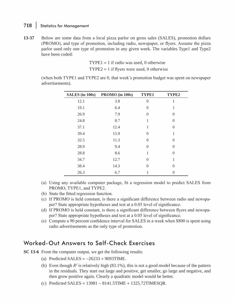
718 Statistics for Management
13-37 Below are some data from a local pizza parlor on gross sales (SALES), promotion dollars
parlor used only one type of promotion in any given week. The variables Type1 and Type2 have been coded:
TYPE1 = 1 if radio was used, 0 otherwise TYPE2 =
advertisements).
SALES (in 100s) PROMO (in 100s) TYPE1 TYPE212.1 3.8 0 119.1 6.4 0 126.9 7.9 0 024.8 8.7 1 037.1 12.4 1 039.4 15.9 0 132.5 11.3 0 028.9 9.4 0 028.8 8.6 1 034.7 12.7 0 138.4 14.3 0 026.3 6.7 1 0
-
-
radio advertisements as the only type of promotion.
Worked-Out Answers to Self-Check ExercisesSC 13-6 From the computer output, we get the following results:
(a) Predicted SALES = −26233 + 9093TIME.(b) Even though R2 is relatively high (83.1%), this is not a good model because of the pattern
in the residuals. They start out large and positive, get smaller, go large and negative, and then grow positive again. Clearly a quadratic model would be better.
(c) Predicted SALES = 13981 − 8141.5TIME + 1325.72TIMESQR.

Multiple Regression and Modeling 719
This model is distinctly better. R2 has increased to 99.6%, and there is no pattern in the residuals.
SC 13-7 From the computer output, we get the following results:= 2036 + − 1664GENDER.
(b) H0: BGENDER = 0 H1: BGENDER α = 0.10 Since the prob value for our test (0.103) is greater than α (0.10), we cannot reject H0; the
= 2036 + 0.818(40,000) − 1664(1) = $33,092. With 9 degrees of freedom, the t
Y ± tse = 33,092 ± 2.262(1,015) = 33,092 ± 2,296 = ($30,796, $35,388).
STATISTICS AT WORK
Loveland ComputersCase 13: Multiple Regression and Modeling Lee was pleased to be able to report to Nancy Rainwater that the defects occurring in the keyboard cases were indeed related to the daily recorded low tempera-
But on these real cold winter nights, the heaters run all night, but the warehouse gets pretty cold.”“So we need more heaters?” Nancy queried.“Not necessarily—the problem is that all the warm air stays up high and it gets pretty cold close to
up and the lower level—where everything is stored–comes up to room temperature.”“So we might be able to cure the problem by installing a couple of ceiling fans,” interjected Tyronza
Wilson.-
“A great example of quality management!” said Lee. “See, Nancy, the people doing the job already know the answer—you just have to empower them to implement a solution.”
“Well, let me take you to lunch and have you talk to someone who has a more complicated problem.”
She handles the big picture. My job is to focus on the advertising budget and to target our ads so they result in the highest increase in sales.”
“So how do you decide how much of which media to buy?” asked Lee.
quarter. Margot kept telling them that was the opposite of a good strategy—there are many times when

720 Statistics for Management
increasing your advertising will get you out of a sales slump. But I guess they were always in a panic
“So how do you decide where to run the ads?” Lee was anxious to learn more about marketing in the real world.
presentations about cost per thousand, target readership, and so on. The computer monthly magazines
success of an individual ad.”
“Well, no. That would be a good idea. Do we keep those statistics?”
whether call volume or sales volume was the best indicator.” Lee was on a roll.
plate of burritos and pulling up a chair. “Mind if I join you?”
“No offense to you touchy-feely advertising types, but I think that forces outside of Loveland deter-
tough times in the early 80s.”
easily. Look at the back numbers of the computer magazines and see how many ad pages they bought
printed right there in each ad.”Lee made a mental note that this was going to be a lot easier than in many industries, where competi-
“How do we factor in our newspaper ads?” Sherrel wondered aloud. It costs us a lot to advertise in the Wall Street Journal
signaling the waiter for more picante sauce.
Study Questions: What measure of “advertising success” would you investigate? What factors would you consider in an analysis? How would you handle factors that appear to be irrelevant? In addition to the review of the historical data, are there any “experiments” you would recommend?
CHAPTER REVIEW
Terms Introduced in Chapter 13Analysis of Variance for Regression The procedure for computing the F ratio used to test the sig-
R The positive square root of R2
R2 The fraction of the variation of the dependent variable that
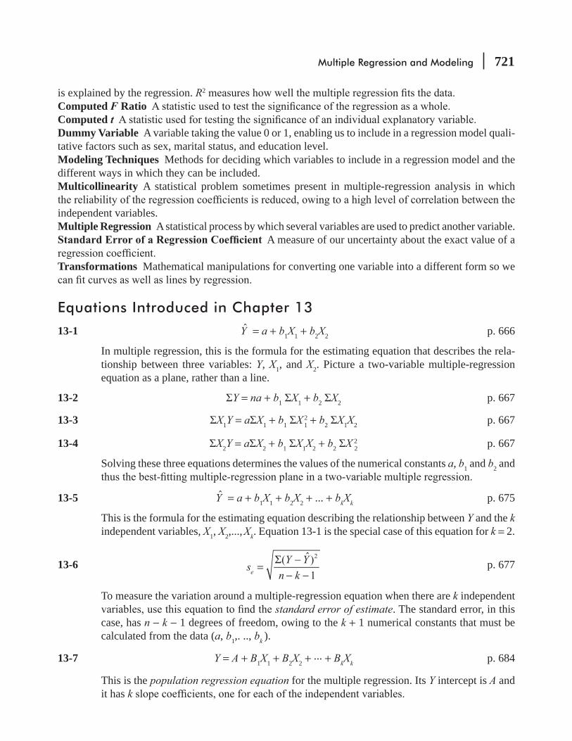
Multiple Regression and Modeling 721
is explained by the regression. R2
Computed F RatioComputed tDummy Variable A variable taking the value 0 or 1, enabling us to include in a regression model quali-tative factors such as sex, marital status, and education level.Modeling Techniques Methods for deciding which variables to include in a regression model and the different ways in which they can be included.Multicollinearity A statistical problem sometimes present in multiple-regression analysis in which
independent variables.Multiple Regression A statistical process by which several variables are used to predict another variable.
A measure of our uncertainty about the exact value of a
Transformations Mathematical manipulations for converting one variable into a different form so we
Equations Introduced in Chapter 13
13-1 Y = a + b1X1 + b2X2 p. 666
In multiple regression, this is the formula for the estimating equation that describes the rela-tionship between three variables: Y, X1, and X2. Picture a two-variable multiple-regression equation as a plane, rather than a line.
13-2 Y = na + b1 X1 + b2 X2 p. 667
13-3 X1Y = a X1 + b1 X 21 + b2 X1X2 p. 667
13-4 X2Y = a X2 + b1 X1X2 + b2 X 22 p. 667
Solving these three equations determines the values of the numerical constants a, b1 and b2 and
13-5 Y = a + b1X1 + b2X2 + ... + bkXk p. 675
This is the formula for the estimating equation describing the relationship between Y and the k independent variables, X1, X2,..., Xk. Equation 13-1 is the special case of this equation for k = 2.
13-6 ( ˆ)
1
2
sY Y
n ke =Σ −
− − p. 677
To measure the variation around a multiple-regression equation when there are k independent standard error of estimate. The standard error, in this
case, has n − k − 1 degrees of freedom, owing to the k + 1 numerical constants that must be calculated from the data (a, b1,. .., bk ).
13-7 Y = A + B1X1 + B2X2 + ... + BkXk p. 684
This is the population regression equation for the multiple regression. Its Y intercept is A and it has k
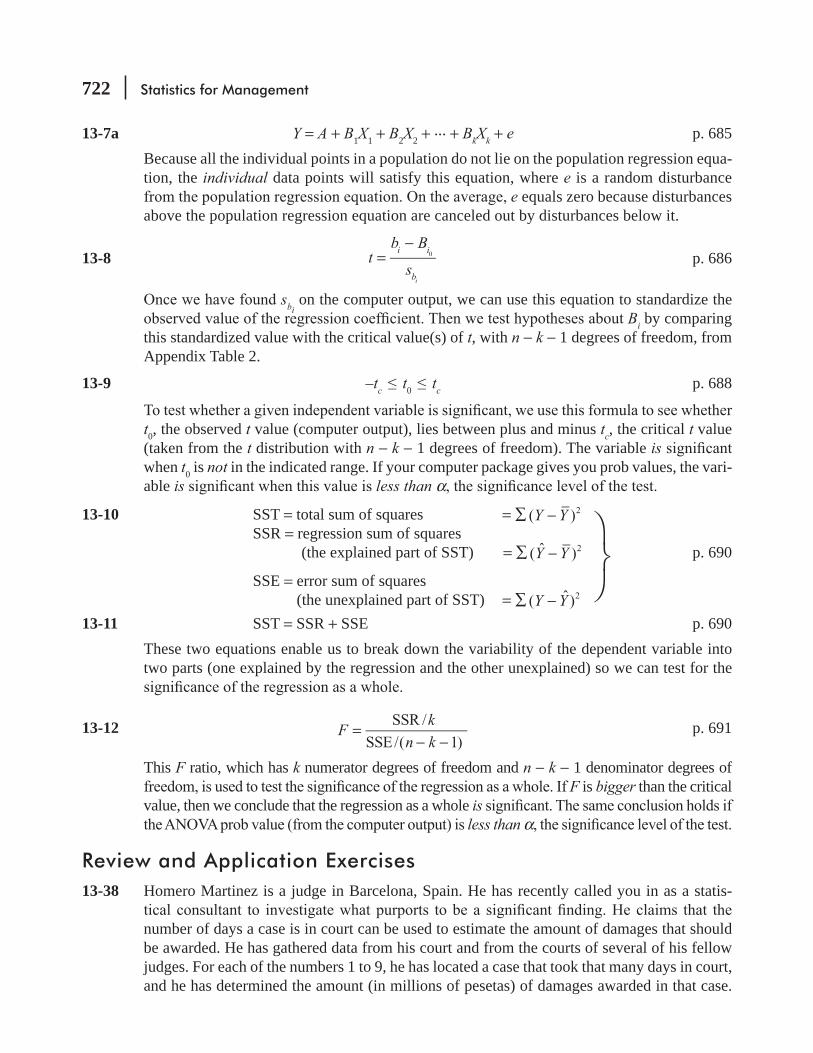
722 Statistics for Management
13-7a Y = A + B1X1 + B2X2 + ... + BkXk + e p. 685Because all the individual points in a population do not lie on the population regression equa-tion, the individual data points will satisfy this equation, where e is a random disturbance
e equals zero because disturbances above the population regression equation are canceled out by disturbances below it.
13-8 0tb B
si i
bi
=−
p. 686
sbi on the computer output, we can use this equation to standardize the
Bi by comparing this standardized value with the critical value(s) of t, with n − k − 1 degrees of freedom, from Appendix Table 2.
13-9 –tc t0 tc p. 688
t0, the observed t value (computer output), lies between plus and minus tc, the critical t value (taken from the t distribution with n − k − 1 degrees of freedom). The variable iswhen t0 is not in the indicated range. If your computer package gives you prob values, the vari-able is less than α
13-10 SST = total sum of squares = ∑ ( )2Y Y− SSR = regression sum of squares
(the explained part of SST) = ∑ ( ˆ )2Y Y− p. 690
SSE = error sum of squares (the unexplained part of SST) = ∑ ( ˆ)2Y Y−
13-11 SST = SSR + SSE p. 690These two equations enable us to break down the variability of the dependent variable into two parts (one explained by the regression and the other unexplained) so we can test for the
13-12 Fk
n k
SSR /
SSE/( 1)=
− − p. 691
This F ratio, which has k numerator degrees of freedom and n − k − 1 denominator degrees of F is bigger than the critical
value, then we conclude that the regression as a whole is less than α
Review and Application Exercises13-38 Homero Martinez is a judge in Barcelona, Spain. He has recently called you in as a statis-
number of days a case is in court can be used to estimate the amount of damages that should be awarded. He has gathered data from his court and from the courts of several of his fellow judges. For each of the numbers 1 to 9, he has located a case that took that many days in court, and he has determined the amount (in millions of pesetas) of damages awarded in that case.
Multiple Regression and Modeling 723
The following Minitab results were generated when damages awarded were regressed on days in court.
The regression equation isDAMAGES = – 0.406 + 0.518 DAYS
Predictor Coef Stdev t-ratio pConstant -0.4063 0.2875 -1.41 0.201DAYS 0.51792 0.0511 10.14 0.000
s = 0.3957 R-sq = 93.6%
Analysis of Variance
SOURCE DF SS MS FRegression 1 16.094 16.094 102.77Error 7 1.096 0.157Total 8 17.191
ROW DAMAGES FITS1 RESI1
1 0.645 0.1117 0.53333 2 0.750 0.6296 0.12042 3 1.000 1.1475 -0.14750 4 1.300 1.6654 -0.36542 5 1.750 2.1833 -0.43333 6 2.205 2.7013 -0.49625 7 3.500 3.2192 0.28083 8 4.000 3.7371 0.26292 9 4.500 4.2550 0.24500
R2 is very high. But the judge is
if this line does smart statistician!”
(b) Suggest a better model that will satisfy the judge.13-39 Jon Grant, supervisor of the Carven Manufacturing Facility, is examining the relationship
12. The measure of on-the-job success is based on a point system involving total output and
obtained the following:
X1Aptitude Test Score
X2Prior Experience
YPerformance Evaluation
74 5 2887 11 3369 4 2193 9 4081 7 3897 10 46

724 Statistics for Management
(a) Develop the estimating equation best describing these data.(b) If an employee scored 83 on the aptitude test and had a prior work experience of 7, what
performance evaluation would be expected?13-40 Successful selling is as much an art as a science, but many sales managers believe that
personal attributes are important in predicting sales success. Design Alley is a full- service interior design store that sells custom blinds, carpets and wall coverings. The store manager, Dee Dempsey, contracted with a sales-force selection company to conduct pre- hiring tests on four aptitudes. Dee has collected sales growth data for 25 of the salespeople who were hired, along with the scores from the four tests of aptitude: creativity, mechanical ability, abstract thinking, and mathematical calculation. Using a desktop computer, Dee gener-
The regression equation isGROWTH = 70.1 + 0.422 CREAT + 0.271 MECH + 0.745 ABST = 0.420 MATH
Predictor Coef Stdev t-ratio pConstant 70.066 2.130 32.89 0.000CREAT 0.42160 0.17192 2.45 0.024MECH 0.27140 0.21840 1.24 0.228ABST 0.74504 0.28982 2.57 0.018MATH 0.41955 0.06871 6.11 0.000
s = 2.048 R-sq = 92.6%
Analysis of Variance
SOURCE DF SS MS F pRegression 4 1050.78 262.70 62.64 0.000Error 20 83.88 4.19 Total 24 1134.66
(a) Write the regression equation for sales growth in terms of the four factors tested.(b) How much of the variation in sales growth is explained by the aptitude tests?
variables for sales growth?
(e) Jay is a new applicant with scores on the four tests as follows: CREAT = 12, MECH = 14, ABST = 18, and MATH = 30. What sales growth is predicted by the model for this candidate?
13-41 The Money Bank desires to open new checking accounts for customers who will write at least 30 checks per month. To assist in selecting new customers, the bank has studied the relation-ship between the number of checks written and the age and annual income of eight of their
in thousands of dollars. The data are as follows:
Checks Age Income29 37 16.2
42 34 25.4
(Continued)

Multiple Regression and Modeling 725
Checks Age Income
9 48 12.4
56 38 25.0
2 43 8.0
10 25 18.3
48 33 24.2
4 45 7.9
(a) Develop an estimating equation to use age and income to predict the number of checks written per month.
(b) How many checks per month would be expected from a 35-year-old with annual income of $22,500?
The proportion of disposable income that consumers spend on different product categories is not the same in all towns—for example, in college towns, sales of pizza are likely to be above average, while the sales of new cars may be below average. In Exercises 13-42 through 13-45, you will construct regressions to try to explain the variability of the EATING variable. (An important technical note:
EATING variable becomes $216.666 million instead of $216,666 thousand.)13-42 Develop two simple regression models for EATING, using the population and the median
effective buying income per household (EBI) as the independent variables. Which indepen-dent variable accounts for more of the variation in the observed sales?
13-43 -ables. What fraction of the variation in EATING is explained by this model? Is the regression
α = 0.05?13-44 Include SINGLE (the number of single-person households in the area) as a third explana-
-tory variable in this regression?)
13-45
single-person households and a median effective buying income of $30,000.13-46 Dr. Harden Ricci is a veterinarian in Sacramento, California. Recently, he has been trying
to develop a predicting equation for the amount of anesthesia (measured in milliliters) to be used in operations. He feels that the amount used will depend on the weight of the animal (in pounds), length of the operation (in hours), and whether the animal is a cat (coded 0) or a dog (coded 1). He used Minitab to run a regression on his data from 13 recent operations, and got these results:
(Contd.)
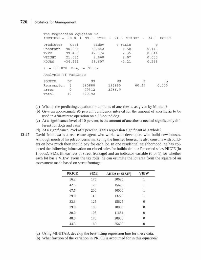
726 Statistics for Management
The regression equation isANESTHES = 90.0 + 99.5 TYPE + 21.5 WEIGHT - 34.5 HOURS
Predictor Coef Stdev t-ratio pConstant 90.032 56.842 1.58 0.148TYPE 99.486 42.374 2.35 0.044WEIGHT 21.536 2.668 8.07 0.000HOURS -34.461 28.607 -1.21 0.259
s = 57.070 R-sq = 95.3%
Analysis of Variance
SOURCE DF SS MS F pRegression 3 590880 196960 60.47 0.000Error 9 29312 3256.9 Total 12 620192
(a) What is the predicting equation for amounts of anesthesia, as given by Minitab?
used in a 90-minute operation on a 25-pound dog.-
ferent for dogs and cats?
13-47 David Ichikawa is a real estate agent who works with developers who build new houses. -
ers on how much they should pay for each lot. In one residential neighborhood, he has col-lected the following information on closed sales for buildable lots: Recorded sales PRICE (in $l,000s), SIZE (linear feet of street frontage) and an indicator variable (0 or 1) for whether each lot has a VIEW. From the tax rolls, he can estimate the lot area from the square of an assessment made based on street frontage.
PRICE SIZE AREA (= SIZE2) VIEW
56.2 175 30625 142.5 125 15625 167.5 200 40000 139.0 115 13225 133.3 125 15625 029.0 100 10000 030.0 108 11664 048.0 170 28900 044.3 160 25600 0
(b) What fraction of the variation in PRICE is accounted for in this equation?

Multiple Regression and Modeling 727
having a VIEW.(d) Was it helpful to use AREA (the square of SIZE) in the regression? Explain.
13-48 three-season tent for weekend campers. To set a fair price, they look at eight comparable tents currently on the market, in terms of weight and square footage. The data follow:
Weight (oz) Sq Ft. Price
Kelty Nautilus 94 37 $225
North Face Salamander 90 36 240
REI Mountain Hut 112 35 225
Sierra Designs Meteor Light 92 40 220
Eureka! Cirrus 3 93 48 167
Sierra Designs Clip 3 98 40 212
Eureka! Timberline Deluxe 114 40 217
Diamond Brand Free Spirit 108 35 200
(a) Calculate the least-squares equation to predict price from weight and square footage.
should they charge?13-49 The Carolina Athletic Association is interested in organizing the First Annual Tarheel
-ers by setting times for both men and women overall winners. Because this course has never been run before, the CAA has chosen 10 races of varying lengths that they consider compa-rable in weather and course conditions.
MilesWinning Times(Hr:Min:Sec)
Triathlon Swim Bike Run Men Women
Bud Light Ironman 2.4 112 26.2 8:09:15 9:00:56
2.0 100 18.6 8:25:09 9:49:04
Muncie Endurathon 1.2 55.3 13.1 4:05:30 4:40:06
Texas Hill Country 1.5 48 10.0 3:24:24 3:55:02
0.93 24.8 6.2 1:54:32 2:07:10
Sacramento International 0.93 24.8 6.2 1:48:16 2:00:45
Malibu 0.50 18 5.0 1:19:25 1:30:19
Bud Light Endurance 2.4 112 26.2 9:26:30 11:00:29
0.5 20 4.0 1:14:59 1:23:09
Mammoth/Snowcreek 0.6 25 6.2 1:56:07 2:11:49

728 Statistics for Management
of the length of each individual race segment. (Convert the times to minutes for use in calculations.)
(b) Predict the winning times if the Tarheel Triathlon comprises a 1-mile swim, 50-mile bike ride, and a 12.5-mile run.
for the incentive times for men and women, what would these times be?13-50 Peoria, Illinois, is in the process of modifying its tax structure. Twelve cities of comparable
revenue.(a) Use the following data to determine the least-squares equation relating revenue to the
three tax rates.
PropertyTax Rates
Sales GasolineTax Revenue($ thousands)
1.639% 2.021% 3.300 ¢/gal $28,867.5
1.686 1.972 3.300 28,850.2
1.639 2.041 3.300 29,011.5
1.639 2.363 0.131 28,806.5
1.639 2.200 2.540 28,821.7
1.639 2.201 1.560 28,774.6
1.654 2.363 0.000 28,803.2
2.643 1.000 3.300 28,685.7
2.584 1.091 2.998 28,671.8
2.048 1.752 1.826 28,671.0
2.176 1.648 1.555 28,627.4
1.925 1.991 0.757 28,670.7
(b) Two proposals have been submitted for Peoria. Estimate total tax revenues if the tax rates are
Property Sales GasolineProposal A 2.763% 1.000% 1.0¢/galProposal B 1.639 2.021 3.3
Determine which proposal the city should adopt.13-51 The National Cranberry Cooperative, an organization formed and owned by growers of cran-
berries to process and market their berries, is trying to establish a relationship between aver-age price per barrel received in any given year and the total number of barrels sold in the previous year (divided into fresh sales and berries sold for processing).

Multiple Regression and Modeling 729
Sales (in thousands of barrels)
Following Year’s
Sales (in thousands of barrels)
Following Year’s
Fresh Process Price Fresh Process Price
844 256 15.50 320 460 9.79
965 335 17.15 528 860 10.90
470 672 11.71 340 761 15.88
13-52 Cellular phones were introduced in Europe in 1980, and since then, their growth in popularity has been phenomenal. The number of subscribers in subsequent years is contained in the fol-lowing table.
1981 3,510 1984 143,300 1987 877,8501982 34,520 1985 288,420 1988 1,471,2001983 80,180 1986 507,930 1989 2,342,080
Using the number of years since the introduction of cellular phones as the independent vari-able (i.e., 1981 =Look at the residuals—do they have a noticeable pattern? Find the least-squares quadratic
13-53 While shopping for a new down sleeping bag, Fred Montana is curious about what features of
Down Fill(oz)
Total Weight(lb)
Loft(in.)
Temp. Rating(oF)
Price($)
Swallow 14.0 2.00 5.5 20 255Snow Bunting 18.0 2.25 6.5 10 285
24.0 3.13 6.5 10 329Widgeon 25.5 3.25 7.5 10 395Tern 32.5 3.63 9.0 –30 459Snow Goose 41.0 4.25 10.0 –40 509
α = 0.01 level.α = 0.01
(c) What problem might there be in using all these variables together? Do the answers to parts (a) and (b) seem to indicate this problem might be present?
730 Statistics for Management
Questions on Running Case: SURYA Bank Pvt. Ltd.
1. Build a regression model to study the level of satisfaction of the customers with e-services provided by their banks on the basis of the importance of e-facilities on bank selection. [Regress Q9 on Q7(a)-(m)]
2. Is there evidence of presence of multicollinearity in the data? 3. If there is multicollinearity problem, what remedial action, if any, would you take?
@
CASE
@

Multiple Regression and Modeling 731
Flow Chart: Multiple Regression and Modeling
If you want to use more thanone independent variable to
estimate the dependent variableand, thereby, attempt to increasethe accuracy of the estimate, usemultiple-regression techniques
START
Yes
No
Usedummy
variables
p. 703
Yes
p. 709
p. 692 p. 691 p. 705
No
Transform someof the variablesso you can fit
curvilinearrelationships
Use a computer toestimate your multiple-
regression model.(Without a computer,
multiple regression can betedious and impractical)
To test theappropriateness of your
model, use thefollowing three techniques
1. Use “prob>|t|” values to see whether X, is a significant explanatory variable
2. Use “prob >F ” value to see whether the regression as a whole is significant
3. See whether the residuals show any nonrandom patterns
Try a differentmodel, with other
variables,transformations, etc.
No
Yes
Doyou think
any of the relationshipsbetween the variables
are nonlinear?
Doesyour model
appear to beappropriate
?
Doyou want to
include any qualitativevariables in your
model?
A
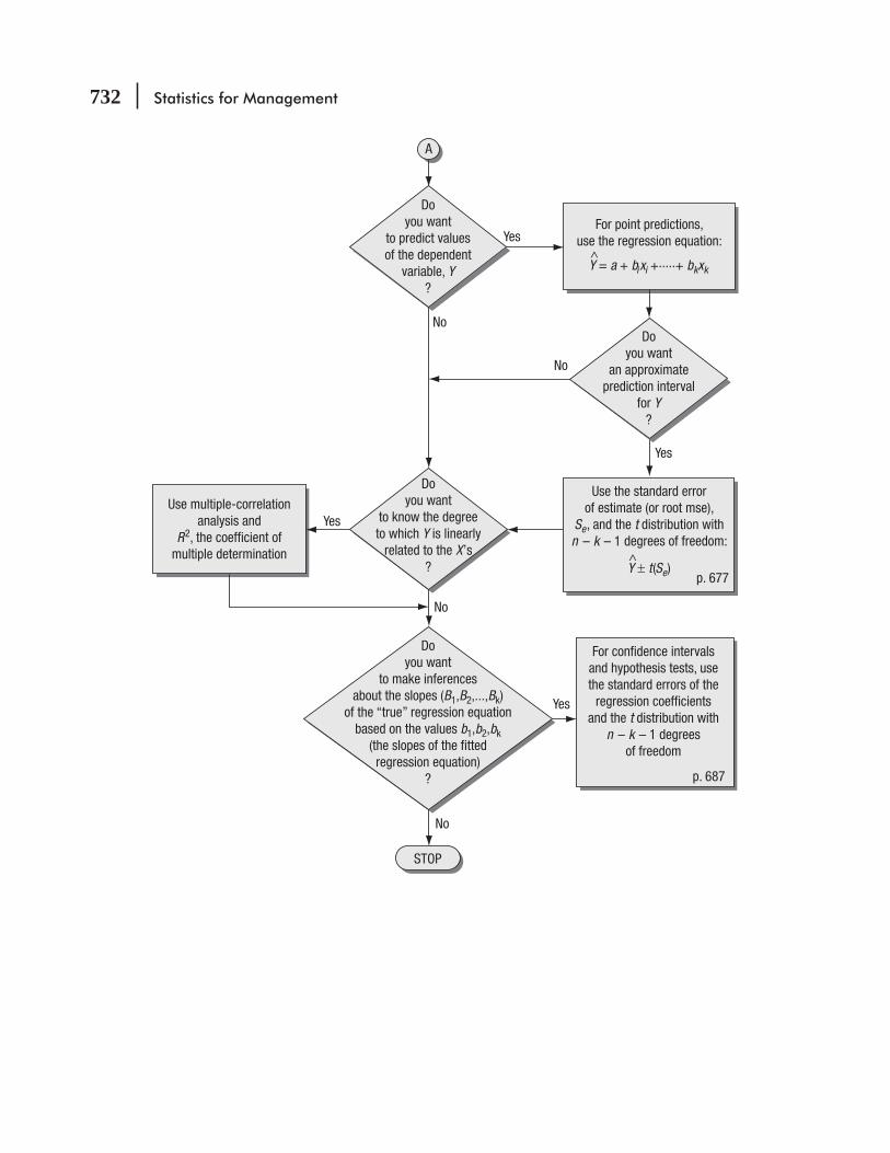
732 Statistics for Management
A
Yes
Yes
No
No
Yes
No
No
Doyou want
to predict valuesof the dependent
variable, Y?
For point predictions,use the regression equation:
Y = a + bixi +.....+ bkxk^
Doyou want
an approximateprediction interval
for Y?
Use multiple-correlationanalysis and
R2, the coefficient ofmultiple determination
Doyou want
to know the degreeto which Y is linearly
related to the X’s? Y ± t(Se)
^
Use the standard errorof estimate (or root mse),
Se, and the t distribution withn – k – 1 degrees of freedom:
p. 677
Doyou want
to make inferencesabout the slopes (B1,B2,...,Bk)
of the “true” regression equationbased on the values b1,b2,bk
(the slopes of the fittedregression equation)
?
For confidence intervalsand hypothesis tests, usethe standard errors of the
regression coefficientsand the t distribution with
n – k – 1 degreesof freedom
p. 687
Yes
STOP

LEARNING OBJECTIVES
14After reading this chapter, you can understand:
CHAPTER CONTENTS
To test hypotheses when we cannot make any assumptions about the distribution from which we are sampling
To know which distribution-free (nonparametric) tests are appropriate for different situations
14.1 Introduction to Nonparametric Statistics 734
14.2 The Sign Test for Paired Data 73614.3 Rank Sum Tests: The Mann–Whitney U
Test and the Kruskal–Wallis Test 74414.4 The One-Sample Runs Test 75814.5 Rank Correlation 76714.6 The Kolmogorov–Smirnov Test 779
To use and interpret each of six standard nonparametric hypothesis tests
To learn the advantages and disadvantages of nonparametric tests
Statistics at Work 786 Terms Introduced in Chapter 14 787 Equations Introduced in Chapter 14 788 Review and Application Exercises 789 Flow Chart: Nonparametric Methods 800
Nonparametric Methods
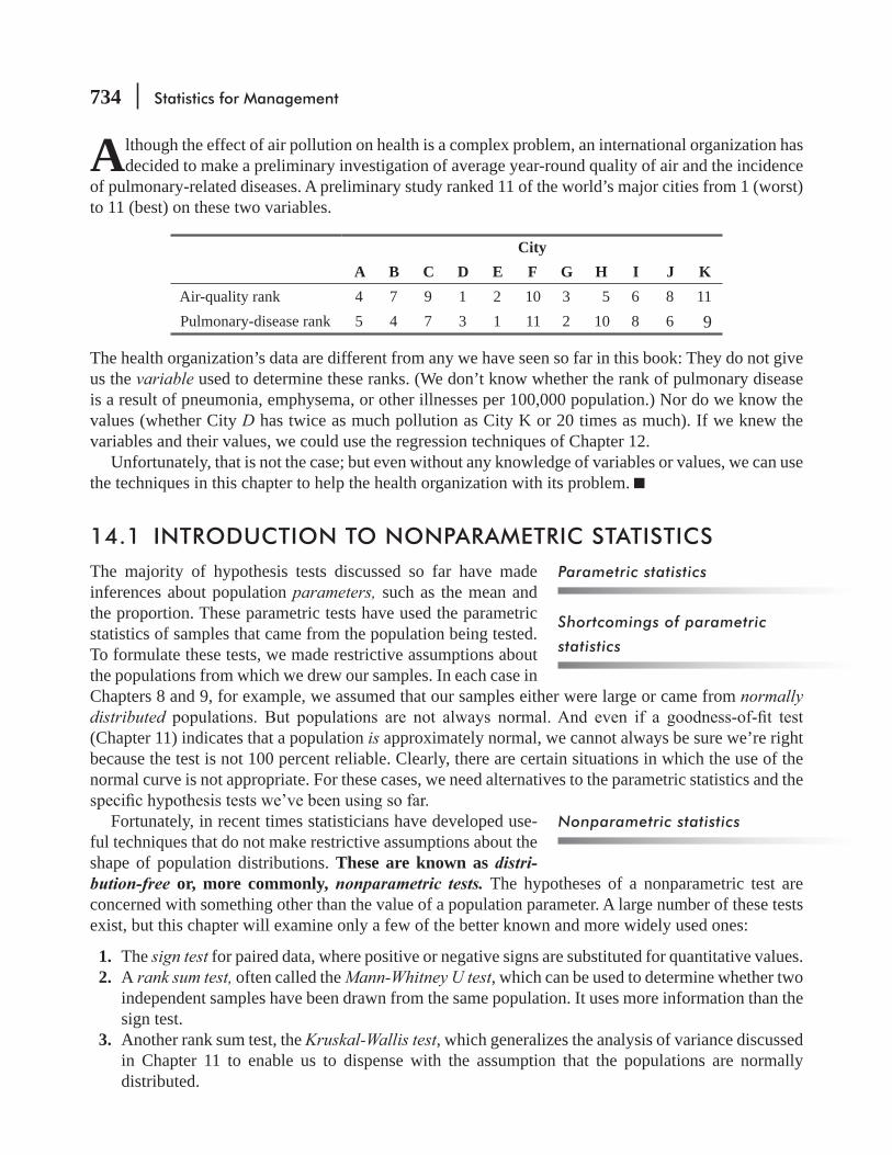
734 Statistics for Management
Although the effect of air pollution on health is a complex problem, an international organization has decided to make a preliminary investigation of average year-round quality of air and the incidence
of pulmonary-related diseases. A preliminary study ranked 11 of the world’s major cities from 1 (worst) to 11 (best) on these two variables.
CityA B C D E F G H I J K
Air-quality rank 4 7 9 1 2 10 3 5 6 8 11Pulmonary-disease rank 5 4 7 3 1 11 2 10 8 6 9
The health organization’s data are different from any we have seen so far in this book: They do not give us the variable used to determine these ranks. (We don’t know whether the rank of pulmonary disease is a result of pneumonia, emphysema, or other illnesses per 100,000 population.) Nor do we know the values (whether City D has twice as much pollution as City K or 20 times as much). If we knew the variables and their values, we could use the regression techniques of Chapter 12.
Unfortunately, that is not the case; but even without any knowledge of variables or values, we can use the techniques in this chapter to help the health organization with its problem.
14.1 INTRODUCTION TO NONPARAMETRIC STATISTICSThe majority of hypothesis tests discussed so far have made inferences about population parameters, such as the mean and the proportion. These parametric tests have used the parametric statistics of samples that came from the population being tested. To formulate these tests, we made restrictive assumptions about the populations from which we drew our samples. In each case in Chapters 8 and 9, for example, we assumed that our samples either were large or came from normally distributed(Chapter 11) indicates that a population is approximately normal, we cannot always be sure we’re right because the test is not 100 percent reliable. Clearly, there are certain situations in which the use of the normal curve is not appropriate. For these cases, we need alternatives to the parametric statistics and the
Fortunately, in recent times statisticians have developed use-ful techniques that do not make restrictive assumptions about the shape of population distributions. These are known as distri-bution-free or, more commonly, nonparametric tests. The hypotheses of a nonparametric test are concerned with something other than the value of a population parameter. A large number of these tests exist, but this chapter will examine only a few of the better known and more widely used ones:
1. The sign test for paired data, where positive or negative signs are substituted for quantitative values. 2. A rank sum test, often called the Mann-Whitney U test, which can be used to determine whether two
independent samples have been drawn from the same population. It uses more information than the sign test.
3. Another rank sum test, the Kruskal-Wallis test, which generalizes the analysis of variance discussed in Chapter 11 to enable us to dispense with the assumption that the populations are normally distributed.
Parametric statistics
Shortcomings of parametric
statistics
Nonparametric statistics

Nonparametric Methods 735
4. The one-sample runs test, a method for determining the randomness with which sampled items have been selected.
5. Rank correlation, a method for doing correlation analysis when the data are not available to
and so forth. 6. The Kolmogorov–Smirnov test
observed sample and a theoretical probability distribution.
Advantages of Nonparametric MethodsNonparametric methods have a number of clear advantages over parametric methods:
1. They do not require us to make the assumption that a
2. Generally, they are easier to do and to understand. Most nonparametric tests do not demand the kind of laborious computations often required, for example, to calculate a standard deviation. A nonparametric test may ask us to replace numerical values with the order in which those values occur in a list, as has been done in Table 14-1. Obviously, dealing computationally with 1, 2, 3, 4, and 5 takes less effort than working with 13.33, 76.50, 101.79, 113.45, and 189.42.
3. Sometimes even formal ordering or ranking is not required. Often, all we can do is describe one outcome as “better” than another. When this is the case, or when our measurements are not as accurate as is necessary for parametric tests, we can use nonparametric methods.
Disadvantages of Nonparametric MethodsTwo disadvantages accompany the use of nonparametric tests:
1. They ignore a certain amount of information. We have demonstrated how the values 1, 2, 3, 4, and 5 can replace the numbers 13.33, 76.50, 101.79, 113.45, and 189.42. Yet if we represent “189.42” by “5,” we lose information that is contained in the value of 189.42. Notice that in our ordering of the values 13.33,
largest, value in the list. But if this list is a data set, we can learn more knowing that the highest value is 1,189.42 instead of 189.42 than we can by representing both of these numbers by the value 5.
2. The estimate of an interval at the
a parametric test such as those in Chapters 8 and 9. When we use nonparametric tests, we make a trade-off: We lose sharpness in estimating intervals, but we gain the ability to use less information and to calculate faster.
Advantages of nonparametric
methods
Shortcomings of nonparametric
methods
TABLE 14-1 CONVERTING PARAMETRIC VALUES TO NONPARAMETRIC RANKS
Parametric value 113.45 189.42 76.50 13.33 101.79Nonparametric value 4 5 2 1 3
736 Statistics for Management
EXERCISES 14.1
Basic Concepts14-1 What is the difference between the kinds of questions answered by parametric tests and those
answered by nonparametric tests?14-2 The null hypothesis most often examined in nonparametric tests (choose one answer)
(b) Is used to evaluate some general population aspect.(c) Is very similar to that used in regression analysis.(d) Simultaneously tests more than two population parameters.
14-3 What are the major advantages of nonparametric methods over parametric methods?14-4 What are the primary shortcomings of nonparametric tests?14-5 George Shoaf is an interviewer with a large insurance company. George works in the com-
to schedule his interviews according to a precise schedule. There is no 5-minute period unac-counted for, including telephone calls. Unfortunately, the receptionist has been underestimat-ing the amount of time interviews will take, and she has been scheduling too many prospective employees, resulting in long waits in the lobby. Although waiting periods may be short in the morning, as the day progresses and the interviewer gets further behind, the waits become lon-ger. In assessing the problem, should the interviewer assume that the successive waiting times are normally distributed?
Applications14-6
in a pamphlet and distributed among employees, whose preferences were then recorded. The results follow:
Rank 1 2 3 4 5 6 7 8 9 10 11 12 13 14 15 16 17 18 19
Retirement Combination 15 5 14 4 6 16 7 8 13 3 17 18 12 2 9 1 11 19 10Number of Preferences 52 49 39 38 37 36 32 29 26 25 24 18 15 15 14 10 10 10 9
-rion? (Hint: You might graph the data.)
14.2 THE SIGN TEST FOR PAIRED DATAOne of the easiest nonparametric tests to use is the sign test. Its name comes from the fact that it is based on the direction (or signs for pluses or minuses) of a pair of observations, not on their numerical magnitude.
Use the sign test for paired data
Nonparametric Methods 737
Consider the result of a test panel of 40 college juniors evaluating the effectiveness of two types of classes: large lectures by full professors and small sections by graduate assistants. Table 14-2 lists the responses to this request: “Indicate how you rate the effectiveness in transmitting knowledge of these two types of classes by giving them a number from 4 to 1. A rating of 4 is excellent and 1 is poor.” In this case, the sign test can help us determine whether students feel there is a difference between the effectiveness of the two types of classes.
We can begin, as we have in Table 14-2, by converting the evaluations of the two teaching methods into signs. Here a plus sign means the student prefers large lectures, a minus sign indi-cates a preference for small sections, and a zero represents a tie (no preference). If we count the bottom row of Table 14-2, we get these results:
Number of + signs 19Number of − signs 11Number of 0s 10Total sample size 40
Stating the HypothesesWe are using the sign test to determine whether our panel can dis-cern a real difference between the two types of classes. Because we are testing perceived differences, we shall exclude tie evalua-tions (0s). We can see that we have 19 plus signs and 11 minus signs, for a total of 30 usable responses. If there is no difference between the two types of classes, p the second score) would be 0.5, and we would expect to get about 15 plus signs and 15 minus signs. We would set up our hypotheses like this:
H0: p = Null hypothesis: There is no difference between the two types of classes
H1: p Alternative hypothesis: There is a difference between the two types of classes
If you look carefully at the hypotheses, you will see that the situation is similar to the fair-coin toss we discussed in Chapter 4. If we tossed a fair coin 30 times, p would be 0.5, and we would expect about 15 heads and 15 tails. In that case, we would use the binomial distribu-tion as the appropriate sampling distribution. You may also remember that when np and nq are each at least 5. we can use the normal distribution to approximate the binomial. This is just the case with the results from our panel of college juniors. Thus, we can apply the normal distribution to our test of the two teaching methods.
pH0= Hypothesized proportion of the population that prefers large lectures
qH0
= Hypothesized proportion of the population that prefers small sections ( qH0
= 1− q )H0
n = Sample size
p = Proportion of successes in the sample (19/30)
q = Proportion of failures in the sample (11/30)
Converting values to signs
Finding the sample size
Choosing the distribution
Setting up the problem
symbolically
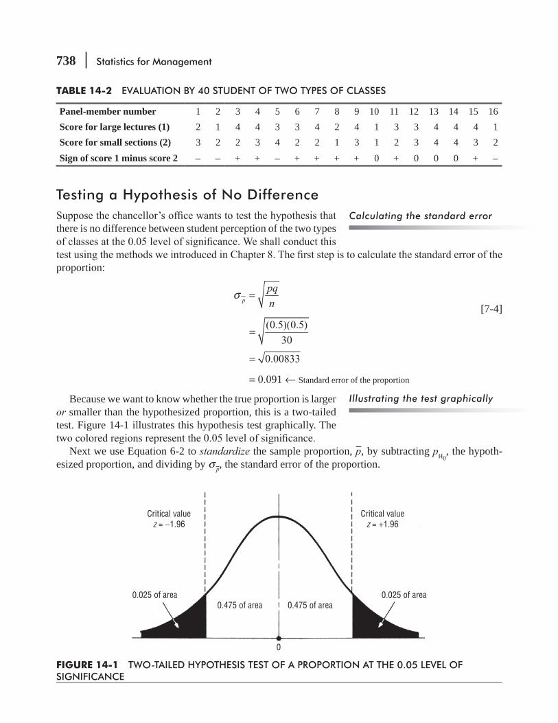
738 Statistics for Management
Testing a Hypothesis of No Difference
there is no difference between student perception of the two types
proportion:
σ =p
pqn [7-4]
(0.5)(0.5)
30=
0.00833=
= 0.091 ← Standard error of the proportion
Because we want to know whether the true proportion is larger or smaller than the hypothesized proportion, this is a two-tailed test. Figure 14-1 illustrates this hypothesis test graphically. The
Next we use Equation 6-2 to standardize the sample proportion, p, by subtracting pH0, the hypoth-
esized proportion, and dividing by σ p, the standard error of the proportion.
Calculating the standard error
Illustrating the test graphically
Critical valuez = −1.96
Critical valuez = +1.96
0.025 of area 0.025 of area0.475 of area0.475 of area
0
FIGURE 14-1 TWO-TAILED HYPOTHESIS TEST OF A PROPORTION AT THE 0.05 LEVEL OF SIGNIFICANCE
TABLE 14-2 EVALUATION BY 40 STUDENT OF TWO TYPES OF CLASSES
Panel-member number 1 2 3 4 5 6 7 8 9 10 11 12 13 14 15 16Score for large lectures (1) 2 1 4 4 3 3 4 2 4 1 3 3 4 4 4 1Score for small sections (2) 3 2 2 3 4 2 2 1 3 1 2 3 4 4 3 2Sign of score 1 minus score 2 − − + + − + + + + 0 + 0 0 0 + −
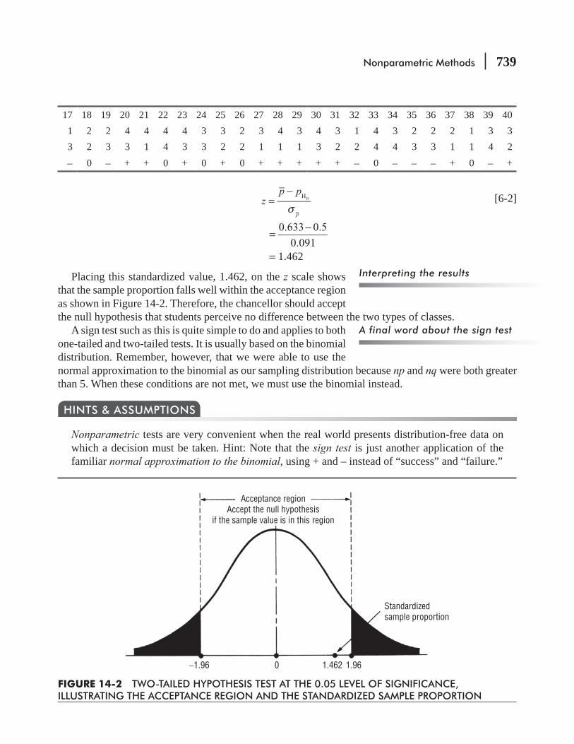
Nonparametric Methods 739
zp p
p
H0
σ=
− [6-2]
0.633 0.5
0.091
−=
= 1.462
Placing this standardized value, 1.462, on the z scale shows that the sample proportion falls well within the acceptance region as shown in Figure 14-2. Therefore, the chancellor should accept the null hypothesis that students perceive no difference between the two types of classes.
A sign test such as this is quite simple to do and applies to both one-tailed and two-tailed tests. It is usually based on the binomial distribution. Remember, however, that we were able to use the normal approximation to the binomial as our sampling distribution because np and nq were both greater than 5. When these conditions are not met, we must use the binomial instead.
Nonparametric tests are very convenient when the real world presents distribution-free data on which a decision must be taken. Hint: Note that the sign test is just another application of the familiar normal approximation to the binomial, using + and – instead of “success” and “failure.”
HINTS & ASSUMPTIONS
Interpreting the results
A final word about the sign test
17 18 19 20 21 22 23 24 25 26 27 28 29 30 31 32 33 34 35 36 37 38 39 401 2 2 4 4 4 4 3 3 2 3 4 3 4 3 1 4 3 2 2 2 1 3 33 2 3 3 1 4 3 3 2 2 1 1 1 3 2 2 4 4 3 3 1 1 4 2
− 0 − + + 0 + 0 + 0 + + + + + − 0 − − − + 0 − +
Acceptance regionAccept the null hypothesis
if the sample value is in this region
Standardizedsample proportion
−1.96 0 1.462 1.96
FIGURE 14-2 TWO-TAILED HYPOTHESIS TEST AT THE 0.05 LEVEL OF SIGNIFICANCE, ILLUSTRATING THE ACCEPTANCE REGION AND THE STANDARDIZED SAMPLE PROPORTION
740 Statistics for Management
EXERCISES 14.2
Self-Check ExercisesSC 14-1 The following data show employees’ rates of defective work before and after a change in the
wage incentive plan. Compare the following two sets of data to see whether the change low-
Before 8 7 6 9 7 10 8 6 5 8 10 8
After 6 5 8 6 9 8 10 7 5 6 9 8
SC 14-2 After collecting data on the amount of air pollution in Los Angeles, the Environmental Pro-tection Agency decided to issue strict new rules to govern the amount of hydrocarbons in the air. For the next year, it took monthly measurements of this pollutant and compared them to the preceding year’s measurements for corresponding months. Based on the following data,
rules were effective in lowering the amount of hydrocarbons in the air? To justify these laws for another year, it must conclude at α = 0.10 that they are effective. Will these laws still be in effect next year?
Last Year* This Year
Jan. 7.0 5.3
Feb. 6.0 6.1
Mar. 5.4 5.6
April 5.9 5.7
May 3 9 3.7
June 5.7 4.7
July 6.9 6.1
Aug. 7.6 7.2
Sept. 6.3 6.4
Oct. 5.8 5.7
Nov. 5.1 4.9
Dec. 5.9 5.8*Measured in parts per million.
Applications14-7 The following data show employees’ satisfaction levels (as a percentage) before and after their
Before 98.4 96.6 82.4 96.3 75.4 82.6 81.6 91.4 90.4 92.4After 82.4 95.4 94.2 97.3 77.5 82.5 81.6 84.5 89.4 90.6
Nonparametric Methods 741
14-8 Use the sign test to see whether there is a difference between the number of days required to -
cance level.
Before 33 36 41 32 39 47 34 29 32 34 40 42 33 36 29After 35 29 38 34 37 47 36 32 30 34 41 38 37 35 28
14-9 A light-aircraft engine repair shop switched the payment method it used from hourly wage to hourly wage plus a bonus computed on the time required to disassemble, repair, and reas-semble an engine. The following are data collected for 25 engines before the change and 25
Hours Required Hours Required
Before After Before After
29 32 25 34
34 19 42 27
32 22 20 26
19 21 25 25
31 20 33 31
22 24 34 19
28 25 20 22
31 31 21 32
32 18 22 31
44 22 45 30
41 24 43 29
23 26 31 20
34 41
14-10 Because of the severity of recent winters, there has been talk that the earth is slowly pro-gressing toward another ice age. Some scientists hold different views, however, because the summers have brought extreme temperatures as well. One scientist proposed looking at the mean temperature for each month to see whether it was lower than in the previous year. Another meteorologist at the government weather service argued that perhaps they should look as well at temperatures in the spring and fall months of the last 2 years, so that their conclusions would be based on other than extreme temperatures. In this way, he said, they could detect whether there appeared to be a general warming or cooling trend or just extreme temperatures in the summer and winter months. So 15 dates in the spring and fall were randomly selected, and the temperatures in the last 2 years were noted for a particular location with generally moderate temperatures. Following are the dates and corresponding temperatures for 1994 and 1995.(a) Is the meteorologist’s reasoning as to the method of evaluation sound? Explain.(b) Using a sign test, determine whether the meteorologist can conclude at α = 0.05 that 1995
was cooler than 1994, based on these data.

742 Statistics for Management
Temperature (Fahrenheit)Date 1994 1995 Date 1994 1995
Mar. 29 58 57 Oct. 12 54 48Apr. 4 45 70 May 31 74 79Apr. 13 56 46 Sept. 28 69 60May 22 75 67 June 5 80 74Oct. 1 52 60 June 17 82 79Mar. 23 49 47 Oct. 5 59 72Nov. 12 48 45 Nov. 28 50 50Sept. 30 67 71
14-11 With the concern over radiation exposure and its relationship to the incidence of cancer, city environmental specialists keep a close eye on the types of industry coming into the area and the degree to which they use radiation in their production. An index of exposure to radioactive contamination has been developed and is being used daily to determine whether the levels are increasing or are higher under certain atmospheric conditions.
Environmentalists claim that radioactive contamination has increased in the last year be-cause of new industry in the city. City administrators, however, claim that new, more stringent regulations on industry in the area have made levels lower than last year, even with new in-dustry using radiation. To test their claim, records for 11 randomly selected days of the year have been checked, and the index of exposure to radioactive contamination has been noted. The following results were obtained:
Index of Radiation Exposure1994 1.402 1.401 1.400 1.404 1.395 1.402 1.406 1.401 1.404 1.406 1.3971995 1.440 1.395 1.398 1.404 1.393 1.400 1.401 1.402 1.400 1.403 1.402
Can the administrators conclude at α = 0.15 that the levels of radioactive contamination have
14-12 As part of the recent interest in population growth and the sizes of families, a population researcher examined a number of hypotheses concerning the family size that various people look upon as ideal. She suspected that variables of race, sex, age, and background might ac-count for some of the different views. In one pilot sample, the researcher tested the hypoth-esis that women today think of an ideal family as being smaller than the ideal held by their mothers. She asked each of the participants in the pilot study to state the number of children she would choose to have or that she considered ideal. Responses were anonymous, to guard against the possibility that people would feel obligated to give a socially desirable answer. In addition, people of different backgrounds were included in the sample. The following are the responses of the mother–daughter pairs.
Ideal Family SizeSample Pair A B C D E F G H I J K L MDaughter 3 4 2 1 5 4 2 2 3 3 1 4 2Mother 4 4 4 3 5 3 3 5 3 2 2 3 1

Nonparametric Methods 743
(a) Can the researcher conclude at α = 0.03 that the mothers and daughters do not have essentially the same ideal of family size? Use the binomial distribution.
(b) Determine whether the researcher could conclude that the mothers do not have essentially the same family-size preferences as their daughters by using the normal approximation to the binomial.
(c) Assume that for each pair listed, there were 10 more pairs who responded in an iden-tical manner. Calculate the range of the proportion for which the researcher would conclude that there is no difference in the mothers and daughters. Is your conclusion different?
(d) Explain any differences in conclusions obtained in parts (a), (b), and (c).14-13 A nationwide used-car company has developed a new instructional video to educate sales-
people. Twenty employees’ average monthly car sales are presented below for time peri-ods both before and after the video’s creation. Does the company have enough evidence
average number of cars sold? If we just consider the employees with low sales (less than an average of 12 cars per month before the video), did the video increase their selling performance?
Before 18.4 16.9 17.4 11.6 10.5 12.7 22.3 18.5 17.5 16.4
After 18.6 16.8 17.3 15.6 19.5 12.6 22.3 16.5 18.0 16.4
Before 15.9 18.6 23.5 18.7 9.4 16.3 18.5 17.4 11.3 8.4
After 17.4 18.6 23.5 18.9 15.6 15.4 17.6 17.4 16.5 13.4
Worked-Out Answers to Self-Check ExercisesSC 14-1
Before 8 7 6 9 7 10 8 6 5 8 10 8
After 6 5 8 6 9 8 10 7 5 6 9 8
Sign − − + − + − + + 0 − − 0
12 responses: 4(+), 6(), 2(0).
For n = 10, p = 0.5, the probability of 6 or more minuses is 0.3770 (Appendix Table 3). Because 0.3770 > 0.10, we cannot reject H0lower the rates of defective work.
SC 14-2Before 7.0 6.0 5.4 5.9 3.9 5.7 6.9 7.6 6.3 5.8 5.1 5.9
After 5.3 6.1 5.6 5.7 3.7 4.7 6.1 7.2 6.4 5.7 4.9 5.8
Sign − + + − − − − − + − − −
12 responses: 3(+), 9(−).
For n = 12, p = 0.5, the probability of 9 or more minuses is 0.0729 (Appendix Table 3).
have been lowered, but they will conclude at α = 0.10 that the rules are effective. Hence, they will still be in effect next year.

744 Statistics for Management
14.3 RANK SUM TESTS: THE MANN–WHITNEY U TEST AND THE KRUSKAL–WALLIS TEST
In Chapter 11, we showed how to use analysis of variance to test the hypothesis that several population means are equal. We assumed in such tests that the populations were normally distrib-uted with equal variances. Many times these assumptions cannot be met, and in such cases, we can use two nonparametric tests, neither of which depends on the normal-ity assumptions. Both of these tests are called rank sum tests because the test depends on the ranks of the sample observations.
Rank sum tests are a whole family of tests. We shall concentrate on just two members of this family, the Mann–Whitney U test and the Kruskal–Wallis test. We’ll use the Mann–Whitney test when only two populations are involved and the Kruskal–Wallis test when more than two populations are involved. Use of these tests will enable us to determine whether independent samples have been drawn from the same population (or from different populations having the same distribution). The use of ranking information rather than pluses and minuses is less wasteful of data than the sign test.
Solving a Problem Using the Mann–Whitney U TestSuppose that the board of regents of a large eastern state university wants to test the hypothesis that the mean SAT scores of students at two branches of the state university are equal. The board keeps statistics on all students at all branches of the system. A random sample of 15 students from each branch has produced the data shown in Table 14-3.
To apply the Mann–Whitney U test to this problem, we begin by ranking all the scores in order from lowest to highest, indicat-ing beside each the symbol of the branch. Table 14-4 accom-plishes this.
Next, let’s learn the symbols used to conduct a Mann–Whitney U test in the context of this problem:
n1 = number of items in sample 1, that is, the number of students at Branch An2 = number of items in sample 2, that is, the number of students at Branch SR1 = sum of the ranks of the items in sample 1: the sum from
Table 14-5 of the ranks of all the Branch A scoresR2 = sum of the ranks of the items in sample 2: the sum from
Table 14-5 of the ranks of all the Branch S scores
In this case, both n1 and n2 are equal to 15, but it is not necessary for both samples to be of the same size. Now in Table 14-5, we can reproduce the data from Table 14-3, adding the ranks from Table 14-4.
Use based on the number of
populations involved
Ranking the items to be tested
Symbols for expressing the
problem
TABLE 14-3 SAT SCORES FOR STUDENTS AT TWO STATE UNIVERSITY BRANCHES
Branch A 1,000 1,100 800 750 1,300 950 1,050 1,250Branch S 920 1,120 830 1,360 650 725 890 1,600Branch A 1,400 850 1,150 1,200 1,500 600 775Branch S 900 1,140 1,550 550 1,240 925 500
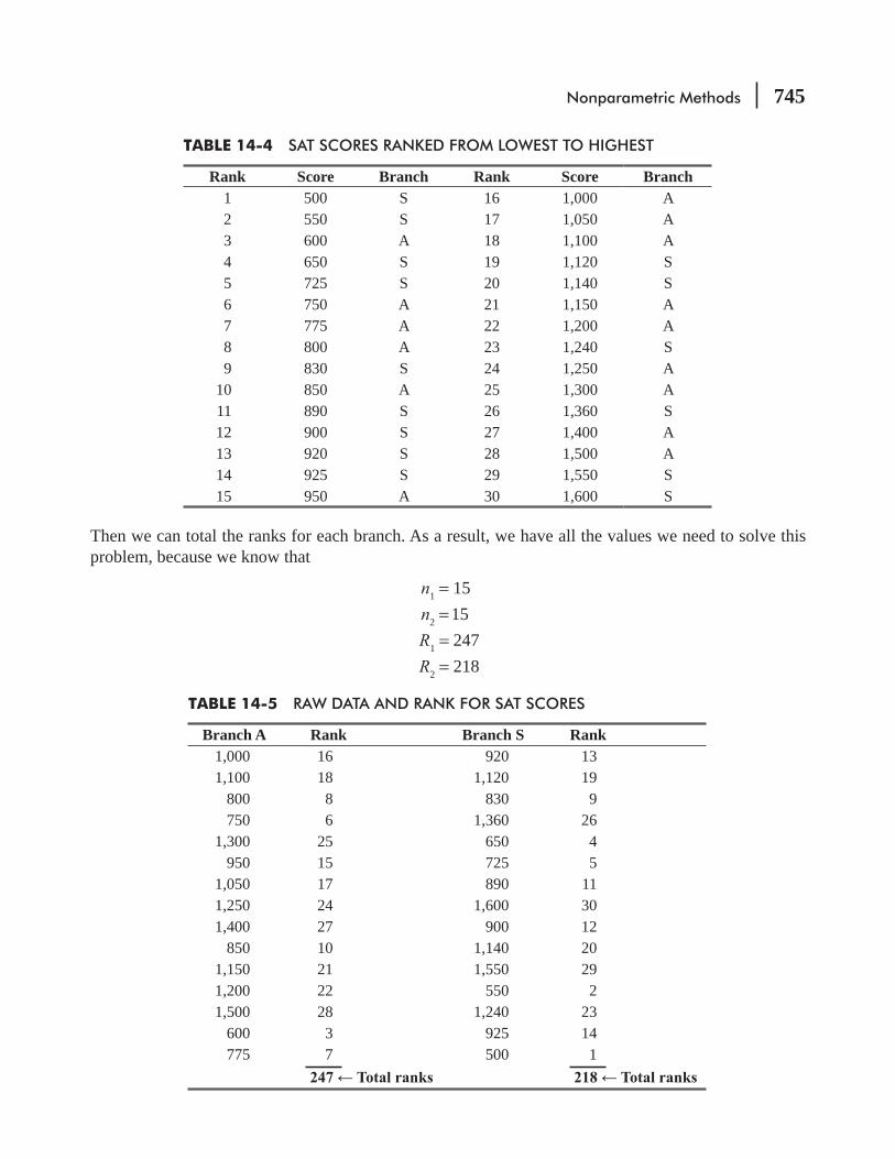
Nonparametric Methods 745
Then we can total the ranks for each branch. As a result, we have all the values we need to solve this problem, because we know that
n1 = 15n2 = 15R1 = 247R2 = 218
TABLE 14-4 SAT SCORES RANKED FROM LOWEST TO HIGHEST
Rank Score Branch Rank Score Branch1 500 S 16 1,000 A2 550 S 17 1,050 A3 600 A 18 1,100 A4 650 S 19 1,120 S5 725 S 20 1,140 S6 750 A 21 1,150 A7 775 A 22 1,200 A8 800 A 23 1,240 S9 830 S 24 1,250 A
10 850 A 25 1,300 A11 890 S 26 1,360 S12 900 S 27 1,400 A13 920 S 28 1,500 A14 925 S 29 1,550 S15 950 A 30 1,600 S
TABLE 14-5 RAW DATA AND RANK FOR SAT SCORES
Branch A Rank Branch S Rank1,000 16 920 131,100 18 1,120 19
800 8 830 9750 6 1,360 26
1,300 25 650 4950 15 725 5
1,050 17 890 111,250 24 1,600 301,400 27 900 12
850 10 1,140 201,150 21 1,550 291,200 22 550 21,500 28 1,240 23
600 3 925 14775 7 500 1
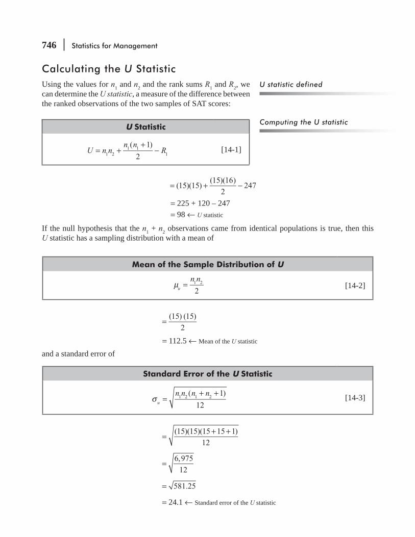
746 Statistics for Management
Calculating the U StatisticUsing the values for n1 and n2 and the rank sums R1 and R2, we can determine the U statistic, a measure of the difference between the ranked observations of the two samples of SAT scores:
U Statistic
U n nn n
R( 1)
21 21 1
1= ++
− [14-1]
(15)(15)(15)(16)
2247= + −
= 225 + 120 – 247 = 98 ← U statistic
If the null hypothesis that the n1 + n2 observations came from identical populations is true, then this U statistic has a sampling distribution with a mean of
Mean of the Sample Distribution of U
μ =n n2
u1 2 [14-2]
=(15) (15)
2
= 112.5 ← Mean of the U statistic
and a standard error of
Standard Error of the U Statistic
σ =+ +n n n n( 1)
12u1 2 1 2 [14-3]
=+ +(15)(15)(15 15 1)
12
6,975
12=
581.25=
= 24.1 ← Standard error of the U statistic
U statistic defined
Computing the U statistic
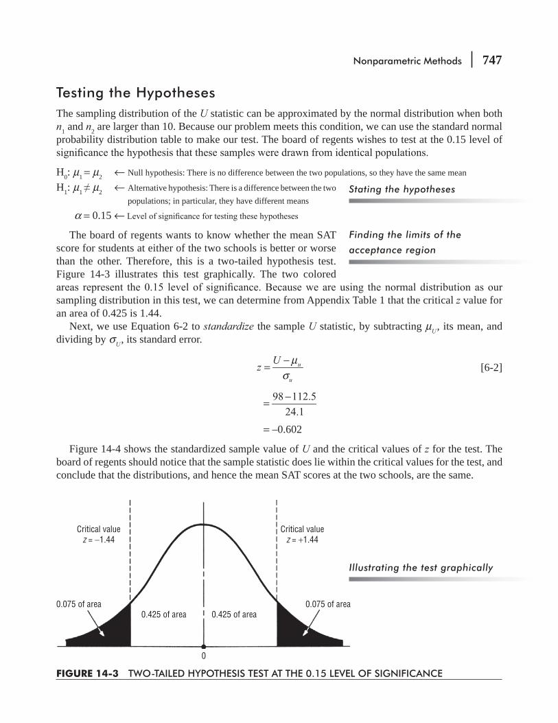
Nonparametric Methods 747
Testing the HypothesesThe sampling distribution of the U statistic can be approximated by the normal distribution when both n1 and n2 are larger than 10. Because our problem meets this condition, we can use the standard normal probability distribution table to make our test. The board of regents wishes to test at the 0.15 level of
H0: μ1 = μ2 ← Null hypothesis: There is no difference between the two populations, so they have the same mean
H1: μ1 μ2 ← Alternative hypothesis: There is a difference between the two populations; in particular, they have different means
α = 0.15 ←
The board of regents wants to know whether the mean SAT score for students at either of the two schools is better or worse than the other. Therefore, this is a two-tailed hypothesis test. Figure 14-3 illustrates this test graphically. The two colored
sampling distribution in this test, we can determine from Appendix Table 1 that the critical z value for an area of 0.425 is 1.44.
Next, we use Equation 6-2 to standardize the sample U statistic, by subtracting μU , its mean, and dividing by σ U , its standard error.
μ
σ−= u
u
Uz [6-2]
98 112.5
24.1
−=
= –0.602
Figure 14-4 shows the standardized sample value of U and the critical values of z for the test. The board of regents should notice that the sample statistic does lie within the critical values for the test, and conclude that the distributions, and hence the mean SAT scores at the two schools, are the same.
Stating the hypotheses
Finding the limits of the
acceptance region
Critical valuez = +1.44
Critical valuez = −1.44
0.075 of area 0.075 of area0.425 of area0.425 of area
0
FIGURE 14-3 TWO-TAILED HYPOTHESIS TEST AT THE 0.15 LEVEL OF SIGNIFICANCE
Illustrating the test graphically

748 Statistics for Management
Special Properties of the U TestThe U statistic has a feature that enables users to save calculat-ing time when the two samples under observation are of unequal size. We just computed the value of U using Equation 14-1:
1 11 2 1
( 1)
2
+= + −n nU n n R [14-1]
But just as easily, we could have computed the U statistic using the R2 value, like this:
Alternate Formula for the U Statistic
2 21 2 2
( 1)
2
+= + −n nU n n R [14-4]
The answer would have been 127 (which is just as far above the mean of 112.5 as 98 is below it). In this problem, we would have spent the same amount of time calculating the value of the U statistic using either Equation 14-1 or Equation 14-4. In other cases, when the number of items is larger in one sample than in the other, choose the equation that will require less work. Regardless of whether you calculate U using Equation 14-1 or 14-4, you will come to the same conclusion. Notice that in this example, the answer 127 falls in the acceptance region just as 98 did.
What about ties that may happen when we rank the items for this test? For example, what if the two scores ranked 13 and 14
the average of their ranks (13 + 14)/2 = 13.5, and assign the result to both of them. If there were a three-way tie among the scores ranked 13, 14, and 15, we would average these ranks (13 + 14 + 15)/3 = 14, and use that value for all three items.
Another way to compute the
U statistic
Handling ties in the data
Standardizedsample value of U
−1.44 −0.602 0 1.44
Acceptance regionAccept the null hypothesis
if the sample value is in this region
FIGURE 14-4 TWO-TAILED HYPOTHESIS TEST AT THE 0.15 LEVEL OF SIGNIFICANCE, SHOWING THE ACCEPTANCE REGION AND THE STANDARDIZED SAMPLE U STATISTIC
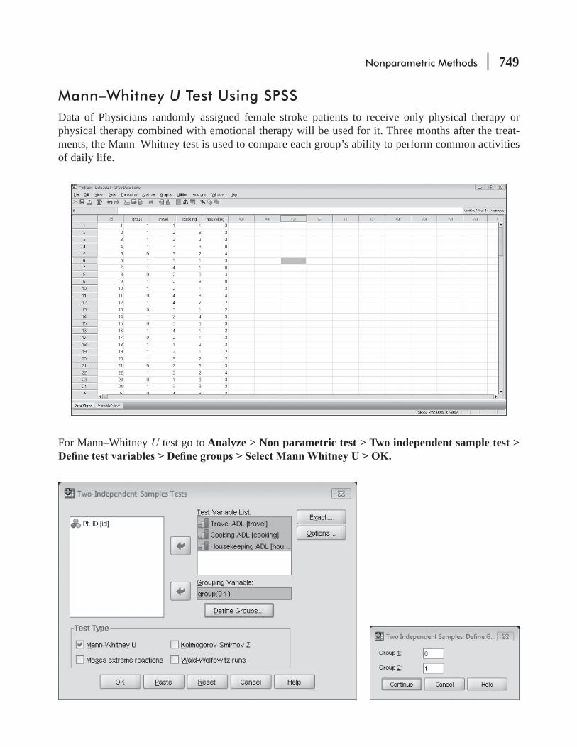
Nonparametric Methods 749
Mann–Whitney U Test Using SPSSData of Physicians randomly assigned female stroke patients to receive only physical therapy or physical therapy combined with emotional therapy will be used for it. Three months after the treat-ments, the Mann–Whitney test is used to compare each group’s ability to perform common activities of daily life.
For Mann–Whitney U test go to Analyze > Non parametric test > Two independent sample test >

750 Statistics for Management
Solving a Problem Using the Kruskal–Wallis TestAs we noted earlier in this section, the Kruskal–Wallis test is an extension of the Mann–Whitney test to situations where more than two populations are involved. This test, too, depends on the ranks of the sample observations.
In Table 14-6, we have shown the scores of a sample of 20 student pilots on their Federal Aviation Agency written examination, arranged according to which method was used in their training: video cassette, audio cassette, or class room training.
student pilots trained by each of these three methods are equal. Because we have more than two popu-lations involved, the Kruskal–Wallis test is appropriate in this instance. To apply the Kruskal–Wallis test to this problem, we begin in Table 14-7 by ranking all the scores in order, from lowest to highest, indicating beside each the symbol of the training method that was used. Ties are handled by averaging ranks, exactly as we did with the Mann–Whitney test.
Testing for differences when
more than two populations are
involved
Ranking the items to be tested
TABLE 14-6 WRITTEN EXAMINATION SCORES FOR 20 STUDENT PILOTS TRAINED BY THREE DIFFERENT METHODS
Video cassette 74 88 82 93 55 70
Audio cassette 78 80 65 57 89
Classroom 68 83 50 91 84 77 94 81 92
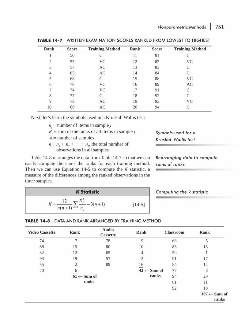
Nonparametric Methods 751
Next, let’s learn the symbols used in a Kruskal–Wallis test:nj = number of items in sample jRj = sum of the ranks of all items in sample j k = number of samplesn = n1 + n2 + … + nk, the total number of
observations in all samplesTable 14-8 rearranges the data from Table 14-7 so that we can
easily compute the sums the ranks for each training method. Then we can use Equation 14-5 to compute the K statistic, a measure of the differences among the ranked observations in the three samples.
K Statistic2
123( 1)
( 1)= − +
+ ∑ j
j
RK n
n n n[14-5]
Symbols used for a
Kruskal–Wallis test
Rearranging data to compute
sums of ranks
Computing the k statistic
TABLE 14-7 WRITTEN EXAMINATION SCORES RANKED FROM LOWEST TO HIGHEST
Rank Score Training Method Rank Score Training Method1 50 C 11 81 C2 55 VC 12 82 VC3 57 AC 13 83 C4 65 AC 14 84 C5 68 C 15 88 VC6 70 VC 16 89 AC7 74 VC 17 91 C8 77 C 18 92 C9 78 AC 19 93 VC
10 80 AC 20 94 C
TABLE 14-8 DATA AND RANK ARRANGED BY TRAINING METHOD
Video Cassette Rank Audio Cassette Rank Classroom Rank
74 7 78 9 68 588 15 80 10 83 1382 12 65 4 50 193 19 57 3 91 1755 2 89 16 84 1470 6 42 77 8
61 94 2081 1192 18
107
Sum of ranks Sum of
ranks
Sum of ranks

752 Statistics for Management
=+
+ +⎡
⎣
⎢⎢
⎤
⎦⎥⎥− +
12
20(20 1)
(61)
6
(42)
5
(107)
9
3(20 1)
2 2 2
= (0.02857) (620.2 + 352.8 + 1,272.1) – 63= 1.143
Testing the HypothesesThe sampling distribution of the K statistic can be approximated by a chi-square distribution when all the sample sizes are at least 5. Because our problem meets this condition, we can use the chi-square dis-tribution and Appendix Table 5 for this test. In a Kruskal-Wallis test, the appropriate number of degrees of freedom is k – 1, which in this problem is (3 – 1) or 2 because we are dealing with three samples. The hypotheses can be stated as follows:
H0: μ1 = μ2 = μ3 Null hypothesis; There are no differences among the three populations, so they have the same mean
H1 : μ1, μ2 and μ3 are not all equal
Alternative hypothesis: There are differences among the three populations, in particular, they have different means
α =
Figure 14-5 illustrates a chi-square distribution with 2 degrees -
cance. Notice that the acceptance region for the null hypothesis (that there are no differences among the three populations) extends from zero to a chi-square value of 4.605. Obviously, the sample K value of 1.143 is within this acceptance region; therefore, the FAA should accept the null hypothesis and conclude that there are no differences in the results obtained by using the three training methods.
Stating the hypotheses
Interpreting the results
0.10 of area
0 4.605
Sample valueof K, 1.143
Acceptance regionAccept the null hypothesis
if the sample value is in this region
FIGURE 14-5 KRUSKAL–WALLIS TEST AT THE 0.10 LEVEL OF SIGNIFICANCE, SHOWING THE ACCEPTANCE REGION AND THE SAMPLE K STATISTIC
Illustrating the test graphically
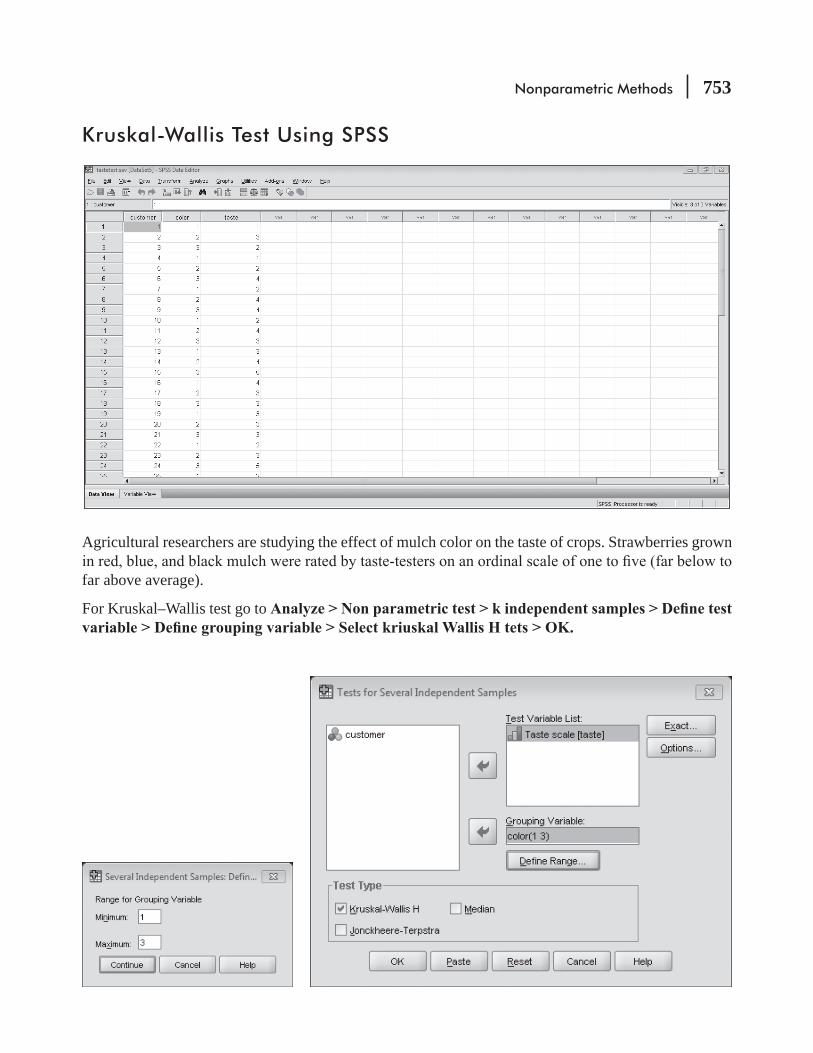
Nonparametric Methods 753
Kruskal-Wallis Test Using SPSS
Agricultural researchers are studying the effect of mulch color on the taste of crops. Strawberries grown
far above average).
For Kruskal–Wallis test go to

754 Statistics for Management
Rank sum tests such as the Mann-Whitney and the Kruskal-Wallis tests often produce ties in rank-ings. Hint: When you encounter ties, remember that each tied value gets an average rank. If the 10th and 11th items are tied, each of them gets a rank of 10.5. In the case of ties of more than 2 items, they all still get the average rank (a tie in the 3rd, 4th, 5th, and 6th items means all four of them get a rank of (3 + 4 + 5 + 6)/4 = 4.5).
HINTS & ASSUMPTIONS
EXERCISES 14.3
Self-Check ExercisesSC 14-3 Melisa’s Boutique has three mall locations. Melisa keeps a daily record for each location of the
number of customers who actually make a purchase. A sample of those data follows. Using the
number of customers who buy?
Eastowne Mail 99 64 101 85 79 88 97 95 90 100Craborchard Mall 83 102 125 61 91 96 94 89 93 75Fairforest Mall 89 98 56 105 87 90 87 101 76 89
SC 14-4 A large hospital hires most of its nurses from the two major universities in the area. Over the last year, they have been giving a test to the newly graduated nurses entering the hospital to determine which school, if either, seems to educate its nurses better. Based on
Nonparametric Methods 755
determine whether the schools differ in quality. Use the Mann–Whitney U test with a
Test ScoresSchool A 97 69 73 84 76 92 90 88 84 87 93School B 88 99 65 69 97 84 85 89 91 90 87 91 72
Applications14-14 Test the hypothesis of no difference between the ages of male and female employees of a
certain company using the Mann–Whitney U test for the sample data. Use the 0.10 level of
Males 31 25 38 33 42 40 44 26 43 35Females 44 30 34 47 35 32 35 47 48 34
14-15 The following table shows sample retail prices for three brands of shoes. Use the Kruskal–Wallis test to determine whether there is any difference among the retail prices of the brands
Brand A $89 90 92 81 76 88 85 95 97 86 100Brand B $78 93 81 87 89 71 90 96 82 85Brand C $80 88 86 85 79 80 84 85 90 92
14-16 A mail-order gift company has the following sample data on dollar sales, separated according to how the order was paid. Test the hypothesis that there is no difference in the dollar amount of orders paid for by cash, by check, or by credit card. Use the Kruskal–Wallis test with a 0.05
Credit-card orders 78 64 75 45 82 69 60Check orders 110 70 53 51 61 68Cash orders 90 68 70 54 74 65 59
14-17 The following data show annual hours missed due to illness for the 24 men and women at the -
tributable to gender? Use the Mann–Whitney U test.
Men 31 44 25 30 70 63 54 42 36 22 25 5038 34 33 47 58 83 18 36 41 37 24 48
14-18 A manufacturer of toys changed the type of plastic molding machines it was using because a new one gave evidence of being more economical. As the Christmas season began, however, productivity seemed somewhat lower than last year. Because production records for the past years were readily available, the production manager decided to compare the monthly output for the 15 months when the old machines were used and the 11 months of production so far this year. Records show these output amounts with the old and new machines.
756 Statistics for Management
New Machines
992 966 965 956945 889 1,054 900938 972 912 938
1,027 940 850892 873 796983 1,016 911
1,014 897 8771,258 902
reduced output?14-19 Hanks’ Hot Dogs has four hot dog stands at Memorial Stadium. Hank knows how many hot
dogs are sold at each stand during each football game, and he wants to determine whether the four stands are selling the same number. Using the Kruskal–Wallis test, can you say at the 0.10
Game 1 2 3 4 5 6 7 8 9Visitors north 755 698 725 895 886 794 694 827 814Visitors south 782 724 754 825 815 826 752 784 789Home north 714 758 684 816 856 884 774 812 734Home south 776 824 654 779 898 687 716 889 917
14-20 To increase sales during heavy shopping days, a chain of stores selling cheese in shopping
shopping days and randomly selects the days for sampling. From a sample of days that were considered heavy shopping days, the following data give one store’s sales on days when cheese sampling was done and on days when it was not done.
Sales (in hundreds)Promotion days 18 21 23 15 19 26 17 18 22 20 18 21 27Regular days 22 17 15 23 25 20 26 24 16 17 23 21
Use the Mann–Whitney Ustorefront sampling produced greater Sales
14-21 A company is interested in knowing whether there is a difference in the output rate for men and women employees in the molding department. Judy Johnson, production manager, was asked to conduct a study in which male and female workers’ output was measured for 1 week.
only the following information from the records of the tests:
σ u = 176.4275 μu = 1,624R1 = 3,255
Judy also remembered that the sample size for men, n2, had been two units larger than n1.

Nonparametric Methods 757
Reconstruct a z value for the test and determine whether the weekly output can be assumed,
values for n1,n2, and R2.14-22 A university that accepts students from both rural and urban high schools is interested in
urban background. Use the Mann–Whitney U
GPA
Rural 3.19 2.05 2.82 2.16 3.84 4.0 2.91 2.75 3.01 1.982.58 2.76 2.943.45 3.16 2.84 2.09 2.11 3.08 3.97 3.85 3.72 2.732.81 2.64 1.57 1.87 2.54 2.62
14-23 Twenty salespeople of Henley Paper Company have received sales training during the past year. Some were sent to a national program conducted by Salesmasters. The other received
quotas realized by both groups during last year are shown. Mr. Boyden Henley, president, believes that the backgrounds, sales aptitudes, and motivation of both groups are comparable.
Whitney U test.
Percentage of Quota RealizedSalesmasters 90 95 105 110 100 75 80 90 105 120Company 80 90 100 120 95 95 90 100 95 105
Worked-Out Answers to Self-Check ExercisesSC 14-3 Eastowne ranks 99 64 101 85 79 88 97 95 90 100
24 3 26.5 8 6 11 22 20 15.5 25Craborchard ranks 83 102 125 61 91 96 94 89 93 75
7 28 30 2 17 21 19 13 18 4Fairforest ranks 89 98 56 105 87 90 87 101 76 89
13 23 1 29 9.5 15.5 9.5 26.5 5 13
n1 =10 n2 = 10 n3 = 10 α = 0.05R1 = 161 R2 = 159 R3 = 145H0: μ1 = μ2 = μ3 H1: the μ’s are not all the same
kn n
R
nn
12
( 1)3( 1)j
j
2
∑=+
− +
2 2 2 21 12 (161) (159) (145)3(31) 0.196
30(31) 10 10 10
⎛ ⎞= + + − =⎜ ⎟
⎝ ⎠j
j
R
nn
758 Statistics for Management
With 3 – 1 = 2 degrees of freedom and α = 0.05, the upper limit of the acceptance region is x2 = 5.991, so we accept H0 -cantly different.
SC 14-4 School A 97 69 73 84 76 92 90 88 84 87 93
ranks 22.5 2.5 5 8 6 20 16.5 13.5 8 11.5 21
School B 88 99 65 69 97 84 85 89 91 90 87 91 72
ranks 13.5 24 1 2.5 22.5 8 10 15 18.5 16.5 11.5 18.5 4
n1 = 11 n2 = 13 α = 0.10R1 = 134.5 R2 = 165.5H0:μ1= μ2 H1: μ1 ≠ μ2
1 11 2 1
( 1) 11(12)11(13) 134.5 74.5
2 2
n nU n n R
+= + − = + − =
1 2
11(13)
71.5
2 2
un nμ = = =
1 2 1 2
( 1) 11(13)(25)
17.26
12 12
un n n nσ + += = =
The critical values of z are ± 1.645. The standardized value of U is
74.5 71.5
0.174
17.26
u
u
Uz μσ− −= = =
Because the standardized value of U lies within the critical values, we accept H0. There is no
14.4 THE ONE-SAMPLE RUNS TESTSo far, we have assumed that the samples in our problems were randomly selected—that is, chosen without preference or bias. What if you were to notice recurrent patterns in a sample chosen by someone else? Suppose that applicants for advanced job training were to be selected without regard to gender from a large population. Using the notation W = woman and M =group enters in this order:
W, W, W, W, M, M, M, M, W, W, W, W, M, M, M, M
By inspection, you would conclude that although the total number of applicants is equally divided between the sexes, the order is not random. A random process would rarely list two items in alternating groups of four. Suppose now that the applicants begin to arrive in this order:
W, M, W, M, W, M, W, M, W, M, W, M, W, M, W, M
Concept of randomness
Nonparametric Methods 759
It is just as unreasonable to think that a random selection process would produce such an orderly pattern of men and women. In this case, too, the proportion of women to men is right, but you would be suspi-cious about the order in which they are arriving.
To allow us to test samples for the randomness of their order, statisticians have developed the theory of runs. A run is a sequence of identical occurrences preceded and followed by different occurrences or by none at all. If men and women enter as follows, the sequence will contain three runs:
W,
1st
M, M, M, M,
2nd
W
3rd� ��� ��� ��
And this sequence contains six runs:
W, W, W
1st� �� �� M, M,
2nd��� W,
3rd� M, M, M, M
4th� ��� ��� W, W, W,W
5th� ��� ��� M
6th�
A test of runs would use the following symbols if it contained just two kinds of occurrences:
n1 = number of occurrences of type 1n2 = number of occurrences of type 2 r = number of runs
Let’s apply these symbols to a different pattern for the arrival of applicants:
M, W, W, M, M, M, M, W, W, W, M, M, W, M, W, W, M
In this case, the values of n1, n2, and r would be
n1 = 8 ← Number of women
n2 = 9 ← Number of men
r = 9 ← Number of runs
A Problem Illustrating a One-Sample Runs TestA manufacturer of breakfast cereal uses a machine to insert randomly one of two types of toys in each box. The company wants randomness so that every child in the neighborhood does not get the same toy. Testers choose samples of 60 successive boxes to see whether the machine is properly mixing the two types of toys. Using the symbols A and B to represent the two types of toys, a tester reported that one such batch looked like this:
B, A, B, B, B, A, A, A, B, B, A, B, B, B, B, A, A, A, A, B,A, B, A, A, B, B, B, A, A, B, A, A, A, A, B, B, A, B, B, A,A, A, A, B, B, A, B, B, B, B, A, A, B, B, A, B, A, A, B, B
The values in our test will be
n1 = 29 ← Number of boxes containing toy A
n2 = 31 ← Number of boxes containing toy B
r = 29 ← Number of runs
The theory of runs
Symbols used for a runs test
760 Statistics for Management
The Sampling Distribution of the r StatisticThe number of runs, or r, is a statistic with its own special sam-pling distribution and its own test Obviously, runs may be of differing lengths, and various numbers of runs can occur in one sample. Statisticians can prove that too many or too few runs in a sample indicate that something other than chance was at work when the items were selected. A one-sample runs test, then, is based on the idea that too few or too many runs show that the items were not chosen randomly.
To derive the mean of the sampling distribution of the r statistic, use the following formula:
Mean of the Sampling Distribution of the r Statistic
1 2
1 2
21r
n n
n nμ = +
+ [14-6]
Applying this to the cereal company, the mean of the r statistic would be
(2)(29)(31)
1
29 31
μ = ++r
1,798
160
= +
= 29.97 + 1 = 30.97 ← Mean of the r statistic
The standard error of the r statistic can be calculated with this formidable-looking formula:
Standard Error of the r Statistic
n n n n n nn n n n2 (2 )
( ) ( 1)
r1 2 1 2 1 2
1 2
2
1 2
σ =− −
+ + −[14-7]
For our problem, the standard error of the r statistic becomes
2
(1,798)(1,738)
(60) (59)=
14.71= = 3.84 ← Standard error of the r statistic
The r statistic, the basis of a
one-sample runs test
Mean and standard error of the
r statistic
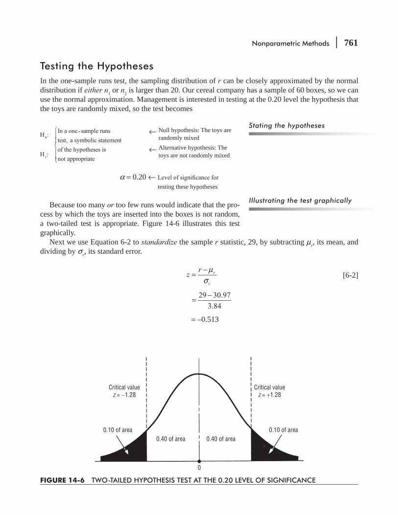
Nonparametric Methods 761
Testing the HypothesesIn the one-sample runs test, the sampling distribution of r can be closely approximated by the normal distribution if either n1 or n2 is larger than 20. Our cereal company has a sample of 60 boxes, so we can use the normal approximation. Management is interested in testing at the 0.20 level the hypothesis that the toys are randomly mixed, so the test becomes
- ←
←
Null hypothesis: The toys are randomly mixedAlternative hypothesis: The toys are not randomly mixed
α = 0.20 ← testing these hypotheses
Because too many or too few runs would indicate that the pro-cess by which the toys are inserted into the boxes is not random, a two-tailed test is appropriate. Figure 14-6 illustrates this test graphically.
Next we use Equation 6-2 to standardize the sample r statistic, 29, by subtracting μr, its mean, and dividing by σ r, its standard error.
μ
σ−= r
r
r [6-2]
29 30.97
3.84
−=
= –0.513
Stating the hypotheses
Illustrating the test graphically
Critical valuez = +1.28
Critical valuez = −1.28
0.10 of area 0.10 of area0.40 of area0.40 of area
0
FIGURE 14-6 TWO-TAILED HYPOTHESIS TEST AT THE 0.20 LEVEL OF SIGNIFICANCE
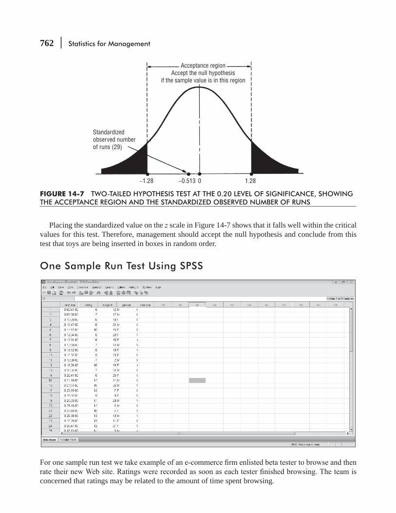
762 Statistics for Management
Placing the standardized value on the z scale in Figure 14-7 shows that it falls well within the critical values for this test. Therefore, management should accept the null hypothesis and conclude from this test that toys are being inserted in boxes in random order.
One Sample Run Test Using SPSS
concerned that ratings may be related to the amount of time spent browsing.
Standardizedobserved numberof runs (29)
−1.28 −0.513 0 1.28
Acceptance regionAccept the null hypothesis
if the sample value is in this region
FIGURE 14-7 TWO-TAILED HYPOTHESIS TEST AT THE 0.20 LEVEL OF SIGNIFICANCE, SHOWING THE ACCEPTANCE REGION AND THE STANDARDIZED OBSERVED NUMBER OF RUNS

Nonparametric Methods 763
For one sample run tetst go to

764 Statistics for Management
Runs tests can be used effectively in quality control situations. You will recall from Chapter 10 that variation in quality is either systematic or random, and if it’s systematic variation we can cor-rect it. Thus, a runs test can detect the kinds of patterns in output quality that are associated with systematic variation. Hint: Almost all runs tests are two-tailed because the question to be answered is whether there are too many or too few runs. Remember also that runs tests use the r statistic whose distribution can be well described by a normal distribution as long as either n1 or n2 is larger than 20.
HINTS & ASSUMPTIONS
EXERCISES 14.4
Self-Check ExerciseSC 14-5 Professor Ike Newton is interested in determining whether his brightest students (those mak-
ing the best grades) tend to turn in their tests earlier (because they can recall the material faster) or later (because they take longer to write down all they know) than the others in the class. For a particular physics test, he observes that the students make the following grades in order of turning their tests in:
Grades1–10 94 70 85 89 92 98 63 88 74 8511–20 69 90 57 86 79 72 80 93 66 7421–30 50 55 47 59 68 63 89 51 90 88
(a) If Professor Newton counts those making a grade of 90 and above as his brightest stu-
turned their tests in randomly?(b) If 60 and above is passing in Professor Newton’s class, then did the students passing
-cance level.)
Basic Concepts14-24
A, B, A, A, A, B, B, A, B, B, A, A, B, A, B, A, A, B, B, B, B, A, B, B,A, A, A, B, A, B, A, A, B, B, A, B, B, A, A, A, B, B, A, A, B, A, A, A
Applications14-25 A sequence of small glass sculptures was inspected for shipping damage. The sequence of
acceptable and damaged pieces was as follows:
D, A, A, A, D, D, D, D, D, A, A, D, D, A, A, A, A, D, A, A, D, D, D, D, D
Nonparametric Methods 765
14-26 The News and Clarionto complain about delivery problems with the Sunday paper. For a recent Sunday, these data were as follows:
M, F, F, F, M, M, F, M, F, F, F, F, M, M, M, F, M, F, M, F, F, F, F, M, M, M, M, M
the nature of this problem that would cause you to believe that such a sequence would not be random?
14-27 Kerwin County Social Services Agency kept this record of the daily number of applicants -
ing days.
3, 4, 6, 8, 4, 6, 7, 2, 5, 7, 4, 8, 4, 7, 9, 5, 9, 10,5, 7, 4, 9, 8, 9, 11, 6, 7, 5, 9, 12
Test the randomness of this sequence by seeing whether the values above and below the -
reached?14-28 A restaurant owner has noticed over the years that older couples appear to eat earlier than
young couples at his quiet, romantic restaurant. He suspects that perhaps it is because of chil-dren having to be left with babysitters and also because the older couples may retire earlier at night. One night, he decided to keep a record of couples’ arrivals at the restaurant. He noted whether each couple was over or under 30. His notes are reproduced below. (A = 30 and older; B = younger than 30.)
(5:30 P.M.) A, A, A, A, A, A, B, A, A, A, A, A, A, B, B,B, A, B, B, B, B, B, B, A, B, B, B, A, B, B, B, (10 P.M.)
of his customers at different dining hours is less than random?14-29 Kathy Phillips is in charge of production scheduling for a printing company. The company
has six large presses, which frequently break down, and one of Kathy’s biggest problems is meeting deadlines when there are unexpected breakdowns in presses. She suspects that the older presses break down earlier in the week than the new presses, because all presses are checked and repaired over the weekend. To test her hypothesis, Kathy recorded the number of all the presses as they broke down during the week. Presses numbered 1, 2, and 3 are the older ones.
1, 2, 3, 1, 4, 5, 3, 1, 2, 5, 1, 3, 6, 2, 3, 6, 2, 2, 3, 5, 4,6, 4, 2, 1, 3, 4, 5, 5, 1, 4, 5, 2, 3, 5, 6, 4, 3, 2, 5, 4, 3
-downs of presses are not random?
(b) Is her hypothesis appropriate for the decision she wishes to make about rescheduling more work earlier in the week on the newer presses?
766 Statistics for Management
14-30
her responsibility. The department employs a number of research assistants to do some analyses and uses a computer to do other analyses. Typically, each week Martha randomly chooses completed analyses before they are reported and conducts tests to ensure that they have been done correctly and thoroughly. Martha’s assistant, Kim Tadlock, randomly
the reanalyses. Martha wanted to make certain that the selection process was a random one, so she could provide assurances that the computer analyses and those done by hand were both periodically checked. She arranged to have the research assistants place a special
mark, so the randomness of the test would not be affected. Kim completed her sample with the following data:
(1: by computer, 2: by hand)
1, 1, 1, 1, 1, 1, 1, 1, 1, 2, 1, 1, 1, 1, 1, 1, 1, 1, 1, 2, 1, 1, 1, 1, 1,1, 1, 1, 1, 2, 1, 1, 1, 1, 1, 1, 1, 1, 1, 2, 1, 1, 1, 1, 1, 1, 1, 1, 1
(b) If the sample were distributed as follows, would the sample be random?
1, 1, 1, 1, 1, 1, 1, 1, 1, 1, 1, 1, 1, 1, 1, 1, 1, 1, 1, 1, 1, 1, 1, 1, 1,1, 1, 1, 1, 1, 1, 1, 1, 1, 1, 1, 1, 1, 1, 1, 1, 1, 1, 1, 1, 2, 2, 2, 2
(c) Because computer analyses are much faster than those done by hand, and because a number of the analyses can be done by computer, there are about three times as many computer analyses per week as hand analyses. Is there statistical evidence in part (a) to support the belief that somewhere in the sampling process there is something less than randomness occurring? If so, what is the evidence?
(d) Does the conclusion you reached in part (c) lead you to any new conclusions about the one-sample runs test, particularly in reference to your answer in part (a)?
14-31 Bank of America is curious about the grade level of people who use their ATM at the Student
are presented below for 45 people who used the ATM during one Friday afternoon. Test this
BBBAAABAAAAAABBBBABAAAABBAABBBBABBBBAAAAAABBB
14-32 -peared last Tuesday with this notation:
M, F, M, M, M, M, F, F, M, M, M, F, M, M, M, M, M, F, F, M,F, M, M, M, F, M, M, M, M, M, M, F, M, M, M, M, M, F, F, M
banking or in the nature of this problem that would lead you to accept intuitively what you have found statistically?
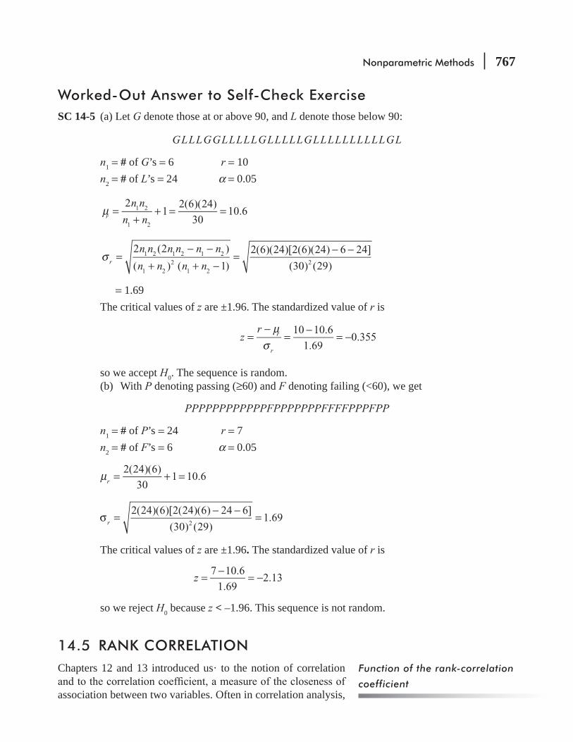
Nonparametric Methods 767
Worked-Out Answer to Self-Check ExerciseSC 14-5 (a) Let G denote those at or above 90, and L denote those below 90:
GLLLGGLLLLLGLLLLLGLLLLLLLLLLGL
n1 = # of G’s = 6 r = 10n2 = # of L’s = 24 α = 0.05
n n
n n
21
2(6)(24)
3010.6r
1 2
1 2
μ =+
+ = =
n n n n n n
n n n n
2 (2 )
( ) ( 1)
2(6)(24)[2(6)(24) 6 24]
(30) (29)r1 2 1 2 1 2
1 22
1 22
σ =− −
+ + −=
− −
= 1.69The critical values of z are ±1.96. The standardized value of r is
zr 10 10.6
1.690.355r
r
μσ
=−
=−
= −
so we accept H0. The sequence is random.(b) With P denoting passing (≥60) and F denoting failing (<60), we get
PPPPPPPPPPPPFPPPPPPPFFFFPPPFPP
n1 = # of P’s = 24 r = 7n2 = # of F’s = 6 α = 0.05
2(24)(6)
301 10.6μ = + =r
2(24)(6)[2(24)(6) 24 6]
(30) (29)1.69r 2
σ =− −
=
The critical values of z are ±1.96. The standardized value of r is
7 10.62.13
1.69z
−= = −
so we reject H0 because z < –1.96. This sequence is not random.
14.5 RANK CORRELATIONChapters 12 and 13 introduced us· to the notion of correlation
association between two variables. Often in correlation analysis,
Function of the rank-correlation
coefficient
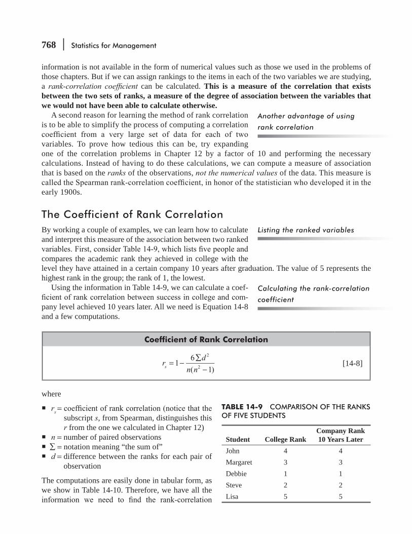
768 Statistics for Management
information is not available in the form of numerical values such as those we used in the problems of those chapters. But if we can assign rankings to the items in each of the two variables we are studying, a rank-correlation coef cient can be calculated. This is a measure of the correlation that exists between the two sets of ranks, a measure of the degree of association between the variables that we would not have been able to calculate otherwise.
A second reason for learning the method of rank correlation is to be able to simplify the process of computing a correlation
variables. To prove how tedious this can be, try expanding one of the correlation problems in Chapter 12 by a factor of 10 and performing the necessary calculations. Instead of having to do these calculations, we can compute a measure of association that is based on the ranks of the observations, not the numerical values of the data. This measure is
early 1900s.
The Coefficient of Rank CorrelationBy working a couple of examples, we can learn how to calculate and interpret this measure of the association between two ranked
compares the academic rank they achieved in college with the level they have attained in a certain company 10 years after graduation. The value of 5 represents the highest rank in the group; the rank of 1, the lowest.
Using the information in Table 14-9, we can calculate a coef--
pany level achieved 10 years later. All we need is Equation 14-8 and a few computations.
Coefficient of Rank Correlation
rd
n n1
6
( 1)s
2
2= −
∑−
[14-8]
where
rs = subscript s, from Spearman, distinguishes this r from the one we calculated in Chapter 12)
n = number of paired observations ∑ = notation meaning “the sum of” d = difference between the ranks for each pair of
observation
The computations are easily done in tabular form, as we show in Table 14-10. Therefore, we have all the
Another advantage of using
rank correlation
Listing the ranked variables
Calculating the rank-correlation
coefficient
TABLE 14-9 COMPARISON OF THE RANKS OF FIVE STUDENTS
Student College RankCompany Rank 10 Years Later
John 4 4Margaret 3 3Debbie 1 1Steve 2 2Lisa 5 5
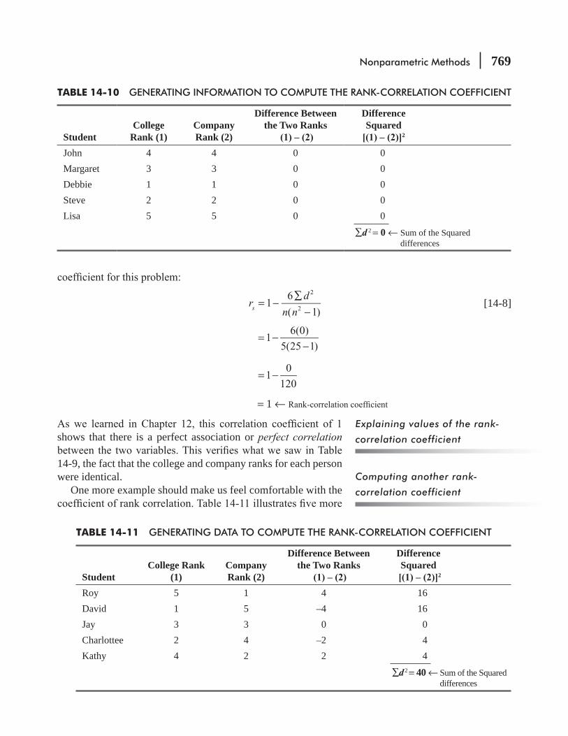
Nonparametric Methods 769
rd
n n1
6
( 1)s
2
2= −
∑−
[14-8]
6(0)1
5(25 1)= −
−
01
120= −
= 1 ←
shows that there is a perfect association or perfect correlation
14-9, the fact that the college and company ranks for each person were identical.
One more example should make us feel comfortable with the
Explaining values of the rank-
correlation coefficient
Computing another rank-
correlation coefficient
TABLE 14-10 GENERATING INFORMATION TO COMPUTE THE RANK-CORRELATION COEFFICIENT
StudentCollege
Rank (1)Company Rank (2)
Difference Between the Two Ranks
Difference Squared
2
John 4 4 0 0Margaret 3 3 0 0Debbie 1 1 0 0Steve 2 2 0 0Lisa 5 5 0 0
∑d 2 = 0 ← Sum of the Squared differences
TABLE 14-11 GENERATING DATA TO COMPUTE THE RANK-CORRELATION COEFFICIENT
StudentCollege Rank
(1)Company Rank (2)
Difference Between the Two Ranks
Difference Squared
2
Roy 5 1 4 16David 1 5 –4 16Jay 3 3 0 0Charlottee 2 4 –2 4Kathy 4 2 2 4
∑d 2 = 40 ← Sum of the Squared differences

770 Statistics for Management
people, but this time the ranks in college and in a company 10 years later seem to be extreme opposites. d 2, and then take
the sum of all the d 2 -
rd
n n1
6
( 1)s
2
2= −
∑−
[14-8]
6(40)1
5(25 1)= −
−
240
1120
= −
= 1 – 2 = –1 ←
represents perfect inverse correlation. And that is just what hap-pened in our case: The people who did the best in college wound up 10 years later in the lowest ranks of an organization. Now let’s apply these ideas.
Solving a Problem Using Rank CorrelationRank correlation is a useful technique for looking at the connection between air quality and the evidence of pulmonary-related diseases that we discussed in our chapter-opening problem. Table 14-12 repro-duces the data found by the health organization studying the problem. In the same table, we also do
rs.
− [14-8]
6(58)1
11(121 1)= −
−
3481
1,320= −
= 1 – 0.2636 = 0.7364 ←
association between average air quality and the occurrence of pulmonary disease, at least in the 11 cities sampled; that is, high levels of pollution go with high incidence of pulmonary disease.
How can we test this value of 0.736? We can apply the same methods we used to test hypotheses in Chapter 8 and 9. In performing such tests on rs, We are trying to avoid the error of concluding that
Interpreting the results
Finding the rank-correlation
coefficient
Interpreting the results

Nonparametric Methods 771
an association exists between two variables if, in fact, no such association exists in the population from which these two samples were drawn, that is, if the population ρs (rho sub s), is really equal to zero.
For small values of n, (n less than or equal to 30), the distribution of rs is not normal, and unlike other small sample statistics we have encountered, it is not appropriate to use the t distribution for testing hypotheses about the rank-correlation
. Instead, we use Appendix Table 7, Spearman’s Rank Correlation Values, to determine the acceptance and rejection regions for such hypotheses. In our current problem, suppose that the health
in the ranked data of all cities in the world. Our problem then becomes:
H0: ρs = 0 ← Null hypothesis: There is no correlation in the ranked data of the population
H1: ρs ≠ 0 ← Alternative hypothesis: There is a correla-tion in the ranked data of the populations
α = 0.05 ←
A two-tailed test is appropriate, so we look at Appendix Table 7 in the row for n = 11 (the number s are
±0.6091, that is, the upper limit of the acceptance region is 0.6091, and the lower limit of the acceptance region is –0.6091.
acceptance region. Therefore, we would reject the null hypothesis of no correlation and conclude that there is an association between air-quality levels and the incidence of pulmonary disease in the world’s cities.
Testing hypotheses about rank
correlation
Stating the hypotheses
TABLE 14-12 RANKING OF ELEVEN CITIES
City
Air Quality Rank
(1)
Pulmonary-Disease Rank
(2)
Difference between the Two Ranks Difference Squared
2
A 4 5 –1 1B 7 4 3 9C 9 7 2 4D 1 3 –2 4E 2 1 1 1F 10 11 –1 1G 3 2 1 1H 5 10 –5 25I 6 8 –2 4J 8 6 2 4K 11 9 2 4
Best rank = 11 Worst rank = 1
∑d 2 = 58 ← Sum of the squared differences

772 Statistics for Management
If the sample size is greater than 30, we can no longer use Appendix Table 7. However, when n is greater than 30, the sam-pling distribution of rs is approximately normal, with a mean of zero and a standard deviation of n1/ 1.− Thus, the standard error of rs is,
Standard Error of the Coefficient of Rank Correlation
n
1
1rs
σ =−
[14-9]
z values for testing hypotheses about the population rank correlation.
As an example of hypothesis testing of rank-correlation coef- n is greater than 30, consider the case of a social
scientist who tries to determine whether bright people tend to choose spouses who are also bright. He
of the couples. His data and computations are given in Table 14-13.
problem:
rd
n n1
6
( 1)s
2
2= −
∑−
[14-8]
6(1,043.51
32(1,024 1)= −
−
Example with n greater than 30
Critical value fromAppendix Table 7
Critical value fromAppendix Table 7
Distribution of rsfor 11 sample points
Sample rank-correlationcoefficient of 0.736
−0.6091 0.60910
Acceptance regionAccept the null hypothesis
if the sample value is in this region
FIGURE 14-8 TWO-TAILED HYPOTHESIS TEST, USING APPENDIX TABLE 7 AT THE 0.05 LEVEL OF SIGNIFICANCE, SHOWING THE ACCEPTANCE REGION AND SAMPLE RANK-CORRELATION COEFFICIENT.
The appropriate distribution ‘for
values of n greater than 30
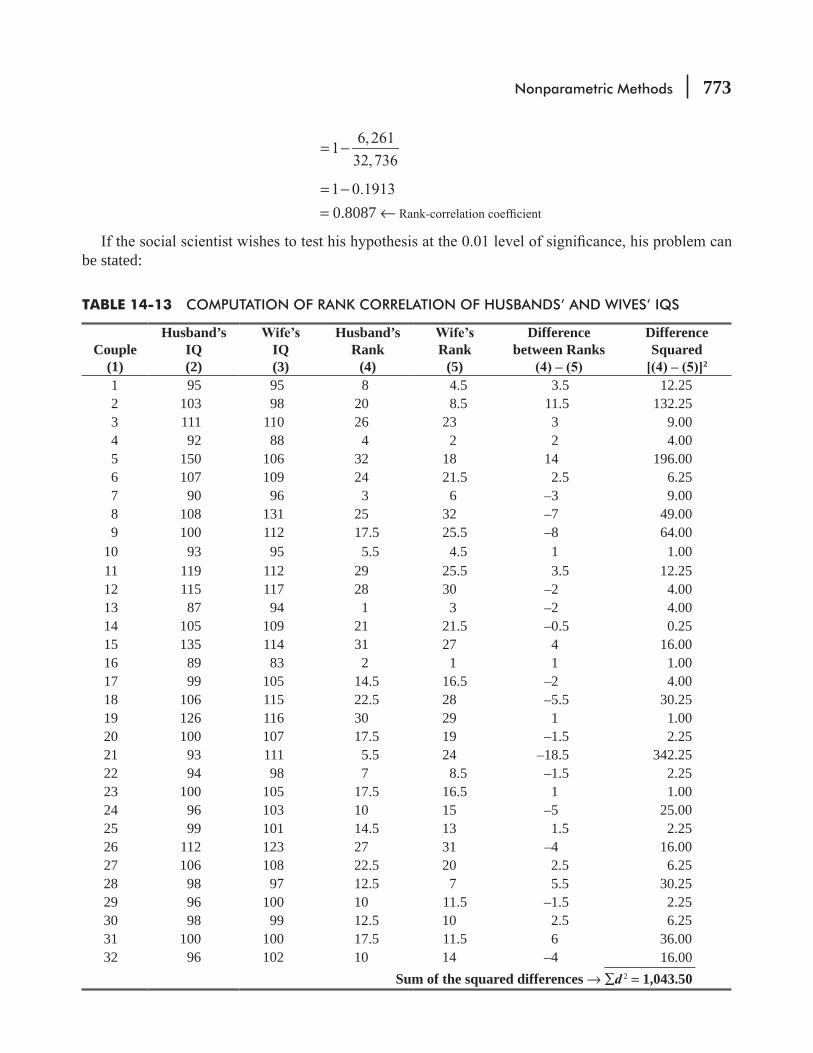
Nonparametric Methods 773
6,2611
32,736= −
1 0.1913= − = 0.8087 ←
be stated:
TABLE 14-13 COMPUTATION OF RANK CORRELATION OF HUSBANDS’ AND WIVES’ IQS
Couple (1)
Husband’sIQ(2)
IQ(3)
Husband’sRank
(4)Rank
(5)
Difference between Ranks
Difference Squared
2
1 95 95 8 4.5 3.5 12.252 103 98 20 8.5 11.5 132.253 111 110 26 23 3 9.004 92 88 4 2 2 4.005 150 106 32 18 14 196.006 107 109 24 21.5 2.5 6.257 90 96 3 6 –3 9.008 108 131 25 32 –7 49.009 100 112 17.5 25.5 –8 64.00
10 93 95 5.5 4.5 1 1.0011 119 112 29 25.5 3.5 12.2512 115 117 28 30 –2 4.0013 87 94 1 3 –2 4.0014 105 109 21 21.5 –0.5 0.2515 135 114 31 27 4 16.0016 89 83 2 1 1 1.0017 99 105 14.5 16.5 –2 4.0018 106 115 22.5 28 –5.5 30.2519 126 116 30 29 1 1.0020 100 107 17.5 19 –1.5 2.2521 93 111 5.5 24 –18.5 342.2522 94 98 7 8.5 –1.5 2.2523 100 105 17.5 16.5 1 1.0024 96 103 10 15 –5 25.0025 99 101 14.5 13 1.5 2.2526 112 123 27 31 –4 16.0027 106 108 22.5 20 2.5 6.2528 98 97 12.5 7 5.5 30.2529 96 100 10 11.5 –1.5 2.2530 98 99 12.5 10 2.5 6.2531 100 100 17.5 11.5 6 36.0032 96 102 10 14 –4 16.00
Sum of the squared differences → ∑d 2 = 1,043.50

774 Statistics for Management
H0: σs = 0 ← Null hypothesis: There is no rank correlation in the population; that is, husbands’ intelligence and wives’ intelligence are randomly mixed
H1: σs > 0 ← Alternative hypothesis: The population rank correlation is positive; that is, bright people choose bright spouses
α = 0.01 ←
z value for
there the colored region in the upper tail of the distribution that corresponds to the 0.01 level of
rs:
n
1
1rs
σ =−
[14-9]
10.1796
32 1= =
−
Now we can use Equation 6-2 to standardize rs, by subtracting 0, its hypothesized value, and dividing by rs
σ , its standard error.
zr 0s
rs
=−
σ [6-2]
= 4.503
Figure 14-10 shows the limit of the acceptance region and the
correlation and conclude that bright people tend to choose bright spouses.
Interpreting the results
Critical valuez = 2.33
0.50 of area 0.49 of area0.01 of area
PsH0 = 0
FIGURE 14-9 UPPER-TAILED HYPOTHESIS TEST AT THE 0.01 LEVEL OF SIGNIFICANCE

Nonparametric Methods 775
A Special Property of Rank CorrelationRank correlation has a useful advantage over the correlation method we discussed in Chapter 12. Suppose we have cases in which one or several very extreme observations exist in the origi-
be a good description of the association that exists between two variables. Yet extreme observations in a rank-correlation test will never produce a large rank difference.
Consider the following data array of two variables, x and y:
X 10 13 16 19 25Y 34 40 45 51 117
y r using the conventional and the rank-correlation methods. In this case, the rank-correlation method would be less sensitive to the extreme value. We would assign a rank order of 5 to the numerical value
When there are extreme values in the original data, rank correlation can produce more useful results than the correlation method explained in Chapter 12 because extreme observations never produce a large difference in rank. Hint: Rank correlation is very useful when data are non-normally distributed. Take the case of university fund-raising where you get a few “big hitter” gifts, lots and lots of gifts below $100, and a very broad range in between. Using the correlation techniques of Chapter 12 to investigate the relationship between number of appeal mailings and size of gift with this kind of distribution doesn’t make sense because the million-dollar gifts would
HINTS & ASSUMPTIONS
Advantage of rank correlation
Distribution of rs
Acceptance regionAccept the null hypothesis
if the sample value is in this region
Standardized sample rankcorrelation coefficient
2.33 4.5030
FIGURE 14-10 UPPER-TAILED HYPOTHESIS TEST AT THE 0.01 LEVEL OF SIGNIFICANCE, SHOWING THE ACCEPTANCE REGION AND THE STANDARDIZED SAMPLE RANK-CORRELATION COEFFICIENT
776 Statistics for Management
EXERCISES 14.5
Self-Check ExerciseSC 14-6 The following are ratings of aggressiveness (X) and amount of sales in the last year (Y) for
X 30 17 35 28 42 25 19 29Y 35 31 43 46 50 32 33 42
Applications14-33 The following are years of experience (X) and average customer satisfaction (Y) for 10 service
-
X 6.3 5.8 6.1 6.9 3.4 1.8 9.4 4.7 7.2 2.4Y 5.3 8.6 4.7 4.2 4.9 6.1 5.1 6.3 6.8 5.2
14-34 A plant supervisor ranked a sample of eight workers on the number of hours of overtime -
cant at the 0.01 level?
Amount of over time 5.0 8.0 2.0 4.0 3.0 7.0 1.0 6.0Years employed 1.0 6.0 4.5 2.0 7.0 8.0 4.5 3.0
14-35 Most people believe that managerial experience produces better interpersonal relationships -
correlation between these two suggest that experience improves relationships?
Years of experience 7 18 17 4 21 27 20 14 15 10Number of grievances 5 2 4 4 3 2 4 5 4 6
14-36 The Occupational Safety and Health Administration (OSHA) was conducting a study of the relationship between expenditures for plant safety and the accident rate in the plants. OSHA
that existed among some of the plants, OSHA had converted its data into expenditures per production employee. The results follow:
Expenditure by Chemical Companies per Production Employee in Relation to Accidents per Year
Company A B C D E F G H I J KExpenditure $60 $37 $30 $20 $24 $42 $39 $54 $48 $58 $26Accidents 2 7 6 9 7 4 8 2 4 3 8

Nonparametric Methods 777
plants? Use a rank correlation (with 1 representing highest expenditure and accident rate) to
14-37 graduates based on grades alone. One professor thought that the number of years of experi-ence MBAs had before returning for their degrees was probably a better predictor. Using the
career success?
Years experience 4 3 4 3 6 7 1 5 5 2
Grade-point average 3.4 3.2 3.5 3.0 2.9 3.4 2.5 3.9 3.6 3.0
Success rank (10 = top) 4 2 6 5 7 9 1 8 10 3
14-38 The Carolina Lighting Company has two trained interviewers to recruit manager trainees for new sales outlets. Although each of the interviewers has a unique style, both are thought to be good preliminary judges of managerial potential. The personnel manager wondered how closely the interviewers would agree, so she had both of them independently evaluate 14 applicants. They ranked the applicants in terms of their degree of potential contribution to
rankings.
Applicant 1 2 3 4 5 6 7 8 9 10 11 12 13 14
Interviewer 1 1 11 13 2 12 10 3 4 14 5 6 9 7 8
Interviewer 2 4 12 11 2 14 10 1 3 13 8 6 7 9 5
14-39 Nancy McKenzie, supervisor for a lithographic camera assembly process, feels that the longer a group of employees works together, the higher the daily output rate. She gathered the follow-
Day 1 2 3 4 5 6 7 8 9 10
4.0 7.0 5.0 6.0 8.0 2.0 3.0 0.5 9.0 6.0
number of days worked together and the daily output?14-40 -
that the population rank correlation between applicants’ résumés scored by the personnel de-
and use résumé scores to hire?

778 Statistics for Management
IndividualInterview
ScoreRésumé
Score IndividualInterview
ScoreRésumé
Score1 81 113 19 81 1112 88 88 20 84 1213 55 76 21 82 834 83 129 22 90 795 78 99 23 63 716 93 142 24 78 1087 65 93 25 73 688 87 136 26 79 1219 95 82 27 72 109
10 76 91 28 95 12111 60 83 29 81 14012 85 96 30 87 13213 93 126 31 93 13514 66 108 32 85 14315 90 95 33 91 11816 69 65 34 94 14717 87 96 35 94 13818 68 101
14-41 The following are salary and age data for the 10 Ph.D. candidates graduating this year from
rank correlation of age and salary suggest that older candidates get higher starting salaries?
Salary Age$67,000 29
60,000 25
57,500 30
59,500 35
50,000 27
55,000 31
59,500 32
63,000 38
69,500 28
72,000 34
14-42 Dee Boone operates a repair facility for light-aircraft engines. He is interested in improving his estimates of repair time required and believes that the best predictor is the number of operating hours on the engine since its last major repair. Below are data on ten engines Dee
relationship?
Nonparametric Methods 779
EngineHouse Since Last
Major RepairHouse Required
to Repair1 1,000 402 1,200 543 900 414 1,450 605 2,000 656 1,300 507 1,650 428 1,700 659 500 43
10 2,100 66
Worked-Out Answer to Self-Check ExerciseSC 14-6
X(ranks) 6 1 7 4 8 3 2 5Y(ranks) 4 1 6 7 8 2 3 5d 2 0 1 –3 0 1 –1 0d 2 4 0 1 9 0 1 1 0
∑d 2 = 16 n = 8 α = 0.10H0: ρs = 0 H1: ρs ≠ 0
rd
n n1
6
( 1)1
6(16)
8(63)0.8095s
2
2= −
∑−
= − =
From Appendix Table 7, the critical values for rs are ±0.6190. Because 0.8095 > 0.6190, we reject H0
14.6 THE KOLMOGOROV-SMIRNOV TESTThe Kolmogorov-Smirnov test, named for statisticians A. N. Kolmogorov and N. V. Smirnov, is a simple nonparametric
between an observed frequency distribution and a theoretical frequency distribution. The K-S test is therefore another measure of the goodness-of- t of a theoretical frequency distribution, as was the chi-square test we studied in Chapter 11. However, the K-S test has several advantages over the χ 2 test: It is a more powerful test, and it is easier to use because it does not require that data be grouped in any way.
The K-S statistic, Dn, is particularly useful for judging how close the observed frequency distribution is to the expected frequency distribution, because the probability distribution of Dn depends on the sample size n but is independent of the expected frequency distribution (Dn is a distribution-free statistic).
The K-S test and its advantages
A special advantage

780 Statistics for Management
A Problem Illustrating the K-S TestSuppose that the Orange County Telephone Exchange has been keeping track of the number of “send-ers” (a type of automatic equipment used in telephone exchanges) that were in use at a given instant. Observations were made on 3,754 different occasions. For capital-investment planning purposes, the
We would set up our hypotheses like this:
H0: A Poisson distribution with λ = 8.5 is a good description of the pattern of usage ← Null hypothesis
H1: A Poisson distribution with λ = 8.5 is not a good description of the pattern of usage ← Alternative hypothesis
α = 0.01 ←
Next, we would list the data that we observed. Table 14-14 lists the observed frequencies and transforms them into observed rela-tive cumulative frequencies.
Now we can use the Poisson formula to compute the expected frequencies.
p xe
x( )
!
xλ=
× λ− [5-4]
By comparing these expected frequencies with our observed frequencies, we can examine the extent of the difference between them: the absolute deviation. Table 14-15 lists the observed relative cumu-lative frequencies Fo, the expected relative cumulative frequencies Fe, and the absolute deviations for x = 0 to 22.
Calculating the K-S StatisticTo compute the K-S statistic for this problem, you simply pick out Dn, the maximum absolute deviation of Fe from Fo.
K-S Statistic
Dn = max | Fe – Fo | [14-10]
In this problem, dn = 0.2582 at x = 9.A K-S test must always be a one-tailed test. The critical val-
ues for Dn have been tabulated and can be found in Appendix Table 8. By looking in the row for n = 3,754 (the sample size)
Stating the hypotheses
Computing and comparing
expected frequencies
Computing the K-S statistic
Computing the critical value
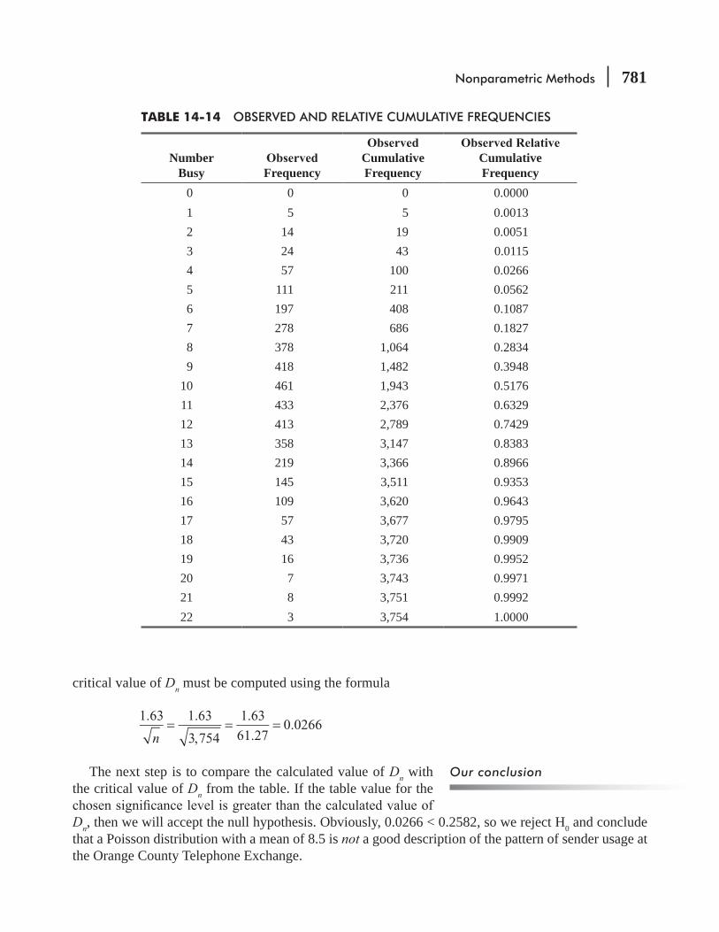
Nonparametric Methods 781
critical value of Dn must be computed using the formula
n
1.63 1.63
3,754
1.63
61.270.0266= = =
The next step is to compare the calculated value of Dn with the critical value of Dn from the table. If the table value for the
Dn, then we will accept the null hypothesis. Obviously, 0.0266 < 0.2582, so we reject H0 and conclude that a Poisson distribution with a mean of 8.5 is not a good description of the pattern of sender usage at the Orange County Telephone Exchange.
Our conclusion
TABLE 14-14 OBSERVED AND RELATIVE CUMULATIVE FREQUENCIES
NumberBusy Frequency
CumulativeFrequency
Cumulative Frequency
0 0 0 0.00001 5 5 0.00132 14 19 0.00513 24 43 0.01154 57 100 0.02665 111 211 0.05626 197 408 0.10877 278 686 0.18278 378 1,064 0.28349 418 1,482 0.3948
10 461 1,943 0.517611 433 2,376 0.632912 413 2,789 0.742913 358 3,147 0.838314 219 3,366 0.896615 145 3,511 0.935316 109 3,620 0.964317 57 3,677 0.979518 43 3,720 0.990919 16 3,736 0.995220 7 3,743 0.997121 8 3,751 0.999222 3 3,754 1.0000

782 Statistics for Management
Kolmogrov–Smirnov Test Using SPSS
TABLE 14-15 RELATIVE OBSERVED CUMULATIVE FREQUENCIES, EXPECTED RELATIVE CUMULATIVE FREQUENCIES, AND ABSOLUTE DEVIATIONS
Number Busy Frequency
Cumulative Frequency
Relative Cumulative Frequency
ExpectedRelative
CumulativeFrequency
⎢Fe – Fo ⎢
AbsoluteDeviation
0 0 0 0.0000 0.0002 0.00021 5 5 0.0013 0.0019 0.00062 14 19 0.0051 0.0093 0.00423 24 43 0.0115 0.0301 0.01864 57 100 0.0266 0.0744 0.04785 111 211 0.0562 0.1496 0.09346 197 408 0.1087 0.2562 0.14757 278 686 0.1827 0.3856 0.20298 378 1,064 0.2834 0.5231 0.23979 418 1,482 0.3948 0.6530 0.2582
10 461 1,943 0.5176 0.7634 0.245811 433 2,376 0.6329 0.8487 0.215812 413 2,789 0.7429 0.9091 0.166213 358 3,147 0.8383 0.9486 0.110314 219 3,366 0.8966 0.9726 0.076015 145 3,511 0.9353 0.9862 0.050916 109 3,620 0.9643 0.9934 0.029117 57 3,677 0.9795 0.9970 0.017518 43 3,720 0.9909 0.9987 0.007819 16 3,736 0.9952 0.9995 0.004320 7 3,743 0.9971 0.9998 0.002721 8 3,751 0.9992 0.9999 0.000722 3 3,754 1.0000 1.0000 0.0000
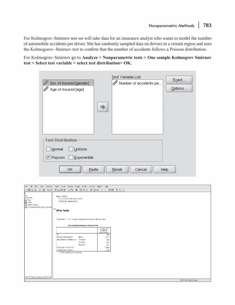
Nonparametric Methods 783
For Kolmogrov–Smirnov test we will take data for an insurance analyst who wants to model the number of automobile accidents per driver. She has randomly sampled data on drivers in a certain region and uses
For Kolmogrov–Smirnov go to

784 Statistics for Management
Think of the Kolmogorov-Smirnov test as another goodness-of- t test, just like the chi-square test in Chapter 11, except that this time it’s easier to use because we do not have to do all the arithmetic
both observed frequencies and expected frequencies and then tests how far apart they are. If the
distribution. Hint: K-S tests are always one-tailed tests because we are always testing whether
HINTS & ASSUMPTIONS
EXERCISES 14.6
Self-Check ExerciseSC 14-7 The following is an observed frequency distribution. Using a normal distribution with μ = 6.80
and σ = 1.24:(a) Find the probability of falling into each class.(b) From part (a), compute the expected frequency of each category.(c) Calculate Dn.
suggested normal distribution?
Value of the variable ≤4.009 4.010–5.869 5.870–7.729 7.730–9.589 >9.59013 158 437 122 20
Basic Concepts14-43
distribution with λ = 3?
Number of arrivals per day 0 1 2 3 4 5 6 or moreNumber of days 6 18 30 24 11 2 9
14-44 The following is an observed frequency distribution. Using a normal distribution with μ = 98.6 and σ = 3.78(a) Find the probability of falling into each class.(b) From part (a), compute the expected frequency of each category.(c) Calculate Dn.(d) At -
gested normal distribution?
Value of the variable <92.0 92.0–95.99 96.0–99.99 100–103.99 69 408 842 621 137
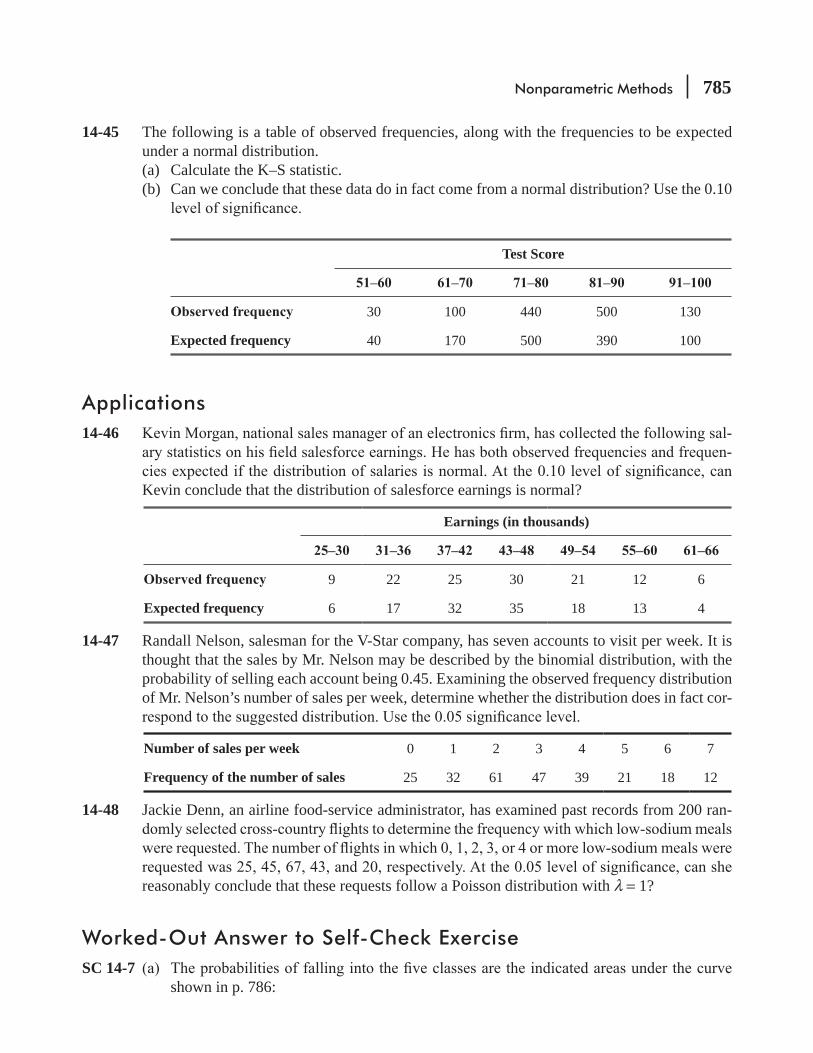
Nonparametric Methods 785
14-45 The following is a table of observed frequencies, along with the frequencies to be expected under a normal distribution.(a) Calculate the K–S statistic.(b) Can we conclude that these data do in fact come from a normal distribution? Use the 0.10
Test Score
30 100 440 500 130
Expected frequency 40 170 500 390 100
Applications14-46 -
-
Kevin conclude that the distribution of salesforce earnings is normal?
Earnings (in thousands)
9 22 25 30 21 12 6
Expected frequency 6 17 32 35 18 13 4
14-47 Randall Nelson, salesman for the V-Star company, has seven accounts to visit per week. It is thought that the sales by Mr. Nelson may be described by the binomial distribution, with the probability of selling each account being 0.45. Examining the observed frequency distribution of Mr. Nelson’s number of sales per week, determine whether the distribution does in fact cor-
Number of sales per week 0 1 2 3 4 5 6 7
Frequency of the number of sales 25 32 61 47 39 21 18 12
14-48 Jackie Denn, an airline food-service administrator, has examined past records from 200 ran-
reasonably conclude that these requests follow a Poisson distribution with λ = 1?
Worked-Out Answer to Self-Check ExerciseSC 14-7
shown in p. 786:

786 Statistics for Management
−2.25 0.75 0.75 2.25
.0122
4.01 5.87 7.73 9.59
.2144 .5468 .2144 .0122x
1.24z = x − 6.80
(b) n = 13 + 158 + 437 + 122 + 20 = 750. Thus, the expected frequencies are 0.0122(750) = 9.15, 0.2144(750) = 160.80, 0.5468(750) = 410.1, 160.80, and 9.15.
(c) fo cum. fo Fo Fe |Fe – Fo|13 13 0.0173 0.0122 0.0051
158 171 0.2280 0.2266 0.0014437 608 0.8107 0.7734 0.0373122 730 0.9733 0.9878 0.014520 750 1.0000 1.0000 0.0000
(d) Dn
1.14 1.14
7500.0416.table = = = Dn < Dtable, so accept H0.
The data are well described by the suggested normal distribution.
STATISTICS AT WORK
Loveland ComputersCase 14: Nonparametric Methods “I forgot to tell you,” said Sherrel Wright, the advertising man-
before you start on this advertising project.”“I need help!” Margot announced in a voice that could be heard in Cheyenne, Wyoming. “I spent a
lot of money to get some data, and now that it’s here, I don’t know what we’ve got.”“Well I don’t either,” Lee joked, trying to lighten the mood. “Why don’t you tell me what’s going on.”“For some of the midrange models—basically PCs with fast chips and a reasonable amount of disk
storage—we can make them look three different ways. The old AT style machines are the size of a small suitcase. People liked the big box because it had the image of a big, powerful machine. But in the last year or so, some of the very powerful workstations have been made in a pizza box format with a fairly
just the same innards in a smaller box that does not take up as much desk space. Finally, some competi-
“So which style did Loveland go with?” Lee asked.
Nonparametric Methods 787
“Frankly, we’ve been all over the place—during different marketing campaigns. Sometimes we’ve offered two of the three formats, but we’ve changed back and forth as we’ve tried to guess what custom-
-ing under their desks to use the disk drive.”
“Okay. So offer all three styles,” Lee smiled at this simple-but-elegant solution.“That just adds to our costs. If we run three styles, we lose the volume discounts that we can get by
going with just one. And then we have to advertise three formats while I’m also launching new high-end products and keeping up with demand for our lowest-price machines. I’d like to be able to recommend the single best format to management.”
“Well, I don’t have a crystal ball,” Lee began.
and Oregon. There were eight people in each group, and two groups at each site, so altogether I’ve got 48 response cards—and several hours of videotaped discussions that I’ll save you from watching. As you’d expect, we asked the participants to rank the three formats in terms of the style they’d prefer if
which of the other two formats would you prefer. Tell me how we’re going to make some sense out of this so I can make a recommendation to the product-planning group.”
Study Questions: How should Lee organize the data and which statistical tests are appropriate? What should Loveland do if the analysis of data from this small group is inconclusive?
CHAPTER REVIEW
Terms Introduced in Chapter 14 A nonparametric test, which does not require that data be grouped in any
-tion and a theoretical frequency distribution.
A nonparametric method for testing whether three or more independent samples have been drawn from populations with the same distribution. It is a nonparametric version of ANOVA, which we studied in Chapter 11.
U Test A nonparametric method used to determine whether two independent sam-ples have been drawn from populations with the same distribution.
Nonparametric Tests Statistical techniques that do not make restrictive assumptions about the shape of a population distribution when performing a hypothesis test.
A nonparametric method for determining the randomness with which the items in a sample have been selected.
Rank Correlation A method for doing correlation analysis when the data are not available to use in
A measure of the degree of association between two variables that is based on the ranks of observations, not their numerical values.
Rank Sum Tests A family of nonparametric tests that the order information in a set of data.
788 Statistics for Management
Run A sequence of identical occurrences preceded and followed by different occurrences or by none at all.
Sign Test A test for the difference between paired observations where + and – signs are substituted for quantitative values.
Theory of Runs A theory developed to allow us to test samples for the randomness of their order.
Equations Introduced in Chapter 14
14-1 U n nn n
R( 1)
21 21 1
1= ++
− p. 746
To apply the Mann–Whitney U test, you need this formula to derive the U statistic, a measure of the difference between the ranked observations of the two variables. R1 is the sum of the ranks of observations of variable 1; n1 and n2 are the numbers of items in samples 1 and 2, respectively. Both samples need not be of the same size.
14-2 n n2
U1 2μ = p. 746
If the null hypothesis of a Mann–Whitney U test is that n1 + n2 observations came from iden-tical populations, then the U statistic has a sampling distribution with a mean equal to the product of n1 and n2 divided by 2.
14-3 n n n n( 1)
12
U1 2 1 2σ =
+ + p. 746
This formula enables us to derive the standard error of the U statistic of a Mann–Whitney U test.
14-4 U n nn n
R( 1)
21 22 2
2= ++
− p. 748
This formula and Equation 14-1 can be used interchangeably to derive the U statistic in the Mann–Whitney U test. To save time, use this formula if the number of observations in sample
14-5 Kn n
R
nn
12
( 1)3( 1)j
j
2
∑=+
− + p. 751
The formula computes the K statistic used in the Kruskal–Wallis test for different means among three or more populations. The appropriate sampling distribution for K is chi-square with k
14-6 n nn n2
1r1 2
1 2
μ =+
+ p. 760
When doing a one-sample runs test, use this formula to derive the mean of the sampling dis-tribution of the r statistic. This r statistic is equal to the number of runs in the sample being tested.
Nonparametric Methods 789
14-7 n n n n n nn n n n2 (2 )
( ) ( 1)
r1 2 1 2 1 2
1 2
2
1 2
σ =− −
+ + − p. 760
This formula enables us to derive the standard error of the r statistic in a one-sample runs test.
14-8 rd
n n1
6
( 1)s
2
2= −
∑−
p. 768
The coef cient of rank correlation, rs, is a measure of the closeness of association between two ranked variables.
14-9 n
1
1
rsσ =
− p. 772
This formula enables us to calculate the standard errorrank correlation.
14-10 Dn = max |Fe – Fo| p. 780
If we compare this computed value to a critical value of Dn in the K–S table, we can test dis-
Review and Application Exercises14-49 A college football coach has a theory that in athletics, success feeds on itself. In other words, he
feels that winning a championship one year increases the team’s motivation to win it the next year. He expressed his theory to a student of statistics, who asked him for the records of the team’s wins and losses over the last several years. The coach gave him a list, specifying whether the team had won (W) or lost (L) the championship that year. The results of this tally are
W, W, W, W, W, W, L, W, W, W, W, W, L, W, W, W, W, L, L, W, W, W, W, W, W
(b) Does your answer to part (a), combined with a sight inspection of the data, tell you any-thing about the one-sample runs test?
14-50 upper-income residential area. Complaints of excessive noise had deluged the airport author-
on the turbines of the jets to reduce noise and help ease the pressure on the authority. Both
they increased fuel consumption. Based on the following random samples of 13 days before
laints?
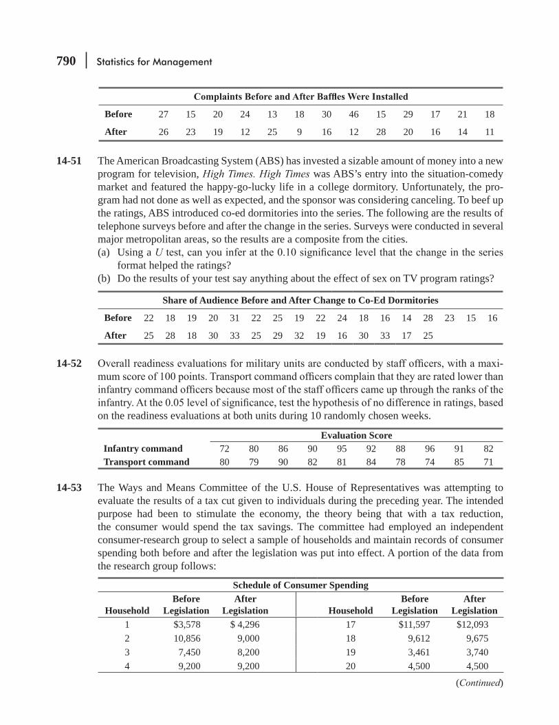
790 Statistics for Management
Before 27 15 20 24 13 18 30 46 15 29 17 21 18
After 26 23 19 12 25 9 16 12 28 20 16 14 11
14-51 The American Broadcasting System (ABS) has invested a sizable amount of money into a new program for television, High Times. High Times was ABS’s entry into the situation-comedy market and featured the happy-go-lucky life in a college dormitory. Unfortunately, the pro-gram had not done as well as expected, and the sponsor was considering canceling. To beef up the ratings, ABS introduced co-ed dormitories into the series. The following are the results of telephone surveys before and after the change in the series. Surveys were conducted in several major metropolitan areas, so the results are a composite from the cities.(a) Using a U
format helped the ratings?(b) Do the results of your test say anything about the effect of sex on TV program ratings?
Share of Audience Before and After Change to Co-Ed Dormitories
Before 22 18 19 20 31 22 25 19 22 24 18 16 14 28 23 15 16
After 25 28 18 30 33 25 29 32 19 16 30 33 17 25
14-52 -
on the readiness evaluations at both units during 10 randomly chosen weeks.
Evaluation ScoreInfantry command 72 80 86 90 95 92 88 96 91 82Transport command 80 79 90 82 81 84 78 74 85 71
14-53 The Ways and Means Committee of the U.S. House of Representatives was attempting to evaluate the results of a tax cut given to individuals during the preceding year. The intended purpose had been to stimulate the economy, the theory being that with a tax reduction, the consumer would spend the tax savings. The committee had employed an independent consumer-research group to select a sample of households and maintain records of consumer spending both before and after the legislation was put into effect. A portion of the data from the research group follows:
Schedule of Consumer Spending
HouseholdBefore
LegislationAfter
Legislation HouseholdBefore
LegislationAfter
Legislation1 $3,578 $ 4,296 17 $11,597 $12,0932 10,856 9,000 18 9,612 9,6753 7,450 8,200 19 3,461 3,7404 9,200 9,200 20 4,500 4,500
(Continued)
Nonparametric Methods 791
Schedule of Consumer Spending
HouseholdBefore
LegislationAfter
Legislation HouseholdBefore
LegislationAfter
Legislation5 8,760 8,840 21 8,341 8,5006 4,500 4,620 22 7,589 7,6097 15,000 14,500 23 25,750 24,3218 22,350 22,500 24 14,673 13,5009 7,346 7,250 25 5,003 6,072
10 10,345 10,673 26 10,940 11,39811 5,298 5,349 27 8,000 9,00712 6,950 7,000 28 14,256 14,50013 34,782 33,892 29 4,322 4,25814 12,837 14,297 30 6,828 7,20415 7,926 8,437 31 7,549 7,67816 5,789 6,006 32 8,129 8,125
its desired goals.14-54 Many entertainment companies have invested in theme parks with tie-ins to hit movies.
Attendance depends on many factors, including the weather. Should the weather be considered a random event?
14-55 Two television weather forecasters got into a discussion one day about whether years with heavy rainfall tended to occur in spurts. One of them said he thought that there were patterns of annual rainfall amounts, and that several wet years were often followed by a number of drier-than-average years. The other forecaster was skeptical and said she thought that the amount of rainfall for consecutive years was fairly random. To investigate the question, they decided to look at the annual rainfall for several years back. They found the median amount
their results follows:
A, A, A, B, B, B, A, B, A, A, B, B, A, B, A, B, A, A, B, B, A, A, A, B, A, A,A, A, A, B, B, B, A, B, B, B, A, B, A, A, A, B, A, A, A, B, A, B, B, A, B, B
-fall amounts do not occur in patterns?
14-56 Anne J. Montgomery, administrative director of executive education at Southern University, uses two kinds of promotional material to announce seminars: personal letters and brochures. She feels quite strongly that brochures are the more effective method. She has collected data on numbers of people attending each of the last 10 seminars promoted with each method. At
Number AttendingPersonal letter 35 85 90 92 88 46 78 57 85 67Brochure 42 74 82 87 45 73 89 75 60 94
(Continued)
792 Statistics for Management
14-57 The National Association of Better Advertising for Children (NABAC), a consumer group for improving children’s television, was conducting a study on the effect of Saturday morning
-ing was stimulated by advertising directed at children, and if there was a positive correlation between Saturday morning TV advertising time and product sales. NABAC chose the children’s breakfast-cereal market as a sample group. It selected prod-ucts whose advertising message was aimed entirely at children. The results of the study follow. (The highest-selling cereal has sales rank 1.)
Comparison of TV Advertising Time and Product Sales Advertising Time
Product in Minutes Sales RankCaptain Grumbles 0.50 10Obnoxious Berries 3.00 1Fruity Hoops 1.25 9OO La Granola 2.00 5Sweet Tweets 3.50 2Chocolate Chumps 1.00 11Sugar Spots 4.00 3County Cavity 2.50 8Crunchy Munchies 1.75 6Karamel Kooks 2.25 4Flakey Flakes 1.50 7
Can the group conclude that there is a positive rank correlation between the amount of Sat-urday morning advertising time and sales volume of break-fast cereals? Test at the 5 percent
14-58 American Motoring Magazine recently tested two brake-disk materials for stopping effective-ness. Data representing stopping distances for both kinds of materials follow. At the 0.05 level of
Stopping Distance (feet)Graphite bonded 110 120 130 110 100 105 110 130 145 125Sintered bronze 100 110 135 105 105 100 100 115 135 120
14-59 As part of a survey on restaurant quality, a local magazine asked area residents to rank two steak houses. On a scale of 1 to 10, subjects were to rate characteristics such as food quality, atmosphere, service, and price. After data were collected, one of the restaurant
he would like to see a mean and standard deviation for the responses to each question about each restaurant, in order to see which one had scored better. Several of the magazine workers argued against his suggestions, noting that the quality of input data would not justify a detailed statistical analysis. They argued that what was important was the residents’ rankings of the two restaurants. Evaluate the arguments presented by the restaurant owner and the magazine employees.

Nonparametric Methods 793
14-60 Senior business students interviewed by the Ohio Insurance Company were asked not to dis-cuss their interviews with others in the school until the recruiter left. The recruiter, however, suspected that the later applicants knew more about what she was looking for. Were her sus-
InterviewNumber Score
InterviewNumber Score
InterviewNumber Score
InterviewNumber Score
1 63 6 57 11 77 16 702 59 7 76 12 61 17 753 50 8 81 13 53 18 904 60 9 58 14 74 19 805 66 10 65 15 82 20 89
14-61 More than 3 years ago, the Occupational Safety and Health Administration (OSHA) required a number of safety measures to be implemented in the Northbridge Aluminum plant. Now OSHA would like to see whether the changes have resulted in fewer accidents in the plant. It has collected these data:
Accidents at the Northbridge PlantJan. Feb. Mar. Apr. May June July Aug. Sept. Nov. Dec.
1992 5 3 4 2 6 4 3 3 2 4 5 31993 4 4 3 3 3 4 0 5 4 2 0 11994 3 2 1 1 0 2 4 3 2 1 1 21995 2 1 0 0 1 2
(a) Determine the median number of accidents per month. If the safety measures have been -
low the median. Accordingly, there will be a small number of runs above and below the
randomly distributed.(b) What can you conclude about the effectiveness of the safety measures?
14-62 A large countywide ambulance service calculates that for any given township it serves, during any given 6-hour shift, there is a 35 percent chance of receiving at least one call for assistance. The following is a random sampling of 90 days:
Number of shifts during which calls were received 0 1 2 3 4Number of days 5 35 30 13 7
14-63 Jim Bailey, owner of Crow’s Nest Marina, believes that the number of hours a boat engine has been run in salt water and not the age of the boat is the best predictor of engine failure. His service manager has collected data from his repair records on failed engines. At the 0.05 level

794 Statistics for Management
Engine Age of Engine (years) Cost of Repair (dollars)1 300 4 6252 150 6 3503 200 3 3904 250 6 5305 100 4 2006 400 5 1,0007 275 6 5508 350 6 8009 325 3 700
10 375 2 600
14-64 SavEnergy, an international activist group concerned about the gross domination of Western areas in energy usage, has claimed that population size and energy consumption are negatively correlated. Their opponents claim no correlation is present. Using the following data, test the hypothesis that no rank correlation exists between population and energy consumption, versus
1989 Population(000,000 omitted)
Total Energy Consumption(1015 joules)
249 68Latin America 438 16Africa 646 11Europe 499 65
289 54India 835 9China 1,100 24
14-65 Highway crashes killed more than 75,000 occupants of passenger cars during 1993–1996. Using that grim statistic as a starting point, researchers at the Insurance Institute for Highway Safety computed death rates for the 103 largest-selling vehicle series. Vehicles were catego-rized as station wagons & vans, four-door cars, two-door cars, or sports & specialty cars.
Large 1.2 1.3 1.4 1.5 1.5 1.5 1.6 1.8Midsize 1.1 1.2 1.2 1.2 1.3 1.3 1.3 1.3 1.4 1.4
1.5 1.6 1.6 1.6 1.7 1.7 1.8 1.9 2.0 2.32.3 2.4 2.5 2.6 2.9
Small 1.1 1.5 1.6 1.7 1.8 2.0 2.0 2.0 2.3 2.52.6 2.8 3.2 4.1
Use the Kruskal–Wallis test to test whether the three population means are equal. Test at the
14-66 The year 1996 was particularly bad for injuries to professional baseball players. From the following data, does a sign test for paired data indicate that American League players suffered

Nonparametric Methods 795
Injury Location AL NL Injury Location AL NLShoulder 46 22 Back 10 7Neck 3 0 Wrist 10 2Rib 7 5 Hip 1 1Elbow 21 19 Hand 6 4Finger 7 5 Ankle 6 4Thigh 17 14 Foot 1 4Groin 7 3 Toe 0 1Knee 16 18 Other 10 4
14-67 Recent research about the kinds of weather patterns that may be correlated with sunspots, has focused on polar temperature (the average temperature in the stratosphere above the North Pole) during periods when certain equatorial winds are blowing. When these winds are from the west, the polar temperature appears to rise and fall with solar activity. When the winds are easterly, the temperature appears to do the opposite of what the sun is doing. From the data,
winds, negative correlation for easterly winds).
Polar Temperature (°F)Solar Activity
230 –85 –76160 –97 –86 95 –88 –100 75 –85 –110100 –90 –108165 –96 –85155 –91 –70120 –76 –100 75 –80 –110 65 –86 –112125 –90 –99195 –104 –91190 –95 –93125 –99 –99 75 –73 –103
14-68 The Model Town Highways has issued a notice in the beginning of February 2012 for the early redemption of some of its infra-bonds. There were a total of 10000 such bonds. The interest rate for the bonds was 6.5% and scheduled to mature in 2015. The decision for the
796 Statistics for Management
selected for redemption should be free from any bias. The bonds selected for redemption were numbered as:
2 10 15 19 35 78 175 549 989 1135 1367 16681896 2235 2387 2885 2954 3098 3793 4367 4486 4809 5076 66876906 6999 7056 7216 7389 7999 8006 8451 8601 8991 9005 91809361 9571 9688 9799
(a) Assuming that the infra-bonds were selected randomly for the purpose of redemption,
(b) Is it reasonable to conclude that the infra-bonds called for redemption were selected ran-
(c) Use Kolmogorov–Simirnov Test to examine the claim that the selection of the bonds is indeed random.
(d) Compare your results in parts (b) and (c) and give your comments. 14-69 Managers in service-operations businesses have to handle peak times, when many customers
arrive at once. The manager of the information booth at a suburban mall collected the following data on arrivals per minute between 7:10 and 8:00 on Thursday, the mall’s late shopping night:
Number of Arrivals 1 2 3 4 5 6 7 8 9 10 11Frequency 5 3 2 6 6 2 6 10 4 4 2
Test whether a Poisson distribution with a mean of 6 adequately describes these data. Use the
14-70
M M M M M M M M M M M M M W M M M M M M W M M M MM W M M M M M M M M M W M W M M M M W M M M M W MM W M M M M M M W M M W M M M W W W W M W M W W MW M M M W M W W M W W W W M M W M M
14-71 Several groups were given a list of 30 activities and technological advances and were asked to rank them, considering the risk of dying as a consequence of each. The results are in the
ranking. Which group seemed to have the most accurate perception of the risks involved?
A = ExpertsB =C = College Students D = Civic Club Members
Risk A B C DMotor vehicles 1 2 5 3Smoking 2 4 3 4Alcoholic beverages 3 6 7 5Handguns 4 3 2 1
(continued)

Nonparametric Methods 797
Risk A B C DSurgery 5 10 11 9Motorcycles 6 5 6 2X-rays 7 22 17 24Pesticides 8 9 4 15Electric power (nonnuclear) 9 18 19 19Swimming 10 19 30 17Contraceptives 11 20 9 22General (private) aviation 12 7 15 11Large construction 13 12 14 13Food preservatives 14 25 12 28Bicycles 15 16 24 14Commercial aviation 16 17 16 18Police work 17 8 8 7
18 11 10 6Railroads 19 24 23 20Nuclear power 20 1 1 8Food coloring 21 26 20 30Home appliances 22 29 27 27Hunting 23 13 18 10Prescription antibiotics 24 28 21 26Vaccinations 25 30 29 29Spray cans 26 14 13 23High school & college football 27 23 26 21Power mowers 28 27 28 25Mountain climbing 29 15 22 12Skiing 30 21 25 16
14-72 In testing a new hayfever medication, researchers measured the incidence of adverse side effects of the drug by administering it to a large number of patients and evaluating them against a control group. The percentages of patients reporting 13 types of side effects were recorded. Using a sign test for paired data, can you determine whether, on the whole, either
Side Effect Drug ControlA 9.0 18.1B 6.3 3.8C 2.9 5.8D 1.4 1.0E 0.9 0.6F 0.9 0.2G 0.6 0.0H 4.6 2.7I 2.3 3.5J 0.9 0.5K 0.5 0.5L 0.0 0.2M 1.0 1.4
(contd.)
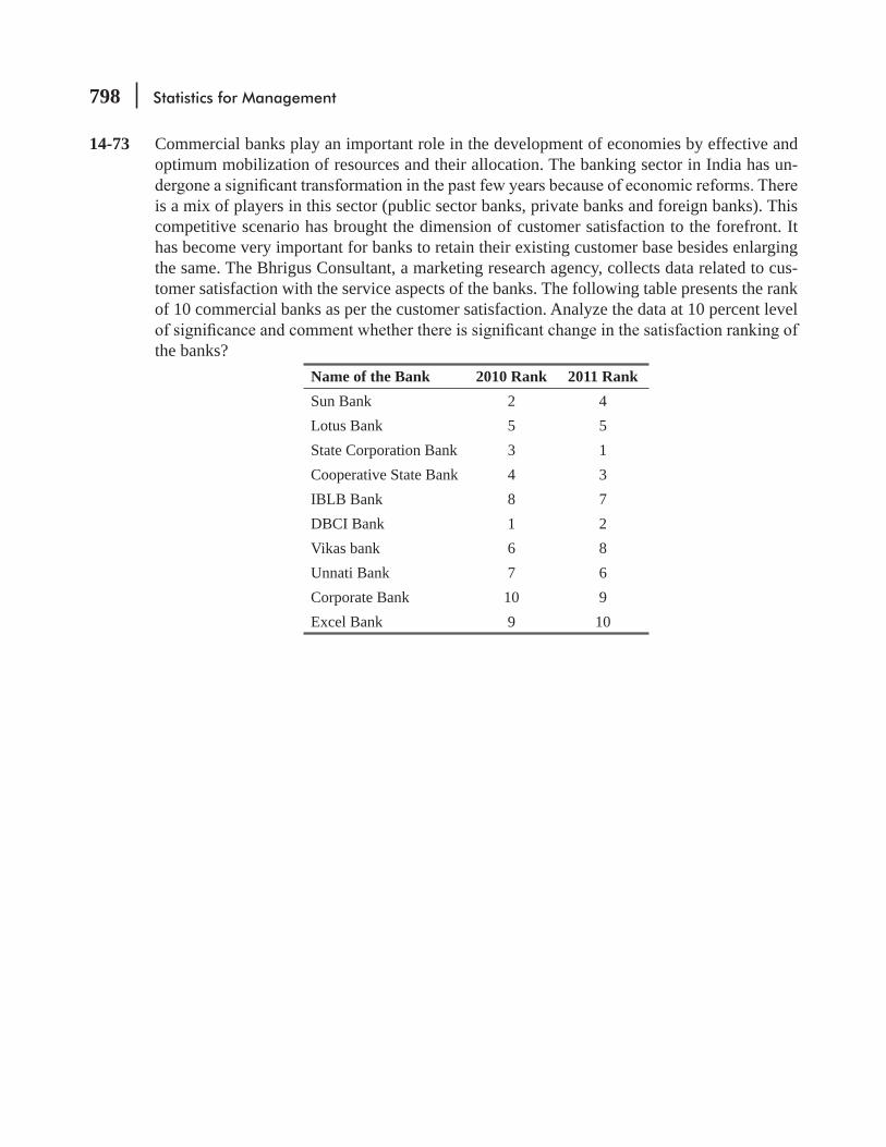
798 Statistics for Management
14-73 Commercial banks play an important role in the development of economies by effective and optimum mobilization of resources and their allocation. The banking sector in India has un-
is a mix of players in this sector (public sector banks, private banks and foreign banks). This competitive scenario has brought the dimension of customer satisfaction to the forefront. It has become very important for banks to retain their existing customer base besides enlarging the same. The Bhrigus Consultant, a marketing research agency, collects data related to cus-tomer satisfaction with the service aspects of the banks. The following table presents the rank of 10 commercial banks as per the customer satisfaction. Analyze the data at 10 percent level
the banks?Name of the Bank 2010 Rank 2011 RankSun Bank 2 4Lotus Bank 5 5State Corporation Bank 3 1Cooperative State Bank 4 3IBLB Bank 8 7DBCI Bank 1 2Vikas bank 6 8Unnati Bank 7 6Corporate Bank 10 9Excel Bank 9 10

Nonparametric Methods 799
Questions on Running Case: SURYA Bank Pvt. Ltd.
1. Test whether the sample of respondents for this study were selected randomly on the basis of gender.
2. Test whether the sample of respondents for this study were selected randomly on the basis of marital status.
3. 4. Test the hypothesis that the level of satisfaction of the customers with regards to the e-services provided by
5. Test the hypothesis that the level of satisfaction of the customers with regards to the e-services provided by
6. Test the hypothesis that the level of satisfaction of the customers with regards to the e-services provided by
7. Test the hypothesis that the level of satisfaction of the customers with regards to the e-services provided by
@
CASE
@

800 Statistics for Management
Flow Chart: Nonparametric Methods
Use nonparametric methodsto reach conclusions about
populations when the shapesof their distributions are
unkonwn
START
Use a sign test withpaired samples to
see whether two populationsare different
Use a Mann–WhitneyU test to see whether two
independent samplescome from the same
population
Use a Kruskal–Wallis testto see whether 3 or more
independent samplescome from the same
population
Use the binomial distribution(or the normal, if the sample is
large enough) to testH0: p = 0.5 against theappropriate alternative
Use the normal distribution(if the samples are large
enough) to test H0: populationsare the same against theappropriate alternative
Use the chi-square distributionif each sample has more
than 5 observations to testH0: populations are the same
against the appropriatealternative
1. Convert the data to + and – signs2. Compute p 1 the sample proportion of + signs
1. Rank the data2. Calculate the U statistic and its mean and standard error
1. Rank the data2. Calculate the K statistic
p. 737
p. 738
p. 746 p. 751
p. 752p. 747
Reject H0
Translate the statisticalresults into appropriate
managerial action
Doesthe sample
statistic fall within theacceptance
region?
YesNo
Nonparametric Methods 801
Use a one-sample runstest to see whether asample was randomly
selected
Use Spearman’s rankcorrelation coefficient tomeasure the degree of
association between twosets of ranked variables
Use a Kolmogorov–Smirnovtest to see whether a particulardistribution is consistent witha given set of data. (You could
also use a χ2 test. SeeChapter 11.)
Use the normal distribution(if the sample is
large enough) to testH0: the sample is random
againstH1: it is not random
Use Appendix Table 8to test
H0: the fit is goodagainst
H1: the fit is not good
Compute the number ofruns, r, and its meanand standard error
1. Rank the data2. Calculate rs (and its standard error if n > 30)
Compute the relative observedcumulative frequencies, Fo, and
compare them to theexpected Fe to get the K–S
statistic,Dn p. 758
p. 761
p. 768 p. 780
p.780
Use Appendix Table 7(or the normal
distribution if n > 30)to test H0: ps = 0
against the appropriatealternative
p. 771
Accept H0
STOP

This page is intentionally left blank

LEARNING OBJECTIVES
15After reading this chapter, you can understand:
CHAPTER CONTENTS
To learn why forecasting changes that take place over time are an important part of decision making
To understand the four components of a time series
To use regression-based techniques to estimate and forecast the trend in a time series
To learn how to measure the cyclical component of a time series
15.1 Introduction 80415.2 Variations in Time Series 80415.3 Trend Analysis 80615.4 Cyclical Variation 81815.5 Seasonal Variation 82415.6 Irregular Variation 83315.7 A Problem Involving All Four Components
of a Time Series 83415.8 Time-Series Analysis in Forecasting 844
To compute seasonal indices and use them to deseasonalize a time series
To be able to recognize irregular variation in a time series
To deal simultaneously with all four components of a time series and to use time-series analysis for forecasting
Statistics at Work 844 Terms Introduced in Chapter 15 846 Equations Introduced in Chapter 15 846 Review and Application Exercises 847 Flow Chart: Time Series 853
Time Series and Forecasting

804 Statistics for Management
The management of a ski resort has these quarterly occupancy data over a 5-year period:
Year 1st Qtr 2nd Qtr 3rd Qtr 4th Qtr
1991 1,861 2,203 2,415 1,9081992 1,921 2,343 2,514 1,9861993 1,834 2,154 2,098 1,7991994 1,837 2,025 2,304 1,9651995 2,073 2,414 2,339 1,967
To improve service, management must understand the seasonal pattern of demand for rooms. Using methods covered in this chapter, we shall help the hotel discern such a seasonal pattern, if it exists, and use it to forecast demand for rooms.
15.1 INTRODUCTIONForecasting, or predicting, is an essential tool in any decision-making process. Its uses vary from deter-mining inventory requirements for a local shoe store to estimating the annual sales of video games. The quality of the forecasts management can make is strongly related to the information that can be extracted and used from past data. Time-series analysis is one quantitative method we use to determine patterns in data collected over time. Table 15-1 is an example of time-series data.
Time-series analysis is used to detect patterns of change in statistical information over regular intervals of time. We project these patterns to arrive at an estimate for the future. Thus, time-series analysis helps us cope with uncertainty about the future.
EXERCISES 15.1
Basic Concepts15-1 Of what value are forecasts in the decision-making process?15-2 For what purpose do we apply time-series analysis to data collected over a period of time?15-3 15-4 How would errors in forecasts affect a city government?
15.2 VARIATIONS IN TIME SERIESWe use the term time series to refer to any group of statistical infor-mation accumulated at regular intervals. There are four kinds of change, or variation, involved in time-series analysis:
1. Secular trend 2.
Use of time-series analysis
Four kinds of variation in
time-series
TABLE 15.1 TIME SERIES FOR THE NUMBER OF SHIPS LOADED AT MOREHEAD CITY, N.C.
Year 1988 1989 1990 1991 1992 1993 1994 1995Number 98 105 116 119 135 156 177 208
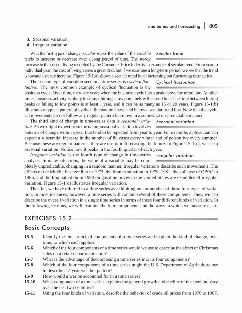
Time Series and Forecasting 805
3. Seasonal variation 4. Irregular variation
secular trend, the value of the variable tends to increase or decrease over a long period of time. The steady increase in the cost of living recorded by the Consumer Price Index is an example of secular trend. From year to individual year, the cost of living varies a great deal, but if we examine a long-term period, we see that the trend
The second type of variation seen in a time series is cyclical uc-tuation.business cycle. Over time, there are years when the business cycle hits a peak above the trend line. At other times, business activity is likely to slump, hitting a low point below the trend line. The time between hitting peaks or falling to low points is at least 1 year, and it can be as many as 15 or 20 years. Figure 15-1(b)
-cal movements do not follow any regular pattern but move in a somewhat un-predictable manner.
The third kind of change in time-series data is seasonal varia-tion. As we might expect from the name, seasonal variation involves patterns of change within a year that tend to be repeated from year to year. For example, a physician can
Because these are regular patterns, they are useful in forecasting the future. In Figure 15-1(c), we see a
Irregular variation is the fourth type of change in time-series analysis. In many situations, the value of a variable may be com-pletely unpredictable, changing in a random manner. Irregular variations describe such movements. The
1986, and the Iraqi situation in 1990 on gasoline prices in the United States are examples of irregular variation. Figure 15-1(d) illustrates irregular variation.
Thus far, we have referred to a time series as exhibiting one or another of these four types of varia-tion. In most instances, however, a time series will contain several of these components. Thus, we can describe the overall variation in a single time series in terms of these four different kinds of variation. In the following sections, we will examine the four components and the ways in which we measure each.
EXERCISES 15.2
Basic Concepts15-5 Identify the four principal components of a time series and explain the kind of change, over
time, to which each applies.15-6 Which of the four components of a time series would we use to describe the effect of Christmas
sales on a retail department store?15-7 What is the advantage of decomposing a time series into its four components?15-8 Which of the four components of a time series might the U.S. Department of Agriculture use
to describe a 7-year weather pattern?15-9 How would a war be accounted for in a time series?15-10 What component of a time series explains the general growth and decline of the steel industry
over the last two centuries?15-11 Using the four kinds of variation, describe the behavior of crude oil prices from 1970 to 1987.
Secular trend
Cyclical fluctuation
Seasonal variation
Irregular variation

806 Statistics for Management
15.3 TREND ANALYSISOf the four components of a time series, secular trend represents the long-term direction of the series. One way to describe the trend
given graph, however, is subject to slightly different interpretations by different individuals. We can also
completely dependable process.
Two methods of fitting a
trend line
Actual time series
Cyclical fluctuation
Seasonal variation
Irregular variation
Trend line
Y
X
X
X
X
Y
Y
Y
(a)
(b)
(c)
(d)
Secular trend
Time in years
Time in years
Time in years
Time in years
FIGURE 15-1 TIME-SERIES VARIATIONS

Time Series and Forecasting 807
Reasons for Studying TrendsThere are three reasons for why it is useful to study secular trends:
1. The study of secular trends allows us to describe a historical pattern. There are many instances when we can use a past trend to evaluate the success of a previous policy. For example, a university may evaluate the effectiveness of a recruiting program by examining its past enrollment trends.
2. Studying secular trends permits us to project past patterns, or trends, into the future. Knowledge of the past can tell us a great deal about the future. Examining the growth rate of the world’s population, for example, can help us estimate the population for some future time.
3. In many situations, studying the secular trend of a time series allows us to eliminate the trend component from the series. This makes it easier for us to study the other three components of the time series. If we want to determine the seasonal variation in ski sales, for example, eliminating the trend component gives us a more accurate idea of the seasonal component.
Trends can be linear or curvilinear. Before we examine the linear, or straight-line, method of describing trends, we should remem-ber that some relationships do not take that form. The increase of pollutants in the environment follows an upward sloping curve similar to that in Figure 15-2(a). Another common example of a curvilinear relationship is the life cycle of a new business product, illustrated in Figure 15-2(b). When a new product is introduced, its sales volume is low (I). As the product gains
established, its unit sales grow at a stable rate (III). Finally, as the product reaches the end of its life cycle, unit sales begin to decrease (IV).
Fitting the Linear Trend by the Least-Squares MethodBesides trends that can be described by a curved line, there are others that are described by a straight line. These are called linear trends. Before developing the equation for a linear trend, we need to review the general equation for estimating a straight line (Equation 12-3):
Equation for estimating a straight line Y a bX→ = + [12-3]
Three reasons for studying
secular trends
Trend lines take different
forms
Pollu
tion
Year
ly s
ales
in u
nits
Trend ofpollutionincrease
(a) (b)
I II
III
IV
Time
Y
X
Y
XTime
FIGURE 15-2 CURVILINEAR TREND RELATIONSHIPS

808 Statistics for Management
where
Y = estimated value of the dependent variable X = independent variable (time in trend analysis) a = Y-intercept (the value of Y when X = 0) b = slope of the trend line
We can describe the general trend of many time series using a
-mined by Equations 12-4 and 12-5, which are now renumbered as Equations 15-1 and 15-2.
Slope of the Best-Fitting Regression Line
b XY nXYX nX2 2=
∑ −∑ − [15-1]
Y-Intercept of the Best-Fitting Regression Line a Y bX= − [15-2]
where
Y = values of the dependent variable X = values of the independent variable Y = mean of the values of the dependent variable X = mean of the values of the independent variable n = number of data points in the time series a = Y-intercept b = slope
However, the regularity of time-series data allows us to simplify the calculations in Equations 15-1 and 15-2 through the process we shall now describe.
Translating, or Coding, Time time in terms such
as weeks, months, and years. Fortunately, we can convert these tra-
In Chapter 3, we called this process codingthat value from each of the sample times. Suppose our time series consists of only three points, 1992,
resultant calculations tedious. Instead, we can transform the values 1992, 1993, and 1994 into corresponding values of −1, 0, and 1, where 0 represents the mean (1993), −(1992 − 1993 = −1), and 1 represents the last year (1994 − 1993 = 1).
We need to consider two cases when we are coding time values. odd number of elements, as in the
Finding the best-fitting
trend line
Coding the time variable to
simplify computation
Treating odd and even numbers
of elements
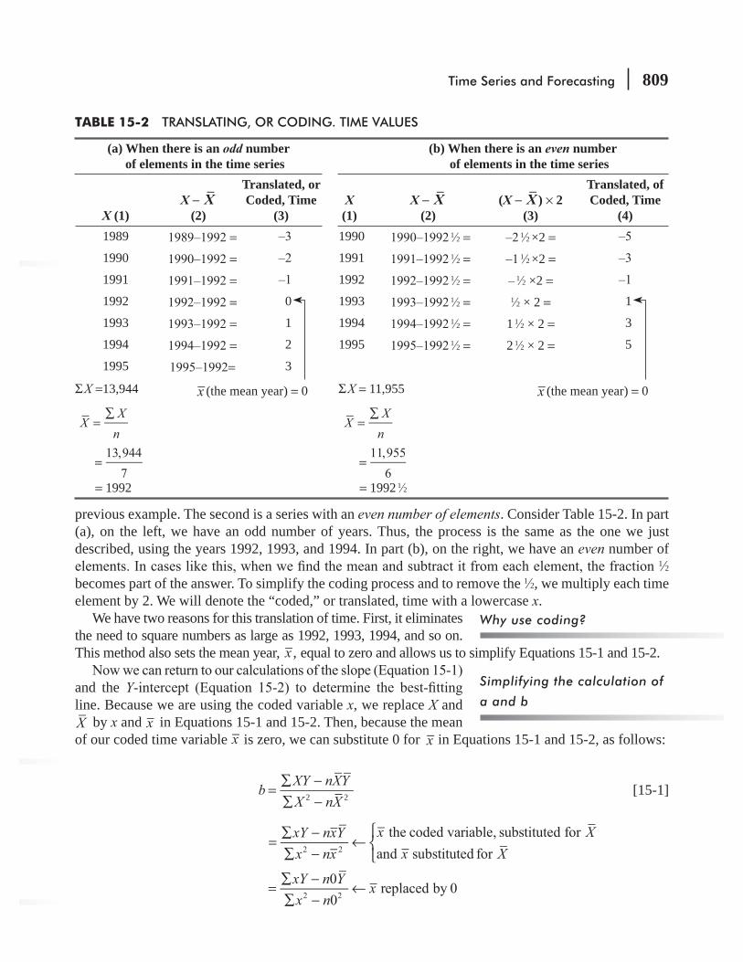
Time Series and Forecasting 809
previous example. The second is a series with an even number of elements. Consider Table 15-2. In part (a), on the left, we have an odd number of years. Thus, the process is the same as the one we just described, using the years 1992, 1993, and 1994. In part (b), on the right, we have an even number of
1 2 becomes part of the answer. To simplify the coding process and to remove the 1 2, we multiply each time element by 2. We will denote the “coded,” or translated, time with a lowercase x.
We have two reasons for this translation of time. First, it eliminates the need to square numbers as large as 1992, 1993, 1994, and so on. This method also sets the mean year, ,x equal to zero and allows us to simplify Equations 15-1 and 15-2.
and the Yline. Because we are using the coded variable x, we replace X and X by x and x in Equations 15-1 and 15-2. Then, because the mean of our coded time variable x is zero, we can substitute 0 for x in Equations 15-1 and 15-2, as follows:
b XY nXYX nX2 2=
∑ −∑ −
[15-1]
xY nxYx nx
x Xx X
the coded variable, substituted forand substituted for2 2=
∑ −∑ −
←⎧⎨⎩
xY n Yx n
x00
replaced by 02 2=∑ −∑ −
←
Why use coding?
Simplifying the calculation of
a and b
TABLE 15-2 TRANSLATING, OR CODING. TIME VALUES
(a) When there is an odd number of elements in the time series
(b) When there is an even number of elements in the time series
X (1)X − X
(2)
Translated, or Coded, Time
(3)X
(1)X − X
(2)(X − X ) × 2
(3)
Translated, of Coded, Time
(4)1989 = 1990 1 2 = 1 2 ×2 =1990 = 1991 1 2 = 1 2 ×2 =1991 = 1992 1 2 = 1 2 ×2 =1992 = 0 1993 1 2 = 1 2 × 2 = 1
1993 = 1 1994 1 2 = 1 1 2 × 2 = 3
1994 = 2 1995 1 2 = 2 1 2 × 2 = 5
1995 = 3
Σ X =13,944 x (the mean year) = 0 Σ X = 11,955 x (the mean year) = 0
XXn
=∑ X
Xn
=∑
13,9447
= 11,9556
=
= 1992 = 1992 1 2

810 Statistics for Management
Slope of the Trend Line for Coded Time Values
2b xYx
=∑∑ [15-3]
Equation 15-2 changes as follows: a Y bX= − [15-2] Y bx x xsubstituted for= − ← Y b0 x replaced by 0= − ←
Intercept of the Trend Line for Coded Time Values
a Y= [15-4]
Equations 15-3 and 15-4 represent a substantial improvement over Equations 15-1 and 15-2.
A Problem Using the Least-Squares Method in a Time Series (Even Number of Elements)Consider the data in Table 15-1, illustrating the number of ships loaded at Morehead City between 1988 and 1995. In this problem,
loadings. To calculate the necessary values for Equations 15-3 and 15-4, let us look at Table 15-3.
Using the least-squares
method
TABLE 15.3 INTERMEDIATE CALCULATIONS FOR COMPUTING THE TREND
X(1) Y †
(2)X X−
(3)x
(3) × 2 = (4)xY
(4) × (2)x2
(4)2
1988 98 1988 − 1991 1 2‡ = 1 2 1 2 × 2 = −7 49
1989 105 1989 − 1991 1 2 = 1 2 1 2 × 2 = −5 25
1990 116 1990 − 1991 1 2 = 1 2 1 2 × 2 = −3 9
1991 119 1991 − 1991 1 2 = 1 2 1 2 × 2 = −1 1
1992 135 1992 − 1991 1 2 = 1 2 1 2 × 2 = 1 135 1
1993 156 1993 − 1991 1 2 = 1 1 2 1 1 2 × 2 = 3 468 9
1994 177 1994 − 1991 1 2 = 2 1 2 2 1 2 × 2 = 5 885 25
1995 208 1995 − 1991 1 2 = 3 1 2 3 1 2 × 2 = 7 1,456 49
Σ X = 15,932 Σ Y = 1,114 Σ xY = 1,266 Σ x2 = 168
XXn
15,9328
1,99112=
∑= =
YYn
1,1148
139.25=∑
= =
†Y is the number of ships.‡19911 2 corresponds to x = 0.
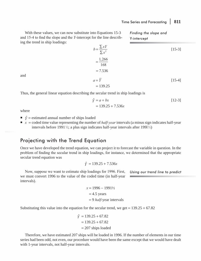
Time Series and Forecasting 811
With these values, we can now substitute into Equations 15-3 Y-intercept for the line describ-
ing the trend in ship loadings:
2b xYx
=∑∑
[15-3]
1,266168
=
= 7.536and a Y= [15-4] = 139.25
Thus, the general linear equation describing the secular trend in ship loadings is
Y = a + bx [12-3] = 139.25 + 7.536xwhere
Y = estimated annual number of ships loaded x = coded time value representing the number of half-year intervals (a minus sign indicates half-year
intervals before 1991 1 2; a plus sign indicates half-year intervals after 199l 1 2)
Projecting with the Trend EquationOnce we have developed the trend equation, we can project it to forecast the variable in question. In the
secular trend equation was
Y = 139.25 + 7.536x
we must convert 1996 to the value of the coded time (in half-year intervals).
x = 1996 − 1991½ = 4.5 years = 9 half-year intervals
Substituting this value into the equation for the secular trend, we get = 139.25 + 67.82
Y = 139.25 + 67.82 = 139.25 + 67.82 = 207 ships loaded
Therefore, we have estimated 207 ships will be loaded in 1996. If the number of elements in our time series had been odd, not even, our procedure would have been the same except that we would have dealt with 1-year intervals, not half-year intervals.
Finding the slope and
Y-intercept
Using our trend line to predict

812 Statistics for Management
Use of a Second-Degree Trend in a Time Series
time series. But many time series are best described by curves, not straight lines. In these instances, the linear trend model does not adequately describe the change in the variable as time changes. To overcome this problem, we often use a parabolic curve, which is described mathematically by a second-degree equation. Such a curve is illustrated in Figure 15-3. The general form for an estimated second-degree equation is
General Form for. Fitted Second-Degree Curve
Y = a + bx + cx2 [15-5]
where
Y = estimate of the dependent variable a, b, and c = numerical constants x = coded values of the time variable.
Again we use the least-squares method to determine the
second-degree equation is beyond the scope of this text. However, we can determine the value of the numerical constants (a, b, and c) from the following three equations:
Least-Squares Coefficients for a Second-Degree Trend
Equations to find a,, and to fit a parabolic curve
2
2 2 4
2
b c
Y an c xx Y a x c x
b xYx
⎯ →⎯⎯⎯
∑ = + ∑∑ = ∑ + ∑
=∑∑
⎧
⎨
⎪⎪
⎩
⎪⎪
[15-6]
[15-7]
[15-3]
Handling time series that are
described by curves
Finding the values for a, b,
and c
FIGURE 15-3 FORM AND EQUATION FOR A PARABOLIC CURVE
Unit
of m
easu
re
Parabolic curve
Time
General equation fora parabolic cruve:Y = a + bx + cx2
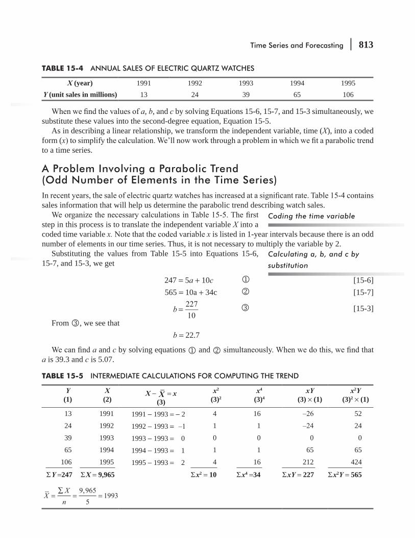
Time Series and Forecasting 813
a, b, and c by solving Equations 15-6, 15-7, and 15-3 simultaneously, we substitute these values into the second-degree equation, Equation 15-5.
As in describing a linear relationship, we transform the independent variable, time (X), into a coded form (xto a time series.
A Problem Involving a Parabolic Trend (Odd Number of Elements in the Time Series)
sales information that will help us determine the parabolic trend describing watch sales.
step in this process is to translate the independent variable X into a coded time variable x. x is listed in 1-year intervals because there is an odd number of elements in our time series. Thus, it is not necessary to multiply the variable by 2.
Substituting the values from Table 15-5 into Equations 15-6, 15-7, and 15-3, we get
247 = 5a + 10c [15-6] 565 = 10a + 34c [15-7]
22710
b = [15-3]
From , we see that b = 22.7
a and c by solving equations and a is 39.3 and c is 5.07.
Coding the time variable
Calculating a, b, and c by
substitution
TABLE 15-4 ANNUAL SALES OF ELECTRIC QUARTZ WATCHES
X (year) 1991 1992 1993 1994 1995Y (unit sales in millions) 13 24 39 65 106
TABLE 15-5 INTERMEDIATE CALCULATIONS FOR COMPUTING THE TREND
Y(1)
X(2)
X − X = x(3)
x2
(3)2x4
(3)4xY
(3) × (1)x2Y
(3)2 × (1)
13 1991 1991 − 1993 = − 2 4 16 52
24 1992 1992 − 1993 = 1 1 24
39 1993 1993 − 1993 = 0 0 0 0 0
65 1994 1994 − 1993 = 1 1 1 65 65
106 1995 1995 − 1993 = 2 4 16 212 424
Σ Y =247 Σ X = 9,965 Σ x2 = 10 Σ x4 =34 Σ xY = 227 Σ x2Y = 565
XXn
9,9655
1993=∑
= =

814 Statistics for Management
This gives us the appropriate values of a, b, and c to describe the time series presented in Table 15-4 by the following equation
Y = a + bx + cx2 [15-5] = 39.3 + 22.7x +5.07x2
Let’s graph the watch data to see how well the parabola we just
Forecasts Based on a Second-Degree EquationSuppose we want to forecast watch sales for 2000. To make a
x by subtracting the mean year, 1993.
X − X = X 2000 − 1993 = 7
This coded value (x = 7) is then substituted into the second-degree equation describing watch sales:
Y = 39.3 + 22.7x + 5.07x2
= 39.3 + 22.7(7) + 5.07(7)2
= 39.3 + 158.9 + 248.4 = 446.6
We conclude, based on the past secular trend, that watch sales should be approximately 446,600,000 units by 2000. This extraordinarily large forecast suggests, however, that we must be more careful in forecasting with a parabolic trend than we are when using a linear trend. The slope of the second-degree equation in Figure 15-4 is continually increasing. Therefore, the parabolic trend may become a poor estimator as we attempt to predict further into the future. In using the second-degree-equation method, we must also take into consideration factors that may be slowing or reversing the growth rate of the variable.
In our watch example, we can assume that during the time period under consideration, the product is at a very rapid growth stage in its life cycle. But we must realize that as the cycle approaches a
Does our curve fit the data?
Making the forecast
Being careful in interpreting
the forcast
140120100
80604020
−7 −6 −5 −4 −3 −2 −1 0 1
1987 1989 1991 1993Time
1995 1997
2 3 4
Actual points
Parabolic trendY = 39.3 + 22.7x + 5.07x2
5 6
Sale
s in
mill
ions
of u
nits
Y
X
FIGURE 15-4 PARABOLIC TREND FITTED TO DATA IN TABLE 15-4

Time Series and Forecasting 815
mature stage, sales will probably decelerate and no longer be predicted accurately by our parabolic curve. When we calculate predictions for the future, we need to consider the possibility that the trend line may change. Such a situation could cause considerable error. It is therefore necessary to exercise particular care when using a second-degree equation as a forecasting tool.
forever. It’s also true here for forecasts made with second-degree equations. Extrapolating the growth rate of a startup company (which starts with zero sales so a dollar of sales is automatically an in nite growth rate) is risky. Early growth rates seldom continue.
HINTS & ASSUMPTIONS
EXERCISES 15.3
Self-Check ExercisesSC 15-1
they have sold is represented by this time series:
Year 1987 1988 1989 1990 1991 1992 1993 1994 1995 1996Tables sold 42 50 61 75 92 111 120 127 140 138
(a) Find the linear equation that describes the trend in the number of tables sold by Robin and Stewart.
(b) Estimate their sales of tables in 1998.SC 15-2 The number of faculty-owned personal computers at the University of Ohio increased dra-
matically between 1990 and 1995:
Year 1990 1991 1992 1993 1994 1995Number of PCs 50 110 350 1,020 1,950 3,710
(a) Develop a linear estimating equation that best describes these data.(b) Develop a second-degree estimating equation that best describes these data.(c) Estimate the number of PCs that will be in use at the university in 1999, using both equations.(d) If there are 8,000 faculty members at the university, which equation is the better predictor?
Why?
Applications15-12 Jeff Richardson invested his life savings and began a part-time carpet-cleaning business in
1986. Since 1986, Jeff’s reputation has spread and business has increased. The average num-bers of homes he has cleaned per month each year are:
Year 1986 1987 1988 1989 1990 1991 1992 1993 1994 1995 1996Homes cleaned 6.4 11.3 14.7 18.4 19.6 25.7 32.5 48.7 55.4 75.7 94.3

816 Statistics for Management
(a) Find the linear equation that describes the trend in these data.(b) Estimate the number of homes cleaned per month in 1997,1998, and 1999.
15-13 The owner of Progressive Builders is examining the number of solar homes started in the region in each of the last 7 months:
Month June July Aug. Sept. Oct. Dec.Number of homes 16 17 25 28 32 43 50
(a) Plot these data.(b) Develop the linear estimating equation that best describes these data, and plot the line on
the graph from part (a) (let x units equal 1 month).(c) Develop the second-degree estimating equation that best describes these data and plot this
curve on the graph from part (a).(d) Estimate March sales using both curves you have plotted.
15-14 Richard Jackson developed an ergonomically superior computer mouse in 1989, and sales have been increasing ever since. Data are presented below in terms of thousands of mice sold per year.
Year 1989 1990 1991 1992 1993 1994 1995 1996Number sold 82.4 125.7 276.9 342.5 543.6 691.5 782.4 889.5
(a) Develop a linear estimating equation that best describes these data.(b) Develop a second-degree estimating equation that best describes these data.(c) Estimate the number of mice that will be sold in 1998, using both equations.(d) If we assume the rate of increase in mouse sales will decrease soon based on supply and
demand, which model would be a better predictor for your answer in part (c)?15-15 Mike Godfrey, the auditor of a state public school system, has reviewed the inventory records
to determine whether the current inventory holdings of textbooks are typical. The following inventory amounts are from the previous 5 years:
Year 1991 1992 1993 1994 1995Inventory (× $1,000) $4,620 $4,910 $5,490 $5,730 $5,990
(a) Find the linear equation that describes the trend in the inventory holdings. (b) Estimate for him the value of the inventory for the year 1996.15-16
Year 1968 1970 1972 1974 1976 1978 1980 1982 1984 1986 1988 1990 1992 1994 1996Rate (¢) 5 5 8 8 10 13 15 18 20 22 25 25 29 29 32
(a) Develop the linear estimating equation that best describes these data.(b) Develop the second-degree estimating equation that best describes these data.(c) Is there anything in the economic or political environment that would suggest that one or
the other of these two equations is likely to be the better predictor of postal rates?15-17 -
tration devices, has recorded the following sales record over the last 9 years:
Year 1987 1988 1989 1990 1991 1992 1993 1994 1995Sales (× $100,000) 13 15 19 21 27 35 47 49 57

Time Series and Forecasting 817
(a) Plot these data.(b) Develop the linear estimating equation that best describes these data, and plot this line on
the graph from part (a).(c) Develop the second-degree estimating equation that best describes these data, and plot
this curve on the graph from part (a).(d) Does the market to the best of your knowledge favor (b) or (c) as the more accurate esti-
mating method?15-18 Here are data describing the air pollution rate (in ppm of particles in the air) in a western city:
Year 1980 1985 1990 1995Pollution rate 220 350 800 2,450
(a) Would a linear or a second-degree estimating equation provide the better prediction of future pollution in that city?
(b) Considering the economic, social, and political environment, would you change your answer to part (a)?
(c) Describe how political and social action could change the effectiveness of either of the estimating equations in part (a).
15-19 resulting from drunk driving for each of the last 9 years.
Year 1987 1988 1989 1990 1991 1992 1993 1994 1995Deaths 175 190 185 195 180 200 185 190 205
state resulting from drunk driving.
expect in 1996.
Worked-Out Answers to Self-Check ExercisesSC 15-1 (a) Year x Y xY x2
1987 42 811988 50 491989 61 251990 75 91991 92 11992 1 111 111 11993 3 120 360 91994 5 127 635 251995 7 140 980 491996 9 138 1242 81
0 956 1,978 330
95610
95.6 1,978330
5.99392= = = =∑∑
= =a Y b xYx
Y = 95.6 + 5.9939 x (when 1991.5 = 0 and x units = 0.5 year)(b) Y = 95.6 + 5.9939(13) = 173.5 tables
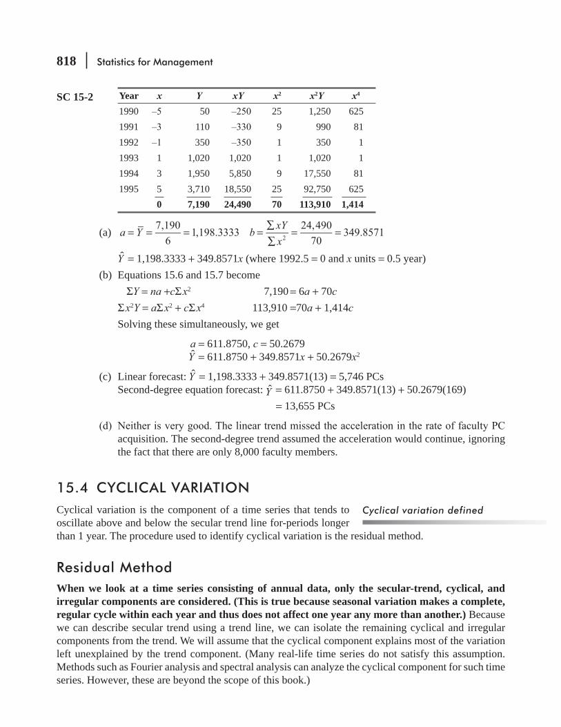
818 Statistics for Management
SC 15-2 Year x Y xY x2 x2Y x4
1990 50 25 1,250 6251991 110 9 990 811992 350 1 350 11993 1 1,020 1,020 1 1,020 11994 3 1,950 5,850 9 17,550 811995 5 3,710 18,550 25 92,750 625
0 7,190 24,490 70 113,910 1,414
(a) 7,1906
1,198.3333 24,49070
349.85712= = = =∑∑
= =a Y b xYx
Y = 1,198.3333 + 349.8571x (where 1992.5 = 0 and x units = 0.5 year)(b) Equations 15.6 and 15.7 become ΣY = na +cΣ x2 7,190 = 6a + 70c Σ x2Y = aΣ x2 + cΣ x4 113,910 =70a + 1,414c Solving these simultaneously, we get
a = 611.8750, c = 50.2679 Y = 611.8750 + 349.8571x + 50.2679x2
(c) Linear forecast: Y = 1,198.3333 + 349.8571(13) = 5,746 PCs Second-degree equation forecast: Y = 611.8750 + 349.8571(13) + 50.2679(169)
= 13,655 PCs
acquisition. The second-degree trend assumed the acceleration would continue, ignoring the fact that there are only 8,000 faculty members.
15.4 CYCLICAL VARIATIONCyclical variation is the component of a time series that tends to oscillate above and below the secular trend line for-periods longer than 1 year. The procedure used to identify cyclical variation is the residual method.
Residual MethodWhen we look at a time series consisting of annual data, only the secular-trend, cyclical, and irregular components are considered. (This is true because seasonal variation makes a complete, regular cycle within each year and thus does not affect one year any more than another.) Because we can describe secular trend using a trend line, we can isolate the remaining cyclical and irregular components from the trend. We will assume that the cyclical component explains most of the variation left unexplained by the trend component. (Many real-life time series do not satisfy this assumption. Methods such as Fourier analysis and spectral analysis can analyze the cyclical component for such time series. However, these are beyond the scope of this book.)
Cyclical variation defined
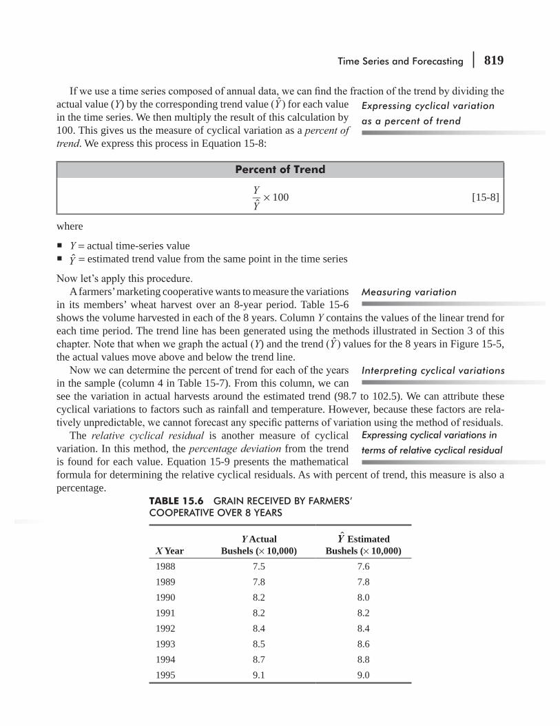
Time Series and Forecasting 819
actual value (Y) by the corresponding trend value ( ˆ)Y for each value in the time series. We then multiply the result of this calculation by 100. This gives us the measure of cyclical variation as a percent of trend. We express this process in Equation 15-8:
Percent of Trend
ˆYY
× 100 [15-8]
where
Y = actual time-series value Y = estimated trend value from the same point in the time series
A farmers’ marketing cooperative wants to measure the variations in its members’ wheat harvest over an 8-year period. Table 15-6 shows the volume harvested in each of the 8 years. Column Y contains the values of the linear trend for each time period. The trend line has been generated using the methods illustrated in Section 3 of this
Y) and the trend ( ˆ)Y values for the 8 years in Figure 15-5, the actual values move above and below the trend line.
in the sample (column 4 in Table 15-7). From this column, we can see the variation in actual harvests around the estimated trend (98.7 to 102.5). We can attribute these cyclical variations to factors such as rainfall and temperature. However, because these factors are rela-
The relative cyclical residual is another measure of cyclical variation. In this method, the percentage deviation from the trend is found for each value. Equation 15-9 presents the mathematical formula for determining the relative cyclical residuals. As with percent of trend, this measure is also a percentage.
Expressing cyclical variation
as a percent of trend
Measuring variation
Interpreting cyclical variations
Expressing cyclical variations in
terms of relative cyclical residual
TABLE 15.6 GRAIN RECEIVED BY FARMERS’ COOPERATIVE OVER 8 YEARS
X YearY Actual
Bushels (× 10,000)Y Estimated
Bushels (× 10,000)1988 7.5 7.61989 7.8 7.81990 8.2 8.01991 8.2 8.21992 8.4 8.41993 8.5 8.61994 8.7 8.81995 9.1 9.0
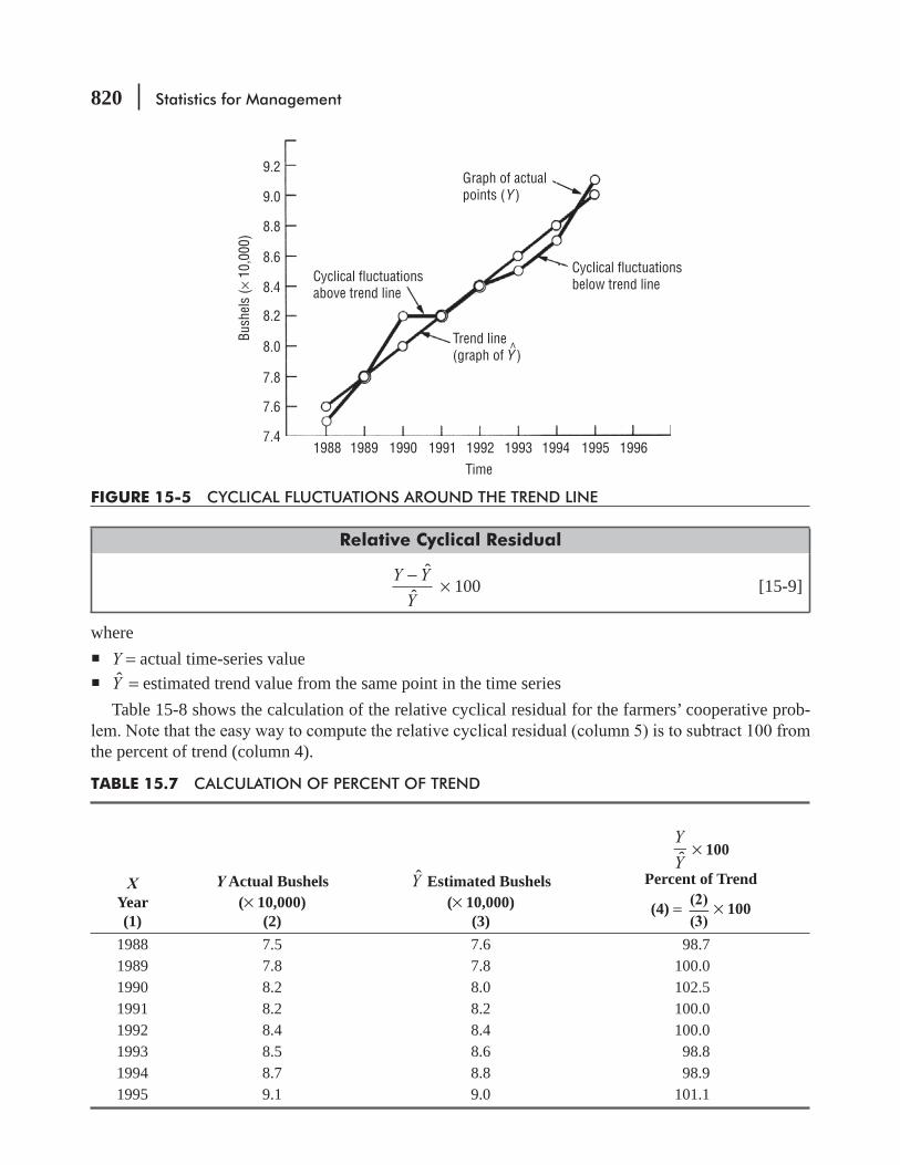
820 Statistics for Management
Relative Cyclical Residual
ˆ
ˆY Y
Y− × 100 [15-9]
where Y = actual time-series value Y = estimated trend value from the same point in the time series
Table 15-8 shows the calculation of the relative cyclical residual for the farmers’ cooperative prob-
the percent of trend (column 4).
9.2
9.0
8.8
8.6
8.4Cyclical fluctuationsabove trend line
Cyclical fluctuationsbelow trend line
Graph of actualpoints (Y )
Trend line(graph of Y )
8.2
8.0
7.8
7.6
7.41988 1989 1990 1991 1992 1993 1994 1995 1996
Time
Bush
els
(× 1
0,00
0)
FIGURE 15-5 CYCLICAL FLUCTUATIONS AROUND THE TREND LINE
TABLE 15.7 CALCULATION OF PERCENT OF TREND
XYear(1)
Y Actual Bushels(× 10,000)
(2)
Y Estimated Bushels(× 10,000)
(3)
ˆYY
× 100
Percent of Trend
(4) = (2)(3)
× 100
1988 7.5 7.6 98.71989 7.8 7.8 100.01990 8.2 8.0 102.51991 8.2 8.2 100.01992 8.4 8.4 100.01993 8.5 8.6 98.81994 8.7 8.8 98.91995 9.1 9.0 101.1
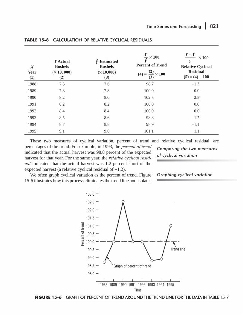
Time Series and Forecasting 821
These two measures of cyclical variation, percent of trend and relative cyclical residual, are percentages of the trend. For example, in 1993, the percent of trend indicated that the actual harvest was 98.8 percent of the expected harvest for that year. For the same year, the relative cyclical resid-ual indicated that the actual harvest was 1.2 percent short of the expected harvest (a relative cyclical residual of −1.2).
We often graph cyclical variation as the percent of trend. Figure 15-6 illustrates how this process eliminates the trend line and isolates
Comparing the two measures
of cyclical variation
Graphing cyclical variation
103.0
102.5
102.0
101.5
101.0
100.5
100.0
99.5
99.0
98.5
98.0
1988 1989 1990 1991
Graph of percent of trend
Trend line
1992 1993Time
1994 1995
Perc
ent o
f tre
nd
FIGURE 15-6 GRAPH OF PERCENT OF TREND AROUND THE TREND LINE FOR THE DATA IN TABLE 15-7
TABLE 15-8 CALCULATION OF RELATIVE CYCLICAL RESIDUALS
XYear(1)
Y Actual Bushels
(× 10, 000)(2)
Y Estimated Bushels
(× 10,000) (3)
YY
× 100
Percent of Trend
(4) = (2)(3)
× 100
Y YY
ˆˆ−
× 100
Relative Cyclical Residual
(5) = (4) − 100
1988 7.5 7.6 98.71989 7.8 7.8 100.0 0.01990 8.2 8.0 102.5 2.51991 8.2 8.2 100.0 0.01992 8.4 8.4 100.0 0.01993 8.5 8.6 98.81994 8.7 8.8 98.91995 9.1 9.0 101.1 1.1
822 Statistics for Management
the cyclical component of the time series. It must be emphasized that the procedures discussed in this section can be used only for describing past cyclical variations and not for predicting future cyclical varia-tions. Predicting cyclical variation requires the use of techniques which are beyond the scope of this book.
Remember that cyclical variation is the component of a time series that oscillates above and below the trend line for periods longer than a year. Warning: Seasonal variation makes a complete cycle within each year and does not affect one year any more than another. Cyclical variation is
of the trend, hence its name percent of trend. The second method (the relative cyclical residual) calculates the variation as a percent deviation from the trend.
HINTS & ASSUMPTIONS
EXERCISES 15.4
Self-Check ExerciseSC 15-3
gas, respectively, for the years 1991 to 1995.(a) Find the linear estimating equation that best describes these data.(b) Calculate the percent of trend for these data.(c) Calculate the relative cyclical residual for these data.
methods?
Applications15-20
following revenue records for the years 1989 to 1995
Year 1989 1990 1991 1992 1993 1994 1995Revenue (× $100,000) 1.1 1.5 1.9 2.1 2.4 2.9 3.5
The second-degree equation that best describes the secular trend for these data is
Y = 2.119 + 0.375x + 0.020x2, where 1992 = 0, and x units = 1 year
(a) Calculate the percent of trend for these data.(b) Calculate the relative cyclical residual for these data.(c) Plot the percent of trend from part (a).
methods?15-21 The Bulls Eye department store has been expanding market share during the past 7 years,
posting the following gross sales in millions of dollars:
Year 1990 1991 1992 1993 1994 1995 1996Sales 14.8 20.7 24.6 32.9 37.8 47.6 51.7
Time Series and Forecasting 823
(a) Find the linear estimating equation that best describes the data.(b) Calculate the percent of trend for these data.(c) Calculate the relative cyclical residual for these data.
methods?15-22 Joe Honeg, the sales manager responsible for the appliance division of a large consumer-
products company, has collected the following data regarding unit sales for his division during the last 5 years:
Year 1991 1992 1993 1994 1995Units (× 10,000) 32 46 50 66 68
The equation describing the secular trend for appliance sales is
Y = 52.4 + 9.2 x, where 1993 = 0, and x units = 1 year
(a) Calculate the percent of trend for these data.(b) Calculate the relative cyclical residual for these data.(c) Plot the percent of trend from part (a).
methods?15-23 -
ments over the last few years have been
Year 1989 1990 1991 1992 1993 1994 1995Millions of dollars required 2.2 2.1 2.4 2.6 2.7 2.9 2.8
The trend equation that best describes these data isY = 2.53 + 0.13x, where 1992 = 0, and x units = 1 year
(a) Calculate the percent of trend for these data.(b) Calculate the relative cyclical residual for these data.
methods?-
ties you perform?15-24 Parallel Breakfast Foods has data on the number of boxes of cereal it has sold in each of the
last 7 years.
Year 1989 1990 1991 1992 1993 1994 1995Boxes (× 10,000) 21.0 19.4 22.6 28.2 30.4 24.0 25.0
(a) Find the linear estimating equation that best describes these data.(b) Calculate the percent of trend for these data.(c) Calculate the relative cyclical residual for these data.
cyclical variation? Is this year the same for both measures? Explain.15-25 Wombat Airlines, an Australian company, has gathered data on the number of passengers who

824 Statistics for Management
Year 1991 1992 1993 1994 1995Passengers (in tens of thousands) 3.5 4.2 3.9 3.8 3.6
(a) Find the linear estimating equation that best describes these data.(b) Calculate the percent of trend for these data.(c) Calculate the relative cyclical residual for these data.(d) Based on the data and your previous calculations, give a one-sentence summary of the
Worked-Out Answer to Self-Check ExerciseSC 15-3
Year x Y xY x2 YYY
× 100 Y YY
ˆˆ− × 100
1991 18 4 17.8 101.12 1.121992 20 1 19.9 100.50 0.501993 0 21 0 0 22.0 95.451994 1 25 25 1 24.1 103.73 3.731995 2 26 52 4 26.2 99.24
0 110 21 10
(a) a=Y = 1105
22 2110
2.12= =∑∑
= =b xYx
Y = 22 + 2.1 x (where 1993 = 0 and x units = 1 year)
(b) See the next-to-the-last column above for percent of trend.(c) See the last column above for relative cyclical residual.
15.5 SEASONAL VARIATIONBesides secular trend and cyclical variation, a time series also includes seasonal variation. Seasonal variation -tive and predictable movement around the trend line in one year or less. In order to detect seasonal variation, time intervals must be measured in small units, such as days, weeks, months, or quarters.
We have three main reasons for studying seasonal variation:
1. We can establish the pattern of past changes. This gives us a way to compare two time intervals that would otherwise be too
in business during December is normal, it can examine the seasonal pattern in previous years and
2. It is useful to project past patterns into the future. In the case of long-range decisions, secular-
is often essential. Consider a wholesale food chain that wants to maintain a minimum adequate stock
Seasonal variation defined
Three reasons for studying
seasonal variation

Time Series and Forecasting 825
of all items. The ability to predict short-range patterns, such as the demand for turkeys at Thanksgiving, candy at Christmas, or peaches in the summer, is useful to the management of the chain.
3. Once we have established the seasonal pattern that exists, we can eliminate its effects from the time series. This adjustment allows us to calculate the cyclical variation that takes place each year. When we eliminate the effect of seasonal variation from a time series, we have deseasonalized the time series.
Ratio-to-Moving-Average MethodIn order to measure seasonal variation, we typically use the ratio-to-moving-average method. This technique provides an index that describes the degree of seasonal variation. The index is based on a mean of 100, with the degree of seasonality measured by variations away from the base. For example, if we examine the seasonality of canoe rentals at a summer resort, we
quarterly rental occur in the spring. If management recorded 2,000 canoe rentals for all of last year, then the average quarterly rental would be 2,000/4 = 500. Because the spring-quarter index is 142, we estimate the number of spring rentals as follows:
Average quarterly rental
Spring-quarter index
Seasonalized spring quarter rental500 142100
710× =
Our chapter-opening example can illustrate the ratio-to-moving-average method. The resort hotel wanted to establish the seasonal pattern of room demand by its clientele. Hotel management wants to improve customer service and is considering several plans to employ personnel during peak periods to achieve this goal. Table 15-9 contains the quarterly occupancy, that is, the average number of guests during each quarter of the last 5 years.
We will refer to Table 15-9 to demonstrate the six steps required to compute a seasonal index.
1. the 4-quarter moving total for the time series. To do this, we
Using the ratio-to-moving-
average method of measuring
seasonal variation
An example of the ratio-to-
moving-average method
Step1: Calculate the 4-quarter
moving total
TABLE 15-9 TIME SERIES FOR HOTEL OCCUPANCY
Number of Guests per Quarter
Year I II III IV1991 1,861 2,203 2,415 1,9081992 1,921 2,343 2,514 1,9861993 1,834 2,154 2,098 1,7991994 1,837 2,025 2,304 1,9651995 2,073 2,414 2,339 1,967

826 Statistics for Management
Table 15-9:1,861 + 2,203 + 2,415 + 1,908 = 8,387. A moving total is associated with the middle data
from four data points, we place it opposite the midpoint of those quarters, so it falls in column 4 of Table 15-10, between the rows for the 1991-II and 1991-III quarters.
values added now are 2,203 + 2,415 + 1,908 + 1,921 = 8,447. This total is entered in Table 15-10
total over the time series until we have included the last value in the series. In this example, it is the 1,967 rooms in the fourth quarter of 1995, the last number in column 3 of Table 15-10. The last entry in the moving total column is 8,793. It is between the rows for the 1995-II and 1995-III quar-ters because it was calculated from the data for the 4 quarters of 1995.
2. In the second step, we compute the 4-quarter moving average by dividing each of the 4-quarter totals by 4. In Table 15-10, we divided the values in column 4 by 4, to arrive at the values for column 5.
3. In the third step, we center the 4-quarter moving average. The moving averages in column 5 all fall halfway between the quarters. We would like to have moving averages associated with each quarter. In order to center our moving averages, we associate with each quarter the average of the two 4-quarter moving averages falling just above and just below it. For the 1991-III quarter, the resulting 4-quarter centered moving average is 2,104.25, that is, (2,096.75 + 2,111.75)/2. The other entries in column 6 are calculated the same way. Figure 15-7 illustrates how
Step 2: Compute the 4-quarter
moving average
Step 3: Center the 4-quarter
moving average
2,500
2,400
2,300
2,200
2,100
2,000
1,900
1,800
1,700
1991 1992 1993 1994Time
I II III IV I II III IV I II III IV I II III IV I II III IV I II III IV
1995
Four-quarter centered moving average(column 6 of Table 15-10)
Original time series
2,198
1996
Occu
pant
s pe
r qua
rter
FIGURE 15-7 USING A MOVING AVERAGE TO SMOOTH THE ORIGINAL TIME SERIES

Time Series and Forecasting 827
the moving average has smoothed the peaks and troughs of the original time series. The seasonal and irregular components have been smoothed, and the resulting dotted colored line represents the cyclical and trend components of the series.
Suppose we were working with the admissions data for a hospital emergency room, and we wanted to compute daily indices. In steps 1 and 2, we would compute 7-day moving totals and moving averages, and the moving averages would already be centered (because the middle of a 7-day period is the fourth of those 7 days). In this case, step 3 is unnecessary. Whenever the number of periods for which we want indices is odd (7 days in a week, three shifts in a day), we can skip step 3. However, when the number of periods is even (4 quarters, 12 months, 24 hours), then we must use step 3 to center the moving averages we get with step 2.
4. Next, we calculate the percentage of the actual value to the moving-average value for each quarter in the time series having a 4-quarter moving-average entry. This step allows us to recover the seasonal component for the quarters. We determine this percentage by dividing each of the actual quarter values in column 3 of Table 15-10 by the corresponding 4-quarter centered moving-average values
Sometimes step 3 can be skipped
Step 4: Calculate the
percentage of actual value
to moving average value
TABLE 15-10 CALCULATING THE 4-QUARTER CENTERED MOVING AVERAGE
Year(1)
Quarter(2)
Occupancy(3)
Step 1:4-Quarter
MovingTotal
(4)
Step 2:4-Quarter
MovingTotal
Average(5) = (4) ÷ 4
Stem 3:4-Quarter Centered MovingAverage
(6)
Step 4:Percentage of
Actual to Moving Average Values
(7) = (3)(6)
× 100
1991 IIIIIIIV
1,8612,2032,4151,908
8,3878,447
2,096.752,111.75
2,104.2502,129.250
114.889.6
1992 IIIIIIIV
1,9212,3432,5141,986
8,5878,6868,7648,677
2,146.752,171.502,191.002,169.25
2,159.1252,181.2502,180.1252,145.625
89.0107.4115.392.6
1993 IIIIIIIV
1,8342,1542,0981,799
8,4888,0727,8857,888
2,122.002,018.001,971.251,972.00
2,070.0001,994.6251,971.6251,955.875
88.6108.0106.492.0
1994 IIIIIIIV
1,8372,0252,3041,965
7,7597,9658,1318,367
1,939.751,991.252,032.752,091.75
1,965.5002,012.0002,062.2502,140.375
93.5100.6111.791.8
1995 IIIIIIIV
2,0732,4142,3391,967
8,7568,7918,793
2,189.002,197.752,198.25
2,193.3752,198.000
94.5109.8

828 Statistics for Management
as follows:
ActualMoving average
× 100 = 2,4152,104.250
× 100
= 114.8
5. To collect all the percentage of actual to moving-average values in column 7 of Table 15-10, arrange them by quarter. Then calculate the modi ed mean for each quarter. The
The seasonal values we recovered for the quarters in column 7 of Table 15-10 still contain the cyclical and irregular components of variation in the time series. By eliminating the highest and lowest values from each quarter, we reduce the extreme cyclical and irregular variations. When we average the remaining values, we further smooth the cyclical and irregular components.
Step 5: Collect answers from step 4
Reducing extreme cyclical and
irregular variations
TABLE 15-11 DEMONSTRATION OF STEP 5 IN COMPUTING A SEASONAL INDEX*
Year Quarter l Quarter ll Quarter lll Quarter lV1991 — — 114.8 89.6
1992 89.0 107.4 115.3 92.6
1993 88.6 108.0 106.4 92.0
1994 93.5 100.6 111.7 91.8
1995 94.5 109.8 — —182.5 215.4 226.5 183.8
Quarter I: 182.52
91.25=
Quarter II: 215.42
107.70=
Quarter III: 226.52
113.25=
Quarter IV: 183.82
91.90=
Total of indices = 404.1*Eliminated values are indicated by a colored slash.
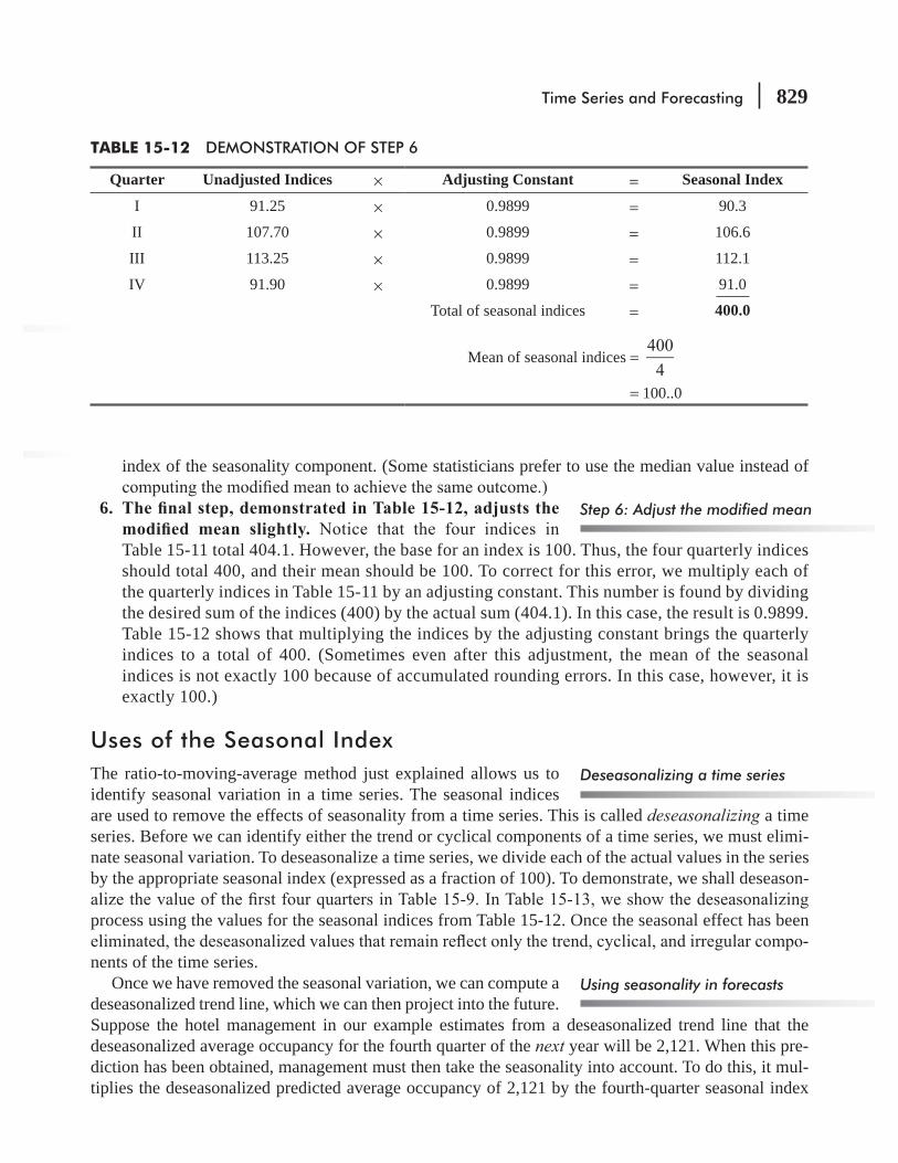
Time Series and Forecasting 829
index of the seasonality component. (Some statisticians prefer to use the median value instead of
6.
Table 15-11 total 404.1. However, the base for an index is 100. Thus, the four quarterly indices should total 400, and their mean should be 100. To correct for this error, we multiply each of the quarterly indices in Table 15-11 by an adjusting constant. This number is found by dividing the desired sum of the indices (400) by the actual sum (404.1). In this case, the result is 0.9899. Table 15-12 shows that multiplying the indices by the adjusting constant brings the quarterly indices to a total of 400. (Sometimes even after this adjustment, the mean of the seasonal indices is not exactly 100 because of accumulated rounding errors. In this case, however, it is exactly 100.)
Uses of the Seasonal IndexThe ratio-to-moving-average method just explained allows us to identify seasonal variation in a time series. The seasonal indices are used to remove the effects of seasonality from a time series. This is called deseasonalizing a time series. Before we can identify either the trend or cyclical components of a time series, we must elimi-nate seasonal variation. To deseasonalize a time series, we divide each of the actual values in the series by the appropriate seasonal index (expressed as a fraction of 100). To demonstrate, we shall deseason-
process using the values for the seasonal indices from Table 15-12. Once the seasonal effect has been -
nents of the time series.Once we have removed the seasonal variation, we can compute a
deseasonalized trend line, which we can then project into the future. Suppose the hotel management in our example estimates from a deseasonalized trend line that the deseasonalized average occupancy for the fourth quarter of the next year will be 2,121. When this pre-diction has been obtained, management must then take the seasonality into account. To do this, it mul-tiplies the deseasonalized predicted average occupancy of 2,121 by the fourth-quarter seasonal index
Deseasonalizing a time series
Using seasonality in forecasts
TABLE 15-12 DEMONSTRATION OF STEP 6
Quarter Unadjusted Indices × Adjusting Constant = Seasonal Index
I 91.25 × 0.9899 = 90.3
II 107.70 × 0.9899 = 106.6
III 113.25 × 0.9899 = 112.1
IV 91.90 × 0.9899 = 91.0
Total of seasonal indices = 400.0
Mean of seasonal indices = 400
4 = 100..0

830 Statistics for Management
(expressed as a fraction of 100) to obtain a seasonalized estimate of 1,930 rooms for the fourth-quarter average occupancy. Here are the calculations:
Deseasonalized estimatedvalue from trend line
Seasonalized estimate of fourth-quarter occupancy
Seasonal index for fourth quarter
2,12191.0
1001,930× =
Using seasonal indices to adjust quarterly and monthly data helps us detect the underlying secular
in some management decisions this missing information is valuable. For example, if a state motor vehicle department reports last month’s new vehicle registrations were 25,000 at a seasonally adjusted ratemats predict demand for next month without knowing the actual number of new cars? Often, for
HINTS & ASSUMPTIONS
EXERCISES 15.5
Self-Check ExerciseSC 15-4 Using the following percentages of actual to moving average describing the quarterly amount
seasonal index for each quarter.
TABLE 15-13 DEMONSTRATION OF DESEASONALIZING DATA
Year(1)
Quarter(2)
ActualOccupancy
(3)
Seasonal Index100
⎛⎝⎜
⎞⎠⎟
(4)
DeseasonalizedOccupancy
(5) = (3) ÷ (4)1991 I 1,861 ÷ 90.3
100⎛⎝⎜
⎞⎠⎟
= 2,061
1991 II 2,203 ÷ 106.6100
⎛⎝⎜
⎞⎠⎟
= 2,067
1991 III 2,415 ÷ 112.1100
⎛⎝⎜
⎞⎠⎟
= 2,154
1991 IV 1,908 ÷ 91.0100
⎛⎝⎜
⎞⎠⎟
= 2,097
Time Series and Forecasting 831
Spring Summer Fall Winter1992 87 106 86 1251993 85 110 83 1271994 84 105 87 1281995 88 104 88 124
Applications15-26
regarding the company’s level of accounts receivable over the last 5 years (× $1,000):
Spring Summer Fall Winter1991 102 120 90 781992 110 126 95 831993 111 128 97 861994 115 135 103 911995 122 144 110 98
(a) Calculate a 4-quarter centered moving average.(b) Find the percentage of actual to moving average for each period.
15-27 Marie Wiggs, personnel director for a pharmaceutical company, recorded these percentage absentee rates for each quarter over a 4-year period:
Spring Summer Fall Winter1992 5.6 6.8 6.3 5.21993 5.7 6.7 6.4 5.41994 5.3 6.6 6.1 5.11995 5.4 6.9 6.2 5.3
(a) Construct a 4-quarter centered moving average and plot it on a graph along with the original data.
(b) What can you conclude about absenteeism from part (a)?15-28 Using the following percentages of actual to moving average describing the seasonal sales of
sporting goods over a 5-year period, calculate the seasonal index for each season.
Year Baseball Football Basketball Hockey1992 96 128 116 771993 92 131 125 691994 84 113 117 841995 97 118 126 891996 91 121 124 81
832 Statistics for Management
15-29 A large manufacturer of automobile springs has determined the following percentages of
Spring Summer Fall Winter1990 108 128 94 701991 112 132 88 681992 109 134 84 731993 110 131 90 691994 108 135 89 681995 106 129 93 72
Calculate the seasonal index for each quarter. Comment on how it compares to the indices you calculated for Exercise 15-26.
15-30 the previous 5 years (×100):
Fall Winter Spring Summer 1991 220 203 193 841992 235 208 206 761993 236 206 209 731994 241 215 206 921995 239 221 213 115
(a) Calculate a 4-quarter centered moving average.(b) Find the percentage of actual to moving average for each period.
15-31 The Ski and Putt Resort, a combination of ski slopes and golf courses, has just recently tabu-lated its data on the number of customers (in thousands) it has had during each season of the last 5 years. Calculate the seasonal index for each quarter. If 15 people are employed in the summer, what should winter employment be, assuming both sports have equal labor requirements?
Spring Summer Fall Winter1991 200 300 125 3251992 175 250 150 3751993 225 300 200 4501994 200 350 225 3751995 175 300 200 350
15-32 David Curl Builders has collected quarterly data on the number of homes it has started during the last 5 years.
Spring Summer Fall Winter1991 8 10 7 51992 9 10 7 61993 10 11 7 61994 10 12 8 71995 11 13 9 8

Time Series and Forecasting 833
(a) Calculate the seasonal index for each quarter.(b) If David’s working capital needs are related directly to the number of starts, by how much
should his working capital need decrease between summer and winter?
Worked-Out Answer to Self-Check ExerciseSC 15-4 Year Spring Summer Fall Winter
1992 87 106 86 1251993 85 110 83 1271994 84 105 87 1281995 88 104 88 124
172 211 173 25286 105.5 86.5 126
Seasonal index 85.15 104.46 85.64 124.75
= 0.9901. The seasonal
15.6 IRREGULAR VARIATION
have eliminated trend, cyclical, and seasonal variations from a time series, we still have an unpredictable factor left. Typically, irregular variation occurs over short intervals and follows a random pattern.
Because of the unpredictability of irregular variation, we do not attempt to explain it mathemati-
was an irregular factor that severely depressed the municipal bond market. In 1984, the unusually
increased electricity and fuel oil consumption. The Persian Gulf War in 1991 was another irregular
allows managers to cope with irregular variation is that over time, these random movements tend to counteract each other.
Warning: Irregular variation is very important but is not explainable mathematically. It’s what is “left over” after we eliminate trend, cyclical, and seasonal variation from a time series. In most
a footnote or a comment on a graph. Examples of this would be “Market closed for Labor Day Holiday” or “Spring break fell in March instead of April last year.”
HINTS & ASSUMPTIONS
variation

834 Statistics for Management
EXERCISES 15.6
Basic Concepts15-33 Why don’t we project irregular variations into the future?15-34 Which of the following illustrate irregular variations?
(a) An extended drought leading to higher food prices.(b) The effect of snow on ski slope business.(c) A one-time federal tax rebate provision for the purchase of new houses.(d) The collapse of crude oil prices in early 1986.(e) The energy use reduction after the 1973 oil embargo.
15-35 routine.
15-36 What allows management to cope with irregular variation in time series?
15.7 A PROBLEM INVOLVING ALL FOUR COMPONENTS OF A TIME SERIES
-ducing recreational equipment. To forecast future sales based on an analysis of its past pattern of sales,
consist of three stages:
1. Deseasonalizing the time series 2. Developing the trend line 3. Finding the cyclical variation around the trend line
Because the data are available on a quarterly basis, we must
Tables 15-15 and 15-16. These steps are the same as those originally introduced in Section 15-5.
we complete the procesOnce we have computed the quarterly seasonal indices, we can
actual sales (in Table 15-14) by the seasonal indices. Table 15-17 (on page 837) shows the calculation of the deseasonalized time-series values.
Step 1: Computing seasonal indices
Finding the deseasonalized values
TABLE 15-14 QUARTERLY SALES
Sales per Quarter (× $10,000)Year I II III IV1991 16 21 9 181992 15 20 10 181993 17 24 13 221994 17 25 11 211995 18 26 14 25

Time Series and Forecasting 835
The second step in describing the components of the time series is to develop the trend line. We accomplish this by applying the least-squares method to the deseasonalized time series (after we have translated the time vari-able). Table 15-18 presents the calculations to identify the trend component (see page 838).
Y-intercept for the trend line as follows:
b xYx2=
∑∑
[15-3]
420.32,660
=
= 0.16
a = Y [15-4] = 18.0
Step 2: Developing the trend line
using the least-squares method
TABLE 15-15 CALCULATION OF THE FIRST FOUR STEPS TO COMPUTE THE SEASONAL INDEX
Year(1)
Quarter(2)
ActualSales(3)
Step 1:4-Quarter
MovingTotal
(4)
Step 2:4-Quarter
MovingAverage
(5) =(4)4
Step 3:4-Quarter CenteredMovingAverage
(6)
Step 4:Percentage of
Actual toMoving Average
(7) =(3)(6)
× 100
1991 IIIIIIIV
16219
186463
16.0015.75
15.87515.625
56.7115.2
1992 IIIIIIIV
15201018
62636365
15.5015.7515.7516.25
15.62515.75016.00016.750
96.0127.062.5
107.51993 I
IIIIIIV
17241322
69727676
17.2518.0019.0019.00
17.62518.50019.00019.125
96.5129.768.4
115.01994 I
IIIIIIV
17251121
77757475
19.2518.7518.5018.75
19.00018.62518.62518.875
89.5134.259.1
111.31995 I
IIIIIIV
18261425
767983
19.0019.7520.75
19.37520.250
92.9128.4

836 Statistics for Management
The appropriate trend line is described using the straight-line equation (Equation 12-3), with X replaced by x:
Y = a + bx [12-3] = 18 + 0.16x
problem, we will calculate cyclical variation in Table 15-19, using the residual method (see page 839).
Step 3: Finding the cyclical variation
TABLE 15-16 STEPS 5 AND 6 IN COMPUTING THE SEASONAL INDEX
Step 5*Year I II III IV1991 — — 56.7 115.2
1992 96.0 127.0 62.5 107.5
1993 96.5 129.7 68.4 115.0
1994 89.5 134.2 59.1 111.31995 92.9 128.4 — —
= 188.9 258.1 121.6 226.3
188.92
94.45=
II: 258.12
129.05=
III: 121.62
60.80=
IV: 226.32
= 113.15397.45
Step 6†
Adjusting factor = 400397.45
= 1.0064
Quarter Indices × Adjusting Factor = Seasonal Indices
I 94.45 × 1.0064 = 95.1
II 129.05 × 1.0064 = 129.9
III 60.80 × 1.0064 = 61.2
IV 113.15 × 1.0064 = 113.9Sum of seasonal indices = 400.1
†Correcting the indices in step 5.

Time Series and Forecasting 837
If we assume that irregular variation is generally short-term and
series in this problem using the trend, cyclical, and seasonal compo-nents. Figure 15-8 (on page 840) illustrates the original time series, its moving average (containing both the trend and cyclical components), and the trend line.
we have been using as an example wants to estimate the sales volume for the third quarter of 1996. What should management do?
It has to determine the deseasonalized value for sales in the third quarter of 1996 by using the trend equation, Y − 18 + 0.16 x. This requires it to code the time, 1996-III. That quarter (1996-III) is three quarters past 1995-IV, which, we see in Table 15-18, has a coded time value of 19. Adding 2 for each quarter, management
x = 19 + 2(3) = 25. Substituting this value (x = 25) into the trend equation produces the following result:
Y = a + bx = 18 + 0.16(25) = 18 + 4 = 22
Assumptions about irregular
variation
Predictions using a time series
Step 1: Determining the
deseasonalized value for sales
for the period desired
TABLE 15-17 CALCULATION OF DESEASONALIZED TIME-SERIES VALUES
Year(1)
Quarter
(2)
Actual Sales
(3)
Seasonal Index100(4)
Deseasonalized Sales
(5) = (3) ÷ (4)1991 I
IIIIIIV
16219
18
0.9511.2990.6121.139
16.816.214.715.8
1992 IIIIIIIV
15201018
0.9511.2990.6121.139
15.815.416.315.8
1993 IIIIIIIV
17241322
0.9511.2990.6121.139
17.918.521.219.3
1994 IIIIIIIV
17251121
0.9511.2990.6121.139
17.919.218.018.4
1995 IIIIIIIV
18261425
0.9511.2990.6121.139
18.920.022.921.9
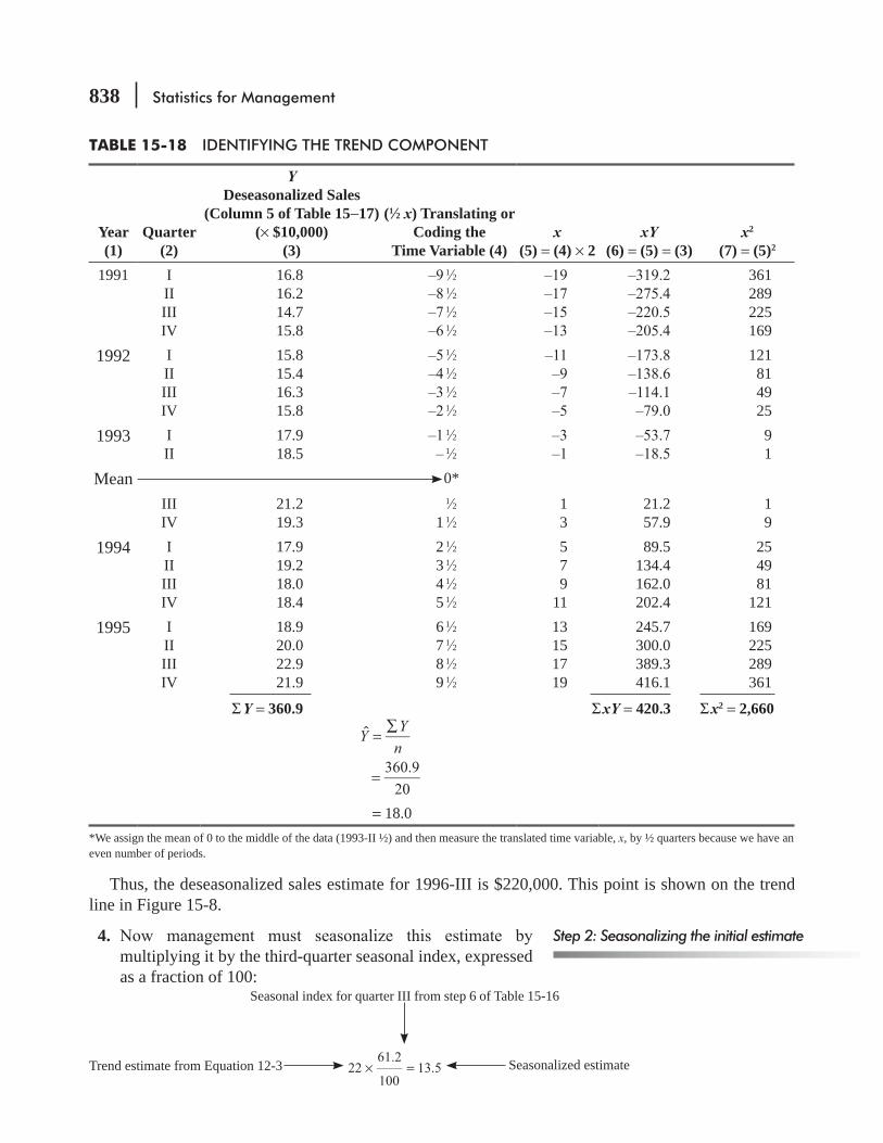
838 Statistics for Management
Thus, the deseasonalized sales estimate for 1996-III is $220,000. This point is shown on the trend line in Figure 15-8.
4. multiplying it by the third-quarter seasonal index, expressed as a fraction of 100:
Trend estimate from Equation 12-3 Seasonalized estimate
Seasonal index for quarter III from step 6 of Table 15-16
2261.2
10013.5× =
Step 2: Seasonalizing the initial estimate
TABLE 15-18 IDENTIFYING THE TREND COMPONENT
Year(1)
Quarter(2)
YDeseasonalized Sales
(Column 5 of Table 15−17) (× $10,000)
(3)
(1 2 x) Translating orCoding the
Time Variable (4)x
(5) = (4) × 2xY
(6) = (5) = (3)x2
(7) = (5)2
1991 IIIIIIIV
16.816.214.715.8
1 21 21 21 2
361289225169
1992 IIIIIIIV
15.815.416.315.8
1 21 21 21 2
121814925
1993 III
17.918.5
1 21 2
91
Mean 0*
IIIIV
21.219.3
1 2
1 1 2
13
21.257.9
19
1994 IIIIIIIV
17.919.218.018.4
2 1 2
3 1 2
4 1 2
5 1 2
579
11
89.5134.4162.0202.4
254981
121
1995 IIIIIIIV
18.920.022.921.9
6 1 2
7 1 2
8 1 2
9 1 2
13151719
245.7300.0389.3416.1
169225289361
Σ Y = 360.9 Σ xY = 420.3 Σ x2 = 2,660
ˆ =
∑Y Yn
360.920
=
= 18.0*We assign the mean of 0 to the middle of the data (1993-II ½) and then measure the translated time variable, x, by ½ quarters because we have an even number of periods.

Time Series and Forecasting 839
TABLE 15-19 IDENTIFYING THE CYCLICAL VARIATION
Year(1)
Quarter(2)
YDeseasonalized
Sales(Column 5,Table 15-17)
(3)a + bx = Y *
(4)
YY
× 100
Percent of Trend
(15) = (3)(4)
× 100
1991 IIIIIIIV
16.816.214.715.8
18 + = 14.9618 + = 15.2818 + = 15.6018 + = 15.92
112.3106.094.299.2
1992 IIIIIIIV
15.815.416.315.8
18 + = 16.2418 + = 16.5618 + = 16.8818 + = 17.20
97.393.096.691.9
1993 IIIIIIIV
17.918.521.219.3
18 + = 17.5218 + = 17.8418 + 0.16( 1) = 18.1618 + 0.16( 3) = 18.48
102.2103.7116.7104.4
1994 IIIIIIIV
17.919.218.018.4
18 + 0.16( 5) = 18.8018 + 0.16( 7) = 19.1218 + 0.16( 9) = 19.4418 + 0.16( 11) = 19.76
95.2100.492.693.1
1995 IIIIIIIV
18.920.022.921.9
18 + 0.16( 13) = 20.0818 + 0.16( 15) = 20.4018 + 0.16( 17) = 20.7218 + 0.16( 19) = 21.04
94.198.0
110.5104.1
*The appropriate value for x in this equation is obtained from column 5 of Table 15-18.
1996-III will be $135,000. We must stress, however, that this value is only an estimate and does not take into account the cyclical and irregular components. As we noted earlier, the irregular variation cannot be predicted mathematically. Also, remember that our earlier treatment of cyclical variation was descriptive of past behavior and not predictive of future behavior.
A complete analysis of a time series tries to account for secular trend, cyclical variation, and sea-sonal variation. What’s left is irregular variation. Warning: Even the best analysis of a time series describes past behavior, and may not be predictive of future behavior. Hint: The correct way to
-tify irregular variation from what is left.
HINTS & ASSUMPTIONS
Caution in using the forecast

840 Statistics for Management
EXERCISES 15.7
Self-Check ExerciseSC 15-5 A state commission designed to monitor energy consumption assembled the following
seasonal data regarding natural gas consumption, in millions of cubic feet:
Winter Spring Summer Fall1992 293 246 231 2821993 301 252 227 2911994 304 259 239 2961995 306 265 240 300
(a) Determine the seasonal indices and deseasonalize these data (using a 4-quarter centered moving average).
(b) Calculate the least-squares line that best describes these data.(c) Identify the cyclical variation in these data by the relative cyclical residual method.(d) Plot the original data, the deseasonalized data, and the trend.
26
Time series fromTable 15-14 (allfour components)
Deseasonalizedsales estimatefor 1996-III($220,000)
4-quarter centered moving average(both trend and cyclical components)
x = 0
25242322212019181716151413121110
9
1991 1992 1993 1994 1995 1996
Sale
s (×
$ 1
0,00
0)
Y = 18 + 0.16x(trend only)
I II III IV I II III IV I II III IV I II III IV I II III IV I II III IV
FIGURE 15-8 TIME SERIES, TREND LINE, AND 4-QUARTER CENTERED MOVING AVERAGE FOR QUARTERLY SALES DATA IN TABLE 15-14

Time Series and Forecasting 841
Applications15-37
has assembled the following seasonal data regarding amount of contaminants (in parts per million) in the air:
Year Winter Spring Summer Fall
1992 452 385 330 385
1993 474 397 356 399
1994 494 409 375 415
1995 506 429 398 437
1996 527 454 421 482
(a) Determine the seasonal indices and deseasonalize these data (using a 4-quarter centered moving average).
(b) Calculate the least-squares line that best describes these data.(c) Identify the cyclic variation in these data by the relative cyclical residual method.(d) Plot the original data, the deseasonalized data, and the trend.
15-38 The following data describe the marketing performance of a regional beer producer:
Sales by Quarter (× $100,000)
Year I II III IV
1991 19 24 38 25
1992 21 28 44 23
1993 23 31 41 23
1994 24 35 48 21
(a) Calculate the seasonal indices for these data. (Use a 4-quarter centered moving average.)
(b) Deseasonalize these data using the indices from part (a).15-39 For Exercise 15-38:
(a) Find the least-squares line that best describes the trend in deseasonalized beer sales.(b) Identify the cyclical component in this time series by computing the percent
of trend.

842 Statistics for Management
Worked-Out Answer to Self-Check ExerciseSC 15-5 (a)
Year Quarter
ActualGas
Usage
4-QuarterMovingAverage
CenteredMovingAverage
Percentageof Actual to
Moving AverageSeasonal
IndexDeseasonalized
Usage1992 Winter
SpringSummerFall
293246231282
263.00265.00
264.000265.750
87.50106.11
111.6694.3986.82
107.13
262.4037260.6208266.0677263.2316
1993 WinterSpringSummerFall
301252227291
266.50265.50267.75268.50
266.000266.625268.125269.375
113.1694.5184.66
108.03
111.6694.3986.82
107.13
269.5683266.9774261.4605271.6326
1994 WinterSpringSummerFall
304259239296
270.25273.25274.50275.00
271.750273.875274.750275.750
111.8794.5786.99
107.34
111.6694.3986.82
107.13
272.2551274.3935275.2822276.2998
1995 WinterSpringSummerFall
306265240300
276.50276.75277.75
276.625277.250
110.6295.58
111.6694.3986.82
107.13
274.0462280.7501276.4340280.0336
Year Winter Spring Summer Fall1992 87.50 106.111993 113.16 94.51 84.66 108.031994 111.87 94.57 86.99 107.341995 110.62 95.58
111.87 94.57 86.99 107.34Seasonal index 111.66 94.39 86.82 107.13
= 0.99808. The seasonal
(b, c)
Year QuarterDeseasonalized
Usage (Y) x xY x2
Deseasonalized trend Y = 270.7161+ 0.6301x
RelativeCyclicalResidual
Y YY
ˆˆ− × 100
1992 WinterSpringSummerFall
262.4037260.6208266.0677263.2316
22516912181
261.2646262.5248263.7850265.0452
0.44
0.87
1993 Winter 269.5683 49 266.3054 1.23Spring 266.9774 25 267.5656
(Continued)
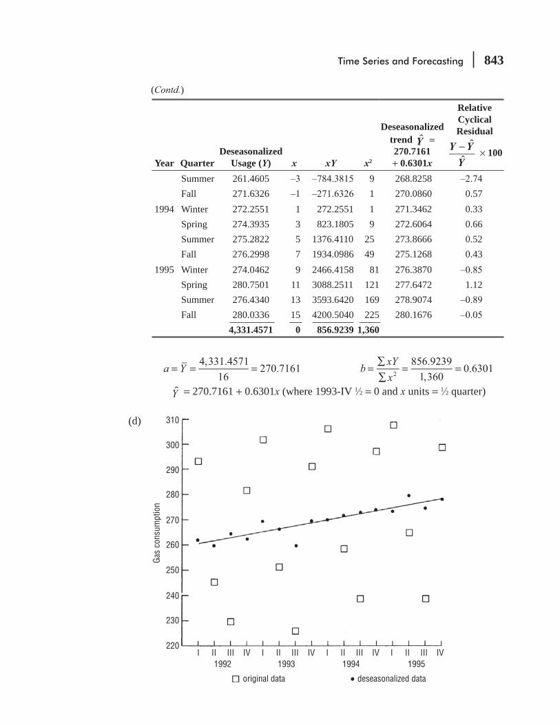
Time Series and Forecasting 843
(d) 310
300
290
280
270
Gas
cons
umpt
ion
260
250
240
230
220I II
1992
original data deseasonalized data
1993 1994 1995III IV I II III IV I II III IV I II III IV
Year QuarterDeseasonalized
Usage (Y) x xY x2
Deseasonalized trend Y = 270.7161+ 0.6301x
RelativeCyclicalResidual
Y YY
ˆˆ− × 100
SummerFall
261.4605271.6326
91
268.8258270.0860 0.57
1994 WinterSpringSummerFall
272.2551274.3935275.2822276.2998
1357
272.2551823.1805
1376.41101934.0986
19
2549
271.3462272.6064273.8666275.1268
0.330.660.520.43
1995 WinterSpringSummerFall
274.0462280.7501276.4340280.0336
4,331.4571
91113150
2466.41583088.25113593.64204200.5040856.9239
81121169225
1,360
276.3870277.6472278.9074280.1676
1.12
4,331.457116
270.7161 856.92391,360
0.63012a Y b xYx
= = = =∑∑
= =
Y = 270.7161 + 0.6301x (where 1993-IV 1 2 = 0 and x units = 1 2 quarter)
(Contd.)
844 Statistics for Management
15.8 TIME-SERIES ANALYSIS IN FORECASTINGIn this chapter, we have examined all four components of a time series. We have described the process of projecting past trend and seasonal variation into the future, while taking into consideration the inher-ent inaccuracies of this analysis. In addition, we noted that although the irregular and cyclical compo-
We must realize that the mechanical approach of time-series analysis is subject to considerable error and change. It is necessary for management to combine these simple procedures with knowl-edge of other factors in order to develop workable forecasts. Analysts are constantly revising, updating, and discarding their forecasts. If we wish to cope successfully with the future, we must do the same.
When using the procedures described in this chapter, we should pay particular attention to two problems:
1. In forecasting, we project past trend and seasonal variation into the future. We must ask, “How regular and lasting were the past trends? What are the chances that these patterns are changing?”
2. How accurate are the historical data we use in time series analysis? If a company has changed from
are not comparable and not very useful for forecasting.
Warning: Smart managers realize that accounting for most of the variation in a time series of past data does not mean that this same pattern will continue in the future. Hint: These same smart managers combine the predictions available from time series with intuitive answers to broad what-if questions concern the future business environment (sociological, economic, political) and whether it will
HINTS & ASSUMPTIONS
EXERCISES 15.815-40 List four errors that can affect forecasting with a time series.15-41 When using a time series to predict the future, what assurances do we need about the historical
data on which our forecasts are based?15-42 What problems would you see developing if we used past college enrollments to predict future
college enrollments?15-43 How would forecasts using time-series analysis handle things such as
(a) Changes in the federal tax laws?(b) Changes in accounting systems?
STATISTICS AT WORK
Loveland ComputersCase 15: Time Series Lee Azko was resting on well-earned laurels. The complicated regression analysis
Recognizing limitations of time-
series analysis

Time Series and Forecasting 845
hit or miss—there really were some rules to this game.
of Loveland’s latest personal computers. “Thanks for showing I was right. And you’re even making me a believer in that expensive newspaper advertising, too.”
“We’re going to deal with that next week—too early to say. But don’t get too comfortable. 1 have a whole new project for you—go and see Gratia.”
Gratia Delaguardia was clearly sharing a joke. The laughter was audible down the corridor— Gratia
Loveland’s team.“Lee, come on in and meet Roberto Palomar. Bert runs the phone bank—you know, our order depart-
ment. We were just talking about you.”“Hence the laughter?” Lee was nervous.
available to take orders. We need to plan for hiring....”“And to install enough incoming 800 lines,” added Roberto, whom everyone called Bert.“We plotted out the quarterly data,” continued Gratia, “and, as an engineer, let me tell you I can
recognize a nonlinear trend when I see one.” Gratia pointed to a curve that looked like the path of the space shuttle going into orbit. “Of course, we aren’t complaining about our growth. It’s good to be on a winning team.”
“But if we continue this trend,” said Bert, sliding a ruler into place on the graph, “within 10 years, we’ll have to employ the whole population of Loveland just to staff our phone banks.” With that, Gratia and Bert again dissolved with laughter. “Lee, look at these numbers and say it isn’t so.”
“Well, there’s no doubt there’s a very strong underlying trend,” Lee observed, noting the obvious. “Is there any seasonality—you know, differences from month to month?”
“Good question,” Bert replied. “These quarterly totals tend to mask some of the monthly ups and downs. For example, August is always a bust because people are away on vacation. But December is a very heavy month. We’re not really in the Christmas gift business, although some home users apparently do ask Santa for a new Loveland Computer. The main effect comes from small businesses that want to book equipment expenditures before the end of the year for tax purposes.”
“And I don’t suppose the call volume is evenly spaced over the week,” Lee ventured.“Ah, rainy days and Mondays!” Bert answered. “We have a rule of thumb that we do twice as
much business on Mondays as on Tuesdays. So we try to avoid training sessions or staff meetings on Mondays. Sometimes the supervisory staff will pitch in—whatever it takes. If we miss a call, a potential customer may buy from one of our competitors.
“But now we’re at the point where I really should plan a little better for the number of staff to have available. If I schedule too many people, it’s a waste of money and the reps get bored. They’d rather be at home.”
“Well I think I can help,” Lee offered. “Let me tell you what I’ll need.”
Study Questions: What data will Lee want to examine? What analysis will be performed? How will Bert make use of the information that Lee develops?

846 Statistics for Management
CHAPTER REVIEW
Terms Introduced in Chapter 15Coding(often called translating).
Cyclical Fluctuationabove and below a secular trend line.
Deseasonalization A statistical process used to remove the effects of seasonality from a time series.
Irregular Variation A condition in a time series in which the value of a variable is completely unpredictable.
A statistical method used in time-series analysis. Discards the highest and lowest values when computing a mean.
Ratio-to-Moving-Average Method A statistical method used to measure seasonal variation. Uses an index describing the degree of that variation.
Relative Cyclical Residual A measure of cyclical variation, it uses the percentage deviation from the trend for each value in the series.
Residual Method A method of describing the cyclical component of a time series. It assumes that most of the variation in the series not explained by the secular trend is cyclical variation.
Seasonal Variation Patterns of change in a time series within a year; patterns that tend to be repeated from year to year.
Second-Degree Equation A mathematical form used to describe a parabolic curve that may be used in time-series trend analysis.
Secular Trend A type of variation in a time series, the value of the variable tending to increase or decrease over a long period of time.
Time Series Information accumulated at regular intervals and the statistical methods used to deter-mine patterns in such data.
Equations Introduced in Chapter 15
15-1 b= XY nXYX nX2 2
∑ −∑ −
p. 808
This formula, originally introduced in Chapter 12 as Equation 12-4, enables us to calculate the slope of the best- tting regression line for any two-variable set of data points. The symbols X and Y represent the means of the values of the independent variable and dependent variable respectively; n
15-2 a=Y bX− p. 808 We met this formula as Equation 12-5. It enables us to compute the Y-intercept of the best-
tting regression line for any two-variable set of data points.
15-3 b Y2
xx
=∑∑
p. 810
Time Series and Forecasting 847
When the individual years (X) are changed to coded time values (x) by subtracting the mean (x = X − XEquation 15-3.
15-4 a=Y p. 810 In a similar fashion, using coded time values also allows us to simplify Equation 15-2 for the
intercept of the trend line.15-5 Y = a+bx+cxˆ 2 p. 812
line (Y = a + bxthe second-degree term (cx2) in the equation for Y
15-6 Y = an+c x2∑ ∑ p. 812
15-7 x Y a x +c x2 2 4∑ = ∑ ∑ p. 812
15-6 and 15-7 simultaneously for the values of a and c. The value for b is obtained from Equation 15-3.
15-8 Percent of trend = YY
× 100 p. 819
We can measure cyclical variation as a percent of trend by dividing the actual value (Y) by the trend value Y( ˆ) and then multiplying by 100.
15-9 Relative cyclical residual = Y YY
ˆˆ− × 100 p. 820
Another measure of cyclical variation is the relative cyclical residual, obtained by dividing the deviation from the trend (Y − Y ) by the trend value, and multiplying the result by 100. The relative cyclical residual can easily be obtained by subtracting 100 from the percent of trend.
Review and Application Exercises15-44
table:
Spring Summer Fall Winter1992 29 30 41 431993 27 34 45 481994 33 36 46 511995 34 40 47 53
(a) Calculate the seasonal indices for these data (use a 4-quarter centered moving average).(b) Deseasonalize these data using the indices from part (a).
15-45 Wheeler Airline, a regional carrier, has estimated the number of passengers to be 595,000 (deseasonalized) for the month of December. How many passengers should the company anticipate if the December seasonal index is 128?
848 Statistics for Management
15-46 An EPA research group has measured the level of mercury contamination in the ocean at a cer-tain point off the East Coast. The following percentages of mercury were found in the water:
Jan. Feb. Mar. Apr May June July Aug. Sept. Oct. Nov. Dec.1993 0.3 0.7 0.8 0.8 0.7 0.7 0.6 0.6 0.4 0.7 0.2 0.51994 0.4 0.9 0.7 0.9 0.5 0.8 0.7 0.7 0.4 0.6 0.3 0.41995 0.2 0.6 0.6 0.9 0.7 0.7 0.8 0.8 0.5 0.6 0.3 0.5
Construct a 4-month centered moving average, and plot it on a graph along with the original data.
15-47 A production manager for a Canadian paper mill has accumulated the following information describing the millions of pounds processed quarterly:
Winter Spring Summer Fall1992 3.1 5.1 5.6 3.61993 3.3 5.1 5.8 3.71994 3.4 5.3 6.0 3.81995 3.7 5.4 6.1 3.9
(a) Calculate the seasonal indices for these data (percentage of actual to centered moving average).
(b) Deseasonalize these data, using the seasonal indices from part (a).(c) Find the least-squares line that best describes these data.(d) Estimate the number of pounds that will be processed during the spring of 1996.
15-48 (a) Gasoline mileage achieved by U.S. automobiles.(b) Fatalities in commercial aviation.(c) The grain exports of a single country.(d) The price of gasoline.
15-49 Magna International is a large Canadian manufacturer of automotive components such as molded door panels. Magna’s 1992 annual report listed the company’s revenues for the previ-ous ten years (in millions of Canadian dollars):
Year 1983 1984 1985 1986 1987 1988 1989 1990 1991 1992Revenue 302.5 493.6 690.4 1,027.8 1,152.5 1,458.6 1,923.7 1,927.2 2,017.2 2,358.8
(a) Find the least-squares trend line for these data.(b) Plot the annual data and the trend line on the same graph. Do the variations from the trend
appear random or cyclical?
data. Is c x2
models would you recommend using to forecast Magna’s 1993 revenues? Explain.(d) Forecast Magna’s 1993 revenues.
15-50 predict the future behavior of the process that generated these data:(a) Sales of personal computers in the United States.

Time Series and Forecasting 849
(b) Use of video games in the United States.(c) Premiums for medical malpractice insurance.(d) The number of MBAs graduated from U.S. universities.
15-51 The following table shows the number of franchisees of Beauty Bar, Inc., operating at the end of each year:
Year 1990 1991 1992 1993 1994 1995Number of franchisees 596 688 740 812 857 935
(a) Find the linear equation that best describes these data.(b) Estimate the number of operations manuals (one to a franchisee) that must be printed
for 1997.15-52 An assistant undersecretary in the U.S. Commerce Department has the following data describ-
ing the value of grain exported during the last 16 quarters (in billions of dollars):
I II III IV1992 1 3 6 41993 2 2 7 51994 2 4 8 51995 1 3 8 6
(a) Determine the seasonal indices and deseasonalize these data (using a 4-quarter centered moving average).
(b) Calculate the least-squares line that best describes these data.(c) Identify the cyclical variation in these data by the relative cyclical residual method.(d) Plot the original data, the deseasonalized data, and the trend.
15-53 Richie Bell’s College Bicycle Shop has determined from a previous trend analysis that spring sales should be 165 bicycles (deseasonalized). If the spring seasonal index is 143, how many bicycles should the shop sell this spring?
15-54 manufacturers of heavy earth-moving equipment as they attempt to forecast sales? What new data would you suggest they use in their forecasting?
15-55 Automobile manufacturing is often cited as an example of a cyclical industry (one subject to changes in demand according to an underlying business cycle). Consider automobile produc-tion worldwide (in millions of units) and in the former U.S.S.R. (in hundreds of thousands of units) from 1970 through 1990:
Year World U.S.S.R. Year World U.S.S.R.1970 22.5 3.4 1981 27.5 13.21971 26.4 5.3 1982 26.6 13.11972 27.9 7.3 1983 30.0 13.21973 30.0 9.2 1984 30.5 13.31974 25.9 11.2 1985 32.3 13.31975 25.0 12.0 1986 32.9 13.3
(Continued)
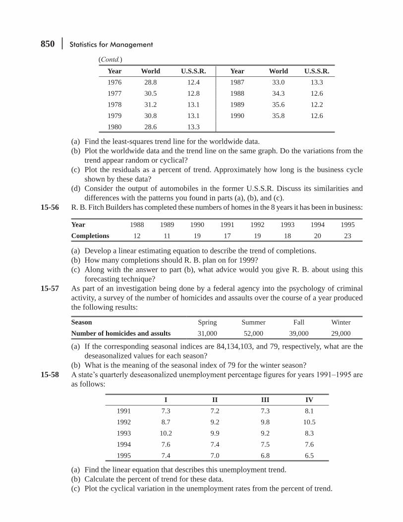
850 Statistics for Management
Year World U.S.S.R. Year World U.S.S.R.1976 28.8 12.4 1987 33.0 13.31977 30.5 12.8 1988 34.3 12.61978 31.2 13.1 1989 35.6 12.21979 30.8 13.1 1990 35.8 12.61980 28.6 13.3
(a) Find the least-squares trend line for the worldwide data.(b) Plot the worldwide data and the trend line on the same graph. Do the variations from the
trend appear random or cyclical?(c) Plot the residuals as a percent of trend. Approximately how long is the business cycle
shown by these data?(d) Consider the output of automobiles in the former U.S.S.R. Discuss its similarities and
differences with the patterns you found in parts (a), (b), and (c).15-56 R. B. Fitch Builders has completed these numbers of homes in the 8 years it has been in business:
Year 1988 1989 1990 1991 1992 1993 1994 1995Completions 12 11 19 17 19 18 20 23
(a) Develop a linear estimating equation to describe the trend of completions.(b) How many completions should R. B. plan on for 1999?(c) Along with the answer to part (b), what advice would you give R. B. about using this
forecasting technique?15-57 As part of an investigation being done by a federal agency into the psychology of criminal
activity, a survey of the number of homicides and assaults over the course of a year produced the following results:
Season Spring Summer Fall WinterNumber of homicides and assults 31,000 52,000 39,000 29,000
(a) If the corresponding seasonal indices are 84,134,103, and 79, respectively, what are the deseasonalized values for each season?
(b) What is the meaning of the seasonal index of 79 for the winter season?15-58
as follows:
I II III IV1991 7.3 7.2 7.3 8.11992 8.7 9.2 9.8 10.51993 10.2 9.9 9.2 8.31994 7.6 7.4 7.5 7.61995 7.4 7.0 6.8 6.5
(a) Find the linear equation that describes this unemployment trend.(b) Calculate the percent of trend for these data.(c) Plot the cyclical variation in the unemployment rates from the percent of trend.
(Contd.)

Time Series and Forecasting 851
15-59 1988 to 1992 were 2,4, 7,13, and 21, respectively.(a) Develop the linear regression line for these data.(b) Find the least-squares second-degree curve for these data.(c) Construct a table of each year’s actual cases, the linear estimates from the regression in
part (a), and the second-degree values from the curve in part (b).(d) Which regression appears to be the better estimator?
15-60 RJ’s Grocers has added broiled whole chickens to its line of takeout food for busy profession-
7 weeks are as follows:
Week 1 2 3 4 5 6 7Sales 41 52 79 76 72 59 41
(b) Estimate the expected number of sales for week 8.(c) Based on the estimate in part (b) and the available data, does the regression accurately
describe the sales trend for this item?15-61 The College Town busing system has collected the following count of passengers per season
during 1994 and 1995. The deseasonalized data (in thousands of passengers) are
Spring Summer Fall Winter1994 593 545 610 5751995 640 560 600 555
(a) If the seasonal indices used to deseasonalize these data were 110,73, 113, and 104, respec-
(b) Which season in 1995 saw the fewest passengers? The most?(c) If the linear estimating equation for these deseasonalized data is Y = 584.75 − 0.45x (with
x measured in 1 2 quarters, and x = 0 between the winter 1994 and spring 1995 quarters), what is the expected number of actual riders (in thousands) for the fall 1996 season?
15-62 Ferris Wheeler, director of the Whirly World amusement park, has provided the following attendance data (in thousands of admissions) for the park’s open seasons:
Spring Summer Fall1992 750 1,150 6801993 780 1,100 5801994 800 1,225 6101995 640 1,050 600
(a) Calculate the seasonal indices for these data using a 3-period moving average.(b) Deseasonalize these data using the seasonal indices from part (a).
15-63 A restaurant manager wishes to improve customer service and employee scheduling based on the daily levels of customers in the past 4 weeks. The numbers of customers served in the restaurant during that period were

852 Statistics for Management
Mon Tue Wed Thu Fri Sat Sun1 345 310 385 416 597 706 653
Week 2 418 333 400 515 664 761 7023 393 387 311 535 625 711 5984 406 412 377 444 650 803 822
Determine the seasonal (daily) indices for these data. (Use a 7-day moving average.)15-64
Year 1991 1992 1993 1994 1995Sales 230 250 265 300 310
(a) Develop the second-degree estimating equation for these data. a, b, and c tell you about the choice of a
second-degree equation for these data?15-65 The Zapit Company has recorded the following numbers (in hundreds of thousands) of total
sales of its line of microwave ovens over the last 5 years:
Year 1991 1992 1993 1994 1995Sales 3.5 3.8 4.0 3.7 3.9
The equation describing the trend for these sales volumes is
Y = 3.78 + 0.07x, where 1993 = 0, and x units = 1 year
(a) Which year had the largest percent of trend?(b) Which year was closest to the trend line?
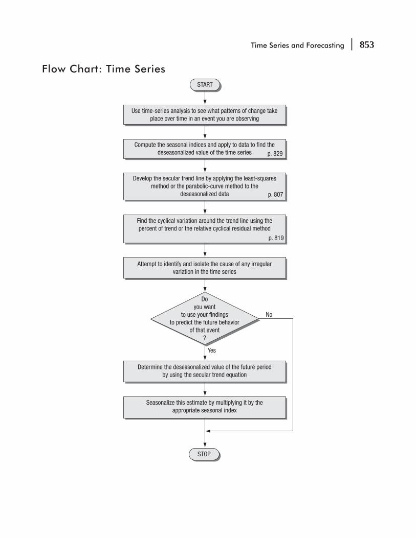
Time Series and Forecasting 853
Flow Chart: Time Series
Use time-series analysis to see what patterns of change takeplace over time in an event you are observing
Compute the seasonal indices and apply to data to find thedeseasonalized value of the time series p. 829
Develop the secular trend line by applying the least-squaresmethod or the parabolic-curve method to the
deseasonalized data p. 807
p. 819
Find the cyclical variation around the trend line using thepercent of trend or the relative cyclical residual method
Attempt to identify and isolate the cause of any irregularvariation in the time series
START
STOP
Determine the deseasonalized value of the future periodby using the secular trend equation
Seasonalize this estimate by multiplying it by theappropriate seasonal index
Doyou want
to use your findingsto predict the future behavior
of that event?
No
Yes

This page is intentionally left blank

16Index Numbers
After reading this chapter, you can understand:
CHAPTER CONTENTS
To understand that index numbers describe how much economic variables have changed over time
To become familiar with the three principal types of indices: price indices, quantity indices, and value indices
To understand and avoid problems resulting from the incorrect use of index numbers
To learn how to calculate various kinds of index numbers
LEARNING OBJECTIVES
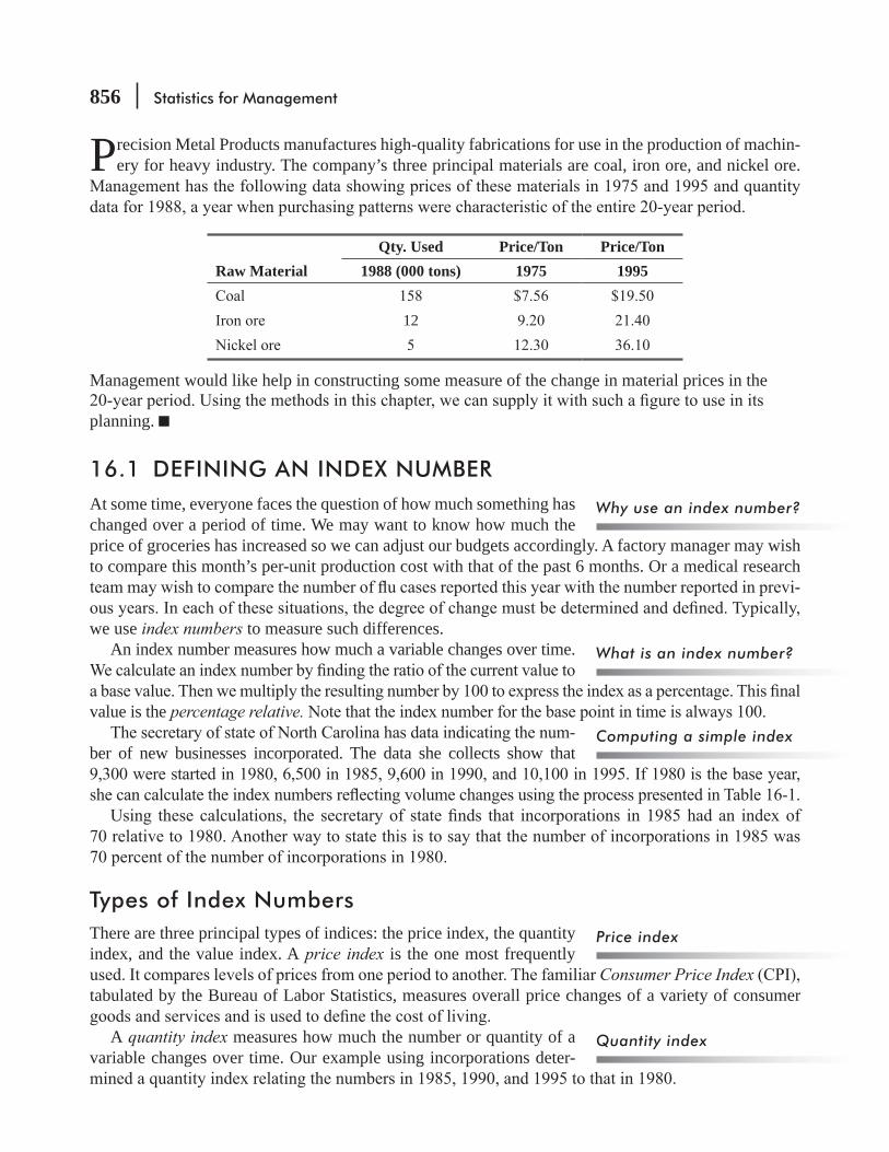
856 Statistics for Management
Precision Metal Products manufactures high-quality fabrications for use in the production of machin-ery for heavy industry. The company’s three principal materials are coal, iron ore, and nickel ore.
Qty. Used Price/Ton Price/TonRaw Material 1988 (000 tons) 1975 1995
12
Management would like help in constructing some measure of the change in material prices in the
planning.
16.1 DEFINING AN INDEX NUMBERAt some time, everyone faces the question of how much something has changed over a period of time. We may want to know how much the price of groceries has increased so we can adjust our budgets accordingly. A factory manager may wish to compare this month’s per-unit production cost with that of the past 6 months. Or a medical research
-
we use index numbers to measure such differences.An index number measures how much a variable changes over time.
value is the percentage relative.-
ber of new businesses incorporated. The data she collects show that
Types of Index NumbersThere are three principal types of indices: the price index, the quantity index, and the value index. A price index is the one most frequently
Consumer Price Indextabulated by the Bureau of Labor Statistics, measures overall price changes of a variety of consumer
A quantity index measures how much the number or quantity of a variable changes over time. Our example using incorporations deter-
Why use an index number?
What is an index number?
Computing a simple index
Price index
Quantity index

Index Numbers 857
Value indexThe last type of index, the value index, measures changes in total monetary worth. That is, it measures changes in the dollar value of a
dollar effect by computing the total incorporated value for the years under consideration. Table 16-2
that the value index
Usually, an index measures change in a variable over a period of time, such as in a time series.
done by simultaneously collecting data in different locations and then comparing the data. The
TABLE 16-1 CALCULATION OF INDEX NUMBERS (BASE YEAR = 1980)
Year(1)
Number of New Incorporations (000)
(2)Ratio
(3) = (2) ∏ 9.3
Index or Percentage Ralative
(4) = (3) ¥ 100
9.31.00
9.3=
× =
6.50.70
9.3=
× =
9.61.03
9.3=
× =
10.11.09
9.3=
× =
TABLE 16-2 COMPUTING A VALUE INDEX (BASE YEAR = 1980)
Year(1)
IncorporatedValue
(millions)(2)
Ratio(3) = (2) ∏ 18.4
Index orPercentage Relative
(4) = (3) ¥ 100
18.41.00
18.4= × =
14.6 14.60.79
18.4= × =
26.2 26.21.42
18.4= 1.42 × =142
29.41.60
18.4= × =
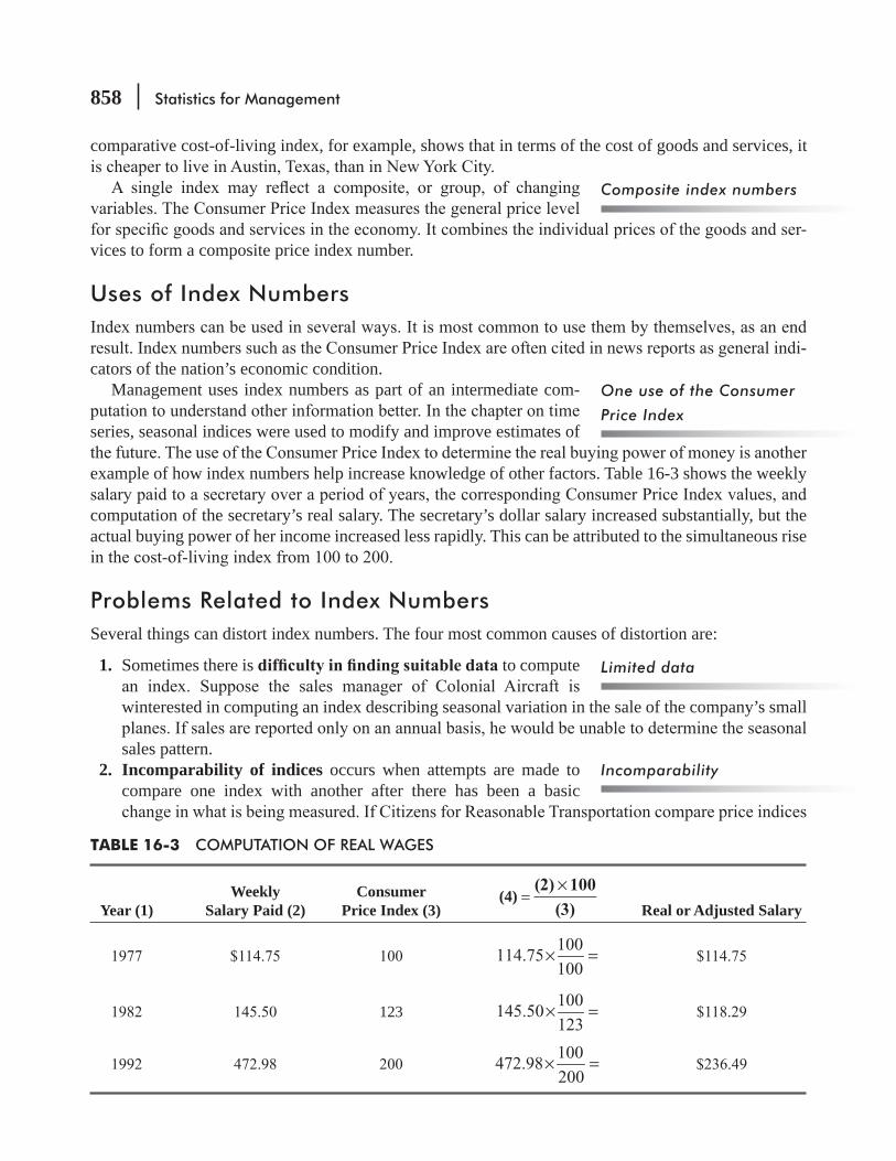
858 Statistics for Management
comparative cost-of-living index, for example, shows that in terms of the cost of goods and services, it
-vices to form a composite price index number.
Uses of Index Numbers
-cators of the nation’s economic condition.
Management uses index numbers as part of an intermediate com-
series, seasonal indices were used to modify and improve estimates of
example of how index numbers help increase knowledge of other factors. Table 16-3 shows the weekly
computation of the secretary’s real salary. The secretary’s dollar salary increased substantially, but the actual buying power of her income increased less rapidly. This can be attributed to the simultaneous rise
Problems Related to Index NumbersSeveral things can distort index numbers. The four most common causes of distortion are:
1. Sometimes there is to compute
winterested in computing an index describing seasonal variation in the sale of the company’s small
sales pattern. 2. Incomparability of indices occurs when attempts are made to
compare one index with another after there has been a basic
Composite index numbers
One use of the Consumer
Price Index
Limited data
Incomparability
TABLE 16-3 COMPUTATION OF REAL WAGES
Year (1)Weekly
Salary Paid (2)Consumer
Price Index (3)(4) =
(2) 100(3)×
Real or Adjusted Salary
100114.75
100× =
123100
145.50123
× =
100472.98
200× =

Index Numbers 859
comparison does not take into consideration technological advances in the quality of automobiles achieved over the time period in consideration.
3. Inappropriate weighting of factors
we must consider changes in some variables to be more important than changes in others. The effect
gas cost has a much greater effect on consumers. Thus, greater weight has to be assigned to the increased gas price than to the decrease in the cost of cars.
4. Distortion of index numbers also occurs when selection of an improper base
and why the base period was selected before we accept a claim based on the result of, comparing index numbers.
Sources of Index NumbersWhen managers apply index numbers to everyday problems, they use many sources to obtain the necessary information. The source depends
level of business activity, publications such as the Federal Reserve Bulletin, Moody’s, Monthly Labor Review, and the Consumer Price Index provide a wealth of data. Many federal and state publications are
Measuring Markets. Almost all government agen-
EXERCISES 16.1
Basic Concepts16-1 What is the index for a base year?16-2 Explain the differences among the three principal types of indices: price, quantity, and value.16-3 -
ite of variables? 16-4 What are two basic ways of using index numbers? 16-5 What does an index number measure? 16-6
Inappropriate weighting
Use of an improper base
Sources of data for index
numbers
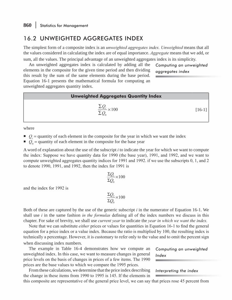
860 Statistics for Management
16.2 UNWEIGHTED AGGREGATES INDEXThe simplest form of a composite index is an unweighted aggregates index. Unweighted means that all the values considered in calculating the index are of equal importance. Aggregate means that we add, or sum, all the values. The principal advantage of an unweighted aggregates index is its simplicity.
An unweighted aggregates index is calculated by adding all the elements in the composite for the given time period and then dividing this result by the sum of the same elements during the base period. Equation 16-1 presents the mathematical formula for computing an unweighted aggregates quantity index.
Unweighted Aggregates Quantity Index
Q
Q100i
0
∑∑
× [16-1]
where
Qi = quantity of each element in the composite for the year in which we want the index Q = quantity of each element in the composite for the base year
A word of explanation about the use of the subscript i to indicate the year for which we want to compute
1
0
100Q
Q
Σ ×Σ
2
0
100Q
Q
Σ ×Σ
Both of these are captured by the use of the generic subscript i in the numerator of Equation 16-1. We shall use i in the same fashion in the formulaschapter. For sake of brevity, we shall use current year to indicate the year in which we want the index.
either
when discussing index numbers.The example in Table 16-4 demonstrates how we compute an
From these calculations, we determine that the price index describing
Computing an unweighted
aggregates index
Computing an unweighted
Index
Interpreting the index
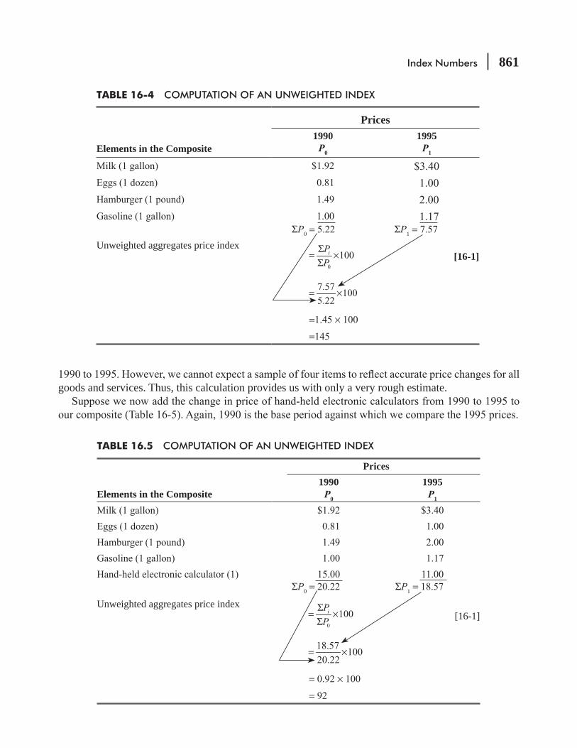
Index Numbers 861
goods and services. Thus, this calculation provides us with only a very rough estimate.
TABLE 16-4 COMPUTATION OF AN UNWEIGHTED INDEX
Elements in the Composite
Prices1990
P0
1995P1
ΣP = ΣP1 =
Unweighted aggregates price index
0
100iP
P
Σ= ×Σ [16-1]
7.57
1005.22
= ×
= ×
=
TABLE 16.5 COMPUTATION OF AN UNWEIGHTED INDEX
Elements in the Composite
Prices1990
P0
1995P1
ΣP = ΣP1 =
Unweighted aggregates price index
0
100iP
P
Σ= ×Σ [16-1]
18.57
10020.22
= ×
= ×
=

862 Statistics for Management
the major disadvantage of an unweighted index. It does not attach greater importance, or weight, to the price change of a high-use item than it does to a low-volume item.
price change for slow-moving items can completely distort an index. For this reason, it is not common to use a simple unweighted index in important analyses.
to calculate more sophisticated indices. Each of these will be discussed in detail in the following sections.
Warning: An unweighted index can be distorted, and lose its value from changes in a few items in
measure of housing costs. But most Social Security recipients are not in the market for a new mortgage. With the exception of those who have an adjustable-rate mortgage, their mortgage
disadvantage of an unweighted index is that it does not attach greater importance to price changes
appropriate, look carefully at the product/service components of that index to see whether their usage has been constant.
HINTS & ASSUMPTIONS
EXERCISES 16.2
Self-Check ExerciseSC 16-1
personnel.
1993 1994 1995
Skip Ford
Ken Johnson
an unweighted aggregates index.
Limitations of an unweighted
index
Index Numbers 863
Applications16-7
unweighted aggregates index.
Product A B C D E$221
$2,314
16-8 For purposes of bidding on U.S. contracts, the management of a large overseas manufacturing facility are compiling data on wage levels. The following data concern base pay for the differ-ent classes of labor in the facility over a 4-year period.
Wages per Hour1992 1993 1994 1995
$11.16
4.11
16-9 A study of college costs has collected data for the amount of tuition a fulltime undergraduate paid during the last 4 years at four schools:
1993 1994 1995 1996Eastem U. $3,142State U.Western U.
unweighted aggregates index.16-10
regarding food purchased for, the hospital kitchen. For the commodities listed, the corre-
Commodity 1993 1994 1995Dairy products $2.34Meat products 3.41 3.36
Fruit products 1.11
864 Statistics for Management
16-11
Material A B C D E
113
1,466
aggregates index.16-12 John Dykstra, a management trainee in a bank, has collected, information on the bank’s trans-
Withdrawals Deposits
Savings Checking Savings Checking
of an unweighted aggregates index. 16-13
summary of the company’s records shows how many new books it published in each year in the following areas:
1993 1994 1995
Biology
Mathematics 32
22
English 16 21
Sociology 24 26
Physics 26 32
26
Philosophy 11

Index Numbers 865
Worked-Out Answer to Self-Check ExerciseSC 16-1 1993
Q0
1994Q1
1995Q2
FordPriceWilliamsJohnson
199,300 228,500 260,750
= 0
100 :iQ
Q
Σ ×Σ
= = =
16.3 WEIGHTED AGGREGATES INDEXAs we have said, often we have to attach greater importance to changes in some variables than to other when we compute an index. This weighting allows us to include more information than just the change
sample. The problem is to decide how much weight to attach to each of the variables in the sample.The general formula for computing a weighted aggregates price
index is
Weighted Aggregates Price Index
PQPQ
100
i
0
ΣΣ × [16-2]
where
Pi = price of each element in the composite in the current year P = price of each element in the composite in the base year Q = quantity weighting factor chosen
=Typically, management uses the quantity of an item consumed as the measure of its importance in
computing a weighted aggregates index. This leads to an important question in applying the process: Which quantities are used?
using quantities consumed during the base period in computing each index number. This is called the Laspeyres method, after the statistician
Advantages of weighting
in an index
Computing a weighted
aggregates index
Three ways to weight an
index
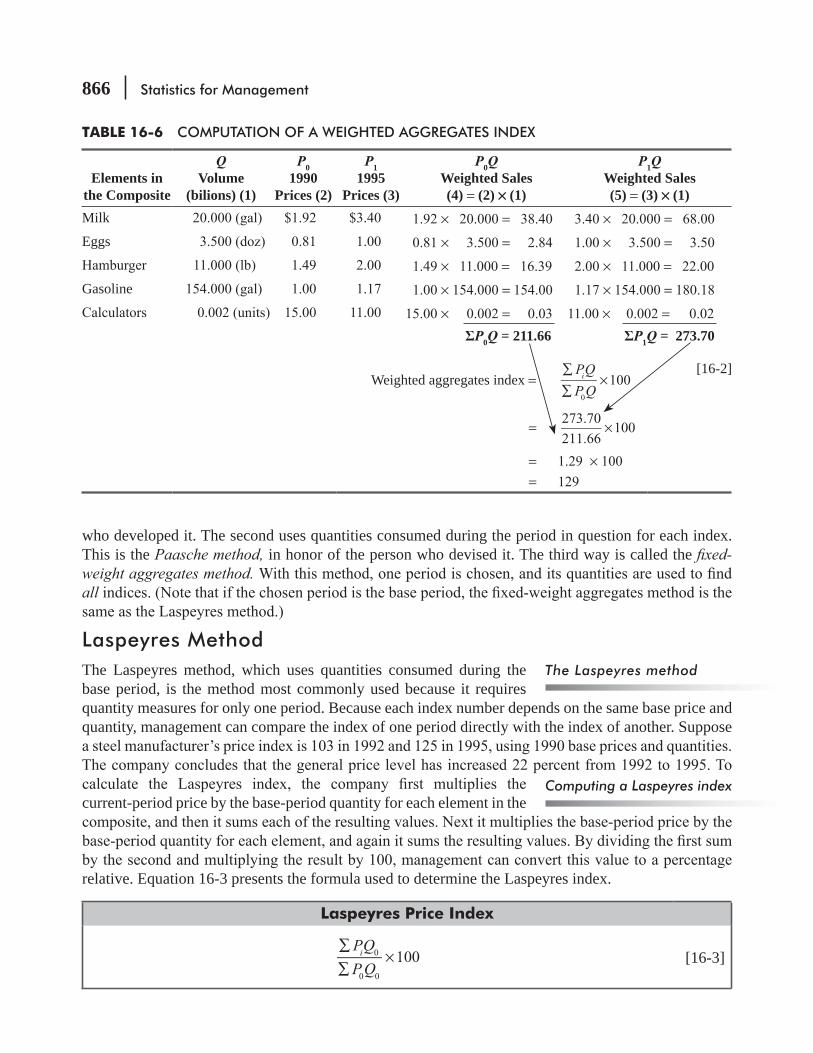
866 Statistics for Management
who developed it. The second uses quantities consumed during the period in question for each index. This is the Paasche method, in honor of the person who devised it. The third way is called the xed-weight aggregates method. all
Laspeyres MethodThe Laspeyres method, which uses quantities consumed during the base period, is the method most commonly used because it requires quantity measures for only one period. Because each index number depends on the same base price and quantity, management can compare the index of one period directly with the index of another. Suppose
current-period price by the base-period quantity for each element in the
relative. Equation 16-3 presents the formula used to determine the Laspeyres index.
Laspeyres Price Index
PQ
P Q100i 0
0 0
∑∑
× [16-3]
The Laspeyres method
Computing a Laspeyres index
TABLE 16-6 COMPUTATION OF A WEIGHTED AGGREGATES INDEX
Elements in the Composite
QVolume
(bilions) (1)
P01990
Prices (2)
P11995
Prices (3)
P0QWeighted Sales(4) = (2) ¥ (1)
P1QWeighted Sales(5) = (3) ¥ (1)
Milk × = × =Eggs × = × =
× = × =Gasoline × = × =
× = × =P0Q = 211.66 P1Q = 273.70
Weighted aggregates index = 1000
∑∑
×PQ
P Qi
[16-2]
= 273.70
211.66100×
= × =
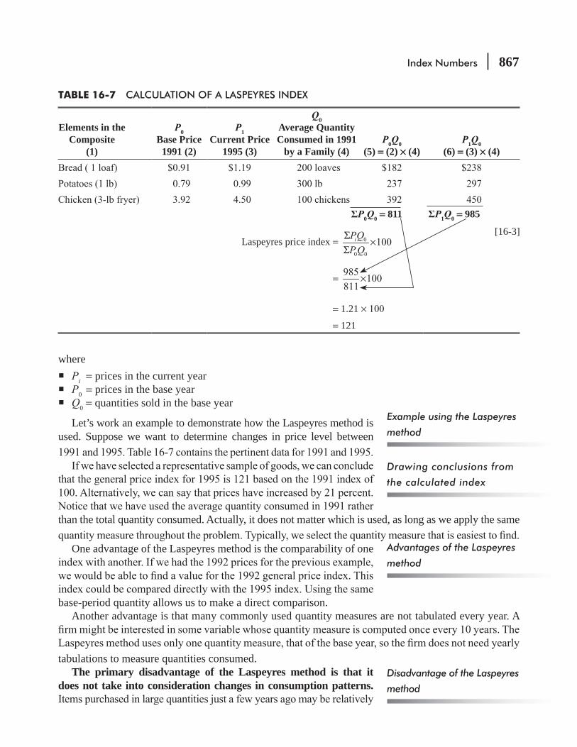
Index Numbers 867
where Pi = prices in the current year P = prices in the base year Q = quantities sold in the base year
Let’s work an example to demonstrate how the Laspeyres method is used. Suppose we want to determine changes in price level between
than the total quantity consumed. Actually, it does not matter which is used, as long as we apply the same
One advantage of the Laspeyres method is the comparability of one
base-period quantity allows us to make a direct comparison.Another advantage is that many commonly used quantity measures are not tabulated every year. A
tabulations to measure quantities consumed.The primary disadvantage of the Laspeyres method is that it
does not take into consideration changes in consumption patterns.
Example using the Laspeyres
method
Drawing conclusions from
the calculated index
Advantages of the Laspeyres
method
Disadvantage of the Laspeyres
method
TABLE 16-7 CALCULATION OF A LASPEYRES INDEX
Elements in the Composite
(1)
P0Base Price
1991 (2)
P1Current Price
1995 (3)
Q0Average Quantity Consumed in 1991
by a Family (4)P0Q0
(5) = (2) ¥ (4)P1Q0
(6) = (3) ¥ (4)
P0Q0 = 811 P1Q0 = 985
Laspeyres price index = 0
0 0
100iPQ
P Q
Σ ×Σ
[16-3]
= 985100
811×
= 1.21 ×
= 121
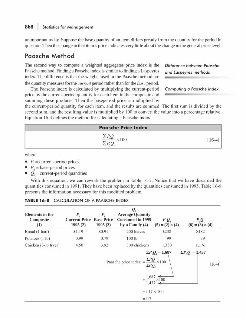
868 Statistics for Management
unimportant today. Suppose the base quantity of an item differs greatly from the quantity for the period in question. Then the change in that item’s price indicates very little about the change in the general price level.
Paasche MethodThe second way to compute a weighted aggregates price index is the
index. The difference is that the weights used in the Paasche method are the quantity measures for the current period rather than for the base period.
The Paasche index is calculated by multiplying the current-period price by the current-period quantity for each item in the composite and summing these products. Then the baseperiod price is multiplied by
Paasche Price Index
PQ
P Q100i i
i0
∑∑
× [16-4]
where Pi = current-period prices P = base-period prices Qi = current-period quantities
Difference between Paasche
and Laspeyres methods
Computing a Paasche index
TABLE 16-8 CALCULATION OF A PAASCHE INDEX
Elements in the Composite
(1)
P1Current Price
1995 (2)
P0Base Price
1995 (3)
Q1Average QuantityConsumed in 1995
by a Family (4)P1Q1
(5) = (2) ¥ (4)P0Q1
(6) = (3) ¥ (4)
P1Q1 = 1,687 P0Q1 = 1,437
Paasche price index 0
100i i
i
PQ
P Q
Σ= ×Σ [16-4]
1,687100
1,437= ×
= ×
=
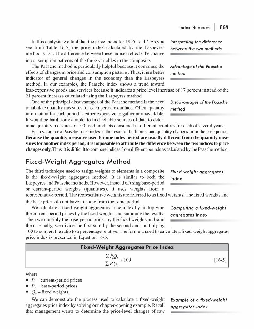
Index Numbers 869
in consumption patterns of the three variables in the composite.The Paasche method is particularly helpful because it combines the
effects of changes in price and consumption patterns. Thus, it is a better indicator of general changes in the economy than the Laspeyres
21 percent increase calculated using the Laspeyres method.One of the principal disadvantages of the Paasche method is the need
to tabulate quantity measures for each period examined. Often, quantity information for each period is either expensive to gather or unavailable.
-
Each value for a Paasche price index is the result of both price and quantity changes from the base period. Because the quantity measures used for one index period are usually different from the quantity mea-sures for another index period, it is impossible to attribute the difference between the two indices to price changes only.
Fixed-Weight Aggregates MethodThe third technique used to assign weights to elements in a composite
the base prices do not have to come from the same period.
Fixed-Weight Aggregates Price Index
∑∑
×PQ
P Q100i 2
0 2
where Pi = current-period prices P = base-period prices Q2 =
aggregates price index by solving our chapter-opening example. Recall that management wants to determine the price-level changes of raw
Interpreting the difference
between the two methods
Advantage of the Paasche
method
Disadvantages of the Paasche
method
Fixed-weight aggregates
index
Computing a fixed-weight
aggregates index
Example of a fixed-weight
aggregates index

870 Statistics for Management
(quantity).as the base-price level may have an uncharacteristic consumption level. Therefore, by being able to
because quantity measures are often expensive or impossible to obtain for certain periods.
The three methods covered in this section all produce a weighted aggregates index by using the quan-tities consumedeach uses to select these quantities. The Laspeyres method uses quantities from the base period. The Paasche method uses quantities from the period in question. The xed-weight aggregates method
xed-weight aggregates method is the base period, this method becomes the Laspeyres for weighting requires careful observation and common sense. The decision maker is looking for a period that has characteristic consumption,of the situation. There is no mathematical formula that will give you the right answer to this.
HINTS & ASSUMPTIONS
Advantage of a fixed-
weight aggregates index
TABLE 16-9 COMPUTATION OF A FIXED-WEIGHT AGGREGATES INDEX
RawMaterials
(1)
Q2Quantity
Consumed 1988(thousands of tons)
(2)
P0Average Price
1975($ per ton)
(3)
P1Average Price
1995($ per ton)
(4)
P0Q2Weighted
Aggregate 1975(5) = (3) ¥ (2)
P1Q2Weighted Aggregate
1995(6) = (4) ¥ (2)
12
P0Q2 = 1,366.38 P0Q2 = 3,518.30
Fixed-weight aggregates price index 1002
0 2
=∑∑
×PQ
P Qi
3,518.30
1001,366.38
= ×
= ×
=

Index Numbers 871
EXERCISES 16.3
Self-Check ExercisesSC 16-2 -
Price (per ton) Quantity Harvested (tons)Type of Grape 1992 1993 1994 1995 1992 1993 1994 1995
$113 $111Barbera
SC 16-3
SC 16-4 the base period.
Applications16-14
Selling Price ($) Number Sold (thousands)Model 1993 1994 1995 1996 1993 1994 1995 1996
ED ElectraED Optima 1,462 134.6
16-15
16-16 base period.
16-17 Julie Pristash, the marketing manager of Mod-Stereo, a manufacturer of blank cassette tapes,
Length of Tape(minutes) 1993 1994 1995
Average Quantity (¥ 100,000)1993–1995
32
16
Retail Price
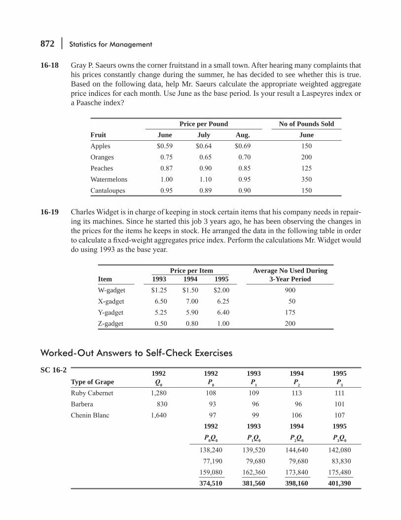
872 Statistics for Management
16-18 Gray P. Saeurs owns the corner fruitstand in a small town. After hearing many complaints that his prices constantly change during the summer, he has decided to see whether this is true. Based on the following data, help Mr. Saeurs calculate the appropriate weighted aggregate
a Paasche index?
Price per Pound No of Pounds SoldFruit June July Aug. JuneApplesOrangesPeachesWatermelons
16-19 -ing its machines. Since he started this job 3 years ago, he has been observing the changes in
Item 1993 1994 1995Average No Used During
3-Year PeriodW-gadget
Z-gadget
Worked-Out Answers to Self-Check Exercises
SC 16-2 Type of Grape
1992Q0
1992P0
1993P1
1994P2
1995P3
113 111Barbera
1992 1993 1994 1995P0Q0 P1Q0 P2Q0 P3Q0
374,510 381,560 398,160 401,390
Price per Item

Index Numbers 873
= 0
0 0
100iPQ
P Q
Σ ×Σ
: 37,451,000
374,510
38,156,000374,510
39,816,000374,510
40,139,000374,510
= = = =
SC 16-3 Type of Grape
1995Q3
1992P0
1993P1
1994P2
1995P3
113 111Barbera
1992 1993 1994 1995P0Q3 P1Q3 P2Q3 P3Q3
390,670 398,020 415,080 418,470
= PQP Q
100
i 3
0 3
∑∑
× : 39,067,000390,670
39,802,000
390,670
41,508,000390,670
41,847,000
390,670
= = = =
SC 16-4 Type of Grape
1992P1
1993P0
1994P2
1995P3
1992Q1
1993Q0
1994Q2
1995Q3
113 111Barbera
1992 1994 1995P1Q1 P0Q1 P2Q2 P0Q2 P3Q3 P0Q3
374,510 381,560 404,670 387,940 418,470 398,020
= 0
100 :i i
i
PQ
P Q
Σ ×Σ
37,451,000
381,560
98.2=
40,467,000387,940
104.3=
41,847,000398,020
105.1=

874 Statistics for Management
16.4 AVERAGE OF RELATIVES METHODS
Unweighted Average of Relatives MethodAs an alternative to the aggregates methods, we can use the average of relatives method to construct an index. Once again, we will use a price index to introduce the process.
Actually, we used a form of the average of relatives method in calculating the simple index in
the number of incorporations in the current year, Q1, by the number in the base year, Q , and multiplying
current price to the base price for each product and multiply each ratio
in Section 16-3 differ from this method. They sum all the prices beforepresents the general form for the unweighted average of relatives method.
Unweighted Average of Relatives Price Index
P
P
n
100i
0
∑ ×⎛
⎝⎜⎞
⎠⎟ [16-6]
where
Pi = current-period prices P = base-period prices n =
using the unweighted average of relatives method rather than the unweighted aggregates method.
the unweighted average of relatives method, we compute the average of the ratios of the prices for each product. With the unweighted aggregates method, we compute the
more weight than others. Rather, the average of relatives method converts each element to a relative scale where each element is represented as a percentage rather than an amount. Because of this, each of
Weighted Average of Relatives MethodMost problems management has to deal with require weighting by importance. Thus, it is more common to use the weighted average of relatives method than the unweighted method. When we
Computing an unweighted
average of relatives index
Comparing the unweighted
aggregates index and the
unweighted average of
relatives index
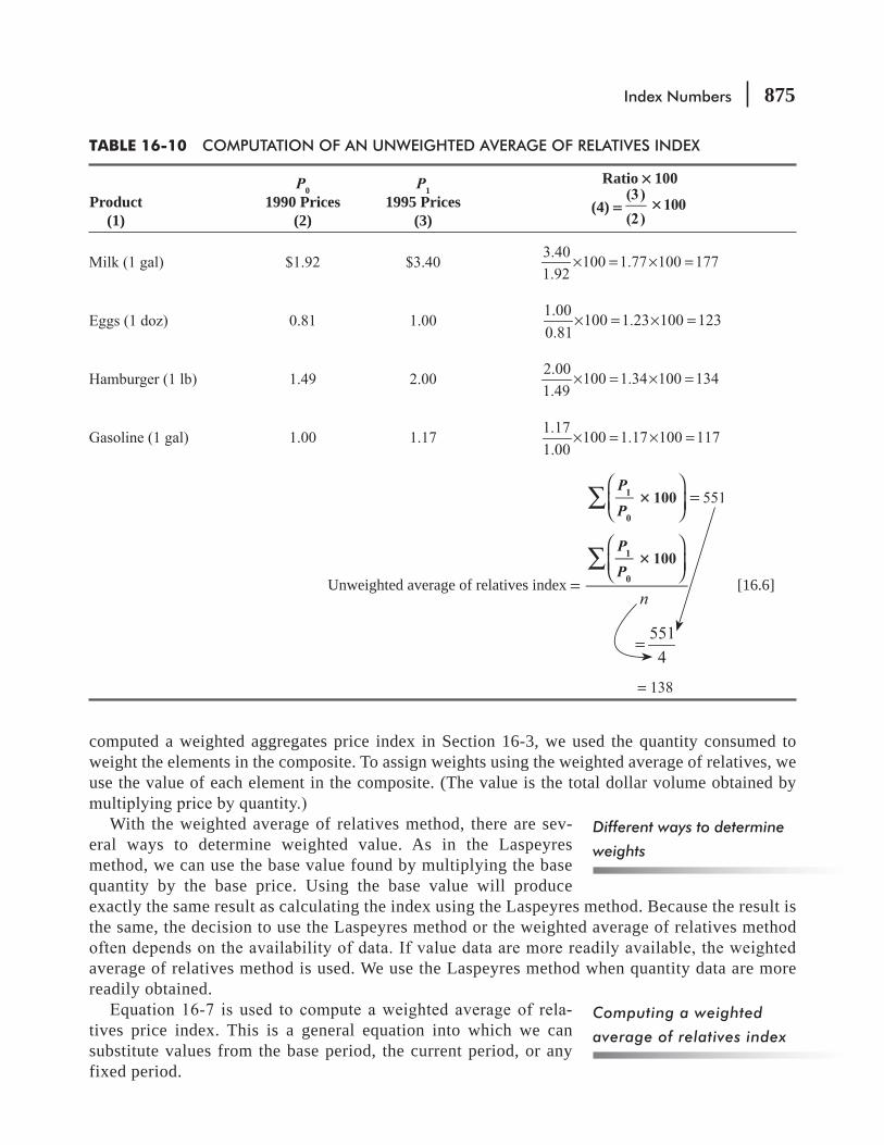
Index Numbers 875
computed a weighted aggregates price index in Section 16-3, we used the quantity consumed to weight the elements in the composite. To assign weights using the weighted average of relatives, we use the value of each element in the composite. (The value is the total dollar volume obtained by
With the weighted average of relatives method, there are sev-eral ways to determine weighted value. As in the Laspeyres method, we can use the base value found by multiplying the base quantity by the base price. Using the base value will produce exactly the same result as calculating the index using the Laspeyres method. Because the result is the same, the decision to use the Laspeyres method or the weighted average of relatives method
average of relatives method is used. We use the Laspeyres method when quantity data are more readily obtained.
-tives price index. This is a general equation into which we can substitute values from the base period, the current period, or any fixed period.
Different ways to determine
weights
Computing a weighted
average of relatives index
TABLE 16-10 COMPUTATION OF AN UNWEIGHTED AVERAGE OF RELATIVES INDEX
Product(1)
P01990 Prices
(2)
P11995 Prices
(3)
Ratio ¥ 100
(4) = (3)(2)
100
3.40100 1.77 100 177
1.92× = × =
1.00100 1.23 100 123
0.81× = × =
2.00100 1.34 100 134
1.49× = × =
1.17100 1.17 100 117
1.00× = × =
PP
100 551
1
0∑
⎛
⎝⎜⎞
⎠⎟=
Unweighted average of relatives index n
=
PP
1001
0∑
⎛
⎝⎜⎞
⎠⎟ [16.6]
5514
=
=
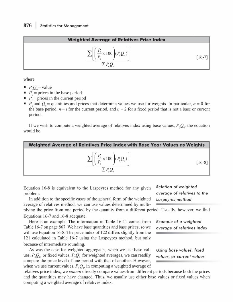
876 Statistics for Management
Weighted Average of Relatives Price Index
P
PP Q
P Q
100 ( )in n
n n
0
∑ ×⎛
⎝⎜⎞
⎠⎟⎡
⎣⎢⎢
⎤
⎦⎥⎥
∑
where
PnQn = value P = prices in the base period Pi = prices in the current period Pn and Qn = n =
the base period, n = i for the current period, and n =period.
P Q , the equation would be
Weighted Average of Relatives Price Index with Base Year Values as Weights
P
PP Q
P Q
100 ( )i
00 0
0 0
∑ ×⎛
⎝⎜⎞
⎠⎟⎡
⎣⎢⎢
⎤
⎦⎥⎥
∑
problem.
average of relatives method, we can use values determined by multi-
because of intermediate rounding.As was the case for weighted aggregates, when we use base val-
ues, P Q , P2Q2 , for weighted averages, we can readily
when we use current values, P1Q1, in computing a weighted average of relatives price index, we cannot directly compare values from different periods because both the prices
computing a weighted average of relatives index.
Relation of weighted
average of relatives to the
Laspeyres method
Example of a weighted
average of relatives index
Using base values, fixed
values, or current values
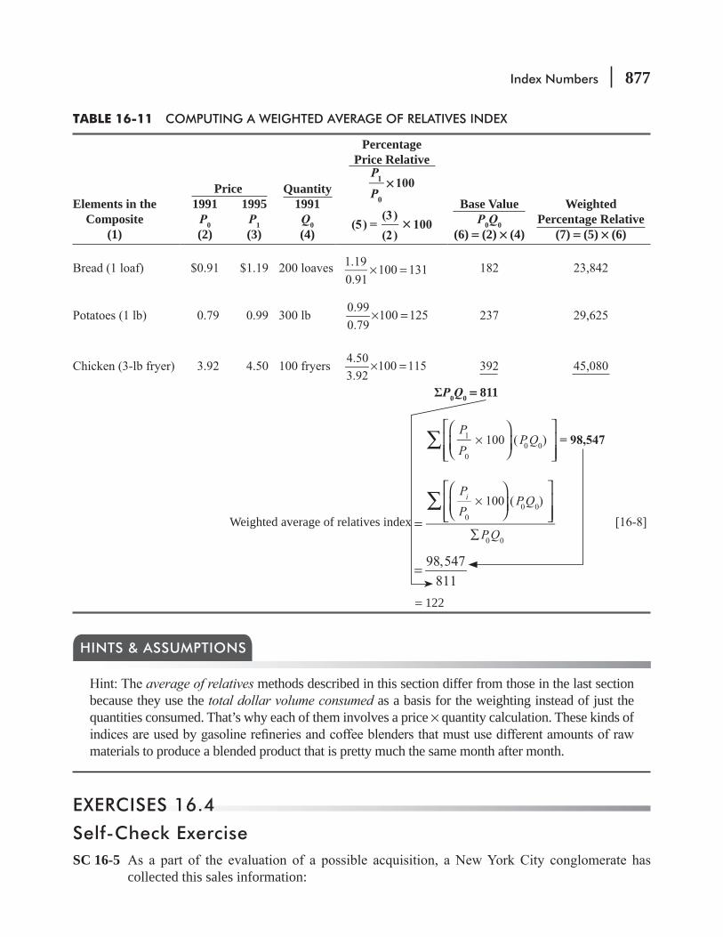
Index Numbers 877
average of relatives methods described in this section differ from those in the last section because they use the total dollar volume consumed as a basis for the weighting instead of just the quantities consumed. That’s why each of them involves a price × quantity calculation. These kinds of
materials to produce a blended product that is pretty much the same month after month.
HINTS & ASSUMPTIONS
EXERCISES 16.4
Self-Check ExerciseSC 16-5
collected this sales information:
TABLE 16-11 COMPUTING A WEIGHTED AVERAGE OF RELATIVES INDEX
Elements in the Composite
(1)
1991P0(2)
1995P1(3)
Quantity1991Q0(4)
PercentagePrice RelativePP
1001
0
(5) =(3)(2)
100Base Value
P0Q0(6) = (2) ¥ (4)
WeightedPercentage Relative
(7) = (5) ¥ (6)
1.19
0.91
100 131× =
0.99100 125
0.79× =
4.50100 115
3.92× =
P0Q0 = 811
PP
PQ = 98,547× 100 ( )
1
0
0 0
∑⎛
⎝⎜⎞
⎠⎟⎡
⎣⎢⎢
⎤
⎦⎥⎥
Weighted average of relatives index
PP
PQ
PQ
× 100 ( )
i
0
0 0
0 0
∑=
⎛
⎝⎜⎞
⎠⎟⎡
⎣⎢⎢
⎤
⎦⎥⎥
∑
98,547
811=
= 122
Price

878 Statistics for Management
Average AnnualPrice
Total Dollar Value(Thousands)
Product 1993 1995 1993
Radios 42
Applications
16-20 and volume for his franchise over the last 4 years.
Average Annual Price Tickets Sold (¥ 10,000)1992 1993 1994 1995 1992 1993 1994 1995
Box seats 26 31General admission
16-21 The following table contains information from the raw-material purchase records of a tire
Average AnnualPurchase Price/Ton
Value of Purchase (thousands)
Material 1993 1994 1995 1995Butadiene $ 11StyreneRayon cord 331
62Sodium pyrophosphate
weighting and for the base year.16-22 A Tennessee public interest group has surveyed the labor cost of automobile repairs in three
Type of Repair 1991 1993 1995Replacement of water pump $ 41
216Wheel balancing 26
16 16

Index Numbers 879
16-23
using the levels on those days, he determined the following yearly averages:
1993 1994 1995
Saving accounts
period.16-24
PriceTotal Dollar Value
(Thousands)Product 1994 1996 19941-megabyte chips $ 424-megabyte chips16-megabyte chips $612
period.
16-25 European cities produced these results:
Average Annual Passenger RatesPassengers(¥ 1,000)
Destination 1991 1992 1993 1994 1995 1995ParisLondonMunichRome
16-26
the base period, calculate an unweighted average of relatives price index for each year.
Insurance Group 1992 1993 1994 1995PhysiciansStudents 41Government employees 61Teachers 46

880 Statistics for Management
16-27 commitment to start construction, it wants to check the room prices charged nightly by the other motels and hotels. After sending an employee to investigate the prices, the motel chain received data in the following form:
Price per Room per NightNo. Rooms
RentedHotel 1993 1994 1995 1993
$42Room Service Rooms 26Executive Motel
44Family Fun Motel 26 31
unweighted average of relatives index.16-28
The maps that are sold are of the nearest city, the county the gas station is in, the state it is in, and the entire United States. From the following table, calculate the weighted average of rela-
Quantity SoldMaps 1993 1994 1995 1993
StateUnited States
Worked-Out Answer to Self-Check ExerciseSC 16-5
Product1993
P0
1995P1
P
P1
0 P0Q0
P
P1
0
⎛
⎝⎜⎞
⎠⎟(P0Q0)
111.11Radios 42
3.0643 2,420 2,636.44
= P
P
n
100
306.43
3
102.1
i
0
∑ ×⎛
⎝⎜⎞
⎠⎟= =
P
PP Q
P Q
100 ( )
263,644
2,420
108.9
i
0
0 0
0 0
∑∑
=×
⎛
⎝⎜⎞
⎠⎟= =

Index Numbers 881
16.5 QUANTITY AND VALUE INDICES
Quantity IndicesOur discussion of index numbers up to now has concentrated on price indices so that it would be easier to understand the general
these two, we use quantity indices more often. The Federal Reserve Board calculates quarterly indices in its monthly publication The Index of Industrial Production
-
corresponding value index does. Similarly, agricultural production is best measured using a quantity index because it eliminates misleading
to considerable price variation.Any of the methods discussed in previous sections of this chapter to determine price indices can be
used to calculate quantity indices. When we computed price indices, we used quantities or values as -
sider the construction of a weighted average of relatives quantity index.The general process for computing a weighted average of relatives
quantity index is the same as that used to compute a price index.
The value associated with each quantity is used to weight the elements in the composite.
Weighted Average of Relatives Quantity Index
Q
QQ P
Q P
100 ( )
in n
n n
0
∑ ×⎛
⎝⎜⎞
⎠⎟⎡
⎣⎢⎢
⎤
⎦⎥⎥
∑
where
Qi = quantities for the current period Q = quantities for the base period Pn and Qn = n =
the base period, n = 1 for the current period, and n =period.
of relatives quantity index. The value QnPn is determined from the base period and is therefore Q P0.
Using a quantity index
Advantages of a quantity
index
Computing a weighted
average of relatives
quantity index

882 Statistics for Management
Value IndicesA value index measures general changes in the total value of some variable. Because value is determined both by price and quantity, a value index actually measures the combined effects of price and quantity changes. The principal disadvantage of a value index is that it does not distinguish between the effects of these two components.
Medical insurance companies, for example, often cite the sharp increase in the value of payments awarded in medical malpractice suits as the primary reason for dis-
and larger cash amounts awarded.
A disadvantage of a value
index
Advantages of a value index
TABLE 16-12 COMPUTATION OF A WEIGHTED AVERAGE OF RELATIVES QUANTITY INDEX
Elements in the
Composite(1)
1991Q0(2)
1995Q1(3)
Price (per bushel)
1991P0(4)
1001
0
Percentage Relatives
(5) =
(3)(2)
100
BaseValueQ0P0
(6) = (2) ¥ (4)
Q P1001
00 0××
Weighted Relatives(7) = (5) ¥ (6)
Wheat 24 24.0
29.0
100 83× = × =
3 2.5
3
100 83× = 3 × =
Soybeans 12 1414.0
12.0
100 117× =
Q P = 196.9312 × 6.50 = 78.00
0 0
Q P100 ( )
1
0
0 0
∑ ×⎛
⎝⎜⎞
⎠⎟⎡
⎣⎢⎢
⎤
⎦⎥⎥
=
18,997.19
Weighted average of relatives quantity index
Q P
Q P
100 ( )
i
0
0 0
0 0
∑=
×⎛
⎝⎜⎞
⎠⎟⎡
⎣⎢⎢
⎤
⎦⎥⎥
∑
18, 997.19
196.93
=
=
Quantities (billions of
bushels)

Index Numbers 883
total dollar revenue may decrease during periods of high use of discount coupons. Because the company expects the quantitymore useful in making decisions about reordering cheese, toppings, and dough and scheduling delivery people.
HINTS & ASSUMPTIONS
EXERCISES 16.5
Self-Check ExerciseSC 16-6
Value of Sales (¥ $ 1,000)Salesperson 1992 1993 1994 1995ThompsonAlfredJacksonBlockard
period.
Basic Concepts
16-29 Explain the principal disadvantage in using value indices.16-30 What is the major difference between a weighted aggregates index and a weighted average of
relatives index?
Applications
16-31
Value of Sales (¥ $ 100,000)1991 1992 1993 1994 1995
6.322.41 2.33
period.16-32 -
884 Statistics for Management
Quantities ProducedCost of Production/
Unit (thousands)Product 1993 1994 1995 1995River barges $ 33Railroad gondola carsOff-the-road trucks 116
16-33 Arkansas Electronics has marketed three basic types of calculators: for the business sector, the
information describes unit sales for the past 3 years:
Number Sold (¥ 100,000) Price
Model 1993 1994 1995 1995Business 13.32
Basic
16-34 collected the following information:
Type of Crime 1992 1993 1994 1995Assault and rape 134MurderRobberyLarceny
16-35 music. Data are presented in hundreds of compact discs sold per year.
Number of SalesType 1991 1992 1993 1994 1995 1996
Soft rock 642.4426.4
123.6122.4
Alternative
base year.

Index Numbers 885
16-36 After encouraging a chemical company to make its employees handle certain dangerous chem-
ruling has had its effect in curbing the number of cancer deaths in that area. Before this rule went into effect, cancer was widespread not only among the workers at the company, but also among their families, close friends, and neighbors. The following data show what these num-
Age GroupNo. in Population
for 1973 Deaths in 1973 Deaths in 1993<4 yr
16-37 A veterinarian has noticed she has treated a large number of pets this past winter. She wonders whether this number was spread across the 3 winter months evenly or whether she treated more pets in any certain month. Using December as the base period, calculate the weighted average of relatives quantity indices for January and February.
Number Treated Price per VisitDec. Jan. Feb. Average for 3 Months
DogsParrotsSnakes
Worked-Out Answer to Self-Check Exercise
SC 16-6 1992 1993 1994 1995 1992 1993 1994 1995Salesperson V0 V1 V2 V3 V0/V0 V1/V0 V2/V0 V3/V0
Thompson 1.143AlfredJacksonBlockard
4.000 4.206 4.048 4.953
∑Index =
×⎛
⎝⎜⎞
⎠⎟100
4
:
400.0
4
420.6
4
404.8
4
495.3
= 100.0 = 105.2 = 101.2 = 123.8
4
0
VVi

886 Statistics for Management
16.6 ISSUES IN CONSTRUCTING AND USING INDEX NUMBERS
time spans. Actually, index numbers are computed for composites with many elements, and they cover long periods of time. This produces
Problems in ConstructionAlthough there are many problems in constructing index numbers, there are three principal areas of
1. Selecting an item to be included in a composite. Almost all indices are constructed to answer a particular question. Thus, the items included in the composite depend on the question. The
moderate-income urban Americans changed from one period to another?” From this question, we
income urban families. 2. Selecting the appropriate weights.
should represent the relative importance of the various elements. Unfortunately, what is appropriate in one period may become inappropriate in a short period of time. This must be kept in mind when comparing values of indices computed at different times.
3. Selecting the base period. Typically, the base period selected should be a normal period, preferably a fairly recent period.
of several consecutive periods to determine a normal value. The U.S. Bureau of Labor Statistics
management to relate its index to the major indices.
Caveats in Interpreting an Index-
ing indices:
1. One of the most common
combination of goods purchased by moderate-income urban Americans have changed. Despite its
Imperfections in index
numbers
Which items should be
included in a composite?
Need for selection of
appropriate weights
What is a normal base
period?
Problems with generalizing
from an index

Index Numbers 887
all Americans. Although it is related to the cost of living to some degree, to say that it measures the change in the cost of living is not correct.
2. Lack of general knowledge regarding published indices. Part
what the various published indices measure. All the well-known indices are accompanied by detailed statements concerning measurement. Management should become familiar with exactly what each index measures
3. Effect of time span on an index. Factors related to an index tend
change. Thus, unless the weights are changed accordingly, the index becomes less reliable. 4. Quality changes. One common criticism of index numbers is that
or overstates the price-level changes. For example, if we construct an index number to describe price changes in pocket calculators over the last decade, the resulting index would understate the actual change that is due to rapid technological improvements in calculators.
EXERCISES 16.6
Basic Concepts16-38 What is the effect of time on the weighting of a composite index? 16-39 List several preferences for the choice of base period.16-40 Describe a technique used to avoid the use of an irregular period for a base. 16-41 16-42 What problems exist with index numbers if the quality of an item changes?
STATISTICS AT WORK
Loveland ComputersCase 16: Index Numbersat a contract about half an inch thick. “The way we do our buying, the manufacturers are responsible for delivering an order to the airport and then an international shipping agent arranges for all the paperwork
excuse about the cost of living going up.”
“Well, at least you don’t have to worry about exchange rates,” Lee said, glancing over the contract. “This says you’re to make payment in U.S. dollars.”
“That’s true—we do send them a check in dollars and they clear it through the local branch of an American bank. Even though the dollar isn’t quite the universal currency it once was, people still think it’s less risky than many other currencies. But once the agent has cashed the check, they still have to exchange dollars for local currency. They can’t pay their warehouse workers in dollars. So, even though the price
Additional knowledge
needed
Time affects an index
Lack of measurement
of quality

888 Statistics for Management
“The cost of living is one factor, the cost of aviation fuel is another, and the exchange rate is the third. Does that cover everything?”
Denver and talk with the international department of our bank?”
Study Questions: What solution is Lee going to propose as a way to evaluate the proposed price for the shipping agent’s contract? What information will Lee be looking for in the bank’s international department?
CHAPTER REVIEW
Terms Introduced in Chapter 16Consumer Price Index The U.S. government prepares this index, which measures changes in the prices of a representative set of consumer items.Fixed-Weight Aggregates Method To weight an aggregates index, this method uses as weights quanti-ties consumed during some representative period.Index of Industrial Productionquantity of production in the areas of manufacturing, mining, and utilities.Index Number A ratio that measures how much a variable changes over time.Laspeyres Method To weight an aggregates index, this method uses as weights the quantities consumed during the base period.Paasche Methodconsumed during the current period.Percentage RelativePrice IndexQuantity Index A measure of how much the number or quantity of a variable changes over time.Unweighted Aggregates Index Uses all the values considered and assigns equal importance to each of these values.Unweighted Average of Relatives Methodof the current price to the base price for each product, adds the resulting percentage relatives, and then divides by the number of products.Weighted Aggregates Index Using all the values considered, this index assigns weights to these values.Weighted Average of Relatives Method To construct an index number, this method weights by impor-tance the value of each element in the composite.
Equations Introduced in Chapter 16
16-1 Unweighted aggregates quantity index = Q
Q100i
0
∑∑
×
To compute an unweighted aggregates index, divide the sum of the currentyear quantities of
Index Numbers 889
16-2 Weighted aggregates price index = PQ
P Q100i
0
∑∑
×
For a weighted aggregates price index using quantities as weights, obtain the weighted sum of the current-year prices by multiplying each price in the index by its associated quantity and summing the results. Then divide this weighted sum by the weighted sum of the base-year
16-3 Laspeyres index = PQ
P Q100i 0
0 0
∑∑
×
The Laspeyres price index is a weighted aggregates price index using the base-year quanti-ties as weights.
16-4 Paasche index = PQ
P Q100i i
i0
∑∑
×
To get the Paasche price index, we compute a weighted aggregates price index using the current-year quantities for weights.
16-5 Fixed-weight aggregates price index = PQ
P Q100i 2
0 2
∑∑
×
the quantities from a representative year, not necessarily either the base year or the current year.
16-6 Unweighted average of relatives price index
P
P
n
100i
0
∑=
×⎛
⎝⎜⎞
⎠⎟
We compute an unweighted average of relatives price index by multiplying the ratios of cur-
elements used in the index.
16-7 Weighted average of relatives price index
P
PP Q
P Q
100 ( )in n
n n
0
∑=
×⎛
⎝⎜⎞
⎠⎟⎡
⎣⎢⎢
⎤
⎦⎥⎥
∑
values as weights, we get
16-8
P
PP Q
P Q
100 ( )i
00 0
0 0
∑ ×⎛
⎝⎜⎞
⎠⎟⎡
⎣⎢⎢
⎤
⎦⎥⎥
∑
which is the same as the Laspeyres price index.

890 Statistics for Management
16-9 Weighted average of relatives quantity index
Q
QQ P
Q P
100 ( )in n
n n
0
∑=
×⎛
⎝⎜⎞
⎠⎟⎡
⎣⎢⎢
⎤
⎦⎥⎥
∑
period and divide the weighted sum by the sum of the weights.
Review and Application Exercises16-43
Average AnnualPrice
Units Sold(¥ 10,000)
Model 1993 1994 1995 1993 1994 19954.1
2.3 4.61.6 2.1 3.4
16-44
Commodity 1991 1993 1995$1,436 $1,321
Sugar 122 241
Zinc 142
16-45
weighted average of relatives quantity index for each of the 4 years.
Production(millions of tons)
Value($ millions)
Type of Coal 1989 1990 1991 1992 1992AnthraciteBituminous
Index Numbers 891
16-46
Average Price per UnitTotal Quantity
(billions)Product 1991 1995 1991
2.6 1.61
3.1
16-47
Products 1992 1993 1994 1995JeansJacketsShirts
16-48 What problem would exist in comparing price indices describing computer sales over the past few decades?
16-49 expenses incurred by selected salespeople. Of particular interest were the following data regarding expenditures for taxis and the price paid per mile.
Expenditures on Taxis Average Price/MileSalespeople 1991 1992 1993 1991
AB
DE
16-50 This information describes the unit sales of a bicycle shop for 3 years:
Number Sold PriceModel 1993 1994 1995 1993SportTouring 64
Sprint 21 16

892 Statistics for Management
16-51
exchange. This sum is then adjusted to account for splits and changes in the companies whose shares make up the index.
-
over long time periods. But stockbrokers sometimes choose low points in the market
16-52 Pem Jenkins runs a lumberyard and has the following information on costs for 3 years:
Costs 1991 1993 1995
Wages $36,421
Lumber 2,136
Utilities
as the base year. 16-53 An Ohio consumer protection agency has surveyed the price changes of a meatpacking com-
pany. The following table contains the average annual per-pound prices for a sample of the
Products 1993 1994 1995
Sirloin
1.24
Bologna
Rib eyes 2.61
16-54 Why must one exercise caution in selecting a base period?

Index Numbers 893
16-55
Material 1992 1993 1994 1995AluminumSteelBrass tubing
16-56 A USDA survey of grain production for selected areas in the United States yielded this information:
Quantities Produced(millions of bushels) Price per Bushel
Product 1991 1992 1993 1994 1995 1991Wheat
OatsRyeBarleySoybeans
for each year.16-57 John Pringle, an international mineral trader, has collected the following information on
Quantity (million tons) Price (per lb)Mineral 1995 1994 1995
LeadZinc
16-58 A European automobile manufacturer has compiled the following information on car sales of one U.S. manufacturer:
Average Annual Price (hundreds) Units Sold (¥ 1,000)Size 1991 1993 1995 1991 1993 1995Subcompact $62 32
Sedan 462

894 Statistics for Management
16-59 -
Products 1993 1994 1995 1996Dishwasher $241Washing machine 362 413Dryer 241 261Refrigerator
unweighted aggregates index.16-60
-ing data from four departments.
Total ExpendituresDepartment 1994 1995 1996Mechanical $3,642
BiomedicalElectrical
16-61
16-62 A national shopping survey was conducted to study the average weekly buying habits of a
1992 1996Items Unit Price Quantity Unit Price Quantity
2 13 32 1
1.36 2 2
16-63 Snow Mountain has several different ticket prices, including discounts for people who own property in the area, handicapped skiers, and snowboarders. The average number of tickets sold per ski-day was as follows:
1993 1994 1995 1996Local 112Snowboard 163 162Disabled 163Regular price

Index Numbers 895
16-64
Amount Exported(in millions of tons) Price per Ton
Product 1992 1993 1994 1995 1994Wheat 4.6Feed grains 6.2 1.2Soybeans 1.2
16-65 Andrea Graham, a budget analyst for a long-distance phone company, has collected price and
schedules are as follows:
Price per Call(per minute) Total # Calls
Rate (times) 1991 1996 (millions) 1991A.M. – 5 P.M.)
P.M – 11 P.MP.M. – 8 A.M.
16-66
Average SellingPrice per Bus
Number ofBuses Sold
Town 1992 1994 1996 1994
Greenville14
Middletown 21
16-67 A local fast-food restaurant wants to examine how sales are changing for each of its four most
Unit Price Quantity Sold (millions)Menu Item 1993 1994 1995 1996 1993 1994 1995 1996
2.11.2 2.1
French fries 2.3 2.4Onion rings 1.14 3.1 2.4 1.6

896 Statistics for Management
16-68 base period.
Flow Chart: Index Numbers
Use index numbers for ashorthand method to measure
the changes that occur ineconomic variables
To construct price, quantity,or value indices, begin by
collecting the appropriate data
START
Use unweightedrelatives index:
Σ(Pj /P0) × 100n⎯⎯⎯⎯⎯⎯
p. 874
Use weightedrelatives index:
Σ[(Pj /P0) × 100]PnQnΣPnQn
⎯⎯⎯⎯⎯⎯⎯⎯⎯
p. 876
Doyou want
an aggregates or relativesindex?
p. 860
Use weightedaggregates index:
ΣPj⎯⎯ΣP0
× 100
p. 865
Use Passche (p. 868),Laspeyres (p. 866), orsome other weighted
aggregates index:
ΣPjQ⎯⎯ΣP0Q
× 100
STOP
Doyou want
to attach greaterimportance tosome items
than toothers?
Doyou want
to attach greaterimportance tosome items
than toothers?
Relatives
No Yes No Yes
Aggregates

17Decision Theory
After reading this chapter, you can understand:
CHAPTER CONTENTS
To learn methods for making decisions under uncertainty
To use expected value and utility as decision criteria
To understand why additional information is useful and to calculate its value
17.1 The Decision Environment 898
Assigning Probability Values 899
Analysis 908
the Right Probabilities 921
17.6 Decision-Tree Analysis 925
To help decision makers supply needed probability values even when they do not understand probability theory
To learn how to use decision trees to structure and analyze complex decision-making problems
Review and Application Exercises 940
LEARNING OBJECTIVES
898 Statistics for Management
A
decision making. There we worked through a simple problem involving the purchase of strawberries for resale. That kind of problem is part of a set of problems that can be solved using the techniques devel-oped in this chapter.
statistical techniques to solve problems for which information was -
statistical decision theory, Bayesian decision theory decision theory. These names are used interchangeably.
- monetary reper-
cussions of our actions. A manager who must select from among a number of available investments
involves selecting an alternative and having a reasonable idea of the economic consequences of choos-ing that action.
17.1 THE DECISION ENVIRONMENT
decision makers approach their solutions in fairly consistent ways. The elements common to most
1. An objective the decision maker is trying to reach. If the
downtime each month. 2. Several courses of action. acts .
3. can be negative or positive and are called payoffs.cost of lost production time resulting from a motor burnout both when a spare is on hand and when
in the event of a power failure. Not having enough could cost lives as well as money. 4. Events beyond the control of the decision maker. These uncontrollable occurrences are often
called outcomes or states of nature,
What is decision theory?
Elements common to
decision-theory problems

Decision Theory 899
production machinery that will burn out in a given month. Preventive maintenance will reduce
5. we are uncertain about how many motors will burn out. This uncertainty is generally handled by the
EXERCISES 17.1
Applications17-1 -
17-2 -
provides a methodology that can help her decide which ventures to support and at what level.
17-3
Today’s Romancesmagazines. The number of copies that the bookstore would sell was never known for
-itability from the sale of its magazines and was considering the optimal number of Today’s Romances
17.2 EXPECTED PROFIT UNDER UNCERTAINTY: ASSIGNING PROBABILITY VALUES
is only one case in which decisions have to be made under uncer-tainty. Another involves a newspaper dealer who buys newspapers for 30¢ each and sells them for 50¢ each. Any papers not sold by the end of the day are completely
Buying decision under
conditions of uncertainty
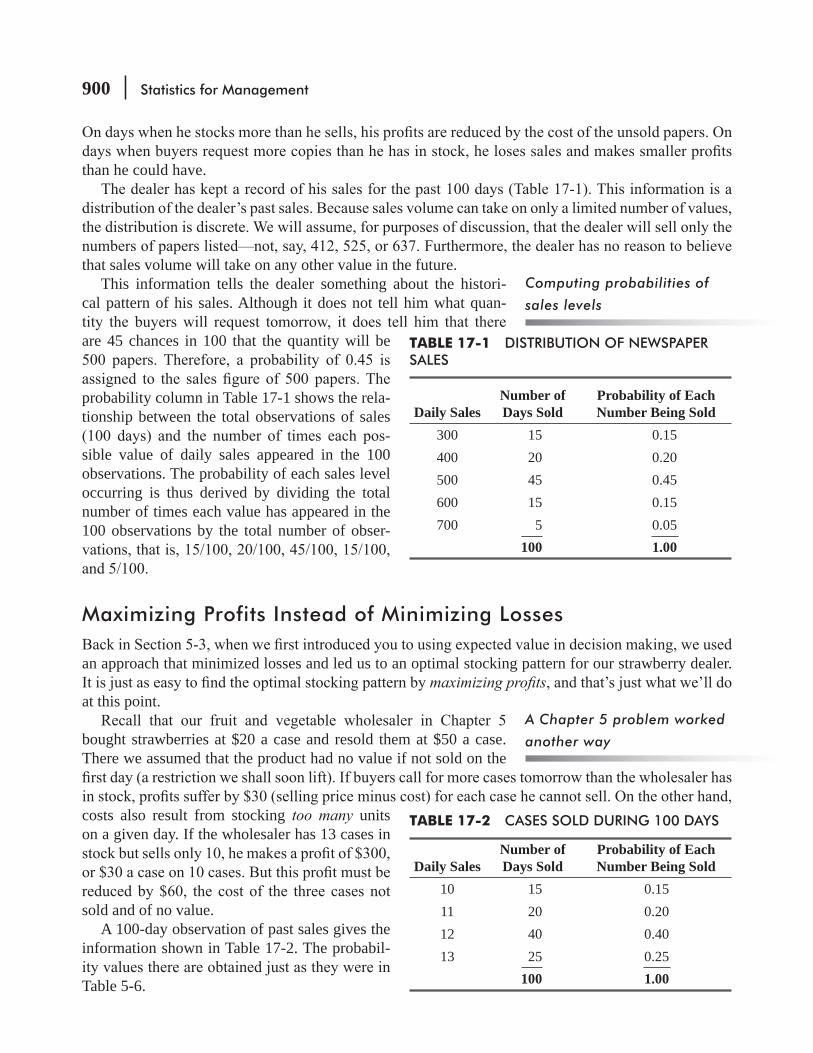
900 Statistics for Management
than he could have.
that sales volume will take on any other value in the future.This information tells the dealer something about the histori-
cal pattern of his sales. Although it does not tell him what quan-
are 45 chances in 100 that the quantity will be
probability column in Table 17-1 shows the rela-tionship between the total observations of sales
-sible value of daily sales appeared in the 100 observations. The probability of each sales level occurring is thus derived by dividing the total number of times each value has appeared in the 100 observations by the total number of obser-
Maximizing Profits Instead of Minimizing Losses
an approach that minimized losses and led us to an optimal stocking pattern for our strawberry dealer. maximizing pro ts
at this point.
bought strawberries at $20 a case and resold them at $50 a case. There we assumed that the product had no value if not sold on the
costs also result from stocking too many units on a given day. If the wholesaler has 13 cases in
sold and of no value.A 100-day observation of past sales gives the
information shown in Table 17-2. The probabil-
Table 5-6.
Computing probabilities of
sales levels
A Chapter 5 problem worked
another way
TABLE 17-1 DISTRIBUTION OF NEWSPAPER SALES
Daily SalesNumber of Days Sold
Probability of Each Number Being Sold
300 15 0.15400 20 0.20500 45 0.45600 15 0.15700 5 0.05
100 1.00
TABLE 17-2 CASES SOLD DURING 100 DAYS
Daily SalesNumber of Days Sold
Probability of Each Number Being Sold
10 15 0.1511 20 0.2012 40 0.4013 25 0.25
100 1.00

Decision Theory 901
reason to believe sales volume will behave differently in the future.
Calculating Conditional Profits
combinations of purchases and sales. The only values for purchases and for sales that have meaning to
more than 13 cases. conditional pro t table
resulting from any possible combination of supply and demand.
stocked.
-
not show the retailer how many cases he should
Conditional profit table
Explaining elements in the
conditional profit table
Function of the conditional
profit table
TABLE 17-3 CONDITIONAL PROFIT TABLE
Possible Demand (Sales) in Cases
Possible Stock Action10 Cases 11 Cases 12 Cases 13 Cases
10 $300 $280 $260 $24011 300 330 310 29012 300 330 360 34013 300 330 360 390

902 Statistics for Management
Calculating Expected ProfitsThe next step in determining the best number of cases to stock is assigning probabilities to the possible
Cases 10 11 12 13Probability 0.15 0.20 0.40 0.25
-
as we have done in Table 17-5. This tells us that if the retailer stocks
Computing expected profit
For 10 units
For 11 units
TABLE 17-4 EXPECTED PROFIT FROM STOCKING 10 CASES
Market Size in Cases
(1)
Conditional
(2)
Probability of Market Size
(3)
(4)10 $300 × 0.15 = $ 45.00
11 300 × 0.20 = 60.00
12 300 × 0.40 = 120.00
13 300 × 0.25 = 75.00
1.00 $300.00
TABLE 17-5 EXPECTED PROFIT FROM STOCKING 11 CASES
Market Size in Cases
Conditional Probability of Market Size
10 $280 × 0.15 = $42.00
11 330 × 0.20 = 66.00
12 330 × 0.40 = 132.00
13 330 × 0.25 = 82.50
1.00 $322.50

Decision Theory 903
TABLE 17-6 EXPECTED PROFIT FROM STOCKING 12 CASES
Market Size in Cases
Conditional Probability of Market Size
10 $260 × 0.15 = $39.00
11 310 × 0.20 = 62.00
12 360 × 0.40 = 144.00
stock← action
13 360 × 0.25 = 90.00
1.00 $335.00
TABLE 17-7 EXPECTED PROFIT FROM STOCKING 13 CASES
Market Size in Cases
Conditional Probability of Market Size
10 $240 × 0.15 = $36.00
11 290 × 0.20 = 58.00
12 340 × 0.40 = 136.00
13 390 × 0.25 = 97.00
1.00 $327.50
The optimal stock action is the one that results in the greatest
-tions given.
not reduced uncertainty in the problem facing the
best stock action open to him. He still does not know how many cases will be requested on any given
averagethe best
For 12 and 13 units
Optimal solution
What the solution means

904 Statistics for Management
Expected Profit with Perfect InformationNow suppose that the retailer in our illustration could remove all uncertainty from his problem by obtaining complete and accurate
perfect information. This does not mean that sales would not
for each day.
exact number of cases buyers will want tomorrow. For sales of
all losses from obsolete stock as well as allstrawberries.
-tion. This is shown in Table 17-9. The procedure is the same as that
because it is the maximum expected pro t possible.
Use of perfect information
Expected profit with perfect
information
TABLE 17-8 CONDITIONAL PROFIT TABLE WITH PERFECT INFORMATION
Possible Salesin Cases
Possible Stock Action10 Cases 11 Cases 12 Cases 13 Cases
10 $300 — — —11 — $330 — —12 — — $360 —13 — — — $390
TABLE 17-9 EXPECTED PROFIT WITH PERFECT INFORMATION
Market Size in Cases Perfect Information
Probability of Market Size Perfect Information
10 $300 × 0.15 = $45.00
11 330 × 0.20 = 66.00
12 360 × 0.40 = 144.00
13 390 × 0.25 = 97.50
1.00 $352.50
Decision Theory 905
Expected Value of Perfect InformationAssuming that a retailer could obtain a perfect predictor about the
expected value of perfect information and is referred to as
the knowledge is worth.
-
managers are really attempting to evaluate the worth of information that will enable them to make bet-
not
either $10 or
HINTS & ASSUMPTIONS
EXERCISES 17.2
Self-Check ExerciseSC 17-1
-
Number of machines 22 23 24 25 26 27Probability 0.12 0.16 0.22 0.27 0.18 0.05
Value of perfect information
Why do we need the value of
perfect information?

906 Statistics for Management
Even if Deborah could obtain a perfectly accurate forecast of the demand for each and
Applications17-4 -
garage will be likely to need.
HoursProbability 0.2 0.3 0.4 0.1
The manager plans to pay each mechanic $9.00 per hour and to charge customers $16.00.
-
17-5
-
Number of cars rented 10 11 12 13 14 15Probability 0.18 0.19 0.21 0.15 0.14 0.13
sell them and recapture 45 percent of the original cost. Ignoring the time value of money and .
17-6 -
vided the embossing machine. The personalizing was done on the department store premises.

Decision Theory 907
37.5 ¢ per box sold.
15 16 17 18 19 20Probability 0.05 0.20 0.30 0.25 0.10 0.10
17-7
Consulting jobs 24 27 30 33Probability 0.3 0.2 0.4 0.1
17-8 -
Historical sales indicated that between 55 and 60 dozen pizzas will be sold with the probabil-
55 56 57 58 59 60Probability 0.15 0.20 0.10 0.35 0.15 0.05
17-9
of a new design of fashion sandals. These sandals have posed problems in the past for two rea-
Pairs (thousands) 45 50 55 60 65Probability 0.25 0.30 0.20 0.15 0.10
Information from the production department reveals that the sandal will cost $15.25 per pair
should recommend that the company produce.

908 Statistics for Management
Worked-Out Answer to Self-Check ExerciseSC 17-1
Machines needed 22 23 24 25 26 27Probability 0.12 0.16 0.22 0.27 0.18 0.05
22 157.30 157.30 157.30 157.30 157.30 157.30 157.3023 156.45 164.45 164.45 164.45 164.45 164.45 163.49
Machines 24 155.60 163.60 171.60 171.60 171.60 171.60 168.4025 154.75 162.75 170.75 178.75 178.75 178.75 171.5526 153.90 161.90 169.90 177.90 185.90 185.90 172.54 ←27 153.05 161.05 169.05 177.05 185.05 193.25 172.09
EVPI == $1.787
hour-by-hour forecast of demand is of little value to her in this situation.
17.3 USING CONTINUOUS DISTRIBUTIONS: MARGINAL ANALYSIS
-
-
The marginal approach avoids this problem.
If we let p p must be the probability of not selling it. If the additional
marginal pro t MP.
Table 17-10 illustrates this point. If we stock 10 units each day and daily demand is for 10 or more
stockingresult only when demand is for 11 or more units. This will be the case 85 percent of the time.
an additional unit and not selling it. This reduces our conditional
Limitations of the tabular
approach
Derivation of marginal profit
Marginal loss

Decision Theory 909
marginal loss ML
the item.
Additional units should be stocked as long as the expected mar-
marginal loss from stocking each. The size of each day’s order
unsold.
Market Size Probability of Market Size10 0.1511 0.2012 0.4013 0.25
1.00
p
Probability that demand will be for 11 0.20Probability that demand will be for 12 0.40Probability that demand will be for 13 0.25Probability that demand will be for 11 or more units 0.85
the time.
Derivation of stocking rule
TABLE 17-10 CONDITIONAL PROFIT TABLE
Possible Demand (sales) in Cases
Probability of Market Size
Possible Stock Actions10 Cases 11 Cases 12 Cases 13 Cases
10 0.15 $300 $280 $260 $24011 0.20 300 330 310 29012 0.40 300 330 360 34013 0.25 300 330 360 390

910 Statistics for Management
Deriving the Minimum Probability EquationThe expected marginal pro t from stocking and selling an additional
p MP . The expected marginal loss from stocking and not selling an additional unit is the marginal loss incurred if the unit is unsold mul-
p ML . retailer in this situation would stock up to the point at which
p MP = p ML
p MP p ML . As long as p MP p ML
one value of p
equation and solving it for p
p MP = p ML
p MP = ML p ML
p
p MP p ML = MLor
p MP ML = ML
Dividing both sides of the equation by MP ML gives
Minimum Probability Required to Stock Another Unit
* =+
pML
MP ML
The symbol p* represents the minimum required probability of selling at least one additional unit to -
ability of selling at least an additional unit is greater than p*. p*
pML
MP ML*
$20
$30 $20
$20
$500.40=
+=
+= =
This value of 0.40 for p*must have at least a 0.40 cumulative probability of selling that unit or more. In order to determine the
Expected marginal profit and
loss defined
Optimal inventory stock action
Minimum-probability
equation

Decision Theory 911
The cumulative probabilities in the right-hand column of Table 17-11 represent the probabilities that sales will reach or exceed each
the 10-unit sales level means that we are 100 percent of selling 10 or more units. This must be true because our assumes that one of the four sales levels will always occur.
0.200.40
0.85 = probability of selling 11 or more
which has a probability of 0.15.
All possible outcomes 1.00Probability of selling10
0.85 = Probability of selling 11 or more
The cumulative probability value of 0.65 assigned to sales of 12 units or more can be established in
Probability of selling 12 0.40Probability of selling 13
0.65 = probability of selling 12 or more
sales will never exceed 13. p decreases as the level of stock increases. This causes the
the probability of selling at least an additional unit is greater than pshould be stocked.
Calculation of cumulative
probabilities
Stocking rule
TABLE 17-11 CUMULATIVE PROBABILITIES OF SALES
Sales Units
Probability of This Sales Level
Cumulative Probability That Sales Will Be at This Level or Greater
10 0.15 1.0011 0.20 0.8512 0.40 0.6513 0.25 0.25

912 Statistics for Management
p*
p MP = = p ML = = $3.00 expected marginal loss
than the required p*
p MP = =p ML = = $7.00 expected marginal loss
Twelve is the optimal addition of a thirteenth unit carried with it only a 0.25 probability
p* of 0.40. The
p MP = =p ML = = $15.00 expected marginal loss
Notice that the use of marginal analysis leads us to the same conclusion that we reached with the use
stock 12 units each period.
often take on recognizable patterns depending on the particular day
-
stocking level for each -
Using the Standard Normal Probability Distribution
use this idea to help us solve a decision-theory problem using a continuous distribution.Assume that a manager sells an article having normally distributed
sales with a mean of 50 units daily and a standard deviation in daily sales of 15 units. The manager purchases this article for $4 per unit
- p*
pML
MP ML* =
+
$4
$5 $40.44=
+=
Optimal stocking level for this
problem
Adjusting the optimal
stocking level
Solving a problem using
marginal analysis
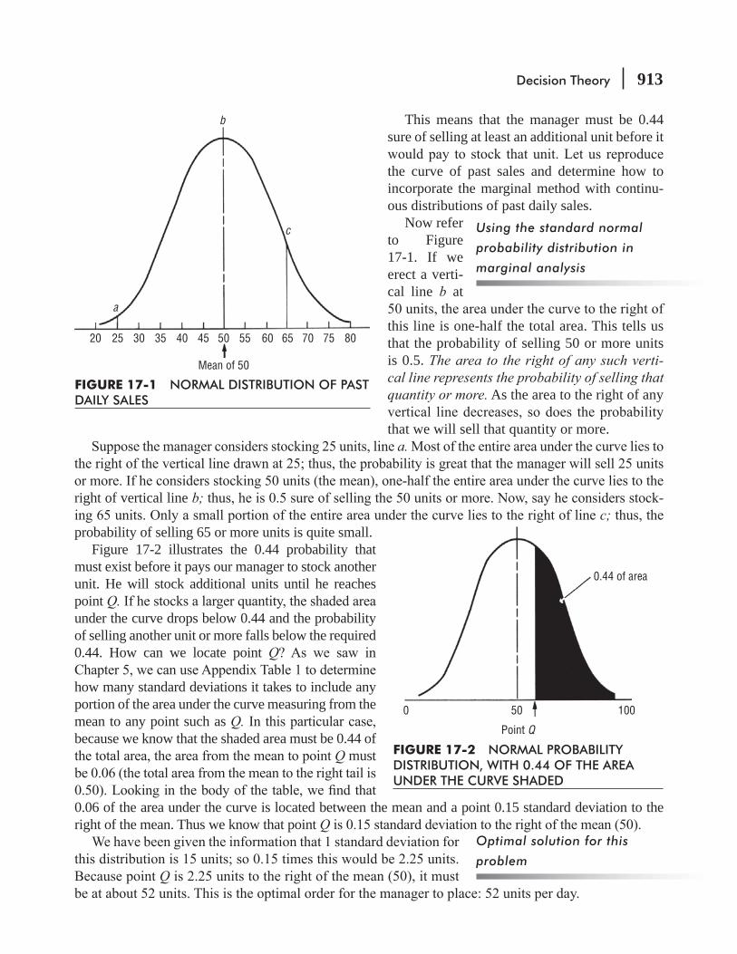
Decision Theory 913
This means that the manager must be 0.44 sure of selling at least an additional unit before it
the curve of past sales and determine how to incorporate the marginal method with continu-ous distributions of past daily sales.
Now refer to Figure 17-1. If we erect a verti-cal line b at
this line is one-half the total area. This tells us that the probability of selling 50 or more units is 0.5. The area to the right of any such verti-cal line represents the probability of selling that quantity or more. As the area to the right of any
that we will sell that quantity or more. a.
right of vertical line b; - c;
probability of selling 65 or more units is quite small.Figure 17-2 illustrates the 0.44 probability that
must exist before it pays our manager to stock another unit. He will stock additional units until he reaches point Q.under the curve drops below 0.44 and the probability of selling another unit or more falls below the required 0.44. How can we locate point Q
how many standard deviations it takes to include any portion of the area under the curve measuring from the mean to any point such as Q.because we know that the shaded area must be 0.44 of
Q must
0.06 of the area under the curve is located between the mean and a point 0.15 standard deviation to the right of the mean. Thus we know that point Q
Q
Using the standard normal
probability distribution in
marginal analysis
Optimal solution for this
problem
20 25 30
a
b
c
35 40 45 50 55
Mean of 50
60 65 70 75 80
FIGURE 17-1 NORMAL DISTRIBUTION OF PAST DAILY SALES
0
Point Q
50
0.44 of area
100
FIGURE 17-2 NORMAL PROBABILITY DISTRIBUTION, WITH 0.44 OF THE AREA UNDER THE CURVE SHADED

914 Statistics for Management
Now that we have been through one problem using a continuous
60 boxes
sales distribution 10 boxes$20$32$ 2
p*
Chapter-opening problem
Minimum required probability
0
Point Q
60
0.60 of area
0.25std.dev
120
FIGURE 17-3 NORMAL PROBABILITY DISTRIBUTION, WITH 0.60 OF THE AREA UNDER THE CURVE SHADED
pML
MP ML* =
+$20 $2
$12 ($20 $2)=
−+ −
Notice that a salvage value of $2is deducted from the cost of $20
to obtain the ML
$18
$12 $18=
+$18
$300.60= =
Figure 17-3.The manager wants to increase his order size until it
reaches point Q. Now point Q lies to the leftwhereas in the preceding problem it lay to the right. How
= Q with 0.0987 of the area under the curve
contained between the mean and point Q. The table indicates point Q is 0.25 standard deviation from the Q
0.25 × standard deviation = 0.25 × 10 boxes = 2.5 boxes Point Q = mean less 2.5 boxes = = 57.5 or 57 boxes
Optimal solution for chapter-
opening problem
Decision Theory 915
expected pro t calculated from a single sales distribution as your decision rule assumes that the sales distribution you are dealing with represents all of the informa-
daily differences exist. These daily differences are themselves quite different in certain countries.
near zero in Israel because it is their sabbath.
HINTS & ASSUMPTIONS
EXERCISES 17.3
Self-Check ExerciseSC 17-2
City Herald Herald is well described by a normal
distribution with mean μ = 165 and standard deviation σ = Herald sell for Heralds are left
many copies of the Herald
Applications17-10
-chases new signs each year. Although the signs are made under the auspices of the Department
signs from an outside source. The interdepartmental charge for the signs is $21 if more than 35
-
17-11
transfer patches from a supplier for $0.75 and plain white cotton T-shirts for $1.50. A local merchant supplies the appropriate heating device and also purchases all unsold white cotton

916 Statistics for Management
similar shirt sales have averaged 200 with a standard deviation of 34. The council knows that there will be no market for the patches after the celebration. How many patches should the
17-12
17-13 small and newly established bicycle shops that needed access to a wide variety of inven-
replacement parts and accessories but does not maintain any stock of completed bicycles. ″ × 11 4″ -
average of 120 rims per summer with a standard deviation of 28. The company expects
Parts has been quite successful and plans to move its operations to a larger plant during the
selling price is $8.10.17-14 -
portion is such a bargain that the barbecued chicken special has become a very popular item. Data taken from the last year indicate that demand for the special is normally distributed with mean μ = 190 portions and standard deviation σ =
17-15 The polyester-belted radials cost the company $30 each and sell for $35. The steel-belted
annual sales of both types of radial tires are normally distributed with the following means
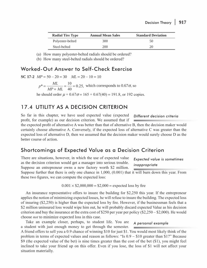
Decision Theory 917
Annual Mean Sales Standard DeviationPolyester-belted 300 50
200 20
Worked-Out Answer to Self-Check ExerciseSC 17-2 MP = = 30 ML = = 10
pML
MP ML*
10
400.25,=
+= = which corresponds to 0.67σ
he should order μ σ = =
17.4 UTILITY AS A DECISION CRITERION
better course of action.
Shortcomings of Expected Value as a Decision Criterion
as the decision criterion would get a manager into serious trouble.
0.001 × = =
choose not to minimize expected loss in this case.
−
situation materially.
Different decision criteria
Expected value is sometimes
inappropriate
A personal example
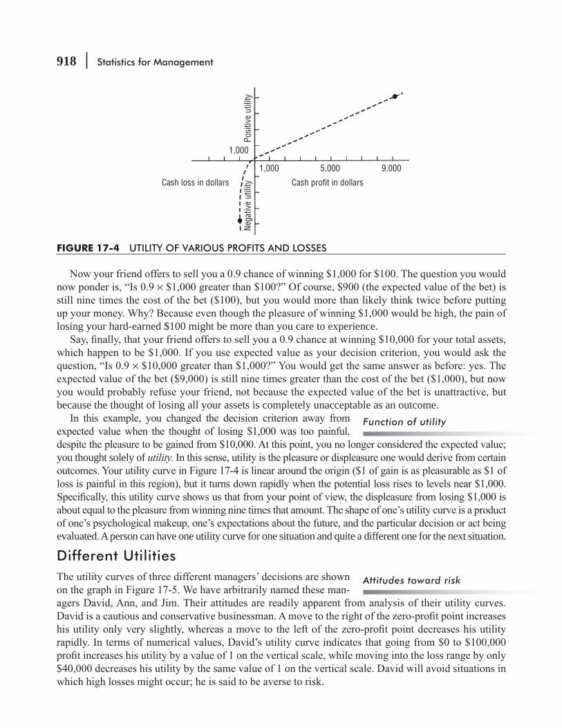
918 Statistics for Management
×
losing your hard-earned $100 might be more than you care to experience.
×
because the thought of losing all your assets is completely unacceptable as an outcome.
you thought solely of utility.
evaluated. A person can have one utility curve for one situation and quite a different one for the next situation.
Different Utilities
-
Function of utility
Attitudes toward risk
1,000
1,000
5,000
Cash profit in dollarsCash loss in dollars
Nega
tive
utili
tyPo
sitiv
e ut
ility
9,000
FIGURE 17-4 UTILITY OF VARIOUS PROFITS AND LOSSES

Decision Theory 919
Because his utility curve is
An important prerequisite to understanding the behavior of investors is realizing that their utility
heavy family obligations tend to be risk averse and invest only when the expected outcome is posi-tive. An interesting question for you to discuss with your classmates is why the elderly are victims
HINTS & ASSUMPTIONS
Who would use expected
value?
+5
David
Jim
Ann
+4
+3
+2
+1
−1
−2
−3
−4
−5−80,000 −40,000 0 40,000
Cash profit or loss80,000
0
Utili
ty
FIGURE 17-5 THREE UTILITY CURVES

920 Statistics for Management
EXERCISES 17.4
Applications17-16
-
17-17
17-18 An investor is convinced that the price of a share of PDQ stock will rise in the near future.
Price 50 55 60 65 70 75Probability at 2 months 0.05 0.15 0.15 0.25 0.35 0.05Probability at 4 months 0 0.05 0.05 0.20 0.30 0.40
-
Change 0Utility 1.0 0.9 0.8 0.7 0.1 0.0

Decision Theory 921
17.5 HELPING DECISION MAKERS SUPPLY THE RIGHT PROBABILITIES
The two problems we worked using the normal probability distribu-μ
σ -
values by using an intuitive approach.
An Intuitive Approach to Estimating the Mean and Standard DeviationAssume that you are thinking about purchasing a machine to replace hand labor on an operation. The
=
show his answer on a probability distribution in Figure 17-6.
Missing information
Estimating the mean
Estimating the standard
deviation
3 34 4
1,200
Mean
1,400 1,600Q
FIGURE 17-6 FOREMAN’S ODDS INTERVALS FOR OPERATING TIMES OF PROPOSED MACHINES

922 Statistics for Management
point on the distribution in Figure 17-6 point Q. Then we can see that the area under the curve between the mean and point Q half
= total area under the curve. Q is 0.79
Q is
0.79 standard deviation = 200 hours
and thus1 standard deviation =
= 253 hours
Now that we know the mean and standard deviation of the
1,250 1,400
253
150
253
−=
−
=
more
knowledge about a situation without requiring them to understand the intricacies of various statistical techniques.
Calculating the break-even
probability
Securing information for
models
0.79 standarddeviation
1,200
Hours
1,400 Q = 1,600
FIGURE 17-7 DETERMINATION OF STANDARD DEVIATION FROM FOREMAN’S ODDS

Decision Theory 923
able to get the foreman to give us workable estimates of the mean and standard deviation of the distribu-
experience and probably little knowledge of expected value models. The real challenge is to capture the industry wisdom of these veterans and focus it on making sensible decisions when the future is unknown.
HINTS & ASSUMPTIONS
EXERCISES 17.5
Self-Check ExerciseSC 17-3 -
verbal and quantitative parts of those exams by at least 120 points. Each student taking the
FIGURE 17-8 PROBABILITY THE MACHINE WILL OPERATE BETWEEN 1,250 AND 1,400 HOURS
0.59 standarddeviation
Break-evenoperatinghours
1,250
Hours
1,400

924 Statistics for Management
He also feels that the odds are about 8 to 5 that actual enrollment will be between 25 and 35 students and that it is appropriate to use the normal distribution to describe course enrollment.
Applications17-19
-tion manager noted there were only about 185 hours a year of welding on which the new arc welder could be substituted for the present one. He gave 7 to 3 odds that the actual outcome
17-20 its products has risen in recent months. The company is considering hiring six new people for
-
-
economy will last at least 8 months and gives 7 to 2 odds that the length of the upswing will
17-21
17-22
the resulting tax savings will pay for the car over its lifetime. Natalie has been in a combined
for the foreseeable future. A reputable automotive magazine states that the average life of the
17-23
Decision Theory 925
is sure that the unit will pay for itself through the increased number of $20 citations that he
the town council be 99 percent sure that the unit will be paid for by the increase in revenue
17-24
Broker Best Estimate OddsA 68 2 to 1
65 5 to 1
If you had decided that you would buy the stock only if each broker was at least 80 percent
Worked-Out Answer to Self-Check ExerciseSC 17-3 = σ σ = =
3,330 2,200
27520
+=
z 20 30
5.751.74.=
−= − z =
17.6 DECISION-TREE ANALYSISA decision treecan introduce probabilities into the analysis of complex decisions
of a set of discrete probabilities or a continuous probability distribution. Decision-tree analysis is a use-
The term decision tree is derived from the physical appearance of the usual graphic representation
tree contains not only but also
decision pointsactions. From these decision nodes branch for each of the possible actions.
Decision-tree fundamentals

926 Statistics for Management
chance events
outcome.
-marized by Table 17-12.
-less of the amount of natural snowfall. If she decides to use snowmakers to supplement the natural
-
three branches emanating from the decision node represent her
terminates in a chance node representing the amount of snow that will fall during the season. Each
Decision-tree example:
Running a ski resort
Christie’s decision tree
TABLE 17-12 DISTRIBUTION OF SNOWFALL AND PROFIT FOR SNOW FUN SKI RESORT
Probability of Occurrence0.4
20 to 40 inches 0.2
0.4
Let hotel operate
0.4 >40" snow
$45,000
$120,000
$40,000
$98,000
$58,000
$18,000
−$40,000
20" − 40" snow
20" − 40" snow
<20" snow
<20" snow
>40" snow
0.4
0.4
0.4
0.2
0.2
Operate by selfwithout snowmaker
Operate by selfwith snowmaker
FIGURE 17-9 CHRISTIE STEM’S DECISION TREE

Decision Theory 927
probabilities of that much snow are indicated on each branch.
-ing decision trees.
(The
back to the left (to the root of the tree). In this rollback
1. If we are analyzing a chance node circle
branch and then summing the products for all of the branches emanating from the node. 2. If we are analyzing a decision node square
action with the largest expected value and we prune
expected value of hiring the hotel chain to manage the resort is
=
=
Rules for analyzing a
decision tree
Christie’s optimal decision
Let hotel operate
0.4 >40" snow
$45,000
$120,000
$40,000
$40,000
$58,000
$58,000
$98,000
$58,000
$18,000
−$40,000
20" − 40" snow
20" − 40" snow
<20" snow
<20" snow
>40" snow
0.4
0.4
0.4
0.2
0.2
Operate by selfwithout snowmaker
Operate by selfwith snowmaker
FIGURE 17-10 CHRISTIE STEM’S ANALYZED DECISION TREE
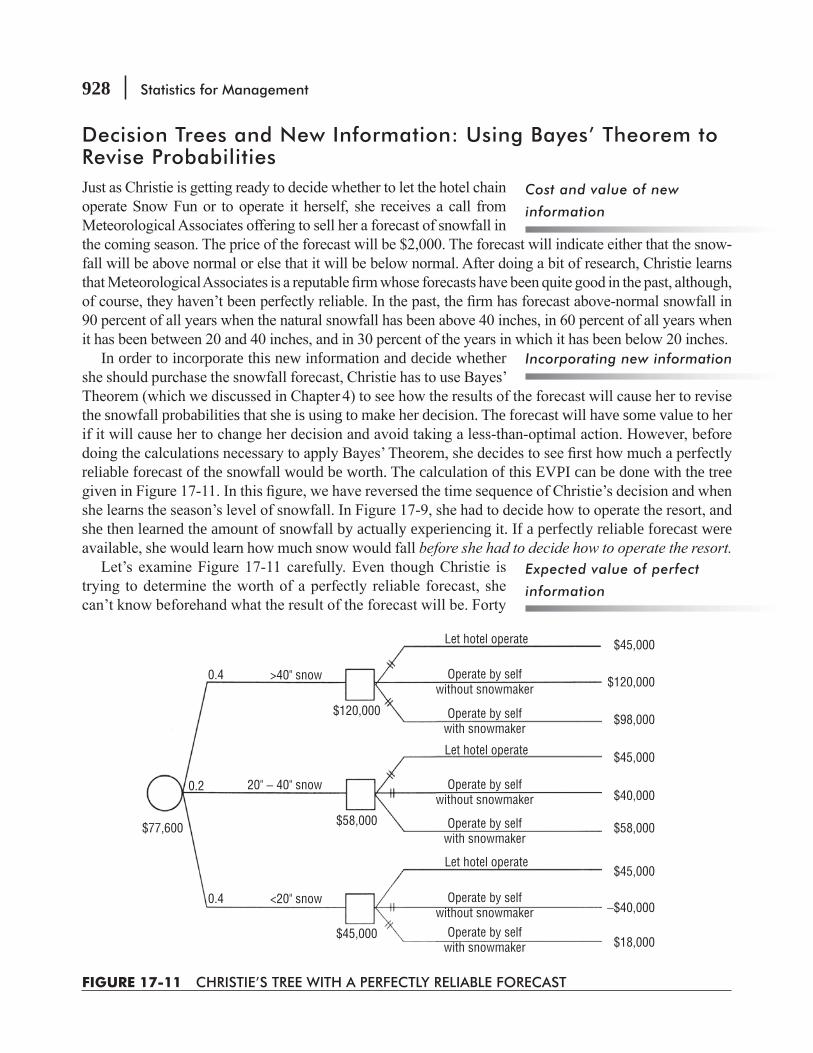
928 Statistics for Management
Decision Trees and New Information: Using Bayes’ Theorem to Revise Probabilities
-
In order to incorporate this new information and decide whether
the snowfall probabilities that she is using to make her decision. The forecast will have some value to her
reliable forecast of the snowfall would be worth. The calculation of this EVPI can be done with the tree
she then learned the amount of snowfall by actually experiencing it. If a perfectly reliable forecast were before she had to decide how to operate the resort.
Cost and value of new
information
Incorporating new information
Expected value of perfect
information
$77,600
$120,000
$58,000
$45,000
0.2
0.4
0.4
>40" snow
20" − 40" snow
<20" snow
Let hotel operate
Let hotel operate
Operate by selfwithout snowmaker
Operate by selfwithout snowmaker
Operate by selfwith snowmaker
Operate by selfwith snowmaker
Let hotel operate
Operate by selfwithout snowmaker
Operate by selfwith snowmaker
$45,000
$120,000
$98,000
$40,000
$58,000
$45,000
−$40,000
$18,000
$45,000
FIGURE 17-11 CHRISTIE’S TREE WITH A PERFECTLY RELIABLE FORECAST

Decision Theory 929
=
this question can be found in Table 17-13 and Figure 17-12. Table 17-13 uses the same format we used
the results of the forecast.-
Updating probabilities with
Bayes’ Theorem
Analyzing the entire tree
TABLE 17-13 CHRISTIE’S POSTERIOR PROBABILITIES
Forecast P(event) P(forecast event)P(forecast& event)
P(eventforecast)
Above ″ 0.4 0.9 0.4 × 0.9 = 0.36 = 0.6 normal 20″ ″ 0.2 0.6 0.2 × 0.6 = 0.12 = 0.2
″ 0.4 0.3 0.4 × 0.3 = 0.12 = 0.2
P(above normal) = 0.60
″ 0.4 0.1 0.4 × 0.1 = 0.04 = 0.1 normal 20″ ″ 0.2 0.4 0.2 × 0.4 = 0.08 = 0.2
″ 0.4 0.7 0.4 × 0.7 = 0.28 = 0.7
= 0.40
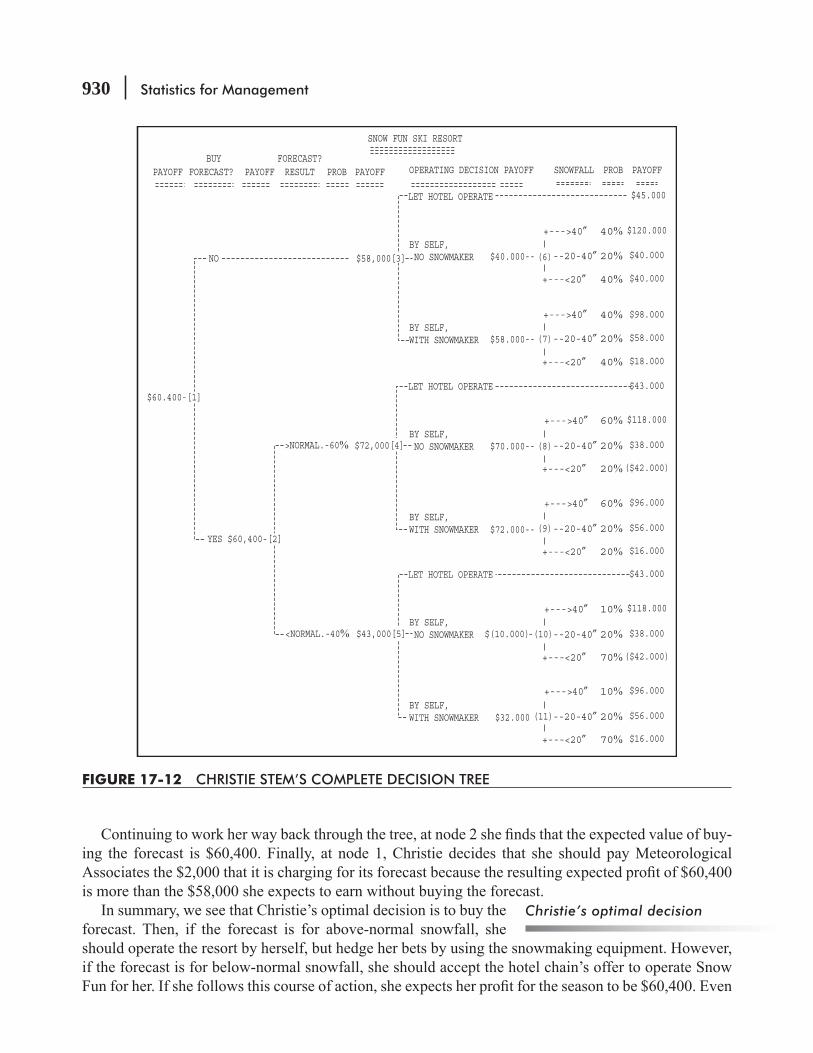
930 Statistics for Management
-
Christie’s optimal decision
FIGURE 17-12 CHRISTIE STEM’S COMPLETE DECISION TREE
SNOW FUN SKI RESORT
OPERATING DECISION PAYOFF SNOWFALL PROB PAYOFF
LET HOTEL OPERATE
LET HOTEL OPERATE
LET HOTEL OPERATE
$45.000
$120.000
$40.000--
$58.000--
$70.000--
$72.000--
(8)
(7)
(6)
(9)
$(10.000)-
$32.000
$40.000
$40.000
$98.000
$58.000
$18.000
$43.000
$118.000
$96.000
$56.000
$16.000
$96.000
$56.000
$16.000
$43.000
$118.000
$38.000
$38.000
($42.000)
($42.000)
+--->40″
+---<20″
--20-40″
40%
20%
40%
+--->40″
+---<20″
--20-40″
40%
20%
40%
+--->40″
+---<20″
--20-40″
60%
20%
20%
+--->40″
+---<20″
--20-40″
60%
20%
20%
(10)
+--->40″
+---<20″
--20-40″
10%
20%
70%
(11)
+--->40″
+---<20″
--20-40″
10%
20%
70%
BY SELF,NO SNOWMAKER
BY SELF,WITH SNOWMAKER
BY SELF,NO SNOWMAKER
BY SELF,
<NORMAL.-40%
>NORMAL.-60%
YESWITH SNOWMAKER
BY SELF,NO SNOWMAKER
BY SELF,WITH SNOWMAKER
BUYPAYOFF FORECAST?
FORECAST?PAYOFF RESULT PROB PAYOFF
NO
$60,400-[2]
$60.400-[1]
$58,000[3]
$72,000[4]
$43,000[5]

Decision Theory 931
expected value of sample information
The European Journal of Operations Research
OR/MS Today
-
strategies
1. 2.
3.
Decision trees on the
personal computer
Changing some input data
Reasonable strategies
Sensitivity analysis
FIGURE 17-13 SPREADSHEET WITH CHRISTIE’S INPUT AND BAYES’ THEOREM CALCULATIONS
INPUT DATA AND BAYES’ REVISIONS FOR CHRISIIE STEM AND THE SNOW FUN SKI RESORT
SNOWFALLSTATE
PRIORPROB
SNOWMAKEROPERATING COST
PROFIT WITHSNOWMAKER
FORECAST RESULTPROBABILITIES>NORMAL <NORMAL
JOINTPROBABILITIES>NORMAL <NORMAL
REVISEDPROBABILITIES>NORMAL >NORMAL
PROFIT WITHOUTSNOWMAKER
>40"20−40">20"
$10,000$50,000$90,000
$98,000$58,000$18,000
$120,000 $40,000 ($40,000)
40%20%40%
90%60%30%
10%40%70%
36%12%12%
60%20%20%
10%20%70%
4%8%28%
PROFIT FROM=> $45,000HOTEL LEASE
$120,000 <=REVENUE WITH SNOWMAKER$ 12,000 <=COST OF SNOWMAKER LEASE
40% <=PROBABILITY OFFORECAST RESULTS
$2,000 <=COST OF FORECAST
60%

932 Statistics for Management
sensitivity analysis
adopt strategy 2.
-ward fashion on a personal computer. The ability to perform such sensitivity analyses greatly enhances the value of decision trees in helping us to make important decisions.
Using Decision-Tree Analysis-
sion analysis problems can be much more complex. There can be many more alternatives to consider
Other sensitivities
FIGURE 17-14 SENSITIVITY ANALYSIS ON THE COST OF LEASING THE SNOWMAKING EQUIPMENT
SENSITIVITY ANALYSIS ON SNOWMAKER LEASE COST
STRATEGY 1: OPERATE BY SELF WITH SNOWMAKERSSTRATEGY 2: BUY FORECAST AND OPERATE BY SELF W/O SNOWMAKERS IF >NORMAL LET HOTEL CHAIN OPERATE IF <NORMALSTRATEGY 3: BUY FORECAST AND OPERATE BY SELF WITH SNOWMAKERS IF >NORMAL LET HOTEL CHAIN OPERATE IF <NORMAL COST OF STRATEGY / EXPECTED PROFIT
SNOW-MAKERS
OPTIMALSTRATEGY
EXPECTEDVALUE
MAXIMUMTO PAY FORFORECAST1 2 3
$5,000$6,000$7,000$8,000$9,000$10,000$11,000$12,000$13,000$14,000$15,000$16,000$17,000$18,000$19,000$20,000
$1,600$2,000$2,400$2,800$3,200$3,600$4,000$4,400$4,800$5,200$6,200$7,200$8,200$9,200$10,200$11,200
$65,000$64,000$63,000$62,000$61,000$60,000$59,000$58,000$57,000$56,000$55,000$54,000$53,000$52,000$51,000$50,000
$59,200$59,200$59,200$59,200$59,200$59,200$59,200$59,200$59,200$59,200$59,200$59,200$59,200$59,200$59,200$59,200
$64,600$64,000$63,400$62,800$62,200$61,600$61,000$60,400$59,800$59,200$58,600$58,000$57,400$56,800$56,200$55,600
$65,000$64,000$63,400$62,800$62,200$61,600$61,000$60,400$59,800$59,200$59,200$59,200$59,200$59,200$59,200$59,200
11 OR 3
3333333
2 OR 3222222

Decision Theory 933
-
too much detail.
1. which factors are relevant to the solution. Then estimate
2. involved in the problem. This step structures the problem in that it allows the entire decision process
maker chooses the number of periods into which the future is to be divided. 3. to each of the branches and
subbranches of the decision tree. This will enable you to distinguish the probability value and conditional monetary value associated with each outcome.
4. “Solve” the decision tree.particular branch of the tree that has the largest expected value or that maximizes the decision
5. Perform sensitivity analysis;
the magnitude and the direction of the reaction. This step allows experiments without real commitments or real mistakes and without disrupting operations.
6. Explain the estimating techniques used to arrive at the probability
not be valid.
Decision-tree analysis is a technique managers use to struc-ture and display alternatives and decision processes. It is popular because it
-tial fashion.
Decision-tree steps
Advantages of the decision-
tree approach
934 Statistics for Management
-
probabilities to outcomes in a consistent manner is why successful managers are paid more than suc-
surprise you that companies actually use decision trees as a part of expert systems
make
HINTS & ASSUMPTIONS
EXERCISES 17.6
Self-Check ExerciseSC 17-4
-
Applications17-25
pilot plant for limited production for the coming model year. If the results of the limited pro-
plant would still be possible 3 years from now. If it decides to proceed with the pilot plant and

Decision Theory 935
ProductionFacility
Consumer($ millions)
New plant High 14New plantPilot plant High 2Pilot plant 1
consumer acceptance will be high and 50 percent that it will be low. If the pilot plant is put into
probabilities are 45 percent for high consumer acceptance and 55 percent for low acceptance.
-
17-26
original estimate.
17-27 International Pictures is trying to decide how to distribute its new movie Claws. Claws is the
to decide whether to release the picture for general distribution initially or to start out with a “lim-
Claws:
($ millions)
Level Success Probability Limited ReleaseGeneral
Distribution0.3 22 120.4 9 80.3

936 Statistics for Management
Claws.
Claws
-
Claws
17-28 that would have taken him to campus for his 9 A.M A.M
10 15 20 25Probability 0.30 0.45 0.15 0.10
minimizethe decision tree and determine his best option.
maximize his expected utility as measured by the
decision now.
Arrival timeProjected test score 95 85 70 60 45
17-29
value of increased revenue from a new airport is in question. There is a 70 percent prob-
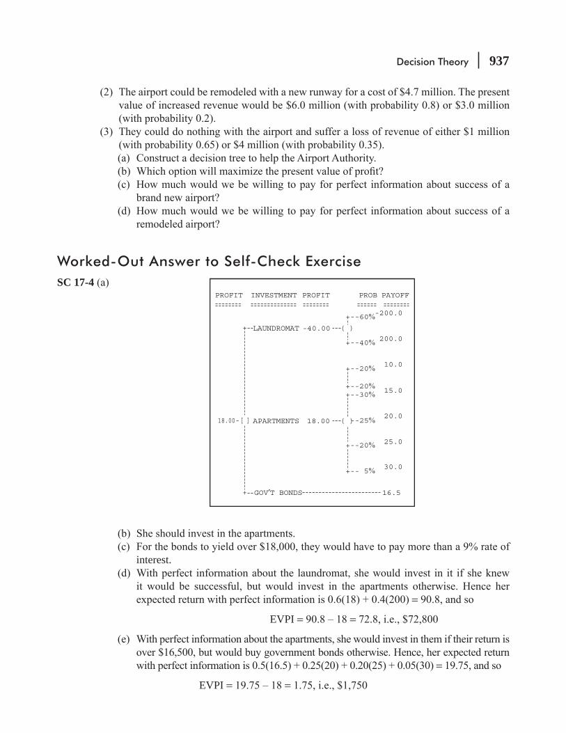
Decision Theory 937
Worked-Out Answer to Self-Check ExerciseSC 17-4
PROFIT PROFIT PROB PAYOFFINVESTMENT
APARTMENTS 18.00 ( )
( )LAUNDROMAT -40.00+
+ GOV′T BONDS 16.5
+--60%-200.0
200.0
10.0
15.0
20.0
25.0
30.0
+--40%
+--20%
+--20%+--30%
+--20%
5%
--25%18.00-[ ]
+--
interest.
=
EVPI = =
=
EVPI = =

938 Statistics for Management
STATISTICS AT WORK
Loveland ComputersCase 17: Decision Theory
-
-dering if it was too early to ask for a bonus.
their machines they could greatly increase the number of computers they sell. And they both have manu-
Study Questions:

Decision Theory 939
CHAPTER REVIEW
Terms Introduced in Chapter 17Certainty The decision environment in which only one state of nature exists.
state of nature.Decision PointDecision Tree
The marginal loss multiplied by the probability of not selling that unit.
the probability that it will happen.
which of the states of nature will occur. A criterion requiring the decision maker to calculate the expected value for
Marginal Loss The loss incurred from stocking a unit that is not sold.
Minimum Probabilitystocking that unit.Node The point at which a chance event or a decision takes place on a decision tree.Obsolescence Loss The loss occasioned by stocking too many units and having to dispose of unsold units.
that was demanded.PayoffRollbackworking from right to left in the tree.
The value of an item after the initial selling period.State of Nature A future event not under the control of the decision maker.Utilityderives from an outcome.
Equations Introduced in Chapter 1717-1 p MP = – p ML p. 910
This equation describes the point at which the expected marginal pro t from stocking and p MP expected marginal loss from stocking and

940 Statistics for Management
p ML . As long as p MP p ML
the expected marginal loss.
17-2 =+
pML
MP ML* p. 910
This is the minimum probability equation. The symbol p* represents the minimum required
As long as the probability of selling one additional unit is greater than p*stock that unit. This equation is Equation 17-1 solved for p.
Review and Application Exercises17-30
print heads. The company foresees annual demand for its printers to be normally distributed with mean μ = σ =
a 60 percent chance that usage is 1.5 standard deviations above the make-or-buy break-even
17-31
-
17-32
only haute cuisine, he employs an agent to place freshly refrigerated lobster tails on a plane leaving the peninsula each day. Any tail not served the day it is shipped must be discarded. The chef wants to know how many tails the agent should ship each day. He wants to be able
could involve substantial waste on days with low demand. He has calculated the cost of a
Decision Theory 941
Number 18 19 20 21 22 23 24 25Probability 0.07 0.09 0.11 0.16 0.20 0.15 0.14 0.08
17-33
The spreader is estimated to save 8 minutes labor for every hour it is in use. Head lawn-care
corrosion and the odds are 7 to 5 that its life will be between 42 and 54 hours. If the company
17-34
-
Bags 32 33 35 35 36 37 38Probability 0.10 0.14 0.15 0.20 0.17 0.13 0.11
The store is planning to sell the tote bag for $42.75. The wholesale cost is $26.00. How many
17-35
17-36 -
-
options available to Triangle in each case are to settle out of court or to let the trial take place.
-

942 Statistics for Management
it is tried and lost.
-
17-37 -ering adding prescription underwater goggles for customers who like to scuba or snorkel.
17-38
Units demanded 19 20 21 22 23 24 25Probability 0.05 0.18 0.21 0.22 0.16 0.10 0.08
17-39
Units demanded 6 7 8 9 10 11Probability 0.04 0.12 0.30 0.24 0.18 0.12
Decision Theory 943
17-40
the accompanying risk involved with higher rates of return. The utility for 15 percent is only
utility curve.17-41 -
whether the mill should extend credit to this manufacturer.17-42
-
credit category in which the manufacturer belongs.
True CategoryAgency Rating Poor Average Good
A 0.1 0.1 0.60.2 0.8 0.30.7 0.1 0.1
the credit rating.
17-43 Jolly Roger
odds are about 7 to 3 in favor of good weather for the season.

944 Statistics for Management
Jolly Rogerseason.
17-44
17-45 spec
--
Playoffs (loss)Days to sell Probability Build Don’t Build
30 0.20 $060 0.30 $090 0.50 $0
17-46
-
Decision Theory 945
Event Probability 20 Games 25 Games 35 GamesHigh demand 0.55
0.300.15
17-47 The new engineering school at a small southern university is currently deciding which text-books to use in its undergraduate courses. The department chairpersons want to know whether
Event ProbabilityRequirement passed 0.70 $ 8 $13Requirement not passed 0.30 16 13
17-48 -
No. of magazines 500 600 700 800 900Probability 0.10 0.12 0.15 0.33 0.30
using the expected-value decision criterion.17-49 The women of Alpha Zeta sorority at a small midwestern college are getting ready to par-
should purchase. 17-50 The chief administrator of a chain of convalescent homes wants to open a new facility in
946 Statistics for Management
Event Probability 50-Bed 75-Bed 150-Bed0.20.3
High demand 0.5
information.17-51
Event Stock Additional Shirts Don’t Stock ShirtsTeam wins $0Team loses $0
17-52
the management estimates the sales of the remote machine as given in the following table.
Sales 15 16 17 18 19 20 21Probability 0.12 0.17 0.26 0.23 0.15 0.05 0.02
marginal analysis to determine the number of remote machines that the distributor should order.
17-53 Trade talks have broken down and there is a strong possibility of punitive tariffs being assessed
Ordering DecisionEvent Probability Double Don’t DoubleTariffs imposed 0.15No tariff 0.85
Decision Theory 947
17-54
cost basis.
The investment group had substantial cash reserves on which they expected to earn 8 per-
be added to these cash reserves. -
=

This page is intentionally left blank
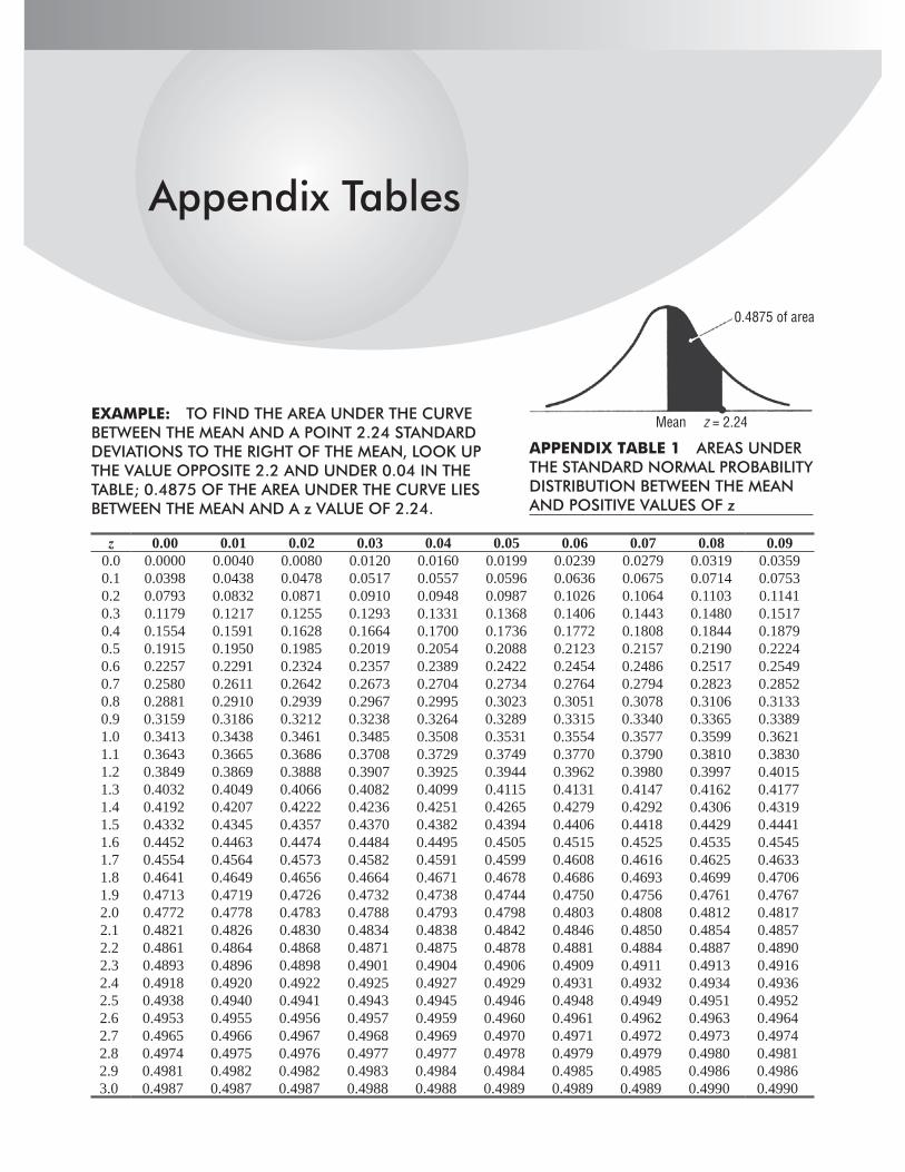
Appendix Tables
EXAMPLE: TO FIND THE AREA UNDER THE CURVE BETWEEN THE MEAN AND A POINT 2.24 STANDARD DEVIATIONS TO THE RIGHT OF THE MEAN, LOOK UP THE VALUE OPPOSITE 2.2 AND UNDER 0.04 IN THE TABLE; 0.4875 OF THE AREA UNDER THE CURVE LIES BETWEEN THE MEAN AND A z VALUE OF 2.24.
z 0.00 0.01 0.02 0.03 0.04 0.05 0.06 0.07 0.08 0.090.0 0.0000 0.0040 0.0080 0.0120 0.0160 0.0199 0.0239 0.0279 0.0319 0.03590.1 0.0398 0.0438 0.0478 0.0517 0.0557 0.0596 0.0636 0.0675 0.0714 0.07530.2 0.0793 0.0832 0.0871 0.0910 0.0948 0.0987 0.1026 0.1064 0.1103 0.11410.3 0.1179 0.1217 0.1255 0.1293 0.1331 0.1368 0.1406 0.1443 0.1480 0.15170.4 0.1554 0.1591 0.1628 0.1664 0.1700 0.1736 0.1772 0.1808 0.1844 0.18790.5 0.1915 0.1950 0.1985 0.2019 0.2054 0.2088 0.2123 0.2157 0.2190 0.22240.6 0.2257 0.2291 0.2324 0.2357 0.2389 0.2422 0.2454 0.2486 0.2517 0.25490.7 0.2580 0.2611 0.2642 0.2673 0.2704 0.2734 0.2764 0.2794 0.2823 0.28520.8 0.2881 0.2910 0.2939 0.2967 0.2995 0.3023 0.3051 0.3078 0.3106 0.31330.9 0.3159 0.3186 0.3212 0.3238 0.3264 0.3289 0.3315 0.3340 0.3365 0.33891.0 0.3413 0.3438 0.3461 0.3485 0.3508 0.3531 0.3554 0.3577 0.3599 0.36211.1 0.3643 0.3665 0.3686 0.3708 0.3729 0.3749 0.3770 0.3790 0.3810 0.38301.2 0.3849 0.3869 0.3888 0.3907 0.3925 0.3944 0.3962 0.3980 0.3997 0.40151.3 0.4032 0.4049 0.4066 0.4082 0.4099 0.4115 0.4131 0.4147 0.4162 0.41771.4 0.4192 0.4207 0.4222 0.4236 0.4251 0.4265 0.4279 0.4292 0.4306 0.43191.5 0.4332 0.4345 0.4357 0.4370 0.4382 0.4394 0.4406 0.4418 0.4429 0.44411.6 0.4452 0.4463 0.4474 0.4484 0.4495 0.4505 0.4515 0.4525 0.4535 0.45451.7 0.4554 0.4564 0.4573 0.4582 0.4591 0.4599 0.4608 0.4616 0.4625 0.46331.8 0.4641 0.4649 0.4656 0.4664 0.4671 0.4678 0.4686 0.4693 0.4699 0.47061.9 0.4713 0.4719 0.4726 0.4732 0.4738 0.4744 0.4750 0.4756 0.4761 0.47672.0 0.4772 0.4778 0.4783 0.4788 0.4793 0.4798 0.4803 0.4808 0.4812 0.48172.1 0.4821 0.4826 0.4830 0.4834 0.4838 0.4842 0.4846 0.4850 0.4854 0.48572.2 0.4861 0.4864 0.4868 0.4871 0.4875 0.4878 0.4881 0.4884 0.4887 0.48902.3 0.4893 0.4896 0.4898 0.4901 0.4904 0.4906 0.4909 0.4911 0.4913 0.49162.4 0.4918 0.4920 0.4922 0.4925 0.4927 0.4929 0.4931 0.4932 0.4934 0.49362.5 0.4938 0.4940 0.4941 0.4943 0.4945 0.4946 0.4948 0.4949 0.4951 0.49522.6 0.4953 0.4955 0.4956 0.4957 0.4959 0.4960 0.4961 0.4962 0.4963 0.49642.7 0.4965 0.4966 0.4967 0.4968 0.4969 0.4970 0.4971 0.4972 0.4973 0.49742.8 0.4974 0.4975 0.4976 0.4977 0.4977 0.4978 0.4979 0.4979 0.4980 0.49812.9 0.4981 0.4982 0.4982 0.4983 0.4984 0.4984 0.4985 0.4985 0.4986 0.49863.0 0.4987 0.4987 0.4987 0.4988 0.4988 0.4989 0.4989 0.4989 0.4990 0.4990
APPENDIX TABLE 1 AREAS UNDER THE STANDARD NORMAL PROBABILITY DISTRIBUTION BETWEEN THE MEAN AND POSITIVE VALUES OF z
0.4875 of area
Mean z = 2.24
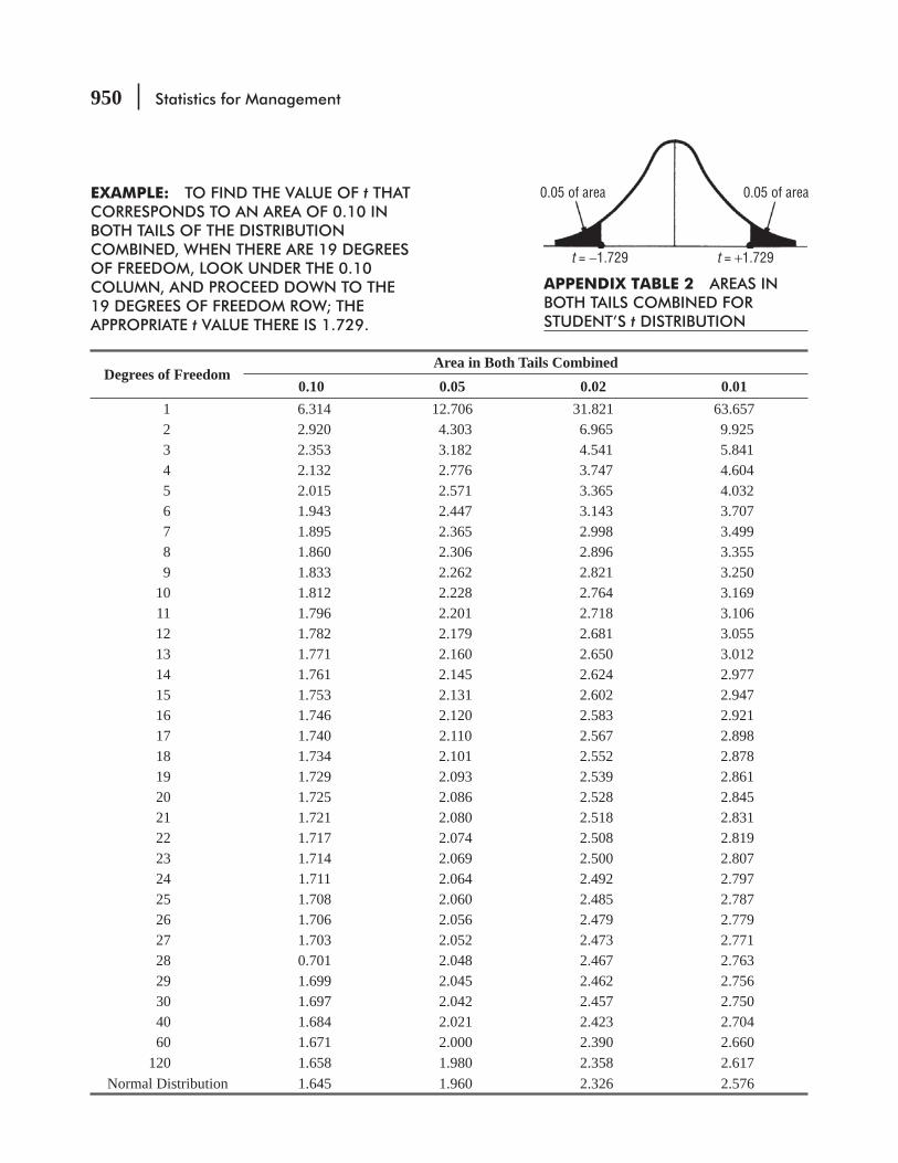
950 Statistics for Management
0.05 of area0.05 of area
t = −1.729 t = +1.729
APPENDIX TABLE 2 AREAS IN BOTH TAILS COMBINED FOR STUDENT’S t DISTRIBUTION
EXAMPLE: TO FIND THE VALUE OF t THAT CORRESPONDS TO AN AREA OF 0.10 IN BOTH TAILS OF THE DISTRIBUTION COMBINED, WHEN THERE ARE 19 DEGREES OF FREEDOM, LOOK UNDER THE 0.10 COLUMN, AND PROCEED DOWN TO THE 19 DEGREES OF FREEDOM ROW; THE APPROPRIATE t VALUE THERE IS 1.729.
Degrees of FreedomArea in Both Tails Combined
0.10 0.05 0.02 0.011 6.314 12.706 31.821 63.6572 2.920 4.303 6.965 9.9253 2.353 3.182 4.541 5.8414 2.132 2.776 3.747 4.6045 2.015 2.571 3.365 4.0326 1.943 2.447 3.143 3.7077 1.895 2.365 2.998 3.4998 1.860 2.306 2.896 3.3559 1.833 2.262 2.821 3.250
10 1.812 2.228 2.764 3.16911 1.796 2.201 2.718 3.10612 1.782 2.179 2.681 3.05513 1.771 2.160 2.650 3.01214 1.761 2.145 2.624 2.97715 1.753 2.131 2.602 2.94716 1.746 2.120 2.583 2.92117 1.740 2.110 2.567 2.89818 1.734 2.101 2.552 2.87819 1.729 2.093 2.539 2.86120 1.725 2.086 2.528 2.84521 1.721 2.080 2.518 2.83122 1.717 2.074 2.508 2.81923 1.714 2.069 2.500 2.80724 1.711 2.064 2.492 2.79725 1.708 2.060 2.485 2.78726 1.706 2.056 2.479 2.77927 1.703 2.052 2.473 2.77128 0.701 2.048 2.467 2.76329 1.699 2.045 2.462 2.75630 1.697 2.042 2.457 2.75040 1.684 2.021 2.423 2.70460 1.671 2.000 2.390 2.660
120 1.658 1.980 2.358 2.617Normal Distribution 1.645 1.960 2.326 2.576

AP
PEN
DIX
TA
BLE
3
BIO
NO
MIA
L PR
OBA
BILI
TIES
pn
r0.
010.
020.
030.
040.
050.
060.
070.
080.
090.
100.
110.
120.
130.
140.
150.
160.
170.
18r
n2
00.
9801
0.96
040.
9409
0.92
160.
9025
0.88
360.
8649
0.84
640.
8281
0.81
000.
7921
0.77
440.
7569
0.73
960.
7225
0.70
560.
6889
0.67
242
10.
0198
0.03
920.
0582
0.07
680.
0950
0.11
280.
1302
0.14
720.
1638
0.18
000.
1958
0.21
120.
2262
0.24
080.
2550
0.26
880.
2822
0.29
521
20.
0001
0.00
040.
0009
0.00
160.
0025
0.00
360.
0049
0.00
640.
0081
0.01
000.
0121
0.01
440.
0169
0.01
960.
0225
0.02
560.
0289
0.03
240
23
00.
9703
0.94
120.
9127
0.88
470.
8574
0.83
060.
8044
0.77
870.
7536
0.72
900.
7050
0.68
150.
6585
0.63
610.
6141
0.59
270.
5718
0.55
143
10.
0294
0.05
760.
0847
0.11
060.
1354
0.15
900.
1816
0.20
310.
2236
0.24
300.
2614
0.27
880.
2952
0.31
060.
3251
0.33
870.
3513
0.36
312
20.
0003
0.00
120.
0026
0.00
460.
0071
0.01
020.
0137
0.01
770.
0221
0.02
700.
0323
0.03
800.
0441
0.05
060.
0574
0.06
450.
0720
0.07
971
30.
0000
0.00
000.
0000
0.00
010.
0001
0.00
020.
0003
0.00
050.
0007
0.00
100.
0013
0.00
170.
0022
0.00
270.
0034
0.00
410.
0049
0.00
580
34
00.
9606
0.92
240.
8853
0.84
930.
8145
0.78
070.
7481
0.71
640.
6857
0.65
610.
6274
0.59
970.
5729
0.54
700.
5220
0.49
790.
4746
0.45
214
10.
0388
0.07
530.
1095
0.14
160.
1715
0.19
930.
2252
0.24
920.
2713
0.29
160.
3102
0.32
710.
3424
0.35
620.
3685
0.37
930.
3888
0.39
703
20.
0006
0.00
230.
0051
0.00
880.
0135
0.01
910.
0254
0.03
250.
0402
0.04
860.
0575
0.06
690.
0767
0.08
700.
0975
0.10
840.
1195
0.13
072
30.
0000
0.00
000.
0001
0.00
020.
0005
0.00
080.
0013
0.00
190.
0027
0.00
360.
0047
0.00
610.
0076
0.00
940.
0115
0.01
380.
0163
0.01
911
4–
–0.
0000
0.00
000.
0000
0.00
000.
0000
0.00
000.
0001
0.00
010.
0001
0.00
020.
0003
0.00
040.
0005
0.00
070.
0008
0.00
100
45
00.
9510
0.90
390.
8587
0.81
540.
7738
0.73
390.
6957
0.65
910.
6240
0.59
050.
5584
0.52
770.
4984
0.47
040.
4437
0.41
820.
3939
0.37
075
10.
0480
0.09
220.
1328
0.16
990.
2036
0.23
420.
2618
0.28
660.
3086
0.32
800.
3451
0.35
980.
3724
0.38
290.
3915
0.39
830.
4034
0.40
694
20.
0010
0.00
380.
0082
0.01
420.
0214
0.02
990.
0394
0.04
980.
0610
0.07
290.
0853
0.09
810.
1113
0.12
470.
1382
0.15
170.
1652
0.17
863
30.
0000
0.00
010.
0003
0.00
060.
0011
0.00
190.
0030
0.00
430.
0060
0.00
810.
0105
0.01
340.
0166
0.02
030.
0244
0.02
890.
0338
0.03
922
4–
0.00
000.
0000
0.00
000.
0000
0.00
010.
0001
0.00
020.
0003
0.00
040.
0007
0.00
090.
0012
0.00
170.
0022
0.00
280.
0035
0.00
431
5–
––
––
0.00
000.
0000
0.00
000.
0000
0.00
000.
0000
0.00
000.
0000
0.00
010.
0001
0.00
010.
0001
0.00
020
56
00.
9415
0.88
580.
8330
0.78
280.
7351
0.68
990.
6470
0.60
640.
5679
0.53
140.
4970
0.46
440.
4336
0.40
460.
3771
0.35
130.
3269
0.30
406
10.
0571
0.10
850.
1546
0.19
570.
2321
0.26
420.
2922
0.31
640.
3370
0.35
430.
3685
0.38
000.
3888
0.39
520.
3993
0.40
150.
4018
0.40
045
20.
0014
0.00
550.
0120
0.02
040.
0305
0.04
220.
0550
0.06
880.
0833
0.09
840.
1139
0.12
950.
1452
0.16
080.
1762
0.19
120.
2057
0.21
974
30.
0000
0.00
020.
0005
0.00
110.
0021
0.00
360.
0055
0.00
800.
0110
0.01
460.
0188
0.02
360.
0289
0.03
490.
0415
0.04
860.
0562
0.06
433
4–
0.00
000.
0000
0.00
000.
0001
0.00
020.
0003
0.00
050.
0008
0.00
120.
0017
0.00
240.
0032
0.00
430.
0055
0.00
690.
0086
0.01
062
5–
––
–0.
0000
0.00
000.
0000
0.00
000.
0000
0.00
010.
0001
0.00
010.
0002
0.00
030.
0004
0.00
050.
0007
0.00
091
6–
––
––
––
––
0.00
000.
0000
0.00
000.
0000
0.00
000.
0000
0.00
000.
0000
0.00
000
67
00.
9321
0.86
810.
8080
0.75
140.
6983
0.64
850.
6017
0.55
780.
5168
0.47
830.
4423
0.40
870.
3773
0.34
790.
3206
0.29
510.
2714
0.24
937
10.
0659
0.12
400.
1749
0.21
920.
2573
0.28
970.
3170
0.33
960.
3578
0.37
200.
3827
0.39
010.
3946
0.39
650.
3960
0.39
350.
3891
0.38
306
20.
0020
0.00
760.
0162
0.02
740.
0406
0.05
550.
0716
0.08
860.
1061
0.12
400.
1419
0.15
960.
1769
0.19
360.
2097
0.22
480.
2391
0.25
235
30.
0000
0.00
030.
0008
0.00
190.
0036
0.00
590.
0090
0.01
280.
0175
0.02
300.
0292
0.03
630.
0441
0.05
250.
0617
0.07
140.
0816
0.09
234
4–
0.00
000.
0000
0.00
010.
0002
0.00
040.
0007
0.00
110.
0017
0.00
260.
0036
0.00
490.
0066
0.00
860.
0109
0.01
360.
0167
0.02
033
5–
––
0.00
000.
0000
0.00
000.
0000
0.00
010.
0001
0.00
020.
0003
0.00
040.
0006
0.00
080.
0012
0.00
160.
0021
0.00
272
6–
––
––
––
0.00
000.
0000
0.00
000.
0000
0.00
000.
0000
0.00
000.
0001
0.00
010.
0001
0.00
021
7–
––
––
––
––
––
––
–0.
0000
0.00
000.
0000
0.00
000
7n
r0.
990.
980.
970.
960.
950.
940.
930.
920.
910.
900.
890.
880.
870.
860.
850.
840.
830.
82r
np
FOR
A G
IVEN
CO
MBI
NA
TIO
N O
F n
AN
D p
, EN
TRY
IND
ICA
TES
THE
PRO
BABI
LITY
OF
OBT
AIN
ING
A S
PEC
IFIE
D V
ALU
E O
F r.
TO
LO
CA
TE
ENTR
Y: W
HEN
p ≤
0.5
0,
REA
D p
AC
ROSS
TH
E TO
P A
ND
BO
TH n
AN
D r
DO
WN
TH
E LE
FT M
ARG
IN;
WH
EN p
≥ 0
.50
, RE
AD
p A
CRO
SS T
HE
BOTT
OM
AN
D B
OTH
n A
ND
r U
P TH
E RI
GH
T M
ARG
IN.

pn
r0.
010.
020.
030.
040.
050.
060.
070.
080.
090.
100.
110.
120.
130.
140.
150.
160.
170.
18r
n 8
00.
9227
0.85
080.
7837
0.72
140.
6634
0.60
960.
5596
0.51
320.
4703
0.43
050.
3937
0.35
960.
3282
0.29
920.
2725
0.24
790.
2252
0.20
448
10.
0746
0.13
890.
1939
0.24
050.
2793
0.31
130.
3370
0.35
700.
3721
0.38
260.
3892
0.39
230.
3923
0.38
970.
3847
0.37
770.
3691
0.35
907
20.
0026
0.00
990.
0210
0.03
510.
0515
0.06
950.
0888
0.10
870.
1288
0.14
880.
1684
0.18
720.
2052
0.22
200.
2376
0.25
180.
2646
0.27
586
30.
0001
0.00
040.
0013
0.00
290.
0054
0.00
890.
0134
0.01
890.
0255
0.03
310.
0416
0.05
110.
0613
0.07
230.
0839
0.09
590.
1084
0.12
115
40.
0000
0.00
000.
0001
0.00
020.
0004
0.00
070.
0013
0.00
210.
0031
0.00
460.
0064
0.00
870.
0115
0.01
470.
0185
0.02
280.
0277
0.03
324
5–
–0.
0000
0.00
000.
0000
0.00
000.
0001
0.00
010.
0002
0.00
040.
0006
0.00
090.
0014
0.00
190.
0026
0.00
350.
0045
0.00
583
6–
––
––
–0.
0000
0.00
000.
0000
0.00
000.
0000
0.00
010.
0001
0.00
020.
0002
0.00
030.
0005
0.00
062
7–
––
––
––
––
––
0.00
000.
0000
0.00
000.
0000
0.00
000.
0000
0.00
001
8–
––
––
––
––
––
––
––
––
–0
8
90
0.91
350.
8337
0.76
020.
6925
0.63
020.
5730
0.52
040.
4722
0.42
790.
3874
0.35
040.
3165
0.28
550.
2573
0.23
160.
2082
0.18
690.
1676
91
0.08
300.
1531
0.21
160.
2597
0.29
850.
3292
0.35
250.
3695
0.38
090.
3874
0.38
970.
3884
0.38
400.
3770
0.36
790.
3569
0.34
460.
3312
82
0.00
340.
0125
0.02
620.
0433
0.06
290.
0840
0.10
610.
1285
0.15
070.
1722
0.19
270.
2119
0.22
950.
2455
0.25
970.
2720
0.28
230.
2908
73
0.00
010.
0006
0.00
190.
0042
0.00
770.
0125
0.01
860.
0261
0.03
480.
0446
0.05
560.
0674
0.08
000.
0933
0.10
690.
1209
0.13
490.
1489
64
0.00
000.
0000
0.00
010.
0003
0.00
060.
0012
0.00
210.
0034
0.00
520.
0074
0.01
030.
0138
0.01
790.
0228
0.02
830.
0345
0.04
150.
0490
55
––
0.00
000.
0000
0.00
000.
0001
0.00
020.
0003
0.00
050.
0008
0.00
130.
0019
0.00
270.
0037
0.00
500.
0066
0.00
850.
0108
46
––
––
–0.
0000
0.00
000.
0000
0.00
000.
0001
0.00
010.
0002
0.00
030.
0004
0.00
060.
0008
0.00
120.
0016
37
––
––
––
––
–0.
0000
0.00
000.
0000
0.00
000.
0000
0.00
000.
0001
0.00
010.
0001
28
––
––
––
––
––
––
––
–0.
0000
0.00
000.
0000
19
––
––
––
––
––
––
––
––
––
0 9
100
0.90
440.
8171
0.73
740.
6648
0.59
870.
5386
0.48
400.
4344
0.38
940.
3487
0.31
180.
2785
0.24
840.
2213
0.19
690.
1749
0.15
520.
1374
101
0.09
140.
1667
0.22
810.
2770
0.31
510.
3438
0.36
430.
3777
0.38
510.
3874
0.38
540.
3798
0.37
120.
3603
0.34
740.
3331
0.31
780.
3017
92
0.00
420.
0153
0.03
170.
0519
0.07
460.
0988
0.12
340.
1478
0.17
140.
1937
0.21
430.
2330
0.24
960.
2639
0.27
590.
2856
0.29
290.
2980
83
0.00
010.
0008
0.00
260.
0058
0.01
050.
0168
0.02
480.
0343
0.04
520.
0574
0.07
060.
0847
0.09
950.
1146
0.12
980.
1450
0.16
000.
1745
74
0.00
000.
0000
0.00
010.
0004
0.00
100.
0019
0.00
330.
0052
0.00
780.
0112
0.01
530.
0202
0.02
600.
0326
0.04
010.
0483
0.05
730.
0670
65
––
0.00
000.
0000
0.00
010.
0001
0.00
030.
0005
0.00
090.
0015
0.00
230.
0033
0.00
470.
0064
0.00
850.
0111
0.01
410.
0177
56
––
––
0.00
000.
0000
0.00
000.
0000
0.00
010.
0001
0.00
020.
0004
0.00
060.
0009
0.00
121.
0018
0.00
240.
0032
47
––
––
––
––
0.00
000.
0000
0.00
000.
0000
0.00
000.
0001
0.00
010.
0002
0.00
030.
0004
38
––
––
––
––
––
––
–0.
0000
0.00
000.
0000
0.00
000.
0000
29
––
––
––
––
––
––
––
––
––
110
––
––
––
––
––
––
––
––
––
010
nr
0.99
0.98
0.97
0.96
0.95
0.94
0.93
0.92
0.91
0.90
0.89
0.88
0.87
0.86
0.85
0.84
0.83
0.82
rn
p
952
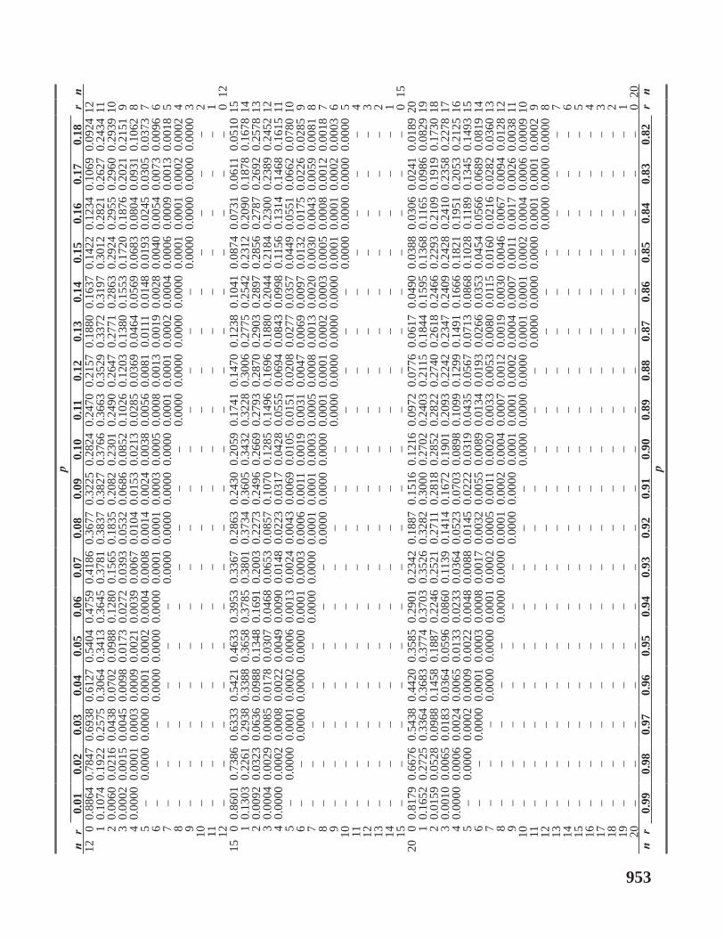
pn
r0.
010.
020.
030.
040.
050.
060.
070.
080.
090.
100.
110.
120.
130.
140.
150.
160.
170.
18r
n12
00.
8864
0.78
470.
6938
0.61
270.
5404
0.47
590.
4186
0.36
770.
3225
0.28
240.
2470
0.21
570.
1880
0.16
370.
1422
0.12
340.
1069
0.09
2412
10.
1074
0.19
220.
2575
0.30
640.
3413
0.36
450.
3781
0.38
370.
3827
0.37
660.
3663
0.35
290.
3372
0.31
970.
3012
0.28
210.
2627
0.24
3411
20.
0060
0.02
160.
0438
0.07
020.
0988
0.12
800.
1565
0.18
350.
2082
0.23
010.
2490
0.26
470.
2771
0.28
630.
2924
0.29
550.
2960
0.29
3910
30.
0002
0.00
150.
0045
0.00
980.
0173
0.02
720.
0393
0.05
320.
0686
0.08
520.
1026
0.12
030.
1380
0.15
530.
1720
0.18
760.
2021
0.21
519
40.
0000
0.00
010.
0003
0.00
090.
0021
0.00
390.
0067
0.01
040.
0153
0.02
130.
0285
0.03
690.
0464
0.05
690.
0683
0.08
040.
0931
0.10
628
5–
0.00
000.
0000
0.00
010.
0002
0.00
040.
0008
0.00
140.
0024
0.00
380.
0056
0.00
810.
0111
0.01
480.
0193
0.02
450.
0305
0.03
737
6–
––
0.00
000.
0000
0.00
000.
0001
0.00
010.
0003
0.00
050.
0008
0.00
130.
0019
0.00
280.
0040
0.00
540.
0073
0.00
966
7–
––
––
–0.
0000
0.00
000.
0000
0.00
000.
0001
0.00
010.
0002
0.00
040.
0006
0.00
090.
0013
0.00
185
8–
––
––
––
––
–0.
0000
0.00
000.
0000
0.00
000.
0001
0.00
010.
0002
0.00
024
9–
––
––
––
––
––
––
–0.
0000
0.00
000.
0000
0.00
003
10–
––
––
––
––
––
––
––
––
–2
11–
––
––
––
––
––
––
––
––
–1
12–
––
––
––
––
––
––
––
––
–0
1215
00.
8601
0.73
860.
6333
0.54
210.
4633
0.39
530.
3367
0.28
630.
2430
0.20
590.
1741
0.14
700.
1238
0.10
410.
0874
0.07
310.
0611
0.05
1015
10.
1303
0.22
610.
2938
0.33
880.
3658
0.37
850.
3801
0.37
340.
3605
0.34
320.
3228
0.30
060.
2775
0.25
420.
2312
0.20
900.
1878
0.16
7814
20.
0092
0.03
230.
0636
0.09
880.
1348
0.16
910.
2003
0.22
730.
2496
0.26
690.
2793
0.28
700.
2903
0.28
970.
2856
0.27
870.
2692
0.25
7813
30.
0004
0.00
290.
0085
0.01
780.
0307
0.04
680.
0653
0.08
570.
1070
0.12
850.
1496
0.16
960.
1880
0.20
440.
2184
0.23
000.
2389
0.24
5212
40.
0000
0.00
020.
0008
0.00
220.
0049
0.00
900.
0148
0.02
230.
0317
0.04
280.
0555
0.06
940.
0843
0.09
980.
1156
0.13
140.
1468
0.16
1511
5–
0.00
000.
0001
0.00
020.
0006
0.00
130.
0024
0.00
430.
0069
0.01
050.
0151
0.02
080.
0277
0.03
570.
0449
0.05
510.
0662
0.07
8010
6–
–0.
0000
0.00
000.
0000
0.00
010.
0003
0.00
060.
0011
0.00
190.
0031
0.00
470.
0069
0.00
970.
0132
0.01
750.
0226
0.02
859
7–
––
––
0.00
000.
0000
0.00
010.
0001
0.00
030.
0005
0.00
080.
0013
0.00
200.
0030
0.00
430.
0059
0.00
818
8–
––
––
––
0.00
000.
0000
0.00
000.
0001
0.00
010.
0002
0.00
030.
0005
0.00
080.
0012
0.00
187
9–
––
––
––
––
–0.
0000
0.00
000.
0000
0.00
000.
0001
0.00
010.
0002
0.00
036
10–
––
––
––
––
––
––
–0.
0000
0.00
000.
0000
0.00
005
11–
––
––
––
––
––
––
––
––
–4
12–
––
––
––
––
––
––
––
––
–3
13–
––
––
––
––
––
––
––
––
–2
14–
––
––
––
––
––
––
––
––
–1
15–
––
––
––
––
––
––
––
––
–0
1520
00.
8179
0.66
760.
5438
0.44
200.
3585
0.29
010.
2342
0.18
870.
1516
0.12
160.
0972
0.07
760.
0617
0.04
900.
0388
0.03
060.
0241
0.01
8920
10.
1652
0.27
250.
3364
0.36
830.
3774
0.37
030.
3526
0.32
820.
3000
0.27
020.
2403
0.21
150.
1844
0.15
950.
1368
0.11
650.
0986
0.08
2919
20.
0159
0.05
280.
0988
0.14
580.
1887
0.22
460.
2521
0.27
110.
2818
0.28
520.
2822
0.27
400.
2618
0.24
660.
2293
0.21
090.
1919
0.17
3018
30.
0010
0.00
650.
0183
0.03
640.
0596
0.08
600.
1139
0.14
140.
1672
0.19
010.
2093
0.22
420.
2347
0.24
090.
2428
0.24
100.
2358
0.22
7817
40.
0000
0.00
060.
0024
0.00
650.
0133
0.02
330.
0364
0.05
230.
0703
0.08
980.
1099
0.12
990.
1491
0.16
660.
1821
0.19
510.
2053
0.21
2516
5–
0.00
000.
0002
0.00
090.
0022
0.00
480.
0088
0.01
450.
0222
0.03
190.
0435
0.05
670.
0713
0.08
680.
1028
0.11
890.
1345
0.14
9315
6–
–0.
0000
0.00
010.
0003
0.00
080.
0017
0.00
320.
0055
0.00
890.
0134
0.01
930.
0266
0.03
530.
0454
0.05
660.
0689
0.08
1914
7–
––
0.00
000.
0000
0.00
010.
0002
0.00
050.
0011
0.00
200.
0033
0.00
530.
0080
0.01
150.
0160
0.02
160.
0282
0.03
6013
8–
––
––
0.00
000.
0000
0.00
010.
0002
0.00
040.
0007
0.00
120.
0019
0.00
300.
0046
0.00
670.
0094
0.01
2812
9–
––
––
––
0.00
000.
0000
0.00
010.
0001
0.00
020.
0004
0.00
070.
0011
0.00
170.
0026
0.00
3811
10–
––
––
––
––
0.00
000.
0000
0.00
000.
0001
0.00
010.
0002
0.00
040.
0006
0.00
0910
11–
––
––
––
––
––
–0.
0000
0.00
000.
0000
0.00
010.
0001
0.00
029
12–
––
––
––
––
––
––
––
0.00
000.
0000
0.00
008
13–
––
––
––
––
––
––
––
––
–7
14–
––
––
––
––
––
––
––
––
–6
15–
––
––
––
––
––
––
––
––
–5
16–
––
––
––
––
––
––
––
––
–4
17–
––
––
––
––
––
––
––
––
–3
18–
––
––
––
––
––
––
––
––
–2
19–
––
––
––
––
––
––
––
––
–1
20–
––
––
––
––
––
––
––
––
–0
20n
r0.
990.
980.
970.
960.
950.
940.
930.
920.
910.
900.
890.
880.
870.
860.
850.
840.
830.
82r
np
953
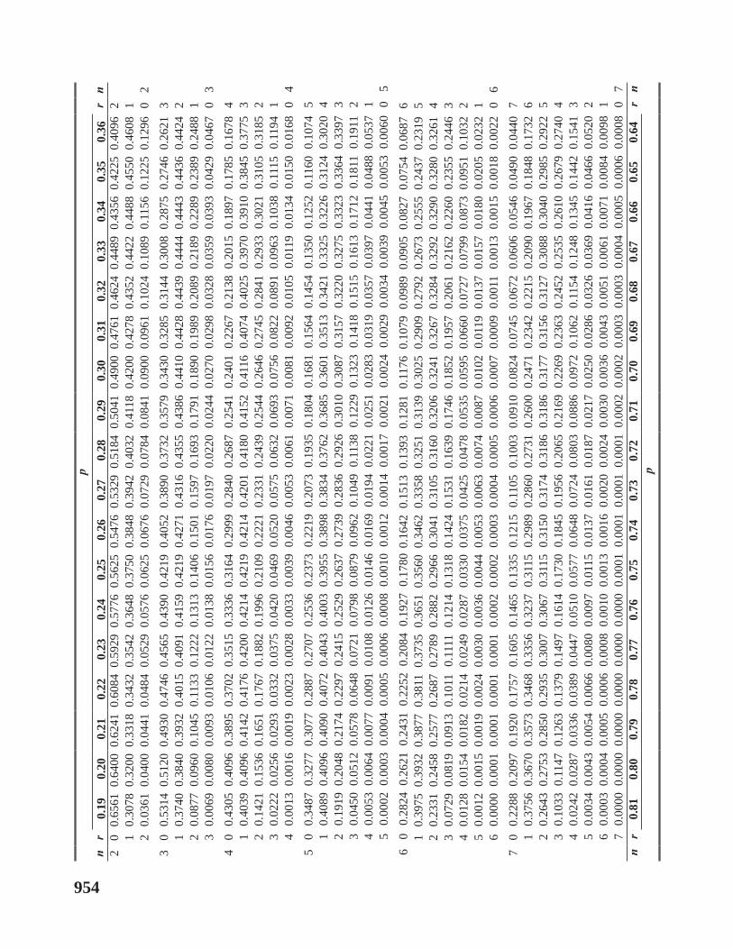
pn
r0.
190.
200.
210.
220.
230.
240.
250.
260.
270.
280.
290.
300.
310.
320.
330.
340.
350.
36r
n2
00.
6561
0.64
000.
6241
0.60
840.
5929
0.57
760.
5625
0.54
760.
5329
0.51
840.
5041
0.49
000.
4761
0.46
240.
4489
0.43
560.
4225
0.40
962
10.
3078
0.32
000.
3318
0.34
320.
3542
0.36
480.
3750
0.38
480.
3942
0.40
320.
4118
0.42
000.
4278
0.43
520.
4422
0.44
880.
4550
0.46
081
20.
0361
0.04
000.
0441
0.04
840.
0529
0.05
760.
0625
0.06
760.
0729
0.07
840.
0841
0.09
000.
0961
0.10
240.
1089
0.11
560.
1225
0.12
960
23
00.
5314
0.51
200.
4930
0.47
460.
4565
0.43
900.
4219
0.40
520.
3890
0.37
320.
3579
0.34
300.
3285
0.31
440.
3008
0.28
750.
2746
0.26
213
10.
3740
0.38
400.
3932
0.40
150.
4091
0.41
590.
4219
0.42
710.
4316
0.43
550.
4386
0.44
100.
4428
0.44
390.
4444
0.44
430.
4436
0.44
242
20.
0877
0.09
600.
1045
0.11
330.
1222
0.13
130.
1406
0.15
010.
1597
0.16
930.
1791
0.18
900.
1989
0.20
890.
2189
0.22
890.
2389
0.24
881
30.
0069
0.00
800.
0093
0.01
060.
0122
0.01
380.
0156
0.01
760.
0197
0.02
200.
0244
0.02
700.
0298
0.03
280.
0359
0.03
930.
0429
0.04
670
34
00.
4305
0.40
960.
3895
0.37
020.
3515
0.33
360.
3164
0.29
990.
2840
0.26
870.
2541
0.24
010.
2267
0.21
380.
2015
0.18
970.
1785
0.16
784
10.
4039
0.40
960.
4142
0.41
760.
4200
0.42
140.
4219
0.42
140.
4201
0.41
800.
4152
0.41
160.
4074
0.40
250.
3970
0.39
100.
3845
0.37
753
20.
1421
0.15
360.
1651
0.17
670.
1882
0.19
960.
2109
0.22
210.
2331
0.24
390.
2544
0.26
460.
2745
0.28
410.
2933
0.30
210.
3105
0.31
852
30.
0222
0.02
560.
0293
0.03
320.
0375
0.04
200.
0469
0.05
200.
0575
0.06
320.
0693
0.07
560.
0822
0.08
910.
0963
0.10
380.
1115
0.11
941
40.
0013
0.00
160.
0019
0.00
230.
0028
0.00
330.
0039
0.00
460.
0053
0.00
610.
0071
0.00
810.
0092
0.01
050.
0119
0.01
340.
0150
0.01
680
45
00.
3487
0.32
770.
3077
0.28
870.
2707
0.25
360.
2373
0.22
190.
2073
0.19
350.
1804
0.16
810.
1564
0.14
540.
1350
0.12
520.
1160
0.10
745
10.
4089
0.40
960.
4090
0.40
720.
4043
0.40
030.
3955
0.38
980.
3834
0.37
620.
3685
0.36
010.
3513
0.34
210.
3325
0.32
260.
3124
0.30
204
20.
1919
0.20
480.
2174
0.22
970.
2415
0.25
290.
2637
0.27
390.
2836
0.29
260.
3010
0.30
870.
3157
0.32
200.
3275
0.33
230.
3364
0.33
973
30.
0450
0.05
120.
0578
0.06
480.
0721
0.07
980.
0879
0.09
620.
1049
0.11
380.
1229
0.13
230.
1418
0.15
150.
1613
0.17
120.
1811
0.19
112
40.
0053
0.00
640.
0077
0.00
910.
0108
0.01
260.
0146
0.01
690.
0194
0.02
210.
0251
0.02
830.
0319
0.03
570.
0397
0.04
410.
0488
0.05
371
50.
0002
0.00
030.
0004
0.00
050.
0006
0.00
080.
0010
0.00
120.
0014
0.00
170.
0021
0.00
240.
0029
0.00
340.
0039
0.00
450.
0053
0.00
600
56
00.
2824
0.26
210.
2431
0.22
520.
2084
0.19
270.
1780
0.16
420.
1513
0.13
930.
1281
0.11
760.
1079
0.09
890.
0905
0.08
270.
0754
0.06
876
10.
3975
0.39
320.
3877
0.38
110.
3735
0.36
510.
3560
0.34
620.
3358
0.32
510.
3139
0.30
250.
2909
0.27
920.
2673
0.25
550.
2437
0.23
195
20.
2331
0.24
580.
2577
0.26
870.
2789
0.28
820.
2966
0.30
410.
3105
0.31
600.
3206
0.32
410.
3267
0.32
840.
3292
0.32
900.
3280
0.32
614
30.
0729
0.08
190.
0913
0.10
110.
1111
0.12
140.
1318
0.14
240.
1531
0.16
390.
1746
0.18
520.
1957
0.20
610.
2162
0.22
600.
2355
0.24
463
40.
0128
0.01
540.
0182
0.02
140.
0249
0.02
870.
0330
0.03
750.
0425
0.04
780.
0535
0.05
950.
0660
0.07
270.
0799
0.08
730.
0951
0.10
322
50.
0012
0.00
150.
0019
0.00
240.
0030
0.00
360.
0044
0.00
530.
0063
0.00
740.
0087
0.01
020.
0119
0.01
370.
0157
0.01
800.
0205
0.02
321
60.
0000
0.00
010.
0001
0.00
010.
0001
0.00
020.
0002
0.00
030.
0004
0.00
050.
0006
0.00
070.
0009
0.00
110.
0013
0.00
150.
0018
0.00
220
67
00.
2288
0.20
970.
1920
0.17
570.
1605
0.14
650.
1335
0.12
150.
1105
0.10
030.
0910
0.08
240.
0745
0.06
720.
0606
0.05
460.
0490
0.04
407
10.
3756
0.36
700.
3573
0.34
680.
3356
0.32
370.
3115
0.29
890.
2860
0.27
310.
2600
0.24
710.
2342
0.22
150.
2090
0.19
670.
1848
0.17
326
20.
2643
0.27
530.
2850
0.29
350.
3007
0.30
670.
3115
0.31
500.
3174
0.31
860.
3186
0.31
770.
3156
0.31
270.
3088
0.30
400.
2985
0.29
225
30.
1033
0.11
470.
1263
0.13
790.
1497
0.16
140.
1730
0.18
450.
1956
0.20
650.
2169
0.22
690.
2363
0.24
520.
2535
0.26
100.
2679
0.27
404
40.
0242
0.02
870.
0336
0.03
890.
0447
0.05
100.
0577
0.06
480.
0724
0.08
030.
0886
0.09
720.
1062
0.11
540.
1248
0.13
450.
1442
0.15
413
50.
0034
0.00
430.
0054
0.00
660.
0080
0.00
970.
0115
0.01
370.
0161
0.01
870.
0217
0.02
500.
0286
0.03
260.
0369
0.04
160.
0466
0.05
202
60.
0003
0.00
040.
0005
0.00
060.
0008
0.00
100.
0013
0.00
160.
0020
0.00
240.
0030
0.00
360.
0043
0.00
510.
0061
0.00
710.
0084
0.00
981
70.
0000
0.00
000.
0000
0.00
000.
0000
0.00
000.
0001
0.00
010.
0001
0.00
010.
0002
0.00
020.
0003
0.00
030.
0004
0.00
050.
0006
0.00
080
7n
r0.
810.
800.
790.
780.
770.
760.
750.
740.
730.
720.
710.
700.
690.
680.
670.
660.
650.
64r
np
954

pn
r0.
190.
200.
210.
220.
230.
240.
250.
260.
270.
280.
290.
300.
310.
320.
330.
340.
350.
36r
n8
00.
1853
0.16
780.
1517
0.13
700.
1236
0.11
130.
1001
0.08
990.
0806
0.07
220.
0646
0.05
760.
0514
0.04
570.
0406
0.03
600.
0319
0.02
818
10.
3477
0.33
550.
3226
0.30
920.
2953
0.28
120.
2670
0.25
270.
2386
0.22
470.
2110
0.19
770.
1847
0.17
210.
1600
0.14
840.
1373
0.12
677
20.
2855
0.29
360.
3002
0.30
520.
3087
0.31
080.
3115
0.31
080.
3089
0.30
580.
3017
0.29
650.
2904
0.28
350.
2758
0.26
750.
2587
0.24
946
30.
1339
0.14
680.
1596
0.17
220.
1844
0.19
630.
2076
0.21
840.
2285
0.23
790.
2464
0.25
410.
2609
0.26
680.
2717
0.27
560.
2786
0.28
055
40.
0393
0.04
590.
0530
0.06
070.
0689
0.07
750.
0865
0.09
590.
1056
0.11
560.
1258
0.13
610.
1465
0.15
690.
1673
0.17
750.
1875
0.19
734
50.
0074
0.00
920.
0113
0.01
370.
0165
0.01
960.
0231
0.02
700.
0313
0.03
600.
0411
0.04
670.
0527
0.05
910.
0659
0.07
320.
0808
0.08
883
60.
0009
0.00
110.
0015
0.00
190.
0025
0.00
310.
0038
0.00
470.
0058
0.00
700.
0084
0.01
000.
0118
0.01
390.
0162
0.01
880.
0217
0.02
502
70.
0001
0.00
010.
0001
0.00
020.
0002
0.00
030.
0004
0.00
050.
0006
0.00
080.
0010
0.00
120.
0015
0.00
190.
0023
0.00
280.
0033
0.00
401
80.
0000
0.00
000.
0000
0.00
000.
0000
0.00
000.
0000
0.00
000.
0000
0.00
000.
0001
0.00
010.
0001
0.00
010.
0001
0.00
020.
0002
0.00
030
89
00.
1501
0.13
420.
1199
0.10
690.
0952
0.08
460.
0751
0.06
650.
0589
0.05
200.
0458
0.04
040.
0355
0.03
110.
0272
0.02
380.
0207
0.01
809
10.
3169
0.30
200.
2867
0.27
130.
2558
0.24
040.
2253
0.21
040.
1960
0.18
200.
1685
0.15
560.
1433
0.13
170.
1206
0.11
020.
1004
0.09
128
20.
2973
0.30
200.
3049
0.30
610.
3056
0.30
370.
3003
0.29
570.
2899
0.28
310.
2754
0.26
680.
2576
0.24
780.
2376
0.22
700.
2162
0.20
527
30.
1627
0.17
620.
1891
0.20
140.
2130
0.22
380.
2336
0.24
240.
2502
0.25
690.
2624
0.26
680.
2701
0.27
210.
2731
0.27
290.
2716
0.26
936
40.
0573
0.06
610.
0754
0.08
520.
0954
0.10
600.
1168
0.12
780.
1388
0.14
990.
1608
0.17
150.
1820
0.19
210.
2017
0.21
090.
2194
0.22
725
50.
0134
0.01
650.
0200
0.02
400.
0285
0.03
350.
0389
0.04
490.
0513
0.05
830.
0657
0.07
350.
0818
0.09
040.
0994
0.10
860.
1181
0.12
784
60.
0021
0.00
280.
0036
0.00
450.
0057
0.00
700.
0087
0.01
050.
0127
0.01
510.
0179
0.02
100.
0245
0.02
840.
0326
0.03
730.
0424
0.04
793
70.
0002
0.00
030.
0004
0.00
050.
0007
0.00
100.
0012
0.00
160.
0020
0.00
250.
0031
0.00
390.
0047
0.00
570.
0069
0.00
820.
0098
0.01
162
80.
0000
0.00
000.
0000
0.00
000.
0001
0.00
010.
0001
0.00
010.
0002
0.00
020.
0003
0.00
040.
0005
0.00
070.
0008
0.00
110.
0013
0.00
161
9–
––
–0.
0000
0.00
000.
0000
0.00
000.
0000
0.00
000.
0000
0.00
000.
0000
0.00
000.
0000
0.00
010.
0001
0.00
010
910
00.
1216
0.10
740.
0947
0.08
340.
0733
0.06
430.
0563
0.04
920.
0430
0.03
740.
0326
0.02
820.
0245
0.02
110.
0182
0.01
570.
0135
0.01
1510
10.
2852
0.26
840.
2517
0.23
510.
2188
0.20
300.
1877
0.17
300.
1590
0.14
560.
1330
0.12
110.
1099
0.09
950.
0898
0.08
080.
0725
0.06
499
20.
3010
0.30
200.
3011
0.29
840.
2942
0.28
850.
2816
0.27
350.
2646
0.25
480.
2444
0.23
350.
2222
0.21
070.
1990
0.18
730.
1757
0.16
428
30.
1883
0.20
130.
2134
0.22
440.
2343
0.24
290.
2503
0.25
630.
2609
0.26
420.
2662
0.26
680.
2662
0.26
440.
2614
0.25
730.
2522
0.24
627
40.
0773
0.08
810.
0993
0.11
080.
1225
0.13
430.
1460
0.15
760.
1689
0.17
980.
1903
0.20
010.
2093
0.21
770.
2253
0.23
200.
2377
0.24
246
50.
0218
0.02
640.
0317
0.03
750.
0439
0.05
090.
0584
0.06
640.
0750
0.08
390.
0933
0.10
290.
1128
0.12
290.
1332
0.14
340.
1536
0.16
365
60.
0043
0.00
550.
0070
0.00
880.
0109
0.01
340.
0162
0.01
950.
0231
0.02
720.
0317
0.03
680.
0422
0.04
820.
0547
0.06
160.
0689
0.07
674
70.
0006
0.00
080.
0011
0.00
140.
0019
0.00
240.
0031
0.00
390.
0049
0.00
600.
0074
0.00
900.
0108
0.01
300.
0154
0.01
810.
0212
0.02
473
80.
0001
0.00
010.
0001
0.00
020.
0002
0.00
030.
0004
0.00
050.
0007
0.00
090.
0011
0.00
140.
0018
0.00
230.
0028
0.00
350.
0043
0.00
522
90.
0000
0.00
000.
0000
0.00
000.
0000
0.00
000.
0000
0.00
000.
0001
0.00
010.
0001
0.00
010.
0002
0.00
020.
0003
0.00
040.
0005
0.00
061
10–
––
––
––
–0.
0000
0.00
000.
0000
0.00
000.
0000
0.00
000.
0000
0.00
000.
0000
0.00
000
1012
00.
0798
0.06
870.
0591
0.05
070.
0434
0.03
710.
0317
0.02
700.
0229
0.01
940.
0164
0.01
380.
0116
0.00
980.
0082
0.00
680.
0057
0.00
4712
10.
2245
0.20
620.
1885
0.17
170.
1557
0.14
070.
1267
0.11
370.
1016
0.09
060.
0804
0.07
120.
0628
0.05
520.
0484
0.04
220.
0368
0.03
1911
20.
2897
0.28
350.
2756
0.26
630.
2558
0.24
440.
2323
0.21
970.
2068
0.19
370.
1807
0.16
780.
1552
0.14
290.
1310
0.11
970.
1088
0.09
8610
30.
2265
0.23
620.
2442
0.25
030.
2547
0.25
730.
2581
0.25
730.
2549
0.25
110.
2460
0.23
970.
2324
0.22
410.
2151
0.20
550.
1954
0.18
499
40.
1195
0.13
290.
1460
0.15
890.
1712
0.18
280.
1936
0.20
340.
2122
0.21
970.
2261
0.23
110.
2349
0.23
730.
2384
0.23
820.
2367
0.23
408
50.
0449
0.05
320.
0621
0.07
170.
0818
0.09
240.
1032
0.11
430.
1255
0.13
670.
1477
0.15
850.
1688
0.17
870.
1879
0.19
630.
2039
0.21
067
60.
0123
0.01
550.
0193
0.02
360.
0285
0.03
400.
0401
0.04
690.
0542
0.06
200.
0704
0.07
920.
0885
0.09
810.
1079
0.11
800.
1281
0.13
826
70.
0025
0.00
330.
0044
0.00
570.
0073
0.00
920.
0115
0.01
410.
0172
0.02
070.
0246
0.02
910.
0341
0.03
960.
0456
0.05
210.
0591
0.06
665
80.
0004
0.00
050.
0007
0.00
100.
0014
0.00
180.
0024
0.00
310.
0040
0.00
500.
0063
0.00
780.
0096
0.01
160.
0140
0.01
680.
0199
0.02
344
90.
0000
0.00
010.
0001
0.00
010.
0002
0.00
030.
0004
0.00
050.
0007
0.00
090.
0011
0.00
150.
0019
0.00
240.
0031
0.00
380.
0048
0.00
593
10–
0.00
000.
0000
0.00
000.
0000
0.00
000.
0000
0.00
010.
0001
0.00
010.
0001
0.00
020.
0003
0.00
030.
0005
0.00
060.
0008
0.00
102
11–
––
––
––
0.00
000.
0000
0.00
000.
0000
0.00
000.
0000
0.00
000.
0000
0.00
010.
0001
0.00
011
12–
––
––
––
––
––
––
––
0.00
000.
0000
0.00
000
12n
r0.
810.
800.
790.
780.
770.
760.
750.
740.
730.
720.
710.
700.
690.
680.
670.
660.
650.
64r
np
955

pn
r0.
190.
200.
210.
220.
230.
240.
250.
260.
270.
280.
290.
300.
310.
320.
330.
340.
350.
36r
n15
00.
0424
0.03
520.
0291
0.02
410.
0198
0.01
630.
0134
0.01
090.
0089
0.00
720.
0059
0.00
470.
0038
0.00
310.
0025
0.00
200.
0016
0.00
1215
10.
1492
0.13
190.
1162
0.10
180.
0889
0.07
720.
0668
0.05
670.
0494
0.04
230.
0360
0.03
050.
0258
0.02
170.
0182
0.01
520.
0126
0.01
0414
20.
2449
0.23
090.
2162
0.20
100.
1858
0.17
070.
1559
0.14
160.
1280
0.11
500.
1029
0.09
160.
0811
0.07
150.
0627
0.05
470.
0476
0.04
1113
30.
2489
0.25
010.
2490
0.24
570.
2405
0.23
360.
2252
0.21
560.
2051
0.19
390.
1821
0.17
000.
1579
0.14
570.
1338
0.12
220.
1110
0.10
0212
40.
1752
0.18
760.
1986
0.20
790.
2155
0.22
130.
2252
0.22
730.
2276
0.22
620.
2231
0.21
860.
2128
0.20
570.
1977
0.18
880.
1792
0.16
9211
50.
0904
0.10
320.
1161
0.12
900.
1416
0.15
370.
1651
0.17
570.
1852
0.19
350.
2005
0.20
610.
2103
0.21
300.
2142
0.21
400.
2123
0.20
9310
60.
0353
0.04
300.
0514
0.06
060.
0705
0.08
090.
0917
0.10
290.
1142
0.12
540.
1365
0.14
720.
1575
0.16
710.
1759
0.18
370.
1906
0.19
639
70.
0107
0.01
380.
0176
0.02
200.
0271
0.03
290.
0393
0.04
650.
0543
0.06
270.
0717
0.08
110.
0910
0.10
110.
1114
0.12
170.
1319
0.14
198
80.
0025
0.00
350.
0047
0.00
620.
0081
0.01
040.
0131
0.01
630.
0201
0.02
440.
0293
0.03
480.
0409
0.04
760.
0549
0.06
270.
0710
0.07
987
90.
0005
0.00
070.
0010
0.00
140.
0019
0.00
250.
0034
0.00
450.
0058
0.00
740.
0093
0.01
160.
0143
0.01
740.
0210
0.02
510.
0298
0.03
496
100.
0001
0.00
010.
0002
0.00
020.
0003
0.00
050.
0007
0.00
090.
0013
0.00
170.
0023
0.00
300.
0038
0.00
490.
0062
0.00
780.
0096
0.01
185
110.
0000
0.00
000.
0000
0.00
000.
0000
0.00
010.
0001
0.00
020.
0002
0.00
030.
0004
0.00
060.
0008
0.00
110.
0014
0.00
180.
0024
0.00
304
12–
––
––
0.00
000.
0000
0.00
000.
0000
0.00
000.
0001
0.00
010.
0001
0.00
020.
0002
0.00
030.
0004
0.00
063
13–
––
––
––
––
–0.
0000
0.00
000.
0000
0.00
000.
0000
0.00
000.
0001
0.00
012
14–
––
––
––
––
––
––
––
–0.
0000
0.00
001
15–
––
––
––
––
––
––
––
––
–0
1520
00.
0148
0.01
150.
0090
0.00
690.
0054
0.00
410.
0032
0.00
240.
0018
0.00
140.
0011
0.00
080.
0006
0.00
040.
0003
0.00
020.
0002
0.00
0120
10.
0693
0.05
760.
0477
0.03
920.
0321
0.02
610.
0211
0.01
700.
0137
0.01
090.
0087
0.00
680.
0054
0.00
420.
0033
0.00
250.
0020
0.00
1519
20.
1545
0.13
690.
1204
0.10
500.
0910
0.07
830.
0669
0.05
690.
0480
0.04
030.
0336
0.02
780.
0229
0.01
880.
0153
0.01
240.
0110
0.00
8018
30.
2175
0.20
540.
1920
0.17
770.
1631
0.14
840.
1339
0.11
990.
1065
0.09
400.
0823
0.07
160.
0619
0.05
310.
0453
0.03
830.
0323
0.02
7017
40.
2168
0.21
820.
2169
0.21
310.
2070
0.19
910.
1897
0.17
900.
1675
0.15
530.
1429
0.13
040.
1181
0.10
620.
0947
0.08
390.
0738
0.06
4516
50.
1627
0.17
460.
1845
0.19
230.
1979
0.20
120.
2023
0.20
130.
1982
0.19
330.
1868
0.17
890.
1698
0.15
990.
1493
0.13
840.
1272
0.11
6115
60.
0954
0.10
910.
1226
0.13
560.
1478
0.15
890.
1686
0.17
680.
1833
0.18
790.
1907
0.19
160.
1907
0.18
810.
1839
0.17
820.
1712
0.16
3214
70.
0448
0.05
450.
0652
0.07
650.
0883
0.10
030.
1124
0.12
420.
1356
0.14
620.
1558
0.16
430.
1714
0.17
700.
1811
0.18
360.
1844
0.18
3613
80.
0171
0.02
220.
0282
0.03
510.
0429
0.05
150.
0609
0.07
090.
0815
0.09
240.
1034
0.11
440.
1251
0.13
540.
1450
0.15
370.
1614
0.16
7812
90.
0053
0.00
740.
0100
0.01
320.
0171
0.02
170.
0271
0.03
320.
0402
0.04
790.
0563
0.06
540.
0750
0.08
490.
0952
0.10
560.
1158
0.12
5911
100.
0014
0.00
200.
0029
0.00
410.
0056
0.00
750.
0099
0.01
280.
0163
0.02
050.
0253
0.03
080.
0370
0.04
400.
0516
0.05
980.
0686
0.07
7910
110.
0003
0.00
050.
0007
0.00
100.
0015
0.00
220.
0030
0.00
410.
0055
0.00
720.
0094
0.01
200.
0151
0.01
880.
0231
0.02
800.
0336
0.03
989
120.
0001
0.00
010.
0001
0.00
020.
0003
0.00
050.
0008
0.00
110.
0015
0.00
210.
0029
0.00
390.
0051
0.00
660.
0085
0.01
080.
0136
0.01
688
130.
0000
0.00
000.
0000
0.00
000.
0001
0.00
010.
0002
0.00
020.
0003
0.00
050.
0007
0.00
100.
0014
0.00
190.
0026
0.00
340.
0045
0.00
587
14–
––
–0.
0000
0.00
000.
0000
0.00
000.
0001
0.00
010.
0001
0.00
020.
0003
0.00
050.
0006
0.00
090.
0012
0.00
166
15–
––
––
––
–0.
0000
0.00
000.
0000
0.00
000.
0001
0.00
010.
0001
0.00
020.
0003
0.00
045
16–
––
––
––
––
––
–0.
0000
0.00
000.
0000
0.00
000.
0000
0.00
014
17–
––
––
––
––
––
––
––
––
0.00
003
18–
––
––
––
––
––
––
––
––
–2
19–
––
––
––
––
––
––
––
––
–1
20–
––
––
––
––
––
––
––
––
–0
20n
r0.
810.
800.
790.
780.
770.
760.
750.
740.
730.
720.
710.
700.
690.
680.
670.
660.
650.
64r
np
956

pn
r0.
370.
380.
390.
400.
410.
420.
430.
440.
450.
460.
470.
480.
490.
50r
n2
00.
3969
0.38
440.
3721
0.36
000.
3481
0.33
640.
3249
0.31
360.
3025
0.29
160.
2809
0.27
040.
2601
0.25
002
10.
4662
0.47
120.
4758
0.48
000.
4838
0.48
720.
4902
0.49
280.
4950
0.49
680.
4982
0.49
920.
4998
0.50
001
20.
1369
0.14
440.
1521
0.16
000.
1681
0.17
640.
1849
0.19
360.
2025
0.21
160.
2209
0.23
040.
2401
0.25
000
23
00.
2500
0.23
830.
2270
0.21
600.
2054
0.19
510.
1852
0.17
560.
1664
0.15
750.
1489
0.14
060.
1327
0.12
503
10.
4406
0.43
820.
4354
0.43
200.
4282
0.42
390.
4191
0.41
400.
4084
0.40
240.
3961
0.38
940.
3823
0.37
502
20.
2587
0.26
860.
2783
0.28
800.
2975
0.30
690.
3162
0.32
520.
3341
0.34
280.
3512
0.35
940.
3674
0.37
501
30.
0507
0.05
490.
0593
0.06
400.
0689
0.07
410.
0795
0.08
520.
0911
0.09
730.
1038
0.11
060.
1176
0.12
500
34
00.
1575
0.14
780.
1385
0.12
960.
1212
0.11
320.
1056
0.09
830.
0915
0.08
500.
0789
0.07
310.
0677
0.06
254
10.
3701
0.36
230.
3541
0.34
560.
3368
0.32
780.
3185
0.30
910.
2995
0.28
970.
2799
0.27
000.
2600
0.25
003
20.
3260
0.33
300.
3396
0.34
560.
3511
0.35
600.
3604
0.36
430.
3675
0.37
020.
3723
0.37
380.
3747
0.37
502
30.
1276
0.13
610.
1447
0.15
360.
1627
0.17
190.
1813
0.19
080.
2005
0.21
020.
2201
0.23
000.
2400
0.25
001
40.
0187
0.02
090.
0231
0.02
560.
0283
0.03
110.
0342
0.03
750.
0410
0.04
480.
0488
0.05
310.
0576
0.06
250
45
00.
0992
0.09
160.
0845
0.07
780.
0715
0.06
560.
0602
0.05
510.
0503
0.04
590.
0418
0.03
800.
0345
0.03
125
10.
2914
0.28
080.
2700
0.25
920.
2484
0.23
760.
2270
0.21
640.
2059
0.19
560.
1854
0.17
550.
1657
0.15
624
20.
3423
0.34
410.
3452
0.34
560.
3452
0.34
420.
3424
0.34
000.
3369
0.33
320.
3289
0.32
400.
3185
0.31
253
30.
2010
0.21
090.
2207
0.23
040.
2399
0.24
920.
2583
0.26
710.
2757
0.28
380.
2916
0.29
900.
3060
0.31
252
40.
0590
0.06
460.
0706
0.07
680.
0834
0.09
020.
0974
0.10
490.
1128
0.12
090.
1293
0.13
800.
1470
0.15
621
50.
0069
0.00
790.
0090
0.01
020.
0116
0.01
310.
0147
0.01
650.
0185
0.02
060.
0229
0.02
550.
0282
0.03
120
56
00.
0625
0.05
680.
0515
0.04
670.
0422
0.03
810.
0343
0.03
080.
0277
0.02
480.
0222
0.01
980.
0176
0.01
566
10.
2203
0.20
890.
1976
0.18
660.
1759
0.16
540.
1552
0.14
540.
1359
0.12
670.
1179
0.10
950.
1014
0.09
375
20.
3235
0.32
010.
3159
0.31
100.
3055
0.29
940.
2928
0.28
560.
2780
0.26
990.
2615
0.25
270.
2436
0.23
444
30.
2533
0.26
160.
2693
0.27
650.
2831
0.28
910.
2945
0.29
920.
3032
0.30
650.
3091
0.31
100.
3121
0.31
253
40.
1116
0.12
020.
1291
0.13
820.
1475
0.15
700.
1666
0.17
630.
1861
0.19
580.
2056
0.21
530.
2249
0.23
442
50.
0262
0.02
950.
0330
0.03
690.
0410
0.04
550.
0503
0.05
540.
0609
0.06
670.
0729
0.07
950.
0864
0.09
371
60.
0026
0.00
300.
0035
0.00
410.
0048
0.00
550.
0063
0.00
730.
0083
0.00
950.
0108
0.01
220.
0138
0.01
560
67
00.
0394
0.03
520.
0314
0.02
800.
0249
0.02
210.
0195
0.01
730.
0152
0.01
340.
0117
0.01
030.
0090
0.00
787
10.
1619
0.15
110.
1407
0.13
060.
1211
0.11
190.
1032
0.09
500.
0872
0.07
980.
0729
0.06
640.
0604
0.05
476
20.
2853
0.27
780.
2698
0.26
130.
2524
0.24
310.
2336
0.22
390.
2140
0.20
400.
1940
0.18
400.
1740
0.16
415
30.
2793
0.28
380.
2875
0.29
030.
2923
0.29
340.
2937
0.29
320.
2918
0.28
970.
2867
0.28
300.
2786
0.27
344
40.
1640
0.17
390.
1838
0.19
350.
2031
0.21
250.
2216
0.23
040.
2388
0.24
680.
2543
0.26
120.
2676
0.27
343
50.
0578
0.06
40
0.07
050.
0774
0.08
470.
0923
0.10
030.
1086
0.11
720.
1261
0.13
530.
1447
0.15
430.
1641
26
0.01
130.
0131
0.01
500.
0172
0.01
960.
0223
0.02
520.
0284
0.03
200.
0358
0.04
000.
0445
0.04
940.
0547
17
0.00
090.
0011
0.00
140.
0016
0.00
190.
0023
0.00
270.
0032
0.00
370.
0044
0.00
510.
0059
0.00
680.
0078
07
nr
0.63
0.62
0.61
0.60
0.59
0.58
0.57
0.56
0.55
0.54
0.53
0.52
0.51
0.50
rn
p
957

pn
r0.
370.
380.
390.
400.
410.
420.
430.
440.
450.
460.
470.
480.
490.
50r
n8
00.
0248
0.02
180.
0192
0.01
680.
0147
0.01
280.
0111
0.00
970.
0084
0.00
720.
0062
0.00
530.
0046
0.00
398
10.
1166
0.10
710.
0981
0.08
960.
0816
0.07
420.
0672
0.06
080.
0548
0.04
930.
0442
0.03
950.
0325
0.03
127
20.
2397
0.22
970.
2194
0.20
900.
1985
0.18
800.
1776
0.16
720.
1569
0.14
690.
1371
0.12
750.
1183
0.10
946
30.
2815
0.28
150.
2806
0.27
870.
2759
0.27
230.
2679
0.26
270.
2568
0.25
030.
2431
0.23
550.
2273
0.21
875
40.
2067
0.21
570.
2242
0.23
220.
2397
0.24
650.
2526
0.25
800.
2627
0.26
650.
2695
0.27
170.
2730
0.27
344
50.
0971
0.10
580.
1147
0.12
390.
1332
0.14
280.
1525
0.16
220.
1719
0.18
160.
1912
0.20
060.
2098
0.21
873
60.
0285
0.03
240.
0367
0.04
130.
0463
0.05
170.
0575
0.06
370.
0703
0.07
740.
0848
0.09
260.
1008
0.10
942
70.
0048
0.00
570.
0067
0.00
790.
0092
0.01
070.
0124
0.01
430.
0164
0.01
880.
0215
0.02
440.
0277
0.03
121
80.
0004
0.00
040.
0005
0.00
070.
0008
0.00
100.
0012
0.00
140.
0017
0.00
200.
0024
0.00
280.
0033
0.00
390
8
90
0.01
560.
0135
0.01
170.
0101
0.00
870.
0074
0.00
640.
0054
0.00
460.
0039
0.00
330.
0028
0.00
230.
0020
91
0.08
260.
0747
0.06
730.
0605
0.05
420.
0484
0.04
310.
0383
0.03
390.
0299
0.02
630.
0231
0.02
020.
0176
82
0.19
410.
1831
0.17
210.
1612
0.15
060.
1402
0.13
010.
1204
0.11
100.
1020
0.09
340.
0853
0.07
760.
0703
73
0.26
600.
2618
0.25
670.
2508
0.24
420.
2369
0.22
910.
2207
0.21
190.
2027
0.19
330.
1837
0.17
390.
1641
64
0.23
440.
2407
0.24
620.
2508
0.25
450.
2573
0.25
920.
2601
0.26
000.
2590
0.25
710.
2543
0.25
060.
2461
55
0.13
760.
1475
0.15
740.
1672
0.17
690.
1863
0.19
550.
2044
0.21
280.
2207
0.22
800.
2347
0.24
080.
2641
46
0.05
390.
0603
0.06
710.
0743
0.08
190.
0900
0.09
830.
1070
0.11
600.
1253
0.13
480.
1445
0.15
420.
1641
37
0.01
360.
0158
0.01
840.
0212
0.02
440.
0279
0.03
180.
0360
0.04
070.
0458
0.05
120.
0571
0.06
350.
0703
28
0.00
200.
0024
0.00
290.
0035
0.00
420.
0051
0.00
600.
0071
0.00
830.
0097
0.01
140.
0132
0.01
530.
0176
19
0.00
010.
0002
0.00
020.
0003
0.00
030.
0004
0.00
050.
0006
0.00
080.
0009
0.00
110.
0014
0.00
160.
0020
09
100
0.00
980.
0084
0.00
710.
0060
0.00
510.
0043
0.00
360.
0030
0.00
250.
0021
0.00
170.
0014
0.00
120.
0010
101
0.05
780.
0514
0.04
560.
0403
0.03
550.
0312
0.02
730.
0238
0.02
070.
0180
0.01
550.
0133
0.01
140.
0098
92
0.15
290.
1419
0.13
120.
1209
0.11
110.
1017
0.09
270.
0843
0.07
630.
0688
0.06
190.
0554
0.04
940.
0439
83
0.23
940.
2319
0.22
370.
2150
0.20
580.
1963
0.18
650.
1765
0.16
650.
1564
0.14
640.
1364
0.12
670.
1172
74
0.24
610.
2487
0.25
030.
2508
0.25
030.
2488
0.24
620.
2427
0.23
840.
2331
0.22
710.
2204
0.21
300.
2051
65
0.17
340.
1829
0.19
200.
2007
0.20
870.
2162
0.22
290.
2289
0.23
400.
2383
0.24
170.
2441
0.24
560.
2461
56
0.08
490.
0934
0.10
230.
1115
0.12
090.
1304
0.14
010.
1499
0.15
960.
1692
0.17
860.
1878
0.19
660.
2051
47
0.02
850.
0327
0.03
740.
0425
0.04
800.
0540
0.06
040.
0673
0.07
460.
0824
0.09
050.
0991
0.10
800.
1172
38
0.00
630.
0075
0.00
900.
0106
0.01
250.
0147
0.01
710.
0198
0.02
290.
0263
0.03
010.
0343
0.03
890.
0439
29
0.00
080.
0010
0.00
130.
0016
0.00
190.
0024
0.00
290.
0035
0.00
420.
0050
0.00
590.
0070
0.00
830.
0098
110
0.00
000.
0001
0.00
010.
0001
0.00
010.
0002
0.00
020.
0003
0.00
030.
0004
0.00
050.
0006
0.00
080.
0010
010
nr
0.63
0.62
0.61
0.60
0.59
0.58
0.57
0.56
0.55
0.54
0.53
0.52
0.51
0.50
rn
p
958
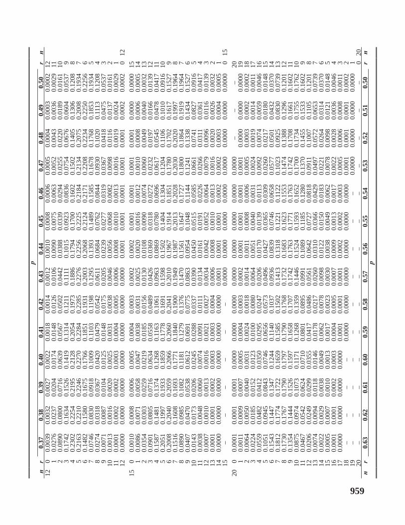
pn
r0.
370.
380.
390.
400.
410.
420.
430.
440.
450.
460.
470.
480.
490.
50r
n12
00.
0039
0.00
320.
0027
0.00
220.
0018
0.00
140.
0012
0.00
100.
0008
0.00
060.
0005
0.00
040.
0003
0.00
0212
10.
0276
0.02
370.
0204
0.01
740.
0148
0.01
260.
0106
0.00
900.
0075
0.00
630.
0052
0.00
430.
0036
0.00
2911
20.
0890
0.08
000.
0716
0.06
390.
0567
0.05
020.
0442
0.03
880.
0339
0.02
940.
0255
0.02
200.
0189
0.01
6110
30.
1742
0.16
340.
1526
0.14
190.
1314
0.12
110.
1111
0.10
150.
0923
0.08
360.
0754
0.06
760.
0604
0.05
379
40.
2302
0.22
540.
2195
0.21
280.
2054
0.19
730.
1886
0.17
940.
1700
0.16
020.
1502
0.14
050.
1306
0.12
088
50.
2163
0.22
100.
2246
0.22
700.
2284
0.22
850.
2276
0.22
560.
2225
0.21
840.
2134
0.20
750.
2008
0.19
347
60.
1482
0.15
800.
1675
0.17
660.
1851
0.19
310.
2003
0.20
680.
2124
0.21
710.
2208
0.22
340.
2250
0.22
566
70.
0746
0.08
300.
0918
0.10
090.
1103
0.11
980.
1295
0.13
930.
1489
0.15
850.
1678
0.17
680.
1853
0.19
345
80.
0274
0.03
180.
0367
0.04
200.
0479
0.05
420.
0611
0.06
840.
0762
0.08
440.
0930
0.10
200.
1113
0.12
084
90.
0071
0.00
870.
0104
0.01
250.
0148
0.01
750.
0205
0.02
390.
0277
0.03
190.
0367
0.04
180.
0475
0.05
373
100.
0013
0.00
160.
0020
0.00
250.
0031
0.00
380.
0046
0.00
560.
0068
0.00
820.
0098
0.01
160.
0137
0.01
612
110.
0001
0.00
020.
0002
0.00
030.
0004
0.00
050.
0006
0.00
080.
0010
0.00
130.
0016
0.00
190.
0024
0.00
291
120.
0000
0.00
000.
0000
0.00
000.
0000
0.00
000.
0000
0.00
010.
0001
0.00
010.
0001
0.00
010.
0002
0.00
020
1215
00.
0010
0.00
080.
0006
0.00
050.
0004
0.00
030.
0002
0.00
020.
0001
0.00
010.
0001
0.00
010.
0000
0.00
0015
10.
0086
0.00
710.
0058
0.00
470.
0038
0.00
310.
0025
0.00
200.
0016
0.00
120.
0010
0.00
080.
0006
0.00
0514
20.
0354
0.03
030.
0259
0.02
190.
0185
0.01
560.
0130
0.01
080.
0090
0.00
740.
0060
0.00
490.
0040
0.00
3213
30.
0901
0.08
050.
0716
0.06
340.
0558
0.04
890.
0426
0.03
690.
0318
0.02
720.
0232
0.01
970.
0166
0.01
3912
40.
1587
0.14
810.
1374
0.12
680.
1163
0.10
610.
0963
0.08
690.
0780
0.06
960.
0617
0.05
450.
0478
0.04
1711
50.
2051
0.19
970.
1933
0.18
590.
1778
0.16
910.
1598
0.15
020.
1404
0.13
040.
1204
0.11
060.
1010
0.09
1610
60.
2008
0.
2040
0.20
590.
2066
0.20
600.
2041
0.20
100.
1967
0.19
140.
1851
0.17
800.
1702
0.16
170.
1527
97
0.15
160.
1608
0.16
930.
1771
0.18
400.
1900
0.19
490.
1987
0.20
130.
2028
0.20
300.
2020
0.19
970.
1964
88
0.08
900.
0985
0.10
820.
1181
0.12
790.
1376
0.14
700.
1561
0.16
470.
1727
0.18
000.
1864
0.19
190.
1964
79
0.04
070.
0470
0.05
380.
0612
0.06
910.
0775
0.08
630.
0954
0.10
480.
1144
0.12
410.
1338
0.14
340.
1527
610
0.01
430.
0173
0.02
060.
0245
0.02
880.
0337
0.03
900.
0450
0.05
150.
0585
0.06
610.
0741
0.08
270.
0916
511
0.00
380.
0048
0.00
600.
0074
0.00
910.
0111
0.01
340.
0161
0.01
910.
0226
0.02
660.
0311
0.03
610.
0417
412
0.00
070.
0010
0.00
130.
0016
0.00
210.
0027
0.00
340.
0042
0.00
520.
0064
0.00
790.
0096
0.01
160.
0139
313
0.00
010.
0001
0.00
020.
0003
0.00
030.
0004
0.00
060.
0008
0.00
100.
0013
0.00
160.
0020
0.00
260.
0032
214
0.00
000.
0000
0.00
000.
0000
0.00
000.
0000
0.00
010.
0001
0.00
010.
0002
0.00
020.
0003
0.00
040.
0005
115
––
––
––
0.00
000.
0000
0.00
000.
0000
0.00
000.
0000
0.00
000.
0000
015
200
0.00
010.
0001
0.00
010.
0000
0.00
000.
0000
0.00
000.
0000
0.00
000.
0000
0.00
00–
––
201
0.00
110.
0009
0.00
070.
0005
0.00
040.
0003
0.00
020.
0001
0.00
010.
0001
0.00
010.
0000
0.00
000.
0000
192
0.00
640.
0050
0.00
400.
0031
0.00
240.
0018
0.00
140.
0011
0.00
080.
0006
0.00
050.
0003
0.00
020.
0002
183
0.02
240.
0185
0.01
520.
0123
0.01
000.
0080
0.00
640.
0051
0.00
400.
0031
0.00
240.
0019
0.00
140.
0011
174
0.05
590.
0482
0.04
120.
0350
0.02
950.
0247
0.02
060.
0170
0.01
390.
0113
0.00
920.
0074
0.00
590.
0046
165
0.10
510.
0945
0.08
430.
0746
0.06
560.
0573
0.04
960.
0427
0.03
650.
0309
0.02
600.
0217
0.01
800.
0148
156
0.15
430.
1447
0.13
470.
1244
0.11
400.
1037
0.09
360.
0839
0.07
460.
0658
0.05
770.
0501
0.04
320.
0370
147
0.18
120.
1774
0.17
220.
1659
0.15
850.
1502
0.14
130.
1318
0.12
210.
1122
0.10
230.
0925
0.08
300.
0739
138
0.17
300.
1767
0.17
900.
1797
0.17
900.
1768
0.17
320.
1683
0.16
230.
1553
0.
1474
0.13
880.
1296
0.12
0112
90.
1354
0.14
440.
1526
0.15
970.
1658
0.17
070.
1742
0.17
630.
1771
0.17
630.
1742
0.17
080.
1661
0.16
0211
100.
0875
0.
0974
0.10
730.
1171
0.12
680.
1359
0.14
460.
1524
0.15
930.
1652
0.17
000.
1734
0.17
550.
1762
1011
0.04
670.
0542
0.06
240.
0710
0.08
010.
0895
0.09
910.
1089
0.11
850.
1280
0.13
700.
1455
0.15
330.
1602
912
0.02
060.
0249
0.02
990.
0355
0.04
170.
0486
0.
0561
0.06
420.
0727
0.08
180.
0911
0.10
070.
1105
0.12
018
130.
0074
0.00
940.
0118
0.01
460.
0178
0.02
170.
0260
0.03
100.
0366
0.04
290.
0497
0.05
720.
0653
0.07
397
140.
0022
0.00
290.
0038
0.00
490.
0062
0.00
780.
0098
0.01
220.
0150
0.01
830.
0221
0.02
640.
0314
0.03
706
150.
0005
0.00
070.
0010
0.00
130.
0017
0.00
230.
0030
0.00
380.
0049
0.00
620.
0078
0.00
980.
0121
0.01
485
160.
0001
0.00
010.
0002
0.00
030.
0004
0.00
050.
0007
0.00
090.
0013
0.00
170.
0022
0.00
280.
0036
0.00
464
170.
0000
0.00
000.
0000
0.00
000.
0001
0.00
010.
0001
0.00
020.
0002
0.00
030.
0005
0.00
060.
0008
0.00
113
18–
––
–0.
0000
0.00
000.
0000
0.00
000.
0000
0.00
000.
0001
0.00
010.
0001
0.00
022
19–
––
––
––
––
–0.
0000
0.00
000.
0000
0.00
001
20–
––
––
––
––
––
––
–0
20n
r0.
630.
620.
610.
600.
590.
580.
570.
560.
550.
540.
530.
520.
510.
50r
np
959

960 Statistics for Management
λ e– λ e– λ e λ e–
0.1 0.90484 2.6 0.07427 5.1 0.00610 7.6 0.000500.2 0.81873 2.7 0.06721 5.2 0.00552 7.7 0.000450.3 0.74082 2.8 0.06081 5.3 0.00499 7.8 0.000410.4 0.67032 2.9 0.05502 5.4 0.00452 7.9 0.000370.5 0.60653 3.0 0.04979 5.5 0.00409 8.0 0.000340.6 0.54881 3.1 0.04505 5.6 0.00370 8.1 0.000300.7 0.49659 3.2 0.04076 5.7 0.00335 8.2 0.000270.8 0.44933 3.3 0.03688 5.8 0.00303 8.3 0.000250.9 0.40657 3.4 0.03337 5.9 0.00274 8.4 0.000221.0 0.36788 3.5 0.03020 6.0 0.00248 8.5 0.000201.1 0.33287 3.6 0.02732 6.1 0.00224 8.6 0.000181.2 0.30119 3.7 0.02472 6.2 0.00203 8.7 0.000171.3 0.27253 3.8 0.02237 6.3 0.00184 8.8 0.000151.4 0.24660 3.9 0.02024 6.4 0.00166 8.9 0.000141.5 0.22313 4.0 0.01832 6.5 0.00150 9.0 0.000121.6 0.20190 4.1 0.01657 6.6 0.00136 9.1 0.000111.7 0.18268 4.2 0.01500 6.7 0.00123 9.2 0.000101.8 0.16530 4.3 0.01357 6.8 0.00111 9.3 0.000091.9 0.14957 4.4 0.01228 6.9 0.00101 9.4 0.000082.0 0.13534 4.5 0.01111 7.0 0.00091 9.5 0.000072.1 0.12246 4.6 0.01005 7.1 0.00083 9.6 0.000072.2 0.11080 4.7 0.00910 7.2 0.00075 9.7 0.000062.3 0.10026 4.8 0.00823 7.3 0.00068 9.8 0.000062.4 0.09072 4.9 0.00745 7.4 0.00061 9.9 0.000052.5 0.08208 5.0 0.00674 7.5 0.00055 10.0 0.00005
APPENDIX TABLE 4(a) VALUES OF e–λ FOR COMPUTING POISSON PROBABILITIES
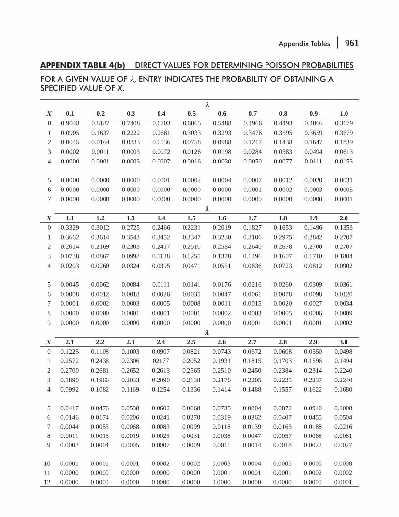
Appendix Tables 961
lX 0.1 0.2 0.3 0.4 0.5 0.6 0.7 0.8 0.9 1.00 0.9048 0.8187 0.7408 0.6703 0.6065 0.5488 0.4966 0.4493 0.4066 0.36791 0.0905 0.1637 0.2222 0.2681 0.3033 0.3293 0.3476 0.3595 0.3659 0.36792 0.0045 0.0164 0.0333 0.0536 0.0758 0.0988 0.1217 0.1438 0.1647 0.18393 0.0002 0.0011 0.0003 0.0072 0.0126 0.0198 0.0284 0.0383 0.0494 0.06134 0.0000 0.0001 0.0003 0.0007 0.0016 0.0030 0.0050 0.0077 0.0111 0.0153
5 0.0000 0.0000 0.0000 0.0001 0.0002 0.0004 0.0007 0.0012 0.0020 0.00316 0.0000 0.0000 0.0000 0.0000 0.0000 0.0000 0.0001 0.0002 0.0003 0.00057 0.0000 0.0000 0.0000 0.0000 0.0000 0.0000 0.0000 0.0000 0.0000 0.0001
lX 1.1 1.2 1.3 1.4 1.5 1.6 1.7 1.8 1.9 2.00 0.3329 0.3012 0.2725 0.2466 0.2231 0.2019 0.1827 0.1653 0.1496 0.13531 0.3662 0.3614 0.3543 0.3452 0.3347 0.3230 0.3106 0.2975 0.2842 0.27072 0.2014 0.2169 0.2303 0.2417 0.2510 0.2584 0.2640 0.2678 0.2700 0.27073 0.0738 0.0867 0.0998 0.1128 0.1255 0.1378 0.1496 0.1607 0.1710 0.18044 0.0203 0.0260 0.0324 0.0395 0.0471 0.0551 0.0636 0.0723 0.0812 0.0902
5 0.0045 0.0062 0.0084 0.0111 0.0141 0.0176 0.0216 0.0260 0.0309 0.03616 0.0008 0.0012 0.0018 0.0026 0.0035 0.0047 0.0061 0.0078 0.0098 0.01207 0.0001 0.0002 0.0003 0.0005 0.0008 0.0011 0.0015 0.0020 0.0027 0.00348 0.0000 0.0000 0.0001 0.0001 0.0001 0.0002 0.0003 0.0005 0.0006 0.00099 0.0000 0.0000 0.0000 0.0000 0.0000 0.0000 0.0001 0.0001 0.0001 0.0002
lX 2.1 2.2 2.3 2.4 2.5 2.6 2.7 2.8 2.9 3.00 0.1225 0.1108 0.1003 0.0907 0.0821 0.0743 0.0672 0.0608 0.0550 0.04981 0.2572 0.2438 0.2306 02177 0.2052 0.1931 0.1815 0.1703 0.1596 0.14942 0.2700 0.2681 0.2652 0.2613 0.2565 0.2510 0.2450 0.2384 0.2314 0.22403 0.1890 0.1966 0.2033 0.2090 0.2138 0.2176 0.2205 0.2225 0.2237 0.22404 0.0992 0.1082 0.1169 0.1254 0.1336 0.1414 0.1488 0.1557 0.1622 0.1680
5 0.0417 0.0476 0.0538 0.0602 0.0668 0.0735 0.0804 0.0872 0.0940 0.10086 0.0146 0.0174 0.0206 0.0241 0.0278 0.0319 0.0362 0.0407 0.0455 0.05047 0.0044 0.0055 0.0068 0.0083 0.0099 0.0118 0.0139 0.0163 0.0188 0.02168 0.0011 0.0015 0.0019 0.0025 0.0031 0.0038 0.0047 0.0057 0.0068 0.00819 0.0003 0.0004 0.0005 0.0007 0.0009 0.0011 0.0014 0.0018 0.0022 0.0027
10 0.0001 0.0001 0.0001 0.0002 0.0002 0.0003 0.0004 0.0005 0.0006 0.000811 0.0000 0.0000 0.0000 0.0000 0.0000 0.0001 0.0001 0.0001 0.0002 0.000212 0.0000 0.0000 0.0000 0.0000 0.0000 0.0000 0.0000 0.0000 0.0000 0.0001
APPENDIX TABLE 4(b) DIRECT VALUES FOR DETERMINING POISSON PROBABILITIES
FOR A GIVEN VALUE OF λ, ENTRY INDICATES THE PROBABILITY OF OBTAINING A SPECIFIED VALUE OF X.
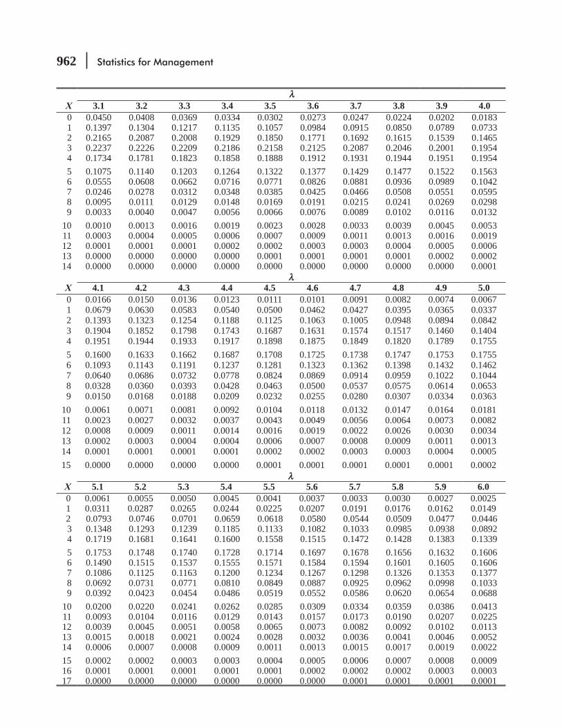
962 Statistics for Management
lX 3.1 3.2 3.3 3.4 3.5 3.6 3.7 3.8 3.9 4.00 0.0450 0.0408 0.0369 0.0334 0.0302 0.0273 0.0247 0.0224 0.0202 0.01831 0.1397 0.1304 0.1217 0.1135 0.1057 0.0984 0.0915 0.0850 0.0789 0.07332 0.2165 0.2087 0.2008 0.1929 0.1850 0.1771 0.1692 0.1615 0.1539 0.14653 0.2237 0.2226 0.2209 0.2186 0.2158 0.2125 0.2087 0.2046 0.2001 0.19544 0.1734 0.1781 0.1823 0.1858 0.1888 0.1912 0.1931 0.1944 0.1951 0.19545 0.1075 0.1140 0.1203 0.1264 0.1322 0.1377 0.1429 0.1477 0.1522 0.15636 0.0555 0.0608 0.0662 0.0716 0.0771 0.0826 0.0881 0.0936 0.0989 0.10427 0.0246 0.0278 0.0312 0.0348 0.0385 0.0425 0.0466 0.0508 0.0551 0.05958 0.0095 0.0111 0.0129 0.0148 0.0169 0.0191 0.0215 0.0241 0.0269 0.02989 0.0033 0.0040 0.0047 0.0056 0.0066 0.0076 0.0089 0.0102 0.0116 0.0132
10 0.0010 0.0013 0.0016 0.0019 0.0023 0.0028 0.0033 0.0039 0.0045 0.005311 0.0003 0.0004 0.0005 0.0006 0.0007 0.0009 0.0011 0.0013 0.0016 0.001912 0.0001 0.0001 0.0001 0.0002 0.0002 0.0003 0.0003 0.0004 0.0005 0.000613 0.0000 0.0000 0.0000 0.0000 0.0001 0.0001 0.0001 0.0001 0.0002 0.000214 0.0000 0.0000 0.0000 0.0000 0.0000 0.0000 0.0000 0.0000 0.0000 0.0001
lX 4.1 4.2 4.3 4.4 4.5 4.6 4.7 4.8 4.9 5.00 0.0166 0.0150 0.0136 0.0123 0.0111 0.0101 0.0091 0.0082 0.0074 0.00671 0.0679 0.0630 0.0583 0.0540 0.0500 0.0462 0.0427 0.0395 0.0365 0.03372 0.1393 0.1323 0.1254 0.1188 0.1125 0.1063 0.1005 0.0948 0.0894 0.08423 0.1904 0.1852 0.1798 0.1743 0.1687 0.1631 0.1574 0.1517 0.1460 0.14044 0.1951 0.1944 0.1933 0.1917 0.1898 0.1875 0.1849 0.1820 0.1789 0.17555 0.1600 0.1633 0.1662 0.1687 0.1708 0.1725 0.1738 0.1747 0.1753 0.17556 0.1093 0.1143 0.1191 0.1237 0.1281 0.1323 0.1362 0.1398 0.1432 0.14627 0.0640 0.0686 0.0732 0.0778 0.0824 0.0869 0.0914 0.0959 0.1022 0.10448 0.0328 0.0360 0.0393 0.0428 0.0463 0.0500 0.0537 0.0575 0.0614 0.06539 0.0150 0.0168 0.0188 0.0209 0.0232 0.0255 0.0280 0.0307 0.0334 0.0363
10 0.0061 0.0071 0.0081 0.0092 0.0104 0.0118 0.0132 0.0147 0.0164 0.018111 0.0023 0.0027 0.0032 0.0037 0.0043 0.0049 0.0056 0.0064 0.0073 0.008212 0.0008 0.0009 0.0011 0.0014 0.0016 0.0019 0.0022 0.0026 0.0030 0.003413 0.0002 0.0003 0.0004 0.0004 0.0006 0.0007 0.0008 0.0009 0.0011 0.001314 0.0001 0.0001 0.0001 0.0001 0.0002 0.0002 0.0003 0.0003 0.0004 0.000515 0.0000 0.0000 0.0000 0.0000 0.0001 0.0001 0.0001 0.0001 0.0001 0.0002
lX 5.1 5.2 5.3 5.4 5.5 5.6 5.7 5.8 5.9 6.00 0.0061 0.0055 0.0050 0.0045 0.0041 0.0037 0.0033 0.0030 0.0027 0.00251 0.0311 0.0287 0.0265 0.0244 0.0225 0.0207 0.0191 0.0176 0.0162 0.01492 0.0793 0.0746 0.0701 0.0659 0.0618 0.0580 0.0544 0.0509 0.0477 0.04463 0.1348 0.1293 0.1239 0.1185 0.1133 0.1082 0.1033 0.0985 0.0938 0.08924 0.1719 0.1681 0.1641 0.1600 0.1558 0.1515 0.1472 0.1428 0.1383 0.13395 0.1753 0.1748 0.1740 0.1728 0.1714 0.1697 0.1678 0.1656 0.1632 0.16066 0.1490 0.1515 0.1537 0.1555 0.1571 0.1584 0.1594 0.1601 0.1605 0.16067 0.1086 0.1125 0.1163 0.1200 0.1234 0.1267 0.1298 0.1326 0.1353 0.13778 0.0692 0.0731 0.0771 0.0810 0.0849 0.0887 0.0925 0.0962 0.0998 0.10339 0.0392 0.0423 0.0454 0.0486 0.0519 0.0552 0.0586 0.0620 0.0654 0.0688
10 0.0200 0.0220 0.0241 0.0262 0.0285 0.0309 0.0334 0.0359 0.0386 0.041311 0.0093 0.0104 0.0116 0.0129 0.0143 0.0157 0.0173 0.0190 0.0207 0.022512 0.0039 0.0045 0.0051 0.0058 0.0065 0.0073 0.0082 0.0092 0.0102 0.011313 0.0015 0.0018 0.0021 0.0024 0.0028 0.0032 0.0036 0.0041 0.0046 0.005214 0.0006 0.0007 0.0008 0.0009 0.0011 0.0013 0.0015 0.0017 0.0019 0.002215 0.0002 0.0002 0.0003 0.0003 0.0004 0.0005 0.0006 0.0007 0.0008 0.000916 0.0001 0.0001 0.0001 0.0001 0.0001 0.0002 0.0002 0.0002 0.0003 0.000317 0.0000 0.0000 0.0000 0.0000 0.0000 0.0000 0.0001 0.0001 0.0001 0.0001
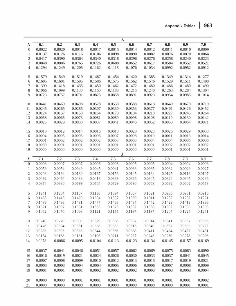
Appendix Tables 963
lX 6.1 6.2 6.3 6.4 6.5 6.6 6.7 6.8 6.9 7.00 0.0022 0.0020 0.0018 0.0017 0.0015 0.0014 0.0012 0.0011 0.0010 0.00091 0.0137 0.0126 0.0116 0.0106 0.0098 0.0090 0.0082 0.0076 0.0070 0.00642 0.0417 0.0390 0.0364 0.0340 0.0318 0.0296 0.0276 0.0258 0.0240 0.02233 0.0848 0.0806 0.0765 0.0726 0.0688 0.0652 0.0617 0.0584 0.0552 0.05214 0.1294 0.1249 0.1205 0.1162 0.1118 0.1076 0.1034 0.0992 0.0952 0.0912
5 0.1579 0.1549 0.1519 0.1487 0.1454 0.1420 0.1385 0.1349 0.1314 0.12776 0.1605 0.1601 0.1595 0.1586 0.1575 0.1562 0.1546 0.1529 0.1511 0.14907 0.1399 0.1418 0.1435 0.1450 0.1462 0.1472 0.1480 0.1486 0.1489 0.14908 0.1066 0.1099 0.1130 0.1160 0.1188 0.1215 0.1240 0.1263 0.1284 0.13049 0.0723 0.0757 0.0791 0.0825 0.0858 0.0891 0.0923 0.0954 0.0985 0.1014
10 0.0441 0.0469 0.0498 0.0528 0.0558 0.0588 0.0618 0.0649 0.0679 0.071011 0.0245 0.0265 0.0285 0.0307 0.0330 0.0353 0.0377 0.0401 0.0426 0.045212 0.0124 0.0137 0.0150 0.0164 0.0179 0.0194 0.0210 0.0227 0.0245 0.026413 0.0058 0.0065 0.0073 0.0081 0.0089 0.0098 0.0108 0.0119 0.0130 0.014214 0.0025 0.0029 0.0033 0.0037 0.0041 0.0046 0.0052 0.0058 0.0064 0.0071
15 0.0010 0.0012 0.0014 0.0016 0.0018 0.0020 0.0023 0.0026 0.0029 0.003316 0.0004 0.0005 0.0005 0.0006 0.0007 0.0008 0.0010 0.0011 0.0013 0.001417 0.0001 0.0002 0.0002 0.0002 0.0003 0.0003 0.0004 0.0004 0.0005 0.000618 0.0000 0.0001 0.0001 0.0001 0.0001 0.0001 0.0001 0.0002 0.0002 0.000219 0.0000 0.0000 0.0000 0.0000 0.0000 0.0000 0.0000 0.0001 0.0001 0.0001
lX 7.1 7.2 7.3 7.4 7.5 7.6 7.7 7.8 7.9 8.00 0.0008 0.0007 0.0007 0.0006 0.0006 0.0005 0.0005 0.0004 0.0004 0.00031 0.0059 0.0054 0.0049 0.0045 0.0041 0.0038 0.0035 0.0032 0.0029 0.00272 0.0208 0.0194 0.0180 0.0167 0.0156 0.0145 0.0134 0.0125 0.0116 0.01073 0.0492 0.0464 0.0438 0.0413 0.0389 0.0366 0.0345 0.0324 0.0305 0.02864 0.0874 0.0836 0.0799 0.0764 0.0729 0.0696 0.0663 0.0632 0.0602 0.0573
5 0.1241 0.1204 0.1167 0.1130 0.1094 0.1057 0.1021 0.0986 0.0951 0.09166 0.1468 0.1445 0.1420 0.1394 0.1367 0.1339 0.1311 0.1282 0.1252 0.12217 0.1489 0.1486 0.1481 0.1474 0.1465 0.1454 0.1442 0.1428 0.1413 0.13968 0.1321 0.1337 0.1351 0.1363 0.1373 0.1382 0.1388 0.1392 0.1395 0.13969 0.1042 0.1070 0.1096 0.1121 0.1144 0.1167 0.1187 0.1207 0.1224 0.1241
10 0.0740 0.0770 0.0800 0.0829 0.0858 0.0887 0.0914 0.0941 0.0967 0.099311 0.0478 0.0504 0.0531 0.0558 0.0585 0.0613 0.0640 0.0667 0.0695 0.072212 0.0283 0.0303 0.0323 0.0344 0.0366 0.0388 0.0411 0.0434 0.0457 0.048113 0.0154 0.0168 0.0181 0.0196 0.0211 0.0227 0.0243 0.0260 0.0278 0.029614 0.0078 0.0086 0.0095 0.0104 0.0113 0.0123 0.0134 0.0145 0.0157 0.0169
15 0.0037 0.0041 0.0046 0.0051 0.0057 0.0062 0.0069 0.0075 0.0083 0.009016 0.0016 0.0019 0.0021 0.0024 0.0026 0.0030 0.0033 0.0037 0.0041 0.004517 0.0007 0.0008 0.0009 0.0010 0.0012 0.0013 0.0015 0.0017 0.0019 0.002118 0.0003 0.0003 0.0004 0.0004 0.0005 0.0006 0.0006 0.0007 0.0008 0.000919 0.0001 0.0001 0.0001 0.0002 0.0002 0.0002 0.0003 0.0003 0.0003 0.0004
20 0.0000 0.0000 0.0001 0.0001 0.0001 0.0001 0.0001 0.0001 0.0001 0.000221 0.0000 0.0000 0.0000 0.0000 0.0000 0.0000 0.0000 0.0000 0.0001 0.0001
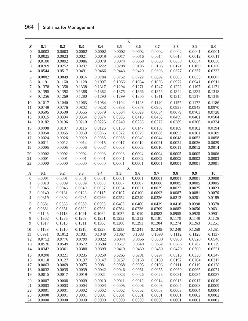
964 Statistics for Management
lX 8.1 8.2 8.3 8.4 8.5 8.6 8.7 8.8 8.9 9.00 0.0003 0.0003 0.0002 0.0002 0.0002 0.0002 0.0002 0.0002 0.0001 0.00011 0.0025 0.0023 0.0021 0.0019 0.0017 0.0016 0.0014 0.0013 0.0012 0.00112 0.0100 0.0092 0.0086 0.0079 0.0074 0.0068 0.0063 0.0058 0.0054 0.00503 0.0269 0.0252 0.0237 0.0222 0.0208 0.0195 0.0183 0.0171 0.0160 0.01504 0.0544 0.0517 0.0491 0.0466 0.0443 0.0420 0.0398 0.0377 0.0357 0.03375 0.0882 0.0849 0.0816 0.0784 0.0752 0.0722 0.0692 0.0663 0.0635 0.06076 0.1191 0.1160 0.1128 0.1097 0.1066 0.1034 0.1003 0.0972 0.0941 0.09117 0.1378 0.1358 0.1338 0.1317 0.1294 0.1271 0.1247 0.1222 0.1197 0.11718 0.1395 0.1392 0.1388 0.1382 0.1375 0.1366 0.1356 0.1344 0.1332 0.13189 0.1256 0.1269 0.1280 0.1290 0.1299 0.1306 0.1311 0.1315 0.1317 0.1318
10 0.1017 0.1040 0.1063 0.1084 0.1104 0.1123 0.1140 0.1157 0.1172 0.118611 0.0749 0.0776 0.0802 0.0828 0.0853 0.0878 0.0902 0.0925 0.0948 0.097012 0.0505 0.0530 0.0555 0.0579 0.0604 0.0629 0.0654 0.0679 0.0703 0.072813 0.0315 0.0334 0.0354 0.0374 0.0395 0.0416 0.0438 0.0459 0.0481 0.050414 0.0182 0.0196 0.0210 0.0225 0.0240 0.0256 0.0272 0.0289 0.0306 0.032415 0.0098 0.0107 0.0116 0.0126 0.0136 0.0147 0.0158 0.0169 0.0182 0.019416 0.0050 0.0055 0.0060 0.0066 0.0072 0.0079 0.0086 0.0093 0.0101 0.010917 0.0024 0.0026 0.0029 0.0033 0.0036 0.0040 0.0044 0.0048 0.0053 0.005818 0.0011 0.0012 0.0014 0.0015 0.0017 0.0019 0.0021 0.0024 0.0026 0.002919 0.0005 0.0005 0.0006 0.0007 0.0008 0.0009 0.0010 0.0011 0.0012 0.001420 0.0002 0.0002 0.0002 0.0003 0.0003 0.0004 0.0004 0.0005 0.0005 0.000621 0.0001 0.0001 0.0001 0.0001 0.0001 0.0002 0.0002 0.0002 0.0002 0.000322 0.0000 0.0000 0.0000 0.0000 0.0001 0.0001 0.0001 0.0001 0.0001 0.0001
lX 9.1 9.2 9.3 9.4 9.5 9.6 9.7 9.8 9.9 100 0.0001 0.0001 0.0001 0.0001 0.0001 0.0001 0.0001 0.0001 0.0001 0.00001 0.0010 0.0009 0.0009 0.0008 0.0007 0.0007 0.0006 0.0005 0.0005 0.00052 0.0046 0.0043 0.0040 0.0037 0.0034 0.0031 0.0029 0.0027 0.0025 0.00233 0.0140 0.0131 0.0123 0.0115 0.0107 0.0100 0.0093 0.0087 0.0081 0.00764 0.0319 0.0302 0.0285 0.0269 0.0254 0.0240 0.0226 0.0213 0.0201 0.01895 0.0581 0.0555 0.0530 0.0506 0.0483 0.0460 0.0439 0.0418 0.0398 0.03786 0.0881 0.0851 0.0822 0.0793 0.0764 0.0736 0.0709 0.0682 0.0656 0.06317 0.1145 0.1118 0.1091 0.1064 0.1037 0.1010 0.0982 0.0955 0.0928 0.09018 0.1302 0.1286 0.1269 0.1251 0.1232 0.1212 0.1191 0.1170 0.1148 0.11269 0.1317 0.1315 0.1311 0.1306 0.1300 0.1293 0.1284 0.1274 0.1263 0.1251
10 0.1198 0.1210 0.1219 0.1228 0.1235 0.1241 0.1245 0.1249 0.1250 0.125111 0.0991 0.1012 0.1031 0.1049 0.1067 0.1083 0.1098 0.1112 0.1125 0.113712 0.0752 0.0776 0.0799 0.0822 0.0844 0.0866 0.0888 0.0908 0.0928 0.094813 0.0526 0.0549 0.0572 0.0594 0.0617 0.0640 0.0662 0.0685 0.0707 0.072914 0.0342 0.0361 0.0380 0.0399 0.0419 0.0439 0.0459 0.0479 0.0500 0.052115 0.0208 0.0221 0.0235 0.0250 0.0265 0.0281 0.0297 0.0313 0.0330 0.034716 0.0118 0.0127 0.0137 0.0147 0.0157 0.0168 0.0180 0.0192 0.0204 0.021717 0.0063 0.0069 0.0075 0.0081 0.0088 0.0095 0.0103 0.0111 0.0119 0.012818 0.0032 0.0035 0.0039 0.0042 0.0046 0.0051 0.0055 0.0060 0.0065 0.007119 0.0015 0.0017 0.0019 0.0021 0.0023 0.0026 0.0028 0.0031 0.0034 0.003720 0.0007 0.0008 0.0009 0.0010 0.0011 0.0012 0.0014 0.0015 0.0017 0.001921 0.0003 0.0003 0.0004 0.0004 0.0005 0.0006 0.0006 0.0007 0.0008 0.000922 0.0001 0.0001 0.0002 0.0002 0.0002 0.0002 0.0003 0.0003 0.0004 0.000423 0.0000 0.0001 0.0001 0.0001 0.0001 0.0001 0.0001 0.0001 0.0002 0.000224 0.0000 0.0000 0.0000 0.0000 0.0000 0.0000 0.0000 0.0001 0.0001 0.0001

Appendix Tables 965
lX 11 12 13 14 15 16 17 18 19 200 0.0000 0.0000 0.0000 0.0000 0.0000 0.0000 0.0000 0.0000 0.0000 0.00001 0.0002 0.0001 0.0000 0.0000 0.0000 0.0000 0.0000 0.0000 0.0000 0.00002 0.0010 0.0004 0.0002 0.0001 0.0000 0.0000 0.0000 0.0000 0.0000 0.00003 0.0037 0.0018 0.0008 0.0004 0.0002 0.0001 0.0000 0.0000 0.0000 0.00004 0.0102 0.0053 0.0027 0.0013 0.0006 0.0003 0.0001 0.0001 0.0000 0.0000
5 0.0224 0.0127 0.0070 0.0037 0.0019 0.0010 0.0005 0.0002 0.0001 0.00016 0.0411 0.0255 0.0152 0.0087 0.0048 0.0026 0.0014 0.0007 0.0004 0.00027 0.0646 0.0437 0.0281 0.0174 0.0104 0.0060 0.0034 0.0018 0.0010 0.00058 0.0888 0.0655 0.0457 0.0304 0.0194 0.0120 0.0072 0.0042 0.0024 0.00139 0.1085 0.0874 0.0661 0.0473 0.0324 0.0213 0.0135 0.0083 0.0050 0.0029
10 0.1194 0.1048 0.0859 0.0663 0.0486 0.0341 0.0230 0.0150 0.0095 0.005811 0.1194 0.1144 0.1015 0.0844 0.0663 0.0496 0.0355 0.0245 0.0164 0.010612 0.1094 0.1144 0.1099 0.0984 0.0829 0.0661 0.0504 0.0368 0.0259 0.017613 0.0926 0.1056 0.1099 0.1060 0.0956 0.0814 0.0658 0.0509 0.0378 0.027114 0.0728 0.0905 0.1021 1.1060 0.1024 0.0930 0.0800 0.0655 0.0514 0.0387
15 0.0534 0.0724 0.0885 0.0989 0.1024 0.0992 0.0906 0.0786 0.0650 0.051616 0.0367 0.0543 0.0719 0.0866 0.0960 0.0992 0.0963 0.0884 0.0772 0.064617 0.0237 0.0383 0.0550 0.0713 0.0847 0.0934 0.0963 0.0936 0.0863 0.076018 0.0145 0.0256 0.0397 0.0554 0.0706 0.0830 0.0909 0.0936 0.0911 0.084419 0.0084 0.0161 0.0272 0.0409 0.0557 0.0699 0.0814 0.0887 0.0911 0.0888
20 0.0046 0.0097 0.0177 0.0286 0.0418 0.0559 0.0692 0.0798 0.0866 0.088821 0.0024 0.0055 0.0109 0.0191 0.0299 0.0426 0.0560 0.0684 0.0783 0.084622 0.0012 0.0030 0.0065 0.0121 0.0204 0.0310 0.0433 0.0560 0.0676 0.076923 0.0006 0.0016 0.0037 0.0074 0.0133 0.0216 0.0320 0.0438 0.0559 0.066924 0.0003 0.0008 0.0020 0.0043 0.0083 0.0144 0.0226 0.0328 0.0442 0.0557
25 0.0001 0.0004 0.0010 0.0024 0.0050 0.0092 0.0154 0.0237 0.0336 0.044626 0.0000 0.0002 0.0005 0.0013 0.0029 0.0057 0.0101 0.0164 0.0246 0.034327 0.0000 0.0001 0.0002 0.0007 0.0016 0.0034 0.0063 0.0109 0.0173 0.025428 0.0000 0.0000 0.0001 0.0003 0.0009 0.0019 0.0038 0.0070 0.0117 0.018129 0.0000 0.0000 0.0001 0.0002 0.0004 0.0011 0.0023 0.0044 0.0077 0.0125
30 0.0000 0.0000 0.0000 0.0001 0.0002 0.0006 0.0013 0.0026 0.0049 0.008331 0.0000 0.0000 0.0000 0.0000 0.0001 0.0003 0.0007 0.0015 0.0030 0.005432 0.0000 0.0000 0.0000 0.0000 0.0001 0.0001 0.0004 0.0009 0.0018 0.003433 0.0000 0.0000 0.0000 0.0000 0.0000 0.0001 0.0002 0.0005 0.0010 0.002034 0.0000 0.0000 0.0000 0.0000 0.0000 0.0000 0.0001 0.0002 0.0006 0.0012
35 0.0000 0.0000 0.0000 0.0000 0.0000 0.0000 0.0000 0.0001 0.0003 0.000736 0.0000 0.0000 0.0000 0.0000 0.0000 0.0000 0.0000 0.0001 0.0002 0.000437 0.0000 0.0000 0.0000 0.0000 0.0000 0.0000 0.0000 0.0000 0.0001 0.000238 0.0000 0.0000 0.0000 0.0000 0.0000 0.0000 0.0000 0.0000 0.0000 0.000139 0.0000 0.0000 0.0000 0.0000 0.0000 0.0000 0.0000 0.0000 0.0000 0.0001

966 Statistics for Management
EXAMPLE: IN A CHI-SQUARE DISTRIBUTION WITH 11 DEGREES OF FREEDOM, TO FIND THE CHI-SQUARE VALUE FOR 0.20 OF THE AREA UNDER THE CURVE (THE COLORED AREA IN THE RIGHT TAIL) LOOK UNDER THE 0.20 COLUMN IN THE TABLE AND THE 11 DEGREES OF FREEDOM ROW; THE APPROPRIATE CHI-SQUARE VALUE IS 14.631.
Degrees ofFreedom 0.99 0.975
Area in Right Tail0.95 0.90 0.800
1 0.00016 0.00098 0.00398 0.0158 0.06422 0.0201 0.0506 0.103 0.211 0.4463 0.115 0.216 0.352 0.584 1.0054 0.297 0.484 0.711 1.064 1.6495 0.554 0.831 1.145 1.610 2.3436 0.872 1.237 1.685 2.204 3.0707 1.239 1.690 2.167 2.833 3.8228 1.646 2.180 2.733 3.490 4.5949 2.088 2.700 3.325 4.168 5.380
10 2.558 3.247 3.940 4.865 6.17911 3.053 3.816 4.575 5.578 6.98912 3.571 4.404 5.226 6.304 7.80713 4.107 5.009 5.892 7.042 8.63414 4.660 5.629 6.571 7.790 9.46715 5.229 6.262 7.261 8.547 10.30716 5.812 6.908 7.962 9.312 11.15217 6.408 7.564 8.672 10.085 12.00218 7.015 8.231 9.390 10.865 12.85719 7.633 8.907 10.117 11.651 13.71620 8.260 9.591 10.851 12.443 14.57821 8.897 10.283 11.591 13.240 15.44522 9.542 10.982 12.338 14.041 16.31423 10.196 11.689 13.091 14.848 17.18724 10.856 12.401 13.848 15.658 18.06225 11.524 13.120 14.611 16.473 18.94026 12.198 13.844 15.379 17.292 19.82027 12.879 14.573 16.151 18.114 20.70328 13.565 15.308 16.928 18.939 21.58829 14.256 16.047 17.708 19.768 22.47530 14.953 16.791 18.493 20.599 23.364
APPENDIX TABLE 5 AREA IN THE RIGHT TAIL OF A CHI-SQUARE (χ 2) DISTRIBUTION
0.20 of area
Values of χ2 14.631
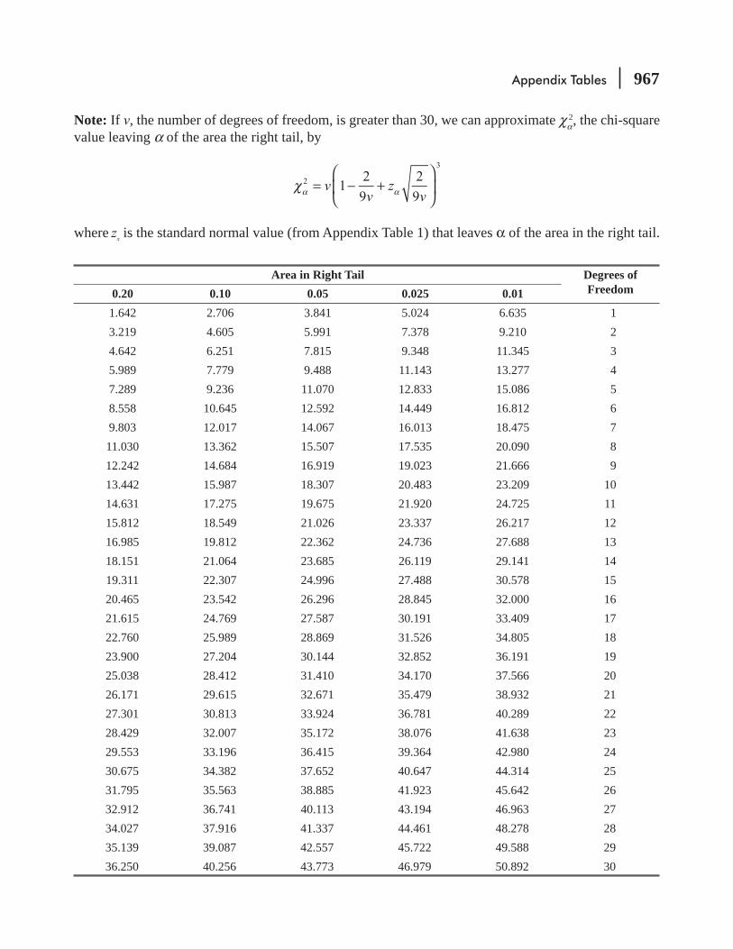
Appendix Tables 967
Note: If v, the number of degrees of freedom, is greater than 30, we can approximate χα2, the chi-square
value leaving α of the area the right tail, by
vv
zv
12
9
2
92
3
χ = − +⎛
⎝⎜
⎞
⎠⎟α α
where zx is the standard normal value (from Appendix Table 1) that leaves α of the area in the right tail.
Area in Right Tail Degrees of Freedom0.20 0.10 0.05 0.025 0.01
1.642 2.706 3.841 5.024 6.635 13.219 4.605 5.991 7.378 9.210 24.642 6.251 7.815 9.348 11.345 35.989 7.779 9.488 11.143 13.277 47.289 9.236 11.070 12.833 15.086 58.558 10.645 12.592 14.449 16.812 69.803 12.017 14.067 16.013 18.475 711.030 13.362 15.507 17.535 20.090 812.242 14.684 16.919 19.023 21.666 913.442 15.987 18.307 20.483 23.209 1014.631 17.275 19.675 21.920 24.725 1115.812 18.549 21.026 23.337 26.217 1216.985 19.812 22.362 24.736 27.688 1318.151 21.064 23.685 26.119 29.141 1419.311 22.307 24.996 27.488 30.578 1520.465 23.542 26.296 28.845 32.000 1621.615 24.769 27.587 30.191 33.409 1722.760 25.989 28.869 31.526 34.805 1823.900 27.204 30.144 32.852 36.191 1925.038 28.412 31.410 34.170 37.566 2026.171 29.615 32.671 35.479 38.932 2127.301 30.813 33.924 36.781 40.289 2228.429 32.007 35.172 38.076 41.638 2329.553 33.196 36.415 39.364 42.980 2430.675 34.382 37.652 40.647 44.314 2531.795 35.563 38.885 41.923 45.642 2632.912 36.741 40.113 43.194 46.963 2734.027 37.916 41.337 44.461 48.278 2835.139 39.087 42.557 45.722 49.588 2936.250 40.256 43.773 46.979 50.892 30
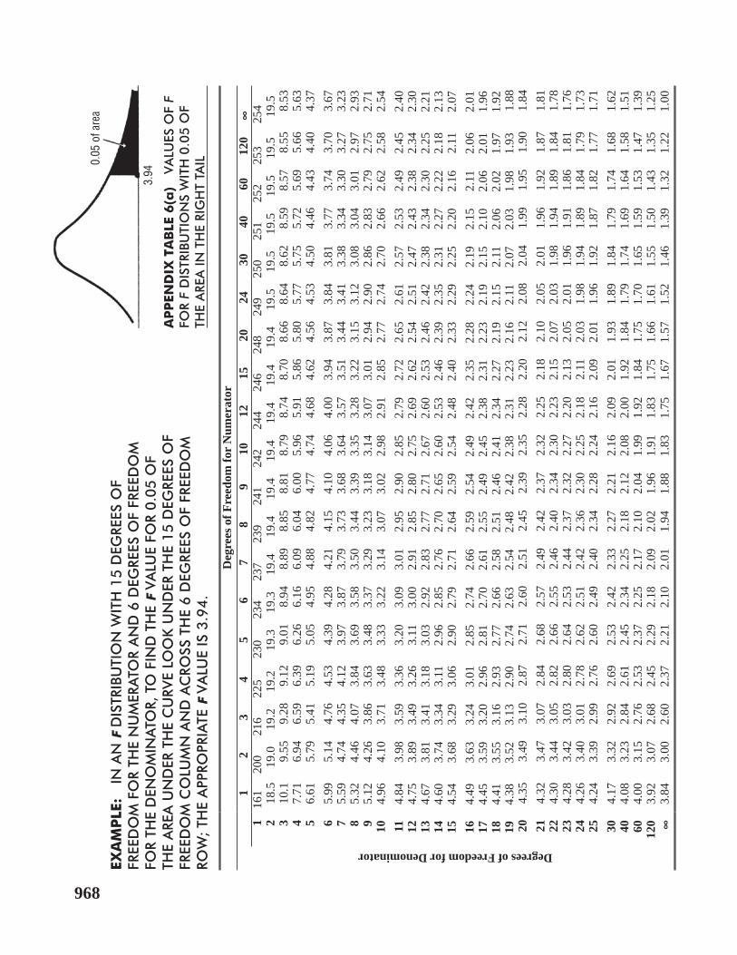
EXA
MP
LE:
IN A
N F
DIS
TRIB
UTI
ON
WIT
H 1
5 D
EGRE
ES O
F FR
EED
OM
FO
R TH
E N
UM
ERA
TOR
AN
D 6
DEG
REES
OF
FREE
DO
M
FOR
THE
DEN
OM
INA
TOR,
TO
FIN
D T
HE
F VA
LUE
FOR
0.0
5 O
F TH
E A
REA
UN
DER
TH
E C
URV
E LO
OK
UN
DER
TH
E 15 D
EGRE
ES O
F FR
EED
OM
CO
LUM
N A
ND
AC
ROSS
TH
E 6 D
EGRE
ES O
F FR
EED
OM
RO
W;
THE
APP
ROPR
IATE
F V
ALU
E IS
3.9
4.
0.05
of a
rea
3.94
AP
PEN
DIX
TA
BLE
6(a
) VA
LUES
OF
F FO
R F
DIS
TRIB
UTI
ON
S W
ITH
0.0
5 O
F TH
E A
REA
IN T
HE
RIG
HT
TAIL
Deg
rees
of F
reed
om fo
r N
umer
ator
Degrees of Freedom for Denominator
12
34
56
78
910
1215
2024
3040
6012
0•
116
1 20
021
622
523
023
423
723
924
124
224
424
624
824
925
025
125
225
325
42
18.5
19.0
19.2
19.2
19.3
19.3
19.4
19.4
19.4
19.4
19.4
19.4
19.4
19.5
19.5
19.5
19.5
19.5
19.5
310
.19.
559.
289.
129.
018.
948.
898.
858.
818.
798.
748.
708.
668.
648.
628.
598.
578.
558.
534
7.71
6.94
6.59
6.39
6.26
6.16
6.09
6.04
6.00
5.96
5.91
5.86
5.80
5.77
5.75
5.72
5.69
5.66
5.63
56.
615.
795.
415.
195.
054.
954.
884.
824.
774.
744.
684.
624.
564.
534.
504.
464.
434.
404.
376
5.99
5.14
4.76
4.53
4.39
4.28
4.21
4.15
4.10
4.06
4.00
3.94
3.87
3.84
3.81
3.77
3.74
3.70
3.67
75.
594.
744.
354.
123.
973.
873.
793.
733.
683.
643.
573.
513.
443.
413.
383.
343.
303.
273.
238
5.32
4.46
4.07
3.84
3.69
3.58
3.50
3.44
3.39
3.35
3.28
3.22
3.15
3.12
3.08
3.04
3.01
2.97
2.93
95.
124.
263.
863.
633.
483.
373.
293.
233.
183.
143.
073.
012.
942.
902.
862.
832.
792.
752.
7110
4.96
4.10
3.71
3.48
3.33
3.22
3.14
3.07
3.02
2.98
2.91
2.85
2.77
2.74
2.70
2.66
2.62
2.58
2.54
114.
843.
983.
593.
363.
203.
093.
012.
952.
902.
852.
792.
722.
652.
612.
572.
532.
492.
452.
4012
4.75
3.89
3.49
3.26
3.11
3.00
2.91
2.85
2.80
2.75
2.69
2.62
2.54
2.51
2.47
2.43
2.38
2.34
2.30
134.
673.
813.
413.
183.
032.
922.
832.
772.
712.
672.
602.
532.
462.
422.
382.
342.
302.
252.
2114
4.60
3.74
3.34
3.11
2.96
2.85
2.76
2.70
2.65
2.60
2.53
2.46
2.39
2.35
2.31
2.27
2.22
2.18
2.13
154.
543.
683.
293.
062.
902.
792.
712.
642.
592.
542.
482.
402.
332.
292.
252.
202.
162.
112.
0716
4.49
3.63
3.24
3.01
2.85
2.74
2.66
2.59
2.54
2.49
2.42
2.35
2.28
2.24
2.19
2.15
2.11
2.06
2.01
174.
453.
593.
202.
962.
812.
702.
612.
552.
492.
452.
382.
312.
232.
192.
152.
102.
062.
011.
9618
4.41
3.55
3.16
2.93
2.77
2.66
2.58
2.51
2.46
2.41
2.34
2.27
2.19
2.15
2.11
2.06
2.02
1.97
1.92
194.
383.
523.
132.
902.
742.
632.
542.
482.
422.
382.
312.
232.
162.
112.
072.
031.
981.
931.
8820
4.35
3.49
3.10
2.87
2.71
2.60
2.51
2.45
2.39
2.35
2.28
2.20
2.12
2.08
2.04
1.99
1.95
1.90
1.84
214.
323.
473.
072.
842.
682.
572.
492.
422.
372.
322.
252.
182.
102.
052.
011.
961.
921.
871.
8122
4.30
3.44
3.05
2.82
2.66
2.55
2.46
2.40
2.34
2.30
2.23
2.15
2.07
2.03
1.98
1.94
1.89
1.84
1.78
234.
283.
423.
032.
802.
642.
532.
442.
372.
322.
272.
202.
132.
052.
011.
961.
911.
861.
811.
7624
4.26
3.40
3.01
2.78
2.62
2.51
2.42
2.36
2.30
2.25
2.18
2.11
2.03
1.98
1.94
1.89
1.84
1.79
1.73
254.
243.
392.
992.
762.
602.
492.
402.
342.
282.
242.
162.
092.
011.
961.
921.
871.
821.
771.
7130
4.17
3.32
2.92
2.69
2.53
2.42
2.33
2.27
2.21
2.16
2.09
2.01
1.93
1.89
1.84
1.79
1.74
1.68
1.62
404.
083.
232.
842.
612.
452.
342.
252.
182.
122.
082.
001.
921.
841.
791.
741.
691.
641.
581.
5160
4.00
3.15
2.76
2.53
2.37
2.25
2.17
2.10
2.04
1.99
1.92
1.84
1.75
1.70
1.65
1.59
1.53
1.47
1.39
120
3.92
3.07
2.68
2.45
2.29
2.18
2.09
2.02
1.96
1.91
1.83
1.75
1.66
1.61
1.55
1.50
1.43
1.35
1.25
•3.
843.
002.
602.
372.
212.
102.
011.
941.
881.
831.
751.
671.
571.
521.
461.
391.
321.
221.
00
968

Deg
rees
of F
reed
om fo
r N
umer
ator
Degrees of Freedom for Denominator
12
34
56
78
910
1215
2024
3040
6012
0•
14,
052
5,00
05,
403
5,62
55,
764
5,85
95,
928
5,98
26,
023
6,05
66,
106
6,15
76,
209
6,23
56,
261
6,28
76,
313
6,33
96,
366
298
.599
.099
.299
.299
.399
.399
.499
.499
.499
.499
.499
.499
.499
.599
.599
.599
.599
.599
.53
34.1
30.8
29.5
28.7
28.2
27.9
27.7
27.5
27.3
27.2
27.1
26.9
26.7
26.6
26.5
26.4
26.3
26.2
26.1
421
.218
.016
.716
.015
.515
.215
.014
.814
.714
.514
.414
.214
.013
.913
.813
.713
.713
.613
.55
16.3
13.3
12.1
11.4
11.0
10.7
10.5
10.3
10.2
10.1
9.89
9.72
9.55
9.47
9.38
9.29
9.20
9.11
9.02
613
.710
.99.
789.
158.
758.
478.
268.
107.
987.
877.
727.
567.
407.
317.
237.
147.
066.
976.
887
12.2
9.55
8.45
7.85
7.46
7.19
6.99
6.84
6.72
6.62
6.47
6.31
6.16
6.07
5.99
5.91
5.82
5.74
5.65
811
.38.
657.
597.
016.
636.
376.
186.
035.
915.
815.
675.
525.
365.
285.
205.
125.
034.
954.
869
10.6
8.02
6.99
6.42
6.06
5.80
5.61
5.47
5.35
5.26
5.11
4.96
4.81
4.73
4.65
4.57
4.48
4.40
4.31
1010
.07.
566.
555.
995.
645.
395.
205.
064.
944.
854.
714.
564.
414.
334.
254.
174.
084.
003.
9111
9.65
7.21
6.22
5.67
5.32
5.07
4.89
4.74
4.63
4.54
4.40
4.25
4.10
4.02
3.94
3.86
3.78
3.69
3.60
129.
336.
935.
955.
415.
064.
824.
644.
504.
394.
304.
164.
013.
863.
783.
703.
623.
543.
453.
3613
9.07
6.70
5.74
5.21
4.86
4.62
4.44
4.30
4.19
4.10
3.96
3.82
3.66
3.59
3.51
3.43
3.34
3.25
3.17
148.
866.
515.
565.
044.
704.
464.
284.
144.
033.
943.
803.
663.
513.
433.
353.
273.
183.
093.
0015
8.68
6.36
5.42
4.89
4.56
4.32
4.14
4.00
3.89
3.80
3.67
3.52
3.37
3.29
3.21
3.13
3.05
2.96
2.87
168.
536.
235.
294.
774.
444.
204.
033.
893.
783.
693.
553.
413.
263.
183.
103.
022.
932.
842.
7517
8.40
6.11
5.19
4.67
4.34
4.10
3.93
3.79
3.68
3.59
3.46
3.31
3.16
3.08
3.00
2.92
2.83
2.75
2.65
188.
296.
015.
094.
584.
254.
013.
843.
713.
603.
513.
373.
233.
083.
002.
922.
842.
752.
662.
5719
8.19
5.93
5.01
4.50
4.17
3.94
3.77
3.63
3.52
3.43
3.30
3.15
3.00
2.92
2.84
2.76
2.67
2.58
2.49
208.
105.
854.
944.
434.
103.
873.
703.
563.
463.
373.
233.
092.
942.
862.
782.
692.
612.
522.
4221
8.02
5.78
4.87
4.37
4.04
3.81
3.64
3.51
3.40
3.31
3.17
3.03
2.88
2.80
2.72
2.64
2.55
2.46
2.36
227.
955.
724.
824.
313.
993.
763.
593.
453.
353.
263.
122.
982.
832.
752.
672.
582.
502.
402.
3123
7.88
5.66
4.76
4.26
3.94
3.71
3.54
3.41
3.30
3.21
3.07
2.93
2.78
2.70
2.62
2.54
2.45
2.35
2.26
247.
825.
614.
724.
223.
903.
673.
503.
363.
263.
173.
032.
892.
742.
662.
582.
492.
402.
312.
2125
7.77
5.57
4.68
4.18
3.86
3.63
3.46
3.32
3.22
3.13
2.99
2.85
2.70
2.62
2.53
2.45
2.36
2.27
2.17
307.
565.
394.
514.
023.
703.
473.
303.
173.
072.
982.
842.
702.
552.
472.
392.
302.
212.
112.
0140
7.31
5.18
4.31
3.83
3.51
3.29
3.12
2.99
2.89
2.80
2.66
2.52
2.37
2.29
2.20
2.11
2.02
1.92
1.80
607.
084.
984.
133.
653.
343.
122.
952.
822.
722.
632.
502.
352.
202.
122.
031.
941.
841.
731.
6012
06.
854.
793.
953.
483.
172.
962.
792.
662.
562.
472.
342.
192.
031.
951.
861.
761.
661.
531.
38•
6.63
4.61
3.78
3.32
3.02
2.80
2.64
2.51
2.41
2.32
2.18
2.04
1.88
1.79
1.70
1.59
1.47
1.32
1.00
EXA
MP
LE:
IN A
N F
DIS
TRIB
UTI
ON
WIT
H 7
DEG
REES
OF
FREE
DO
M F
OR
THE
NU
MER
ATO
R A
ND
5 D
EGRE
ES O
F FR
EED
OM
FO
R TH
E D
ENO
MIN
ATO
R, T
O F
IND
TH
E F
VA
LUE
FOR
0.0
1
OF
THE
ARE
A U
ND
ER T
HE
CU
RVE
LOO
K U
ND
ER T
HE
7 D
EGRE
ES O
F FR
EED
OM
CO
LUM
N
AN
D A
CRO
SS T
HE
5 D
EGRE
ES O
F FR
EED
OM
RO
W;
THE
APP
ROPR
IATE
F V
ALU
E IS
10.5
.
AP
PEN
DIX
TA
BLE
6(b
) VA
LUES
OF
F FO
R F
DIS
TRIB
UTI
ON
S W
ITH
0.0
1
OF
THE
ARE
A IN
TH
E RI
GH
T TA
IL
0.01
of a
rea
10.5
969
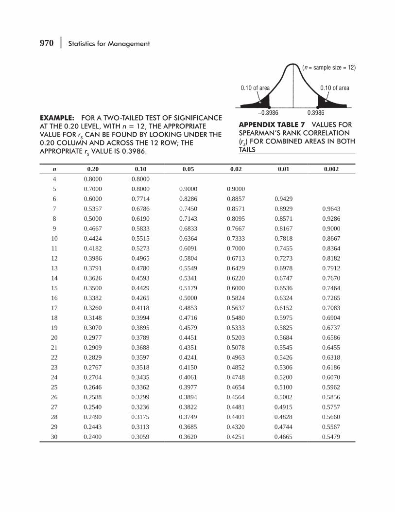
970 Statistics for Management
EXAMPLE: FOR A TWO-TAILED TEST OF SIGNIFICANCE AT THE 0.20 LEVEL, WITH n = 12, THE APPROPRIATE VALUE FOR rS CAN BE FOUND BY LOOKING UNDER THE 0.20 COLUMN AND ACROSS THE 12 ROW; THE APPROPRIATE rS VALUE IS 0.3986.
(n = sample size = 12)
0.10 of area0.10 of area
−0.3986 0.3986
APPENDIX TABLE 7 VALUES FOR SPEARMAN’S RANK CORRELATION (rS) FOR COMBINED AREAS IN BOTH TAILS
n 0.20 0.10 0.05 0.02 0.01 0.0024 0.8000 0.80005 0.7000 0.8000 0.9000 0.90006 0.6000 0.7714 0.8286 0.8857 0.94297 0.5357 0.6786 0.7450 0.8571 0.8929 0.96438 0.5000 0.6190 0.7143 0.8095 0.8571 0.92869 0.4667 0.5833 0.6833 0.7667 0.8167 0.9000
10 0.4424 0.5515 0.6364 0.7333 0.7818 0.866711 0.4182 0.5273 0.6091 0.7000 0.7455 0.836412 0.3986 0.4965 0.5804 0.6713 0.7273 0.818213 0.3791 0.4780 0.5549 0.6429 0.6978 0.791214 0.3626 0.4593 0.5341 0.6220 0.6747 0.767015 0.3500 0.4429 0.5179 0.6000 0.6536 0.746416 0.3382 0.4265 0.5000 0.5824 0.6324 0.726517 0.3260 0.4118 0.4853 0.5637 0.6152 0.708318 0.3148 0.3994 0.4716 0.5480 0.5975 0.690419 0.3070 0.3895 0.4579 0.5333 0.5825 0.673720 0.2977 0.3789 0.4451 0.5203 0.5684 0.658621 0.2909 0.3688 0.4351 0.5078 0.5545 0.645522 0.2829 0.3597 0.4241 0.4963 0.5426 0.631823 0.2767 0.3518 0.4150 0.4852 0.5306 0.618624 0.2704 0.3435 0.4061 0.4748 0.5200 0.607025 0.2646 0.3362 0.3977 0.4654 0.5100 0.596226 0.2588 0.3299 0.3894 0.4564 0.5002 0.585627 0.2540 0.3236 0.3822 0.4481 0.4915 0.575728 0.2490 0.3175 0.3749 0.4401 0.4828 0.566029 0.2443 0.3113 0.3685 0.4320 0.4744 0.556730 0.2400 0.3059 0.3620 0.4251 0.4665 0.5479

Appendix Tables 971
APPENDIX TABLE 8 CRITICAL VALUES OF D IN THE KOLMOGOROV-SMIRNOV GOODNESS-OF-FIT TEST
Sample Size(n)
D = Maximum |Fe – Fo|0.20 0.15 0.10 0.05 0.01
1 0.900 0.925 0.950 0.975 0.9952 0.684 0.726 0.776 0.842 0.9293 0.565 0.597 0.642 0.708 0.8284 0.494 0.525 0.564 0.624 0.7335 0.446 0.474 0.510 0.565 0.669
6 0.410 0.436 0.470 0.521 0.6187 0.381 0.405 0.438 0.486 0.5778 0.358 0.381 0.411 0.457 0.5439 0.339 0.360 0.388 0.432 0.514
10 0.322 0.342 0.368 0.410 0.490
11 0.307 0.326 0.352 0.391 0.46812 0.295 0.313 0.338 0.375 0.45013 0.284 0.302 0.325 0.361 0.43314 0.274 0.292 0.314 0.349 0.41815 0.266 0.283 0.304 0.338 0.404
16 0.258 0.274 0.295 0.328 0.39217 0.250 0.266 0.286 0.318 0.38118 0.244 0.259 0.278 0.309 0.37119 0.237 0.252 0.272 0.301 0.36320 0.231 0.246 0.264 0.294 0.356
25 0.21 0.22 0.24 0.27 0.3230 0.19 0.20 0.22 0.24 0.2935 0.18 0.19 0.21 0.23 0.27
Over 351.07
n
1.14
n
1.22
n
1.36
n
1.63
n
Note: The values of D given in the table are critical values associated with selected values of n. Any value of D that is greater than

972 Statistics for Management
APPENDIX TABLE 9 CONTROL CHART FACTORS
x Charts R Charts
Sample size, nó2
Rd = σ 2
2
3A =
d n 3Rd =
ó
σσ
− 33
2
31
dD =
d+ 3
42
31
dD =
d
2 1.128 1.881 0.853 0 3.269 3 1.693 1.023 0.888 0 2.574 4 2.059 0.729 0.880 0 2.282 5 2.326 0.577 0.864 0 2.114 6 2.534 0.483 0.848 0 2.004 7 2.704 0.419 0.833 0.076 1.924 8 2.847 0.373 0.820 0.136 1.864 9 2.970 0.337 0.808 0.184 1.81610 3.078 0.308 0.797 0.223 1.77711 3.173 0.285 0.787 0.256 1.74412 3.258 0.266 0.779 0.283 1.71713 3.336 0.249 0.770 0.308 1.69214 3.407 0.235 0.763 0.328 1.67215 3.472 0.223 0.756 0.347 1.65316 3.532 0.212 0.750 0.363 1.63717 3.588 0.203 0.744 0.378 1.62218 3.640 0.194 0.739 0.391 1.60919 3.689 0.187 0.734 0.403 1.59720 3.735 0.180 0.729 0.414 1.58621 3.778 0.173 0.724 0.425 1.57522 3.819 0.167 0.720 0.434 1.56623 3.858 0.162 0.716 0.443 1.55724 3.895 0.157 0.712 0.452 1.54825 3.931 0.153 0.708 0.460 1.540
Note: If 1 – 3d3/d2 < 0, then D3 = 0.
Bibliography
Data Analysis and PresentationCleveland, W. S., The Elements of Graphing Data, rev. ed., Murray Hill, NJ, AT&T Bell Laboratories,
1994.everitt, B. S., and G. dunn. Advanced Methods of Data Exploration and Modelling, London,
Heinemann Education Books, Ltd., 1983.tufte, e. r., The Visual Display of Quantitative Information, Chelshire, CT, Graphics Press, 1983.tukey, J. W., Understanding Robust and Exploratory Data Analysis, New York, John Wiley & Sons, 1983.
History of StatisticsStiGler, S. M., The History of Statistics: The Measurement of Uncertainty before 1900, Cambridge, MA,
Belknap Press, 1986.
Introductory StatisticsBerenSon, M. l., and D. M. levine, Basic Business Statistics: Concepts and Applications, 6th ed.,
Englewood Cliffs, NJ, Prentice Hall, 1996.freund, J. E., F. J. WilliamS, and B. M. PerleS, Elementary Business Statistics, 6th ed., Englewood
Cliffs, NJ, Prentice Hall, 1993.mCClave, J. t., and P. G. BenSon, Statistics for Business and Economics, 6th ed., Englewood Cliffs,
nJ, Prentice Hall, 1994.
Nonparametric StatisticsConover, W. J., Practical Nonparametric Statistics, 2d ed., New York, John Wiley & Sons, 1980.GiBBonS, J. D., and S. ChakraBorti, Nonparametric Statistical Inference, 3d ed., New York, Marcel
Dekker, 1992.
974 Statistics for Management
ProbabilityHOGG, R. V., AND E. A. TANIS, Probability and Statistical Inference, 5th ed., Englewood Cliffs, NJ,
Prentice Hall, 1997.ROWNTREE, D., Probability, New York, Charles Scribner’s Sons, 1984.
Quality and Quality ControlDEMING, W. E., Out of the Crisis, Cambridge, MA, MIT Center for Advanced Engineering Study, 1986.GITLOW, H., S. GITLOW, A. OPPENHEIM, AND R. OPPENHEIM, 2d ed., Quality Management: Tools and
Methods for Improvement, Homewood, IL, Richard D. Irwin, Inc., 1995.GRANT, E. L., AND R. S. LEAVENWORTH, Stastistical Quality Control, 7th ed., New York, McGraw-Hill
Book Co., 1996.ISHIKAWA, K., Guide to Quality Control, 2d ed., White Plains, NY, Kraus International Publications,
1986.
Regression and Analysis of VarianceBERRY, W. D., Multiple Regression in Practice Beverly Hills, Sage Publications, 1985.KLEINBAUM, D. G., L. L. KUPPER, AND K. E. MULLER, Applied Regression Analysis and Other Multivariable
Methods, 2d ed. Boston, PWS-Kent Publishing Co., 1988.MENDENHALL, W. AND T. SINCICH, A Second Course in Statistics: Regression Analysis, 5th ed., Englewood
Cliffs, NJ, Prentice Hall, 1996.NETER, J., W. WASSERMAN, AND M. H. KUTNER, Applied Linear Statistical Models, 2d ed., Homewood,
IL, Richard D. Irwin, Inc., 1985.
SamplingGUY, D. M., D. R. CARMICHAEL, AND O. R. WHITTINGTON, Audit Sampling: An Introduction, 3rd ed., New
York, John Wiley & Sons, 1994.SCHAEFER, R. L., W. MENDENHALL, AND L. OTT, Elementary Survey Sampling, Boston, 5th ed., Duxbury
Press, 1996.
Special Topics in StatisticsHUFF, D., How to Lie with Statistics, New York, W. W. Norton & Co., 1954.JAFFE, A. J., Misused Statistics: Straight Talk for Twisted Numbers, New York, Marcel Dekker, 1987.MADANSKY, A., Prescriptions for Working Statisticians, New York, Springer-Verlag, 1988.
Statistical Decision TheoryCOOK, T. M., AND R. A. RUSSELL, Introduction to Management Science, 5th ed., Englewood Cliffs, NJ,
Prentice Hall, 1993.HILLIER, F. S., AND G. J. LIEBERMAN, Introduction to Operations Research, 6th ed., New York, McGraw-
Hill Book Co., 1995.LEVIN, R. I, D. S. RUBIN, J. P. STINSON, AND E. S. GARDNER, JR., Quantitative Approaches to Management,
8th ed. New York, McGraw-Hill Book Co., 1992.
Bibliography 975
Statistical SoftwareMINITAB, INC., MINITAB User’s Guide: Release 10 Xtra, State College, PA, 1995.SAS INSTITUTE, INC., SAS Introductory Guide for Personal Computers, Release 6.03 ed., Cary, NC, 1988.
Time SeriesBOWERMAN, B. L. AND R. T. O’CONNELL, Forecasting and Time Series: An Applied Approach, 3d ed.,
Boston, Duxbury Press, 1993.FARNUM, N. R., AND L. W. STANTON, Quantitative Forecasting Methods, Boston, PWS-Kent Publishing
Co., 1989.MILLS, T. C., Time Series Techniques for Economists, Cambridge, Cambridge University Press, 1990.

This page is intentionally left blank
Aα (the greek letter, alpha), 343, 373A priori, 158Absolute values, 608Acceptable quality level (AQL), 501Acceptance sampling, 500Acts, 898Addition rule, 166Alternative hypothesis, 371Analysis correlation, 629 decision-tree, 925–933 marginal, 908 multiple regression and correlation, 664 of variance, 542 time-series, 804 trend, 806Analysis of variance (ANOVA), 542
Analysis of variance(ANOVA) for the regression, 691
Appropriate distribution, 534
Approximate prediction intervals, 619Assignable variation, 469Attribute, 487Average of relatives methods, 874Average outgoing quality (AOQ) graph, 504
Bβ (the greek letter beta), 373Bayes, Reverend Thomas, 154, 188Bayes’ theorem, 188–189Bayesian decision theory, 898Bernoulli process, 222
Bernoulli, Jacob, 154Between-column variance, 544Biased samples, 270Bills of mortality, 3Bimodal distribution, 106, 222Binomial formula, 223Bivariate frequency distributions, 30Boxplot, 141Brennan, Maureen, 503
CCausal relationship, 598Cause-and-effect diagram, 495Census, 268Center line (CL), 470Central limit theorem, 296Central tendency, 74Certainty, 939Chance events, 926Chance node, 927Chebyshev. P. L., 122Chebyshev’s theorem, 122Chi-square as a test of goodness
Chi-square as a test of independence, 519Chi-square distribution, 523Chi-square statistic, 522Chi-square test, 518Chi-square test using spss, 529–531Class class, 98–99 discrete, 22 equal, 27 open ended, 22Classical linear regression model
(CLRM), 670
Index
978 Index
Classical probability, 158Cluster sampling, 274Clusters, 274Codes, 81Coding, 81
Collectively exhaustive, 156Common variation, 469Complete enumeration, 268Computed f ratio, 721Computed t, 721Conditional probability, 175Conditional probability of
dependent events, 179
Consistent estimator, 318Consumer price index (CPI), 856Consumer’s risk, 501Contingency table, 520Continuity correction factors, 250Continuous data, 22Continuous probability distributions, 210Continuous quality improvement (CQI), 497Continuous random variable, 212Convenience sampling, 279Correlation analysis, 629Critical value, 381Curve(s) power, 388 skewed, 75 symmetrical, 75
utility, 918Curvilinear, 599
Cyclical variation, 818
DData, 14 array, 18 array, 18 continuous, 22 point, 14 raw, 17
sample arithmetic mean of grouped, 79 set, 14 tests for, 15 ungrouped, 79Data array, 18 advantages of, 19 disadvantages of, 19Data point, 14Data set, 14De Fermat, Pierre, 154De Laplace, Marquis, 154De Moivre, Abraham, 154Deciles, 115Decision environment, 898–899Decision node, 927Decision points, 925Decision theory, 4, 897–939Decision tree, 925Decision-tree analysis, 925–933Degrees of freedom, 341Dependence, 179Dependent samples, 431Dependent variable, 597Deterministic models, 155Diagram cause-and-effect, 495
ishikawa, 495 scatter, 598 venn, 165Direct relationship, 597Discrete classes, 22Discrete probability distributions, 210Discrete random variable, 212Dispersion, 74Distance measures, 113Distribution appropriate, 534 bimodal, 106 binomial, 222 bivariate frequency, 30 chi-square, 523 continuous probability, 210 discrete probability, 210 frequency, 16,19, 210 gaussian, 238

Index 979
hypergeometric, 502 normal, 238 of proportion, 298 poisson, 230 population, 290 probability, 208 relative frequency, 20 sampling, 289 standard normal probability, 242 student’s, 341 student’s t, 341 theoretical sampling, 291Distribution-free tests, 734Dodge, Harold F.,500Domesday book, 3Doublesampling, 500Dummy variable, 665, 706
E
Equal classes, 27Error margin of, 2 root-mean-square, 677 sampling, 287 standard, 287 type I, 373 type II, 373Estimate, 317 intervel, 317 point, 317
Estimation, 316Estimation using the regression
line, 603Estimator, 317Event(s), 155, 282 chance, 926 conditional probability of
dependent, 179 joint probability independent, 171 marginal probability of
independent, 170 mutually exclusive, 156 statistically independent, 170Expected frequencies, 521
Expected marginal loss, 910
Expected value, 214Expected value of sample
information (EVSI), 931Experiment, 155, 282
FFactorial, 223Federal trade commission (FTC), 113Finite population multiplier, 303, 375Fishbone diagrams, 495Fixed-weight aggregates
method, 866 , 869Fixed-weight aggregates price
index, 869Food and Drug Administration, 2Fractile, 114, 116
deciles, 115, 141percentile, 115quartile, 115
Frequency distribution, 16, 19, 210 bivariate, 30 constructing a, 27–30 cumulative, 41 graphing, 38–52 relative, 20Frequency polygons, 39, 45–47Frequency table, 19
GGalton, Sir Francis, 596Garbage in, garbage out (GIGO), 15Gardner, Everette S., Jr., 503Gauss, Karl, 238Gaussian distribution, 238Geometric mean (G.M.), 93Geometric mean growth rate, 93Gombauld, Antoine, 154Gottfried Achenwall, 3Good, Richard, 161
Graunt, Captain John, 3Grade-point averages (GPAS), 17Grand mean (x), 473Gross domestic product (GDP), 597
980 Index
HHenry VII, 3Histogram, 38 relative frequency, 38How to lie with statistics, 3Hypergeometric distribution, 502Hypothesis, 366 alternative, 371 hypothesis, 369, 371 null, 371 testing for differences between means
and proportions, 412 testing using the standardized scale, 381–383Hypothesis testing, 369, 371Hypothesis testing for differences between
means and proportions, 412Hypothesis testing using the standardized
scale, 381–383
IInferential statistics, 4Independent events conditional probability, 175 joint probability, 174 marginal probability, 170Independent variable, 597Index numbers, 856Indicator variable, 706Inferences about a population
variance, 568Inferences about two population
variances, 576
Inherent variation, 469Interfractile range, 114Interquartile range, 115Interval estimates, 317, 324–326Irregular variation, 805, 833Ishikawa diagrams, 495Ishikawa, Kaoru, 495
JJoint probability, 174Joint probability independent
events, 171Judgement sampling, 279Juran, Joseph M., 467
KKolmogorov, A. N., 779Kolmogorov–Smirnov test, 735, 779Koopman, Bernard, 161Kruskal-wallis test, 734K-S test, 779Kurtosis, 76
LLagrange, Joseph, 154Laspeyres method, 865Latin square, 286Law of diminishing return, 305Least-squares method, 609Left-tailed test, 376, 384Less-than ogive, 41–42Linear relationship, 599Losses, 218 obsolescence, 218 opportunity, 218Lot tolerance percent
defective (LTPD), 501(LCL), 329
Lower control limit (LCL) line, 470Lower-tailed test, 376
Mμ (the Greek letter mu), 77Making inferences about population
parameters, 643Mann-Whitney U test, 734Margin of error, 2Marginal analysis, 908Marginal loss (ML), 909Marginal probabilities under statistical
dependence, 183Marginal probability, 165, 174Marginal probability of independent
events, 170
Mean, 20arithmetic, 77–83compared to median and mode, 107
distribution of the, 291 geometric, 93 grand, 473 one-tailed test of, 383

Index 981
population, 316 population arithmetic, 78 sample arithmetic, 78 sampling distribution of the, 286, 291 standard error of the, 287 weighted, 87Measures of central tendency, 74Measures of location, 74Median, 96
advantages and disadvantages of, 100–101
compared to mean and mode, 107class, 98, 141
Median class, 98–99Minimum probability, 910Minitab, 30Modal class, 105Mode, 104–105, 141
advantages and disadvantages of, 106compared to mean and median, 107
Model, 703Modeling techniques, 703Mu (μ), 77Multicollinearity, 692, 721Multimodal distributions, 106Multiple regression and correlation
analysis, 664Mutually exclusive events, 156
NNatural and Political Observations … Made Upon
the Bills of Morality, 3Negative slope, 597Node, 939Nonparametric methods, 733–784Nonparametric tests, 734Nonrandom sampling, 269Non-random sampling, 279–280Normal distribution, 238Null hypothesis, 371
OObserved value, 381Obsolescence losses, 218, 939Ogive, 41–42, 60One-sample runs test, 735, 758, 759One-tailed test of a variance, 572–573
One-tailed test of means, 383One-tailed tests, 375One-tailed tests for differences between
proportions, 445–448One-tailed tests of proportions, 393Open ended class, 22Operating characteristic (OC)
graph, 503Opportunity losses, 218, 939Original scale, 381Outcomes, 898Outliers, 471
PP charts, 487–491Paasche method, 866, 868Paasche price index, 868Paired samples, 431Parameters, 77, 269, 734Pareto chart, 496Pareto, Vilfredo, 496Pascal, Blaise, 154Payoffs, 898Percentiles, 115Perfect correlation, 630Point estimates, 319–322Poisson distribution, 230Poisson, Siméon Denis, 230Population, 16, 268, 543
Population arithmetic mean, 78Population characteristics, 268Population distribution, 290Population mean, 316Population parameter, 269Population proportion, 316Population standard deviation, 120Positive slope, 597Posterior probabilities, 188Power curve, 388Precision, 302Price index, 856Prob values, 450Probabilistic models, 155Probability, 4 classical, 158 conditional, 175

982 Index
distributions, 208 joint, 174 marginal, 165, 174 minimum, 910 sampling, 269 single, 165 tree, 172 unconditional, 165Probability distributions, 208 continuous, 210 discrete, 210 standard normal, 242Probability sampling, 269Probability tree, 172Producer’s risk, 501Proportion, 286Proportions, 391
QQuadratic regression model, 713Qualitative data, 703Quality, 467Quantitative data, 703Quantity index, 856Quantity indices, 881Quartiles, 115Quota sampling, 279
RR charts, 481–484Ramsey, Frank, 161Random models, 155Random sampling, 269, 271Random variables, 212Random variation, 469Range, 113
interfractile, 114, 141interquartile, 115, 141
Rank correlation, 735, 767Rank sum tests, 734, 744
Ratio-to-moving-average method, 825Raw data, 17Raw scale, 381Regression, 596Relative cyclical residual, 819
Relative frequency distribution, 20Relative frequency histogram, 38Relative frequency of
occurrence, 159Relative frequency polygon, 40Relative measure, 132Representative sample, 16Residual method, 818Response variable, 283Revised probabilities, 188Right-tailed test, 377Rollback process, 927Romig, Harry G., 500Root-mean-square error, 677Run, 759
Sσ (population standard deviation), 124Salvage value, 939Sample representative, 16, 60 standard deviation, 124–125Sample arithmetic mean, 78Sample arithmetic mean of
grouped data, 79
determination, 629
Sample space, 155Sample statistic, 269Sampling acceptance, 500 cluster, 274 convenience, 279 distribution of proportion, 298 distribution of the mean, 291 double, 500 fraction, 304 from nonnormal populations, 294–296 from normal populations, 291–294 judgement, 279 nonrandom, 269 non-random, 279 probability, 269 quota, 279 random, 269, 271

Index 983
shopping-mall intercept, 279 simple random, 271 single, 500
systematic, 273Sampling distribution of
proportion, 298Sampling distribution of the
mean, 286, 291Sampling distributions, 289Sampling error, 287Sampling fraction, 304Sampling from nonnormal
populations, 294–296Sampling from normal
populations, 291–294SAS, 30Savage, Leonard, 161Scatter diagram, 598Seasonal variation, 805, 824Second-degree regression model, 713Secular trend, 804Shewhart, Walter, 500Shopping-mall intercept
sampling, 279Sigma (σ), 78, 290Sigma hat, 333Sign test, 734Sign test for paired data, 736
Simon, Pierre, 154Simple random sampling, 271Single probability, 165Single-sampling, 500Skewed curves, 75Skewness, 75Slope, 654 negative, 597 positive, 597Smirnov, N.V., 779Snowball sampling, 280Special cause variation, 469Spinks, Leon, 154SPSS, 30Standard deviation, 119, 120Standard error, 287Standard error of estimate, 615
Standard error of the difference between two means, 414
Standard error of the mean, 287Standard error of the median, 287Standard error of the
proportion, 287, 337Standard error of the range, 287Standard error of the regression
Standard error of the statistic, 287Standard normal probability
distribution, 242Standard score, 122Standard units, 244Standardized scale, 381Statistical Account of Scotland
1791–1799, 3States of nature, 898Statistical account of scotland, 3Statistical decision theory, 898Statistical dependence, 179Statistical independence, 170Statistical inference, 275Statistical process control
(SPC), 468Statistically independent, 223Statistically independent events, 170Statistics, 2, 3, 77, 269 chi-square, 522 descriptive, 4 inference, 4 inferential, 4 sample, 269 summary, 74Stem and leaf display, 142Strata, 274
Student’s distribution, 341Subjective probabilities, 160
Summary statistics, 74Symmetrical curves, 75Systat, 30Systematic sampling, 273Systematic variation, 469

984 Index
TT distribution, 341Table of random digits, 272Test of independence, 519Testing differences between means with
dependent samples, 431Tests distribution-free, 734 for differences between means:
large sample sizes, 414 for differences between means:
small sample sizes, 420 for differences between proportions:
large sample sizes, 441 kolmogorov–smirnov, 779 nonparametric, 734 one-tailed, 375 rank sum, 744Tests for differences between means:
large sample sizes, 414Tests for differences between means:
small sample sizes, 420Tests for differences between proportions:
large sample sizes, 441The foundation of mathematics and other
logical essays, 161The index of industrial production (IIP), 881Theoretical sampling distribution, 291Theory of runs, 759Time-series analysis, 804Time-series analysis in forecasting, 844Total quality management (TQM),
466, 494–497Transformations, 721
curves, 709–713
Trend analysis, 806Two-tailed prob values, 451Two-tailed test, 375Two-tailed test of a variance, 571–572Two-tailed tests for differences between
proportions, 442–445Type I error, 373Type II error, 373
UUnbiased estimator, 319Unbiasedness, 318Unconditional probability, 165Ungrouped data, 79Unweighted aggregates index, 860Unweighted average of relatives
method, 874(UCL), 329
Upper control limit (UCL) line, 470Upper-tailed test, 377Utility, 917–918Utility curves, 918
VValue index, 857Value indices, 882Value(s) absolute, 608 critical, 381 expected, 214 index, 857 indices, 882 observed, 381 prob, 450 salvage, 939 two-tailed prob, 451Variance, 119 analysis of, 542 between-column, 544 one-tailed test of a, 572–573 two-tailed test of a, 571–572 within-column, 545
(VIF), 694Variation, 469, 629 assignable, 469
common, 469 in time series, 804 inherent, 469 random, 469 special cause, 469 systematic, 469Variations in time series, 804

Index 985
Venn diagram, 165Venn, John, 165
WWeighted average, 88Weighted average of relatives
method, 874Weighted mean, 87Width of a class interval, 28Within-column variance, 545
Xx charts, 470
YYate’s correction, 531
ZZero defects, 468Zimmerman. E.A.W., 3