Mahler measure under variations of the base group

Oliver T. Dasbach ∗

Louisiana State UniversityDepartment of Mathematics

Baton Rouge, LA 70803e-mail: kasten@math.lsu.edu

Matilde Lalin †

University of British ColumbiaDepartment of Mathematics

Vancouver, BC V6T 1Z2, Canadae-mail: mlalin@math.ubc.ca

November 28, 2006

Abstract

We study properties of a generalization of the Mahler measure toelements in group rings, in terms of the Luck-Fuglede-Kadison deter-minant. Our main focus is the variation of the Mahler measure whenthe base group is changed. In particular, we study how to obtain theMahler measure over an infinite group as limit of Mahler measures overfinite groups, for example, in the classical case of the free abelian groupor the infinite dihedral group, and others.

Keywords: Mahler measure, Luck-Fuglede-Kadison determinant, Spec-tra of Cayley graphs

MSC: 11C08, 16S34, 05C25, 57M25

1 Introduction

The Mahler measure of a Laurent polynomial P ∈ C[x±11 , . . . , x±1

n ], is definedby

m(P ) :=1

(2πi)n

∫

Tn

log |P (x1, . . . , xn)| dx1

x1. . .

dxn

xn(1)

=∫ 1

0. . .

∫ 1

0log |P (e2πit1 , . . . , e2πitn)| dt1 . . . dtn. (2)

∗The first author was supported in part by NSF grants DMS-0306774 and DMS-0456275(FRG)

†The second author was partially supported by the NSF under DMS-0111298.

1

In particular, Jensen’s formula implies, for a one-variable polynomialthat

m(P ) = log |a|+∑

i

log max{|αi|, 1} for P (x) = a∏

i

(x− αi). (3)

In this article we use some ideas of Rodriguez-Villegas [RV99] to gen-eralize the definition of the Mahler measure to certain elements of grouprings. Our construction yields the logarithm of the Luck-Fuglede-Kadisondeterminant as defined by Luck in [Luc02].

We relate the Mahler measure for elements in the group ring of a fi-nite group to the characteristic polynomial of the adjacency matrix of a(weighted) Cayley graph and also to characters of the group (Theorem 6).We obtain certain rationality results for the Mahler measure of group ringelements of the form 1−λP . In Section 9 we recover a result of Luck [Luc02]that the (classical) Mahler measure is limit of Mahler measures over finiteabelian groups. We extend this result to a more general case. In particular,we complement it in Theorem 16 and Corollary 17 by proving an analogousproperty for the infinite dihedral group, PSL2(Z), and other infinite groups.Finally, we study how the Mahler measure changes when we vary the basegroup. In particular we focus our attention to the dihedral group Dm versusthe abelianization Z/mZ× Z/2Z in the general case (Theorem 12).

2 The general technique

In this section we will review the techniques and one example of Rodriguez-Villegas [RV99]. The section after that will point out the connections tothe combinatorial L2-torsion of Luck [Luc02]. Let P ∈ C[x±1, y±1] be apolynomial, λ ∈ C, and let Pλ(x, y) = 1 − λP (x, y). Assume that P isa reciprocal polynomial i.e., P (x, y) = P (x−1, y−1). For instance, as in[RV99], we may think of P (x, y) = x + x−1 + y + y−1.

We define m(P, λ) := m(Pλ). Then

m(P, λ) =1

(2πi)2

∫

T2

log |1− λP (x, y)| dx

x

dy

y. (4)

=∫ 1

0

∫ 1

0log |P (e2πit, e2πis)| dt ds. (5)

Since P (x, y) is a continuous function defined in the torus T2, it isbounded and |λP (x, y)| < 1 for λ small enough and x, y ∈ T2. For in-

2

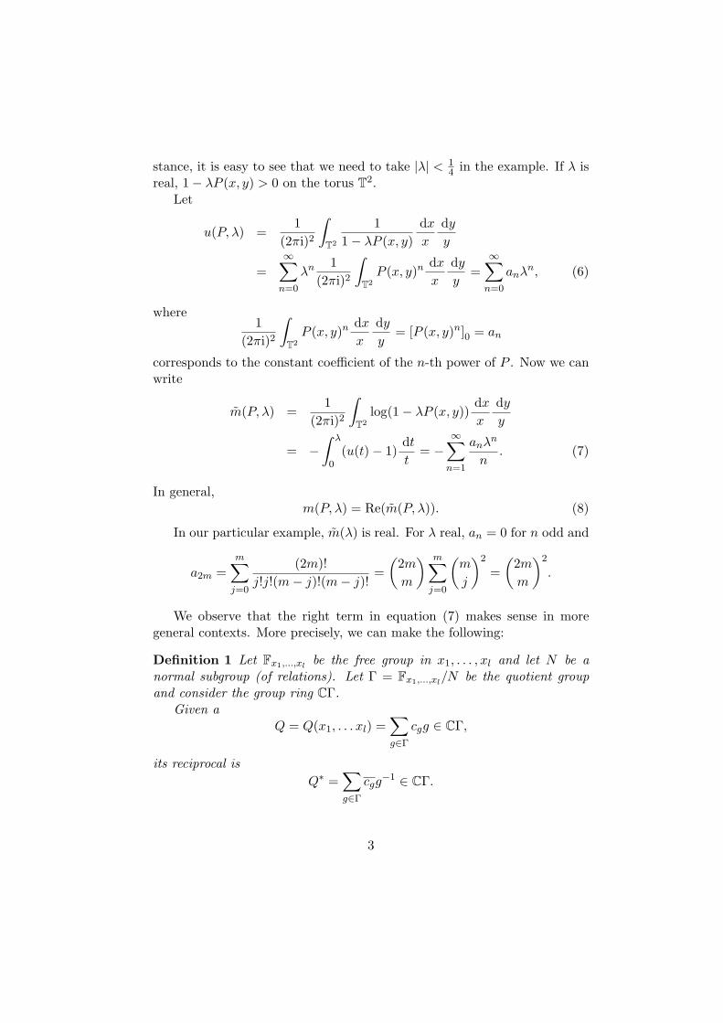
stance, it is easy to see that we need to take |λ| < 14 in the example. If λ is

real, 1− λP (x, y) > 0 on the torus T2.Let

u(P, λ) =1

(2πi)2

∫

T2

11− λP (x, y)

dx

x

dy

y

=∞∑

n=0

λn 1(2πi)2

∫

T2

P (x, y)n dx

x

dy

y=

∞∑

n=0

anλn, (6)

where1

(2πi)2

∫

T2

P (x, y)n dx

x

dy

y= [P (x, y)n]0 = an

corresponds to the constant coefficient of the n-th power of P . Now we canwrite

m(P, λ) =1

(2πi)2

∫

T2

log(1− λP (x, y))dx

x

dy

y

= −∫ λ

0(u(t)− 1)

dt

t= −

∞∑

n=1

anλn

n. (7)

In general,m(P, λ) = Re(m(P, λ)). (8)

In our particular example, m(λ) is real. For λ real, an = 0 for n odd and

a2m =m∑

j=0

(2m)!j!j!(m− j)!(m− j)!

=(

2m

m

) m∑

j=0

(m

j

)2

=(

2m

m

)2

.

We observe that the right term in equation (7) makes sense in moregeneral contexts. More precisely, we can make the following:

Definition 1 Let Fx1,...,xlbe the free group in x1, . . . , xl and let N be a

normal subgroup (of relations). Let Γ = Fx1,...,xl/N be the quotient group

and consider the group ring CΓ.Given a

Q = Q(x1, . . . xl) =∑

g∈Γ

cgg ∈ CΓ,

its reciprocal isQ∗ =

∑

g∈Γ

cgg−1 ∈ CΓ.

3

Let P = P (x1, . . . , xl) ∈ CΓ reciprocal, (i.e., P = P ∗). Let |λ| < 1k

where k is the l1-norm of the coefficients of P as an element in CΓ. Thenwe define the Mahler measure of Pλ(x1, . . . , xl) = 1− λP (x1, . . . xl) by

mΓ(P, λ) = −∞∑

n=1

anλn

n, (9)

where an is the constant coefficient of the nth power of P (x1, . . . , xl), inother words,

an = [P (x1, . . . , xl)n]0 . (10)

We will also use the notation

uΓ(P, λ) =∞∑

n=0

anλn

for the generating function of the an.

We will confine ourselves mainly to the two variable case and we willkeep the notation m(P, λ) for mZ×Z(P, λ).

Remark 2 Let us observe that we can extend this definition for any poly-nomial Q(x1, . . . , xl) ∈ CΓ. It suffices to write

QQ∗ =1λ

(1− (1− λQQ∗))

for λ real and positive and 1/λ larger than the length of QQ∗. Define

mΓ(Q) = − log λ

2−

∞∑

n=1

bn

2n, (11)

wherebn = [(1− λQQ∗)n]0 .

This sum might not necessarily converge. When it is convergent then itis clear that mΓ(Q) is well-defined as it does not depend on the choice of λ:write

(1− (1− λµx)) = λµx = (1− (1− λx))µ

then

log(1− (1− λµx))− log(λµ) = log(1− (1− λx)) + log µ− log(λµ)

= log(1− (1− λx))− log λ.

4

3 Luck’s combinatorial L2-torsion.

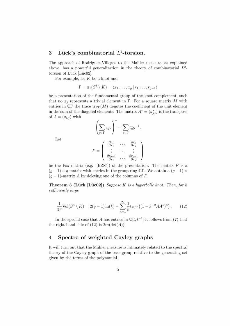
The approach of Rodriguez-Villegas to the Mahler measure, as explainedabove, has a powerful generalization in the theory of combinatorial L2-torsion of Luck [Luc02].

For example, let K be a knot and

Γ = π1(S3 \K) = 〈x1, . . . , xg | r1, . . . , rg−1〉be a presentation of the fundamental group of the knot complement, suchthat no xj represents a trivial element in Γ. For a square matrix M withentries in CΓ the trace trCΓ(M) denotes the coefficient of the unit elementin the sum of the diagonal elements. The matrix A∗ = (a∗j,i) is the transposeof A = (ai,j) with

∑

g∈Γ

cgg

∗

=∑

g∈Γ

cgg−1.

Let

F =

∂r1∂x1

. . . ∂r1∂xg

.... . .

...∂rg−1

∂x1. . .

∂rg−1

∂xg

be the Fox matrix (e.g. [BZ85]) of the presentation. The matrix F is a(g− 1)× g matrix with entries in the group ring CΓ. We obtain a (g− 1)×(g − 1)-matrix A by deleting one of the columns of F .

Theorem 3 (Luck [Luc02]) Suppose K is a hyperbolic knot. Then, for ksufficiently large

13π

Vol(S3 \K) = 2(g − 1) ln(k)−∞∑

n=1

1n

trCΓ

((1− k−2AA∗)n

). (12)

In the special case that A has entries in C[t, t−1] it follows from (7) thatthe right-hand side of (12) is 2m(det(A)).

4 Spectra of weighted Cayley graphs

It will turn out that the Mahler measure is intimately related to the spectraltheory of the Cayley graph of the base group relative to the generating setgiven by the terms of the polynomial.

5

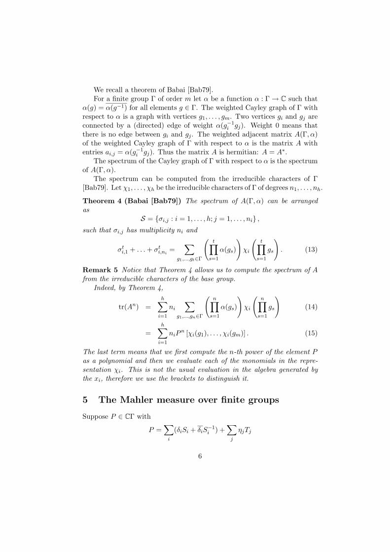
We recall a theorem of Babai [Bab79].For a finite group Γ of order m let α be a function α : Γ → C such that

α(g) = α(g−1) for all elements g ∈ Γ. The weighted Cayley graph of Γ withrespect to α is a graph with vertices g1, . . . , gm. Two vertices gi and gj areconnected by a (directed) edge of weight α(g−1

i gj). Weight 0 means thatthere is no edge between gi and gj . The weighted adjacent matrix A(Γ, α)of the weighted Cayley graph of Γ with respect to α is the matrix A withentries ai,j = α(g−1

i gj). Thus the matrix A is hermitian: A = A∗.The spectrum of the Cayley graph of Γ with respect to α is the spectrum

of A(Γ, α).The spectrum can be computed from the irreducible characters of Γ

[Bab79]. Let χ1, . . . , χh be the irreducible characters of Γ of degrees n1, . . . , nh.

Theorem 4 (Babai [Bab79]) The spectrum of A(Γ, α) can be arrangedas

S = {σi,j : i = 1, . . . , h; j = 1, . . . , ni} ,

such that σi,j has multiplicity ni and

σti,1 + . . . + σt

i,ni=

∑

g1,...,gt∈Γ

(t∏

s=1

α(gs)

)χi

(t∏

s=1

gs

). (13)

Remark 5 Notice that Theorem 4 allows us to compute the spectrum of Afrom the irreducible characters of the base group.

Indeed, by Theorem 4,

tr(An) =h∑

i=1

ni

∑

g1,...,gn∈Γ

(n∏

s=1

α(gs)

)χi

(n∏

s=1

gs

)(14)

=h∑

i=1

niPn [χi(g1), . . . , χi(gm)] . (15)

The last term means that we first compute the n-th power of the element Pas a polynomial and then we evaluate each of the monomials in the repre-sentation χi. This is not the usual evaluation in the algebra generated bythe xi, therefore we use the brackets to distinguish it.

5 The Mahler measure over finite groups

Suppose P ∈ CΓ with

P =∑

i

(δiSi + δiS−1i ) +

∑

j

ηjTj

6

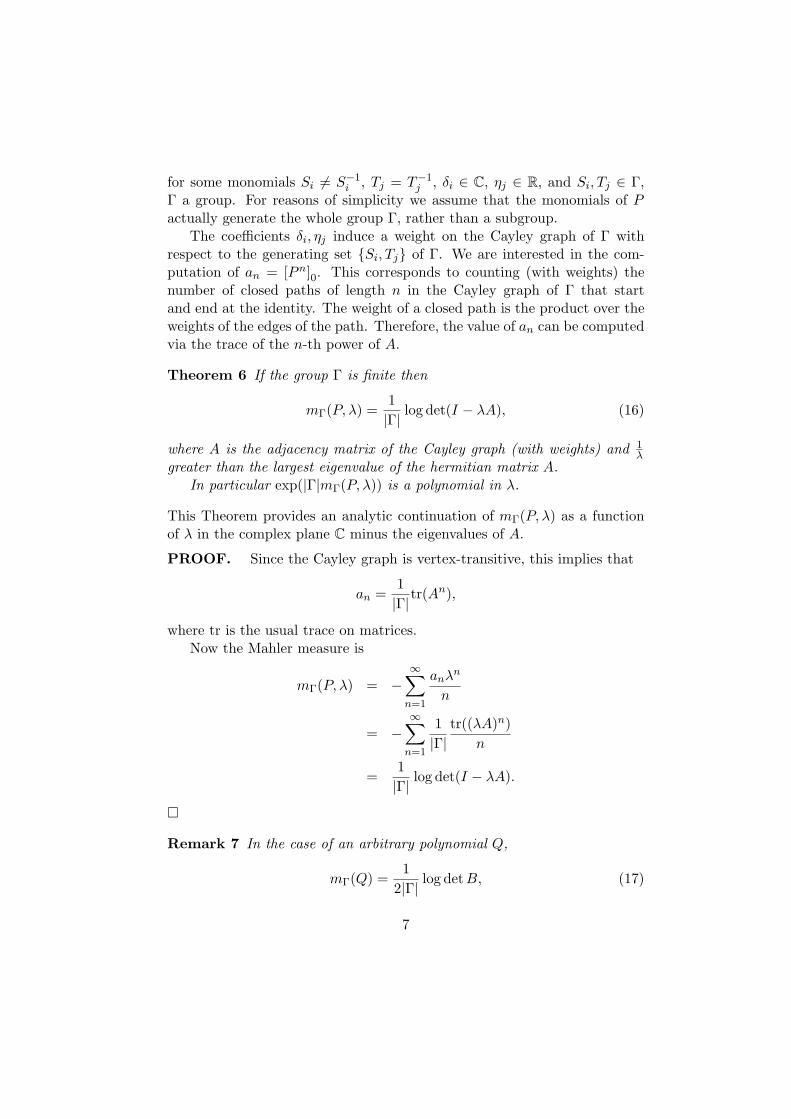
for some monomials Si 6= S−1i , Tj = T−1

j , δi ∈ C, ηj ∈ R, and Si, Tj ∈ Γ,Γ a group. For reasons of simplicity we assume that the monomials of Pactually generate the whole group Γ, rather than a subgroup.

The coefficients δi, ηj induce a weight on the Cayley graph of Γ withrespect to the generating set {Si, Tj} of Γ. We are interested in the com-putation of an = [Pn]0. This corresponds to counting (with weights) thenumber of closed paths of length n in the Cayley graph of Γ that startand end at the identity. The weight of a closed path is the product over theweights of the edges of the path. Therefore, the value of an can be computedvia the trace of the n-th power of A.

Theorem 6 If the group Γ is finite then

mΓ(P, λ) =1|Γ| log det(I − λA), (16)

where A is the adjacency matrix of the Cayley graph (with weights) and 1λ

greater than the largest eigenvalue of the hermitian matrix A.In particular exp(|Γ|mΓ(P, λ)) is a polynomial in λ.

This Theorem provides an analytic continuation of mΓ(P, λ) as a functionof λ in the complex plane C minus the eigenvalues of A.

PROOF. Since the Cayley graph is vertex-transitive, this implies that

an =1|Γ|tr(A

n),

where tr is the usual trace on matrices.Now the Mahler measure is

mΓ(P, λ) = −∞∑

n=1

anλn

n

= −∞∑

n=1

1|Γ|

tr((λA)n)n

=1|Γ| log det(I − λA).

¤

Remark 7 In the case of an arbitrary polynomial Q,

mΓ(Q) =1

2|Γ| log detB, (17)

7

where B is the adjacency matrix corresponding to QQ∗. The Mahler measuremΓ(Q) is defined if and only if B is nonsingular.

Remark 8 Recall that the generating function for the an is

uΓ(P, λ) =∞∑

j=0

anλn

and satisfies:

−λddλ

mΓ(P, λ) = uΓ(P, λ)− 1.

Let σi be the eigenvalues of A. By Theorem 6 we have:

uΓ(P, λ) = 1− λ

|Γ|ddλ det(I − λA)det(I − λA)

=1|Γ|

∑

i

11− λσi

. (18)

In particular, uΓ(P, λ) is a rational function in λ.

5.1 An example

We will consider the example of the group

Z/3Z× Z/2Z = 〈x, y |x3, y2, [x, y]〉.

Let us compute the Mahler measure of the general polynomial

Pλ(x, y) = 1− λ(a + bx + bx−1 + cy + dyx + dyx−1

).

Numbering the vertices e, x, x−1, y, yx, yx−1 as 1, . . . , 6, we get an adjacencymatrix:

a b b c d d

b a b d c d

b b a d d c

c d d a b b

d c d b a b

d d c b b a

.

We see that the characteristic polynomial det(tI −A) is

((t−a+c+Re(b−d))2−3(Im(b−d))2)((t−a−c+Re(b+d))2−3(Im(b+d))2)

·(t− a− 2Re(b) + c + 2Re(d))(t− a− 2 Re(b)− c− 2Re(d)).

8

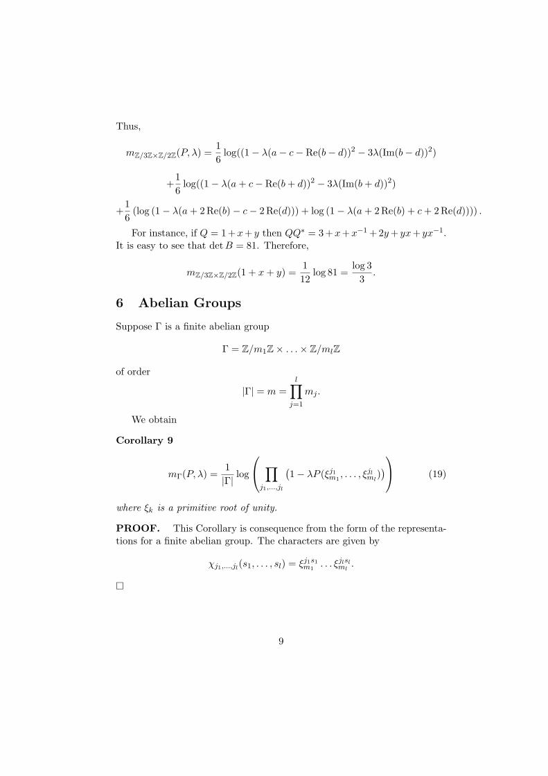
Thus,

mZ/3Z×Z/2Z(P, λ) =16

log((1− λ(a− c− Re(b− d))2 − 3λ(Im(b− d))2)

+16

log((1− λ(a + c− Re(b + d))2 − 3λ(Im(b + d))2)

+16

(log (1− λ(a + 2Re(b)− c− 2Re(d))) + log (1− λ(a + 2Re(b) + c + 2 Re(d)))) .

For instance, if Q = 1+x+ y then QQ∗ = 3+x+x−1 +2y + yx+ yx−1.It is easy to see that detB = 81. Therefore,

mZ/3Z×Z/2Z(1 + x + y) =112

log 81 =log 3

3.

6 Abelian Groups

Suppose Γ is a finite abelian group

Γ = Z/m1Z× . . .× Z/mlZ

of order

|Γ| = m =l∏

j=1

mj .

We obtain

Corollary 9

mΓ(P, λ) =1|Γ| log

∏

j1,...,jl

(1− λP (ξj1

m1, . . . , ξjl

ml)) (19)

where ξk is a primitive root of unity.

PROOF. This Corollary is consequence from the form of the representa-tions for a finite abelian group. The characters are given by

χj1,...,jl(s1, . . . , sl) = ξj1s1

m1. . . ξjlsl

ml.

¤

9

For the following result we recall some notation of Boyd and Lawton.For an integral vector m = (m1, . . . , ml) let

q(m) = min

{H(s)

∣∣∣∣∣ s = (s1, . . . , sl) ∈ Zl,l∑

i=1

misi = 0

},

where H(s) = max1≤i≤l |si|.Thus, for a reciprocal polynomial P ∈ C[Zl] in the Laurent polynomial

ring of l variables, we have the following approximation.

Theorem 10 For sufficiently small λ,

limq(m)→∞

mZ/m1Z×...×Z/mlZ(P, λ) = mZl(P, λ). (20)

PROOF. Following Rodriguez-Villegas technique

mZl(P, λ) = −∫ 1

0. . .

∫ 1

0log(1− λP (e2πit1 , . . . , e2πitl)) dt1 . . . dtl.

Now the function log(1 − λP (e2πit1 , . . . , e2πitl)) is continuous and with nosingularities in Tl. Then we can compute the Riemann integral by takinglimits on evaluations on the roots of unity. ¤

This Theorem should be compared to the result (for the one variablecase) by Luck (page 478 of [Luc02]).

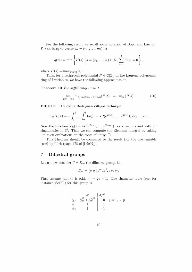
7 Dihedral groups

Let us now consider Γ = Dm the dihedral group, i.e.,

Dm = 〈ρ, σ | ρm, σ2, σρσρ〉.

First assume that m is odd, m = 2p + 1. The character table (see, forinstance [Ser77]) for this group is

ρk σρk

χj ξjkm + ξ−jk

m 0 j = 1, . . . pψ1 1 1ψ2 1 −1

10

Assume that P is reciprocal. In computing the Mahler measure of 1−λPwe need to determine

tr(An) = Pn[1, . . . , 1] + Pn[1, . . . , 1,−1, . . . ,−1]

+2p∑

j=1

Pn[2, ξj

m + ξ−jm , . . . , ξj(m−1)

m + ξ−j(m−1)m , 0, . . . , 0

].

Note that P can be thought as a polynomial in two variables ρ and σ. Forthe first two terms we can write Pn(1, 1) + Pn(1,−1), then we obtain

= Pn(1, 1) + Pn(1,−1)

+2p∑

j=1

(Pn

[1, ξj

m, . . . , ξj(m−1)m , 0, . . . , 0

]+ Pn

[1, ξ−j

m , . . . , ξ−j(m−1)m , 0, . . . , 0

])

= Pn(1, 1) + Pn(1,−1)

+2m−1∑

j=1

Pn[1, ξj

m, . . . , ξj(m−1)m , 0, . . . , 0

]

= Pn(1, 1) + Pn(1,−1) +m−1∑

j=1

(Pn

(ξjm, 1

)+ Pn

(ξjm,−1

))

=m∑

j=1

(Pn

(ξjm, 1

)+ Pn

(ξjm,−1

)). (21)

At this point we should be more specific about the meaning of this formula.Given P we consider its nth-power, then we write it as a combinations ofmonomials ρk and σρk, and after that we evaluate each of the variables ρ,σ.

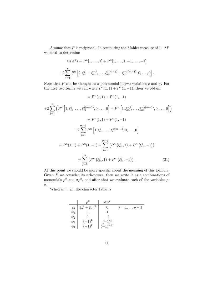
When m = 2p, the character table is

ρk σρk

χj ξjkm + ξ−jk

m 0 j = 1, . . . p− 1ψ1 1 1ψ2 1 −1ψ3 (−1)k (−1)k

ψ4 (−1)k (−1)k+1

11

and we obtain a similar expression as in equation (21).Hence, we have proved:

Theorem 11 Let P ∈ C[Dm] be reciprocal. Then

tr(An) =m∑

j=1

(Pn

(ξjm, 1

)+ Pn

(ξjm,−1

)), (22)

where Pn is expressed as a sum of monomials ρk, σρk before being evaluated.

On the other hand, for Γ = Z/mZ× Z/2Z = 〈x, y |xm, y2, [x, y]〉,

tr(An) =m∑

j=1

(P

(ξjm, 1

)n + P(ξjm,−1

)n)

.

From now on, in order to compare elements in the group rings of Dm

and Z/mZ× Z/2Z we will rename x = ρ and y = σ in Dm.We have

Theorem 12 Let

P =m−1∑

k=0

αkxk +

m−1∑

k=0

βkyxk

with real coefficients and reciprocal in Z/mZ × Z/2Z (therefore it is alsoreciprocal in Dm). Then

mZ/mZ×Z/2Z(P, λ) = mDm(P, λ). (23)

PROOF. It is important to note that being reciprocal in Z/mZ× Z/2Zis not the same as being reciprocal in Dm.

Being reciprocal in Z/mZ×Z/2Zmeans that αk = αm−k and βk = βm−k.On the other hand, being reciprocal in Dm means that αk = αm−k and βk

is real.Then condition that αk, βk are real and the reciprocity in Z/mZ×Z/2Z

imply that and αk = αm−k, βk = βm−k and reciprocity in Dm.We will prove that the powers of P are the same in both groups rings

by induction. Assume that Pn looks the same in both group rings and thatit satisfies the conditions:

Pn =m−1∑

k=0

akxk +

m−1∑

k=0

bkyxk

12

with ak = am−k and bk = bm−k. Then, in Z/mZ× Z/2Z,

PPn =∑

k1,k2

(αk1ak2 + βk1bk2) xk1+k2 +∑

k1,k2

(αk1bk2 + βk1ak2) yxk1+k2 .

In Dm,

PPn =∑

k1,k2

(αk1ak2 + βm−k1bk2) xk1+k2 +∑

k1,k2

(αm−k1bk2 + βk1ak2) yxk1+k2 .

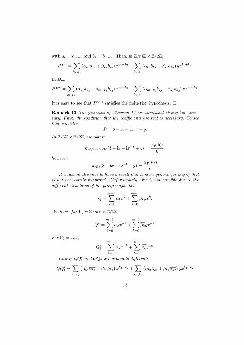
It is easy to see that Pn+1 satisfies the induction hypothesis. ¤

Remark 13 The premises of Theorem 12 are somewhat strong but neces-sary. First, the condition that the coefficients are real is necessary. To seethis, consider

P = 3 + ix− ix−1 + y.

In Z/3Z× Z/2Z, we obtain

mZ/3Z×Z/2Z(3 + ix− ix−1 + y) =log 104

6,

however,

mD3(3 + ix− ix−1 + y) =log 200

6.

It would be also nice to have a result that is more general for any Q thatis not necessarily reciprocal. Unfortunately, this is not possible due to thedifferent structures of the group rings. Let

Q =m−1∑

k=0

αkxk +

m−1∑

k=0

βkyxk.

We have, for Γ1 = Z/mZ× Z/2Z,

Q∗1 =

m−1∑

k=0

αkx−k +

m−1∑

k=0

βkyx−k.

For Γ2 = Dm,

Q∗2 =

m−1∑

k=0

αkx−k +

m−1∑

k=0

βkyxk.

Clearly QQ∗1 and QQ∗

2 are generally different:

QQ∗1 =

∑

k1,k2

(αk1αk2 + βk1βk2

)xk1−k2 +

∑

k1,k2

(αk1βk2 + βk1αk2

)yxk1−k2

13

QQ∗2 =

∑

k1,k2

(αk1αk2 + βk1βk2

)xk1−k2 +

∑

k1,k2

(βk1αk2 + βk1αk2

)yxk1−k2

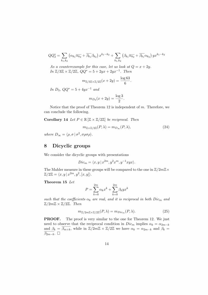
As a counterexample for this case, let us look at Q = x + 2y.In Z/3Z× Z/2Z, QQ∗ = 5 + 2yx + 2yx−1. Then

mZ/3Z×Z/2Z(x + 2y) =log 63

6.

In D3, QQ∗ = 5 + 4yx−1 and

mD3(x + 2y) =log 3

2.

Notice that the proof of Theorem 12 is independent of m. Therefore, wecan conclude the following.

Corollary 14 Let P ∈ R [Z× Z/2Z] be reciprocal. Then

mZ×Z/2Z(P, λ) = mD∞(P, λ), (24)

where D∞ = 〈ρ, σ |σ2, σρσρ〉.

8 Dicyclic groups

We consider the dicyclic groups with presentations

Dicm = 〈x, y |x2m, y2xm, y−1xyx〉.The Mahler measure in these groups will be compared to the one in Z/2mZ×Z/2Z = 〈x, y |x2m, y2, [x, y]〉.Theorem 15 Let

P =2m∑

k=0

αkxk +

2m∑

k=0

βkyxk

such that the coefficients αk are real, and it is reciprocal in both Dicm andZ/2mZ× Z/2Z. Then

mZ/2mZ×Z/2Z(P, λ) = mDicm(P, λ). (25)

PROOF. The proof is very similar to the one for Theorem 12. We justneed to observe that the reciprocal condition in Dicm implies αk = α2m−k

and βk = βm+k, while in Z/2mZ × Z/2Z we have αk = α2m−k and βk =β2m−k. ¤

14

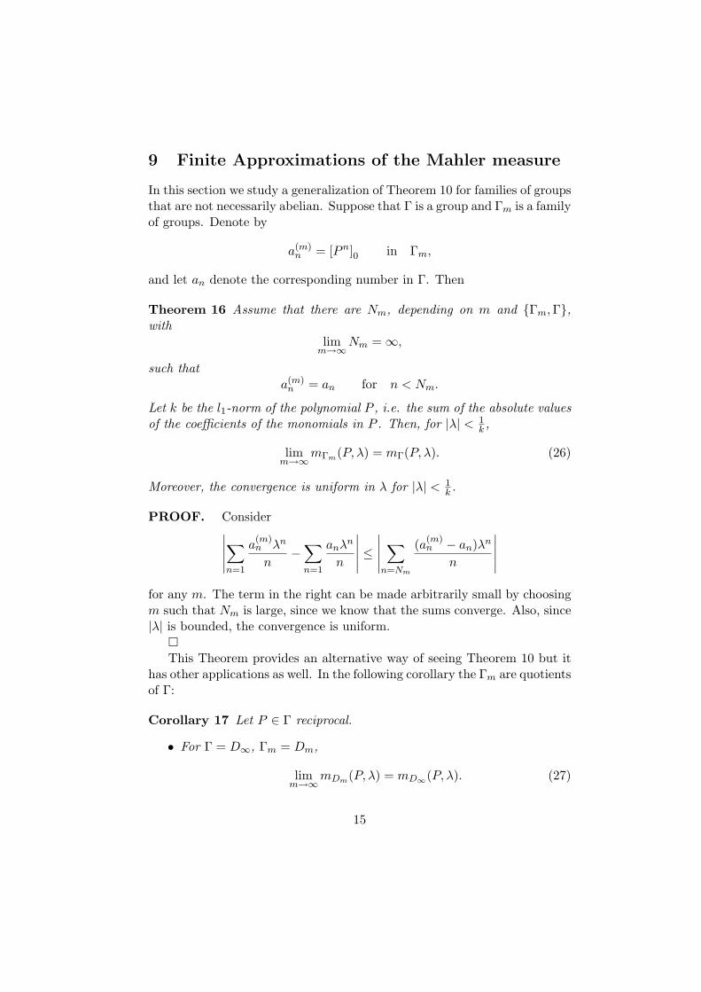
9 Finite Approximations of the Mahler measure

In this section we study a generalization of Theorem 10 for families of groupsthat are not necessarily abelian. Suppose that Γ is a group and Γm is a familyof groups. Denote by

a(m)n = [Pn]0 in Γm,

and let an denote the corresponding number in Γ. Then

Theorem 16 Assume that there are Nm, depending on m and {Γm, Γ},with

limm→∞Nm = ∞,

such thata(m)

n = an for n < Nm.

Let k be the l1-norm of the polynomial P , i.e. the sum of the absolute valuesof the coefficients of the monomials in P . Then, for |λ| < 1

k ,

limm→∞mΓm(P, λ) = mΓ(P, λ). (26)

Moreover, the convergence is uniform in λ for |λ| < 1k .

PROOF. Consider∣∣∣∣∣∑

n=1

a(m)n λn

n−

∑

n=1

anλn

n

∣∣∣∣∣ ≤∣∣∣∣∣

∑

n=Nm

(a(m)n − an)λn

n

∣∣∣∣∣

for any m. The term in the right can be made arbitrarily small by choosingm such that Nm is large, since we know that the sums converge. Also, since|λ| is bounded, the convergence is uniform.

¤This Theorem provides an alternative way of seeing Theorem 10 but it

has other applications as well. In the following corollary the Γm are quotientsof Γ:

Corollary 17 Let P ∈ Γ reciprocal.

• For Γ = D∞, Γm = Dm,

limm→∞mDm(P, λ) = mD∞(P, λ). (27)

15

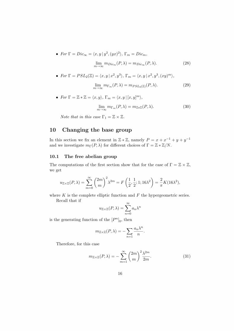
• For Γ = Dic∞ = 〈x, y | y2, (yx)2〉, Γm = Dicm,

limm→∞mDicm(P, λ) = mDic∞(P, λ). (28)

• For Γ = PSL2(Z) = 〈x, y |x2, y3〉, Γm = 〈x, y |x2, y3, (xy)m〉,

limm→∞mΓm(P, λ) = mPSL2(Z)(P, λ). (29)

• For Γ = Z ∗ Z = 〈x, y〉, Γm = 〈x, y | [x, y]m〉,

limm→∞mΓm(P, λ) = mZ∗Z(P, λ). (30)

Note that in this case Γ1 = Z× Z.

10 Changing the base group

In this section we fix an element in Z ∗ Z, namely P = x + x−1 + y + y−1

and we investigate mΓ(P, λ) for different choices of Γ = Z ∗ Z/N .

10.1 The free abelian group

The computations of the first section show that for the case of Γ = Z × Z,we get

uZ×Z(P, λ) =∞∑

m=0

(2m

m

)2

λ2m = F

(12,12; 1; 16λ2

)=

2π

K(16λ2),

where K is the complete elliptic function and F the hypergeometric series.Recall that if

uZ×Z(P, λ) =∞∑

n=0

anλn

is the generating function of the [Pn]0, then

mZ×Z(P, λ) = −∑

n=1

anλn

n.

Therefore, for this case

mZ×Z(P, λ) = −∞∑

m=1

(2m

m

)2 λ2m

2m. (31)

16

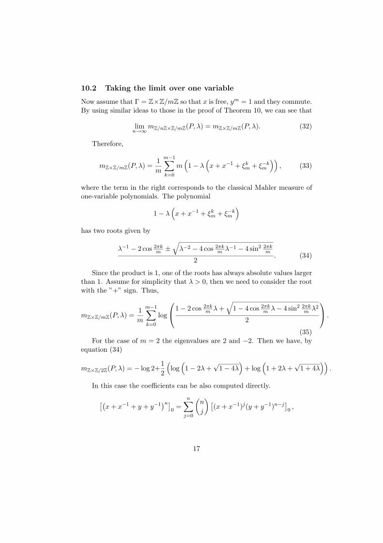
10.2 Taking the limit over one variable

Now assume that Γ = Z×Z/mZ so that x is free, ym = 1 and they commute.By using similar ideas to those in the proof of Theorem 10, we can see that

limn→∞mZ/nZ×Z/mZ(P, λ) = mZ×Z/mZ(P, λ). (32)

Therefore,

mZ×Z/mZ(P, λ) =1m

m−1∑

k=0

m(1− λ

(x + x−1 + ξk

m + ξ−km

)), (33)

where the term in the right corresponds to the classical Mahler measure ofone-variable polynomials. The polynomial

1− λ(x + x−1 + ξk

m + ξ−km

)

has two roots given by

λ−1 − 2 cos 2πkm ±

√λ−2 − 4 cos 2πk

m λ−1 − 4 sin2 2πkm

2. (34)

Since the product is 1, one of the roots has always absolute values largerthan 1. Assume for simplicity that λ > 0, then we need to consider the rootwith the ”+” sign. Thus,

mZ×Z/mZ(P, λ) =1m

m−1∑

k=0

log

1− 2 cos 2πk

m λ +√

1− 4 cos 2πkm λ− 4 sin2 2πk

m λ2

2

.

(35)For the case of m = 2 the eigenvalues are 2 and −2. Then we have, by

equation (34)

mZ×Z/2Z(P, λ) = − log 2+12

(log

(1− 2λ +

√1− 4λ

)+ log

(1 + 2λ +

√1 + 4λ

)).

In this case the coefficients can be also computed directly.

[(x + x−1 + y + y−1

)n]0

=n∑

j=0

(n

j

) [(x + x−1)j(y + y−1)n−j

]0,

17

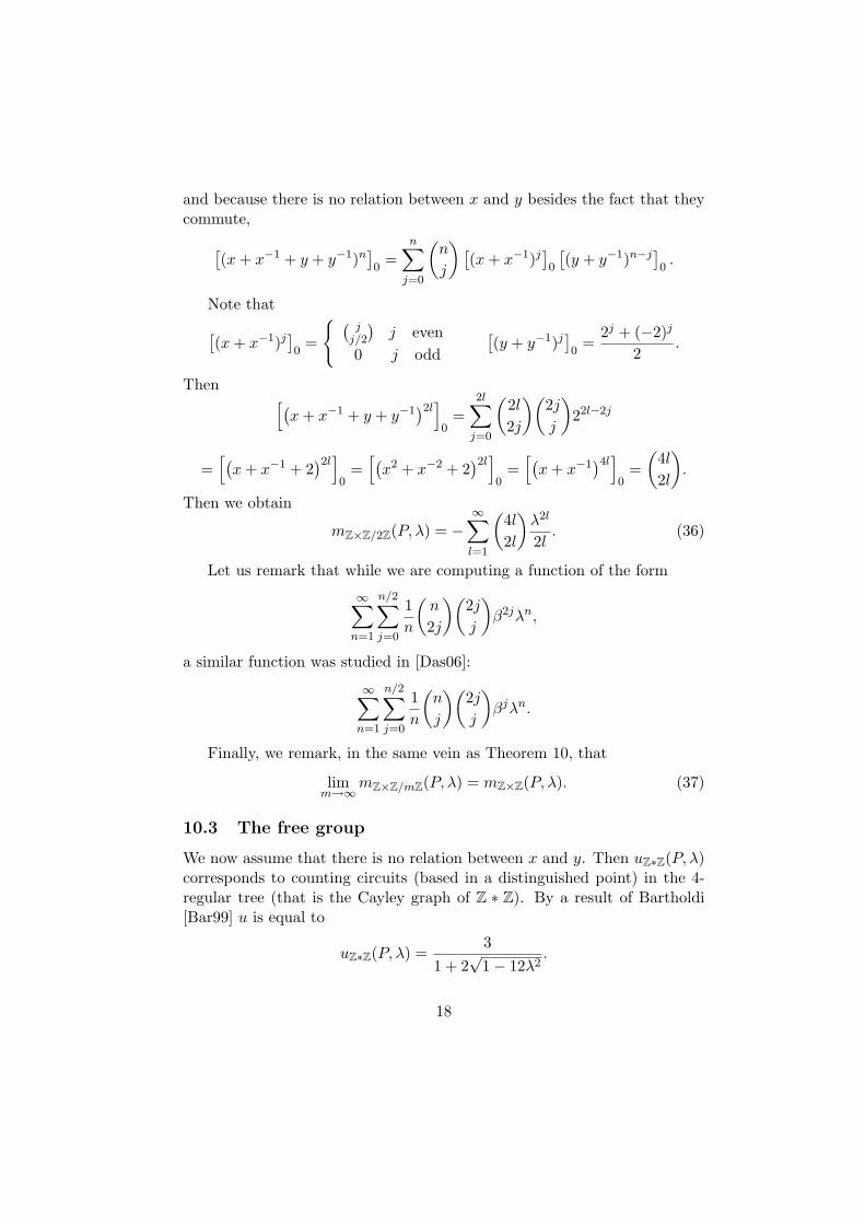
and because there is no relation between x and y besides the fact that theycommute,

[(x + x−1 + y + y−1)n

]0

=n∑

j=0

(n

j

)[(x + x−1)j

]0

[(y + y−1)n−j

]0.

Note that

[(x + x−1)j

]0

=

{ ( jj/2

)j even

0 j odd

[(y + y−1)j

]0

=2j + (−2)j

2.

Then [(x + x−1 + y + y−1

)2l]0

=2l∑

j=0

(2l

2j

)(2j

j

)22l−2j

=[(

x + x−1 + 2)2l

]0

=[(

x2 + x−2 + 2)2l

]0

=[(

x + x−1)4l

]0

=(

4l

2l

).

Then we obtain

mZ×Z/2Z(P, λ) = −∞∑

l=1

(4l

2l

)λ2l

2l. (36)

Let us remark that while we are computing a function of the form

∞∑

n=1

n/2∑

j=0

1n

(n

2j

)(2j

j

)β2jλn,

a similar function was studied in [Das06]:

∞∑

n=1

n/2∑

j=0

1n

(n

j

)(2j

j

)βjλn.

Finally, we remark, in the same vein as Theorem 10, that

limm→∞mZ×Z/mZ(P, λ) = mZ×Z(P, λ). (37)

10.3 The free group

We now assume that there is no relation between x and y. Then uZ∗Z(P, λ)corresponds to counting circuits (based in a distinguished point) in the 4-regular tree (that is the Cayley graph of Z ∗ Z). By a result of Bartholdi[Bar99] u is equal to

uZ∗Z(P, λ) =3

1 + 2√

1− 12λ2.

18

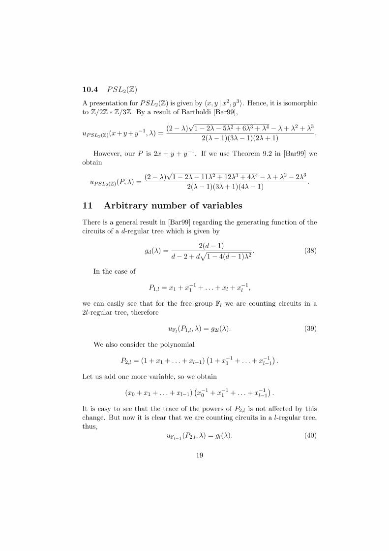
10.4 PSL2(Z)

A presentation for PSL2(Z) is given by 〈x, y |x2, y3〉. Hence, it is isomorphicto Z/2Z ∗ Z/3Z. By a result of Bartholdi [Bar99],

uPSL2(Z)(x+y +y−1, λ) =(2− λ)

√1− 2λ− 5λ2 + 6λ3 + λ4 − λ + λ2 + λ3

2(λ− 1)(3λ− 1)(2λ + 1).

However, our P is 2x + y + y−1. If we use Theorem 9.2 in [Bar99] weobtain

uPSL2(Z)(P, λ) =(2− λ)

√1− 2λ− 11λ2 + 12λ3 + 4λ4 − λ + λ2 − 2λ3

2(λ− 1)(3λ + 1)(4λ− 1).

11 Arbitrary number of variables

There is a general result in [Bar99] regarding the generating function of thecircuits of a d-regular tree which is given by

gd(λ) =2(d− 1)

d− 2 + d√

1− 4(d− 1)λ2. (38)

In the case of

P1,l = x1 + x−11 + . . . + xl + x−1

l ,

we can easily see that for the free group Fl we are counting circuits in a2l-regular tree, therefore

uFl(P1,l, λ) = g2l(λ). (39)

We also consider the polynomial

P2,l = (1 + x1 + . . . + xl−1)(1 + x−1

1 + . . . + x−1l−1

).

Let us add one more variable, so we obtain

(x0 + x1 + . . . + xl−1)(x−1

0 + x−11 + . . . + x−1

l−1

).

It is easy to see that the trace of the powers of P2,l is not affected by thischange. But now it is clear that we are counting circuits in a l-regular tree,thus,

uFl−1(P2,l, λ) = gl(λ). (40)

19

In particular,mFl

(P1,l, λ) = mF2l−1(P2,2l, λ). (41)

Let us examine the abelian versions of these polynomials. By usingelementary combinatorics we compute the trace of the powers of P1,l andP2,l: [

Pn1,l

]0

=∑

a1+...+al=n

(2n)!(a1!)2 . . . (al!)2

,

[Pn

2,l

]0

=∑

a1+...+al=n

(n!

a1! . . . al!

)2

.

For l > 2 these expressions do not seem to simplify, in the sense thatwe are unable to find a closed formula that does not involve a summation.However, we make the following interesting observation:

[P 2n

1,l

]0

=(

2n

n

)[Pn

2,l

]0, (42)

where the trace in the left is taken over Z×l and the one in the right is takenover Z×(l−1).

In other words, there are relations among the Mahler measure of thesetwo families of polynomials. But the relations depend on the base group.

Acknowledgements: The authors would like to thank Neal Stoltzfusand Fernando Rodriguez-Villegas for helpful discussions. Part of this workwas completed while ML was a member at the Institute for Advanced Studyand during visits to the Department of Mathematics at Louisiana StateUniversity. She is deeply grateful for their support and hospitality.

References

[Bab79] Laszlo Babai, Spectra of Cayley graphs, J. Combin. Theory Ser. B27 (1979), no. 2, 180–189.

[Bar99] Laurent Bartholdi, Counting paths in graphs, Enseign. Math. (2)45 (1999), no. 1-2, 83–131.

[BZ85] Gerhard Burde and Heiner Zieschang, Knots, de Gruyter Studiesin Mathematics, vol. 5, Walter de Gruyter & Co., Berlin, 1985.

[Das06] Oliver T. Dasbach, Torus knots complements: A natural series forthe natural logarithm, 2006, preprint, math.GT/0611025.

20

[Luc02] Wolfgang Luck, L2-invariants: Theory and Applications to Geome-try and K-theory, Ergebnisse der Mathematik und ihrer Grenzgebi-ete. 3. Folge. A Series of Modern Surveys in Mathematics [Resultsin Mathematics and Related Areas. 3rd Series. A Series of ModernSurveys in Mathematics], vol. 44, Springer-Verlag, Berlin, 2002.

[RV99] Fernando Rodriguez Villegas, Modular Mahler measures. I, Topicsin number theory (University Park, PA, 1997), Math. Appl., vol.467, Kluwer Acad. Publ., Dordrecht, 1999, pp. 17–48.

[Ser77] Jean-Pierre Serre, Linear representations of finite groups, Springer-Verlag, New York, 1977, Translated from the second French editionby Leonard L. Scott, Graduate Texts in Mathematics, Vol. 42.

21