Measure representations of genealogical processes and ...

Measure representations of genealogicalprocesses and applications to

Fleming-Viot models

Der Naturwissenschaftlichen Fakultat

der Friedrich-Alexander-Universitat

Erlangen-Nurnberg

zur

Erlangung des Doktorgrades Dr. rer. nat.

vorgelegt von

Max Grieshammer

aus Bad Windsheim

Als Dissertation genehmigt

von der Naturwissenschaftlichen Fakultat

der Friedrich-Alexander-Universitat Erlangen-Nurnberg

Tag der mundlichen Prufung: 10.05.2017

Vorsitzender des Promotionsorgans: Prof. Dr. Georg Kreimer

Gutachter: Prof. Dr. Andreas Greven

Gutachterin: Prof. Dr. Anita Winter

Maßwertige Darstellung genealogischerProzesse und Anwendungen auf

Fleming-Viot Modelle

Zusammenfassung

Wir untersuchen maßwertige Prozesse, die im Bezug auf baumwertige Prozesse auf-tauchen und die Evolution der relativen Großen verschiedener Familien in einer Populationbeschreiben. Es wird sich heraustellen, dass diese maßwertigen Prozesse die evolvierendenGenealogien eindeutig beschreiben und dass diese Abhangigkeit stetig ist, d.h. wir wer-den zeigen, dass Konvergenz der maßwertigen Prozesse Konvergenz der entsprechendenbaumwertigen Prozesse impliziert.

Als Beispiel werden wir sehen, dass man eine Kollektion maßwertiger (neutraler) inter-agierender Fleming-Viot Prozesse benutzen kann um die Genealogie eines baumwertigeninteragierenden Fleming-Viot Prozesses zu beschreiben. Diese Beobachtung wird uns danndabei helfen eine Konvergenzaussage fur den mittleren genealogischen Abstand des raum-lich interagierenden Fleming-Viot Prozesses zu treffen, wenn die Große des geographischenRaumes gegen Unendlich geht.

Als Nachstes definieren wir eine Halbordnung auf dem Raum der metrischen Maß-raume. Wir werden zeigen, dass diese Halbordnung abgeschlossen ist und dass man im Fallvon Dominanz den Abstand zweier Maßraume sehr einfach durch den Eurandomabstandberechnen kann. Als Beispiel werden wir sehen, dass die Genealogien zweier (neutraler)Fleming-Viot Prozesse mit unterschiedlichen Resamplingraten einander dominieren.

Schließlich werden wir untersuchen, wie man einen neutralen baumwerigen Fleming-Viot Prozess mit einem nicht neutralen, d.h. selektiven, baumwerigen Fleming-ViotProzess vergleichen kann.

Ich mochte meinem Doktorvater Prof. Andreas Greven danken, dass er mir die Mog-lichkeit gegeben hat, an diesem interessanten Thema zu arbeiten, und mich immer best-moglichst unterstutzt hat. Außerdem mochte ich mich bei meinen Kollegen Stefan Flei-scher, Frank Schirmeier, Peter Seidel, Johannes Singer und insbesondere Thomas Ripplfur die gemeinsamen mathematischen und nicht mathematischen Diskussionen bedanken.Schließlich gilt mein besonderer Dank meiner Familie und meiner Lebensgefahrtin Micha-ela, die mir in jeder Lebenslage immer zur Seite standen.

Nurnberg, Januar 2017 Max Grieshammer

Abstract

We study the connection between a class of tree-valued processes, arising as the evolv-ing genealogies of population models, and measure-valued processes, that describe the evo-lution of the different frequencies of families in the population. It will turn out that thesemeasure-valued processes describe the evolving genealogies uniquely and this dependenceis continuous, i.e. we will prove that convergence of these measure-valued representationsimplies convergence of the corresponding tree-valued processes.

As an example we will show that a collection of measure-valued (neutral) spatialFleming-Viot processes can be used to describe the genealogy of the tree-valued spatialFleming-Viot process. This allows us to deduce a convergence result of the mean genealog-ical distance of the spatial Fleming-Viot process when the size of the geographical spacegoes to infinity.

Next, we define a partial order on metric measure spaces. We show that this orderis closed and that, in case of dominance, one can easily calculate the Eurandom distanceof two metric measure-spaces. As an example we will see that the genealogies of two(neutral) Fleming-Viot processes with different resampling rates dominate each other.

Finally, we will study how to compare a neutral with a non neutral, i.e. selective,tree-valued Fleming-Viot process.

Contents

1 Introduction . . . . . . . . . . . . . . . . . . . . . . . . . . . . . . . . . . . . 72 Metric measure spaces and the Gromov-weak atomic topology . . . . . . . . 173 Main results I: Measure-valued representation . . . . . . . . . . . . . . . . . 21

3.1 Measure-valued representation backward in time . . . . . . . . . . . 213.2 Measure-valued representations of evolving genealogies . . . . . . . . 23

4 Main results II: The generalized Eurandom distance and partial orders onmetric measure spaces . . . . . . . . . . . . . . . . . . . . . . . . . . . . . . 264.1 The generalized Eurandom distance . . . . . . . . . . . . . . . . . . 264.2 Partial orders . . . . . . . . . . . . . . . . . . . . . . . . . . . . . . . 27

5 Further results . . . . . . . . . . . . . . . . . . . . . . . . . . . . . . . . . . 305.1 An invariant quantity of the map M . . . . . . . . . . . . . . . . . . 30

5.1.1 Definitions . . . . . . . . . . . . . . . . . . . . . . . . . . . 315.1.2 Results . . . . . . . . . . . . . . . . . . . . . . . . . . . . . 32

5.2 Some results on the weak atomic topology . . . . . . . . . . . . . . . 345.3 The partial order ¤measure and ¤metric . . . . . . . . . . . . . . . . . 36

6 Application I: A finite system scheme result for the genealogy in a spatialFleming-Viot population . . . . . . . . . . . . . . . . . . . . . . . . . . . . . 396.1 Tree-valued interacting Moran models . . . . . . . . . . . . . . . . . 396.2 A finite system scheme result for the tree-valued interacting Fleming-

Viot processes . . . . . . . . . . . . . . . . . . . . . . . . . . . . . . 427 Application II: Stochastic dominance of tree-valued Fleming-Viot processes 44

7.1 Stochastic dominance . . . . . . . . . . . . . . . . . . . . . . . . . . 447.2 Tree-valued Fleming-Viot processes with different resampling rates . 457.3 A result on selection . . . . . . . . . . . . . . . . . . . . . . . . . . . 46

7.3.1 The tree-valued Moran model with mutation and selection 467.3.2 A result on dominance . . . . . . . . . . . . . . . . . . . . 49

8 Proofs . . . . . . . . . . . . . . . . . . . . . . . . . . . . . . . . . . . . . . . 508.1 Preparations . . . . . . . . . . . . . . . . . . . . . . . . . . . . . . . 50

8.1.1 Bounds for the marked Gromov-Prohorov metric and thefunction Φ . . . . . . . . . . . . . . . . . . . . . . . . . . . 50

8.1.2 Concatenation of trees . . . . . . . . . . . . . . . . . . . . . 538.2 Proofs for section 5.1 . . . . . . . . . . . . . . . . . . . . . . . . . . . 54

8.2.1 Proof of Lemma 5.2 . . . . . . . . . . . . . . . . . . . . . . 548.2.2 A result on relative compactness and proof of Lemma 5.9 . 558.2.3 Proof of Theorem 8 and Corollary 5.12 . . . . . . . . . . . 61

8.3 Proofs for section 5.2 . . . . . . . . . . . . . . . . . . . . . . . . . . . 668.4 Proofs for section 3.1 . . . . . . . . . . . . . . . . . . . . . . . . . . . 71

8.4.1 Proof of Lemma 3.5 and Lemma 3.6 . . . . . . . . . . . . . 728.4.2 A different point of view - Proof of Theorem 2 . . . . . . . 74

8.5 Proofs for section 3.2 . . . . . . . . . . . . . . . . . . . . . . . . . . . 828.5.1 Preparations and proof of Proposition 3.11 . . . . . . . . . 828.5.2 Proof of Theorem 3 . . . . . . . . . . . . . . . . . . . . . . 848.5.3 Convergence in subspace topology - Proof of Theorem 4 . . 86

8.6 Proofs for section 5.3 . . . . . . . . . . . . . . . . . . . . . . . . . . . 928.7 Proofs for section 4.1 . . . . . . . . . . . . . . . . . . . . . . . . . . . 968.8 Proofs for section 4.2 . . . . . . . . . . . . . . . . . . . . . . . . . . . 998.9 Proofs for section 6.1 . . . . . . . . . . . . . . . . . . . . . . . . . . . 102

5

8.9.1 The measure-valued interacting Moran models and the spa-tial Kingman coalescent . . . . . . . . . . . . . . . . . . . . 102

8.9.2 A measure-valued representation for the tree-valued inter-acting Moran models . . . . . . . . . . . . . . . . . . . . . 106

8.10 Proofs of section 6.2 . . . . . . . . . . . . . . . . . . . . . . . . . . . 1118.10.1 Properties of the measure-valued representation . . . . . . 1118.10.2 A convergence result for the measure-valued representations1138.10.3 Measure-valued interacting Fleming-Viot processes . . . . . 1248.10.4 Proof of Theorem 11 . . . . . . . . . . . . . . . . . . . . . . 1268.10.5 Proof of Theorem 12 . . . . . . . . . . . . . . . . . . . . . . 132

8.11 Proofs for section 7.2 . . . . . . . . . . . . . . . . . . . . . . . . . . . 1368.11.1 Proof of Proposition 7.5 . . . . . . . . . . . . . . . . . . . . 1368.11.2 Proof of Corollary 7.6 . . . . . . . . . . . . . . . . . . . . . 137

8.12 Proofs for section 7.3 . . . . . . . . . . . . . . . . . . . . . . . . . . . 1408.12.1 A forward representation . . . . . . . . . . . . . . . . . . . 1408.12.2 A different point of view . . . . . . . . . . . . . . . . . . . 1418.12.3 Convergence of the finite models . . . . . . . . . . . . . . . 1448.12.4 Approximation of the pairwise distance . . . . . . . . . . . 1468.12.5 Proof of Theorem 15 . . . . . . . . . . . . . . . . . . . . . . 147

1 Introduction

One objective in studying population models is the description of the genealogical tree ofthe population alive at the present time t. To do this there are several approaches. Forexample, one can study a process which generates the genealogy backward in time or onedefines a richer process in which the genealogies evolve forward in time. The latter leads,inter alia, to the concept of the tree-valued processes: One can define an ultra-metric r,that gives the genealogical distance of two individuals x, y P X of a population X, i.e. thedistance to the most recent common ancestor of x and y. We will assume that pX, rq iscomplete and separable. Moreover, all individuals carry some type t P T, for a compactmetric space T, with some probability κpx, dtq, i.e. we consider a (finite) Borel measure µon X T, where µpdx, dtq κpx, dtqµpdxq, for some finite Borel measure µ on X. We callthe triple pX, r, µq a marked (ultra-) metric measure space and note that an ultra-metricspace can be mapped isometrically to the set of leaves of a rooted R-tree (see Remark 2.7in [DGP12] and Remark 2.2 in [DGP11]). This justifies the name tree for an ultra-metricmeasure space.

In this context it is useful to define equivalence classes rX, r, µs, where we say thatpX, r, µq and pX 1, r1, µ1q are equivalent, if we can find an isometry ϕ : supppµp Tqq Ñsupppµ1p Tqqq and ϕpx, tq : pϕpxq, tq is measure-preserving. We denote by

UT pMTq (1.1)

the space of such equivalence classes (the space of equivalence classes where we allow rto be an arbitrary metric). Metric measure spaces were studied in great detail in [Gro99]and [Stu12] as classical references and [GPW09] and [DGP11] as probability theory relatedreferences.

As mentioned above, the goal is to describe the genealogy by an UT-valued (cadlag)process U and we are interested in two questions:

• Can we analyze the genealogy of a population, i.e. the process U , in terms ofmeasure-valued processes?

• Is there a way how to decide if one genealogy is smaller than another?

The first question and its answer is based on the following observation: Given a (finite)population X tx1, . . . , xNu at a time T with some genealogy described by an (ultra-)metric rT . As time goes on, the population evolves and, during their lives, individuals(parents) give birth to new individuals (children). Now it is clear that there is a set ofindividuals, tA1, A2, . . . , Anu X at time T , called the ancestors, of whom the entirepopulation at a time T h are the descendants. If we now look at the genealogicalrelationship of the population at this time T h, described by rTh, then the genealogicalstructure may change in the interval pT, T hs but as long as two individuals do not havea common ancestor in this interval, their genealogical distance is completely describedby the distance of their respective ancestors. Roughly speaking rThpx, yq ¡ h impliesrThpx, yq rT pApxq, Apyqqh, where Apxq, Apyq P tA1, A2, . . . , Anu are the ancestors ofthe individuals x and y, and we call a process U with this property an evolving genealogy.

Note that since UT is an equivalence class and since the above property is in some sensea property of representatives, we need to find a way to describe these representatives andwe will do this by introducing suitable measure-valued processes.

The first idea is based on a “backward in time” point of view: We decompose thepopulation at time T in families, where we say that two individuals x, y P X are in the

7

same family of a given age h ¥ 0, if both individuals have the same ancestor at time T h.In other words we say that x, y are in the same family if they are in the same h ball withrespect to rT , i.e. rT px, yq ¤ h. When we now label the families by rh1 , r

h2 , . . . and assume

that X is equipped with a sampling measure µ (for example the uniform distribution),then we can define the path of measures h ÞÑ HTh :

°i µpBpr

hi , hqqδrhi

, where Bpx, hq

denotes the closed ball of radius h around x. Note that HTh ptrhi uq gives the relative size of

the family labeled by rhi . This gives a first connection of an ultra-metric measure spaceand a measure-valued path.

The second idea is based on a “forward in time” point of view: We consider a measure-valued process X T that starts in X T0 1

N

°Ni1 δxi and counts the relative number of

descendents of the individuals xi as time goes on. For example, at time h the support ofX Th is tA1, A2, . . . , Anu and X Th ptA1uq is the relative number of descendents of A1 at timeT h.

We observe that both HT and X T can be defined for all times T and roughly speakingtX T : T ¥ 0u is called a measure-valued representation, where the coupling of theseprocesses is described by HT in the sense that pX Thphqq0¤h¤T pHTh q0¤h¤T for all T .

Before we give a more formal introduction we turn to the second question.

Comparing genealogical distances leads to the question how to define a suitable partialorder on M (i.e. the set of equivalence classes with |T| 1). We note at this pointthat most results on the partial order were developed in collaboration with Thomas Rippl(see [GR16]).

In order to define a partial order ¤general on M we use the following two ideas: Compar-ing masses and comparing distances. I.e. we say x : rX, rX , µXs ¤general rY, rY , µY s : yif there is a Borel-measure µ1Y on Y such that x ¤metric rY, rY , µ

1Y s : y1 ¤measure y, where

we say x ¤metric y1 if there is a measure-preserving sub-isometry (i.e. 1Lipschitz map)supppµ1Y q Ñ supppµXq and we say y1 ¤measure y if µ1Y ¤ µY (see Figure 1).

¤measure ¤metric

Figure 1: Here we see the two concepts of dominance ¤measure and ¤metric.

Partial orders on metric measure spaces were already considered before. In sec-tion 3.1

2 .15 of Gromov’s book [Gro99] the Lipschitz order ¡ is defined. There are someother articles who studied ¡ and we mention [Shi16] for a comprehensive overview. Thisrelation ¡ is identical to ¤metric. So the relation ¤general is an extension to ¡. Moreover,we can prove the important facts for the relation ¤general: We show that ¤general is apartial order on M and that ¤general is closed, i.e. tpx, yq PMM : x ¤general yu is closedin the product topology, where M is equipped with the Gromov-weak topology (see (1.14)below). Considering the partial order ¤metric we provide an analytical characterizationwith distance matrix measures, see (1.15) below.

Beside this results, we will show that there is a connection of the partial order ¤general

and the Eurandom distance dEur (see section 10 in [GPW09]). Recall that dEur is a(non complete) distance on M1 (i.e. metric measure spaces with normalized measure) that

8

generates the Gromov-weak topology (see (1.14) below) and is given by

dEurpx, yq infµ

»|rXpx, x

1q rY py, y1q| ^ 1 µpdpx, x1qqµpdpy, y1qq, (1.2)

where the infimum is taken over all couplings of µX and µY . In our situation we considerthe following modification of dEur, namely for λ ¡ 0 set

dλEurpx, yq : infµ

» eλrXpx,x1q eλrY py,y1q µpdpx, x1qqµpdpy, y1qq. (1.3)

Before we present the connection of ¤general and dλEur, we note that while ¤general is apartial order on M, dλEur is only a metric on M1 and hence, to get a general result, we need

to generalize the dλEur to a metric on M: We denote by rX, rX , µXs : µXpXq the totalmass of a metric measure space and define for x, y PM the generalized Eurandom distance

dλgEurpx, yq : infx1,y1PM, x1y1

x1¤measurex, y1¤measurey

Dλpx1, y1; x, yq dλEurpx

1, y1q, (1.4)

where (set fprq : 1 exppλrq and νxpfq :³fprXpx, yqqdµXpdxqµXpdyq)

Dλpx1, y1; x, yq νxpfq νx1pfq νypfq νy

1pfq. (1.5)

We will show that this defines a metric on M that coincides with dλEur on M1 andgenerates the Gromov-weak topology (see again (1.14) below). Moreover, we will showthe following connection to ¤general: x ¤general y implies

dλgEurpx, yq

» »p1 eλrY py,y

1qqµY pdyqµY pdy1q

» »p1 eλrXpx,x

1qqµXpdxqµXpdx1q.

(1.6)

9

Now we give a more formal introduction to the first question. As mentioned above weneed to choose a suitable representative and there might be problems like continuity oreven measurability of a choice function (recall that UT is a set of equivalence classes andit is not clear how to pick a path of representatives in a “measurable” way) and hence itis necessary to have a better understanding of elements in UT. This in turn is related tothe notion of a “backward” representation m of a marked ultra-metric measure space uthat reflects in some sense the classical approach in terms of coalescing models.

u

14pδx1 . . . δx4q

14p2δx1 δx3 δx4q

14p2δx1 2δx4q

δx1

T30

T2

T1

h1

h2

h3

m0

mh1

mh2

mh3

Figure 2: Let px1, x2, x3, x4q be for example p14, 24, 34, 1q, then m P X would be the element thatis constant up to the three jump points h1, h2, h3, where mh 1

4pδ14 . . . δ1q for h h1, mh

14p2δ14 δ34 δ1q for h P rh1, h2q, mh 1

4pδ14 2δ1q for h P rh3, h4q and mh δ14 for h ¥ h3. The

corresponding tree u Mpmq rt14, 24, 34, 44u, r1, 14°4i1 δi4s rt1, 2, 3, 4u, r, 14

°4i1 δis is drawn

on the right side, where r is a metric with rp1, 2q h1, rp1, 3q rp2, 3q rp1, 4q rp2, 4q h3, rp3, 4q h2.Note that in this case we set |T| 1, and hence consider trees without marks. Moreover, observe that

if τ0,h1 p14, 14, 34, 44q (i.e. 14 ÞÑ 14, 24 ÞÑ 14, 34 ÞÑ 34, 44 ÞÑ 44), τ0,h2 p14, 14, 44, 44q,τ0,h3 p14, 14, 14, 14q, τh1,h2 p14, 44, 44q, . . ., then mhj mhi τ

1hi,hj

, 0 ¤ i j ¤ 3.

Note that instead of p14, 24, 34, 44q we could also take any quadruple of pairwise disjoint elementsin r0, 1s.

The points T1, T2, T3 are considered in Figure 5

We call m a backward representation if m : R Ñ Mf pr0, 1s Tq is constant up tocountable many jump points, where it is right continuous and the limit from the left existsand if it additionally has the following properties (see also Figure 2):

(i) If we write mh khpx, dyqmhpdxq, then mh is purely atomic for all h ¡ 0.

(ii) For all discontinuity points h ¡ 0, we can find a set A Apmhq with |A| ¥ 2(where Apµq denotes the set of atoms of some measure µ, i.e. x P Apµq iff µtxu ¡ 0)and a point a P A such that mhpAztauq 0 and

mhptauq ¥ maxbPAztau

mhptbuq (1.7)

mhptau q

»Akhpx, qmhpdxq, (1.8)

mhptxu q mhptxu q, @x P r0, 1szA. (1.9)

Note that this implies that the total mass mhpr0, 1sq stays constant for all h ¥ 0.

(iii) mh ñ m8 for hÑ8 where m8 m0pr0, 1sqδppdxq for some p P r0, 1s.

10

We denote byX (1.10)

the space of such m with the above properties. We note that by a classical result, everyPolish space can be mapped to a Borel subset of r0, 1s by a bijective measurable map.This explains the choice r0, 1s. But in fact we could also choose an arbitrary (uncountablecompact) Polish space instead of r0, 1s.

We can now use an element m P X to construct an element u P UT. Namely we observethat the above properties imply the existence of a (unique) collection

tτδ,h : 0 δ ¤ hu (1.11)

of measurable maps τδ,h : Apmδq Ñ Apmhq with the property that mh mδ τ1δ,h for all

0 δ ¤ h, where τpx, tq : pτpxq, tq.

In the classical context of coalescing processes and if m0 has finite support tx1, . . . , xnu,one could interpret τhpxiq xj as the map that maps each element xi of a certain partitionelement Ai of a coalescing process at time h to minpAiq xj.

This collection of maps allows us to define

M : XÑ UT, m ÞÑ limδÓ0rr0, 1s, rδ,mδs : um, (1.12)

whererδpx, yq infth ¥ δ : τδ,hpxq τδ,hpyqu δ1px yq. (1.13)

We will prove that the map M is continuous, when UT is equipped with the markedGromov-weak topology. But we even get continuity in a finer topology. This finer topology,which we call Gromov-weak atomic topology in the following, gives additional control ofthe “branching points” of the tree. We chose the name Gromov-weak atomic topology,since there is a close connection to the weak atomic topology introduced by [EK94] but wenote that while the latter is a topology on a space of measures, the marked Gromov-weakatomic topology is a topology on UT.

Before we say something about the connection to the weak-atomic topology, and thedifference to the Gromov-weak topology, recall that a sequence punqnPN in UT convergesto some u rX, r, µs P UT in the (marked) Gromov-weak topology, if

νm,unnÑ8ùñ νm,u (1.14)

in the weak topology on Mf pRpm2 q Tmq, for all m P N, where

νm,u : pRm,pX,rqqµbm PM1pR

pm2 q Tmq (1.15)

is the push-forward measure under the map

Rm,pX,rq :

#pX Tqm Ñ Rp

m2 q

Tm,pxi, tiq1¤i¤m ÞÑ pprpxi, xjqq1¤i j¤m, ptiq1¤i¤mq .

(1.16)

We can think of ν2,up Tq as an atomic measure that gives the locations of the“branching points” of the genealogical tree, described by u rX, r, µs, in the sense that ifν2,upthuTq ¡ 0, then there are x, y P X with rpx, yq h. We can use this observation to

11

define a finer topology on UT, which gives some control over the location of these branchingpoints: We say that un Ñ u in the (marked) Gromov-weak atomic topology, if in additionto (1.14) (write u if we only consider the genealogical part, i.e. u rX, r, µs)

pν2,unq ñ pν2,uq, (1.17)

where pν2,uq °h¥0 ν

2,upthuq2δh.Roughly speaking this topology guaranties that convergence takes place if branching

points do not merge (or lie at the same level) in the limit.

Now, back to the original question. The observations we made give a first connectionof an element u P UT and a measure-valued process m. In fact, it is a different point ofview on the backward dynamics normally described by coalescing processes. In this sensethis result is not really handy since in most situations the backward dynamics are reallycomplex. The way out is to consider genealogies that evolve in time, i.e. instead of fixinga present time t we consider the evolution of the genealogy up to time t. In other words,we consider a special class of UT-valued processes, which we call evolving genealogies.

n 1

n

n 1

x1 x2 x3 x4

x1 x13 x3

Figure 3: Individuals x2, x4 die and x3 gives birth to x13. Note that in this picture no marks are added.

What we have in mind if we talk about evolving genealogies is the following: Givena population at some generation n 1 with some underlying genealogical tree. In thenext generation n a few individuals will be born, a few will die, or other interactions mayhappen that influence the genealogical structure of the population. That means that thetree at time n 1 will grow to the height n up to the active individuals that will removesome branches of the tree or add new ones at the height n.

If we consider the population at generation n 1, then we can see in Figure 3, thatprovided the genealogical distance of two individuals is larger than 1, it is completelydetermined by the genealogical tree of the population in the nth generation. Next we wantto explain this observation in more detail.

First, observe that if pX, r, µq P rX, r, µs is a marked ultra-metric measure space, then,since pX, rq is separable, we can find for all h ¡ 0 elements trih : i 1, 2, . . . , nphqu forsome nphq P NY t8u such that

µBprhi , hq X Bprhj , hq T

0, @i j, (1.18)

µpX Tq nphq

i1

µBprhi , hq T

. (1.19)

12

Now we decompose µpdx, dtq κpx, dtqµpdxq for some probability kernel κ and definefor h ¡ 0 the function Φh : UT Ñ UT, which maps a marked ultra-metric measure space uto its so called h-trunk, by

ΦhprX, r, µsq trhi : i P t1, . . . , nphquu, r1, µh

, (1.20)

where r1px, yq rpx, yq h1px yq and

µhpABq :¸

iPt1,...,nphqu

»Bprhi ,hq

κpx,BqµpdxqδrhipAq (1.21)

for all measurable sets A trhi : i P t1, . . . , nphquu, B T (see Figure 4).

1 1 1 1 2

1 1 4

Figure 4: For u P UT the right hand side is Φhpuq for some h ¡ 0.

Moreover, we define the space

DX Dpr0,8q, Dpr0,8q,Mf pr0, 1s Tqqq (1.22)

as the space consisting of those elements ppmthqh¥0qt¥0 with the following properties:

(i) pm0hqh¥0 P X and mt

0 is purely atomic for all t ¡ 0.

(ii) If tτδ,h : 0 ¤ δ ¤ hu are as in (1.11) for h ÞÑ m0h, then for all 0 δ ¤ h we have

mth mt

δ τ1δ,h , @t ¥ 0. (1.23)

Here and for the rest of this paper, h will denote a time that runs backward and ta time that runs forward, i.e. for a fixed time t, h ÞÑ mt

h is in some sense a backwardrepresentation as described in Figure 2. Moreover we will use T as the (forward in) timeparameter of an UT-valued process.

We note that since M is defined in terms of tτδ,h : 0 ¤ δ ¤ hu, there is a naturalextension of this map in this situation and we are able to define

Mpppmthqh¥0qt¥0q : pMppmt

hqh¥0qqt¥0. (1.24)

Now we call an UT-valued cadlag process U an evolving genealogy if there is a collectiontRT : T ¥ 0u of DX-valued random variables such that

LpΦh1pUT1h1qqh1¥0, . . . , pΦhnpUTnhnqqhn¥0

L

MpRT1q, . . . , MpRTnq

, (1.25)

for all 0 ¤ T1 T2 . . . Tn, n P N and we call tRT : T ¥ 0u a measure-valuedrepresentation (see Figure 5).

13

UT1

UT2

UT3

T1

T2

T3Time

Time

T1

T2

T1 T2

T3

T3

RT10 RT1

T2T1RT1T3T1

RT20 RT2

T3T2

RT30

Figure 5: Here RTit : RTip; tq. At the left side we draw a realization of an evolving genealogy,

where UT1 rt1, 2, 3u, r1, µ1s, UT2 rt1, 2, 3u, r2, µ2s, UT2 rt1, 2, 3, 4u, r3, µ3s and µi are, for example,uniform distributions on their spaces and ri are metrics suggested in the drawing. Then, as the rightside indicates Φ0pUT1q MpRT1p; 0qq, Φ0pUT2q MpRT2p; 0qq, Φ0pUT3q MpRT3p; 0qq, ΦT2T1pUT2q MpRT1p;T2 T1qq, ΦT3T1pUT3q MpRT1p;T3 T1qq, ΦT3T2pUT3q MpRT2p;T3 T2qq.

For a sequence Un of evolving genealogies there is a simple tightness criterion in termsof their measure-valued representations tRn,T : T ¥ 0u. Roughly speaking, Un is tightin the Skorohod space if Un0 is tight, and the processes X n,Tt : Rn,T p0; tq, t ¥ 0 convergeweakly to a limit process X T for all T . That means that we get tightness of Un if pX n,T qT¥0

converges in “one dimensional distribution”. As we will see in the application section, thetree-valued interacting Moran models are evolving genealogies and the process X n,T isdescribed by a system of interacting measure-valued Moran models. Hence, the classicalresults on this measure-valued process can be applied to obtain tightness of the tree-valuedmodel.

The next question we are interested in is the question, when the limit of evolvinggenealogies are again evolving genealogies. It will turn out that (beside some weak condi-tions) it is enough to show f.d.d. convergence of pRn,T p, 0qqT¥0 in the Skorohod topology.As we will see in the application section, this result can be applied in the case of tree-valued interacting Moran models to show that the genealogy in the large population limit,described by the so called tree-valued interacting Fleming-Viot process, is again an evolv-ing genealogy.

As we have mentioned above, the tree-valued interacting Moran model is an evolvinggenealogy. Recall that the tree-valued interacting Moran models describe (dynamically)the genealogical relationship between individuals that live on some geographical space Gand evolve as follows: The individuals located at the same site act like the non-spatialMoran models, i.e. after some exponential time with rate γ two individuals are chosenindependently and one of the two individuals inherits the type of the other individual.This mechanism is called resampling. Since this dynamic is only allowed when the twoindividuals are located at the same site, we additionally assume, that the individualsmigrate according to some homogeneous kernel ap, q on G.

If we now take the large population limit of this tree-valued process, we get the tree-valued interacting Fleming-Viot process U . As a main application of our theory on evolvinggenealogies, we will prove a finite system scheme result for this limit process. To beprecisely, assume UN are tree-valued interacting Fleming-Viot processes on some finitegeographical spaces GN with suitable migration kernels aN , where GN Ò G and G isinfinite. If aN converges to some transient migration kernel a on G, then clearly themutual distance between to individuals grows to infinity when N Ñ 8. The question is

14

how fast do these distances grow to infinity and can we show some convergence result undera suitable rescaling. Here we will consider the caseG Zd, d ¥ 3 andGN pN,N sdXZd.In this situation, the answer is that the speed of divergence is proportional to |GN |, thesize of the finite spaces. If we rescale the distances by the factor 1|GN | and speed uptime by the factor |GN |, we will prove, that the mean distances of these rescaled processesconverge to a unique limit process, namely again a (non-spatial) tree-valued Fleming-Viotprocess.

The key observations for the proof are the following: One can show that UN is anevolving genealogy and the measure-valued representation tRT : T ¥ 0u can be chosensuch that RT ph, q is a system of measure-valued interacting Fleming-Viot processes forall T ¥ 0 and h ¥ 0 and that the coupling of the processes pRT ph, qqh¥0 is determined bya spatial Kingman coalescent. Since a finite system scheme result for the measure-valuedprocess and for the spatial Kingman-coalescent is known, we can apply our theory to getthe corresponding result for the tree-valued Fleming-Viot process.

Beside this application of the theory of evolving genealogies and their measure-valuedrepresentation, we will show a comparison result for two non-spatial, i.e. |G| 1, Fleming-Viot processes Uγ and Uγ1 with different resampling rates 0 γ γ1. Namely we will

prove that there is a coupling such that Uγ1

t ¤metric Uγt almost surely for all t ¡ 0. Asa consequence of our result on the Eurandom distance, we can explicitly calculate theWasserstein distance of these two processes:

dW pUγt ,Uγ1

t q E

» »eλrν2,Uγt

E

» »eλrν2,Uγ

1

t

γ1

γ1 λ

γ

γ λ

λ

γ1 λepλγ

1qt λ

γ λepλγqt,

(1.26)

where we assumed that Uγ0 Uγ1

0 rt1u, 0, δ1s. Note that γγλ is the Laplace-transform

of an exponential distributed random variable, which equals the coalescing time of twoblocks in a (non spatial) Kingman coalescent. In fact, one could use duality to verify thisformula but we will follow a different strategy, namely we will use our results on evolvinggenealogies. The key observation is that if we consider the (non-spatial) measure-valuedFleming-Viot process with resampling rate γ, denoted by X T,γ , then we have the identity:

ν2,UγTtpr0, tsq

»X T,γt ptxuqX T,γt pdxq. (1.27)

This is an important observation that is not only true for neutral Fleming-Viot pro-cesses, but also for Fleming-Viot populations where mutation and selection are present.We will use this to prove a comparison result for the pairwise distance of two randomlychosen individuals, i.e. the distance matrix distribution of order 2, in the situation ofFleming-Viot processes with mutation and selection: We will prove that for a large classof selection parameters the pairwise distance in the case without selection is stochasticallylarger than the distance with selection. To get an idea of this result we can interpret it asfollows.

Assume that there is a large number N of individuals. Moreover, assume that allindividuals were related at the beginning of time (i.e. there is one single ancestor thatgives birth to all individuals at time 0) and that they were either born as a fit individual(with some probability p) or as an unfit individual, independent of the type of the otherindividuals. As time goes on, pairs of individuals die and give birth to pairs of children,

15

where the children choose exactly one of their parents as their ancestor and inherit thetype of this particular individual. In the selective case, a parent with a fit type is morelikely to be chosen as the ancestor of both children than a parent with an unfit type. Atcertain times the type of the individuals mutates and a fit individual becomes unfit andvice versa.

Now the result says that (completely independent of the parameter p) the genealogicaldistance, i.e. the time to their most recent common ancestor, of two randomly chosenindividuals from the present population is shorter in a population where selection is presentthan in a population where selection does not play a role in the evolution of the individuals.

16

2 Metric measure spaces and the Gromov-weak atomic topol-ogy

Here we give the definition and basic properties of marked metric measure spaces (see[DGP11]) and the Gromov-weak (see [DGP11] and [GPW09]) and Gromov-weak atomictopology.

First, recall that the support of a finite Borel measure µ, denoted by supppµq, on someseparable metric space pX, dq is defined as the smallest closed set C with µpXzCq 0.Note that supppµq is also given as

supppµq tx P X @ε ¡ 0 : µpBpx, εqq ¡ 0u, (2.1)

where Bpx, εq is the open ball of radius ε around x.

Assumption 1: Throughout this paper we assume that

pT, dTq is a compact metric space. (2.2)

Definition 2.1: (Marked metric measure spaces)We call the triple pX, r, µq a T-marked metric measure space, short mmm-space, if

(a) pX, rq is a complete separable metric space, where we assume that X R (one needsthis to avoid set theoretic pathologies).

(b) µ PMf pXTq, i.e. µ is a finite measure on the Borel sets with respect to the producttopology generated by r and dT. We will write µpdx, dtq κpx, dtqµpdxq for someprobability kernel κ and µ : µ τ1

X , where τX : X TÑ X is the projection. Notethat we will always use in order to indicate the projection to the first component.

We say that two mmm-spaces pX, rX , µXq and pY, rY , µY q are equivalent if there is anisometry, i.e. a map ϕ : supppµXq Ñ supppµY q with rXpx, yq rY pϕpxq, ϕpyqq, x, y PsupppµXq and µY µX ϕ1, where ϕpx, tq : pϕpxq, tq.

This property defines an equivalence relation (see Lemma 2.3 below), and we denoteby rX, r, µs the equivalence class of a mmm-space pX, r, µq.

We call a marked metric measure space pX, r, µq ultra-metric, if

rpx1, x2q ¤ rpx1, x3q _ rpx3, x2q, (2.3)

for µ almost all x1, x2, x3 and define the following sets:

MT trX, r, µs : pX, r, µq is a marked metric measure spaceu ,

UT trX, r, µs PM : pX, r, µq is a marked ultra-metric measure spaceu ,(2.4)

We say rX, r, µs is purely atomic, if°xPX µptxuq µpXq, and rX, r, µs is non atomic if°

xPX µptxuq 0.

Remark 2.2: We call the triple pX, r, µq, where µ PMf pXq, a metric measure space. Asabove we consider the space M (and the analogue U) of equivalence classes with respect tothe equivalence relation induced by measure preserving isometries. We note that if |T| 1then we can identify the spaces MT and UT with M and U.

17

In view of this remark, we define for u rX, r, µs PMT:

u : rX, r, µs PM. (2.5)

Lemma 2.3: The relation given in (b) is an equivalence relation.

Proof: Reflexivity and transitivity are clear. For the symmetry, let pX, rX , µXq andpY, rY , µY q be two marked metric measure spaces and ϕ : supppµXq Ñ supppµY q be anisometry such that ϕpx, tq : pϕpxq, tq is measure preserving. Note that this implies ϕ ismeasure preserving for µX and µY .

We first proof that ϕpsupppµXqq is dense in supppµY q. Assume not. Then we find anε ¡ 0 and y P supppµY q such that ϕpsupppµXqq X Bpy, εq 0, where Bpy, εq is the openball of radius ε around y. Since ϕ is measure preserving,

µY pBpy, εqq µX ϕ1pBpy, εqq 0. (2.6)

This is a contradiction (see (2.1)). Now, since ϕpsupppµXqq is dense in supppµY q andϕ1 : ϕpsupppµXqq Ñ supppµXq is an isometry, we can extend ϕ1 to a (surjective)isometry χ : supppµY q Ñ supppµXq. It is straight forward to see that χpy, tq : pχpyq, tqis measure-preserving.

Remark 2.4: As we have seen in the proof of Lemma 2.3 we can assume w.l.o.g. that ϕand hence ϕ are surjective.

Definition 2.5: (Distance matrix distribution) Let m P N¥2, u rX, r, µs PMT and set

Rm,pX,rq :

#pX Tqm Ñ Rp

m2 q

Tm,pxi, tiq1¤i¤m ÞÑ pprpxi, xjqq1¤i j¤m, ptiq1¤i¤mq .

(2.7)

We define the distance matrix distribution of order m by:

νm,u : pRm,pX,rqqµbm PMf pR

pm2 q Tmq. (2.8)

For m 1 we define (note that κ is a probability kernel)

ν1,u : u : µpXq aν2,upR Tq. (2.9)

Remark 2.6: Note that νm,u in the above definition does not depend on the representativepX, r, µq of u. In particular νm,u is well defined.

We first recall the usual topology on MT:

Definition 2.7: (Marked Gromov-weak topology) Let u, u1, u2, . . . P MT. We say un Ñ ufor nÑ8 in the Gromov-weak topology, if

νm,unnÑ8ùñ νm,u (2.10)

in the weak topology on Mf pRpm2 q Tmq for all m ¥ 2, where Rp

m2 q

Tm is equipped withthe product topology.

18

In the following we will drop the prefix ”marked” and use the same name for thetopology on MT and M. For our results it will be important to consider a finer topology.

Definition 2.8: (marked Gromov-weak atomic topology) Let u, u1, u2, . . . P UT. We sayun Ñ u for nÑ 8 in the (marked) Gromov-weak atomic topology, if un Ñ u for nÑ 8in the Gromov-weak topology and

pν2,unq ñ pν2,uq, (2.11)

where pν2,uq °t¥0 ν

2,upttuq2δt and u is given in (2.5).

Now recall the definition of the Prohorov distance of two finite measures µ1 and µ2 ona metric space pE, rq with Borel σ-field BpEq

dPrpµ1, µ2q : inf!ε ¡ 0 : µ1pAq ¤ µ2pA

εq ε,

µ2pAq ¤ µ1pAεq ε for all A closed

),

(2.12)

whereAε :

!x P E : rpx, x1q ε, for some x1 P A

). (2.13)

The next proposition summarizes some important facts about the Gromov-weak topol-ogy (see [DGP11] and [LVW15] section 2.1; compare also [GPW09]).

Proposition 2.9: (Properties of the Gromov-weak topology) (a) MT and M equipped withthe Gromov-weak topology are Polish and the subspaces UT MT and U M are closed.

(b) An example for a complete metric on MT (respectively UT) is the marked Gromov-Prohorov metric dmGP, where for two marked metric measure spaces rX, rX , µXs andrY, rY , µY s

dmGPprX, rX , µXs, rY, rY , µY sq : infpϕX ,ϕY ,Zq

dpZ,rZqPr

µX ϕ1

X , µY ϕ1Y

, (2.14)

where ϕXpx, tq : pϕXpxq, tq and ϕY py, tq : pϕY pyq, tq and the infimum is taken overall isometric embeddings ϕX and ϕY from supppµXq and supppµY q into some complete

separable metric space pZ, rZq and dpZ,rZqPr denotes the Prohorov distance on Mf pZ Tq.

Remark 2.10: If we take |T| 1 then the above induces a complete metric dGPr on M(respectively U), called the Gromov-Prohorov metric (see [GPW09]). In this sense dmGP

is a generalization of dGPr.

Analogue to the above we get

Theorem 1: (Gromov-weak atomic topology is Polish) UT and hence U equipped with the(marked) Gromov-weak atomic topology are Polish spaces.

Proof: Separability follows immediately since the (marked) Gromov-weak topology isseparable and every open set in the (marked) Gromov-weak atomic topology is also openin the (marked) Gromov-weak topology. The other part follows from Proposition 5.15.

19

We close this section with an example. This example shows, that convergence in theGromov-weak atomic topology is equivalent to convergence in the Gromov-weak topologyplus some additional conditions on the convergence of the “branching points of the tree”.

Example 2.11: (Convergence in the Gromov-weak atomic topology) Let

un rtx1, x2, x3u, rn, δx1 δx2 δx3s P U, (2.15)

with

rnpx1, x2q 1

n 1, rnpx1, x3q rnpx2, x3q

2

n 1, rnpxi, xiq 0, i 1, 2, 3 (2.16)

for some n ¥ 1 andu rtx1, x2, x3u, r, δx1 δx2 δx3s P U, (2.17)

whererpxi, xjq 1, i j, rpxi, xjq 0, i j. (2.18)

then un Ñ u in the Gromov-weak topology (see also Figure 6).

1n

"1n

"nÑ8

Figure 6: Convergence in the Gromov-weak topology but not in the Gromov-weak atomic topology.

Note that

pν2,unq 32δ0 22δ1 1n 42δ1 2

n

pν2,uq 32δ0 62δ1.(2.19)

Hencepν2,unq ñ 32δ0 p22 42qδ1 pν2,uq. (2.20)

This means un Û u in the Gromov-weak atomic topology.

20

3 Main results I: Measure-valued representation

In this section we give the first main results of this thesis. In section 3.1 we showhow to construct an element in UT by a measure-valued cadlag function m P X Dpr0,8q,Mf pr0, 1s Tqq. This leads to a map M : X Ñ UT and we show that thismap is continuous.

In section 3.2 we give the definition of evolving genealogies and their measure-valuedrepresentations and we present a tightness criterion and a convergence result for thosekind of processes.

3.1 Measure-valued representation backward in time

In this section we define a measure-representation backward in time. Since this will be acadlag function with values in Mf pr0, 1s Tq we start by defining a suitable topology onthis space.

Definition 3.1: (Topology on Mf pr0, 1s Tq) We equip the space Mf pr0, 1s Tq withthe following topology:

Let µ, µ1, µ2, . . . PMf pr0, 1sTq. Then µn Ñ µ if and only if µn ñ µ and µn ñ µ

in the weak topology, where µ °xPr0,1s µptxuq

2δx and µpq : µp Tq.

Remark 3.2: The above topology is induced by the following (complete) metric:

dMVRpµ, νq dPrpµ, νq apµ, νq, µ, ν PMf pr0, 1s Tq, (3.1)

where a is given in Definition 5.14. Hence, this topology is Polish (see Proposition 5.15).

Let µ PMf pr0, 1sq, then we will denote by Apµq the set of atoms of µ, i.e.

Apµq : tx P r0, 1s : µptxuq ¡ 0u. (3.2)

LetDpr0,8q,Mf pr0, 1s Tqq, (3.3)

be the space of cadlag functions equipped with the usual Skorohod topology. We are nowinterested in a subset of Dpr0,8q,Mf pr0, 1sTqq and consider m P Dpr0,8q,Mf pr0, 1sTqq with the following properties, where we write

mh khpx, dyqmhpdxq, (3.4)

for some kernel kh : r0, 1sBpTq Ñ r0,8q (note that such a decomposition always exists):

(a) h ÞÑ mh is constant up to its (at most) countable many discontinuity points.

(b) mh is purely atomic for all h ¡ 0.

21

(c) For all discontinuity points h ¡ 0, we can find a set A Apmhq with |A| ¥ 2 anda point a P A such that mhpAztauq 0 and

mhptauq ¥ maxbPAztau

mhptbuq (3.5)

mhptau q


mhptxu q mhptxu q, @x P r0, 1szA. (3.7)

Note that this implies on the one hand, that the total mass mhpr0, 1sq stays con-stant for all h ¥ 0, and we denote this mass by m. On the other hand, we have³khpx, dyqmhpdxq

³k0px, dyqm0pdxq.

(d) mh Ñ m8 for hÑ8 where m8 mδppdxq for some p P r0, 1s.

We refer to the introduction section for the idea behind this definition and set

X : tm P Dpr0,8q,Mf pr0, 1s Tqq : (a), (b), (c) and (d) holdsu . (3.8)

Assumption 2: We will always assume that k : r0, 1s BpTq Ñ r0,8q is a probabilitykernel.

Remark 3.3: The above assumption can be generalized to kernels k with kpx,Tq ¤ C forsome (universal) constant C ¡ 0.

Remark 3.4: In the following it will sometimes be necessary to relax (c) in the abovedefinition and we consider

(c’) For all discontinuity points h ¡ 0, we can find a set A Apmhq and a pointa P AY pr0, 1szApmhqq such that mhpAztauq 0 and

mhptau q


mhptxu q mhptxu q, @x P r0, 1szpAY tauq. (3.10)

We define

X : tm P Dpr0,8q,Mf pr0, 1s Tqq : (a), (b), (c’) and (d) holdsu . (3.11)

Lemma 3.5: Let m P X, then there is an unique family tτδ,h : 0 δ ¤ hu of mapsτδ,h : Apmδq Ñ Apmhq, 0 δ ¤ h such that for all 0 δ ¤ h1 ¤ h the following holds:

i) mδ τ1δ,h mh, where τδ,hpx, tq : pτδ,hpxq, tq for px, tq P Apmδq T.

ii) τδ,h τh1,h τδ,h1.

iii) τ1δ,h ptauq Q a, for all a P Apmhq.

We can now use Lemma 3.5 to define a map XÑ UT. Let δ ¡ 0 and set

rδpx, yq : inf th ¥ δ : τδ,hpxq τδ,hpyqu δ1px yq, x, y P Apmδq. (3.12)

Then the following holds:

22

Lemma 3.6: The sequence uδ : rApmδq, rδ,mδs converges in UT, equipped with dmGP,

as δ Ó 0 .

Definition 3.7: (The function M) We define

M : XÑ UT, m ÞÑ um, (3.13)

where um is the limit point in Lemma 3.6.

We note that by Lemma 3.5 this map is well-defined and we get as the main result ofthis section:

Theorem 2: (Continuity of M) M : X Ñ UT is continuous, where UT is equipped withthe Gromov-weak atomic topology.

Remark 3.8: We can not expect that the map M is surjective. In fact property (c) inthe definition of X corresponds to “non simultaneous trees”, where we say that a elementu rX, r, µs P U is non simultaneous, if for pairwise different points x, y, z, w P X:

rpx, yq rpz, wq ñ rpx, zq _ rpy, zq rpx, yq. (3.14)

We will discuss some kind of generalization of the above result in section 8.4.2.

3.2 Measure-valued representations of evolving genealogies

In this section we want to define the notation of evolving genealogies. The definitionbelow seems to be quite restrictive but we think that most processes constructed througha “graphical construction”, i.e. through a family of Poisson processes, satisfy this definition(we can not prove this yet but the arguments given in the application section seem to betrue in general).

We assume in this section that Mf pr0, 1s Tq is equipped with the topology given inDefinition 3.1 and start with following definition:

Definition 3.9: (State space of measure-valued representations) Let DX Dpr0,8q, Xq(see Remark 3.4) be the subset consisting of elements ppmt

hqh¥0qt¥0 with the followingproperties:

(i) m0 P X and mt0 is purely atomic for all t ¡ 0.

(ii) Recall the definition of tτδ,h : 0 ¤ δ ¤ hu in Lemma 3.5 for m0. For all 0 δ ¤ hwe have

mth mt

δ τ1δ,h , @t ¥ 0. (3.15)

Remark 3.10: We note that if we use the construction in (3.12) it is possible to defineutδ : rApmt

δq, rδ,mt

δs, where rδ is given by tτδ,h : 0 ¤ δ ¤ hu. By the same argumentas in the proof of Lemma 3.6 we get putδqδ¡0 converges for δ Ó 0 for all t ¥ 0. Hence, wecan extend the definition of M in this special case and it is possible to define M : DX ÑpUTqr0,8q, ppmt

hqh¥0qt¥0 ÞÑ pMppmthqh¥0qqt¥0.

23

Proposition 3.11: (Properties of the extension M) We have MpDXq Dpr0,8q,UTq.Moreover if we take ppmn,t

h qh¥0qt¥0, ppmthqh¥0qt¥0 P DX, n P N such that ppmn,t

h qh¥0qt¥0 Ñppmt

hqh¥0qt¥0 in the Skorohod topology and assume that

mn,0δ ptxnuq Ñ 0 implies mn,t

δ ptxnuq Ñ 0 for all t ¥ 0, δ ¡ 0 and xn P Apmn,0δ q.

Then Mpppmn,th qh¥0qt¥0q Ñ Mpppmt

hqh¥0qt¥0q in the Skorohod topology, where UT is equippedwith the Gromov-weak atomic topology.

Before we give the definition of an evolving genealogy, we observe the following: LetpX, r, µq P rX, r, µs be a marked ultra-metric measure space. Since pX, rq is separable, wecan find for all h ¡ 0 elements trih : i 1, 2, . . . , nphqu for some nphq P NY t8u such that

µBprhi , hq X Bprhj , hq T

0, @i j, (3.16)

µpX Tq nphq

i1

µBprhi , hq T

, (3.17)

where Bpx, hq denotes the closed ball of radius h around x. Now we decompose µpdx, dtq κpx, dtqµpdxq for some probability kernel κ and define for h ¡ 0 the function Φh : UT Ñ UT,which maps a marked ultra-metric measure space u to its so called h-trunk, by

ΦhprX, r, µsq trhi : i P t1, . . . , nphquu, r1, µh

, (3.18)

where r1px, yq rpx, yq h1px yq and

µhpABq :¸

iPt1,...,nphqu

»Bprhi ,hq


for all measurable sets A trhi : i P t1, . . . , nphquu, B T (see Figure 4).We will discuss the above in more detail; see section 8.1.

Definition 3.12: (Evolving genealogies) Let tRT : T ¥ 0u be a collection of DX-valuedrandom variables defined on the same probability space, where we write RT p; tq P X for allt ¥ 0 and T ¥ 0. We call an UT-valued process U with cadlag sample paths an evolvinggenealogy (EG), if

LpΦh1pUT1h1qqh1¥0, . . . , pΦhnpUTnhnqqhn¥0

L

MpRT1q, . . . , MpRTnq

, (3.20)

for all 0 ¤ T1 T2 . . . Tn, n P N and tRT : T ¥ 0u a measure-valued representation(MVR).

Let T ¥ 0 and RT : ppmthqh¥0qt¥0. Then we define for h ¥ 0 theMf pr0, 1sTq-valued

processes pX T,ht qt¥0 with cadlag sample paths, by

X T,ht : mth, X Tt : X T,0t , t ¥ 0. (3.21)

Moreover, for t ¥ 0, we define the X (X)-valued random variables HT,t, by

HT,th : mth, HTh : HT,0h , h ¥ 0. (3.22)

24

In order to get an idea of the above definition we refer to section 8.9, especially Figure13 and Figure 14.

For these kind of processes we have the following tightness result.

Theorem 3: (Tightness criterion via MVR) Let pUnqnPN be a sequence of evolving ge-nealogies with measure-valued representation tRn,T : T ¥ 0u. Then Un is tight (here UT

is equipped with the Gromov-weak topology), if

(i) Un0 is tight and there is a D ¥ 0 such that (recall (2.5) for the definition of )

lim supnÑ8

P pν2,Un0 ppD,8qq ¡ 0q 0. (3.23)

(ii) X n,T ñ X T in the weak topology on the Skorohod space for some measure-valuedcadlag process X T for all T ¥ 0.

(iii) For all T ¥ 0 the following holds almost surely: X Tt p Tq is purely atomic for allt ¡ 0.

(iv) For all ε ¡ 0 and T ¥ 0 there is a Cε ¥ 0 such that

lim supnÑ8

P

¸

xPr0,1s

X n,TCεptxu Tq

2

¸xPr0,1s

X n,TCεptxu Tq2

¡ ε

¤ ε. (3.24)

As we will see in the application section, the spatial tree-valued Moran model is anevolving genealogy and the question is, when this property of being an evolving genealogyis preserved in the large population limit.

Theorem 4: (Convergence criterion via MVR) Let UT be equipped with the Gromov-weak topology. Let pUnqnPN be a sequence of evolving genealogies with measure-valuedrepresentation tRn,T : T ¥ 0u. If

(i) Un0 ñ U0 converge to an UT-valued random variable, where we assume that there isa D ¥ 0 such that

lim supnÑ8

P pν2,Un0 ppD,8qq ¡ 0q 0. (3.25)

(ii) pRn,T qT¥0f.d.d.ùñ pRT qT¥0 weakly on (the product space of) Dpr0,8q, Dpr0,8q,Mf pr0, 1s

Tqqq for nÑ8, where RT are defined on the same probability space for all T ¥ 0.

(iii) X n,T satisfies the conditions of Theorem 3.

(iv) HT RT p; 0q P X almost surely for all T ¥ 0.

(v) For all ε ¡ 0, δ ¡ 0 and T ¥ 0 there is a C ¡ 0 such that

lim supnÑ8

P

DA measurable : sup

t¥0X n,T,δt pA Tq ¥ CX n,T,δ0 pA Tq

¤ ε. (3.26)

Then Un ñ U , where U is an evolving genealogy with measure-valued representation tRT :T ¥ 0u and LpU0q LpU0q.

25

4 Main results II: The generalized Eurandom distance andpartial orders on metric measure spaces

In this section we introduce the generalized Eurandom distance (see section 4.1) and apartial order ¤general on the space of metric measure spaces, where we assume in thissection that no marks are present, i.e. we consider the space M. We will show in section4.2, that ¤general is a closed partial order on M and give in the situation of dominancean useful identity for the generalized Eurandom distance in terms of the distance matrixdistribution of order 2.

We assume throughout this section that M is equipped with the Gromov-weak topology.

4.1 The generalized Eurandom distance

The Eurandom distance dEur was introduced by [GPW09] as a distance on the spaceof metric measure spaces with normalized measures. They proved that it generates theGromov-weak topology but is not complete. Nevertheless, it has some interesting proper-ties as we will see in section 4.2. Here we want to generalize this distance to a distanceon M. This generalization is connected to the question how to measure the distance oftwo finite measures in the Wasserstein sense and we will use some ideas of [PR14] for theconstruction.

We start with the definition of the modified Eurandom-metric inspired by (10.27)of [GPW09]. Let x rX, rX , µXs, y rY, rY , µY s P M1 (i.e. the set of metric measurespaces rX, r, µs with µpXq 1) and λ ¡ 0 then the (modified) Eurandom-metric is givenby:

dλEurpx, yq :

infµPΠpµX ,µY q

»pXY q2

eλrY py,y1q eλrXpx,x1q µpdpx, yqqµpdpx1, y1qq, (4.1)

where the infimum is taken over all couplings ΠpµX , µY q tµ PM1pX Y q : µp Y q µX and µpX q µY u. This is not exactly the definition given in [GPW09], butwe note that it is not hard to obtain the analogue results as in [GPW09].

Remark 4.1: (a) Note that r ÞÑ 1 exppλrq is a homeomorphism R Ñ r0, 1q.(b) If we assume that the first moment of both, ν2,x and ν2,y, exists, then one can alsoconsider

d1Eurpx, yq : infµ

»|rY py, y

1q rXpx, x1q|µpdpx, yqqµpdpx1, y1qq. (4.2)

(c) By Proposition 10.5 in [GPW09] d1Eur and hence dλEur (λ ¡ 0) are metrics that metricizesthe Gromov-weak topology.

Now, in order to generalize the above, we follow the idea of [PR14] and define:

Definition 4.2: (The relation ¤measure) Let x rX, rX , µXs, y rY, rY , µY s P M. Wesay that x ¤measure y if there is a Borel-measure µ1Y on Y such that µ1Y pAq ¤ µY pAq forall Borel-sets A and pY, rY , µ

1Y q P x.

We will study this relation in more detail in section 4.2. We are now able to generalizethe above definition and note that if x rX, rX , µXs, y rY, rY , µY s P M with x :

26

µXpXq µY pY q : y, we can generalize (4.1) when we take the infimum over all measuresµ x µ where µ is a coupling of the normalizations of µX and µY (if one - and thereforeboth - measures are the null-measure, then µ 0 ). This idea motivates the followingdefinition:

Definition 4.3: (Generalized Eurandom distance) Let x, y PM. We define the generalizedEurandom metric as

dλgEurpx, yq : infx1,y1PM, x1y1

x1¤measurex, y1¤measurey

Dλpx1, y1; x, yq dλEurpx

1, y1q, (4.3)

where

Dλpx1, y1; x, yq

»p1eλrqν2,xpdrq

»p1 eλrqν2,x1pdrq

»p1 eλrqν2,ypdrq

»p1 eλrqν2,y1pdrq.

(4.4)

As the main result of this section we get

Theorem 5: The following is true for all λ ¡ 0:

(i) Let x, y PM. If x y, then dλgEurpx, yq dλEurpx, yq.

(ii) dλgEur is a metric on M that metricizes the Gromov-weak topology.

We close this section with the following important observation:

Proposition 4.4: The infimum in (4.3) is attained.

Remark 4.5: As in Remark 4.1 it is also possible (under the integrability assumptions)to replace dλEur by d1Eur in (4.3) and the results in Theorem 5 and Proposition 4.4 staytrue.

4.2 Partial orders

We define a relation ¤general on the set M of metric measure spaces. It will turn out that¤general is a partial order with some additional properties. We note that the results in thissection were developed in collaboration with Thomas Rippl (see [GR16]).

Definition 4.6: (The relation ¤general) For x, y P M we define x ¤general y if for x rX, rX , µXs and y rY, rY , µY s there is a Borel-measure µ1Y ¤ µY on Y and a mapτ : supppµ1Y q Ñ supppµXq such that

µX µ1Y τ1, (4.5)

rXpτpy1q, τpy2qq ¤ rY py1, y2q for all y1, y2 P supppµ1Y q. (4.6)

We say that τ is a measure-preserving mapping and a sub-isometry (or 1-Lipschitz map).

27

Of course one needs to verify that this definition does not depend on the particularrepresentation of x and y. But this can be easily seen by the definition of the equivalenceclasses.

Before we give an example we note that the above definition consists of two ideas,namely (compare also Definition 4.2):

Definition 4.7: (The relation ¤measure) Let x rX, rX , µXs, y rY, rY , µY s P M. Wesay that x ¤measure y if there is a Borel-measure µ1Y ¤ µY on Y (i.e. µ1Y pAq ¤ µY pAq forall Borel-sets A) and an isometry τ : supppµ1Y q Ñ X such that

µX µ1Y τ1. (4.7)

And

Definition 4.8: (The relation ¤metric) Let x rX, rX , µXs, y rY, rY , µY s, P M1. Wesay that x ¤metric y if there is a map τ : supppµY q Ñ supppµXq such that µY τ

1 µXand

rY py1, y2q ¥ rXpτpy1q, τpy2qq for all y1, y2 P supppµY q. (4.8)

As above these definitions do not depend on the representatives and we remark:

Remark 4.9: Note that x ¤general y if and only if there is a mm space y1 such thatx ¤metric y1 ¤measure y, where we can extend the definition of ¤metric to mm-spaces withthe same mass.

Let us now apply the definition in an example. Even though it is trivial, it illustratesthe two important concepts: larger in distance and larger in mass.

Example 4.10: (a) x1 rX, rX , µXs rta, bu, rpa, bq 1, pδa δbq2s and y1 rY, rY , µY s rtc, du, rpc, dq 2, pδc δdq2s. Define τ1 : Y Ñ X via τ1pcq aand τ1pdq b. Then we have

rXpτ1pcq, τ1pdqq rXpa, bq 1 ¤ 2 rY pc, dq. (4.9)

So (4.8) holds, i.e. x1 ¤metric y1. By Remark 4.9 this implies x1 ¤general y1.

(b) x2 rX, rX , µXs rteu, 0, δes and y2 rY, rY , µY s rtfu, 0, 2δf s. Then µ1Y δf ¤µY and τ2 : Y Ñ X defined by τ2pfq e is an isometry with δe δf τ

12 . Thus

x2 ¤measure y2 and again, by Remark 4.9, this implies x2 ¤general y2.

We include another example.

Example 4.11: Let x rX, rX , µXs rt1, 2, 4u, rpi, jq |i j|, δ1 δ2 δ4s and y rY, rY , µY s rt1, 2, 3, 4u, rpi, jq |i j|,

°4i1 δis. Then there is no 1-Lipschitz map

τ : t1, 2, 3, 4u Ñ t1, 2, 4u that is sub-measure preserving, i.e. µX ¤ µY τ1, but we still

have x ¤general y.

28

We will now present two results on ¤general. The first point is that ¤general definesa partial order on M, i.e. a reflexive, transitive and antisymmetric relation. The secondpoint is, that ¤general is closed, i.e. the set tpx, yq P M M : x ¤general yu is closed inMM, equipped with the product topology (with respect to the Gromov-weak topology).

Theorem 6: ¤general is a closed partial order on M.

Remark 4.12: We could also define a partial order ¤1 on M, where we say x ¤1 y if thereis a sub-measure preserving sub-isometry supppµY q Ñ supppµXq. It is easy to see thatx ¤1 y implies x ¤general y but a slight modification of Example 4.11 shows that this partialorder is not closed.

We have the following connection to the generalized Eurandom distance:

Theorem 7: (Connection to the Eurandom distance) Let x, y PM with x ¤general y, then

dλgEurpx, yq

»p1 eλrqν2,ypdrq

»p1 eλrqν2,xpdrq. (4.10)

We close this section with the following observation:

Proposition 4.13: Let A M be compact. Then the set

yPAtx P M : x ¤general yu iscompact.

29

5 Further results

In this section we present some further results. One question we want to study is, if we caninvert M in a certain way. Unfortunately we can not give a full answer to this question,but we can identify a quantity Opmq of m P X that is invariant under the map M, i.e.there is a map F defined on U such that FpMpmqq Opmq. We will study the map F insection 5.1 and explain how F and M are connected.

In section 5.2, we cite some results of [EK94] with respect to the weak atomic topologyon finite measures and prove some further results. These results will be an important toolin order to prove our main results.

Finally in section 5.3, we study some further properties of the relations ¤metric and¤measure given in Definition 4.8 and Definition 4.7. We will show that both relations defineclosed partial orders on M and give a characterization of ¤metric in terms of monomials.

5.1 An invariant quantity of the map M

We will now introduce the function F that gives the size of the different families of anultra-metric space u.

h

rh1 rh2 rh3 rh4

Figure 7: On the left side we draw an ultra-metric space pX, r, µq, where |X| 7 and µptxuq 1 for allx P X. We decompose this tree into (closed) balls of radius h ¡ 0 (drawn on the right side).

Example 5.1: As we can see in Figure 7, there are 4 disjoint balls of radius h. Ignoringthe “almost sure” in the definition of the ultra-metric space (see Definition 2.1), we caninterpret these balls as equivalence classes of the equivalence relation

x h y ðñ rpx, yq ¤ h. (5.1)

We can now pick representatives of the four equivalence classes (closed balls), and denotethem by rh1 , . . . , r

h4 . Now we define fppX, r, µq, hq as the reordering of pµpBprhqqqi1,...,4; in

this case

fppX, r, µq, hq : pµpBprh1qq, . . . , µpBprh4qq, 0, 0, . . .q p3, 2, 1, 1, 0, 0, . . .q. (5.2)

Although this function is an interesting object itself we can use it for a better under-standing of M. Namely we will show that FpMpmqq is the reordering of sizes of atoms ofm.

30

5.1.1 Definitions

We note that during this section we will assume that |T| 1, i.e. we are in the situationwithout marks.

We start with the following Lemma, that gives us the existence of an “almost surely”disjoint decomposition of an ultra-metric measure space into closed balls.

Lemma 5.2: Let 0 h, u rX, r, µs P U and Bpx, hq the closed ball of radius ¤ h aroundx P X. Then there is a nphq P NYt8u and a family trhi : i P t1, 2, . . . , nphquu of elementsof supppµq with

µBprhi , hq X Bprhj , hq

0, (5.3)

for i j and

µpXq

nphq

i1

µBprhi , hq

. (5.4)

Moreover if 0 δ ¤ h, then there is a partition tIiuiP1,...,nphq of t1, . . . , npδqu such that

µpBprhi , hqq ¸jPIi

µpBprδj , δqq, @i 1, . . . , nphq. (5.5)

Remark 5.3: (i) By the definition of the support we get µpBprhi , hqq ¡ 0 for all i Pt1, . . . , nphqu.

(ii) The analogue of Lemma 5.2 holds if we replace ¤ h by h.

Next we remark, that this decomposition does not depend on the representative ofrX, r, µs and the choice of trhi : i P t1, 2, . . . , nphquu.

Remark 5.4:

(i) Let pX, rX , µXq and pY, rY , µY q be two equivalent ultra-metric measure spaces andlet ϕ : supppµXq Ñ supppµY q be a measure preserving isometry. If trhi : i Pt1, 2, . . . , nphquu supppµXq is the set from Lemma 5.2, then (we write Brpx, hqinstead of Bpx, hq in order to indicate the dependence on r)

µXBrX prhi , hq

µX

ϕ1

BrY pϕprhi q, hq

µY

BrY pϕprhi q, hq

. (5.6)

(ii) If x P supppµXq and h ¡ 0, then there is exactly one i P t1, . . . , nphqu with

µXpBprhi , hqq µXpBpr

hi , hq X Bpx, hqq µXpBpx, hqq. (5.7)

This follows from Lemma 5.2 together with the fact that r is an ultra-metric µ almostsurely.

Now we can define the function fpu, q, that gives the mass of the disjoint balls:

31

Definition 5.5: (Definition of f)

(i) For C ¥ 0 define

SÓC :

#px1, x2, . . .q P r0,8q

N :¸iPN

xi ¤ C, x1 ¥ x2 ¥ . . .

+(5.8)

and

SÓ : SÓ8 :

#px1, x2, . . .q P r0,8q

N :¸iPN

xi 8, x1 ¥ x2 ¥ . . .

+(5.9)

We equip SÓC and SÓ with the following distance:

d1px, yq 8

i1

|xi yi| x y

1. (5.10)

(ii) Let u P U. We define the map fpu, q : p0,8q Ñ SÓ,

fpu, hq pa1phq, a2phq, . . .q, (5.11)

where the akphq are given by

akphq max

$&%c ¥ 0 :

nphq

i1

1pµpBprhi , hqq ¥ cq ¥ k

,.- , k 1, 2, . . . , nphq,

akphq 0, for k ¡ nphq.

(5.12)

Note that akphq ¥ ak1phq is the non-increasing reordering of pµpBprhi , hqqqi1,...,nphq.

Now we remark, that f is well-defined.

Remark 5.6: By Remark 5.4, the definition of f is independent of the representativepX, r, µq of rX, r, µs.

Note that the domain of fpu, q is p0,8q. In some cases it is also possible to add 0 tothe domain and we close this section by the following remark:

Remark 5.7: In the case, where u rX, r, µs is purely atomic, i.e. µ is purely atomic,we can extend the function fpu, q to a function fpu, q : r0,8q Ñ SÓ.

5.1.2 Results

We start with the following definition:

Definition 5.8: (Definition of F) We define

F : UÑ pSÓqp0,8q, u ÞÑ fpu, q. (5.13)

32

Next we show that F maps ultra-metric measure spaces to cadlag functions:

Lemma 5.9: FpUq Dpp0,8q,SÓq.

Now the question is whether F is continuous and we observe the following:

Example 5.10: Assume we are in the situation of Example 2.11. Observe that if we takefor example tn 1 1

n Ñ 1 then

fpun, tnq

2, 1, 0, . . .R!

1, 1, 1, . . .,

3, 0, 0, . . .)

!fpu, 1q, fpu, 1q

), (5.14)

i.e. fpun, q Û fpu, q in the Skorohod topology (see Proposition 3.6.5 in [EK86]).

In other words we can not expect F to be continuous, when FpUq is equipped withthe Skorohod topology. But as we have seen in Example 2.11, the sequence un doesnot converge in the Gromov-weak atomic topology and in fact, we can show continuityprovided that U is equipped with this topology (see Theorem 8 below).

Before we give the main result of this section, we need some additional notations. Leto :Ma

f pEq Ñ SÓ be the map that maps a purely atomic measure µ on some Polish spaceE to the reordering of its atoms, i.e. opµqi ¥ opµqi1 is the reordering of pµptxuqqxPApµq(see also (5.12)). Moreover we define

O : XÑ Dpp0,8q,SÓq, m ÞÑ popmtqqt¡0 (5.15)

(the fact that the image is cadlag is a consequence of Lemma 5.16 from the next section).

Theorem 8: (Properties of F) The following holds:

(i) If m P X and u :Mpmq, then Opmq Fpuq, where u P U is given in (2.5).

(ii) F : U Ñ Dpp0,8q,SÓq is continuous, where U is equipped with the Gromov-weakatomic topology. Moreover if K FpUq is compact, then F1pKq U is compact inthe Gromov-weak topology.

We close this section with two special cases, namely the case where u P U is purelyatomic or non atomic (see Definition 2.1). In the situation of purely atomic mm-spaces,we can extend the definition of hÑ fpu, hq to include the case h 0 (see Remark 5.7) andand we use the same symbol F for this extension.

We recall that a function f : X Ñ Y between two topological spaces is called perfect,if it is continuous, surjective, closed (i.e. maps closed sets to closed sets) and f1ptyuq iscompact in X for all y P Y . We remark the following:

Remark 5.11: If X is a topological space and Y is a compactly generated Hausdorffspace (for example a metric space) and f : X Ñ Y is surjective, then the following isequivalent (see for example [Mun04]):

(i) f is perfect,

(ii) f is continuous and proper, i.e. f1pKq is compact in X for all compact sets K Y .

Note that a perfect map is also a quotient map, i.e. surjective and f1pUq is open in Xiff U is open in Y .

33

Corollary 5.12: (F is perfect) Let us denote the purely atomic ultra-metric measurespaces by Ua and the non atomic ultra-metric measure spaces by Uc. If U is equipped withthe Gromov-weak atomic topology and Ua, Uc with the subspace topology, then F : Ua ÑFpUaq Dpr0,8q,SÓq and F : Uc Ñ FpUcq Dpp0,8q,SÓq are perfect.

5.2 Some results on the weak atomic topology

In order to prove our results it is important to get an understanding of how convergencein the weak atomic topology, defined in [EK94], looks like. We start with the definitionof the topology and give a complete metric and a Lemma, which is crucial for our proofs.We refer to section 2 in [EK94] for the proofs of these results.

Definition 5.13: (Weak atomic topology) Let pE, rq be a complete separable metric spaceand µ1, µ2, . . . PMf pEq (space of finite Borel-measures on E). We say that µn Ñ µ inthe weak-atomic topology if

• µn ñ µ in the weak topology and

• µn ñ µ in the weak topology, where µ :°xPE µptxuq

2δx.

Let us now define a suitable metric:

Definition 5.14: (The metric dATOM) Let pE, rq be as above and dPr be the Prohorovdistance on Mf pEq. Moreover let Ψ : r0,8q Ñ r0, 1s be a continuous non increasingfunction with Ψp0q 1 and Ψp1q 0. We define

dATOMpµ, νq dPrpµ, νq apµ, νq, (5.16)

where

apµ, νq : sup0 ε¤1

»E

»E

Ψ

rpx, yq

ε

µpdxqµpdyq

»E

»E

Ψ

rpx, yq

ε

νpdxqνpdyq

. (5.17)

The next proposition tells us, that the above metric is complete and the inducedtopology coincides with the weak-atomic topology:

Proposition 5.15: (Properties of the weak atomic topology) Let pE, rq be as above andµ1, µ2, . . . PMf pEq. Then the following holds:

(i) pMf pEq, dATOMq is a complete separable metric space,

(ii) µn Ñ µ if and only if µn ñ µ in the weak topology and µnpEq Ñ µpEq.

(iii) µn Ñ µ if and only if dATOMpµn, µq Ñ 0.

Proof: This is Lemma 2.1, Lemma 2.2 and Lemma 2.3 in [EK94].

34

Now we can make the following important observations:

Lemma 5.16: Assume we are in the situation of Proposition 5.15.

(a) If dATOMpµn, µq Ñ 0 then the sizes and locations of atoms of µn converge to the sizesand locations of the atoms of µ in the sense that for each atom aδx of µ there exists asequence of atoms anδxn of µn such that limnÑ8pan, xnq pa, xq, and any sequenceof atoms of anδxn of µn satisfying infn an ¡ 0 contains a subsequence converging toan atom of µ.

(b) Suppose µn ñ µ. Let tani δxni u be the set of atoms of µn ordered so that an1 ¥ an2 ¥ . . .

and let taiδxiu be the set of atoms of µ with a1 ¥ a2 ¥ . . .. Then dATOMpµn, µq Ñ 0if and only if ani Ñ ai for each i. If dATOMpµn, µq Ñ 0 and ak ¡ ak1 for somek ¥ 1, then the set of locations txn1 . . . , x

nku converge to tx1, . . . , xku. In particular

if a1 ¡ a2 ¡ . . ., then xni Ñ xi for all i ¥ 1.

(c) Suppose that µn ñ µ weak and that µ is purely atomic. Then dATOMpµn, µq Ñ 0 ifand only if

°i |a

ni ai| Ñ 0, where ani and ai are as in part (b).

Proof: This is Lemma 2.5 in [EK94].

We reformulate the above Lemma:

Lemma 5.17: Let µ, µ1, µ2, . . . P Mf pEq be purely atomic and assume that µn ñ µ inthe weak topology. Then the following is equivalent

(i) µn Ñ µ in the weak atomic topology.

(ii) For all x P E with µptxuq ¡ 0 there is a sequence pxnqnPN in E with xn Ñ x such thatµnptxnuq Ñ µptxuq and any other sequence pynqnPN in E with yn Ñ x and yn xnfor all n sufficiently large satisfies µnptynuq Ñ 0.

(iii) For all x P E with µptxuq ¡ 0 there is a sequence pxnqnPN in E with xn Ñ x andµnptxnuq Ñ µptxuq and for all ε ¡ 0 there is a δ ¡ 0 and a N P N such thatµnpBδpxqztxnuq ε for all n ¥ N .

Now we consider the special case where E R and give a connection to the convergenceof the corresponding cumulative distribution functions:

Lemma 5.18: Assume that E R, and let µ, µ1, µ2, . . . P Mf pEq be purely atomic,then µn Ñ µ in the weak atomic topology if and only if Fn Ñ F in the Skorohod topologyon DpR,Rq, where F ptq : µpr0, tsq, F1ptq : µ1pr0, tsq, F2ptq : µ2pr0, tsq, . . ., t ¥ 0.

Now the problem is, that the metric from Definition 5.14 is not very practical, and forthe application we would like to have a metric that reflects the properties given in Lemma5.16 and Lemma 5.17 in a more obvious way. A first hint how to do this was Lemma5.18. Since the goal is to define the metric onMf pr0, 1s Tq such that the correspondingtopology coincides with the topology given in Definition 3.1 we consider:

35

Definition 5.19: (The metric da) We define Maf pr0, 1s Tq to be the set of measures

µ PMf pr0, 1s Tq with the property

(i) µpdx, dtq κpx, dtqµpdxq for some probability kernel κ,

(ii) µ is purely atomic.

Moreover, we set

Λµ,ν : tλ : X Ñ Apνq : X Apµq, |X| 8, λ : X Ñ λpXq is bijectiveu, (5.18)

and

dapµ, νq : infλPΛµ,ν

Epµ, ν;λq

: infλPΛµ,ν

!||µ λ1 ν

λpXq

||var ||µApµqzX ||var ||ν

ApνqzλpXq||var

supxPX

dPrpKpx, q, Lpλpxq, qq supxPX

|λpxq x|),

(5.19)

where ||µ||var :°xPr0,1s |µptxuq| and µpdx, dtq Kpx, dtqµpdxq, νpdx, dtq Lpx, dtqνpdxq

for some probability kernels K,L.

Remark 5.20: If µ P Maf pr0, 1s Tq, then the probability kernel κ with µpdx, dtq

κpx, dtqµpdxq is unique in the sense that if µpdx, dtq κ1px, dtqµpdxq for some other kernelκ1, then κpx, q κ1px, q for all x P Apµq.

We close this section with the following proposition, which tells us that the aboveobject is indeed a metric generating the topology from Definition 3.1.

Proposition 5.21: (Properties of da) da is a metric on Maf pr0, 1sTq that generates the

subspace topology given in Definition 3.1.

5.3 The partial order ¤measure and ¤metric

In this section, we will describe the relations ¤measure and ¤metric given in Definition4.7 and Definition 4.8 in more detail. As in section 4.2, the results were developed incollaboration with Thomas Rippl (see [GR16]). We start with the following observations:

Proposition 5.22: The relation ¤measure of Definition 4.7 is a closed partial order on M.

Proposition 5.23: The relation ¤metric of Definition 4.8 is a closed partial order on M1.

And analogue to Proposition 4.13 we have

Proposition 5.24: Let x, y PM.

(a) If x ¤measure y and x y, then x y.

(b) Let A M be compact. Then the set

yPAtx PM : x ¤measure yu is compact.

36

Proposition 5.25: Let x, y PM1.

(a) If x ¤metric y and ν2,x ν2,y, then x y.

(b) Let A M1 be compact. Then the set

yPAtx PM1 : x ¤metric yu is compact.

In contrast to the other partial orders, we can characterize a set LUBpx1, x2q of “leastupper bounds” for ¤metric using optimal couplings for the involved measures:

Let x1 rX1, r1, µ1s and x2 rX2, r2, µ2s be both in M1. Consider an optimal couplingQ : Qλx1,x2 PM1pX1 X2q such that the Eurandom distance

dλEurpx1, x2q

»|eλr1px1,x11q eλr2px2,x12q|Qpdpx11, x

12qqQpdpx1, x2qq (5.20)

is minimized for a λ ¡ 0. Such a coupling always exists (this is Lemma 1.7 in [Stu12] oralternatively Theorem 4.1 in [Vil09]). We define

rppx1, x2q, px11, x

12qq : r1px1, x

11q _ r2px2, x

12q, x1, x

11 P X1, x2, x

12 P X2 (5.21)

andz rX1 X2, r, Qs. (5.22)

Proposition 5.26: Let x1, x2, z, λ ¡ 0 be as above, then the following holds.

(a) It is true that xi ¤metric z, i 1, 2.

(b) We have the following identity:

dλEurpx1, x2q dλEurpx1, zq dλEurpz, x2q. (5.23)

(c) Let w rX3, r3, µ3s P M1 with xi ¤metric w, i 1, 2. If w ¤metric z, then we havew z.

The last and main result of this section is a characterization of ¤metric in terms ofmonomials, where we call a function Φ : M Ñ R a monomial if there is a m ¥ 1 and

φ P CbpRpm2 qq such that

Φpxq Φm,φpxq xφ, νm,xy

»Rp

m2 qφprqνm,xpdrq. (5.24)

We write Π for the set of monomials and abbreviate Π : tΦm,φ P Π : φ ¥ 0u.

Let m P t2, 3, . . . u and define the following partial order on Rpm2 q: For the two elements

r, r1 P Rpm2 q we say r ¤ r1 iff r

ij¤ r1

ijfor 1 ¤ i j ¤ m. Then we call a function

φ P CpRpm2 qq increasing if φprq ¤ φpr1q for all r, r1 P Rp

m2 q with r ¤ r1. A set A Rp

m2 q is

called increasing if its indicator function 1A is increasing, i.e. if r P A then r1 P A for all

r1 P Rpm2 q with r ¤ r1. A monomial Φm,φ P Π is called increasing if φ is increasing.

37

Theorem 9: Let x rX, rX , µXs, y rY, rY , µY s PM1. The following are equivalent:

(a) x ¤metric y.

(b) Φpxq ¤ Φpyq for all increasing Φ.

(c) νm,xpAq ¤ νm,ypAq for all increasing A P BpRpm2 qq, m P N¥2.

(d) ν8,xpAq ¤ ν8,ypAq for all increasing A P BpRpN2qq, where ν8,x is defined as in (2.8)

with m replaced by 8.

One may think that for “small” spaces (with few points) one only needs to look at loworder polynomials. We close this section with and example that shows that this is notthe case. Nevertheless, we think that the characterization result, Theorem 9, might bealgorithmically helpful to determine whether x ¤metric y holds.

Example 5.27: We consider x pta, bu, rpa, bq 1, pδaδbq2q and y ptc, d, eu, rpc, dq 1, rpc, eq rpd, eq 2, pδcδdδeq3q. Then, on the one hand, one can not find a measurepreserving sub-isometry but on the other hand it is not obvious that the distance matrixdistributions do not dominate each other. In particular one needs to consider the distancematrix distribution of order m 10 to see that νm,x ¦ νm,y: If we look at the sequence ofpoints

x :

a, . . . , alooomooon

m

, b, . . . , bloomoonm

(5.25)

and denote by R : Rm,xpxq the corresponding distance matrix, then

νm,x

¡1¤i j¤m

rRi,j ,8q

2

22m. (5.26)

On the other hand:

νm,y

¡1¤i j¤m

rRi,j ,8q

3 2m 3 p2m 2q

32m. (5.27)

It follows that

νm,y

¡1¤i j¤m

rRi,j ,8q

¤ νm,x

¡1¤i j¤m

rRi,j ,8q

ðñ 2m1 2 ¤

3

2

2m1

ðñ m ¥ 10.

(5.28)

So, in order to distinguish if a space of two points is dominated by one of three points, oneneeds to consider the distance matrix distribution of order 10.

38

6 Application I: A finite system scheme result for the ge-nealogy in a spatial Fleming-Viot population

Here we apply our theory to the tree-valued interacting Fleming-Viot process in order tostudy the behavior of the mean genealogy in a spatial Fleming-Viot population under asuitable time scale, in the case where the geographical space tends to infinity.

In section 6.1 we introduce the tree-valued interacting Moran model. We show thatthis model is an evolving genealogy. In section 6.2 we show that its limit, the tree-valuedinteracting Fleming-Viot process, is again an evolving genealogy and give the main resulton the behavior of the mean genealogy in a spatial Fleming-Viot population.

6.1 Tree-valued interacting Moran models

We start by defining the basic model and then use a graphical construction to definethe corresponding tree-valued interacting Moran models, where we follow the approachin [DGP12] and [GPW13].

The model

We are in the following situation: We want to describe a population that lives in a geo-graphical space G, where we assume that

G tg1, . . . , gmu is a finite abelian group. (6.1)

For a fixed N P N, we assume that our population consists of N |G| individuals, wherethe initial spatial configuration of the individuals is independent uniformly on G, i.e.

pζip0qqiPt1,2,...,N |G|u, are i.i.d. with P pζ1p0q gq 1

|G|, @g P G. (6.2)

The population evolves according to the following dynamics:

(1) Resampling: Every pair i j is replaced with the resampling rate

γ ¡ 0. (6.3)

If such an event occurs, i is replaced by an offspring of j, or j is replaced by anoffspring of i, each with probability 1

2 if their locations coincide.

(2) Migration: Every individual migrates (independently) according to a random walkkernel ap, q on G, where we assume

apξ, ξ1q P r0, 1s, apξ, ξ1q ap0, ξ ξ1q,¸ξPG

ap0, ξq 1, @ξ, ξ1 P G. (6.4)

Graphical construction:

For N P N and G as above we set

IN : t1, 2, . . . , N |G|u. (6.5)

Let ζ pζptqqt¥0 be a continuous time random walk on G with transition rate apζ, ζ 1qand tζkukPIN be a family of independent copies of ζ, where we assume that pζip0qqiPIN areindependent and uniformly distributed on G.

39

Lettξk : k P INu (6.6)

be a realization of tζkukPIN and let

tρi,j : i, j P IN , i ju (6.7)

be a realization of a family of independent rate γ2 Poisson processes, defined on the

same probability space as tζkukPIN , where we assume that both are independent.

Let i, i1 P IN , 0 ¤ h ¤ t 8 we say that there is a path from pi, hq to pi1, tq if there isa n P N, h ¤ u1 u2 un ¤ t and j1, . . . , jn P IN such that for all k P t1, . . . , n1u(j0 : i, jn1 : i1) ρjk1,jktuku 1, ξjk1

pukq ξpukqjk and ρx,jk1tsu 0 for all x P INwith ξxpsq ξjk1

psq, s P puk1, ukq.

Note that for all i P IN and 0 ¤ h ¤ t there exists an unique element

Ahpi, tq P IN (6.8)

with the property that there is a path from pAhpi, tq, hq to pi, tq. We call Ahpi, tq theancestor of pi, tq at time h (measured backwards).

Let r0 be a pseudo-ultra-metric on IN . We define the pseudo-ultra-metric (i, j P IN ):

rtpi, jq :

#t supth P r0, ts : Ahpi, tq Ahpj, tqu, if A0pi, tq A0pj, tq,

t r0pA0pi, tq, A0pj, tqq, if A0pi, tq A0pj, tq.(6.9)

1 2 3 4

1 2 3 4t

t1

t2

t3

time

Figure 8: Graphical construction of the TVIMM (i.e. the tree on the right side), where we assumed forsimplicity that |G| 1, i.e. all individuals are located on one single site, and N 4. At times t1, t2, t3we sample the individuals px1

1, x12q p2, 3q, px2

1, x22q p2, 1q, px3

1, x32q p3, 4q and draw an arrow from xj1

to xj2. At time t the ancestors Ahpi, tq, i 1, . . . , 4 at time h P pt1, t2s, for example, are Ahp1, tq 2,Ahp2, tq 2, Ahp3, tq 3 and Ahp4, tq 3. In the case where |G| 1, µNt is the uniform distribution ont1, 2, 3, 4u.

For t P r0,8q, we define µNt PMf pIN Gq by

µNt pA tguq 1

|ti : ξiptq gu| ^ 1

¸kPA

1pξkptq gq, A IN , g P G. (6.10)

40

Now, since rt is only a pseudo-metric, we consider the following equivalence relationt on IN :

x t y ô rtpx, yq 0. (6.11)

We define the set ItN : INt of equivalence classes and note that we can find a set

of representatives ItN such that I

tN Ñ ItN , x ÞÑ rxst is a bijection. We define

rtpi, jq rtpi, jq, µNt ptiu tguq µN prist tguq, i, j P ItN , g P G. (6.12)

Then the tree-valued interacting Moran model (TVIMM) of size N P N is defined as

UNt : rItN , rt, µNt s. (6.13)

Remark 6.1: In the situation where |G| 1 we can identify UN with an U-valued processand we call this process (non spatial) tree-valued Moran model.

Assumption 3: In the following we will always assume that

r0 0, (6.14)

i.e. at time 0 all individuals are related.

Remark 6.2: Note that this assumptions implies

UN0 rt1u, 0, νs, (6.15)

withνpt1u Bq |B|, @B G (6.16)

Main result

As the main result of this section we have the following:

Theorem 10: (TVIMM is an evolving genealogy) The tree-valued interacting Moranmodel UN is an evolving genealogy.

In order to work with this result it is necessary to define a suitable measure-valuedrepresentation. We will do this in the proof section. But to get an idea, we remark thefollowing:

Remark 6.3: There is a measure-valued representation tRN,T : T ¥ 0u such thatRN,T p, tq is driven by a spatial Kingman coalescent for all t ¥ 0 and RN,T p0, q canbe described by a system of measure-valued interacting Moran models.

41

6.2 A finite system scheme result for the tree-valued interacting Fleming-Viot processes

In order to analyze properties of a finite (but large) model it sometimes is useful toconsider a large population limit. In the case of measure-valued interacting Moran modelsthe resulting process is the so called system of measure-valued interacting Fleming-Viotprocesses (or measure-valued interacting Fleming-Viot process) and in the case of tree-valued interacting Moran models the resulting process is called the tree-valued interactingFleming-Viot process (TVIFV):

Theorem 11: (Large population limit) Let UG be equipped with the Gromov-weak topology.Let UN be the tree-valued interacting Moran model on the finite geographical space Gdefined in Section 6.1. Then

pUNt qt¥0NÑ8ñ pUtqt¥0 (6.17)

weakly in the Skorohod topology on DUGpr0,8qq, where LpU0q rt1u, 0, νs (recall Remark6.2) and pUtqt¥0 is an evolving genealogy.

Remark 6.4: We can choose the measure-valued representation tRT : T ¥ 0u such thatpXT,gqgPG, defined by

X T p tguq XT,g, (6.18)

is a system of measure-valued interacting Fleming Viot processes with XT,g0 λ the

Lebesgue-measure on r0, 1s. Moreover, the process RT p; tq is driven by spatial Kingmancoalescent for all t. Of course this is a bit imprecisely but we will define these objects anddiscuss their properties in the proof section.

The convergence result can be proven using a generator approach, where U can be char-acterized by the solution of a well-posed martingale problem (see [DGP12] and [GSW16]).In our situation we will prove this theorem by using the results from section 3.2.

Now we are in the situation where the geographical space G is large (i.e. |G| Ñ 8)and the expected meeting time of two random walks (with respect to ap, q) is also large(i.e. a is “almost” transient). In this situation the genealogical distance of two randomlychosen individuals grows to infinity and the goal is on the one hand to identify the rate ofdivergence and on the other to determine how the genealogy looks like in this critical timescale. Note that for a fixed finite space G the kernel is recurrent and hence, this questionis related to the question in which time scale the finite systems notices that it is finite.This comparison of a large finite and an infinite system is called finite system scheme. Wewant to make this more precisely:

Let G Zd and GN : rN,Nqd X Zd, N P N. Moreover, we assume that themigration kernels aN p, q are given by

aN pi, jq ¸kPZd

api, j 2Nkq, i, j P GN , (6.19)

where j 2N : pj1 2N, . . . , jd 2Nq and ap, q is a transient migration kernel on Gwith the properties that for all ξ, ξ1 P G

apξ, ξ1q P r0, 1s, apξ, ξ1q ap0, ξ ξ1q,¸ξPG

ap0, ξq 1, (6.20)

42

and ¸nPN

papnqp0, ξq apnqpξ, 0qq ¡ 0,¸ξPG

|ξ|d2ap0, ξq 8. (6.21)

We denote by pUNt qt¥0 the tree-valued interacting Fleming-Viot processes on the geograph-ical spaces GN (defined in Theorem 11).

Observe that given two independent continuous time random walks Z1ptq, Z2ptq on Gwith transition kernel ap, q the distance process pZ1ptq Z2ptqqt¥0 is a random walk onG with transition kernel ap, q and jump rate 2, where for ξ, ξ1 P G:

apξ, ξ1q 1

2papξ, ξ1q apξ1, ξqq. (6.22)

DefineD

γ

1 γ³80 a2sp0, 0qds

, (6.23)

where for ξ, ξ1 P G, atpξ, ξ1q is given by

atpξ, ξ1q et

8

k0

tk

k!apkqpξ, ξ1q. (6.24)

We consider the following functions

hN : UGN Ñ U : rX, r, µs ÞÑ

X,

1

|GN |r,

1

|GN |

¸gPGN

µp tguq

(6.25)

and

θN :MGN pr0, 1s GN q ÑM1pr0, 1sq, µ ÞÑ1

|GN |

¸gPGN

µp tguq, (6.26)

where µ PMGN pr0, 1s GN q :ô µpr0, 1s GN q |GN |. Then we obtain the followingmain result:

Theorem 12: (A finite system scheme result from a global perspective) Assume that ap, qis transient. Then

phN pUNt|GN |qqt¥0 ñ pUtqt¥0, (6.27)

where pUtqt¥0 is the (non spatial) tree-valued Fleming-Viot process with resampling rate Dthat starts in U0 rt1u, 0, δ1s.

The above result is a result from a macroscopic point of view in the sense that the renor-malized genealogical distance of randomly chosen individuals from the whole populationon GN evolves asymptotically, in the above time scale, like the non spatial Fleming-Viotprocess.

We close this section with a remark on a generalization of this result. This remark isbased on the observations in the proof section and we note that even though this seemsto be straight forward, we did not prove this yet.

Remark 6.5: One can generalize this result to arbitrary abelian groups GN . The onlything needed is on the one hand that pθN pXN,ThβN

qqh¥0 (for a suitable scaling βN ) convergesas a processes with values in M1pr0, 1sq equipped with the weak atomic topology to the(non-spatial) Fleming-Viot process with diffusion rate D, and on the other hand that theblock process of a spatial Kingman coalescent converges in the same time scale to thenon-spatial Kingman coalescent with coalescing rate D.

43

7 Application II: Stochastic dominance of tree-valued Fle-ming-Viot processes

Here we apply our results on the partial order ¤general and the generalized Eurandomdistance dgEur to deduce a comparison result for tree-valued Fleming Viot processes. Insection 7.1 we start with the definition of stochastic dominance and give a consequencefor the Wasserstein distance of two M-valued random variables in the sense of Theorem7. In section 7.2 we show that two tree-valued Fleming-Viot processes Uγ and Uγ1 with

resampling rates 0 γ γ1 can be coupled such that Uγ1

t ¤metric Uγt almost surely forall t and determine their Wasserstein distance. We note that the above results have beenworked out in collaboration with Thomas Rippl (see [GR16]).

Finally, in section 7.3, we give a comparison result for the genealogical distance of tworandomly chosen individuals in a neutral Fleming-Viot population and a Fleming-Viotpopulation where mutation and selection are present. We prove that for a large class ofselection parameters the distance under neutrality is stochastically larger than the distanceunder selection. But we point out that the proofs are not worked out in full detail andeven though we think that an interested reader can fill in the details, one should considerthese results as a first hint how to apply the theory on measure-valued representations todeduce comparison results for tree-valued processes.

7.1 Stochastic dominance

Consider two random variables taking values in a partially ordered space E. In which sensecan the former be smaller than the latter? Even for E R there are various concepts ofa stochastic order. We refer to the book of [SS07] for a recent overview. The order we areinterested in is the so called stochastic order.

Definition 7.1: (Stochastic order) Let pE, q be a partially ordered set. For two randomvariables X and Y with values in E we say that X

st Y (X is stochastically smaller thanY) iff ErfpX qs ¤ ErfpYqs for all bounded continuous increasing functions f .

We recall the following result of Strassen [Str65]:

Proposition 7.2: Let E be Polish, be a closed partial order on E and π1, π2 be twoBorel probability measures on E. Then the following is equivalent:

(a) There is a Borel probability measure π on EE, with marginals π1 and π2 such thatπptpx, yq P E E : x yuq 1,

(b) For all real-valued bounded continuous increasing functions f on E,³fdπ1 ¤

³fdπ2.

Proof: See [Str65] or [Lin99].

Remark 7.3: As a consequence of the above proposition one can show that two R-valued random variables X and Y (defined on some probability space pΩ,F , P q) can becoupled such that X ¤ Y almost surely iff P pX ¤ tq ¥ P pY ¤ tq for all t P R (see forexample [KKO77]).

44

Let X ,Y be two M-valued random variables. We are now interested in the question,whether there is an analogue result as in Theorem 7 when we know that X is stochasticallysmaller than Y. In order to get such a result we need a suitable metric on M1pMq anddefine for λ ¡ 0 the so called Wasserstein distance:

dλW pLpX q,LpYqq : infQEQrd

λgEurpX ,Yqs, (7.1)

where the infimum is taken over all couplings of LpX q and LpYq.

Remark 7.4: Since dλgEur generates the Gromov-weak topology, convergence in dλW im-plies convergence in the weak topology onM1pMq (for all λ ¡ 0). If we consider the spaceM¤K , i.e. mm-spaces with total mass bounded by some K ¥ 0, then M¤K is bounded(with respect to dλgEur) and therefore dλW metricizes the weak topology onM1pM¤Kq (forall λ ¡ 0) (see [GS02] for details).

As the main result of this section we get:

Theorem 13: Let X ,Y be two random variable with values in M and λ ¡ 0. If X¤stgeneralY,

then for all λ ¡ 0:

dλW pX ,Yq E

»p1 eλrqν2,Ypdrq

E

»p1 eλrqν2,X pdrq

. (7.2)

Proof: This is a direct consequence of Proposition 7.2 and Theorem 7.

7.2 Tree-valued Fleming-Viot processes with different resampling rates

Recall the construction of the tree-valued Moran model from section 6.1. We assume herethat |G| 1, i.e. all individuals are located at one site. We note that in this special casethe resulting process Uγ,N can be identified by a process with values in U (i.e. withoutmarks) and we call this process the tree-valued Moran model (TVMM) with resamplingrate γ. As a first result we get a comparison result for two neural Moran models withdifferent resampling rates.

Proposition 7.5: (Dominance of TVMM with different resampling rates) Let 0 ¤ γ, γ1.For all N P N and t ¥ 0, there is a coupling such that

P pUγγ1,N

t ¤metric Uγ,Nt q 1. (7.3)

As we have seen in section 6.2 the TVMM converges for N Ñ 8, where the limitpUγt qt¥0 is called the tree-valued Fleming-Viot process (TVFV) (see also [GPW13]). As aconsequence of the closeness of the partial order ¤general we get the following main result:

Theorem 14: (Dominance of TVFV with different resampling rates) Let 0 γ γ1 and

t ¥ 0. Then there is a coupling such that Uγ1

t ¤metric Uγt almost surely.

45

Proof: This follows by Proposition 7.5 together with the closeness of ¤metric given inProposition 5.23 and Proposition 5.25 (see also Proposition 3 in [KKO77]).

We can now apply this result to calculate the Wasserstein distance of Uγt and Uγ1

t .

Corollary 7.6: Let 0 γ γ1, then for all λ ¡ 0 and t ¥ 0:

dW pUγt ,Uγ1

t q γ1

γ1 λ

γ

γ λ

λ

γ1 λepλγ

1qt λ

γ λepλγqt. (7.4)

7.3 A result on selection

In section 7.3.1 we define the Moran model with mutation and selection. In section 7.3.2we give the main result of this section: We show that the genealogical distance of two ran-domly chosen individuals from a neutral Fleming-Viot population is stochastically largerthan the corresponding distance when selection and mutation are present (for a certainclass of selection parameters). We note that the proof of the result is not worked out infull detail. But even though we think that an interested reader can fill in the details, theresult should be seen as an indication of what can be achieved with a “forward in time”representation of genealogical information.

7.3.1 The tree-valued Moran model with mutation and selection

We start by extending the definition given in section 6.1 to include types in our popula-tion. We assume here that |G| 1, i.e. all individuals are located at one site.

The model

We want to describe the genealogy of a population consisting of N P N individuals,where we assume that each individual k P t1, . . . , Nu carries some type uk P K : t0, 1u.We assume that the types pukptqqkPt1,...,Nu evolve according to the following dynamics:

(1) Resampling: Every pair i j is replaced with the resampling rate

γ ¡ 0. (7.5)

If such an event occurs, i is replaced by an offspring of j with probability 12 , or j is

replaced by an offspring of i with probability 12 and the offspring always carries the

type of its parent.

(2) Mutation: The type of an individual i changes (independent of the others) from uito 1 ui with the mutation rate

ϑ ¥ 0. (7.6)

(3) Selection: Let α ¥ 0 be the selection parameter. For a pair i j at rate

α

N ui (7.7)

a selection event takes place, i.e. individual j is replaced by an offspring of individuali. Note that this implies that type 1 has a selective advantage compared to 0 andwe call 1 the fit type.

46

Graphical construction

As in section 6.1 we use Poisson processes to define our tree-valued model (see also[DGP12]). Let IN : t1, . . . , Nu, N P N, K : t0, 1u and

tηi,jres : i, j P IN , i ju (7.8)

be a realization of a family of independent rate γ2 Poisson point processes,

tηi,jsel : i, j P IN , i ju (7.9)

be a realization of a family of independent rate αN Poisson point processes and

tηimut : i P INu (7.10)

be a realization of a family of independent rate ϑ Poisson point processes. We assumethat all random mechanisms are independent of each other.

If ηi,jrespttuq 1 (ηi,jselpttuq 1), we draw a resampling (selective) arrow from pi, tq topj, tq (see Figure 9).

1 2 3 4

t

time

Figure 9: On the left side we see the graphical construction of the Moran model with mutation andselection: Ñ is a resampling arrow, 99K is a selective arrow and X indicates a mutation event. is the fittype, which corresponds to 1, is the unfit type, which corresponds to 0. Note that selection arrows canonly be used by a fit type. On the right side we see the genealogical tree of the population at time t.

Now we consider the type process puiptqqiPIN ,t¥0, that starts in some initial valuepu1p0q, . . . , uN p0qq P KIN , where we assume

puip0qqi1,...,N are i.i.d. with P puip0q 1q p P r0, 1s (7.11)

and evolves according to the following dynamic: If ηi,jrespttuq 1, then we set ujptq uiptq

(such an event is called resampling event). If ηi,jselpttuq 1, then we set ujptq uiptqif uiptq 1 (such an event is called selection event). If ηimutpttuq 1, we set uiptq 1 uiptq (such an event is called mutation event).

47

As in section 6.1 there is an unique element

Ahpi, tq P IN (7.12)

for all i P IN and 0 ¤ h ¤ t with the property that there is a path from pAhpi, tq, hq topi, tq and we call it the ancestor of pi, tq at time h.

Let rt be defined as in (6.9) and µNt PM1pIN Kq be given by

µNt 1

N

¸kPIN

δpk,ukptqq. (7.13)

Then we call the resulting process (see (6.12))

UNt : rItN , rt, µNt s (7.14)

the tree-valued Moran model with mutation and selection (TVMMMS). As mentionedabove, this is the definition given in [DGP12] (see also [GPW13]).

Remark 7.7: In view of Assumption 3 we have

UN0 rt1u, 0, νN s, (7.15)

with

νN pt1u q 1

N

N

k1

δukp0q. (7.16)

We close this section with the type 1 frequency process, also called two type Moranmodel or Wright-Fisher model.

Remark 7.8: If we define

ZN ptq :1

N

N

k1

ukptq (7.17)

as the relative frequency of type 1-process, then it is well-known (see for example [EK86]section 10) that ZN ñ Z, for N Ñ 8 (in the weak topology on the Skorohod-space),where the limit has the following generator:

Gfpxq :1

2xp1 xq

B2

Bx2fpxq pϑx ϑp1 xq αxp1 xqq

B

Bxfpxq. (7.18)

The limit is called Wright-Fisher diffusion with mutation and selection. Moreover weremark that the Wright-Fisher diffusion Z has a unique stationary distribution, that isgiven by the following density

ρpxq x2ϑ1p1 xq2ϑ1 exppαp1 2xqq³10 x

2ϑ1p1 xq2ϑ1 exppαp1 2xqq(7.19)

with respect to the Lebesgue measure (see again section 10.2 in [EK86]).

48

7.3.2 A result on dominance

Observe that by the Glivenko-Cantelli theorem (see for example [Par05] and recall (7.11)and Remark 7.7)

UN0 ñ U0 rt1u, 0, νs, (7.20)

whereνpt1u q pδ1 p1 pqδ0. (7.21)

By a result in [DGP12], this is enough to get UN pUNt qt¥0 ñ pUtqt¥0 for N ñ 8,where the limit can be characterized as a solution of a well-posed martingale problem. Thislimit process is called the tree-valued Fleming-Viot process with mutation and selection(TFVMS).

Moreover, they proved (see Theorem 4 in [DGP12] and recall Remark 7.8) that Ut ñU8 as tÑ8, where the law of U8 is the unique invariant distribution for the process U .

Definition 7.9: We define Rt to be the distance of two randomly chosen points from Ut(t P r0,8s), i.e.

P pRt P Aq : Eν2,UtpAq

. (7.22)

We call Rt the genealogical distance in a Fleming-Viot population at time t and we willsometimes write Rα to indicate the dependence on the selection parameter.

By definition of the Gromov-weak topology, Ut ñ U8 implies Rt ñ R8 and, as indi-cated in Corollary 7.6, R0

8 (i.e. the distance under neutrality) is exponentially distributedwith parameter γ. This reflects the duality to the Kingman coalescent, namely it isthe time it takes for a coalescing event of two partition elements (see also Remark 3.16in [DGP12]). In this paper they proved that Rα8 ¤ R0

8 in the Laplace order for small α,i.e. α Ñ 0. But (as far as we know) it is still open to prove Rα8 ¤ R0

8 stochastically forsmall α. As the main result of this section, we will get this dominance. But we even provemore, we will not only show that Rα8 ¤ R0

8 stochastically for small α but we will provethat this holds for a large class of α and that we don’t even need to go to the equilibrium.

Theorem 15: (Dominance of pairwise distances) Let γ 1 and α ¤ 3 2ϑ. Then

P pRαt ¤ sq ¥ P pR0t ¤ sq, (7.23)

for all s ¥ 0 and t ¥ 0. Hence

Rαt ¤ R0t , almost surely for all t ¥ 0. (7.24)

Remark 7.10: (a) By Remark 7.3, (7.23) and (7.24) are equivalent.(b) Note that this result is true for the initial condition given in (7.20) and (7.21),

independent of the parameter p P r0, 1s.(c) One can weaken the initial condition (7.11) and allow puip0qqi1,...,N to be exchange-

able.

49

8 Proofs

Here we give the proofs of our results.

8.1 Preparations

We start with some preparations needed for the proofs of our main results. In section 8.1.1we consider the function Φ, given in (3.18), in more detail. We will show that h ÞÑ Φhpuqis cadlag and prove some bounds for the Gromov-Prohorov metric. In section 8.1.2 weintroduce the notion of concatenation of trees, which will be useful in order to prove thecontinuity of F.

8.1.1 Bounds for the marked Gromov-Prohorov metric and the function Φ

We start with the following observation.

Remark 8.1: (i) Let pX, r, µq and pX, r, µq be two equivalent ultra-metric measure space.If we denote by trhi : i 1, . . . , nphqu and trhi : i 1, . . . , nphqu two families of repre-sentatives in the sense of Lemma 5.2, then it is not hard to see (see also Remark 5.4)that

trhi : i P t1, . . . , nphquu, r,¸

iPt1,...,nphqu

µpBrprhi , hqqδrhi

trhi : i P t1, . . . , nphquu, r,

¸iPt1,...,nphqu

µpBrprhi , hqqδrhi

(8.1)

and it is possible to define for h ¡ 0

Φhpuq

trhi : i P t1, . . . , nphquu, r,

¸iPt1,...,nphqu

µpBprhi , hqqδrhi

. (8.2)

(ii) If u rX, r, µs P UT and µpA Bq ³A κpx,Bqµpdxq for some probability kernel

κ, then we set

µhpABq :¸

iPt1,...,nphqu

»Bprhi ,hq


for all measurable sets A trhi : i P t1, . . . , nphquu, B T and we define analogue to (i):

Φhpuq trhi : i P t1, . . . , nphquu, r, µh

. (8.4)

(iii) If u rX, r, µs P UT, then we define analogue to (ii):

Φhpuq trhi : i P t1, . . . , nphquu, r h 1prhi rhj q, µh

. (8.5)

These functions will appear in several proofs. The reason is the following Lemma:

50

Lemma 8.2: Let 0 h and u rX, r, µs P UT.

(i) If A X is measurable, and µAp q : µp XA q then

dmGPprA, r, µAs, rX, r, µsq ¤ µpXzA Tq. (8.6)

(ii) If u1 rX, r, µ1s P UT, then

dmGPpu, u1q ¤ dPrpµ, µ

1q, (8.7)

where the Prohorov distance is taken on the set of Borel-measures on X T (withthe product metric).

(iii) Let Φh and Φh be the functions from Remark 8.1. Then

dmGPpu, Φhpuqq ¤ h, dmGPpΦhpuq, Φhpuqq ¤ h. (8.8)

(iv) The functions h ÞÑ Φhpuq and h ÞÑ Φhpuq are cadlag.

Proof: (i) Note that the identity id : X Ñ X is an isometric embedding from A to X.Using the definition of the marked Gromov-Prohorov metric from Proposition 2.9, it isenough to bound (note that µA ¤ µ):

dPrpµA, µq inftε ¡ 0 : µpBq ¤ µApBεq ε, @B X T Borel-measurableu, (8.9)

where (recall (2.2))

Bε tpx, tq P X T : Dpx1, t1q P B, rpx, x1q dTpt, t1q εu. (8.10)

Note that if µpXzA Tq 0 then dPrpµA, µq 0 and if µpXzA Tq ¡ 0 we can takeε µpXzA Tq and the result follows.

(ii) As in (i) one can use the identity as isometric embedding. Now this is obvious bydefinition.

(iii) We use the notation of Remark 8.1 and note that id is an isometric embedding fromtrhi , i P Nu to X. Let

γxpGq :

»TT

1Gpt, t1qδtpdt

1qκpx, dtq, (8.11)

for all measurable G T T and observe that

γxpDq 1, (8.12)

where D tpt, t1q P T T : t t1u is the diagonal and that γx is a coupling of Kpx, qand Kpx, q. We define the measure µ on pX Tq pX Tq by

µppA1 T1q pA2 T2qq :¸iPN

»A1XBprhi ,hq

γxpT1 T2qµpdxqδrhipA2q. (8.13)

for all measurable sets A1, A2 X and T1, T2 T and observe that µ is a coupling ofµ and µh. Since µhptr

hi , i P Nu Tq µpX Tq and by the definition of the marked

51

Gromov-Prohorov metric from Proposition 2.9 together with Theorem 3.1.2 in [EK86](with the obvious extension to couplings of finite measures with the same mass), we get

dGPrpu, Φhpuqq ¤ infν

inf!ε ¡ 0 : νptppx, tq, px1, t1qq P pX Tq2 :

rpx, x1q dTpt1, tq ¥ εuq ¤ ε),

(8.14)

where the infimum is taken over all couplings ν of µ and µh. It follows that

dGPrpu, Φhpuqq

¤ inftε ¡ 0 : µptppx, tq, px1, t1qq P pX Tq2 : rpx, x1q dTpt1, tq ¥ εuq ¤ εu

inftε ¡ 0 : µptppx, tq, px1, t1qq P pX Tq2 : rpx, x1q ¥ εuq ¤ εu

(8.15)

and if we choose ε ¡ h then

µptppx, tq,px1, t1qq P pX Tq2 : rpx, x1q ¥ εuq

¤¸

i,jPN, i jµpBprhi , hq X Bprhi , hq Tqδrhi pBpr

hj , hqq

0.

(8.16)

For the second part, we use the same argument as in section 3 in [Loe13]: Let Y : trhi :i P t1, . . . , nphqu, r1 r, r2 r h1px yq and µ1 µ2 µh. We denote by Y \ Ythe disjoint union of Y and Y and let ϕi : Y Ñ Y \ Y the canonical embeddings, i 1, 2.Moreover, let ϕipy, tq : pϕipyq, tq for py, tq P Y T and define the metric d on Y \ Y by

dpϕ1pxq, ϕ1pyqq r1px, yq, (8.17)

dpϕ2pxq, ϕ2pyqq r2px, yq, (8.18)

dpϕ1pxq, ϕ2pyqq infzPY

pr1px, zq r2py, zqq h, (8.19)

where x, y P Y . Then, as in [Loe13] it is easy to see that this is a metric on Y \ Y thatextends the metrics r1 and r2 (i.e. ϕi is an isometry for i 1, 2) and we have

ϕ2pϕ11 pF qq F h0 : tpx, tq P Y \Y T : Dpx1, t1q P F s.t. dppx, tq, px1, t1qq h0u, (8.20)

for all h0 ¡ h, where d d dT. Since µ1 µ2 this gives:

µ1 ϕ11 pF q µ2 ϕ1

1 pF q ¤ µ2 ϕ12 pϕ2pϕ

11 pF qq ¤ µ2 ϕ1

2 pF h0q h0, (8.21)

for all h0 ¡ h and the result follows.

(iv) A similar argument as in (iii) shows that Φh1puq Ñ Φhpuq for h1 Ó h and by definitionwe have Φhδpuq ΦδpΦhpuqq and hence by (iii) Φh1puq Ñ Φhpuq for h1 Ó h. This showsthe right continuity. For the left continuity set

uh :trhi : i P t1, . . . , nphquu, r h 1pτi τjq, µ

h

, (8.22)

uh :trhi : i P t1, . . . , nphquu, r, µh

, (8.23)

where

µhpABq :¸

iPt1,...,nphqu

»Bprhi ,hq


is given in terms of open balls with radius h (instead of ¤ h - see Remark 5.3 (ii)). Bya similar argument as in (iii) we get

dmGPpΦh1puq, uhq _ dmGPpΦh1puq, uhq Ñ 0, h1 Ò h. (8.25)

52

8.1.2 Concatenation of trees

We summarize some properties of the concatenation of trees given in [GGR16] (see also[EM17]), where we assume in this section that |T| 1, i.e. no marks are present.

Definition 8.3: (Concatenation of trees) Let h ¡ 0 and puiqiPI prXi, ri, µisqiPI (I NY t8u) be a sequence in U with

°iPI µipXiq ¤ C 8,

ui : µipXiq aν2,uir0,8qq ¡ 0 (8.26)

andν2,uiph,8q 0. (8.27)

We define the concatenation:

h§iPI

ui : ui1 \h ui2 \h . . . :

¥iPI

Xi, rh,¸iPI

µi

, (8.28)

whereiPI Xi is the disjoint union of the Xi and

rhpx, yq

"ripx, yq, for x, y P Xi,h, for x P Xi, y P Xj , i j.

(8.29)

Definition 8.4: (h-top) In the sense of Lemma 5.2 we define for 0 h and u rX, r, µs PU the h-top Ψhpuq P U as

Ψhpuq :h§

iPt1,...,nphqu

Bpτhi , hq, r, µ|Bpτhi ,hq

(8.30)

where µ|Bpτhi ,hqpq µp X Bpτhi , hqq. By Remark 5.4 this definition is independent of the

representative pX, r, µq.

Remark 8.5: Note that ΨhprX, r, µsq rX, rh, µs with

rhpx, yq

"rpx, yq, if rpx, yq ¤ h,h, otherwise.

(8.31)

Remark 8.6: (i) Let h ¡ 0 and ui : rBpτhi , hq, r, µ|Bpτhi ,hqs P U, then ν2,uipph,8q 0

for all i 1, 2, . . . , nphq.(ii) Let u P U and ui given as in (i) for some h ¡ 0. If x P supppµq, then there is a

i, j P t1, . . . , nphqu such that

µpBpx, hqq ui fph, uiq fph, uqj . (8.32)

(iii) As in (ii) we get for h ¡ 0:

u µpXq

nphq

i1

fph, uqi

nphq

i1

ui. (8.33)

Note that u ÞÑ u is continuous, since u aν2,upr0,8qq.

53

Definition 8.7: Define for 0 h the relation ¤h on U by saying u ¤h v if there is au1 P U with ν2,vph,8q 0 such that Ψhpvq Ψhpuq \h u

1.

Lemma 8.8: Let 0 h and U be equipped with the Gromov-weak topology.

(i) Let punq and pvnq be two sequences in U. Suppose that Ψhpunq Ñ u and χn :Ψhpunq \h Ψhpvnq Ñ χ, for nÑ8. Then u ¤h χ.

(ii) If un, u P U with dGPrpun, uq Ñ 0, then Ψhpunq Ñ Ψhpuq for all h ¡ 0, i.e. u ÞÑΨhpuq is continuous. Moreover, if hn Ñ h, then Ψhnpuq Ñ Ψhpuq.

(iii) If un Ñ u, for n Ñ 8, and vn ¤h un, for all n P N, then tΨhpvnq : n P Nu iscompact.

(iv) Assume we are in the situation of Remark 8.6 for some h ¡ 0, then ν2,ui ¤ ν2,u forall i 1, . . . , nphq.

(v) Let un, u1n P U such that un Ñ u P U and u1n Ñ u1 P U and assume that un, u, u

1n, u

1

satisfy (8.27), then un \h u1n Ñ u\h u

1.

Proof: This Lemma is a summary of Lemma 3.15 and Lemma 3.17 in [GGR16].

8.2 Proofs for section 5.1

Here we prove the results on the function F. We start with the proof of Lemma 5.2 insection 8.2.1. Then, in section 8.2.2, we give a criterion for relative compactness of asequence punqnPN in U in terms of the function fpun, q and vice versa. Moreover, we provethat FpUq Dpp0,8q,SÓq. These observations will be important in section 8.2.3, wherewe prove our main results on the function F.

8.2.1 Proof of Lemma 5.2

For the first part we observe that since psupppµq, rq is separable there is a countable setJ supppµq, such that

supppµq ¤xPJ

Bpx, hq. (8.34)

We define the set

I : I J : µ

Bpx, hq X Bpy, hq

0, @x, y P I, x y

(. (8.35)

Note that defines a partial order on I. If we take a totally ordered subset T I,then

APT A P I (for two different elements x, y P

APT A, there is a set A1 P T , since T

is totally ordered, such that x, y P A1) is a upper bound for T . By Zorn’s lemma, we canfind a maximal set I P I.

It remains to proof that

µpXq µpsupppµqq ¸xPI

µpBpx, hqq. (8.36)

54

Note that for x, y P supppµq, since r is an ultra-metric µ almost surely, we either have

µBpx, hq X Bpy, hq

0, (8.37)

orµBpx, hq X Bpy, hq

µ

Bpy, hq

. (8.38)

By (8.34), we have

µpXq µ

¤xPJ

Bpx, hq

. (8.39)

If we would assume that µpXq ¡°xPI µpBpx, hqq, then, since I J , we would find a

x P J such thatµBpx, hq X Bpx, hq

0, @x P I. (8.40)

This is a contradiction, since I is a maximal element of I.

For the second part we set

Ii :!j P t1, . . . , npδqu : µpBpτ δj , δq X Bpτhi , hqq ¡ 0

). (8.41)

Since r is an ultra-metric µ almost surely, we get µpBpτ δj , δq X Bpτhi , hqq µpBpτ δj , δqq for

all j P Ii. This together with the first part implies ¥.Let A : Bpτhi , hqz

jPIi

Bpτ δj , δq. If we assume that µpAq ¡ 0, then we can take a x P

AX supppµq and, by Remark 5.4, we find a j such that µpBpx, δqX Bpτ δj , δqq µpBpx, δqq.

It follows that µpBpτhi , hq X Bpτδj , δqq µpBpτ δj , δqq ¡ 0 and hence j P Ii. A contradiction

and therefore µpAq 0. To see that tIiui1,...,nphq forms a partition follows by similararguments.

8.2.2 A result on relative compactness and proof of Lemma 5.9

We have the following result on relative compactness:

Proposition 8.9: (Relative compactness and further properties) Let punqnPN be a sequencein U and u P U.

(i) If un Ñ u in the Gromov-weak topology and phnqnPN is a sequence in p0,8q withhn Ñ h P p0,8q, then tfpun, hnq : n P Nu is relatively compact in SÓ.

(ii) FpUq Dpp0,8q,SÓq. Moreover there is a x P SÓ such that limnÑ8 maxi |fphn, uqixi| 0, where hn Ó 0.

(iii) If d1pfpun, hq, fpu, hqq Ñ 0 for all continuity points h of fpu, q, then tun : n P Nu isrelatively compact with respect to the Gromov-weak topology.

Remark 8.10: Note that (ii) is Lemma 5.9.

Before we start we need the following result on monotonicity.

55

Lemma 8.11: Let 0 δ ¤ h, u P U and assume we are in the situation of Lemma 5.2.Then nphq ¤ npδq. Moreover, for M ¤ nphq:

M

i1

fpu, hqi ¥M

i1

fpu, δqi. (8.42)

Proof: This follows by Lemma 5.2.

We are now able to prove Proposition 8.9 (i).

Proof: Proposition 8.9 - (i) Note that if we equip SÓC , C ¡ 0 with

dmpx, yq : maxt|xi yi| : i P Nu, x, y P SÓC , (8.43)

then pSÓC , dmq is a compact space (this follows analogue to Proposition 2.1. in [Ber06]).Note that un Ñ u implies un Ñ u, where u

aν2,upr0,8qq and hence we find a

constant C ¡ 0 such that

supnPN

un supnPN

¸iPN

fpun, hnqi ¤ C. (8.44)

It follows that tfpun, hnq : n P Nu is relatively compact in pSÓC , dmq. Hence, there is

a x P SÓC such that dmpfpunk , hnkq, xq Ñ 0 along some subsequence and we have to showthat d1pfpunk , hnkq, xq Ñ 0. We suppress the dependence on the subsequence and set

δ : infnPN

hn ¡ 0. (8.45)

Next we prove that for all 0 ε ¤ δ there is a M P N such that

supnPN

8

iM1

fpun, hnqi ε. (8.46)

We assume the converse, i.e. assume there is an ε ¡ 0 with ε ¤ δ such that for allM P N there is a n P N with

8

iM1

fpun, hnqi ¥ ε. (8.47)

Note that fpun, εqi ¤CM for all i ¥M , M P N, ε ¡ 0 and if ε ¤ δ, Lemma 8.11 implies

8

iM1

fpun, εqi ¥ ε. (8.48)

56

Since rXn, rn, µns un Ñ u, we have (see Proposition 7.1 in [GPW09] and PropositionB.2 in [GGR16]):

0 limMÑ8

supnPN

ν CMpunq

limMÑ8

supnPN

inf

"ε ¡ 0 : µn

tx P Xn : µnpB

rnpx, εqq ¤C

Mu¤ ε

*

¥ limMÑ8

supnPN

inf

"ε ¡ 0 : µn

tx P Xn : µnpB

rnpx, εqq ¤C

Mu¤ ε

*

limMÑ8

supnPN

inf

#ε ¡ 0 :

8

i1

fpun, εqi1pfpun, εqi ¤C

Mq ¤ ε

+

¥ limMÑ8

supnPN

inf

#ε ¡ 0 :

8

iM1

fpun, εqi ¤ ε

+

¥ ε,

(8.49)

a contradiction and (8.46) follows.

If we now define for ε ¡ 0

Mx : min!K :

8

iK1

xi ε), (8.50)

then (8.46) implies for all 0 ε ¤ δ, there is a M P N such that

8

i1

fpun, hnqi xi ¤ pM _Mxq max

iPN

fpun, hnqi xi 2ε, @n P N. (8.51)

Therefore8

i1

fpun, hnqi xi nÑ8ÝÑ 0. (8.52)

Remark 8.12: The above proof also shows: If x P SÓC , un Ñ u in the Gromov-weaktopology and 0 hn Ñ h ¡ 0, then the following is equivalent:

(i) d1fpun, hnq, x

Ñ 0,

(ii) dmfpun, hnq, x

Ñ 0.

Moreover, by Proposition 2.1. in [Ber06], the above is equivalent to

(iii) fpun, hnqi Ñ xi for all i P N.

Next we show that F takes values in the space of cadlag functions:

Proof: Proposition 8.9 - (ii) Let h P p0,8q and phnqnPN be a sequence in p0,8q withhn Ó h and u rX, r, µs. Let trhi : i P t1, . . . , nphqu be as in Lemma 5.2. Then we have

Bprhi , hq £nPN

Bprhi , hnq, @i 1, . . . , nphq (8.53)

57

and the σ-continuity of the measure µ gives fpu, hnqi Ñ fpu, hqi for all i P t1, . . . , nphqu.By Remark 8.12, this is enough to get the right continuity.

In order to prove that the limits from the left exist, assume hn Ò h. Note that byProposition 8.9 (i), tfpu, hnq : n P Nu is relatively compact in pSÓ, dmq. Let x P SÓ bea limit point along some subsequence pnkqkPN, ε ¡ 0 and M P t1, . . . , nphqu. By Lemma8.11 we have for m large enough

M

i1

fpu, hqi ¥M

i1

fpu, hnqi ¥M

i1

fpu, hmqi, @n ¥ m. (8.54)

Hence 0 ¤°Mi1 fpu, hnqi is a monotonically increasing sequence and therefore it converges

to some SM ¥ 0. It follows that fpu, hnq1 Ñ S1 and for M ¡ 1

fpu, hnqM M

i1

fpu, hnqi M1¸i1

fpu, hnqinÑ8ÝÑ SM SM1, (8.55)

i.e. xi Si Si1 (S0 : 0) for all i P t1, . . . , nphqu independent of the subsequence andthe existence of the left limit follows by Remark 8.12.

For the second part let rX, r, µs P U. We decompose µ µa µc where µa is purelyatomic and µc is non atomic. If we denote by tri : i 1, . . . , Nu, N P NY t8u the set ofatoms of µa, then we can define

fpu, 0q : pa1p0q, a2p0q, . . . , aN p0q, 0, 0, . . .q, (8.56)

where ap0q is the reordering of tµaptriuq : i 1, . . . , Nu. Now observe that we can usethe same argument as above when we restrict M to be ¤ N . It follows that

limnÑ8

maxi¤N

|fpu, hnqi fpu, 0qi| 0. (8.57)

Assume that fpu, hnkqN1 Ñ c ¡ 0 along some subsequence. In this situation, we haveµpXq ¥ µapXq c and by definition of fpu, hq, since r is an ultra-metric a.s. (see alsoRemark 5.4), this implies for all ε ¡ 0 small enough the existence of a x P supppµq suchthat µpBpri, εqX Bpx, εqq 0 but µpBpx, εqq µcpBpx, εqq ¡ c2. We will now prove thatthis is not possible when ε Ó 0. First of all we observe that there is a compact set K suchthat µcpXzKq c4. and that µcpBpx, εqq Ó 0 for ε Ó 0 and all x P K. Since r is anultra-metric, φε : K Ñ R, x ÞÑ µpBpx, εqq are continuous functions on a compact spacewith φεpxq ¥ φε1pxq for all ε1 ¤ ε. We can apply Dini’s theorem and get that φε Ñ 0uniformly on K. If follows that for ε small enough

supxPX

µcpBpx, εqq ¤ supxPK

µcpBpx, εqq c4 ¤ c2, (8.58)

a contradiction, and hence

limnÑ8

maxi|fpu, hnqi fpu, 0qi| 0. (8.59)

Before we prove Proposition 8.9 (iii), we need the following connection of Fpuq for agiven u P U and the pairwise distance matrix distribution ν2,u:

58

Lemma 8.13: Let u rX, r, µs P U, h ¡ 0. Then

ν2,ur0, hs ¸iPNpfpu, hqiq

2 (8.60)

and ν2,uthu 0 if and only if d1pfpu, hq, fpu, hqq 0, i.e. the continuity points of ν2,u

are exactly the ones of fpu, q.

Proof: Recall Lemma 5.2. By definition we have

ν2,ur0, hs µb µ px, yq P X X : rpx, yq ¤ h

(

¸iPt1,...,nphqu

µpBprhi , hqq2

¸iPNpfpu, hqiq

2.(8.61)

Moreover, since Fpuq is cadlag we get

ν2,ur0, hq limεÓ0

ν2,ur0, h εs ¸iPNpfpu, hqiq

2. (8.62)

It follows thatν2,uthu

¸iPN

pfpu, hqiq

2 pfpu, hqiq2. (8.63)

As a consequence we get (recall u :aν2,upr0,8qq is the total mass.)

ν2,uthu ¸iPN

pfpu, hqiq

2 pfpu, hqiq2

¤¸iPN

fpu, hqi fpu, hqifpu, hqi fpu, hqi

¤ 2u d1

fpu, hq, fpu, hq

.

(8.64)

and “ð” follows. Now let tqhi : i P t1, 2, . . . , n1phquu be as in Lemma 5.2 (for pX, r, µq)where we replaced the closed balls by open balls (see Remark 5.3). Following the proof ofLemma 5.2 we find for each i P t1, . . . , nphqu a set Ii t1, 2, . . . , n1phqu such that

µpBprhi , hqq ¸jPIi

µpBpqhj , hqq (8.65)

and tIiui1,...,nphq is a partition of t1, 2, . . . , n1phqu. Now, using (8.61) and (8.62), we get

¸iPN

fpu, hq2i

n1phq¸i1

µpBpqhi , hqq2 (8.66)

and ν2,upthuq 0 implies that

n1phq¸i1

µpBpqhi , hqq2

nphq

i1

µpBprhi , hqq2

nphq

i1

¸jPIi

µpBpqhj , hqq

2

. (8.67)

But this is equivalent to

59

nphq

i1

¸jPIi

µpBpqhj , hqq2

¸jPIi

µpBpqhj , hqq

2 0. (8.68)

Since

¸jPIi

µpBpqhi , hqq2

¸jPIi

µpBpqhj , hqq

2

¤ 0, (8.69)

we get ¸jPIi

µpBpqhi , hqq2

¸jPIi

µpBpqhj , hqq

2

, (8.70)

for all i P t1, . . . , nphqu and hence |Ii| 1 (note that µpBpqhj , hqq ¡ 0 for all j - see Remark

5.3). But this shows that µpBprhi , hqq µpBpqhi , hqq for all i and by definition of f (as thereordering of such masses), the result follows.

We can now finish the proof of Proposition 8.9:

Proof: Proposition 8.9 - (iii) To prove relative compactness recall that

ν2,ur0, hs ¸iPNpfpu, hqiq

2 @h ¡ 0 (8.71)

and that h ¡ 0 is a continuity point of fp, uq iff ν2,ur0, hq : ν2,ur0, hs, by Lemma 8.13.Since d1pfpun, hq, fpu, hqq Ñ 0 for all continuity points h of fpu, q and

0 ¤ lim supnÑ8

ν2,unpt0uq ¤ ν2,upr0, δqq (8.72)

for all continuity points δ ¡ 0, we get

limnÑ8

ν2,unpt0uq lim supnÑ8

ν2,unpt0uq 0, (8.73)

if ν2,ut0u 0. This gives

ν2,un nÑ8ùñ ν2,u. (8.74)

For the relative compactness of tun : n P Nu it remains to show, that (see Theorem 2and Remark 2.11 in [GPW09]; see also Proposition B.2 in [GGR16]):

limδÑ0

lim supnÑ8

νδpunq 0, (8.75)

where νδpq is the modulus of mass distribution:

νδprX, r, µsq inf!ε ¡ 0 : µ

tx P X : µpBpx, εqq ¤ δu ¤ ε

). (8.76)

Note that if un rXn, rn, µns, then (see Lemma 8.13 and its proof)

µntx P Xn : µnpB

rnpx, 2εqq ¤ δu¤ µn

tx P Xn : µnpB

rnpx, εqq ¤ δu

8

i1

fpun, εqi 1pfpun, εqi ¤ δq,(8.77)

60

for all ε ¡ 0. DefineMpδ; εq : minti P N : fpu, εqi δu. (8.78)

If ε is a continuity point of fpu, q we get d1pfpun, εq, fpu, εqq Ñ 0 and hence

lim supnÑ8

8

i1

fpun, εqi 1pfpun, εqi δq lim supnÑ8

8

iMpδ;εq

fpun, εqi 8

iMpδ;εq

fpu, εqi. (8.79)

Since the right hand side converges to 0 when δ Ó 0, the result follows.

8.2.3 Proof of Theorem 8 and Corollary 5.12

The main ingredient for the proof of Theorem 8 is the following Lemma.

Lemma 8.14: Let punqnPN be a sequence in U and u P U. If dGPrpun, uq Ñ 0 thend1pfpun, hq, fpu, hqq Ñ 0 for all continuity points h of fpu, q.

Before we can prove this Lemma we need the following:

Lemma 8.15: Recall the notation of section 8.1.2. Let punqnPN be a sequence in U,u P U and uni , ui be as in Remark 8.6. Moreover let un :

hiPJn

uni and assume that|Jn| C P N. If h is a continuity point of fp, uq, un Ñ u and un Ñ u, then u ¤h Ψhpuqand u

hiPJ ui P U with |J | ¤ C.

Proof: Note that un ¤h Ψhpunq and hence Lemma 8.8 (i) and (ii) implies u ¤h Ψhpuq.Moreover, by Lemma 8.13 and Lemma 8.8 (iv) we get

ν2,uiprh,8qq 0, @i 1, . . . , nphq (8.80)

and hence Theorem 2.8 in [GGR16] implies the existence of a set J such that

u h§iPJ

ui. (8.81)

If we take a sequence in P Jn, then Lemma 8.8 (iii) and (i) gives the existence of asubsequence such that unkink

Ñ u ¤h u and hence, there is a subset J J such that

u h§iPJ

ui. (8.82)

We assume that|J | ¥ 2. (8.83)

Then there are j1, j2 P J such that (see Lemma 8.13, Remark 8.6 and Lemma 5.2 ):

ν2,upthuq ¥ uj1 uj2 ¡ 0 (8.84)

61

and for every δ ¡ 0, by the Portmanteau Theorem:

0 ν2,upthuq ¤ ν2,uph δ, h δq ¤ lim infkÑ8

ν2,u

nkink ph δ, h δq

Lem 8.8pivq¤ lim inf

kÑ8ν2,unk ph δ, h δq

¤ lim supkÑ8

ν2,unk rh δ, h δs ¤ ν2,urh δ, h δs.

(8.85)

Sinceδ¡0rh δ, h δs thu, this is a contradiction to Lemma 8.13. Hence |J | ¤ 1 and

therefore there is either one i P J such that

uinknk Ñ ui, (8.86)

oruinknk Ñ rt0u, 0, 0s : e, (8.87)

the neutral element with respect to

, i.e. u\e u e\u. Combining this with Lemma8.8 (iii) and (v) implies |J | ¤ C.

Now we can prove Lemma 8.14:

Proof: (Lemma 8.14) Let pnkqkPN such that fpunk , hq Ñ x P SÓ (see Proposition 8.9 (i)).We suppress the dependence on the subsequence and assume that fpun, hq Ñ x. Define

x1 : x1,

xl : maxptxi : i P Nuztx1, . . . , xl1uq, l ¥ 1.(8.88)

Note that d1pfpun, hq, xq Ñ 0 implies: For all K P N there is a ε ¡ 0 and N P N such that

ti P N : |fpun, hqi xl| εu ti P N : xi xlu : Cl, (8.89)

for all n ¥ N and l ¤ K. Let uni and ui be as in Remark 8.6 and define

U ln : ti P N : |uni xl| εu. (8.90)

Then, by Remark 8.6, for n large enough we have

|U ln| |ti P N : |fpun, hqi xl| εu| Cl. (8.91)

and by Lemma 8.15 and Lemma 8.8 (iii) and (v), we can find for l ¤ K a subsequencepnkqkPN and a set U l N with |U l| ¤ Cl such that

tunki : i P U lnku Ñ tui : i P U lu (8.92)

(where we allow duplications in the above sets) and§iPU lnk

unki Ñ§iPU l

ui. (8.93)

LetU l : ti P N : ui xlu. (8.94)

Since unin Ñ xl for every sequence in P Uln we get U l U l (independent of the choice of

pnkq). By the observation in (8.87) we can conclude that |U l| Cl but, since |U l| Cl,this is enough to show that U l U l and hence x fpu, hq.

62

In order to prove Theorem 8, we need the following Lemma.

Lemma 8.16: Let pxnqnPN, pynqnPN be a sequence in p0,8q with xn Ñ x ¡ 0, yn Ñ y ¡ 0for n Ñ 8 and xn yn for all n P N. Moreover, let punqnPN be a sequence in U withun Ñ u P U, for nÑ8 (with respect to the Gromov-weak topology). Then

(i) ν2,unpxn, yns Ñ 0 iff d1fun, xn

, fun, yn

Ñ 0, for nÑ8.

(ii) ν2,unrxn, ynq Ñ 0 iff d1fun, xn

, fun, yn

Ñ 0, for nÑ8.

(iii) ν2,unpxn, ynq Ñ 0 iff d1fun, xn

, fun, yn

Ñ 0, for nÑ8.

Proof: Similar to (8.64) we get “ð” and it remains to prove “ñ”. By Lemma 8.13 wehave

ν2,unpxn, yns ¸iPN

pfpun, xnqiq

2 pfpun, ynqiq2

(8.95)

and by Lemma 5.2 we find for all n P N a partition tIni ui1,...,Npynq of t1, . . . , Npxnqu(where we write Nphq instead of nphq to avoid confusion with the index of the sequenceun) such that

¸iPN

pfpun, ynqiq

2 pfpun, xnqiq2

Npynq¸i1

¸jPIni

fpun, xnqj

2

Npxnq¸i1

pfpun, xnqiq2

Npynq¸i1

¸k,lPIni , kl

fpun, xnqk fpun, xnql

2

Npynq¸i1

1p|Ini | ¥ 2q¸

k,lPIni , k l

fpun, xnqk fpun, xnql.

(8.96)

For in P t1, . . . , npynqu we get by assumption

1p|Inin | ¥ 2q¸

k,lPInin , k l

fpun, xnqk fpun, xnqlnÑ8ÝÑ 0. (8.97)

Let mn : minpIninq then this implies (along some subsequence) one of the followingtwo cases:

(a) There is a N , such that |Inin | 1 (Inin is not empty for all n), for all n ¥ N ,

(b) fpun, xnqjn Ñ 0 for all jn P Inin

with jn ¡ mn.

If we apply Proposition 8.9 (i) twice we find a, b P SÓ such that

d1funk , xnk

, aÑ 0, d1

fpunk , ynkq, b

Ñ 0, (8.98)

63

along some subsequence pnkqkPN. Using an induction argument we will now prove thata b holds.

We suppress the dependence on the subsequence and observe that by the `1 conver-gence:

b1 limnÑ8

fpun, ynq1 limnÑ8

¸jPIn1

fpun, xnqj

limnÑ8

fpun, xnqminpIn1 q¤ a1.

(8.99)

Since tIni ui1,...,npynq is a partition of t1, . . . , npxnqu we find a in P t1, . . . , npynqu, suchthat 1 P In

in. It follows that

b1 limnÑ8

fpun, ynq1 ¥ limnÑ8

fpun, ynqin

limnÑ8

¸jPIn

in

fpun, xnqj limnÑ8

fpun, xnq1 a1(8.100)

and hence a1 b1. Let k P N and assume that al bl for all l 1, 2, . . . , k, i.e.

limnÑ8

|fpun, ynql fpun, xnql| 0. (8.101)

By the same argument as in (8.99) together with the induction hypothesis we getbk1 ¤ ak1. If we assume bk1 ak1 it is not hard to see that we get a contradiction ifwe combine the argument in (8.100) and the induction hypothesis.

Similar arguments show that the other cases hold (see again Lemma 5.2 and its proof).

Now we are ready to prove the main result:

Proof: (Theorem 8) We start with (ii) and prove that un Ñ u in the Gromov-weakatomic topology implies Fpunq Ñ Fpuq in the Skorohod topology, i.e. we prove that F iscontinuous.

We apply Lemma 5.18 and get that Fn Ñ F in the Skorohod topology, where Fnphq :ν2,unpr0, hsq and F phq : ν2,upr0, hsq, h ¡ 0. Take a sequence hn ¡ 0 such that hn Ñ h ¡ 0and assume that Fnphnq Ñ F phq. Let ε ¡ 0 and take an ε ¡ 0 such that |F phεqF phq| ε and h ε is a continuity point of F . It follows that |Fnphnq Fnph εq| ε for all nlarge enough and hence, by Lemma 8.16, for all ε ¡ 0 there is an ε ¡ 0 such that

d1fun, hn

, fun, h ε

ε (8.102)

for all n large enough. Since we can choose ε such that h ε is a continuity point of Fand hence of fp, uq (see Lemma 8.13), Lemma 8.14 implies that for all n large enough

d1fun, hn

, fu, h ε

ε. (8.103)

Since fu, h ε

Ñ f

u, h

for ε Ó 0, this gives

d1fun, hn

, fu, h

Ñ 0. (8.104)

64

If Fnphnq Ñ F phq we can use a similar argument to show that

d1fun, hn

, fu, h

Ñ 0. (8.105)

Hence, by Proposition 3.6.5 in [EK86] we get Fpunq Ñ Fpuq in the Skorohod topology.

The second part of (ii) is a direct consequence of Proposition 8.9.

Next we prove (i). Recall the definition of uδ in Lemma 3.6 and rδ in (3.12) for δ ¡ 0.

We observe that if x P Apmδq and if we consider Brδpx, hq, the closed ball with respect torδ with radius h ¡ δ around x, then by definition of tτδ,h : 0 δ ¤ hu, we have

mδpBrδpx, hqq mδpτ

1δ,h pτδ,hptxuqq mhpτδ,hptxuqq. (8.106)

Moreover we have by definition of X, rδpx, yq ¡ h iff x, y P Apmhq with x y andx P Apmhq implies τδ,hpxq x. Combining this observations gives

Φhpuδq

Apmhq, r

δ,¸

xPApmhqmhptxuqδx

. (8.107)

It follows that fpuδ, hq is the reordering of tmhptxuq : x P Apmhqu. Note that if h is acontinuity point of h ÞÑ fpuδ, hq, then it is a continuity point of h ÞÑ fpuδ1 , hq for 0 δ1 ¤ δ.Now the result follows by the continuity of F and the definition of M (see also Proposition3.5.2 in [EK86]).

We close this section with the proof of Corollary 5.12.

Proof: (Corollary 5.12) F is continuous by Theorem 8. By Remark 5.11 we only needto show that if K FpUaq (K FpUcq) is compact, then F1pKq is compact. Again byTheorem 8 we know it is compact in the Gromov-weak topology. If we take un P F1pKqthis gives unk Ñ u P K along some subsequence (where we suppress in the following thisdependence) in the Gromov-weak topology and hence it remains to show that pν2,unq ñpν2,uq. By Lemma 5.18, this is equivalent to show that Fn Ñ F in the Skorohod topology,where Fnphq : ν2,unpr0, hsq and F phq : ν2,upr0, hsq, h ¥ 0. By Lemma 8.13 and its proofwe have

|Fnpsq F phq| ¤ d1pfpun, sq, fpu, hqq, |Fnpsq F phq| ¤ d1pfpun, sq, fpu, hqq (8.108)

for all s, h ¡ 0 and in the case of purely atomic measures we can include 0, i.e. the aboveholds for all s, t ¥ 0. As a direct consequence this gives the result for the purely atomiccase (see also Proposition 3.6.5 in [EK86]) and it remains to consider the non atomic case.In particular it remains to prove that hn Ó 0 implies Fnphnq Ñ F p0q 0. But this is(8.73).

Remark 8.17: Note that the above proof implies: If punqnPN is a sequence in U suchthat Fpunq Ñ Fpuq, then tun : n P Nu is relatively compact in the Gromov-weak atomictopology, provided that it is relatively compact in the Gromov-weak topology and thateach limit point (along the convergent subsequences) is non atomic.

65


We start with the proof of Lemma 5.17.

Proof: (Lemma 5.17) piq ñ piiiq The first part is (a) of Lemma 5.16. For the second parttake δ small enough such that µpBδpxqztxuq ε. Then (c) of Lemma 5.16 gives the result.

piiiq ñ piiq This is clear.piiq ñ piq This is a direct consequence of (b) of Lemma 5.16: Since, by assumption for

all atoms aδx of µ, there is exactly one sequence of atoms anδxn of µn with pan, xnq Ñ pa, xq,we only need to show that if anδxn is a sequence of atoms of µn with lim infnÑ8 an lim infnÑ8 µnptxnuq : c ¡ 0, then pan, xnq contains a subsequence that converge topµptxuq, xq with µptxuq ¡ 0 for some x P E.

In order to see this we assume w.l.o.g. that µnptxnuq Ñ c, i.e. the limit exists(otherwise we go to a subsequence). Since µn ñ µ we can find a compact set K E suchthat supn µnpEzKq ¤ c2. It follows that xn P K and hence we find a subsequence xnkthat converge to some x P K . Assume µptxuq 0. Then we can choose δ small enoughsuch that µpB2δpxqztxuq µpB2δpxqq ¤ c2. This implies µpBδpxqq ¤ c2 for the closedball around x and hence the Portmanteau theorem gives us

limnÑ8

µnptxnuq limkÑ8

µnkptxnkuq ¤ lim supkÑ8

µnkpBδpxqq ¤ c2, (8.109)

a contradiction and hence µptxuq ¡ 0.

Next we prove Lemma 5.18.

Proof: (Lemma 5.18) Let µn Ñ µ in the weak atomic topology and note that µn ñ µ ifand only if Fnptq Ñ F ptq for all continuity points t of F (or equivalent for those t withµpttuq 0). This is the well-known connection of weak convergence and convergenceof the corresponding cumulative distribution functions and a direct consequence of thePortmanteau theorem.

If µpttuq ¡ 0, we take ptnqnPN as the sequence of Lemma 5.17 (iii) and ε ¡ 0. Thenchoose δ ¡ 0 such that t δ is a continuity point of F and µnppt δ, tnq Y ptn, t δqq εfor all n large enough and µppt δ, tq Y pt, t δqq ε. This gives

limnÑ8

|Fnptnq F ptq| limnÑ8

|µnpr0, tnsq µpr0, tsq|

¤ limnÑ8

|Fnpt δq F pt δq| limnÑ8

|µnppt δ, tnqq µppt δ, tqq|

limnÑ8

|µnpttnuq µpttuq|

¤ ε

(8.110)

and hence Fnptnq Ñ F ptq. A similar argument shows that the conditions of Proposition3.6.5 in [EK86] are satisfied and therefore Fn Ñ F in the Skorohod topology.

Now let Fn Ñ F in the Skorohod topology. Then Fnptq Ñ F ptq for all continuity pointst of F and hence µn ñ µ in the weak topology. Moreover, for all discontinuity points t ¥ 0of F there is exactly one sequence ptnqnPN in p0,8q such that F ptnq Ñ F ptq and F ptnq Ñ

66

F ptq (see the proof of Proposition 3.6.5 in [EK86]). Since µpttuq F ptq F ptq thisgives

limnÑ8

µnpttnuq limnÑ8

pFnptnq Fnptnqq F ptq F ptq µpttuq ¡ 0. (8.111)

Moreover, all other sequences psnqnPN with sn tn and sn Ñ t satisfy |FnpsnqF ptq| Ñ 0and hence

limnÑ8

µnptsnuq limnÑ8

pFnpsnq Fnpsnqq 0 (8.112)

and the analogue holds for sequences sn ¡ tn and sn Ñ t. Hence we can apply Lemma5.17 and get the result.

We are now ready to prove the main result of section 5.2.

Proof: (Proposition 5.21)

Part 1 - Metric properties. Symmetry holds, since λ is a bijection. dapµ, νq ¥ 0and µ ν implies dapµ, νq 0 (one can choose λ as identity). On the other hand, ifdapµ, νq 0, then there is a sequence λn P Λµ,ν , n P N, such that Epµ, ν;λnq Ñ 0. Inorder to prove µ ν it is enough to prove » f1pxqf2ptqKpx, dtqµpxq

»f1pxqf2ptqLpx, dtqνpxq

0, (8.113)

for all 1-Lipschitz functions f1, f2 on r0, 1s T (combine Proposition 3.4.6 in [EK86] withthe fact that 1-Lipschitz-functions determine measures). To see this we calculate (setλn : λ1

n , C : µpr0, 1sq and write op1q for a sequence that converges to zero):

» f1pxqf2ptqKpx, dtqµpdxq

»f1pxqf2ptqLpx, dtqνpdxq

¤

» f1pxqf2ptq1XnpxqKpx, dtqµpdxq

»f1pxqf2ptq1λnpXnqpxqLpx, dtqνpdxq

» f1pxqf2ptq1ApµqzXnpxqKpx, dtqµpdxq

» f1pxqf2ptq1ApνqzλnpXnqpxqLpx, dtqνpdxq

¤

» f1pxqf2ptq1XnpxqKpx, dtqµpdxq

»f1pλnpxqqf2ptq1XnpxqLpλnpxq, dtqν λ

1n pdxq

||f1|| ||f2|| p||µ

ApµqzXn ||var ||ν

ApνqzλnpXnq||varq

(8.114)

67

¤ »Xn

»Tf1pxqf2ptqKpx, dtq

»Tf1pλnpxqqf2ptqLpλnpxq, duq

µpdxq

»Xn

»Tf1pλnpxqqf2ptqLpλnpxq, dtqµpdxq

»Xn

»Tf1pλnpxqqf2ptqLpλnpxq, dtqν λ

1n pdxq

op1q

¤

»Xn

|f1pxq f1pλnpxqq| »

Tf2ptqKpx, dtq

µpdxq

»Xn

|f1pλnpxqq| »

Tf2ptqKpx, dtq

»Tf2ptqLpλnpxq, dtq

µpdxq

¸xPXn

|µptxuq νptλnpxquq| ||f1|| ||f2|| op1q

¤ supxPXn

|λnpxq x| ||f2||C

C||f1|| supxPXn

»Tf2ptqKpx, duq


||f1|| ||f2|| ||µ λ

1n νApνqzλnpXnq||var op1q

C||f1|| supxPXn

»Tf2ptqKpx, dtq


op1q.

(8.115)

Finally observe that »Tf2ptqKpx, dtq


¤ dW pKpx, q, Lpλnpxq, qq, (8.116)

where dW denotes the Wasserstein distance on the space of probability measures anddW ¤ 2dPr (see [GS02]) and hence we get µ ν.

It remains to prove the triangle inequality: Let µ1 PMaf pr0, 1s Tq, write µ1pdx, dtq

K 1px, dtqµ1pdxq and take λ P Λµ,µ1 , λ1 P Λµ1,ν and denote the domains by X and X 1. Now

define X : pλ1 λ11qpλ1 λpXqq and λ : X Ñ λpXq, x ÞÑ λ1 λpxq. Then λ P Λµ,ν ,X X, λpXq X 1 and we get

supxPX

|λ1 λpxq x| ¤ supxPX 1

|λ1pxq x| supxPX

|λpxq x|. (8.117)

Now observe that

||µApµqzX ||var

¸

xPApµqzXµptxuq

¸xPXzX

µptxuq

||µApµqzX ||var

¸xPλpXqzX 1

µ λ1ptxuq

¤ ||µApµqzX ||var

¸xPλpXqzX 1

|µ λ1ptxuq µ1ptxuq| ¸

xPλpXqzX 1

µ1ptxuq

¤ ||µApµqzX ||var ||µ1

Apµ1qzX 1 ||var

¸xPλpXqzX 1

|µ λ1ptxuq µ1ptxuq|.

(8.118)

A similar calculation shows

||νApνqzλpXq||var ¤ ||ν

Apνqzλ1pX 1q

||var ||µ1Apµ1qzλpXq||var

¸

xPλ1pX 1qzλpXq

|νptxuq µ1 λ11ptxuq|. (8.119)

68

Note that λ11pλpXqq X 1 X λpXq and hence:

||µ λ1 νλpXq

||var

¤¸

xPλpXq

|µ pλ1 λq1ptxuq µ1 λ11txu|

¸

xPλpXq

|µ1 λ11txu νtxu|

¤¸

xPX 1XλpXq

|µ λ1ptxuq µ1txu| ¸

xPλpXq

|µ1 λ11txu νtxu|.

(8.120)

Combining the above observations gives (note that λpXq λ1pX 1q):

||µλ1 νλpXq

||var ||µApµqzX ||var ||ν

ApνqzλpXq||var

¤ ||νApνqzλ1pX 1q

||var ||µ1Apµ1qzλpXq||var

¸xPλ1pX 1q

|νptxuq µ1 λ11ptxuq|

||µApµqzX ||var ||µ1

Apµ1qzX 1 ||var

¸xPλpXq

|µ λ1ptxuq µ1ptxuq|

||µ λ1 µ1λpXq

||var ||µApµqzX ||var ||µ1

Apµ1qzλpXq||var

||µ1 λ11 νλ1pX 1q

||var ||νApνqzλ1pX 1q

||var ||µ1Apµ1qzX 1 ||var.

(8.121)

Finally observe that (recall λpXq X 1)

supxPX

dPrpKpx, q, Lpλpxq, qq

¤ supxPX

dPrpKpx, q,K1pλpxq, qq sup

xPX

dPrpK1pλpxq, q, Lpλpxq, qq

¤ supxPX

dPrpKpx, q,K1pλpxq, qq sup

xPX 1dPrpK

1px, q, Lpλ1pxq, qq

(8.122)

and hence the triangle inequality follows.

Part 2 - Topology. This is a consequence of Lemma 8.19 and Lemma 8.20 below.

Lemma 8.18: Let µn, µ PMaf pr0, 1s Tq be equipped with the topology from Definition

3.1 and write µnpdx, dtq Knpx, dtqµnpdxq and µpdx, dtq Kpx, dtqµpdxq. If µn Ñ µthen for all x P Apµq there is a sequence xn P Apµnq such that Knpxn, q ñ Kpx, q weaklyon M1pTq.

Proof: Observe that if A r0, 1s is a continuity set of µ and B T is a continuity set of³Kpx, qµpdxq, then (see Theorem 2.8 in [Bil99])

µnpABq Ñ µpABq. (8.123)

Now, by Lemma 5.17 (iii), we find for all x P Apµq a sequence xn P Apµnq such thatxn Ñ x and µnptxnuq Ñ µptxuq. Moreover, for ε ¡ 0, we can choose a δ such that Bδpxq

69

is a continuity set of µ, µpBδpxqztxuq ε and µnpBδpxqztxnuq ε for all n large enough.It follows that

limnÑ8

|Knpxn, Bq Kpx,Bq|

1

µptxuqlimnÑ8

|µnptxnuqKnpxn, Bq µptxuqKpx,Bq|

¤1

µptxuqlimnÑ8

|µnpBδpxq Bq µpBδpxq Bq|

1

µptxuqlimnÑ8

|µnptxnuq µnpBδpxqq|

1

µptxuqlimnÑ8

|µptxuq µpBδpxqq|

¤2ε

µptxuq.

(8.124)

Since this holds for all ε ¡ 0, the result follows.

Lemma 8.19: Let µn, µ P Maf pr0, 1s Tq, n P N such that µn Ñ µ with respect to the

topology introduced in Definition 3.1. Then dapµn, µq Ñ 0.

Proof: First observe that by Lemma 5.17 we know that for all x P Apµq there is exactly onesequence xn P Apµnq such that µnptxnuq Ñ µptxuq and xn Ñ x, where µpq : µpTq. Letε ¡ 0 and S Apµq be a finite set such that µpApµqzSq ε. Then the above observationinduces, for n large enough, a bijective map λn : S Ñ λnpSq : Sn, x ÞÑ xn. We notethat by Lemma 5.16 (c) we can choose S such that lim supnÑ8 µnpApµnqzSnq ¤ ε and weget (set λn : λ1

n )

supxPSn

|λnpxq x| Ñ 0, (8.125)

¸xPS

µn λ1n ptxuq µptxuq| ||µn λ

1n µ

λnpSnq

||var Ñ 0, (8.126)

lim supnÑ8

||µnApµnqzSn ||var ¤ ε, (8.127)

||µApµqzλnpSnq||var ||µ

ApµqzS ||var ε. (8.128)

In addition, we know that by Lemma 8.18 (write µnpdx, dtq Knpx, dtqµnpdxq andµpdx, dtq Kpx, dtqµpdxq)

supxPSn

dPrpKnpx, q,Kpλnpxq, qq supxPS

dPrpKnpλnpxq, q,Kpx, qq Ñ 0. (8.129)

Lemma 8.20: Let µn, µ PMaf pr0, 1s Tq, n P N with dapµn, µq Ñ 0, then µn Ñ µ with

respect to the topology introduced in Definition 3.1.

70

Proof: Write µnpdx, dtq Knpx, dtqµnpdxq and µpdx, dtq Kpx, dtqµpdxq. We start byproving µn ñ µ. In order to do this, it is enough to prove

limnÑ8

» f1pxqf2ptqµnpdpx, tqq

»f1pxqf2ptqµpdpx, tqq

lim

nÑ8

» f1pxqf2ptqKnpx, dtqµnpdxq

»f1pxqf2ptqKpx, dtqµpdxq

0,

(8.130)

for all 1-Lipschitz functions f1, f2 (combine Proposition 3.4.6 in [EK86] with the fact that1-Lipschitz-functions are convergence determining). To see this let C µpr0, 1s Tq _supn µnpr0, 1sTq and λn be a sequence such that Eppµn, ϕnq, pµ, ϕq;λnq Ñ 0 and denoteby Xn the domain of λn for n P N. Then we get analogue to (8.114) and (8.116) (writeop1q for a sequence that converges to zero):

» f1pxqf2ptqKnpx, dtqµnpdxq

»f1pxqf2ptqKpx, dtqµpdxq

¤

¸xPXn

f1pxq

»f2ptqKnpx, dtqµntxu

¸xPλnpXnq

f1pxq

»f2ptqKpx, dtqµtxu

||f1||8 ||f2||8

||µn

ApµnqzXn ||var ||µ

ApµqzλnpXnq||var

¤ ||f2||8

¸xPXn

f1pxqµntxu f1pλnpxqqµtλnpxqu

||f1||8 ¸xPXn

» f2ptqKnpx, dtq

»f2ptqKpλnpxq, dtq

µtλnpxqu op1q

¤ ||f1||8 ||f2||8 ¸xPXn

µntxu µtλnpxqu C ||f2||8 sup

xPXn

|λnpxq x|

2C ||f1||8 supxPXn

dPrpKnpx, q,Kpλnpxq, qq op1q

nÑ8ÝÑ 0 .

(8.131)

It remains to prove that µn Ñ µ in the weak atomic topology. To see that let x P Apµqwith µptxuq : c ¡ 0 and note that if n is large enough then ||µ

ApµqzλnpXnq||var c. Hence,

for all ε ¡ 0 there is a N P N such that |λ1n pxq x| ε and |µnptλ

1n pxqu µptxuqq| ε

for all n ¥ N . That means for all x P Apµq there is a sequence xn P Apµnq (namelyxn : λ1

n pxq) such that xn Ñ x and µnptxnuq Ñ µptxuq. Now assume that there isanother sequence yn P Apµnq with yn Ñ x. Since λn is a bijection, supxPXn |λnpxqx| Ñ 0and µpBδpxqztxuq c2 for all δ small enough, we get yn P ApµnqzXn for all n large enoughand hence µnptynuq Ñ 0. We can now apply Lemma 5.17 (ii) and get the convergence inthe weak atomic topology.


In section 8.4.1 we prove that M is well-defined. Then, in section 8.4.2, we define anew map T, which is related to the observations in Lemma 3.5. To be more precisely,it maps an element m P X to ppm0, τhqqh¥0, where we need to assume that m0 is purelyatomic. We introduce a suitable topology on the image of T and show that this map is ahomeomorphism. This result will finally be applied to prove Theorem 2.

71

8.4.1 Proof of Lemma 3.5 and Lemma 3.6

We start by proving Lemma 3.5.

Proof: (Lemma 3.5) Let δ ¡ 0 and N P N. Then there is a finite set SN Apmδq suchthat (see section 5.2 for the notation)

||mδ mδ

SN||var ¤

1

N. (8.132)

Since m is cadlag and by (c), mN , where mNh : mhp X SN q for h ¥ δ and mN

h mNδ

for h δ, has only finitely many discontinuity points th1, . . . , hmu, for some m P N.Another consequence of (c) is, that we find a set Ai Apmhiq and a point ai P Ai

such thatmhiptaiuq mhipAiq. (8.133)

We define the maps ϕi : Apmhiq Ñ Apmhiq, i 1, . . . , n by

ϕipxq ai, @x P Ai, (8.134)

ϕipxq x, @x P ApmhiqzAi (8.135)

and setϕipx, tq pϕipxq, tq. (8.136)

Note that by definitionmhi mhi ϕ

1i . (8.137)

Let τNδ,h ϕk1 . . . ϕ1, where k is the first index such that hk ¡ h. Then, by the

choice of SN and (c) (the argument is quite similar to the one in the proof of Lemma 8.26)the above gives

limNÑ8

suph¥δ

||mNδ pτNδ,hq

1 mNh ||var 0. (8.138)

Finally note that, since SN Ò Apmδq,

τδ,h : limNÑ8

τNδ,h, (8.139)

exists pointwise and satisfies

dPrpmδ τ1δ,h ,mhq lim

NÑ8dPrpmδ pτ

Nδ,hq

1,mNh q

limNÑ8

dPrpmNδ pτNδ,hq

1,mNh q 0.

(8.140)

It remains to prove uniqueness. But this follows on the one hand since A and a in (c)are uniquely determined and on the other hand by the following observation: By theconvergence in the weak atomic topology (see Lemma 5.17), we know that for all atoms xof mh there is exactly one sequence of atoms xn of mhn (where hn Ò h) such that xn Ñ xand mhnptxnuq Ñ mhptxuq. Since for all ε ¡ 0 there is a N P N such that for all n ¥ Na change of xn results in a jump of h ÞÑ mh of size at least mhptxuq ε ¡ 0 (if ε issmall enough) xn x for n large enough. It follows that limnÑ8 τhn,hpxq ϕhpxq forall x P Apmhq. And hence (i), (ii) and (iii) of this Lemma are enough to determine thefamily tτδ,h : 0 δ ¤ hu uniquely.

72

Next we prove that the sequence uδ : rApmδq, rδ,mδs of trees constructed through

pmhqh¥δ converges as δ Ó 0.

Proof: (Lemma 3.6) We note that by property (d) in the definition of X, rδ 8 and ifwe take x, y, z P Apmδq, with x y, then

rδpx, yq infth ¥ δ : τδ,hpxq τδ,hpyqu δ1px yq (8.141)

¤ infth ¥ δ : τδ,hpxq τδ,hpzq ^ τδ,hpzq τδ,hpyqu δ1px yq (8.142)

¤ prδpx, zq δ1px zqq _ prδpz, yq δ1py zqq, (8.143)

i.e. uδ is ultra-metric (the other properties are easy to see).It remains to prove convergence. Observe that by definition Apmδq Apmhq for all

0 δ ¤ h. Moreover, since x P Apmhq implies τδ,hpxq x, we know τδ,hpxq converges

pointwise as a function on X :δPQ¡0

Apmδq and we denote its limit by τh. Analogue

to the definition of rδ, we can define a metric r on X in terms of τh and denote by pX, rqits completion. Note that pX, rq is separable since X is countable and dense. Moreovermδ can be seen as a measure on X T. We will now prove, by a similar argument as inLemma 8.2, that pmδqδ¡0 is Cauchy in Mf pX Tq. Observe that by definition of r,

rpx, yq rδpx, yq, @x, y P Apmδq (8.144)

and that by definition of X and rδ (recall τδ,h is the identity on Apmhq),!x1 P Apmhq : Dx P A, rδpx, x1q ¤ h

)

x1 P Apmhq : Dx P A, τδ,hpxq τδ,hpx

1q(

τδ,hpAq,

(8.145)

for all A Apmδq. If we now take B T and recall that τδ,hpx, tq pτδ,hpxq, tq for allt P T,

mδpABq ¤ mδpτ1δ,h pτδ,hpABqqq mhpτδ,hpABqq ¤ mhppABqh0q, (8.146)

for all h0 ¡ h, where Ah0 tx P X : Dx P A, rpx, x1q h0u. Since mδpApmδq Tq mhpApmhq Tq and Apmδq is countable this gives

dPrpmδ,mhq ¤ h (8.147)

and hence pmδqδ¡0 is Cauchy in the complete space Mf pX Tq. It follows that there isa measure m0 on X T such that mδ ñ m0 and if we apply Lemma 5.8 in [GPW09] thisgives

dmGPpuδ, rX, r, m0sq Ñ 0. (8.148)

We close this section with the following Lemma.

73

Lemma 8.21: Recall the notation of section 8.1.1. Let m P X, δ ¡ 0 and define mδh : mh

for h ¥ δ and mδh mδ for h δ and mδ

h : mhδ. Then

ΦδpMpmqq Mpmδq, ΦδpMpmqq Mpmδq (8.149)

and for all h ¡ δ:

ΦhpMpmδqq Mpmhq ΦhpMpmqq, (8.150)

ΦhpMpmδqq Mpmδhq ΦhδpMpmqq. (8.151)

Proof: Recall the definition of uδ in Lemma 3.6 and rδ in (3.12) for δ ¡ 0. We observe

that if x P Apmδq and if we consider Brδpx, hq, the closed ball with respect to rδ withradius h ¡ δ around x, then by definition of tτδ,h : 0 δ ¤ hu, we have

mδpBrδpx, hqq mδpτ

1δ,h pτδ,hptxuqq mhpτδ,hptxuqq. (8.152)

Moreover we have by definition of X, rδpx, yq ¡ h iff x, y P Apmhq, x y and x P Apmhqimplies τδ,hpxq x. Combining these observations gives

ΦhpMpmδqq rApmhq, rδ,

¸xPApmhq

mhptxu qδxs

rApmhq, rh,

¸xPApmhq

mhptxu qδxs

Mpmhq.

(8.153)

Let pX, r, m0q be the marked metric measure space defined in the proof of Lemma 3.6.Then, by construction of this space and the discussion above, we have

Mpmhq rApmhq, rh,

¸xPApmhq

mhptxu qδxs

rApmhq, r,¸

xPApmhqmδpB

rδpx, hq qδxs

rApmhq, r,¸

xPApmhqm0pB

rpx, hq qδxs

ΦhpMpmqq,

(8.154)

where the third equality follows since mδpBrδpx, hq q mδpB

rpx, hq q and Brpx, hq isclosed and open (r is an ultra-metric). By a similar argument we get the result for Φh.

8.4.2 A different point of view - Proof of Theorem 2

As we have seen in Lemma 3.5 and (3.12), the map M is defined in terms of a collection ofmaps tτδ,h : 0 δ ¤ hu. In this section we want to have a closer look at these maps thatwill help us to understand the behavior of M. In fact, the following is a generalization of

74

X in the case of purely atomic measures, i.e. in the case where m P X satisfies m0p Tqis purely atomic.

We start with the following observations: Let m P X and assume that m0p Tq : m0

is purely atomic. Let tτh : h ¥ 0u : tτ0,h : h ¥ 0u be the unique family of measurablemaps τhpx, tq pτhpxq, tq given in Lemma 3.5, where τh : Apm0q Ñ Apmhq.

Definition 8.22: (The function T) We set

Xa : tm P X : m0 is purely atomicu. (8.155)

Now we define the map T : Xa ÑMa

f pr0, 1s Tq L8pr0, 1s TqR

, m ÞÑ ppm0, τhqh¥0q,

where L8pr0, 1s Tq denotes the set of bounded measurable functions.

Now we want to equip TpXaq with a suitable metric and we use the idea of Definition5.19 to do this.

Definition 8.23: Recall the notations of Definition 5.19. We define for µ, ν PMaf pr0, 1s

Tq and φ, ψ P L8pr0, 1s Tq

dTppµ, ϕq, pν, ψqq : infλPΛµ,ν

ETppµ, ϕq, pν, ψq;λq,

: infλPΛµ,ν

Epµ, ν;λq sup

xPX,tPT|ϕpx, tq ψpλpxq, tq|

.

(8.156)

Lemma 8.24: dT is a metric on Maf pr0, 1s Tq L8pr0, 1s Tq.

Proof: The proof is basically the same as the proof of Proposition 5.21. First of allobserve that by Proposition 5.21, dTppµ, ϕq, pν, ψqq 0 implies µ ν. Let λn P Λµ,νsuch that ETppµ, ϕq, pν, ψq;λnq Ñ 0. Since µ ν we get that for all X Apµq with|X| 8, λn

X id

X

for all n large enough. This follows since on the one hand°xPX |µ

λ1n ptxuq µptxuq| Ñ 0 and therefore λ1

n pXq X for all n large enough and on the otherhand supxPX |λnpxq x| Ñ 0. But this is enough to get φ ψ. Since

supxPX

|ϕpx, tq ψpλpxq, tq|

¤ supxPX

|ϕpx, tq ϕ1pλpxq, tq| supxPX

|ϕ1pλpxq, tq ψpλ1 λpxq, tq|

¤ supxPX

|ϕpx, tq ϕ1pλpxq, tq| supxPλpXq

|ϕ1px, tq ψpλ1pxq, tq|

¤ supxPX

|ϕpx, tq ϕ1pλpxq, tq| supxPX 1

|ϕ1px, tq ψpλ1pxq, tq|,

(8.157)

the other properties follow analogue to Proposition 5.21.

Lemma 8.25: We have I : TpXaq Dpr0,8q,Maf pr0, 1s Tq L8pr0, 1s Tqq is a

subset of the Skorohod space.

75

Proof: Let x P Apm0q. Then, by definition, mhpτhptxuqq ¥ m0ptxuq : c ¡ 0. Lethn Ò h and set xn : τhnpxq. Since mhn Ñ mh exists with respect to the metric givenin Definition 5.19, and a change of xn would result in a jump of at least size c, we knowthat there is a N and a y ypxq such that xn y for all n ¥ N . It follows thatτhnpxq Ñ ypxq : τhpxq. This holds for all x P Apm0q and hence we get the existence ofleft limits (note that τhpx, tq pτhpxq, tq).

For the right continuity take hn Ó h and x P Apm0q, then τhnpxq τh,hn τhpxq(see Lemma 3.5). By construction (in the proof of Lemma 3.5) of τh,hn we know thatlimnÑ8 τh,hn id (pointwise). Now a similar argument to the above yields the rightcontinuity.

Of course we could consider the Skorohod distance on the space I. But we would liketo consider a stronger distance on this space that also generates the Skorohod topology.Before we do this we recall the definition of the Skorohod distance: Let pE, dq be acomplete separable metric space. Then the Skorohod distance dSK is a distance on thespace of cadlag functions DpR, Eq, given by

dSKpx, yq infγPΓ

||γ|| _

» 8

0eu sup

t¥01^ dpxpt^ uq, ypγptq ^ uqqdu

, (8.158)

where Γ is the set of bijective strictly increasing Lipschitz continuous functions R Ñ R

and

||γ|| : sup0¤t s

logγpsq γptq

s t

8. (8.159)

We refer to section 3.6 in [EK86] for some properties of the Skorohod distance. In thesituation of E Xa, we modify the above metric in the following way (recall Definition5.19). For m,m1 P Xa define

dXpm,m1q : infλPΛm0,m

10

infγPΓ

||γ|| _

» 8

0eu sup

t¥01^ Epmt^u,m

1γptq^u;λqdu

. (8.160)

Then we have

Lemma 8.26: dX is a metric and it induces the Skorohod topology on Xa.

Proof: Using the idea of the proof that dSK is a metric (see section 3.5 in [EK86]), itis straight forward to see that dX is a metric. Moreover, convergence with respect to dX

implies convergence in the Skorohod topology (obviously we have dSK ¤ dX, where dSK istaken with respect to da) and it only remains to prove that if mn Ñ m in the Skorohodtopology, then dXpmn,mq Ñ 0.

Assume that dapmn0 ,m0q Ñ 0 and dapmn

hn,mhq Ñ 0 for some h ¥ 0 and hn Ñ h.

Then there is a λn P Λmn0 ,m0and λ1n P Λmnhn ,mh

such that Eppmn0 , idq, pm0, idq;λnq _

Eppmnhn, idq, pmh, idq;λ

1nq Ñ 0 and the result follows if we can show that we can choose

λ1n λn|Apmnhn q(note that by definition Apmn

hnq Apmn

0 q and we consider the restricted

map as a map onto its image).

76

Take a x P Apmhq. Then, by Proposition 5.21 and Lemma 5.17 there is a sequence xn PApmn

hnq such that xn Ñ x and mn

hnptxnuq Ñ mhptxuq. Assume lim infnÑ8 mn

0 ptxnuq Ñ0. Then, by definition of Xa, there is a ε ¡ 0 and a set Xn such that xn P Xn,lim infn m

n0 pXnq ¡ ε but lim infn m

n0 ptynuq Ñ 0 for all yn P Xn. This is clearly a con-

tradiction to Lemma 5.16 (c). It follows by the definition of da and the construction inthe proof of Lemma 8.19 that mn

0 ptxnuq Ñ m0ptxuq and this is enough to get the result(see again the construction in the proof of Lemma 8.19).

Now we want to have the same result for I and define for pµ, τhqh¥0q, pµ1, τ 1hqh¥0q P I

dSKT ppµ, τhqh¥0q, pµ

1, τ 1hqh¥0qq

: infλPΛµ,µ1

infγPΓ

||γ|| _

» 8

0eu sup

t¥01^ ETppµ, τt^uq, pµ

1, τ 1γptq^uq;λqdu

.

(8.161)

We have the analogue to Lemma 8.26:

Lemma 8.27: dSKT is a metric and it induces the Skorohod topology on I.

As the main result we get:

Proposition 8.28: T : Xa Ñ I is a homeomorphism.

In order to prove this Proposition, we need the following Lemma:

Lemma 8.29: Let µn, µ PMaf pr0, 1s Tq, n P N and ϕnpx, tq pϕnpxq, tq and ϕpx, tq

pϕpxq, tq where ϕn : Apµnq Ñ Apµnq and ϕ : Apµq Ñ Apµq.If pµn, ϕnq Ñ pµ, ϕq in the sense of (8.156), then µn ϕ

1n ñ µ ϕ1 in the weak

topology.

Proof: The proof is analogue to the first part of the proof of Lemma 8.20. The onlydifference is that we need to show

limnÑ8

» f1pxqf2ptqµn ϕ1n pdpx, tqq

»f1pxqf2ptqµ ϕ

1pdpx, tqq

limnÑ8

» f1pϕnpxqqf2ptqKnpx, dtqµnpdxq

»f1pϕpxqqf2ptqKpx, dtqµpdxq

0.

(8.162)

This leads to an additional term in (8.131), namely » f1pϕnpxqqf2ptqKnpx, dtqµnpdxq

»f1pϕpxqqf2ptqKpx, dtqµpdxq

¤ ||f2||8

¸xPXn

µtλnpxquf1pϕnpxqq f1pϕpλnpxqqq

op1q

¤ C||f2||8 supxPXn

|ϕnpxq ϕpλnpxqq| op1qnÑ8ÝÑ 0 .

(8.163)

77

Proof: (Proposition 8.28) Note that by construction, the function is injective and hence,restricted on its image, a bijection.

Continuity of T: Let mn Ñ m in the sense of Lemma 8.26 and denote the correspondingfamily of maps by tτnh , h ¥ 0u and tτh, h ¥ 0u. We first note that

mn0 Ñ m0, (8.164)

with respect to da (see Definition 5.19).Now let hn Ñ h, for h ¥ 0. Then by Lemma 8.26 and by Proposition 3.6.5 in [EK86]

there is a sequence λn P Λmn0 ,m0 with Epmn0 ,m0;λnq Ñ 0 such that one of the following

cases holds:

Epmnhn ,mh;λnq Ñ 0, Epmn

hn ,mh;λnq Ñ 0. (8.165)

Since mh m0 τ1h by construction (see Lemma 3.5 and its proof) we will only consider

the first case.We choose λn as in the proof of Lemma 8.19. Then by the construction in this proof, we

find for all ε ¡ 0 a finite set S Apm0q with m0pApm0qzSq ε and mn0 pApmn

0 qzλnpSqq εfor all n large enough. We will now prove that

τnhnpλnpxqq Ñ τhpxq (8.166)

for all x P S. If this holds, we can let ε εn go to 0 such that S Sεn tends to Apm0qslowly enough to get

supxPSεn

|τnhnpλnpxqq τhpxq| Ñ 0. (8.167)

To see (8.166) we set Sn : λnpSq and

tn : infth ¡ 0 : τnh pSnq τnhpSnqu, (8.168)

t : infth ¡ 0 : τhpSq τhpSqu. (8.169)

Then by the convergence in the Skorohod topology (see (3.5.7), (3.5.14) and Proposition3.5.6 in [EK86]) we may assume w.l.o.g. that tn Ñ t and mtn Ñ mt in the weak atomictopology. By definition of X, we find a set A Apm0q and a P A such that mtptauq m0pAq.

By the convergence in the weak atomic topology there is a sequence an Ñ a such thatmntnpta

nuq Ñ mtptauq. Assume there is a subsequence such that mnktnk pta

nkuq mnk0 ptankuq.

Then we either have lim infkÑ8 mnk0 ptankuq 0 or mnk

0 ptankuq Ñ m0ptauq. The firstcase gives mtptauq 0, a contradiction since a is an atom, and the second case givesmtptauq m0ptauq, a contradiction since m0ptauq mtptauq . It follows that an satisfiesthe definition (c) of X.

On the other hand we know that there is a sequence of elements xn1 , . . . , xn|AXS| P Sn

with xni Ñ xi P AXS, mn0 ptx

ni uq Ñ m0ptxiuq and xi xj for i j, i, j 1, . . . , |AXS| (in

fact xni λnpxiq). Let An : txn1 , . . . , xn|AXS|u and An pτntnq

1ptanuq X Sn. We will now

prove that An An. Assume there is a sequence yn P AnzAn. Then (after going to some

subsequence but we suppress the dependence) we have yn Ñ y and either mn0 ptynuq Ñ 0

(which implies yn R Sn by definition of λn, a contradiction) or mn0 ptynuq Ñ m0ptyuq (see

Lemma 5.16 (a)). But the latter is also a contradiction: Since y R A we get mtptyuq

78

m0ptyuq ¡ 0 and hence there is a sequence zn Ñ y such that mntnptznuq Ñ mtptyuq. It

follows that zn R An (since zn an) and therefore mn

0 ptznuq Ñ m0ptyuq. By the uniquenessof the sequence yn (see Lemma 5.17 (ii)), we get zn yn for all n large enough but yn P A

n,a contradiction.

Assume now that there is a sequence yn P AnzAn with yn Ñ y P A (this is true alongsome subsequence, where we suppress the dependence). If y a then mtptyuq 0 andby the convergence in the weak atomic topology mn

tnptznuq Ñ 0 for all sequences zn Ñ y.Since yn an, we have

0 mtptyuq limnÑ8

mntnpty

nuq limnÑ8

mn0 ptynuq m0ptyuq ¡ 0, (8.170)

a contradiction. On the other hand, if y a, then yn an but this is again a contradiction,since an R AnzAn.

It follows that Sn Q xn Ñ x P S implies τntnpxnq Ñ τtpxq. If we now set

tn0 : 0, tnk : infth ¡ tnk1 : τnh pSnq τnhpSnqu, k P N (8.171)

t0 : 0, tk : infth ¡ tk1 : τhpSq τhpSqu, k P N (8.172)

we can follow the same idea as above and using Lemma 8.26 it is straight forward to getthe convergence τnhnpxnq Ñ τhpxq (note that one has τt2 τt1,t2 τt1).

Continuity of T1: Let pµn, τnh qh¥0 Ñ pµ, τhqh¥0, then we need to show that mn :pµn pτnh q

1qh¥0 Ñ m : pµ pτhq1qh¥0. According to Proposition 3.6.5 in [EK86] we

need to show that for hn Ñ h ¥ 0, one of the following cases holds:

mnhn Ñ mh, mn

hn Ñ mh. (8.173)

We know by the same proposition that either pµn, τnhnq Ñ pµ, τhq or pµn, τnhnq Ñ pµ, τhq.But by Lemma 8.29 this gives either

µn pτnhnq1 ñ µ pτhq

1, or µn pτnhnq1 ñ µ pτhq. (8.174)

Since µ τ1h mh the result follows once we have shown that (w.l.o.g. we assume the

first convergence) µn pτnhnq1 Ñ µ pτhq

1 in the weak atomic topology.Note that by definition of Xa we have Apµ pτhq1q Apµq and τhpxq x for all

x P Apµ pτhq1q. Since µn Ñ µ in the weak atomic topology, we get the existence ofa sequence xn P Apµnq such that xn Ñ x and µnptxnuq Ñ µptxuq. Define zn : τnhnpxnq

and assume that zn xn. By definition of dSKT , we get that zn Ñ τhpxq x and by

Lemma 5.17 µnptznuq Ñ 0. But by definition of Xa this implies the existence of an ε ¡ 0and sets Xn such that zn P Xn, lim infnÑ8 µ

npXnq ¥ limnÑ8 µnptxnuq µptxuq and

µnptynuq Ñ 0 for all yn P Xn. Obviously this is a contradiction to the `1 convergence in

Lemma 5.16 and hence we get τnhnpxnq xn for all n large enough.If we now take y P pτhq

1ptxuq, then again we find a sequence yn Ñ y such thatµnptynuq Ñ µptyuq and zn : τnhnpynq Ñ τhpxq x. Assume now that zn xn τnhnpxnq.Then µnptznuq Ñ 0 and a similar argument as above gives a contradiction.

It follows that xn Ñ x and µn pτnhnq1ptxnuq Ñ µ pτhq

1ptxuq. But by Lemma 5.17(b) (the proof of the other condition is again similar to the above) this is enough to getthe result.

79

Now we can finally prove Theorem 2.

Proof: (Theorem 2) Let m,m1,m2, . . . P X such that mn Ñ m for nÑ8.

Step 1: Let δ ¡ 0 be a continuity point of m. Note that the convergence implies that

mn,δ Ñ mδ, (8.175)

where for n P N:

mn,δh : mn

δ , h ¤ δ, mn,δh : mn

h, h ¡ δ. (8.176)

We suppress the dependence on δ and note that mnh is purely atomic for all h ¥ 0.

By definition of dSKT , Lemma 8.27 and by Proposition 3.5.3 in [EK86], there is a map

λn P Λm0,mn0with domain Xn Apm0q and a γn P Γ such that

limnÑ8

||γn|| 0, (8.177)

limnÑ8

sup0¤h¤H

ETppm0, τhq, pmn0 , τ

nγnphq

q;λnq 0, (8.178)

for all H ¡ 0. Let λn be as in the proof of Lemma 8.19 and note that by construction inthis proof we find for all ε ¡ 0 a finite set S : Sε Apm0q with m0pApm0qzSq ε andmn

0 pApmn0 qzλnpSqq ε for all n large enough.

Now a similar argument to the second part of the proof of Proposition 8.28, shows thatif we take n large enough, then

λnpτhpxqq τnγnphqpλnpxqq (8.179)

for all x P S Sε.Recall the definition of the metric r in (3.12) (induced by τ) and let rn be the metric

induced by τn (obviously we can include the case δ 0 in this situation). Then the aboveobservation implies the existence of a N P N such that

supx,yPSε

|rpx, yq rnpλnpxq, λnpyqq|

supx,yPSε

|rpx, yq γ1n prpx, yqq| ¤ sup

h¤Hε|h γ1

n phq| ε,(8.180)

for all n ¥ N , where Hε : maxtrpx, yq : x, y P Sεu (see (3.5.7) in [EK86]).

We set unε rλnpSεq, rn,mn

ε s, where mnε p q mnp X λnpSεq q and analogue

uε rSε, r,mεs. Now Lemma 8.2 gives

dmGPpMpmnq, unε q ¤ mn0 pr0, 1szλnpSqq ε,

dmGPpMpmq, uεq ¤ m0pr0, 1szSq ε.(8.181)

Moreover, by the convergence with respect to dT and the above observation, we find forall ε ¡ 0 a N P N such thatrpx, yq rnpλnpxq, λnpyqq

ε @x, y P Sε, (8.182)¸xPSε

|mn0 ptλnpxquq m0ptxuq

ε, (8.183)

supxPSε

dPrpKnpλnpxq, q,Kpx, qq ε, (8.184)

80

for all n ¥ N , where mn0 pdx, dtq Knpx, tqmn

0 pdxq and m0pdx, dtq Kpx, tqm0pdxq. Finallyobserve that analogue to the proof of Lemma 8.20, the above gives (set λn : λ1

n )

»λnpSεqmTm

m¹l1

glptlqm¹

kl1

fk,lprnpxk, xlqqK

npx1, dt1qmn0 pdx1q

Knpxm, dtmqmn0 pdxmq

»Smε Tm

m¹l1

glptlqm¹

kl1

fk,lprnpλnpxkq, λnpxlqqqK

npλnpx1q, dt1q

mn0 λ

1n pdx1q K

npλnpxmq, dtmqmn0 λ

1n pdxmq

Ñ

»Smε Tm

m¹l1

glptlqm¹

kl1

fk,lprpxk, xlqqKpx1, dt1qm0pdx1q

Kpxm, dtmqm0pdxmq

(8.185)

for all bounded Lipschitz continuous functions fk,l, gl : R Ñ R, k, l 1, . . . ,m. But thisis enough to prove

νm,unε ùñ νm,uε (8.186)

for all m P N¥2 (see section 4.2 in [DGP11] and the proof of Lemma 8.20) and (8.181)gives Mpmnq ñMpmq in the Gromov-weak topology.

Step 2: What we actually proved in Step 1 is, that mn Ñ m implies Mpmn,δq ñ Mpmδqfor all continuity points δ ¡ 0 of m and here we want to show that this is enough to get

Mpmnq ñMpmq. (8.187)

In order to see this observe, by Lemma 8.21,

Mpmδq ΦδpMpmqq. (8.188)

Now, by Lemma 8.2, we get

dmGPpMpmnq,Mpmqq ¤ dmGPpMpmnq, ΦδpMpmnqqq dmGPpΦδpMpmqq,Mpmqq

dmGPpΦδpMpmnqq, ΦδpMpmqqq

¤ dmGPpΦδpMpmnqq, ΦδpMpmqqq 2δ Ñ 2δ

(8.189)

for all continuity points δ ¡ 0 of m and hence the result follows.

Step 3: In this step we finally prove that the convergence holds in the Gromov-weak atomictopology. Set un : Mpmnq and u : Mpmq. Then, by Lemma 5.18, it is enough to showFn Ñ F in the Skorohod topology, where Fnphq : ν2,unpr0, hsq and F phq : ν2,upr0, hsq,h ¡ 0. By Lemma 8.13 and its proof we have

|Fnpsq F phq| ¤ d1pfpun, sq, fpu, hqq, |Fnpsq F phq| ¤ d1pfpun, sq, fpu, hqq (8.190)

for all s, h ¡ 0. If we now apply Theorem 8 (i), Lemma 5.16 (c) and combine this withProposition 3.6.5 in [EK86] we get the desired convergence, once we have shown thathn Ó 0 implies |Fnphnq F p0q| Ñ 0. In order to see this, observe that

ν2,unpt0uq ¸

xPr0,1s

mn0 ptxuq

2 Ñ¸

xPr0,1s

m0ptxuq2 ν2,upt0uq, (8.191)

81

by Proposition 5.15. Hence we have Fnp0q Ñ F p0q. Since

F p0q limnÑ8

Fnp0q ¤ lim infnÑ8

Fnphnq ¤ lim supnÑ8

Fnphnq ¤ lim supnÑ8

Fnpδq ¤ F pδq, (8.192)

for all δ ¡ 0, and F pδq Ó F p0q, we get the result.

Remark 8.30: Note that Step 1 in fact proves that the corresponding map IÑ Ua (thepurely atomic ultra-metric measure spaces) is continuous.

We close this section with the following observation we made in the above proof.

Lemma 8.31: Recall the notation of section 8.1.1, in particular Lemma 8.2 (iv). Letmn P X with mn Ñ m P X and δ ¡ 0 be a continuity point of h ÞÑ Φh, then

dmGPpΦδpMpmnqq, ΦδpMpmqqqnÑ8ÝÑ 0. (8.193)

If δ is a continuity point of h ÞÑ Φh, then

dmGPpΦδpMpmnqq,ΦδpMpmqqqnÑ8ÝÑ 0. (8.194)

Proof: The first part of this Lemma is exactly the first part in the proof of Theorem 2together with Lemma 8.21. The second part of this Lemma follows by the same argument,since pmδ,n

t qt¥0, defined by mδ,nt : mn

tδ, converges to pmtδqt¥0 (see again Lemma 8.21).


Beside the proof of Proposition 3.11, we give some important Lemmas in section 8.5.1,needed for the proofs in the following sections. In section 8.5.2 we give the proof ofour tightness result (Theorem 3). After that, in section 8.5.3, we give some sufficientconditions for convergence in the subspace topology on DX and characterize compact setsin DX. These results will then be applied to prove Theorem 4.

8.5.1 Preparations and proof of Proposition 3.11

We start with the following Lemma.

Lemma 8.32: Let ppmthqh¥0qt¥0 P DX, then Apmt

δq Apm0δq for all t ¡ 0 and δ ¡ 0.

Proof: Assume that there is an atom x P Apmtδq such that x R Apm0

δq. Since τδ,h is a mapdefined on Apm0

δq we get x R τ1δ,h pr0, 1s Tq. But

mthpr0, 1s Tq mt

δ τ1δ,h pr0, 1s Tq mt

δpr0, 1s Tq (8.195)

82

by definition of X and hence

mtδpr0, 1sq mt

δpr0, 1sztxuq mtδptxuq

mthpr0, 1sq mt

δptxuq mtδpr0, 1sq mt

δptxuq,(8.196)

i.e. mtδptxuq 0, a contradiction.

Now we need the following.

Lemma 8.33: Let ppmthqh¥0qt¥0 P DX and ut : Mppmt

hqh¥0q (see Remark 3.10). Thenfor all 0 ¤ t1 t

dmGPput, ut1q ¤ dPrpmt0,m

t1

0 q. (8.197)

Proof: By construction together with Lemma 8.2, Lemma 8.21 (see also its proof) andLemma 8.32 leads for all δ ¡ 0 to

dmGPput, ut1q ¤ dmGPpΦδputq, Φδput1qq 2δ

dmGPprApm0δq, r

δ,mtδs, rApm0

δq, rδ,mt1

δ sq 2δ

¤ dPrpmtδ,m

t1

δ q 2δ.

(8.198)

If we let δ Ó 0, then, by the right continuity of mt and mt1

, we get

dmGPput, ut1q ¤ dPrpmt0,m

t1

0 q. (8.199)

Lemma 8.34: Let pν, τq, pν1, τ1q, pν2, τ2q, . . . PMaf pr0, 1sTqL8pr0, 1sTq and µ, µ1, µ2,

. . . P Maf pr0, 1s Tq (the superscript a indicates the set of purely atomic measures).

Assume that Apµnq Apνnq for all n P N and νnptxnuq Ñ 0 implies µptxnuq Ñ 0, wherexn P Apµnq. Then dTppνn, τnq, pν, τqq _ dapµn, µq Ñ 0 implies dTppµn, τnq, pµ, τqq Ñ 0 (seeDefinition 8.23). In particular, if λn P Λνn,ν such that ETppνn, τnq, pν, τq;λnq Ñ 0 thenETppµn, τnq, pµ, τq;λnq Ñ 0.

Proof: We note that the convergence implies dTppµn, idq, pµ, idqq Ñ 0. Now observe that ifdTppνn, τnq, pν, τqq ε, then there is a λn P Γν,νn such that ETppνn, τnq, pν, τq;λnq ε andthe result follows once we have shown that ETppµn, idq, pµ, idq;λnq Ñ 0. In order to do thiswe first note that Apµq Apνq. This holds by the following observation: Let xn P Apµnqsuch that xn Ñ x P Apµq and µnptxnuq Ñ µptxuq. If x R Apνq, then νnptxnuq Ñ 0 (seeLemma 5.16), a contradiction.

Since we know that x P Apνq, Lemma 5.17 implies the existence of exactly one sequenceyn P Apνnq such that yn Ñ x and νnptynuq Ñ νptxuq. But this implies either xn ynor νnptxnuq Ñ 0 and the latter is again a contradiction. This together with Lemma 8.18gives the result.

83

Now we can prove Proposition 3.11.

Proof: (Proposition 3.11) By Lemma 8.33 we have right continuity since t ÞÑ mt0 is cadlag.

Moreover, if we set ut :Mppmth qh¥0q, then the same argument as in Lemma 8.33 shows

that limt0Òt dmGPput0 , utq 0.Using Lemma 8.34 the second part follows by the same argument as in the proof of

Theorem 2.

8.5.2 Proof of Theorem 3

We come to the proof of the first result:

Proof: (Theorem 3) To show relative compactness recall that we have to prove two things(see Corollary 3.7.4 in [EK86]):

(1) For all ε ¡ 0, t ¥ 0, there is a compact set K UT such that lim infnÑ8 P pUnt PKq ¥ 1 ε.

(2) For every ε ¡ 0 and T ¡ 0 there is a δ ¡ 0 such that

lim supnÑ8

P pw1pUn, δ, T q ¥ εq ¤ ε, (8.200)

withw1pUn, δ, T q inf

timaxi

sups,tPrti1,tiq

dmGPpUnt ,Uns q, (8.201)

where ttiu is a finite partition of r0, T s with miniptiti1q ¥ δ (see (3.6.2) in [EK86]).

(1) Recall that u is the projection of u P UT to its metric component (see (2.5)).According to Theorem 4 in [DGP11] and Proposition 6.1 in [GPW13] and, since T iscompact, there are two things to show (the following should also be compared with theproof of Proposition 8.9 (iii)).

(a) Define for ε ¡ 0, u P U (without types):

Sεpuq : maxtM P N :¸

i¥M1

fpu, εqi ¥ εu. (8.202)

Then for all ε ¡ 0, there is a Cε such that

supnPN

P pSεpUnt q ¥ Cεq ¤ ε, (8.203)

for all t ¡ 0 (note that we have tightness for t 0 by assumption).

(b) For all ε ¡ 0, there is a Cε such that

supnPN

P pν2,Unt ppCε,8qq ¥ εq ¤ ε, (8.204)

for all t ¡ 0.

84

We set X t,nε pq : X t,nε pTq and start with (a). Observe that fpUntε, εqd opX t,nε q (see

Theorem 8 and its proof). Next observe that X t,n converges weakly, where Mf pr0, 1sq isequipped with the weak atomic topology, as n Ñ 8, and that this implies weak conver-gence of opX t,nε q ñ opX tεq for all ε with P pX tε X tεq 0, where SÓ is equipped with d1

(see Lemma 5.16 (c)). But this is enough to prove (a) (see also the proof of Proposition8.9 (iii)).

Now we prove (b). Observe that by definition of Φh (see section 8.1.1)

ν2,Unthr0, hs ν2,ΦhpUnthqt0u (8.205)

ν2,Unthr0,8q ν2,ΦhpUnthqr0,8q (8.206)

and by definition of ν2,, Definition 3.9 and Definition 3.12 and the fact that m0pr0, 1sq mhpr0, 1sq for all h ¥ 0 and m P X, we get

ν2, ˜Unthr0, hsd

»r0,1sX t,nh ptxuqX t,nh pdxq, (8.207)

ν2,Unthr0,8qd X t,nh pr0, 1sq2, @h ¥ 0. (8.208)

Let D be as in (i). Then, as above,

lim supnÑ8

P pν2,Unt pptD,8qq ¡ 0q 0. (8.209)

It follows that if we choose Cε as in (iv) and t Cε, then

lim supnÑ8

P pν2,Unt pD Cε,8q ¡ 0q 0, (8.210)

and if t ¥ Cε, or equivalently consider t Cε ¥ 0 for some t ¥ 0, then

lim supnÑ8

P pν2,UntCε ppCε,8qq ¥ εq

lim supnÑ8

Pν2,UntCε r0,8q ν2,UntCε pr0, Cεsq ¥ ε

lim supnÑ8

P

X t,nCε pr0, 1sq

2

»r0,1sX t,nCε ptxuqX

t,nCεpdxq ¥ ε

lim supnÑ8

P

¸

xPr0,1s

X n,tCεptxu Tq

2

¸xPr0,1s

X n,tCεptxu Tq2 ¡ ε

¤ ε.

(8.211)

Next we prove (2). We assume w.l.o.g. that ε8K T and δ ε

8L for some K,L P N.Moreover, let sj pj 1q ε8 , j 1, . . . ,K 1 and ti pi 1qδ, i 1, . . . , L K 1.We define Ipiq : j iff sj ¤ ti sj1. Observe that if we take s, t P rti1, tiq, then (sets1 : 0)

dmGPpUnt ,Uns q ¤ dmGPpUns ,ΦssIpi1q1pUns qq

dmGPpΦssIpi1q1pUns q,ΦtsIpi1q1

pUnt qq dmGPpUnt ,ΦtsIpi1q1

pUnt qq.(8.212)

85

Now, by Lemma 8.2,

dmGPpUns ,ΦssIpi1q1pUns qq dmGPpUnt ,ΦtsIpi1q1

pUnt qq ¤ 2ε

4ε

2(8.213)

and by the definition of an evolving genealogy together with Lemma 8.33, this gives

P pw1pUn,δ, T q ¥ εq

¤ P pmaxi

sups,tPrti1,tiq

dmGPpΦssIpi1q1pUns q,ΦtsIpi1q1

pUnt qq ¥ε

2q

¤ P pmaxi

sups,tPrti1,tiq

dPrpXn,sIpi1q1

ssIpi1q1,X n,sIpi1q1

tsIpi1q1q ¥

ε

2q

¤ P p maxjPt1,...,K1u

maxi

sups,tPrti1,tiq

dPrpXn,sjs ,X n,sjt q ¥

ε

2q

¤K1

j1

P pmaxi

sups,tPrti1,tiq

dPrpXn,sjs ,X n,sjt q ¥

ε

2q.

(8.214)

Now, since ti ti1 δ, we have

maxi

sups,tPrti1,tiq

dPrpXn,sjs ,X n,sjt q

¤ maxi

sups,tPrti1,tiq

dPrpXn,sjs ,X n,sjt q max

isup

s,tPrti1,tiq

dPrpXn,sjsδ ,X

n,sjtδ q

(8.215)

for all partitions ttiu of r0, T s with mini |ti ti1| ¥ 2δ. Finally, observe that K ¥ 2(for ε small) does only depend on ε and therefore (w1 for the measure-valued process X isanalogue defined as in (2) but with dmGP replaced by dPr):

P pw1pUn, δ, T q ¥ εq

¤K

j0

P pw1pX n,sj , 2δ, T q ¥ ε

4q P pw1ppX n,sjtδ qt¥0, 2δ, T δq ¥

ε

4q

¤K

j0

supnP pw1pX n,sj , 2δ, T q ¥ ε

2Kq sup

nP pw1ppX n,sjtδ qt¥0, 2δ, T δq ¥

ε

2Kq

¤ Kpε

2K

ε

2Kq ε,

(8.216)

by Theorem 3.7.2 in [EK86] (applied on the processes X n,sj ). This gives (2) an the relativecompactness follows.

8.5.3 Convergence in subspace topology - Proof of Theorem 4

In order to prove Theorem 4, we need a characterization of compact sets in DX. We startwith a characterization of convergence in the subspace topology on DX (with respect tothe Skorohod topology).

86

Lemma 8.35: Let ppmn,th qh¥0qt¥0 P DX, n P N. Assume that

(i) ppmn,th qh¥0qt¥0 Ñ ppmt

hqh¥0qt¥0 P Dpr0,8q, Dpr0,8q,Mf pr0, 1s Tqqq in the Skoro-hod topology.

(ii) mt0 is purely atomic for all t ¡ 0.

(iii) mn,0δ ptxnuq Ñ 0 implies mn,t

δ ptxnuq Ñ 0 for all t ¥ 0, δ ¡ 0 and xn P Apmn,0δ q.

(iv) pmn,0h qh¥0 and pm0

hqh¥0q satisfy

(a) m0h is purely atomic, for all h ¡ 0

(b) For all ε ¡ 0 there is a H ¥ 0 such that

lim supnÑ8

suph¥H

¸xPr0,1s

mn,0h ptxuq

2

¸

xPr0,1s

mn,0h ptxuq2

¤ ε. (8.217)

Then ppmthqh¥0qt¥0 P DX.

As a consequence we get the following condition for compact sets in the subspacetopology:

Proposition 8.36: (Characterization of compactness in DX) Assume that K DX iscompact in the Skorohod topology. Let K DX be a set consisting of elements ppmt

hqh¥0qt¥0 PDX with the following properties:

(a) oppm0hqh¡0 P L

1, oppmt0qt¡0 P L

2 , where L1, L2 Dpp0,8q,SÓq are compact in theSkorohod topology, where SÓ is equipped with the `1 distance.

Assume that

(b) For all ε ¡ 0 there is a H ¥ 0 such that

supppmthqh¥0qt¥0PK

suph¥H

¸xPr0,1s

m0hptxuq

2

¸

xPr0,1s

m0hptxuq

2

¤ ε. (8.218)

(c) For all δ ¡ 0 there is a C P N such that

supppmthqh¥0qt¥0PK

inf

"C 1 P N : sup

t¥0mtδ ¤ C 1m0

δ

*¤ C (8.219)

where mtδ ¤ C 1m0

δ if and only if supt¥0 mtδpAq ¤ C 1m0

δpAq for all measurable A.

Then K X K DX is compact in the subspace topology.

Proof: Let ppmn,th qh¥0qt¥0 P KXK for n P N. Then ppmnk,t

h qh¥0qt¥0 Ñ ppmthqh¥0qt¥0, for a

ppmthqh¥0qt¥0 P Dpr0,8q, Dpr0,8q,Mf pr0, 1sTqqq, in the Skorohod topology along some

subsequence. We need to prove that ppmthqh¥0qt¥0 P DX. In order to do this we suppress

the dependence on the subsequence.

87

Note that if µn P Mf pEq is a sequence of purely atomic measures on some Polishspace E and µ PMf pEq is arbitrary, then the convergence in the weak atomic topology ofµn to µ implies that the reordering pani qiPN P SÓ of atoms µnptxuqxPE converge pointwiseto the reordering paiqiPN P SÓ of µptxuqxPE (see Lemma 5.16). If in addition one has `1

convergences of pani qiPN, then°i ai µpEq and hence the limit measure is purely atomic.

Applying this observation in combination with Proposition 3.6.5 in [EK86] on pmn,0h qh¥0

and pmn,t0 qt¥0 gives that m0

h and mt0 are purely atomic for all h, t ¡ 0.

Now observe that condition (b) together with the definition of X implies condition (b)of Lemma 8.35 and that we have: For all δ ¡ 0 there is a C P N such that

supnPN

inf

"C 1 P N : sup

t¥0mn,tδ ¤ C 1mn,0

δ

*¤ C. (8.220)

It follows that for all δ ¡ 0 there is a C P N such that

supt¥0

mn,tδ ¤ Cmn,0

δ @n P N (8.221)

and hence, given a sequence xn P Apmn,0δ q such that mn,0

δ ptxnuq Ñ 0 implies mn,tδ ptxnuq Ñ 0

for all t ¥ 0 and δ ¡ 0. We can now apply Lemma 8.35 to get the result.

We split the proof of Lemma 8.35 in two lemmas.

Lemma 8.37: Let m1,m2, . . . P X with mn Ñ m in Dpr0,8q,Mf pr0, 1s Tqq, then m P Xif and only if

(i) mh is purely atomic, for all h ¡ 0,

(ii) For all ε ¡ 0 there is a H ¥ 0 such that

lim supnPÑ8

suph¥H

¸xPr0,1s

mnhptxuq

2

¸

xPr0,1s

mnhptxuq

2

¤ ε. (8.222)

Proof: If m P X, then (i) holds by definition. For (ii) we observe that (d) in the definitionof X implies: For all ε ¡ 0, there is a H ¥ 0 and a xH P ApmHq such that

mhpr0, 1sztxHuq ¤ ε, @h ¥ H. (8.223)

But this is equivalent to ¸xPr0,1s

mhptxuq

2

¸

xPr0,1s

mhptxuq2

¤ ε, @h ¥ H. (8.224)

Now we assume that (ii) does not hold, then there is a ε ¡ 0 such that for all H ¥ 0:

lim supnÑ8

¸xPr0,1s

mnHptxuq

2

¸

xPr0,1s

mnHptxuq

2

¡ ε. (8.225)

88

Since ¸xPr0,1s

mnHptxuq mn

Hpr0, 1sq Ñ mHpr0, 1sqq (8.226)

and by the convergence in the weak atomic topology (see Proposition 5.15)¸xPr0,1s

mnHptxuq

2 Ñ¸

xPr0,1s

mHptxuq2, (8.227)

for all H ¥ 0, we get a contradiction.For the other direction observe that (b) in the definition of X is satisfied and (d) follows

by a similar argument as above. Now observe that if we take a continuity point δ ¡ 0 ofm then pmn

hqh¥δ Ñ pmhqh¥δ. Recall the notation in the proof of Proposition 8.28 (replaceh by δ in (8.165)). Note that since tnk Ñ tk for all k P N (in particular there is only a finitenumber of those k) and mn

tnk

Sn mn

tnk1

Sn

, we get mtk

S mtk1

S

and (a) follows.

The proof of (c) basically uses the same argument as the proof of Proposition 8.28 andhence we only sketch it (where we use the same notation). Let δ ¡ 0 be as above and a bean atom of mt with mtptauq mtptauq, for some t ¡ δ. Then there is a sequence tn Ñ tand a sequence an of atoms of mn

tn with mntnpta

nuq Ñ mtptauq ¡ 0, An : τ1tn,tnptanuq Ñ A

and mntnpAnq Ñ mtpAq. By definition of X, a R A would imply limnÑ8 mn

tnptanuq 0

and hence limnÑ8 mntnptx

nuq 0 for all xn P An, a contradiction to the `1 convergence inLemma 5.16.

On the other hand if b a is another atom of mt with mtptbuq mtptbuq, then thereis a sequence bn of atoms of mn

tn with bn Ñ b and mntnptbnuq Ñ mtptbuq. But again by

definition of X, this implies

mtptbuq limnÑ8

mntnptbnuq lim

nÑ8mntnptbnuq mtptbuq (8.228)

a contradiction, where the last equality holds since mnktnkptbnkuq Û mtptbuq along some

subsequence would imply that mnktnkptbnkuq Ñ 0 (see Lemma 5.17) and hence mnk

tnk ptbnkuq Ñ0 is another contradiction. If we now combine this with Lemma 8.18 (see also its proof) andobserve that mn

tnpanq ¥ maxbPAn mntnpbq implies mtpaq ¥ maxbPA mtpbq, (c) follows.

Lemma 8.38: Let ppmn,th qh¥0qt¥0 P DX, n P N. Assume that

(i) pmn,00 q is purely atomic for all n P N.

(ii) pmn,0h qh¥0

nÑ8Ñ pAhqh¥0 P X.

(iii) pmn,t0 qt¥0

nÑ8Ñ pBtqt¥0 P Dpr0,8q,Mf pr0, 1s Tqq and Bt is purely atomic @t ¥ 0.

(iv) mn,0δ ptxnuq Ñ 0 implies mn,t

δ ptxnuq Ñ 0 for all t, δ ¥ 0 and xn P Apmn,0δ q.

Then there is a ppmthqh¥0qt¥0 P DX with pm0

hqh¥0 pAhqh¥0 and pmt0qt¥0 pBtqt¥0 such

thatppmn,t

h qh¥0qt¥0nÑ8Ñ ppmt

hqh¥0qt¥0. (8.229)

In particular, if we denote by tτ0,h : h ¥ 0u : tτh : h ¥ 0u the set of functions given inLemma 3.5 (where we can include the case δ 0) for A, then

mth mt

0 τ1h , @t, h ¥ 0. (8.230)

89

Proof: As a direct consequence of Lemma 8.27, Proposition 8.28 and Lemma 8.34 togetherwith Proposition 3.6.5 in [EK86] we get (8.229) (in the Skorohod topology) and (8.230)and it remains to prove ppmt

hqh¥0qt¥0 P DX, i.e. we need to prove mt P X for all t ¡ 0.Clearly (a), (b) and (c’) holds. Moreover by definition of X, we get the existence of a

p P r0, 1s such that τhpx, tq Ñ pp, tq as hÑ8 for all x P Apm00q. Since

mth mt

0 τ1h , @h ¥ 0, (8.231)

(d) follows.

Now we are ready to prove Lemma 8.35.

Proof: (Lemma 8.35) First observe that m0 P X by Lemma 8.37. Assume for the moment,that mt

δ is purely atomic for all δ ¡ 0. Let δ ¡ 0 be a continuity point of both m0 and mt

for t ¥ 0. Then we can apply the argument in the proof of Lemma 8.38 to get

mth mt

δ τ1δ,h , (8.232)

for all common continuity points h of m0 and mt. If we apply the right continuity of m0

and mt (see also Section 8.4.2), this result extents to all δ ¡ 0 and h ¥ δ.Using Lemma 8.37 and the observation in the proof of Lemma 8.38 we get mt P X for

all t ¡ 0, once we have shown that mtδ is purely atomic for all δ ¡ 0. Recall the notation in

Theorem 8 and take δ as continuity point of mt . Then by definition of X we have (compare

also Lemma 8.11)

Nn,ε0 : inf

#k P N :

8

l¥k

Opmn,tq0plq ε

+

¥ inf

#k P N :

8

l¥k

Opmn,tqδplq ε

+: Nn,ε

δ

(8.233)

for all ε ¡ 0 and mn,t0 pr0, 1sq mn,t

δ pr0, 1sq. By the convergence in the weak atomictopology (see Lemma 5.16 (c)), we have supnN

n,ε0 8 for all ε ¡ 0. If mt

δ would possessa continuous part, denoted by mt,c

δ , then mt,cδ pr0, 1sq : ε ¡ 0 and there need to be an

increasing (to infinity) number of atoms of mn,tδ with masses converging to zero but sum

up to ε. But if we choose ε ε in (8.233), this is a contradiction. It follows that mtδ is

purely atomic for all continuity points of mt and hence for all δ ¥ 0.

We are now ready to prove Theorem 4.

Proof:(Theorem 4) We first note that (i) and (iii) imply tightness of Un by Theorem 3and hence (ii) together with the continuity of M and the continuous mapping theorem(see also Theorem 3.7.8 in [EK86]) gives the convergence of Un.

90

Now let 0 T1 T2 . . . Tm, m P N then

LRn,T1 , . . . ,Rn,Tm

nÑ8ñ L

RT1 , . . . ,RTm

(8.234)

by (ii) in particular, for all ε ¡ 0, there is a compact setK Dpr0,8q, Dpr0,8q,Mf pr0, 1sTqqq in the Skorohod topology such that

lim infnÑ8

P pRn,Ti P Kq ¥ 1ε

5m. (8.235)

Note that X n,Ti Rn,Tip0; q converges in the weak atomic topology to a process X Ti ,by (iii), with X Tit is purely atomic for all t ¡ 0 and Hn,Ti Rn,Tip; 0q ñ HTi with HTi P Xalmost surely for all i 1, . . . ,m by (iv). We can now apply Lemma 8.37 and the factthat o : Ma

f pr0, 1sq Ñ SÓ, µ ÞÑ paiqiPN given as in Theorem 8 is a continuous map (see

Lemma 5.16) to find for all ε ¡ 0 compact sets L1ε, L

2ε Dpp0,8q,SÓq such that

lim infnÑ8

PpopX n,Tit qqt¡0 P L

1ε

¥ 1

ε

5m, (8.236)

lim infnÑ8

PpopHn,Tih qqh¡0 P L

2ε

¥ 1

ε

5m, (8.237)

and to find a H ¥ 0 such that

lim infnÑ8

P

suph¥H

¸xPr0,1s

Hn,Tih ptxuq

2

¸

xPr0,1s

Hn,Tih ptxuq2

¤ ε

¥ 1

ε

5m, (8.238)

for all i 1, . . . ,m. We define

K1ε :

m P DX : oppm0

hqh¡0 P L1(, (8.239)

K2ε :

m P DX : oppmt

0qt¡0 P L2(, (8.240)

K3ε :

$&%m P DX : sup

h¥H

¸xPr0,1s

mnhptxuq

2

¸

xPr0,1s

mnhptxuq

2

¤ ε

,.- , (8.241)

K4δ,ε :

"m P DX : sup

t¥0mtδ ¤ Cm0

δ

*, (8.242)

where the latter is chosen according to (v), i.e.

lim infnÑ8

P pRn,Ti P K41k,εq ¥ 1

ε2k

5m, @k P N. (8.243)

Note that if µ and ν are two purely atomic measures on some metric space E with Apνq Apµq, ϕ : Apµq Ñ Apµq is a map and C is a constant such that ν ¤ Cµ, then

ν ϕpAq ¸

xPϕ1pAq

νptxuq ¤¸

xPϕ1pAq

Cµptxuq Cµpϕ1pAqq. (8.244)

It follows that K4δ1,ε K4

δ,ε for all 0 δ1 ¤ δ.

If we now define Kk,ε : K1ε X K2

ε X K3ε X K4

1k,ε X K and Kε :kPN Kk,ε, then,

according to Proposition 8.36, the set KXKε is compact in DX and by the above discussion

91

(set K4ε :

kPNK

41k,ε and suppress the dependence on ε):

lim infnÑ8

P pRn,Ti P K X K, i 1, . . . ,mq ¥ 1m

i1

lim supnÑ8

P pRn,Ti R K X Kq

¥ 1m

i1

lim supnÑ8

P pRn,Ti R Kq

4

j1

P pRn,Ti R Kjq

¥ 1m

i1

4ε

5m

8

k1

lim supnÑ8

P pRn,Ti R K41kq

¥ 1m

i1

4ε

5m

8

k1

ε2k

5m

1 ε.

(8.245)

Finally observe that if we take an continuity point δ of RT p; 0q, then by (ii) in Definition3.9, this is also a continuity point of RT p; tq for all t ¥ 0. Now applying Proposition 3.11,the continuous mapping theorem and Lemma 8.2 in combination with Lemma 8.21 andLemma 8.31, gives the result.


We start with the proof that ¤measure is a closed partial order:

Proof: (Proposition 5.22) Note that x ¤measure y ¤measure z rZ, rZ , µZs PM iff there areBorel-measures µX , µY on the Borel subsets of Z such that x rZ, rZ , µXs, y rZ, rZ , µY sand µX ¤ µY ¤ µZ (with the classical partial order on measures). This implies that¤measure is a partial order.

If we take xn, yn, x, y P M, n P N with xn Ñ x rX, rX , µXs, yn Ñ y rY, rY , µY s andxn ¤measure yn for all n P N, then we need to show that x ¤measure y. Note that, as before,we find measures µnX ¤ µnY such that xn rY n, rnY , µ

nXs and yn rY n, rnY , µ

nY s, n P N and

we assume w.l.o.g. that lim infnPN µnXpY

nq ¡ 0 (otherwise the result is obviously true).By a straight forward calculation in terms of distance matrix distributions, we get

y1n : rY n, rnY , an µnY s Ñ y, where an

µY pY q

µnY pYnq, (8.246)

x1n : rY n, rnY , bn µnXs Ñ x, where bn

µXpXq

µnXpYnq. (8.247)

By the explicit construction in the proof of Lemma 5.8 (see also Lemma 5.7) in[GPW09], we find a complete separable metric space pZ, rZq and isometric embeddingsϕX , ϕY , ϕ1, ϕ2, . . . from X,Y, Y 1, Y 2, . . . into pZ, rZq such that

dPrpan µnY ϕ

1n , µY ϕ

1Y q Ñ 0 (8.248)

anddPrpbn µ

nX ϕ1

n , µX ϕ1X q Ñ 0, (8.249)

92

where the Prohorov metric is defined on the set of Borel-measures on pZ, rZq. Sincean Ñ 1 and bn Ñ 1 and µnX ϕ1

n ¤ µnY ϕ1n for all n P N, this gives»

f dµX ϕ1X ¤

»f dµY ϕ

1Y , (8.250)

for all bounded continuous functions f : Z Ñ R¥0. Now observe that one can (point-wise)approximate the indicator function on an open set by an increasing sequence of positivecontinuous functions bounded by 1. Since pZ, rZq is complete and separable and henceµX ϕ1

X and µX ϕ1X are outer regular, this is enough to prove µX ϕ1

X ¤ µY ϕ1Y

and therefore x rZ, rZ , µX ϕ1s ¤measure rZ, rZ , µY ϕ1s y.

Since the property that ¤metric is a closed partial order is a direct consequence ofTheorem 9 we skip the proof of Proposition 5.23 at this point and continue with the proofProposition 5.24 and Proposition 5.25.

Proof: (Proposition 5.24) (a) Note that if two measures µ, ν on a set Y satisfy µ ¤ ν andµpY q νpY q, this is enough to get µ ν.

(b) Take a sequence pxnqnPN in

yPAtx P M : x ¤measure yu. Then there is a sequencepynqnPN in A such that xn ¤measure yn rY n, rnY , µ

nY s for all n P N. Since A is compact we

get yn Ñ y P A along some subsequence, where we suppress the dependence. Followingthe proof of Proposition 5.22, we can assume w.l.o.g. that there is a complete separablemetric space pZ, rZq and isometric embeddings ϕ,ϕ1, ϕ2, . . . from Y, Y 1, Y 2, . . . into pZ, rZqsuch that µnY ϕ

1n ñ µY ϕ

1. Since µnX ϕ1n ¤ µnY ϕ

1n for all n P N, Prohorov’s

theorem implies µnX ϕ1n ñ µX along some subsequence, where we again suppress the

dependence. With the same argument as after (8.249) we get µX ¤ µY ϕ1 and by

Lemma 5.8 in [GPW09], this is enough to prove xn Ñ rZ, rZ , µXs : x. Since x ¤measure

rZ, rZ , µY ϕ1s rY, rY , µY s, the result follows.

Proof: (Proposition 5.25) (a) is Lemma 2.6 in [Shi16]. But we note that (a) is also adirect consequence of Theorem 7.

(b) This is 3.12 .15(c) in [Gro99], but for the sake of completeness we will give a proof.

SetLpAq

¤yPA

tx PM1 : x ¤metric yu. (8.251)

According to Proposition 7.1 in [GPW09], the set LpAq is compact (note that it is closed)if:

ν2,y; y P LpAq(M1pr0,8qq is tight and (8.252)

supxPLpAq

vδpxqδÑ0ÝÝÝÑ 0, (8.253)

where for x rX, r, µs, δ, ε ¡ 0 and Brεpyq : tx P X : rpx, yq εu

vδpxq inf tε : µ tx P X : µpBrεpxqq ¤ δu εu . (8.254)

93

By Theorem 9, (8.252) is straight forward, since A is compact (see again Proposition 7.1in [GPW09]).

To prove (8.253) we take x P LpAq. Then we find a y P A such that x rX, rX , µXs¤metric y rY, rY , µY s. This implies the existence of a measure-preserving sub-isometryτ : supppµY q Ñ supppµXq. It follows that BrY

ε pyq τ1BrXε pτpyqq

, for y P supppµY q

and hence

vδpxq inf tε : µX tx P X : µXpBrXε pxqq ¤ δu εu

inf ε : µY

x P X : µY pτ

1BrXε pτpxqqq ¤ δ

( ε

(¤ vδpyq.

(8.255)

Combining this with the fact that A is compact, (8.253) follows again by Proposition 7.1in [GPW09].

Now we prove the characterization of the “least upper bounds”.

Proof: (Proposition 5.26)(a) Consider the mapping πi : X1 X2 Ñ Xi, px1, x2q ÞÑ xi, i 1, 2. This mapping is

measure-preserving on the corresponding image set and a sub-isometry.(b) We use Theorem 7 to calculate:

dλEurpx1, x2q

» eλr1px,x1q eλr2py,y1qQpdpx, yqqQpdpx1, y1qq

»eλr1px,x

1q eλr2py,y1q 2eλr1px,x

1q ^ eλr2py,y1qQpdpx, yqqQpdpx1, y1qq

»eλr1px,x

1q eλr2py,y1q 2eλr1px,x

1q_r2py,y1qQpdpx, yqqQpdpx1, y1qq

dλEurpx1, zq dλEurpz, x2q.

(8.256)

(c) Note that Theorem 7 gives

dλEurpz,wq dλEurpx1, zq dλEurpx1,wq, (8.257)

dλEurpz,wq dλEurpx2, zq dλEurpx2,wq. (8.258)

This implies

dλEurpz,wq 1

2

dλEurpx1, zq dλEurpx2, zq

1

2

dλEurpx1,wq dλEurpx2,wq

. (8.259)

Now we can use the result in (b) and the triangle inequality to get

dλEurpz,wq ¤1

2dλEurpx1, x2q

1

2dλEurpx1, x2q 0. (8.260)

And therefore w z.

Now we prove the main result of section 5.3.

94

Proof: (Theorem 9) “(a) ñ (b)” is straight forward and “(b) ñ (c)” follows by a standardapproximation argument.

For “(c) ñ (d)” we note that RpN2q A

m π

1m pπmpAqq, where πm : Rp

N2q Ñ Rp

m2 q

is the projection, and that ν8,xpπ1m pπmpAqqq νm,xpπmpAqq.

The proof of “(d) ñ (a)” is based on the proof of the mm-reconstruction Theorem(see for example [Kon05] and [Ver04]). We can assume w.l.o.g. that X supppµXq andY supppµY q. Let EX XN be the set of all sequences pxiqiPN with

limnÑ8

1

n

n

i1

fpxiq

»XfpxqµXpdxq, @f P CbpXq. (8.261)

Note that µbNX pEXq 1 (by the Glivenko-Cantelli theorem, e.g. in [Par05]) and thattxi : i P Nu is dense in X for all x P EX (we assumed X supppµXq). We denote by EYthe analogue set of sequences in Y , where we replace µX by µY . Define

A :

"r P Rp

N2q : DpxiqiPN P EX : rXpxi, xjq ¤ ri,j , @1 ¤ i ¤ j

*, (8.262)

B :

"r P Rp

N2q : DpyiqiPN P EY : rY pyi, yjq ¥ ri,j , @1 ¤ i ¤ j

*. (8.263)

Clearlyν8,xpAq ν8,ypBq 1. (8.264)

Observe that RpN2q zB is an increasing set and we have

ν8,xRp

N2q zB

¤ ν8,y

Rp

N2q zB

0. (8.265)

It follows that ν8,xpA X Bq 1 and hence A X B is not empty. Now, by definition, wefind a sequence pxiqiPN P EX and pyiqiPN P EY with the property that rXpxi, xjq ¤ r

ij¤

rY pyi, yjq for all i, j P N. Fix these two sequences. Define the map τ : tyi : i P Nu Ñ X,yi ÞÑ xi, then τ is a sub-isometry defined on a dense subset of Y and therefore extends toa sub-isometry τ : Y Ñ X. Finally observe that by definition of the sequences pxiqiPN andpyiqiPN: »

f dµY τ1

»f τdµY lim

nÑ8

1

n

n

i1

fpτpyiqq

limnÑ8

1

n

n

i1

fpxiq

»f dµX .

(8.266)

for all functions f P CbpXq, i.e. µY τ1 µX and therefore τ is a measure-preserving

sub-isometry as required.

As a consequence of this Theorem we get that ¤metric is a closed partial order:

Proof: (Proposition 5.23) This proof follows directly from Theorem 9: While the reflex-ivity and transitivity are obvious, the antisymmetry follows by the fact that Φpxq Φpyqfor all increasing Φ P Π implies x y. This follows because the algebra generated byincreasing Φ is dense in the set of all polynomials and this suffices to deduce x y (seeProposition 2.6 in [GPW09]).

The closeness follows since the monomials generate the Gromov-weak topology.

95


Before we start, we note that some ideas of this section are based on ideas in [PR14].

Proof: (Proposition 4.4) Let x rX, rX , µXs, y rY, rY , µY s P M. Moreover, let xn, yn PM, n P N be a sequence with xn ¤measure x, yn ¤measure y, xn yn for all n P N and

limnÑ8

Dλpxn, ynq dλEurpxn, ynq

dλgEurpx, yq. (8.267)

First note that by Proposition 5.24, the sets txn : n P Nu and tyn : n P Nu are relativelycompact and, after going to some subsequence where we suppress the dependence, xn Ñx PM, yn Ñ y PM in the Gromov-weak topology with x ¤measure x y

¤measure y. Thisimplies Dλpxn, ynq Ñ Dλpx, yq and cn : xn Ñ x : c, i.e. we only need to considerthe dλEur term and it remains to prove that

limnÑ8

dλEurpxn, ynq ¥ dλEurpx, yq. (8.268)

If c 0, then dλEurpx, yq 0 and we are done. Otherwise we can assume w.l.o.g. that

inf cn ¡ 0 and define for n P N (define a rX, r, µs : rX, r, a µs for some mm spacerX, r, µs and a ¥ 0):

xn :1

cn xn, yn :

1

cn yn. (8.269)

By the convergence of xn, yn and cn we know that xn Ñ x : 1c x and yn Ñ y :1c y in the Gromov-weak topology. This is enough to prove:

limnÑ8

dλEurpxn, ynq limnÑ8

c2n d

λEurpxn, ynq c2

dλEurpx, yq dλEurpx, yq. (8.270)

Note that the above holds independent of the subsequence.

Proof: (Proposition 5 (i)) “¤” follows directly by definition.For the “¥” direction let x1 rX, rX , µ

1Xs ¤measure x rX, rX , µXs and y1 rY, rY , µ

1Y s

¤measure y rY, rY , µY s with x1 y1 be minimizer for dλgEur as in Proposition 4.4. We cannow find an optimal coupling Q1 of µ1X and µ1Y (see Lemma 1.7 in [Stu12] or alternativelyTheorem 4.1 in [Vil09]) such that

dλEurpx1, y1q

» eλr1X eλr1Y

dQ1 bQ1. (8.271)

It follows that

Dλpx1, y1q dλEurpx1, y1q

»p1 eλrqνxpdrq

»p1 eλrqνypdrq

2

»p1 eλrX q ^ p1 eλrY qdQ1 bQ1.

(8.272)

96

Let Q2 be an optimal coupling of (the positive finite measures) µX µ1X and µY µ

1Y ,

and set Q : Q1 Q2. Then Q is a coupling of µX and µY with Q ¥ Q1. It follows that

Dλpx1,y1q dλEurpx1, y1q

¥

»p1 eλrqνxpdrq

»p1 eλrqνypdrq

2

»p1 eλrX q ^ p1 eλrY qdQbQ

¥ dλEurpx, yq.

(8.273)

We will now prove Proposition 5 (ii), where we split the proof in two parts. In part 1we will prove that dgEur is a metric. In the second part we will show that dgEur metricizesthe Gromov-weak topology.

Proof: (Proposition 5 (ii) - Part 1) Let x rX, rX , µXs, y rY, rY , µY s, z rZ, rZ , µZs PM. Then we have dλgEurpx, yq dλgEurpy, xq by definition and dλgEurpx, yq 0 implies x1 x,

y1 y, where x1, y1 are two minimizer given in Proposition 4.4. By Proposition 5 (i) thisimplies that dλgEurpx, yq dλEurpx, yq 0. and hence x y, since dEur is a metric. It remainsto prove the triangle inequality.

Let x1 rX, rX , µ1Xs ¤measure x, y1 rY, rY , µ

1Y s ¤measure y be minimizer of dλgEurpx, yq

and z1 rZ, rZ , µ1Zs ¤measure z, y2 rY, rY , µ

2Y s ¤measure y be minimizer of dλgEurpy, zq, in

the sense of Proposition 4.4. By Lemma 1.7 in [Stu12] we can find couplings Q1 and Q2

of µ1X , µ1Y and µ1Z , µ

2Y such that

dλEurpx1, y1q

» eλrY eλrX dQ1 bQ1,

dλEurpy2, z1q

» eλrY eλrZ dQ2 bQ2.

(8.274)

Observe that we can find two stochastic kernels K1,K2 with Q1pdy, dxq K1py, dxqµ1Y pdyq

and Q2pdy, dzq K2py, dzqµ2Y pdyq.

Now defineµY : µ1

Y pµ1Y µ2

Y q, (8.275)

where pµ1Y µ

2Y q

pµ1Y µ

2Y q

is the Hahn-Jordan decomposition of µ1Y µ

2Y . It can be

shown that µY is the greatest lower bound of µ1Y and µ2

Y (see for example [AO98], chapter7. section 36), and therefore µY ¤ µ1

Y ¤ µY and µY ¤ µ2Y ¤ µY .

We set Q1pdy, dxq : K1py, dxqµY pdyq and Q2pdy, dxq : K2py, dxqµY pdyq and denoteby µXpq : Q1pY q, µZpq : Q2pY q the corresponding marginals. Then we getµX ¤ µX and µZ ¤ µZ . We define x : rX, rX , µXs, y : rY, rY , µY s and z : rZ, rZ , µZsand note that x z. We can now calculate:

dλgEurpx, zq ¤ Dλpx, z; x, zq dλEurpx, zq

¤ Dλpx, z; x, zq dλEurpx, yq dλEurpy, zq.(8.276)

We set ∆1 : Q1Q1, fX : 1eλrX , fY : 1eλrY and note that Q1bQ1Q1bQ1 ¥0. Hence

97

dλEurpx, yq ¤

»|fX fY | dQ

b21

»|fX fY | dQ1 b∆1

»|fX fY | d∆1 b Q1

dλEurpx1, y1q

»fXdµ

b2X

»fXdpµ

1Xq

b2

»fY dµ

b2Y

»fY dpµ

1Y q

b2 2

»fX ^ fY dQ1 b dQ1 2

»fX ^ fY dQ1 b Q1

dλEurpx1, y1q

»fXdµ

b2X

»fXdpµ

1Xq

b2

»fY dµ

b2Y

»fY dpµ

1Y q

b2 2

»fX ^ fY dpQ1 bQ1 Q1 b Q1q

¤ dλEurpx1, y1q

»fXdµ

b2X

»fXdpµ

1Xq

b2

»fY dpµ

1Y q

b2

»fY dµ

b2Y .

(8.277)

Now observe that UY : µ2Y pµ1

Y µ2Y q

µ1Y pµ1

Y µ2Y q

is a least upper bound ofµ1Y and µ2

Y (see for example [AO98], chapter 7. section 36) and, since both are dominatedby µY , we get UY ¤ µY . It follows that (recall the definition of µY in (8.275))»

fY dpµ1Y q

b2

»fY dµ

b2Y

2

»fY dpµ

1Y µ2

Y q b µ1

Y

»fY dpUY µ2

Y q b pUY µ2Y q

2

»fY dpµ

1Y µ2

Y q b µ1

Y

»fY dpµ

2Y q

b2

»fY dU

b2Y 2

»fY dUY b µ2

Y

¤ 2

»fY dpµ

1Y µ2

Y q b UY

»fY dUY b µ2

Y

»fY dpµ

2Y q

b2

»fY dU

b2Y

»fY dUY b UY

»fY dµ

2Y b µ2

Y

¤

»fY dµY b µY

»fY dµ

2Y b µ2

Y

»1 eλrν2,y

»1 eλrν2,y2 .

(8.278)

Therefore

dλEurpx, yq ¤ dλEurpx1, y1q

»1eλrdν2,x

»1 eλrdν2,x1

»1 eλrν2,y

»1 eλrν2,y2 .

(8.279)

Since the same argument holds for z and y2, the result follows.

98

Proof: (Proposition 5 (ii) - Part 2) It remains to prove that dgEur metricizes the Gromov-weak topology on M. Take a sequence xn P M, n P N such that xn Ñ x P M in theGromov-weak topology, then cn : xn Ñ x : c.

(1) Assume that cn Ò c and set (define a rX, r, µs : rX, r, a µs for some mm spacerX, r, µs and a ¥ 0) xn : cn

c x (if c 0 the result is obvious). Then xn ¤measure x and

xn xn for all n P N. Since xn Ñ x and xn Ñ x in the Gromov-weak topology, we get that

dλgEurpxn, xq ¤

»1 eλrν2,xpdrq

»1 eλrν2,xnpdrq dλEurpxn, xnq

nÑ8ÝÑ 0.

(8.280)

(2) If cn Ó c consider xn : ccn xn ¤measure xn and x ¤measure x (if c 0 the result is

obvious. If c ¡ 0 we can assume w.l.o.g. inf cn ¡ 0). Then one can use the same argumentas in (1).

(3) After going to the subsequences, (1) and (2) imply the result.

Now we assume that dλgEurpxn, xq Ñ 0 as nÑ8. We denote by pyn, znq PM2 the sequence

of minimizer of dλgEurpxn, xq given in Proposition 4.4. Then we have

dλEurpyn, znq Ñ 0 (8.281)

and (choose yn ¤measure yn, zn ¤measure x)

dλgEurpyn, xq ¤ dλgEurpxn, xq Ñ 0. (8.282)

Since zn ¤measure x for all n P N we get that znk Ñ z (along some subsequence, seeProposition 5.24) and hence ynk Ñ z (along the same subsequence) in the Gromov-weaktopology. But we have

dλgEurpx, zq ¤ limkÑ8

dλgEurpynk , zq limkÑ8

dλgEurpx, ynkq 0, (8.283)

and hence z x, i.e. zn Ñ x and yn Ñ x in the Gromov-weak topology (independent ofthe subsequence).

Since cn : xnznÑ 1 (the case where x 0 is again trivial and hence we assume that

infn zn ¡ 0) and hence cn zn Ñ x (the multiplication is defined as above) in the Gromov-weak topology, we get dλgEurpcn zn, xq Ñ 0 by the first part. Finally observe that sincexn cn zn we can apply Theorem 5 (i) and get

dλEurpxn, cn znq dλgEurpxn, cn znq ¤ dλgEurpxn, xq dλgEurpx, cn znq Ñ 0. (8.284)

This gives the result (see Lemma 10.3 together with Theorem 5 in [GPW09]).


We start the proofs with a result which states that the definition of¤general is a consequenceof a similar statement where the roles of ¤measure and ¤metric are reversed.

Lemma 8.39: Let x rX, rX , µXs, y rY, rY , µY s, x1 rX 1, r1X , µ

1Xs P M such that

x rX 1, r1X , µXs¤measure rX1, r1X , µ

1Xs¤metric y. Then there is a Borel-measure µ1Y on Y

such that x ¤metric rY, rY , µ1Y s ¤measure y.

99

Proof: Let τ : supppµY q Ñ supppµ1Xq be a measure-preserving sub-isometry and takew.l.o.g. Y supppµY q, X

1 supppµ1Xq. We note that since µY is tight, there is asequence of compact sets pKnqnPN such that µY pKnq Ñ µY pY q and, since τ is measure-preserving:

µY pY q µ1XpX1q ¥ µ1XpτpKnqq µY pτ

1pτpKnqqq ¥ µY pKnq, (8.285)

where we used the fact that τpKnq as the continuous image of a compact set is compact andhence Borel. This implies µ1XpτpKnqq Ñ µ1XpX

1q and µnXpAq : µ1XpAX τpKnqq Ñ µ1XpAqfor all measurable A X 1.

Fix a n P N and recall that τ : Kn Ñ τpKnq surjective Borel implies that the push-forward operator τ :Mf pKnq ÑMf pτpKnqq is surjective Borel (see [Dob07], Proposition1.101) and therefore we find a Borel-measure ρn on Kn (and hence on Y ) such thatρn τ1 µnX µnX , where µnX : µXp X τpKnqq. Define

νnY pAq : µY pAXKnq ρnpAq, @A P σpτq, (8.286)

where σpτq BpY q is the sigma-field generated by τ . We note that σpτq is countablegenerated and hence we can apply Lubin’s Theorem (see [Lub74]) that gives an (notnecessary unique) extension µnY of νnY to BpY q. Following the proof, it is easy to see thatµnY is a finite measure with µnY ¤ µY p XKnq ¤ µY pq and in addition:

µnY pτ1pAqq µY pτ

1pAq XKnq pµnXpAq µnXpAqqnÑ8ÝÑ µY pτ

1pAqq pµ1XpAq µXpAqq

µXpAq.

(8.287)

Here we used that µnXpAq Ñ µ1XpAq implies µnXpAq Ñ µXpAq, since µX ¤ µ1X .Finally observe that µnY ¤ µY implies relative compactness of tµnY : n P Nu and if we

take a limit point µ1Y (along any subsequence) we get µ1Y ¤ µY . In addition by (8.287)and the continuous mapping theorem, we find that µ1Y τ

1 µX .

We can now prove Theorem 6 and Proposition 4.13.

Proof: (Theorem 6) Reflexivity is clear and the transitivity is a consequence of Lemma8.39.

For the antisymmetry observe that x ¤general y and y ¤general x implies that x y andhence we get x ¤metric y and y ¤metric x. Since ¤metric is a partial order, the result follows.

Now let xn, yn, x, y P M, n P N with xn Ñ x, yn Ñ y and xn ¤general yn for all n P N.By Remark 4.9 we find a sequence py1nqnPN in M with xn ¤metric y1n ¤measure yn for alln P N. By Proposition 5.24 (b) we find y1 PM such that y1n Ñ y1 along some subsequence,where we suppress the dependence. Now, since both partial orders are closed, we get thatx ¤metric y

1 ¤measure y and the result follows.

Proof: (Proposition 4.13) Let LpAq :

yPAtx P M : x ¤general yu and pxnqnPN be asequence in LpAq. Then there is a sequence pynqnPN in A and py1nqnPN in M such thatxn ¤metric y

1n ¤measure yn for all n P N (see Remark 4.9). Now combining Proposition 5.24

(b) with Proposition 5.25 (b) gives the result.

100

Finally we prove the result on the connection to the Eurandom distance and start byproving the analogue for the (non-generalized) Eurandom distance:

Lemma 8.40: Let x, y PM1. Assume that x ¤metric y. Then the following holds:

dEurpx, yq

»1 eλrdν2,y

»1 eλrdν2,x. (8.288)

Proof: Let τ : supppµY q Ñ supppµXq be a measure-preserving sub-isometry and definethe measure µ on supppµXq supppµY q by setting µpdx, dyq δτpyqpdxqµY pdyq. Then µis a coupling of µX and µY and

dλEurpx, yq ¤

»|eλrY py,y

1q eλrXpx,x1q|µpdpx, yqqµpdpx1, y1qq

»eλrXpτpyq,τpy

1qq eλrY py,y1qµpdpx, yqqµpdpx1, y1qq

»1 eλrdν2,y

»1 eλrdν2,x

(8.289)

and “¤” follows. If µ is an arbitrary coupling of µX and µY , then»1 eλrν2,ypdrq

»1 eλrν2,xpdrq

¤

»|eλrY py,y

1q eλrXpx,x1q|µpdpx, yqqµpdpx1, y1qq.

(8.290)

We are now ready to prove Theorem 7:

Proof: (Theorem 7) By definition there is a y1 PM such that x ¤metric y1 ¤measure y. First,

“¤” follows if we choose x1 x, y1 y1 in the definition of dλgEur and apply Lemma 8.40to this situation.

For the “¥” direction, let x1 rX 1, r1X , µ1Xs, y

1 rY 1, r1Y , µ1Y s PM, x1 y1 be minimizer

of dλgEurpx, yq. Such minimizer do always exist (see Proposition 4.4). By (8.290) we have

dλEurpx1, y1q ¥

»

1 eλrν2,y1pdrq

»1 eλrν2,x1pdrq

. (8.291)

If we set fprq : 1 eλr and write νxpfq :³fdν2,x, then this implies:

dλgEurpx, yq ¥ νypfq νxpfq νy1pfq νx

1pfq

νy1pfq νx1pfq

νypfq νxpfq νy

1pfq νx

1pfq

νy1pfq νx

1pfq 2νx

1pfq ^ νy

1pfq

νypfq νxpfq 2νxpfq ^ νypfq

νypfq νxpfq 2νxpfq

»p1 eλrqν2,ypdrq

»p1 eλrqν2,xpdrq.

(8.292)

101


In the following we will show how to construct a measure-valued representation for thetree-valued interacting Moran models. In section 8.9.1 we recall the definition of themeasure-valued Moran model and show how one can construct the genealogy of a Moranmodel given the Kingman coalescent. In section 8.9.2 we use these observations to give ameasure-valued representation, i.e. we prove Theorem 10.

8.9.1 The measure-valued interacting Moran models and the spatial Kingmancoalescent

Firstly, we define the measure-valued interacting Moran models, i.e. the model that givesthe evolution of relative frequencies of types in a population that lives on some geograph-ical space. Secondly, we define the Kingman coalescent, which can be used to model thegenealogy of the population for a fixed time T ¡ 0.

The measure-valued model

Here we give the definition of the classical measure-valued interacting Moran models.We denote by pηiptq, ξiptqqiPIN the type and location (in G) of an individual i, where

the type space is r0, 1s. Then this process (with values in pr0, 1s GqIN ) has the followingdynamic:

• (resampling) At rate γ2 we pick a pair pi, jq P IN IN , i j. If ξiptq ξjptq wehave the following transition:

pηkptq, ξkptqq Ñ

"pηiptq, ξiptqq, if k j,pηkptq, ξkptqq, if k j.

(8.293)

• (migration) At rate 1 we pick an individual i P IN and we have the following tran-sition:

pηkptq, ξkptqq Ñ

"pηiptq, gq, if k i, with probability apξiptq, gq,pηkptq, ξkptqq, if k i.

(8.294)

Now we are interested in the frequency of types at each colony. Namely we define

XN,gt :

1

|ti : ξiptq gu| ^ 1¸iPIN

δηiptq1pξiptq gq (8.295)

for g P G and we call the process ppXN,gt qgPGqt¥0 with values in M¤1pr0, 1sq

G (note that

XN,gt is a probability measure except for the case where no individuals are located at some

site g P G) a system of interacting measure-valued Moran models.

Remark 8.41: Alternatively one can also define

XN,gt :

1

N¸iPIN

δηiptq1pξiptq gq (8.296)

102

x1 x2 x3 x4

t1

t2

t3

time

x2

x2

x2

x2 x2 x2 x2

Figure 10: We are in the situation of Figure 8. Here pηipt0qqi1,...,4 pxiqi1,...,4, where xi P r0, 1s (notnecessarily pairwise different). The process t ÞÑ pηiptqqi1,...,4 is constant up to the three times t1, t2, t3,where ηpt1q px1, x2, x2, x4q, ηpt2q px2, x2, x2, x4q and ηpt3q px2, x2, x2, x2q. The correspondingfrequency of types XN

t is also constant up to the three times t1, t2, t3, where XNt0 1

4

°4i1 δxi , X

Nt1

14δx1

12δx2

14δx4 , XN

t2 34δx2

14δx4 and XN

t3 δx2 .

and we note that this process can be characterized as the solution of a well-posed martin-gale problem (see section 4 in [EK86]), where the linear operator GN , acting on continuousfunctions F P CbpMf pr0, 1sq

Gq, is given by

GNF ppygqgPGq ¸gPG

γ

Nygpr0, 1sq

2

» » F pyu,vg q F pyq

ygpduqygpdvq

¸g,qPG

N ygpr0, 1sqapg, qq

» F pyug,qq F pyq

ygpduq,

(8.297)

where

pyu,vg qξ

#yξ if ξ g,

pyg 1N δu

1N δvq if ξ g

(8.298)

and

pyug,qqξ

$''&''%

yξ if ξ g, q,

pyg 1N δuq if ξ g,

pyq 1N δuq if ξ q.

(8.299)

If we set MN,gt : |ti P IN : ξiptq gu|, where pξiqiPN is a sequence of independent random

walks on G such that ξ1p0q is uniformly distributed on G, then it is not hard to see thatppMN,g

t NqgPGqt¥0 ñ I weakly in M1pDpr0,8q, r0, 1sGqq, where I 1. This follows since

the one (and hence the finite) dimensional distributions converge almost surely by thestrong law of large numbers together with a generator calculation in the sense of Lemma4.5.1 and Remark 4.5.2 in [EK86]. We note that this also gives convergence in probabilitywith respect to the Skorohod metric dSK, i.e. for all ε ¡ 0:

limNÑ8

P

dSK

MN,gt

N

gPG

t¥0

, I

¥ ε

0. (8.300)

103

If we now set XNt pABq :°gPB X

N,gt pAq and XNt pABq :

°gPBX

N,gt pAq, then

dPrpXNt ,XNt q ¤¸gPG

dPrpXN,gt , XN,g

t q

¤¸gPG

¸xPr0,1s

|XN,gt ptxuq XN,g

t ptxuq| ¤¸gPG

1 MN,gt

N

(8.301)

and hence for all ε ¡ 0:

P pdSKpXN ,XN q ¥ εq ¤¸gPG

P

» 8

0sup

0¤t¤u

1 MN,gt

N

du ¥ ε

|G|

¸gPG

P

dSK

MN,gt

N

t¥0

, I

¥

ε

|G|

NÑ8ÝÑ 0.

(8.302)

The spatial Kingman coalescent

In this section we introduce the spatial Kingman coalescent and show how one canconstruct the genealogy for a fixed time T ¡ 0 in a Moran model. We construct thecoalescent as in [LS06] - see also [Ber09].

Let N P N and write PprN sq for the set of partitions of rN s : t1, . . . , Nu, wherewe assume that the partition elements are ordered by their least elements, i.e. givenπ tπ1, . . . , πmu P PprN sq we assume minpπiq ¤ minpπjq, whenever i ¤ j. AnaloguePpNq denotes the set of partitions of N, where we assume the same order as before. Forπ P PprN sq or π P PpNq we denote by |π| the number of blocks (or elements) of π.

Let G tg1, . . . , gmu be the geographical space, defined as in section 6.1 (see (6.1)).Then the spatial Kingman coalescent takes values in

PpNqG : ttpπi, ξiq : i 1, . . . , |π|u : πi P π, ξi P G, i 1, . . . , |π|, π P PpNqu. (8.303)

Analogue, we define PprN sqG as above but with PpNq replaced by PprN sq. For π tpπ1, ξ1q, pπ2, ξ2q, . . .u P PprN sqG or in PpNqG we define π

nP Pprnsq for n ¤ N as the

element induced by pπ1 X rns, ξ1q, pπ2 X rns, ξ2q, . . .. Moreover we define the map π :PpNq Ñ N, πpiq minpπiq (analogue N replaced by rN s). We equip PpNqG with thefollowing distance:

dΠpπ, π1q : supmPN

2m1tπ|mπ1|mu, π, π1 P PpNqG, (8.304)

and PprN sqG with

dΠN pπ, π

1q : supm¤N

2m1tπ|mπ1|mu, π, π1 P PprN sqG. (8.305)

104

We are now able to define the spatial Kingman coalescent.

Proposition 8.42: (Properties of the Kingman coalescent) For each π P PpNqG thereis a cadlag Feller and strong Markov process KG on PpNqG called the spatial Kingmancoalescent such that KGp0q π and

(i) if we write KG tpκGi , ξiq : i 1, . . . , nu for some n P N, then two blocks κGi andκGj with the same label (i.e. ξi ξj) coalesce according to a (non spatial) Kingman

coalescent with rate γ, i.e. at rate γ we pick independently two elements KGi ptq andKGj ptq (at some time t) with the same label and have the transition KGptq Ñ KG,i,jptq,where (assume i j)

KG,i,jk ptq

$''&''%

pκGk ptq, ξkptqq, k i,pκGi ptq Y κGj ptq, ξiptqq, k i,

pκGk ptq, ξkptqq, i k j,pκGk1ptq, ξk1ptqq, j ¤ k ¤ n 1.

(8.306)

(ii) independently, each block with label gi P G changes its label to gj P G at rate apgi, gjq.

This process also satisfies

(iii) pKGptqnqt¥0 is a spatial Kingman coalescent started from KGp0q

n

,

and its law is characterized by (iii) and the initial distribution π.

Proof: This is Theorem 1 and the first Remark below this Theorem in [LS06].

In the following we will always write κG for the partition process of the spatialKingman-coalescent KG.

Now we give the connection to the tree-valued interacting Moran model. In order todo this recall the notations from section 6.1.

Let T ¡ 0 be fixed. We set Aiphq : AThpi, T q and ξiphq : ξippT hqq, 0 ¤ h ¤ T ,i P IN . Then pAiphq, ξiphqqiPIN is a processes with values in pIN Gq|IN | that starts inA0piq i, ξip0q ξipT q, i P IN and has the following dynamic: Whenever ρi,jptThuq 1for some i j, i, j P IN and ξiphq ξjphq, then

Akphq i, @k P tl P IN : Alphq ju. (8.307)

and ξ1, ξ2, . . . are independent random walks with transition kernel apg, qq : apq, gq. Ifwe define

κGi phq tj P IN : Ajphq Aiphqu, (8.308)

then it is straight forward to see that KGphq : tpκG1 phq, ξ1phqq, . . .u is a spatial Kingmancoalescent up to time T that starts in tpt1u, ξ1pT qq, . . . , pt|IN |u, ξ|IN |pT qqu (compare alsothe construction in [Ber09], section 2.1).

Remark 8.43: Even though the above process is only defined up to time T , we will inthe following always assume that there is a spatial Kingman coalescent K (on an extensionof the probability space) defined for all times t P R such that pKtq0¤t¤T pKGt q0¤t¤T .

105

Since KG depends on N and T we will write in the following κG,N,T in order to indicatethis dependence or K when it is clear from the context what N,T and G are. As a directconsequence of the construction, we get the following:

Lemma 8.44: Let h ¥ 0. We say i h j iff there is a pB, gq P KG,N,T phq such thati, j P B. If we define

rκT pi, jq : inft0 ¤ h ¤ T : i h ju ^ T, i, j P IN , (8.309)

then (see (6.10) for the definition of µNT )

UNT rIN , rκT , µ

NT s. (8.310)

1 2 3 4

t3

t2

t1

T

time

1 2 3 4tt1u, t2u, t3u, t4uu

tt1u, t2u, t3, 4uu

tt1, 2u, t3, 4uu

tt1, 2, 3, 4uu

Figure 11: We are in the situation of Figure 8. On the left side we see the graphical construction for theTVIMM and on the right side a realization of the corresponding Kingman coalescent.

Another consequence of the above construction, together with the fact that the Poissonprocesses used in the graphical construction have independent increments, is the followingLemma:

Lemma 8.45: The processes pKG,N,T phqq0¤h¤T and pKG,N,TT1phqq0¤h¤T 1 are indepen-

dent conditioned on ξT .

8.9.2 A measure-valued representation for the tree-valued interacting Moranmodels

We will now show how we can construct a measure-valued representation for the tree-valued interacting Moran models, given the spatial Kingman-coalescent and the measure-valued interacting Moran models.

106

A measure-valued representation - Connection to the measure-valued Moranmodel

Let M IN , 0 ¤ t ¤ T and define

Dt,T pMq : ti P IN : Atpi, T q PMu. (8.311)

We call Dt,T pMq the set of descendents at time T of the individuals in M that lived attime t. We abbreviate Dt,T pxq : Dt,T ptxuq and write Dt,T : ti P IN : Dt,T piq Hu forthe set of ancestors at time Tt (measured backward). We note that Dt,T piq BrT

Ttpjq ti P IN : rT pi, jq ¤ T tu is a closed ball of radius T t for all i P IN and j P Dt,T piq. Itfollows that

IN ¥

iPDt,T

Dt,T piq (8.312)

is the disjoint union of closed balls (with respect to rT ) with radius T t.

Now let T ¥ 0 and pV Ti qiPN be independent (also independent of the random mech-

anisms in section 6.1) uniformly r0, 1s-distributed random variables, where we assumew.l.o.g. that the underlying probability space is large enough.

We define for 0 ¤ t, T , g P G

XN,T,gt :

¸iPDT,Tt

µNTtpDT,Ttpiq tguqδV Ti

¸iPIN

µNTtpDT,Ttpiq tguqδV Ti.

(8.313)

Now ppXN,T,gt qgPGqt¥0 is a system of interacting measure-valued Moran models that

starts in

XN,T,g0

1

|ti : ξipT q gu| ^ 1

¸iPIN

δV Ti1pξipT q gq. (8.314)

To see this define ηiptq : V TAT ptT,iq

and ξiptq : ξiptT q, i P IN . Then t ÞÑ pηiptq, ξiptqqiPIN

has the following dynamic. If ρi,jptt T uq 1 and ξiptq ξjptq, then AT pj, T tq AT pi, T tq and hence

pηkptq, ξkptqq Ñ

"pηiptq, ξiptqq, if k j,

pηkptq, ξkptqq, if k j.(8.315)

Moreover, at rate 1 each random walk ξiptq moves (independently of the others) from ξiptqto g P G with probability apξiptq, gq, i.e. we have the transition

pηkptq, ξkptqq Ñ

"pηiptq, gq, if k i, with probability apξiptq, gq,

pηkptq, ξkptqq, if k i.(8.316)

107

It follows that

XN,T,gt

1

|ti P IN : ξiptq gu| ^ 1¸iPIN

δηiptq1pξiptq gq

¸iPIN

¸jPDT,Ttpiq

µNTtptju tguqδηjptq

¸iPIN

¸jPDT,Ttpiq

µNTtptju tguqδV Ti

¸iPIN


(8.317)

satisfies the definition of a system of interacting Moran models.

Remark 8.46: If we look at Figure 10 (see also Figure 8) and define xi : V Ti then the

above observation is clear: The mass of descendents at some time t ¡ T of the individualxi can be interpreted as the mass of the ”type” xi at time t.

A measure-valued representation - Connection to the Kingman-coalescent

Here we define the random element HN,T P X. Let T ¥ 0 be fixed, KG,N,T be thespatial Kingman coalescent given in section 8.9.1 and V T : pV T

i qiPN be the sequenceof independent uniformly r0, 1s-distributed random variables, given as in the previoussection. Let nt : |κG,N,Tt | be the number of blocks of KG,N,Tt at time t P r0, T s andMN,T,g : ti P IN : ξipT q gu be the indices of the individuals located at g. Moreover wedenote by τk : inftt ¥ 0 : nt ku, k nT , . . . , |IN | the coalescing times of the partitionprocess κG,N,T and note that τ|IN | 0 almost surely.

We define HN,T as the process that starts in

HN,T0 p tguq 1

|MN,T,g| ^ 1

¸iPMN,T,g

δV Ti, g P G (8.318)

and for h P rτk, τk1q, k nT 1, . . . , |IN | or h P rτnT , T q:

HN,Th p tguq 1

|MN,T,g| ^ 1

¸iPMN,T,g

δV Tbkpiq

, g P G, (8.319)

where bk : IN Ñ IN is an arbitrary map that maps all elements of a partition elementκG,N,Ti pτkq to one element j P κG,N,Ti pτkq (for example the least element). We call suchmaps selection maps. For h ¥ T we take an arbitrary element i P bnT pIN q, definebhpiq : bT piq : i for all i P IN and set

HN,Th p tguq 1

|MN,T,g| ^ 1

¸iPMN,T,g

δV Tbhpiq

, g P G. (8.320)

We remark:

Remark 8.47: For every choice pbkq of selection maps the resulting process HN,T is in X.

108

Of course we need an element in X, i.e. we need to consider a special choice ofselection maps and we choose bk in the following way: We note that by construction foreach coalescing event, there are exactly two blocks π1, π2 in KG,N,T pτkq KG,N,T pτk1qthat coalesce. Let i1 : bTk1piq, i P π

1 arbitrary and i2 : bTk1piq, i P π2 arbitrary. Then

bTk pjq bTk1pjq for all j R π1 Y π2 and for j P π1 Y π2 we have

bTk pjq

"i1, if |π1| ¡ |π2|i2, if |π1| |π2|,

(8.321)

and in the case where |π1| |π2| we choose i1 or i2 each with probability 12.Let C : ti P IN : |b1

nTtiu| ¥ |b1

nTtju|, j P INu be the “set of those partition elements

with the largest number of elements”. Then, at time T , we pick uniformly one element i

in C and define for h ¥ T :

HN,Th p tguq 1

|MN,T,g| ^ 1

¸iPMN,T,g

δV TbnT1piq

, g P G, (8.322)

where bnT1 : IN Ñ IN , i ÞÑ i (see Figure 12 for the construction of HN,T ).

t1

t2

t3

time

T

14

°4i1 δV Ti

14δV T1

14δV T2

12δV T4

12δV T1

12δV T4

δV T1

1 2 3 4tt1u, t2u, t3u, t4uu

tt1u, t2u, t3, 4uu

tt1, 2u, t3, 4uu

tt1, 2, 3, 4uu

Figure 12: Again we are in the situation of Figure 8 (compare also Figure 11). We consider the followingrealization of b: bTt3 p1, 2, 4, 4q (i.e. 1 ÞÑ 1, 2 ÞÑ 2, 3 ÞÑ 4, 4 ÞÑ 4), bTt2 p1, 1, 4, 4q, bTt1 p1, 1, 1, 1q. HN,T is drawn on the left side: It starts in HN,T0 1

4

°4i1 δV T

iand is constant up to the three

times T t3, T t2, T t1 where we have HN,TTt3 1

4δV T

1 1

4δV T

2 1

2δV T

4, HN,TTt2

12δV T

1 1

2δV T

4and

HN,TTt1 δV T

1.

In the following we will sometimes extent the definition of pbkqknT1,...,|IN | to functionspbhqh¥0 by defining bh : bk for h P rτk, τk1q, k nT , . . . , |IN | and bh bnT1 for h ¥ T .

Remark 8.48: We have HN,T P X for all N P N and T ¥ 0 by construction.

Definition of the measure-valued representation - Proof of Theorem 10

We denote by pXN,T,gqgPG the system of interacting measure-valued Moran models asgiven above. Moreover, we take HN,T as above. Since HN,T P X and according to Lemma3.5 (where we can obviously include the case δ 0) we can find maps tτN,Th : h ¥ 0u such

that HN,Th HN,T0 pτN,Th q1 for all h ¥ 0. We can now define

RN,T p0; tq : XN,Tt , t ¥ 0, (8.323)

109

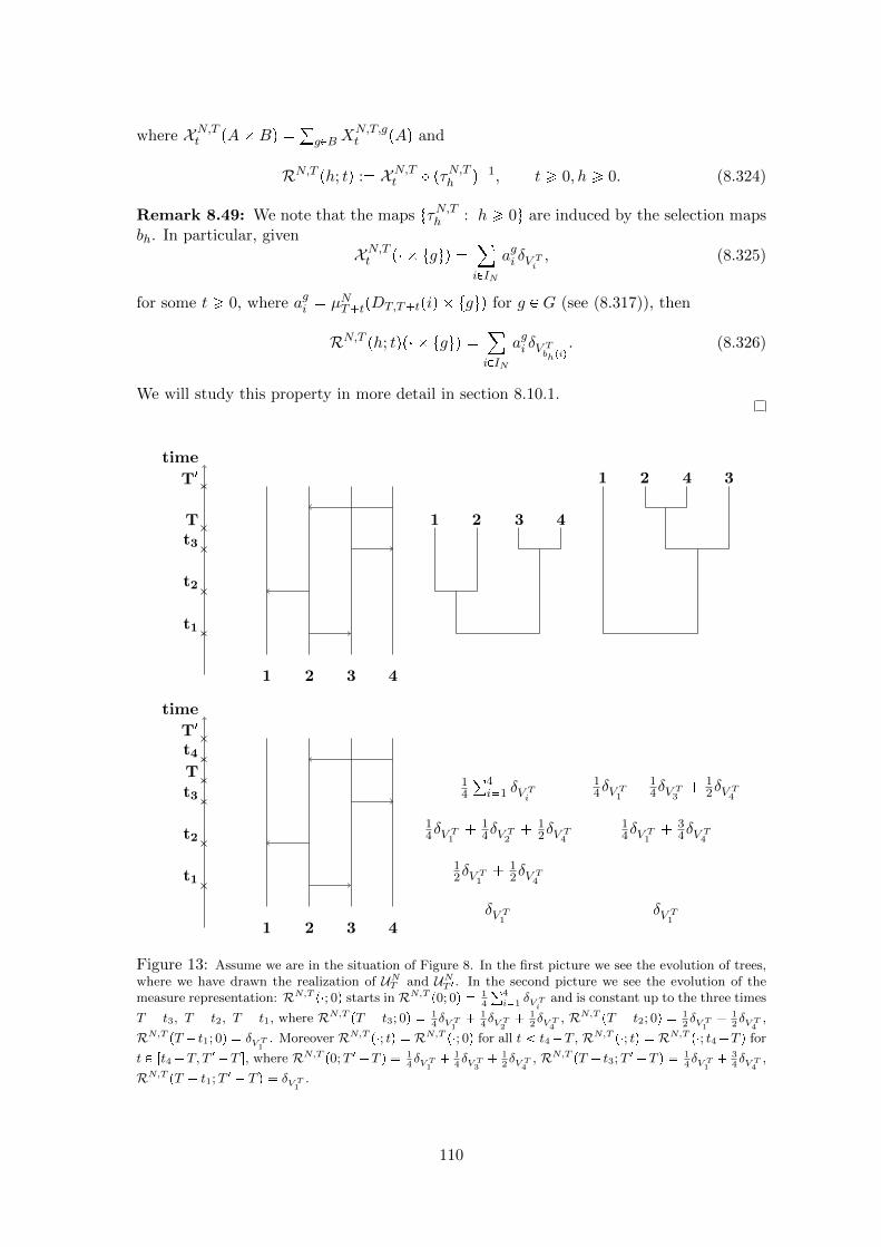
where XN,Tt pABq °gPBX

N,T,gt pAq and

RN,T ph; tq : XN,Tt pτN,Th q1, t ¥ 0, h ¥ 0. (8.324)

Remark 8.49: We note that the maps tτN,Th : h ¥ 0u are induced by the selection mapsbh. In particular, given

XN,Tt p tguq ¸iPIN

agi δV Ti, (8.325)

for some t ¥ 0, where agi µNTtpDT,Ttpiq tguq for g P G (see (8.317)), then

RN,T ph; tqp tguq ¸iPIN

agi δV Tbhpiq. (8.326)

We will study this property in more detail in section 8.10.1.

t1

t2

t3

time

T

T1

1 2 3 4

1 2 3 4

1 2 4 3

t1

t4

t2

t3

time

T

T1

1 2 3 4

14

°4i1 δV Ti

14δV T1

14δV T2

12δV T4

12δV T1

12δV T4

δV T1

14δV T1

14δV T3

12δV T4

14δV T1

34δV T4

δV T1

Figure 13: Assume we are in the situation of Figure 8. In the first picture we see the evolution of trees,where we have drawn the realization of UNT and UNT 1 . In the second picture we see the evolution of themeasure representation: RN,T p; 0q starts in RN,T p0; 0q 1

4

°4i1 δV T

iand is constant up to the three times

T t3, T t2, T t1, where RN,T pT t3; 0q 14δV T

1 1

4δV T

2 1

2δV T

4, RN,T pT t2; 0q 1

2δV T

1 1

2δV T

4,

RN,T pT t1; 0q δV T1

. Moreover RN,T p; tq RN,T p; 0q for all t t4T , RN,T p; tq RN,T p; t4T q for

t P rt4 T, T1T s, where RN,T p0;T 1T q 1

4δV T

1 1

4δV T

3 1

2δV T

4, RN,T pT t3;T 1T q 1

4δV T

1 3

4δV T

4,

RN,T pT t1;T 1 T q δV T1

.

110

time

T

T1 14 14 14 14

14δVT

1 1

4δVT3 1

2δVT4

14δVT

1 3

4δVT4

δVT1

ΦT 1T 14 12 14 M

Figure 14: Assume we are in the situation of Figure 13. In this case, the above picture shows theconnection of ΦTT 1pUNT 1q and RN,T p, T 1 T q.

We note that by definition of the measure-valued Moran models, we have ApXN,Tt q

ApXN,T0 q and hence RN,T p, tq P X for all t ¡ 0.As a direct consequence of the construction of pXN,T,gqgPG and HN,T we get

ΦtpUNTtq MpRN,T p; tqq, @t, T ¥ 0, (8.327)

where UN is the tree-valued interacting Moran model (see also Figure 13 and Figure 14).We can summarize this observation in the following Proposition, which also proves

Theorem 10:

Proposition 8.50: (TVIMM is an evolving genealogy) The tree-valued interacting Moranmodel UN is an evolving genealogy, with measure-valued representation tRN,T : T ¥ 0u,defined as above.

8.10 Proofs of section 6.2

Here we prove the results from section 6.2. In order to show that the tree-valued interactingFleming-Viot model is also an evolving genealogy we will apply Theorem 4, where themost difficult part is to prove (ii) and (iv) of this Theorem. In section 8.10.1 we givesome properties of the measure-valued representation that will be use in section 8.10.2 toshow some convergence results which are needed to verify these two conditions. In section8.10.3 we recall the definition of the measure-valued Fleming-Viot process and give someproperties of this process we need in order to prove Theorem 11. In section 8.10.4 we willthen prove this theorem. Finally in section 8.10.5 we will prove the finite system schemeresult for the tree-valued interacting Fleming-Viot process.

8.10.1 Properties of the measure-valued representation

We are interested how RN,T and RN,T 1 are related for T, T 1 ¥ 0.We fix the two times T, T 1 ¥ 0 and start with the following observation. Recall that

for g P G and t ¥ 0, XN,T is given by

XN,Tt p tguq :¸

iPDT,Tt


¸iPIN

µNTtpDT,Ttpiq tguqδV Ti.

(8.328)

111

We note that by definition of XN,TT 1 and KG,N,TT1, for all i P DT,TT 1 there is one

partition element κG,N,TT1

k pT 1q such that

µNT 1pDT,T 1piq tguq 1

|MN,TT 1,g| _ 1|κG,N,TT

1

k pT 1q XMN,TT 1,g|, (8.329)

where MN,T,g : ti P IN : ξipT q gu. In particular

DT,T 1piq κG,N,TT1

k pT 1q. (8.330)

Of course this does not need to induce a well defined map since there could be morethan one partition element with the same number of elements. In order to get aroundthis problem, we define for g P G, Ig : ti P t1, . . . , |κG,N,TT

1pT 1q|u : ξTT

1

i pT 1q gu,

where ξTT1

i pT 1q is the location of the ith partition element at time T 1 of KG,N,TT1.

By construction the number of elements in Ig coincides with the number of elements ofIg : ti P DT,Tt : ξipT q gu. Now define Cgk as the indices in Ig such that i P Cgkimplies κG,N,TT

1

i pT 1q has the k most elements, i.e. for all ik, jk P Cgk , |κG,N,TT

1

ikpT 1q|

|κG,N,TT1

jkpT 1q| and |κG,N,TT

1

ikpT 1q| |κG,N,TT

1

ik1pT 1q|. We define the analogue sets Cgk ,

namely ik, jk P Cgk satisfies µNT 1pDT,T 1pikq Gq µNT 1pDT,T 1pjkq Gq and µNT 1pDT,T 1pikq

Gq µNT 1pDT,T 1pik1q Gq.

Now we define the injective map B1 : t1, . . . , |κG,N,TT1pT 1q|u Ñ t1, . . . , |IN |u as fol-

lows: If Cgk ti1, . . . , ilu then pB1pi1q, . . . , B1pilqq is sampled without replacement from

the set Cgk . As a consequence we get

XN,TT 1 p tguq

|κG,N,TT1pT 1q|¸

i1

|κG,N,TT1

i pT 1q XMN,TT 1,g|

|MN,TT 1,g| _ 1δV TB1piq

. (8.331)

Moreover, if we set

agi :1

|MN,TT 1,g| _ 1|κG,N,TT

1

i pT 1q XMN,TT 1,g| (8.332)

and denote by pbhqh¥0 the selection maps, used for the construction of HN,T , then

RN,T ph;T 1qp tguq

|κG,N,TT1pT 1q|¸

i1

agi δV TbhpB

1piqq, (8.333)

for all h ¥ 0 and g P G (compare also Remark 8.49).We close this section with the following observation which is again a direct consequence

of the construction:

Lemma 8.51: The law of RTT 1pT 1; q is the law of a system of interacting measure-valuedMoran models. To be more precisely:

LpRTT 1pT 1; qq LppXN,TT 1tqt¥0q. (8.334)

Moreover, we have pXN,Tt qt¥0d pXN,T

1

t qt¥0 for all T, T 1 ¥ 0.

Remark 8.52: As we have seen in the above Lemma, the law of pXN,Tt qt¥0 does notdependent on T and hence, we will sometimes write pXNt qt¥0 if we only work with thismarginals.

112

8.10.2 A convergence result for the measure-valued representations

Here we prove that HN,T RN,T p; 0q converges weakly for N Ñ8, where we assume forthe rest of this thesis:

Assumption 4: The Kingman coalescents are coupled in the way that if we denote byKG,T the spatial Kingman coalescent with KG,T p0q tpt1u, ξ1pT qq, pt2u, ξ2pT qq, . . .u, whereppξiptqqt¥0qiPN are independent random walks on G (defined analogue as in section 6.1),then KG,T

IN KG,N,T (compare Proposition 8.42).

Remark 8.53: Analogue to Remark 8.43 we assume that the spatial Kingman-coalescent

KG,T is defined for all t ¥ 0. Note that by construction KG,Td KG,T

1for all T, T 1 ¡ 0.

We start with the following observation.

Lemma 8.54: For all T ¥ 0 and g P G we have XN,T0 p tguq Ñ λ in the weak atomictopology almost surely as N Ñ8, where λ denotes the Lebesgue measure on r0, 1s.

Proof: Since

XN,T0 p tguq 1

|MN,T,g| ^ 1

¸iPMN,T,g

δV Ti(8.335)

and |MN,TT 1,g|N Ñ 1 almost surely, by the strong law of large numbers, we get

XN,T0 p tguq ñ λ (8.336)

in the weak topology almost surely, by the Glivenko-Cantelli theorem (see [Par05]). Sinceλ has no atoms, we can use Lemma 2.1 in [EK94] to complete the proof.

Next we define a suitable limit object. In order to do this recall that if B N satisfies:

limNÑ8

|B X rN s|

N: |B|f (8.337)

exists, then we call |B|f the asymptotic frequency of B. We start with the followingimportant observation:

Lemma 8.55: Let π pπptqqt¥0 be the non spatial Kingman coalescent that starts intt1u, t2u, . . .u. Denote by τπk : inftt ¥ 0 : |πptq| ku. Moreover, let KG,T be the spatialKingman-coalescent defined in the previous sections and τk : inftt ¥ 0 : |κG,T | ku.Then there is a coupling of π and KG,T such that for all k P N and i 1, . . . , k

|πipτπk q|f |κG,Ti pτkq|f almost surely. (8.338)

As a consequence, the decreasing rearrangement of p|κG,Ti pτkq|f qi1,...,k has the law of thedecreasing rearrangement of a variable that is uniformly distributed on the simplex

∆k1 :

#px1, . . . , xkq P r0, 1s

k :k

i1

xk 1

+, (8.339)

i.e. it has the density pk 1q!1∆k1with respect to the Lebesgue measure (see Definition

2.4 in [Ber06]).

113

Proof: Fix a N P N and let πN : π|IN be the non spatial coalescing that starts inπN p0q tt1u, . . . , t|IN |uu. Since the locations pξiqi1,...,|IN | of the partition elements of

KG,N,T evolve as independent random walks on G, with ξ1p0q being uniformly distributedon G, at each coalescing event we uniformly choose two partition elements over all existingpartition elements and then merge them to one big block (see also the proof of Proposition14 in [LS06]). But the same holds for the non spatial process πN . Hence we can coupleboth processes such that (we use the same Assumption 4 for the processes πN )

πN pτπk q κG,N,T pτkq, @k 1, . . . , |IN |. (8.340)

The result is now a consequence of section 4.1.3 in [Ber06] (see in particular Corollary4.1).

As a consequence we get the following:

Lemma 8.56: Assume we are in the situation of Lemma 8.55. Then for all k P N,i 1, . . . , k and g P G

1

|MN,T,g| _ 1|MN,T,g X κG,N,Ti pτkq| Ñ |κG,Ti pτkq|f (8.341)

almost surely.

Proof: We define MT,g : ti P N : ξipT q gu, then tMT,gugPG is a random partition ofN. Moreover, since pξipT qqiPN are i.i.d., this random partition is exchangeable and henceit posses asymptotic frequency (see Theorem 2.1 in [Ber06]). In particular

|MT,g X IN |

|IN |Ñ

1

|G|, (8.342)

by the strong law of large numbers for all g P G. We can now use (8.340), note that πptqis independent of MT,g and apply Corollary 2.5 in [Ber06] to get

limNÑ8

1

|MN,T,g| _ 1|MN,T,g X κG,N,Ti pτkq| |G| lim

NÑ8

1

|IN ||MT,g X πipτ

πk q X IN |

|G| limNÑ8

1

|IN |2|MT,g X IN | |πipτ

πk q X IN | |κG,Ti pτkq|f .

(8.343)

We can now use the above observations to define HT . Let pUTi qiPN be independent anduniformly distributed on r0, 1s and assume that they are also independent of the Kingmancoalescent KG,T . Let MT,g : ti P N : ξipT q gu be the indices of the individuals locatedat g. Moreover, we denote by τk : inftt ¥ 0 : |κG,T ptq| ku the coalescing times of thepartition process κG,T .

Let K : |κG,T pTq| and g P G. We define for h ¥ T :

HTh p tguq : δUT1. (8.344)

114

We denote by px1, . . . , xKq the decreasing reordering of the asymptotic block frequency ofκG,T pτKq, i.e. xi ¥ xi1. Let σK be a random permutation of t2, . . . ,Ku, set σKp1q 1and define for h P rτK , T q:

HTh p tguq :K

i1

xσKpiqδUTi. (8.345)

We note that since xi ¡ xi1 for all i almost surely (the vector x has a density with respectto the Lebesgue measure), the map

px1, . . . , xKq ÞÑ

x1δUT

σ1K

p1q

, . . . , xKδUTσ1K

pKq

, (8.346)

is well defined almost surely. We set pxK1 , . . . , xKKq : pxKσKp1q, . . . , x

KσKpKq

q.

Now observe that at time τk and if we denote by xk : pxk1, . . . , xkkq the reordering of the

asymptotic block frequency of κG,T pτkq, then there is an i P t1, . . . , ku and y1, y2 P r0, 1ssuch that xk1 is the decreasing ordering of

pxk1, . . . , xki1, x

ki1, . . . , x

kk, y

1, y2q. (8.347)

In particular i is uniformly distributed on t1, . . . , ku and there is an uniformly r0, 1s-distributed random variable Zk such that y1 Zkx

ki and y2 p1 Zkqx

ki . Moreover, i

and Zk are independent and also independent of xk (compare section 4.1.2 in [Ber06]).Let ik be the associated index in pxk1, . . . , x

kkq. Then we define for h P rτk1, τkq and in the

case where y1 ¡ y2, i.e. Zk ¡ p1 Zkq

HTh p tguq :k

i1,iik

xki δUTi y1δUT

ik

y2δUTk1.

:k1

i1

xk1i δUTi

,

(8.348)

and in the case where y1 ¤ y2 we interchange y1 and y2 in the above definition.

Lemma 8.57: The process pHTh qh¥δ is well-defined and we have HTh p tguq Ñ λ almostsurely for all g P G, where λ is the Lebesgue measure on r0, 1s. As a consequence HT :limδÓ0pH

Th qh¥δ P X for all T ¥ 0.

Before we prove this, we give the first main result of this section:

Proposition 8.58: (Convergence of HN,T ) For all T ¥ 0:

LpHN,T q ñ LpHT q, (8.349)

whereMf pr0, 1sGq is equipped with the topology from Definition 3.1. Moreover, we have

HT P X and pHTt q0¤t¤Td pHT

1

t q0¤t¤T for all T 1 ¡ T .

Remark 8.59: We note that the last property in this proposition is a direct consequenceof the construction (see also Remark 8.53).

115

We split the proofs in several Lemmas.

Lemma 8.60: Assume we are in the situation of Lemma 8.57. Then HTh p tguq Ñ λ inthe weak atomic topology almost surely for all g P G.

Proof: Recall that the vector xk has the law of the reordering of a variable Qk pQki qi1,...,k that is uniformly distributed on the simplex ∆k1 (see Lemma 8.55) andthat

ErQki s 1

k, (8.350)

VarrQki s k 1

k2pk 1q, (8.351)

CovrQki , Qkj s

1

k2pk 1q, i j. (8.352)

By [OW11] we also have that

Erxk1s lnpkq

k, as k Ñ8 (8.353)

and hence (note that°ki1 x

ki

°ki1 x

ki 1)

P

¸xPr0,1s

HTτkptxu tguq2 ¡ ε

P

k

i1

pxki q2 ¡ ε

¤1

ε

k

i1

Epxki q

2¤

1

εExk1

Ñ 0,

(8.354)

for all ε ¡ 0. It follows that

¸xPr0,1s

HTτkptxu tguq2 k

i1

pxki q2 (8.355)

is an almost surely non-increasing sequence of random variables that converge to 0 inprobability, and hence ¸

xPr0,1s

HTτkptxu tguq2kÑ8ÝÑ 0 almost surely. (8.356)

Since λ has no atoms the above, together with Proposition 5.15, gives the result, once wehave shown

µk : HTτkp tguqkÑ8ùñ λ almost surely. (8.357)

In order to do this we recall that weak convergence can be metricized by several metrics,and we choose the Wasserstein distance (see [GS02]) for measures µ, ν PM1pr0, 1sq:

dW pµ, νq :

» 1

0|F puq Gpuq|du, (8.358)

116

where F,G are the corresponding cumulative distribution functions. For a fixed u P r0, 1swe set Xi : 1pUTi ¤ uq and note that by definition of µk

Fkpuq : µkpr0, usq k

i1

xki 1pUTi ¤ uq

¸iik

xkiXi ZkxkikXik

p1 ZkqxkikXik

.(8.359)

We may assume for the following that Zk ¡ p1 Zkq and hence

Fkpuq :¸iik

xkiXi ZkxkikXik

p1 ZkqxkikXik

¸iik

xkiXi xk1ik

Xik xk1

k1Xik

Fk1puq xk1k1pXik

Xk1q.

(8.360)

It follows that

dW pµk, µklq ¤

» 1

0

l1

nk

xn1n1

1pUTin ¤ uq 1pUTn1 ¤ uq

du. (8.361)

Now we observe that Sk : supl¥k dW pµk, µlq is non increasing in k almost surely and thatby the Jensen and Markov inequality:

P pSk ¥ εq ¤1

ε2E

» 1

0

8

nk

xn1n1


2

du

1

ε2

» 1

0E

8

nk

xn1n1


2 du

(8.362)

for all ε ¡ 0. We will prove below that the right hand side converges to 0 and observe thatthis implies Sk Ñ 0 almost surely. Hence pµkqkPN is Cauchy almost surely and therefore

117

converges to some limit µ almost surely. But (recall that UT and xk are independent)

P pdW pµk, λq ¡ εq ¤1

ε2

» 1

0E

k

i1

xki 1pUTi ¤ uq u

2 du

1

ε2

» 1

0

k

i1

E

xki

1

n

2

p1pUTi ¤ uq uq2

du

» 1

0

k

i,j1ij

E

xki 1

n

xkj

1

n

p1pUTi ¤ uq uqp1pUTj ¤ uq uqdu

1

ε2

» 1

0

k

i1

V arxki

V ar

1pUTi ¤ uq

du

» 1

0

k

i,j1ij

Covpxki , xkj qE

p1pUTj ¤ uq uq

2du

1

ε2

» 1

0

k

i1

k 1

k2pk 1qup1 uqdu

¤1

4ε2

k 1

kpk 1qÑ 0,

(8.363)

for all ε ¡ 0 and hence µ λ almost surely.It remains to prove the convergence in (8.362) and we calculate

8

nk

E

pxn1n1q

2

1pUTin ¤ uq 1pUTn1 ¤ uq2

8

nk

E

p1 Znqx

nin

2E


2

¤8

nk

Epxninq

2

8

nk

n 1

n2pn 1q: Ak

(8.364)

with Ak Ñ 0 as k Ñ 8. We abbreviate Xn : 1pUT

in¤ uq and Xn1 : 1pUTn1 ¤ uq and

observe that by definition Xm1, Xn and Xn1 are independent for all m ¡ n (recall in P

t1, . . . , nu). Moreover Xm is independent of Xn1 and X

n provided that im R tin, n 1u.We note that by definition of HT , X

m Xn (i.e. im in) implies xm1

m1 p1 Zmqxmin

and Xm Xn1 (i.e. im n 1) implies xm1

m1 p1 Zmqxmn1. Since im is uniformly

distributed on t1, . . . ,mu and independent of the other random mechanism the above gives(note that ErXn1s ErX

ns u for all n):

118

Exn1n1x

m1m1pX

n Xn1qpX

m Xm1q

E

xn1n1x

m1m1pX

n Xn1qpX

m Xm1q1pi

m R tin, n 1uq

E

p1 Zmqp1 Znqx

ninxminpX

n Xn1qpX

n Xm1q1pi

m inq

E

p1 Zmqx

nn1x

mn1pX

n Xn1qpXn1 Xm1q1pi

m n 1q

¤ E

xn1n1x

m1m11pim R tin, n 1uq

E rpX

n Xn1qsE rpXm Xm1qs

1

mExninx

min

1

mExnn1x

mn1

1

mExninx

min

1

mExnn1x

mn1

.

(8.365)

Now we observe that by definition of HT , xmin

xnin±Ll1 Zi, where pZiqiPN are

independent uniformly r0, 1s-distributed random variables and L is a random number,that is independent of the Zi and xn

in, and has the following law: Assume there is 1 red

ball and n 1 black balls in an urn. We sample l times a ball from this urn where at eachtime we add a black ball (independent of the color we sampled). L is now the number ofred balls, given there are l draws. In other words, if B1, B2, . . . are independent Bernoullivariables with success probabilities pi

1ni1 , then

L mn

l1

Bl. (8.366)

Hence L follows a Poisson binomial distribution. Note that

Exninx

min

E

pxninq

2 L¹l1

Zi

E

pxninq

2E L¹l1

Zi

n 1

n2pn 1q

mn

l1

ErZ1slP pL lq

n 1

n2pn 1q

mn

l1

1

2

lP pL lq

n 1

n2pn 1qΘmnp12q,

(8.367)

where Θmnptq denotes the probability generating function of L. Since

Θmnp12q mn¹l1

p1 pl 12plq mn¹l1

1

1

2pn l 1q

m1¹ln

1

1

2l

e°m1ln lnp1 1

2lq ¤ e

°m1ln

12l ¤ e

12plnpmqlnpnq1q

nm

12e1,

(8.368)

we get

28

nk

8

mn1

1

mExninx

min

¤ 28

nk

8

mn1

n 1

n32pn 1q

1

m32e1

¤ 4e18

nk

1

n32

: Bk,

(8.369)

119

with Bk Ñ 0 as k Ñ8 and by a similar argument:

28

nk

8

mn1

1

mExnpn1qx

mn1

¤ Ck, (8.370)

with Ck Ñ 0 as k Ñ8. Combining these observations we get the convergence in (8.362):

P pSk ¥ εq ¤1

ε2pAk Bk Ckq Ñ 0 as k Ñ8. (8.371)

As a consequence we can prove Lemma 8.57:

Proof: (Lemma 8.57) By construction pHTh qh¥δ is well-defined for all δ ¡ 0. MoreoverLemma 8.60 shows that HT pHTh qh¥0 limδÓ0pH

Th qh¥δ exists and is cadlag. By the

construction of pHTh qh¥δ we get HT P X and the result follows.

In order to prove Proposition 8.58 we need the following observation, namely that wecan construct HN,T in a similar way as HT :

Let nt : |κG,N,Tt | be the number of blocks of KG,N,Tt at time t P r0, T s and MN,T,g :ti P IN : ξipT q gu be the indices of the individuals located at g. Moreover we denoteby τk : inftt ¥ 0 : nt ku, k nT , . . . , |IN | the coalescing times of the partition processκG,N,T and pUTi qiPN be as in the construction of HT . Now we define HN,T as follows:

HN,Th p tguq : δUT1, @g P G, h ¥ T. (8.372)

Let

C :

"i P t1, . . . , nTu : |κG,N,Ti pTq| max

jPt1,...,nTu|κG,N,Tj pTq|

*(8.373)

be the index set of those partition elements with the largest number of elements. Weuniformly pick one element i P C and define

HN,TT ptUT1 u tguq :

|MN,T,g X κN,Ti pTq|

|MN,T,g| ^ 1(8.374)

and for i 2, . . . , nT:

HN,TT ptUTi u tguq :

$'''&'''%

|MN,T,gXκN,Ti1 pTq|

|MN,T,g |^1, i i,

|MN,T,gXκN,Ti pTq|

|MN,T,g |^1, i ¡ i.

(8.375)

We observe that at each time τk there are exactly two partition elements πi, πj PκN,T pτkq tπ1, . . . , πk1u for some i, j P t1, . . . , k 1u, where we assume that i j,such that

κN,T pτkq tπ1, . . . , πi1, πi Y πj , πi1, . . . , πj1, πj1, . . . , πk1u. (8.376)

Now we define HN,Tt HN,TT for t P rτnT , T q and for t P rτk1, τkq, k nT , . . . , |IN | wedefine

HN,Tt ptUTl u tguq : HN,TτkptUTl u tguq, (8.377)

120

if l P t1, . . . , ku, l i (recall i j) and if l i we distinguish three different cases.

If |πi| ¡ |πj | we define

HN,Tt ptUTi u tguq |MN,T,g X πi|

|MN,T,g| ^ 1, (8.378)

HN,Tt ptUTk1u tguq |MN,T,g X πj |

|MN,T,g| ^ 1, (8.379)

if |πi| |πj | we define

HN,Tt ptUTi u tguq |MN,T,g X πj |

|MN,T,g| ^ 1, (8.380)

HN,Tt ptUTk1u tguq |MN,T,g X πi|

|MN,T,g| ^ 1(8.381)

and if |πi| |πj | we toss a coin with success probability 12, i.e. we choose (8.378) or(8.380) each with probability 12.

It is now straight forward to verify the following Lemma:

Lemma 8.61: We have HN,Td HN,T .

As a consequence we can prove Proposition 8.58:

Proof: (Proposition 8.58) Note that by Lemma 8.56 and the construction we can coupleHN,T and HT such that

HN,Tτkp tguq Ñ HTτkp tguq (8.382)

in the weak atomic topology almost surely for all g and k (see Lemma 8.55 for the notation).Now observe that by construction, the jump times of pHN,Th qh¥δ are included in the jumptimes τk of the block process of the spatial Kingman coalescent pKG,T phqqh¥δ and hence thenumber of jumps are almost surely finite and the jump times are “uniformly separated”for all δ ¡ 0, which means that for all ε ¡ 0 there is a η ¡ 0 such that

P p|τk τk1| ηq ε. (8.383)

In order to get tightness in the Skorohod topology and hence convergence (see Theorem3.7.8 in [EK86]), it is therefore enough to prove (see Corollary 3.7.4 in [EK86] - comparealso Lemma 3.8.1 in [EK86]) that for all ε ¡ 0 there is a δ ¡ 0 such that

lim supNÑ8

P

sup

0¤h¤δdMVRpHN,Th ,HN,T0 q ¥ ε

¤ ε. (8.384)

Since the Skorohod topology on Dpr0,8q, Eq does not depend on the particular metric onE (see Proposition 3.6.5 in [EK86]), it is enough to prove (recall Proposition 5.15):

lim supNÑ8

P

sup

0¤h¤δdPrpH

N,Th ,HN,T0 q ¥ ε

¤ ε. (8.385)

and

lim supNÑ8

P

sup

0¤h¤δ

¸

xPr0,1s

HN,Th ptxu tGuq2 ¸

xPr0,1s

HN,T0 ptxu tGuq2

¥ ε

¤ ε. (8.386)

121

Since by definition¸xPr0,1s

HN,Tδ ptxu tGuq2 ¥¸

xPr0,1s

HN,Th ptxu tGuq2, @0 ¤ h ¤ δ, (8.387)

the latter is satisfied by a similar argument as in Lemma 8.57 combined with the almostsure convergence from above. Now observe that

dPrpHN,Th ,HN,T0 q ¤

¸gPG

dPr

HN,Th p tguq,HN,T0 p tguq

, (8.388)

and hence it is enough to bound the right hand side of (8.385) for all g P G. But

P

sup0¤h¤δ

dPrpµNh , µ

N0 q ¥ ε

P

max

KN pδq¤k¤|IN |dPrpµ

Nk , µ

N0 q ¥ ε

, (8.389)

where µNh : HN,Th p tguq and µNk : µNτk and KN pδq denotes the number of blocks ofκG,N,T pδq. Hence (8.385) holds by the same argument as in Lemma 8.57 combined withthe almost sure convergence.

Now we remark how HT and HT1

are related for two different T T 1:

Remark 8.62: As we have seen in the construction of HT , we find a map ΘT and ΞT suchthat HT ΘT pK

G,T , UT q ΞT pp|κG,Th |f qh¥0, U

T q and we note that the spatial Kingman

coalescents are coupled as follows: Let T, T 1 ¡ 0 and Ig : ti P t1, . . . , |κG,TT1pT 1q|u :

ξipT1q gu, where ξipT

1q, i 1, . . . , |κG,TT1pT 1q| are the locations of the partition ele-

ments of KG,TT1pT 1q. Let Ig be the first |Ig| elements of the set ti P N : ξipT q gu and

take a random permutation σ : I :gPG I

g Ñ I :gPG I

g with σpIgq Ig such that

σ is independent of the coalescents. Now we define the partitions κphq of I as follows:i, j P κlphq for some l if and only if there is a k such that σpiq, σpjq P κG,Tk phq. We notethat this is equivalent to say σpiq, σpjq P pκG,T |Iqkphq and that KG,T

I

is again a spatialKingman coalescent. Moreover, we note that each partition element κlphq has a locationξlphq given by the location of the corresponding partition element κG,Tk phq. If we nowdefine

κG,T,TT1

i phq :¤

jPκiphq

κG,TT1

j pT 1q, (8.390)

and

KG,T,TT1phq :

!pκG,T,TT

1

1 phq, ξ1phqq, . . . , pκG,T,TT 1n phq, ξnphqq

), (8.391)

where n |κG,TIphq|, then

LKG,T , pKG,TT

1phqqh¤T 1 ,pK

G,TT 1ph T 1qqh¥0

L

KG,T , pKG,TT

1phqqh¤T 1 , pK

G,T,TT 1phqqh¥0

.

(8.392)

We finally note that this also implies that

pHTT1

h qh¥T 1d ΘT pK

G,T,TT 1 , V TT 1q. (8.393)

122

We close this section with the following important fact:

Proposition 8.63: (F.d.d. convergence) Let 0 ¤ T1 T2 . . . Tm, m P N. ThenLppRN,Tip;TijTiqq1¤i¤j¤mq converges weakly inM1pDpr0,8q,Mf pr0, 1sGqq

mpm1q2qas N Ñ8, where Mf pr0, 1s Gq is equipped with the topology given in Definition 3.1.

Proof: Recall Remark 8.49 and note that the family tτN,Th : h ¥ 0u for HN,T is given asfollows: First observe that by definition

ApHN,Th p Gq tUT1 , . . . , UTnNhu, (8.394)

for all h ¥ 0, where nNh : |κG,N,T phq| denotes the number of blocks at time h. Now τN,Th

is constant up to the discontinuity points h of h ÞÑ HN,Th p Gq, where we can find aih P t1, . . . , n

Nh u such that

τhpUTk q

#UTk , if k nNh,

UTih , if k nNh.(8.395)

This means, in terms of selection maps pchqh¥0 for the Kingman-coalescent, that ch isthe map that maps all partition elements in a partition κG,N,Tk to its minimal element, i.e.

chpiq minpκG,N,Tk q for all i P κG,N,Tk .Let T 1 ¥ 0 and δ ¥ 0. Then we can combine this observation with (8.333) and get the

existence of a permutation σδ of t1, . . . , nNδ u such that

LpRN,T ph, 0qqh¥δ, pRN,T ph, T 1qqh¥δ, pRN,TT

1ph, 0qqh¥δ

L

pHN,Th qh¥δ, pRN,T ph;T 1qqh¥δ, pH

N,TT 1

h qh¥δ

,

(8.396)

where for g P G and h ¥ 0,

RN,T ph;T 1qp tguq :

|κG,N,TT1pT 1q|¸

i1

agi δUTchpσδpiqq. (8.397)

Since nNδ Ñ nδ : |κG,T pδq| 8 almost surely and by the properties we proved inthis section (recall the definition of agi from (8.332)), it is now straight forward to showconvergence of

L

HN,Thi, RN,Thi

, HN,T1

h1i

i1,...,k

(8.398)

for N Ñ 8, for all 0 δ : h1 . . . hk, 0 δ : h11 . . . h1k1 ¤ T 1, h1k11 h1 T 1, . . . , h1kk1 hk T 1, k, k1 P N.

If we now combine this observation with Theorem 3.7.2 in [EK86] and the fact thatfinite dimensional distributions are tight if the one dimensional distributions are tight,we get the result for the case m 2, once we have shown that RN,T p; tq is tight for allt, T ¡ 0. But this follows by the same argument as in the proof of Proposition 8.58 sincethe number of atoms of XN,Tt is given by |κG,N,Ttptq|, which is uniformly finite almost

123

surely and the jump points of RN,T p; tq are exactly the jump points of pHN,Tth qh¥t and

hence included in the jump points of pκG,Tth qh¥t.It remains to generalize this result to arbitrary m P N but this follows by a similar

argument and we leave out the details.

8.10.3 Measure-valued interacting Fleming-Viot processes

We recall the definition of a system of interacting Fleming-Viot processes on the geograph-ical space G. This process can be characterized as the solution of a well-posed martingaleproblem. We will only sketch the properties here, for more details see [DGV95] (comparealso [Daw93] for a general introduction to measure-valued processes and [EK86], section4, for the definition and properties of solutions of martingale problems).

We denote by D CppM1r0, 1sqGq the set of polynomials, i.e. the span of functions F

of the following form:

F pxq m¹i1

»r0,1s

fi dxξi

, fi P Cbpr0, 1sq i 1, . . . ,m, (8.399)

where m P N and pξiqi1,...,m is a finite collection of elements in G. We note that D isan algebra that separates points and hence is dense in CppM1r0, 1sq

Gq by the Theorem ofStone-Weierstrass, when M1r0, 1s is equipped with the weak topology. Moreover, we candefine partial derivations for elements F P A:

BF pxq

Bxξpuq : lim

ε×0

1

ε

F pxεpξ, uqq F pxq

, (8.400)

with xεpξ, uq

ξ1

:

"xξ falls ξ1 ξ,

xξ εδu falls ξ1 ξ.

The second derivations are given by

B2F pxq

Bxξxξpu, vq

B

Bxξ

BF pxq

Bxξpuq

pvq. (8.401)

LetQxξpdu, dvq xξpduqδupdvq xξpduqxξpdvq (8.402)

and define the linear operator Ω : D Ñ CppM1r0, 1sqGq by

ΩF pxq ¸

ξ,ξ1PG

apξ, ξ1q

»r0,1s

BF pxq

Bxξpuq

xξ1pduq xξpduq

γ

2

¸ξPG

»r0,1s

»r0,1s

B2F pxq

BxξBxξpu, vqQxξpdu, dvq,

(8.403)

where γ ¡ 0 is the resampling rate.

124

Proposition 8.64: (Characterization and properties of the measure-valued Fleming-Viotprocess) The system of interacting measure-valued Fleming-Viot processes ppXg

t qgPGqt¥0

with pXg0 qgPG pµgqgPG : µ P pM1r0, 1sq

G can be characterized by the well-posed mar-tingale problem pΩ,D, µq. It has the following properties:

i) P pppXgt qgPGqt¥0 P CpR, pM1r0, 1sq

Gqq 1.

ii) pXgt qgPG is purely atomic for all t ¡ 0 almost surely. Note that this property holds

for all (even continuous) initial measures µ.

iii) pXgt qgPG is Markov and Feller.

Proof: The above properties can be found in Theorem 0.0 in [DGV95].

Remark 8.65: One has to be careful with property i) in the above proposition. In fact,what we mean by ppXg

t qgPGqt¥0 has almost surely continuous paths, is that there is a lawQ on CpR, pM1r0, 1sq

Gq such that

F pXtq F pX0q

» t0

ΩF pX2qds (8.404)

is a martingale under Q for all F P D, where Xtpωq ωptq is the coordinate process (seesection 4.3 in [EK86] for more details).

Lemma 8.66: Let ppXN,T,gqgPGqt¥0 be the system of measure-valued Moran models givenin section 8.9.2 for some T ¡ 0. Then its limit is a system of interacting measure-valuedFleming-Viot processes ppXT,g

t qgPGqt¥0, i.e.

ppXN,T,gqgPGqt¥0 ñ ppXgt qgPGqt¥0, (8.405)

weakly in the Skorohod topology, where Mf pr0, 1sq is equipped with the weak atomic topol-ogy, and Xg

0 λ, the Lebesgue-measure on r0, 1s, for all g P G.

We will prove this Lemma in (iii) of the next section. A consequence of this Lemmais:

Remark 8.67: We remark that in our situation pXgt qgPG has only finitely many atoms

for all t ¡ 0 almost surely. This follows immediately by the fact that the number ofatoms is given by the number of blocks of a spatial Kingman coalescent (see section 8.10.1and Lemma 8.56), and that the spatial Kingman coalescent comes down from infinity(see [LS06]).

125


We will now show that the tree-valued interacting Moran model satisfies the conditions ofTheorem 4.

(i) This is satisfied by definition.

(iii) To see that this holds, recall that XN,Tt p tguq XN,T,gt pq for g P G, where

pXN,T,gqgPG is a system of interacting Moran models (see section 8.9.1). By Lemma 8.54

we know that XN,T0 p tguq Ñ λ almost surely in the weak atomic topology for all g P G,where λ is the Lebesgue-measure on r0, 1s.

Let pXT,gqgPG be the system of interacting Fleming-Viot processes given as in Propo-

sition 8.64 with XT,g0 λ for all g P G and set X Tt p tguq : XT,g

t , t ¥ 0. Weknow that the initial distributions converge, the space M1pr0, 1sq

G is compact, equippedwith the weak topology, and the martingale problem for the measure-valued interact-ing Fleming-Viot processes is well-posed (see Proposition 8.64). Now the convergencepXN,T,gqgPG ñ pXT,gqgPG follows by the convergence of the generators given in Remark8.41 and (8.403) together with Lemma 4.5.1 and Remark 4.5.2 in [EK86], where the con-vergence of the generators is a straight forward calculation and hence we skip it. As aconsequence we get that

XN,T ñ X T (8.406)

weak in the Skorohod topology, whereMf pr0, 1sGq is equipped with the weak topology.Now we prove that this convergence also holds whenMf pr0, 1s Gq is equipped with thetopology given in Definition 3.1.

According to Theorem 2.12 and Remark 2.13 in [EK94] we need to prove that for allS ¡ 0, δ ¡ 0 there is an ε ¡ 0 such that

lim infnÑ8

P

supt¤S

» »fεpx, yqXN,Tt pdxGqXN,Tt pdy Gq

¤ δ

¥ 1 δ, (8.407)

where

fεpx, yq Ψ

|x y|

ε

1px yq, (8.408)

and Ψ : r0,8q Ñ r0, 1s is an arbitrary non increasing continuous function with Ψp0q 1,Ψp1q 0. Recall Remark 8.41 and observe that, by the martingale problem characteriza-tion, » »

fεpx, yq XN,Tt pdxGqXN,Tt pdy Gq

¸g,qPG

» »fεpx, yq X

N,T,gt pdxqXN,T,q

t pdyq(8.409)

is a non negative martingale with cadlag paths. We can now apply Doob’s martingaleinequality (see for example Proposition 2.2.16 in [EK86]) and get that

126

P

supt¤S

» »fεpx, yqXN,Tt pdxGqXN,Tt pdy Gq

¥ δ

¤¸g,qPG

1

δE

» »fεpx, yq X

N,T,gS pdxqXN,T,q

S pdyq

¸g,qPG

1

δE

» »fεpx, yq X

N,T,g0 pdxqXN,T,q

0 pdyq

.

(8.410)

As we have seen above XN,T,g0 Ñ λ almost surely and hence

E

» »fεpx, yq X

N,T,g0 pdxqXN,T,q

0 pdyq

Ñ

» »Ψ

|x y|

ε

λpdxqλpdyq

¤

»r0,1s

» yεyε

λpdxqλpdyq 2ε.

(8.411)

If we choose ε δ2|G|2

and combine this with the convergence result in Remark 8.41,

where we note that convergence in the total variation norm implies convergence in theweak atomic topology (this is straight forward and follows by Proposition 5.15 (ii)), thenthe above observations give the result in the weak atomic topology.

Since pXT,gt qgPG is purely atomic for all t ¡ 0 (see Proposition 8.64) it remains to

prove: For all ε ¡ 0 and T ¥ 0 there is a Cε ¥ 0 such that

lim supNÑ8

P

|G|2 ¸

xPr0,1s

XN,TCεptxu Gq2

¡ ε

¤ ε. (8.412)

In order to see this observe that the result follows, if there is an almost surely finite timeC 8 such that XN,TC p Gq has only one atom for all N P N. By construction of XN,T

(see section 8.10.1), the number of atoms of XN,Tt is given by the number of blocks ofthe spatial Kingman coalescent KG,N,Ttptq. Since there is an almost surely finite time τsuch that |κG,T pτq| 1 and |κG,N,T ptq| ¤ |κG,T ptq| for all t ¥ 0 (recall Assumption 4), theresult follows.

(iv) This is Proposition 8.58.

(v) In view of Lemma 8.51, Remark 8.41 and similar to (iii) we may assume w.l.o.g. thatt ÞÑ RN,T pδ; tqptxu Gqq is a positive martingale and hence we get by Doob’s martingaleinequality for all δ, S ¡ 0 and C CpµN0 q, where we abbreviate µNt : RN,T pδ; tqp Gqfor t ¥ 0,

PDx P ApµN0 q : sup

0¤t¤SµNt ptxuq ¥ C µN0 ptxuq

µN0

¤¸

xPApµN0 q

1

C µN0 ptxuqEµN0

rµNS ptxuqs

¸

xPApµN0 q

1

C µN0 ptxuqµN0 ptxuq

ApRN,T pδ; 0qp Gqq

C.

(8.413)

127

Observe that KN pδq :ApRN,T pδ; 0qp Gqq

is the number of blocks of the spatialKingman-coalescent KG,N,T at time δ and that this number satisfies KN pδq ¤ Kpδq 8almost surely, where Kpδq denotes the number of blocks in KG,T (see section 3 in [LS06] -also recall Assumption 4). Hence, if we choose for ε ¡ 0

C 2|Kpδq|

ε, (8.414)

and C such that

P pC ¡ Cq ¤ε

2, (8.415)

then we get

lim supNÑ8



¤ lim sup

NÑ8PDx P ApµN0 q : sup

0¤t¤SµNt ptxuq ¥ C µN0 ptxuq,

pC ¤ C _ C ¡ Cq

¤ lim supNÑ8



P pC ¡ Cq

¤ε

2ε

2 ε.

(8.416)

Finally observe that another consequence of the proof in (iii) is that there is an S 8almost surely such that

RN,T pδ; tqp Gq RN,T pδ; Sqp Gq, @t ¥ S (8.417)

and hence, the result follows.

(ii) We need to prove that pRN,T qT¥0 converges in finite dimensional distribution. ByKolmogorov’s extension theorem, this gives the existence of a family of random variablestRT : T ¥ 0u defined on the same probability space such that

pRN,T qT¥0f.d.d.ñ pRT qT¥0. (8.418)

In order to prove the convergence of the finite dimensional distributions, we need toshow that the finite dimensional distribution of pRN,T1 , . . . ,RN,Tmq converge, see Theo-rem 3.7.8 in [EK86] and that the pRN,T1 , . . . ,RN,Tmq are tight in the (product space ofthe) Skorohod space. Observe that convergence of the finite dimensional distributions ofpRN,T1 , . . . ,RN,Tmq is Proposition 8.63 and in order to prove tightness of pRN,T1 , . . . ,RN,Tmq,it is enough to prove tightness of the one dimensional distributions RN,T for all T ¥ 0. Inparticular, since we know that the finite dimensional distributions of RN,T converge forall T ¥ 0 and according to Corollary 3.7.4 in [EK86], we only need to verify:

For every ε ¡ 0 and τ ¡ 0 there is a δ ¡ 0 such that

lim supNÑ8

P pw1pRN,T , δ, τq ¥ εq ¤ ε, (8.419)

128

with

w1pRN,T , δ, τq infti

maxi

sups,tPrti1,tiq

dSKpRN,T p; sq,RN,T p; tqq, (8.420)

where ttiu is a finite partition of r0, τ s with miniptiti1q ¥ δ (see (3.6.2) in [EK86]).

We note that the Skorohod topology does not depend on the particular metric on thecorresponding space (see Proposition 3.6.5 in [EK86]), and hence, in terms of Proposition5.15, we consider the metric (compare Definition 3.1 and Remark 3.2)

dMVRpµ, νq : dPrpµ, νq |µ ν|, (8.421)

where µ : µpEq °xPr0,1s µptxuq. Take δ ¡ 0 and observe that

P pw1pRN,T , δ, τq ¥ εq ¤ P pw1ppRN,T p; t δqqt¥0, δ, τq ¥ε

2q

P p sup0¤t¤δ

dSKpRN,T p; tq,RN,T p; 0qq ¥ε

2q.

(8.422)

Now observe that h ÞÑ RN,T ph, δq is constant up to the jump points of the block processof the spatial Kingman coalescent KG,N,Tδ and that the jump times of h ÞÑ RN,T ph, tqare contained in the jump times of h ÞÑ RN,T ph, δq for all t ¥ δ by Definition 3.9. If wedenote by Kpδq the number of blocks of the spatial Kingman coalescent KG,N,Tδ at timeδ and by τk : inftt ¥ 0 : Kptq ku the jump times, then this implies (compare also theproof of Proposition 8.58)

P pw1ppRN,T p; t δqqt¥0, δ, τq ¥ εq

P pinfti

maxi

sups,tPrti1,tiq

dSKpRN,T p; s δq,RN,T p; t δqq ¥ εq

¤ P pinfti

maxi

sups,tPrti1,tiq

suph¥0

dMVRpRN,T ph; s δq,RN,T ph; t δqq ¥ εq

P pinfti

maxi

sups,tPrti1,tiq

sup1¤k¤Kpδq

dMVRpRN,T pτk; s δq,RN,T pτk; t δqq ¥ εq

¤L

k1

P pinfti

maxi

sups,tPrti1,tiq

dMVRpRN,T pτk; s δq,RN,T pτk; t δqq ¥ εq ε

4,

(8.423)

where we used the fact that Kpδq 8 almost surely and chose L such that

P pKpδq ¥ Lq ¤ε

4. (8.424)

But we know that t ÞÑ RN,T pτk; t δq is a system of interacting Moran models (seeLemma 8.51), that converges in the Skorohod space to the interacting Fleming-Viot process(compare (iii) and note that convergence of LpRN,T pτkq, δq holds by the construction inthe proof of Proposition 8.63 - compare also the proof of Proposition 8.58). Hence we canchoose δ small enough (see Corollary 3.7.4 in [EK86]) such that

lim supNÑ8

P pw1ppRN,T p; t δqqt¥0, δ, τq ¥ εq ¤ε

2. (8.425)

129

Now we calculate

P p sup0¤t¤δ

dSKpRN,T p; tq,RN,T p; 0qq ¥ε

2q

¤ P

sup

0¤t¤δsuph¥δ

dMVRpRN,T ph; tq,RN,T ph; 0qq

_ suph¤δ

dMVRpRN,T ph; tq,RN,T ph; 0qq ¥ε

2

¤ P

sup

0¤t¤δsuph¥δ


2

P

sup

0¤t¤δsuph¤δ


2

(8.426)

and a similar argument as above shows that we can choose δ small enough such that

lim supNÑ8

P p sup0¤t¤δ

suph¥δ


2q ¤

ε

4. (8.427)

In order to prove that this is also true for the last term, we consider the followingLemma:

Lemma 8.68: Let µ, ν be two finite measures on some metric space pE, rq with the samemass and assume that both are purely atomic with finitely many atoms such that Apνq Apµq. Moreover, let ϕ : Apµq Ñ Apµq and υµ be the uniform distribution on Apµq. Then

dPrpµ, νq ¤ dPrpν ϕ1, µ ϕ1q dPrpµ, µ ϕ

1q 2dPrpµ, υµq. (8.428)

Moreover, if ψ : Apµ ϕ1q Ñ Apµ ϕ1q is another map, then

|pµ ϕ1q pν ϕ1q| ¤ |µ ν| |pµ ϕ1 ψ1q µ|

|pµ ϕ1 ψ1q pν ϕ1 ψ1q|,(8.429)

where µ : µpEq °xPE µptxuq

2δxpEq.

Proof: Let

ε1 ¡ dPrpν ϕ1, µ ϕ1q, (8.430)

ε2 ¡ dPrpµ, µ ϕ1q, (8.431)

ε3 ¡ dPrpµ, υµq. (8.432)

Then we get for all A Apµq:

νpAq ¤ νpϕ1pϕpAqqq ¤ µpϕ1pϕpAqε1qq ε1 ¤ µpϕpAqε1ε2q ε1 ε2

¤ υµpϕpAqε1ε2ε3q ε1 ε2 ε3 ¤ υµpA

ε1ε2ε3q ε1 ε2 ε3

¤ µpAε1ε22ε3q ε1 ε2 2ε3.

(8.433)

This is the first part. For the second part observe that

pµ ϕ1q ¸x

¸yPϕ1ptxuq

µptyuq

2

¥¸x

¸yPϕ1ptxuq

µptyuq2 µ. (8.434)

130

It follows that

pνϕ1q pµ ϕ1q

¤ pν pψ ϕq1q pµ pψ ϕq1q pµ pψ ϕq1q pµ ϕ1q(8.435)

and

pνϕ1q pµ ϕ1q ¥ ν µ µ pµ ϕ1q. (8.436)

This givespνϕ1q pµ ϕ1q

¤pν pψ ϕq1q pµ pψ ϕq1q

|ν µ|

pµ pψ ϕq1q pµ ϕ1q

µ pµ ϕ1q

pν pψ ϕq1q pµ pψ ϕq1q

|ν µ|

pµ pψ ϕq1q µ

.(8.437)

Now observe for ε, δ ¡ 0

P

sup0¤t,h¤δ

dMVRpRN,T ph; tq,RN,T ph; 0qq ¥ ε

¤ P

sup0¤t,h¤δ

dPrpRN,T ph; tq,RN,T ph; 0qq ¥ε

2

P

sup

0¤t,h¤δ

RN,T ph; tq RN,T ph; 0q ¥ ε

2

(8.438)

and that

dPrpRN,T ph; tq,RN,T ph; 0qq ¤¸gPG

dPrpRN,T ph; tqp tguq,RN,T ph; 0qp tguqq. (8.439)

We denote by υh the uniform distribution on the set of atoms of RN,T ph; 0qp tguq :RN,T,gph; 0qpq. Then, by Lemma 8.68 and for N large enough:

dPrpRN,T,gph; tq,RN,T,gph; 0qq

¤ dPrpRN,T,gpδ; 0q,RN,T,gph; 0qq dPrpRN,T,gpδ; tq,RN,T,gpδ; 0qq

2dPrpυh,RN,T,gph; 0qq

(8.440)

and hence

lim supNÑ8

P

sup0¤t,h¤δ

dPrpRN,T ph; tq,RN,T ph; 0qq ¥ε

2

¤ lim supNÑ8

¸gPG

P

sup

0¤h¤δdPrpRN,T,gpδ; 0q,RN,T,gph; 0qq ¥

ε

6|G|

lim supNÑ8

P

sup

0¤t¤δdPrpRN,T,gpδ; tq,RN,T,gpδ; 0qq ¥

ε

6|G|

lim supNÑ8

P

sup

0¤h¤δdPrpυh,RN,T,gph; 0qq ¥

ε

12|G|

.

(8.441)

131

As we have proved before, the first two terms can be bounded by ε6|G| when we choose

δ small enough. Moreover:

lim supNÑ8

¸gPG

P

sup0¤h¤δ

dPrpυh,RN,T,gph; 0qq ¥ε

12|G|

¤¸gPG

lim supNÑ8

P

sup0¤h¤δ

dPrpRN,T,gph; 0q,RN,T,gp0; 0qq ¥ε

24|G|

¸gPG

lim supNÑ8

P

sup0¤h¤δ

dPrpυh,RN,T,gp0; 0qq ¥ε

24|G|

.

(8.442)

Again, if we choose δ small enough, the first term is less or equal than ε24|G| . Now observe

that if we apply Lemma 8.61 and denote by τNk : inftt ¥ 0 : |κG,N,T,gptq| ku, where|KN ptq| : |κG,N,T,gptq| is the number of blocks process of the spatial Kingman coalescentrestricted to MN,T,g : ti P IN : ξipT q gu, then υk : υτNk

is the uniform distribution on

tUT1 , . . . , UTk u. Moreover, RN,T,gp0; 0q is the uniform distribution on tUT1 , . . . , U

T|MN,T,g |

u.

Since pUTi qiPN is independent of the Kingman coalescent RN,T,gp0; 0q Ñ λ, the Lebesguemeasure on r0, 1s (see Lemma 8.54) and KN pδq Ñ Kpδq almost surely, where Kpδq is thenumber of blocks of a spatial Kingman coalescent KG,T (restricted to ti : ξipT q gu) attime δ, we get

lim supNÑ8

P

sup

0¤h¤δdPrpυh,RN,T,gp0; 0qq ¡ ε

lim supNÑ8

P

sup

k¥KN pδq

dPrpυk,RN,T,gp0; 0qq ¡ ε

P

sup

k¥KpδqdPrpυk, λq ¡ ε

.

(8.443)

Since the empirical distribution of pV Ti qiPN converges weakly almost surely to λ, i.e.

dPrpυk, λq Ñ 0 as k Ñ 8 almost surely, and Kpδq Ñ 8 for δ Ó 0, we get that for allε ¡ 0:

limδÓ0

P

sup

k¥KpδqdPrpυk, λq ¡ ε

0. (8.444)

It follows that if ε is small enough, then

P

sup0¤t,h¤δ

dPrpRn,T ph; tq,Rn,T ph; 0qq ¥ε

2

¤ε

2. (8.445)

Finally observe that Lemma 8.68 and a similar argument as above gives

P

sup0¤t,h¤δ

Rn,T ph; tq Rn,T ph; 0q ¥ ε

2

¤ε

2(8.446)

and the result follows.


Let RN,T be the measure-valued representation of the tree-valued interacting Fleming-Viot processes on GN given as in Theorem 11. Then it is straight forward to see that by

132

definition, tRN,T : T ¥ 0u given by

RN,T ph; tq θN pRN,T |GN |ph|GN |; t|GN |qq, h, t ¥ 0, (8.447)

is a measure-valued representation of UN : phN pUNt|GN |qqt¥0. In the following we will

always write a for the quantities of RN,T . We need to check two things, tightness of UNand convergence of the finite dimensional distributions (see Theorem 3.7.8 in [EK86]).

Tightness of UN

We start by proving tightness of UN : phN pUNt|GN |qqt¥0 and use the criterion of The-

orem 3. Note that (i) is satisfied by definition and observe that we can write XN,Tt °gPGN

XN,T |GN |,gt|GN |

, where pXN,T |GN |,gqgPGN is a system of measure-valued interacting Fle-

ming-Viot processes (see Theorem 11) for all T ¥ 0. Moreover, by Lemma 8.51 and

Remark 8.52 we have pXN,T |GN |,gqgPGNd pXN,T,gqgPGN and pXN,T,gqgPGN converges if

M1pr0, 1sqG is equipped with the weak topology (its product topology respectively). In

particularXN,T ñ X T , (8.448)

and X T is the (non spatial) Fleming-Viot process with diffusion rate D (see [CG94] for asketch of the proof and [Gri12] for more details). Now we prove that this result holds whenM1pr0, 1sq is equipped with the weak atomic topology. In order to do this we note that°gPGN

XN,T,gt pfq is a martingale for all bounded continuous functions f (this is a direct

consequence of the martingale-problem characterization of this process). Moreover theclass of functions f , such that

°gPGN

XN,T,gt pfq is a martingale, is closed under bounded

pointwise convergence. Hence the process

¸gPGN

¸gPGN

» »fεpx, yqX

N,T,gt pdxqXN,T,g

t pdyq (8.449)

where

fεpx, yq Ψ

|x y|

ε

1px yq ¥ 0, (8.450)

for some non increasing continuous function Ψ : r0,8q Ñ r0, 1s with Ψp0q 1, Ψp1q 0,is a continuous non-negative martingale. Now we can apply Doob’s martingale inequalityand the result follows analogue to (iii) in the proof of Theorem 11.

We note that the non-spatial Fleming-Viot process is purely atomic for all positivetimes t ¡ 0 (independent of the initial value - see Proposition 8.64) and hence it remainsto proof that for all ε ¡ 0 and T ¥ 0 there is a Cε ¥ 0 such that

lim supNÑ8

P

1 ¸

xPr0,1s

XN,TCεptxuq2

¡ ε

lim supNÑ8

P

1 ¸

xPr0,1s

XN,T |GN |Cεptxuq2

¡ ε

¤ ε.

(8.451)

In order to see this we note that the number of atoms of XN,T |GN |t is given by the

number of blocks of the spatial Kingman coalescent KGN ,Tt|GN |p|GN |tqd KGN ,T p|GN |tq

133

(recall Remark 8.53). Since the block process of the spatial Kingman coalescent convergesin this time scale to a non-spatial Kingman coalescent with coalescing rate D (see Theo-rem 19 in [LS06]) we get the result analogue to (iii) in the proof of Theorem 11.

F.d.d. convergence of UN

Let T ¥ 0, SNh be the reordering of p|κ

GN ,T |GN |i p|GN |hq|f qi1,...,|κGN,T p|GN |hq|

in the way

that SNh p1q ¥ SN

h p2q ¥ . . .. We split the proof in three steps. In the first step we show

convergence of SN , in the second step we show convergence of the joint distributions ofSN (given for different times T ) and in the third step we show that this convergence isenough to get f.d.d. convergence of the tree-valued processes.

Step 1: We note that SNh P SÓ for all h ¡ 0 and (recall Lemma 8.56)

pSNh q0 h¤T

d FpMppHN,Th q0¤h¤T q

F

M

1

|GN |

¸gPGN

HN,T |GN ||GN |h

p tguq

0¤h¤T

. (8.452)

We use Remark 8.53 and assume in the following that SNh is the decreasing rearrangement

of p|κGN ,Ti p|GN |hq|f qi1,...,|κGN,T p|GN |hq|(which is only true in law, but in order to prove

weak convergence it is sufficient to show convergence of this object).Now we will prove that SN is relatively compact in Dpr0,8q,SÓq, where we equip SÓ

with dm (see (8.43)) and note that by Theorem 19 in [LS06] we have

p|κGN ,T ph|GN |q|qh¥δ ñ p|κT phq|qh¥δ, @δ ¡ 0, (8.453)

where κT is the (non spatial) Kingman coalescent with coalescing rate D. Note thatpSÓ1 , dmq is compact (this follows analogue to Proposition 2.1. in [Ber06]) and that thejump points of pSN

h qh¥δ are exactly the jump points of p|κGN ,T ph|GN |q|qh¥δ. Now a similarargument as in Proposition 8.58 combined with Corollary 3.7.4 in [EK86] shows relativecompactness of pSN

h qh¥δ in the Skorohod space. In order to get relative compactness of

pSNh qh¥0 it remains to prove

limδÓ0

lim supNÑ8

P p sup0¤h¤δ

dmpSNh , 0q ¥ εq 0, @ε ¡ 0. (8.454)

Set KN pδq : |κGN ,T pδ|GN |q| and

τNk : infth ¥ 0 : |κGN ,T p|GN |hq| ku. (8.455)

Then

P p sup0¤h¤δ

dmpSNh , 0q ¥ εq P p sup

k¥KpδqdmpSN

τNk, 0q ¥ εq. (8.456)

Observe that by the argument in the proof of Lemma 8.60:

P psupk¥L

dmpSNτNk, 0q ¥ εq : AL Ñ 0 as LÑ8 (8.457)

and AL does not depend on N . Since KN pδq ñ Kpδq : |κT pδq| and Kpδq Ò 8 as δ Ó 0,we get relative compactness of SN in the Skorohod space.

134

In fact we can prove convergence of SN : If we apply Lemma 8.55 we get

pSNτNkqkPN

d pSτkqkPN, (8.458)

where

τk : infth ¥ 0 : |κT phq| ku (8.459)

and S is defined as SN but in terms of κT .As mentioned above, the jump times of pSN

h qh¥δ equal the jump times of pKN phqqh¥δ.We can now apply (8.453) to get

pτNk qk1,...,KN pδq ñ pτkqk1,...,Kpδq, (8.460)

for all δ ¡ 0. But this is enough to prove

LFpUNT q

L

pSN

h qh¡0

ñ L

pShqh¡0

L

FpUT q

, (8.461)

for all T ¥ 0 and we note that this convergence is still true when SÓ1 is equipped with d1

(see Remark 8.12 and recall that we already proved tightness of UNT ). This observationwill be important in the last step.

Step 2: Now let 0 ¤ T1 . . . Tm, m P N and SN,i be defined as above where weconsider κGN ,Ti|GN | instead of κGN ,T |GN |. By the above we know that SN,i converges andhence pSN,iqi1,...,m is relatively compact in the product space. Now we prove that the

convergence of pSN,iqi1,...,m does also hold and start with the case m 2, where we setT : T1, T

1 : T2 T1.By the observation in Remark 8.62 (with the modification that we consider δ and T 1δ

instead of 0 and T 1) together with the fact that the locations of the partition elements ofκN,T |GN |pδ|GN |q are independent and uniformly distributed on GN , we obtain the commonlaw of pκN,T ph|GN |qqh¥δ and pκN,TT

1ph|GN |qqh¥T 1δ by the following construction:

Whenever two partition elements with indices i and j of κN,T |GN |ph|GN |q, for someh ¡ δ, coalesce, then there is a coalescence of the ith and jth partition element ofκN,pTT

1q|GN |pph T 1q|GN |q provided that i, j ¤ |κN,pTT1q|GN |pph T 1q|GN |q| : n

and if i ¡ n or j ¡ n nothing happens.We note that the locations of κN,T |GN |pδ|GN |q and κN,T |GN |ph|GN |q are approximately

independent for h ¡ δ (see the proof of Proposition 14 in [LS06]). Using the observationsin Step 1, it is now straight forward to see that

LpSN,1

h qh¥δ, pSN,2T2T1h

qh¥δ, pSN,2h qδ¤h¤T2T1

ñ L

pS1

hqh¥δ, pS2T2T1hqh¥δ, pS

2hqδ¤h¤T2T1

.

(8.462)

We can generalize this observation to arbitrary m P N by a similar argument and hence weget f.d.d. convergence of pSN,iqi1,...,m for all 0 ¤ T1 T2 . . . Tm, m P N. Combin-ing this with the tightness from Step 1, this gives the result (see Theorem 3.7.8 in [EK86]).

Step 3: Finally we need to prove that convergence of SN,i is enough to get convergence

of UNTi . Note that HN,TTd δV T1

for all N P N and recall

FpMppΞT |GN |pSN,i, V Ti|GN |qqqq SN,i, (8.463)

by Remark 8.62 (strictly speaking, the right hand side has to be assumed to be constantafter time T , i.e. SN,i

h p1, 0, 0, . . .q for all h ¥ T ). Before we continue we need thefollowing:

135

Lemma 8.69: Let pEi, diq, i 1, 2 be two metric spaces and f : E1 Ñ E2 be perfect (seeRemark 5.11). Assume there is a subset A E1 such that fpxq fpyq implies x y forall x, y P A, i.e. f

A

is injective, and denote by B : fpAq its image. If yn P B, n P N isa sequence in B with yn Ñ y P B, then f1pynq Ñ f1pyq.

Proof: Note that there is a sequence xn P A such that fpxnq yn Ñ y fpxq for somex P A. Moreover, there is a subsequence such that f1pynkq xnk Ñ x P E1. This givesfpxnkq ynk Ñ fpxq fpxq and therefore x x.

Now observe that Remark 8.62 and (8.463) give us the existence of a set A Uc (recallCorollary 5.12) such that UNT P A and UT P A almost surely and such that F restricted

to A is injective and that M Ξ : F is the inverse of FA

(this is not completely correct

but given V Ti|GN | we can reformulate this observation to get this property). We can nowapply Lemma 8.69 and get that pSN,iqi1,...,m ñ pSiqi1,...,m implies

LpUNTi qi1,...,m

L

pMpΞT |GN |pS

N,i, V Ti|GN |qqqi1,...,m

ùñ L

pMpΞT pS

i, V Tiqqqi1,...,m

L

pUTiqi1,...,m

.

(8.464)


In this section we will prove the results from section 7.2. In section 8.11.1 we give asuitable coupling of two Moran models with different resampling rates based on a couplingof Kingman coalescents in order to prove Proposition 7.5. In section 8.11.2, we proveCorollary 7.6, where we use our theory on measure-valued representations to deduce theresult.

8.11.1 Proof of Proposition 7.5

Recall the connection of Uγ,NT and the Kingman coalescent κγ,N,T given in Lemma 8.44(recall that |G| 1). The proof is now based on a coupling of the two Kingman coalescentsκγ,N,T and κγγ

1,N,T , for γ, γ1 ¡ 0.Let pT γk q2¤k¤N be independent rate γ

k2

-exponential random variables and pUnqn2,...,N

pU1n, U

2nqn2,...,N be independent IN IN -valued random variables with

P pUk pi, jqq 1

k pk 1q1pi jq1pi, j P t1, . . . , kuq, (8.465)

where we assume that both random mechanisms are defined on the same probability spaceand are independent. Let κγ,N,T be the PprN sq-valued process that starts in tt1u, . . . , tNuuand evolves as follows: At the time hk, where

hNk : Sγk :N

jk1

T γk , k 1, . . . , N 1, (8.466)

we coalesce the U1Nk1 and U2

Nk1 partition element, i.e. given Sγk h, κγ,N,T phq

tπ1, . . . , πk1u and U1k1 i, U2

k1 j, where we assume that i j (otherwise interchangei and j), we get

κγ,N,T phq tπ1, . . . , πi1, πi Y πj , πi1, . . . , πj1, πj1, . . . , πk1u. (8.467)

136

We note that by Proposition 8.42 the process κγ,N,T is a version of the Kingmancoalescent and hence we have Lpκγ,N,T q Lpκγ,N,T q.

Given this construction of the Kingman coalescent, we can now couple κγ,N,T and

κγγ1,N,T as follows: Define T γγ

1

k : T γk ^ T γ1

k , where we assume that T γk and T γ1

k are

independent for all k 1, . . . , N . It follows that T γγ1

k is exponential distributed with

rate pγ γ1q k2

and

T γγ1

k ¤ T γk . (8.468)

If we now use this particular choice of T γγ1

k in the construction of κγγ1,N,T but the same

variables pUnqn2,...,N pU1n, U

2nqn2,...,N for both κγγ

1,N,T and κγ,N,T , then

κγγ1,N,T pSγγ

1

k q κγ,N,T pSγk q, @k 1, . . . , N 1, (8.469)

and we get the result by Proposition 8.44 with the identity as measure-preserving 1-Lipschitz map.

8.11.2 Proof of Corollary 7.6

It remains to prove Corollary 7.6 and we will do this by using our results on measure-valued representations. Recall the notation from section 8.9.2 and denote by X γ,N,T thecorresponding (non-spatial) measure-valued Moran model with resampling rate γ (notethat |G| 1 and identify this process by a process with values inM1pr0, 1sq). By definitionof this measure-valued process we have the following identity for all T, t ¥ 0:

ν2,Uγ,NTtpr0, tsq

»r0,1sX γ,N,Tt ptxuqX γ,N,Tt pdxq. (8.470)

As we have seen in the proof of Theorem 11 X γ,N,T ñ X γ,T and Uγ,N ñ Uγ , whereX γ,T is the measure-valued Fleming-Viot process with resampling rate γ that starts inX γ,T p0q λ, the Lebesgue-measure, and Uγ is the tree-valued Fleming-Viot process thatstarts in rt1u, 0, δ1s. Note that we even proved a bit more: We verified the conditions ofTheorem 4 and (ii) and (iv) of this Theorem combined with Theorem 2 and the continuousmapping Theorem, gives that Uγ,Nt ñ Uγt , when U is equipped with the Gromov-weakatomic topology. But by Lemma 5.18 combined with the continuous mapping theorem,this is enough to get

pν2,Uγ,NT pr0, tsqqt¥0 ñ pν2,UγT pr0, tsqqt¥0, (8.471)

where this convergence holds on M1pDpr0,8q, r0, 1sqq. Moreover, we note that»r0,1sX γ,N,Tt ptxuqX γ,N,Tt pdxq

¸xPr0,1s

X γ,N,Tt ptxuq2, (8.472)

and hence, since the convergence to the Fleming-Viot process holds when M1pr0, 1sq isequipped with the weak atomic topology, we get

Lν2,UγTtpr0, tsq

L

»r0,1sX γ,Tt ptxuqX γ,Tt pdxq

, @t ¥ 0. (8.473)

Remark 8.70: Note that the convergence Uγ,Nt ñ Uγt , when U is equipped with theGromov-weak atomic topology, is not necessary for this result. In fact it is enough to havet ÞÑ ν2,UγT pr0, tsq, t T is continuous in probability.

137

The last ingredient for the proof of Corollary 7.6 is the following Lemma:

Lemma 8.71: For all 0 ¤ t ¤ T the following holds:

E

»r0,1sX γ,Tt ptxuqX γ,Tt pdxq

1 exppγtq (8.474)

independent of T .

As a consequence of this Lemma we get:

Proof: (Corollary 7.6) Using Theorem 13 and (8.473) and the fact that ν2,UγT pr0, tsq 1for t ¡ T (by construction), the result follows by Lemma 8.71:

E » 8

0eλrν2,UγT pdrq

» 8

0λeλtE

ν2,UγT pr0, tsq

dt

» T0λeλtE

ν2,UγT pr0, tsq

dt eλT

1 eλT λ

λ γp1 epλγqT q eλT

γ

λ γ

λ

λ γepλγqT .

(8.475)

It remains to prove Lemma 8.71. The idea is to approximate the Fleming-Viot processby suitable functionals of a Wright-Fisher diffusion and we start by briefly recalling thedefinition of a n-dimensional Wright Fisher diffusion Xn for n P N (see for exampleTheorem 8.2.8 in [EK86] for more details). Let Sn : tpx1, . . . , xnq P r0, 1s

n :°ni xi ¤ 1u

and C2pSq be the set of twice continuously differentiable functions on Sn. Moreover, letLn be the linear operator with domain C2pSq C0pSq, given by

Lnfpxq γ

2

n

i,j1

xipδi,j xjqB

Bxi

B

Bxjfpxq, (8.476)

where δi,j 1 if i j and 0 otherwise. Let Xn be the Feller process associated with Ln thatstarts in Xnp0q x P S. Then we call Xn1, given by Xn1

i Xi, Xn1n1 1

°ni1 X

ni

the n 1-dimensional Wright-Fisher diffusion with initial point Xn1i p0q xi, X

n1n1 p0q

1°ni1 xi.

Lemma 8.72: Let

E : Sn ÑM1pr0, 1sq, x ÞÑ Epx; q n

i1

xiδ in1

1

n

i1

xi

δ1, (8.477)

then the process µnt : pEpXnptqqqt¥0 is a measure-valued Fleming-Viot process with µ0 EpXnp0qq.

138

Proof: Let f P C0pr0, 1sq be a continuous function, m P N and define

G : Gf,m : Sn Ñ R, x ÞÑ

»fpyqEpx; dyq

m

n1

i1

xif

i

n 1

m

, (8.478)

where we set xn1 1 px1 . . . xnq, and

F : F f,m :M1pr0, 1sq Ñ R, µ ÞÑ

»fpyqdµ

m. (8.479)

Then G is twice continuously differentiable and a simple calculation shows that

LnGpxq ΩF pEpxqq, (8.480)

where Ω is the generator of the measure-valued Fleming-Viot process (see (8.403)). Nowthe result follows by the well-posedness in Proposition 8.64.

We are now ready to prove Lemma 8.71:

Proof: (Lemma 8.71) Consider the sequence xni : 1n1 , i 1, . . . , n of initial points.

Then we have Epxnq ñ λ in the weak atomic topology and hence pµnt qt¥0 ñ X γ,T , whereM1pr0, 1sq is equipped with the weak atomic topology (this is a direct consequence ofTheorem 3.5 in [EK94] together with Lemma 4.5.1 in [EK86]). Note that this implies inparticular ¸

xPr0,1s

pµnt ptxuqq2 ñ

¸xPr0,1s

pX γ,Tt ptxuqq2. (8.481)

Finally observe that by Proposition 1.1.5 in [EK86]:

d

dtE ¸xPr0,1s

pµnt ptxuqq2

d

dtE

n

i1

pXni ptqq

2

1

n

i1

Xni ptq

2

γE

n

i1

Xni ptqp1 Xn

i ptqq n

i1

Xni ptq

1

n

i1

Xni ptq

γE

n

i1

Xn1i ptqp1Xn1

i ptqq p1Xn1n1 qX

n1n1

γE

1

n1

i1

pXn1i ptqq2

γ

1 E

¸xPr0,1s

pµnt ptxuqq2

(8.482)

and hence

E

¸xPr0,1s

pµnt ptxuqq2

1

n 1eγt p1 eγtq Ñ p1 eγtq (8.483)

as nÑ8.

139


Here we prove Theorem 15 and, analogue to section 8.9.2, we start by defining a measure-valued “forward” process that describes the evolution of family sizes (see section 8.12.1).In section 8.12.2, we reformulate this process to get a connection to the (finite dimensional)Wright-Fisher model. We then prove in section 8.12.3 convergence of this finite model toa suitable limit object and show in section 8.12.4 how to use this limit process to obtaingenealogical information. This observation will finally be applied in section 8.12.5 to proveour main result.

8.12.1 A forward representation

Here we use the same idea as in section 8.9.2 (compare also section 8.9.1) to define aforward process XN,T . We start by defining a process pX,Y q ppXt, Y tqqt¥0 with valuesin pr0, 1s r0, 1sqN , where we interpret Xtpiq as the relative number of descendents ofindividual i P IN and Y piq as the relative number of fit individuals under the descendentsof i. (8.315) for the neutral case gives a first hint how the dynamic should look like:

At rate γ N2

we have four different transitions (let eipjq 0 for j i and eipiq 1):

pXt, Y tq Ñ pXt 1

Nei

1

Nej , Y t

1

Neiq (8.484)

with probability Ytpiq pXtpjq Ytpjqq (i.e. resampling of a fit descendent of i with anunfit descendent of j),

pXt, Y tq Ñ pXt 1

Nei

1

Nej , Y t

1

Nei

1

Nejq (8.485)

with probability Ytpiq Ytpjq (i.e. resampling of a fit descendent of i with a fit descendentof j),

pXt, Y tq Ñ pXt 1

Nei

1

Nej , Y t

1

Nejq (8.486)

with probability pXtpiq Ytpiqq Ytpjq (i.e. resampling of an unfit descendent of i with anfit descendent of j),

pXt, Y tq Ñ pXt 1

Nei

1

Nej , Y tq (8.487)

with probability pXtpiq Ytpiqq pXtpjq Ytpjqq (i.e. resampling of an unfit descendent ofi with an unfit descendent of j).

At rate αN

N2

we have

pXt, Y tq Ñ pXt 1

Nei

1

Nej , Y t

1

Neiq (8.488)

with probability Ytpiq pXtpjq Ytpjqq (i.e. selection event for a fit descendent of i withan unfit descendent of j),

pXt, Y tq Ñ pXt 1

Nei

1

Nej , Y t

1

Nei

1

Nejq (8.489)

with probability Ytpiq Ytpjq (i.e. selection event for a fit descendent of i with a fit descen-dent of j).

At rate ϑ we have

pXt, Y tq Ñ pXt, Y t 1

Neiq (8.490)

140

with probability Xtpiq Ytpiq (i.e. mutation from an unfit descendent of i to a fit descen-dent),

pXt, Y tq Ñ pXt, Y t 1

Neiq (8.491)

with probability Ytpiq (i.e. mutation from a fit descendent of i to an unfit descendent).

Lemma 8.73: Recall the notation of section 8.9.2 and define

XN,Tt :N

i1

Ytpiqδp iN,1q

N

i1

pXtpiq Ytpiqqδp iN,0q, (8.492)

then

XN,Tt ¸

iPDT,Tt

µNTtpDT,Ttpiq t0uqδp iN,0q

¸

iPDT,Tt

µNTtpDT,Ttpiq t1uqδp iN,1q.

(8.493)

Proof: This is basically the same argument as in section 8.9.2 and hence we skip it.

We write in the following pXN , Y N q in order to indicate the dependence on N andremark the following:

Remark 8.74: As a direct consequence of the construction we have

ν2,UNTtpr0, tsq

»XN,Tt ptxu KqXN,Tt pdxKq

N

i1

pXNt piqq

2. (8.494)

8.12.2 A different point of view

While the process in section 8.12.1 has a nice interpretation, we need to modify it a bitto get an object we can better work with. Namely we set pF ,Uq ppF t, U tqqt¥0 asFtpiq Ytpiq and Utpiq Xtpiq Ytpiq and interpret Ftpiq as the relative number of fitdescends at time t and Utpiq as the relative number of unfit descends at time t of individuali. We observe that pF ,Uq has the following dynamic:

At rate γ N2

we have four different transitions (let eipjq 0 for j i and eipiq 1):

pF t, U tq Ñ pF t 1

Nei, U t

1

Nejq (8.495)

with probability Ftpiq Utpjq (i.e. resampling of a fit descendent of i with an unfit descen-dent of j),


Nei

1

Nej , U tq (8.496)

141

with probability Ftpiq Ftpjq (i.e. resampling of a fit descendent of i with a fit descendentof j),


Nej , U t

1

Neiq (8.497)

with probability Utpiq Ftpjq (i.e. resampling of an unfit descendent of i with an fitdescendent of j),

pF t, U tq Ñ pF t, U t 1

Nei

1

Nejq (8.498)

with probability Utpiq Utpjq (i.e. resampling of an unfit descendent of i with an unfitdescendent of j).

At rate αN

N2

we have


Nei, U t

1

Nejq (8.499)

with probability Ftpiq Utpjq (i.e. selection event for a fit descendent of i with an unfitdescendent of j),


Nei

1

Nej , U tq (8.500)

with probability Ftpiq Ftpjq (i.e. selection event for a fit descendent of i with a fitdescendent of j).

At rate ϑ we have


Nei, U t

1

Neiq (8.501)

with probability Utpiq (i.e. mutation from an unfit descendent of i to a fit descendent),


Nei, U t

1

Neiq (8.502)

with probability Ftpiq (i.e. mutation from a fit descendent of i to an unfit descendent).

The above construction has the following advantage. Namely we get that pF ,Uq is a2N dimensional Wright-Fisher model:

Lemma 8.75: Let φ : r0, 1sN r0, 1sN Ñ R be twice continuously differentiable. Then thegenerator LN of the Markov jump process XN with XN

t piq FNt piq, XNt piNq UNt piq,

i 1, . . . , N is given by

LNφpxq γ

N

2

2N

i,j1

xixjφpx1

Nei

1

Nejq φpxq

(8.503)

α

N

N

2

N

i,j1

xixjNφpx 1Nei 1NejN q (8.504)

xixjφpx 1Nei 1Nejq φpxq

(8.505)

ϑNN

i1

xiφpx 1Nei 1NeiN q (8.506)

xiNφpx 1Nei 1NeiN q φpxq. (8.507)

142

As in section 8.12.1 we could define the process XN,T in terms of pFN , UN q. But it isbetter to modify its definition a bit.

Lemma 8.76: We define XN,T to be the process with values in M1pr0, 2sq that is givenby

XN,Tt N

i1

Ftpiqδ iN

N

i1

Utpiqδ iNN. (8.508)

Let φ : r0, 2sm Ñ R be bounded and continuous for some m ¤ N and consider

Φ xφ, µmy :

»φ dµbm. (8.509)

Then the generator ΩN of XN,T is given by

ΩNΦpµq : ΩNresΦpµq ΩN

selΦpµq ΩNmutΦpµq (8.510)

with

ΩNresΦpµq : γ

N

2

»r0,2s

»r0,2s

pΦpµu,vq Φpµqqµpduqµpdvq, (8.511)

ΩNselΦpµq :

α

N

N

2

»r0,2s

»r0,2s

pΦpµu,vqχpuq Φpµqqµpduqµpdvq, (8.512)

where χpuq 1pu ¤ 1q and

ΩNmutΦpµq : ϑN

»r0,1s

pΦpΘupµqq Φpµqqµpduq

»p1,2s

ΦpΘ1

upµq Φpµqµpduq ,

(8.513)

where

µu,v µ1

Nδu

1

Nδv (8.514)

and

Θupµq µ1

Nδu1

1

Nδu, (8.515)

Θ1upµq µ

1

Nδu1

1

Nδu. (8.516)

Proof: This follows analogue to Lemma 8.72 and we skip it.

Remark 8.77: Note that

XN,T0 1

N

N

i1

uipT qδ iN

1

N

N

i1

p1 uipT qqδ iNN. (8.517)

and that (recall Remark 8.74)

ν2,UNTtpr0, tsq N

i1

pFtpiq Utpiqq2

¸xPr0,1s

XN,T ptxuq XN,T ptx 1uq

2. (8.518)

143

8.12.3 Convergence of the finite models

Let

Sn : tx P r0, 1s2n1 :2n1¸i1

xi ¤ 1u, (8.519)

for some n P N. Moreover, let φ : Sn Ñ R be a twice continuously differentiable function(in each component) and define x2n : 1

°2n1i1 xi for x P Sn. We define the following

operatorLαφpxq Lresφpxq Lsel

α φpxq Lmutφpxq, (8.520)

where for α, ϑ ¥ 0:

Lresφpxq 1

2

2n1¸i,j1

xipδi,j xjqB

Bxi

B

Bxjφpxq, (8.521)

Lselα φpxq α

n

i1

xin

n

i1

xiB

Bxiφpxq

n

i1

xi

2n1¸in1

xiB

Bxiφpxq

(8.522)

and

Lmutφpxq ϑn

i1

pxin xiqB

Bxiφpxq ϑ

n1

i1

pxi xinqB

Bxinφpxq. (8.523)

Proposition 8.78: The martingale problem associated with pL,C2pSnq, xq is well-posedfor all initial values x P Sn. Moreover, the associated process Xn is Feller (i.e. thecorresponding semigroup is Feller) and has almost surely continuous paths.

Proof: Define for i ¤ n

bipxq : α

n

i1

xin

xi ϑpxin xiq (8.524)

and for i P tn 1, . . . , 2n 1u

bipxq : α

n

i1

xi

xi ϑpxin xiq. (8.525)

then b : Sn Ñ R2n1 is Lipschitz and satisfies

bipxq ¥ 0, if xi 0,

2n1¸i1

bipxq 0, if2n1¸i1

xi 1.(8.526)

Now the result follows by Theorem 8.2.8 in [EK86].

144

Remark 8.79: Recall the definition of LN given in Lemma 8.75. If we restrict its defi-nition to functions φ P C2pSnq, where we set x2n 1

°2n1i1 xi for x P Sn, then it is a

straight forward calculation (using Taylor expansion) to show that

||LNφ Lφ||8 Ñ 0. (8.527)

Now we need to define a suitable limit object for XN,T given in Lemma 8.76. Weconsider the following operator (recall the notation of Lemma 8.76 and the definition ofthe partial derivations from section 8.10.3 - see also [DG99])

ΩΦpµq : ΩresΦpµq ΩselΦpµq ΩmutΦpµq, (8.528)

with

ΩresΦpµq γ

2

»r0,2s

»r0,2s

B2Φpµq

BµBµpu, vqQµpdu, dvq, (8.529)

ΩselΦpµq α

»r0,2s

»r0,2s

BΦpµq

BµpuqχpvqQµpdu, dvq, (8.530)

and

ΩmutΦpµq : ϑ

»r0,2s

»r0,2s

BΦpµq

BµpvqMpu, dvq F pµq

µpduq, (8.531)

where

Qµpdu, dvq µpduqδupdvq µpduqµpdvq (8.532)

and

Mpu, dvq δu1pdvq1pu ¤ 1q δu1pdvq1pu ¡ 1q. (8.533)

Proposition 8.80: (Characterization and properties of the limit process) Let D be theclass of functions of the form

Φ

»φ dµbm, (8.534)

for some bounded continuous function φ : r0, 2sm Ñ R and m P N. Moreover, letM1pr0, 1sqbe equipped with the weak atomic topology. Then the following holds:

(i) The pΩ,D, νq-martingale problem has a unique solution for all initial values ν PM1pr0, 2sq,

(ii) If we denote by X T its solution then X T has almost surely continuous paths,

(iii) If XN,T p0q ñ µT for some random measure µT , then

XN,T ñ X T , (8.535)

as processes and X T0 µT .

145

Proof: It is not hard to see that

||ΩNΦ ΩΦ||8 Ñ 0, (8.536)

for all functions Φ P D. Now this is analogue to Theorem 1.1, Theorem 3.1 and Theorem3.2 in [EK94].

8.12.4 Approximation of the pairwise distance

Here we use the results from section 8.12.3 to define a suitable approximation for ν2,UT .We start with the following Lemma.

Lemma 8.81: There is a random measure µT such that XN,T0 ñ µT , where M1pr0, 2sqis equipped with the weak atomic topology.

Proof: Recall that we assumed puN1 p0q, . . . uNN p0qq are exchangeable (see (7.11)) and that

(see (8.77))

XN,T0 1

N

N

i1

uipT qδ iN

1

N

N

i1

p1 uipT qqδ iNN. (8.537)

By a result in [DK99] puN1 pT q, . . . , uNN pT qq is exchangeable and there is an exchangeable

sequence puipT qqiPN such that the limit

LpuN1 pT q, . . . , uNmpT qq ñ Lpu1pT q, . . . , umpT qq (8.538)

exists for all m P N.Since M1pr0, 2sq is compact in the weak topology, we get convergence of LpXN,T0 q

along some subsequence when M1pr0, 2sq is equipped with the weak topology. Denote byµT and µT two weak limit points and observe that for all continuous bounded functionφ : r0, 2s Ñ R and m P N we have

E

»r0,2s

φ dXN,T0

m

1

Nm

¸i1,...,im

E

m¹k1

puNikpT qφpikNq p1 uNikpT qqφp1 ikNqq

1

Nm

¸i1,...,im

E

m¹k1

puNk pT qφpikNq p1 uNk pT qqφp1 ikNqq

op1q

Ñ E

m¹k1

ukpT q

»r0,1s

φpxqdλ p1 ukpT qq

»r0,1s

φpxqdλ

(8.539)

independent of the subsequence. It follows that

E

»r0,2s

φdµT

m E

»r0,2s

φdµT

m(8.540)

146

for all continuous functions φ and m P N. Since the linear span of functions of the formF pµq p

³fdµqm is an algebra that separates points, the Stone Weierstrass theorem gives

us µTd µT (see Theorem 3.4.5 in [EK86]).

It remains to prove convergence in the weak atomic topology and we observe that

XN,T ¤ 1

N

2N

i1

δiN ñ λr0,2s

, (8.541)

the Lebesgue-measure on r0, 2s. Since the Lebesgue-measure has no atoms, we can applyLemma 2.1 in [EK94] to get the result.

Using this observation we can now prove an approximation result:

Proposition 8.82: (Approximation of the pairwise distance) Let Xn be the process fromProposition 8.78, that starts in Z, where

Z

un1 pT q

n, . . . ,

unnpT q

n,1 un1 pT q

n, . . . ,

1 unn1pT q

n

. (8.542)

Then (set Xnt p2nq : 1

°2n1i1 Xn

t piq)

Eν2,UTtpr0, tsq

lim

nÑ8E

n

i1

pXnt piq Xn

t pi nqq2

. (8.543)

Proof: Using Lemma 8.81 and the observations from section 8.12.3 this is now basicallythe situation as in section 8.11.2, where we use Remark 8.70: Due to the fact that wehave a representation in terms of a Kingman coalescent, the neutral Fleming Viot process,UT , satisfies t ÞÑ ν2,UT pr0, tsq, t T is continuous in probability. One can now apply theGirsanov transform given in [DGP12], to get the same result for the process UT .


We will use Proposition 8.82 to prove Theorem 15 and start with the following Lemma:

147

Lemma 8.83: Recall Proposition 8.78 and define the functions

φ1 : Sn Ñ R, x ÞÑn

i1

pxi xinq2, (8.544)


i1

pxi xinqpxi pxi xinqn

j1

xjq, (8.545)

2n

jn1

xj

n

i1

xipxi xinq n

j1

xj

n

i1

xinpxi xinq, (8.546)


i1

xi pxi xinqn

j1

xj

2

(8.547)

2pxi xinq

xi pxi xinq

n

j1

xj

n

j1

xj

, (8.548)

where x2n : 1°2n1i1 xi. Then

Lαφ1pxq 1 φ1pxq 2αφ2pxq, (8.549)

Lαφ2pxq p3 2ϑ αqφ2pxq αφ3pxq. (8.550)

Proof: This is a straight forward calculation and hence we skip it.

Now we define the random times

τ0 : inftt ¥ 0 : φ2pXnt q 0u, (8.551)

τ0 : inftt ¥ τ0 : cltφ2pXns q : τ0 ¤ s ¤ tu X r0,8q Hu, (8.552)

τε : inftt ¥ 0 : φ2pXnt q εu, (8.553)

where cl denotes the closure.

Lemma 8.84: If we denote by Ft the filtration generated by Xn, then τ0, τ0, τε are Ft :s¡tFs-stopping times and they satisfy τε Ó τ0 almost surely and τ0 τ0 almost surely.

Moreover, we have φ2pXnτ0q φ2pX

nτ0q 0 almost surely.

Proof: The first part is Lemma 2.1.1 and Proposition 2.1.5 in [EK86]. Since

φ2pXn0 q

1

n2

n

i1

p1 uni pT qqn

i1

uni pT q 1

n2

n

i1

uni pT qn

i1

p1 uni pT qq 0 (8.554)

and t ÞÑ φ2pXnt q is continuous, the second part follows.

148

Lemma 8.85: There is an almost surely finite stopping time S such that φ2pXnt q 0 for

all t ¥ S.

Proof: Let S : inftt ¡ 0 : Di s.t. Xnt piq Xn

t pi nq 1u. By the construction for theneutral Fleming-Viot process, UT , we know that in the case where α 0, this is the timeit takes for all partition elements (in a Kingman-coalescent) to be coalesced to one singlepartition element or in other words S inftt ¡ 0 : ν2,UT pt T,8q 0u (for α 0). Wecan now apply the Girsanov transform given in [DGP12] to get the result.

We are now ready to prove our main result

Proof: (Theorem 15) We start by showing φ2pXnt q ¥ 0 for all t ¥ 0 almost surely (actually

we only need φ2pXnt q ¥ 0 almost surely for all t ¥ 0) and we will use some sort of mean

value theorem, based on the observation that φ2pXnt q 0 implies Lαφ2pX

nt q ¥ 0 for

α ¤ 3 2ϑ, to prove that claim.We abbreviate gt : φ2pX

nt q and start with the following calculation:

E rgτ0^τε^t gτ0^ts EMgτ0^τε^t

Mgτ0^t

E

» τ0^τε^tτ0^t

Lαgsds

, (8.555)

where

Mgt : gt g0

» t0Lαφ2pX

ns qds (8.556)

is a martingale (see Proposition 8.78). By Corollary 2.2.10 in [EK86] Mg is also a martin-gale with respect to tFtu (compare Lemma 8.84) and by the optional stopping theorem(see 2.2.13 in [EK86]) together with Lemma 8.84 we get

EMgτ0^τε^t

E

Mgτ0^t

0. (8.557)

Now recall thatLαφ2pxq ¥ 0, whenever φ2pxq ¤ 0. (8.558)

By definition of the random times, this gives

E rgτ0^τε^t gτ0^ts E» τ0^τε^t

τ0^tLαφ2pX

ns qds

¥ 0 (8.559)

and henceE rgτ0^τε^ts ¥ E rgτ0^ts . (8.560)

In view of Lemma 8.85, we get

P pτ0 ¥ Sq P pτ0 ¥ Sq P pτε ¥ Sq 0 (8.561)

and therefore almost surely:

limtÑ8

gτ0^τε^t gτ0^τεp1pτ0 ¤ τε 8q 1pτε ¤ τ0 8qq

ε1pτε ¤ τ0 8q(8.562)

149

and

limtÑ8

gτ0^t 0. (8.563)

It follows that εP pτε ¤ τ0 8q ¥ 0 (8.564)

for all ε ¡ 0 and henceP pτε ¤ τ0 8q 0, @ε ¡ 0. (8.565)

Since τε Ó τ0 almost surely and τ0 τ0 almost surely, we get

P pτ0 8q 0. (8.566)

Let Ω : tτ0 8u, then the above implies gt 0 for all t ¥ τ0 on Ω. But, since S 8almost surely and gt 0 for all t ¥ S, this event can not have any positive probability. Itfollows that

P pτ0 8q 0 (8.567)

and therefore gt ¥ 0 for all t ¥ 0 almost surely.

We denote by UT the neutral (i.e. α ϑ 0) Fleming-Viot process, and recall that

pXni p0q Xn

inp0qq 1

n. (8.568)

If we now apply Corollary 7.6 (see also its proof) and Proposition 8.82 we have (set γ 1),

Eν2,UTtpr0, tsq

lim

nÑ8Erφ1pX

nptqqs ¥ limnÑ8

1

neγt p1 etq

p1 etq Eν2,UTtpr0, tsq

.

(8.569)

150

References

[AO98] C.D. Aliprantis and Burkinshaw O. Principles of Real Analysis. Academic Press,third edition, 1998.

[Ber06] Jean Bertoin. Random fragmentation and coagulation processes, volume 102 ofCambridge Studies in Advanced Mathematics. Cambridge University Press, Cam-bridge, 2006.

[Ber09] Nathanael Berestycki. Recent progress in coalescent theory, volume 16 of EnsaiosMatematicos [Mathematical Surveys]. Sociedade Brasileira de Matematica, Rio deJaneiro, 2009.

[Bil99] Patrick Billingsley. Convergence of probability measures. Wiley Series in Prob-ability and Statistics: Probability and Statistics. John Wiley & Sons, Inc., NewYork, second edition, 1999. A Wiley-Interscience Publication.

[CG94] J. Theodore Cox and Andreas Greven. The finite systems scheme: an abstracttheorem and a new example. In Measure-valued processes, stochastic partial dif-ferential equations, and interacting systems (Montreal, PQ, 1992), volume 5 ofCRM Proc. Lecture Notes, pages 55–67. Amer. Math. Soc., Providence, RI, 1994.

[Daw93] Donald A. Dawson. Measure-valued Markov processes. In Ecole d’Ete de Proba-bilites de Saint-Flour XXI—1991, volume 1541 of Lecture Notes in Math., pages1–260. Springer, Berlin, 1993.

[DG99] Donald A. Dawson and Andreas Greven. Hierarchically interacting Fleming-Viotprocesses with selection and mutation: multiple space time scale analysis andquasi-equilibria. Electron. J. Probab., 4:no. 4, 81, 1999.

[DGP11] Andrej Depperschmidt, Andreas Greven, and Peter Pfaffelhuber. Marked metricmeasure spaces. Electron. Commun. Probab., 16:174–188, 2011.

[DGP12] Andrej Depperschmidt, Andreas Greven, and Peter Pfaffelhuber. Tree-valuedFleming-Viot dynamics with mutation and selection. Ann. Appl. Probab.,22(6):2560–2615, 2012.

[DGV95] Donald A. Dawson, Andreas Greven, and Jean Vaillancourt. Equilibria andquasiequilibria for infinite collections of interacting Fleming-Viot processes. Trans.Amer. Math. Soc., 347(7):2277–2360, 1995.

[DK99] Peter Donnelly and Thomas G. Kurtz. Genealogical processes for Fleming-Viotmodels with selection and recombination. Ann. Appl. Probab., 9(4):1091–1148,1999.

[Dob07] Ernst-Erich Doberkat. Stochastic Relations: Foundations for Markov TransitionSystems. CRC Press, 2007.

[EK86] Stewart N. Ethier and Thomas G. Kurtz. Markov processes: Characterization andconvergence. Wiley Series in Probability and Mathematical Statistics: Probabilityand Mathematical Statistics. John Wiley & Sons, Inc., New York, 1986.

[EK94] S. N. Ethier and Thomas G. Kurtz. Convergence to Fleming-Viot processes in theweak atomic topology. Stochastic Process. Appl., 54(1):1–27, 1994.

151

[EM17] Steven N. Evans and Ilya Molchanov. The semigroup of metric measure spaces andits infinitely divisible probability measures. Trans. Amer. Math. Soc., 369(3):1797–1834, 2017.

[GGR16] P. Gloede, A. Greven, and T. Rippl. Branching trees I: Concatenation andinfinite divisibility. ArXiv e-prints, December 2016.

[GPW09] Andreas Greven, Peter Pfaffelhuber, and Anita Winter. Convergence in distri-bution of random metric measure spaces (Λ-coalescent measure trees). Probab.Theory Related Fields, 145(1-2):285–322, 2009.

[GPW13] Andreas Greven, Peter Pfaffelhuber, and Anita Winter. Tree-valued resamplingdynamics martingale problems and applications. Probab. Theory Related Fields,155(3-4):789–838, 2013.

[GR16] M. Grieshammer and T. Rippl. Partial orders on metric measure spaces. ArXive-prints, May 2016.

[Gri12] Max Grieshammer. Interagierende Fleming-Viot Prozesse - Finite-System-Scheme. Master thesis, 2012.

[Gro99] Misha Gromov. Metric structures for Riemannian and non-Riemannian spaces,volume 152 of Progress in Mathematics. Birkhauser, Boston, MA, 1999.

[GS02] Alison L Gibbs and Francis Edward Su. On choosing and bounding probabilitymetrics. International statistical review, 70(3):419–435, 2002.

[GSW16] Andreas Greven, Rongfeng Sun, and Anita Winter. Continuum space limit ofthe genealogies of interacting Fleming-Viot processes on Z. Electron. J. Probab.,21:64 pp., 2016.

[KKO77] T. Kamae, U. Krengel, and G. L. O’Brien. Stochastic inequalities on partiallyordered spaces. Ann. Probab., 5(6):899–912, 1977.

[Kon05] Takefumi Kondo. Probability distribution of metric measure spaces. DifferentialGeom. Appl., 22(2):121–130, 2005.

[Lin99] T. Lindvall. On Strassen’s Theorem on Stochastic Domination. Electronic Com-munications in Probability, 4:51–59, 1999.

[Loe13] Wolfgang Loehr. Equivalence of Gromov-Prohorov- and Gromov’s λ-metric onthe space of metric measure spaces. Electron. Commun. Probab., 18:no. 17, 10,2013.

[LS06] Vlada Limic and Anja Sturm. The spatial Λ-coalescent. Electron. J. Probab.,11:no. 15, 363–393, 2006.

[Lub74] A. Lubin. Extensions of Measures and the Von Neumann Selection Theorem.Proceedings of the American Mathematical Society, 43(1):118–122, 1974.

[LVW15] Wolfgang Lohr, Guillaume Voisin, and Anita Winter. Convergence of bi-measure R-trees and the pruning process. Ann. Inst. Henri Poincare Probab.Stat., 51(4):1342–1368, 2015.

152

[Mun04] James Munkres. Lecture notes: Introduction to Topology.https://ocw.mit.edu/courses/mathematics/18-901-introduction-to-topology-fall-2004/lecture-notes/notes k.pdf , Fall 2004.

[OW11] Shmuel Onn and Ishay Weissman. Generating uniform random vectors over asimplex with implications to the volume of a certain polytope and to multivariateextremes. Ann. Oper. Res., 189:331–342, 2011.

[Par05] K. R. Parthasarathy. Probability measures on metric spaces. AMS Chelsea Pub-lishing, Providence, RI, 2005. Reprint of the 1967 original.

[PR14] B. Piccoli and F. Rossi. Generalized wasserstein distance and its application totransport equations with source. Archive for Rational Mechanics and Analysis,211(1):335–358, 2014.

[Shi16] T. Shioya. Metric measure geometry. IRMA Lectures in Mathematics and Theo-retical Physics (IRMA) Vol.25. European Mathematical Society Publishing House,Zurich, 2016.

[SS07] Moshe Shaked and J. George Shanthikumar. Stochastic orders. Springer Series inStatistics. Springer, New York, 2007.

[Str65] V. Strassen. The existence of probability measures with given marginals. Ann.Math. Statist., 36:423–439, 1965.

[Stu12] K.-T. Sturm. The space of spaces: curvature bounds and gradient flows on thespace of metric measure spaces. ArXiv e-prints, August 2012.

[Ver04] A. M. Vershik. Random metric spaces and universality. Uspekhi Mat. Nauk,59(2(356)):65–104, 2004.

[Vil09] C. Villani. Optimal transport - old and new, volume 388 of Grundlagen der Math-ematischen Wissenschaften. Springer-Verlag, Berlin, 2009.

153

Measure representations of genealogical processes and ...

Documents

Transcript of Measure representations of genealogical processes and ...