Magnetic Levitation of Polymeric

Photo-thermal Microgrippers

by

Caglar Elbuken

A thesis

presented to the University of Waterloo

in fulfillment of the

thesis requirement for the degree of

Doctor of Philosophy

in

Mechanical Engineering

Waterloo, Ontario, Canada, 2008

c© Caglar Elbuken 2008

I hereby declare that I am the sole author of this thesis. This is a true copy of the

thesis, including any required final revisions, as accepted by my examiners.

I understand that my thesis may be made electronically available to the public.

ii

Abstract

Precise manipulation of micro objects became great interest in engineering and

science with the advancements in microengineering and microfabrication. In this

thesis, a magnetically levitated microgripper is presented for microhandling tasks.

The use of magnetic levitation for positioning reveals the problems associated with

modeling of complex surface forces and the use of jointed parts or wires. The

power required for the levitation of the microgripper is generated by an external

drive unit that makes further minimization of the gripper possible. The gripper is

made of a biocompatible material and can be activated remotely. These key features

make the microgripper a great candidate for manipulation of micro components and

biomanipulation.

In order to achieve magnetic levitation of microrobots, the magnetic field gen-

erated by the magnetic levitation setup is simulated. The magnetic flux density in

the air gap region is improved by the integration of permanent magnets and an ad-

ditional electromagnet to the magnetic loop assembly. The levitation performance

is evaluated with millimeter size permanent magnets. An eddy current damping

method is implemented and the levitation accuracy is doubled by reducing the

positioning error to 20.3 µm.

For a MEMS-compatible microrobot design, the electrodeposition of Co-Ni-

Mn-P magnetic thin films is demonstrated. Magnetic films are deposited on silicon

substrate to form the magnetic portion of the microrobot. The electrodeposited

films are extensively characterized. The relationship between the deposition pa-

rameters and structural properties is discussed leading to an understanding of the

effect of deposition parameters on the magnetic properties. It is shown that both

in-plane and out-of-plane magnetized films can be obtained using electrodeposition

with slightly differentiated deposition parameters. The levitation of the electrode-

posited magnetic samples shows a great promise toward the fabrication of levitating

MEMS devices.

The end-effector tool of the levitating microrobot is selected as a microgripper

that can achieve various manipulation operations such as pulling, pushing, tapping,

grasping and repositioning. The microgripper is designed based on a bent-beam

actuation technique. The motion of the gripper fingers is achieved by thermal

expansion through laser heat absorption. This technique provided non-contact ac-

iii

tuation for the levitating microgripper. The analytical model of the displacement

of the bent-beam actuator is developed. Different designs of microgripper are fab-

ricated and thoroughly characterized experimentally and numerically. The two

microgripper designs that lead to the maximum gripper deflection are adapted for

the levitating microrobot.

The experimental results show that the levitating microrobot can be positioned

in a volume of 3 × 3 × 2 cm3. The positioning error is measured as 34.3 µm

and 13.2 µm when electrodeposited magnets and commercial permanent magnets

are used, respectively. The gripper fingers are successfully operated on-the-fly by

aligning a visible wavelength laser beam on the gripper. Micromanipulation of

100 µm diameter electrical wire, 125 µm diameter optical fiber and 1 mm diameter

cable strip is demonstrated. The microgripper is also positioned in a closed chamber

without sacrificing the positioning accuracy.

iv

Acknowledgements

First of all, I would like to express my sincere gratitude to my advisors, Dr.

Mustafa Yavuz and Dr. M. Behrad Khamesee. With their continuous support,

patience and encouragement, I have enjoyed every moment of my graduate studies.

I can not thank them enough for their persistent guidance and friendly assistance

that helped me improve my technical skills and academic knowledge.

I would like to thank my colleagues Dr. Ehsan Shameli and Dr. Lin Gui for their

priceless help during the experimental phase of my research. I was so fortunate to

have such experienced and knowledgeable people in our lab.

I owe a debt of gratitude to my committee members Dr. William Melek, Dr. Y.

Norman Zhou and Dr. Raafat Mansour for serving in my examination committee,

sharing their facilities with me and for their invaluable feedback. In particular,

their guidance and comments about the MEMS design portion of my thesis can not

be overemphasized. I would like to thank Dr. Metin Sitti for participating in my

defence exam as the external faculty member.

I greatly appreciate the support and co-operation of Dr. Carolyn L. Ren and

Dr. Patricia Nieva. I have learned a lot from them through our discussions. I

would like to thank Dr. Xiaogang Li and Dr. Yuquan Ding for their thoughtful

help during my experimental measurements.

Thank you to my office mates, M. Said Boybay and Nezih Topaloglu. Thank

you to Murat Gevrekci, Cem Emre Sozgen, Zekeriya Aksoy and Tahsin Ertugrul

Yaprak. It is their endless friendship, moral support and inspirational advice that

I will never ever forget throughout my life. Thank you all to my dearest friends

and brain-mates.

I extend my deepest heartfelt thanks to my parents Zehra and Ibrahim Elbuken

for their faithful support and confidence in me. I would always be indebted to

them.

Funding for this research was provided in part by the Natural Sciences and

Engineering Research Council of Canada (NSERC).

v

Contents

List of Tables ix

List of Figures xi

1 Introduction 1

1.1 Related Work . . . . . . . . . . . . . . . . . . . . . . . . . . . . . . 2

1.1.1 Review of Magnetic Levitation . . . . . . . . . . . . . . . . . 2

1.1.2 Review of Micromanipulation . . . . . . . . . . . . . . . . . 4

1.2 Problem Statement and Research Objectives . . . . . . . . . . . . . 6

1.3 Outline . . . . . . . . . . . . . . . . . . . . . . . . . . . . . . . . . . 8

2 Magnetic Levitation of Permanent Magnets 10

2.1 Background and Related Work . . . . . . . . . . . . . . . . . . . . . 10

2.2 Experimental Setup . . . . . . . . . . . . . . . . . . . . . . . . . . . 13

2.3 Principle of Magnetic Levitation . . . . . . . . . . . . . . . . . . . . 19

2.4 Levitation of Permanent Magnets . . . . . . . . . . . . . . . . . . . 25

2.5 Eddy Current Damping . . . . . . . . . . . . . . . . . . . . . . . . . 27

3 Magnetic Levitation of Electrodeposited Thin Films 31

3.1 Background and Related Work . . . . . . . . . . . . . . . . . . . . . 31

3.1.1 Atomic Magnetization Theory . . . . . . . . . . . . . . . . . 33

3.1.2 Deposition Methods . . . . . . . . . . . . . . . . . . . . . . 35

vi

3.1.3 Material Selection . . . . . . . . . . . . . . . . . . . . . . . . 36

3.2 Fabrication . . . . . . . . . . . . . . . . . . . . . . . . . . . . . . . 37

3.2.1 Overview of Electrodeposition . . . . . . . . . . . . . . . . . 37

3.2.2 Parameters of Electroplating . . . . . . . . . . . . . . . . . . 39

3.2.3 Experimental Procedure . . . . . . . . . . . . . . . . . . . . 40

3.3 Characterization . . . . . . . . . . . . . . . . . . . . . . . . . . . . 43

3.3.1 Scanning Electron Microscope - Energy Dispersive Spectroscopy 44

3.3.2 X-Ray Diffraction . . . . . . . . . . . . . . . . . . . . . . . . 49

3.3.3 Magnetic Property Measurements . . . . . . . . . . . . . . . 57

3.4 Levitation of Electrodeposited Thin Films . . . . . . . . . . . . . . 59

4 Design, Simulation and Characterization of Microgrippers 68

4.1 Background and Related Work . . . . . . . . . . . . . . . . . . . . . 69

4.2 Analytical Model of Photo-thermal Bent-beam Actuation . . . . . . 72

4.2.1 Photo-thermal Analysis . . . . . . . . . . . . . . . . . . . . 73

4.2.2 Thermo-mechanical Analysis . . . . . . . . . . . . . . . . . . 79

4.3 Microgripper Design . . . . . . . . . . . . . . . . . . . . . . . . . . 81

4.3.1 Design I (d-I) . . . . . . . . . . . . . . . . . . . . . . . . . . 83

4.3.2 Design II (d-II) . . . . . . . . . . . . . . . . . . . . . . . . . 83

4.3.3 Design III (d-III) . . . . . . . . . . . . . . . . . . . . . . . . 83

4.3.4 Design IV (d-IV) . . . . . . . . . . . . . . . . . . . . . . . . 83

4.4 Simulation and Fabrication of Microgrippers . . . . . . . . . . . . . 84

4.5 Experimental Setup and Verification of the Actuation Model . . . . 86

4.6 Characterization of Microgrippers . . . . . . . . . . . . . . . . . . . 92

4.6.1 Finger Deflection . . . . . . . . . . . . . . . . . . . . . . . . 92

4.6.2 Gripping Force . . . . . . . . . . . . . . . . . . . . . . . . . 95

4.6.3 Time Response . . . . . . . . . . . . . . . . . . . . . . . . . 97

4.6.4 Repeatability . . . . . . . . . . . . . . . . . . . . . . . . . . 99

4.6.5 Overall performance of photo-thermal microgrippers . . . . . 100

vii

5 Magnetic Levitation of Microgrippers 104

5.1 Setpoint Ramping Controller . . . . . . . . . . . . . . . . . . . . . . 104

5.2 Assembly of Levitating Microrobot . . . . . . . . . . . . . . . . . . 107

5.3 Levitation of Microgrippers using Electrodeposited Magnets . . . . 110

5.4 Levitation of Microgrippers using Commercial Magnets . . . . . . . 111

5.5 Micromanipulation Experiments . . . . . . . . . . . . . . . . . . . . 116

6 Conclusions and Potential Future Work 123

6.1 Summary of Contributions . . . . . . . . . . . . . . . . . . . . . . . 123

6.2 Suggestions for Future Work . . . . . . . . . . . . . . . . . . . . . . 125

6.2.1 Modifications on the current setup . . . . . . . . . . . . . . 126

6.2.2 Additional features . . . . . . . . . . . . . . . . . . . . . . . 127

Appendices 129

A Derivation of Eddy Current Damping Effect 129

B Reference XRD Data 134

C Matlab Script to Plot the Simulated Data 136

D ANSYS Script for Finite Element Modeling of Microgrippers 138

E The Transparency Mask Used for d-II Type Microgrippers 144

F FEMLAB Simulations of Magnetic Field of Microrobots 146

G List of Publications 150

G.1 Journal Articles . . . . . . . . . . . . . . . . . . . . . . . . . . . . . 150

G.2 Conference Papers . . . . . . . . . . . . . . . . . . . . . . . . . . . 150

G.3 Submitted Journal and Conference Papers . . . . . . . . . . . . . . 151

References 152

viii

List of Tables

2.1 Magnet properties and experimental rms position error . . . . . . . 25

2.2 Disc dimensions and rms position error with damping . . . . . . . . 29

3.1 Composition of electroplating bath . . . . . . . . . . . . . . . . . . 42

3.2 K and L series of x-ray energies . . . . . . . . . . . . . . . . . . . . 46

3.3 EDS results for the deposited Co-Ni-Mn-P film (in weight %) . . . . 48

3.4 Film content for varying Ni . . . . . . . . . . . . . . . . . . . . . . 50

3.5 Selected samples for XRD . . . . . . . . . . . . . . . . . . . . . . . 50

3.6 Experimental results of the film with low Ni content (11.83 %) . . . 54

3.7 Ideal XRD values for pure Co . . . . . . . . . . . . . . . . . . . . . 54

3.8 Experimental results of the film with high Ni content (30.14 %) . . 55

3.9 Ideal XRD values for cubic CoNi . . . . . . . . . . . . . . . . . . . 56

3.10 Magnetic properties of the deposited thin films . . . . . . . . . . . . 57

4.1 Parameters of the numerical temperature model . . . . . . . . . . . 75

4.2 Material properties of SU-8 and simulation parameters . . . . . . . 85

4.3 The simulated gripping force values for all microgripper designs . . 97

4.4 The experimental values of opening and closing time together with

maximum operating frequency for all the designs . . . . . . . . . . . 99

4.5 Overall performance of polymeric photo-thermal microgrippers . . . 100

5.1 The comparison of microrobots using different magnetic samples . . 115

ix

B.1 Best fit for the Ni-poor film . . . . . . . . . . . . . . . . . . . . . . 135

B.2 Best fit for the Ni-rich film . . . . . . . . . . . . . . . . . . . . . . . 135

x

List of Figures

1.1 Micromanipulation techniques and applications. . . . . . . . . . . . 4

1.2 Problem statement and research objectives. . . . . . . . . . . . . . . 8

2.1 A schematic of the basic levitation principle. . . . . . . . . . . . . . 11

2.2 The levitated robot by Khamesee et al. . . . . . . . . . . . . . . . . 12

2.3 Schematic of the levitation system. . . . . . . . . . . . . . . . . . . 13

2.4 Picture of the levitation system with a close-up to the working domain. 14

2.5 Configuration of electromagnets. . . . . . . . . . . . . . . . . . . . . 15

2.6 Measurement accuracy of laser sensors. . . . . . . . . . . . . . . . . 16

2.7 The user interface screen for the operator. . . . . . . . . . . . . . . 17

2.8 Cordless keypad control for maglev operation. . . . . . . . . . . . . 18

2.9 High magnification vision system. . . . . . . . . . . . . . . . . . . . 19

2.10 3D drawing of magnetic levitation setup in ANSYS. . . . . . . . . . 21

2.11 Simulated magnetic flux density on horizontal plane. . . . . . . . . 22

2.12 Step responses of cylindrical objects with various dimensions. . . . . 26

2.13 Effect of disc radius & disc-object distance on damping coefficient. . 29

2.14 Step responses of 2.5×2.5 mm magnet with/without eddy current

dampers. . . . . . . . . . . . . . . . . . . . . . . . . . . . . . . . . . 30

3.1 A sample hysteresis loop. . . . . . . . . . . . . . . . . . . . . . . . . 32

3.2 Magnetic domains and stray fields. . . . . . . . . . . . . . . . . . . 34

3.3 Schematic of the electrodeposition process. . . . . . . . . . . . . . . 38

xi

3.4 The picture of the electrodeposition setup. . . . . . . . . . . . . . . 41

3.5 The characterization strategy. . . . . . . . . . . . . . . . . . . . . . 43

3.6 Surface morphology of the film deposited at high current without

agitation. . . . . . . . . . . . . . . . . . . . . . . . . . . . . . . . . 45

3.7 Surface morphology of the film deposited at low current with agitation. 45

3.8 EDS measurements showing 16 marked regions. . . . . . . . . . . . 47

3.9 Film Ni content (in weight %). . . . . . . . . . . . . . . . . . . . . . 47

3.10 Phase diagram of CoNi alloys. . . . . . . . . . . . . . . . . . . . . . 49

3.11 Cross-sectional view of the low Ni content film. . . . . . . . . . . . 51

3.12 Cross-sectional view of the high Ni content film. . . . . . . . . . . . 51

3.13 XRD data of low Ni content film. . . . . . . . . . . . . . . . . . . . 53

3.14 XRD data of high Ni content film. . . . . . . . . . . . . . . . . . . . 55

3.15 Ordered and disordered lattice structures. . . . . . . . . . . . . . . 56

3.16 In-plane magnetization. . . . . . . . . . . . . . . . . . . . . . . . . . 58

3.17 Out-of-plane magnetization. . . . . . . . . . . . . . . . . . . . . . . 58

3.18 The picture of the modified levitation system with gaussmeter. . . . 61

3.19 Magnetic field and its gradient along vertical axis. . . . . . . . . . . 61

3.20 Magnetic field and its gradient with magnet integrated. . . . . . . . 62

3.21 Magnetic field and its gradient with 8 electromagnets. . . . . . . . . 63

3.22 Horizontal magnetic field at different heights. . . . . . . . . . . . . 64

3.23 The image of the levitating Co-Ni-Mn-P magnetic film. . . . . . . . 65

3.24 Levitation of Co-Ni-Mn-P thin film at a constant level. . . . . . . . 65

3.25 The schematic of the laser reading for levitated thin films. . . . . . 66

3.26 Levitation of Co-Ni-Mn-P thin film for step input trajectory. . . . . 67

4.1 The most common thermal actuation mechanisms. . . . . . . . . . . 70

4.2 The chevron-beam microactuator shown with dimensional parameters. 73

4.3 The schematic drawing of the microactuator . . . . . . . . . . . . . 74

xii

4.4 Temperature distribution of the microactuator obtained by finite dif-

ference modeling. . . . . . . . . . . . . . . . . . . . . . . . . . . . . 77

4.5 Temperature distribution of the microactuator obtained by finite el-

ement modeling using ANSYS. . . . . . . . . . . . . . . . . . . . . . 78

4.6 Temperature distribution of the microactuator along the center-line

of the arm obtained by finite difference model (FDM) and ANSYS. 78

4.7 The single arm model of the chevron-beam actuator. . . . . . . . . 80

4.8 2D schematic view of the microgripper designs. . . . . . . . . . . . 82

4.9 Top view of fabricated SU-8 microgrippers with closed fingers. . . . 87

4.10 2D schematic view of the experimental setup. . . . . . . . . . . . . 87

4.11 The experimental setup for characterization of the grippers. . . . . 88

4.12 The fabricated SU-8 microgrippers of various sizes. . . . . . . . . . 90

4.13 Dependence of the tip displacement on arm length plotted for ana-

lytical, simulation and experimental results (w1=50 µm, θ=6o). . . 90

4.14 Dependence of the tip displacement on arm width plotted for ana-

lytical, simulation and experimental results (L1=700 µm, θ=6o). . . 91

4.15 Dependence of the tip displacement on bending angle plotted for

analytical, simulation and experimental results (L1=1000 µm, w1=50

µm). . . . . . . . . . . . . . . . . . . . . . . . . . . . . . . . . . . . 91

4.16 Top view of finite element model simulations of the deflected model

(left) and temperature distribution (right) along the microgrippers

using ANSYS. . . . . . . . . . . . . . . . . . . . . . . . . . . . . . . 93

4.17 Top view of SU-8 microgrippers when fingers are opened with a laser

diode input voltage of 2.8 V. . . . . . . . . . . . . . . . . . . . . . . 95

4.18 Experimental results of finger deflection for each microgripper design.

The absorption of dyed SU-8 is around 1% . . . . . . . . . . . . . . 96

4.19 The simulation results of finger deflection of d-I as a function of

gripping force used to calculate the spring constant. . . . . . . . . . 98

4.20 The simulation results of finger deflection as a function of time used

to calculate the response time. . . . . . . . . . . . . . . . . . . . . . 98

xiii

4.21 Top view of finite element model simulations of von Mises stress

along the microgrippers using ANSYS. . . . . . . . . . . . . . . . . 101

5.1 Two permanent magnets snapped together. . . . . . . . . . . . . . . 105

5.2 The controllers designed for magnetic levitation system. . . . . . . . 106

5.3 Block diagram of the setpoint ramping controller. . . . . . . . . . . 107

5.4 Vertical and horizontal levitation. . . . . . . . . . . . . . . . . . . . 108

5.5 The microgrippers to be levitated. . . . . . . . . . . . . . . . . . . . 108

5.6 Different configurations of microrobots. . . . . . . . . . . . . . . . . 109

5.7 The limited motion range for vertically levitated objects. . . . . . . 110

5.8 Vertical motion of microrobot with electrodeposited magnets. . . . 111

5.9 Horizontal motion of microrobot with electrodeposited magnets. . . 112

5.10 Vertical motion of microrobot with permanent magnets. . . . . . . . 113

5.11 Horizontal motion of microrobot with commercial magnets. . . . . . 114

5.12 Sequence of images demonstrating the operation of the levitating

microgripper. . . . . . . . . . . . . . . . . . . . . . . . . . . . . . . 117

5.13 Sequence of images demonstrating the manipulation of optical fiber. 117

5.14 Sequence of images demonstrating the manipulation of cable strip. . 118

5.15 Sequence of images demonstrating the microgripper lifting a piece of

wire. . . . . . . . . . . . . . . . . . . . . . . . . . . . . . . . . . . . 119

5.16 Sequence of images demonstrating the microgripper pulling a piece

of wire. . . . . . . . . . . . . . . . . . . . . . . . . . . . . . . . . . . 120

5.17 The schematic drawing of serrated finger tips to reduce adhesion

between the gripper and gripped object. . . . . . . . . . . . . . . . 121

5.18 Levitation of the microrobot in a closed transparent chamber. . . . 122

A.1 Oscillatory motion of the permanent magnet above the circular plate. 130

A.2 Effect of disc radius & disc-object distance on damping coefficient. . 133

E.1 Sample transparency mask. Scaled to the page limits. . . . . . . . . 145

xiv

F.1 Magnetic flux density generated by the microrobot shown in Fig-

ure 5.6(a). . . . . . . . . . . . . . . . . . . . . . . . . . . . . . . . . 147

F.2 Magnetic flux density generated by the microrobot shown in Fig-

ure 5.6(c). . . . . . . . . . . . . . . . . . . . . . . . . . . . . . . . . 148

F.3 Magnetic flux density generated by the microrobot shown in Fig-

ure 5.6(e). . . . . . . . . . . . . . . . . . . . . . . . . . . . . . . . . 149

xv

Chapter 1

Introduction

In the past few decades, there is a tremendous rise in the number of multidisci-

plinary projects. The boundaries between disciplines is getting narrower, as re-

searchers in different fields come up with fascinating ideas that combine knowledge

in different areas. Such collaborations have opened new avenues especially in sci-

ence and engineering where fundamental knowledge is applied in solving practical

problems. This thesis presents such a multidisciplinary project where magnetic levi-

tation is combined with micromanipulation to design and implement a magnetically

levitated polymeric photo-thermal microgripper.

The advancements in the MicroElectroMechanical Systems (MEMS) in the past

few years, made the implementation of micromanipulation systems possible. Re-

searchers have developed various methods for engineering of micro systems to have

more control on the micro domain. Micromanipulation enables positioning of micro

objects with high precision. Applications of micromanipulation are numerous such

as microassembly of micro components, manipulation of biological samples or single

cells, microsurgery, modeling in microtribology and imaging of other micro/nano

systems. When the accuracy required in these applications is considered together

with the complexity of the dominant forces in micro domain, it can be seen that

micromanipulation systems are facing significant hurdles. This thesis presents a

new technology platform where micromanipulation is achieved using a non-contact

actuated microgripper that is positioned in space using magnetic fields. Thanks to

magnetic levitation, friction and adhesion forces are completely eliminated during

the positioning of the microgripper. Dust-free operation, controllability in closed

environments and remote actuation are the other key features of the magnetically

1

levitated microgripper presented in this dissertation.

1.1 Related Work

This thesis addresses various research challenges in different fields. In this section,

a general overlook of magnetic levitation and micromanipulation is given. Detailed

background information about problems addressed in each chapter is given at the

beginning of the corresponding chapter to assist the reader.

1.1.1 Review of Magnetic Levitation

Magnetic levitation is a unique technology by which an object is suspended above

the ground using magnetic fields. The basic principle of magnetic levitation is

to balance the gravitational force with an equivalent electromagnetic force. The

research and development in magnetic levitation was initiated in 1970’s for faster

transportation technology. Germany, Japan and US were the leading countries

investing in this new technology. The goal was to levitate trains on the rails to

achieve higher speeds. The elimination of the friction between the rail and the trail

led to considerable power savings and high speeds up to 581 km/h as reported in

2003 [1].

Besides non-contact manipulation, magnetic levitation offers dust-free operation

as well. The long-reached jointed parts and any other moving mechanical compo-

nents are eliminated. This ensures that no dust is generated during operation.

Additionally, elimination of moving components resolves most of the maintenance

problems associated with wearing and lubrication. Due to these unique features,

magnetic levitation has been used in many other areas as well.

Magnetic levitation is used for teleoperated systems. In [2], using magnetically

levitated aircraft models, the flight variables and aerodynamic variables were tested

independently. Electromagnets were placed around the tunnel to adjust the mag-

netic field. The system has achieved lateral motion control for two orthogonal axis

and rotational control around one axis. In [3], a teleoperation system was shown

with a master and slave configuration. Six Lorentz actuators were positioned at

60◦ intervals around a horizontal base. The levitated master head eliminated static

friction and could be moved in 6-DOF.

2

Bearings making use of magnetic levitation (magnetic bearings), eliminate the

contact between the rotor and stator yielding higher rotation speeds. In [4], YBCO

(Yttrium Barium Copper Oxide) based superconductor magnets were used for lev-

itation. Displacement sensors were used for active position control. The sensors

were tested in air and liquid nitrogen. It was seen that the use of superconductor

magnets brings lots of practical complexities such as the cost and extra space for

cooling system. 80 µm displacement was achieved in two axes. In [5], instead of a

single large electromagnet, 24 tiny electromagnets were used for the rotor and the

stator of the magnetic bearing. It was shown that the system could levitate 1.4 kg

with this revised configuration.

Micropositioning stages benefit from magnetic levitation to provide ultra-precise

positioning capabilities. These microstages are very promising because they over-

come wearing, backlash and hysteresis observed in conventional systems. The wear-

ing and backlash problems in conventional system mostly originate from the gear

mechanisms, while hysteresis can be seen in piezoelectric actuators. In [6], a mi-

cropositioning stage with 5 nm resolution was shown. A triangular actuator as-

sembly was used with electrostatic position sensors. The system could position a

maximum payload of 1 kg with 6-DOF. In [7], ten electromagnets were used for

a 6-DOF micropositioning stage. The position detection was implemented using

laser interferometry. For a 1 mm travel motion range, the positioning error was

measured as 10 nm.

Magnetic levitation is also promising in microelectronic fabrication. [8] suc-

ceeded in crystal growth of ionic crystals from a magnetically levitated melt. Two

sets of electromagnets were used to levitate the melted aqueous solution suspended

at 7.8 cm from the electromagnets. Using this method, the uncontrollable hetero-

geneous nucleation occurring due to container walls was suppressed. This led to

improved crystal properties. In [9], magnetic suspension was used for silicon wafer

transportation. Permanent magnets were used on the carrier to reduce the weight

of the carrier stage. Electromagnets were placed on the base for stabilization of

position. The propulsion force for transportation was obtained by using six coils

patterned depending on the trajectory of motion.

These systems can achieve micrometer or even sub-micron resolution. However,

the small air gap distance between the levitated object and the driving unit consid-

erably limits the operating range. There is a need for a system which can magneti-

3

Figure 1.1: Micromanipulation techniques and applications.

cally control objects at large distances. Khamesee et al proposed a 3-DOF large gap

magnetic levitation device with a traveling range of 29 × 29 × 26 mm3 [10]. The

levitated cylindrical robot was 50 mm in length and 12 mm in diameter. The robot

accomplished precise pick-and-place tasks with millimeter size objects. However,

there is still a need to further minimize the robot to access operation of micro-sized

objects. If the robot can be successfully downsized, the large gap system can be

used for operation in closed environments and inside human body, in addition to all

the above mentioned applications. With the realization of a dexterous end-effector

tool, such a system can be a breakthrough for biological tests and microsurgery

where precision and clean operation are the main concerns.

1.1.2 Review of Micromanipulation

Micromanipulation is the movement of micro-scale or millimeter-scale objects from

one position to another with micron or sub-micron accuracy. The currently available

micromanipulation techniques can be listed as: atomic force microscopy (AFM),

optical trapping and microrobotic stations. These techniques provide manipulation

in different scales as shown in Figure 1.1

AFM is a powerful technique that is principally used for imaging the surface

4

morphology of samples with nanometer resolution. It was introduced by Binnig et

al in 1986 [11]. Besides its use as a high sensitivity force sensing tool, AFM can

be used for manipulation of objects. Atomic force microscope has a very sharp

tip mounted at the end of a cantilever beam. While scanning the tip over the

surface of the sample, the interaction between the sample and the tip is measured

by monitoring the deflection of the beam. This sharp tip can be used to push

micro objects as seen in [12]. However, use of AFM as a micromanipulation tool

is very limited because of the high cost of the device. In addition, it is only used

for pushing or rotating objects. Therefore, AFM is mostly being improved as an

imaging or force sensing tool rather than a manipulation technique.

Optical trapping (or laser trapping) is another technique which was first intro-

duced by Ashkin et al in 1985 [13]. When a laser beam is focused on a dielectric

particle whose refractive index is higher than its surrounding medium, a polarizing

force is applied to the particle. The direction of the force is always to the focal

point of the laser. Then, by moving the focal point of the laser beam, the parti-

cles can be manipulated in a non-contact manner. The force resolution of optical

trapping is sub-pN, therefore it is mostly used for gentle movement of single DNA

molecule [14,15] or cells [16,17]. The main limitation of optical trapping is the low

maximum force which is around a few pN. In addition, it can directly be used for

manipulation of dielectric materials only. For manipulation of conductive or laser-

sensitive objects, microbeads should be attached to the samples and these beads

should be trapped by the laser which is a labor-intensive task [18].

The most common method of micromanipulation is using microrobotic sta-

tions. These stations are generally composed of a controllable motion stage, an

end-effector tool and sensors for position, force or visual feedback. The design and

implementation of these system are strongly influenced from the size, geometry,

complexity of manipulated objects and the kind of task to be performed. The

positioning of objects can be done by pulling, pushing, rotating, tilting, lifting or

picking & placing of objects. The required action of manipulation sets the most

important criteria when designing the end-effector tool.

There are numerous microrobotic manipulation tools in the literature. Due to

their scientific and industrial uses, many research groups all around the world have

implemented microrobotic stations. The microrobotic stations are usually classified

according to the following system parameters:

5

• The degree of freedom

• Type of end-effector tool (needle, beam, probe, pipette, gripper, etc...)

• The operation principle (manual, tele-operated-automated)

• Resolution and speed

• Type of operation (serial, parallel, self-assembly)

There is vast amount of published data about micromanipulation and micro-

robotics. The recent review articles by B. J. Nelson’s group [19, 20] and latest

microrobotic systems [21–23] provide a nice overlook to the field. It can be seen

that these microrobotic systems are usually custom-designed systems dedicated to

a single application. Since the dominant forces in the microdomain are not com-

pletely understood and modeled, significant amount of energy is spent for develop-

ing advanced controller algorithms. The reliability of the end-effector tool and the

repeatability of operation are other important questions that is not fully addressed

due to the micro-scale operation range of the systems. Therefore, despite numer-

ous available systems, there is still need for versatile micromanipulation systems

that can be repeatedly used for multiple purposes that overcomes the hurdles of

dominant surface forces in micro scale.

1.2 Problem Statement and Research Objectives

This thesis is presenting a new platform for precise manipulation of micro objects.

The content of the thesis spans various disciplines. Therefore, many challenges in

different research fields are addressed as schematically demonstrated in Figure 1.2.

As discussed in the previous section, for micromanipulation due to scaling laws

body forces become less significant compared to surface forces. Since the manip-

ulated objects are small, the end-effectors are designed as micro tools. The van

der Waals forces, stiction, surface adhesion forces should be taken into account

when aligning the end-effectors with the objects to be manipulated. To overcome

all these forces, powerful driving mechanisms are required, which is very hard to

achieve in micro-scale. Additionally, having the end-effector tool connected to a

6

meso-scale manipulator or controller limits the motion range and maneuverabil-

ity of the end-effector because of the inconvenience of connection arms and wires.

These problems can be completely eliminated if the end-effector is positioned using

magnetic levitation. The levitated device does not get into contact with any surface

and it is powered by an external system. This dissertation presents a novel system

which positions the micro-scale end-effector tool by magnetic levitation. In order to

levitate the end-effector tool, it should carry a magnetic material to interact with

the external magnetic field generated by the levitation system. The levitation of

the end-effector is achieved in two ways; attaching it to either commercial perma-

nent magnets or electrodeposited magnetic films. In this way, the levitating portion

of the microrobot is designed independently from the end-effector. The benefit of

designing the magnetic section of the levitated object independently is that differ-

ent end-effectors can be levitated without changing the manipulator setup that is

designed based on the fixed magnetic section of the microrobot.

The next big question is choosing a dexterous end-effector. Comparing the

available tools such as microprobes, needles, pipettes, beams, grippers, it is seen

that microgrippers can be used for multiple tasks. A microgripper can achieve

not only the simple operations of pulling, pushing, rotating, tilting but it can

also be used for relatively complicated pick-and-place operations. Manipulation

using microgrippers resembles operation of human fingers. This explains the higher

accuracy that can be achieved by microgrippers compared to other end-effector

tools.

When the use of microgrippers is considered, it is seen that low-cost, safe han-

dling and biocompatibility are important constraints, specifically for biomanipu-

lation applications. This problem is addressed by fabricating the grippers from a

biocompatible polymeric material (SU-8) that achieves gentle grasping.

Having the passive polymeric microgrippers attached to magnetic objects and

levitated, actuation of the microgripper still remains a big challenge. Conventional

techniques of electrothermal, electrostatic, pneumatic actuation can not be used be-

cause the levitating grippers require a non-contact actuation mechanism. Magnetic

actuation can not be applied since high magnetic fields are used to levitate and po-

sition the objects. This problem is resolved by applying non-contact photo-thermal

actuation. Photo-thermal actuation combined with the use of polymeric materials

allowed repeatable and high displacement gripper finger operation that makes the

7

Figure 1.2: Problem statement and research objectives.

manipulation of objects with various sizes possible as demonstrated in this disser-

tation. The combination of magnetic levitation with polymeric microgripper and

photo-thermal actuation led us to the design and implementation of “magnetically

levitated polymeric photo-thermal microgripper”. This micromanipulation

system not only addressed the above mentioned problems, but also offers unique

features such as dust-free operation and operation in closed environments.

1.3 Outline

The goal of this project is to design and implement a magnetically levitated poly-

meric photo-thermal microgripper that is capable of manipulating micro objects.

The dissertation is divided into five main parts: introduction, levitation of per-

manent magnets, levitation of electrodeposited thin films, design, fabrication and

characterization of polymeric photo-thermal microgrippers and levitation of micro-

grippers. Background information and related work are presented at the beginning

of each corresponding chapter.

Chapter 1 introduces the idea of micromanipulation using magnetic levitation.

A review of magnetic levitation and micromanipulation is given. The objectives of

the dissertation are presented.

Chapter 2 explains the experimental setup used for magnetic levitation. Indi-

8

vidual components of the setup are explained in detail. Theory of magnetic levita-

tion is discussed. Experiments are performed with permanent magnets of different

sizes. Eddy current damping is implemented to improve the levitation accuracy.

Chapter 3 explains the magnetic levitation of electrodeposited magnetic thin

film samples. First, an overview of atomic magnetization and magnetic material

deposition techniques is given. Fabrication of the magnetic thin films is presented

followed by the in-depth structural and magnetic characterization of the films.

Experimental results of levitating deposited magnetic films are presented.

Chapter 4 addresses the design and modeling of photo-thermal microgripper.

An analytical model of photo-thermal bent-beam actuator is presented. Using

the photo-thermal bent-beam actuator, different microgrippers are designed. Each

microgripper design is simulated to verify the operation of the gripper fingers. The

microgrippers are fabricated using conventional photo-lithography. Through the

experiments of microgrippers, the analytical model is verified and microgrippers

are characterized in detail.

Chapter 5 combines the results of the previous chapters to demonstrate mi-

cromanipulation using magnetically levitated photo-thermal microgripper. Various

microrobot configurations are presented. Both permanent magnets and electrode-

posited magnets are used for the levitation. The performance of the levitated

microrobots is evaluated for one-dimensional (1D) and three-dimensional (3D) tra-

jectories. Successful manipulation of micro objects is presented as well as the

manipulation of the microrobot in a closed chamber.

Chapter 6 summarizes the contributions of this study. Some potential direc-

tions are suggested as future work.

9

Chapter 2

Magnetic Levitation of Permanent

Magnets

In this chapter, the magnetic levitation system is explained in detail. Section 2.1

presents the background and related work about magnetic levitation. Section 2.2

explains the components of the magnetic levitation setup. Section 2.3 describes

the magnetic levitation theory and the controller of the levitation setup. Sec-

tion 2.4 presents the experimental results of magnetic levitation of various sizes

of permanent magnets. In Section 2.5 an eddy current damping mechanism is

introduced and positioning precision is discussed.

2.1 Background and Related Work

Magnetic levitation is a widely known phenomenon today. However, in 1842 Samuel

Earnshaw proved that it is not possible to achieve stable levitation using any com-

bination of fixed magnets and electrical charges. For stable levitation, the net force

acting on the body should be zero. The static force acting on a body due to grav-

itation, electrostatic and magnetic fields is always divergenceless, ∇.F = 0. If an

object is levitated at a point in space, the net force must point to that equilibrium

point on a surface encircling the point, i.e.∮

SF.dS 6= 0. However, using divergence

theorem, ∮S

F.dS =

∫V

∇.F dV =

∫V

0 dV = 0 (2.1)

10

Figure 2.1: A schematic of the basic levitation principle.

it can be shown that the closed surface integral results in zero which contradicts

with nonzero net force statement. Interestingly, this result forbids static levitation

as stated by Earnshaw’s theorem.

The electromagnetic suspension levitation systems get around this theorem by

continuously varying the magnetic field that compensates the gravitation force.

Although the levitated objects are constantly oscillating around the equilibrium

point, it looks like a flawless levitation since the resolution of human eye is only

200 µm.

Therefore in electromagnetic suspension systems, the levitation force is in-

creased when the object drops below the desired point and increased again if it

passes over the point (Figure 2.1). As long as these deflections are kept below 200

µm, the vibrations can not be perceived by human eye. Obviously, for a real micro-

manipulation application, the deflections should be further decreased. A magnetic

levitation set-up realized by Khamesee et al , in 2002 Japan, has proven to be very

successful in this [10]. A positioning precision of 50 µm was reported. The system

can magnetically control the robot shown in Figure 2.2 in 3D to perform pick-and-

place tasks. The robot is 50 mm in length and 12 mm in diameter and consists

of a magnetic head, a body frame and fingers. The magnetic head is formed by

cross assembly of permanent magnets that supply the required energy for levitation.

The gravitational force of the robot is balanced by the levitation force generated by

these magnets. Using commercial rare earth permanent magnets a force of 0.088

11

Figure 2.2: The levitated robot by Khamesee et al. [10].

N was generated and levitation of the robot with a net mass of 8.1 g was accom-

plished. The body of the device carries the electronic circuitry and the batteries.

A circuit with a photo-IC was designed for switching the gripping mechanism. The

fingers are made of copper alloy and they are connected with a shape memory alloy

(SMA) actuator that enabled the gripping action when a current is passed through.

Although this system is capable of manipulating cm-sized objects, due to the size

of the robot (Figure 2.2), it can not be used for micromanipulation.

In the literature, there are only a few studies that report levitation in micro

scale. Iizuka and Fujita levitated a cylindrical slider with 3 mm diameter and

1.1 mm thickness [24]. They have used YBCO (Yttrium Barium Copper Oxide)

superconductors for magnetic levitation. The motion range was limited with the

size of the superconductor disk which had a diameter of 25 mm. They obtained 40

µm accuracy but the air gap was only 1 mm which restricts the applicability of the

system. In 2002, Morita et al introduced a microlevitation system that levitated a

small iron ball of 2 mm diameter [25]. The system balanced the weight of the ball

by utilizing motion control of the levitation unit which carried a SmCo (Samarium

Cobalt) permanent magnet. The distance between the levitated object and the

assembled permanent magnet was adjusted continuously to balance the weight of

the object with the attractive magnetic force. The magnetic levitation of the ball

in 1-DOF was achieved, but with high vibrations. Also, the motion range and air

gap were 40 µm only, since they were limited with the stroke of the piezoelectric

actuator. Although these systems can levitate tiny objects, they suffer from very

low gap distances which limit their applicability. In addition, the challenge of

integrating a micromanipulator tool to the levitated object and actuation of this

tool is not addressed by these studies [24, 25]. Therefore, the magnetic levitation

12

Figure 2.3: Schematic of the levitation system [28].

system presented in this study is unique in terms of the large motion range, precision

achieved, size of the levitated object and the actuation principle.

2.2 Experimental Setup

The mechanical assembly of the magnetic levitation setup was mainly designed

and implemented by E. Shameli [26] and D. Craig [27]. A brief description of the

levitation setup is presented in this section. For a more detailed description about

the determination of mechanical parameters and controller design, the interested

readers can refer to [26,27].

The magnetic levitation setup consists of a real-time (RT) controller (National

Instruments - NI PXI-8186), a host computer, three CCD laser line displacement

sensors (Keyence LS-5041), a custom-design iron yoke and seven electromagnets

connected with a pole piece. A schematic drawing of the levitation system and a

picture of the setup without the controller are shown in Figure 2.3 and Figure 2.4,

respectively.

The body of the device is made of iron to complete the magnetic circuit and

to preserve high magnetic field in the large air gap which is around 29 cm. The

magnetic flux generated by the electromagnets can loop along the iron yoke so that

large magnetic fields can be obtained. The dimensions of the yoke are determined

13

Figure 2.4: Picture of the levitation system with a close-up to the working domain.

based on the magnetic saturation limit of iron and the leakage flux from the air gap

opening. The yoke has a square cross section with a side length of 6.35 cm. The

height of the yoke can be adjusted between 65 cm and 80 cm. These dimensions

ensured that the system has enough structural stiffness as a stand-alone setup

and also it can carry the magnetic flux generated by the electromagnets without

saturation [26].

The electromagnets are placed at the upper end of the yoke. Each electromag-

net has a magnetomotive force of 1543 Ampere-turns with 750 turns of wire and

a current limit of slightly greater than 2 A. The limiting factor on the magneto-

motive force is the maximum current that can be applied to the electromagnets

due to the excessive heating. The electromagnets are positioned very close to each

other and no cooling system is used. Therefore high currents cause considerable

heat that can not be dissipated and affect the magnetization properties of the iron

yoke. Therefore, the system parameters are changed and stability is lost when

current levels exceed 2 A. In order to achieve 3-dimensional (3D) position control,

the magnetic field should be adjusted in the 3D space below the electromagnets.

For that purpose, multiple electromagnets are used. The currents applied to the

electromagnets can be individually controlled that allows the precise adjustment of

the magnetic field in 3D. The seven electromagnets are connected with a circular

soft iron pole piece and positioned as shown in Figure 2.5. The pole piece has a

diameter of 13.2 cm and a thickness of 0.635 cm. The finite element simulations

shown in Section 2.3 demonstrate that the configuration demonstrated in Figure 2.5

14

Figure 2.5: Configuration of electromagnets, side view (left) and top view (right).

can control the magnetic field both horizontally and vertically, therefore allows 3D

magnetic levitation.

The laser sensors are placed on a stand connected to the yoke. The stand

height can be adjusted to change the working range of the microrobot. Three sets

of laser sensors are used to detect the position in 3D. Each set consists of a laser

transmitter and receiver with a measuring range of 0.2 - 40 mm. The laser sensors

have a maximum resolution of 2 - 8 µm which varies depending on the position

range as shown in Figure 2.6 [26]. The lasers has an analog output range of +/- 10

V with 5 mV resolution.

The NI PXI-8186 real-time controller communicates to the laser position sensors

and the electromagnets through 16-bit A/D and 16-bit D/A converters, respectively.

The position sensors provide the position feedback to the controller and the currents

applied to the electromagnets are adjusted accordingly to control the magnetic field

in the air gap. The control power is provided by 40 V voltage supplies (Sorensen

DCS40-30E) amplified by a custom–design power amplifier. The power amplifier

provides current according to its input voltage that is determined by the controller.

Each electromagnet is connected to a channel of the amplifier and the gain of the

amplifier is experimentally determined as

I = 0.355 V (2.2)

NI LabVIEW RT 8.0 and NI LabVIEW 8.0 software are used for the real-time

controller and the host computer respectively. The two systems communicate with

15

Figure 2.6: Measurement accuracy of laser sensors.

a TCP/IP connection. LabVIEW facilitates the implementation of the controller

by providing a graphical-based programming environment. The LabVIEW RT 8.0

is run on the controller and provides a real-time deterministic control while the user

interface is provided on the host computer for parameter changes. A sample user

interface screen is given in Figure 2.7. LabVIEW pre-defined functions allow the

measured position data from the three laser sensors to be saved as a single file (in

CSV format). The position of the levitating object can be plotted from this CSV

file using Matlab.

As seen in Figure 2.7, the user can change the position of the levitating object

using the input text boxes provided by LabVIEW. Although fixed trajectories can

be defined for the levitating object, in most cases the operator inputs are required

for fine adjustments during levitation experiments. In order to further facilitate

the operation of the system, a cordless USB keypad (Logitech) is implemented. Al-

though it is a straightforward task to write keyboard listening codes for LabVIEW,

it is a tedious task for the real-time controller to listen for keyboard interruptions

during real-time operation. Any interruption for the real-time controller introduces

a delay to the high-priority controller loop and causes instability of the levitating

object. This problem is addressed by the “shared variable” feature introduced in

LabVIEW 8.0. Similar to “global variables” which can exchange values between

different portions of the code in a single project, “shared variables” can exchange

16

Figure 2.7: The user interface screen for the operator.

values over the TCP/IP connection during real-time operation. Defining the de-

sired position inputs as shared variables, the keyboard listening routine is run by

the host computer and the entered values are transferred to the real-time controller

through the shared variables.

A picture of the cordless keypad is given in Figure 2.8. The keypad allows the

position control of the levitating object using the “arrow” keys defined for x, y and

z directions. The speed of the levitating robot can also be controlled by changing

the step length for the arrow keys using “fine” and “coarse” keys. Some additional

features are also defined for the operator that increases the control of the operator

during the experiments. For instance, three keys are reserved for setpoint defining

(keys “A”, “B” and “C”). The instantaneous position of the levitating microrobot

can be saved as a setpoint by pressing one of these keys. When it is required for the

robot to get back to this point, the user just presses “GoTo” and the corresponding

setpoint (“A”, “B” and “C”) simultaneously. The type of motion can also be

changed from step motion to ramp motion.

Another add-on feature included to the levitation system is the high resolution

long working distance camera. Apart from the levitation and control of the mi-

crorobots, monitoring the microrobot and its environment is also quite challenging

17

Figure 2.8: Cordless keypad control for maglev operation.

due to the high magnification required. The presence of high magnetic fields makes

it difficult to position a camera close to the objects. Therefore there is a need

for a vision system with a high resolution camera and a lens system with large

depth-of-field and long working distance. A 5-Megapixel Prosilica GC2450 camera

is used together with 5-pieces Schneider lenses as shown in Figure 2.9. This system

provides a 2 µm/pixel resolution for a 9 x 11 mm2 field-of-view at approximately

12 cm. The performance of the vision system can be seen in Figure 2.9 when it is

focused to a coin at a distance of 12 cm. The camera provides black/white images

at a rate of 15 fps. Each frame taken by the camera is around 4.2 Mb which re-

quires a data transfer of 60 Mb/sec during recording. This massive data transfer

rata is handled by using two 10.000 rpm hard-drives in parallel configuration that

are configured by the Streampix software.

18

Figure 2.9: High magnification vision system.

2.3 Principle of Magnetic Levitation

It is important to have an understanding of magnetic levitation before discussing

3D motion control during levitation. Magnetic levitation is achieved with the in-

teraction of an external magnetic field with a magnetic body. If a magnetic object

is subjected to an external magnetic field, the magnetic coupling arises an energy

called Zeeman energy. If the object has a volume magnetization of M and the

external field is represented by H, Zeeman energy can be calculated as

Ez = −µ0

∫V

M.H dV, (2.3)

where µ0 is the absolute permeability. If the object is uniformly magnetized, the

dipole moment of the object can be found by multiplying the magnetization with

volume as

m = V M. (2.4)

19

Substituting Eq. 2.4 into Eq. 2.3, Zeeman energy can be expressed as

Ez = −µ0

∫V

(m

V.H

)dV. (2.5)

For very small objects as in this thesis, it can be assumed that the applied field,

H, is constant throughout the volume of the object. Then Zeeman energy in free

space can be simplified to

Ez = −µ0

(m

V.H

)V = −µ0m.H = −m.B, (2.6)

where B denotes magnetic flux density. Virtual displacement method allows cal-

culation of force if the corresponding energy is known. Using this principle, the

magnetic force, i.e. the levitation force, can be found as

Flev = −∇Ez = −∇(−m.B) = ∇(m.B). (2.7)

In cartesian coordinate system, the levitation force can be written as

Flev = x∂

∂x(m.B) + y

∂

∂y(m.B) + z

∂

∂z(m.B) . (2.8)

Eq. 2.8 demonstrates that to have a force in a certain direction the magnetic

flux density, B, should be nonuniform along that direction. The object moves

along the increasing field direction and comes to an equilibrium at the maximum

field point, Bmax. This is an important criterion for the design of the electromagnet

configuration and pole piece shape explained in Section 2.2. Khamesee and Shameli

have shown that a circular pole piece can generate a single Bmax point in space [29].

In addition, they have demonstrated that by varying the ratios of current applied

to the electromagnets, it is possible to move the Bmax point on the horizontal

plane. In this way, 3D motion of the levitated object can be achieved. The total

current of the electromagnets determine the vertical position while the ratio of the

electromagnets placed across the center vary the horizontal location.

For a better understanding of horizontal motion, some horizontal positioning

simulations are shown in this section. These simulations demonstrate the horizon-

tal motion capability of the magnetic levitation system. The electromagnets are

positioned as demonstrated in Figure 2.5. To move the levitating robot on the

horizontal plane, the position of the maximum flux density point, Bmax, should

be changed. The precise manipulation of the Bmax point can be shown by finite

20

Figure 2.10: 3D drawing of magnetic levitation setup in ANSYS.

element simulations. A 3D solid body of the levitation system was drawn by AN-

SYS as seen in Figure 2.10. When equal currents of 1.5 A was applied to the

electromagnets, the magnetic field strength on the horizontal plane 8 cm below the

electromagnets was simulated as shown in Figure 2.11. The magnetic flux density

was shown on the left as surface plots together with the contour plots on the right.

To move the Bmax point in x direction, the current applied to electromagnets 1

and 4 was increased to 2 A, while the current applied to electromagnets 3 and 6

was reduced to 1 A. Figure 2.11(b) shows that Bmax shifted in x direction by 2.1

cm. Similarly, the Bmax point is moved in y direction by increasing the currents

of electromagnets 1-2-3 to 2 A and reducing the currents of electromagnets 4-5-6

to 1 A (Figure 2.11(c)). The nonsymmetric positioning of the electromagnets for

x and y directions should be kept in mind for horizontal position control. To move

the levitated objects in x direction, current of four electromagnets are changed,

whereas for a motion along y direction, currents of six electromagnets are varied.

The levitation system uses a PID closed-loop controller for the vertical levitation

and an open loop controller for horizontal position control. For the vertical position

control, the position of the levitated object is continuously detected by the laser

21

(a)

(b)

(c)

Figure 2.11: Simulated magnetic flux density on horizontal plane: (a) Same current

is applied to all electromagnets, (b) More current is applied to electromagnets in

-x direction, (c) More current is applied to electromagnets in +y direction.

22

sensor and is sampled by the A/D converter. Based on the position data, the

position error, change in the position and position integral error are calculated.

Multiplying these values with controller gains, the control current that needs to be

applied to the electromagnets is determined. If the object is moved vertically along

the symmetry axis of the air gap, this current is applied to all of the electromagnets.

When horizontal motion is required, the amount of current is increased for the

electromagnets in the desired direction of motion, while keeping the summation of

currents constant. The governing equations for the horizontal motion were derived

by D. Craig as [27]

I1 = I(1 + xctrl)(1 + yctrl) (2.9)

I3 = I(1− xctrl)(1 + yctrl) (2.10)

I4 = I(1 + xctrl)(1− yctrl) (2.11)

I6 = I(1− xctrl)(1− yctrl) (2.12)

I2 =(6I − I1 − I3 − I4 − I6)(1 + 1.25 yctrl)

2(2.13)

I5 =(6I − I1 − I3 − I4 − I6)(1− 1.25 yctrl)

2(2.14)

I7 = I (2.15)

where xctrl and yctrl are the current ratio factors changed by the operator com-

mands and Ii is the current applied to the i’th electromagnet. Depending on the

measurement range of the laser sensors, the range of xctrl and yctrl were determined

as following using ANSYS simulations.

−1.8 6 xctrl 6 1.8 (2.16)

−1.8 6 yctrl 6 1.8 (2.17)

It can be seen that when xctrl = yctrl = 0, the same current is applied to the

electromagnets and the robot is aligned with central axis of air gap.

The PID controller for the vertical levitation was designed by a state feedback

controller design approach. For 1-DOF levitation, the governing equation of motion

can be written as

md2z

dt2= Flev −mg, (2.18)

where m is the mass of the levitated object, g is the gravitational acceleration

and Flev is the z component of the levitation force applied by the magnetic drive

23

unit. For an object that has a net dipole moment of m in z direction, the vertical

levitation force can be expressed as

Flev = m∂Bz

∂z, (2.19)

where Bz is the vertical magnetic flux density generated by levitation system. Due

to the effect of yoke and pole piece, obtaining a formula for magnetic flux den-

sity generated by the system is very challenging. Shameli et al has followed an

experimental method to derive a formula for the levitation force to be [30]

Flev = αIz + βI, (2.20)

where α and β are fitting constants, I is the current applied to the electromagnets

and z is the distance between the object and the pole piece. Substituting Eq. (2.20)

into (2.18), the differential equation of the system is derived as

md2z

dt2= αIz + βI −mg. (2.21)

The state variables are chosen as position error (x1 = z − zc), velocity (x2 =

dz/dt) and integral position error (x3 =∫

(z− zc)dt) of the levitating object, where

zc is the position command. Defining the input of the system as the current (I)

applied to the electromagnets, state equations of the system can be obtained as

dx1

dt= Φ1 = x2, (2.22)

dx2

dt= Φ2 =

α

mIx1 +

β

mI − g (2.23)

dx3

dt= Φ3 = x1. (2.24)

By linearizing the system around multiple working points (I0, z0) using La-

grange’s method, the state matrices can be found as

A =

∂Φ1

∂x1

∂Φ1

∂x2

∂Φ1

∂x3

∂Φ2

∂x1

∂Φ2

∂x2

∂Φ2

∂x3

∂Φ3

∂x1

∂Φ3

∂x2

∂Φ3

∂x3

z0,I0

=

0 1 0

αm

I0 0 0

1 0 0

(2.25)

B =

∂Φ1

∂U∂Φ2

∂U∂Φ3

∂U

z0,I0

=

0

αm

z0 + βm

0

(2.26)

X =

x1

x2

x3

, U = I,dX

dt= AX + BU. (2.27)

24

Then, the control current (I) can be determined as

I = I0 − [K1x1 + K2x2 + K3x3], (2.28)

where K1, K2, K3 are the feedback gains determined by pole placement. For

the levitation experiments shown in the following section, the feedback gains are

selected as 130, 100 and 4 respectively.

2.4 Levitation of Permanent Magnets

In order the investigate the performance of the levitation system, various exper-

iments were performed with commercially available cylindrical neodymium iron

boron (NdFeB) permanent magnets. The experiments were carried with different

sizes of magnets. The size of the levitated object was decreased gradually. The

weights and the dimensions of the magnets are summarized in Table 2.1. Step

inputs were applied to the system as reference for the levitated object to follow

(shown as dashed line in Figure 2.12).

Table 2.1: Magnet properties and experimental rms position error

(a) (b) (c) (d)

Magnet weight (mg) 5950 757 386 140

Radius × thickness (mm) 5×10 2.5×5 2.5×2.5 2×1.5

Rms error for z=-0.084 m (µm) 22.58 32.75 55.90 50.42

Rms error for z=-0.083 m (µm) 19.07 43.55 78.25 134.77

Average rms error (µm) 20.83 38.15 67.08 92.60

The experimental results are illustrated in Figure 2.12. It is observed that when

levitated object size is decreased, less precision is obtained. The rms position errors

for each experiment are also shown in Table 2.1 1. The overshoot due to the step

input and noise cause smaller objects to experience higher vibrations around the

reference position. The average position error is 20.83 µm for the largest magnet

1Rms error is calculated starting from the second crossing of the position data with the reference

input, so the first overshoot is not taken into account.

25

Figure 2.12: Step responses of cylindrical objects with different dimensions (radius

× thickness): (a) 5×10 mm, (b) 2.5×5 mm, (c) 2.5×2.5 mm, (d) 2×1.5 mm [28].

while it is 92.60 µm for the smallest one. Therefore, the levitation of small objects

suffers from the low environment stiffness and requires a damping mechanism.

The drastic increase in the positioning error for small objects might be because

of the increasing effect of noise on a smaller object. Due to the scaling laws, the

electrostatic force becomes dominant in micro scale, while gravitational force loses

significance. Therefore, electrostatic noise in the environment is more effective on

a smaller object. Also, any inherent noise of the system, which can be caused by

measurement noise and conversion errors is more disturbing for a smaller object.

In addition, air drag force, which is neglected in the dynamic equation of motion

in the controller design, is more significant for a smaller object. The air drag force

is scaled down by two (proportional to surface area) while the mass of the system

is scaled by three (proportional to volume) resulting in a larger acceleration due to

a = F/m. All these factors contribute to the larger deflection in the positioning of

small objects.

26

2.5 Eddy Current Damping

The levitation experiments revealed that an additional mechanism is required to

suppress the oscillations for microlevitation. Especially for levitation of micro-

scale objects, a damping mechanism is highly required to improve the positioning

accuracy.

An eddy current damping mechanism was proposed because of its ease of em-

ployment and non-contact operation. In addition, eddy current damping does not

require a change in the controller algorithm or does not increase the cost or com-

plexity of the system.

In this section, magnetic damping is presented that forms the guidelines of

optimum eddy current damper design for microlevitation systems. A quantitative

analysis is presented in Appendix A.

Eddy current damping was applied to the system by placing non-ferromagnetic

(aluminum) plates underneath the levitated object. Since levitated objects were

cylindrical, disc-shaped plates were used that simplifies the analytical calculation

of flux passing through the plate in a great extent. A 6061-Al disc was placed on

a glass stand, below the working domain of the magnet.

During the oscillations of the levitated object, a changing magnetic field is

generated in the gap region. The time-varying magnetic field has two sources:

1- The change of the field generated by the electromagnets (when position of the

object changes, the controller adjusts the currents supplied to the electromagnets).

2- The self magnetic field of the moving permanent magnet. If a conductor is

placed in the varying field, circulating eddy currents are formed. The direction of

the current is such that, magnetic field generated by this eddy current opposes the

change in the field itself. Consequently, the conductor serves as a damper to the

levitating magnet.

Experimental results of Section 2.4 present that small objects have an oscillatory

motion of levitation. Therefore, the magnetic flux in the vicinity of the object

oscillates, as well.

Appendix A gives the detailed derivation of the damping coefficient for oscillat-

27

ing permanent magnets. The damping coefficient was calculated as

c =dπσΦ2

1

8h2and (2.29)

Φ1 =µ0

2m

[r2

(r2 + (z′ − h)2)3/2− r2

(r2 + z′2)3/2

]+ ∆Φem (2.30)

where

d = disc thickness

σ = conductivity of plate

h = the maximum deflection during oscillation

m = dipole moment of the magnet

r = disc radius

z′ = disc-object distance

∆Φem = Change in the flux density generated by electromagnets due to the oscil-

latory motion of the magnet.

The damping effect is plotted as a function of disc radius, r, and disc-object

distance, z′, in Figure 2.13. It is seen that there is a critical disc radius which

maximizes the damping effect for each disc-object distance. This behavior stems

from the fact that magnetic flux lines of levitated permanent magnet forms a loop

from its north pole to its south pole. When the radius of the disc is increased, the

returning flux lines are also encircled by the plate which cancels the net magnetic

field change.

The proposed damping mechanism was applied to the levitation of the magnet

with 2.5 mm radius and 2.5 mm height. In Section 2.4, it was demonstrated that,

this magnet wobbles during levitation with an rms error of 67.08 µm. To observe

the effect of eddy current, levitation of the same magnet was carried out with

eddy current damping. Three Al-6061 discs were prepared with different radii and

thicknesses as specified in Table 2.2. The same reference input was given to the

system while the discs were placed as dampers. For all experiments, the discs were

kept at z = −0.090 m that resulted in a disc-object distance of 7 mm maximum.

For comparison, the experimental results without damping and with different

dampers are illustrated in Figure 2.14. The experiments confirm that eddy current

damping is very effective to suppress vibrations. The positioning error was reduced

28

Figure 2.13: The effect of disc radius & disc-object distance on damping coefficient.

h = 0.2 mm [28].

Table 2.2: Disc dimensions and rms position error with damping

Figure 2.14 (b) (c) (d)

Plate radius × thickness (mm) 19×4.5 19×9 51×9

Rms error for z=-0.084 m (µm) 42.69 22.10 20.16

Rms error for z=-0.083 m (µm) 45.89 22.72 20.44

Average rms error (µm) 44.29 22.41 20.30

from 67.08 µm to 20.30 µm. Even the smallest disc (19×4.5 mm) improved the

levitation performance significantly (Figure 2.14(b)). It was observed that as the

disc thickness was increased, higher precision was achieved (Figure 2.14(c)). In

addition, as Eq. 2.30 implies, increasing the disc radius from 19 mm to 51 mm

did not result in a significant change in precision. The rms error decreased from

22.41 µm to 20.30 µm (Figure 2.14(c) and (d)) due to the behavior plotted in

Figure 2.13. Using a two-step input trajectory during the experiments allowed to

observe the effect of disc-object distance on damping, as well. The disc was located

at z = −0.090 m. When the object was levitated from -0.084 to -0.083 m, the

disc distance increased from 6 mm to 7 mm. The rms position errors for each

height were calculated separately. Although, it is hard to observe the difference

29

Figure 2.14: Step responses of 2.5×2.5 mm magnet with/without eddy current

dampers: (a) no damper, (b) 19×4.5 mm disc, (c) 19×9 mm disc, (d) 51×9 mm

disc [28].

from Figure 2.14, Table 2.2 indicates the slight increase in error for z = −0.083 m

compared to z = −0.084 m. Therefore, the damping effect decreases and larger

vibrations are observed when disc-object distance increases.

30

Chapter 3

Magnetic Levitation of

Electrodeposited Thin Films

In this chapter, the development of magnetic thin films is presented. These films

form the body of the levitated microrobot and interacts with the external magnetic

field to generate the levitation force. A basic theory of magnetism is presented

in Section 3.1. In Section 3.2 the electrochemical deposition of thin film mag-

nets is discussed. The characterization of the films are done by scanning electron

microscopy, energy dispersive x-ray spectroscopy, x-ray diffraction and magnetic

property measurement system as demonstrated in Section 3.3. The relationship

between the deposition parameters and the resultant films are determined based

on the theoretical and experimental results. In Section 3.4 magnetic levitation of

these films is presented.

3.1 Background and Related Work

Thin film hard magnet deposition is of high interest to researchers in the last few

decades. Thin film hard magnets are mainly used for magnetic recording media and

bidirectional micro-actuation. Producing more powerful magnets is the ultimate

aim of these studies.

The magnetic properties of a substance are evaluated using its hysteresis loop.

Ferromagnetic materials show an hysteresis behavior when they are subjected to an

external field. Hysteresis loop (also called magnetization loop) is found by plotting

31

Figure 3.1: A sample hysteresis loop.

either the magnetic flux density (B) or the magnetization (M) of the material versus

the applied field (H).

There are certain critical points on the hysteresis loop as shown in Figure 3.1.

Remanent field (Br) denotes the remaining flux density at zero external field af-

ter magnetization of the material. Coercive field (Hc) denotes the magnetic field

required to completely cancel the magnetization of the material. The magnetic en-

ergy density of a magnet is related to the product of B (magnetic flux density) and

H (magnetic induction) in the second quadrant of the hysteresis curve as shown in

Figure 3.1. This product, which is usually denoted as BHmax or energy maximum

product, is a figure of merit to evaluate the strength of a magnet.

In order to achieve levitation in a large gap, the magnetic layer of the proposed

microrobot should meet certain specifications such as:

• High coercive field (Hc) to keep the magnetization direction unchanged.

• High remanent field (Br) to lead to higher levitation force.

• High thickness to have higher volume and dipole moment and to levitate

higher weight.

• Good adhesion to the substrate.

• Low cost.

• High vertical or horizontal magnetic anisotropy depending on the design of

the levitated microrobot.

32

3.1.1 Atomic Magnetization Theory

In order to develop high quality magnets, it is crucial to have an understanding of

atomic magnetization.

Magnetic field is generated by moving electrons. It is common knowledge that a

current-carrying wire generates magnetic field encircling the wire. The spontaneous

magnetization of some materials, such as iron and nickel is based on the same prin-

ciple of electron motion. In an atom, electrons orbit around nucleus generating an

orbital magnetic moment. Also, the spinning of electrons around themselves gen-

erates a spinning magnetic moment. Due to Pauli exclusion principle, two paired

electrons in an orbit have opposite spins canceling their magnetic moments. There-

fore, for an element to show net magnetization, it should have unpaired electrons.

That is why transition metals, which have unpaired d-orbit electrons (3d), and

rare earth elements, which have unpaired f-orbit electrons (4f), show spontaneous

magnetization [31].

Materials can be classified into four main groups depending on their magnetic

properties: diamagnetic, paramagnetic, ferrimagnetic and ferromagnetic. Diamag-

netic and paramagnetic materials have a relative permeability (µr) very close to 1

and do not show any remanent magnetization (Br). Ferrimagnetic materials have

a higher relative permeability, but because of the existence of both parallel and

anti-parallel magnetization, they are not as strongly magnetized as ferromagnets.

Ferromagnets show the highest relative permeability values among the four types.

A ferromagnetic material is generally subdivided into regions which can have dif-

ferent magnetization directions. These regions are called magnetic domains. The

reason for the material to form domains is to minimize its total energy. There

are three types of magnetic energies that need to be covered to understand do-

main nucleation: exchange energy, demagnetization energy and magnetocrystalline

anisotropy energy.

Exchange energy (We) is the energy caused by the exchange interaction of neigh-

boring atoms. Two close atoms having magnetic moments of m1 and m2 have an

exchange energy of

We = −2β|m1||m2|cosθ , (3.1)

where β is a constant and θ is the angle between the magnetization directions. The

summation of all such interactions gives total exchange energy for a material. As

33

Figure 3.2: Stray fields for a structure with (a) a single domain, (b) two domains,

(c) four domains [32].

Eq. 3.1 implies, this energy is minimized when all moments are pointing in the

same direction, i.e. θ = 0.

If all moments are perfectly aligned in a single direction, the material has a

uniform magnetization as Figure 3.2(a) illustrates. This generates a high amount of

stray field, H, around the material as shown by streamlines. The energy associated

with this field is called demagnetizing energy 1 and can be calculated by

Wd =1

2

∫H2dV , (3.2)

However, if the material is magnetized as shown in Figure 3.2(b) or (c), stray

field and the corresponding energy gets smaller. Each region with a uniform mag-

netization is called a magnetic domain. Therefore, the material will divide itself

into magnetic domains as long as the increase in the exchange energy is less than

the decrease in the demagnetizing energy. Consequently, the total energy of the

material is decreased.

It should also be noted that demagnetizing energy is related to the shape of the

material. For a non-spherical material the demagnetizing energy is higher if the

material is magnetized along its short axis than magnetization along hard axis. The

parallel plate capacitor analogy is very helpful to understand this phenomenon [33].

Capacitance of a parallel plate capacitor increases if larger plates (surface poles)

are positioned closer to each other (along short axis). Similarly, a non-spherical

1The surface magnetic poles generating stray field forms a magnetic field in the material which

is reverse to the original magnetization. That is why Wd is called as demagnetizing energy.

34

material minimizes its energy if it is magnetized along its long axis which is also

referred as easy-axis.

Another type of energy is magnetocrystalline anisotropy energy which arises

from crystallinity of materials. It suggests that certain directions will be preferred

for magnetization depending on the crystal type. For instance, body-centered cubic

(bcc) structures prefer [100] direction, while face-centered cubic (fcc) prefers [111]

and hexagonal closed pack (hcp) favors magnetization in [0001] direction [34].

3.1.2 Deposition Methods

Magnetic materials can be incorporated into MEMS devices in various ways such

as microassembly, screen printing, sputtering, electroless deposition and electrode-

position.

Microassembly involves handling, positioning and integration of commercial per-

manent magnets. Although, powerful hard magnets can be integrated using this

method, there are certain limitations on shape and the size of the magnet that can

be handled [35–37]. Also, it is a complex process and requires skilled operators due

to the high precision required.

In screen printing, polymer magnetic composite (prepared by mixing magnetic

powders into polymeric matrix) is screen printed and cured subsequently. The

patterning is achieved by conventional photolithography. Although, screen printing

is more flexible than microassembly, the minimum feature size achievable through

photolithography and high temperature curing of polymer composite puts a limit

to the applicability of this method [9, 38–42].

Sputtering is a very common technique. However, deposition of thick magnets

using sputtering is significantly time-consuming and deposited magnets may require

high temperature annealing to maximize magnetic performance which makes the

process MEMS incompatible [43–45].

Electroless deposition would be a very good choice if the plating bath were

not complex and process parameters such as pH, temperature and current density

were not very strict. Besides these challenges, it is also very hard to control the

deposition rate in electroless deposition [46,47].

35

Electrodeposition provides a good compromise in many aspects. The advantages

of electrodeposition can be summarized as:

• Very easy, room temperature process.

• Relatively high deposition rates.

• Deposition can be done with low cost, easily maintained equipment without

vacuum requirements.

• Excellent shape fidelity with highly conformal and uniform layers of magnets

on complicated shapes [48].

• A flexible method enabling easy tailoring of film properties by varying process

parameters.

Due to the explained reasons, electrodeposition was selected as fabrication

method for the production of magnetic thin films.

3.1.3 Material Selection

After determining the deposition method, the next step is to select the material.

Iron group (Fe, Co, Ni) - rare earth (Nd, Sm) alloyed magnets such as NdFeB and

SmCo can be a good choice due to their paramount magnetic properties. However, it

is difficult to electrochemically deposit rare earth elements from aqueous electrolytes

because of their highly negative standard deposition potentials. Electrodeposition

of rare earth magnets is achieved by non-aqueous electrolytes, but the resultant

magnetic properties are less appealing. The bath complexity is another issue to

be addressed for non-aqueous electrolytes. Increasing bath complexity draws a

boundary to variation of deposition parameters and makes the film properties hard

to be controlled.

Literature reports that cobalt (Co)-based alloys have satisfactory magnetic

properties and show high vertical magnetocrystalline anisotropy. These alloys -

such as Co-P, Co-Pt, Co-Ni, Co-Pt-P, Co-Ni-P, Co-Mn-P, Co-Ni-Mn-P can be elec-

trodeposited from aqueous solutions. The electrolyte of Co-based alloys is formed

by salts of constituent elements and additive compounds to enhance mechanical

36

properties of deposit. Myung et al provided a comparison of magnetic properties

of Co-based hard magnetic alloys [48]. It is revealed that Co-X-P (X = Ni, Mn,

Pt, NiMn) type alloys proven far superior in providing highest Hc and Br both for

in-plane (horizontal) and out-of-plane (vertical) magnetization. Another important

requirement for magnetic levitation is to have high thickness of film to obtain max-

imum stored energy. The magnetic dipole moment of the film is proportional to

its volume, therefore in order to have higher dipole moments and greater levitation

force, thicker films are required. It is seen that Co-Ni-Mn-P hard magnets can

preserve their magnetic properties up to a few tens of micrometer thickness while

others deteriorate as thickness of the film increases [49]. Besides, Ni and Mn added

films are more cost effective than Pt added ones. Consequently, Cobalt-Nickel-

Manganese-Phosphorus, Co-Ni-Mn-P, was chosen as the magnetic layer material

since it satisfies all the aforementioned requirements of the magnetic layer of the

microrobot to be levitated.

3.2 Fabrication

3.2.1 Overview of Electrodeposition

In last decades, electrodeposition has evolved from a primitive method to a versatile,

precise and popular microfabrication technique. The developments in electrodepo-

sition mostly originated from the metal interconnect deposition in integrated circuit

industry [50], magnetic alloy deposition for magnetic storage media [51] and depo-

sition of multilayer structures [52]. The studies proved that electrodeposition is

superior to other deposition techniques such as sputtering, e-beam evaporation,

chemical vapor deposition not only by cost-effectiveness but also in terms of flexi-

bility, ease-of-operation and excellent shape fidelity.

Electrochemical deposition (electrodeposition in short) is the growth of a metal-

lic layer on a conductive substrate using electrical current. An electrodeposition

system consists of three main components:

1. A solution (called electrolyte) that contains the salts (chloride or sulfate) of

the material to be deposited.

37

Figure 3.3: Schematic of the electrodeposition process.

2. Two electrodes with positive and negative voltage biasing. These electrodes

are called anode and cathode, respectively.

3. Electric circuitry to maintain a potential difference between electrodes.

This basic setup can be improved with peripherals such as agitation paddle, recy-

cling pump, heater, reference electrode or additives mixed in the electrolyte.

The schematic of a simple setup is shown in Figure 3.3. When a potential

difference is applied between electrodes the positively charged ions in the solution

are attracted by the cathode and reduced on the substrate. Meanwhile electrons

are removed from the solution at the anode side by oxidation of anode material to

preserve charge neutrality.

First studies of electrodeposition of magnetic layers are reviewed by Edelman

and Wolf [53, 54]. Although deposition of magnetic layers goes back to 1940’s,

electrodeposition of Co-Ni-Mn-P was first mentioned by Horkans et al in 1990 [55].

Horkans studied Co-Ni-Mn-P films for perpendicular magnetic media storage and

obtained a perpendicular coercivity (Hc⊥) of 2100 Oe.

Efficiency of electrodeposition can be measured in different ways. The most

common method is current efficiency (CE) which is defined as the ratio of the

actual amount of metal (Ma) deposited to the theoretical amount (Mt) calculated

38

by Faraday’s Law.

CE =Ma

Mt

× 100 (3.3)

Mt =ItM

nF(3.4)

with I total current, t duration of the deposition, M molecular weight of the de-

posited material, n charge of the deposited ions, F the Faraday’s constant.

The electrodeposition of an alloy, i.e. codeposition, is based on the same basic

principle. In codeposition of Co and Ni, although Ni is the most easily reduced ion,

the Ni content in the bath is kept very high compared to the Ni content required

in the deposit. This is because of the decrease in the deposition rate of Ni in CoNi

solutions, a phenomenon called anomalous deposition. Despite the higher rate of

deposition of pure Ni, in CoNi alloys, Co deposits faster than Ni.

3.2.2 Parameters of Electroplating

The main factors that influence film properties can be enumerated as current den-

sity, bath composition, agitation, current waveform, surface structure of substrate,

temperature and pH.

The available ion concentrations in the bath have a profound effect on the de-

posit composition. Therefore by modifying bath concentration, the film properties

can be tailored.

Current density is another crucial parameter. Low current density causes a

significant decrease in deposition rate and increases impurity concentration in the

deposit. On the other hand, high current density may cause hydrogen discharge

which causes metal hydroxide formation in the film. Also, at a certain current

density the deposition process becomes mass transport limited meaning that the

ions reaching the electrode are reacted instantly. A further increase of current

density increases the cathode potential until other reactions are excited.

Agitation of the solution bath is necessary because concentration of reactants

forms a gradient around the cathode when deposition is in mass transport limited

case. This causes a nonuniform film composition. Besides, agitation removes the

hydrogen bubbles adhering to substrate surface and also helps to homogenize the

solution.

39

The current waveform applied to the electrodes has a profound effect on the film

properties, as well. Applying a pulsed current waveform instead of DC can help to

remove hydrogen bubbles, to obtain better leveling and to modify the grain size by

varying the duty cycle. In cases where DC current is used, agitation is especially

important because depending on the diffusion coefficient of ions in the vicinity of

the cathode, depletion of ions may result in poor film properties.

The surface of the substrate should be clean and smooth for minimum contami-

nation and obtaining uniform film thickness. The physical and chemical properties

of the substrate are especially important for epitaxial film growth.

High temperature can be helpful to increase deposition rate, improve anode

oxidation and to excite dilute baths [56].

The acidity of the solution should be controlled because H+ ions in the solutions

compete with metal ions for the electrons available at cathode. The H+ reduction at

cathode wastes electrons and decreases current efficiency. Also H2 bubbles formed

after reduction may adhere to the substrate surface and hinder further deposition.

Therefore, current efficiencies and film properties deteriorate noticeably when depo-

sition is done at low pH. The upper limit for hydrogen concentration is determined

by the increasing tendency of some ions to oxidize at higher pH. The pH range of

2.5 - 7 is determined to be optimum for Co-Ni alloy deposition [57].

It has been revealed that among those parameters, temperature and pH have a

minor effect on Co-Ni based alloys. The deposit properties are almost invariant to

the temperature and pH changes in the ranges of 10 - 70◦C and 2.5 - 7, respectively.

In electroplated films, stress induced in the structure is a very big challenge.

Specifically for magnetic films, stress should be prevented at all cost because mag-

netization is closely related to shape changes due to stress (due to magnetoelastic

interaction). Stress facilitates domain wall displacement and reduces Hc markedly.

3.2.3 Experimental Procedure

An experimental setup was prepared for electrodeposition of the Co-Ni-Mn-P thin

films (Figure 3.4). The steps of electrodeposition are summarized below:

• RCA cleaning of silicon wafers (4-inch 100).

40

Figure 3.4: The picture of the electrodeposition setup.

• E-beam evaporation of 30 nm chromium layer for adhesion of the seed layer.

• DC sputtering of 300 nm copper seed layer for conductivity.

• Dicing wafers into pieces of 5 × 5 mm2 squares.

• Preparation of the electrodeposition bath and stirring for 120 min.

• Dip wafer into piranha solution (3:1 ratio of H2SO4 and H2O2) for 2 min. (to

clean the surface and achieve better adhesion by surface activation).

• Electrical contacts are made to the diced substrates using silver paste.

• Placement of the cobalt electrode and the substrate into the electrodeposition

bath.

• Electrical connections and adjustment of applied current between 3 - 8 mA/cm2.

• Continuous bath stirring during deposition by N2 agitation.

Previously, the deposition studies are performed with whole wafers by most of the

research groups. However, in this project dicing the wafers before electroplating

41

Table 3.1: Composition of electroplating bath

Compound gram/L

CoCl2.6H2O 4 - 24

NiCl2.6H2O 24

MnSO4.H2O 3.6

NaH2PO2.H2O 4.6

Boric acid (B(OH)3) 22

Sodium lauryl sulfate 0.2

Saccharin (o-benzoic sulfimide) 0.8

Sodium chloride (NaCl) 22

gave us the chance to run a series of experiments by just using one wafer. The

deposition parameters are optimized by various controlled experiments.

For electroplating of Co-Ni-Mn-P, the bath composition was modified from

Horkans et al (Table 3.1) [58]. The first four compounds in Table 3.1 were added

as the source of the required ions of cobalt, nickel, manganese and phosphorus,

respectively. Boric acid and sodium chloride were added to adjust bath pH and

conductivity. Sodium lauryl sulfate was the wetting agent to minimize hydrogen

pitting which cause corrosion on film surface. Saccharin (or o-benzoic sulfimide,

C7H5NO3S) was the stress reducer to increase surface activity and hinder passive

film formation. A cobalt strip of 50 × 5 × 1 mm3 was used as anode to prevent

oxidation of hypophosphite and keep up the solution ion composition [55].

The deposition was performed at room temperature with a constant pH level

of 3.5 for all samples. The interelectrode separation distance was kept constant at

7 cm. Electrolyte composition, current density, bath stirring were selected as the

parameters to be varied to modify film properties. Cobalt chloride concentration of

the electrolyte was varied between 4 and 24 g/l to observe its impact on the ratio of

Co and Ni in the deposited alloy. A DC current density between 3 and 8 mA/cm2

was applied. Continuous agitation of the bath was achieved by nitrogen pumping

for selected depositions.

42

Figure 3.5: The characterization strategy.

3.3 Characterization

Nearly all of the studies about Co-based hard magnetic thin films deal with the rela-

tionship between magnetic properties (Hc, Br, µ) and deposition parameters (bath

composition, current density, temperature, pH). However, deposition parameters

have a cumulative effect on magnetic properties. Therefore, there is not a single

rule that can give dependence of these properties on fabrication parameters. It is

especially true for alloy depositions because of the cross correlation of all variables.

For magnetic thin films; crystal structure, grain type, microcracks and stress

have a profound effect on magnetic properties. Therefore, a better insight can be

obtained if electrodeposition parameters are first related to structural properties

and then the correlation between magnetic properties and structural properties is

established as suggested by Armyanov et al [59]. In this project, the in-between

structural parameters used for this method are selected to be deposit concentra-

tion, phase composition, grain structure and microcrack density as illustrated in

Figure 3.5.

43

3.3.1 Scanning Electron Microscope - Energy Dispersive

Spectroscopy

Scanning electron microscope (SEM, JSM-6460) combined with energy dispersive

x-ray spectroscopy (EDS, Oxford Instruments) was used to examine the surface

morphology and local elemental composition of the films.

First of all, the surface morphology was investigated by SEM. It was seen that

there exist microcracks in the deposited film due to the high residual stress. Al-

though dislocations in the structure might be helpful to increase Hc by hindering

domain wall motion, the high density of cracks as shown in Figure 3.6 is unwanted

because it generates discontinuity in the structure and deteriorates magnetic prop-

erties. To overcome this problem, the deposition bath was constantly agitated with

N2 pumping at low speeds and a lower current density was applied.

Agitation removes the hydrogen bubbles adhere to the surface and homogenizes

the solution. Additionally, agitation removes the effect of diffusion layer thickness

which is formed in the vicinity of cathode because of the depletion of ions [56].

The surface morphology of the deposits clearly shows that agitation significantly

reduces the microcrack density (Figure 3.7).

Cracks originate from non-coherent nucleation at growth surface because such a

nucleation generates stacking faults and other defects. Increasing current density,

increases nucleation rate and density of defects. Therefore, high current density

induces more cracks.

It was observed that films deposited with low current density and constant

agitation have a surface free of microcracks as shown in Figure 3.7.

After depositing the thin films, the content of the deposits was investigated by

EDS (Oxford Instrument). The films were expected to include Co, Ni, Mn and P

at various ratios depending on the composition of the bath, processing parameters

(current density, temperature, pH etc.) and the crystal structure.

Before the EDS measurements, energies of Kα and Lα x-rays and corresponding

critical energies were determined using the look-up tables [60]. Table 3.2 illustrates

that the x-ray energies of Co, Ni, Mn and P are very close to each other. When

the energy of a certain x-ray is greater than the edge energy of another x-ray, it is

very likely for the initial x-ray to be absorbed in the structure causing fluorescence

44

Figure 3.6: Surface morphology of the film deposited at high current without agi-

tation.

Figure 3.7: Surface morphology of the film deposited at low current with agitation.

45

Table 3.2: K and L series of x-ray energies

Element Kα Kα-edge Lα Lα-edge

Cobalt 6.93 7.71 0.776 0.779

Nickel 7.478 8.332 0.852 0.854

Manganese 5.899 6.538 0.637 0.639

Phosphorus 2.014 2.144 - -

of the second x-ray. The possible absorption and fluorescence scenarios for Kα and

Lα x-rays can be expressed as follows:

• Ni Kα can be absorbed by Mn → fluorescence of Mn Kα.

• Mn Kα can be absorbed by P → fluorescence of P Kα.

• P Kα can be absorbed by Co, Ni, Mn → fluorescence of Co Lα, Ni Lα, Mn

Lα.

• Co Lα can be absorbed by Mn → fluorescence of Mn Lα.

• Ni Lα can be absorbed by Co, Mn → fluorescence of Co Lα, Mn Lα.

As the number of elements in the deposit increases the probability of absorption

and fluorescence increases. The EDS software (INCAEnergy 4.06) was used for

auto-correction of fluorescence affect.

The deposited films have a nonuniform composition, since the current density

on the deposition surface is not uniform. Therefore, the EDS analysis was made

by marking various spots on the film surface (Figure 3.8) and averaging them as

shown in Table 3.3.

The film shown in Figure 3.8 was deposited using the bath composition given

in Table 3.1 with 24 g/L of CoCl2.6H2O. The mean values shown in Table 3.3 were

taken as the resultant film content. Although same amount of cobalt and nickel

were added into the bath, Co (86.54 %) is more abundant in the deposit compared

to Ni (11.85 %). This is due to the anomalous deposition explained in Section 3.2.

Despite the higher deposition rate of pure Ni compared to pure Co, when they are

codeposited Co deposits faster than Ni.

46

Figure 3.8: EDS measurements showing 16 marked regions.

Figure 3.9: Film Ni content (in weight %).

In the crystal lattice, Ni can replace Co atoms because of their similar atomic

radius size and electronegativity. Different forms of Co-Ni-Mn-P thin films were

obtained by increasing the Ni content in the deposit. For this purpose, the concen-

tration of cobalt chloride (CoCl2.6H2O) in the electrodeposition bath was decreased

gradually, while repeating the EDS measurement for each deposited film. All other

additives are used at constant compositions as showed in Table 3.1. The concentra-

47

Table 3.3: EDS results for the deposited Co-Ni-Mn-P film (in weight %)

Region Co Ni Mn P Total

1 87.19 12.72 0.09 0.00 100.00

2 88.13 12.12 0.28 0.04 100.00

3 87.22 12.63 0.30 0.45 100.00

4 86.54 11.93 0.24 1.29 100.00

5 88.93 10.33 0.73 0.00 100.00

6 86.04 12.55 0.02 1.39 100.00

7 86.95 11.90 0.21 1.37 100.00

8 85.80 12.02 0.11 2.08 100.00

9 88.80 10.21 0.34 0.66 100.00

10 99.39 9.82 0.02 1.77 100.00

11 84.77 13.42 0.08 1.73 100.00

12 84.26 12.84 0.33 2.57 100.00

13 86.58 11.83 0.23 1.37 100.00

14 85.73 11.28 0.27 2.73 100.00

15 84.20 12.63 0.30 2.88 100.00

16 85.13 11.44 0.34 3.09 100.00

Mean 86.54 11.85 0.14 1.46 100.00

Std. deviation 1.53 1.02 0.26 1.03 100.00

tions of CoCl2.6H2O for 200 ml bath and the resultant film contents are summarized

in Table 3.4. Using the experimental measurement data on Table 3.4, the Ni content

of the film is plotted as a function of CoCl2.6H2O content in the bath (Figure 3.9).

EDS results revealed that Ni can replace atoms in Co lattice. However, Mn and

P are deposited at very low ratios. These results are consistent with previous studies

that show that Mn and P mostly segregate at grain boundaries as nonmagnetic or

weakly magnetic regions, while Ni is incorporated into the Co lattice [48,61].

It was shown that Ni content can be modified in a high range. The high Ni

content in the film might have a major effect on the film properties because it

48

Figure 3.10: Phase diagram of CoNi alloys.

might modify the crystal structure. The phase diagram of Co-Ni alloys is provided

in Figure 3.10. At room temperature, different forms of Co can be obtained by

varying the weight of Ni. The phase transition of Co is observed around 30% of Ni

content at room temperature. Therefore, it is possible to observe different crystal

formations of Co-Ni-Mn-P films and tailor the magnetic properties of the films

according to the application.

To study the influence of crystal structure on magnetic properties, two samples

are chosen with Ni contents of 11.83% and 30.14%. The deposition conditions and

concentrations of the selected films are summarized in Table 3.5.

Firstly, SEM was used to observe the cross-section of the selected films. Figures

3.11 and 3.12 respectively illustrate the grain structures. The low Ni content film

clearly demonstrates a columnar grain structure along its thickness (Figure 3.11).

On the other hand, Ni-rich sample did not show a preferred grain orientation (Fig-

ure 3.12).

3.3.2 X-Ray Diffraction

X-ray diffraction (XRD, Rigaku SA-HF3) was used to determine crystal structure of

the two selected samples. The spectra were obtained with a Cu-Kα x-ray radiation

of 1.54 A wavelength and 0.2 mm radius collimator. The exposure time was set

49

Table 3.4: Film content for varying Ni

CoCl2.6H2OObtained concentrations (wt %)

concentration (g/L)

Co Ni Mn P

24 86.54 11.84 0.14 1.46

22.5 85.21 14.39 0.22 1.21

21 83.49 15.92 0.24 0.35

19.5 83.14 16.4 0.12 0.35

18 80.45 17.82 0.25 1.49

16.5 81.05 18.67 0.04 0.24

15 76.9 22.83 0.1 0.28

13.5 72.92 26.54 0.15 0.39

12 75.64 22.32 0.38 1.65

10.5 65.17 34.28 0.10 0.45

9 61.63 37.99 0.03 0.35

7.5 49.83 49.67 0.31 0.19

6 50.73 45.52 1.20 2.56

4.5 35.56 64.1 0.13 0.21

3 35.51 60.01 1.92 2.76

1.5 21.18 74.04 1.16 3.62

0.75 14.03 79.48 2.4 4.09

Table 3.5: Selected samples for XRD

Sample Co Ni Mn P Current Density Deposition duration

Low Ni 86.34 11.83 0.15 1.66 4 mA/cm2 4.5 h

High Ni 67.07 30.14 0.20 2.59 3 mA/cm2 6 h

50

Figure 3.11: Cross-sectional view of the low Ni content film.

Figure 3.12: Cross-sectional view of the high Ni content film.

to 480 s and diffraction angles between 35◦ and 115◦ were spanned with 0.02◦

increments.

Co-Ni-Mn-P thin films are reported to show hexagonal structure with preferably

the c-axis orientation parallel to film surface normal [62]. However, the weight

percentage of each element of the alloy is an important factor affecting the crystal

structure. The phase diagram of Co-Ni alloys suggests that incorporation of Ni

in the Co lattice at room temperature may result in cubic phase if Ni content is

51

greater than 35% [63]. Co-Ni-Mn-P films are expected to show a similar property

since Mn and P content is kept below a few percent.

The thickness of the films were measured to be approximately 20 µm. Obtaining

relatively high thickness is important not only for better XRD results, but also for

obtaining higher stored magnetic energy which is proportional to the film volume.

The initial layers of the deposited film are very much dependent on the substrate

properties. This region of the deposit, usually up to 1 µm, is called as “initial

texture”. The subsequent region deposited on initial texture is called “growth tex-

ture” [64]. The films are deposited thick enough to minimize the effect of substrate

and to analyze growth texture only. Relatively thick films hinder any peaks due

to the crystalline substrate. The demonstrated data belong to the deposited films

only and can easily be interpreted.

Crystal structures of various concentrations of Co-Ni-Mn-P films deposited at

a current density of 6 mA/cm2 were studied using XRD. Interestingly, none of the

samples gave any peaks, because of the non-crystalline structure of the thin films.

A set of annealing experiments were done for various durations and temperatures,

however no improvement in the XRD results can be obtained, either.

It is known that the electrodeposition kinetics are greatly influenced by the

current density and agitation. To obtain crystalline thin films, a series of experi-

ments were performed with varying current density and nitrogen agitation. It was

observed that the lower the current density, the higher impurity content measured

in the film. On the other side, increasing current density introduces more stress in

the film and causes high density of microcracks. Accordingly, the current density

is varied between 3 and 8 mA/cm2. It is worth mentioning that the deposition

duration was varied correspondingly to keep the film thickness constant around 20

µm as current density was changed.

As the current density was decreased, XRD patterns were started to be observed.

To test the effect of agitation, after the solution was prepared it was poured into

two containers only one of which is agitated by nitrogen pumping (Figure 3.4).

XRD peaks were obtained for only the baths that are not agitated. Therefore the

optimum deposition conditions to obtain a crystalline structure can be summarized

as low current density and no agitation.

Zana states that reduced current density increases grain size and crystallinity

52

Figure 3.13: XRD data of low Ni content film.

[64]. Similarly, our results showed that crystallinity is promoted by low current

density and it might be mainly because low current density reduces hydrogen bubble

formation and induces smaller stress. Therefore, less discontinuity is formed in the

film structure resulting in a highly crystallized material.

The XRD results of the first sample with low Ni content is provided in Fig-

ure 3.13. Although, the noise level is high, six peaks are clearly distinguished.

The diffraction angles, actual intensities and relative intensities of these peaks are

summarized in Table 3.6. The interplanar spacings were calculated using Bragg’s

Law

nλ = 2dsinθ . (3.5)

In order to determine the crystal structure, experimental data is compared

to both analytical results and the reference data match provided by the XRD

software (Appendix B). Comparing the results to the theoretical XRD peaks of pure

hexagonal closed pack (hcp) Co (Table 3.7), the measured peaks were determined

to be (10.0), (00.2), (10.1), (11.0), (11.2) and (20.1). Thus, it was shown that the

films with low Ni content forms an hcp structure as the phase diagram suggests.

The reason for not observing the other peaks and obtaining different intensities

can be due to more than 13% impurity content in the film (Ni, Mn and P can be

53

Table 3.6: Experimental results of the film with low Ni content (11.83 %)

Peak 2 θ◦ d (A) I (counts) I (%)

1 41.76 2.161 14799 75.6

2 44.72 2.025 4561 23.3

3 47.56 1.910 19579 100.0

4 76.04 1.251 15217 77.7

5 92.66 1.065 15438 78.8

6 94.78 1.047 4850 24.8

Table 3.7: Ideal XRD values for pure Co

Hexagonal Co, c = 4.07, a = 2.507 A

2 θ◦ d (A) I (%) (hk.l)

41.56 2.171 24.8 10.0

44.48 2.035 27.8 00.2

47.42 1.917 100.0 10.1

62.50 1.487 11.5 10.2

75.83 1.254 11.6 11.0

84.06 1.151 12.9 10.3

90.40 1.086 1.9 20.0

92.39 1.067 14.1 11.2

94.51 1.049 9.8 20.1

98.51 1.018 2.3 00.4

considered as impurity when comparing to pure Co). The impurity content affects

the c/a ratio of the hexagonal structure and the unobserved peaks might be very

sensitive to this variation.

When CoCl2.6H2O concentration in the bath was decreased to 10 g/l from 24 g/l

and a current density of 3 mA/cm2 was applied for 6 h, a Ni-rich alloy was obtained.

The same measurements were repeated for this second sample. It can be seen that

there is a significant amount of change in the crystal structure since number of

peaks are reduced to four. The experimental peak locations and intensities are

54

Figure 3.14: XRD data of high Ni content film.

Table 3.8: Experimental results of the film with high Ni content (30.14 %)

Peak 2 θ◦ d (A) I (counts) I (%)

1 44.64 2.028 16325 100.0

2 47.90 1.898 3853 23.60

3 76.24 1.248 10104 61.89

4 92.90 1.063 4121 25.24

summarized in Table 3.8. XRD measurements of this Ni-rich film clearly showed

the attenuation of the hcp peaks in the XRD results of the first sample.

For the second sample, the EDS results revealed that the Co to Ni ratio was

around two in the deposit and the lattice parameters for Co (3.544 A) and Ni (3.524

A) are close to each other. Therefore, it is expected to observe a substitutional solid

solution of Co and Ni in the film structure.

Solid solutions can be classified as ordered and disordered. If atoms of one type

prefer certain atomic locations, a long-range order is seen which leads to ordered

solid solutions as shown in Figure 3.15.

It is known that ordered and disordered solutions will have different diffraction

55

Table 3.9: Ideal XRD values for cubic CoNi

Cubic CoNi, aavg = 3.537 A

2 θ◦ d (A) I (%) (hkl)

44.32 2.042 100.0 111

51.64 1.769 46.0 200

76.04 1.251 22.7 220

92.48 1.067 31.3 311

97.94 1.021 10.3 222

Figure 3.15: Ordered and disordered lattice structures.

patterns. A complete disordered solid solution generates diffraction patterns similar

to a single element sample with the same crystal structure. On the other hand,

an ordered solid solution will have some extra peaks (called superlattice lines) in

addition to the original peaks (called fundamental lines) [60]. The comparison

of the experimental data with the examples in the powder diffraction database

showed that the obtained result was an example of face-centered cubic (fcc) crystal

structure with similarities to PDF# 65-2865 (Appendix B). Besides, no additional

peaks were observed. Therefore, it was concluded that the Co-Ni-Mn-P films form

a disordered solid solution of Co-Ni.

When experimental results are compared with the analytical results for dis-

ordered Co-Ni films presented in Table 3.9, the formation of cubic phase can be

determined. (111), (220) and (311) peaks of the cubic structure are easily observed.

The second peak is the attenuating peak of the hcp lattice. A comparison of Fig-

ures 3.13 and 3.14 reveals that by increasing the nickel content the crystal structure

56

Table 3.10: Magnetic properties of the deposited thin films

hexagonal films cubic films

in-plane out-of-plane in-plane out-of-plane

Br (kG) 1.4 - 1.6 0.5 - 0.7 1.6 - 2.3 0.3 -0.5

Hc (Oe) 145 - 158 103 - 204 230 - 546 65 - 145

BHmax (kJ/m3) 0.44 - 0.45 0.13 - 0.16 1.07 - 1.77 0.03 - 0.14

was readily modified from hexagonal to cubic.

3.3.3 Magnetic Property Measurements

The magnetic properties of the films were determined by hysteresis loop measure-

ments performed by a Quantum Design (Model 1822) Magnetic Property Measure-

ment System (MPMS) at Brockhouse Institute of Materials Research, McMaster

University.

Depending on the design of the microrobot, levitation will be horizontally or

vertically. When levitating the microrobot parallel to the horizontal plane, the

out-of-plane magnetization values are of interest. If the microrobot is levitated

perpendicularly, the in-plane magnetization values should be enhanced. Therefore,

measurement of both in-plane and out-of-plane magnetization properties is crucial

for the deposited thin films.

Magnetic properties including coercive field (Hc), remanent field (Br), and max-

imum energy product (BHmax) are listed in Table 3.10. Maximum energy product

values are calculated from the second quadrant of the hysteresis loops. Sample

in-plane and out-of-plane magnetization loops are shown in Figures 3.16 and 3.17.

These plots were obtained using a film with a thickness of 25 µm.

As can be seen from Table 3.10, hexagonal films outperform cubic films in terms

of perpendicular magnetization properties, whereas cubic films have superior hor-

izontal magnetization characteristics. For instance, out-of-plane BHmax increases

up to 70% in average with a cubic to hexagonal transformation and in-plane BHmax

triples for cubic films compared to hexagonal films.

The promoted out-of-plane magnetization of hexagonal films can be attributed

57

Figure 3.16: In-plane magnetization.

Figure 3.17: Out-of-plane magnetization.

58

to the fact that magnetocrystalline anisotropy of hexagonal Co is much higher than

cubic Co [59]. When [0001] axis of the films (c-axis) coincides with the normal of

the film surface, perpendicular magnetization is improved. In addition, the per-

pendicularly oriented grain structures of hexagonal films observed in Figure 3.11

promotes shape anisotropy. Resultantly, magnetocrystalline anisotropy and shape

anisotropy reinforce each other in hcp films that leads to better out-of-plane mag-

netic properties compared to in-plane magnetization.

It should be noted that magnetic properties of both hexagonal and cubic Co-

Ni-Mn-P films are not as strong as rare-earth magnets (NdFeB, SmCo). How-

ever, electrodeposited Co-Ni-Mn-P films provide multi-directional magnetization

and they are much inexpensive to produce. Therefore, they can be a good choice

for disposable microsystems. In addition, as stated in previous studies, the mag-

netic properties listed in Table 3.10 can be improved by incorporating additional

stress relievers to the solution [65], applying magnetic field during deposition [66]

or producing array structures instead of monolithic films [67].

3.4 Levitation of Electrodeposited Thin Films

Depositing Co-Ni-Mn-P thin films, the next step is to levitate these samples using

the experimental setup explained in Section 2.2. For the levitation of the thin films,

we confronted the challenge of having enough magnetic field in the large air gap.

The levitation of permanent magnets have been demonstrated in Section 2.4, how-

ever, the magnetic field may not be sufficient for the levitation of electrodeposited

films for two reasons:

• The volume magnetization (M), therefore the magnetic dipole (m) of the Co-

Ni-Mn-P films are not as high as NdFeB magnets. Thus, there is a need for

significantly higher magnetic field.

• For the NdFeB permanent magnets, the complete structure is the ferromag-

netic material, however for the films, there is a silicon layer of 500 µm thick-

ness. Therefore the 20 - 30 µm thick Co-Ni-Mn-P layer should also carry the

silicon layer.

59

For the levitation of Co-Ni-Mn-P films, the film deposited with 2 mA/cm2 for

a duration of 6 h was selected. Using Eq. 2.20, the vertical levitation equation can

be written as

Flev = m∂Bz

∂z(3.6)

To achieve weight balancing, the levitation force should be as high as the weight of

the object, i.e.

mg z = m∂Bz

∂z(3.7)

should be satisfied.

Magnetic property measurements showed that the films have an in-plane volume

magnetization of 3250 G. In SI units, this is equivalent to

M = 3250× 103

4π= 258626.78 A/m. (3.8)

The weight of the film is 18.8 mg and its dimensions are 5×5 × 25.10−3 mm3. Then,

magnetic dipole moment of the film can be calculated by

m = M×V → m = 258626.78×(5×5×25.10−3)×10−9 = 1.6164×10−4 Am2

(3.9)

The obtained values are substituted into Eq. 3.7 to obtain the required field gradient

as

18.8× 10−6 × 9.8 = 1.6164× 10−4 × ∂Bz

∂z, (3.10)

∂Bz

∂z= 1.14 T/m = 11.4 G/mm. (3.11)

To test the capability of the system for levitation of the thin films, the magnetic

field in the air gap region was measured by a gaussmeter (Lakeshore 421) using

a five-joint robot arm (Figure 3.18). Then the corresponding field gradient was

calculated as plotted in Figure 3.19.

The maximum field gradient was around 1.5 G/mm with 2 A applied to the

electromagnets. According to Eq. 3.11, the field gradient was not high enough

to levitate the films. In order to increase the field, a large cylindrical permanent

magnet was integrated at the upper yoke end of the levitation setup (Figure 3.18).

This magnet has enhanced the magnetic field in the magnetic circuit and resulted in

doubling of the field gradient as illustrated in Figure 3.20. However, the maximum

gradient that occurs at a distance of 50 mm from the pole piece was still not high

60

Figure 3.18: The picture of the modified levitation system with gaussmeter.

Figure 3.19: Magnetic field and its gradient along vertical axis.

61

Figure 3.20: Magnetic field and its gradient with magnet integrated.

enough. To further increase the field, one more electromagnet was attached at the

bottom of the pole piece as shown in Figure 3.18. This extra electromagnet was

aligned such that its center coincides with the central axis of the air gap. This

modification has improved the magnetic field and its gradient in two ways:

1. By reducing fringing field with a reduction of air gap.

2. By concentrating the magnetic field along the central axis with a sharp edge

effect.

Magnetic fields as high as 700 G can be obtained with the modified system as

shown in Figure 3.21. The field gradient is also shown together with the critical level

of 11.4 G/mm. The inset clearly demonstrates that the required field gradient can

be achieved with even 0.5 A. The drawback of the extra electromagnet is limiting

the maximum range of operation by decreasing the gap region. The intersection

point of field gradient curves with the critical limit determines the motion range of

the films. With 0.5 A applied to the electromagnets, the object can be levitated in

a range of 5 mm (between 60 mm and 65 mm). By increasing the current to 2 A,

it is possible to increase the range up to 12 mA (between 60 mm and 72 mm).

If higher quality magnets or thicker magnets were deposited, the required field

gradient would be smaller and the motion range can be promoted even more.

62

Figure 3.21: Magnetic field and its gradient with 8 electromagnets.

Obtaining the sufficient field gradient is not the only requirement for stable

levitation as already mentioned in Section 2.3. The magnetic field on the horizontal

plane should have a single Bmax point for the object to be levitated at a single point.

Therefore, the horizontal field distribution in the working domain should be checked

as well to ensure levitation.

The horizontal field measurements were performed at the distances of 60, 70 and

80 mm from the pole piece at a moderate current level of 1 A. Figure 3.22 demon-

strates the results of the magnetic field measurements on the horizontal plane. The

magnetic field forms a unique Bmax point on the central axis in all cases. It was

also observed that as the distance from the pole piece decreases, the field becomes

less uniform and the magnetic field forms a sharper peak.

Ensuring the magnetic levitation with vertical and horizontal magnetic field

measurements, the levitation experiments were performed. The out-of-plane mag-

netized sample whose hysteresis loop is shown in Figure 3.17 was successfully lev-

itated at a height of z = −0.065 m from the pole piece as seen in Figure 3.23. A

constant reference input was applied for 60 s (Figure 3.24) and a positioning rms

error of 15.7 µm was measured until t = 50 s. The huge deflection at the measured

data at t = 50 s is due to the rotation of the levitated object around itself. The ob-

ject was levitated vertically along its surface diagonal direction. The square shape

63

Figure 3.22: Horizontal magnetic field at different heights.

64

Figure 3.23: The image of the levitating Co-Ni-Mn-P magnetic film.

Figure 3.24: Levitation of Co-Ni-Mn-P thin film at a constant level.

of the object and its spin around itself resulted in a misreading of the position level

as schematically shown in Figure 3.25.

The levitation performance was also tested by 0.5 mm step inputs. Figure 3.26

illustrates that the object can follow the trajectory in a motion range of 1 mm.

Non-uniform magnetization is responsible from the orientation of the sample during

65

Figure 3.25: The schematic of the laser reading for levitated thin films.

levitation. The magnet is not levitated vertically in a complete manner. It has a

small angle with the vertical axis which is caused by the non-uniform magnetic

properties along the thickness of the film. The experiments reveal that the biggest

hurdle to overcome is the self spin of the levitated object. During this spin, the

laser measurement was done at different level of heights of the object. This spinning

problem is addressed in Section 5.2 where square-head magnet assemblies are used

for the levitating microrobot.

66

Figure 3.26: Levitation of Co-Ni-Mn-P thin film for step input trajectory.

67

Chapter 4

Design, Simulation and

Characterization of Microgrippers

Micromanipulation is a tedious task when the dominating surface forces and the

high precision requirement is considered. Microneedles, micropipettes, microprobes

and microgrippers are some of the available tools that can be used for microma-

nipulation. Among these tools, microgrippers are commonly used since they can

firmly handle the objects with different sizes [68]. In addition, microgrippers can

be used for simpler manipulation operations such as pushing, pulling and lifting.

Therefore, microgripper has been chosen as the dexterous micromanipulation tool

for the magnetically levitated micromanipulator. Microgrippers are usually made

of two or more compliant gripping fingers that can be moved individually or to-

gether. The objects of interest are hold at the tip of the gripping fingers which can

be designed in various geometries.

In this chapter, the photo-thermally actuated polymeric bent-beam microgrip-

pers that are specifically designed for the levitation system are explained. In Sec-

tion 4.1, microgrippers reported in the literature is given. The choice of polymeric

materials and photo-thermal actuation are explained together with other available

materials and actuation methods. In Section 4.2, the analytical model of the

photo-thermal bent-beam actuation is derived. In Section 4.3, design constraints

of microgrippers are discussed and four microgripper designs are introduced. Sec-

tion 4.4 explains the finite element simulations and fabrication procedure in detail.

In Section 4.5, the microgripper testing setup is shown and the verification of the

68

analytical model is demonstrated. Finally, in Section 4.6, the four microgripper

designs are characterized. A comparison of the polymeric photo-thermal microgrip-

pers with the other microgrippers in the literature is also given in Section 4.6.

4.1 Background and Related Work

Literature reports numerous microgrippers implemented using different materials

and actuation methods. The most common materials used for microgrippers are

silicon [69–73], metals [74–77] and polymeric materials [78–82]. Out of these three

types of materials, polymers provide a good compromise in many aspects. Poly-

mers are both mechanically and chemically stable as opposed to metals [78, 83].

Damaging the gripped objects can be a big hurdle to overcome for metal or silicon

microgrippers. However, polymer microgrippers are biocompatible and allow gen-

tle handling of objects thanks to their elastic structures. Also, some polymers are

transparent that can be a great advantage for in-situ observation. Moreover, low

Young’s modulus and high thermal coefficient of expansion of polymers enable easy

actuation at relatively low temperatures that is crucial for viability in biomedical

applications [79,80,82]. SU-8 is a very common type of polymer being used in fabri-

cating microdevices using softlithography technology. It is an epoxy-based negative

photoresist that can be used as structural material, as well. The processing of SU-8

is much easier and cost-effective compared to that for silicon and metallic materials.

In addition, high aspect ratio structures can be fabricated from SU-8 using conven-

tional photolithography techniques. The low density of SU-8 compared to silicon

and metals is another asset for the microgrippers to be levitated, since the load on

the magnetic unit can be minimized using low density materials. Therefore, SU-8

was chosen as the structural material for the magnetically levitated microgrippers.

In general, the most common actuation methods for MEMS are thermal, elec-

trostatic, magnetic, piezoelectric and pneumatic actuation, among which thermal

actuation is promising due to its large displacements, high accuracy and simplic-

ity in design [84, 85]. Thermal actuation can be achieved in various ways such

as hot-cold arm actuator, bimorph design and bent-beam actuator as shown in

Figure 4.1. The most common way is using a hot-cold arm actuation mechanism

which utilizes different thermal expansion of a narrow (hot) and a wide (cold) arm

bonded together to achieve actuation [86]. Bimorph thermal actuation is another

69

Figure 4.1: The most common thermal actuation mechanisms.

popular mechanism which requires stacking of two materials with different thermal

expansion coefficients. When the two layers are heated together, their differential

thermal expansion generates the desired actuation [75]. Bent-beam designs (also

called v-beam or chevron-beam) can also be used for thermal actuation [87]. In

the bent-beam design, two fixed-free arms are connected at their free ends to form

a v-shape where the tip is usually added to the connection point of the two arms.

When the arms are heated, the tip point moves in a linear manner due to symmetric

thermal expansion of the two bent-beam arms.

When the three most common thermal actuation methods are compared, it

can be seen that although the hot-cold arm design has been very popular, it has

intrinsic problems such as back bending and the risk of touching arms limiting

its performance [88]. Back bending occurs when the narrow hot arm is deformed

due to very high temperatures required for high deflections. Thus, the initial zero-

deflection position of the actuator shifts and characteristics of motion changes.

Similarly, for increased deflections the hot and cold arms can touch each other

due to the arching motion of the two arms and the narrow air gap in-between

the two arms. Drawbacks of the bimorph structure are associated with the need

for multiple deposition steps which may cause delamination at the interface of the

stacked layers [83, 89, 90]. In contrast, the bent-beam design is made of a single

layer and does not suffer peel-off or mechanical failure during operation. Moreover,

bent-beam actuators provide a rectilinear displacement and do not have the risk

of touching arms at increased deflections [83]. The force output of the bent-beam

design can be increased using parallel-beam configurations [91]. Therefore, bent-

70

beam design is adopted in this study.

The previously reported SU-8 microgrippers use pneumatic [92,93], piezoelectric

(PZT) [81], shape memory alloy (SMA) [79] and electro-thermal actuation [78, 82,

94]. Among these grippers only pneumatically powered ones have a monolithic SU-

8 layer, however they suffer from very complex designs. The other microgrippers

use SU-8 layer only as a passive structural layer. For actuation of the microgripper

another layer (PZT, SMA or metallic) is attached or deposited on SU-8 resulting

in a multilayer structure. Having a multilayer structure has serious drawbacks:

• Firstly, additional fabrication steps are required with high precision which

increases the cost and decreases the throughput.

• During long operation cycles, multilayer structures are susceptive to peel-off

which causes failure of the device [95].

• Attachment of actuation mechanism on SU-8 requires skilled operators. It is

a very challenging task particularly when the microgripper is downsized as

seen in the PZT [81] and SMA [79] actuated microgrippers.

• Another major problem mostly associated with metallic/SU-8 multilayer electro-

thermally actuated SU-8 microgrippers is the undesired out-of-plane deflec-

tions. When metallic layers are deposited on SU-8 to pass electric current,

because of the difference between the coefficients of thermal expansion of

metals and SU-8, the microgripper fingers deflect vertically as well [78].

Therefore, although SU-8 microgrippers are very promising, the previously reported

actuation mechanisms face significant hurdles due to the use of multilayer struc-

tures.

To develop reliable microgrippers made of a single SU-8 layer (monolithic), a

photo-thermal bent-beam actuation scheme is demonstrated in this dissertation

that eliminates the use of multilayer structure as well as achieving non-contact

actuation. Photo-thermal actuation, which provides required heat using a remote

laser source, has been used since 1980’s [96]. The combination of photo-thermal

actuation and single layer of SU-8 for microgrippers reduces the device size because

the microgripper itself does not carry any circuitry or any mechanism related to

71

actuation. Another aspect of photo-thermal actuation that is particularly impor-

tant is that the microgrippers can be operated in a completely off-chip manner

without any cable connections. As a result, they have higher maneuverability and

dexterity [97] and more biocompatible than electro-thermal microgrippers since the

latter ones can damage the cells in ionic solutions because of the required current

flow in actuation [98]. Photo-thermal actuation for polysilicon chevron actuators

have been presented before [98–100], however, no results have been reported for the

combination of photo-thermal actuation with polymeric (SU-8) materials partly

because SU-8 is a new material of choice for microgripper applications.

4.2 Analytical Model of Photo-thermal Bent-beam

Actuation

Photo-thermal actuation is proposed for the microgrippers that utilize the bent-

beam actuator shown in Figure 4.2. In this design, a laser beam is focused on the

circular disk which connects the two arms. The arms are connected to a fixed base

at their one end. The absorbed heat at the focusing point flows through the arms

and expands the two arms simultaneously causing a vertical motion of the tip. The

reason for introducing a large circular disk is to allow easy alignment of the laser on

the microactuator, which otherwise would be difficult in the conventional designs

where the two arms are directly connected at their ends. Polymeric photo-thermal

actuation is challenging because the actuator performance is highly dependent on a

combination of the applied laser power, the dimensions of the arms and the circular

disk, and the material properties. For example, if the laser power is too high,

it may potentially damage actuators as demonstrated previously for polysilicon

actuators [98] that are far less temperature sensitive than polymer materials. If it

is too low, however, it might not be sufficient to achieve the goal of displacement for

a given design. Therefore, it is very important to analytically evaluate the design

and operation parameters prior to experimental studies.

In order to accurately determine the tip displacement, the temperature distri-

bution of the entire design including the circular region and the two arms must

be calculated and the expansion of the circular region should also be taken into

account. Most of previously reported photo-thermal actuators [98,99] did not pro-

72

Figure 4.2: The chevron-beam microactuator shown with dimensional parameters.

vide a model for the temperature profile along the actuator arms. Que et al [87]

and Lobontiu et al [101] derived an equation for the displacement of the bent-beam

actuators, however, an average increase in temperature of the two arms was used

in this equation, which can not accurately predict the temperature profile of the

entire design. Therefore, a theoretical model must be established which is intro-

duced in this section. Parametric studies using the developed model lead to an

appropriate design. This model is set up based on a bent-beam actuator made of

a single SU-8 layer, which simplifies the fabrication procedure compared to multi-

layer structures since only one transparent mask is required and no alignment is

needed. This design resolves the problems associated with the hot-cold arm design

and bimorph structure. In addition, it does not suffer from the peeling associated

with the operation of multilayer actuators.

The analysis of the tip displacement as a function of absorbed laser power is done

in two steps. Firstly, the numerical photo-thermal analysis gives the temperature

distribution across the device when laser is absorbed. Secondly, the temperature

distribution is used in the analytical thermo-mechanical model to calculate the

amount of tip displacement.

4.2.1 Photo-thermal Analysis

The heating of the bent-beam actuator is achieved by focusing a laser beam on its

circular disk as shown in Figure 4.2. The actuator is suspended in air; therefore,

heat loss through convection occurs from the top, bottom and side surfaces of the

73

Figure 4.3: The schematic of the half microactuator used in finite difference model-

ing. For clarity, the grid lines are drawn with more spacing than the actual analysis.

The actual meshing is shown in Figure 4.4.

device to its surroundings which are considered in the model. The radiation heat

loss is neglected due to relatively low temperature of operation (less than 425 K)

compared to silicon-based actuators.

It was assumed that the temperature profile is uniform through the thickness of

the device, thus a two-dimensional (2D) heat analysis is implemented. The circular

geometry and spreading resistance between the disc and arms [102] complicate

the analytical solution of the 2D heat equation. Therefore, a numerical approach

was followed to obtain the temperature distribution across the device. The finite

difference method (FDM) was used to find the steady-state temperature profile.

The 2D solid body was placed on a grid as shown in Figure 4.3. The intersections

of grid lines are the nodal points where temperature is calculated iteratively.

Due to symmetry, half of the device is modeled as illustrated in Figure 4.3. The

arm is drawn horizontally straight without loss of generality. Although FDM can

handle circular geometries, the disc region is approximated by lines for simplicity.

The parameters used for the numerical model are summarized in Table 4.1.

The heat equation at a single node (m,n) can be found based on the energy

74

Table 4.1: Parameters of the numerical temperature model: material properties of

SU-8, numerical modeling parameters, geometrical parameters of the actuator

Parameter Value Unit

Specific heat (c) 1500 J kg−1 K−1

Density (ρ) 1200 kg m−3

Thermal conduction coefficient (k) 0.2 W m−1 K−1

Convection coefficient (h) 10 W m−2 K−1

Laser heat density (qlaser) 452e6 W m−3

Initial temperature (T0) 300 K

Time increment (∆t) 5e-5 s

Position increment (∆x, ∆y) 5 µm

Total time 5 s

Arm length (L1) 75 µm

Arm width (w1) 15 µm

Tip length (L2) 25 µm

Tip width (w2) 20 µm

Disc radius (r) 75 µm

Thickness (∆z) 100 µm

balance as

qheating + qcond + qconv = qstored, (4.1)

where qheating is the absorbed laser heat, qcond and qconv are the heat flow rates due

to conduction and convection, respectively. qstored denotes the net change of stored

energy. The most general form of Eq. (4.1) can be written as

qheatingm,n + qcond

m−1,n + qcondm+1,n + qcond

m,n+1 + qcondm,n−1 + qconv

m,n = qstoredm,n , (4.2)

considering the heat conduction between all neighboring nodes.

75

Using the explicit-form FDM modeling, the heat equation becomes [103]

qlaserm,n ∆x∆y∆z + kleft∆y∆z

(T i

m−1,n − T im,n

∆x

)+ kright∆y∆z

(T i

m+1,n − T im,n

∆x

)+ kup∆x∆z

(T i

m,n+1 − T im,n

∆y

)+ kdown∆x∆z

(T i

m,n−1 − T im,n

∆y

)+ hm,n(T0 − T i

m,n)∆x∆y = ρc∆x∆y∆z

(T i+1

m,n − T im,n

∆t

), (4.3)

where qlaser is the absorbed laser heat density, k is the thermal conduction coef-

ficient, T is the temperature, c is the specific heat, ρ is the density and h is the

convection coefficient. ∆x, ∆y, ∆z are the dimensional increments in rectangular

coordinate system. In Eq. (4.3), the superscripts of T denote the time increment.

Using Eq. (4.3), the update equation for the nodal point m,n can be derived as

T i+1m,n = T i

m,n + qlaserm,n

∆t

ρc+

kleft(T im−1,n − T i

m,n)∆t

ρc(∆x)2+

kright(T im+1,n − T i

m,n)∆t

ρc(∆x)2

+kup(T i

m,n+1 − T im,n)∆t

ρc(∆y)2+

kdown(T im,n−1 − T i

m,n)∆t

ρc(∆y)2

+hm,n(T0 − T i

m,n)∆t

ρc∆z. (4.4)

The set of update equations for all nodes was solved with isolation boundary

conditions. The temperature at the fixed end of the arm was kept constant at 300

K. The thermal conductivities and heat convection coefficients for the nodes were

entered as matrices. For the edge of the structure, convection occurs from three

surfaces, top, bottom and side; whereas for internal nodal points convection occurs

from top and bottom surfaces. Multiplying each element of the heat convection

coefficient matrix by a weight factor (3 for nodal points at the edge and 2 for inter-

nal nodal points), the heat convection difference at the edges was also taken into

account. As seen in Eq. (4.4), the explicit-form FDM approach resulted in uncou-

pled update equations that can be easily solved with matrix operations. However,

care should be taken when determining the time increments (∆t) to ensure stable

solutions. The stability condition for 2D heat transfer is

κ∆t

(∆x)2≤ 0.25, (4.5)

where κ is the thermal diffusivity. Selecting ∆t as 5 × 10−5 s resulted in a stable

solution for the system parameters specified in Table 4.1. The corresponding heat

distribution for this model is shown in Figure 4.4.

76

Figure 4.4: Temperature distribution of the microactuator obtained by finite differ-

ence modeling. The FDM parameters are given in Table 4.1. The distance between

each nodal point is 5 µm.

As expected, the temperature reaches the maximum (396 K) at the center of the

disc and decreases along the arm. The temperature profile along the arm appears

to be monotonically decreasing from 370 to 300 K.

For verification purposes, the same temperature distribution model was solved

using ANSYS. The simulated temperature profile is illustrated in Figure 4.5. In

order to compare both results, the temperature distribution obtained by finite dif-

ference model and ANSYS simulation are plotted along the horizontal line passing

from the center of the arm. As seen in Figure 4.6, the results are in good agreement

with a difference of approximately 5 K in the maximum temperature. The FDM

discretization error can be the source of the discrepancy that can be minimized

further by using finer mesh sizes (smaller than 5 × 5 µm2) at the expense of longer

computation times.

77

Figure 4.5: Temperature distribution of the microactuator obtained by finite ele-

ment modeling using ANSYS.

Figure 4.6: Temperature distribution of the microactuator along the center-line

of the arm obtained by finite difference model (FDM) and ANSYS. The distance

between each nodal point is 5 µm.

78

4.2.2 Thermo-mechanical Analysis

Once the temperature distribution is determined, the tip displacement can be cal-

culated using linear thermal expansion of the arms, disc and finger. The symmetric

arms expand in a way that pushes the tip along its vertical axis as shown in Fig-

ure 4.7. This displacement can be calculated by modeling the arm as a fixed-guided

beam. The guided end can move along y-axis due to symmetry of the two arms. In

Figure 4.7, the guided end is replaced by a free end with a reactive force (Fx) and

a reactive moment (Mz). The thermal heating causes elongation of the arm that is

modeled as an axial force, Fa (Figure 4.7). This system is statically indeterminate

with a degree of indeterminacy of two.

The boundary conditions at the guided end provide the required equations for

the analytical solution. The x-displacement, ux, and rotation around the z-axis,

Θz, are both zero at the guided end [101]. In mathematical terms,

ux = 0 and Θz = 0. (4.6)

Then applying Castigliano’s displacement theorem [101], the following equations

are obtained

ux =∂U

∂Fx

=cos(θ)L1(Fx cos(θ)− Fa)

EA+

sin(θ)L21(3Mz + 2Fx sin(θ)L1)

6EI= 0

Θz =∂U

∂Mz

=2MzL1 + Fx sin(θ)L2

1

2EI= 0, (4.7)

where U is the total strain energy, θ is the beam angle, I is the moment of inertia, A

is the cross-sectional area and E is Young’s modulus of SU-8. Using the above two

equations, Fx and Mz can be expressed in terms of Fa and geometrical parameters

of the actuator. Then, the y-displacement of the arm, uy, can be calculated by

applying a virtual force, Fv, in y-direction at the free end of the beam. The bending

moment around z-axis, Mb, and normal force, FN , can be written as

Mb = Mz + Fx sin(θ)x′ + Fv cos(θ)x′ (4.8)

FN = Fa − Fx cos(θ) + Fv sin(θ). (4.9)

It should be noted that x′ is the unit vector along the axis of the beam as shown

in Figure 4.7. The total strain for the beam under a bending moment and an axial

force is given as

U =1

2

∫ L1

0

(F 2

N

EA+

M2b

EI

)dx′. (4.10)

79

Figure 4.7: The single arm model of the chevron-beam actuator.

Applying Castigliano’s theorem and setting the virtual force to zero (Fv = 0) yields

uy =∂U

∂Fv

=L3

1 sin(θ)Fa

12EI cos2(θ) + E sin2(θ)L21A

. (4.11)

The axial force due to heat increase can be found using Hooke’s law as

Fa = Aσ = AEε = AE∆L1

L1

, (4.12)

where σ, ε are the stress and strain, respectively. The change in length is calculated

by the temperature profile derived in Section 4.2.1 as following

∆L1 = α

∫ L1

0

(T (x′)− T0) dx′, (4.13)

where α is the coefficient of thermal expansion and T0 is the initial temperature

(300 K). Substituting Eqs. (4.12)-(4.13) into Eq. (4.11) yields

uy =αL2

1 sin(θ)A∫ L1

0(T (x′)− T0) dx′

12I cos2(θ) + sin2(θ)L21A

. (4.14)

In order to find the total tip displacement, utip, the thermal expansion of the

disc and the finger should be taken into account as well

utip = uy + ufinger + udisc. (4.15)

Assuming the heated disc has a uniform temperature, the final equation for the tip

displacement can be obtained as

uy =αL2

1 sin(θ)A∫ L1

0(T (x′)− T0) dx′

12I cos2(θ) + sin2(θ)L21A

+ α

∫ L2

0

(Ttip(y)− T0) dy + αr∆T. (4.16)

80

The uy term in Eq. (4.15) is more dominant than ufinger and udisc since the arm

length is much larger than the disc radius and finger length. From Eq. (4.16), it can

be seen that thickness of the actuator does not have an affect on the displacement

(A = w × t, I = w3t/12). Also, larger arm length, smaller arm width and smaller

bending angle result in larger tip displacements.

4.3 Microgripper Design

The proposed polymeric microgrippers use the photo-thermal actuation explained

in the previous section together with the SU-8 structural layer. The elimination of

an additional actuation layer and the ease of processing of SU-8 give great flexibility

in the design of the gripper. The fingers and flexures can be realized in various

shapes and dimensions. Optimizing the geometrical parameters according to the

design requirements is of paramount importance for the proposed microgrippers.

Although various microgrippers have been produced as prototypes by the scientific

community, there are only a few companies on the market producing commercial

microgrippers [104–107]. Obtaining reliable operation while maximizing the tip

deflection and force is a challenging task. Therefore, there are great demands for

efficient and reliable microgrippers as a manipulation tool.

The most important design constraints of microgrippers are the deflection of the

fingers, gripping force, time response and repeatability. In this section, four photo-

thermally actuated microgripper designs were demonstrated. The microgrippers

were compared in terms of these design parameters in the following sections using

finite element modeling and experiments. A detailed discussion of each design

parameter is presented. This thorough analysis can be applied to microgrippers

operated with other actuation mechanisms, as well.

Four types of photo-thermal microgrippers were designed as shown in Figure 4.8.

These designs have some common characteristics. All of these microgrippers have

a monolithic structure with compliant parts. They are suspended in air at the edge

of a large base region (the base is not shown in Figure 4.8). The laser beam is

focused on the center of the circular region for heating the structure. All of the

four microgrippers have one degree-of-freedom and operate in a normally closed

configuration which means, when there is no laser irradiation, the fingers remain

81

a) Design I (d-I) b) Design II (d-II)

c) Design III (d-III) d) Design IV (d-IV)

Figure 4.8: 2D schematic view of the microgripper designs.

in the closed position. During gripping or releasing, the laser is turned on and

elongation of the arms, due to thermal expansion, moves the gripping arms apart

that in turn open the fingers.

To be able to compare the performance of the four microgrippers, certain ge-

ometrical parameters were fixed for all designs. The length and the thickness of

microgrippers were taken as 1000 µm and 50 µm, respectively. The initial finger

opening was set to be 20 µm. The disc region has a radius of 75 µm. Each of the

four designs is discussed below.

82

4.3.1 Design I (d-I)

This design is based on the microgripper reported by Choi et al [81]. They have

used a perturbation-based configuration design methodology to realize a SU-8 mi-

crogripper with PZT actuation. They have optimized the geometrical shape of the

actuator using this method. The overall length and the width of the microgripper

were 2 mm and 0.3 mm, respectively. Since photo-thermal actuation is employed

in this study, the fixed end of the design was modified to have bent-beam arms

demonstrated in Section 4.2. The rest of the design was kept the same. The length

of the bent-arms is 400 µm with a bending angle of 6◦.

4.3.2 Design II (d-II)

The second design (d-II) is a simplified version of d-I. The lateral movement of the

circular region is still achieved by bent-arms as in d-I. However, the gripping fingers

are placed at an angle and connected to the circular region with just one arm. It

should be noted that bent-beam actuators give more deflection when the arm length

is increased. Using inclined gripping arms allows one to use longer bent-beams for

this design. Similar to d-I, the length of the bent-arms is taken as 400 µm and the

bending angle is set as 6◦.

4.3.3 Design III (d-III)

This is a slightly modified version of d-II. Laser heating causes thermal expansion

and elongation in all arms. The elongation of gripping arms in d-II decreases the gap

between gripper ends, therefore opposes the opening motion. In order to prevent

this behavior, the gripper arms are modified to be straight as shown in Figure 4.8.

Although the elongation of the arms at finger tips can generate a closing, it is

negligible due to very low temperature increase at those regions. The bent-beam

arms of d-III have the same dimensions and bending angle as in d-II.

4.3.4 Design IV (d-IV)

In the final design, the bent-arms are replaced with a single arm connecting the

disk region to the base. This design can not be applied to electro-thermal actuators

83

because they require at least two connections to the base as they require a current

flow. However, photo-thermal actuation removes this stringent condition. The

lateral movement of the disc can be achieved by heating of a single arm using laser

heat absorption. The gripping arms are connected to the disc by single arms as in

d-II. It should be noted that since bent-beam arms are not used, the width of this

design is much smaller compared to the first three designs.

4.4 Simulation and Fabrication of Microgrippers

Before proceeding with the fabrication, the operation of the microgrippers are veri-

fied using finite element simulations. Finite element modeling is crucial for the pre-

sented microgrippers in order to estimate the required laser power for the desired

operation range of the microgrippers. Additionally, it is very challenging to obtain

the experimental heat distribution along the microgrippers during operation. How-

ever, simulations can provide the temperature distribution and the corresponding

mechanical deflection. By simply comparing the experimentally measured deflec-

tion values with the simulated ones, the temperature profile during the experiments

can be estimated. This step is especially important when working with polymers

(SU-8 in this work) which have low melting temperatures or glass-transition tem-

peratures.

Finite element simulations of the microgrippers were performed using ANSYS.

A sample ANSYS script is given in Appendix D. The 3D models of all designs were

established to take into account complex 3D heat transfer mechanisms. The sequen-

tial modeling approach was followed to simulate the photo-thermal heating and the

resultant deflection. First, the temperature distribution analysis was performed

when a laser beam is absorbed by the microgripper. Then the structural analysis

was performed to determine the motion of the microgripper. Two separate ANSYS

physics environments were defined for these two analyses with different boundary

conditions since motion of the microgripper does not affect the temperature dis-

tribution. The built-in 3D solid model elements of SOLID90 and SOLID95 were

used for the temperature and structural environments, respectively. The material

properties used in the simulations are listed in Table 4.2.

In the temperature analysis, laser heating was simulated with an input heat

84

Table 4.2: Material properties of SU-8 [108] and simulation parameters

Parameter Value Unit

Specific heat (c) 1500 J/kg/K

Coefficient of thermal expansion (α) 52 ppm/K

Thermal conduction coefficient (k) 0.2 W/m/K

Convection coefficient (h) 10 W/m2/K

Initial temperature (T0) 300 K

Volume laser heat density (qabsorbed) 350-500e6 W/m3

Young’s modulus (E) 4 GPa

Poisson’s ratio (υ) 0.22 -

Yield strength (σy) 60-73 MPa

flux on one side of the circular region. Considering the large heat capacity of the

base due to its large size, temperature was kept constant at 300 K at the base

connection surfaces. A heat convection loss was defined for all surfaces while ra-

diation heat losses from the surfaces of the device were neglected due to relatively

low operation temperatures (less than 500 K) compared to silicon microgrippers.

Temperature-dependent material properties were not considered for the same rea-

son. The results of the temperature analysis were used as inputs for the structural

analysis. For the structural modeling, only one boundary condition was defined.

The base connection surfaces were fixed with zero displacement. The structural

analysis allowed the thermal expansion and deflection of the microgripper to be

calculated based on the temperature profile obtained from the temperature envi-

ronment. Both environments employ the same meshing that used approximately

16 000 - 20 000 elements. A static solution was performed except the time response

simulations where a full-method transient solution was used. In transient solution,

the time step was set to be 0.01 s.

The microgrippers were fabricated using conventional photolithography tech-

niques as summarized below:

• First, SU-8 2075 (MicroChem Corp.) was spin-coated on a 4-inch silicon wafer

(Montco silicon Technologies p-type [100]) at a coating speed of 1800 rpm.

85

• The coated 50 µm-thick SU-8 layer was then soft baked at 65◦C for 5 min

and then 95◦C for 15 min.

• The features were defined with UV-exposure at 800 mJ/cm2 through a single

transparency mask. At the mask design step, the sharp corners of the designs

were rounded by fillets to minimize the induced stress and reduce the risk of

crack initiation. The transparency mask used for d-II is shown in Appendix E.

• The exposed SU-8 was hard baked at 65◦C for 4 min and then at 95◦C for 10

min.

• The structures were ramped cooled down to room temperature

• The features were developed in SU-8 developer for 12 min.

• The microgrippers were released off the chip in a 40% KOH solution and

rinsed in DI (deionized) water.

Optical micrographs of the fabricated designs are shown in Figure 4.9. The micro-

grippers are suspended at the edge of the base.

4.5 Experimental Setup and Verification of the

Actuation Model

The microgrippers have been characterized using an inverted microscope (Olympus

GX 71) with a CCD camera. It is worth mentioning that photo-thermal actuation

is a non-contact actuation mechanism. Therefore, there is no need to place the

microgrippers on a probe station or a wire-bonded chip for the operation as done

in most other actuation schemes. The photo-thermal microgrippers can be oper-

ated in an off-chip manner, which is practically useful. The experimental setup is

schematically illustrated in Figure 4.10.

During experiments, the microgripper was placed on the x-y stage of the inverted

microscope. A 5.6 mm diameter 200 mW laser diode was used for laser radiation.

The laser has a peak wavelength of 635 nm. The laser diode was connected to

a voltage source that supplied a pulsed waveform. The laser beam spot size was

reduced down to 50 µm-radius using a collimating lens and a focusing lens as shown

86

a) Design I (d-I) b) Design II (d-II)

c) Design III (d-III) d) Design IV (d-IV)

Figure 4.9: Top view of fabricated SU-8 microgrippers with closed fingers.

Figure 4.10: 2D schematic view of the experimental setup.

87

Figure 4.11: The experimental setup for characterization of the grippers.

in Figure 4.10. The laser diode and the lenses were placed on a z-stage to finely tune

the laser focusing. By changing the height of the stage, the distance between the

focusing lens and the microgripper was varied and the spot size was finely adjusted.

A picture of the experimental setup is given in Figure 4.11.

When the power of the laser beam was measured using a powermeter (LaserCheck

Coherent), it was observed that 3/4 of the beam power is lost through the optics

until the beam reaches the microgripper. Therefore, the initial 200 mW laser beam

provides an incident beam of 50 mW. SU-8 is transparent to the laser beam at

635 nm wavelength. To increase the laser absorption for more heating, the circular

region of the microgrippers were dyed with black ink using a microprobe before the

experiments. The laser absorbance of the dyed microgripper was measured with

the powermeter and it was observed that 1% of the incident beam was absorbed

by the gripper. Since most of the focused laser beam was transmitted through the

gripper, a short-pass filter with a cut-off frequency of 550 nm was placed under-

neath the x-y stage. In this arrangement, the objective of the inverted microscope

was protected during the experiments. Optical absorbance of SU-8 is higher for

low wavelength beams [109]. Therefore, the dying process can be eliminated by

using an optical beam with a lower wavelength. However, a visible-range beam of

635 nm wavelength was preferred for the ease of alignment and observation during

the experiments. The motion of the grippers was recorded at 10 fps using image

analysis software. Using the captured images, the position of the tips was measured

to calculate the tip deflection and the time response was measured as well. The

88

force at the tip was not measured experimentally, therefore the discussion about

the gripping force was based on finite element modeling. For the repeatability tests,

a square wave signal was used for actuation.

All of the analysis in this chapter is done for microgrippers operated in air.

For the biomanipulation applications in aqueous solutions, it is worth noting that

only the tip of the microgripper should be dipped into the solution in a tilted

manner [81]. Keeping the body part of the microgripper out of the solution would

be a good practice to avoid overheating of the solution and for precise laser focusing

for actuation.

It should be noted that the dimensions of the microgrippers can be varied ac-

cording to the size of the objects to be gripped. Figure 4.12 shows many different

sizes of microgrippers fabricated in a single batch. The photo-thermal microactua-

tor model developed in Section 4.2, was tested by fabricating several configurations

of actuators using the same steps explained above. Bent-beam microactuators were

fabricated with various arm lengths, widths and bending angles and characterized

using the inverted microscope. The tip motion was measured to test the effect of

changing arm parameters (length, width and angle). In the first set, the microac-

tuators vary in terms of the arm length (from 750 µm to 1100 µm) whereas the

width and angle were kept constant at 50 µm and 6◦, respectively.

The measured tip motion is plotted in Figure 4.13 together with the results of

the analytical model and simulations. For the model and the simulations, 0.5 mW

of input heating power was applied while observing the tip deflection for various

geometries. The effects of arm width and bending angle were similarly tested and

the results are plotted in Figure 4.14 and Figure 4.15, respectively. Using these

three plots, it can be observed that larger tip displacement can be obtained with

increasing arm length and decreasing arm width and bending angle as Eq. (4.14)

suggested. It can be seen that the experimental results are in good agreement

with the analytical model. It is worth mentioning that the maximum uncertainty

for the tip displacement measurements was calculated as 2.48 µm in ten repeti-

tive measurements. The highest mismatch between the experiments and the model

is observed for microactuators with an arm length of larger than 1000 µm (Fig-

ure 4.13). This can be attributed to the fact that increasing arm length might

generate some undesired out-of-plane displacement of the arms that is taken as

zero during the derivation of the analytical model. Therefore, the difference be-

89

Figure 4.12: The fabricated SU-8 microgrippers of various sizes.

Figure 4.13: Dependence of the tip displacement on arm length plotted for analyt-

ical, simulation and experimental results (w1=50 µm, θ=6o).

90

Figure 4.14: Dependence of the tip displacement on arm width plotted for analyt-

ical, simulation and experimental results (L1=700 µm, θ=6o).

Figure 4.15: Dependence of the tip displacement on bending angle plotted for

analytical, simulation and experimental results (L1=1000 µm, w1=50 µm).

91

tween the experimental and calculated tip displacements increases in Figure 4.13

as the arm length increases.

4.6 Characterization of Microgrippers

Characterization is critical to maximize the application-specific performance, how-

ever, it was not paid full attention in most of the published studies [81, 110]. In

this section, a thorough evaluation of the proposed microgrippers is provided in

terms of four gripper parameters: finger deflection, gripping force, time response

and repeatability, as discussed in detail below.

4.6.1 Finger Deflection

The amount of deflection at the tip of the fingers is one of the most important

design constraints since it determines the size of the object that can be handled by

the microgripper.

It is intuitive that as the laser power is increased, the temperature and thermal

expansion increase that yields higher finger deflections. However, it should be no-

ticed that there is a maximum temperature limit for repeatable operation of SU-8

devices. If the glass-transition temperature of SU-8 (around 210◦C) is exceeded,

the structure softens and fails to keep its original shape. For repeatable operation,

the maximum temperature should be kept below this limit. In numerical analysis,

the maximum allowed temperature was kept as 90% of the glass-transition temper-

ature (i.e. 189◦C). During the experiments, the incident laser power was increased

gradually until plastic deformation was observed. The absorbed laser heat power

required that causes plastic deformation can be predicted by the finite element

simulations. For all microgrippers, the laser diode input voltage at the instance of

plastic deformation was recorded. It was observed that all microgrippers operate

repetitively without any plastic deformation when the laser input voltage was kept

below 3 V. The temperature distribution along the microgrippers was not measured

experimentally, but it was predicted using the simulation results. The link between

the simulations and the experiments was established through the finger displace-

ment measurements which can be measured both experimentally and numerically.

92

Figure 4.16: Top view of finite element model simulations of the deflected model

(left) and temperature distribution (right) along the microgrippers using ANSYS.

93

However, first the finite element simulations should be verified. This was achieved

by using the glass-transition temperature. The laser power was increased while

noting down the laser diode voltage until the structures are plastically deformed.

At the instance of plastic deformation, the finger deflection value was compared

with the simulations run at the plastic deformation limit (210◦C). This comparison

verified the finite element simulations which allowed the prediction of experimental

temperature values through simulations. During the experiments, the deflection of

the fingers was continuously monitored and compared with the simulations which

also give the temperature distribution.

Figure 4.16 demonstrates the ANSYS simulation results when each of the four

microgrippers was simulated at its maximum operating temperature of approxi-

mately 462 K (189◦C). The input laser powers used under this condition were

520 µW, 512 µW, 505 µW and 425 µW for d-I, d-II, d-III and d-IV, respectively.

These ANSYS results are extremely important to determine the microgripper that

achieves the maximum deflection within the allowed temperature range because the

temperature profile was not observed through experiments. Figure 4.16 illustrates

the temperature profile (shown on the right) and the corresponding deformed struc-

ture (left) with an inset zooming the gripping finger tips. It can be seen that the

finger deflections are 3.7 µm, 28.6 µm, 29.3 µm and 6.4 µm for d-I, d-II, d-III and

d-IV, respectively. D-III can achieve the largest deflection when the microgrippers

are operated at the same maximum temperature condition. The finger opening

of d-III can be increased from 20 µm to 78.6 µm if 505 µW of laser power was

absorbed.

The finger deflections were also measured experimentally. Figure 4.17 shows the

optical micrographs of the grippers at steady state when 2.8 V was applied to the

laser diode which corresponded to approximately 500 µW of absorbed heat power.

For a comparison of all the polymeric photo-thermal microgrippers, Figure 4.18

plots the finger deflection as a function of incident laser power with error margins

for five measurements. The laser diode input voltage was varied between 2.3 V

and 3 V with 0.1 V increments while measuring the power of the focused beam

(incident beam) and the finger deflection. It was observed that the laser power

increases linearly with the increasing input voltage. The power measurements have

an uncertainty of approximately 5% due to the device limitations and the incident

angle of the beam during the measurements. It is seen that d-III yields the highest

94

a) Design I (d-I) b) Design II (d-II)

c) Design III (d-III) d) Design IV (d-IV)

Figure 4.17: Top view of SU-8 microgrippers when fingers are opened with a laser

diode input voltage of 2.8 V.

deflection whereas d-I gives the minimum deflection for all input voltage values.

4.6.2 Gripping Force

The amount of force applied by the gripping fingers to the object should be known

and precisely controlled for some critical applications of microgrippers such as

biomanipulation. In fact, gripping force is a function of the finger deflection. Sim-

ilar to springs, the larger the gripping arm deflection, the higher the retracting

force. Therefore, it is hard to interpret the results that mention the gripping force

without reporting the deflection.

For a thorough analysis of gripping force, each gripping arm has been modeled

95

Figure 4.18: Experimental results of finger deflection for each microgripper design.

The absorption of dyed SU-8 is around 1%

as a spring where its spring constant was determined using ANSYS simulations.

In these simulations, only structural environment was defined as explained in Sec-

tion 4.4.

To open the fingers, an external force, Fgrip, was perpendicularly applied to

the surfaces which get in contact with the gripped object. The resultant tip dis-

placement in the direction of the force was noted while varying the gripping force

(Fgrip). The recorded results for d-I were plotted in Figure 4.19, as circles. Then

a least-square linear regression fitting model was applied to find the linear rela-

tionship between the tip deflection (µm) and force (µN). The linear fitted line is

shown in Figure 4.19, as well. The reciprocal of the slope of this line gives the

spring constant, karm, for the gripping arm. A similar procedure was followed for

all designs and the results were summarized in Table 4.3. The maximum gripping

force, Fmax, was found by multiplying the spring constant, karm, with the maximum

displacement, dmax, numerically calculated in Section 4.6.1. The force resolution

was calculated using the spring constant and experimental finger deflection val-

ues. From Figure 4.18 it can be seen that the finger deflection is proportional to

the incident beam power and the laser input voltage. For each microgripper, this

proportionality constant was calculated as 3.44 µm/V (d-I), 27.98 µm/V (d-II), 29

96

Table 4.3: The simulated gripping force values for all microgripper designs

karm (N/m) dmax (µm) Fmax (µN) Force res. (µN/V)

d-I 33.4 3.7 123.6 114.9

d-II 5.03 28.6 143.9 140.7

d-III 4.33 29.3 126.9 125.6

d-IV 4.24 6.4 27.1 31.7

µm/V (d-III), 7.48 µm/V (d-IV). Multiplying these values with the spring constant

gives the force resolution as listed in Table 4.3.

D-IV has a force resolution of 31.7 µN/V. Therefore, when voltage is varied

by 0.01 V increments, the force can be adjusted with a resolution of 0.3 µN. This

allows fine-adjustment of force which is especially crucial for handling of delicate

objects [111].

It is also possible to find the spring constant of the arms experimentally using

atomic force microscope (AFM). The interested readers can refer to [112] where the

spring constant of cantilever beams are determined using AFM.

4.6.3 Time Response

The time response of polymeric photo-thermally actuated microgrippers was stud-

ied using finite element simulations and through experiments. In this study, the

response time of the microgrippers is specified as the time to raise the finger deflec-

tion to 90% of its final value when a step load is applied [113]. Transient-solution

simulations of the microgrippers were performed with 0.01 s time steps. The de-

flection of the fingers is plotted as a function of time for d-I at 520 µW of input

laser power in Figure 4.20. The response time of d-I was measured as 1.93 s from

this plot. FEM simulations have shown that for the other designs, similar values

were obtained. D-II, d-III and d-IV have response times of 1.42 s, 1.41 s and 1.06

s, respectively.

It is seen that the response of polymer microgrippers are very slow. Since the

experimental setup used in this study was capable of recording the microgripper’s

deflection at 10 fps, the response times were measured experimentally as well. The

97

Figure 4.19: The simulation results of finger deflection of d-I as a function of

gripping force used to calculate the spring constant.

Figure 4.20: The simulation results of finger deflection as a function of time used

to calculate the response time.

98

Table 4.4: The experimental values of opening and closing time together with

maximum operating frequency for all the designs

topening (s) tclosing (s) max. operating freq. (Hz)

d-I 1.8 0.7 0.4

d-II 1.4 0.6 0.5

d-III 1.3 0.7 0.5

d-IV 1.1 0.6 0.59

recorded movies of the operating grippers allow the measurements with a resolution

of 0.1 s. For d-I, it was observed that the opening of the fingers was completed

in 1.8 s after the laser was turned on. During closing, steady-state was reached

at approximately 0.7 s. Then, one opening-closing cycle of d-I can be found as

2.5 s that gives a maximum operating frequency of 0.4 Hz (1/2.5). The results of

experimental measurements of response time for all designs are listed in Table 4.4.

The four designs are similar in terms of their response time which is around 2 s

for one complete cycle. One drawback of using SU-8 as an actuation layer is the high

response time due to low thermal conductivity (k=0.2 W/m/K for SU-8, whereas

k=30 W/m/K for polySi). On the other hand, this may not be a limitation for the

applications proposed for these microgrippers such as biomanipulation where the

required motion is slow. Kim et al stated that generally the operating frequency of

such microgrippers varies between 0.1 Hz and 10 Hz [114]. The maximum operating

frequency values listed in Table 4.4 are in this region.

4.6.4 Repeatability

For repeatable operation of the microgrippers, plastic deformation should be avoided.

Therefore, maximum stress should be kept less than the yield strength. The deflec-

tion induced stress is calculated by simulations for all designs. The von Mises stress

results are shown in Figure 4.21 with insets focusing the highly stressed regions.

The microgrippers were driven to the maximum allowed temperature limit of 462

K. The maximum von Mises stress values were simulated as 31.2 MPa, 27.3 MPa,

27.5 MPa, 4.8 MPa for d-I, d-II, d-III and d-IV, respectively. These values are

well below the yield strength of SU-8 (60 MPa) which ensures that the grippers

99

Table 4.5: Overall performance of polymeric photo-thermal microgrippers

Defl. (µm) Fmax (µN) Resp. time (s) Repeatability Application

d-I 3.7 123.6 1.8 good biomanipulation

d-II 28.6 143.9 1.4 good microsurgery

d-III 29.3 126.9 1.3 good microsurgery

d-IV 6.4 27.1 1.1 excellent microassembly

are operated in the elastic deformation regime. The reliability of the microgrippers

was also tested experimentally since the actual material constants might be affected

by the operating conditions, temperature in particular. Considering the maximum

operating temperature of the grippers derived in Section 4.6.1, the grippers were

actuated at 80% of their maximum displacement for 10 h using a 0.3 Hz square

wave with 40% duty cycle. This corresponds to 1080 cycles in an hour. When the

deflection of the grippers was investigated after completing more than 104 cycles,

no degradation or plastic deformation was observed. It can be attributed to the

fact that the sharp corners that induce the maximum stress are rounded in the

fabricated designs. The insets of Figure 4.9(b) demonstrate the rounded corners

that minimize the induced stress to allow repeatable operation.

4.6.5 Overall performance of photo-thermal microgrippers

The overall performance of all four microgrippers is summarized in Table 4.5 to-

gether with possible fields of application. It was observed that d-II and d-III out-

perform in finger deflection. The modified gripping arms of d-III allow it to have

slightly higher deflections than d-II. However, the difference is not very high that

can be explained by the temperature profile results shown in Figure 4.16. The tem-

perature at the modified region of the gripping fingers is around 330 K. Therefore,

there is little thermal expansion at these regions. If these two designs are compared

using electro-thermally actuated silicon or metal microgrippers higher differences

in deflection can be observed due to higher temperatures reached. When the tem-

perature distribution of the grippers is observed (Figure 4.16), it can be seen that

d-I has the lowest temperature at the tip of the fingers, thus provides the safest

handling and more applicable to biomanipulation experiments.

100

a) Design I (d-I) b) Design II (d-II)

c) Design III (d-III) d) Design IV (d-IV)

Figure 4.21: Top view of finite element model simulations of von Mises stress along

the microgrippers using ANSYS.

In terms of gripping force, d-II provides the highest value which is 143.9 µN.

Although d-IV has the lowest Fmax value, it provides the highest force resolution

as 31.7 µN/V (Table 4.3), therefore allows the finest control of force compared to

other designs.

When response time of the grippers are compared, it is seen that d-IV is the

fastest with 1.1 s whereas d-I is the slowest microgripper with a response time of 1.8

s. The reason for these high response time values is the low thermal conductivity of

SU-8. D-IV has the fastest response because instead of long chevron-arms, it uses

a shorter arm to connect the laser focusing region to the base. Therefore, heat can

be transferred to the base in less amount of time and steady-state is reached faster.

101

For microassembly applications where speed might be an important constraint,

d-IV would yield better results.

All of the four designs proved to be reliable in 104 cycles of operation. However,

the difference between the maximum von Mises stress values should be pointed out

for comparison. Figure 4.21 demonstrates that the maximum stress value of d-IV

(4.8 MPa) is five times smaller than the first three designs. Therefore, one can

conclude that d-IV would minimize the probability of observing fatigue in the long

run.

It should be noted that the values in Table 4.5 were obtained when the mi-

crogrippers were driven to 90% of the maximum allowed temperature limit. It is

observed that d-I, d-II and d-III approach the yield strength limit, whereas d-IV

stays well below the plastic deformation threshold (Figure 4.21). Thus, the main

limiting factor for d-IV is the temperature. If this design is applied to silicon or

metal microgrippers where stress is the main limiting factor, the deflection and

maximum force values of d-IV can be improved by increasing the operation tem-

perature.

In this section, the thickness, length or width of the designs were kept constant

to compare the four designs. However after selecting one of these microgrippers

depending on the application, the performance can be further improved by tailoring

the thickness, length or width of the beams. For instance, it is known that by

increasing the length of bent-beam arms or reducing the bending angle, it is possible

to increase the displacement of bent-beam arms that in turn increases the finger

deflection [87].

It is also critical to evaluate the performance of SU-8 photo-thermal microgrip-

pers in general compared to previously reported microgrippers. Molhave et al [68]

and Kim et al [114] provide nice comparisons of electro-thermal, electro-static,

piezo-electric and shape memory alloy (SMA) microgrippers. It is seen that poly-

meric photo-thermal microgrippers achieve similar deflections as the other micro-

grippers at the same size while keeping the operating temperate considerably low.

This is a great asset of polymer microgrippers. On the other hand, the maximum

gripping force of polymer microgripper is much lower compared to its counterparts.

Metal microgrippers can provide gripping forces on the order of mN [114]. Although

this can be considered as a limitation of polymer microgrippers used in microassem-

bly applications, for biological applications the gripping forces of a few µN is enough

102

for handling of cells. Jericho et al reported a gripping force of 0.2 µN for success-

ful manipulation of gram-positive S. aureus bacteria and stated that even smaller

forces are required to handle gram-negative bacteria [111]. The time response of

microgripper is generally not studied in the reported literature. However, compar-

ing electro-thermal, electro-static, piezo-electric and SMA actuators with polymer

photo-thermal actuators, it is apparent that polymeric photo-thermal actuators

are very slow. Usually the speed of operation is not a concern for microgrippers as

stated by Kim et al [114]. In fact, the slow operation of polymer microgrippers can

be an advantage for biomanipulation tasks. Chronis et al have mentioned that one

of the biggest hurdles of manipulation of samples in solution is the drag of fluid be-

cause of the motion of microgripper in the vicinity of the sample [78]. As a solution

to this problem, they suggest moving the microgripper slowly when approaching

the sample which is also experimentally verified. Therefore, the slow motion of the

gripping fingers of polymer microgripper can be an advantage by minimizing the

fluid drag force on the object of interest during the closing of the fingers.

Combining polymer materials with photo-thermal actuation brings unique ad-

vantages to the microgrippers designed for the magnetic levitation system. Due

to non-contact photo-thermal actuation, the grippers can be operated on the fly,

in an off-chip manner. For the magnetic levitation experiments provided in the

following chapters, d-II and d-III were selected mainly because of their superior

finger displacement results as given in Table 4.5.

103

Chapter 5

Magnetic Levitation of

Microgrippers

As explained in the introduction section, magnetic levitation of microgrippers is

achieved by attaching them to permanent magnets or magnetic thin films. In this

way, the magnetic material and the end-effector tool can be designed independently.

By simply changing the microgripper with another MEMS tool, the system can be

used for various other applications.

In this chapter, first the controller of the magnetic levitation setup is discussed.

The levitation performance of mm-size permanent magnets are improved using a

setpoint ramping controller as demonstrated in Section 5.1. In Section 5.2,

different microrobot configurations are shown using in-plane and out-of-plane mag-

netized samples. In Section 5.3 and Section 5.4, levitation of microgrippers

are demonstrated using electrodeposited magnets and commercial magnets, respec-

tively. Finally, Section 5.5 demonstrates the micromanipulation of tiny compo-

nents such as optical fiber and electric wire. For all the experiments demonstrated

in this section, eddy current damping explained in Section 2.5 is employed using

a 5 mm thick, 5 cm radius cylinder plate as the launching pad for the microrobot.

5.1 Setpoint Ramping Controller

For the magnetic levitation experiments of levitating microrobots, four types of

controllers were tested. These controllers were designed by E. Shameli [26]. They

104

Figure 5.1: Two permanent magnets snapped together: (a) schematic drawing, (b)

picture.

can be listed as model-reference feed forward controller, feedback linearization con-

troller, setpoint ramping controller and adaptive controller. For micromanipulation

applications presented in this chapter, the mass of the levitated object is less than

5% of the weight of the microrobot, therefore the mass change can be neglected.

This suggests that adaptive controller is not required for these experiments. The

levitation performance of the first three controllers were tested using the magnets

configuration shown in Figure 5.1. Two magnets are snapped to each other. The

top magnet has an out-of-plane magnetization and the lower one has an in-plane

magnetization. The alignment of the magnetic dipole moments make the magnets

stable at the configuration shown in Figure 5.1.

The same trajectory composed of step and ramp input commands are given

for all controllers and the results are shown in Figure 5.2. It can be seen that all

of the controllers provide roughly the same positioning error which is around 14

µm. Although feedback linearization and model reference feed forward controllers

provide very small settling times, they both suffer from high over and undershoots.

On the other hand, the setpoint ramping controller minimizes the over and under-

shoots since the command signal is fed to a path planning block as demonstrated

in Figure 5.3.

It can be seen that there is a trade-off between the speed of the control and

achieving small overshoots. For the levitation of the photo-thermal polymeric mi-

105

Figure 5.2: The controllers designed for magnetic levitation system: (a) Model

reference feed-forward controller, (b) Feedback linearization controller, (c) Setpoint

ramping controller

106

Figure 5.3: Block diagram of the setpoint ramping controller [26].

crogrippers, minimizing overshoots and undershoots is more important than the

speed of the system. It is crucial to minimize the undershoots, because when the

microrobot is moved down, the potential undershoot can cause the microgripper

to hit surrounding objects or the platform underneath and either the gripper or

the objects can be damaged. Since gentle handling is more important than speedy

motion, the setpoint ramping controller (shown in Figure 5.3) was implemented for

the experiments in this chapter. The path-planning block is a second order system

with a transfer function as

Gpath−planning =ω2

n

s2 + 2ξωns + ω2n

(5.1)

where the natural frequency (ωn) and damping ratio (ξ) were optimized by E.

Shameli as 5 rad/s and 1.05 [26].

5.2 Assembly of Levitating Microrobot

As explained in Section 2.3, the magnetic levitation setup presented in this disser-

tation generates a vertical magnetic field gradient. The magnetic dipole moment

vector aligns itself with this gradient and determines the type of levitation: vertical

or horizontal as shown in Figure 5.4. The in-plane and out-of-plane magnetized

samples can be used together as shown in Figure 5.1.

Comparison of the microgripper designs presented in Section 4.6 revealed that

gripper d-II and d-III achieve maximum deflection. Thus, these grippers are used

to demonstrate the features of micromanipulation system. The objects to be ma-

nipulated are cylindrical samples with a diameter of 100 µm, 125 µm and 1 mm.

Therefore, microgrippers are designed to have an initial opening of 80 µm and have

107

Figure 5.4: Vertical and horizontal levitation.

Figure 5.5: The microgrippers to be levitated, d-II (bottom) and d-III (top).

a size of 3 mm by 4 mm as shown in Figure 5.5. These grippers can achieve finger

openings up to 300 µm.

The microgrippers were fabricated with rectangular base to be attached to the

magnetic samples. Given the different levitating sample configurations and the

stand-alone microgrippers, it can be seen that microrobots can be assembled in

many different ways. Some of the possible combinations are shown in Figure 5.6

using the in-plane and out-of-plane magnetized samples. The microgripper can be

attached to the magnetic samples (either electrodeposited thin film or commercial

permanent magnet). The finite element simulations showing the magnetic flux

density of each robot is shown in Appendix F.

From these configurations, (a) and (d) are not very practical since the micro-

108

Figure 5.6: Different configurations of microrobots.

grippers are located at the bottom. These two microrobots would be prone to

damaging during launching and landing of the microrobot. Configuration (b) was

not implemented because of the line laser position sensors. As shown in Figure 5.7,

a vertically levitated design would have a limited x-motion range, because it may

lose the sight of the vertical laser line due to its small width. Configuration (c)

seems to get around with this problem by having a wider span on the horizontal

plane, however it complicates the actuation of the gripper. Since the gripper is

perpendicular to the vertical axis, the laser should be focused from the bottom or

top for gripper actuation. However the laser optics can only be placed on the side

of the working domain as shown in Figure 2.4. For these reasons, configuration (e)

shown in Figure 5.6 was used for the levitating microgripper.

When an in-plane and out-of-plane magnetized sample were used together as

shown in Figure 5.6(e), the mass of the magnetic portion of the microrobot is

increased. Then, if the total weight of the microrobot is considered, the mass of the

109

Figure 5.7: The limited motion range for vertically levitated objects.

microgripper and the levitated object can be neglected when the microrobot has a

massive magnetized section. Therefore, this configuration is also expected to yield

better results for the non-adaptive controller selected.

5.3 Levitation of Microgrippers using Electrode-

posited Magnets

The levitation performance of the selected microrobot configuration was initially

tested using the electrodeposited samples. An in-plane and out-of-plane magne-

tized sample were snapped together as shown in Figure 5.6(e). The magnetization

direction of the samples holds these magnets together. The magnetic levitation

setup is modified as explained in Section 3.4. The microgrippers are attached to

the magnets using epoxy glue. A trajectory composed of step and ramp inputs was

applied and the experimental position data is shown in Figure 5.8. It is seen that

the electrodeposited samples can follow the trajectory in a motion range of 4 mm

in the vertical direction. The rms positioning accuracy was measured as 34.3 µm.

The horizontal motion performance of the system was tested by moving the

microrobot on a square trajectory with 4 mm side length (xctrl and yctrl are changed

from -0.03 to 0.03 for this range). The recorded experimental position data is shown

110

Figure 5.8: Vertical motion of microrobot with electrodeposited magnets.

in Figure 5.9. The positioning error during horizontal positioning was calculated

as 212 µm from this plot.

5.4 Levitation of Microgrippers using Commer-

cial Magnets

The same experiments presented in Section 5.3 were repeated using commercial

NdFeB magnets instead of electrodeposited samples. The dimensions of the micro-

robot is shown in Figure 5.1. After attaching the microgripper, the weight of the

microrobot was measured as 620 mg.

The experimental results of vertical and horizontal positioning are shown in

Figure 5.10 and Figure 5.11, respectively. The rms positioning for the experimental

data were measured as 13.2 µm for the vertical levitation experiments. It is seen

that the levitated microgripper can successfully follow the given trajectory in a

motion range of 4 mm. The under/overshoots are suppressed for both 2 mm and 4

mm step commands.

For the horizontal motion, it is seen that the microrobot can be positioned in a

square motion range of 4 mm side length. For the given horizontal testing trajectory,

the microrobot was held constant at the corners of the square for 10 s, before moving

111

Figure 5.9: Horizontal motion of microrobot with electrodeposited magnets: (a)

Measured x position of microrobot with electrodeposited magnets, (b) Measured y

position of microrobot with electrodeposited magnets, (c) Measured x-y trajectory

of microrobot with electrodeposited magnets

112

Figure 5.10: Vertical motion of microrobot with permanent magnets.

to the next corner. The x and y recordings shown in Figures 5.11(a)(b) show that

the positioning error is higher for the horizontal positioning compared to vertical

precision. This can be attributed to the fact that the microrobot is composed of

non-cylindrical magnets (square magnets as shown in Figure 5.1). Therefore, any

spin of the microrobot around itself is sensed as a position change by the horizontal

laser sensor.

Demonstrating the levitation experiments for the microrobots composed of elec-

trodeposited magnets and commercial magnets, it is crucial to make a comparison

between the two systems.

The microrobots using the electrodeposited thin films are much more cost ef-

fective. In a single batch using a 4-inch silicon wafer, hundreds of robots can be

produced. In addition, the use of a MEMS-compatible deposition process allows the

design of various levitating MEMS robots using different end-effector tools. After

the MEMS robot is manufactured, it can be coated with the magnetic film as shown

in Section 3.2 and can be levitated. On the other hand, the electrodeposited films

have inferior magnetic properties compared to the commercial magnets. Stronger

magnetic field should be generated by the magnetic drive unit, which requires higher

currents applied to the electromagnets. This generates excessive heating of the elec-

tromagnet assembly and affects the system properties. Also, the positioning error

is more than two times higher for the microrobots using electrodeposited thin films

113

Figure 5.11: Horizontal motion of microrobot with commercial magnets: (a) Mea-

sured x position of microrobot with commercial magnets, (b) Measured y position

of microrobot with commercial magnets, (c) Measured x-y trajectory of microrobot

with commercial magnets.

114

Table 5.1: The comparison of microrobots using different magnetic samples

Microrobot with Microrobot with

electrodeposited films commercial magnets

Pros (+)

• MEMS compatible, • Higher positioning accuracy

integrated fabrication • Operates in a larger air gap

• Low cost • Low current

• Does not require cooling

• Can be used for manipulation

of magnetic objects

Cons (-)

• Non-uniform magnetization • The size of the robot is limited

values, so less precision • Does not allow custom designed

• Requires higher current, microrobots for specific applications

not power friendly

• Excessive heating, so requires

cooling (limits operation time)

than the ones with commercial magnets. The comparison between the microrobots

using electrodeposited thin films and commercial magnets is summarized in Ta-

ble 5.1.

When the levitation performance of microrobots with commercial magnets is

considered, it is first observed that precision is greatly improved. This can be

explained by the uniform magnetization of the commercial permanent magnets.

Another explanation for the higher precision is the removal of the permanent mag-

nets in the upper yoke end of the drive unit. Therefore, the magnetic field is only

generated by the electromagnets which is completely controlled by the controller.

However, when permanent magnets are included in the loop to improve magnetic

field density, the controller can only adjust the portion of the magnetic field that

is controlled by the electromagnets. The use of powerful commercial magnets also

required less current and revealed the problems with excessive heating. When the

additional 8th electromagnet is removed, a larger air gap is obtained for the lev-

itating microrobot. Another advantage of using commercial magnets is that the

microrobot can be used for the manipulation of magnetic samples as well. The

115

levitation force is a function of the gradient of magnetic flux density as derived in

Section 2.3. When powerful magnets are used, the required magnetic field gradient

is smaller. Therefore, objects which have smaller magnetic dipole moments will not

be levitated by the drive unit. In this way, the microrobot can be operated close

to magnetic objects, as well. The downsides of the microrobot with commercial

magnets is that the dimensions of the robot is determined by the sizes of the per-

manent magnets available in the market. Also, the flexibility in terms of the shape

of the robot is very limited. Although custom designed magnets can be used, it

substantially increases the cost of the robot. The attachment of the microrobot

with the commercial magnet can also be an issue to be addressed if the size of the

microrobot is further reduced.

5.5 Micromanipulation Experiments

In this section, the results of some micromanipulation experiments are demon-

strated. In Section 5.4, it has been shown that the microrobot with commercial

permanent magnets can achieve a positioning accuracy of 13.2 µm. This allows

handling of micro objects such as optical fiber, electrical wire and cable strip as

demonstrated in this section. The position of the levitated microrobot was con-

trolled by the operator through visual feedback. The high magnification camera

was used for real-time imaging of the robot and its surrounding. Movies were

recorded during the operation of the microrobot. Sequential snapshots were taken

from the recorded movies to demonstrate the gripping, lifting and pulling of some

micro objects. All operations were operated on a surface with 1 cm × 1 cm grid

lines to give a sense of the dimension to the readers.

First, the actuation of the microgripper fingers is shown in Figure 5.12. In the

first image, the fingers are in closed position. When the laser is focused on the

circular spot, the fingers are opened as shown in the second image. The laser spot

is aligned with the microrobot using x-y microstages. The z-axis adjustment is

done manually.

Figure 5.13 shows the manipulation of a 125 µm diameter fiber piece. First the

microgripper approaches the fiber and the fingers are opened (a). Then, the fingers

are closed and fiber is hold at the tip of the fingers (b). The microrobot is moved

116

Figure 5.12: Sequence of images demonstrating the operation of the levitating

microgripper.

Figure 5.13: Sequence of images demonstrating the manipulation of optical fiber.

while holding the fiber (c) and finally by opening the fingers, the fiber is released

(d).

A similar type of manipulation was done for a large cable strip of 1 mm diameter

by using d-III type microgripper. Since the object is large, this time the object is

held by the longitudinal gripper arms instead of the tip of the fingers (Figure 5.14).

117

Figure 5.14: Sequence of images demonstrating the manipulation of cable strip.

Similar to the manipulation of the fiber, the fingers are opened during the grasping

and releasing of the cable strip. One end of the objects are always left on the stage,

because it is hard to balance the weight of the object equally when the microgripper

is attached vertically.

Different kind of manipulation schemes are also tested such as lifting and pulling.

An electrical wire with a diameter of 100 µm is positioned at the edge of a stage.

Figure 5.15 shows the sequence of images during the lifting of the wire. The micro-

robot first approaches to the wire from underneath and aligns its tip with the wire

118

Figure 5.15: Sequence of images demonstrating the microgripper lifting a piece of

wire.

(a). Then, the wire is carried by the side of one of the fingers (b-d).

In Figure 5.16, it has been shown that the wire is pulled by the finger tips

without using the laser. This appears to be the easiest type of manipulation. The

wire is moved using the inside of the fingers. Larger objects can be manipulated

by pulling them, however, gripping can only be used for certain sizes of objects.

The motion range of the fingers and the contact area of the finger tips puts a limit

on the size of the objects to be gripper. Therefore, the microgripper should be

replaced with a different size one, when objects with various dimensions need to be

moved.

It has been realized that, for some objects lifting the object can be more con-

venient rather than gripping the object. The attempts to grip the electrical wire

failed because of the small contact area of the microgripper finger tips. Another

challenge was the adhesion of the gripper fingers with the gripped object. This

was addressed by releasing the objects at an angle as suggested by [115]. It is

also worth mentioning that when the size of the object is reduced, the adhesion

119

Figure 5.16: Sequence of images demonstrating the microgripper pulling a piece of

wire.

becomes more problematic. The adhesion is mainly caused by van der Waals and

electrostatic forces [116]. Due to the scaling laws, weight of the object becomes

negligible and the adhesion forces dominate as the gripped objects become smaller.

Surface treatment of the gripper fingers for hydrophobic coating and making ser-

rated finger tips can overcome the adhesion problem. The serrated finger tips will

reduce the contact area between the gripped object as seen in Figure 5.17. In this

work, the minimum feature size was 10 µm because of the resolution of the trans-

parency mask. Chromium masks can be used to achieve the serrated structures

which require higher lithography resolutions.

Finally, the levitation of the microgrippers was tested inside closed environ-

ments. The microrobot was placed inside a pyrex chamber as demonstrated in

Figure 5.18. The top of the chamber was fully covered. The 3D trajectories dis-

cussed in Section 5.4 was applied and the same position recordings were observed.

These experiments showed that the system is successful for operation in closed en-

vironments. It is worth mentioning that the chamber itself should not be conductor

120

Figure 5.17: The schematic drawing of serrated finger tips to reduce adhesion

between the gripper and gripped object.

for the magnetic field to penetrate inside it. In addition, for the current system,

because the position measurements are performed using line-of-sight laser sensors,

the chamber should be transparent. However, if another technique is used for po-

sition detection (see Section 6.2), the system can also be applied for manipulation

in opaque chambers or closed channels, as well.

121

Figure 5.18: Levitation of the microrobot in a closed transparent chamber.

122

Chapter 6

Conclusions and Potential Future

Work

6.1 Summary of Contributions

In this thesis, a magnetically levitated microgripper is presented for precise micro-

manipulation tasks. The magnetic levitation setup is composed of a magnetic loop

assembly that can adjust the magnetic flux density in a large air gap. Electromag-

nets are used to control the generated magnetic field. The position of the levitating

object is continuously measured and the magnetic field is adjusted simultaneously.

To determine the vertical position of the levitating object, the total amount of cur-

rent applied to all electromagnets is changed. For horizontal position control, the

current for each electromagnet is adjusted individually.

A microrobot is made that is composed of a polymer microgripper and magnetic

samples. The magnetic portion of the robot interacts with the magnetic field formed

by the levitation rig in order to generate the levitation force. The microgripper

is used to pull, push, lift or grasp certain micro objects. Two versions of the

microrobot is produced that vary depending on the material used for the magnetic

section. Either electrodeposited Co-Ni-Mn-P magnetic thin films or commercial

NdFeB permanent magnets are used.

One of the biggest challenges for the levitation of microrobot is the increasing

effect of environment noise on the system. Air damping for the levitating object is

almost negligible. It is seen that as the size of the levitating object is decreased,

123

the positioning precision decreases. This problem is addressed by eddy current

damping. When a conductor plate is placed underneath the levitating objects, the

eddy currents formed in the plate attenuates the vibration of the object. The eddy

current damping effect is modeled and optimum plate dimensions are determined.

The positioning accuracy was improved from 67.08 µm to 20.30 µm for a cylindrical

NdFeB magnet with 2.5 mm height, 2.5 mm radius and 386 mg weight.

The levitating microrobot requires a dexterous tool for manipulation tasks. A

microgripper is chosen to achieve pushing, pulling, lifting of objects as well as rel-

atively complicated pick-and-place tasks. The microgripper uses bent-beam arms

actuated photo-thermally. This allowed a single-mask fabrication without the te-

dious multi-mask fabrication steps. The microgrippers are made of SU-8 which

is biocompatible and more easily deflected compared to metal and silicon. Thus,

finger displacements of hundreds of micrometer are achieved with relatively low

temperatures (200◦C). The benefit of using lower temperature is the reduced risk

of damaging of the gripped object. Four designs of microgrippers are fabricated

and characterized in terms of finger deflection, gripper force, time response and

repeatability. It is seen that all designs have high repeatability that is another

important criterion for microgripper design. The gripping force is around 130 µN

and time response is measured as approximately 1-2 seconds.

The microgripper designs that yield the maximum finger deflection are attached

to mm-size permanent magnets to form the microrobot. The 3D positioning of the

microrobot is demonstrated with an accuracy of 13.2 µm and 31 µm for vertical and

horizontal position, respectively. The levitated microgripper is used for gripping of

125 µm diameter optical fiber and 1 mm diameter cable strip. In addition, pulling

and lifting of 100 µm diameter electrical wire is also demonstrated.

The main contributions of the thesis are summarized below:

• Non-contact eddy current damping was modeled and implemented. This im-

proved the positioning accuracy and decreased the positioning error to one

third.

• Both in-plane and out-of-plane magnetized films were electrodeposited by

modifying the bath concentration. This can lead to levitation of magnetic

film coated devices in the desired orientation.

124

• Single-layer, biocompatible, low-cost microgrippers were fabricated. Photo-

thermal actuation of polymeric structures was shown for the first time in the

literature.

• The microgrippers were actuated in a non-contact manner which resolved

problems associated with fabrication/integration of controller mechanism and

power supply on the levitating device. Therefore, the microrobot can be

minimized in parallel to the advancements in the microfabrication technology.

• Micromanipulation of micro objects was demonstrated for the first time for

such a large air gap levitation system. Micrometer precision is obtained which

is sufficient for positioning of 100 µm diameter objects.

• Operation in a closed chamber was also shown which may potentially lead

to microsurgery or biomanipulation applications in human body with the

implementation of a position detection technique that does not require line-

of-sight.

This new technology presented in this dissertation offers unique features such

as the elimination of moving components, dust-free operation, high motion range,

flexible microrobot design. Using magnetic fields for positioning get around the

problems of modeling complex surface forces. The driving power for the motion

is generated by an external source, therefore the levitating robot itself does not

have to carry any controller or power source, which makes further minimization

possible. With the use of photo-thermal actuator, the microrobot can be fully

controlled wirelessly and can be used in closed environments. Thus, the system

foresees applications for in-vivo manipulation, microassembly and microsurgery.

6.2 Suggestions for Future Work

It can not be overemphasized that the system presented in this thesis is a novel

technology platform which can be developed in many directions. Targeting for a

very specific application can be the first step for the future modifications of the sys-

tem. Considering the success of the system in micromanipulation, the system is not

far away from being the upcoming technology in biomanipulation or microsurgery.

The suggestions given in this section can guide the researchers and engineers for the

125

improvement of the system. Some references are also given which might be a good

starting point. The suggestions are categorized under two titles: modifications on

the current system and improvements by additional features.

6.2.1 Modifications on the current setup

• The quality of the deposited magnets can be improved to enhance the precision

achieved by the electrodeposited thin films. Levitating microrobots with thin film

coatings can be an ultimate solution if smaller robots are required. Although lev-

itation was achieved using the electrodeposited magnets, these magnets still have

much room for improvement. More extensive analysis can be performed on the

magnetic properties of the films. If electrodeposition is used as a deposition tech-

nique, out-of-plane magnetization values can be improved by using non-monolithic

deposited structures. In [58], it is shown that deposition of magnet arrays rather

than a single layer film, greatly enhances the vertical magnetization values. The

main reason for the enhancement is the use of shape anisotropy as a reinforcing

force for the magnetization. Different methods of magnetic film production can be

used as well. In a recent study of Floyd et al , laser micromachining of NdFeB mag-

nets is presented for an untethered microrobot [117]. The use of rare earth magnets

can greatly improve the magnetic properties as already shown in this thesis.

• Another improvement can be increasing the working range by replacing the laser

displacement sensors. The currently available sensors limit the maximum working

range and they require line-of-sight measurement. Therefore, the levitated object

should always be optically traced. If the position of the levitating object can be

measured electromagnetically or using heat radiation, the system can be used for

in-vivo operations. NDI, a Waterloo based company, produces electromagnetic

position sensors with a range of 50 × 50 × 50 cm3 (Aurora series) [118]. The high

magnetic field required for levitation is a big challenge for any electromagnetic type

position measurement. Therefore, radiative heat can be the first path to follow.

In any case, the current laser sensors can be replaced with more advanced ones

with higher resolution and higher operation range. This can be the easiest way to

increase the precision and working range of the system.

• As a further improvement to increase the success of micromanipulation, the ad-

hesion to the gripped object can be addressed. It is known that main sources of

126

adhesion are van der Waals and electrostatic forces. These forces vary depending on

the materials, contact angles and surface properties. A detailed modeling of these

forces can be done as in [116, 119]. To reduce these adhesion forces, [115] suggests

reducing the humidity of the environment and hydrophobic surface treatment of

the microgripper fingers. Another possible solution can be modifying the tip of the

gripping fingers as a serrated (saw-like) structure as already shown in Figure 5.17.

This requires the use of a chromium mask with minimum feature sizes of a few

micrometer. The transparency masks used in this thesis can only give a minimum

feature size of 10 µm.

• During the experiments throughout this work, it has been seen that modifying the

levitation setup for levitation of permanent magnets and electrodeposited magnets

is a tedious tasks. The lasers should be uninstalled to safely remove the upper end

of the yoke pole piece. Then, permanent magnets are assembled into that piece. To

facilitate this time-consuming process, the mechanical assembly of the setup can

be redesigned for easy modification of the setup for levitation of different objects.

• A portable version of the system can be developed with reduced air gap and

reduced motion range. Such a version of the system can target more applications

such as on-site characterization and point-of-care operations. If the specifications of

the application can be well-defined, the mechanical assembly can be redesigned for

portability. A detailed discussion of mechanical design of the setup is given by E.

Shameli in [26]. Similar approaches used in [26] can be followed when redesigning

the system.

• The downscaling of microrobots to micrometer-size might push the limits of the

current controller. If the manipulated objects are on the same scale with the mi-

crorobot, then the controller should compensate for the extensive weight change

during manipulation. In that case, an adaptive controller may be required for a

robust controller approach.

6.2.2 Additional features

• An additional feature that can be of great use can be autonomous operation.

The user interface can be modified to show the real-time image of the microrobot

and its surrounding together with the system parameters. When a certain object

around the microrobot is clicked by the user, the microrobot can automatically move

127

towards the object and grip it. In this case, extensive image processing should be

done. Pattern recognition will be an important step for automation. Also, models

should be developed for trajectory calculation and path following. Many studies

can be found in the literature regarding pattern recognition, distance calculation

and trajectory planning.

• The levitation system can be used to characterize adhesion forces for various

surfaces. The microrobot can be levitated and get into contact with certain objects

while monitoring the currents applied to the electromagnets and xctrl, yctrl command

inputs. When adhesion forces increase, the values of the command inputs should

also increase to overcome the adhesion forces. This might allow modeling of very

complex surface forces. Calibration of the levitation parameters is of paramount

importance for this application. A haptic controller can be integrated with the

system, to provide a more intuitive way of feedback to the operator. Also, the

microrobot can be modified to carry some MEMS sensors for improved sensing.

• Another enhancement of the system can be the levitation of multiple robots. If

multiple robots can be manipulated simultaneously, parallel manipulation can be

possible. More advanced manipulation operations can be performed, which is very

critical for a microsurgery application, for instance. To achieve the levitation of

multiple robots, multiple Bmax points should be formed in the gap region. The

assembly of the electromagnets and the pole piece should be modified for this

purpose. The finite element simulations shown in this thesis will be of great help

at this step.

128

Appendix A

Derivation of Eddy Current

Damping Effect

In order to quantify the damping effect, flux penetrating the Al-disc should be

determined. The magnetic flux has two components: Φem and Φpm that are the

fluxes generated by the electromagnets and the permanent magnet, respectively.

Although Φpm can easily be calculated, calculation of Φem is quite complicated be-

cause of the influence of the pole piece that connects the electromagnets. Therefore,

oscillatory motion of the object is approximated by a sine function as illustrated in

Figure A.1. For simplicity, flux penetrating the disc can be expressed as

Φ(t) = Φref − Φ1sin(2πft), (A.1)

where Φref is the flux penetrating the disc when the magnet is at reference position

and f is the frequency of oscillation. Therefore, the flux penetration when the

magnet moves to the lower peak position becomes Φref + Φ1 (Figure A.1). Then

Φ1 can be written as

Φ1 = Φpeak − Φref , (A.2)

where Φpeak is the flux penetration for the magnet’s lower peak position. The flux

penetration through the plate due to the permanent magnet can easily be calculated

when a circular plate is used. In spherical coordinates, magnetic flux density of the

permanent magnet can be written as [120]

B =µ0

4πm

(r2 cos θ

r3+ θ

sin θ

r3

), (A.3)

129

Figure A.1: Oscillatory motion of the permanent magnet above the circular plate

[28].

where m is the dipole moment of the magnet and θ is the angle from the central

axis. Flux passing through the plate is equal to the flux passing through the outer

surface of the semi-sphere shown as dashed line in Figure A.1. Then penetrating

flux can be found as

Φpm =

∫B·ds =

∫sph

B·rds =

∫ cos−1 z′√z′2+r2

0

∫ 2π

0

Brr2 sin θ dφdθ =

µ0

2m

r2

(r2 + z′2)3/2,

(A.4)

where z′ is the object-disc distance and r is the radius of the disc.

Eq. (A.2) can be decomposed into components from the permanent magnet

(pm) and the electromagnets (em)

Φ1 = (Φpm,peak + Φem,peak)− (Φpm,ref + Φem,ref ). (A.5)

Then, using Eq. (A.4), Φpeak and Φref takes the following form

Φpeak = µ0

2m r2

(r2+(z′−h)2)3/2 + Φem,peak (A.6)

Φref = µ0

2m r2

(r2+z′2)3/2 + Φem,ref . (A.7)

Substituting Eqs. (A.6, A.7) into (A.5), the analytical expression for Φ1 can be

obtained as

Φ1 =µ0

2m

[r2

(r2 + (z′ − h)2)3/2− r2

(r2 + z′2)3/2

]+ ∆Φem. (A.8)

130

Obtaining an expression for Φ1 suffices to derive a damping coefficient since the Φref

component in Eq. (A.1) does not have a time dependency and does not contribute

to the varying magnetic field.

Representing the conducting disc as N turns of wire and using Eq. (A.1), the

induced electromotive force in the conductor can be found as

Vind = −NdΦ

dt= N2πfΦ1cos(2πft). (A.9)

Then the average power dissipation in the conductor can be calculated as

Pavg =1

T

∫ t0+T

t0

V 2ind

Rdt =

(N2πfΦ1)2

2R, (A.10)

where T = 1/f is the period of the motion and R is the resistance of the path that

eddy currents travel.

Denoting the force causing the vibrations as F and assuming that the magnet

moves with an average speed of v during oscillations, the power dissipation can be

written as

Pavg = Fv. (A.11)

The frequency of vibration is found as f = v/(4h) using the maximum deflection

during oscillation which is denoted as h in (Figure A.1). Then Eq. (A.10) takes the

form

Pavg =(N2πΦ1)

2

2R.( v

4h

)2

=(NπΦ1v)2

8Rh2. (A.12)

Substituting Eq. (A.12) into (A.11) yields

F =(NπΦ1)

2

8Rh2v. (A.13)

Using the relationship between the force and velocity, F = cv, it is now possible to

write the damping coefficient as following

c =(NπΦ1)

2

8Rh2. (A.14)

To investigate the optimum damping, this damping coefficient should be ex-

pressed as a function of plate parameters. For that purpose N can be written

as

N =dr

a, (A.15)

131

where d is the disc thickness, r is the disc radius and a is the cross-sectional area

of the current pathway. The resistance of the path of current can be calculated by

R =l

σa, (A.16)

where l = N2π r2

= Nπr. Substituting Eq. (A.16) into (A.14), the damping coeffi-

cient can be found as

c =dπσΦ2

1

8h2. (A.17)

Eq. (A.17) indicates that damping introduced by the disc is proportional to

the disc thickness and conductivity. However, it should be emphasized that eddy

currents penetrate up to a certain depth from the surface of the disc, which is given

by the penetration depth. Therefore, it is expected to observe a saturation of the

damping, if the disc thickness is increased further than the standard penetration

depth.

The other two parameters that affect the damping coefficient are the disc ra-

dius (r) and disc-object distance (z′) which are the variables that change Φ1 in

Eq. (A.17). Intuitively, disc radius (r) should have a similar effect on damping

as the disc thickness (d), i.e. increasing disc radius should increase the damping.

However, when the disc is placed close to the magnet, a larger disc will cut through

more returning flux (flux with a positive z component) and there will be a decrease

in the net flux penetrating the disc, resulting in a smaller damping.

The relationship between the damping coefficient and the disc radius can be

investigated by using Eq. (A.8). Figure A.2 illustrates the term in square brackets

in Eq. (A.8), plotted for a certain deflection from the reference position (h). ∆Φem

is not included, since there is not an analytical expression for the magnetic field

generated by the magnetic drive unit that consists of electromagnets, pole piece and

a returning yoke. However; due to the effect of the returning yoke, electromagnets

generate a uniform magnetic field in the motion range of interest. Therefore, ∆Φem

has a linear effect on the plot in Figure A.2, which would simply shift the curve

up for increasing disc radius without affecting the observed behavior. The plot

indicates that up to a certain limit, increasing disc radius increases the damping

effect. Although further increase in radius increases the ∆Φem term in Eq. (A.8),

the change in damping will not be as significant because of the decrease observed

in the plot. The critical radius for which damping is maximized (around 10 mm

132

Figure A.2: The effect of disc radius & disc-object distance on damping coefficient.

h = 0.2 mm [28].

in Figure A.2), is a function of maximum deflection (h) and disc-object distance

(z′). Therefore, to maximize the damping effect, damper dimensions and location

should be set using Eq. (A.8).

133

Appendix B

Reference XRD Data

134

Table B.1: Best fit for the Ni-poor film

Cobalt - hexagonal, PDF# 05-0727

Ref: Hofer, Peebles. J. Am. Chem. Soc., v69 p897 (1947)

2 θ◦ d (A) I (%) (hk.l)

41.68 2.165 20.0 10.0

44.76 2.023 60.0 00.2

47.57 1.910 100.0 10.1

62.73 1.480 1.0 10.2

75.94 1.252 80.0 11.0

84.20 1.149 80.0 10.3

90.62 1.084 20.0 20.0

92.54 1.066 80.0 11.2

94.73 1.047 60.0 20.1

98.73 1.015 20.0 00.4

Table B.2: Best fit for the Ni-rich film

Nickel - cubic, PDF# 65-2865

Ref: A.Taylor J. Inst. Met., v77 p585 (1950)

2 θ◦ d (A) I (%) (hkl)

44.49 2.035 100.0 111

51.85 1.862 42.7 200

76.38 1.246 18.5 220

92.93 1.063 17.3 311

98.43 1.017 4.9 222

135

Appendix C

Matlab Script to Plot the

Simulated Data

The following Matlab script is used to plot the 2D magnetic field data recorded at

the postprocessing step of ANSYS simulations.

[A B]=textread(’PRPATH.lis’,’%f %f ’,’headerlines’,1);

FF = zeros(17,17);

C = 0;

EN = -15;

for x=1:1:17

ST = EN + 16;

EN = ST + 16;

if mod(x,2)==1

V = B( ST:1: EN );

end

if mod(x,2)==0

V = B( EN:-1: ST );

end

FF(:,x)=V;

end

figure

136

contour(FF,150)

grid

title(’Horizontal 7EM z -80mm, Bmax=46 G’)

ylabel(’Distance (cm)’)

xlabel(’Distance (cm). Pole piece is where the title is’)

set(gca,’XTick’,1:2:17)

set(gca,’XTickLabel’,{’-8’,’-6’,’-4’,’-2’,’0’,’2’,’4’,’6’,’8’})

set(gca,’YTick’,1:2:17)

set(gca,’YTickLabel’,{’-8’,’-6’,’-4’,’-2’,’0’,’2’,’4’,’6’,’8’})

FF = FF*10000; %Tesla to Gauss conversion

max(max(FF))

137

Appendix D

ANSYS Script for Finite Element

Modeling of Microgrippers

The following script demonstrates the finite element model simulation of microgrip-

per d-II.

1. The material constants and geometrical parameters are defined. MicroMKS

units are used.

*SET,pi,22/7

*SET,d_su8,1200e-18

*SET,E_su8,4e3

*SET,PR_su8,0.22

*SET,TCE_su8,52e-6

*SET,k_su8,0.2e6

*SET,c_su8,1500e12

*SET,L1,400

*SET,L2,350

*SET,d0,20

*SET,d1,70

*SET,d2,60

*SET,w1,20

*SET,w2,23

138

*SET,w3,27

*SET,theta1,6*pi/180

*SET,theta2,45*pi/180

*SET,thickness,50

*SET,radius,75

*SET,spot,60

*SET,laser_heat,500e-6*1e12

*SET,heat_flux,laser_heat/pi/spot/spot

*SET,force_tip,3/2 !applied at two nodes

*SET,filmCoeff,10

2. The 3D model of the microgripper is drawn.

*SET,x_1,0

*SET,y_1,L1*sin(theta1)

*SET,x_2,0

*SET,y_2,y_1+w1/cos(theta1)

*SET,x_4,L1*cos(theta1)

*SET,y_4,0

*SET,x_3,x_4

*SET,y_3,w1/cos(theta1)

*SET,x_5,0

*SET,y_5,y_2+d1

*SET,x_6,w2/sin(theta2)

*SET,y_6,y_5

*SET,x_8,L2*cos(theta2)

*SET,y_8,y_5+L2*sin(theta2)

*SET,x_7,x_8+w2/sin(theta2)-10

*SET,y_7,y_8-10

*SET,x_12,x_4+d2

*SET,y_12,0

*SET,theta3,atan(y_8/(x_12-x_8))

*SET,x_11,x_12+w3/sin(theta3)

*SET,y_11,0

139

*SET,x_9,d0/2

*SET,y_9,y_8+tan(theta3)*(x_8-d0/2)

*SET,x_10,x_9

*SET,y_10,y_9+w3/cos(theta3)

/PREP7

K,1,x_1,y_1,0

K,2,x_2,y_2,0

K,3,x_3,y_3,0

K,4,x_4,y_4,0

A,1,2,3,4

K,5,x_5,y_5,0

K,6,x_6,y_6,0

K,7,x_7,y_7,0

K,8,x_8,y_8,0

A,5,6,7,8

K,9,x_9,y_9,0

K,10,x_10,y_10,0

K,11,x_11,y_11,0

K,12,x_12,y_12,0

A,9,10,11,12

ARSYM,x,ALL,,,,0,0

CYL4,0,y_2+d1/2,radius

AADD,ALL

NUMCMP,AREA

VOFFST,1,thickness, !extrudes to minus z direction.

ALLSEL,ALL

140

CYL4,0,y_2+d1/2,spot, , , ,-thickness

VOVLAP,1,2 NUMCMP,VOLU

3. Material properties are defined for the photo-thermal analysis.

ET,1,SOLID90

MP,KXX,1,k_su8 ! thermal conductivity

MP,DENS,1,d_su8 ! density

MP,C,1,c_su8 ! specific heat

VSEL,ALL VATT,1,,, ! makes all volumes SU-8

4. Meshing is done using smart-meshing feature.

SMRT,6

MSHAPE,1,3D

MSHKEY,0

VSEL,ALL

VMESH,ALL

ALLSEL,ALL

5. Boundary conditions are defined as fixed temperature at base connection

surfaces of the arms. Also heat flux is applied on the circular region to

simulate the focused laser beam. Convection losses are defined for the outer

surfaces.

ASEL,S,,,15,,, ! thick arm1

ASEL,A,,,9,,, ! thin arm1

ASEL,A,,,4,,, ! thin arm2

ASEL,A,,,26,,, ! thick arm2

NSLA,S,1 D,ALL, ,300, , , ,TEMP, , , , , ! fixed temperature

SFA,32,,HFLUX,heat_flux ! heat flux is applied

NSEL,ALL

141

TUNIF,300

ALLSEL, ALL

ASEL,ALL

NSLA,S,1

SF,ALL,CONV,filmCoeff,300 ! convection loss is defined.

! The temperature environment is saved

PHYSICS,WRITE,thermal

PHYSICS,CLEAR

6. Material properties are defined for the thermo-mechanical analysis.

ET,1,SOLID95

MP,EX,1,E_su8 ! Young’s modulus

MP,PRXY,1,PR_su8 ! Poisson’s ratio

MP,ALPX,1,TCE_su8 ! Coef. thermal expansion

MP,DENS,1,d_su8 ! Density

7. Boundary conditions are defined as fixed arm connections to the base.

ASEL,S,,,15,,, ! thick arm1

ASEL,A,,,9,,, ! thin arm1

ASEL,A,,,4,,, ! thin arm2

ASEL,A,,,26,,, ! thick arm2

NSLA,S,1 D,ALL, ,0, , , ,UX,UY,UZ, , ,

ALLSEL,ALL

TREF,300 ! reference temperature for alpha*(T-TREF).

! The structural environment is saved

PHYSICS,WRITE,struct

SAVE

FINISH

142

8. The solution is done in two steps. First the temperature distribution is de-

termined, then the results of the temperature analysis is used to calculate

elongations and deformed structure.

/SOL

PHYSICS,READ,thermal

SOLVE

FINISH

/SOL

PHYSICS,READ,struct

LDREAD,TEMP,,,,,,RTH

SOLVE

FINISH

9. The deformations, temperature distribution and von Mises stress are plotted

as post-processing.

/POST1

/EFACET,1

PLNSOL, U,X, 2,1.0 ! Plots Ux displacement

PLNSOL, U,Z, 2,1.0 ! Plots Uz displacement

PLNSOL, BFE,TEMP, 0,1.0 ! Plots temperature distribution

PLNSOL, S,EQV, 2,1.0 ! Plots von Mises stress

143

Appendix E

The Transparency Mask Used for

d-II Type Microgrippers

The following mask shows the pdf-print of the transparency mask used for fab-

rication of d-II type of microgrippers. It can be seen that the microgrippers are

positioned row-wise. In a single batch, hundreds of microgrippers can be fabricated

on a single wafer. The geometrical parameters are different for the microgrippers

to test their affect on finger deflection. The size of the microgripper to be levitated

is determined by the size of the objects to be manipulated.

144

Figure E.1: Sample transparency mask. Scaled to the page limits.

145

Appendix F

FEMLAB Simulations of

Magnetic Field of Microrobots

The following figures show the magnetic flux density generated by microrobot con-

figurations given in Figure 5.6. Out-of-plane and in-plane magnetized NdFeB mag-

nets were used when configuring these robots. The magnetization value for NdFeB

was taken as 106 A/m. The simulations show the 3D magnetic field distribution

using the arrows and the magnetic flux density on the plane that crosses the mi-

crorobot.

146

(a)

(b)

Figure F.1: Magnetic flux density generated by the microrobot shown in Fig-

ure 5.6(a): (a) 3D magnetic flux density, (b) Magnetic flux density on a plane.

147

(a)

(b)

Figure F.2: Magnetic flux density generated by the microrobot shown in Fig-

ure 5.6(c): (a) 3D magnetic flux density, (b) Magnetic flux density on a plane.

148

(a)

(b)

Figure F.3: Magnetic flux density generated by the microrobot shown in Fig-

ure 5.6(e): (a) 3D magnetic flux density, (b) Magnetic flux density on a plane.

149

Appendix G

List of Publications

G.1 Journal Articles

1. C. Elbuken, M. B. Khamesee and M. Yavuz, ”Eddy Current Damping for

Magnetic Levitation: Downscaling from macro to micro levitation,” J. Phys.

D: Appl. Phys., vol. 39, 2006, pp 3932-3938.

2. C. Elbuken, E. Shameli and M. B. Khamesee, ”Modeling and Analysis of

Eddy Current Damping for High Precision Magnetic Levitation of a Small

Magnet,” IEEE Tran. on Magnetics, vol. 43, 2007, pp 26-32.

3. C. Elbuken, M. Yavuz and M. B. Khamesee, ”Development of Crystalline

Magnetic Thin Films for Microlevitation,” AIP J. of Applied Physics, 104,

044905, 2008.

4. C. Elbuken, L. Gui, C. L. Ren, M. Yavuz and M. B. Khamesee. ”Design

and analysis of a polymeric photo-thermal actuator,” Sens. Actuators A, vol.

147, 2008, pp 292-299.

G.2 Conference Papers

1. C. Elbuken, M. B. Khamesee and M. Yavuz, ”Damping Control in Magnetic

Levitation of Micro Objects,” 32nd Conf. IEEE Industrial Electronics Society,

IECON’06, Paris, France, Nov 2006, pp 4170-4175.

150

2. C. Elbuken, M. Yavuz and M. B. Khamesee, ”Structural and Mechanical

Properties of Electrodeposited Co-Ni-Mn-P films,” 21st Canadian Congress

of Applied Mechanics, CANCAM’07, Toronto, Canada, June 2007.

3. C. Elbuken, M. B. Khamesee and M. Yavuz, ”Magnetic Levitation of Co-

Ni-Mn-P Coated Silicon Samples toward Microlevitation,” 21st Canadian

Congress of Applied Mechanics, CANCAM’07, Toronto, Canada, June 2007.

4. C. Elbuken, M. Yavuz, M. B. Khamesee, S. Kambe and O. Ishii, ”Inves-

tigation of Electrodeposited Co-based Films Used for Magnetic Levitation

Application,” Materials Science & Technology Conference MST’07, Detroit,

MI, Sep 2007, pp 195-205.

5. C. Elbuken, M. B. Khamesee and M. Yavuz, ”Large Air-gap Magnetic Lev-

itation of Electrodeposited Co-Ni-Mn-P films,” Int. Conf. on Mechatronics

and Automation, ICMA’07, Harbin, China, August 2007, pp 3272-3277.

G.3 Submitted Journal and Conference Papers

1. C. Elbuken, L. Gui, C. L. Ren, M. Yavuz and M. B. Khamesee, ”Photo-

thermally Actuated Polymeric Microgripper Design,” IEEE Journal of Mi-

croElectroMechanical Systems, (submission ID: JMEMS-2008-0073.R1).

2. C. Elbuken, L. Gui, C. L. Ren, M. Yavuz and M. B. Khamesee, ”A Monolithic

Polymeric Microgripper with Photo-thermal Actuation for Biomanipulation,”

ICMA’08, Takamatsu, Kagawa, Japan, (submission ID: ICMA2008-3452).

3. C. Elbuken, L. Gui, C. L. Ren, M. Yavuz and M. B. Khamesee, ”Design and

Simulation of a Polymeric Photo-thermal Microgripper for Micromanipula-

tion,” ASME’08, Boston, MA, (submission ID: IMECE2008-68798).

4. C. Elbuken M. B. Khamesee and M. Yavuz ”Magnetic Levitation as a Micro-

manipulation Technique for MEMS,” 53rd annual conf. on magnetism and

magnetic materials, MMM’08, Austin, TX, (submission ID: 525124).

151

References

[1] Maglev Train. http://www.gizmohighway.com/transport/japan-maglev-

train.htm. Japan’s Maglev Train.

[2] F. N. Koumboulis and M. G. Skarpetis. Static controller for magnetic sus-

pension and balance systems. IEE Proc. Control Theory Appl., 143:338–348,

July 1996.

[3] B. Unger and R. Hollis. Design and operation of a force-reflecting mag-

netic levitation coarse-fine teleoperation system. In Proceedings of the IEEE

- The International Conference on Robotics and Automation), pages 4147–

4152, New Orleans, LA, USA, April 2004.

[4] M. Komori and C. Shiraishi. A levitated motor with superconducting mag-

netic bearings assisted by self-sensing AMBs. IEEE Trans. Appl. Supercon-

duct., 13:2189–2192, June 2003.

[5] S. C. Mukhopadhyay, J. Donaldson, G. Sengupta, S. Yamada,

C. Chakraborty, and D. Kacprzak. Fabrication of a repulsive-type magnetic

bearing using a novel arrangement of permanent magnets for vertical-rotor

suspension. IEEE Trans. Magn., 39:3220–3222, September 2003.

[6] S. Verma, W. J Kim, and J. Gu. Six-axis nanopositioning device with preci-

sion magnetic levitation technology. IEEE/ASME Trans. Mechatron., 9:384–

391, June 2004.

[7] X. Shan, S. K. Kuo, J. Zhang, and C. H. Menq. Ultra precision motion control

of a multiple degrees of freedom magnetic suspension stage. IEEE/ASME

Trans. Mechatron., 7:67–78, March 2002.

152

[8] M. Motokawa, M. Hamai, T. Sato, I. Mogi, S. Awaji, K. Watanabe, N. Ki-

tamura, and M. Makihara. Crsytal growth and materials processing in the

magnetic levitation condition. Journal of Magnetism and Magnetic Materials,

226-230:2090–2093, May 2001.

[9] K. H. Park, K. Y. Ahn, S. H. Kim, and Y. K. Kwak. Wafer distribution system

for a clean room using a novel magnetic suspension technique. IEEE/ASME

Trans. Mechatron., 3:73–78, March 1998.

[10] M. B. Khamesee, Y. Kato, Y. Nomura, and T. Nakamura. Design and control

of a microrobotic system using magnetic levitation. IEEE/ASME Trans.

Mechatronics, 7:1–14, March 2001.

[11] G. Binnig, C. F. Quate, and C. Gerber. Atomic force microscope. Phys. Rev.

Lett., 56:930–933, 1986.

[12] M. Sitti. Atomic force microscope probe based controlled pushing for nan-

otribological characterization. IEEE/ASME Trans. Mechatron., 9:343–348,

2004.

[13] A. Ashkin and J. M. Dziedzic. Observation of radiation-pressure trapping of

particles by alternating light beams. Phys. Rev. Lett., 54:1245–1248, 1985.

[14] S. B. Smith, Y. Cui, and C. Bustamante. Overstretching B-DNA: The elastic

response of individual double-stranded and single-stranded DNA molecules.

Science, 271:795, February 1996.

[15] Z. Bryant, M. D. Stone, J. Gore, S. B. Smith, and N. R. Cozzarelli C. Bus-

tamante. Structural transitions and elasticity from torque measurements on

DNA. Nature, 424:338–341, 2003.

[16] J. Sleep, D. Wilson, R. Simmons, and W. Gratzer. Elasticity of the red cell

membrane and its relation to hemolytic disorders: an optical tweezers study.

Biophys. J., 77:3085–3095, December 1999.

[17] G. Lenormand, S. Henon, A. Richert, J. Simeon, and F. Gallet. Elasticity of

the human red blood cell skeleton. Biorheology, 40:247–251, December 2003.

153

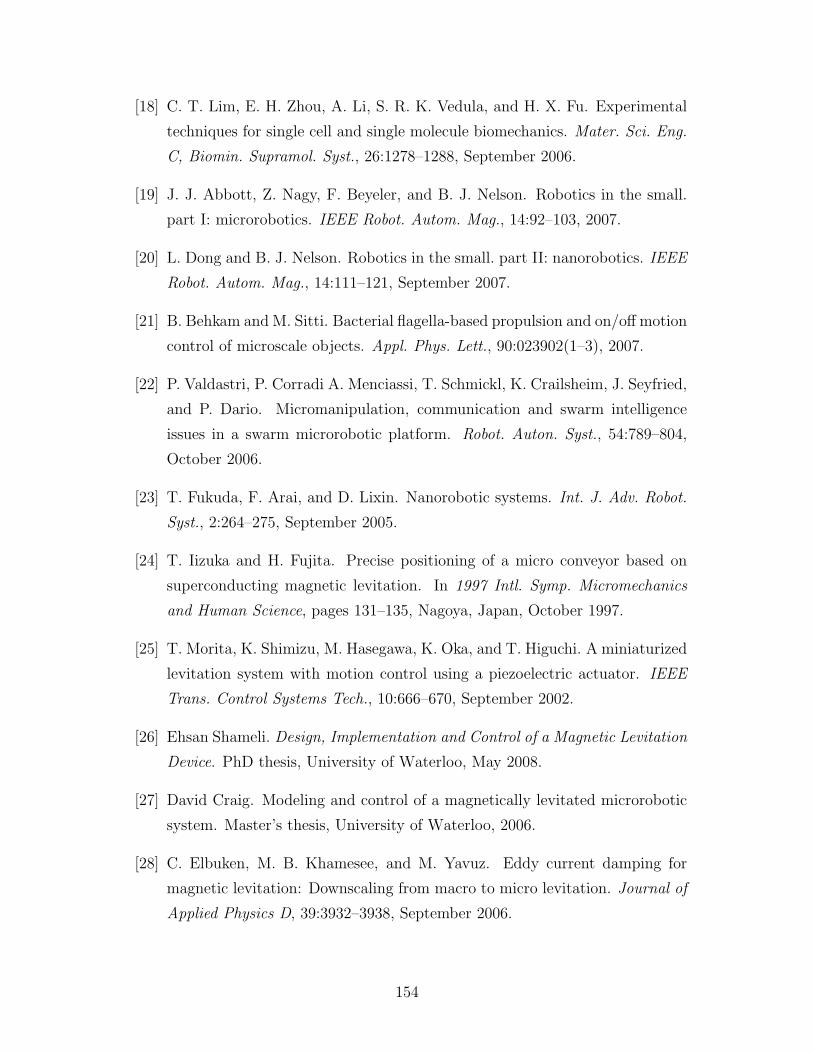
[18] C. T. Lim, E. H. Zhou, A. Li, S. R. K. Vedula, and H. X. Fu. Experimental

techniques for single cell and single molecule biomechanics. Mater. Sci. Eng.

C, Biomin. Supramol. Syst., 26:1278–1288, September 2006.

[19] J. J. Abbott, Z. Nagy, F. Beyeler, and B. J. Nelson. Robotics in the small.

part I: microrobotics. IEEE Robot. Autom. Mag., 14:92–103, 2007.

[20] L. Dong and B. J. Nelson. Robotics in the small. part II: nanorobotics. IEEE

Robot. Autom. Mag., 14:111–121, September 2007.

[21] B. Behkam and M. Sitti. Bacterial flagella-based propulsion and on/off motion

control of microscale objects. Appl. Phys. Lett., 90:023902(1–3), 2007.

[22] P. Valdastri, P. Corradi A. Menciassi, T. Schmickl, K. Crailsheim, J. Seyfried,

and P. Dario. Micromanipulation, communication and swarm intelligence

issues in a swarm microrobotic platform. Robot. Auton. Syst., 54:789–804,

October 2006.

[23] T. Fukuda, F. Arai, and D. Lixin. Nanorobotic systems. Int. J. Adv. Robot.

Syst., 2:264–275, September 2005.

[24] T. Iizuka and H. Fujita. Precise positioning of a micro conveyor based on

superconducting magnetic levitation. In 1997 Intl. Symp. Micromechanics

and Human Science, pages 131–135, Nagoya, Japan, October 1997.

[25] T. Morita, K. Shimizu, M. Hasegawa, K. Oka, and T. Higuchi. A miniaturized

levitation system with motion control using a piezoelectric actuator. IEEE

Trans. Control Systems Tech., 10:666–670, September 2002.

[26] Ehsan Shameli. Design, Implementation and Control of a Magnetic Levitation

Device. PhD thesis, University of Waterloo, May 2008.

[27] David Craig. Modeling and control of a magnetically levitated microrobotic

system. Master’s thesis, University of Waterloo, 2006.

[28] C. Elbuken, M. B. Khamesee, and M. Yavuz. Eddy current damping for

magnetic levitation: Downscaling from macro to micro levitation. Journal of

Applied Physics D, 39:3932–3938, September 2006.

154

[29] M. B. Khamesee and E. Shameli. Regulation technique for a large gap mag-

netic field for 3D non-contact manipulation. Mechatronics, 15:1073–1087,

November 2005.

[30] E. Shameli, M. B. Khamesee, and J. P. Huissoon. Nonlinear controller de-

sign for a magnetic levitation device. In ASME/JSME Joint Conference on

Micromechatronics for Information and Precision Equipment (MIPE 2006),

page N/A, Santa Clara, CA, USA, June 2006.

[31] R. Skomski and J. M. D. Coey. Permanent Magnetism. Institute of Physics,

California, USA, 1999.

[32] Magnetic domains. http://www.aacg.bham.ac.uk/magneticMaterials/domains.htm.

A study of magnetism from University of Birmingham.

[33] H. H. Yang, N. V. Myung, J. Yee, D. Y. Park, B. Y. Yoo, and M. Schwartz.

Ferromagnetic micromechanical magnetometer. Sensors and Actuators A,

97-98:88–97, April 2002.

[34] J. P. Jakubovics. Magnetism and Magnetic Materials. Institute of Materials,

London, UK, 1994.

[35] T.Matsuura, T. Fukami, M. Chabloz, Y. Sakai, S. I. Izuo, A. Uemura, S. I.

Kaneko, K. Tsutsumi, and K. Hamanaka. Silicon micro optical switching

device with an electromagnetically operated cantilever. Sensors and Actuators

A, 8:220–224, May 2000.

[36] B. Vikramaditya, B. J. Nelson, G. Yang, and E. T. Enikov. Microassembly

of hybrid magnetic MEMS. Journal of Micromechatronics, 1:99–116, April

2001.

[37] Y. Shinozawa, T. Abe, and T. Kondo. A proportional microvalve using a bi-

stable magnetic actuator. In IEEE The Tenth Ann, Intl. Workshop on Micro

Electro Mechanical Systems, pages 233–237, Nagoya, Japan, January 1997.

[38] L. K. Lagorce and M. G. Allen. Magnetic and mechanical properties of micro-

machined strontium ferrite/polymide composites. Journal of Micromechani-

cal Systems, 6:307–312, December 1997.

155

[39] L. K. Lagorce, O. Brand, and M. G. Allen. Magnetic microactuators based in

polymer magnets. Journal of Micromechanical Systems, 8:2–9, March 1999.

[40] K. Vollmers, R. Anderson, B. Nelson, and J. Pepin. High strength rare

earth-iron-boron printed magnets used in a long throw-high force electro-

magnetic actuator with microfabricated coils. In IEEE Sixteenth Ann. Intl.

Conf. on Micro Electro Mechanical Systems, pages 60–63, Kyoto, Japana,

January 2003.

[41] B. M. Dutoit, P. A. Besse, H. Blanchard, L. Guerin, and R. S. Popovic.

High performance micromachined Sm2Co17 polymer magnets. Sensors and

Actuators A, 77:178–182, November 1999.

[42] H. Cho and C. H. Ahn. Microscale resin-bonded permanent magnets for

magnetic micro-electro-mechanical systems applications. Journal of Applied

Physics, 93:8674–8676, May 2003.

[43] S. E. Park, P. Y. Jung, and K. B. Kim. Magnetic properties and microstruc-

tural analysis of sputter-deposited and annealed Co-Pt alloys. Journal of

Applied Physics, 77:2641–2647, March 1995.

[44] A. S. Lileev, A. A. Parilov, and V. G. Blatov. Properties of hard magnetic

Nd-Fe-B films versus different sputtering conditions. Journal of Magnetism

and Magnetic Materials, 242-245:1300–1303, March 2002.

[45] L. K. E. B. Serrona, R. Fujisaki, A. Sugimura, T. Okuda, N. Adachi,

H. Ohsato, I. Sakamoto, A. Nokanishi, M. Motokawa, D. H. Ping, and

K. Hono. Enhanced magnetic properties of Nd-Fe-B thin films crystallized by

heat treatment. Journal of Magnetism and Magnetic Materials, 260:406–414,

March 2002.

[46] Q. Zeng, Y. Zhang, M. J. Bonder, and G. C. Hadjipanayis. Fabrication of

Sm-Co/Co (Fe) composites by electroless Co and Co-Fe plating. Journal of

Applied Physics, 93:6498–6500, May 2003.

[47] S. Guan and B. J. Nelson. Fabrication of hard magnetic microarrays by elec-

troless codeposition for MEMS actuator. Sensors and Actuators A, 118:307–

312, February 2005.

156

[48] N. V. Myung, D. Y. Park, M. Schwartz, K. Nobe, H. Yang, C. K. Yang,

and J. W. Judy. Electrodeposited hard magnetic thin films for MEMS ap-

plications. In Sixth Intl. Symposium on Magnetic Materials, Processes and

Devices, pages 2000–2029, Pheonix, AZ, USA, October 2000.

[49] S. Guan and B. J. Nelson. Electrodeposition of low residual stress CoN-

iMnP hard magnetic thin films for magnetic MEMS actuators. Journal of

Magnetism and Magnetic Materials, 292:49–58, February 2005.

[50] C. K. Hu and J. M. E. Harper. Copper interconnections and reliability.

Material Chemistry and Physics, 52:5–18, February 1998.

[51] W. Xu, J. Wong, C. C. Cheng, R. Johnson, and R. Scherer. Fabrication

of ultrasmall magnets by electroplating. Journal of Vacuum Science and

Technology B, 13:2372–2375, November 1995.

[52] D. M. Tench and J. T. White. Considerations in electrodeposition of compo-

sitionally modulated alloys. Journal of the Electrochemical Society, 137:3061–

3066, October 1990.

[53] F. H. Edelman. The Preparation and Characteristics of Thin Ferromagnetic

Films. Technical Report no. PB151525, US Department of Commence, 1958.

[54] I. W. Wolf. Electrodeposition of magnetic materials. Journal of Applied

Physics, 33:1152–1159, March 1962.

[55] J. Horkans, D. J. Seagle, and I. H. Chang. Electroplated magnetic media

with vertical anisotropy. Journal of the Electrochemical Society, 137:2056–

2061, July 1990.

[56] M. Paunovic and M. Schlesinger. Fundamentals of Electrochemical Deposi-

tion. John Wiley & Sons, New Jersey, USA, 1998.

[57] M. Prutton. Thin Ferromagnetic Films. Butterworth & Co. Ltd., London,

UK, 1964.

[58] H. J. Cho and C. H. Ahn. A bidirectional magnetic microactuator using

electroplated permanent magnet arrays. Journal of Microelectromechanical

Systems, 11:78–84, February 2002.

157

[59] S. Armyanov. Crystallographic structure and magnetic properties of elec-

trodeposited cobalt and cobalt alloys. Electrochimica Acta, 45:3323–3335,

May 2000.

[60] D. Cullity B and S. R. Stock. Elements of X-ray Diffraction. Prentice Hall,

New Jersey, USA, 2001.

[61] I. Koiwa, T. Osaka, Y. Yamazaki, and T. Namikawa. A study on the crystal

growth of the electroless-plated Co-Ni-Re-P alloy films for perpendicular mag-

netic recording. IEEE Transactions on Magnetics, 23:2800–2802, September

1987.

[62] T. Osaka, N. Kasai, I. Koiwa, F. Gato, and Y. Suganuma. A preparation

of perpendicular magnetic recording media by an electroless plating method.

Journal of the Electrochemical Society, 130:568–571, March 1983.

[63] J. R. Davis. ASM Specialty Handbook : nickel, cobalt, and their alloys. ASM

International.

[64] I. Zana. Magnetic and Structural Characterization of High Anisotropy Co-

rich Alloys: Thin Films and Patterns. PhD thesis, University of Alabama,

May 2003.

[65] S. Guan and B. J. Nelson. Electrodeposition of low residual stress CoN-

iMnP hard magnetic thin films for magnetic MEMS actuators. Journal of

Magnetism and Magnetic Materials, 292:49–58, February 2005.

[66] H. J. Cho and C. H. Ahn. A novel bi-directional magnetic microactuator using

electroplated permanent magnet arrays with vertical anisotropy. In IEEE,

Thirteenth Annual Intl. Conference on Micro Electro Mechanical Systems,

pages 686–691, Piscataway, NJ, USA, October 2000.

[67] T. F. Liakopoulos, W. Zhang, and C. H. Ahn. Electroplated thick CoNiMnP

permanent magnet arrays for micromachined magnetic device applications.

In IEEE, The Ninth Annual Intl. Workshop on Micro Electro Mechanical

Systems, pages 79–84, San Diego, CA, USA, February 1996.

[68] K. Molhave, T. Wich, A. Kortschack, and P. Boggild. Pick–and–place

nanomanipulation using microfabricated grippers. Nanotechnology, 17:2434–

2441, May 2006.

158

[69] C.-J. Kim, A. P. Pisano, and R. S. Muller. Silicon-processed overhanging

microgripper. J. Microelectromech. Syst., 1:31–36, March 1992.

[70] B. E. Volland, H. Heerlein, and I. W. Rangelow. Electrostatically driven

microgripper. Microelectron. Eng., 61-62:1015–1023, 2002.

[71] K. Ivanova, T. Ivanov, A. Badar, B. E. Volland, I. W. Rangelow, D. An-

drijasevic, F. Sumecz, S. Fischer, M. Spitzbart, W. Brenner, and I. Kostic.

Thermally driven microgripper as a tool for micro assembly. Microelectron.

Eng., 83:1393–1395, April 2003.

[72] J. H. Comtois and V. M. Bright. Applications for surface-micromachined

polysilicon thermal. Sensors Actuators A, A58:19–25, January 1997.

[73] O. Millet, P. Bernardoni, S. Regnier, P. Bidaud, E. Tsitsiris, D. Collard, and

L. Buchaillot. Electrostatic actuated micro gripper using an amplification

mechanism. Sensors Actuators A, A114:371–378, September 2004.

[74] P. Lerch, C. K. Slimane, B. Romanowicz, and P. Renaud. Modelization and

characterization of asymmetrical thermal micro-actuators. J. Micromech.

Microeng., 6:134–137, March 1996.

[75] J. K. Luo, A. J. Flewitt, S. M. Spearing, N. A. Fleck, and W. I. Milne.

Normally closed microgrippers using a highly stressed diamond-like carbon

and ni bimorph structure. Appl. Phys. Lett., 85:5748–5750, December 2004.

[76] S. Ballandras, S. Basrour, L. Robert, S. Megtert, P. Blind, M. Rouillay,

P. Bernede, and W. Daniau. Microgrippers fabricated by the LIGA tech-

nique. Sensors Actuators A, 58:265–272, March 1997.

[77] M. Kohl, B. Krevet, and E. Just. SMA microgripper system. Sensors Actu-

ators A, A97-98:646–652, April 2002.

[78] N. Chronis and L. P. Lee. Electrothermally activated SU-8 microgripper for

single cell manipulation in solution. J. Microelectromech. Syst., 14:857–863,

August 2005.

[79] I. Roch, P. Bidaud, D. Collard, and L. Buchaillot. Fabrication and charac-

terization of an SU-8 gripper actuated by a shape memory alloy thin film. J.

Micromech. Microeng., 13:330–336, March 2003.

159

[80] B. Solano and D. Wood. Design and testing of a polymeric microgripper for

cell manipulation. Microelectron. Eng., 84:1219–1222, May 2007.

[81] H.-S. Choi, D.-C. Lee, S.-S. Kim, and C.-S. Han. The development of a

microgripper with a perturbation-based configuration design method. J. Mi-

cromech. Microeng., 15:1327–1333, 2005.

[82] N.-T. Nguyen, S.-S. Ho, and C. L.-N. Low. A polymeric microgripper with

integrated thermal actuators. J. Micromech. Microeng., 14:969–974, 2004.

[83] D. Sameoto, S.-H. Tsang, and M. Parameswaran. Polymer MEMS processing

for multi-user applications. Sensors Actuators A, 134:457–464, March 2007.

[84] D. J. Bell, T. J. Lu, N. A. Fleck, and S. M. Spearing. MEMS actuators

and sensors: observations on their performance and selection for purpose. J.

Micromech. Microeng., 15:S153–164, 2005.

[85] R. Venditti, J. S. H. Lee, Y. Sun, and D. Li. An in-plane, bi-directional elec-

trothermal MEMS actuator. J. Micromech. Microeng., 16:2067–2070, October

2006.

[86] H. Guckel, J. Klein, T. Christenson, K. Skrobis, M. Laudon, and E. G. Lovell.

Thermo-magnetic metal flexure actuators. In Proc. 5th IEEE Solid-State

Sensor and Actuator Workshop, pages 73–5, Hilton Head Island, SC, USA,

1992.

[87] L. Que, J.-S. Park, and Y. B. Gianchandani. Bent-beam electrothermal

actuators-part i: Single beam and cascaded devices. J. Microelectromech.

Syst., 10:247–254, 2001.

[88] Y. Dong, A. Khajepour, and R. Mansour. Modeling of two-hot-arm horizontal

thermal actuator. J. Micromech. Microeng., 13:312–322, March 2003.

[89] J. K. Luo, A. J. Flewitt, S. M. Spearing, N. A. Fleck, and W. I. Milne.

Comparison of microtweezers based on three lateral thermal actuator config-

urations. J. Micromech. Microeng., 15:1294–1302, 2005.

[90] M. R. Begley and B. N. Scott. Analysis and design of kinked (bent) beam

sensors. J. Micromech. Microeng., 17:350–357, February 2007.

160

[91] R. Hickey, D. Sameoto, T. Hubbard, and M. Kujath. Time and frequency

response of two-arm micromachined thermal actuators. J. Micromech. Mi-

croeng., 13:40–46, January 2003.

[92] V. Seidemann, S. Butefisch, and S. Buttgenbach. Fabrication and investiga-

tion of in-plane compliant SU8 structures for mems and their application to

micro valves and micro grippers. Sensors Actuators A, A97-98:457–461, April

2002.

[93] S. Butefisch, V. Seidemann, and S. Buttgenbach. Novel micro-pneumatic

actuator for MEMS. Sensors Actuators A, A97-98:638–645, April 2002.

[94] B. Kim, D. Collard, M. Lagouge, F. Conseil, B. Legrand, and L. Buchaillot.

Thermally actuated probe arrays for manipulation and characterization of

individual bio-cell. In IEEE Int. Conf. Solid-State Sens. and Act., pages

1255–1258, Boston, MA, USA, 2003.

[95] S.-H. Tsang, D. Sameoto, and M. Parameswaran. Out-of-plane electrothermal

actuators in silicon-on-insulator technology. Can. J. Electr. Comput. Eng.,

31:97–103, 2006.

[96] E. Dieulesaint, D. Royer, and C. Bonnefoy. Mechanical excitation of a mem-

brane by an optical beam. In IEEE 1981 Ultrasonics Symposium, pages

802–805, Chicago, IL, USA, October 1981.

[97] J. Fraser, T. Hubbard, and M. Kujath. Theoretical and experimental analysis

of an off-chip microgripper. Can. J. Electr. Comput. Eng., 31:76–84, 2006.

[98] L. M. Phinney and J. R. Serrano. Influence of target design on the damage

threshold for optically powered MEMS thermal actuators. Sensors Actuators

A, 134:538–543, March 2007.

[99] A. D. Oliver, S. R. Vigil, and Y. B. Gianchandani. Photothermal surface-

micromachined actuators. IEEE Trans. Electron Devices, 50:1156–1157, April

2003.

[100] S. Baglio, S. Castorina, L. Fortuna, and N. Savalli. Modeling and de-

sign of novel photo-thermo-mechanical microactuators. Sensors Actuators

A, 101:185–193, September 2002.

161

[101] N. Lobontiu and E. Garcia. Mechanics of microelectromechanical systems.

Kluwer Academic Publishers, New York, USA, 2005, 186-192.

[102] W. M. Rohsenow, J. P. Hartnett, and Y. Cho. Handbook of heat transfer.

McGraw-Hill, New York, USA, 3rd edition, 1998, 261-393.

[103] S. Kakac and Y. Yener. Heat conduction. Taylor - Francis, Washington DC,

USA, 3rd edition, 1993, 283-313.

[104] MEMS Precision Instruments. http://www.memspi.com/. 2008.

[105] Preiser Scientific Incorporation. http://www.preiser.com/. 2008.

[106] Kleindiek Nanotechnik. http://www.nanotechnik.com/. 2008.

[107] Klocke Nanotechnik. http://www.nanomotor.de. 2008.

[108] MicroChem Corp. MCC Products. http://www.microchem.com/products/index.htm.

2008.

[109] W. Wang and S. A. Soper. Bio-MEMS: Technologies and Applications. Taylor

Francis Group, Florida, USA, 2007, 13-14.

[110] Y.-C. Tsai, S. H. Lei, and H. Sudin. Design and analysis of planar compli-

ant microgripper based on kinematic approach. J. Microelectromech. Syst.,

15:143–156, January 2005.

[111] S. K. Jericho, M. H. Jericho, T. Hubbard, and M. Kujath. Micro-electro-

mechanical systems microtweezers for the manipulation of bacteria and small

particles. Rev. Sci. Instrum., 75:1280–1282, May 2004.

[112] S. K. Jericho and M. H. Jericho. Device for the determination of spring

constants of atomic force microscope cantilevers and micromachined springs.

Rev. Sci. Instrum., 73:2483–2485, 2002.

[113] C. J. Booth. The new IEEE Standard Dictionary of Electrical and Electronics

Terms, 5th ed. The Inst. of Electrical and Electronics Eng. Inc., New York,

USA, 1992, 1138-1139.

162

[114] D.-H. Kim, M. G. Lee, B. Kim, and Y. Sun. A superelastic alloy microgrip-

per with embedded electromagnetic actuators and piezoelectric force sensors:

A numerical and experimental study. Smart Mater. Struct., 14:1265–1272,

December 2005.

[115] F. Arai, D. Andou, Y. Nonoda, T. Fukuda, H. Iwata, and K. Itoigawa. Inte-

grated microendeffector for micromanipulation. IEEE/ASME Trans. Mecha-

tronics, 3:17–23, 1998.

[116] Y. Rollot, S. Regnier, and J.C. Guinot. Simulation of micromanipulations:

adhesion forces and specific dynamic models. Int. J. Adhes. Adhes., 19:35–48,

May 1999.

[117] S. Floyd, C. Pawashe, and M. Sitti. An untethered magnetically actuated

micro-robot capable of motion on arbitrary surfaces. In 2008 IEEE Interna-

tional Conference on Robotics and Automation. The Half-Day Workshop on:

Towards Autonomous Agriculture of Tomorrow, pages 419–424, Pasadena,

CA, USA, May 2008.

[118] NDI Measurement You Can Trust. http://www.ndigital.com/. 2008.

[119] P. Lambert and S. Regnier. Surface and contact forces models within the

framework of microassembly. J. Micromechatronics 3, 2:123–157, 2006.

[120] U. S. Inan and A. S. Inan. Engineering Electromagnetics. Addison-Wesley,

Menlo Parl, California, USA, 1999.

163