
Machine learning techniques for autonomous multi-sensor ...
189
Machine Learning Techniques for Autonomous Multi-Sensor Long-Range Environmental Perception System Muhammad Abdul Haseeb Universität Bremen 2020
-
Upload
khangminh22 -
Category
Documents
-
view
1 -
download
0
Transcript of Machine learning techniques for autonomous multi-sensor ...
Machine Learning Techniques for Autonomous
Multi-Sensor Long-Range Environmental Perception
System
Muhammad Abdul Haseeb
Universität Bremen 2020

Machine Learning Techniques for Autonomous
Multi-Sensor Long-Range Environmental Perception
System
Vom Fachbereich für Physik und Elektrotechnik
der Universität Bremen
zur Erlangung des akademischen Grades
Doktor–Ingenieur (Dr.-Ing.)
genehmigte Dissertation
von
M.Sc. Muhammad Abdul Haseeb
aus Pakistan
Referent: Prof. Dr.-Ing. Axel Gräser
Korreferent: Prof. Dr.-Ing. Udo Frese
Eingereicht am: 04.09.2020
Tag des Promotionskolloquiums: 28.01.2021


i
Acknowledgements
First of all, I would like to express my gratitude to my supervisor Prof. Dr.-Ing. Axel
Gräser for offering me a Ph.D. position at the Institute of Automation (IAT) and for
his valuable guidance, expert advice, and support throughout my research work. I
would like to thank Prof. Dr.-Ing. Udo Frese for accepting to be the second reviewer
of this thesis as well as Prof. Dr.-Ing. Alberto Garcia-Ortiz and Prof. Dr.-Ing. Walter
Lang for accepting to be examiners of this thesis.
I would like to express my gratitude to my colleague Dr. Danijela Ristic-Durrant for
extended discussions and valuable suggestions which have significantly contributed to
the improvement of the thesis. Additionally, I would like to thank my former
colleague Dr.-Ing. Maria Kyrarini for her encouragement and support.
Special thanks to the University of Nis partners for making the arrangments and
obtaining the permits to perform experiments on the Serbian railway's sites, which
helps to collect data for the thesis. My gratitude goes as well to all the participants in
my experiments. I would like to thank Mr. Michael Ehlen for his technical support. I
also thank all students who during the work on their Master Theses and Master
Projects contributed to this thesis.
I am very thankful to the Postgraduate International Programme (PIP) of Physics and
Electrical Engineering faculty at the University of Bremen for partially funding my
participation in conferences.
I am deeply thankful to my parents, sister, and brother, for their love and
unconditional support. I am forever grateful to my parents for giving me the
opportunities and experiences that have made me who I am. Their encouragement
made me pursue my destiny and explore new directions in life. I dedicate this
milestone to them.
My thesis acknowledgement would be incomplete without thanking my wife Zarmeen
for always being there for me, without her, this thesis would never have written and
my baby-daughter, Ayra, whose smiling face always made me happy and inspired me.
Having her midway during my Ph.D. was certainly not easy for me, but she has made
my life wonderful, better, and more fulfilled than I could have ever imagined.

ii
iii
Abstract
An environment perception system is one of the most critical components of an
automated vehicle, which is defined as a vehicle where the driver does not require to
monitor the vehicle’s behaviour and its surroundings during driving. This thesis
addresses some of the main challenges in the development of vision-based
environment perception methods for automated driving, focusing on railway vehicles.
The thesis aims at developing methods for detecting obstacles on the rail tracks in
front of a moving train to reduce the number of collisions between trains and various
obstacles, thus increasing the safety of rail transport.
In the field of autonomous obstacle detection for automated driving, besides
recognising the objects on the way, the crucial information for collision avoidance is
estimated distances between the vehicle and the recognised objects (e.g. cars,
pedestrians, cyclists). With the limited capabilities of current state-of-the-art sensor-
based environment perception approaches, it is unrealistic to detect distant objects and
estimates the distance to them. Mid-to-long-range obstacle detection system is one of
the fundamental requirements for heavy vehicles such as railway vehicle or trucks,
due to required long braking distance. However, this problem is unaddressed in the
computer vision community. The emphasis of this thesis is on the development of
robust and reliable algorithms for real-time vision-based mid-to-long-range obstacle
detection. In this thesis, the algorithms for obstacle detection from single cameras
were developed and evaluated on images captured from RGB, Thermal and Night-
Vision camera.
The developed algorithms are based on advanced machine/deep learning techniques.
The development of machine-learning-based algorithms was supported by a novel
mid-to-long-range obstacle detection dataset for railways that is proposed in the
thesis, which compiles of annotated images with the object class, bounding box, and
ground truth distance to the object.
The developed novel methods for autonomous long-range obstacle detection, tracking
and distance estimation for railways were evaluated on real-world images, which were
recorded in different illumination and weather conditions by the obstacle detection
system mounted on a static test-bed set-up on the straight rail track and as well on a
iv
moving train. Although the focus is on railways, the developed algorithms are also
capable to use for road vehicles, hence evaluated on the images of road-scene
captured by a camera mounted on moving cars.
v
Kurzfassung
Ein System zur Wahrnehmung der Umgebung ist eine der kritischsten Komponenten
eines automatisierten Fahrzeugs, der Definition nach also eines Fahrzeugs, bei dem
der Fahrer das Verhalten des Fahrzeugs und seiner Umgebung während der Fahrt
nicht überwachen muss. Diese Arbeit befasst sich mit einigen der wichtigsten
Herausforderungen in der Entwicklung sensorgestützter Methoden zur
Umgebungswahrnehmung im Kontext automatisierten Fahrens, wobei der
Schwerpunkt auf Schienenfahrzeugen liegt. Ziel der Arbeit ist die Entwicklung von
Methoden zur Erkennung von Hindernissen auf den Gleisen vor einem fahrenden
Zug, um die Anzahl der Kollisionen zwischen Zügen und verschiedenen Hindernissen
zu reduzieren und damit die Sicherheit des Schienenverkehrs zu erhöhen.
Im Bereich der autonomen Hinderniserkennung für automatisiertes Fahren sind neben
der Erkennung der Objekte auf der Straße die für die Kollisionsvermeidung
entscheidenden Informationen die geschätzten Abstände zwischen dem Fahrzeug und
den erkannten Objekten (z.B. Autos, Fußgänger, Radfahrer). Mit den begrenzten
Möglichkeiten der heutigen sensorbasierten Umgebungswahrnehmung ist es
unrealistisch, entfernte Objekte zu erkennen und den Abstand zu ihnen abzuschätzen.
Das System zur Erkennung von Hindernissen im mittleren bis langen Bereich ist
aufgrund des erforderlichen langen Bremsweges eine der grundlegenden
Anforderungen an schwere Fahrzeuge wie Schienenfahrzeuge oder Lastwagen. Dieses
Problem wird jedoch in der Computer-Vision-Gemeinschaft nicht angegangen. Der
Schwerpunkt dieser Arbeit liegt in der Entwicklung echtzeitfähiger, robuster und
zuverlässiger Algorithmen für eine bildbasierende Hinderniserkennung im mittleren
bis langen Bereich. In dieser Arbeit werden die Algorithmen zur Hinderniserkennung
von Einzelkameras entwickelt und anhand von Bildern, die von RGB-, Wärme- und
Nachtsichtkameras aufgenommen wurden, bewertet.
Die entwickelten Algorithmen basieren auf fortgeschrittenen machine/deep learning
Techniken. Die Entwicklung der auf maschinellem Lernen basierenden Algorithmen
wurde durch einen neuartigen Datensatz zur Hinderniserkennung im mittleren bis
langen Bereich für Eisenbahnen unterstützt, der in der Arbeit vorgeschlagen wurde
und der aus annotierten Bildern mit der Objektklasse, der Bounding Box und dem
Abstand zum Objekt zusammengestellt wurde.

vi
Die entwickelten neuartigen Methoden zur autonomen weiträumigen
Hinderniserkennung, -verfolgung und -abschätzung für Eisenbahnen wurden an realen
Bildern evaluiert, die unter verschiedenen Beleuchtungs- und Witterungsbedingungen
durch das Hinderniserkennungssystem auf einem statischen Prüfstandsaufbau auf der
geraden Schiene und auch auf einem fahrenden Zug aufgenommen wurden. Obwohl
der Schwerpunkt auf Eisenbahnen liegt, wurden die entwickelten Algorithmen auch
auf den Bildern der Straßenszene ausgewertet, die von einer auf einem fahrenden
Wagen montierten Kamera aufgenommen wurden.

vii
viii
Table of Contents
Acknowledgements ......................................................................................................... i
Abstract ........................................................................................................................ iii
Kurzfassung .................................................................................................................... v
1. Introduction ............................................................................................ 1
1.1 Problem statement .................................................................................................... 2
1.2 Thesis Contributions ................................................................................................ 3
1.3 Thesis Overview ....................................................................................................... 5
2. Machine learning-based environmental perception for
autonomous systems ..................................................................................... 7
2.1 Machine learning techniques .................................................................................... 7
2.1.1 Supervised Learning ................................................................................. 8
2.1.2 Unsupervised learning .............................................................................. 9
2.1.3 Semi-supervised learning ......................................................................... 9
2.1.4 Reinforcement learning ............................................................................ 9
2.2 Artificial neural networks....................................................................................... 10
2.2.1 Activation Function ................................................................................ 11
2.2.2 Training .................................................................................................. 12
2.2.3 Optimisation algorithm .......................................................................... 13
2.2.4 Regularisation ........................................................................................ 13
2.2.5 Error and Loss function .......................................................................... 14
2.2.6 Hyperparameter ...................................................................................... 15
2.2.7 Training, testing and validation set ........................................................ 16
2.3 Deep Neural Networks ........................................................................................... 16
2.3.1 Deep Learning for Computer vision ...................................................... 18
2.3.1.1. Classification ...................................................................................... 21
2.3.1.2. ............................................................................................................. 21
2.3.1.3. ............................................................................................................. 22
2.3.2 You Only Look Once (YOLO) .............................................................. 22
2.4 Datasets for environmental perception ................................................................... 34
2.4.1 Kitti Dataset ........................................................................................... 35
2.5 Distance estimation ................................................................................................ 38
2.5.1 LiDAR .................................................................................................... 38
ix
2.5.2 RADAR .................................................................................................. 39
2.5.3 Stereo Camera ........................................................................................ 39
2.5.4 Monocular Camera-based approaches ................................................... 42
2.5.1 Evaluation Matrices ............................................................................... 44
3. Dataset for long-range object detection and distance estimation ... 46
3.1. Dataset Preparation ............................................................................................... 47
3.1.1.Sensors Specifications ............................................................................ 48
3.1.2. Data Collection Experiments ................................................................ 53
3.1.3. Data Acquisition Procedure .................................................................. 57
3.1.4 Dataset labelling ..................................................................................... 58
3.2 Data Augmentation ................................................................................................ 61
4. A machine learning-based distance estimation from a single
camera .......................................................................................................... 65
4.1 DisNet: a machine learning-based object-specific distance estimation from a single
camera .......................................................................................................................... 65
4.1.1 Feature Extraction .................................................................................. 67
4.1.2 DisNet architecture and training ............................................................ 68
4.1.3. Performance Evaluation ........................................................................ 72
4.2 YOLO-D: a deep learning-based object-specific distance estimation from a single
camera .......................................................................................................................... 86
4.2.1 Modification of YOLOv3 network ........................................................ 87
4.2.2 Loss Function ......................................................................................... 89
4.2.3 Dataset preparation ................................................................................. 90
4.2.4 Training and testing ................................................................................ 92
4.2.5 Performance Evaluation ......................................................................... 94
4.2.6 Discussion ............................................................................................ 105
5. A machine learning based distance estimation from multiple
cameras ...................................................................................................... 108
5.1 Multi-DisNet: a machine learning-based robust distance estimation from multiple
cameras ...................................................................................................................... 108
5.1.1 Feature Extraction ................................................................................ 109
5.1.2 Multi-DisNet Architecture ................................................................... 110
5.1.3 Performance Evaluation ....................................................................... 111
5.1.3 Discussion ............................................................................................ 117
6. A machine learning based multiple object tracking ....................... 119
x
6.1 DisNet-RNN Tracker: robust distance estimation and multiple objects tracking
from a single camera .................................................................................................. 120
6.1.1 Deep Learning Network architecture ................................................... 122
6.1.2 Dataset .................................................................................................. 124
6.1.3 Features selection ................................................................................. 125
6.1.4 Training and testing phase ................................................................... 126
6.1.5 Multiple Object Mapping (MOM) ....................................................... 128
6.1.6 Evaluation ............................................................................................ 128
6.1.7 Discussion ............................................................................................ 130
7. Real-time Performance Evaluation .................................................. 133
7.1 Requirement Analysis ..................................................................................... 133
7.2 Hardware ......................................................................................................... 135
7.2.1 Sensors ............................................................................................. 136
7.2.2 Network ............................................................................................ 136
7.2.3 Processing unit ................................................................................. 137
7.3 Software .......................................................................................................... 137
7.3. Machine learning-based algorithms timing considerations ............................ 139
8. Conclusion and Outlook .................................................................... 143
8.1 Conclusion ...................................................................................................... 143
8.2 Outlook ........................................................................................................... 145
Bibliography ............................................................................................................... 147
Appendix A: Publications by the author .................................................................... 164
Abbreviations ............................................................................................................. 167
Table of Figures ......................................................................................................... 169

i
1
1. Introduction
Autonomous environment perception is one of the fundamental elements of
automated vehicles as well as of many other autonomous indoor and outdoor
applications such as mobile robots [1], assistive robots [2], and industrial robots [3].
The purpose of environment perception systems is to provide crucial information on
the autonomous system surroundings, including potential obstacles, their velocities
and locations, and even prediction of their future states. The collected information
helps the automated vehicle in many ways, such as to avoid collision with obstacles,
localisation, and navigation [4].
As research in the field of autonomous systems has matured in the previous decades,
outstanding work has been seen in the advancements of the environment perception
systems. Environment perception for automated vehicles typically combines multiple
sensing technologies (i.e., LiDAR, radar, ultrasound, and visual) to detect obstacles
and to provide their physical position in the environment. The fusion of multiple
sensing technologies helps to overcome the drawbacks and limitations of one sensor
by utilising the benefits of others [4].
Though the accuracy of the active sensing technologies such as LiDAR, RADAR, and
ultrasound sensors is high, it is quite computational power consuming and expensive.
On the other side, cameras are considered as the most functioning perception sensor
which provides rich visual information of the surrounding, with every possible detail
in it, in the form of images [5]. Cameras work in the same way as the human eye; help
to detect and classify objects, understand the situation, and estimate the depth.
However, the depth estimation is a critical task using cameras. Stereo-vision is the
most common approach to estimate depth. The images taken by two cameras are used
to triangulate and estimate distances [6].
1.1 Problem statement
2
Although stereo-vision systems work well in many applications, they are
fundamentally limited by the baseline, which is the distance between the two stereo
cameras. The stereo-vision based depth estimates tend to be inaccurate when the
distances measured are large as the baseline is long. The reason behind the inaccurate
measurement for longer distance is that even very minor errors in triangulation
estimation cause very large errors in distance measurement [7]. Additionally, stereo-
vision tends to fail for textureless regions of images, in which it is difficult to find the
corresponding regions reliably [8].
Monocular cameras-based vision detection systems have been proposed to overcome
the limitations of stereo-vision. As traditional monocular vision is unable to provide
accurate and robust distance measurement, most of the methods are machine learning-
based solutions [9]. These monocular cameras based object detection approaches rely
on the dataset with ground truth collected via LiDAR or stereo-vision [10].
1.1 Problem statement
Many approaches for autonomous environmental perception have been presented for
different application fields and scenarios. Whereas other transport modes have been
quick to automate certain operations, the rail runs the risk of lagging behind. One of
the critical challenges, which has so far hindered the automation of rail systems, is the
lack of a safe and reliable onboard obstacle detection system for trains within existing
infrastructure [11]. In recent years, there is a tendency to use experience from obstacle
detection both in the automotive and the aviation sector for the development of
autonomous obstacle detection in railways [12] [13]. While the main principle of
obstacle detection in front of a vehicle from the automotive sector can be applied to
railway applications, there are also specific challenges. Since this topic is not much
explored, there are countless challenges, and one of the primary challenges is Long-
Range Obstacle Detection.
Long-range obstacle detection: Sensor technology in current land transport research
can look some 200 m ahead [14]. The required rail obstacle detection interfacing with
loco control should be able to look ahead up to 1000 m detecting objects on and near
track which may potentially interfere with the clearance and ground profile. The trains
are running with high speed due to which and the train size and weight, the braking
1.1 Problem statement
3
distance is much longer than for road vehicles. Therefore, a long-range obstacle
detection system for railway vehicles is crucial. It is a very challenging task to detect
objects in real-time which are at far distance and project in a couple of pixels on an
image plane [15].
1.2 Thesis Contributions
The focus of this thesis is on long-range autonomous environmental perception.
Therefore the novel algorithms for object detection, distance estimation, multiple
object tracking, and sensor fusion are presented. The long-range perception is
required and needed in many areas such as long-range obstacle detection system for
autonomous trains or other heavy vehicles. The methods for long-range obstacle
detection presented in this thesis are developed with the main goal of providing a
solution to railways. However, the same methods can be used for self-driving cars as
well; hence the evaluation of the developed was also performed on images of road
scenes taken from a camera mounted on a moving passenger car.
The developed methods for railway scenarios were evaluated on the images taken by
cameras of a prototype autonomous Obstacle Detection System (ODS) developed
within the H2020 Shift2Rail project SMART-Smart Automation of Rail Transport
[11] [16].
The major contributions of this thesis are listed below:
1. Long-range object detection and distance estimation dataset (LRODD)
There are object detection datasets available that contain labeled objects and
distance information however the size of objects in images is relatively large
due to the ground truth distance up to nearly 150 meters. There are no datasets
available which provide annotated bounding boxes of distant objects at more
than 150 meters with the ground truth distance information which indeed
required to build long-range obstacle detection system. A novel dataset for
long-range object detection is presented in this thesis. The dataset is built on
the images acquired from three RGB cameras set up at different zooming
factors to cover short, mid to long-distance range, a thermal camera, a night
vision camera, a LiDAR sensor for short-range ground truth distance
measurement, and a GPS (Global Positioning System) sensor for positioning.
1.1 Problem statement
4
The dataset contains the images of rail scenes that occurred during the data
recording experiments taking place in the lifetime of H2020 Shift2Rail Project
SMART. Although containing images of rail scenes, the dataset can be used in
many other applications for long-range obstacle detection, distance estimation,
and tracking, such as automotive and robotics applications. The dataset ranges
from 0 to 1000 meters and contains several object classes.
2. A single camera-based distance estimation to a detected object in an image
(DisNet)
Distance estimation to the detected object using a vision sensor either with the
monocular camera or stereo cameras is one of the critical tasks in computer
vision. In this thesis, a novel method for long-range distance estimation using
a single camera is presented. The proposed method is able to work with any
type of monocular camera, such as thermal or RGB camera, and can estimate
the distance to the object from short to long-range depending on the resolution
of the image. The method can be used in various applications where distance
estimation is required for short to long-range using a monocular camera.
Moreover, the method does not require any prior calibration of the camera.
3. Distant object detection and distance estimation (YOLO-D)
Current state-of-the-art object detection methods are designed to localise and
classify the objects in an image. However, they do not estimate object
distance. In this thesis, the existing state-of-the-art machine learning-based
method YOLO (You Only Look Once) for object detection was modified to
estimate the distance to the detected objects and so-called end-to-end learning
was enabled.
4. Sensor fusion of multiple cameras for distance estimation (Multi-DisNet)
A novel machine learning-based sensor fusion method for distance estimation
is presented in this thesis. The method based on the fusion of object detection
results from thermal and RGB camera estimates the distance to the detected
object. The method helps to provide reliable distance estimation to the
obstacle in adverse weather and illumination condition or in the case where
one of the sensors fails to detect the object.
5. Multiple object tracking (DisNet-RNN Tracker)
1.1 Problem statement
5
A machine learning-based method for multiple object tracking is also
investigated in the thesis as a method for improving reliability of object
detection and distance estimation. The method helps to track objects in cases
where the object detection module fails to detect or produces unreliable object
detection. It further helps to estimate the distance to the undetected object
based on the tracked information.
6. Evaluation of developed algorithms in real-world scenarios
The machine learning based algorithms developed in this thesis were tested on
real-world scenarios in railways. The algorithms were developed to meet the
requirements of real-time performance.
1.3 Thesis Overview
This thesis is organized in the following chapters:
• Chapter 2 introduces the application of machine learning in computer vision.
As first, an introduction to machine learning is given, following with the state-
of-the-art machine learning-based computer vision algorithms and their
applications.
• Chapter 3 describes the novel dataset for long-range object detection and
distance estimation LRODD.
• Chapter 4 presents the two novel machine learning-based methods for distance
estimation using a single camera, namely DisNet and YOLO-D. The
performance evaluation of each method is presented within the chapter.
• Chapter 5 describes the machine learning-based sensor-fusion method for
distance estimation from multiple cameras Multi-DisNet. The evaluation
results are discussed in the chapter.
• Chapter 6 presents the methods for multiple objects tracking DisNet-RNN
Tracker and the results achieved.
• Chapter 7 presents the real-time implementation and requirements analysis of
developed methods.
• Chapter 8 summarises the conclusions from all the chapters and discusses the
outlook.

6

2.1 Machine learning techniques
7
2. Machine learning-based
environmental perception for
autonomous systems
The main aim of this chapter is to provide the necessary theoretical background of
machine learning, its application in the field of computer vision and datasets to
support the proposed methods described in the following chapters. Therefore, an
introduction to machine learning and datasets is given followed by state-of-the-art
particularly in vision-based object recognition, distance estimation, and object
tracking.
2.1 Machine learning techniques
Computer Vision is defined as a field of study about how computers see and
understand the content of digital images. Computer vision aims to develop methods
that imitate human visual perception. With the great evolvement in the field of
computer vision in the last couple of decades, still many problems remain unsolved.
The main reason is due to the limited understanding of human vision and the human
brain [17].
However, integration of machine learning and deep learning in computer vision
brought significant advancement in high-level problems such as text understanding
[18], 3D model building (photogrammetry) [19], medical imaging [20], human-
computer interaction [21], automotive safety [22], surveillance [23], fingerprint
recognition and biometrics [24], and others.
Machine learning (ML) is a subgroup of Artificial intelligence (AI). In the last few
decades, several fields were revolutionized within the ML. Neural Network (NN) is a
sub-field of ML, and Deep Learning (DL) lies within the NN [25]. Similar to machine

2.1 Machine learning techniques
8
learning algorithms, deep learning methods can also be classified as follows:
supervised, semi-supervised, or partially supervised, and unsupervised. Additionally,
there is another learning approach category called Reinforcement Learning (RL) or
Deep RL (DRL) that is often discussed under semi-supervised or sometimes
unsupervised approaches to learning [26].
Figure 1. The grouping of AI and its sub-groups [25]
2.1.1 Supervised Learning
Supervised learning is a method of learning that use labelled data. In the case of
supervised approaches, the environment has a set of inputs and corresponding outputs
(xi, yi). For example, if for input xu, the agent predicts yu/= f(xu), the agent will receive
a loss value L(yu, yu/). The agent will modify the network parameters iteratively until
it achieved a better estimate of the desired outputs. After training, the agent will be
able to predict the output close to the desired output on the given set of input from the
environment [27].
Some popular supervised machine learning algorithms are linear regression for
regression problems, random forest for classification and regression problems,
Support vector machines (SVM) for classification problems. Likewise, several
supervised learning approaches are involved in deep learning, including Deep Neural
Networks (DNN), Convolutional Neural Networks (CNN), Recurrent Neural
Networks (RNN), containing Long Short Term Memory (LSTM), and Gated
Recurrent Units (GRU) [25].
Supervised learning can be split into two main types, that are classification and
regression. Classification is used when the required output is categorical for example
2.1 Machine learning techniques
9
sorting of email into “spam” or “non-spam” class, diagnosis of a disease based on
observation of the patient such as sex, blood pressure, or certain symptoms. On the
other hand, regression is used when the output is continuous value; for example, the
prediction of stock based on observation [28].
2.1.2 Unsupervised learning
The unsupervised learning method is based on unlabeled data. The data without the
presence of labels is known as unlabeled data. In this case, the machine learning
model understands the internal representation, pattern, or features to determine
unknown relationships or mapping within the given unlabeled input data. Typically,
clustering, generative, and dimensional reduction techniques come into unsupervised
learning approaches. Most popular unsupervised machine learning algorithms are K-
means for clustering and Apriori algorithm for association rule learning problems
[29]. Generative Adversarial Networks (GAN), RNNs such as LSTM and RL are used
for unsupervised deep learning methods as well [25].
Similar to supervised learning, unsupervised learning is also classified as two main
types which are Clustering and Association. Clustering is used when it is needed to
organise or group data based on similarities between them, for example, grouping
customers based on their purchasing behaviour or interests. Whereas Association is
used to correlate or find relations between variables in the data, for example, you find
the rule if a person buys X also tend to buy Y.
2.1.3 Semi-supervised learning
Semi-supervised learning is another learning method that uses partially labelled
datasets. Typically in this learning technique, a small labelled data together with large
unlabeled data are used in training. Deep Reinforcement Learning (DRL) and
Generative Adversarial Networks (GAN), RNN, including LSTM and GRU, are also
used with semi-supervised learning [30].
2.1.4 Reinforcement learning
Reinforcement learning is another type of Machine Learning, where an agent learns
how to act in a situation by performing actions and observing the results. The main
idea behind RL is that an agent learns from the environment by interacting with it and
2.2 Artificial neural networks
10
by receiving rewards for the taken actions. For the right results, the positive reward is
given to the action and similarly a negative reward in case of bad results. In this way,
an agent learns the sequence of actions to be taken by interacting with the
environment [25].
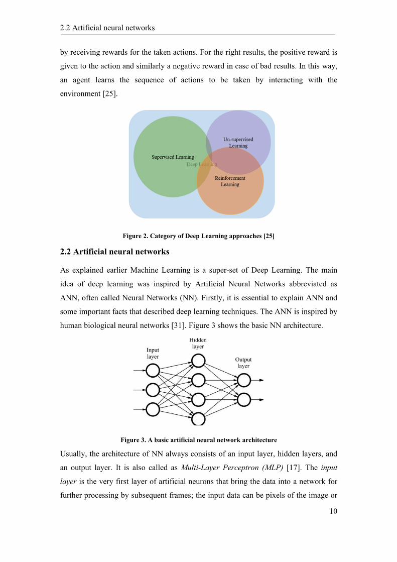
Figure 2. Category of Deep Learning approaches [25]
2.2 Artificial neural networks
As explained earlier Machine Learning is a super-set of Deep Learning. The main
idea of deep learning was inspired by Artificial Neural Networks abbreviated as
ANN, often called Neural Networks (NN). Firstly, it is essential to explain ANN and
some important facts that described deep learning techniques. The ANN is inspired by
human biological neural networks [31]. Figure 3 shows the basic NN architecture.
Figure 3. A basic artificial neural network architecture
Usually, the architecture of NN always consists of an input layer, hidden layers, and
an output layer. It is also called as Multi-Layer Perceptron (MLP) [17]. The input
layer is the very first layer of artificial neurons that bring the data into a network for
further processing by subsequent frames; the input data can be pixels of the image or
2.2 Artificial neural networks
11
any computed feature. The hidden layers are layers between input and output layers
where artificial neurons take weighted input and produce output through an activation
function. The weights of artificial neurons are learned during the training process,
whereas activation function defines the output of the neuron. The output layer is the
final layer of NN that outputs the prediction result based on the input data feed into
the neural network.
Briefly, the Neural Network can be defined as an approximation function of the any
given problem in which learn parameters (weights) in hidden layers multiply with
input and predict output close to desired output [28].
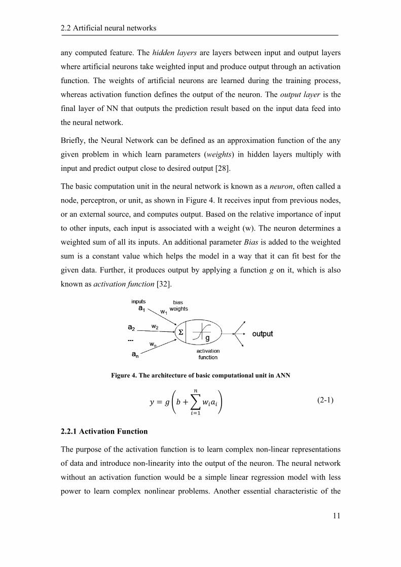
The basic computation unit in the neural network is known as a neuron, often called a
node, perceptron, or unit, as shown in Figure 4. It receives input from previous nodes,
or an external source, and computes output. Based on the relative importance of input
to other inputs, each input is associated with a weight (w). The neuron determines a
weighted sum of all its inputs. An additional parameter Bias is added to the weighted
sum is a constant value which helps the model in a way that it can fit best for the
given data. Further, it produces output by applying a function g on it, which is also
known as activation function [32].
Figure 4. The architecture of basic computational unit in ANN
𝑦 = 𝑔 (𝑏 + ∑𝑤𝑖𝑎𝑖
𝑛
𝑖=1
) (2-1)
2.2.1 Activation Function
The purpose of the activation function is to learn complex non-linear representations
of data and introduce non-linearity into the output of the neuron. The neural network
without an activation function would be a simple linear regression model with less
power to learn complex nonlinear problems. Another essential characteristic of the
2.2 Artificial neural networks
12
activation function is that it should be differentiable. It is required to be differentiable
so as to compute gradients of Error (Loss) with respect to weights while performing
backpropagation optimisation to fine-tune the weights using optimisation techniques
to reduce error. There are many activation functions, but the most popular one is
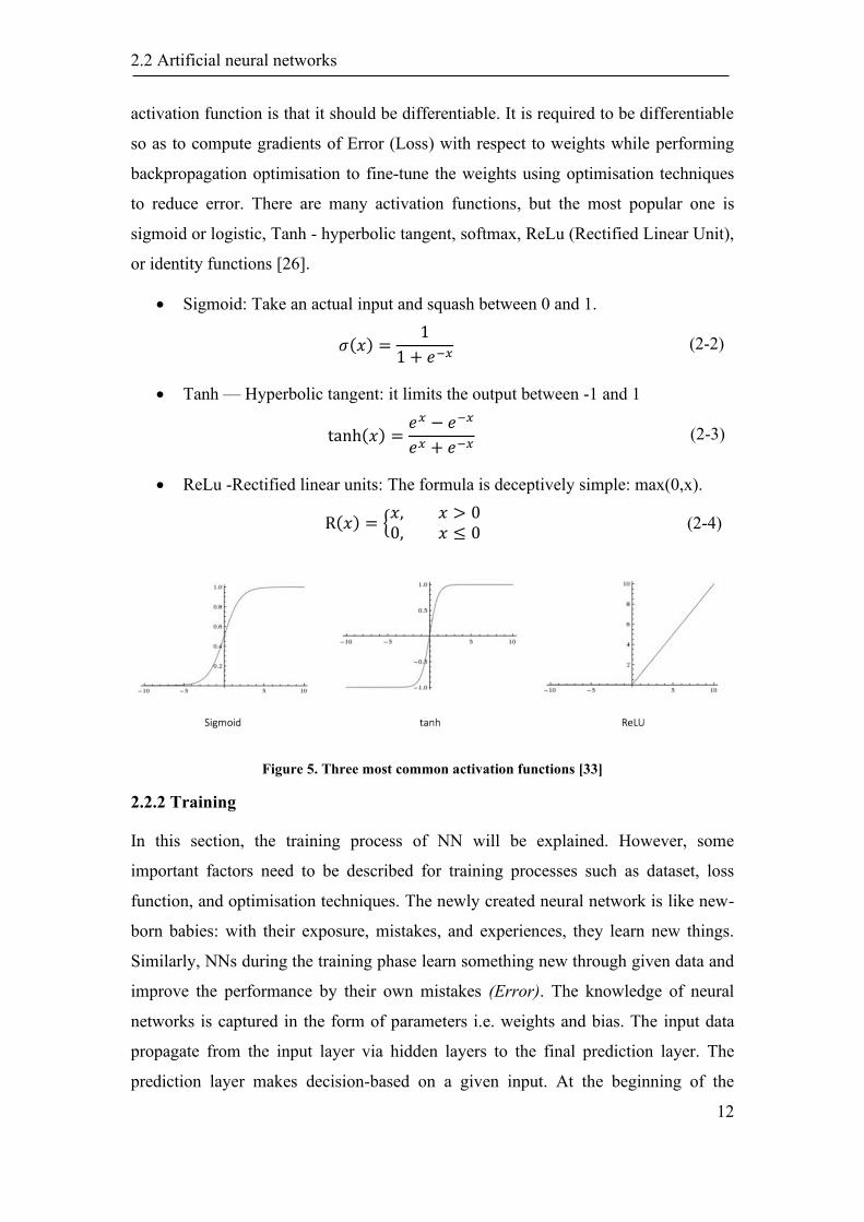
sigmoid or logistic, Tanh - hyperbolic tangent, softmax, ReLu (Rectified Linear Unit),
or identity functions [26].
• Sigmoid: Take an actual input and squash between 0 and 1.
𝜎(𝑥) =1
1 + 𝑒−𝑥 (2-2)
• Tanh — Hyperbolic tangent: it limits the output between -1 and 1
tanh(𝑥) =𝑒𝑥 − 𝑒−𝑥
𝑒𝑥 + 𝑒−𝑥 (2-3)
• ReLu -Rectified linear units: The formula is deceptively simple: max(0,x).
R(𝑥) = {𝑥, 𝑥 > 00, 𝑥 ≤ 0
(2-4)
Figure 5. Three most common activation functions [33]
2.2.2 Training
In this section, the training process of NN will be explained. However, some
important factors need to be described for training processes such as dataset, loss
function, and optimisation techniques. The newly created neural network is like new-
born babies: with their exposure, mistakes, and experiences, they learn new things.
Similarly, NNs during the training phase learn something new through given data and
improve the performance by their own mistakes (Error). The knowledge of neural
networks is captured in the form of parameters i.e. weights and bias. The input data
propagate from the input layer via hidden layers to the final prediction layer. The
prediction layer makes decision-based on a given input. At the beginning of the
2.2 Artificial neural networks
13
training phase, often the decision made by NN is wrong because the parameters
through which data propagate are not optimally adjusted. Typically training process
composed of multiple iterations or also known as epochs until the NN learns correctly
and predicts output close to the desired output. For each epoch, the error is measured
which is defined as Loss function and parameters of NN are adjusted in a way to
reduce the error to make predictions close to the desired output. The error J(w) is the
function of NN internal parameters, i.e. weights and bias. If the parameters change, the
error changes as well [30] [25].
2.2.3 Optimisation algorithm
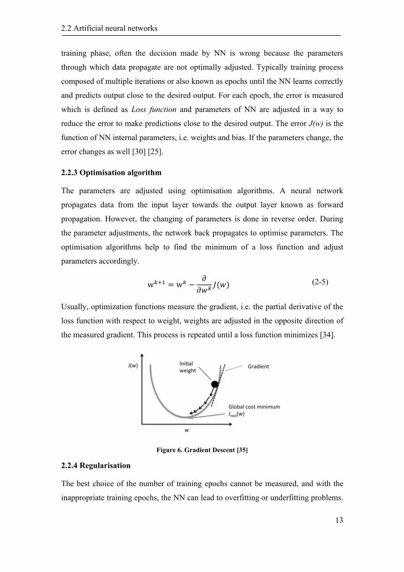
The parameters are adjusted using optimisation algorithms. A neural network
propagates data from the input layer towards the output layer known as forward
propagation. However, the changing of parameters is done in reverse order. During
the parameter adjustments, the network back propagates to optimise parameters. The
optimisation algorithms help to find the minimum of a loss function and adjust
parameters accordingly.
w𝑘+1 = w𝑘 −𝜕
𝜕𝑤𝑘𝐽(𝑤) (2-5)
Usually, optimization functions measure the gradient, i.e. the partial derivative of the
loss function with respect to weight, weights are adjusted in the opposite direction of
the measured gradient. This process is repeated until a loss function minimizes [34].
Figure 6. Gradient Descent [35]
2.2.4 Regularisation
The best choice of the number of training epochs cannot be measured, and with the
inappropriate training epochs, the NN can lead to overfitting or underfitting problems.
2.2 Artificial neural networks
14
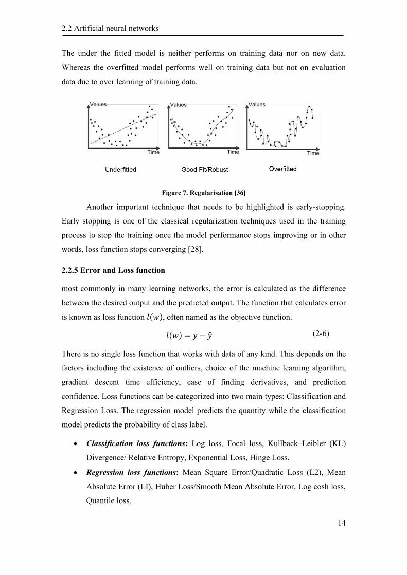
The under the fitted model is neither performs on training data nor on new data.
Whereas the overfitted model performs well on training data but not on evaluation
data due to over learning of training data.
Figure 7. Regularisation [36]
Another important technique that needs to be highlighted is early-stopping.
Early stopping is one of the classical regularization techniques used in the training
process to stop the training once the model performance stops improving or in other
words, loss function stops converging [28].
2.2.5 Error and Loss function
most commonly in many learning networks, the error is calculated as the difference
between the desired output and the predicted output. The function that calculates error
is known as loss function 𝑙(𝑤), often named as the objective function.
𝑙(𝑤) = 𝑦 − �̂� (2-6)
There is no single loss function that works with data of any kind. This depends on the
factors including the existence of outliers, choice of the machine learning algorithm,
gradient descent time efficiency, ease of finding derivatives, and prediction
confidence. Loss functions can be categorized into two main types: Classification and
Regression Loss. The regression model predicts the quantity while the classification
model predicts the probability of class label.
• Classification loss functions: Log loss, Focal loss, Kullback–Leibler (KL)
Divergence/ Relative Entropy, Exponential Loss, Hinge Loss.
• Regression loss functions: Mean Square Error/Quadratic Loss (L2), Mean
Absolute Error (LI), Huber Loss/Smooth Mean Absolute Error, Log cosh loss,
Quantile loss.
2.2 Artificial neural networks
15
Below two very popular regression loss functions are described.
Mean Absolute Error (MAE) – L1 Loss: Another loss function used for regression
models is Mean Absolute Error. It is defined as the sum of the absolute differences
between our target and the variables predicted.
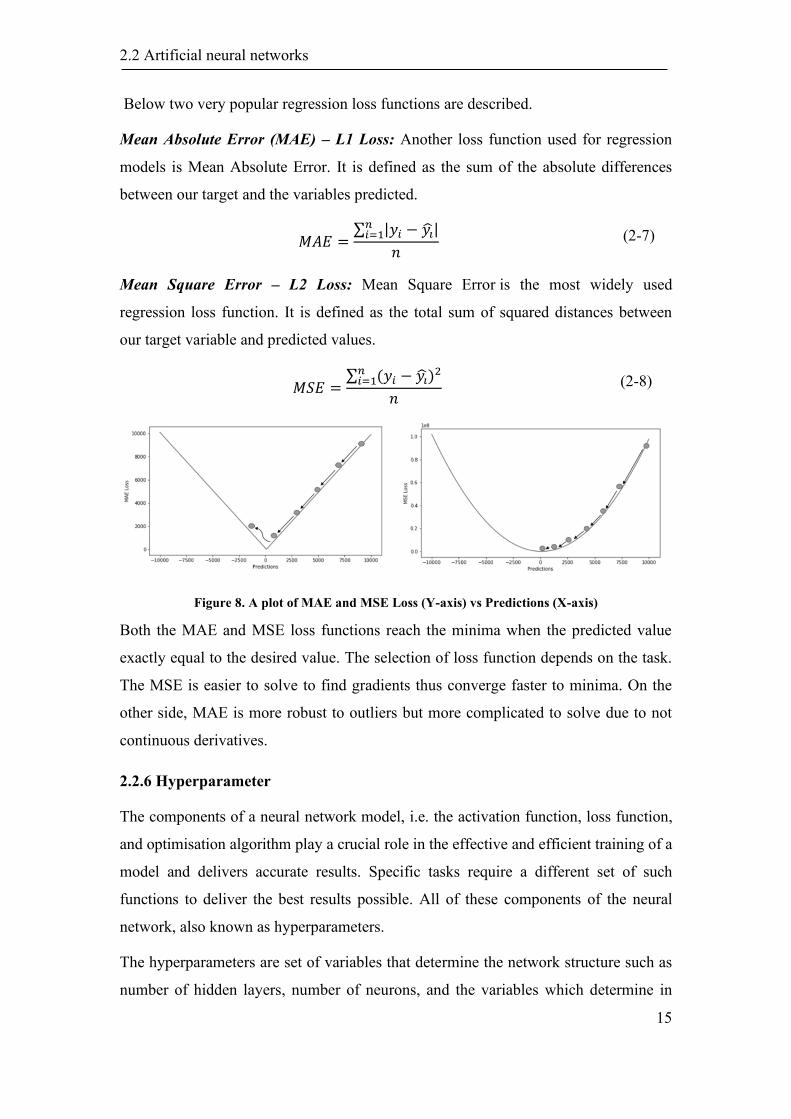
𝑀𝐴𝐸 =∑ |𝑦𝑖 − 𝑦�̂�|
𝑛𝑖=1
𝑛 (2-7)
Mean Square Error – L2 Loss: Mean Square Error is the most widely used
regression loss function. It is defined as the total sum of squared distances between
our target variable and predicted values.
𝑀𝑆𝐸 =∑ (𝑦𝑖 − 𝑦�̂�)
2𝑛𝑖=1
𝑛 (2-8)
Figure 8. A plot of MAE and MSE Loss (Y-axis) vs Predictions (X-axis)
Both the MAE and MSE loss functions reach the minima when the predicted value
exactly equal to the desired value. The selection of loss function depends on the task.
The MSE is easier to solve to find gradients thus converge faster to minima. On the
other side, MAE is more robust to outliers but more complicated to solve due to not
continuous derivatives.
2.2.6 Hyperparameter
The components of a neural network model, i.e. the activation function, loss function,
and optimisation algorithm play a crucial role in the effective and efficient training of a
model and delivers accurate results. Specific tasks require a different set of such
functions to deliver the best results possible. All of these components of the neural
network, also known as hyperparameters.
The hyperparameters are set of variables that determine the network structure such as
number of hidden layers, number of neurons, and the variables which determine in
2.3 Deep Neural Networks
16
what way the network is trained such as weight initialisation, batch size, number of
epochs, learning rate, activation function.
There is no pre-defined or specific way to select the hyperparameters for the
construction and training of a neural network. The most common practice of tuning of
hyperparameters or optimisation of hyperparameters to find the best configuration of
parameters is the manual search method. There are hyperparameters selection
methods such as RandomSearch [37] and GridSearch [38] which find the best
parameters from the given set of parameters. Both methods are very similar; the best
parameters are selected based on the training of network with all possible
combinations of parameters. This method is suitable for simple models which take
less time to train, but if the model takes longer time, almost all deep learning
networks or the search space is big, this approach could not be the best option.
2.2.7 Training, testing and validation set
Usually, the labelled dataset is split into three sets training, validation, and test. The
training set on which the model find optimal values of weights to fit the given set. The
validation set is used during the training process to find optimal hyperparameters of
neural networks, such as the number of hidden layers, stopping point of training, and
others. The test set is used to estimate the performance of the final trained model. The
test set does not have any impact on the training of the neural network. The splitting
of the dataset depends on the size of the dataset. Most commonly, the dataset spits
into 80% for the training set, 10% for validation, and 10% for testing [25] [26].
2.3 Deep Neural Networks
The procedure and techniques of feature extraction and learning are the key difference
between traditional machine learning and deep learning [39]. Traditional machine
learning used handcrafted engineering, several feature extraction methods extract
features, and then the extracted features are provided to the learning model to predict
the output. Additionally, often several pre-processing algorithms are involved in
traditional machine learning. Whereas in deep learning, DL itself extract and learn
features from raw data. DL minimises the human effort by extracting the features
itself. Features are represented hierarchically in the multi-layer network. Similar to
human brain biological neural networks, deep learning contains layered architecture
2.3 Deep Neural Networks
17
where high-level features are extracted from the last layers, and low-level features are
extracted by first layers. Table 1 shows the different learning methods based on the
features with different learning steps [25].
Table 1. Different feature learning approaches
Approaches Learning Steps
Rule-based Input Hand-design
features
Output
Traditional
Machine Learning
Input Hand-design
features
Mapping
from features
Output
Representation
Learning
Input Features Mapping
from features
Output
Deep Learning Input Simple
features
Complex
Features
Mapping
from features
Output
A basic structure of deep neural networks is the traditional ANN network with
multiple hidden layers. The ‘shallow’ neural network has only one hidden layer is
opposed to deep neural network contains more than one hidden layer, often of several
types. There are many deep learning methods rooted in the initial ANNs, including
supervised (DBNs, RNNs, CNNs), unsupervised (AE, DBNs, RBMs, GAN), semi-
supervised (often GAN) and DRL. The deep neural networks learning techniques are
similar to neural networks. However, some advancement is also made in the learning
process to fasten the learning process of a large number of parameters.
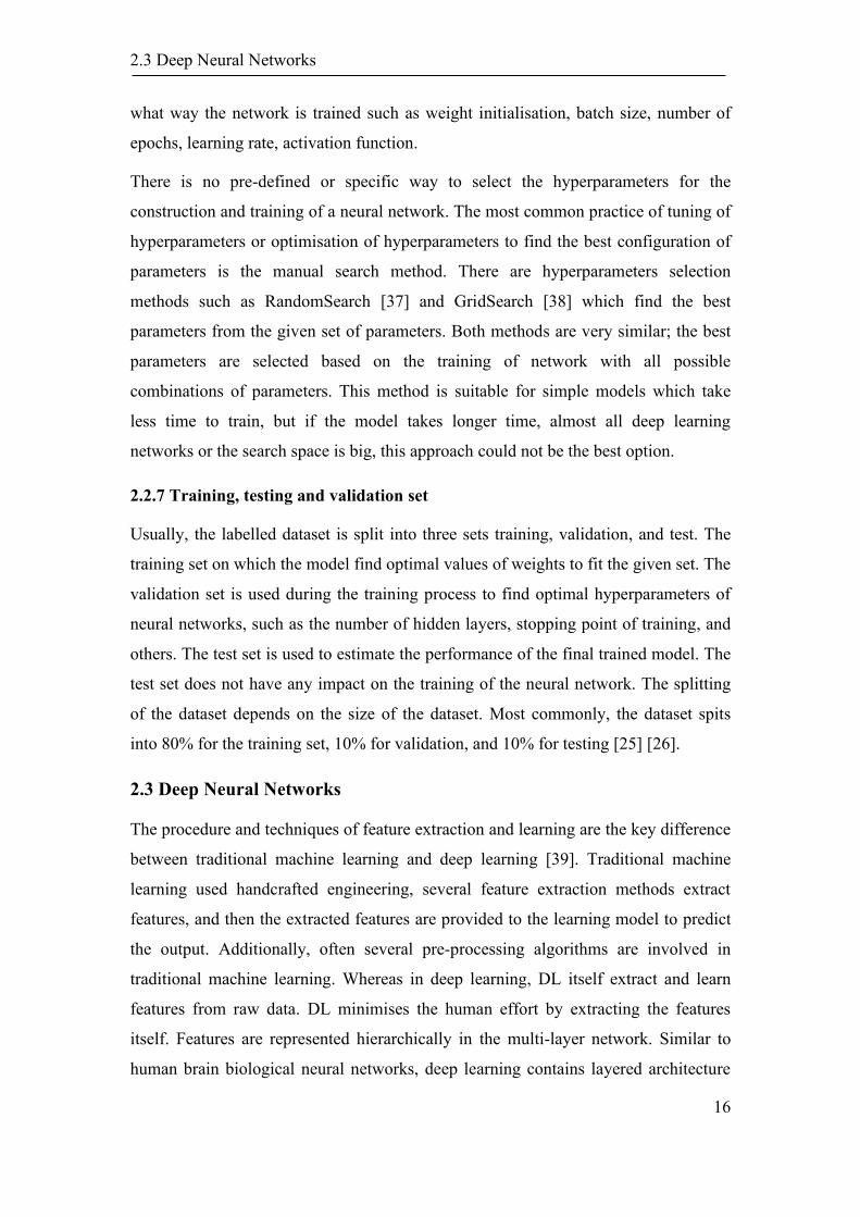
Another significant difference between traditional ML and DL is the performance of
ML and DL with respect to the amount of data. The study [40] shows that the ML
approaches show better performance for a lesser amount of data. Whereas the amount
of data increases beyond certain limits, the performance of ML does not show further
improvements and becomes steady. on the other side, the performance of DL
approaches increases with respect to the increase in the data value [41].
2.3 Deep Neural Networks
18
Figure 9. The deep learning efficiency with regard to the amount of data
2.3.1 Deep Learning for Computer vision
The deep learning often refers to universal learning because it can be used and applied
in many application domains. With the many success stories of deep learning in
almost every field, one of the well-known and evident applications of deep learning is
in Computer Vision (CV). The DNN is widely used in CV and has excellent
capabilities such as in image pattern recognition [39]. Convolution Neural Network
(CNN) is the type of DNN most commonly applied in computer vision to analysing
images in a similar way as human visual sense does. The first Convolution Neural
Network (CNN) was introduced in 1988 however; it was not so popular back then due
to limited sources of computational power to process and train the CNN network. In
the 1990s, the authors [42] achieved excellent results for handwritten digits
classification problems using a gradient-based learning algorithm to CNNs. After that,
the drastic change has been noticed in the 2000s after the revolution of high-
performance processing components such as GPUs [43] and computer platforms such
as Nvidia Drive [44] that were explicitly designed to work for convolutional network
and to work with high-dimensional data [43].
Mostly computer vision problems are surrounded by CNN architectures.
Convolutional Neural Network (CNN) is a type of Deep Neural Networks (DNN) and
is commonly used for image classification and segmentation. A convolutional neural
network (CNN) is made up of an input layer, output layer as well as multiple hidden
layers. In contrast, hidden layers are typically comprised of convolutional layers,
pooling layers, and fully connected layers.
2.3 Deep Neural Networks
19
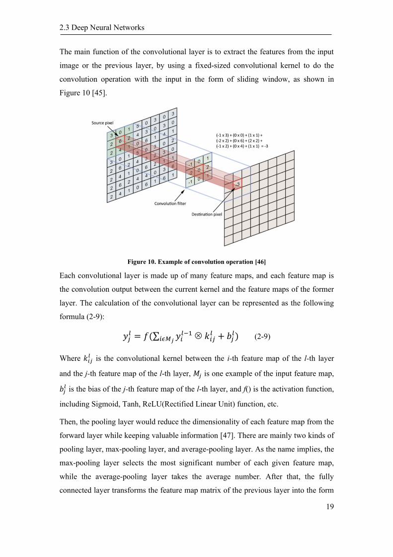
The main function of the convolutional layer is to extract the features from the input
image or the previous layer, by using a fixed-sized convolutional kernel to do the
convolution operation with the input in the form of sliding window, as shown in
Figure 10 [45].
Figure 10. Example of convolution operation [46]
Each convolutional layer is made up of many feature maps, and each feature map is
the convolution output between the current kernel and the feature maps of the former
layer. The calculation of the convolutional layer can be represented as the following
formula (2-9):
𝑦𝑗𝑙 = 𝑓(∑ 𝑦𝑖
𝑙−1𝑖𝜖𝑀𝑗
𝑘𝑖𝑗𝑙 + 𝑏𝑗
𝑙) (2-9)
Where 𝑘𝑖𝑗𝑙 is the convolutional kernel between the i-th feature map of the l-th layer
and the j-th feature map of the l-th layer, 𝑀𝑗 is one example of the input feature map,
𝑏𝑗𝑙 is the bias of the j-th feature map of the l-th layer, and f() is the activation function,
including Sigmoid, Tanh, ReLU(Rectified Linear Unit) function, etc.
Then, the pooling layer would reduce the dimensionality of each feature map from the
forward layer while keeping valuable information [47]. There are mainly two kinds of
pooling layer, max-pooling layer, and average-pooling layer. As the name implies, the
max-pooling layer selects the most significant number of each given feature map,
while the average-pooling layer takes the average number. After that, the fully
connected layer transforms the feature map matrix of the previous layer into the form
2.3 Deep Neural Networks
20
of vector. Finally, the output layer outputs the class by using an activation function,
which includes softmax regression or logistic regression, and classifies the images.
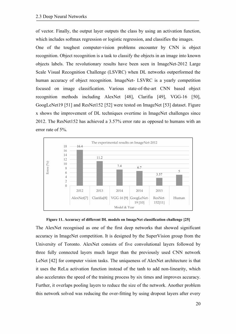
One of the toughest computer-vision problems encounter by CNN is object
recognition. Object recognition is a task to classify the objects in an image into known
objects labels. The revolutionary results have been seen in ImageNet-2012 Large
Scale Visual Recognition Challenge (LSVRC) when DL networks outperformed the
human accuracy of object recognition. ImageNet- LSVRC is a yearly competition
focused on image classification. Various state-of-the-art CNN based object
recognition methods including AlexNet [48], Clarifia [49], VGG-16 [50],
GoogLeNet19 [51] and ResNet152 [52] were tested on ImageNet [53] dataset. Figure
x shows the improvement of DL techniques overtime in ImageNet challenges since
2012. The ResNet152 has achieved a 3.57% error rate as opposed to humans with an
error rate of 5%.
Figure 11. Accuracy of different DL models on ImageNet classification challenge [25]
The AlexNet recognised as one of the first deep networks that showed significant
accuracy in ImageNet competition. It is designed by the SuperVision group from the
University of Toronto. AlexNet consists of five convolutional layers followed by
three fully connected layers much larger than the previously used CNN network
LeNet [42] for computer vision tasks. The uniqueness of AlexNet architecture is that
it uses the ReLu activation function instead of the tanh to add non-linearity, which
also accelerates the speed of the training process by six times and improves accuracy.
Further, it overlaps pooling layers to reduce the size of the network. Another problem
this network solved was reducing the over-fitting by using dropout layers after every
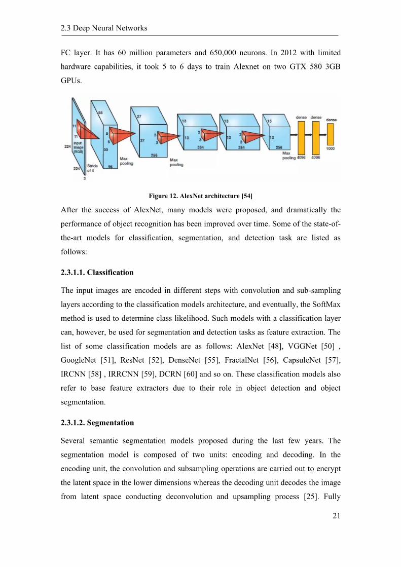
2.3 Deep Neural Networks
21
FC layer. It has 60 million parameters and 650,000 neurons. In 2012 with limited
hardware capabilities, it took 5 to 6 days to train Alexnet on two GTX 580 3GB
GPUs.
Figure 12. AlexNet architecture [54]
After the success of AlexNet, many models were proposed, and dramatically the
performance of object recognition has been improved over time. Some of the state-of-
the-art models for classification, segmentation, and detection task are listed as
follows:
2.3.1.1. Classification
The input images are encoded in different steps with convolution and sub-sampling
layers according to the classification models architecture, and eventually, the SoftMax
method is used to determine class likelihood. Such models with a classification layer
can, however, be used for segmentation and detection tasks as feature extraction. The
list of some classification models are as follows: AlexNet [48], VGGNet [50] ,
GoogleNet [51], ResNet [52], DenseNet [55], FractalNet [56], CapsuleNet [57],
IRCNN [58] , IRRCNN [59], DCRN [60] and so on. These classification models also
refer to base feature extractors due to their role in object detection and object
segmentation.
2.3.1.2. Segmentation
Several semantic segmentation models proposed during the last few years. The
segmentation model is composed of two units: encoding and decoding. In the
encoding unit, the convolution and subsampling operations are carried out to encrypt
the latent space in the lower dimensions whereas the decoding unit decodes the image
from latent space conducting deconvolution and upsampling process [25]. Fully
2.3 Deep Neural Networks
22
Convolutional Network (FCN) is the very first form of segmentation [61]. Later the
improved version of this network which is called SegNet is introduced [62]. Recently,
several new models have been introduced which include RefineNet [63], PSPNEt
[64], and DeepLab [65].
2.3.1.3. Detection
The topic of detection is a bit different compared with classification and segmentation
problems. The purpose of the model is to classify target categories with their
respective positions. The model answers two questions: What is the object
(classification problem)? and where the object (regression problem)? To achieve these
goals, two losses are calculated for classification and regression unit at the top of the
feature extraction module, and the model weights are updated with respect to both
losses. For the very first time, Region-based CNN (RCNN) is proposed for object
detection task [66]. Recently, there are some improved solutions to detection have
been suggested, including focal loss for dense object detector [67] better detection
approaches have been proposed, Later the different improved version of this network
is proposed called fast RCNN [68]. mask R-CNN [69], You only look once (YOLO)
[70] and SSD: Single Shot MultiBox Detector [71]. All these detection models use
classification models as their base to make feature extraction.
In addition, the classical methods can be found back in the 1960s, and later, some of
the widely used methods are Haar-like features [72], SIFT [73], SURF [74], GLOH
[75] and HOG detectors [76].
2.3.2 You Only Look Once (YOLO)
In this section, YOLO object detection model is discussed to support the
implementation and modifications in the next chapters.
Up till 2015, object detection systems were re-purposing existing classifiers to
perform detection. This meant the use of a sliding window technique in looking at
specific regions of the image one by one and making predictions accordingly based on
that region. YOLO (You Only Look Once) identifies object detection as a regression
problem, thereby spatially separating bounding boxes and their associated class
probabilities. YOLO uses a single neural network to detect multiple objects directly
from an RGB camera image and predict its bounding boxes with associated class
2.3 Deep Neural Networks
23
probabilities [70]. Up to now, there are three YOLO version available: YOLO [70],
YOLOv2 [77] and YOLOv3 [78]
2.3.2.1 YOLO
YOLO aims to perform object detection in real-time. Therefore, it does not use the
sliding window technique traversing over the image region by region. Instead, it looks
at the entire image once during training and testing to formulate contextual
information about object appearance and class. This makes YOLO much faster than
other detection algorithms. Competing detection algorithms of the time like Fast R-
CNN [79] had better accuracy when compared to YOLO but was considerably slower
with much more background noise [70].
YOLO is a CNN which uses 24 convolutional layers and two FC (fully connected)
layers. The convolutional layers extract feature maps from the image and the two FC
layers regress the network for bounding box parameters and class.
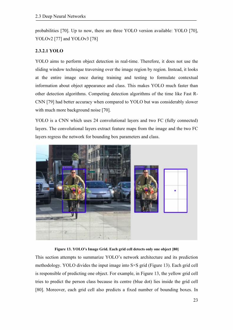
Figure 13. YOLO’s Image Grid. Each grid cell detects only one object [80]
This section attempts to summarize YOLO’s network architecture and its prediction
methodology. YOLO divides the input image into S×S grid (Figure 13). Each grid cell
is responsible of predicting one object. For example, in Figure 13, the yellow grid cell
tries to predict the person class because its centre (blue dot) lies inside the grid cell
[80]. Moreover, each grid cell also predicts a fixed number of bounding boxes. In
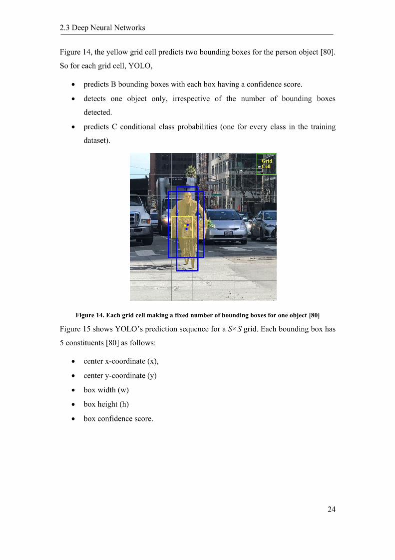
2.3 Deep Neural Networks
24
Figure 14, the yellow grid cell predicts two bounding boxes for the person object [80].
So for each grid cell, YOLO,
• predicts B bounding boxes with each box having a confidence score.
• detects one object only, irrespective of the number of bounding boxes
detected.
• predicts C conditional class probabilities (one for every class in the training
dataset).
Figure 14. Each grid cell making a fixed number of bounding boxes for one object [80]
Figure 15 shows YOLO’s prediction sequence for a S×S grid. Each bounding box has
5 constituents [80] as follows:
• center x-coordinate (x),
• center y-coordinate (y)
• box width (w)
• box height (h)
• box confidence score.

2.3 Deep Neural Networks
25
Figure 15. YOLO making S x S predictions with B bounding boxes [80]
Figure 16. YOLO detecting B bounding boxes for a single image with S x S grid
The confidence score reflects the likelihood of an object present in the bounding box
and also accuracy of the bounding box [80]. Each grid cell also predicts C conditional
class probabilities for every bounding box detected, giving the class probability of
each detected object where C is the number of classes in the training dataset.
Therefore, YOLO’s prediction shape for a single image is (S, S, B × 5 + C) [80].
Figure 16 shows YOLO predictions on a single image for a complete S × S gird.
2.3 Deep Neural Networks
26
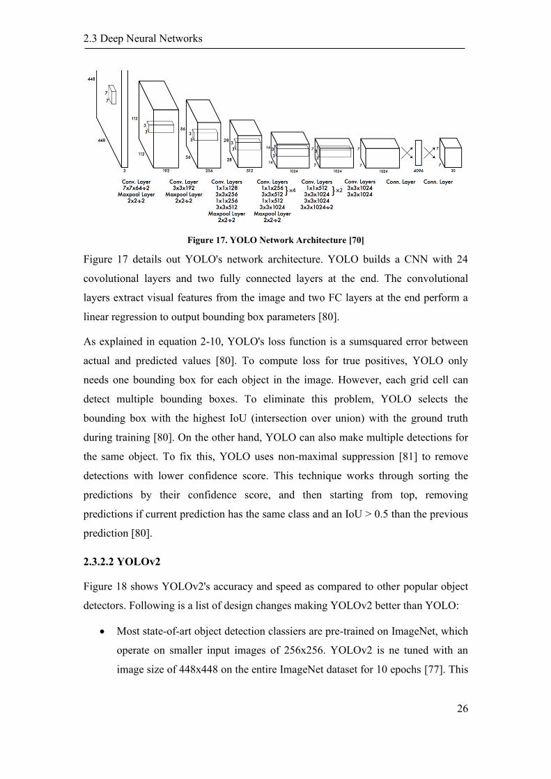
Figure 17. YOLO Network Architecture [70]
Figure 17 details out YOLO's network architecture. YOLO builds a CNN with 24
covolutional layers and two fully connected layers at the end. The convolutional
layers extract visual features from the image and two FC layers at the end perform a
linear regression to output bounding box parameters [80].
As explained in equation 2-10, YOLO's loss function is a sumsquared error between
actual and predicted values [80]. To compute loss for true positives, YOLO only
needs one bounding box for each object in the image. However, each grid cell can
detect multiple bounding boxes. To eliminate this problem, YOLO selects the
bounding box with the highest IoU (intersection over union) with the ground truth
during training [80]. On the other hand, YOLO can also make multiple detections for
the same object. To fix this, YOLO uses non-maximal suppression [81] to remove
detections with lower confidence score. This technique works through sorting the
predictions by their confidence score, and then starting from top, removing
predictions if current prediction has the same class and an IoU > 0.5 than the previous
prediction [80].
2.3.2.2 YOLOv2
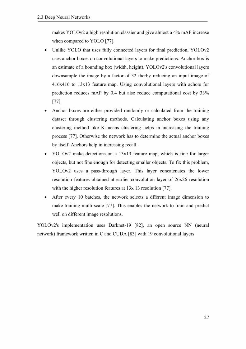
Figure 18 shows YOLOv2's accuracy and speed as compared to other popular object
detectors. Following is a list of design changes making YOLOv2 better than YOLO:
• Most state-of-art object detection classiers are pre-trained on ImageNet, which
operate on smaller input images of 256x256. YOLOv2 is ne tuned with an
image size of 448x448 on the entire ImageNet dataset for 10 epochs [77]. This
2.3 Deep Neural Networks
27
makes YOLOv2 a high resolution classier and give almost a 4% mAP increase
when compared to YOLO [77].
• Unlike YOLO that uses fully connected layers for final prediction, YOLOv2
uses anchor boxes on convolutional layers to make predictions. Anchor box is
an estimate of a bounding box (width, height). YOLOv2's convolutional layers
downsample the image by a factor of 32 therby reducing an input image of
416x416 to 13x13 feature map. Using convolutional layers with achors for
prediction reduces mAP by 0.4 but also reduce computational cost by 33%
[77].
• Anchor boxes are either provided randomly or calculated from the training
dataset through clustering methods. Calculating anchor boxes using any
clustering method like K-means clustering helps in increasing the training
process [77]. Otherwise the network has to determine the actual anchor boxes
by itself. Anchors help in increasing recall.
• YOLOv2 make detections on a 13x13 feature map, which is fine for larger
objects, but not fine enough for detecting smaller objects. To fix this problem,
YOLOv2 uses a pass-through layer. This layer concatenates the lower
resolution features obtained at earlier convolution layer of 26x26 resolution
with the higher resolution features at 13x 13 resolution [77].
• After every 10 batches, the network selects a dfferent image dimension to
make training multi-scale [77]. This enables the network to train and predict
well on different image resolutions.
YOLOv2's implementation uses Darknet-19 [82], an open source NN (neural
network) framework written in C and CUDA [83] with 19 convolutional layers.
2.3 Deep Neural Networks
28
Figure 18. YOLOv2 Accuracy and Speed Compared to other Object Detectors [77]
2.3.2.3 YOLOv3
YOLOv3 improves onto YOLOv2 detection metrics by adding some incremental
changes [78]. Following is a list of design changes making YOLOv3 slightly better
than YOLOv2 [78]:
• YOLOv3 predicts an object confidence score for each bounding box through
logistic regression and gets a score of 1 if its overlap with ground truth is more
than any other prediction.
• Each bounding box has an independent logistic classifier to predict detected
object class.
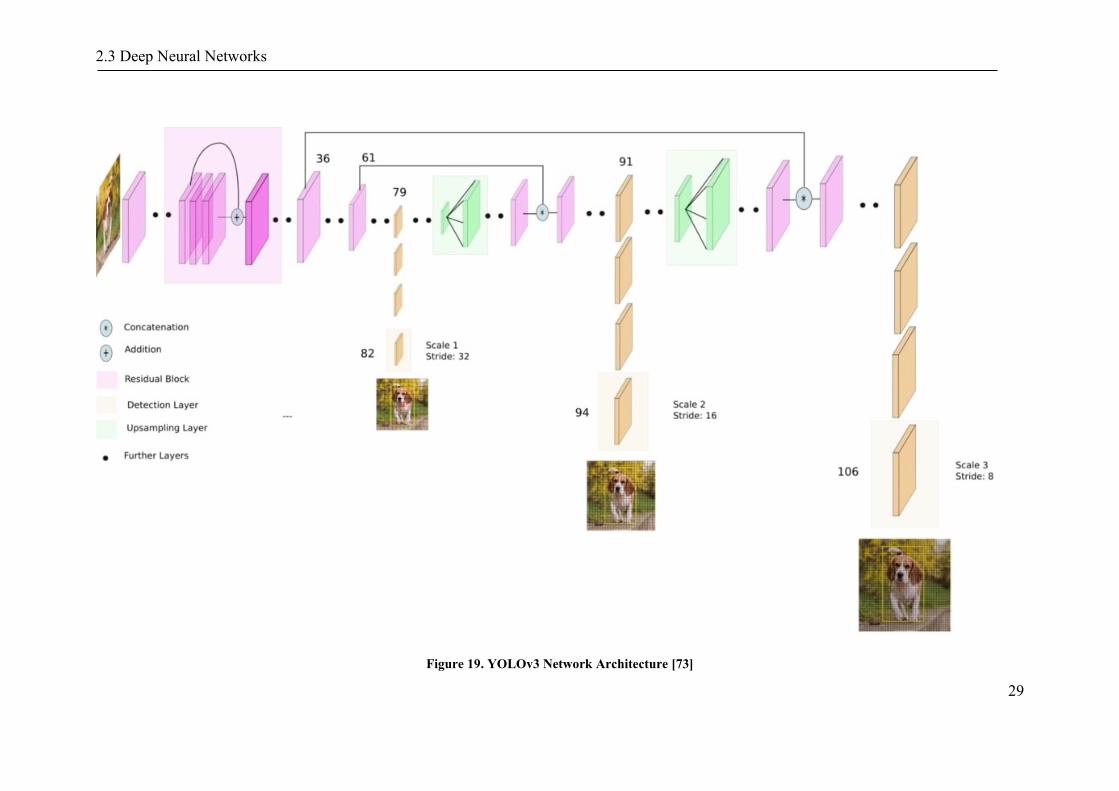
• Figure 19 shows YOLOv3's network architecture. Unlike YOLOv2, YOLOv3
predicts bounding boxes at 3 different scales. Feature maps are up-sampled
and merged with feature maps from former layers. Furthermore, new
convolutional layers are added to precess these feature maps predict object
bounding boxes. K-means clustering is used to determine anchor boxes. 9
cluster are selected and divided equally between 3 scales, with 3 predictions at
each scale.
2.3 Deep Neural Networks
29
Figure 19. YOLOv3 Network Architecture [73]
2.3 Deep Neural Networks
30
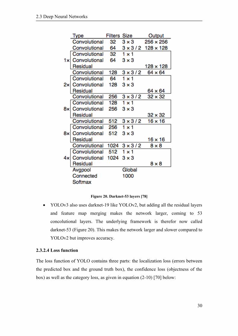
Figure 20. Darknet-53 layers [78]
• YOLOv3 also uses darknet-19 like YOLOv2, but adding all the residual layers
and feature map merging makes the network larger, coming to 53
concolutional layers. The underlying framework is therefor now called
darknet-53 (Figure 20). This makes the network larger and slower compared to
YOLOv2 but improves accuracy.
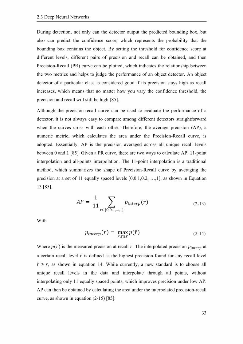
2.3.2.4 Loss function
The loss function of YOLO contains three parts: the localization loss (errors between
the predicted box and the ground truth box), the confidence loss (objectness of the
box) as well as the category loss, as given in equation (2-10) [70] below:
2.3 Deep Neural Networks
31
𝐿𝑜𝑠𝑠 = 𝑙𝑜𝑠𝑠𝑙𝑜𝑐𝑎𝑙𝑖𝑧𝑎𝑡𝑖𝑜𝑛 + 𝑙𝑜𝑠𝑠𝑐𝑜𝑛𝑓𝑖𝑑𝑒𝑛𝑐𝑒 + 𝑙𝑜𝑠𝑠𝑐𝑙𝑎𝑠𝑠
= ∑∑1𝑖,𝑗𝑜𝑏𝑗
𝐵
𝑗=0
𝑆2
𝑖=0
[(𝑡𝑥 − �̂�𝑥)2 + (𝑡𝑦 − �̂�𝑦)
2+ (𝑡𝑤 − �̂�𝑤)2 + (𝑡ℎ − �̂�ℎ)2]
+∑∑(1𝑖,𝑗𝑜𝑏𝑗[− log(𝜎(𝑡𝑜)]
𝐵
𝑗=0
𝑆2
𝑖=0
+ 1𝑖,𝑗𝑛𝑜𝑏𝑗[− log(1 − 𝜎(𝑡𝑜)])
+∑ ∑ 1𝑖,𝑗𝑜𝑏𝑗𝐵
𝑗=0𝑆2
𝑖=0 [∑ 𝐵𝐶𝐸(�̂�𝑐, 𝜎(𝑝𝑐))𝐶𝑐=1 ]
(2-10)
Here, each line represents each part of loss. 𝑡𝑥,𝑡𝑦 are the predicted bounding box
coordinates and 𝑡𝑤,𝑡ℎ are the width and height of the box. 1𝑖,𝑗𝑜𝑏𝑗
indicates that j th
bounding box in i th cell is responsible for that prediction [70]. 𝑡𝑜 is the predicted
objectness score for that box and 𝑝𝑐 is the predicted class probability. Mean Squared
Error (MSE) function is adopted to calculate the localization loss and Binary Cross
Entropy (BCE) function is employed to calculate the confidence loss and
classification loss.
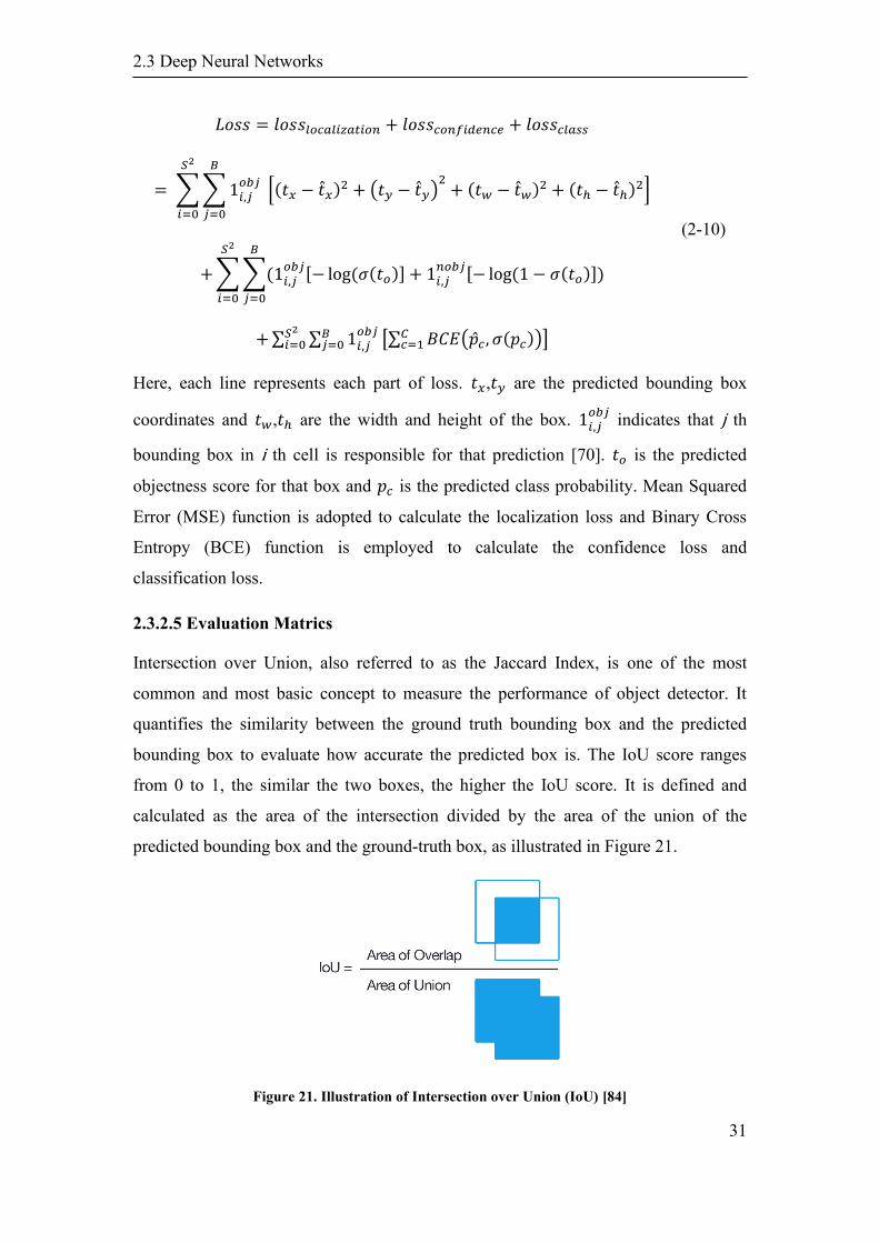
2.3.2.5 Evaluation Matrics
Intersection over Union, also referred to as the Jaccard Index, is one of the most
common and most basic concept to measure the performance of object detector. It
quantifies the similarity between the ground truth bounding box and the predicted
bounding box to evaluate how accurate the predicted box is. The IoU score ranges
from 0 to 1, the similar the two boxes, the higher the IoU score. It is defined and
calculated as the area of the intersection divided by the area of the union of the
predicted bounding box and the ground-truth box, as illustrated in Figure 21.
Figure 21. Illustration of Intersection over Union (IoU) [84]

2.3 Deep Neural Networks
32
By computing the IoU score for each detection, the IoU values above the defined
threshold are considered positive predictions and those below are considered to be
false predictions. More precisely, the predictions are classified into True Positives
(TP), False Negatives (FN), and False Positives (FP) [85].
An example of confusion matrix of car detection is shown in Table 2- 3.Generally
speaking, when the prediction class matches the class of the ground truth and IoU is
greater than some certain threshold, then this prediction would be considered as truth
positive (TP); otherwise, when the prediction class doesn’t match the ground truth
class or the IoU is lower than the threshold, then it would be viewed as false positive
(FP). False negative (FN) refers to that the ground truth cannot be detected and true
negative (TN) represents a correct misdetection.
Table 2. An example of confusion matrix of car detection
Actual
Prediction Car Not Car
Car True Positive (TP) False Positive (FP)
Not Car False Negative (FN) True Negative (TN)
Based on the confusion matrix, precision and recall can then be calculated and
obtained. Precision is the ability of a model to detect only the relevant objects, which
is defined as the number of true positives divided by the sum of true positives and
false positives, as shown in equation (2-11):
𝑃𝑟𝑒𝑐𝑖𝑠𝑖𝑜𝑛 = 𝑇𝑃
𝑇𝑃 + 𝐹𝑃=
𝑡𝑟𝑢𝑒 𝑜𝑏𝑗𝑒𝑐𝑡 𝑑𝑒𝑡𝑒𝑐𝑡𝑖𝑜𝑛
𝑎𝑙𝑙 𝑑𝑒𝑡𝑒𝑐𝑡𝑒𝑑 𝑏𝑜𝑥𝑒𝑠
(2-11)
Recall is the ability of a model to identify all the relevant objects, which is defined as
the number of the true positives divided by the sum of true positive and false
negatives (all ground truths), as shown in equation (2-12) [85]:
𝑅𝑒𝑐𝑎𝑙𝑙 = 𝑇𝑃
𝑇𝑃 + 𝐹𝑁=
𝑡𝑟𝑢𝑒 𝑜𝑏𝑗𝑒𝑐𝑡 𝑑𝑒𝑡𝑒𝑐𝑡𝑖𝑜𝑛
𝑎𝑙𝑙 𝑔𝑟𝑜𝑢𝑛𝑑 𝑡𝑟𝑢𝑡ℎ 𝑏𝑜𝑥𝑒𝑠
(2-12)
2.3 Deep Neural Networks
33
During detection, not only can the detector output the predicted bounding box, but
also can predict the confidence score, which represents the probability that the
bounding box contains the object. By setting the threshold for confidence score at
different levels, different pairs of precision and recall can be obtained, and then
Precision-Recall (PR) curve can be plotted, which indicates the relationship between
the two metrics and helps to judge the performance of an object detector. An object
detector of a particular class is considered good if its precision stays high as recall
increases, which means that no matter how you vary the confidence threshold, the
precision and recall will still be high [85].
Although the precision-recall curve can be used to evaluate the performance of a
detector, it is not always easy to compare among different detectors straightforward
when the curves cross with each other. Therefore, the average precision (AP), a
numeric metric, which calculates the area under the Precision-Recall curve, is
adopted. Essentially, AP is the precision averaged across all unique recall levels
between 0 and 1 [85]. Given a PR curve, there are two ways to calculate AP: 11-point
interpolation and all-points interpolation. The 11-point interpolation is a traditional
method, which summarizes the shape of Precision-Recall curve by averaging the
precision at a set of 11 equally spaced levels [0,0.1,0.2, …,1], as shown in Equation
13 [85].
𝐴𝑃 = 1
11∑ 𝑝𝑖𝑛𝑡𝑒𝑟𝑝(𝑟)
𝑟∈{0,0.1,…,1}
(2-13)
With
𝑝𝑖𝑛𝑡𝑒𝑟𝑝(𝑟) = max�̃�:�̃�≥𝑟
𝑝(�̃�) (2-14)
Where 𝑝(�̃�) is the measured precision at recall �̃�. The interpolated precision 𝑝𝑖𝑛𝑡𝑒𝑟𝑝 at
a certain recall level 𝑟 is defined as the highest precision found for any recall level
�̃� ≥ 𝑟, as shown in equation 14. While currently, a new standard is to choose all
unique recall levels in the data and interpolate through all points, without
interpolating only 11 equally spaced points, which improves precision under low AP.
AP can then be obtained by calculating the area under the interpolated precision-recall
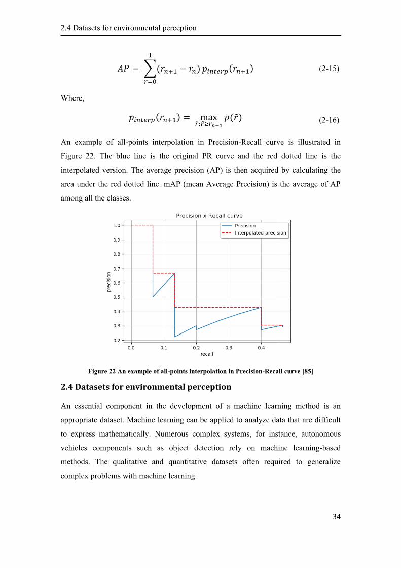
curve, as shown in equation (2-15) [85]:
2.4 Datasets for environmental perception
34
𝐴𝑃 = ∑(𝑟𝑛+1 − 𝑟𝑛)
1
𝑟=0
𝑝𝑖𝑛𝑡𝑒𝑟𝑝(𝑟𝑛+1) (2-15)
Where,
𝑝𝑖𝑛𝑡𝑒𝑟𝑝(𝑟𝑛+1) = max�̃�:�̃�≥𝑟𝑛+1
𝑝(�̃�) (2-16)
An example of all-points interpolation in Precision-Recall curve is illustrated in
Figure 22. The blue line is the original PR curve and the red dotted line is the
interpolated version. The average precision (AP) is then acquired by calculating the
area under the red dotted line. mAP (mean Average Precision) is the average of AP
among all the classes.
Figure 22 An example of all-points interpolation in Precision-Recall curve [85]
2.4 Datasets for environmental perception
An essential component in the development of a machine learning method is an
appropriate dataset. Machine learning can be applied to analyze data that are difficult
to express mathematically. Numerous complex systems, for instance, autonomous
vehicles components such as object detection rely on machine learning-based
methods. The qualitative and quantitative datasets often required to generalize
complex problems with machine learning.

2.4 Datasets for environmental perception
35
Assuming a correctly designed machine learning model, a high computational power
machine and optimally set training parameters, the model is likely to perform well.
However, it is proven [86] that the size of dataset makes a lot of impact on results.
Especially for the machine learning-based visual object detection techniques, the
quantity of dataset improves the performance of the machine learning model [86].
In this section, some popular datasets available for object detection and their
performance on different object detection models will be discussed. Some of the
available object detection dataset provides range information up to about 100 meters
measured by LiDAR or stereo camera as a ground truth, but none of the dataset is
focussed or specifically designed to predict the distance to the detected object.
Additionally, the available datasets contains annotated objects which are relatively big
in size, in other words, close to the camera and secondly contains images of urban
driving scenarios, captured during sunny day and in decent weather conditions.
The recently published nuScenes [87] is a multimodal dataset for autonomous driving.
This dataset was recorded with 6 cameras, 5 radars, and 1 lidar, all with a 360-degree
field of view. It consists of 1000 scenes, each 20 seconds long and fully annotated
with 3-dimensional bounded boxes for 23 classes and 8 attributes. The Honda
Research Institute 3D (H3D) Dataset [88] is a large scare 3D multi-object detection a
tracking dataset collected using a 3D LiDAR Scanner. H3D consists of 160 crowded
traffic scenes. However, both datasets are focused on urban environments and traffic
scenes, which differ from a railway setup.
Microsoft COCO Dataset (MS COCO) [89] contains complex scenes with common
everday objects. Dataset contains in total 91 object classes with 2.5 million instances
in about 328k images. The dataset is basically for object recognition purpose hence
does not contaians any objects pose information. Objects are labeled using
segmenting individual object instances.
2.4.1 Kitti Dataset
KITTI dataset [90] is a dataset built by the Karlsruhe Institute of Technology and
Toyota Technological Institute at Chicago. The dataset was recorded from a car
equipped with one Inertial Navigation System (GPS/IMU), one Laser scanner, two
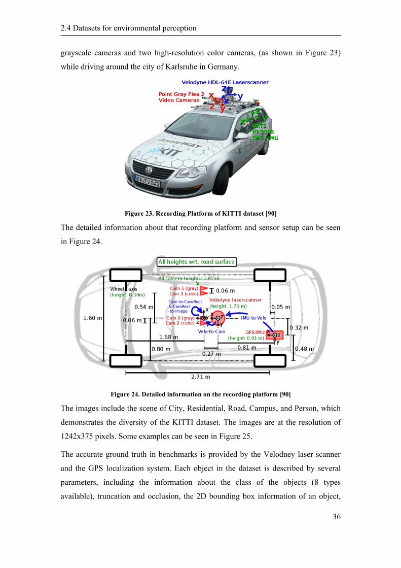
2.4 Datasets for environmental perception
36
grayscale cameras and two high-resolution color cameras, (as shown in Figure 23)
while driving around the city of Karlsruhe in Germany.
Figure 23. Recording Platform of KITTI dataset [90]
The detailed information about that recording platform and sensor setup can be seen
in Figure 24.
Figure 24. Detailed information on the recording platform [90]
The images include the scene of City, Residential, Road, Campus, and Person, which
demonstrates the diversity of the KITTI dataset. The images are at the resolution of
1242x375 pixels. Some examples can be seen in Figure 25.
The accurate ground truth in benchmarks is provided by the Velodney laser scanner
and the GPS localization system. Each object in the dataset is described by several
parameters, including the information about the class of the objects (8 types
available), truncation and occlusion, the 2D bounding box information of an object,
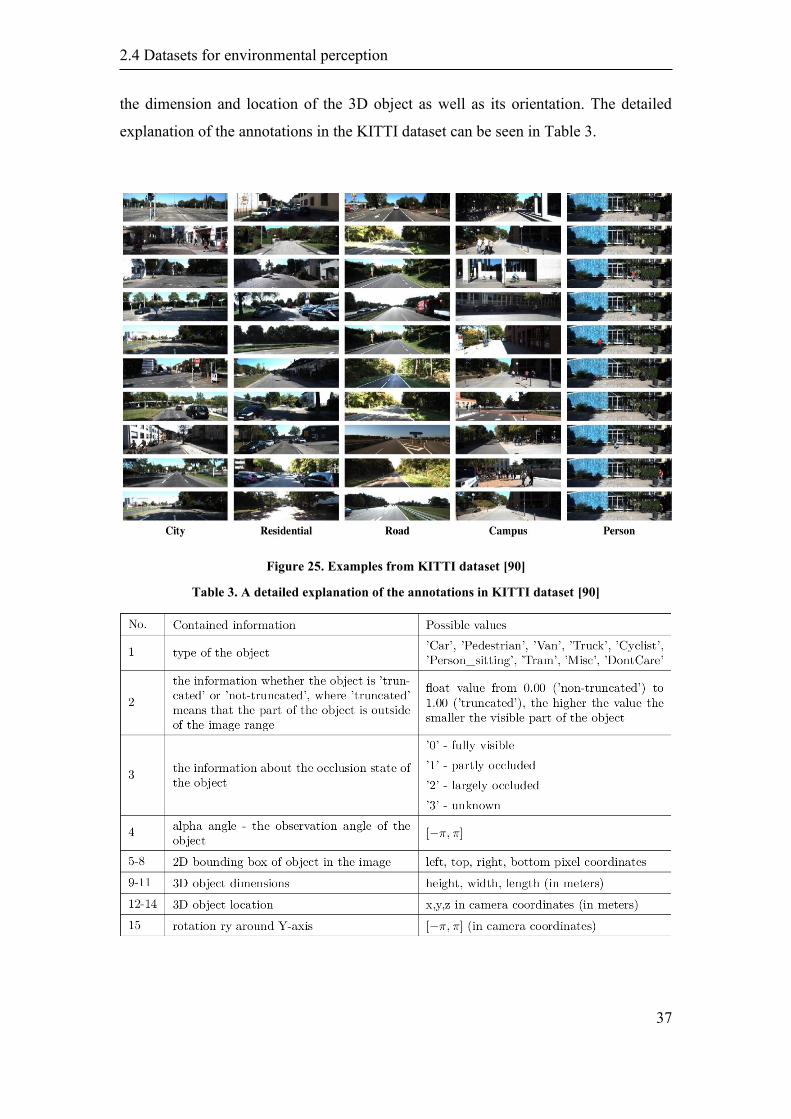
2.4 Datasets for environmental perception
37
the dimension and location of the 3D object as well as its orientation. The detailed
explanation of the annotations in the KITTI dataset can be seen in Table 3.
Figure 25. Examples from KITTI dataset [90]
Table 3. A detailed explanation of the annotations in KITTI dataset [90]
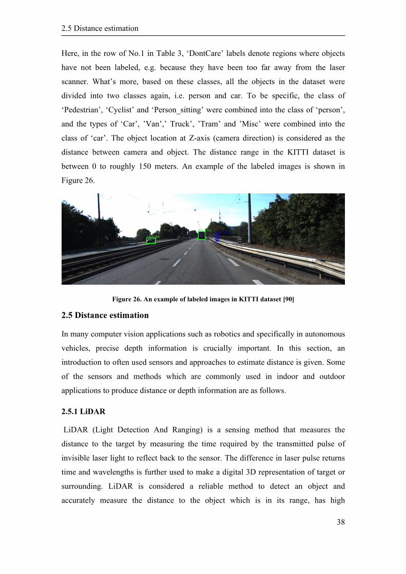
2.5 Distance estimation
38
Here, in the row of No.1 in Table 3, ‘DontCare’ labels denote regions where objects
have not been labeled, e.g. because they have been too far away from the laser
scanner. What’s more, based on these classes, all the objects in the dataset were
divided into two classes again, i.e. person and car. To be specific, the class of
‘Pedestrian’, ‘Cyclist’ and ‘Person_sitting’ were combined into the class of ‘person’,
and the types of ‘Car’, ’Van’,’ Truck’, ’Tram’ and ’Misc’ were combined into the
class of ‘car’. The object location at Z-axis (camera direction) is considered as the
distance between camera and object. The distance range in the KITTI dataset is
between 0 to roughly 150 meters. An example of the labeled images is shown in
Figure 26.
Figure 26. An example of labeled images in KITTI dataset [90]
2.5 Distance estimation
In many computer vision applications such as robotics and specifically in autonomous
vehicles, precise depth information is crucially important. In this section, an
introduction to often used sensors and approaches to estimate distance is given. Some
of the sensors and methods which are commonly used in indoor and outdoor
applications to produce distance or depth information are as follows.
2.5.1 LiDAR
LiDAR (Light Detection And Ranging) is a sensing method that measures the
distance to the target by measuring the time required by the transmitted pulse of
invisible laser light to reflect back to the sensor. The difference in laser pulse returns
time and wavelengths is further used to make a digital 3D representation of target or
surrounding. LiDAR is considered a reliable method to detect an object and
accurately measure the distance to the object which is in its range, has high
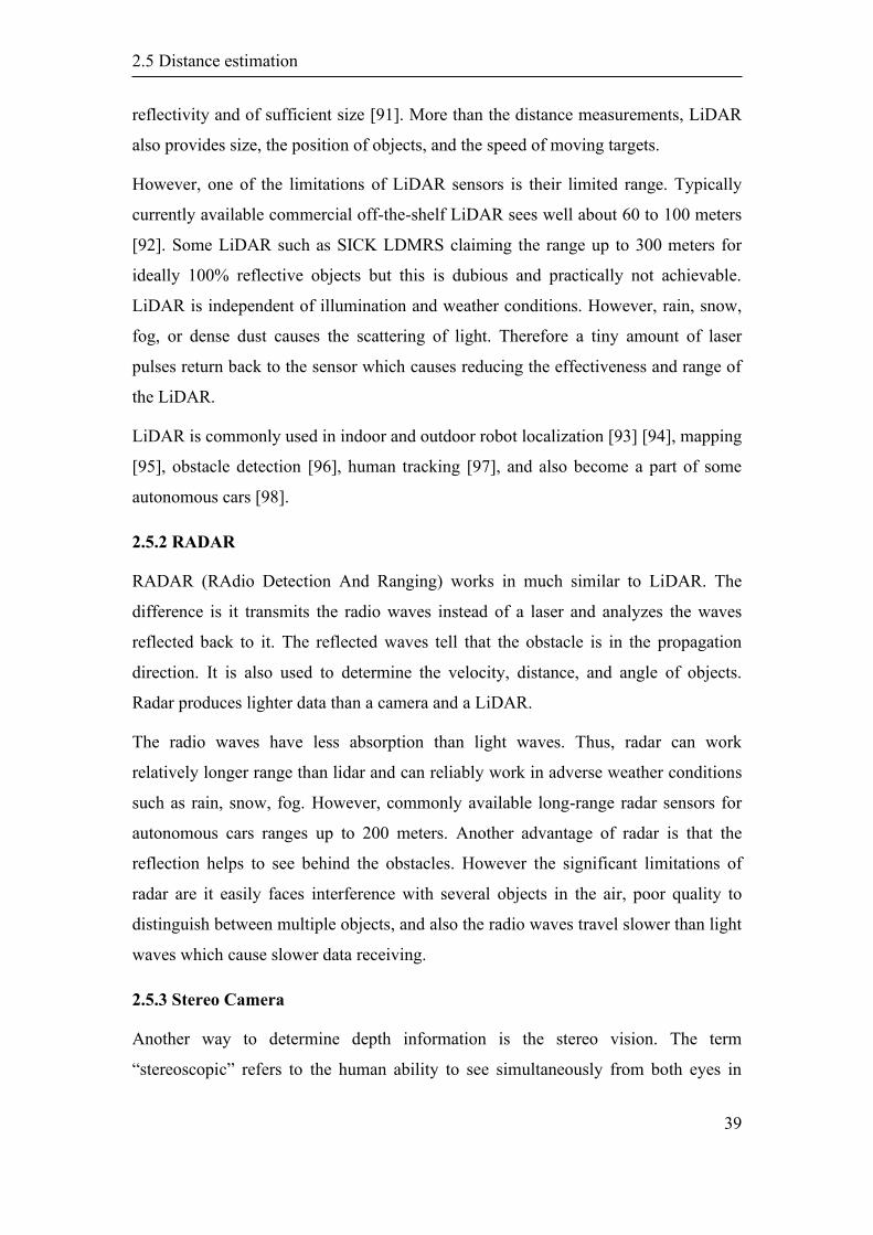
2.5 Distance estimation
39
reflectivity and of sufficient size [91]. More than the distance measurements, LiDAR
also provides size, the position of objects, and the speed of moving targets.
However, one of the limitations of LiDAR sensors is their limited range. Typically
currently available commercial off-the-shelf LiDAR sees well about 60 to 100 meters
[92]. Some LiDAR such as SICK LDMRS claiming the range up to 300 meters for
ideally 100% reflective objects but this is dubious and practically not achievable.
LiDAR is independent of illumination and weather conditions. However, rain, snow,
fog, or dense dust causes the scattering of light. Therefore a tiny amount of laser
pulses return back to the sensor which causes reducing the effectiveness and range of
the LiDAR.
LiDAR is commonly used in indoor and outdoor robot localization [93] [94], mapping
[95], obstacle detection [96], human tracking [97], and also become a part of some
autonomous cars [98].
2.5.2 RADAR
RADAR (RAdio Detection And Ranging) works in much similar to LiDAR. The
difference is it transmits the radio waves instead of a laser and analyzes the waves
reflected back to it. The reflected waves tell that the obstacle is in the propagation
direction. It is also used to determine the velocity, distance, and angle of objects.
Radar produces lighter data than a camera and a LiDAR.
The radio waves have less absorption than light waves. Thus, radar can work
relatively longer range than lidar and can reliably work in adverse weather conditions
such as rain, snow, fog. However, commonly available long-range radar sensors for
autonomous cars ranges up to 200 meters. Another advantage of radar is that the
reflection helps to see behind the obstacles. However the significant limitations of
radar are it easily faces interference with several objects in the air, poor quality to
distinguish between multiple objects, and also the radio waves travel slower than light
waves which cause slower data receiving.
2.5.3 Stereo Camera
Another way to determine depth information is the stereo vision. The term
“stereoscopic” refers to the human ability to see simultaneously from both eyes in
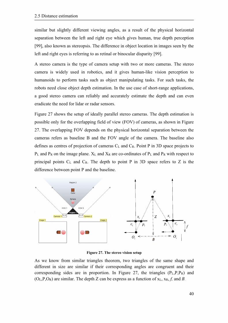
2.5 Distance estimation
40
similar but slightly different viewing angles, as a result of the physical horizontal
separation between the left and right eye which gives human, true depth perception
[99], also known as stereopsis. The difference in object location in images seen by the
left and right eyes is referring to as retinal or binocular disparity [99].
A stereo camera is the type of camera setup with two or more cameras. The stereo
camera is widely used in robotics, and it gives human-like vision perception to
humanoids to perform tasks such as object manipulating tasks. For such tasks, the
robots need close object depth estimation. In the use case of short-range applications,
a good stereo camera can reliably and accurately estimate the depth and can even
eradicate the need for lidar or radar sensors.
Figure 27 shows the setup of ideally parallel stereo cameras. The depth estimation is
possible only for the overlapping field of view (FOV) of cameras, as shown in Figure
27. The overlapping FOV depends on the physical horizontal separation between the
cameras refers as baseline B and the FOV angle of the camera. The baseline also
defines as centres of projection of cameras CL and CR. Point P in 3D space projects to
PL and PR on the image plane. XL and XR are co-ordinates of PL and PR with respect to
principal points CL and CR. The depth to point P in 3D space refers to Z is the
difference between point P and the baseline.
Figure 27. The stereo vision setup
As we know from similar triangles theorem, two triangles of the same shape and
different in size are similar if their corresponding angles are congruent and their
corresponding sides are in proportion. In Figure 27, the triangles (PL,P,PR) and
(OL,P,OR) are similar. The depth Z can be express as a function of xL, xR, f, and B.
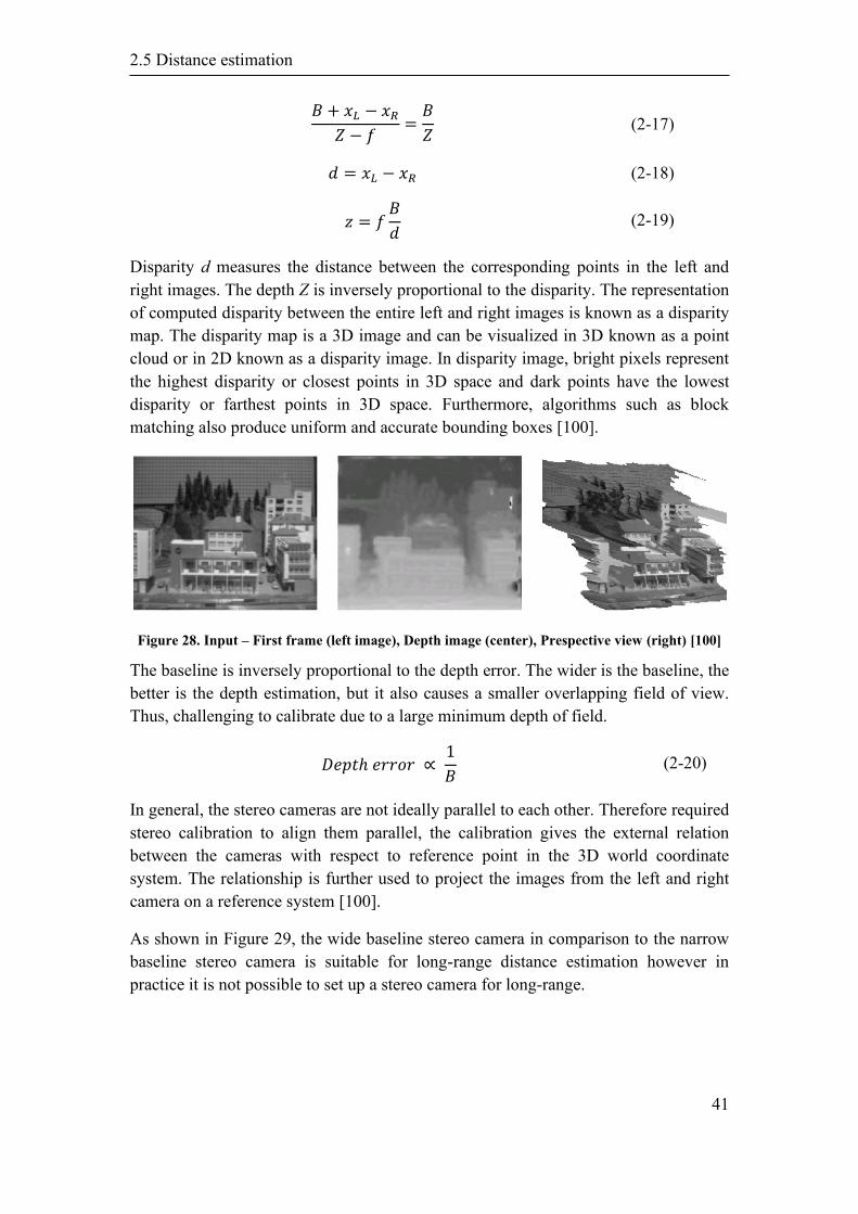
2.5 Distance estimation
41
𝐵 + 𝑥𝐿 − 𝑥𝑅
𝑍 − 𝑓=
𝐵
𝑍 (2-17)
𝑑 = 𝑥𝐿 − 𝑥𝑅 (2-18)
𝑧 = 𝑓𝐵
𝑑 (2-19)
Disparity d measures the distance between the corresponding points in the left and
right images. The depth Z is inversely proportional to the disparity. The representation
of computed disparity between the entire left and right images is known as a disparity
map. The disparity map is a 3D image and can be visualized in 3D known as a point
cloud or in 2D known as a disparity image. In disparity image, bright pixels represent
the highest disparity or closest points in 3D space and dark points have the lowest
disparity or farthest points in 3D space. Furthermore, algorithms such as block
matching also produce uniform and accurate bounding boxes [100].
Figure 28. Input – First frame (left image), Depth image (center), Prespective view (right) [100]
The baseline is inversely proportional to the depth error. The wider is the baseline, the
better is the depth estimation, but it also causes a smaller overlapping field of view.
Thus, challenging to calibrate due to a large minimum depth of field.
𝐷𝑒𝑝𝑡ℎ 𝑒𝑟𝑟𝑜𝑟 ∝ 1
𝐵 (2-20)
In general, the stereo cameras are not ideally parallel to each other. Therefore required
stereo calibration to align them parallel, the calibration gives the external relation
between the cameras with respect to reference point in the 3D world coordinate
system. The relationship is further used to project the images from the left and right
camera on a reference system [100].
As shown in Figure 29, the wide baseline stereo camera in comparison to the narrow
baseline stereo camera is suitable for long-range distance estimation however in
practice it is not possible to set up a stereo camera for long-range.
2.5 Distance estimation
42
Figure 29. Error-Depth diagram for narrow and wide baseline [101]
2.5.4 Monocular Camera-based approaches
Previous research for distance estimation mainly paid particular attention to build a
model that represents the geometry relationship between points on images and their
corresponding physical distances on the real-world coordinates. Inverse perspective
mapping (IPM) [102] is one of these classical methods, which transforms the forward-
facing images to a top-down “bird’s eye” view and changes the nonlinear relationship
between distances in the image and the real world into a linear relationship. However,
the limitation of this method is that it performs poorly when objects lie on the sides of
the camera or the curved road and when objects are far away from the camera (above
40 meters) [103].
Sadreddini et al. [104] proposed a system that estimates distances from a single
camera for an indoor mobile robot application. The developed method utilized
information from floor line detection and morphological operations extracted from an
object to estimate the distance. However, this method was evaluated in only one use
case. Pathi et al. proposed a method to estimate the distance between humans and a
robot using images from a single camera mounted on the robot. The method first
extracts 2D poses (skeleton structure) of the humans in the scene and then it uses the
effect of perspective distortion from the camera’s point of view to estimate the
distance. For the experimental validation of the method, the authors collected three
datasets and the method demonstrated its effectiveness.
A recent work by Ali et al. [105] proposed a real-time vehicle distance estimation
using a single view geometry. A fully convolutional deep network is used for lane
detection on the road. Subsequently, an Inverse Perspective Mapping (IPM) and

2.5 Distance estimation
43
camera height are estimated from a known lane width and the detected horizon. At
last, the distances of the vehicles on the road are calculated by back projecting image
point to a ray intersecting the reconstructed road plane. The method was evaluated in
three datasets, KITTI [90], nuScences [87], and Lyft level 5 dataset [106]. All the
datasets have color images along with LiDAR data. The proposed method performed
better on the nuScenes and Lyft datasets in comparison to two other deep learning
approaches. However, the proposed method did not perform well on the KITTI
dataset.
In [103], a base model that directly predicts distances for given objects in the images
was introduced, which contains three parts: a feature extractor to generate a feature
map for the entire RGB image, a distance regressor to directly predict a distance from
the object-specific Region Of Interest (ROI) feature and a multi-class classifier to
predict the category of an object from the ROI feature, as shown in Figure 30 [103].
Figure 30. Framework of the base model [103]
To be specific, the popular network structures (vgg16 and res50) are adopted as
feature extractor and extract the feature map for the whole image. Then the extracted
feature map from the feature extractor and the object bounding boxes are feed into an
ROI pooling layer to generate a fix-size feature vector to represent each object in the
image [103]. After that, the distance regressor and classifier utilize the pooled feature
to predict a distance and class information for each object. The distance regressor is
made up of three fully connected layers and a softplus activation is employed on the
output of the last fully connected layer to make sure the predicted distance is positive.
The classifier uses a fully connected layer followed by a softmax function to predict
the category.
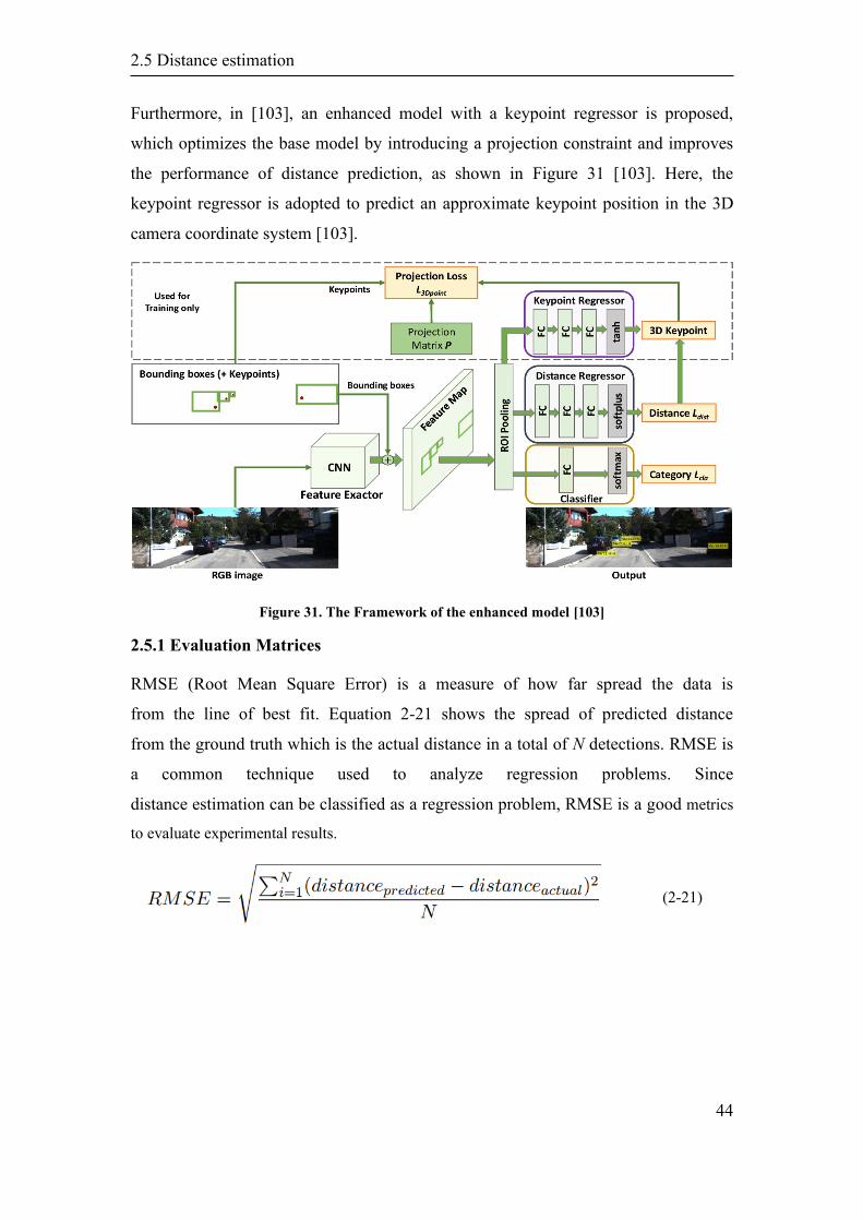
2.5 Distance estimation
44
Furthermore, in [103], an enhanced model with a keypoint regressor is proposed,
which optimizes the base model by introducing a projection constraint and improves
the performance of distance prediction, as shown in Figure 31 [103]. Here, the
keypoint regressor is adopted to predict an approximate keypoint position in the 3D
camera coordinate system [103].
Figure 31. The Framework of the enhanced model [103]
2.5.1 Evaluation Matrices
RMSE (Root Mean Square Error) is a measure of how far spread the data is
from the line of best fit. Equation 2-21 shows the spread of predicted distance
from the ground truth which is the actual distance in a total of N detections. RMSE is
a common technique used to analyze regression problems. Since
distance estimation can be classified as a regression problem, RMSE is a good metrics
to evaluate experimental results.
(2-21)

45
46
3. Dataset for long-range object
detection and distance estimation
Among all the significant advancements in many sectors due to the introduction of
machine learning, the most notable achievement has been seen in object recognition.
Numerous datasets for object recognition were created in recent years from the
images gathered from the internet such as Google, for example, COCO [89], SUN
[107], PASCAL VOC [108] and ILSVRC [53] [109]. Some datasets were formed by
collecting the images from a multisensory obstacle detection system containing
cameras and other short-range ranging sensors such as LiDAR or RADAR mounted
on a car moving on streets such as KITTI [90] and the Caltech Pedestrian Datasets
[110]. The labelled datasets are used to train and evaluate machine learning models
such as AlexNet [48], Faster-RCNN [111], YOLO [70] and FCIS [112]. Also, the
comparison of various datasets and performance of machine learning models on the
datasets is made [110] to evaluate the quality of datasets and performance of models.
The current popular datasets and object detection models show promising results for
object detection in indoor and outdoor applications.
However, there are no datasets which are suitable for long-range object detection and
distance estimation. The currently available dataset contains labelled objects which
are at short-distance; hence the object size in the image is relatively big. Such as the
state-of-the-art datasets COCO [89], KITTI [90] consists of images captured
relatively at a short-range up to approximately 100 meters thus the size of the object is
large in the image and tends to work for short-range object detection. The distance
range and close objects labelling fulfill the requirement of autonomous cars obstacle
detection system where the required range is relatively less in comparison to an
obstacle detection system for railways. Due to that in the thesis, it was needed first to
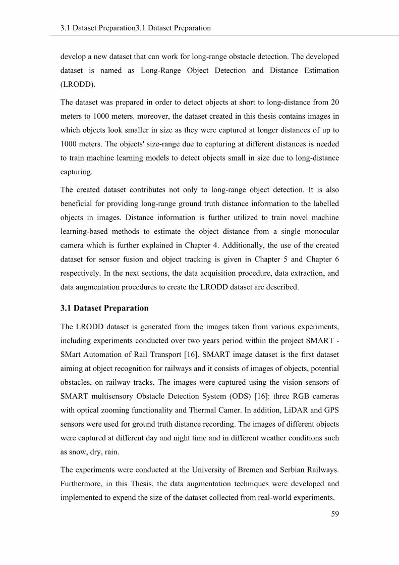
3.1 Dataset Preparation3.1 Dataset Preparation
59
develop a new dataset that can work for long-range obstacle detection. The developed
dataset is named as Long-Range Object Detection and Distance Estimation
(LRODD).
The dataset was prepared in order to detect objects at short to long-distance from 20
meters to 1000 meters. moreover, the dataset created in this thesis contains images in
which objects look smaller in size as they were captured at longer distances of up to
1000 meters. The objects' size-range due to capturing at different distances is needed
to train machine learning models to detect objects small in size due to long-distance
capturing.
The created dataset contributes not only to long-range object detection. It is also
beneficial for providing long-range ground truth distance information to the labelled
objects in images. Distance information is further utilized to train novel machine
learning-based methods to estimate the object distance from a single monocular
camera which is further explained in Chapter 4. Additionally, the use of the created
dataset for sensor fusion and object tracking is given in Chapter 5 and Chapter 6
respectively. In the next sections, the data acquisition procedure, data extraction, and
data augmentation procedures to create the LRODD dataset are described.
3.1 Dataset Preparation
The LRODD dataset is generated from the images taken from various experiments,
including experiments conducted over two years period within the project SMART -
SMart Automation of Rail Transport [16]. SMART image dataset is the first dataset
aiming at object recognition for railways and it consists of images of objects, potential
obstacles, on railway tracks. The images were captured using the vision sensors of
SMART multisensory Obstacle Detection System (ODS) [16]: three RGB cameras
with optical zooming functionality and Thermal Camer. In addition, LiDAR and GPS
sensors were used for ground truth distance recording. The images of different objects
were captured at different day and night time and in different weather conditions such
as snow, dry, rain.
The experiments were conducted at the University of Bremen and Serbian Railways.
Furthermore, in this Thesis, the data augmentation techniques were developed and
implemented to expend the size of the dataset collected from real-world experiments.
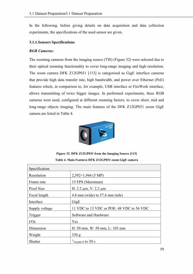
3.1 Dataset Preparation3.1 Dataset Preparation
59
In the following, before giving details on data acquisition and data collection
experiments, the specifications of the used sensor are given.
3.1.1.Sensors Specifications
RGB Cameras:
The zooming cameras from the imaging source (TIS) (Figure 32) were selected due to
their optical zooming functionality to cover long-range imaging and high resolution.
The zoom camera DFK Z12GP031 [113] is categorised as GigE interface cameras
that provide high data transfer rate, high bandwidth, and power over Ethernet (PoE)
features which, in comparison to, for example, USB interface or FireWork interface,
allows transmitting of twice bigger images. In performed experiments, three RGB
cameras were used, configured at different zooming factors, to cover short, mid and
long-range objects imaging. The main features of the DFK Z12GP031 zoom GigE
camera are listed in Table 4.
Figure 32. DFK Z12GP031 from the Imaging Source [113]
Table 4. Main Features DFK Z12GP031 zoom GigE camera
Specification
Resolution 2,592×1,944 (5 MP)
Frame rate 15 FPS (Maximum)
Pixel Size H: 2.2 µm, V: 2.2 µm
Focal length 4.8 mm (wide) to 57.6 mm (tele)
Interface GigE
Supply voltage 11 VDC to 13 VDC or POE: 48 VDC to 56 VDC
Trigger Software and Hardware
I/Os Yes
Dimension H: 50 mm, W: 50 mm, L: 103 mm
Weight 330 g
Shutter 1/20,000 s to 30 s
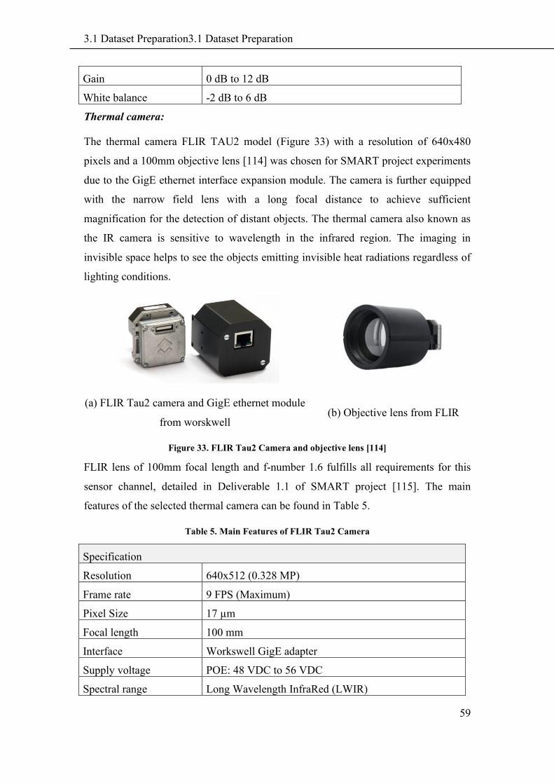
3.1 Dataset Preparation3.1 Dataset Preparation
59
Gain 0 dB to 12 dB
White balance -2 dB to 6 dB
Thermal camera:
The thermal camera FLIR TAU2 model (Figure 33) with a resolution of 640x480
pixels and a 100mm objective lens [114] was chosen for SMART project experiments
due to the GigE ethernet interface expansion module. The camera is further equipped
with the narrow field lens with a long focal distance to achieve sufficient
magnification for the detection of distant objects. The thermal camera also known as
the IR camera is sensitive to wavelength in the infrared region. The imaging in
invisible space helps to see the objects emitting invisible heat radiations regardless of
lighting conditions.
(a) FLIR Tau2 camera and GigE ethernet module
from worskwell (b) Objective lens from FLIR
Figure 33. FLIR Tau2 Camera and objective lens [114]
FLIR lens of 100mm focal length and f-number 1.6 fulfills all requirements for this
sensor channel, detailed in Deliverable 1.1 of SMART project [115]. The main
features of the selected thermal camera can be found in Table 5.
Table 5. Main Features of FLIR Tau2 Camera
Specification
Resolution 640x512 (0.328 MP)
Frame rate 9 FPS (Maximum)
Pixel Size 17 µm
Focal length 100 mm
Interface Workswell GigE adapter
Supply voltage POE: 48 VDC to 56 VDC
Spectral range Long Wavelength InfraRed (LWIR)
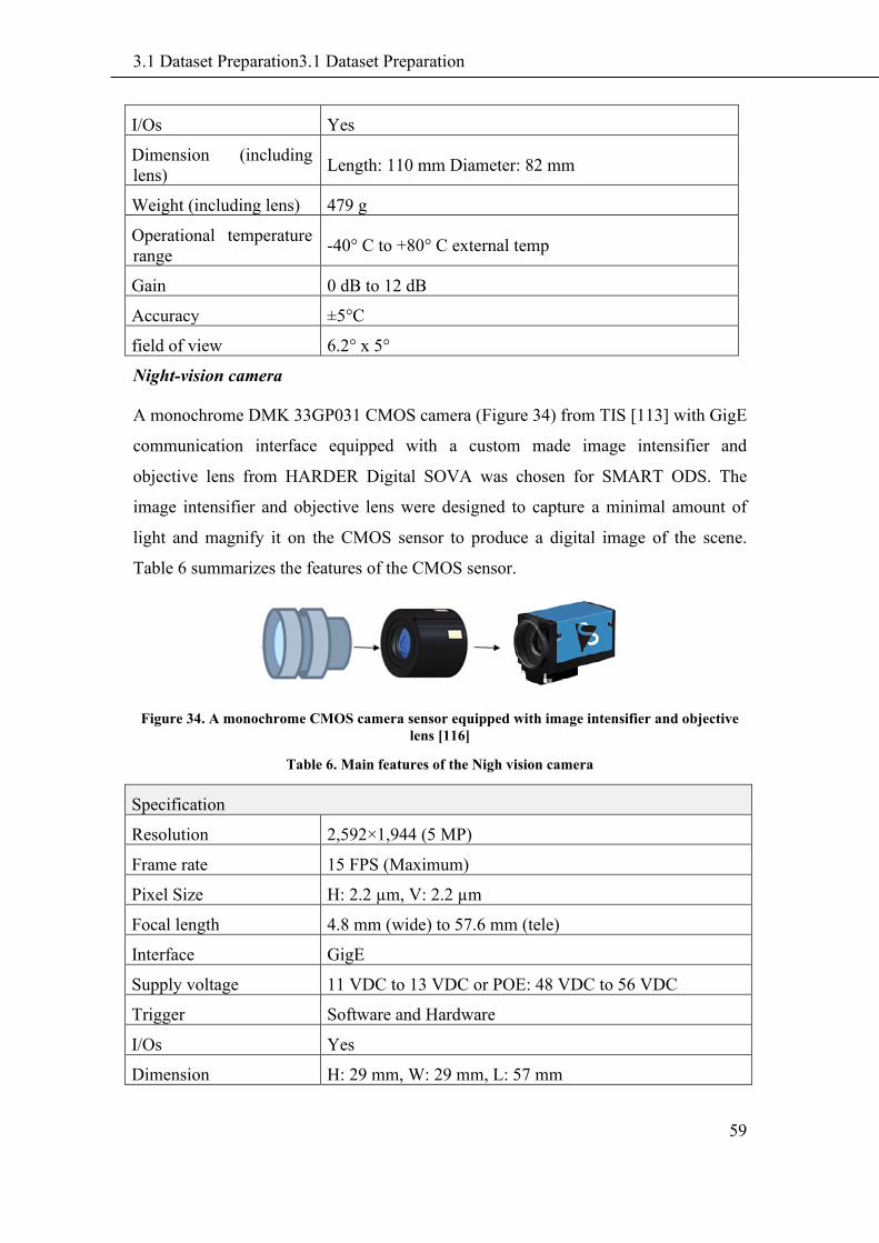
3.1 Dataset Preparation3.1 Dataset Preparation
59
I/Os Yes
Dimension (including
lens) Length: 110 mm Diameter: 82 mm
Weight (including lens) 479 g
Operational temperature
range -40° C to +80° C external temp
Gain 0 dB to 12 dB
Accuracy ±5°C
field of view 6.2° x 5°
Night-vision camera
A monochrome DMK 33GP031 CMOS camera (Figure 34) from TIS [113] with GigE
communication interface equipped with a custom made image intensifier and
objective lens from HARDER Digital SOVA was chosen for SMART ODS. The
image intensifier and objective lens were designed to capture a minimal amount of
light and magnify it on the CMOS sensor to produce a digital image of the scene.
Table 6 summarizes the features of the CMOS sensor.
Figure 34. A monochrome CMOS camera sensor equipped with image intensifier and objective
lens [116]
Table 6. Main features of the Nigh vision camera
Specification
Resolution 2,592×1,944 (5 MP)
Frame rate 15 FPS (Maximum)
Pixel Size H: 2.2 µm, V: 2.2 µm
Focal length 4.8 mm (wide) to 57.6 mm (tele)
Interface GigE
Supply voltage 11 VDC to 13 VDC or POE: 48 VDC to 56 VDC
Trigger Software and Hardware
I/Os Yes
Dimension H: 29 mm, W: 29 mm, L: 57 mm
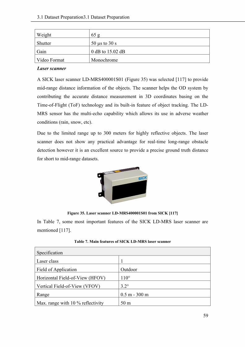
3.1 Dataset Preparation3.1 Dataset Preparation
59
Weight 65 g
Shutter 50 µs to 30 s
Gain 0 dB to 15.02 dB
Video Format Monochrome
Laser scanner
A SICK laser scanner LD-MRS400001S01 (Figure 35) was selected [117] to provide
mid-range distance information of the objects. The scanner helps the OD system by
contributing the accurate distance measurement in 3D coordinates basing on the
Time-of-Flight (ToF) technology and its built-in feature of object tracking. The LD-
MRS sensor has the multi-echo capability which allows its use in adverse weather
conditions (rain, snow, etc).
Due to the limited range up to 300 meters for highly reflective objects. The laser
scanner does not show any practical advantage for real-time long-range obstacle
detection however it is an excellent source to provide a precise ground truth distance
for short to mid-range datasets.
Figure 35. Laser scanner LD-MRS400001S01 from SICK [117]
In Table 7, some most important features of the SICK LD-MRS laser scanner are
mentioned [117].
Table 7. Main features of SICK LD-MRS laser scanner
Specification
Laser class 1
Field of Application Outdoor
Horizontal Field-of-View (HFOV) 110°
Vertical Field-of-View (VFOV) 3.2°
Range 0.5 m - 300 m
Max. range with 10 % reflectivity 50 m
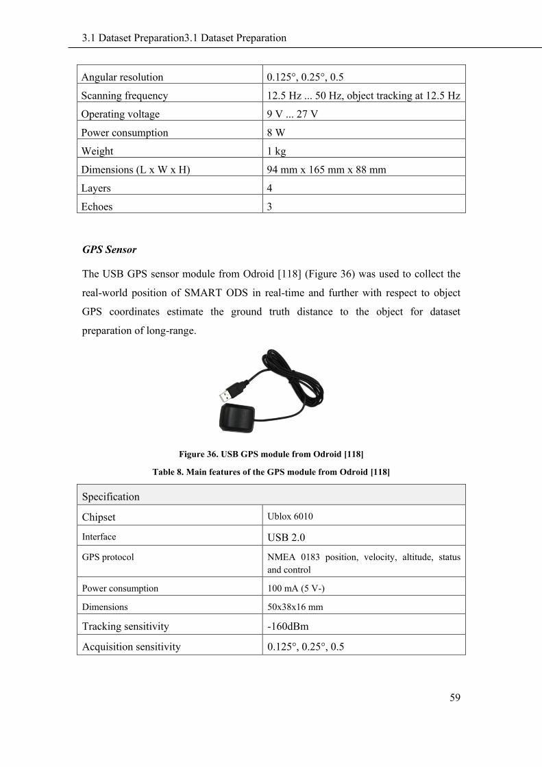
3.1 Dataset Preparation3.1 Dataset Preparation
59
Angular resolution 0.125°, 0.25°, 0.5
Scanning frequency 12.5 Hz ... 50 Hz, object tracking at 12.5 Hz
Operating voltage 9 V ... 27 V
Power consumption 8 W
Weight 1 kg
Dimensions (L x W x H) 94 mm x 165 mm x 88 mm
Layers 4
Echoes 3
GPS Sensor
The USB GPS sensor module from Odroid [118] (Figure 36) was used to collect the
real-world position of SMART ODS in real-time and further with respect to object
GPS coordinates estimate the ground truth distance to the object for dataset
preparation of long-range.
Figure 36. USB GPS module from Odroid [118]
Table 8. Main features of the GPS module from Odroid [118]
Specification
Chipset Ublox 6010
Interface USB 2.0
GPS protocol NMEA 0183 position, velocity, altitude, status
and control
Power consumption 100 mA (5 V-)
Dimensions 50x38x16 mm
Tracking sensitivity -160dBm
Acquisition sensitivity 0.125°, 0.25°, 0.5
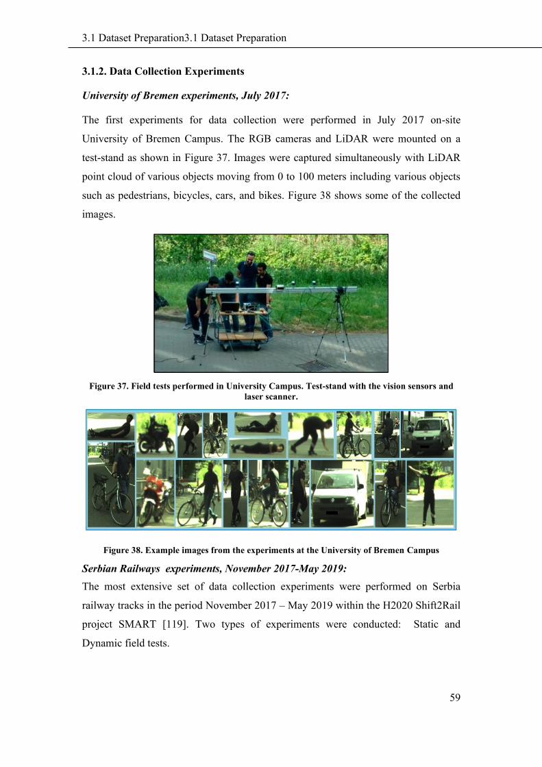
3.1 Dataset Preparation3.1 Dataset Preparation
59
3.1.2. Data Collection Experiments
University of Bremen experiments, July 2017:
The first experiments for data collection were performed in July 2017 on-site
University of Bremen Campus. The RGB cameras and LiDAR were mounted on a
test-stand as shown in Figure 37. Images were captured simultaneously with LiDAR
point cloud of various objects moving from 0 to 100 meters including various objects
such as pedestrians, bicycles, cars, and bikes. Figure 38 shows some of the collected
images.
Figure 37. Field tests performed in University Campus. Test-stand with the vision sensors and
laser scanner.
Figure 38. Example images from the experiments at the University of Bremen Campus
Serbian Railways experiments, November 2017-May 2019:
The most extensive set of data collection experiments were performed on Serbia
railway tracks in the period November 2017 – May 2019 within the H2020 Shift2Rail
project SMART [119]. Two types of experiments were conducted: Static and
Dynamic field tests.
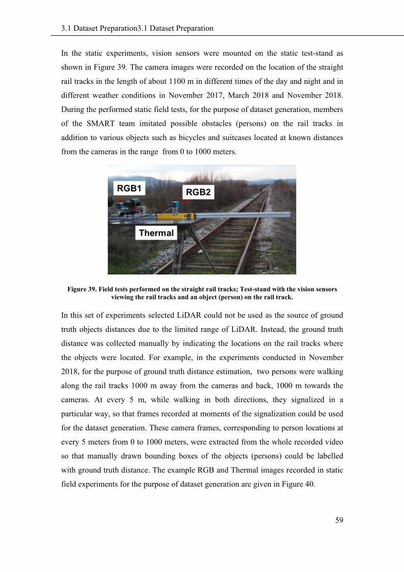
3.1 Dataset Preparation3.1 Dataset Preparation
59
In the static experiments, vision sensors were mounted on the static test-stand as
shown in Figure 39. The camera images were recorded on the location of the straight
rail tracks in the length of about 1100 m in different times of the day and night and in
different weather conditions in November 2017, March 2018 and November 2018.
During the performed static field tests, for the purpose of dataset generation, members
of the SMART team imitated possible obstacles (persons) on the rail tracks in
addition to various objects such as bicycles and suitcases located at known distances
from the cameras in the range from 0 to 1000 meters.
Figure 39. Field tests performed on the straight rail tracks; Test-stand with the vision sensors
viewing the rail tracks and an object (person) on the rail track.
In this set of experiments selected LiDAR could not be used as the source of ground
truth objects distances due to the limited range of LiDAR. Instead, the ground truth
distance was collected manually by indicating the locations on the rail tracks where
the objects were located. For example, in the experiments conducted in November
2018, for the purpose of ground truth distance estimation, two persons were walking
along the rail tracks 1000 m away from the cameras and back, 1000 m towards the
cameras. At every 5 m, while walking in both directions, they signalized in a
particular way, so that frames recorded at moments of the signalization could be used
for the dataset generation. These camera frames, corresponding to person locations at
every 5 meters from 0 to 1000 meters, were extracted from the whole recorded video
so that manually drawn bounding boxes of the objects (persons) could be labelled
with ground truth distance. The example RGB and Thermal images recorded in static
field experiments for the purpose of dataset generation are given in Figure 40.

3.1 Dataset Preparation3.1 Dataset Preparation
59
Figure 40. RGB and thermal images recorded in field experiments performed on the long-range
straight rail tracks for dataset generation [120]
Dynamic experiments were performed in July 2018 and May 2019. During these
experiments, vision sensors were integrated into specially designed protective
sensors’ housing (as shown in Figure 41), which was mounted onto the moving
locomotive Serbia Cargo type 444 pulling the freight train with 21 wagons on the
Serbian part of the Pan European Corridor X to Thessaloniki in the length of 120 km
with a maximal train speed of 80 km/h. The sensors’ housing mounted onto
locomotive at the beginning of dynamic experiments is shown in Figure 41. The on-
board cameras recorded the data of the real-world rail tracks scenes in front of the
locomotive. SMART team members mimicked objects (obstacles) on several
crossings along the route according to previously adopted test protocols. During the
rest of the tests, as the train was in real traffic, unintended objects were detected along
the route. These objects represented possible obstacles, which could cause an
accident. The GPS coordinates of the train were recorded simultaneously with
cameras’ images recording to label ground truth distance. The ground truth object
distances were calculated off-line using recorded GPS coordinates of the train and
approximate GPS positions of objects on Google Maps calculated using Google maps
GPS coordinates of the infrastructure (e.g. crossings) and railway infrastructure
information (e.g. distance between pillars).
The Serbian Railways experiments were performed in different illumination
conditions including day, night, and dawn as well as in different weather conditions
including winter (snow) and summer (38°C environmental temperature). In this way,
recorded data formed a dataset of diversity needed for the development of reliable
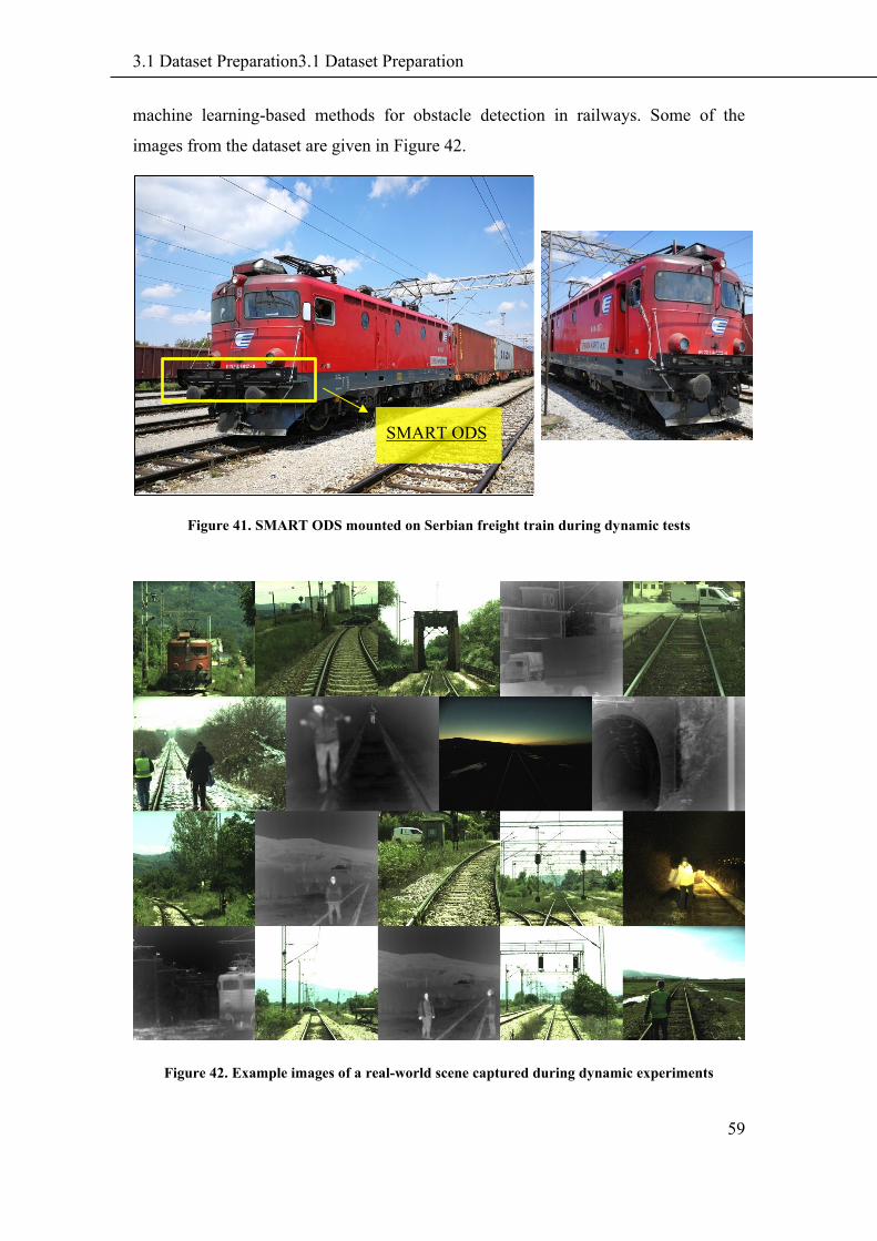
3.1 Dataset Preparation3.1 Dataset Preparation
59
machine learning-based methods for obstacle detection in railways. Some of the
images from the dataset are given in Figure 42.
Figure 41. SMART ODS mounted on Serbian freight train during dynamic tests
Figure 42. Example images of a real-world scene captured during dynamic experiments
SMART ODS
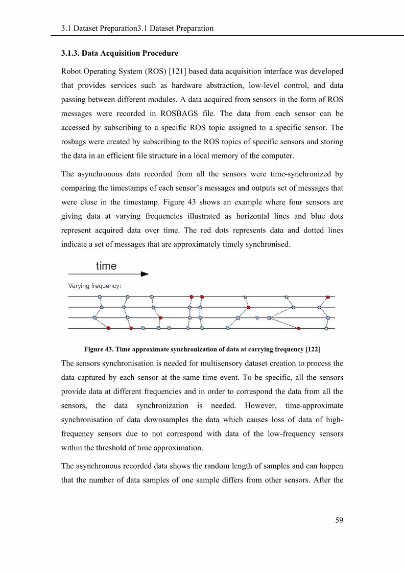
3.1 Dataset Preparation3.1 Dataset Preparation
59
3.1.3. Data Acquisition Procedure
Robot Operating System (ROS) [121] based data acquisition interface was developed
that provides services such as hardware abstraction, low-level control, and data
passing between different modules. A data acquired from sensors in the form of ROS
messages were recorded in ROSBAGS file. The data from each sensor can be
accessed by subscribing to a specific ROS topic assigned to a specific sensor. The
rosbags were created by subscribing to the ROS topics of specific sensors and storing
the data in an efficient file structure in a local memory of the computer.
The asynchronous data recorded from all the sensors were time-synchronized by
comparing the timestamps of each sensor’s messages and outputs set of messages that
were close in the timestamp. Figure 43 shows an example where four sensors are
giving data at varying frequencies illustrated as horizontal lines and blue dots
represent acquired data over time. The red dots represents data and dotted lines
indicate a set of messages that are approximately timely synchronised.
Figure 43. Time approximate synchronization of data at carrying frequency [122]
The sensors synchronisation is needed for multisensory dataset creation to process the
data captured by each sensor at the same time event. To be specific, all the sensors
provide data at different frequencies and in order to correspond the data from all the
sensors, the data synchronization is needed. However, time-approximate
synchronisation of data downsamples the data which causes loss of data of high-
frequency sensors due to not correspond with data of the low-frequency sensors
within the threshold of time approximation.
The asynchronous recorded data shows the random length of samples and can happen
that the number of data samples of one sample differs from other sensors. After the
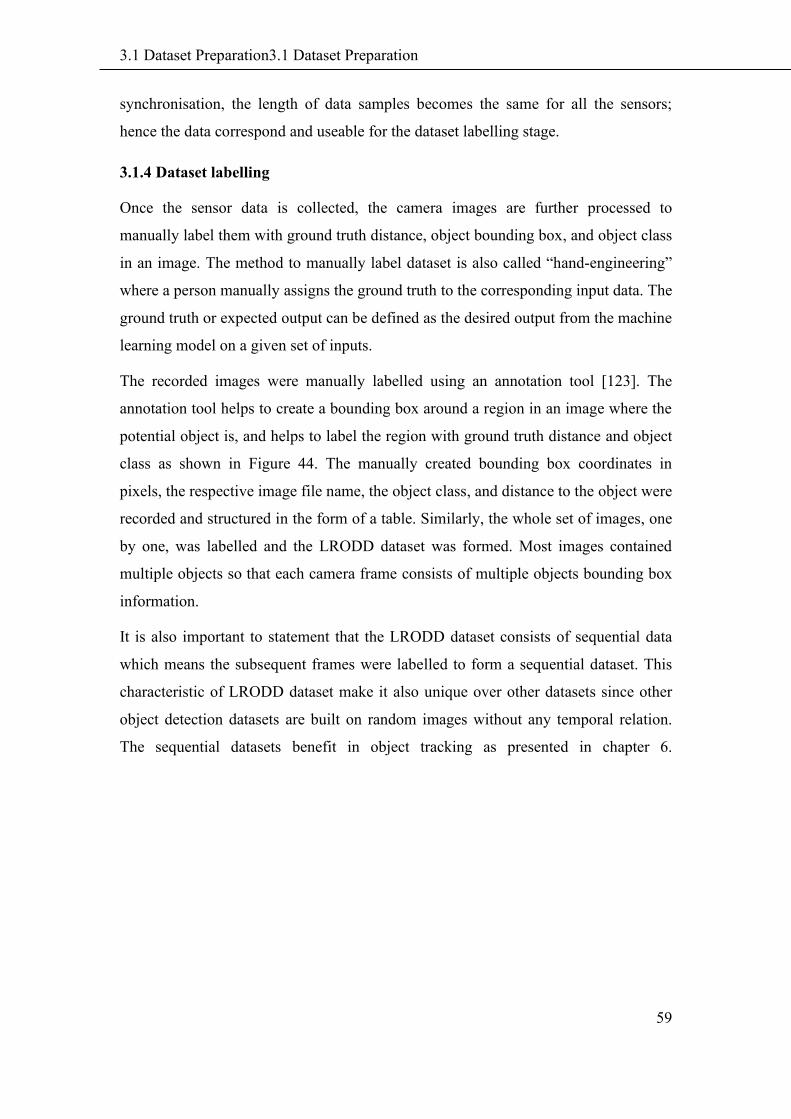
3.1 Dataset Preparation3.1 Dataset Preparation
59
synchronisation, the length of data samples becomes the same for all the sensors;
hence the data correspond and useable for the dataset labelling stage.
3.1.4 Dataset labelling
Once the sensor data is collected, the camera images are further processed to
manually label them with ground truth distance, object bounding box, and object class
in an image. The method to manually label dataset is also called “hand-engineering”
where a person manually assigns the ground truth to the corresponding input data. The
ground truth or expected output can be defined as the desired output from the machine
learning model on a given set of inputs.
The recorded images were manually labelled using an annotation tool [123]. The
annotation tool helps to create a bounding box around a region in an image where the
potential object is, and helps to label the region with ground truth distance and object
class as shown in Figure 44. The manually created bounding box coordinates in
pixels, the respective image file name, the object class, and distance to the object were
recorded and structured in the form of a table. Similarly, the whole set of images, one
by one, was labelled and the LRODD dataset was formed. Most images contained
multiple objects so that each camera frame consists of multiple objects bounding box
information.
It is also important to statement that the LRODD dataset consists of sequential data
which means the subsequent frames were labelled to form a sequential dataset. This
characteristic of LRODD dataset make it also unique over other datasets since other
object detection datasets are built on random images without any temporal relation.
The sequential datasets benefit in object tracking as presented in chapter 6.
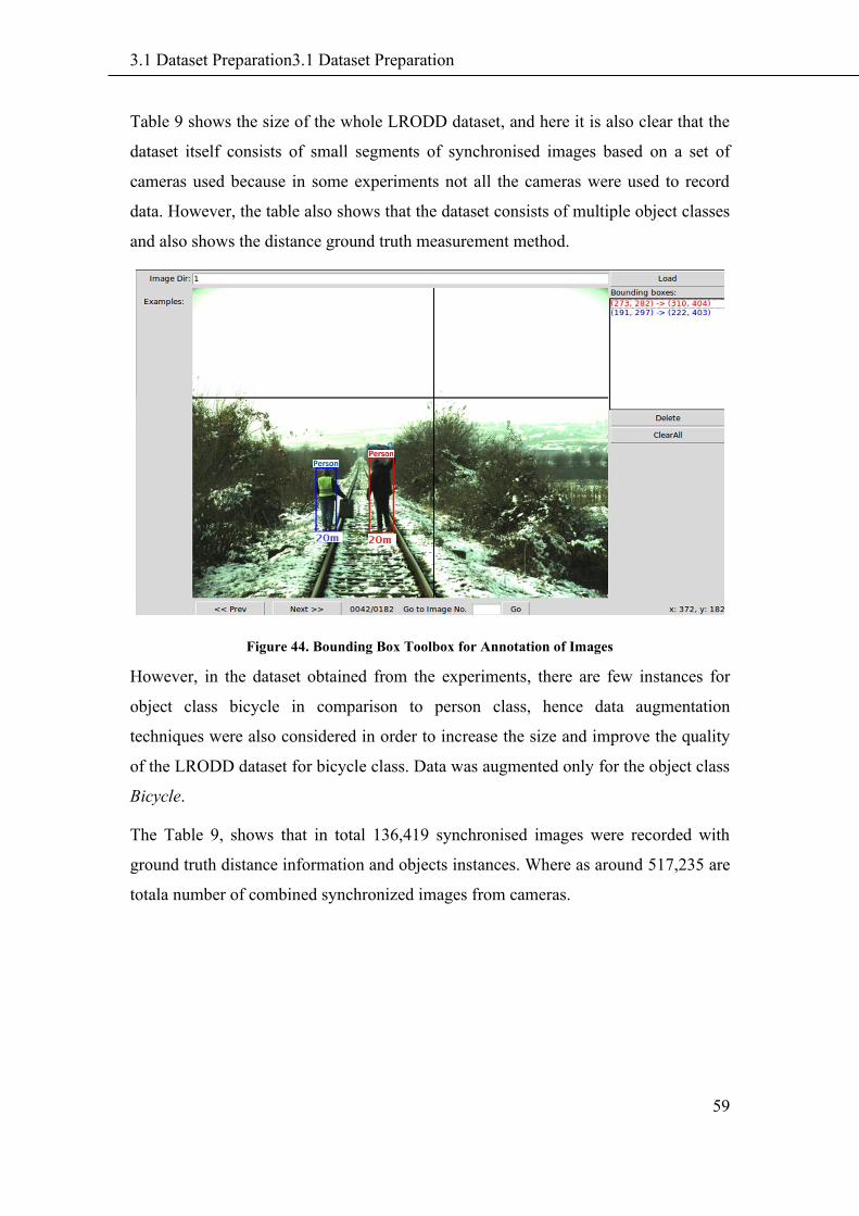
3.1 Dataset Preparation3.1 Dataset Preparation
59
Table 9 shows the size of the whole LRODD dataset, and here it is also clear that the
dataset itself consists of small segments of synchronised images based on a set of
cameras used because in some experiments not all the cameras were used to record
data. However, the table also shows that the dataset consists of multiple object classes
and also shows the distance ground truth measurement method.
Figure 44. Bounding Box Toolbox for Annotation of Images
However, in the dataset obtained from the experiments, there are few instances for
object class bicycle in comparison to person class, hence data augmentation
techniques were also considered in order to increase the size and improve the quality
of the LRODD dataset for bicycle class. Data was augmented only for the object class
Bicycle.
The Table 9, shows that in total 136,419 synchronised images were recorded with
ground truth distance information and objects instances. Where as around 517,235 are
totala number of combined synchronized images from cameras.
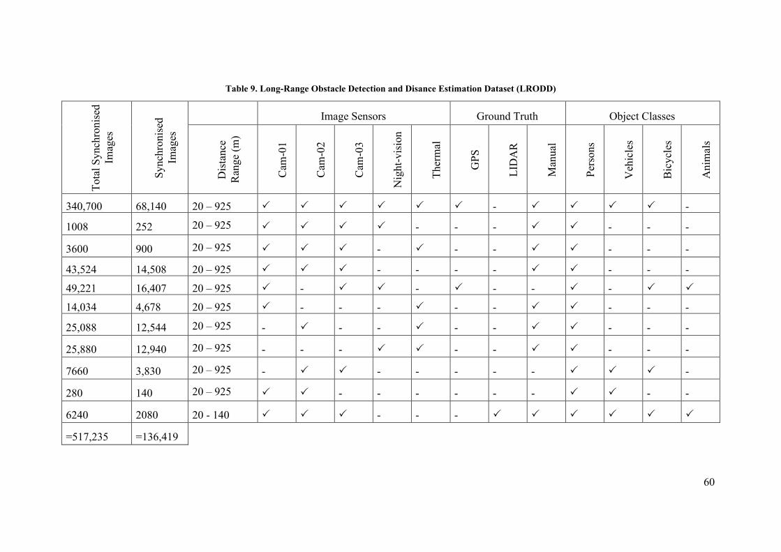
60
Table 9. Long-Range Obstacle Detection and Disance Estimation Dataset (LRODD) T
ota
l S
ynch
ronis
ed
Imag
es
Synch
ronis
ed
Imag
es
Image Sensors Ground Truth Object Classes
Dis
tance
Ran
ge
(m)
Cam
-01
Cam
-02
Cam
-03
Nig
ht-
vis
ion
Ther
mal
GP
S
LID
AR
Man
ual
Per
sons
Veh
icle
s
Bic
ycl
es
Anim
als
340,700 68,140 20 – 925 - -
1008 252 20 – 925 - - - - - -
3600 900 20 – 925 - - - - - -
43,524 14,508 20 – 925 - - - - - - -
49,221 16,407 20 – 925 - - - - -
14,034 4,678 20 – 925 - - - - - - - -
25,088 12,544 20 – 925 - - - - - - - -
25,880 12,940 20 – 925 - - - - - - - -
7660 3,830 20 – 925 - - - - - - -
280 140 20 – 925 - - - - - - - -
6240 2080 20 - 140 - - -
=517,235 =136,419
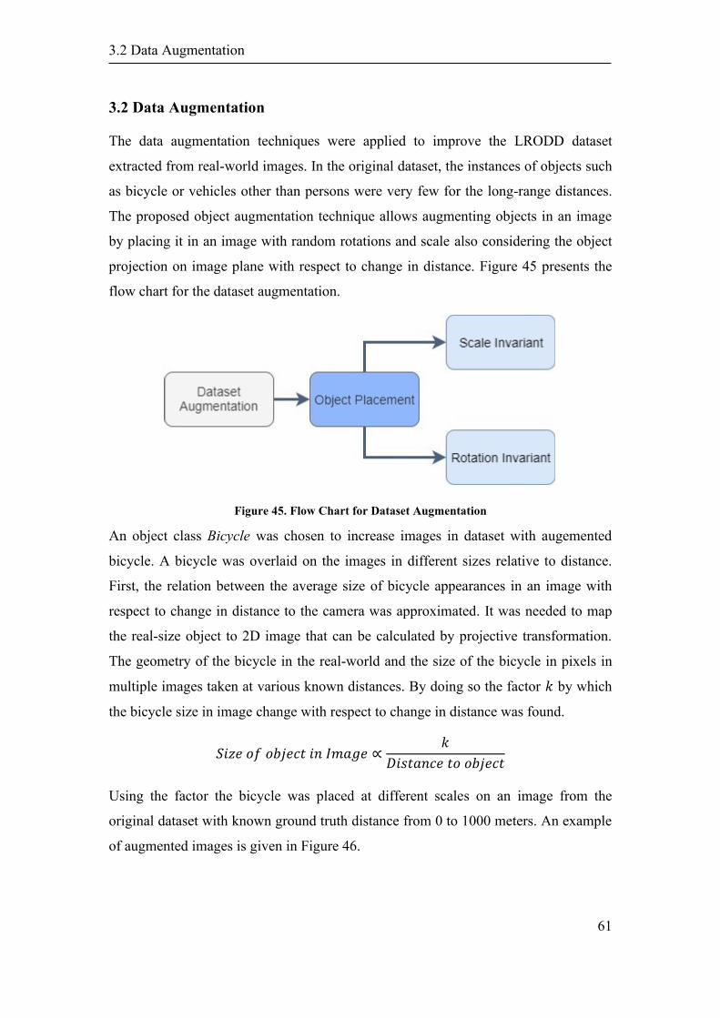
3.2 Data Augmentation
61
3.2 Data Augmentation
The data augmentation techniques were applied to improve the LRODD dataset
extracted from real-world images. In the original dataset, the instances of objects such
as bicycle or vehicles other than persons were very few for the long-range distances.
The proposed object augmentation technique allows augmenting objects in an image
by placing it in an image with random rotations and scale also considering the object
projection on image plane with respect to change in distance. Figure 45 presents the
flow chart for the dataset augmentation.
Figure 45. Flow Chart for Dataset Augmentation
An object class Bicycle was chosen to increase images in dataset with augemented
bicycle. A bicycle was overlaid on the images in different sizes relative to distance.
First, the relation between the average size of bicycle appearances in an image with
respect to change in distance to the camera was approximated. It was needed to map
the real-size object to 2D image that can be calculated by projective transformation.
The geometry of the bicycle in the real-world and the size of the bicycle in pixels in
multiple images taken at various known distances. By doing so the factor 𝑘 by which
the bicycle size in image change with respect to change in distance was found.
𝑆𝑖𝑧𝑒 𝑜𝑓 𝑜𝑏𝑗𝑒𝑐𝑡 𝑖𝑛 𝐼𝑚𝑎𝑔𝑒 ∝𝑘
𝐷𝑖𝑠𝑡𝑎𝑛𝑐𝑒 𝑡𝑜 𝑜𝑏𝑗𝑒𝑐𝑡
Using the factor the bicycle was placed at different scales on an image from the
original dataset with known ground truth distance from 0 to 1000 meters. An example
of augmented images is given in Figure 46.
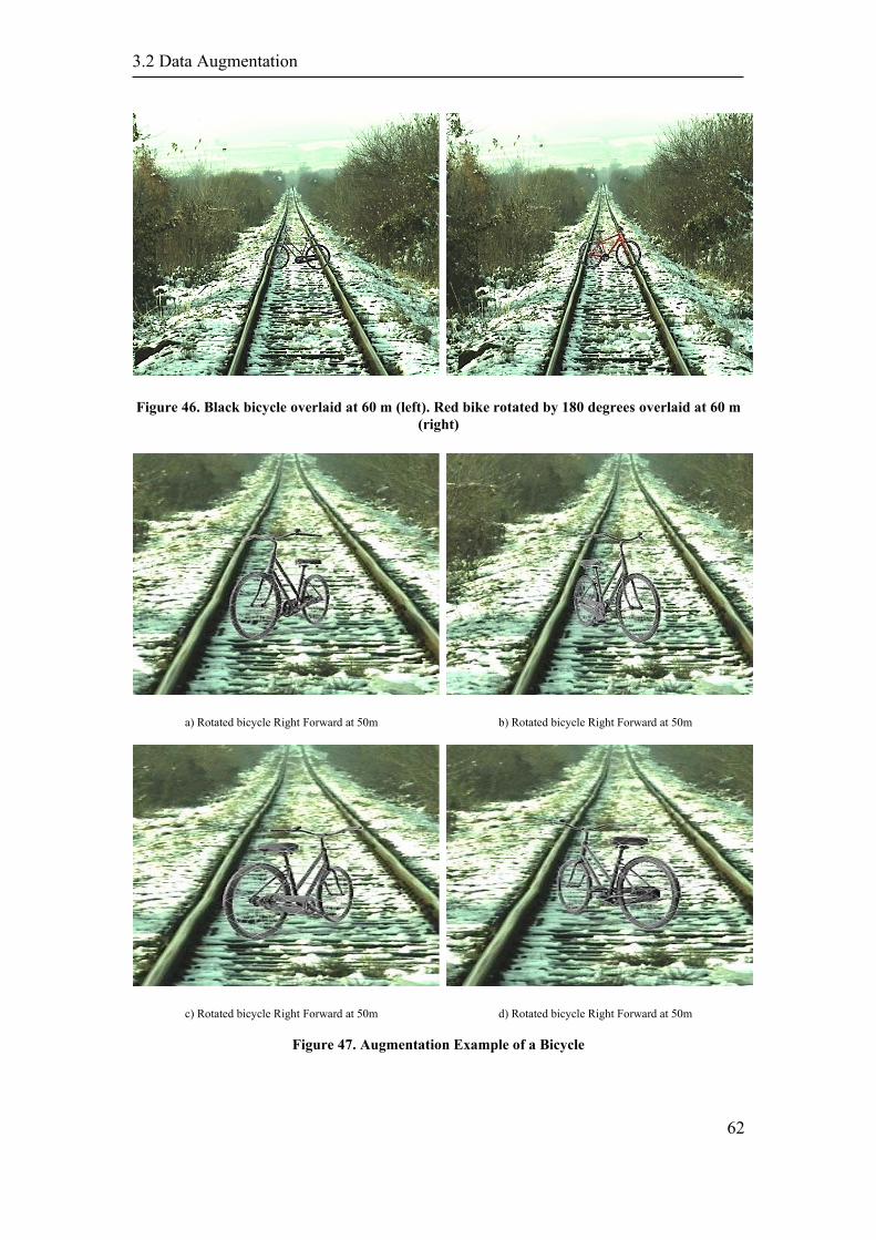
3.2 Data Augmentation
62
Figure 46. Black bicycle overlaid at 60 m (left). Red bike rotated by 180 degrees overlaid at 60 m
(right)
a) Rotated bicycle Right Forward at 50m b) Rotated bicycle Right Forward at 50m
c) Rotated bicycle Right Forward at 50m d) Rotated bicycle Right Forward at 50m
Figure 47. Augmentation Example of a Bicycle
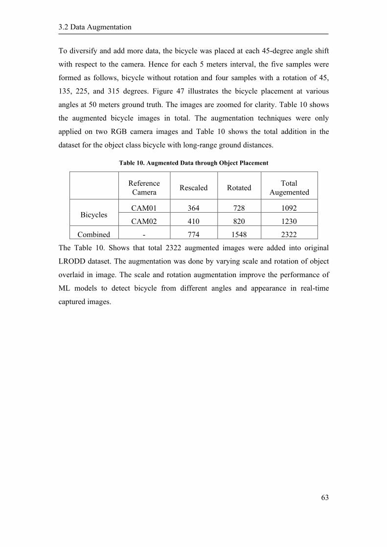
3.2 Data Augmentation
63
To diversify and add more data, the bicycle was placed at each 45-degree angle shift
with respect to the camera. Hence for each 5 meters interval, the five samples were
formed as follows, bicycle without rotation and four samples with a rotation of 45,
135, 225, and 315 degrees. Figure 47 illustrates the bicycle placement at various
angles at 50 meters ground truth. The images are zoomed for clarity. Table 10 shows
the augmented bicycle images in total. The augmentation techniques were only
applied on two RGB camera images and Table 10 shows the total addition in the
dataset for the object class bicycle with long-range ground distances.
Table 10. Augmented Data through Object Placement
Reference
Camera Rescaled Rotated
Total
Augemented
Bicycles CAM01 364 728 1092
CAM02 410 820 1230
Combined - 774 1548 2322
The Table 10. Shows that total 2322 augmented images were added into original
LRODD dataset. The augmentation was done by varying scale and rotation of object
overlaid in image. The scale and rotation augmentation improve the performance of
ML models to detect bicycle from different angles and appearance in real-time
captured images.

64
4.1 DisNet: a machine learning-based object-specific distance estimation from a
single camera
65
4. A machine learning-based distance
estimation from a single camera
A single camera-based distance estimation to the object is a very challenging task and
up to now, this topic is not explored considerably. In this chapter, two novel object
distance estimation methods from a single camera are presented. The first proposed
method named DisNet (Distance Network) has been presented by Haseeb et al. in
[124] and in [125]. The method estimates the distance of the objects detected by the
object detector. DisNet makes use of features extracted from the objects bounding box
and object class type, to estimate the distance to the detected objects. The method can
be used with any object detector that outputs object bounding box and object class.
However, in this work, a state-of-art object detector namely You Only Look Once
(YOLO) has been used.
The second proposed method is named YOLO-D. It is another approach to estimate
distance to the detected object by modifying the architecture of the YOLO object
detection model, a deep learning network. In this method, the modified architecture of
YOLO predicts the distance to the detected object besides its primary function of the
object bounding box and class prediction.
4.1 DisNet: a machine learning-based object-specific distance estimation
from a single camera
In this thesis, the very first method DisNet that estimates the distance based on
bounding box information of detected objects is presented. Any object detector that
outputs object bounding box and class in an image such as YOLO, fast RCNN,
MaskNet can be used with DisNet to estimate the distance to the detected objects.
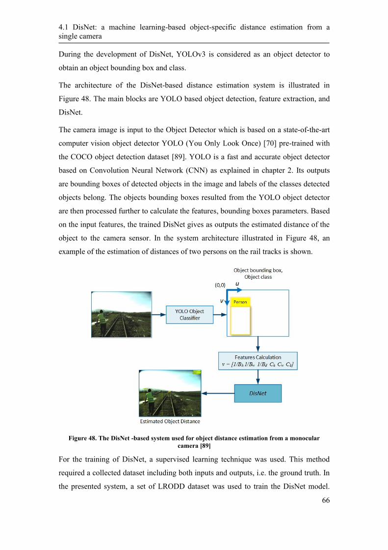
4.1 DisNet: a machine learning-based object-specific distance estimation from a
single camera
66
During the development of DisNet, YOLOv3 is considered as an object detector to
obtain an object bounding box and class.
The architecture of the DisNet-based distance estimation system is illustrated in
Figure 48. The main blocks are YOLO based object detection, feature extraction, and
DisNet.
The camera image is input to the Object Detector which is based on a state-of-the-art
computer vision object detector YOLO (You Only Look Once) [70] pre-trained with
the COCO object detection dataset [89]. YOLO is a fast and accurate object detector
based on Convolution Neural Network (CNN) as explained in chapter 2. Its outputs
are bounding boxes of detected objects in the image and labels of the classes detected
objects belong. The objects bounding boxes resulted from the YOLO object detector
are then processed further to calculate the features, bounding boxes parameters. Based
on the input features, the trained DisNet gives as outputs the estimated distance of the
object to the camera sensor. In the system architecture illustrated in Figure 48, an
example of the estimation of distances of two persons on the rail tracks is shown.
Figure 48. The DisNet -based system used for object distance estimation from a monocular
camera [89]
For the training of DisNet, a supervised learning technique was used. This method
required a collected dataset including both inputs and outputs, i.e. the ground truth. In
the presented system, a set of LRODD dataset was used to train the DisNet model.
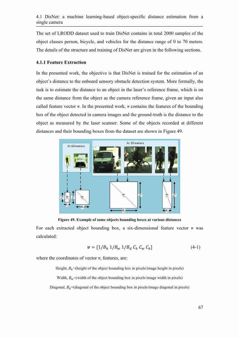
4.1 DisNet: a machine learning-based object-specific distance estimation from a
single camera
67
The set of LRODD dataset used to train DisNet contains in total 2000 samples of the
object classes person, bicycle, and vehicles for the distance range of 0 to 70 meters.
The details of the structure and training of DisNet are given in the following sections.
4.1.1 Feature Extraction
In the presented work, the objective is that DisNet is trained for the estimation of an
object’s distance to the onboard sensory obstacle detection system. More formally, the
task is to estimate the distance to an object in the laser’s reference frame, which is on
the same distance from the object as the camera reference frame, given an input also
called feature vector v. In the presented work, v contains the features of the bounding
box of the object detected in camera images and the ground-truth is the distance to the
object as measured by the laser scanner. Some of the objects recorded at different
distances and their bounding boxes from the dataset are shown in Figure 49.
Figure 49. Example of some objects bounding boxes at various distances
For each extracted object bounding box, a six-dimensional feature vector v was
calculated:
𝒗 = [1/𝐵ℎ 1/𝐵𝑤 1/𝐵𝑑 𝐶ℎ 𝐶𝑤 𝐶𝑏] (4-1)
where the coordinates of vector v, features, are:
Height, 𝐵ℎ=(height of the object bounding box in pixels/image height in pixels)
Width, 𝐵𝑤=(width of the object bounding box in pixels/image width in pixels)
Diagonal, 𝐵𝑑=(diagonal of the object bounding box in pixels/image diagonal in pixels)
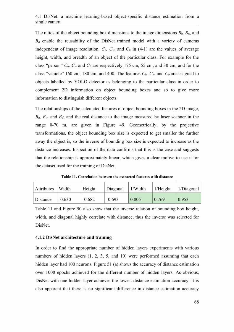
4.1 DisNet: a machine learning-based object-specific distance estimation from a
single camera
68
The ratios of the object bounding box dimensions to the image dimensions Bh, Bw, and
Bd enable the reusability of the DisNet trained model with a variety of cameras
independent of image resolution. Ch, Cw, and Cb in (4-1) are the values of average
height, width, and breadth of an object of the particular class. For example for the
class “person” Ch, Cw and Cb are respectively 175 cm, 55 cm, and 30 cm, and for the
class “vehicle” 160 cm, 180 cm, and 400. The features Ch, Cw, and Cb are assigned to
objects labelled by YOLO detector as belonging to the particular class in order to
complement 2D information on object bounding boxes and so to give more
information to distinguish different objects.
The relationships of the calculated features of object bounding boxes in the 2D image,
Bh, Bw, and Bd, and the real distance to the image measured by laser scanner in the
range 0-70 m, are given in Figure 49. Geometrically, by the projective
transformations, the object bounding box size is expected to get smaller the further
away the object is, so the inverse of bounding box size is expected to increase as the
distance increases. Inspection of the data confirms that this is the case and suggests
that the relationship is approximately linear, which gives a clear motive to use it for
the dataset used for the training of DisNet.
Table 11. Correlation between the extracted features with distance
Attributes Width Height Diagonal 1/Width 1/Height 1/Diagonal
Distance -0.630 -0.682 -0.693 0.805 0.769 0.953
Table 11 and Figure 50 also show that the inverse relation of bounding box height,
width, and diagonal highly correlate with distance, thus the inverse was selected for
DisNet.
4.1.2 DisNet architecture and training
In order to find the appropriate number of hidden layers experiments with various
numbers of hidden layers (1, 2, 3, 5, and 10) were performed assuming that each
hidden layer had 100 neurons. Figure 51 (a) shows the accuracy of distance estimation
over 1000 epochs achieved for the different number of hidden layers. As obvious,
DisNet with one hidden layer achieves the lowest distance estimation accuracy. It is
also apparent that there is no significant difference in distance estimation accuracy
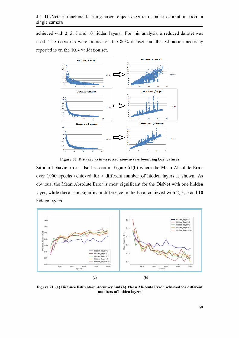
4.1 DisNet: a machine learning-based object-specific distance estimation from a
single camera
69
achieved with 2, 3, 5 and 10 hidden layers. For this analysis, a reduced dataset was
used. The networks were trained on the 80% dataset and the estimation accuracy
reported is on the 10% validation set.
Figure 50. Distance vs inverse and non-inverse bounding box features
Similar behaviour can also be seen in Figure 51(b) where the Mean Absolute Error
over 1000 epochs achieved for a different number of hidden layers is shown. As
obvious, the Mean Absolute Error is most significant for the DisNet with one hidden
layer, while there is no significant difference in the Error achieved with 2, 3, 5 and 10
hidden layers.
(a) (b)
Figure 51. (a) Distance Estimation Accuracy and (b) Mean Absolute Error achieved for different
numbers of hidden layers

4.1 DisNet: a machine learning-based object-specific distance estimation from a
single camera
70
Even though the smallest values of Mean Absolute Error were achieved for 10 hidden
layers and the distance accuracy was highest for 10 hidden layers, a trade-off was
made between the computational time and accuracy/error and finally, DisNet with 3
hidden layers was chosen.
After deciding on the network with 3 hidden layers, in order to find the appropriate
number of neurons for the hidden layers experiments with various numbers of hidden
neurons were performed. Figure 52(a) shows the accuracy of distance estimation over
1000 epochs achieved for the different number of neurons per hidden layer. As
obvious, the distance estimation accuracy achieved with 10 hidden neurons is very
low, much lower than distance estimation accuracy achieved with 30, 100 and 200
hidden neurons. The magnified diagram in Figure 52 (b) shows that distance
estimation accuracy with 30 hidden neurons is lower than with 100 and 200 neurons.
Bearing in mind that there is no significant difference in distance accuracy estimation
with 100 and 200 hidden neurons, in order to reduce the complexity of DisNet,
finally, 100 neurons per hidden layer were chosen.
(a) (b)
Figure 52. Distance Estimation Accuracy achieved for different number of hidden neurons per
hidden layer in 3-hidden layers neural network DisNet
The final structure of DisNet having 3 hidden layers with 100 hidden neurons per
layer is shown in Figure 53.
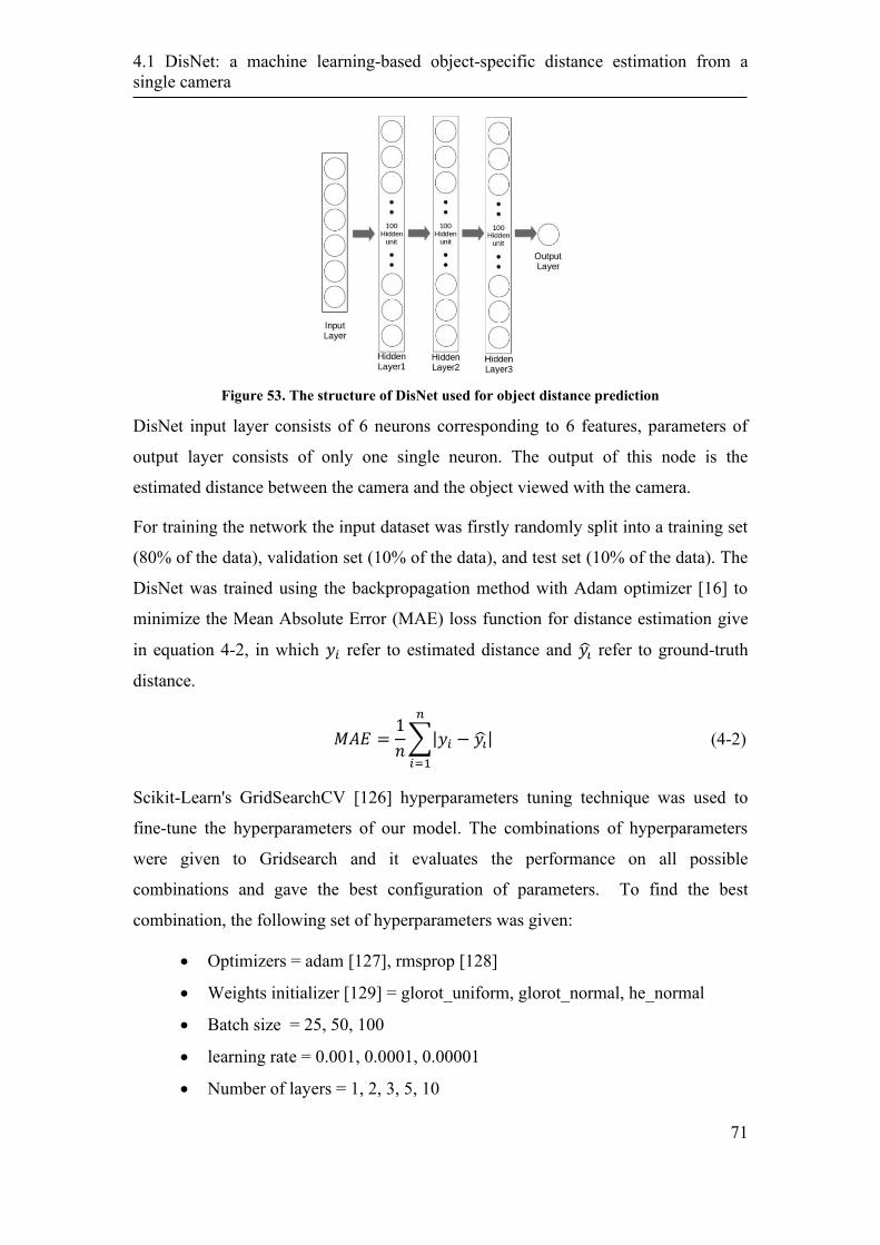
4.1 DisNet: a machine learning-based object-specific distance estimation from a
single camera
71
Figure 53. The structure of DisNet used for object distance prediction
DisNet input layer consists of 6 neurons corresponding to 6 features, parameters of
output layer consists of only one single neuron. The output of this node is the
estimated distance between the camera and the object viewed with the camera.
For training the network the input dataset was firstly randomly split into a training set
(80% of the data), validation set (10% of the data), and test set (10% of the data). The
DisNet was trained using the backpropagation method with Adam optimizer [16] to
minimize the Mean Absolute Error (MAE) loss function for distance estimation give
in equation 4-2, in which 𝑦𝑖 refer to estimated distance and 𝑦�̂� refer to ground-truth
distance.
𝑀𝐴𝐸 =1
𝑛∑|𝑦𝑖 − 𝑦�̂�|
𝑛
𝑖=1
(4-2)
Scikit-Learn's GridSearchCV [126] hyperparameters tuning technique was used to
fine-tune the hyperparameters of our model. The combinations of hyperparameters
were given to Gridsearch and it evaluates the performance on all possible
combinations and gave the best configuration of parameters. To find the best
combination, the following set of hyperparameters was given:
• Optimizers = adam [127], rmsprop [128]
• Weights initializer [129] = glorot_uniform, glorot_normal, he_normal
• Batch size = 25, 50, 100
• learning rate = 0.001, 0.0001, 0.00001
• Number of layers = 1, 2, 3, 5, 10
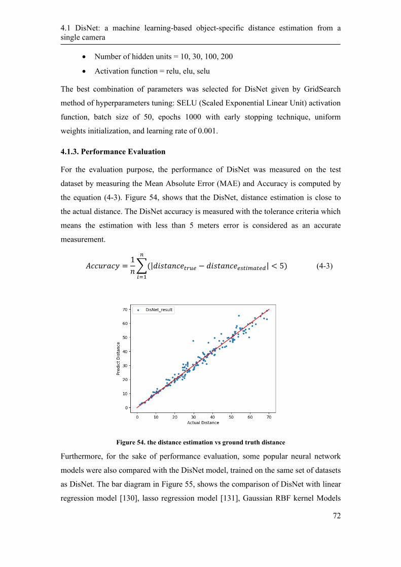
4.1 DisNet: a machine learning-based object-specific distance estimation from a
single camera
72
• Number of hidden units = 10, 30, 100, 200
• Activation function = relu, elu, selu
The best combination of parameters was selected for DisNet given by GridSearch
method of hyperparameters tuning: SELU (Scaled Exponential Linear Unit) activation
function, batch size of 50, epochs 1000 with early stopping technique, uniform
weights initialization, and learning rate of 0.001.
4.1.3. Performance Evaluation
For the evaluation purpose, the performance of DisNet was measured on the test
dataset by measuring the Mean Absolute Error (MAE) and Accuracy is computed by
the equation (4-3). Figure 54, shows that the DisNet, distance estimation is close to
the actual distance. The DisNet accuracy is measured with the tolerance criteria which
means the estimation with less than 5 meters error is considered as an accurate
measurement.
𝐴𝑐𝑐𝑢𝑟𝑎𝑐𝑦 =1
𝑛∑(|𝑑𝑖𝑠𝑡𝑎𝑛𝑐𝑒𝑡𝑟𝑢𝑒 − 𝑑𝑖𝑠𝑡𝑎𝑛𝑐𝑒𝑒𝑠𝑡𝑖𝑚𝑎𝑡𝑒𝑑| < 5)
𝑛
𝑖=1
(4-3)
Figure 54. the distance estimation vs ground truth distance
Furthermore, for the sake of performance evaluation, some popular neural network
models were also compared with the DisNet model, trained on the same set of datasets
as DisNet. The bar diagram in Figure 55, shows the comparison of DisNet with linear
regression model [130], lasso regression model [131], Gaussian RBF kernel Models
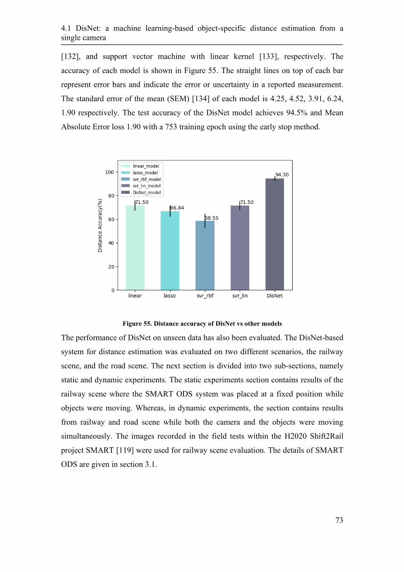
4.1 DisNet: a machine learning-based object-specific distance estimation from a
single camera
73
[132], and support vector machine with linear kernel [133], respectively. The
accuracy of each model is shown in Figure 55. The straight lines on top of each bar
represent error bars and indicate the error or uncertainty in a reported measurement.
The standard error of the mean (SEM) [134] of each model is 4.25, 4.52, 3.91, 6.24,
1.90 respectively. The test accuracy of the DisNet model achieves 94.5% and Mean
Absolute Error loss 1.90 with a 753 training epoch using the early stop method.
Figure 55. Distance accuracy of DisNet vs other models
The performance of DisNet on unseen data has also been evaluated. The DisNet-based
system for distance estimation was evaluated on two different scenarios, the railway
scene, and the road scene. The next section is divided into two sub-sections, namely
static and dynamic experiments. The static experiments section contains results of the
railway scene where the SMART ODS system was placed at a fixed position while
objects were moving. Whereas, in dynamic experiments, the section contains results
from railway and road scene while both the camera and the objects were moving
simultaneously. The images recorded in the field tests within the H2020 Shift2Rail
project SMART [119] were used for railway scene evaluation. The details of SMART
ODS are given in section 3.1.
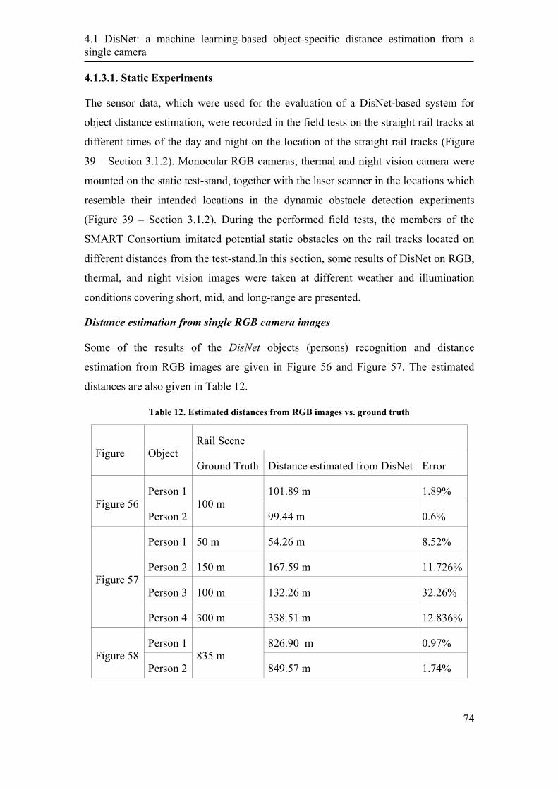
4.1 DisNet: a machine learning-based object-specific distance estimation from a
single camera
74
4.1.3.1. Static Experiments
The sensor data, which were used for the evaluation of a DisNet-based system for
object distance estimation, were recorded in the field tests on the straight rail tracks at
different times of the day and night on the location of the straight rail tracks (Figure
39 – Section 3.1.2). Monocular RGB cameras, thermal and night vision camera were
mounted on the static test-stand, together with the laser scanner in the locations which
resemble their intended locations in the dynamic obstacle detection experiments
(Figure 39 – Section 3.1.2). During the performed field tests, the members of the
SMART Consortium imitated potential static obstacles on the rail tracks located on
different distances from the test-stand.In this section, some results of DisNet on RGB,
thermal, and night vision images were taken at different weather and illumination
conditions covering short, mid, and long-range are presented.
Distance estimation from single RGB camera images
Some of the results of the DisNet objects (persons) recognition and distance
estimation from RGB images are given in Figure 56 and Figure 57. The estimated
distances are also given in Table 12.
Table 12. Estimated distances from RGB images vs. ground truth
Figure Object Rail Scene
Ground Truth Distance estimated from DisNet Error
Figure 56 Person 1
100 m 101.89 m 1.89%
Person 2 99.44 m 0.6%
Figure 57
Person 1 50 m 54.26 m 8.52%
Person 2 150 m 167.59 m 11.726%
Person 3 100 m 132.26 m 32.26%
Person 4 300 m 338.51 m 12.836%
Figure 58 Person 1
835 m 826.90 m 0.97%
Person 2 849.57 m 1.74%
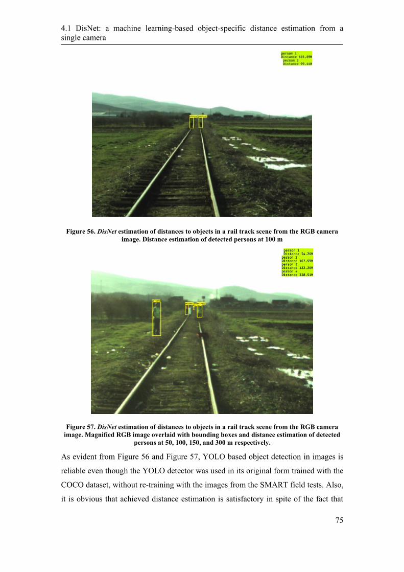
4.1 DisNet: a machine learning-based object-specific distance estimation from a
single camera
75
Figure 56. DisNet estimation of distances to objects in a rail track scene from the RGB camera
image. Distance estimation of detected persons at 100 m
Figure 57. DisNet estimation of distances to objects in a rail track scene from the RGB camera
image. Magnified RGB image overlaid with bounding boxes and distance estimation of detected
persons at 50, 100, 150, and 300 m respectively.
As evident from Figure 56 and Figure 57, YOLO based object detection in images is
reliable even though the YOLO detector was used in its original form trained with the
COCO dataset, without re-training with the images from the SMART field tests. Also,
it is obvious that achieved distance estimation is satisfactory in spite of the fact that
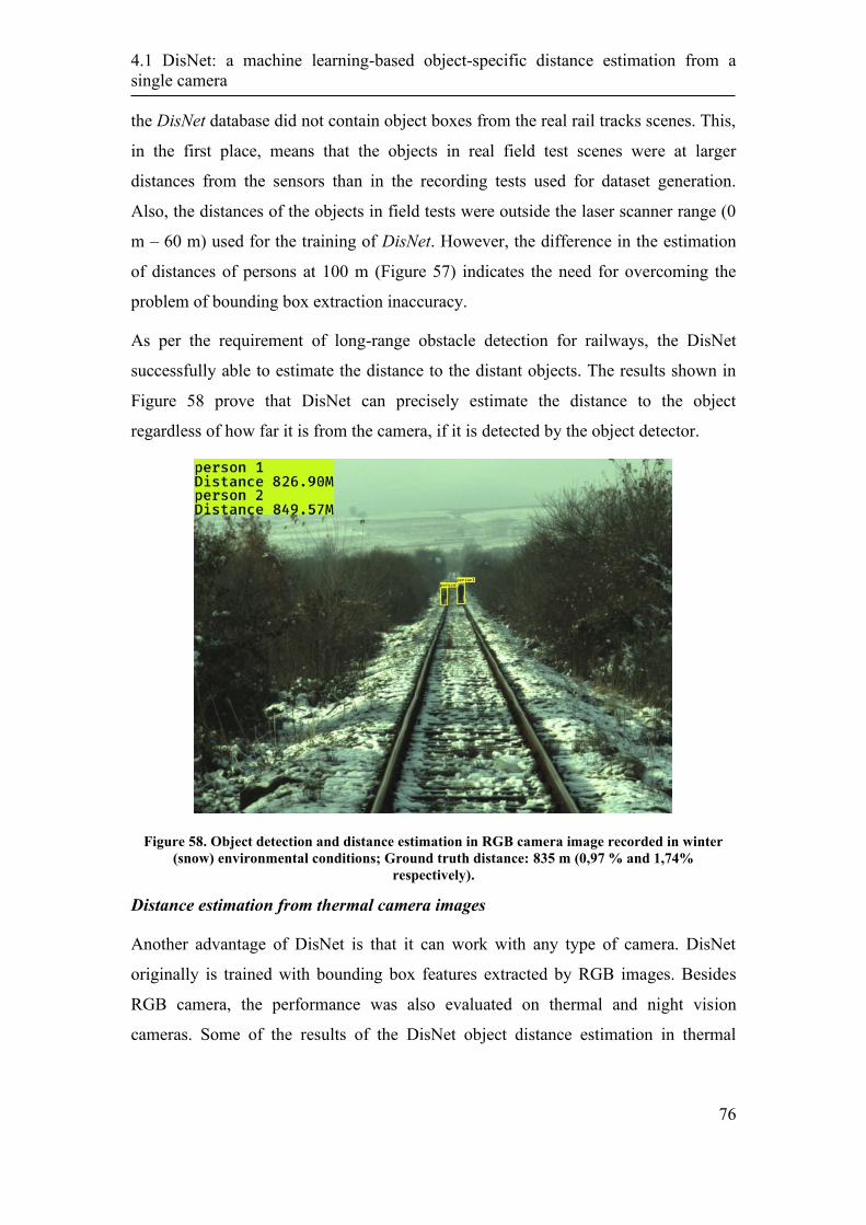
4.1 DisNet: a machine learning-based object-specific distance estimation from a
single camera
76
the DisNet database did not contain object boxes from the real rail tracks scenes. This,
in the first place, means that the objects in real field test scenes were at larger
distances from the sensors than in the recording tests used for dataset generation.
Also, the distances of the objects in field tests were outside the laser scanner range (0
m – 60 m) used for the training of DisNet. However, the difference in the estimation
of distances of persons at 100 m (Figure 57) indicates the need for overcoming the
problem of bounding box extraction inaccuracy.
As per the requirement of long-range obstacle detection for railways, the DisNet
successfully able to estimate the distance to the distant objects. The results shown in
Figure 58 prove that DisNet can precisely estimate the distance to the object
regardless of how far it is from the camera, if it is detected by the object detector.
Figure 58. Object detection and distance estimation in RGB camera image recorded in winter
(snow) environmental conditions; Ground truth distance: 835 m (0,97 % and 1,74%
respectively).
Distance estimation from thermal camera images
Another advantage of DisNet is that it can work with any type of camera. DisNet
originally is trained with bounding box features extracted by RGB images. Besides
RGB camera, the performance was also evaluated on thermal and night vision
cameras. Some of the results of the DisNet object distance estimation in thermal
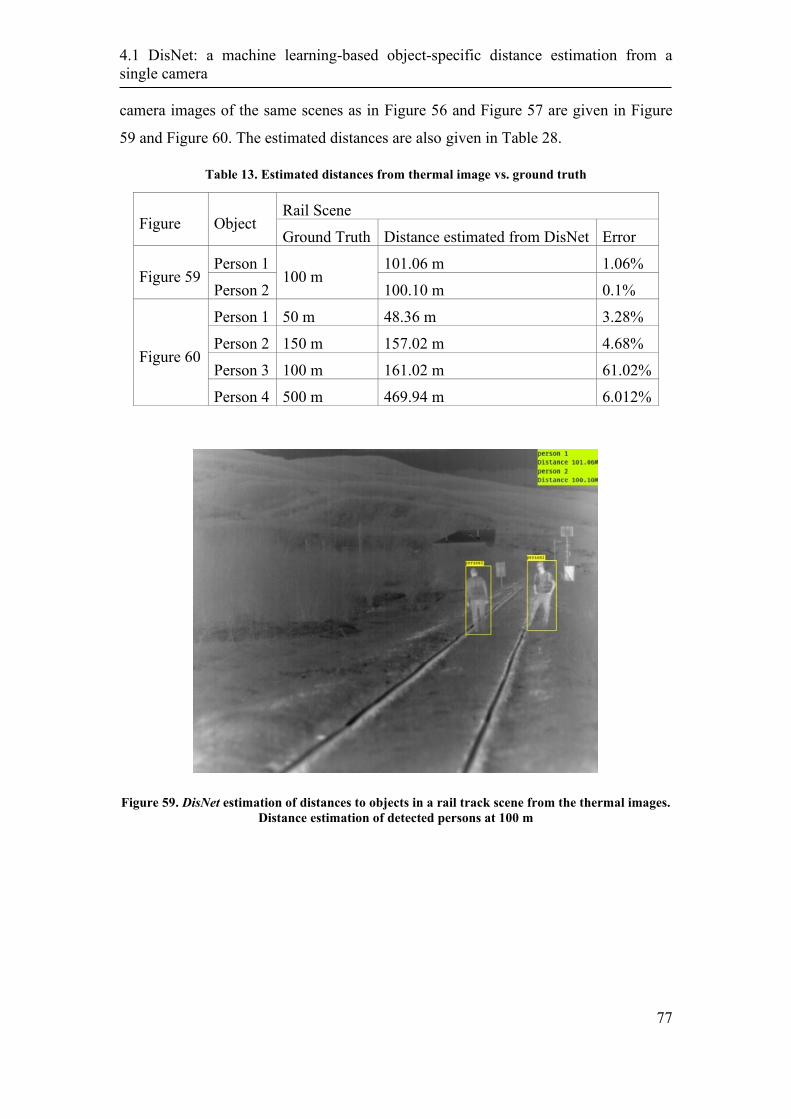
4.1 DisNet: a machine learning-based object-specific distance estimation from a
single camera
77
camera images of the same scenes as in Figure 56 and Figure 57 are given in Figure
59 and Figure 60. The estimated distances are also given in Table 28.
Table 13. Estimated distances from thermal image vs. ground truth
Figure Object Rail Scene
Ground Truth Distance estimated from DisNet Error
Figure 59 Person 1
100 m 101.06 m 1.06%
Person 2 100.10 m 0.1%
Figure 60
Person 1 50 m 48.36 m 3.28%
Person 2 150 m 157.02 m 4.68%
Person 3 100 m 161.02 m 61.02%
Person 4 500 m 469.94 m 6.012%
Figure 59. DisNet estimation of distances to objects in a rail track scene from the thermal images.
Distance estimation of detected persons at 100 m
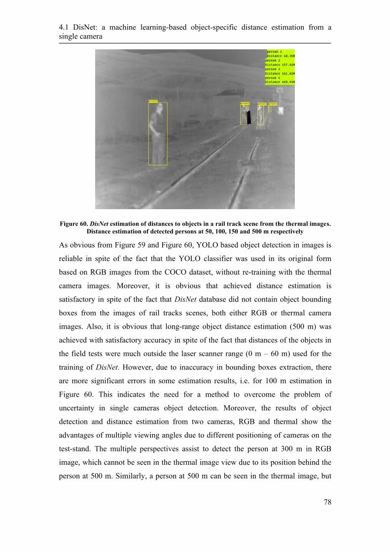
4.1 DisNet: a machine learning-based object-specific distance estimation from a
single camera
78
Figure 60. DisNet estimation of distances to objects in a rail track scene from the thermal images.
Distance estimation of detected persons at 50, 100, 150 and 500 m respectively
As obvious from Figure 59 and Figure 60, YOLO based object detection in images is
reliable in spite of the fact that the YOLO classifier was used in its original form
based on RGB images from the COCO dataset, without re-training with the thermal
camera images. Moreover, it is obvious that achieved distance estimation is
satisfactory in spite of the fact that DisNet database did not contain object bounding
boxes from the images of rail tracks scenes, both either RGB or thermal camera
images. Also, it is obvious that long-range object distance estimation (500 m) was
achieved with satisfactory accuracy in spite of the fact that distances of the objects in
the field tests were much outside the laser scanner range (0 m – 60 m) used for the
training of DisNet. However, due to inaccuracy in bounding boxes extraction, there
are more significant errors in some estimation results, i.e. for 100 m estimation in
Figure 60. This indicates the need for a method to overcome the problem of
uncertainty in single cameras object detection. Moreover, the results of object
detection and distance estimation from two cameras, RGB and thermal show the
advantages of multiple viewing angles due to different positioning of cameras on the
test-stand. The multiple perspectives assist to detect the person at 300 m in RGB
image, which cannot be seen in the thermal image view due to its position behind the
person at 500 m. Similarly, a person at 500 m can be seen in the thermal image, but
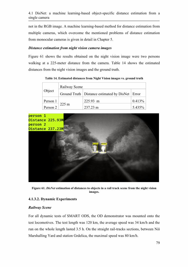
4.1 DisNet: a machine learning-based object-specific distance estimation from a
single camera
79
not in the RGB image. A machine learning-based method for distance estimation from
multiple cameras, which overcome the mentioned problems of distance estimation
from monocular cameras is given in detail in Chapter 5.
Distance estimation from night vision camera images
Figure 61 shows the results obtained on the night vision image were two persons
walking at a 225-meter distance from the camera. Table 14 shows the estimated
distances from the night vision images and the ground truth.
Table 14. Estimated distances from Night Vision images vs. ground truth
Object Railway Scene
Ground Truth Distance estimated by DisNet Error
Person 1 225 m
225.93 m 0.413%
Person 2 237.23 m 5.435%
Figure 61. DisNet estimation of distances to objects in a rail track scene from the night vision
images.
4.1.3.2. Dynamic Experiments
Railway Scene
For all dynamic tests of SMART ODS, the OD demonstrator was mounted onto the
test locomotives. The test length was 120 km, the average speed was 34 km/h and the
run on the whole length lasted 3.5 h. On the straight rail-tracks sections, between Niš
Marshalling Yard and station Grdelica, the maximal speed was 80 km/h.

4.1 DisNet: a machine learning-based object-specific distance estimation from a
single camera
80
Similar to Static experiments, SMART team members mimicked objects (obstacles)
on two crossings along the route according to previously adopted test protocols.
During the rest of the test, as the train was in real traffic, accidental objects were
detected along the route. These objects represented possible obstacles, which could
cause an accident, for example, a truck crossing the unsecured crossing at the station
while the train was approaching.
Some of the results of the DisNet based distance calculation with RGB cameras are
shown in Figure 62. Figure 62 (a)-(d) show four subsequent frames of the RGB
camera video in which two persons crossing the track are recognized out of which one
person is pushing the bike, which also was recognized. The person and the bike were
recognized though they are not on the same track as the train. As can be seen from
Figure 62, a person without the bike, who is crossing the rail track, in four subsequent
frames was recognized at distances 121,74 m, 114,16 m, 86,37 m, and 81,71 m as
opposed to ground truth distances of 120.12 m, 111.95 m, 83.66 m, and 80.62 m
respectively. The ground truth distances were calculated using GPS coordinates of the
train, Google maps GPS coordinates (e.g. crossing), and railway infrastructure
information (e.g. distance between pillars).
Table 15. Long-range distance estimation
Object Railway Scene
Ground Truth Distance estimated by DisNet Error
Person
120.12 m 121.74 m 1.34%
111.95 m 114.16 m 1.97%
83.66 m 86.37 m 3.23%
80.62 m 81.71 m 1.35%
Due to the geometry of the rail tracks in dynamic tests, there were no straight rail
tracks sections longer than 600 m on which accidental objects could be detected.
However, Mid- to Long-range results of about 200 m - 600 m were achieved as
illustrated in Figure 63-66, from RGB, thermal and night vision camera. Static tests
were performed in November 2018 on the straight rail tracks in the length of about
1000 m, with the planned (mimicked objects) on the whole length, complementing so
dynamic tests (a result shown in Figure 57). Due to the positive results achieved in

4.1 DisNet: a machine learning-based object-specific distance estimation from a
single camera
81
static field tests, similar performance is expected to be achieved in operational
conditions as well.
(a)
(b)
(c)
(d)
Figure 62. Four subsequent frames of the RGB camera video overlaid with the bounding boxes of
the detected objects as well as with the estimated distances from the locomotive to the objects
Table 16. Long-range distance estimation for RGB, Thermal and Night Vision Images
Figure Object Rail Scene
Ground Truth Distance estimated from DisNet Error
Figure 63 Person 1 272.75 m 245.02 m 10%
Figure 64
Person 1
231.97 m
253.65 m 8.2%
Person 2 251.09 m 8.24%
Figure 65 Person 1 266.69 m 231.42 m ~8.32%
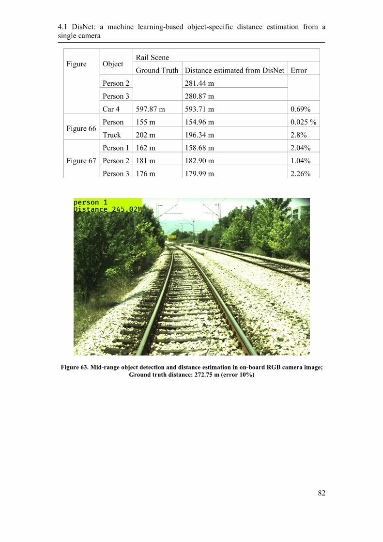
4.1 DisNet: a machine learning-based object-specific distance estimation from a
single camera
82
Figure Object Rail Scene
Ground Truth Distance estimated from DisNet Error
Person 2 281.44 m
Person 3 280.87 m
Car 4 597.87 m 593.71 m 0.69%
Figure 66 Person 155 m 154.96 m 0.025 %
Truck 202 m 196.34 m 2.8%
Figure 67
Person 1 162 m 158.68 m 2.04%
Person 2 181 m 182.90 m 1.04%
Person 3 176 m 179.99 m 2.26%
Figure 63. Mid-range object detection and distance estimation in on-board RGB camera image;
Ground truth distance: 272.75 m (error 10%)
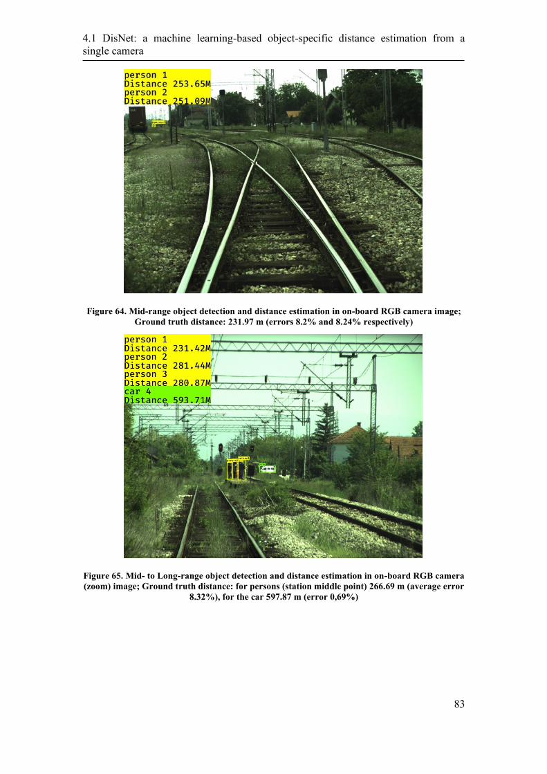
4.1 DisNet: a machine learning-based object-specific distance estimation from a
single camera
83
Figure 64. Mid-range object detection and distance estimation in on-board RGB camera image;
Ground truth distance: 231.97 m (errors 8.2% and 8.24% respectively)
Figure 65. Mid- to Long-range object detection and distance estimation in on-board RGB camera
(zoom) image; Ground truth distance: for persons (station middle point) 266.69 m (average error
8.32%), for the car 597.87 m (error 0,69%)
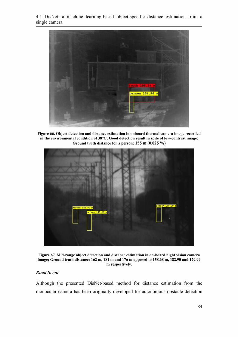
4.1 DisNet: a machine learning-based object-specific distance estimation from a
single camera
84
Figure 66. Object detection and distance estimation in onboard thermal camera image recorded
in the environmental condition of 38°C; Good detection result in spite of low-contrast image;
Ground truth distance for a person: 155 m (0.025 %)
Figure 67. Mid-range object detection and distance estimation in on-board night vision camera
image; Ground truth distance: 162 m, 181 m and 176 m opposed to 158.68 m, 182.90 and 179.99
m respectively.
Road Scene
Although the presented DisNet-based method for distance estimation from the
monocular camera has been originally developed for autonomous obstacle detection
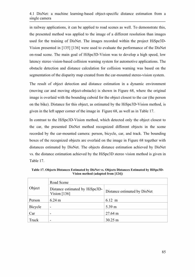
4.1 DisNet: a machine learning-based object-specific distance estimation from a
single camera
85
in railway applications, it can be applied to road scenes as well. To demonstrate this,
the presented method was applied to the image of a different resolution than images
used for the training of DisNet. The images recorded within the project HiSpe3D-
Vision presented in [135] [136] were used to evaluate the performance of the DisNet
on-road scene. The main goal of HiSpe3D-Vision was to develop a high speed, low
latency stereo vision-based collision warning system for automotive applications. The
obstacle detection and distance calculation for collision warning was based on the
segmentation of the disparity map created from the car-mounted stereo-vision system.
The result of object detection and distance estimation in a dynamic environment
(moving car and moving object-obstacle) is shown in Figure 68, where the original
image is overlaid with the bounding cuboid for the object closest to the car (the person
on the bike). Distance for this object, as estimated by the HiSpe3D-Vision method, is
given in the left upper corner of the image in Figure 68, as well as in Table 17.
In contrast to the HiSpe3D-Vision method, which detected only the object closest to
the car, the presented DisNet method recognized different objects in the scene
recorded by the car-mounted camera: person, bicycle, car, and track. The bounding
boxes of the recognized objects are overlaid on the image in Figure 68 together with
distances estimated by DisNet. The objects distance estimation achieved by DisNet
vs. the distance estimation achieved by the HiSpe3D stereo vision method is given in
Table 17.
Table 17. Objects Distances Estimated by DisNet vs. Objects Distances Estimated by HiSpe3D-
Vision method (adapted from [124])
Object
Road Scene
Distance estimated by HiSpe3D-
Vision [136] Distance estimated by DisNet
Person 6.24 m 6.12 m
Bicycle - 5.39 m
Car - 27.64 m
Truck - 30.25 m
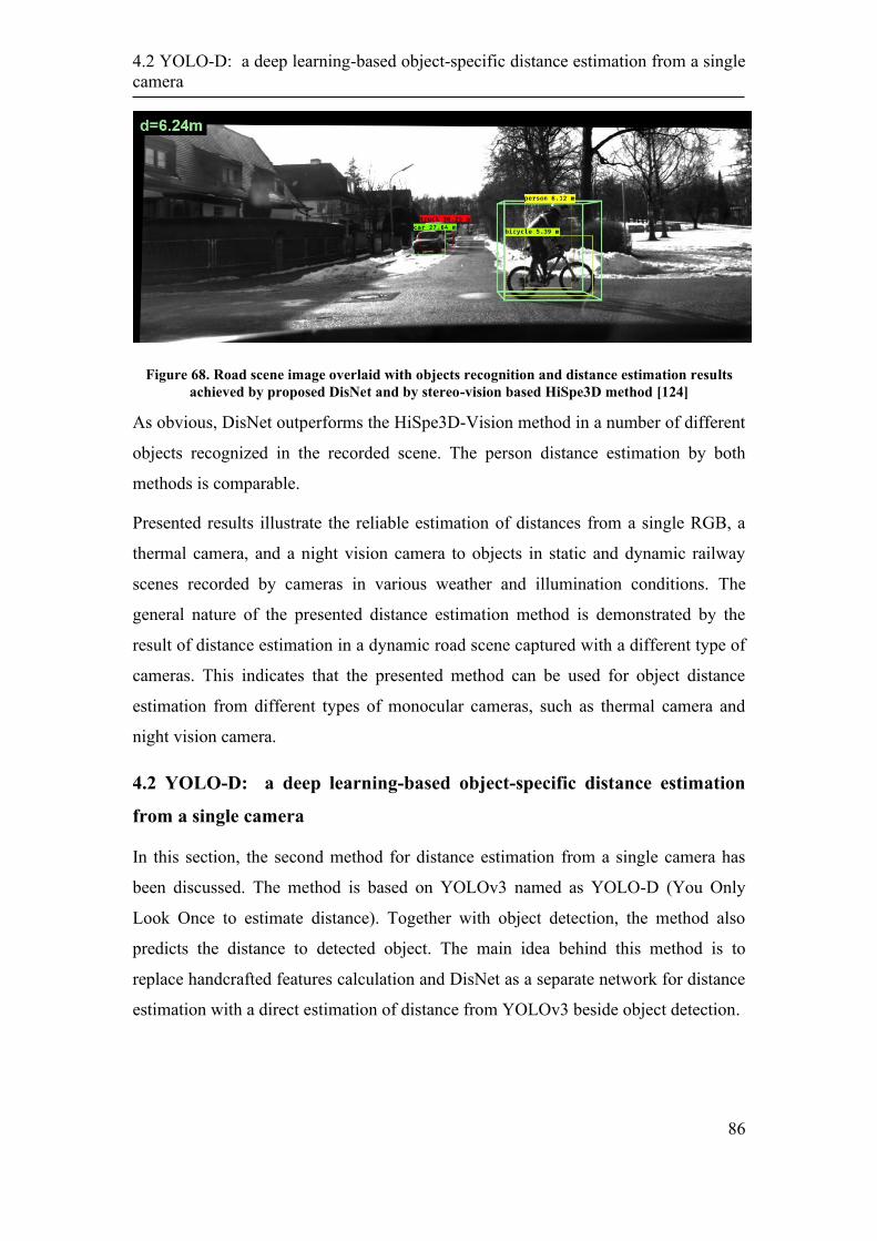
4.2 YOLO-D: a deep learning-based object-specific distance estimation from a single
camera
86
Figure 68. Road scene image overlaid with objects recognition and distance estimation results
achieved by proposed DisNet and by stereo-vision based HiSpe3D method [124]
As obvious, DisNet outperforms the HiSpe3D-Vision method in a number of different
objects recognized in the recorded scene. The person distance estimation by both
methods is comparable.
Presented results illustrate the reliable estimation of distances from a single RGB, a
thermal camera, and a night vision camera to objects in static and dynamic railway
scenes recorded by cameras in various weather and illumination conditions. The
general nature of the presented distance estimation method is demonstrated by the
result of distance estimation in a dynamic road scene captured with a different type of
cameras. This indicates that the presented method can be used for object distance
estimation from different types of monocular cameras, such as thermal camera and
night vision camera.
4.2 YOLO-D: a deep learning-based object-specific distance estimation
from a single camera
In this section, the second method for distance estimation from a single camera has
been discussed. The method is based on YOLOv3 named as YOLO-D (You Only
Look Once to estimate distance). Together with object detection, the method also
predicts the distance to detected object. The main idea behind this method is to
replace handcrafted features calculation and DisNet as a separate network for distance
estimation with a direct estimation of distance from YOLOv3 beside object detection.
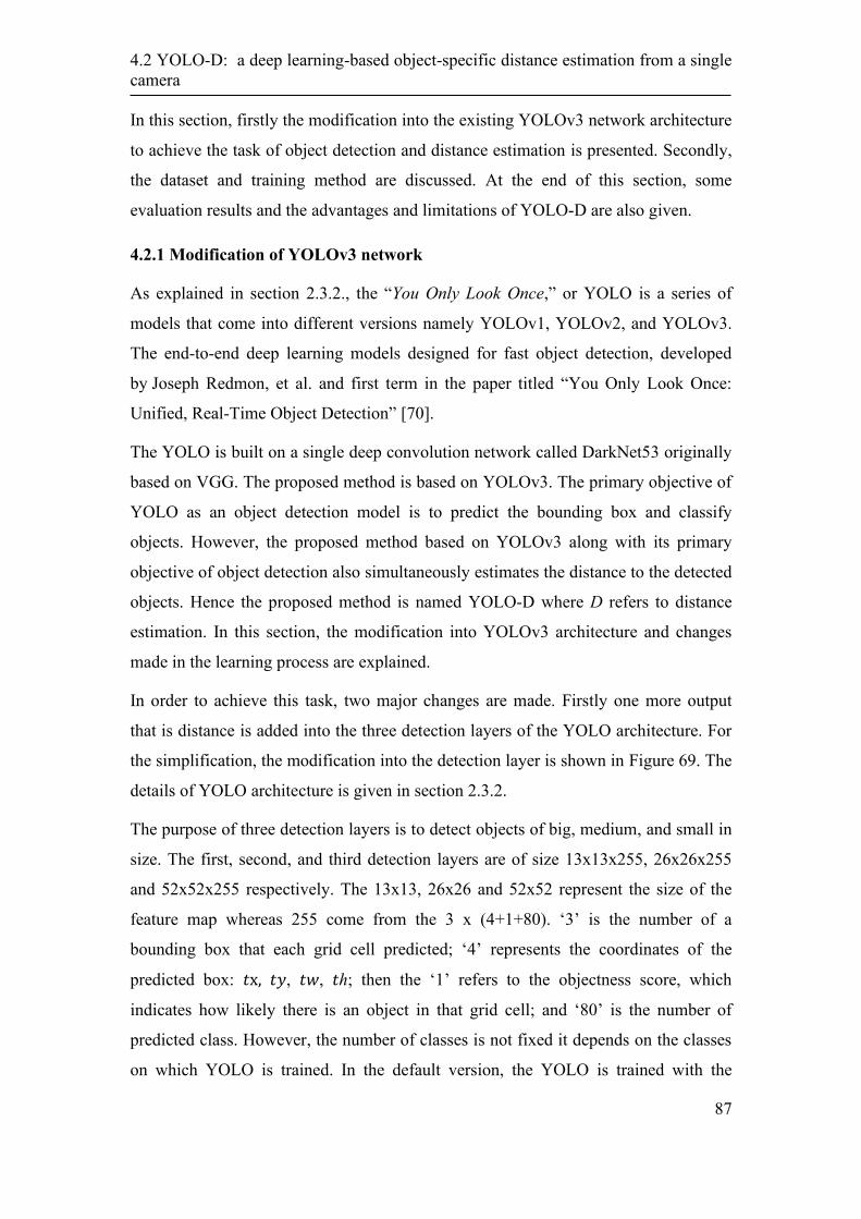
4.2 YOLO-D: a deep learning-based object-specific distance estimation from a single
camera
87
In this section, firstly the modification into the existing YOLOv3 network architecture
to achieve the task of object detection and distance estimation is presented. Secondly,
the dataset and training method are discussed. At the end of this section, some
evaluation results and the advantages and limitations of YOLO-D are also given.
4.2.1 Modification of YOLOv3 network
As explained in section 2.3.2., the “You Only Look Once,” or YOLO is a series of
models that come into different versions namely YOLOv1, YOLOv2, and YOLOv3.
The end-to-end deep learning models designed for fast object detection, developed
by Joseph Redmon, et al. and first term in the paper titled “You Only Look Once:
Unified, Real-Time Object Detection” [70].
The YOLO is built on a single deep convolution network called DarkNet53 originally
based on VGG. The proposed method is based on YOLOv3. The primary objective of
YOLO as an object detection model is to predict the bounding box and classify
objects. However, the proposed method based on YOLOv3 along with its primary
objective of object detection also simultaneously estimates the distance to the detected
objects. Hence the proposed method is named YOLO-D where D refers to distance
estimation. In this section, the modification into YOLOv3 architecture and changes
made in the learning process are explained.
In order to achieve this task, two major changes are made. Firstly one more output
that is distance is added into the three detection layers of the YOLO architecture. For
the simplification, the modification into the detection layer is shown in Figure 69. The
details of YOLO architecture is given in section 2.3.2.
The purpose of three detection layers is to detect objects of big, medium, and small in
size. The first, second, and third detection layers are of size 13x13x255, 26x26x255
and 52x52x255 respectively. The 13x13, 26x26 and 52x52 represent the size of the
feature map whereas 255 come from the 3 x (4+1+80). ‘3’ is the number of a
bounding box that each grid cell predicted; ‘4’ represents the coordinates of the
predicted box: 𝑡x, 𝑡𝑦, 𝑡𝑤, 𝑡ℎ; then the ‘1’ refers to the objectness score, which
indicates how likely there is an object in that grid cell; and ‘80’ is the number of
predicted class. However, the number of classes is not fixed it depends on the classes
on which YOLO is trained. In the default version, the YOLO is trained with the
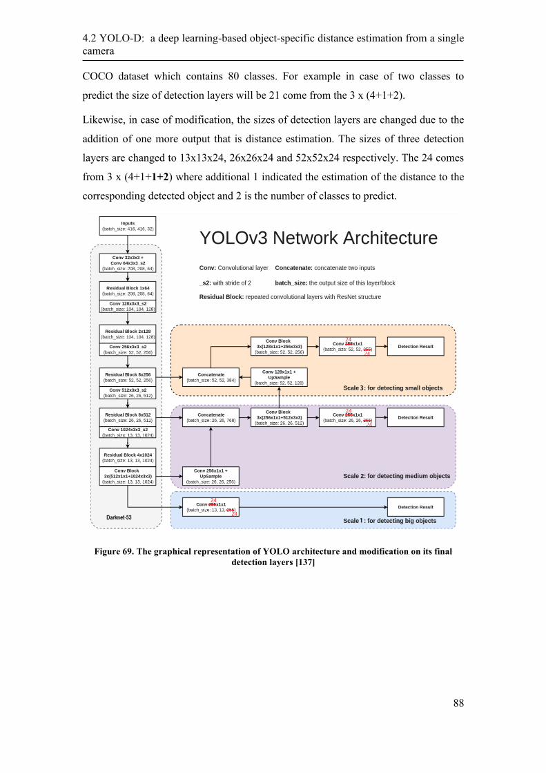
4.2 YOLO-D: a deep learning-based object-specific distance estimation from a single
camera
88
COCO dataset which contains 80 classes. For example in case of two classes to
predict the size of detection layers will be 21 come from the 3 x (4+1+2).
Likewise, in case of modification, the sizes of detection layers are changed due to the
addition of one more output that is distance estimation. The sizes of three detection
layers are changed to 13x13x24, 26x26x24 and 52x52x24 respectively. The 24 comes
from 3 x (4+1+1+2) where additional 1 indicated the estimation of the distance to the
corresponding detected object and 2 is the number of classes to predict.
Figure 69. The graphical representation of YOLO architecture and modification on its final
detection layers [137]
4.2 YOLO-D: a deep learning-based object-specific distance estimation from a single
camera
89
Figure 70. The architecture of modified YOLOv3 (YOLO-D)
4.2.2 Loss Function
The second major change to achieve distance estimation from YOLOv3 is made into
its loss function by adding the distance loss function into the YOLOv3 default loss
function. The YOLO loss function is a cumulative loss function of localization (errors
between the predicted bounding box and the ground truth bounding box), confidence
(likelihood of objectness of the box) and class type. By adding the loss function for
distance estimation the loss function for YOLO-D will be as given in equation (4-4).
𝐿𝑜𝑠𝑠𝑡𝑜𝑡𝑎𝑙 = 𝐿𝑜𝑠𝑠𝑙𝑜𝑐𝑎𝑙𝑖𝑧𝑎𝑡𝑖𝑜𝑛 + 𝐿𝑜𝑠𝑠𝑐𝑜𝑛𝑓𝑖𝑑𝑒𝑛𝑐𝑒 + 𝐿𝑜𝑠𝑠𝑐𝑙𝑎𝑠𝑠 + 𝑳𝒐𝒔𝒔𝒅𝒊𝒔𝒕𝒂𝒏𝒄𝒆 (4-4)
From the understanding of loss function selection during the development of DisNet,
the Mean Absolute Error function was selected over other loss function due to its
small loss relative to other loss functions. Similarly, the loss function selection
process was also conducted for YOLO-D training. Since the distance estimation is a
regression problem, the selection of loss functions was made between the two famous
MAE and MSE loss function as given in equation x and y.
𝑀𝐴𝐸 =1
𝑛∑|𝑑𝑖𝑠𝑡𝑖 − 𝑑𝑖𝑠𝑡�̂�|
𝑛
𝑖=1
(4-5)
𝑀𝑆𝐸 =1
𝑛∑(𝑑𝑖𝑠𝑡𝑖 − 𝑑𝑖𝑠𝑡�̂�)
2𝑛
𝑖=0
(4-6)
Let’s add the distance loss into the YOLO loss function. The total loss function of
YOLO-D based on MAE based distance loss function is given in equation (4-7) and
similarly the total loss function by adding the MSE based distance loss function is
given in equation (4-8).
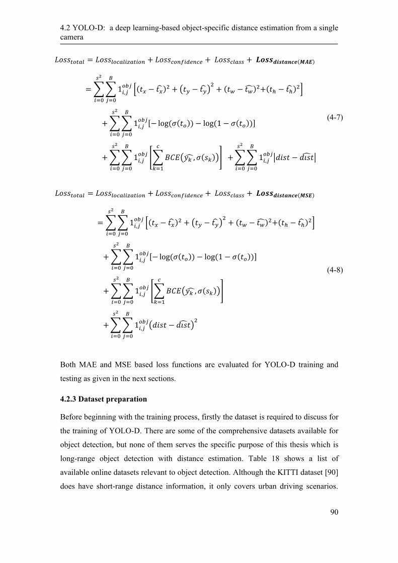
4.2 YOLO-D: a deep learning-based object-specific distance estimation from a single
camera
90
𝐿𝑜𝑠𝑠𝑡𝑜𝑡𝑎𝑙 = 𝐿𝑜𝑠𝑠𝑙𝑜𝑐𝑎𝑙𝑖𝑧𝑎𝑡𝑖𝑜𝑛 + 𝐿𝑜𝑠𝑠𝑐𝑜𝑛𝑓𝑖𝑑𝑒𝑛𝑐𝑒 + 𝐿𝑜𝑠𝑠𝑐𝑙𝑎𝑠𝑠 + 𝑳𝒐𝒔𝒔𝒅𝒊𝒔𝒕𝒂𝒏𝒄𝒆(𝑴𝑨𝑬)
= ∑∑1𝑖,𝑗𝑜𝑏𝑗
[(𝑡𝑥 − 𝑡�̂�)2 + (𝑡𝑦 − 𝑡�̂�)
2+ (𝑡𝑤 − 𝑡�̂�)2+(𝑡ℎ − 𝑡ℎ̂)2]
𝐵
𝑗=0
𝑠2
𝑖=0
+ ∑∑ 1𝑖,𝑗𝑜𝑏𝑗[− log(𝜎(𝑡𝑜)) − log(1 − 𝜎(𝑡𝑜))]
𝐵
𝑗=0
𝑠2
𝑖=0
+ ∑∑ 1𝑖,𝑗𝑜𝑏𝑗
[∑ 𝐵𝐶𝐸(𝑦𝑘 ,̂ 𝜎(𝑠𝑘))
𝑐
𝑘=1
] +
𝐵
𝑗=0
𝑠2
𝑖=0
∑∑1𝑖,𝑗𝑜𝑏𝑗
|𝑑𝑖𝑠𝑡 − 𝑑𝑖𝑠𝑡̂ |
𝐵
𝑗=0
𝑠2
𝑖=0
(4-7)
𝐿𝑜𝑠𝑠𝑡𝑜𝑡𝑎𝑙 = 𝐿𝑜𝑠𝑠𝑙𝑜𝑐𝑎𝑙𝑖𝑧𝑎𝑡𝑖𝑜𝑛 + 𝐿𝑜𝑠𝑠𝑐𝑜𝑛𝑓𝑖𝑑𝑒𝑛𝑐𝑒 + 𝐿𝑜𝑠𝑠𝑐𝑙𝑎𝑠𝑠 + 𝑳𝒐𝒔𝒔𝒅𝒊𝒔𝒕𝒂𝒏𝒄𝒆(𝑴𝑺𝑬)
= ∑∑1𝑖,𝑗𝑜𝑏𝑗
[(𝑡𝑥 − 𝑡�̂�)2 + (𝑡𝑦 − 𝑡�̂�)
2+ (𝑡𝑤 − 𝑡�̂�)2+(𝑡ℎ − 𝑡ℎ̂)2]
𝐵
𝑗=0
𝑠2
𝑖=0
+ ∑∑1𝑖,𝑗𝑜𝑏𝑗[− log(𝜎(𝑡𝑜)) − log(1 − 𝜎(𝑡𝑜))]
𝐵
𝑗=0
𝑠2
𝑖=0
+ ∑∑1𝑖,𝑗𝑜𝑏𝑗
[∑ 𝐵𝐶𝐸(𝑦𝑘 ,̂ 𝜎(𝑠𝑘))
𝑐
𝑘=1
]
𝐵
𝑗=0
𝑠2
𝑖=0
+∑∑ 1𝑖,𝑗𝑜𝑏𝑗
(𝑑𝑖𝑠𝑡 − 𝑑𝑖𝑠𝑡̂ )2
𝐵
𝑗=0
𝑠2
𝑖=0
(4-8)
Both MAE and MSE based loss functions are evaluated for YOLO-D training and
testing as given in the next sections.
4.2.3 Dataset preparation
Before beginning with the training process, firstly the dataset is required to discuss for
the training of YOLO-D. There are some of the comprehensive datasets available for
object detection, but none of them serves the specific purpose of this thesis which is
long-range object detection with distance estimation. Table 18 shows a list of
available online datasets relevant to object detection. Although the KITTI dataset [90]
does have short-range distance information, it only covers urban driving scenarios.
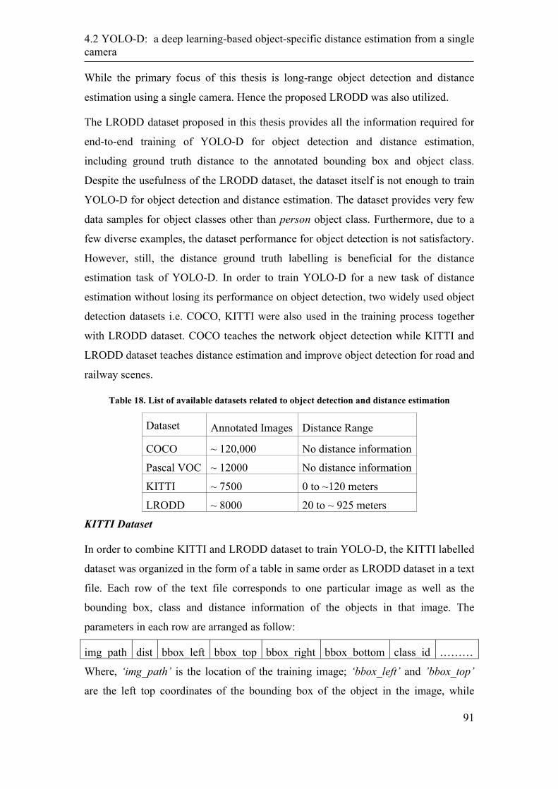
4.2 YOLO-D: a deep learning-based object-specific distance estimation from a single
camera
91
While the primary focus of this thesis is long-range object detection and distance
estimation using a single camera. Hence the proposed LRODD was also utilized.
The LRODD dataset proposed in this thesis provides all the information required for
end-to-end training of YOLO-D for object detection and distance estimation,
including ground truth distance to the annotated bounding box and object class.
Despite the usefulness of the LRODD dataset, the dataset itself is not enough to train
YOLO-D for object detection and distance estimation. The dataset provides very few
data samples for object classes other than person object class. Furthermore, due to a
few diverse examples, the dataset performance for object detection is not satisfactory.
However, still, the distance ground truth labelling is beneficial for the distance
estimation task of YOLO-D. In order to train YOLO-D for a new task of distance
estimation without losing its performance on object detection, two widely used object
detection datasets i.e. COCO, KITTI were also used in the training process together
with LRODD dataset. COCO teaches the network object detection while KITTI and
LRODD dataset teaches distance estimation and improve object detection for road and
railway scenes.
Table 18. List of available datasets related to object detection and distance estimation
Dataset Annotated Images Distance Range
COCO ~ 120,000 No distance information
Pascal VOC ~ 12000 No distance information
KITTI ~ 7500 0 to ~120 meters
LRODD ~ 8000 20 to ~ 925 meters
KITTI Dataset
In order to combine KITTI and LRODD dataset to train YOLO-D, the KITTI labelled
dataset was organized in the form of a table in same order as LRODD dataset in a text
file. Each row of the text file corresponds to one particular image as well as the
bounding box, class and distance information of the objects in that image. The
parameters in each row are arranged as follow:
img_path dist bbox_left bbox_top bbox_right bbox_bottom class_id ………
Where, ‘img_path’ is the location of the training image; ‘bbox_left’ and ’bbox_top’
are the left top coordinates of the bounding box of the object in the image, while
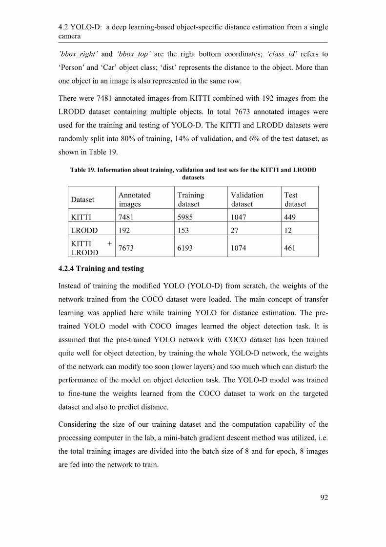
4.2 YOLO-D: a deep learning-based object-specific distance estimation from a single
camera
92
’bbox_right’ and ‘bbox_top’ are the right bottom coordinates; ‘class_id’ refers to
‘Person’ and ‘Car’ object class; ‘dist’ represents the distance to the object. More than
one object in an image is also represented in the same row.
There were 7481 annotated images from KITTI combined with 192 images from the
LRODD dataset containing multiple objects. In total 7673 annotated images were
used for the training and testing of YOLO-D. The KITTI and LRODD datasets were
randomly split into 80% of training, 14% of validation, and 6% of the test dataset, as
shown in Table 19.
Table 19. Information about training, validation and test sets for the KITTI and LRODD
datasets
Dataset Annotated
images
Training
dataset
Validation
dataset
Test
dataset
KITTI 7481 5985 1047 449
LRODD 192 153 27 12
KITTI +
LRODD 7673 6193 1074 461
4.2.4 Training and testing
Instead of training the modified YOLO (YOLO-D) from scratch, the weights of the
network trained from the COCO dataset were loaded. The main concept of transfer
learning was applied here while training YOLO for distance estimation. The pre-
trained YOLO model with COCO images learned the object detection task. It is
assumed that the pre-trained YOLO network with COCO dataset has been trained
quite well for object detection, by training the whole YOLO-D network, the weights
of the network can modify too soon (lower layers) and too much which can disturb the
performance of the model on object detection task. The YOLO-D model was trained
to fine-tune the weights learned from the COCO dataset to work on the targeted
dataset and also to predict distance.
Considering the size of our training dataset and the computation capability of the
processing computer in the lab, a mini-batch gradient descent method was utilized, i.e.
the total training images are divided into the batch size of 8 and for epoch, 8 images
are fed into the network to train.
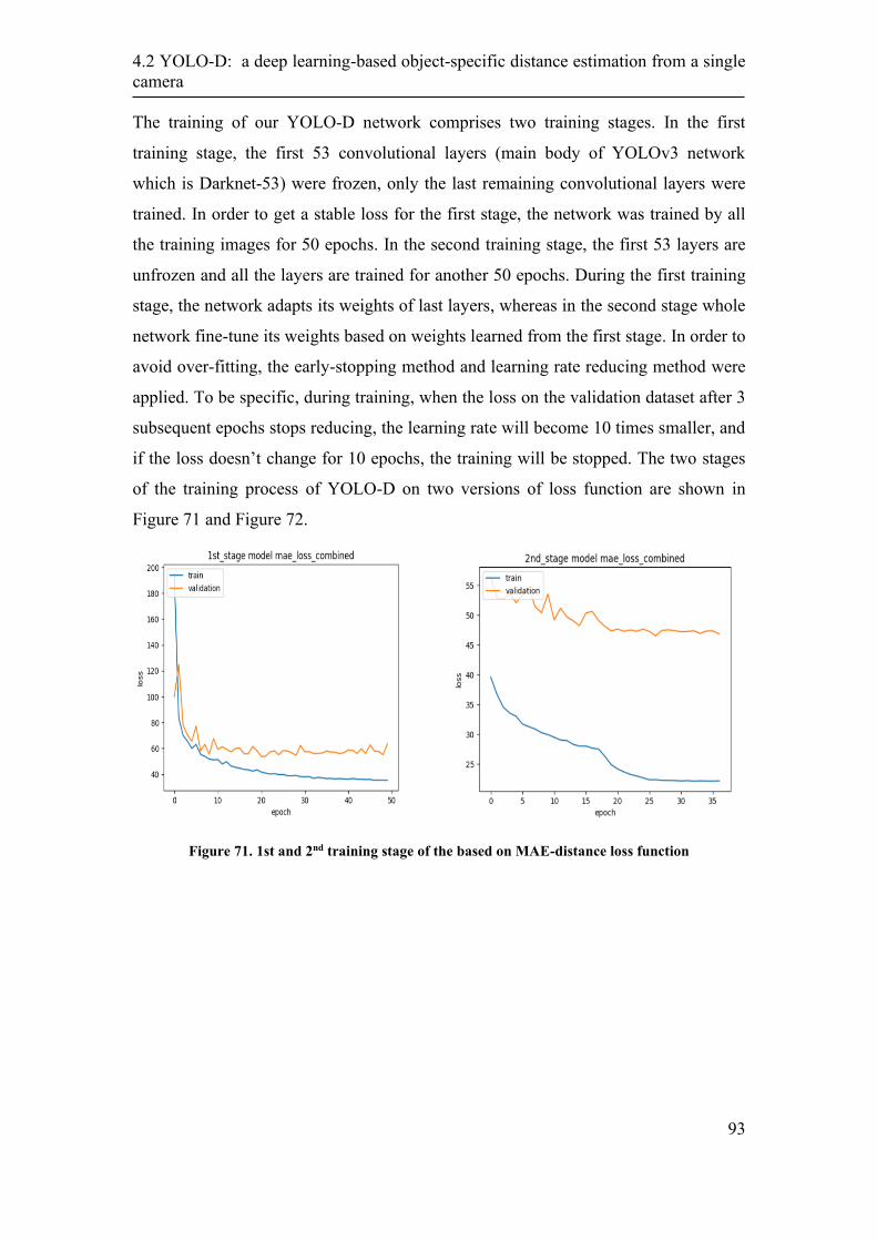
4.2 YOLO-D: a deep learning-based object-specific distance estimation from a single
camera
93
The training of our YOLO-D network comprises two training stages. In the first
training stage, the first 53 convolutional layers (main body of YOLOv3 network
which is Darknet-53) were frozen, only the last remaining convolutional layers were
trained. In order to get a stable loss for the first stage, the network was trained by all
the training images for 50 epochs. In the second training stage, the first 53 layers are
unfrozen and all the layers are trained for another 50 epochs. During the first training
stage, the network adapts its weights of last layers, whereas in the second stage whole
network fine-tune its weights based on weights learned from the first stage. In order to
avoid over-fitting, the early-stopping method and learning rate reducing method were
applied. To be specific, during training, when the loss on the validation dataset after 3
subsequent epochs stops reducing, the learning rate will become 10 times smaller, and
if the loss doesn’t change for 10 epochs, the training will be stopped. The two stages
of the training process of YOLO-D on two versions of loss function are shown in
Figure 71 and Figure 72.
Figure 71. 1st and 2nd training stage of the based on MAE-distance loss function
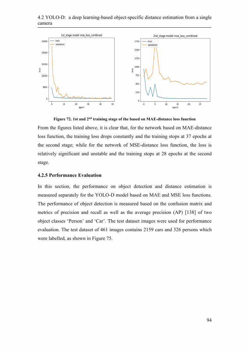
4.2 YOLO-D: a deep learning-based object-specific distance estimation from a single
camera
94
Figure 72. 1st and 2nd training stage of the based on MAE-distance loss function
From the figures listed above, it is clear that, for the network based on MAE-distance
loss function, the training loss drops constantly and the training stops at 37 epochs at
the second stage; while for the network of MSE-distance loss function, the loss is
relatively significant and unstable and the training stops at 28 epochs at the second
stage.
4.2.5 Performance Evaluation
In this section, the performance on object detection and distance estimation is
measured separately for the YOLO-D model based on MAE and MSE loss functions.
The performance of object detection is measured based on the confusion matrix and
metrics of precision and recall as well as the average precision (AP) [138] of two
object classes ‘Person’ and ‘Car’. The test dataset images were used for performance
evaluation. The test dataset of 461 images contains 2159 cars and 326 persons which
were labelled, as shown in Figure 75.
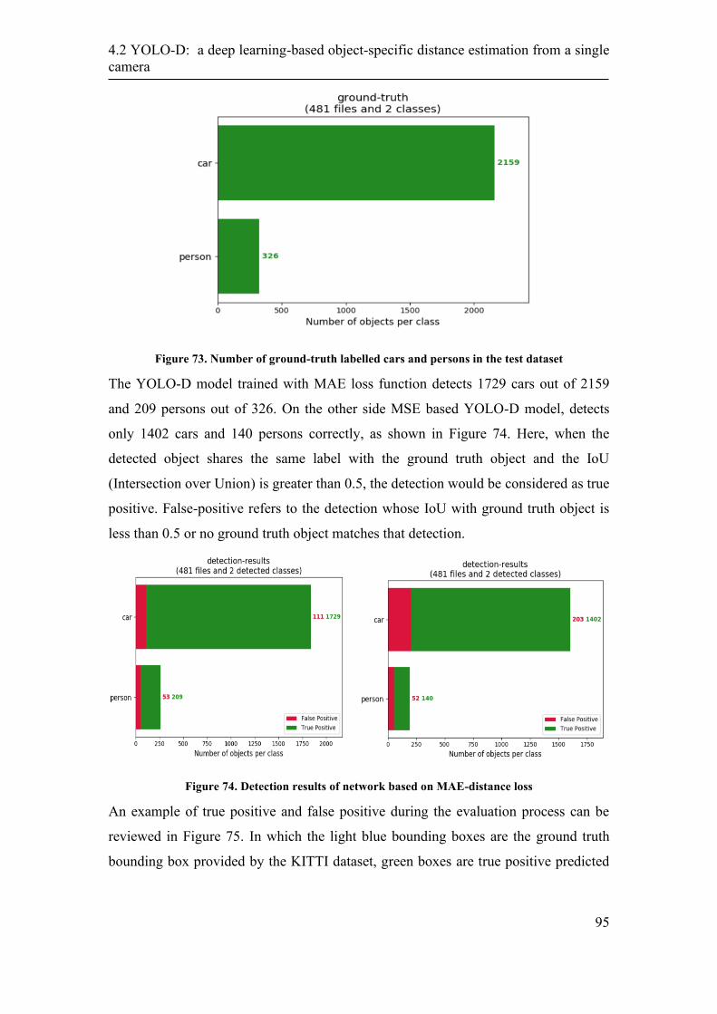
4.2 YOLO-D: a deep learning-based object-specific distance estimation from a single
camera
95
Figure 73. Number of ground-truth labelled cars and persons in the test dataset
The YOLO-D model trained with MAE loss function detects 1729 cars out of 2159
and 209 persons out of 326. On the other side MSE based YOLO-D model, detects
only 1402 cars and 140 persons correctly, as shown in Figure 74. Here, when the
detected object shares the same label with the ground truth object and the IoU
(Intersection over Union) is greater than 0.5, the detection would be considered as true
positive. False-positive refers to the detection whose IoU with ground truth object is
less than 0.5 or no ground truth object matches that detection.
Figure 74. Detection results of network based on MAE-distance loss
An example of true positive and false positive during the evaluation process can be
reviewed in Figure 75. In which the light blue bounding boxes are the ground truth
bounding box provided by the KITTI dataset, green boxes are true positive predicted

4.2 YOLO-D: a deep learning-based object-specific distance estimation from a single
camera
96
bounding boxes, and red box is the false positive prediction that falsely predicts that
symbol as a person.
Figure 75. An example of true positive and false positive during the evaluation process
By referring to the method [138] and setting a different threshold for the confidence
score that we predicted, we got different pairs of precision and recall value and then
plotted the Precision-Recall (PR) curve of these two classes, as shown in Figure 76
and Figure 77.
Figure 76. PR curve of car prediction by network-based on MAE and MSE-distance loss
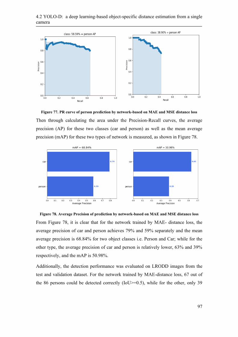
4.2 YOLO-D: a deep learning-based object-specific distance estimation from a single
camera
97
Figure 77. PR curve of person prediction by network-based on MAE and MSE distance loss
Then through calculating the area under the Precision-Recall curves, the average
precision (AP) for these two classes (car and person) as well as the mean average
precision (mAP) for these two types of network is measured, as shown in Figure 78.
Figure 78. Average Precision of prediction by network-based on MAE and MSE distance loss
From Figure 78, it is clear that for the network trained by MAE- distance loss, the
average precision of car and person achieves 79% and 59% separately and the mean
average precision is 68.84% for two object classes i.e. Person and Car; while for the
other type, the average precision of car and person is relatively lower, 63% and 39%
respectively, and the mAP is 50.98%.
Additionally, the detection performance was evaluated on LRODD images from the
test and validation dataset. For the network trained by MAE-distance loss, 67 out of
the 86 persons could be detected correctly (IoU>=0.5), while for the other, only 39

4.2 YOLO-D: a deep learning-based object-specific distance estimation from a single
camera
98
persons could be detected correctly. An example of these two detections at the ground
truth distance of 320m is shown in Figure 79 and Figure 80, respectively.
Figure 79. Detected objects at 320m by network-based on MAE-distance loss
Figure 80. Detected objects at 320m by network-based on MSE-distance loss
From the figures and statistics listed above, the conclusion could be obtained that, the
object detection performance of the YOLO-D model trained by MAE-distance loss is
better than that trained by MSE-distance loss.
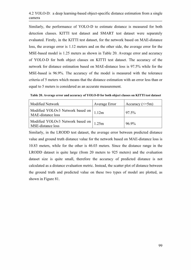
4.2 YOLO-D: a deep learning-based object-specific distance estimation from a single
camera
99
Similarly, the performance of YOLO-D to estimate distance is measured for both
detection classes. KITTI test dataset and SMART test dataset were separately
evaluated. Firstly, in the KITTI test dataset, for the network based on MAE-distance
loss, the average error is 1.12 meters and on the other side, the average error for the
MSE-based model is 1.25 meters as shown in Table 20. Average error and accuracy
of YOLO-D for both object classes on KITTI test dataset. The accuracy of the
network for distance estimation based on MAE-distance loss is 97.5% while for the
MSE-based is 96.9%. The accuracy of the model is measured with the tolerance
criteria of 5 meters which means that the distance estimation with an error less than or
equal to 5 meters is considered as an accurate measurement.
Table 20. Average error and accuracy of YOLO-D for both object classes on KITTI test dataset
Modified Network Average Error Accuracy (<=5m)
Modified YOLOv3 Network based on
MAE-distance loss 1.12m 97.5%
Modified YOLOv3 Network based on
MSE-distance loss 1.25m 96.9%
Similarly, in the LRODD test dataset, the average error between predicted distance
value and ground truth distance value for the network based on MAE-distance loss is
10.83 meters, while for the other is 46.03 meters. Since the distance range in the
LRODD dataset is quite large (from 20 meters to 925 meters) and the evaluation
dataset size is quite small, therefore the accuracy of predicted distance is not
calculated as a distance evaluation metric. Instead, the scatter plot of distance between
the ground truth and predicted value on these two types of model are plotted, as
shown in Figure 81.

4.2 YOLO-D: a deep learning-based object-specific distance estimation from a single
camera
100
Figure 81. Scatter plot of distance on the network based on MAE and MSE distance loss
In Figure 81, the left plot shows that the estimated values are closer to ground truth
distance compared to the right plot. It shows that, for long-range distance estimation,
the performance of network-based on MAE distance loss is better than the network
based on MSE distance loss function.
In conclusion, when it comes to the performance of object detection, the network
trained by MAE-distance loss performs much better than the model trained by MSE-
distance loss. With regard to the performance of distance estimation on the KITTI
dataset, there is no noticeable difference between these two networks, while for the
long-range distance in the LRODD dataset, the performance of network-based on
MAE-distance loss is better than the MSE-based model.
4.2.5.1 Road Scene
Some results of test images as well as the ground truth information is shown in the
following figures 81-83 and tables 21-23:
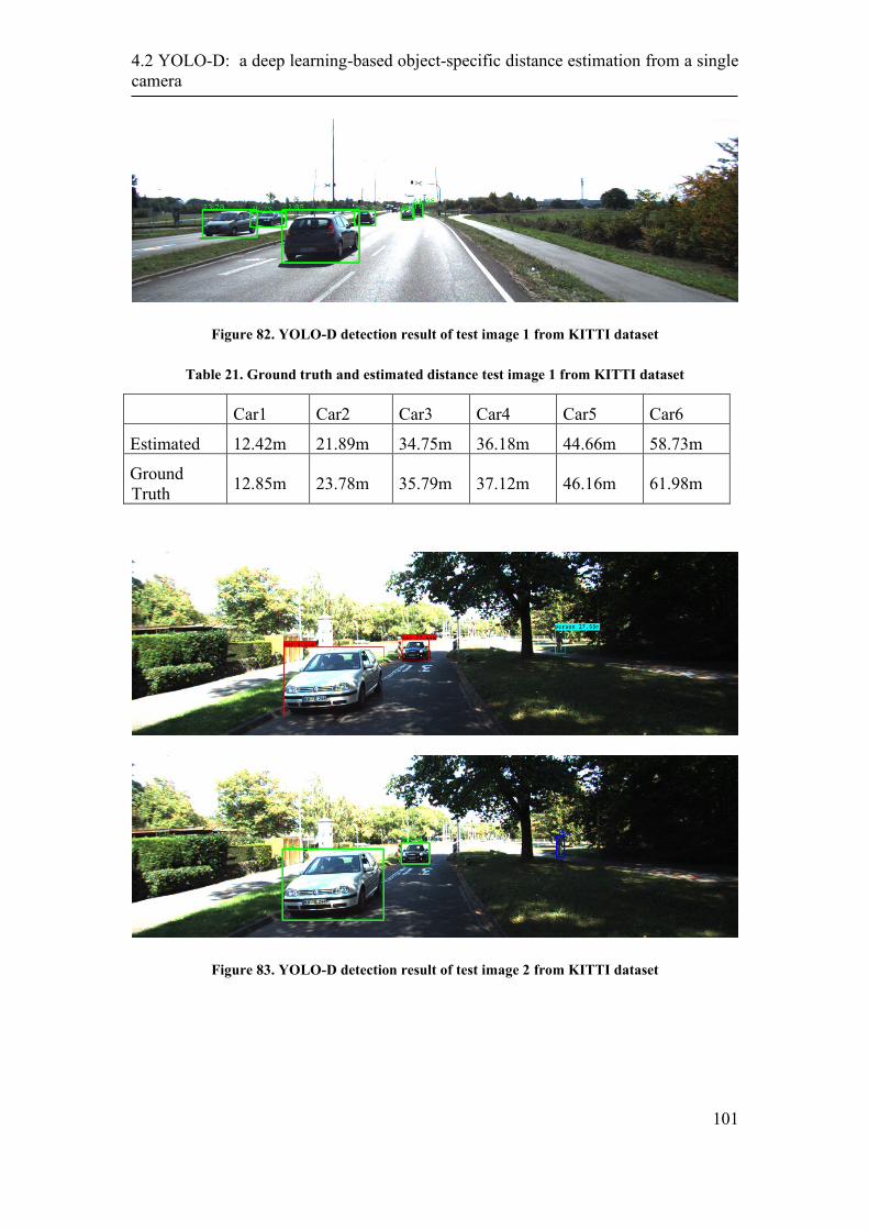
4.2 YOLO-D: a deep learning-based object-specific distance estimation from a single
camera
101
Figure 82. YOLO-D detection result of test image 1 from KITTI dataset
Table 21. Ground truth and estimated distance test image 1 from KITTI dataset
Car1 Car2 Car3 Car4 Car5 Car6
Estimated 12.42m 21.89m 34.75m 36.18m 44.66m 58.73m
Ground
Truth 12.85m 23.78m 35.79m 37.12m 46.16m 61.98m
Figure 83. YOLO-D detection result of test image 2 from KITTI dataset
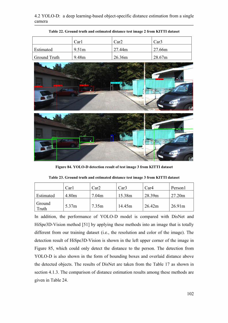
4.2 YOLO-D: a deep learning-based object-specific distance estimation from a single
camera
102
Table 22. Ground truth and estimated distance test image 2 from KITTI dataset
Car1 Car2 Car3
Estimated 9.51m 27.44m 27.66m
Ground Truth 9.48m 26.36m 28.67m
Figure 84. YOLO-D detection result of test image 3 from KITTI dataset
Table 23. Ground truth and estimated distance test image 3 from KITTI dataset
Car1 Car2 Car3 Car4 Person1
Estimated 4.80m 7.04m 15.38m 28.39m 27.20m
Ground
Truth 5.37m 7.35m 14.45m 26.42m 26.91m
In addition, the performance of YOLO-D model is compared with DisNet and
HiSpe3D-Vision method [51] by applying these methods into an image that is totally
different from our training dataset (i.e., the resolution and color of the image). The
detection result of HiSpe3D-Vision is shown in the left upper corner of the image in
Figure 85, which could only detect the distance to the person. The detection from
YOLO-D is also shown in the form of bounding boxes and overlaid distance above
the detected objects. The results of DisNet are taken from the Table 17 as shown in
section 4.1.3. The comparison of distance estimation results among these methods are
given in Table 24.
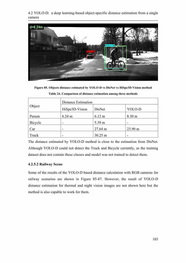
4.2 YOLO-D: a deep learning-based object-specific distance estimation from a single
camera
103
Figure 85. Objects distance estimated by YOLO-D vs DisNet vs HiSpe3D-Vision method
Table 24. Comparison of distance estimation among three methods
Object Distance Estimation
HiSpe3D-Vision DisNet YOLO-D
Person 6.24 m 6.12 m 8.30 m
Bicycle - 5.39 m -
Car - 27.64 m 23.90 m
Truck - 30.25 m -
The distance estimated by YOLO-D method is close to the estimation from DisNet.
Although YOLO-D could not detect the Truck and Bicycle currently, as the training
dataset does not contain these classes and model was not trained to detect them.
4.2.5.2 Railway Scene
Some of the results of the YOLO-D based distance calculation with RGB cameras for
railway scenarios are shown in Figure 85-87. However, the result of YOLO-D
distance estimation for thermal and night vision images are not shown here but the
method is also capable to work for them.
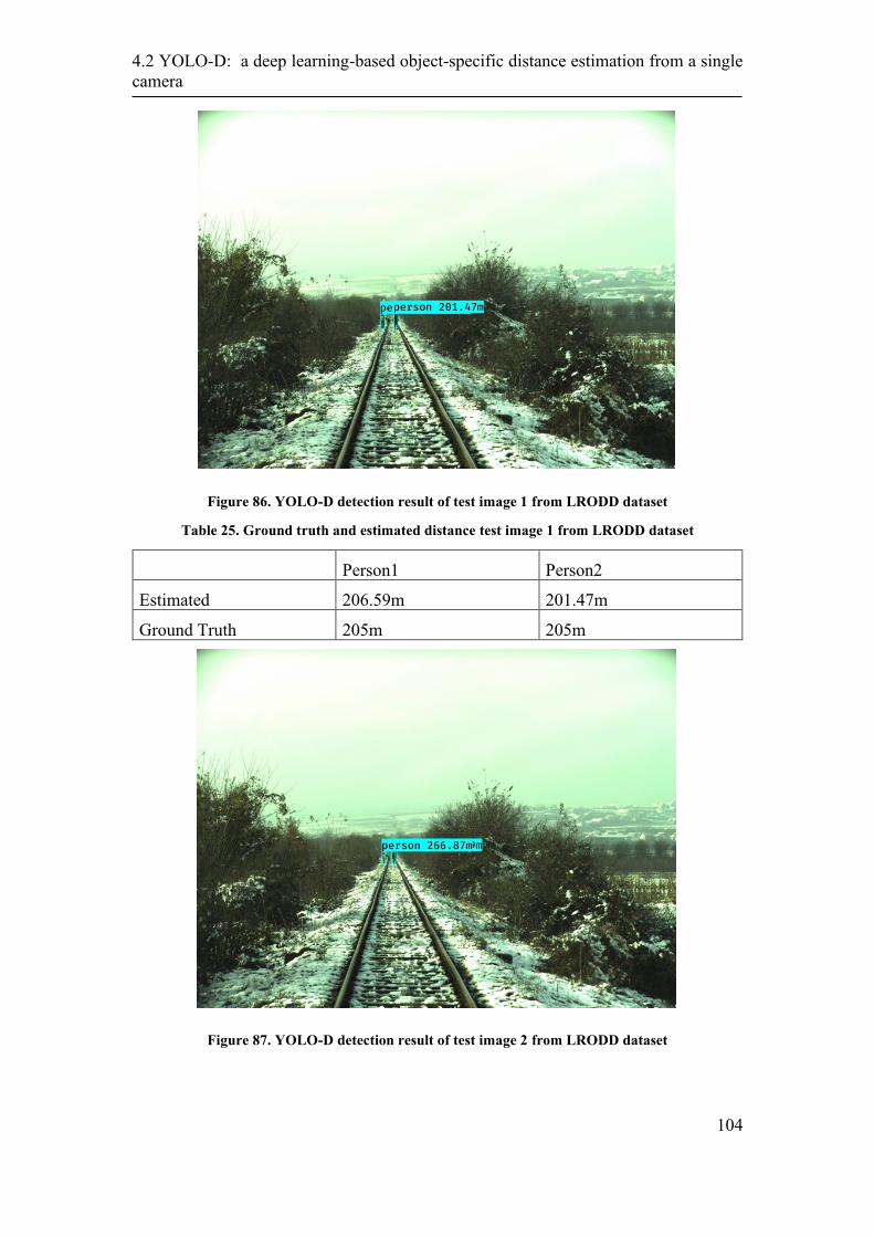
4.2 YOLO-D: a deep learning-based object-specific distance estimation from a single
camera
104
Figure 86. YOLO-D detection result of test image 1 from LRODD dataset
Table 25. Ground truth and estimated distance test image 1 from LRODD dataset
Person1 Person2
Estimated 206.59m 201.47m
Ground Truth 205m 205m
Figure 87. YOLO-D detection result of test image 2 from LRODD dataset
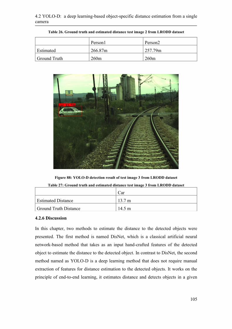
4.2 YOLO-D: a deep learning-based object-specific distance estimation from a single
camera
105
Table 26. Ground truth and estimated distance test image 2 from LRODD dataset
Person1 Person2
Estimated 266.87m 257.79m
Ground Truth 260m 260m
Figure 88: YOLO-D detection result of test image 3 from LRODD dataset
Table 27: Ground truth and estimated distance test image 3 from LRODD dataset
Car
Estimated Distance 13.7 m
Ground Truth Distance 14.5 m
4.2.6 Discussion
In this chapter, two methods to estimate the distance to the detected objects were
presented. The first method is named DisNet, which is a classical artificial neural
network-based method that takes as an input hand-crafted features of the detected
object to estimate the distance to the detected object. In contrast to DisNet, the second
method named as YOLO-D is a deep learning method that does not require manual
extraction of features for distance estimation to the detected objects. It works on the
principle of end-to-end learning, it estimates distance and detects objects in a given

4.2 YOLO-D: a deep learning-based object-specific distance estimation from a single
camera
106
input image. It finds itself the relation to change of distance to the object of a specific
class in an image by investigating the visual features.
In this chapter, the methodology, concept, and evaluation results of DisNet and
YOLO-D were explained. Both the methods show promising results for distance
estimation; however, some limitations and future ideas to improve their performance
are important to highlight.
One of the main limitations of both methods is to deal with object occlusion,
unreliable distance estimation in case of false and imprecise object bounding box
prediction from the object detection model. Furthermore, the methods were evaluated
on a limited size dataset, the performance can be improved more with the increase in
dataset specifically for YOLO-D which as deep learning-based object detection and
distance estimation network required more data to train in comparison to DisNet. The
dataset designed explicitly for object detection and distance estimation such as the
LRODD dataset can fulfill the requirement for the training of YOLO-D. Additionally,
more object classes can be added to the dataset.
In the next section and chapters, the problems encounter is addressed and some new
ideas are presented to overcome such problems.

107
5.1 Multi-DisNet: a machine learning-based robust distance estimation from multiple
cameras
108
5. A machine learning based distance
estimation from multiple cameras
In this chapter, a novel method for distance estimation from multiple cameras to the
object viewed with these cameras is presented named Multi-DisNet. Multi-DisNet is a
multilayer neural network, which is used to learn the relationship between the sizes of
the bounding boxes of the objects in the camera's images and the distance between the
object and cameras.
The supervised learning technique was used to train the Multi-DisNet network where
the input features were manually calculated parameters of the objects bounding boxes
in the camera's images and desired outputs were ground-truth distances between the
objects and the cameras. The performance of multi-DisNet was evaluated on images
of real-world railway scenes. As a proof-of-concept, the results on the fusion of two
sensors, an RGB and thermal camera mounted on a moving train, in the Multi-DisNet
distance estimation system are shown. Presented results demonstrate both the good
performance of the Multi-DisNet system to estimate the mid (up to 200 m) and long-
range (up to 1000 m) object distance and benefit of sensor fusion to overcome the
problem of not reliable object detection. The Multi-DisNet was presented by Haseeb
et al. in [120].
5.1 Multi-DisNet: a machine learning-based robust distance estimation
from multiple cameras
The architecture of the Multi-DisNet-based distance estimation system, with the setup
assuming two cameras mounted horizontally parallel, an RGB camera and a thermal
camera, is illustrated in Figure 89.
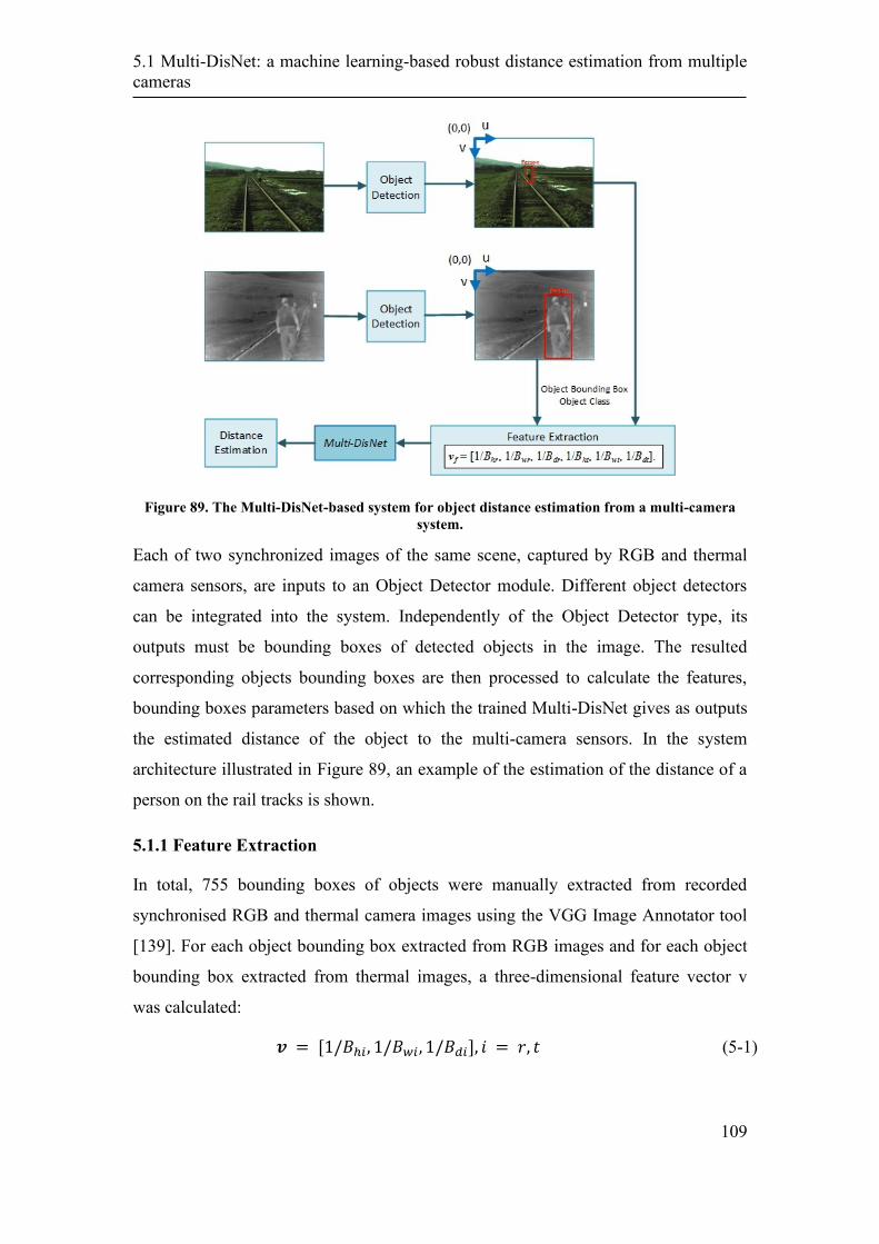
5.1 Multi-DisNet: a machine learning-based robust distance estimation from multiple
cameras
109
Figure 89. The Multi-DisNet-based system for object distance estimation from a multi-camera
system.
Each of two synchronized images of the same scene, captured by RGB and thermal
camera sensors, are inputs to an Object Detector module. Different object detectors
can be integrated into the system. Independently of the Object Detector type, its
outputs must be bounding boxes of detected objects in the image. The resulted
corresponding objects bounding boxes are then processed to calculate the features,
bounding boxes parameters based on which the trained Multi-DisNet gives as outputs
the estimated distance of the object to the multi-camera sensors. In the system
architecture illustrated in Figure 89, an example of the estimation of the distance of a
person on the rail tracks is shown.
5.1.1 Feature Extraction
In total, 755 bounding boxes of objects were manually extracted from recorded
synchronised RGB and thermal camera images using the VGG Image Annotator tool
[139]. For each object bounding box extracted from RGB images and for each object
bounding box extracted from thermal images, a three-dimensional feature vector v
was calculated:
𝒗 = [1/𝐵ℎ𝑖, 1/𝐵𝑤𝑖, 1/𝐵𝑑𝑖], 𝑖 = 𝑟, 𝑡 (5-1)
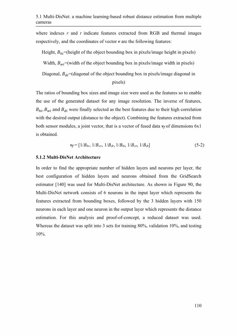
5.1 Multi-DisNet: a machine learning-based robust distance estimation from multiple
cameras
110
where indexes r and t indicate features extracted from RGB and thermal images
respectively, and the coordinates of vector v are the following features:
Height, 𝐵ℎ𝑖=(height of the object bounding box in pixels/image height in pixels)
Width, 𝐵𝑤𝑖=(width of the object bounding box in pixels/image width in pixels)
Diagonal, 𝐵𝑑𝑖=(diagonal of the object bounding box in pixels/image diagonal in
pixels)
The ratios of bounding box sizes and image size were used as the features so to enable
the use of the generated dataset for any image resolution. The inverse of features,
𝐵ℎ𝑖, 𝐵𝑤𝑖 and 𝐵𝑑𝑖 were finally selected as the best features due to their high correlation
with the desired output (distance to the object). Combining the features extracted from
both sensor modules, a joint vector, that is a vector of fused data vf of dimensions 6x1
is obtained.
vf = [1/Bhr, 1/Bwr, 1/Bdr, 1/Bht, 1/Bwt, 1/Bdt] (5-2)
5.1.2 Multi-DisNet Architecture
In order to find the appropriate number of hidden layers and neurons per layer, the
best configuration of hidden layers and neurons obtained from the GridSearch
estimator [140] was used for Multi-DisNet architecture. As shown in Figure 90, the
Multi-DisNet network consists of 6 neurons in the input layer which represents the
features extracted from bounding boxes, followed by the 3 hidden layers with 150
neurons in each layer and one neuron in the output layer which represents the distance
estimation. For this analysis and proof-of-concept, a reduced dataset was used.
Whereas the dataset was split into 3 sets for training 80%, validation 10%, and testing
10%.
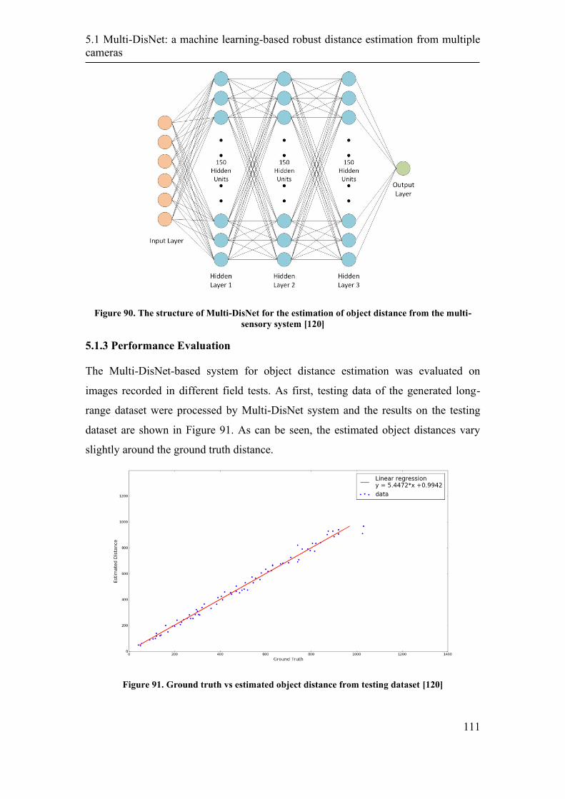
5.1 Multi-DisNet: a machine learning-based robust distance estimation from multiple
cameras
111
Figure 90. The structure of Multi-DisNet for the estimation of object distance from the multi-
sensory system [120]
5.1.3 Performance Evaluation
The Multi-DisNet-based system for object distance estimation was evaluated on
images recorded in different field tests. As first, testing data of the generated long-
range dataset were processed by Multi-DisNet system and the results on the testing
dataset are shown in Figure 91. As can be seen, the estimated object distances vary
slightly around the ground truth distance.
Figure 91. Ground truth vs estimated object distance from testing dataset [120]
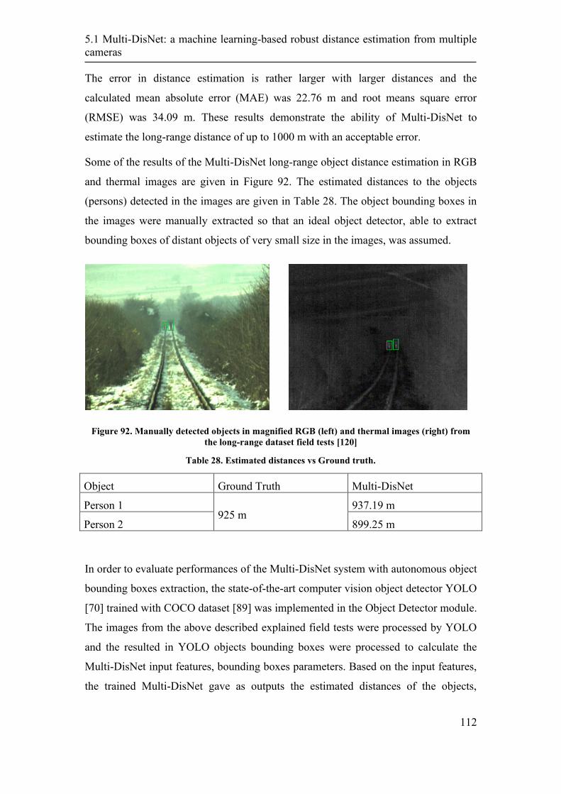
5.1 Multi-DisNet: a machine learning-based robust distance estimation from multiple
cameras
112
The error in distance estimation is rather larger with larger distances and the
calculated mean absolute error (MAE) was 22.76 m and root means square error
(RMSE) was 34.09 m. These results demonstrate the ability of Multi-DisNet to
estimate the long-range distance of up to 1000 m with an acceptable error.
Some of the results of the Multi-DisNet long-range object distance estimation in RGB
and thermal images are given in Figure 92. The estimated distances to the objects
(persons) detected in the images are given in Table 28. The object bounding boxes in
the images were manually extracted so that an ideal object detector, able to extract
bounding boxes of distant objects of very small size in the images, was assumed.
Figure 92. Manually detected objects in magnified RGB (left) and thermal images (right) from
the long-range dataset field tests [120]
Table 28. Estimated distances vs Ground truth.
Object Ground Truth Multi-DisNet
Person 1 925 m
937.19 m
Person 2 899.25 m
In order to evaluate performances of the Multi-DisNet system with autonomous object
bounding boxes extraction, the state-of-the-art computer vision object detector YOLO
[70] trained with COCO dataset [89] was implemented in the Object Detector module.
The images from the above described explained field tests were processed by YOLO
and the resulted in YOLO objects bounding boxes were processed to calculate the
Multi-DisNet input features, bounding boxes parameters. Based on the input features,
the trained Multi-DisNet gave as outputs the estimated distances of the objects,
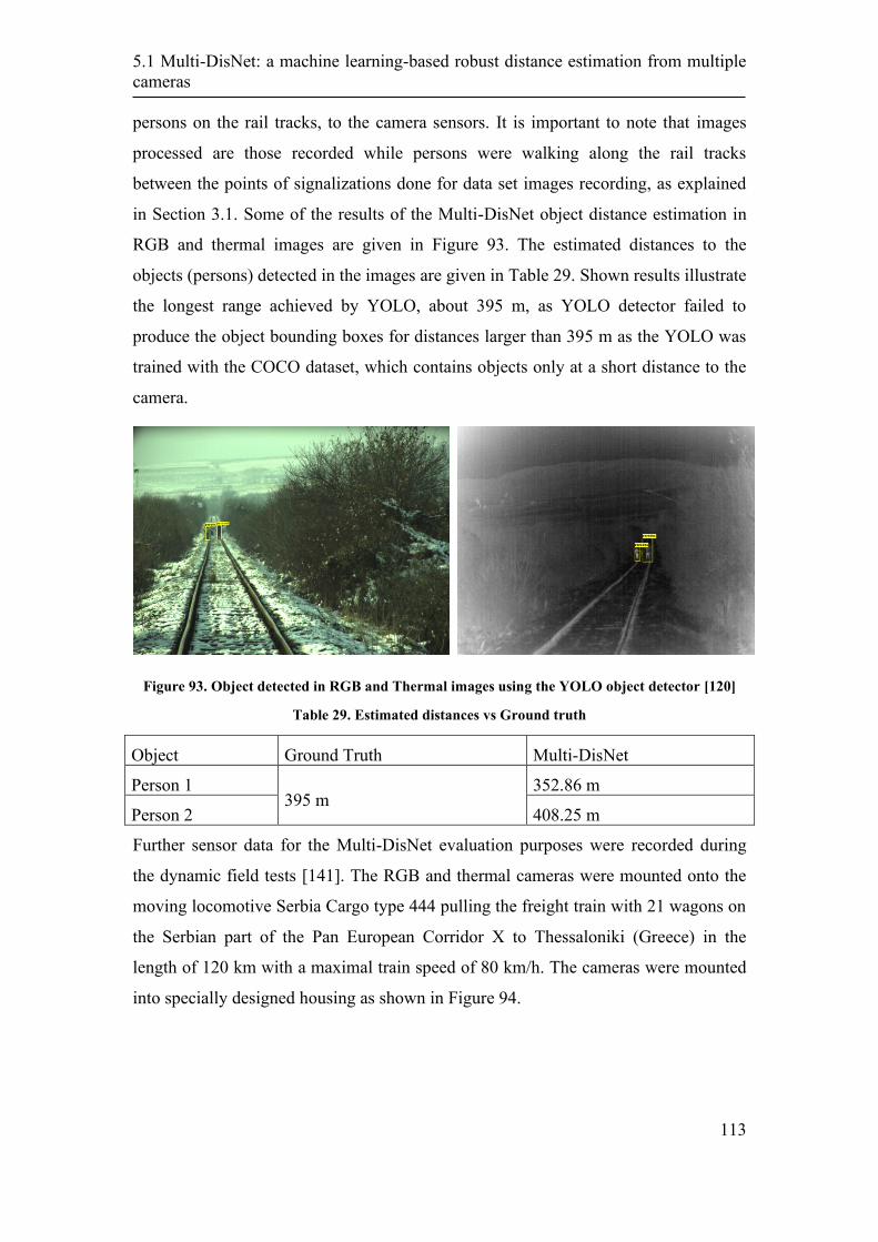
5.1 Multi-DisNet: a machine learning-based robust distance estimation from multiple
cameras
113
persons on the rail tracks, to the camera sensors. It is important to note that images
processed are those recorded while persons were walking along the rail tracks
between the points of signalizations done for data set images recording, as explained
in Section 3.1. Some of the results of the Multi-DisNet object distance estimation in
RGB and thermal images are given in Figure 93. The estimated distances to the
objects (persons) detected in the images are given in Table 29. Shown results illustrate
the longest range achieved by YOLO, about 395 m, as YOLO detector failed to
produce the object bounding boxes for distances larger than 395 m as the YOLO was
trained with the COCO dataset, which contains objects only at a short distance to the
camera.
Figure 93. Object detected in RGB and Thermal images using the YOLO object detector [120]
Table 29. Estimated distances vs Ground truth
Object Ground Truth Multi-DisNet
Person 1 395 m
352.86 m
Person 2 408.25 m
Further sensor data for the Multi-DisNet evaluation purposes were recorded during
the dynamic field tests [141]. The RGB and thermal cameras were mounted onto the
moving locomotive Serbia Cargo type 444 pulling the freight train with 21 wagons on
the Serbian part of the Pan European Corridor X to Thessaloniki (Greece) in the
length of 120 km with a maximal train speed of 80 km/h. The cameras were mounted
into specially designed housing as shown in Figure 94.
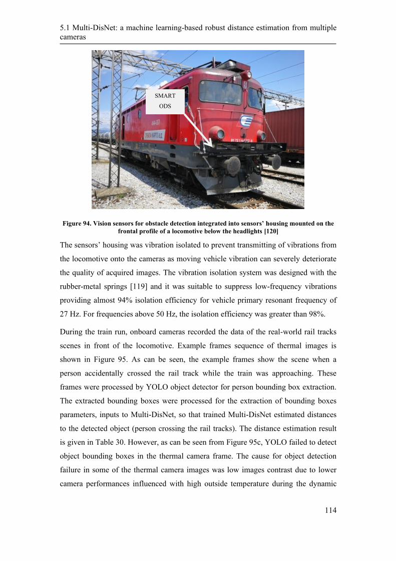
5.1 Multi-DisNet: a machine learning-based robust distance estimation from multiple
cameras
114
Figure 94. Vision sensors for obstacle detection integrated into sensors’ housing mounted on the
frontal profile of a locomotive below the headlights [120]
The sensors’ housing was vibration isolated to prevent transmitting of vibrations from
the locomotive onto the cameras as moving vehicle vibration can severely deteriorate
the quality of acquired images. The vibration isolation system was designed with the
rubber-metal springs [119] and it was suitable to suppress low-frequency vibrations
providing almost 94% isolation efficiency for vehicle primary resonant frequency of
27 Hz. For frequencies above 50 Hz, the isolation efficiency was greater than 98%.
During the train run, onboard cameras recorded the data of the real-world rail tracks
scenes in front of the locomotive. Example frames sequence of thermal images is
shown in Figure 95. As can be seen, the example frames show the scene when a
person accidentally crossed the rail track while the train was approaching. These
frames were processed by YOLO object detector for person bounding box extraction.
The extracted bounding boxes were processed for the extraction of bounding boxes
parameters, inputs to Multi-DisNet, so that trained Multi-DisNet estimated distances
to the detected object (person crossing the rail tracks). The distance estimation result
is given in Table 30. However, as can be seen from Figure 95c, YOLO failed to detect
object bounding boxes in the thermal camera frame. The cause for object detection
failure in some of the thermal camera images was low images contrast due to lower
camera performances influenced with high outside temperature during the dynamic
SMART
ODS
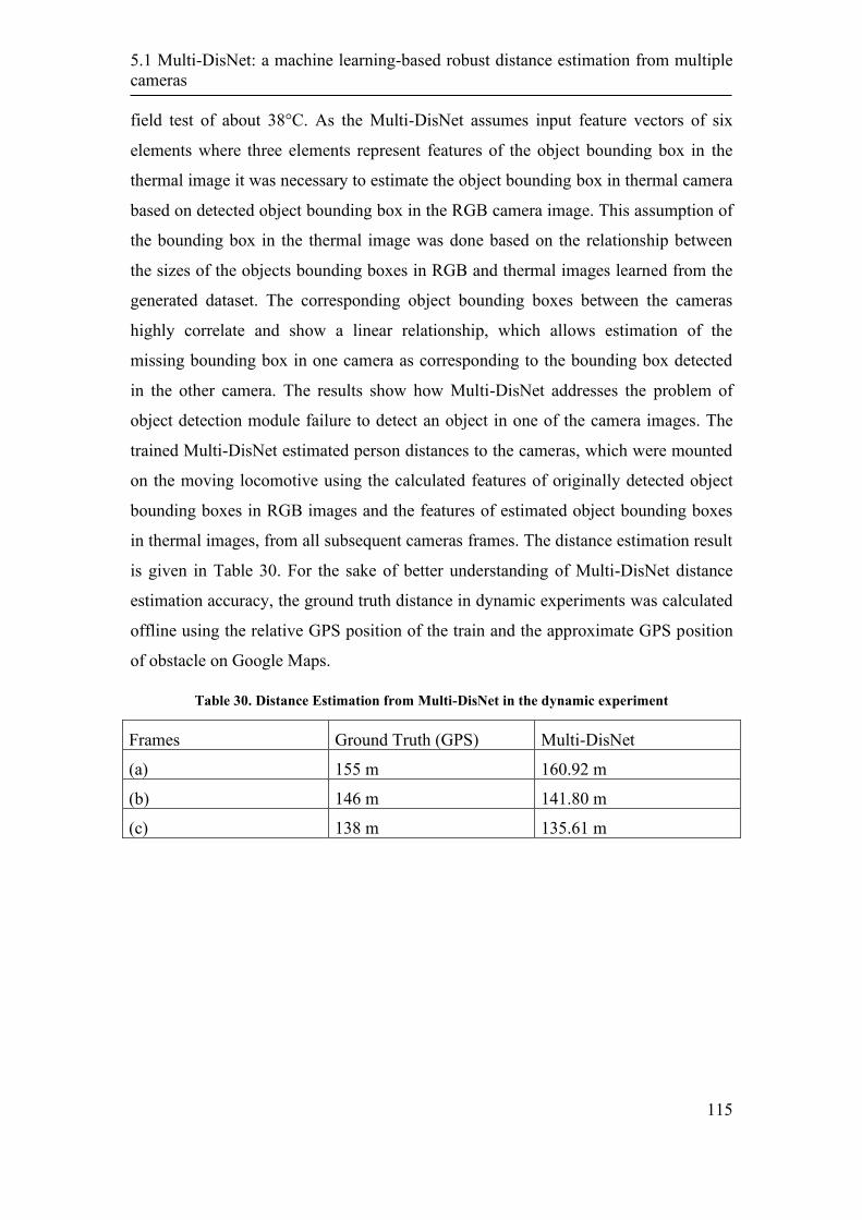
5.1 Multi-DisNet: a machine learning-based robust distance estimation from multiple
cameras
115
field test of about 38°C. As the Multi-DisNet assumes input feature vectors of six
elements where three elements represent features of the object bounding box in the
thermal image it was necessary to estimate the object bounding box in thermal camera
based on detected object bounding box in the RGB camera image. This assumption of
the bounding box in the thermal image was done based on the relationship between
the sizes of the objects bounding boxes in RGB and thermal images learned from the
generated dataset. The corresponding object bounding boxes between the cameras
highly correlate and show a linear relationship, which allows estimation of the
missing bounding box in one camera as corresponding to the bounding box detected
in the other camera. The results show how Multi-DisNet addresses the problem of
object detection module failure to detect an object in one of the camera images. The
trained Multi-DisNet estimated person distances to the cameras, which were mounted
on the moving locomotive using the calculated features of originally detected object
bounding boxes in RGB images and the features of estimated object bounding boxes
in thermal images, from all subsequent cameras frames. The distance estimation result
is given in Table 30. For the sake of better understanding of Multi-DisNet distance
estimation accuracy, the ground truth distance in dynamic experiments was calculated
offline using the relative GPS position of the train and the approximate GPS position
of obstacle on Google Maps.
Table 30. Distance Estimation from Multi-DisNet in the dynamic experiment
Frames Ground Truth (GPS) Multi-DisNet
(a) 155 m 160.92 m
(b) 146 m 141.80 m
(c) 138 m 135.61 m
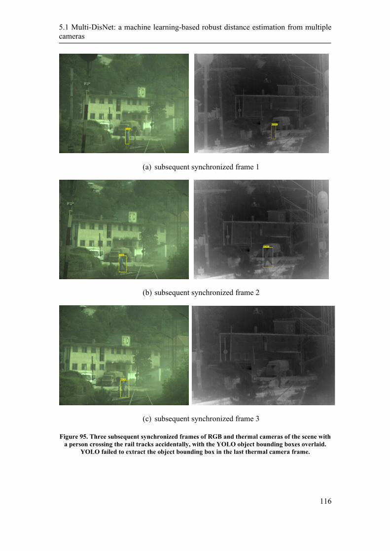
5.1 Multi-DisNet: a machine learning-based robust distance estimation from multiple
cameras
116
(a) subsequent synchronized frame 1
(b) subsequent synchronized frame 2
(c) subsequent synchronized frame 3
Figure 95. Three subsequent synchronized frames of RGB and thermal cameras of the scene with
a person crossing the rail tracks accidentally, with the YOLO object bounding boxes overlaid.
YOLO failed to extract the object bounding box in the last thermal camera frame.
5.1 Multi-DisNet: a machine learning-based robust distance estimation from multiple
cameras
117
5.1.3 Discussion
In this Thesis, a method for long-range obstacle detection from multiple monocular
cameras is presented. The method is based on a novel multilayer neural network
named Multi-DisNet that learns the relationship between the distance from the
multiple cameras to the detected objects and the corresponding sizes of the objects in
both camera images. The presented work is a part of the research and development of
a novel integrated onboard obstacle detection system for railway applications. The
presented system was evaluated for the setup consisting of an RGB and thermal
camera.
This Thesis also presents the generation of the first long-range dataset reflecting the
real-life railway applications, which was necessary for supervised training of the
Multi-DisNet network to enable learning of the relationship between the sizes of the
bounding boxes of the detected object in the camera’s images and the distance of the
object to the cameras. For the calculation of the object bounding boxes parameters,
the Multi-DisNet distance estimation system assumes an Object Detector able to
extract object bounding boxes. The evaluation results shown in this Thesis
demonstrate the performance of the Multi-DisNet to reliably estimate the long-range
distances in case the object bounding boxes are manually extracted. The system
achieved long-range object detection of about 1000 m, which is the desired
performance in applications such as railway applications. However, the evaluation
results in the case of using the YOLO for automatic object detection demonstrated
system performance of estimating the distance up to 400 m, as the YOLO object
detector failed to extract the bounding boxes in long-range images. These results
indicate the need for improvement of the object detection system module and need of
training of object detector module with datasets consist of objects at a longer distance
(small in size) in the future work, so to achieve reliable autonomous long-range
obstacle detection. Nevertheless, the presented system reflects the novelty in long-
range obstacle detection as current sensor technology in current land transport
research is able to look some 200 m ahead [14] [142]. However, the required rail
obstacle detection interfacing with loco control should be able to look ahead up to
1000 m detecting objects on and near track which may potentially interfere with the
clearance and ground profile [143].

118
5.1 Multi-DisNet: a machine learning-based robust distance estimation from multiple
cameras
119
6. A machine learning based multiple
object tracking
The environmental perception system, which performs object detection and tracking
task, is the core for autonomous vehicles. Object detection tremendously evolves
along with the advancement in sensor technology, and with the development of
classical and machine learning-based algorithms, while multiple object tracking seems
less developed [144]. Object tracking is essential for many tasks of autonomous
driving such as obstacle avoidance and intention prediction [145]. It is a critical task
and it becomes more challenging for situations such as objects at far distance, low
frame rate video sequence, frequent occlusion, camera vibration or movement, and so
on.
Mainly there are four object tracking methods categorized as region-based tracking
[146], model-based tracking [147], contour-based tracking [148], and feature-based
tracking [149]. All those methods rely on object detection. In general, tracking utilizes
the detection information from previous frames to predict the detection in frames
where detection is missing.
In [145] a traditional object tracking method based on a monocular camera for
autonomous vehicles is present. By using the camera model to map pixel position into
the distance, the distance to the vehicles with respect to the vehicle was measured.
Further Kalman Filter (EKF) is used to refine distance accuracy and track detected
vehicles. The results show that the method is capable to track 3D positions with
sufficient accuracy.
Relatively modern machine learning-based methods [150] are introduced for object
tracking based on Recurrent Neural Networks (RNNs) followed by long short-term

6.1 DisNet-RNN Tracker: robust distance estimation and multiple objects tracking
from a single camera
120
memory (LSTM) and Gated recurrent units (GRU). The RNN based networks are
often used for sequential data and thus also applicable for object tracking in video
sequences.
6.1 DisNet-RNN Tracker: robust distance estimation and multiple objects
tracking from a single camera
In this Thesis, a novel approach for multiple object tracking and distance estimation
from an onboard monocular camera, aiming at improvements in the safety and
security of railways, is presented. The approach is based on deep learning architecture
using a deep Convolutional Neural Network (CNN) object detection followed by a
multi hidden-layer Gated Recurrent Neural Network (RNN) referred to as DisNet-
RNN Tracker, which consists of two sub-networks for distance estimation and
bounding box prediction respectively. The DisNet-RNN Tracker learns and estimates
the distance between the detected object and the camera sensor, and predicts the
object bounding box based on sequential input from previous and current detection.
The presented DisNet-RNN Tracker tracks multiple objects in case where the object
detection module fails to detect an object. The presented method is evaluated on the
real-world railway dataset recorded with the onboard Obstacle Detection System
developed within an H2020 Shift2Rail project SMART - Smart Automation of Rail
Transport. The presented work has the potential to benefit other applications where
reliable object detection, tracking, and long-range distance estimation are needed such
as autonomous cars, transportation, and public security.
The workflow of DisNet-RNN Tracker based object detection, tracking, and distance
estimation from a single monocular camera is illustrated in Figure 96. The frames
captured by an RGB monocular camera are inputs to Object Detector Module.
Different object detectors, which outputs bounding box and class of detected objects,
can be integrated into the system. The resulted object bounding boxes from the
detection module further feed into the Multiple Objects Mapping (MOM) module.
The object mapping module matches previous object detection results to the current
detection results for the sake of objects tracking and assigning unique IDs for
unmatched or newly detected objects. Further, the Features Calculation module
extracts features of the objects bounding boxes and based on those features DisNet-
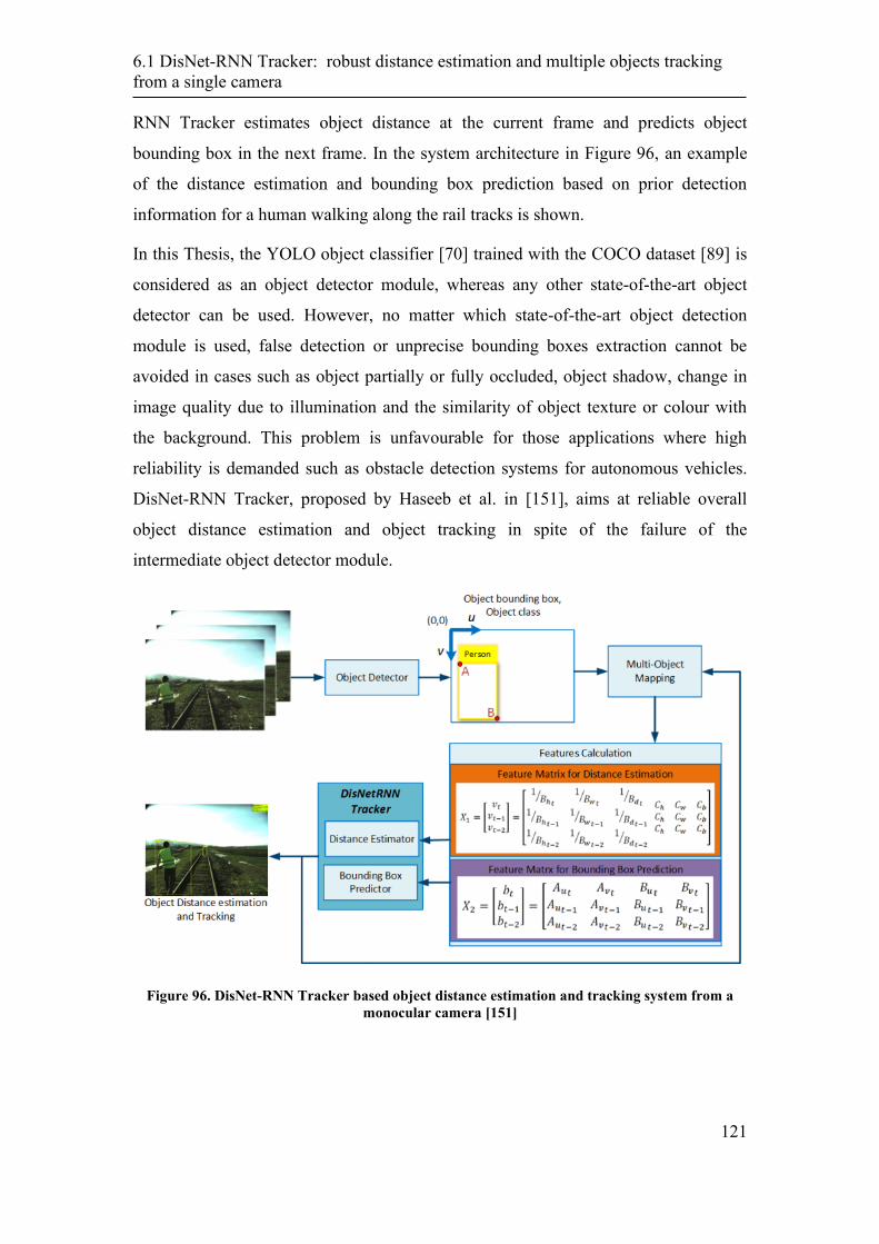
6.1 DisNet-RNN Tracker: robust distance estimation and multiple objects tracking
from a single camera
121
RNN Tracker estimates object distance at the current frame and predicts object
bounding box in the next frame. In the system architecture in Figure 96, an example
of the distance estimation and bounding box prediction based on prior detection
information for a human walking along the rail tracks is shown.
In this Thesis, the YOLO object classifier [70] trained with the COCO dataset [89] is
considered as an object detector module, whereas any other state-of-the-art object
detector can be used. However, no matter which state-of-the-art object detection
module is used, false detection or unprecise bounding boxes extraction cannot be
avoided in cases such as object partially or fully occluded, object shadow, change in
image quality due to illumination and the similarity of object texture or colour with
the background. This problem is unfavourable for those applications where high
reliability is demanded such as obstacle detection systems for autonomous vehicles.
DisNet-RNN Tracker, proposed by Haseeb et al. in [151], aims at reliable overall
object distance estimation and object tracking in spite of the failure of the
intermediate object detector module.
Figure 96. DisNet-RNN Tracker based object distance estimation and tracking system from a
monocular camera [151]
6.1 DisNet-RNN Tracker: robust distance estimation and multiple objects tracking
from a single camera
122
6.1.1 Deep Learning Network architecture
The DisNet-RNN Tracker consists of two independent sub-networks based on
Recurrent Neural Network (RNN) architecture. The reason to use RNN is that due to
its unique characteristic of being suitable to work with sequential data and its memory
cell able to preserve information from inputs provided in previous time moments
[150]. In the scenario considered in this Thesis, two types of object detection failures
are possible: the target objects are not detected in some frames, and the bounding
boxes of some of the detected objects are not accurate. Using the RNN, which has a
memory of previous inputs, can help to predict the object position and estimate
distance more reliably. DisNet-RNN Tracker uses the sequential data from previous
two-time steps to improve the estimation of the object distance at the current time step
and predicts the position and size of the object bounding box in the next time step.
Figure 97 shows the DisNet-RNN Tracker architecture. The architecture consists of
two subnetworks represented with two main blocks one under the other in Figure 97.
The upper network is used to estimate the object distance named as distance estimator
and the lower network named as bounding box predictor is used to predict the top left
corner A, and the bottom right corner B, of the object bounding box. Prediction of
these two bounding box corners’ points relates to the prediction of the bounding box
position and size.
As shown in Figure 97, a three hidden layers network was adopted for the distance
estimation. A deep recurrent neural network is stacked with Gated Recurrent Unit
(GRU) layers and the output from the last GRU layer is connected to a fully
connected output layer to perform final distance estimation. For the bounding box
prediction, the network consists of a single hidden layer of GRUs with a fully
connected layer as an output layer. A new loss function in training distance estimator
network was defined and it is given in (6-1). This loss function calculates losses from
all distance prediction results from three time-steps and in a similar way, the Mean
Absolute Error (MAE) loss function for the bounding box predictor network was
defined given in (6-2).
𝑙𝑜𝑠𝑠 𝑓𝑢𝑛𝑐𝑡𝑖𝑜𝑛 = 1
3𝑛∑∑|𝑌𝑖𝑗−𝑡𝑟𝑢𝑒 − 𝑌𝑖𝑗−𝑒𝑠𝑡𝑖𝑚𝑎𝑡𝑒𝑑|
𝑛
𝑗=1
3
𝑖=1
(6-1)
6.1 DisNet-RNN Tracker: robust distance estimation and multiple objects tracking
from a single camera
123
𝑙𝑜𝑠𝑠 𝑓𝑢𝑛𝑐𝑡𝑖𝑜𝑛
= 1
3𝑛∑∑|𝐴𝑢𝑖𝑗−𝑡𝑟𝑢𝑒 − 𝐴𝑢𝑖𝑗−𝑝𝑟𝑒𝑑𝑖𝑐𝑡𝑒𝑑|
𝑛
𝑗=1
3
𝑖=1
+ |𝐴𝑣𝑖𝑗−𝑡𝑟𝑢𝑒 − 𝐴𝑣𝑖𝑗−𝑝𝑟𝑒𝑑𝑖𝑐𝑡𝑒𝑑|
+ |𝐵𝑢𝑖𝑗−𝑡𝑟𝑢𝑒 − 𝐵𝑢𝑖𝑗−𝑝𝑟𝑒𝑑𝑖𝑐𝑡𝑒𝑑|
+ |𝐵𝑣𝑖𝑗−𝑡𝑟𝑢𝑒 − 𝐵𝑣𝑖𝑗−𝑝𝑟𝑒𝑑𝑖𝑐𝑡𝑒𝑑|
(6-2)
where:
• 𝑛 : training data numbers
• 𝑌𝑖𝑗−𝑡𝑟𝑢𝑒: the ground truth distance of jth training data at time step i.
• 𝑌𝑖𝑗−𝑒𝑠𝑡𝑖𝑚𝑎𝑡𝑒𝑑- the estimated distance of jth training data at time step i.
• 𝐴𝑢𝑖𝑗−𝑡𝑟𝑢𝑒, 𝐴𝑣𝑖𝑗−𝑡𝑟𝑢𝑒: the top-left corner coordinates of ground truth object
bounding box of jth training data at time step i.
• 𝐵𝑢𝑖𝑗−𝑡𝑟𝑢𝑒, 𝐵𝑣𝑖𝑗−𝑡𝑟𝑢𝑒: the bottom-right corner coordinates of ground truth
object bounding box of jth training data at time step i.
• 𝐴𝑢𝑖𝑗−𝑝𝑟𝑒𝑑𝑖𝑐𝑡𝑒𝑑, 𝐴𝑣𝑖𝑗−𝑝𝑟𝑒𝑑𝑖𝑐𝑡𝑒𝑑: the top-left corner coordinates of predicted
object bounding box of jth training data at time step i.
• 𝐵𝑢𝑖𝑗−𝑝𝑟𝑒𝑑𝑖𝑐𝑡𝑒𝑑, 𝐵𝑣𝑖𝑗−𝑝𝑟𝑒𝑑𝑖𝑐𝑡𝑒𝑑: the bottom-right corner coordinates of
predicted truth object bounding box of jth training data at time step i.

6.1 DisNet-RNN Tracker: robust distance estimation and multiple objects tracking
from a single camera
124
Figure 97. DisNet-RNN Tracker Architecture consists of two sub-networks namely distance
estimator on top and bounding box predictor in bottom [151]
6.1.2 Dataset
Recurrent Neural Networks requires a sequential dataset that needs to be prepared
before training DisNet-RNN Tracker. As described earlier, DisNet-RNN Tracker
consists of two sub independent RNN networks. In order to train and test these
subnetworks, manually a dataset of the size of 8000 sequential inputs was created
using images recorded in real-world railways scenarios. Each sample of the dataset
represents extracted features from three subsequent frames. The annotation tool [14]
provides the object bounding boxes coordinates, which were labelled together with
ground truth distance. The ground truth for distance estimation network was recorded
during the dataset generation using the GPS positioning system which later in the
offline phase allows calculating the relative distance between train and objects.
Whereas for bounding box prediction, the manually drawn bounding box on the fourth
frame is considered as a ground truth as shown in Figure 98.
Figure 98. Dataset generation for bounding box prediction [151]
6.1 DisNet-RNN Tracker: robust distance estimation and multiple objects tracking
from a single camera
125
In the next section, it is explained how the features were calculated and the dataset
was organized to train the DisNet-RNN Tracker, to learn distance estimation and
bounding box prediction.
6.1.3 Features selection
As it is known from the projective transformation, the object’s size in the camera
image is inversely proportional to the object’s distance from the camera. The distance
estimator network, trained to learn the relationship between the changes in sizes of the
objects’ bounding boxes in an image with respect to change in the distances between
the objects and the camera over time. The dataset for network Distance Estimator,
organized in the form of a two-dimensional feature matrix 𝑋1 for distance estimation
is given in (6-4), where each matrix row represents the six features of the feature
vector 𝒗 of an object at time-steps t, t-1 and t-2 respectively. Vector 𝒗 was calculated
from manually annotated objects’ bounding boxes for a class label as:
𝒗 = [1/𝐵ℎ 1/𝐵𝑤 1/𝐵𝑑 𝐶ℎ 𝐶𝑤 𝐶𝑏] (6-3)
• 𝐵ℎ: height of the object bounding box in pixels/image height in pixels
• 𝐵𝑤: Width of the object bounding box in pixels/image width in pixels
• 𝐵𝑑: diagonal of the object bounding box in pixels/image diagonal in pixels
• Ch, Cw, and Cb: average height, width and length of each object class in meters
Ch, Cw, and Cb are defined as unique features that actually represent different classes.
These features generalize the network to learn distance vs bounding box relation for
multiple object classes. For example, the predefined features for object class person
are the average height, width, and breadth of the humans, and similarly, these features
were predefined for other classes. These features do not have any meaning and
contribution to distance learning but help to differentiate different object types.
Similarly feature matrix 𝑋2 was calculated for network Bounding Box Predictor. Each
row in 𝑋2 matrix represents coordinates of the top left corner A and the bottom right
corner B of an object bounding box at time-steps t, t-1 and t-2 respectively, where
(u,v) are image point coordinates.
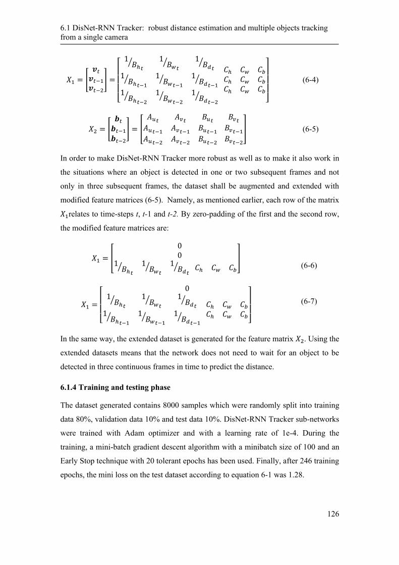
6.1 DisNet-RNN Tracker: robust distance estimation and multiple objects tracking
from a single camera
126
𝑋1 = [
𝒗𝑡
𝒗𝑡−1
𝒗𝑡−2
] =
[
1𝐵ℎ
⁄𝑡
1𝐵𝑤
⁄𝑡
1𝐵𝑑
⁄𝑡
1𝐵ℎ
⁄𝑡−1
1𝐵𝑤
⁄𝑡−1
1𝐵𝑑
⁄𝑡−1
1𝐵ℎ
⁄𝑡−2
1𝐵𝑤
⁄𝑡−2
1𝐵𝑑
⁄𝑡−2
𝐶ℎ 𝐶𝑤 𝐶𝑏
𝐶ℎ 𝐶𝑤 𝐶𝑏
𝐶ℎ 𝐶𝑤 𝐶𝑏
]
(6-4)
𝑋2 = [
𝒃𝑡
𝒃𝑡−1
𝒃𝑡−2
] = [
𝐴𝑢𝑡𝐴𝑣𝑡
𝐵𝑢𝑡
𝐴𝑢𝑡−1𝐴𝑣𝑡−1
𝐵𝑢𝑡−1
𝐴𝑢𝑡−2𝐴𝑣𝑡−2
𝐵𝑢𝑡−2
𝐵𝑣𝑡
𝐵𝑣𝑡−1
𝐵𝑣𝑡−2
] (6-5)
In order to make DisNet-RNN Tracker more robust as well as to make it also work in
the situations where an object is detected in one or two subsequent frames and not
only in three subsequent frames, the dataset shall be augmented and extended with
modified feature matrices (6-5). Namely, as mentioned earlier, each row of the matrix
𝑋1relates to time-steps t, t-1 and t-2. By zero-padding of the first and the second row,
the modified feature matrices are:
𝑋1 = [
00
1𝐵ℎ
⁄𝑡
1𝐵𝑤
⁄𝑡
1𝐵𝑑
⁄𝑡
𝐶ℎ 𝐶𝑤 𝐶𝑏
]
𝑋1 =
[
01
𝐵ℎ⁄
𝑡
1𝐵𝑤
⁄𝑡
1𝐵𝑑
⁄𝑡
1𝐵ℎ
⁄𝑡−1
1𝐵𝑤
⁄𝑡−1
1𝐵𝑑
⁄𝑡−1
𝐶ℎ 𝐶𝑤 𝐶𝑏
𝐶ℎ 𝐶𝑤 𝐶𝑏]
(6-6)
(6-7)
In the same way, the extended dataset is generated for the feature matrix 𝑋2. Using the
extended datasets means that the network does not need to wait for an object to be
detected in three continuous frames in time to predict the distance.
6.1.4 Training and testing phase
The dataset generated contains 8000 samples which were randomly split into training
data 80%, validation data 10% and test data 10%. DisNet-RNN Tracker sub-networks
were trained with Adam optimizer and with a learning rate of 1e-4. During the
training, a mini-batch gradient descent algorithm with a minibatch size of 100 and an
Early Stop technique with 20 tolerant epochs has been used. Finally, after 246 training
epochs, the mini loss on the test dataset according to equation 6-1 was 1.28.
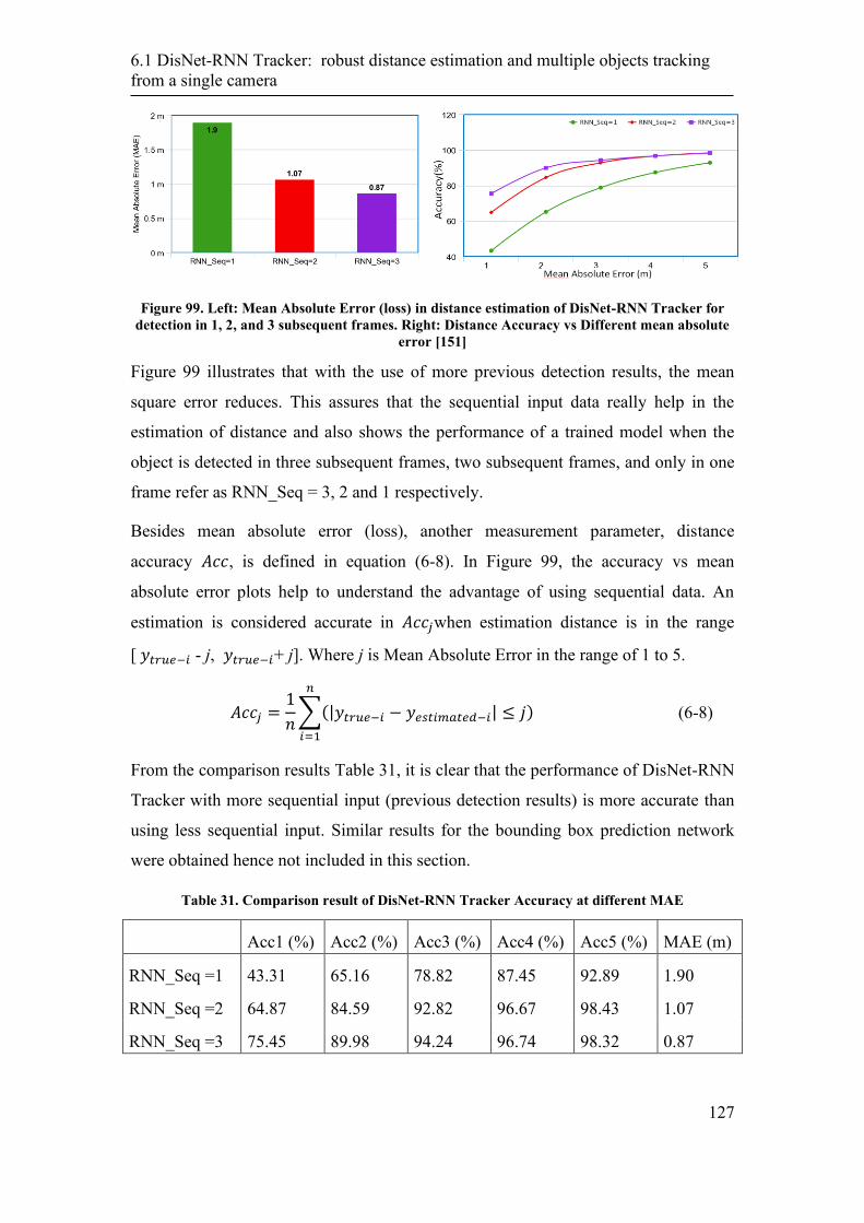
6.1 DisNet-RNN Tracker: robust distance estimation and multiple objects tracking
from a single camera
127
Figure 99. Left: Mean Absolute Error (loss) in distance estimation of DisNet-RNN Tracker for
detection in 1, 2, and 3 subsequent frames. Right: Distance Accuracy vs Different mean absolute
error [151]
Figure 99 illustrates that with the use of more previous detection results, the mean
square error reduces. This assures that the sequential input data really help in the
estimation of distance and also shows the performance of a trained model when the
object is detected in three subsequent frames, two subsequent frames, and only in one
frame refer as RNN_Seq = 3, 2 and 1 respectively.
Besides mean absolute error (loss), another measurement parameter, distance
accuracy 𝐴𝑐𝑐, is defined in equation (6-8). In Figure 99, the accuracy vs mean
absolute error plots help to understand the advantage of using sequential data. An
estimation is considered accurate in 𝐴𝑐𝑐𝑗when estimation distance is in the range
[ 𝑦𝑡𝑟𝑢𝑒−𝑖 - j, 𝑦𝑡𝑟𝑢𝑒−𝑖+ j]. Where j is Mean Absolute Error in the range of 1 to 5.
𝐴𝑐𝑐𝑗 =1
𝑛∑(|𝑦𝑡𝑟𝑢𝑒−𝑖 − 𝑦𝑒𝑠𝑡𝑖𝑚𝑎𝑡𝑒𝑑−𝑖| ≤ 𝑗)
𝑛
𝑖=1
(6-8)
From the comparison results Table 31, it is clear that the performance of DisNet-RNN
Tracker with more sequential input (previous detection results) is more accurate than
using less sequential input. Similar results for the bounding box prediction network
were obtained hence not included in this section.
Table 31. Comparison result of DisNet-RNN Tracker Accuracy at different MAE
Acc1 (%) Acc2 (%) Acc3 (%) Acc4 (%) Acc5 (%) MAE (m)
RNN_Seq =1 43.31 65.16 78.82 87.45 92.89 1.90
RNN_Seq =2 64.87 84.59 92.82 96.67 98.43 1.07
RNN_Seq =3 75.45 89.98 94.24 96.74 98.32 0.87

6.1 DisNet-RNN Tracker: robust distance estimation and multiple objects tracking
from a single camera
128
6.1.5 Multiple Object Mapping (MOM)
Another problem needs to be solved before DisNet-RNN Tracker can be used in
object tracking. The multiple detected objects in the current frame need to be
associated with the multiple detected objects in previous frames to form sequential
data (6-6) and (6-7), which is input to DisNet-RNN Tracker. Therefore, a Multiple
Object Mapping (MOM) module is introduced to perform object association and
generate sequential feature matrices for DisNet-RNN Tracker. The MOM module
calculates the Intersection Over Union (IOU) of current detected and previously
detected objects and based on high correlation associate the objects. The entire
working of the MOM module is shown in Figure 100. If the objects do not correlate
then MOM initialises the new tracker for newly detected objects and assigns a unique
ID.
Figure 100. Multiple Object Mapping based object association of current detected objects and
previously detected objects
6.1.6 Evaluation
The DisNet-RNN Tracker based system for distance estimation and object tracking
was evaluated on images recorded by an RGB monocular camera mounted on the
frontal profile of the moving freight train during the field tests within H2020

6.1 DisNet-RNN Tracker: robust distance estimation and multiple objects tracking
from a single camera
129
Shift2Rail project SMART. The RGB camera from The Imaging Source [152]
provides images with the maximum resolution of 2592x1944 at 2 FPS.
Figure 101 shows the performance of DisNet-RNN Tracker on six subsequent frames
from a video of a real-world dynamic railway scene with a truck parked in the rail
track area (vehicle 3), which is a potential intrusion, and a van (vehicle 4) crossing the
unsecured crossing while the train is approaching the crossing. The estimated
distance to the vehicle objects from the camera (i.e. from the locomotive), object
class, and tracking ID are shown in the left upper corner of each frame. The
detection/prediction of the objects is marked by the object bounding boxes. The blue
and brown coloured bounding boxes represent the prediction results, achieved by
DisNet-RNN Tracker, whereas the red bounding boxes represent the object detection
results of the YOLO object detection. As it is evident, the DisNet-RNN Tracker is
able to track the object (vehicle 3), to predict its bounding box and to estimate the
distance even in the case object is occluded by the other vehicle (frames 2 and 3) and
YOLO object detector failed. Moreover, the YOLO object detector failed even in the
case of a fully visible object (vehicle 3) in frame 6, whereas the proposed DisNet-
RNN Tracker achieved the object bounding box prediction and distance estimation.
During the train run, the ground truth was also measured using relative GPS positions
of the objects (from the google maps) and the train (GPS on the train). According to
the ground truth distance, the van (vehicle 3) and truck (vehicle 4) were
approximately 45 meters apart. The ground truth distances to the van were measured
as 135m, 128 m, 123m, 120m, 117m and 108m respectively for six subsequent frames
shown in Figure 99. Hence, the estimated distance from DisNet-RNN Tracker in
comparison with the ground truth demonstrates also reliability of the proposed
method.
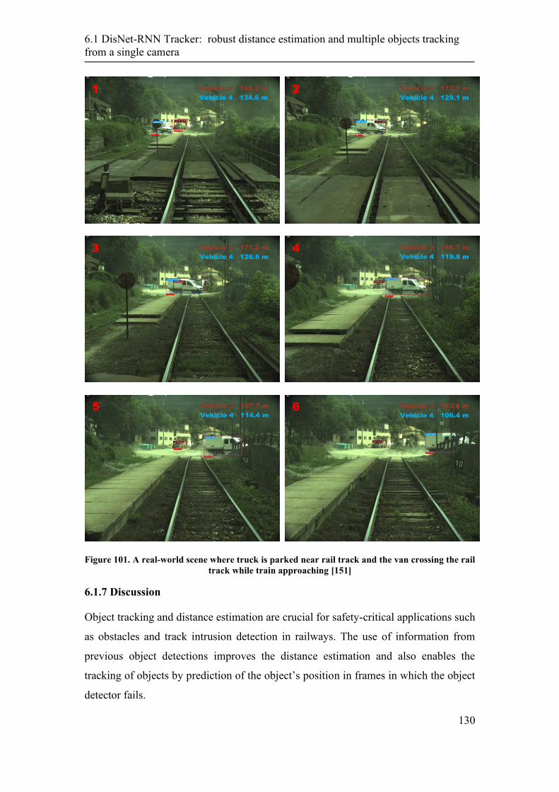
6.1 DisNet-RNN Tracker: robust distance estimation and multiple objects tracking
from a single camera
130
Figure 101. A real-world scene where truck is parked near rail track and the van crossing the rail
track while train approaching [151]
6.1.7 Discussion
Object tracking and distance estimation are crucial for safety-critical applications such
as obstacles and track intrusion detection in railways. The use of information from
previous object detections improves the distance estimation and also enables the
tracking of objects by prediction of the object’s position in frames in which the object
detector fails.
Vehicle 3 180.2 m
Vehicle 4 134.6 m 1 2 Vehicle 3 173.7 m
Vehicle 4 129.1 m
4 Vehicle 3 166.7 m
Vehicle 4 119.8 m 3 Vehicle 3 171.2 m
Vehicle 4 126.6 m
5 Vehicle 3 157.7 m
Vehicle 4 114.4 m 6 Vehicle 3 153.8 m
Vehicle 4 106.4 m
6.1 DisNet-RNN Tracker: robust distance estimation and multiple objects tracking
from a single camera
131
In this Thesis, DisNet-RNN Tracker consists of two sub-independent networks named
distance estimator and bounding box predictor is presented. Gated Recurrent Neural
Network architecture is chosen for object distance estimation and object tracking. By
using a monocular camera, the presented method can precisely track and estimate the
distance to the target objects as shown by the evaluation results from a real-world
railway scenario. However, the proposed object distance estimation system still has
several limitations such as object occlusion for a longer period introduces an error that
increases with time. So dependency on prediction results for a longer period is not
recommended, as the error increases with time until the estimation is corrected by the
detection.
Some efforts could be made in the following aspects in order to improve the
performance and conquer the drawbacks of presented distance estimation and object
tracking system. Moreover, for the improvement of distance estimation and object
tracking, the dataset needs to be extended, for long.-range detection and tracking of
multiple objects.

132
7.1 Requirement Analysis
133
7. Real-time Performance Evaluation
The basic need to detect and estimate the distance of various obstacles on the rail
tracks in real-time is a big challenge. In this chapter, the main development and
performance characteristics of proposed object detection, tracking, and distance
estimation methods in real-time are presented. The focus is on vision-based obstacle
detection system as in the final realization of ODS, vision sensors (cameras) were
used for mid- and long-range obstacle detection in the operational environment. Real-
time systems (RTS) are defined as hardware and software-based systems that assure
the system response within the specified time constraints. The required “event-to-
response time”, or in other words, “system response time” depends on many factors.
For example, in a high-speed machine vision application where the system is
physically moving fast or the capturing scene is moving fast, many factors such as
processing time and hardware selection, to be taken into account during the
development of such systems.
A challenging machine vision application is a highly bandwidth-demanding
application which brings a considerable amount of data streams from a vision sensor
to the processing unit. The obstacle detection system requires a high-bandwidth and
low latency network to connect all cameras to the central processing unit. Based on
the nature of the application, during the development of real-time Obstacle Detection
System (ODS) for rail transport, both challenges were presumed, high-speed and
high-bandwidth. In the next section, the requirements of the ODS system discussed in
detail.
7.1 Requirement Analysis
The requirements to make SMART ODS real-time grouped in two main categories:
high processing speed and high bandwidth requirements as listed below.

7.1 Requirement Analysis
134
High processing speed:
1. ODS mounted on a moving freight train running at 80 km/h, which is a
speed of a conventional freight train.
2. Train-stopping distance of approximately 700 meters for the above-
mentioned speed according to the regulations.
3. Moving or continuously changing scene/environment
High bandwidth:
1. Mid-range (up to 200 m) and Long-range (up to 1000 m) obstacle
detection requires high-resolution images to enable distant objects'
visibility in the image.
2. Simultaneous data acquisition from multiple vision sensors.
Based on the factors mentioned above the minimal required response time and
bandwidth analysis were performed as described in the following sections.
Minimum requirement approximation:
In order to estimate the minimum requirement of ODS, let’s assume a freight train
moving at 80 km/h (22.22 m/s) on a straight rail track. According to railway
regulations, the stopping distance of the freight train for speed of 80 km/h is about
700 meters.
The required event-to-response time 𝑡𝑟𝑒𝑠 (time required by perception module) should
be less than the data acquisition time 𝑡𝑎𝑐𝑞 , which means the system should be able to
process the captured data (camera frame) and response before the acquisition of the
next subsequent frame:
𝑡𝑟𝑒𝑠 < 𝑡𝑎𝑐𝑞 (7-1)
𝑡𝑝𝑟𝑜𝑐𝑒𝑠𝑠 = 𝑡𝑎𝑐𝑞 + 𝑡𝑟𝑒𝑠 (7-2)
The stopping distance 𝑑𝑠𝑡𝑜𝑝 and stopping time 𝑡𝑠𝑡𝑜𝑝 of the train equipped with ODS
while running with speed 𝑣 can be calculated as:
𝑡𝑠𝑡𝑜𝑝 = 𝑡𝑝𝑟𝑜𝑐𝑒𝑠𝑠 + 𝑡𝑏𝑟𝑎𝑘𝑖𝑛𝑔 + 𝑡𝑑𝑒𝑙𝑎𝑦 (7-3)
𝑑𝑠𝑡𝑜𝑝 = 𝑣 ∙ 𝑡𝑠𝑡𝑜𝑝 (7-4)
7.2 Hardware
135
Where 𝑡𝑏𝑟𝑎𝑘𝑖𝑛𝑔 refers to the time required to stop the train after the brake engagement
fully, 𝑡𝑑𝑒𝑙𝑎𝑦 refers as driver reaction time after the ODS system warning and 𝑡𝒑𝒓𝒐𝒄𝒆𝒔𝒔
can be defined as total processing time, i.e. time required by the hardware and
software components to deliver output from the moment at which the event occurred.
However, the braking time 𝑡𝑏𝑟𝑎𝑘𝑖𝑛𝑔 depends on many physical factors of the train
itself [153]:
1. the speed of the train at the time when the brakes are engaged;
2. the deceleration rate available with a full-service brake application, which
varies according to the coefficient of friction between wheel and rail;
3. the delay from when the train driver commands the brakes to when they are
become effective (brake delay time);
4. the state of the wear of the brake pads and the air pressure available in the
brake cylinders;
5. the geography of the track, in particular, the track gradient the train travels
over from when the brakes commanded to where the front of the train stops;
6. the mass distribution of the train.
7.2 Hardware
A real-time obstacle detection system for operational trains can be challenging to
implement as a PC computer-based system because of the needed potential for high
computational cost and algorithm complexity.
Emerging embedded vision system-based solutions for robotics and security
applications allow swift processing information and taking appropriate actions. Such
systems show high performance, high accuracy while requiring low energy
consumptions. Despite high demanding needs, in work for prototyping the ODS, a PC
computer-based system was considered for real-time implementation because it was
sufficient to meet the prototype system requirement. In order to cope with object
detection and distance estimation as a computationally expensive task, hardware-
specific optimisations of the proposed algorithms were performed, that allow the
algorithms to run in real-time. The hardware contains three parts: Sensors, Network,
and Processing Unit which are explained in the next sections.
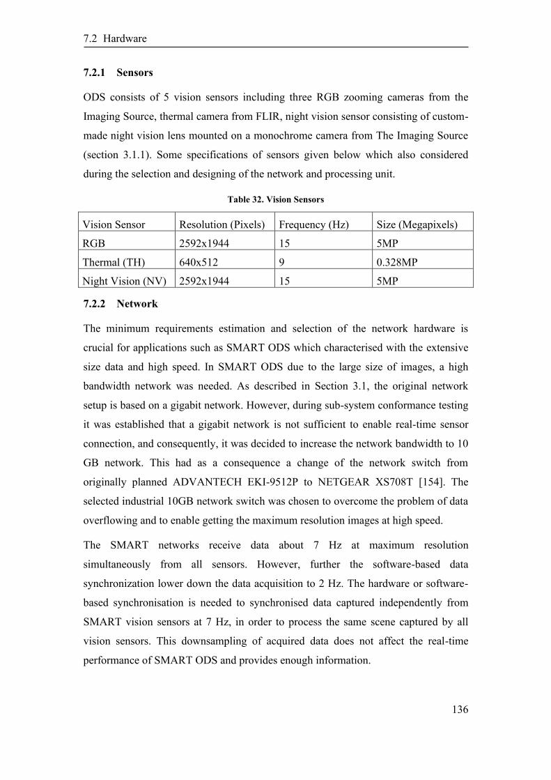
7.2 Hardware
136
7.2.1 Sensors
ODS consists of 5 vision sensors including three RGB zooming cameras from the
Imaging Source, thermal camera from FLIR, night vision sensor consisting of custom-
made night vision lens mounted on a monochrome camera from The Imaging Source
(section 3.1.1). Some specifications of sensors given below which also considered
during the selection and designing of the network and processing unit.
Table 32. Vision Sensors
Vision Sensor Resolution (Pixels) Frequency (Hz) Size (Megapixels)
RGB 2592x1944 15 5MP
Thermal (TH) 640x512 9 0.328MP
Night Vision (NV) 2592x1944 15 5MP
7.2.2 Network
The minimum requirements estimation and selection of the network hardware is
crucial for applications such as SMART ODS which characterised with the extensive
size data and high speed. In SMART ODS due to the large size of images, a high
bandwidth network was needed. As described in Section 3.1, the original network
setup is based on a gigabit network. However, during sub-system conformance testing
it was established that a gigabit network is not sufficient to enable real-time sensor
connection, and consequently, it was decided to increase the network bandwidth to 10
GB network. This had as a consequence a change of the network switch from
originally planned ADVANTECH EKI-9512P to NETGEAR XS708T [154]. The
selected industrial 10GB network switch was chosen to overcome the problem of data
overflowing and to enable getting the maximum resolution images at high speed.
The SMART networks receive data about 7 Hz at maximum resolution
simultaneously from all sensors. However, further the software-based data
synchronization lower down the data acquisition to 2 Hz. The hardware or software-
based synchronisation is needed to synchronised data captured independently from
SMART vision sensors at 7 Hz, in order to process the same scene captured by all
vision sensors. This downsampling of acquired data does not affect the real-time
performance of SMART ODS and provides enough information.

7.3 Software
137
Considering the train speed of 80 km/h, the data acquisition frame rate was set to 7
FPS (frame per 143 milliseconds) which means that at about every 3 meters travelled
distance the new data has been captured. Whereas the actual processing is done on
two frames out of seven captured frames meaning that SMART ODS processes an
image taken at every 500 milliseconds or in other words at every 11.11 meters
travelled distance.
7.2.3 Processing unit
Machine learning-based algorithms for obstacle detection and distance estimation
require a high-performance processing unit to enable real-time processing. Because of
the different sizes in which objects may appear in the image, the large image search
space is involved in object detection algorithms, which increases the complexity and
slows down the overall performance of SMART ODS real-time implementation.
SMART PC-computer based processing unit was used for the real-time obstacle
detection system prototyping. The processing unit was equipped with INTEL core i9
CPU and two Nvidia GTX 1080 16 GB GPUs (graphics processing units). Parallel
GPUs computing enable real-time object detection and distance estimation.
7.3 Software
ODS software architecture developed on the Robot Operating System (ROS) [121]
distribution Kinetic Kame operated on a Linux operating system (Ubuntu 16.04 64-
bit, http://releases.ubuntu.com/16.04/). During developing hardware and software for
SMART the goal was to achieve high reliability, modularity, redundancy,
performance, speed and redundancy characteristics for SMART ODS.
The ROS works here as middleware that provides the virtual interface between
different software modules such as data acquisition, object detection, distance
estimation, visualisation and offline processing modules (Figure 102).
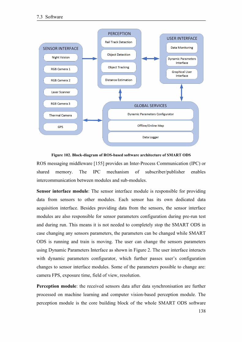
7.3 Software
138
Figure 102. Block-diagram of ROS-based software architecture of SMART ODS
ROS messaging middleware [155] provides an Inter-Process Communication (IPC) or
shared memory. The IPC mechanism of subscriber/publisher enables
intercommunication between modules and sub-modules.
Sensor interface module: The sensor interface module is responsible for providing
data from sensors to other modules. Each sensor has its own dedicated data
acquisition interface. Besides providing data from the sensors, the sensor interface
modules are also responsible for sensor parameters configuration during pre-run test
and during run. This means it is not needed to completely stop the SMART ODS in
case changing any sensors parameters, the parameters can be changed while SMART
ODS is running and train is moving. The user can change the sensors parameters
using Dynamic Parameters Interface as shown in Figure 2. The user interface interacts
with dynamic parameters configurator, which further passes user’s configuration
changes to sensor interface modules. Some of the parameters possible to change are:
camera FPS, exposure time, field of view, resolution.
Perception module: the received sensors data after data synchronisation are further
processed on machine learning and computer vision-based perception module. The
perception module is the core building block of the whole SMART ODS software
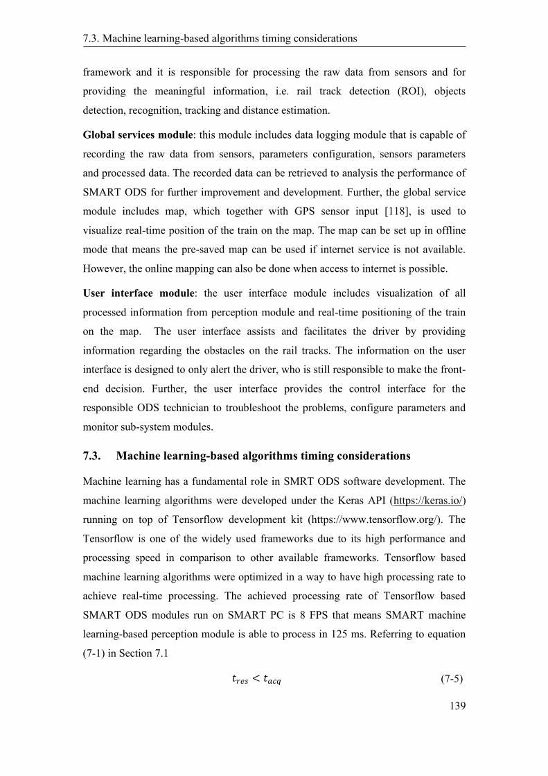
7.3. Machine learning-based algorithms timing considerations
139
framework and it is responsible for processing the raw data from sensors and for
providing the meaningful information, i.e. rail track detection (ROI), objects
detection, recognition, tracking and distance estimation.
Global services module: this module includes data logging module that is capable of
recording the raw data from sensors, parameters configuration, sensors parameters
and processed data. The recorded data can be retrieved to analysis the performance of
SMART ODS for further improvement and development. Further, the global service
module includes map, which together with GPS sensor input [118], is used to
visualize real-time position of the train on the map. The map can be set up in offline
mode that means the pre-saved map can be used if internet service is not available.
However, the online mapping can also be done when access to internet is possible.
User interface module: the user interface module includes visualization of all
processed information from perception module and real-time positioning of the train
on the map. The user interface assists and facilitates the driver by providing
information regarding the obstacles on the rail tracks. The information on the user
interface is designed to only alert the driver, who is still responsible to make the front-
end decision. Further, the user interface provides the control interface for the
responsible ODS technician to troubleshoot the problems, configure parameters and
monitor sub-system modules.
7.3. Machine learning-based algorithms timing considerations
Machine learning has a fundamental role in SMRT ODS software development. The
machine learning algorithms were developed under the Keras API (https://keras.io/)
running on top of Tensorflow development kit (https://www.tensorflow.org/). The
Tensorflow is one of the widely used frameworks due to its high performance and
processing speed in comparison to other available frameworks. Tensorflow based
machine learning algorithms were optimized in a way to have high processing rate to
achieve real-time processing. The achieved processing rate of Tensorflow based
SMART ODS modules run on SMART PC is 8 FPS that means SMART machine
learning-based perception module is able to process in 125 ms. Referring to equation
(7-1) in Section 7.1
𝑡𝑟𝑒𝑠 < 𝑡𝑎𝑐𝑞 (7-5)

7.3. Machine learning-based algorithms timing considerations
140
the processing rate should be larger than the data acquisition rate. In case of SMART
ODS, the data acquisition rate is 7 Hz, however after data synchronization the data at
2 Hz are forwarded to processing unit where the SMART perception module is able to
process at 8 Hz on SMART PC. The processing rate is four times the actual data
acquisition rate. This shows that the algorithms are highly optimized to perform
reliably in real-time environment and can perform on higher data acquisition rate as
well.
As described in chapter 4, state-of-the-art object detection algorithm YOLO-You
Only Look Once was chosen as object detector for SMART DisNet-based object
detection and distance estimation (Figure 48). YOLO uses a single deep-learning
network for both object classification and object localization in an image, and it is
considered as real-time fast multi-object detection algorithm with higher accuracy
rate.
The DisNet-based algorithm was developed for object detection and distance
estimation from a monocular camera and can be applied to all three SMART camera
types, RGB, Thermal and Night Vision camera. As described in Section 4, the results
of obstacle detection from single-camera are satisfactory, but the results could be
improved when performing the sensor fusion so that there is interest to process more
than one camera image at the time. For the purpose of timing consideration, the
calculation of total processing time when only one sensor (RGB camera) used is
performed and compared to the total processing time when more than one sensor
used, 2 (thermal+ RGB camera) and 5 (all 5 SMART vision sensors, 3 RGB, Thermal
and Night Vision). The sensors’ data acquisition times are given in Table 32 as well
as in Table 33. The time performance table (Table 33) shows that SMART ODS
satisfies the minimal requirement approximation. However, the time can be reduced
more with the better-performing processing unit.
In Table 33, 𝑓 refers to frequency and 𝑡𝒑𝒓𝒐𝒄𝒆𝒔𝒔 is the total time required by the
acquisition module and perception module to provide an output in case of a single
camera, whereas the data synchronization time is considered instead of data
acquisition time in case of multiple cameras.
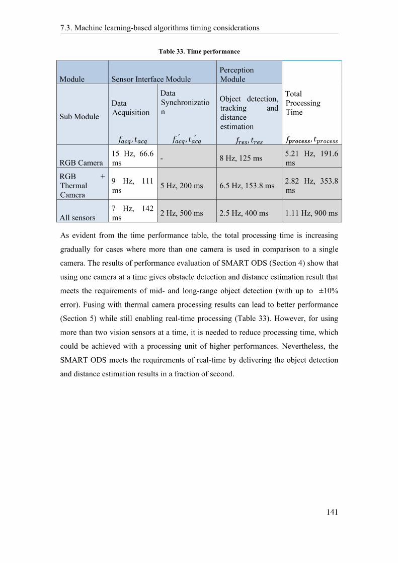
7.3. Machine learning-based algorithms timing considerations
141
Table 33. Time performance
Module Sensor Interface Module
Perception
Module
Total
Processing
Time
𝑓𝒑𝒓𝒐𝒄𝒆𝒔𝒔, 𝑡𝑝𝑟𝑜𝑐𝑒𝑠𝑠
Sub Module
Data
Acquisition
𝑓𝑎𝑐𝑞 , 𝑡𝑎𝑐𝑞
Data
Synchronizatio
n
𝑓𝑎𝑐𝑞́ , 𝑡𝑎𝑐𝑞́
Object detection,
tracking and
distance
estimation
𝑓𝑟𝑒𝑠, 𝑡𝑟𝑒𝑠
RGB Camera
15 Hz, 66.6
ms - 8 Hz, 125 ms
5.21 Hz, 191.6
ms
RGB +
Thermal
Camera
9 Hz, 111
ms 5 Hz, 200 ms 6.5 Hz, 153.8 ms
2.82 Hz, 353.8
ms
All sensors
7 Hz, 142
ms 2 Hz, 500 ms 2.5 Hz, 400 ms 1.11 Hz, 900 ms
As evident from the time performance table, the total processing time is increasing
gradually for cases where more than one camera is used in comparison to a single
camera. The results of performance evaluation of SMART ODS (Section 4) show that
using one camera at a time gives obstacle detection and distance estimation result that
meets the requirements of mid- and long-range object detection (with up to ±10%
error). Fusing with thermal camera processing results can lead to better performance
(Section 5) while still enabling real-time processing (Table 33). However, for using
more than two vision sensors at a time, it is needed to reduce processing time, which
could be achieved with a processing unit of higher performances. Nevertheless, the
SMART ODS meets the requirements of real-time by delivering the object detection
and distance estimation results in a fraction of second.

142
8.1 Conclusion
143
8. Conclusion and Outlook
8.1 Conclusion
This thesis addresses the problem of long-range environmental perception for the
applications where autonomous obstacle detection is safety-critical such as automated
vehicles. The particular focus of the thesis is on autonomous obstacle detection for
railways bearing in mind that long-range obstacle detection is explicitly required due
to longer braking distances for trains. Following the traditional and state-of-the-art
approaches for object detection in other applications, the first dataset for long-range
obstacle detection and distance estimation (LRODD) was generated in this Thesis as
described in chapter 3. The dataset contains images captured by monocular cameras
including three RGB cameras set with three different focal lengths to cover the short,
mid to long-range, a thermal camera and a night vision camera, short-range distance
information from LiDAR and GPS for positioning of ODS. The images were recorded
during various static and dynamic experiments conducted within project SMART and
contain examples of real-world scenarios that a train driver usually faces every day
including potential obstacles on the rail track or near to the rail track. The recorded
images, containing potential obstacles, were manually labelled for object bounding
boxes, object classes and related object ground truth distance, using an annotation tool
to form a dataset LRODD. Further, the labelled dataset was used in the development
of algorithms proposed in this thesis.
In chapter 4, the focus is on monocular camera-based distance estimation to the object
imaged by the camera. Two different approaches to the estimation of the distance to
the object using a single monocular camera have been presented. Both approaches
show the potential of using a single camera to object distance estimation without the
need for any camera parameters calibration. The first method proposed in chapter 3 is
8.1 Conclusion
144
referred to as DisNet, which is an abbreviation for Distance Network, and it is based
on a neural network which estimates the distance to the object based on the size of the
object bounding box in the image. DisNet expects to receive an input, containing
object bounding box and object class, from an object detection module in order to
estimate the distance to the object. DisNet can work with any object detection module
which produces the object bounding box and object class. DisNet is a single network
that works for multiple object classes. However, in some cases, it shows some
limitations to accurate distance estimation. For example, it tends to wrongly estimate
the object distance when a false or unprecise bounding box, produced by object
detection module inputs the DisNet, or objects of the same class appear in different
sizes in the image which leads to the understanding to consider object at a different
distance than the actual distance. In the same chapter, the second method named
YOLO-D, which is derived from the state-of-the-art object detection module You
Only Look Once (YOLO) and - D is added to represent distance estimation. YOLO is
a well-known object detector that localises and classifies the objects in an image. In
YOLO-D, the original YOLO architecture, loss function, and training methods were
modified so that an additional output was added, which is distance estimation to the
detected object. Due to the addition of another output, the original loss function was
also modified to adapt to the changes in the network architecture. In comparison to
original YOLO, the YOLO-D estimates the distance to the object in the image in
addition to object localisation and classification.
Further, for the training of YOLO-D additional information is necessary that is ground
truth distance to the object in a training image. That is why YOLO-D was trained in
this thesis with novel dataset LRODD containing labelled objects and also the
distance to them. Additionally, a transfer learning approach was applied to train
YOLO-D further with another state-of-the-art dataset KITTI which also has distance
information to the objects in order to improve the accuracy distance estimation by
YOLO-D.
In comparison to DisNet, YOLO-D is a single end-to-end network that detects an
object and estimates object distance and works with multiple object classes. Both
proposed methods in chapter 4 were tested in real-time and real-world applications
including railway and road scenarios.
8.2 Outlook
145
In chapter 5, a machine learning-based sensor fusion method named Multi-DisNet has
been proposed to estimate the distance to an object based on the object’s appearance
in the images captured from two cameras mounted apart from each other. The main
principle of this method was inspired by the DisNet method. After the simultaneous
object detection on images captured from both cameras, the size of the corresponding
object bounding box of the same object in both images is feed to the neural network
that estimates distance. However, only an object class ‘Person’ was investigated in the
development of this method.
In chapter 6, the Recurrent Neural Network-based method of multiple object tracking
has been presented. The RNN based network architecture tracks and predicts the
position of the object in the frames where the object detection module fails to identify
the object or the object is occluded. This method further estimates the distance to the
object continuously. Additionally, this method also refines the object bounding box
position and size based on the previous detection results in a current frame.
In chapter 7, the real-time implementation of the developed algorithms and
capabilities to use these algorithms in the real-world application was investigated. The
minimum hardware and software requirements for the obstacle detection system for
freight trains were also studied considering the physical braking constraints.
8.2 Outlook
The proposed methods in this thesis focusing on long-range detection and distance
estimation shows potential to overcome the limitation of commercial off-the-shelf
sensors technology to measure long-range distances. The methods shows that distant
objects can be detected and distance to them can be estimated by processing the high
resolution image obtained from a single camera.
Although the results presented in this Thesis show the reliability of the autonomous
multi-sensor long-range obstacle detection, tracking and distance estimation system,
there are few open questions are future directions. These are summarized as follows.
One research question is how the information from the autonomous system will be
communicated with the driver of the train. An intelligent Human-Computer
Interaction (HCI) system will be needed, which will need to ensure that it does not
distract the driver but also it is not ignored. Research and decades of commercial
8.2 Outlook
146
development in aviation, that has advanced the interaction between planes and pilots,
could guide the development of a successful HCI system for trains.
As it was mentioned before, the developed obstacle detection and distance estimation
system could also be applied for short-range detection, not only on autonomous cars
but also on autonomous robots. In a laboratory setting, DisNet was adjusted to detect
and estimate the position of household objects, such as cup and glass, and humans
with very promising results [21]. Further research will be needed to enable the
employment of DisNet in robotics.
Furthermore, YOLO-D shows potential to be use as a single neural network that can
detect object and simultenoulsy estimate distance to it. The performance can be
improve by further training with large annotated dataset, more classes and ground
truth distance.
Bibliography
147
Bibliography
[1] Y. J. Li, Z. Zhang, D. Luo and G. Meng, "Multi-sensor environmental
perception and information fusion for vehicle safety," in IEEE International
Conference on Information and Automation, Lijiang, 2015.
[2] H. Nguyen and C. C. Kemp, "Bio-inspired assistive robotics: Service dogs as a
model for human-robot interaction and mobile manipulation," in 2nd IEEE RAS
& EMBS International Conference on Biomedical Robotics and
Biomechatronics,, Scottsdale, 2008.
[3] J.-K. Oh and C.-H. Lee, "Development of a stereo vision system for industrial
robots," in International Conference on Control, Automation and Systems,
Seoul, 2007.
[4] J. Foucault, S. Lesecq, G. Dudnik, M. Correvon, R. O’Keeffe, V. Di Palma, M.
Passoni, F. Quaglia, L. Ouvry, S. Buckley, J. Herveg, A. di Matteo, T.
Rakotovao, O. Debicki, N. Mareau, J. Barrett, S. Rea, A. McGibney, F. Birot
and de Chaumont, "INSPEX: Optimize Range Sensors for Environment
Perception as a Portable System.," Sensors , vol. 19, p. 4350, October 2019.
[5] M. Bernas, B. Płaczek, W. Korski, P. Loska, J. Smyła and P. Szymała, "A
Survey and Comparison of Low-Cost Sensing Technologies for Road Traffic
Monitoring," Sensors , vol. 18(10), p. 3243, September 2018.
[6] L. Nalpantidis and A. Gasteratos, "Stereo Vision Depth Estimation Methods for
Robotic Applications," in Depth Map and 3D Imaging Applications: Algorithms
and Technologies, IGI Global, 2011, pp. 397-417.
[7] A. Saxena, J. Schulte and A. Ng, "Depth Estimation Using Monocular and
Stereo Cues.," in IJCAI International Joint Conference on Artificial
Intelligence, 2007.
[8] R. Atienza, "Fast Disparity Estimation using Dense Networks," in International
Conference on Robotics and Automation (ICRA), Brisbane, 2018.

Bibliography
148
[9] M. Moukari, S. Picard, S. L. and F. Jurie, "Deep Multi-Scale Architectures for
Monocular Depth Estimation," in 25th IEEE International Conference on Image
Processing (ICIP), Athens, 2018.
[10] W. Maddern, G. Pascoe, C. Linegar and P. Newman, "1 Year, 1000km: The
Oxford RobotCar Dataset," in The International Journal of Robotics Research
(IJRR), 2016.
[11] Shift2Rail, "Multi-Annual Action Plan," Brussels, 2015.
[12] J. Weichselbaum, C. Zinner, O. Gebauer and W. Pree, "Accurate 3D-vision-
based obstacle detection for an autonomous train," Computers in Industry, vol.
64, p. 1209–1220, 2013.
[13] A. Berg, K. Oefjaell, J. Ahlberg and M. Felsberg, "Detecting Rails and
Obstacles Using a Train-Mounted Thermal Camera," in Lecture Notes in
Computer Science, vol. 9127, Springer, Cham, SCIA 2015, p. 492–503.
[14] P. Pinggera, U. Franke and R. Mester, "High-performance long range obstacle
detection using stereo vision," in IEEE/RSJ International Conference on
Intelligent Robots and Systems (IROS), Hamburg , 2015.
[15] N. Fürstenau, Virtual and Remote Control Tower: Research, Design,
Development and Validation, 2014.
[16] P. SMART, 07 2020. [Online]. Available: http://www.smartrail-automation-
project.net.
[17] J. Brownlee, "A Gentle Introduction to Computer Vision," July 2019. [Online].
Available: https://machinelearningmastery.com/what-is-computer-vision/.
[18] S. Long, X. He and C. Yao, "Scene Text Detection and Recognition: The Deep
Learning Era," Computer Vision and Pattern Recognition, November 2018.
[19] K. Bobkowska, A. Kaczyńska, A. Kosiński and M. Przyborski, "Digital
Photogrammetry in the Analysis of the Ventricles' Shape and Size," in Baltic
Geodetic Congress (BGC Geomatics), Gdansk, 2017.
Bibliography
149
[20] W. Zhao, J. Y, Chang, D. M. Smith and M. D. Ginsberg, "Disparity analysis
and its application to three-dimensional reconstruction of medical images," in
Proceedings Fifth Annual IEEE Symposium on Computer-Based Medical
Systems, NC, USA, 1992.
[21] M. Kyrarini, Q. Zheng, M. A. Haseeb and A. Gräser, "Robot Learning of
Assistive Manipulation Tasks by Demonstration via Head Gesture-based
Interface," in IEEE 16th International Conference on Rehabilitation Robotics
(ICORR), Toronto, ON, Canada, 2019.
[22] D. Howard , "Enhanced driver safety with advanced vision systems," in Pan
Pacific Microelectronics Symposium (Pan Pacific), Waimea, HI, 2018.
[23] G. Jianju, M. Kyrarini, M. A. Haseeb, D. Ristic-Durrant and A. Gräser, "Safety
Surveillance System for Co-operative Robot using 360-Degree Camera," in
Conference: XIV International SAUM Conference on Systems, Automatic
Control and Measurements, Niš, Serbia, 2018.
[24] X. Li, X. Zhao, Y. Fu and Y. Liu, "Bimodal gender recognition from face and
fingerprint," in IEEE Computer Society Conference on Computer Vision and
Pattern Recognition, San Francisco, CA, 2010.
[25] M. Alom, T. Taha, C. Yakopcic, S. Westberg, P. Sidike, M. Nasrin, M. Hasan,
B. Van Essen, A. Awwal and V. Asari, "A State-of-the-Art Survey on Deep
Learning Theory and Architectures," Electronics 2019, vol. 8, p. 292, 2019.
[26] O. Campesato, Artificial Intelligence, Machine Learning, and Deep Learning,
San Francisco, CA: Stylus Publishing, LLC, 2020.
[27] M. R. M. Talabis, I. Miyamoto and D. Kaye, Information Security Analytics, R.
McPherson and J. L. Martin, Eds., Syngress, 2015.
[28] V. Roman, Jan 2019. [Online]. Available:
https://towardsdatascience.com/supervised-learning-basics-of-classification-
and-main-algorithms-c16b06806cd3.
[29] J. Brownlee, "Supervised and Unsupervised Machine Learning Algorithms," 16
Bibliography
150
March 2016. [Online]. Available:
https://machinelearningmastery.com/supervised-and-unsupervised-machine-
learning-algorithms/.
[30] J.-N. Vittaut, M.-R. Amini and P. Gallinari, "Learning Classification with Both
Labeled and Unlabeled Data," in Learning Classification with Both Labeled and
Unlabeled Data, 2002.
[31] A. Orhan E, "Computational Basis of Neural Elements," in Artificial Neural
Network for Drug Design, Delivery and Disposition, Elsevier , 2016, pp. 29-82.
[32] G. Shenk, August 2019. [Online]. Available:
https://www.functionize.com/blog/machine-learning-humans-behind-screen/.
[33] M. R. Tarabay, August 2020. [Online]. Available:
http://rafietarabay.blogspot.com/2019/05/pytorch-and-deep-learning.html.
[34] J. Duchi, E. Hazan and Y. Singer, "A Survey of Optimization Methods from a
Machine Learning Perspective," Journal of Machine Learning Research, vol.
12, p. 2121–2159, 2011.
[35] S. Raschka, August 2020. [Online]. Available:
http://rasbt.github.io/mlxtend/user_guide/general_concepts/gradient-
optimization/.
[36] A. Bhande, "What is underfitting and overfitting in machine learning and how
to deal with it," July 2020. [Online]. Available:
https://medium.com/greyatom/what-is-underfitting-and-overfitting-in-machine-
learning-and-how-to-deal-with-it-6803a989c76.
[37] J. Bergstra and Y. Bengio, "Random Search for Hyper-Parameter
Optimization," Journal of Machine Learning Research, vol. 13, pp. 281-305,
2012.
[38] E. Ndiaye, T. Le, O. Fercoq, J. Salmon and I. Takeuchi, "Safe Grid Search with
Optimal Complexity," in International Conference on Machine Learning, 2019.
[39] J. Walsh, N. O' Mahony, S. Campbell, A. Carvalho, L. Krpalkova, G. Velasco-
Bibliography
151
Hernandez, S. Harapanahalli and D. Riordan, "Deep Learning vs. Traditional
Computer Vision," in Computer Vision Conference (CVC), Las Vegas, 2019.
[40] Z. Zhou, . N. V. Chawla, . Y. Jin and G. J. Williams, "Big Data Opportunities
and Challenges: Discussions from Data Analytics Perspectives [Discussion
Forum]," IEEE Computational Intelligence Magazine, vol. 9, no. 4, pp. 62-74,
November 2014.
[41] H. D. Hlynsson, N. Alberto, B. Escalante and W. Laurenz, "Measuring the Data
Efficiency of Deep Learning Methods," in 8th International Conference on
Pattern Recognition Applications and Methods, 2019.
[42] Y. LeCun, L. Bottou, Y. Bengio and P. Haffner, "Gradient-Based Learning
Applied to Document Recognition," in Proceedings of the IEEE, 1998.
[43] A. R., Brodtkorb, T. R., Hagen, S. Christian and H. Geir, "GPU computing in
discrete optimization. Part I: Introduction to the GPU," EURO Journal on
Transportation and Logistics, vol. 2, p. 129–157, 2013.
[44] nvidia. [Online]. Available: https://www.nvidia.com/en-us/self-driving-
cars/drive-platform/.
[45] Y. Liu, "Feature Extraction and Image Recognition with Convolutional Neural
Networks," Journal of Physics: Conference Series, vol. 6, September 2018.
[46] A. Dertat, 02 2020. [Online]. Available:
https://towardsdatascience.com/applied-deep-learning-part-4-convolutional-
neural-networks-584bc134c1e2.
[47] "Convolutional Neural Networks (CNNs / ConvNets)," Stanford CS class,
[Online]. Available: https://cs231n.github.io/convolutional-networks/.
[48] A. Krizhevsky, I. Sutskever and G. E. Hinton, "ImageNet Classification with
Deep Convolutional Neural Networks," in Neural Information Processing
Systems, 2012.
[49] M. D Zeiler and R. Fergus, "Visualizing and Understanding Convolutional
Networks," 2013.

Bibliography
152
[50] K. Simonyan and A. Zisserman, "Very Deep Convolutional Networks for
Large-Scale Image Recognition," 2014.
[51] C. Szegedy, W. Liu, Y. Jia, P. Sermanet, S. Reed, D. Anguelov, D. Erhan, V.
Vanhoucke and Rabinovich, " Going deeper with convolutions," in In
Proceedings of the IEEE Conference on Computer Vision and Pattern
Recognition, Boston, MA, USA, 2015.
[52] K. He, X. Zhang, S. Ren and J. Sun, " Deep residual learning for image
recognition," in In Proceedings of the IEEE, Las Vegas, NV, USA, 2016.
[53] J. Deng, W. Dong, R. Socher, L. Li, K. Li and L. Fei-Fei, "ImageNet: A Large-
Scale Hierarchical Image Database," [Online]. Available: http://www.image-
net.org/papers/imagenet_cvpr09.bib.
[54] X. Han, Y. Zhong, L. Cao and L. Zhang, "Pre-Trained AlexNet Architecture
with Pyramid Pooling and Supervision for High Spatial Resolution Remote
Sensing Image Scene Classification," Remote Sens, vol. 9, 2017.
[55] G. Huang, Z. Liu, L. Van Der Maaten and K. Weinberger, "Densely connected
convolutional networks," in In Proceedings of the IEEE conference on
computer vision and pattern recognition , 2017.
[56] G. Larsson, M. Maire and G. Shakhnarovich, "Fractalnet: Ultra-deep neural
networks without residuals," in arXiv preprint arXiv:1605.07648, 2016.
[57] S. Sabour, N. Frosst and G. Hinton, "Dynamic routing between capsules," in
Advances in neural information processing systems , 2017.
[58] K. Zhang, W. Zuo, S. Gu and L. Zhang, "earning deep CNN denoiser prior for
image restoration," in Proceedings of the IEEE conference on computer vision
and pattern recognition, 2017.
[59] M. Alom, M. Hasan, C. Yakopcic, T. Taha and V. Asari, "Improved inception-
residual convolutional neural network for object recognition," Neural
Computing and Applications, vol. 32, no. 1, pp. 279-293, 2020.
[60] S. Gao, Z. Miao, Q. Zhang and Q. Li, "DCRN: Densely Connected Refinement
Bibliography
153
Network for Object Detection," Journal of Physics: Conference Series, vol.
1129, no. 1, 2019.
[61] J. Long, E. Shelhamer and T. Darrell, "Fully convolutional networks for
semantic segmentation," in In Proceedings of the IEEE Conference on
Computer Vision and Pattern Recognition, Boston, MA, USA, 2015.
[62] V. Badrinarayanan, A. Kendall and R. Cipolla, "SegNet: A Deep Convolutional
Encoder-Decoder Architecture for Image Segmentation," IEEE Transactions on
Pattern Analysis and Machine Intelligence, vol. 39, no. 12, pp. 2481-2495,
December 2017.
[63] G. Lin, A. Milan, C. Shen and I. Reid, "Refinenet: Multi-path refinement
networks for high-resolution semantic segmentation," in In Proceedings of the
2017 IEEE Conference on Computer Vision and Pattern Recognition CVPR, ,
Honolulu, HI, USA, 2017.
[64] H. Zhao, J. Shi, X. Qi, X. Wang and J. Jia, "Pyramid scene parsing network," in
In Proceedings of the IEEE Conference on Computer Vision and Pattern
Recognition (CVPR), Honolulu, HI, USA, 2017.
[65] L. Chen, G. Papandreou, I. Kokkinos, K. Murphy and A. Yuille, "Deeplab:
Semantic image segmentation with deep convolutional nets, atrous convolution,
and fully connected," in IEEE Trans. Pattern Anal. Mach. Intell., 2018.
[66] R. Girshick, J. Donahue, T. Darrell and J. Malik, " Rich feature hierarchies for
accurate object detection and," in In Proceedings of the IEEE Conference on
Computer Vision and Pattern Recognition CVPR, Columbus, OH, USA, 2014.
[67] T.-Y. Lin, P. Goyal, R. Girshick, K. He and P. Dollár, "Focal Loss for Dense
Object Detection," in Computer Vision and Pattern Recognition (CVPR), 2018.
[68] R. Girshick, "Fast R-CNN," in International Conference on Computer Vision
(ICCV), 2015.
[69] K. He, G. Gkioxari, P. Dollár and R. Girshick, "Mask R-CNN," in IEEE
International Conference on Computer Vision (ICCV), Venice, 2017.
Bibliography
154
[70] J. Redmon, S. Divvala, . R. Girshick and A. Farhadi, "You Only Look Once:
Unified, Real-Time Object Detection," in IEEE Conference on Computer Vision
and Pattern Recognition (CVPR), Las Vegas, NV, 2016.
[71] W. Liu, D. Anguelov, D. Erhan, C. Szegedy, S. Reed, C.-Y. Fu and A. C. Berg,
"SSD: Single Shot MultiBox Detector," Lecture Notes in Computer Science,
Springer International Publishing, p. 21–37, 2016.
[72] P. Viola and M. Jones, "Rapid Object Detection Using a Boosted Cascade of
Simple Features," in IEEE Computer Society Conference on Computer Vision
and Pattern Recognition. CVPR , Kauai, HI, USA, 2001.
[73] D. Lowe, "Distinctive image features from scale-invariant keypoints,"
International Journal of Computer Vision, vol. 60, p. 91–110, 2004.
[74] H. Bay, T. Tuytelaars and L. Van Gool, "Surf: Speeded up robust features," in
In European Conference on Computer Vision, Springer , Berlin, Germany,
2006.
[75] K. Mikolajczyk and C. Schmid, "A Performance Evaluation of Local
Descriptors," IEEE TRANSACTIONS ON PATTERN ANALYSIS AND
MACHINE INTELLIGENCE, vol. 27, no. 19, pp. 1615-1630, October 2005.
[76] N. Dalal and B. Triggs, "Histograms of Oriented Gradients for Human
Detection," in In Proceedings of the IEEE Conference on Computer Vision and
Pattern Recognition, San Diego, CA, USA, 2005.
[77] J. Redmon and A. Farhadi, "YOLO9000: Better, Faster, Stronger," in IEEE
Conference on Computer Vision and Pattern Recognition (CVPR), Honolulu,
HI, 2017.
[78] J. Redmon and A. Farhadi, "YOLOv3: An Incremental Improvement," in ArXiv
abs/1804.02767, 2018.
[79] R. Girshick, "Fast R-CNN," in IEEE International Conference on Computer
Vision (ICCV), Santiago, 2015.
[80] J. Hui, August 2019. [Online]. Available:
Bibliography
155
https://medium.com/@jonathan_hui/real-time-object-detection-with-yolo-
yolov2-28b1b93e2088..
[81] L. Van Gool and A. Neubeck, "Efficient Non-Maximum Suppression," in 18th
International Conference on Pattern Recognition, Hong Kong, 2006.
[82] J. Redmon. [Online]. Available: http://pjreddie.com/darknet/, 2013{2016.
[83] N. Developer, August 2020. [Online]. Available:
https://developer.nvidia.com/about-cuda.
[84] August 2020. [Online]. Available: https://github.com/Cartucho/mAP.
[85] M. E. Aidouni, October 2019. [Online]. Available:
https://manalelaidouni.github.io/manalelaidouni.github.io/Evaluating-Object-
Detection-Models-Guide-to-Performance-Metrics.html.
[86] M. Johnson, "How much data is enough? Predicting how accuracy varies with
training data size," 2017.
[87] H. Caesar, V. Bankiti, A. Lang, S. Vora, V. Liong, Q. Xu, A. Krishnan, Y. Pan,
G. Baldan and O. Beijbom, "nuScenes: A multimodal dataset for autonomous
driving," in Proceedings of the IEEE/CVF Conference on Computer Vision and
Pattern Recognition, 2020.
[88] A. Patil, S. Malla, H. Gang and Y. Chen, "The H3D Dataset for Full-Surround
3D Multi-Object Detection and tracking in crowded urban scenes," in 2019
International Conference on Robotics and Automation (ICRA), 2019.
[89] T. Lin, M. Maire, S. Belongie, J. Hays, P. Perona, D. Ramanan, P. Dollár and C.
Zitnick, "Microsoft COCO: Common Objects in Context," ECCV 2014, Lecture
Notes in Computer Science, vol. 8693, 2014.
[90] A. Geiger, P. Lenz and R. Urtasun, "Are we ready for autonomous driving? The
KITTI vision benchmark suite,," in IEEE Conference on Computer Vision and
Pattern Recognition, Providence, RI, 2012.
[91] A. Kashani, M. Olsen, C. Parrish and N. Wilson, "A Review of LIDAR
Bibliography
156
Radiometric Processing: From Ad Hoc Intensity Correction to Rigorous
Radiometric Calibration," Sensors , vol. 15, pp. 28099-28128, 2015.
[92] J. Hecht, "Lasers for Lidar: FMCW lidar: An alternative for self-driving cars,"
2019.
[93] Y. Wang, C. Peng, A. Ravankar and A. Ravankar, "A single LiDAR-based
feature fusion indoor localization algorithm," Sensors, vol. 18, no. 4, p. 1294,
2018.
[94] T. Gee, J. James, W. Van Der Mark, P. Delmas and G. Gimel'farb, "Lidar
guided stereo simultaneous localization and mapping (SLAM) for UAV outdoor
3-D scene reconstruction," in 2016 International Conference on Image and
Vision Computing New Zealand (IVCNZ), 2016.
[95] B. Schwarz, "Mapping the world in 3D," Nature Photonics, vol. 4, no. 7, pp.
429-430, 2010.
[96] W. Ali, S. Abdelkarim, M. Zidan, M. Zahran and A. El Sallab, "Yolo3d: End-
to-end real-time 3d oriented object bounding box detection from lidar point
cloud," in Proceedings of the European Conference on Computer Vision
(ECCV), 2018.
[97] D. Ristić-Durrant, G. Gao and A. Leu, "Facta Universitatis, Series: Automatic
Control and Robotics," Low-level sensor fusion-based human tracking for
mobile robot, vol. 1, no. 1, pp. 17-32, 2016.
[98] J. Hecht, "Lidar for self-driving cars," Optics and Photonics News, vol. 29, no.
1, pp. 26-33, 2018.
[99] N. Qian, "Binocular disparity and the perception of depth," Neuron, vol. 18, no.
3, pp. 359-368, 1997.
[100] L. Matthies, R. Szeliski and T. Kanade, "Incremental estimation of dense depth
maps from image sequences," in CVPR, 1988.
[101] N. Short, "3-D Point Cloud Generation from Rigid and Flexible Stereo Vision
Systems," 2020.

Bibliography
157
[102] M. Bertozz, A. Broggi and A. Fascioli, "Stereo inverse perspective mapping:
theory and applications," Image and vision computing, vol. 16, no. 8, pp. 585-
590, 1998.
[103] J. Zhu and e. al, "Learning Object-specific Distance from a Monocular Image,"
in International Conference on Computer Vision (ICCV), Seoul, Korea, 2019.
[104] Z. Sadreddini, T. Çavdar and H. Jond, "A distance measurement method using
single camera for indoor environments," in 2016 39th International Conference
on Telecommunications and Signal Processing (TSP), 2016.
[105] A. Ali, A. Hassan, A. Ali, H. Khan, W. Kazmi and A. Zaheer, "Real-time
vehicle distance estimation using single view geometry," in The IEEE Winter
Conference on Applications of Computer Vision, 2020.
[106] "Lyft Level 5 Dataset," [Online]. Available: https://self-
driving.lyft.com/level5/data/.
[107] J. Xiao, J. Hays, K. A. Ehinger, A. Oliva and A. Torralba, "SUN database:
Large-scale scene recognition from abbey to zoo," in IEEE Computer Society
Conference on Computer Vision and Pattern Recognition, San Francisco, CA,
2010.
[108] M. Everingham, S. Eslami, L. Van Gool, C. Williams, J. Winn and A.
Zisserman, "The PASCAL Visual Object Classes Challenge: A Retrospective,"
in International Journal of Computer Vision, 2015.
[109] O. Russakovsky, J. Deng, H. Su, J. Krause, S. Satheesh, S. Ma, Z. Huang, A.
Karpathy, A. Khosla, M. Bernstein and A. Berg, "Imagenet large scale visual
recognition challenge," International Journal of Computer Vision, vol. 115, pp.
211-252, 2015.
[110] P. Dollár, C. Wojek, B. Schiele and P. Perona, "Pedestrian Detection: A
Benchmark," in IEEE Conference on Computer Vision and Pattern Recognition,
Miami, FL, 2009.
[111] S. Ren, K. He, R. Girshick and J. Sun, "Faster r-cnn: Towards real-time object
Bibliography
158
detection with region proposal networks," IEEE Transactions on Pattern
Analysis and Machine Intelligence, vol. 39, no. 6, pp. 1137-1149, June 2017.
[112] Y. Li, H. Qi, J. Dai, X. Ji and Y. Wei, "Fully Convolutional Instance-Aware
Semantic Segmentation," in IEEE Conference on Computer Vision and Pattern
Recognition (CVPR), 2017.
[113] "The Imaging Source Europe GmbH," July 2020. [Online]. Available:
https://www.theimagingsource.com/products/zoom-autofocus-cameras/gige-
color-zoom-cameras/dfkz12gp031/.
[114] F. Systems, July 2020. [Online]. Available: https://www.flir.com/products/tau-
2/.
[115] D. Ristić-Durrant, M. A. Haseeb, M. Banić and I. Ćirić, "D1.1 Obstacle
Detection System Requirements and Specification," Bremen, 2019.
[116] M. A. H. M. B. a. D. R. Danijela Ristić-Durrant, "D2.1 - Report on selected
sensors for multi-sensory system for obstacle detection," Bremen, 2017.
[117] "3D LiDAR sensors LD-MRS / LD-MRS 4-Layer / Outdoor," SICK, [Online].
Available: https://www.sick.com/ag/en/detection-and-ranging-solutions/3d-
lidar-sensors/ld-mrs/ld-mrs400001s01/p/p251942.
[118] "USB GPS Module," [Online]. Available:
https://www.hardkernel.com/shop/usb-gps-module/.
[119] "SMART - Smart Automation of Rail Transport," [Online]. Available:
http://www.smartrail-automation-project.net/.
[120] M. Haseeb, D. Ristic-Durrant, A. Gräser, B. M. and S. D., "Multi-DisNet:
Machine Learning-Based Object Distance Estimation from Multiple Cameras,"
in International Conference on Computer Vision Systems, 2019.
[121] M. Quigley, K. Conley, B. Gerkey, J. Faust, T. Foote, J. Leibs, R. Wheeler and
A. Ng, "ROS: an open-source Robot Operating System," in ICRA workshop on
open source software, 2009.
Bibliography
159
[122] "Approximate Time," ROS, [Online]. Available:
http://wiki.ros.org/message_filters/ApproximateTime.
[123] B. Russell, A. Torralba, K. Murphy and W. Freeman, "LabelMe: a database and
web-based tool for image annotation," International journal of computer vision,
vol. 77, no. 1-3, pp. 157-173, 2008.
[124] M. Haseeb, J. Guan, D. Ristic-Durrant and A. Gräser, "Disnet: A novel method
for distance estimation from monocular camera," in 10th Planning, Perception
and Navigation for Intelligent Vehicles (PPNIV18), IROS, 2018.
[125] M. Haseeb, D. Ristić-Durrant and A. Gräser, "Long-range obstacle detection
from a monocular camera," in ACM Computer Science in Cars Symposium
(CSCS 2018), ECCV, 2018.
[126] "Tuning the hyper-parameters of an estimator," scikit learn, [Online]. Available:
https://scikit-learn.org/stable/modules/grid_search.html#grid-search.
[127] D. Kingma and J. Ba, "Adam: A method for stochastic optimization," in arXiv
preprint arXiv:1412.6980, 2014.
[128] T. Tieleman and G. Hinton, "Lecture 6.5-rmsprop, coursera: Neural networks
for machine learning," University of Toronto, Technical Report, 2012.
[129] "Layer weight initializers," Keras, [Online]. Available:
https://keras.io/api/layers/initializers/.
[130] S. Chatterjee and A. Hadi, Regression analysis by example, John Wiley & Sons,
2015.
[131] R. Tibshirani, "Regression shrinkage and selection via the lasso," Journal of the
Royal Statistical Society: Series B (Methodological), vol. 58, no. 1, pp. 267-288,
1996.
[132] J. Wang, A. Hertzmann and D. Fleet, "Gaussian process dynamical models,"
Advances in neural information processing systems, pp. 1441-1448, 2006.
[133] J. Suykens and J. Vandewalle, "Least squares support vector machine
Bibliography
160
classifiers," Neural processing letters, vol. 9, no. 3, pp. 293-300, 1999.
[134] D. Lee, J. In and S. Lee, "Standard deviation and standard error of the mean,"
Korean journal of anesthesiology, vol. 68, no. 3, p. 220, 2015.
[135] A. Leu, D. Aiteanu and A. Gräser, "High speed stereo vision based automotive
collision warning system," Applied Computational Intelligence in Engineering
and Information Technology, pp. 187-199, 2012.
[136] A. Leu, D. Bacără, D. Aiteanu and A. Gräser, "Hardware acceleration of image
processing algorithms for collision warning in automotive applications," in
Methods and Applications in Automation: 32nd – 33rd Colloquium of
Automation, Salzhausen/Leer, Germany, 2012.
[137] August 2020. [Online]. Available:
https://www.itread01.com/content/1541167345.html.
[138] Z. E. and Z. Y., "Average Precision," Encyclopedia of Database Systems, 2009.
[139] A. Dutta and A. Zisserman, "The VIA annotation software for images, audio
and video," in Proceedings of the 27th ACM International Conference on
Multimedia, 2019.
[140] F. Pedregosa, G. Varoquaux, A. Gramfort, V. Michel, B. Thirion, O. Grisel, M.
Blondel, P. Prettenhofer, R. Weiss, V. Dubourg, J. Vanderplas, A. Passos, D.
Cournapeau, M. Brucher, P. M. and E. Duchesnay, "Scikit-learn: Machine
Learning in Python," Journal of Machine Learning, Research, 2011.
[141] D. Ristić-Durrant, M. A. Haseeb, M. Banić, S. D., S. M., Ć. I., N.-k. V., N. D.
and R. D., "SMART: a novel on-board integrated multi-sensor long-range
obstacle detection system for railways," in RAILCON, 2018.
[142] L. Duvieubourg, F. Cabestaing, S. Ambellouis and P. Bonnet, "Long distance
vision sensor for driver assistance," IFAC Proceedings Volumes, vol. 40, no. 15,
pp. 330-336, 2007.
[143] "Shift2Rail Joint Undertaking, Multi-Annual Action Plan," Brussels, 2015.
Bibliography
161
[144] Y. Zhang, Y. Huang and L. Wang, "Multi-task deep learning for fast online
multiple object tracking," in 2017 4th IAPR Asian Conference on Pattern
Recognition (ACPR), 2017.
[145] A. Kuramoto, M. Aldibaja, R. Yanase, J. Kameyama, K. Yoneda and N.
Suganuma, "Mono-camera based 3d object tracking strategy for autonomous
vehicles," in 2018 IEEE Intelligent Vehicles Symposium (IV), 2018.
[146] Y. Huang, T. Huang and H. Niemann, "A region-based method for model-free
object tracking," in Object recognition supported by user interaction for service
robots, 2002.
[147] H. Cho, S. Song, J. Kim and J. Cho, "Simple object coordination tracking based
on background modeling," in 2015 Signal Processing: Algorithms,
Architectures, Arrangements, and Applications (SPA), 2015.
[148] M. Yokoyama and T. Poggio, "A contour-based moving object detection and
tracking," in Visual Surveillance and Performance Evaluation of Tracking and
Surveillance, 2005.
[149] L. Fan, "A feature-based object tracking method using online template
switching and feature adaptation," in 2011 Sixth International Conference on
Image and Graphics, 2011.
[150] H. Hsu and J. Ding, "FasterMDNet: Learning model adaptation by RNN in
tracking-by-detection based visual tracking," in 2017 Asia-Pacific Signal and
Information Processing Association Annual Summit and Conference (APSIPA
ASC) , 2017.
[151] M. Haseeb, D. Ristić-Durrant and A. Gräser, " A deep learning based
autonomous distance estimation and tracking of multiple objects for
improvement in safety and security in railways," in BMVC 2019 workshop on
Object Detection and Recognition for Security Screening (ODRSS2019),
Cardiff, 2019.
[152] "The imaging Source - Technology based on standards," [Online]. Available:
Bibliography
162
https://www.theimagingsource.com/.
[153] D. Barney, D. Haley and G. Nikandros, "Calculating train braking distance," in
Conferences in Research and Practice in Information Technology Series, 2001.
[154] "10-Gigabit Smart Managed Pro Switch Series," [Online]. Available:
https://www.netgear.com/business/products/switches/smart/XS708T.aspx.
[155] S. Cousins, "Welcome to ros topics [ros topics]," IEEE Robotics & Automation
Magazine, vol. 17, no. 1, pp. 13-14, 2010.
[156] S. Pendleton, H. Andersen, X. Du, X. Shen, M. Meghjani, Y. Eng, D. Rus and
M. Ang, "Perception, Planning, Control, and Coordination for Autonomous
Vehicles," Machines , vol. 6, no. Mechatronics: Intelligent Machines, 2017.
[157] A. Geiger, P. Lenz, C. Stille and R. Urtasun, "Vision meets robotics: the KITTI
dataset," The International Journal of Robotics Research, vol. 32, pp. 1231-
1237, 2013.
[158] J. Hui, "Real-time Object Detection with YOLO, YOLOv2 and now YOLOv3,"
17 March 2018. [Online]. Available: https://medium.com/@jonathan_hui/real-
time-object-detection-with-yolo-yolov2-28b1b93e2088.
[159] "Choosing a Convolutional Neural Network Architecture for Real-Time Object
Tracking (Part 1)," 1 December 2017. [Online]. Available:
https://blog.kickview.com/choosing-a-convolutional-neural-network-
architecture-for-real-time-object-tracking-part-1/.
[160] A. Rosebrock, "Intersection over Union (IoU) for object detection," 7
November 2016. [Online]. Available:
https://www.pyimagesearch.com/2016/11/07/intersection-over-union-iou-for-
object-detection/.
[161] Y. Liu, "The Confusing Metrics of AP and mAP for Object Detection / Instance
Segmentation," 25 October 2018. [Online]. Available:
https://medium.com/@yanfengliux/the-confusing-metrics-of-ap-and-map-for-
object-detection-3113ba0386ef.
Bibliography
163
[162] J. Hui, "mAP (mean Average Precision) for Object Detection," 6 March 2018.
[Online]. Available: https://medium.com/@jonathan_hui/map-mean-average-
precision-for-object-detection-45c121a31173.
[163] "Most popular metrics used to evaluate object detection algorithms," Python
Awesome, 21 July 2018. [Online]. Available:
https://pythonawesome.com/most-popular-metrics-used-to-evaluate-object-
detection-algorithms/.
[164] A. Geiger, P. Lenz, C. Stiller and R. Urtasun, "Vision meets robotics: The kitti
dataset," International Journal of Robotics Research, vol. 32, no. 11, pp. 1231-
1237, 2013.
Appendix A: Publications by the author
164
Appendix A: Publications by the author
This appendix lists the publications by the author, which have been produced
throughout this thesis, and they are the basis of this thesis.
Related Publications to the PhD thesis
[1] Ristic-Durrant, D., Haseeb, M.A., Franke, M., Banić, M., Simonović, M. and
Stamenković, D., 2020. Artificial intelligence for obstacle detection in
railways: Project SMART and beyond. In 1st International Workshop on
Artificial Intelligence for RAILwayS (AI4RAILS), Dependable Computing -
EDCC 2020 Workshops, Springer, Munich, Germany
[2] Haseeb, M.A., Ristic-Durrant, D., Gräser, A., Banić M. and Stamenković D.,
2019. Multi-DisNet: Machine Learning-Based Object Distance Estimation
from Multiple Cameras. In International Conference on Computer Vision
Systems (ICCV), pp. 457-469. Springer, Cham., Thessaloniki, Greece, doi:
10.1007/978-3-030-34995-0_41
[3] Haseeb, M.A., Ristic-Durrant, D., Gräser, A., 2019. A deep learning based
autonomous distance estimation and tracking of multiple objects for
improvement in safety and security in railways. In British Machine Vision
Conference (BMVC) - Workshop on Object Detection and Recognition for
Security Screening (ODRSS2019), Cardiff, UK
[4] Haseeb, M.A., Guan, J., Ristic-Durrant, D. and Gräser, A., 2018. Disnet: A
novel method for distance estimation from monocular camera. 10th Planning,
Perception and Navigation for Intelligent Vehicles (PPNIV18), IROS, Madrid,
Spain.
[5] Haseeb, M.A., Ristić-Durrant, D. and Gräser, A., 2018. Long-range obstacle
detection from a monocular camera. In ACM Computer Science in Cars
Symposium (CSCS 2018), ECCV, Munich, Germany
[6] Ristić-Durrant, D., Haseeb, M.A., Emami, D., Gräser, A., 2018. Multimodal
Sensor Fusion for Reliable Detection of Obstacles on Railway Tracks. Journal
of Mechatronics, Automation and Identification Technology, 3(2), pp. 1-7,
Novi Sad, Serbia
[7] Ristić-Durrant, D., Haseeb, M.A., Banić M., Stamenković, D., Ćirić, I.,
Simonović, M., Nikolić, V., Nikolić, D. and Radovanović, D., 2018. SMART:
Appendix A: Publications by the author
165
a novel on-board integrated multi-sensor long-range obstacle detection system
for railways. RAILCON, Nis, Serbia.
[8] Ristić-Durrant, D., Haseeb M. A., Emami, D., Gräser A., 2018, SMART
concept of an integrated multi-sensory on-board system for obstacle
recognition in 7th Transport Research Arena (TRA) , Vienna, Austria
[9] Ristić-Durrant, D., Haseeb, M.A., Emami, D., Gräser, A., Ćirić, I.,
Simonović, M., Nikolić, V., Nikolić, D., Eßer, F.P., Schindler, C., 2017.
Reliable Obstacle Detection for Smart Automation of Rail Transport. In 1st
International Railway Symposium Aachen (IRSA), Aachen, Germany. doi:
10.18154/RWTH-2018-222952
Other Publications
[1] Kyrarini M., Haseeb M.A., Ristić-Durrant D., Gräser A., 2019. Robot
Learning of Industrial Assembly Task via Human Demonstrations.
Autonomous Robots, 43(1), pp. 239-257. doi: 10.1007/s10514-018-9725-6
[2] Kyrarini M., Zheng Q., Haseeb M.A, Gräser A., 2019. Robot Learning of
Assistive Manipulation Tasks by Demonstration via Head Gesture-based
Interface. In International Conference on Rehabilitation Robotics (ICORR),
Toronto, Canada, pp.210-216. IEEE. doi: 10.1109/ICORR.2019.8779521
[3] Haseeb M.A, Kyrarini M., Jiang S., Ristić-Durrant D., Gräser A., 2018. Head
Gesture-based Control for Assistive Robots. In 11th ACM International
Conference on Pervasive Technologies Related to Assistive Environments
(PETRA), Corfu Greece, pp. 379-383. ACM. doi: 10.1145/3197768.3201574
[4] Guan J., Kyrarini M., Haseeb M.A, Ristić-Durrant D., Gräser A., 2018. Safety
Surveillance System for Co-operative Robot using 360-Degree Camera. In
XIV International SAUM Conference on Systems, Automatic Control and
Measurements, Niš, Serbia
[5] Kyrarini M., Haseeb M.A., Ristić-Durrant D., Gräser A., 2017. Robot
Learning of Object Manipulation Task Actions from Human Demonstrations.
Facta Universitatis, series: Mechanical Engineering (FU Mech Eng), 15(2),
pp. 217-229. doi: 10.22190/FUME170515010K

166
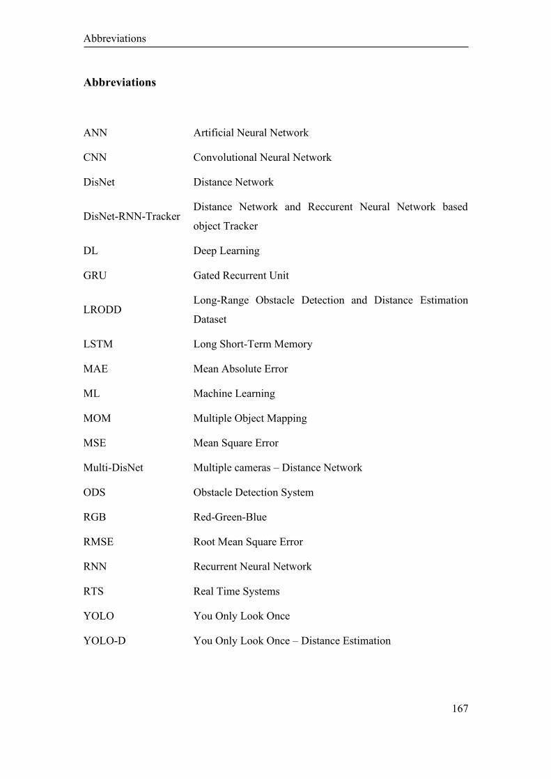
Abbreviations
167
Abbreviations
ANN Artificial Neural Network
CNN Convolutional Neural Network
DisNet Distance Network
DisNet-RNN-Tracker Distance Network and Reccurent Neural Network based
object Tracker
DL Deep Learning
GRU Gated Recurrent Unit
LRODD Long-Range Obstacle Detection and Distance Estimation
Dataset
LSTM Long Short-Term Memory
MAE Mean Absolute Error
ML Machine Learning
MOM Multiple Object Mapping
MSE Mean Square Error
Multi-DisNet Multiple cameras – Distance Network
ODS Obstacle Detection System
RGB Red-Green-Blue
RMSE Root Mean Square Error
RNN Recurrent Neural Network
RTS Real Time Systems
YOLO You Only Look Once
YOLO-D You Only Look Once – Distance Estimation

168

Table of Figures
169
Table of Figures
Figure 1. The grouping of AI and its sub-groups [25] ................................................... 8
Figure 2. Category of Deep Learning approaches [25] ................................................ 10
Figure 3. A basic artificial neural network architecture .............................................. 10
Figure 4. The architecture of basic computational unit in ANN .................................. 11
Figure 5. Three most common activation functions [33] ............................................. 12
Figure 6. Gradient Descent [35] ................................................................................... 13
Figure 7. Regularisation [36] ....................................................................................... 14
Figure 8. A plot of MAE and MSE Loss (Y-axis) vs Predictions (X-axis) ................. 15
Figure 9. The deep learning efficiency with regard to the amount of data .................. 18
Figure 10. Example of convolution operation [46] ...................................................... 19
Figure 11. Accuracy of different DL models on ImageNet classification challenge
[25] ............................................................................................................................... 20
Figure 12. AlexNet architecture [54] ........................................................................... 21
Figure 13. YOLO’s Image Grid. Each grid cell detects only one object [80] ............. 23
Figure 14. Each grid cell making a fixed number of bounding boxes for one object
[80] ............................................................................................................................... 24
Figure 15. YOLO making S x S predictions with B bounding boxes [80] .................. 25
Figure 16. YOLO detecting B bounding boxes for a single image with S x S grid .... 25
Figure 17. YOLO Network Architecture [70] ............................................................. 26
Figure 18. YOLOv2 Accuracy and Speed Compared to other Object Detectors [77] 28
Figure 19. YOLOv3 Network Architecture [73] ......................................................... 29
Figure 20. Darknet-53 layers [78] ................................................................................ 30
Figure 21. Illustration of Intersection over Union (IoU) [84] ...................................... 31
Table of Figures
170
Figure 22 An example of all-points interpolation in Precision-Recall curve [85] ....... 34
Figure 23. Recording Platform of KITTI dataset [90] ................................................. 36
Figure 24. Detailed information on the recording platform [90] ................................. 36
Figure 25. Examples from KITTI dataset [90] ............................................................ 37
Figure 26. An example of labeled images in KITTI dataset [90] ................................ 38
Figure 27. The stereo vision setup ............................................................................... 40
Figure 28. Input – First frame (left image), Depth image (center), Prespective view
(right) [100] .................................................................................................................. 41
Figure 29. Error-Depth diagram for narrow and wide baseline [101] ......................... 42
Figure 30. Framework of the base model [103] ........................................................... 43
Figure 31. The Framework of the enhanced model [103] ........................................... 44
Figure 32. DFK Z12GP031 from the Imaging Source [113] ....................................... 48
Figure 33. FLIR Tau2 Camera and objective lens [114] ............................................. 49
Figure 34. A monochrome CMOS camera sensor equipped with image intensifier and
objective lens [116] ...................................................................................................... 50
Figure 35. Laser scanner LD-MRS400001S01 from SICK [117] ............................... 51
Figure 36. USB GPS module from Odroid [118] ........................................................ 52
Figure 38. Field tests performed in University Campus Test-stand with the vision
sensors and laser scanner. ............................................................................................ 53
Figure 37. Example images from the experiments at the University of Bremen
Campus ........................................................................................................................ 53
Figure 39. Field tests performed on the straight rail tracks; Test-stand with the vision
sensors viewing the rail tracks and an object (person) on the rail track. ..................... 54
Figure 40. RGB and thermal images recorded in field experiments performed on the
long-range straight rail tracks for dataset generation [120] ......................................... 55
Figure 41. SMART ODS mounted on Serbian freight train during dynamic tests ...... 56
Table of Figures
171
Figure 42. Example images of a real-world scene captured during dynamic
experiments .................................................................................................................. 56
Figure 43. Time approximate synchronization of data at carrying frequency [122] ... 57
Figure 44. Bounding Box Toolbox for Annotation of Images ..................................... 59
Figure 45. Flow Chart for Dataset Augmentation ....................................................... 61
Figure 46. Black bicycle overlaid at 60 m (left). Red bike rotated by 180 degrees
overlaid at 60 m (right) ................................................................................................ 62
Figure 47. Augmentation Example of a Bicycle .......................................................... 62
Figure 48. The DisNet -based system used for object distance estimation from a
monocular camera [89] ................................................................................................ 66
Figure 49. Example of some objects bounding boxes at various distances ................. 67
Figure 50. Distance vs inverse and non-inverse bounding box features ...................... 69
Figure 51. (a) Distance Estimation Accuracy and (b) Mean Absolute Error achieved
for different numbers of hidden layers ......................................................................... 69
Figure 52. Distance Estimation Accuracy achieved for different number of hidden
neurons per hidden layer in 3-hidden layers neural network DisNet ........................... 70
Figure 53. The structure of DisNet used for object distance prediction ...................... 71
Figure 54. the distance estimation vs ground truth distance ........................................ 72
Figure 55. Distance accuracy of DisNet vs other models ............................................ 73
Figure 56. DisNet estimation of distances to objects in a rail track scene from the
RGB camera image. Distance estimation of detected persons at 100 m ..................... 75
Figure 57. DisNet estimation of distances to objects in a rail track scene from the
RGB camera image. Magnified RGB image overlaid with bounding boxes and
distance estimation of detected persons at 50, 100, 150, and 300 m respectively. ...... 75
Figure 58. Object detection and distance estimation in RGB camera image recorded in
winter (snow) environmental conditions; Ground truth distance: 835 m (0,97 % and
1,74% respectively). ..................................................................................................... 76
Table of Figures
172
Figure 59. DisNet estimation of distances to objects in a rail track scene from the
thermal images. Distance estimation of detected persons at 100 m ............................ 77
Figure 60. DisNet estimation of distances to objects in a rail track scene from the
thermal images. Distance estimation of detected persons at 50, 100, 150 and 500 m
respectively .................................................................................................................. 78
Figure 61. DisNet estimation of distances to objects in a rail track scene from the
night vision images. ..................................................................................................... 79
Figure 62. Four subsequent frames of the RGB camera video overlaid with the
bounding boxes of the detected objects as well as with the estimated distances from
the locomotive to the objects ....................................................................................... 81
Figure 63. Mid-range object detection and distance estimation in on-board RGB
camera image; Ground truth distance: 272.75 m (error 10%) ..................................... 82
Figure 64. Mid-range object detection and distance estimation in on-board RGB
camera image; Ground truth distance: 231.97 m (errors 8.2% and 8.24% respectively)
...................................................................................................................................... 83
Figure 65. Mid- to Long-range object detection and distance estimation in on-board
RGB camera (zoom) image; Ground truth distance: for persons (station middle point)
266.69 m (average error 8.32%), for the car 597.87 m (error 0,69%) ......................... 83
Figure 66. Object detection and distance estimation in onboard thermal camera image
recorded in the environmental condition of 38°C; Good detection result in spite of
low-contrast image; Ground truth distance for a person: 155 m (0.025 %) ................. 84
Figure 67. Mid-range object detection and distance estimation in on-board night
vision camera image; Ground truth distance: 162 m, 181 m and 176 m opposed to
158.68 m, 182.90 and 179.99 m respectively. ............................................................. 84
Figure 68. Road scene image overlaid with objects recognition and distance
estimation results achieved by proposed DisNet and by stereo-vision based HiSpe3D
method [124] ................................................................................................................ 86
Figure 69. The graphical representation of YOLO architecture and modification on its
final detection layers [137] .......................................................................................... 88
Figure 70. The architecture of modified YOLOv3 (YOLO-D) ................................... 89
Table of Figures
173
Figure 71. 1st and 2nd training stage of the based on MAE-distance loss function ..... 93
Figure 72. 1st and 2nd training stage of the based on MAE-distance loss function ..... 94
Figure 73. Number of ground-truth labelled cars and persons in the test dataset ........ 95
Figure 74. Detection results of network based on MAE-distance loss ........................ 95
Figure 75. An example of true positive and false positive during the evaluation
process .......................................................................................................................... 96
Figure 76. PR curve of car prediction by network-based on MAE and MSE-distance
loss ............................................................................................................................... 96
Figure 77. PR curve of person prediction by network-based on MAE and MSE
distance loss ................................................................................................................. 97
Figure 78. Average Precision of prediction by network-based on MAE and MSE
distance loss ................................................................................................................. 97
Figure 79. Detected objects at 320m by network-based on MAE-distance loss ......... 98
Figure 80. Detected objects at 320m by network-based on MSE-distance loss ......... 98
Figure 81. Scatter plot of distance on the network based on MAE and MSE distance
loss ............................................................................................................................. 100
Figure 35. YOLO-D detection result of test image 1 from KITTI dataset ................ 101
Figure 36. YOLO-D detection result of test image 2 from KITTI dataset ................ 101
Figure 37. YOLO-D detection result of test image 3 from KITTI dataset ................ 102
Figure 38. Objects distance estimated by YOLO-D vs DisNet vs HiSpe3D-Vision
method ........................................................................................................................ 103
Figure 39. YOLO-D detection result of test image 1 from LRODD dataset ............. 104
Figure 40. YOLO-D detection result of test image 2 from LRODD dataset ............. 104
Figure 41: YOLO-D detection result of test image 3 from LRODD dataset ............. 105
Figure 89. The Multi-DisNet-based system for object distance estimation from a
multi-camera system. ................................................................................................. 109
Table of Figures
174
Figure 90. The structure of Multi-DisNet for the estimation of object distance from
the multi-sensory system [120] .................................................................................. 111
Figure 91. Ground truth vs estimated object distance from testing dataset [120] ..... 111
Figure 92. Manually detected objects in magnified RGB (left) and thermal images
(right) from the long-range dataset field tests [120] .................................................. 112
Figure 93. Object detected in RGB and Thermal images using the YOLO object
detector [120] ............................................................................................................. 113
Figure 94. Vision sensors for obstacle detection integrated into sensors’ housing
mounted on the frontal profile of a locomotive below the headlights [120] ............. 114
Figure 95. Three subsequent synchronized frames of RGB and thermal cameras of the
scene with a person crossing the rail tracks accidentally, with the YOLO object
bounding boxes overlaid. YOLO failed to extract the object bounding box in the last
thermal camera frame. ............................................................................................... 116
Figure 96. DisNet-RNN Tracker based object distance estimation and tracking system
from a monocular camera [151] ................................................................................. 121
Figure 97. DisNet-RNN Tracker Architecture consists of two sub-networks namely
distance estimator on top and bounding box predictor in bottom [151] .................... 124
Figure 98. Dataset generation for bounding box prediction [151] ............................. 124
Figure 99. Left: Mean Absolute Error (loss) in distance estimation of DisNet-RNN
Tracker for detection in 1, 2, and 3 subsequent frames. Right: Distance Accuracy vs
Different mean absolute error [151] .......................................................................... 127
Figure 100. Multiple Object Mapping based object association of current detected
objects and previously detected objects ..................................................................... 128
Figure 101. A real-world scene where truck is parked near rail track and the van
crossing the rail track while train approaching [151] ................................................ 130
Figure 102. Block-diagram of ROS-based software architecture of SMART ODS .. 138