Machine Learning for Simplifying the Use of Cardiac Image ...
193
MINES ParisTech Centre de Mathématiques Appliquées Rue Claude Daunesse B.P. 207, 06904 Sophia Antipolis Cedex, France École doctorale n° 84 : Sciences et technologies de l’information et de la communication présentée et soutenue publiquement par Ján MARGETA le 14 Décembre 2015 Apprentissage automatique pour simplifier l’utilisation de banques d’images cardiaques Machine Learning for Simplifying the Use of Cardiac Image Databases Doctorat ParisTech T H È S E pour obtenir le grade de docteur délivré par l’École nationale supérieure des mines de Paris Spécialité “ Contrôle, optimisation et prospective ” Directeurs de thèse : Nicholas AYACHE et Antonio CRIMINISI T H È S E Jury M. Patrick CLARYSSE, DR, Creatis, CNRS, INSA Lyon Rapporteur M. Bjoern MENZE, Professeur, ImageBioComp Group, TU München Rapporteur M. Hervé DELINGETTE, DR, Asclepios Research Project, Inria Sophia Antipolis Président M. Antonio CRIMINISI, Chercheur principal, MLP Group, Microsoft Research Cambridge Examinateur M. Hervé LOMBAERT, Docteur, Asclepios Research Project, Inria Sophia Antipolis Examinateur M. Alistair A. YOUNG, Professeur, Auckland Bioengineeding Institute, University of Auckland Examinateur M. Nicholas AYACHE, DR, Asclepios Research Project, Inria Sophia Antipolis Examinateur
-
Upload
khangminh22 -
Category
Documents
-
view
4 -
download
0
Transcript of Machine Learning for Simplifying the Use of Cardiac Image ...
N°: 2009 ENAM XXXX
MINES ParisTech Centre de Mathématiques Appliquées
Rue Claude Daunesse B.P. 207, 06904 Sophia Antipolis Cedex, France
École doctorale n° 84 :
Sciences et technologies de l’information et de la communication
présentée et soutenue publiquement par
Ján MARGETA
le 14 Décembre 2015
Apprentissage automatique pour simplifier
l’utilisation de banques d’images cardiaques
Machine Learning for Simplifying
the Use of Cardiac Image Databases
Doctorat ParisTech
T H È S E
pour obtenir le grade de docteur délivré par
l’École nationale supérieure des mines de Paris
Spécialité “ Contrôle, optimisation et prospective ”
Directeurs de thèse : Nicholas AYACHE et Antonio CRIMINISI
T
H
È
S
E
Jury
M. Patrick CLARYSSE, DR, Creatis, CNRS, INSA Lyon Rapporteur
M. Bjoern MENZE, Professeur, ImageBioComp Group, TU München Rapporteur M. Hervé DELINGETTE, DR, Asclepios Research Project, Inria Sophia Antipolis Président
M. Antonio CRIMINISI, Chercheur principal, MLP Group, Microsoft Research Cambridge Examinateur
M. Hervé LOMBAERT, Docteur, Asclepios Research Project, Inria Sophia Antipolis Examinateur
M. Alistair A. YOUNG, Professeur, Auckland Bioengineeding Institute, University of Auckland Examinateur
M. Nicholas AYACHE, DR, Asclepios Research Project, Inria Sophia Antipolis Examinateur

Acknowledgments
This has been an incredible journey. A journey of learning and self-discovery. Manypeople, papers, or books have helped to shape the thesis and my thinking. I havebeen lucky to have had amazing mentors and have worked with many incrediblysmart people. A complete list would easily take up another chapter. It has been agreat pleasure and honour to work and spend time with you. Thank you all!
First, I would like to thank my PhD supervisors and mentors. I fell many timesbut they never gave up on me, always helped me to stand back up and to pull myselfforward. To Nicholas Ayache, not only for inviting me to join Asclepios, but alsofor sharing his vision with me and for his inspiring leadership of our vibrant team.Thank you for helping me to get better clarity in cloudy times. I am also immenselygrateful to Antonio Criminisi. For his encouragement, for the discussions thathelped to spark new ideas. For showing me how to practically do machine learningand the importance of visualisation. I am also indebted to you for the opportunityto visit MSR in Cambridge and spend a fantastic summer on a fascinating project.
I am grateful to Hervé Lombaert for his enthusiasm that never vaned, for thor-oughly rereading the thesis and helping me to find the right voice. For all theunforgettable moments at and outside of Asclepios. I would like to express mygratitude to Peter Kontschieder, my MSR summer mentor, for sharing his endlesspassion and energy, for pushing me into challenging problems and for helping meto improve my focus and iteration speed. I would like to thank to all permanent re-searchers at Asclepios. To Maxime Sermesant, for all cardiac discussions, to HervéDelingette for inspiring work and presiding my jury, to Xavier Pennec for inspiringscientific rigor, to Olivier Clatz for sharing his enterpreneurial spirit with me.
I would like to thank to all of my jury members and my thesis reviewers forjoining us in Sophia Antipolis from faraway lands, for thoroughly reading the thesisand for sharing their feedback with me. I enjoyed the pre-defence chat with PatrickClarysse, thank you for the encouraging words. I am grateful to Bjoern Menze,for the discussions we have had during his visits to Asclepios. They helped mebetter understand what content retrieval should be about. I cannot thank enoughto Alistair Young. Not only for providing us with the fantastic data resource butalso for making the world of cardiac imaging a better place. For the care put intothe Cardiac atlas project and for the number of inspiring papers that influencedmy work. My big thanks and kudos go to Catalina Tobon and Avan Suinesiaputra,for making science more objective and for organising two incredibly fun challengesthat I had the chance to participate in.
I am grateful to all cardiologists I have met and had the chance to work with.In particular, my thanks go to Daniel C Lee, for input on our papers, I learneda lot from your feedback. To Philipp Beerbaum for talking us through real MRIacquisitions at St. Thomas Hospital, and for patiently responding to a number ofnaive cardiac questions. To Andrew Taylor and the whole GOSH team. I truly

ii
enjoyed the exchanges we have had. They helped me to get better understandingof the clinical challenges.
This would be so much more difficult without the flawless support of IsabelleStrobant. I would also like to thank Scarlet Schwiderski-Grosche and Laurent Mas-soulié for making the joint PhD with MSR possible. I am grateful to Valérie Roy,for her incredible help in the final and most important stage of the thesis. To Vi-bot, the finest master in computer vision, for the foundations it gave me. To Prof.Hamed Sari-Sarraf for an impeccable machine learning course.
I have had the chance to share the office with some truly remarkable people.Thank you all for your friendships and for the good times we have had. To Stéphanieand Loïc, for their kindness and patience with many of my questions. To Thomasfor his wit, cheerfulness and for always being there. To Clair for his curiosity. ToDarko for your inspiring healthier research lifestyle. Thanks to all PhDs, Post-Docsand engineers at Asclepios. For providing the foundation for all that is so greatabout the team. My huge thanks go to Chloé, Krissy (also for being a fantasticscientific wife), Marine, Rocío, and Flo for the great times together in and out ofthe lab in the nature. To Ezequiel, for helping me out with my first academic paper.To Matthieu, Raphael, Sophie, Marc-Michel, for selflessly being there till the lastrehearsal. To Nicolas and Vikash, for sharing laughs and the path till the end ofthe Mesozoic era. To Adityo, Alan, Barbara, Bishesh, Christof, Federico, Hakim,Héloïse, Hugo, Irina, John, Loïc, Marco, Marzieh, Mehdi, Michael and Roch. I hadan incredible summer internship at MSR in Cambridge. I am grateful to Yani andSam for the “deep talks” and crawls “under the table”, to Qinxun for great timeand culinary experiences (keep rolling Jerry!), Ina, Diana and Jonas. To Rubénand Oscar.
To my friends, to Kos and Amanda, Natalka and Zhanwu, Alex, Beto, Emka,Tjaša and Xtian for their undisputed friendship. To Math, Issis, Hernán and Arjanfor the wonderful time during my visits of Paris, Barcelona and London. To Zoom,Nico, Clém, Francis for their hospitality. To my kayak friends, for their camaraderie,and for keeping me physically alive and mentally sane. To Oli for showing meanother perspective on the world. To Raph, Laurent, Hervé, Thierry, Fred, Ericand the whole SPCOCCK. To Steffi and Pascal. I am indebted to Mumu and theteams at CHU Nice and Bratislava for saving my life.
Last, but not least, none of this would be possible without the love and supportof my family, I am deeply grateful for always believing in me. To my dad, atremendous source of inspiration to me, to my mum for constantly pushing me tillthe finish line, and to Karol, the best brother ever! To Magdalénka, my (not only)tireless copywriter, for her endless love and patience along this journey.
This work was supported by Microsoft Research through its PhD Scholarship
Programme and ERC Advanced Grant MedYMA 2011-291080. The research leading
to these results has received funding from the European Union’s Seventh Framework
Programme for research, technological development and demonstration under grant
agreement no. 611823 (VP2HF).
Table of Contents
1 Introduction 5
1.1 The dawn of the cardiac data age . . . . . . . . . . . . . . . . . . . . 51.2 Challenges of large cardiac data organisation . . . . . . . . . . . . . 6
1.2.1 Data aggregation from multi-centre studies . . . . . . . . . . 61.2.2 Data standardisation . . . . . . . . . . . . . . . . . . . . . . . 71.2.3 Retrieving similar cases . . . . . . . . . . . . . . . . . . . . . 81.2.4 Data annotation and consensus . . . . . . . . . . . . . . . . . 81.2.5 The need for automated tools . . . . . . . . . . . . . . . . . . 8
1.3 A deceptively simple problem . . . . . . . . . . . . . . . . . . . . . . 91.3.1 Automating the task . . . . . . . . . . . . . . . . . . . . . . . 101.3.2 The machine learning approach . . . . . . . . . . . . . . . . . 10
1.4 Research questions of this thesis . . . . . . . . . . . . . . . . . . . . 111.4.1 Automatic clean-up of missing DICOM information . . . . . 111.4.2 Segmentation of cardiac structures . . . . . . . . . . . . . . . 121.4.3 Crowdsourcing cardiac attributes . . . . . . . . . . . . . . . . 121.4.4 Cardiac image retrieval . . . . . . . . . . . . . . . . . . . . . 12
1.5 Manuscript organisation . . . . . . . . . . . . . . . . . . . . . . . . . 131.6 List of publications . . . . . . . . . . . . . . . . . . . . . . . . . . . . 13
2 Learning how to recognise cardiac acquisition planes 17
2.1 Brief introduction to cardiac data munging . . . . . . . . . . . . . . 182.2 Cardiac acquisition planes . . . . . . . . . . . . . . . . . . . . . . . . 19
2.2.1 The need for automatic plane recognition . . . . . . . . . . . 192.2.2 Short axis acquisition planes . . . . . . . . . . . . . . . . . . 202.2.3 Left ventricular long axis acquisition planes . . . . . . . . . . 20
2.3 Methods . . . . . . . . . . . . . . . . . . . . . . . . . . . . . . . . . . 222.3.1 Previous work . . . . . . . . . . . . . . . . . . . . . . . . . . . 222.3.2 Overview of our methods . . . . . . . . . . . . . . . . . . . . 22
2.4 Using DICOM orientation tag . . . . . . . . . . . . . . . . . . . . . . 232.4.1 From DICOM metadata towards image content . . . . . . . . 24
2.5 View recognition from image miniatures . . . . . . . . . . . . . . . . 242.5.1 Decision forest classifier . . . . . . . . . . . . . . . . . . . . . 242.5.2 Alignment of radiological images . . . . . . . . . . . . . . . . 262.5.3 Pooled image miniatures as features . . . . . . . . . . . . . . 262.5.4 Augmenting the dataset with geometric jittering . . . . . . . 282.5.5 Forest parameter selection . . . . . . . . . . . . . . . . . . . . 28
2.6 Convolutional neural networks for view recognition . . . . . . . . . . 292.6.1 Layers of the Convolutional Neural networks . . . . . . . . . 302.6.2 Training CNNs with Stochastic gradient descent . . . . . . . 32

iv Table of Contents
2.6.3 Network architecture . . . . . . . . . . . . . . . . . . . . . . . 332.6.4 Reusing Convolutional neural network (CNN) features tuned
for visual recognition . . . . . . . . . . . . . . . . . . . . . . . 342.6.5 CardioViewNet architecture and parameter fine-tuning . . . . 352.6.6 Training the network from scratch . . . . . . . . . . . . . . . 36
2.7 Validation . . . . . . . . . . . . . . . . . . . . . . . . . . . . . . . . . 372.8 Results and discussion . . . . . . . . . . . . . . . . . . . . . . . . . . 382.9 Conclusion and perspectives . . . . . . . . . . . . . . . . . . . . . . . 42
3 Segmenting cardiac images with classification forests 43
3.1 Segmentation of the left ventricle . . . . . . . . . . . . . . . . . . . . 443.1.1 Measurements in cardiac magnetic resonance imaging . . . . 443.1.2 Previous work . . . . . . . . . . . . . . . . . . . . . . . . . . . 453.1.3 Overview of our method . . . . . . . . . . . . . . . . . . . . . 463.1.4 Layered spatio-temporal decision forests . . . . . . . . . . . . 473.1.5 Features for left ventricle segmentation . . . . . . . . . . . . . 483.1.6 First layer: Intensity and pose normalisation . . . . . . . . . 513.1.7 Second layer: Learning to segment with the shape . . . . . . 543.1.8 Validation . . . . . . . . . . . . . . . . . . . . . . . . . . . . . 553.1.9 Results and discussion . . . . . . . . . . . . . . . . . . . . . . 563.1.10 Volumetric measure calculation . . . . . . . . . . . . . . . . . 583.1.11 Conclusions . . . . . . . . . . . . . . . . . . . . . . . . . . . . 58
3.2 Left atrium segmentation . . . . . . . . . . . . . . . . . . . . . . . . 593.2.1 Dataset . . . . . . . . . . . . . . . . . . . . . . . . . . . . . . 603.2.2 Preprocessing . . . . . . . . . . . . . . . . . . . . . . . . . . . 603.2.3 Training forests with boundary voxels . . . . . . . . . . . . . 603.2.4 Segmentation phase . . . . . . . . . . . . . . . . . . . . . . . 603.2.5 Additional channels for left atrial segmentation . . . . . . . . 603.2.6 Validation . . . . . . . . . . . . . . . . . . . . . . . . . . . . . 623.2.7 Results and discussion . . . . . . . . . . . . . . . . . . . . . . 643.2.8 Conclusions . . . . . . . . . . . . . . . . . . . . . . . . . . . . 64
3.3 Conclusions and perspectives . . . . . . . . . . . . . . . . . . . . . . 653.3.1 Perspectives . . . . . . . . . . . . . . . . . . . . . . . . . . . . 65
4 Crowdsourcing semantic cardiac attributes 67
4.1 Describing cardiac images . . . . . . . . . . . . . . . . . . . . . . . . 684.1.1 Non-semantic description of the hearts . . . . . . . . . . . . . 684.1.2 Semantic attributes . . . . . . . . . . . . . . . . . . . . . . . 69
4.2 Attributes for failing post-myocardial infarction hearts . . . . . . . . 704.2.1 Pairwise comparisons for image annotation . . . . . . . . . . 724.2.2 Selected attributes for shape, motion and appearance . . . . 73
4.3 Crowdsourcing in medical imaging . . . . . . . . . . . . . . . . . . . 744.3.1 A ground-truth collection web application . . . . . . . . . . . 74
4.4 Learning attributes from pairwise comparisons . . . . . . . . . . . . 74
Table of Contents v
4.5 Spectral description of cardiac shapes . . . . . . . . . . . . . . . . . 774.6 Texture features to describe image quality . . . . . . . . . . . . . . . 784.7 Evaluation and results . . . . . . . . . . . . . . . . . . . . . . . . . . 78
4.7.1 Data and preprocessing . . . . . . . . . . . . . . . . . . . . . 784.7.2 Evaluation . . . . . . . . . . . . . . . . . . . . . . . . . . . . 79
4.8 Conclusions and perspectives . . . . . . . . . . . . . . . . . . . . . . 794.8.1 Perspectives . . . . . . . . . . . . . . . . . . . . . . . . . . . . 80
5 Learning how to retrieve semantically similar hearts 83
5.1 Content based retrieval in medical imaging . . . . . . . . . . . . . . 845.1.1 Visual information search behaviour in clinical practice . . . 845.1.2 Where are we now? . . . . . . . . . . . . . . . . . . . . . . . 85
5.2 Similarity for content-based retrieval . . . . . . . . . . . . . . . . . . 865.2.1 Bag of visual words histogram similarity . . . . . . . . . . . . 865.2.2 Segmentation-based similarity . . . . . . . . . . . . . . . . . . 865.2.3 Shape-based similarity . . . . . . . . . . . . . . . . . . . . . . 875.2.4 Registration-based similarity . . . . . . . . . . . . . . . . . . 875.2.5 Euclidean distance between images . . . . . . . . . . . . . . . 875.2.6 Using decision forests to approximate image similarity . . . . 88
5.3 Neighbourhood approximating forests . . . . . . . . . . . . . . . . . 895.3.1 Learning how to structure the dataset . . . . . . . . . . . . . 905.3.2 Finding similar images . . . . . . . . . . . . . . . . . . . . . . 905.3.3 NAFs for post-myocardial infarction hearts . . . . . . . . . . 91
5.4 Learning the functional similarity . . . . . . . . . . . . . . . . . . . . 915.4.1 Cluster compactness based on ejection fraction difference . . 915.4.2 Preprocessing . . . . . . . . . . . . . . . . . . . . . . . . . . . 915.4.3 Spatio-temporal image features . . . . . . . . . . . . . . . . . 95
5.5 Validation and results . . . . . . . . . . . . . . . . . . . . . . . . . . 985.5.1 Retrieval experiment . . . . . . . . . . . . . . . . . . . . . . . 985.5.2 Feature importance . . . . . . . . . . . . . . . . . . . . . . . . 99
5.6 Discussion and perspectives . . . . . . . . . . . . . . . . . . . . . . . 1045.6.1 Limitations . . . . . . . . . . . . . . . . . . . . . . . . . . . . 1055.6.2 Perspectives . . . . . . . . . . . . . . . . . . . . . . . . . . . . 105
6 Conclusions and perspectives 107
6.1 Summary of the contributions . . . . . . . . . . . . . . . . . . . . . . 1076.1.1 Estimating missing metadata from image content . . . . . . . 1076.1.2 Segmentation of cardiac images . . . . . . . . . . . . . . . . . 1086.1.3 Collection of ground-truth for describing the hearts with se-
mantic attributes . . . . . . . . . . . . . . . . . . . . . . . . . 1096.1.4 Structuring the datasets with clinical similarity . . . . . . . . 110
6.2 Perspectives . . . . . . . . . . . . . . . . . . . . . . . . . . . . . . . . 1116.2.1 Multimodal approaches . . . . . . . . . . . . . . . . . . . . . 1116.2.2 Growing data . . . . . . . . . . . . . . . . . . . . . . . . . . . 111
vi Table of Contents
6.2.3 Generating more data . . . . . . . . . . . . . . . . . . . . . . 1126.2.4 Data augmentation . . . . . . . . . . . . . . . . . . . . . . . . 1126.2.5 Collecting labels through crowdsourcing and gamification . . 1136.2.6 Moving from diagnosis to prognosis . . . . . . . . . . . . . . . 113
A Distance approximating forests for sparse label propagation 115
A.1 Introduction . . . . . . . . . . . . . . . . . . . . . . . . . . . . . . . . 115A.2 Previous work . . . . . . . . . . . . . . . . . . . . . . . . . . . . . . . 116A.3 Distance approximating forests . . . . . . . . . . . . . . . . . . . . . 117
A.3.1 Finding shortest paths to the labels . . . . . . . . . . . . . . 118A.4 Results and discussion . . . . . . . . . . . . . . . . . . . . . . . . . . 120
A.4.1 Synthetic classification example . . . . . . . . . . . . . . . . . 120A.4.2 Towards interactive cardiac segmentation . . . . . . . . . . . 121
A.5 Conclusions . . . . . . . . . . . . . . . . . . . . . . . . . . . . . . . . 123A.5.1 Perspectives . . . . . . . . . . . . . . . . . . . . . . . . . . . . 123
B Regressing cardiac landmarks from CNN features for image align-
ment 125
B.1 Introduction . . . . . . . . . . . . . . . . . . . . . . . . . . . . . . . . 125B.2 Aligning with landmarks and regions of interest . . . . . . . . . . . . 126B.3 Definition of cardiac landmarks . . . . . . . . . . . . . . . . . . . . . 126B.4 Cascaded shape regression . . . . . . . . . . . . . . . . . . . . . . . . 128B.5 Conclusions . . . . . . . . . . . . . . . . . . . . . . . . . . . . . . . . 131
C A note on pericardial effusion for retrieval 133
C.1 Overview . . . . . . . . . . . . . . . . . . . . . . . . . . . . . . . . . 133C.2 Introduction . . . . . . . . . . . . . . . . . . . . . . . . . . . . . . . . 133C.3 Pericardial effusion based similarity . . . . . . . . . . . . . . . . . . . 134
C.3.1 Compactness on effusion . . . . . . . . . . . . . . . . . . . . . 134C.4 An additional image channel . . . . . . . . . . . . . . . . . . . . . . 134C.5 Retrieving similar images . . . . . . . . . . . . . . . . . . . . . . . . 135C.6 Conclusions and perspectives . . . . . . . . . . . . . . . . . . . . . . 135
D Abstracts from coauthored work 137
E Sommaire en français 141
E.1 L’aube du Big Data cardiaque . . . . . . . . . . . . . . . . . . . . . . 141E.2 Les défis pour l’organisation des données cardiaques à grande échelle 142
E.2.1 Agrégation des données provenant des études multi-centriques 142E.2.2 Normalisation des données . . . . . . . . . . . . . . . . . . . . 142E.2.3 Récupération des cas similaires . . . . . . . . . . . . . . . . . 143E.2.4 Annotation des données et le consensus . . . . . . . . . . . . 143E.2.5 Le besoin d’outils automatisés . . . . . . . . . . . . . . . . . 144
E.3 Un problème trompeusement simple . . . . . . . . . . . . . . . . . . 144E.3.1 Automatisation de la tâche . . . . . . . . . . . . . . . . . . . 144
Table of Contents vii
E.3.2 L’approche de l’apprentissage automatique . . . . . . . . . . 145E.4 Les questions de recherche de cette thèse . . . . . . . . . . . . . . . . 146
E.4.1 Nettoyage automatique des balises DICOM . . . . . . . . . . 146E.4.2 Segmentation des structures cardiaques . . . . . . . . . . . . 146E.4.3 Approvisionnement par la foule et description sémantique . . 147E.4.4 Peut-on récupérer automatiquement les coeurs semblables ? . 147
E.5 Organisation du manuscrit . . . . . . . . . . . . . . . . . . . . . . . . 148E.6 Sommaires des chapitres . . . . . . . . . . . . . . . . . . . . . . . . . 148
E.6.1 Reconnaisance des plans d’acquisition cardiaques . . . . . . . 148E.6.2 Segmentation d’images cardiaques . . . . . . . . . . . . . . . 149E.6.3 Approvisionnement par la foule des attributs semantiques . . 150E.6.4 Recherche d’image par le contenu . . . . . . . . . . . . . . . . 150
E.7 Conclusions et perspectives . . . . . . . . . . . . . . . . . . . . . . . 151E.7.1 Synthèse des contributions . . . . . . . . . . . . . . . . . . . . 151E.7.2 Perspectives . . . . . . . . . . . . . . . . . . . . . . . . . . . . 155
Bibliography 159


Abbreviations and Acronyms
AHA American Heart Association
Ao aorta
AoD descending aorta
AV aortic valve
BOW Bag of words
CAP Cardiac atlas project
CBIR Content based image retrieval
CMR Cardiac magnetic resonance imaging
CNN Convolutional neural network
CT Computed tomography
DE-MRI Delayed enhancement MRI
DF Decision forest
DICOM Digital Imaging and Communications inMedicine
DTW Dynamic time warping
ECG Electrocardiogram
ED end diastole
EDV end diastolic volume
EF ejection fraction
EHR Electronic health record
ES end systole
ESV end systolic volume
GPU Graphical processing unit
GRE Gradient echo

2 Abbreviations and Acronyms
HIPAA Health Insurance Portability and Accountabil-ity Act
LA left atrium
LoG Laplacian of Gaussian
LRN Local response normalisation
LV left ventricle
LVC left ventricular cavity
LVOT Left ventricular outflow tract
ML machine learning
MR Magnetic resonance
MRI Magnetic resonance imaging
MV mitral valve
NAF Neighbourhood approximating forest
NPV Negative predictive value
PACS Picture archiving and communication system
PCA Principal Component Analysis
PET Positron emission tomography
PM papillary muscle
PPM posterior papillary muscle
PPV Positive predictive value
RA right atrium
ReLU Rectified linear unit
RGB Red-Green-Blue
RV right ventricle
SAX short axis
SCMR Society for Cardiac Magnetic Resonance
SGD Stochastic gradient descent

Abbreviations and Acronyms 3
SNOMED CT Systematized Nomenclature of Medicine -Clinical Terms
SSFP Steady state free precession
STACOM Statistical Atlases and Computational Model-ing of the Heart
SVM Support vector machine
TOF Tetralogy of Fallot
TV tricuspid valve
US Ultrasound

Chapter 1
Introduction
Contents
1.1 The dawn of the cardiac data age . . . . . . . . . . . . . . . . 5
1.2 Challenges of large cardiac data organisation . . . . . . . . . 6
1.2.1 Data aggregation from multi-centre studies . . . . . . . . . . 6
1.2.2 Data standardisation . . . . . . . . . . . . . . . . . . . . . . . 7
1.2.3 Retrieving similar cases . . . . . . . . . . . . . . . . . . . . . 8
1.2.4 Data annotation and consensus . . . . . . . . . . . . . . . . . 8
1.2.5 The need for automated tools . . . . . . . . . . . . . . . . . . 8
1.3 A deceptively simple problem . . . . . . . . . . . . . . . . . . 9
1.3.1 Automating the task . . . . . . . . . . . . . . . . . . . . . . . 10
1.3.2 The machine learning approach . . . . . . . . . . . . . . . . . 10
1.4 Research questions of this thesis . . . . . . . . . . . . . . . . 11
1.4.1 Automatic clean-up of missing DICOM information . . . . . 11
1.4.2 Segmentation of cardiac structures . . . . . . . . . . . . . . . 12
1.4.3 Crowdsourcing cardiac attributes . . . . . . . . . . . . . . . . 12
1.4.4 Cardiac image retrieval . . . . . . . . . . . . . . . . . . . . . 12
1.5 Manuscript organisation . . . . . . . . . . . . . . . . . . . . . 13
1.6 List of publications . . . . . . . . . . . . . . . . . . . . . . . . 13
1.1 The dawn of the cardiac data age
The developments in cardiology over the last century (Cooley and Frazier, 2000;Braunwald, 2014) have been quite spectacular. Many revolutions have happenedsince the first practical Electrocardiogram (ECG) by Einthoven in 1903. Theseinclude cardiac catheterization (1929), heart and lung machine and first animalmodels in the 1950s, minimally invasive surgeries (1958), and drug development (βblockers (1962), statins (1971), and angiotensins (1974)). The diagnostic imaging ofthe heart has also vastly improved. The post-war development of cardiac Ultrasound(US), Computed tomography (CT) (1970s) and Magnetic resonance imaging (MRI)(1980s) have helped us to non-invasively peek into the heart at a remarkable levelof detail.

6 Chapter 1. Introduction
All of these advances have dramatically changed the course of cardiovasculardisease management and by 1970 the mortality due to these diseases in high incomecountries has tipped and has been steadily declining (Fuster and Kelly, 2010, p52)ever since. Yet, the cardiovascular diseases remain the number one killer in theworld (Nichols et al., 2012, p 10;Roger et al., 2011), causing 47% of all deaths inEurope.
We are at the dawn of the age where new cardiac image acquisition techniques,predictive in silico cardiac models (Lamata et al., 2014), realistic image simulations(Glatard et al., 2013; Prakosa et al., 2013; Alessandrini et al., 2015), real-time pa-tient monitoring (Xia et al., 2013), and large-scale cardiac databases (Suinesiaputraet al., 2014a; Petersen et al., 2013; Bruder et al., 2013) become ubiquitous and havethe chance to further improve cardiac health and our understanding.
Data within these databases are only as useful as the questions they can helpto answer, the insights they can generate, and the decisions they enable to make.Large population clinical studies with treatment recommendations can be made,supporting evidence can be tailored for each patient individually. Treatment canbe adjusted by looking at similar, previously treated patients, comparing their out-comes, and predicting what is likely to happen. New teaching tools can be developedusing the data to create virtual patient case studies and surgery simulations on 3D-printed models (Bloice et al., 2013; Kim et al., 2008; Jacobs et al., 2008) and boostthe education and practice of cardiologists.
1.2 Challenges of large cardiac data organisation
The opportunities for novel uses of large image databases are countless, however,the usage of these databases poses new challenges. Rich cardiac collections withrelevant images (including many rare conditions) are scattered across thousands ofPicture archiving and communication system (PACS) servers across many countriesand hospitals. Data coming from these heterogeneous sources are not only massive,but often also quite unstructured and noisy.
1.2.1 Data aggregation from multi-centre studies
The biobanks and international consortia managing medical imaging databases,such as the UK biobank (Petersen et al., 2013), the Cardiac atlas project (CAP) (Fon-seca et al., 2011) or the VISCERAL project (Langs et al., 2013), have solved manydifficult problems in ethics of data sharing, medical image organisation and data dis-tribution — in particular, when aggregating the data from multiple sources. ThePACS together with the Digital Imaging and Communications in Medicine (DI-COM) standards have been invaluable in these efforts. Studies coming from multiplecentres often use specific nomenclature, follow different guidelines or utilise differentacquisition protocols. In these cases, even these standards are not sufficient.
1.2. Challenges of large cardiac data organisation 7
1.2.2 Data standardisation
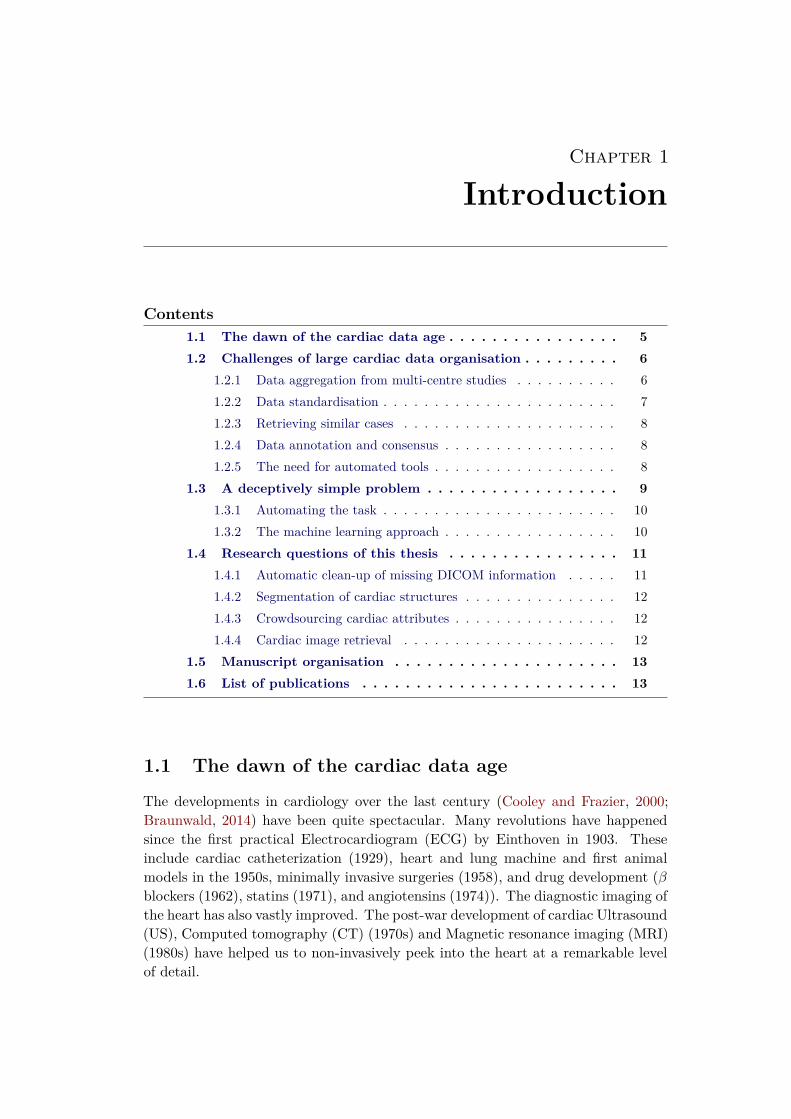
The image collections on PACS servers can be queried by patient information (e.g.
ID, name, birth date, sex, height, weight), image modality, study date and otherDICOM tags, sometimes by study description, custom tags of the clinicians, associ-ated measurements (e.g. arterial blood pressure and cardiac heart rate) and diseaseor procedure codes. See Fig. 1.1 for an example of such interface.
Figure 1.1: Cardiac atlas project web client interface.
There is no standard way to store some of the important image related infor-mation (e.g. the cardiac acquisition image plane information), where the namingdepends on custom set-up of the viewing workstation and on the language prac-ticed at the imaging centre. Even the standard DICOM tags often contain vendorspecific nomenclature. For example, the same Cardiac magnetic resonance imaging(CMR) acquisition sequences are branded differently across the Magnetic resonance(MR) machine vendors (Siemens, 2010). While some implementation differences ex-ist, these are not relevant for image interpretation, and the terminology could besignificantly simplified (Friedrich et al., 2014). Parsing electronic publications withimages is even a bigger challenge. These images are rarely in DICOM format andonly the image content with textual description is available.
Such differences reduce our ability to effectively query and explore the databasesfor relevant images. The standardisation can be enforced by strictly following guide-lines during image acquisition, and consistently using terminologies to encode theassociated information such as the Systematized Nomenclature of Medicine - Clini-cal Terms (SNOMED CT) (Stearns et al., 2001). Care has to be taken to eliminatemanual input errors. Images previously stored in the databases without the stan-dardised information should be revisited for better accessibility.

8 Chapter 1. Introduction
1.2.3 Retrieving similar cases
Manually crawling through these growing databases to find similar previously treatedpatients (with supporting evidence) becomes very time consuming. Deliveringarchived images from PACS is, in practice, quite slow for such exploratory use.In addition, the cardiac imaging data stored in the databases are frequently 3D+tsequences, and important details can be easily missed during such visual inspection.
An alternative to this brute-force approach is to consistently describe the imageswith more compact representations. This prepares the cardiac image databases forfuture image retrieval. Though, it limits the search to the annotated data or to thecases known to the particular clinician. Most of the unannotated data thereforenever gets used again and unused data means useless data.
1.2.4 Data annotation and consensus
Annotating these images simplifies their later reuse. However, together with thegrowth of the data, the demand for manual input becomes an increasing burdenon the expert raters. One way to tackle this is to reduce the annotation task intovery simpler questions that can be answered by a larger number of less experiencedraters, for example via crowdsourcing.
As studied by Suinesiaputra et al. (2015), the variability of different radiologists(experts following the same guidelines) is not negligible. For example, in left ven-tricle (LV) segmentation, the papillary muscles (PMs) are myocardial tissue andtherefore according to Schulz-Menger et al. (2013) should ideally be included inthe myocardial mass and excluded from the left ventricular cavity (LVC) volumecalculation. The corresponding reference values for volumes and masses (Maceiraet al., 2006; Hudsmith†et al., 2005) should be used in this case. Some tools includethe papillary muscles into the cavity volume instead. In this case a different setof reference values should be considered (Natori et al., 2006). The two reportedmeasures can differ substantially. Ultimately, the PMs are part of the disease pro-cess (Harrigan et al., 2008) and deserve individual attention on their own.
The acquisition centres are equipped with different software tools and not allof these tools are equally capable. We still have a long way ahead to achievereproducible extraction of image-based measures and consistent description of allrelevant image information, especially given the constantly evolving guidelines.
1.2.5 The need for automated tools
For success in large scale analysis and use of the data, efficient ways of automaticclean-up and description of the cardiac data coming from several clinical centreswith tools scalable to large data (Medrano-Gracia et al., 2015) are primordial. Aswe will see on the following example, manual design of such tools can rapidly becomequite challenging.
1.3. A deceptively simple problem 9
1.3 A deceptively simple problem
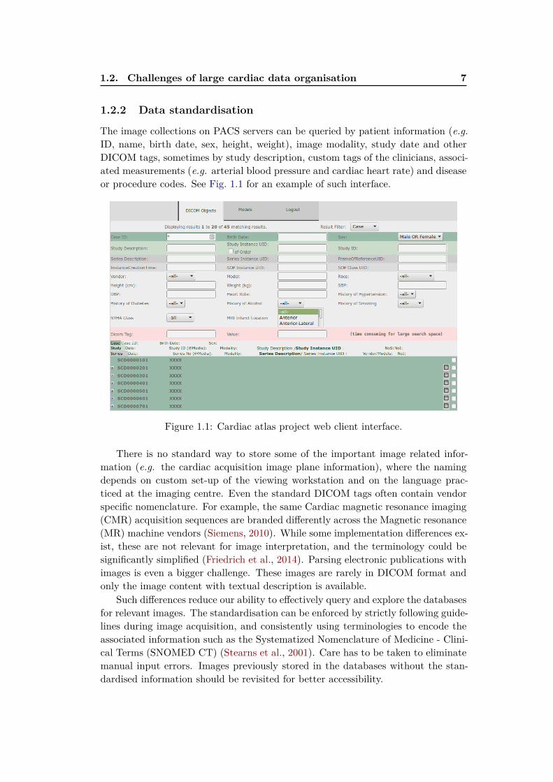
Examine the following four CMR mid-ventricular short axis (SAX) slices obtainedusing the Steady state free precession (SSFP) acquisition sequence shown in Fig. 1.2.They belong to four individuals with different pathologies. One of them is an imageof a healthy heart, another belongs to a patient after a myocardial infarction in thelateral wall, the third to a patient with a severely failing and non-compacting leftventricle and the last one shows a patient with idiopathic pericardial effusion. Canyou correctly tell which one is which?
Figure 1.2: Four cardiac pathologies on MRI: heart with pericardial effusion, postlateral wall myocardial infarction heart, left ventricular non-compaction and ahealthy heart. Can you identify them?1
This task of pathology identification is seemingly effortless for a person expe-rienced in interpretation of cardiac images. Intuitively, we could recognise thepost-myocardial infarction heart by a marked thinning of the lateral wall due toa transmural infarction and subsequent myocardial necrosis. One might also notesternal wire artefacts from a prior surgery. The failing non-compacting heart man-

10 Chapter 1. Introduction
ifests itself with massive dilation, prominent trabeculations in the left ventricularcavity, and significant reduction in myocardial contractility (best seen on cinematicimage sequences). The pericardial effusion can be seen as a bright ring of liquidoutside of the myocardium and swinging heart motion. And finally, the healthyheart looks “normal.”
1.3.1 Automating the task
Only when we try to write a program to mimic this reasoning on a computer wecan start to fully appreciate the true complexity of the visual tasks performed bythe brain. The simplicity of relevant information extraction from the images is verydeceptive. Intuitive concepts like the myocardial thinning, the cavity dilation, lowcontractility, bright ring, or swinging motion are concepts unknown to a machine.Not to mention the more global problem to automatically tell that all these imagesare short axis slices coming from a SSFP MR acquisition sequence.
One of the possibilities to extract this information by a computer is to startwriting a set of rules. Myocardial thinning measurement can be measured as thelength of the shortest line across the myocardium, counting pixels between two edgesseparating the white blob (the blood pool) and the grey (except for the effusion case)outer surroundings of the heart. Dilation is linked to the number of voxels withinthe ventricular blood pool and the cavity diameter. Both of these measures can becomputed from segmentation of the left ventricular myocardium. The contractilitycan be estimated from displacement of the pixels, e.g., via image registration. Thesubtle changes we might want to recognise are easily overshadowed by acquisitiondifferences, e.g., images coming from different MR acquisition machines, acquisitionartefacts or differences in image orientation and heart position in the images. Theimages have no longer similar resolutions and image quality, tissue intensities onCMR between different machines do not match, acquisition artefacts are presentor vendor specific variations of similar acquisition protocols are used. We soondiscover that the set of rules to encode the relevant information and extract featuresto describe the cardiac images is endless.
1.3.2 The machine learning approach
The machine learning approach is quite different. Instead of manually hardcodingthe rules, we specify a learning model and let the learning algorithm automaticallyfigure out a set of rules by looking at the data, i.e., to train the model. In thesupervised learning setting, a set of examples together with desired outputs (e.g.
images and their voxel-wise segmentations) is shown the training algorithm. Thealgorithm then picks rules that best map the inputs to the desired outputs. It isimportant that the learnt model generalises, i.e., can reliably predict outputs forpreviously unseen images while ignoring irrelevant acquisition differences.
1Top left: Lateral infarction with thinning, top right: healthy, bottom left: left ventricular
non-compaction, bottom right: pericardial effusion

1.4. Research questions of this thesis 11
Although good prediction is desirable, it is common to use “less than perfect”machine learning systems in a loop, and improve the models over time, when moredata arrives. Also when guidelines change, these algorithms can be retrained andthe images can be reparsed. Incorrect predictions can be fixed and added to thenew training set and the model can then be retrained.
Machine learning in medical imaging has become remarkably important. Thisis partly due to the algorithmic improvements but mainly thanks to the increasedavailability of large quantities of data. While there are many machine learningalgorithms, there is not (yet) a perfect one dealing with all the tasks at hand. Onethat is working for both large and small datasets.
Throughout this thesis we will use mainly three families of supervised machinelearning (ML) algorithms: Linear regression models (the Support vector machines(SVMs) (Cortes and Vapnik, 1995) and ridge regression (Golub et al., 1979)), theDecision forests (DFs) (Ho, 1995; Amit and Geman, 1997; Breiman, 1999), and theConvolutional neural network (CNN) (Fukushima, 1980; LeCun et al., 1989).
1.4 Research questions of this thesis
This thesis aims to answer the following global question: “How can we simplify
the use of CMR image databases for cardiologists and researchers using
machine learning?” To help us answer this question, we addressed some of themain challenges introduced in Section 1.2.
1.4.1 How can we clean up and standardise DICOM tags for easier
filtering and grouping of image series?
One of the first problems we face in cardiac imaging when dealing with large multi-vendor databases is the lack of standardisation in used notation in acquisition pro-tocols (Friedrich et al., 2014) or naming of cardiac acquisition planes. Especiallythe knowledge of cardiac planes is essential for grouping the images into series andchoosing the right image processing pipeline.
Chapter 2 presents our two methods for fixing noisy DICOM metadata withinformation estimated directly from image content. Our first method to recogniseCMR acquisition planes uses classification forests applied on image miniatures. Weshow how cheaply generated new images can help to improve the recognition.
We then show how we modify a state of the art technique in a large scale visualobject recognition, based on CNNs, to a much smaller cardiac imaging dataset. Oursecond method recognises short axis and 2-, 3- and 4-chamber long axis views withvery promising recognition performance.
In Appendix B we show how the CNN-based features can be reused to regresscardiac point distribution models for inter-patient image alignment.

12 Chapter 1. Introduction
1.4.2 Can we teach the computer to understand cardiac anatomy
and to segment cardiac structures from MR images?
Once we can describe cardiac images based on their views and merge them intospatio-temporal 3D+t series we can move on to teach the computer the basics ofcardiac anatomy, i.e., how to segment the cardiac images. Successful segmentationis essential to index cardiac images based on standard volumetric measures such assystolic and diastolic volume, ejection fraction, and myocardial mass.
In Chapter 3 we extend the previous work on semantic segmentation usingclassification forests (Shotton et al., 2008; Geremia et al., 2011). We show how ourmodified algorithm learns to segment left ventricles from 3D+t MR short axis SSFPsequences without imposing any shape prior. Our decision forest classifier is trainedin a layered fashion, and we propose new spatio-temporal features to classify the3D+t sequences. We show that avoiding to hard-code the segmentation problemhelps us to easily adapt this technique to segment other cardiac structures, the leftatria — the black box of the heart, both from CMR and CT. We contributed thesealgorithms to two comparison studies for fair evaluation.
In Appendix A we propose a segmentation method exploiting unlabelled datain a semi-supervised setting to learn how to segment from sparse annotations.
1.4.3 How can we collect data needed by the computer for training
of the machine learning algorithms and learn how to describe
the hearts with semantically meaningful attributes?
Most of the practical machine learning problems are currently still solved in a fullysupervised manner. It is therefore essential to acquire the ground-truth. Chapter 4
deals with label collection for machine learning algorithms. We design a web-basedtool for crowd-sourcing of cardiac attributes and use it to collect pairwise imageannotations. We describe the cardiac shapes with their spectral signatures and usea linear predictor based on SVM classifier to learn ordering of the images based ontheir attribute values. Our preliminary results suggest that in addition to volumetricmeasurements obtainable from cardiac segmentations, the hearts could be describedby cardiac attributes.
1.4.4 Can we automatically retrieve similar hearts?
The image similarity depends on the clinical question to be answered. Queries wemight want to ask the retrieval system can be quite variable. Chapter 5 buildson the Neighbourhood approximating forest (NAF) of Konukoglu et al. (2013) andpresents our pipeline to learn shape, appearance and motion similarities between car-diac images and how we use them to structure the spatio-temporal cardiac datasets.We show how hearts with similar properties (similar ejection fraction) can be ex-tracted from the database. In (Bleton et al., 2015), we then used a similar techniqueto localise cardiac infarcts from dynamic shapes only (no contrast agent needed).

1.5. Manuscript organisation 13
1.5 Manuscript organisation
The presented thesis is organised around our published work and our work in prepa-ration for submission. The manuscript also roughly progresses from global towardsfine-grained description of the cardiac images. Each chapter in this thesis attemptsto answer one of the objectives and to bring content-based retrieval of images fromlarge-scale CMR databases closer to reality.
First, we train a system to fix image tags that are not captured by DICOMdirectly from image content. In Chapter 2, we show how to automatically recognisecardiac planes of acquisition. In Chapter 3, we propose a flexible automatic seg-mentation technique that learns to segment cardiac structures from spatio-temporalimage data, using simple voxel-wise ground-truth as input, that could be used forautomatic measurements. In Chapter 4, we suggest a way of collecting annotationsnecessary for training of automatic algorithms, and to describe the cardiac imageswith sets of semantic attributes. Finally, in Chapter 5, we propose an algorithm tostructure the datasets and find similar cases with respect to different clinical criteria.Chapter 6 concludes the thesis with perspectives and future work. In the appendices,we illustrate how unlabelled data can be used for guided image segmentation (Ap-pendix A), how to estimate cardiac landmarks for image alignment (Appendix B),or how to enhance pericardial effusion for image retrieval (Appendix C).
1.6 List of publications
Journal articles
• J. Margeta, A. Criminisi, R. Cabrera Lozoya, D. C. Lee, and N. Ayache,“Fine-tuned convolutional neural nets for cardiac MRI acquisition plane recog-
nition”, Computer methods in biomechanics and biomedical engineering: Imag-ing & visualisation, 2015.
• C. Tobon-Gomez, A. Geers, J. Peters, J. Weese, K. Pinto, R. Karim, M.Ammar, A. Daoudi, J. Margeta, Z. Sandoval, B. Stender, Y. Zheng, M. A.Zuluaga, J. Betancur, N. Ayache, M. A. Chikh, J.-L. Dillenseger, M. Kelm, S.Mahmoudi, S. Ourselin, A. Schlaefer, T. Schaeffter, R. Razavi, and K. Rhode,“Benchmark for Algorithms Segmenting the Left Atrium From 3D CT and
MRI Datasets”, IEEE Transactions on Medical Imaging, vol. 34, no. 7, pages1460 1473, 2015.
• A. Suinesiaputra, B. R. Cowan, A. O. Al-Agamy, M. A. Elattar, N. Ayache, A.S. Fahmy, A. M. Khalifa, P. Medrano-Gracia, M. P. Jolly, A. H. Kadish, D. C.Lee, J. Margeta, S. K. Warfield, and A. A. Young, “A collaborative resource
to build consensus for automated left ventricular segmentation of cardiac MR
images”, Medical Image Analysis, vol. 18, no. 1, pages 50 62, 2014.
14 Chapter 1. Introduction
Peer reviewed conference and workshop papers
• J. Margeta, A. Criminisi, D. C. Lee, and N. Ayache, “Recognizing cardiac
magnetic resonance acquisition planes”, in Conference on Medical Image Un-derstanding and Analysis (MIUA 2014), 2014. Oral podium presentation.
• J. Margeta, K. S. McLeod, A. Criminisi, and N. Ayache, “Decision forests
for segmentation of the left atrium from 3D MRI”, in International Work-shop on Statistical Atlases and Computational Models of the Heart. Imagingand Modelling Challenges, Held in conjunction with MICCAI 2013, Beijing,Lecture Notes in Computer Science, vol. 8830, pages 49 56, O. Camara, T.Mansi, M. Pop, K. Rhode, M. Sermesant, and A. Young, Eds., Springer Berlin/ Heidelberg, 2014. Oral podium presentation.
• J. Margeta, E. Geremia, A. Criminisi, and N. Ayache, “Layered Spatio-
temporal Forests for Left Ventricle Segmentation from 4D Cardiac MRI Data”,in International Workshop on Statistical Atlases and Computational Modelsof the Heart. Imaging and Modelling Challenges, Held in conjunction withMICCAI 2011, Toronto, Lecture Notes in Computer Science, vol. 7085, pages109 119, O. Camara, E. Konukoglu, M. Pop, K. Rhode, M. Sermesant, and A.Young, Eds., Springer Berlin / Heidelberg, 2012, Oral podium presentation.
• H. Bleton, J. Margeta, H. Lombaert, H. Delingette, and N. Ayache, “My-
ocardial Infarct Localisation using Neighbourhood Approximation Forests”, inInternational Workshop on Statistical Atlases and Computational Models ofthe Heart. Imaging and Modelling Challenges, Held in conjunction with MIC-CAI 2015, Munich, O. Camara, T. Mansi, M. Pop, K. Rhode, M. Sermesant,and A. Young, Eds., 2015. Oral podium presentation.
• R. C. Lozoya, J. Margeta, L. Le Folgoc, Y. Komatsu, B. Berte, J. Relan, H.Cochet, M. Haïssaguerre, P. Jaïs, N. Ayache, and M. Sermesant, “Confidence-
based Training for Clinical Data Uncertainty in Image-based Prediction of
Cardiac Ablation Targets”, in International Workshop on Medical ComputerVision: Algorithms for Big Data, Held in conjunction with MICCAI 2014,Boston, Lecture Notes in Computer Science, vol. 8848, pages 148 159, B.Menze, G. Langs, A. Montillo, M. Kelm, H. Müller, S. Zhang, W. Cai, and D.Metaxas, Eds., Springer Berlin / Heidelberg, 2014. Oral podium presentation.
• R. C. Lozoya, J. Margeta, L. Le Folgoc, Y. Komatsu, B. Berte, J. S. Relan,H. Cochet, M. Haïssaguerre, P. Jaïs, N. Ayache, and M. Sermesant, “Local late
gadolinium enhancement features to identify the electrophysiological substrate
of post-infarction ventricular tachycardia: a machine learning approach”, inJournal of Cardiovascular Magnetic Resonance, vol. 17, no. Suppl 1, poster234, 2015. Poster presentation.

1.6. List of publications 15
In preparation
• J. Margeta, H. Lombaert, D. C. Lee, A. Criminisi, and N. Ayache, “Learning
to retrieve semantically similar hearts.”
• J. Margeta, E. Konukoglu, D. C. Lee, A. Criminisi, and N. Ayache, “Crowd-
sourcing cardiac attributes”,

Chapter 2
Learning how to recognise
cardiac acquisition planes
Contents
2.1 Brief introduction to cardiac data munging . . . . . . . . . . 18
2.2 Cardiac acquisition planes . . . . . . . . . . . . . . . . . . . . 19
2.2.1 The need for automatic plane recognition . . . . . . . . . . . 19
2.2.2 Short axis acquisition planes . . . . . . . . . . . . . . . . . . 20
2.2.3 Left ventricular long axis acquisition planes . . . . . . . . . . 20
2.3 Methods . . . . . . . . . . . . . . . . . . . . . . . . . . . . . . . 22
2.3.1 Previous work . . . . . . . . . . . . . . . . . . . . . . . . . . . 22
2.3.2 Overview of our methods . . . . . . . . . . . . . . . . . . . . 22
2.4 Using DICOM orientation tag . . . . . . . . . . . . . . . . . . 23
2.4.1 From DICOM metadata towards image content . . . . . . . . 24
2.5 View recognition from image miniatures . . . . . . . . . . . 24
2.5.1 Decision forest classifier . . . . . . . . . . . . . . . . . . . . . 24
2.5.2 Alignment of radiological images . . . . . . . . . . . . . . . . 26
2.5.3 Pooled image miniatures as features . . . . . . . . . . . . . . 26
2.5.4 Augmenting the dataset with geometric jittering . . . . . . . 28
2.5.5 Forest parameter selection . . . . . . . . . . . . . . . . . . . . 28
2.6 Convolutional neural networks for view recognition . . . . . 29
2.6.1 Layers of the Convolutional Neural networks . . . . . . . . . 30
2.6.2 Training CNNs with Stochastic gradient descent . . . . . . . 32
2.6.3 Network architecture . . . . . . . . . . . . . . . . . . . . . . . 33
2.6.4 Reusing CNN features tuned for visual recognition . . . . . . 34
2.6.5 CardioViewNet architecture and parameter fine-tuning . . . . 35
2.6.6 Training the network from scratch . . . . . . . . . . . . . . . 36
2.7 Validation . . . . . . . . . . . . . . . . . . . . . . . . . . . . . . 37
2.8 Results and discussion . . . . . . . . . . . . . . . . . . . . . . 38
2.9 Conclusion and perspectives . . . . . . . . . . . . . . . . . . . 42
Based on our published work (Margeta et al., 2014) on the use of decision forestsfor cardiac view recognition and the convolutional neural network approach (Mar-geta et al., 2015c) to further improve the performance.
18 Chapter 2. Learning how to recognise cardiac acquisition planes
Chapter overview
When dealing with large multi-centre and multi-vendor databases, inconsistent no-tations are a limiting factor for automated analysis. Cardiac MR acquisition planesare a particularly good example of a notation standardisation failure. Withoutknowing which cardiac plane we deal with, further use of the data without manualintervention is limited. In this chapter, we propose two supervised machine learn-ing techniques to automatically retrieve missing or noisy cardiac acquisition planeinformation from Magnetic resonance imaging (MRI) and to predict the five mostcommon cardiac views (or acquisition planes). We show that cardiac acquisitionsare roughly aligned with the heart in the image center and use this to learn cardiacacquisition plane predictors from 2D images.
In our first method we train a classification forest on image miniatures. Datasetaugmentation with a set of label preserving transformations is a cheap way thathelps us to improve classification accuracy without neither acquiring nor anno-tating extra data. We further improve the forest-based cardiac view recogniser’sperformance by fine-tuning a deep Convolutional neural network (CNN) originallytrained on a large image recognition dataset (ImageNet LSVRC 2012) and transferthe learnt feature representations to cardiac view recognition.
We compare these approaches with predictions using off the shelf CNN imagefeatures, and with CNNs learnt from scratch. We show that fine-tuning is a viableapproach to adapt parameters of large convolutional networks for smaller problems.We validate this algorithm on two different cardiac studies with 200 patients and15 healthy volunteers respectively. The latter comes from an open access cardiacdataset which simplifies direct comparison of similar techniques in the future. Weshow that there is value in fine-tuning a model trained for natural images to transferit to medical images. The presented approaches are quite generic and can be appliedto any image recognition task. Our best approach achieves an average F1 scoreof 97.66% and significantly improves the state of the art in image-based cardiacview recognition. It avoids any extra annotations and automatically learns theappropriate feature representation.
This is an important building block to organise and filter large collections ofcardiac data prior to further analysis. It allows us to merge studies from multiplecenters, to enable smarter image filtering, to select the most appropriate imageprocessing algorithm, to enhance visualisation of cardiac datasets in content-basedimage retrieval, and to perform quality control.
2.1 Brief introduction to cardiac data munging
The rise of large cardiac imaging studies has opened us the door to better under-standing and management of cardiac diseases. When handling data from varioussources, inconsistent, missing, or non-standard information is unavoidable. TheDigital Imaging and Communications in Medicine (DICOM) standard has solvedmany common problems in handling, archival, and exchange of information in med-

2.2. Cardiac acquisition planes 19
ical imaging by adding metadata to images and defining communication protocols.Nevertheless, a lot of the metadata crucial for filtering cases for studies is not stan-dardised and still remains site and vendor specific.
Prior to any analysis, the data must be cleaned up and put into the sameformat. This process is often called data munging or data wrangling. Cardiac MRIacquisition plane information is a particularly important piece of information to bewrangled.
2.2 Cardiac acquisition planes
Instead of commonly used body planes (coronal, axial and sagittal) the CMR imagesare acquired along several oblique directions aligned with the structures of theheart. Imaging in these standard cardiac planes ensures efficient coverage of relevantcardiac territories (while minimising the acquisition time) and enables comparisonsacross modalities, thus enhancing patient care and cardiovascular research. Theoptimal cardiac planes depend on global positioning of the heart in the thorax.This is more vertical in young individuals and more diaphragmatic in elderly andobese.
An excellent introduction to the standard CMR acquisition planes can be foundin Taylor and Bogaert (2012). These planes are often categorized into two groups— the short and the long axis planes (see Figures 2.1 and 2.2 for a visual overview).In this chapter, we learn to predict the five most commonly used cardiac planesacquired with Steady state free precession (SSFP) acquisition sequences to evaluatethe left heart. These are the short axis, 2-, 3- and 4- chamber and left ventricular
outflow tract views. These five labels are the targets for our learning algorithm.
2.2.1 The need for automatic plane recognition
Why is it important to have an automatic way of recognising this information?Automatic recognition of this metadata is essential to appropriately select imageprocessing algorithms, to group related slices into volumetric image stacks, to en-able filtering of cases for a clinical study based on presence of particular views, tohelp with interpretation and visualisation by showing the most relevant acquisitionplanes, and in content-based image retrieval for automatic description generation.Although this orientation information is sometimes encoded within two DICOMimage tags: Series Description (0008,103E) and Protocol Name (0018,1030), it isnot standardised, operator errors are frequently present, or this information is com-pletely missing. In general, the DICOM tags are often too noisy for accurate imagecategorization (Gueld et al., 2002). Searching through large databases to manu-ally cherrypick relevant views from the image collections is therefore very tedious.The main challenge for an image-content-based automated cardiac plane recogni-tion method is the variability of the thoracic cavity appearance. Different parts oforgans can be visible even in the same acquisition planes between different patients.
20 Chapter 2. Learning how to recognise cardiac acquisition planes
2.2.2 Short axis acquisition planes
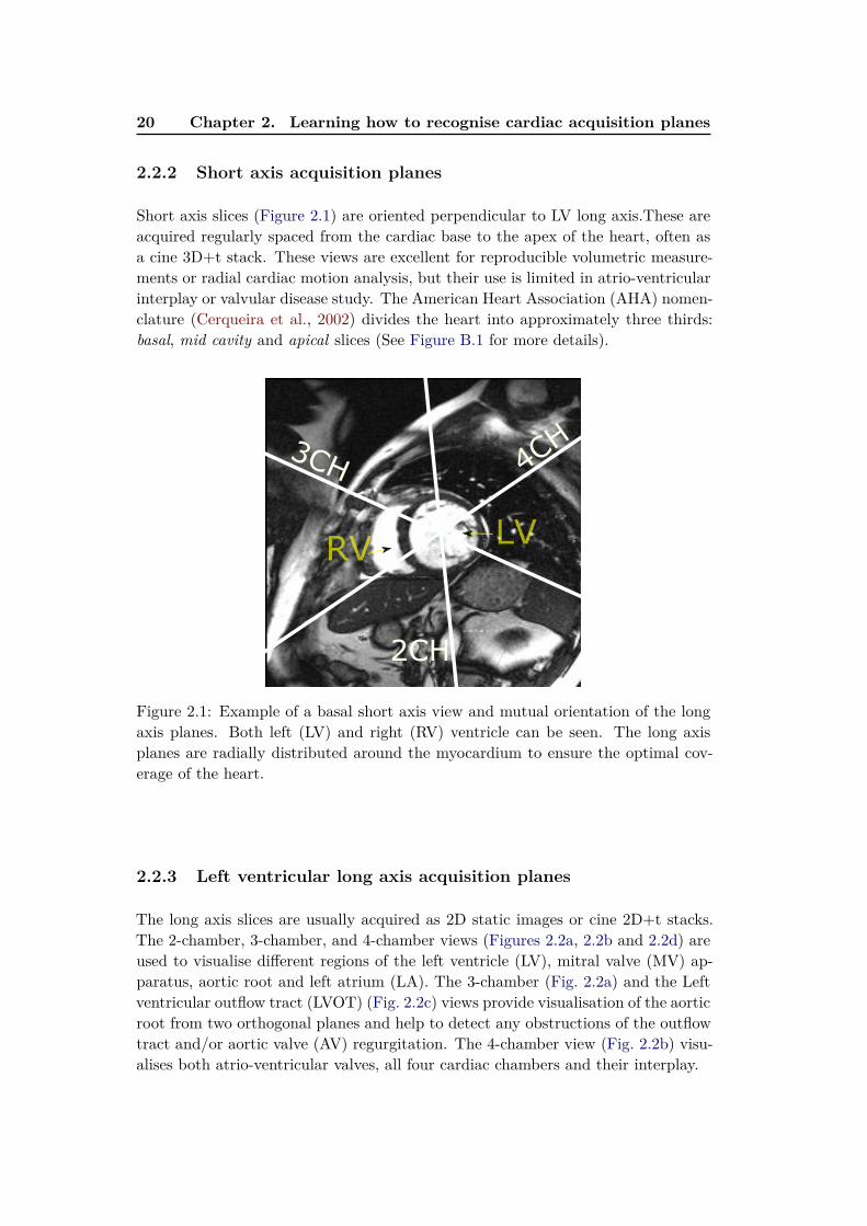
Short axis slices (Figure 2.1) are oriented perpendicular to LV long axis.These areacquired regularly spaced from the cardiac base to the apex of the heart, often asa cine 3D+t stack. These views are excellent for reproducible volumetric measure-ments or radial cardiac motion analysis, but their use is limited in atrio-ventricularinterplay or valvular disease study. The American Heart Association (AHA) nomen-clature (Cerqueira et al., 2002) divides the heart into approximately three thirds:basal, mid cavity and apical slices (See Figure B.1 for more details).
2CH
3CH 4CH
RVLV
Figure 2.1: Example of a basal short axis view and mutual orientation of the longaxis planes. Both left (LV) and right (RV) ventricle can be seen. The long axisplanes are radially distributed around the myocardium to ensure the optimal cov-erage of the heart.
2.2.3 Left ventricular long axis acquisition planes
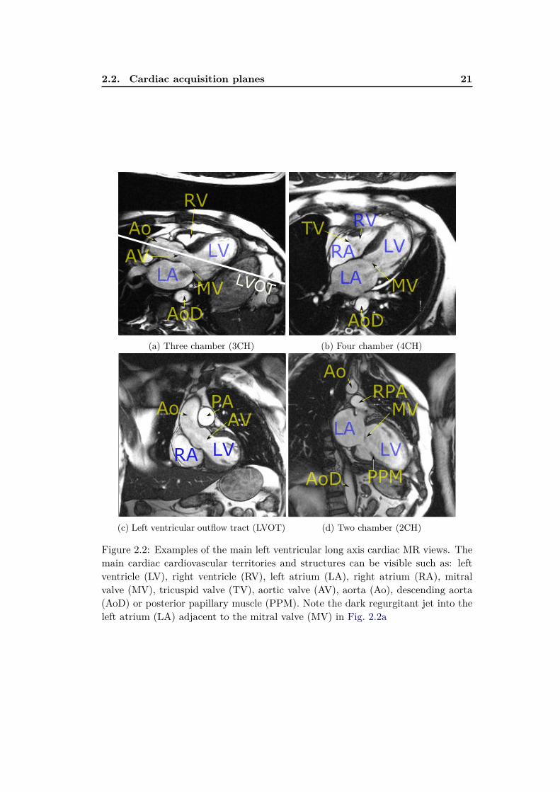
The long axis slices are usually acquired as 2D static images or cine 2D+t stacks.The 2-chamber, 3-chamber, and 4-chamber views (Figures 2.2a, 2.2b and 2.2d) areused to visualise different regions of the left ventricle (LV), mitral valve (MV) ap-paratus, aortic root and left atrium (LA). The 3-chamber (Fig. 2.2a) and the Leftventricular outflow tract (LVOT) (Fig. 2.2c) views provide visualisation of the aorticroot from two orthogonal planes and help to detect any obstructions of the outflowtract and/or aortic valve (AV) regurgitation. The 4-chamber view (Fig. 2.2b) visu-alises both atrio-ventricular valves, all four cardiac chambers and their interplay.
2.2. Cardiac acquisition planes 21
LVOT
Ao
LV
AoD
MVLA
RV
AV
(a) Three chamber (3CH)
TV
LV
AoD
MVLA
RV
RA
(b) Four chamber (4CH)
Ao
LV
AV
RA
PA
(c) Left ventricular outflow tract (LVOT)
AoD
LV
MV
LA
RPA
Ao
PPM
(d) Two chamber (2CH)
Figure 2.2: Examples of the main left ventricular long axis cardiac MR views. Themain cardiac cardiovascular territories and structures can be visible such as: leftventricle (LV), right ventricle (RV), left atrium (LA), right atrium (RA), mitralvalve (MV), tricuspid valve (TV), aortic valve (AV), aorta (Ao), descending aorta(AoD) or posterior papillary muscle (PPM). Note the dark regurgitant jet into theleft atrium (LA) adjacent to the mitral valve (MV) in Fig. 2.2a
22 Chapter 2. Learning how to recognise cardiac acquisition planes
2.3 Methods
2.3.1 Previous work
The previous work on cardiac view recognition has been concentrated mainly on real-time recognition of cardiac planes for echography (Otey et al., 2006; Park et al., 2007;Beymer et al., 2008). In addition to our work, there exists some work on MR (Zhouet al., 2012; Shaker et al., 2014). The common methods are based on dynamic activeshape models (Beymer et al., 2008), require to train part detectors (Park et al., 2007)or landmark detectors (Zhou et al., 2012). Therefore, any new view will require theseextra annotations to be made. Otey et al. (2006) avoid this limitation by trainingan ultrasound cardiac view classifier using gradient based image features. The mostrecently proposed work on cardiac view recognition from MR (Shaker et al., 2014)uses autoencoders. These learn image representations in an unsupervised fashion(the goal is to reconstruct images from a lower dimensional representation) and usethis representation to distinguish between two cardiac views.
The state of the art in image recognition has been heavily influenced by theseminal works of Krizhevsky et al. (2012) and Cireşan et al. (2012) using Convolu-tional neural network (CNN). Krizhevsky et al. (2012) trained a large (60 millionparameters) CNN on a massive dataset consisting of 1.2 million images and 1000classes (Russakovsky et al., 2014). They employed two major improvements: Rec-
tified linear unit nonlinearity to improve convergence, and Dropout (Hinton et al.,2012) to reduce overfitting.
Training a large network from scratch without a large number of samples stillremains a challenging problem. A trained CNN can be adapted to a new domainby reusing already trained hidden layers of the network, though. It has been shown,e.g., by Sharif et al. (2014) that the classification layer of the neural net can bestripped, and the hidden layers can serve as excellent image descriptors for a varietyof computer vision tasks (such as for photography style recognition by Karayev et al.(2014)). Alternatively, the prediction layer model can be replaced by a new one andthe network parameters can be fine-tuned through backpropagation.
2.3.2 Overview of our methods
A ground truth target label (2CH, 3CH, 4CH, LVOT or SAX) was assigned to eachimage in our training set by an expert in cardiac imaging. We use these labelsin the training phase as a target to train. In the testing phase, we predict thecardiac views from the images and use the ground-truth only to evaluate our viewrecognition methods.
In this chapter, we compare the three groups of methods for automatic cardiacacquisition plane recognition. The first one is based on DICOM-derived orientationinformation. The algorithms in the other two families completely ignore the DICOMtags and learn to recognise cardiac views directly from image intensities.
In Section 2.4, we first present the recognition method using DICOM-derivedfeatures (the image plane orientation vectors, similar to Zhou et al. (2012)). Here,

2.4. Using DICOM orientation tag 23
we train a decision forest classifier using these 3-dimensional feature vectors.The latter two approaches learn to recognise cardiac views from image content
without using any DICOM meta-information. In Section 2.5, we present our classi-fication forest-based method (Margeta et al., 2014) using pixels from image minia-tures as features. We then introduce the third path for cardiac view recognition,using CNNs, as described in Section 2.6. In this section, we consider all commonlyused approaches (training a network from scratch, reusing a hidden layer featuresfrom a network trained on another problem, and fine-tuning of a pretrained network)for using a CNN in cardiac view recognition.
To increase the number of the training samples (for image content-based algo-rithms) we augment the dataset with small label preserving transformations such asimage translations, rotations, and scale changes. See Section 2.5.4 for more details.
In Section 2.7, we compare all of these approaches. We show how the CNN-based approaches outperform the previously introduced forest-based method andachieve very good perfomance. Finally, in Section 2.8, we present and discuss ourresults.
2.4 Using DICOM orientationtag
Plane normal + Forest
Zhou et al. (2012) showed that where the DICOM orientation (0020,0037) tag ispresent we can use it to predict the cardiac image acquisition plane (see Figure 2.3).This tag is not defined as a cardiac view but as two 3-dimensional vectors definingorientation of the imaging plane with respect to the MR scanner coordinate frame.
Figure 2.3: Tips of DICOM plane normals for different cardiac views. In our dataset,distinct clusters can be observed (best viewed in colour). Nevertheless, the separa-tion might not be the case for a more diverse collection of images. Moreover, as wecannot always rely on the presence of this tag an image-content-based recogniser isnecessary.
24 Chapter 2. Learning how to recognise cardiac acquisition planes
It is straightforward to compute the 3-dimensional normal vectors of this planeas a cross-product of these two vectors specified in the tag. We then feed thesethree-dimensional feature vectors into any classifier, in our case a classificationforest (see Section 2.5.1 for more details on classification forests). This method isshown in the results section as Plane normal + forest.
2.4.1 From DICOM metadata towards image content
This method uses feature vectors computed from the DICOM orientation tag andcannot be used in the absence of this tag. This happens for example in DICOMtag removal after an incorrectly configured anonymisation procedure, when parsingimages from clinical journals or when using image formats other than DICOM. Inthese cases we have to rely on recognition methods using exclusively the imagecontent.
In the next two sections, we present two such methods. One that is based onclassification forests and image miniatures (Margeta et al., 2014) and the otherone is using CNNs. We learn to predict the cardiac views from 2D image slicesindividually, rather than using 2D+ t, 3D or 3D+ t volumes. This decision makesour methods more flexible and applicable also to view recognition scenarios whenonly 2D images are present, e.g., when parsing clinical journals or images fromelectronic publications.
2.5 View recognition from image miniatures
Miniatures + forest
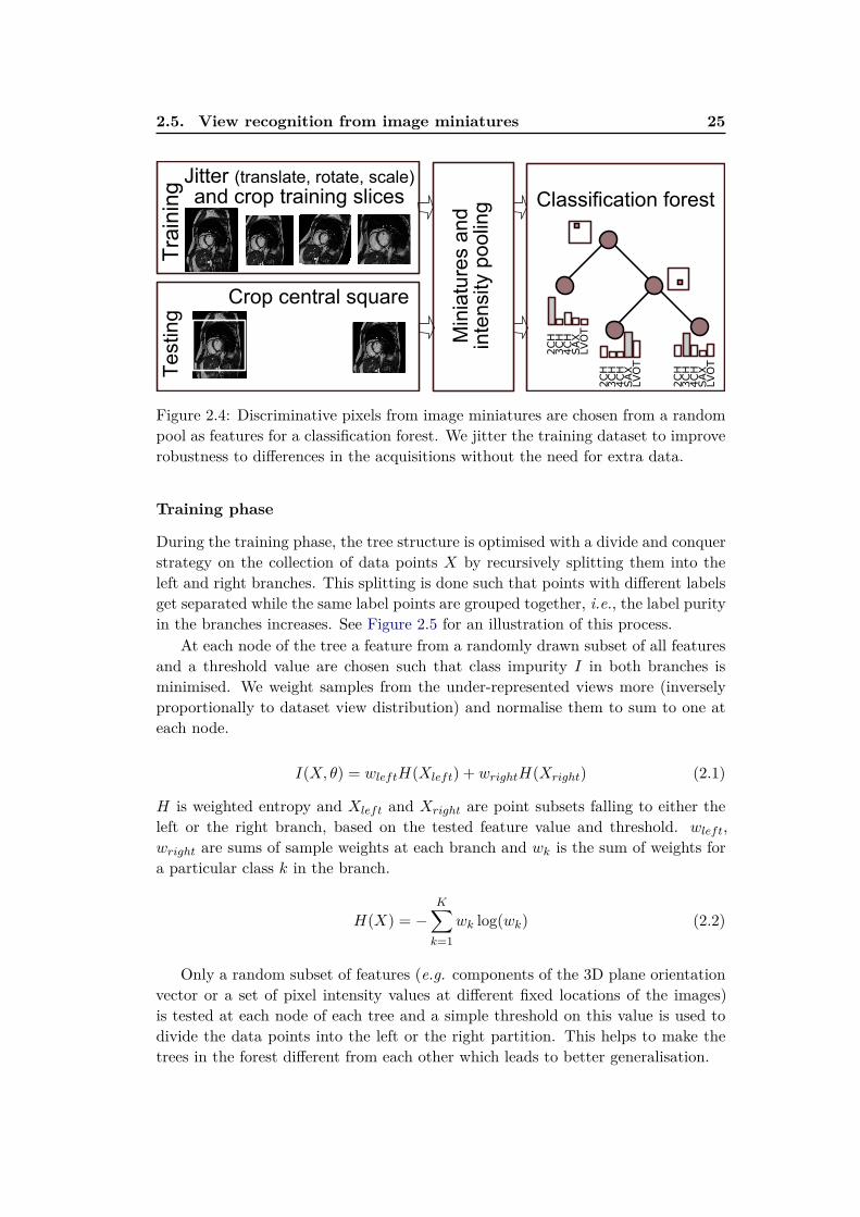
First, we propose an automatic cardiac view recognition pipeline (see Fig. 2.4) thatlearns to recognise the acquisition planes directly from CMR images by combiningimage miniatures with classification forests.
2.5.1 Decision forest classifier
Decision forest classifier or classification forest (Ho, 1995; Amit and Geman, 1997;Breiman, 1999) is an ensemble machine learning method that constructs a set ofbinary decision trees with split decisions optimised for classification. This methodis computationally efficient and allows automatic selection of relevant features forthe prediction.
The decision forest framework itself is also quite flexible (Criminisi et al., 2011b;Pauly, 2012) and has already been used to solve a number of problems in medicalimaging. For example, for image segmentation (Geremia et al., 2011), organ de-tection (Criminisi and Shotton, 2011; Pauly et al., 2011), manifold learning (Grayet al., 2011), or shape representation (Swee and Grbić, 2014).
2.5. View recognition from image miniatures 25
Crop central square
Classification forestJitter (translate, rotate, scale) and crop training slices
Min
iatu
res a
nd
inte
nsity p
oolin
g
Tra
inin
gT
esting
2CH
3CH
4CH
SAX
2CH
3CH
4CH
SAX
2CH
3CH
4CH
SAX
LVOT
LVOT
LVOT
Figure 2.4: Discriminative pixels from image miniatures are chosen from a randompool as features for a classification forest. We jitter the training dataset to improverobustness to differences in the acquisitions without the need for extra data.
Training phase
During the training phase, the tree structure is optimised with a divide and conquerstrategy on the collection of data points X by recursively splitting them into theleft and right branches. This splitting is done such that points with different labelsget separated while the same label points are grouped together, i.e., the label purityin the branches increases. See Figure 2.5 for an illustration of this process.
At each node of the tree a feature from a randomly drawn subset of all featuresand a threshold value are chosen such that class impurity I in both branches isminimised. We weight samples from the under-represented views more (inverselyproportionally to dataset view distribution) and normalise them to sum to one ateach node.
I(X, θ) = wleftH(Xleft) + wrightH(Xright) (2.1)
H is weighted entropy and Xleft and Xright are point subsets falling to either theleft or the right branch, based on the tested feature value and threshold. wleft,wright are sums of sample weights at each branch and wk is the sum of weights fora particular class k in the branch.
H(X) = −K∑
k=1
wk log(wk) (2.2)
Only a random subset of features (e.g. components of the 3D plane orientationvector or a set of pixel intensity values at different fixed locations of the images)is tested at each node of each tree and a simple threshold on this value is used todivide the data points into the left or the right partition. This helps to make thetrees in the forest different from each other which leads to better generalisation.

26 Chapter 2. Learning how to recognise cardiac acquisition planes
0
1
3 4 5 6
2
SAX
2CH
3CH
4CH
LVOT
SAX
2CH
3CH
4CH
LVOT
SAX
2CH
3CH
4CH
LVOT
SAX
2CH
3CH
4CH
LVOT
θ1
θ2 5
6
3
4
θ1>T0θ1>T0θ1>T0
θ2>T1 θ2>T2
T0
T1
T2
Figure 2.5: We illustrate a 2D feature space and a single tree from the classificationforest. At the training phase, the feature space (for example constructed by sam-pling image miniature intensities at random locations) is recursively partitioned(horizontal and vertical lines cut through the feature space) to recognise cardiacplanes of acquisition. Class distributions at the leaves are stored for the test time.At the test time, the tested images are passed through the decisions of each treeuntil they reach the final set of leaves (one per tree). Class with maximal averageprobability across the forest is chosen as the prediction.
When classifying a new image, features chosen at the training stage are extractedand the image is passed through the decisions of the forest (fixed in the trainingphase) to reach a set of leaves. Class distributions of the reached leaves are averagedacross the forest and the most probable label is selected as the image view. Forexcellent in-depth discussions on decision forests, in particular applied to medicalimaging, see (Criminisi et al., 2011b; Pauly, 2012).
2.5.2 Alignment of radiological images
The radiological images are mostly acquired with the object of interest in the imagecenter and some rough alignment of structures can be expected (see Figure 2.6).
Note the large bright cavity in the center (3CH, 4CH), dark lung pixels justabove the cavity (SAX), or black air pixels on the left and right side (2CH, SAX).Image intensity samples at fixed positions (even without registration) provide strongcues about the position of different tissues.
2.5.3 Pooled image miniatures as features
It has been shown by Torralba et al. (2008) that significantly down-sampled imageminiatures can be used for image recognition. In our case, we extract the centralsquare from each image, resample it to 128× 128 pixels (with linear interpolation),and linearly rescale to an intensity range between 0 and 255. We subsample the

2.5. View recognition from image miniatures 27
2CH 4CH3CH LVOT SAX
Figure 2.6: Example of each cardiac view used in this work (above) and correspond-ing central square region mean intensities across the whole dataset (below).
cropped centers to two fixed sizes (20 × 20 and 40 × 40 pixels). In addition, wedivide the image into non-overlapping 4×4 tiles and for each of these tiles computethe intensity minima and maxima (see Figure 2.7).
Image tiles miniatures
min and max pool
40x40 20x20
32x32 32x32128x128 (4x4 tiles)
Figure 2.7: Image miniatures features: downsampled images and tile intensity min-ima and maxima are used.
This creates a set of pooled image miniatures (32 × 32 pixels each). The pool-ing adds some invariance to small image translations and rotations (whose effectis within the tile size). The pixel values at random positions of these miniaturechannels are then used directly as features.
In total 64 random locations across all four miniatures channels are testedat each node of each tree when training the forest. The location and thresholdvalue combination that best (Eq. (2.1)) partition the data-points are then selectedand stored and the data points are correspondingly divided into the left and right
28 Chapter 2. Learning how to recognise cardiac acquisition planes
branches. We recursively continue dividing the dataset until not less than 2 pointsare left in each leaf or no gain is obtained by further splitting. We trained 160 treesin total using Scikit-learn (Pedregosa et al., 2011).
This method is shown in the evaluation as Miniatures + forest.
2.5.4 Augmenting the dataset with geometric jittering
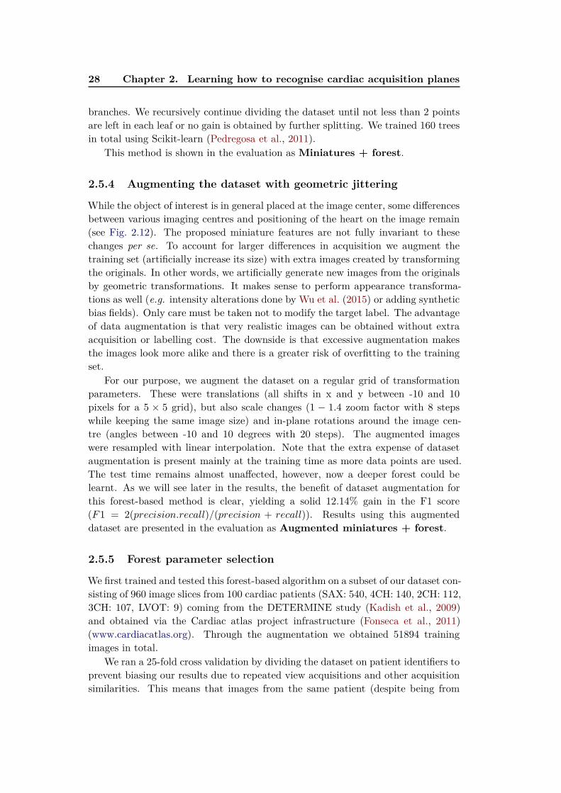
While the object of interest is in general placed at the image center, some differencesbetween various imaging centres and positioning of the heart on the image remain(see Fig. 2.12). The proposed miniature features are not fully invariant to thesechanges per se. To account for larger differences in acquisition we augment thetraining set (artificially increase its size) with extra images created by transformingthe originals. In other words, we artificially generate new images from the originalsby geometric transformations. It makes sense to perform appearance transforma-tions as well (e.g. intensity alterations done by Wu et al. (2015) or adding syntheticbias fields). Only care must be taken not to modify the target label. The advantageof data augmentation is that very realistic images can be obtained without extraacquisition or labelling cost. The downside is that excessive augmentation makesthe images look more alike and there is a greater risk of overfitting to the trainingset.
For our purpose, we augment the dataset on a regular grid of transformationparameters. These were translations (all shifts in x and y between -10 and 10pixels for a 5 × 5 grid), but also scale changes (1 − 1.4 zoom factor with 8 stepswhile keeping the same image size) and in-plane rotations around the image cen-tre (angles between -10 and 10 degrees with 20 steps). The augmented imageswere resampled with linear interpolation. Note that the extra expense of datasetaugmentation is present mainly at the training time as more data points are used.The test time remains almost unaffected, however, now a deeper forest could belearnt. As we will see later in the results, the benefit of dataset augmentation forthis forest-based method is clear, yielding a solid 12.14% gain in the F1 score(F1 = 2(precision.recall)/(precision + recall)). Results using this augmenteddataset are presented in the evaluation as Augmented miniatures + forest.
2.5.5 Forest parameter selection
We first trained and tested this forest-based algorithm on a subset of our dataset con-sisting of 960 image slices from 100 cardiac patients (SAX: 540, 4CH: 140, 2CH: 112,3CH: 107, LVOT: 9) coming from the DETERMINE study (Kadish et al., 2009)and obtained via the Cardiac atlas project infrastructure (Fonseca et al., 2011)(www.cardiacatlas.org). Through the augmentation we obtained 51894 trainingimages in total.
We ran a 25-fold cross validation by dividing the dataset on patient identifiers toprevent biasing our results due to repeated view acquisitions and other acquisitionsimilarities. This means that images from the same patient (despite being from
2.6. Convolutional neural networks for view recognition 29
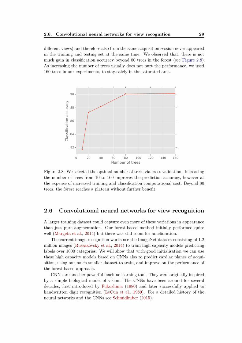
different views) and therefore also from the same acquisition session never appearedin the training and testing set at the same time. We observed that, there is notmuch gain in classification accuracy beyond 80 trees in the forest (see Figure 2.8).As increasing the number of trees usually does not hurt the performance, we used160 trees in our experiments, to stay safely in the saturated area.
0 20 40 60 80 100 120 140 160
Number of trees
82
84
86
88
90
Cla
ssific
ati
on a
ccura
cy
Figure 2.8: We selected the optimal number of trees via cross validation. Increasingthe number of trees from 10 to 160 improves the prediction accuracy, however atthe expense of increased training and classification computational cost. Beyond 80trees, the forest reaches a plateau without further benefit.
2.6 Convolutional neural networks for view recognition
A larger training dataset could capture even more of these variations in appearancethan just pure augmentation. Our forest-based method initially performed quitewell (Margeta et al., 2014) but there was still room for amelioration.
The current image recognition works use the ImageNet dataset consisting of 1.2million images (Russakovsky et al., 2014) to train high capacity models predictinglabels over 1000 categories. We will show that with good initialisation we can usethese high capacity models based on CNNs also to predict cardiac planes of acqui-sition, using our much smaller dataset to train, and improve on the performance ofthe forest-based approach.
CNNs are another powerful machine learning tool. They were originally inspiredby a simple biological model of vision. The CNNs have been around for severaldecades, first introduced by Fukushima (1980) and later successfully applied tohandwritten digit recognition (LeCun et al., 1989). For a detailed history of theneural networks and the CNNs see Schmidhuber (2015).

30 Chapter 2. Learning how to recognise cardiac acquisition planes
Recently, there has been a renewed surge in interest in the CNNs, allowed byrapid pace of improvements and understanding of their theoretical foundations.Their most recent applications significantly outperform previous approaches inmany difficult machine learning problems and in some cases reach near humanlevel performance — e.g., in handwritten digit recognition (Cireşan et al., 2010),traffic sign recognition (Cireşan et al., 2012), face identification (Taigman et al.,2014), general image recognition (Ioffe and Szegedy, 2015; He et al., 2015), andspeech recognition (Hannun et al., 2014). However, not much has changed in theoriginal principles of the CNNs since first introduced to image processing.
We have just got better at optimisation (Bottou, 2010; Bengio, 2012; Dauphinet al., 2014), large training datasets became available (Russakovsky et al., 2014;Lin et al., 2014), we have greater processing power available, found good ways toinitialise the networks (Glorot and Bengio, 2010; He et al., 2015; Ioffe and Szegedy,2015), and overcame problems of diminishing gradients and with overfitting (Hintonet al., 2012; Ioffe and Szegedy, 2015).
This renewed interest, especially in image recognition, is mainly driven by theseminal works of Ciresan et al. (2011) and Krizhevsky et al. (2012), and is fuelledby the large ImageNet dataset (Deng et al., 2009) for image recognition and betterhardware. The ImageNet Large scale visual recognition competition (Russakovskyet al., 2014) has become the battlefield in machine learning since. Many significantimprovements have followed. Fortunately, we start to see similar efforts in medicalimaging now.
2.6.1 Layers of the Convolutional Neural networks
In essence, the CNN is still just a hierarchical bank of convolutional filters combinedwith some nonlinearity in between, and whose parameters are optimised with gra-dient descent. It is composed of several layers, most frequently sequential stackedwhere outputs of the lower layers are fed into inputs of the upper ones. There areseveral layer types being currently used.
Convolutional layers
Convolution is a frequently used operation to enhance various aspects of imagessuch as gradient orientation or a particular texture. It is the main element in CNNs.The convolutional layers map the input multichannel images into new multichannelimages by convolving them with a trainable filter bank (see Fig. 2.9).
The output multichannel images from the convolutional layer are then trans-formed with a non-linear activation function σ.
Non-linear transformation - activation function
Most of the layers in the network are linear. Without any nonlinearity in betweentheir combination can be reduced into a single linear operation. In the last fewyears, the Rectified linear unit (ReLU) nonlinearity (Krizhevsky et al., 2012; Malik

2.6. Convolutional neural networks for view recognition 31
Figure 2.9: Example SAX image (top left) and channels obtained by convolvingthe source image with filters from the first convolutional layer of our convolutionalnetwork CardioViewNet detailed in Section 2.6.5. The first layer mainly picks uplow level information such as edges at various orientations.
and Perona, 1990) has become quite popular. It simply clips negative input valuesto 0:
σ(x) = max(0, x) (2.3)
This nonlinearity was shown to dramatically speed up training of the network.
Local response aggregation via max-pooling
Max-pooling is another important operation in the CNNs. It can be seen as a formof nonlinear down-sampling. The role of the max-pooling operation is similar to itsrole in the previously described forest-based method with miniatures in Section 2.5.Max-pooling aggregates local responses within rectangular neighbourhoods and foreach neighbourhood outputs the maximum response value. This adds some invari-ance to small image transformations. The output of the max-pooling operationcreates a new set of image channels which are then fed into another layer of convo-lutions and nonlinearities.
Fully connected layers
However, the final layers of the network are usually not convolutional. We still needto transform the multi-channel images into class predictions. The image channelsare therefore fed into the fully connected (fc) layers. The fully connected layers oftenreduce the data dimensionality and in the final layer produce the class activationvector (one element for each target class).
The multi-channel input images are first reshaped into flat vectors xmi (i is data-point index and m is index of the layer). The fully connected layers then transformthis vector into a vector of new length via matrix multiplication. This layer isparametrised by a matrix Wm and a bias vector bm:
xm+1i =Wmxmi + bm (2.4)

32 Chapter 2. Learning how to recognise cardiac acquisition planes
Soft-max to estimate cardiac view probabilities
To obtain the target label probabilities yi ∈ RK (K is the number of classes), the
output vector of the final fully-connected layer ai = xlasti is transformed by the
soft-max function.
yi[k] =eai[k]
∑Kk=1 e
ai[k](2.5)
To predict the view of a never seen image, it has to be passed through the layersof the CNN until the soft-max output is reached. The most likely view is thenchosen. But first, the parameters of the network must be optimised.
Loss function for classification
With decision forests, a surrogate loss is greedily optimised at every node insteadof a global loss for the classifier. The CNNs on the other hand are an end-to-endapproach, i.e., they learn optimal feature representation directly from raw imageintensity values by minimizing some global loss L(θt). For classification we use thecross-entropy loss:
L = −1
N
N∑
i=1
K∑
k=1
zki ln yki (2.6)
Here, i indexes over the data-points in the training batch and k indexes overthe views. yi is the vector with predicted probabilities for each view (dependingon parameters of the network θt and the input image). zi is the ground-truth labelindicator vector. E.g. for an image labelled as LVOT where the complete set ofviews is (2CH, 3CH, 4CH, LVOT, SAX), its ground-truth vector zi is encoded as(0, 0, 0, 1, 0).
Note that in a binary case (K = 2) this becomes the better known logisticregression loss:
L = −1
N
N∑
i
zi ln yi + (1− zi) ln(1− yi) (2.7)
It is common, to also add a term regularising the network parameters into theloss function. This is in our case a simple L2 penalty on the parameters of thenetwork (Ld = 0.5∥θ∥22) which we add to the total loss weighted by parameter β,also called weight decay.
2.6.2 Training CNNs with Stochastic gradient descent
If the cost function is differentiable, we should be able to jiggle parameters of thenetwork θt to minimize this cost. The parameters of the network such as weights ofthe convolutional filter kernels are then optimised through backpropagation in thedirection of the steepest descent.
2.6. Convolutional neural networks for view recognition 33
The batch Stochastic gradient descent (SGD) (Bottou, 2010, 2012) algorithm hasbeen quite successful to optimise large neural networks. The principle is very similarto the gradient descent algorithm except that the descent direction is estimatedfrom a smaller random batch only (instead of using the whole training dataset atthe same time). This not only dramatically speeds up the optimisation, it alsoreduces the chances of getting trapped in local minima. The batch SGD is shownin Algorithm 1.
Algorithm 1: Batch Stochastic gradient descent (SGD) algorithm
while stopping criteria not satisfied do
Take a small random batch of examples from different classes;Compute average descent direction with respect to these images;Update parameters with the update rule;
end
The stochastic gradient descent updates parameters of the network θ at eachiteration using the following update rule:
Vt+1 = µVt − αt∇Lθt (2.8)
θt+1 = θt + Vt+1 (2.9)
Momentum µ helps to regularize the locally estimated steepest descent directionof the cost function ∇Lθt with the previous weight update Vt which results in morestable and faster convergence. For zero momentum and when using all trainingimages in the batch, this equals to the standard gradient descent algorithm withlearning rate α.
As the network learns the optimal parameters through training in mini-batches,the average descent direction for the mini-batch is used. For generalisation andconvergence, care has to be taken to avoid too many images from the same subjector the same class in one batch.
The batch training allows us to use massive (possibly infinite) quantities oftraining data or data generated on the fly by data augmentation. While it istechnically possible to do similar data generation at each node for a decision forest,the forest structure is fixed in training and is usually not revisited afterwards.TheSGD makes it simpler to continuously keep updating all of the network parameterswhen new data become available.
2.6.3 Network architecture
The state of the art in image recognition has been heavily influenced by the pre-viously mentioned seminal work of Krizhevsky et al. (2012) who trained a large(60 million parameters) CNN on a massive dataset consisting of 1.2 million imagesand 1000 target classes. They employed two major improvements to the previ-ously used CNNs: Rectified linear unit nonlinearity to improve convergence, andDropout (Hinton et al., 2012) to reduce the effect of overfitting.
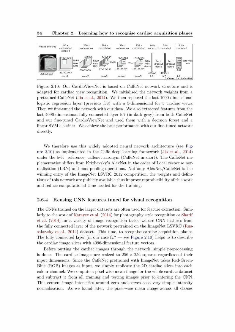
34 Chapter 2. Learning how to recognise cardiac acquisition planes
227x227x3
96Ax
convolution
11x11x3
256Ax
convolution
55x55x96
5x5x96
27x27x256
3x3x256
384AxA
convolution
13x13x384
3x3x384
256Ax
convolution
4096x1
5x1
fully
connected
LVOT
2CH
3CH
4CH
SAX
256x256x3
ResizeAandAcrop
227x227x3
conv1 conv2
ReLU
max
LRN
conv3
13x13x384
3x3x384
384AxA
convolution
conv4 conv5
ReLU
max
LRN
ReLU ReLUReLU
max
Adense
fc6
ReLU
dropout
dense
4096x1
fc7
ReLU
dropout
dense
fc8
fully
connected
fully
connected
soft-max
loss
CaffeNet CardioViewNet
strideA4
Figure 2.10: Our CardioViewNet is based on CaffeNet network structure and isadapted for cardiac view recognition. We initialised the network weights from apretrained CaffeNet (Jia et al., 2014). We then replaced the last 1000-dimensionallogistic regression layer (previous fc8) with a 5-dimensional for 5 cardiac views.Then we fine-tuned the network with our data. We also extracted features from thelast 4096-dimensional fully connected layer fc7 (in dark gray) from both CaffeNetand our fine-tuned CardioViewNet and used them with a decision forest and alinear SVM classifier. We achieve the best performance with our fine-tuned networkdirectly.
We therefore use this widely adopted neural network architecture (see Fig-ure 2.10) as implemented in the Caffe deep learning framework (Jia et al., 2014)under the bvlc_reference_caffenet acronym (CaffeNet in short). The CaffeNet im-plementation differs from Krizhevsky’s AlexNet in the order of Local response nor-malisation (LRN) and max-pooling operations. Not only AlexNet/CaffeNet is thewinning entry of the ImageNet LSVRC 2012 competition, the weights and defini-tions of this network are publicly available thus improve reproducibility of this workand reduce computational time needed for the training.
2.6.4 Reusing CNN features tuned for visual recognition
The CNNs trained on the larger datasets are often used for feature extraction. Simi-larly to the work of Karayev et al. (2014) for photography style recognition or Sharifet al. (2014) for a variety of image recognition tasks, we use CNN features fromthe fully connected layer of the network pretrained on the ImageNet LSVRC (Rus-sakovsky et al., 2014) dataset. This time, to recognise cardiac acquisition planes.The fully connected layer (in our case fc7 — see Figure 2.10) helps us to describethe cardiac image slices with 4096-dimensional feature vectors.
Before putting the cardiac images through the network, simple preprocessingis done. The cardiac images are resized to 256 × 256 squares regardless of theirinput dimensions. Since the CaffeNet pretrained with ImageNet takes Red-Green-Blue (RGB) images as input, we simply replicate the 2D cardiac slices into eachcolour channel. We compute a pixel-wise mean image for the whole cardiac datasetand subtract it from all training and testing images prior to entering the CNN.This centers image intensities around zero and serves as a very simple intensitynormalisation. As we found later, the pixel-wise mean image across all classes

2.6. Convolutional neural networks for view recognition 35
is almost uniform in the central region of interest and a scalar value could besubtracted instead. The central (227 × 227 × 3) crop of this image is then fedforward through the network.
We then use the extracted CaffeNet fc7 features with a linear SVM classi-fier (Cortes and Vapnik, 1995) to predict the cardiac views. We ran cross-validationon the training subset folds to maximise the prediction precision. This helped usto choose the penalty parameter C of the SVM classifier from standard set of val-ues [0.1, 1, 10, 100, 1000] as C = 1. We report results of this method as Caf-
feNet fc7 + SVM.Similarly, we trained a classification forest (with 64 tested features per node
and 1000 trees) using these CNN features (instead of image miniatures) and reportthese results as CaffeNet fc7 + forest.
These features were adapted to a general object recognition task and come froma CNN that never saw a cardiac MR image to optimise its weights. As we will showin Table 2.1, this already performs quite well for the cardiac view recognition, infact, much better than our method using classification forests with image miniatures.In the following, we will show how we can further improve performance by adaptingthe CNN weights to our target domain.
2.6.5 CardioViewNet architecture and parameter fine-tuning
In practice, many examples are often needed to train a large capacity neural network.However, by starting from the weights of a pretrained network we can just fine-tunethe network parameters with new data and adapt it to the new target domain. Here,we use the pretrained CaffeNet (Jia et al., 2014) and replace the last 1000-classmultinomial regression layer with a 5-class one (see Figure 2.10).
The net is fine-tuned with stochastic gradient descent. We use higher learningrate α for parameters in the newly added layer (10−2) and smaller (10−3) in the restof the network — we want to mainly optimise the newly added layer and preservethe more general low level preprocessing ones. We choose momentum µ of 0.9 inthe SGD optimiser, and a small weight decay β (10−4). The batch size used in eachiteration was 32 images and the step size is kept constant for the whole training.As done in the previous section, the images were resized to 256 × 256 × 3 and themean image was subtracted from them prior to the training.
At each iteration, a batch of 32 random (not necessarily central) 227× 227× 3
crops is extracted from the resized cardiac slices and is fed forward through thenetwork. Compared to the implementation of the forest-based method where allaugmented images were precomputed, the translations are cheaply generated onthe fly at each iteration. Already after 3000 iterations the prediction error on thevalidation dataset reaches a plateau and further improvements are only marginal(see Figure 2.11). We stop the optimisation at 8000 iterations and pick this modelin our experiments as it yields the best performance. To reduce overfitting, we usethe Dropout strategy (Hinton et al., 2012) in the fully connected layers fc6 and fc7
with probability of dropping output of a neuron to be 0.5.
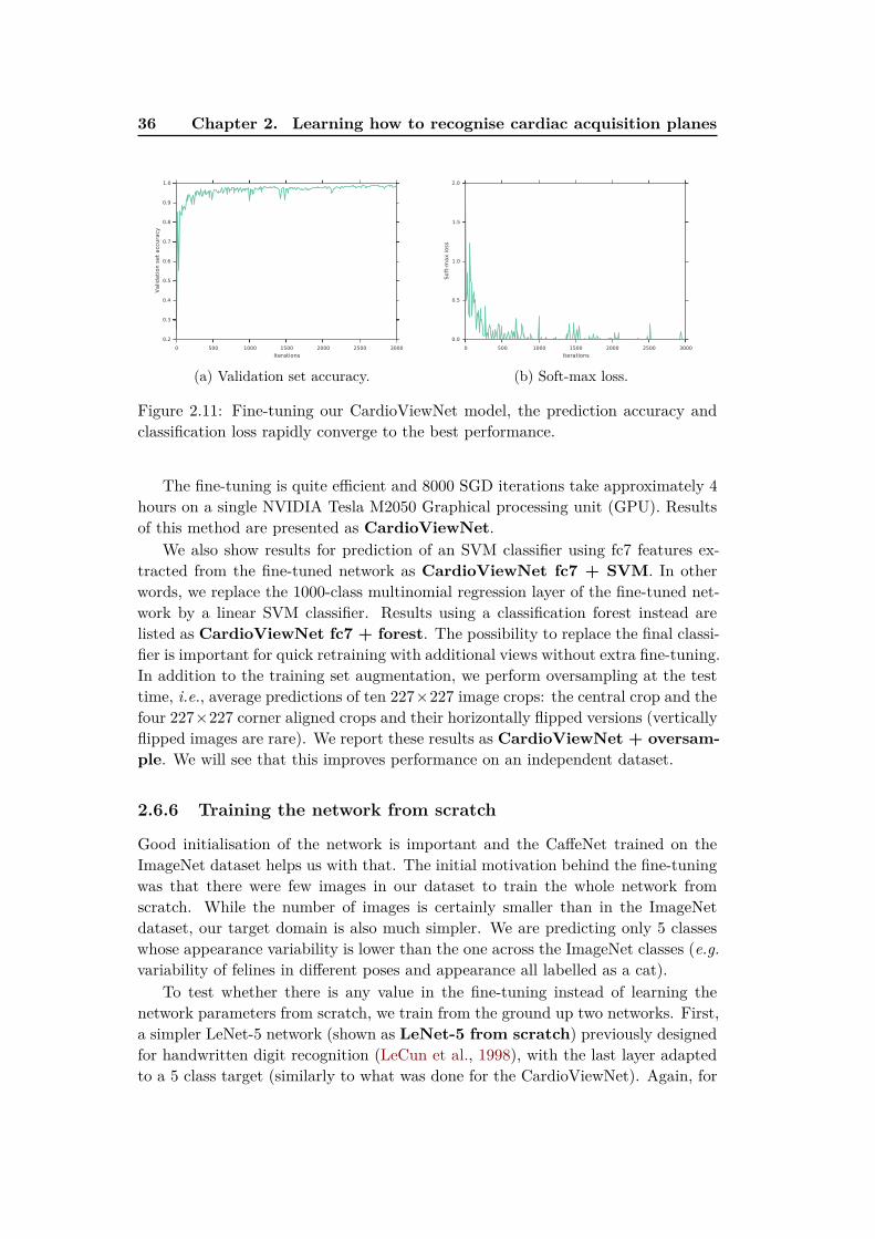
36 Chapter 2. Learning how to recognise cardiac acquisition planes
0 500 1000 1500 2000 2500 3000
Iterations
0.2
0.3
0.4
0.5
0.6
0.7
0.8
0.9
1.0
Valid
ati
on
set
acc
ura
cy
(a) Validation set accuracy.
0 500 1000 1500 2000 2500 3000
Iterations
0.0
0.5
1.0
1.5
2.0
Soft
-max loss
(b) Soft-max loss.
Figure 2.11: Fine-tuning our CardioViewNet model, the prediction accuracy andclassification loss rapidly converge to the best performance.
The fine-tuning is quite efficient and 8000 SGD iterations take approximately 4hours on a single NVIDIA Tesla M2050 Graphical processing unit (GPU). Resultsof this method are presented as CardioViewNet.
We also show results for prediction of an SVM classifier using fc7 features ex-tracted from the fine-tuned network as CardioViewNet fc7 + SVM. In otherwords, we replace the 1000-class multinomial regression layer of the fine-tuned net-work by a linear SVM classifier. Results using a classification forest instead arelisted as CardioViewNet fc7 + forest. The possibility to replace the final classi-fier is important for quick retraining with additional views without extra fine-tuning.In addition to the training set augmentation, we perform oversampling at the testtime, i.e., average predictions of ten 227×227 image crops: the central crop and thefour 227×227 corner aligned crops and their horizontally flipped versions (verticallyflipped images are rare). We report these results as CardioViewNet + oversam-
ple. We will see that this improves performance on an independent dataset.
2.6.6 Training the network from scratch
Good initialisation of the network is important and the CaffeNet trained on theImageNet dataset helps us with that. The initial motivation behind the fine-tuningwas that there were few images in our dataset to train the whole network fromscratch. While the number of images is certainly smaller than in the ImageNetdataset, our target domain is also much simpler. We are predicting only 5 classeswhose appearance variability is lower than the one across the ImageNet classes (e.g.
variability of felines in different poses and appearance all labelled as a cat).To test whether there is any value in the fine-tuning instead of learning the
network parameters from scratch, we train from the ground up two networks. First,a simpler LeNet-5 network (shown as LeNet-5 from scratch) previously designedfor handwritten digit recognition (LeCun et al., 1998), with the last layer adaptedto a 5 class target (similarly to what was done for the CardioViewNet). Again, for
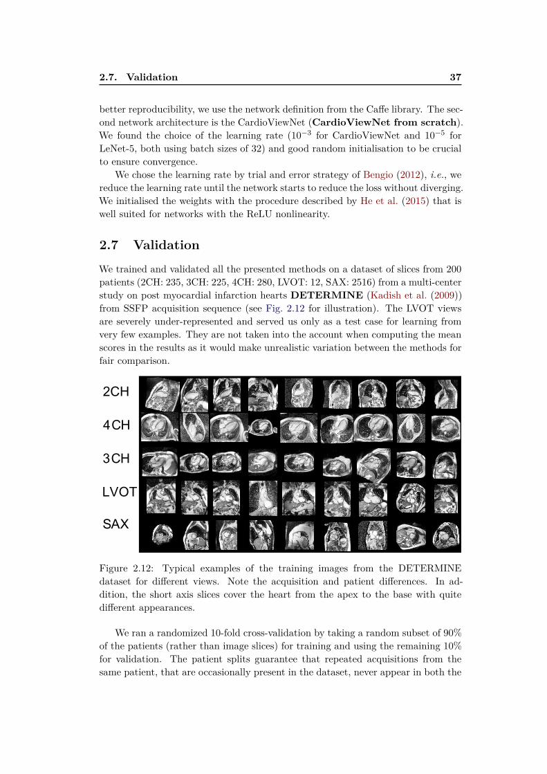
2.7. Validation 37
better reproducibility, we use the network definition from the Caffe library. The sec-ond network architecture is the CardioViewNet (CardioViewNet from scratch).We found the choice of the learning rate (10−3 for CardioViewNet and 10−5 forLeNet-5, both using batch sizes of 32) and good random initialisation to be crucialto ensure convergence.
We chose the learning rate by trial and error strategy of Bengio (2012), i.e., wereduce the learning rate until the network starts to reduce the loss without diverging.We initialised the weights with the procedure described by He et al. (2015) that iswell suited for networks with the ReLU nonlinearity.
2.7 Validation
We trained and validated all the presented methods on a dataset of slices from 200patients (2CH: 235, 3CH: 225, 4CH: 280, LVOT: 12, SAX: 2516) from a multi-centerstudy on post myocardial infarction hearts DETERMINE (Kadish et al. (2009))from SSFP acquisition sequence (see Fig. 2.12 for illustration). The LVOT viewsare severely under-represented and served us only as a test case for learning fromvery few examples. They are not taken into the account when computing the meanscores in the results as it would make unrealistic variation between the methods forfair comparison.
2CH
4CH
3CH
LVOT
SAX
Figure 2.12: Typical examples of the training images from the DETERMINEdataset for different views. Note the acquisition and patient differences. In ad-dition, the short axis slices cover the heart from the apex to the base with quitedifferent appearances.
We ran a randomized 10-fold cross-validation by taking a random subset of 90%of the patients (rather than image slices) for training and using the remaining 10%for validation. The patient splits guarantee that repeated acquisitions from thesame patient, that are occasionally present in the dataset, never appear in both the
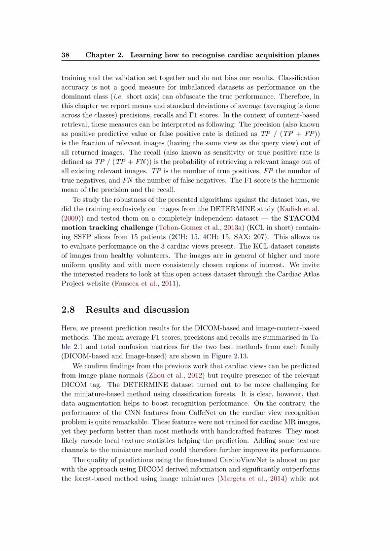
38 Chapter 2. Learning how to recognise cardiac acquisition planes
training and the validation set together and do not bias our results. Classificationaccuracy is not a good measure for imbalanced datasets as performance on thedominant class (i.e. short axis) can obfuscate the true performance. Therefore, inthis chapter we report means and standard deviations of average (averaging is doneacross the classes) precisions, recalls and F1 scores. In the context of content-basedretrieval, these measures can be interpreted as following: The precision (also knownas positive predictive value or false positive rate is defined as TP / (TP + FP))is the fraction of relevant images (having the same view as the query view) out ofall returned images. The recall (also known as sensitivity or true positive rate isdefined as TP / (TP + FN )) is the probability of retrieving a relevant image out ofall existing relevant images. TP is the number of true positives, FP the number oftrue negatives, and FN the number of false negatives. The F1 score is the harmonicmean of the precision and the recall.
To study the robustness of the presented algorithms against the dataset bias, wedid the training exclusively on images from the DETERMINE study (Kadish et al.(2009)) and tested them on a completely independent dataset — the STACOM
motion tracking challenge (Tobon-Gomez et al., 2013a) (KCL in short) contain-ing SSFP slices from 15 patients (2CH: 15, 4CH: 15, SAX: 207). This allows usto evaluate performance on the 3 cardiac views present. The KCL dataset consistsof images from healthy volunteers. The images are in general of higher and moreuniform quality and with more consistently chosen regions of interest. We invitethe interested readers to look at this open access dataset through the Cardiac AtlasProject website (Fonseca et al., 2011).
2.8 Results and discussion
Here, we present prediction results for the DICOM-based and image-content-basedmethods. The mean average F1 scores, precisions and recalls are summarised in Ta-ble 2.1 and total confusion matrices for the two best methods from each family(DICOM-based and Image-based) are shown in Figure 2.13.
We confirm findings from the previous work that cardiac views can be predictedfrom image plane normals (Zhou et al., 2012) but require presence of the relevantDICOM tag. The DETERMINE dataset turned out to be more challenging forthe miniature-based method using classification forests. It is clear, however, thatdata augmentation helps to boost recognition performance. On the contrary, theperformance of the CNN features from CaffeNet on the cardiac view recognitionproblem is quite remarkable. These features were not trained for cardiac MR images,yet they perform better than most methods with handcrafted features. They mostlikely encode local texture statistics helping the prediction. Adding some texturechannels to the miniature method could therefore further improve its performance.
The quality of predictions using the fine-tuned CardioViewNet is almost on parwith the approach using DICOM derived information and significantly outperformsthe forest-based method using image miniatures (Margeta et al., 2014) while not
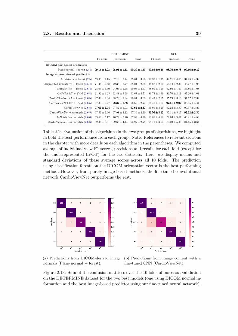
2.8. Results and discussion 39
DETERMINE KCL
F1 score precision recall F1 score precision recall
DICOM tag based prediction
Plane normal + forest (2.4) 99.14± 1.2399.14± 1.2399.14± 1.23 98.91± 1.1398.91± 1.1398.91± 1.13 99.20± 1.5399.20± 1.5399.20± 1.53 99.08± 0.4699.08± 0.4699.08± 0.46 98.76± 0.7898.76± 0.7898.76± 0.78 99.16± 0.3299.16± 0.3299.16± 0.32
Image content-based prediction
Miniatures + forest (2.5) 59.33± 4.15 62.13± 5.74 55.61± 3.80 39.36± 1.75 42.71± 4.63 37.98± 4.39
Augmented miniatures + forest (2.5.4) 71.46± 2.68 72.33± 2.77 68.01± 2.65 48.87± 2.02 54.74± 2.33 43.77± 1.98
CaffeNet fc7 + forest (2.6.4) 75.94± 4.50 94.03± 1.75 69.08± 4.53 88.09± 1.29 92.60± 1.63 86.86± 1.08
CaffeNet fc7 + SVM (2.6.4) 91.86± 4.33 92.48± 3.98 91.61± 4.71 86.72± 1.49 86.70± 2.19 87.30± 1.08
CardioViewNet fc7 + forest (2.6.5) 97.48± 2.34 98.28± 1.84 96.81± 3.03 93.43± 2.05 95.79± 3.10 91.67± 2.34
CardioViewNet fc7 + SVM (2.6.5) 97.39± 2.27 98.37± 1.8898.37± 1.8898.37± 1.88 96.65± 2.77 88.40± 1.84 97.51± 2.0297.51± 2.0297.51± 2.02 88.95± 4.44
CardioViewNet (2.6.5) 97.66± 2.0497.66± 2.0497.66± 2.04 97.82± 1.93 97.62± 2.3797.62± 2.3797.62± 2.37 91.01± 3.29 92.23± 3.80 90.57± 3.26
CardioViewNet oversample (2.6.5) 97.53± 2.06 97.98± 2.12 97.30± 2.30 93.50± 3.1293.50± 3.1293.50± 3.12 95.31± 5.17 92.62± 2.3092.62± 2.3092.62± 2.30
LeNet-5 from scratch (2.6.6) 69.59± 5.12 76.79± 5.40 67.89± 4.26 63.81± 4.88 72.03± 9.67 60.41± 4.53
CardioViewNet from scratch (2.6.6) 92.36± 3.51 92.63± 4.44 92.97± 2.79 79.72± 3.65 80.39± 5.39 81.65± 3.64
Table 2.1: Evaluation of the algorithms in the two groups of algorithms, we highlightin bold the best performance from each group. Note: References to relevant sectionsin the chapter with more details on each algorithm in the parentheses. We computedaverage of individual view F1 scores, precisions and recalls for each fold (except forthe underrepresented LVOT) for the two datasets. Here, we display means andstandard deviations of these average scores across all 10 folds. The predictionusing classification forests on the DICOM orientation vector is the best performingmethod. However, from purely image-based methods, the fine-tuned convolutionalnetwork CardioViewNet outperforms the rest.
(a) Predictions from DICOM-derived imagenormals (Plane normal + forest).
(b) Predictions from image content with afine-tuned CNN (CardioViewNet).
Figure 2.13: Sum of the confusion matrices over the 10 folds of our cross-validationon the DETERMINE dataset for the two best models (one using DICOM normal in-formation and the best image-based predictor using our fine-tuned neural network).
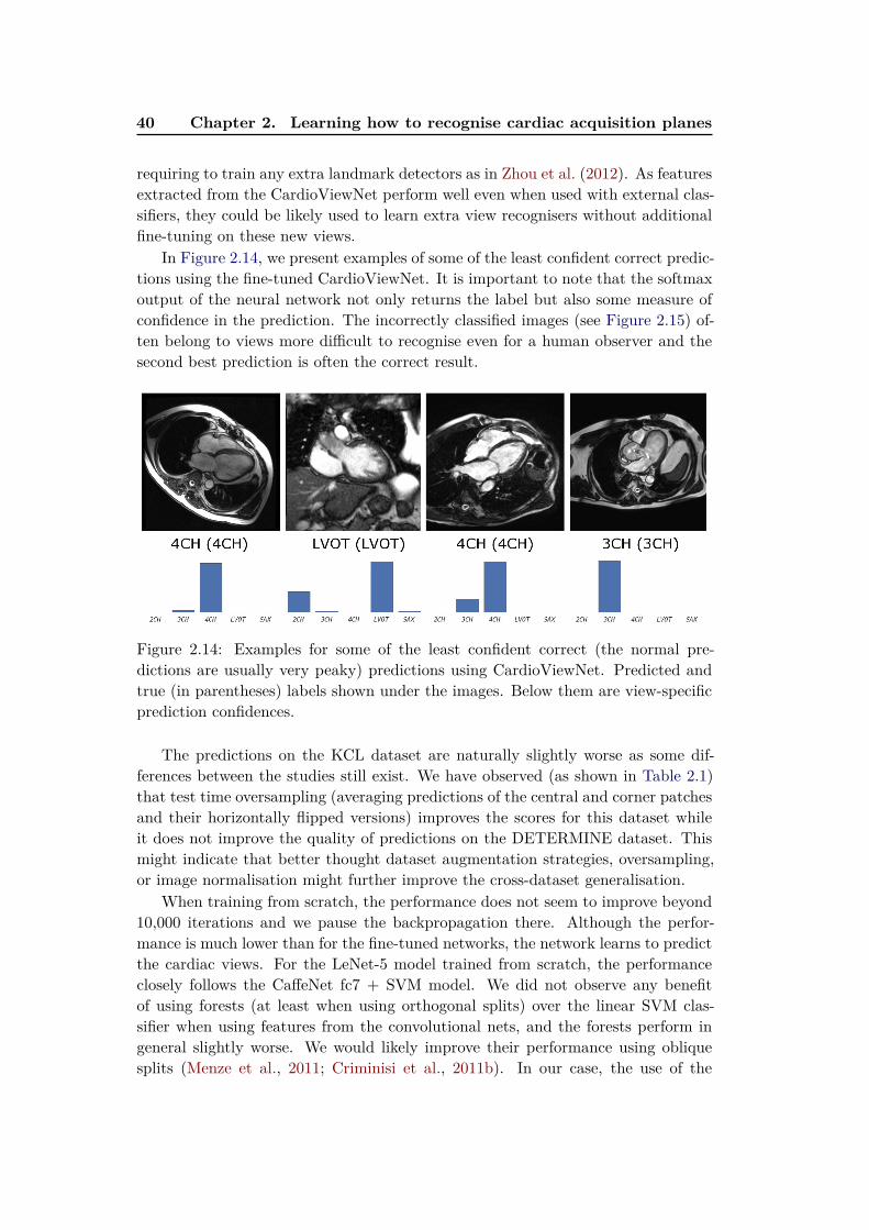
40 Chapter 2. Learning how to recognise cardiac acquisition planes
requiring to train any extra landmark detectors as in Zhou et al. (2012). As featuresextracted from the CardioViewNet perform well even when used with external clas-sifiers, they could be likely used to learn extra view recognisers without additionalfine-tuning on these new views.
In Figure 2.14, we present examples of some of the least confident correct predic-tions using the fine-tuned CardioViewNet. It is important to note that the softmaxoutput of the neural network not only returns the label but also some measure ofconfidence in the prediction. The incorrectly classified images (see Figure 2.15) of-ten belong to views more difficult to recognise even for a human observer and thesecond best prediction is often the correct result.
Figure 2.14: Examples for some of the least confident correct (the normal pre-dictions are usually very peaky) predictions using CardioViewNet. Predicted andtrue (in parentheses) labels shown under the images. Below them are view-specificprediction confidences.
The predictions on the KCL dataset are naturally slightly worse as some dif-ferences between the studies still exist. We have observed (as shown in Table 2.1)that test time oversampling (averaging predictions of the central and corner patchesand their horizontally flipped versions) improves the scores for this dataset whileit does not improve the quality of predictions on the DETERMINE dataset. Thismight indicate that better thought dataset augmentation strategies, oversampling,or image normalisation might further improve the cross-dataset generalisation.
When training from scratch, the performance does not seem to improve beyond10,000 iterations and we pause the backpropagation there. Although the perfor-mance is much lower than for the fine-tuned networks, the network learns to predictthe cardiac views. For the LeNet-5 model trained from scratch, the performanceclosely follows the CaffeNet fc7 + SVM model. We did not observe any benefitof using forests (at least when using orthogonal splits) over the linear SVM clas-sifier when using features from the convolutional nets, and the forests perform ingeneral slightly worse. We would likely improve their performance using obliquesplits (Menze et al., 2011; Criminisi et al., 2011b). In our case, the use of the
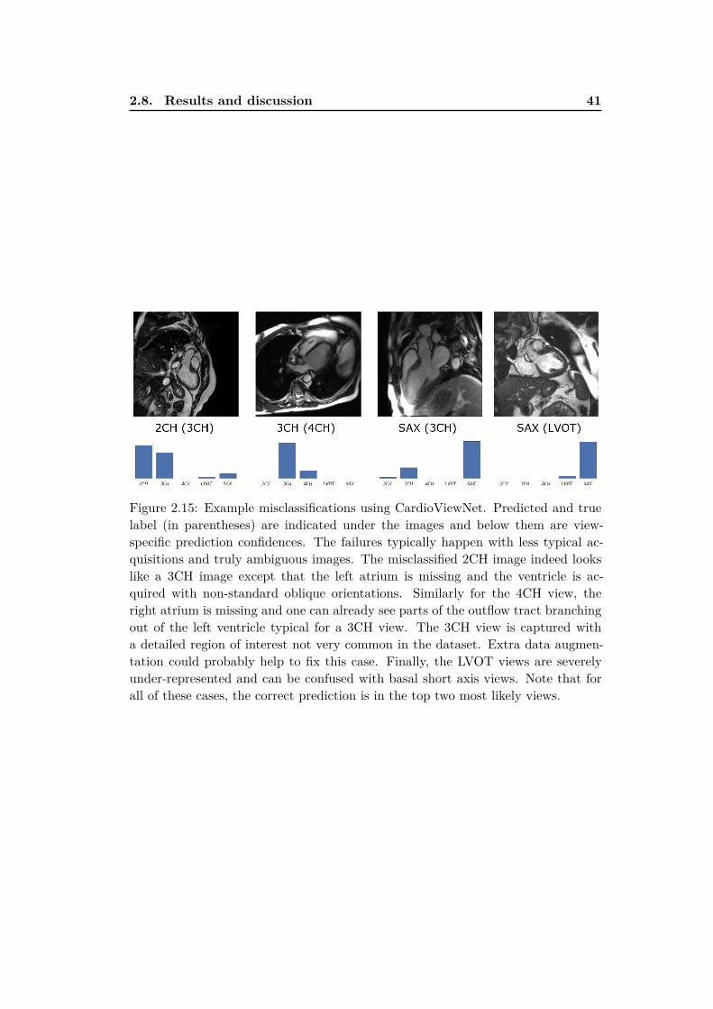
2.8. Results and discussion 41
Figure 2.15: Example misclassifications using CardioViewNet. Predicted and truelabel (in parentheses) are indicated under the images and below them are view-specific prediction confidences. The failures typically happen with less typical ac-quisitions and truly ambiguous images. The misclassified 2CH image indeed lookslike a 3CH image except that the left atrium is missing and the ventricle is ac-quired with non-standard oblique orientations. Similarly for the 4CH view, theright atrium is missing and one can already see parts of the outflow tract branchingout of the left ventricle typical for a 3CH view. The 3CH view is captured witha detailed region of interest not very common in the dataset. Extra data augmen-tation could probably help to fix this case. Finally, the LVOT views are severelyunder-represented and can be confused with basal short axis views. Note that forall of these cases, the correct prediction is in the top two most likely views.
42 Chapter 2. Learning how to recognise cardiac acquisition planes
CardioViewNet trained from scratch is a better choice than using the generic fc7
features from CaffeNet. However, the training is significantly more time-consuming.The fine-tuning approach is the clear winner among the image-based methods interms of performance.
2.9 Conclusion and perspectives
Convolutional neural networks and features extracted from them seem to workremarkably well for medical images. As large datasets to train complex models areoften not available, retargeting the domain of a previously trained model by fine-tuning can help. This speeds up the learning process and achieves better predictions.Even models trained for general object recognition might be a great baseline tostart. In our case, doing network surgery by replacing the final layer and fine-tuning the pretrained model allowed us to make significant progress in cardiac viewrecognition from image content without handcrafting the features or training withextra annotations.
This also allowed us to gain performance over models learnt from scratch. How-ever, even the performance of models learnt from scratch is very encouraging forfurther exploration. More recent and much deeper network architectures (e.g.
VGG (Simonyan and Zisserman, 2014) or GoogLeNet (Szegedy et al., 2014; Ioffeand Szegedy, 2015)) have achieved significant improvements in image recognitionperformance over AlexNet, and would likely help to further improve performanceof the view recognition.
Features extracted from our network should be useful as descriptors for newviews (e.g. pathology specific views such as those used in congenital heart diseases)and acquisition sequences other than SSFP, but also to recognise the acquisition se-quences themselves. Several recommendations (Friedrich et al., 2014; Kramer et al.,2013) have been recently proposed to simplify and remove vendor specific namingof acquisition sequences. Such efforts are crucial for improved communication incardiology. The methods presented in this chapter could help us to learn the map-ping from image content to these standardised nomenclatures and further clean upinconsistent and missing metadata for better organisation and search within car-diac databases. As we will see later in this thesis, the features from our fine-tunednetwork can also be used to predict positions of cardiac landmarks (Appendix B).
These are important additions to the arsenal of tools for handling noisy meta-data in our datasets and are already helping us to organise collections of cardiacimages. In the future, our method can be used for semantic image retrieval andparsing of medical literature. Recognition at an image level (image classification)can be also extremely useful for the costly problem of quality control (as done, e.g.,by Criminisi et al. (2011a) to verify contrast enhanced images). For example, “Ihave asked my radiographer to take all standard views of the heart. Did he do itcorrectly?”

Chapter 3
Segmenting cardiac images with
classification forests
Contents
3.1 Segmentation of the left ventricle . . . . . . . . . . . . . . . . 44
3.1.1 Measurements in cardiac magnetic resonance imaging . . . . 44
3.1.2 Previous work . . . . . . . . . . . . . . . . . . . . . . . . . . . 45
3.1.3 Overview of our method . . . . . . . . . . . . . . . . . . . . . 46
3.1.4 Layered spatio-temporal decision forests . . . . . . . . . . . . 47
3.1.5 Features for left ventricle segmentation . . . . . . . . . . . . . 48
3.1.6 First layer: Intensity and pose normalisation . . . . . . . . . 51
3.1.7 Second layer: Learning to segment with the shape . . . . . . 54
3.1.8 Validation . . . . . . . . . . . . . . . . . . . . . . . . . . . . . 55
3.1.9 Results and discussion . . . . . . . . . . . . . . . . . . . . . . 56
3.1.10 Volumetric measure calculation . . . . . . . . . . . . . . . . . 58
3.1.11 Conclusions . . . . . . . . . . . . . . . . . . . . . . . . . . . . 58
3.2 Left atrium segmentation . . . . . . . . . . . . . . . . . . . . . 59
3.2.1 Dataset . . . . . . . . . . . . . . . . . . . . . . . . . . . . . . 60
3.2.2 Preprocessing . . . . . . . . . . . . . . . . . . . . . . . . . . . 60
3.2.3 Training forests with boundary voxels . . . . . . . . . . . . . 60
3.2.4 Segmentation phase . . . . . . . . . . . . . . . . . . . . . . . 60
3.2.5 Additional channels for left atrial segmentation . . . . . . . . 60
3.2.6 Validation . . . . . . . . . . . . . . . . . . . . . . . . . . . . . 62
3.2.7 Results and discussion . . . . . . . . . . . . . . . . . . . . . . 64
3.2.8 Conclusions . . . . . . . . . . . . . . . . . . . . . . . . . . . . 64
3.3 Conclusions and perspectives . . . . . . . . . . . . . . . . . . 65
3.3.1 Perspectives . . . . . . . . . . . . . . . . . . . . . . . . . . . . 65
Based on our paper on left ventricle segmentation (Margeta et al., 2012) whoseresults we contributed to the left ventricle collation study by Suinesiaputra et al.(2014b). Our left atrial segmentation work was published in (Margeta et al., 2013)and was contributed to the benchmark study led by Tobon-Gomez et al. (2015).
44 Chapter 3. Segmenting cardiac images with classification forests
Chapter overview
The most commonly used clinical indices for cardiac disease quantification are basedon geometrical measurements of structures in the images, such as cavity volumes,myocardial masses or wall thicknesses. It would be quite useful to have them storedin the cardiac databases alongside the images and use them to select patient cohortsfor clinical studies. These measurements are often computed from segmentations ofthese cardiac structures. The segmentation also forms the basis for understandingthe cardiac anatomy by a computer.
In this chapter we present a flexible machine learning based method for CMRimage segmentation of two of the most important cardiac structures. First, welearn how to segment the left ventricles from dynamic 3D+t SAX images directlyfrom voxel-wise ground-truth by training classification forests with spatio-temporalcontext rich features. We then show that this method can be easily adapted toother segmentation problems such as the left atria.
3.1 Segmentation of the left ventricle
3.1.1 Measurements in cardiac magnetic resonance imaging
The left ventricle plays a fundamental role in circulation of oxygenated blood tothe body. To assess its function in clinical practice, the guidelines (Kramer et al.,2013; Fratz et al., 2013; Friedrich et al., 2012) suggest to measure, calculate andreport several measures. Many of these are based on ventricular volume and massmeasurements at reference cardiac phases. These can be then compared with refer-ence values (Schulz-Menger et al., 2013; Maceira et al., 2006; Hudsmith†et al., 2005;Chuang et al., 2014; Buechel et al., 2009) for CMR.
Compared to CT, CMR imaging offers superior temporal resolution, excellentsoft tissue contrast, no ionising radiation, and a vast flexibility in image acquisi-tion characteristics. On the other side, MRI scans often yield significantly lowerresolution in the plane orthogonal to the plane of acquisition, the images can suf-fer from magnetic field inhomogeneities and respiration artefacts can manifest asslice shifts. Moreover, the lack of standard units (compared to the Hounsfield scalein CT) makes it more challenging to directly apply most of the intensity basedsegmentation techniques.
Still, to calculate the quantities, accurate delineations of the myocardium andthe cavity borders are often necessary. Such manual delineations are still labourintensive (2 minutes per cardiac phase), especially when applied retrospectively tothe previously acquired data. The inter-rater variability of manual segmentations(and derived measures) is also quite noticeable (Suinesiaputra et al., 2015) and canbe likely improved by finding a consensus and training of the raters.
Moreover, the differences in measures between inclusion or exclusion of papillarymuscles and trabeculations can be also significant (Papavassiliu et al., 2005; Winteret al., 2008; Chuang et al., 2011; Han et al., 2008).
3.1. Segmentation of the left ventricle 45
To obtain consistent measurements, to be able to resegment the images when theguidelines change (or segment all variations), and to save clinicians’ time, automaticsegmentation techniques are desirable.
3.1.2 Previous work
There have been numerous examples of semi-automatic or automatic LV segmen-tation algorithms to this date. See Petitjean et al. (2011) for a thorough review.Here, we mention only a selection of the notable automatic ones.
Shape based segmentation
Two beautiful frameworks for automatic whole heart cardiac image segmentationwere proposed by Zheng et al. (2008); Ecabert et al. (2008). Machine learning baseddetection of the heart is followed by an iterative refinement of the segmentationregularised with probabilistic shape models.
These methods offer an excellent performance and regularisation of the segmen-tations. In addition, they naturally complete out of image shapes, e.g., in the apicalor atrial regions and divide the image into the compartments even when no imagegradient between them is present. As they are often based on Principal ComponentAnalysis (PCA), they perform slighly worse on data that cannot be well representedby the linear combination of the bases and do not work at all when the topology sig-nificantly changes (such as for congenital heart diseases). In these cases, additionalmodels have to be built specifically for each topology.
Atlas-based segmentation
The atlas-based segmentation techniques (Shi et al., 2011) use non-rigid image reg-istration to deform and position a previously segmented image (or images for amulti-atlas segmentation) to better match the target image. The labels are thenpropagated from the atlas to the target image. These methods rely on robustnon-rigid registration.
The inter-patient non-rigid registration is in general a difficult problem due tothe extra-cardiac structures which misguide the registration metric. Masking of theimages (with cardiac segmentation) might be needed (Ou et al., 2012). To avoidthe chicken and egg problem (segmenting the heart in order to register in orderto segment) Shi et al. (2011), proposed to register the images and use only theinformation contained within the cardiac region of interest. This region is detectedwith a standard trainable object detector (Viola and Jones, 2004).
Voxel-wise semantic segmentation
Instead of shape-based or atlas-based methods, the cardiac segmentation can beposed as a semantic image segmentation problem (Shotton et al., 2008). Here, eachpixel is assigned a class label (myocardium or background). In the work of Shotton
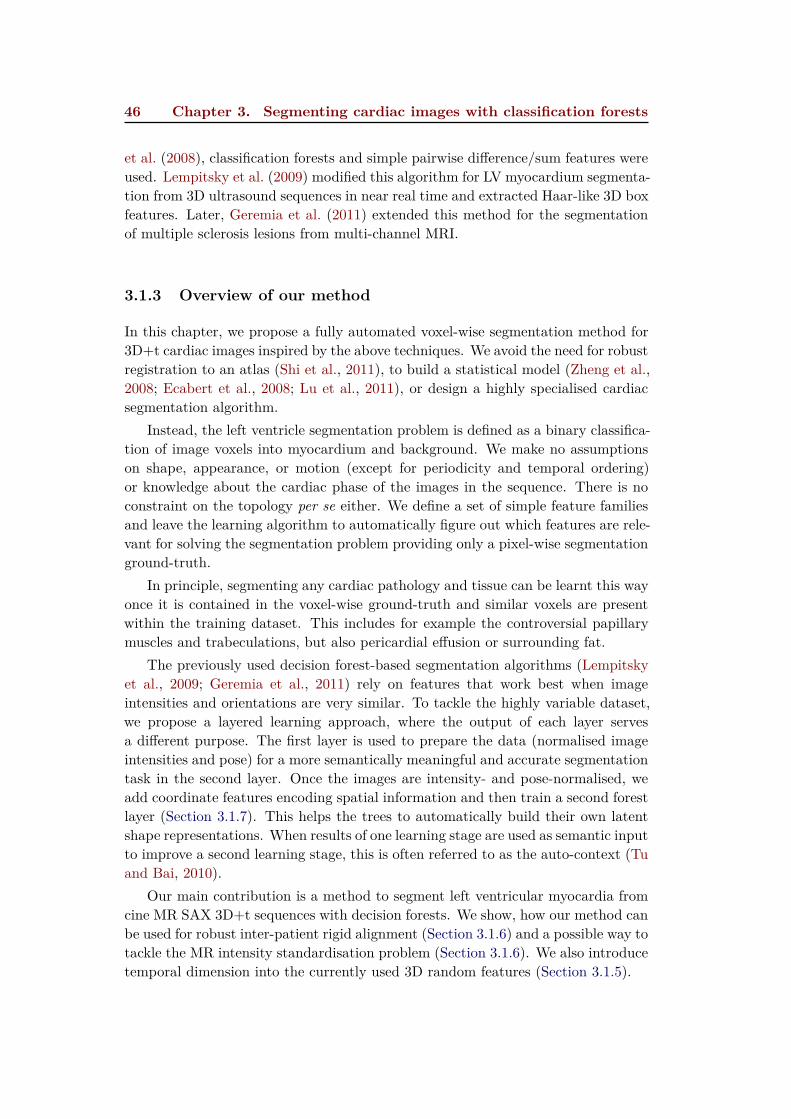
46 Chapter 3. Segmenting cardiac images with classification forests
et al. (2008), classification forests and simple pairwise difference/sum features wereused. Lempitsky et al. (2009) modified this algorithm for LV myocardium segmenta-tion from 3D ultrasound sequences in near real time and extracted Haar-like 3D boxfeatures. Later, Geremia et al. (2011) extended this method for the segmentationof multiple sclerosis lesions from multi-channel MRI.
3.1.3 Overview of our method
In this chapter, we propose a fully automated voxel-wise segmentation method for3D+t cardiac images inspired by the above techniques. We avoid the need for robustregistration to an atlas (Shi et al., 2011), to build a statistical model (Zheng et al.,2008; Ecabert et al., 2008; Lu et al., 2011), or design a highly specialised cardiacsegmentation algorithm.
Instead, the left ventricle segmentation problem is defined as a binary classifica-tion of image voxels into myocardium and background. We make no assumptionson shape, appearance, or motion (except for periodicity and temporal ordering)or knowledge about the cardiac phase of the images in the sequence. There is noconstraint on the topology per se either. We define a set of simple feature familiesand leave the learning algorithm to automatically figure out which features are rele-vant for solving the segmentation problem providing only a pixel-wise segmentationground-truth.
In principle, segmenting any cardiac pathology and tissue can be learnt this wayonce it is contained in the voxel-wise ground-truth and similar voxels are presentwithin the training dataset. This includes for example the controversial papillarymuscles and trabeculations, but also pericardial effusion or surrounding fat.
The previously used decision forest-based segmentation algorithms (Lempitskyet al., 2009; Geremia et al., 2011) rely on features that work best when imageintensities and orientations are very similar. To tackle the highly variable dataset,we propose a layered learning approach, where the output of each layer servesa different purpose. The first layer is used to prepare the data (normalised imageintensities and pose) for a more semantically meaningful and accurate segmentationtask in the second layer. Once the images are intensity- and pose-normalised, weadd coordinate features encoding spatial information and then train a second forestlayer (Section 3.1.7). This helps the trees to automatically build their own latentshape representations. When results of one learning stage are used as semantic inputto improve a second learning stage, this is often referred to as the auto-context (Tuand Bai, 2010).
Our main contribution is a method to segment left ventricular myocardia fromcine MR SAX 3D+t sequences with decision forests. We show, how our method canbe used for robust inter-patient rigid alignment (Section 3.1.6) and a possible way totackle the MR intensity standardisation problem (Section 3.1.6). We also introducetemporal dimension into the currently used 3D random features (Section 3.1.5).
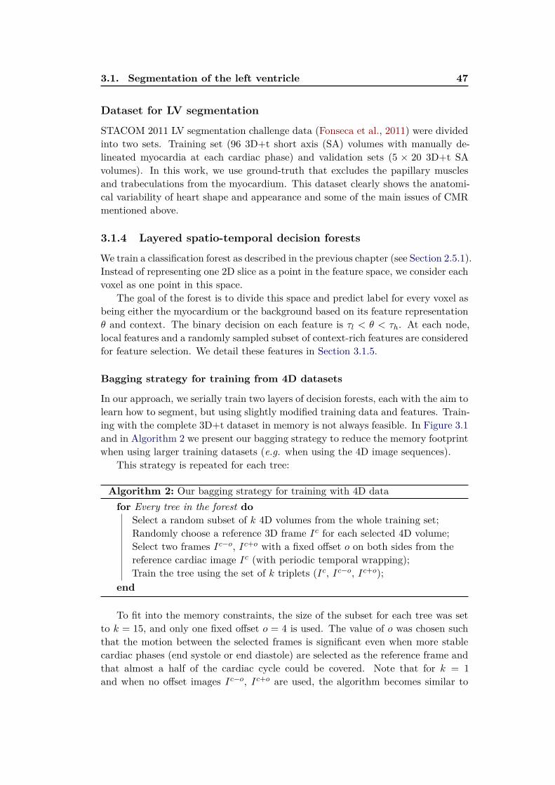
3.1. Segmentation of the left ventricle 47
Dataset for LV segmentation
STACOM 2011 LV segmentation challenge data (Fonseca et al., 2011) were dividedinto two sets. Training set (96 3D+t short axis (SA) volumes with manually de-lineated myocardia at each cardiac phase) and validation sets (5 × 20 3D+t SAvolumes). In this work, we use ground-truth that excludes the papillary musclesand trabeculations from the myocardium. This dataset clearly shows the anatomi-cal variability of heart shape and appearance and some of the main issues of CMRmentioned above.
3.1.4 Layered spatio-temporal decision forests
We train a classification forest as described in the previous chapter (see Section 2.5.1).Instead of representing one 2D slice as a point in the feature space, we consider eachvoxel as one point in this space.
The goal of the forest is to divide this space and predict label for every voxel asbeing either the myocardium or the background based on its feature representationθ and context. The binary decision on each feature is τl < θ < τh. At each node,local features and a randomly sampled subset of context-rich features are consideredfor feature selection. We detail these features in Section 3.1.5.
Bagging strategy for training from 4D datasets
In our approach, we serially train two layers of decision forests, each with the aim tolearn how to segment, but using slightly modified training data and features. Train-ing with the complete 3D+t dataset in memory is not always feasible. In Figure 3.1and in Algorithm 2 we present our bagging strategy to reduce the memory footprintwhen using larger training datasets (e.g. when using the 4D image sequences).
This strategy is repeated for each tree:
Algorithm 2: Our bagging strategy for training with 4D data
for Every tree in the forest do
Select a random subset of k 4D volumes from the whole training set;Randomly choose a reference 3D frame Ic for each selected 4D volume;Select two frames Ic−o, Ic+o with a fixed offset o on both sides from thereference cardiac image Ic (with periodic temporal wrapping);Train the tree using the set of k triplets (Ic, Ic−o, Ic+o);
end
To fit into the memory constraints, the size of the subset for each tree was setto k = 15, and only one fixed offset o = 4 is used. The value of o was chosen suchthat the motion between the selected frames is significant even when more stablecardiac phases (end systole or end diastole) are selected as the reference frame andthat almost a half of the cardiac cycle could be covered. Note that for k = 1
and when no offset images Ic−o, Ic+o are used, the algorithm becomes similar to

48 Chapter 3. Segmenting cardiac images with classification forests
Training 3D triplets
Ic-o Ic+oIc
Ic-o Ic+oIc
Ic-oIc+oIc
Source 4D images
Figure 3.1: Our strategy to train a segmentation forest from 3D+t cardiac data.For each tree we randomly select a subset of training images (3 in this example). Foreach image we pick a random reference frame and two frames offset by a constantnumber of frames (while respecting the periodicity of the sequence). We then trainthe forest on these triplets.
the later introduced Atlas encoding by randomized forests (Zikic et al., 2013). Inaddition, instead of randomly selecting the reference images for each tree, guidedbagging (e.g. by training each tree on similar images only) could help to improvethe segmentation quality as shown by Lombaert et al. (2014).
3.1.5 Features for left ventricle segmentation
We use several feature families to generate the random feature pool operating onthe triplets of frames. These can be seen in Figs. 3.2 to 3.6.
Local features
Proposed in Geremia et al. (2011) as an average of intensities in the vicinity of thetested voxel to deal with noise in magnetic resonance imaging:
θlocIc (x) = θlocIc ([x, y, z]) =
x′≤x+1∑
x′=x−1
y′≤y+1∑
y′=y−1
z′≤z+1∑
z′=z−1
Ic([x′, y′, z′]) (3.1)
Although these features are not intensity invariant, they can still quite well rejectsome highly improbable intensities (e.g. bright blood-like voxels will likely neverbelong to the myocardium).
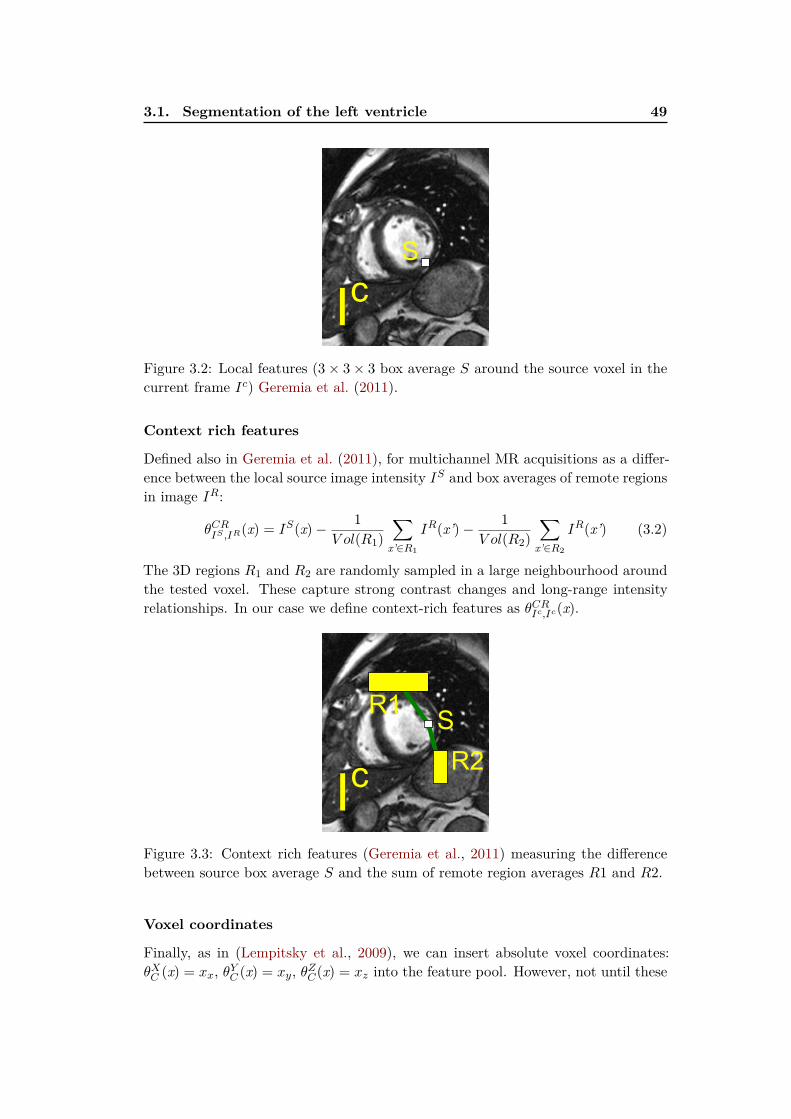
3.1. Segmentation of the left ventricle 49
Ic
S
Figure 3.2: Local features (3× 3× 3 box average S around the source voxel in thecurrent frame Ic) Geremia et al. (2011).
Context rich features
Defined also in Geremia et al. (2011), for multichannel MR acquisitions as a differ-ence between the local source image intensity IS and box averages of remote regionsin image IR:
θCRIS ,IR(x) = IS(x)−
1
V ol(R1)
∑
x’∈R1
IR(x’)−1
V ol(R2)
∑
x’∈R2
IR(x’) (3.2)
The 3D regions R1 and R2 are randomly sampled in a large neighbourhood aroundthe tested voxel. These capture strong contrast changes and long-range intensityrelationships. In our case we define context-rich features as θCR
Ic,Ic(x).
R1
R2
S
Ic
Figure 3.3: Context rich features (Geremia et al., 2011) measuring the differencebetween source box average S and the sum of remote region averages R1 and R2.
Voxel coordinates
Finally, as in (Lempitsky et al., 2009), we can insert absolute voxel coordinates:θXC (x) = xx, θYC (x) = xy, θZC(x) = xz into the feature pool. However, not until these

50 Chapter 3. Segmenting cardiac images with classification forests
coordinates have a strong anatomical meaning. This happens later, in the secondforest layer when we reorient the images into the standard pose.
Ic
x,y,z
Figure 3.4: Components x,y,z of voxel coordinates as features (Lempitsky et al.,2009).
Spatio-temporal context rich features
The domain of the moving heart can be coarsely extracted by just thresholding thetemporal intensity ranges of the image (Section 5.4.2.1). We propose to exploitthe wealth of information in time and extend the previous context-rich featuresinto the temporal domain by comparing the “current” 3D frame Ic and anotherframe offset from c by ±o. The temporal context-rich features can be defined asθTCR1Ic = θCR
Ic,Ic+o(x) and θTCR1Ic = θCR
Ic,Ic−o(x).
Ic
R1
R2
S
Ic
Ic±o
Figure 3.5: Spatio-temporal context rich features with one of the offset frames asthe source image and the other as remote.
Similarly, we measure the differences between the symmetrically offset framescontained in the triplet as θTCR2
Ic (x) = θCRIc+o,Ic−o(x) and θTCR2
Ic (x) = θCRIc−o,Ic+o(x).
These spatio-temporal features can be seen as an approximation to temporal differ-
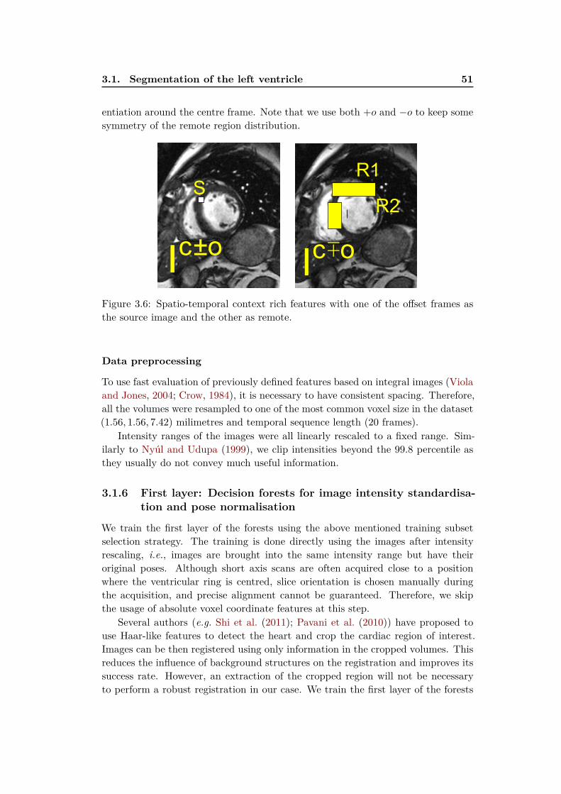
3.1. Segmentation of the left ventricle 51
entiation around the centre frame. Note that we use both +o and −o to keep somesymmetry of the remote region distribution.
I
R1
R2
S
I Ic±o c∓o
Figure 3.6: Spatio-temporal context rich features with one of the offset frames asthe source image and the other as remote.
Data preprocessing
To use fast evaluation of previously defined features based on integral images (Violaand Jones, 2004; Crow, 1984), it is necessary to have consistent spacing. Therefore,all the volumes were resampled to one of the most common voxel size in the dataset(1.56, 1.56, 7.42) milimetres and temporal sequence length (20 frames).
Intensity ranges of the images were all linearly rescaled to a fixed range. Sim-ilarly to Nyúl and Udupa (1999), we clip intensities beyond the 99.8 percentile asthey usually do not convey much useful information.
3.1.6 First layer: Decision forests for image intensity standardisa-
tion and pose normalisation
We train the first layer of the forests using the above mentioned training subsetselection strategy. The training is done directly using the images after intensityrescaling, i.e., images are brought into the same intensity range but have theiroriginal poses. Although short axis scans are often acquired close to a positionwhere the ventricular ring is centred, slice orientation is chosen manually duringthe acquisition, and precise alignment cannot be guaranteed. Therefore, we skipthe usage of absolute voxel coordinate features at this step.
Several authors (e.g. Shi et al. (2011); Pavani et al. (2010)) have proposed touse Haar-like features to detect the heart and crop the cardiac region of interest.Images can be then registered using only information in the cropped volumes. Thisreduces the influence of background structures on the registration and improves itssuccess rate. However, an extraction of the cropped region will not be necessaryto perform a robust registration in our case. We train the first layer of the forests
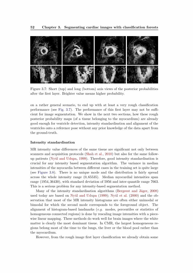
52 Chapter 3. Segmenting cardiac images with classification forests
Figure 3.7: Short (top) and long (bottom) axis views of the posterior probabilitiesafter the first layer. Brighter value means higher probability.
on a rather general scenario, to end up with at least a very rough classificationperformance (see Fig. 3.7). The performance of this first layer may not be suffi-cient for image segmentation. We show in the next two sections, how these roughposterior probability maps (of a tissue belonging to the myocardium) are alreadygood enough for ventricle detection, intensity standardisation and alignment of theventricles onto a reference pose without any prior knowledge of the data apart fromthe ground-truth.
Intensity standardisation
MR intensity value differences of the same tissue are significant not only betweenscanners and acquisition protocols (Shah et al., 2010) but also for the same follow-up patients (Nyúl and Udupa, 1999). Therefore, good intensity standardisation iscrucial for any intensity based segmentation algorithm. The variance in medianintensities of the myocardia between different cases in the training set is quite large(see Figure 3.8). There is no unique mode and the distribution is fairly spreadacross the whole intensity range (0, 65535). Median myocardial intensities spanrange (1954, 36430), with standard deviation of 5956 and inter-quantile range 7663.This is a serious problem for any intensity-based segmentation method.
Many of the intensity standardisation algorithms (Bergeest and Jäger, 2008)used today are based on Nyúl and Udupa (1999); Nyúl et al. (2000) and the ob-servation that most of the MR intensity histograms are often either unimodal orbimodal for which the second mode corresponds to the foreground object. Thealignment of histogram-based landmarks (e.g. modes, percentiles or statistics ofhomogeneous connected regions) is done by rescaling image intensities with a piece-wise linear mapping. These methods do work well for brain images where the whitematter is clearly the most dominant tissue. In CMR, the largest homogeneous re-gions belong most of the time to the lungs, the liver or the blood pool rather thanthe myocardium.
However, from the rough image first layer classification we already obtain some
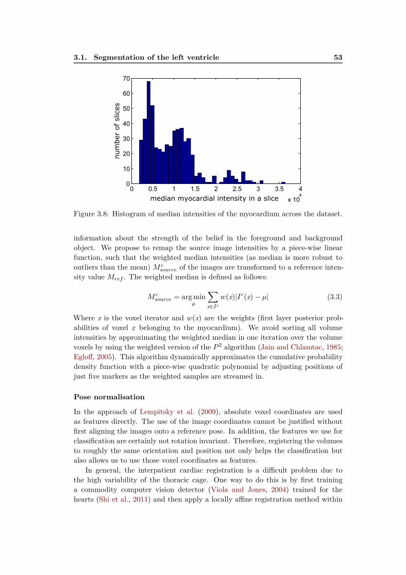
3.1. Segmentation of the left ventricle 53
0 0.5 1 1.5 2 2.5 3 3.5 4
x 104
0
10
20
30
40
50
60
70
median myocardial intensity in a slice
num
ber
of slices
Figure 3.8: Histogram of median intensities of the myocardium across the dataset.
information about the strength of the belief in the foreground and backgroundobject. We propose to remap the source image intensities by a piece-wise linearfunction, such that the weighted median intensities (as median is more robust tooutliers than the mean) M c
source of the images are transformed to a reference inten-sity value Mref . The weighted median is defined as follows:
M csource = arg min
µ
∑
x∈Ic
w(x)|Ic(x)− µ| (3.3)
Where x is the voxel iterator and w(x) are the weights (first layer posterior prob-abilities of voxel x belonging to the myocardium). We avoid sorting all volumeintensities by approximating the weighted median in one iteration over the volumevoxels by using the weighted version of the P 2 algorithm (Jain and Chlamtac, 1985;Egloff, 2005). This algorithm dynamically approximates the cumulative probabilitydensity function with a piece-wise quadratic polynomial by adjusting positions ofjust five markers as the weighted samples are streamed in.
Pose normalisation
In the approach of Lempitsky et al. (2009), absolute voxel coordinates are usedas features directly. The use of the image coordinates cannot be justified withoutfirst aligning the images onto a reference pose. In addition, the features we use forclassification are certainly not rotation invariant. Therefore, registering the volumesto roughly the same orientation and position not only helps the classification butalso allows us to use those voxel coordinates as features.
In general, the interpatient cardiac registration is a difficult problem due tothe high variability of the thoracic cage. One way to do this is by first traininga commodity computer vision detector (Viola and Jones, 2004) trained for thehearts (Shi et al., 2011) and then apply a locally affine registration method within

54 Chapter 3. Segmenting cardiac images with classification forests
this detected region followed by a non-rigid alignment. A robust learning based lin-ear inter-patient organ registration was proposed by Konukoglu et al. (2011). Here,each organ is represented with a smooth probability map fit to the bounding boxesobtained as a result of a regression forest. Then, registration of these probabilitymaps is performed. This representation of probabilities is however rather limitingas the boxes are axis-aligned and disregard the orientation that we would like tocorrect for.
We propose to rigidly align the myocardium enhanced first layer posterior prob-ability maps instead. For this step we use a fast and robust rigid block matchingregistration technique (Ourselin et al., 2000). The reference we used is chosen semi-randomly from images where the apex was at least partially present and closed. Aneven more automatic way to construct the reference such as an algorithm similarto Hoogendoorn et al. (2010) or a generative technique like described in Iglesiaset al. (2011) could be used.
To reduce the computational time, only probability maps of frames from themiddle of the sequence are used to estimate the intensity and pose transformations.The same transformations are then applied for all the frames and ground-truths inthe sequence which will be needed to train the second layer.
3.1.7 Second layer: Learning to segment with the shape
Retraining with pose and intensity-normalised images
Once the images are registered to a reference volume and intensities are standard-ised, we retrain a new classification forest. The voxel coordinates start to encodespatial relationships with respect to the reference coordinate frame and the coor-dinate features can be now included in training of the second decision forest layer.Moreover, if the intensity standardisation step succeeds, the intensities have moretissue specific meaning (at least for the myocardium).
Figure 3.9: Mid-cavity short (top) and artificial long (bottom) axis views on theposterior probabilities after the second layer. The predictions are clearly moreconfident and most of the remote misclassified voxels are now properly removed.
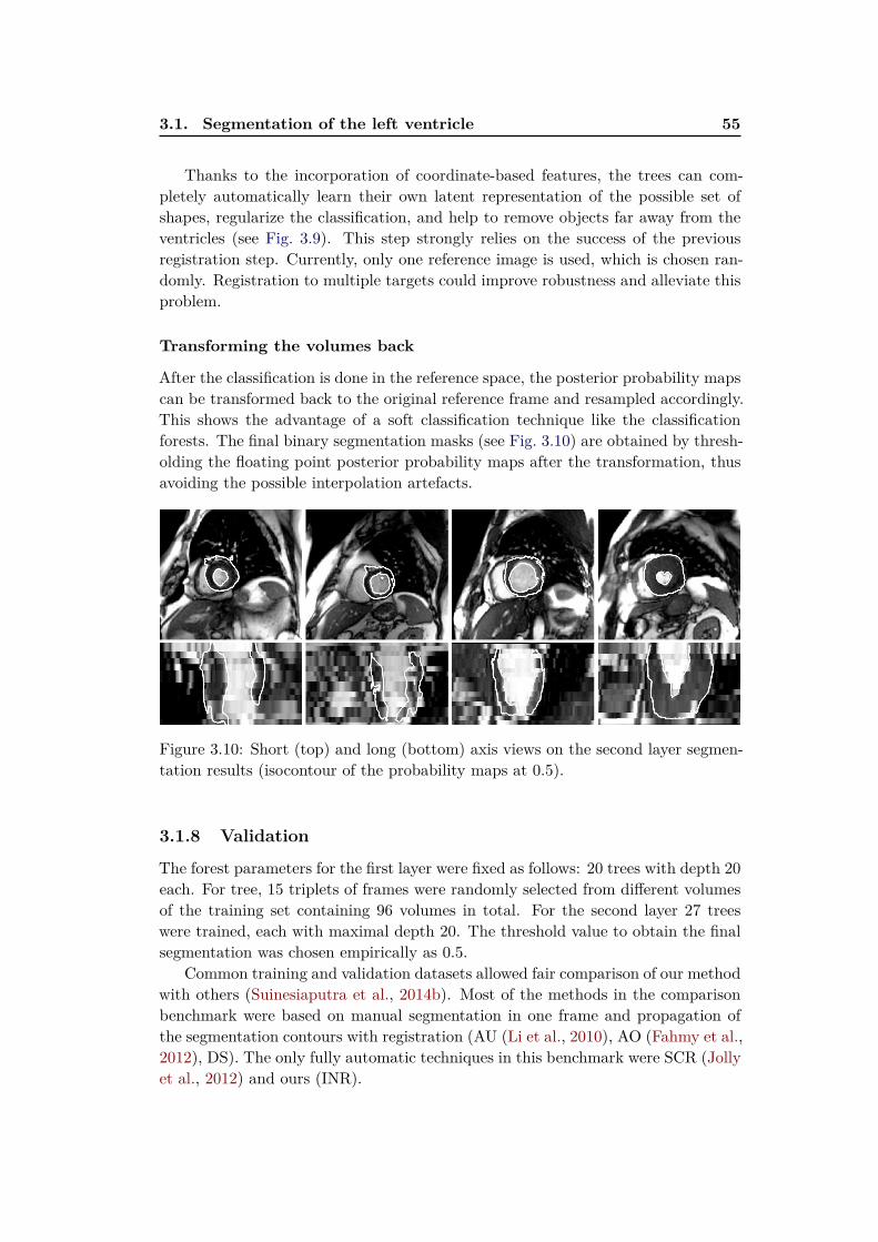
3.1. Segmentation of the left ventricle 55
Thanks to the incorporation of coordinate-based features, the trees can com-pletely automatically learn their own latent representation of the possible set ofshapes, regularize the classification, and help to remove objects far away from theventricles (see Fig. 3.9). This step strongly relies on the success of the previousregistration step. Currently, only one reference image is used, which is chosen ran-domly. Registration to multiple targets could improve robustness and alleviate thisproblem.
Transforming the volumes back
After the classification is done in the reference space, the posterior probability mapscan be transformed back to the original reference frame and resampled accordingly.This shows the advantage of a soft classification technique like the classificationforests. The final binary segmentation masks (see Fig. 3.10) are obtained by thresh-olding the floating point posterior probability maps after the transformation, thusavoiding the possible interpolation artefacts.
Figure 3.10: Short (top) and long (bottom) axis views on the second layer segmen-tation results (isocontour of the probability maps at 0.5).
3.1.8 Validation
The forest parameters for the first layer were fixed as follows: 20 trees with depth 20each. For tree, 15 triplets of frames were randomly selected from different volumesof the training set containing 96 volumes in total. For the second layer 27 treeswere trained, each with maximal depth 20. The threshold value to obtain the finalsegmentation was chosen empirically as 0.5.
Common training and validation datasets allowed fair comparison of our methodwith others (Suinesiaputra et al., 2014b). Most of the methods in the comparisonbenchmark were based on manual segmentation in one frame and propagation ofthe segmentation contours with registration (AU (Li et al., 2010), AO (Fahmy et al.,2012), DS). The only fully automatic techniques in this benchmark were SCR (Jollyet al., 2012) and ours (INR).
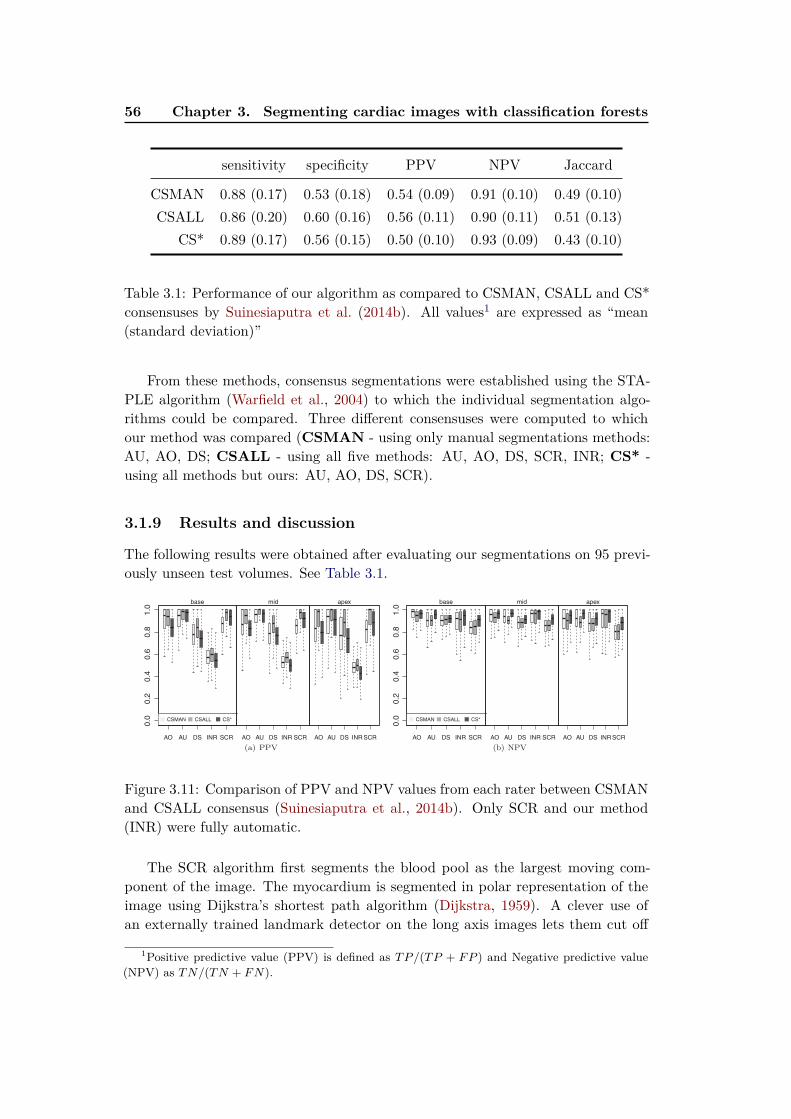
56 Chapter 3. Segmenting cardiac images with classification forests
sensitivity specificity PPV NPV Jaccard
CSMAN 0.88 (0.17) 0.53 (0.18) 0.54 (0.09) 0.91 (0.10) 0.49 (0.10)
CSALL 0.86 (0.20) 0.60 (0.16) 0.56 (0.11) 0.90 (0.11) 0.51 (0.13)
CS* 0.89 (0.17) 0.56 (0.15) 0.50 (0.10) 0.93 (0.09) 0.43 (0.10)
Table 3.1: Performance of our algorithm as compared to CSMAN, CSALL and CS*consensuses by Suinesiaputra et al. (2014b). All values1 are expressed as “mean(standard deviation)”
From these methods, consensus segmentations were established using the STA-PLE algorithm (Warfield et al., 2004) to which the individual segmentation algo-rithms could be compared. Three different consensuses were computed to whichour method was compared (CSMAN - using only manual segmentations methods:AU, AO, DS; CSALL - using all five methods: AU, AO, DS, SCR, INR; CS* -using all methods but ours: AU, AO, DS, SCR).
3.1.9 Results and discussion
The following results were obtained after evaluating our segmentations on 95 previ-ously unseen test volumes. See Table 3.1.
Figure 3.11: Comparison of PPV and NPV values from each rater between CSMANand CSALL consensus (Suinesiaputra et al., 2014b). Only SCR and our method(INR) were fully automatic.
The SCR algorithm first segments the blood pool as the largest moving com-ponent of the image. The myocardium is segmented in polar representation of theimage using Dijkstra’s shortest path algorithm (Dijkstra, 1959). A clever use ofan externally trained landmark detector on the long axis images lets them cut off
1Positive predictive value (PPV) is defined as TP/(TP + FP ) and Negative predictive value
(NPV) as TN/(TN + FN).
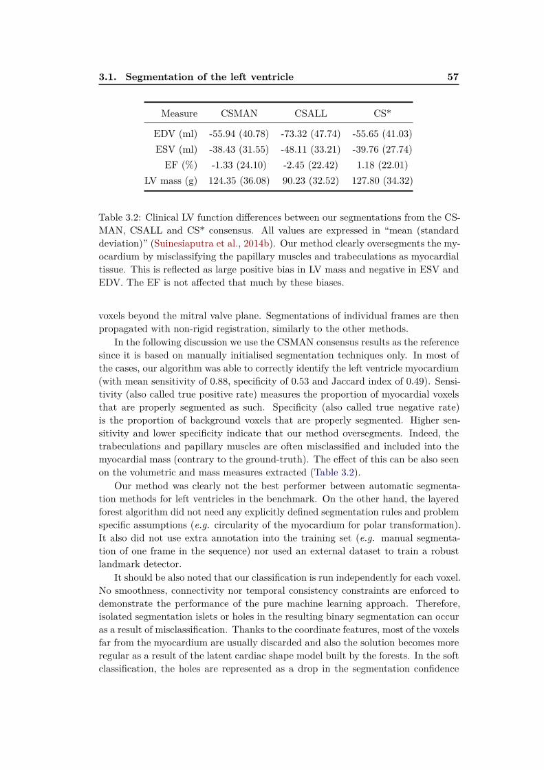
3.1. Segmentation of the left ventricle 57
Measure CSMAN CSALL CS*
EDV (ml) -55.94 (40.78) -73.32 (47.74) -55.65 (41.03)
ESV (ml) -38.43 (31.55) -48.11 (33.21) -39.76 (27.74)
EF (%) -1.33 (24.10) -2.45 (22.42) 1.18 (22.01)
LV mass (g) 124.35 (36.08) 90.23 (32.52) 127.80 (34.32)
Table 3.2: Clinical LV function differences between our segmentations from the CS-MAN, CSALL and CS* consensus. All values are expressed in “mean (standarddeviation)” (Suinesiaputra et al., 2014b). Our method clearly oversegments the my-ocardium by misclassifying the papillary muscles and trabeculations as myocardialtissue. This is reflected as large positive bias in LV mass and negative in ESV andEDV. The EF is not affected that much by these biases.
voxels beyond the mitral valve plane. Segmentations of individual frames are thenpropagated with non-rigid registration, similarly to the other methods.
In the following discussion we use the CSMAN consensus results as the referencesince it is based on manually initialised segmentation techniques only. In most ofthe cases, our algorithm was able to correctly identify the left ventricle myocardium(with mean sensitivity of 0.88, specificity of 0.53 and Jaccard index of 0.49). Sensi-tivity (also called true positive rate) measures the proportion of myocardial voxelsthat are properly segmented as such. Specificity (also called true negative rate)is the proportion of background voxels that are properly segmented. Higher sen-sitivity and lower specificity indicate that our method oversegments. Indeed, thetrabeculations and papillary muscles are often misclassified and included into themyocardial mass (contrary to the ground-truth). The effect of this can be also seenon the volumetric and mass measures extracted (Table 3.2).
Our method was clearly not the best performer between automatic segmenta-tion methods for left ventricles in the benchmark. On the other hand, the layeredforest algorithm did not need any explicitly defined segmentation rules and problemspecific assumptions (e.g. circularity of the myocardium for polar transformation).It also did not use extra annotation into the training set (e.g. manual segmenta-tion of one frame in the sequence) nor used an external dataset to train a robustlandmark detector.
It should be also noted that our classification is run independently for each voxel.No smoothness, connectivity nor temporal consistency constraints are enforced todemonstrate the performance of the pure machine learning approach. Therefore,isolated segmentation islets or holes in the resulting binary segmentation can occuras a result of misclassification. Thanks to the coordinate features, most of the voxelsfar from the myocardium are usually discarded and also the solution becomes moreregular as a result of the latent cardiac shape model built by the forests. In the softclassification, the holes are represented as a drop in the segmentation confidence
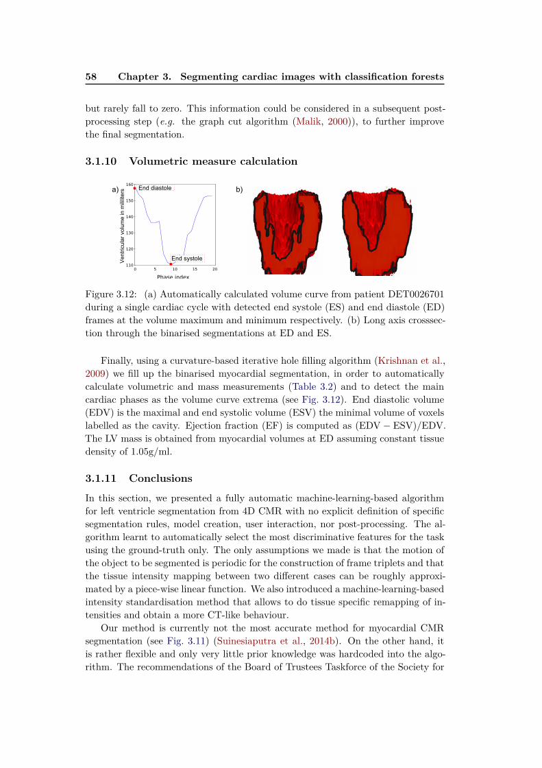
58 Chapter 3. Segmenting cardiac images with classification forests
but rarely fall to zero. This information could be considered in a subsequent post-processing step (e.g. the graph cut algorithm (Malik, 2000)), to further improvethe final segmentation.
3.1.10 Volumetric measure calculation
End diastole
End systoleVen
tricu
lar v
olum
e in
mili
liter
sa) b)
Figure 3.12: (a) Automatically calculated volume curve from patient DET0026701during a single cardiac cycle with detected end systole (ES) and end diastole (ED)frames at the volume maximum and minimum respectively. (b) Long axis crosssec-tion through the binarised segmentations at ED and ES.
Finally, using a curvature-based iterative hole filling algorithm (Krishnan et al.,2009) we fill up the binarised myocardial segmentation, in order to automaticallycalculate volumetric and mass measurements (Table 3.2) and to detect the maincardiac phases as the volume curve extrema (see Fig. 3.12). End diastolic volume(EDV) is the maximal and end systolic volume (ESV) the minimal volume of voxelslabelled as the cavity. Ejection fraction (EF) is computed as (EDV − ESV)/EDV.The LV mass is obtained from myocardial volumes at ED assuming constant tissuedensity of 1.05g/ml.
3.1.11 Conclusions
In this section, we presented a fully automatic machine-learning-based algorithmfor left ventricle segmentation from 4D CMR with no explicit definition of specificsegmentation rules, model creation, user interaction, nor post-processing. The al-gorithm learnt to automatically select the most discriminative features for the taskusing the ground-truth only. The only assumptions we made is that the motion ofthe object to be segmented is periodic for the construction of frame triplets and thatthe tissue intensity mapping between two different cases can be roughly approxi-mated by a piece-wise linear function. We also introduced a machine-learning-basedintensity standardisation method that allows to do tissue specific remapping of in-tensities and obtain a more CT-like behaviour.
Our method is currently not the most accurate method for myocardial CMRsegmentation (see Fig. 3.11) (Suinesiaputra et al., 2014b). On the other hand, itis rather flexible and only very little prior knowledge was hardcoded into the algo-rithm. The recommendations of the Board of Trustees Taskforce of the Society for
3.2. Left atrium segmentation 59
Cardiac Magnetic Resonance (SCMR) suggest excluding the trabeculations and pa-pilary muscles from the ventricular cavity and including them into the myocardialmass (Schulz-Menger et al., 2013). This is a challenging problem for the shape andregistration-based methods. In addition to the papillary muscles and the trabecu-lations, there are other important cardiac fine-scale anatomical structures (Lamataet al., 2014) and findings of interest. These also include small blood vessels, or hyper-intense scar regions in late enhanced MRI or pericardial effusion. In these cases,voxel-wise semantic segmentation techniques are likely a better solution. Onceenough examples of voxels belonging to these small structures are annotated in theground-truth, our method should be able to figure out how to discriminate themfrom other tissue, and segment these without much modification. This methodcould also be easily adapted to the segmentation of long axis views, usually 2D or2D+t sequences. In this case we could just replace the spatio-temporal boxes withspatio-temporal rectangles.
We will now show that our algorithm is also amenable to segment anotherimportant but large cardiac structure — the left atrium (LA).
3.2 Left atrium segmentation
The LA plays an important role in facilitating uninterrupted circulation of oxy-genated blood from pulmonary veins to the left ventricle and in cardiac electro-physiology. To quantify its function, simulate electrical wave propagation and de-termine the best location for ablation therapy, it is important to be able to firstaccurately segment the atrial contours. A common approach to segment the leftatrium from 3D images is to use statistical shape models (Kutra et al., 2012; Ecabertet al., 2008). A levelset-based method with a heuristic region split and merge strat-egy was proposed by Karim et al. (2007). Finally, label fusion techniques (Depaet al., 2010) seem to yield accurate atrial segmentations but require to non-rigidlyregister the image to be segmented to every training image. All of these methods arespecifically hand-crafted for atrial segmentation and thus treat the training set in aparticular way or need a set of non-rigid registrations which can be computationallyexpensive.
Similarly to our method for LV segmentation, we use a fully automated voxel-wise segmentation technique based on classification forests. This time, the problemis formulated as a binary classification between atrial and background voxels. Theadvantage of these approaches is that very few assumptions are necessary and it ispossible to learn how to segment directly from the image - label map pairs. Forthis method we do not use a robust registration method, build a statistical model,nor explicitly define the classification problem. We only require a larger number oftraining images with the atria carefully delineated and good blood pool contrast inthe images.
60 Chapter 3. Segmenting cardiac images with classification forests
3.2.1 Dataset
Compared to the LV segmentation, the dataset is much smaller in this case. TheSTACOM 2013 LA segmentation challenge dataset (Tobon-Gomez et al., 2013b)contains 30 CT and 30 MR images. Each of these sets was divided into a trainingset (10 3D volumes with voxel-wise LA segmentation maps) and a validation set(20 3D volumes with no delineation provided used for blind evaluation).
3.2.2 Preprocessing
The only preprocessing step is linear intensity rescaling of the 0 and 98.5 percentileimage range as done in the first layer of the LV segmentation. This was chosen tocut off high intensity variation due to noise and imaging artefacts, similarly to Nyúland Udupa (1999).
3.2.3 Training forests with boundary voxels
Training of decision forests is in general relatively fast as each tree can be learntindividually in parallel. To further cut down from the training time, and more im-portantly to better balance the background/atrium voxel proportion and to betterlearn how to classify voxels on the boundaries, we train only on some of the voxelsfrom the annotated training set. We include all atrial voxels in the training set aspositive examples. However, we subsample the negative example voxels. These aresampled only on a sparse regular grid. We also add all voxels in the immediateatrial neighbourhood (approximately 15 pixels thick, obtained by morphologicallydilating the atrial mask).
3.2.4 Segmentation phase
During the segmentation phase, each voxel of the test image is passed throughthe forest to reach a set of leaves. The average class distributions of all reachedleaves then represent the posterior probabilities of the voxel belonging to eitherthe atrium or the background given its appearance in the feature space. Thismeans that we obtain an atrial probability map for the whole volume. To obtainbinary masks required for evaluation in the benchmark study of Tobon-Gomezet al. (2015), we simply threshold the atrial probability maps with a fixed thresholdvalue. Afterwards, we apply simple morphological hole-filling and extract the largestconnected component which we deliver as the final binary atrial segmentation.
3.2.5 Additional channels for left atrial segmentation
To describe the appearance of each voxel and discriminate between the atrium andbackground we generate a random feature pool operating on the 3D images fromtwo feature families (local and context-rich) previously shown in Section 3.1.5 andin Geremia et al. (2011), but applied on three different image channels. These twofeature families capture both local and remote information about the tested voxel.

3.2. Left atrium segmentation 61
a) im age + gt b) blood pool c) distance d) tubularity
Figure 3.13: Image channels extracted from two example images. (a) Source imageoverlaid with the ground-truth segmentation. (b) Blood segmented with sequen-tially applied Otsu thresholding.(c) Distance to the blood contours.(d) Tubularityenhancing vascular structures (e.g. the strong signal in the aorta)
3.2.5.1 MR image intensity
Voxel intensity in combination with context rich features give wealth of informationabout its position. For example, regions of the bright atrium are located close tothe darker spine or lungs, and next to other bright cavities. It is however muchmore difficult to discriminate between voxels on the border between the atrium andthe ventricle as there is no clear intensity change (apart from occasional faint signaldrop from the mitral valve). Therefore, we extract the local and the context richfeatures not only on image intensity (Fig. 3.13a), but also add two other channels(see Fig. 3.13c and Fig. 3.13d).
3.2.5.2 Distance to blood pool contours
The atrium is always contained within the bright blood pool in the image. Thanksto the high contrast between the blood pool and the rest of the image, all blood canbe simply extracted by sequentially applying the thresholding algorithm of Otsu(1979). The first round divides image voxels into the black air and the brighterpart of the thorax. The second round splits the brighter part of the thorax into thevery bright blood and the rest (Fig. 3.13b).
We can observe that the atrium is mostly separated at blood pool narrowings(such as at the mitral plane or atrial septum). These can be located by measuringthe distance to blood pool contours as distance minima (Fig. 3.13c). Local maximaare, on the other hand, located near centres of blobs in the image such as the atrium.Therefore, similarly to Karim et al. (2007), we exploit these properties and computethe Euclidean distance to the blood pool surface for each voxel in the image (voxels
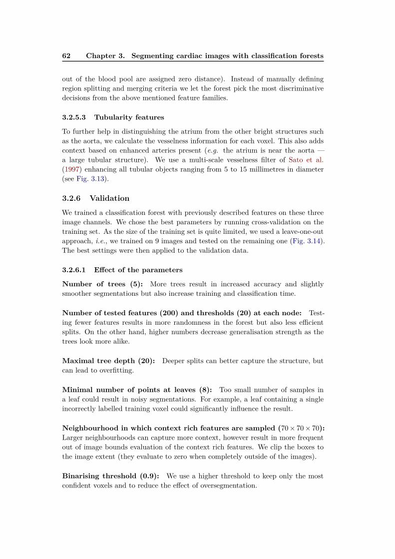
62 Chapter 3. Segmenting cardiac images with classification forests
out of the blood pool are assigned zero distance). Instead of manually definingregion splitting and merging criteria we let the forest pick the most discriminativedecisions from the above mentioned feature families.
3.2.5.3 Tubularity features
To further help in distinguishing the atrium from the other bright structures suchas the aorta, we calculate the vesselness information for each voxel. This also addscontext based on enhanced arteries present (e.g. the atrium is near the aorta —a large tubular structure). We use a multi-scale vesselness filter of Sato et al.(1997) enhancing all tubular objects ranging from 5 to 15 millimetres in diameter(see Fig. 3.13).
3.2.6 Validation
We trained a classification forest with previously described features on these threeimage channels. We chose the best parameters by running cross-validation on thetraining set. As the size of the training set is quite limited, we used a leave-one-outapproach, i.e., we trained on 9 images and tested on the remaining one (Fig. 3.14).The best settings were then applied to the validation data.
3.2.6.1 Effect of the parameters
Number of trees (5): More trees result in increased accuracy and slightlysmoother segmentations but also increase training and classification time.
Number of tested features (200) and thresholds (20) at each node: Test-ing fewer features results in more randomness in the forest but also less efficientsplits. On the other hand, higher numbers decrease generalisation strength as thetrees look more alike.
Maximal tree depth (20): Deeper splits can better capture the structure, butcan lead to overfitting.
Minimal number of points at leaves (8): Too small number of samples ina leaf could result in noisy segmentations. For example, a leaf containing a singleincorrectly labelled training voxel could significantly influence the result.
Neighbourhood in which context rich features are sampled (70× 70× 70):
Larger neighbourhoods can capture more context, however result in more frequentout of image bounds evaluation of the context rich features. We clip the boxes tothe image extent (they evaluate to zero when completely outside of the images).
Binarising threshold (0.9): We use a higher threshold to keep only the mostconfident voxels and to reduce the effect of oversegmentation.

3.2. Left atrium segmentation 63
Figure 3.14: Coronal, sagittal and axial views of the segmentation results on one ofthe test cases during the leave-one-out cross-validation. Top row: source image withground-truth, middle row: atrial probability map with contour of the probabilitymap at 0.6 (brighter values means more confidence in the segmentation), bottom:source image with overlaid ground-truth (green) and final segmentation after holefilling (red).

64 Chapter 3. Segmenting cardiac images with classification forests
3.2.7 Results and discussion
After the selection of parameters above via cross-validation we obtained a dicecoefficient 0.63± 0.14. This small forest of 5 trees took on average 2 hours to trainand just around a minute to fully automatically segment a single atrial MR imageon a 12 core Intel Xeon 3.3GHz CPU.
This algorithm performs reasonably well to extract the main part of the atrialvolume, its shortcomings are mainly in the segmentation of the pulmonary veinswhich are often missed or misclassified. The other main drawbacks of our method isthat that the segmentation contours do not necessarily adapt to the cavity contoursin the images (see Fig. 3.14).
3.2.7.1 Benchmark results
Tobon-Gomez et al. (2015) developed an elegant benchmarking framework for com-parison of the atrial segmentation for various parts of the LA. We submitted oursegmentation results from the MR images and ran almost the identical pipeline tosegment also the CT images. The comparison of all submitted methods on thewhole validation set for the LA body can be seen in Fig. 3.15.
0
0.1
0.2
0.3
0.4
0.5
0.6
0.7
0.8
0.9
1
BECHAR
INRIA
LTSI_VRG
LTSI_VSRG
LUB_SRG
LUB_SSM
SIE_PMB
SIE_MRG
TLEMCEN
UCL_1C
UCL_4C
OBS_2
(a) MRI
0
0.1
0.2
0.3
0.4
0.5
0.6
0.7
0.8
0.9
1
BECHAR
INRIA
LTSI_VRG
LTSI_VSRG
LUB_SRG
LUB_SSM
SIE_PMB
SIE_MRG
TLEMCEN
UCL_1C
UCL_4C
OBS_2
(b) CT
Figure 3.15: Boxplot of Dice coefficients for all methods in the benchmark (Tobon-Gomez et al., 2015). The dotted line represents the mean of medians of the bench-marked methods. Our method is listed as INRIA, OBS_2 is second rater.
3.2.8 Conclusions
We used our machine-learning-based image segmentation technique and extendedit with a set of image features to better distinguish vascular structures from therest of the blood pool. We then learnt to directly predict voxel labels (atrium /background) from the images without hand-tuning the segmentation pipeline. Ouronly assumptions were the strong blood pool contrast and the presence of tubularstructures in the images.
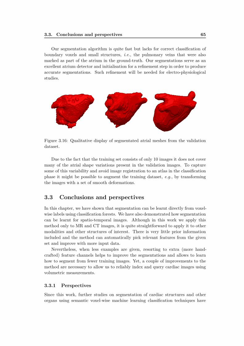
3.3. Conclusions and perspectives 65
Our segmentation algorithm is quite fast but lacks for correct classification ofboundary voxels and small structures, i.e., the pulmonary veins that were alsomarked as part of the atrium in the ground-truth. Our segmentations serve as anexcellent atrium detector and initialisation for a refinement step in order to produceaccurate segmentations. Such refinement will be needed for electro-physiologicalstudies.
Figure 3.16: Qualitative display of segmentated atrial meshes from the validationdataset.
Due to the fact that the training set consists of only 10 images it does not covermany of the atrial shape variations present in the validation images. To capturesome of this variability and avoid image registration to an atlas in the classificationphase it might be possible to augment the training dataset, e.g., by transformingthe images with a set of smooth deformations.
3.3 Conclusions and perspectives
In this chapter, we have shown that segmentation can be learnt directly from voxel-wise labels using classification forests. We have also demonstrated how segmentationcan be learnt for spatio-temporal images. Although in this work we apply thismethod only to MR and CT images, it is quite straightforward to apply it to othermodalities and other structures of interest. There is very little prior informationincluded and the method can automatically pick relevant features from the givenset and improve with more input data.
Nevertheless, when less examples are given, resorting to extra (more hand-crafted) feature channels helps to improve the segmentations and allows to learnhow to segment from fewer training images. Yet, a couple of improvements to themethod are necessary to allow us to reliably index and query cardiac images usingvolumetric measurements.
3.3.1 Perspectives
Since this work, further studies on segmentation of cardiac structures and otherorgans using semantic voxel-wise machine learning classification techniques have
66 Chapter 3. Segmenting cardiac images with classification forests
appeared. These include different sets of features or image channels to describe thevoxels (Mahapatra, 2014; Wang et al., 2014), to use more than two layers (Kerau-dren et al., 2014), to more intelligently select subsets example training images foreach tree (Lombaert et al., 2014), or to exploit also unlabelled data (Appendix A).Many ideas in these approaches are orthogonal to ours and could further help toimprove the quality of our segmentations. In Lombaert et al. (2014) alone, the Dicecoefficient increased from 66.6% up to 79% by smarter selection of training imagesubsets for each tree.
The use of classification forests for segmentation greatly simplifies the problem oflearning how to segment directly from voxel-wise ground-truth without hardcodingthe segmentation rules. Nevertheless, the algorithm still requires to define thefeature families and design image channels that enhance relevant regions, and toimprove the smoothness and contour matching. In addition, the tree structure isoptimised and fixed in the training.
For growing databases, when new training examples are continuously added intothe training set, the forest can be retrained from scratch or the leaf distributionscan be updated accordingly. The more recent CNN-based segmentation approaches(e.g. Long et al. (2015)), automatically learn optimal image channels to solve thesegmentation and can update the network parameters with SGD when new databecome available. Finally, Kontschieder et al. (2015) showed a hybrid approachwhere the classification forests are made differentiable and trained within a CNNusing backpropagation.
Chapter 4
Crowdsourcing semantic cardiac
attributes
Contents
4.1 Describing cardiac images . . . . . . . . . . . . . . . . . . . . 68
4.1.1 Non-semantic description of the hearts . . . . . . . . . . . . . 68
4.1.2 Semantic attributes . . . . . . . . . . . . . . . . . . . . . . . 69
4.2 Attributes for failing post-myocardial infarction hearts . . . 70
4.2.1 Pairwise comparisons for image annotation . . . . . . . . . . 72
4.2.2 Selected attributes for shape, motion and appearance . . . . 73
4.3 Crowdsourcing in medical imaging . . . . . . . . . . . . . . . 74
4.3.1 A ground-truth collection web application . . . . . . . . . . . 74
4.4 Learning attributes from pairwise comparisons . . . . . . . 74
4.5 Spectral description of cardiac shapes . . . . . . . . . . . . . 77
4.6 Texture features to describe image quality . . . . . . . . . . 78
4.7 Evaluation and results . . . . . . . . . . . . . . . . . . . . . . 78
4.7.1 Data and preprocessing . . . . . . . . . . . . . . . . . . . . . 78
4.7.2 Evaluation . . . . . . . . . . . . . . . . . . . . . . . . . . . . 79
4.8 Conclusions and perspectives . . . . . . . . . . . . . . . . . . 79
4.8.1 Perspectives . . . . . . . . . . . . . . . . . . . . . . . . . . . . 80
Based on our work in preparation for submission (Margeta et al., 2015b).
Chapter overview
In Chapter 2, we have shown how to automatically predict the CMR image viewinformation using CNNs. We can easily retrieve, for example, all short axis imageslices from the database. Automatic cardiac image segmentation methods (such asthe ones presented in Chapter 3) allow us to index and query the cardiac databasesusing simple geometric measurements, (e.g. cavity volumes, myocardial mass, orwall thickness). These two tools are important steps towards automated content-based image retrieval of cardiac images.
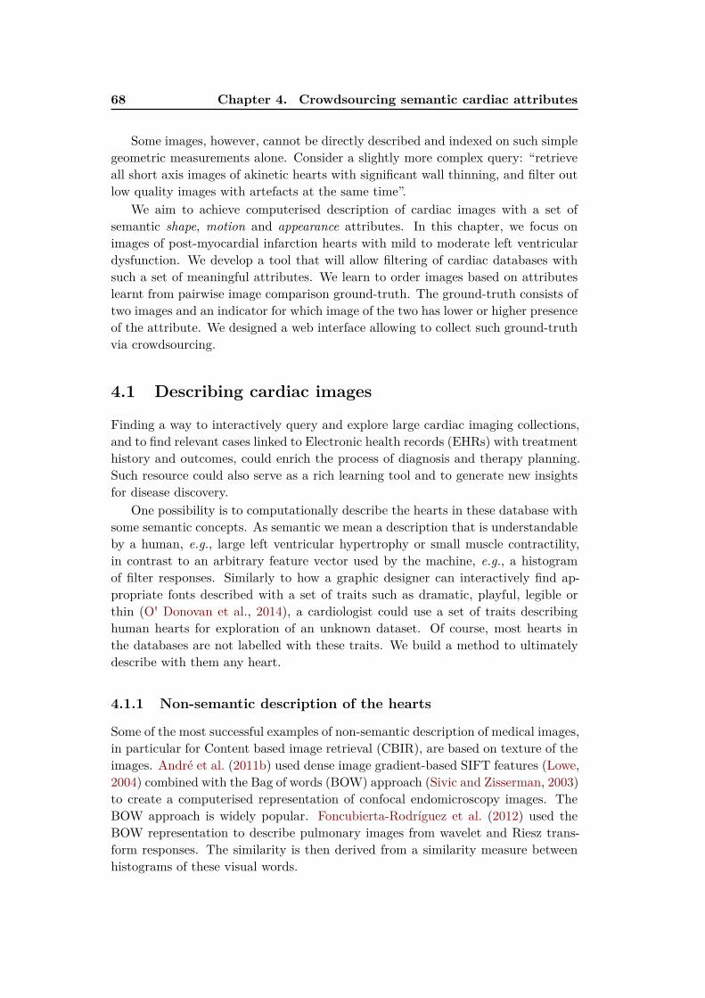
68 Chapter 4. Crowdsourcing semantic cardiac attributes
Some images, however, cannot be directly described and indexed on such simplegeometric measurements alone. Consider a slightly more complex query: “retrieveall short axis images of akinetic hearts with significant wall thinning, and filter outlow quality images with artefacts at the same time”.
We aim to achieve computerised description of cardiac images with a set ofsemantic shape, motion and appearance attributes. In this chapter, we focus onimages of post-myocardial infarction hearts with mild to moderate left ventriculardysfunction. We develop a tool that will allow filtering of cardiac databases withsuch a set of meaningful attributes. We learn to order images based on attributeslearnt from pairwise image comparison ground-truth. The ground-truth consists oftwo images and an indicator for which image of the two has lower or higher presenceof the attribute. We designed a web interface allowing to collect such ground-truthvia crowdsourcing.
4.1 Describing cardiac images
Finding a way to interactively query and explore large cardiac imaging collections,and to find relevant cases linked to Electronic health records (EHRs) with treatmenthistory and outcomes, could enrich the process of diagnosis and therapy planning.Such resource could also serve as a rich learning tool and to generate new insightsfor disease discovery.
One possibility is to computationally describe the hearts in these database withsome semantic concepts. As semantic we mean a description that is understandableby a human, e.g., large left ventricular hypertrophy or small muscle contractility,in contrast to an arbitrary feature vector used by the machine, e.g., a histogramof filter responses. Similarly to how a graphic designer can interactively find ap-propriate fonts described with a set of traits such as dramatic, playful, legible orthin (O' Donovan et al., 2014), a cardiologist could use a set of traits describinghuman hearts for exploration of an unknown dataset. Of course, most hearts inthe databases are not labelled with these traits. We build a method to ultimatelydescribe with them any heart.
4.1.1 Non-semantic description of the hearts
Some of the most successful examples of non-semantic description of medical images,in particular for Content based image retrieval (CBIR), are based on texture of theimages. André et al. (2011b) used dense image gradient-based SIFT features (Lowe,2004) combined with the Bag of words (BOW) approach (Sivic and Zisserman, 2003)to create a computerised representation of confocal endomicroscopy images. TheBOW approach is widely popular. Foncubierta-Rodríguez et al. (2012) used theBOW representation to describe pulmonary images from wavelet and Riesz trans-form responses. The similarity is then derived from a similarity measure betweenhistograms of these visual words.

4.1. Describing cardiac images 69
These systems work particularly well for images where the semantic gap (thedifference between the information captured with the extracted features and theexpert similarity) is quite small. Except for some measures simple to obtain fromimage segmentation (such as cardiac volumes, muscle masses or myocardial wallthickness) the semantic gap in cardiac imaging can be a real challenge.
In cardiac imaging, Glatard et al. (2004) extracted texture-based features topre-segment the images and to find similarly segmented cardiac slices. Eslami et al.(2012) used a binary cardiac segmentation overlap measure to query a database ofalready segmented images for the closest match and to guide their segmentationalgorithm.
Numerous feature representations have been used to characterise cardiac shapes(Bernardis et al., 2012; Zhang et al., 2014b; Le Folgoc et al., 2013; Medrano-Graciaet al., 2014), and cardiac motion (Duchateau et al., 2011; Mantilla et al., 2013;McLeod et al., 2015), in order to discriminate between normal and abnormal cases.An interesting way to compare cardiac shape differences due to the remodelling wasproposed by Medrano-Gracia et al. (2014) and by Zhang et al. (2014b). These atlasbased methods look at differences in the principal modes of shape variation (theLV is represented with a personalised finite element model) between two differentcardiac cohorts. Zhang et al. (2014b) compared shapes of infarcted hearts againstasymptomatic volunteers. The left ventricle shapes at both systole and diastolewere then described with up to 20 parameters, the first 20 modes best explainingthe shape variation. This approach discovered statistically significant shape changesbetween the two cohorts that are not simple to capture otherwise.
A search for images with similar or greater value of the 5th mode of variation forexample is not very intuitive though. Links of the modes of variation to semanticattributes of the heart (first mode linked to the size of the LV, second mode to thesphericity of the ventricle, and the third to the mitral valve orientation) were founda posteriori, by observation.
4.1.2 Semantic attributes
Sphericity has been previously linked to long term survival (Wong et al., 2015).Semantic descriptions like this one are commonly seen in the clinical journals, how-ever, their computational definition is often challenging or ambiguous. Nevertheless,even simpler attributes commonly used to describe the hearts (such as the hypertro-
phy) are often not straightforward to compute automatically. For example, considerassigning the value of hypertrophy to be a number between 0 and 100, where 0 isa normal heart and 100 is an extreme case where the myocardium even in relaxedstate leaves little space for the cavity.
André et al. (2011b) proposed an interesting way of retrieving similar sequencesfrom endomicroscopic videos of the colon by first computing a Bag of words (BOW)representation from dense textural descriptions of the image. Then, they mappedthe histograms of visual words to a semantically meaningful description (Andréet al., 2012) helping with interpretation of the images.

70 Chapter 4. Crowdsourcing semantic cardiac attributes
Quantifying concepts such as the degree of remodelling is quite challenging.Zhang et al. (2014b) used logistic regression to discriminate healthy from infarctedhearts from the modes of shape variation as a feature vector. Instead of the binaryclassification of the hearts, the learnt weights of the linear projector in the logisticregression could be used to obtain a measure of remodelling.
Learning a linear model that projects the extracted features to semantic at-tributes is similar to our work in this chapter. The attributes are very differentfrom classses. Classes are discrete (e.g. normal, hypoplastic left heart syndrom,Tetralogy of Fallot heart) and they do not even have ordinal relation, attributes arecontinuous (more or less dilated, more or less spherical, more or less akinetic). Inmany ways, attributes are related to a regression type of task.
We aim to describe at least some of the aspects of post-myocardial infarctionhearts and use the extracted values to filter the dataset. We learn to regress theseattributes from pairwise comparisons using machine learning tools used in webranking. First, let’s have a look, which characteristics of the hearts are the mostfrequently present in the database (Kadish et al., 2009).
4.2 Attributes for failing post-myocardial infarction hearts
Following myocardial infarct, the hearts have several compensatory remodellingmechanisms in play. As a consequence of the myocardial infarction and the loss ofviable tissue, myocardial cells are corrupted by the synthesis of interstitial fibrillarcollagen. The affected myocardial wall becomes thinner (Figure 4.1) and stiffer
(Mihl et al., 2008). The overall kineticity1 of the heart becomes compromised.
Figure 4.1: Thinning of the lateral wall due to transmural post-infarction necrosis.
To deal with pressure overload secondary to conditions such as aortic stenosis or1The kineticity can be seen as a continuous extension of the discrete clinical labels: hyperkinetic,
normokinetic, hypokinetic, akinetic, or dyskinetic
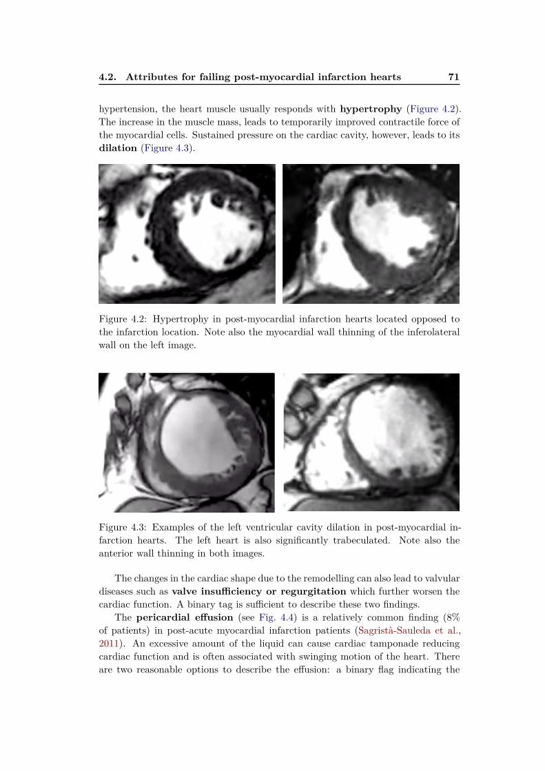
4.2. Attributes for failing post-myocardial infarction hearts 71
hypertension, the heart muscle usually responds with hypertrophy (Figure 4.2).The increase in the muscle mass, leads to temporarily improved contractile force ofthe myocardial cells. Sustained pressure on the cardiac cavity, however, leads to itsdilation (Figure 4.3).
Figure 4.2: Hypertrophy in post-myocardial infarction hearts located opposed tothe infarction location. Note also the myocardial wall thinning of the inferolateralwall on the left image.
Figure 4.3: Examples of the left ventricular cavity dilation in post-myocardial in-farction hearts. The left heart is also significantly trabeculated. Note also theanterior wall thinning in both images.
The changes in the cardiac shape due to the remodelling can also lead to valvulardiseases such as valve insufficiency or regurgitation which further worsen thecardiac function. A binary tag is sufficient to describe these two findings.
The pericardial effusion (see Fig. 4.4) is a relatively common finding (8%of patients) in post-acute myocardial infarction patients (Sagristà-Sauleda et al.,2011). An excessive amount of the liquid can cause cardiac tamponade reducingcardiac function and is often associated with swinging motion of the heart. Thereare two reasonable options to describe the effusion: a binary flag indicating the

72 Chapter 4. Crowdsourcing semantic cardiac attributes
Figure 4.4: Pericardial effusion — fluid built up in the sac around the heart. Thisis often seen as a bright ring around the heart. The effusion can be easily confusedwith pericardial fat.
presence or absence of the effusion, or a real value quantifying the amount of thepericardial fluid.
4.2.1 Pairwise comparisons for image annotation
Most of the attributes are continuous. Unless these are derived from well definedmeasures, expert annotations of such values can differ from centre to centre. It isoften much simpler to visualise two cardiac images side by side and let the expertchoose which of the two hearts has a more dominant presence of the attribute, e.g.,“heart on the left has more hypertrophy than heart on the right” (see Fig. 4.5).
Learning continuous attributes (scores) from pairwise comparisons is a powerfultechnique to deal with the attribute value assignment from multiple experts (or lessexperienced annotators, such as students of cardiology). The effect of inter-expertvariability will likely be smaller than if assigning an absolute score in isolation.
The consistency of pairwise annotations between different centres and differentexperts has been recently shown by Burggraaff et al. (2015). The experts viewedpairs of videos of multiple sclerosis patients doing standardised actions. For thevideo pairs, the experts indicated if the patients were performing equally or oneof them had poorer performance. TrueSkillTM (Herbrich et al., 2007; Dangauthieret al., 2007) algorithm, was then used to learn continuous scores (and confidencesin them) from the pairwise comparisons for each video. This simple Bayesian modelis used daily by millions of people playing Xbox online games for matching playersof similar skills. Finding opponents with similar skills from as few matching trialsas possible is important for fun and engaging games, and faster and more accurateskill estimation. In the case of pairwise medical sequence annotation, proposingmatching videos is important for faster (less burden on the annotators) and moreaccurate clinical score/attribute predictions.
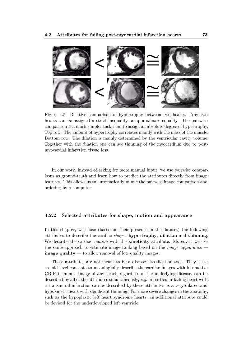
4.2. Attributes for failing post-myocardial infarction hearts 73
<
< ≅≅
Figure 4.5: Relative comparison of hypertrophy between two hearts. Any twohearts can be assigned a strict inequality or approximate equality. The pairwisecomparison is a much simpler task than to assign an absolute degree of hypertrophy,Top row: The amount of hypertrophy correlates mainly with the mass of the muscle.Bottom row: The dilation is mainly determined by the ventricular cavity volume.Together with the dilation one can see thinning of the myocardium due to post-myocardial infarction tissue loss.
In our work, instead of asking for more manual input, we use pairwise compar-isons as ground-truth and learn how to predict the attributes directly from imagefeatures. This allows us to automatically mimic the pairwise image comparison andordering by a computer.
4.2.2 Selected attributes for shape, motion and appearance
In this chapter, we chose (based on their presence in the dataset) the followingattributes to describe the cardiac shape: hypertrophy, dilation and thinning.We describe the cardiac motion with the kineticity attribute. Moreover, we usethe same approach to estimate image ranking based on the image appearance —image quality — to allow removal of low quality images.
These attributes are not meant to be a disease classification tool. They serveas mid-level concepts to meaningfully describe the cardiac images with interactiveCBIR in mind. Image of any heart, regardless of the underlying disease, can bedescribed by all of the attributes simultaneously, e.g., a particular failing heart witha transmural infarction can be described by these attributes as a very dilated andhypokinetic heart with significant thinning. For more severe changes in the anatomy,such as the hypoplastic left heart syndrome hearts, an additional attribute couldbe devised for the underdeveloped left ventricle.
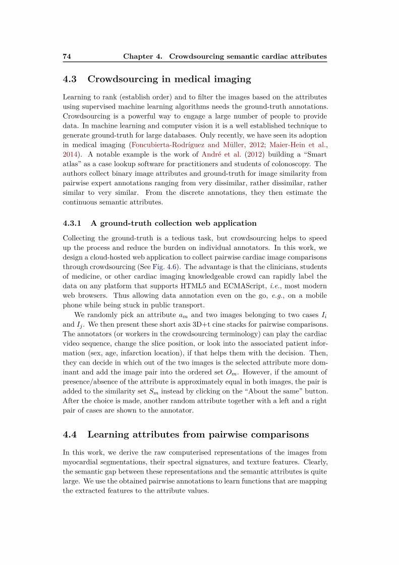
74 Chapter 4. Crowdsourcing semantic cardiac attributes
4.3 Crowdsourcing in medical imaging
Learning to rank (establish order) and to filter the images based on the attributesusing supervised machine learning algorithms needs the ground-truth annotations.Crowdsourcing is a powerful way to engage a large number of people to providedata. In machine learning and computer vision it is a well established technique togenerate ground-truth for large databases. Only recently, we have seen its adoptionin medical imaging (Foncubierta-Rodríguez and Müller, 2012; Maier-Hein et al.,2014). A notable example is the work of André et al. (2012) building a “Smartatlas” as a case lookup software for practitioners and students of colonoscopy. Theauthors collect binary image attributes and ground-truth for image similarity frompairwise expert annotations ranging from very dissimilar, rather dissimilar, rathersimilar to very similar. From the discrete annotations, they then estimate thecontinuous semantic attributes.
4.3.1 A ground-truth collection web application
Collecting the ground-truth is a tedious task, but crowdsourcing helps to speedup the process and reduce the burden on individual annotators. In this work, wedesign a cloud-hosted web application to collect pairwise cardiac image comparisonsthrough crowdsourcing (See Fig. 4.6). The advantage is that the clinicians, studentsof medicine, or other cardiac imaging knowledgeable crowd can rapidly label thedata on any platform that supports HTML5 and ECMAScript, i.e., most modernweb browsers. Thus allowing data annotation even on the go, e.g., on a mobilephone while being stuck in public transport.
We randomly pick an attribute am and two images belonging to two cases Iiand Ij . We then present these short axis 3D+t cine stacks for pairwise comparisons.The annotators (or workers in the crowdsourcing terminology) can play the cardiacvideo sequence, change the slice position, or look into the associated patient infor-mation (sex, age, infarction location), if that helps them with the decision. Then,they can decide in which out of the two images is the selected attribute more dom-inant and add the image pair into the ordered set Om. However, if the amount ofpresence/absence of the attribute is approximately equal in both images, the pair isadded to the similarity set Sm instead by clicking on the “About the same” button.After the choice is made, another random attribute together with a left and a rightpair of cases are shown to the annotator.
4.4 Learning attributes from pairwise comparisons
In this work, we derive the raw computerised representations of the images frommyocardial segmentations, their spectral signatures, and texture features. Clearly,the semantic gap between these representations and the semantic attributes is quitelarge. We use the obtained pairwise annotations to learn functions that are mappingthe extracted features to the attribute values.
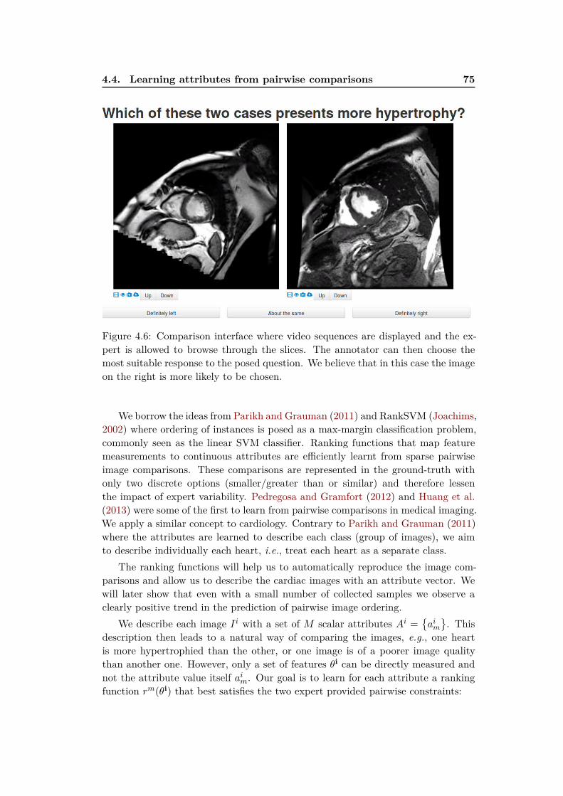
4.4. Learning attributes from pairwise comparisons 75
Figure 4.6: Comparison interface where video sequences are displayed and the ex-pert is allowed to browse through the slices. The annotator can then choose themost suitable response to the posed question. We believe that in this case the imageon the right is more likely to be chosen.
We borrow the ideas from Parikh and Grauman (2011) and RankSVM (Joachims,2002) where ordering of instances is posed as a max-margin classification problem,commonly seen as the linear SVM classifier. Ranking functions that map featuremeasurements to continuous attributes are efficiently learnt from sparse pairwiseimage comparisons. These comparisons are represented in the ground-truth withonly two discrete options (smaller/greater than or similar) and therefore lessenthe impact of expert variability. Pedregosa and Gramfort (2012) and Huang et al.(2013) were some of the first to learn from pairwise comparisons in medical imaging.We apply a similar concept to cardiology. Contrary to Parikh and Grauman (2011)where the attributes are learned to describe each class (group of images), we aimto describe individually each heart, i.e., treat each heart as a separate class.
The ranking functions will help us to automatically reproduce the image com-parisons and allow us to describe the cardiac images with an attribute vector. Wewill later show that even with a small number of collected samples we observe aclearly positive trend in the prediction of pairwise image ordering.
We describe each image Ii with a set of M scalar attributes Ai =
aim
. Thisdescription then leads to a natural way of comparing the images, e.g., one heartis more hypertrophied than the other, or one image is of a poorer image qualitythan another one. However, only a set of features θi can be directly measured andnot the attribute value itself aim. Our goal is to learn for each attribute a rankingfunction rm(θi) that best satisfies the two expert provided pairwise constraints:
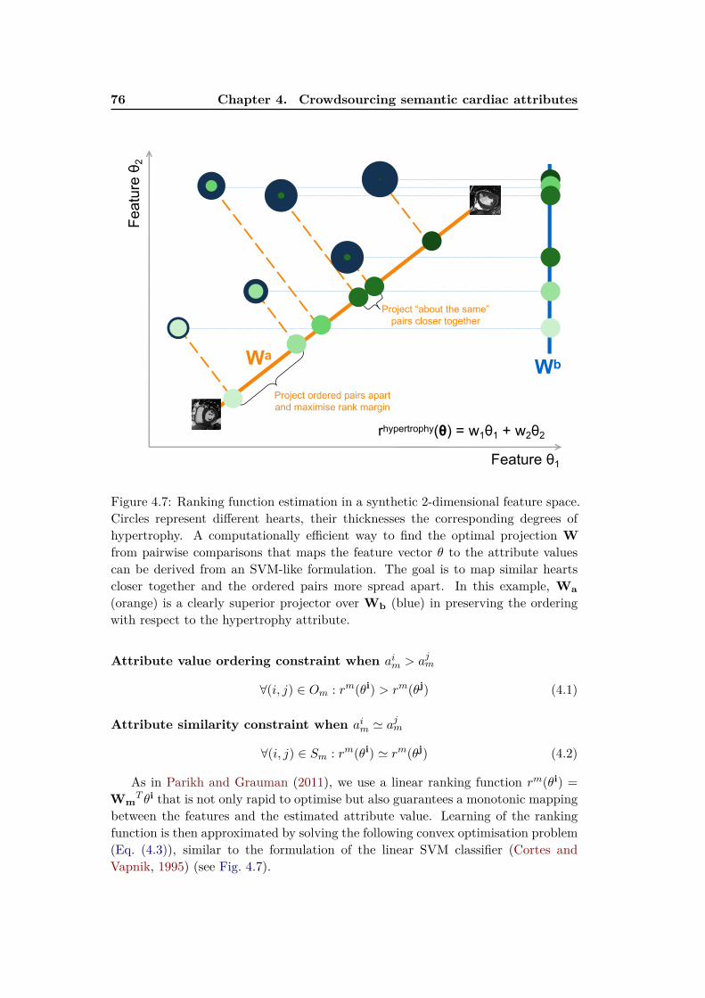
76 Chapter 4. Crowdsourcing semantic cardiac attributes
Feature θ1
Project ordered pairs apartand maximise rank margin
Project “about the same”pairs closer together
Feat
ure θ 2
WbWa
rhypertrophy(θ) = w1θ1 + w2θ2
Figure 4.7: Ranking function estimation in a synthetic 2-dimensional feature space.Circles represent different hearts, their thicknesses the corresponding degrees ofhypertrophy. A computationally efficient way to find the optimal projection Wfrom pairwise comparisons that maps the feature vector θ to the attribute valuescan be derived from an SVM-like formulation. The goal is to map similar heartscloser together and the ordered pairs more spread apart. In this example, Wa(orange) is a clearly superior projector over Wb (blue) in preserving the orderingwith respect to the hypertrophy attribute.
Attribute value ordering constraint when aim > ajm
∀(i, j) ∈ Om : rm(θi) > rm(θj) (4.1)
Attribute similarity constraint when aim ≃ ajm
∀(i, j) ∈ Sm : rm(θi) ≃ rm(θj) (4.2)
As in Parikh and Grauman (2011), we use a linear ranking function rm(θi) =Wm
T θi that is not only rapid to optimise but also guarantees a monotonic mappingbetween the features and the estimated attribute value. Learning of the rankingfunction is then approximated by solving the following convex optimisation problem(Eq. (4.3)), similar to the formulation of the linear SVM classifier (Cortes andVapnik, 1995) (see Fig. 4.7).
4.5. Spectral description of cardiac shapes 77
Wm = argmin(
1
2∥Wm∥
22 + CO
∑
ξij2 + CS
∑
γij2
)
subject to WTm(
θi − θj) ≥ 1− ξij; ∀ (i, j) ∈ Om∣
∣WTm(
θi − θj)∣∣ ≤ γij; ∀ (i, j) ∈ Sm
ξij ≥ 0; γij ≥ 0
(4.3)
Here, CO and CS are the trade-offs between margin maximisation between theranked points and satisfying the pairwise ordering constraints (CO) and pairwisesimilarity (CS) constraints provided by the experts. The slack variables ξij and γijare penalties for incorrect ranking.
4.5 Spectral description of cardiac shapes
If we consider the heart as a binary object on a closed and bounded domain Ω ⊂ Rd,it can be represented with its spectral signature. In essence, the spectral signatureis representing the hearts’ modes of vibration, similar to how a drum membranewould vibrate when hit by a stick. This has been used to globally describe theintrinsic geometry of the heart shape and to discriminate between healthy heartsand repaired tetralogy of Fallot patients (Bernardis et al., 2012; Konukoglu et al.,2012), and similarly by Lombaert et al. (2012) to establish better correspondencesfor inter-patient cardiac image registration. The main advantage of this methodover the traditionally used active shape methods is that no shape correspondencesare required. The description is also invariant to rigid transformations.
The spectral signature is determined by the spectrum of the Laplace operator∆Ω defined on a domain Ω as shown in Eq. (4.4).
∆Ωf ≜∑
i=1
∂2
∂x2if, ∀x ∈ Ω (4.4)
Eigenvalues λi and eigenfunctions fi of the operator ∆Ω are solutions of theHelmholtz equation with Dirichlet type boundary conditions, ∂Ω is the object’sboundary and x are the image coordinates.
∆f = λf ∀x ∈ Ω, ∀x ∈ ∂Ω, f (x) = 0 (4.5)
There are infinitely many pairs (λi, fi) that satisfy this equation. The spectralshape description is formed by ordering N smallest eigenvalues such that 0 < λ1 <
· · · < λN .In our case, we describe mid-cavity slices of each heart by the 100 smallest
eigenvalues of the spectrum; separately for the cavity and the myocardium at theend-diastolic and end-systolic frame. We concatenate these vectors and call it θs100in the evaluation. We also compute temporal volume curves of the cavity blood pooland the mass of the myocardium. We concatenate these measurements with thespectral feature vector and obtain the final shape vector θs100,vm. Please note that
78 Chapter 4. Crowdsourcing semantic cardiac attributes
we use manual segmentations in this work to discount the effect of bad automaticsegmentation. There is a large body of work on automatic or semi-automatic cardiacimage segmentation (see Section 3.1 for a brief overview). Any sufficiently accurateand regularised segmentation method can be used to extract the binary masks ofthe myocardium and the blood pool for the spectral representation.
4.6 Texture features to describe image quality
Images corrupted by the imaging artefacts might be required to be removed (Marko-nis et al., 2012) from the retrieval results. Twelve criteria were proposed by Klinkeet al. (2013) to assess the CMR image quality based on the present artefacts. Theseinclude banding or field of view wrap-around artefacts (often seen as dark curvedlines across the images), respiratory and cardiac motion ghosting (replication ofthoracic structures), mistriggering (image blurring), metal artefacts (changes ofmagnetic field homogeneity, e.g., around sternal wires), shimming artefacts (darkbands across the image caused by off-resonance) and flow related artefacts.
The spectral shape or volumetric features described above are not capturing anyof this information. We assume that the main information about image quality canbe inferred from the texture statistics of the images. To capture this informationwe use the first thirteen textural features defined by Haralick et al. (1973).Haralickfeatures are a set of measures (such as contrast, entropy, or variance) on localgrayscale co-occurrence matrices. These features make our texture feature vector θh.
4.7 Evaluation and results
The goal of relative attributes is to establish pairwise comparisons between anypair of images, and then be able to order them with respect to the attribute ofchoice.The absolute ground-truth values aleft,gt and aright,gt and not known exceptfor their relative ordering. As we do not have a global ordering nor the value of theattributes as ground-truth, we report average success rate of order prediction forimage pairs simply as S = P/(P +Q). Where P is the number of concordant pairs,i.e., pairs where the the estimated pairwise comparison of the left and right imagesrleft < rright is in agreement with the ground-truth comparison aleft,gt < aright,gt
for a particular attribute. Q is the number of discordant pairs, i.e., pairs where theestimated and ground-truth comparisons differ from the prediction. We ignore ties(pairs labelled as “about the same”) in the evaluation.
4.7.1 Data and preprocessing
The data used in this study consists of 96 post myocardial infarction acquisitionsof short axis Steady State Free Precession (SSFP) 3D+t stack of varying resolutionand image quality from the DETERMINE dataset (Kadish et al., 2009). We usethe manual expert segmentations of the LV myocardium.
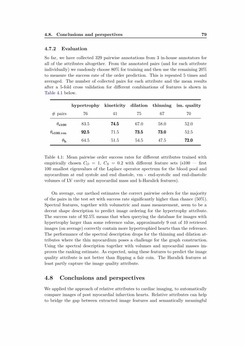
4.8. Conclusions and perspectives 79
4.7.2 Evaluation
So far, we have collected 329 pairwise annotations from 3 in-house annotators forall of the attributes altogether. From the annotated pairs (and for each attributeindividually) we randomly choose 80% for training and then use the remaining 20%to measure the success rate of the order prediction. This is repeated 5 times andaveraged. The number of collected pairs for each attribute and the mean resultsafter a 5-fold cross validation for different combinations of features is shown inTable 4.1 below.
hypertrophy kineticity dilation thinning im. quality
# pairs 76 41 75 67 70
θs100 83.5 74.574.574.5 67.0 58.0 52.0
θs100,vm 92.592.592.5 71.5 73.573.573.5 73.073.073.0 52.5
θh 64.5 51.5 54.5 47.5 72.072.072.0
Table 4.1: Mean pairwise order success rates for different attributes trained withempirically chosen CO = 1, CS = 0.2 with different feature sets (s100 — first100 smallest eigenvalues of the Laplace operator spectrum for the blood pool andmyocardium at end systole and end diastole, vm - end-systolic and end-diastolicvolumes of LV cavity and myocardial mass and h-Haralick features).
On average, our method estimates the correct pairwise orders for the majorityof the pairs in the test set with success rate significantly higher than chance (50%).Spectral features, together with volumetric and mass measurement, seem to be adecent shape description to predict image ordering for the hypertrophy attribute.The success rate of 92.5% means that when querying the database for images withhypertrophy larger than some reference value, approximately 9 out of 10 retrievedimages (on average) correctly contain more hypertrophied hearts than the reference.The performance of the spectral description drops for the thinning and dilation at-tributes where the thin myocardium poses a challenge for the graph construction.Using the spectral description together with volumes and myocardial masses im-proves the ranking estimate. As expected, using these features to predict the imagequality attribute is not better than flipping a fair coin. The Haralick features atleast partly capture the image quality attribute.
4.8 Conclusions and perspectives
We applied the approach of relative attributes to cardiac imaging, to automaticallycompare images of post myocardial infarction hearts. Relative attributes can helpto bridge the gap between extracted image features and semantically meaningful
80 Chapter 4. Crowdsourcing semantic cardiac attributes
descriptions of the images. In our preliminary study, we obtained encouragingpairwise image ordering based on the estimated semantic attribute values. However,collecting a much larger training set and/or better features will be needed to capturethe continuous attribute values, to extrapolate to extreme values of the attributes,and to completely sort the dataset.
In this study, the attributes were global, without any spatial information. Thisdescription is invariant to the underlying cardiac condition and by adding extraattributes it should be possible to extend this work to more complex pathologies.For a congenital heart disease, such as the Tetralogy of Fallot (TOF), relevant at-tributes describing the right ventricle, the pulmonary valve, and the ventricularseptum should be added. Here, we would likely discover that in general the rightventricles are more dilated and hypertrophied than normal hearts. This approachalso opens up possibilities for faster creation cohorts for studies using the attributevalues, e.g., select hearts with a hypertrophy larger than some reference case andwith sufficiently high image quality. We also have to remind the reader that describ-ing cardiac images without any motion information is not ideal. Adding motioncould help us to introduce attributes such as asynchrony, stiffness, and contractility,or better estimate the kineticity of the myocardium. Also, although linear rankingfunctions are very fast to train and test, they might not create the most optimalmappings between the features and attributes.
4.8.1 Perspectives
We developed a crowdsourcing platform to start collecting ground-truth in cardiol-ogy. Once more annotations from several experts are collected, it might be possibleto compare rankings of different experts and weigh their contributions in the costfunction accordingly. The more certain decisions usually happen much faster. Thetime to decide could therefore be used as the decision strength.
Further improvements can be done to reduce the required annotators’ time.Smarter choices of the image pair — attribute triplets could be done by presentingthe most similar images (Tamuz and Belongie, 2011) and to avoid annotating theobvious cases. Currently, the annotators are free to ignore the transitive relationsbetween the annotated images (if A is greater than B, and B is greater than C, Adoes not have to be annotated as being greater than C). Therefore, probabilisticmodelling of the attributes and their comparisons (e.g., as done with TrueSkillin Burggraaff et al. (2015); Herbrich et al. (2007)) should be explored. It would beuseful to have a measure of confidence in the attribute and to decide, which casesneed more input and which attributes are less certain. A gamified interface (vonAhn and Dabbish, 2004) should be designed to improve engagement and learningof the annotators.
Approaches like this one will help to reduce the semantic gap and enable naturallanguage queries of the databases, e.g., Retrieve images like this one, but with amore dilated ventricle and with higher image quality. They also allow us to retrievethe images using a set of sliders specifying the desired attribute ranges (Kovashka

4.8. Conclusions and perspectives 81
et al., 2012). They could be also used directly to assess relevance of the images forimage retrieval. The ground-truth collection application could then ask questionssuch as “If you had a patient with the current image, which of the images presentedare more relevant for the diagnosis and prognosis?”

Chapter 5
Learning how to retrieve
semantically similar hearts
Contents
5.1 Content based retrieval in medical imaging . . . . . . . . . . 84
5.1.1 Visual information search behaviour in clinical practice . . . 84
5.1.2 Where are we now? . . . . . . . . . . . . . . . . . . . . . . . 85
5.2 Similarity for content-based retrieval . . . . . . . . . . . . . 86
5.2.1 Bag of visual words histogram similarity . . . . . . . . . . . . 86
5.2.2 Segmentation-based similarity . . . . . . . . . . . . . . . . . . 86
5.2.3 Shape-based similarity . . . . . . . . . . . . . . . . . . . . . . 87
5.2.4 Registration-based similarity . . . . . . . . . . . . . . . . . . 87
5.2.5 Euclidean distance between images . . . . . . . . . . . . . . . 87
5.2.6 Using decision forests to approximate image similarity . . . . 88
5.3 Neighbourhood approximating forests . . . . . . . . . . . . . 89
5.3.1 Learning how to structure the dataset . . . . . . . . . . . . . 90
5.3.2 Finding similar images . . . . . . . . . . . . . . . . . . . . . . 90
5.3.3 NAFs for post-myocardial infarction hearts . . . . . . . . . . 91
5.4 Learning the functional similarity . . . . . . . . . . . . . . . . 91
5.4.1 Cluster compactness based on ejection fraction difference . . 91
5.4.2 Preprocessing . . . . . . . . . . . . . . . . . . . . . . . . . . . 91
5.4.3 Spatio-temporal image features . . . . . . . . . . . . . . . . . 95
5.5 Validation and results . . . . . . . . . . . . . . . . . . . . . . . 98
5.5.1 Retrieval experiment . . . . . . . . . . . . . . . . . . . . . . . 98
5.5.2 Feature importance . . . . . . . . . . . . . . . . . . . . . . . . 99
5.6 Discussion and perspectives . . . . . . . . . . . . . . . . . . . 104
5.6.1 Limitations . . . . . . . . . . . . . . . . . . . . . . . . . . . . 105
5.6.2 Perspectives . . . . . . . . . . . . . . . . . . . . . . . . . . . . 105
Based on our work in preparation for submission (Margeta et al., 2015a) andour work presented at Statistical Atlases and Computational Modeling of the Heart(STACOM) workshop (Bleton et al., 2015).
84 Chapter 5. Learning how to retrieve semantically similar hearts
Chapter overview
In this chapter, we propose a method for automated content-based retrieval ofsemantically similar hearts by learning how to approximate the similarity mea-sure between the images. We build upon the Neighbourhood approximating forest(NAF) (Konukoglu et al., 2013) algorithm which we train to capture similaritiesbetween cardiac images and to allow efficient retrievals of hearts from the mostsimilar patients based on clinical criteria. We illustrate its use on a database ofpost-myocardial infarction patients.
In Bleton et al. (2015), we already showed how cardiac neighbours can be usedto locate infarcts from dynamic LV segmentations without injecting any contrast.Here, we combine spatio-temporal image-based features and the NAFs with ejection-fraction-derived similarity to find hearts with similar pumping function. No imagesegmentation is required.
5.1 Content based retrieval in medical imaging
An important step in the diagnosis process is to compare findings with the state ofthe art literature and collections of previously treated patients. This is particularlyuseful when found abnormalities are not known. Finding the most similar imagesis also useful to better estimate prognosis, to choose from the available treatments,to better predict their outcomes, and to discuss with patients possible impact ontheir quality of life. Retrieval of similar patients can also indicate cases that can beretrospectively studied as virtual patients. The CBIR systems aim to fill up theseneeds.
5.1.1 Visual information search behaviour in clinical practice
Markonis et al. (2012) conducted a survey on visual information search behaviourand requirements on a sample of 34 young radiologists. Despite the limited samplesize and potentially biased selection, some insights on the use cases of such systemscan be drawn.
5.1.1.1 Personal annotated collections
At the time of the survey, the radiologists mostly relied on text-based web searchon Google, PubMed, Goldminer, eAnatomy, or Eurorad in order to find publishedliterature with relevant findings. They often maintained local personal collectionsof images, annotated with keywords, and tagged interesting cases for later reuse inclinical practice and teaching.
Without these personal annotated collections, searching within large collectionsof image data can rapidly become tedious. Such a search involves slow retrieval ofthe data from PACS archives, and interpretation of previously unseen 3D+t imagesto find cases with relevant characteristics. The DICOM tags are also not very
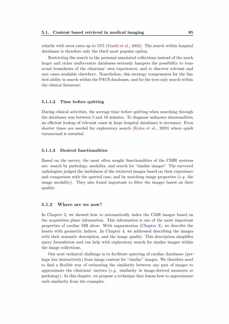
5.1. Content based retrieval in medical imaging 85
reliable with error rates up to 15% (Gueld et al., 2002). The search within hospitaldatabases is therefore only the third most popular option.
Restricting the search to the personal annotated collections instead of the muchlarger and richer multi-centre databases seriously hampers the possibility to tran-scend boundaries of the clinicians’ own experiences, and to discover relevant andrare cases available elsewhere. Nonetheless, this strategy compensates for the lim-ited ability to search within the PACS databases, and for the text-only search withinthe clinical literature.
5.1.1.2 Time before quitting
During clinical activities, the average time before quitting when searching throughthe databases was between 5 and 10 minutes. To diagnose unknown abnormalities,an efficient lookup of relevant cases in large hospital databases is necessary. Evenshorter times are needed for exploratory search (Kules et al., 2009) where quickturnaround is essential.
5.1.1.3 Desired functionalities
Based on the survey, the most often sought functionalities of the CBIR systemsare: search by pathology, modality, and search for “similar images”. The surveyedradiologists judged the usefulness of the retrieved images based on their experienceand comparison with the queried case, and by matching image properties (e.g. theimage modality). They also found important to filter the images based on theirquality.
5.1.2 Where are we now?
In Chapter 2, we showed how to automatically index the CMR images based onthe acquisition plane information. This information is one of the most importantproperties of cardiac MR slices. With segmentation (Chapter 3), we describe thehearts with geometric indices. In Chapter 4, we addressed describing the imageswith their semantic description, and the image quality. This description simplifiesquery formulation and can help with exploratory search for similar images withinthe image collections.
Our next technical challenge is to facilitate querying of cardiac databases (per-haps less interactively) from image content for “similar” images. We therefore needto find a flexible way of estimating the similarity between any pair of images toapproximate the clinicians’ metrics (e.g. similarity in image-derived measures orpathology). In this chapter, we propose a technique that learns how to approximatesuch similarity from the examples.
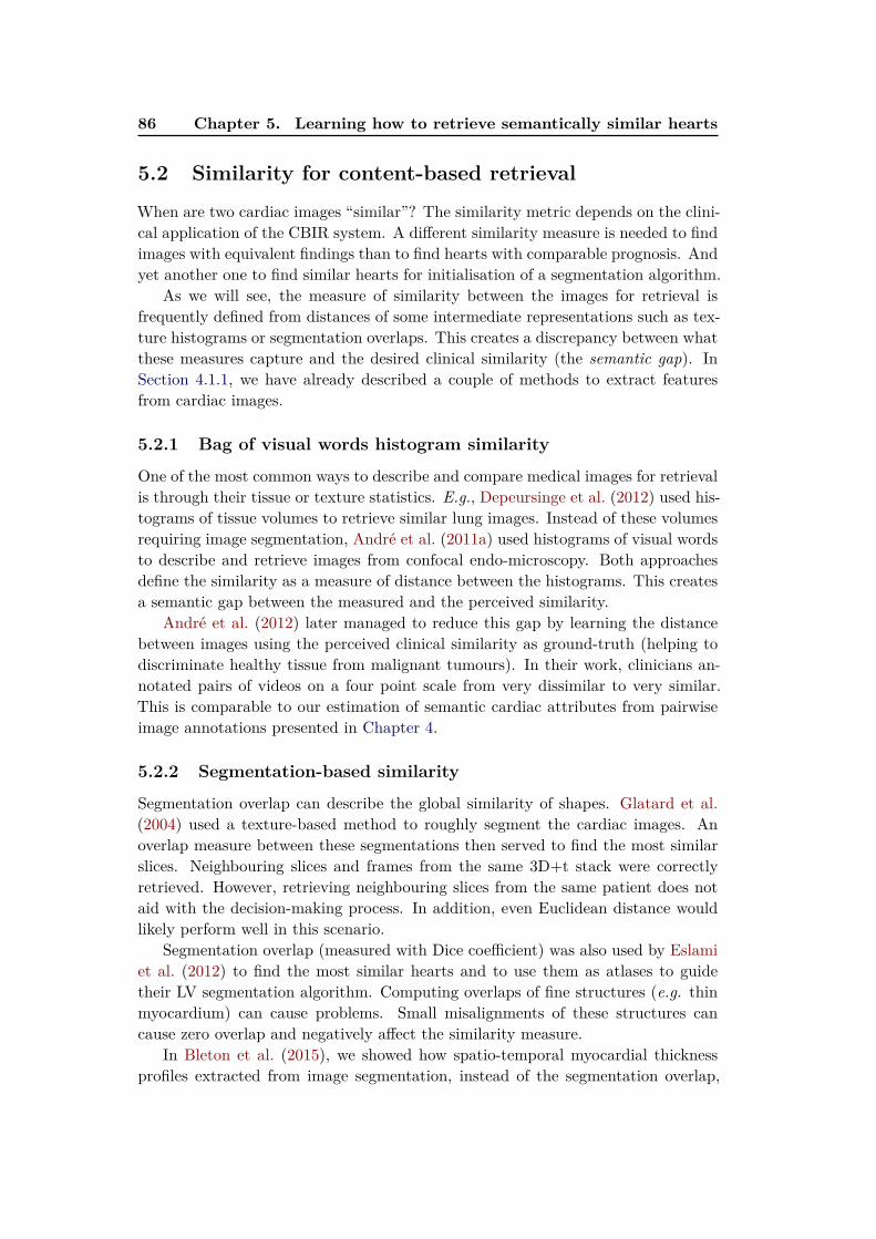
86 Chapter 5. Learning how to retrieve semantically similar hearts
5.2 Similarity for content-based retrieval
When are two cardiac images “similar”? The similarity metric depends on the clini-cal application of the CBIR system. A different similarity measure is needed to findimages with equivalent findings than to find hearts with comparable prognosis. Andyet another one to find similar hearts for initialisation of a segmentation algorithm.
As we will see, the measure of similarity between the images for retrieval isfrequently defined from distances of some intermediate representations such as tex-ture histograms or segmentation overlaps. This creates a discrepancy between whatthese measures capture and the desired clinical similarity (the semantic gap). InSection 4.1.1, we have already described a couple of methods to extract featuresfrom cardiac images.
5.2.1 Bag of visual words histogram similarity
One of the most common ways to describe and compare medical images for retrievalis through their tissue or texture statistics. E.g., Depeursinge et al. (2012) used his-tograms of tissue volumes to retrieve similar lung images. Instead of these volumesrequiring image segmentation, André et al. (2011a) used histograms of visual wordsto describe and retrieve images from confocal endo-microscopy. Both approachesdefine the similarity as a measure of distance between the histograms. This createsa semantic gap between the measured and the perceived similarity.
André et al. (2012) later managed to reduce this gap by learning the distancebetween images using the perceived clinical similarity as ground-truth (helping todiscriminate healthy tissue from malignant tumours). In their work, clinicians an-notated pairs of videos on a four point scale from very dissimilar to very similar.This is comparable to our estimation of semantic cardiac attributes from pairwiseimage annotations presented in Chapter 4.
5.2.2 Segmentation-based similarity
Segmentation overlap can describe the global similarity of shapes. Glatard et al.(2004) used a texture-based method to roughly segment the cardiac images. Anoverlap measure between these segmentations then served to find the most similarslices. Neighbouring slices and frames from the same 3D+t stack were correctlyretrieved. However, retrieving neighbouring slices from the same patient does notaid with the decision-making process. In addition, even Euclidean distance wouldlikely perform well in this scenario.
Segmentation overlap (measured with Dice coefficient) was also used by Eslamiet al. (2012) to find the most similar hearts and to use them as atlases to guidetheir LV segmentation algorithm. Computing overlaps of fine structures (e.g. thinmyocardium) can cause problems. Small misalignments of these structures cancause zero overlap and negatively affect the similarity measure.
In Bleton et al. (2015), we showed how spatio-temporal myocardial thicknessprofiles extracted from image segmentation, instead of the segmentation overlap,
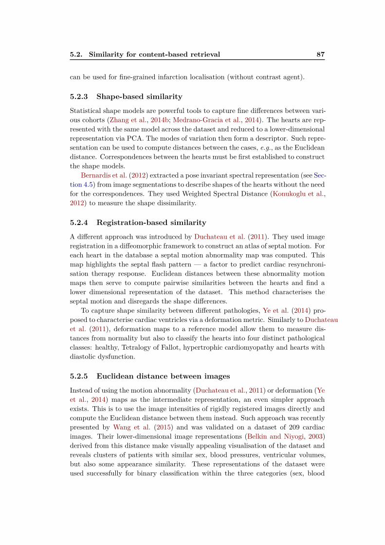
5.2. Similarity for content-based retrieval 87
can be used for fine-grained infarction localisation (without contrast agent).
5.2.3 Shape-based similarity
Statistical shape models are powerful tools to capture fine differences between vari-ous cohorts (Zhang et al., 2014b; Medrano-Gracia et al., 2014). The hearts are rep-resented with the same model across the dataset and reduced to a lower-dimensionalrepresentation via PCA. The modes of variation then form a descriptor. Such repre-sentation can be used to compute distances between the cases, e.g., as the Euclideandistance. Correspondences between the hearts must be first established to constructthe shape models.
Bernardis et al. (2012) extracted a pose invariant spectral representation (see Sec-tion 4.5) from image segmentations to describe shapes of the hearts without the needfor the correspondences. They used Weighted Spectral Distance (Konukoglu et al.,2012) to measure the shape dissimilarity.
5.2.4 Registration-based similarity
A different approach was introduced by Duchateau et al. (2011). They used imageregistration in a diffeomorphic framework to construct an atlas of septal motion. Foreach heart in the database a septal motion abnormality map was computed. Thismap highlights the septal flash pattern — a factor to predict cardiac resynchroni-sation therapy response. Euclidean distances between these abnormality motionmaps then serve to compute pairwise similarities between the hearts and find alower dimensional representation of the dataset. This method characterises theseptal motion and disregards the shape differences.
To capture shape similarity between different pathologies, Ye et al. (2014) pro-posed to characterise cardiac ventricles via a deformation metric. Similarly to Duchateauet al. (2011), deformation maps to a reference model allow them to measure dis-tances from normality but also to classify the hearts into four distinct pathologicalclasses: healthy, Tetralogy of Fallot, hypertrophic cardiomyopathy and hearts withdiastolic dysfunction.
5.2.5 Euclidean distance between images
Instead of using the motion abnormality (Duchateau et al., 2011) or deformation (Yeet al., 2014) maps as the intermediate representation, an even simpler approachexists. This is to use the image intensities of rigidly registered images directly andcompute the Euclidean distance between them instead. Such approach was recentlypresented by Wang et al. (2015) and was validated on a dataset of 209 cardiacimages. Their lower-dimensional image representations (Belkin and Niyogi, 2003)derived from this distance make visually appealing visualisation of the dataset andreveals clusters of patients with similar sex, blood pressures, ventricular volumes,but also some appearance similarity. These representations of the dataset wereused successfully for binary classification within the three categories (sex, blood
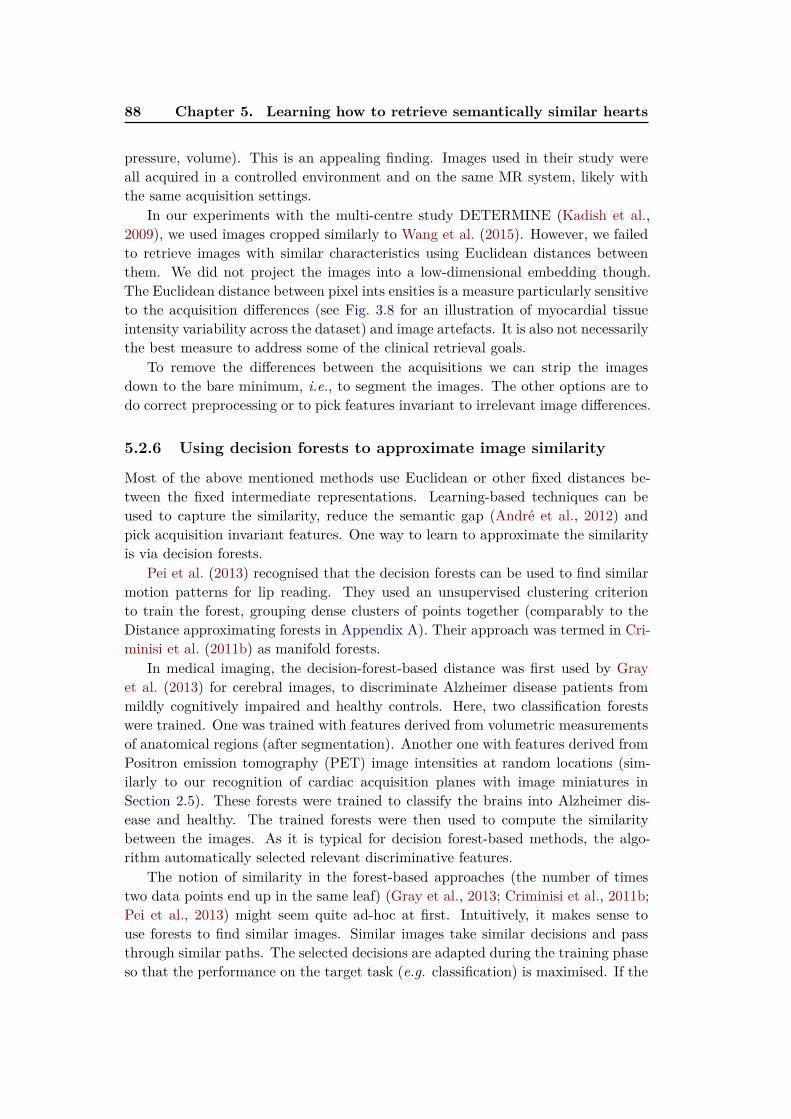
88 Chapter 5. Learning how to retrieve semantically similar hearts
pressure, volume). This is an appealing finding. Images used in their study wereall acquired in a controlled environment and on the same MR system, likely withthe same acquisition settings.
In our experiments with the multi-centre study DETERMINE (Kadish et al.,2009), we used images cropped similarly to Wang et al. (2015). However, we failedto retrieve images with similar characteristics using Euclidean distances betweenthem. We did not project the images into a low-dimensional embedding though.The Euclidean distance between pixel ints ensities is a measure particularly sensitiveto the acquisition differences (see Fig. 3.8 for an illustration of myocardial tissueintensity variability across the dataset) and image artefacts. It is also not necessarilythe best measure to address some of the clinical retrieval goals.
To remove the differences between the acquisitions we can strip the imagesdown to the bare minimum, i.e., to segment the images. The other options are todo correct preprocessing or to pick features invariant to irrelevant image differences.
5.2.6 Using decision forests to approximate image similarity
Most of the above mentioned methods use Euclidean or other fixed distances be-tween the fixed intermediate representations. Learning-based techniques can beused to capture the similarity, reduce the semantic gap (André et al., 2012) andpick acquisition invariant features. One way to learn to approximate the similarityis via decision forests.
Pei et al. (2013) recognised that the decision forests can be used to find similarmotion patterns for lip reading. They used an unsupervised clustering criterionto train the forest, grouping dense clusters of points together (comparably to theDistance approximating forests in Appendix A). Their approach was termed in Cri-minisi et al. (2011b) as manifold forests.
In medical imaging, the decision-forest-based distance was first used by Grayet al. (2013) for cerebral images, to discriminate Alzheimer disease patients frommildly cognitively impaired and healthy controls. Here, two classification forestswere trained. One was trained with features derived from volumetric measurementsof anatomical regions (after segmentation). Another one with features derived fromPositron emission tomography (PET) image intensities at random locations (sim-ilarly to our recognition of cardiac acquisition planes with image miniatures inSection 2.5). These forests were trained to classify the brains into Alzheimer dis-ease and healthy. The trained forests were then used to compute the similaritybetween the images. As it is typical for decision forest-based methods, the algo-rithm automatically selected relevant discriminative features.
The notion of similarity in the forest-based approaches (the number of timestwo data points end up in the same leaf) (Gray et al., 2013; Criminisi et al., 2011b;Pei et al., 2013) might seem quite ad-hoc at first. Intuitively, it makes sense touse forests to find similar images. Similar images take similar decisions and passthrough similar paths. The selected decisions are adapted during the training phaseso that the performance on the target task (e.g. classification) is maximised. If the
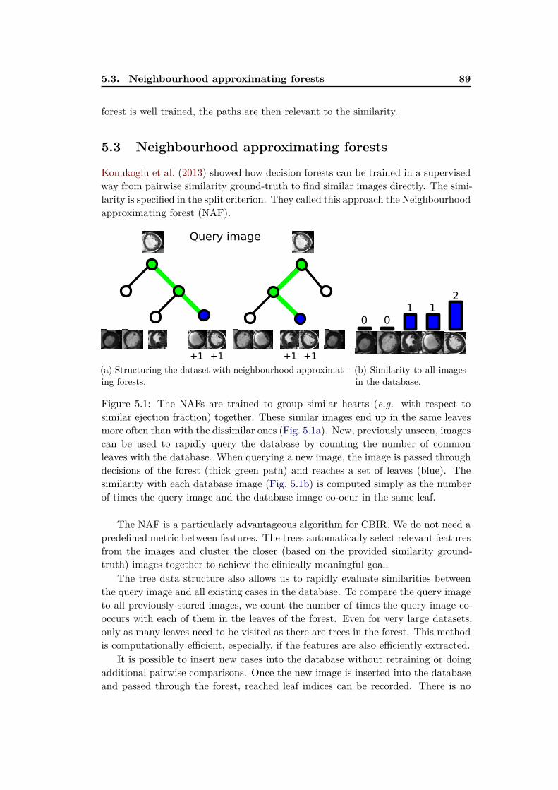
5.3. Neighbourhood approximating forests 89
forest is well trained, the paths are then relevant to the similarity.
5.3 Neighbourhood approximating forests
Konukoglu et al. (2013) showed how decision forests can be trained in a supervisedway from pairwise similarity ground-truth to find similar images directly. The simi-larity is specified in the split criterion. They called this approach the Neighbourhoodapproximating forest (NAF).
+1 +1 +1 +1
Query image
(a) Structuring the dataset with neighbourhood approximat-ing forests.
2
11
00
(b) Similarity to all imagesin the database.
Figure 5.1: The NAFs are trained to group similar hearts (e.g. with respect tosimilar ejection fraction) together. These similar images end up in the same leavesmore often than with the dissimilar ones (Fig. 5.1a). New, previously unseen, imagescan be used to rapidly query the database by counting the number of commonleaves with the database. When querying a new image, the image is passed throughdecisions of the forest (thick green path) and reaches a set of leaves (blue). Thesimilarity with each database image (Fig. 5.1b) is computed simply as the numberof times the query image and the database image co-ocur in the same leaf.
The NAF is a particularly advantageous algorithm for CBIR. We do not need apredefined metric between features. The trees automatically select relevant featuresfrom the images and cluster the closer (based on the provided similarity ground-truth) images together to achieve the clinically meaningful goal.
The tree data structure also allows us to rapidly evaluate similarities betweenthe query image and all existing cases in the database. To compare the query imageto all previously stored images, we count the number of times the query image co-occurs with each of them in the leaves of the forest. Even for very large datasets,only as many leaves need to be visited as there are trees in the forest. This methodis computationally efficient, especially, if the features are also efficiently extracted.
It is possible to insert new cases into the database without retraining or doingadditional pairwise comparisons. Once the new image is inserted into the databaseand passed through the forest, reached leaf indices can be recorded. There is no

90 Chapter 5. Learning how to retrieve semantically similar hearts
longer any need to have direct access to the image for future comparisons. This iscompatible with collaborative indexing of personal collections from several clinicians.Sharing sets of leaf indices from images in personal collection would be sufficient tofind where the relevant images can be found.
5.3.1 Learning how to structure the dataset
This tree-based method hierarchically structures the dataset such that similar im-ages are clustered closer together while the dissimilar ones are spread more apart.Since this is a supervised method, pairwise distances ρ(I, J) between images I andJ in the training set must be known. The ground-truth similarity between the casescan be defined from virtually anything meaningful, e.g., pathology, blood pressure,patient’s age, or in our case the ejection fraction, infarct location (Bleton et al.,2015), or the presence of pericardial effusion (Appendix C).
In lieu of the information gain used previously (see Eq. (2.1)), a criterion derivedfrom cluster compactness is used to select split parameters that lead to the bestpartitioning of the dataset. Cluster compactness Cρ for a set of images Ds at thenode s and with respect to the training image distance ρ is defined as:
Cρ(Ds) =1
|D|2
∑
i∈Ds
∑
j∈Ds
ρ(Ii, Ij) (5.1)
During the training phase, at each node, the parameters of the binary splits θsare fixed in order to divide the images at the node into the left IsL and the right IsRbranches. The parameters are chosen such that the following gain measure Gρ ismaximised:
Gρ(Is, θs) = Cρ(Is)−|IsL|
|Is|Cρ(IsL)−
|IsR|
|Is|Cρ(IsR) (5.2)
To maximise this quantity, the compactness (e.g. the pairwise sum of absoluteejection fractions differences for all the pairs within the node) in both left Cρ(IsL) andright Cρ(IsR) branch must be as low as possible. This quantity therefore encouragesthe forest to pick decisions where similar images (with similar ejection fractions)are put together into the same branch.
5.3.2 Finding similar images
The trained trees can be then used to obtain a measure of similarity S betweenany two images I and J (even if they were not part of the training set). Afterpassing each image through the trees, a set of leaves is reached (see Fig. 5.1a). Thesimilarity is approximated by counting how many times the same decisions weretaken, i.e., by measuring the number of trees where two images both reach thesame leaf (Lt(I) = Lt(J)) as illustrated in Fig. 5.1b.
S(Ii, Ij) =
nT∑
t=1
1(Lt(Ii) = Lt(Ij)) (5.3)
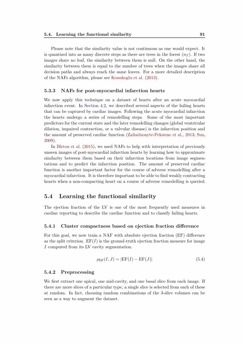
5.4. Learning the functional similarity 91
Please note that the similarity value is not continuous as one would expect. Itis quantised into as many discrete steps as there are trees in the forest (nT ). If twoimages share no leaf, the similarity between them is null. On the other hand, thesimilarity between them is equal to the number of trees when the images share alldecision paths and always reach the same leaves. For a more detailed descriptionof the NAFs algorithm, please see Konukoglu et al. (2013).
5.3.3 NAFs for post-myocardial infarction hearts
We now apply this technique on a dataset of hearts after an acute myocardialinfarction event. In Section 4.2, we described several aspects of the failing heartsthat can be captured by cardiac images. Following the acute myocardial infarctionthe hearts undergo a series of remodelling steps. Some of the most importantpredictors for the current state and the later remodelling changes (global ventriculardilation, impaired contraction, or a valvular disease) is the infarction position andthe amount of preserved cardiac function (Zaliaduonyte-Peksiene et al., 2013; Sun,2009).
In Bleton et al. (2015), we used NAFs to help with interpretation of previouslyunseen images of post-myocardial infarction hearts by learning how to approximatesimilarity between them based on their infarction locations from image segmen-tations and to predict the infarction position. The amount of preserved cardiacfunction is another important factor for the course of adverse remodelling after amyocardial infarction. It is therefore important to be able to find weakly contractinghearts when a non-compacting heart on a course of adverse remodelling is queried.
5.4 Learning the functional similarity
The ejection fraction of the LV is one of the most frequently used measures incardiac reporting to describe the cardiac function and to classify failing hearts.
5.4.1 Cluster compactness based on ejection fraction difference
For this goal, we now train a NAF with absolute ejection fraction (EF) differenceas the split criterion. EF(I) is the ground-truth ejection fraction measure for imageI computed from its LV cavity segmentation.
ρEF(I, J) = |EF(I)− EF(J)| (5.4)
5.4.2 Preprocessing
We first extract one apical, one mid-cavity, and one basal slice from each image. Ifthere are more slices of a particular type, a single slice is selected from each of theseat random. In fact, choosing random combinations of the 3-slice volumes can beseen as a way to augment the dataset.

92 Chapter 5. Learning how to retrieve semantically similar hearts
We then align the images to a reference image with a set of landmarks belongingto the LV epicardium on the mid-cavity slice (as detailed in Appendix B.3) with asimilarity transformation model (rigid + scale). The reference image is cropped to128× 128 pixels, such that it wholy contains the target landmarks with some smallextra margin. The intensity of the images is normalised (similarly to whitening) byshifting the mean of the cropped images to 127 and by forcing a single standarddeviation value across the whole dataset such that the most common intensityranges (between 0 and 98.5%) fully span the 0 to 255 intensity range.
We strip away the thorax pixels (Section 5.4.2.1) and compute the temporalpseudo-volumetric curves from the image crops. We then extract the end diastolicand end systolic frames from the images (Section 5.4.2.3).
5.4.2.1 Thorax stripping
To reduce the influence of background structures, we focus on the regions adjacentto the moving left ventricle only. Such preprocessing is similar to what is commonlydone in brain imaging - skull stripping. Rough estimation of the moving cardiacregion can be obtained from temporal intensity changes (see Figure 5.2). We firstcompute the temporal range of intensity values at each pixel, in other words thedifference of maximal and minimal intensity values of the pixel in time. We spatiallysmoothen the range image and binarise it using the method of Otsu (1979).
Intensities beyond some distance from the largest moving blob can therefore besafely labelled as the background and masked to be removed from the image. It isimportant to keep some extra region around the heart to avoid removing importantcardiac findings such as the pericardial effusion. Smooth blending of the backgroundis obtained by mapping the distance to the blob with a sigmoid.
5.4.2.2 Spatial alignment
In Appendix B, we describe our landmark model and how cardiac landmarks canbe estimated. Once the landmarks are estimated, we can align the hearts. Having alandmark-based model allows us to rapidly choose the reference structure of interest.This is a big advantage over the intensity-based registration techniques. The mainoptions include registration to all available landmarks, to both LV endocardial andLV epicardial landmarks, to RV endocardial landmarks alone, or to a specific subsetof landmarks, e.g., the antero-septal wall.
In this chapter, we choose the LV epicardium as the reference. We regis-ter the left ventricular epicardial landmarks to the mean left ventricle epicardiummodel with similarity (rigid + scale) transformation model. The transformation pa-rameters are estimated with Procrustes analysis (Suinesiaputra et al., 2004). Thesimilarity transformation preserves most of the image information and puts thehearts into correspondence without introducing artefacts from non-linear methods.The standard acquisitions were performed by expert radiologists so the long axis isin general in good alignment with the short axis plane normal vector. However, the
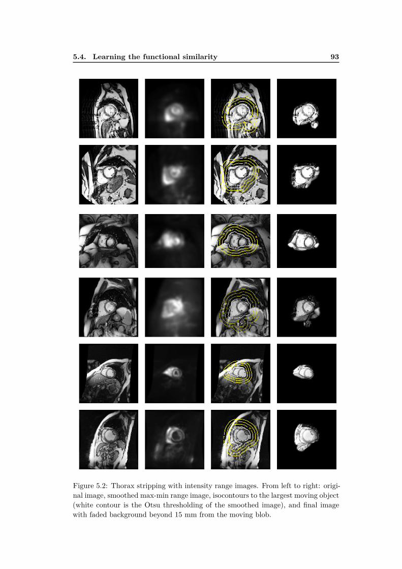
5.4. Learning the functional similarity 93
Figure 5.2: Thorax stripping with intensity range images. From left to right: origi-nal image, smoothed max-min range image, isocontours to the largest moving object(white contour is the Otsu thresholding of the smoothed image), and final imagewith faded background beyond 15 mm from the moving blob.
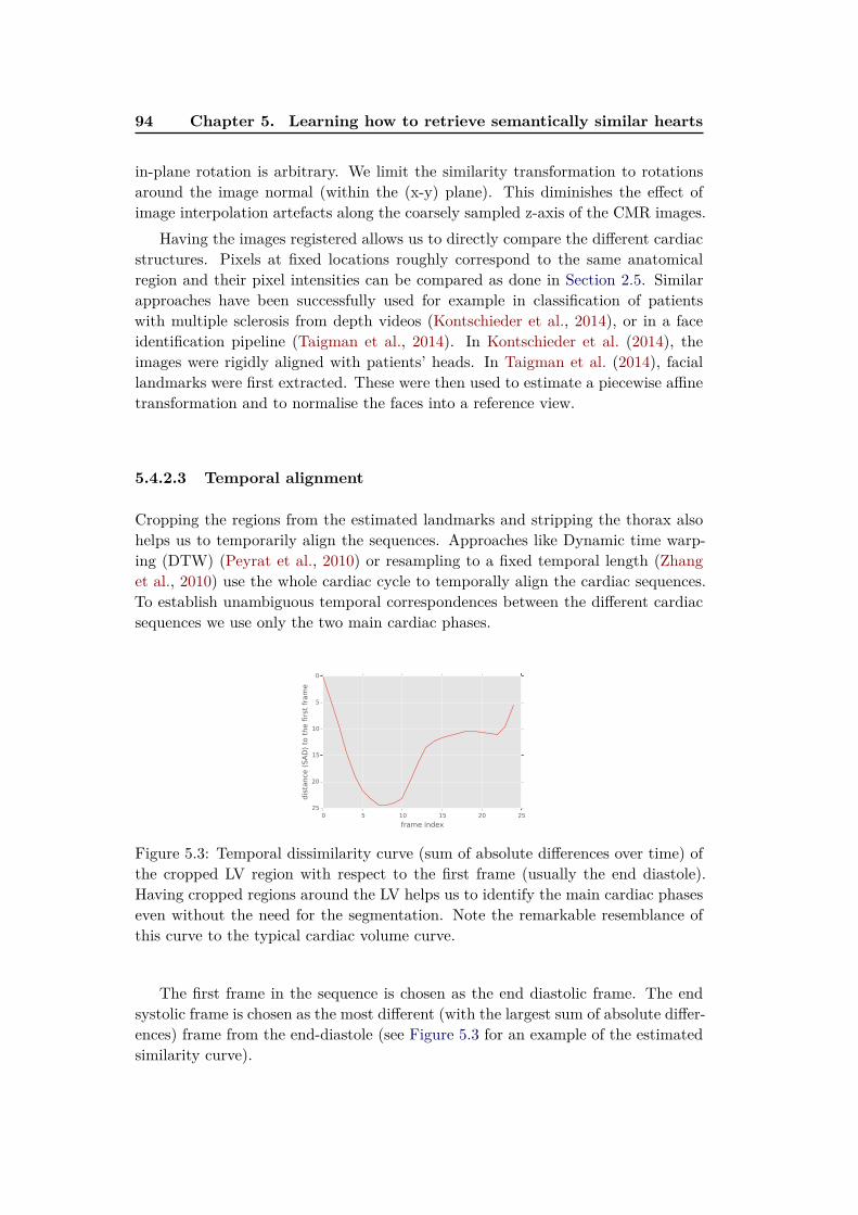
94 Chapter 5. Learning how to retrieve semantically similar hearts
in-plane rotation is arbitrary. We limit the similarity transformation to rotationsaround the image normal (within the (x-y) plane). This diminishes the effect ofimage interpolation artefacts along the coarsely sampled z-axis of the CMR images.
Having the images registered allows us to directly compare the different cardiacstructures. Pixels at fixed locations roughly correspond to the same anatomicalregion and their pixel intensities can be compared as done in Section 2.5. Similarapproaches have been successfully used for example in classification of patientswith multiple sclerosis from depth videos (Kontschieder et al., 2014), or in a faceidentification pipeline (Taigman et al., 2014). In Kontschieder et al. (2014), theimages were rigidly aligned with patients’ heads. In Taigman et al. (2014), faciallandmarks were first extracted. These were then used to estimate a piecewise affinetransformation and to normalise the faces into a reference view.
5.4.2.3 Temporal alignment
Cropping the regions from the estimated landmarks and stripping the thorax alsohelps us to temporarily align the sequences. Approaches like Dynamic time warp-ing (DTW) (Peyrat et al., 2010) or resampling to a fixed temporal length (Zhanget al., 2010) use the whole cardiac cycle to temporally align the cardiac sequences.To establish unambiguous temporal correspondences between the different cardiacsequences we use only the two main cardiac phases.
0 5 10 15 20 25
frame index
0
5
10
15
20
25
dis
tance
(SA
D)
to t
he f
irst
fra
me
Figure 5.3: Temporal dissimilarity curve (sum of absolute differences over time) ofthe cropped LV region with respect to the first frame (usually the end diastole).Having cropped regions around the LV helps us to identify the main cardiac phaseseven without the need for the segmentation. Note the remarkable resemblance ofthis curve to the typical cardiac volume curve.
The first frame in the sequence is chosen as the end diastolic frame. The endsystolic frame is chosen as the most different (with the largest sum of absolute differ-ences) frame from the end-diastole (see Figure 5.3 for an example of the estimatedsimilarity curve).

5.4. Learning the functional similarity 95
5.4.3 Spatio-temporal image features
To describe the images and to achieve acceptable query responsiveness, we proposefast temporal intensity-based features (see Fig. 5.4), using no segmentation nornon-rigid image registration. These features are derived from 3D Haar-like features,similar to the ones we used for cardiac image segmentation in Chapter 3, measuringregional intensity statistics. This time, the images are aligned and cropped with thebackground faded. Measures at fixed positions roughly capture information fromthe same cardiac regions.
spatial
intensity stats
spatial
differences
spatio-temporal
differences
systo
le o
r dia
sto
le
systo
le o
r dia
sto
le
+ ++
+
+
+
+
-
-
- -
--
-
+
+
systo
le a
nd d
iasto
le
Figure 5.4: Overview of our features. Short axis images are cropped, reoriented andaligned and features are extracted for the NAFs to find similar hearts. These arederived from 3D Haar-like features computing regional intensity averages, standarddeviations and maxima, together with their differences. We use several featurefamilies in this work, both spatial only and fully spatio-temporal.
Again, we define several feature families from which we sample the features andwe extract not only the average regional intensities within the boxes but alsostandard deviations (capturing texture and intensity homogeneity) and regional
maxima. The first two can be computed very efficiently with integral images asproposed by Viola and Jones (2004). We find the regional maxima directly, but theycan be also roughly approximated with integral images using the soft-max functionlog
∑
i exp(xi). In other words, by exponentiating the voxel intensity values prior tothe integral image computation and computing logarithms of the extracted regionalsums. Care must be taken to avoid numerical overflows.
In all cases, we limit the parameters of these boxes to fit into the alignedspatio-temporal image crops. We do this by parametrising the spatio-temporalrectangles with coordinates of their two extreme corners (L - lower and U - upper):(Lx, Ly, Lt, Ux, Uy, Ut). Each coordinate is represented as percentage of the croppedimage size and is bounded between 0 and 1. This way of defining the rectanglesguarantees them to stay within the cropped image and no extra out-of-bounds boxevaluation or clipping are necessary. Note, we currently always use the whole rangeof z values (computing statistics in voxel across all three slices), and only two main
96 Chapter 5. Learning how to retrieve semantically similar hearts
temporal instants (diastole and systole).
In total, we define 30 “semantic” families of features for easier interpretation ofthe results. We sample 200 random features from each family as we will describebelow. This generates a large number of features from several different featurefamilies and assumptions on how they should capture the content. The advantageof the forest-based algorithm is that it can automatically pick features that trulymatter to find similar hearts.
5.4.3.1 Intensity statistics of static central rectangles (“centered rect”)
First, we propose to measure intensity statistics of the central image region, indi-vidually at systole and at diastole. A dilated and poorly contracting ventricle, withlarge bright blood pool should have higher systolic and diastolic average intensitythan a heart whose cavity is much smaller and where the myocardium drives downthe average image intensity.
We extract spatial boxes with their centre aligned with the image centre. Theimage centre coordinates are simply c = (0.5, 0.5, 0.5). These boxes have dimensionsproportional to the image crop size (in our case the extracted region is a squareand so are the extracted rectangles). Their extent can be anywhere from singlecentral pixel to the extent of the whole crop. In other words, we uniformly samplea single variable d between 0 and 0.5. The rectangles are then defined as Rcentre
dia =
(cx − d, cy − d, 0, cx + d, cy + d, 0.5) for diastolic frames, and for systolic frames asRcentre
sys = (cx−d, cy−d, 0.5, cx+d, cy+d, 1). We use the generated boxes to computetheir intensity averages (avg), standard deviations (std) and maxima (max), at bothend frames (sys, dia).
This results in 6 feature families (1200 features): centered rect dia avg, cen-
tered rect sys avg, centered rect dia std, centered rect sys std, centered
rect dia max, centered rect sys max.
5.4.3.2 Intensity statistics of arbitrary static rectangles (“rect”)
By measuring regions at arbitrary spatial positions we can capture extra informationto help with more fine-grained division of the hearts based on local measurements.Therefore, we also sample randomly-sized diastolic or systolic boxes at arbitraryspatial positions. From a uniform distribution we sample two pairs of spatial co-ordinates x and y to lie anywhere between 0 and 1. For each coordinate, we pickthe smaller of the components to create the lower corner of the box (L) and thelarger ones to create the upper corner (U). We can then extract the boxes for sys-tole Rspatial
dia = (Lx, Ly, 0, Ux, Uy, 0.5) and diastole Rspatialsys = (Lx, Ly, 0.5, Ux, Uy, 1).
The following 6 feature families were extracted (1200 features): rect dia avg,rect sys avg, rect dia std, rect sys std, rect dia max, rect sys max.
5.4. Learning the functional similarity 97
5.4.3.3 Full-cycle box statistics (“rectangles full extractor”)
We also compute regional statistics of arbitrarily placed rectangles as describedabove in Section 5.4.3.2, but this time spanning both temporal instants: Rfull =
(Lx, Ly, 0, Ux, Uy, 1). This results in 3 additional feature families (600 features):rectangles full extractor avg, rectangles full extractor std, rectangles full
extractor max.
5.4.3.4 Regional differences (“offset rect spatial diff”)
For now, we have computed individual boxes and considered them independently.Comparisons between two spatial regions can help to better discriminate subtlershape differences with single decisions. We compute the spatial differences in re-gional average intensities, standard deviations and maxima between two boxes ofdifferent sizes and at two different positions within the same frame. We sam-ple two independent rectangles as described in Section 5.4.3.2, i.e., Rspatial,0
dia =
(L0x, L
0y, 0, U
0x , U
0y , 0.5) and R
spatial,1dia = (L1
x, L1y, 0, U
1x , U
1y , 0.5) for diastolic boxes.
Apart from the boxes being fully contained within the image crop (by construc-tion), we do not restrict their positions and sizes. These boxes can even fullyoverlap or do not touch each other. Then, we compute the differences in theirstatistics (stats(Rspatial,0
dia ) − stats(Rspatial,1dia )) and use them as additional features.
For systolic boxes we add 0.5 to the temporal components.This results in 6 feature families and 1200 features: offset rect avg spatial
diff dia, offset rect avg spatial diff sys, offset rect std spatial diff dia, offset
rect std spatial diff sys, offset rect max spatial diff dia, offset rect max
spatial diff sys.
5.4.3.5 Central temporal differences (“centered rect temporal diff”)
In the end, the function of the heart is best captured with volume changes in time.Temporal intensity changes (between the diastolic and systolic frame) can help tofurther discriminate the hearts based on the chosen criteria. In particular, shifts inregional image intensities are an excellent mean to roughly capture the amount ofmotion without registration.
The intuition behind using temporal intensity differences is that average in-tensities in static or stiff regions do not change temporally much while properlycontracting voxels cause a visible drop in average regional intensity due to changedblood-myocardium distribution. Temporal changes in the image histogram distri-bution due to cardiac contraction have already been used previously to estimatethe ejection fraction by Afshin et al. (2012a,b).
The main intensity changes between the ED and ES should happen within theventricular cavity. Therefore, we first define differences of statistics within equallysized centred rectangles: stats(Rcentre
dia ) − stats(Rcentresys ). This yields 3 more feature
families (600 features): centered rect avg temporal diff, centered rect std
temporal diff, centered rect max temporal diff.
98 Chapter 5. Learning how to retrieve semantically similar hearts
5.4.3.6 Regional temporal changes (“rect temporal diff”)
The central temporal differences are limited in the shape of the region they cancapture. We therefore measure temporal change of rectangular regions, i.e., thedifferences between two fixed spatial boxes: R0 = (Lx, Ly, 0, Ux, Uy, 0.5) and R1 =
(Lx, Ly, 0.5, Ux, Uy, 1). In other words, apart from the temporal coordinate, the boxstays fixed for the two frames and the features are computed as stats(R0)−stats(R1).This adds 3 families (600 features): rect avg temporal diff, rect std temporal
diff, rect max temporal diff.
5.4.3.7 Spatio-temporal differences (“offset rect avg temporal diff”)
Finally, we combine arbitrary space and time together and include regional spatio-temporal diastole-systole differences of independently placed and sized boxes. Onebox from the diastolic frame: R0 = (L0
x, L0y, 0, U
0x , U
0y , 0.5) and one from the systolic
one: R1 = (L1x, L
1y, 0.5, U
1x , U
1y , 1). Differences in all three box statistics of the
two boxes are then computed: stats(R0) − stats(R1), which makes for the last 3feature families and 600 features: offset rect avg temporal diff, offset rect std
temporal diff, offset rect max temporal diff.
5.5 Validation and results
Dataset
Our image database comes from a multi-centre study and consists of 96 post-myocardial infarction patients with cine short axis MR SSFP acquisitions (Fonsecaet al., 2011; Kadish et al., 2009). The infarctions are healed, but the hearts are inarbitrary phases of the remodelling process and with arbitrary myocardial salvage.
5.5.1 Retrieval experiment
For each heart we extracted the 6000 previously described features from the corre-sponding images to capture the hearts’ functional and appearance characteristics.We then trained the NAFs to select the relevant ones and approximate the imagesimilarity with respect to the functional aspect of the heart — the ejection fraction.Our forests consist of 2000 trees with maximum depth 6. All training images wereselected to train the trees, 500 randomly selected features and 50 random thresholds(per feature) were tested at each node.
We then queried the database with validation images in order to retrieve themost similar hearts from the training database. We evaluate the quality of the re-trieval via the differences in ejection fraction of the query images and mean ejectionfraction of their nearest neighbours retrieved by the NAFs.

5.5. Validation and results 99
5.5.1.1 Mean absolute prediction error
First, we divided the dataset into 10 random folds (90 percent of the data fortraining and 10 for testing). The mean absolute prediction error of the ejectionfraction (computed as a mean of ejection fractions of the retrieved four nearestneighbours) across our cross-validation folds was 5.48% ± 4.60. No segmentationwas used to measure the ejection fraction. This appears to be slightly better thanestimation of the ejection fractions (EFs) by visual inspection (Gudmundsson et al.,2005) with mean variability 7.0%1.
5.5.1.2 Bucket leave-one-out
To test how well the ejection fractions are predicted across the whole range of valuesin the dataset, we set up a different experiment. In this step, we sorted the imagesin the training set with respect to their ejection fractions. We then split the sortedimages into 10 equally-sized buckets (each containing roughly the same number ofimages), for a 10-fold leave-one-out cross-validation. At each fold we picked oneof the buckets, and chose the image at its centre as the query image. All otherremaining images were left for training.
The retrieval results using this leave-one-out strategy are shown in Fig. 5.5.Especially for the lower and middle EF buckets, the mean EF of the retrieved imagesclosely matches the query ejection fraction (within 4%). The retrieved ejectionfractions of buckets at the higher end of the spectrum (> 49%) are much noisier.This is likely because more hearts in the dataset are in the lower EF buckets andthere are more examples to learn from. Note also that the most dissimilar imagesare often located in the opposite side of the functional spectrum.
To visualise how the forest predicts across the whole range of EFs present in thedataset, we fit a linear regression model to the mean predictions of the leave-one-outfolds (see Fig. 5.6).
5.5.1.3 Computational time
The full query pipeline (loading the image, predicting the cardiac landmarks, thoraxstripping, detecting main cardiac phases, feature extraction, forest traversal andretrieval of similar images) currently runs together in less than 30 seconds. Ifthe features are pre-calculated, the tree traversal and similarity computation withevery image in our database is performed in a fraction of a second. Wrapping thistool into a friendly user interface could enable fast interaction with the dataset forexploration.
5.5.2 Feature importance
We mentioned a few times in this thesis that the forest picks the relevant features byitself and allows inspection of the decisions taken. This is a great benefit compared
1Try it for yourself: http://www.cardiacejectionfraction.com

100 Chapter 5. Learning how to retrieve semantically similar hearts
Query
DET0044801 (28)
DET0005101 (32)
DET0003901 (36)
DET0001401 (41)
DET0005401 (43)
DET0008901 (47)
DET0037101 (49)
DET0008801 (55)
DET0006301 (58)
DET0001801 (38)
Most similar
Similarity 1068DET0045301 (30)
Similarity 1145DET0028801 (32)
Similarity 546DET0006401 (36)
Similarity 732DET0015401 (43)
Similarity 884DET0005501 (40)
Similarity 1219DET0003301 (49)
Similarity 1472DET0006501 (61)
Similarity 1186DET0003501 (51)
Similarity 673DET0004901 (36)
Similarity 1111DET0024501 (30)
Similarity 1028DET0004801 (24)
Similarity 1127DET0005201 (26)
Similarity 527DET0009001 (41)
Similarity 703DET0016101 (42)
Similarity 847DET0035501 (44)
Similarity 1155DET0008801 (55)
Similarity 1427DET0001601 (62)
Similarity 1128DET0008901 (47)
Similarity 643DET0006001 (56)
Similarity 1096DET0001301 (41)
Similarity 1024DET0028801 (32)
Similarity 1081DET0026801 (33)
Similarity 506DET0016101 (42)
Similarity 640DET0009001 (41)
Similarity 783DET0028301 (41)
Similarity 1104DET0002601 (45)
Similarity 1425DET0021701 (63)
Similarity 1099DET0002601 (45)
Similarity 627DET0003101 (43)
Similarity 990DET0004601 (36)
Mostdissimilar
Similarity 0DET0015601 (57)
Similarity 0DET0009001 (41)
Similarity 93DET0008801 (55)
Similarity 17DET0005201 (26)
Similarity 43DET0001301 (41)
Similarity 17DET0035501 (44)
Similarity 0DET0005101 (32)
Similarity 1DET0021701 (63)
Similarity 58DET0044801 (28)
Similarity 0DET0021701 (63)
29
30
40
42
42
50
62
48
45
36
Mean EF
Figure 5.5: Retrieval of similar hearts based on the function criterion with a forestof 2000 trees. Each row represents a query and database retrieval results. Theleftmost heart is the query image (shown diastolic and systolic mid cavity slices),next is the mean ejection fraction of the retrieved neighbours, the three most similarhearts, and the most dissimilar heart. Similarity (the number of shared leaves) tothe query is marked above the images. The ground-truth ejection fractions aremarked next to the case name in the parentheses.
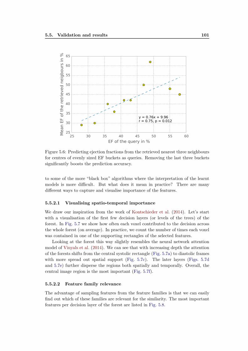
5.5. Validation and results 101
25 30 35 40 45 50 55 60
EF of the query in %
25
30
35
40
45
50
55
60
65
Mean E
F of
the r
etr
ieved n
eig
bours
in %
y = 0.76x + 9.96r = 0.75, p = 0.012
Figure 5.6: Predicting ejection fractions from the retrieved nearest three neighboursfor centres of evenly sized EF buckets as queries. Removing the last three bucketssignificantly boosts the prediction accuracy.
to some of the more “black box” algorithms where the interpretation of the learntmodels is more difficult. But what does it mean in practice? There are manydifferent ways to capture and visualise importance of the features.
5.5.2.1 Visualising spatio-temporal importance
We draw our inspiration from the work of Kontschieder et al. (2014). Let’s startwith a visualisation of the first few decision layers (or levels of the trees) of theforest. In Fig. 5.7 we show how often each voxel contributed to the decision acrossthe whole forest (on average). In practice, we count the number of times each voxelwas contained in one of the supporting rectangles of the selected features.
Looking at the forest this way slightly resembles the neural network attentionmodel of Vinyals et al. (2014). We can see that with increasing depth the attentionof the forests shifts from the central systolic rectangle (Fig. 5.7a) to diastolic frameswith more spread out spatial support (Fig. 5.7c). The later layers (Figs. 5.7dand 5.7e) further disperse the regions both spatially and temporally. Overall, thecentral image region is the most important (Fig. 5.7f).
5.5.2.2 Feature family relevance
The advantage of sampling features from the feature families is that we can easilyfind out which of these families are relevant for the similarity. The most importantfeatures per decision layer of the forest are listed in Fig. 5.8.
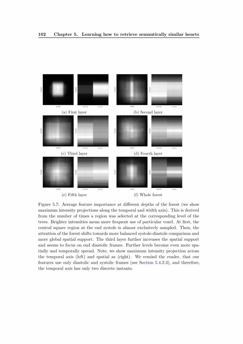
102 Chapter 5. Learning how to retrieve semantically similar hearts
width
height
diastole systole
height
(a) First layer
width
height
diastole systole
height
(b) Second layer
width
height
diastole systole
height
(c) Third layer
width
height
diastole systoleheight
(d) Fourth layer
width
height
diastole systole
height
(e) Fifth layer
width
height
diastole systole
width
(f) Whole forest
Figure 5.7: Average feature importance at different depths of the forest (we showmaximum intensity projections along the temporal and width axis). This is derivedfrom the number of times a region was selected at the corresponding level of thetrees. Brighter intensities mean more frequent use of particular voxel. At first, thecentral square region at the end systole is almost exclusively sampled. Then, theattention of the forest shifts towards more balanced systole-diastole comparison andmore global spatial support. The third layer further increases the spatial supportand seems to focus on end diastolic frames. Further levels become even more spa-tially and temporally spread. Note, we show maximum intensity projection acrossthe temporal axis (left) and spatial as (right). We remind the reader, that ourfeatures use only diastolic and systolic frames (see Section 5.4.2.3), and therefore,the temporal axis has only two discrete instants.
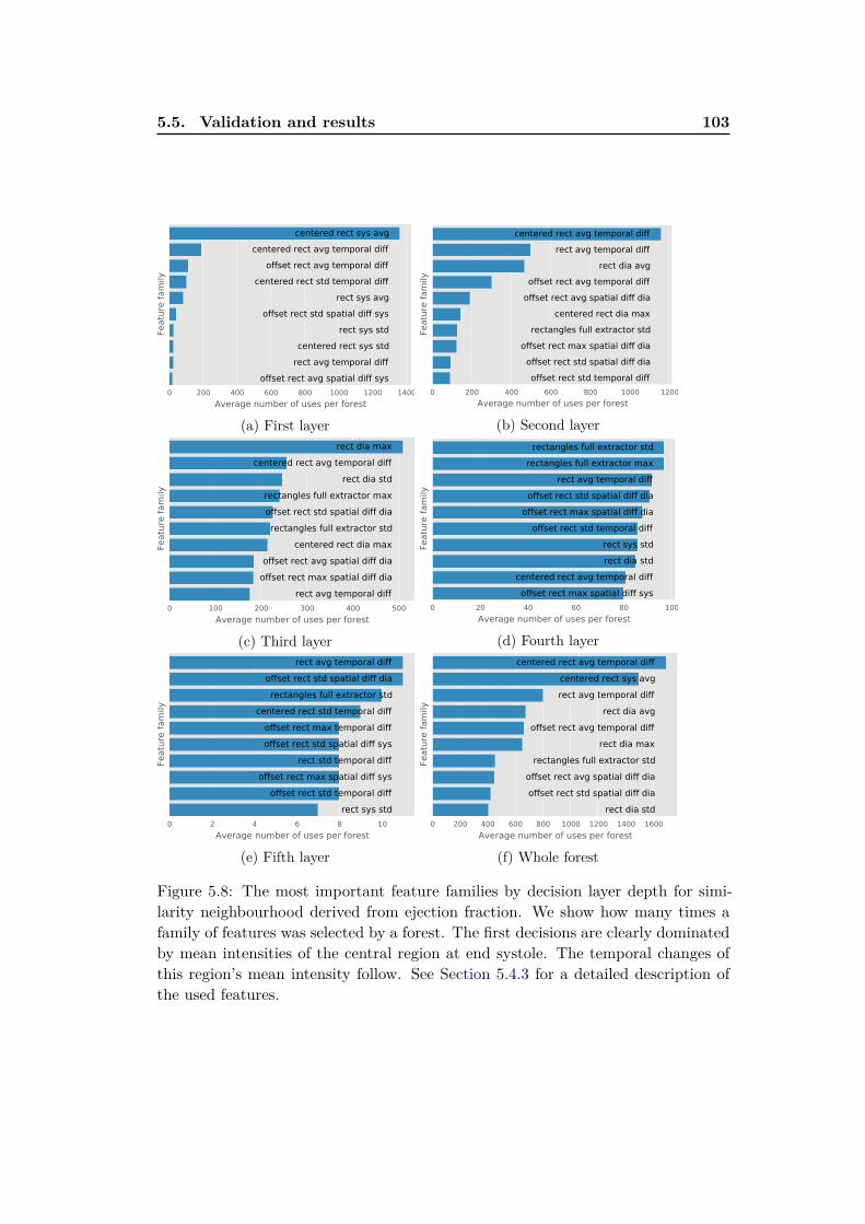
5.5. Validation and results 103
0 200 400 600 800 1000 1200 1400
Average number of uses per forest
Featu
re f
am
ily
offset rect avg spatial diff sys
rect avg temporal diff
centered rect sys std
rect sys std
offset rect std spatial diff sys
rect sys avg
centered rect std temporal diff
offset rect avg temporal diff
centered rect avg temporal diff
centered rect sys avg
(a) First layer
0 200 400 600 800 1000 1200
Average number of uses per forest
Featu
re f
am
ily
offset rect std temporal diff
offset rect std spatial diff dia
offset rect max spatial diff dia
rectangles full extractor std
centered rect dia max
offset rect avg spatial diff dia
offset rect avg temporal diff
rect dia avg
rect avg temporal diff
centered rect avg temporal diff
(b) Second layer
0 100 200 300 400 500
Average number of uses per forest
Featu
re f
am
ily
rect avg temporal diff
offset rect max spatial diff dia
offset rect avg spatial diff dia
centered rect dia max
rectangles full extractor std
offset rect std spatial diff dia
rectangles full extractor max
rect dia std
centered rect avg temporal diff
rect dia max
(c) Third layer
0 20 40 60 80 100
Average number of uses per forest
Featu
re f
am
ily
offset rect max spatial diff sys
centered rect avg temporal diff
rect dia std
rect sys std
offset rect std temporal diff
offset rect max spatial diff dia
offset rect std spatial diff dia
rect avg temporal diff
rectangles full extractor max
rectangles full extractor std
(d) Fourth layer
0 2 4 6 8 10
Average number of uses per forest
Featu
re f
am
ily
rect sys std
offset rect std temporal diff
offset rect max spatial diff sys
rect std temporal diff
offset rect std spatial diff sys
offset rect max temporal diff
centered rect std temporal diff
rectangles full extractor std
offset rect std spatial diff dia
rect avg temporal diff
(e) Fifth layer
0 200 400 600 800 1000 1200 1400 1600
Average number of uses per forest
Featu
re f
am
ily
rect dia std
offset rect std spatial diff dia
offset rect avg spatial diff dia
rectangles full extractor std
rect dia max
offset rect avg temporal diff
rect dia avg
rect avg temporal diff
centered rect sys avg
centered rect avg temporal diff
(f) Whole forest
Figure 5.8: The most important feature families by decision layer depth for simi-larity neighbourhood derived from ejection fraction. We show how many times afamily of features was selected by a forest. The first decisions are clearly dominatedby mean intensities of the central region at end systole. The temporal changes ofthis region’s mean intensity follow. See Section 5.4.3 for a detailed description ofthe used features.
104 Chapter 5. Learning how to retrieve semantically similar hearts
In the first layer (see Fig. 5.8a), the most commonly used feature is the meanintensity of central rectangles at systole (“centered rect sys avg”). This choice makesperfect sense. For intensity-normalised and aligned images (as in our case) the cen-tral region image intensity clearly determines the proportion of myocardium andblood pool. In other words, well contracting heart will cover the region with my-ocardium and the mean intensity will be lower. The second most frequent decisionin the first layer (Fig. 5.8a), the most frequent in the second layer (Fig. 5.8b), andthe most popular feature family across the whole forest (Fig. 5.8f) is the intensitychange in time of the central region (“centered rect avg temporal diff ”). The averageintensity changes in the central rectangle are indeed intuitive features to capturethe ejection fraction similarity. Since the images are pose-normalised by aligningthe epicardia at end diastole, the first splits strongly prefer the systolic measuresand the diastolic ones are almost completely irrelevant.
The second layer of the forests (Fig. 5.8b) captures mainly the temporal changeof mean intensity in the central rectangle and other randomly placed rectangles.But also, the first diastolic features start to appear and their relevance starts togrow (Fig. 5.8c). This is likely to capture complementary information to the systole-dominant decisions in the first layer.
The further layers (Figs. 5.8d and 5.8e) use combinations of a variety of featurefamilies, capturing more and more of the fine-grained image details. The preferenceof one feature over another becomes less clear. Our analysis could differ for a muchlarger dataset.
5.6 Discussion and perspectives
We presented an efficient supervised method for content-based image retrieval forcardiac images based on the Neighbourhood approximating forest (NAF) using a setof generic spatio-temporal features. The retrieval similarity was learned from pair-wise distance ground-truth derived from semantically meaningful parameters andthe NAF automatically picked relevant features. The NAF algorithm has severalproperties particularly well-suited for content-based image retrieval. The distancesto every heart in the database can be rapidly obtained.
The structure of the forest is fixed during the training phase. To insert a newimage into the database, it is passed through the decisions and its reference numberis recorded at the reached leaves. To compare the query image with images in thedatabase, it is no longer necessary to access the pixel intensities of the stored images.This process is also computationally efficient.
Finally, peeking into the tree decisions can give us insights on which parts ofthe heart and which features are relevant for a particular goal. However, additionalvalidation will be needed to ensure reliability of this method and its use in other(more interesting) similarity criteria than the EF.

5.6. Discussion and perspectives 105
5.6.1 Limitations
The forest-based method has a drawback for small datasets. The recursive divisionof the dataset creates nodes with only very few examples after a few splits. E.g.,in our case, using 96 cases is not much for a forest-based method with binary trees.Perfectly balanced trees recursively divide the dataset and rapidly leave less than 3cases per node after just 5 decisions. As the number of leaves grows exponentiallywith tree depth, this reduces the chances of two truly similar images sharing a leaf.Therefore, for smaller datasets, no deep decisions can be taken.
This method is also limited by what the box features can capture. The boxfeatures can be seen as a way to aggregate local information. Some finer aspectsof the hearts are less distinct for the forest to pick up the signal when using rawimage intensity channels.
Since this method is based on image intensities, mixing datasets from othermodalities or even CMR acquisition sequences is currently not possible. In partic-ular, the use of the MESA dataset (Bild, 2002) with thousands of asymptomaticvolunteers is a great resource to learn the differences between healthy and patho-logical hearts. In our case, with the intensity-based features, we would likely learnto discriminate the Gradient echo (GRE) from the SSFP sequences. A simple fix(such as the one for correction of cardiac shape biases by (Medrano-Gracia et al.,2013)) is not available.
5.6.2 Perspectives
To address the rapid drop in the number of cases per node, alternative learningstructures are worth exploration. For example, Neighbourhood approximating jun-gles could be derived from the recently introduced Decision jungles (Shotton et al.,2013). In Decision jungles, directed acyclic graphs are used instead of the trees,occasionally merging similar nodes. This can help to keep higher number of pointsat the nodes, while, at the same time, keeping the decision structure more compact.
Retrieving hearts with similar ejection fractions is just the start. Training thismethod with more cases should help to improve relevance of the retrieved results,detect more subtle differences between the hearts, or experiment with differentsimilarity criteria, e.g., based on clinical outcome or clinical findings.
Adding additional channels enhancing the pericardial effusion (Appendix C),myocardial thinning, valvular jets, particular motion direction, or other motion-field derived features (such as the acceleration features of Kontschieder et al. (2014))could help to better capture the appearance and motion information in the images.In addition, Kontschieder et al. (2015) recently proposed a method to train decisionforests with backpropagation. This way the optimal convolutional filters and theforest structure could be trained simutaneously.
It is also important to explore how to combine NAFs with different similaritycriteria together, so that mixed search criteria could be allowed, and to explorequerying by ensembles of example images (e.g. by summing up the leaf counts). It

106 Chapter 5. Learning how to retrieve semantically similar hearts
is likely that querying the datasets with these ensembles will enhance leaf countsfor the common characteristics while the less common will be “averaged out”.
Chapter 6
Conclusions and perspectives
Over the past few years, several initiatives collecting cardiac images have appeared.These include the Cardiac atlas project (Fonseca et al., 2011) containing the DE-TERMINE subset (Kadish et al., 2009) we frequently used in this thesis, but alsoa study of asymptomatic hearts MESA (Bild, 2002). The UK biobank (Petersenet al., 2013) aims to image a large part of British population, and the EuropeanCardiovascular Magnetic Resonance (EuroCMR) registry (Bruder et al., 2013) col-lecting imaging data from 57 centers in 15 countries. These already quite massivecollections are here to grow and will cause impact on cardiac healthcare. We willneed to find ways to automatically interpret the information contained within thesedatabases and simplify search.
In this thesis we addressed some of the most important challenges of cardiacdata organisation and information extraction from these datasets using machinelearning.
6.1 Summary of the contributions
We addressed the following four issues. Here, we show them with our respectivecontributions and limitations of the proposed methods.
6.1.1 Estimating missing metadata from image content
Many of the DICOM tags are inherently noisy and cannot be realiably used. Inthis thesis we showed that instead of relying on DICOM, we can estimate some ofthe metadata from the image content — the cardiac acquisition plane information.
The main contribution of Chapter 2 is that a good cardiac view recogniser(reaching state of the art performance) can be efficiently trained end-to-end withoutdesigning features using a convolutional neural network. This is possible by fine-tuning parameters of a CNN previously trained for a large scale image recognitionproblem. We published our findings in Margeta et al. (2015c, 2014).
• We achieve state of the art performance in cardiac view recognition by learningan end-to-end system from raw image intensities using CNNs
• This is one of the first works to demonstrate the value of features extractedfrom medical images using CNNs, originally trained on a large scale visualobject recognition dataset
108 Chapter 6. Conclusions and perspectives
• We show that fine-tuning parameters of the CNN pretrained on an objectrecognition dataset is a good strategy that helps to improve performance andspeed up the network training
• We show that the CNNs can be applied to smaller datasets (a common prob-lem in medical imaging) thanks to careful network initialisation and datasetaugmentation, even when training the network from scratch
• We also reproduce the observation of Zhou et al. (2012) that the 3-dimensionalorientations vectors that can be derived from DICOM tags can be used forcardiac view recognition (if the orientation tags are present)
Fine-tuning of a network is a great way to learn complex models from smallersize medical data and CNNs are powerful machine learning tools that have yet tofully propagate into medical imaging.
We trained the views only on a dataset of post-myocardial infarction hearts.These hearts certainly have some particularities as we showed in the thesis, never-theless, their appearance and topology are still rather “normal”. We have yet totest this method on severely pathological cases or less standard acquisitions (non-centred, oriented with atypical angles).
There are also many more cardiac views left to be recognised (Taylor and Bo-gaert, 2012) from other acquisition sequences. Such ground-truth has to be collectedfor all acquisition sequences with which the views are acquired, which leads to acombinatorial problem. Many of these combinations are underrepresented, andlearning from very few examples remains a challenging problem.
In addition, the recognition of the views should not stop on describing the views.This work is a cornerstone for recognition of image modalities and MR acquisitionprotocols and for automatic generation of full image description as done recentlyfor natural images using Recurrent neural networks (Vinyals et al., 2014; Karpathyet al., 2015; Donahue et al., 2014).
6.1.2 Segmentation of cardiac images
Segmentation of cardiac structures allows to index the databases using automaticmeasurements of tissue volumes and estimation of their masses. In Chapter 3 wepropose to segment cardiac MR images with classification forests as in Shotton et al.(2008); Lempitsky et al. (2009); Geremia et al. (2011).
The main contribution of this part of the work is that voxel-wise segmentationof cardiac structures can be learnt from voxel-wise ground-truth.
• We proposed a forest-based segmentation method for LVs from 3D+t cardiacMR sequences and for LAs from 3D MR and CT images
• We introduced a novel two layered approach for standardisation of imageintensities and inter-patient cardiac registration

6.1. Summary of the contributions 109
• We designed spatio-temporal features for learning how to segment dynamicsequences
• We proposed to use other image channels such as vesselness, or distances toblood pool (which can be easily segmented) to segment the atrial images
• We also showed (Appendix A), how non-labelled data can help to segmentthe images in a semi-supervised way and how the best points for labelling canbe proposed
This work led to our publications (Margeta et al., 2012, 2013), and we con-tributed the results from our algorithms to two benchmarking studies (Suinesiapu-tra et al., 2014b; Tobon-Gomez et al., 2015) for fair evaluation. Our methods arenot the best performers in terms of segmentation accuracy. However, they shine interms of how little knowledge about the problem was hardcoded into the algorithmwhich makes them quite flexible. The algorithms also get better with more exam-ples. This makes our approaches much more ready to be applied to other cardiacmodalities, views and tissues, and for the growing data.
While our methods do not use much prior information, some postprocessingto regularise the solution and large datasets to learn sufficiently robust features isessential. Extra steps such as data augmentation and learning discriminative imagechannels would likely help to further improve their performance.
6.1.3 Collection of ground-truth for describing the hearts with se-
mantic attributes
In this thesis, we mainly focused on supervised machine learning approaches. Thismeans that the algorithm learns from examples where ground-truth labels are re-quired. The acquisition of these labels is at least as important as the acquisition ofthe images. Our solution to the annotation collection problem is a web-based crowd-sourcing tool for collection of annotations in order to learn semantic descriptions ofthe hearts described in Chapter 4.
The disease itself is usually not a discrete (yes or no) flag and it manifests itselfthrough several ways. Some of them can be described by clinicians in semanticterms, the cardiac attributes. There is discrepancy between this semantic descrip-tion and the representation by the computer, making searching for hearts in cardiacdatabases using such description difficult. Thanks to the pairwise comparisons, lessexperience in interpretation of cardiac images is needed to correctly answer difficultquestions.
• We design a web interface for crowdsourcing of such ground-truth.
• We propose to describe the cardiac images with semantic attributes such ashypertrophy, thinning, kineticity, dilation, or image quality from pairwiseimage comparisons.

110 Chapter 6. Conclusions and perspectives
• We show, how concepts from web-ranking can be used to learn these at-tributes.
Our crowd (3 in-house annotators) size is very limited and so is the amountof ground-truth currently collected and the conclusions we can draw. Annotatorvariability and quality is also an important aspect to study. When Health InsurancePortability and Accountability Act (HIPAA) compliance is assured, such a toolcould be distributed among medical students to generate a rich resource for learningwhile contributing to the dataset at the same time. Having multiple annotationswould also help us to assess how reliable the predictions are.
Presenting random combination of images to the annotators is not ideal as itredundantly wastes their time on simpler questions that the machine can alreadyconfidently predict. An active loop should be rather used where human input willbe solicited predominantly for the least confident cases.
While we claim that any pathology could be described with semantic attributes,the spectral representations of the hearts cannot capture all of the aspects. Notonly we restricted the research to the LVs, for small structures (such as thin wallsof the myocardium) the spectral features become unstable due to the change oftopology. Moreover, these features depend on good quality image segmentation.
We are also limited by our imagination of the attributes. Attribute discoverytechniques are essential in the next steps.
Once more data is collected, learning better feature representations (e.g. (Kanget al., 2015; Zhang et al., 2014a)) for prediction of the attributes is crucial forimproving the predictions.
6.1.4 Structuring the datasets with clinical similarity
Finally, Chapter 5 discussed how the decision forest structure has desirable prop-erties to structure imaging datasets and can be used to learn similarity for CBIRusing a decision forest-based method.
• We show how NAFs can be used to approximate clinical similarity with respectto ejection fraction or infarction location (Bleton et al., 2015) i.e. aspectscapturing shape, motion and appearance similarity of cardiac sequences.
• We show simple ways to remove static background and estimate the maincardiac phases from the images
• We propose to reuse previously fine-tuned CNN features for cardiac landmarkestimation and image alignment (Appendix B).
• We hint, how the pericardial effusion could be enhanced with simple filtering(Appendix C)
In theory, the NAFs can be trained with arbitrary image similarity ground-truthand used for fast exploratory queries within the large cardiac datasets. Using EF
6.2. Perspectives 111
itself does not lead to any benefit over using pure automatic segmentation andimage measurements.
Our method needs more validation and larger datasets for improved reliability ofthe retrieved results and predictions on different similarity criteria. Also, additionalimage channels will be needed to enhance the relevant information.
While the returned results are not perfect, they are significantly better than justretrieving images at random and the retrieved images are relevant to the query. Inthe end, collection of real usage data in a feedback loop will be necessary to definewhich similarity criteria are actually useful and to personalise the retrieval results.
6.2 Perspectives
In this thesis we only scratched the surface of management of large cardiac databaseswith machine learning, the collection of annotations, or content-based image re-trieval of similar cases. There are many challenges lying ahead.
6.2.1 Multimodal approaches
Different cardiac imaging modalities complement each other with the informationcontained therein. There is a need for multi-modality approaches (Galderisi et al.,2015). None of our tools is modality specific, and the same algorithms could bealmost directly applied to these modalities.
In this thesis, we used mainly SAX images, acquired with the SSFP MR proto-col. This is clearly not sufficient. Other cardiac views can offer deep insights intodifferent aspects of the heart that are not seen on short axis slices. The Delayedenhancement MRI (DE-MRI) acquisition protocol captures the extent of myocar-dial infarction, the tagged imaging sequences help to better estimate the motion,the phase contrast imaging captures the blood flow through the valves and in thearteries. New modalities and protocols appear. T1 imaging at 3T magnetic fieldscan be used to reliably detect and quantify myocardial fibrosis without the need forcontrast agent (Kali et al., 2014) (e.g. to image infarcted regions in hypertrophiccardiomyopathies, dilated cardiomyopathies, or aortic stenoses). Gradient echo T2∗
sequences (Anderson, 2001) capture myocardial iron overload and allow early de-tection of ventricular dysfunction, before it develops. Other modalities such as CTand US can bring yet another angle into study of cardiac anatomy and motion.
6.2.2 Growing data
The study of the EuroCMR registry (Bruder et al., 2009) scanned 27,309 patientsacross 57 sites in 15 European Countries according to standard protocol (Krameret al., 2008). In 61.8% of all subjects, the study found that CMR had significantimpact on diagnosis and therapeutic consequences (change in medication, invasiveprocedure, hospital discharge or admission). About 8.7% of the scans revealed newdiagnoses not suspected before.

112 Chapter 6. Conclusions and perspectives
But we have yet to establish the benefits of CMR on the outcomes. Morepeople will likely be scanned and more data will be generated. Wearable computinghas already started to record real-time health information. It will soon becomenecessary to search through this data with automatic software tools.
With these humongous databases and heterogeneuous data sources, automaticcleaning of the metadata directly from image content and indexing of the databasesfor fast access to relevant studies become even more relevant than before.
6.2.3 Generating more data
We still face the challenges of expensive data acquisition, patient privacy in datacollection and distribution and missing ground-truth. In the meanwhile, if we cangenerate massive synthetic but realistic data and images using biophysical models,we shall be able to train richer models and only then tune them to the real dataproblem. This is known as transfer learning (Pan and Yang, 2010) and is one ofthe main goals of the ERC MedYMA project.
It is significantly cheaper to generate more synthetic data than to acquire andannotate them. There is no need for patients’ consent or restriction on data shar-ing, the underlying parameters used to generate the images (the ground-truth)are known. These in-sillico approaches can generate large quantities of imageswith known ground-truth labels, facilitating training algorithms to reverse the gen-erative process and obtain the labels back from the image data. High qualitygenerators of synthetic cardiac image generators already exist for a wide rangeof modalities (Alessandrini et al., 2015; Prakosa et al., 2013; De Craene et al.,2014; Tobon-Gomez et al., 2011). Whole platforms on the web are dedicated tothe multi-modality medical image simulation to democratise this process (Glatardet al., 2013).
Similarly to how synthetic depth data made real-time pose estimation fromdepth cameras possible (Shotton et al., 2011), robust detectors were trained on syn-thesised fluoroscopic images (Heimann et al., 2014). Geremia et al. (2013) learntto estimate tumour cell density estimation on clinical images by training models onsimulated multi-modal MR images using biophysical models growing synthetic cere-bral tumours at various positions in the brain. Simulated cardiac images (Prakosaet al., 2013) were used to inverse cardiac electrophysiology (Prakosa et al., 2014)and the models transferred to real images. The opportunities are endless.
6.2.4 Data augmentation
We showed that even a simpler way to generate synthetic but very realistic trainingexamples and to improve performance of the machine learning system is to modifythe already existing images such that the labels are preserved. This is called dataaugmentation or data jittering. The augmentation is a cheap and efficient way tocover some of the dataset variability (this can help if features are not invariant tothese changes). Simple image transformations (Decoste and Schölkopf, 2002) and
6.2. Perspectives 113
intensity manipulations are often performed. Image acquisition artefacts such as vi-gnetting or barrel distortion (Wu et al., 2015) or realistic background noise (Hannunet al., 2014) are added.
In general, the problem of augmenting medical images is more difficult as caremust be taken only to change the image content and not the associated label (e.g.
merely changing the image size by an isotropic scale could make a normal heartlook like a dilated one) but not impossible. Adding artificial noise, bias fields orimage artefacts will increase the robustness of our methods.
We will need machine learning models that have the capacity to learn from thesemassive data. Ideally, these will be models into which the training data can beiteratively streamed in batches (such as for neural networks trained with stochasticgradient descent, or in bootstrapped forests) so that it will be quite simple to trainwith new data and update their parameters on the fly. The CNNs as we usedfor recognition of cardiac planes are a good fit for the growing multi-modal dataproblem.
6.2.5 Collecting labels through crowdsourcing and gamification
Now, the challenge is not only to keep acquiring and aggregating the data but alsoto design annotation tools for our algorithms to learn. The solutions are multiple.One is to generate synthetic data with known ground-truth, another one is to askthe clinicians or the “crowd” for them. Many complex questions can be reduced tosimpler ones where the crowd can competently answer them.
Pair-wise image annotations we used are not the only way. Large companieslike Google are using the crowdsourcing to collect ground-truth for its Street viewservice house number recognition or to translate books. Galaxy Zoo teaches peopleastronomy while collecting precious annotations for automated description of galax-ies. Duolingo teaches people foreign languages and the users help them to trainautomatic translation systems in return, gamifying (von Ahn and Dabbish, 2004)the ground-truth collection.
There are many challenges to make these systems more engaging and how touse the often not perfect ground-truth.
6.2.6 Moving from diagnosis to prognosis
In the end, diagnosis is not the end. Finding evidence about “what is likely tohappen” should shape clinical practice. Follow-up evidence is needed for cardiacimaging to improve quality of care and the outcomes. Shift in focus from diagno-sis to prognosis and outcomes (Timmis et al., 2015) should happen with patientsreporting the outcome measures and their quality of life. If prognosis is to replacediagnosis (Croft et al., 2015), this will be impossible without automating the wholeprocess of data management and effectively retrieving the supporting data basedon the outcomes and benefits to the patients.

Appendix A
Distance approximating forests
for sparse label propagation
Contents
A.1 Introduction . . . . . . . . . . . . . . . . . . . . . . . . . . . . 115
A.2 Previous work . . . . . . . . . . . . . . . . . . . . . . . . . . . 116
A.3 Distance approximating forests . . . . . . . . . . . . . . . . . 117
A.3.1 Finding shortest paths to the labels . . . . . . . . . . . . . . 118
A.4 Results and discussion . . . . . . . . . . . . . . . . . . . . . . 120
A.4.1 Synthetic classification example . . . . . . . . . . . . . . . . . 120
A.4.2 Towards interactive cardiac segmentation . . . . . . . . . . . 121
A.5 Conclusions . . . . . . . . . . . . . . . . . . . . . . . . . . . . . 123
A.5.1 Perspectives . . . . . . . . . . . . . . . . . . . . . . . . . . . . 123
Overview
In this appendix, we present a semi-supervised label propagation algorithm basedon the density decision forest to approximate geodesic distances in feature space tolabelled points. The algorithm hierarchically partitions the data (both labelled andunlabelled) by a simple unsupervised splitting criterion in order to approximatefeature space density. Using the density approximation, we then propagate labelsfrom the nearest annotated points in the dataset to all unlabelled points, using afast-marching-like propagation strategy.
This allows us to exploit the unlabelled data and use significantly less manualinput. Moreover, the obtained distances to the labels can help us to suggest newpoints to be labelled in an active learning loop. We test this learning method onleft ventricle segmentation from CMR.
A.1 Introduction
Large quantities of medical images have been recently made available. Manualinputs (e.g. labelling of each voxel in an image or assigning a pathology for eachimage in the database) can be a tedious, time consuming and expensive process.
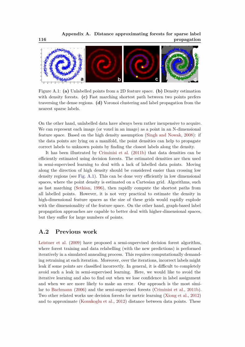
116Appendix A. Distance approximating forests for sparse label
propagation
a b c d
Figure A.1: (a) Unlabelled points from a 2D feature space. (b) Density estimationwith density forests. (c) Fast marching shortest path between two points preferstraversing the dense regions. (d) Voronoi clustering and label propagation from thenearest sparse labels.
On the other hand, unlabelled data have always been rather inexpensive to acquire.We can represent each image (or voxel in an image) as a point in an N-dimensionalfeature space. Based on the high density assumption (Singh and Nowak, 2008): ifthe data points are lying on a manifold, the point densities can help to propagatecorrect labels to unknown points by finding the closest labels along the density.
It has been illustrated by Criminisi et al. (2011b) that data densities can beefficiently estimated using decision forests. The estimated densities are then usedin semi-supervised learning to deal with a lack of labelled data points. Movingalong the direction of high density should be considered easier than crossing lowdensity regions (see Fig. A.1). This can be done very efficiently in low dimensionalspaces, where the point density is estimated on a Cartesian grid. Algorithms, suchas fast marching (Sethian, 1996), then rapidly compute the shortest paths fromall labelled points. However, it is not very practical to estimate the density inhigh-dimensional feature spaces as the size of these grids would rapidly explodewith the dimensionality of the feature space. On the other hand, graph-based labelpropagation approaches are capable to better deal with higher-dimensional spaces,but they suffer for large numbers of points.
A.2 Previous work
Leistner et al. (2009) have proposed a semi-supervised decision forest algorithm,where forest training and data relabelling (with the new predictions) is performediteratively in a simulated annealing process. This requires computationally demand-ing retraining at each iteration. Moreover, over the iterations, incorrect labels mightleak if some points are classified incorrectly. In general, it is difficult to completelyavoid such a leak in semi-supervised learning. Here, we would like to avoid theiterative learning and also to find out when we lose confidence in label assignmentand when we are more likely to make an error. Our approach is the most simi-lar to Bachmann (2006) and the semi-supervised forests (Criminisi et al., 2011b).Two other related works use decision forests for metric learning (Xiong et al., 2012)and to approximate (Konukoglu et al., 2012) distance between data points. These

A.3. Distance approximating forests 117
approaches, however, require pairwise point distances as the input.In Bachmann (2006), an efficient forest-based method called Vantage point forest
is used to partition the large high-dimensional data space of pixels from multi-spectral satellite images. They avoid exhaustive point-to-point distance calculationsfor a subsequent dimensionality reduction algorithm. In their approach, each treesees a different feature subset and is associated to one landmark point in the image.The authors do not exploit the density direction that can be obtained from a densityforest.
In our approach, we propose to avoid the need for feature space rasterisationand use the trees to jointly estimate local point densities. We partition the initialspace into several smaller subsets and find approximate geodesic distances fromevery unlabelled point to the closest label. The tree ensemble then averages thetree distances for a smoother approximation.
In this appendix we propose
1. A method for geodesic distance estimation in the feature space to find candi-dates for relabelling.
2. A practical implementation of density forests for learning with sparsely la-belled data.
A.3 Distance approximating forests
Although a semi-supervised problem like the one illustrated in Fig. A.1 could besolved by the above mentioned methods or traditional manifold learning algorithms,it becomes much more difficult with increasing dimension of the feature space andsize of the training set.
By partitioning the data using the “divide and conquer” strategy of the forests,we recursively divide the whole dataset into much smaller chunks of data and workin parallel for each tree. We also use different feature space dimensions at eachnode for increased computational efficiency while adapting to the the underlyingdata density.
The training process is very simple. We start at the root node and recursivelypartition the data S until the stopping criteria (maximum depth, minimum numberof points in a leaf) are satisfied. At each node, we partition the data using ρ
configurations of binary split functions θn(x) = τn(ψn(Φn(x))). These consist of alinear projector ψn(x) = W Tx and a threshold τn(x) = x < T . Each split functiondivides the points into two disjoint partitions V = 0, 1.
Out of the ρ choices we then select the split that maximizes the total splitquality I. In our case, we use a fully unsupervised the differential information gain(Eq. (A.1)) as the cost function, encouraging splits that can be represented with twocompact multivariate Gaussians. Here, |Λ(S)| is the determinant of the covariancematrix of the Gaussian distribution.
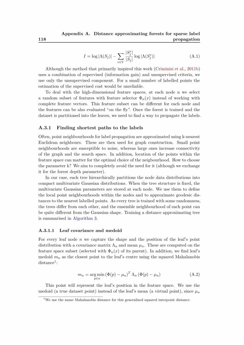
118Appendix A. Distance approximating forests for sparse label
propagation
I = log |Λ(Sj)| −∑
v∈V
|Svj |
|Sj |log |Λ(Sv
j )| (A.1)
Although the method that primarily inspired this work (Criminisi et al., 2011b)uses a combination of supervised (information gain) and unsupervised criteria, weuse only the unsupervised component. For a small number of labelled points theestimation of the supervised cost would be unreliable.
To deal with the high-dimensional feature spaces, at each node n we selecta random subset of features with feature selector Φn(x) instead of working withcomplete feature vectors. This feature subset can be different for each node andthe features can be also evaluated “on the fly”. Once the forest is trained and thedataset is partitioned into the leaves, we need to find a way to propagate the labels.
A.3.1 Finding shortest paths to the labels
Often, point neighbourhoods for label propagation are approximated using k-nearestEuclidean neighbours. These are then used for graph construction. Small pointneighbourhoods are susceptible to noise, whereas large ones increase connectivityof the graph and the search space. In addition, location of the points within thefeature space can matter for the optimal choice of the neigbourhood. How to choosethe parameter k? We aim to completely avoid the need for it (although we exchangeit for the forest depth parameter).
In our case, each tree hierarchically partitions the node data distributions intocompact multivariate Gaussian distributions. When the tree structure is fixed, themultivariate Gaussian parameters are stored at each node. We use them to definethe local point neighbourhoods within the nodes and to approximate geodesic dis-tances to the nearest labelled points. As every tree is trained with some randomness,the trees differ from each other, and the ensemble neighbourhood of each point canbe quite different from the Gaussian shape. Training a distance approximating treeis summarised in Algorithm 3.
A.3.1.1 Leaf covariance and medoid
For every leaf node n we capture the shape and the position of the leaf’s pointdistribution with a covariance matrix Λn and mean µn. These are computed on thefeature space subset (selected with Φn(x) of its parent). In addition, we find leaf’smedoid mn as the closest point to the leaf’s centre using the squared Mahalanobisdistance1:
mn = arg minp∈n
(Φ(p)− µn)T Λn (Φ(p)− µn) (A.2)
This point will represent the leaf’s position in the feature space. We use themedoid (a true dataset point) instead of the leaf’s mean (a virtual point), since µn
1We use the name Mahalanobis distance for this generalized squared interpoint distance.
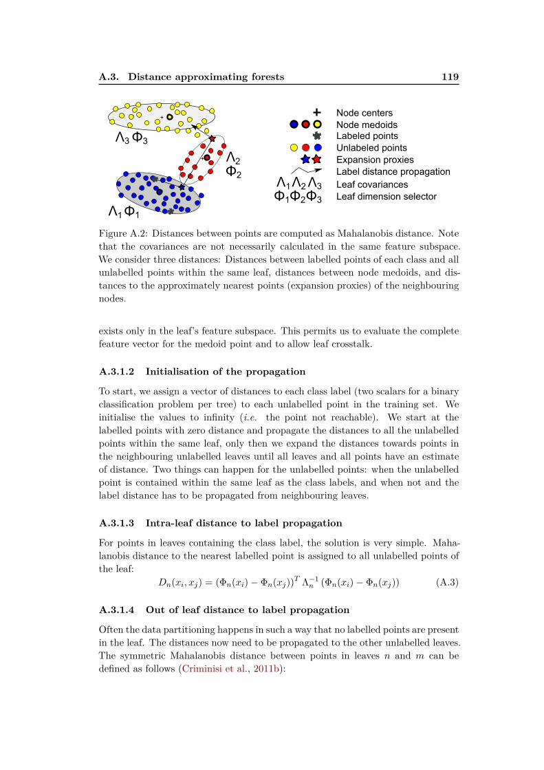
A.3. Distance approximating forests 119
Node centers
Node medoidsLabeled points
Unlabeled points
Expansion proxies
Label distance propagation
Leaf covariances
Leaf dimension selector
Λ1
Λ2
Λ3
Φ2
Φ1
Φ3
Λ1Λ2Λ3
Φ2Φ1 Φ3
Figure A.2: Distances between points are computed as Mahalanobis distance. Notethat the covariances are not necessarily calculated in the same feature subspace.We consider three distances: Distances between labelled points of each class and allunlabelled points within the same leaf, distances between node medoids, and dis-tances to the approximately nearest points (expansion proxies) of the neighbouringnodes.
exists only in the leaf’s feature subspace. This permits us to evaluate the completefeature vector for the medoid point and to allow leaf crosstalk.
A.3.1.2 Initialisation of the propagation
To start, we assign a vector of distances to each class label (two scalars for a binaryclassification problem per tree) to each unlabelled point in the training set. Weinitialise the values to infinity (i.e. the point not reachable). We start at thelabelled points with zero distance and propagate the distances to all the unlabelledpoints within the same leaf, only then we expand the distances towards points inthe neighbouring unlabelled leaves until all leaves and all points have an estimateof distance. Two things can happen for the unlabelled points: when the unlabelledpoint is contained within the same leaf as the class labels, and when not and thelabel distance has to be propagated from neighbouring leaves.
A.3.1.3 Intra-leaf distance to label propagation
For points in leaves containing the class label, the solution is very simple. Maha-lanobis distance to the nearest labelled point is assigned to all unlabelled points ofthe leaf:
Dn(xi, xj) = (Φn(xi)− Φn(xj))T Λ−1
n (Φn(xi)− Φn(xj)) (A.3)
A.3.1.4 Out of leaf distance to label propagation
Often the data partitioning happens in such a way that no labelled points are presentin the leaf. The distances now need to be propagated to the other unlabelled leaves.The symmetric Mahalanobis distance between points in leaves n and m can bedefined as follows (Criminisi et al., 2011b):
120Appendix A. Distance approximating forests for sparse label
propagation
Dn,m(xi, xj) = 0.5 (Dn(xi, xj) +Dm(xi, xj)) (A.4)
This is similar to Jeffries-Matsushita distance (Bachmann, 2006) used for clus-ter similarity. Note that when n equals to m this becomes equivalent to Eq. (A.3).However, as in the graph-based methods, pairwise point distances to find the bestinter-leaf point-to-point combination could be prohibitively expensive for highernumber of points to be computed exhaustively. We reduced this problem to findingonly the nearest node medoid and then a point of expansion. This can be repre-sented with a much smaller pairwise medoid distance matrix Wt for each tree t.Once computed, this matrix stays fixed.
A.3.1.5 Finding the nearest point from another node
Now, we will discuss how to use this matrix to find the nearest leaves and propagatethe label distances. First, the best labelled-unlabelled medoid combination forexpansion is found as the minimum pairwise Mahalanobis distance of the medoids.We call leaves containing these two medoids a source (fixed) and a target (expansion)leaf. From the source leaf, where each point is already assigned a distance to thelabel, we expand the distances to the target leaf.
To reduce another exhaustive pairwise distance problem (i.e., for each point inthe target leaf find the closest point in the source leaf), we first find a single proxypoint within the target leaf. This proxy represents the connection between the twoleaves. Ideally, this should be a point on the boundary of the source leaf distributionand at the same time close enough to the target leaf distribution (see Fig. A.2). Wechoose it to be a point from the source leaf closest to the target leaf medoid. Now,the symmetric Mahalanobis distances between this point to all points in the targetleaf can be calculated. These distances are summed withthe “distance to the label”value of the proxy point. The sum of the two is then stored for each target leafpoint.
A.3.1.6 The ensemble decision
This distance propagation procedure is independent for each class (for classification)and each tree. Ultimately, the minimum distances to each class label are assignedto every point in the training set. The final label of each data point is then assignedto be the class with minimal average distance across all forests.
A.4 Results and discussion
A.4.1 Synthetic classification example
We first tested our algorithm on two-class classification problem of a synthetic 3Dspirals dataset. We generated two spirals consisting of a total of 1000 points.

A.4. Results and discussion 121
64
20
24
6 6 4 2 0 2 4 6 8
4
6
8
10
12
14
1 2 3 4 5 6 7 8 9 1 01 11 21 31 41 51 61 71 81 92 04 0
5 0
6 0
7 0
8 0
9 0
1 0 0Su p p or t gv ect o r gm ach in e gRBF
1 2 3 4 5 6 7 8 9 1 01 11 21 31 41 51 61 71 81 92 04 0
5 0
6 0
7 0
8 0
9 0
1 0 0Lab e l gp r op ag at ion
1 2 3 4 5 6 7 8 9 1 01 11 21 31 41 51 61 71 81 92 04 0
5 0
6 0
7 0
8 0
9 0
1 0 0Lab e l gsp r ead in g
1 2 3 4 5 6 7 8 9 1 01 11 21 31 41 51 61 71 81 92 04 0
5 0
6 0
7 0
8 0
9 0
1 0 0Ran d om gFor est s
1 2 3 4 5 6 7 8 9 1 01 11 21 31 41 51 61 71 81 92 04 0
5 0
6 0
7 0
8 0
9 0
1 0 0Dist an cegap p r ox im at in g gf o r est sgFu l l
Figure A.3: Comparison of classification accuracy with respect to number of labelledpoints for various learning algorithms on a 3D spirals dataset. Labelled points arechosen from the dataset at random. Our distance approximating forest reacheshigher accuracies significantly faster.
Out of these points we randomly selected 15 points (5.7% of the training data) tobe labelled and ran our semi-supervised forest. We trained 300 trees with maximaldepth 4 and tested 50 split function configurations per node.
In order to validate the inter-leaf distance propagation we restrict the numberof tested dimensions at each node to two (with all three dimensions we were able torapidly achieve >90% average classification accuracy). Similarly, denser distributionalso improves the classification accuracy as the leaf covariances are estimated muchmore robustly, however, this hides real problems with noisy points. Also whenlabelled points are placed more uniformly, much better coverage can be obtained.The setup from Fig. A.4 misclassifies only 18.3% of the points.
It is easy to see that the misclassified points in some regions (marked withellipses on (b) and (c)) have much larger distance to the label than others. Thiscan be exploited in an active learning strategy to propose new points to be labelled.
A.4.2 Towards interactive cardiac segmentation
Traditionally, decision forests have already been used in medical imaging for quitea large range of segmentation problems. This often requires large databases richwith segmentation information. We will show here that our semi-supervised forestscan be used when the data is sparsely labelled, e.g. in an interactive segmentation.
Prior to the segmentation, we train a fully unsupervised forest using all voxelsof the image to be segmented according to the differential entropy splitting cost asdescribed above. This helps us to decompose the image into several configurations

122Appendix A. Distance approximating forests for sparse label
propagation
−8 −6 −4 −2 0 2 4 6 8
−6
−4
−2
0
2
4
6
5
10
15
20
25
30
35
40
45
50
55
−8 −6 −4 −2 0 2 4 6 8
−6
−4
−2
0
2
4
6
−8 −6 −4 −2 0 2 4 6 8
−6
−4
−2
0
2
4
6a b c
Figure A.4: (a) Two 3D spirals in an orthogonal 2D view and labelled points(black squares and circles). (b) Labels assigned according to the nearest label. (c)
Minimum distances to nearest labelled points (encoded by colour) clearly show thatthe misclassified regions are far from the labels and would be good candidates forrelabelling.
of meaningful partitions. Which also means that similar feature measurementsare clustered together and can benefit from the geodesic label propagation. Thenmedoids and their pairwise distance matrices can be precomputed and fixed for eachtree in an off-line step. The much faster propagation of the distances to the labelscan be then done during the interaction.
A.4.2.1 Features
We use a combination of very simple features for each voxel - image intensity (attwo scales of a Gaussian pyramid from the current frame and the frame from themiddle of the cardiac sequence). Since we apply the semi-supervision on a singleimage, there is no need for registration to the reference pose and we use also voxelcoordinates as features to spatially regularise the segmentation. For a 2D case, thisresults in a feature vector of dimension 6.
A.4.2.2 Stabilisation of the covariance matrices
Real MR images pose a problem for the differential entropy. Homogeneous back-ground (air) forms intensity clusters with little variation and the covariance matricesmight not be invertible. Therefore, similarly to Levenberg-Marquardt optimisationalgorithm (Marquardt, 1963), we regularise our covariance matrices with a scaledidentity, i.e., Λr
n ← Λn + γI both for the computation of differential informationgain and for the Mahalanobis distance computation. This significantly improvesthe numerical stability while did not seem to compromise the performance for ourexperiments. In our experiments we use γ = 0.1.
The output of our segmentation algorithm is still soft. However, distances tolabels are used instead of the label posterior probabilities. The forests were nottrained for this particular segmentation problem rather than to decompose theimage into something meaningful. Hence, the structure already learned could beused to extend the segmentation to more classes or even regression very easilywithout retraining - only label propagation step is needed.

A.5. Conclusions 123
a b c
Figure A.5: (a) We sparsely labelled 4 points on the myocardium and 20 pointsfrom the background. (b) Binary mask of points with shorter distance to thenearest myocardial label than to the background label. We used 17 trees, ρ = 10,and dimension subset 2. (c) Overlay of the final segmentation (Canny edges).
A.5 Conclusions
We proposed a semi-supervised learning algorithm that uses unsupervised foresttraining to estimate feature space density and to later approximate geodesic dis-tances to the labeled points in this space. Although distances from individual treesare not perfect, they already create a signal of the distance. The distances are thenaveraged to get the final estimate. As a result we associate the shortest distance tothe nearest labelled point of each class to all points in the training dataset. For atwo class segmentation problem this means that a 2D vector is associated to eachvoxel in the image.
We observed that this technique works even if we do a lower-dimensional featuresubspace selection, when the subspace is different at each node. This permits tospeed up the distance calculation and gives us the possibility to deal with very high-dimensional datasets or even datasets where features are evaluated “on the fly.” Thedecision forests help us to partition the feature space into several smaller regions,each represented by a point subspace, covariance, and a medoid. We can there-fore replace expensive pairwise point-to-point with distances between the leaves asa rough estimate of the connectivity. One has to be careful with deep trees asthe number of leaves (and hence medoids) grows exponentially with depth (up to2depth−1).
We tested this algorithm on a synthetic dataset and for an interactive segmen-tation of left ventricles from CMR. As the structure of the trees and the medoiddistance matrix can be fixed we can do a rapid update of the distances once newlabels are added. As the forests are inherently parallel this can be further sped up.
A.5.1 Perspectives
Assigning distances to labels for each points enables us to actively guide pointselection process in an active learning loop. Points far from any label should beconsidered to be labelled first. It is important to note that this approach is not
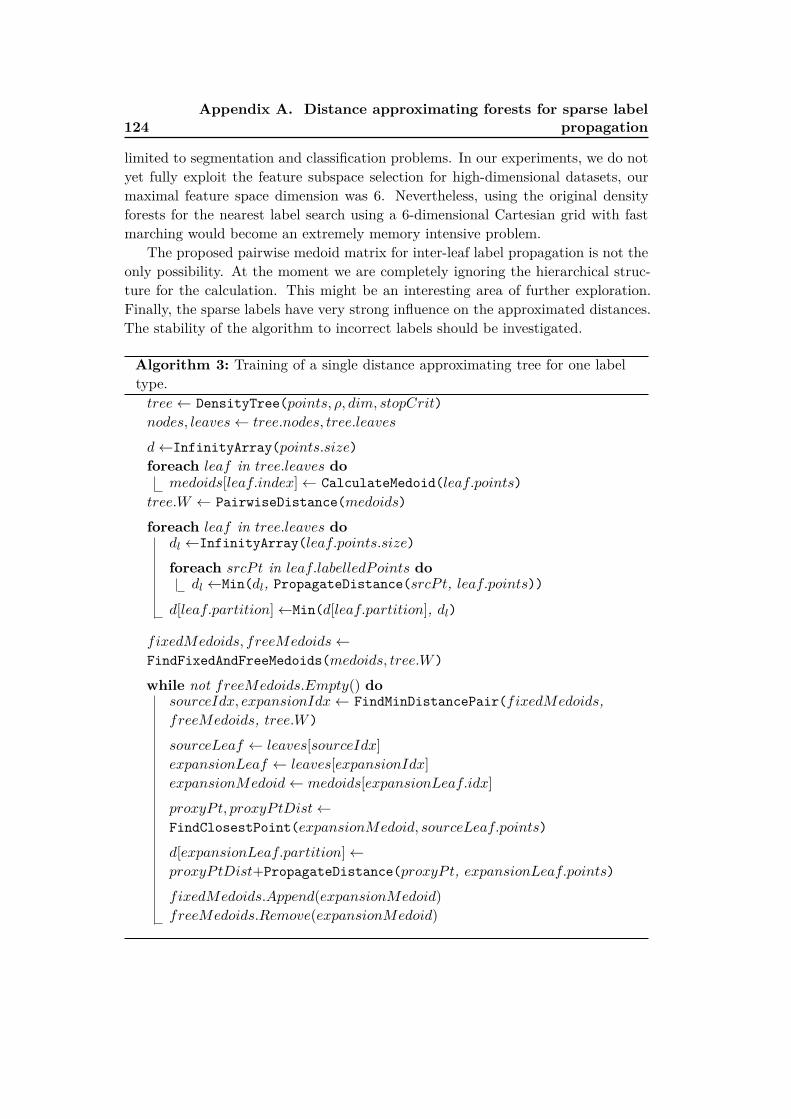
124Appendix A. Distance approximating forests for sparse label
propagation
limited to segmentation and classification problems. In our experiments, we do notyet fully exploit the feature subspace selection for high-dimensional datasets, ourmaximal feature space dimension was 6. Nevertheless, using the original densityforests for the nearest label search using a 6-dimensional Cartesian grid with fastmarching would become an extremely memory intensive problem.
The proposed pairwise medoid matrix for inter-leaf label propagation is not theonly possibility. At the moment we are completely ignoring the hierarchical struc-ture for the calculation. This might be an interesting area of further exploration.Finally, the sparse labels have very strong influence on the approximated distances.The stability of the algorithm to incorrect labels should be investigated.
Algorithm 3: Training of a single distance approximating tree for one labeltype.tree← DensityTree(points, ρ, dim, stopCrit)
nodes, leaves← tree.nodes, tree.leaves
d←InfinityArray(points.size)
foreach leaf in tree.leaves domedoids[leaf.index]← CalculateMedoid(leaf.points)
tree.W ← PairwiseDistance(medoids)
foreach leaf in tree.leaves dodl ←InfinityArray(leaf.points.size)
foreach srcP t in leaf.labelledPoints dodl ←Min(dl, PropagateDistance(srcP t, leaf.points))
d[leaf.partition]←Min(d[leaf.partition], dl)
fixedMedoids, freeMedoids←
FindFixedAndFreeMedoids(medoids, tree.W)
while not freeMedoids.Empty() dosourceIdx, expansionIdx← FindMinDistancePair(fixedMedoids,
freeMedoids, tree.W)
sourceLeaf ← leaves[sourceIdx]
expansionLeaf ← leaves[expansionIdx]
expansionMedoid← medoids[expansionLeaf.idx]
proxyPt, proxyPtDist←
FindClosestPoint(expansionMedoid, sourceLeaf.points)
d[expansionLeaf.partition]←
proxyPtDist+PropagateDistance(proxyPt, expansionLeaf.points)
fixedMedoids.Append(expansionMedoid)
freeMedoids.Remove(expansionMedoid)
Appendix B
Regressing cardiac landmarks
from CNN features for image
alignment
Contents
B.1 Introduction . . . . . . . . . . . . . . . . . . . . . . . . . . . . 125
B.2 Aligning with landmarks and regions of interest . . . . . . . 126
B.3 Definition of cardiac landmarks . . . . . . . . . . . . . . . . . 126
B.4 Cascaded shape regression . . . . . . . . . . . . . . . . . . . . 128
B.5 Conclusions . . . . . . . . . . . . . . . . . . . . . . . . . . . . . 131
Overview
To compare relevant cardiac territories across different subjects and cardiac shapevariations we must first establish correspondences between the hearts. This is espe-cially necessary since the features we use throughout the thesis (Section 5.4.3) arenot invariant even to simple rotations and translations. We show how features fromthe CNN previously fine-tuned for recognition of acquisition planes (Chapter 2) canbe reused for cardiac landmark estimation, and to align the cardiac sequences.
B.1 Introduction
Image registration is one of the obvious choices for registration of cardiac images.Robust inter-subject cardiac alignment via traditional image registration methodsis in general quite difficult due to the presence of trabeculations, papillary muscles,extra-cardiac thoracic structures, and MRI acquisition artefacts (Klinke et al., 2013;Naehle et al., 2011; Saremi et al., 2008) frequently appearing on cardiac images. Ouet al. (2012) address the inter-patient cardiac registration by first masking the heartswith manual segmentation. Masking the heart prior to the registration reducesthe effect of irrelevant structures but requires cardiac segmentation instead. InChapter 3, we trained two layers of decision forests, the first one roughly segmentedthe heart and returned soft probability maps which we used for registering imagesbetween different patients. The thorax stripping presented in Section 5.4.2.1 helps
126Appendix B. Regressing cardiac landmarks from CNN features for
image alignment
to automatically remove the outer structures by fading the irrelevant non-movingbackground information without the detailed segmentation.
Even a perfect masking of the images with segmentation does not guaranteeaccurate correspondences between the cardiac images (except for rigid alignment)using non-linear registration as ambiguities exists for large deformations. Lombaertet al. (2012) suggest that better correspondences between cardiac images for regis-tration can be obtained by registering spectral representations of the images insteadof registering the image intensity channels directly. Nevertheless, image registrationmethods, in general, result in little control on which parts should and which partsshould not matter for the alignment.
We argue that landmark-based inter-patient approaches are a more flexible wayto define correspondences between the hearts. The advantage of using landmark-based methods for alignment of the cardiac images is the flexibility to rapidly changethe correspondence model (rigid, similarity, affine, or piecewise affine) and the ref-erence cardiac structure on the fly.
B.2 Aligning with landmarks and regions of interest
In practice, cardiac images are commonly aligned by automatically or manuallyplacing a set of landmarks. These often include the junction points of the left ven-tricle, or ventricular barycentres (Wang et al., 2015; Bai et al., 2015). The CAP(Fonseca et al., 2011) provides an interactive tool for fitting much denser left ventric-ular meshes to the cardiac images. An alternative is drawing tight contours Afshinet al. (2012b) or rectangles (Afshin et al., 2012a) that encapsulate the left ventricle.
For large scale analysis it is desirable to automate this process but still keep thepossibility of simple manual corrections for failure and to establish correspondencesalso for the right ventricle and possibly other structures. It has been shown (e.g.
by Zhou et al. (2012)), that separate detectors can be trained for the main cardiaclandmarks. In theory, it is possible to train a detector for any landmark. Thisrequires to train and test a large number of detectors, to suppress multiple maximaand regularize the final solution.
In this appendix, we propose an automated landmark detection method inspiredby the technique of Ren et al. (2014) for face alignment in face recognition. Theirmethod is quite robust to occlusion in natural images, e.g., hair across the eyesand working under varying light conditions. The MR acquisition artefacts can bealso modelled as occlusions. The acquisition intensity differences and bias fields areanalogous to the variation of the lighting conditions. We therefore approach thealignment of hearts with this technique.
B.3 Definition of cardiac landmarks
Which landmarks to choose for our model and how to consistently establish the cor-respondences even for the free walls? To compare corresponding cardiac territories
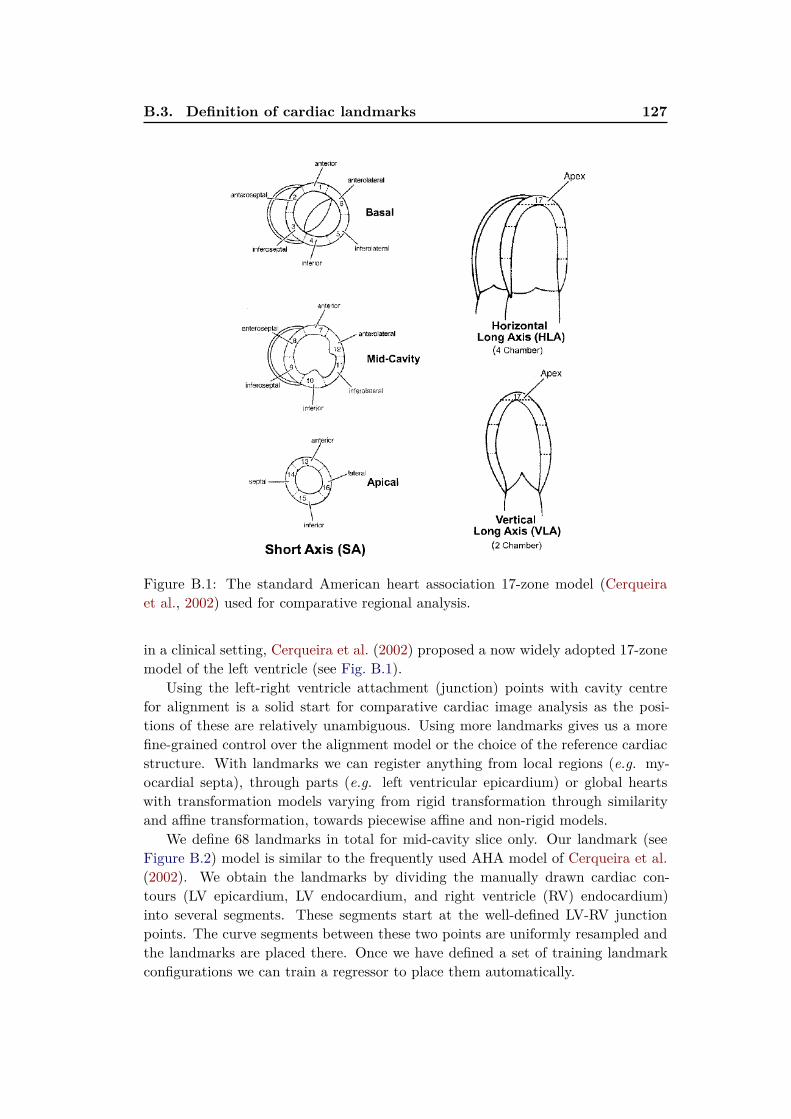
B.3. Definition of cardiac landmarks 127
Figure B.1: The standard American heart association 17-zone model (Cerqueiraet al., 2002) used for comparative regional analysis.
in a clinical setting, Cerqueira et al. (2002) proposed a now widely adopted 17-zonemodel of the left ventricle (see Fig. B.1).
Using the left-right ventricle attachment (junction) points with cavity centrefor alignment is a solid start for comparative cardiac image analysis as the posi-tions of these are relatively unambiguous. Using more landmarks gives us a morefine-grained control over the alignment model or the choice of the reference cardiacstructure. With landmarks we can register anything from local regions (e.g. my-ocardial septa), through parts (e.g. left ventricular epicardium) or global heartswith transformation models varying from rigid transformation through similarityand affine transformation, towards piecewise affine and non-rigid models.
We define 68 landmarks in total for mid-cavity slice only. Our landmark (seeFigure B.2) model is similar to the frequently used AHA model of Cerqueira et al.(2002). We obtain the landmarks by dividing the manually drawn cardiac con-tours (LV epicardium, LV endocardium, and right ventricle (RV) endocardium)into several segments. These segments start at the well-defined LV-RV junctionpoints. The curve segments between these two points are uniformly resampled andthe landmarks are placed there. Once we have defined a set of training landmarkconfigurations we can train a regressor to place them automatically.
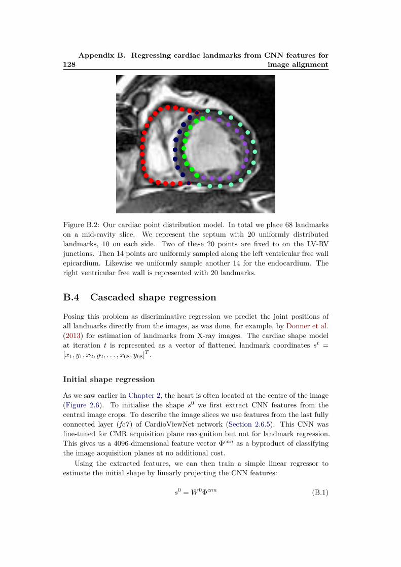
128Appendix B. Regressing cardiac landmarks from CNN features for
image alignment
Figure B.2: Our cardiac point distribution model. In total we place 68 landmarkson a mid-cavity slice. We represent the septum with 20 uniformly distributedlandmarks, 10 on each side. Two of these 20 points are fixed to on the LV-RVjunctions. Then 14 points are uniformly sampled along the left ventricular free wallepicardium. Likewise we uniformly sample another 14 for the endocardium. Theright ventricular free wall is represented with 20 landmarks.
B.4 Cascaded shape regression
Posing this problem as discriminative regression we predict the joint positions ofall landmarks directly from the images, as was done, for example, by Donner et al.(2013) for estimation of landmarks from X-ray images. The cardiac shape modelat iteration t is represented as a vector of flattened landmark coordinates st =
[x1, y1, x2, y2, . . . , x68, y68]T .
Initial shape regression
As we saw earlier in Chapter 2, the heart is often located at the centre of the image(Figure 2.6). To initialise the shape s0 we first extract CNN features from thecentral image crops. To describe the image slices we use features from the last fullyconnected layer (fc7 ) of CardioViewNet network (Section 2.6.5). This CNN wasfine-tuned for CMR acquisition plane recognition but not for landmark regression.This gives us a 4096-dimensional feature vector Φcnn as a byproduct of classifyingthe image acquisition planes at no additional cost.
Using the extracted features, we can then train a simple linear regressor toestimate the initial shape by linearly projecting the CNN features:
s0 =W 0Φcnn (B.1)

B.4. Cascaded shape regression 129
Where W 0 is estimated using ridge regression (Golub et al., 1979) as:
W 0 = argminW
∑
i
∥WΦcnn(Ii)− si∥+ λ∥W∥ (B.2)
The regularisation of the weight matrix W t is necessary for the method topredict realistic cardiac shapes at its output. The best parameter λ was chosen bycross-validation.
Refinement of the prediction with CNN features
The initial estimate (Figure B.3) can then be refined with cascaded regression.Instead of the CNN features, the cascaded regression uses shape-indexed featuresΦt(I, st−1), i.e., features evaluated from patches centred at landmark positions ofthe current shape estimate. A new ridge regressor is then trained to predict theshape update jointly from all features. The shape update can be represented as:
st = st−1 +W tΦt(I, st−1) (B.3)
At each stage of the cascade a shape estimation matrix W t is trained via ridgeregression. We use local binary features (Ren et al., 2014) for the shape-indexedfeatures.
W t = argminW
∑
i
∥st−1i +WΦt(Ii, s
t−1i )− si∥+ λ∥W∥ (B.4)
Dataset augmentation
In practice, some differences in hearts’ positions and orientations between the ac-quisitions exist. These are quite arbitrary and depend on the radiologist or theacquisition machine settings. Nevertheless, they do not change the underlying in-formation content of the images.
To better capture variability of the dataset and to increase the training setsize, we generate new images indistinguishable from the real ones by rotating andtranslating the original image slices. Even small changes to the image scale can stillgenerate images of hearts of realistic sizes. We therefore use the original training setand augment it (both the images and the landmarks) with additional scale changes,rotations, and small translations.
The parameters of these transformations were sampled from three Gaussiandistributions. Scaling factors were sampled from N(µ = 1, σ2 = 0.0025), rotationangles (in radians) from N(µ = 0, σ2 = 0.0025), and translations offsets from abivariate Gaussian N2(µ = 0, σ2x = 4, σ2y = 4). In total, we generated 10,000 imagesout of 100 training images.
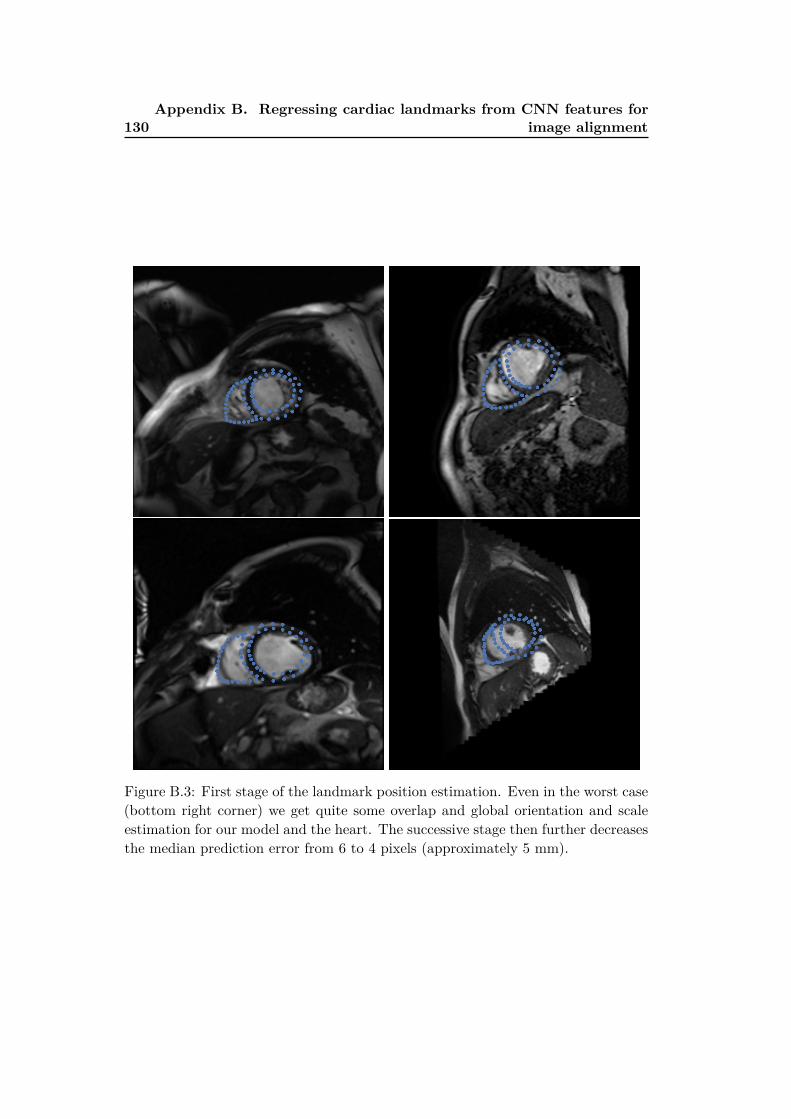
130Appendix B. Regressing cardiac landmarks from CNN features for
image alignment
Figure B.3: First stage of the landmark position estimation. Even in the worst case(bottom right corner) we get quite some overlap and global orientation and scaleestimation for our model and the heart. The successive stage then further decreasesthe median prediction error from 6 to 4 pixels (approximately 5 mm).

B.5. Conclusions 131
Validation and results
We did not observe any further performance gains beyond approximately 2,400 ex-ample images. This is most likely due to strong correlations between the generatedimages.
We use 90% of the images for training and the remaining 10% for testing. Wesplit the dataset such that images from patients in the training set do not leakinto the testing set. The direct prediction from the CNN features predicts thelandmarks with a median error of 6 pixels (approximately 7.5 mm). The medianlandmark position error then further decreases to 4 pixels (approximately 5 mm)in the second stage.
B.5 Conclusions
We learnt to predict cardiac landmarks by simple regression from CNN-derivedfeatures that were adapted to recognise cardiac acquisition planes. For such asimple method, this is quite remarkable. Adding images from different patients,or additional image augmentation techniques such as adding artificial bias fields,could further improve the dataset span for better landmark regression quality forpreviously unseen images. Of course, fine-tuning is a natural next step to betteradapt the CNN parameters and to potentially completely remove the need for theiterative refinement.


Appendix C
A note on pericardial effusion
for retrieval
Contents
C.1 Overview . . . . . . . . . . . . . . . . . . . . . . . . . . . . . . 133
C.2 Introduction . . . . . . . . . . . . . . . . . . . . . . . . . . . . 133
C.3 Pericardial effusion based similarity . . . . . . . . . . . . . . 134
C.3.1 Compactness on effusion . . . . . . . . . . . . . . . . . . . . . 134
C.4 An additional image channel . . . . . . . . . . . . . . . . . . . 134
C.5 Retrieving similar images . . . . . . . . . . . . . . . . . . . . 135
C.6 Conclusions and perspectives . . . . . . . . . . . . . . . . . . 135
C.1 Overview
Similarly to the atrial segmentation (Section 3.2), we can use extra image channelsto enhance some aspects of the images, such as the pericardial effusion, and poten-tially use them for image retrieval with the Neighbourhood approximating forest(NAF) algorithm we describe in Chapter 5. In this preliminary study we use analmost identical pipeline to the one we used to retrieve hearts with similar ejectionfractions in order.
C.2 Introduction
Pericardial effusion is a common finding in myocardial infarction patients. It man-ifests itself as an accumulation of liquid in the pericardial sac around the heart.It can be seen on SSFP CMR images as a bright ring around the LV epicardium(see Fig. C.1a). The pericardial effusion is, however, more difficult to detect andto capture. It consists of fewer pixels and has significant variability in appearance.In addition, the pericardial effusion and the pericardial fat are also visually quitesimilar (apart from small intensity difference).
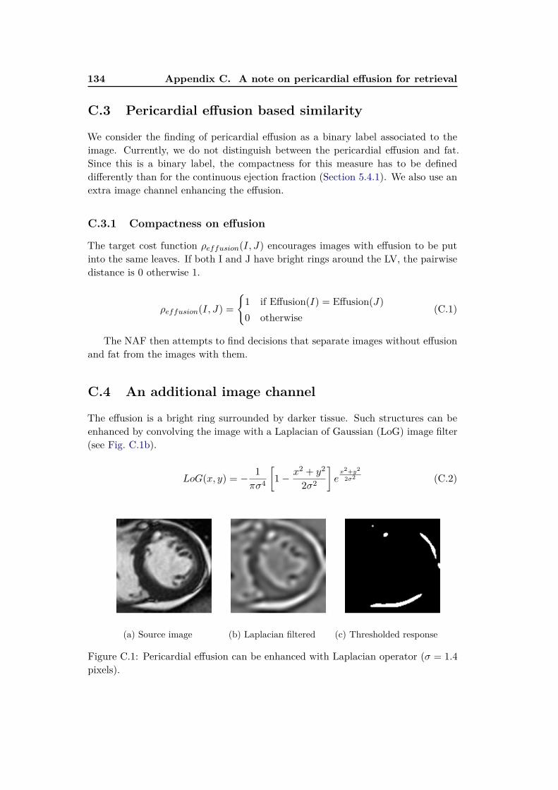
134 Appendix C. A note on pericardial effusion for retrieval
C.3 Pericardial effusion based similarity
We consider the finding of pericardial effusion as a binary label associated to theimage. Currently, we do not distinguish between the pericardial effusion and fat.Since this is a binary label, the compactness for this measure has to be defineddifferently than for the continuous ejection fraction (Section 5.4.1). We also use anextra image channel enhancing the effusion.
C.3.1 Compactness on effusion
The target cost function ρeffusion(I, J) encourages images with effusion to be putinto the same leaves. If both I and J have bright rings around the LV, the pairwisedistance is 0 otherwise 1.
ρeffusion(I, J) =
1 if Effusion(I) = Effusion(J)
0 otherwise(C.1)
The NAF then attempts to find decisions that separate images without effusionand fat from the images with them.
C.4 An additional image channel
The effusion is a bright ring surrounded by darker tissue. Such structures can beenhanced by convolving the image with a Laplacian of Gaussian (LoG) image filter(see Fig. C.1b).
LoG(x, y) = −1
πσ4
[
1−x2 + y2
2σ2
]
ex2+y2
2σ2 (C.2)
(a) Source image (b) Laplacian filtered (c) Thresholded response
Figure C.1: Pericardial effusion can be enhanced with Laplacian operator (σ = 1.4
pixels).
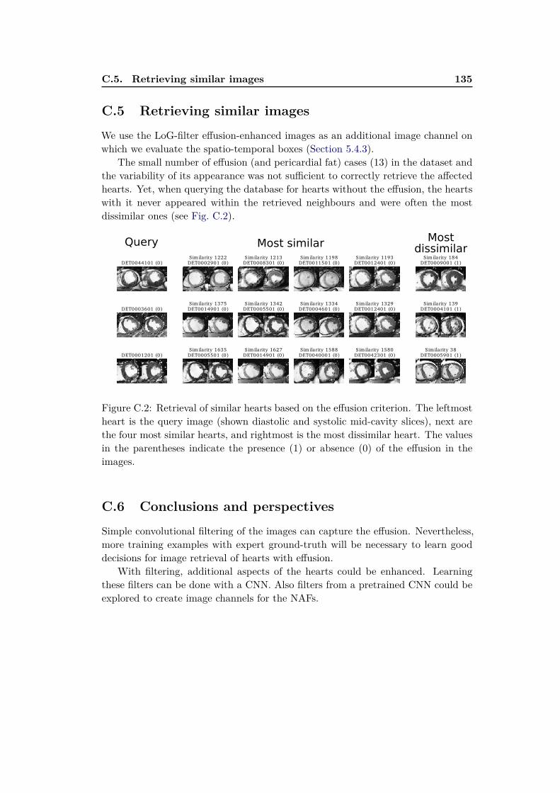
C.5. Retrieving similar images 135
C.5 Retrieving similar images
We use the LoG-filter effusion-enhanced images as an additional image channel onwhich we evaluate the spatio-temporal boxes (Section 5.4.3).
The small number of effusion (and pericardial fat) cases (13) in the dataset andthe variability of its appearance was not sufficient to correctly retrieve the affectedhearts. Yet, when querying the database for hearts without the effusion, the heartswith it never appeared within the retrieved neighbours and were often the mostdissimilar ones (see Fig. C.2).
DET0001201 (0)
DET0003601 (0)
DET0044101 (0)
Similarity 1635DET0005501 (0)
Similarity 1375DET0014901 (0)
Similarity 1222DET0002901 (0)
Similarity 1627DET0014901 (0)
Similarity 1342DET0005501 (0)
Similarity 1213DET0008301 (0)
Similarity 1588DET0040001 (0)
Similarity 1334DET0004601 (0)
Similarity 1198DET0011501 (0)
Similarity 1580DET0042301 (0)
Similarity 1329DET0012401 (0)
Similarity 1193DET0012401 (0)
Similarity 38DET0005901 (1)
Similarity 139DET0004101 (1)
Similarity 184DET0009001 (1)
Query Most similarMost
dissimilar
Figure C.2: Retrieval of similar hearts based on the effusion criterion. The leftmostheart is the query image (shown diastolic and systolic mid-cavity slices), next arethe four most similar hearts, and rightmost is the most dissimilar heart. The valuesin the parentheses indicate the presence (1) or absence (0) of the effusion in theimages.
C.6 Conclusions and perspectives
Simple convolutional filtering of the images can capture the effusion. Nevertheless,more training examples with expert ground-truth will be necessary to learn gooddecisions for image retrieval of hearts with effusion.
With filtering, additional aspects of the hearts could be enhanced. Learningthese filters can be done with a CNN. Also filters from a pretrained CNN could beexplored to create image channels for the NAFs.

Appendix D
Abstracts from coauthored work
Benchmark for Algorithms Segmenting the Left Atrium
From 3D CT and MRI Datasets.
C. Tobon-Gomez, A. Geers, J. Peters, J. Weese, K. Pinto, R. Karim, M. Ammar,A. Daoudi, J. Margeta, Z. Sandoval, B. Stender, Y. Zheng, M. A. Zuluaga, J.Betancur, N. Ayache, M. A. Chikh, J.-L. Dillenseger, M. Kelm, S. Mahmoudi, S.Ourselin, A. Schlaefer, T. Schaeffter, R. Razavi, and K. Rhode, in IEEE Transac-tions on Medical Imaging, vol. 34, no. 7, pages 1460 1473, 2015.
Knowledge of left atrial (LA) anatomy is important for atrial fibrillation ablationguidance, fibrosis quantification and biophysical modelling. Segmentation of the LAfrom Magnetic Resonance Imaging (MRI) and Computed Tomography (CT) imagesis a complex problem. This manuscript presents a benchmark to evaluate algorithmsthat address LA segmentation. The datasets, ground truth and evaluation codehave been made publicly available through the http://www.cardiacatlas.org website.This manuscript also reports the results of the Left Atrial Segmentation Challenge(LASC) carried out at the STACOM13 workshop, in conjunction with MICCAI13.Thirty CT and 30 MRI datasets were provided to participants for segmentation.Each participant segmented the LA including a short part of the LA appendagetrunk and proximal sections of the pulmonary veins (PVs). We present resultsfor nine algorithms for CT and eight algorithms for MRI. Results showed thatmethodologies combining statistical models with region growing approaches werethe most appropriate to handle the proposed task. The ground truth and automaticsegmentations were standardised to reduce the influence of inconsistently definedregions (e. g. mitral plane, PVs end points, LA appendage). This standardisationframework, which is a contribution of this work, can be used to label and furtheranalyse anatomical regions of the LA. By performing the standardisation directlyon the left atrial surface, we can process multiple input data, including meshesexported from different electroanatomical mapping systems.
A collaborative resource to build consensus for auto-
mated left ventricular segmentation of cardiac MR im-
ages.
A. Suinesiaputra, B. R. Cowan, A. O. Al-Agamy, M. A. Elattar, N. Ayache, A. S.Fahmy, A. M. Khalifa, P. Medrano-Gracia, M. P. Jolly, A. H. Kadish, D. C. Lee,
138 Appendix D. Abstracts from coauthored work
J. Margeta, S. K. Warfield, and A. A. Young, in Medical Image Analysis, vol. 18,no. 1, pages 50 62, 2014.
A collaborative framework was initiated to establish a community resource ofground truth segmentations from cardiac MRI. Multi-site, multi-vendor cardiacMRI datasets comprising 95 patients (73 men, 22 women; mean age 62.73 ś 11.24years) with coronary artery disease and prior myocardial infarction, were randomlyselected from data made available by the Cardiac Atlas Project (Fonseca et al.,2011). Three semi- and two fully-automated raters segmented the left ventricularmyocardium from short-axis cardiac MR images as part of a challenge introducedat the STACOM 2011 MICCAI workshop (Suinesiaputra et al., 2012). Consensusmyocardium images were generated based on the ExpectationMaximization prin-ciple implemented by the STAPLE algorithm (Warfield et al., 2004). The meansensitivity, specificity, positive predictive and negative predictive values ranged be-tween 0.63 and 0.85, 0.60 and 0.98, 0.56 and 0.94, and 0.83 and 0.92, respectively,against the STAPLE consensus. Spatial and temporal agreement varied in differ-ent amounts for each rater. STAPLE produced high quality consensus images ifthe region of interest was limited to the area of discrepancy between raters. Tomaintain the quality of the consensus, an objective measure based on the candidateautomated rater performance distribution is proposed. The consensus segmentationbased on a combination of manual and automated raters were more consistent thanany particular rater, even those with manual input. The consensus is expected toimprove with the addition of new automated contributions. This resource is openfor future contributions, and is available as a test bed for the evaluation of new seg-mentation algorithms, through the Cardiac Atlas Project (www.cardiacatlas.org).
Confidence-based Training for Clinical Data Uncertainty
in Image-based Prediction of Cardiac Ablation Targets.
R. C. Lozoya, J. Margeta, L. Le Folgoc, Y. Komatsu, B. Berte, J. Relan, H. Cochet,M. Haïssaguerre, P. Jaïs, N. Ayache, and M. Sermesant, in International Workshopon Medical Computer Vision: Algorithms for Big Data, Held in conjunction withMICCAI 2014, Boston, Lecture Notes in Computer Science, vol. 8848, pages 148159, B. Menze, G. Langs, A. Montillo, M. Kelm, H. Müller, S. Zhang, W. Cai, andD. Metaxas, Eds., Springer Berlin / Heidelberg, 2014.
Ventricular radio-frequency ablation (RFA) can have a critical impact on pre-venting sudden cardiac arrest but is challenging due to a highly complex arrhyth-mogenic substrate. This work aims to identify local image characteristics capableof predicting the presence of local abnormal ventricular activities (LAVA). This canallow, pre-operatively and non-invasively, to improve and accelerate the procedure.To achieve this, intensity and texture-based local image features are computed andrandom forests are used for classification. However, using machine-learning ap-proaches on such complex multimodal data can prove difficult due to the inherenterrors in the training set. In this manuscript we present a detailed analysis of
139
these error sources due in particular to catheter motion and the data fusion process.We derived a principled analysis of confidence impact on classification. Moreover,we demonstrate how formal integration of these uncertainties in the training pro-cess improves the algorithms performance, opening up possibilities for non-invasiveimage-based prediction of RFA targets.
Local late gadolinium enhancement features to identify
the electrophysiological substrate of post-infarction ven-
tricular tachycardia: a machine learning approach.
R. C. Lozoya, J. Margeta, L. Le Folgoc, Y. Komatsu, B. Berte, J. S. Relan, H.Cochet, M. Haïssaguerre, P. Jaïs, N. Ayache, and M. Sermesant, in Journal ofCardiovascular Magnetic Resonance, vol. 17, no. Suppl 1, poster 234, 2015.
Most ventricular tachycardias occur on structurally diseased hearts with fibroticscar, where bundles of surviving tissue promote electrical circuit re-entry. Thesebundles can be identified on invasive electrophysiological (EP) mapping as localabnormal ventricular activities (LAVA) during sinus rhythm. Although the elimi-nation of LAVAs by radiofrequency ablation was shown to be an efficient therapeuticoption, their identification requires is a lengthy and invasive process. Late gadolin-ium enhancement (LGE) magnetic resonance imaging enables a non-invasive 3Dassessment of scar topology and heterogeneity with millimetric spatial resolution.The aim of this work is to identify imaging features associated with LAVA, fea-tures that may subsequently be used to target ablation or to stratify the risk ofarrhythmia.
Myocardial Infarct Localisation using Neighbourhood Ap-
proximation Forests.
H. Bleton, J. Margeta, H. Lombaert, H. Delingette, and N. Ayache, in Interna-tional Workshop on Statistical Atlases and Computational Models of the Heart.Imaging and Modelling Challenges, Held in conjunction with MICCAI 2015, Mu-nich, O. Camara, T. Mansi, M. Pop, K. Rhode, M. Sermesant, and A. Young, Eds.,2015.
This paper presents a machine-learning algorithm for the automatic localisationof myocardial infarct in the left ventricle. Our method constructs neighbourhoodapproximation forests, which are trained with previously diagnosed 4D cardiac se-quences. We introduce a new set of features that simultaneously exploit informationfrom the shape and motion of the myocardial wall along the cardiac cycle. Moreprecisely, characteristics are extracted from a hyper surface that represents the pro-file of the myocardial thickness. The method has been tested on a database of 65cardiac MRI images in order to retrieve the diagnosed infarct area. The resultsdemonstrate the effectiveness of the NAF in predicting the left ventricular infarct

140 Appendix D. Abstracts from coauthored work
location in 7 distinct regions. We evaluated our method by verifying the databaseground truth. Following a new examination of the 4D cardiac images, our algorithmmay detect misclassified infarct locations in the database.
Appendix E
Sommaire en français
E.1 L’aube du Big Data cardiaque
Les développements en cardiologie au cours du dernier siècle (Cooley and Frazier,2000; Braunwald, 2014) ont étés assez spectaculaires. Beaucoup de révolutions sesont passées depuis le premier électrocardiogramme (ECG) pratique par Einthovenen 1903. Ceux-ci comprennent le cathétérisme cardiaque (1929), la machine coeur-poumon et les premiers modèles animaux dans les années 1950, les chirurgies mini-invasives (1958), et le développement de médicaments (les bêta-bloquants (1962),les statines (1971), et les angiotensines (1974)). L’imagerie diagnostique cardiaque aaussi considérablement améliorée. Le développement après-guerre de l’échographiecardiaque (EC), la tomodensitométrie (TDM) (1970) et l’imagerie par résonancemagnétique (IRM) (des années 1980) nous ont aidés à obtenir un regard non-invasifdans le coeur et avec un niveau de détail remarquable.
Toutes ces avancées ont considérablement changées le cours de gestion de lamaladie cardio-vasculaire. En 1970, le taux de mortalité liée à ces deux maladiesdans les pays à revenu élevé a basculé et a été en baisse constante (Fuster and Kelly,2010, p52) depuis. Pourtant, les maladies cardiovasculaires demeurent la premièrecause de mortalité dans le monde (Nichols et al., 2012, p 10;Roger et al., 2011),et causent 47% de tous les décès en Europe. Nous sommes à l’aube de l’âge oùde nouvelles techniques cardiaques d’acquisition d’image, des modèles prédictifs (insillico) cardiaques (Lamata et al., 2014), des simulations d’images réalistes (Glatardet al., 2013; Prakosa et al., 2013; Alessandrini et al., 2015), la surveillance en tempsréel du patient (Xia et al., 2013), et les banques d’images cardiaques à grande échelle(Suinesiaputra et al., 2014a; Petersen et al., 2013; Bruder et al., 2013) ont devenusomniprésents et ont la chance d’améliorer la santé cardiaque et notre compréhension.Les données dans ces bases de données ne sont aussi utiles que les questions qu’ilspeuvent aider à répondre, les idées qu’ils peuvent engendrer, et les décisions qu’ilspermettent de faire. Des grandes études de population avec les recommandationsde traitement cliniques peuvent être faites, preuves à l’appui peuvent être adaptéesà chaque patient individuellement. Le traitement peut être ajusté en regardantles patients similaires précédemment traités, en comparant leurs résultats et lesévolutions de leurs maladies. Des nouveaux outils d’enseignement peuvent aussi êtredéveloppés en utilisant les données pour créer les patients virtuels comme les étudesde cas et des simulations de chirurgie sur les modèles imprimé 3D (Bloice et al., 2013;Kim et al., 2008; Jacobs et al., 2008) Ceci pourrait stimuler l’enseignement et lapratique des cardiologues.

142 Appendix E. Sommaire en français
E.2 Les défis pour l’organisation des données cardiaques
à grande échelle
Les possibilités pour les nouvelles utilisations de grandes bases de données d’imagesont innombrables, cependant, l’utilisation de ces bases de données pose de nou-veaux défis. Collections cardiaques riches avec des images pertinentes (y comprisde nombreuses maladies rares) sont dispersés à travers des milliers de systèmesd’archivage et de transmission d’images (PACS) dans de nombreux pays et hôpi-taux. Ces données provenant de sources hétérogènes sont non seulement massives,mais aussi assez non-structurées et bruyantes.
E.2.1 Agrégation des données provenant des études multi-centriques
Les biobanques et consortia internationaux de gestion des bases de données d’imageriemédicale, tels que UK Biobank (Petersen et al., 2013), Cardiac atlas project (CAP)(Fonseca et al., 2011) ou le projet VISCERAL (Langs et al., 2013), ont résolu de nom-breux problèmes difficiles dans l’éthique de partage de données d’imagerie médicaleet dans l’organisation de la distribution de données — en particulier l’agrégationdes données provenant de sources multiples. Dans ces efforts (PACS) ainsi quela norme dimagerie numérique en médecine (DICOM) ont étés inestimables. Desétudes provenant de plusieurs centres utilisent souvent des nomenclatures spéci-fiques, suivent des orientations différentes ou utilisent des protocoles d’acquisitiondifférents. Dans ces cas, même ces deux normes ne sont pas suffisantes.
E.2.2 Normalisation des données
Les collections d’images sur des serveurs PACS peuvent être interrogées par l’informationdu patient (par exemple ID, nom, date de naissance, sexe, taille, poids), la modalitéde l’image, la date de l’étude et d’autres balises DICOM, parfois par descriptionde l’étude, des balises personnalisées des cliniciens, des mesures associées (par ex-emple la pression artérielle ou la fréquence cardiaque) et les codes de maladie oud’intervention. Voir Fig. 1.1 pour un exemple d’une telle interface.
Il n’y a pas de façon standard pour stocker une partie de l’information d’imageimportante associée (par exemple, de l’information sur le plan d’acquisition d’imagescardiaques). Pour cette information le nom dépend de la mise au point de la stationde travail, ou de la langue pratiqué au centre d’imagerie. Même les balises de lanorme DICOM contiennent souvent des nomenclatures spécifiques du fournisseur.Par exemple, les mêmes séquences d’acquisition dIRM cardiaque sont marquées dif-féremment à travers des fabricants (Siemens, 2010). Alors que certaines différencesde mise en oeuvre existent, elles ne sont pas pertinentes pour l’interprétation desimages, et la terminologie pourrait être considérablement simplifiée (Friedrich et al.,2014). L’analyse des publications électroniques avec des images est encore un plusgrand défi. Ces images sont rarement en format DICOM et seul le contenu de l’imageet la description textuelle sont présents. Ces différences réduisent notre capacité à

E.2. Les défis pour l’organisation des données cardiaques à grandeéchelle 143
interroger et explorer les bases de données pour les images pertinentes de manièreefficace. La normalisation peut être appliquée en strictement appliquant les lignesdirectrices lors de l’acquisition des images, et en utilisant systématiquement les ter-minologies pour coder les informations associées: tels que SNOMED CT (Stearnset al., 2001). Des précautions doivent être prises pour éliminer les erreurs de saisiemanuelle. Les images déjà stockées dans les bases de données sans l’informationnormalisée devraient être revues pour une meilleure accessibilité.
E.2.3 Récupération des cas similaires
Traverser ces bases de données manuellement et trouver des patients similaires (avecpreuves à l’appui) devient donc très chronophage. Récupération des images archivéesen PACS est, dans la pratique, assez lent pour une telle utilisation exploratoire.En plus, les données d’imagerie cardiaque stockées dans les bases de données sontfréquemment des séquences 3D+t, et des détails importants peuvent être facilementmanqués lors de cette inspection visuelle. Une alternative à cette approche (forcebrute) est de décrire systématiquement les images avec des représentations plus com-pactes. Cela prépare les bases de données d’images cardiaques pour la récupérationfuture. Cependant, cette approche limite la recherche sur les cas annotés ou pourles cas connus au clinicien particulier. La plupart de données annotées ne sera doncjamais réutilisée et les données qui ne sont pas utilisées sont les données inutiles.
E.2.4 Annotation des données et le consensus
Lannotation des images simplifie leur réutilisation. Cependant, avec la croissancedes données, la demande pour la saisie manuelle devient un fardeau sur les an-notateurs experts. Une façon de lapprocher est de réduire les tâches d’annotationen questions simples qui peuvent être très répondues par un plus grand nombred’évaluateurs moins expérimentés, par exemple via le crowdsourcing. Comme étudiépar Suinesiaputra et al. (2015), la variabilité des différents radiologues (expertssuivant les mêmes lignes directrices) est non négligeable. Par exemple, dans la seg-mentation du ventricule gauche, les muscles papillaires sont du tissu myocardiqueet donc selon Schulz-Menger et al. (2013) devraient idéalement être inclus dans lamasse myocardique et exclus du calcul du volume ventriculaire gauche. Les valeursde référence pour les volumes et les masses correspondantes (Maceira et al., 2006;Hudsmith†et al., 2005) devrait être utilisé dans ce cas. Certains outils incluent lesmuscles papillaires dans le volume de la cavité à la place. Dans ce cas, un autreensemble de valeurs de référence doit être envisagée (Natori et al., 2006). Les deuxmesures signalées peuvent différer substantiellement. En fin de compte, les musclespapillaires font partie de la progression de la maladie (Harrigan et al., 2008) et méri-tent une attention individuelle. Les centres d’acquisition sont équipés de différentsoutils logiciels et tous ces outils ne sont pas aussi capables. Nous avons encore unlong chemin à parcourir pour réaliser l’extraction reproductible de mesures baséessur l’image et description cohérente de toutes les informations d’image pertinentes,
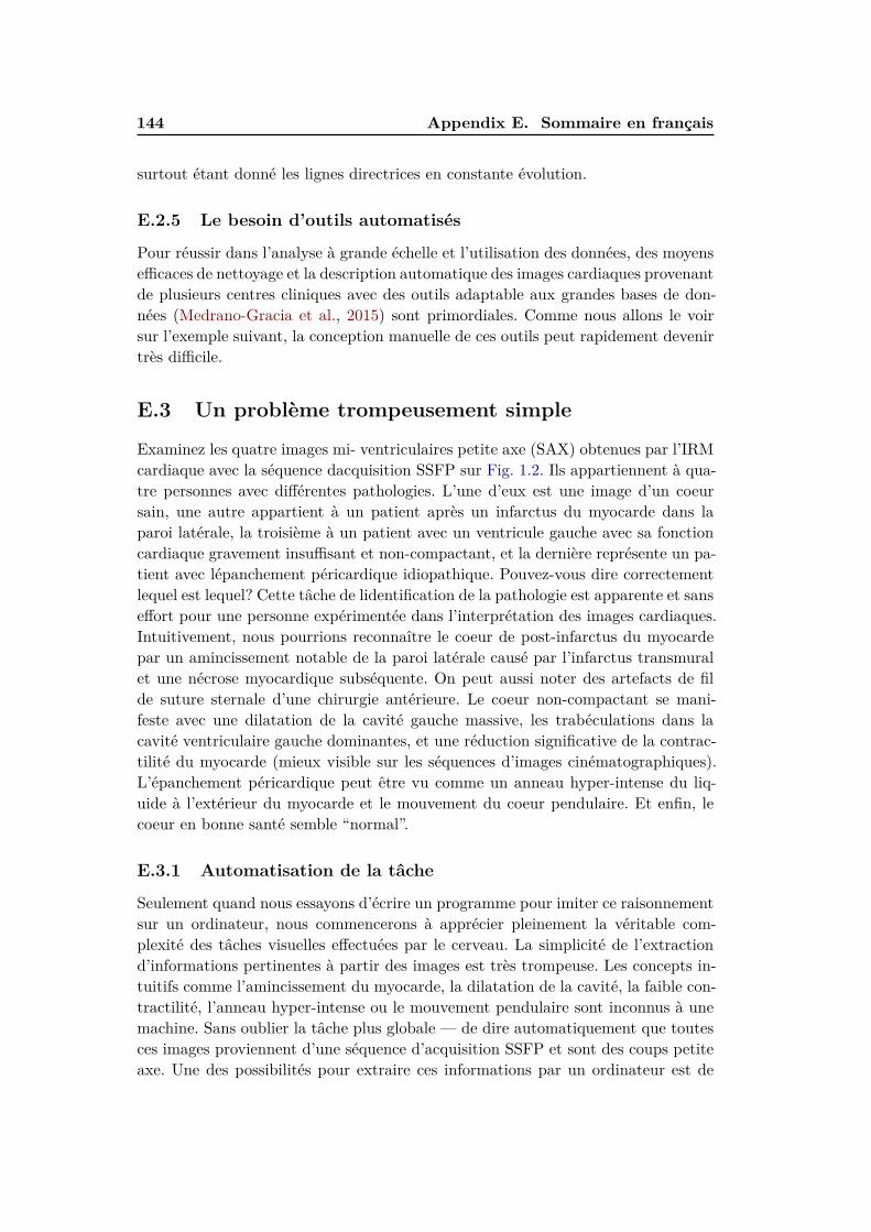
144 Appendix E. Sommaire en français
surtout étant donné les lignes directrices en constante évolution.
E.2.5 Le besoin d’outils automatisés
Pour réussir dans l’analyse à grande échelle et l’utilisation des données, des moyensefficaces de nettoyage et la description automatique des images cardiaques provenantde plusieurs centres cliniques avec des outils adaptable aux grandes bases de don-nées (Medrano-Gracia et al., 2015) sont primordiales. Comme nous allons le voirsur l’exemple suivant, la conception manuelle de ces outils peut rapidement devenirtrès difficile.
E.3 Un problème trompeusement simple
Examinez les quatre images mi- ventriculaires petite axe (SAX) obtenues par l’IRMcardiaque avec la séquence dacquisition SSFP sur Fig. 1.2. Ils appartiennent à qua-tre personnes avec différentes pathologies. L’une d’eux est une image d’un coeursain, une autre appartient à un patient après un infarctus du myocarde dans laparoi latérale, la troisième à un patient avec un ventricule gauche avec sa fonctioncardiaque gravement insuffisant et non-compactant, et la dernière représente un pa-tient avec lépanchement péricardique idiopathique. Pouvez-vous dire correctementlequel est lequel? Cette tâche de lidentification de la pathologie est apparente et sanseffort pour une personne expérimentée dans l’interprétation des images cardiaques.Intuitivement, nous pourrions reconnaître le coeur de post-infarctus du myocardepar un amincissement notable de la paroi latérale causé par l’infarctus transmuralet une nécrose myocardique subséquente. On peut aussi noter des artefacts de filde suture sternale d’une chirurgie antérieure. Le coeur non-compactant se mani-feste avec une dilatation de la cavité gauche massive, les trabéculations dans lacavité ventriculaire gauche dominantes, et une réduction significative de la contrac-tilité du myocarde (mieux visible sur les séquences d’images cinématographiques).L’épanchement péricardique peut être vu comme un anneau hyper-intense du liq-uide à l’extérieur du myocarde et le mouvement du coeur pendulaire. Et enfin, lecoeur en bonne santé semble “normal”.
E.3.1 Automatisation de la tâche
Seulement quand nous essayons d’écrire un programme pour imiter ce raisonnementsur un ordinateur, nous commencerons à apprécier pleinement la véritable com-plexité des tâches visuelles effectuées par le cerveau. La simplicité de l’extractiond’informations pertinentes à partir des images est très trompeuse. Les concepts in-tuitifs comme l’amincissement du myocarde, la dilatation de la cavité, la faible con-tractilité, l’anneau hyper-intense ou le mouvement pendulaire sont inconnus à unemachine. Sans oublier la tâche plus globale — de dire automatiquement que toutesces images proviennent d’une séquence d’acquisition SSFP et sont des coups petiteaxe. Une des possibilités pour extraire ces informations par un ordinateur est de
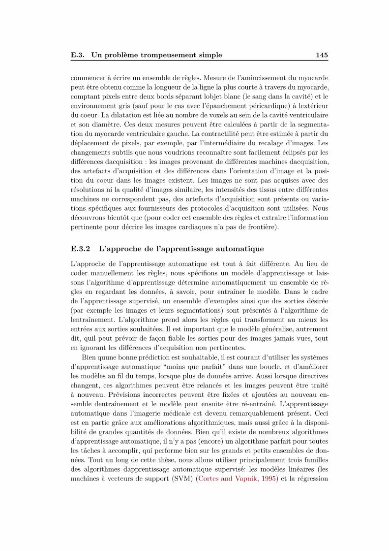
E.3. Un problème trompeusement simple 145
commencer à écrire un ensemble de règles. Mesure de l’amincissement du myocardepeut être obtenu comme la longueur de la ligne la plus courte à travers du myocarde,comptant pixels entre deux bords séparant lobjet blanc (le sang dans la cavité) et leenvironnement gris (sauf pour le cas avec l’épanchement péricardique) à lextérieurdu coeur. La dilatation est liée au nombre de voxels au sein de la cavité ventriculaireet son diamètre. Ces deux mesures peuvent être calculées à partir de la segmenta-tion du myocarde ventriculaire gauche. La contractilité peut être estimée à partir dudéplacement de pixels, par exemple, par l’intermédiaire du recalage d’images. Leschangements subtils que nous voudrions reconnaître sont facilement éclipsés par lesdifférences dacquisition : les images provenant de différentes machines dacquisition,des artefacts d’acquisition et des différences dans l’orientation d’image et la posi-tion du coeur dans les images existent. Les images ne sont pas acquises avec desrésolutions ni la qualité d’images similaire, les intensités des tissus entre différentesmachines ne correspondent pas, des artefacts d’acquisition sont présents ou varia-tions spécifiques aux fournisseurs des protocoles d’acquisition sont utilisées. Nousdécouvrons bientôt que (pour coder cet ensemble des règles et extraire l’informationpertinente pour décrire les images cardiaques n’a pas de frontière).
E.3.2 L’approche de l’apprentissage automatique
L’approche de l’apprentissage automatique est tout à fait différente. Au lieu decoder manuellement les règles, nous spécifions un modèle d’apprentissage et lais-sons l’algorithme d’apprentissage détermine automatiquement un ensemble de rè-gles en regardant les données, à savoir, pour entraîner le modèle. Dans le cadrede l’apprentissage supervisé, un ensemble d’exemples ainsi que des sorties désirée(par exemple les images et leurs segmentations) sont présentés à l’algorithme delentraînement. L’algorithme prend alors les règles qui transforment au mieux lesentrées aux sorties souhaitées. Il est important que le modèle généralise, autrementdit, quil peut prévoir de façon fiable les sorties pour des images jamais vues, touten ignorant les différences d’acquisition non pertinentes.
Bien quune bonne prédiction est souhaitable, il est courant d’utiliser les systèmesd’apprentissage automatique “moins que parfait” dans une boucle, et d’améliorerles modèles au fil du temps, lorsque plus de données arrive. Aussi lorsque directiveschangent, ces algorithmes peuvent être relancés et les images peuvent être traitéà nouveau. Prévisions incorrectes peuvent être fixées et ajoutées au nouveau en-semble dentraînement et le modèle peut ensuite être ré-entraîné. L’apprentissageautomatique dans l’imagerie médicale est devenu remarquablement présent. Ceciest en partie grâce aux améliorations algorithmiques, mais aussi grâce à la disponi-bilité de grandes quantités de données. Bien qu’il existe de nombreux algorithmesd’apprentissage automatique, il n’y a pas (encore) un algorithme parfait pour toutesles tâches à accomplir, qui performe bien sur les grands et petits ensembles de don-nées. Tout au long de cette thèse, nous allons utiliser principalement trois famillesdes algorithmes dapprentissage automatique supervisé: les modèles linéaires (lesmachines à vecteurs de support (SVM) (Cortes and Vapnik, 1995) et la régression
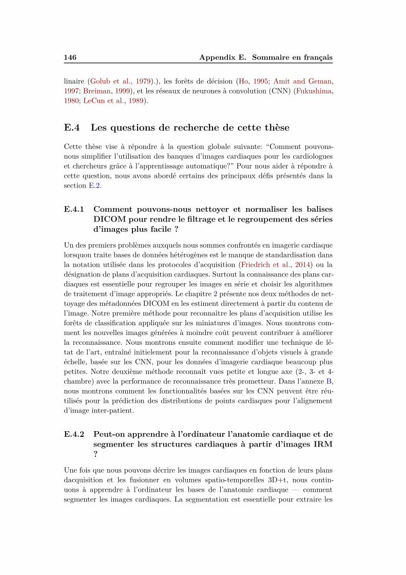
146 Appendix E. Sommaire en français
linaire (Golub et al., 1979).), les forêts de décision (Ho, 1995; Amit and Geman,1997; Breiman, 1999), et les réseaux de neurones à convolution (CNN) (Fukushima,1980; LeCun et al., 1989).
E.4 Les questions de recherche de cette thèse
Cette thèse vise à répondre à la question globale suivante: “Comment pouvons-nous simplifier l’utilisation des banques d’images cardiaques pour les cardiologueset chercheurs grâce à l’apprentissage automatique?” Pour nous aider à répondre àcette question, nous avons abordé certains des principaux défis présentés dans lasection E.2.
E.4.1 Comment pouvons-nous nettoyer et normaliser les balises
DICOM pour rendre le filtrage et le regroupement des séries
d’images plus facile ?
Un des premiers problèmes auxquels nous sommes confrontés en imagerie cardiaquelorsquon traite bases de données hétérogènes est le manque de standardisation dansla notation utilisée dans les protocoles d’acquisition (Friedrich et al., 2014) ou ladésignation de plans d’acquisition cardiaques. Surtout la connaissance des plans car-diaques est essentielle pour regrouper les images en série et choisir les algorithmesde traitement d’image appropriés. Le chapitre 2 présente nos deux méthodes de net-toyage des métadonnées DICOM en les estiment directement à partir du contenu del’image. Notre première méthode pour reconnaître les plans d’acquisition utilise lesforêts de classification appliquée sur les miniatures d’images. Nous montrons com-ment les nouvelles images générées à moindre coût peuvent contribuer à améliorerla reconnaissance. Nous montrons ensuite comment modifier une technique de lé-tat de l’art, entraîné initielement pour la reconnaissance d’objets visuels à grandeéchelle, basée sur les CNN, pour les données d’imagerie cardiaque beaucoup pluspetites. Notre deuxième méthode reconnaît vues petite et longue axe (2-, 3- et 4-chambre) avec la performance de reconnaissance très prometteur. Dans l’annexe B,nous montrons comment les fonctionnalités basées sur les CNN peuvent être réu-tilisés pour la prédiction des distributions de points cardiaques pour l’alignementd’image inter-patient.
E.4.2 Peut-on apprendre à l’ordinateur l’anatomie cardiaque et de
segmenter les structures cardiaques à partir d’images IRM
?
Une fois que nous pouvons décrire les images cardiaques en fonction de leurs plansdacquisition et les fusionner en volumes spatio-temporelles 3D+t, nous contin-uons à apprendre à l’ordinateur les bases de l’anatomie cardiaque — commentsegmenter les images cardiaques. La segmentation est essentielle pour extraire les
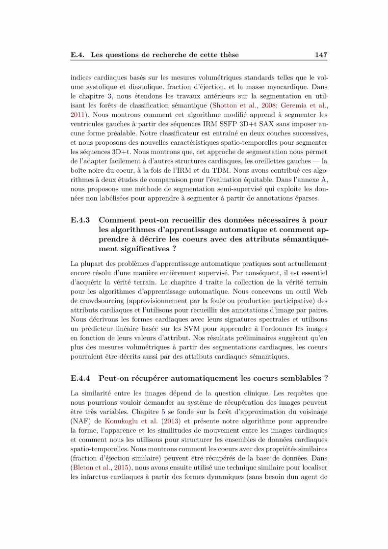
E.4. Les questions de recherche de cette thèse 147
indices cardiaques basés sur les mesures volumétriques standards telles que le vol-ume systolique et diastolique, fraction d’éjection, et la masse myocardique. Dansle chapitre 3, nous étendons les travaux antérieurs sur la segmentation en util-isant les forêts de classification sémantique (Shotton et al., 2008; Geremia et al.,2011). Nous montrons comment cet algorithme modifié apprend à segmenter lesventricules gauches à partir des séquences IRM SSFP 3D+t SAX sans imposer au-cune forme préalable. Notre classificateur est entraîné en deux couches successives,et nous proposons des nouvelles caractéristiques spatio-temporelles pour segmenterles séquences 3D+t. Nous montrons que, cet approche de segmentation nous permetde l’adapter facilement à d’autres structures cardiaques, les oreillettes gauches — laboîte noire du coeur, à la fois de l’IRM et du TDM. Nous avons contribué ces algo-rithmes à deux études de comparaison pour l’évaluation équitable. Dans l’annexe A,nous proposons une méthode de segmentation semi-supervisé qui exploite les don-nées non labélisées pour apprendre à segmenter à partir de annotations éparses.
E.4.3 Comment peut-on recueillir des données nécessaires à pour
les algorithmes d’apprentissage automatique et comment ap-
prendre à décrire les coeurs avec des attributs sémantique-
ment significatives ?
La plupart des problèmes d’apprentissage automatique pratiques sont actuellementencore résolu d’une manière entièrement supervisé. Par conséquent, il est essentield’acquérir la vérité terrain. Le chapitre 4 traite la collection de la vérité terrainpour les algorithmes d’apprentissage automatique. Nous concevons un outil Webde crowdsourcing (approvisionnement par la foule ou production participative) desattributs cardiaques et l’utilisons pour recueillir des annotations d’image par paires.Nous décrivons les formes cardiaques avec leurs signatures spectrales et utilisonsun prédicteur linéaire basée sur les SVM pour apprendre à l’ordonner les imagesen fonction de leurs valeurs d’attribut. Nos résultats préliminaires suggèrent qu’enplus des mesures volumétriques à partir des segmentations cardiaques, les coeurspourraient être décrits aussi par des attributs cardiaques sémantiques.
E.4.4 Peut-on récupérer automatiquement les coeurs semblables ?
La similarité entre les images dépend de la question clinique. Les requêtes quenous pourrions vouloir demander au système de récupération des images peuventêtre très variables. Chapitre 5 se fonde sur la forêt d’approximation du voisinage(NAF) de Konukoglu et al. (2013) et présente notre algorithme pour apprendrela forme, l’apparence et les similitudes de mouvement entre les images cardiaqueset comment nous les utilisons pour structurer les ensembles de données cardiaquesspatio-temporelles. Nous montrons comment les coeurs avec des propriétés similaires(fraction d’éjection similaire) peuvent être récupérés de la base de données. Dans(Bleton et al., 2015), nous avons ensuite utilisé une technique similaire pour localiserles infarctus cardiaques à partir des formes dynamiques (sans besoin dun agent de
148 Appendix E. Sommaire en français
contraste).
E.5 Organisation du manuscrit
Cette thèse est organisée autour de notre travail publié et nos travaux en prépara-tion. Le manuscrit progresse à peu près du niveau global vers la description plusfine des images cardiaques. Chaque chapitre de cette thèse tente de répondre àl’un des objectifs et d’emmener la récupération d’images basée sur le contenu desbases de données à grande échelle CMR plus proche vers la pratique. Tout d’abord,nous entraînons un système de nettoyage des balises d’images qui ne sont pas cap-turés par DICOM directement à partir du contenu d’image. Dans le chapitre 2,nous montrons comment reconnaître automatiquement les plans dacquisition car-diaques. Dans le chapitre 3, nous proposons une technique de segmentation automa-tique flexible qui apprend à segmenter les structures cardiaques à partir de donnéesd’image spatio-temporelles, en utilisant de simples cartes des voxels comme la véritéterrain. La segmentation pourrait être utilisée pour l’extraction automatique desmesures clinique. Dans le chapitre 4, nous proposons un moyen de collectionnerles annotations nécessaires pour lentraînement des algorithmes automatiques, etpour décrire les images cardiaques avec un ensemble d’attributs sémantiques. Enfin,dans le chapitre 5, nous proposons un algorithme pour structurer les ensembles dedonnées pour y trouver des cas similaires à l’égard de différents critères cliniques.Le chapitre 6 conclut la thèse avec des perspectives et des travaux futurs. Dansles annexes, nous avons illustré comment les données non labélisées peuvent êtreutilisées pour la segmentation d’images guidée (Annexe A), comment estimer lesrepères cardiaques pour l’alignement des images (Annexe B), ou comment rehausserépanchement péricardique pour la récupération d’image (Annexe C).
E.6 Sommaires des chapitres
E.6.1 Reconnaisance des plans d’acquisition cardiaques
Lorsqu’on traite des grandes bases de données depuis plusieurs centres et four-nisseurs de machines d’acquisition, notations incompatibles sont un facteur limi-tant pour l’analyse automatisée. Les plans d’acquisition de l’IMR cardiaque sontun très bon exemple d’un tel échec de normalisation de la notation. Sans savoirquel plan cardiaque on traite, l’utilisation des données sans intervention manuelleest limitée. Dans ce chapitre, nous proposons deux techniques d’apprentissage au-tomatique supervisée pour récupérer automatiquement les informations manquantesou bruyantes et de prédire les cinq vues (ou plans d’acquisition) cardiaques les pluscourants. Nous montrons que les plans d’acquisitions cardiaques sont à peu prèsalignés pour situer le coeur au centre de l’image. Nous l’utilisons pour apprendreprédicteurs des plans d’acquisition cardiaques à partir d’images 2D.
Dans notre première méthode nous entraînons une forêt de classification surles miniatures d’image. L’augmentation de l’ensemble de données avec des transfor-
E.6. Sommaires des chapitres 149
mations géométriques (qui préservent les étiquettes) est un moyen efficace qui nousaide à améliorer la précision de la classification sans des acquisitions ou des donnéessupplémentaires. Nous améliorons la performance de la forêt en affinant un réseaude neurones à convolution profond, à l’origine pré-entrainé sur une grande base dedonnées pour la reconnaissance d’images naturelles (ImageNet LSVRC 2012). Noustransférons la représentation apprise à la reconnaissance des vues cardiaques.
Nous comparons ces approches avec les prédictions à l’aide des caractéristiquesextraites des images en utilisant le CNN entraîné directement sur ImageNet, etavec un CNN entraîné à partir de zéro. Nous montrons que peaufinage est uneapproche viable pour adapter les paramètres des grands CNN pour les petits prob-lèmes. Nous validons respectivement cet algorithme sur deux études cardiaquesdifférentes avec 200 patients et 15 témoins sains. Celui-ci provient d’un ensemblede données cardiaques en libre accès qui simplifie la comparaison directe avec destechniques similaires dans l’avenir. Nous montrons qu’il y a une valeur significativeà peaufiner un modèle entrainé pour des images naturelles et de le transférer auximages médicales. Les approches présentées sont tout à fait générales et peuventêtre appliquées à toute tâche de reconnaissance d’image. Notre meilleure approcheréalise un score de F1 moyen de 97, 66% et améliore l’état de l’art sur la recon-naissance de vues cardiaques en utilisant le contenu d’image seulement. Elle éviteles annotations supplémentaires et apprend la représentation de la fonction voulueautomatiquement.
Ceci est une composante important pour organiser et filtrer des grandes collec-tions de données cardiaques avant de les analyser. Elle nous permet de fusionnerdes études à partir de plusieurs centres, afin de permettre le filtrage d’image plusintelligent, la sélection des algorithmes de traitement d’image les plus appropriés,et une amélioration de la visualisation d’ensembles de données cardiaques, et pourla recherche d’image par le contenu et un contrôle de qualité.
E.6.2 Segmentation d’images cardiaques
Les indices cliniques les plus couramment utilisés pour la quantification des mal-adies cardiaques sont souvent basés sur les mesures géométriques des structuresanatomiques, telles que les volumes des cavités, des masses du myocarde ou desépaisseurs de paroi. Il serait très utile de les avoir stockées dans les bases de don-nées cardiaques à côté des images et les utiliser pour sélectionner les cohortes depatients pour les études cliniques. Ces mesures sont souvent calculées à partir dessegmentations de ces structures cardiaques. La segmentation constitue égalementla base pour la compréhension de l’anatomie cardiaque par un ordinateur.
Dans ce chapitre, nous présentons une méthode d’apprentissage automatiqueflexible pour la segmentation d’images IRM cardiaques. Nous segmentons deux desstructures cardiaques les plus importantes. Tout d’abord, nous apprenons commentsegmenter les ventricules gauches des séquences dynamiques 3D+t SAX directementà partir de la vérité-terrain par voxel en utilisant les forêts de classification avecle contexte spatio-temporel. Ensuite, nous montrons que cette méthode peut être
150 Appendix E. Sommaire en français
facilement adaptée à d’autres structures du coeur, tel que l’oreillette gauche.
E.6.3 Approvisionnement par la foule des attributs semantiques
Dans chapitre 2, nous avons montré comment automatiquement prédire les mé-tadonnées d’image de grâce aux CNNs. Nous pouvons facilement récupérer, parexemple, toutes les coupes SAX du ventricule gauche dans la base de données. Lesméthodes automatiques de segmentation d’image (tels que celles présentés dans lechapitre 3) nous permettent d’indexer et d’interroger les bases de données en util-isant des mesures géométriques simples (par exemple les volumes des cavités, lamasse myocardique ou l’épaisseur du mur). Ces deux outils sont des étapes impor-tantes vers la récupération d’images cardiaque en fonction du contenu automatisée.
Quelques images, cependant, ne peuvent être directement décrits et répertoriéssur si simple mesures géométriques seules. Considérons une requête un peu pluscomplexe: “récupérer toutes les images de petite axe des coeurs akinétiques avecun amincissement significatif de la paroi, et le limiter que sur les images de qualitédiagnostique”.
Nous visons à atteindre la description informatisée des images cardiaques avecun ensemble des attributs sémantiques pour la forme, le mouvement et l’apparence.Dans ce chapitre, nous nous concentrons sur les images de coeurs d’infarctus dumyocarde avec une légère à modérée dysfonction ventriculaire gauche. Nous dévelop-pons un outil qui va permettre de filtrer les bases de données cardiaques avec untel ensemble d’attributs. Nous apprenons la machine à décrire les images en fonc-tion des caractéristiques extraites de l’image et les comparaisons par pair. La véritéterrain se compose de deux images et un indicateur disant quelle image des deuxdispose d’une présence inférieure ou supérieure de l’attribut. Nous avons conçuune interface web permettant de recueillir telles annotations de vérité-terrain viaapprovisionnement par la foule.
E.6.4 Recherche d’image par le contenu
Dans ce chapitre, nous proposons une méthode pour apprendre à rapprocher lasimilitude entre les images pour la récupération automatique d’images basée sur lecontenu des coeurs sémantiquement similaires. Nous nous appuyons sur les foretsd’approximation du voisinage (NAF) de (Konukoglu et al., 2013), un algorithmeque nous entraînons pour capturer les similitudes entre les images cardiaques. Ilpermet les récupérations efficaces des coeurs les plus similaires basés sur des critèrescliniques. Nous illustrons son utilisation sur une base de données des patients aprèsun infarctus du myocarde.
En Bleton et al. (2015), nous avons déjà montré comment des voisins cardiaquepeuvent être utilisés pour localiser infarctus sans injecter l’agent de contraste àpartir des segmentations dynamiques. Ici, nous combinons les attributs d’imagesspatio-temporelles avec les NAFs et utilisons la similitude dérivée de la fractiond’éjection pour trouver les coeurs avec une fonction de pompage similaire. Aucune

E.7. Conclusions et perspectives 151
segmentation d’image n’est plus nécessaire.
E.7 Conclusions et perspectives
Au cours des dernières années, plusieurs initiatives de collecte des images cardiaquesont apparus. Ceux-ci incluent Cardiac Atlas Project (Fonseca et al., 2011) contenantle sous-ensemble DETERMINE (Kadish et al., 2009) fréquemment utilisé dans cettethèse, mais aussi une étude sur les coeurs asymptomatiques MESA (Bild, 2002). UKBiobank (Petersen et al., 2013) vise à imager une grande partie de la population,et le registre EuroCMR (Bruder et al., 2013) collectionne de données d’imagerie àpartir de 57 centres dans 15 des pays. Ces collections déjà très massives sont icipour grandir et vont avoir un impact sur la santé cardiaque. Nous devrons trouverdes façons d’automatiquement interpréter l’information contenue dans ces bases dedonnées et de simplifier la recherche dedans.
Dans cette thèse, nous avons abordé certains des défis les plus importants dansl’organisation des données cardiaques et dans l’extraction d’informations à partirde ces ensembles de données grâce à l’apprentissage automatique.
E.7.1 Synthèse des contributions
Nous avons abordé les quatre questions suivantes. Ici, nous les remontrons avec noscontributions et les limites des méthodes proposées.
E.7.1.1 Estimation des métadonnées manquantes à partir de contenu
de l’image
Les balises DICOM sont intrinsèquement bruyantes et ne peuvent pas être utiliséesavec confiance. Dans cette thèse, nous avons montré qu’au lieu de compter surDICOM, nous pouvons estimer une partie des métadonnées (les plans d’acquisitioncardiaques) à partir du contenu de l’image.
La contribution principale du chapitre 2 est qu’un algorithme robuste de recon-naissance des vues cardiaques peut être efficacement entraîné de bout en bout sansl’aide d’une conception des attributs avec un réseau de neurones à convolution. Ceciest possible en peaufinant des paramètres du réseau préalablement formés pour unproblème de reconnaissance d’image à grande échelle. Nous avons publié nos résul-tats dans Margeta et al. (2015c, 2014).
• Nous atteignons la performance de l’état de l’art en reconnaissance des vuescardiaques par l’apprentissage d’un système de bout en bout à partir desintensités d’image grâce à l’aide d’un CNN
• Ceci est l’un des premiers travaux à démontrer la valeur de l’extraction desattributs à partir des images médicales utilisant un CNN initialement entraînépour la reconnaissance d’objets visuels avec une large quantité de données
152 Appendix E. Sommaire en français
• Nous montrons que le peaufinage des paramètres d’un CNN pré-entraîné pourla reconnaissance d’objets visuels est une bonne stratégie qui aide à améliorerla performance et à accélérer l’entraînement du réseau
• Nous montrons qu’un CNN peut être appliquée à des ensembles de donnéesplus petits (un problème commun en imagerie médicale) grâce à l’initialisationdu réseau prudent et l’augmentation artificielle de l’ensemble de données,même lors de l’entraînement du réseau à partir de zéro
• Nous reproduisons également l’observation de Zhou et al. (2012) que lesvecteur d’orientation peuvent être tirés de balises DICOM pour une recon-naissance de vue cardiaque (si ces balises d’orientation sont présentes)
Le peaufinage d’un réseau est un excellent moyen d’apprendre des modèles com-plexes avec des données médicales d’une plus petite taille et les CNNs sont desoutils puissants d’apprentissage automatique qui devraient encore complètementpropager dans l’imagerie médicale. Nous avons entraîné le modèle que sur les vuescardiaques uniquement et sur un ensemble de données des coeurs de l’infarctus dumyocarde. Ces coeurs ont certainement quelques particularités que nous avons mon-tré dans la thèse, néanmoins, leurs apparences et leurs topologies sont encore assez“normales”. Nous avons encore à tester cette méthode sur des cas pathologiques oudes acquisitions moins standards (non-centrées, orientées avec des angles atypiques).Il y a aussi beaucoup plus de vue cardiaques et d’autres séquences d’acquisition pourêtre reconnus (Taylor and Bogaert, 2012). La vérité terrain doit être recueilli pourtoutes ces séquences d’acquisition avec les vues, ce qui conduit à un problème com-binatoire. Beaucoup de ces combinaisons sont sous-représentées, et l’apprentissageavec très peu exemples toujours reste un problème difficile. En outre, la reconnais-sance des images cardiaques ne devrait pas s’arrêter sur la description des vues. Cetravail est une pierre angulaire pour la reconnaissance des modalités d’image, desprotocoles d’acquisition et pour la génération automatique des descriptions d’imagecomme fait récemment pour des images naturelles à l’aide récurrente de neuronesréseaux (Vinyals et al., 2014; Karpathy et al., 2015; Donahue et al., 2014).
E.7.1.2 Segmentation d’images cardiaques
Segmentation des structures cardiaques permet d’indexer les bases de données àl’aide automatique des mesures des volumes de tissus et l’estimation de leurs masses.Dans le chapitre 3 nous proposons de segmenter les images d’IRM cardiaque avec lesforêts de classification comme dans Shotton et al. (2008); Lempitsky et al. (2009);Geremia et al. (2011). La principale contribution de cette partie de l’ouvrage estque la segmentation des structures cardiaques peut être réalisée à partir de la véritéterrain par voxel.
• Nous avons proposé une méthode de segmentation basée sur la forêt de classi-fication pour ventricule gauche (LV) à partir des séquences cardiaques d’IRM3D+t et de l’oreillette gauche à partir des images 3D d’IRM et de TDM
E.7. Conclusions et perspectives 153
• Nous avons introduit une nouvelle approche en deux couches pour la normal-isation des intensités de l’image et le recalage cardiaque inter-patients
• Nous avons conçu caractéristiques spatio-temporelles pour apprendre à seg-menter les séquences dynamiques
• Nous avons proposé d’utiliser d’autres canaux d’image tels que la vascularité,ou distances aux contours sanguines pour segmenter les images auriculaires
• Nous avons également montré (chapitre A), comment les données non-étiquetéespeuvent aider à segmenter les images d’une manière semi-supervisé et com-ment les meilleurs points pour étiquetage peuvent être proposés
Ce travail a abouti à deux publications (Margeta et al., 2012, 2013), et nousavons envoyé les résultats de nos algorithmes à deux études comparatives (Suine-siaputra et al., 2014b; Tobon-Gomez et al., 2015) pour l’évaluation équitable. Nosméthodes ne sont pas les meilleurs performeurs en termes de précision de segmen-tation. Cependant, elles brillent en termes de la façon dont peu de connaissancesur le problème étaient codé en dur dans l’algorithme ce qui les rend assez flexi-ble. Les algorithmes se comporteront également mieux avec plus d’exemples. Celarend nos approches beaucoup plus prêt à être appliquées à d’autres modalités car-diaques, les vues et les tissus différents, et pour les données en pleine croissance.Bien que nos méthodes n’utilisent pas beaucoup d’informations à priori, certainpost-traitement pour la régularisation et les grands ensembles de données sont es-sentiels pour apprendre une solution robuste. Des mesures supplémentaires tellesque l’augmentation des données et l’apprentissage des canaux d’image discriminantsprobablement aideraient à encore améliorer la performance.
E.7.1.3 Collection de vérité-terrain pour décrire les coeurs avec les at-
tributs sémantiques
Dans cette thèse, nous nous sommes concentrés principalement sur les approchesd’apprentissage machine supervisé. Cela signifie que l’algorithme apprend à partird’exemples où la vérité terrain est requise. L’acquisition de la vérité terrain est aumoins aussi importante que l’acquisition des images. Notre solution au problème dela collecte d’annotation est l’approvisionnement par la foule, un outil qui collecte lesannotations sur internet afin d’apprendre les descriptions sémantiques des coeursdécrits dans le chapitre 4.
La maladie elle-même n’est généralement pas un processus discret (oui ou non)et se manifeste elle-même à travers des plusieurs façons. Certains d’entre eux peu-vent être décrits par les cliniciens en termes sémantiques, les attributs cardiaques.Il y a une discordance entre cette description sémantique et la représentation parl’ordinateur, qui rend la recherche pour les coeurs dans les bases de données à l’aidede telle description difficile. Grâce aux comparaisons par paires, moins d’expériencedans l’interprétation des images cardiaques est nécessaires pour répondre correcte-ment à des questions difficiles.
154 Appendix E. Sommaire en français
• Nous concevons une interface web pour le crowdsourcing de cette vérité-terrain.
• Nous proposons de décrire les images cardiaques avec des attributs séman-tiques tels que l’hypertrophie, l’amincissement, la kineticité, la dilatation oula qualité d’image à partir des comparaisons par paires.
• Nous montrons, comment les concepts du Web ranking peuvent être utiliséspour apprendre ces attributs.
Notre experts (3 annotateurs internes) restent limités par la quantité de véritésterrains productibles, ce qui affecte les conclusions que nous pouvons tirer. La vari-abilité et la qualité des annotateurs est également un aspect important à étudier.Lorsque HIPAA est assurée, un tel outil pourrait être réparti entre les étudiantsen médecine pour générer une ressource précieuse pour l’apprentissage tout en con-tribuant à l’ensemble de données en même temps. Ayant de multiples annotationsnous aiderait également à évaluer la fiabilité des prédictions. La présentation d’unecombinaison aléatoire des images pour les annoter n’est pas idéal non plus car ilgaspille leur temps sur des questions potentiellement trop simples que la machinepeut déjà prévoir avec certitude. Une boucle active devrait être plutôt utilisée,l’intervention humaine serait sollicitée principalement pour les cas les moins confi-ants.
Alors que nous affirmons que toute pathologie pourrait être décrite avec desattributs sémantiques, les représentations spectrales des coeurs ne peuvent pas cap-turer tous les aspects. Non seulement nous avons limité la recherche aux ventriculesgauches mais aussi pour les petites structures (tels que parois du myocarde trèsminces) les caractéristiques spectrales deviennent instables à cause du changementde la topologie. En outre, ces représentations dépendent d’une segmentation debonne qualité.
Nous sommes également limités par notre imagination des attributs. Les tech-niques de découverte des attributs sont essentielles dans les prochaines étapes. Unefois plus de données sont collectées, l’apprentissage de meilleures représentationsd’entités (par exemple (Kang et al., 2015; Zhang et al., 2014a)) pour la prédictiondes attributs est crucial pour améliorer les prédictions.
E.7.1.4 Structurer les ensembles de données avec similitude clinique
Enfin, chapitre 5 discute comment les forêts de décision approximant le voisinage(NAF) possèdent des propriétés souhaitables pour structurer des ensembles desdonnées d’imagerie et peut être utilisé pour apprendre la similarité pour la recherched’image base sur le contenu.
• Nous montrons comment NAF peut être utilisée pour calculer la similaritéclinique à l’égard de la fraction d’éjection (EF) ou l’emplacement du my-ocarde (Bleton et al., 2015): les aspects qui captent la forme, le mouvementet l’apparence des séquences cardiaques.
E.7. Conclusions et perspectives 155
• Nous montrons des façons simples de supprimer l’arrière-plan statique etd’estimer les principales phases cardiaques à partir des images
• Nous proposons de réutiliser le CNN précédemment peaufiné pour l’estimationdes repères cardiaques et alignement de l’image (chapitre B).
• Nous indiquons, comment l’épanchement péricardique pourrait être amélioréavec le filtrage simple (chapitre C)
En théorie, la NAF peut être entraînée avec une vérité terrain de similitudearbitraire et utilisé pour les requêtes exploratoires rapides au sein de la grande basede données cardiaque. L’utilisation de la fraction d’éjection elle-même ne conduit pasà une prestation supérieure à l’usage de la segmentation automatique et extractiondes mesures.
Notre méthode a besoin de plus de validation et de grands ensembles de donnéespour améliorer la fiabilité des résultats récupérés et effectuer des prédictions sur dif-férentes critères de similitude. En outre, les canaux d’image supplémentaires serontnécessaires pour mieux capter l’information pertinente. Alors que les résultats re-tournés ne sont pas parfaits, ils sont nettement mieux que simplement récupérerdes images au hasard. Les images récupérées sont pertinents pour la question clin-ique. En fin de compte, la collecte des données d’utilisation réelle dans une bouclesera nécessaire pour définir quels critères de similarité sont réellement utiles et pourpersonnaliser les résultats de récupération.
E.7.2 Perspectives
Dans cette thèse, nous avons seulement gratté la surface de la gestion de grandesbases de données cardiaques avec l’apprentissage automatique, la collecte des an-notations, ou la recherche d’image par le contenu des cas similaires. Il y a encorebeaucoup de défis à relever.
E.7.2.1 Les approaches multimodales
Différentes modalités d’imagerie cardiaque se complètent mutuellement avec l’informationqui y est contenues. Les approches multi-modalités (Galderisi et al., 2015) serontindispensables. Aucun de nos outils n’est pas spécifique à la modalité, et les mêmesalgorithmes pourraient être presque directement appliqués à ces modalités.
Dans cette thèse, nous avons utilisé principalement les images d’IRM SAX,acquises avec le protocole SSFP. Ceci n’est clairement pas suffisant. Autres vuescardiaques peuvent offrir un éclairage précieux sur les différents aspects du coeurqu’on ne voit pas sur de courtes images SAX. Le protocole d’acquisition IRM avecle rehaussement retardé capte l’ampleur de l’infarctus du myocarde, les séquencesd’imagerie marqués aident à mieux estimer le mouvement, l’imagerie à contraste dephase capte le flux sanguin à travers des veines et des artères. De nouvelles modal-ités et protocoles apparaissent. Imagerie T1 à la puissance du champ magnétiquesà 3T peut être utilisé pour détecter de manière fiable et quantifier la fibrose du
156 Appendix E. Sommaire en français
myocarde sans avoir besoin d’agent de contraste (Kali et al., 2014) (par exempleaux régions infarcis d’image dans les cardiomyopathies hypertrophiques dilatées, lescardiomyopathies, ou sténoses aortiques). Les séquences de T2∗ (Anderson, 2001)captent la surcharge de fer et permettent la détection précoce de la dysfonctionventriculaire, avant qu’elle se développe. D’autres modalités telles que la TDM etl’EC peuvent apporter un autre point de vue dans étude de l’anatomie cardiaqueet du mouvement.
E.7.2.2 Données croissantes
L’étude du registre EuroCMR (Bruder et al., 2009) a imagé 27309 patients à traversde 57 sites dans 15 pays européens selon un protocole standard (Kramer et al.,2008). Dans 61, 8% de tous les sujets, l’étude a révélé que l’IRM avaient l’impactsignificative sur le diagnostic et les conséquences thérapeutiques (changement demédication, procédure invasive, sortie de l’hôpital ou de l’admission). Au tour de8, 7% des analyses ont révélés des nouvelles diagnoses ne pas soupçonnés avant.
Mais nous avons encore à établir les avantages de l’IRM cardiaque sur les résul-tats. Plus de gens seront probablement scannés et plus de données seront générés.Les ordinateurs corporels (wearable computing) ont déjà commencés à enregistrerdes informations de santé en temps réel. Il deviendra bientôt nécessaire de chercherdans ces données avec des outils automatiques.
Avec ces bases de données faramineuses et ces sources de données hétérogènes, lenettoyage automatique des métadonnées directement à partir du contenu de l’imageet de l’indexation des bases de données pour un accès rapide aux études pertinentesdeviennent d’autant plus importants que jamais.
E.7.2.3 Génération de plus de données
Nous sommes toujours confrontés aux défis de l’acquisition de données coûteuse, del’intimité du patient, de la collecte de données et leur distribution et de l’absence dela vérité terrain. En attendant, si nous pouvions générer des données synthétiques,massives et réalistes à l’aide des modèles biophysiques, nous serons en mesure deformer des modèles plus riches et seulement après les accorder aux problèmes dedonnées réelles. Ceci est connu comme l’apprentissage par transfert (Pan and Yang,2010) et est l’un des principaux objectifs du projet ERC MedYMA.
Il est nettement moins cher à produire des données synthétiques que de lesacquérir et les annoter. Il n’y a pas besoin d’obtenir le consentement ou la restric-tion des patients sur le partage de données, les paramètres sous-jacents utiliséspour générer les images (la vérité terrain) sont connu. Ces approches in sillico peu-vent produire de grandes quantités d’images avec des étiquettes connues, facilitantalgorithmes d’entraînement pour inverser le processus génératif et d’obtenir les éti-quettes à partir du contenu d’image. Générateurs d’images cardiaques synthétiquesde haute qualité existent déjà pour une large gamme de modalités (Alessandriniet al., 2015; Prakosa et al., 2013; De Craene et al., 2014; Tobon-Gomez et al., 2011).
E.7. Conclusions et perspectives 157
Il y a des plates-formes sur le Web qui sont dédiées à la simulation multi-modalitéd’image médicale qui permettent de démocratiser ce processus (Glatard et al., 2013).
Les données synthétiques de profondeur ont rendu l’estimation de la pose entemps réel possible (Shotton et al., 2011) et les détecteurs robustes ont été en-traînés sur les images radioscopiques synthétisés (Heimann et al., 2014). Geremiaet al. (2013) a appris à estimer la densité cellulaire des tumeurs sur les imagescliniques grâce à la simulation des images multimodales en utilisant les modèlesbiophysiques de croissance des tumeurs cérébrales synthétiques à diverses positionsdans le cerveau. Les images cardiaques simulées (Prakosa et al., 2013) ont été util-isées pour inverser l’électrophysiologie cardiaque (Prakosa et al., 2014) et puis lesmodèles ont été transférés à des images réelles. Les possibilités sont infinies.
E.7.2.4 Augmentation de données
Nous avons montré que même un moyen plus simple de générer des images synthé-tique mais aussi très réalistes pour améliorer la performance du système d’apprentissageautomatique: modifier les images déjà existantes, telles que les étiquettes sont con-servées. Ceci est appelé l’augmentation de données. L’augmentation est un moyenpas cher et efficace pour couvrir une partie de la variabilité dans l’ensemble dedonnées (cela peut aider si les attributs extraites ne sont pas invariantes à ceschangements). Transformations d’image simples (Decoste and Schölkopf, 2002) etmanipulations d’intensité sont souvent effectués. Artefacts d’acquisition d’imagetels que vignettage ou la distorsion en barillet (Wu et al., 2015) ou bruit de fondréaliste (Hannun et al., 2014) sont fréquemment ajoutés.
En général, le problème d’augmentation des images médicales est plus difficileparce que soins doivent être prises pour ne changer que le contenu de l’image etpas l’étiquette associée (par exemple un changement simple de la taille de l’imagepar une échelle isotrope pourrait faire un coeur normal ressembler plus à un coeurdilaté). L’ajout du bruit artificiel, du champ de biais d’IRM synthetique ou desartefacts d’images vont tous augmenter la robustesse de nos méthodes.
Nous aurons besoin de modèles d’apprentissage automatique qui ont la capacitéd’apprendre à partir de ces données massives. Idéalement, ceux-ci seront des modèlesdans lesquels les données de l’entraînement peuvent être itérativement streamés enlots (tels que les CNNs entraîné avec la descente de gradient stochastique, ou dansles forêts bootstrapés) de sorte que ce sera assez simple à entraîner avec des nouvellesdonnées et mettre à jour leurs paramètres à la volée. Le CNN que nous avons utilisépour la reconnaissance de plans cardiaques sont un bon outil pour le problème dedonnées multimodal de croissance.
E.7.2.5 Collecte d’étiquettes par crowdsourcing et gamification
Maintenant, le défi est non seulement de maintenir l’acquisition et l’agrégation desdonnées, mais également de concevoir des outils d’annotation pour nos algorithmesà apprendre. Les solutions sont multiples. La première consiste à générer des don-nées synthétiques avec une vérité terrain connue, une autre est de demander aux

158 Appendix E. Sommaire en français
cliniciens ou la foule pour eux. Beaucoup de questions complexes peuvent être rem-placées par des questions plus simples où la foule a assez de compétence de lesrépondre.
Les annotations des images par pairs que nous avons utilisées ne sont pas le seulmoyen. Les grandes entreprises comme Google utilisent l’approvisionnement par lafoule pour recueillir la vérité terrain pour ses produits e.g. Street View (reconnais-sance du numéro du bâtiment) ou la traduction automatisée. Galaxy Zoo enseigneau public l’astronomie tout en collectant des annotations précieuses pour la descrip-tion automatisé des galaxies. Duolingo enseigne aux gens des langues étrangères etles utilisateurs les aide à entraîner des systèmes de traduction automatique en re-tour, grâce à la collecte de la vérité terrain amusante (von Ahn and Dabbish, 2004).Il y a beaucoup de défis pour rendre ces systèmes plus engageante et commentutiliser la vérité terrain souvent pas parfait.
E.7.2.6 Du diagnostic au pronostic
En fin de compte, le diagnostic n’est pas la fin. Trouver des preuves à propos de“ ce qui est susceptible de se produire ” devrait conduire la pratique clinique. Lesuivi est nécessaire pour l’imagerie cardiaque pour améliorer la qualité des soins etles résultats. Changement d’orientation du diagnostic aux pronostic et aux résul-tats (Timmis et al., 2015) devrait apparaître avec les patients signalant les mesuresdes résultats et leur qualité de vie. Si le pronostic est de remplacer le diagnos-tic (Croft et al., 2015), ce sera impossible sans automatisation de l’ensemble duprocessus de gestion des données et une récupération efficace des données avecl’appui basé sur les résultats et les avantages pour les patients.
Bibliography
Afshin, M., Ben Ayed, I., Islam, A., Goela, A., Peters, T. M., and Li, S. (2012a).Global assessment of cardiac function using image statistics in Mri. Medical
image computing and computer-assisted intervention : MICCAI ... International
Conference on Medical Image Computing and Computer-Assisted Intervention,15(Pt 2):535–43. (Cited on pages 97 and 126.)
Afshin, M., Ben Ayed, I., Islam, A., Goela, A., Ross, I., Peters, T., and Li, S.(2012b). Estimation of the Cardiac Ejection Fraction from image statistics. In2012 9th IEEE International Symposium on Biomedical Imaging (ISBI), pages824–827. IEEE. (Cited on pages 97 and 126.)
Alessandrini, M., De Craene, M., Bernard, O., Giffard-Roisin, S., Allain, P.,Weese, J., Saloux, E., Delingette, H., Sermesant, M., and D' hooge, J. (2015).A pipeline for the Generation of Realistic 3D synthetic Echocardiographic Se-quences: Methodology and Open-access Database. IEEE Transactions on Medi-
cal Imaging, pages 1–1. (Cited on pages 6, 112, 141 and 156.)
Amit, Y. and Geman, D. (1997). Shape Quantization and Recognition with Ran-domized Trees. Neural Computation, 9(7):1545–1588. (Cited on pages 11, 24and 146.)
Anderson, L. (2001). Cardiovascular T2-star magnetic resonance for the early di-agnosis of myocardial iron overload. European Heart Journal, 22(23):2171–2179.(Cited on pages 111 and 156.)
André, B., Vercauteren, T., Buchner, A. M., Wallace, M. B., and Ayache, N. (2011a).A smart atlas for endomicroscopy using automated video retrieval. Medical Image
Analysis, 15(4):460–476. (Cited on page 86.)
André, B., Vercauteren, T., Buchner, A. M., Wallace, M. B., and Ayache, N. (2011b).Retrieval evaluation and distance learning from perceived similarity between en-domicroscopy videos. In Fichtinger, G., Martel, A., and Peters, T., editors, Med-
ical Image Computing and Computer-Assisted Intervention - MICCAI 2011, vol-ume 6893 LNCS, pages 297–304. Springer. (Cited on pages 68 and 69.)
André, B., Vercauteren, T., Buchner, A. M., Wallace, M. B., and Ayache, N. (2012).Learning Semantic and Visual Similarity for Endomicroscopy Video Retrieval.IEEE Transactions on Medical Imaging, 31(6):1276–1288. (Cited on pages 69,74, 86 and 88.)
Bachmann, C. M. (2006). Improved manifold coordinate representations of large-scale hyperspectral scenes. Geoscience and Remote Sensing, Transactions on,44(10):2786–2803. (Cited on pages 116, 117 and 120.)

160 Bibliography
Bai, W., Peressutti, D., Oktay, O., Shi, W., ORegan, D. P., King, A. P., andRueckert, D. (2015). Learning a Global Descriptor of Cardiac Motion from aLarge Cohort of 1000+ Normal Subjects. In 8th International Conference on
Functional Imaging and Modeling of the Heart (FIMH) 2015, volume 1, pages3–11. (Cited on page 126.)
Belkin, M. and Niyogi, P. (2003). Laplacian Eigenmaps for Dimensionality Reduc-tion and Data Representation. Neural Computation, 15(6):1373–1396. (Cited onpage 87.)
Bengio, Y. (2012). Practical recommendations for gradient-based training of deeparchitectures. Lecture Notes in Computer Science (including subseries Lecture
Notes in Artificial Intelligence and Lecture Notes in Bioinformatics). (Cited onpages 30 and 37.)
Bergeest, J.-P. and Jäger, F. (2008). A comparison of Five Methods for Signal Inten-sity Standardization in Mri. In Tolxdorff, T., Braun, J., Deserno, T. M., Horsch,A., Handels, H., Meinzer, H.-P., and Brauer, W., editors, Bildverarbeitung für
die Medizin 2008, pages 36–40. Springer Berlin Heidelberg, Berlin, Heidelberg.(Cited on page 52.)
Bernardis, E., Konukoglu, E., and Ou, Y. (2012). Temporal shape analysis via thespectral signature. In Medical Image Computing and Computer-Assisted Inter-
vention. (Cited on pages 69, 77 and 87.)
Beymer, D., Syeda-Mahmood, T., and Wang, F. (2008). Exploiting spatio-temporalinformation for view recognition in cardiac echo videos. 2008 IEEE Computer So-
ciety Conference on Computer Vision and Pattern Recognition Workshops, pages1–8. (Cited on page 22.)
Bild, D. E. (2002). Multi-Ethnic Study of Atherosclerosis: Objectives and Design.American Journal of Epidemiology, 156(9):871–881. (Cited on pages 105, 107and 151.)
Bleton, H., Margeta, J., Lombaert, H., Delingette, H., and Ayache, N. (2015). My-ocardial Infarct Localization using Neighbourhood Approximation Forests. InStatistical Atlases and Computational Models of the Heart. (Cited on pages 12,83, 84, 86, 90, 91, 110, 147, 150 and 154.)
Bloice, M. D., Simonic, K.-M., and Holzinger, A. (2013). On the usage of healthrecords for the design of virtual patients: a systematic review. BMC medical
informatics and decision making, 13(1):103. (Cited on pages 6 and 141.)
Bottou, L. (2010). Large-Scale Machine Learning with Stochastic Gradient De-scent. In Proceedings of COMPSTAT'2010, pages 177–186. Physica-Verlag HD,Heidelberg. (Cited on pages 30 and 33.)
Bibliography 161
Bottou, L. (2012). Stochastic Gradient Descent Tricks. Neural Networks: Tricks of
the Trade, 1(1):421–436. (Cited on page 33.)
Braunwald, E. (2014). The ten advances that have defined modern cardiology.Trends in Cardiovascular Medicine, 24(5):179–183. (Cited on pages 5 and 141.)
Breiman, L. (1999). Random forests-random features. Technical report, Universityof California, Berkeley. (Cited on pages 11, 24 and 146.)
Bruder, O., Schneider, S., Nothnagel, D., Dill, T., Hombach, V., Schulz-Menger,J., Nagel, E., Lombardi, M., van Rossum, A. C., Wagner, A., Schwitter, J.,Senges, J., Sabin, G. V., Sechtem, U., and Mahrholdt, H. (2009). EuroCmr(European Cardiovascular Magnetic Resonance) Registry. Results of the GermanPilot Phase. Journal of the American College of Cardiology, 54(15):1457–1466.(Cited on pages 111 and 156.)
Bruder, O., Wagner, A., Lombardi, M., Schwitter, J., van Rossum, A., Pilz, G.,Nothnagel, D., Steen, H., Petersen, S., Nagel, E., Prasad, S., Schumm, J.,Greulich, S., Cagnolo, A., Monney, P., Deluigi, C. C., Dill, T., Frank, H., Sabin,G., Schneider, S., and Mahrholdt, H. (2013). European Cardiovascular Mag-netic Resonance (EuroCmr) registry–multi national results from 57 centers in 15countries. Journal of cardiovascular magnetic resonance : official journal of the
Society for Cardiovascular Magnetic Resonance, 15(1):9. (Cited on pages 6, 107,141 and 151.)
Buechel, E. V., Kaiser, T., Jackson, C., Schmitz, A., and Kellenberger, C. J. (2009).Normal right- and left ventricular volumes and myocardial mass in children mea-sured by steady state free precession cardiovascular magnetic resonance. Journal
of cardiovascular magnetic resonance : official journal of the Society for Cardio-
vascular Magnetic Resonance, 11:19. (Cited on page 44.)
Burggraaff, J., Dorn, J., D` Souza, M., Kamm, C. P., Morrison, C., Kontschieder, P.,Tewarie, P., Steinheimer, S., Sellen, A., Criminisi, A., Dahlke, F., Kappos, L., andUitdehaag, B. (2015). Video-based pairwise comparison is a consistent granularmethod of rating movement function. In Congress of the European Committee for
the Treatment and Research in Multiple Sclerosis. (Cited on pages 72 and 80.)
Cerqueira, M. D., Imaging, C., Cerqueira, M. D., Weissman, N. J., Dilsizian, V.,Jacobs, A. K., Kaul, S., Laskey, W. K., Pennell, D. J., Rumberger, J. A., Ryan,T., and Verani, M. S. (2002). Standardized Myocardial Segmentation and Nomen-clature for Tomographic Imaging of the Heart: A statement for Healthcare Pro-fessionals From the Cardiac Imaging Committee of the Council on Clinical Car-diology of the American Heart Association. Circulation, 105(4):539–542. (Citedon pages 20 and 127.)
Chuang, M. L., Gona, P., Hautvast, G., Salton, C. J., Blease, S. J., Yeon, S. B.,Breeuwer, M., O' Donnell, C. J., and Manning, W. J. (2011). Impact of left
162 Bibliography
ventricular trabeculations and papillary muscles on measures of cavity volumeand ejection fraction. Journal of Cardiovascular Magnetic Resonance, 13(Suppl1):P36. (Cited on page 44.)
Chuang, M. L., Gona, P., Hautvast, G. L. T. F., Salton, C. J., Breeuwer, M.,O' Donnell, C. J., and Manning, W. J. (2014). CMr reference values for leftventricular volumes, mass, and ejection fraction using computer-aided analysis:the Framingham Heart Study. Journal of magnetic resonance imaging : JMRI,39(4):895–900. (Cited on page 44.)
Cireşan, D. C., Meier, U., Gambardella, L. M., and Schmidhuber, J. (2010). Deep,big, simple neural nets for handwritten digit recognition. Neural computation,22(12):3207–3220. (Cited on page 30.)
Ciresan, D. C., Meier, U., and Masci, J. (2011). Flexible, high performance convo-lutional neural networks for image classification. International Joint Conference
on Artificial Intelligence, pages 1237–1242. (Cited on page 30.)
Cireşan, D. C., Meier, U., and Schmidhuber, J. (2012). Multi-column deep neuralnetworks for image classification. In Proceedings of the IEEE Computer Society
Conference on Computer Vision and Pattern Recognition, volume 32, pages 3642–3649. (Cited on pages 22 and 30.)
Cooley, D. A. and Frazier, O. H. (2000). The Past 50 Years of Cardiovascu-lar Surgery. Circulation, 102(Supplement 4):IV–87–IV–93. (Cited on pages 5and 141.)
Cortes, C. and Vapnik, V. (1995). Support-vector networks. Machine Learning,20(3):273–297. (Cited on pages 11, 35, 76 and 145.)
Criminisi, A., Juluru, K., and Pathak, S. (2011a). A discriminative-GenerativeModel for Detecting Intravenous Contrast in Ct Images. In Medical Image Com-
puting and Computer-Assisted Intervention, pages 49–57. (Cited on page 42.)
Criminisi, A. and Shotton, J. (2011). Regression forests for efficient anatomy de-tection and localization in Ct studies. Medical Computer Vision, pages 106–117.(Cited on page 24.)
Criminisi, A., Shotton, J., and Konukoglu, E. (2011b). Decision Forests: A unifiedFramework for Classification, Regression, Density Estimation, Manifold Learningand Semi-Supervised Learning. (Cited on pages 24, 26, 40, 88, 116, 118 and 119.)
Croft, P., Altman, D. G., Deeks, J. J., Dunn, K. M., Hay, A. D., Hemingway, H.,LeResche, L., Peat, G., Perel, P., Petersen, S. E., Riley, R. D., Roberts, I., Sharpe,M., Stevens, R. J., Van Der Windt, D. a., Von Korff, M., and Timmis, A. (2015).The science of clinical practice: disease diagnosis or patient prognosis? Evidenceabout “what is likely to happen”should shape clinical practice. BMC Medicine,13(1):1–8. (Cited on pages 113 and 158.)
Bibliography 163
Crow, F. C. (1984). Summed-area tables for texture mapping. ACM SIGGRAPH
Computer Graphics, 18(3):207–212. (Cited on page 51.)
Dangauthier, P., Herbrich, R., Minka, T., and Graepel, T. (2007). TrueSkillThrough Time : Revisiting the History of Chess. Advances in Neural Information
Processing Systems, 20:1–8. (Cited on page 72.)
Dauphin, Y. N., Pascanu, R., Gulcehre, C., Cho, K., Ganguli, S., and Bengio, Y.(2014). Identifying and attacking the saddle point problem in high-dimensionalnon-convex optimization. Advances in Neural Information Processing Systems
27, pages 2933–2941. (Cited on page 30.)
De Craene, M., Alessandrini, M., Allain, P., Marchesseau, S., Waechter-Stehle, I.,Weese, J., Saloux, E., Morales, H. G., Cuingnet, R., Delingette, H., Sermesant,M., Bernard, O., and D' hooge, J. (2014). Generation of ultra-realistic syntheticechocardiographic sequences. In 2014 IEEE 11th International Symposium on
Biomedical Imaging (ISBI), pages 73–76. IEEE. (Cited on pages 112 and 156.)
Decoste, D. and Schölkopf, B. (2002). Training invariant support vector machines.Machine Learning, 46(1-3):161–190. (Cited on pages 112 and 157.)
Deng, J., Dong, W., Socher, R., Li, L.-j., Li, K., and Fei-fei, L. (2009). Imagenet:A large-scale hierarchical image database. In In CVPR. (Cited on page 30.)
Depa, M., Sabuncu, M. R. M., Holmwang, G., Nezafat, R., Schmidt, E. E. J.,Golland, P., Holmvang, G., Nezafat, R., Schmidt, E. E. J., and Golland, P. (2010).Robust Atlas-Based Segmentation of Highly Variable Anatomy: Left AtriumSegmentation. In Camara, O., Pop, M., Rhode, K., Sermesant, M., Smith, N.,and Young, A., editors, Statistical Atlases and Computational Models of the Heart,volume 6364 of Lecture Notes in Computer Science, pages 85–94. Springer BerlinHeidelberg. (Cited on page 59.)
Depeursinge, A., Vargas, A., Gaillard, F., Platon, A., Geissbuhler, A., Poletti, P.-A., and Müller, H. (2012). Case-based lung image categorization and retrieval forinterstitial lung diseases: clinical workflows. International journal of computer
assisted radiology and surgery, 7(1):97–110. (Cited on page 86.)
Dijkstra, E. W. (1959). A note on two problems in connexion with graphs. Nu-
merische Mathematik, 1(1):269–271. (Cited on page 56.)
Donahue, J., Hendricks, L. A., Guadarrama, S., Rohrbach, M., Venugopalan, S.,Saenko, K., and Darrell, T. (2014). Long-term Recurrent Convolutional Networksfor Visual Recognition and Description. arXiv. (Cited on pages 108 and 152.)
Donner, R., Menze, B. H., Bischof, H., and Langs, G. (2013). Fast anatomicalstructure localization using top-down image patch regression. In Lecture Notes
in Computer Science (including subseries Lecture Notes in Artificial Intelligence
164 Bibliography
and Lecture Notes in Bioinformatics), volume 7766 LNCS, pages 133–141. (Citedon page 128.)
Duchateau, N., De Craene, M., Piella, G., Silva, E., Doltra, A., Sitges, M., Bijnens,B. H., and Frangi, A. F. (2011). A spatiotemporal statistical atlas of motionfor the quantification of abnormal myocardial tissue velocities. Medical Image
Analysis, 15(3):316–328. (Cited on pages 69 and 87.)
Ecabert, O., Peters, J., Schramm, H., Lorenz, C., von Berg, J., Walker, M. J.,Vembar, M., Olszewski, M. E., Subramanyan, K., Lavi, G., and Weese, J. (2008).Automatic model-based segmentation of the heart in Ct images. IEEE transac-
tions on medical imaging, 27(9):1189–201. (Cited on pages 45, 46 and 59.)
Egloff, D. (2005). Weighted P2 quantile, Boost Accumulators 1.46 (www.boost.org).(Cited on page 53.)
Eslami, A., Karamalis, A., Katouzian, A., and Navab, N. (2012). Segmentation ByRetrieval With Guided Random Walks: Application To Left Ventricle Segmen-tation in Mri. Medical Image Analysis. (Cited on pages 69 and 86.)
Fahmy, A. S., Al-Agamy, A. O., and Khalifa, A. (2012). Myocardial segmenta-tion using contour-constrained optical flow tracking. Lecture Notes in Computer
Science (including subseries Lecture Notes in Artificial Intelligence and Lecture
Notes in Bioinformatics), 7085 LNCS:120–128. (Cited on page 55.)
Foncubierta-Rodríguez, A., Depeursinge, A., and Müller, H. (2012). Using Mul-tiscale Visual Words for Lung Texture Classification and Retrieval. In Müller,H., Greenspan, H., and Syeda-Mahmood, T., editors, Medical Content-Based Re-
trieval for Clinical Decision Support, volume 7075 of Lecture Notes in Computer
Science, pages 69–79. Springer Berlin Heidelberg. (Cited on page 68.)
Foncubierta-Rodríguez, A. and Müller, H. (2012). Ground Truth Generation inMedical Imaging A crowdsourcing –based Iterative Approach. In Workshop on
Crowdsourcing for Multimedia, ACM Multimedia, pages 1–6. (Cited on page 74.)
Fonseca, C. G., Backhaus, M., Bluemke, D. A., Britten, R. D., Chung, J. D.,Cowan, B. R., Dinov, I. D., Finn, J. P., Hunter, P. J., Kadish, A. H., Lee, D. C.,Lima, J. A. C., Medrano-Gracia, P., Shivkumar, K., Suinesiaputra, A., Tao, W.,and Young, A. A. (2011). The Cardiac Atlas Project- an Imaging Database forComputational Modeling and Statistical Atlases of the Heart. Bioinformatics,27(16):2288–2295. (Cited on pages 6, 28, 38, 47, 98, 107, 126, 142 and 151.)
Fratz, S., Chung, T., Greil, G. F., Samyn, M. M., Taylor, A. M., ValsangiacomoBuechel, E. R., Yoo, S.-J., and Powell, A. J. (2013). Guidelines and protocols forcardiovascular magnetic resonance in children and adults with congenital heartdisease: ScmR expert consensus group on congenital heart disease. Journal of
cardiovascular magnetic resonance : official journal of the Society for Cardiovas-
cular Magnetic Resonance, 15(1):51. (Cited on page 44.)
Bibliography 165
Friedrich, M. G., Bucciarelli-Ducci, C., White, J. a., Plein, S., Moon, J. C., Almeida,A. G., Kramer, C. M., Neubauer, S., Pennell, D. J., Petersen, S. E., Kwong, R. Y.,Ferrari, V. a., Schulz-Menger, J., Sakuma, H., Schelbert, E. B., Larose, É., Eitel,I., Carbone, I., Taylor, A. J., Young, A., de Roos, A., and Nagel, E. (2014). Sim-plifying cardiovascular magnetic resonance pulse sequence terminology. Journal
of cardiovascular magnetic resonance : official journal of the Society for Cardio-
vascular Magnetic Resonance, 16:3960. (Cited on pages 7, 11, 42, 142 and 146.)
Friedrich, M. G., Larose, E., Patton, D., Dick, A., Merchant, N., and Paterson,I. (2012). Canadian Society for Cardiovascular Magnetic Resonance (CanScmR)Recommendations for Cardiovascular Magnetic Resonance Image Analysis andReporting. (Cited on page 44.)
Fukushima, K. (1980). Neocognitron: A self-organizing Neural Network Model fora Mechanism of Pattern Recognition Unaffected by Shift in Position. Biological
cybernetics, (36):193–202. (Cited on pages 11, 29 and 146.)
Fuster, V. and Kelly, B. B., editors (2010). Promoting Cardiocascular Health in the
Developing World: A Critical Challenge to Achieve Global Health. Washington,D.C.: National Academies Press. (Cited on pages 6 and 141.)
Galderisi, M., Cardim, N., D' Andrea, A., Bruder, O., Cosyns, B., Davin, L., Donal,E., Edvardsen, T., Freitas, A., Habib, G., Kitsiou, A., Plein, S., Petersen, S. E.,Popescu, B. a., Schroeder, S., Burgstahler, C., Lancellotti, P., Document Review-ers, Sicari, R., Muraru, D., Lombardi, M., Dulgheru, R., and Gerche, a. L. (2015).The multi-modality cardiac imaging approach to the Athlete's heart: an expertconsensus of the European Association of Cardiovascular Imaging. European
Heart Journal - Cardiovascular Imaging. (Cited on pages 111 and 155.)
Geremia, E., Clatz, O., Menze, B. H., Konukoglu, E., Criminisi, A., and Ayache,N. (2011). Spatial decision forests for Ms lesion segmentation in multi-channelmagnetic resonance images. NeuroImage, 57(2):378–390. (Cited on pages 12, 24,46, 48, 49, 60, 108, 147 and 152.)
Geremia, E., Menze, B. H., Prastawa, M., Weber, M., Criminisi, A., and Ayache,N. (2013). Brain Tumor Cell Density Estimation from Multi-modal Mr ImagesBased on a Synthetic Tumor Growth Model. Medical Computer Vision. Recogni-
tion Techniques and Applications in Medical Imaging, 7766:273–282. (Cited onpages 112 and 157.)
Glatard, T., Lartizien, C., Gibaud, B., Da Silva, R. F., Forestier, G., Cervenansky,F., Alessandrini, M., Benoit-Cattin, H., Bernard, O., Camarasu-Pop, S., Cerezo,N., Clarysse, P., Gaignard, A., Hugonnard, P., Liebgott, H., Marache, S., Mar-ion, A., Montagnat, J., Tabary, J., and Friboulet, D. (2013). A virtual imagingplatform for multi-modality medical image simulation. IEEE Transactions on
Medical Imaging, 32(1):110–118. (Cited on pages 6, 112, 141 and 157.)
166 Bibliography
Glatard, T., Montagnat, J., and Magnin, I. E. (2004). Texture based medical imageindexing and retrieval : application to cardiac imaging. In MIR '04 Proceedings
of the 6th ACM SIGMM international workshop on Multimedia information re-
trieval, pages 135 – 142. (Cited on pages 69 and 86.)
Glorot, X. and Bengio, Y. (2010). Understanding the difficulty of training deepfeedforward neural networks. Proceedings of the 13th International Conference on
Artificial Intelligence and Statistics (AISTATS), 9:249–256. (Cited on page 30.)
Golub, G. H., Heath, M., and Wahba, G. (1979). Generalized cross-validation asa method for choosing a good ridge parameter. Technometrics, 21(2):215–223.(Cited on pages 11, 129 and 146.)
Gray, K. R., Aljabar, P., Heckemann, R. a., Hammers, A., and Rueckert, D.(2011). Random forest-based manifold learning for classification of imaging datain dementia. In Lecture Notes in Computer Science (including subseries Lecture
Notes in Artificial Intelligence and Lecture Notes in Bioinformatics), volume 7009LNCS, pages 159–166. Springer. (Cited on page 24.)
Gray, K. R., Aljabar, P., Heckemann, R. a., Hammers, A., and Rueckert, D.(2013). Random forest-based similarity measures for multi-modal classificationof Alzheimer's disease. NeuroImage, 65:167–175. (Cited on page 88.)
Gudmundsson, P., Rydberg, E., Winter, R., and Willenheimer, R. (2005). Visuallyestimated left ventricular ejection fraction by echocardiography is closely cor-related with formal quantitative methods. International Journal of Cardiology,101(2):209–212. (Cited on page 99.)
Gueld, M. O., Kohnen, M., Keysers, D., Schubert, H., Wein, B. B., Bredno, J.,and Lehmann, T. M. (2002). Quality of DicOm header information for imagecategorization. In Proceedings of SPIE, volume 4685, pages 280–287. (Cited onpages 19 and 85.)
Han, Y., Olson, E., Maron, M. S., Manning, W. J., and Yeon, S. B. (2008). 2075 Pap-illary muscles and trabeculations significantly impact ventricular volume, ejectionfraction, and regurgitation assessment by cardiovascular magnetic resonance inpatients with hypertrophic cardiomyopathy. Journal of Cardiovascular Magnetic
Resonance, 10(Suppl 1):A344. (Cited on page 44.)
Hannun, A., Case, C., Casper, J., Catanzaro, B., Diamos, G., Elsen, E., Prenger,R., Satheesh, S., Sengupta, S., Coates, A., and Ng, A. Y. (2014). Deep Speech:Scaling up end-to-end speech recognition. arxiv, pages 1–12. (Cited on pages 30,113 and 157.)
Haralick, R. M., Shanmugam, K., and Dinstein, I. H. (1973). Textural Featuresfor Image Classification. IEEE Transactions on Systems, Man, and Cybernetics,3(6):610–621. (Cited on page 78.)

Bibliography 167
Harrigan, C. J., Appelbaum, E., Maron, B. J., Buros, J. L., Gibson, C. M., Lesser,J. R., Udelson, J. E., Manning, W. J., and Maron, M. S. (2008). Significance ofPapillary Muscle Abnormalities Identified by Cardiovascular Magnetic Resonancein Hypertrophic Cardiomyopathy. American Journal of Cardiology, 101(5):668–673. (Cited on pages 8 and 143.)
He, K., Zhang, X., Ren, S., and Sun, J. (2015). Delving Deep into Rectifiers:Surpassing Human-Level Performance on ImageNet Classification. ArXiv e-prints.(Cited on pages 30 and 37.)
Heimann, T., Mountney, P., John, M., and Ionasec, R. (2014). Real-time ultrasoundtransducer localization in fluoroscopy images by transfer learning from synthetictraining data. Medical Image Analysis, 18(8):1320–1328. (Cited on pages 112and 157.)
Herbrich, R., Minka, T., and Graepel, T. (2007). TrueSkill (Tm): A bayesian SkillRating System. In Advances in Neural Information Processing Systems, pages569–576. (Cited on pages 72 and 80.)
Hinton, G. E., Srivastava, N., Krizhevsky, A., Sutskever, I., and Salakhutdinov,R. R. (2012). Improving neural networks by preventing co-adaptation of featuredetectors. arXiv: 1207.0580, pages 1–18. (Cited on pages 22, 30, 33 and 35.)
Ho, T. K. (1995). Random decision forests. Proceedings of 3rd International Con-
ference on Document Analysis and Recognition, 1:278–282. (Cited on pages 11,24 and 146.)
Hoogendoorn, C., Whitmarsh, T., Duchateau, N., Sukno, F. M., De Craene, M.,and Frangi, A. F. (2010). A groupwise mutual information metric for cost effi-cient selection of a suitable reference in cardiac computational atlas construction.In SPIE Medical Imaging, volume 7962, pages 76231R–76231R–9. (Cited onpage 54.)
Huang, W., Zhang, P., and Wan, M. (2013). A novel similarity learning method viarelative comparison for content-based medical image retrieval. Journal of Digital
Imaging, 26(5):850–865. (Cited on page 75.)
Hudsmith†, L., Petersen†, S., Francis, J., Robson, M., and Neubauer, S. (2005). Nor-mal Human Left and Right Ventricular and Left Atrial Dimensions Using SteadyState Free Precession Magnetic Resonance Imaging. Journal of Cardiovascular
Magnetic Resonance, 7(5):775–782. (Cited on pages 8, 44 and 143.)
Iglesias, J. E., Konukoglu, E., Montillo, A., Tu, Z., and Criminisi, A. (2011). Com-bining Generative and Discriminative Models for Semantic Segmentation of CtScans via Active Learning. In Székely, G. and Hahn, H. K., editors, Informa-
tion Processing in Medical Imaging, volume 6801 of LNCS. Springer. (Cited onpage 54.)

168 Bibliography
Ioffe, S. and Szegedy, C. (2015). Batch Normalization: Accelerating Deep NetworkTraining by Reducing Internal Covariate Shift. Arxiv. (Cited on pages 30 and 42.)
Jacobs, S., Grunert, R., Mohr, F. W., and Falk, V. (2008). 3D-imaging of cardiacstructures using 3D heart models for planning in heart surgery: a preliminarystudy. Interactive cardiovascular and thoracic surgery, 7(1):6–9. (Cited on pages 6and 141.)
Jain, R. and Chlamtac, I. (1985). The P2 algorithm for dynamic calculation ofquantiles and histograms without storing observations. Communications of the
ACM, 28(10):1076–1085. (Cited on page 53.)
Jia, Y., Shelhamer, E., Donahue, J., Karayev, S., Long, J., Girshick, R., Guadar-rama, S., and Darrell, T. (2014). Caffe: Convolutional Architecture for FastFeature Embedding. arXiv preprint arXiv:1408.5093. (Cited on pages 34 and 35.)
Joachims, T. (2002). Optimizing search engines using clickthrough data. Proceedings
of the eighth ACM SIGKDD international conference on Knowledge discovery and
data mining - KDD '02, pages 133–142. (Cited on page 75.)
Jolly, M.-P., Guetter, C., Lu, X., Xue, H., and Guehring, J. (2012). Automatic Seg-mentation of the Myocardium in Cine Mr Images Using Deformable Registration.volume 7085, pages 98–108. (Cited on page 55.)
Kadish, A. H., Bello, D., Finn, J. P., Bonow, R. O., Schaechter, A., Subacius, H.,Albert, C., Daubert, J. P., Fonseca, C. G., and Goldberger, J. J. (2009). Ra-tionale and design for the Defibrillators to Reduce Risk by Magnetic ResonanceImaging Evaluation (DetErmIne) trial. Journal of cardiovascular electrophysiol-
ogy, 20(9):982–7. (Cited on pages 28, 37, 38, 70, 78, 88, 98, 107 and 151.)
Kali, A., Cokic, I., Tang, R. L. Q., Yang, H.-J., Sharif, B., Marbán, E., Li, D.,Berman, D. S., and Dharmakumar, R. (2014). Determination of location, size,and transmurality of chronic myocardial infarction without exogenous contrastmedia by using cardiac magnetic resonance imaging at 3 T. Circ Cardiovasc
Imag, 7(3):471–81. (Cited on pages 111 and 156.)
Kang, K., Loy, C. C., and Wang, X. (2015). Deeply Learned Attributes for CrowdedScene Understanding. In Computer Vision and Pattern Recognition (CVPR),
2015 IEEE Conference on. (Cited on pages 110 and 154.)
Karayev, S., Trentacoste, M., Han, H., Agarwala, A., Darrell, T., Hertzmann, A.,and Winnemoeller, H. (2014). Recognizing Image Style. In Valstar, M., French,A., and Pridmore, T., editors, Proceedings of the British Machine Vision Confer-
ence, pages 1–20. BMVA Press. (Cited on pages 22 and 34.)
Karim, R., Mohiaddin, R., and Rueckert, D. (2007). Automatic Segmentation ofthe Left Atrium. In Medical Image Under standing And Analysis Conference.(Cited on pages 59 and 61.)
Bibliography 169
Karpathy, A., Li, F.-F., and Fei-Fei, L. (2015). Deep Visual-Semantic Alignmentsfor Generating Image Descriptions. Computer Vision and Pattern Recognition
(CVPR), 2015 IEEE Conference on. (Cited on pages 108 and 152.)
Keraudren, K., Oktay, O., Shi, W., Hajnal, J. V., and Rueckert, D. (2014). En-docardial 3D ultrasound Segmentation using Autocontext Random Forests. InChallenge on Endocardial Three-dimensional Ultrasound Segmentation - MICCAI
2014. (Cited on page 66.)
Kim, M. S., Hansgen, A. R., and Carroll, J. D. (2008). Use of Rapid Prototypingin the Care of Patients with Structural Heart Disease. Trends in Cardiovascular
Medicine, 18(6):210–216. (Cited on pages 6 and 141.)
Klinke, V., Muzzarelli, S., Lauriers, N., Locca, D., Vincenti, G., Monney, P., Lu, C.,Nothnagel, D., Pilz, G., Lombardi, M., van Rossum, A. C., Wagner, A., Bruder,O., Mahrholdt, H., and Schwitter, J. (2013). Quality assessment of cardiovascularmagnetic resonance in the setting of the European Cmr registry: description andvalidation of standardized criteria. Journal of cardiovascular magnetic resonance
: official journal of the Society for Cardiovascular Magnetic Resonance, 15(1):55.(Cited on pages 78 and 125.)
Kontschieder, P., Dorn, J., Morrison, C., Corish, R., Zikic, D., Sellen, A. K., DSouza,M., Kamm, C., Burggraaff, J., Tewarie, P., Vogel, T., Azzarito, M., Chin, P.,Dahlke, F., Polman, C., Kappos, L., Uitdehaag, B., and Criminisi, A. (2014).Quantifying Progression of Multiple Sclerosis via Classification of Depth Videos.In Medical Image Computing and Computer-Assisted Intervention. (Cited onpages 94, 101 and 105.)
Kontschieder, P., Fiterau, M., Criminisi, A., Bul, S. R., and Kessler, F. B. (2015).Deep Neural Decision Forests. In International Conference on Computer Vision.(Cited on pages 66 and 105.)
Konukoglu, E., Criminisi, A., Pathak, S., Robertson, D., White, S., Haynor, D.,and Siddiqui, K. (2011). Robust linear registration of Ct images using randomregression forests. In SPIE Medical Imaging, volume 7962, pages 79621X–79621X–8. (Cited on page 54.)
Konukoglu, E., Glocker, B., Criminisi, A., and Pohl, K. M. (2012). WEsd - WeightedSpectral Distance for Measuring Shape Dissimilarity. Pattern Analysis and Ma-
chine Intelligence, IEEE Transactions on, pages 1–35. (Cited on pages 77, 87and 116.)
Konukoglu, E., Glocker, B., Zikic, D., and Criminisi, A. (2013). Neighbourhoodapproximation using randomized forests. Medical image analysis, 17(7):790–804.(Cited on pages 12, 84, 89, 91, 147 and 150.)
170 Bibliography
Kovashka, A., Parikh, D., and Grauman, K. (2012). WhittleSearch: Image searchwith relative attribute feedback. In 2012 IEEE Conference on Computer Vision
and Pattern Recognition, pages 2973–2980. IEEE. (Cited on page 80.)
Kramer, C. M., Barkhausen, J., Flamm, S. D., Kim, R. J., and Nagel, E. (2008).Standardized cardiovascular magnetic resonance imaging (Cmr) protocols, societyfor cardiovascular magnetic resonance: board of trustees task force on standard-ized protocols. Journal of Cardiovascular Magnetic Resonance, 10(1):35. (Citedon pages 111 and 156.)
Kramer, C. M., Barkhausen, J., Flamm, S. D., Kim, R. J., and Nagel, E. (2013).Standardized cardiovascular magnetic resonance (Cmr) protocols 2013 update.Journal of cardiovascular magnetic resonance : official journal of the Society for
Cardiovascular Magnetic Resonance, 15(1):91. (Cited on pages 42 and 44.)
Krishnan, K., Ibanez, L., Turner, W., and Avila, R. (2009). Algorithms, architec-ture, validation of an open source toolkit for segmenting Ct lung lesions. In Brown,M., de Bruijne, M., van Ginneken, B., Kiraly, A., Kuhnigk, J.-M., Lorenz, C.,McClelland, J. R., Mori, K., Reeves, A., and Reinhardt, J. M., editors, MICCAI
Workshop on Pulmonary Image Analysis, pages 365–375. CreateSpace. (Cited onpage 58.)
Krizhevsky, A., Sutskever, I., and Hinton, G. (2012). ImageNet Classification withDeep Convolutional Neural Networks. In Advances in Neural Information Pro-
cessing Systems. (Cited on pages 22, 30 and 33.)
Kules, B., Capra, R., Banta, M., and Sierra, T. (2009). What do exploratorysearchers look at in a faceted search interface? Proceedings of the 9th ACM/IEEE-
CS joint conference on Digital libraries, pages 313–322. (Cited on page 85.)
Kutra, D., Saalbach, A., Lehmann, H., Groth, A., Dries, S. P. M., Krueger, M. W.,Dössel, O., and Weese, J. (2012). Automatic multi-model-based segmentation ofthe left atrium in cardiac Mri scans. Medical image computing and computer-
assisted intervention : MICCAI ... International Conference on Medical Im-
age Computing and Computer-Assisted Intervention, 15(Pt 2):1–8. (Cited onpage 59.)
Lamata, P., Casero, R., Carapella, V., Niederer, S. a., Bishop, M. J., Schneider,J. E., Kohl, P., and Grau, V. (2014). Images as drivers of progress in cardiaccomputational modelling. (Cited on pages 6, 59 and 141.)
Langs, G., Hanbury, A., Menze, B., and Müller, H. (2013). VIscEraL: Towards largedata in medical imaging - Challenges and directions. Lecture Notes in Computer
Science (including subseries Lecture Notes in Artificial Intelligence and Lecture
Notes in Bioinformatics), 7723 LNCS:92–98. (Cited on pages 6 and 142.)
Le Folgoc, L., Delingette, H., Criminisi, A., and Ayache, N. (2013). Current-based4D shape analysis for the mechanical personalization of heart models. In Lecture
Bibliography 171
Notes in Computer Science (including subseries Lecture Notes in Artificial Intel-
ligence and Lecture Notes in Bioinformatics), volume 7766 LNCS, pages 283–292.(Cited on page 69.)
LeCun, Y., Boser, B., Denker, J. S., Henderson, D., Howard, R. E., Hubbard, W.,and Jackel, L. D. (1989). Backpropagation Applied to Handwritten Zip CodeRecognition. Neural Computation. (Cited on pages 11, 29 and 146.)
LeCun, Y., Bottou, L., Bengio, Y., and Haffner, P. (1998). Gradient Based LearningApplied to Document Recognition. Proceedings of the IEEE, 86(11):2278–2324.(Cited on page 36.)
Leistner, C., Saffari, A., Santner, J., and Bischof, H. (2009). Semi-supervised ran-dom forests. In Proceedings of the IEEE International Conference on Computer
Vision, pages 506–513. (Cited on page 116.)
Lempitsky, V., Verhoek, M., Noble, J., and Blake, A. (2009). Random Forest Clas-sification for Automatic Delineation of Myocardium in Real-Time 3D echocar-diography. In Ayache, N., Delingette, H., and Sermesant, M., editors, Func-
tional Imaging and Modeling of the Heart, volume 5528 of LNCS, pages 447–456.Springer. (Cited on pages 46, 49, 50, 53, 108 and 152.)
Li, B., Liu, Y., Occleshaw, C. J., Cowan, B. R., and Young, A. a. (2010). In-lineautomated tracking for ventricular function with magnetic resonance imaging.JACC: Cardiovascular Imaging, 3(8):860–866. (Cited on page 55.)
Lin, T.-y., Maire, M., Belongie, S., Hays, J., Perona, P., Ramanan, D., Dollár, P.,and Zitnick, C. L. (2014). Microsoft CocO: Common Objects in Context. In Fleet,D., Pajdla, T., Schiele, B., and Tuytelaars, T., editors, European Conference on
Computer Vision –ECCV 2014, volume 8693, pages 740–755. Springer. (Citedon page 30.)
Lombaert, H., Grady, L., Pennec, X., Ayache, N., and Cheriet, F. (2012). Spectraldemons - Image registration via global spectral correspondence. In Lecture Notes
in Computer Science (including subseries Lecture Notes in Artificial Intelligence
and Lecture Notes in Bioinformatics), volume 7573 LNCS, pages 30–44. (Citedon pages 77 and 126.)
Lombaert, H., Zikic, D., Criminisi, A., and Ayache, N. (2014). Laplacian Forests:Semantic Image Segmentation by Guided Bagging. In Medical Image Computing
and Computer-Assisted Intervention –MICCAI 2014 - 17th International Confer-
ence, pages 496–504. (Cited on pages 48 and 66.)
Long, J., Shelhamer, E., and Darrell, T. (2015). Fully Convolutional Networks forSemantic Segmentation. In Computer Vision and Pattern Recognition (CVPR),
2015 IEEE Conference on. (Cited on page 66.)
172 Bibliography
Lowe, D. G. (2004). Distinctive Image Features from Scale-Invariant Keypoints.International Journal of Computer Vision, 60(2):91–110. (Cited on page 68.)
Lu, X., Wang, Y., Georgescu, B., Littman, A., and Comaniciu, D. (2011). Auto-matic Delineation of Left and Right Ventricles in Cardiac Mri Sequences Using aJoint Ventricular Model. In Metaxas, D. and Axel, L., editors, Functional Imag-
ing and Modeling of the Heart, volume 6666 of LNCS, pages 250–258. Springer.(Cited on page 46.)
Maceira, a. M., Prasad, S. K., Khan, M., and Pennell, D. J. (2006). Normalizedleft ventricular systolic and diastolic function by steady state free precessioncardiovascular magnetic resonance. Journal of cardiovascular magnetic resonance
: official journal of the Society for Cardiovascular Magnetic Resonance, 8(3):417–426. (Cited on pages 8, 44 and 143.)
Mahapatra, D. (2014). Automatic Cardiac Segmentation Using Semantic Informa-tion from Random Forests. Journal of Digital Imaging, 27(6):794–804. (Cited onpage 66.)
Maier-Hein, L., Mersmann, S., Kondermann, D., Bodenstedt, S., Sanchez, A., Stock,C., Kenngott, H. G., Eisenmann, M., and Speidel, S. (2014). Can Masses of Non-Experts Train Highly Accurate Image Classifiers? In Golland, P., Hata, N.,Barillot, C., Hornegger, J., and Howe, R., editors, Medical Image Computing and
Computer-Assisted Intervention –MICCAI 2014, volume 8674, pages 438–445.Springer, Boston, MA. (Cited on page 74.)
Malik, J. (2000). Normalized cuts and image segmentation. IEEE Transactions on
Pattern Analysis and Machine Intelligence, 22(8):888–905. (Cited on page 58.)
Malik, J. and Perona, P. (1990). Preattentive texture discrimination with earlyvision mechanisms. Journal of the Optical Society of America. A, Optics and
image science, 7(5):923–932. (Cited on page 30.)
Mantilla, J., Garreau, M., Bellanger, J.-J., and Paredes, J. L. (2013). MachineLearning Techniques for Lv Wall Motion Classification Based on Spatio-temporalProfiles from Cardiac Cine Mri. 2013 12th International Conference on Machine
Learning and Applications, 2(04):167–172. (Cited on page 69.)
Margeta, J., Bleton, H., Lee, D. C., Criminisi, A., and Ayache, N. (2015a). Learningto retrieve semantically similar hearts. in preparation for submission. (Cited onpage 83.)
Margeta, J., Cabrera Lozoya, R., Lee, D. C., Criminisi, A., and Ayache, N. (2015b).Crowdsourcing cardiac attributes. in preparation for submission. (Cited onpage 67.)
Margeta, J., Criminisi, A., and Ayache, N. (2013). Decision forests for segmentationof left atria from 3D mRi . Statistical Atlases and Computational Models of the
Bibliography 173
Heart. Imaging and Modelling Challenges, pages 2–5. (Cited on pages 43, 109and 153.)
Margeta, J., Criminisi, A., Cabrera Lozoya, R., Lee, D., and Ayache, N. (2015c).Fine-tuned convolutional neural nets for cardiac Mri acquisition plane recogni-tion. Computer Methods in Biomechanics and Biomedical Engineering: Imaging
\& Visualization, pages 1–11. (Cited on pages 17, 107 and 151.)
Margeta, J., Criminisi, A., Lee, D. C., and Ayache, N. (2014). Recognizing cardiacmagnetic resonance acquisition planes. In Conference on Medical Image Un-
derstanding and Analysis (MIUA 2014), Egham. Reyes-Aldasoro, ConstantinoCarlos and Slabaugh, Gregory. (Cited on pages 17, 23, 24, 29, 38, 107 and 151.)
Margeta, J., Geremia, E., Criminisi, A., and Ayache, N. (2012). Layered Spatio-temporal Forests for Left Ventricle Segmentation from 4D cardiac Mri Data. InCamara, O., Konukoglu, E., Pop, M., Rhode, K., Sermesant, M., and Young,A., editors, Statistical Atlases and Computational Models of the Heart. Imaging
and Modelling Challenges, volume 7085 of Lecture Notes in Computer Science,pages 109–119. Springer Berlin / Heidelberg, Toronto. (Cited on pages 43, 109and 153.)
Markonis, D., Holzer, M., Dungs, S., Vargas, a., Langs, G., Kriewel, S., and Müller,H. (2012). A survey on visual information search behavior and requirementsof radiologists. Methods of Information in Medicine, 51(6):539–548. (Cited onpages 78 and 84.)
Marquardt, D. W. (1963). An algorithm for least-squares estimation of nonlinearparameters. Journal of the society for Industrial and Applied. (Cited on page 122.)
McLeod, K., Sermesant, M., Beerbaum, P., and Pennec, X. (2015). Spatio-TemporalTensor Decomposition of a Polyaffine Motion Model for a Better Analysis ofPathological Left Ventricular Dynamics. IEEE Transactions on Medical Imaging,34(7):1562–1575. (Cited on page 69.)
Medrano-Gracia, P., Cowan, B. R., Bluemke, D. a., Finn, J. P., Kadish, A. H.,Lee, D. C., Lima, J. A., Suinesiaputra, A., and Young, A. a. (2013). Atlas-basedanalysis of cardiac shape and function: correction of regional shape bias dueto imaging protocol for population studies. Journal of cardiovascular magnetic
resonance : official journal of the Society for Cardiovascular Magnetic Resonance,15(1):80. (Cited on page 105.)
Medrano-Gracia, P., Cowan, B. R., Suinesiaputra, A., and Young, A. a. (2014).Atlas-based anatomical modeling and analysis of heart disease. (Cited on pages 69and 87.)
Medrano-Gracia, P., Cowan, B. R., Suinesiaputra, A., and Young, A. a. (2015).Challenges of Cardiac Image Analysis in Large-Scale Population-Based Studies.Current Cardiology Reports, 17. (Cited on pages 8 and 144.)
174 Bibliography
Menze, B. H., Kelm, B. M., Splitthoff, D. N., Koethe, U., and Hamprecht, F. a.(2011). On oblique random forests. In Lecture Notes in Computer Science (in-
cluding subseries Lecture Notes in Artificial Intelligence and Lecture Notes in
Bioinformatics), volume 6912 LNAI, pages 453–469. (Cited on page 40.)
Mihl, C., Dassen, W. R. M., and Kuipers, H. (2008). Cardiac remodelling: concen-tric versus eccentric hypertrophy in strength and endurance athletes. Netherlands
Heart Journal, 16(4):129–133. (Cited on page 70.)
Naehle, C. P., Kreuz, J., Strach, K., Schwab, J. O., Pingel, S., Luechinger, R.,Fimmers, R., Schild, H., and Thomas, D. (2011). Safety, feasibility, and diagnosticvalue of cardiac magnetic resonance imaging in patients with cardiac pacemakersand implantable cardioverters/defibrillators at 1.5 T. American heart journal,161(6):1096–105. (Cited on page 125.)
Natori, S., Lai, S., Finn, J. P., Gomes, A. S., Hundley, W. G., Jerosch-Herold,M., Pearson, G., Sinha, S., Arai, A., Lima, J. a. C., and Bluemke, D. a. (2006).Cardiovascular function in multi-ethnic study of atherosclerosis: Normal valuesby age, sex, and ethnicity. American Journal of Roentgenology, 186(6 SUPPL.A). (Cited on pages 8 and 143.)
Nichols, M., Townsend, N., Luengo-Fernandez, R., Leal, J., Gray, A., Scarborough,P., Rayner, M., and Luengo-Fernandez, R. (2012). European CardiovascularDisease Statistics 2012. Technical report. (Cited on pages 6 and 141.)
Nyúl, L. G. and Udupa, J. K. (1999). On standardizing the Mr image intensityscale. Magnetic Resonance in Medicine, 42(6):1072–1081. (Cited on pages 51, 52and 60.)
Nyúl, L. G., Udupa, J. K., and Zhang, X. (2000). New variants of a method of Mriscale standardization. IEEE Transactions on Medical Imaging, 19(2):143–150.(Cited on page 52.)
O' Donovan, P., Lıbeks, J., Agarwala, A., and Hertzmann, A. (2014). Exploratoryfont selection using crowdsourced attributes. ACM Transactions on Graphics,33(4):1–9. (Cited on page 68.)
Otey, M., Bi, J., Krishna, S., and Rao, B. (2006). Automatic view recognition forcardiac ultrasound images. In International Workshop on Computer Vision for
Intravascular and Intracardiac Imaging, pages 187–194. (Cited on page 22.)
Otsu, N. (1979). A threshold selection method from gray-level histograms. IEEE
Transactions on Systems, Man and Cybernetics, C(1):62–66. (Cited on pages 61and 92.)
Ou, Y., Ye, D. H., Pohl, K. M., and Davatzikos, C. (2012). Validation of DraMmsamong 12 popular methods in cross-subject cardiac Mri registration. Lecture
Bibliography 175
Notes in Computer Science (including subseries Lecture Notes in Artificial In-
telligence and Lecture Notes in Bioinformatics), 7359 LNCS:209–219. (Cited onpages 45 and 125.)
Ourselin, S., Roche, A., Prima, S., and Ayache, N. (2000). Block matching: Ageneral framework to improve robustness of rigid registration of medical images.In Delp, S., DiGoia, A., and Jaramaz, B., editors, Medical Image Computing and
Computer-Assisted Intervention 2000, volume 1935 of LNCS. Springer. (Cited onpage 54.)
Pan, S. J. and Yang, Q. (2010). A survey on transfer learning. IEEE Transactions
on Knowledge and Data Engineering, 22(10):1345–1359. (Cited on pages 112and 156.)
Papavassiliu, T., Kühl, H. P., Schröder, M., Süselbeck, T., Bondarenko, O., Böhm,C. K., Beek, A., Hofman, M. M. B., and van Rossum, A. C. (2005). Effectof endocardial trabeculae on left ventricular measurements and measurement re-producibility at cardiovascular Mr imaging. Radiology, 236(1):57–64. (Cited onpage 44.)
Parikh, D. and Grauman, K. (2011). Relative attributes. In Proceedings of the IEEE
International Conference on Computer Vision, number Iccv, pages 503–510. Ieee.(Cited on pages 75 and 76.)
Park, J. H., Zhou, S. K., Simopoulos, C., Otsuki, J., and Comaniciu, D. (2007).Automatic cardiac view classification of echocardiogram. In Proceedings of the
IEEE International Conference on Computer Vision, pages 1–8. Ieee. (Cited onpage 22.)
Pauly, O. (2012). Random Forests for Medical Applications. PhD thesis, TechnicalUniversity Munich. (Cited on pages 24 and 26.)
Pauly, O., Glocker, B., and Criminisi, A. (2011). Fast multiple organ detection andlocalization in whole-body Mr Dixon sequences. Medical Image Computing and
Computer-Assisted Intervention, pages 239–247. (Cited on page 24.)
Pavani, S.-K., Delgado, D., and Frangi, A. F. (2010). Haar-like features withoptimally weighted rectangles for rapid object detection. Pattern Recognition,43(1):160–172. (Cited on page 51.)
Pedregosa, F. and Gramfort, A. (2012). Learning to rank from medical imagingdata. In Third International Workshop on Machine Learning in Medical Imaging
- MLMI 2012. (Cited on page 75.)
Pedregosa, F., Varoquaux, G., Gramfort, A., Michel, V., Thirion, B., Grisel, O.,Blondel, M., Prettenhofer, P., Weiss, R., Dubourg, V., Vanderplas, J., Passos,

176 Bibliography
A., Cournapeau, D., Brucher, M., Perrot, M., and Duchesnay, E. (2011). Scikit-learn: Machine Learning in Python. Journal of Machine Learning Research,12:2825–2830. (Cited on page 28.)
Pei, Y., Kim, T.-K., and Zha, H. (2013). Unsupervised Random Forest ManifoldAlignment for Lipreading. Computer Vision (ICCV), 2013 IEEE International
Conference on, pages 129–136. (Cited on page 88.)
Petersen, S. E., Matthews, P. M., Bamberg, F., Bluemke, D. a., Francis, J. M.,Friedrich, M. G., Leeson, P., Nagel, E., Plein, S., Rademakers, F. E., Young,A. a., Garratt, S., Peakman, T., Sellors, J., Collins, R., and Neubauer, S. (2013).Imaging in population science: cardiovascular magnetic resonance in 100,000 par-ticipants of Uk Biobank - rationale, challenges and approaches. Journal of cardio-
vascular magnetic resonance : official journal of the Society for Cardiovascular
Magnetic Resonance, 15(1):46. (Cited on pages 6, 107, 141, 142 and 151.)
Petitjean, C., Dacher, J.-n., Petitjean, C., and A, J.-n. D. (2011). A review ofsegmentation methods in short axis cardiac Mr images . A review of segmentationmethods in short axis cardiac Mr images. (Cited on page 45.)
Peyrat, J.-M., Delingette, H., Sermesant, M., Xu, C., and Ayache, N. (2010). Regis-tration of 4D cardiac Ct sequences under trajectory constraints with multichanneldiffeomorphic demons. IEEE transactions on medical imaging, 29(7):1351–1368.(Cited on page 94.)
Prakosa, A., Sermesant, M., Allain, P., Villain, N., Rinaldi, C. A., Rhode, K.,Razavi, R., Delingette, H., and Ayache, N. (2014). Cardiac electrophysiologi-cal activation pattern estimation from images using a patient-specific databaseof synthetic image sequences. IEEE Transactions on Biomedical Engineering,61(2):235–245. (Cited on pages 112 and 157.)
Prakosa, A., Sermesant, M., Delingette, H., Marchesseau, S., Saloux, E., Allain, P.,Villain, N., and Ayache, N. (2013). Generation of synthetic but visually realistictime series of cardiac images combining a biophysical model and clinical images.IEEE Transactions on Medical Imaging, 32:99–109. (Cited on pages 6, 112, 141,156 and 157.)
Ren, S., Cao, X., Wei, Y., and Sun, J. (2014). Face Alignment at 3000 Fps viaRegressing Local Binary Features. In Computer Vision and Pattern Recognition
(CVPR), 2014 IEEE Conference on, volume 1, pages 1685 – 1692, Columbus,OH. IEEE. (Cited on pages 126 and 129.)
Roger, V. L., Go, A. S., Lloyd-Jones, D. M., Adams, R. J., Berry, J. D., Brown,T. M., Carnethon, M. R., Dai, S., de Simone, G., Ford, E. S., Fox, C. S., Fullerton,H. J., Gillespie, C., Greenlund, K. J., Hailpern, S. M., Heit, J. a., Ho, P. M.,Howard, V. J., Kissela, B. M., Kittner, S. J., Lackland, D. T., Lichtman, J. H.,Lisabeth, L. D., Makuc, D. M., Marcus, G. M., Marelli, A., Matchar, D. B.,
Bibliography 177
McDermott, M. M., Meigs, J. B., Moy, C. S., Mozaffarian, D., Mussolino, M. E.,Nichol, G., Paynter, N. P., Rosamond, W. D., Sorlie, P. D., Stafford, R. S., Turan,T. N., Turner, M. B., Wong, N. D., and Wylie-Rosett, J. (2011). Heart diseaseand stroke statistics–2011 update: a report from the American Heart Association.Circulation, 123(4):e18–e209. (Cited on pages 6 and 141.)
Russakovsky, O., Deng, J., Su, H., Krause, J., Satheesh, S., Ma, S., Huang, Z.,Karpathy, A., Khosla, A., Bernstein, M., Berg, A. C., and Fei-Fei, L. (2014).ImageNet Large Scale Visual Recognition Challenge. page 37. (Cited on pages 22,29, 30 and 34.)
Sagristà-Sauleda, J., Mercé, A. S., and Soler-Soler, J. (2011). Diagnosis and man-agement of pericardial effusion. World journal of cardiology, 3(5):135–143. (Citedon page 71.)
Saremi, F., Grizzard, J. D., and Kim, R. J. (2008). Optimizing cardiac Mr imag-ing: practical remedies for artifacts. Radiographics : a review publication of the
Radiological Society of North America, Inc, 28(4):1161–87. (Cited on page 125.)
Sato, Y., Nakajima, S., Atsumi, H., Koller, T., Gerig, G., Yoshida, S., and Kikinis,R. (1997). 3D multi-scale line filter for segmentation and visualization of curvi-linear structures in medical images. In Troccaz, J., Grimson, E., and Mösges, R.,editors, CVRMed-MRCAS'97 SE - 22, volume 1205 of Lecture Notes in Computer
Science, pages 213–222. Springer Berlin Heidelberg. (Cited on page 62.)
Schmidhuber, J. (2015). Deep learning in neural networks: An overview. Neural
Networks, 61:85–117. (Cited on page 29.)
Schulz-Menger, J., Bluemke, D. a., Bremerich, J., Flamm, S. D., Fogel, M. a.,Friedrich, M. G., Kim, R. J., Knobelsdorff-Brenkenhoff, F. V., Kramer, C. M.,Pennell, D. J., Plein, S., and Nagel, E. (2013). Standardized image interpretationand post processing in cardiovascular magnetic resonance: Society for Cardiovas-cular Magnetic Resonance (ScmR) Board of Trustees Task Force on StandardizedPost Processing. Journal of Cardiovascular Magnetic Resonance, 15(1):35. (Citedon pages 8, 44, 59 and 143.)
Sethian, J. A. (1996). A fast marching level set method for monotonically advancingfronts. Proceedings of the National Academy of. (Cited on page 116.)
Shah, M., Xiao, Y., Subbanna, N., Francis, S., Arnold, D. L., Collins, D. L., andArbel, T. (2010). Evaluating intensity normalization on Mris of human brain withmultiple sclerosis. Medical image analysis, 15(2):267–282. (Cited on page 52.)
Shaker, M. S., Wael, M., Yassine, I. A., and Fahmy, A. S. (2014). Cardiac Mri viewclassification using autoencoder. In Biomedical Engineering Conference (CIBEC),
2014 Cairo International, pages 125–128. (Cited on page 22.)
178 Bibliography
Sharif, A., Hossein, R., Josephine, A., Stefan, S., and Royal, K. T. H. (2014). CNnFeatures off-the-shelf : an Astounding Baseline for Recognition. In CVPRW
'14 Proceedings of the 2014 IEEE Conference on Computer Vision and Pattern
Recognition Workshops, pages 512–519. (Cited on pages 22 and 34.)
Shi, W., Zhuang, X., Wang, H., Duckett, S., Oregan, D., Edwards, P., Ourselin, S.,and Rueckert, D. (2011). Automatic Segmentation of Different Pathologies fromCardiac Cine Mri Using Registration and Multiple Component Em Estimation.In Metaxas, D. and Axel, L., editors, Functional Imaging and Modeling of the
Heart, volume 6666 of LNCS, pages 163–170. Springer. (Cited on pages 45, 46,51 and 53.)
Shotton, J., Fitzgibbon, A., Cook, M., Sharp, T., Finocchio, M., Moore, R., Kip-man, A., and Blake, A. (2011). Real-time human pose recognition in parts fromsingle depth images. In In CVPR, volume 2, page 3. (Cited on pages 112 and 157.)
Shotton, J., Johnson, M., and Cipolla, R. (2008). Semantic texton forests for imagecategorization and segmentation. 2008 IEEE Conference on Computer Vision
and Pattern Recognition, pages 1–8. (Cited on pages 12, 45, 108, 147 and 152.)
Shotton, J., Sharp, T., and Kohli, P. (2013). Decision Jungles: Compact and RichModels for Classification. In Burges, C., Bottou, L., Welling, M., Ghahramani,Z., and Weinberger, K. Q., editors, Advances in Neural Information Processing
Systems 26, pages 234–242. Curran Associates, Inc. (Cited on page 105.)
Siemens (2010). MRi Acronyms. Siemens Healthcare, pages 1–6. (Cited on pages 7and 142.)
Simonyan, K. and Zisserman, A. (2014). Very Deep Convolutional Networks forLarge-Scale Image Recognition. ICLR 2015, pages 1–10. (Cited on page 42.)
Singh, A. and Nowak, R. (2008). Unlabeled data: Now it helps, now it doesn't.Advances in Neural Information Processing, pages 1–8. (Cited on page 116.)
Sivic, J. and Zisserman, A. (2003). Video Google: a text retrieval approach toobject matching in videos. Proceedings Ninth IEEE International Conference on
Computer Vision, (Iccv):2–9. (Cited on page 68.)
Stearns, M. Q., Price, C., Spackman, K. a., and Wang, a. Y. (2001). SNomEd clin-ical terms: overview of the development process and project status. Proceedings
/ AMIA ... Annual Symposium. AMIA Symposium, pages 662–666. (Cited onpages 7 and 143.)
Suinesiaputra, A., Bluemke, D. a., Cowan, B. R., Friedrich, M. G., Kramer, C. M.,Kwong, R., Plein, S., Schulz-Menger, J., Westenberg, J. J. M., Young, A. a.,and Nagel, E. (2015). Quantification of Lv function and mass by cardiovascularmagnetic resonance: multi-center variability and consensus contours. Journal of
Cardiovascular Magnetic Resonance, 17(1):63. (Cited on pages 8, 44 and 143.)
Bibliography 179
Suinesiaputra, A., Cowan, B., Medrano-Gracia, P., and Young, A. (2014a). BigHeart Data: Advancing Health Informatics through Data Sharing in Cardiovas-cular Imaging. IEEE Journal of Biomedical and Health Informatics, 2194(c):1–1.(Cited on pages 6 and 141.)
Suinesiaputra, A., Cowan, B. R., Al-Agamy, A. O., Elattar, M. A., Ayache, N.,Fahmy, A. S., Khalifa, A. M., Medrano-Gracia, P., Jolly, M. P., Kadish, A. H.,Lee, D. C., Margeta, J., Warfield, S. K., and Young, A. A. (2014b). A collabo-rative resource to build consensus for automated left ventricular segmentation ofcardiac Mr images. Medical Image Analysis, 18(1):50–62. (Cited on pages 43, 55,56, 57, 58, 109 and 153.)
Suinesiaputra, A., Üzümcü, M., Frangi, A. F., Kaandorp, T. A. M., Reiber, J.H. C., and Lelieveldt, B. P. F. (2004). Detecting Regional Abnormal CardiacContraction in Short-Axis Mr Images Using Independent Component Analysis.In Medical Image Computing and Computer-Assisted Intervention, pages 737–744.(Cited on page 92.)
Sun, Y. (2009). Myocardial repair/remodelling following infarction: roles of localfactors. Cardiovascular research, 81(3):482–90. (Cited on page 91.)
Swee, J. K. and Grbić, S. (2014). Advanced Transcatheter Aortic Valve Implanta-tion ( TavI ) Planning from Ct with ShapeForest. Medical Image Computing and
Computer-Assisted Intervention –MICCAI 2014, 8674:1–8. (Cited on page 24.)
Szegedy, C., Liu, W., Jia, Y., Sermanet, P., Reed, S., Anguelov, D., Erhan, D.,Vanhoucke, V., and Rabinovich, A. (2014). Going Deeper with Convolutions.arXiv preprint arXiv:1409.4842, (2):1879–1886. (Cited on page 42.)
Taigman, Y., Yang, M., Ranzato, M. A., and Wolf, L. (2014). DeepFace: Closing theGap to Human-Level Performance in Face Verification. Conference on Computer
Vision and Pattern Recognition (CVPR), page 8. (Cited on pages 30 and 94.)
Tamuz, O. and Belongie, S. (2011). Adaptively Learning the Crowd Kernel. (Citedon page 80.)
Taylor, A. M. and Bogaert, J. (2012). Cardiovascular Mr Imaging Planes andSegmentation. In Bogaert, J., Dymarkowski, S., Taylor, A. M., and Muthurangu,V., editors, Clinical Cardiac MRI SE - 333, Medical Radiology, pages 93–107.Springer Berlin Heidelberg. (Cited on pages 19, 108 and 152.)
Timmis, a., Flather, M., and Gale, C. (2015). European Heart Journal - Qualityof Care and Clinical Outcomes: a new journal for the 21st century. European
Heart Journal - Quality of Care and Clinical Outcomes, pages 16–17. (Cited onpages 113 and 158.)
Tobon-Gomez, C., De Craene, M., McLeod, K., Tautz, L., Shi, W., Hennemuth, A.,Prakosa, A., Wang, H., Carr-White, G., Kapetanakis, S., Lutz, A., Rasche, V.,
180 Bibliography
Schaeffter, T., Butakoff, C., Friman, O., Mansi, T., Sermesant, M., Zhuang, X.,Ourselin, S., Peitgen, H.-O., Pennec, X., Razavi, R., Rueckert, D., Frangi, a. F.,and Rhode, K. S. (2013a). Benchmarking framework for myocardial trackingand deformation algorithms: An open access database. Medical image analysis,17(6):632–648. (Cited on page 38.)
Tobon-Gomez, C., Geers, A. J., Peters, J., Weese, J., Pinto, K., Karim, R., Ammar,M., Daoudi, A., Margeta, J., Sandoval, Z., Stender, B., Zheng, Y., Zuluaga,M. a., Betancur, J., Ayache, N., Chikh, M. A., Dillenseger, J.-L., Kelm, B. M.,Mahmoudi, S., Ourselin, S., Schlaefer, A., Schaeffter, T., Razavi, R., and Rhode,K. S. (2015). Benchmark for Algorithms Segmenting the Left Atrium From 3DcT and Mri Datasets. IEEE Transactions on Medical Imaging, 34(7):1460–1473.(Cited on pages 43, 60, 64, 109 and 153.)
Tobon-Gomez, C., Peters, J., Weese, J., Pinto, K., Karim, R., Schaeffter, T., Razavi,R., and Rhode, K. S. (2013b). Left Atrial Segmentation Challenge : a unifiedbenchmarking framework. In Statistical atlases and computational models of the
heart. (Cited on page 60.)
Tobon-Gomez, C., Sukno, F. M., Bijnens, B. H., Huguet, M., and Frangi, a. F.(2011). Realistic simulation of cardiac magnetic resonance studies modelinganatomical variability, trabeculae, and papillary muscles. Magnetic resonance
in medicine : official journal of the Society of Magnetic Resonance in Medicine
/ Society of Magnetic Resonance in Medicine, 65:280–288. (Cited on pages 112and 156.)
Torralba, A., Fergus, R., and Freeman, W. T. (2008). 80 Million Tiny Images: aLarge Data Set for Nonparametric Object and Scene Recognition. IEEE trans-
actions on pattern analysis and machine intelligence, 30(11):1958–70. (Cited onpage 26.)
Tu, Z. and Bai, X. (2010). Auto-context and its application to high-level visiontasks and 3D brain image segmentation. IEEE transactions on pattern analysis
and machine intelligence, 32(10):1744–57. (Cited on page 46.)
Vinyals, O., Toshev, A., Bengio, S., and Erhan, D. (2014). Show and Tell: A neuralImage Caption Generator. (Cited on pages 101, 108 and 152.)
Viola, P. and Jones, M. (2004). Rapid object detection using a boosted cascade ofsimple features. In Proceedings of the 2001 IEEE Computer Society Conference
on Computer Vision and Pattern Recognition. CVPR 2001, volume 1, pages I–511–I–518. IEEE Comput. Soc. (Cited on pages 45, 51, 53 and 95.)
von Ahn, L. and Dabbish, L. (2004). Labeling images with a computer game.Proceedings of the 2004 conference on Human factors in computing systems -
CHI '04, pages 319–326. (Cited on pages 80, 113 and 158.)

Bibliography 181
Wang, H., Shi, W., Bai, W., de Marvao, A. M. S. M., Dawes, T. J. W., ORegan,D. P., Edwards, P., Cook, S., and Rueckert, D. (2015). Prediction of ClinicalInformation from Cardiac Mri Using Manifold Learning. In 8th International
Conference on Functional Imaging and Modeling of the Heart (FIMH) 2015, vol-ume 1, pages 91–98. (Cited on pages 87, 88 and 126.)
Wang, Z., Bhatia, K., Glocker, B., Marvao, A. D., Misawa, K., Mori, K., andRueckert, D. (2014). Geodesic Patch-based Segmentation. In MICCAI 2014,pages 1–8. (Cited on page 66.)
Warfield, S. K., Zou, K. H., and Wells, W. M. (2004). Simultaneous truth andperformance level estimation (StaPle): An algorithm for the validation of imagesegmentation. IEEE Transactions on Medical Imaging, 23(7):903–921. (Cited onpage 56.)
Winter, M. M., Bernink, F. J., Groenink, M., Bouma, B. J., van Dijk, A. P., Helbing,W. a., Tijssen, J. G., and Mulder, B. J. (2008). Evaluating the systemic rightventricle by Cmr: the importance of consistent and reproducible delineation ofthe cavity. Journal of cardiovascular magnetic resonance : official journal of the
Society for Cardiovascular Magnetic Resonance, 10:40. (Cited on page 44.)
Wong, S. P., French, J. K., Lydon, A.-M., Manda, S. O. M., Gao, W., Ashton,N. G., and White, H. D. (2015). Relation of left ventricular sphericity to 10-year survival after acute myocardial infarction. American Journal of Cardiology,94(10):1270–1275. (Cited on page 69.)
Wu, R., Yan, S., Shan, Y., Dang, Q., and Sun, G. (2015). Deep Image: Scaling upImage Recognition. Arxiv. (Cited on pages 28, 113 and 157.)
Xia, H., Asif, I., and Zhao, X. (2013). Cloud-Ecg for real time Ecg monitoringand analysis. Computer Methods and Programs in Biomedicine, 110(3):253–259.(Cited on pages 6 and 141.)
Xiong, C., Johnson, D., Corso, J. J., Xu, R., Corso, J. J., and Xu, R. (2012).Random Forests for Metric Learning with Implicit Pairwise Position Dependence.ArXiv e-prints, pages 1–13. (Cited on page 116.)
Ye, D. H., Desjardins, B., Ferrari, V., Metaxas, D., and Pohl, K. M. (2014). Auto-Encoding of Discriminating Morphometry from Cardiac Mri. In IEEE 11th In-
ternational Symposium on Biomedical Imaging (ISBI), pages 217–221, Beijing.IEEE. (Cited on page 87.)
Zaliaduonyte-Peksiene, D., Simonyte, S., Lesauskaite, V., Vaskelyte, J., Gustiene,O., Mizariene, V., Jurkevicius, R., Jariene, G., Tamosiunas, A., and Zaliunas, R.(2013). Left ventricular remodelling after acute myocardial infarction: Impactof clinical, echocardiographic parameters and polymorphism of angiotensinogengene. Journal of the renin-angiotensin-aldosterone system : JRAAS. (Cited onpage 91.)

182 Bibliography
Zhang, H., Wahle, A., Johnson, R. K., Scholz, T. D., and Sonka, M. (2010). 4-Dcardiac Mr image analysis: Left and right ventricular morphology and function.IEEE Transactions on Medical Imaging, 29(2):350–364. (Cited on page 94.)
Zhang, N., Paluri, M., Ranzato, M. A., Darrell, T., and Bourdev, L. (2014a).PAndA: Pose Aligned Networks for Deep Attribute Modeling. In 2014 IEEE
Conference on Computer Vision and Pattern Recognition, pages 1637–1644. IEEE.(Cited on pages 110 and 154.)
Zhang, X., Cowan, B. R., Bluemke, D. a., Finn, J. P., Fonseca, C. G., Kadish, A. H.,Lee, D. C., Lima, J. a. C., Suinesiaputra, A., Young, A. a., and Medrano-Gracia,P. (2014b). Atlas-based quantification of cardiac remodeling due to myocardialinfarction. PloS one, 9(10):e110243. (Cited on pages 69, 70 and 87.)
Zheng, Y., Barbu, A., Georgescu, B., Scheuering, M., Comaniciu, D., Guerra, E.,de Lara, J., Malizia, A., and Díaz, P. (2008). Four-chamber heart modeling andautomatic segmentation for 3-D cardiac Ct volumes using marginal space learningand steerable features. IEEE Transactions on Medical Imaging, 27(11):1668–1681.(Cited on pages 45 and 46.)
Zhou, Y., Peng, Z., and Zhou, X. S. (2012). Automatic view classification for cardiacMri. In 9th IEEE International Symposium on Biomedical Imaging (ISBI), pages1771–1774, Barcelona. IEEE. (Cited on pages 22, 23, 38, 40, 108, 126 and 152.)
Zikic, D., Glocker, B., and Criminisi, A. (2013). Atlas encoding by randomizedforests for efficient label propagation. Lecture Notes in Computer Science (in-
cluding subseries Lecture Notes in Artificial Intelligence and Lecture Notes in
Bioinformatics), 8151 LNCS:66–73. (Cited on page 48.)
Apprentissage Automatique pour Simplifierl'Utilisation de Banques d'Images Cardiaques
RÉSUMÉ : L’explosion récente de données d’imagerie cardiaque a été phénoménale.L'utilisation intelligente des grandes bases de données annotées pourrait constituer une aideprécieuse au diagnostic et à la planification de thérapie. En plus des défis inhérents à la grandetaille de ces banques de données, elles sont difficilement utilisables en l'état. Les données nesont pas structurées, le contenu des images est variable et mal indexé, et les métadonnées nesont pas standardisées. L'objectif de cette thèse est donc le traitement, l’analyse etl’interpretation automatique de ces bases de données afin de faciliter leur utilisation par lesspécialistes de cardiologie. Dans ce but, la thèse explore les outils d'apprentissage automatiquesupervisé, ce qui aide à exploiter ces grandes quantités d'images cardiaques et trouver demeilleures représentations. Tout d'abord, la visualisation et l’interpretation d'images estaméliorée en développant une méthode de reconnaissance automatique des plans d'acquisitioncouramment utilisés en imagerie cardiaque. La méthode se base sur l'apprentissage par forêtsaléatoires et par réseaux de neurones à convolution, en utilisant des larges banques d'images,où des types de vues cardiaques sont préalablement établies. La thèse s’attache dans undeuxième temps au traitement automatique des images cardiaques, avec en perspectivel'extraction d'indices cliniques pertinents. La segmentation des structures cardiaques est uneétape clé de ce processus. A cet effet une méthode basée sur les forêts aléatoires qui exploitedes attributs spatio-temporels originaux pour la segmentation automatique dans des images 3Det 3D+t est proposée. En troisième partie, l'apprentissage supervisé de sémantique cardiaqueest enrichi grâce à une méthode de collecte en ligne d'annotations d'usagers. Enfin, la dernièrepartie utilise l'apprentissage automatique basée sur les forêts aléatoires pour cartographier desbanques d'images cardiaques, tout en établissant les notions de distance et de voisinaged'images. Une application est proposée afin de retrouver dans une banque de données, lesimages les plus similaires à celle d'un nouveau patient.
Mots clés : Résonance magnétique cardiaque, apprentissage automatique, forêts de décision,réseaux de neurones à convolution, nettoyage automatique de données, segmentation d’image,recherche d'image par le contenu
Machine Learning for Simplifying the Use of Cardiac Image DatabasesABSTRACT : The recent growth of data in cardiac databases has been phenomenal. Cleveruse of these databases could help find supporting evidence for better diagnosis and treatmentplanning. In addition to the challenges inherent to the large quantity of data, the databases aredifficult to use in their current state. Data coming from multiple sources are often unstructured,the image content is variable and the metadata are not standardised. The objective of thisthesis is therefore to simplify the use of large databases for cardiology specialists withautomated image processing, analysis and interpretation tools. The proposed tools are largelybased on supervised machine learning techniques, i.e. algorithms which can learn from largequantities of cardiac images with groundtruth annotations and which automatically find the bestrepresentations. First, the inconsistent metadata are cleaned, interpretation and visualisation ofimages is improved by automatically recognising commonly used cardiac magnetic resonanceimaging views from image content. The method is based on decision forests and convolutionalneural networks trained on a large image dataset. Second, the thesis explores ways to usemachine learning for extraction of relevant clinical measures (e.g. volumes and masses) from3D and 3D+t cardiac images. New spatio-temporal image features are designed andclassification forests are trained to learn how to automatically segment the main cardiacstructures (left ventricle and left atrium) from voxel-wise label maps. Third, a web interface isdesigned to collect pairwise image comparisons and to learn how to describe the hearts withsemantic attributes (e.g. dilation, kineticity). In the last part of the thesis, a forest-based machinelearning technique is used to map cardiac images to establish distances and neighborhoodsbetween images. One application is retrieval of the most similar images.
Keywords : Cardiac magnetic resonance, machine learning, decision forests, convolutionalneural networks, data munging, segmentation, content-based image retrieval