Machine Learning-Based Analysis of Gaze Error ... - MDPI

vision

Article

MLGaze: Machine Learning-Based Analysis of GazeError Patterns in Consumer Eye Tracking Systems

Anuradha Kar

École Normale Supérieure de Lyon, 46 Allée d’Italie, 69007 Lyon, France; [email protected] [email protected]; Tel.: +33-6238-20074

Received: 28 January 2020; Accepted: 23 April 2020; Published: 6 May 2020��

Abstract: Analyzing the gaze accuracy characteristics of an eye tracker is a critical task as its gazedata is frequently affected by non-ideal operating conditions in various consumer eye trackingapplications. In previous research on pattern analysis of gaze data, efforts were made to modelhuman visual behaviors and cognitive processes. What remains relatively unexplored are questionsrelated to identifying gaze error sources as well as quantifying and modeling their impacts onthe data quality of eye trackers. In this study, gaze error patterns produced by a commercial eyetracking device were studied with the help of machine learning algorithms, such as classifiers andregression models. Gaze data were collected from a group of participants under multiple conditionsthat commonly affect eye trackers operating on desktop and handheld platforms. These conditions(referred here as error sources) include user distance, head pose, and eye-tracker pose variations,and the collected gaze data were used to train the classifier and regression models. It was seen thatwhile the impact of the different error sources on gaze data characteristics were nearly impossible todistinguish by visual inspection or from data statistics, machine learning models were successfulin identifying the impact of the different error sources and predicting the variability in gaze errorlevels due to these conditions. The objective of this study was to investigate the efficacy of machinelearning methods towards the detection and prediction of gaze error patterns, which would enablean in-depth understanding of the data quality and reliability of eye trackers under unconstrainedoperating conditions. Coding resources for all the machine learning methods adopted in this studywere included in an open repository named MLGaze to allow researchers to replicate the principlespresented here using data from their own eye trackers.

Keywords: eye gaze; gaze data; pattern recognition; modelling; machine learning; neural networks

1. Introduction

1.1. Research Questions and Motivation

Gaze data obtained from eye trackers operating on various consumer platforms is frequentlyaffected by a multitude of factors (or error sources), such as the head pose, user distance,display properties of the setup, illumination variations, and occlusions. The impact of these factors ongaze data are manifested in the form of gaze estimation errors whose characteristics or distributionshave not been explored adequately in contemporary gaze research [1]. Conventionally, researchersattempt to improve the accuracy of eye trackers or calibration methods, while gaze error patternsare rarely analyzed and thus there remain many questions regarding the nature of gaze estimationerrors. For example, it is not known whether the above error sources produce any particular pattern oferrors or if the nature of gaze errors follows any statistical distribution or if they are simply random.These aspects cannot be understood by looking at raw gaze data, which is almost always corruptedwith noise and outliers, or even by studying mean gaze error values.

Vision 2020, 4, 25; doi:10.3390/vision4020025 www.mdpi.com/journal/vision

http://www.mdpi.com/journal/vision

http://www.mdpi.com

https://orcid.org/0000-0002-2543-1697

http://dx.doi.org/10.3390/vision4020025

http://www.mdpi.com/journal/vision

https://www.mdpi.com/2411-5150/4/2/25?type=check_update&version=2

Vision 2020, 4, 25 2 of 33

With respect to gaze error analysis, several questions arise: These include: (1) how can gaze errorscaused by one error source be distinguished from those caused by another? (2) How can the presence ofdifferent error sources in a certain gaze dataset be detected without prior knowledge? (3) Is it possibleto predict the level of gaze errors that have been caused by different error sources? (4) Can suitablefeatures be extracted from gaze datasets to identify the different error sources. These questions formthe main topics that are addressed in this paper.

This paper focuses on defining methods for detailed analysis of eye tracking data obtained froma generic commercial eye tracker for the detection, identification, and prediction of gaze errors. The aimof this study was to observe gaze error patterns produced by three error sources that commonlyaffect eye trackers in consumer platforms like desktop and tablets. These include head movement,user distance, and platform orientation. It was found that there currently exists no publicly availablegaze dataset that contains raw gaze and ground truth (gaze target location) data along with signaturesof these error sources. Therefore, a new eye tracking dataset was built by collecting gaze data from20 participants using a commercial eye tracker on both a desktop and a tablet platform. This datasetwas published in an open repository for use by the gaze research community (link to the datasetwebpage is in Section 2.5.5). During data collection, variations in head pose, user distance, and platformorientations were introduced sequentially and in a calibrated manner so that the gaze data containsthe influence of one known condition (or error source) at a time. Reference data, which does not havethe influence of any of these conditions, was collected as well.

For the detection of gaze error patterns caused by the different error sources, the collected datawas used for training machine learning (ML) algorithms by creating training features from the datasets.As the operating conditions change, the feature variables in the training data get affected and as a resultthe ML models learn to differentiate between error patterns caused by different sources. In this way,anomalous gaze data may be distinguished using classifiers, which were trained using both affectedand reference gaze datasets. Finally, regression algorithms were built to model and predict gaze errorsthat may be produced by the above three error sources.

1.2. Background and Scope

Pattern classification and modelling approaches have been applied on eye tracking data for variouspurposes. In [2], the effect of the video frame rate on the viewing behavior and visual perception ofusers was studied by comparing gaze data patterns collected for high and low video frame rates. In [3],a new hybrid fuzzy approach was introduced to distinguish gaze patterns when users performedface and text scanning. In [4], the dominant gaze characteristics of experienced and inexperiencedtrain drivers were classified using the Markov cluster (MCL) algorithm, and marked differences wereobserved between gaze patterns of the two driver classes. The authors in [5] used a Bayesian mixturemodel to learn the gaze behavior of drivers who perform a variety of tasks during conditionallyautomated driving, by classifying the driver’s fixations and saccades. Gaze patterns were used withclustering and classification algorithms to predict the user’s intention to perform a set of tasks in [6].

A special de-noising and segmentation algorithm based on naive segmented linear regressionand hidden Markov models was developed in [7] to classify gaze features into fixations,smooth pursuits, saccades, and post-saccadic oscillations using good-quality as well as noisy data.Automated classification of fixations and saccades was achieved using random forest classifiers onhigh-quality as well as noisy gaze datasets in [8].

It may be observed that gaze or eye movement pattern modelling have mostly been appliedtowards either cognitive studies, i.e., to interpret viewing patterns or distinguish between oculomotorevent types, e.g., saccades, fixations, and smooth pursuits. With respect to studying gaze error patterns,however, only a few works were reported. Examples include the work in [9], which estimated thetwo-dimensional gaze error distribution and used a predictive model to shift the gaze according toa directional error estimate. This is based on a previous study [10], which proposed a gaze estimationerror model that can predict gaze error by taking into consideration factors, such as the mapping

Vision 2020, 4, 25 3 of 33

of pupil positions to scene camera coordinates, marker-based display detection, and mapping froma scene camera to on-screen gaze coordinates. The major difference between the approaches takenin [9,10] and the current study is that the authors in those papers modelled the gaze error based onthe contributions from the components of the gaze estimation process, e.g., mapping of the pupil tothe scene camera coordinates and that from the scene camera to the on-screen coordinates. However,in this study, the gaze errors were studied as impacts of operating conditions that are external tothe gaze estimation system. The reason for adopting this approach in this study was that for mostconsumer eye trackers, the gaze estimation principle and components of the eye trackers are notaccessible for inspection to users; however, the influence of the operating conditions is manifestedvia variations in the gaze data characteristics. Therefore, it is feasible to model the gaze errors of eyetrackers by studying their output data characteristics in response to different operating conditions.It was also found that no research works till now have covered the aspect of the classification of gazeerror patterns induced by different operating conditions and prediction of error levels under theirinfluence. These form the basis of the concepts that are presented in this paper.

The identification of unusual or anomalous data patterns has motivated research in areas, such ascomputer networks, business intelligence, and data mining [11]. This study was inspired by researchin these fields and applied machine learning principles, which have been used successfully in anomalydetection algorithms. Automatic detection of anomalous data has manifold advantages, for example,in identifying the presence of defects, and getting insights into system behavior while also helping inreducing the number of system failures and improving the chances of recovery [12]. Similar to theabove research areas, eye tracking devices also generate bulk amounts of data and the data qualityis critical for the use of the collected datasets. It is therefore imperative for researchers to ensurethat over the periods of experiments, the gaze data follows consistent accuracy patterns. However,several factors, as described in this paper, arising from the user or experimental setup conditions canresult in altered data characteristics, which must be detected and corrected to maintain the consistencyof gaze research results. This forms the motivation behind the gaze error pattern identification andmodelling work presented in this paper.

In this study, the term gaze error is frequently used, which is the angular difference between thegaze locations estimated by an eye tracker and the actual locations of the visual targets (also calledground truth), typically appearing on a display screen or viewing area. The “gaze error patterns”described here signify the magnitude distributions of the gaze error values over a given numberof samples or display area. Error sources refer to non-ideal operating conditions, such as a highdegree of head pose variation with respect to the frontal pose, too long or too short user distances,or conditions where an eye tracking platform is tilted to different angles as opposed to their neutralpositions. Such conditions were considered in this study because they occur frequently during realworld operations of eye trackers. However, it is not known to what extent these conditions affect thegaze data characteristics and impact the gaze error patterns.

The impact of these error sources on the gaze error patterns produced by a given eye tracker wasstudied in this paper. The scope of the paper was limited to studying one error source or operatingcondition at a time (i.e., either the head pose or user distance or platform pose was varied at a time).However, eye trackers could face more complex scenarios, for example, two or more error sourcescould occur together and affect an eye tracker’s data. Such analysis was not covered in this study asfirstly, relevant data was not available, and secondly, the occurrences of such complex circumstancesare rarer than the ones considered here. It is likely that at a time there is only one error source affectingan eye tracker with a major influence compared to other sources, which may or may not be present.For example, the user distance is fixed in a desktop or automotive-based eye tracking systems andhead motion is the major source of gaze tracking error in these platforms. The analysis in this paperwas based on data collected from static remote eye tracker setups on desktop and tablet platforms.

Vision 2020, 4, 25 4 of 33

1.3. Organization of Contents

The paper is organized as follows. Section 2 describes the gaze data collection setup and procedurefor data pre-processing and exploration. Section 3 presents the gaze error detection using machinelearning models. Section 4 presents the regression algorithms for the modelling of gaze errors. Section 5describes the code repository for the implementation of the methods described in this paper.

2. Experimental Methodology and Data Exploration

The concepts of this study were implemented in several phases. Eye tracking data was collectedthrough special experiments using two consumer platforms, a desktop and a tablet, under differentoperating conditions. The collected data went through the processing pipeline (Figure 1) with an initialinvestigation using statistical methods and visualizations before being fed to the machine learningmodels. The data collection experiments, experimental setup, and steps of the data analysis workfloware described below. All subjects gave their informed consent for inclusion before they participated inthe study. The study was conducted in accordance with the Declaration of Helsinki, and the protocolwas approved by the Ethics Committee of SFI Project ID: 13/SPP/I2868.

Vision 2020, 4, x FOR PEER REVIEW 4 of 33

The paper is organized as follows. Section 2 describes the gaze data collection setup and

procedure for data pre-processing and exploration. Section 3 presents the gaze error detection using

machine learning models. Section 4 presents the regression algorithms for the modelling of gaze

errors. Section 5 describes the code repository for the implementation of the methods described in

this paper.

2. Experimental Methodology and Data Exploration

The concepts of this study were implemented in several phases. Eye tracking data was collected

through special experiments using two consumer platforms, a desktop and a tablet, under different

operating conditions. The collected data went through the processing pipeline (Figure 1) with an

initial investigation using statistical methods and visualizations before being fed to the machine

learning models. The data collection experiments, experimental setup, and steps of the data analysis

workflow are described below. All subjects gave their informed consent for inclusion before they

participated in the study. The study was conducted in accordance with the Declaration of Helsinki,

and the protocol was approved by the Ethics Committee of SFI Project ID: 13/SPP/I2868.

Figure 1. Gaze data processing and analysis pipeline followed in this study.

2.1. Eye Tracking Data Collection

A detailed description of the gaze data collection process and setup using a commercial eye

tracker was provided in [1] and also in the sections below. Gaze data was collected from a group of

20 participants and for four user distances from both the desktop and tablet platforms.

2.2. Eye Tracking UI and Device

For eye tracking data collection, an eye tracker coupled with a visual stimulus interface (also

called UI) was used. The trackers used were a Tobii EyeX 4C and an Eye tribe remote eye tracking

device, which come with their own calibration routines. During an experiment session, participants

were seated in front of the tracker with a chin rest and the UI ran simultaneously with the eye

tracker. The UI shows a moving dot, which sequentially traces a grid of (5 × 3) known locations (also

called the area of interest or AOI) over the desktop or tablet’s display. The dot radius is 10 pixels and

it stops at each AOI for 3 s before moving to the next, and gaze data was collected while participants

looked at the dot. Gaze data comprised of a participant’s gaze coordinates (x, y positions in pixels)

on the (desktop/tablet) display and corresponding time stamps as estimated by the eye tracker. The

known on-screen dot locations form the ground truth data and were used for accuracy calculations.

The chin rest was used for stabilizing the participant’s head for all experiments (Figure 2g). A

nine-point eye calibration was performed for all participants before each experiment session. Photos

from the desktop and tablet experimental setup are shown in Figure 2a,b, respectively.

Figure 1. Gaze data processing and analysis pipeline followed in this study.

2.1. Eye Tracking Data Collection

A detailed description of the gaze data collection process and setup using a commercial eyetracker was provided in [1] and also in the sections below. Gaze data was collected from a group of20 participants and for four user distances from both the desktop and tablet platforms.

2.2. Eye Tracking UI and Device

For eye tracking data collection, an eye tracker coupled with a visual stimulus interface (also calledUI) was used. The trackers used were a Tobii EyeX 4C and an Eye tribe remote eye tracking device,which come with their own calibration routines. During an experiment session, participants wereseated in front of the tracker with a chin rest and the UI ran simultaneously with the eye tracker. The UIshows a moving dot, which sequentially traces a grid of (5 × 3) known locations (also called the area ofinterest or AOI) over the desktop or tablet’s display. The dot radius is 10 pixels and it stops at eachAOI for 3 s before moving to the next, and gaze data was collected while participants looked at the dot.Gaze data comprised of a participant’s gaze coordinates (x, y positions in pixels) on the (desktop/tablet)display and corresponding time stamps as estimated by the eye tracker. The known on-screen dotlocations form the ground truth data and were used for accuracy calculations. The chin rest was usedfor stabilizing the participant’s head for all experiments (Figure 2g). A nine-point eye calibration wasperformed for all participants before each experiment session. Photos from the desktop and tabletexperimental setup are shown in Figure 2a,b, respectively.

Vision 2020, 4, 25 5 of 33

2.3. Setup and Experiment Details

2.3.1. Setup Description

The desktop setup consisted of the eye tracker mounted on the screen of a desktop computer(Figure 2a). The screen diagonal was 22 inches (model: Asus VW22ATL–LCD), with a pixel resolutionof 1680 × 1050. Two experiments were done with this setup. These were: (a) User distance experiments:In these, gaze data was collected at user-eye tracker distances of 50, 60, 70, and 80 cm; and (b) head-posevariability experiments: Head pose here refers to the position of a user’s head in 3-D space in terms ofthe roll, pitch, and yaw (RPY) angles. During the experiments, a user was seated at a fixed distance(60 cm) from the tracker and was asked to vary their head position to distinct pose (RPY) angles eachtime, with respect to the frontal position (RPY = 0) while looking at the UI on the display. Their gazewas tracked on the UI and their head position was tracked simultaneously using an active appearancemodel [13], or AAM, which is a computer vision-based software that measures head pose RPY angleswith 1 degree accuracy. To run the AAM, a Logitech HD Webcam C270 (1280 × 720px) was used tocapture the facial video of users from which the head pose was estimated by the model. Sample imagesfrom the AAM showing various head pose angles are in Figure 2c. A sample video showing head poseestimation using AAM is in the Supplementary Materials with this paper. Neutral pose data is thesame as the user distance data at 60 cm.

The tablet model was a Lenovo MIIX 310 with a screen diagonal size of 10.1 inches and pixelresolution of 1920 × 800. For the tablet experiments, the tablet was mounted on a gimbal tripod asshown in Figure 2d and the orientations were measured using the readings from the inbuilt inertialsensors of the tablet. For the tablet setup, two sets of experiments were dome with the same test UI asused for the desktop. The first were the user distance experiments done in the same way as for thedesktop platform. The other was done by studying the impact of a variable platform orientation onthe eye tracker data. For this, the orientation of the combined tablet-eye tracker setup was varied toknown platform roll, pitch, and yaw angles (20 degree in each of roll, pitch yaw directions) as shownin Figure 2d. The user’s head and distance from the tablet-tracker setup were kept fixed at 60 cm.Gaze data was collected for each tablet orientation. Data for the neutral orientation was the same asgaze data at 60 cm from the tablet. The full list of experiments is shown in Figure 2e.

The maximum head and platform pose allowed by the eye tracker was 20 degrees and no trackerdata could be obtained at distances below 50 cm or above 80 cm. Data from the user distanceexperiments were called UD50, UD60, UD70, and UD80 for distances of 50, 60, 70, and 80 cm,respectively. “HP” was used to denote head pose experiments. The process flow of experiments(Figure 2h) comprised of positioning the user in front of the desktop or tablet setup and calibratingtheir eyes with the tracker calibration software. Next, the UI was run with its data-logging routine torecord gaze data in comma-separated values or CSV files, along with millisecond timestamps.


2.3. Setup and Experiment Details

2.3.1. Setup Description

The desktop setup consisted of the eye tracker mounted on the screen of a desktop computer

(Figure 2a). The screen diagonal was 22 inches (model: Asus VW22ATL–LCD), with a pixel

resolution of 1680 × 1050. Two experiments were done with this setup. These were: (a) User distance

experiments: In these, gaze data was collected at user-eye tracker distances of 50, 60, 70, and 80 cm;

and (b) head-pose variability experiments: Head pose here refers to the position of a user’s head in

3-D space in terms of the roll, pitch, and yaw (RPY) angles. During the experiments, a user was

seated at a fixed distance (60 cm) from the tracker and was asked to vary their head position to

distinct pose (RPY) angles each time, with respect to the frontal position (RPY = 0) while looking at

the UI on the display. Their gaze was tracked on the UI and their head position was tracked

simultaneously using an active appearance model [13], or AAM, which is a computer vision-based

software that measures head pose RPY angles with 1 degree accuracy. To run the AAM, a Logitech

HD Webcam C270 (1280 × 720px) was used to capture the facial video of users from which the head

pose was estimated by the model. Sample images from the AAM showing various head pose angles

are in Figure 2c. A sample video showing head pose estimation using AAM is in the supplementary

materials with this paper. Neutral pose data is the same as the user distance data at 60 cm.

The tablet model was a Lenovo MIIX 310 with a screen diagonal size of 10.1 inches and pixel

resolution of 1920 × 800. For the tablet experiments, the tablet was mounted on a gimbal tripod as

shown in Figure 2d and the orientations were measured using the readings from the inbuilt inertial

sensors of the tablet. For the tablet setup, two sets of experiments were dome with the same test UI

as used for the desktop. The first were the user distance experiments done in the same way as for the

desktop platform. The other was done by studying the impact of a variable platform orientation on

the eye tracker data. For this, the orientation of the combined tablet-eye tracker setup was varied to

known platform roll, pitch, and yaw angles (20 degree in each of roll, pitch yaw directions) as shown

in Figure 2d. The user’s head and distance from the tablet-tracker setup were kept fixed at 60cm.

Gaze data was collected for each tablet orientation. Data for the neutral orientation was the same as

gaze data at 60 cm from the tablet. The full list of experiments is shown in Figure 2e. The maximum head and platform pose allowed by the eye tracker was 20 degrees and no

tracker data could be obtained at distances below 50cm or above 80cm. Data from the user distance

experiments were called UD50, UD60, UD70, and UD80 for distances of 50, 60, 70, and 80 cm,

respectively. “HP” was used to denote head pose experiments. The process flow of experiments

(Figure 2h) comprised of positioning the user in front of the desktop or tablet setup and calibrating

their eyes with the tracker calibration software. Next, the UI was run with its data-logging routine to

record gaze data in comma-separated values or CSV files, along with millisecond timestamps.

To position a user on the desktop and tablet setup, the center of the user’s head was kept

aligned with the screen center line as shown in Figure 2i. The height of the chin rest was adjusted

according to the height of each participant to keep the user eyes level with the center of the display

screen. To change the user distance, the user was made to sit at increasing distances along the center

line while keeping their head aligned with the center of the display.

(a) (b)

Figure 2. Cont.

Vision 2020, 4, 25 6 of 33Vision 2020, 4, x FOR PEER REVIEW 6 of 33

(c) (d)

(i)

Figure 2. (a) Desktop setup and (b) tablet setup for gaze data collection using eye tracker. (c) Desktop

setup and (d) variation of the tablet orientation for the experiments. (e) List of the experiments

performed in this study. (f) Layout of the user interface (UI) for gaze data collection. (g) The user-eye

tracker setup. (h) Process flow for data collection and analysis. (i) Schematic diagram showing the

positioning of users during the experiments.

Figure 2. (a) Desktop setup and (b) tablet setup for gaze data collection using eye tracker. (c) Desktopsetup and (d) variation of the tablet orientation for the experiments. (e) List of the experimentsperformed in this study. (f) Layout of the user interface (UI) for gaze data collection. (g) The user-eyetracker setup. (h) Process flow for data collection and analysis. (i) Schematic diagram showing thepositioning of users during the experiments.

Vision 2020, 4, 25 7 of 33

To position a user on the desktop and tablet setup, the center of the user’s head was kept alignedwith the screen center line as shown in Figure 2i. The height of the chin rest was adjusted accordingto the height of each participant to keep the user eyes level with the center of the display screen.To change the user distance, the user was made to sit at increasing distances along the center line whilekeeping their head aligned with the center of the display.

2.3.2. Participants and Demography Information

For both the desktop and tablet experiments, the same group of 20 participants (15 males, 5 females)were involved in the data collection for all experiments. The age range of all the users was between30 and 45 years with a median age of 38 years. This study was done with participants not wearingglasses, in an indoor space and under uniform illumination levels, to rule out the impact of occlusionand illumination changes on the gaze data. The users were made familiar with the eye tracking setupthrough instructions and pilot experiments before the main data collection process was started.

2.4. Data Preparation

Figure 3 below shows the raw gaze data overlaid on the ground truth (or target locations),as obtained from the different experiments described above. It can be seen that it is impossible todecipher error patterns from gaze data by simply looking at it in raw form, and data from very differentoperating conditions often look similar and vice versa. However, as will be shown next, the eyetracking data obtained under different operating conditions do have diverse error distributions andstatistical properties.

The first step to prepare the gaze data for the learning tasks was to convert the raw gaze datacoordinates (in pixels) into frontal gaze angles and gaze yaw and pitch angles. The ground truth datacomprised of the screen locations (x, y coordinates in pixels) at which the black dot in the stimuli UIstopped during the gaze data collection (Figure 2f). The raw gaze x,y pixel coordinates of the left andright eye (Xleft, Yleft, and Xright, Yright respectively) obtained from the tracker were used to estimate thegaze angle and gaze yaw and pitch angles as follows [1]:

GazeX = mean(X left+Xright

2

), GazeY = mean

( Yleft + Yright

2

)(1)

The on-screen distance (OSD) of a user’s gaze point was the distance between the origin anda certain gaze point with the coordinates (GazeX, GazeY). In our case, the tracker was attached directlybelow the screens and the origin was the center of the screen. Therefore:

OSD (mm) = µ√(

(GazeX )2 + ( GazeY )2)

(2)

where µ is the pixel pitch of the display where the gaze was tracked in units of mm/pixel.The gaze angle of a point on the screen relative to a user’s eyes was calculated as:

Gaze angle (θgaze) = tan−1(OSD/Z) (3)

The ground truth (θgt) gaze angles for the AOI locations with coordinates (AOI_X, AOI_Y) were:

OSD_GT = µ√(

(AOI_X )2 + ( AOI_Y )2)

GT(θgt) = tan−1(OSD_GT/Z)(4)

The gaze yaw and pitch angles were derived as follows:

Gaze pitch(θpitch) = tan−1(GazeY/Z), Gaze yaw (θyaw) = tan−1(GazeX/Z) (5)

Vision 2020, 4, 25 8 of 33Vision 2020, 4, x FOR PEER REVIEW 8 of 33

Vision 2020, 4, x; doi: FOR PEER REVIEW www.mdpi.com/journal/vision

(a) (b) (c) (d)

Figure 3. Raw gaze data (blue points) overlaid on ground truth data (black lines) for (a) neutral head pose (b) head pose with roll of 20 degrees (c), head pitch of 20

degrees, and (d) head yaw 20 degrees. It can be seen that it is very hard to visually distinguish between data from different experiments done under different conditions,

unless special pre-processing steps and learning algorithms are employed to identify the error source affecting the eye tracker.

Figure 3. Raw gaze data (blue points) overlaid on ground truth data (black lines) for (a) neutral head pose (b) head pose with roll of 20 degrees (c), head pitch of20 degrees, and (d) head yaw 20 degrees. It can be seen that it is very hard to visually distinguish between data from different experiments done under differentconditions, unless special pre-processing steps and learning algorithms are employed to identify the error source affecting the eye tracker.

Vision 2020, 4, 25 9 of 33

The ground truth pitch and yaw angular values for each AOI dot with screen coordinates (AOI_X,AOI_Y) were given by:

AOI pitch = tan−1(AOIy/Z), AOI yaw = tan−1(AOIx/Z) (6)

These gaze variables along with their statistics were later used to construct the feature vectorsfor the learning algorithms. The plots of the gaze frontal and rotational angles are shown below inFigure 4. Throughout this paper, the terminologies gaze angle, gaze yaw, and gaze pitch angle willbe used to indicate the variables defined by Equations (3)–(6) above. Readers must not be confusedbetween the terms gaze yaw/pitch and user head roll/yaw/pitch and platform pose roll/yaw/pitch,which are also used in this paper.



These gaze variables along with their statistics were later used to construct the feature vectors

for the learning algorithms. The plots of the gaze frontal and rotational angles are shown below in

Figure 4. Throughout this paper, the terminologies gaze angle, gaze yaw, and gaze pitch angle will

be used to indicate the variables defined by Equations (3)–(6) above. Readers must not be confused

between the terms gaze yaw/pitch and user head roll/yaw/pitch and platform pose roll/yaw/pitch,

which are also used in this paper.

(a) (b) (c)

Figure 4. Time series of (a) gaze angles, (b) gaze yaw, and (c) gaze pitch angles (black lines with

ground truth in blue lines) for one person during one experimental session for a neutral pose

captured on the desktop setup.

The common problems associated with analyzing the collected gaze dataset were: (a) The

presence of outliers, (b) missing or null values, and (c) unequal data row lengths. Therefore, before

using the data to train the models and yield meaningful results, it was essential that the data went

through certain pre-processing steps. To fill the missing values, a mean substitution was used. For

outlier removal, the following methods were tested: (i) 1-D Median filtering: This method can detect

isolated out-of-range values from legitimate data features. In this method, the value of a data point is

replaced by that of the median of all data points in a neighborhood w [14], such that:

y[m,n] = median {x[i,j], (i,j) ϵ w} (7)

(ii) Median absolute deviation (MAD): This is calculated by taking the absolute difference between

each point and the median, and then calculating the median of those differences. This is more robust

than using the standard deviation for outlier detection as the standard deviation is itself affected by

the presence of outliers [15]. (d) Inter-quartile range(IQR): The concepts of using the Z-score and

inter-quartile range (IQR) to study outliers were discussed in our previous study [1]. A data point is

denoted as an outlier if the value for the point is 1.5⋅IQR above the third quartile or below the first

quartile of the data. The results from the three outlier removal methods are shown in Figure 5a–c

and it is seen from the figures that median filtering (with a kernel size =41, which is the mean

number of data points around each AOI) worked best for all of the datasets.

(a) (b) (c)

Figure 5. Outlier detection and removal with (a) median filtering, (b) MAD, and (c) IQR methods.

Median filtering (a) is seen to remove nearly all outliers.

Figure 4. Time series of (a) gaze angles, (b) gaze yaw, and (c) gaze pitch angles (black lines with groundtruth in blue lines) for one person during one experimental session for a neutral pose captured on thedesktop setup.

The common problems associated with analyzing the collected gaze dataset were: (a) The presenceof outliers, (b) missing or null values, and (c) unequal data row lengths. Therefore, before using thedata to train the models and yield meaningful results, it was essential that the data went throughcertain pre-processing steps. To fill the missing values, a mean substitution was used. For outlierremoval, the following methods were tested: (i) 1-D Median filtering: This method can detect isolatedout-of-range values from legitimate data features. In this method, the value of a data point is replacedby that of the median of all data points in a neighborhood w [14], such that:

y[m,n] = median {x[i,j], (i,j) ε w} (7)

(ii) Median absolute deviation (MAD): This is calculated by taking the absolute difference betweeneach point and the median, and then calculating the median of those differences. This is more robustthan using the standard deviation for outlier detection as the standard deviation is itself affected bythe presence of outliers [15]. (d) Inter-quartile range(IQR): The concepts of using the Z-score andinter-quartile range (IQR) to study outliers were discussed in our previous study [1]. A data point isdenoted as an outlier if the value for the point is 1.5·IQR above the third quartile or below the firstquartile of the data. The results from the three outlier removal methods are shown in Figure 5a–c andit is seen from the figures that median filtering (with a kernel size =41, which is the mean number ofdata points around each AOI) worked best for all of the datasets.

Vision 2020, 4, 25 10 of 33



These gaze variables along with their statistics were later used to construct the feature vectors

for the learning algorithms. The plots of the gaze frontal and rotational angles are shown below in

Figure 4. Throughout this paper, the terminologies gaze angle, gaze yaw, and gaze pitch angle will

be used to indicate the variables defined by Equations (3)–(6) above. Readers must not be confused

between the terms gaze yaw/pitch and user head roll/yaw/pitch and platform pose roll/yaw/pitch,

which are also used in this paper.

(a) (b) (c)

Figure 4. Time series of (a) gaze angles, (b) gaze yaw, and (c) gaze pitch angles (black lines with

ground truth in blue lines) for one person during one experimental session for a neutral pose

captured on the desktop setup.

The common problems associated with analyzing the collected gaze dataset were: (a) The

presence of outliers, (b) missing or null values, and (c) unequal data row lengths. Therefore, before

using the data to train the models and yield meaningful results, it was essential that the data went

through certain pre-processing steps. To fill the missing values, a mean substitution was used. For

outlier removal, the following methods were tested: (i) 1-D Median filtering: This method can detect

isolated out-of-range values from legitimate data features. In this method, the value of a data point is

replaced by that of the median of all data points in a neighborhood w [14], such that:

y[m,n] = median {x[i,j], (i,j) ϵ w} (7)

(ii) Median absolute deviation (MAD): This is calculated by taking the absolute difference between

each point and the median, and then calculating the median of those differences. This is more robust

than using the standard deviation for outlier detection as the standard deviation is itself affected by

the presence of outliers [15]. (d) Inter-quartile range(IQR): The concepts of using the Z-score and

inter-quartile range (IQR) to study outliers were discussed in our previous study [1]. A data point is

denoted as an outlier if the value for the point is 1.5⋅IQR above the third quartile or below the first

quartile of the data. The results from the three outlier removal methods are shown in Figure 5a–c

and it is seen from the figures that median filtering (with a kernel size =41, which is the mean

number of data points around each AOI) worked best for all of the datasets.

(a) (b) (c)

Figure 5. Outlier detection and removal with (a) median filtering, (b) MAD, and (c) IQR methods.

Median filtering (a) is seen to remove nearly all outliers.

Figure 5. Outlier detection and removal with (a) median filtering, (b) MAD, and (c) IQR methods.Median filtering (a) is seen to remove nearly all outliers.

2.5. Exploratory data analysis and visualizations

Since the eye tracking datasets were collected under unconstrained conditions and the nature ofsuch data or its distributions were unknown, data exploration was essential to observe any underlyingpatterns before proceeding to the machine learning step. This was done after the data cleaning stepsdescribed above as the presence of outliers and null values made it impossible to study any meaningfulpatterns prior to data preprocessing. After null and outlier removal, gaze angular errors for the frontaland rotational components were computed in absolute units (degrees) as the angular deviation betweenground truth and estimated gaze angular values using Equations (3)–(6), as:

(Gaze frontal angular error)i = (θgaze)i − (θgt)i, (8)

(Gaze yaw angle error)i = (θyaw)i − (AOI_Yaw)i, (9)

(Gaze pitch angle error)i = (θgaze )i − (AOI_Pitch)i. (10)

The gaze frontal angular error and gaze yaw and pitch errors are three categories derived fromthe same gaze data sample. This aspect was used to generate the training sample set from the collectedgaze datasets.

2.5.1. Studying Gaze Data Statistics for Desktop and Tablets

The first step in studying the error characteristics of gaze data obtained from the differentexperiments was to look into the error statistical parameters, such as the mean, median absolutedeviation, inter-quartile range, and 95% confidence interval. These parameters also form parts of thefeature vector for the classification studies described later in this paper. Table 1 shows the statisticalproperties of the gaze errors for different desktop experiments. It was seen that the gaze error is higherat low user distances and the error reduces as the user-tracker distance increases. This was primarilydue to a reduction in the visual angle and eccentricity with increasing distance as discussed in [1].Error due to head yaw was seen to have the highest magnitude, although errors due to head pitch hadthe highest inter-quartile range or highest variability in error values. Additionally, the error levels dueto various head poses were quite high compared to when the head pose was neutral (UD60 values inTable 1). All values in the tables units of degrees of angular resolution.

Vision 2020, 4, 25 11 of 33

Table 1. Gaze error statistics from the desktop experiments.

Desktop UD50 UD60 UD70 UD80 Roll 20 Yaw 20 Pitch 20

Mean 3.37 2.04 1.21 1.02 3.7 8.51 3.15MAD 3.49 1.77 0.82 0.66 3.63 10.0 1.90IQR 1.13 0.77 0.76 0.79 1.21 1.49 1.59

95% interval 3.15–3.59 1.90–2.18 1.15–1.26 1.16–1.24 3.30–4.09 7.60–9.43 2.83–3.47

Table 2 shows the statistical properties of the gaze errors for different experiments on the tabletplatform, including variations in the user distance and tablet pose (here the roll, pitch, and yawrepresent tablet poses). The magnitudes of errors due to tablet pose changes were high and the highesterror was caused due to platform roll variations. It was also seen that the error characteristics of tabletdata are quite different than those from the desktop platform. Compared to desktop data, the errormagnitudes were lower for the tablet for all user distances. However, the magnitude of errors produceddue to different platform poses was higher compared to errors induced due to the head pose.

Table 2. Gaze error statistics from the tablet experiments.

Tablet UD50 UD60 UD70 UD80 Roll 20 Yaw 20 Pitch 20

Mean 2.68 2.46 0.59 1.55 7.74 4.25 2.45MAD 0.38 0.42 0.29 0.24 0.77 0.60 0.46IQR 0.39 0.54 0.33 0.22 0.75 0.53 0.23

95% interval 2.65–2.71 2.43–2.48 0.57–0.61 1.53–1.57 7.69–7.80 4.22–4.29 2.41–2.49

2.5.2. Studying Gaze Error Distributions for Desktop and Tablet Data

The one-dimensional distributions of the angular error values for different gaze datasets werestudied using the kernel density estimate (KDE) [16]. Since the exact distributions of the gaze errorswere unknown, the kernel density estimation was useful since it is a non-parametric way to approximatethe probability density function of the data, compared to parametric estimation, where a fixed functionalform and its parameters are required to fit the data. For data with samples x(i), using a kernel function(K) and bandwidth h, the probability density at a point x is:

KDE =N∑

i=1

K(y− xi )

h(11)

The Gaussian kernel K is given by:

K(u)= 1/√

2πe−0.5u2(12)

Using the data collected from the desktop and tablet experiments, the KDE plots of gaze errors forthree different user distances were plotted (bandwidth = 0.2) in Figures 6 and 7 above. It was seen thatdifferent user distances have individual impacts on the gaze error distribution. These error patternswere difficult to decipher when looking at raw gaze data or simple error magnitudes. Further, the KDEplots were found to be non-Gaussian or resembling any known statistical distribution, which makesit difficult to predict nature of the gaze errors. These form the background for studying gaze errorcharacteristics and implementing the learning tasks described in this paper.

Vision 2020, 4, 25 12 of 33



The one-dimensional distributions of the angular error values for different gaze datasets were

studied using the kernel density estimate (KDE) [16]. Since the exact distributions of the gaze errors

were unknown, the kernel density estimation was useful since it is a non-parametric way to

approximate the probability density function of the data, compared to parametric estimation, where

a fixed functional form and its parameters are required to fit the data. For data with samples x(i),

using a kernel function (K) and bandwidth h, the probability density at a point x is:

KDE = ∑K(y − xi )

h

N

i=1

(11)


K(u)= 1√2π

⁄ e-0.5u2 (12)

Using the data collected from the desktop and tablet experiments, the KDE plots of gaze errors

for three different user distances were plotted (bandwidth = 0.2) in Figures 6 and 7 above. It was seen

that different user distances have individual impacts on the gaze error distribution. These error

patterns were difficult to decipher when looking at raw gaze data or simple error magnitudes.

Further, the KDE plots were found to be non-Gaussian or resembling any known statistical

distribution, which makes it difficult to predict nature of the gaze errors. These form the background

for studying gaze error characteristics and implementing the learning tasks described in this paper.

(a) (b) (c)

Figure 6. Kernel density plots over histograms of gaze error for user distances of (a) 50cm, (b) 60cm,

and (c) 70cm for desktop data.

(a) (b) (c)

Figure 7. KDE plots over histograms of gaze error for user distances (a) 50cm, (b) 60cm, and (c) 70cm

for tablet data.

2.5.3. Studying Spatial Error Distribution Properties

The two-dimensional spatial distribution of gaze error values over the display screen area, as a

function of the corresponding visual angles for different datasets, were computed and are shown in

Figure 6. Kernel density plots over histograms of gaze error for user distances of (a) 50 cm, (b) 60 cm,and (c) 70 cm for desktop data.



The one-dimensional distributions of the angular error values for different gaze datasets were

studied using the kernel density estimate (KDE) [16]. Since the exact distributions of the gaze errors

were unknown, the kernel density estimation was useful since it is a non-parametric way to

approximate the probability density function of the data, compared to parametric estimation, where

a fixed functional form and its parameters are required to fit the data. For data with samples x(i),

using a kernel function (K) and bandwidth h, the probability density at a point x is:

KDE = ∑K(y − xi )

h

N

i=1

(11)


K(u)= 1√2π

⁄ e-0.5u2 (12)

Using the data collected from the desktop and tablet experiments, the KDE plots of gaze errors

for three different user distances were plotted (bandwidth = 0.2) in Figures 6 and 7 above. It was seen

that different user distances have individual impacts on the gaze error distribution. These error

patterns were difficult to decipher when looking at raw gaze data or simple error magnitudes.

Further, the KDE plots were found to be non-Gaussian or resembling any known statistical

distribution, which makes it difficult to predict nature of the gaze errors. These form the background

for studying gaze error characteristics and implementing the learning tasks described in this paper.

(a) (b) (c)

Figure 6. Kernel density plots over histograms of gaze error for user distances of (a) 50cm, (b) 60cm,

and (c) 70cm for desktop data.

(a) (b) (c)

Figure 7. KDE plots over histograms of gaze error for user distances (a) 50cm, (b) 60cm, and (c) 70cm

for tablet data.


The two-dimensional spatial distribution of gaze error values over the display screen area, as a

function of the corresponding visual angles for different datasets, were computed and are shown in

Figure 7. KDE plots over histograms of gaze error for user distances (a) 50 cm, (b) 60 cm, and (c) 70 cmfor tablet data.


The two-dimensional spatial distribution of gaze error values over the display screen area,as a function of the corresponding visual angles for different datasets, were computed and are shownin Figure 8a–h. These plots show that factors like head pose angles have distinct impacts on the gazeerror spatial patterns, with minimum errors obtained for neutral head positions. Similar features wereseen from the tablet data plots, for different platform poses.


Figure 8a–h. These plots show that factors like head pose angles have distinct impacts on the gaze

error spatial patterns, with minimum errors obtained for neutral head positions. Similar features

were seen from the tablet data plots, for different platform poses.

(a)

(b)

(c)

(d)

(e)

(f)

(g)

(h)

Figure 8. Gaze error spatial distribution as a function of the visual angles (x axis= yaw angle, y axis=

pitch angle) over the display area. Figure 8 (a–d) show the spatial error variation due to the head

pose (desktop). Figure 8 (e–h) show the error distributions due to the tablet poses.

2.5.4. Studying Data Correlations

Desktop data from user distance experiments at 50, 60, 70, and 80 cm (UD 50, UD60, UD70,

UD80) and head pose experiments at head roll, pitch, and yaw angles of 20 degrees, (R20, Y20, P20)

were used to compute the desktop data correlation matrix of Figure 9a. Similarly, data from the

tablet experiments for four user distances and three platform poses were used to compute the tablet

data correlation matrix of Figure 9b. As can be observed, the gaze data collected under different

operating conditions from the same platform and eye tracker do not have any correlations between

their characteristics.

(a) (b)

Figure 9. Correlation between data from (a) desktop and (b) tablet experiments.

2.5.5. Discussions

In the above sections, various parts of the gaze data processing pipeline were described, and

detailed visual and numerical exploration of the eye tracking data was done. With respect to the data

demographics, no age bias could be found, and the effect of glasses were ruled out by having no

participants wearing glasses during the experiments. There was also no gender bias found in the

Figure 8. Gaze error spatial distribution as a function of the visual angles (x axis= yaw angle,y axis= pitch angle) over the display area. Figure 8 (a–d) show the spatial error variation due to thehead pose (desktop). Figure 8 (e–h) show the error distributions due to the tablet poses.

Vision 2020, 4, 25 13 of 33


Desktop data from user distance experiments at 50, 60, 70, and 80 cm (UD 50, UD60, UD70, UD80)and head pose experiments at head roll, pitch, and yaw angles of 20 degrees, (R20, Y20, P20) were usedto compute the desktop data correlation matrix of Figure 9a. Similarly, data from the tablet experimentsfor four user distances and three platform poses were used to compute the tablet data correlationmatrix of Figure 9b. As can be observed, the gaze data collected under different operating conditionsfrom the same platform and eye tracker do not have any correlations between their characteristics.


Figure 8a–h. These plots show that factors like head pose angles have distinct impacts on the gaze

error spatial patterns, with minimum errors obtained for neutral head positions. Similar features

were seen from the tablet data plots, for different platform poses.

(a)

(b)

(c)

(d)

(e)

(f)

(g)

(h)

Figure 8. Gaze error spatial distribution as a function of the visual angles (x axis= yaw angle, y axis=

pitch angle) over the display area. Figure 8 (a–d) show the spatial error variation due to the head

pose (desktop). Figure 8 (e–h) show the error distributions due to the tablet poses.


Desktop data from user distance experiments at 50, 60, 70, and 80 cm (UD 50, UD60, UD70,

UD80) and head pose experiments at head roll, pitch, and yaw angles of 20 degrees, (R20, Y20, P20)

were used to compute the desktop data correlation matrix of Figure 9a. Similarly, data from the

tablet experiments for four user distances and three platform poses were used to compute the tablet

data correlation matrix of Figure 9b. As can be observed, the gaze data collected under different

operating conditions from the same platform and eye tracker do not have any correlations between

their characteristics.

(a) (b)


2.5.5. Discussions

In the above sections, various parts of the gaze data processing pipeline were described, and

detailed visual and numerical exploration of the eye tracking data was done. With respect to the data

demographics, no age bias could be found, and the effect of glasses were ruled out by having no

participants wearing glasses during the experiments. There was also no gender bias found in the


2.5.5. Discussions

In the above sections, various parts of the gaze data processing pipeline were described,and detailed visual and numerical exploration of the eye tracking data was done. With respectto the data demographics, no age bias could be found, and the effect of glasses were ruled out byhaving no participants wearing glasses during the experiments. There was also no gender bias foundin the data. The chin rest had to be adjusted according to individual participants’ heights to make theparticipants head level with the center of the display screen and so that their eyes could be clearlyvisible to the eye tracker’s camera. Participants were made familiar with the experiments throughinstructions and pilot experiments.

The gaze data showed varied levels of in-homogeneities, and only after outlier removal coulddistinct gaze error patterns be observed. One significant aspect noted is that the gaze errors from thetablet are much lower than the errors from the desktop for the same user distances. This could indicatethat the distinguishing aspect between the two platforms, which is the display size and resolution,could be a factor determining the error levels for an eye tracker. However, further comparison ofthe data from the two platforms was not done in this study. Other takeaways from this sectioninclude the identification of robust outlier removal methods for gaze data and observations of thegaze error distributions, which were heavily affected by operating conditions but were not observablein the raw gaze data plots. Additionally, studies on the correlation of different eye tracking datasets(Figure 9) revealed an important aspect: Under different operating conditions, an eye tracker’s datamay behave in totally independent ways, which are not related to the tracker’s data characteristicsunder stable conditions.

In order for other researchers to compare their eye trackers’ data characteristics with the datacollected during this study, the full set of data collected for the different setups and operatingconditions was provided in the Mendeley open data repository and can be accessed in the link here:https://data.mendeley.com/datasets/cfm4d9y7bh/1 (See Supplementary Materials section at the end ofthis paper).

https://data.mendeley.com/datasets/cfm4d9y7bh/1

Vision 2020, 4, 25 14 of 33

3. Identification of Error Patterns in Eye Gaze Data

3.1. Objectives and Task Definition for Classification of Desktop and Tablet Data

In this section, the main goal was to identify a certain error source or operating condition solelyfrom the output data from an eye tracker, which was influenced by the condition. For this purpose,multiple classifier models were trained using data collected from the different eye tracking experiments,which were seen to produce different error patterns. The objective was to see if machine learningmodels [17,18] could learn to distinguish between these gaze error patterns as they appear amonga mix of data captured under different operating conditions.

The following classification tasks were performed using the desktop datasets: (1) Classificationof errors for different user distances (i.e., between four classes of data from a user distance of 50-,60-, 70-, 80-cm datasets), (2) classification of errors for different head poses (i.e., between four classes:neutral pose, roll (20 degrees), pitch (20 degrees), and yaw (20 degrees) datasets), and (3) classificationbetween the head pose and user distance errors patterns (i.e., between four user distance classes,and three head pose classes, with a total of seven classes). With data from the tablet experiments,the following classification tasks were implemented: (1) Classification of errors for different userdistances (i.e., between four classes of user distances data), (2) error classification for different tabletorientation poses (i.e., between four classes of data from the neutral tablet pose, roll (20 degrees),pitch (20 degrees), and yaw (20 degrees) datasets), and (3) classification between the tablet orientationand user distance error patterns (i.e., between four user distance classes, and three tablet pose classes,with a total of seven classes).

Before implementing the classification algorithms on both the desktop or tablet data, the userdistance, head-pose, and tablet orientation datasets were augmented to increase the number of trainingsamples [19,20]. After this, training features were constructed and formatted before being inputinto the models. Same data augmentation strategies were used for both the desktop and tablet data.For the training and testing, the gaze angle, yaw, and pitch feature datasets were created and used.The classification results from the desktop data are provided in Section 3.3 while that from the thetablet datasets are in Section 3.4.

3.2. Data Augmentation Strategies

With our dataset size (20 persons × 4 operating conditions each for the user distance and headpose), in order to use a sufficient number of features for classification without facing the overfittingproblem, augmentation of the dataset was essential. In this study, 10-fold augmentation strategies wereused on the gaze angle, yaw, and pitch error datasets estimated from raw data using Equations (8)–(10).The methods used for data augmentation were as follows: (1) The addition of Gaussian noise: Gaze errormagnitudes at all data points were perturbed with Gaussian noise with 0 mean and 0.2 sigma [21];(2) addition of jitter: Human eye jitter was modelled as pink noise [22,23], in which the power spectraldensity is inversely proportional to the frequency of the signal, given by PSD = 1/fα. The jitter signalwas simulated by first generating white noise with the mean, sigma (0, 0.2), and successively applyinga pink noise filter with the parameters α = 0.8 at a frequency of 2Hz and added to the error datasets;(3) interpolation: Linear interpolation on the input data points was used to produce variants of theoriginal gaze error samples [24]; (4) convolution: The error signals were convolved with a raised cosinekernel with a window size of N = 30 with the form of Equation (13) below to produce a smoothedvariant of the original data [25]:

w(n) =12

(1− cos

( 2πnN− 1

))(13)

The convolution operation was given by:

(f ∗ g)(t) =∫∞

−∞

f(t− τ)g(τ) (14)

Vision 2020, 4, 25 15 of 33

(5) time shifting: The gaze data were shifted by 10 samples to estimate new variants in error values fromthe shifted datasets [26]; (6) combinations: Combinations of the addition of different noise patterns tointerpolated signal were used to augment the dataset; and (7) flipping: Horizontal and vertical flippingof error magnitudes at the different AOIs were used to augment the dataset as well as to remove anyviewer bias towards the top, bottom, and side locations of the screen. In horizontal flipping, the errormagnitudes of the top AOI-1 to AOI 5 (Figure 2b) were replaced by the values of the bottom AOIs(AOI-11 to AOI 15). In vertical flipping, the error magnitudes of the left AOIs (AOI No. 1,6,11) wereswapped with the right AOIs, (No. 5,10,15). Figure 10 shows how the samples from a dataset weremodified by these augmentation methods. Table 3 shows how training samples were created from thecollected dataset.


With our dataset size (20 persons x 4 operating conditions each for the user distance and head

pose), in order to use a sufficient number of features for classification without facing the overfitting

problem, augmentation of the dataset was essential. In this study, 10-fold augmentation strategies

were used on the gaze angle, yaw, and pitch error datasets estimated from raw data using Equations

(8)–(10). The methods used for data augmentation were as follows: 1) The addition of Gaussian

noise: Gaze error magnitudes at all data points were perturbed with Gaussian noise with 0 mean and

0.2 sigma [21]; (2) addition of jitter: Human eye jitter was modelled as pink noise [22,23], in which

the power spectral density is inversely proportional to the frequency of the signal, given by PSD=

1/fα. The jitter signal was simulated by first generating white noise with the mean, sigma (0, 0.2), and

successively applying a pink noise filter with the parameters α = 0.8 at a frequency of 2Hz and added

to the error datasets; (3) interpolation: Linear interpolation on the input data points was used to

produce variants of the original gaze error samples [24];(4) convolution: The error signals were

convolved with a raised cosine kernel with a window size of N = 30 with the form of Equation (13)

below to produce a smoothed variant of the original data [25]:

w(n)=1

2 (1-cos (

2πn

N-1)) (13)

The convolution operation was given by:

(f*g)(t)= ∫ f(t-τ)∞

-∞

g(τ) (14)

(5) time shifting: The gaze data were shifted by 10 samples to estimate new variants in error values

from the shifted datasets [26]; (6) combinations: Combinations of the addition of different noise

patterns to interpolated signal were used to augment the dataset; and (7) flipping: Horizontal and

vertical flipping of error magnitudes at the different AOIs were used to augment the dataset as well

as to remove any viewer bias towards the top, bottom, and side locations of the screen. In horizontal

flipping, the error magnitudes of the top AOI-1 to AOI 5 (Figure 2b) were replaced by the values of

the bottom AOIs (AOI-11 to AOI 15). In vertical flipping, the error magnitudes of the left AOIs (AOI

No. 1,6,11) were swapped with the right AOIs, (No. 5,10,15). Figure 10 shows how the samples from

a dataset were modified by these augmentation methods. Table 3 shows how training samples were

created from the collected dataset.

Figure 10. Shows a sample from a dataset after applying each augmentation strategy. The blue lines

represent samples from the original data, while the red lines are from the augmented dataset after

applying each strategy.

3.3. Feature Engineering, Exploration, and Selection

The original data sample set in this study had 20 participants and for each participant, there

were three categories, i.e., gaze angular error, yaw error, and pitch error (Equations (8)–(10)) from

which training features were computed [27–30]. The training feature set was constructed by

Figure 10. Shows a sample from a dataset after applying each augmentation strategy. The blue linesrepresent samples from the original data, while the red lines are from the augmented dataset afterapplying each strategy.

Table 3. Training and test dataset details.

Samples forTrain, Test

Original Feature Set(20 Features)

AugmentationStrategies

Samples PerPerson Samples and Classes

Total participants:2012–16participants fortraining,8-5 for testData labelled andrandomlyshuffled

(1) Gaze errorvalues at 15AOIs, Mean,SD, IQR, 0.95interval boundsof gaze error

(2) Yaw errorvalues at 15AOIs, Mean,SD, IQR, 0.95interval boundsof yaw error

(3) Pitch errorvalues at 15AOIs, Mean,SD, IQR, 0.95interval limitsof pitch error

Reduced feature set(5 features)Mean, SD, IQR, 0.95interval bounds foreach sample.

(1) Gaussian noise(2) Jitter or

pink noise(3) Horizontal

data flipping(4) Vertical

data flipping(5)

Magnitude warping(6) Time warp(7) Interpolation

and combinations

10 × gaze error10 × yaw error10 × pitch errorMerged dataset30 samples

(1) Desktop userdist, 2400samples, 4 classes

(2) Head pose, 2400samples, 4 classes

(3) Desktop mixed:4200 samples,7 classes

(5) Tablet user dist,2400 samples,4 classes

(6) Tablet pose, 2400samples, 4 classes

(7) Tablet mixed:4200 samples,7 classes

Vision 2020, 4, 25 16 of 33

3.3. Feature Engineering, Exploration, and Selection

The original data sample set in this study had 20 participants and for each participant, there werethree categories, i.e., gaze angular error, yaw error, and pitch error (Equations (8)–(10)) from whichtraining features were computed [27–30]. The training feature set was constructed by estimatingthe error magnitudes at 15 AOI locations distributed all over the display screen (to account for thespatial distribution of errors), and statistical values for each sample, i.e., mean error (µ), error standarddeviation (σ), interquartile range (IQR), and upper and lower bounds of the 95% confidence interval ofthe sample. Thus, each training sample had 20 features as follows:

[Error_AOI-1, Error_AOI-2, Error_AOI-15, µ, σ, IQR, 95% conf upper, 95% conf lower]sample. (15)

The above feature set was calculated from the gaze angle as well as the yaw and pitch angle datafor each sample. To train the machine learning models, the features from all datasets were standardizedso that they had a zero mean and unit variance and were shuffled randomly before splitting the datasetsinto the train and test sections. The proportion of train vs. test samples was varied between 0.4 to 0.25.Table 3 below describes the contents of all the training and test datasets used in this study.

For visualization of the high-dimensional feature set, the t-distributed stochastic neighborembedding (t-SNE) method [31] was used, which maps data points xi in the high-dimensional featurespace RD (D is the dimension of the feature set, D = 20 here) to points yi in a lower d-dimensionalspace (Rd, here d= 2) by finding similarities (pji) between the data and learning the corresponding lowdimensional mapping points y1, . . . , yN (with yi εRd {\displaystyle \mathbf {y} _{1},\dots, \mathbf{y} _{N}} that reflects these similarities {\displaystyle p_{ij}} as best as possible [32–34]. The pairwisesimilarity (pji) between points xi and xj is:

p ji=exp(−‖xi − x j ‖

2/2σ2i∑

k,i exp(−‖xi − xk ‖2/2σ2

i

(16)

To observe the training data in the feature space, the t-SNE algorithm (with n_components = 2,perplexity = 80) was applied on the feature sets computed from the user distance, head pose,and platform pose datasets, as plotted in Figure 11a,b for the desktop and tablet data, respectively.On the datasets from both the desktop and tablet, the t-SNE points look scattered with no structure.For the head pose data and platform pose data and mixed datasets, the t-SNE plots show severalclusters, but within them, the class labels were found to be highly mixed. This reflects the high degreeof complexity of the datasets used in this study since the different classes within them do not form anyobservable clusters; they are neither symmetrically distributed nor have any clear separation betweenthem. This is close to real world gaze datasets in which normal gaze data is most often mixed withanomalous data due to unpredictable operating conditions.

For feature selection, the relative importance of features (Equation (15)) were estimated usinga random forest classifier method [35–37]. This model comprises of a number of decision trees in whichit can be computed how much each feature reduces the weighted impurity [38] in the tree. The totalimpurity decrease due to each feature was averaged to rank the feature’s importance.

Features computed on desktop and tablet datasets were fed to a random tree classifier modelwith hyperparameters (n_estimators = 200, max_depth = 8). The rankings of features for the desktopand tablet datasets are shown in Figure 12a,b. In all the datasets, the mean, standard deviation, IQR,and confidence intervals (feature numbers 16–20) emerged as the most significant features. Based onthis, the following reduced feature set was computed: [µ, σ, 95%Conf_up, 95%Conf_down, IQR].This reduced feature set was used with SVM and KNN for classification. However, the neural networkmodels required the full feature set to reduce the training error and prevent under-fitting.

Vision 2020, 4, 25 17 of 33


estimating the error magnitudes at 15 AOI locations distributed all over the display screen (to

account for the spatial distribution of errors), and statistical values for each sample, i.e., mean error

(µ), error standard deviation (σ), interquartile range (IQR), and upper and lower bounds of the 95%

confidence interval of the sample. Thus, each training sample had 20 features as follows:

[Error_AOI-1, Error_AOI-2,.Error_AOI-15, µ, σ, IQR, 95% conf upper, 95% conf lower]sample. (15)

The above feature set was calculated from the gaze angle as well as the yaw and pitch angle

data for each sample. To train the machine learning models, the features from all datasets were

standardized so that they had a zero mean and unit variance and were shuffled randomly before

splitting the datasets into the train and test sections. The proportion of train vs. test samples was

varied between 0.4 to 0.25. Table 3 below describes the contents of all the training and test datasets

used in this study.

For visualization of the high-dimensional feature set, the t-distributed stochastic neighbor

embedding (t-SNE) method [31] was used, which maps data points xi in the high-dimensional

feature space RD (D is the dimension of the feature set, D=20 here) to points yi in a lower

d-dimensional space (Rd, here d= 2) by finding similarities (pji) between the data and learning the

corresponding low dimensional mapping points y1, …, yN (with yi ϵRd that reflects these similarities

as best as possible [32–34]. The pairwise similarity (pji) between points xi and xj is:

𝑝𝑗𝑖 = exp(−‖𝑥𝑖 − 𝑥𝑗 ‖

2/2𝜎𝑖

2

∑ exp(−‖𝑥𝑖 − 𝑥𝑘 ‖2/2𝜎𝑖2

𝑘≠𝑖

(16)

To observe the training data in the feature space, the t-SNE algorithm (with n_components = 2,

perplexity = 80) was applied on the feature sets computed from the user distance, head pose, and

platform pose datasets, as plotted in Figure 11a,b for the desktop and tablet data, respectively. On

the datasets from both the desktop and tablet, the t-SNE points look scattered with no structure. For

the head pose data and platform pose data and mixed datasets, the t-SNE plots show several

clusters, but within them, the class labels were found to be highly mixed. This reflects the high

degree of complexity of the datasets used in this study since the different classes within them do not

form any observable clusters; they are neither symmetrically distributed nor have any clear

separation between them. This is close to real world gaze datasets in which normal gaze data is most

often mixed with anomalous data due to unpredictable operating conditions.

(a)

(b)

Figure 11. (a). t-SNE plots for (i) user distance (ii) head pose (iii) merged user-distance and head pose

for desktop datasets. Legends 1, 2, 3, and 4 are user distance classes UD50-UD80, 5, 6, 7, and 8 are

Figure 11. (a). t-SNE plots for (i) user distance (ii) head pose (iii) merged user-distance and head posefor desktop datasets. Legends 1, 2, 3, and 4 are user distance classes UD50-UD80, 5, 6, 7, and 8 are headpose classes the neutral, roll, pitch, and yaw. (b). t-SNE plots for (i) the user distance, (ii) tablet pose,and (iii) merged user-distance and tablet pose for tablet datasets. Legends 1, 2, 3, and 4 are user-tabletdistance classes UD50-UD80, 5, 6, 7, and 8 are tablet pose classes neutral, roll, pitch, and yaw.


(a)

(b)

Figure 12. (a): Relative importance of features for different desktop datasets. (b): Relative importance

of features for different tablet datasets.

3.4. Classification Models: k-NN, SVM, and ANN

After data augmentation and exploration of the feature set and labelling, the datasets were used

with three different machine learning models from the Python Scikit-Learn libraries, run on a

Windows 7 computer with core i7 2.6 GHz processor. A brief description of the models is given

below.

(a) K-nearest neighbors (k-NN): In this, the underlying assumption is that samples of the same

class will be the nearest neighbors of each other, i.e., the distance between them will be small since

they are related [39,40]. While using this method, the training samples form vectors in a

multidimensional feature space, each with its class label. In the training phase of the algorithm, the

feature vectors are stored along with class labels of the training samples. In the classification phase,

the distance between an unlabelled input vector and the training dataset is calculated to get the k (a

user defined hyperparameter number) nearest points of the input sample. Then, the input sample is

categorized into the class of the majority in the k nearest points. Thus, if the training data is {(x1,,y1),

(x2,,y2),…, (xN,yN)} and x is the feature vector of an input sample, the KNN finds the class of the input

sample x using a distance metric [41,42], which in this study is the Euclidean distance given by:

Dist (xi,xj) = √(∑ (𝑥𝑖 − 𝑥𝑗)𝑁𝑖=1 )

2 (17)

(b) Support vector machines (SVMs): It is a supervised learning method [43,44] that works on the

principle of transforming the input feature space by a nonlinear transformation to a

high-dimensional feature space, and searching for an optimal separating hyperplane for the input

classes in this new high-dimensional space [45,46]. With this separating hyperplane, the training

data xi with labels yi can be classified so that the minimal distance of each point from the hyperplane

is maximized. The training data are depicted as an instance-label pair (xi, yi), i = 1,...,m, where xi ϵ Rn

represents the input vector and yi ϵ (−1,1) is the corresponding output label of xi. The objective

function for SVMs can be defined as:

min

w, b, ξ

1

2‖𝑤‖2 + C ∑ 𝜉2𝑁

𝑖=1 (18)

with the condition:

yi(wTx +b)≥ 1- ξ2 (i=1,…N) (19)

Figure 12. (a): Relative importance of features for different desktop datasets. (b): Relative importanceof features for different tablet datasets.

3.4. Classification Models: k-NN, SVM, and ANN

After data augmentation and exploration of the feature set and labelling, the datasets were usedwith three different machine learning models from the Python Scikit-Learn libraries, run on a Windows7 computer with core i7 2.6 GHz processor. A brief description of the models is given below.

(a) K-nearest neighbors (k-NN): In this, the underlying assumption is that samples of the sameclass will be the nearest neighbors of each other, i.e., the distance between them will be small since theyare related [39,40]. While using this method, the training samples form vectors in a multidimensional

Vision 2020, 4, 25 18 of 33

feature space, each with its class label. In the training phase of the algorithm, the feature vectorsare stored along with class labels of the training samples. In the classification phase, the distancebetween an unlabelled input vector and the training dataset is calculated to get the k (a user definedhyperparameter number) nearest points of the input sample. Then, the input sample is categorizedinto the class of the majority in the k nearest points. Thus, if the training data is {(x1,y1), (x2,y2), . . . ,(xN,yN)} and x is the feature vector of an input sample, the KNN finds the class of the input sample xusing a distance metric [41,42], which in this study is the Euclidean distance given by:

Dist (xi, xj) =

√(∑N

i=1

(xi − x j

))

2(17)

(b) Support vector machines (SVMs): It is a supervised learning method [43,44] that works on theprinciple of transforming the input feature space by a nonlinear transformation to a high-dimensionalfeature space, and searching for an optimal separating hyperplane for the input classes in this newhigh-dimensional space [45,46]. With this separating hyperplane, the training data xi with labelsyi can be classified so that the minimal distance of each point from the hyperplane is maximized.The training data are depicted as an instance-label pair (xi, yi), i = 1,...,m, where xi ε Rn represents theinput vector and yi ε (−1,1) is the corresponding output label of xi. The objective function for SVMscan be defined as:

minw, b, ξ

12‖w‖2+C

∑N

i=1ξ2 (18)

with the condition:yi(wTx +b)≥ 1 − ξ2 (i = 1, . . . N) (19)

where C > 0 is the regularization parameter and ξi is the slack variable, w is the weight vector, and b isthe offset. To classify unlabelled examples xk according to labels yk using the kernel function K(xi, xk),the optimal separating hyperplane equation becomes:

yk = sign(∑

xi εSai yi K(xi, xk) + b

)(20)

where S is the set of support vectors xi, and ai are Lagrange multipliers (used for solving the optimizationproblem). In this study, a Gaussian radial basis function or RBF kernel is used, which is given by:

K(xi, xk) = exp[−γ‖xi − xk‖

2]

(21)

The hyperparameters C and γ are chosen for optimal fitting and discussed in the next section.(c) Multilayer perceptrons (MLP) or neural networks: There are supervised learning

algorithms [47–50], which takes in labelled training examples and solves the complex non-linearhypothesis by a network of computing units called “neurons”. Learning in an MLP takes place byupdating the connection weights of each neuron after passing a batch of data samples from input tooutput, depending on the amount of error in the output compared to the target. The general updaterule for weights (∆wji) in an MLP based on backpropagation and the gradient descent is:

∆wji = − η∂E(n)∂wij

yi(n) (22)

where yi(n) is the output of the previous neuron and η {\displaystyle \eta} is the learning rate, and E isthe error in the nth node. In this study, neural networks with ReLU activation, Adam optimizer,and a constant learning rate of 0.001 were used.

Vision 2020, 4, 25 19 of 33

3.5. KNN, SVM, and MLP-Based Classification Results on Desktop Data

In the sub-sections below, the results from training the three ML models with the datasetdescribed in Table 3 are presented, along with statistics of the learning process. The models usedhere were optimized through experimentation to select the set of hyperparameters that best improvetheir cross-validation scores. In some cases, the results show underfitting, especially in seven classclassification problems, which are inherently complex. For this kind of problem with little separationbetween classes, model underfitting is a commonly observed issue.

3.5.1. Results, Task I: Classification of Desktop Data for Different User Distances

The KNN, SVM, and MLP models were used for the classification of gaze datasets correspondingto four different classes of user distances (50, 60, 70, 80 cm) and the results are given in Table 4. In thetable, only the cross-validation accuracies are mentioned. A training-test sample proportion of 30% and10-fold cross validation was used in all cases [51]. For all models, grid search [52] with cross-validationwas used to determine the optimal hyperparameters. For K-NN, the optimal number of neighbors wasfound to be 3. For SVM, the RBF kernel was used [53], with the soft margin cost function parameter Cset to 10 and gamma set to 1.0. C defines the trade-off between misclassification and the simplicity ofthe decision surface. Gamma is the RBF kernel parameter (Equation (21)). For MLP, the grid searchyielded a best hidden layer size of 3 with neuron configurations of (50, 100, 50) units in the layers,with a full training set of 20 features being used.

Table 4. Classifier accuracies for different datasets and machine learning models.

For User Distance For Head Pose On Mixed Datasets

Dataset k-NN SVM MLP k-NN SVM MLP k-NN SVM MLP

Only gaze angle features 89% 69% 86% 91% 83% 90% 87% 74% 83%Only gaze yaw features 83% 64% 84% 88% 78% 86% 81% 66% 80%Only gaze pitch features 96% 89% 73% 95% 96% 83% 92% 91% 79%

Merged (gaze, yaw, pitch) feature dataset 84% 67% 81% 89% 80% 84% 85% 70% 77%

3.5.2. Results, Task II: Classification of Desktop Data for Different Head Poses

In this task, the gaze datasets collected from the desktop setup for different user head poseswere used. The head pose datasets include the gaze error values for the head roll (20 degrees),pitch (20 degrees), yaw (20 degrees), and neutral (roll, pitch, yaw = 0 degrees). The KNN, SVM,and MLP models were used and the classification accuracies for the different classifiers are tabulatedin Table 5.

Table 5. True and false detection rates from classifiers of the desktop (user distance, head pose,and mixed datasets).

For User Distance Dataset For Head Pose Dataset On Mixed Dataset

KNN SVM MLP KNN SVM MLP KNN SVM MLP

TPR 0.96 0.95 0.85 TPR 0.97 0.91 0.95 TPR 0.83 0.93 0.83FPR 0.01 0.01 0.04 FPR 0.01 0.02 0.01 FPR 0.02 0.01 0.02TNR 0.98 0.98 0.95 TNR 0.99 0.97 0.98 TNR 0.97 0.98 0.97FNR 0.04 0.04 0.14 FNR 0.03 0.08 0.04 FNR 0.16 0.06 0.16

Precision 0.98 0.93 0.85 Precision 0.97 0.97 0.95 Precision 0.85 0.93 0.85

Using the grid search, for KNN, the best number of neighbors was found to be 3 and a reducedfeature set was used. For SVM, a C value of 10 and gamma of 1.25 was used with the reduced featureset. For the MLP model, a three-layer network was used, and its architecture was tuned by varying thenumber of units in each layer between 50 and 100 and varying the regularization parameter valuesbetween 0.001 to 0.5 to control overfitting. Additionally, the full feature set was used for training.

Vision 2020, 4, 25 20 of 33

3.5.3. Results, Task III: Classification on Merged User Distance and Head Pose Datasets from Desktop

In this task, the head-pose and user distance datasets were merged, and classifiers were appliedto do a seven-class classification on this mixed dataset. The classification results are presented inTable 4 and the confusion matrix for the MLP model is shown in Figure 13. Since the head posedata was collected at a user distance of 60 cm, the neutral head pose data and the UD60 data arethe same, and therefore only one of these two datasets were used to avoid a class imbalance in themixed dataset. As above, the three classifiers were trained and tested on this dataset. For the KNN,the best number of neighbors was chosen to be 3 as shown in Figure 14a below, which shows thedependence of the train, test, and cross-validation error on the number of neighbors l. For the SVMmodel, the parameters were the same for the above two tasks. For the MLP, 2 hidden layers with100 units each and a regularization value of 0.001 were used with the full set of features. Table 5 showsthe performance of the three classifiers on different datasets, with true and false detection rates andprecision values. Figure 14b−d show the dependence of MLP parameters on model accuracy. The KNNand MLP classification performances are close, with KNN performing well for all the datasets.


set. For the MLP model, a three-layer network was used, and its architecture was tuned by varying

the number of units in each layer between 50 and 100 and varying the regularization parameter

values between 0.001 to 0.5 to control overfitting. Additionally, the full feature set was used for

training.

3.5.3. Results, Task III: Classification on Merged User Distance and Head Pose Datasets from

Desktop

In this task, the head-pose and user distance datasets were merged, and classifiers were applied

to do a seven-class classification on this mixed dataset. The classification results are presented in

Table 4 and the confusion matrix for the MLP model is shown in Figure 13. Since the head pose data

was collected at a user distance of 60 cm, the neutral head pose data and the UD60 data are the same,

and therefore only one of these two datasets were used to avoid a class imbalance in the mixed

dataset. As above, the three classifiers were trained and tested on this dataset. For the KNN, the best

number of neighbors was chosen to be 3 as shown in Figure 14a below, which shows the dependence

of the train, test, and cross-validation error on the number of neighbors l. For the SVM model, the

parameters were the same for the above two tasks. For the MLP, 2 hidden layers with 100 units each

and a regularization value of 0.001 were used with the full set of features. Table 5 shows the

performance of the three classifiers on different datasets, with true and false detection rates and

precision values. Figure 14b−d show the dependence of MLP parameters on model accuracy. The

KNN and MLP classification performances are close, with KNN performing well for all the datasets.

Table 4. Classifier accuracies for different datasets and machine learning models.

For user Distance For Head Pose On Mixed Datasets


Only gaze angle features 89% 69% 86% 91% 83% 90% 87% 74% 83%

Only gaze yaw features 83% 64% 84% 88% 78% 86% 81% 66% 80%

Only gaze pitch features 96% 89% 73% 95% 96% 83% 92% 91% 79%

Merged (gaze, yaw, pitch)

feature dataset 84% 67% 81% 89% 80% 84% 85% 70% 77%

Figure 13. Confusion matrix using K-neared neighbor on the mixed head pose and user distance

dataset for the desktop.

Figure 13. Confusion matrix using K-neared neighbor on the mixed head pose and user distancedataset for the desktop.Vision 2020, 4, x FOR PEER REVIEW 20 of 33

(a) (b) (c)

(d)

Figure 14. Effect of varying the model hyperparameters for KNN (a) and (b,c) Multilayer perceptron.

(d) Confusion matrix using K-nearest neighbour on the mixed head pose and user distance dataset

for the tablet.

Table 5. True and false detection rates from classifiers of the desktop (user distance, head pose, and

mixed datasets).

For User Distance Dataset For Head Pose Dataset On Mixed Dataset

KNN SVM MLP KNN SVM MLP KNN SVM MLP

TPR 0.96 0.95 0.85 TPR 0.97 0.91 0.95 TPR 0.83 0.93 0.83

FPR 0.01 0.01 0.04 FPR 0.01 0.02 0.01 FPR 0.02 0.01 0.02

TNR 0.98 0.98 0.95 TNR 0.99 0.97 0.98 TNR 0.97 0.98 0.97

FNR 0.04 0.04 0.14 FNR 0.03 0.08 0.04 FNR 0.16 0.06 0.16

Precision 0.98 0.93 0.85 Precision 0.97 0.97 0.95 Precision 0.85 0.93 0.85

3.6. KNN, SVM, and MLP-Based Classification Results on Tablet Data

Here the results from using the tablet data with various classification models are presented.

These include datasets for different user-tablet distances (50, 60, 70, 80 cm) and tablet poses of the

neutral, platform roll, pitch, and yaw of 20 degrees. A mixed dataset was created by merging the

datasets for the user distance and platform pose, and classifier models were trained to do seven class

classifications, i.e., distinguish between four user distance and three tablet pose classes.

3.6.1. Results, Task IV: Classification of Tablet Data for Different User Distances

For the user distance dataset from the tablet platform, the KNN classifier with three neighbors

was used. The SVM was used with the RBF kernel, C = 10 and gamma of 1, and the MLP classifier

was used with 3 layers, 200 units each, and with a regularization value of 0.0001. The best

performance was by MLP and the classification results are shown in Table 6.

Figure 14. Effect of varying the model hyperparameters for KNN (a) and (b,c) Multilayer perceptron.(d) Confusion matrix using K-nearest neighbour on the mixed head pose and user distance dataset forthe tablet.

Vision 2020, 4, 25 21 of 33

3.6. KNN, SVM, and MLP-Based Classification Results on Tablet Data

Here the results from using the tablet data with various classification models are presented.These include datasets for different user-tablet distances (50, 60, 70, 80 cm) and tablet poses of theneutral, platform roll, pitch, and yaw of 20 degrees. A mixed dataset was created by merging thedatasets for the user distance and platform pose, and classifier models were trained to do seven classclassifications, i.e., distinguish between four user distance and three tablet pose classes.

3.6.1. Results, Task IV: Classification of Tablet Data for Different User Distances

For the user distance dataset from the tablet platform, the KNN classifier with three neighborswas used. The SVM was used with the RBF kernel, C = 10 and gamma of 1, and the MLP classifier wasused with 3 layers, 200 units each, and with a regularization value of 0.0001. The best performancewas by MLP and the classification results are shown in Table 6.

Table 6. Classifier performance for different datasets.

For User-Tablet Distance For Tablet Pose On Mixed Datasets


Only gaze angle features 81% 82% 81% 86% 88% 75% 80% 80% 78%Only gaze yaw features 84% 86% 78% 93% 92% 85% 84% 84% 70%Only gaze pitch features 90% 81% 71% 94% 91% 89% 84% 84% 79%Merged (gaze, yaw, pitch)

feature dataset 85% 84% 76% 88% 85% 82% 83% 83% 75%

3.6.2. Results, Task V: Classification of Tablet Data for Different Tablet Poses

For the tablet pose dataset, the KNN classifier with three neighbors was used. The SVM was usedwith RBF kernel, C = 5, and gamma of 0.5. The MLP model was used with 2 layers, 100 units each,and a regularization value of 0.0001. The best classification results were by KNN and are shwon inTable 6.

3.6.3. Results, Task VI: Classification of Tablet Data for Mixed User Distance and Tablet Pose Datasets

For the mixed user distance and platform pose datasets, the KNN classifier with three neighborswas used. The SVM was used with RBF kernel, C = 5, and gamma of 0.5 and the MLP classifier wasused with 2 layers, 100 units each, and with a regularization value of 0.0001. Both SVM and MLPperformed well and the classification results are shown in Table 6.

3.7. Discussion

The results demonstrate that ML models can distinguish between gaze data collected undernormal and varying operating conditions. Thus, when using these models, anomalies present in gazedatasets may be detected. This is similar to the anomaly detection approaches [54–56] used in fields,such as cyber intrusion and video surveillance, where training sets of normal and nominal examplesare used to design a decision rule such that occurrences of erroneous data samples are detected.

For the classification tasks, gaze datasets were constructed such that they contained signaturesof a single or multiple error sources. It was found through the decision tree-based feature selectiontechnique that statistical attributes, such as gaze error confidence levels and interquartile ranges,are significant parameters that can be used to distinguish gaze error sources. In the classification tasks,the KNNs and MLP classifiers performed the best for all datasets, although the MLP models take moretime to converge. Additionally, it is seen from Tables 4 and 6 that using the gaze yaw and pitch featuresresult in better detection accuracies than the frontal gaze datasets. From Tables 5 and 7, it is seen thatthe rate of false detections is also low for all the models. All the datasets, especially the ones createdwith seven classes, were found to be quite complex as no class separation could be detected from the

Vision 2020, 4, 25 22 of 33

t-SNE results. Despite this, the classification models achieved a cross-validation score of 85–90% onmost datasets. This shows the feasibility of the ML models in detecting gaze error sources even fromcomplex gaze datasets where more than one source is present.

Table 7. True and false detection results from classifiers of the tablet (user distance, tablet pose, andmixed datasets). * Prec refers to the precision of classification.

User-Tablet Distance Dataset Tablet Pose Dataset Mixed Dataset

UD KNN SVM MLP Pose KNN SVM MLP Mixed KNN SVM MLP

TPR 0.87 0.85 0.71 TPR 0.90 0.83 0.79 TPR 0.80 0.83 0.70FPR 0.04 0.04 0.09 FPR 0.03 0.27 0.06 FPR 0.03 0.02 0.04TNR 0.95 0.95 0.90 TNR 0.96 0.97 0.93 TNR 0.96 0.97 0.95FNR 0.12 0.14 0.28 FNR 0.09 0.16 0.20 FNR 0.19 0.16 0.29Prec.* 0.87 0.88 0.72 Prec.* 0.91 0.86 0.79 Prec.* 0.82 0.88 0.72

4. Modelling and Prediction of Gaze Errors

Using the collected desktop and tablet datasets, regression models [57,58] were trained to predictgaze estimation errors using the gaze angle, yaw, and pitch angle values as input features. Two differentmodels were built, which may be used to predict the gaze errors of an eye tracker under two differentoperating conditions. These include the head-pose error model, which can be used to predict gaze errorsoccurring due to various user head poses. The other is the platform pose error model, for predictinggaze error corresponding to different poses of the eye tracker. The gaze errors were predicted asa function of a user’s gaze angle and gaze yaw/pitch angles (Equation (28)). The results from thevarious gaze error models are presented in sub-Sections 4.1 and 4.2 below.

A regression model describes a dependent variable Y as a function of an independent variable xwith the generic relation: Y = a + b1X1 + b2X2 + b3X3 + . . . + btXt + u, where X1, X2... Xt are theindependent variables, a is the intercept, b is the slope, and u is the regression residual [59]. The costfunction used for the evaluation of the model fit is given by the root mean squared error or RMSE:

RMSE =

√1n

∑n

i=1

(yi − yi

)2(23)

where n is the number of observations, yi is the true value of target to predict, and yi is the model’spredicted result. The optimization function of a standard linear regression can be expressed as:

min || Xw − y ||2, (24)

where X is the set of feature variables, w represents the weights, and y comprises of the ground truth datapoints. In this study, several regression models were used, including Ridge, Lasso, ElasticNet [60,61],and neural network-based models [62]. In Ridge regression, the issue of high variance is mitigatedthrough the addition of a squared bias factor as regularization in the form:

min || Xw—y ||2 + z|| w ||2. (25)

Whereas in Lasso regression, an absolute value bias of the form below is used:

min || Xw—y ||2 + z|| w ||. (26)

The ElasticNet regression uses the regularization factors of both the above techniques:

min || Xw—y ||2 + z_1|| w || + z_2|| w ||2. (27)

Vision 2020, 4, 25 23 of 33

In this study, the regression models were used to map the gaze frontal and yaw, and pitch anglevalues to gaze errors produced under different operating conditions. The task of the regressionalgorithms is not only to find the mapping between input and output variables but also take intoconsideration the interactions between the input variables. The input features (X1, X2, X3) were:

[Gaze_Angle, Gaze_Yaw, Gaze_Pitch]→ Gaze error. (28)

For the regression tasks, the input features were standardized, such that their distributions hada mean value of 0 and standard deviation of 1. Six different regression models for predicting thegaze errors were trained on the features created using Equation (28) on the head pose (desktop) andplatform pose (tablet) datasets. For each model, the fit estimates in RMSE values are summarized inTable 8. The coefficients of the best performing models are listed in Table 9.

Table 8. Prediction errors (RMSE) for models of the desktop (left, red columns) and tablet (right, bluecolumns).

Neutral R20 P20 Y20 Neutral R20 P20 Y20Linear 2.24 1.36 1.45 2.71 0.73 1.79 0.58 0.72

Polynomial 7.48 1.82 7.88 2.88 2.61 1.99 5.24 0.81Ridge 2.24 1.36 1.44 2.70 0.73 1.79 0.58 0.72Lasso 2.24 1.15 1.31 2.70 0.73 1.73 0.58 0.71

ElasticNet 2.25 1.07 1.29 2.69 0.73 1.71 0.50 0.70Neural network 4.01 1.21 2.09 2.75 1.75 1.78 2.39 1.18

Table 9. Coefficients and intercept of the best model for the head pose and platform pose.

Platform/Condition ElasticNet Coefficients B1, B2 and B3 Intercept B0Desktop: Head pose neutral [0.09336917, 0.19406989, −0.00279198] −1.99912371 × 10−16

Desktop: Head Roll 20 [0.0, 0.65189252, 0.07303053] 3.23942926 × 10−16

Desktop: Head Pitch 20 [0.22606558, 0.11028886, 0.05731872] −9.55229176 × 10−17

Desktop: Head Yaw 20 [0.0, 0.51352565, 0.08149052] 8.94037155 × 10−17

Tablet: Platform pose neutral [0.07333954, 0.0, −0.17956056] 1.76076146 × 10−16

Tablet: Platform Roll 20 [0.0, −0.31460996, −0.23620848] −2.87637414 × 10−16

Tablet: Platform Pitch 20 [0.0, −0.05682588, −0.20804325] 2.34007877 × 10−16

Tablet: Platform Yaw20 [0.0, −0.01596391, −0.06346607] −2.41027682 × 10−17

4.1. Head Pose Error Model

The plots for the actual gaze error values due to the head pose (obtained from desktop setup) andthe error values predicted after training by the different models are shown in Figure 15a–d.

Table 8 shows that ElasticNet (with penalty parameter = 0.5) has the lowest prediction errors forall head pose datasets. The regularization used for the Ridge and Lasso models is 0.001. The MLPmodel is used with 1 hidden layer with 100 units, ReLU activation, and a regularization value of 0.001.

Vision 2020, 4, 25 24 of 33


platform pose (tablet) datasets. For each model, the fit estimates in RMSE values are summarized in

Table 8. The coefficients of the best performing models are listed in Table 9.

4.1. Head Pose Error Model

The plots for the actual gaze error values due to the head pose (obtained from desktop setup)

and the error values predicted after training by the different models are shown in Figure 15a–d.

Figure 15. Actual (red) and predicted gaze errors for the head pose neutral, roll, pitch, and yaw (a–d)

datasets.

Table 8 shows that ElasticNet (with penalty parameter = 0.5) has the lowest prediction errors for

all head pose datasets. The regularization used for the Ridge and Lasso models is 0.001. The MLP

model is used with 1 hidden layer with 100 units, ReLU activation, and a regularization value of

0.001.

4.2. Platform Pose Error Model

For the tablet pose dataset, the ElasticNet performs well (Figure 16a–d), with a penalty

parameter value of 0.5. The MLP and polynomial regression models were seen to overestimate the

error values. It was seen that outliers and noise strongly affect all the models and therefore outlier

removal and data standardization methods to convert the input features to have a normal

distribution were essential.

Figure 15. Actual (red) and predicted gaze errors for the head pose neutral, roll, pitch, and yaw(a–d) datasets.

4.2. Platform Pose Error Model

For the tablet pose dataset, the ElasticNet performs well (Figure 16a–d), with a penalty parametervalue of 0.5. The MLP and polynomial regression models were seen to overestimate the error values.It was seen that outliers and noise strongly affect all the models and therefore outlier removal and datastandardization methods to convert the input features to have a normal distribution were essential.Vision 2020, 4, x FOR PEER REVIEW 24 of 33

(a)

(b)

(c)

(d)

Figure 16. Actual gaze errors (red) and predicted gaze errors for the tablet pose neutral, roll, pitch,

and yaw (a–d) datasets.

Table 8. Prediction errors (RMSE) for models of the desktop (left, red columns) and tablet (right, blue

columns).

Neutral R20 P20 Y20 Neutral R20 P20 Y20

Linear 2.24 1.36 1.45 2.71 0.73 1.79 0.58 0.72

Polynomial 7.48 1.82 7.88 2.88 2.61 1.99 5.24 0.81

Ridge 2.24 1.36 1.44 2.70 0.73 1.79 0.58 0.72

Lasso 2.24 1.15 1.31 2.70 0.73 1.73 0.58 0.71

ElasticNet 2.25 1.07 1.29 2.69 0.73 1.71 0.50 0.70

Neural network 4.01 1.21 2.09 2.75 1.75 1.78 2.39 1.18

4.3. Establishment of the Error Models

As described above, a regression model with three predictor variables can be expressed as:

Y = B0 + B1*X1 + B2*X2 + B3*X3, (29)

where B0 is the intercept; B1, B2, and B3 are coefficients; and X1, X2, and X3 are input features (gaze, yaw,

pitch angles). Since the ElasticNet model had the lowest RMSE for predicting the head and tablet

pose errors, the B0, B1, B2, and B3 parameters of this model were computed for the head pose and

tablet pose datasets and are presented in Table 9. With these parameters, the head and platform pose

error models may be constructed for error prediction using gaze angular variables as the input.

Figure 16. Actual gaze errors (red) and predicted gaze errors for the tablet pose neutral, roll, pitch,and yaw (a–d) datasets.

Vision 2020, 4, 25 25 of 33

4.3. Establishment of the Error Models

As described above, a regression model with three predictor variables can be expressed as:

Y = B0 + B1*X1 + B2*X2 + B3*X3, (29)

where B0 is the intercept; B1, B2, and B3 are coefficients; and X1, X2, and X3 are input features (gaze, yaw,pitch angles). Since the ElasticNet model had the lowest RMSE for predicting the head and tablet poseerrors, the B0, B1, B2, and B3 parameters of this model were computed for the head pose and tabletpose datasets and are presented in Table 9. With these parameters, the head and platform pose errormodels may be constructed for error prediction using gaze angular variables as the input.

5. MLGaze: An Open Machine Learning Repository for Gaze Error Pattern Recognition

In this study, the major aim was to present the research direction on the pattern recognition of gazeerrors and to show, as a proof of concept, that machine learning algorithms can be used to distinguishgaze error patterns created due to different operating conditions of an eye tracker. To test and replicatethe principles, the full set of gaze data collected for this study was provided in the Mendeley datarepository as mentioned in Section 2.5.5 above.

For any eye tracker other than the Eyetribe, the gaze error characteristics will be different basedon the tracking principle and tracker hardware. Therefore, for other eye trackers, the classifier modelsdescribed in this study have to be re-trained using data from the respective eye trackers if theircharacteristics vary widely from Eyetribe (which can be determined by comparing the respective eyetracker’s data with the data provided in the Mendeley data repository). To facilitate this and makeit possible for researchers to replicate the principles of this study on their own eye tracker’s data,the codes for implementing the full data processing pipeline as described in this paper and in Figure 1are provided in an open repository called MLGaze, hosted on GitHub ((Figure 17a). The link to therepository may be found here: https://github.com/anuradhakar49/MLGaze.


Table 9. Coefficients and intercept of the best model for the head pose and platform pose.

Platform/Condition ElasticNet Coefficients B1, B2 and B3 Intercept B0

Desktop: Head pose neutral [0.09336917, 0.19406989, −0.00279198] −1.99912371e-16

Desktop: Head Roll 20 [0.0, 0.65189252, 0.07303053] 3.23942926e-16

Desktop: Head Pitch 20 [0.22606558, 0.11028886, 0.05731872] −9.55229176e-17

Desktop: Head Yaw 20 [0.0, 0.51352565, 0.08149052] 8.94037155e-17

Tablet: Platform pose neutral [0.07333954, 0.0, −0.17956056] 1.76076146e-16

Tablet: Platform Roll 20 [0.0, −0.31460996, −0.23620848] −2.87637414e-16

Tablet: Platform Pitch 20 [0.0, −0.05682588, −0.20804325] 2.34007877e-16

Tablet: Platform Yaw20 [0.0, −0.01596391, −0.06346607] −2.41027682e-17

5. MLGaze: An Open Machine Learning Repository for Gaze Error Pattern Recognition

In this study, the major aim was to present the research direction on the pattern recognition of

gaze errors and to show, as a proof of concept, that machine learning algorithms can be used to

distinguish gaze error patterns created due to different operating conditions of an eye tracker. To

test and replicate the principles, the full set of gaze data collected for this study was provided in the

Mendeley data repository as mentioned in Section 2.5.5 above.

For any eye tracker other than the Eyetribe, the gaze error characteristics will be different based

on the tracking principle and tracker hardware. Therefore, for other eye trackers, the classifier

models described in this study have to be re-trained using data from the respective eye trackers if

their characteristics vary widely from Eyetribe (which can be determined by comparing the

respective eye tracker’s data with the data provided in the Mendeley data repository). To facilitate

this and make it possible for researchers to replicate the principles of this study on their own eye

tracker’s data, the codes for implementing the full data processing pipeline as described in this paper

and in Figure 1 are provided in an open repository called MLGaze, hosted on GitHub ((Figure 17a).

The link to the repository may be found here: https://github.com/anuradhakar49/MLGaze.

(a)

Figure 17. Cont.

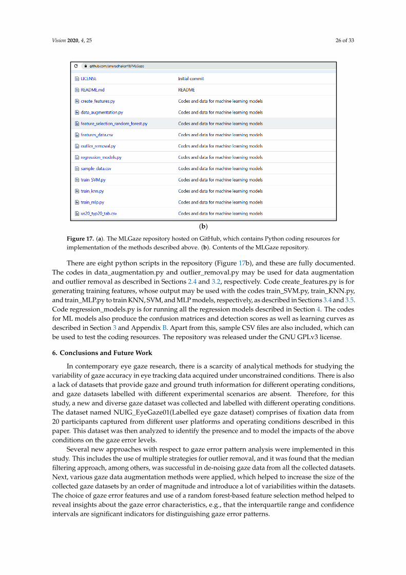
https://github.com/anuradhakar49/MLGaze

Vision 2020, 4, 25 26 of 33


(b)

Figure 17. (a). The MLGaze repository hosted on GitHub, which contains Python coding resources

for implementation of the methods described above. (b). Contents of the MLGaze repository.

There are eight python scripts in the repository (Figure 17b), and these are fully documented.

The codes in data_augmentation.py and outlier_removal.py may be used for data augmentation and

outlier removal as described in Sections 3.2 and 2.4, respectively. Code create_features.py is for

generating training features, whose output may be used with the codes train_SVM.py,

train_KNN.py, and train_MLP.py to train KNN, SVM, and MLP models, respectively, as described

in Sections 3.4 and 3.5. Code regression_models.py is for running all the regression models

described in Section 4. The codes for ML models also produce the confusion matrices and detection

scores as well as learning curves as described in Section 3 and Appendix B. Apart from this, sample

CSV files are also included, which can be used to test the coding resources. The repository was

released under the GNU GPLv3 license.

6. Conclusions and Future Work

In contemporary eye gaze research, there is a scarcity of analytical methods for studying the

variability of gaze accuracy in eye tracking data acquired under unconstrained conditions. There is

also a lack of datasets that provide gaze and ground truth information for different operating

conditions, and gaze datasets labelled with different experimental scenarios are absent. Therefore,

for this study, a new and diverse gaze dataset was collected and labelled with different operating

conditions. The dataset named NUIG_EyeGaze01(Labelled eye gaze dataset) comprises of fixation

data from 20 participants captured from different user platforms and operating conditions described

in this paper. This dataset was then analyzed to identify the presence and to model the impacts of

the above conditions on the gaze error levels.

Several new approaches with respect to gaze error pattern analysis were implemented in this

study. This includes the use of multiple strategies for outlier removal, and it was found that the

median filtering approach, among others, was successful in de-noising gaze data from all the

collected datasets. Next, various gaze data augmentation methods were applied, which helped to

increase the size of the collected gaze datasets by an order of magnitude and introduce a lot of

variabilities within the datasets. The choice of gaze error features and use of a random forest-based

feature selection method helped to reveal insights about the gaze error characteristics, e.g., that the

interquartile range and confidence intervals are significant indicators for distinguishing gaze error

patterns.

Figure 17. (a). The MLGaze repository hosted on GitHub, which contains Python coding resources forimplementation of the methods described above. (b). Contents of the MLGaze repository.

There are eight python scripts in the repository (Figure 17b), and these are fully documented.The codes in data_augmentation.py and outlier_removal.py may be used for data augmentationand outlier removal as described in Sections 2.4 and 3.2, respectively. Code create_features.py is forgenerating training features, whose output may be used with the codes train_SVM.py, train_KNN.py,and train_MLP.py to train KNN, SVM, and MLP models, respectively, as described in Sections 3.4 and 3.5.Code regression_models.py is for running all the regression models described in Section 4. The codesfor ML models also produce the confusion matrices and detection scores as well as learning curves asdescribed in Section 3 and Appendix B. Apart from this, sample CSV files are also included, which canbe used to test the coding resources. The repository was released under the GNU GPLv3 license.

6. Conclusions and Future Work

In contemporary eye gaze research, there is a scarcity of analytical methods for studying thevariability of gaze accuracy in eye tracking data acquired under unconstrained conditions. There is alsoa lack of datasets that provide gaze and ground truth information for different operating conditions,and gaze datasets labelled with different experimental scenarios are absent. Therefore, for thisstudy, a new and diverse gaze dataset was collected and labelled with different operating conditions.The dataset named NUIG_EyeGaze01(Labelled eye gaze dataset) comprises of fixation data from20 participants captured from different user platforms and operating conditions described in thispaper. This dataset was then analyzed to identify the presence and to model the impacts of the aboveconditions on the gaze error levels.

Several new approaches with respect to gaze error pattern analysis were implemented in thisstudy. This includes the use of multiple strategies for outlier removal, and it was found that the medianfiltering approach, among others, was successful in de-noising gaze data from all the collected datasets.Next, various gaze data augmentation methods were applied, which helped to increase the size of thecollected gaze datasets by an order of magnitude and introduce a lot of variabilities within the datasets.The choice of gaze error features and use of a random forest-based feature selection method helped toreveal insights about the gaze error characteristics, e.g., that the interquartile range and confidenceintervals are significant indicators for distinguishing gaze error patterns.

Vision 2020, 4, 25 27 of 33

The t-SNE algorithm is a relatively new concept in machine learning, which was used in thisstudy to visualize the distribution of classes within the gaze datasets, when gaze data influenced bydifferent error sources were mixed together. This technique demonstrated the complexities of the gazedatasets used in this study, which are close to what might be expected in gaze data from unconstrainedpractical applications. Finally, the use of machine learning for classification and prediction of gazeerror patterns in artificially created heterogeneous gaze datasets as done in this study is a new concept,which has been sparsely explored before.

The results from the training of the ML models reveal that these could be highly robust inidentifying gaze error patterns even in complex gaze datasets. It was seen that classifier models cansuccessfully distinguish between eye tracking data collected under normal conditions and data collectedunder varying operating conditions, such as a high degree of head pose variations, different userdistances, and platform poses. With these classifiers, familiar error patterns in eye gaze datasets maybe detected, and gaze error patterns that do not match the normal gaze behavior may be identified andrecognized as new error types.

The various concepts developed in this study, including the application of classifier and regressionmodels to gaze error data, may be used to build improved eye tracking systems and algorithms andalso to obtain better results from them. The main benefit of training the classifier models is that theycan distinguish anomalous gaze data present in realistic and complex gaze datasets as used in thisstudy and possibly recognize what caused them (e.g., impact of user distance or head pose). This canhelp eye gaze application developers, researchers, or engineers to deploy appropriate preventionmethods, compensation strategies, or setup improvements to reduce the impacts of the error sourcesaffecting their data.

The regression models may be used predict how an eye tracker might behave under practicaloperating conditions like a high degree of head pose or platform pose variations and forecast thepossible levels of error caused by different error sources. This can help eye gaze researchers or engineersto quantitatively specify the limits of their systems while operating under these challenging conditionsand also develop suitable error correction methods.

Additionally, the outlier detection techniques described in this study could be useful forapplications to any gaze dataset prior to analyzing them, to observe underlying data patterns.Overall, the gaze data analysis pipeline as implemented in this study could be of use to any eye gazeresearcher or engineer who wishes to gain deeper insights into their collected gaze data and have anestimate about the impacts of various non-ideal operating conditions on their eye tracking system.

There are also several ways to extend the study presented here since extracting and analyzingerror patterns from gaze data is a new and unexplored field in gaze research. For example, deep neuralnetworks may be used for the detection of anomalous gaze data collected from dynamic eye trackingapplications under unconstrained operating conditions. As mentioned in Section 1.2, in this study,the influence of one operating was considered at a time while collecting gaze data. However, complexscenarios may arise, where gaze data may be affected by more than one error source, such as, for example,in automotive use cases. The problem of a multi-factor influence on gaze data could be an interestingand complex research question but can only be answered when relevant and labelled data is available.Therefore, the collection of relevant gaze datasets from complex operational scenarios using desktop,handheld, head mounted, or automotive setups to understand a diverse range of gaze error patternscould be another potential future study in this domain.

Supplementary Materials: The following are available online at http://www.mdpi.com/2411-5150/4/2/25/s1.The eye gaze dataset collected from desktop and tablet platforms and used in this study is available online at:https://data.mendeley.com/datasets/cfm4d9y7bh/1. A GitHub repository containing the Python implementations ofthe gaze error pattern recognition pipeline is made available online at: https://github.com/anuradhakar49/MLGaze.A supplementary video (AK_face_pose.mp4) showing the application of the head pose model used in this studyon video frames in real time is available with this manuscript.

http://www.mdpi.com/2411-5150/4/2/25/s1

https://data.mendeley.com/datasets/cfm4d9y7bh/1

https://github.com/anuradhakar49/MLGaze

Vision 2020, 4, 25 28 of 33

Funding: The research work presented here was funded under the Strategic Partnership Program of ScienceFoundation Ireland (SFI) and co-funded by FotoNation Ltd. Project ID: 13/SPP/I2868 on “Next Generation Imagingfor Smartphone and Embedded Platforms”.

Conflicts of Interest: The author declares no conflict of interest.

Appendix A

The tablet was mounted on a gimbal holder as shown below in Figure A1a. To measure the deviceangles, the data from the inertial measurement sensor of the tablet were used. These are highly accuratesensors found in most tablet/smartphones to estimate the orientation of the device with 0.5-1 degree ofprecision. There are apps like Accelerometer analyser for Windows tablets and smartphones, which canprovide device orientation angles (in 3-D). Apart from this, the tablet orientation was verified byaligning a device (e.g., Android phone) with the tablet and running an Accelerometer app on the deviceto see if the two orientation results were similar. A screenshot from such an app (Tiltmeter, available onGoogle Play for Android) is shown in Figure A1b. Mechanical protractors were occasionally used tomanually verify the angles. Readings for one orientation were taken for all participants in consequentsessions to allow minimum tablet setup perturbation between the experiments.


Funding: The research work presented here was funded under the Strategic Partnership Program of Science

Foundation Ireland (SFI) and co-funded by FotoNation Ltd. Project ID: 13/SPP/I2868 on “Next Generation

Imaging for Smartphone and Embedded Platforms”.

Conflicts of Interest: The author declares no conflict of interest

Appendix A

The tablet was mounted on a gimbal holder as shown below in Figure A1a. To measure the

device angles, the data from the inertial measurement sensor of the tablet were used. These are

highly accurate sensors found in most tablet/smartphones to estimate the orientation of the device

with 0.5-1 degree of precision. There are apps like Accelerometer analyser for Windows tablets and

smartphones, which can provide device orientation angles (in 3-D). Apart from this, the tablet

orientation was verified by aligning a device (e.g., Android phone) with the tablet and running an

Accelerometer app on the device to see if the two orientation results were similar. A screenshot from

such an app (Tiltmeter, available on Google Play for Android) is shown in Figure A1b. Mechanical

protractors were occasionally used to manually verify the angles. Readings for one orientation were

taken for all participants in consequent sessions to allow minimum tablet setup perturbation

between the experiments.

(a) (b)

Figure A1. (a) Gimbal tripod mount for the tablet; (b) 3-D position reading from inertial sensors

using an smartphone/tablet app.

Appendix B

For this study, the selection of the participant number was based on the criteria about the

number of data samples required compared to the size of the feature set used for training the

machine learning (ML) algorithms. For the ML models like SVM, KNN, and MLP, there is an

empirical rule that the training dataset size should be at least 10 times the size of the feature set. This

is also termed as the “rule of 10” [63]. Going by this rule, it may be seen that in this paper, the

maximum size of the feature set is 20 (Equation (15)) for the classification problem. Therefore, data

from 20 persons with 10-fold augmentation were used. Additionally, the gaze yaw and pitch

features were included in the training set, so the total training data size was (20 × 3 × 10) = 600

samples per class. As an example, for the classification of the user distance data from the desktop or

tablet, there were four classes and all three categories of gaze data were collected for each of them.

So, the total number of training samples was 600 × 4 = 2400 samples for the 4-class classification

problem (this is shown in Table 3 above). This feature size was deemed to be useful while training

and is supported by the learning curves for the different ML models whose plots are shown in

Figure B1a–d below for the KNN, SVM, and MLP classifiers and the ElasticNet regression model,

Figure A1. (a) Gimbal tripod mount for the tablet; (b) 3-D position reading from inertial sensors usingan smartphone/tablet app.

Appendix B

For this study, the selection of the participant number was based on the criteria about the numberof data samples required compared to the size of the feature set used for training the machine learning(ML) algorithms. For the ML models like SVM, KNN, and MLP, there is an empirical rule that thetraining dataset size should be at least 10 times the size of the feature set. This is also termed asthe “rule of 10” [63]. Going by this rule, it may be seen that in this paper, the maximum size of thefeature set is 20 (Equation (15)) for the classification problem. Therefore, data from 20 persons with10-fold augmentation were used. Additionally, the gaze yaw and pitch features were included in thetraining set, so the total training data size was (20 × 3 × 10) = 600 samples per class. As an example,for the classification of the user distance data from the desktop or tablet, there were four classes andall three categories of gaze data were collected for each of them. So, the total number of trainingsamples was 600 × 4 = 2400 samples for the 4-class classification problem (this is shown in Table 3above). This feature size was deemed to be useful while training and is supported by the learningcurves for the different ML models whose plots are shown in Figure A2a–d below for the KNN, SVM,and MLP classifiers and the ElasticNet regression model, respectively. The training set size in thefigures indicates the number of data samples used for training the respective model.

Vision 2020, 4, 25 29 of 33

From the figures, it is seen that the training/cross validation accuracy for the different machinelearning models converges and stabilizes into an asymptote within the training sample size for theclassification and regression tasks and therefore it can be said that the training set size chosen issuitable for the machine learning model. Once the training and validation curves converge, it isunlikely that increasing the training data size will increase the model performance. While it is alwayspossible to gather more data for studying the gaze error patterns, based on the trade-off betweenthe available number of participants, the data collection time required, and the training/validationaccuracy, the number of participants chosen in this study was found to be optimal.


respectively. The training set size in the figures indicates the number of data samples used for

training the respective model.

From the figures, it is seen that the training/cross validation accuracy for the different machine

learning models converges and stabilizes into an asymptote within the training sample size for the

classification and regression tasks and therefore it can be said that the training set size chosen is

suitable for the machine learning model. Once the training and validation curves converge, it is

unlikely that increasing the training data size will increase the model performance. While it is

always possible to gather more data for studying the gaze error patterns, based on the trade-off

between the available number of participants, the data collection time required, and the

training/validation accuracy, the number of participants chosen in this study was found to be

optimal.

(a) (b)

(c) (d)

Figure B1. Learning curves for (a) KNN, (b) SVM, and (c) MLP classifiers, and the (d) Elastic-Net

model.

References

1. Kar, A.; Corcoran, P. Performance Evaluation Strategies for Eye Gaze Estimation Systems with

Quantitative Metrics and Visualizations. Sensors 2018, 18, 3151.

2. Cheon, M.; Lee, J. Gaze pattern analysis for video contents with different frame rates. In Proceedings of the

2013 Visual Communications and Image Processing (VCIP), Kuching, Malaysia, 17–20 November 2013; pp. 1–5.

3. Zhu, D.; Mendis, B.S.U.; Gedeon, T.; Asthana, A.; Goecke, R. A Hybrid Fuzzy Approach for Human

Eye Gaze Pattern Recognition. In Advances in Neuro-Information Processing; ICONIP 2008; Lecture

Notes in Computer Science; Köppen, M., Kasabov, N., Coghill, G., Eds.; Springer: Berlin/Heidelberg ,

Germany, 2009; Volume 5507.

4. Horiguchi, Y.; Suzuki, T.; Sawaragi, T.; Nakanishi, H.; Takimoto, T. Extraction and Investigation of

Dominant Eye-Gaze Pattern in Train Driver’s Visual Behavior Using Markov Cluster Algorithm. 2016 Joint

Figure A2. Learning curves for (a) KNN, (b) SVM, and (c) MLP classifiers, and the (d) Elastic-Net model.

References

1. Kar, A.; Corcoran, P. Performance Evaluation Strategies for Eye Gaze Estimation Systems with QuantitativeMetrics and Visualizations. Sensors 2018, 18, 3151. [CrossRef] [PubMed]

2. Cheon, M.; Lee, J. Gaze pattern analysis for video contents with different frame rates. In Proceedings ofthe 2013 Visual Communications and Image Processing (VCIP), Kuching, Malaysia, 17–20 November 2013;pp. 1–5.

3. Zhu, D.; Mendis, B.S.U.; Gedeon, T.; Asthana, A.; Goecke, R. A Hybrid Fuzzy Approach for Human EyeGaze Pattern Recognition. In ICONIP 2008: Advances in Neuro-Information Processing; Lecture Notes inComputer Science; Köppen, M., Kasabov, N., Coghill, G., Eds.; Springer: Berlin/Heidelberg, Germany, 2009;Volume 5507.

4. Horiguchi, Y.; Suzuki, T.; Sawaragi, T.; Nakanishi, H.; Takimoto, T. Extraction and Investigation of DominantEye-Gaze Pattern in Train Driver’s Visual Behavior Using Markov Cluster Algorithm. In Proceedings ofthe 2016 Joint 8th International Conference on Soft Computing and Intelligent Systems (SCIS) and 17thInternational Symposium on Advanced Intelligent Systems (ISIS), Sapporo, Japan, 25–28 August 2016;pp. 578–581.

http://dx.doi.org/10.3390/s18093151

http://www.ncbi.nlm.nih.gov/pubmed/30231547

Vision 2020, 4, 25 30 of 33

5. Braunagel, C.; Geisler, D.; Stolzmann, W.; Rosenstiel, W.; Kasneci, E. On the necessity of adaptive eyemovement classification in conditionally automated driving scenarios. In Proceedings of the Ninth BiennialACM Symposium on Eye Tracking Research & Applications (ETRA 16); ACM: New York, NY, USA, 2016;pp. 19–26.

6. Koochaki, F.; Najafizadeh, L. Predicting Intention Through Eye Gaze Patterns. In Proceedings of the 2018IEEE Biomedical Circuits and Systems Conference (BioCAS), Cleveland, OH, USA, 17–19 October 2018;pp. 1–4.

7. Pekkanen, J.; Lappi, O. A new and general approach to signal denoising and eye movement classificationbased on segmented linear regression. Sci. Rep. 2017, 7, 1–13. [CrossRef] [PubMed]

8. Zemblys, R.; Niehorster, D.C.; Komogortsev, O.; Holmqvist, K. Using machine learning to detect events ineye-tracking data. Behav. Res. Methods 2018, 50, 160–181. [CrossRef]

9. Barz, M.; Daiber, F.; Sonntag, D.; Bulling, A. Error-aware gaze-based interfaces for robust mobile gazeinteraction. In Proceedings of the 2018 ACM Symposium on Eye Tracking Research & Applications (ETRA’18);ACM: New York, NY, USA, 2018; Article 24; 10p.

10. Barz, M.; Daiber, F.; Sonntag, D.; Bulling, A. Prediction of gaze estimation error for error-aware gaze-basedinterfaces. In Proceedings of the Ninth Biennial ACM Symposium on Eye Tracking Research & Applications(ETRA’16); ACM: New York, NY, USA, 2016; pp. 275–278.

11. Chandola, V.; Banerjee, A.; Kumar, V. Anomaly Detection: A Survey. ACM Comput. Surv. (CSUR) 2009, 41,15:1–15:58. [CrossRef]

12. Song, F.; Diao, Y.; Read, J.; Stiegler, A.; Bifet, A. EXAD: A System for Explainable Anomaly Detection onBig Data Traces. In Proceedings of the 2018 IEEE International Conference on Data Mining Workshops,Singapore, 17–20 November 2016; 2018; pp. 1435–1440.

13. Ishikawa, T.; Baker, S.; Matthews, I.; Kanade, T. Passive Driver Gaze Tracking with Active AppearanceModels. Proc. World Congr. Intell. Transp. Syst. 2004, 1–12. [CrossRef]

14. Chen, T.; Ma, K.; Chen, L.H. Tri-state median filter for image denoising. IEEE Trans. Image Process. 1999, 8,1834–1838. [CrossRef]

15. Khalil, H.H.; Rahmat, R.O.K.; Mahmoud, W.A. Chapter 15: Estimation of Noise in Gray-Scale and ColoredImages Using Median Absolute Deviation (MAD). In Proceedings of the 3rd International Conference onGeometric Modeling and Imaging, London, UK, 9–11 July 2008; pp. 92–97.

16. Chen, Y.C. A tutorial on kernel density estimation and recent advances. Biostat. Epidemiol. 2017, 1, 161–187.[CrossRef]

17. Koydemir, H.C.; Feng, S.; Liang, K.; Nadkarni, R.; Tseng, D.; Benien, P.; Ozcan, A. A survey ofsupervised machine learning models for mobile-phone based pathogen identification and classification.In Proceedings of the SPIE 10055, Optics and Bio-photonics in Low-Resource Settings III, 100550A (7 March 2017);International Society for Optics and Photonics: Washington, DC, USA, 2017.

18. Qiu, J.; Wu, Q.; Ding, G.; Xu, Y.; Feng, S. A survey of machine learning for big data processing. EURASIP J.Adv. Sig. Process. 2016, 2016, 67. [CrossRef]

19. Bjerrum, E.J.; Glahder, M.; Skov, T. Data Augmentation of Spectral Data for Convolutional Neural Network(CNN) Based Deep Chemometrics. arXiv 2017, arXiv:1710.01927.

20. Polson, N.G.; Scott, S.L. Data augmentation for support vector machines. Bayesian Anal. 2011, 6, 23.[CrossRef]

21. Sáiz-Abajo, M.J.; Mevik, B.H.; Segtnan, V.H.; Næs, T. Ensemble methods and data augmentation by noiseaddition applied to the analysis of spectroscopic data. Anal. Chim. Acta 2005, 533, 147–159, ISSN 0003-2670.

22. Duchowski, A.; Jörg, S.; Allen, T.N.; Giannopoulos, I.; Krejtz, K. Eye movement synthesis. In Proceedings ofthe Ninth Biennial ACM Symposium on Eye Tracking Research & Applications (ETRA ’16); ACM: New York, NY,USA, 2016; pp. 147–154.

23. Duchowski, A.; Jörg, S.; Lawson, A.; Bolte, T.; Swirski, L.; Krejtz, K. Eye movement synthesis with 1/f pinknoise. In Proceedings of the 8th ACM SIGGRAPH Conference on Motion in Games (MIG’15); ACM: New York,NY, USA, 2015; pp. 47–56.

24. Devries, T.; Taylor, G.W. Dataset Augmentation in Feature Space. arXiv 2017, arXiv:1702.05538.

http://dx.doi.org/10.1038/s41598-017-17983-x


http://dx.doi.org/10.3758/s13428-017-0860-3

http://dx.doi.org/10.1145/1541880.1541882

http://dx.doi.org/10.1184/R1/6557315.v1

http://dx.doi.org/10.1109/83.806630

http://dx.doi.org/10.1080/24709360.2017.1396742

http://dx.doi.org/10.1186/s13634-016-0355-x

http://dx.doi.org/10.1214/11-BA601

Vision 2020, 4, 25 31 of 33

25. Um, T.; Pfister, F.; Pichler, D.; Endo, S.; Lang, M.; Hirche, S.; Fietzek, U.; Kulic, D. Data augmentation ofwearable sensor data for parkinson’s disease monitoring using convolutional neural networks. In Proceedingsof the 19th ACM International Conference on Multimodal Interaction (ICMI’17); ACM: New York, NY, USA, 2017;pp. 216–220.

26. Salamon, J.; Bello, J.P. Deep Convolutional Neural Networks and Data Augmentation for EnvironmentalSound Classification. IEEE Signal Process. Lett. 2017, 24, 279–283. [CrossRef]

27. Li, Q.; Zhou, Y.; Chen, D. Research on machine learning algorithms and feature extraction for time series.In Proceedings of the 2017 IEEE 28th Annual International Symposium on Personal, Indoor, and MobileRadio Communications (PIMRC), Montreal, QC, Canada, 8–13 October 2017; pp. 1–5.

28. Popescu, M.C.; Sasu, L.M. Feature extraction, feature selection and machine learning for image classification:A case study. In Proceedings of the 2014 International Conference on Optimization of Electrical and ElectronicEquipment (OPTIM), Bran, Romania, 22–24 May 2014; pp. 968–973.

29. Khalid, S.; Khalil, T.; Nasreen, S. A survey of feature selection and feature extraction techniques in machinelearning. In Proceedings of the 2014 Science and Information Conference, London, UK, 27–29 August 2014;pp. 372–378.

30. Oravec, M. Feature extraction and classification by machine learning methods for biometric recognition offace and iris. In Proceedings of the ELMAR-2014, Zadar, Croatia, 10–12 September 2014; pp. 1–4.

31. van der Maaten, L.J.P.; Hinton, G.E. Visualizing High-Dimensional Data Using t-SNE. J. Mach. Learn. Res.2008, 9, 2579–2605.

32. Rogovschi, N.; Kitazono, J.; Grozavu, N.; Omori, T.; Ozawa, S. t-Distributed stochastic neighbor embeddingspectral clustering. In Proceedings of the 2017 International Joint Conference on Neural Networks (IJCNN),Anchorage, AK, USA, 14–19 May 2017; pp. 1628–1632.

33. Mounce, S. Visualizing Smart Water Meter Dataset Clustering With Parametric T-distributed StochasticNeighbour Embedding. In Proceedings of the 2017 13th International Conference on Natural Computation,Fuzzy Systems and Knowledge Discovery (ICNC-FSKD), Guilin, China, 29–31 July 2017; pp. 1940–1945.

34. Retsinas, G.; Stamatopoulos, N.; Louloudis, G.; Sfikas, G.; Gatos, B. Nonlinear Manifold Embedding onKeyword Spotting Using t-SNE. In Proceedings of the 2017 14th IAPR International Conference on DocumentAnalysis and Recognition (ICDAR), Kyoto, Japan, 9–15 November 2017; pp. 487–492.

35. Pancerz, K.; Paja, W.; Gomuła, J. Random forest feature selection for data coming from evaluation sheets ofsubjects with ASDs. In Proceedings of the 2016 Federated Conference on Computer Science and InformationSystems (FedCSIS), Gdansk, Poland, 11–14 September 2016; pp. 299–302.

36. Cao, W.; Xu, J.; Liu, Z. Speaker-independent speech emotion recognition based on random forest featureselection algorithm. In Proceedings of the 2017 36th Chinese Control Conference (CCC), Dalian, China,26–28 July 2017; pp. 10995–10998.

37. Gomes, R.; Ahsan, M.; Denton, A. Random Forest Classifier in SDN Framework for User-Based IndoorLocalization. In Proceedings of the 2018 IEEE International Conference on Electro/Information Technology(EIT), Rochester, MI, USA, 3–5 May 2018; pp. 0537–0542.

38. Song, Q.; Liu, X.; Yang, L. The random forest classifier applied in droplet fingerprint recognition.In Proceedings of the 2015 12th International Conference on Fuzzy Systems and Knowledge Discovery(FSKD), Zhangjiajie, China, 15–17 August 2015; pp. 722–726.

39. Okfalisa, I.; Gazalba, M.; Reza, N.G.I. Comparative analysis of k-nearest neighbor and modified k-nearestneighbor algorithm for data classification. In Proceedings of the 2017 2nd International conferences onInformation Technology, Information Systems and Electrical Engineering (ICITISEE), Yogyakarta, Indonesia,1–2 November 2017; pp. 294–298.

40. Guan, F.; Shi, J.; Ma, X.; Cui, W.; Wu, J. A Method of False Alarm Recognition Based on k-Nearest Neighbor.In Proceedings of the 2017 International Conference on Dependable Systems and Their Applications (DSA),Beijing, China, 31 October–2 November 2017; pp. 8–12.

41. Cai, Y.; Huang, H.; Cai, H.; Qi, Y. A K-nearest neighbor locally search regression algorithm for short-termtraffic flow forecasting. In Proceedings of the 2017 9th International Conference on Modelling, Identificationand Control (ICMIC), Kunming, China, 10–12 July 2017; pp. 624–629.

42. Zhang, X.; Li, B.; Sun, X. A k-nearest neighbor text classification algorithm based on fuzzy integral.In Proceedings of the 2010 Sixth International Conference on Natural Computation, Yantai, China,10–12 August 2010; pp. 2228–2231.

http://dx.doi.org/10.1109/LSP.2017.2657381

Vision 2020, 4, 25 32 of 33

43. Waske, B.; Benediktsson, J.A. Fusion of Support Vector Machines for Classification of Multisensor Data.IEEE Trans. Geosci. Remote Sens. 2007, 45, 3858–3866. [CrossRef]

44. Sheng, L.; Mengjun, W.; Lanyong, Z. Research on information fusion of infrared and radar sensor basedon SVM. In Proceedings of the 2012 International Conference on Measurement, Information and Control,Harbin, China, 18–20 May 2012; pp. 98–101.

45. Nakano, T.; Nukala, B.T.; Tsay, J.; Zupancic, S.; Rodriguez, A.; Lie, D.Y.C.; Lopez, J.; Nguyen, T.Q.Gaits Classification of Normal vs Patients by Wireless Gait Sensor and Support Vector Machine (SVM)Classifier. Int. J. Softw. Innov. (IJSI) 2017, 5, 17–29. [CrossRef]

46. Jeong, G.; Truong, P.H.; Choi, S. Classification of Three Types of Walking Activities Regarding. IEEE Sens. J.2017, 17, 2638–2639. [CrossRef]

47. Bengio, Y.; Courville, A.; Vincent, P. Representation Learning: A Review and New Perspectives. IEEE Trans.Pattern Anal. Mach. Intell. 2013, 35, 1798–1828. [CrossRef]

48. Koldowski, U.M.M. Spiking neural network vs multilayer perceptron: Who is the winner in the racing carcomputer game. Soft Comput. 2015, 12, 3465–3478.

49. Bieniasz, J.; Rawski, M.; Skowron, K.; Trzepinski, M. Evaluation of multilayer perceptron algorithmsfor an analysis of network flow data. In Photonics Applications in Astronomy, Communications, Industry,and High-Energy Physics Experiments 2016; International Society for Optics and Photonics: Washington, DC,USA, 2016.

50. Lang, B. Monotonic Multi-layer Perceptron Networks as Universal Approximators. In Artificial NeuralNetworks: Formal Models and Their Applications–ICANN 2005; Lecture Notes in Computer Science; Duch, W.,Kacprzyk, J., Oja, E., Zadrozny, S., Eds.; Springer: Berlin/Heidelberg, Germany, 2005; Volume 3697.

51. Astorino, A.; Fuduli, A. The Proximal Trajectory Algorithm in SVM Cross Validation. IEEE Trans. NeuralNetworks Learn. Syst. 2016, 27, 966–977. [CrossRef]

52. Huang, Q.; Mao, J.; Liu, Y. An Improved Grid Search Algorithm of SVR Parameters Optimization.In Proceedings of the 2012 IEEE 14th International Conference on Communication Technology, Chengdu,China, 9–11 November 2012; pp. 1022–1026.

53. Chen, S.; Liu, C. Eye detection using discriminatory Haar features and a new efficient SVM. Image Vis. Comput.2015, 33, 68–77. [CrossRef]

54. Shang, W.; Cui, J.; Song, C.; Zhao, J.; Zeng, P. Research on Industrial Control Anomaly Detection Basedon FCM and SVM. In Proceedings of the 12th IEEE International Conference on Big Data Science andEngineering, TrustCom/BigDataSE, New York, NY, USA, 1–3 August 2018; pp. 218–222.

55. Xie, Y.; Zhang, Y. An intelligent anomaly analysis for intrusion detection based on SVM. In Proceedings ofthe 2012 International Conference on Computer Science and Information Processing (CSIP), Xi’an, China,24–26 August 2012; pp. 739–742.

56. Guang, Y.; Min, N.I.E. Anomaly Intrusion Detection Based on Wavelet Kernel LS-SVM. In Proceedingsof the 2013 3rd International Conference on Computer Science and Network Technology, Dalian, China,12–13 October 2013; pp. 434–437.

57. Eswaran, C.; Logeswaran, R.A. Comparison of ARIMA, Neural Network and Linear Regression Models forthe Prediction of Infant Mortality Rate. In Proceedings of the 2010 Fourth Asia International Conferenceon Mathematical/Analytical Modelling and Computer Simulation, Bornea, Malaysia, 26–28 May 2010;IEEE: Piscataway, NJ, USA, 2010; pp. 34–39.

58. Friedman, J.; Hastie, T.; Tibshirani, R. Regularization Paths for Generalized Linear Models via CoordinateDescent. J. Stat. Softw. 2010, 33, 1–22. [CrossRef]

59. Jones, L.K. Local Minimax Learning of Functions with Best Finite Sample Estimation Error Bounds:Applications to Ridge and Lasso Regression, Boosting, Tree Learning, Kernel Machines, and InverseProblems. IEEE Trans. Inf. Theory 2009, 55, 5700–5727. [CrossRef]

60. Kirpich, A.; Ainsworth, E.A.; Wedow, J.M.; Newman, J.R.B.; Michailidis, G.; McIntyre, L. M Variable selectionin omics data: A practical evaluation of small sample sizes. PLoS ONE 2018, 13, e0197910. [CrossRef][PubMed]

61. Bayindir, R.; Gok, M.; Kabalci, E.; Kaplan, O. An Intelligent Power Factor Correction Approach Based onLinear Regression and Ridge Regression Methods. In Proceedings of the 2011 10th International Conference onMachine Learning and Applications and Workshops, Honolulu, HI, USA, 18–21 December 2011; pp. 313–315.

http://dx.doi.org/10.1109/TGRS.2007.898446

http://dx.doi.org/10.4018/IJSI.2017010102

http://dx.doi.org/10.1109/JSEN.2017.2682322

http://dx.doi.org/10.1109/TPAMI.2013.50

http://dx.doi.org/10.1109/TNNLS.2015.2430935

http://dx.doi.org/10.1016/j.imavis.2014.10.007

http://dx.doi.org/10.18637/jss.v033.i01

http://dx.doi.org/10.1109/TIT.2009.2027479

http://dx.doi.org/10.1371/journal.pone.0197910


Vision 2020, 4, 25 33 of 33

62. Verma, T.; Tiwana, A.P.S.; Reddy, C.C. Data Analysis to Generate Models Based on Neural Network andRegression for Solar Power Generation Forecasting. In Proceedings of the 2016 7th International Conferenceon Intelligent Systems, Modelling and Simulation (ISMS), Bangkok, Thailand, 25–27 January 2016; pp. 97–100.

63. Vabalas, A.; Gowen, E.; Poliakoff, E.; Casson, A. Machine learning algorithm validation with a limited samplesize. PLoS ONE 2019, 14, e0224365. [CrossRef] [PubMed]

© 2020 by the author. Licensee MDPI, Basel, Switzerland. This article is an open accessarticle distributed under the terms and conditions of the Creative Commons Attribution(CC BY) license (http://creativecommons.org/licenses/by/4.0/).

http://dx.doi.org/10.1371/journal.pone.0224365


http://creativecommons.org/

http://creativecommons.org/licenses/by/4.0/.

Machine Learning-Based Analysis of Gaze Error ... - MDPI

Documents

Transcript of Machine Learning-Based Analysis of Gaze Error ... - MDPI