MA10192 Mathematics I - University of Bath
100
MA10192 Mathematics I Lecture Notes Roger Moser Department of Mathematical Sciences University of Bath Semester 1, 2017/8
-
Upload
khangminh22 -
Category
Documents
-
view
1 -
download
0
Transcript of MA10192 Mathematics I - University of Bath
MA10192 Mathematics I
Lecture Notes
Roger MoserDepartment of Mathematical Sciences
University of Bath
Semester 1, 2017/8

2
Contents
1 Functions and Equations 5
1.1 What are functions and equations? . . . . . . . . . . . . . . . 5
1.2 Special functions . . . . . . . . . . . . . . . . . . . . . . . . . 7
1.2.1 Polynomials . . . . . . . . . . . . . . . . . . . . . . . . 7
1.2.2 Exponential functions . . . . . . . . . . . . . . . . . . 9
1.2.3 Logarithms . . . . . . . . . . . . . . . . . . . . . . . . 11
1.2.4 Trigonometric functions . . . . . . . . . . . . . . . . . 12
1.2.5 Inverse trigonometric functions . . . . . . . . . . . . . 14
1.2.6 Hyperbolic functions . . . . . . . . . . . . . . . . . . . 16
1.3 Applications of trigonometric functions . . . . . . . . . . . . . 16
1.3.1 Polar coordinates . . . . . . . . . . . . . . . . . . . . . 16
1.3.2 Solving trigonometric equations . . . . . . . . . . . . . 18
1.4 Limits . . . . . . . . . . . . . . . . . . . . . . . . . . . . . . . 20
1.5 The bisection method . . . . . . . . . . . . . . . . . . . . . . 24
2 Differentiation 27
2.1 Fundamentals . . . . . . . . . . . . . . . . . . . . . . . . . . . 27
2.1.1 Definition . . . . . . . . . . . . . . . . . . . . . . . . . 27
2.1.2 Notation . . . . . . . . . . . . . . . . . . . . . . . . . . 28
2.1.3 Derivatives of a few simple functions . . . . . . . . . . 28
2.2 Differentiation rules . . . . . . . . . . . . . . . . . . . . . . . 30
2.2.1 The sum rule . . . . . . . . . . . . . . . . . . . . . . . 30
2.2.2 The product rule . . . . . . . . . . . . . . . . . . . . . 30
2.2.3 The quotient rule . . . . . . . . . . . . . . . . . . . . . 31
2.2.4 The chain rule . . . . . . . . . . . . . . . . . . . . . . 32
2.3 Further differentiation techniques . . . . . . . . . . . . . . . . 33
2.3.1 Logarithmic differentiation . . . . . . . . . . . . . . . 34
2.3.2 Derivatives of inverse functions . . . . . . . . . . . . . 34
2.3.3 Parametric differentiation . . . . . . . . . . . . . . . . 35
2.3.4 Implicit differentiation . . . . . . . . . . . . . . . . . . 36
2.4 Applications . . . . . . . . . . . . . . . . . . . . . . . . . . . . 37
2.4.1 Maxima and minima . . . . . . . . . . . . . . . . . . . 37
2.4.2 L’Hopital’s rule . . . . . . . . . . . . . . . . . . . . . . 38
3

4 CONTENTS
2.4.3 Newton’s method . . . . . . . . . . . . . . . . . . . . . 402.5 Taylor polynomials . . . . . . . . . . . . . . . . . . . . . . . . 412.6 Numerical differentiation . . . . . . . . . . . . . . . . . . . . . 44
3 Integration 473.1 Two approaches to integration . . . . . . . . . . . . . . . . . 47
3.1.1 Antidifferentiation and the indefinite integral . . . . . 473.1.2 Area and the definite integral . . . . . . . . . . . . . . 48
3.2 Integration techniques . . . . . . . . . . . . . . . . . . . . . . 503.2.1 The substitution rule . . . . . . . . . . . . . . . . . . . 513.2.2 Integration by parts . . . . . . . . . . . . . . . . . . . 533.2.3 Partial fractions . . . . . . . . . . . . . . . . . . . . . 55
3.3 Further integration techniques . . . . . . . . . . . . . . . . . . 623.3.1 Integrating an inverse function . . . . . . . . . . . . . 623.3.2 Trigonometric rational functions . . . . . . . . . . . . 633.3.3 Trigonometric substitution . . . . . . . . . . . . . . . 643.3.4 Hyperbolic substitution . . . . . . . . . . . . . . . . . 65
3.4 Numerical integration . . . . . . . . . . . . . . . . . . . . . . 673.5 Improper integrals . . . . . . . . . . . . . . . . . . . . . . . . 70
4 Differential equations 734.1 Introduction . . . . . . . . . . . . . . . . . . . . . . . . . . . . 734.2 Separation of variables . . . . . . . . . . . . . . . . . . . . . . 744.3 Linear equations . . . . . . . . . . . . . . . . . . . . . . . . . 77
4.3.1 Integrating factors . . . . . . . . . . . . . . . . . . . . 774.3.2 The method of undetermined coefficients . . . . . . . 79
4.4 Numerical methods . . . . . . . . . . . . . . . . . . . . . . . . 824.4.1 Euler’s method . . . . . . . . . . . . . . . . . . . . . . 824.4.2 Backward Euler method . . . . . . . . . . . . . . . . . 834.4.3 Other methods . . . . . . . . . . . . . . . . . . . . . . 85
5 Functions of several variables 875.1 Background . . . . . . . . . . . . . . . . . . . . . . . . . . . . 875.2 Partial derivatives . . . . . . . . . . . . . . . . . . . . . . . . 885.3 Tangent plane and linear approximation . . . . . . . . . . . . 885.4 Total derivatives . . . . . . . . . . . . . . . . . . . . . . . . . 905.5 Second derivatives . . . . . . . . . . . . . . . . . . . . . . . . 915.6 Applications . . . . . . . . . . . . . . . . . . . . . . . . . . . . 92
5.6.1 Maxima and minima . . . . . . . . . . . . . . . . . . . 925.6.2 Exact differential equations . . . . . . . . . . . . . . . 95
Index 99

Chapter 1
Functions and Equations
1.1 What are functions and equations?
An equation is a statement saying that two things (in this course typicallynumbers or quantities) are equal. For example, the equation
2 + 3 = 5
expresses the fact that the sum of 2 and 3 is equal to 5. We often considerequations involving an unknown quantity or number, say x. For example,consider the equation
x2 = 2.
To solve an equation of this type means to determine all values of x suchthat the equation is true.
Example 1.1.1. Consider the equation
x2 − 4 = 0.
It has two solutions, namely x = 2 and x = −2.
A function is a rule by which one quantity depends unambiguously onanother. We can think of a function as a process that takes a certain in-put and turns it into a unique output. (The word ‘unambiguously’ in theprevious definition means that every input generates one single output.)
Example 1.1.2. The formula
y = x2 + 2x− 1
2
gives rise to a function by which the quantity y depends on x. The inputx = 2, say, leads to y = 22 + 2 · 2− 1
2 = 152 , and every other value for x will
give a single value for y.
5
6 CHAPTER 1. FUNCTIONS AND EQUATIONS
We will mostly study functions that are given by formulas such as in theexample, because these are particularly useful.
We may use symbols to represent a given function, just as we use x torepresent numbers in the above examples. If our function is denoted by f ,then f(x) stands for the output arising from the input x. If we wish to assigna symbol to this quantity as well, say y, then we can write y = f(x). Herex is called the independent variable and y is called the dependent variableof the function.
Example 1.1.3. Consider the function determined by the formula
y = x2 + 2x− 1
2.
If we represent this function by the symbol f , then we may also write
f(x) = x2 + 2x− 1
2.
Then we have, for example, f(2) = 152 .
A function f can be represented geometrically in terms of the set of allpoints in the plane with coordinates (x, y) such that
y = f(x).
This is called the graph of the function f .
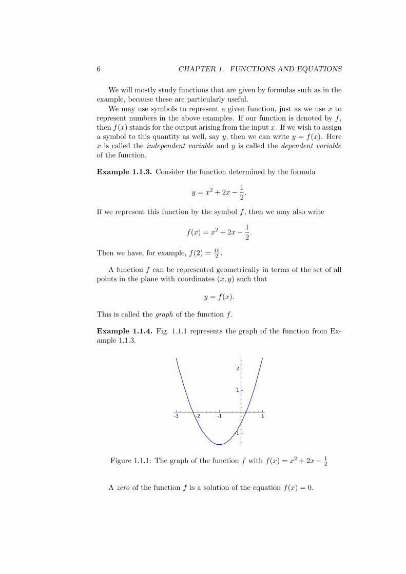
Example 1.1.4. Fig. 1.1.1 represents the graph of the function from Ex-ample 1.1.3.
Figure 1.1.1: The graph of the function f with f(x) = x2 + 2x− 12
A zero of the function f is a solution of the equation f(x) = 0.
1.2. SPECIAL FUNCTIONS 7
1.2 Special functions
1.2.1 Polynomials
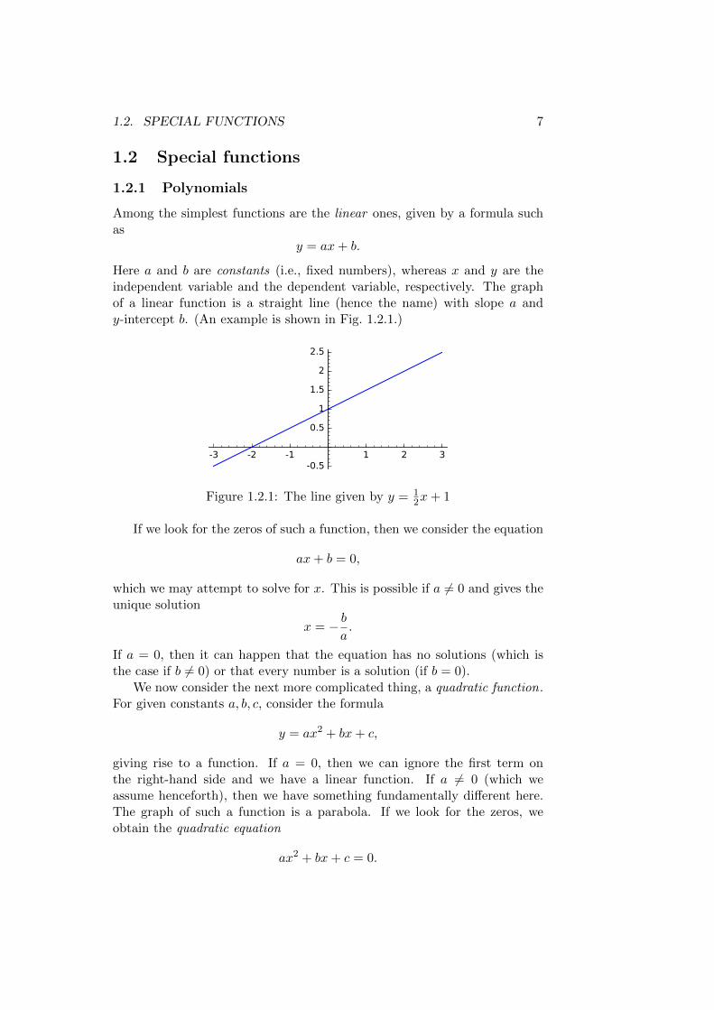
Among the simplest functions are the linear ones, given by a formula suchas
y = ax+ b.
Here a and b are constants (i.e., fixed numbers), whereas x and y are theindependent variable and the dependent variable, respectively. The graphof a linear function is a straight line (hence the name) with slope a andy-intercept b. (An example is shown in Fig. 1.2.1.)
Figure 1.2.1: The line given by y = 12x+ 1
If we look for the zeros of such a function, then we consider the equation
ax+ b = 0,
which we may attempt to solve for x. This is possible if a 6= 0 and gives theunique solution
x = − ba.
If a = 0, then it can happen that the equation has no solutions (which isthe case if b 6= 0) or that every number is a solution (if b = 0).
We now consider the next more complicated thing, a quadratic function.For given constants a, b, c, consider the formula
y = ax2 + bx+ c,
giving rise to a function. If a = 0, then we can ignore the first term onthe right-hand side and we have a linear function. If a 6= 0 (which weassume henceforth), then we have something fundamentally different here.The graph of such a function is a parabola. If we look for the zeros, weobtain the quadratic equation
ax2 + bx+ c = 0.

8 CHAPTER 1. FUNCTIONS AND EQUATIONS
If we want to solve the equation, it is convenient to divide by a on bothsides first (which we can do as a 6= 0):
x2 +b
ax+
c
a= 0.
Then we ‘complete the square’, i.e., we reformulate this as follows:(x+
b
2a
)2
− b2
4a2+c
a= 0.
Thus (x+
b
2a
)2
=b2
4a2− c
a.
Assuming that b2 − 4ac ≥ 0, we can take the square root on both sides:
x+b
2a= ±
√b2
4a2− c
a= ±√b2 − 4ac
2a.
Now subtract b/2a on both sides to obtain the well-known formula
x =−b±
√b2 − 4ac
2a.
So for b2 − 4ac > 0, we have two solutions, and for b2 − 4ac = 0, we haveone, which is − b
2a . If b2 − 4ac < 0, then the equation has no solutions.1
Another method to solve a quadratic equation is factorisation. Assumingthat we have an equation of the form
x2 + bx+ c = 0,
(which is the case after the first step for the above method), we try to findtwo numbers α, β such that
x2 + bx+ c = (x− α)(x− β).
This is true if α+β = −b and αβ = c. It is not always possible to find α andβ that satisfy both conditions, but if they do, then we have the solutionsx = α and x = β of the quadratic equation.
A cubic function arises from a formula of the form
y = ax3 + bx2 + cx+ d
and a quartic function from a formula of the form
y = ax4 + bx3 + cx2 + dx+ e,
1This is the case if you work with real numbers as we do here. In MA10193 Mathematics2, you will see complex numbers, and if you work with these, then you have two solutionsin this case as well.
1.2. SPECIAL FUNCTIONS 9
where a, b, c, d, e are constants and in both cases it is assumed that a 6= 0.There are still methods to solve the corresponding equations, but they arerather more complicated.
There is no reason to stop at fourth powers of x, of course. Any functionbuilt up from powers of x in this way is called a polynomial . For example,the function given by
p(x) = x22 − x16 + 8x5 − 9
is a polynomial. The highest power in this expression is called the degree ofthe polynomial. So in this example, the degree of p is 22.
1.2.2 Exponential functions
An exponential function is a function f that can be represented in the form
f(x) = ax
for some constant a > 0. Here a is called the base and x is called theexponent .
If a > 0, then ax exists for any number x and is always positive (i.e.,ax > 0). A central property of exponentials is expressed by the formula
ax+y = axay, (1.2.1)
which holds true for all numbers x and y. In terms of the function f , thiscan be written as
f(x+ y) = f(x)f(y).
This formula has a number of important consequences. For example, itfollows that
f(0) = f(0 + 0) = f(0)f(0).
Since f(0) = a0 > 0, we can divide by f(0) on both sides of the equationand we obtain f(0) = 1. That is, we have
a0 = 1,
regardless of the value of a. Also, since x+ (−x) = 0 for any number x, weconclude that
1 = f(0) = f(x)f(−x).
Dividing by f(x) on both sides, we obtain f(−x) = 1/f(x). That is, wealways have
a−x =1
ax.
Another formula to remember is
(ax)y = axy, (1.2.2)
which is true for any pair of numbers x and y.
10 CHAPTER 1. FUNCTIONS AND EQUATIONS
Example 1.2.1. What is (214)1/7?
Solution. We have (214)1/7 = 214/7 = 22 = 4.
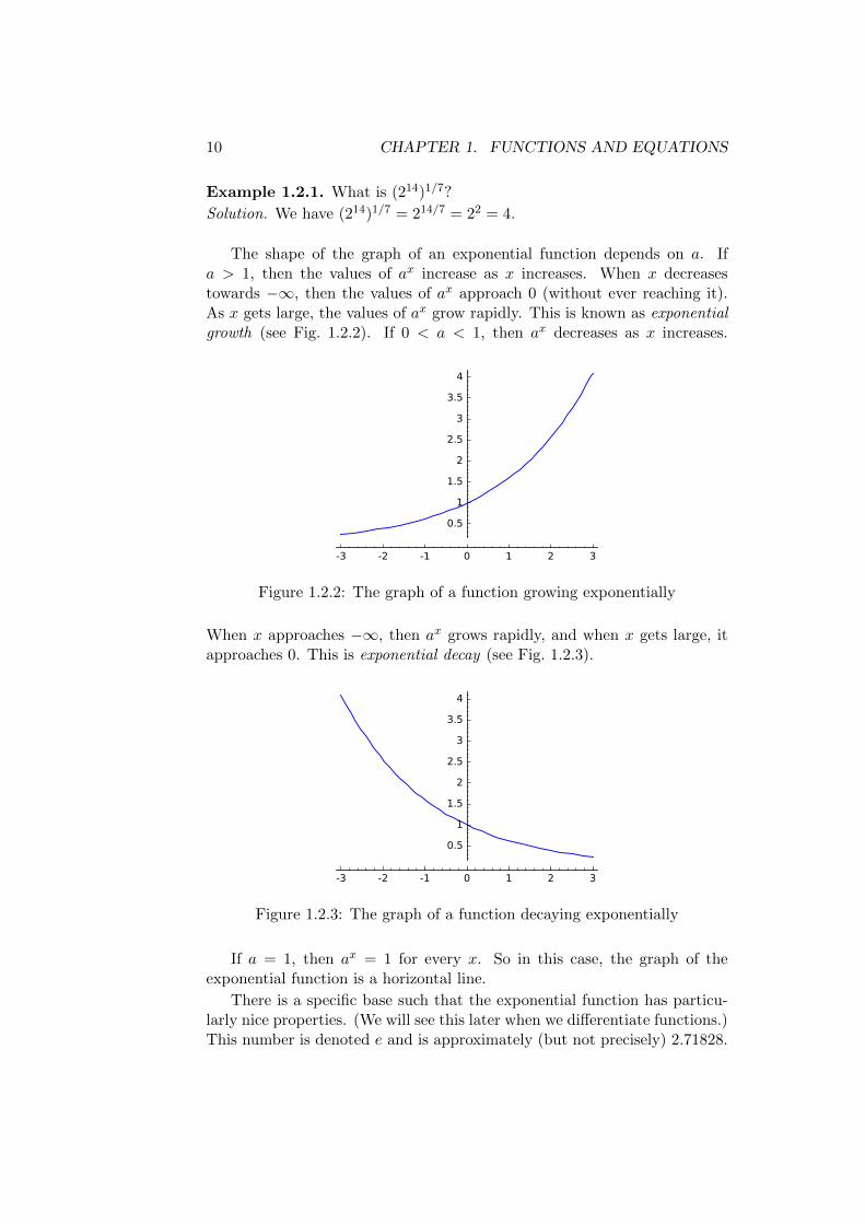
The shape of the graph of an exponential function depends on a. Ifa > 1, then the values of ax increase as x increases. When x decreasestowards −∞, then the values of ax approach 0 (without ever reaching it).As x gets large, the values of ax grow rapidly. This is known as exponentialgrowth (see Fig. 1.2.2). If 0 < a < 1, then ax decreases as x increases.
Figure 1.2.2: The graph of a function growing exponentially
When x approaches −∞, then ax grows rapidly, and when x gets large, itapproaches 0. This is exponential decay (see Fig. 1.2.3).
Figure 1.2.3: The graph of a function decaying exponentially
If a = 1, then ax = 1 for every x. So in this case, the graph of theexponential function is a horizontal line.
There is a specific base such that the exponential function has particu-larly nice properties. (We will see this later when we differentiate functions.)This number is denoted e and is approximately (but not precisely) 2.71828.

1.2. SPECIAL FUNCTIONS 11
1.2.3 Logarithms
Suppose that we fix a number y > 0 and we want to solve the equation
y = ax. (1.2.3)
Geometrically, this means finding the intersection points of the graph of theexponential function with a horizontal line at height y. If a 6= 1, then inview of the above observations, it is clear that there exists a unique solution.In other words, given y > 0, there exists a unique number x satisfying theequation y = ax. This number is called the logarithm of y to the base a. Weuse the notation
x = loga y (1.2.4)
for this concept.
Since the number x from (1.2.4) solves equation (1.2.3), we have
y = aloga y
for every y > 0. Moreover, for any x, if we substitute ax for y in (1.2.3),then the equation is clearly satisfied. Therefore, we have
loga ax = x.
So we can think of loga as the function that does the reverse of the exponen-tial function with the same base. We say that they are inverse functions.
Example 1.2.2. Find log5 125.
Solution. We calculate that 53 = 125. So log5 125 = 3.
When we work with the base e, then we write ln for the correspondinglogarithm. That is, we abbreviate lnx = loge x. (But in some books youmay find different conventions.)
Now recall formula (1.2.1). If we choose two numbers x and y and setu = ax, v = ay, and w = ax+y, then we can write the equation as uv = w.But we also have x = loga u, y = loga v, and x+ y = logaw = loga(uv). So
loga(uv) = loga u+ loga v.
This formula is true for all positive numbers u, v > 0. (Recall the thelogarithm only exists for positive numbers.)
How does equation (1.2.2) translate to the language of logarithms? Givenx and y, set b = ax and z = by. Then y = logb z and x = loga b. Moreover,equation (1.2.2) says that z = axy. So loga z = xy. It follows that
loga z = loga b · logb z.

12 CHAPTER 1. FUNCTIONS AND EQUATIONS
This formula is particularly useful when you want to convert logarithms forone base into logarithms for another, because it means that
logb z =loga z
loga b
for all z > 0.Another consequence of (1.2.2) is the following. Suppose that a > 0 and
b > 0. Then for any number x, we have
ax loga b =(aloga b
)x= bx.
Therefore,loga b
x = x loga b.
This fact is useful when we want to solve equations where the unknown isin the exponent.
Example 1.2.3. Solve the equation e7x+2 = 13 for x.Solution. The equation implies that 7x + 2 = ln 13. This is now easy tosolve for x and we obtain
x =1
7(ln 13− 2).
Example 1.2.4. Solve the equation log2(x2 − 4) = 4 for x.
Solution. The equation implies that x2 − 4 = 24 = 16. Hence x2 = 20 andso x = ±
√20 = ±2
√5.
Example 1.2.5. Solve the equation 2x2
= 3x for x.Solution. Apply ln on both sides:
x2 ln 2 = x ln 3.
This is equivalent to x2 ln 2−x ln 3 = 0, and we can factorise x(x ln 2−ln 3) =0. We have either x = 0 or x ln 2 − ln 3 = 0, and in the second case, weobtain
x =ln 3
ln 2= log2 3.
(Remark: we could have used logarithms for any base here and would haveobtained the same result.)
1.2.4 Trigonometric functions
The following definition of the sine and cosine may seem a bit odd at first,but bear with me.
Imagine a circle of radius 1 in the plane, the centre of which has thecoordinates (0, 0). (Henceforth we will call this the unit circle.) So the
1.2. SPECIAL FUNCTIONS 13
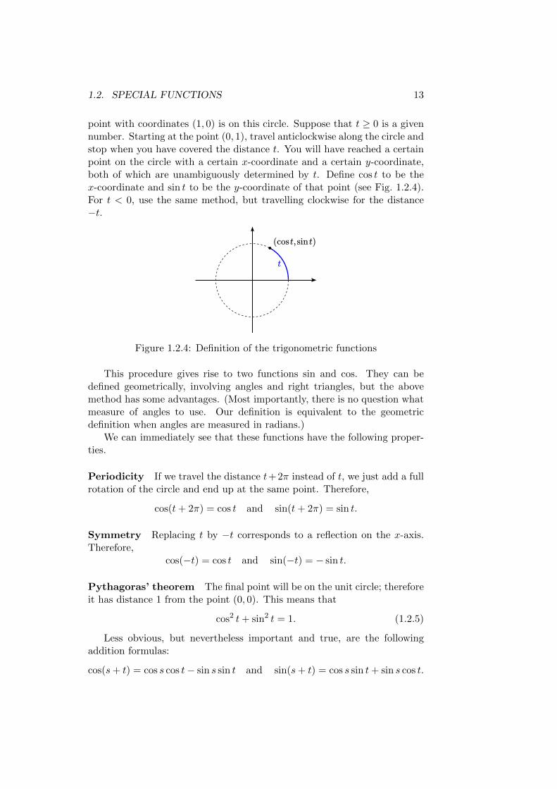
point with coordinates (1, 0) is on this circle. Suppose that t ≥ 0 is a givennumber. Starting at the point (0, 1), travel anticlockwise along the circle andstop when you have covered the distance t. You will have reached a certainpoint on the circle with a certain x-coordinate and a certain y-coordinate,both of which are unambiguously determined by t. Define cos t to be thex-coordinate and sin t to be the y-coordinate of that point (see Fig. 1.2.4).For t < 0, use the same method, but travelling clockwise for the distance−t.
(cost,sint)
t
Figure 1.2.4: Definition of the trigonometric functions
This procedure gives rise to two functions sin and cos. They can bedefined geometrically, involving angles and right triangles, but the abovemethod has some advantages. (Most importantly, there is no question whatmeasure of angles to use. Our definition is equivalent to the geometricdefinition when angles are measured in radians.)
We can immediately see that these functions have the following proper-ties.
Periodicity If we travel the distance t+2π instead of t, we just add a fullrotation of the circle and end up at the same point. Therefore,
cos(t+ 2π) = cos t and sin(t+ 2π) = sin t.
Symmetry Replacing t by −t corresponds to a reflection on the x-axis.Therefore,
cos(−t) = cos t and sin(−t) = − sin t.
Pythagoras’ theorem The final point will be on the unit circle; thereforeit has distance 1 from the point (0, 0). This means that
cos2 t+ sin2 t = 1. (1.2.5)
Less obvious, but nevertheless important and true, are the followingaddition formulas:
cos(s+ t) = cos s cos t− sin s sin t and sin(s+ t) = cos s sin t+ sin s cos t.

14 CHAPTER 1. FUNCTIONS AND EQUATIONS
Once we have the sine and cosine, we can also define a number of othertrigonometric functions:
tan t =sin t
cos t, cot t =
cos t
sin t, sec t =
1
cos t, csc t =
1
sin t.
These are not defined for all values of t, because we always have to avoid avanishing denominator. (The functions cos and sin, in contrast, are definedfor all values.) Most of these we will rarely use explicitly, because we can,after all, write them as a fraction involving the sine and cosine.
1.2.5 Inverse trigonometric functions
Given a fixed number y, suppose that we want to solve the equation
sinx = y
for x. Geometrically, this amounts to the following question: how far do weneed to travel along the unit circle in order to reach a point with a giveny-coordinate? If there is a solution at all, there are always several answers(in fact infinitely many), because we can always decide to add a full turn ofthe circle and we will get back to the same point.
Example 1.2.6. Solve the equation
sin t =1
2.
Solution. Consider the intersection of the unit circle with the horizontalline y = 1
2 (see Fig. 1.2.5). There are two intersection points. In order to
Figure 1.2.5: The unit circle and the line with y = 12
reach the first, we travel the distance π/6. So t = π/6 is one solution. Butt = 5π/6 is another solution, corresponding to the second intersection point.Moreover, we can add arbitrary multiples (positive or negative) of 2π. Soevery number of the form t = π/6 + 2πn or t = 5π/6 + 2πn, for any integern, is a solution.
1.2. SPECIAL FUNCTIONS 15
Example 1.2.7. Solve the equation
cos t =1
2.
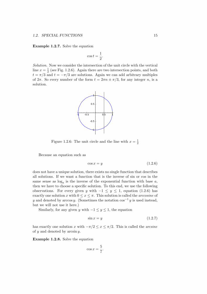
Solution. Now we consider the intersection of the unit circle with the verticalline x = 1
2 (see Fig. 1.2.6). Again there are two intersection points, and botht = π/3 and t = −π/3 are solutions. Again we can add arbitrary multiplesof 2π. So every number of the form t = 2πn ± π/3, for any integer n, is asolution.
Figure 1.2.6: The unit circle and the line with x = 12
Because an equation such as
cosx = y (1.2.6)
does not have a unique solution, there exists no single function that describesall solutions. If we want a function that is the inverse of sin or cos in thesame sense as loga is the inverse of the exponential function with base a,then we have to choose a specific solution. To this end, we use the followingobservations. For every given y with −1 ≤ y ≤ 1, equation (1.2.6) hasexactly one solution x with 0 ≤ x ≤ π. This solution is called the arccosine ofy and denoted by arccos y. (Sometimes the notation cos−1 y is used instead,but we will not use it here.)
Similarly, for any given y with −1 ≤ y ≤ 1, the equation
sinx = y (1.2.7)
has exactly one solution x with −π/2 ≤ x ≤ π/2. This is called the arcsineof y and denoted by arcsin y.
Example 1.2.8. Solve the equation
cosx =5
7.

16 CHAPTER 1. FUNCTIONS AND EQUATIONS
Solution. By definition, the number arccos 57 is one solution. But it is not
the only one. By the symmetry and the periodicity, any number of the form2πn± arccos 5
7 , for any integer n, is a solution.
Note that for y > 1 or y < −1, equations (1.2.6) and (1.2.7) have nosolutions. So there is no arccosine or arcsine of such a number.
Now consider the function tan. For any number y, the equation
tanx = y
has infinitely many solutions, but exactly one of them satisfies −π/2 < x <π/2. This solution is called the arctangent of y and denoted arctan y.
1.2.6 Hyperbolic functions
The hyperbolic sine, denoted sinh, and the hyperbolic cosine, denoted cosh,are the functions defined by the formulas
sinhx =1
2(ex − e−x),
coshx =1
2(ex + e−x).
The reason for these names is that the behaviour of these functions resemblesthat of the sine and cosine in some respects. One example is the identity
cosh2 x− sinh2 x = 1,
which should be compared with (1.2.5). The identity can easily be checkedby inserting the above expressions. We will see other similarities later.
In addition to these, we can now define other hyperbolic functions anal-ogously to the trigonometric functions:
tanhx =sinhx
coshx, cothx =
coshx
sinhx, sechx =
1
coshx, cschx =
1
sinhx.
1.3 Applications of trigonometric functions
1.3.1 Polar coordinates
Instead of representing a point P in the plane by its Cartesian coordinates(x, y), it is sometimes convenient to use polar coordinates. In order tofind the polar coordinates, assume that P is not the origin O (the pointwith Cartesian coordinates (0, 0)). Draw a circle centred at O through P .Denote the radius of this circle by r. (This is the distance between O andP .) Moreover, denote the length of the arc between the points (0, r) and P ,travelling anticlockwise, by s (see Fig. 1.3.1). The numbers r and t = s/rdetermine the position of P uniquely, and (r, t) are the polar coordinates

1.3. APPLICATIONS OF TRIGONOMETRIC FUNCTIONS 17
P
s
O
r
Figure 1.3.1: Construction of polar coordinates (r, t) of the point P
of P . We usually insist that t satisfies 0 ≤ t < 2π, and then the polarcoordinates are determined uniquely by P as well, unless P = O. Given thepolar coordinates (r, t), it is easy to determine the Cartesian coordinates ofthe same point:
x = r cos t, (1.3.1)
y = r sin t. (1.3.2)
The converse is a bit more complicated. Given the Cartesian coordinates(x, y), we have r =
√x2 + y2 by Pythagoras’ theorem. In order to find t, we
want to solve the system of equations (1.3.1), (1.3.2) for t. We first eliminater by taking a quotient:
y
x=
sin t
cos t= tan t
(provided that x 6= 0). So in order to solve for t, we take the arctangent,
t = arctany
x,
provided that we expect −π/2 < t < π/2. This is the case if P is in the firstquadrant, i.e., if x > 0 and y ≥ 0. Otherwise, however, this gives the wronganswer! (That’s because solutions of this equation are not unique and we’vemade a choice when defining the arctangent.) The true answer is
t =
arctan yx if x > 0 and y ≥ 0,
arctan yx + π if x < 0,
arctan yx + 2π if x > 0 and y < 0,
π2 if x = 0 and y > 0,3π2 if x = 0 and y < 0.
This covers all cases except x = y = 0, where we do not have polar coordi-nates. In practice, rather than remembering all of these cases, it is usuallymore convenient to draw a picture and find out what range to expect for t.
18 CHAPTER 1. FUNCTIONS AND EQUATIONS
Example 1.3.1. Find the Cartesian coordinates of the point with polarcoordinates (3, π/3).Solution. This is
x = 3 cosπ
3=
3
2,
y = 3 sinπ
3=
3√
3
2.
Example 1.3.2. Find the polar coordinates of the point with Cartesiancoordinates (3,−4).Solution. We have r =
√9 + 16 = 5. The point is in the fourth quadrant,
so we expect that 3π/2 < t < 2π. As we have
−π/2 < arctan−4
3< 0,
we should add 2π. So
t = arctan−4
3+ 2π = 2π − arctan
4
3.
1.3.2 Solving trigonometric equations
Suppose that you want to solve the equation
3 cos t+ 2 sin t = 2.
Should we use the arcsine or the arccosine here, or something else?More generally, suppose that A,B,C are three given numbers and we
want to solveA cos t+B sin t = C. (1.3.3)
The idea is to use the addition formulas for the sine and cosine. Try to findr and θ such that
A cos t+B sin t = r cos(t+ θ).
By the addition formula, this works if
A = r cos θ and B = −r sin θ.
But this means that (r, θ) are the polar coordinates of the point with Eu-clidean coordinates (A,−B). We know how to solve for r and θ by theprevious section, even if it can be a bit complicated. Having done that, wehave the equation
r cos(t+ θ) = C.
This is called the harmonic form of equation (1.3.3).We can now solve it. Dividing by r, we obtain cos(t+ θ) = C/r. Hence
t+ θ = ± arccos(C/r) + 2πn for some integer n, and
t = ± arccos(C/r) + 2πn− θ.

1.3. APPLICATIONS OF TRIGONOMETRIC FUNCTIONS 19
Example 1.3.3. Solve the equation
3 cos t+ 4 sin t = 4.
Solution. We first need to find the polar coordinates of the point (3,−4),which we have done in Example 1.3.2: we have r = 5 and θ = π − arctan 4
3 .Thus the equation becomes
cos
(t+ π − arctan
4
3
)=
4
5.
So the solutions are of the form
t = ± arccos4
5+ arctan
4
3− π + 2πn
for any integer n.
The above equation is still fairly simple. In general, when you need tosolve an equation involving trigonometric functions, you need to keep thetrigonometric identities from section 1.2.4 in mind, because they often allowyou to simplify the equation. Also remember that you can in general expectmany solutions.
Example 1.3.4. Solve the equation
cos2 x− 3 cosx+ 2 = 0.
Solution. Substitute u = cosx to obtain the equation
u2 − 3u+ 2 = 0.
This equation we can solve, using the factorisation u2−3u+2 = (u−2)(u−1).So u = 2 or u = 1. There is no number x such that cosx = 2, so we can ruleout one of the solutions. This leaves u = 1 and therefore cosx = 1. Thesolutions of this equation are of the form x = 2πn for an integer n.
Example 1.3.5. Solve the equation
3− sin2 x− 3 cosx = 0.
Solution. Using the identity cos2 x + sin2 x = 1, we can reformulate theequation as follows:
cos2 x− 3 cosx+ 2 = 0.
This is the equation from the previous example and we obtain the samesolutions.
20 CHAPTER 1. FUNCTIONS AND EQUATIONS
Example 1.3.6. Solve the equation
cos(2x)− 2 sinx = 1.
Solution. We first use the addition formula and the formula from Pythago-ras’ theorem to rewrite
cos(2x) = cos2 x− sin2 x = 1− 2 sin2 x.
Hence the equation becomes
1− 2 sin2 x− 2 sinx = 1,
which is equivalent tosin2 x+ sinx = 0.
The substitution u = sinx yields 0 = u2 + u = u(u + 1). So u = 0 oru = −1. If u = 0, then sinx = 0, so x = nπ for an integer n. If u = −1,then sinx = −1, so x = mπ − π
2 for an integer m. All of these are solutionsof the equation.
1.4 Limits
Sometimes a quantity approaches a certain value without necessarily everreaching it. For example, consider a radioactive material with half-life T .That means after time T , the quantity of the material is reduced by halfthrough radioactive decay. After time 2T , there is a quarter of the originalquantity left, after 3T an eighth, and so on. We may prescribe any acceptablelevel, and as long as it is positive and we are willing to wait long enough, theremaining quantity will eventually be below. In particular, it approaches 0as the time tends to ∞.
More generally, consider a function f of the independent variable x. Ifthere exists a number L such that f(x) approaches L as x tends to∞, in thesense that the distance between f(x) and L will eventually remain smallerthan any prescribed positive error level,2 then we say that L is the limit off(x) as x→∞. In symbols, we express this as follows:
L = limx→∞
f(x).
Sometimes, we also write f(x)→ L as x→∞.
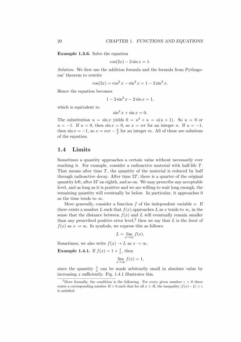
Example 1.4.1. If f(x) = 1 + 1x , then
limx→∞
f(x) = 1,
since the quantity 1x can be made arbitrarily small in absolute value by
increasing x sufficiently. Fig. 1.4.1 illustrates this.
2More formally, the condition is the following. For every given number ε > 0 thereexists a corresponding number R > 0 such that for all x > R, the inequality |f(x)−L| < εis satisfied.

1.4. LIMITS 21
Figure 1.4.1: The graph of the function f with f(x) = 1 + 1x
We have limits not just for x→∞. The expression
limx→−∞
f(x),
if it exists, is defined similarly, considering values of x that are large in mag-nitude but negative. Furthermore, we can define limits when x approachesa finite number.
Suppose that a and L are numbers such that f(x) approaches L as xapproaches a, in the sense that the distance between f(x) and L shrinksbelow any prescribed positive error level as soon as x is sufficiently close toa.3 Then we say that L is the limit of f(x) as x→ a and we write
L = limx→a
f(x).
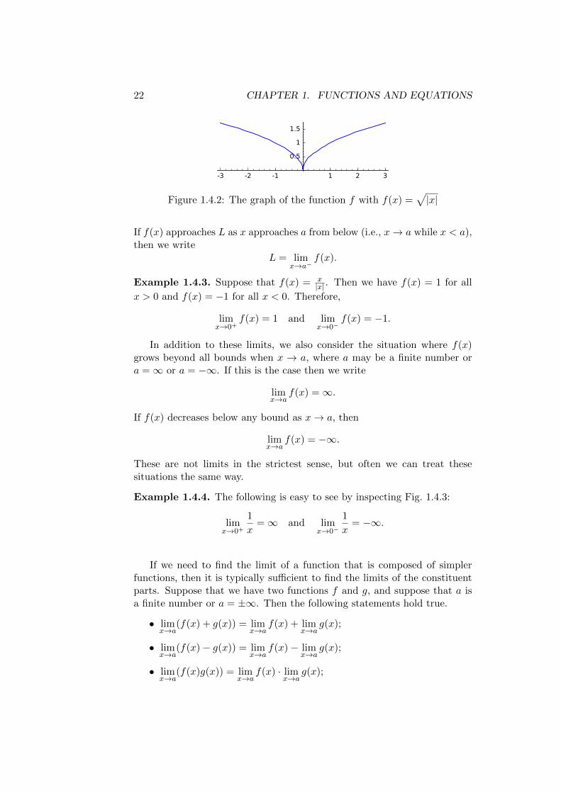
Example 1.4.2. Consider the function f given by f(x) =√|x| (see Fig.
1.4.2). Since the distance between f(x) and 0 is always√|x|, which becomes
arbitrarily small when |x| is small enough, we have
limx→0
f(x) = 0.
Note that when we determine limx→a f(x), then the value f(a) is irrele-vant. It need not even be defined.
Sometimes we take one-sided limits. If f(x) approaches L as x ap-proaches a from above, meaning that x → a but at the same time x > a,then we write
L = limx→a+
f(x).
3For any given ε > 0 there exists h > 0 such that for all x with 0 < |x − a| < h, theinequality |f(x)− L| < ε is satisfied.
22 CHAPTER 1. FUNCTIONS AND EQUATIONS
Figure 1.4.2: The graph of the function f with f(x) =√|x|
If f(x) approaches L as x approaches a from below (i.e., x→ a while x < a),then we write
L = limx→a−
f(x).
Example 1.4.3. Suppose that f(x) = x|x| . Then we have f(x) = 1 for all
x > 0 and f(x) = −1 for all x < 0. Therefore,
limx→0+
f(x) = 1 and limx→0−
f(x) = −1.
In addition to these limits, we also consider the situation where f(x)grows beyond all bounds when x → a, where a may be a finite number ora =∞ or a = −∞. If this is the case then we write
limx→a
f(x) =∞.
If f(x) decreases below any bound as x→ a, then
limx→a
f(x) = −∞.
These are not limits in the strictest sense, but often we can treat thesesituations the same way.
Example 1.4.4. The following is easy to see by inspecting Fig. 1.4.3:
limx→0+
1
x=∞ and lim
x→0−
1
x= −∞.
If we need to find the limit of a function that is composed of simplerfunctions, then it is typically sufficient to find the limits of the constituentparts. Suppose that we have two functions f and g, and suppose that a isa finite number or a = ±∞. Then the following statements hold true.
• limx→a
(f(x) + g(x)) = limx→a
f(x) + limx→a
g(x);
• limx→a
(f(x)− g(x)) = limx→a
f(x)− limx→a
g(x);
• limx→a
(f(x)g(x)) = limx→a
f(x) · limx→a
g(x);

1.4. LIMITS 23
Figure 1.4.3: The graph of the function f with f(x) = 1x
• if limx→a g(x) 6= 0, then limx→a
f(x)
g(x)=
limx→a f(x)
limx→a g(x).
This applies when we have actual limits, but in most cases also for ∞ and−∞, provided that we interpret the resulting expressions correctly. Forexample, we use the convention that L+∞ = ∞ and L
∞ = 0 for any finitenumber L. In some cases, however, we have to be more careful. There isno natural way to interpret expressions such as ∞−∞ or ∞∞ , and if theyappear, then these rules do not help. (But in the second case, another rule,which we will discuss in Sect. 2.4.2, often helps.)
The same rules apply to one-sided limits.
Example 1.4.5. We know that limx→∞1x = 0. Therefore,
limx→∞
1
x2= lim
x→∞
1
x· limx→∞
1
x= 0
Example 1.4.6. Find
limx→∞
x2 − x+ 3
2x2 − 7.
Solution. We have
limx→∞
x2 − x+ 3
2x2 − 7= lim
x→∞
1− 1x + 3
x2
2− 7x2
=1− limx→∞
1x + 3 lim 1
x2
2− 7 limx→∞1x2
=1
2.
There is also a rule for limits of the form limx→a f(g(x)), where f andg are two given functions, but this requires some conditions on f that weneed to discuss first.
A function is called continuous if a small change of the independentvariable will result only in a small change of the dependent variable. Geo-metrically this means that the graph of the function has no gaps. Nearly allof the functions discussed so far are continuous.

24 CHAPTER 1. FUNCTIONS AND EQUATIONS
Now suppose that f is a continuous function and g is any function suchthat limx→a g(x) exists, where again, a is a finite number or ±∞. Then
limx→a
f(g(x)) = f(
limx→a
g(x)).
Again, the rule applies to one-sided limits as well.
Example 1.4.7. For any base b > 0, the exponential function given byy = bx is continuous. Hence
limx→∞
b1/x = blimx→∞ 1/x = b0 = 1.
1.5 The bisection method
So far we have only seen examples of equations that we were able to solveexactly. This is only because the examples were chosen to demonstratecertain solution methods. For even moderately complicated equations, itis rare that we can solve them exactly and we normally have to make dowith a numerical approximation. But often we can say with certainty thata suitably constructed number is in fact a good approximation of an actualsolution, and even give a bound for the error.
The following is a simple scheme to find approximate solutions and errorbounds. There are more efficient methods (in terms of required computationtime), but what makes this one useful, especially for theoretical purposes,is that it gives you a high degree of certainty. The method works for allcontinuous functions.
The basis of the bisection method is the intermediate value theorem,which states the following. Suppose that f is a continuous function and y afixed number. Furthermore, suppose that a, b are two numbers with a < b,such that f(a) and f(b) are on different sides of y. That is, either
• f(a) < y and f(b) > y, or
• f(a) > y and f(b) < y.
Then there exists a number c between a and b (that is, with a < c < b) suchthat f(c) = y.
This is a useful statement because it tells us that in certain circum-stances, there is definitely a solution of the equation f(x) = y in the interval(a, b). The bisection method now works as follows.
Step 1 Find two numbers a0 and b0 with a0 < b0 such that either f(a0) <y < f(b0) or f(a0) > y > f(b0). (So a solution of the equation f(x) = y isguaranteed between a0 and b0.)
1.5. THE BISECTION METHOD 25
Step 2 Define the number c0 = 12(a0 + b0).
• If f(c0) = y, then we have found an exact solution.
• If f(a0) < y < f(c0) or f(a0) > y > f(c0), then define a1 = a0 andb1 = c0.
• If f(c0) < y < f(b0) or f(c0) > y > f(b0), then define a1 = c0 andb1 = b0.
Step 3 If b1 − a1 is smaller than a tolerable error bound, use any numberin the interval (a1, b1) as an approximate solution. Otherwise, go back toStep 2 and repeat with a1 and b1 instead of a0 and b0.
Example 1.5.1. Find an approximate solution of the equation
lnx = 2
with error smaller than 14 .
Solution. We compute ln 7 = 1.945910149 and ln 8 = 2.079441542. Sothere is a solutions somewhere between 7 and 8. Next we compute ln 7.5 =2.014903021. So the solution must be in the interval (7, 7.5). As ln 7.25 =1.981001469, it’s in fact in the interval (7.25, 7.5). We may use as an ap-proximate solution:
x ≈ 7.375.
26 CHAPTER 1. FUNCTIONS AND EQUATIONS

Chapter 2
Differentiation
2.1 Fundamentals
2.1.1 Definition
Consider the graph of a function f . For a given number x, we have a pointwith coordinates (x, f(x)) on the graph. If this graph is a sufficiently nicecurve, then there is a unique tangent line at this point. The slope of thetangent line is called the derivative of f at x and denoted by f ′(x). (Differentnotation for the same thing will be discussed later.)
Since a tangent line can be a tricky thing to work with, we also considersecant lines. These are lines passing through two points of the graph (seeFig. 2.1.1). More specifically, suppose that h is a number different from 0.
Figure 2.1.1: Two secant lines (green) and a tangent line (red)
Then (x + h, f(x + h)) is another point on the graph, and the two pointsdetermine a unique secant line, the slope of which is
f(x+ h)− f(x)
h.
This is called a difference quotient . Assuming that f is nice enough topossess a derivative at x, this expression will approach f ′(x) when h tends
27

28 CHAPTER 2. DIFFERENTIATION
to 0. That is,
f ′(x) = limh→0
f(x+ h)− f(x)
h.
Example 2.1.1. Consider the function defined by f(x) = x2. We havef(x+ h) = x2 + 2hx+ h2, so
f(x+ h)− f(x)
h= 2x+ h.
When h approaches 0, the last term is small, so the difference quotient willtend to 2x. So f ′(x) = 2x.
Not every function has a derivative at every point. For example, considerthe function with f(x) = |x|. The graph has a corner at (0, 0). The secantlines through (0, 0) and (h, |h|) have slope 1 if h > 0 and slope −1 if h < 0.There is no number that is approached by both of these, and there is notangent line to the graph at (0, 0). In other words, this function does nothave a derivative at 0.
2.1.2 Notation
Several conventions for the notation of the derivative are in use. Among themost common ways to write the object defined above are:
f ′, f , anddf
dx.
These have different historical origins and have been introduced by La-grange, Newton, and Leibniz, respectively. The first one is the most commonin theoretical treatments of the derivative. The notation f is common inscience, especially if a function of time is studied. Leibniz’s notation is con-venient for certain computations. It is no coincidence that it resembles aquotient; in fact, it reminds us that the derivative is computed through ap-proximations by difference quotients as in section 2.1.1. Nevertheless, whenusing this notation, it is worth keeping in mind that the quotient structureof the expression df
dx is merely symbolic. It does not represent an actualquotient, but rather a limit of difference quotients.
Sometimes the derivative of a function is differentiated again. The result
is the second derivative, which is denoted by f ′′, f , or d2fdx2
. Similarly, thethird derivative is the derivative of the second derivative and denoted f ′′′ or...f or d3f
dx3. For even higher derivatives, the first two types of notation become
too cumbersome and we write f (n) or dnfdxn for the n-th derivative.
2.1.3 Derivatives of a few simple functions
As we have seen in Sect. 2.1.1, we can compute a derivative by consideringdifference quotients. We don’t need to do this for all functions, however,
2.1. FUNDAMENTALS 29
because once we know the derivatives of certain functions, we can figure outthe derivatives of other functions composed from these by simple rules.
First we consider the simplest functions of all. For a fixed number a, letf be the constant function with f(x) = a for all x. Then for h 6= 0, we have
f(x+ h)− f(x)
h=a− ah
= 0. (2.1.1)
So f ′(x) = 0. In other words, a constant function has the derivative 0.We have already seen the derivative of the function with f(x) = x2. But
more fundamental is the function f given by f(x) = x. For h 6= 0, we have
f(x+ h)− f(x)
h=x+ h− x
h=h
h= 1.
Hence for this function, we have f ′(x) = 1. Every polynomial can be com-posed from this function and constants. We will see later how this helps todetermine the derivative of any polynomial.
Now consider exponential functions. Let a > 0 and suppose that thefunction f is defined by f(x) = ax. Then for h 6= 0, we have
f(x+ h)− f(x)
h=ax+h − ax
h=axah − ax
h= ax
ah − 1
h= ax
f(h)− 1
h.
This does not immediately tell us what the derivative is, but it does give ussome information about it. Note that the expression
f(h)− 1
h
is the difference quotient of f at 0. So while the left-hand side will approachf ′(x) when h approaches 0, the right-hand side will approach axf ′(0). Thatis, we have f ′(x) = axf ′(0). Here f ′(0) is just a constant, albeit for themoment an unknown one. Writing for convenience C = f ′(0), we have
f ′(x) = Cf(x).
In other words, the derivative of an exponential function coincides with thefunction up to a constant. For the base e, that constant is 1. So
d
dxex = ex.
Now consider the trigonometric function sin. For h 6= 0, we use theaddition formula to compute
sin(x+ h)− sinx
h=
sinx cosh+ cosx sinh− sinx
h
= sinxcosh− 1
h+ cosx
sinh
h.

30 CHAPTER 2. DIFFERENTIATION
It can be shown that cosh−1h approaches 0 and sinh
h approaches 1 as h tendsto 0. Therefore, we have
d
dxsinx = cosx.
Similarly, we compute
cos(x+ h)− cosx
h=
cosx cosh− sinx sinh− cosx
h
= cosxcosh− 1
h− sinx
sinh
h.
Henced
dxcosx = − sinx.
Other trigonometric functions can be composed from the sine and the cosine,and we will find their derivatives later.
2.2 Differentiation rules
In this section, we will see how to differentiate a an expression composedfrom simpler functions.
2.2.1 The sum rule
Our first rule, the sum rule, is very simple: the derivative of a sum is thesum of the derivatives of the summands. In other words, if f and g aretwo functions and a third function h is given by h(x) = f(x) + g(x), thenh′(x) = f ′(x) + g′(x). The rule may also be expressed by the formula
(f + g)′(x) = f ′(x) + g′(x)
ord
dx(f + g) =
df
dx+dg
dx.
Example 2.2.1. Find the derivative of the function f with f(x) = x2 + x.Solution. We know that d
dxx2 = 2x and d
dxx = 1, so
d
dx(x2 + x) = 2x+ 1.
2.2.2 The product rule
The product rule, as the name suggests, is about products of functions. (Itis not as simple as the sum rule, and the false analogy with the latter is asource of many mistakes.) For two given functions f and g, the rule is
(fg)′(x) = f ′(x)g(x) + f(x)g′(x),

2.2. DIFFERENTIATION RULES 31
or, in different notation,
d
dx(fg) =
df
dxg + f
dg
dx.
Why do we have this expression? Let’s look at the difference quotients.For h 6= 0, we have
f(x+ h)g(x+ h)− f(x)g(x)
h
=f(x+ h)g(x+ h)− f(x)g(x+ h) + f(x)g(x+ h)− f(x)g(x)
h
=f(x+ h)− f(x)
hg(x+ h) + f(x)
g(x+ h)− g(x)
h.
Keeping in mind that the difference quotients will tend to the correspondingderivatives, and observing that g(x + h) will approach g(x) when we let happroach 0, we conclude that the above formula holds true.
As an application, we can now compute the value of ddxx
2 from ddxx,
rather than deriving it from first principles. As x2 = x · x, we have
d
dxx2 = 1 · x+ x · 1 = 2x.
Similarly, we have
d
dxx3 =
d
dx(x · x2) = 1 · x2 + x · 2x = 3x2.
More generally, for any positive integer n, we obtain
d
dxxn = nxn−1.
(The formula is actually true not just for positive integers, but it’s easiestto see in this case.)
Example 2.2.2. Differentiate x2 sinx.Solution. By the product rule,
d
dx(x2 sinx) = 2x sinx+ x2 cosx.
2.2.3 The quotient rule
For the derivative of a quotient, we have the formula(f
g
)′(x) =
f ′(x)g(x)− f(x)g′(x)
(g(x))2;
that is,
d
dx(f/g) =
dfdxg − f
dgdx
g2.
32 CHAPTER 2. DIFFERENTIATION
Example 2.2.3. Find the derivative of the function tan.Solution. We know that tanx = sinx
cosx . Hence
d
dxtanx =
d
dx
(sinx
cosx
)=
cos2 x+ sin2 x
cos2 x= 1 + tan2 x.
By Pythagoras’ theorem, we have cos2 x + sin2 x = 1. Hence we have thealternative representation
d
dxtanx =
1
cos2 x.
Example 2.2.4. Differentiate ex
x .Solution. By the quotient rule,
d
dx
(ex
x
)=xex − ex
x2=x− 1
x2ex.
2.2.4 The chain rule
This rule is about the composition of functions in the sense of using theoutput of one function as the input of another. Suppose that we have twofunctions f and g. Then we can define another function h with h(x) =f(g(x)). Then we have
h′(x) = f ′(g(x))g′(x).
This can be expressed very conveniently with Leibniz’s notation. For thispurpose, we write u = g(x) and y = f(u) = h(x). Then
dy
dx=dy
du
du
dx.
Written like this, the formula looks obvious. (But remember that these arenot actual fractions. This may look like the reduction of a fraction, but it’sreally something more complicated.)
The chain rule can be extended to chains of more than two functions.For example, in the case of three functions, we have
dy
dx=dy
dv
dv
du
du
dx.
This is a convenient form to write it in, but it suppresses some information.In particular, it’s not immediately clear in which way these quantities dependon each other, and this can lead to some confusion. To make everything moreexplicit: we have three functions here, say f , g, and h, and the compositioni with i(x) = f(g(h(x))). We write u = h(x), v = g(u) = g(h(x)), andy = f(v) = f(g(h(x))). The formula can also be written as follows:
i′(x) = f ′(g(h(x)))g′(h(x))h′(x).
2.3. FURTHER DIFFERENTIATION TECHNIQUES 33
Example 2.2.5. Given a constant c, differentiate ecx.
Solution. This is the composition of the exponential function (with base e)and the function f with f(x) = cx, the derivative of which is f ′(x) = c. So
d
dxecx =
d
dxef(x) = ef(x)f ′(x) = cecx.
(In Leibniz notation, write u = cx and y = eu. Then
d
dxecx =
dy
dx=dy
du
du
dx= eu · c = cecx.)
Using this example, we may now also give a more explicit expression forthe derivatives of exponential functions. Let a > 0 and consider ax. Recallthat
ax = ex ln a.
Thus setting c = ln a in Example 2.2.5, we find
d
dxax = ex ln a ln a = ax ln a.
Example 2.2.6. Differentiate cos2 x.
Solution. Set u = cosx and y = u2. Then
d
dxcos2 x =
dy
dx=dy
du
du
dx= 2u(− sinx) = −2x sinx cosx.
Example 2.2.7. Differentiate cos(x2).
Solution. Set u = x2 and y = cosu. Then
d
dxcos(x2) =
dy
du
du
dx= − sinu · 2x = −2x sin(x2).
Example 2.2.8. Differentiate esin3 x.
Solution. Writing u = sinx, v = u3, and y = ev, we find
d
dxesin
3 x =dy
dx=dy
dv
dv
du
du
dx= ev · 3u2 · cosx = 3esin
3 x sin2 x cosx.
2.3 Further differentiation techniques
In this section we discuss how to find the slope of a curve that is not neces-sarily given by a simple expression as in the previous examples or where anapplication of the rules would be too laborious.
34 CHAPTER 2. DIFFERENTIATION
2.3.1 Logarithmic differentiation
Suppose that we want to differentiate a product of many functions. Then wemay use the product rule several times, but this can become complicated.Often the following method is easier.
Let f be the product of the functions f1, f2, . . . , fn. That is,
f(x) = f1(x)f2(x) · · · fn(x).
Apply the natural logarithm to both sides of this equation. Then by therules for the logarithm,
ln f(x) = ln f1(x) + ln f2(x) + · · ·+ ln fn(x).
Now we can use the sum rule rather than the product rule. Differentiatingwith the help of the chain rule, we obtain
f ′(x)
f(x)=f ′1(x)
f1(x)+f ′2(x)
f2(x)+ · · ·+ f ′n(x)
fn(x).
Therefore,
f ′(x) = f1(x) · · · fn(x)
(f ′1(x)
f1(x)+ · · ·+ f ′n(x)
fn(x)
).
Example 2.3.1. Differentiate the expression y =√xex cosx coshx.
Solution. Using logarithmic differentiation, we find
dy
dx=√xex cosx coshx
(1
2√x ·√x
+ex
ex+− sinx
cosx+
sinhx
coshx
)=√xex cosx coshx
(1
2x+ 1− tanx+ tanhx
).
2.3.2 Derivatives of inverse functions
We have seen some functions (namely logarithms and inverse trigonometricfunctions) that we obtain by solving an equation of the form y = f(x) for x.The resulting function is called the inverse of f and denoted by f−1. If weknow the derivatives of f , then we can easily compute the derivatives of theinverse as well by the following formula, which is most easily represented inLeibniz’s notation. Write y = f(x), so that x = f−1(y). Then
dx
dy=
1dydx
.
Written differently, that is
(f−1)′(y) =1
f ′(f−1(y)).

2.3. FURTHER DIFFERENTIATION TECHNIQUES 35
Example 2.3.2. Differentiate√y.
Solution. The root is the inverse of the function y = x2. So
d
dy
√y =
dx
dy=
1dydx
=1
2x=
1
2√y.
Note that we can write√y = y1/2, and then the result from this example
is consistent with the formula
d
dyyn = nyn−1,
which we have seen earlier, although n is no longer an integer here.We can use the above formula to find derivatives of logarithms and in-
verse trigonometric functions. For a > 0, we write y = ax, so that x = loga y.Then dy
dx = ax ln a, as we have seen earlier. Hence
d
dyloga y =
1
ax ln a=
1
y ln a.
For base e, we have the particular case
d
dyln y =
1
y.
Now suppose that y = sinx and x = arcsin y. Then
dx
dy=
1dydx
=1
cosx=
1√cos2 x
=1√
1− sin2 x=
1√1− y2
.
That is,d
dyarcsin y =
1√1− y2
.
Similarly,d
dyarccos y = − 1√
1− y2.
Finally, if we have y = tanx and x = arctan y, then dydx = 1+tan2 x = 1+y2.
Henced
dyarctan y =
1
1 + y2.
2.3.3 Parametric differentiation
Sometimes a curve in the plane is given not as the graph of a function,but rather through a parametrisation. This is a pair of functions x and ydescribing a motion along the curve as follows: if we think of the independentvariable t as time, then we reach the point with coordinates (x(t), y(t)) at

36 CHAPTER 2. DIFFERENTIATION
the time t. We have already seen an example for this: when introducing thetrigonometric functions, we considered the functions given by x(t) = cos tand y(t) = sin t. Because we think of t as time here, we denote the derivativesby x and y.
A curve like this does not necessarily correspond to the graph of a func-tion. But if it does, say if y is a function of x, then
dy
dx=y
x,
provided that these derivatives exist and x does not vanish. (Writing theright-hand side in Leibniz notation may again help you memorise this.)
Example 2.3.3. Find the slope at the point (1, 0) of the curve parametrisedby x(t) = cos t+ t and y(t) = t4 + t.Solution. We have x(t) = − sin t + 1 and y(t) = 4t3 + 1. The point (1, 0)corresponds to a time t with x(t) = 1 and y(t) = 0; that is,
cos t+ t = 1,
t4 + t = 0.
The second equation gives t(t3 + 1) = 0. We have two solutions: t = 0 andt = −1. But the second one does not satisfy the first equation. So we needto consider the time t = 0 here. Now x(0) = 1 and y(0) = 1. Therefore, theslope is
dy
dx(1) =
y(0)
x(0)= 1.
2.3.4 Implicit differentiation
Sometimes a curve is given only implicitly through an equation in x and y.For example, the equation x2+y2 = 1 describes the unit circle. While in thiscase, we can solve for y and then differentiate (namely, y = ±
√1− x2 and
dydx = ± −x√
1−x2 ) or we can parametrise as in the previous section, in general it
may be difficult to do either. Nevertheless, we can still find the slopes of thecurve by the following process, demonstrated with the example x2 + y2 = 1.
We first differentiate both sides of the equation with respect to x:
d
dx(x2 + y2) =
d
dx1.
Using the chain rule for the terms involving y (in this case only one term),we obtain
2x+ 2ydy
dx= 0.
Now we solve for dydx :
dy
dx= −x
y.

2.4. APPLICATIONS 37
(You can check easily that the result agrees with the calculations at thebeginning of this section.)
Example 2.3.4. Consider the curve implicitly given by the equation
yex + xey = 1.
The points (1, 0) and (0, 1) lie on this curve. Find the slopes at both points.
Solution. We differentiate both sides of the equation:
dy
dxex + yex + ey + xey
dy
dx= 0.
We can simplify as follows:
dy
dx(ex + xey) + yex + ey = 0.
Now we solve for dydx :
dy
dx= −ye
x + ey
ex + xey.
If we insert x = 1 and y = 0, we obtain dydx = 1
e+1 . For x = 0 and y = 1, we
obtain dydx = e+ 1.
2.4 Applications
2.4.1 Maxima and minima
Suppose that you are given a function and want to understand its behaviour.One of the most notable features of a function are its local maxima andminima, so it helps to find them.
Given a function f and a number c, we say that f has a local maximumat c if f(x) ≤ f(c) for all x in the immediate neighbourhood of c. We saythat f has a local minimum at c if f(x) ≥ f(c) for all x in the immediateneighbourhood of c.
If f has a local minimum or a local maximum at c and has a derivativeat c, then it must necessarily satisfy f ′(c) = 0. Therefore, if we look for localmaxima and local minima, then we may differentiate and solve the equation
f ′(x) = 0
for x. This, together with the set of points where the derivative does notexist, gives a set of candidates for local maxima and minima. But there maybe solutions of the equation that are neither maxima nor minima.
38 CHAPTER 2. DIFFERENTIATION
Example 2.4.1. Consider the function given by f(x) = (1−x2)2. We havef ′(x) = −4x(1 − x2) = −4x(1 − x)(1 + x). The solutions of the equationf ′(x) = 0 are x = −1, x = 0, and x = 1. Since f(x) ≥ 0 for all x (as it isa square), while f(−1) = f(1) = 0, we have local minima at −1 and 1. Wewill see later that we have a local maximum at 0.
Example 2.4.2. Consider the function given by f(x) = x3. Its derivativeis f ′(x) = 3x2, which vanishes at 0 and nowhere else. We have f(0) = 0,but this function has positive and negative values in the immediate neigh-bourhood of 0. So here we have no local minima or maxima.
Example 2.4.3. Consider the function given by f(x) = |x|. The derivativeis f ′(x) = −1 for x < 0 and f ′(x) = 1 for x > 0. At 0, the derivative doesnot exist. The function satisfies f(0) = 0 and f(x) ≥ 0 for all x. Therefore,it has a local minimum at 0.
Now that we have these candidates, how do we distinguish local maximaand local minima from each other and from all the ‘false’ candidates? Thisis not always easy, but in many cases, it helps to differentiate again.
Suppose that we have a point c where both the first and the secondderivatives exist. If f ′(c) = 0 and f ′′(c) < 0, then it is guaranteed that c is alocal maximum of f . If f ′(c) = 0 and f ′′(c) > 0, then c is a local minimum.However, if f ′(c) = 0 and f ′′(c) = 0, then we are none the wiser.
Example 2.4.4. Consider the function f with f(x) = (1− x2)2 again. Wehave f ′′(x) = 12x2 − 4. As f ′(0) = 0 and f ′′(0) = −4 < 0, it has a localmaximum at 0. (We have already seen in example 2.4.1 that f has localminima at ±1, but if necessary, we could verify it with this method as well.)
Example 2.4.5. Find the local maxima and minima of the function givenby f(x) = sinx.Solution. We have f ′(x) = cosx and f ′′(x) = − sinx. The equation f ′(x) =0 (that is, cosx = 0) has solutions of the form π
2 + nπ for all integers n.Now we test the sign of the second derivative
f ′′(π
2+ nπ
)= − sin
(π2
+ nπ)
We note that − sin(π2 ) = −1 and − sin(−π2 ) = 1. Therefore, we have a local
maximum at π2 and a local minimum at −π
2 . By the periodicity, we alsohave local maxima at π
2 +2πn and local minima at −π2 +2πn for all integers
n.
2.4.2 L’Hopital’s rule
Finding limits can be tricky when we have fractions that give the formallimits ∞∞ or 0
0 . Differentiation can help here. Suppose that you want to find

2.4. APPLICATIONS 39
a limit of the form
limx→c
f(x)
g(x),
where f and g are two functions and c may be a finite number or c =∞ orc = −∞. If either
• limx→c f(x) = 0 and limx→c g(x) = 0 or
• limx→c f(x) = ±∞ and limx→c g(x) = ±∞,
then
limx→c
f(x)
g(x)= lim
x→c
f ′(x)
g′(x).
Example 2.4.6. We have
limx→0
sinx
x= lim
x→0
cosx
1= 1.
Example 2.4.7. Find
limx→∞
x
lnx.
Solution. We are in a situation where we can apply l’Hopital’s rule. So
limx→∞
x
lnx= lim
x→∞
1
1/x= lim
x→∞x =∞.
Example 2.4.8. Find
limx→π
cosx− 1
(x− π)2.
Solution. Again we can apply l’Hopital’s rule, as cosx−1→ 0 and (x−π)2 →0 as x→ π. We obtain
limx→π
cosx− 1
(x− π)2= lim
x→π
− sinx
2(x− π).
It is still not obvious what the limit is, but we can use the rule again:
limx→π
− sinx
2(x− π)= lim
x→π
− cosx
2=
1
2.
Hence
limx→π
cosx− 1
(x− π)2=
1
2.
40 CHAPTER 2. DIFFERENTIATION
2.4.3 Newton’s method
The following is another method to solve an equation approximately. It ismore efficient than the bisection method that we have seen in Sect. 1.5, butit has a disadvantage, too: unlike the bisection method, it comes with noguarantees. It works well most of the time, but sometimes it doesn’t, and itis not always easy to predict its behaviour.
The basic idea is as follows. Suppose that you want to solve the equationf(x) = 0, where f is a given function. This means finding a point wherethe graph of f intersects the x-axis. We first take an initial guess for thesolution, say x0. Then we approximate the graph of f by the tangent lineat the corresponding point, given by the equation
y = f(x0) + f ′(x0)(x− x0).
Unless f ′(x0) = 0 (in which case this tangent line is parallel to the x-axis),there exists a unique intersection with the x-axis. We can compute whereit occurs, namely, at
x1 = x0 −f(x0)
f ′(x0).
We expect that this is a better approximation of the solution than x0. Wekeep repeating the same steps until we are satisfied that we have a goodapproximation. That is, we define recursively
xn+1 = xn −f(xn)
f ′(xn)
and stop after a suitable number of steps.
Example 2.4.9. Find an approximate solution of the equation
lnx = 2.
Solution. Here we use the function with f(x) = lnx − 2, which satisfiesf ′(x) = 1
x . So the above formula becomes
xn+1 = xn − xn(lnxn − 2) = xn(3− lnxn).
Beginning with x0 = 8, we compute
x1 ≈ 7.364467667,
x2 ≈ 7.389015142,
x3 ≈ 7.389056099.
The result has not changed up to the fourth decimal place in the last step,so we can be reasonably confident that this is a good approximation to thatprecision (but it’s actually much better).
For comparison, with the bisection method, beginning with an intervalof length 1, it would have taken 10 steps to reach this precision. But wewould have been certain that our approximation is really that good, whereashere, it’s an educated guess.
2.5. TAYLOR POLYNOMIALS 41
2.5 Taylor polynomials
Consider a function f and a number a. What we have used for Newton’smethod is the fact that the graph of f can be approximated by its tangentline near (a, f(a)). In other words, the function f is approximated by alinear function near a, which is given by the formula
y = f(a) + f ′(a)(x− a).
This is the unique linear function with the value f(a) at a and slope f ′(a).We can hope to find even better approximations of f by using higher
order polynomials. This is indeed possible, and in order to find these poly-nomials, we have to make sure that as many derivatives as possible agreewith the derivatives of f at a.
Given a positive integer n, consider the formula
Tn,a(x) = f(a) + f ′(a)(x− a) +f ′′(a)
2(x− a)2 + · · ·+ f (n)(a)
2 · 3 · · ·n(x− a)n,
or in shorthand notation,
Tn,a(x) =n∑k=0
f (k)(a)
k!(x− a)k.
(Here k! = 1 · 2 · 3 · · · k, with the convention that 0! = 1.) The function Tn,adefined thus is called the Taylor polynomial or Taylor expansion for f oforder n at a. It has the property that
T (k)n,a(a) = f (k)(a)
for k = 0, . . . , n and is the polynomial of order n providing the best possibleapproximation of f near a.
In the special case a = 0, the Taylor polynomial is also called Maclaurinpolynomial .
Example 2.5.1. For the function ln, we have
ln′(x) =1
x, ln′′(x) = − 1
x2, ln′′′(x) =
2
x3, ln(4)(x) = − 6
x4.
Therefore, the fourth order Taylor polynomial for ln at 1 is given by
T4,1(x) = (x− 1)− (x− 1)2
2+
(x− 1)3
3− (x− 1)4
4.
As already mentioned, the Taylor polynomial approximates the functionf near a; that is,
Tn,a(x) ≈ f(x)

42 CHAPTER 2. DIFFERENTIATION
when x ≈ a. We can also say something about the quality of this approxi-mation. Suppose that
Rn,a(x) = f(x)− Tn,a(x)
represents the error of the approximation and define
hn,a(x) =Rn,a(x)
(x− a)n.
Then Taylor’s theorem states the following. If f has derivatives up to ordern, then
limx→a
hn,a(x) = 0.
That is, if x is sufficiently close to a, then the error term is even smallerthan any multiple of (x − a)n, which is very small itself, especially if n ischosen large. In most cases, the error behaves in fact like (x− a)n+1.
Instead of computing the terms of the Taylor polynomials up to a certainorder, we can just continue indefinitely and write down an infinite sum,called the Taylor series or infinite Taylor expansion of f at a:
f(a)
0!+f ′(a)
1!(x− a) +
f ′′(a)
2!(x− a)2 +
f ′′′(a)
3!(x− a)3 + · · · ,
or, in shorthand notation,
∞∑k=0
f (k)(a)
k!(x− a)k.
But we first have to think about whether this makes any sense. How canwe sum infinitely many terms? In fact, it does not always make sense, butin many cases, we can interpret this series as a limit:
∞∑k=0
f (k)(a)
k!(x− a)k = lim
n→∞
n∑k=0
f (k)(a)
k!(x− a)k.
If this is the case, then we may hope that the approximation for Taylorpolynomials turns into equality for Taylor series and we have
f(x) =∞∑k=0
f (k)(a)
k!(x− a)k.
But caution: this is not true for all functions, even if they have derivativesof all orders, and not necessarily for all values of x. It is not easy to findout if a given function satisfies the identity, but it is known, for example,

2.5. TAYLOR POLYNOMIALS 43
for the following functions, giving rise to the following identities (all of themfor a = 0):
ex =∞∑k=0
xk
k!= 1 + x+
x2
2+x3
6+x4
24+ · · · for all x,
cosx =∞∑k=0
(−1)kx2k
(2k)!= 1− x2
2+x4
24− · · · for all x,
sinx =∞∑k=0
(−1)kx2k+1
(2k + 1)!= x− x3
6+
x5
120− · · · for all x,
1
1 + x=∞∑k=0
(−1)kxk = 1− x+ x2 − x3 + x4 − · · · for −1 < x < 1,
ln(1 + x) =∞∑k=1
(−1)k−1xk
k= x− x2
2+x3
3− x4
4− · · · for −1 < x < 1.
If you know that a function is represented in this way, then you cancalculate with Taylor series term by term as you do for polynomials.
Example 2.5.2. Using the above series for sinx, we obtain
x sinx =
∞∑k=0
(−1)kx2k+2
(2k + 1)!= x2 − x4
6+
x6
120− · · ·
and this hold for all x again. Moreover,
sinx
x=∞∑k=0
(−1)kx2k
(2k + 1)!= 1− x2
6+
x4
120− · · ·
for all x 6= 0 (because the left-hand side is meaningless for x = 0).
Example 2.5.3. We have
ex
1 + x=
(1 + x+
x2
2+x3
6+x4
24+ · · ·
)(1− x+ x2 − x3 + x4 − · · ·
)= 1 +
x2
2− x3
3+
3x4
8+ · · ·
for −1 < x < 1.
Example 2.5.4. Using the expansion for 11+x and replacing x by x2, we
obtain
1
1 + x2=
∞∑k=0
(−1)kx2k = 1− x2 + x4 − x6 + x8 − · · · ,
which holds for −1 < x < 1 as well (because then 0 ≤ x2 < 1).
44 CHAPTER 2. DIFFERENTIATION
Example 2.5.5. The derivative of ln(1 +x) is 11+x . This fact is reflected in
the Taylor expansions: every term in the expansion of 11+x is the derivative
of the corresponding term for ln(1 + x).
Example 2.5.6. If an unknown function f has the Taylor expansion
f(x) =∞∑k=0
kxk
for −1 < x < 1, what is its derivative?Solution. Without further information, we will be able to give an answeronly in terms of the Taylor series again, which is
f ′(x) =
∞∑k=0
k2xk−1 =
∞∑`=0
(`+ 1)2x`.
This is again true for −1 < x < 1. (In the last step of the computation wehave substituted ` = k − 1 in order to obtain a nicer expression.)
2.6 Numerical differentiation
With the rules that we’ve seen so far, we can differentiate any functionthat is composed of the standard functions for which we already know thederivative (and we also have some methods for implicitly given functions).In practice, however, the functions may not be in the required form or youmay even have to deal with functions that you don’t know exactly. (Forexample, you may only know the values at certain data points.) For thisreason, you may sometimes have to make do with numerical approximations.
As the derivative is defined as a limit, there is an obvious way to obtainapproximations. We have
f ′(x) ≈ f(x+ h)− f(x)
h(2.6.1)
and the approximation gets better the smaller h is chosen. But there is abetter approximation, and we can see why using Taylor series.
We assume here that the function f is represented by its Taylor seriesnear x. (This is not true for all functions, but we can still use similararguments with finite Taylor polynomials otherwise.) Hence
f(x+ h) = f(x) + f ′(x)h+f ′′(x)
2h2 +
f ′′′(x)
6h3 + · · · . (2.6.2)
This implies that
f(x+ h)− f(x)
h= f ′(x) +
f ′′(x)
2h+
f ′′′(x)
6h2 + · · · .
2.6. NUMERICAL DIFFERENTIATION 45
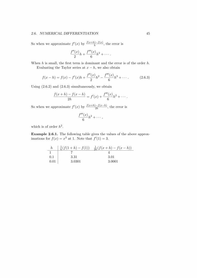
So when we approximate f ′(x) by f(x+h)−f(x)h , the error is
f ′′(x)
2h+
f ′′′(x)
6h2 + · · · .
When h is small, the first term is dominant and the error is of the order h.Evaluating the Taylor series at x− h, we also obtain
f(x− h) = f(x)− f ′(x)h+f ′′(x)
2h2 − f ′′′(x)
6h3 + · · · . (2.6.3)
Using (2.6.2) and (2.6.3) simultaneously, we obtain
f(x+ h)− f(x− h)
2h= f ′(x) +
f ′′′(x)
6h2 + · · · .
So when we approximate f ′(x) by f(x+h)−f(x−h)2h , the error is
f ′′′(x)
6h2 + · · · ,
which is of order h2.
Example 2.6.1. The following table gives the values of the above approx-imations for f(x) = x3 at 1. Note that f ′(1) = 3.
h 1h(f(1 + h)− f(1)) 1
2h(f(x+ h)− f(x− h))
1 7 40.1 3.31 3.010.01 3.0301 3.0001

46 CHAPTER 2. DIFFERENTIATION

Chapter 3
Integration
3.1 Two approaches to integration
3.1.1 Antidifferentiation and the indefinite integral
Consider the following question: for a given function f , is there anotherfunction F such that F ′ = f? In other words, is there a way to reversedifferentiation? For reasonably nice functions, the answer is typically yes.
Example 3.1.1. Is there a function F such that F ′(x) = x5 + 6?
Solution. It is easy to check that F (x) = x6
6 + 6x provides a solution.
If F is a function that satisfies F ′ = f , then we say that F is an an-tiderivative of f (also called primitive of f). In practice, the difficulty isusually not in deciding whether an antiderivative exists, but rather to findit. We will see some methods for this later. First, we discuss a few generalfacts.
Note that antiderivatives are not unique. In Example 3.1.1, we couldhave given the answer x6
6 + 6x + 10, and you can write down many moresimilar answers. In fact, whenever F is an antiderivative of a function f andC is a constant, then F + C is another antiderivative of f . We can verifythis by differentiation: if F ′ = f , then
d
dx(F (x) + C) = F ′(x) = f(x)
for all x by the summation rule and (2.1.1). Moreover, it is also true thatany two antiderivatives of a function differ by a constant. Therefore, bycombining these two facts, we obtain the following statement.
If F is an antiderivative of a given function f , then all antiderivatives off are of the form F + C, where C is a constant.
The indefinite integral of f is a symbolic representation of a genericantiderivative. When we write ˆ
f(x) dx,
47
48 CHAPTER 3. INTEGRATION
we mean an unspecified antiderivative of f , with the understanding thatadding various constants will produce all antiderivatives. When evaluat-ing an indefinite integral, we usually use the symbol C to represent thisunspecified constant. For example,
ˆx2 dx =
1
3x3 + C.
Example 3.1.2. Evaluate
ˆ(x5 + 6) dx.
Solution. This is ˆ(x5 + 6) dx =
x6
6+ 6x+ C.
3.1.2 Area and the definite integral
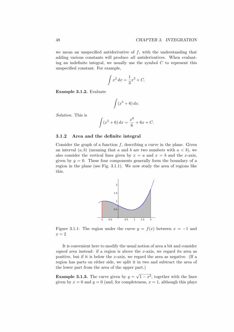
Consider the graph of a function f , describing a curve in the plane. Givenan interval (a, b) (meaning that a and b are two numbers with a < b), wealso consider the vertical lines given by x = a and x = b and the x-axis,given by y = 0. These four components generally form the boundary of aregion in the plane (see Fig. 3.1.1). We now study the area of regions likethis.
Figure 3.1.1: The region under the curve y = f(x) between x = −1 andx = 2
It is convenient here to modify the usual notion of area a bit and considersigned area instead: if a region is above the x-axis, we regard its area aspositive, but if it is below the x-axis, we regard the area as negative. (If aregion has parts on either side, we split it in two and subtract the area ofthe lower part from the area of the upper part.)
Example 3.1.3. The curve given by y =√
1− x2, together with the linesgiven by x = 0 and y = 0 (and, for completeness, x = 1, although this plays
3.1. TWO APPROACHES TO INTEGRATION 49
no role here), bounds a quarter disk of radius 1 above the x-axis. The areais π
4 .
On the other hand, if we consider the curve given by y = −√
1− x2,then we have a quarter disk below the x-axis. According to our convention,the area of this region is −π
4 .
We use the following notation for this concept. The definite integral
ˆ b
af(x) dx
is the signed area (in the above sense) of the region bounded by the curvedescribed y = f(x) and the lines given by x = a, x = b, and y = 0. Thenumbers a and b are called the (lower and upper) limits of the integral.(The symbol x here is a dummy variable and may be replaced by any othersymbol.)
Why do we use notation and terminology so similar to the indefiniteintegral discussed in Sect. 3.1.1? It turns out that computing area is closelyrelated to antidifferentiation. In order to see why this is the case, fix thelower limit a, but replace the upper limit by a variable t. Then we maydefine a function F by the formula
F (t) =
ˆ t
af(x) dx.
Now let h be a number with h 6= 0 and compare the value F (t) with F (t+h).The difference F (t+h)−F (t) corresponds to the area of the region boundedby the graph of f , the x-axis, and the lines given by x = t and x = t + h.Assuming that h is small, this is a narrow strip, and assuming that f iscontinuous (and therefore does not vary much between t and t+h), the areais approximately hf(t). Hence
F (t+ h)− F (t)
h≈ f(t).
In fact, taking limits, we obtain
F ′(t) = limh→0
F (t+ h)− F (t)
h= f(t).
In other words, we have found an antiderivative for f .
The following statement is known as the first fundamental theorem ofcalculus. Suppose that f is a continuous function and a is a fixed number.Let the function F be defined through
F (x) =
ˆ x
af(t) dt.
50 CHAPTER 3. INTEGRATION
Then F ′(x) = f(x) for all values of x.Now remember that any other antiderivative differs from F by a con-
stant. So if we consider an arbitrary antiderivative of f , say G, then thereexists a constant C such that G = F + C. It is clear that F (a) = 0 (as thisis the area of a strip of width 0), so G(a) = C. On the other hand,
ˆ b
af(x) dx = F (b) = G(b)− C = G(b)−G(a).
This is the second fundamental theorem of calculus. If f is a continuousfunction and F is an antiderivative of f , then
ˆ b
af(x) dx = G(b)−G(a).
Because expressions like this appear a lot when we work with definiteintegrals, we use the following shorthand notation:
[G(x)]ba = G(b)−G(a).
If it may be unclear what the relevant variable is, we may instead write
[G(x)]bx=a.
The condition that f be continuous can be relaxed, although it takes asophisticated theory to determine a more appropriate condition. In practice,the condition can almost always be ignored. It is important, however, thatthe condition F ′(x) = f(x) is satisfied for all x in the interval [a, b], unlessyou add other conditions instead.
Example 3.1.4. Consider the functions f and F with f(x) = x|x| and
F (x) = |x|. Then F ′(x) = f(x) at any x except when x = 0, and westill have ˆ 1
−1f(x) dx = 0 = F (1)− F (−1).
However, the function given by G(x) = |x| + x|x| also satisfies G′(x) = f(x)
everywhere except when x = 0, and we have G(1)−G(0) = 2. So we cannotreplace F by G in the above formula.
3.2 Integration techniques
Since we can think of integration as the reverse of differentiation, it is nosurprise that the differentiation rules in Sect. 2.2 give rise to integrationrules. However, with integration, it is often far less obvious which rule toapply, and so this often takes some experience.
3.2. INTEGRATION TECHNIQUES 51
3.2.1 The substitution rule
The substitution rule is the counterpart of the chain rule for differentiation.Recall that the chain rule says that for two functions F and g, we have
d
dxF (g(x)) = F ′(g(x))g′(x).
Thus if we write f = F ′, thenˆf(g(x))g′(x) dx = F (g(x)) + C. (3.2.1)
We can write the same rule in more convenient notation: write u = g(x), sothat du
dx = g′(x). Then we may substitute du = g′(x) dx and thus
ˆf(g(x))g′(x) dx =
ˆf(u) du = F (u) + C = F (g(x)) + C.
(As before, expressions such as dx or du should be thought of as convenientsymbols rather than objects in their own right. In this context, they canactually be given precise meaning, but this theory is outside of the scope ofthis course.)
While it appears that you need a very special integrand for this, inpractice many functions can be written in this form.
Example 3.2.1. Evaluate ˆxex
2dx.
Solution. Write u = x2, so that du = 2x dx. Thenˆxex
2dx =
1
2
ˆ2xex
2dx =
1
2
ˆeu du =
1
2eu + C =
1
2ex
2+ C.
Example 3.2.2. Evaluateˆ
cos(7x) dx.
Solution. The substitution u = 7x gives du = 7dx andˆ
cos(7x) dx =1
7
ˆcosu du =
1
7sinu+ C =
1
7sin(7x) + C.
Example 3.2.3. Evaluate ˆdx
(2− x)2.
Solution. The substitution u = 2− x gives du = −dx andˆ
dx
(2− x)2= −ˆdu
u2=
1
u+ C =
1
2− x+ C.

52 CHAPTER 3. INTEGRATION
Instead of writing u = g(x), we may turn the substitution around andwrite x = h(u) for some function h. This amounts to the previous methodif we choose h = g−1. Then by Sect. 2.3.2, we have h′(u) = 1
g′(x) and thus
we still have dx = h′(u) du, as expected.
Example 3.2.4. Evaluate ˆdx√
1− x2.
Solution. Use the substitution x = sinu, so that dx = cosu du. Thenˆ
dx√1− x2
=
ˆcosu√
1− sin2 udu =
ˆdu = u+ C = arcsinx+ C.
When we want to evaluate a define integral, then one method is to firstevaluate the indefinite integral (perhaps using the substitution rule) andthen insert the limits. But when we use the substitution rule, then thereis a more direct method. Using the functions F and g again and settingf = F ′, we have
ˆ b
af(g(x))g′(x) dx = F (g(b))− F (g(a))
by (3.2.1). That is,
ˆ b
af(g(x))g′(x) dx =
ˆ g(b)
g(a)f(u) du.
Thus after the substitution u = g(x), there is no need to go back to thevariable x, provided that we substitute the limits as well.
Example 3.2.5. Evaluate
ˆ 1
0
√x+ 1 dx.
Solution. With the substitution u = x+1, giving rise to du = dx, we obtain
ˆ 1
0
√x+ 1 dx =
ˆ 2
1
√u du =
[2
3u3/2
]2u=1
=4√
2− 2
3.
Example 3.2.6. Evaluate
ˆ 4
0
x
x2 + 1dx.
Solution. The substitution u = x2 + 1 gives du = 2x dx and
ˆ 4
0
x
x2 + 1dx =
1
2
ˆ 17
1
du
u=
1
2[lnu]171 =
1
2(ln 17− ln 1) =
1
2ln 17.
3.2. INTEGRATION TECHNIQUES 53
It can happen that after the substitution, the lower limit is larger thanthe upper limit. But this is no problem. We may just ignore this issue oruse the convention ˆ b
af(x) dx = −
ˆ a
bf(x) dx.
Example 3.2.7. Evaluate ˆ 0
−√π/2
x cos(x2) dx.
Solution. The substitution u = x2 givesˆ 0
−√π/2
x cos(x2) dx =1
2
ˆ 0
π/2cosu du =
1
2[sinu]0u=π/2 = −1
2.
There are a few substitutions that are far from obvious but very useful.We will discuss these later.
3.2.2 Integration by parts
This is the counterpart to the product rule for differentiation, which tells usthat for two functions f and g, we have
(fg)′(x) = f ′(x)g(x) + f(x)g′(x).
Hence ˆ(f ′(x)g(x) + f(x)g′(x)) dx = f(x)g(x) + C.
We will rarely have an integrand of this precise form, but we can rearrangethe terms as follows:ˆ
f(x)g′(x) dx = f(x)g(x)−ˆf ′(x)g(x) dx.
This only expresses one integral in terms of the other, but we can hope thatthe one on the right-hand side is easier to evaluate.
Again it is convenient to use the following notation: write u = f(x) andv = g(x). Then du = f ′(x) dx and dv = g′(x) dx. Substituting this in theabove formula yields ˆ
u dv = uv −ˆv du.
Example 3.2.8. Evaluate ˆxex dx.
Solution. We apply the integration by parts formula for f(x) = x andg(x) = ex. That is, we write u = x and v = ex. Then du = dx anddv = ex dx. Soˆ
xex dx =
ˆu dv = uv −
ˆv du = xex −
ˆex dx = xex − ex + C.

54 CHAPTER 3. INTEGRATION
Example 3.2.9. Evaluate ˆx2ex dx.
Solution. Setting u = x2 and v = ex, we obtainˆx2ex dx =
ˆu dv = uv −
ˆv du = x2ex − 2
ˆxex dx.
We already know how to evaluate the last integral by Example 3.2.8. In-serting the expression, we obtain
ˆx2ex dx = x2ex − 2(xex − ex) + C = (x2 − 2x+ 2)ex + C.
Example 3.2.10. Evaluateˆex cosx dx
Solution. With u = ex and v = sinx, we haveˆex cosx dx =
ˆu dv = uv −
ˆv du = ex sinx−
ˆex sinx dx.
In order to evaluate the last integral, we use integration by parts again. Letu = ex and v = − cosx. Then
ˆex sinx dx =
ˆu dv = uv −
ˆv du = −ex cosx+
ˆex cosx dx.
Insert this into the first formula:ˆex cosx dx = ex sinx+ ex cosx−
ˆex cosx dx.
Add´ex cosx dx on both sides, then divide by 2. This yields
ˆex cosx dx =
ex
2(sinx+ cosx) + C.
The method is exactly the same for definite integrals. We use the formula
ˆ b
af(x)g′(x) dx = [f(x)g(x)]ba −
ˆ b
af ′(x)g(x) dx
or we first find an antiderivative and then insert the limits.
Example 3.2.11. Evaluate
ˆ 7
4x lnx dx.

3.2. INTEGRATION TECHNIQUES 55
Solution. Using the functions f(x) = x2/2 and g(x) = lnx, we observe that
ˆ 7
4x lnx dx =
ˆ 7
4f ′(x)g(x) dx = [f(x)g(x)]74 −
ˆ 7
4f(x)g′(x) dx
=
[x2
2lnx
]74
−ˆ 7
4
x2
2xdx =
49
2ln 7− 8 ln 4−
[x2
4
]74
=49
2ln 7− 8 ln 4− 49
4+ 4.
3.2.3 Partial fractions
In this section we study quotients of polynomials, which are called rationalfunctions. The method discussed here is not just for integration. It is amethod to decompose a rational function into simpler parts, which helps inparticular for integration, but may be useful for other purposes, too.
In order to motivate the following, we first observe what happens whenwe add some simple rational functions. For example,
1
x+ 3+
8
x− 2=x− 2 + 8(x+ 3)
(x+ 3)(x− 2)=
9x+ 22
x2 + x− 6.
The idea is now to reverse this process. That is, given a rational function,we want to split it up into simpler rational functions. It turns out that thisis always possible up to a certain point.
Suppose that we have a rational function, that is, a function of the form
p(x)
q(x),
where p and q are polynomials.
Step 1: Use polynomial long division This will give two polynomialsp1(x) and r(x) such that
p(x)
q(x)=p1(x)
q(x)+ r(x)
and the degree of p1(x) is strictly less than the degree of q(x).
Example 3.2.12. Consider the rational function
x2 − x+ 1
x+ 2.
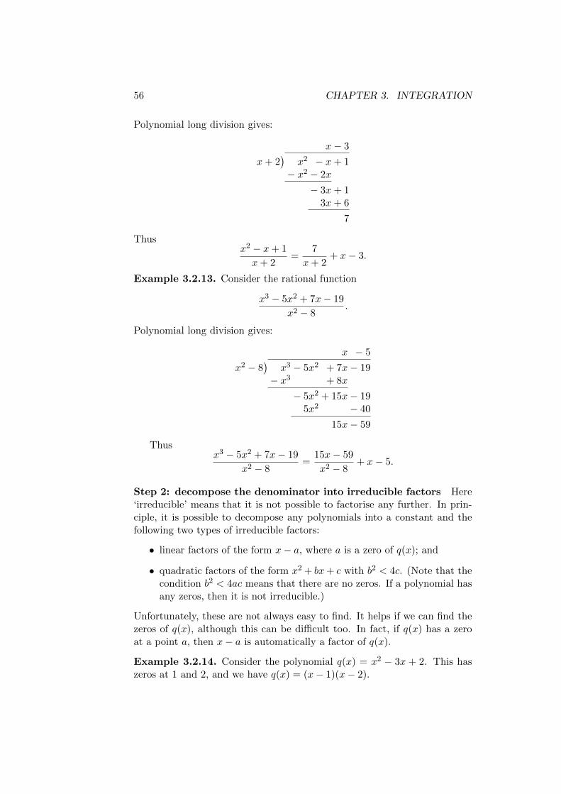
56 CHAPTER 3. INTEGRATION
Polynomial long division gives:
x− 3
x+ 2)
x2 − x+ 1− x2 − 2x
− 3x+ 13x+ 6
7
Thusx2 − x+ 1
x+ 2=
7
x+ 2+ x− 3.
Example 3.2.13. Consider the rational function
x3 − 5x2 + 7x− 19
x2 − 8.
Polynomial long division gives:
x − 5
x2 − 8)
x3 − 5x2 + 7x− 19− x3 + 8x
− 5x2 + 15x− 195x2 − 40
15x− 59
Thusx3 − 5x2 + 7x− 19
x2 − 8=
15x− 59
x2 − 8+ x− 5.
Step 2: decompose the denominator into irreducible factors Here‘irreducible’ means that it is not possible to factorise any further. In prin-ciple, it is possible to decompose any polynomials into a constant and thefollowing two types of irreducible factors:
• linear factors of the form x− a, where a is a zero of q(x); and
• quadratic factors of the form x2 + bx+ c with b2 < 4c. (Note that thecondition b2 < 4ac means that there are no zeros. If a polynomial hasany zeros, then it is not irreducible.)
Unfortunately, these are not always easy to find. It helps if we can find thezeros of q(x), although this can be difficult too. In fact, if q(x) has a zeroat a point a, then x− a is automatically a factor of q(x).
Example 3.2.14. Consider the polynomial q(x) = x2 − 3x + 2. This haszeros at 1 and 2, and we have q(x) = (x− 1)(x− 2).
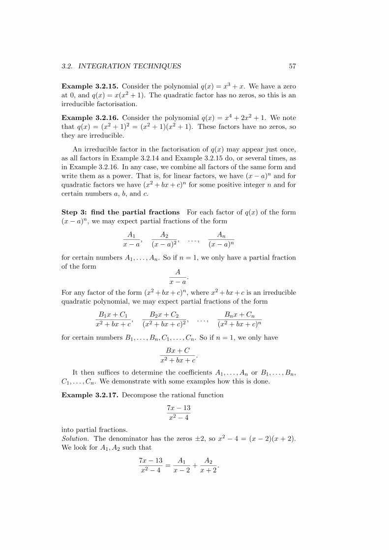
3.2. INTEGRATION TECHNIQUES 57
Example 3.2.15. Consider the polynomial q(x) = x3 + x. We have a zeroat 0, and q(x) = x(x2 + 1). The quadratic factor has no zeros, so this is anirreducible factorisation.
Example 3.2.16. Consider the polynomial q(x) = x4 + 2x2 + 1. We notethat q(x) = (x2 + 1)2 = (x2 + 1)(x2 + 1). These factors have no zeros, sothey are irreducible.
An irreducible factor in the factorisation of q(x) may appear just once,as all factors in Example 3.2.14 and Example 3.2.15 do, or several times, asin Example 3.2.16. In any case, we combine all factors of the same form andwrite them as a power. That is, for linear factors, we have (x− a)n and forquadratic factors we have (x2 + bx+ c)n for some positive integer n and forcertain numbers a, b, and c.
Step 3: find the partial fractions For each factor of q(x) of the form(x− a)n, we may expect partial fractions of the form
A1
x− a,
A2
(x− a)2, . . . ,
An(x− a)n
for certain numbers A1, . . . , An. So if n = 1, we only have a partial fractionof the form
A
x− a.
For any factor of the form (x2 + bx+ c)n, where x2 + bx+ c is an irreduciblequadratic polynomial, we may expect partial fractions of the form
B1x+ C1
x2 + bx+ c,
B2x+ C2
(x2 + bx+ c)2, . . . ,
Bnx+ Cn(x2 + bx+ c)n
for certain numbers B1, . . . , Bn, C1, . . . , Cn. So if n = 1, we only have
Bx+ C
x2 + bx+ c.
It then suffices to determine the coefficients A1, . . . , An or B1, . . . , Bn,C1, . . . , Cn. We demonstrate with some examples how this is done.
Example 3.2.17. Decompose the rational function
7x− 13
x2 − 4
into partial fractions.Solution. The denominator has the zeros ±2, so x2 − 4 = (x − 2)(x + 2).We look for A1, A2 such that
7x− 13
x2 − 4=
A1
x− 2+
A2
x+ 2.

58 CHAPTER 3. INTEGRATION
Simplifying the right-hand side, we obtain
A1
x− 2+
A2
x+ 2=A1(x+ 2) +A2(x− 2)
(x− 2)(x+ 2)=
(A1 +A2)x+ 2A1 − 2A2
x2 − 4.
In order to obtain the desired rational function, we need to solve the systemof equations
A1 +A2 = 7
2A1 − 2A2 = −13.
The solution is A1 = 14 and A2 = 27
4 . Hence
7x− 13
x2 − 4=
A1
x− 2+
A2
x+ 2=
1
4(x− 2)+
27
4(x+ 2).
Example 3.2.18. Decompose
x+ 6
x2 + 8x+ 16
into partial fractions.
Solution. We have x2 + 8x + 16 = (x + 4)2. Note that we have a repeatedfactor here. Thus we look for A1, A2 such that
x+ 6
x2 + 8x+ 16=
A1
x+ 4+
A2
(x+ 4)2=A1(x+ 4) +A2
x2 + 8x+ 16=A1x+ 4A1 +A2
x2 + 8x+ 16.
We have to solve the system
A1 = 1,
4A1 +A2 = 6.
The solution is A1 = 1 and A2 = 2. So
x+ 6
x2 + 8x+ 16=
1
x+ 4+
2
(x+ 4)2.
Example 3.2.19. Decompose
5x2 − 6x+ 3
x3 + x2 − 2
into partial fractions
Solution. Here it is not obvious how to find the irreducible factors of thedenominator. However, we can check that 1 is a zero. Hence x−1 is a factor.Polynomial long division reveals that x3 + x2 − 2 = (x − 1)(x2 + 2x + 2).

3.2. INTEGRATION TECHNIQUES 59
Since the quadratic polynomial x2 + 2x+ 2 has no zeros, it is irreducible aswell. Therefore, we look for A,B,C such that
5x2 − 6x+ 3
x3 + x2 − 2=
A
x− 1+
Bx+ C
x2 + 2x+ 2=A(x2 + 2x+ 2) + (Bx+ C)(x− 1)
(x− 1)(x2 + 2x+ 2)
=(A+B)x2 + (2A−B + C)x+ 2A− C
x3 + x2 − 2.
We need to solve the system
A+B = 5,
2A−B + C = −6,
2A− C = 3.
The solution is A = 25 , B = 23
5 , and C = −115 . So we have found that
5x2 − 6x+ 1
x3 + x2 − 2=
2
5(x− 1)+
23x− 11
5(x2 + 2x+ 2).
Step 4: find the integrals Assuming that we can find the partial frac-tions of our rational function, we now have a sum of simpler expressions.We finally need to integrate these.
This is quite easy for an expression of the form
A
(x− a)n.
We can use the substitution u = x− a to computeˆ
A
x− adx = A
ˆdu
u= A ln |u|+ C = A ln |x− a|+ C
andˆA
(x− a)ndx = A
ˆdu
un=
A
(1− n)un−1+ C =
A
(1− n)(x− a)n−1+ C
if n ≥ 2.Now we have a closer look at the partial fractions of the form
Bx+ C
x2 + bx+ c,
where b2 < 4c. Here the first step is to rewrite the denominator. Recall thatwe have solved quadratic equations in Sect. 1.2.1 by completing the square.We do the same thing here, finding that
x2 + bx+ c =
(x+
b
2
)2
+ c− b2
4.

60 CHAPTER 3. INTEGRATION
Set β = b2 and γ =
√c− b2/4. Then
Bx+ C
x2 + bx+ c=
Bx+ C
(x+ β)2 + γ2=
Bx+ C
γ2((
x+βγ
)2+ 1
) .In order to evaluate the integral, use the substitution u = x+β
γ . Thenx = γu− β and thus
ˆBx+ C
x2 + bx+ cdx =
ˆB(γu− β) + C
γ(u2 + 1)du
= B
ˆu
u2 + 1du+
C −Bβγ
ˆdu
u2 + 1.
The first of the integrals on the right-hand side we can evaluate with thesubstitution v = u2 + 1, giving dv = 2u du andˆ
u
u2 + 1du =
1
2
ˆdv
v=
1
2ln v + C =
1
2ln(u2 + 1) + C.
For the second one, we use the fact that ddu arctanu = 1
u2+1. Hence
ˆdu
u2 + 1= arctanu+ C.
Combining everything, we obtainˆBx+ C
x2 + bx+ c=B
2ln(u2 + 1) +
C −Bβγ
arctanu+ C
=B
2ln
((x+ β
γ
)2
+ 1
)+C −Bβ
γarctan
x+ β
γ+ C,
where β = b2 and γ =
√c− b2/4.
We may also have partial fractions of the form
Bx+ C
(x2 + bx+ c)n
for some integer n ≥ 0. In practice, however, this is rare, and so we discussthis only briefly. The first steps are the same as in the case n = 1 above.This will now give rise to integrals of the formˆ
u
(u2 + 1)ndu and
ˆdu
(u2 + 1)n.
The first of these can be evaluated with the substitution v = u2 + 1 again,which yieldsˆ
u
(u2 + 1)ndu =
1
2
ˆdv
vn=
1
2(1− n)vn−1=
1
2(1− n)(u2 + 1)n−1.

3.2. INTEGRATION TECHNIQUES 61
For the second integral, we use the substitution u = tan v. Then u2 + 1 =tan2 v + 1 = 1
cos2 vand du = dv
cos2 v. Hence
ˆdu
(u2 + 1)n=
ˆcos2n−2 v dv.
These integrals can now be evaluated with a repeated integration by parts.We have already found the partial fractions of some rational functions,
so we can now evaluate their integrals.
Example 3.2.20. Evaluateˆ
7x− 13
x2 − 4dx.
Solution. We have seen in Example 3.2.17 that
7x− 13
x2 − 4=
1
4(x− 2)+
27
4(x+ 2).
Hence ˆ7x− 13
x2 − 4dx =
1
4ln |x− 2|+ 27
4ln |x+ 2|+ C.
Example 3.2.21. Evaluateˆ
x+ 6
x2 + 8x+ 16dx.
Solution. We have seen in Example 3.2.18 that
x+ 6
x2 + 8x+ 16=
1
x+ 4+
2
(x+ 4)2.
Hence ˆx+ 6
x2 + 8x+ 16= ln |x+ 4| − 2
x+ 4+ C.
Example 3.2.22. Evaluate
ˆ5x2 − 6x+ 3
x3 + x2 − 2dx.
Solution. We have seen in Example 3.2.19 that
5x2 − 6x+ 1
x3 + x2 − 2=
2
5(x− 1)+
23x− 11
5(x2 + 2x+ 2).
Moreover, we haveˆ
2
5(x− 1)dx =
2
5ln |x− 1|+ C.

62 CHAPTER 3. INTEGRATION
In order to evaluate the remaining integral, we write
x2 + 2x+ 2 = (x+ 1)2 + 1.
We use the substitution u = x+ 1, which givesˆ
23x− 11
5(x2 + 2x+ 2)=
ˆ23(u− 1)− 11
5(u2 + 1)du
=23
5
ˆu
u2 + 1du− 34
5
ˆdu
u2 + 1
=23
10ln(u2 + 1)− 34
5arctanu+ C
=23
10ln(x2 + 2x+ 2)− 34
5arctan(x+ 1) + C.
3.3 Further integration techniques
3.3.1 Integrating an inverse function
Recall that we have seen in Sect. 2.3.2 how to differentiate the inverse f−1
of a function f . We can use this information, combined with integration byparts and the substitution rule, to find antiderivatives of f−1 as well.
We demonstrate the method with an example. Consider the integralˆarcsinx dx.
Use integration by parts with u = arcsinx and v = x, giving rise toˆarcsinx dx = x arcsinx−
ˆx√
1− x2dx.
Now substitute w = 1− x2, so that dw = −2x dx. Thusˆarcsinx dx = x arcsinx+
1
2
ˆdw√w
= x arcsinx+√w + C = x arcsinx+
√1− x2 + C.
In general, if we want to integrate an inverse function f−1, then we canalways use integration by parts with u = f−1(x) and v = x, followed by asubstitution. The resulting formula becomes particularly simple when wewrite y = f(x) (and therefore x = f−1(y) is the expression that we want tointegrate). Then we have
ˆx dy = xy −
ˆy dx.
But because this is so terse, using this formula blindly may result in confu-sion. In practice, it is often better to do the above steps directly.

3.3. FURTHER INTEGRATION TECHNIQUES 63
Example 3.3.1. Evaluate ˆlnx dx.
Solution. Note that ln is the inverse of the exponential function with basee, so we can use the above method. Set u = lnx and v = x. This gives
ˆlnx dx = x lnx−
ˆx
xdx = x lnx− x+ C.
3.3.2 Trigonometric rational functions
It’s easiest to understand what trigonometric rational functions are by look-ing at some examples such as the following:
sin3 x− cos2 x+ 2
cos3 x− sin3 x+ 8 cosx,
cosx
14 sin8 x+ 5 cos7 x+ sin3 x,
cos4 x+ sin4 x
cos3 x.
A standard trick to integrate these is the substitution
u = tanx
2.
Then
cosx =1− u2
1 + u2, sinx =
2u
1 + u2, and dx =
2 du
1 + u2.
It is clear that inserting all of this, we obtain the integral of a rationalfunction, which we can, in principle, evaluate with the method of partialfractions. In practice, however, this can give very complicated expressions.(Imagine using it for the above examples.) But for simple trigonometricrational functions, this works well.
Example 3.3.2. Evaluate ˆsecx dx.
Solution. Note that sec is a trigonometric rational function, as secx = 1cosx .
The standard substitution u = tan x2 gives
ˆsecx dx =
ˆ1 + u2
1− u22
1 + u2du =
ˆ2
1− u2du.
The method of partial fractions gives
2
1− u2=
1
u+ 1− 1
u− 1.
Henceˆ2
1− u2du =
ˆdu
u+ 1−ˆ
du
u− 1= ln |u+ 1| − ln |u− 1|+ C.

64 CHAPTER 3. INTEGRATION
We finally obtainˆsecx dx = ln
∣∣∣tanx
2+ 1∣∣∣− ln
∣∣∣tanx
2− 1∣∣∣+ C.
(Note that there are other methods to compute this and there are otherways to represent the result.)
3.3.3 Trigonometric substitution
This is a method that is often useful for integrals involving the expression√1− x2. The trick is to substitute x = sinu. Then dx = cosu du and√
1− x2 =√
1− sin2 u =√
cos2 u = cosu.
(Here we have used the assumption that −π2 ≤ u ≤
π2 .)
Example 3.3.3. Evaluate ˆ √1− x2 dx.
Solution. Using the above substitution x = sinu, we obtainˆ √1− x2 dx =
ˆcos2 u du =
1
2(u+ sinu cosu) + C.
In order to reverse the substitution, we note that u = arcsinx. Moreover,
we have sinu = x and cosu =√
1− sin2 u =√
1− x2. Thusˆ √1− x2 dx =
1
2(arcsinx+ x
√1− x2) + C.
Integrals involving√ax2 + bx+ c can often be treated similarly, because
we can transform them by completing the square.
Example 3.3.4. Evaluate ˆ √8 + 2x− x2 dx.
Solution. We have
8 + 2x− x2 = 9− (x− 1)2 = 9
(1−
(x− 1
3
)2),
which suggests the substitution u = x−13 . Thenˆ √
8 + 2x− x2 dx = 9
ˆ √1− u2 du
=9
2(arcsinu+ u
√1− u2) + C
=9
2arcsin
x− 1
3+
1
2(x− 1)
√8 + 2x− x2 + C.

3.3. FURTHER INTEGRATION TECHNIQUES 65
For integrals involving√
1 + x2, the substitution x = tanu is sometimesuseful. Then dx = du
cos2 uand
√1 + x2 =
√1 + tan2 u =
√1
cos2 u=
1
cosu
(again assuming that −π2 ≤ u ≤
π2 ).
Example 3.3.5. Evaluate ˆdx√
1 + x2.
Solution. With the above substitution, we obtain
ˆdx√
1 + x2=
ˆdu
cosu=
ˆsecu du.
We have computed this integral in Example 3.3.2, but it is more convenientto use a different method here. Note that
ˆdu
cosu=
ˆcosu
cos2 udu =
ˆcosu
1− sin2 udu.
With v = sinu, we obtain the integral
ˆdv
1− v2=
1
2
ˆdv
1 + v+
1
2
ˆdv
1− v
=1
2ln |1 + v| − 1
2ln |1− v|+ C =
1
2ln
∣∣∣∣1 + v
1− v
∣∣∣∣+ C.
Since x = tanu and v = sinu, we have v = x√1+x2
. Hence
1 + v
1− v=
1 + v
1− v1 + v
1 + v=
(1 + v)2
1− v2=
(1 + x√
1+x2
)21− x2
1+x2
= (1 + x2)
(1 +
x√1 + x2
)2
=(x+
√1 + x2
)2.
It follows thatˆ
dx
1 + x2=
1
2ln(x+
√1 + x2
)2+ C = ln
(x+
√1 + x2
)+ C.
3.3.4 Hyperbolic substitution
Recall the functions
coshx =1
2(ex + e−x) and sinhx =
1
2(ex − e−x),

66 CHAPTER 3. INTEGRATION
which satisfycosh2 x− sinh2 x = 1
andd
dxcoshx = sinhx and
d
dxsinhx = coshx.
If we have an integral involving the expression√
1 + x2, then they canbe useful as well. The substitution x = sinhu then gives√
1 + x2 =√
1 + sinh2 u =√
cosh2 u = coshu
and dx = coshu du.
Example 3.3.6. Evaluate ˆdx√
1 + x2.
Solution. We have already found the answer in Example 3.3.5, but we nowuse a different method. With the above substitution, we obtainˆ
dx√1 + x2
=
ˆcoshu
coshudu =
ˆdu = u+ C.
Now we need to express u in terms of x; that is, we need to find the inverseof the function sinh. To this end, we solve sinhu = x for u. Recalling thedefinition of sinh, we obtain
1
2(eu − e−u) = x.
If we substitute v = eu, this becomes
v
2− 1
2v= x.
Multiply by 2v:v2 − 1 = 2xv.
Rearrange:v2 − 2vx− 1 = 0.
This is a quadratic equation in v. The solutions are
v = x±√x2 + 1.
But since v = eu > 0, while x −√x2 + 1 < 0, we can only use the positive
solution v = x+√x2 + 1. Hence
u = ln v = ln(x+
√x2 + 1
).
It follows that ˆdx√x2 + 1
= ln(x+
√x2 + 1
)+ C.
3.4. NUMERICAL INTEGRATION 67
3.4 Numerical integration
Up to now we have calculated our integrals symbolically. But often this isimpossible and we have to resort to numerical approximations. As a definiteintegral, such as ˆ b
af(x) dx,
is the area of a region in the plane, the basic idea is to approximate thisregion by simpler shapes. One common way to do this is to divide theinterval [a, b] into lots of smaller intervals and thereby divide the region intolots of thin strips. Each of these strips can then be approximated by arectangle, and we know how to compute the area of a rectangle.
Suppose that we want to divide [a, b] into n intervals of equal length.Then h = b−a
n is this length and the numbers
xk = a+ hk, k = 0, . . . , n,
are the end points of the intervals. If wk denotes the height of the k-threctangle, then its area is hwk. (This may be negative, as we still considersigned area here.) So the total area of the approximation is
hn∑k=1
wk.
The question is now how to choose wk. There are several common ways todo it.
Left point rule Choose the value of f at the left end point of the cor-responding interval, so wk = f(xk−1). Then the total area of theapproximation is
hn∑k=1
f(xk−1).
Right point rule Use the right end point instead. Then wk = f(xk) andwe obtain
hn∑k=1
f(xk).
Mid-point rule Use the mid-pointxk−1+xk
2 . Then wk = f(xk−1+xk
2 ) andwe have the expression
h
n∑k=1
f
(xk−1 + xk
2
).

68 CHAPTER 3. INTEGRATION
Trapezium rule This rule is motivated by an approximation by trapezia
rather than rectangles. It corresponds to wk =f(xk−1)+f(xk)
2 and givesrise to
h
n∑k=1
f(xk−1) + f(xk)
2=h
2f(x0) + h
n−1∑k=1
f(xk) +h
2f(xn).
In addition, there is another important method that does not quite fit inthis framework. We will see later why it works (and works very well).
Simpson’s rule Here we assume that n is even and we use the formula
h
3
n/2∑k=1
(f(x2k−2) + 4f(x2k−1) + f(x2k)) .
Example 3.4.1. Suppose that we want to integrate
ˆ 1
0x5 dx
numerically. We know that the exact answer is 16 ≈ 0.166667, and this will
allow us to compare the results for different methods.
Here we have a = 0 and b = 1. We first choose n = 2, giving rise toh = 1
2 . Then we have the following approximations
Left point rule 12
(0 + 1
32
)= 1
64 ≈ 0.0156,
Mid-point rule 12
(1
1024 + 2431024
)= 61
512 ≈ 0.1191,
Right point rule 12
(132 + 1
)= 33
64 ≈ 0.5156,
Trapezium rule 12
(0+ 1
322 +
132
+1
2
)= 17
64 ≈ 0.2656,
Simpson’s rule 16
(0 + 4
32 + 1)
= 316 ≈ 0.1875.
The following table contains the results for various values of n.
n 2 4 8 16
Left point rule 0.0156 0.0674 0.1107 0.1370Mid-point rule 0.1191 0.1539 0.1634 0.1659Right point rule 0.5156 0.3174 0.2357 0.1995Trapezium rule 0.2656 0.1924 0.1732 0.1683Simpson’s rule 0.1875 0.1680 0.1667 0.1667
3.4. NUMERICAL INTEGRATION 69
In order to explain the different performances of these methods, we com-pare their errors for the integrals over two consecutive intervals in the subdi-vision of [a, b]. More precisely, for a given number c and h > 0, we examinethe errors in the approximation of
I(h) =
ˆ c+h
c−hf(x) dx
when the interval [c − h, c + h] is divided into two subintervals. The total
error for the integral´ ba f(x) dx will then be roughly this error times n/2.
We assume that f is represented by its Taylor series near c (otherwisewe can use similar arguments with finite Taylor polynomials). Then
f(x) = f(c) + f ′(c)(x− c) +f ′′(c)
2(x− c)2 +
f ′′′(c)
6(x− c)3 + · · · , (3.4.1)
and therefore
I(h) =
[f(c)(x− c) +
f ′(c)
2(x− c)2 +
f ′′(c)
6(x− c)3 + · · ·
]c+hc−h
= 2f(c)h+ 2f ′′(c)
6h3 + 2
f (4)(c)
5!h5 + · · · .
Now we compute the results of the approximation methods. The leftpoint rule and the right point rule are similar, and we only treat the latterhere. It gives the approximation
h(f(c) + f(c+ h)).
Using (3.4.1) for the second term, we obtain
2f(c)h+ f ′(c)h2 +f ′′(c)
2h3 + · · · .
The error is of order h2. The mid-point rule gives
h(f(c− h/2) + f(c+ h/2)) = 2f(c)h+f ′′(c)
4h3 + · · · ,
with an error of order h3. The trapezium rule gives
h
2(f(c− h) + 2f(c) + f(c+ h)) = 2f(c)h+
f ′′(c)
2h3 + · · · ,
again with an error of order h3. Finally, Simpson’s rule gives
h
3(f(c− h) + 4f(c) + f(c+ h)) = 2f(c)h+
f ′′(c)
3h3 +
f (4)(c)
36h5 + · · · .
This is an error of order h5.Once we add up the errors over the whole interval [a, b], we obtain
• order h for the left and right point rules,
• order h2 for the mid-point and trapezium rules, and
• order h4 for Simpson’s rule.
70 CHAPTER 3. INTEGRATION
3.5 Improper integrals
So far we have considered the area of regions bounded by the graph of afunction f , the x-axis, and two vertical lines, given by x = a and x = b. Butsometimes we want to remove one or both of these vertical lines and considerregions stretching to infinity. A similar situation occurs if f(x) tends to ∞or −∞ as x approaches a or b. It is not always clear what the area of sucha region is, but in some cases the notion still makes sense.
We define ˆ ∞a
f(x) dx = limb→∞
ˆ b
af(x) dx,
provided that this limit exists. Similarly,ˆ b
−∞f(x) dx = lim
a→−∞
ˆ b
af(x) dx,
provided, again, that the limit exists.
Example 3.5.1. We haveˆ b
0e−x dx = 1− e−b → 1
as b→∞. Hence ˆ ∞0
e−x dx = 1.
Similarly, ˆ 0
aex dx = 1− ea → 1
as a→ −∞. Hence ˆ 0
−∞ex dx = 1.
But ˆ 0
−∞e−x dx =∞
and ˆ ∞0
ex dx =∞.
If limx→a+ f(x) = ±∞, then we defineˆ b
af(x) dx = lim
c→a+
ˆ b
cf(x) dx,
provided that the limit exists. If limx→b− f(x) = ±∞, thenˆ b
af(c) dx = lim
c→b−
ˆ c
af(x) dx,
provided that the limit exists.

3.5. IMPROPER INTEGRALS 71
Example 3.5.2. We have
ˆ 1
c
dx√x
= 2(1−√c)→ 2
as c→ 0+. Hence ˆ 1
0
dx√x
= 2.
But ˆ 1
0
dx
x= lim
a→0+(− ln a) =∞.
All integrals of this type are called improper .

72 CHAPTER 3. INTEGRATION

Chapter 4
Differential equations
4.1 Introduction
If an equation involves a function and some of its derivatives, then it is calleda differential equation. For example, the following is a differential equation:
f ′ = f. (4.1.1)
This expresses the fact that a function coincides with its own derivative.Often the equation is written in the form
f ′(x) = f(x),
and then this is usually meant to be true for all x. If we write y for thedependent variable (so that y = f(x)), then we may also write
dy
dx= y
for the same equation.To solve a differential equation means to find the functions that make
it a true statement. For example, we know that the exponential functionwith base e, i.e., the function with f(x) = ex, satisfies (4.1.1). You can alsocheck that for any constant c, the function defined by f(x) = cex is anothersolution. In fact these are all the solutions of this equation.
When we solve a differential equation, we typically obtain infinitely manysolutions. For this reason, a differential equation often comes together withadditional conditions that are designed to pick a specific solution. For thetype of equations that we study here, the most common condition is one ofthe form
f(x0) = y0, (4.1.2)
where x0 and y0 are given numbers. That is, we prescribe the value of thesolution at a specific point. Very often in problems of this sort, the indepen-dent variable represents time and condition (4.1.2) represents a measurement
73
74 CHAPTER 4. DIFFERENTIAL EQUATIONS
of the quantity y at an initial time. Therefore, a problem consisting of adifferential equation and a condition of this sort is called an initial valueproblem.
For example, equations (4.1.1) and (4.1.2) constitute an initial valueproblem. Any function of the form f(x) = cex is a solution of (4.1.1). Wecan now use (4.1.2) to determine the value of c. It must satisfy
cex0 = y0,
so c = y0e−x0 . Therefore, the unique solution of the initial value problem is
f(x) = y0e−x0ex = y0e
x−x0 .
In general, it can be rather difficult to solve a given differential equation,but there are methods for equations of a specific form.
4.2 Separation of variables
A differential equation is called separable if it can be written in the form
f ′(x) = g(x)h(f(x))
for some functions g and h. If y = f(x), then we can also write
dy
dx= g(x)h(y).
These equations are relatively easy to solve. The basic idea is to separatevariables, meaning that we write all expressions involving the independentvariable (including the derivative) on one side and all expressions involvingthe dependent variable on the other side of the equation. That is,
f ′(x)
h(f(x))= g(x).
It is convenient to represent this in the form
dy
h(y)= g(x)dx, (4.2.1)
keeping in mind, as ever, that these expressions have only symbolic charac-ter. Now we integrate:
ˆf ′(x)
h(f(x))dx =
ˆg(x) dx.
By the substitution rule, we haveˆ
f ′(x)
h(f(x))dx =
ˆdy
h(y),
4.2. SEPARATION OF VARIABLES 75
so ˆdy
h(y)=
ˆg(x) dx.
(This is what we also get by just writing the integral sign in front of theexpressions in (4.2.1).) Assuming that we can evaluate these indefinite in-tegrals, say ˆ
g(x) dx = G(x) + C1
and ˆdy
h(y)= H(y) + C2,
we obtain
H(y) = G(x) + C.
(Here C = C1 − C2 is another generic constant.) Thus we have turneda differential equation into an algebraic equation, which we can now try tosolve for y. There is still an undetermined constant C in that equation, whichreflects that fact that differential equations normally have many solutions.We will obtain one solution for every value of C.
Example 4.2.1. Solve the differential equation f ′ = f .
Solution. First we introduce more convenient notation. Write y = f(x).Then the equation becomes dy
dx = y, which gives rise to
dy
y= dx.
Integration gives ˆdy
y=
ˆdx.
As ˆdx = x+ C1 and
ˆdy
y= ln |y|+ C2,
we obtain
ln |y| = x+ C.
Solving for y, we conclude that
y = ex+C = eCex or y = −ex+C = −eCex.
Writing c = eC or c = −eC , we obtain the solution
y = cex.
We can check that this is a solution for any constant c.
76 CHAPTER 4. DIFFERENTIAL EQUATIONS
Example 4.2.2. Solve the equation dydx = x
y .Solution. We first separate variables:
y dy = x dx.
Thus ˆy dy =
ˆx dx.
We have ˆy dy =
y2
2+ C1 and
ˆx dx =
x2
2+ C2.
Hencey2
2=x2
2+ C.
Solving for y, we obtain
y =√x2 + 2C or y = −
√x2 + 2C.
Again we can check that these are indeed solutions.
Example 4.2.3. Solve the initial value problem
dy
dx= ex+y, y(0) = 8.
Solution. Using the fact that ex+y = exey, we separate variables:
e−ydy = ex dx.
Thus ˆe−y dy =
ˆex dx.
We have ˆe−y dy = −e−y + C1 and
ˆex dx = ex + C2.
Therefore,−e−y = ex + C.
Solving for y, we obtain
y = − ln(−ex − C).
Now we use the initial condition to determine C. We must have
8 = − ln(−1− C).
Hence C = −e−8 − 1. We finally obtain
y = − ln(e−8 + 1− ex).
4.3. LINEAR EQUATIONS 77
4.3 Linear equations
Here we study differential equations that can be written in the form
p(x)dy
dx+ q(x)y(x) = r(x) (4.3.1)
for certain functions p, q, and r. If either q(x) = 0 or r(x) = 0, then thisis a separable equation and we can normally solve it with the method fromthe previous section. Otherwise, we need a different method.
We say that equation (4.3.1) is homogeneous if r(x) = 0 for all x.
4.3.1 Integrating factors
The main idea behind this method is that the equation may become easierif we multiply y by another function, say m. Setting z = my, we obtain,using the product rule
dz
dx=dm
dxy(x) +m(x)
dy
dx.
If y is to solve (4.3.1), then
dz
dx=dm
dxy(x) +
r(x)
p(x)m(x)− q(x)
p(x)m(x)y(x).
If we choose m such that is solves the equation
dm
dx=q(x)
p(x)m, (4.3.2)
then two of these terms cancel each other, and we have
dz
dx=r(x)
p(x)m(x). (4.3.3)
This is then an equation that is easy to solve.In order to implement this idea, we need to solve (4.3.2). We can do this
by separation of variables, as we can write the equation in the form
dm
m=q(x)
p(x)dx,
which gives
lnm =
ˆq(x)
p(x)dx+ C.
For our purpose here, it is sufficient to find one solutions. So we may setC = 0. Then
m = e´q(x)/p(x) dx.
78 CHAPTER 4. DIFFERENTIAL EQUATIONS
Once we have determined m, we can solve (4.3.3) just by integration. Wehave
z =
ˆr(x)
p(x)m(x) dx.
From this we now easily obtain y.So the method works as follows.
Step 1 Evaluate ˆq(x)/p(x) dx.
Step 2 Setm = e
´q(x)/p(x) dx.
Step 3 Evaluate
z =
ˆr(x)
p(x)m(x) dx.
Step 4 The desired solution is y = z/m.
Example 4.3.1. Solve the equation
dy
dx+y
x= x2.
Solution. We first note that ˆdx
x= lnx+ C.
Our integrating factor is m = elnx = x. Next we set
z =
ˆx3 dx =
x4
4+ C.
So
y =x4
4 + C
x=x3
4+C
x.
At the end it is usually a good idea to check if this is really a solution.
Example 4.3.2. Solve the equation
dy
dx+ 2y = x.
Solution. We use the integrating factor
m = e´2 dx = e2x
4.3. LINEAR EQUATIONS 79
here. Then
z =
ˆxe2x dx =
x
2e2x − 1
4e2x + C
and
y = e−2xz =x
2− 1
4+ Ce−2x.
4.3.2 The method of undetermined coefficients
This method typically works only for equations of the specific form
ady
dx+ by = r(x), (4.3.4)
where a and b are constants, and only when the function r has a specialstructure.1 The idea is to find solutions that mimic the structure of r(x).This is easiest explained with some examples.
Example 4.3.3. Consider the equation
dy
dx+ 2y = x.
The right-hand side is a polynomial of degree 1. We conjecture that there isa solution that is also a polynomial of degree 1, so y(x) = ax+ b. Insertingthis into the equation, we obtain
a+ 2(ax+ b) = x.
Rearrange the terms:(2a− 1)x+ a+ 2b = 0.
This is satisfied if we choose a and b such that
2a = 1,
a+ 2b = 0.
This system has a unique solution, which is a = 12 and b = −1
4 . So we obtainthe solution
y =x
2− 1
4
of the differential equation.
Example 4.3.4. Consider the equation
2dy
dx+ 3y = e2x.
1It also works for certain equations involving higher order derivatives, but this is outsidethe scope of this course.

80 CHAPTER 4. DIFFERENTIAL EQUATIONS
Here we conjecture that there may be a solution of the form y(x) = ce2x forsome constant c. Inserting this into the equation, we obtain
4ce2x + 3ce2x = e2x.
That is,(7c− 1)e2x = 0.
This is satisfied for c = 17 . So we have the solution
y =1
7e2x.
The following table gives expressions that may fruitfully be tried fordifferent forms of r(x).
r(x) y(x)
anxn + · · ·+ a0 bnx
n + · · ·+ b0aeαx beαx
(anxn + · · ·+ a0)e
αx (bnxn + · · ·+ b0)e
αx
a cos(αx) b cos(αx) + c sin(αx)a sin(αx) b cos(αx) + c sin(αx)(anx
n + · · ·+ a0) cos(αx) (bnxn + · · ·+ b0) cos(αx)++(cnx
n + · · ·+ c0) sin(αx)(anx
n + · · ·+ a0) sin(αx) (bnxn + · · ·+ b0) cos(αx)++(cnx
n + · · ·+ c0) sin(αx)
But even if this works, we are not done yet. We have found just onesolution out of infinitely many, and it is unlikely to be the one we are lookingfor. Fortunately, it is now easy to generate all other solutions as well. Herethe idea is to solve the corresponding homogeneous equation, i.e.,
adz
dx+ bz = 0.
This can be done by separation of variables, and because we have an equationof a specific form, we can immediately write down the general solution:
z(x) = Ce−bxa .
The general solution of the original equation (4.3.4) is the sum of this andthe particular solution found earlier.
Example 4.3.5. The general solution of
dy
dx+ 2y = x.
is
y =x
2− 1
4+ Ce−2x.
(Cf. Example 4.3.2.)
4.3. LINEAR EQUATIONS 81
Example 4.3.6. The general solution of
2dy
dx+ 3y = e2x.
is
y =1
7e2x + Ce−
3x2 .
Example 4.3.7. Solve the differential equation
dy
dx− 2y = 3x cosx.
Solution. We want to find the general solution, but first we try to find oneparticular solution of the form
y = (ax+ b) cosx+ (cx+ d) sinx.
This gives
dy
dx= a cosx− (ax+ b) sinx+ c sinx+ (cx+ d) cosx
= (cx+ a+ d) cosx+ (−ax+ c− b) sinx.
Inserting this into the equation, we obtain
((c− 2a)x+ a+ d− 2b) cosx+ (−(a+ 2c)x+ c− b− 2d) sinx = 3x cosx.
We now want to solve the system
−2a+ c = 3,
a− 2b+ d = 0,
a+ 2c = 0,
−b+ c− 2d = 0.
This has the unique solution a = −65 , b = − 9
25 , c = 35 , d = 12
25 . Thus asolution of the equation is
y = −30x+ 9
25cosx+
15x+ 12
25sinx.
The general solution of the homogeneous equation is z = Ce2x, and so thegeneral solution of the full equation is
y = Ce2x − 30x+ 9
25cosx+
15x+ 12
25sinx.

82 CHAPTER 4. DIFFERENTIAL EQUATIONS
4.4 Numerical methods
For more complicated differential equations, we typically cannot find ex-act solutions and therefore we have to resort to numerical approximations.Consider an initial value problem of the form
dy
dx= F (x, y(x)), y(x0) = y0, (4.4.1)
where F is an arbitrary function in two variables. (We will discuss functionsin two variables in more detail later. For the moment, just think of somequantity depending on x and y.)
The basic idea for almost all numerical methods is the same as for inte-gration: divide the x-axis (or an interval) into small intervals and find anapproximation in each interval. But in contrast to integration, we now haveto compute the approximations in the right order and use the output fromone computation as an input for the next.
4.4.1 Euler’s method
The following is a very simple method, called Euler’s method (or sometimescalled forward Euler method to distinguish it from the backward versiondiscussed below). Here we divide the interval [x0,∞) into small intervals ofthe same length, say h. Define xn = x0 + nh; then [xn, xn+1] is one of theseintervals for n = 0, 1, 2, . . . . Set yn = y(xn). Now use a difference quotientto approximate the derivative in (4.4.1). More precisely,
dy
dx(xn) ≈ y(xn+1)− y(xn)
h=yn+1 − yn
h.
Inserting this into the equation, we obtain
yn+1 − ynh
≈ F (xn, y(xn)) = F (xn, yn).
Replace the approximation by equality and solve for yn+1:
yn+1 = yn + hF (xn, yn).
The equation yn+1 = y(xn+1) is no longer true exactly, but we expectthat it is true approximately; so yn+1 ≈ y(xn+1). Therefore, we can use thisidea to compute approximations for y(xn) recursively. Using the value y0from (4.4.1), we set
yn+1 = yn + hF (xn, yn), n = 0, 1, 2, . . . .
In the end we expect thaty(xn) ≈ yn.
The results will of course depend on the choice of h, which is called the stepsize, and we will get better approximations the smaller the values of h.

4.4. NUMERICAL METHODS 83
Example 4.4.1. Consider the initial value problem
dy
dx=
1
y, y(0) = 1.
In this case, we have the formula
yn+1 = yn +h
yn
and we choose y0 = 1. The following table gives the approximations for thevalues of y up to y(2) for h = 0.5 and h = 0.25.
h y(0) y(0.25) y(0.5) y(0.75) y(1) y(1.25) y(1.5) y(1.75) y(2)
0.5 1 1.5 1.8333 2.1061 2.34350.25 1 1.25 1.45 1.6224 1.7765 1.9172 2.0476 2.1697 2.2849
In this case, the equation is separable and we can calculate the exactsolution, namely y(x) =
√2x+ 1, with y(2) =
√5 ≈ 2.2361.
In order to understand more sophisticated methods, we now have a lookat Euler’s method from a different point of view. If y is a solution of (4.4.1),then the fundamental theorem of calculus implies that
y(xn+1) = y(xn) +
ˆ xn+1
xn
F (x, y(x)) dx. (4.4.2)
If we imagine that we know what F (x, y(x)) is and approximate the integralby the left point rule, we obtain
y(xn+1) ≈ y(xn) + hF (xn, y(xn)).
This is exactly the approximation formula underpinning the method. Wemay now replace the left point rule by something else and see what happens.
4.4.2 Backward Euler method
As the name suggests, this method is closely related to Euler’s method. Therelationship between the two is similar to the relationship between the leftpoint rule and the right point rule for numerical integration. But whenwe solve differential equations, the fact that we need to treat the pointsx1, x2, . . . consecutively, gives rise to some new complications.
Again we divide the interval [x0,∞) into small intervals of the samelength h, giving rise to xn = x0 + nh for n = 1, 2, . . . , and set yn = y(xn).But now we use the approximation formula
dy
dx(xn+1) ≈
yn+1 − ynh
.
84 CHAPTER 4. DIFFERENTIAL EQUATIONS
Using (4.4.1), this gives rise to
yn+1 − ynh
≈ F (xn+1, yn+1)
If we replace the approximation by equality and rewrite the formula, weobtain
yn+1 = yn + hF (xn+1, yn+1).
The next step is to solve this equation for y(xn+1). But since it appearson both sides of the equation, this may be difficult to do. The way out ofthis difficulty is to solve the equation numerically. For example, we may useNewton’s method at this step.
Assuming that we have successfully done this, we expect that
y(xn+1) ≈ yn+1.
Just like for the previous method, we then feed yn+1 into the next step andconstruct an approximate solution step by step.
Because this method does not provide explicit formulas, but rather re-quires an additional numerical method as an intermediate step, it is called animplicit method (in contrast to the forward Euler method, which is explicit).
Example 4.4.2. Consider the initial value problem
dy
dx= −y, y(0) = 1.
If we want to solve this with the backward Euler method, we obtain theformula
yn+1 = yn − hyn+1.
In this case, we can solve for yn+1 exactly:
yn+1 =yn
1 + h.
Thus for h = 0.25, we obtain the following values.
h y(0) y(0.25) y(0.5) y(0.75) y(1) y(1.25) y(1.5) y(1.75) y(2)
0.25 1 0.8 0.64 0.512 0.4096 0.3277 0.2621 0.2097 0.1678
The exact solution is y(x) = e−x and y(2) ≈ 0.1353.
This is example is not typical; in general we will need to use Newton’smethod or something similar in each step, which means that this methodwill require a lot more computation than the forward Euler method. Thereason why implicit methods are used nevertheless is that they are more ro-bust. Certain differential equations require an extremely small step size h forexplicit methods, making them impractical. In contrast, implicit methodstypically work well for these equations.
4.4. NUMERICAL METHODS 85
4.4.3 Other methods
We have seen that for numerical integration, the trapezium rule is betterthan the left or right point rule. If we use it to approximate the integral in(4.4.2), it gives rise to
yn+1 = yn +h
2(F (xn, yn) + F (xn+1, yn+1)). (4.4.3)
This is the trapezium method . It is an implicit method, because in order tosolve (4.4.3) for yn+1, we typically have to use numerical methods again.
There are many other methods. For example, we could have approxi-mated the integral by Simpson’s rule. This would have given one of a familyof methods called Runge-Kutta methods. These methods are among themost commonly used, because they are very efficient, but as they are alsoslightly complicated, we do not discuss them in detail.

86 CHAPTER 4. DIFFERENTIAL EQUATIONS
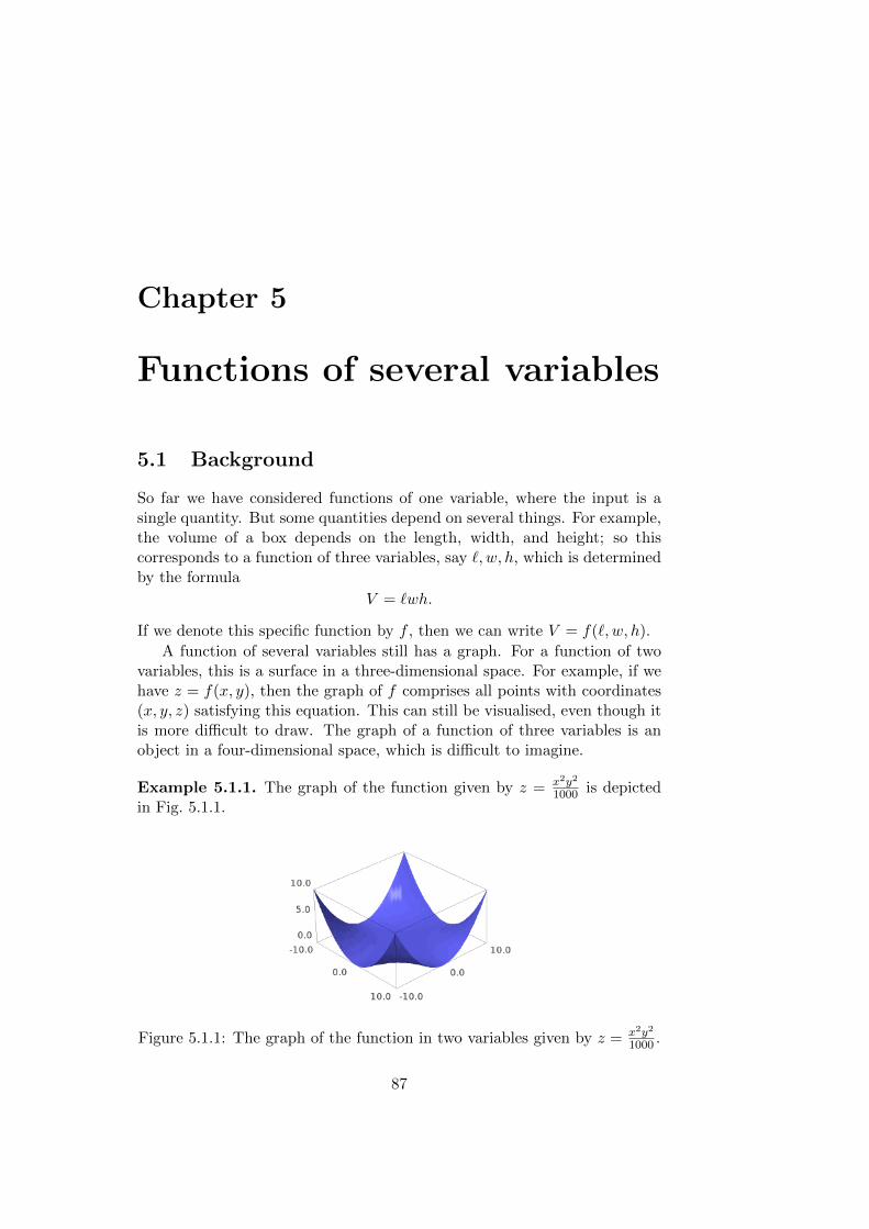
Chapter 5
Functions of several variables
5.1 Background
So far we have considered functions of one variable, where the input is asingle quantity. But some quantities depend on several things. For example,the volume of a box depends on the length, width, and height; so thiscorresponds to a function of three variables, say `, w, h, which is determinedby the formula
V = `wh.
If we denote this specific function by f , then we can write V = f(`, w, h).
A function of several variables still has a graph. For a function of twovariables, this is a surface in a three-dimensional space. For example, if wehave z = f(x, y), then the graph of f comprises all points with coordinates(x, y, z) satisfying this equation. This can still be visualised, even though itis more difficult to draw. The graph of a function of three variables is anobject in a four-dimensional space, which is difficult to imagine.
Example 5.1.1. The graph of the function given by z = x2y2
1000 is depictedin Fig. 5.1.1.
Figure 5.1.1: The graph of the function in two variables given by z = x2y2
1000 .
87
88 CHAPTER 5. FUNCTIONS OF SEVERAL VARIABLES
Most of the things we have seen so far have generalisations for functionsin several variables. We will discuss differentiation in particular here.
5.2 Partial derivatives
The easiest way to differentiate a function in several variables is to treatit like a function in one variable. That is, we single out one variable andpretend that the other variables are constants. This has the advantage thatwe can use all the techniques seen earlier, but it has the disadvantage that wewill get only partial information, as we have ignored all the other variables.
Suppose, for example, that we have a function f , depending on thevariables x and y. If we ‘freeze’ y, then we have a function depending onlyon x. The derivative of this function is called the partial derivative of f withrespect to x and denoted by ∂f
∂x . This is still a function of x and y, so if we
evaluate it at a specific point, we write ∂f∂x (x, y). More formally, we have
∂f
∂x(x, y) = lim
h→0
f(x+ h, y)− f(x, y)
h.
Similarly, if we ‘freeze’ x and then differentiate, we obtain the partial deriva-tive with respect to y, denoted ∂f
∂y . Thus
∂f
∂y(x, y) = lim
h→0
f(x, y + h)− f(x, y)
h.
For functions of more than two variables, we can define partial derivativesthe same way, ‘freezing’ all variables but one. For a function of n variables,this gives rise to n different partial derivatives.
Example 5.2.1. For f(x, y) = xy2, we have
∂f
∂x(x, y) = y2 and
∂f
∂y(x, y) = 2xy.
Example 5.2.2. For f(x, y, z) = xey + cos z, we have
∂f
∂x(x, y, z) = ey,
∂f
∂y(x, y, z) = xey, and
∂f
∂z(x, y, z) = − sin z.
5.3 Tangent plane and linear approximation
We restrict our attention to functions of two variables here, because it isuseful to visualise the following concepts geometrically. Nevertheless, similarstatements are also valid for functions of more than two variables.
Just like the graph of a function of one variable can be approximated bythe tangent line near a specific point, for functions of two variables, we have

5.3. TANGENT PLANE AND LINEAR APPROXIMATION 89
an approximation by tangent planes. Suppose that we have z = f(x, y) for acertain function f . Fix a point (x0, y0) in the plane. Then for z0 = f(x0, y0),the point (x0, y0, z0) belongs to the graph of f . If we want to determine thetangent plane at this point, we can again ‘freeze’ one variable. If we fixy0, then effectively we consider the intersection of the graph with the planegiven by y = y0. The intersection of the tangent plane with the planey = y0 corresponds to the tangent line to the graph of the function given byz = f(x, y0), which is now a function in one variable (see Fig. 5.3.1). Thistangent line is given by the equations
z = f(x0, y0) +∂f
∂x(x0, y0)(x− x0),
y = y0.
If we ‘freeze’ x = x0, we obtain another line, given by
Figure 5.3.1: The graph of the function f with f(x, y) = 1 − x2+y2
20 (blue)together with its tangent plane at (2, 2, 35) (green), the plane given by y = 2(grey) and the intersection of these planes (red)
z = f(x0, y0) +∂f
∂y(x0, y0)(y − y0),
x = x0.
The tangent plane is the plane containing both of these lines. It is given bythe equation
z = f(x0, y0) +∂f
∂x(x0, y0)(x− x0) +
∂f
∂y(x0, y0)(y − y0).
Why is this useful? Sometimes we want to compute approximate valuesof a function using a linear approximation, and for a function in two vari-ables, the tangent plane tells us what the appropriate linear approximationis. Recall the Taylor polynomials for functions in one variable from Sect.
90 CHAPTER 5. FUNCTIONS OF SEVERAL VARIABLES
2.5. In its simplest form, Taylor’s theorem says that for a function g of onevariable, we have
g(x) ≈ g(x0) + g′(x0)(x− x0),provided that x is near x0. For a function f of two variables, the corre-sponding statement is:
f(x, y) ≈ f(x0, y0) +∂f
∂x(x0, y0)(x− x0) +
∂f
∂y(x0, y0)(y − y0).
Again this holds if x is near x0 and y is near y0. Sometimes it is moreconvenient to write the formula in terms of the differences δx = x− x0 andδy = y − y0. Then it becomes
f(x0 + δx, y0 + δy) ≈ f(x0, y0) +∂f
∂x(x0, y0)δx+
∂f
∂y(x0, y0)δy.
This is valid for small values of δx and δy.For a function of three variables, the corresponding formula is:
f(x, y, z) ≈ f(x0, y0, z0) +∂f
∂x(x0, y0, z0)(x− x0)
+∂f
∂y(x0, y0, z0)(y − y0) +
∂f
∂z(x0, y0, z0)(z − z0)
or
f(x0 + δx, y0 + δy, z0 + δz) ≈ f(x0, y0, z0) +∂f
∂x(x0, y0, z0)δx
+∂f
∂y(x0, y0, z0)δy +
∂f
∂z(x0, y0, z0)δz
For functions of more than three variables, we have to modify it accordingly.
5.4 Total derivatives
Suppose that z = f(x, y) for a certain function f , and the quantities x andy both depend on another quantity, say t (so they correspond to certainfunctions, too). This makes z depend on t, and we may ask what dz
dt is. Thisis called the total derivative of z with respect to t.
In order to answer this question, we need a version of the chain rule fromSect. 2.2.4 for functions in several variables. For the situation describedabove, this is
dz
dt=∂z
∂x
dx
dt+∂z
∂y
dy
dt. (5.4.1)
Similar rules hold for functions of three or more variables. For example, ifw = f(x, y, z), and x, y, and z all depend on t, then
dw
dt=∂w
∂x
dx
dt+∂w
∂y
dy
dt+∂w
∂z
dz
dt.
5.5. SECOND DERIVATIVES 91
A situation that is very common, especially if t stands for time, is thatwe have z = f(t, x, y) (possibly involving other variables as well). Then wecan use the same chain rule and observe in addition that dt
dt = 1. This gives
dz
dt=∂z
∂t+∂z
∂x
dy
dt+∂z
∂y
dy
dt.
We can see why we have these formulas using the linear approximationsfrom the preceding section. For example, in the situation z = f(x, y), wehave
f(x+ δx, y + δy) ≈ f(x, y) +∂z
∂xδx+
∂z
∂yδy.
Moreover,
δx ≈ dx
dtδt and δy ≈ dy
dtδt,
so thatf(x+ δx, y + δy)− f(x, y)
δt≈ ∂z
∂x
dx
dt+∂z
∂y
dy
dt.
The left-hand side is a difference quotient and will converge to dzdt when we
let δt→ 0. This gives rise to formula (5.4.1).
Example 5.4.1. A particle moves in a circular motion on the plane, so thatits coordinates at time t are given by x = cos t, y = sin t. The concentrationc of some chemical at time t at the point (x, y) is given by exy sin t. Whatis the rate of change of the concentration experienced by the particle?Solution. We have
dc
dt=∂c
∂t+∂c
∂x
dx
dt+∂c
∂y
dy
dt= exy cos t− exy sin2 t+ ex sin t cos t.
5.5 Second derivatives
If we compute the partial derivatives of a function f(x, y) of two variables, weobtain two new functions ∂f
∂x (x, y) and ∂f∂y (x, y). Both of them are functions
of two variables again. So we can try to differentiate them as well. Ifsuccessful, we get the second order partial derivatives of f . These are
∂2f
∂x2(x, y) =
∂
∂x
(∂f
∂x(x, y)
),
∂2f
∂x∂y(x, y) =
∂
∂x
(∂f
∂y(x, y)
),
∂2f
∂y∂x(x, y) =
∂
∂y
(∂f
∂x(x, y)
),
∂2f
∂y2(x, y) =
∂
∂y
(∂f
∂y(x, y)
).
Example 5.5.1. If f(x, y) = x3 cos y, then
∂f
∂x(x, y) = 3x2 cos y and
∂f
∂y(x, y) = −x3 sin y.
92 CHAPTER 5. FUNCTIONS OF SEVERAL VARIABLES
Hence
∂2f
∂x2(x, y) = 6x cos y,
∂2f
∂x∂y(x, y) = −3x2 sin y,
∂2f
∂y∂x(x, y) = −3x2 sin y,
∂2f
∂y2(x, y) = −x3 cos y.
It is no coincidence that two of the expressions in this example are thesame. It is in fact always true that
∂2f
∂x∂y(x, y) =
∂2f
∂y∂x(x, y).
Thus we only need to calculate three second derivatives for a function of twovariables.
For a function f(x, y, z) of three variables, we may differentiate the par-tial derivatives ∂f
∂x (x, y, z), ∂f∂y (x, y, z), and ∂f
∂z (x, y, z) once more and weobtain
∂2f
∂x2(x, y, y),
∂2f
∂x∂y(x, y, z),
∂2f
∂x∂z(x, y, z),
∂2f
∂y∂x(x, y, z)
∂2f
∂y2(x, y, z),
∂2f
∂y∂z(x, y, z),
∂2f
∂z∂x(x, y, z)
∂2f
∂z∂y(x, y, z),
∂2f
∂z2(x, y, z).
In practice, we don’t have to calculate all of these, as
∂2f
∂x∂y=
∂2f
∂y∂x,
∂2f
∂x∂z=
∂2f
∂z∂x, and
∂2f
∂y∂z=
∂2f
∂z∂y.
Of course we can differentiate more than twice, and we use similar no-tation for these higher order partial derivatives, e.g.,
∂3f
∂y3or
∂5f
∂x3∂y2.
5.6 Applications
5.6.1 Maxima and minima
Just as for functions of one variable, a function of two variables, say z =f(x, y), has a local maximum at a given point (c, d) if f(x, y) ≤ f(c, d) forall points (x, y) in the immediate neighbourhood of (c, d). Similarly, we saythat f has a local minimum at (c, d) if f(x, y) ≥ f(c, d) for all points (x, y)in the immediate neighbourhood of (c, d).

5.6. APPLICATIONS 93
For functions of one variable, we can typically find the local minima andmaxima by considering the derivative. For functions of several variables, wecan apply similar principles.
Suppose that f has a local maximum at the point (c, d). Then considerthe function g obtained by ‘freezing’ the second variable. That is, g(x) =f(x, d). This function automatically has a local maximum at c, and if aderivative exists, then we know that it has to vanish at c. But of course thederivative of g is the partial derivative of f . So
∂f
∂x(c, d) = 0.
Similarly, ‘freezing’ the first variable, we see that
∂f
∂y(c, d) = 0.
Also, the same applies to local minima. Therefore, if we look for localmaxima or minima, we can get a set of candidates by solving this pair ofequations for c and d.
Example 5.6.1. Find the local maxima and minima of z = f(x, y) =(1− x2)2 + y2.Solution. We compute
∂f
∂x(x, y) = −4x(1− x2),
∂f
∂y(x, y) = 2y.
Thus we need to solve the system of equations
−4x(1− x2) = 0,
2y = 0.
The second equation is easy to solve: y = 0. The first one we can factorise,as
−4x(1− x2) = −4x(1− x)(1 + x).
We obtain the solutions x = 0, x = 1, and x = −1. For the system consistingof both equations, we have the solutions (0, 0), (1, 0), and (−1, 0).
It is not difficult to see that (1, 0) and (−1, 0) are local minima. This isbecause f(±1, 0) = 0, while f(x, y) ≥ 0 everywhere. The other point, (0, 0),is less obvious. Here we need other ways to decide.
As for the case of functions of one variable, we can usually (but notalways) distinguish between local maxima, local minimia, and other candi-dates using second derivatives. The following criteria apply

94 CHAPTER 5. FUNCTIONS OF SEVERAL VARIABLES
• If ∂f∂x (c, d) = 0 and ∂f
∂y (c, d) = 0, and in addition,
∂2f
∂x2(c, d) +
∂2f
∂y2(c, d) < 0
and∂2f
∂x2(c, d)
∂2f
∂y2(c, d)−
(∂2f
∂x∂y(c, d)
)2
> 0,
then f has a local maximum at (c, d).
• If ∂f∂x (c, d) = 0 and ∂f
∂y (c, d) = 0, and in addition,
∂2f
∂x2(c, d) +
∂2f
∂y2(c, d) > 0
and∂2f
∂x2(c, d)
∂2f
∂y2(c, d)−
(∂2f
∂x∂y(c, d)
)2
> 0,
then f has a local minimum at (c, d).
• If ∂f∂x (c, d) 6= 0 or ∂f
∂y (c, d) 6= 0 or
∂2f
∂x2(c, d)
∂2f
∂y2(c, d)−
(∂2f
∂x∂y(c, d)
)2
< 0,
then f has neither a local maximum nor a local minimum at (c, d).
Example 5.6.2. In Example 5.6.1, we compute
∂2f
∂x2(x, y) = 12x2 − 4,
∂2f
∂x∂y(x, y) = 0,
∂2f
∂y2(x, y) = 2.
Thus∂2f
∂x2(0, 0)
∂2f
∂y2(0, 0)−
(∂2f
∂x∂y(0, 0)
)= −8.
So we have neither a local minimum nor a local maximum at (0, 0).
The method is not restricted to two variables. For example, for a functionf(x, y, z) of three variables, we would solve the system
∂f
∂x(x, y, z) = 0,
∂f
∂y(x, y, z) = 0,
∂f
∂z(x, y, z) = 0,
in order to find candidates for local maxima or minima. It is still possibleto use second derivatives in order to distinguish between local maxima andlocal minima, but this is rather more complicated for functions in threevariables and is not discussed here.
5.6. APPLICATIONS 95
5.6.2 Exact differential equations
Occasionally problems for functions of one variable become easier when wereformulate it in terms of functions of several variables. Here we considerordinary differential equations of the form
M(x, y) +N(x, y)dy
dx= 0, (5.6.1)
where M and N are two given functions in two variables.
Example 5.6.3. The differential equation
ydy
dx= sin(x+ y)
can be written in this form, where M(x, y) = − sin(x+ y) and N(x, y) = y.(But there are other ways to do it. For example, the choice M(x, y) =
− sin(x+y)y and N(x, y) = 1 would have produced the required form, too.)
Suppose that we look for solutions y(x) of (5.6.1) that are given implicitlythrough an equation of the form h(x, y) = 0. Then the total derivative ofz = h(x, y) with respect to x is
dz
dx=∂h
∂x+∂h
∂y
dy
dx.
But since z = h(x, y) = 0, we must have the equation dzdx = 0. So
∂h
∂x+∂h
∂y
dy
dx= 0.
(This is in fact just an example of implicit differentiation. If we consider afunction y = y(x) given implicitly by the equation h(x, y) = 0, then implicitdifferentiation gives this formula.) Comparing this equation with (5.6.1), wesee that we will get a solution if we can find h such that
∂h
∂x(x, y) = M(x, y) and
∂h
∂y(x, y) = N(x, y).
It is not always possible to solve this system of equations. In fact, if wehave a solution, then it will necessarily satisfy
∂2h
∂x∂y=
∂2h
∂y∂x,
as we have seen in Sect. 5.5. In terms of M and N , this is expressed asfollows:
∂M
∂y=∂N
∂x. (5.6.2)
96 CHAPTER 5. FUNCTIONS OF SEVERAL VARIABLES
If (5.6.2) is satisfied, then we say that the differential equation (5.6.1) isexact . If (5.6.2) is not satisfied, then there is no chance to solve (5.6.1) withthis method. On the other hand, if our equation is exact, then it turns outthat we can solve the above system for h, and this will give a solution of(5.6.1) in implicit form.
Example 5.6.4. Consider the differential equation
2x+ y2 + (2xy + 1)dy
dx= 0.
This is of the form (5.6.1) with M(x, y) = 2x + y2 and N(x, y) = 2xy + 1.We first check that the equation is exact, computing
∂M
∂y= 2y and
∂N
∂x= 2y.
Thus we may attempt the method, to which end we need to solve
∂h
∂x(x, y) = 2x+ y2 and
∂h
∂y(x, y) = 2xy + 1.
In order to find h, we first consider the first equation only. If we fix y,then this just means that we need to find an antiderivative of the function2x+ y2 (with respect to the variable x). Hence
h(x, y) = x2 + xy2 + C(y)
for some integration ‘constant’ C(y), which is important here and may de-pend on y. (So it is a function of y rather than a proper constant.) We nowneed to determine C(y), and to this end, we consider the second equationfor h. Inserting the expression that we already have, we obtain
2xy +dC
dy= 2xy + 1.
So we find that dCdy = 1, which implies that C(y) = y + c for another
integration constant c. This finally gives
h(x, y) = x2 + xy2 + y + c.
That is, we have found implicit solutions of the differential equations interms of the equation
x2 + xy2 + y + c = 0.
If we want the solution explicitly, we have to solve this for y. It is aquadratic equation in y, so we can do that and we get
y =−1±
√1− 4x(x2 + c)
2x.
5.6. APPLICATIONS 97
Example 5.6.5. Consider the equation
y cosx+ 2xey + (sinx+ x2ey − y2)dydx
= 0.
Here we set M(x, y) = y cosx + 2xey and N(x, y) = sinx + x2ey − y2 andcheck that
∂M
∂y= cosx+ 2xey =
∂N
∂x.
So the equation is exact. We need to solve
∂h
∂x= y cosx+ 2xey and
∂h
∂y= sinx+ x2ey − y2.
The first equation implies that
h(x, y) = y sinx+ x2ey + C(y)
for some function C(y). The second equation implies that
sinx+ x2ey +dC
dy= sinx+ x2ey − y2.
Hence C(y) = c− y3
3 , and we have solutions of the differential equation givenimplicitly in terms of the equation
y sinx+ x2ey − y3
3+ c = 0.
In this case, it’s difficult to find an explicit representation, so we leave it inthis form.

98 CHAPTER 5. FUNCTIONS OF SEVERAL VARIABLES

Index
antiderivative, 47arccosine, 15arcsine, 15arctangent, 16
backward Euler method, 83base, 9
continuous, 23cosine, 12cubic function, 8
definite integral, 49degree, 9dependent variable, 6derivative, 27difference quotient, 27differential equation, 73
equation, 5Euler’s method, 82exact differential equation, 96exponent, 9exponential decay, 10exponential function, 9exponential growth, 10
factorisation, 8first fundamental theorem of
calculus, 49forward Euler method, 82function, 5
graph, 6
harmonic form, 18homogeneous, 77hyperbolic cosine, 16
hyperbolic sine, 16
implicit method, 84
improper integral, 71
indefinite integral, 47
independent variable, 6
infinite Taylor expansion, 42
initial value problem, 74
inverse function, 11, 34
inverse trigonometric functions, 14
limit, 20
limits of an integral, 49
linear function, 7
local maximum, 37, 92
local minimum, 37, 92
logarithm, 11
Maclaurin polynomial, 41
one-sided limit, 21
parametrisation, 35
partial derivative, 88
polar coordinates, 16
polynomial, 9
primitive, 47
product rule, 30
quadratic equation, 7
quadratic function, 7
quartic function, 8
quotient rule, 31
Runge-Kutta methods, 85
second derivative, 28
99
100 INDEX
second fundamental theorem ofcalculus, 50
separable differential equation, 74separation of variables, 74signed area, 48sine, 12step size, 82substitution rule, 51sum rule, 30
Taylor expansion, 41Taylor polynomial, 41Taylor series, 42Taylor’s theorem, 42total derivative, 90trapezium method, 85trigonometric functions, 12
unit circle, 12
zero, 6