Lightweight Structures for Remote Areas - University of Bath
325
Lightweight Structures for Remote Areas Jessica Bak A thesis submitted for the degree of Doctor of Philosophy University of Bath Department of Architecture and Civil Engineering December 2015 COPYRIGHT Attention is drawn to the fact that copyright of this thesis rests with the author. A copy of this thesis has been supplied on condition that anyone who consults it is understood to recognise that its copyright rests with the author and that they must not copy it or use material from it except as permitted by law or with the consent of the author. This thesis may be made available for consultation within the University Library and may be photocopied or lent to other libraries for the purposes of consultation. Jessica Bak
-
Upload
khangminh22 -
Category
Documents
-
view
1 -
download
0
Transcript of Lightweight Structures for Remote Areas - University of Bath

Lightweight Structuresfor Remote Areas
Jessica Bak
A thesis submitted for the degree of Doctor of Philosophy
University of Bath
Department of Architecture and Civil Engineering
December 2015
COPYRIGHT
Attention is drawn to the fact that copyright of this thesis rests with theauthor. A copy of this thesis has been supplied on condition that anyone whoconsults it is understood to recognise that its copyright rests with the authorand that they must not copy it or use material from it except as permitted bylaw or with the consent of the author.
This thesis may be made available for consultation within the UniversityLibrary and may be photocopied or lent to other libraries for the purposesof consultation.
Jessica Bak


This thesis is dedicated to my husband Andreas and daughter Isabel.
i


Acknowledgements
I firstly want to thank to the Chilean Council for Science and Technology(CONICYT) for providing me with this opportunity by funding my MPhil andPhD studies at the University of Bath.
My sincerest gratitude goes to my supervisor, Dr. Paul Shepherd, whose knowl-edge, creativity and support has been essential for the fulfillment of this endeavour. Iam truly honoured to have completed this research under Dr. Shepherd’s supervisionand have been part of the Digital Architectonics Research Group.
This thesis would have not been possible without the invaluable advice and uncondi-tional support of Andreas Bak, from Søren Jensen’s Computational Design Group.I certainly cannot not express my gratitude for the help received at different stagesof my research.
I also want to thank my second supervisor, Professor Paul Richens, for providingme with enlightening advice, particularly during the early stages of my studies, aswell as my examiners, Dr. Chris Williams and Professor Andrew Ballantyne,for making my Viva such an enjoyable experience.
Special thanks goes to Dr. Francisco Fernandoy for his guidance regardingantarctic subjects; as well as Gordon Dolbear and Aske Birkelund for theircontributions to the formatting and post-production of this thesis.
iii


Abstract
The Antarctic built environment is characterised for its particular occu-pational regimen and includes whole-year stations, small-scale seasonal stationand refuges, and temporary field camps. In recent years, Antarctic constructionhas begun to be considered of interest for the architectural and engineeringcommunities, and interesting efforts have been made to provide solutions forspanning building, energy efficiency and improvements in indoor habitability.
A fascinating array of lightweight constructions can be identified, whosecontribution has not, until now, been fully documented and acknowledged.They represent remarkable examples of smart use of structural efficiency andminimal impact strategies enduring one of the harshest environments.
This research is design-led and is motivated by the extension of the useof lightweight structures in remote fragile areas. The research validates theconcept of polar lightweight design through a sound narrative describing thehistory and potential of this type of construction. For this, this research looksat the case of the Antarctic built environment.
Furthermore, this research proposes that extension in the use lightweightconstruction could offer a sustainable solution for the predicted increase in thenumber of settlements being established in Antarctica. Knowledge and solutionsachieved in this context can also be applied in other less demanding and fragilescenarios.
In this regard, advanced computational design tools have been extensivelyvalidated for the realisation of structural surfaces of high geometrical complex-ity. Parametric design tools, are of particular interest to this research, as theyallow the optimisation of a structure, either as a whole, or via its physicalcomponents. This research proposes that such tools can be employed for thedevelopment of Polar lightweight systems of larger scale and more complexconfigurations than currently seen.
The first part is dedicated to the documentation and systematic character-isation of the vernacular Subantarctic and Antarctic lightweight constructionsas structural systems. In the second part, the integration of polar constraintsin the design of a generic lightweight structural system using parametric designtools is developed, in order to demonstrate the potential of this field for thecreation of novel design methods and solutions. The particular case of a newmedium-scale seasonal station is used as a case-study.
v


CONTENTS
Contents
Preface 1
1 Context and Research Aim 71.1 Introduction . . . . . . . . . . . . . . . . . . . . . . . . . . . . . . . . 71.2 Occupation at the Antarctic region . . . . . . . . . . . . . . . . . . . 81.3 Overview of the Antarctic Built Environment . . . . . . . . . . . . . 121.4 Current Scenario and Perspectives for New Construction in Antarc-
tica . . . . . . . . . . . . . . . . . . . . . . . . . . . . . . . . . . . . 181.5 Design Brief for an Antarctic Seasonal Station . . . . . . . . . . . . 20
1.5.1 Scope . . . . . . . . . . . . . . . . . . . . . . . . . . . . . . . 201.5.2 Site Conditions . . . . . . . . . . . . . . . . . . . . . . . . . . 211.5.3 Environmental Conditions . . . . . . . . . . . . . . . . . . . . 221.5.4 Logistics Conditions . . . . . . . . . . . . . . . . . . . . . . . 221.5.5 Overall Requirements . . . . . . . . . . . . . . . . . . . . . . 23
1.6 Conclusions and Research Aim . . . . . . . . . . . . . . . . . . . . . 24
2 Characterisation of Antarctic and Subantarctic Lightweight Struc-tures 292.1 Introduction . . . . . . . . . . . . . . . . . . . . . . . . . . . . . . . 292.2 The Amundsen-Scott South Pole Station . . . . . . . . . . . . . . . . 332.3 The Teniente Arturo Parodi Polar Station (EPTAP) . . . . . . . . . 382.4 The Shockwave Tent . . . . . . . . . . . . . . . . . . . . . . . . . . . 432.5 Subantarctic Indigenous dwellings . . . . . . . . . . . . . . . . . . . . 47
2.5.1 The Kaweshkar (Alacalufe) Case . . . . . . . . . . . . . . . . 492.5.2 The Yámana (Yaghan) Case . . . . . . . . . . . . . . . . . . 512.5.3 The Selk’nam (Ona) Case. . . . . . . . . . . . . . . . . . . . . 532.5.4 The Tehuelche (Aoniken) Case . . . . . . . . . . . . . . . . . 56
2.6 Antarctic Portable Dwellings . . . . . . . . . . . . . . . . . . . . . . 622.6.1 ‘In the Footsteps of Scott’ Expedition Tent . . . . . . . . . . 632.6.2 Sastruggi Tent . . . . . . . . . . . . . . . . . . . . . . . . . . 642.6.3 The Apple . . . . . . . . . . . . . . . . . . . . . . . . . . . . . 67
2.7 Conclusions . . . . . . . . . . . . . . . . . . . . . . . . . . . . . . . . 69
vii

CONTENTS
3 Design Criteria 753.1 Introduction . . . . . . . . . . . . . . . . . . . . . . . . . . . . . . . . 753.2 Design Criteria . . . . . . . . . . . . . . . . . . . . . . . . . . . . . . 763.3 Geometric Scheme . . . . . . . . . . . . . . . . . . . . . . . . . . . . 77
3.3.1 Aggregation . . . . . . . . . . . . . . . . . . . . . . . . . . . 773.3.2 Adaptability . . . . . . . . . . . . . . . . . . . . . . . . . . . 80
3.4 Modularity versus Adaptability . . . . . . . . . . . . . . . . . . . . . 843.5 Design Scheme . . . . . . . . . . . . . . . . . . . . . . . . . . . . . . 943.6 Design Method . . . . . . . . . . . . . . . . . . . . . . . . . . . . . . 1033.7 Conclusions . . . . . . . . . . . . . . . . . . . . . . . . . . . . . . . . 103
4 Nodal Forces Method and Structural Components Design 1054.1 Introduction . . . . . . . . . . . . . . . . . . . . . . . . . . . . . . . . 1054.2 Sensitivity Study for a Single Trussed Arch . . . . . . . . . . . . . . 1064.3 General Characterisation of the Main Structural Component . . . . 1084.4 Method . . . . . . . . . . . . . . . . . . . . . . . . . . . . . . . . . . 1094.5 Basic Material Properties . . . . . . . . . . . . . . . . . . . . . . . . 114
4.5.1 Aluminium . . . . . . . . . . . . . . . . . . . . . . . . . . . . 1144.5.2 Composites . . . . . . . . . . . . . . . . . . . . . . . . . . . . 1154.5.3 Membranes . . . . . . . . . . . . . . . . . . . . . . . . . . . . 118
4.6 Calculation of External Loads on a Single Trussed Arch. . . . . . . 1184.6.1 Load Case 3: Wind Derived Loads as Nodal Forces . . . . . 1194.6.2 Load Case 2. Snow Derived Load as Nodal Forces . . . . . . 1204.6.3 Calculation Method of Nodal Forces . . . . . . . . . . . . . . 123
4.7 Interpretation of FE Model Results . . . . . . . . . . . . . . . . . . 1254.8 Variation Study . . . . . . . . . . . . . . . . . . . . . . . . . . . . . 129
4.8.1 Variation Study on the Arch’s Geometry . . . . . . . . . . . 1294.8.2 Variation Study for Joint Shape . . . . . . . . . . . . . . . . . 1374.8.3 Variation Study on the Number of Subdivisions . . . . . . . . 1404.8.4 Variation Study on the Arch’s Depth . . . . . . . . . . . . . 143
4.9 Conclusions . . . . . . . . . . . . . . . . . . . . . . . . . . . . . . . . 144
5 Multi-Objective Design Process 1475.1 Introduction . . . . . . . . . . . . . . . . . . . . . . . . . . . . . . . . 1475.2 Revision of pre-conditions for Sensitivity Study . . . . . . . . . . . . 149
5.2.1 Material properties . . . . . . . . . . . . . . . . . . . . . . . 1495.2.2 Pre-stress . . . . . . . . . . . . . . . . . . . . . . . . . . . . . 1495.2.3 Standardisation of Span Values . . . . . . . . . . . . . . . . . 150
5.3 Sensitivity study . . . . . . . . . . . . . . . . . . . . . . . . . . . . . 1515.3.1 Uniform Cross Section of Aluminium Joints . . . . . . . . . 152
viii

CONTENTS
5.3.2 Variations of Rod Cross-Sections According to Span. . . . . 1525.3.3 Variation of Arches’ Depth According to Span . . . . . . . . 1555.3.4 Grouping of Arches’ Attributes for Reduction of Internal Stresses
. . . . . . . . . . . . . . . . . . . . . . . . . . . . . . . . . . . 1565.3.5 Geometry-based Method to reduce Pre-stress in Arches . . . 1595.3.6 Uniform Load Condition of Arches’ Loaded Area . . . . . . . 165
5.4 Geometry-based Studies for the Reduction of Components . . . . . . 1735.4.1 Reduction of the Number of Nodes per Arch Group . . . . . 1765.4.2 Reduction on the Number of Different Joints . . . . . . . . . 188
5.5 Parametric Model . . . . . . . . . . . . . . . . . . . . . . . . . . . . 1975.6 Conclusions . . . . . . . . . . . . . . . . . . . . . . . . . . . . . . . . 203
6 Complementary Studies 2076.1 Introduction . . . . . . . . . . . . . . . . . . . . . . . . . . . . . . . . 2076.2 Study for Variable Configurations . . . . . . . . . . . . . . . . . . . 2076.3 Components Definition . . . . . . . . . . . . . . . . . . . . . . . . . . 213
6.3.1 Carbon Fibre Bars . . . . . . . . . . . . . . . . . . . . . . . . 2136.3.2 Angled Bar Connections . . . . . . . . . . . . . . . . . . . . 2146.3.3 Aluminium Crosses . . . . . . . . . . . . . . . . . . . . . . . . 2156.3.4 Membrane Patterning and voids . . . . . . . . . . . . . . . . 2256.3.5 Rigid Boundary Arches . . . . . . . . . . . . . . . . . . . . . 2286.3.6 Ending of tunnels . . . . . . . . . . . . . . . . . . . . . . . . 2336.3.7 Anchorages . . . . . . . . . . . . . . . . . . . . . . . . . . . . 234
6.4 Assembly sequence . . . . . . . . . . . . . . . . . . . . . . . . . . . . 2346.5 Examples of Possible Applications for the Glacier Union Case . . . . 2436.6 Conclusions . . . . . . . . . . . . . . . . . . . . . . . . . . . . . . . . 247
7 Conclusions 2497.1 Introduction . . . . . . . . . . . . . . . . . . . . . . . . . . . . . . . 2497.2 Contributions to Knowledge . . . . . . . . . . . . . . . . . . . . . . 2537.3 Theoretical implications . . . . . . . . . . . . . . . . . . . . . . . . . 2547.4 Limitation of this study . . . . . . . . . . . . . . . . . . . . . . . . . 2567.5 Future work . . . . . . . . . . . . . . . . . . . . . . . . . . . . . . . 2587.6 Final comments . . . . . . . . . . . . . . . . . . . . . . . . . . . . . . 260
Bibliography 261
Appendices
A Prospects on a Formfinding Method using Surface Evolver andParametric CAD Tools 273
ix

LIST OF FIGURES
A.1 The Surface Evolver . . . . . . . . . . . . . . . . . . . . . . . . . . . 273A.2 Integrated geometry-based method using a Catenoid . . . . . . . . . 277A.3 Testing Examples . . . . . . . . . . . . . . . . . . . . . . . . . . . . 279
A.3.1 First Optimization of an Extruded Free-Form Curve . . . . . 282A.3.2 Second Optimization of a Cylinder with a Free-Form Section 284
A.4 Further Work Using Surface Evolver . . . . . . . . . . . . . . . . . . 286A.4.1 Form-finding with oriented Boundaries . . . . . . . . . . . . 286A.4.2 Triple Periodic Minimal Surfaces . . . . . . . . . . . . . . . . 286A.4.3 Synclastic Surfaces Using other Energies . . . . . . . . . . . . 287
A.5 Conclusions . . . . . . . . . . . . . . . . . . . . . . . . . . . . . . . . 290A.6 References . . . . . . . . . . . . . . . . . . . . . . . . . . . . . . . . 290
B Calculations of Peak Velocity Pressure 293
C C-sharp Component for the Placement of Trussed Arches alonga NURBS Curve 297
List of Figures
1.1 Magallanic Penguin at the Antarctic Peninsula. . . . . . . . . . . . . 81.2 Antarctic territorial claim. . . . . . . . . . . . . . . . . . . . . . . . . 91.3 Villa las Estrellas (Chile), one of two Antarctic settlements for a
civilian community in Antarctica. . . . . . . . . . . . . . . . . . . . . 101.4 Map of Antarctic permanent and seasonal research stations’ locations. 101.5 Maximum summer capacity of Antarctica’s small scale stations. . . . 121.6 Early Antarctic Construction. . . . . . . . . . . . . . . . . . . . . . . 141.7 Industrial looking constructions. . . . . . . . . . . . . . . . . . . . . 141.8 Views of the ’City in Antarctica’ study project, an air hall as a
protection against climate over a residential town. . . . . . . . . . . 151.9 Halley VI, the 6th British base commissioned in 2009. . . . . . . . . 151.10 Germany’s Neumayer III Station, 1992. . . . . . . . . . . . . . . . . 151.11 Seasonal station and refuges. . . . . . . . . . . . . . . . . . . . . . . 171.12 Number of tourists visiting Antarctica during 1965-2007. . . . . . . . 191.13 Installation of the new ’Union Glacier Station, Ellsworth Hills. . . . 201.14 Location of the Union Glacier Station. . . . . . . . . . . . . . . . . . 22
2.1 Categories of surface structures in the context of structural system. . 32
x

LIST OF FIGURES
2.2 Gaussian curvature of surfaces. . . . . . . . . . . . . . . . . . . . . . 332.3 The Amundsen Scott Dome after snow removal in preparation to
deconstruction work. . . . . . . . . . . . . . . . . . . . . . . . . . . . 342.4 Artist’s concept of the design new USA South Pole’s design. . . . . . 342.5 Announcement of the competition of the new USA Polar Station. . . 342.6 Diagram of the South Pole Dome geodesic dome construction accord-
ing to manufacturer Temcor©. . . . . . . . . . . . . . . . . . . . . . . 362.7 1:10 scale model of Amundsen-Scott Station used to study snow drift
pattern. . . . . . . . . . . . . . . . . . . . . . . . . . . . . . . . . . . 362.8 Gusset plate showing installed Huck bolts for the Amundsen-Scott
Dome. . . . . . . . . . . . . . . . . . . . . . . . . . . . . . . . . . . . 372.9 Diagram for geodesic dome construction according to manufacturer
Temcor © . . . . . . . . . . . . . . . . . . . . . . . . . . . . . . . . . 372.10 Erection progress viewed from outside the South Pole dome as the
frame is hoisted up the tower. . . . . . . . . . . . . . . . . . . . . . . 372.11 Interior of the South Pole Dome’s dismounting party. . . . . . . . . . 382.12 Exterior of the South Pole Dome’s dismounting party. . . . . . . . . 382.13 Group of domes installed at the Union Glacier Station. . . . . . . . . 382.14 The EPTAP. . . . . . . . . . . . . . . . . . . . . . . . . . . . . . . . 382.15 Physical components at the EPTAP. . . . . . . . . . . . . . . . . . . 392.16 Delivery for the construction of the EPTAP. . . . . . . . . . . . . . . 402.17 Assembly of components for the EPTAP. . . . . . . . . . . . . . . . 402.18 Cutting pattern of the EPTAP’s PVC membrane. Image: Pol Taylor,
undated. . . . . . . . . . . . . . . . . . . . . . . . . . . . . . . . . . . 412.19 Membrane sections being attached to the structure for the EPTAP. . 412.20 Curved visors at the EPTAP. . . . . . . . . . . . . . . . . . . . . . . 422.21 The EPTAP after two years of service. . . . . . . . . . . . . . . . . . 432.22 Chilean Air force personnel unearthing the EPTAP after 14 years of
service. . . . . . . . . . . . . . . . . . . . . . . . . . . . . . . . . . . . 432.23 The Shockwave Tent in Villa Las Estrellas, Antarctica. . . . . . . . . 432.24 Side view of the Shockwave tent in its original version. . . . . . . . . 442.25 Stereometric structure of the Shockwave tent, Villa Las Estrellas. . . 442.26 Galvanised steel tubes used for the Shockwave Tent. . . . . . . . . . 452.27 Standard disc-shaped joint used in the Shockwave Tent. . . . . . . . 452.28 Tripod support used in the Shockwave Tent. . . . . . . . . . . . . . . 452.29 Stereometric truss for the Shockwave tent being assembled and trans-
ported. . . . . . . . . . . . . . . . . . . . . . . . . . . . . . . . . . . . 452.30 Reinforcement elements for the Shockwave Tent being installed using
the grid as a scaffolding. . . . . . . . . . . . . . . . . . . . . . . . . . 452.31 Original soft entrance cover designed of the Shockwave tent. . . . . . 46
xi

LIST OF FIGURES
2.32 Front view of Shockwave implemented in Villa Las Estrellas. . . . . 462.33 Proposal of an adaptation of the Shockwave structural system for a
hangar for the Chilean Air Force’s fighter aircraft in the AtacamaDesert. . . . . . . . . . . . . . . . . . . . . . . . . . . . . . . . . . . . 46
2.34 Map of the areas occupied by southern indigenous communities. . . . 482.35 Kaweshkar Dwelling, Puerto Eden, Chile. . . . . . . . . . . . . . . . 502.36 Reconstruction of a Kaweshkar in Puerto Eden. . . . . . . . . . . . . 502.37 Alacalufe dwelling’s components. . . . . . . . . . . . . . . . . . . . . 512.38 Last examples of Yaghan Dwellings in Lago Fagnano, Tierra del Fuego. 522.39 Structure of a cupula-shape Yagan dwelling with an elliptic base. . . 522.40 Diagram of a conic Yaghan dwelling and its main components. . . . 532.41 Dwelling of the southern Onas, made out of logs with the shape of an
inclined cone. . . . . . . . . . . . . . . . . . . . . . . . . . . . . . . . 542.42 Illustration of a dwelling of the northern Selk’nams with a ’sub-conic’
shape made during the years 1918-1924. . . . . . . . . . . . . . . . . 542.43 Photograph of a dwelling of the northern Selk’nams with a ’sub-conic’
shape taken during the years 1918 -1924. . . . . . . . . . . . . . . . . 542.44 Sketches of a windscreen used by the northern Selk’nams made during
the years 1918-1924. . . . . . . . . . . . . . . . . . . . . . . . . . . . 552.45 Tehuelche dwelling. . . . . . . . . . . . . . . . . . . . . . . . . . . . . 562.46 Diagram with the main elements of an Tehuelche tent according to
Baeriswyl. . . . . . . . . . . . . . . . . . . . . . . . . . . . . . . . . . 572.47 Diagram of a Tehuelche dwelling, made by Outes in 1905 based on
the description made in middle 18th century. . . . . . . . . . . . . . 572.48 Diagram of a Tehuelche dwelling based on the description of Viedma
made in middle 18th century. . . . . . . . . . . . . . . . . . . . . . . 582.49 Semi-spherical model of a Teheulche tent belonging to the nothern
Cacique Manikiken who posed with his family in Chubut, Argentinaat the end of 20th century. . . . . . . . . . . . . . . . . . . . . . . . . 59
2.50 Semi-spherical Tehuelche dwelling completely covered on fabric inSanta Cruz, Argentina. . . . . . . . . . . . . . . . . . . . . . . . . . . 60
2.51 Asymmetrical tent model from a Southern Tehuelche family. Halfstructure is covered with animal skins, while the smallest section iscovered with fabrics. . . . . . . . . . . . . . . . . . . . . . . . . . . . 60
2.52 Tent covered with horse skin belonging to the Caquique Cangapol,during middle 18th Century, reproduced by the Jesuit Falkner BuenosAires Province Argentina. . . . . . . . . . . . . . . . . . . . . . . . . 61
2.53 Touristic basecamp at Patriot Hills. . . . . . . . . . . . . . . . . . . 622.54 Touristic basecamp at Vinson Massif. . . . . . . . . . . . . . . . . . . 622.55 Frei Otto’s German Pavilion Expo ’67, Montreal. . . . . . . . . . . . 63
xii

LIST OF FIGURES
2.56 ’2-Meter Dome’ tent produced by The North Face. . . . . . . . . . . 632.57 BAS Antarctic Expedition Tent. . . . . . . . . . . . . . . . . . . . . 632.58 Pyramid tent set up upon the King Edward VII Plateau as part of
1910-1913 British Antarctic Survey Expedition. . . . . . . . . . . . . 642.59 Sketches of the 1985 BAS double curved surface and structure’s tent
by designer Ian Liddel. . . . . . . . . . . . . . . . . . . . . . . . . . . 652.60 Sketch of the crown joint for the 1985 BAS d tent by designer Ian
Liddel. . . . . . . . . . . . . . . . . . . . . . . . . . . . . . . . . . . . 652.61 Sastruggi Room as part of the EPTAP Station, Antarctica. . . . . . 652.62 Diagram of the Sastruggi’s structure. . . . . . . . . . . . . . . . . . . 652.63 Articulated joint designed for the Sastruggi Tent. . . . . . . . . . . . 652.64 Cutting patterns of the Sastruggi Tent. . . . . . . . . . . . . . . . . . 662.65 Installation of insulation layers at the Sastruggi Room, Antarctica. . 672.66 The ’Apple’ hub installed in McMurdo Station, Antarctic. . . . . . . 672.67 The ’Melon’ hub set up in Antarctica. . . . . . . . . . . . . . . . . . 672.68 Panelling of the Apple and the Melon hubs. . . . . . . . . . . . . . . 682.69 Design scheme of a prototypical Antarctic field station. . . . . . . . . 682.70 Structural Characterisation of Polar lightweight Structures. . . . . . 732.71 Geometrical Characterization of Polar Lightweight Structures. . . . . 74
3.1 Comparative diagram of a volume’s compactness. . . . . . . . . . . . 783.2 Examples of arrangements for touristic settlement’s using lightweight
constructions. . . . . . . . . . . . . . . . . . . . . . . . . . . . . . . . 793.3 Evolution of the Schwarz’ P Surface using Surface Evolver. . . . . . 803.4 Prototype of the ‘Radiolaria Project’ (structural tessellation of double
curved surfaces) developed by University of Kassel, Germany. . . . . 813.5 Prototype of free-form gridshell based on geodesic method developed
by the Politecnico di Torino, Italy. . . . . . . . . . . . . . . . . . . . 813.6 Prototype of one the variations of the ‘Eccentric Umbrella Structure’
based on the Locust hind wing developed by the Israel Institute ofTechnology. . . . . . . . . . . . . . . . . . . . . . . . . . . . . . . . . 83
3.7 Military base camp in Afghanistan implemented by Wheatherhaven ©. 843.8 Construction phases of the EPTAP. . . . . . . . . . . . . . . . . . . 863.9 The Jotabeche Station. . . . . . . . . . . . . . . . . . . . . . . . . . . 873.10 Alternatives of variations of the anchor system, from left to right:
plates for snow and sand, crampons for rock, and shoes rocky soils. . 873.11 Assembly test for the Echaurren Glacier Monitoring Station. . . . . 883.12 Configuration of components for Echaurren Station. . . . . . . . . . 883.13 Configuration of components for Echaurren Station. . . . . . . . . . 893.14 Panul Warehouse. . . . . . . . . . . . . . . . . . . . . . . . . . . . . . 89
xiii

LIST OF FIGURES
3.15 Panul Shed. . . . . . . . . . . . . . . . . . . . . . . . . . . . . . . . . 893.16 Geometric scheme for Panul warehouse. . . . . . . . . . . . . . . . . 903.17 Geometric scheme for Panul shed. . . . . . . . . . . . . . . . . . . . . 903.18 Front view, progression of the Panul warehouse’s components. . . . . 913.19 Front view, progression of the Panul shed’s components. . . . . . . . 913.20 Model of the ‘Grotto Project’ developed by Aranda and Lash in
collaboration with ARUP. . . . . . . . . . . . . . . . . . . . . . . . . 923.21 Danzer Tillings. . . . . . . . . . . . . . . . . . . . . . . . . . . . . . . 933.22 Design process of the Grotto’s modular boulders. . . . . . . . . . . . 943.23 Design proposal for a kayaking station on an isthmus on the North
coast of Navarino Island. . . . . . . . . . . . . . . . . . . . . . . . . . 953.24 Three geographic milestones on north coast route were selected for
the kayaking circuit at Navarino Island, a harbour, an isthmus, andan islet. . . . . . . . . . . . . . . . . . . . . . . . . . . . . . . . . . . 95
3.25 Three geographic milestones selected for the kayaking circuit at NavarinoIsland. . . . . . . . . . . . . . . . . . . . . . . . . . . . . . . . . . . . 96
3.26 Architectural scheme of one of the three stations of the circuit, theisthmus-station. . . . . . . . . . . . . . . . . . . . . . . . . . . . . . . 96
3.27 Definition of the three set of arches for the station in Navarino Island. 973.28 Two different enclosures at the Navarino Island Kayak Station. . . . 973.29 Two semi-open structures being supported by trussed arches. . . . . 983.30 Lateral supporting trusses. . . . . . . . . . . . . . . . . . . . . . . . . 983.31 Cross-shaped pins joining the four flexible bars which compose a
‘primary arch’. . . . . . . . . . . . . . . . . . . . . . . . . . . . . . . 993.32 Cross-shaped pin joints serve also as a support for the two bracing
systems. . . . . . . . . . . . . . . . . . . . . . . . . . . . . . . . . . . 993.33 Rectangular pieces of PVC fabric forming the membrane. . . . . . . 1003.34 Regular triangulated grid bracing the structure. The image also shows
the radial distribution of the arches on the floor. . . . . . . . . . . . 1003.35 Equally degree distribution of joints along the arches. . . . . . . . . 1003.36 Scheme for set of reciprocate bracing cables. . . . . . . . . . . . . . . 1013.37 Anchorages designed as ties and supports for flexible arches. . . . . . 102
4.1 Original subdivision scheme with restrained arch width. . . . . . . . 1064.2 Second version for subdivision scheme with variable arch span. . . . 1064.3 Vierendeel Bridge at Grammene, Belgium. Source: McGill Univer-
sity’s School of Architecture, undated. . . . . . . . . . . . . . . . . . 1084.4 Adjustable parameters on single trussed arch. . . . . . . . . . . . . . 1104.5 Parametric pipeline. . . . . . . . . . . . . . . . . . . . . . . . . . . . 1124.6 Geometry variations. . . . . . . . . . . . . . . . . . . . . . . . . . . . 112
xiv

LIST OF FIGURES
4.7 Custom Robot API component. . . . . . . . . . . . . . . . . . . . . . 1134.8 Automatically generated FE-model. . . . . . . . . . . . . . . . . . . 1134.9 Presentation of results in Excel. . . . . . . . . . . . . . . . . . . . . . 1144.10 Geometric parameters on vaulted roof and domes for the valuation of
external pressure coefficients. . . . . . . . . . . . . . . . . . . . . . . 1194.11 Snow load shape coefficient for cylindrical roof. . . . . . . . . . . . . 1224.12 Calculation of curve segments for snow load factors. . . . . . . . . . 1224.13 Set of subdividing points on an arc for the calculation of nodal forces. 1254.14 Diagram of geometric attributes for calculation of nodal forces. . . . 1264.15 Numbering of nodes in an arch. . . . . . . . . . . . . . . . . . . . . . 1264.16 Characteristic distribution of internal axial and bending stresses along
a simply supported arch under compression for a symmetrical load case.1284.17 Combined normal stresses (S value) as the addition of axial and
bending stresses throughout section 1-1’ for a symmetrical load case. 1284.18 Different versions of trussed arches with 4 m span to be compared. . 1294.19 Schematic deformation of an aluminium joint under bending. . . . . 1344.20 Distribution of maximum S values on the arches’ bars in Model 1 due
to load case 6. . . . . . . . . . . . . . . . . . . . . . . . . . . . . . . . 1354.21 Distribution of maximum S values on the arches’ bars Model 2 due
to load case 6. . . . . . . . . . . . . . . . . . . . . . . . . . . . . . . . 1354.22 Distribution of maximum S values on the arches’ bars in Model 3 due
to load case 6. . . . . . . . . . . . . . . . . . . . . . . . . . . . . . . . 1354.23 Distribution of maximum S values on cross’s bars from Model 1 due
to load case 6. . . . . . . . . . . . . . . . . . . . . . . . . . . . . . . . 1354.24 Distribution of maximum S values on cross’s bars from Model 2 due
to load case 6. . . . . . . . . . . . . . . . . . . . . . . . . . . . . . . . 1354.25 Distribution of maximum S values on cross’s bars from Model 3 due
to load case 6. . . . . . . . . . . . . . . . . . . . . . . . . . . . . . . . 1354.26 Distribution of minimum S values on arch’s bars from Model 1 due
to load case 6. . . . . . . . . . . . . . . . . . . . . . . . . . . . . . . . 1364.27 Distribution of minimum S values on arch’s bars from Model 2 due
to load case 6. . . . . . . . . . . . . . . . . . . . . . . . . . . . . . . . 1364.28 Distribution of minimum S values on arch’s bars from Model 3 due
to load case 6. . . . . . . . . . . . . . . . . . . . . . . . . . . . . . . . 1364.29 Distribution of minimum S values on cross’s bars from Model 1 due
to load case 6. . . . . . . . . . . . . . . . . . . . . . . . . . . . . . . . 1364.30 Distribution of minimum S values on cross’s bars from Model 2 due
to load case 6. . . . . . . . . . . . . . . . . . . . . . . . . . . . . . . . 1364.31 Distribution of minimum S values on cross’s bars from Model 3 due
to load case 6. . . . . . . . . . . . . . . . . . . . . . . . . . . . . . . . 136
xv

LIST OF FIGURES
4.32 Deformations of Model 1 caused by combined loads. . . . . . . . . . 1374.33 Deformations of Model 2 caused by combined loads. . . . . . . . . . 1374.34 Deformations of Model 3 caused by combined loads. . . . . . . . . . 1374.35 Scheme for cross-shaped joints and diagonal cross-shape joints. . . . 1384.36 Variation fashion for diagonal-crosses joints. . . . . . . . . . . . . . . 1394.37 Sensitivity comparison of different geometric attributes for a single
trussed arch. . . . . . . . . . . . . . . . . . . . . . . . . . . . . . . . 145
5.1 Top view of a curve standardised with different values. . . . . . . . . 1505.2 Diagram of the different attributes, values and constraints assessed
for the definition of components. . . . . . . . . . . . . . . . . . . . . 1535.3 Cases of values’ segmentation. . . . . . . . . . . . . . . . . . . . . . . 1575.4 Angle between an arc’s segments according to different level of cur-
vature. . . . . . . . . . . . . . . . . . . . . . . . . . . . . . . . . . . . 1605.5 First geometry-based method for controlling the curvature of an arc’s
bar segments. . . . . . . . . . . . . . . . . . . . . . . . . . . . . . . . 1615.6 Second geometry-based method for controlling the curvature of an
arc’s bar segments. . . . . . . . . . . . . . . . . . . . . . . . . . . . . 1635.7 Definition of a ‘Surface Segment’ and ‘Gap’. . . . . . . . . . . . . . . 1655.8 oordination of attributes for uniform loaded condition of arches. . . . 1705.9 Coordination of attributes for the uniformity of distance between arches.1745.10 Triangulation of a set of arches with cases of variation on the number
of nodes of 2 units. . . . . . . . . . . . . . . . . . . . . . . . . . . . . 1775.11 Number of different aluminium joint when differentiated number of
arches’ nodes according to span segment. . . . . . . . . . . . . . . . 1785.12 Two examples of nodes lacing with different subdivision approaches:
(a) equal angle-distance and (b) equal linear distance. . . . . . . . . 1795.13 Lacing of a set of arcs with increasing number of subdivision starting
from the first arc (Case 1). . . . . . . . . . . . . . . . . . . . . . . . . 1795.14 Lacing of a set of arcs with increasing number of subdivisions starting
from the second arc (Case 2). . . . . . . . . . . . . . . . . . . . . . . 1795.15 Lacing of a set of arcs with increasing number of subdivisions with
last lacing step altered to ‘n(i,j) to n(i+1,j+2)’ (Case 3). . . . . . . . . 1805.16 Lacing of a set of arcs with increasing number of subdivisions with
the second sequence inverted (Case 4). . . . . . . . . . . . . . . . . . 1805.17 Solution A. Lacing of a set of arcs with increasing number of subdi-
visions with last lacing step altered to ‘n(i,j) to n(i+1,j)’ (Case 5). . . 1815.18 Lacing with an increasing number of nodes with the sequence inverted
from second arch onwards. (Case 6). . . . . . . . . . . . . . . . . . . 182
xvi

LIST OF FIGURES
5.19 Solution B for continuous lacing with an increasing number of nodes(Case 7). . . . . . . . . . . . . . . . . . . . . . . . . . . . . . . . . . . 182
5.20 Three dimensional test of solution A in an arbitrary set of arches. . . 1835.21 Three-dimensional test of solution B in an arbitrary set of arches. . . 1845.22 Three-dimensional test of lacing scheme starting from central node
toward both sides. . . . . . . . . . . . . . . . . . . . . . . . . . . . . 1855.23 Three-dimensional test of a lacing method starting from a central
node and where specific even-divided arcs have altered the number ofnode to n+ 1. . . . . . . . . . . . . . . . . . . . . . . . . . . . . . . . 186
5.24 Three-dimensional test of a lacing method starting from a centralnode and where specific even-divided arcs have altered the number ofnode to n− 1. . . . . . . . . . . . . . . . . . . . . . . . . . . . . . . . 186
5.25 Flow chart for nodes’ lacing continuity assessment. . . . . . . . . . . 1905.26 Simplified flow chart for nodes’ lacing continuity assessment. . . . . 1915.27 Scheme for an adaptable aluminium joint. . . . . . . . . . . . . . . 1915.28 Early model of a adaptable joint (Model 4). . . . . . . . . . . . . . . 1945.29 First example of the parametric model applied on a curve. . . . . . . 2015.30 Second example of the parametric model applied on curve. . . . . . . 2025.31 Third example of the parametric model applied on a curve. . . . . . 203
6.1 Two membrane tunnels meeting perpendicularly. . . . . . . . . . . . 2086.2 Three units meeting together. . . . . . . . . . . . . . . . . . . . . . . 2096.3 Three units meeting at the same point using a synclastic membrane. 2106.4 Set of four units meeting at the same point. . . . . . . . . . . . . . . 2116.5 Four different units meeting on a non-orthogonal configuration. . . . 2116.6 Rigid arch being used as reinforcement element for long tunnels and
lateral voids. . . . . . . . . . . . . . . . . . . . . . . . . . . . . . . . 2126.7 Conflict between two membranes pieces meeting perpendicularly. . . 2136.8 List of the bars’ length on a surface output by the parametric model
for two subsequent arches with the same span. . . . . . . . . . . . . 2156.9 Diagram of the bars’ length in a surface output by the parametric
model. . . . . . . . . . . . . . . . . . . . . . . . . . . . . . . . . . . . 2166.10 Sketch of an aluminium ring attached to a joint. . . . . . . . . . . . 2176.11 Sketch of a set of pieces for an aluminium ring. . . . . . . . . . . . . 2176.12 Second proposal for an aluminium ring set. . . . . . . . . . . . . . . 2186.13 Study of variations for angled connectors. . . . . . . . . . . . . . . . 2196.14 Assembling sequence of an aluminium ring, angled connection, carbon-
fibre bars and scissor-shaped joint. . . . . . . . . . . . . . . . . . . . 2206.15 Model of an aluminium ring and angled connection. . . . . . . . . . 220
xvii
LIST OF FIGURES
6.16 Lists of an arch’s joint typified their length and angle produced bythe Grasshopper model. . . . . . . . . . . . . . . . . . . . . . . . . . 221
6.17 Surface with aluminium joints identified by colours according to length-based type. . . . . . . . . . . . . . . . . . . . . . . . . . . . . . . . . 222
6.18 First version of an aluminium joint. . . . . . . . . . . . . . . . . . . . 2236.19 Second version of an aluminium joint. . . . . . . . . . . . . . . . . . 2236.20 Sketch of a scissor-shaped joint connected to the membrane. . . . . . 2246.21 Model of a scissor-shape joint. . . . . . . . . . . . . . . . . . . . . . 2256.22 Sketch of connection between consecutives membrane pieces. . . . . 2266.23 Example of a set of membrane cutting pattern obtained from the
parametric model. . . . . . . . . . . . . . . . . . . . . . . . . . . . . 2276.24 Assessment of surface curvature. . . . . . . . . . . . . . . . . . . . . 2286.25 Section and profile of a rigid arch. . . . . . . . . . . . . . . . . . . . 2296.26 Proposal for assembling of rigid arches. . . . . . . . . . . . . . . . . . 2316.27 Rigid arch designed for perpendicular intersections with flexible arches.2316.28 Cases of spanning arches supported by a lateral boundary arch. . . . 2326.29 Spanning arches intersecting a boundary arch at irregular intervals. . 2326.30 Front and back view of an intersection between a boundary arch and
a set of 4 m span spanning arches. . . . . . . . . . . . . . . . . . . . 2336.31 Proposal for a membrane cover as an ending element. . . . . . . . . 2336.32 Rigid curved panels as a closing element. . . . . . . . . . . . . . . . . 2346.33 Sequences for the preparation of crosses. . . . . . . . . . . . . . . . . 2366.34 Marking the location of arches on site and installing anchorages. . . 2376.35 Boundary arch assembling. . . . . . . . . . . . . . . . . . . . . . . . 2376.36 Boundary arch completed. . . . . . . . . . . . . . . . . . . . . . . . 2376.37 Boundary arch with membrane piece attached. . . . . . . . . . . . . 2386.38 Assembling arches from bottom to top. . . . . . . . . . . . . . . . . . 2386.39 Completed flexible arch. . . . . . . . . . . . . . . . . . . . . . . . . . 2386.40 Installation of membrane segments. . . . . . . . . . . . . . . . . . . . 2386.41 Flexible arch reinforced with lateral cables. . . . . . . . . . . . . . . 2396.42 Installation of bracing cables between two arches. . . . . . . . . . . . 2396.43 Aluminium scissor joint with all components connected. . . . . . . . 2406.44 Progression of arches instalment. . . . . . . . . . . . . . . . . . . . . 2416.45 Direction for the membrane piece’s deployment. . . . . . . . . . . . . 2416.46 Progression of membrane segments deployment. . . . . . . . . . . . . 2426.47 Handmade sketch of side view of an early design scheme. . . . . . . . 2436.48 Side view of early design scheme with basic type of components recog-
nise by colour. . . . . . . . . . . . . . . . . . . . . . . . . . . . . . . 2436.49 Handmade sketch of plan diagram for an early design scheme. . . . . 244
xviii
LIST OF TABLES
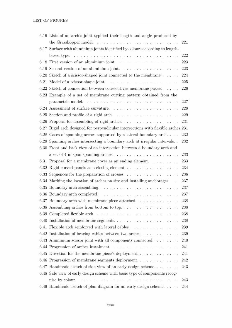
6.50 Top view of early design scheme with basic type of components recog-nised by colour. . . . . . . . . . . . . . . . . . . . . . . . . . . . . . . 244
6.51 Architectural plan for a design scheme. . . . . . . . . . . . . . . . . . 2456.52 Isometric view of design scheme. . . . . . . . . . . . . . . . . . . . . 2456.53 Isometric view of design scheme. . . . . . . . . . . . . . . . . . . . . 2466.54 Isometric view of design scheme. . . . . . . . . . . . . . . . . . . . . 2466.55 Bar types identified according to length using colour code, side view. 2476.56 Bar types identified according to length using colour code, perspective
view. . . . . . . . . . . . . . . . . . . . . . . . . . . . . . . . . . . . . 247
List of Tables
1.1 Variation of Population in Antarctica. . . . . . . . . . . . . . . . . . 111.2 Assessment of environmental impact derived from maintenance activ-
ities of the XL Scientific Antarctic Expedition 2005-2006. . . . . . . 161.3 Average number of occupants in the University of Magallanes Re-
search Station. . . . . . . . . . . . . . . . . . . . . . . . . . . . . . . 241.4 Domestic facilities for University of Magallanes Research Station. . 251.5 Technical facilities for University of Magallanes Research Station. . . 261.6 Scientific facilities for University of Magallanes Research Station. . . 27
4.1 Parameters and Initial Values of a Generic Single Arch. . . . . . . . 1104.2 Characteristic Mechanical Properties of Aluminium. . . . . . . . . . 1154.3 Characteristic Mechanical Properties of GFRP at room temperature. 1174.4 Characteristic Mechanical Properties for GFRP between 20 °C and
−60 °C. . . . . . . . . . . . . . . . . . . . . . . . . . . . . . . . . . . 1174.5 Cartesian Values of Nodal Forces Derived from Snow and Wind on a
4[m] span Arch. . . . . . . . . . . . . . . . . . . . . . . . . . . . . . . 1274.6 Extreme combined internal stresses on Model 1, 2 and 3. . . . . . . . 1314.7 Maximum Smax values on an arch’s bars by load cases in Models 1, 2
and 3. . . . . . . . . . . . . . . . . . . . . . . . . . . . . . . . . . . . 1314.8 Minimum Smin values on an arch’s bars by load cases in Models 1, 2
and 3. . . . . . . . . . . . . . . . . . . . . . . . . . . . . . . . . . . . 1314.9 Maximum Smaxvalues on joints bars by load cases in Models 1, 2 and 3.1324.10 Minimum Smin values on joints bars by load cases in Models 1, 2 and 3.1324.11 Maximum nodes displacement on Models 1, 2 and 3. . . . . . . . . . 137
xix
LIST OF TABLES
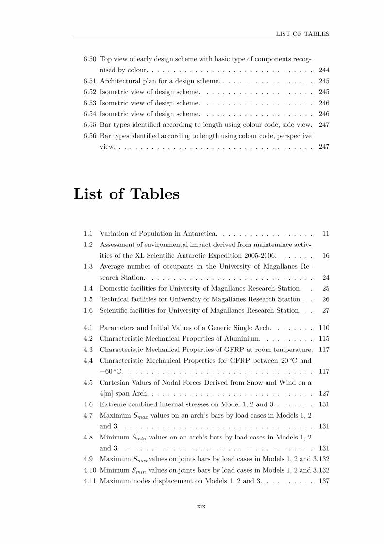
4.12 Maximum bars deflection on Models 1, 2 and 3. . . . . . . . . . . . . 1374.13 Extreme internal stresses for arches with different joint geometry. . . 1394.14 Extreme internal stresses in arches and joints bars with different
components sizing. . . . . . . . . . . . . . . . . . . . . . . . . . . . . 1404.15 Extreme internal stresses in arches with different number of segments. 1414.16 Bars segments lengths of arches with different spans and number of
joints. . . . . . . . . . . . . . . . . . . . . . . . . . . . . . . . . . . . 1424.17 Extreme internal stresses for arches with different mid-span depth. . 144
5.1 Sensitivity study for the definition of arches’ bars’ cross section. . . . 1545.2 Group of arches according to span range and bars’ cross section. . . 1555.3 Internal stresses according to segmentation of arches’ attributes Case
A. . . . . . . . . . . . . . . . . . . . . . . . . . . . . . . . . . . . . . 1585.4 Internal stresses according to segmentation of arches’ attributes, Case
B. . . . . . . . . . . . . . . . . . . . . . . . . . . . . . . . . . . . . . 1585.5 Internal stresses according to segmentation of arches’ attributes, Case
C. . . . . . . . . . . . . . . . . . . . . . . . . . . . . . . . . . . . . . 1595.6 Internal Stresses according to grouping of arches’ attributes, Case A,
with 50% of pre-stress reduction. . . . . . . . . . . . . . . . . . . . . 1645.7 Internal Stresses according to grouping of arches’ attributes, Case A,
with 90% of pre-stress reduction. . . . . . . . . . . . . . . . . . . . . 1645.8 Internal stresses and adjusted distance between two arches given a
uniform load condition. . . . . . . . . . . . . . . . . . . . . . . . . . 1695.9 Internal stresses and assigned loaded area according to arches’ spans
given a uniform load condition. . . . . . . . . . . . . . . . . . . . . . 1715.10 List of adjusted membrane’s segments widths according to span values.1715.11 List of possible sequences of two consecutives spans with ±1meter of
variation. . . . . . . . . . . . . . . . . . . . . . . . . . . . . . . . . . 1725.12 Number of different aluminium joints. . . . . . . . . . . . . . . . . . 1755.13 Brute-force test for the lacing of four arcs. . . . . . . . . . . . . . . . 1895.14 Aluminium joint’s bar’s length according to different spans rounded
to nearest 0.5 m. . . . . . . . . . . . . . . . . . . . . . . . . . . . . . 1925.15 Angle between aluminium joints’ bars according to different spans
values, with a span values rounded to nearest 0.5 m. . . . . . . . . . 1935.16 Variations of angle between joints’ bars found in each length group. . 1945.17 Reduced variations of angle between joints in each length group with
a tolerance of ±1ř imposed. . . . . . . . . . . . . . . . . . . . . . . . 1945.18 Aluminium joint’s bar’s length according to different spans values,
with a span values rounded to nearest 1.00 m. . . . . . . . . . . . . . 195
xx

LIST OF TABLES
5.19 Angle between aluminium joints’ bars according to different spansvalues, with a span values rounded to nearest 1.00 m . . . . . . . . . 196
5.20 Length of Upper Carbon Fibre bars, according to span with a spansrounded to nearest 0.5 m value. . . . . . . . . . . . . . . . . . . . . . 198
5.21 Length of joint’s bars and angle between joint’s bars with number ofnodes altered in +1 units for evenly-divided arcs. . . . . . . . . . . . 199
5.22 Set of resulting attributes and values. . . . . . . . . . . . . . . . . . 199
6.1 Variation in upper bars’ length in altered arches. . . . . . . . . . . . 2146.2 Study for different subdivision options of a 6 m rigid arch. . . . . . . 2296.3 Study for different subdivision options of a 4 m rigid arch. . . . . . . 230
xxi

Preface
I. Context
This is design-led research which proposes that Polar lightweight structures shouldbe recognised as a valid design field.
Based on the background of the author, this research looks at the Antarctic andSubantarctic context to demonstrate such a statement.
In recent years, Antarctic constructions have been considered of interest for designersand engineers. However, the remarkable history of lightweight construction inextreme southern environments has not yet been fully acknowledged by the designand engineering community. This research gathers sufficient evidence to validate theconcept of Polar lightweight structures. The fascinating array of cases portrayed inthis thesis ranges from Subpolar vernacular constructions to innovative structuralsurfaces implemented in more recent years.
There is a fast growing increase in the number of Antarctic parties willing to carryout scientific and touristic activities, who are therefore interested in deploying eitherpermanent, seasonal, or temporary settlements. This represents a threat for theconservation of the pristine Antarctic continent.
This research suggests that the extension in use of lightweight construction couldoffer a sustainable solution, and that more applied research is needed on differentaspects of the use of minimal construction in extremely harsh environments. Oneaspect to be studied is the search for larger and more flexible configurations thatrespond to the particularities of the remote southern context.
At the same time, advanced computational design tools have been extensively vali-dated for generating structural surfaces of high geometrical complexity. Parametricdesign tools, such as Rhinoceros’ Grasshopper© are of particular relevance to thisresearch, as they allow optimisation, either of a structure as a whole or of its physicalcomponents. This research proposes that such tools can be successfully employed forthe further development of more complex Polar lightweight systems. In this case,
1

PREFACE
the application of such tools requires the integration of the strict environmental,constructional and logistical constraints derived from the Antarctic context.
Therefore, the application of polar constraints in the design of lightweight construc-tions using parametric design tools can produce novel methods and solutions. Thisresearch provides an example of a design method that demonstrates such a proposal.
II. Research Aim
This research aims to contribute to the extension of the use of lightweight structuresin remote fragile environments, especially in Antarctic and Subantarctic areas. Inorder to drive academic and applied research in this field, a more active and formalinclusion of designers and engineers as part of polar research communities is required.
The author understands that an initial step towards this is the validation of Polarlightweight construction as a field in its own right, which is of common interest forthe architectural and engineering domains and is the core aim of this work.
III. Objectives
The validation of Polar lightweight polar design through academic research has beendone by creating a narrative that portrays the existing evidence of this concept asa design field.
The development of such narrative requires three main objectives to be achieved.The first consists of providing evidence of the history of lightweight structuresin Subantarctic and Antarctic areas. This should demonstrate the diversity ofapproaches attempted by using a systematic classification of the examples found.
The second objective in this narrative consists of the formulation of a design problemthat can challenge the complexity and scale of current Polar structures.
The final objective is the development of a solution to such a problem which will beachieved by developing a novel design method in which the use of parametric CADtools and polar constraints are integrated.
IV. Background
The research presented herein is design-led, and has been fully sponsored by the‘Capacitación de Capital Humano Avanzado’ Programme from the Chilean NationalCommission for Science and Technology (CONICYT). The purpose of this scheme
2

PREFACE
is to boost academic research and activities in areas that are key for the scientificand technological development of the country.
V. Scope of the Research
The scope of the research can be described as the intersection of the architecturalgeometry and structural design domains. Thereby the literature review, and itsresultant classification of Polar and Subpolar surface structures is based on a struc-tural approach, and a second classification is also offered regarding to the typeof curvature that these constructions present. Following, the development of anarchitectural scheme of a certain level of geometrical complexity is also enabled bythe structural design of components based on Polar conditions, where variations andrelations between classes of components are studied in detail.
It is evident that one of the biggest challenges that Polar and Subpolar buildings faceis thermal insulation, which is particularly critical when working with lightweightconstructions. However, this aspect is not addressed in this research. Althoughthis is a field where much applied research is yet to be completed in order to makelightweight systems in very cold environments thermally sound, it is believed by theauthor that there is sufficient evidence that this will be achieved to consider theuse of lightweight system as feasible. Some of the pioneering solutions for thermalinsulation will be described. Other practical aspects that are not addressed by thisresearch include strategies for energy supply and waste disposal.
VI. Thesis Structure
The research has been organised into two main parts. The first part, describedin chapters one and two, is dedicated to the validation of the concept of ‘polarlightweight design’. The second part, documented in Chapters 3 to 6, is dedicatedto the description of a design-based study for a medium-scale lightweight structurefor remote areas that exemplify this field’s prospect.
Chapter 1 initiates the first part by describing the evolution of the Antarctic builtenvironment, the particularities of the occupation regimen in that context, and theprospect that foresees an increment in the number of polar settlements, for whichlightweight structures could offer a sustainable solution. A brief for the designof a new seasonal polar research station is also described. Chapter 2 offers thedescription of a collection of Subantarctic and Antarctic lightweight constructions.Their portrayal is mainly based on their behaviour as mechanical systems. This first
3

PREFACE
part concludes with the classification of the cases found, in order to demonstratethe diversity of approaches intended by polar designers.
The second part, a design-led study, is initiated in Chapter 3. In this chapter, aspecific research problem is presented, which examines the possibility of conceivinga lightweight structure with an adaptable configuration that maintains a controllednumber of different components and a simple assembly sequence. Reflections onthe paradox of conceiving a modular-yet-adaptable lightweight system are also pre-sented, including evidence of cases which have previously addressed such problem.Chapter 3 concludes with the description of an early scheme for the design of alightweight construction previously conceived by the author. This is a generic systemcomposed from a set trussed arches whose span varies.
Chapter 4 describes a structural sensitivity study, which characterises the mainstructural component of the system, this is, the set of trussed arches with varyingspan. The objective of the study is to assess how the structural performance of thetrussed arch is affected by the variation of its geometrical attributes.
Chapter 5 describes a method for balancing the three conflicting objectives that thesystem should fulfil, involving the ‘partial-optimisation’ of the structural system.Through a series of studies, the controlled variation of each attribute of the mainsystem’s components is achieved. The final section of this chapter presents a singleparametric model where all the resultant attributes and their values are integrated.
Chapter 6 offers a series of studies which assess the architectural and constructionalfeasibility of the generic system designed. The resulting inventory of physical com-ponents of the system is also presented.
Chapter 7 offers conclusion and reflections on the research process and its results,as well as it proposes areas for further work.
VII. Methodology
The description of the context, included in Chapter 1, is carried out using existingliterature and a number of different primary sources (such as interviews and datacollection). The portrayal of lightweight structures in Chapter 2 is based on the liter-ature and the structural characterisation of these systems is based on a classificationof structural surfaces originally proposed by M. Bechthold.
Chapter 3, which presents the specific design-led research is based on the author’sowns reflections and proposals and builds on their early design scheme for a lightweightstructure.
The sensitivity study presented in Chapter 4 is carried out via a recursive iterationbetween a single parametric CAD model, used to generate a sample of each trussed
4

PREFACE
arch’s variation, and a Finite Element Modelling platform, used to evaluate the stresscondition and deformations of each sample. Snow and wind-derived loads expected inthe specified Polar location are recalculated for every iteration following the DanishStandards for snow and wind loads on structures. An initial method of manuallyexporting every CAD geometry into the FEM platform and assigning the nodal loadswas quickly dismissed as fragile and impractical, so a custom CAD/FEM script-based software tool was later implemented, allowing the simultaneous productionand evaluation of a large number of variations of the trussed arch.
Chapter 5, concerns a multi-objective study which consists of six parts. Two of theseparts relate to the definition of the geometrical attributes of the set of trussed archesfor which the CAD/FEM software tool was also employed. The next part looks atthe reduction of the pre-stress in arches via a geometry-based method. The fourthpart presents a method by which the load of the different arch types is equalised byadjusting the distance between arches. The last two parts are dedicated to reducingof the number of joints and the number of different joint types by the identification ofpatterns which are summarised in patterns (or pseudo codes) and lists of values whichare then integrated into a single parametric model. All the resultant components,attributes and their values implement using standard components offered by theRhinoceros’ application Grasshopper.
The architectural feasibility studies, presented in Chapter 6 look into differentpossibilities of aggregation using basic CAD applications. The definition of the setof physical component uses a combination of methods including digital rendering,parametric CAD definitions, handmade sketching and models. The proposal for anassembly sequence, is also developed using standard Rhinoceros applications.
5

Chapter 1
Context and Research Aim
1.1 Introduction
This Chapter begins by briefly describing the occupation process in the Antarcticcontinent, as well as the evolution of the Antarctic infrastructure (Section 1.2).
The revision of the main constructive typologies employed during this process, whichstarted about a century ago, is also offered in Section 1.3. Additionally, Section 1.3deals with the categorisation of the existing infrastructure. This is based on the scaleof the buildings, which is commonly in correspondence with their use: large-scalepermanent constructions used as year-round stations, summer-only stations andshelters using small scale buildings, and temporary field camps using lightweighttents and structures.
The revision of the general aspects of Polar buildings, both technical and operational,intends to provide a clear framework for the design proposal presented in the secondpart of this research. Furthermore, basic design principles are identified, based onthe previous experiences here described.
Additionally, the portrayal of the current and anticipated occupation scenario ispresented in Section 1.4.
Finally, a design brief for a new medium-scale research station is presented in Section1.5. The brief details the programmatic and quantitative requirements, as well asenvironmental, logistical, technical and site’s constraints. The design proposal of alightweight structure presented in the second part of this thesis (Chapter 4, 5 and6), will be based on these requirements.
7

CHAPTER 1. CONTEXT AND RESEARCH AIM
Figure 1.1: Magallanic Penguin at the Antarctic Peninsula. Photo: F. Fernandoy.2012.
1.2 Occupation at the Antarctic region
The Antarctic continent has a surface of 14,000,000 km2. The variety of geographicfeatures, climate regimes, biological diversity and ecological dynamics is not yetfully understood. Therefore, any generalisation regarding this vast territory mightbe subject to question.
However, it can still be stated that Antarctica can be considered the most pristineterritory [Fig. 1.1], as well as the highest, driest, and coldest continent [1]. The totalisolation from human civilisation can be justified by its extreme energy conditionand the absence of significant biotic systems [1].
Geographical features have been determinant in the process of human occupationin Antarctica. The lack of terrestrial connection has been responsible for the slowspeed of the insertion of human settlements, which is practically free of anthropicimpact.
Antarctica is the least populated continent. Human presence in Antarctica canbe generally described by two different phases in its short history. The initialexplorations, carried out in the late 1700s were often commissioned for sovereigntypurposes, and they were followed by scientific schemes undertaken by nationalAntarctica programmes of different states [1]. Such disciplines include biology, geol-ogy, astronomy, glaciology, global climate change research and others. This activityis now being complimented by an increasing quantity of touristic programmes, basedmainly in self-sufficient passenger ships around the coast with certain intrusions intothe interior of the continent and hiking touristic programmes, which present a threatto terrestrial and coastal ecosystems [1].
8

CHAPTER 1. CONTEXT AND RESEARCH AIM
Argentina Australia Chile France N. Zealand Norway UK
Figure 1.2: Antarctic territorial claim. Source: CONMAP, 2011.
There are seven states which initially claimed sovereignty over theAntarctic Territoryin the first half of the Twentieth century: Chile, Argentina, UK, France, Australia,New Zealand, and Norway [Fig. 1.2]. In 1959, the ‘Antarctic Treaty’ was issuedwhere the initial claiming parties, along with another group of states (Spain, SouthAfrica, Brazil, Ecuador, Peru and Uruguay), which also expressed their intereston establishing presence for scientific purposes, agreed to manage Antarctica col-lectively. Consequently, their positions in respect to Antarctic territory remainedunchanged [2]. Since 1961, another group of states succeeded in proving legitimateinterest in Antarctic Research and therefore, could found settlements. Currently,a group of 29 ‘consultative’ members are responsible for the decision-making atAntarctica, administratively grouped by the Antarctic Treaty Secretariat (ATS).Actions are collectively coordinated by the Council of Managers of National Antarc-tic Programs (COMNAP), dependent of the ATS.
Due this agreement, Antarctic territory is under a system of special protection, bywhich it has been declared as a territory exclusively dedicated to ‘purposes of peaceand science’ [3].
In 1991, all the consultant parts of the ATS approved the ‘Protocol to the AntarcticTreaty for Environmental Protection’, by which the whole continent was designatedas a Natural Reserve. The Protocol of Madrid, valid from 1998, established all theprinciples, procedures and obligations for the protection of the Antarctic Environ-ment [3]. With this Protocol, all the activities are regulated and controlled, includinggovernmental, non-governmental and private schemes. The instrument is aimedto guarantee that none of these activities will produce any adverse environmentalimpact, including construction tasks and their management.
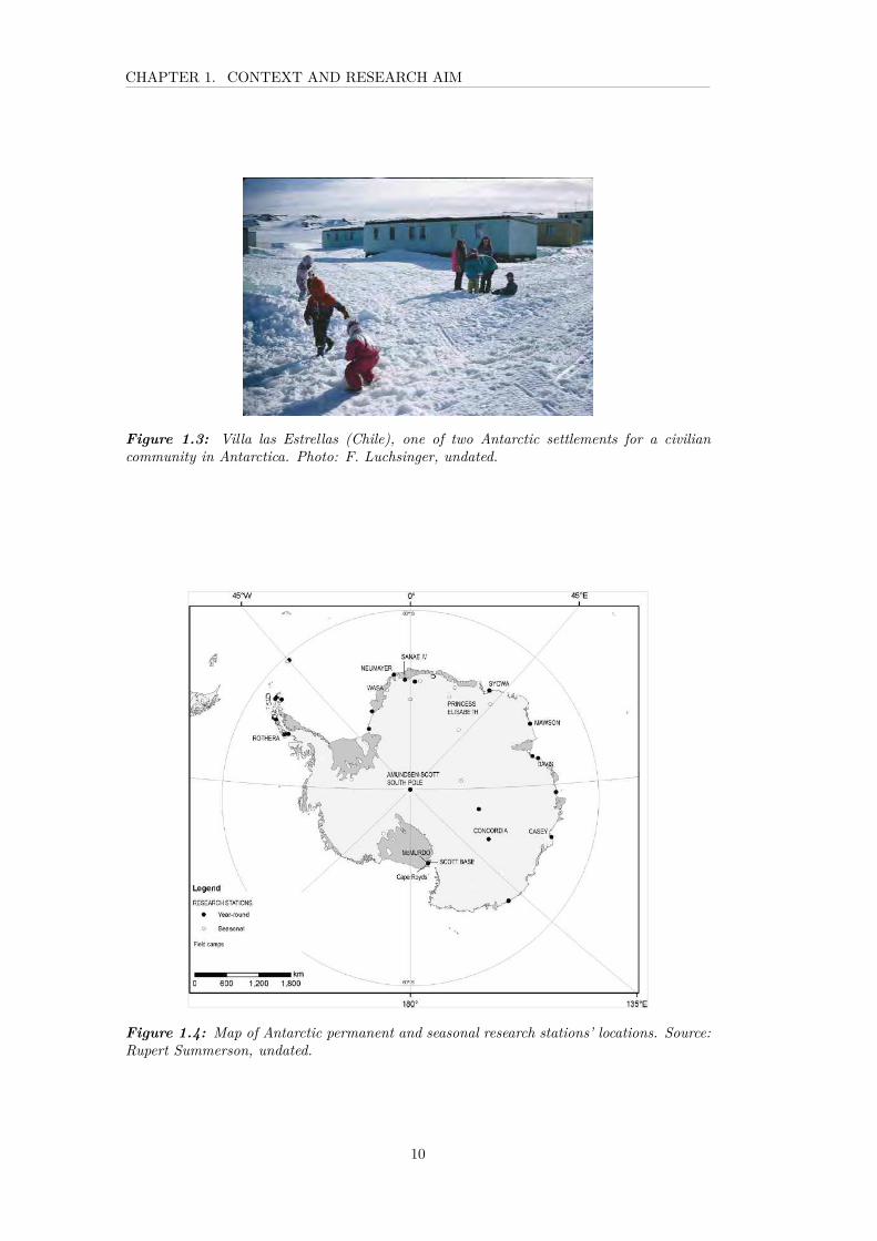
The ATS members consequently have a deployed presence by the establishment ofpermanent, temporary or seasonal settlements in Antarctica [Fig. 1.3].
To date, there are 113 registered settlements in Antarctica. They can be classifiedas: whole-year stations (37), seasonal station and refuges (33), and field camps (31).The rest corresponds to either temporarily closed stations or seasonal fuel depots[4]. The location of principal permanent infrastructure is shown in Figure 1.4.
9
CHAPTER 1. CONTEXT AND RESEARCH AIM
Figure 1.3: Villa las Estrellas (Chile), one of two Antarctic settlements for a civiliancommunity in Antarctica. Photo: F. Luchsinger, undated.
Figure 1.4: Map of Antarctic permanent and seasonal research stations’ locations. Source:Rupert Summerson, undated.
10

CHAPTER 1. CONTEXT AND RESEARCH AIM
Year-round stationAverage Summer 3598Peak Winter 1059
Seasonal Facilities (Station and refuges)Average Summer 786Peak Winter 0
Field CampsAverage Summer N/APeak Winter 0
Table 1.1: Variation of Population in Antarctica. Source: CONMAP, 2010.
One of the most relevant characteristics of the human activity in Antarctica is thesignificant fluctuation on the population during the different seasons of the year, asmost of the research activities are only possible to be carried out during summerseason, namely from October until March. Such a variation is summarised in Table1.1.
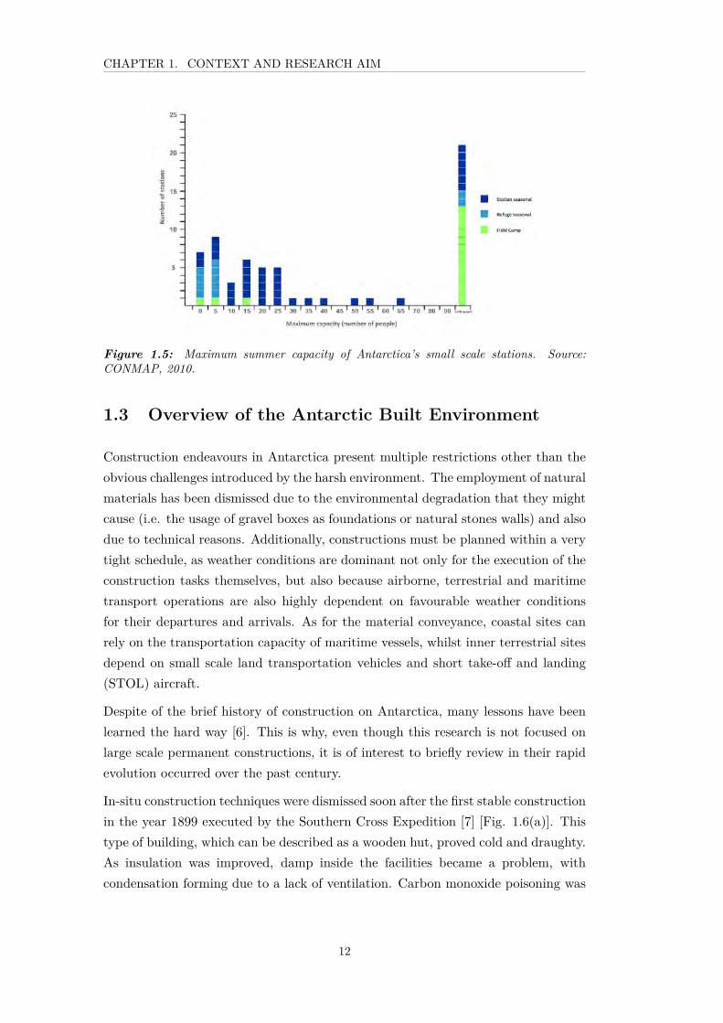
The average capacity of each type of building (permanent station, seasonal station,refuges, or field camps) largely differs from one another. Most of the stations havebeen designed to accommodate up to 50 people, while the largest, about 12 stations,can accommodated 100-200 people. The largest station in Antarctica is McMurdo(USA), which provides accommodation for up to 1000 people in summer and averageof 250 people in winter [5].
Regarding small scale permanent infrastructure, most of the seasonal stations havecapacity for 10-30 people; few of them (only five) have capacity for more than 40researchers. For the eight registered refuges, capacity is estimated at between range2 to 10 people [4].
For field camps, and apart from their regular locations, no reliable informationis available on the average number of users, although it is expected to be highlyfluctuant. Every summer season, each Antarctic National Program proposes newtemporary settlements, according to their own scientific interests and schemes. Sim-ilar criteria apply for touristic base camps. Given that both activities are rapidlygrowing, the use of lightweight structures is estimated to be much higher in thecoming years.
Figure 1.5 summarises the information gathered during this research in respect tothe capacity of small scale Antarctic infrastructure.
11
CHAPTER 1. CONTEXT AND RESEARCH AIM
Figure 1.5: Maximum summer capacity of Antarctica’s small scale stations. Source:CONMAP, 2010.
1.3 Overview of the Antarctic Built Environment
Construction endeavours in Antarctica present multiple restrictions other than theobvious challenges introduced by the harsh environment. The employment of naturalmaterials has been dismissed due to the environmental degradation that they mightcause (i.e. the usage of gravel boxes as foundations or natural stones walls) and alsodue to technical reasons. Additionally, constructions must be planned within a verytight schedule, as weather conditions are dominant not only for the execution of theconstruction tasks themselves, but also because airborne, terrestrial and maritimetransport operations are also highly dependent on favourable weather conditionsfor their departures and arrivals. As for the material conveyance, coastal sites canrely on the transportation capacity of maritime vessels, whilst inner terrestrial sitesdepend on small scale land transportation vehicles and short take-off and landing(STOL) aircraft.
Despite of the brief history of construction on Antarctica, many lessons have beenlearned the hard way [6]. This is why, even though this research is not focused onlarge scale permanent constructions, it is of interest to briefly review in their rapidevolution occurred over the past century.
In-situ construction techniques were dismissed soon after the first stable constructionin the year 1899 executed by the Southern Cross Expedition [7] [Fig. 1.6(a)]. Thistype of building, which can be described as a wooden hut, proved cold and draughty.As insulation was improved, damp inside the facilities became a problem, withcondensation forming due to a lack of ventilation. Carbon monoxide poisoning was
12

CHAPTER 1. CONTEXT AND RESEARCH AIM
also present in some cases, caused by the frequent burning of fuel within the hut forheating.
The shape and orientation of the building also became of importance for Antarcticconstruction. After a few years of use it was observed that buildings were affected bystrong winds blowing across a structure carrying snow, which was deposited, usuallyon the downwind side as the wind loses velocity while transiting the building [Fig.1.6(b)]. As result, buildings were buried under snow, especially those with seasonalusage, which remain empty most of the time. Problems derived from placing thebuildings directly on the ground were also often found, especially in coastal areas,due to the volumetric instability of rocks, associated with gelifraction processes [6].
A second stage in the history of Antarctic can be recognized by the wide use ofadapted containers as the basic unit of modular structure [1]. Their adaptationwas successful due the feasibility of improving their thermal insulation, practicaltransportability, and easy assembly. Previous problems related to the stability ofbuildings could be simply overcome by providing independent supports, such asisolated concrete blocks. Nevertheless, this kind of building has led to a ratherindustrial-looking landscape. Davis (Australia) and Rothera (UK) Stations areexamples of this [Fig. 1.7]. The one of two civilian inhabited communities ‘Villa lasEstrellas’ (Chile) also used this solution for its housing park [Fig. 1.3]. The recentlyopen India’s National Center for Antarctic and Ocean Research’s Station, BharatiStation (2012), also used 134 adapted shipping containers as the inner structure forthe station with a revisited design strategy from Bof Architekten.
Since the adoption of the Protocol on Environmental Protection to the AntarcticTreaty by the ATS in the early nineties, it was stated that everything brought to thecontinent, including large buildings should be able to be removed after use, withoutleaving traces on the site. This has become a key constraint for the design strategyand implementation of the so-called permanent infrastructure. This means that, interm of polar infrastructure design, the categorisation of temporary and permanentcan be considered as a relative matter.
Radical visions of temporary and permanent design concepts are also part of thePolar design chronicle. In 1970, Frei Otto’s Warmbronn studio, Kenso Tange andOver Arup and Partners proposed the ‘City in Antarctica’ project, which consistedof an pneumatic membrane, spanning 2 km, aimed at providing shelter for an entireresidential town [8] [Fig. 1.8]. On the other hand, the proposal of MAP Architect’s‘Iceberg Living Station’, a speculative design, in 2014, consisted of a year-roundfacility capable of hosting 100 occupants. The station is meant to be completelyholed out of an iceberg using readily available excavators (commonly used for snowclearance). The station is expected to melt away, which according to the designerswould avoid the problem of material removal at the end of its life span [9].
13

CHAPTER 1. CONTEXT AND RESEARCH AIM
(a) (b)
Figure 1.6: Early Antarctic Construction. (a) Douglas Mawson’s Hut erected 1912, source:Australian Antarctic Division: (b) Douglas Mawson’s Hut buried in hard snow, 2006, source:Australian Antarctic Division.
(a) (b)
Figure 1.7: Industrial looking constructions. (a) Davis station(Australia) in 2005(established in 1957). Image: Graham Denyer (b) Rothera Station, established in 1957.Source: British Antarctic Survey.
During recent years, Antarctic infrastructure has notoriously become of interestto architectural and engineering disciplines [10]. Consequently, recent stations arebeing resolved with more environmentally friendly and bespoke methods. Designersare being challenged by multiple aspects: ensuring an optimized shape for minimumsnowdrift by using snow-blowing simulations and physical scale models, designingcoherent modular construction strategies and using highly thermally efficient mate-rials. The stations Halley VI (UK) [Fig. 1.9] and Neumeyer (Germany) [Fig.1.10]are examples of this. Both use jack-leg supports to avoid snow accumulation, windforces, and minimization of footprints on the site.
Additionally, remarkable efforts for the improvement of energy efficiency in thealready built environment are being made, along with the development of renewableenergy supply systems [5].
One particular aspect of the variability of population for large scale building is theenergy consumption during southern winter season. As an example, a medium scalepermanent station, South Africa’s SANAE IV is considered relatively new and it has
14

CHAPTER 1. CONTEXT AND RESEARCH AIM
(a) (b)
Figure 1.8: Views of the ’City in Antarctica’ study project, an air hall as a protectionagainst climate over a residential town. (a) View of a physical model. Image, F. Otto,1971. (b) Plant view of the residential town. Image: Frei Otto, 1971.
Figure 1.9: Halley VI, the 6th British base commissioned in 2009. Source: BritishAntarctic Survey, 2011.
(a) (b)
Figure 1.10: Germany’s Neumayer III Station, 1992. Source: Alfred Wegener Institutefor Polar Research.
15

CHAPTER 1. CONTEXT AND RESEARCH AIM
Action Emissions(Including
dust)
Waste Noise Leaks Usage ofMechanicalMachinery
Vehicles
Vehicles X X X X XEnergy Generation X X X X
Painting X X XFuel Storage XConstruction X X
Module Dismantling X X XWaste Disposal XMinor Vessels X
Table 1.2: Assessment of environmental impact derived from maintenance activities of theXL Scientific Antarctic Expedition 2005-2006. Source: Chilean Antarctic Institute, 2005.
a capacity for 80 people, but during winter the number of occupants decreases to 10.During winter about 72 kW of power is needed to keep the station at 18°C. For coldperiod the consumption of energy can be more than double. As fuel is transportedfrom Cape Town, logistical and transportation costs should be considered, for whichthe final price at SANAE IV is more than the triple the purchase price [5].
Small scale seasonal buildings, stations and refuges used during summer months, arecurrently very different. Most of them correspond to relatively old constructions (30-40 years old) [Fig. 1.11] and were therefore built using traditional techniques andmaterials. This entails the execution of periodic maintenance schemes, or simplyto be abandoned like the case of the Sub-base Yelcho (Chile). The implicationsof periodic maintenance for this kind of infrastructure imply high economics costs,complex logistical coordination and environmental risks. Table 1.2 lists the assess-ment of environmental threats derived from such maintenance activities carried outon a group of small scale stations and refuges belonging to the Chilean AntarcticInstitute (Escudero Base, Ripamonti, Risopatrón, Shirreff Camp), every 3 years,and which need to be evaluated and resolved before their execution [11].
It is usually seen that despite international collaboration between different AntarcticNational Programs being common, the capacity of these small scaled facilities is oftena limitation for in-land activities, due their reduced capacity. On the other hand,during seasons of relatively reduced demand, stations must be kept operative, forinstance maintaining stations at a minimum temperature (18 °C) [5], which impliesa significant consumption of energy. It should be considered that the more remotethe site, the more expensive and risky the re-fuel tasks turn out to be. This suggeststhe pertinence of considering the capacity of variation or partial deployment in thedesign of small scale buildings, which can respond to a variable range of occupants.
16

CHAPTER 1. CONTEXT AND RESEARCH AIM
(a) (b)
(c)
Figure 1.11: Seasonal station and refuges. (a) Uruguayan Shelter at Antarctic Peninsula,photo: F. Fernandoy, 2011; (b) Hut refuge Fossil Bluff (UK), source: British AntarcticSurvey, 2011; (c) Almirante Brown station (Argentina), source: Argentinean AntarcticInstitute, undated.
17
CHAPTER 1. CONTEXT AND RESEARCH AIM
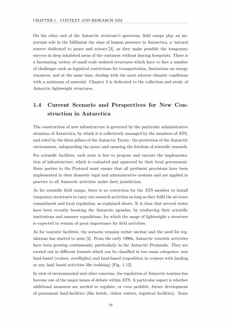
On the other end of the Antarctic structure’s spectrum, field camps play an im-portant role in the fulfilment the aims of human presence in Antarctica, a ‘naturalreserve dedicated to peace and science’[3], as they make possible the temporarysurveys in deep inhabited areas of the continent without leaving footprints. There isa fascinating variety of small scale isolated structures which have to face a numberof challenges such as logistical restrictions for transportation, limitations on energyresources, and at the same time, dealing with the most adverse climatic conditionswith a minimum of material. Chapter 2 is dedicated to the collection and study ofAntarctic lightweight structures.
1.4 Current Scenario and Perspectives for New Con-struction in Antarctica
The construction of new infrastructure is governed by the particular administrativesituation of Antarctica, by which it is collectively managed by the members of ATS,and ruled by the three pillars of the Antarctic Treaty: the protection of the Antarcticenvironment, safeguarding the peace and ensuring the freedom of scientific research.
For scientific facilities, each state is free to propose and execute the implementa-tion of infrastructure, which is evaluated and approved by their local government.State parties to the Protocol must ensure that all pertinent provisions have beenimplemented in their domestic legal and administrative systems and are applied inpractice to all Antarctic activities under their jurisdiction.
As for scientific field camps, there is no restriction for the ATS member to installtemporary structures to carry our research activities as long as they fulfil the no-tracecommitment and local regulation, as explained above. It is clear that several stateshave been recently boosting the Antarctic agendas, by reinforcing their scientificinstitutions and summer expeditions, for which the usage of lightweight a structureis expected to remain of great importance for field activities.
As for touristic facilities, the scenario remains rather unclear and the need for reg-ulations has started to arise [2]. From the early 1990s, Antarctic touristic activitieshave been growing continuously, particularly in the Antarctic Peninsula. They arecarried out in different formats which can be classified in two main categories: nonland-based (cruises, overflights) and land-based (expedition in cruisers with landingor any land based activities like trekking) [Fig. 1.12].
In view of environmental and other concerns, the regulation of Antarctic tourism hasbecome one of the major issues of debate within ATS. A particular aspect is whetheradditional measures are needed to regulate, or even prohibit, future developmentof permanent land-facilities (like hotels, visitor centres, logistical facilities). Some
18

CHAPTER 1. CONTEXT AND RESEARCH AIM
Figure 1.12: Number of tourists visiting Antarctica during 1965-2007. Source: Bastmeijeret al, 2008.
member states of ATS strongly support the idea of prohibiting them. Nevertheless,the question has not received a clear official answer. The most important reasonsfor opposition are related to the environmental risks that are expected, the politicaltensions that it could create derived from the territorial occupation, and the threatfor the development of scientific activities.
Antarctic touristic operators are ruled by the same ATS protocol, thus they needmust meet local environmental regulations. In parallel, there is a self-regulationsystem set up by the Association of Antarctica Tour Operators (IAATO) whichhas established procedures and environmental standards for its member. However,during the last few years IAATO has reported the operations of some unregisteredcompanies, which has highlighted the necessity of a clear regulation for Antarctictourism operators [2].
Currently, touristic companies mostly make use of either governmental or scientificfacilities, which allow different modalities for visitors. Some official stations haveallocated some visitor centres, particularly at historic facilities. Only a few havesucceed in developing their own infrastructure: at Patriot Hills and Vinson Massif,operated by Antarctic Logistics & Expeditions and at Dronning Maud Land, op-erated by Antarctic Logistics Centre International. It is interesting to notice thatboth are tented camps whose materials are stored during austral winter, being theunique modality which has been able to cope with both environmental regulationsand economic goals. This also suggests that lightweight constructions could alsocontribute to the sustainable development of Antarctic tourism.
19

CHAPTER 1. CONTEXT AND RESEARCH AIM
(a) (b)
Figure 1.13: Installation of the new ’Union Glacier Station, Ellsworth Hills. Image:Chilean Antarctic Institute, 2014.
1.5 Design Brief for an Antarctic Seasonal Station
This section explains the requirements for a summer-only research station in Antarc-tica.
As explained, there are several ATS members currently boosting scientific activities.One of the most active is Chile, who since 2004 has expressly made efforts to boostand diversify its scientific activity in Antarctica[12]. In that context, it was agreedin 2013, to establish the first collectively-managed research station in Union Glacier[Fig. 1.13]. This is one of the three stations located within the South Pole Circle,together with Amundsen-Scott (USA) and Kunlun (China). The station is beingmanaged by the Chilean Air Force and jointly operated by the Army, the Navyand the Chilean Antarctic Institute. Opened on January 2014, it is a summer-onlystation and operates from November to January.
The University of Magallanes (UMAG) despite being the only academic institutioncarrying out Polar research for over 30 years, is the only governmental organizationthat has not deployed permanent field work infrastructure in Antarctica.
In this context, the following text describes a notional design brief for the imple-mentation of a research station for the UMAG in Union Glacier. The text has beenredacted in collaboration with the Polar Research Team.
1.5.1 Scope
Magallanes is the natural entrance to Antarctica. The University of Magallanes’sAntarctic and Sub-Antarctic Department (DPA) is the southernmost academic insti-tution carrying out Antarctic research permanently. The DPA has been carrying outresearch since 1994 in multiple scientific areas such as radio-glaciology, tele-detectionengineering, chemistry, Paleo-climate, among others.
20

CHAPTER 1. CONTEXT AND RESEARCH AIM
This brief explains the requirements for the speculative design of the first DPAField Station, the main objective of which is to consolidate the presence of DPAin Antarctica as well as to promote the formation of Antarctic and Sub-Antarcticresearchers. The challenge involves not only to create an efficient and functionaldesign to provide scientist with a safe, effective and comfortable research space, butalso to reflect the strong commitment of the DPA to comply with the AntarcticTreaty Environmental Protocol, as well the innovative spirit of this research group.
The UMAG’s Antarctic Department aims to build a new scientific research stationin Union Glacier within the boundaries of the Chilean Antarctic Territory. Thisstation should house 5 staff (advanced party) at the very early and late Antarcticsummer, rising to 12 during middle summer season.
Operating and living in this extreme environment requires the development of aunique approach to building due to multiple environmental and logistical factors:heavy snow fall, extremely low temperatures and all supplies (including materials,equipment and staff) having to be towed inland from the ice border or flown-in bysmall-capacity aircraft. These factors can be translated as a series of limitations forthe station’s design that should be considered from the initial stage: a quick-erectionmethod of due to a brief time window for construction using limited machinery;maintenance and repair strategies under tough weather conditions and limited weightand size of components. Main environmental issues are water production and wastedisposal.
Apart from these practicalities, this call is also an invitation to explore a no-tracedesign culture, which is one the strongest values to be promoted by the participantof the Antarctic Treaty, as well as a novel architectural expression. The designshould allow the introduction of small-medium scale human settlement with a senseof reversibility, where the whole structure could operate and be removed withoutcausing any permanent impact to one of the most fragile and pristine existingenvironments.
1.5.2 Site Conditions
The site is located 1080 km from the South Pole. The structure will be adjacent tothe rest of the buildings in the Union Glacier Station [Fig. 1.14], the precise positionof wish (79° S / 82° W) was specified in 2013. The elevation is 700 meters abovesea level.
Although the topography at the location is expected to be stable, the annual rateof build-up of snow fall can reach up to 1.5 m [12]. This implies that annualmaintenance and snow-clearance will need to be carried out at the beginning of
21
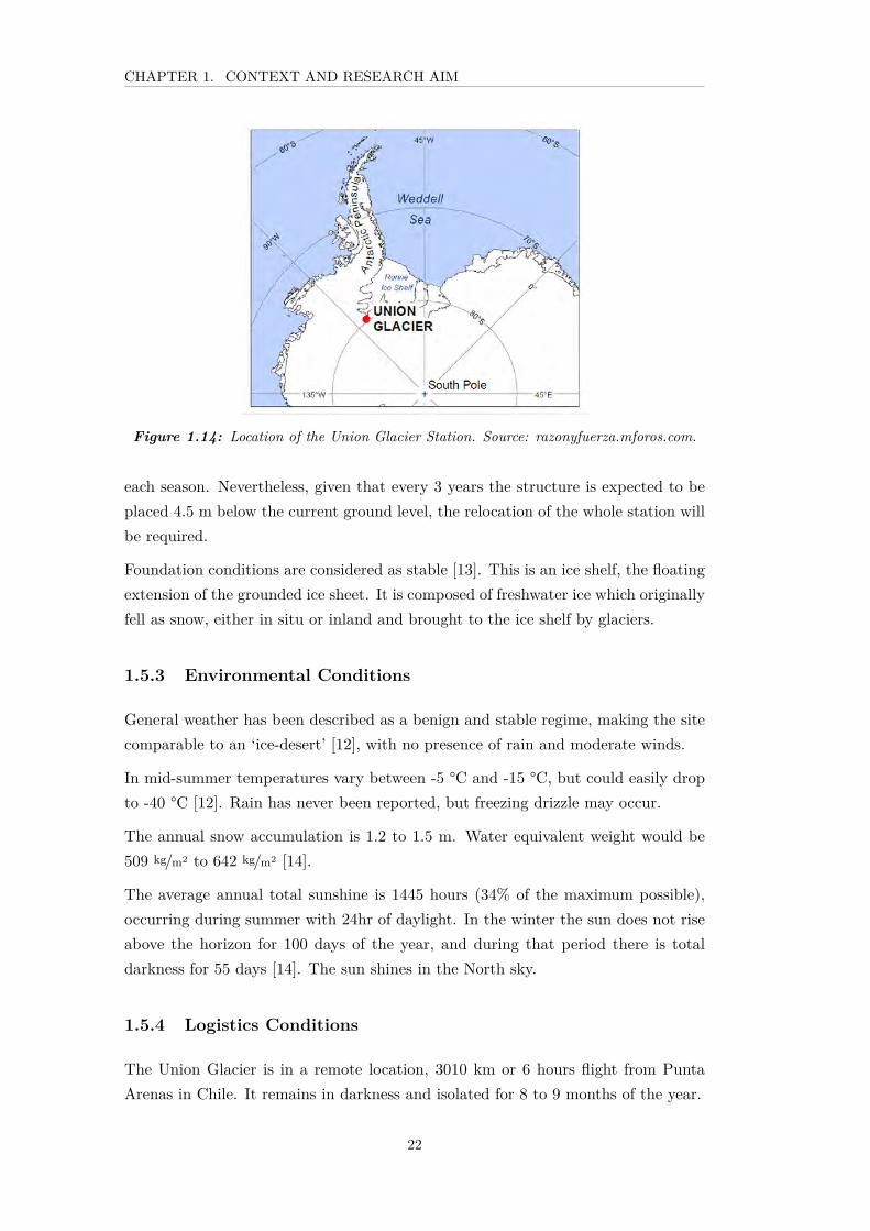
CHAPTER 1. CONTEXT AND RESEARCH AIM
Figure 1.14: Location of the Union Glacier Station. Source: razonyfuerza.mforos.com.
each season. Nevertheless, given that every 3 years the structure is expected to beplaced 4.5 m below the current ground level, the relocation of the whole station willbe required.
Foundation conditions are considered as stable [13]. This is an ice shelf, the floatingextension of the grounded ice sheet. It is composed of freshwater ice which originallyfell as snow, either in situ or inland and brought to the ice shelf by glaciers.
1.5.3 Environmental Conditions
General weather has been described as a benign and stable regime, making the sitecomparable to an ‘ice-desert’ [12], with no presence of rain and moderate winds.
In mid-summer temperatures vary between -5 °C and -15 °C, but could easily dropto -40 °C [12]. Rain has never been reported, but freezing drizzle may occur.
The annual snow accumulation is 1.2 to 1.5 m. Water equivalent weight would be509 kg/m2 to 642 kg/m2 [14].
The average annual total sunshine is 1445 hours (34% of the maximum possible),occurring during summer with 24hr of daylight. In the winter the sun does not riseabove the horizon for 100 days of the year, and during that period there is totaldarkness for 55 days [14]. The sun shines in the North sky.
1.5.4 Logistics Conditions
The Union Glacier is in a remote location, 3010 km or 6 hours flight from PuntaArenas in Chile. It remains in darkness and isolated for 8 to 9 months of the year.
22

CHAPTER 1. CONTEXT AND RESEARCH AIM
The construction and implementation of the station should take place within an8 week frame time, during the months of December and January, when accessand weather conditions are most benign. All items (freight, plant and people) aretransported by wheeled jet cargo aircraft to the site and are likely to be landed onblue ice, then transported by sledge and tracked vehicles to site. The maximum limitof cargo weight for is 13 tonnes, in good conditions. The distance of the re-supplyroute is estimated to be 8-10 km between the blue ice runway and site. Terrestrialtransportation from the runway to the site is likely to be realized with skidoos andsledges, with structural components piled on standard cargo pallets of 3 m by 3 m.
The core aircraft fleet currently used on Union Glacier’s blue-ice runway, consistof: Hercules c130, Ilyushin Il-76, Twin Otter and Basler BT-67. Additionally, snowtractors are also available for the installation and/or site preparation.
The staff to support the construction procedure would consist of 20 people. Afterthe first year, there would be a fixed annual schedule of operation and maintenance.An advance party of 5 crew, along with 2 months of supplies would be flown tothe station at the beginning of each summer season (November) to carry out snowmanagement and making the station operative. This procedure should take no morethan 7 days, weather permitting. The same operation would be carried out at theend of the Antarctic summer season, when a crew of 5 personnel would be in chargeof leaving the station in a winter mode. The crew would be flown back in middle ofMarch each year. There would be one relief operation during the summer season (lateJanuary) to renew personnel, re-supply the station and remove the waste produced.
On-site assembly of small parts and pieces of the structure should be minimized.Instead, structural components should be transported ready for installation whenpossible. Personnel working outdoors would be wearing large bulky items of clothingincluding gloves, which would reduce their manual deftness. Construction andmaintenance methods proposed must consider this reduced ability. In case of urgentrepair, procedures should be simple and possible to be executed by non-specialiststaff.
1.5.5 Overall Requirements
The primary function of the station is to provide accommodation and the necessarysupport facilities to enable a variable number of people to live and work in a remotepolar region for up to two months. The programme, site conditions and supportinglogistical activities of the medium scale station should be considered as a wholeduring the design process. Another key feature is that the station will remain closedduring most of the year, during which period it will not be possible to carry outrepair work.
23

CHAPTER 1. CONTEXT AND RESEARCH AIM
Function Summer StaffScience, Engineers & Visiting Scientists 6Communications / IT / Science Support 1
Cook / Indoor Maintenance 1Electrician / Mechanic 1
Field Operations Director 1Technical staff/ Visiting Students 2
Table 1.3: Average number of occupants in the University of Magallanes Research Station.
The design of the facilities will strike a fine balance between a zero-impact de-sign approach and engineering practicalities. However, a low-tech approach tothe construction is essential due the limited machinery available on site, for whichconstruction, maintenance and relocation processes will be mostly rely on manuallabour. This means that the final design and its logistic maintenance requirementsmust be within the capacity of the targeted crew.
The typical management and staffing envisaged are listed in Table 1.3
The above indicates staff are likely to change which depending on the researchschemes being carried out by DPA. The cycle of a typical research programme is 3years, although the number of staff will be ratified annually.
The required domestic facilities are described in Table 1.4, technical facilities areshown in Table 1.5 and scientific facilities are listed in Table 1.6.
1.6 Conclusions and Research Aim
This chapter has portrayed the particularities of the human presence Antarcticcontinent. A general description of the political and environmental conditions thatgovern Polar constructions has been described in the second section. Other aspectsto consider in the design are the geographical location, soil attributes and climateregimes. It has also been shown how logistical networks play a key role in definingwhat is possible to be constructed. Section 1.2 also offered a general inventory ofexisting constructions, as well as their crew capacity, while Section 1.3 explored thedynamic evolution of Antarctic constructions over their brief history.
The review of the evolution of the built environment presented in this chapter hasevidenced why conventional construction techniques were rapidly discarded and howAntarctic design has risen as an exciting and interdisciplinary new field for engineersand designers, particularly for large scale buildings.
A particular characteristic of the Antarctic population regime, which has beenaddressed in Section 1.2, is the highly fluctuant occupation during an annual period,
24

CHAPTER 1. CONTEXT AND RESEARCH AIM
Capacity(Number of
People
Quantity(Number of
Units)
Description
Mess room 5 1 Dressing & undressing bulky, wetoutdoor clothing & boots before
entering dry areas.Sleeping unit 2 3 Light and sound proof. High
thermal insulation. First willallocate IT expert and FieldDirector, second will serve for
Electrician and Maintenance crewand third for senior science staff
Sleeping unit 4 1 Light and sound proof. Highthermal insulation. Containing two
bunk beds.Wash rooms 1 4 Containing hot shower cabinSanitary unit 1 4 Containing wash hand basins,
Toilets and Sanitary disposal units.Consider ventilation.
Kitchen 1 Area to prepare and serve up to 3meals per day. Storage place for
dried and tinned food.Bulk baggagestore room
5 3 Storage of bulky personal itemssuch as trunks, suitcases,
rucksacks, etc.Common Room 12 1 Communal area for eating, relaxing
and socialising.
Table 1.4: Domestic facilities for University of Magallanes Research Station.
25
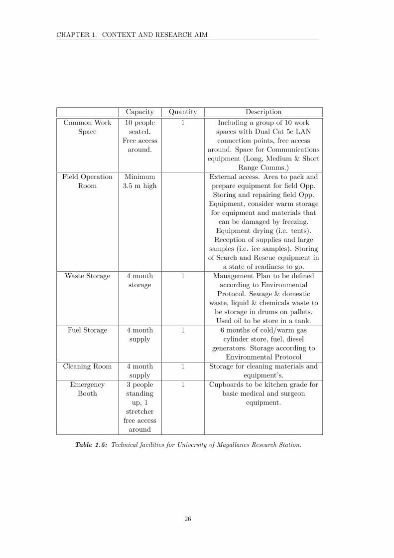
CHAPTER 1. CONTEXT AND RESEARCH AIM
Capacity Quantity DescriptionCommon Work
Space10 peopleseated.
Free accessaround.
1 Including a group of 10 workspaces with Dual Cat 5e LANconnection points, free access
around. Space for Communicationsequipment (Long, Medium & Short
Range Comms.)Field Operation
RoomMinimum3.5 m high
External access. Area to pack andprepare equipment for field Opp.Storing and repairing field Opp.
Equipment, consider warm storagefor equipment and materials that
can be damaged by freezing.Equipment drying (i.e. tents).Reception of supplies and large
samples (i.e. ice samples). Storingof Search and Rescue equipment in
a state of readiness to go.Waste Storage 4 month
storage1 Management Plan to be defined
according to EnvironmentalProtocol. Sewage & domestic
waste, liquid & chemicals waste tobe storage in drums on pallets.Used oil to be store in a tank.
Fuel Storage 4 monthsupply
1 6 months of cold/warm gascylinder store, fuel, diesel
generators. Storage according toEnvironmental Protocol
Cleaning Room 4 monthsupply
1 Storage for cleaning materials andequipment’s.
EmergencyBooth
3 peoplestandingup, 1
stretcherfree accessaround
1 Cupboards to be kitchen grade forbasic medical and surgeon
equipment.
Table 1.5: Technical facilities for University of Magallanes Research Station.
26
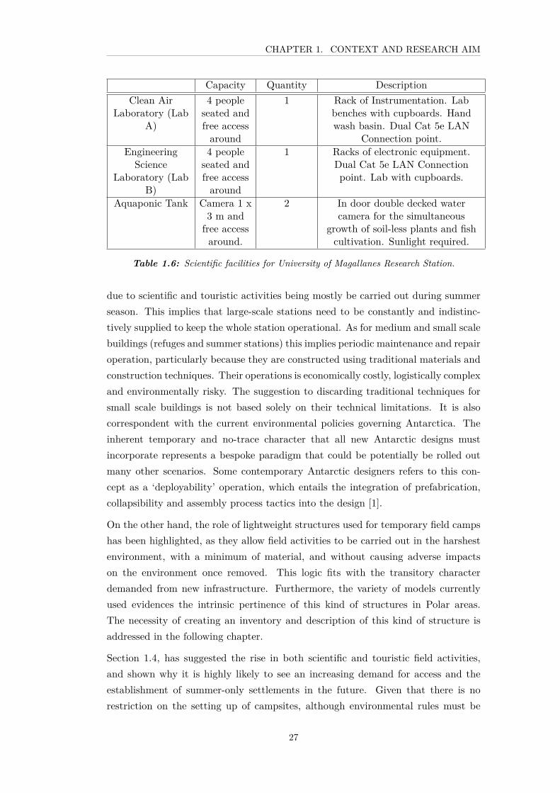
CHAPTER 1. CONTEXT AND RESEARCH AIM
Capacity Quantity DescriptionClean Air
Laboratory (LabA)
4 peopleseated andfree accessaround
1 Rack of Instrumentation. Labbenches with cupboards. Handwash basin. Dual Cat 5e LAN
Connection point.Engineering
ScienceLaboratory (Lab
B)
4 peopleseated andfree accessaround
1 Racks of electronic equipment.Dual Cat 5e LAN Connectionpoint. Lab with cupboards.
Aquaponic Tank Camera 1 x3 m andfree accessaround.
2 In door double decked watercamera for the simultaneous
growth of soil-less plants and fishcultivation. Sunlight required.
Table 1.6: Scientific facilities for University of Magallanes Research Station.
due to scientific and touristic activities being mostly be carried out during summerseason. This implies that large-scale stations need to be constantly and indistinc-tively supplied to keep the whole station operational. As for medium and small scalebuildings (refuges and summer stations) this implies periodic maintenance and repairoperation, particularly because they are constructed using traditional materials andconstruction techniques. Their operations is economically costly, logistically complexand environmentally risky. The suggestion to discarding traditional techniques forsmall scale buildings is not based solely on their technical limitations. It is alsocorrespondent with the current environmental policies governing Antarctica. Theinherent temporary and no-trace character that all new Antarctic designs mustincorporate represents a bespoke paradigm that could be potentially be rolled outmany other scenarios. Some contemporary Antarctic designers refers to this con-cept as a ‘deployability’ operation, which entails the integration of prefabrication,collapsibility and assembly process tactics into the design [1].
On the other hand, the role of lightweight structures used for temporary field campshas been highlighted, as they allow field activities to be carried out in the harshestenvironment, with a minimum of material, and without causing adverse impactson the environment once removed. This logic fits with the transitory characterdemanded from new infrastructure. Furthermore, the variety of models currentlyused evidences the intrinsic pertinence of this kind of structures in Polar areas.The necessity of creating an inventory and description of this kind of structure isaddressed in the following chapter.
Section 1.4, has suggested the rise in both scientific and touristic field activities,and shown why it is highly likely to see an increasing demand for access and theestablishment of summer-only settlements in the future. Given that there is norestriction on the setting up of campsites, although environmental rules must be
27
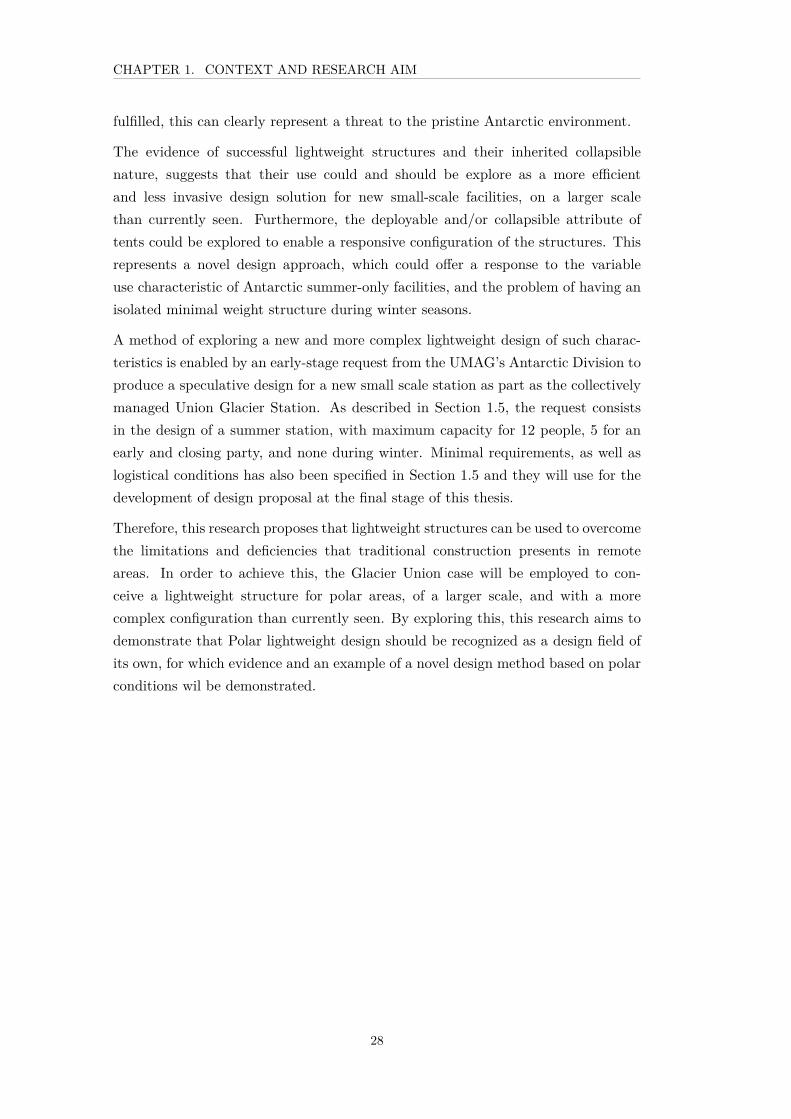
CHAPTER 1. CONTEXT AND RESEARCH AIM
fulfilled, this can clearly represent a threat to the pristine Antarctic environment.
The evidence of successful lightweight structures and their inherited collapsiblenature, suggests that their use could and should be explore as a more efficientand less invasive design solution for new small-scale facilities, on a larger scalethan currently seen. Furthermore, the deployable and/or collapsible attribute oftents could be explored to enable a responsive configuration of the structures. Thisrepresents a novel design approach, which could offer a response to the variableuse characteristic of Antarctic summer-only facilities, and the problem of having anisolated minimal weight structure during winter seasons.
A method of exploring a new and more complex lightweight design of such charac-teristics is enabled by an early-stage request from the UMAG’s Antarctic Division toproduce a speculative design for a new small scale station as part as the collectivelymanaged Union Glacier Station. As described in Section 1.5, the request consistsin the design of a summer station, with maximum capacity for 12 people, 5 for anearly and closing party, and none during winter. Minimal requirements, as well aslogistical conditions has also been specified in Section 1.5 and they will use for thedevelopment of design proposal at the final stage of this thesis.
Therefore, this research proposes that lightweight structures can be used to overcomethe limitations and deficiencies that traditional construction presents in remoteareas. In order to achieve this, the Glacier Union case will be employed to con-ceive a lightweight structure for polar areas, of a larger scale, and with a morecomplex configuration than currently seen. By exploring this, this research aims todemonstrate that Polar lightweight design should be recognized as a design field ofits own, for which evidence and an example of a novel design method based on polarconditions wil be demonstrated.
28
Chapter 2
Characterisation of Antarctic and Sub-antarctic Lightweight Structures
2.1 Introduction
This chapter presents a set of structures built in Antarctica and Subantarctic regions.
The objective of this study is to establish the recognition of Polar lightweightstructures as an architectural subject in its own right, as well as to contributing tothe historical documentation of the most emblematic cases and to the registrationof the evolution of Polar design.
The cases are described with emphasis on their technical characteristics and classifiedunder common criteria, relation to their behaviour as lightweight structures.
Given that there is scarce amount of published academic literature on this area, theauthor was required to collect scattered and material of different forms including:personal interviews, national Antarctic Programs’ magazines, brochures, websitesand handwritten technical sketches. Some corresponds to documents produced bythe early explorers of Patagonia in the 16th century and some others to computerassisted models produced by contemporary designers. This material is presented andinterpreted from a common perspective, namely to demonstrate not only the diver-sity of structures found, but also the pertinence of recognising the Polar lightweightdesign as an architectural paradigm.
One of the challenge of this field is the lack of a source where to derive knowledgefrom. It is generally the case that specialised architectural disciplines are developedfrom a study-subject which is explored and reinterpreted. Such is the case ofvernacular architecture with the study of local materials’ properties, or biomimeticarchitectures and the study of naturals system. In the case of Polar design, suchsource of study is not provided. Solutions and knowledge are achieved by the
29

CHAPTER 2. CHARACTERISATION OF ANTARCTIC AND SUBANTARCTICLIGHTWEIGHT STRUCTURES
repetition of the construction exercise throughout time with different techniques andmaterials, in a trial and error fashion. Although some unique solutions have beenproduced, these have not been systematically documented and shared. This chapteroffers a first exercise to portray and organise the cases of lightweight structures inSouthern areas.
Throughout the very diverse case studies displayed in this chapter, it is expected tocontribute to the general understanding that the extension of the continent conveysa great variety of geographical features and climate regimes that affect the designschemes; as well as factors as location and available logistic networks can dictate how,how much and when things can be transported. In other words, the diversity of casesand solutions included in this chapter, expects to tackle the common misconceptionof considering the subpolar and polar context as a white empty canvas, this timefrom an architectural/engineering perspective.
Lightweight systems have been vastly studied. Best recognised efforts correspond tothe pioneering work of German architect and structural engineer Frei Otto in regardto tensile and membranes structures [8], and Swiss structural engineer Heinz Islerfor the study of thin concrete shells [15], among others.
Consequently, there are many way of understanding and classifying the vast ar-rangement of lightweight structural systems. This thesis adopts the one proposedby Martin Bechthold [16]. The method proposed by Bechthold proposes a straight-forward perspective, where structural surfaces are understood as systems, and at-tributes regarding to the system level (such as span, proportions, orientations,and aggregations), generally within the architectural domain, are discarded for thepurposes of this classification [16]. This vision makes this approach compatible withthe objective of this study, where very diverse structures needed to be studied undera common perspective and classified accordingly.
According to the classification method used, two major groups of surfaces can beidentified based on their structural behaviour. As Figure 2.1 shows, these two groupsare classical rigid systems and non-rigid systems.
The first group is characterised by showing only small deformations when subject toloads. It includes one-way spanning systems such as beam-like or vault-like surfaces(in the shape of shells or folded plates) and two-way systems where loads are carriedthrough membrane stresses, such as shells structures and gridshells. Of course,combinations of these typologies can form hybrid structures and arrangements ofthese basic systems are used to resolved free-form designs.
In the context of this group of rigid surface structures, monocoque structures (‘singleshell’) describe the purest approach to surface structures. Another common term is‘semi-monocoque’, representing combinations of surface and ribs, such as stressed-
30

CHAPTER 2. CHARACTERISATION OF ANTARCTIC AND SUBANTARCTICLIGHTWEIGHT STRUCTURES
skin or stressed skin-on-frame construction. In this sense, there is a similarity be-tween some modular objects like car bodies, aircrafts or boats and semi-monocoquestructures [16]. Within beam-like systems, cylindrical shells, folded plates, and otherelongated shapes are included. Beam-like systems carry loads primarily through dis-tributions of shear and bending stresses, as traditional beams. Beam-like shells haveonly single curvature. Grid approaches (truss-like triangular-grid or quadrilateralgrid with bracing cables) are also possible, where bending stresses are resolved intoaxial forces. Folded plates also classify within this group. In this typology, multiplethin plates are connected along the edges to compose a more complex beam-likesystem [16].
Vault like systems are mainly compression structures. Most classic examples arecontinuous rigid shells, but also vaulted grid shells are possible (either triangular orquadrilateral grids).
Cases of gridshells, membrane stressed shells, and vault-like systems in polar andsubpolar region are presented in this chapter. While few examples of hybrid struc-tures were found, there was no evidence of free-form surfaces could possibly duethe highly complex construction requirements involved either by intricate structuralmethods or by the large number of different structural components required
The second group is defined as a system that is expected to deform whilst inservice. This group includes cable-nets and tensile membranes. Both are tension-only systems, generally pre-stressed and doubly curved. Membranes obtain theirstrength from either mechanical or pneumatic pre-stress [16]. Cable nets or mem-brane edges are mechanically pulled toward the outside, and pneumatic pre-stressinvolves shaping the membrane through pressure difference.
Generally speaking, mechanically-stressed membranes and cable nets are shaped bya tensile element pulling along their edges, and usually form saddle shapes. Asthey are generally held by cables, boundary stresses and forces are transferred torigid masts or other elements. Edges can also be rigid beams, trusses, or arches.Stay-cables are broadly used to stabilise the supporting structure [16].
Pneumatic systems are pre-stressed by the pressure difference between a sealed airchamber and atmospheric pressure. The air cavity can be the complete interior space(air-supported system) or smaller, isolated air volumes (air-inflated system). Allpneumatic membranes are curved, as only a curved membrane can effectively resistpneumatic pressure that is acting perpendicularly onto it surface [16]. Both single aswell as doubly curved (generally dome-like shaped) systems exist. The tailoring ofthe membrane permits the relatively free definition of shape. The stiffness of cablenets and membranes is directly related to degree of curvature and the amount ofpre-stress.
31

CHAPTER 2. CHARACTERISATION OF ANTARCTIC AND SUBANTARCTICLIGHTWEIGHT STRUCTURES
For non-rigid systems, only examples of mechanically stressed membranes couldbe found in the Southern Polar context. The necessity of pneumatic structures toassure a constant high pressure requires the use of maintenance mechanisms thatare unpractical in such extreme contexts, making this option is rather unsuitable forremote areas. A similar concern could explain the lack of cable net structures. Aseach cable transfers load to the reciprocate layer of cables, the constant pre-stress ofevery cable must be assured, which in an extremely dynamic environment like polarareas could be difficult. Additionally, the positioning of each individual claddingpanel supported from the cable grid makes the construction highly problematic inharsh climate zones.
Figure 2.1: Categories of surface structures (white) in the context of structural system(grey). Image: M. Bechthold
The definition of these structural categories suggest that the study of the surfacegeometry is also fundamental for to comprehension of structural behaviour, asthe curvature of a surface is directly related to its stiffness, so both approaches,geometrical and structural, are intrinsically related. Therefore, quantifying thecurvature of a surface is an important aspect for the evaluation of designs.
The Gaussian method allows the curvature of a surface to be measured as theinstantaneous curvature in points on the surface’ [16]. Any point P contains preciselyone line that is normal to the surface. An infinite number of planes can be placedsuch that they contain the perpendicular line and intersect with the surface in P .The value of R varies as the plane is rotated around the perpendicular line. Thereare generally two positions of the planes such that R takes on the largest and thesmallest value. The resulting intersection lines are called curves of principal section,and the associated curvature κ is called the principal curvature in P . The curvatureκ is equal to 1/R [16].
The average value of all κ values in P is called the mean curvature. The product ofthe two principal curvatures κ1 and κ2 is the Gaussian Curvature, and it determinesthree categories for curved surfaces as shown in Figure 2.2:
• Synclastic shapes: with a positive Gaussian Curvature, with both curves inthe same direction.
32

CHAPTER 2. CHARACTERISATION OF ANTARCTIC AND SUBANTARCTICLIGHTWEIGHT STRUCTURES
• Anticlastic shapes: with Gaussian Curvature taking a negative value sincewhere both curves are oriented in opposite directions.
• Developable surface: where one of the principal curvatures is zero. Here thelargest radius of a principal curvature is infinite as it is a straight line.
Figure 2.2: Gaussian curvature of surfaces. Image: M. Bechthold
The present chapter illustrates the presence of these three typologies of geometryin the set of Polar lightweight structures reviewed. Regarding negative Gaussiancurvature shapes, and as shown in Figure 2.2, they are mostly present as modularcomponents of sealed enclosures with a different global geometry (usually as amembrane section of a vaulted structure), rather than single open saddle shapesas usually seen in large span tensile structures. This is linked to the structuralthreat represented by snow and wind induced loads.
The following is a study of the historical cases of lightweight structures in southernpolar and subpolar regions, with their general descriptions and their classificationin structural and geometrical terms. Sections 2.2, 2.3 and 2.4 are dedicated tothe description of some of the largest and more emblematic cases of permanentlightweight constructions in Antarctica. Section 2.5 described a group of vernaculartypologies from the Subantarctic regions. Section 2.6 introduces some modernbespoke portable structures designed for the Antarctic context, and section 2.7finalises this chapter offering some reflection of the subject as well as the classificationof the cases described using the method from Bechthold.
2.2 The Amundsen-Scott South Pole Station
The Amundsen-Scott South Pole Station consisted of a geodesic dome located atthe geographical South Pole and existed between 1975 and 2009 [Fig. 2.3]. Itwas commanded by the U.S. Antarctic Program with the aim of continuing thescientific activities initiated in 1957 on celebration of the International GeophysicalYear (IGY), a global effort to boost polar research. The first settlement (known asOld Pole) was designed to accommodate a team of 16 research and support personnel
33

CHAPTER 2. CHARACTERISATION OF ANTARCTIC AND SUBANTARCTICLIGHTWEIGHT STRUCTURES
Figure 2.3: The Amundsen Scott Dome after snow removal in preparation to deconstructionwork. Image: Andy Martinez, USA National Science Foundation, 2009.
for a whole-year round campaign, consisting of a group of ‘Jamesways’ huts and T-5s (a type of prefabricate wooden buildings) [17]. Due of the significant amountof results obtained from range of scientific disciplines it was decided that activitieswould continue beyond the IGY. In 1967, the U.S. National Science Foundation andthe U.S. Naval Support Force decided to explore the feasibility of constructing anew station, since the old station’s units were becoming distorted under the heavyweight of snow and ice to such an extent that it needed to be declared uninhabitable[17].
The design was elaborated by the U.S. Naval Facilities Engineering Command incollaboration with the Naval Civil Engineering Laboratory [Fig. 2.4]. Constructionwas carried out by the U.S. Naval Construction Battalion 71 during two summercampaigns: 1971-72 and 1973-74 [Fig. 2.5].
Figure 2.4: Artist’s concept of the design newUSA South Pole’s design. Source: The AntarcticJournal 1975.
Figure 2.5: Announcement of thecompetition of the new USA PolarStation. Source: The Antarctic Journal,1975.
The two main adverse factors that rule the design were the remoteness of the site (thenearest seaport at Mc Murdo Stations was located 1,300 kilometres from the Pole)and the harsh environment conditions [17]. The first factor implied that the onlypractical transportation mode would be airplanes, thus components size and weightshould be constrained by the capacity of an LC-130 Hercules, namely 2.5×2.5×11 m,and 9,000 kg. Construction seasons could last about 75 days (mid-November to early
34

CHAPTER 2. CHARACTERISATION OF ANTARCTIC AND SUBANTARCTICLIGHTWEIGHT STRUCTURES
February) during which average temperature would be around -32 °C. The stationwould remain isolated from early February to mid-October, for which reliable life-support system were required. The second factor, implied that the structure wouldhave to cope with a series of adverse environmental conditions including: low withtemperatures of -80 °C, high winds of 24 m/s (86 km/h), drifting snows with averagewind speed of 6 m/s (21.6 km/h), constant displacement of the ice sheet of 9-10 m ayear towards the north and, soil with a low shear strength of 500 g/cm2 to a depth of2.5 m [17].
The dome was designed based on the geometric concepts endorsed by R. BuckminsterFuller [18]. Its great circle spanned 50 meters and 15 meters high at the centre, com-promising about 2/3 of a hemisphere. The dome enclosed three double stores highpre-fabricated buildings for quarters and operations. The structure was protectiveagainst wind and snow, but not cold as the interior needed to be kept under -18 °Cto prevent deformation of the snow support used as foundations [17, 18].Its life spanwas required to be of 15 years.
The use of a spherical shape was justified by its geometrical efficiency, structuralstrength and low profile, which was essential to avoid the building to be buried bythe snow [17]. Effectively, its life span could be greatly extended to over 30 years byclearing the snow off the building annually. Computer models were used to studydifferent framing systems for Antarctic conditions including Radial Rib, Lamella,Lattice and Geodesic [19]. Although several were efficient under symmetrical designloads, the last one showed dramatically higher strength under eccentric loads withmore uniform strength throughout the surface members, which make the structure’sbehaviour closer to a homogenous shell [Fig. 2.6] [19]. Physical models were alsoused on site to study patterns of snow accumulation [Fig. 2.7] whereas other studieswere run in wind tunnels, where wind loads where scaled to the size of the model,in order to determine the effect of blowing snow. A geodesic dome also presentedadvantages from a logistic perspective: components’ production could be repetitivewhich would facilitate the assembly, and no part would be too large or heavy foraircraft or handling.
Components consisted of 1,448 I-beam struts each about 3m long, connected at 490nodes, each of them involving 84 bolts per node [Fig. 2.8]. The cladding consisted ofmore than 900 thin triangular aluminium panels. Aluminium alloys where chosen forall construction for several reasons: ease of fabrication, lightness for transportationand assembly and because it increase its strength and ductility at low temperature,contrary to steel or other materials available at that time, which become brittle inextremely cold environments [19]. The foundation includes 70 timber pads spread-footings buried in the snow, one for each of the 70 dome base points.
35

CHAPTER 2. CHARACTERISATION OF ANTARCTIC AND SUBANTARCTICLIGHTWEIGHT STRUCTURES
Figure 2.6: Diagram of theSouth Pole Dome geodesic domeconstruction according to manufac-turer Temcor©. Source: NationalScience Foundation, 1972.
Figure 2.7: 1:10 scale model of Amundsen-ScottStation used to study snow drift pattern. Source:U.S. Navy, undated.
Components weight and size were also constrained by the Antarctic conditions.While the maximum weight of every component could not be heavier than 22.5 kgto allow parts to be hand-lifted and to minimize the air cargo involved, the sizeof fasteners must not be smaller than 3/8 inch of diameter since the dome had tobe assembled by personnel wearing heavy gloves. It is interesting to notice thanalthough the transport of personnel, material and equipment for the whole stationcompromised over 300 flights during 3 seasons, but materials for the dome could betransported in only 3 flights [18].
As Figure 2.9 shows, the panels were designed to overlap and interlock with inden-tations in the structure’s frame and were secured with extruded splines. This designoption for splines and panels was load tested to 0.03 MPa of panel surface load.Although the panel showed plastic deformation, it did not collapse which provideda safety factor of 2 since the design load was 0.015 MPa [19].
The assembly sequence began from bottom to top, in anticlockwise direction arounda central tower placed at snow level and was hoisted up as struts were added tothe ends. [Fig. 2.10]. Multiple support cables were used to secure the structuretemporarily from the tower. Exactly the reverse procedure was used to disassemblethe dome [Fig. 2.11 and 2.12].
Once the NSF had built a much larger permanent station in 2008, capable ofaccommodating 150 people, the dome was relieved of duty and used as a cold storagewarehouse after almost 35 years of service. A few signs of potential collapse, whichbegan to be identified and repaired from 1988, determined that the structure should
36
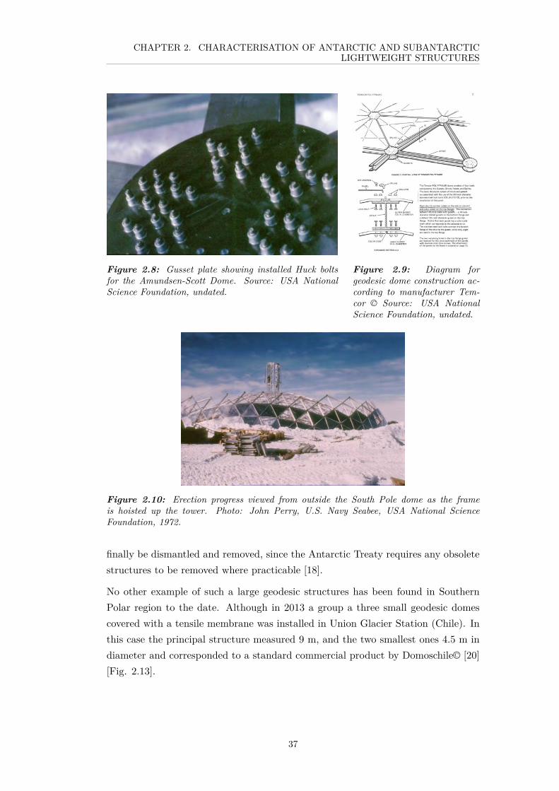
CHAPTER 2. CHARACTERISATION OF ANTARCTIC AND SUBANTARCTICLIGHTWEIGHT STRUCTURES
Figure 2.8: Gusset plate showing installed Huck boltsfor the Amundsen-Scott Dome. Source: USA NationalScience Foundation, undated.
Figure 2.9: Diagram forgeodesic dome construction ac-cording to manufacturer Tem-cor © Source: USA NationalScience Foundation, undated.
Figure 2.10: Erection progress viewed from outside the South Pole dome as the frameis hoisted up the tower. Photo: John Perry, U.S. Navy Seabee, USA National ScienceFoundation, 1972.
finally be dismantled and removed, since the Antarctic Treaty requires any obsoletestructures to be removed where practicable [18].
No other example of such a large geodesic structures has been found in SouthernPolar region to the date. Although in 2013 a group a three small geodesic domescovered with a tensile membrane was installed in Union Glacier Station (Chile). Inthis case the principal structure measured 9 m, and the two smallest ones 4.5 m indiameter and corresponded to a standard commercial product by Domoschile© [20][Fig. 2.13].
37

CHAPTER 2. CHARACTERISATION OF ANTARCTIC AND SUBANTARCTICLIGHTWEIGHT STRUCTURES
Figure 2.11: Interiorof the South Pole Dome’sdismounting party. Source:the Antarctic Sun, 2009.
Figure 2.12: Exterior of the South Pole Dome’s dismountingparty. Source: the Antarctic Sun, 2009.
Figure 2.13: Group of domes installed at the Union Glacier Station. Image: Domoschile,2013.
2.3 The Teniente Arturo Parodi Polar Station (EPTAP)
Figure 2.14: The EPTAP. Image: P. Serrano, 1999.
The EPTAP (1999-2013) was located in Patriot Hills 82 °S, 1085 km from theSouth Pole and 855 m above sea level [Fig. 2.14]. It was the first permanent polarstructure placed on a blue ice zone. It was commissioned by the Chilean Air Force’sAntarctic Division in 1998 and designed by the University of Technology FedericoSanta Maria’s Architecture for Extreme Zones Research Unit under minimal-impactprinciples.
38

CHAPTER 2. CHARACTERISATION OF ANTARCTIC AND SUBANTARCTICLIGHTWEIGHT STRUCTURES
The aim of the project was to provide logistical services throughout summer monthsfor technological and scientific field parties at the inner Antarctic plateau [21].Personnel working at the interior of the continent must usually wait to be pulledout, as aerial operations rely on favourable weather conditions. Thus, the stationplayed an important role in the safety of people and equipment operating in thedeepest part of the continent, as well as navigational and communicational services.
The structure consisted of a membrane tunnel supported by a series of arches. Thetunnel had a curved axis. Along the tunnel a series of modular structures, knownas ‘Igloo Satellite Cabins©’, previously purchased by the Chilean Air Force, couldbe attached [Fig. 2.15]. At its original configuration it engaged 320 m2, and hadcapacity for 24 people. The length of the tunnel was 50 m.
Figure 2.15: Physical components at the EPTAP: 1: tunnel 2: visor 3: module 4: sanitarysystem 5: communication 6: plug in ports. Image: Pol Taylor, 1999.
The morphology of the site represented a critical input for the design. The presenceof the Patriot Hills produces the accelerates the constantly blowing katabatic winds,which flow from the 4000 m Antarctic Plateau and reach a maximum speed of 42 m/s
(150 km/h)[1].
This wind displaces the surface snow layer and exposes a highly dense layer of blueice of 8 km length, 700 m depth and an annual displacement of 8 m each year[22] The potential of these areas to enable the landing of wheeled aircraft, hence tobe used as ‘natural runways’ was confirmed only in 1984, and it was supposed torepresent a major change in the Antarctic logistic network [22]. On the other hand,this extreme wind represented a major issue for any lightweight structure aimed tobe raised. Therefore, the structure was placed on a snowfield area 800 m North ofthe blue ice zone, where winds decelerates and a stable layer of 2 m of hardenedsnow could be found. This layer of snow sited over an ice sheet would also avoid thetypical sinking problem usually affecting coastal Antarctic structures.
39

CHAPTER 2. CHARACTERISATION OF ANTARCTIC AND SUBANTARCTICLIGHTWEIGHT STRUCTURES
The extreme speed of katabatic winds also meant that any static body left on thesurface would interfere with the prevailing snow currents and rapidly become buried.This makes access to any enclosure particularly difficult. Consequently, the tunnelwas conceived as a linear element that would use the accumulation pattern as both,a structural defence against katabatic wind flows and as thermal protection againstextremely low temperatures (with an average summer temperature of -20 °C, aminimum recorded of -35.8 °C) [1].
The membrane tunnel was conceived to be an unheated and uninsulated enclosurethat would serve both as a corridor connecting a group of isolated modules, and asstorage space. The tunnel was located upwind of the units and the entrances. Allthe components were pre-fabricated, and designed to be transported firstly by air(using a LC-130 Hercules with a cargo capacity of 13 tons), and then land, from therunway to the station’s site, using four skidoos and sledges [Fig. 2.16]. Hence, allthe station’s components were designed and adjusted to fit the 3 m × 3 m standardpallet size used for transportation.
Figure 2.16: Delivery for the construction of the EPTAP.Image: Pol Taylor, undated.
Figure 2.17: Assembly ofcomponents for the EPTAP.Source: University of Technol-ogy F. Santa Maria, 1999.
Assembly took place on site during two summer campaigns in 1999 and 2000,involving 85 days in total. It involved a team of 20 trained crew [23] and twoaircrafts [21]. Most of the assembly was made by hand [Fig. 2.17], although asnow-cat tractor belonging to ta ourist company, Adventure Network International,was employed during the installation. Again, all these logistical constraints wereconsidered as part of the design process.
The cross section of the tunnel was designed based on ergonometric conisderations,and later rationalised to a circular arc with 4 m of diameter [1]. Arches consideredan outward inclination angle of 240 degrees [Fig. 2.17], which contributed to keep
40

CHAPTER 2. CHARACTERISATION OF ANTARCTIC AND SUBANTARCTICLIGHTWEIGHT STRUCTURES
the membrane pieces in tension. These dimensions agreed with the cargo palletsused for transportation. Pairs of inclined arches were located at a distance of 2 malong the tunnel.
In terms of materiality, the arches were formed from welded steel segments. Thestrength of this compression section would provide the necessary lateral resistanceto oppose wind-derived loads. However, steel characteristically becomes a fragilematerial with temperatures below -20 °C, making it highly vulnerable to impactfractures. The decision to use this material was made in consideration of the limitedbudget available. As a response, the designers proposed a structural system in whichthe rigid elements were isolated from each other, therefor loads would be distributedwithin a network of flexible joints, dispersing any impact force throughout the system[1].
Pair of inclined arches were tightened with strips of 50 mm nylon slings, which werecompatible with the criteria of flexibility and economy. They could be easily fixedto the arcs and rails using self-perforating screws. This type of joint proved effectiveand easy to implement on site, for which the structure’s geometry could be erectedon site in only five hours [21].
Figure 2.18: Cutting pattern of the EPTAP’s PVC membrane. Image: Pol Taylor,undated.
Figure 2.19: Membrane sections being attached to the structure for the EPTAP. Image:Pol Taylor, 1999.
41

CHAPTER 2. CHARACTERISATION OF ANTARCTIC AND SUBANTARCTICLIGHTWEIGHT STRUCTURES
The tunnel’s cladding was solved as a patterned tension membrane. Each sectionbetween arcs would comprise three discrete hyperbolic wedges. This pattern wouldbe beneficial not only structurally, but also would facilitate the fabrication of themembrane [Fig. 2.18]. The fabric was PVC reinforced with a polyester webbing,weighting 750 g/m2. The surface incorporated an anodised finish and U.V. protectiontreatment, due the constant solar radiation and the thin ozone layer. Pieces ofmembrane were joined using a double flap of 100 mm Velcro©.
Membrane units were attached to the arcs using a large quantity of 35 mm nylonslings and buckles, which could be tightened from the inside and were favourablefor manipulation with thick gloves [Fig. 2.19]. To introduce pre-stress, skidooswere used to pull each unit’s outer arcs outwards, until they achieved the necessaryrotation angle [1].
The modular units, or ‘Igloo Satellite Cabins’© (see section 2.6), could be attachedalong the tunnel using sleeve connections. These elements are considered as es-sential by the designers for the expansion of the structure as a system [1]. Igloos’panels incorporated insulation material at walls and floor of 50 mm of high densitypolyurethane. This provided sufficient thermal protection for the igloos to be usedas bedrooms, toilet and communication equipment storage.
At each end of the tunnel, a concave panel of transparent 4 mm monolithic poly-carbonate were placed, named as ‘visors’. These visors served both as entrances forskidoos and sledges with cargo and as a view point enabling panoramic view of thelandscape [Fig. 2.20]. The double curved elements were fixed to a frame formed bytwo arcs, enabling the panels to rotate vertically thanks to cast steel joints. Thedouble arc frame also provided the whole structure with lateral stiffness.
Figure 2.20: Curved visors at the EPTAP. Image: Pol Taylor, undated.
The structure required periodic maintenance mainly due to snow drifts [Fig. 2.21].In the Southern summer 2013-14, the structure was unburied and disassembled after
42

CHAPTER 2. CHARACTERISATION OF ANTARCTIC AND SUBANTARCTICLIGHTWEIGHT STRUCTURES
14 years of service [Fig. 2.22]. It was then translated to Union Glacier, another blue-ice zone near Vison Massif, characterised by much calmer climatic conditions [24]where a new Antarctic Base, jointly managed by the Chilean Antarctic Institute,Air Force, Navy and Army was created involving a group of different structures.The membrane needed to be replaced but the rest of the structure was reinstalledwithout major inconveniences [21].
Figure 2.21: The EPTAP after two years of service.Image: Pol Taylor, 2002.
Figure 2.22: Chilean Air forcepersonnel unearthing the EPTAPafter 14 years of service. Source:University of Technology F. SantaMaria, 2013.
2.4 The Shockwave Tent
Figure 2.23: The Shockwave Tent in Villa Las Estrellas, Antarctica. Image: Universityof Technology F. Santa Maria, 2010.
The Schockwave tent was also developed by the ARQZE Research Unit (Universityof Technology F. Santa Maria, Chile) in 2002. The original purpose of the structurewas to serve as a hangar for aircrafts at the EPTAP Station [Fig. 2.23]. However, thecancellation of the airborne operation that summer season and a fire consuming theold sport/community centre in Villa Las Estrellas, at the Eduardo Frei ChileanAntarctic Station in 2009, gave the structure a new purpose [Fig. 2.24] as a
43
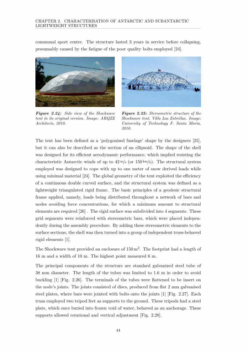
CHAPTER 2. CHARACTERISATION OF ANTARCTIC AND SUBANTARCTICLIGHTWEIGHT STRUCTURES
communal sport centre. The structure lasted 3 years in service before collapsing,presumably caused by the fatigue of the poor quality bolts employed [24].
Figure 2.24: Side view of the Shockwavetent in its original version. Image: ARQZEArchitects, 2010.
Figure 2.25: Stereometric structure of theShockwave tent, Villa Las Estrellas. Image:University of Technology F. Santa Maria,2010.
The tent has been defined as a ‘polygonised fuselage’ shape by the designers [25],but it can also be described as the section of an ellipsoid. The shape of the shellwas designed for its efficient aerodynamic performance, which implied resisting thecharacteristic Antarctic winds of up to 42 m/s (or 150 km/h). The structural systememployed was designed to cope with up to one meter of snow derived loads whileusing minimal material [24]. The global geometry of the tent exploited the efficiencyof a continuous double curved surface, and the structural system was defined as alightweight triangulated rigid frame. The basic principles of a geodesic structuralframe applied, namely, loads being distributed throughout a network of bars andnodes avoiding force concentrations, for which a minimum amount to structuralelements are required [26] . The rigid surface was subdivided into 4 segments. Thesegrid segments were reinforced with stereometric bars, which were placed indepen-dently during the assembly procedure. By adding these stereometric elements to thesurface sections, the shell was then turned into a group of independent truss-behavedrigid elements [1].
The Shockwave tent provided an enclosure of 150 m2. The footprint had a length of16 m and a width of 10 m. The highest point measured 6 m.
The principal components of the structure are standard galvanized steel tube of38 mm diameter. The length of the tubes was limited to 1.6 m in order to avoidbuckling [1] [Fig. 2.26]. The terminals of the tubes were flattened to be insert onthe node’s joints. The joints consisted of discs, produced from flat 2 mm galvanisedsteel plates, where bars were jointed with bolts onto the joints [1] [Fig. 2.27]. Eachtruss employed two tripod feet as supports to the ground. These tripods had a steelplate, which once buried into frozen void of water, behaved as an anchorage. Thesesupports allowed rotational and vertical adjustment [Fig. 2.28].
44
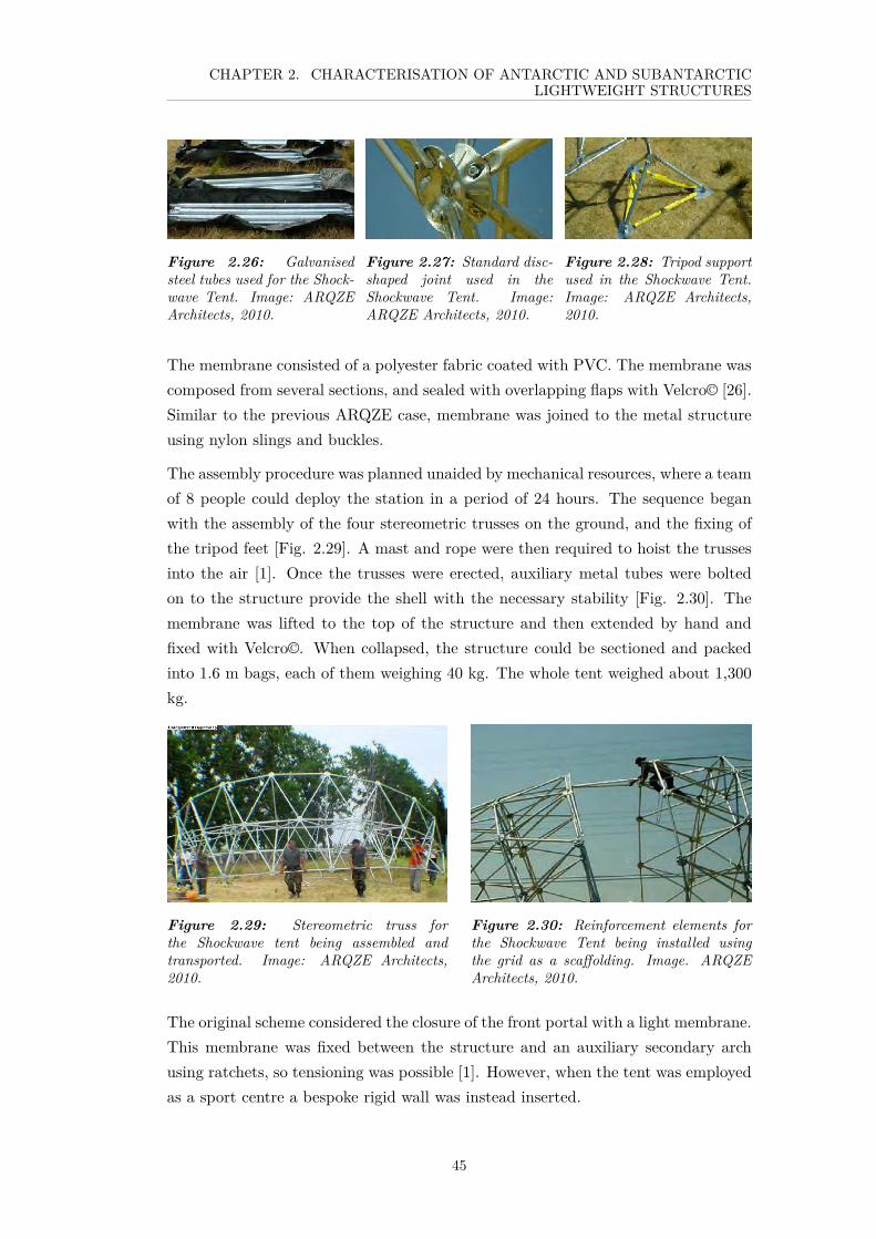
CHAPTER 2. CHARACTERISATION OF ANTARCTIC AND SUBANTARCTICLIGHTWEIGHT STRUCTURES
Figure 2.26: Galvanisedsteel tubes used for the Shock-wave Tent. Image: ARQZEArchitects, 2010.
Figure 2.27: Standard disc-shaped joint used in theShockwave Tent. Image:ARQZE Architects, 2010.
Figure 2.28: Tripod supportused in the Shockwave Tent.Image: ARQZE Architects,2010.
The membrane consisted of a polyester fabric coated with PVC. The membrane wascomposed from several sections, and sealed with overlapping flaps with Velcro© [26].Similar to the previous ARQZE case, membrane was joined to the metal structureusing nylon slings and buckles.
The assembly procedure was planned unaided by mechanical resources, where a teamof 8 people could deploy the station in a period of 24 hours. The sequence beganwith the assembly of the four stereometric trusses on the ground, and the fixing ofthe tripod feet [Fig. 2.29]. A mast and rope were then required to hoist the trussesinto the air [1]. Once the trusses were erected, auxiliary metal tubes were boltedon to the structure provide the shell with the necessary stability [Fig. 2.30]. Themembrane was lifted to the top of the structure and then extended by hand andfixed with Velcro©. When collapsed, the structure could be sectioned and packedinto 1.6 m bags, each of them weighing 40 kg. The whole tent weighed about 1,300kg.
Figure 2.29: Stereometric truss forthe Shockwave tent being assembled andtransported. Image: ARQZE Architects,2010.
Figure 2.30: Reinforcement elements forthe Shockwave Tent being installed usingthe grid as a scaffolding. Image. ARQZEArchitects, 2010.
The original scheme considered the closure of the front portal with a light membrane.This membrane was fixed between the structure and an auxiliary secondary archusing ratchets, so tensioning was possible [1]. However, when the tent was employedas a sport centre a bespoke rigid wall was instead inserted.
45

CHAPTER 2. CHARACTERISATION OF ANTARCTIC AND SUBANTARCTICLIGHTWEIGHT STRUCTURES
Figure 2.31: Original soft entrance coverdesigned of the Shockwave tent. Image: ARQZEArchitects, 2010.
Figure 2.32: Front view of Shockwaveimplemented in Villa Las Estrellas.Image: ARQZE Architects, 2010.
Once the ARQZE group became a private company, the system began to be offeredcommercially as a standardised product. Figure 2.33, shows a proposal from ARQZEfor a military hangar in the desert implemented with as a variation of the samesystem described above.
Figure 2.33: Proposal of an adaptation of the Shockwave structural system for a hangar forthe Chilean Air Force’s fighter aircraft in the Atacama Desert. Image: ARQZE Architects,2010.
The characterisation of a case like this, requires the revision and interpretation of theconcepts proposed by Bechthold [16] for his classification of structural surfaces. Thedistinction made between the ‘beam-like’ structures and ‘vaulted-like’ structures,both unidirectional systems, implies the recognition of a broad spectrum of rigidsurfaces, the limits of which are determined by two ideal elements: a horizontalbeam and a funicular arc. A beam, as a spanning rigid element implies the presenceof out-of-plane forces, namely bending and shear, for which a certain depth in theelement’s geometry is required. Therefore, the combined load stresses make beam-like systems a rather inefficient solution in terms of structural optimisation. On theother hand, a funicular arch is a highly efficient element, dissolving any externalload through tension and compression through an in-plane mechanism. Therefore,the closer a surface gets to a funicular shape the more efficient it is, and the less
46

CHAPTER 2. CHARACTERISATION OF ANTARCTIC AND SUBANTARCTICLIGHTWEIGHT STRUCTURES
structural depth is required. What the categorisation method presented in Figure 2.1proposes, is a large grey area between these two limits, where the Schockwave tentappears to fit in. It could be said therefore, that the classification of such structurewould depend of the assessment of its curvature-depth ratio. Nevertheless, sinceeither classification would not be incorrect, a hybrid labelling seems a better option.
2.5 Subantarctic Indigenous dwellings
There is a fascinating variety of vernacular structures in the southern subpolarregion. Nevertheless, most of the best known authors who have dedicated themselvesto the study of vernacular structures, such as Torvald Faegre, Bernard Rudofsky,Paul Oliver and others have failed to include the cases from the southern subpolarregion as the remarkable example of smart use of local material and structuralefficiency that they are, probably due to the quick extinction of these groups, orthe lack of English literature. These nomad and semi/nomad communities nolonger exist thus, any description of their construction technologies require therevision of manuscripts and reports produced by explorers, settlers and missionaries,starting from middle 16th century until mid-20th century when the last of southerninhabitants were considered either colonised or extinguished.
It is not trivial to observe that the natural answer to the extreme weather conditionsfrom a diverse group of indigenous communities was, in almost all cases, the utilisa-tion of structural surfaces. This can be logically explained by their nomadic/semi-nomadic style of life, but also by their deep understanding of light constructionbehaviour, the performance of materials available, as well as thermal efficiencystrategies. As mentioned below, it is possible that the use of materials obtained fromanimals introduced by European immigrants could have been sufficient to dramati-cally modify and degenerate some of these structures’ behaviour and morphology.
Similarly to their inclusion in the general literature, no study could be found regard-ing the characterisation of these models, and the descriptions of technical details arerather scattered. Therefore, a first attempt to name these constructions as structuralsystems is offered here.
The Subantarctic cases can be classified according to the geographical location.Consequently, two main groups can be distinguished; those from insular Patagoniaand those on Patagonia’s mainland, which also includes the vast Tierra del FuegoIsland [27].
The regions occupied by these communities are illustrated in Figure 2.34.
The insular territory, from Chiloe Archipelago to Cape Horn Archipelago, whereprecipitation can reach 5000 mm annually is characterised by cold, dense and damp
47

CHAPTER 2. CHARACTERISATION OF ANTARCTIC AND SUBANTARCTICLIGHTWEIGHT STRUCTURES
Figure 2.34: Map of the areas occupied by southern indigenous communities.
rainforests and narrow water passages [28]. Here, two small groups of marine hunters,fishers, divers and gatherers were hosted: the Alacalufes (or Kaweshkars), whoinhabited the fragmented territory between Penal Golf and Magallanes Strait, andthe Yaghans (or Yámanas) who inhabited the inhospitable islands south of Tierradel Fuego (Wollaston, Cape Horn, Picton, Nueva, Lennox and part of NavarinoIslands), along the coast of the Beagle Channel and neighbours [29]. Temperaturein the insular Patagonia and Cape Horn would not vary drastically throughoutthe year, 8 °C in summer to an average of 0 °C in winter [29], and an averageannual temperature of 5.2 °C for Cape Horn [30]. Both groups supplied themselvesmainly from sea-lions, birds, fish and seafood [31]. By the time the first Europeanscontacted the Yaghans, in 17th century, their population was estimated around 3,000[31], whereas the Kaweshkars had an estimated population of 5,000 [29].
Yámanas and Kaweshkars’ customs did not differ greatly from each other. The samecan be said regarding their physiology, which was characterised by broad, relativelyshort bodies and slim legs, suitable for their marine activities, when most of theirtime would be spent in canoes [32]. Although Kaweshwar are believed to have beenmore stable and suitable to walk body-structure than the Yámanas, who were expertin their rocky and fragmented territory [33]. Small family units would spent mostof the time in canoes made out of trees, mainly oak cortex. In the case of Yaghans,their canoes were of up to 5 meters length, and used by group of between 12 and 40individuals [28]. Both groups, Kaweshwars and Yámanas, would settle on land only
48

CHAPTER 2. CHARACTERISATION OF ANTARCTIC AND SUBANTARCTICLIGHTWEIGHT STRUCTURES
when sufficient resources had been collected or to find shelter from extreme adverseweather.
The rapid decline of both groups started with the arrival of the whales and sea-calves hunting vessels, mainly from USA and UK at the end of 18th century, andlater with Catholic missionaries. By the beginning of 20th century, the Yaghan andKaweshkar culture were considered extinguished.
On the other hand, the Patagonia mainland and Tierra del Fuego is characterisedby vast and open plains of Poaceaes, guanacos and rheas [28]. Persistent desiccatingEast wind of up to 28 m/s (100 km/h) and high pressure regimes are also distinctiveof these semiarid zones, particularly in the summer months [34]. These zones wereinhabited by two groups of terrestrial hunters and gatherers: the Tehuelches (orAoniken) who occupied the extended area between the river Santa Cruz and theMagallanes Strait (where maximum and minimum temperatures vary from about40 to -2 °C [35]); and the Onas (or Selk’nams) who inhabited the inner Tierra delFuego Island’s plateaus [31] where temperatures would range from 10 to 1 °C [36].
Both group, believed by some to share a common origin [29], were characterised bya tall and robust physical phenotype, 1.80 m average height for male individualsas described by the first encounter by P. de Sarmiento in middle 16th century andconfirmed by explorer Frederick A. Cook in late 19th century [29]. Due to theirhunter skill, they were described as excellent runners. They were organised in bandsof relatives occupying nomadic settlements. Their hunting regime would preventthem from establishing long term settlements, as well from gathering several familygroups in the same place.
At the beginning of the modern colonisation of Tierra del Fuego, circa 1881, thepopulation of the Onas was estimated to be 3,500 individuals [37]. Their extermi-nation at the end of 19th century was quiet abrupt and violent and came from theEuropeans settlers funders of the still existing sheep ranches [31]. The Tehuelchepopulation was estimated to be only 25,000 in the Argentinian region, by the mid-19th century [38]. They adopted the use of horses introduced at the end of 17thcentury, which drastically altered their lifestyle. Later, they created permanentsettlements around the trading colonies. The introduction of livestock at the end of19th century represents the end of the Tehuelche culture [27].
The structures used by these two groups, are briefly described as following:
2.5.1 The Kaweshkar (Alacalufe) Case
The Kaweshkar Dwelling consisted of a slighted ’flattened’ cupola with an ellipticbase. The structure was left on-site to be later repaired and reused by other families,
49

CHAPTER 2. CHARACTERISATION OF ANTARCTIC AND SUBANTARCTICLIGHTWEIGHT STRUCTURES
Figure 2.35: Kaweshkar Dwelling, Puerto Eden, Chile. Source: www.mediateca.cl,undated.
whereas the covers, made out of seal skin and tightened to the structure usinganimal tendons, was transported from site to site [27]. The structure consistedof two symmetric series of bent arcs, made from flexible wooden rods [Fig. 2.35].As described by Baeriswyl et al. [39], the aspect of these structures was ratherfragile, but in practice it presented an efficient protection against wind loads. Theaverage structure would require among 25 to 35 skins. The erection process hasbeen described as straight-forward and uncomplicated, with both interlocked set ofarches installed in tandem [39] [Fig. 2.36].
Figure 2.36: Reconstruction of a Kaweshkar in Puerto Eden. Photo: Maria Isabel Tonko,undated.
From a thermal aspect the dome covered with animal skin, preferably sea-lion[40] provided an excellent heat reflector which uniformly distributed the bonfire’sheat, which was always placed in the centre of the room. A regular sized domewould present a base of 3 by 2 meters and a central height of 1.80 meters [40].Approximately 25 sea-lion skins were necessary to cover one average shelter was
50

CHAPTER 2. CHARACTERISATION OF ANTARCTIC AND SUBANTARCTICLIGHTWEIGHT STRUCTURES
app. 25 units. Each piece conforming the membrane was provided with holes, sothey could be ‘sewed’ and tightened to the structure using animal tendons, providinga sound attachment system [40]. The construction was then covered with big leaves,such as ferns or tress cortex. A final set of strings in multiple directions wouldsurround the entire dome [40].
Every Alacalufe structure presented two low and narrow entrances: one orientedtowards the sea and the other towards the mountains, believed to respond to religiousdrivers [41]. The two accesses were also covered with animal skins. On the top ofthe copula, a third opening was placed for smoke escape, this was partially coveredwith leaves and branches. The flooring consisted of several layers of leafed branches.Inside the dome at the ground level a tight herb pad was placed around the structureto ensure the dwelling was insulated from the cold exterior.
This typology can clearly be recognised as a structural surface, more specificallya grid shell. Although the grid of laths could stand on its own and works as theprimary structural element, the heavy membrane also contributes to the stabilizationof the grid, as well as cladding.
The detail, given by descriptors, that specified that the membrane was attachedor sewed to the nodes’ structure using animal’s tendons, is critical for this classi-fication, since it proves that the membrane was actually part of the system as abracing or shear-bearing element, preventing the deformation of the quadrilateralgrid. Furthermore, the weight of the skin is also beneficial to ensure that such alight structure is not blown away.
The following diagram [Fig. 2.37] shows the characteristic dimensions and maincomponents of an exemplary Kaweshkar shelter.
Figure 2.37: Alacalufe dwelling’s components: 1) laths, 2) nodes, 3) void for passiveventilation, 4) membrane cover, 5) entrance, 6) vegetal flooring, 7) insulation pads, 8)bonfire. Source: Journals of Chilean Architectural Association, 1991.
2.5.2 The Yámana (Yaghan) Case
There were two typologies used by the Yaghans: one was a conic structure [Figs.2.38] and the second was an ellipsoidal copula, similar to the one used by the
51

CHAPTER 2. CHARACTERISATION OF ANTARCTIC AND SUBANTARCTICLIGHTWEIGHT STRUCTURES
Kaweshkars [Fig. 2.39] As most authors described, the first was used as either a unior multi-family dwelling [42], whereas the second model, similar to the Kaweshkar’sgridshell, would be used for male-only initiation ceremonies. There is a large dis-cussion about the possible origins of these two typologies. For example Camisquelasuggested that Yaghans would have inherited the conic structure from the Onas,their neighbours, as well as the tradition of secret ceremonies [41]. He also proposedthe ellipsoidal dome was their original dwelling, only later employed for ceremonialpurposes. Although interesting, this debate remains out of scope for this study’spurpose and is not further explored.
(a) (b)
Figure 2.38: Last examples of Yaghan Dwellings in Lago Fagnano, Tierra del Fuego. a)Lola Kiapra, the last Yaghan, posed in front of the shelter, b) a variation of it. Source: R.Casamiquela personal archives, 1962.
Figure 2.39: Structure of a cupula-shape Yagan dwelling with an elliptic base. Image: M.Gusinde, 1982.
No description could be found presenting major differences between the Yaghan andAlacalufe gridshell in terms of their construction system. Given that the geographybetween the Patagonian archipelagos and the southern part of Tierra del FuegoIsland does not change dramatically, there is no evidence to suggest a significantchange between the materials available for construction that could have caused adissimilarity between both models.
In regards to their every-day conic model, this consisted on a group of rigid logsburied vertically in the soil in a circular arrangement, slightly bent on the top where
52
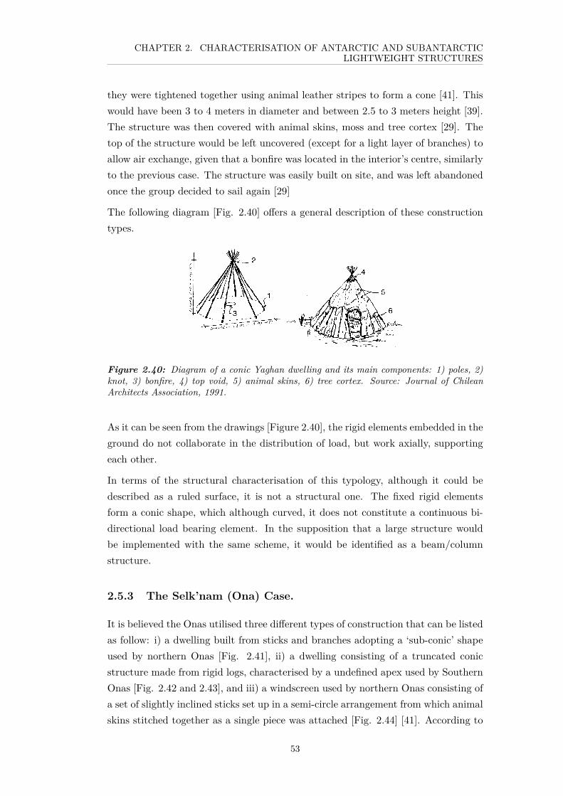
CHAPTER 2. CHARACTERISATION OF ANTARCTIC AND SUBANTARCTICLIGHTWEIGHT STRUCTURES
they were tightened together using animal leather stripes to form a cone [41]. Thiswould have been 3 to 4 meters in diameter and between 2.5 to 3 meters height [39].The structure was then covered with animal skins, moss and tree cortex [29]. Thetop of the structure would be left uncovered (except for a light layer of branches) toallow air exchange, given that a bonfire was located in the interior’s centre, similarlyto the previous case. The structure was easily built on site, and was left abandonedonce the group decided to sail again [29]
The following diagram [Fig. 2.40] offers a general description of these constructiontypes.
Figure 2.40: Diagram of a conic Yaghan dwelling and its main components: 1) poles, 2)knot, 3) bonfire, 4) top void, 5) animal skins, 6) tree cortex. Source: Journal of ChileanArchitects Association, 1991.
As it can be seen from the drawings [Figure 2.40], the rigid elements embedded in theground do not collaborate in the distribution of load, but work axially, supportingeach other.
In terms of the structural characterisation of this typology, although it could bedescribed as a ruled surface, it is not a structural one. The fixed rigid elementsform a conic shape, which although curved, it does not constitute a continuous bi-directional load bearing element. In the supposition that a large structure wouldbe implemented with the same scheme, it would be identified as a beam/columnstructure.
2.5.3 The Selk’nam (Ona) Case.
It is believed the Onas utilised three different types of construction that can be listedas follow: i) a dwelling built from sticks and branches adopting a ‘sub-conic’ shapeused by northern Onas [Fig. 2.41], ii) a dwelling consisting of a truncated conicstructure made from rigid logs, characterised by a undefined apex used by SouthernOnas [Fig. 2.42 and 2.43], and iii) a windscreen used by northern Onas consisting ofa set of slightly inclined sticks set up in a semi-circle arrangement from which animalskins stitched together as a single piece was attached [Fig. 2.44] [41]. According to
53

CHAPTER 2. CHARACTERISATION OF ANTARCTIC AND SUBANTARCTICLIGHTWEIGHT STRUCTURES
Casamiquela [41] the lack of an apex on this last model, prevented the possibility ofdefining it as either the segment of a cone, a hemisphere or a paraboloid.
Figure 2.41: Dwelling of the southern Onas, made out of logs with the shape of an inclinedcone. Image: Gusinde, 1918-1924.
Figure 2.42: Illustration of a dwelling ofthe northern Selk’nams with a ’sub-conic’shape made during the years 1918-1924.Source: Gusinde, 1982.
Figure 2.43: Photograph of a dwelling ofthe northern Selk’nams with a ’sub-conic’shape taken during the years 1918 -1924.Source: Gusinde, 1982.
There is no single hypothesis for this variety, but the most accepted explanationwas stated by Gusinde [33] which proposed that their use was determined by thelocation within Tierra del Fuego, which determined the type of material available.Therefore, while northern Selk’nams would occupy a vast and open region deprivedfrom trees, they would utilise the ‘sub-conics’ dwellings as well as wind-screens.Whilst the occupants of the southern part of the island, rich on forests and readilyaccessible branches could easily implement the conic-like structures. Father Coiazzi,offered a complementary explanation suggesting that the windscreens were utilisedfor short-term settlements while the others structures would be implemented for
54

CHAPTER 2. CHARACTERISATION OF ANTARCTIC AND SUBANTARCTICLIGHTWEIGHT STRUCTURES
longer periods of occupancy [41]. Again, given that this section does not focus onthe origin of these typologies, these hypothesises will not be further discussed.
Conclusively, although it could be said that these three cases are classified as curvedstructures and the last two ones more specifically as lightweight structures, it is notpossible to describe them as structural surfaces. In the first case, the southern Onacase of conic structures behaved similarly to the previous case described, the Yaghandwelling, where the rigid elements embedded on the ground do not collaborate in thedistribution of load bi-directionally, but instead work axially, supporting each other.The second case (sub-conic shape dwelling), although made out of lighter material,can be described similarly to the first typology. Moreover, although the third case(the widescreen used by northern Selk’nams) used a membrane, its behaviour doesnot differ largely from the previous cases: a group of independent poles embedded onthe ground supporting a membrane. Therefore, the rigidity and structural stiffnessof the system were not provided by the membrane, but the poles, with the skinonly inducing certain level of in-plane stability. In that sense, the membrane onlyperformed as a cladding and the system does not appear to have a surface-likebehaviour, with the rigid element working in bending.
From another point of view, the fact that if the membrane were removed the‘structure’ would still remain standing, not only affirms the previous statement,but also allows the objection to the inclusion of this typology as a structure insteadof an object or device. Unfortunately, no description was found regarding to theirminimum and maximum dimensions, which would assist in the estimation of theload involved and to its accurate classification.
Figure 2.44: Sketches of a windscreen used by the northern Selk’nams made during theyears 1918-1924. Source: Gusinde, 1982.
The mention of a fourth Selk’nam model is also found in the literature, this corre-sponds to a segment of an ideal cone that Casamiquela describes as a ceremonialshelter only [41], while Gusinde as a winter dwelling [33]. Its characterisation
55

CHAPTER 2. CHARACTERISATION OF ANTARCTIC AND SUBANTARCTICLIGHTWEIGHT STRUCTURES
would therefore be the same as the Yaghan conic structure, hence, it should notbe considered as a lightweight structural surface.
2.5.4 The Tehuelche (Aoniken) Case
Figure 2.45: Tehuelche dwelling. Image: E. Gerreaud, 1900.
The Tehuelche case is perhaps the most complex case of the Southern vernacularstructures. It represents the largest scale, probably due to the ergonometric char-acteristics of the Tehuelche people and the number of people hosted. There weremultiple variations of the basic model, and differently from the other cases, all thesevariations can be considered as structural surfaces, with exception of the most recentversion. This is also probably the best described and documented case, perhaps dueto the extent of the territory occupied by the Tehuelches, namely all the Patagoniamainland .
Commonly, the basic model is described as a half a dome attached to a front arch,which serves as an open façade. The structure was originally covered by large piecesof animal skin, namely Guanacos [39] [Fig. 2.45]. Later, once contact with firstEuropeans was established in the mid-20th century this cladding could be observedas consisting of horse skin and finally, of big pieces of awning/fabric [43]. Accordingto Baeriswyl [39], the main open façade would measure between 3 to 5 meters, theheight would reach 2 m and the depth would vary between 2 and 3 meters. Similarto other cases, a bonfire would be an important and it would be located at the frontof the dwelling. The description of Baeriswyl is presented in the following diagram[Fig. 2.46].
56

CHAPTER 2. CHARACTERISATION OF ANTARCTIC AND SUBANTARCTICLIGHTWEIGHT STRUCTURES
Figure 2.46: Diagram with the main elements of an Tehuelche tent according to Baeriswyl:1) main direcction of the wind, 2) structural poles, 3) nodes made with animal tendons, 4)pole’s V-endings, 5) guanaco skin covers, 6) front entrance. Source: Journals of ChileanArchitectural Association, 1991.
Canals Frau offered a more detailed description of this case. He described it as a bigtent, made out of 40 to 50 guanacos skins, or horses in the last century, resting onthree rows of poles [43]. Canals Frau also highlighted the ‘rectangular’ arrangementof the poles, which would have a V-top ending over which horizontal poles would laid.He also specified that the pieces of skin would be sewed using animal tendons to forma single membrane [43]. Figure 2.47 and 2.48 show some interpretations made byOutes [44] and Basaglia [45] based on descriptions made in the 18th century collectedby Viedma [46]. According to the classic semi-domed shaped of the tent, Figure 2.48could be pointed as erroneous, since the author omitted the characteristic vaultingof the structure. Other authors like Palavecino described these variations as twodifferent models [47]. Nevertheless, Casamiquela assured that there was only onetypology, whose shape could be adapted, due to the relative height of the nodes madein the front row of poles from where the membrane was attached [41], suggestingthat the structure tolerates a certain degree of variation in its geometry.
(a) (b) (c)
Figure 2.47: Diagram of a Tehuelche dwelling, made by Outes in 1905 based on thedescription made in middle 18th century. a) rear view, b) side view andd c) top view.Image: F. Outes, 1905.
The assemby procedure is known thanks to detailed descriptions made by severalethnographers such as Palavecino [47] and Muster [48]. Muster, described theprocedure would start with the rear row of v-ending top poles, which would beca. 1 meter high. A lath was placed above them, as a ridge beam. Two meters away
57
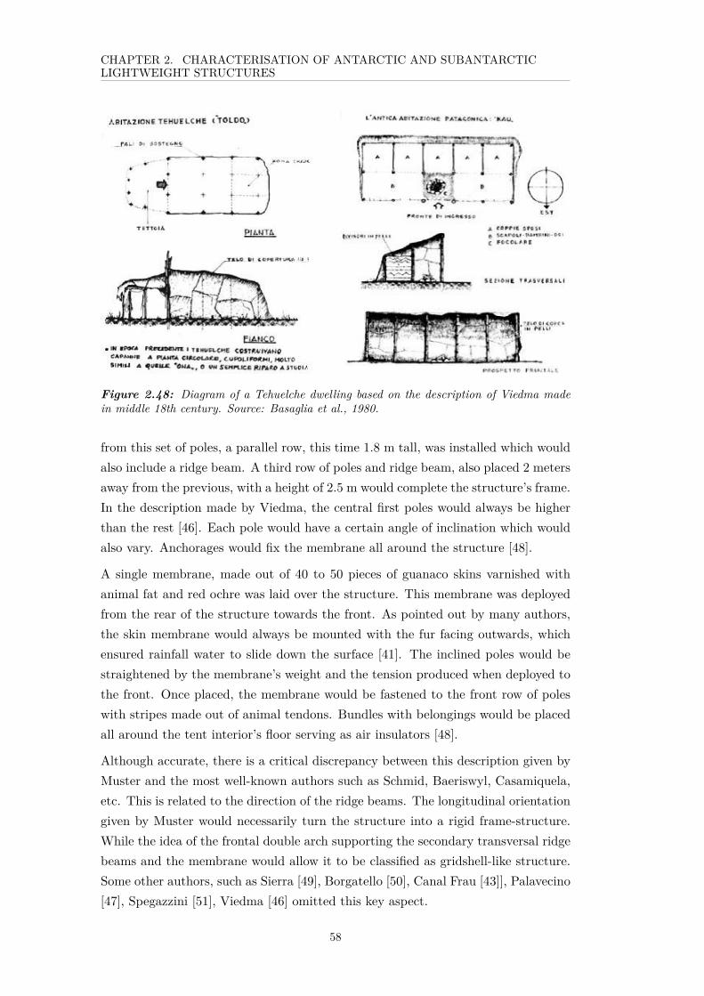
CHAPTER 2. CHARACTERISATION OF ANTARCTIC AND SUBANTARCTICLIGHTWEIGHT STRUCTURES
Figure 2.48: Diagram of a Tehuelche dwelling based on the description of Viedma madein middle 18th century. Source: Basaglia et al., 1980.
from this set of poles, a parallel row, this time 1.8 m tall, was installed which wouldalso include a ridge beam. A third row of poles and ridge beam, also placed 2 metersaway from the previous, with a height of 2.5 m would complete the structure’s frame.In the description made by Viedma, the central first poles would always be higherthan the rest [46]. Each pole would have a certain angle of inclination which wouldalso vary. Anchorages would fix the membrane all around the structure [48].
A single membrane, made out of 40 to 50 pieces of guanaco skins varnished withanimal fat and red ochre was laid over the structure. This membrane was deployedfrom the rear of the structure towards the front. As pointed out by many authors,the skin membrane would always be mounted with the fur facing outwards, whichensured rainfall water to slide down the surface [41]. The inclined poles would bestraightened by the membrane’s weight and the tension produced when deployed tothe front. Once placed, the membrane would be fastened to the front row of poleswith stripes made out of animal tendons. Bundles with belongings would be placedall around the tent interior’s floor serving as air insulators [48].
Although accurate, there is a critical discrepancy between this description given byMuster and the most well-known authors such as Schmid, Baeriswyl, Casamiquela,etc. This is related to the direction of the ridge beams. The longitudinal orientationgiven by Muster would necessarily turn the structure into a rigid frame-structure.While the idea of the frontal double arch supporting the secondary transversal ridgebeams and the membrane would allow it to be classified as gridshell-like structure.Some other authors, such as Sierra [49], Borgatello [50], Canal Frau [43]], Palavecino[47], Spegazzini [51], Viedma [46] omitted this key aspect.
58
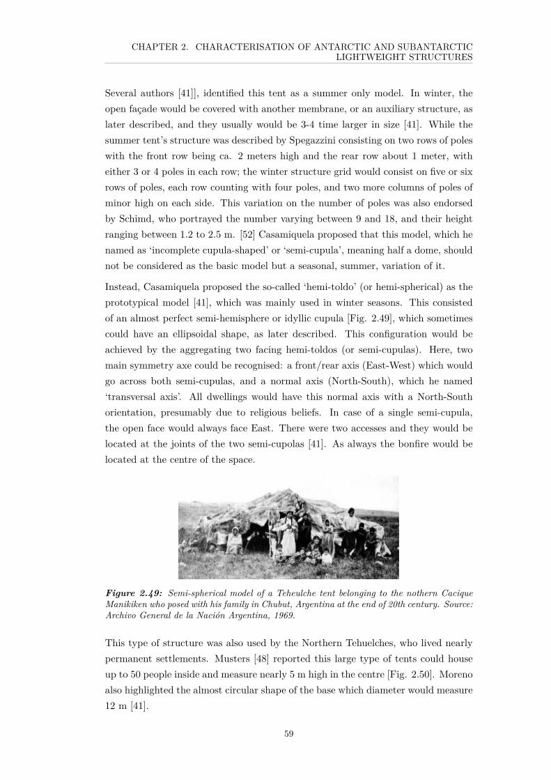
CHAPTER 2. CHARACTERISATION OF ANTARCTIC AND SUBANTARCTICLIGHTWEIGHT STRUCTURES
Several authors [41]], identified this tent as a summer only model. In winter, theopen façade would be covered with another membrane, or an auxiliary structure, aslater described, and they usually would be 3-4 time larger in size [41]. While thesummer tent’s structure was described by Spegazzini consisting on two rows of poleswith the front row being ca. 2 meters high and the rear row about 1 meter, witheither 3 or 4 poles in each row; the winter structure grid would consist on five or sixrows of poles, each row counting with four poles, and two more columns of poles ofminor high on each side. This variation on the number of poles was also endorsedby Schimd, who portrayed the number varying between 9 and 18, and their heightranging between 1.2 to 2.5 m. [52] Casamiquela proposed that this model, which henamed as ‘incomplete cupula-shaped’ or ‘semi-cupula’, meaning half a dome, shouldnot be considered as the basic model but a seasonal, summer, variation of it.
Instead, Casamiquela proposed the so-called ‘hemi-toldo’ (or hemi-spherical) as theprototypical model [41], which was mainly used in winter seasons. This consistedof an almost perfect semi-hemisphere or idyllic cupula [Fig. 2.49], which sometimescould have an ellipsoidal shape, as later described. This configuration would beachieved by the aggregating two facing hemi-toldos (or semi-cupulas). Here, twomain symmetry axe could be recognised: a front/rear axis (East-West) which wouldgo across both semi-cupulas, and a normal axis (North-South), which he named‘transversal axis’. All dwellings would have this normal axis with a North-Southorientation, presumably due to religious beliefs. In case of a single semi-cupula,the open face would always face East. There were two accesses and they would belocated at the joints of the two semi-cupolas [41]. As always the bonfire would belocated at the centre of the space.
Figure 2.49: Semi-spherical model of a Teheulche tent belonging to the nothern CaciqueManikiken who posed with his family in Chubut, Argentina at the end of 20th century. Source:Archivo General de la Nación Argentina, 1969.
This type of structure was also used by the Northern Tehuelches, who lived nearlypermanent settlements. Musters [48] reported this large type of tents could houseup to 50 people inside and measure nearly 5 m high in the centre [Fig. 2.50]. Morenoalso highlighted the almost circular shape of the base which diameter would measure12 m [41].
59

CHAPTER 2. CHARACTERISATION OF ANTARCTIC AND SUBANTARCTICLIGHTWEIGHT STRUCTURES
Figure 2.50: Semi-spherical Tehuelche dwelling completely covered on fabric in SantaCruz, Argentina. Source: Osvaldo Mondelo’s personal archives, undated.
Different authors [53, 54, 46, 47] mentioned internal subdivisions made by hangingpieces of skins. These cubicles would serve as independent bedrooms for the differentfamily members.
A variation of this model is named by Casamiquela as ‘reduce symmetrical’ model(or asymmetrical model) [41]. This would present two options: a) the aggregationof a classic hemi-cupula with an front structure of smaller dimensions and differentmateriality [Fig. 2.51], in which case the global shape could not be described as ahemi-spherical and b) the aggregation of two hemi-toldos, which although identical,would have a reduced depth, for which the base would describe an ellipse rather thanan circle, so that the transversal axis would be clearly longer than the East/Westaxis. Both models were also used as winter structures [47].
Figure 2.51: Asymmetrical tent model from a Southern Tehuelche family. Half structureis covered with animal skins, while the smallest section is covered with fabrics. Santa CruzProvince, Argentina. Source: Dr. Elsa Barberia’s personal archives, undated.
A final variation was a tall, square and slightly curved model described by Sanches-Labrador [55] and Falkner [56], at the beginning of the 20th century. In this model,the structures geometry has varied, and the roof cover is independent from the lateralskins [Fig. 2.52]. Casamiquela proposed that this model was a degenerated versionof the original, triggered by the excessive weight of the horse skin, introduced byEuropean settlers, or the natural mutation of the cupula-shaped tent to a largersized shelter to allow more people to be housed.
60
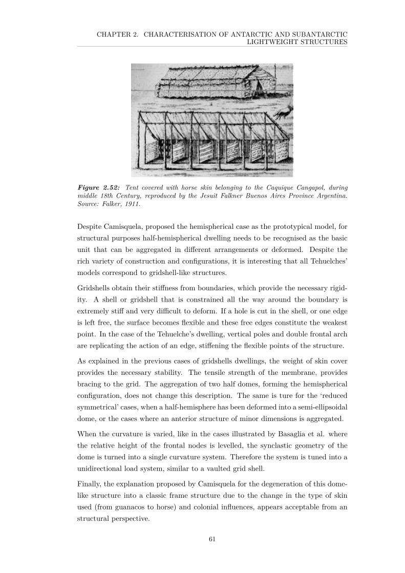
CHAPTER 2. CHARACTERISATION OF ANTARCTIC AND SUBANTARCTICLIGHTWEIGHT STRUCTURES
Figure 2.52: Tent covered with horse skin belonging to the Caquique Cangapol, duringmiddle 18th Century, reproduced by the Jesuit Falkner Buenos Aires Province Argentina.Source: Falker, 1911.
Despite Camisquela, proposed the hemispherical case as the prototypical model, forstructural purposes half-hemispherical dwelling needs to be recognised as the basicunit that can be aggregated in different arrangements or deformed. Despite therich variety of construction and configurations, it is interesting that all Tehuelches’models correspond to gridshell-like structures.
Gridshells obtain their stiffness from boundaries, which provide the necessary rigid-ity. A shell or gridshell that is constrained all the way around the boundary isextremely stiff and very difficult to deform. If a hole is cut in the shell, or one edgeis left free, the surface becomes flexible and these free edges constitute the weakestpoint. In the case of the Tehuelche’s dwelling, vertical poles and double frontal archare replicating the action of an edge, stiffening the flexible points of the structure.
As explained in the previous cases of gridshells dwellings, the weight of skin coverprovides the necessary stability. The tensile strength of the membrane, providesbracing to the grid. The aggregation of two half domes, forming the hemisphericalconfiguration, does not change this description. The same is ture for the ‘reducedsymmetrical’ cases, when a half-hemisphere has been deformed into a semi-ellipsoidaldome, or the cases where an anterior structure of minor dimensions is aggregated.
When the curvature is varied, like in the cases illustrated by Basaglia et al. wherethe relative height of the frontal nodes is levelled, the synclastic geometry of thedome is turned into a single curvature system. Therefore the system is tuned into aunidirectional load system, similar to a vaulted grid shell.
Finally, the explanation proposed by Camisquela for the degeneration of this dome-like structure into a classic frame structure due to the change in the type of skinused (from guanacos to horse) and colonial influences, appears acceptable from anstructural perspective.
61

CHAPTER 2. CHARACTERISATION OF ANTARCTIC AND SUBANTARCTICLIGHTWEIGHT STRUCTURES
2.6 Antarctic Portable Dwellings
There is a rich array of modern portable dwellings being used in Antarctica. Thisincludes tents and rigid modules. They play a key role in the exploration of the con-tinent’s deepest areas for scientific and touristic parties while still fulfilling with thestrict environmental protocols. Although these commercial structures are minimal,they have proved sufficient to provide safe shelter for explorers while still meetingcriteria of collapsibility, minimal weight, un-aided deployment and no trace-left onceremoved. Additionally, these types of structures allow the possibility to reconfigurecampsites according to every season’s requirements [Fig. 2.53 and 2.54].
Figure 2.53: Touristic basecamp at PatriotHills. Image: Antarctic Logistic andExpeditions, 2010.
Figure 2.54: Touristic basecamp at VinsonMassif. Image: International MountainGuides, 2014.
Although there is a broad spectrum of shapes, sizes and materials of tensile tentsfrom a structural point of view they could be classified as isolated membrane struc-tures, where pre-tension and bending are the key criteria for the efficiency of thedouble curved membranes and the flexible bars composing the structure. Anotherwell-known portable tent structure is the so-called ‘Polar Haven’ [Fig. 2.53] com-mercialized by Watherhaven ©, which could be described as a lighter version of theclassic ‘Jamesway’ hub, a vaulted structure of corrugated galvanized steel designedfor Artic conditions in the early 1940’s.
It could be reasonably debated as to whether these kinds of devices can be effectivelyconsidered structures or objects, as they remain in the borderline as architecturalcases. However, it cannot be disallowed that there always has been an interestingdialogue between portable dwellings and constructions.
Firstly, tents were the first type of construction buildings, serving as example forthe design of more permanent housing [57]. Most certainly, this transition may havehappened slowly.
In recent times, the lightness of tensile tents has become a source of interest toarchitects for nearly half a century, particularly those ones interested on developingprefabricated extended covering constructions, such as Renzo Piano, or cable nets,
62
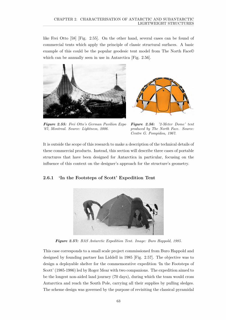
CHAPTER 2. CHARACTERISATION OF ANTARCTIC AND SUBANTARCTICLIGHTWEIGHT STRUCTURES
like Frei Otto [58] [Fig. 2.55]. On the other hand, several cases can be found ofcommercial tents which apply the principle of classic structural surfaces. A basicexample of this could be the popular geodesic tent model from The North Face©which can be annually seen in use in Antarctica [Fig. 2.56].
Figure 2.55: Frei Otto’s German Pavilion Expo’67, Montreal. Source: Lightness, 2006.
Figure 2.56: ’2-Meter Dome’ tentproduced by The North Face. Source:Centre G. Pompidou, 1967.
It is outside the scope of this research to make a description of the technical details ofthese commercial products. Instead, this section will describe three cases of portablestructures that have been designed for Antarctica in particular, focusing on theinfluence of this context on the designer’s approach for the structure’s geometry.
2.6.1 ‘In the Footsteps of Scott’ Expedition Tent
Figure 2.57: BAS Antarctic Expedition Tent. Image: Buro Happold, 1985.
This case corresponds to a small scale project commissioned from Buro Happold anddesigned by founding partner Ian Liddell in 1985 [Fig. 2.57]. The objective was todesign a deployable shelter for the commemorative expedition ‘In the Footsteps ofScott’ (1985-1986) led by Roger Mear with two companions. The expedition aimed tobe the longest non-aided land journey (70 days), during which the team would crossAntarctica and reach the South Pole, carrying all their supplies by pulling sledges.The scheme design was governed by the purpose of revisiting the classical pyramidal
63

CHAPTER 2. CHARACTERISATION OF ANTARCTIC AND SUBANTARCTICLIGHTWEIGHT STRUCTURES
structure used by the British Antarctic Survey. Such structure used wooden polesand turned out to be too heavy to be carried (28 kg) by the expeditioners. On theother hand, no commercial tent could guarantee to withstand the extreme weatherconditions of Antarctica at that time [59].
Figure 2.58: Pyramid tent set up upon the King Edward VII Plateau as part of 1910-1913British Antarctic Survey Expedition. Image: H.G. Ponting, 1911.
The solution was to optimise the original conical volume [Fig. 2.58] towards amore dome-like body, since spherical shapes are volumetrically more efficient andthey are more capable of dealing uniformly with the characteristic shifting windsof Antarctica [Fig. 2.57]. Another consideration was the logistical restrictions oftransport and assembly for this expedition in particular, namely the size of thesledge (2.4 m). Thus, the structure was resolved as an umbrella-system that waspartially deployable, an advantage over traditional total-collapsible tents [Fig. 2.59and 2.60]. The main structure was comprised of six glass-fibre bars contained withina membrane. In this way the entire tent could be transported as a single package.The membrane was defined as a set of doubly curved faces made from Goretex©fabric, an outer nylon layer and an inner PTFE skin. A thermal air buffer wasachieved with a second light inner membrane, helping to avoid the loss of internalheat. The assembly process thus remained simple. The membrane was pulled downfrom top to bottom along the bars, which were forced under compression to form acurved shape and to meet the single base ground sheet.
2.6.2 Sastruggi Tent
The Sastruggi tent is consisted of a ‘triaxial’ modular design to be attached to theEPTAP tunnel (see section 2.3) during the second season of construction in 2000, toserve as a meeting room for the occupants [Fig. 2.61]. Although only one structurewas built, the Sastruggi system was designed as an ever-expansible system, where
64

CHAPTER 2. CHARACTERISATION OF ANTARCTIC AND SUBANTARCTICLIGHTWEIGHT STRUCTURES
Figure 2.59: Sketches of the 1985 BASdouble curved surface and structure’s tent bydesigner Ian Liddel. Source: Buro Happold,undated.
Figure 2.60: Sketch of the crown joint forthe 1985 BAS d tent by designer Ian Liddel.Source: Buro Happold, undated.
Figure 2.61: Sastruggi Room as part of the EPTAP Station, Antarctica. Image: ARQZEArchitects, 2000.
other units could be repeated and aggregated along its three axis. Each modulewas also designed to be internally subdivided, with the peripheral units being useda sleeping cells and central units as common room. The system, created by theARQZE Research Unit from the University of Technology F. Santa Maria (Chile),was specifically designed to support the predominant winds of the area (known askatabatic winds), which can reach up to 41.7 m/s (150 km/h) [1]. Each unit was definedby a set of nine arches and anticlastic membranes forming a closed shape [Fig. 2.62].
Figure 2.62: Diagram of the Sas-truggi’s structure. Image: ARQZEArchitects, 1999.
Figure 2.63: Articulated joint designed for theSastruggi Tent. Image: ARQZE, 2000.
65
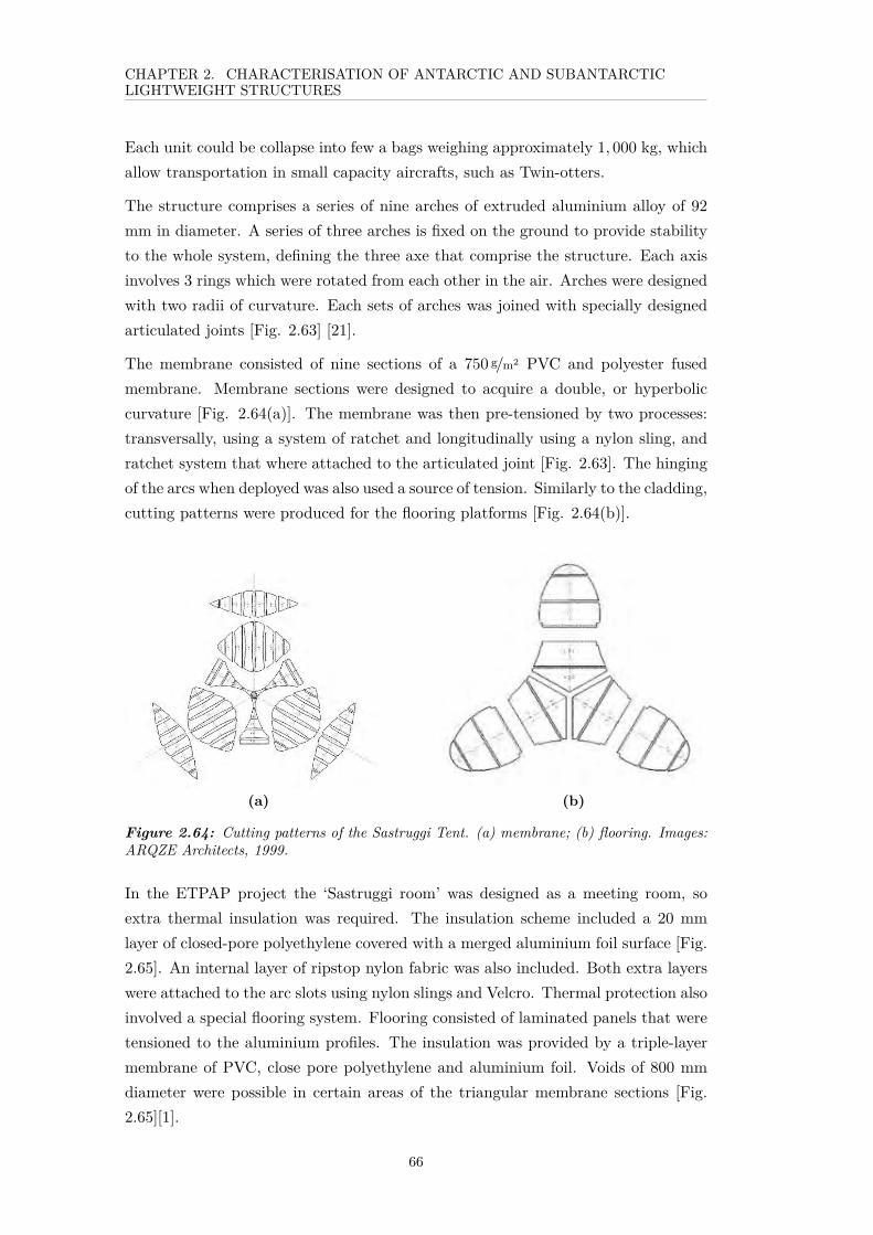
CHAPTER 2. CHARACTERISATION OF ANTARCTIC AND SUBANTARCTICLIGHTWEIGHT STRUCTURES
Each unit could be collapse into few a bags weighing approximately 1, 000 kg, whichallow transportation in small capacity aircrafts, such as Twin-otters.
The structure comprises a series of nine arches of extruded aluminium alloy of 92mm in diameter. A series of three arches is fixed on the ground to provide stabilityto the whole system, defining the three axe that comprise the structure. Each axisinvolves 3 rings which were rotated from each other in the air. Arches were designedwith two radii of curvature. Each sets of arches was joined with specially designedarticulated joints [Fig. 2.63] [21].
The membrane consisted of nine sections of a 750 g/m2 PVC and polyester fusedmembrane. Membrane sections were designed to acquire a double, or hyperboliccurvature [Fig. 2.64(a)]. The membrane was then pre-tensioned by two processes:transversally, using a system of ratchet and longitudinally using a nylon sling, andratchet system that where attached to the articulated joint [Fig. 2.63]. The hingingof the arcs when deployed was also used a source of tension. Similarly to the cladding,cutting patterns were produced for the flooring platforms [Fig. 2.64(b)].
(a) (b)
Figure 2.64: Cutting patterns of the Sastruggi Tent. (a) membrane; (b) flooring. Images:ARQZE Architects, 1999.
In the ETPAP project the ‘Sastruggi room’ was designed as a meeting room, soextra thermal insulation was required. The insulation scheme included a 20 mmlayer of closed-pore polyethylene covered with a merged aluminium foil surface [Fig.2.65]. An internal layer of ripstop nylon fabric was also included. Both extra layerswere attached to the arc slots using nylon slings and Velcro. Thermal protection alsoinvolved a special flooring system. Flooring consisted of laminated panels that weretensioned to the aluminium profiles. The insulation was provided by a triple-layermembrane of PVC, close pore polyethylene and aluminium foil. Voids of 800 mmdiameter were possible in certain areas of the triangular membrane sections [Fig.2.65][1].
66

CHAPTER 2. CHARACTERISATION OF ANTARCTIC AND SUBANTARCTICLIGHTWEIGHT STRUCTURES
Figure 2.65: Installation of insulation layers at the Sastruggi Room, Antarctica. Image:ARQZE Architects, 2000.
2.6.3 The Apple
Figure 2.66: The ’Apple’ hub installedin McMurdo Station, Antarctic. Source:Icewall One, 1998.
Figure 2.67: The ’Melon’ hub set up inAntarctica. Image: Chris Drury, 2006.
The Igloo Satellite Cabin©, also known as the ‘Apple’, is a commercial productwhich was originated by request of the Australian Antarctic Division (AAD) in theearly 1980’s [Fig. 2.66]. It can be described as a semi-monocoque rigid surface, andhas been used by nearly 16 countries, including Artic and Tropical environmentssuch as Far Northern Queesland [60].
In the early 1980’s the AAD called for the design of a lightweight, portable dwelling.Moreover, it needed to be able to be transported by helicopter and cause no impacton site [60]. The solution came in 1982 from MalcolmWallhead, a fibreglass moulder,and consisted of a pre-fabricated and insulated fibreglass cabin. The dome wascomposed of eight single walled panels, interlocked so the structure could either beassembled on site or transported as a unit. The first prototype was produced bycasting the eight panels from a mould made of plywood covered with fibreglass andwaxed. This included three plain panels, four window panels and one door panel
67

CHAPTER 2. CHARACTERISATION OF ANTARCTIC AND SUBANTARCTICLIGHTWEIGHT STRUCTURES
[60]. The hut was 3m diameter and weighed circa 300 kg. Lateral cables needed tobe installed in the panel joints and tensioned to the ground around the cabin.
The first cabin was used on Magnetic Island, near Australian Davis Station, forpenguin research. Nowadays it is still in place, serving as an uninsulated storagehut. The original model has not undergone much variation over the 25 years ofuse. In the latest version, the original insulation has been replaced by polyurethanesheet insulation between layers of fibreglass [61]. This has increased the weight ofthe Igloos, but is still possible to be flown by a helicopter at up to 130 km/h speed.
(a) (b)
Figure 2.68: Panelling of: (a) the Apple and, (b) the Melon hubs. Source: Islands to IceExhibition, Tasmanian Museum & Art Gallery, 2006.
A variation of the first ‘Apple’ model is the ‘Melon’, where a hemi-ellipsoid shape canbe achieved by including some singly curved panels along one axis [Fig. 2.67] [60].Figure 2.68 show the panelling of both models. Furthermore, as Figure 2.69 shows,larger schemes are possible by aggregating several units using auxiliary tunnels.
Figure 2.69: Design scheme of a prototypical Antarctic field station. Source: Islands toIce Exhibition, Tasmanian Museum & Art Gallery, 2006.
68

CHAPTER 2. CHARACTERISATION OF ANTARCTIC AND SUBANTARCTICLIGHTWEIGHT STRUCTURES
2.7 Conclusions
Figures 2.70 and 2.71 shows a diagram which maps the state of art of Antarcticlightweight structures according to the classification proposed by Bechthold, in termsof their structural and geometrical characterisation. This summary demonstrates thevariety of structural lightweight typologies, which was the principal objective of thisliterature review.
Each case described in this chapter provides valuable technical information aboutPolar construction, but furthermore each case tells a part of the history of Polarlightweight construction.
The richness and complexity of the extinct vernacular typologies cannot be portrayedin only a few paragraphs. However, this section makes a first attempt at describingthem and classifying them from a structural point of view. It is believed by theauthor that this set of lightweight dwellings deserves a better understanding andrecognition as remarkable example of structural efficiency.
The iconic Admundsen-Scott Geodesic Dome was the first attempt to demonstratethe possibility of structural surfaces with permanent use in Antarctica and it man-aged to greatly exceed its expected service lifespan. The Shockwave Tent revisitedthis option, deriving an interesting hybrid system and provided a glimpse of the po-tential for geodesic surfaces with more complex geometries in extreme environments,possible nowadays thanks to digital modelling tools.
In the case of the EPTAP station, there are several aspects that make this anoutstanding project. Firstly, it proves that membrane structures with permanentuse are possible to implement, and they can be used in a larger scale that traditionalmodules or tents. It also suggested that the combination materiality, in this casemembrane structures and rigid modules, can be an optimised solution for differentprogrammatic or thermal protection requirements.
There has always been a dialogue between tents and lightweight structures de-sign, most typically flowing from structural design to structure-inspired commercialproducts. In the case of bespoke Antarctic tents, example where this dialogue ispromoted the other way around were found, where tent technology is applied onlarger structures. The Sastruggi tent lays in the borderline between an isolatedstructure and a lightweight structural system, thanks to its ever-growing possibilitiesand its thermal insulation solution. As these projects show, thermal insulation isone of the main obstacles for the use of membrane constructions in Polar regions.The BAS tent promotes the benefit of evolving from a polygonal structure towards adoubly curved surface, with the aim of making it lighter and more efficient. However,
69
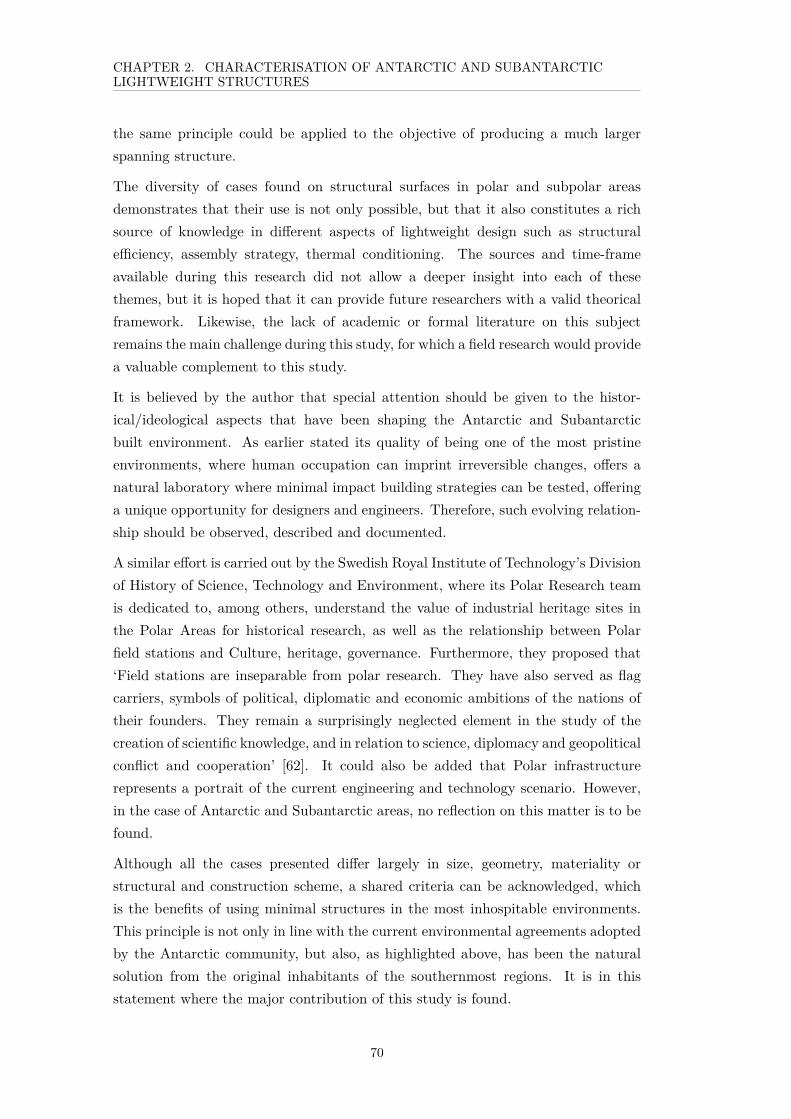
CHAPTER 2. CHARACTERISATION OF ANTARCTIC AND SUBANTARCTICLIGHTWEIGHT STRUCTURES
the same principle could be applied to the objective of producing a much largerspanning structure.
The diversity of cases found on structural surfaces in polar and subpolar areasdemonstrates that their use is not only possible, but that it also constitutes a richsource of knowledge in different aspects of lightweight design such as structuralefficiency, assembly strategy, thermal conditioning. The sources and time-frameavailable during this research did not allow a deeper insight into each of thesethemes, but it is hoped that it can provide future researchers with a valid theoricalframework. Likewise, the lack of academic or formal literature on this subjectremains the main challenge during this study, for which a field research would providea valuable complement to this study.
It is believed by the author that special attention should be given to the histor-ical/ideological aspects that have been shaping the Antarctic and Subantarcticbuilt environment. As earlier stated its quality of being one of the most pristineenvironments, where human occupation can imprint irreversible changes, offers anatural laboratory where minimal impact building strategies can be tested, offeringa unique opportunity for designers and engineers. Therefore, such evolving relation-ship should be observed, described and documented.
A similar effort is carried out by the Swedish Royal Institute of Technology’s Divisionof History of Science, Technology and Environment, where its Polar Research teamis dedicated to, among others, understand the value of industrial heritage sites inthe Polar Areas for historical research, as well as the relationship between Polarfield stations and Culture, heritage, governance. Furthermore, they proposed that‘Field stations are inseparable from polar research. They have also served as flagcarriers, symbols of political, diplomatic and economic ambitions of the nations oftheir founders. They remain a surprisingly neglected element in the study of thecreation of scientific knowledge, and in relation to science, diplomacy and geopoliticalconflict and cooperation’ [62]. It could also be added that Polar infrastructurerepresents a portrait of the current engineering and technology scenario. However,in the case of Antarctic and Subantarctic areas, no reflection on this matter is to befound.
Although all the cases presented differ largely in size, geometry, materiality orstructural and construction scheme, a shared criteria can be acknowledged, whichis the benefits of using minimal structures in the most inhospitable environments.This principle is not only in line with the current environmental agreements adoptedby the Antarctic community, but also, as highlighted above, has been the naturalsolution from the original inhabitants of the southernmost regions. It is in thisstatement where the major contribution of this study is found.
70

CHAPTER 2. CHARACTERISATION OF ANTARCTIC AND SUBANTARCTICLIGHTWEIGHT STRUCTURES
A second feature particular to lightweight Antarctic structures is their temporarycharacter. Almost all the cases described above, including structures implementedas permanent facilities, provide successful experiences of no-footprint retrievals rou-tines. Therefore, it can be stated that reversibility is a fundamental attribute ofmodern and vernacular polar (and subpolar) structures, and this is achieved bybespoke approaches. It could certainly be argued that portable architecture hasbeen explored for more than half a century. However, the design of Polar lightweightstructures provides designers with a vast field of new study areas that could be notreplicated in any other context. For example Polar lightweight structures requiresaspects of structural efficiency and collabsability to be integrated at the earliest stageof the design process. Furthermore, these aspects must be paired with constraintsof limited transportation sources and minimally aided assembly.
Another common aspect observed in the majority of the projects presented is re-lated to their capacity of variation. Perhaps the simplest strategy of variabilityis presented by the mutable configuration of field camps and indigenous camps,where the number of units varies according to the seasonal requirements. A secondlevel of variability is presented by cases of aggregation. The Tehuelche dwellingallows different configurations: standing as only as a semi-hemisphere, aggregatingtwo semi-cupolas (defined as the prototypical model Camisquela), or aggregatinganother less deep structure to the front of the hemisphere. The design of EPTAPalso includes a similar strategy of variability by allowing the aggregation of semi-monocoque modules along the main tunnel, as well as the extension of the tunnel bythe simple repetition of the set of arches and membrane segments. Similar operationis enabled by the Sastruggi Tent, where modules can be repeated along the threeaxes of the structure. The Shockwave tent also permits the variation between avaulted and a double curved surface depending on the aggregation of the 2 type oftrusses, with their proposal for Desert the Atacama corresponding to the first case,and the Antarctic case corresponding to a doubly curved surface.
Perhaps more complex examples of variability are related to those systems whichallowed the adaptability in their configuration. A good example of this is theTehuelche tent, where the number of poles ranged from 9 to 18, allowing multiplesizing options of the dome, as well as the option of an ellipsoidal plan, by reducingthe depth of the semi hemispheres. The curvature of the semi-cupola could alsobe varied, from a simply vaulted to a double curved surface, by varying the heightof the nodes joining the membrane to the frontal poles. The Kaweshkar and theYaghan dome is also believed to be able to vary in size although little study has beendedicated to that feature. The Shockwave tent also allowed the re-arrangement ofthe internal structure by relocating of the stereometric elements, although the impactof such operation on the global geometry could be debated.
71
CHAPTER 2. CHARACTERISATION OF ANTARCTIC AND SUBANTARCTICLIGHTWEIGHT STRUCTURES
These different strategies of variability aim to optimise the use of these structures,according to the different seasons’ demands. Therefore, this feature is also relatedto the temporary character driving the design of Polar lightweight structure, whichis not only required to be removed but also to adapt.
Nevertheless, and however positive the experiences previously presented are assessed,it should be remembered that they correspond to rather experimental models, withthe obvious exception of the indigenous dwellings.
While this chapter has offered sufficient evidence for the recognition of Polar lightweightdesign as a paradigm, the following chapter introduces the second part of thisresearch. This consists on a design-based study aimed at demonstrating that con-straints derived from remote areas can serve for the design of innovative lightweightstructures of more complex geometry and larger scale than currently seen, using thecase of the Union Glacier Station as a starting point. The originality of such studyis expected to prove the vast range of possibilities that this field can offer.
Chapter 3 is devoted to establishing the design criteria and the proposal of a noveldesign paradigm that guides this study.
72
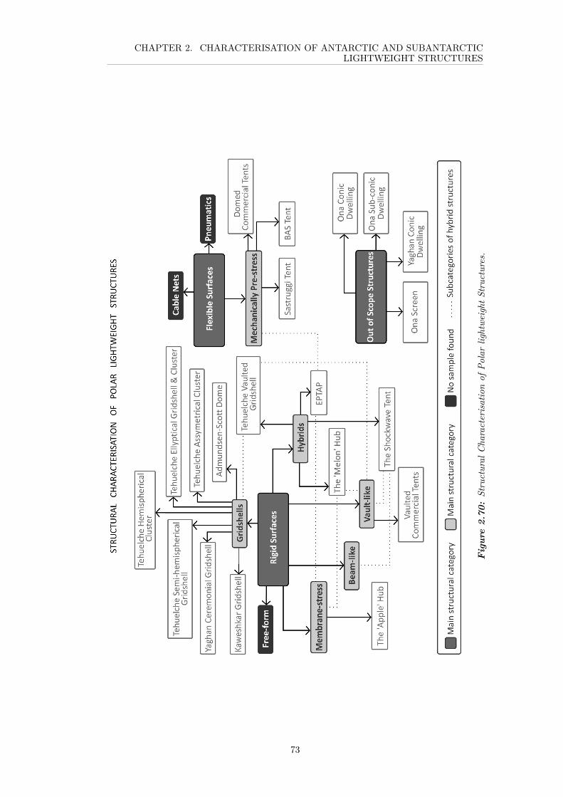
CHAPTER 2. CHARACTERISATION OF ANTARCTIC AND SUBANTARCTICLIGHTWEIGHT STRUCTURES
Fig
ure
2.70
:Structural
Cha
racterisationof
Polarlig
htwe
ight
Structures.
73

CHAPTER 2. CHARACTERISATION OF ANTARCTIC AND SUBANTARCTICLIGHTWEIGHT STRUCTURES
Figur e
2.71:Geom
etricalCharacterization
ofPolarLightweightStructures.
74
Chapter 3
Design Criteria
3.1 Introduction
This chapter describes the theorical agenda that guides the design-based studyoffered by this research. The objective of such exercise is to demonstrate that Polarlightweight design can serve to the development of novel paradigm and solutions.
Chapter 1 described the context of this research, and presented a brief for a newmedium scale summer-only station. This general criteria is summarised in section3.2. Chapter 2 have provided evidence for the recognition of Polar lightweightdesign as a valid design field, by describing and categorising a collection of casesbespoke structural surfaces. To continue this narrative, this third chapter proposesto challenge the inefficiency of classical seasonal constructions by exploring the designof a lightweight structural surfaces to implement the Union Glacier Station. In orderto that, such structural system such be resolved on a larger scale and with a morecomplex geometry than currently used, as it will be explained.
Section 3.2 lists the criteria that this design-led study should incorporate in orderto challenge currently seen Polar lightweight construction. These include commonlyknown problems related to the extreme polar context, as well as new geometricalaspects to be explored, this is, compactness and adjustable configuration. Based onthis particular problem, a specific geometry-based paradigm is formulated in section3.3. This problem consists on exploring the possibility of conceiving an adaptableyet semi-modular lightweight construction system for polar conditions. Evidenceof cases that have resolved such paradox are briefly described in section 3.4. Thischapter therefore, represents an inflection point in the narrative offered by this thesis,where a research question within the geometry-based design domain is formulated,which will guide the second part of this design-led study.
As a starting point for the design-based study, an early scheme is presented in section3.5 . This has been previously developed by the author, and although some of its
75

CHAPTER 3. DESIGN CRITERIA
attributes can be considered suitable for the presented case, several others need tobe further explored. Those missing aspects are described in this section and willguide the following study.
Finally, the method used to explore possible solutions is presented in section 3.6.Here, the structure for the design-based study is described, which involves optimisa-tion at the global and at the structural level, and is developed in the following threechapters.
3.2 Design Criteria
Chapter 1 presented the context and the opportunity for designing an innovativestation for Polar conditions. This design case-study will focus on a medium-scalesummer-only research station in the Glaciar Union Zone Glacier in the ChileanAntarctic Territory. Apart from scientific and logistic facilities, this station shouldprovide shelter for a variable number of crew. During winter, the station shouldremain closed.
The design criteria can be summarised and grouped as following:
In one hand standard constraints include:
1. Unaided assembly. The assembly procedure is to be carried out manuallywith minimal mechanical support and no electrical machinery available. Asdiscussed earlier, harsh weather conditions require personnel to wear bulkyitems of clothing including gloves, for which manual deftness is expectedto be highly reduced. In this sense, the structure’s components should beprefabricated and handleable by people unaided.
2. Straight-forward constructive sequence. The simplicity of the constructionchoreography relies on the avoidance of in-situ fabrication craft, in favourof standardised assembly procedures. It is essential to keep the number ofdifferent bespoke components to a minimum. This condition, and the oneabove, is also critical for purposes of periodic maintenance and emergencyrepair.
3. Logistic constraints are placed on the weight and size of the structure’s pieces.While the cargo capacity of the available aircraft fleet is rather large, the finalterrestrial conveyance will be executed by small capacity vehicles, for whichcomponents are required to be piled on standard pallets.
4. Collapsibility. The assembly procedure needs to be reversible, in terms ofallowing relocation, partial closure (in preparation for winter) or complete
76

CHAPTER 3. DESIGN CRITERIA
withdrawal once the station has fulfilled it lifespan. In any of these cases,the no-trace or ‘temporary’ condition dictated by the environmental policiesis required to be fulfilled.
On the other hand, some further aspects that this cases should include to overcometraditional designs are:
5. Adaptive configuration. The construction system should permit multiple as-sembly options in response to a highly variable number of occupants duringsummer seasons, from a minimum of 5 to a maximum of 16, whilst in winterthe structure is to remain unoccupied.
6. Efficient organisation. The station should be planned and resolved as a unitarybuilding, rather than a collection of facilities, minimising external transit andaccess points as well as the amount of surface exposed to the elements.
3.3 Geometric Scheme
This section develops a more detailed insight into the two geometric requirementsto be integrated into the design proposal, these are, aggregation and adaptability,as described in the previous section. As this section describes, the first of thesefeatures is explored in order to output some of the shortcoming observed in theexisting summer-only field camps, generally using lightweight units; while the secondof these two architectural requirements tackles one of the main aspects that makesmedium-scale seasonal facilities (as pointed out in Chapter 1).
3.3.1 Aggregation
Aggregation is one of the simplest operations to be carried out with geometricalunitary objects, in this case structural surfaces, where their composition (or topol-ogy) is not required to be common [63], but which are constrained by the need forcommon boundary edges.
In the case of polar design, the aggregation of units serves the purpose of an efficientorganization by compactness. Compactness (C) is a simple geometrical propertyof objects, defined by the ratio of the surface area (Stotal) required to ‘wrap’ thevolume engaged, V (C = V/Stotal). The level of compactness of a building isusually an indicator of its thermal efficiency, as the more surface exposed, the higherthe tendency for heat to be lost to the exterior through conduction, assuming ofcourse the external temperature is lower than the internal [64]. The compactnessof a building can be compared against three different geometrical aspects: shape,
77
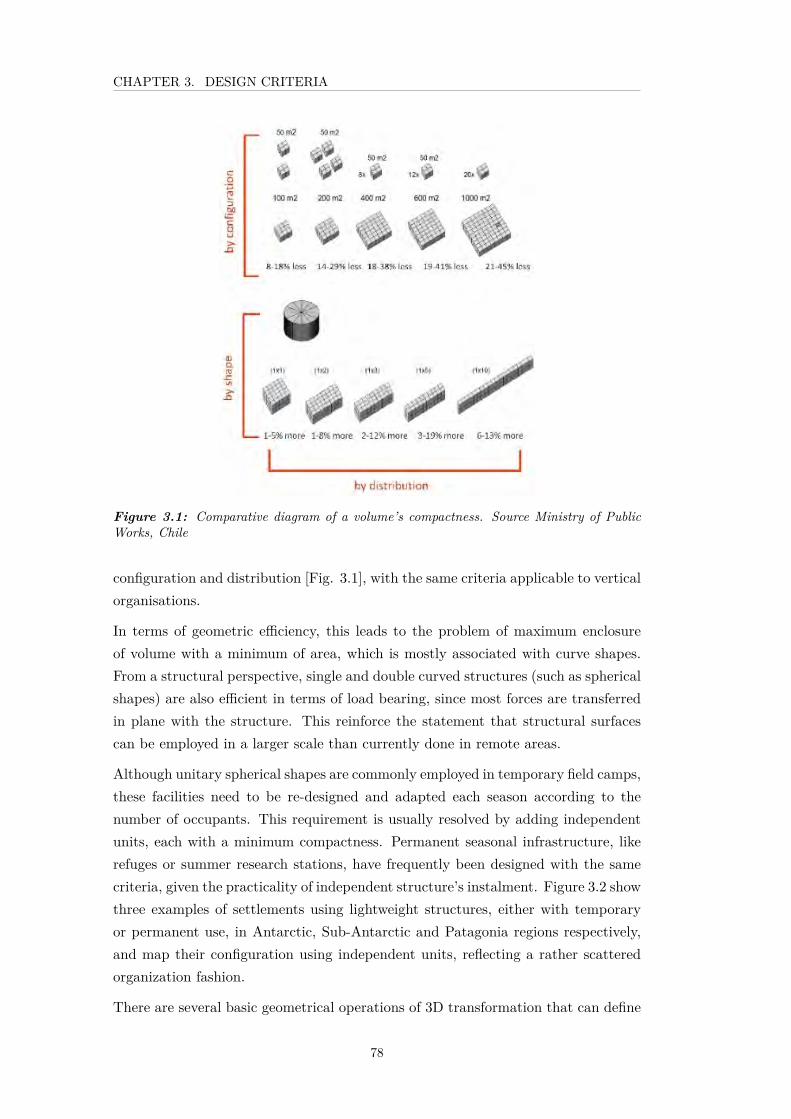
CHAPTER 3. DESIGN CRITERIA
Figure 3.1: Comparative diagram of a volume’s compactness. Source Ministry of PublicWorks, Chile
configuration and distribution [Fig. 3.1], with the same criteria applicable to verticalorganisations.
In terms of geometric efficiency, this leads to the problem of maximum enclosureof volume with a minimum of area, which is mostly associated with curve shapes.From a structural perspective, single and double curved structures (such as sphericalshapes) are also efficient in terms of load bearing, since most forces are transferredin plane with the structure. This reinforce the statement that structural surfacescan be employed in a larger scale than currently done in remote areas.
Although unitary spherical shapes are commonly employed in temporary field camps,these facilities need to be re-designed and adapted each season according to thenumber of occupants. This requirement is usually resolved by adding independentunits, each with a minimum compactness. Permanent seasonal infrastructure, likerefuges or summer research stations, have frequently been designed with the samecriteria, given the practicality of independent structure’s instalment. Figure 3.2 showthree examples of settlements using lightweight structures, either with temporaryor permanent use, in Antarctic, Sub-Antarctic and Patagonia regions respectively,and map their configuration using independent units, reflecting a rather scatteredorganization fashion.
There are several basic geometrical operations of 3D transformation that can define
78

CHAPTER 3. DESIGN CRITERIA
(a) (b)
(c)
Figure 3.2: Examples of arrangements for touristic settlement’s using lightweightconstructions. (a) Toro Lake Lodging Torres del Paine National Park, Patagonia (b)Patriot Hills Field Camp, Antarctica, (c) Whalesound Marine Research Station and Lodging,Francisco Colane National Park. Source: various, undated.
a surface by clustering or collecting repeated unitary elements, the most commonbeing: translation, rotation, helical motion, reflection [65]. Examples of these couldbe: surfaces of revolution, 3D periodic and aperiodic tiling and some cases of ruledsurfaces (such as cylindrical developable surfaces ) [65].
A particularly interesting case of aggregation of repeated surfaces is that of TriplePeriodic Minimal Surfaces (TPMS). Minimal surfaces with crystalline structure areof great interest in the design field due to the architectural possibilities that theirenclosures enable. There is a large number of fascinating TPMSs, many of themoriginally discovered by Alan Schoen in his famous report for NASA in 1970 [66].Currently, there are several digital tools that allow the exploration of minimal surfacedefinition and replication, most associated with generic design platforms such asRhino’s components ‘Geometry Gym’, ‘Minimal Surface’, ‘Kangaroo’ among others[67]. Perhaps, the longest established and most robust digital environment for theexploration of minimal surfaces is ‘Surface Evolver’, a mathematical software tooldeveloped by Brakke [68]. The software works by minimising different energies onconstrained surfaces using a gradient method.
In Surface Evolver, TPMS are achieved by defining and then optimising the fun-damental unit of the geometry, which is then suitably transformed (displaced androtated). Figure 3.3 shows a simple exercise of aggregation of TPMS using Brakke’sEvolver[68]. Toyo Ito’s Taichung Metropolitan Opera House in Japan and the
79

CHAPTER 3. DESIGN CRITERIA
(a) (b) (c) (d)
Figure 3.3: Evolution of the Schwarz’ P Surface using Surface Evolver. (a) fundamentalregion, corresponding to a tetrahedron before its evolution, (b) fundamental region onceevolved, (c) one cubical unit cell, (d) same unit cell repeated four times.
Ingenhoven Architects’ proposal for a new Stuttgart Main Station in Germanycan be considered examples of this principle applied in practice. In 2011, theauthor explored a method to allow the interaction between the Evolver and CADenvironments, which proved feasible [Appendix A].
Chapter 2 identified two basic formats of building typologies widely used as polarlightweight structures, deployable and assembled, which are logically driven by theirmateriality and thus, to their geometry. Assembled structures are mostly related torigid materials and synclastic shapes with deployable structures more often basedon anticlastic fabric membranes. This study will explore a generative system whereboth types of components, rigid and membranes, can be aggregated to differentiatethe station’s varying programmatic requirements. Similarly to the generation ofTPMS, basic transformation operations will be employed in this study to produceaggregations.
3.3.2 Adaptability
Chapter 2 identified three different types of small-scale temporary facilities used inPolar areas: field camps, seasonal research stations and refuges, each employed withdifferent rules. While field camps must be designed annually according to varyingseasonal demand, permanent infrastructure (refuges and summer research stations)must cope with variable numbers of occupants (see Chapter 1), which can sometimesplace a limitation on the size of scientific parties, or result in an excess of energyand logistic resources required to keep the station operative.
Adaptability, related to the responsive capacity of a system to vary its configuration,is the key aspect that this proposal explores. This will allow temporary stationsto be more efficient in terms of permitting a partial or customized use, and willtherefore reduce environmental impacts and unnecessary resource consumption dueto maintenance, transportation and energy consumption when not fully operative.
80

CHAPTER 3. DESIGN CRITERIA
Figure 3.4: Prototype of the‘Radiolaria Project’ (structuraltessellation of double curved sur-faces) developed by Universityof Kassel, Germany. Source:ECAADe.
Figure 3.5: Prototype of free-form gridshell based ongeodesic method developed by the Politecnico di Torino,Italy. Source: IASS Journal.
In the current context of structural design, there are different approaches to geo-metric adaptability. Perhaps the most common is provided by means of parametricdesign methods. Adjustable modelling design tools have been widely explored inthe last decade thanks to the development of interactive parametric design tools,such as Grasshopper by McNeel & Associates, Bentley’s Generative Componentsand Autodesk’s Dynamo. In addition to these generic software platforms, severalthird-party analysis plug-ins have been developed to provide real-time performancefeedback in order to assist the design process at the earliest stage in differentfronts such as structural performance, thermal behaviour, components definition andothers [69]. The explorative combination of generic design tools and performanceanalysis tools allow a variety of design options to be explored simultaneously againstquantitative and qualitative criteria by adjusting numeric parameters [69]. Surfacescapable of handling global adjustments to their geometry are generally used in casesof freeform schemes.
In the specific case of structural surfaces, their implementation generally is resolvedusing meshes (either triangular or quadrilateral) [Fig. 3.4 and 3.5], which in principleincludes structural membranes.
Structural surfaces of complex and variable geometry are generally resolved as agrids using various subdivision methods wich components, either edges or panels,that tend to vary in size. This feature can be moderate, particularly when pre-or post-rationalisation methods are involved. Evidently, when geometric variationsof such surfaces are applied, the number of different components increases greatly.The complexity of the assembly process of these types of structure (surfaces withfree-form or complex geometry), makes the use of these systems unsuitable forremote areas. It is widely known that working with many different pieces which aredifficult to visually distinguish from each other requires a refined assembling strategy.Assembly methods relying on manufacturing and/or delivery sequences generallyproves abortive, as any delay or error made in either in the labelling, stocking or
81

CHAPTER 3. DESIGN CRITERIA
construction stage can have serious consequences in the field. The repercussions areeven more critical when working in isolated areas or in rough climatic conditions.Additionally, surfaces of complex geometry generally require highly skilled personnelfor their erection, as well as sophisticated machinery.
This means that although the use of a more complex geometrical scheme is requiredin order to allow the aggregation of components in multiple arrangements, the vari-ability of said geometry should be carefully controlled. In this regard, Annex II offersa case-study where two very different gridshells are compared from a constructionperspective. The paper, written by the author, describes the design and constructionprocesses of a free-form temporary structure, namely the C-Space DRL10 PavilionProject in London, and the triple-domed gridshell Weald and Downland Open AirMuseum service building in Sussex. The paper discusses the radically different pathsthat the implementation of a structural surfaces might follow, depending on theirgeometrical origin, and highlights the contrasts in the fabrication and constructionprocesses of both projects.
It could be reasonably argued that traditional computational tools have been vali-dated as suitable platforms for the control of information along the entire implemen-tation process for at least the last decade. BIM technology (Building InformationModelling) in platforms like ArchiCAD® and Revit® are capable of assigning ex-tra information to each geometrical entity that compose the building model [70].Furthermore, new parametric design tools, like Bentley’s Generative Components®or Dassault Systèmes’ CATIA®, offer even more integrative environments for thedevelopment of complex shapes, the rationalization of their constructive components,and the assessment of their structural behaviour [69]. However, this exercise pointstowards a much more restricted approach, where the variations of a constructionsystem should be provided by carefully constrained geometric operations.
Another aspect of adaptability in the structural design landscape is demonstratedby responsive buildings. The aim of this extension to engineering and architecturaldesign practice is to allow the measure of actual environmental conditions to enablebuildings to adapt attributes such as shape, form, colour or other characteristicsvia physical actuators [71]. Using intelligent mechanisms, responsive buildings canbe designed to interact with their environment in order to optimise their energyconsumption (such as climate adaptive facades) or to allow dynamic use of spaceby their occupants (such as ORAMBRA’s actuated tensegrity structures or MIT’sintelligent kinetic system) [72].
Early architectural exploration of adaptive structural systems in the mid 1960’sslowly began to struggle due to the lack of computational and structural systemssufficient to allow the exploration. By the 1980s the discipline had been transferredinto the domain of engineering and nowadays engineering solutions for adaptive
82

CHAPTER 3. DESIGN CRITERIA
Figure 3.6: Prototype of one the variations of the ‘Eccentric Umbrella Structure’ based onthe Locust hind wing developed by the Israel Institute of Technology. Source: IASS.
structural system are common. They include technologies such as active dampers,piezoelectric structures, actuated tensegrity and deployable structural system [73].Applications of actuated tensegrity systems can be found within aeronautical, spaceand civil fields. Nevertheless, architectural design methodologies using this type ofsurfaces remain so far relatively unexplored [74]. A particular interesting case is thework of Tristan d’ Estree Sterk, who proposes the revision of Buckminster Fuller’stheory of tensegrity structures to produce a new class of adaptive structures [75].Currently, digital parametric design tools are also progressing this field, with toolssuch as Formsolver [76]. D’ Estree Sterk suggests that the design of an actuatedstructure is not sufficent to produce a responsive structure, which can only be definedas such ‘when actuators are coupled with other devices so that activities and changeswithin the real world can be interpreted, computed or processes and then outputtedback into the real world as an action or response’ [77]. This fundamental conditionis the main restriction on the use of responsive structures in remote areas. Anytype of perceptive device would not be compatible with the simple construction andoperational conditions imposed by a polar environment.
Another limitation of these systems is their geometrical possibilities usually con-fined to regular shapes. There are few incipient examples of mechanically actuatedsurfaces using more complex geometries to be found in the literature. An earlyexample of this is The ‘Eccentric Umbrella Structure’, an asymmetrical deployablesurface based on the Locust hind wing [78] and developed by the Israel Institute ofTechnology [Fig. 3.6]. Although promising, there is no major evidence yet of thescope of such deployable system and its structural and construction feasibility [73],which are critical aspect for its potential use in remote areas.
83

CHAPTER 3. DESIGN CRITERIA
Figure 3.7: Military base camp in Afghanistan implemented by Wheatherhaven ©. Image:Wheatherhaven, 2014.
3.4 Modularity versus Adaptability
While the main goal of the second part of this thesis has been introduced, thisis, the development of an adaptable lightweight system constructed from a lownumber of different components, the application of the conventional parametricdesign methodology has been discarded, as has the use of actuated structures, basedon the limitations that a remote context imposes. Instead, this research investigatesa bespoke approach, where elements are coordinated under a much simpler, if notlow-tech, strategy.
The aggregation of units is an attribute of modular structures, due their strictdimensional coordination and lack of geometric variability [Fig 3.7]. A commonexample of this is the case of LEGO® bricks. Eilers established that there are915,103,765 possible arrangements of using six 2x4 LEGO® bricks, defeating theclassic belief of a limit of 102,981,500 possibilities [79]. Higher configurations remainunsolved [80]. Although trivial, if the same exercise is applied to a set of componentsof any structural surface with bespoke panels, for instance Figure 3.4, the possibilitiesare reduced to one solution. If the options of aggregating more components isconsulted, solutions would then be infinite versus none.
The constraints stablished for this particular case (Section 3.2) entails the integra-tion of both these apparently contradictory approaches, (a system with adaptablegeometry and a modular structure) in a single solution.
The author believes that if a compromise is established between the two approaches,a variety of solutions should be possible. These hybrid solutions should balance theconflicting concepts of modularity and adaptability. Is in the middle of this rangewhere the design proposal is expected to be situated, which proposes a novel designproblem.
In order to this, this exercise entitles the definition of a construction system whoseattributes’ variations are constrained within a pre-established range of degrees ofgeometric freedom (or variation).
84
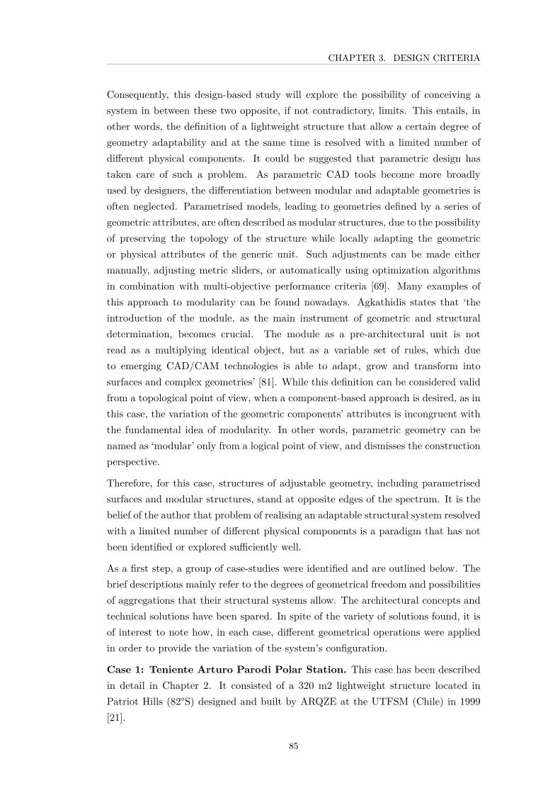
CHAPTER 3. DESIGN CRITERIA
Consequently, this design-based study will explore the possibility of conceiving asystem in between these two opposite, if not contradictory, limits. This entails, inother words, the definition of a lightweight structure that allow a certain degree ofgeometry adaptability and at the same time is resolved with a limited number ofdifferent physical components. It could be suggested that parametric design hastaken care of such a problem. As parametric CAD tools become more broadlyused by designers, the differentiation between modular and adaptable geometries isoften neglected. Parametrised models, leading to geometries defined by a series ofgeometric attributes, are often described as modular structures, due to the possibilityof preserving the topology of the structure while locally adapting the geometricor physical attributes of the generic unit. Such adjustments can be made eithermanually, adjusting metric sliders, or automatically using optimization algorithmsin combination with multi-objective performance criteria [69]. Many examples ofthis approach to modularity can be found nowadays. Agkathidis states that ‘theintroduction of the module, as the main instrument of geometric and structuraldetermination, becomes crucial. The module as a pre-architectural unit is notread as a multiplying identical object, but as a variable set of rules, which dueto emerging CAD/CAM technologies is able to adapt, grow and transform intosurfaces and complex geometries’ [81]. While this definition can be considered validfrom a topological point of view, when a component-based approach is desired, as inthis case, the variation of the geometric components’ attributes is incongruent withthe fundamental idea of modularity. In other words, parametric geometry can benamed as ‘modular’ only from a logical point of view, and dismisses the constructionperspective.
Therefore, for this case, structures of adjustable geometry, including parametrisedsurfaces and modular structures, stand at opposite edges of the spectrum. It is thebelief of the author that problem of realising an adaptable structural system resolvedwith a limited number of different physical components is a paradigm that has notbeen identified or explored sufficiently well.
As a first step, a group of case-studies were identified and are outlined below. Thebrief descriptions mainly refer to the degrees of geometrical freedom and possibilitiesof aggregations that their structural systems allow. The architectural concepts andtechnical solutions have been spared. In spite of the variety of solutions found, it isof interest to note how, in each case, different geometrical operations were appliedin order to provide the variation of the system’s configuration.
Case 1: Teniente Arturo Parodi Polar Station. This case has been describedin detail in Chapter 2. It consisted of a 320 m2 lightweight structure located inPatriot Hills (82°S) designed and built by ARQZE at the UTFSM (Chile) in 1999[21].
85
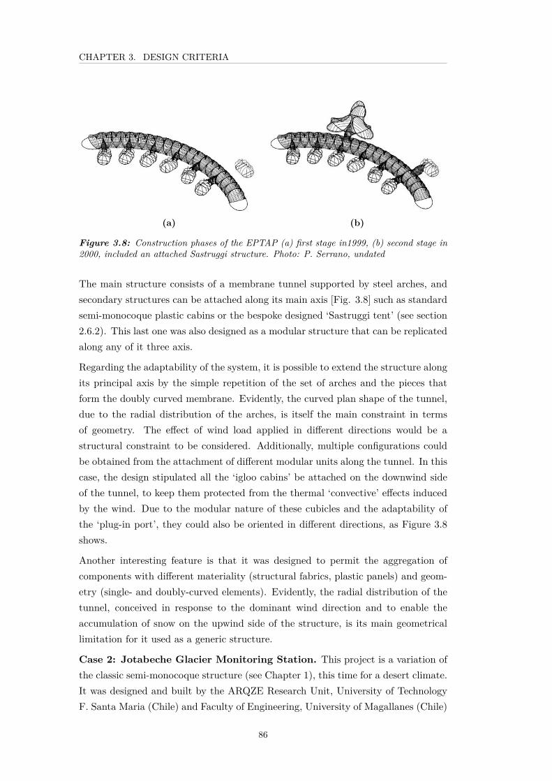
CHAPTER 3. DESIGN CRITERIA
(a) (b)
Figure 3.8: Construction phases of the EPTAP (a) first stage in1999, (b) second stage in2000, included an attached Sastruggi structure. Photo: P. Serrano, undated
The main structure consists of a membrane tunnel supported by steel arches, andsecondary structures can be attached along its main axis [Fig. 3.8] such as standardsemi-monocoque plastic cabins or the bespoke designed ‘Sastruggi tent’ (see section2.6.2). This last one was also designed as a modular structure that can be replicatedalong any of it three axis.
Regarding the adaptability of the system, it is possible to extend the structure alongits principal axis by the simple repetition of the set of arches and the pieces thatform the doubly curved membrane. Evidently, the curved plan shape of the tunnel,due to the radial distribution of the arches, is itself the main constraint in termsof geometry. The effect of wind load applied in different directions would be astructural constraint to be considered. Additionally, multiple configurations couldbe obtained from the attachment of different modular units along the tunnel. In thiscase, the design stipulated all the ‘igloo cabins’ be attached on the downwind sideof the tunnel, to keep them protected from the thermal ‘convective’ effects inducedby the wind. Due to the modular nature of these cubicles and the adaptability ofthe ‘plug-in port’, they could also be oriented in different directions, as Figure 3.8shows.
Another interesting feature is that it was designed to permit the aggregation ofcomponents with different materiality (structural fabrics, plastic panels) and geom-etry (single- and doubly-curved elements). Evidently, the radial distribution of thetunnel, conceived in response to the dominant wind direction and to enable theaccumulation of snow on the upwind side of the structure, is its main geometricallimitation for it used as a generic structure.
Case 2: Jotabeche Glacier Monitoring Station. This project is a variation ofthe classic semi-monocoque structure (see Chapter 1), this time for a desert climate.It was designed and built by the ARQZE Research Unit, University of TechnologyF. Santa Maria (Chile) and Faculty of Engineering, University of Magallanes (Chile)
86

CHAPTER 3. DESIGN CRITERIA
for the Glaciology and Snows Unit of the Chilean Ministry of Public Works in 2009.It was placed in the Nevado Jotabeche (27°S 69°O, 4.700 above sea level.). Inits original configuration the station had a floor area of approximately 18 m2 andcapacity for 8 people [82]. The structure was designed following a component-basedapproach [83], which enabled its transportation, assembly and eventual disassemblywithout any impact on the site [Fig. 3.9]. Transportation included the use ofhelicopters, mountain vehicles and animal traction (donkeys), which needed to beincorporated into the design.
Figure 3.9: The Jotabeche Station. Photo: P. Serrano, 2009.
The adaptability of the structure is related to multiple features. Firstly, the steelplatform is not only capable of coping with the irregularity of the soil due to amanual levelling system with a variation of up to 50 cm, but also the embeddedfoundation system can be changed depending on the different soil conditions: flatstrip footings for sand and snow, crampons for ice and shoes for rocky soil [Fig.3.10] Internal sub-divisions are achieved with the installation of plywood panels.This allows the Jotabeche station to have a separate space allocated as a toilet anda second space dedicated to the production and storage of water.
Figure 3.10: Alternatives of variations of the anchor system, from left to right: plates forsnow and sand, crampons for rock, and shoes rocky soils. Image: A. Veliz, 2009.
87

CHAPTER 3. DESIGN CRITERIA
A deployable membrane can be attached to the two ends (Figure 3.9 only showsa membrane attached to one end) permits the eventual extension of the refuge byadding more of the same components (panels and base platform). The inner spacecan also be easily modified by attaching or removing division panels without affectingthe fuselage due to a simple bolting system.
This simple design strategy proved successful, as a second station was commissionedby the same institution, this time for use in the Northern Ice Field of ChileanPatagonia (47S) [28]. In this case a larger space was achieved by using 12 panels[Figs. 3.11 and 3.12].
A component-based design approach proved adequate for an adaptable semi-monocoquestructure located in a remote site, where a limited set of features allowed a certaindegree of design freedom. The limitations of such geometry are obvious, due its lineararrangement. More complex configurations of this type are represented by casessuch as Weatherhaven modules [84] [Fig. 3.13] and Igoo Cabins (see Chapter 2),which use connecting sleeves and panels defined as part of a sphere’s for expandablearrangements.
Figure 3.11: Assembly test for the EchaurrenGlacier Monitoring Station. Photo: P. Serrano,2010.
Figure 3.12: Configuration ofcomponents for Echaurren Station.Image: A. Veliz, 2009.
88

CHAPTER 3. DESIGN CRITERIA
Figure 3.13: Polar settlement using Weatherhaven modules. Source: Weatherhaven.com,2015.
Case 3: Panul Warehouse and Shed. This project was built in 2004 by the WARApplied Research Office for a private company which commissioned the constructionof a warehouse (410 m2) and a large shed (2140 m2) for aquaculture production [Figs.3.14 and 3.15]. The structures were located on an inhabited area in CoquimboProvince, northern Chile (29°S).
Figure 3.14: Panul Warehouse. Image: D.Rosenberg, 2004.
Figure 3.15: Panul Shed. Image: D.Rosenberg, 2004.
The design team had to cope with the fact that only two materials were avail-able for construction: standard polycarbonate sheets and pine wood planks. Thiscondition raised the opportunity for a variable design and build process based onmodular pieces and material tolerance. The Architects described the project as anopportunity to “highlight the value of designing a construction strategy, allowing thecreation of form rather than predefining it” [85]. Consequently, the design took intoaccount the way in which the structure was going to be built, and at the same time,the building process could be fed by a preceding simulation and manipulation ofthe shape [86]. As a result of the development of such an adaptable construction
89

CHAPTER 3. DESIGN CRITERIA
process, certain aspects of the building’s shape could be manipulated and variationscould be generated.
The adaptability of the design was demanded by two different constraints. Thewarehouse needed to be rectangular front and back to allow a complete slidingdisplacement of the facade, required for the transportation of production equipment(water cisterns). It was therefore decided that three pin-joint frames could providethe geometrical variation of the volume, from a double-pitched roof at the centre,changing to a flat roof at the edges [Fig. 3.16]. On the other hand, the shed neededto coincide with the irregular morphology of the terrain. Thus the structure wasresolved as two displaced rectangular pavilions with double-pitched roofs presentinga break in the central faces so opposite wings gradually rotate until they meet eachother [Fig.3.17].
Figure 3.16: Geometricscheme for Panul warehouse.Image: M. Alonso and D.Rosenberg
Figure 3.17: Geometric scheme for Panul shed.Image: M. Alonso and D. Rosenberg
With this in mind, a modular strategy was chosen for the implementation of thesetwo structures, using two components - conventional wooden trusses and warpedplastic sheet. The design process was intrinsically based around these components,their dimensions and the relation between classes of components. Therefore, rela-tional rules that allowed the change in position between identical constructive units
90

CHAPTER 3. DESIGN CRITERIA
were the starting point for the design. The position of the trusses was fixed by pinnedjoints with only one degree of freedom, rotation. The tolerance of the materials, inthis case the warping capacity of standard polycarbonate sheets, was considered asthe limit for the gradual ‘distortion’ of the shape. This mechanical characteristicwas used to establish a relationship between the polycarbonate and the variation ofthe wooden trusses. Articulated joints were placed on the trusses and steel jointswere placed on each foundation and between each pair of trusses, in order to allowthe rotation of these elements.
As geometric variations lead to a wide range of structural conditions (from optimalstability up to collapse), the constructive units were identical and designed forstrength in their most critical position. The geometrical definition for the gradualvariation in the position of the components was estimated using conventional CADdesign tools [Fig. 3.18 and 3.19].
Figure 3.18: Front view, progression of the Panul warehouse’s components. Image: M.Alonso and D. Rosenberg, 2004.
Figure 3.19: Front view, progression of the Panul shed’s components. Image: M. Alonsoand D. Rosenberg, 2004.
If required, both structures could be unassembled and re-configured in many otherways as a response to different conditions of use or context. Consequently, all theparts were pre-fabricated, transported to site and assembled un-aided by mechanicalmachinery. Again, this strategy facilitated the implementation of the project whichwould have been difficult using traditional construction processes.
91
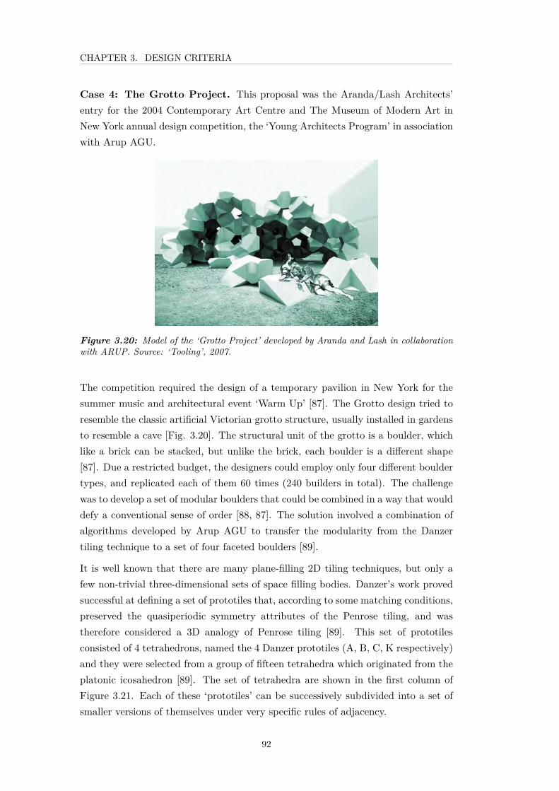
CHAPTER 3. DESIGN CRITERIA
Case 4: The Grotto Project. This proposal was the Aranda/Lash Architects’entry for the 2004 Contemporary Art Centre and The Museum of Modern Art inNew York annual design competition, the ‘Young Architects Program’ in associationwith Arup AGU.
Figure 3.20: Model of the ‘Grotto Project’ developed by Aranda and Lash in collaborationwith ARUP. Source: ‘Tooling’, 2007.
The competition required the design of a temporary pavilion in New York for thesummer music and architectural event ‘Warm Up’ [87]. The Grotto design tried toresemble the classic artificial Victorian grotto structure, usually installed in gardensto resemble a cave [Fig. 3.20]. The structural unit of the grotto is a boulder, whichlike a brick can be stacked, but unlike the brick, each boulder is a different shape[87]. Due a restricted budget, the designers could employ only four different bouldertypes, and replicated each of them 60 times (240 builders in total). The challengewas to develop a set of modular boulders that could be combined in a way that woulddefy a conventional sense of order [88, 87]. The solution involved a combination ofalgorithms developed by Arup AGU to transfer the modularity from the Danzertiling technique to a set of four faceted boulders [89].
It is well known that there are many plane-filling 2D tiling techniques, but only afew non-trivial three-dimensional sets of space filling bodies. Danzer’s work provedsuccessful at defining a set of prototiles that, according to some matching conditions,preserved the quasiperiodic symmetry attributes of the Penrose tiling, and wastherefore considered a 3D analogy of Penrose tiling [89]. This set of prototilesconsisted of 4 tetrahedrons, named the 4 Danzer prototiles (A, B, C, K respectively)and they were selected from a group of fifteen tetrahedra which originated from theplatonic icosahedron [89]. The set of tetrahedra are shown in the first column ofFigure 3.21. Each of these ‘prototiles’ can be successively subdivided into a set ofsmaller versions of themselves under very specific rules of adjacency.
92

CHAPTER 3. DESIGN CRITERIA
Figure 3.21: Danzer tillings. The r tetrahedral of the Danzer Tiling are shown in theright column. The second and third column show a top and bottom view respectively of theset in their first iteration, and the reordering of the vertices that their subdivision produces.Source: Charalumpous 2007.
The iterative nature of these prototiles was used by Shea and ARUP’s AGU, whocarried out the computational implementation of the Grotto, to create the shapegrammar formalism used in the Aranda/Lash tiling project [90]. Briefly, in orderto define a set of space-filling boulders, the Type K Danzer Tile was carried tothe seventh generation. This arrangement consisted of 11,382 tethahedrons whose
93
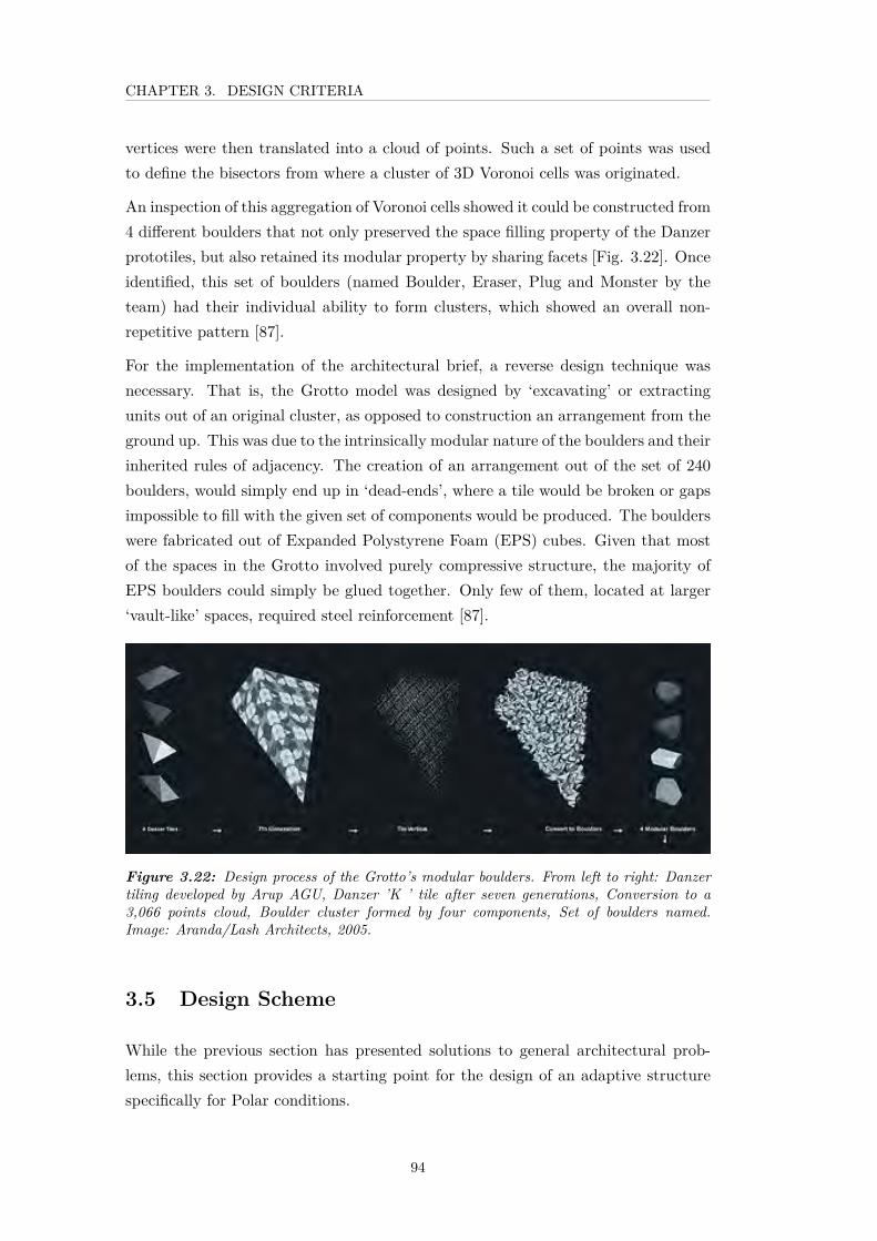
CHAPTER 3. DESIGN CRITERIA
vertices were then translated into a cloud of points. Such a set of points was usedto define the bisectors from where a cluster of 3D Voronoi cells was originated.
An inspection of this aggregation of Voronoi cells showed it could be constructed from4 different boulders that not only preserved the space filling property of the Danzerprototiles, but also retained its modular property by sharing facets [Fig. 3.22]. Onceidentified, this set of boulders (named Boulder, Eraser, Plug and Monster by theteam) had their individual ability to form clusters, which showed an overall non-repetitive pattern [87].
For the implementation of the architectural brief, a reverse design technique wasnecessary. That is, the Grotto model was designed by ‘excavating’ or extractingunits out of an original cluster, as opposed to construction an arrangement from theground up. This was due to the intrinsically modular nature of the boulders and theirinherited rules of adjacency. The creation of an arrangement out of the set of 240boulders, would simply end up in ‘dead-ends’, where a tile would be broken or gapsimpossible to fill with the given set of components would be produced. The boulderswere fabricated out of Expanded Polystyrene Foam (EPS) cubes. Given that mostof the spaces in the Grotto involved purely compressive structure, the majority ofEPS boulders could simply be glued together. Only few of them, located at larger‘vault-like’ spaces, required steel reinforcement [87].
Figure 3.22: Design process of the Grotto’s modular boulders. From left to right: Danzertiling developed by Arup AGU, Danzer ’K ’ tile after seven generations, Conversion to a3,066 points cloud, Boulder cluster formed by four components, Set of boulders named.Image: Aranda/Lash Architects, 2005.
3.5 Design Scheme
While the previous section has presented solutions to general architectural prob-lems, this section provides a starting point for the design of an adaptive structurespecifically for Polar conditions.
94
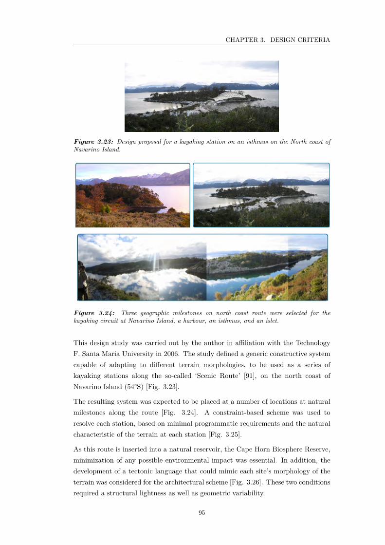
CHAPTER 3. DESIGN CRITERIA
Figure 3.23: Design proposal for a kayaking station on an isthmus on the North coast ofNavarino Island.
Figure 3.24: Three geographic milestones on north coast route were selected for thekayaking circuit at Navarino Island, a harbour, an isthmus, and an islet.
This design study was carried out by the author in affiliation with the TechnologyF. Santa Maria University in 2006. The study defined a generic constructive systemcapable of adapting to different terrain morphologies, to be used as a series ofkayaking stations along the so-called ‘Scenic Route’ [91], on the north coast ofNavarino Island (54°S) [Fig. 3.23].
The resulting system was expected to be placed at a number of locations at naturalmilestones along the route [Fig. 3.24]. A constraint-based scheme was used toresolve each station, based on minimal programmatic requirements and the naturalcharacteristic of the terrain at each station [Fig. 3.25].
As this route is inserted into a natural reservoir, the Cape Horn Biosphere Reserve,minimization of any possible environmental impact was essential. In addition, thedevelopment of a tectonic language that could mimic each site’s morphology of theterrain was considered for the architectural scheme [Fig. 3.26]. These two conditionsrequired a structural lightness as well as geometric variability.
95

CHAPTER 3. DESIGN CRITERIA
(a) (b)
(c)
Figure 3.25: Three geographic milestones selected for the kayaking circuit at NavarinoIsland: (a) a harbour, (b) an isthmus, and (c) an islet.
Figure 3.26: Architectural scheme of one of the three stations of the circuit, the isthmus-station.
96

CHAPTER 3. DESIGN CRITERIA
(a) (b) (c)
Figure 3.27: Definition of the three set of arches for the station in Navarino Island (a)complete arches, (b) half-arches and (c) asymmetrical arches. Images: J. Bak, 2006
(a) (b)
Figure 3.28: Two different enclosures at the Navarino Island Kayak Station, implementedfrom two different set of arches, (a) changing rooms employs complete arches; (b) storageroom, as a semi-opened area, utilize half arches. Images: J. Bak, 2006.
The structural scheme was resolved as a membrane structure, supported by a setof flexible arches, and a double bracing system composed of a combination of astructural membrane and tensile cables.
The ‘flexible arches’ were grouped into three categories: complete (or symmetri-cal) arches, semi-arches and asymmetric arches [Fig. 3.27]. This differentiationresponded to the necessity of both closed and semi-open enclosures within a samestation [Fig. 3.28].
Each group of arches was defined within a range of size variation. In this sense, archesforming each individual structure could be progressively varied in high (restrictedby ergonometric constraints). On the other hand, each set of arches needed to havea uniform width in order to make the cable bracing system possible (as describedbelow). In the case of asymmetric arches, this condition also required the positionof the point of inflection to be the same for the whole array.
As for the structures composed of semi-arches [Fig. 3.28(b)], the inclusion of a rigidtrussed arch (from now on called boundary arch) was necessary, as a supportingelement for flexible spanning arches forming the open side. As shown in Figure3.29, these supporting elements could be located either at the front or the back of
97

CHAPTER 3. DESIGN CRITERIA
(a) (b)
Figure 3.29: Two semi-open structures being supported by trussed arches, (a) storage roomwith frontal face open, (b) semi-covered public stands with the back open as it fallows thenatural shape of the hill.
Figure 3.30: Lateral supporting trusses. Image: J. Bak, 2006.
98
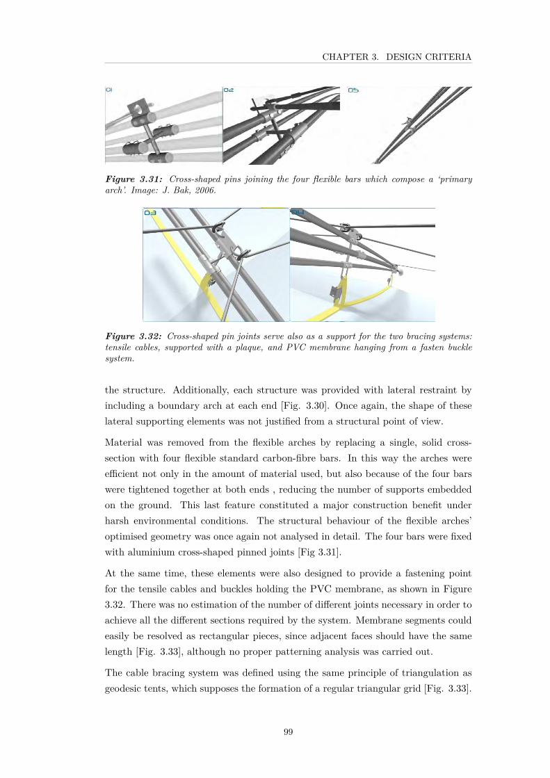
CHAPTER 3. DESIGN CRITERIA
Figure 3.31: Cross-shaped pins joining the four flexible bars which compose a ‘primaryarch’. Image: J. Bak, 2006.
Figure 3.32: Cross-shaped pin joints serve also as a support for the two bracing systems:tensile cables, supported with a plaque, and PVC membrane hanging from a fasten bucklesystem.
the structure. Additionally, each structure was provided with lateral restraint byincluding a boundary arch at each end [Fig. 3.30]. Once again, the shape of theselateral supporting elements was not justified from a structural point of view.
Material was removed from the flexible arches by replacing a single, solid cross-section with four flexible standard carbon-fibre bars. In this way the arches wereefficient not only in the amount of material used, but also because of the four barswere tightened together at both ends , reducing the number of supports embeddedon the ground. This last feature constituted a major construction benefit underharsh environmental conditions. The structural behaviour of the flexible arches’optimised geometry was once again not analysed in detail. The four bars were fixedwith aluminium cross-shaped pinned joints [Fig 3.31].
At the same time, these elements were also designed to provide a fastening pointfor the tensile cables and buckles holding the PVC membrane, as shown in Figure3.32. There was no estimation of the number of different joints necessary in order toachieve all the different sections required by the system. Membrane segments couldeasily be resolved as rectangular pieces, since adjacent faces should have the samelength [Fig. 3.33], although no proper patterning analysis was carried out.
The cable bracing system was defined using the same principle of triangulation asgeodesic tents, which supposes the formation of a regular triangular grid [Fig. 3.33].
99

CHAPTER 3. DESIGN CRITERIA
Figure 3.33: Rectangular pieces of PVC fabric forming the membrane. Images: J. Bak,2006.
Figure 3.34: Regular triangulated gridbracing the structure. The image also showsthe radial distribution of the arches on thefloor.
Figure 3.35: Equally degree distributionof joints along the arches. Images: J. Bak,2006.
Initially, this grid was formed by two perpendicular sets of continuous cables attachedto the arches [Fig. 3.34 and 3.35].
The desire to have a regular grid of joints was challenged by the fact that everyarch had a different length, therefore placing joints at equal distances was not asolution. Instead, the joints were positioned at equal angles around the arches, asmeasured from the centre of the arch [Fig. 3.34]. Hence, each arch had the samenumber of joints, enabling cables to be connected on a ‘consecutive-position’ fashionalong the set of arches. This lacing scheme is shown in Figure 3.36, where archesare represented by black line segments, with nodes numbered according to theirposition, and the two reciprocate set of cables and highlighted and blue and red.The starting point of the lacing are represented by arrows.
It was established that the arches should be constrained to have the same width (orspan), due to both the need to allow a radial distribution on the plane (preventingarches to overlap onto each other), as exemplified in Figure 3.35. It was alsobelieved that this condition was necessary for the uniformity of cables’ triangulation.However, the arches’ height (thus, the length) could vary progressively.
Nevertheless, the implications of having a variable width for the system’s structural
100

CHAPTER 3. DESIGN CRITERIA
Figure 3.36: Scheme for set of reciprocate bracing cables.
and cables’ geometric continuity were not surveyed. For instance, this characteristicwould imply that every arch is defined with a different geometry (or arches can bedefined as a set of semi-circumference’s segments, each of them with variable degreeof curvature) which imply that each arch would perform in a differently fashion.These assumptions are questioned and reviewed in Chapter 4.
As pointed out in Chapter 2, the absence of cable net structures in polar and subpolarregion can be explained due to the difficulty to assure a constant tension underextreme conditions and the technical complexity of their installation process. Inorder to overcome these complications, this scheme proposed that cables should beinstead conceived as discontinuous segments installed in a zig-zag fashion betweentwo consecutives arches. Figure 3.32 illustrates an early proposal for the joint wheretwo discontinuous cables are attached.
The use of discrete bracing elements contributes to both, facilitate the assemblingprocedure and to assure the feasible maintenance or repairing of the structure.
The behaviours of this discrete elements should be no different than a net formedby continuous elements, as long as the regular triangulation principle is preserved.This feature was sustained in the new version of this system.
Anchorages were designed to receive the four flexible bars of the primary arches, aswell as coping with a rocky soil condition [Fig. 3.37]. The type of soil originallyconsidered was subject to the phenomenon of gelifraction on its upper layer (approx-
101

CHAPTER 3. DESIGN CRITERIA
Figure 3.37: Anchorages designed as ties and supports for flexible arches. Images: J. Bak,2006.
imately 300 mm) and so the anchorage was designed to penetrate to a depth of 400to 500 mm where a permanently frozen soil (permafrost) could provide stability.
Consequently, the versatility of this system, capable of handling a wide range ofdifferent shapes, is achieved by coordinating its different set of components. Thus,two groups can be recognized: standard components including flexible bars, ten-sile cables, heavy-duty buckles and anchorages; and a second group of customizedelements which compromises joints, membrane segments and trussed rigid arches.Given this second group, the modularity of the system can be questioned, for whichits classification can be instead considered to be closer to a free-form approach.
There were several features of this system that made it suitable for the purpose of asemi-modular lightweight construction system. However, there were still a number ofunexplored aspects which needed to be addressed. These can be listed as following:
1. Materiality of the components.
2. Structural feasibility of the flexible arches.
3. Structural feasibility of the rigid boundary arches.
4. Geometrical variations (maximum and minimum spans).
5. Design of structural components.
6. Minimum number of nodes necessary (without increasing the number of dif-ferent components or affecting the continuous bracing system).
7. Other possibilities of aggregation apart from axial extensions.
8. Definition of the number of different components necessary for the multipleconfigurations required.
102

CHAPTER 3. DESIGN CRITERIA
3.6 Design Method
The design process of an adaptable construction system with a controlled numberof different components is interconnected procedure rather than a linear one as thefollowing chapter will show.
When working with the design of structural organisations, optimisations can occurin both architectural and engineering domains [16]. As pointed of by Bechthold,modifications at the global level (usually within the architectural domain) can in-volve choices of main surface type, span, proportions, orientations, and aggregations.While optimising the surface itself entails the detailed design of its constituentelements, choices are related to detailed studies of the surface support and properties,choices of membrane versus shell, surface thickness, reinforcement, pre-stress andoptimization of curvature and edge conditions [16]. The design process presentedin this thesis involves a dialogue between aspects of both accounts. Criteria gainedfrom the literature review related to Polar structures served in the decision makingat several stages of the design process.
3.7 Conclusions
This chapter proposed a transition in the narrative of this research. Whilst the firsttwo chapters have identified the particularities of the Polar built environment andpresented a digest of bespoke lightweight structures, this chapter proposes such adomain can also be consider an inspiring design paradigm, from which innovativedesign solutions can be explored.
Furthermore, this chapter has set the initial conditions, including design criteria andan early architectural scheme, to develop the Union Glacier station. This case willbe use to challenge and to further development the typologies of Polar lightweightstructures so far realised.
It was established that this endeavour requires the exploration of a constructionsystem with a more complex geometry and at a larger scale than currently seen, onewhich is capable of performing under extremely severe Antarctic conditions.
In order to achieve this, two key aspects must be incorporated: adaptable configu-rations and compactness.
This chapter has also shown that when logistic and environmental constraints areincorporated, a novel paradox arises, which consists of the design of a lightweightsystem capable of allowing multiple configurations whilst using a restricted numberof different components. Such a paradigm was endorsed with the examination of
103

CHAPTER 3. DESIGN CRITERIA
case studies that achieve such a condition. This chapter therefore, suggests thatthere can be many different design strategies to develop a constructive system whichallows the variation of a structure using a controlled number of different components.Strategies for geometrical variations range from a simple repetition of a module(case 1) and the two dimensional aggregation of a set of components (case 2), to theprogressive distortion of a single construction element to produce irregular shapes(case 3) and the definition of a complex algorithmic grammar to produce a set ofspace-filling elements (case 4). Despite the variety of shapes and strategies, thecondition of realising a generic system that could be demounted and reassembledin different configurations was fulfilled. Such variations can be derived from eitherprogrammatic requirements or from environmental features.
As most of these case studies demonstrate, the design process is supported bynovel CAD methods. Nevertheless, where logistic constraints are imposed (suchas human performance in extreme environments, load capacity of transportationsystems, etc.), a much more controlled approximation to geometry freedom is re-quired. Although parametric design platforms provide an environment for studiesof the variation of generic structural surfaces with complex geometry; it is generallythe case that the results would not meet the requirements of Polar design, given thelarge number of components that each variation requires or the lack of repeatabilityand technical complexity required for their implementation. Additionally, althoughactuated structures are starting to be seen in adaptive design scenarios, there isnot enough evidence of their load bearing capacity in extreme cold, nor of the widerange of geometric possibilities required here. Similarly, free-form surfaces are highcomplex to design and construct, which makes them equally unsuitable for extremeenvironments.
Instead, it is proposed that for remote structures, modularity and geometric adapt-ability define a range, where hybrid solutions can be explored based on the logisticconstraints imposed by the remote context on this case.
Consequently by setting the conditions this case, a novel design paradigm could alsobe defined.
The chapter has also presented an early-stage scheme design for a structural systemfor use in remote environments. A number of improvements were identified inorder to allow its use in a Polar context, and the following chapters address thesechallenges to demonstrate the feasibility of such modular-adaptive hybrid concept.A methodology to address these challenges was also presented, highlighting twomain characteristics that suggest the novelty of such an approach, namely thecompetition between modularity and adaptability, and the necessity of integratingboth geometrical and engineering domains.
104

Chapter 4
Nodal Forces Method and Structural Com-ponents Design
4.1 Introduction
This fourth chapter initiates the second part of this research, which focuses on thedesign of an adaptable lightweight construction system for polar areas under a strictlogistic-based approach. This study will offer an example of how criteria derivedfrom a remote context can influence the design process and furthermore guide anovel design method.
The study uses an early design scheme previously developed by the author, presentedin Chapter 3, as a starting point. The further development of the scheme into alightweight structure suitable for Polar conditions demands the definition of a designstrategy that can balance the competition between a modular practical design and anadaptable configuration (see Chapter 3). The solution of this paradigm, constitutesone of the core contributions of this research.
There are certainly many computer aided design platforms capable of manipulatingquantitative information related to constraint-based design. However, the mainfocus of this design-driven research is not the development of advanced softwaredesign tools, nor the optimisation of the design process. It is however, to investigatehow polar-derived criteria can inform and guide the design narrative in which, eithertraditional or advanced design resources can contribute. In that sense, the concep-tual structure that guides the variation study for a ‘semi-modular’, yet adaptable,lightweight structure is presented in this chapter.
This study by design has been broadly organised into three parts: a sensitiv-ity study (Chapter 4), a multi-objective study(Chapter 5), and a configurationstudy(Chapter 6). While the first, presented in this chapter, considerates differentgeometric features of the system’s components, the second, presented in the next
105
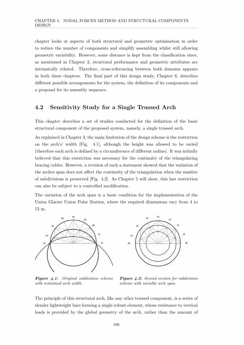
CHAPTER 4. NODAL FORCES METHOD AND STRUCTURAL COMPONENTSDESIGN
chapter looks at aspects of both structural and geometric optimisation in orderto reduce the number of components and simplify assembling whilst still allowinggeometric variability. However, some distance is kept from the classification since,as mentioned in Chapter 2, structural performance and geometric attributes areintrinsically related. Therefore, cross-referencing between both domains appearsin both these chapters. The final part of this design study, Chapter 6, describesdifferent possible arrangements for the system, the definition of its components anda proposal for its assembly sequence.
4.2 Sensitivity Study for a Single Trussed Arch
This chapter describes a set of studies conducted for the definition of the basicstructural component of the proposed system, namely, a single trussed arch.
As explained in Chapter 3, the main limitation of the design scheme is the restrictionon the arch’s’ width [Fig. 4.1], although the height was allowed to be varied(therefore each arch is defined by a circumference of different radius). It was initiallybelieved that this restriction was necessary for the continuity of the triangulatingbracing cables. However, a revision of such a statement showed that the variation ofthe arches span does not affect the continuity of the triangulation when the numberof subdivisions is preserved [Fig. 4.2]. As Chapter 5 will show, this last restrictioncan also be subject to a controlled modification.
The variation of the arch span is a basic condition for the implementation of theUnion Glacier Union Polar Station, where the required dimensions vary from 4 to12 m.
Figure 4.1: Original subdivision schemewith restrained arch width.
Figure 4.2: Second version for subdivisionscheme with variable arch span.
The principle of this structural arch, like any other trussed component, is a series ofslender lightweight bars forming a single robust element, whose resistance to verticalloads is provided by the global geometry of the arch, rather than the amount of
106

CHAPTER 4. NODAL FORCES METHOD AND STRUCTURAL COMPONENTSDESIGN
material employed. Flexible materials obtain their strength from bending, wherepre-stress is applied.
However, the idea of continuous flexible bars proposed in the design scheme wasdiscarded at an early stage for multiple reasons:
i) The standard length of carbon fibre bars range from 1 to 5 m [92]. Whilstthe shortest version would imply an excessive number of joints, the longestversion makes the transportation or manipulation unsuitable for a Polarcontext,
ii) Joints between bars would need and would be located at irregular intervalsdepending on the span of the arch. This would require an additional type ofjoint, while bars would still need to be fixed to the cross-joints in order tostop them from sliding,
iii) The failure of one particular bar segment would require the replacement ofthe entire arch, therefore the whole system would be affected.
To avoid such problems, segmented bars connected at the cross-shaped joints wereconsidered.
The design of the arch was carried out by a sensitivity study, where multiple aspectsrelated to the geometrical attributes were inspected independently by comparingthe structural and construction efficiency of different options. The arch’s attributescompared include: a) the global geometry of the arch, b) the shape of the joints,c) the number of nodes (or subdivision), and d) the depth of the arch’s mid-spanpoint. Each of these steps will be described in this chapter.
Section 4.3 begins by characterising the main structural component, this is, a trussedarch of variable section.
Section 4.4 describes the analysis method used during this study. The challengeconsisted in providing a sound method capable of handling a large number of CADsamples of a single trussed arch. These samples consisted on variations of a singletrussed arch in which different geometrical attributes were modified, to be latercompared using FEM tools.
Section 4.5 describes the basic mechanical properties of the materials proposed forthe main structural component. A brief reflexion on their use in extreme coldenvironments as well as on feasibility of the components productions, is also offeredin this section.
Section 4.6 described the method and standards used for the calculation of externalloads, namely snow and wind. In this case, the challenge consisted on establishing
107
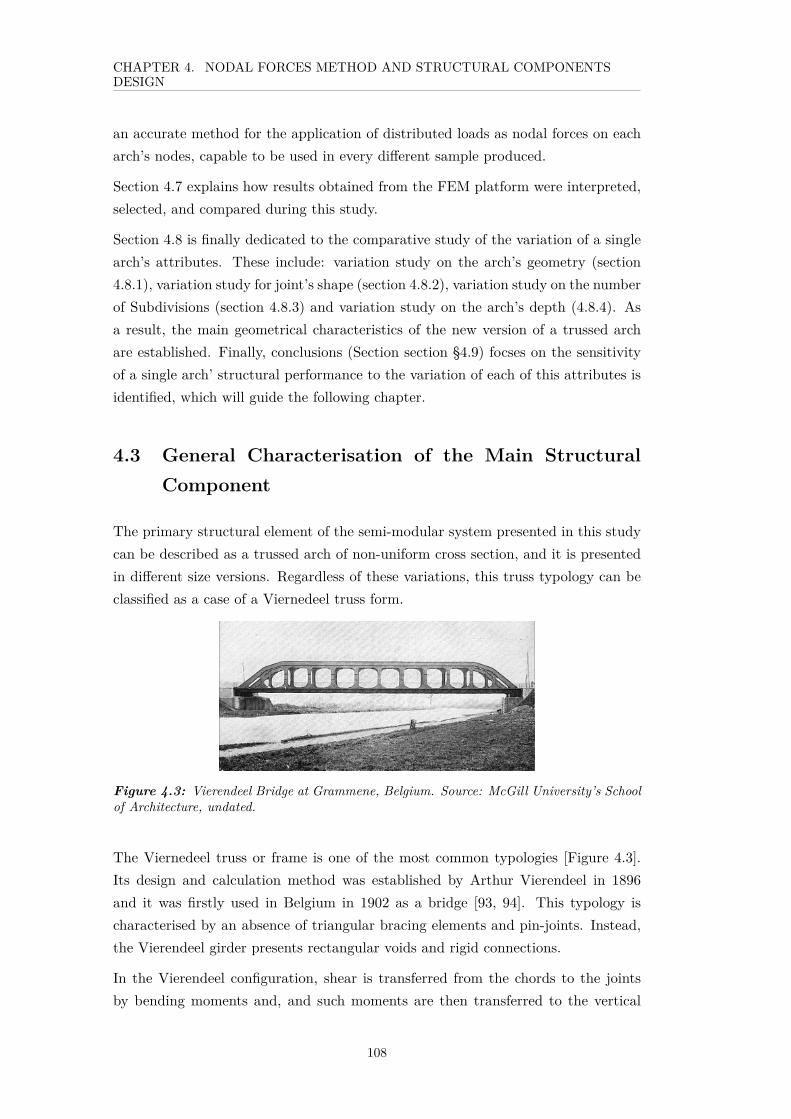
CHAPTER 4. NODAL FORCES METHOD AND STRUCTURAL COMPONENTSDESIGN
an accurate method for the application of distributed loads as nodal forces on eacharch’s nodes, capable to be used in every different sample produced.
Section 4.7 explains how results obtained from the FEM platform were interpreted,selected, and compared during this study.
Section 4.8 is finally dedicated to the comparative study of the variation of a singlearch’s attributes. These include: variation study on the arch’s geometry (section4.8.1), variation study for joint’s shape (section 4.8.2), variation study on the numberof Subdivisions (section 4.8.3) and variation study on the arch’s depth (4.8.4). Asa result, the main geometrical characteristics of the new version of a trussed archare established. Finally, conclusions (Section section §4.9) focses on the sensitivityof a single arch’ structural performance to the variation of each of this attributes isidentified, which will guide the following chapter.
4.3 General Characterisation of the Main StructuralComponent
The primary structural element of the semi-modular system presented in this studycan be described as a trussed arch of non-uniform cross section, and it is presentedin different size versions. Regardless of these variations, this truss typology can beclassified as a case of a Viernedeel truss form.
Figure 4.3: Vierendeel Bridge at Grammene, Belgium. Source: McGill University’s Schoolof Architecture, undated.
The Viernedeel truss or frame is one of the most common typologies [Figure 4.3].Its design and calculation method was established by Arthur Vierendeel in 1896and it was firstly used in Belgium in 1902 as a bridge [93, 94]. This typology ischaracterised by an absence of triangular bracing elements and pin-joints. Instead,the Vierendeel girder presents rectangular voids and rigid connections.
In the Vierendeel configuration, shear is transferred from the chords to the jointsby bending moments and, and such moments are then transferred to the vertical
108

CHAPTER 4. NODAL FORCES METHOD AND STRUCTURAL COMPONENTSDESIGN
elements. Consequently, all components are subject to combined internal forces,involving axial, shear and bending forces. This is a key difference from the typicalpin-connected truss, in which shear is transferred axially through diagonals membersand all components are axially loaded [95].
The presence of bending in chords and vertical webs implies that all membersrequire significantly larger cross-section area compared to an equivalently loadedtruss’s, even though diagonals are removed. As a result, a heavier frame needs tobe employed when using the Vierendeel form of truss [95].
Furthermore, given that elements of the Vierendeel girder are subject of combinedstresses, this is a statically indeterminate structure [96]. Thus, the required cal-culation method were considered laborious, and its feasibility, questionable at thetime of its appearance. Such process can nowadays be aided by computationalmethods. Despite of the development of a more refined calculation method andthe development of the electric welding arc technology contributed to the localpopularity of these system in the early 20th Century [95] (mainly used for shortspan bridges within Belgium), the use of Vierendeel system quickly declined by themid Century.
Consequently, a general agreement about the structural efficiency of the Vierendeelactions has not been settled. The benefit of such configuration is instead given byits architectural possibilities, as it still represents a design solution for cases whereexpressions demands a rectangular grid of openings, such as building structureswhere large shear walls or diagonal elements need to be avoided due to the building’sfunctionality or aesthetics [95, 93].
In the case of the scheme presented in this thesis, the use of such typology isjustified by the benefit of avoiding diagonal members in order to reduce the numberof elements a minimum, as well as the necessity of a simplified assembly process.The characteristic effects on the Vierendeel form of truss on the arches’ mechanicalbehaviour are present in the case of this thesis’s scheme. These actions will bediscussed in this Chapter’s Section section §4.7. Design solutions are discussed inChapter 6 .
4.4 Method
In order to initiate the comparison study of the different geometric attributes ofan single arch, three aspects were predetermined: i) the initial geometry, for whicha parametric CAD tool was employed, ii) the external load conditions, for whicha nodal forces calculation method was used, and iii) the mechanical properties of
109
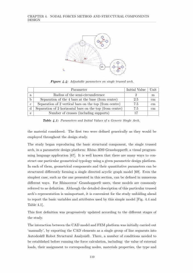
CHAPTER 4. NODAL FORCES METHOD AND STRUCTURAL COMPONENTSDESIGN
Figure 4.4: Adjustable parameters on single trussed arch.
Parameter Initial Value Unita Radius of the semi-circumference 2 mb Separation of the 4 bars at the base (from centre) 2.5 cmc Separation of 2 vertical bars on the top (from centre) 7.5 cmd Separation of 2 horizontal bars on the top (from centre) 7.5 cme Number of crosses (including supports) 17
Table 4.1: Parameters and Initial Values of a Generic Single Arch.
the material considered. The first two were defined generically as they would beemployed throughout the design study.
The study began reproducing the basic structural component, the single trussedarch, in a parametric design platform: Rhino 3D® Grasshopper®, a visual program-ming language application [67]. It is well known that there are many ways to con-struct one particular geometrical typology using a given parametric design platform.In each of them, geometrical components and their quantitative parameters can bestructured differently forming a single directed acyclic graph model [69]. Even thesimplest case, such as the one presented in this section, can be defined in numerousdifferent ways. For Rhinoceros’ Grasshopper® users, these models are commonlyreferred to as definition. Although the detailed description of this particular trussedarch’s representation is unimportant, it is convenient for the study unfolding aheadto report the basic variables and attributes used by this simple model [Fig. 4.4 andTable 4.1].
This first definition was progressively updated according to the different stages ofthe study.
The interaction between the CAD model and FEM platform was initially carried out‘manually’, by exporting the CAD elements as a single group of line segments intoAutodesk® Robot Structural Analysis®. There, a number of conditions needed tobe established before running the force calculation, including: the value of externalloads, their assignment to corresponding nodes, materials properties, the type and
110

CHAPTER 4. NODAL FORCES METHOD AND STRUCTURAL COMPONENTSDESIGN
location of supports (given that this first study was for comparison only, pre-stressesderived from bending were not included in these calculations).
The load cases considered included self-weight, snow and wind derived loads. Thelast two were applied as nodal forces on the lower nodes of each cross-shaped joint,in order to simplify the setting-up of models.
Relevant combinations of load case were included according to the Eurocode stan-dards specifically the Danish national annex. [97]. The list includes linear loadcases of Serviceability Limit State’ (SLS) and Ultimate Limit State (ULS), hencecases combined linearly. For structural design of systems with large deflections, anon-linear load case is most commonly used. Although for the purpose of this study,a linear set of load combinations was considered sufficient. Cases included are asfollows:
Load Cases
1. Self-weight (Dead load)
2. Snow Loads
3. Wind Loads
Serviceability Limit State Load Combinations
4. Dominant Snow = 1.0 · (1) + 1.0 · (2) + 0.3 · (3)
5. Dominant Wind = 1.0 · (1) + 1.0 · (3)
Ultimate Limit State Load Combinations
6. Dominant Snow = 1.0 · (1) + 1.5 · (2) + 1.5 · 0.3 · (3)
7. Dominant Wind = 1.0 · (1) + 1.5 · (3)
Although in this case a very simple model was being studied, some difficultiespresented by this method needed to be overcome. It is estimated than this operationwas repeated over 100 times during the research (some other attributes were initiallystudied, but later discarded) and the method proved extremely time-consumingand susceptible to induced errors, particularly during the setting up of pre-analysisconditions.
Furthermore, the system’s design would be updated at each step of the study,according to the best option outputted by the FEM model results. Consequently,any error found at a given stage would imply the revision of the whole thread of
111

CHAPTER 4. NODAL FORCES METHOD AND STRUCTURAL COMPONENTSDESIGN
Figure 4.5: Parametric pipeline.
Figure 4.6: Geometry variations.
options studied. Although the study was completed using this method, the presenceof inconsistencies in some of the results and the difficulty of tracking down the causeof possible induced errors, suggested that a more fluent interactive method betweenboth platforms was required.
Therefore a second round of tests was conducted using a custom interactive soft-ware tool developed in collaboration with the Søren Jensen® Computational DesignGroup. This application could be defined as a scripting approach, and its objectivewas to produce the large number of models needed during the sensitivity studywith a uniform method. Figure 4.5 shows the organisation of this software tool.The different geometry variations were created using a Grasshopper® model. Themodel was prepared to take multiple parameter variations and create all the possiblegeometry variants by cross-referencing the chosen input parameters [Fig. 4.6]. Aninitial assessment based on engineering judgement (value ranges identified by thepreviously manual method) was used to keep the number of possible parametercombinations at a reasonable level.
A custom C# component was used to reference the Autodesk Structural AnalysisAPI (Application Programming Interface) and create the various FE-Models fromthe Grasshopper geometry [Fig. 4.7]. Wind and snow loading calculations wereimplemented in the parametric model and calculated based on the Grasshoppergeometry. This loading was then added to the FE-models and relevant load combina-tions were created, as earlier detailed. Furthermore, cross-section geometry, support
112
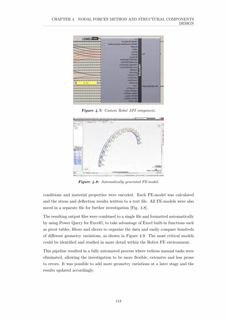
CHAPTER 4. NODAL FORCES METHOD AND STRUCTURAL COMPONENTSDESIGN
Figure 4.7: Custom Robot API component.
Figure 4.8: Automatically generated FE-model.
conditions and material properties were encoded. Each FE-model was calculatedand the stress and deflection results written to a text file. All FE-models were alsosaved in a separate file for further investigation [Fig. 4.8].
The resulting output files were combined to a single file and formatted automaticallyby using Power Query for Excel©, to take advantage of Excel built-in functions suchas pivot tables, filters and slicers to organize the data and easily compare hundredsof different geometry variations, as shown in Figure 4.9. The most critical modelscould be identified and studied in more detail within the Robot FE environment.
This pipeline resulted in a fully automated process where tedious manual tasks wereeliminated, allowing the investigation to be more flexible, extensive and less proneto errors. It was possible to add more geometry variations at a later stage and theresults updated accordingly.
113

CHAPTER 4. NODAL FORCES METHOD AND STRUCTURAL COMPONENTSDESIGN
Figure 4.9: Presentation of results in Excel.
4.5 Basic Material Properties
The original scheme provided a general description of the possible materiality forthe structure: a lightweight composite for the structural arches, aluminium for thejoints and tensile fabric for the membrane [91].
The use of tensile fabric and aluminium as structural materials for lightweightstructures has been extensively validated since appearance in 1920’s and 1970’srespectively [58]. Furthermore, some of the study cases shown in Chapter 2, havedocumented the successful use of the both materials in Antarctic environments.
In the case of carbon fibre/epoxy-resin systems, their mechanical behaviour underlow temperatures is intrinsically related to its origin, and it is therefore also well-documented. One of the earliest studies was carried out by NASA [98], where uni-axial stress was applied to specimens with a quasi-isotropic fibre lay-up at a range ofdecreasing temperature using cryogenic fuels. In general, the study demonstrated nomajor effect with temperature on either tensile modulus or average tensile strength,and a rather modest increase in the matrix stiffness [98]. This idea seems to begenerally supported [99, 100, 101].
4.5.1 Aluminium
Aluminium alloys are in general a good option for key rigid elements as in the case ofthe proposed joints, especially when compared to the obvious second option, steel.The advantage is mainly due to the inherent resistance to most normal atmosphericenvironments (it does not rust, suffer from corrosion, and self-heals when scratched)and also because of its lightweight nature, inherited from a low density (nearly athird of steel’s) [102].
In this case, lightness is an essential requirement for fast and easy installation. Powertools and machinery required for assembly can be considerably reduced by using alightweight metal. This characteristic also allows non-traditional assembly methodsto be employed.
114
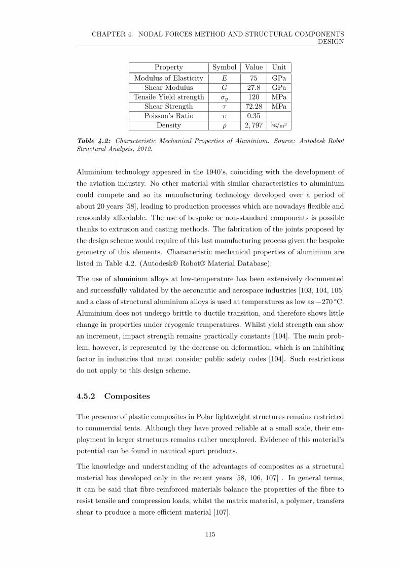
CHAPTER 4. NODAL FORCES METHOD AND STRUCTURAL COMPONENTSDESIGN
Property Symbol Value UnitModulus of Elasticity E 75 GPa
Shear Modulus G 27.8 GPaTensile Yield strength σy 120 MPa
Shear Strength τ 72.28 MPaPoisson’s Ratio υ 0.35
Density ρ 2, 797 kg/m3
Table 4.2: Characteristic Mechanical Properties of Aluminium. Source: Autodesk RobotStructural Analysis, 2012.
Aluminium technology appeared in the 1940’s, coinciding with the development ofthe aviation industry. No other material with similar characteristics to aluminiumcould compete and so its manufacturing technology developed over a period ofabout 20 years [58], leading to production processes which are nowadays flexible andreasonably affordable. The use of bespoke or non-standard components is possiblethanks to extrusion and casting methods. The fabrication of the joints proposed bythe design scheme would require of this last manufacturing process given the bespokegeometry of this elements. Characteristic mechanical properties of aluminium arelisted in Table 4.2. (Autodesk® Robot® Material Database):
The use of aluminium alloys at low-temperature has been extensively documentedand successfully validated by the aeronautic and aerospace industries [103, 104, 105]and a class of structural aluminium alloys is used at temperatures as low as −270 °C.Aluminium does not undergo brittle to ductile transition, and therefore shows littlechange in properties under cryogenic temperatures. Whilst yield strength can showan increment, impact strength remains practically constants [104]. The main prob-lem, however, is represented by the decrease on deformation, which is an inhibitingfactor in industries that must consider public safety codes [104]. Such restrictionsdo not apply to this design scheme.
4.5.2 Composites
The presence of plastic composites in Polar lightweight structures remains restrictedto commercial tents. Although they have proved reliable at a small scale, their em-ployment in larger structures remains rather unexplored. Evidence of this material’spotential can be found in nautical sport products.
The knowledge and understanding of the advantages of composites as a structuralmaterial has developed only in the recent years [58, 106, 107] . In general terms,it can be said that fibre-reinforced materials balance the properties of the fibre toresist tensile and compression loads, whilst the matrix material, a polymer, transfersshear to produce a more efficient material [107].
115
CHAPTER 4. NODAL FORCES METHOD AND STRUCTURAL COMPONENTSDESIGN
In contrast to metals, the use of the specific properties of the material’s compo-nents permits a significant reduction of self-weight. Furthermore, the possibility ofproducing composites for specific purposes and with specific load-bearing capacity,enhances this advantage over traditional construction materials [58]. In general,design guides using composite materials are very conservative. They take intoaccount a variety of possible failures, such as creep and creep rapture, fatigue,environmental degradation, etc. [108]. A general rule for design is to limit theallowable stresses, therefore:
For Glass Fibre Reinforced Polymer (GFRP), Maximum allowable Stress = 0.2ffvand, For Carbon Fibre Reinforced Polymer (CBRP), Maximum allowable Stress= 0.55ffv With ffv as the strength parameter being considered [106].
However, the fast increase in the use of composite materials during the last decadehas contributed to a better understanding of their fundamental properties and theirlong service life, enabling more specific uses. Consequently, security factors aretherefore being reduced to less conservative levels [107]
A disadvantage of composite materials is their brittleness, particularly with carbonfibres. For example, metal would undergo plastic deformation before braking, whilstcomposites on the contrary, either remain intact or break. Along with the highproduction cost, this remains as one of the main reasons for the slow introductionof such materials into the construction industry. Such difficulties have however beenconsiderably reduced in the last decade [58].
While the author does not focus on contributing to the knowledge in the material’sproperties, the general characteristics needed to be considered in the design, as thereis a great flexibility on the design in the material (plastic composite) matrix.
In general terms, the spectrum of possibilities for plastic composites would be definedbetween pure glass fibre, and pure carbon fibre reinforced polymer. In the case ofglass-based composites, the maximum fibre volume is 70%. Most of the fibres will bein the longitudinal direction, while the rest are supplied as a random matt (CSM) onthe external surface to provide robustness [106]. In the case of CFRP, fibre can belaid up in different orientation so the volume of fibre in each direction is lower, buta more isotropic material can be obtained [106]. The cost of GFRP is significantlylower that carbon-fibre reinforced plastics.
According to the Danish provider Fibreline ®, GFRP materials exceed the E23grade. The following general properties can be achieved [107]:
116
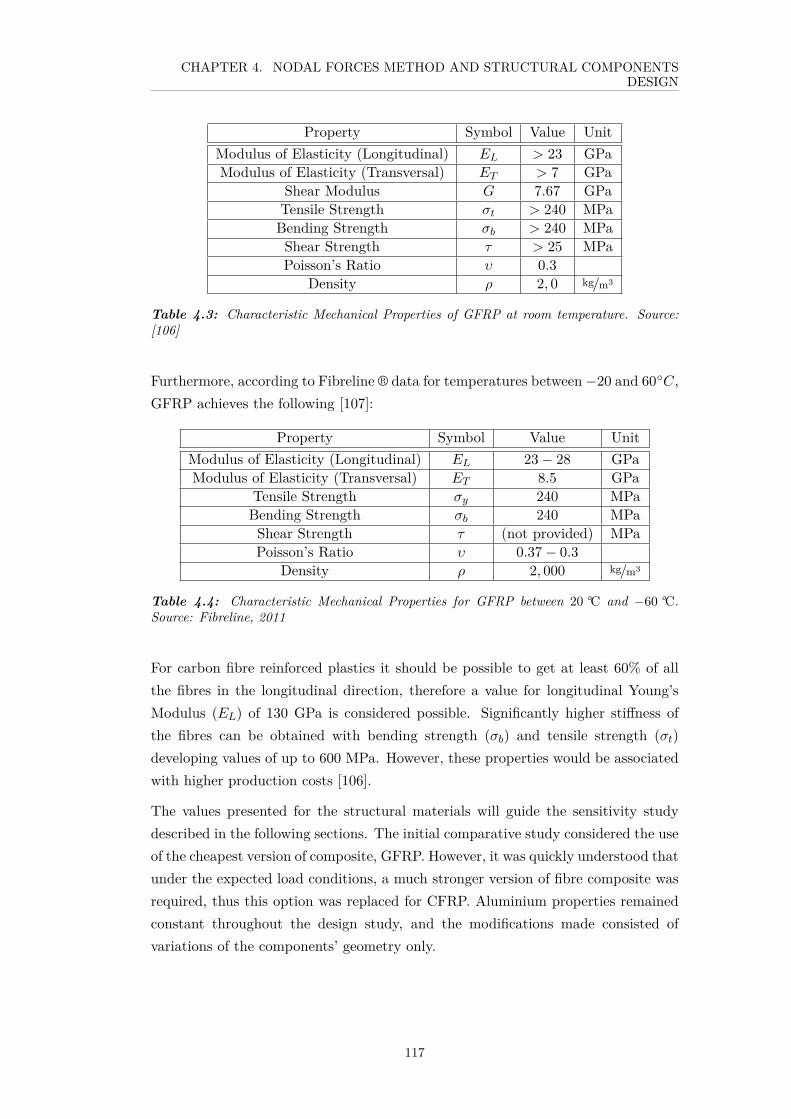
CHAPTER 4. NODAL FORCES METHOD AND STRUCTURAL COMPONENTSDESIGN
Property Symbol Value UnitModulus of Elasticity (Longitudinal) EL > 23 GPaModulus of Elasticity (Transversal) ET > 7 GPa
Shear Modulus G 7.67 GPaTensile Strength σt > 240 MPaBending Strength σb > 240 MPaShear Strength τ > 25 MPaPoisson’s Ratio υ 0.3
Density ρ 2, 0 kg/m3
Table 4.3: Characteristic Mechanical Properties of GFRP at room temperature. Source:[106]
Furthermore, according to Fibreline ® data for temperatures between −20 and 60C,GFRP achieves the following [107]:
Property Symbol Value UnitModulus of Elasticity (Longitudinal) EL 23− 28 GPaModulus of Elasticity (Transversal) ET 8.5 GPa
Tensile Strength σy 240 MPaBending Strength σb 240 MPaShear Strength τ (not provided) MPaPoisson’s Ratio υ 0.37− 0.3
Density ρ 2, 000 kg/m3
Table 4.4: Characteristic Mechanical Properties for GFRP between 20 °C and −60 °C.Source: Fibreline, 2011
For carbon fibre reinforced plastics it should be possible to get at least 60% of allthe fibres in the longitudinal direction, therefore a value for longitudinal Young’sModulus (EL) of 130 GPa is considered possible. Significantly higher stiffness ofthe fibres can be obtained with bending strength (σb) and tensile strength (σt)developing values of up to 600 MPa. However, these properties would be associatedwith higher production costs [106].
The values presented for the structural materials will guide the sensitivity studydescribed in the following sections. The initial comparative study considered the useof the cheapest version of composite, GFRP. However, it was quickly understood thatunder the expected load conditions, a much stronger version of fibre composite wasrequired, thus this option was replaced for CFRP. Aluminium properties remainedconstant throughout the design study, and the modifications made consisted ofvariations of the components’ geometry only.
117

CHAPTER 4. NODAL FORCES METHOD AND STRUCTURAL COMPONENTSDESIGN
4.5.3 Membranes
The use of tensile membranes as a structural material has been explored since themiddle of the 20th century. Most common options include synthetic cloths, such aspolyester, whose strength can reach up to 0.9 kN/mm2 [109]. Glass fibre cloths candevelop much higher tensile strength, ranging from 2.8 to 4.6 kN/mm2 [109]. Coatingsare also commonly added in order to improve waterproofing, durability, reduce dirtretention, and provide UV protection. Common solutions include polyvinyl chloridecoated polyester (PVC), polytetrafluoroethylene (PTFE), Teflon-coated glass fibre,and silicon-coated glass fibre [109].
This is a well-researched topic and sufficient evidence is available to justify the useof tensile membranes in large-scale structures. Chapter 2 provided examples of itsuse in Antarctic environments. Given that its use for the design scheme presentedin this research does not represent any new aspects to be explored, the structuralbehaviour of the tensile membrane in this case has not been studied in detail.
Perhaps another relevant challenge proposed by this design is related to the thermalconditioning of the station. Although thermal insulation of tensile membranes doesnot form part of this study’s scope, some effective solutions have been suggested insome of the case studies presented in Chapter 2, specifically sections 2.3 and 2.6,both developed by ARQZE®. No data characterising the thermal behaviour of thesematerials in these two cases has been collected. Nevertheless, this problem suggeststhat novel solutions could be further investigated.
4.6 Calculation of External Loads on a Single TrussedArch.
This section describes the method used to calculate external forces affecting a singlearch. A nodal forces method was employed, in order to accommodate the variationof different components to be studied.
A set of different tools were used for this calculation. Whilst external nodal forceswere calculated manually, calculation of internal stresses, such as bending and axialforces, were made by exporting the CAD model into a Finite Element Modellingplatform (Autodesk® Robot®), where external nodal forces were then added intothe model.
As discussed earlier, two types of external loads were applied as nodal forces: wind(Case 1) and snow (Case 2). Since the action of distributed loads are summarizedat the nodes, the length of the arch segments (distance between nodes) and gap(distance between two consecutives arches) had to be estimated. Self-weight was
118

CHAPTER 4. NODAL FORCES METHOD AND STRUCTURAL COMPONENTSDESIGN
calculated automatically by the FEM software, although the effect of the structuraldead load are minimal due to the light nature of the structure.
As a starting point, the minimal case of 4 m span was used, with a length of 6.28 m.This restriction was presented in Chapter 1, and it was based on a minimal heightof 2m. The arch was subdivided into 12 segments, in this new version, containing 13nodes and a standard distance between arches of 1 m. At each node, a cross-shapedjoint was placed. Crosses at both ends were discarded, as they are to be replacedby pinned supports.
The following sections describe the calculation of wind and snow loads. The studyfollows the method indicated by the European Standards, specifically the Danishwind load standard [110] for wind actions and the Danish snow load standard DS/EN1991-1-3: 2003 [111] for snow loads.
4.6.1 Load Case 3: Wind Derived Loads as Nodal Forces
Relevant factors for the calculation of wind Loads for vaulted roofs and domes arelisted in Appendix B. As indicated by the Eurocode standard [110], the peak velocitypressure can be determined as qp = 0.21 kN/m2.
For a vaulted roof and when the condition that f/d = 0.5 is observed [Fig. 4.10], asin this case, then the values of pressure coefficients are: ’
A = (0.8) B = (−1.2) C = (−0.4)
Figure 4.10: Geometric parameters on vaulted roof and domes for the valuation of externalpressure coefficients. Source: Eurocode standards, 2007.
The pressure coefficients determined above is dependent on the position on the arch.The arch is divided in the the following ranges:
Range A: 0 to 14 l Range B: 1
4 l to34 l Range C: 3
4 l to l
119

CHAPTER 4. NODAL FORCES METHOD AND STRUCTURAL COMPONENTSDESIGN
Where l is the length of the arch.
For this particular case the ranges are as follows:
Range A: 0 to 1.57 m Range B: 1.57 m to 4.71 m Range C: 4.71 m to 6.28 m
A simple way of calculating the forces applied to each node could be described by:
P = ldqpcpe
Where,
P is a point load acting perpendicular to the surface [kN]
qp is the value of Peak Velocity Pressure value [kN/m2]
l is the lenght of the segment between nodes [m]
d is the distance between arches (standard value of 1.00 [m])
cpe is the correspondent form factor according to the node’s position alongthe curve.
Each of these nodal forces would then be decomposed into their Cartesian com-ponents. However, it must be considered that the segment assigned to one nodecould be part of two different form factor zones, for which some of the nodes wouldbe assigned with the incorrect nodal force. A parametric method was thereforedeveloped, which could offer more precise solutions, as explained in section 4.6.3.
4.6.2 Load Case 2. Snow Derived Load as Nodal Forces
Similarly, snow loads were calculated based on the method indicated by DS/EN1991-1-3: 2003 (E), and then converted into nodal forces.
The most critical case of ground snow loads (sk) indicated in the standards corre-sponds to northern Finland, where snow cover can reach up to 120−150 cm in April[112], which is slightly lower to the case of Union Glacier (See Chapter 1). Thisvalue of ground snow load was then increased linearly by 20 % in order to simulatethe Glacier Union case. The characteristic value of the snow load on the ground istherefore determined as:
sk = 1.2 · 3.9 kN/m2 = 4.68 kN/m2
120

CHAPTER 4. NODAL FORCES METHOD AND STRUCTURAL COMPONENTSDESIGN
Accordingly, for persistent/ transient design situations, snows loads (S) are givenby:
s = µicectsk
Where,
s is the snow load on the roof, acting vertically [kN/m2]
µi is the snow load shape coefficient (see below)
ce is the exposure coefficient = 0.8
ct is the thermal coefficient = 1.0 (N/A)
sk is the characteristic value of snow load on the ground [kN/m2]
As shown in Figure 4.11, the value of shape coefficients is variable along the ‘vaultedroof’ and is dependent on its geometry. Snow load on a vaulted roof should beconsidered in two cases:
(i) Symmetrical blanket loading
(ii) Assymetrical loading (incl. drifting)
For case (i) the shape coefficient is defined as follows:
For β > 60,
µ = 0
for β ≤ 60,
µ = 0.8
For case (ii) the shape coefficient is defined as follows:
For β > 60,
µ3 = 0
for β ≤ 60,
121
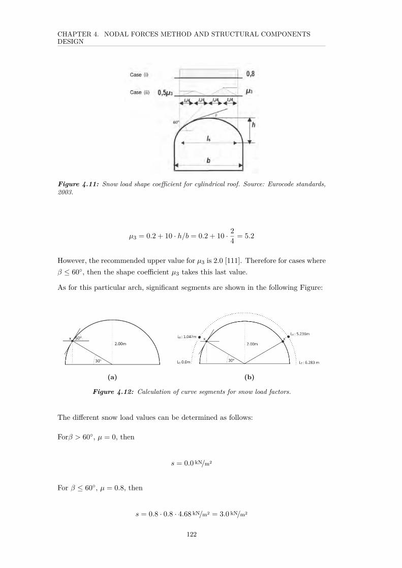
CHAPTER 4. NODAL FORCES METHOD AND STRUCTURAL COMPONENTSDESIGN
Figure 4.11: Snow load shape coefficient for cylindrical roof. Source: Eurocode standards,2003.
µ3 = 0.2 + 10 · h/b = 0.2 + 10 · 24 = 5.2
However, the recommended upper value for µ3 is 2.0 [111]. Therefore for cases whereβ ≤ 60, then the shape coefficient µ3 takes this last value.
As for this particular arch, significant segments are shown in the following Figure:
(a) (b)
Figure 4.12: Calculation of curve segments for snow load factors.
The different snow load values can be determined as follows:
Forβ > 60, µ = 0, then
s = 0.0 kN/m2
For β ≤ 60, µ = 0.8, then
s = 0.8 · 0.8 · 4.68 kN/m2 = 3.0 kN/m2
122

CHAPTER 4. NODAL FORCES METHOD AND STRUCTURAL COMPONENTSDESIGN
Forβ > 60, µ3 = 0, then
s = 0.0 kN/m2
For β ≤ 60, µ3 = 2, then
s = 2.0 · 0.8 · 4.68 kN/m2 = 9.36 kN/m2
for the highest peak of the asymmetrical trapezoidal load.
Again, the simplest way of determining the point loads would be to apply these loadvalues, according to the node position along the arch, over the area assigned. In thiscase forces would act only vertically. Similar to the wind load case, this method canbe considered to be imprecise, and an alternative method was developed, which ispresented in the following section.
For the sake of this study only the symmetrical snow load case was investigated.
4.6.3 Calculation Method of Nodal Forces
The calculation of nodal forces was carried out via a parametric approach usingRhino’s Grasshopper©, where the resultant loads would react to the arch’s geometry.Inputs required are: i) a curve, ii) qp (Peak Velocity Pressure value), and iii) sk(characteristic value of snow load on the ground). As a result, the Grasshopperdefinition outputs two lists of vector forces applied on each node. The approach forsuch application can be described as:
1. The arc is subdivided into a set of point lists (showed in Figure 4.13), whichinclude:
∆ is the node points (ni), a point where a cross-joint is placed.
X is the midpoints between Nodes Points (∆).
is the division points between shape/pressure coefficient ranges.
2. n number of arch segments (sn) is difined by dividing the arch at ∆, X and.
3. The length (ln) of sn is calculated
4. The centre of sn (symbolised by in Figure 4.13)
123

CHAPTER 4. NODAL FORCES METHOD AND STRUCTURAL COMPONENTSDESIGN
5. The corresponding form factor (µn) is asigned to sn in relation to the positionof along the curve.
6. For wind loads, a unit normal vector (−→n n) to the surface acting inwards iscalculated at , for snows loads, a unit vector (0, 0,−1) is assigned as −→k .
7. Force magnitudes are calculated by:
Pn = lnwµnp
Where:
Pn is the force magnitude at the node [kN]
ln is the segment lenght of the nth segment in the case of wind loads andprojected lenght in the case of snow loads [m]
w is the width (standard value of 1.0 m)
µn is the pressure/shape coefficient of the nth segment.
p is the surface load [kN/m2]
8. Forces are calculated by multiplying with the unit vectors:
−→V n = Pn−→n n
for wind and,
−→V n = Pn
−→k
for snow.
9. For each segment sn the closest node ni is found and the force −→V n is assignedto that node.
10. The total wind and snow loads can be respectively calculated as the sum of nforces assigned to the ith node:
−→P i =
∑V n
or,
124

CHAPTER 4. NODAL FORCES METHOD AND STRUCTURAL COMPONENTSDESIGN
Figure 4.13: Set of subdividing points on an arc for the calculation of nodal forces.
−→P i =
∑lnwµnP−→n n
for wind case and
−→P i =
∑lnwµnP
−→k
for snow case.
11. Nodal forces are discomposed into X, Y and Z components, in order to be usedon a FEM platform. Nodes are identified in Figure 4.15. Nodal forces valuesare shown on Table 4.5.
4.7 Interpretation of FE Model Results
The different attributes studied are based on a geometric optimisation approach.Therefore, a predefined set of options was defined for each attribute, as the followingsection shows. This implies that such a method should not be realised as a ‘structuraloptimisation’ process, but a variation study, where the effect on the structure’s me-chanical behaviour is observed and then solution negotiated with Polar-assemblingcriteria.
The main results were used to compare maximum and minimum values for dis-placement, deflection and internal stresses (normal combined stresses) for each case.Whilst attention was given to the possible origin of such critical values, the studydoes not seek solutions to reduce maximum load states, given that variation options
125

CHAPTER 4. NODAL FORCES METHOD AND STRUCTURAL COMPONENTSDESIGN
ln
l2
l1
s2
sn
s1
w1l1p
niw2l2p
wnlnp
n1
nn
Vn
Vn
k
Pi
Formfactor A
Formfactor B
Projected length
Figure 4.14: Diagram of geometric attributes for calculation of nodal forces.
Figure 4.15: Numbering of nodes in an arch.
126

CHAPTER 4. NODAL FORCES METHOD AND STRUCTURAL COMPONENTSDESIGN
Case Node Nodal Forces [kN]FX FY FZ
Snow load
0 0.0 0.0 0.01 0.0 0.0 02 0.0 0.0 -0.553 0.0 0.0 -1.254 0.0 0.0 -1.635 0.0 0.0 -1.826 0.0 0.0 -1.777 0.0 0.0 -1.828 0.0 0.0 -1.639 0.0 0.0 -1.2510 0.0 0.0 -0.5511 0.0 0.0 0.012 0.0 0.0 0.0
Wind load
0 -0.04 0.0 0.01 -0.09 0.0 -0.022 -0.08 0.0 -0.043 0.01 0.0 0.024 0.07 0.0 0.125 0.03 0.0 0.136 0.0 0.0 0.137 -0.03 0.0 0.138 -0.07 0.0 0.129 -0.06 0.0 0.0610 -0.04 0.0 0.0211 -0.04 0.0 0.0112 -0.02 0.0 0.0
Table 4.5: Cartesian Values of Nodal Forces Derived from Snow and Wind on a 4[m] spanArch.
127

CHAPTER 4. NODAL FORCES METHOD AND STRUCTURAL COMPONENTSDESIGN
(a) (b)
Figure 4.16: Characteristic distribution of internal axial (a) and bending (b) stresses alonga simply supported arch under compression for a symmetrical load case.
Figure 4.17: Combined normal stresses (S value) as the addition of axial and bendingstresses throughout section 1-1’ for a symmetrical load case.
are pre-set. The following chapter will look into design solutions that permit thecomponents to function under the allowable limits.
In order to visualise the deformation of each model, the displacements and deflectionswere calculated as a resulting vector (utotal), where:
utotal =√u2x + u2
y + u2z
The main result obtained from Robot is the normal combined stresses (S value).These stresses consists of the combined results for bending and axial stresses. Aspure axial stresses have a uniform distribution over the cross section, this resultcould be dismissed if a simple comparison is required. Figures 4.16 and 4.17 gives ageneral explanation of this.
Due to the different materiality and structural function, results were also evaluatedseparately for the two principal components considered: carbon fibre bars forming
128

CHAPTER 4. NODAL FORCES METHOD AND STRUCTURAL COMPONENTSDESIGN
arches and aluminium bars forming cross-shaped joints.
In the case of displacements, the results obtained are valid for both groups ofelements as it assesses the reposition of nodes, rather than the behaviour of bars.
FEM outputs normal combined stresses (S value), with a minimum and maximumvalue for each bar. Since bending and axial stresses are not uniform along the arc,the S value does not have a uniform distribution for each cross section as explainedin Figure 4.16, although bending and axial stresses have symmetrical values, (due tothe fact that the cross sections have a regular geometry along the arch). Therefore,each bar has a maximum and minimum S value, and this is why the global maximumand minimum values are found in different bars. Hence, results shown on each sectionrefer to the ‘highest’ maximum (Smax) and the ‘lowest’ minimum (Smin) global Svalue for each group of components (arches and crosses).
4.8 Variation Study
In this section, a group of comparative studies is presented. In each of this studies aset of prefixed options are contested in order to establish the geometrical attributesof the main structural component, a trussed single arch. The studies are based inthe smallest version of these element, this is 4 m span.
4.8.1 Variation Study on the Arch’s Geometry
(a) (b) (c)
Figure 4.18: Different versions of trussed arches with 4 m span to be compared. (a) Model1, section at the supports (from node to axis): 50 mm, section at the top (from node to axis):150 mm; (b) Model 2, section at the supports (from node to axis): 150 mm, section at thetop (from node to axis): 50 mm; (c) Model 3, section at the supports and top (from node toaxis) 100 mm.
The objective of this section is to evaluate different design options for a trussed arch.This is the key element of the proposed system.
129

CHAPTER 4. NODAL FORCES METHOD AND STRUCTURAL COMPONENTSDESIGN
The goal of the original arch design was to reduce the number of elements needed tobe buried in the ground. This is of greatest importance from both an environmentaland construction perspective when working in remote protected areas. Below groundlevel operations is one of the most complicated types of tasks when operating inpermafrost, and when in the case of the presence of rocky soils, is exasperated bythe effect of gelifraction on the upper layer [91]. Avoiding this kind of operation notonly benefits the logistical and operational aspects of a field party, it also, and moreimportantly, contributes to minimising invasive activities that can cause permanentalterations to pristine areas. Furthermore, this strategy is also convenient whenconsidering the implementation of an adaptable structure, where components areallowed to be re-organised periodically with the minimum of operational complica-tions.
Although the original scheme already proposed the minimization of support points,it was necessary to understand the effect of such geometry in the structural behaviourof the system by contrasting it with other options.
As discussed previously, each arch comprised four bars. The difference between thethree different models tested consisted of the variation of the cross section, that is,the distance between the bars along an imaginary central axis. All the cases weresymmetrical, so that the variation of the cross section were only found between thetop and ends of the arch. Nevertheless, an asymmetrical design could potentially beimplemented. An application for such a case could be a construction on a site witha known and constant dominant wind direction. Means of architectural expressioncould also require an asymmetrical profile.
Even though the external loads, material properties and the number of bars werelater modified, this exercise offers a fair comparison in terms of global geometry, asthe three cases present the same span (4 m), same number of crosses (12) and sameload cases (see section 4.4). Also, sections were varied proportionally in order toapproximately utilise the ‘same amount’ of material. Figure 4.18 shows the threemodels. In Model 1, the section at the supports (from node to axis) was 50mm andsection at the top (from node to axis): 150 mm. Model 2, presented the oppositeversion, so that the section at the supports (from node to axis) was 150 mm and thesection at the top (from node to axis) was 50 mm. Model 3, consisted on an archwith uniform cross section, therefore the section at the supports and top (from nodeto axis) was 100 mm.
Arches were assumed to be carbon fibre hollow tubes with a diameter of 32 mm and3 mm thick, whereas crosses were designed as aluminium with 25 mm diameter and2 mm thickness. Young’s Modulus in the case of Carbon Fibre is 23 GPa, whereasAluminium is 75 GPa. Once again, these values were later revised and modified.
130

CHAPTER 4. NODAL FORCES METHOD AND STRUCTURAL COMPONENTSDESIGN
Bar Type Geometry Max. of Smax Load Case Min. of Smin Load Case[MPa] [MPa]
ArchesModel 1 221 6 -213 6Model 2 289 6 -251 6Model 3 258 6 -213 6
JointsModel 1 573 6 -562 6Model 2 652 6 -624 6Model 3 552 6 -583 6
Table 4.6: Extreme combined internal stresses on Model 1, 2 and 3.
Bar Type Load Case Max. of Smax [MPa]Model 1 Model 2 Model 3
Arch
1 0 0 02 147 194 1723 15.6 21.0 21.84 46.0 53.8 52.75 15.6 21.0 21.86 221 289 2587 23.4 31.5 32.7
Table 4.7: Maximum Smax values on an arch’s bars by load cases in Models 1, 2 and 3.
Results obtained from the FE models are shown in Tables 4.6 to 4.10
Comparing the results obtained for the normal combined stresses of arches’ barsegments, it can be said that no radical difference is observed between the threemodels, although Model 1, with highest maximum and minimum stress values of221 and −213 MPa respectively, shows a discrete advantage over Model 2 of nearly38 MPa and a more substantial advantage over model 3 of 70 MPa, for Smax values.
Therefore, Model 3 was shown to be a least efficient geometry for both maximumand minimum combined stress values.
All models had highest stresses under Case Load 6, ULS with dominant snow (seesection 4.4), for both maximum and minimum values. Tables 4.7 and 4.8 show the
Bar Type Load Case Min. of Smin [MPa]Model 1 Model 2 Model 3
Arch
1 0 0 02 -107 -167 -1403 -20.1 -19.2 -22.04 -34.3 -50.4 -46.45 -20.1 -19.2 -22.06 -162 -251 -2137 -30.1 -28.9 -33.1
Table 4.8: Minimum Smin values on an arch’s bars by load cases in Models 1, 2 and 3.
131

CHAPTER 4. NODAL FORCES METHOD AND STRUCTURAL COMPONENTSDESIGN
Bar Type Load Case Max. of Smax [MPa]Model 1 Model 2 Model 3
Joint
1 0 0 02 386 436 3763 43.9 54.6 56.24 101 125 1095 43.9 54.6 56.26 573 652 5527 65.9 82.0 84.2
Table 4.9: Maximum Smaxvalues on joints bars by load cases in Models 1, 2 and 3.
Bar Type Load Case Min. of Smin [MPa]Model 1 Model 2 Model 3
Joint
1 0 0 02 -379 -417 -3973 -44.3 -55.2 -57.44 -98.7 -121 -1045 -44.3 -55.2 -57.46 -562 -624 -5837 -66.5 -82.8 -86.0
Table 4.10: Minimum Smin values on joints bars by load cases in Models 1, 2 and 3.
maximum Smax and minimum Smin values for each model, according to the differentload cases.
The results from the crosses bars show a less clear difference. In this case, Models3 seems to have a slight advantage over Model 1, of 20 MPa in the case of positivecombined stresses (552 versus 572 MPa). However this result is inverted whennegative values are compared, with Model 3 showing stresses 20 MPa higher thanModel 1 (-583 and −562 MPa, respectively). Given the symmetry of these results,it is not possible to say which option is more beneficial for the use of cross-shapedjoints. On the other hand, there is a clear disadvantage in Model 2, which exceedsthe most efficient Model’s values in almost 100 MPa, in both positive and negativesparameters. Again, all maximum values are caused by Load Case 6, which in thiscase, also largely overcomes the rest of the load cases, as shown in Tables 4.7, 4.9and 4.10.
An explanation for the efficiency shown by Model 1 over Models 2 and 3 can be foundby relating the geometry of each arch with the distribution of Moments Forces [Fig.4.18].
Model 1 is the option that most closely follows the moment curve. The zone wherethe largest moment is located, mid-span zone, Model 1 opposes them with the largestMoment of Resistance. At the supports, where Moments are zero, the geometry
132

CHAPTER 4. NODAL FORCES METHOD AND STRUCTURAL COMPONENTSDESIGN
also reduces its cross section to the minimum. Model 2, on the other hand, canbe described as an arch with a uniform section undertaking bending stresses witha non-uniform distribution. Therefore, some areas would be underused and someothers would be over-used. Similarly, Model 3, which showed the poorest results,offers a minimum of Moment of Resistance in the mid-span zone, whereas the largestcross section is found at the supports, where the bending stresses are at a minimum.
It can be argued that other zones of nearly zero bending stresses are found atsome intermediate points, where the cross section of Model 1 is not reduced tozero. However, if the cross sections of the three models are compared at this samepoint, they should be the nearly equivalent. Therefore, it can be said that at thesezones, the three models perform equally inefficiently at that point. With regards toaxial stresses, they were not considered given that their value is dependent on thecombined cross sectional area of the bars, which is equal for the three models.
Given that the objective of this section is to evaluate the effect of the geometryon the performance of these models, the fact that the results obtained for maximainternal stresses can be found outside the elastic range for both materials, especiallyin the case of aluminium crosses, is not an aspect to be completely corrected at thisstage.
However, a general explanation for the much higher values of stresses obtained inthe aluminium bars, when compared to the arches’ values, can be found in thecharacteristic effect of the vierendeel actions and the small distance between parallelbars forming the arch (upper and lower). As with any element under bending forces,the upper tension and lower fibres are subjected to normal stresses with oppositesigns. The opposite directions of these stresses cause extremely high shear forces onthe nodes of the aluminium bars, which are perpendicular to the arch’s rods [Figure4.19]. As in the case of the high stresses found in the carbon fibre elements, this canobviously be related to the reduced cross section of the four bars involved. Solutionsto these problems are explored in the following chapter. But as for this section’spurpose, the values obtained for the combined internal stresses of carbon fibre barsare considered the main result to be observed, as these are the primary structuralcomponents using a rather unknown material.
Figures 4.20, 4.21 and 4.22 show the local distribution of highest Maximum Com-bined Normal Stresses for arches’ bars for Models 1, 2 and 3 respectively; whilstfigures 4.23, 4.24 and 4.25 show the distribution of minimum Smin values for eachmodel, all of them due to Load Case 6. Figures 4.26 to 4.31 replicate the samemapping, this time for the aluminium bars forming the joints. The stress maps havebeen scaled according to local minimum and maximum values for each structure,therefore maps are strictly not comparable between them, but they serve to showthe location of critical values.
133
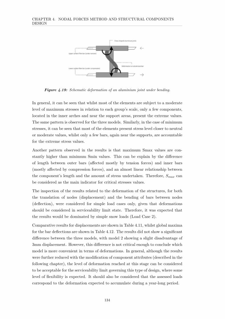
CHAPTER 4. NODAL FORCES METHOD AND STRUCTURAL COMPONENTSDESIGN
Figure 4.19: Schematic deformation of an aluminium joint under bending.
In general, it can be seen that whilst most of the elements are subject to a moderatelevel of maximum stresses in relation to each group’s scale, only a few components,located in the inner arches and near the support areas, present the extreme values.The same pattern is observed for the three models. Similarly, in the case of minimumstresses, it can be seen that most of the elements present stress level closer to neutralor moderate values, whilst only a few bars, again near the supports, are accountablefor the extreme stress values.
Another pattern observed in the results is that maximum Smax values are con-stantly higher than minimum Smin values. This can be explain by the differenceof length between outer bars (affected mostly by tension forces) and inner bars(mostly affected by compression forces), and an almost linear relationship betweenthe component’s length and the amount of stress undertaken. Therefore, Smax canbe considered as the main indicator for critical stresses values.
The inspection of the results related to the deformation of the structures, for boththe translation of nodes (displacement) and the bending of bars between nodes(deflection), were considered for simple load cases only, given that deformationsshould be considered in serviceability limit state. Therefore, it was expected thatthe results would be dominated by simple snow loads (Load Case 2).
Comparative results for displacements are shown in Table 4.11, whilst global maximafor the bar deflections are shown in Table 4.12. The results did not show a significantdifference between the three models, with model 2 showing a slight disadvantage of3mm displacement. However, this difference is not critical enough to conclude whichmodel is more convenient in terms of deformations. In general, although the resultswere further reduced with the modification of component attributes (described in thefollowing chapter), the level of deformation reached at this stage can be consideredto be acceptable for the serviceability limit governing this type of design, where somelevel of flexibility is expected. It should also be considered that the assessed loadscorrespond to the deformation expected to accumulate during a year-long period.
134

CHAPTER 4. NODAL FORCES METHOD AND STRUCTURAL COMPONENTSDESIGN
Fig
ure
4.20
:Distributionof
maxim
umSvalues
onthearches’b
arsin
Model
1du
eto
load
case
6.F
igur
e4.
21:Distributionof
maxim
umSvalues
onthearches’b
arsModel
2du
eto
load
case
6.F
igur
e4.
22:Distributionof
maxim
umSvalues
onthearches’b
arsin
Model
3du
eto
load
case
6.
Fig
ure
4.23
:Distributionof
maxim
umSvalues
oncross’sbars
from
Model
1du
eto
load
case
6.F
igur
e4.
24:Distributionof
maxim
umSvalues
oncross’sbars
from
Model
2du
eto
load
case
6.F
igur
e4.
25:Distributionof
maxim
umSvalues
oncross’sbars
from
Model
3du
eto
load
case
6.
135
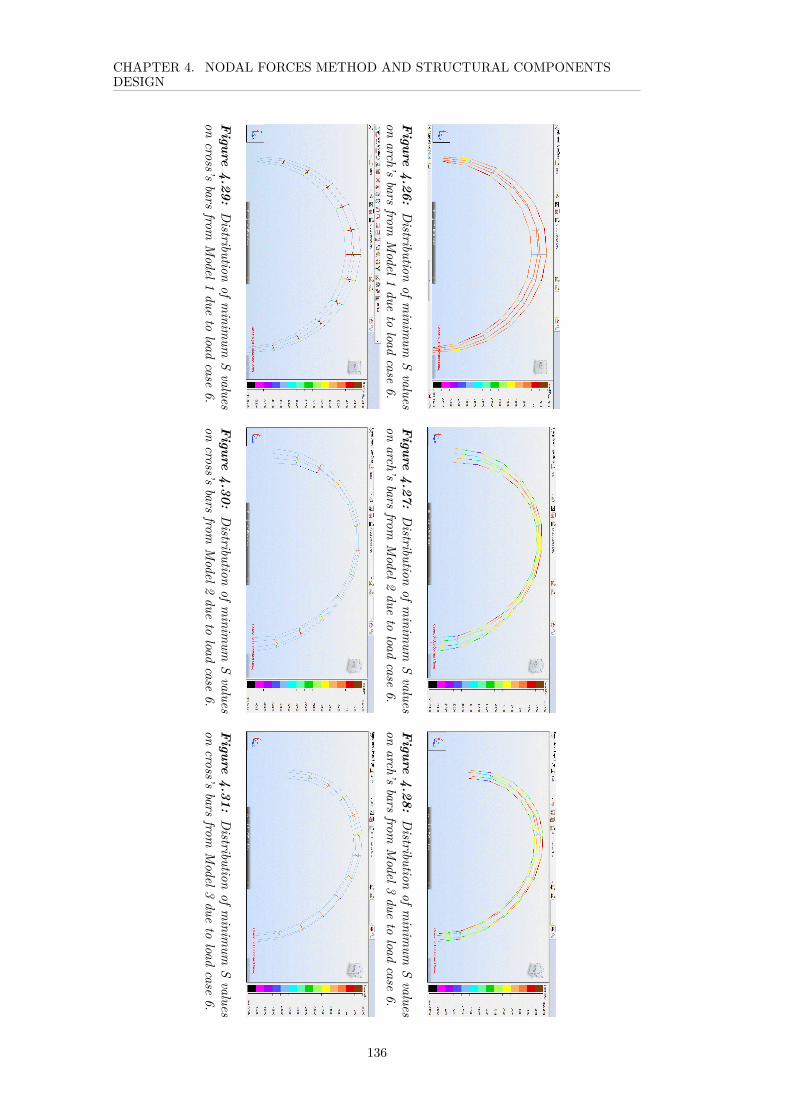
CHAPTER 4. NODAL FORCES METHOD AND STRUCTURAL COMPONENTSDESIGN
Figure
4.26:Distribution
ofminim
umSvalues
onarch’s
barsfrom
Model1
dueto
loadcase
6.F
igure4.27:
Distribution
ofminim
umSvalues
onarch’s
barsfrom
Model2
dueto
loadcase
6.F
igure4.28:
Distribution
ofminim
umSvalues
onarch’s
barsfrom
Model3
dueto
loadcase
6.
Figur e
4.29:Distribution
ofminim
umSvalues
oncross’s
barsfrom
Model1
dueto
loadcase
6.F
igur e4.30:
Distribution
ofminim
umSvalues
oncross’s
barsfrom
Model2
dueto
loadcase
6.F
igur e4.31:
Distribution
ofminim
umSvalues
oncross’s
barsfrom
Model3
dueto
loadcase
6.
136

CHAPTER 4. NODAL FORCES METHOD AND STRUCTURAL COMPONENTSDESIGN
Arch Geometry Maximum Displacement of Nodes [mm] Load Caseux uy uz utotal
Model 1 0 0 -23 23 2Model 2 0 0 -26 26 2Model 3 0 0 -23 23 2
Table 4.11: Maximum nodes displacement on Models 1, 2 and 3.
Arch Geometry Maximum Displacement of Nodes [mm] Load Caseux uy uz utotal
Model 1 0 0 2 2 2Model 2 0 0 3 3 2Model 3 0 0 2 2 2
Table 4.12: Maximum bars deflection on Models 1, 2 and 3.
Figures 4.32, 4.33 and 4.34, show the general distribution of the arch deformations ineach model due to snow loads. The results have been resized to five times the scaleof the structure to make this feature visible. The resultant figures are consistentwith the dominant vertical deformation caused by snow accumulations.
Finally, it is possible to conclude that in terms of internal stresses, Models 1 and3 show a clear advantage over Model 2, for both types of components. Betweenthe two best options Model 1 present a moderate advantage over Model 3. Thisconfirms the structural efficiency of the geometry used in the original scheme. Interms of deformations, no model shows a clear advantage and values are in generalacceptable. Additionally, when constructability and environmental impact criteriaare included, Model 1 becomes the most convenient option, as this represents theleast invasive option.
4.8.2 Variation Study for Joint Shape
As described previously, the trussed arch due part of its resistance to the efficientdistribution of the four flexible bars forming a single rectangular section, rather thanto the four bars’ sections. Therefore, in order to question the convenience of the
Figure 4.32: Deformationsof Model 1 caused by com-bined loads.
Figure 4.33: Deformationsof Model 2 caused by com-bined loads.
Figure 4.34: Deformationsof Model 3 caused by com-bined loads.
137
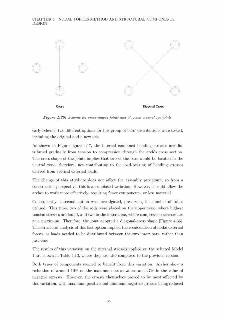
CHAPTER 4. NODAL FORCES METHOD AND STRUCTURAL COMPONENTSDESIGN
Figure 4.35: Scheme for cross-shaped joints and diagonal cross-shape joints.
early scheme, two different options for this group of bars’ distributions were tested,including the original and a new one.
As shown in Figure figure 4.17, the internal combined bending stresses are dis-tributed gradually from tension to compression through the arch’s cross section.The cross-shape of the joints implies that two of the bars would be located in theneutral zone, therefore, not contributing to the load-bearing of bending stressesderived from vertical external loads.
The change of this attribute does not affect the assembly procedure, so from aconstruction perspective, this is an unbiased variation. However, it could allow thearches to work more effectively, requiring fewer components, or less material.
Consequently, a second option was investigated, preserving the number of tubesutilised. This time, two of the rods were placed on the upper zone, where highesttension stresses are found, and two in the lower zone, where compression stresses areat a maximum. Therefore, the joint adopted a diagonal-cross shape [Figure 4.35].The structural analysis of this last option implied the recalculation of nodal externalforces, as loads needed to be distributed between the two lower bars, rather thanjust one.
The results of this variation on the internal stresses applied on the selected Model1 are shown in Table 4.13, where they are also compared to the previous version.
Both types of components seemed to benefit from this variation. Arches show areduction of around 10% on the maximum stress values and 27% in the value ofnegative stresses. However, the crosses themselves proved to be most affected bythis variation, with maximum positive and minimum negative stresses being reduced
138
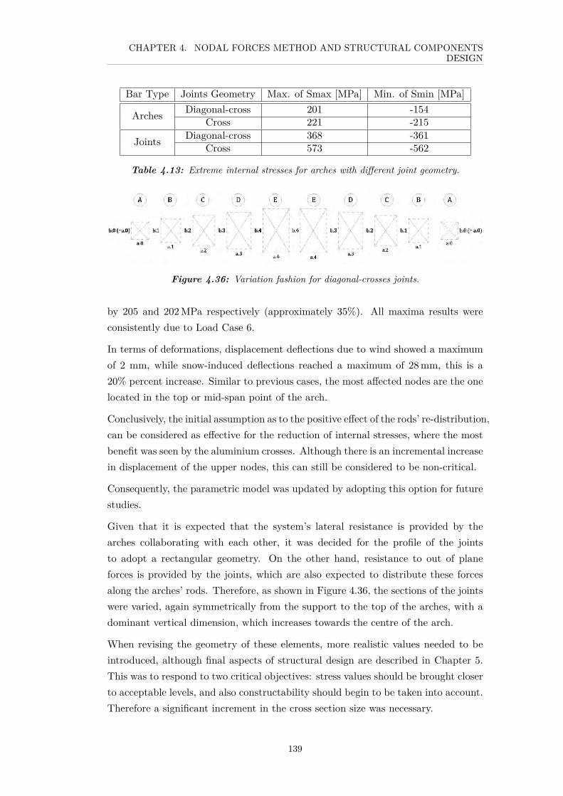
CHAPTER 4. NODAL FORCES METHOD AND STRUCTURAL COMPONENTSDESIGN
Bar Type Joints Geometry Max. of Smax [MPa] Min. of Smin [MPa]
Arches Diagonal-cross 201 -154Cross 221 -215
Joints Diagonal-cross 368 -361Cross 573 -562
Table 4.13: Extreme internal stresses for arches with different joint geometry.
Figure 4.36: Variation fashion for diagonal-crosses joints.
by 205 and 202 MPa respectively (approximately 35%). All maxima results wereconsistently due to Load Case 6.
In terms of deformations, displacement deflections due to wind showed a maximumof 2 mm, while snow-induced deflections reached a maximum of 28 mm, this is a20% percent increase. Similar to previous cases, the most affected nodes are the onelocated in the top or mid-span point of the arch.
Conclusively, the initial assumption as to the positive effect of the rods’ re-distribution,can be considered as effective for the reduction of internal stresses, where the mostbenefit was seen by the aluminium crosses. Although there is an incremental increasein displacement of the upper nodes, this can still be considered to be non-critical.
Consequently, the parametric model was updated by adopting this option for futurestudies.
Given that it is expected that the system’s lateral resistance is provided by thearches collaborating with each other, it was decided for the profile of the jointsto adopt a rectangular geometry. On the other hand, resistance to out of planeforces is provided by the joints, which are also expected to distribute these forcesalong the arches’ rods. Therefore, as shown in Figure 4.36, the sections of the jointswere varied, again symmetrically from the support to the top of the arches, with adominant vertical dimension, which increases towards the centre of the arch.
When revising the geometry of these elements, more realistic values needed to beintroduced, although final aspects of structural design are described in Chapter 5.This was to respond to two critical objectives: stress values should be brought closerto acceptable levels, and also constructability should begin to be taken into account.Therefore a significant increment in the cross section size was necessary.
139

CHAPTER 4. NODAL FORCES METHOD AND STRUCTURAL COMPONENTSDESIGN
Bar Type Joints Geometry Max. of Smax [MPa] Min. of Smin [MPa]
Arches Size (0) 223 -181Size (1) 201 -154
Joints Size (0) 242 -240Size (1) 368 -361
Table 4.14: Extreme internal stresses in arches and joints bars with different componentssizing.
Minimum values of joints’ width (a) and maximum values for joints’ height (b) wereestablished, as shown in Figure figure 4.36. The minimum value for (a), was definedas 150 mm based on the minimum spacing of elements that would allow the manualassembly of multiple bars, bolts and anchors wearing bulky-gear and it was increasedto 300 mm at the top of the arch, where a largest section was needed. The maximum(b) size, 500 mm, was defined by a manageable weight and size (both estimated) ofcomponents needed to be lifted and installed during the unaided set-up processunder severe weather conditions. Therefore, the mid-span cross size was defined bya 300× 500 mm rectangle.
Once the support section was varied from 50×50 mm to 150×150 mm, and the mid-span section increased from 150×150 mm to 300×500 mm, a significant reduction inthe maximum and minimum stress values was observed. The values obtained withthe new sizing (Size 1) are shown in Table 4.14, where they are compared to theoriginal configuration (Size 0).
Whilst the arches exhibited a moderate increase of maximum values (11%) a signif-icant reduction was gained in the crosses’ maximum and minimal stresses (nearly35% of the original values)
4.8.3 Variation Study on the Number of Subdivisions
In the original design, each arch was divided into 16 segments [Chapter 3], withthe bars as continuous elements. Additionally, the new strategy proposed arches asassembled elements, with bar segments fastened to the aluminium joints.
In order to ease the construction procedure, a reduction in the number of joints wasexplored from points of view of structure and a construction.
From a structural perspective, the rigid aluminium joints play a key role: they definethe shape of the arch as well as transmit vertical loads to the bars and thereforeprovide the entire system a resistance to out-of-plane loads. They also provide thenet of bracing cables with fixing points over the surface.
As shown in Figure 4.19, vertical elements on the joints are subject to high bendingstresses, for which it was initially believed that reducing the number of aluminium
140

CHAPTER 4. NODAL FORCES METHOD AND STRUCTURAL COMPONENTSDESIGN
Bar Type Number of segments Max. of Smax [MPa] Min. of Smin [MPa]
Arches
8 (9 nodes) 257 -21711 (12 nodes) 230 -18812 (13 nodes) 223 -18115 (16 nodes) 206 -165
Joints
8 (9 nodes) 284 -28211 (12 nodes) 255 -25512 (13 nodes) 242 -24015 (16 nodes) 214 -213
Table 4.15: Extreme internal stresses in arches with different number of segments.
joints would be responsible for the increment of bending stresses in both arches andjoints. Therefore, the sensitivity of both types of components in relation to thevariation of the number of crosses was assessed, using different samples. The resultsare shown in Table 4.15.
The results show both elements responding to the variation in the number of com-ponents. However a bigger reduction is noticed in the joints. Assuming that thedifference in stresses’ values could be uniformly distributed, then each added nodeis accountable for a reduction of 7.2 MPa in the Smax value of the arches’ bars, anda 10 MPa reduction in the joint’s Smax. This is a reduction of 3.2% in the caseof the arches’ bars and 4.1% in the case of the crosses, based on the values fromthe original configuration (4 m span and 12 segments). For the case of minimumnegative stress values, almost identical variations in combined stresses are observed.Therefore, it can be said that arches and joints are equally sensitive to the variationon the number of components, although that variation can be considered moderate.
Another point to be observed is the effect of the presence of a joint in the mid-spanpoint of the arch. When the results of arches with 11 and 12 segments are inspected,the arches’ highest positive stress in the 12 nodes arch presented a reduction ofexactly 7.2 MPa, which is the average and expected decrease. However, the crossesin this same sample presented a more than proportional reduction, of −14 MPa,where an average reduction of 10 MPa was projected. It has already been saidthat upper elements are the most critically affected components in terms of stressesdistribution and deformations [Fig. figure 4.19], so the presence of a node in the mid-span point (or an uneven number of nodes), should be considerate as a preferableattribute, although with a moderate benefit.
From a construction perspective, reducing the number of joints (from 16), increasesthe length of the bar segments. This can have different effects in the assemblyprocedure depending on the span of the arch. Therefore, a balanced solution for thenumber of joints was derived.
The length of the bars’ segments for the different spans was inspected in Table 4.16.
141

CHAPTER 4. NODAL FORCES METHOD AND STRUCTURAL COMPONENTSDESIGN
Span[m
]TotalLength
[m]
Num
berof3m
barsNum
berofSegm
ents9
1011
1213
1415
Segment
Length[m
]12
18.87
2.091.88
1.711.57
1.451.35
1.2611.5
18.16
2.011.81
1.641.51
1.391.29
1.211
17.36
1.921.73
1.571.44
1.331.23
1.1510.5
16.56
1.831.65
1.51.37
1.271.18
1.110
15.76
1.751.57
1.431.31
1.211.12
1.059.5
14.95
1.661.49
1.361.24
1.151.07
0.999
14.15
1.571.41
1.291.18
1.091.01
0.948.5
13.45
1.481.34
1.211.11
1.030.95
0.898
12.65
1.41.26
1.141.05
0.970.9
0.847.5
11.84
1.311.18
1.070.98
0.910.84
0.797
114
1.221.1
10.92
0.850.79
0.736.5
10.24
1.131.02
0.930.85
0.790.73
0.686
9.44
1.050.94
0.860.79
0.720.67
0.635.5
8.63
0.960.86
0.790.72
0.660.62
0.585
7.93
0.870.79
0.710.65
0.60.56
0.524.5
7.13
0.790.71
0.640.59
0.540.5
0.474
6.33
0.70.63
0.570.52
0.480.45
0.42
Arc h
with
evennum
berofnodes
1.5m
<Segm
entLength
<0.5m
Table
4.16:Bars
segments
lengthsofarches
withdifferentspans
andnum
berofjoints.
142

CHAPTER 4. NODAL FORCES METHOD AND STRUCTURAL COMPONENTSDESIGN
As an initial criterion, the convenience of a node at the mid-span point was estab-lished. Therefore, the election of the number of subdivisions began by discardingthose options with an even number of nodes (uneven number of segments). It wasalso concluded that segments shorter than 0.5 meters should be avoided as thecomplex joints placed at both ends of each segment including tensile cables andmembrane buckles, would be too complicated to manipulate manually or repair.Segments longer than 1.5 meters were also discarded as manipulation could also bedifficult under severe wind conditions. Therefore, two options were assessed to beequally feasible: 12 and 14 segments. The option with the fewer subdivisions wastherefore chosen, namely, 12 segments (or 13 nodes).
4.8.4 Variation Study on the Arch’s Depth
The depth of a trussed arch mid-span provides the system with vertical load bearingto resist out- of-plane forces in the most critical zones. Based on the materialself-weight and the limited aid for assembly, the maximum height of crosses, thusthe arch’s depth, was restricted to a maximum of 500 mm. Due to the 13 nodesconsidered, each arch would require 6 different crosses. Given that the span varies,each of these crosses, with exception of the top and the bottom elements, wouldneed to be bespoke.
However, the uniformity of the arch depth leads some of the arches, particularlythose within the smallest range of span, to be over-structured and/or aestheticallyunproportioned.
Therefore, the effect of the arch’s depth variation on the performance of this par-ticular structural typology was studied by comparing different options: a 4 m spanarch with 300, 400 and 500 mm depth. For all three options, the width of mid-spancross was fixed at 300 mm. Given that all intermediate joints are already bespoke,the proportional variation of the mid-span depth will not result in a higher numberof different components at this stage. The reduction of the number of componentsis explored in the following chapter.
Table 4.17, shows the global extreme combined stresses for bars forming arches andjoints, with these three different configurations.
In this case, a consistent reduction is observed in the variation of the component’sstresses.
For the arches, in terms of highest Smax values, the first step of depth reduction(this is from 0.5 to 0.4 m) caused an increment of 14.1 MPa (or 6.3% with respectto the original configuration), while for the Smin values, the increment was 15.8(8.7%). In the second depth reduction step (from 0.4 to 0.3 m), the highest Smax
143

CHAPTER 4. NODAL FORCES METHOD AND STRUCTURAL COMPONENTSDESIGN
Bar Type Mid-span Depth [m] Max. of Smax [MPa] Min. of Smin [MPa]
Arches0.3 248 -2090.4 234 -1930.5 222 -181
Joints0.3 267 -2650.4 258 -2570.5 242 -240
Table 4.17: Extreme internal stresses for arches with different mid-span depth.
was increased to 11.4 MPa (8.7%), which is almost equivalent to the increment inthe extreme Smin value of 11.7 MPa (6.5%).
The variation in the stresses of the crosses showed coherent results with the reductionof this attribute. Here, a 6.8% increment in both Smax and Smin global extremevalues, was observed with the first reduction, and 3.5% for the second reductionstep, again for both critical values.
Therefore, the variation of this attribute, although effective, can be considered tobe moderate in regards to the internal stresses.
4.9 Conclusions
All the results obtained from the Finite Element models are coherent with thetheoretical notions of a vierendeel form of truss.
The examination of FE results against Polar-based criteria allowed the specificationof the geometrical features for the primary structural element (a single trussed arch)with a minimum span (four meters).
The sensitivity of each geometrical attribute has also been established.
In order to better visualise how sensitive the components are to the variation ofevery attribute, the results were normalised using a bar chart. The graph refers tothe results in the arches’ bars as they are considered the main results.
In these graphs, every iteration (series) sets a new reference value (100%) which isrepresented by the red bars. The geometry was consecutively updated based on thebest option obtained by the previous iteration, highlighted with the symbol ‘*’.
The expected dominance of global geometry and joint’s shape, with respect to therest of the attributes (size of section, number of subdivisions and mid-span depth)was observed.
In the case of sizing, the new version proposed resulted in a moderate incrementon the arches’ bars stresses (equivalent to a 10% increment). This version was
144
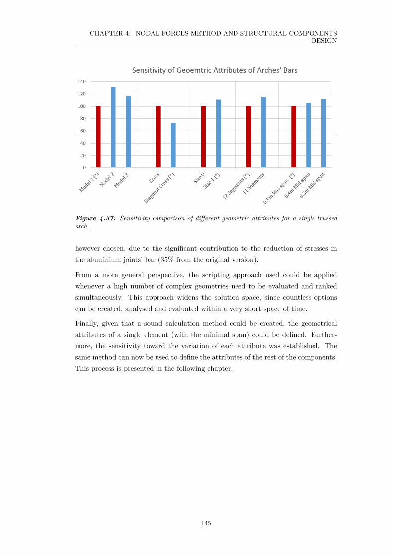
CHAPTER 4. NODAL FORCES METHOD AND STRUCTURAL COMPONENTSDESIGN
Figure 4.37: Sensitivity comparison of different geometric attributes for a single trussedarch.
however chosen, due to the significant contribution to the reduction of stresses inthe aluminium joints’ bar (35% from the original version).
From a more general perspective, the scripting approach used could be appliedwhenever a high number of complex geometries need to be evaluated and rankedsimultaneously. This approach widens the solution space, since countless optionscan be created, analysed and evaluated within a very short space of time.
Finally, given that a sound calculation method could be created, the geometricalattributes of a single element (with the minimal span) could be defined. Further-more, the sensitivity toward the variation of each attribute was established. Thesame method can now be used to define the attributes of the rest of the components.This process is presented in the following chapter.
145

Chapter 5
Multi-Objective Design Process
5.1 Introduction
This chapter presents the second part of the design study for an adaptable lightweightstructure in a Polar area. In the previous sections, the basic characteristics of atrussed arch were defined and a parametric method to calculate the internal stressesin arches was introduced.
This chapter describes the design of the structure as a generic system, meaningthat specific attributes of arches as well as the relationship between the differentcomponents are established.
In the first part (Section 5.2), the initial design conditions are revised in order toboth make accurate assumptions and to bring stress values closer to allowable levels.This includes: inclusion of material properties, pre-stress and span values.
Secondly, geometric variations are studied in order to either allow the adaptabilityof the lightweight system, or to reduce the number of different components.
This exercise could be defined as a multi-objective optimisation study. As in anymulti-attribute problem, there are several objectives to be pursued, where some canbe contradictory. As an analogy, a common engineering problem is the minimisationof a structure’s deflection and the reduction in self-weight, so a single solution thatsimultaneously optimises each objective is not possible. Instead, some level of opti-misation (towards one of the objectives) is achievable, for which a trade-off betweenother attributes is necessary. In this research, the main criteria (or objectives) arelightness of the structure, adaptability of configuration and a reduced number ofdifferent components. Although it is believed that a number of Pareto optimalsolutions are possible, this study will show one set of results using a polar logistic-based weighting method. A solution is called a Pareto optimal (or noninferior) ifnone of the attribute (or objective functions) can be modified or improved withoutdegrading some of the other objective values [113].
147

CHAPTER 5. MULTI-OBJECTIVE DESIGN PROCESS
There can be many ways of carrying out the optimisation of a certain attributeon a given structure, in which the components are resolved individually. However,the extreme logistical and environmental limitations of this case did not allow sucha detailed solution. Instead, this multi-objective study was employed in order toenable the ‘partial-optimisation of the structure’. Where a set of pre-establishedvalues is determined for each attribute and assigned to each class of componentaccording to their size. This study was led by three main criteria (lightness of thestructure, adaptability of configurations, and reduction of the number of differentcomponents).
Once the preconditions were reestablished, a sensitivity study was carried out, whichpresented in Section 5.3. This involved the definition of several variables, such asarches’ span, rods’ cross section, number of crosses, mid-span (or ridge) depth.This study pointed towards introducing a certain degree of ‘optimisation’ to thedifferent aspects of the structure. Therefore, some of the attributes were resolvedby segmenting or grouping its values. As a results, groups of values were establishedfor each component’s attribute according to the arches’ span, rather than singularsolutions.
Whilst span variations and material properties were pre-established, the sensitivitystudy described in Section 5.3 was used to determine the following attributes orvariables:
i) Differentiated cross sections of the arches’ bars according to span.
ii) Differentiated arch mid-span depth according to span.
iii) Uniform load condition of arches according to span and distances betweenarches.
Following, Section 5.4, a set of geometry-based optimisation studies were carried outwith the purpose of reducing the number of different components, in particular:
iv) Reducing the number of joints per arch according to span.
v) Reducing the number of different scissor-joints for the whole system.
The corresponding subsections of sections 5.3 and 5.4 are later introduced. Finally,the information acquired for each set of components and its relation to the others areintegrated into a generic parametric CAD model, which is presented in the Section5.5.
148

CHAPTER 5. MULTI-OBJECTIVE DESIGN PROCESS
5.2 Revision of pre-conditions for Sensitivity Study
The FE test described in Chapter 4 was run multiple times on single trussed archeswith spans ranging from 4 m to 12 m, where external loads valid for a 1m arch-spacing were applied. From analysis of the results, some modification of the initialpre-conditions was considered necessary in order to bring stresses within allowableand realistic levels. These modifications are as follows:
5.2.1 Material properties
Firstly, the large stresses observed in Chapter 4, suggested a change in the materialproperties used for the arches’ bars. This time, the use of Carbon Fibre ReinforcedPolymer (CFRP) was considered, with a modulus of elasticity of 70 GPa, and abending and tensile strength limit of 600 MPa. These values imply the use of aparticular build-up of composite with a specific proportion of longitudinal fibres (atleast 30 %) and the use of a particularly stiff type of carbon fibre. For a material withsuch characteristics and used as part of an arch, compressive strength is not usuallycritical, since buckling would occur before collapse. Density is kept at standardvalues. Poisson Modulus is 0.33 and its Shear Modulus is 50 GPa (see Chapter 4).
5.2.2 Pre-stress
Apart from the externally derived loads, a more realistic study also requires theinclusion of pre-stress derived from internal bending forces. This would be causedby the force necessary to get initially-straight bar segments to adapt to the curvedshape which defines the arch. Pre-stress forces derived from bending are defined bythe expression:
σy⁄Iy = E⁄R
Where,
σy is bending stress
Iy is the moment of inertia
E is the modulus of elasticity
R is the radius of curvature of the arc
149

CHAPTER 5. MULTI-OBJECTIVE DESIGN PROCESS
(a) (b) (c) (d)
Figure 5.1: Top view of a curve standardised with different values: (a) original input curvesubdivided into a number of segments (b) span values rounded to nearest 0.2m value, (c) spanvalues rounded to the nearest 0.5m value and, (d) span values rounded to nearest 1m value.
Therefore, this value needs to be updated according to the arch’s span (defining thearc’s radius) and bar’s cross section (Moment of Inertia, Iy ). It was initially decidedthat the value of pre-stress should be kept below one half of the bending strength, inorder to allow the bars to cope with external forces. This required a careful trade-offbetween material resistances to external forces, since the thickness of bars (dictatingthe ‘Iy’ value) is inversely proportional to the σyvalue. Similarly, the largest arch’sspan (this is the largest radius) would present the lowest value of pre-stress derivedfrom bending. However, such elements would need to cope with the highest valuesof external forces, as their loaded areas would be the largest. Correspondingly, thesmallest radiuses would be derived from the highest values of internal stress derivedfrom bending, and the smallest values of forces derived from snow and wind.
5.2.3 Standardisation of Span Values
It was also decided that, in the case of the Union Glacier Station, the span variationwould be restricted to increments of 1 m. Whilst this constraint could compro-mise the aesthetic aspects of the structure, it would limit the number of differentcomponents significantly.
Figure 5.1 shows early-stage sketches assessing the re-interpretation of the inputcurve with span values rounded to the nearest 1, 0.5 and 0.2 m respectively. Itwas then quickly understood that, given the proportion of the structures, the sub-tle aesthetic difference between options became irrelevant when the benefit of theconstruction and logistics were compared. Therefore, a ‘low degree of variation’strategy was adopted, i.e. span values derived from an architectural scheme, wouldbe standardised and rounded to the nearest whole number of metres.
Up to this stage, the system considered only a standard height for the ridge crossesof 500 x 300 mm and for the crosses at the base of 150 x 150 mm. However,given that each arch would initially have a different length and equal number of
150

CHAPTER 5. MULTI-OBJECTIVE DESIGN PROCESS
subdivision (12 segments), the central joints would inherit bespoke measurementsbased on the arches’ length. This means that every diagonal cross joint, except ridge(or mid-span) and base ones, would require a very specific size to define the arch’sshape. The same would be true for every bar segment. The inclusion of this integervalue restriction on the arches’ span [Fig. 5.1(d)] would narrow down the numberof different components to 8 segment lengths, and the number of different joints to49.
Nevertheless, in the case of a less restrictive context, where more detailed compo-nents can be handled, the original input-curve could be interpreted with a finerdegree of discretisation, by using smaller segment lengths to replicate the originalcurve with higher precision [Fig. 5.1(b) and (c)].
This restriction was finally included into the parametric model as shown in section5.5.
5.3 Sensitivity study
As stated earlier, this multi-objective study is led by three conflicting criteria: light-ness of the structure, adaptability of configurations, and reduction of the number ofdifferent components.
Whilst span variations and material properties were pre-established, the sensitivitystudy was used to determine the following attributes: cross sections of the arches’bars according to span, arches’ mid-span depth according to span, and the distancebetween arches.
The extreme logistical and environmental limitations of this case, proposed that thestructural system could only be ‘partially-optimised’. The introduction of a certaindegree of ‘optimisation’ of the structural system’s attributes implied that these wereresolved as groups of values. As a result, groups of values were established for eachcomponent’s attribute according to the arch span.
The maps of the values tested versus the restrictions imposed are described in Figure5.2.
Subsection 5.3.1 explains the characteristics of the aluminium joints and why thesewere not considered as a variable attribute.
The first of this set of studies, titled ‘Differentiated rod cross sections according tospan’, is described in section 5.3.2. This section looks into a controlled variationof the rods’ cross-section throughout the surface in order to employ the minimumamount of material (smallest possible rod cross-sectional area) whilst keeping stresseswithin allowable limits according to material properties (see Chapter 4).
151

CHAPTER 5. MULTI-OBJECTIVE DESIGN PROCESS
The second study, ‘Differentiated arch depth according to span’, is described inSection 5.3.3 and it looks at variations of the arch’s span and depth based onaesthetic as well as structural criteria.
Section 5.3.4 is dedicated to the third study titled ‘Grouping of arches attributes forthe reduction of internal stresses’. In this section, the attributes of the set of archesare grouped in different arrangements. These arrangements are compared to findthe option which brings stress values closest to an acceptable level. Section 5.3.5explores a geometrical solution to reduce the Carbon Fibre bars’ stresses derivedfrom bending to be applied to the whole set of arches, in order to further reducedthe internal stresses on arches’ bars.
Finally, Section 5.3.6, is dedicated to the standardisation of load conditions for allthe arches of the group. This study proposes a method to uniform the value ofstresses afforded by arches of different span, derived from external loads appliedon the membranes spanning between arches spaced at 1m (initially). As a result,the spacing between arches of different span, as well as the size of the spanningmembrane pieces corresponding to each arch are defined.
5.3.1 Uniform Cross Section of Aluminium Joints
As shown in Figure 5.2, several different variations of the joint’s cross-section weretested, where the objective was to find the minimum value necessary to keep inter-nal stresses below the material capacity. This parameter’s outputted values wereidentified as highly sensitive in Chapter 4, for which the detailed differentiation ofthe aluminium bars’ cross sections (according to the variation of the arches’ span)would be expected. Nevertheless, a unique value needed to be established, since thejoints were grouped according to node position rather than span value, as describedin Section 5.4. Consequently, a section of 40 mm, with a wall thickness of 5 mmwas selected. This was based on that is the one of the minimum values that wascommonly tested for all range of arches span, with most of the stresses values beingwithin acceptable limits.
5.3.2 Variations of Rod Cross-Sections According to Span.
The size of the rods’ cross section has also been described as a sensitive or responsiveparameter (see Chapter 4). Therefore, the partial optimisation of this attributeaccording to different span values was attempted. FE tests were ran for every otherspan value; that is, cases of single trussed arches of 12, 10, 8, 6 and 4 m span. Ineach case, several different rod sections were tested, as shown in Figure 5.2. A linear
152
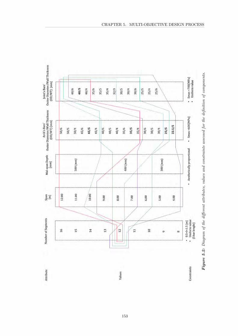
CHAPTER 5. MULTI-OBJECTIVE DESIGN PROCESS
Fig
ure
5.2:
Diagram
ofthediffe
rent
attributes,v
aluesan
dconstra
ints
assessed
forthedefin
ition
ofcompone
nts.
153

CHAPTER 5. MULTI-OBJECTIVE DESIGN PROCESS
Arch’sFeatures
Aluminium Joints’ Bars Arches’ BarsOD/WT [mm] Smax[MPa] OD/WT [mm] Smax[MPa]
Span 12 [m]Depth 500[mm]
40/5
625 45/5 373648 40/5 475664 35/5 640
Span 10 [m]Depth 500[mm]
487 40/5 339503 35/5 457511 30/5 650
Span 10 [m]Depth 400[mm]
395 40/5 437515 35/5 464744 30/5 461
Span 8 [m]Depth 400[mm]
312 40/5 259325 35/5 319427 30/5 333402 25/5 523
Span 6 [m]Depth 400[mm]
185 30/5 253190 25/5 397191 22.5/5 520
Span 6 [m]Depth 300[mm]
228 30/5 295234 25/5 435235 22.5 572235 20/5 785
Span 4 [m]Depth 300[mm]
102 25/5 221104 22.5 277105 20/5 380
Table 5.1: Sensitivity study for the definition of arches’ bars’ cross section.
154

CHAPTER 5. MULTI-OBJECTIVE DESIGN PROCESS
Group 1 2 3 4Span Range 12 ≤ S ≤ 10 10 ≤ S ≤ 8 8 ≤ S ≤ 6 6 ≤ S ≤ 4OD/WT [mm] 40/5 35/5 30/5 25/5
Table 5.2: Group of arches according to span range and bars’ cross section.
behaviour was assumed for the intermediate cases. Some of these results are shownin Table 5.1.
Several different rod sections were used in each span case. Largest and smallest spanswere spared from being tested using maximum and minimum rod sections becausethe resulting values were extensively out of scope. As expected, stress values showeda highly responsive variation to this attribute (diameter of bars’ cross section). Inorder to restrict the number of different components, the options were narroweddown to four option of CFRP bar sections, with external diameters of 40, 35, 30and 25 mm, all with a wall thickness of 5 mm, based on the span values (12 to 10m, 9.99 to 8 m, 7.99 to 6 m and 5.99 to 4 m respectively). The definition of thesefour groups are shown in Table 5.2
In each group, the bar cross section was sized to the most critical load case (thatis, the largest span), where the objective is to identify the minimum size of barcross-section necessary to keep internal stresses below the material strength limit.This grouping strategy is further studied in section 5.3.4.
5.3.3 Variation of Arches’ Depth According to Span
Figure 5.1 and Table 5.1 show the iterations tested where the arches’ mid-span depthwas increased according to the span increment. The three depth values examinedwere 500, 400 and 300 mm.
It could be argued that changing this attribute would increase the number of differentcomponents, particularly the number of aluminium joints and length segments,which had been rationalised to 8 and 48 variations respectively. However, thecontrolled variation of the mid-span depth of arches would significantly contributeto the lightness of the system, which is of benefit for both structural efficiency andarchitectural expression.
The results displayed in Table 5.1 are corresponding with the role assigned to thisgeometrical attribute in Chapter 4, this is, to the distribution of out-of-plane forceswith a rather low sensitivity. In that sense, when stresses from two arches with samespan, same rod section, yet different depths are compared, a moderate difference inthe resulting maximum stress (Smax) is observed. Correspondingly, the arch withthe smallest depth presents slightly higher stress values and vice versa.
155

CHAPTER 5. MULTI-OBJECTIVE DESIGN PROCESS
Given that this feature was not considered to be a highly sensitive attribute, only3 variations were established, forming three groups, based on the arches’ span. Forarches with a span between 12 m and 10 m, the maximum possible value of depth(500 mm) was assigned. For the middle range (9.99 to 6 m), joints would have a400 mm height, whilst the smallest range (5.99 to 4 m) would be defined with theminimum 300 mm height. As explained previously, all crosses were defined with auniform width of 300 mm.
5.3.4 Grouping of Arches’ Attributes for Reduction of InternalStresses
This section looks at the definition and organisation of the different geometricattributes explored (span, rod section and mid-span depth) based on the internalstress values in the arches’ bars.
Additionally, pre-stresses were also included at this stage. Results are representedby the value ‘Total Stress’ (St ) in the tables included from this section onwards.This value stands for the aggregate stress on the most critical bar segment, thisis, the sum of the maximum value of the combined normal stresses derived fromexternal loads (Smax) and the internal stress derived from bending (σy).
Table 5.3 shows the original segmentation of values (Case A) described in theprevious section: uniform values for aluminium bars, four different values of rods’cross section (with a difference of 5 mm) and three different values of mid-span depth(with a difference of 100 mm). All arches were segmented evenly.
Although the Smax values in all cases were acceptable according to their materialcapacity, once the pre-stresses were included, the St values significantly exceededthe affordable limit in some cases.
Alterations to the uniform grouping strategy [Table 5.2] were then explored inorder to reduce the combined internal stresses. Figure 5.3, shows how the uniformdistribution of span values (Case A) was altered in Cases B and C to influence theinternal stress values.
According to Figure 5.3, Case A represent the original groups of span values [Table5.2]. In Case B, the rod section value for the Group 4 (this is arches with spanranging from 4 to 5.99 m) was further reduced from 25 to 22.5 mm. This wasexplored in order to reduce the high pre-bending stress observed at the lower limitof the group, this is, in arches of 4 m span.
Case C studied the effect of reducing the span range of Group 1 , which originallyincluded arches with spans between 12-10 m down, to 12-10.6 m, in order to reducethe high Smax values observed in Case A, particularly in the lower limit of the Group
156

CHAPTER 5. MULTI-OBJECTIVE DESIGN PROCESS
Figure 5.3: Cases of values’ grouping.
1 (this is, arches of 10 m span). This reduction on the span range covered by thefirst group, obviously caused the extension of the range covered by Group 3, whichnow included arches ranging from 8.00 to 10.59 m span)
The results of this are shown in Tables 5.4 and 5.5 for Cases B and C respectively.For all case wall thickness is preserved as 5 mm.
In each span range (or group), the trussed arch with the largest span presented thelowest σy value and the highest Smax value. Every pair of maximum and minimumspan values in each group (12 m and 10 m for Group 1, 9.99 m and 8 m for Group2, 7.99 m and 6 m for Group 3 and, 5.99 m and 4 m for Group 4) show significantvariations. In each case (either A, B or C) and in each pair of limiting values, thesample with the largest span presented the highest Smax value, whilst the arch withsmallest span, presented the highest σy value.
The resultant values of aggregated stress St are generally excessive in comparison tothe material capacity. In several cases, the pre-condition of keeping pre-stress underthe target limit of 30% of the material capacity is largely exceeded. In some cases,the normal stress value is equivalent to nearly 85% of the allowable stress limit.
Although the modifications of some of the attributes or parameters (cases B and Crespectively) in one the span groups, presented consistent results, they proved notonly insufficient, but also reduced the performance of some groups. For case B, thereduction of the bar’s section in Group 4, effectively reduced the high level of pre-stress (21% for the case of a 4 m arch span and 14% for the case of a 5.99 m arch),which was expected, however it also provoked a large increment in the value of Smax.Similarly, the alteration proposed in Case C, caused the expected reduction in σy
157
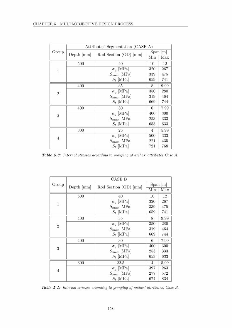
CHAPTER 5. MULTI-OBJECTIVE DESIGN PROCESS
GroupAttributes’ Segmentation (CASE A)
Depth [mm] Rod Section (OD) [mm] Span [m]Min Max
1
500 40 10 12σy [MPa] 320 267Smax [MPa] 339 475St [MPa] 659 741
2
400 35 8 9.99σy [MPa] 350 280Smax [MPa] 319 464St [MPa] 669 744
3
400 30 6 7.99σy [MPa] 400 300Smax [MPa] 253 333St [MPa] 653 633
4
300 25 4 5.99σy [MPa] 500 333Smax [MPa] 221 435St [MPa] 721 768
Table 5.3: Internal stresses according to grouping of arches’ attributes Case A.
GroupCASE B
Depth [mm] Rod Section (OD) [mm] Span [m]Min Max
1
500 40 10 12σy [MPa] 320 267Smax [MPa] 339 475St [MPa] 659 741
2
400 35 8 9.99σy [MPa] 350 280Smax [MPa] 319 464St [MPa] 669 744
3
400 30 6 7.99σy [MPa] 400 300Smax [MPa] 253 333St [MPa] 653 633
4
300 22.5 4 5.99σy [MPa] 397 263Smax [MPa] 277 572St [MPa] 674 834
Table 5.4: Internal stresses according to grouping of arches’ attributes, Case B.
158

CHAPTER 5. MULTI-OBJECTIVE DESIGN PROCESS
GroupCASE C
Depth [mm] Rod Section (OD) [mm] Span [m]Min Max
1
500 40 10.6 12σy [MPa] 264 267Smax [MPa] 377 475St [MPa] 641 741
2
400 35 8 10.59σy [MPa] 350 231Smax [MPa] 319 516St [MPa] 669 748
3
400 30 6 7.99σy [MPa] 400 300Smax [MPa] 253 333St [MPa] 653 633
4
300 25 4 5.99σy [MPa] 500 333Smax [MPa] 221 435St [MPa] 721 768
Table 5.5: Internal stresses according to grouping of arches’ attributes, Case C.
on the lower limit of Group 1 (from 320 MPa for arches of 10 m span to 264 MPafor arches of 10.6 m span). However, this effect is irrelevant when the increment ininternal stresses is considered in both, Groups 3 and 4. Therefore, this can also beinterpreted as an ineffective alternative.
Case A was therefore still considered the closest option towards a ‘pareto’ optimalsolution, although Stotal values were still above acceptable limit.
The fact that σy is derived from geometric parameters and, on the other hand,Smax results from the external loads, offered the possibility of defining a geometrybased solution, provided that combined normal stresses were below the materialmechanical limit for all ranges. This solution in described in the following section.
5.3.5 Geometry-based Method to reduce Pre-stress in Arches
There is an inverse relation between pre-stress and radius of curvature, given by thepreviously defined expression:
σy = IyE
R
Assuming that the span, as well as values of Iy and E are fixed, the minimisation ofpre-stress can be achieved by controlling the radius of the curvature of the arches’segments. That is, the curvature of the bar segments between two joints.
159

CHAPTER 5. MULTI-OBJECTIVE DESIGN PROCESS
Figure 5.4: Angle between an arc’s segments according to different level of curvature.
As Figure 5.4 shows, the arch is originally defined with a radius of X. The levelof curvature can be measured by a scale of angles ranging from a fully curved bardefined by an angle of 180°, and at the other extreme, by a discretised arch formedby straight bar segments with infinite radius of curvature, with segments positionedat kink angle θ. Correspondingly, the curved arch would present a full pre-stresswhereas kinked segments would have zero bending-induced stress.
Given that pre-stress is defined by the arch radius, it is then possible to find acompromise solution; this is an arch formed by segments with a certain degree ofpre-stress, induced by segments with radius of curvature R2 and angle ε
There are multiple possible solutions to determine its value of R2. Figures 5.5 and5.6 present two equivalent geometry-based solutions to determine R2, and thereforeto control the pre-stress by decreasing the curvature of the arch’s segments.
Assuming that the objective is to determine the value of R2, and variables knownare:
R1 is the radius of the original arc
α is the angle defined by radius of the original arc segment
ε is the assigned kink angle between two bent arc segments
160

CHAPTER 5. MULTI-OBJECTIVE DESIGN PROCESS
Figure 5.5: First geometry-based method for controlling the curvature of an arc’s barsegments.
161
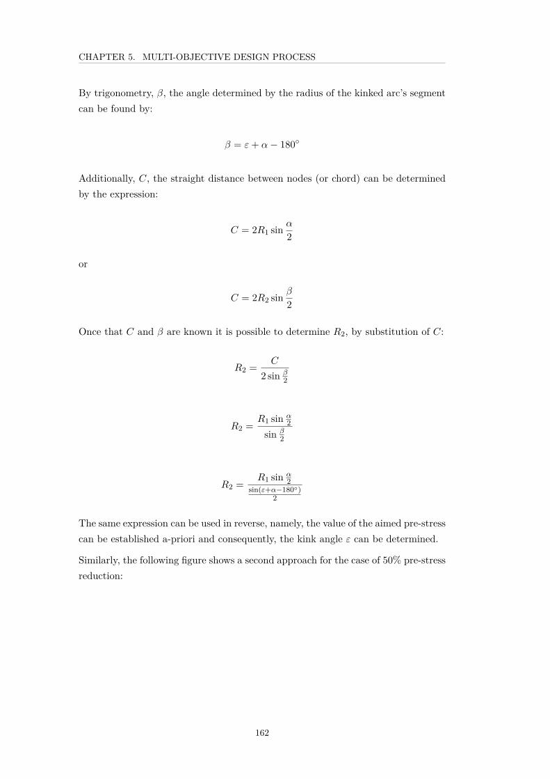
CHAPTER 5. MULTI-OBJECTIVE DESIGN PROCESS
By trigonometry, β, the angle determined by the radius of the kinked arc’s segmentcan be found by:
β = ε+ α− 180
Additionally, C, the straight distance between nodes (or chord) can be determinedby the expression:
C = 2R1 sin α2
or
C = 2R2 sin β2
Once that C and β are known it is possible to determine R2, by substitution of C:
R2 = C
2 sin β2
R2 =R1 sin α
2sin β
2
R2 =R1 sin α
2sin(ε+α−180)
2
The same expression can be used in reverse, namely, the value of the aimed pre-stresscan be established a-priori and consequently, the kink angle ε can be determined.
Similarly, the following figure shows a second approach for the case of 50% pre-stressreduction:
162

CHAPTER 5. MULTI-OBJECTIVE DESIGN PROCESS
Figure 5.6: Second geometry-based method for controlling the curvature of an arc’s barsegments.
Given that:
R1 sin γ = R2 sin γ2
then,
R2 = R1sin γsin γ
2
When required, this percentage of reduction can be adjusted.
Table 5.6 shows the revised results of segregated arches with a 50% reduction inpre-stress values.
Given that the results for St values above are still beyond acceptable limits in severalcases, a further reduction in the pre-stresses, this time 90%, was applied [Table 5.7].
It can be seen from Table 5.7 that no value exceeds the allowable limit, and so CaseA with 90% of pre-stress reduction was chosen as the best alternative. The geometricvalues obtained from this study could then be integrated into the parametric model.
163

CHAPTER 5. MULTI-OBJECTIVE DESIGN PROCESS
Group
Attributes’ Segmentation with 50% Pre-StressSegmentation (Case A)
Depth [mm] Rod Section (OD) [mm] Span [m]Min Max
1
500 40 10 12σy [MPa] 160 133Smax [MPa] 339 475St [MPa] 499 608
2
400 35 8 9.99σy [MPa] 175 140Smax [MPa] 319 464St [MPa] 494 604
3
400 30 6 7.99σy [MPa] 200 150Smax [MPa] 253 333St [MPa] 453 483
4
300 25 4 5.99σy [MPa] 250 167Smax [MPa] 221 435St [MPa] 471 602
Table 5.6: Internal Stresses according to grouping of arches’ attributes, Case A, with 50%of pre-stress reduction.
Group
Group Attributes’ Segmentation with 90%Pre-Stress Segmentation (Case A)
Depth [mm] Rod Section (OD) [mm] Span [m]Min Max
1
500 40 10 12σy [MPa] 32 27Smax [MPa] 339 475St [MPa] 371 501
2
400 35 8 9.99σy [MPa] 35 28Smax [MPa] 319 464St [MPa] 354 492
3
400 30 6 7.99σy [MPa] 40 30Smax [MPa] 253 333St [MPa] 293 363
4
300 25 4 5.99σy [MPa] 50 33Smax [MPa] 221 435St [MPa] 271 468
Table 5.7: Internal Stresses according to grouping of arches’ attributes, Case A, with 90%of pre-stress reduction.
164

CHAPTER 5. MULTI-OBJECTIVE DESIGN PROCESS
area2
SS
connectionlinesurfacesegment
Gap
Area 3
Surface Segment Span 3
Span 2
Span 1
Area 2
Area 1
Figure 5.7: Definition of a ‘Surface Segment’ and ‘Gap’.
5.3.6 Uniform Load Condition of Arches’ Loaded Area
The distance between two consecutives arches, named the ‘Gap’, was the nextgeometrical attribute that needed to be defined.
Once the construction possibilities were studied, this definition could also be re-viewed. As Chapter 6 will detail, the tunnel’s membrane is expected to be con-structed from a series of fabric strips hung from the arches and inter-connected[Figure 5.7]. By this principle, each arch, depending on its span, ‘contributes’ tothe system with external loads applied over its particular area. This loaded areaequals the span of the arch multiplied by 1m, initially. Thus, external forces actingon each arch were calculated as the distributed wind and snow forces applied overthe loaded area.
Accordingly, the definition of ‘Gap’ can now be specified as the sum of two consec-utive fabric segments’ half-widths. Thus, it should be considered that for the firstand last arches, the width of the fabric segment can only be half of what has beenestablished.
As stated in Chapter 4, the distance between arches was initially set as 1 m for allspans (ranging from 4 to 12 m). However, the relationship between the loaded areaand the discretised arches’ attributes requires a deeper inspection.
The reduction of the span possibilities to integer values, as well as the discretisationof related attributes, particularly rod section and arch’s mid-span depth, implies
165

CHAPTER 5. MULTI-OBJECTIVE DESIGN PROCESS
that some of the arches are not using their full load bearing material capacity (600MPa), whilst others, generally the arches at the top limit of each span group, willbe under a higher loading state (see Table 5.7).
This section devises a method to rectify this discrepancy, proposing a solution bywhich all arches are subjected to the same external forces in correspondence to themaximum capacity that the arch could provide. By doing this the number of archesused can be reduced.
A uniform load condition can be achieved by regulating the loaded area. Given thatthe span is pre-fixed, it is the width of each membrane section that can be adjusted,so that all arches have to withstand the same load. As a result of this adjustment,in most of the cases, the distance between arches can be increased and consequentlythe number of arches employed can be reduced.
The adjustment of the loaded area in each segment (distinguished by Depth and RodSection), was carried out using proportional factoring, where the optimal usable areacan be found as follows:
Given that:
S is the span of the arc [m]
Smax is the maximum combined normal stress applied on each arch span [MPa]
S′max is the maximum combined normal stress possible to be applied on eacharch span [MPa],
L is the length of the arc [m]
where,
S′max = σb − σy
and
L = π ×Radius
Area is the original loaded area corresponding to each arch span [m2]
Area′ is the maximum loaded area possible to be defined for each arch span [m2]
Width is the width of Area′ [m]
166

CHAPTER 5. MULTI-OBJECTIVE DESIGN PROCESS
It is then possible to state that:
Area = L×1 m
Additionally,
Area′ = L×Width
Since a linear relation can be established between the areas and combined normalstresses, it is possible to state that:
Area
Area′= SmaxS′max
By replacement of Area′ and Area ,
L×1 mL×Width
= SmaxS′max
Width = S′maxSmax
× 1 m
This approach is explained in Figure 5.8. This logic proposes that the membrane’swidth can be increased along with the spans within every group, given that thepre-stress is reduced at every step of span increment, therefore more load bearingcapacity is ‘available’ to be dedicated to external forces.
In Figure 5.8, pre-set attributes are highlighted in red, values inherited from aprevious step are highlighted in blue, and the influence of one attribute over anotheris represented by black flow-charts.
The diagram [Fig. 5.8] explain this first approach using two span groups as anexample. The first span group ’Group A’ is formed by arches which span rangesbetween 8 and 9.99 m. The second group, ‘Group B’ is formed by arches rangingfrom 6 to 7.99 m.
The diagram begins establishing the preconditions for group A, which are highlightedin red. It is known that span can vary only by integer numbers, so the elementsforming this group can only be arches with 8, 9 and 9.99 m span. The maximumpossible mid-span (or ridge) depth is 500 mm for this group. Given that thisapproach looks to minimise the number of different arches’ components, this value
167
CHAPTER 5. MULTI-OBJECTIVE DESIGN PROCESS
is common for all three arches of the group, so it is highlighted with blue values andflows in the diagram.
Given this two pre-conditions, span and mid-span depth (represented with blackflows), the cross-section of the arch’s bars can then be deduced. The size of the rodsection is defined based on the pre-condition than pre-stress should be no higher thanthe 50% of the material bending capacity ( or σy ≤ 300 MPa). The cross section iscalculated considering the most critical case of pre-stress within the group, this is,the arch with smallest span (8 m). The cross section (/O) is then calculated as A.
This value A is then inherited by the rest of the arches of this group, for the aim ofthis approach is to have a minimum number of arches’ components. As an inheritedvalue, the rod diameter is represented by blue colour in Figure 5.8.
The width value of the loaded area assigned to each arch need to be defined indi-vidually. The definition of this value (loaded area width) is started by the smallestarch of the group, this 8 meter span. The width is influenced by the already definedbar’s cross section, span, and mid-span depth, as shown in the diagram by blackflow-chart. Given than pre-stress is already using half of the material capacity (300out of 600 MPa). The ‘available’ capacity of the material (300 MPa) would onlyallow this distance to be calculated as the minimum, this is X m. X is calculatedso the St value (equivalent to the addition of σy and Smax) is not higher to materialcapacity (σb = 600 MPa). In the case of the structure proposed for Glacier UnionStation, load were calculatedfor a loaded area’s with equivalent to 1 m, being thisthe minimum value.
The next step in the diagram determines the maximum width of the area for a 9m span arch. Mid-span depth and bars’ cross section has been inherited from theprevious step. Given than the radius of curvature is slightly smaller than the previouscase (8 m) and the rod section is the same, the pre-stress (σy) is consequently lowerthan 300 MPa. Therefore, the available material’s capacity to be dedicated to dead,snow and wind derived stresses (S′max) is then higher than 300 MPa (given by:S′max = σb–σy). Therefore, the distance for the 9 m arches can be slightly increasedfrom X to X ′ m. By repeating this procedure, the width for the largest arch ofGroup A (9.99 m) is defined. Similarly, the load area’s width for this last arch,equivalent to X ′′ m, is expected to be larger than X ′ m, given that pre-stress (σy)is even smaller.
For the second group, Group B, the distance of the arches is defined in the sameway. The preconditions for the definition of the rod’s cross section for this groupare: a minimum span of 6 m and a maximum mid-span depth of the arch of 400mm. According to Figure 5.8, the minimum width value is calculated as Y for the
168

CHAPTER 5. MULTI-OBJECTIVE DESIGN PROCESS
Material Bending Capacity 600 MPa
Midspan Depth [mm] Rod Section (OD) [mm] Span [mMin Max
500 40 10 12σy [MPa] 32 26.67Smax [MPa] 338.74 474.6Stotal [MPa] 370.74 501.27S′max [MPa] 568 573.33Width [m] 1.67 1.2
400 35 8 9.99σy [MPa] 35 28Smax [MPa] 319 464Stotal [MPa] 354 492S′max [MPa] 565 572Width [m] 1.77 1.23
400 30 6 7.99σy [MPa] 40 30Smax [MPa] 253 333Stotal [MPa] 293 363S′max [MPa] 560 570Width [m] 2.2 1.71
300 25 4 5.99σy [MPa] 50 33Smax [MPa] 221 435Stotal [MPa] 271 468S′max [MPa] 550 567Width [m] 2.4 1.3
Table 5.8: Internal stresses and adjusted distance between two arches given a uniform loadcondition.
smallest sample, this is 6 m span. This value is increased to Y ′ for the 7 m spansample and to Y ′′ to the largest arch of the group (7.99 m span)
Table 5.8 and 5.9 shows the resulting membrane widths and ‘adjusted loaded areas’for each arch’s span, respectively.
For the purpose of this design study, only variations on the Width values are ofinterest. In this regard, although in some cases the rectification of the maximumallowed distances between arches revealed marginal differences to the original 1mvalue, in some others, a substantial increment can be achieved by this method.
Given that a linear behaviour can be assumed for intermediate spans, the Width
values in these cases can be defined by simple interpolation. Table 5.10 shows thelist of Width values for each span.
This approach, along with the restriction on span variation (see section 5.2.1)controls the number of different membrane segments as components, provided that
169

CHAPTER 5. MULTI-OBJECTIVE DESIGN PROCESS
Figure 5.8: Coordination of attributes for uniform loaded condition of arches.
170
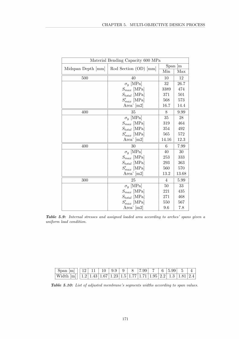
CHAPTER 5. MULTI-OBJECTIVE DESIGN PROCESS
Material Bending Capacity 600 MPa
Midspan Depth [mm] Rod Section (OD) [mm] Span [mMin Max
500 40 10 12σy [MPa] 32 26.7Smax [MPa] 3389 474Stotal [MPa] 371 501S′max [MPa] 568 573Area’ [m2] 16.7 14.4
400 35 8 9.99σy [MPa] 35 28Smax [MPa] 319 464Stotal [MPa] 354 492S′max [MPa] 565 572Area’ [m2] 14.16 12.3
400 30 6 7.99σy [MPa] 40 30Smax [MPa] 253 333Stotal [MPa] 293 363S′max [MPa] 560 570Area’ [m2] 13.2 13.68
300 25 4 5.99σy [MPa] 50 33Smax [MPa] 221 435Stotal [MPa] 271 468S′max [MPa] 550 567Area’ [m2] 9.6 7.8
Table 5.9: Internal stresses and assigned loaded area according to arches’ spans given auniform load condition.
Span [m] 12 11 10 9.9 9 8 7.99 7 6 5.99 5 4Width [m] 1.2 1.43 1.67 1.23 1.5 1.77 1.71 1.95 2.2 1.3 1.81 2.4
Table 5.10: List of adjusted membrane’s segments widths according to span values.
171
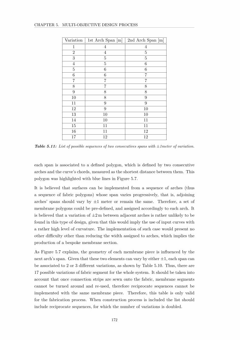
CHAPTER 5. MULTI-OBJECTIVE DESIGN PROCESS
Variation 1st Arch Span [m] 2nd Arch Span [m]1 4 42 4 53 5 54 5 65 6 66 6 77 7 78 7 89 8 810 8 911 9 912 9 1013 10 1014 10 1115 11 1116 11 1217 12 12
Table 5.11: List of possible sequences of two consecutives spans with ±1meter of variation.
each span is associated to a defined polygon, which is defined by two consecutivearches and the curve’s chords, measured as the shortest distance between them. Thispolygon was highlighted with blue lines in Figure 5.7.
It is believed that surfaces can be implemented from a sequence of arches (thusa sequence of fabric polygons) whose span varies progressively, that is, adjoiningarches’ spans should vary by ±1 meter or remain the same. Therefore, a set ofmembrane polygons could be pre-defined, and assigned accordingly to each arch. Itis believed that a variation of ±2 m between adjacent arches is rather unlikely to befound in this type of design, given that this would imply the use of input curves witha rather high level of curvature. The implementation of such case would present noother difficulty other than reducing the width assigned to arches, which implies theproduction of a bespoke membrane section.
As Figure 5.7 explains, the geometry of each membrane piece is influenced by thenext arch’s span. Given that these two elements can vary by either ±1, each span canbe associated to 2 or 3 different variations, as shown by Table 5.10. Thus, there are17 possible variations of fabric segment for the whole system. It should be taken intoaccount that once connection strips are sewn onto the fabric, membrane segmentscannot be turned around and re-used, therefore reciprocate sequences cannot beimplemented with the same membrane piece. Therefore, this table is only validfor the fabrication process. When construction process is included the list shouldinclude reciprocate sequences, for which the number of variations is doubled.
172
CHAPTER 5. MULTI-OBJECTIVE DESIGN PROCESS
Finally, one interesting aspect of considering membrane segments as a componentassociated to the structural performance, is that other approaches can be created torespond to different objectives using the same discretising method. As an example,Figure 5.9 shows an approach in which the objective is to provide a uniform Width
value within each segment. Such an approach could be used to improve aestheticsor to overcome limitations to the fabrication of membrane.
Similarly to Figure 5.8, preconditions are highlighted in red, in this case these arethe span values within each group (Group A or B) and the maximum mid-spandepth for the smallest arch of each group. Based on these precondition, the value ofthe rod section is calculated for the smallest sample of the group based on that σyshould be equal or less than 300 MPa for each sample. Thus, /O is equivalent to Afor an 8 m arch.
Assuming that σy uses nearly 50% of the material bending capacity, the membranewidth is calculated for the smallest arch of the group, based on that St should beno higher than 300 MPa and a maximum mid-span depth of a given value (thisdiagram uses 500 as an example). The value of the membrane width is inheritedfrom the first sample to the rest of the arches of the group, which is equivalent toX for Group A and Y for Group B.
A uniform loaded area’s width for all arches implies that the load applied on everyarch are not uniform, therefore components of each arch need to be adjusted indi-vidually to meet the constraints imposed by the material capacity. In this sense, atevery step of span increment the pre-stress is controlled by adjusting the value ofthe rod section (which can be assumed to be smaller as the span increases), and thevalue of Smax’ is controlled, to be smaller than 300 MPa, by adjusting the mid-spandepth of each arch.
5.4 Geometry-based Studies for the Reduction of Com-ponents
This section looks at the reduction of the number of different physical components.In particular, the reduction of the number of crosses for the whole system wasstudied.
Tensile membranes and cables are expected to play a key role for the lateral resistanceof the system which is characterised by high deformability.
As mentioned earlier, the whole system requires 49 different crosses [Table 5.12].This includes 13 nodes on each arch, 3 different mid-span (or ridge) crosses, andall the supports being identical. Given that supports are resolved with anchoragesrather than joints, it can be stated that the whole system involves 48 joints.
173
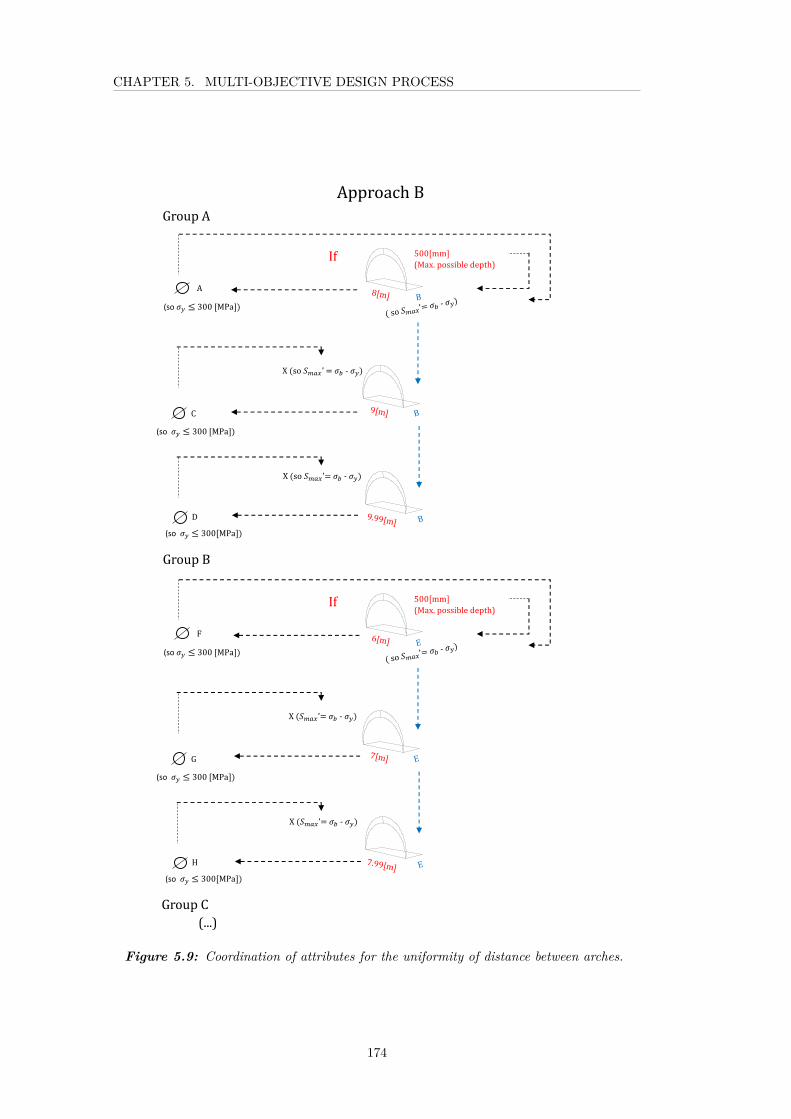
CHAPTER 5. MULTI-OBJECTIVE DESIGN PROCESS
Figure 5.9: Coordination of attributes for the uniformity of distance between arches.
174
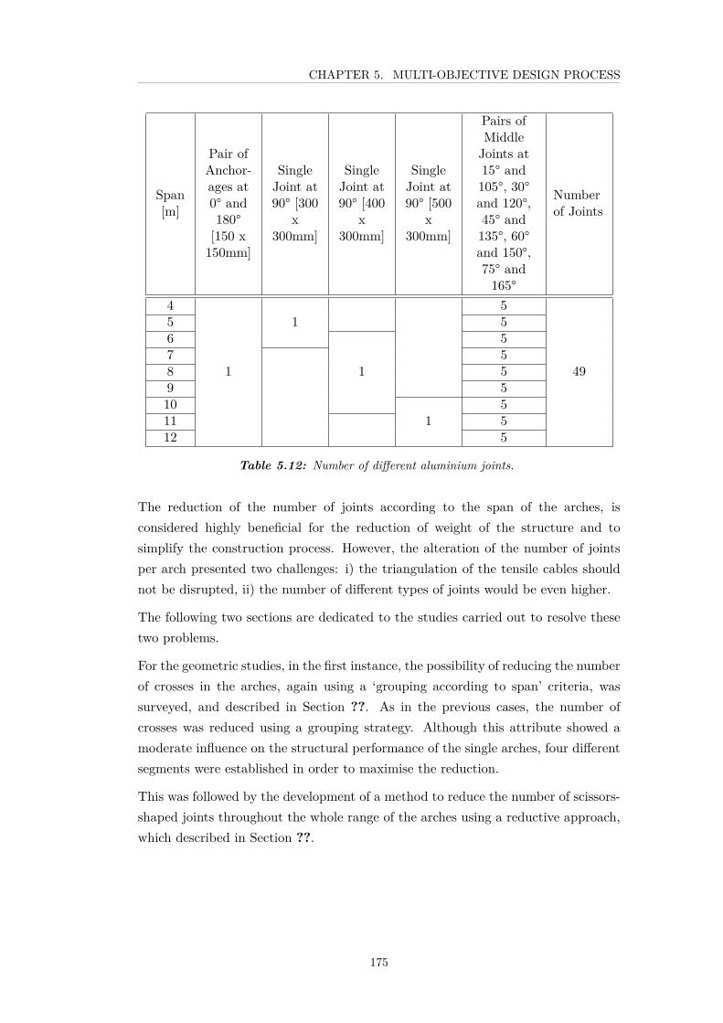
CHAPTER 5. MULTI-OBJECTIVE DESIGN PROCESS
Span[m]
Pair ofAnchor-ages at0° and180°[150 x150mm]
SingleJoint at90° [300
x300mm]
SingleJoint at90° [400
x300mm]
SingleJoint at90° [500
x300mm]
Pairs ofMiddleJoints at15° and105°, 30°and 120°,45° and135°, 60°and 150°,75° and165°
Numberof Joints
4
1
15
49
5 56
1
57 58 59 510
15
11 512 5
Table 5.12: Number of different aluminium joints.
The reduction of the number of joints according to the span of the arches, isconsidered highly beneficial for the reduction of weight of the structure and tosimplify the construction process. However, the alteration of the number of jointsper arch presented two challenges: i) the triangulation of the tensile cables shouldnot be disrupted, ii) the number of different types of joints would be even higher.
The following two sections are dedicated to the studies carried out to resolve thesetwo problems.
For the geometric studies, in the first instance, the possibility of reducing the numberof crosses in the arches, again using a ‘grouping according to span’ criteria, wassurveyed, and described in Section ??. As in the previous cases, the number ofcrosses was reduced using a grouping strategy. Although this attribute showed amoderate influence on the structural performance of the single arches, four differentsegments were established in order to maximise the reduction.
This was followed by the development of a method to reduce the number of scissors-shaped joints throughout the whole range of the arches using a reductive approach,which described in Section ??.
175

CHAPTER 5. MULTI-OBJECTIVE DESIGN PROCESS
5.4.1 Reduction of the Number of Nodes per Arch Group
As presented in Chapter 3, they system achieves a continuous net of triangulatingbracing cables by lacing two consecutives arches in a zigzagging fashion, using thecross-joints as nodes from where the cables can be fastened. It is expected thatthis method contributes to simplify the assembly process and also to avoid longbracing elements whose high tension level would be difficult to keep constant. Thealteration on the number of nodes in the arches (originally 13 nodes for all type ofarches) challenges the continuity of the triangulation.
After several trials it was established that the continuity of the cables’ triangulationcould be assured if the variation of the number of nodes did not exceed ±1 unitbetween consecutives arches. Higher orders of variation would simply disrupt thetriangulation. A generic example is shown in Figure 5.10.
This type of diagrams serve a 2D test of the continuity of the lacing on a set ofarches with variable span. Arches are numbered by the position from inside towardsoutside, for example, Arch 1 correspond to the arch with the smallest span placed atthe centre of the group, while Arch 5 correspond to the outer arch. The direction ofthe lacing follows a clockwise direction, unless otherwise is indicated. Node positionshould also be read in the same direction, as it will be later shown.
Although the variation of this attribute, this is number of joints per arch, wouldcontribute to decreasing the total number of joints required for the implementationof a given scheme, it would, on the other hand, increase the number of differentcomponents, this time to 61 different units. Once again, a precise number ofaluminium joints would be 60, given that anchorages (Nodes A in the figure) will beresolved differently. Figure 5.11, shows all the variation conforming this group of 61different crosses. According to this figure, Group 1 includes 15 variations, Group 2includes 24 variations, Groups 3, 12 variations, and Group 4 with variations.
Different approaches for triangulation arrangements with variation of the number ofnodes were tested. Firstly, the convenience of the original subdivision arrangementwas questioned, and other approaches were tested.
Chapter 3 already highlighted the differences between ‘equal-length’ and ‘equal-angle’ subdivisions schemes. Figure 5.12 shows the effect of these two subdivisionschemes on the cable’s lacing. For the purpose of understanding these figures, thelacing was started from the first node on the inner arc, in a clockwise direction.
Consequently, the triangulation of a set of arcs with different numbers of subdivisionwas studied.
The introduction of a notation that expresses the basic sequence of lacing turnsout necessary for the understanding of the following examples. The original lacing
176

CHAPTER 5. MULTI-OBJECTIVE DESIGN PROCESS
Figure 5.10: Triangulation of a set of arches with cases of variation on the number ofnodes of 2 units.
scheme proposes that the lacing between two arches starts at the first node on Arc0, from now on called n(0,0), and it fastened at the second node on the second arch,this is n(1,1) in Arc 1. The lacing continues from this last node to the node in thethird position on Arc 1, and from there to the node in the fourth position in Arc 1,and so on. This original sequence of lacing between two consecutives arcs is called‘from n(i,j) to n(i+1,j+1)’.
The first aspect studied, was the confirming the relevance of beginning the lacingfrom the inner arch toward the outer one. As Figure 5.13 and 5.14 show, thetriangulation can be affected by node where the lacing starts from. In Case 1, thestarting point is the first node (n(0,0)) in the first arc (9 segments), whilst in thesecond case, the triangulation starts from the first node (n(1,0)) in the second arc(10 segments).
In both cases, although continuity is preserved, the mesh becomes progressivelydisfigured, due to the increasing distance between segments of consecutives arches.This effect would be structurally dysfunctional.
Some other strategies were then tested. In Figure 5.15 (Case 3), the last segment ofthe lacing are completed by altering the sequence ‘n(i,j) to n(i+1,j+1)’, to ‘n(i,j) ton(i+1,j+2)’ for the last two nodes. In Figure 5.16 (Case 4), the direction of the secondlacing (between arc 1 and 2) was inverted. These methods proved to be unsuccessful.In the last case in particular, the method turns out trivial as the lacing between thelast two arcs (Arc 2 And 3) is not updated, this is, the lacing between arcs 2 and 3was still done in the clockwise direction.
Figure 5.17 (Case 5), provides a continuous triangulation where every last stepof the lacing sequences are ‘n(i,j) to n(i+1,j)’. Although geometrically correct, thetriangulation again becomes disfigured.
177

CHAPTER 5. MULTI-OBJECTIVE DESIGN PROCESS
Figure
5.11:Num
berofdifferentalum
iniumjointwhen
differentiatednum
berofarches’nodes
accordingto
spansegm
ent.
178

CHAPTER 5. MULTI-OBJECTIVE DESIGN PROCESS
Figure 5.12: Two examples of nodes lacing with different subdivision approaches: (a) equalangle-distance and (b) equal linear distance.
Figure 5.13: Lacing of a set of arcs with increasing number of subdivision starting fromthe first arc (Case 1).
Figure 5.14: Lacing of a set of arcs with increasing number of subdivisions starting fromthe second arc (Case 2).
179

CHAPTER 5. MULTI-OBJECTIVE DESIGN PROCESS
Figure 5.15: Lacing of a set of arcs with increasing number of subdivisions with last lacingstep altered to ‘n(i,j) to n(i+1,j+2)’ (Case 3).
Figure 5.16: Lacing of a set of arcs with increasing number of subdivisions with the secondsequence inverted (Case 4).
180

CHAPTER 5. MULTI-OBJECTIVE DESIGN PROCESS
Figure 5.17: Solution A. Lacing of a set of arcs with increasing number of subdivisionswith last lacing step altered to ‘n(i,j) to n(i+1,j)’ (Case 5).
Further trials included combinations of some of these operations. Figure 5.18 (Case6), represents a case in which all the lacing sequences are inverted from the secondlacing sequence onwards. Although continuous, the same problem encountered inFigure 5.13 is inherited. Finally, Figure 5.19 (Case 7) shows a case, where althoughonly the second lacing sequence is inverted (lacing between arcs 1 and 2), the thirdsequence (lacing between arc 2 and 3) continues the triangulation with the originalleft to right direction.
Cases 5 and 7 are more feasible options and these were tested in 3D. In this test, alarger number of arcs were placed, with the number of segments varying accordingto the span, and some consecutive arcs presented the same number of segments.The condition of variation on the number of segments on consecutive arches wasrestricted to ±1.
The 3D grammar was then based on the number of subdivisions of each arc, ratherthan the position of the arc in the sequence. This means that for the 3D interpre-tation of case 5, the following logic was used: all the lacing sequences start with thesame clockwise direction, with bracing between consecutive arcs following the ‘n(i,j)
to n(i+1,j+1)’ logic. If there is either a positive or negative variation on the numberof nodes in the second arc (this is the second arc of the sequence present n + 1 orn − 1 nodes), the last lacing segment jumps from node n(i,j) (on the first arch) tothe node n(i+1,j) on the second arc, in other words, a ‘n(i,j) to n(i+1,j)’ sequence isused for the last segment. Based on Figure 5.20, the lacing method of Case 5 provedfeasible, although presented some irregularities on one side of the vault.
For the 3D interpretation of Case 7, whenever a ‘n(i,j) to n(i+1,j±1)’or a ‘n(i,j) ton(i+1,j)’situation between two consecutives arcs is followed by a ‘n(i,j) to n(i+1,j±1)’
181

CHAPTER 5. MULTI-OBJECTIVE DESIGN PROCESS
Figure 5.18: Lacing with an increasing number of nodes with the sequence inverted fromsecond arch onwards. (Case 6).
Figure 5.19: Solution B for continuous lacing with an increasing number of nodes (Case7).
182

CHAPTER 5. MULTI-OBJECTIVE DESIGN PROCESS
(a) (b)
(c)
Figure 5.20: Three dimensional test of solution A in an arbitrary set of arches: (a) topview, (b) left side view and (c) right side view.
183

CHAPTER 5. MULTI-OBJECTIVE DESIGN PROCESS
(a) (b)
(c)
Figure 5.21: Three-dimensional test of solution B in an arbitrary set of arches: (a) topview, (b) left side view and (c) right side view.
case, this second lacing sequence inverts its direction (this means, it starts from 180°and runs to 0°) and the subsequent lacing will continue the triangulation from theoriginal direction (this is from 0° to 180°). The sequence then starts again. Thismeans that if the fourth lacing again presents ±1 nodes, then its lacing directionis inverted. For example, if the following lacing sequences are found: ‘n(i,j) ton(i+1,j)’, ‘n(i,j) to n(i+1,j±1)’, ‘n(i,j) to n(i+1,j±1)’ and ‘n(i,j) to n(i+1,j±1)’; or ‘n(i,j)
to n(i+1,j±1)’, ‘n(i,j) to n(i+1,j±1)’, ‘n(i,j) to n(i+1,j)’ and n(i,j) to n(i+1,j±1)’, in bothcases the direction of the second and fourth lacings are inverted. This method alsoproved viable, and is shown in Figure 5.21.
A second approach to the problem of continuous triangulation with variable numberof nodes (±1) was also explored. This time, arches were classified generically eitheras odd or even according to their number of nodes. Whilst in most of the casestriangulation was possible, some scenarios needed to be dis-allowed, specifically,cases where there was no node in the centre of the arch [114].
The first early study, shown in Figure 5.22, consisted of a scheme where the triangu-lation departs from the central node on the first odd arch (in this case, arc number
184

CHAPTER 5. MULTI-OBJECTIVE DESIGN PROCESS
(a) (b)
Figure 5.22: Three-dimensional test of lacing scheme starting from central node towardboth sides: (a) top view, and (b) side view.
2). The triangulation continues symmetrically in both directions, bottom and top,in an ‘every-other node’ fashion. The process is interrupted when an ‘even to even’situation is encountered and stops, due the lack of a central node to converge into.The logic proposes to search for the next odd arc’s central node and resume thetriangulation from there, again in both directions. In the figures, red lines are usedto identify evenly subdivided arcs, and black for the odd ones.
A solution for the discontinuity of the lacing was found by varying the number ofnodes on some of the even arcs, specifically in arcs 8 and 12. This variation should bemade considering the fundamental restriction of a maximum varation of ±1 numberof nodes between consecutives arcs. Figure 5.23 shows the case where Arc 8 hasbeen subdivided into 12 segments (added +1 nodes), and Arc 12 into 10 segments(11 nodes). Figure 5.24 shows a case where Arc 8 has instead been subdivided with−1 nodes, this is 10 segments. Alhough both cases seemed to resolve the problem,the first case appears to render a smoother surface. The ammended lacing werehighlighted in black.
The use of this particular solution requires some reflection on the effect of otherattributes of the system, given that it would be necessary to induce some distorsionsin the multi-value segmentation established. For example, if Arc 8 was the case of a9 m span arch, therefore subdivided into 11 segments (with 12 nodes) as the aboveexample presents, then a 400 mm midspan (or ridge) depth, and a rod section of 35mm diameter would be required [see section 5.2.2]. If the number of subdivisionson the curve is increased to +1, a total of 12 segments. Arches with 12 segmentscorrespond to Group 4 (spans range from 10 to 12 m), whith a midspan depth of500 mm and a 40 mm diameter cross-section. Therefore, an inconsistency in theattributes grouping will be produced.
185

CHAPTER 5. MULTI-OBJECTIVE DESIGN PROCESS
(a) (b)
Figure 5.23: Three-dimensional test of a lacing method starting from a central node andwhere specific even-divided arcs have altered the number of node to n+ 1: (a) top view, (b)left side view.
(a) (b)
Figure 5.24: Three-dimensional test of a lacing method starting from a central node andwhere specific even-divided arcs have altered the number of node to n− 1: (a) top view, (b)left side view.
186
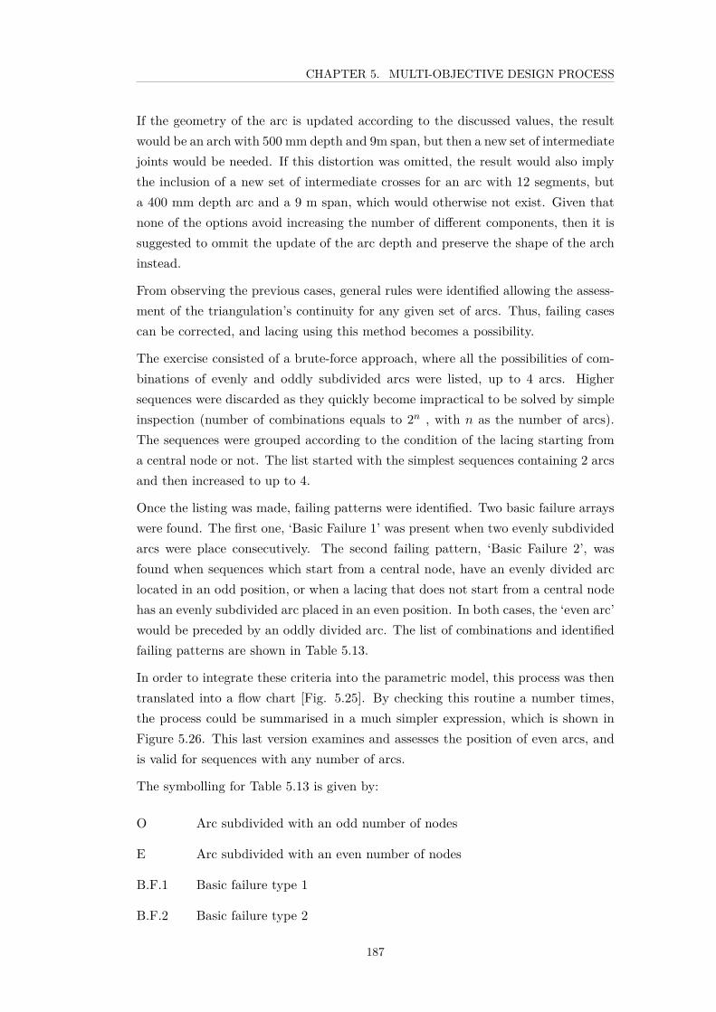
CHAPTER 5. MULTI-OBJECTIVE DESIGN PROCESS
If the geometry of the arc is updated according to the discussed values, the resultwould be an arch with 500 mm depth and 9m span, but then a new set of intermediatejoints would be needed. If this distortion was omitted, the result would also implythe inclusion of a new set of intermediate crosses for an arc with 12 segments, buta 400 mm depth arc and a 9 m span, which would otherwise not exist. Given thatnone of the options avoid increasing the number of different components, then it issuggested to ommit the update of the arc depth and preserve the shape of the archinstead.
From observing the previous cases, general rules were identified allowing the assess-ment of the triangulation’s continuity for any given set of arcs. Thus, failing casescan be corrected, and lacing using this method becomes a possibility.
The exercise consisted of a brute-force approach, where all the possibilities of com-binations of evenly and oddly subdivided arcs were listed, up to 4 arcs. Highersequences were discarded as they quickly become impractical to be solved by simpleinspection (number of combinations equals to 2n , with n as the number of arcs).The sequences were grouped according to the condition of the lacing starting froma central node or not. The list started with the simplest sequences containing 2 arcsand then increased to up to 4.
Once the listing was made, failing patterns were identified. Two basic failure arrayswere found. The first one, ‘Basic Failure 1’ was present when two evenly subdividedarcs were place consecutively. The second failing pattern, ‘Basic Failure 2’, wasfound when sequences which start from a central node, have an evenly divided arclocated in an odd position, or when a lacing that does not start from a central nodehas an evenly subdivided arc placed in an even position. In both cases, the ‘even arc’would be preceded by an oddly divided arc. The list of combinations and identifiedfailing patterns are shown in Table 5.13.
In order to integrate these criteria into the parametric model, this process was thentranslated into a flow chart [Fig. 5.25]. By checking this routine a number times,the process could be summarised in a much simpler expression, which is shown inFigure 5.26. This last version examines and assesses the position of even arcs, andis valid for sequences with any number of arcs.
The symbolling for Table 5.13 is given by:
O Arc subdivided with an odd number of nodes
E Arc subdivided with an even number of nodes
B.F.1 Basic failure type 1
B.F.2 Basic failure type 2
187

CHAPTER 5. MULTI-OBJECTIVE DESIGN PROCESS
@ Opposite option does not exist
5.4.2 Reduction on the Number of Different Joints
The high number of different joints was identified as the second paradigm derivedfrom the arcs’ segmentation strategy that needed attention. In order to have a betterunderstanding of this problem it was necessary to establish the total variation inthe sizes of the joints. Such information is available from the parametric model [seeSection 5.3].
Table 5.14, shows the angles between the joints’ bars (angle α in Figure 5.27) forall the possible arches in the case of a surface where spans have been rounded tovalues of 0.5 m. Table 5.15 shows the study of the blades length for the same case.
Limiting values were identified from these tables. If length values are inspected, themaximum length is 583 mm, whilst the minimum is 285 mm. Values for the supportnodes are dismissed, as they are not expected to be implemented with aluminiumcrosses, but with anchorages. Therefore the variation in length for the whole groupis 297.4 mm. Values were then put into seven groups, which were allocated crosseswith 50 mm variations. The joints included in each group can be identified in Table5.14 according to the assigned colour.
Consequently, this grouping allows the whole surface to be constructed using sevendifferent crosses, each with a length adaptability of 50 mm. This means that eachcross should be able to be adapted by up to 25 mm at each end. An early schemeof this idea is shown in Figure 5.27.
When these results were inspected according to their angular variation, a maximumof 5 variations per group were found, particularly in groups 2 and 4, as shown inTable 5.16. This implies that each of the joints proposed above should have thepossibility to be positioned at different angles. The number of different optionswould then range from only two positions (cross 7), to five different positions (cross2 and 4). Given the proximity of some of these values, a tolerance of 2 degreeswas imposed, which further reduced the number of angular options required, to amaximum of three, again for group 2 and 4. These last values are shown in Table5.17.
Figure 5.28 shows an early study for the design of a cross which allows the adaptationof the length of its blades, as well its angle. This design is further implemented inChapter 6.
If the input curve is discretised by arches which spans are integer values, as inthe case proposed for Union Glacier Station, there is no reduction in the number
188
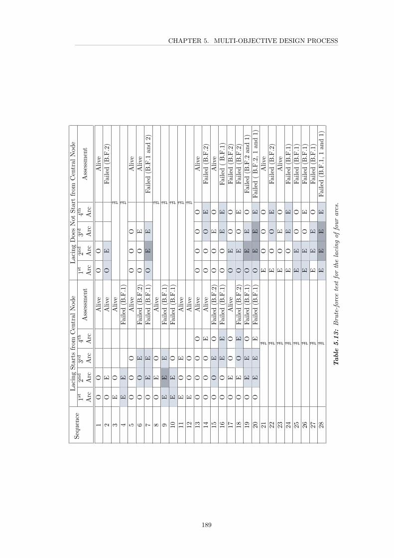
CHAPTER 5. MULTI-OBJECTIVE DESIGN PROCESS
Sequ
ence
Lacing
Starts
from
Central
Nod
eLa
cing
DoesNot
Startfrom
Central
Nod
e1s
t
Arc
2nd
Arc
3rd
Arc
4th
Arc
Assessm
ent
1st
Arc
2nd
Arc
3rd
Arc
4th
Arc
Assessm
ent
1O
OAliv
eO
OAliv
e2
OE
Aliv
eO
EF a
iled(B
.F.2)
3E
OAliv
e@
4E
EF a
iled(B
.F.1)
@5
OO
OAliv
eO
OO
Aliv
e6
OO
EF a
iled(B
.F.2)
OO
EAliv
e7
OE
EF a
iled(B
.F.1)
OE
EF a
iled(B
.F.1
and2)
8O
EO
Aliv
e@
9E
EE
F aile
d(B
.F.1)
@10
EE
OF a
iled(B
.F.1)
@11
EO
EAliv
e@
12E
OO
Aliv
e@
13O
OO
OAliv
eO
OO
OAliv
e14
OO
OE
Aliv
eO
OO
EFa
iled(B
.F.2)
15O
OE
OFa
iled(B
.F.2)
OO
EO
Aliv
e16
OO
EE
F aile
d(B
.F.1)
OO
EE
F aile
d(B.F.1)
17O
EO
OAliv
eO
EO
OF a
iled(B
.F.2)
18O
EO
EF a
iled(B
.F.2)
OE
OE
F aile
d(B
.F.2)
19O
EE
OFa
iled(B
.F.1)
OE
EO
Faile
d(B
.F.2
and1)
20O
EE
EFa
iled(B
.F.1)
OE
EE
Faile
d(B.F.2,1
and1)
21@
EO
OO
Aliv
e22
@E
OO
EF a
iled(B
.F.2)
23@
EO
EO
Aliv
e24
@E
OE
EF a
iled(B
.F.1)
25@
EE
OO
Faile
d(B
.F.1)
26@
EE
OE
Faile
d(B
.F.1)
27@
EE
EO
Faile
d(B
.F.1)
28@
EE
EE
F aile
d(B
.F.1,1
and1)
Tab
le5.
13:Br
ute-forcetest
forthelacing
offour
arcs.
189

CHAPTER 5. MULTI-OBJECTIVE DESIGN PROCESS
Figur e
5.25:Flow
chartfornodes’lacing
continuityassessm
ent.
190
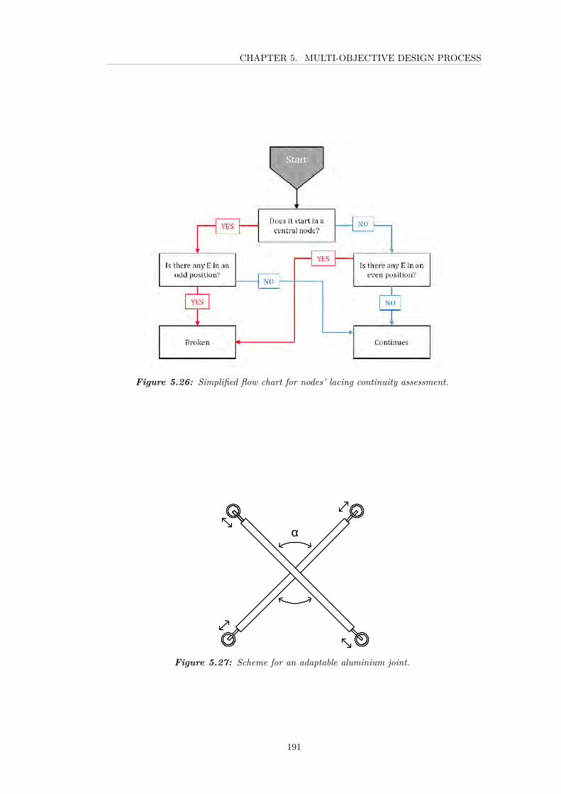
CHAPTER 5. MULTI-OBJECTIVE DESIGN PROCESS
Figure 5.26: Simplified flow chart for nodes’ lacing continuity assessment.
α
α
Figure 5.27: Scheme for an adaptable aluminium joint.
191

CHAPTER 5. MULTI-OBJECTIVE DESIGN PROCESS
Depth
[mm]
500400
300Segm
en ts12
1110
9Span
[m]
1211.5
1110.5
109.9
9.59
8.58
7.997.5
76.5
65.99
5.55
4.54
No de
Length[m
m]
0212
212212
212212
212212
212212
212212
212212
212212
212212
212212
2121
309309
309309
309295
295295
295295
303303
303303
303286
286286
286286
2401
401401
401401
371371
371371
371384
384384
384384
350350
350350
3503
478478
478478
478432
432432
432432
447447
447447
447397
397397
397397
4536
536536
536536
475475
475475
475487
487487
487487
421421
421421
4215
571571
571571
571497
497497
497497
500500
500500
500421
421421
421421
6583
583583
583583
497497
497497
497487
487487
487487
397397
397397
3977
571571
571571
571475
475475
475475
447447
447447
447350
350350
350350
8536
536536
536536
432432
432432
432384
384384
384384
286286
286286
2869
478478
478478
478371
371371
371371
303303
303303
303212
212212
212212
10401
401401
401401
295295
295295
295212
212212
212212
11309
309309
309309
212212
212212
21212
212212
212212
212
Table
5.14:Alum
iniumjoint’s
bar’slength
accordingto
differentspansrounded
tonearest0.5
m.
192

CHAPTER 5. MULTI-OBJECTIVE DESIGN PROCESS
Depth
[mm]
500
400
300
Segm
ents
1211
109
Span
[m]
1211.5
1110.5
109.9
9.5
98.5
87.99
7.5
76.5
65.99
5.5
54.5
4No d
eAng
le[°]
090
9090
9090
9090
9090
9090
9090
9090
9090
9090
901
75.2
75.2
75.2
75.2
75.2
81.5
81.5
81.5
81.5
81.5
80.9
80.9
80.9
80.9
80.9
89.6
89.6
89.6
89.6
89.6
268.2
68.2
68.2
68.2
68.2
77.2
77.2
77.2
77.2
77.2
76.6
76.6
76.6
76.6
76.6
89.5
89.5
89.5
89.5
89.5
364.7
64.7
64.7
64.7
64.7
75.1
75.1
75.1
75.1
75.1
74.7
74.7
74.7
74.7
74.7
89.8
89.8
89.8
89.8
89.8
463
6363
6363
74.2
74.2
74.2
74.2
74.2
7474
7474
7490
9090
9090
562.2
62.2
62.2
62.2
62.2
73.8
73.8
73.8
73.8
73.8
73.7
73.7
73.7
73.7
73.7
9090
9090
906
61.9
61.9
61.9
61.9
61.9
73.8
73.8
73.8
73.8
73.8
7474
7474
7489
.889
.889
.889
.889
.87
62.2
62.2
62.2
62.2
62.2
74.2
74.2
74.2
74.2
74.2
74.7
74.7
74.7
74.7
74.7
89.5
89.5
89.5
89.5
89.5
863
6363
6363
75.1
75.1
75.1
75.1
75.1
76.6
76.6
76.6
76.6
76.6
89.6
89.6
89.6
89.6
89.6
964.7
64.7
64.7
64.7
64.7
77.2
77.2
77.2
77.2
77.2
80.9
80.9
80.9
80.9
80.9
9090
9090
9010
68.2
68.2
68.2
68.2
68.2
81.5
81.5
81.5
81.5
81.5
9090
9090
9011
7575.2
75.2
75.2
75.2
9090
9090
9012
9090
9090
90
Tab
le5.
15:An
glebetweenalum
inium
joints’b
arsaccordingto
diffe
rent
span
svalues,w
ithaspan
values
roun
dedto
nearest0
.5m.
193

CHAPTER 5. MULTI-OBJECTIVE DESIGN PROCESS
Group 1 2 3 4 5 6 7Number of angular variations 01 05 03 04 03 04 02
Lists of variations [°]
90 75.2 76.6 68.2 74.7 74 62.289.6 77.2 75.1 74.2 73.7 61.989.6 89.5 89.8 64.7 73.881.5 89.8 6381.5 90
Table 5.16: Variations of angle between joints’ bars found in each length group.
Group 1 2 3 4 5 6 7Number of angular variations 01 03 03 03 02 02 01
Lists of variations [±1ř]90 75 77 68 75 74 62
90 89 75 65 6382 89
Table 5.17: Reduced variations of angle between joints in each length group with a toleranceof ±1ř imposed.
(a) (b)
(c) (d)
Figure 5.28: Early model of a adaptable joint (Model 4): (a) two blades, (b) blades placedat 89°, (c) blades placed at 75° and (d) blades placed at 68°.
194

CHAPTER 5. MULTI-OBJECTIVE DESIGN PROCESS
Depth
[mm]
500
400
300
Segm
ents
1211
109
Span
[m]
1211
109.9
98
7.99
76
5.99
54
No d
eLe
ngth
[mm]
0212
212
212
212
212
212
212
212
212
212
212
212
1309
309
309
295
295
295
303
303
303
286
286
286
2401
401
401
371
371
371
384
384
384
350
350
350
3478
478
478
432
432
432
447
447
447
397
397
397
4536
536
536
475
475
475
487
487
487
421
421
421
5571
571
571
497
497
497
500
500
500
421
421
421
6583
583
583
497
497
497
487
487
487
397
397
397
7571
571
571
475
475
475
447
447
447
350
350
350
8536
536
536
432
432
432
384
384
384
286
286
286
9478
478
478
371
371
371
303
303
303
212
212
212
10401
401
401
295
295
295
212
212
212
11309
309
309
212
212
212
12212
212
212
Tab
le5.
18:Alum
inium
joint’s
bar’sleng
thaccordingto
diffe
rent
span
svalues,w
ithaspan
values
roun
dedto
nearest1
.00m.
195
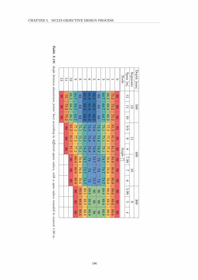
CHAPTER 5. MULTI-OBJECTIVE DESIGN PROCESS
Depth
[mm]
500400
300Segm
en ts12
1110
9Span
[m]
1211
109.9
98
7.997
65.99
54
No de
Angle
[°]0
9090
9090
9090
9090
9090
9090
175.2
75.275.2
81.581.5
81.580.9
80.980.9
89.689.6
89.62
68.268.2
68.277.2
77.277.2
76.676.6
76.689.5
89.589.5
364.7
64.764.7
75.175.1
75.174.7
74.774.7
89.889.8
89.84
6363
6374.2
74.274.2
7474
7490
9090
562.2
62.262.2
73.873.8
73.873.7
73.773.7
9090
906
61.961.9
61.973.8
73.873.8
7474
7489.8
89.889.8
762.2
62.262.2
74.274.2
74.274.7
74.774.7
89.589.5
89.58
6363
6375.1
75.175.1
76.676.6
76.689.6
89.689.6
964.7
64.764.7
77.277.2
77.280.9
80.980.9
9090
9010
68.268.2
68.281.5
81.581.5
9090
9011
7575.2
75.290
9090
1290
9090
Table
5.19:Angle
betweenalum
iniumjoints’bars
accordingto
differentspansvalues,with
aspan
valuesrounded
tonearest1.00
m.
196

CHAPTER 5. MULTI-OBJECTIVE DESIGN PROCESS
of different components, due to the marginal difference in the size of both sets ofcomponents [Tables 5.18 and 5.19].
Therefore, by grouping the different attribute’s values (or by the partial-optimisationof attributes) it has been possible to reduce the number of components, specificallyto six joints plus one standard anchorage, to cover all of the ranges of joints requiredby the proposed surface, for at least two different degrees of span standardisation: 1and 0.5 m. Additionally, each of these joints could eventually be adapted in length,angular position, or be replaced, allowing the surface to modify its shape. Thissegmentation method based on the joint’s length and angle can be implementedin the parametric model to identify the type of joint required at each node, as isdemonstrated in Chapter 6.
With respect to the arches’ bars, the method presents no major complications fortheir definition. Table 5.20 lists all of the possible lengths for a surface with spanvalues standardised to 0.5 m (24 types in total, considering twelve types for upperbars and twelve types for lower bars). Given that the proposed system has onlyfour different bar cross sections, they can easily be cut to size, and in the caseof replacement or repair, spare standard bars can be transported to site and cutaccording to Table 5.20. The length of the arches’ bars is also an attribute thancan be read using Rhino’s graphic programming tools, and therefore the quantity ofeach type of bars required by a surface can be obtained, as described in Chapter 6.
Finally, the case of an arc whose number of subdivisions has been changed by ±1unit was also revised. Table 5.22, shows the length of the joints’ diagonals andthe angle between diagonals for the example previously given: a 9 m span and 400mm deep arch which is required to alter its number of subdivision to +1, i.e. to12 nodes. As highlighted by the colour attribute of Table 5.21, all the nodes fromthis particular arc can be implemented using one element of the previously definedset. It is then assumed that other cases of alteration can be also resolved similarly.Given that the segment’s length in such a case is also uniform, this case representeda satisfactory outcome.
5.5 Parametric Model
The specified attributes were finally integrated into a single parametric model andtheir discretised values are summarised in Table 5.22.
As a general description, the model requires a single input consisting of a nativeCAD NURBS curve drawn on the ground-plane and offset from the x-axis, whichshould be derived from the architectural scheme design. This curve should be definedwithin the limits that the system allows for the arches’ spans, that is, the distance
197

CHAPTER 5. MULTI-OBJECTIVE DESIGN PROCESS
Depth
[mm]
500400
300Segm
en ts12
1110
9Span
[m]
1211.5
1110.5
109.9
9.59
8.58
7.997.5
76.5
65.99
5.55
4.54
Segmen t
Length[m
m]
11.62
1.551.49
1.421.35
1.471.40
1.331.25
1.181.30
1.221.14
1.070.987
1.091.17
0.9110.824
0.7382
1.621.55
1.491.42
1.351.47
1.401.33
1.251.18
1.301.22
1.141.07
0.9871.09
1.170.911
0.8240.738
31.62
1.551.49
1.421.35
1.471.40
1.331.25
1.181.30
1.221.14
1.070.987
1.091.17
0.9110.824
0.7384
1.621.55
1.491.42
1.351.47
1.401.33
1.251.18
1.301.22
1.141.07
0.9871.09
1.170.911
0.8240.738
51.62
1.551.49
1.421.35
1.471.40
1.331.25
1.181.30
1.221.14
1.070.987
1.091.17
0.9110.824
0.7386
1.621.55
1.491.42
1.351.47
1.401.33
1.251.18
1.301.22
1.141.07
0.9871.09
1.170.911
0.8240.738
71.62
1.551.49
1.421.35
1.471.40
1.331.25
1.181.30
1.221.14
1.070.987
1.091.17
0.9110.824
0.7388
1.621.55
1.491.42
1.351.47
1.401.33
1.251.18
1.301.22
1.141.07
0.9871.09
1.170.911
0.8240.738
91.62
1.551.49
1.421.35
1.471.40
1.331.25
1.181.30
1.221.14
1.070.987
1.091.17
0.9110.824
0.73810
1.621.55
1.491.42
1.351.47
1.401.33
1.251.18
1.301.22
1.141.07
0.98711
1.621.55
1.491.42
1.351.47
1.401.33
1.251.18
121.62
1.551.49
1.421.35
Table
5.20:Length
ofUpper
Carbon
Fibrebars,according
tospan
withaspans
roundedto
nearest0.5m
value.
198

CHAPTER 5. MULTI-OBJECTIVE DESIGN PROCESS
Nodes Length of Joints’ Diagonals [mm] Angle between Diagonals [°] Cross Type0 and 12 212 90 11 and 11 289 82 22 and 10 359 77.7 33 and 9 418 75.5 44 and 8 463 74.4 55 and 7 491 73.9 6
6 500 73.7 6
Table 5.21: Length of joint’s bars and angle between joint’s bars with number of nodesaltered in +1 units for evenly-divided arcs.
Group 1 2 3 4Span range 12 ≤ S ≤ 10 10 ≤ S ≤ 8 8 ≤ S ≤ 6 6 ≤ S ≤ 4
Arch’smid-span
depth [mm]500 400 300
Arch’s bar rodsection
(OD/WT)[mm]
40/5 35/5 30/5 25/5
Number ofsubdivision 12 11 10 9
Span [m] 12 11 10 9.9 9 8 7.99 7 6 5.99 5 4Width [m] 1.2 1.43 1.67 1.23 1.5 1.77 1.71 1.95 2.2 1.3 1.81 2.4
Table 5.22: Set of resulting attributes and values.
199

CHAPTER 5. MULTI-OBJECTIVE DESIGN PROCESS
of the curve to the x-axis should be no less than two metres and no larger than sixmetres. The curve is then automatically mirrored to produce the footprint of thesurface.
At this point, arches are then automatically placed at the corresponding distance,which is done with the aid of a C# component integrated into the graphic model.
By using this component, the first arch is located at one end of the curve. Once thefirst point in known, it is stored in a list. A second point is placed at a distanceS (= 0.01 m) along the curve. The diameter (distance between the curves) is thenrounded up and assessed. This means that the code checks the gap between theprevious and the proposed arch does not exceed the value assigned to that particularpair of arches. If this condition is not met, a further point at a Sn+1 distance islocated and the gap is re-assessed. Once the condition is exceeded, an arch is placedat the previous Sn distance and the operation is repeated until placing the nextarch. The C# code source can be found in C.
With the arches defined, the rest of the attributes are assigned using programmingcomponents offered by Grasshopper®. Finally, the membrane was modelled using aformfinding method enabled by Kangaroo Physics® [115].
Figures 5.29, 5.30 and 5.31 show three examples of surfaces created from a NURBScurve (shown in red) using the parametric definition based on the methodologyderived in this chapter.
200

CHAPTER 5. MULTI-OBJECTIVE DESIGN PROCESS
(a)
(b)
(c)
Figure 5.29: First example of the parametric model applied on a curve: (a) isometric view,(b) top view and, (c) side view.
201

CHAPTER 5. MULTI-OBJECTIVE DESIGN PROCESS
(a)
(b)
(c)
Figure 5.30: Second example of the parametric model applied on curve: (a) isometric view,(b) top view and, (c) side view.
202

CHAPTER 5. MULTI-OBJECTIVE DESIGN PROCESS
(a)
(b)
(c)
Figure 5.31: Third example of the parametric model applied on a curve: (a) isometricview, (b) top view and, (c) side view.
5.6 Conclusions
This set of studies has proved the structural feasibility of the proposed system.Furthermore, the objective of conceiving a lightweight system of reduced number of
203

CHAPTER 5. MULTI-OBJECTIVE DESIGN PROCESS
components, whilst still allowing geometric adaptability has also been demonstrated.
The contradiction of a controlled optimisation of the structural system, whilstkeeping the number of different components to a minimum, can be resolved witha discretising strategy of the system’s geometric attributes, which is the grouping ofeach attributes value. This has been called partial optimisation of the structure.
The knowledge acquired in the previous chapter relating to the level of sensitivity ofeach attribute facilitated the assessment required to determine the level of grouping(or number of groups) at each step.
The early restriction on span variations to integers is perhaps the key step thatenabled the rest of the study to be carried out with a similar discretising criteria.
The controlled differentiation of carbon fibres proved to be particularly complex.Due to the high sensitivity of this attribute, it involved numerous sets of variablesto be assessed simultaneously, resulting in a large number of iterations. In this sense,the FEM-CAD software tool developed eased the process significantly.
However, it should also be recognised that even though the results obtained pre-viously, via the manual assessment of FE models (nearly 80 for this stage), werenot completely precise and were finally discarded, they did help to narrow downthe range of values to be later re-tested with the software, which made this secondround of tests simpler. It was estimated that if all the involved values for everyattribute would have been automatically tested, nearly 4 million FE models wouldhave been produced. Given that a range of useful values for every attribute could bedetermined, around 200 iterations were output and only some of them were finallyused.
On the other hand, the method developed to reduce the pre-stress showed how astructural question can be resolved with a geometry-based approach.
The normalisation of loaded areas demanded clear coordination between all at-tributes. As a result, the number of arches employed could be reduced, althoughthe width of membrane pieces needed to be differentiated according to each pairof consecutive arches. However, the number of different membrane pieces did notvary significantly when compared to the original scheme. Apart from reducing thenumber of components, it showed that this method can be used to tackle differentproblems.
The study for reducing the number of subdivisions of arches, whilst preservingthe cables’ triangulation, offered the opportunity to explore the geometric problemunder different approaches. The chosen solution could be increasingly simplifiedand reduced using pseudo-codes, until a simple pattern could be found and waslater applied to the parametric model.
204

CHAPTER 5. MULTI-OBJECTIVE DESIGN PROCESS
The method for reducing the number of crosses, demonstrated that attributes canalso be grouped across the different span values groups. This is, joints can be alsogrouped by their node-position based on their length. The tolerance embedded inthe joints could absorb the increase in the number of components produced by thedifferentiated mid-span depth and the differentiated number of nodes, from which,the number of elements could be significantly reduced from 61 to 7.
Finally, given that all structure’s attributes have been pre-defined in this chapter,the resulting parametric model could be defined by using standard Grasshopperapplications.
Next chapter offers a final round of complementary studies where the architecturaland constructional feasibility of the system is assessed.
205


Chapter 6
Complementary Studies
6.1 Introduction
This chapter is dedicated to the development of the construction system in moredetail, where the main objective is to test its architectural and constructional feasi-bility.
The second section is dedicated to a study of different configurations. As a result,options and limitations are established and auxiliary components are defined.
The third section deals with the definition of the system elements, which includes thebasic components, namely: set of carbon fibre bars, aluminium joints, membranesections, anchorages, and some of the auxiliary components identified in the firstsection (rigid supporting arches and interstitial membranes).
A proposal is then made for an assembly sequence, considering the resources availablein the Union Glacier scenario. And finally, a set of examples are produced to showhow the system could be applied in the case of the Union Glacier station.
6.2 Study for Variable Configurations
One of the initial objectives of the study was to overcome the main constraint of theoriginal version, this is the limited span of the arches. This new version has proventhe structural soundness of a range of options which allow for versatile uses.
The second step of the architectural study consisted of defining different possibleconfigurations. The original scheme proposed that a side opening in tunnels waspossible [Chapter 3]. This possibility was re-studied, this time with the objective toenable the aggregation of two perpendicular tunnels.
As with the original scheme proposal, the inclusion of rigid boundary trussed archeswas necessary. As described in Chapter 3, these boundary arches provide the whole
207

CHAPTER 6. COMPLEMENTARY STUDIES
(a) (b)
(c)
Figure 6.1: Two membrane tunnels meeting perpendicularly: (a) top view, (b) perspectiveview and (c) side view.
system with lateral resistance. In this case, boundary arches are used at both endsof a tunnel, as well as at the side of the tunnel where the lateral void is embedded.In the original scheme, these rigid arches were designed with a cross section whichwas opposite to the one from the flexible arches, this is, a minimum cross section atthe ridge a larger cross section at the base. This geometry was initially replicatedin this study.
In the diagrams shown in Figure 6.1, the rigid boundary arches are coloured red,whilst flexible arches are shown in blue. A central axis is also defined, which provideda set of central points with the minimum height for the new rotated flexible arches.
The choice of geometry on the boundary arches was made in the belief that, as anisolated rigid element, such shape would help to provide additional lateral resistance,although no further analysis was carried out to verify such a principle.
Apart from the boundary arches, this example also revealed the need to define a setof connecting membranes, from now on called ‘interstitial membranes’.
The option of a vault containing a lateral void presented a series of new questions: i)should a special joint be designed for the connection points between the supportingarch and the set of perpendicular flexible arches?, and ii) should the set of rotatedflexible arches then be assessed in terms of their span and corresponding attributes
208

CHAPTER 6. COMPLEMENTARY STUDIES
(a) (b)
(c)
Figure 6.2: Three units meeting together: (a) top view, (b) perspective view and (c) sideview.
(mid-span depth, rod section, number of subdivsions and gap). These problems werelater inspected and are explained in Section 6.3.5.
Following this, the aggregation of three and four units were examined. However,considering that the results from the global geometry study (Chapter 4) suggestedthat the geometry originally employed did not provide the most efficient perfor-mance, this option was revised at this stage. A new version of the element wasthen included, this time with a uniform section, which proved to be a more efficientconfiguration, and from a construction point of view, it is also provides a simplergeometry.
Figure 6.2 shows a version how three tunnels meet using the revised geometry forthe supporting arches.
Evidently, the interstitial membrane in this case turns out to be more complex. Thisis proposed to be resolved using a cable pulling from the centre of this membraneelement to the top of each rigid arch. The alternative option of using a central poleto sustain these membranes, although feasible, was discarded based on architecturalgrounds.
A second version of this case is shown in Figure 6.3, where an almost synclastic
209

CHAPTER 6. COMPLEMENTARY STUDIES
(a) (b)
(c)
Figure 6.3: Three units meeting at the same point using a synclastic membrane: (a) topview, (b) perspective view and (c) side view.
geometry is used for the interstitial membranes, for which the inclusion of a three-pinned joint arch is necessary (highlighted in green).
If these two options (anticlastic interstitial membranes supported by cables andsynclastic membranes using boundary arches) are contested in terms of their fab-rication and feasibility of construction, then the first approach turns out to be themost efficient, given that it does not require the inclusion of more rigid elements.Following this principle, the aggregation of four units was then studied as shown inFigure 6.4.
Finally, aggregations using five or more rigid arches to produce non-perpendicularconfigurations were also studied, one of these examples is shown in Figure 6.5. Manyother options of aggregation can be created.
An additional benefit of including a rigid component is that it can also serve as areinforcing element, either for long tunnels, or more complex configurations, suchas the lateral voids earlier presented. For the first case, the specification of whenthis component should be inserted cannot be easily predicted, as it depends onmany variables of a different nature (such as architectural scheme, span, nearbybifurcations and others). A recommendation for these values is found in the nextsection, where this component is specified. The following section also describes thegeometry of the rigid arch when used as a support element for lateral voids.
210
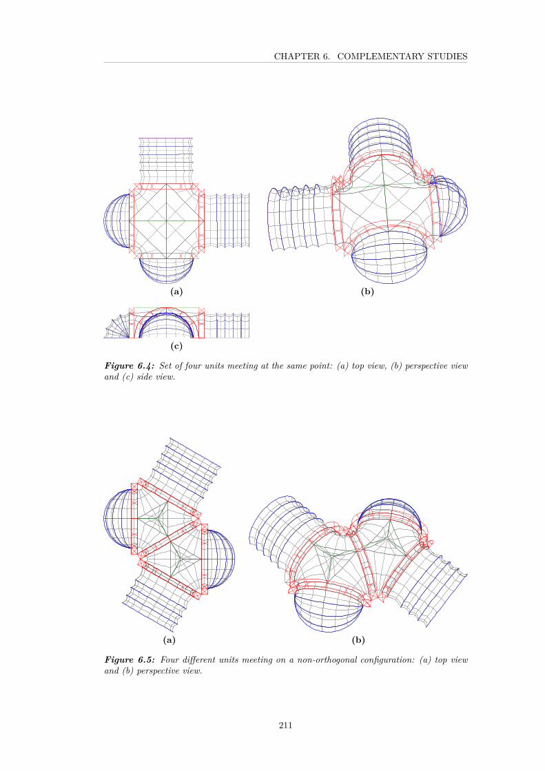
CHAPTER 6. COMPLEMENTARY STUDIES
(a) (b)
(c)
Figure 6.4: Set of four units meeting at the same point: (a) top view, (b) perspective viewand (c) side view.
(a) (b)
Figure 6.5: Four different units meeting on a non-orthogonal configuration: (a) top viewand (b) perspective view.
211
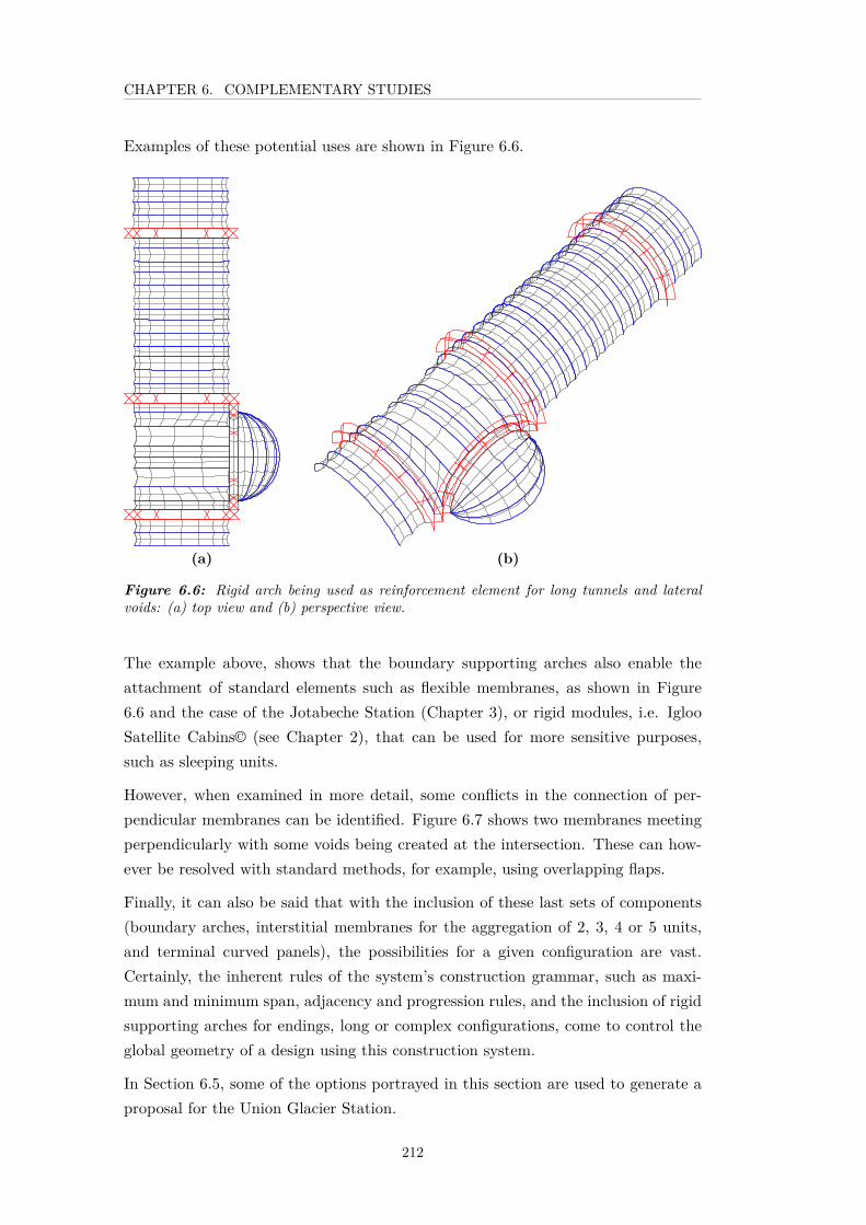
CHAPTER 6. COMPLEMENTARY STUDIES
Examples of these potential uses are shown in Figure 6.6.
(a) (b)
Figure 6.6: Rigid arch being used as reinforcement element for long tunnels and lateralvoids: (a) top view and (b) perspective view.
The example above, shows that the boundary supporting arches also enable theattachment of standard elements such as flexible membranes, as shown in Figure6.6 and the case of the Jotabeche Station (Chapter 3), or rigid modules, i.e. IglooSatellite Cabins© (see Chapter 2), that can be used for more sensitive purposes,such as sleeping units.
However, when examined in more detail, some conflicts in the connection of per-pendicular membranes can be identified. Figure 6.7 shows two membranes meetingperpendicularly with some voids being created at the intersection. These can how-ever be resolved with standard methods, for example, using overlapping flaps.
Finally, it can also be said that with the inclusion of these last sets of components(boundary arches, interstitial membranes for the aggregation of 2, 3, 4 or 5 units,and terminal curved panels), the possibilities for a given configuration are vast.Certainly, the inherent rules of the system’s construction grammar, such as maxi-mum and minimum span, adjacency and progression rules, and the inclusion of rigidsupporting arches for endings, long or complex configurations, come to control theglobal geometry of a design using this construction system.
In Section 6.5, some of the options portrayed in this section are used to generate aproposal for the Union Glacier Station.
212
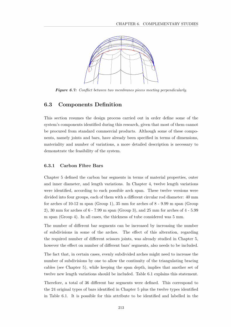
CHAPTER 6. COMPLEMENTARY STUDIES
Figure 6.7: Conflict between two membranes pieces meeting perpendicularly.
6.3 Components Definition
This section resumes the design process carried out in order define some of thesystem’s components identified during this research, given that most of them cannotbe procured from standard commercial products. Although some of these compo-nents, namely joints and bars, have already been specified in terms of dimensions,materiality and number of variations, a more detailed description is necessary todemonstrate the feasibility of the system.
6.3.1 Carbon Fibre Bars
Chapter 5 defined the carbon bar segments in terms of material properties, outerand inner diameter, and length variations. In Chapter 4, twelve length variationswere identified, according to each possible arch span. These twelve versions weredivided into four groups, each of them with a different circular rod diameter: 40 mmfor arches of 10-12 m span (Group 1), 35 mm for arches of 8 - 9.99 m span (Group2), 30 mm for arches of 6 - 7.99 m span (Group 3), and 25 mm for arches of 4 - 5.99m span (Group 4). In all cases, the thickness of tube considered was 5 mm.
The number of different bar segments can be increased by increasing the numberof subdivisions in some of the arches. The effect of this alteration, regardingthe required number of different scissors joints, was already studied in Chapter 5,however the effect on number of different bars’ segments, also needs to be included.
The fact that, in certain cases, evenly subdivided arches might need to increase thenumber of subdivisions by one to allow the continuity of the triangulating bracingcables (see Chapter 5), while keeping the span depth, implies that another set oftwelve new length variations should be included. Table 6.1 explains this statement.
Therefore, a total of 36 different bar segments were defined. This correspond tothe 24 original types of bars identified in Chapter 5 plus the twelve types identifiedin Table 6.1. It is possible for this attribute to be identified and labelled in the
213

CHAPTER 6. COMPLEMENTARY STUDIES
Original number ofsubdivisions(number ofsegments)
Altered numberof subdivisions(+1 segments)
Span[m]
Original barsegmentlength
[m]
Modified barsegmentlength
[m]12 1.57 1.45
12 13 11 1.44 1.3310 1.31 1.21
11 N/A7.99 1.26 1.14
10 11 7 1.1 1.006 0.94 0.86
9 N/A
Table 6.1: Variation in upper bars’ length in altered arches.
parametric model, which facilitates the segment’s production. It can also eventuallyserve as a guideline in case a replacement is needed on site, in which case barsegments can be cut to size from standard length bars.
Figures 6.8 and 6.9 show an example of this application.
6.3.2 Angled Bar Connections
The connection between bar segments is an aspect that needs to be addressedindependently. The bars are designed to be connected at the location of the joints.Given that the cross joints are designed to provide certain tolerance in their bars’rotation angle and length, the kink between bars is required to be resolved with anindependent element.
Figure 6.10 shows an early study for an aluminium attachment ring, where a kinkconnection can be inserted. The carbon fibre bar segments are fastened to each endof this kinked connection with locking pins. One of these aluminium rings protrudefrom each of the four extremities of the scissor-shaped joint.
A sketch of these rings is shown in Figure 6.11.
Alternatively, a second version of this element can be obtained by joining thelocking pin to the protruding connection and considering the connection ring asan independent element, as sketched in Figure 6.12.
Whilst this aluminium ring can then be uniform for all types of connections, theangled connectors need to be designed for each of the carbon fibre variations.Therefore, as figure 6.13 shows, three variations are needed, considering alteredcases.
A sketch showing the assembly sequence is given in Figure 6.14.
214

CHAPTER 6. COMPLEMENTARY STUDIES
Figure 6.8: List of the bars’ length on a surface output by the parametric model for twosubsequent arches with the same span.
The final version of a proposal for this element is shown in Figure 6.15., and thefirst option was implemented, given than this version offers a simpler fabricationand assembly procedure.
6.3.3 Aluminium Crosses
The number and type of different crosses on a given surface can be identified by theparametric model. Figure 6.16 shows an example of this application. Here two listsare generated: one identifying the angle between scissors-joints’ bars and a secondlist inspecting the crosses in an arch according to their length-based type. A secondresult is shown in Figure 6.17, where a diagram was produced identifying the samearch’s joints by colour according to their length-type.
The original design of the aluminium joints (see Chapter 3) was revised and updatedin order to enable this components to: i) support the bar segments, ii) define thecross section of the arch at each node for which length and angle are adaptable iii)provide a node for the continuous lacing cable between two arches and iv) providea hook from which the heavy duty strips (attached to membrane segments) canbe winched and tensioned from (see Chapter 3). Figure 6.18 and 6.19, show earlydesign sketches for the new version of this component. The second version wasfinally adopted.
215

CHAPTER 6. COMPLEMENTARY STUDIES
Figur e
6.9:Diagram
ofthebars’length
inasurface
outputbythe
parametric
model.
Image:
A.Bak.
216

CHAPTER 6. COMPLEMENTARY STUDIES
Figure 6.10: Sketch of an aluminium ring attached to a joint.
Figure 6.11: Sketch of a set of pieces for an aluminium ring.
217
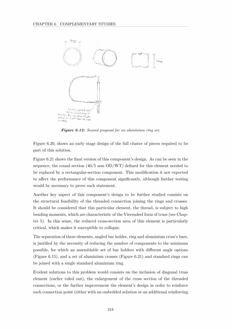
CHAPTER 6. COMPLEMENTARY STUDIES
Figure 6.12: Second proposal for an aluminium ring set.
Figure 6.20, shows an early stage design of the full cluster of pieces required to bepart of this solution.
Figure 6.21 shows the final version of this component’s design. As can be seen in thesequence, the round section (40/5 mm OD/WT) defined for this element needed tobe replaced by a rectangular-section component. This modification it not expectedto affect the performance of this component significantly, although further testingwould be necessary to prove such statement.
Another key aspect of this component’s design to be further studied consists onthe structural feasibility of the threaded connection joining the rings and crosses.It should be considered that this particular element, the thread, is subject to highbending moments, which are characteristic of the Vierendeel form of truss (see Chap-ter 5). In this sense, the reduced cross-section area of this element is particularlycritical, which makes it susceptible to collapse.
The separation of these elements, angled bar holder, ring and aluminium cross’s bars,is justified by the necessity of reducing the number of components to the minimumpossible, for which an assemblable set of bar holders with different angle options(Figure 6.15), and a set of aluminium crosses (Figure 6.21) and standard rings canbe joined with a single standard aluminium ring.
Evident solutions to this problem would consists on the inclusion of diagonal trusselement (earlier ruled out), the enlargement of the cross section of the threadedconnections, or the further improvement the element’s design in order to reinforcesuch connection point (either with an embedded solution or an additional reinforcing
218

CHAPTER 6. COMPLEMENTARY STUDIES
.
For arches within Group 4, with 25mm OD bars' rod section, and 9 subdivisions.
30m
m
For arches within Group 3, with 30mm OD bars' rod section, and 11 subdivisions.
For arches within Group 2, with 35mm OD bars' rod section, and 11 subdivisions.
For arches within Group 1, with 40mm OD bars' rod section, and 12 subdivisions
ε
µ
λ
κ
ι
η
γ
φ
For arches within Group 1, with 40mm OD bar's rod section.and 13 subdivisions.
δ
χ
β
α
Option BOption A
40m
m
40m
m
40m
m
40m
m
35m
m
35m
m
30m
m
30m
m30
mm
For arches within Group 3, with 30mm OD bars' rod section, and 10 subdivisions.
25m
m
25m
m
30 m
m30
mm
25 m
m
40m
m40
mm
40m
m
35m
m
40m
m
40m
m
40m
m
40m
m
40m
m
...
..
.
..
..
.
Note: This option would allow a single standard ring to be employed for all types of angled connections,
as all version are designed with 40mm OD in the central segment.
Note: This option would require three type of rings to be employed (50, 40, 30mm OD), but it would be easier to
manufacture as all sections are uniform.
Figure 6.13: Study of variations for angled connectors.
219

CHAPTER 6. COMPLEMENTARY STUDIES
Figure 6.14: Assembling sequence of an aluminium ring, angled connection, carbon-fibrebars and scissor-shaped joint.
Figure 6.15: Model of an aluminium ring and angled connection. Image: A. Bak.
220

CHAPTER 6. COMPLEMENTARY STUDIES
Figure 6.16: Lists of an arch’s joint typified their length and angle produced by theGrasshopper model.
221

CHAPTER 6. COMPLEMENTARY STUDIES
Figur e
6.17:Surface
withalum
iniumjoints
identifiedby
coloursaccording
tolength-based
type.Im
age:A.Bak.
222

CHAPTER 6. COMPLEMENTARY STUDIES
Figure 6.18: First version of an aluminium joint.
Figure 6.19: Second version of an aluminium joint.
223

CHAPTER 6. COMPLEMENTARY STUDIES
Figure 6.20: Sketch of a scissor-shaped joint connected to the membrane.
224

CHAPTER 6. COMPLEMENTARY STUDIES
Figure 6.21: Model of a scissor-shape joint. Image: A. Bak.
component). However, further analysis and physical testing turns out necessary atthis point.
6.3.4 Membrane Patterning and voids
As stated in Chapter 5, it is possible to obtain the membrane cutting pattern fromthe parametric model by using standard formfinding applications. In this case,the application used was Daniel Piker’s engine Kangaroo. Although this is not anaccurate modeling exercise it offers a good idea of the component’s geometry.
For this particular case, each membrane segment is expected to be hung fromthe arches’ scissors-joints using a series of heavy duty ratchet straps and metalcam-lock buckles (see Chapter 3). The original version of the structure’s designproposed that each segment include a polyester strap sewn along its central axis,from where adjustable bands and buckles were placed. This concept was conserved.Consequently, the number of belts and buckles included in the band attached tothe fabric piece should be equal to the number of scissor joints contained in the
225

CHAPTER 6. COMPLEMENTARY STUDIES
Figure 6.22: Sketch of connection between consecutives membrane pieces.
corresponding arch. Additionally, the membrane segments can be fixed to the groundby attaching them to the anchorages.
The joining of consecutive fabric segments is proposed to be achieved with heavyduty zipper connections. Waterproof materials are readily available and are widelyused by tent manufacturers. Additional protection can be achieved with the inclusionof a fabric flap. The connection of these elements is illustrated in Figure 6.22.
Although the fabric is expected to be implemented with a certain degree of isotropicpre-stress, and the edge cables to have a prescribed tension force, a level of flexi-bility is also expected. Therefore, by pre-tensioning the membrane, a curved edgespanning between the support points will naturally be introduced, thereby, lifting
226

CHAPTER 6. COMPLEMENTARY STUDIES
Figure 6.23: Example of a set of membrane cutting pattern obtained from the parametricmodel. Image: A. Bak.
the membrane off the ground. The curve of the edge cable can be decreased byincreasing the cable force, and reciprocally, decreasing the tension force of the cablewould enlarge this indentation.
A common solution for the closure of the surface consists of attaching a flap alongthe external face of the membrane segment to cover this curved edge and protectthe interior. This fold can be easily be pulled down to the ground with auxiliarytent pegs and cables.
The uniformity of the membrane segments has already been discussed in Chapter 5.Although there are only 8 different possible arches, the fact that each segment ofmembrane is defined in relation to the neighbouring spans and their specific widths,then there are 17 possible variations of membrane polygons (see Chapter 5).
Additionally, the heavy-duty straps sewn into the membrane pieces must containthe corresponding number of connections (ratchet straps and metal buckles). Insome cases (evenly-subdivided arches), such number could have been increased (byone node). Therefore, it is less likely that this element can easily be reused in thecase that the surface is to be reconfigured. Instead, membrane pieces are consideredsemi-bespoke components.
An example of membrane pattering obtained from the parametric model is showedin Figure 6.23.
Customised openings can be allowed by assessing the level of curvature of each fabricpolygon forming the membrane and identifying the zones with suitable curvature.Areas with higher curvature are subject to lower tension forces than flat zones,therefore curved zones can be considered to be more suitable for regular incisions[58]. This option confirms the semi-bespoke character of the membrane strips.
Figure 6.24 shows a map of the membrane where the level of curvature is assessed.The areas with low degree of curvature, therefore unsuitable for the placement ofvoids, are highlighted in yellow, and the areas subject to less tension forces are shownin blue and red.
227

CHAPTER 6. COMPLEMENTARY STUDIES
Figure 6.24: Assessment of surface curvature. Image: A. Bak.
6.3.5 Rigid Boundary Arches
The definition of rigid-arch elements was partially discussed in Section 6.2. Rigidboundary arches were defined as trussed metal elements, whose function is to providethe system with lateral resistance and to support flexible arches when a lateral voidis required.
The first function refers to cases requiring intermediate support for long configu-rations of tunnels, or for end panels. The size of this element was restricted toonly two options: 6 and 4 meter spans. The second option is considered to serveas a connection element for perpendicularly attached units, in which case a lateralopening is produced. Only one configuration is allowed (a 3 m x 2.1 m arch). Largerspans needed to be disregarded, due to restrictions in assembling and transportationcapacity. An aluminium alloy is proposed with similar properties to that used forthe joints.
The segmentation of the 6 m and 4 m arches were studied, based on the weight andsizes of the sections, for which two different cross sections were considered: 40 mmOD, wall thickness of 2.5 mm, with a linear weight of 0.795 kg/m (Case A), and 50mm OD, wall thickness of 3 mm, with a linear weight of 1.196 kg/m (Case B) [Tables6.2 and 6.3]. The composition of the arch was simplified from its original version toperpendicular crosses, with a uniform section of 400 x 400 mm [Fig. 6.25].
The structural performance of the elements was not tested, as it does not contributeto the development of the design method, since features could eventually be modifiedwithout altering the resulting surface. Instead, options were assessed based onthe building and logistical constraints. Arches with components longer than twometers were discarded as they could present difficulty for their manipulation onsite. Similarly, arches heavier than 50 kg were also dismissed on safety grounds and
228

CHAPTER 6. COMPLEMENTARY STUDIES
400 mm
Radius Radius 0,4 m0,4 m
400 mm
567,7mm
Segment Length
Figure 6.25: Section and profile of a rigid arch.
6 m Span Arch Expression Case A Case BLinear weightWL [kg⁄m ]
0.795 1.2
Inner arcsweight (WI)
[kg]
WI = (π × 3)×WL × 2 15 22.5
Outer arcsweight (Wo)
[kg]
Wo = (π × 3.4)×WL ∗ 2 23.5 25.5
Crosses (WC)[kg]
WC = 0.5657×WL × 2 0.89 1.353
Number ofSegments (nc)
5 6 7 5 6 7
Total weight[kg]
WT = [W I +Wo + (nc ×W c)] 27.9 28.8 29.7 54.9 56.21 57.6
SegmentLength [m]
LS = (π × 3.4/nc) 2.13 1.78 1.53 2.13 1.78 1.53
SegmentWeight [kg]
WS = (W T /nc) 5.59 4.8 4.24 11 9.37 8.22
Table 6.2: Study for different subdivision options of a 6 m rigid arch.
229
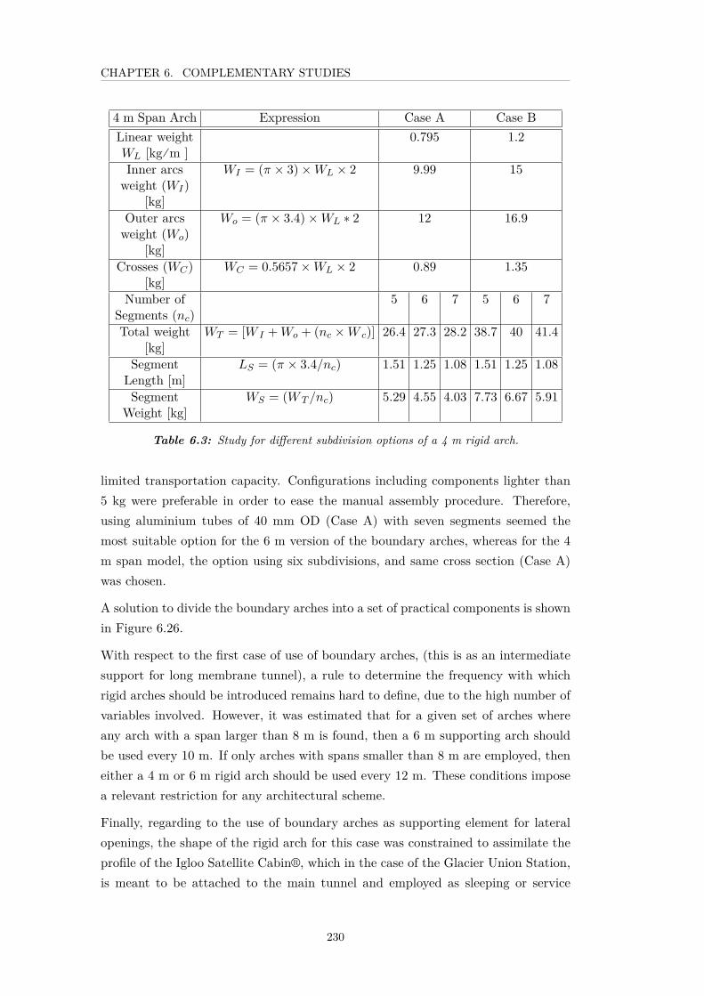
CHAPTER 6. COMPLEMENTARY STUDIES
4 m Span Arch Expression Case A Case BLinear weightWL [kg⁄m ]
0.795 1.2
Inner arcsweight (WI)
[kg]
WI = (π × 3)×WL × 2 9.99 15
Outer arcsweight (Wo)
[kg]
Wo = (π × 3.4)×WL ∗ 2 12 16.9
Crosses (WC)[kg]
WC = 0.5657×WL × 2 0.89 1.35
Number ofSegments (nc)
5 6 7 5 6 7
Total weight[kg]
WT = [W I +Wo + (nc ×W c)] 26.4 27.3 28.2 38.7 40 41.4
SegmentLength [m]
LS = (π × 3.4/nc) 1.51 1.25 1.08 1.51 1.25 1.08
SegmentWeight [kg]
WS = (W T /nc) 5.29 4.55 4.03 7.73 6.67 5.91
Table 6.3: Study for different subdivision options of a 4 m rigid arch.
limited transportation capacity. Configurations including components lighter than5 kg were preferable in order to ease the manual assembly procedure. Therefore,using aluminium tubes of 40 mm OD (Case A) with seven segments seemed themost suitable option for the 6 m version of the boundary arches, whereas for the 4m span model, the option using six subdivisions, and same cross section (Case A)was chosen.
A solution to divide the boundary arches into a set of practical components is shownin Figure 6.26.
With respect to the first case of use of boundary arches, (this is as an intermediatesupport for long membrane tunnel), a rule to determine the frequency with whichrigid arches should be introduced remains hard to define, due to the high number ofvariables involved. However, it was estimated that for a given set of arches whereany arch with a span larger than 8 m is found, then a 6 m supporting arch shouldbe used every 10 m. If only arches with spans smaller than 8 m are employed, theneither a 4 m or 6 m rigid arch should be used every 12 m. These conditions imposea relevant restriction for any architectural scheme.
Finally, regarding to the use of boundary arches as supporting element for lateralopenings, the shape of the rigid arch for this case was constrained to assimilate theprofile of the Igloo Satellite Cabin®, which in the case of the Glacier Union Station,is meant to be attached to the main tunnel and employed as sleeping or service
230

CHAPTER 6. COMPLEMENTARY STUDIES
Figure 6.26: Proposal for assembling of rigid arches.
Figure 6.27: Rigid arch designed for perpendicular intersections with flexible arches.
units. As earlier mentioned, this defines a profile 3 m wide and 2.1 m high [Fig.6.27], which can also be assembled from a reduced number of segments.
Additionally, the introduction of a lateral opening using a boundary arch presents aseries of challenges. The first is related to the geometry of the spanning arches beingsupported by this arch. Figure 6.28 shows two possibilities for the geometry of thespanning arches intersecting a boundary arch. In Option 1, the spanning arches aredefined as quarter-circular, with one end on the floor and the other end located offthe ground at the centre of the boundary arch (see left-hand-side of Figure 6.28). InOption 2, the element consists of half of an arch, defined by an origin point on theground and the mid-span point, where it is interrupted by the intersecting boundaryarch (see right-hand-side of Figure 6.28).
Whilst the second option offers the advantage that fewer new element types arerequired, there are several aspects that make it inconsistent with the structural
231

CHAPTER 6. COMPLEMENTARY STUDIES
Rigid Supporting Arch
Flexible Arch
Option 2Option 1
Flexible Arch
Rigid Supporting Arch
Figure 6.28: Cases of spanning arches supported by a lateral boundary arch.
Rigid Supporting Arch
Flexible Arch
b c d e
Figure 6.29: Spanning arches intersecting a boundary arch at irregular intervals.
grammar proposed. These include the mid-span depth possibly needing to be largerthan necessary, and discrepancies in the cable triangulation rule would be found dueto an irregular number of joints. If the first option was employed, then more coherentfeatures can be expected. Thus, mid-span depth and the number of subdivisionsshould be assumed according to the rules defined, namely, they are determined bytheir span and adjacency rules.
Another aspect to be considered in this situation is the irregular frequency at whichspanning arches are placed, which is dependent of their span (see Chapter 5). Theintersection of arches and a perpendicularly placed boundary arch should also takeinto account the irregular interval and angles at which the boundary arches would beintersected by the spanning arches according to the uniform load condition adopted.Figure 6.29 shows a sketch of such problem, where the a set of spanning arches areplaced at irregular distances (a, b, c, d and e), perpendicularly to a boundary arch.
In order to simplify this situation, it was decided that spanning arches intersectinga boundary arch should have a uniform span. Figure 6.30 shows an early study ofthis proposal, using arches of 4 m span.
A significant challenge imposed by this operation is the resolution of a joint thatpermits these two types of elements to be assembled together. The principle ofthis problem is that the boundary arch should replicate the actions of the ground,receiving and supporting the set of four spanning bars in a common point. Eachspanning arch intersects the rigid arch at a different angle from both, side and frontdirections of the rigid arch. Therefore such a joint should be allowed to rotate inboth directions. The design of such an element was not achieved during the time of
232

CHAPTER 6. COMPLEMENTARY STUDIES
Figure 6.30: Front and back view of an intersection between a boundary arch and a set of4 m span spanning arches.
(a)
MembraneBracing Cables
Supporting Arch
Anchors
(b)
Figure 6.31: Proposal for a membrane cover as an ending element: (a) side view and (b)front view.
this study, but it is believed that with further modelling and prototyping, multiplesolutions could be found.
6.3.6 Ending of tunnels
According to the cases described in Chapter 2, there are two solutions that couldbe implemented to end the tunnels, flexible membranes [Fig. 6.31] or a set of rigidpanels forming a shell [Fig. 6.32].
If a fabric membrane is used, this would require the inclusion of bracing cables, wherethe most efficient configuration would be a triangulated net to provide the stabilitycharacteristic lacking in these types of elements. Additionally, these cables should bepulled down and fixed to the ground by means of anchorages. In Figure 6.31, cablesare highlighted in green. Although this triangulated surface would behave similarlyto a rigid surface, it is expected that some additional tension force would be inducedto the rest of the membrane structure. On the other hand, the use of rigid panelsinstead of a flexible membrane would provide a more robust ending solution. Bothsolutions have already been implemented in remote areas (see Chapter 2), so nofurther analysis was considered necessary.
233
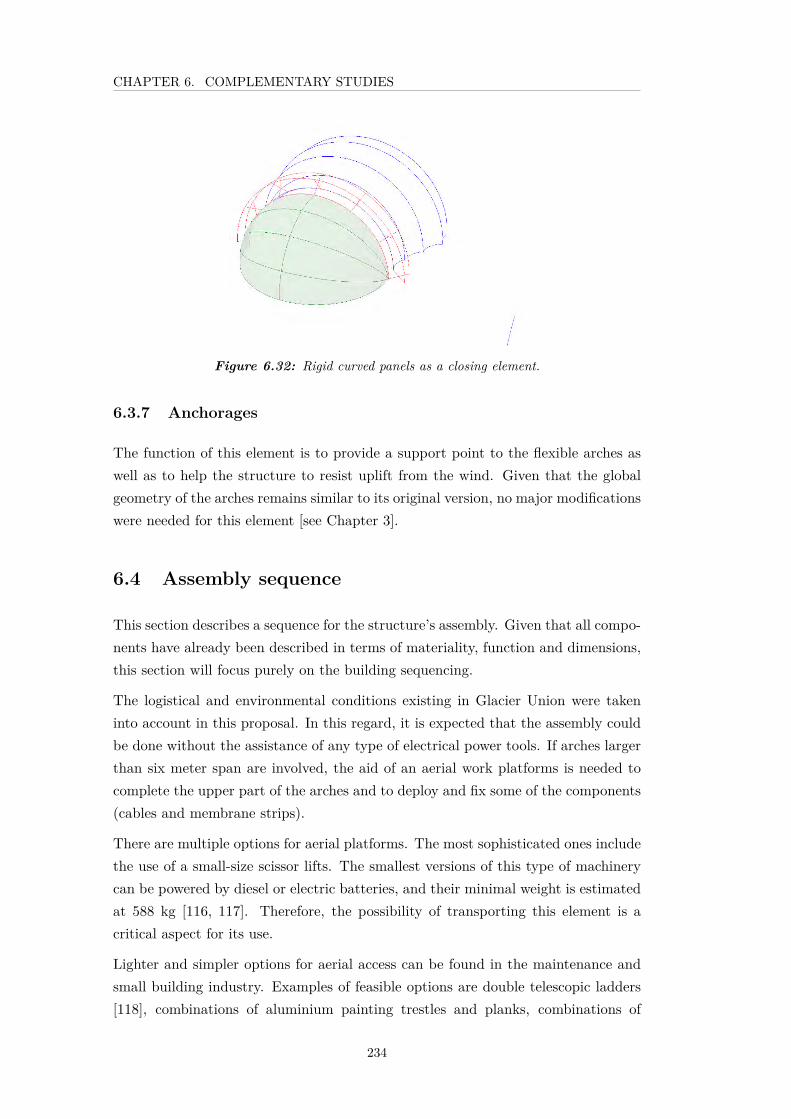
CHAPTER 6. COMPLEMENTARY STUDIES
Figure 6.32: Rigid curved panels as a closing element.
6.3.7 Anchorages
The function of this element is to provide a support point to the flexible arches aswell as to help the structure to resist uplift from the wind. Given that the globalgeometry of the arches remains similar to its original version, no major modificationswere needed for this element [see Chapter 3].
6.4 Assembly sequence
This section describes a sequence for the structure’s assembly. Given that all compo-nents have already been described in terms of materiality, function and dimensions,this section will focus purely on the building sequencing.
The logistical and environmental conditions existing in Glacier Union were takeninto account in this proposal. In this regard, it is expected that the assembly couldbe done without the assistance of any type of electrical power tools. If arches largerthan six meter span are involved, the aid of an aerial work platforms is needed tocomplete the upper part of the arches and to deploy and fix some of the components(cables and membrane strips).
There are multiple options for aerial platforms. The most sophisticated ones includethe use of a small-size scissor lifts. The smallest versions of this type of machinerycan be powered by diesel or electric batteries, and their minimal weight is estimatedat 588 kg [116, 117]. Therefore, the possibility of transporting this element is acritical aspect for its use.
Lighter and simpler options for aerial access can be found in the maintenance andsmall building industry. Examples of feasible options are double telescopic ladders[118], combinations of aluminium painting trestles and planks, combinations of
234

CHAPTER 6. COMPLEMENTARY STUDIES
heavy-duty leaning and stepladders [119], tripod or orchard ladders [120], bakerscaffold towers [121] and mobile scaffold mono towers [122], amongst others.
Aluminium crosses can be adjusted and mounted off-site. If the transportationcapacity allows, the carbon-fibre bars can also be installed, so arches can be formedand transported to site ready for installation. This is described In Figure 6.33.
The assembly of the structure can be described by the following list of activities andfigures:
i) Marking the location of arches on-site and installing anchorages [Fig. 6.34].
ii) Assembling and installing the first boundary arch. If the larger version ofthis element is used (6 m), upper segments would need to be lifted andassembled with the aid of an aerial platform. Figure 6.35 shows the limitfor un-aided assembly. Components are designed to be lifted by one person(weighting approximately. 4.8 kg). Figure 6.36 shows a complete version ofthis element.
iii) Attaching the membrane piece to the arch [Fig. 6.37]. This step is valid foronly one of the boundary arches of a given tunnel (either the first, or thelast one) and is done using the metal hangers provided by the aluminiumjoints and the heavy duty straps-buckles connections (shown in orange). Themembrane piece is required to be installed clasped using temporary fabricVelcro® stripes.
iv) Erecting flexible arches. The installation of these arches can be done byassembling the components from bottom to top. Similarly, for heights abovetwo metres, the installation would need to be assisted. Figure 6.38 showsthe case of an eight metre span arch being assembled. Due to the lightnessof arches, it is also advisable to first construct them on the ground, allowingtheir instalment can be carried out quicker. Figure 6.39 shows a completedflexible arch.
Figure 6.40 shows the installation of the corresponding membrane segment onto thearch. Similarly to the case of rigid supporting arches, fabric pieces are connectedto the arch using the heavy duty straps and buckles provided (shown in orange).Again, fabric pieces are installed collapsed using temporary fabric Velcro® strips(shown in red).
235
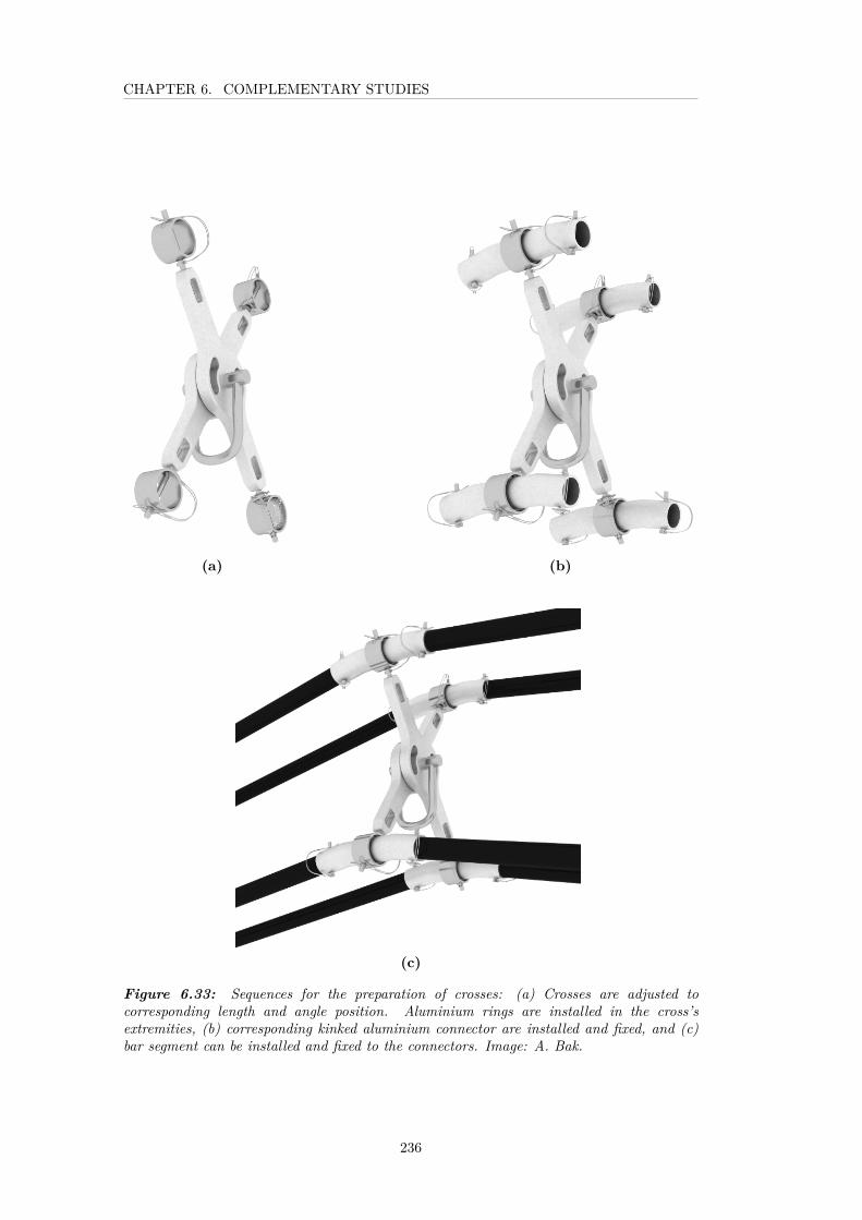
CHAPTER 6. COMPLEMENTARY STUDIES
(a) (b)
(c)
Figure 6.33: Sequences for the preparation of crosses: (a) Crosses are adjusted tocorresponding length and angle position. Aluminium rings are installed in the cross’sextremities, (b) corresponding kinked aluminium connector are installed and fixed, and (c)bar segment can be installed and fixed to the connectors. Image: A. Bak.
236

CHAPTER 6. COMPLEMENTARY STUDIES
Figure 6.34: Marking the location of arches on site and installing anchorages.
Figure 6.35: Boundary arch assembling.
Figure 6.36: Boundary arch completed.
237
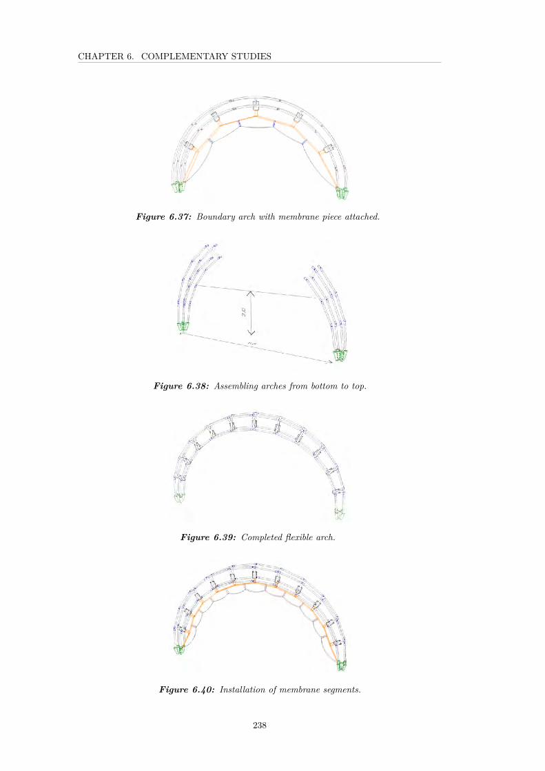
CHAPTER 6. COMPLEMENTARY STUDIES
Figure 6.37: Boundary arch with membrane piece attached.
Figure 6.38: Assembling arches from bottom to top.
Figure 6.39: Completed flexible arch.
Figure 6.40: Installation of membrane segments.
238
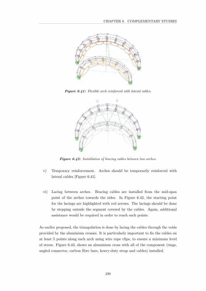
CHAPTER 6. COMPLEMENTARY STUDIES
Figure 6.41: Flexible arch reinforced with lateral cables.
Figure 6.42: Installation of bracing cables between two arches.
v) Temporary reinforcement. Arches should be temporarily reinforced withlateral cables [Figure 6.41].
vi) Lacing between arches. Bracing cables are installed from the mid-spanpoint of the arches towards the sides. In Figure 6.42, the starting pointfor the lacings are highlighted with red arrows. The lacings should be doneby stepping outside the segment covered by the cables. Again, additionalassistance would be required in order to reach such points.
As earlier proposed, the triangulation is done by lacing the cables through the voidsprovided by the aluminium crosses. It is particularly important to fix the cables onat least 5 points along each arch using wire rope clips, to ensure a minimum levelof stress. Figure 6.43, shows an aluminium cross with all of the component (rings,angled connector, carbon fibre bars, heavy-duty strap and cables) installed.
239

CHAPTER 6. COMPLEMENTARY STUDIES
Figure 6.43: Aluminium scissor joint with all components connected. Image: A. Bak.
240
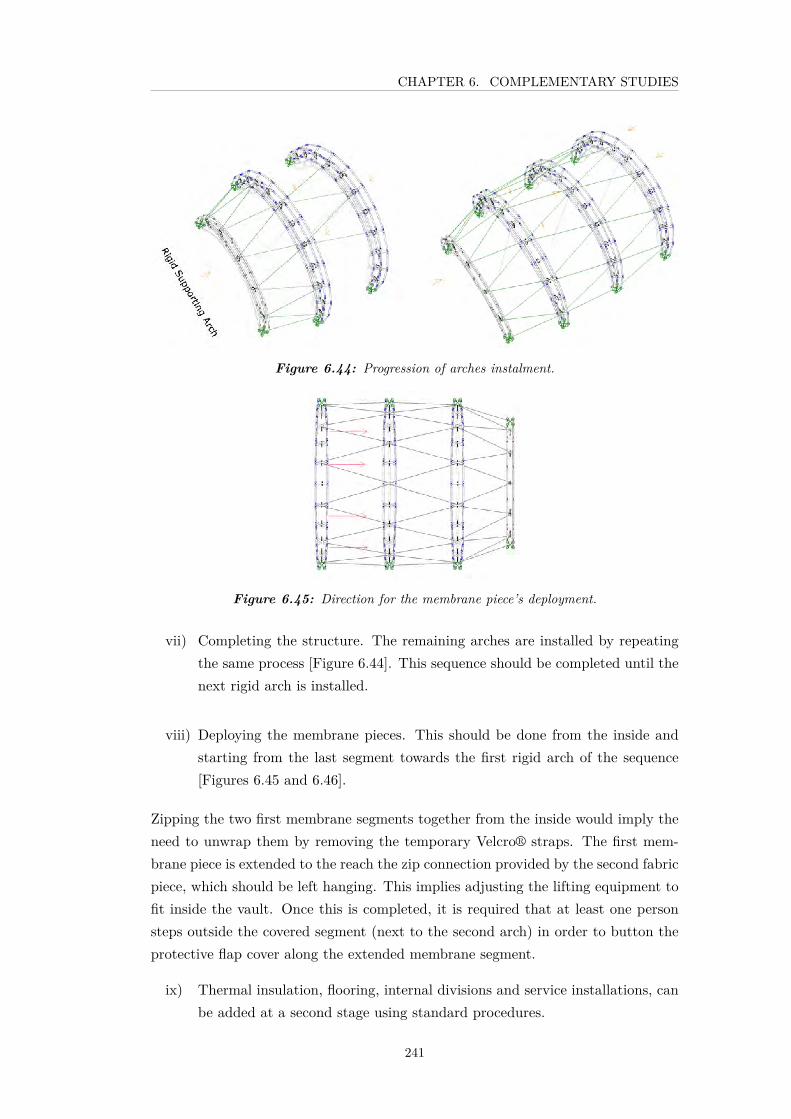
CHAPTER 6. COMPLEMENTARY STUDIES
Figure 6.44: Progression of arches instalment.
Figure 6.45: Direction for the membrane piece’s deployment.
vii) Completing the structure. The remaining arches are installed by repeatingthe same process [Figure 6.44]. This sequence should be completed until thenext rigid arch is installed.
viii) Deploying the membrane pieces. This should be done from the inside andstarting from the last segment towards the first rigid arch of the sequence[Figures 6.45 and 6.46].
Zipping the two first membrane segments together from the inside would imply theneed to unwrap them by removing the temporary Velcro® straps. The first mem-brane piece is extended to the reach the zip connection provided by the second fabricpiece, which should be left hanging. This implies adjusting the lifting equipment tofit inside the vault. Once this is completed, it is required that at least one personsteps outside the covered segment (next to the second arch) in order to button theprotective flap cover along the extended membrane segment.
ix) Thermal insulation, flooring, internal divisions and service installations, canbe added at a second stage using standard procedures.
241

CHAPTER 6. COMPLEMENTARY STUDIES
Figure 6.46: Progression of membrane segments deployment.
242

CHAPTER 6. COMPLEMENTARY STUDIES
Figure 6.47: Handmade sketch of side view of an early design scheme.
Figure 6.48: Side view of early design scheme with basic type of components recognise bycolour.
6.5 Examples of Possible Applications for the GlacierUnion Case
A proposal for a speculative design of a research station in Union Glacier wasproduced based on the requirements described in Chapter 1 and the system proposedin this study. Laboratories and storage units are expected to be implement usingadapted shipping containers.
Figures 6.47 to figure 6.50 show some early sketches of a proposal for the GlacierUnion Research Station. In Figures figure 6.48 and figure 6.50 the basic type ofcomponents are recognised by colours.
The scheme was then revised using the parametric CAD definition and CAD toolsand a second version was produced which is implemented using the componentsspecified in this chapter as well as the rules stablished. Figure 6.51 show thearchitectural plan for the proposal, and Figures 6.52 to 6.54 show some captionsof the digital model.
Figure 6.55 and 6.56 identify the type of bars used in one part of the scheme accordingto their length, using the colour values specified in Figure 5.2.
243

CHAPTER 6. COMPLEMENTARY STUDIES
Figure 6.49: Handmade sketch of plan diagram for an early design scheme.
Figure 6.50: Top view of early design scheme with basic type of components recognised bycolour, boundary arches in red and flexible arches in blue.
244

CHAPTER 6. COMPLEMENTARY STUDIES
Figure 6.51: Architectural plan for a design scheme.
Figure 6.52: Isometric view of design scheme.
245

CHAPTER 6. COMPLEMENTARY STUDIES
Figure 6.53: Isometric view of design scheme.
Figure 6.54: Isometric view of design scheme.
246

CHAPTER 6. COMPLEMENTARY STUDIES
Figure 6.55: Bar types identified according to length using colour code, side view.
Figure 6.56: Bar types identified according to length using colour code, perspective view.
6.6 Conclusions
This chapter has provided the basic solutions to demonstrate the feasibility of theconstruction system proposed in terms of architectural requirements, fabrication andconstruction. This has involved options for different configurations, the design ofkey components, as well as the proposal for an assembly sequence.
As in any design effort, there is no clear limit marking the end of the design process.Nevertheless, a satisfactory level to demonstrate is believed to have been achieved.
There are some components whose solution or definitions were not addressed, eitherbecause they consisted of standard or already tested items (such as membrane flaps,closing membrane covers, inner thermal insulation layer, flooring and inner divisionpanels), their design did not vary from the original scheme (anchorages), or theircomplexity required further study (such as joints for intersecting arches, interstitialmembranes and voids used for windows). Based on the multiple examples presentedin Chapter 2 and Chapter 3, it is believed that solutions of this level of complexityare achievable in all cases.
Finally, the variety of techniques involved in this chapter, ranging across scriptingsoftware tools, digital modelling, manual sketching and 3D printing, evidenced theexperimental nature of this study.
247


Chapter 7
Conclusions
7.1 Introduction
This thesis has been dedicated to the recognition of lightweight structures as a designfield in their own right.
The development of such a narrative involved three main steps: i) the description ofthe research scope and the characterisation of Antarctic and Subantarctic lightweightstructures, ii) the formulation and validation of an original design problem, and iii)the development of a design-based method to solve such a problem.
The actions carried out during these three stages can be summarised as following:
i) Description of the research scope and the characterisation of Antarctic and Sub-antarctic lightweight structures:
In the first chapter, a description of the characteristics of Antarctic constructionsand of their quick evolution during their 100 year history was presented. Thisintroductory synopsis was necessary due to the lack of academic material relatingto this field. Types of Antarctic structures were identified and classified by theirscale and also by the mode of use (permanent, seasonal or temporary), which isa key characteristic of Polar facilities. It was seen that seasonal infrastructure ischaracterised by hard maintenance and inefficient design and use of energy resources.
Chapter 2 was concerned with the documentation of medium and small minimal-weight structures which have been designed for Antarctic and Subantarctic contextsin particular. Some cases described were used as permanent structures (such asthe US South Pole Dome), others as seasonal shelters (such as the Teniente ArturoParodi Station), and others as itinerant dwellings (such as the Aonikenk dwellings).The descriptions were mainly from a structural perspective. A particular classifica-tion of structural surfaces (proposed by Martin Bechthold) was used. This approachenabled the clear description and categorisation of each of the cases found. As a
249

CHAPTER 7. CONCLUSIONS
result, a fascinating array of Polar lightweight structures was documented, wherethe majority corresponded to hybrid schemes. Examples of different materiality,assembly strategies and geometrical patterns were also found.
Arguably some of the most interesting cases corresponded to the group of vernacularconstructions that were used for now extinct indigenous inhabitants of the Sub-antarctic and Patagonian regions. The lightness and variety of these structures con-stitutes remarkable examples of the smart use of materials and structural efficiencyin some of the most extreme environments. The fact that these sets of structureshave remained unstudied and excluded by most of the literature concerned withvernacular constructions is a surprising fact. Though it can perhaps be explainedby the rapid extinction of the Aonikenk, Selk’nam, Yamana and Kaweshkar com-munities, which resulted in very scarce study material. Also the most descriptivetexts have not been published in English nor translated to other languages, leavingthese cases practically excluded from the best-known literature.
Therefore, the novel nature of this literature study, has not only helped to providethis research with a general background, but it is also a fundament contribution tothe statement that Polar lightweight design is a valid field of research.
This first stage concluded by presenting the brief for a new seasonal station for theUniversity of Magallanes’ Antarctic Division in the area of Union Glacier. Such astructure should host a variable number of staff members and should comply withthe strict environmental policy, logistic limitations and rough weather conditionsseen in the Antarctic. In addition to these practicalities, this station should alsopromote an innovative architectural approach.
ii) Formulation and validation of a design problem:
Based on that opportunity, this research suggested that lightweight structures couldbe used in Polar environments in a larger, more permanent and more innovativefashion than currently seen. It was also suggested that the periodic variationin the use of seasonal infrastructure offered the chance to explore the conceptionof a structural system which would allow a certain degree of adaptability in itsconfiguration.
Such a task demonstrated how restrictions derived from such a context (efficientperformance, minimal weight, adaptable configuration, reduced number of physicalcomponents, and feasible assembly procedure) can drive a novel design process, andin doing so promote the expansion in the research and use of Polar lightweightstructures.
The first step towards validating this problem comprised of a review of existing ex-amples of small-scale constructions that by some means have addressed the problem
250
CHAPTER 7. CONCLUSIONS
of adaptability with a controlled number of components. A set of singular cases,defined as semi-modular systems, were found and briefly described.
iii) The development of a design-based method:
The design process commenced by presenting an early scheme for a generic structuralsurface, a hybrid structure, as was previously developed by the author. Accordingto the author’s interpretation of M. Bechthold’s surfaces’ categorisation, this schemecould be classified as a hybrid rigid structure, more specifically, as a truss-like shellwhere the characteristic single curvature is overcome by the use bracing cablesand membrane segments between independent arches of variable span, for whichattributes of a gridshell are also present.
This scheme was outlined in terms of its basic geometrical properties, componentsand limitations. This surface was considered suitable to be further explored andimplemented as a semi-modular system enabled by low-tech construction techniques.Consequently, Chapter 4 was dedicated to the development of a design methodology.
The first step took care of the definition of the geometry of the main structuralcomponent, this is, a trussed arch. In this study, defined as a sensitivity study,different versions of the arch were contested based on their structural behaviourcombined with logistic criteria.
A sensitivity study was carried out, using FE models in combination with logisticalcriteria, to determine the basic geometrical characteristics of the main structuralcomponent, that is, a trussed arch. Finally, the option with minimal structuraldepth at the support points and maximum depth in the mid-span zone was chosendue to both, construction and structural efficiency. The same criteria were used todetermine the initial value and role of different geometric attributes such as the crosssection of bars, number of subdivisions, mid-span depth, and geometry of aluminiumjoints.
The second part of this design process was devoted to the description of the geomet-rical attributes for the whole array of components (with trussed arches at integerintervals ranging from 4 to 12 m span) as well as their options for variations andthe relationship between them. This was done through a multi-objective study,where three goals were considered, namely minimal self-weight, minimal number ofdifferent components and variable configuration.
The set of studies that were in this chapter can be listed as follows:
1. Sensitivity study to determine the attributes of the trussed arches. Attributeswere partially-optimised, meaning that geometrical attribute values were groupedby ranges. These included the cross section size of carbon-fibre bars anddepth of the truss at mid-span. Other attributes were designed with uniform
251

CHAPTER 7. CONCLUSIONS
attributes at this stage, including the size of arches at the support points,the number of subdivisions (aluminium joints) and the aluminium bar cross-section. Additionally, and in order to bring internal stress values to acceptablelevels, a geometry-based method was created to allow the reduction of pre-stress. This solution was homogenously applied to all versions of flexiblearches, resulting in less-stressed collections of components.
2. Control of the number of different components. The study of the variations inlength and angle between the crosses’ bars allowed the definition of a strategyto significantly reduce the number of different joints from 61 types to 7. It wasobserved that most of the different joints would vary only by a few millimetresfrom others. The solution then developed a design concept for a joint whichwould tolerate a length variation of 50 mm, meaning only 7 types would beneeded. Each of these variations would need to adopt a minimum of two, and amaximum of four different positions (angle between the two aluminium bars).Both adaptations (in length and angle) needed to be manually operable.
3. Reduction of number of joints. This study used a geometry-based approachto determine the possibility of reducing the number of aluminium joints whistpreserving the continuity of the bracing cables’ triangulation. This was onlypossible due to this attribute being defined as low-sensitivity according to thecharacterisation carried out in Chapter 4 and the low value stresses achieved inChapter 5. The rules for such an operation were determined via an exhaustivestudy, from where solutions for failing sequences could be derived, resultingin a straight forward method. As a result, the number of different nodes (orarches’ subdivisions) was reduced to 4 different values.
4. Regulation of the distance between arches. The grouping of different attributesled to each arch being subject to different load conditions. On the other hand,loads were calculated assuming a uniform distance between arches. By varyingthe distance between arches, the load condition throughout the array of archescould be normalised. This adjustment did not imply an increase in the numberof components, as membrane pieces were previously considered to be a semi-bespoke component, with 17 different variations identified.
The chapter concluded with the introduction of a parametric CAD model whichallowed such surfaces to be created from a native CAD curve. Such curves outlinethe station footprint, and should be derived from the architectural scheme. Examplesof applications of the Grasshopper® definition were shared.
Once the system grammar was resolved, the next chapter was dedicated to thestudy of other aspects of the system related to the assessment of the system’s
252
CHAPTER 7. CONCLUSIONS
architectural, construction and logistical feasibility. This included different optionsfor aggregations of surfaces, design solutions for key components and a proposal forassembly sequence.
As in the first study, proposals for aggregations of two perpendicular tunnels, aswell as arrangements for the aggregations of three and four units were produced.The geometrical operations revealed the need to include a rigid element into thesystem. A trussed rigid supporting arch was then considered. This element was alsointroduced as a reinforcement component for cases of very long tunnels.
In the second part of this chapter, solutions were offered for the implementation ofkey components, namely:
1. Arches’ bar segments. Bars consisted of standard carbon fibre bars. Thelength-based groups were identified by the parametric model. A total of 36types were identified.
2. Aluminium scissor joints. Node types can also be labelled and accounted forby the scripting tool embedded in the Grasshopper® definition. Identificationof the type is based on the length of the joint’s blades. Additionally, the designprocess for a scissor-shaped joint digital prototype was also explored.
3. Rigid arches. Versions of a mountable rigid arch were also defined, theseincluded three variations: 3 x 2.1, 6, 4 and meter spans.
4. Membrane pieces. A solution for membrane formfinding was also presented,which is done using Rhinoceros© applications as well as a solution for connec-tions of adjacent membrane sections.
5. Terminal elements. Proposals for ending elements were outlined including rigidpanels and flexible membranes.
Although anchorages are also considered a key component, the solution proposed inthe initial scheme was not varied, as it was considered to be sufficiently resolved.
This final chapter concluded with examples of applications of the designed systemfor the implementation of the Glacier Union Station.
7.2 Contributions to Knowledge
There are two principal results achieved from this research. The first part, basedon the literature, was able to produce a descriptive collection of 12 minimal weightconstructions designed for Subantarctic and Antarctic contexts. The description of
253

CHAPTER 7. CONCLUSIONS
each case focused on the materiality used, assembly sequence, and its structuralscheme. A brief description of the historical context and programmatic schemeof each project was also included. Finally, the array of structures was organisedaccording to their structural system, based on a classification proposed by M.Bechthold. The author’s own secondary classification, based on the geometry ofthe surfaces was also introduced.
The second result is the design of a generic lightweight structure. This comprises ahybrid system, featuring aspects of vault-like and gridshell systems. The system’smain components are flexible trussed arches of variable spans (variations consistingof integer values between 4 and 12 m), formed by carbon-fibre bars and aluminiumjoints. Arches are interconnected by two bracing systems: tensile membranes andan array of bracing cables. Vaults are constrained at intervals and at the ends byrigid mountable arches.
The design process was able to balance three conflicting objectives, adaptable con-figuration, reduced number of components and low-tech assembly sequence.
The resulting system is characterised by the possibility of progressively varying thesize of flexible arches in units (ranging from 4 to 12 m span), achieving an adaptivemorphology.
Solutions were proposed for several vaulted units to be aggregated in differentarrangements.
Although arches were partially optimised (in terms of the cross-section of carbonfibre bars, mid-span depth, number of subdivisions, and distance between arches),which implied a diversification of geometrical attributes, it was possible to signifi-cantly reduce the number of different elements. These consisted of three types ofcarbon fibre bar sections, seven different types of scissor-shaped aluminium joints,one type of anchorage, three types of rigid arches, and seventeen different membranepieces. Using principles of parametric design with a low tech approach, designsolutions for these key elements were offered and an assembly choreography wasproposed.
It can finally be stated that both of these results are equally relevant for the purposeof this research.
7.3 Theoretical implications
The diversity of cases and the clear influence of environmental and logistical con-straints derived from Antarctic and Subantarctic contexts in each of the structuresportrayed in the first part of this research enables the recognition of a singularparadigm.
254

CHAPTER 7. CONCLUSIONS
Furthermore, this study has also demonstrated that polar and subpolar scenariosdo not only motivate the search for innovative design solutions, technologies andmethods, but they have also been the natural response of native inhabitants to theextreme conditions of the Subantarctic region, who developed advanced constructiontechnologies.
The diversity of approaches encountered with this study also supports the appealfrom Antarctic scientific communities to conceive polar and subpolar regions ascomplex and varied scenarios, rather than the white empty canvases commonlypictured.
During this research it was found that no formal academic effort in the field ofarchitectural and/or engineering has been previously made to portray such projectsfrom a common perspective. This study is therefore, the first step towards a formalacknowledgement of such a paradigm.
The concept of ‘Polar Lightweight Structures’ was successfully tested in the secondpart of the research. Here, a novel problem was formulated, which dealt with theconcept of an adaptable construction system, ruled by conditions of minimal weight,controlled number of different components, and a low-tech assembly procedure. Theresulting system not only offers a feasible technical solution, but also an architecturaltectonic tool capable of blending into the landscape or responding to the uniqueform of seasonal use experienced by Polar structures. This design represents a stepforward in what has been done so far in the Polar context, in terms of architecturalexpression (as a larger and more complex design have been enabled), and alsostructural optimisation (where the concept of ’partial optimisation’ can offer aresponse to the use of parametric design tools in polar contexts.
Although efforts were made to structure and systematise the design process, itis evident that the specificity of the problem does not allow the generalisation ofthe method to be employed, as in other cases of structural systems. In terms ofparametric design environments, this method could not be translated into a genericdesign process. As an example, human assessment was constantly involved in thedecision of how many values each geometric parameter of the structure should bedivided into.
It is believed by the author that more effort should be made to integrate design andengineering disciplines into Polar scientific communities, which is particularly validfor the Antarctic and Subantarctic cases. This research has provided a frameworkfor this relating to Lightweight design.
255
CHAPTER 7. CONCLUSIONS
7.4 Limitation of this study
Limitations were encountered at different stages of this research, involving aspectssuch as the collection of evidence of a rather undocumented topic, the developmentof a design methodology, and restrictions for post-design testing.
One of the main challenges encountered was the definition of a valid research method-ology. This was particularly evident for the second part of the study (consistingof a design-based study). Although a clear research problem was formulated (thefeasibility of conceiving an adaptable lightweight structure with a limited numberof different components), the method of solving such a problem was undefined. Itwas only after a design scheme was introduced (a double curvature shell approachto a trussed system) that this problem could be broken down into a series of specificquestions, and a suitable methodology (a multi-objective optimisation study) couldthen be identified and applied.
In contrast, the first part of the study, referring to the identification and charac-terisation of Antarctic and Subantarctic lightweight structures, could be plannedand carried out with a clearer perspective. One of the key actions of this exercisewas the identification of suitable categories of lightweight structures, which in thiscase was as proposed by M. Bechthold. As discussed in Chapter 2, the selectionof this approach was based on Bechthold’s idea of using the structural behaviouras the primary parameter, independently of the overall shape, materiality, or scale.This approach enabled the successful assimilation between such diverse structuresas vernacular dwellings and modern portable tents.
Once the methodologies were established for each part of the study (the charac-terisation of Antarctic lightweight structures and the design path of an adaptablelightweight system), different challenges needed to be overcome.
For the first part, the main challenge was the lack of academic literature in thistopic, for which the material presented here was collected from a diverse range ofsources, including interviews, websites, photographs and magazines articles. Thedescription of the diverse array of vernacular structures turned out to be much morecomplex than initially expected. The literature on this topic, mostly by Hispanicauthors (i.e. catholic missionaries), was particularly challenging to re- interpretfor engineering/architectural purposes. Very limited evidence of these vernacularstructures remains. That which does includes replicas reproduced by local museumsin the Chilean and Argentinian Patagonian regions. Similarly, a fraction of the USSouth Pole Dome is now exhibited in a small private museum. Given the limitedresources for this research, these samples could not be visited and documented firsthand. In other cases, such as the Admundsen-Scott Expedition Tent, original hand-
256

CHAPTER 7. CONCLUSIONS
made sketches produced by Ian-Liddell were found with the collaboration of BuroHappold librarians, although it was not possible to establish where the original tentis now. This is a clear reflection of how little research has been done in this regard.
As for the second part of the research, related to the design study of an adaptablelightweight structure, even though an architectural scheme was defined and a set ofquestions or tasks were specified, difficulties encountered were related to the methodused for the structural analysis of numerous different digital models.
The sensitivity study to define the basic characteristics of a trussed arch was carriedout by comparing the results obtained from different models where one parameterwas varied at the time (attributes defined included the rod section, mid-span depth,and the number of segments). The manual and individual production of thesemodels proved tedious, time-consuming and was susceptible to involuntary errors.Every time an error was identified, correction was needed at different stages of theprocess, which could involve the production of a new CAD model, recalculation andreintroduction of nodal forces, re-assignment of materiality to each bar, redefinitionof load cases or other parameters. It is believed that nearly 50 models were producedduring this stage.
This manual method was also used for the first part of the multi-objective studypresented in Chapter 5. In this section, attributes of the whole set of arches (rangingfrom 4m to 12m) were studied in variation, with the objective to reduce the weightof the structure or conceived an aesthetic result (by differentiating the rod sectionsand the arches mid-span depth according to the span of each arch). Similar to theprevious stage, this method proved laborious and unstable. Nearly It is estimatedthan another 450 models were produced at this stage . When the final principalresults were collected and compared, some inconsistencies were found. Thoroughrevision of the models revealed that some erroneous values were induced, some ofthem at an early stage. The consequence of this was that models would createmore conservative results than necessary (ranging from approximately 10 to 30 %of the results finally used, depending on the case). The manual correction of themodels would have been similarly inefficient. As a result, a second method wasintroduced, by which the process was automated by scripting within the parametricenvironment provided by Grasshopper®. This tool not only avoided inaccuracies inthe calculation of nodal forces found in the manual method, but also allowed for thequick production of multiple models, and therefore the detailed comparison of manyindividual attributes.
Another limitation of the research was the impossibility of physically testing theresults obtained. Whilst calculations and assumptions were thoroughly set-up, thenovel and extreme scenario proposed cannot be fully portrayed by digital models.Therefore full-scale prototypes tested in-situ could have provided valuable infor-
257

CHAPTER 7. CONCLUSIONS
mation to several aspects of the project, for instance, relating to the structuralbehaviour of carbon fibre bars under severe low temperatures, or the efficiency ofthe assembly sequence proposed. These tests could not be undertaken due to thelimited budget.
Reflections can also be made regarding the system attributes. Although the ver-satility of the system was reasonably investigated, limitations on the modificationthe system’s typology are acknowledged. As an example of this, the possibility ofrevising the geometry of the arches towards a more efficient configuration such asa funicular shape (rather than a generic semi-circumference) was considered. Thiswould be done for two reasons: to provide a more efficient structural performance,and also because a funicular profile could reduce the unusable space defined by asemicircle. However, the modifications of this attribute require the modificationof many of the grammar’s conditions already established, such as: distribution ofcrosses, mechanical behaviour of bars and aluminium crosses, and the triangulationof nodes, which are dependent of that particular geometry. As pointed out byHarding et al., the creation of sub-optimal solutions and the locked geometry, is acommon limitation of parametrically designed models, and they require much morecomplex parametric definitions to be overcome[69].
A final limited aspect of the system is its capacity to adapt and perform in differentscenarios, for instance being transported and relocated to another site in Antarctica.Elements have been designed according to the critical load conditions of a partic-ular site. Whilst architecturally adaptable, the use of the same system in othercontexts would require the revision of external load conditions (wind and snow),from which components would need to be redefined. Thanks to the second methodimplemented, modifications could be undertaken much more fluently, although thesame components could not be reused in a more demanding environment.
7.5 Future work
There are several topics suggested by this research that should be further explored.
From the theoretical domain, perhaps the most interesting aspect still to be inves-tigated is the opportunity to further study the structural behaviour of Subantarcticdwellings. The fact that a fascinating array of lightweight structures has remainedunaddressed by literature dedicated to vernacular tents or dwellings in general issurprising, as they represent remarkable examples of smart use of minimal materialsin one of the harshest environments. The multiple variations according to thegeographical habitats reflects the complexities of the topic. Such a study, wouldimply the collection of historic documents, graphical recordings, and the consequent
258

CHAPTER 7. CONCLUSIONS
reproduction using physical and digital models to enable further structural analysis.This last action could be done by using advanced finite element tools or state-of-the-art parametric applications to study the membrane and active bending elementbehaviour present in most of the cases.
Another novel prospect suggested by the first study, is the production of academicliterature regarding the many different approaches attempted by polar designersfor the implementation of lightweight structures. In contrast to the many ongoingendeavours to document and comprehend the heritage of Arctic constructions (i.e.the work done by the Swedish Royal Institute of Technology’s Division of History ofScience, Technology and Environment ) [123], Antarctica design lacks of any formalattempt to track the evolution of its built environment.
One of the most critical aspects faced by Polar designers is the impossibility toeasily test materials and designs in the real context. In that respect, there are manylessons from previous experiences that could guide future attempts. Knowledge andtechnologies developed by Antarctic lightweight structures could certainly be em-ployed in other less-demanding environments. Hence, the importance of producingreliable technical material in this field.
With respect to the second part of the research, there are also topics of interest thathave been suggested. An example is the opportunity to further comprehend thebehaviour of carbon-fibre components as a primary structural material in Polarclimates, which has not yet been investigated. As discussed, there are severalexamples of small-scale commercial tents using carbon fibre bars that are annuallybrought to Antarctica. Examples of load-bearing elements using composites in alarger scale are to be found in sailing-sport equipment, such as mast and booms.In the context of this research in 2012, this topic was explored by the Universityof Bath’s Civil Engineering Masters student, Alberta De Nardi, who looked intothe behaviour of carbon fibre bars under bending loads in cold environments. DeNardi designed and carried out a small-scale experiment where small rods of carbonfibre were progressively loaded in bending, immersed in a solution of liquid nitrogensolution and ethanol to force the temperature to be at -90 °C, to simulate Antarcticconditions. By varying the proportion of ethanol De Nardi was able to allow thetemperature to be set to different levels. This represents an example of what couldbe further investigated.
Another topic of interest is the prototyping of the components created as part of thisthesis. The level of detail achieved in the design of arches and their most complexelements, namely the aluminium joints, makes this design suitable for full-scaleprototyping. As earlier discussed, in-situ testing would be a major contribution tothe validation of the material’s performance, assembly sequence, and the adaptivequality of the system.
259

CHAPTER 7. CONCLUSIONS
As for the particular parametric model presented in this research, it is believed bythe author that solutions can be achieved to allow alternatives to the geometricaloptimisation of the system (such as allowing the inspection of funicular shapes ofarches, or an asymmetrical shape in the case where a predominant wind directionis known, or a combination of both, among others) by exploring more complexparametric definitions. Also, other geometrical operations, such as configurationscurved on-plan, could be explored.
As discussed Section 7.4, it is not possible to consider the application of the samemethod as a generic action tool over for the partial-rationalisation of other struc-tural systems . However, it is possible to consider a tool that enables the genericaggregation of elements. Given that the attributes of the physical components werespecified and the system’s grammar was established, it is possible to conceive ascripting tool (for example, a Grasshopper component) to implement a structuralsurface out of a simple NURBS curve, using the elements described in this study.
Regarding the sensitivity study method developed, this also offers an interestingassessment approach that can be employed in early stages by designers, wherecountless options can be quickly generated, evaluated, analysed and either discardedor taken forward. Such an approach could present an innovative interface betweenearly conceptual design and structural analysis stages.
7.6 Final comments
It can finally be stated that the aims and objectives of this research, which areto demonstrate the validity of Polar Lightweight design and the development of anovel design method based on polar-constraints, have been satisfactorily achieved.Polar Lightweight design has been defined and addressed from different perspectives.The creation of a narrative has demanded careful combinations of research methodsderived from both theoretical and technical domains. The two outputs obtainedfrom this research are on one hand, the structural characterisation of a fascinatingarray of Antarctic and Subantarctic lightweight structures, and on the other hand, asemi-modular lightweight system whose design is based in the strict environmentaland logistical constraints imposed by one particular Antarctic scenario. Both resultscontribute equally to the recognition of the polar lightweight system as a valid designparadigm.
It is enthusiastically believed by the author that this thesis can offer a robustand motivating framework for future researchers from a varied range of disciplines(engineers, designers, historians and others), or for whoever is interested in whatcan be distinctively called Polar Lightweight Structures.
260

Bibliography
[1] ARQZE, 2005, “Antarctic Tactics, Valpariaso: ARQZE Architects.” [Online].Available: http://arqze.com/antarctic.htm [Accessed: 2013-11-01]
[2] K. Bastmeijer, M. Lamers, and J. Harcha, apr 2008, “Permanent Land-basedFacilities for Tourism in Antarctica: The Need for Regulation,” Reviewof European Community & International Environmental Law, vol. 17,no. 1, pp. 84–99. [Online]. Available: http://doi.wiley.com/10.1111/j.1467-9388.2008.00585.x
[3] Antarctic Treaty Secretariat, 1959, “The Antarctic Treaty.”
[4] COMNAP Council of Managers of National Antarctic Programs, 2009, “Mapof Main Antarctic Facilities operated by National Antarctic Programs inthe Antarctic Treaty Area, Edition 5, Christchurch: COMNAP.” [Online].Available: https://www.comnap.aq/maps [Accessed: 2010-10-12]
[5] T. Tin, B. K. Sovacool, D. Blake, P. Magill, S. El Naggar, S. Lidstrom,K. Ishizawa, and J. Berte, aug 2010, “Energy efficiency and renewableenergy under extreme conditions: Case studies from Antarctica,”Renewable Energy, vol. 35, no. 8, pp. 1715–1723. [Online]. Available:http://www.sciencedirect.com/science/article/pii/S0960148109004467
[6] P. Ward, 2001, “Paul Ward - Cool Antarctica Webmaster,Cool Antarctica.” [Online]. Available: http://www.coolantarctica.com/PaulWard.htm [Accessed: 2015-11-01]
[7] The United Kingdom and New Zealand Antarctic Heritage Trust,2009, “Antarctic Heritage Trust - Conserving the Expedition Basesfrom Antarctic Explorers, Christchurch: the Antarctic Heritage Trust.”[Online]. Available: http://www.heritage-antarctica.org/aht.htm?CFID=48423567&CFTOKEN=60137447 [Accessed: 2010-09-02]
[8] F.Otto and B. Rasch, 1996, Finding Form: Towards an Architecture of theMinimal, 3rd ed., Stuttgart: Edition Axel Menges.
261
BIBLIOGRAPHY
[9] D. Garcia, 2014, “Iceberg Living Station, Copenhagen:MAParchitects.”[Online]. Available: http://davidgarciastudio.blogspot.dk/2010/09/iceberg-living-station.html [Accessed: 2014-10-20]
[10] Q. Schiermeier, 2004, “Antarctic stations: Cold comfort,” Nature, vol.431, no. 7010, pp. 734–735. [Online]. Available: http://www.nature.com/doifinder/10.1038/431734a
[11] Department of Logistic. Chilean Antarctic Insitute, 2004, “ActividadesLogisticas de la XL Expedicion Cientifica Antártica 2003-2004 del InstitutoAntártico Chileno,” Chilean Antarctic Institute, Punta Arenas: ChileanAntarctic Institute, Tech. Rep.
[12] C. González Isla, jun 2014, “Chile triplica investigación en la Antárticaen los últimos siete años, La Tercera,” pp. 2–3. [Online]. Avail-able: http://diario.latercera.com/2014/12/15/01/contenido/pais/31-179698-9-chile-triplica-investigacion-en-la-antartica-en-los-ultimos-siete-anos.shtml
[13] F. Fernandoy, 2010, ([email protected]), “Informacion sobre construc-ciones en Antartica,” Email to J.Bak ([email protected]).
[14] Buro Happold, 2005, “Halley VI Project (Design Brief),” London: BuroHappold, Tech. Rep.
[15] H. Isler, 1980, “Structural Beauty of Shells,” 11 IABSE Congress Report.Vienna: IABSE-AIPC-IVBH, vol. 11, pp. 147–152.
[16] M. Bechthold, 2008, Innovative Surface Structures: Technologies andApplications, 1st ed., London: Taylor & Francis.
[17] G. Guthridge, 1975, “A New Research Station at the South Pole,” TheAntarctic Journal of the United States. National Science Foundation, vol. 10,no. 2, pp. 37–42. [Online]. Available: http://www.thelivingmoon.com/41pegasus/01archives/Antarctica_Dome_History.htm
[18] P. Rejcek, 2009, “Deconstruction of the Dome, The Antarctic Sun.” [Online].Available: http://antarcticsun.usap.gov/features/contenthandler.cfm?id=1984 [Accessed: 2015-11-01]
[19] D. Richter, “Design of Geodesic Dome, South Pole,” in Proceedings of theAmerican Society of Civil Engineers Fall Convention and Exhibit, Vol. 103.San Francisco: ASCE, San Francisco, California: ASCE, 1977, pp. 19–32.
[20] H. Martínez and F. Montoya, 2014, “Domos Geodesicos, Santiago:Domoschile, Diseno e Ingenieria.” [Online]. Available: http://domoschile.com/index.html [Accessed: 2015-11-02]
262
BIBLIOGRAPHY
[21] Plataforma Arquitectura, 2007, “Estación Polar TenienteArturo Parodi / ARQZE (Arquitectura de ZonasExtremas), Santiago: Plataforma Arquitectura.” [Online].Available: http://www.plataformaarquitectura.cl/cl/750204/estacion-polar-teniente-arturo-parodi-arqze-arquitectura-de-zonas-extremas [Accessed:2010-11-20]
[22] G. Casassa, H. H. Brecher, C. Cardenas, and A. Rivera, 1998, “Mass balanceof the Antarctic ice sheet at Patriot Hills,” Annals of Glaciology, vol. 27, no.November 1995, pp. 130–134.
[23] J. Bak, A. Veliz, and H. Vidal, 2008, “Desarrollo de Propuesta EstacionCientifica Glaciar Tyndall,” University of Magallanes, Punta Arenas:University of Magallanes (unnumbered), Tech. Rep.
[24] P. Tylor, 2014, “Más al Sur del Sur, Valparaiso: Pechakucha TM.” [Online].Available: http://www.pechakucha.org/cities/valparaiso/presentations/mas-al-sur-del-sur [Accessed: 2014-03-15]
[25] Apuntes-Web, 2010, “Hangar desplegable sustituirá a gimnasio antárticode Villa Las Estrellas, Cordoba: 30-60 cuaderno latinoamericanode arquitectura.” [Online]. Available: http://www.30-60.com.ar/sec_apuntes_web_detalle.asp?id_contenido=kP86FaBcUdbA1mVq&titulo=apuntes-web.Hangardesplegablesustituir%E1agimnasioant%E1rticodeVillaLasEstrellas&identificador=apuntesweb [Accessed: 2014-11-10]
[26] Red Universia, ——, “Hangar desplegable sustituirá a gimnasio antártico deVilla Las Estrellas, Santiago, Chile: Universia Chile.” [Online]. Available:http://noticias.universia.cl/vida-universitaria/noticia/2010/01/19/267133/hangar-desplegable-sustituira-gimnasio-antartico-villa-estrellas.html[Accessed: 2015-11-01]
[27] Unknown, “Pueblos indigenas de Chile, Santiago, Mediateca.cl.”[Online]. Available: http://www.mediateca.cl/900/historia/chile/pueblosindigenaschilenos/alacalufes/alacalufessociedad.htm [Accessed: 2011-05-20]
[28] Chilean National Library, 2013, “Etnias Autrales de Chile, Santiago:Memoria Chilena.” [Online]. Available: http://www.memoriachilena.cl/602/w3-article-3412.html [Accessed: 2013-10-10]
[29] R. Pardo, 2007, “Y las culturas fueguinas: kawéskar, Yagán y Selk-nam enrelación con el medio ambiente, Santiago: Critical.cl, vol. XVIII.” [Online].
263

BIBLIOGRAPHY
Available: http://critica.cl/ciencias-sociales/y-las-culturas-fueguinas-kaweskar-yagan-y-selk-nam-en-relacion-con-el-medio-ambiente [Accessed:2014-11-11]
[30] N. W. C. Encyclopedia, 2013, “Cape Horn., In: the New WorldEncyclopedia. New World Encyclopedia.” [Online]. Available: http://www.newworldencyclopedia.org/entry/Cape_Horn [Accessed: 2015-11-01]
[31] Revista Icarito, 2010, “Etnias australes de Chile, Santiago: COPESA.”[Online]. Available: http://www.icarito.cl/enciclopedia/articulo/primer-ciclo-basico/historia-geografia-y-ciencias-sociales/identidad-y-diversidad-cultural/2010/08/45-9265-9-4-etnias-australes-de-chile.shtml [Accessed: 2012-10-20]
[32] R. Ramos, “Caracteristicas y Costrumbres de los Yaganes, Punta Arenas:Wafa Yagan.” [Online]. Available: http://elglobogt.jimdo.com/caracter%C3%ADsticas-y-costumbres [Accessed: 2013-10-13]
[33] M. Gusinde, 1982, Los Selk’nam. De la vida y del mundo espiritual de unpueblo de cazadores. Los indios de Tierra del Fuego. Resultado de mis cuatroexpediciones en los años 1918 hasta 1924, organizadas bajo los auspiciosdel Ministerio de Instrucción Pública de Chile.Tomo, Buenos Aires: CentroArgentino de Etnología Americana. CONICET.
[34] C. M. Hogan, 2014, “Patagonian steppe, In: The Encyclopedia ofEarth. The Encyclopedia of Earth Foundation.” [Online]. Available:http://www.eoearth.org/view/article/51cbee9b7896bb431f6990ba/ [Accessed:2015-11-01]
[35] K. E. Webb, ——, “Patagonia, In: Enclyclopædia Britannica.Chicago: Encyclopædia Britannica Inc.” [Online]. Available: http://global.britannica.com/place/Patagonia-region-Argentina [Accessed: 2014-05-17]
[36] Wikipedia Contributors, “Patagonia, In: Wikipedia: the free encyclopedia,St Petersburg, Florida: Wikimedia Foundation.” [Online]. Available:https://es.wikipedia.org/wiki/Patagonia#Temperatura [Accessed: 2014-11-11]
[37] W. Jason, “Yahgan & Ona - The Road to Extinction,Cambridge, Massachusetts: The Cultural Survival Inc.” [Online].Available: https://www.culturalsurvival.org/publications/cultural-survival-quarterly/argentina/yahgan-ona-road-extinction [Accessed: 2014-11-11]
264
BIBLIOGRAPHY
[38] Unknown, 2004, “Etnias aborígenes de la patagonia: Tehuelche,Idoneos.com.” [Online]. Available: http://patagoniaaustral.idoneos.com/historia_patagonica/aborigenes_patagonicos/ [Accessed: 2014-11-11]
[39] D. Baeriswyl, 1991, “Arquitectura Vernacular del Extremo Sur,” Ciudad yArquitectura. Santiago: Colegio de Arquitectos de Chile, no. 64, pp. 20–24.
[40] C. Pulgar, 2007, “Vivienda indígena, participación y desarrollo local.El caso de la comunidad indígena Kawésqar de Puerto Edén,” RevistaINVI, vol. 22, no. 60, p. 59 to 100. [Online]. Available: http://revistainvi.uchile.cl/index.php/INVI/article/view/281
[41] R. Casamiquela, 2000, “Análisis etnográfico de la morfología del toldotehuelche y sus derivaciones etnológicas (hacia una ’retro-etnología’),”Intersecciones en Antropología, vol. 1, no. 1, pp. 03–33.
[42] J. Gallez, 1976, “La mas antigua descripcion de los Yamana (Schapeham1624),” Buenos Aires: Karukinka, no. 15, pp. 18–23.
[43] S. Canals-Frau, 1953, Las poblaciones indígenas de la Argentina. Su origen.Su pasado. Su presente, Buenos Aires: Sudamericana.
[44] F. Outes, 1905, La edad de piedra en Patagonia, Buenos Aires: XII Anales delMuseo Nacional de Buenos Aires.
[45] B. et al., 1980, Patagonia, terra del silenzio,, vol v. 1ra ed., Venecia: ErizzoEditrice.
[46] A. Viedma, 1972, “Descripción de la costa meridional del sur llamadavulgarmente patagónica desde el puerto de Santa Elena en 44 grados hastael de la Virgen en 52 y boca del Estrecho de Magallanes.” Colección de Obrasy Documentos. Buenos Aires: Plus Ultra, vol. VIII (B).
[47] E. Palavecino, “Tipos de vivienda usada por los aborígenes sudamericanos.” inProceedings of the Twenty-third International Congress of Americanists. NewYork:Americanist Society, 1930.
[48] G. Musters, 1964, Vida entre los patagones. Un año de excursiones portierras no frecuentadas desde el estrecho de Magallanes hasta el río Negro,Solar/Hachette.
[49] E. I. Sierra, 1879, “Relación de los estudios hechos en el estrecho de Magallanesy la Patagonia austral durante los últimos meses de 1877,” Anales Hidrografíade la Marina de Chile.
265

BIBLIOGRAPHY
[50] M. Borgatello, 1921, Nozze D’ Argento ossia 25 anni di Missione Salesiananella Patagonia Meridionale e Terra del Fuoco della Prefettura Apostólica diMons. Giuseppe Fagnano (1887-1912)., Societá Ed. Internazionale.
[51] C. Spegazzini, 1884, “Costumbres de los Patagones,” Anales de la SociedadCientifica Argentina, vol. XVII, no. 1, pp. 1–25.
[52] T. Schmid, 1964, Misionando por Patagonia Austral 1858-1865. Usos ycostumbres de los indios Patagones. Cronistas y viajeros del Río de La Plata,xxii ed., Biblioteca de la Academia Nacional de la Historia.
[53] G. Montandon, 1934, L’ologénése culturelle. Traité d’Ethnologie cycloculturelleet d’ergologie systematique, Payot.
[54] W. Krickeberg, 1964, Etnología de América, Fondo de Cultura Económica.
[55] J. Sánchez-Labrador, 1936, Paraguay Catholico. Los indios Pampas- Puelches-Patagones. Monografía inédita prologada y anotada por G. Furlong Cardiff,Viau & Zona.
[56] T. Falkner, 1911, Descripción de la Patagonia, vol I, Univerisdad Nacional dela Plata, Ed., Univerisdad Nacional de la Plata.
[57] T. Faegre, 1979, Tents: Architecture of the Nomads, anchor boo ed., AnchorPress/Doubleday.
[58] A. Beukers and E. V. Hinte, 2013, Lightness: The Inevitable Renaissance ofMinimum Energy Structures, 4th ed., nai010 publishers.
[59] R. Kronenburg, 1996, Portable Architecture, 3rd ed., Elsevier/ArchitecturalPress.
[60] Australian Antarctic Division, 2008, “Igloo Satellite Cabins : 25 years inAntarctica,” no. 14, pp. 30–31.
[61] Icewall One, 2015, “The Igloo Satellite Cabin, The Igloo SatelliteCabin.” [Online]. Available: http://www.icewall.com.au/about/ [Accessed:2015-11-01]
[62] S. Sörlin, 2008, “Polar field stations and Internationalpolar year history: Culture, heritage, governance (1882-present), pilot project, KTH Research Project Database.” [Online].Available: http://researchprojects.kth.se/index.php/kb_1/io_10181/io.html?str_delete_infobox=io_10181_1 [Accessed: 2015-11-01]
266
BIBLIOGRAPHY
[63] P. stack exchange contributors, 2011, “Aggregationvs Composition, Programmers Stack Exchange.” [Online].Available: http://programmers.stackexchange.com/questions/61376/aggregation-vs-composition [Accessed: 2015-04-22]
[64] Ambiente Consultants, 2000, “Analisis de Variables que Influyen en el Ahorrode Energia y en la Calidad ambiental de los Edificios Publicos,” Ministry ofPublic Works, Punta Arenas: Ministry of Public Works, Tech. Rep.
[65] H. Pottmann, A. Asperl, M. Hofer, and A. Kilian, 2007, ArchitecturalGeometry, 1st ed., Exton: Bentley Institute Press.
[66] A. Schoen, 1970, “Infinite Periodic Minimal Surfaces without Self-intersections,” NASA (TN D-5541), NASA (TN D-5541), Tech. Rep.
[67] S. Davidson, 2015, “Grasshopper Algorithmic Modeling for Rhino, Add-onsfor Grasshopper.” [Online]. Available: http://www.grasshopper3d.com/
[68] K. Brakke, 1992, “The Surface Evolver,” Experimental Mathematics, vol. 1,no. 2, pp. 141–165.
[69] J. Harding, S. Joyce, P. Shepherd, and C. Williams, 2012, “ThinkingTopologically at Early Stage Parametric Design,” Advances in ArchitecturalGeometry 2012, pp. 67–76. [Online]. Available: http://opus.bath.ac.uk/31469/
[70] A. Veliz, J. Bak, and P. Serrano, 2009, “Diseno Arquitectónico basado enComponentes: un Caso de Aplicación en Infraestructura Aislada,” RevistaAustro-Ingeniería, vol. 1, no. 9, pp. 28–36.
[71] Wikipedia, “Estación Polar Científica Conjunta Glaciar Unión, In: Wikipedia:the free encyclopedia, St Petersburg, Florida: Wikimedia Foundation, n.d.”[Online]. Available: https://es.wikipedia.org/wiki/Estación_Polar_Cient%C3%ADfica_Conjunta_Glaciar_Unión [Accessed: 2015-11-01]
[72] Wikipedia Contributors, “Responsive Architecture, In:Wikipedia: the freeencyclopedia. St Petersburg, Florida: Wikimedia.” [Online]. Available:https://en.wikipedia.org/wiki/Responsive_architecture [Accessed: 2016-03-25]
[73] T. d’Estree Sterk, 2006, “Shape control in responsivearchitectural structures - Current Reasons & Challenges,”Responsive Architectures-Subtle Technologies, pp. 1–8. [Online].Available: http://scholar.google.com/scholar?hl=en&btnG=Search&q=intitle:Shape+Control+in+Responsive+Architectural+Structures#3
267

BIBLIOGRAPHY
[74] S. Verma, “Responsive to Adaptive - The shifting trends in Architecture,Arch20.” [Online]. Available: http://www.arch2o.com/responsive-to-adaptive-the-shifting-trends-in-architecture/ [Accessed: 2015-11-01]
[75] S. PARNELL, 2011, “ORAMBA Wants to produce buildings that can changeshape,” MARK No 31, pp. 200–203.
[76] Office for Robotic Architectural Media & Bureau for ResponsiveArchitecture, “Formsolver, Chicago: Orambra.” [Online]. Available:http://www.orambra.com/ [Accessed: 2014-04-22]
[77] T. d’Estree Sterk, 2003, “Using Actuated Tensegrity Structures to Producea Responsive Architecture,” ACADIA22: Connecting Crossroads of DigitalDiscourse, pp. 84–93.
[78] C. Hachem, E. Karni, and A. Hanaor, 2004, “Deployable Structures in Nature:Examples, Analysis and Realization,” Journal of the International Associationfor Shell and Structures IASS, vol. 1, no. 45, pp. 190–198.
[79] S. Eilers, 2004, “Counting LEGO buildings.”
[80] S. Eilers, 2005, “A LEGO Counting problem, Department ofMathematical Sciences, Copenhagen University.” [Online]. Available:http://www.math.ku.dk/~eilers/lego.html#whowe [Accessed: 2015-11-01]
[81] A. Agkathidis, 2009, Modular Structures in Design and Architecture, 2nd ed.,BIS Publishers.
[82] P. Serrano, A. Veliz, and J. Bak, 2009, “The Jotabeche Glacier MonitoringStation: An environmentally sustainable proposal for buildings in extremeenvironments,” Ciudad y Arquitectura, n°139, pp. 56–64.
[83] A. Veliz, P. Serrano, and J. Bak, “Research Facilities in Extreme EnvironmentA low-tech approach to Innovative Building Technologies,” in Proceedingsof the 9th ACUNS International Student Conference on Northern Studiesand Polar Regions, 2-5 October 2009. Whitehorse: Association of CanadianUniversities for Northern Studies, W. A. o. C. U. f. N. Studies, Ed.Whitehorse: Whitehorse: Association of Canadian Universities for NorthernStudies, 2009, pp. 187–195.
[84] Unknown, “Polar Shelters, Weatherhaven.” [Online]. Available: http://www.weatherhaven.com/products/soft-shelters/polar-shelters/ [Accessed:2015-11-01]
268

BIBLIOGRAPHY
[85] R. Evans, 1997, Translations from Drawing to Building, Second, Ed.,Architectural Association London.
[86] M. Alonso and D. Rosenberg, 2005, “Galpón y Cobertizo,” ARQ Ediciones,no. 60, pp. 40–45.
[87] I. Hwang, 1998, VERB NATURES (Actar’s Boogazine), architectu ed., Actar.
[88] B. Aranda and C. Lasch, 2005, Pamphlet Architecture 27: Tooling, 1st ed.,Princeton Architectural Press.
[89] C. Charalampous, 2007, “Responsive spatial growth of the Danzer packing,”Ph.D. dissertation, London: University College London.
[90] K. Sheak, “Explorations In Using An Aperiodic Spatial Tiling as a DesignGenerator,” in International Conference on Design Computing and Cognition2004. Cambridge USA: MIT,, MIT, Cambridge USA, 2004, pp. 137–156.
[91] J. Bak, 2006, “Sistema Constructivo para Eventos Geográficos en IslaNavarino,” Ph.D. dissertation, Valparaiso: University of Technology FedericoSanta Maria.
[92] Easycomposites TM, 2013, “Carbon Fibre Products, EasyComposites.”[Online]. Available: http://www.easycomposites.co.uk/#!/cured-carbon-fibre-products [Accessed: 2013-05-28]
[93] Wikipedia Contributors, 2016, “Truss, In: Wikipedia: the free encyclopedia,St Petersburg, Florida: Wikimedia Foundation.” [Online]. Available:https://en.wikipedia.org/wiki/Truss#Vierendeel_truss [Accessed: 2016-02-02]
[94] A. Vierendeel, 1920, Cours de stabilité des constructions, ser. Cours destabilité des constructions, A. Uystpruyst, no. v. 5.
[95] D. J. Wickersheimer, 1976, “The Vierendeel,” Journal of the Society ofArchitectural Historians., vol. 35, no. 1, pp. 54–60.
[96] Civil Engineering Portal Contributors, 2007, “What are theCharacteristics of Vierendeel Ginder?, Civil Engineering Portal.” [Online].Available: http://www.engineeringcivil.com/what-are-the-characteristics-of-vierendeel-girder.html [Accessed: 2015-02-03]
[97] Danish Standards Foundation, 2013, “DS / EN 1990 DK NA : 2013 NationalAnnex to Eurocode : Basis of structural design.”
[98] T. Nettles and J. Biss, 1996, “NASA Technical Paper 3663,” no. November.
269

BIBLIOGRAPHY
[99] M.-G. Kim, S.-G. Kang, C.-G. Kim, and C.-W. Kong, jun 2007,“Tensile response of graphite/epoxy composites at low temperatures,”Composite Structures, vol. 79, no. 1, pp. 84–89. [Online]. Available:http://www.sciencedirect.com/science/article/pii/S0263822305003612
[100] J. Schutz, jan 1998, “Properties of composite materials for cryogenicapplications,” Cryogenics, vol. 38, no. 1, pp. 3–12. [Online]. Available:http://www.sciencedirect.com/science/article/pii/S0011227597001021
[101] R. Reed and M. Golda, jan 1994, “Cryogenic properties of unidirectionalcomposites,” Cryogenics, vol. 34, no. 11, pp. 909–928. [Online]. Available:http://www.sciencedirect.com/science/article/pii/0011227594900779
[102] Sapa Profiles UK, 2015, “Properties of aluminium, Aluminiumdesign.net.”[Online]. Available: http://www.aluminiumdesign.net/why-aluminium/properties-of-aluminium/ [Accessed: 2015-05-28]
[103] a. Hurlich, 1963, “Low Temperature Metals,” Chemical Engineering, pp. 311–325.
[104] Key to Metals AG, 2001, “Properties of Aluminum Alloys at Cryogenicand Elevated Temperatures, Total Material. The worlds most comprehensivematerials database.” [Online]. Available: http://www.totalmateria.com/page.aspx?ID=CheckArticle&site=ktn&NM=23 [Accessed: 2015-05-28]
[105] O. Senkov, “High Strength Aluminum Alloys for Cryogenic Applications,” inMetallic Materials with High Structural Efficiency, S. A. Senkov, Oleg N.,Miracle, Daniel B., Firstov, Ed. Springer Netherlands, 2004, no. DECEMBER2003, pp. 151–162. [Online]. Available: http://books.google.com/books?id=uzcZU3EZAo8C&pgis=1
[106] M. Evernden, 2013, ([email protected]), “Information on Carbon FibreBars,” Email to J. Bak ([email protected]).
[107] Fibreline Composites, 2011, “Composites, Fibreline Composites Create Morewith Less.” [Online]. Available: http://fiberline.com/composites [Accessed:2015-05-28]
[108] Exel Composites Group World Wide, 2009, “Exel Composite Tubes,Composites Tubes.” [Online]. Available: http://www.exelcomposites.com/en-us/english/products/compositetubes.aspx [Accessed: 2015-05-28]
[109] W. J. Lewis, 2003, Tension Structures: Form and Behaviour, Thomas TelfordPublishing.
270
BIBLIOGRAPHY
[110] Danish Standards Foundation, 2007, “DS/EN 1991-1-4:2007.” [Online].Available: http://sd.ds.dk.zorac.aub.aau.dk/Viewer?ProjectNr=M222442&Status=60.61&Page=0
[111] ——, 2003, “DS/EN 1991-1-3: 2003.”
[112] V. Meløysund, Prediction of local snow loads on roofs Vivian MeløysundDissertation submitted for the Philosophiae Doctor Degree ( PhD ) inStructural Engineering at the Faculty of Engineering Science and Technology, Department of Structural Engineering , Norwegian Un.
[113] Wikipedia Contributors, 2015, “Multi-objective optimization, In:Wikipedia: the free encyclopedia, St Petersburg, Florida: WikimediaFoundation.” [Online]. Available: https://en.wikipedia.org/wiki/Multi-objective_optimization [Accessed: 2015-11-09]
[114] P. Shepherd, “Files,” ([email protected]).
[115] D. Piker, 2013, “Kangaroo: Form finding with computational physics,”Architectural Design, vol. 83, no. 2, pp. 136–137.
[116] Rothlehner, 2015, “Micro-Scissor Lifts, Massing/Oberdietfurt, Germany:Rothlehner Arbeitsbühnen.” [Online]. Available: http://www.rothlehner.de/micro-scherenbuhnen-boss/?lang=en [Accessed: 2015-11-01]
[117] Genie, ——, “Rough Terrain Scissor Lifts, Washington: TerexCorporation.” [Online]. Available: http://www.genielift.com/en/products/scissor-lifts/rough-terrain-scissor-lifts/index.htm [Accessed: 2015-11-01]
[118] Gute Auswahl, “Double Telescopic Ladders, Ladders.” [Online]. Available:http://www.guteauswahl24.de/en/63-0m [Accessed: 2015-09-18]
[119] Ulrich Aluminium Company Ltd, 2015, “Hymer Ladders, CommercialAluminium Ladders.” [Online]. Available: http://www.ullrich-aluminium.co.nz/ladders/Hymer-ladders.php [Accessed: 2015-09-18]
[120] Ulrich Aluminium Company Ltd, ——, “Forestry andOrchard Ladders, Commercial Aluminium Ladders.” [Online].Available: http://www.ullrich-aluminium.co.nz/ladders/forestry_orchard_ladders.php [Accessed: 2015-09-18]
[121] Nothern Tool and Equipment, ——, “Metaltech Multipurpose MaxiSquare Baker-Style Scaffold Tower Package, Product Catalogue.”[Online]. Available: http://www.northerntool.com/shop/tools/product_200578604_200578604 [Accessed: 2015-09-18]
271

BIBLIOGRAPHY
[122] Unknown, “Aluminium Tower System, Instant Upright.” [Online]. Available:http://www.instantupright.com/aluminium-tower-system/ [Accessed: 2015-11-01]
[123] KTH Swedish Royal Institute of Technology, 2015, “Division of Historyof Science, Technology and Environment, About the Division of Historyof Science, Technology and Environment.” [Online]. Available: http://www.kth.se/en/abe/inst/philhist/historia [Accessed: 2015-11-20]
272

Appendix A
Prospects on a Formfinding Method us-ing Surface Evolver and Parametric CADTools
(Note: This text corresponds to an extract of the Transfer Report sub-mitted by the author in 2011 in order to obtain a doctoral candidature inthe Department of Architecture and Civil Engineering at the Universityof Bath)
This chapter discusses the creation of a parametric formfinding method for minimalsurfaces based on the geometric constraints previously given: implementation ofminimal surfaces with different Gaussian curvatures, variation of edge condition,control of the number of the surface’s components and volume. Physical parameterslike loads derived from external forces and mechanical properties of materials areexpected to be implemented in further steps.
The development of such a method requires the comprehension and integration oftwo very different 3-D digital modelling tools: a mathematical software, SurfaceEvolver, and a CAD design tool, Rhino, assisted by C-Sharp scripting in Grasshop-per.
A.1 The Surface Evolver
Surface evolver is a mathematical software tool developed by Kenneth A. Brakkefrom Susquehanna University [1]. The software works with the minimization ofdifferent energies, like tension or others, on surfaces subject to constraints, usinga gradient method. Basic examples are soap films, which are minimal surfaces asthey minimize the area constrained to frames, and soap bubble clusters which do
273

APPENDIX A. PROSPECTS ON A FORMFINDING METHOD USING SURFACEEVOLVER AND PARAMETRIC CAD TOOLS
the same subject to surrounding fixed volumes in each bubble. So both, positive andnegative Gaussian curvature surfaces can be obtained with Surface Evolver. Manyother typologies can be also implemented on this platform.
The surfaces are defined by three arrays of geometrical components: ‘vertices’ (pointsin Euclidian coordinates), ‘edges’ (straight line joining two vertices), and ‘facets’ (atriangular plate defined by three oriented edges) which a listed in a text datafile.
Possible interventions during the evolution process include changes in the proper-ties of the surfaces, or control of the behaviour of the evolution through physicaland geometrical operations [2]. The basic operations that can be carried out onthe surface are: iterations (one descendent gradient step of energy minimization),mesh subdivision or ‘surface refinement’, and mesh relaxation or ‘equangulation’.Geometrical constraints can include fixed boundaries, volumes in the case of bodiesand vertices might be constrained to lie on smooth manifolds, etc.
The most used energy when operating with minimal surfaces is tension, but thereare many other energies that are important in shaping liquid surfaces like gravity,elastic bending, stretching, pressure, etc.
The initial surface is specified as a text datafile that can be produced with anystandard text editor, and then named with the right file extension (.fe), to be ableto be opened from Evolver.
Figure A.1 shows the evolution of a catenoid using tension energy and the threementioned operations.
The capability of running a formfinding process which defines a mesh from a minimalsurface given geometrical and physical constraints, suggests that Surface Evolvercould be a suitable tool as a design environment for the purposes of this research.However, it presents some aspects that needed to be considered, such as:
• Controlling number of components: the optimization of a surface is naturallygenerated by the increment on the number of vertices forming the film. Forthe purposes of this study, the number of edges defining the mesh, which couldrepresent the constructive components of a system, is required to be knownand relatively controlled.
• Mesh geometry: the different structural systems expected to be tested in thefuture might required different geometrical definition of the surface’s construc-tive components (panels for a monocoque shell, umbrella membrane with radialtailoring seams, air-chambers forming a pneumatic system, or any other), thusa triangular mesh might not be always the required result.
274

APPENDIX A. PROSPECTS ON A FORMFINDING METHOD USING SURFACEEVOLVER AND PARAMETRIC CAD TOOLS
(a) (b) (c)
(d) (e)
Figure A.1: Evolution of the catenoid in Surface Evolver using tension energy, using thethree basic operations, (a) original cylinder; (b) cylinder after mesh refinement ;(c)catenoidafter area minimization; (d) catenoid after mesh refinement, area minimization and meshrelaxation; (e) collapse of the unstable surface
• Interoperability: Surface Evolver is not designed to interact with any CADtool. Thus, once a minimal surface has been found, the resulting geometrycoordinates and arrays of edges and facets can only be ‘dumped’ as a text file.
• Parametric definition: The initial data file defines geometries through para-metric coordinates, in this case cylindrical coordinates, which might representa limitation for the desired variations of surfaces and interaction with otherdigital environments.
The Evolver’s data for a cataneoid is presented as following:
PARAMETER RMAX = 1.5088795 // minimum radius for height
PARAMETER ZMAX = 1.0
boundary 1 parameters 1 // upper ring
x1: RMAX * cos(p1)
x2: RMAX * sin(p1)
x3: ZMAX boundary 2 parameters 1 // lower ring
x1: RMAX * cos(p1)
x2: RMAX * sin(p1)
x3: -ZMAX
vertices // given in terms of boundary parameter
1 0.00 boundary 1 fixed
275

APPENDIX A. PROSPECTS ON A FORMFINDING METHOD USING SURFACEEVOLVER AND PARAMETRIC CAD TOOLS
2 pi/3 boundary 1 fixed
3 2*pi/3 boundary 1 fixed
4 pi boundary 1 fixed
5 4*pi/3 boundary 1 fixed
6 5*pi/3 boundary 1 fixed
7 0.00 boundary 2 fixed
8 pi/3 boundary 2 fixed
9 2*pi/3 boundary 2 fixed
10 pi boundary 2 fixed
11 4*pi/3 boundary 2 fixed
12 5*pi/3 boundary 2 fixed edges
1 1 2 boundary 1 fixed
2 2 3 boundary 1 fixed
3 3 4 boundary 1 fixed
4 4 5 boundary 1 fixed
5 5 6 boundary 1 fixed
6 6 1 boundary 1 fixed
7 7 8 boundary 2 fixed
8 8 9 boundary 2 fixed
9 9 10 boundary 2 fixed
10 10 11 boundary 2 fixed
11 11 12 boundary 2 fixed
12 12 7 boundary 2 fixed
13 1 7
14 2 8
15 3 9
16 4 10
17 5 11
18 6 12
faces
1 1 14 -7 -13
2 2 15 -8 -14
3 3 16 -9 -15
4 4 17 -10 -16
5 5 18 -11 -17
6 6 13 -12 -18
276

APPENDIX A. PROSPECTS ON A FORMFINDING METHOD USING SURFACEEVOLVER AND PARAMETRIC CAD TOOLS
Figure A.2: Initial parametric cylinder produced with ‘input’ Grasshopper definition.
A.2 Integrated geometry-based method using a Catenoid
The process of creating a common framework that permits to operate with theoptimized geometry in a CAD environment entailed an in-depth study for theintegration of the different tools (Surface Evolver, Grasshopper and C-Sharp), inorder to overcome the limitations that the differences of languages presented. Thus,different models were developed during this research.
The model presented in this report it is based in the case of the Catenoid, and in-cludes two different Grasshopper definitions, so-called ‘input’ and ‘output’ Grasshop-per definitions.
For the ‘input’ Grasshopper definition, the initial geometry ,in this case a cylinder,is initially parametrically defined where the number of rings, number of subdivisionsand height can be customised; the radii remain fixed for this case [Fig. A.2]. Asresult, it produces a text file in the right format to be directly called from Evolver as adatafile, which means that it includes the arrays of Vertices (Cartesian coordinates),Edges, Faces and Boundaries [Fig A.3] in the right format and in the right order.It also can be used with arbitrary closed curves, as shown in the examples in nextsection.
Consequently, once the datafile is called from Surface Evolver, the formfindingprocess is run and the cylinder is optimised [Fig. A.4]. The number of componentsis preserved by uniquely operating with the reduction of tension energy and meshrelaxation. Once the surface cannot longer be reduced, a text file is obtained withthe new coordinates of the catenoid.
277
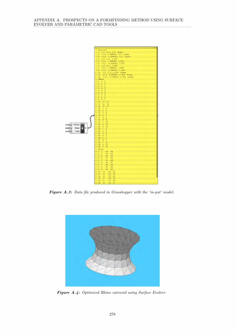
APPENDIX A. PROSPECTS ON A FORMFINDING METHOD USING SURFACEEVOLVER AND PARAMETRIC CAD TOOLS
Figure A.3: Data file produced in Grasshopper with the ‘in-put’ model.
Figure A.4: Optimized Rhino catenoid using Surface Evolver.
278

APPENDIX A. PROSPECTS ON A FORMFINDING METHOD USING SURFACEEVOLVER AND PARAMETRIC CAD TOOLS
The ‘output’ Grasshopper definition permits any Surface Evolver data file to be readin again, by using a short scripting code in Grasshopper, so once the geometries havebeen optimised in Evolver they can be reproduced in a CAD environment. As thedefinition is aimed at being useful for more than one particular entry, the numberof nodes and faces is required to be specified in Grasshopper using sliders, so anyarray of nodes can be imported in Rhino.
Horizontal, vertical and diagonals edges can be implemented separately, so thesurface can be defined by different sets of edges (rings, quadrilateral or triangularmesh, columns, diagonals or combinations of them). As previously mentioned, infurther phases of this research, edges are expected to define constructive elements,so this method will be of benefit when different structural systems are tested. Itmight also facilitate the fabrication process (i.e. definition of membrane’s tailoringseams) itself.
One of the main difficulties that this exercise presented was the addition of midpointsby Evolver at the centre of each quadrilateral facet, as the shape optimisationentailed the triangulation of them, thus it caused the variation on the initial numberof components. This was avoided by defining faces as oriented triangles in the ‘input’model, so when Evolver executes the optimization, no more nodes (thus no moreedges) are added.
Another difficulty that needed to be overcome to permit the interoperability betweenthese two environments was that while arrays in Evolver are zero-based, Grasshopperseries are one-based. Since Grasshopper offers many options to operate with seriesand arrays, it was decided to adapt the entire model to the Evolver’s language.
Screen-shots of both in-put and out-put Grasshopper models are shown in FiguresA.5 and A.6.
A.3 Testing Examples
This section shows the application of the model on two freeform closed curves. Ineach case, the ‘input’ Grasshopper definition was used to produce two very differentirregular shapes, by using different values for subdivision and extrusion parameters.
279
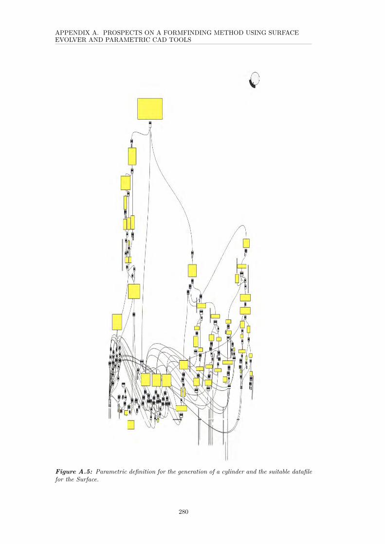
APPENDIX A. PROSPECTS ON A FORMFINDING METHOD USING SURFACEEVOLVER AND PARAMETRIC CAD TOOLS
Figure A.5: Parametric definition for the generation of a cylinder and the suitable datafilefor the Surface.
280

APPENDIX A. PROSPECTS ON A FORMFINDING METHOD USING SURFACEEVOLVER AND PARAMETRIC CAD TOOLS
Figure A.6: Parametric definition for form-found geometry obtained from the SurfaceEvolver.
281

APPENDIX A. PROSPECTS ON A FORMFINDING METHOD USING SURFACEEVOLVER AND PARAMETRIC CAD TOOLS
A.3.1 First Optimization of an Extruded Free-Form Curve
Figure A.7: Free-form curve produced inRhino.
Figure A.8: Extrusion of the free-formcurve by 14 off-settings, separation of 0.508length units, subdivided in 20 segments usingthe ‘input’ Grasshopper definition.
Figure A.9: Surface reproduced in SurfaceEvolver with a triangular mesh.
Figure A.10: Surface after 290 iterations.
Figure A.11: Optimized shape after 290iterations and 1 mesh relaxation step.
Figure A.12: New vertices reproducedin Rhino using the ‘output’ Grasshopperdefinition.
282

APPENDIX A. PROSPECTS ON A FORMFINDING METHOD USING SURFACEEVOLVER AND PARAMETRIC CAD TOOLS
Figure A.13: Vertices joint forming atriangular mesh using Grasshopper ‘output’definition.
Figure A.14: Vertices joint forminga quadrilateral mesh using the ‘output’Grasshopper definition.
Figure A.15: Vertices joint forming a setof parallels rings using Grasshopper ‘output’definition.
Figure A.16: Vertices joint forming paral-lels columns using the ‘output’ Grasshopperdefinition.
283

APPENDIX A. PROSPECTS ON A FORMFINDING METHOD USING SURFACEEVOLVER AND PARAMETRIC CAD TOOLS
A.3.2 Second Optimization of a Cylinder with a Free-Form Section
Figure A.17: Free-form curve produced inRhino.
Figure A.18: Extrusion of the secondfree-form curve by 5 offsetting, with aseparation of 0.217 length units, subdividedin 20 segments using the ‘input’ Grasshopperdefinition.
Figure A.19: Surface reproduced inSurface Evolver with a triangular mesh.
Figure A.20: Surface after 260 iterations.
284
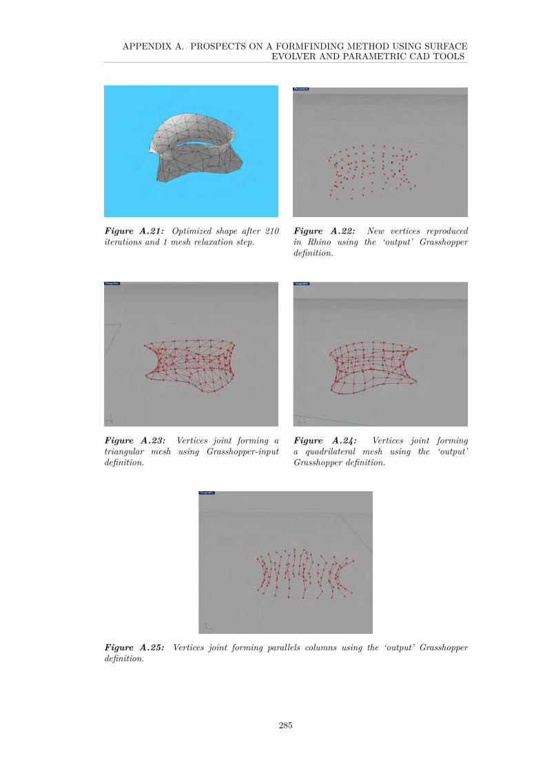
APPENDIX A. PROSPECTS ON A FORMFINDING METHOD USING SURFACEEVOLVER AND PARAMETRIC CAD TOOLS
Figure A.21: Optimized shape after 210iterations and 1 mesh relaxation step.
Figure A.22: New vertices reproducedin Rhino using the ‘output’ Grasshopperdefinition.
Figure A.23: Vertices joint forming atriangular mesh using Grasshopper-inputdefinition.
Figure A.24: Vertices joint forminga quadrilateral mesh using the ‘output’Grasshopper definition.
Figure A.25: Vertices joint forming parallels columns using the ‘output’ Grasshopperdefinition.
285

APPENDIX A. PROSPECTS ON A FORMFINDING METHOD USING SURFACEEVOLVER AND PARAMETRIC CAD TOOLS
Figure A.26: Optimized cylinder with oriented edges using surface Evolver.
A.4 Further Work Using Surface Evolver
A.4.1 Form-finding with oriented Boundaries
As figure A.26 shows, boundaries can be easily modified in their position from thedatafile. For example, this was made by simply modifying the original definition ofthe boundaries of the regular cylinder to:
PARAMETER RMAX = 1.5088795 // minimum radius for height
PARAMETER ZMAX = 1.0
boundary 1 parameters 1 // upper ring
x1: RMAX * cos(p1) * 1.5
x2: RMAX * sin(p1)
x3: ZMAX
boundary 2 parameters 1 // lower ring
x1: RMAX * cos(p1)
x2: RMAX * sin(p1) * 1.5
x3: -ZMAX
This option also suggests than more than two boundaries could be defined in theinitial datafile, so for instance tri or more axial system could be developed
A.4.2 Triple Periodic Minimal Surfaces
Minimal surfaces with crystalline structure are of particular interest for this re-search, both because of the Architectural possibilities that their enclosures mightsuggest, and also because they address the problem of replication, aggregation andtransformation earlier stated.
286

APPENDIX A. PROSPECTS ON A FORMFINDING METHOD USING SURFACEEVOLVER AND PARAMETRIC CAD TOOLS
Figure A.27: Evolution of the Schwarz’ P Surface using Surface Evolver.
There is a large number of fascinating triple periodic minimal surfaces [TPMS],many of them originally discovered by Alan Schoen in his famous report for NASA‘Infinite Periodic Minimal Surface without Self-Intersection’ from 1970 [3].
In Evolver, TPMS are achieved by defining and then optimising the fundamentalregion of the structure, which is then suitably transformed (duplicated, displaced androtated). The fundamental regions are usually very simple due their high symmetry.
Figure A.27 shows the development of the Schwarz’ P Surface in the Evolver, oneof the simplest and best-known cases of TPMS. Its fundamental region correspondsto a tetrahedron.
The upper images correspond to the fundamental section before and after its evo-lution. The lower images show one cubical unit cell (left) and then same unit cellrepeated and four times (right).
A.4.3 Synclastic Surfaces Using other Energies
As discussed earlier, minimal surfaces are intrinsically saddle shapes. Nevertheless,there are many different ways to run formfinding processes using different energies
287

APPENDIX A. PROSPECTS ON A FORMFINDING METHOD USING SURFACEEVOLVER AND PARAMETRIC CAD TOOLS
Figure A.28: Evolution of the mound using gravity.
to produce positive Gaussian curvature surfaces, the most basic ones are gravity andpressure.
Gravitational potential energy is important in shaping liquid drops lying on, hangingfrom, or up against fixed surfaces.
Figure A.28, shows the evolution of the ‘Mound’. As any other body, the initialvalue of gravity is zero and body density is 1. By a simple set of operations it canbe evolved to a hemisphere without gravity. The steps run in this case were:
r e f i n e edge where on_constra int 1g 10 // perform 10 minimizat ion i t e r a t i o n sr // r e f i n e meshg 10rg 20he s s i an // minimize energy by c a l c u l a t i n g second de r i va t e matrixhe s s i an
The same model can be used to model a drop hanging from the ceiling by settingnegative gravity [Fig. A.30]. The model below was made by setting gravity to -5 and
288

APPENDIX A. PROSPECTS ON A FORMFINDING METHOD USING SURFACEEVOLVER AND PARAMETRIC CAD TOOLS
Figure A.29: Hanging mound using negative gravity
turning the graphic window upside down. By evolving the surface to 50 iterations(g 50) it is possible to watch the drop fall.
An alternative method to achieve synclastic shapes is using pressure. Pressure is aforce per unit perpendicular to a surface.
As explained by Brakke [2], in the evolver, pressure can operate in three differentways:
1. “If a body has a volume constraint, then the boundary surface is unlikely to bea minimal surface. Hence, pressure is needed to counteract the desire of thesurface to shrink. When there are volume constraints, the evolver automaticallycalculates the pressure needed.
2. A body may have a prescribed pressure. Then the appropriated force is addedto the forces on the vertices when calculating the motion of the surface. Thisis a way of prescribing mean curvature, since pressure = surface tension *mean curvature. (Therefore, prescribed volume and prescribed pressure arenot possible on the same body, at the same time).
3. The evolver can treat bodies as being made of an isothermal ideal gas that isbodies can be compressible. The pressure given is the ambient pressure outsideall bodies. Each body must have a volume specified, which is the volume of thebody at the ambient pressure”.
Volume constraints are of particular interest for this design-based research. Theimage below shows the evolution of the ‘Bubble pipe’ with prescribed pressure,using the second approach. The maximum pressure state is when the two bubblesare hemispheres, where the pressure is 2 (pressure in a sphere is equal to [2*tension/radius]). The sequence shows the increasing pressure from 1, 1.5, 2, upto 3. Iterations, subdivision and mesh relaxations are run iteratively at each stage.
289
APPENDIX A. PROSPECTS ON A FORMFINDING METHOD USING SURFACEEVOLVER AND PARAMETRIC CAD TOOLS
If the pressure is increased beyond the critical value of 2, the bubble surface mightnot be stable and it is likely to expand infinitely if, as the pressure is too high.
A.5 Conclusions
The proposed formfinding method has proved successful for the generation of min-imal surfaces with different curvatures subject to physical and geometrical con-straints, as well as for the integration of mathematical and CAD software tools.
Although few examples have been demonstrated, Surface Evolver offers an extraor-dinarily powerful platform to operate with well known stable minimal surfaces or toproduce new ones. It is suggested that the aggregation of components with differentgeometrical definitions can be easily executed in the Rhino environment.
The possibility to operate with many diverse constraints suggests that this method-ology can handle the incorporation of the design conditions previously defined inChapter II, for which their parameterization (or translation into quantitative at-tributes) turns out of radical importance. In this way, for example, external forces(like snow and wind load) or specific volume constraints could be incorporate asconstraints for the design of surfaces.
From a geometrical perspective, futures challenge for this method clearly pointstowards the generation of more complex surfaces, which can only be achieved witha deeper comprehension on the mathematical and topological properties of minimalsurfaces, as earlier suggested. Even though the work shown in this chapter is aninitial exploration, the comprehension of the operatibility of very different digitalenvironments, rather than their usage in a traditional way, has opened an incrediblywide range of suitable possibilities to be studied and used for the purposes of thisresearch.
A.6 References
[1] Brakke, K., 1992.The Surface Evolver. Experimental Mathematics, 1(2), pp. 141-165. [2] Brakke K. A., 2008. Surface Evolver Manual. Version 2.30. Selinsgrove,USA: Susquehanna University. [3] Schoen, A., 1970. Infinite Periodic MinimalSurfaces without Self-intersections. Washington, D. C., USA: NASA (TN D-5541)
290
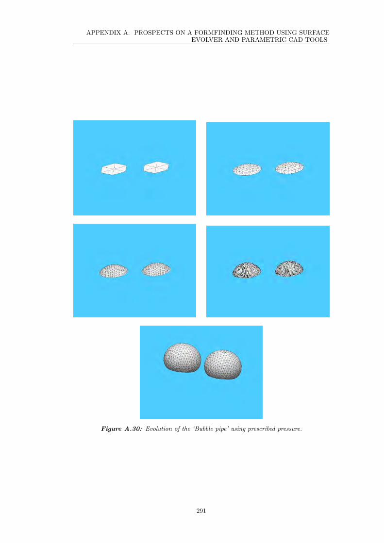
APPENDIX A. PROSPECTS ON A FORMFINDING METHOD USING SURFACEEVOLVER AND PARAMETRIC CAD TOOLS
Figure A.30: Evolution of the ‘Bubble pipe’ using prescribed pressure.
291


Appendix B
Calculations of Peak Velocity Pressure
As indicated by the Danish Standard [1], the factors to be considered for Wind Loadfor Vaulted Roofs and Domes can be listed as:
cdir is a directional factor (1.0 can be used conservatively)
cseason is a seasonal factor (1.0 can be used conservatively)
vb,0 is the base value for the wind velocity (in this case set to 12.8 m/s [2])
The basic wind velocity vb can be calculated as:
vb = cdircseasonvb,0 = 12.8 m/s
Given that,
z0 is the roughness length (0.010 according to Table EC4.1 assuming terraincategory I)
ze is the reference height (6.00 m for the largest span)
zmin is the minimum height (1 m according to Table EC4.1 assuming terraincategory I)
z0,II roughness length for terrain category II (0.05 m according to Table EC4.1)
co is an orography factor (conservatively set to 1.0)
ρ is the air density (1.25 kg/m3 at ground level)
kl is a turbulence factor (recommended value 1.0)
293
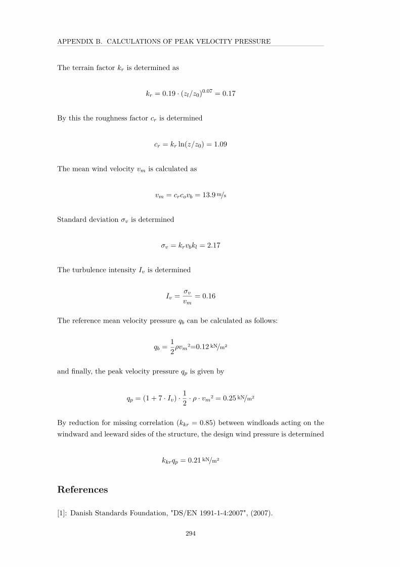
APPENDIX B. CALCULATIONS OF PEAK VELOCITY PRESSURE
The terrain factor kr is determined as
kr = 0.19 · (zl/z0)0.07 = 0.17
By this the roughness factor cr is determined
cr = kr ln(z/z0) = 1.09
The mean wind velocity vm is calculated as
vm = crcovb = 13.9 m/s
Standard deviation σv is determined
σv = krvbkl = 2.17
The turbulence intensity Iv is determined
Iv = σvvm
= 0.16
The reference mean velocity pressure qb can be calculated as follows:
qb = 12ρvm2=0.12 kN/m2
and finally, the peak velocity pressure qp is given by
qp = (1 + 7 · Iv) ·12 · ρ · vm2 = 0.25 kN/m2
By reduction for missing correlation (kkr = 0.85) between windloads acting on thewindward and leeward sides of the structure, the design wind pressure is determined
kkrqp = 0.21 kN/m2
References
[1]: Danish Standards Foundation, "DS/EN 1991-1-4:2007", (2007).
294

APPENDIX B. CALCULATIONS OF PEAK VELOCITY PRESSURE
[2]: C. González, “Chile triplica investigacion en la Antartica en los ultimos años”(2014), Santiago: La Tercera, 2-3.
295


Appendix C
C-sharp Component for the Placementof Trussed Arches along a NURBS Curve
The code below is taken from a C# scripting block within the Grasshopper© envi-ronment.
/// <summary >
/// This procedure contains the user code. Input
parameters are provided as regular arguments ,
/// Output parameters as ref arguments. You don ’t have
to assign output parameters ,
/// they will have a default value.
/// </summary >
private void RunScript(Curve crv1 , Curve crv2 , double
step , ref object P, ref object D, ref object O)
//ONLY WORKS WHEN CURVE IS RUNNING ALONG X-AXIS!!
// Define lists to store results
List <Point3d > points = new List <Point3d >();
List <double > diameters = new List <double >();
List <Point3d > originPoints = new List <Point3d >();
// Define variable to store new point
Point3d newPoint;
// Define s as length parameter on curve
297

APPENDIX C. C-SHARP COMPONENT FOR THE PLACEMENT OF TRUSSEDARCHES ALONG A NURBS CURVE
double s = 0;
// Define lastS as the last valid length parameter
double lastS;
//Calc arc diameter
double diameter = getRoundedDiameter(crv1 , crv2 , s,
step);
//Add point at begining of curve
newPoint = crv1.PointAtLength(s);
//Make sure arch has incremented diameter.
newPoint.Y = diameter / 2;
points.Add(newPoint);
originPoints.Add(new Point3d(newPoint.X, 0, 0));
lastS = s;
// Store last diameter in list
diameters.Add(diameter);
//Move along curve in small increments
while (s < crv1.GetLength ())
//Move a small step along the curve by increasing
the length parameter
s += 0.05;
//Get rounded diameter
diameter = getRoundedDiameter(crv1 , crv2 , s, step);
//Check gap if gap is larger than maximum gap for
the given diameter.
double gap = Math.Abs(points[points.Count - 1].X -
crv1.PointAtLength(s).X);
Print("gap:" + gap);
if (gap > maxgap(diameter , diameters[diameters.
Count - 1]))
298

APPENDIX C. C-SHARP COMPONENT FOR THE PLACEMENT OF TRUSSEDARCHES ALONG A NURBS CURVE
Print("Creatingarc!");
//If gap is too large , create a arc at the last
valid length parameter , lastS.
//Get last valid diameter
diameter = getRoundedDiameter(crv1 , crv2 , lastS ,
step);
// Create point for arc at last valid parameter
newPoint = crv1.PointAtLength(lastS);
// Make sure arch has incremented diameter.
newPoint.Y = diameter / 2;
points.Add(newPoint);
originPoints.Add(new Point3d(newPoint.X, 0, 0));
//Add to list of diameters
diameters.Add(diameter);
else
Print("Keeplooking!");
//If not , update lastS
lastS = s;
P = points;
D = diameters;
O = originPoints;
// <Custom additional code >
double getRoundedDiameter(Curve crv1 , Curve crv2 ,
double s, double step)
double diameter = crv1.PointAtLength(s).DistanceTo(
crv2.PointAtLength(s));
299

APPENDIX C. C-SHARP COMPONENT FOR THE PLACEMENT OF TRUSSEDARCHES ALONG A NURBS CURVE
//Snap to nearest diameter increment
return Math.Round(diameter / step) * step;
double maxgap(double diameter , double prevdiameter)
double maxgap = 0;
if (diameter < 4)
maxgap += 2.4 / 2;
else if (diameter < 5)
maxgap += 1.81 / 2;
else if (diameter < 6)
maxgap += 1.3 / 2;
else if (diameter == 6)
maxgap += 2.2 / 2;
else if (diameter < 7)
maxgap += 1.95 / 2;
else if (diameter < 8)
maxgap += 1.71 / 2;
else if (diameter == 8)
maxgap += 1.77 / 2;
else if (diameter < 9)
maxgap += 1.5 / 2;
else if (diameter < 10)
maxgap += 1.23 / 2;
else if (diameter == 10)
maxgap += 1.67 / 2;
else if (diameter < 11)
maxgap += 1.43 / 2;
else if (diameter <= 12)
maxgap += 1.2 / 2;
if (prevdiameter < 4)
maxgap += 2.4 / 2;
else if (prevdiameter < 5)
maxgap += 1.81 / 2;
else if (prevdiameter < 6)
maxgap += 1.3 / 2;
300

APPENDIX C. C-SHARP COMPONENT FOR THE PLACEMENT OF TRUSSEDARCHES ALONG A NURBS CURVE
else if (prevdiameter == 6)
maxgap += 2.2 / 2;
else if (prevdiameter < 7)
maxgap += 1.95 / 2;
else if (prevdiameter < 8)
maxgap += 1.71 / 2;
else if (prevdiameter == 8)
maxgap += 1.77 / 2;
else if (prevdiameter < 9)
maxgap += 1.5 / 2;
else if (prevdiameter < 10)
maxgap += 1.23 / 2;
else if (prevdiameter == 10)
maxgap += 1.67 / 2;
else if (prevdiameter < 11)
maxgap += 1.43 / 2;
else if (prevdiameter <= 12)
maxgap += 1.2 / 2;
return maxgap;
// </Custom additional code >
301