İSTANBUL TECHNICAL UNIVERSITY INSTITUTE OF SCIENCE AND TECHNOLOGY

M.Sc. Thesis by

Levent ÖNCÜ, B. Sc.

Department : Aeronautics and Astronautics Engineering

Programme : Aeronautics and Astronautics Engineering

Whatever Engineering

JUNE 2008

MULTIDISCIPLINARY DESIGN OPTIMIZATION OF AEROSPACE

STRUCTURES WITH STATIC AEROELASTIC CRITERIA

İSTANBUL TECHNICAL UNIVERSITY INSTITUTE OF SCIENCE AND TECHNOLOGY

M.Sc. Thesis by

Levent ÖNCÜ, B. Sc.

511061015

Date of submission : 05 May 2008

Date of defence examination : 09 June 2008

Supervisor (Chairman) :Assis. Prof. Dr. Melike NİKBAY (İTÜ)

Members of the Examining Committe : Prof. Dr. Metin Orhan KAYA (İTÜ)

Assis. Prof. Dr. Esra SORGÜVEN (Y.Ü.)

JUNE 2008

MULTIDISCIPLINARY DESIGN OPTIMIZATION OF AEROSPACE

STRUCTURES WITH STATIC AEROELASTIC CRITERIA

HAZİRAN 2008

İSTANBUL TEKNİK ÜNİVERSİTESİ FEN BİLİMLERİ ENSTİTÜSÜ

YÜKSEK LİSANS TEZİ

Levent ÖNCÜ

511061015

Tezin Enstitüye Verildiği Tarih : 05 Mayıs 2008

Tezin Savunulduğu Tarih : 09 Haziran 2008

Tez Danışmanı : Yrd. Doç. Dr. Melike NİKBAY (İTÜ)

Diğer Jüri Üyeleri : Prof. Dr. Metin Orhan KAYA (İTÜ)

Yrd. Doç. Dr. Esra SORGÜVEN (Y.Ü.)

UÇAK-UZAY YAPILARININ STATİK AEROELASTİK KRİTER İLE ÇOK

DİSİPLİNLİ TASARIM OPTİMİZASYONU

iii

ACKNOWLEDGEMENT

Although this thesis seems only my work, numerous people contributed to the

production of this thesis. I am grateful to those people who have made this thesis

possible by supporting and encouraging me.

First of all, I wish to express my gratitude to my colleague Arda Yanangönül to be

always with me by listening and answering by never-ending questions in a

constructive way. I would like to thank for his support.

I also want to express my gratitude to my advisor, Assistant Professor Melike Nikbay

for her support and guidance during my graduate. It was a pleasure for me to work in

her career project.

Many thanks to my colleague Ahmet Aysan.

Much appreciation to the academic staff of the Aeronautics and Astronautics Faculty

of the İstanbul Technical University for sharing their valuable knowledge and

experience.

Thank you to The Scientific and Technological Research Council of Turkey –

TÜBİTAK for financial support during my graduate with the National Scholarship

Program for the Graduate Students. This study is also partly financed by the

TÜBİTAK career project titled ―Analysis and Reliability Based Design Optimization

of Fluid-Structure Interaction Problems Subject to Instability Phenomena‖ with grant

number 105M235.

I am pleased to thank Informatics Institute of İstanbul Technical University for

letting me use their facilities.

Thank you to Mauro Poian and Rosario Russo from ESTECO Italy for their

assistance and patience to help me to prepare the core of my study.

I would like to express my deep appreciation and thanks to the general manager of

the DENAK Ship Management&Agency Serdar Akçalı to help me have a new vision

of life and education. Without him I could not be successful in my academic career.

Many friends have helped me stay sane through my graduate. Their support and care

helped me overcome all the difficulties. I greatly value their friendship and I deeply

appreciate their belief in me.

Most importantly, none of this would have been possible without the love and

patience of my family Mustafa, Şerife and Korhan Öncü. I would like to express my

heart-felt gratitude to my family.

Finally, a special appreciate to Melis…for her love, support, patience and

understanding….

June 2008 Levent ÖNCÜ

iv

TABLE OF CONTENTS Page

LIST OF TABLES .................................................................................................... vi

LIST OF FIGURES ................................................................................................. vii

ABBREVIATIONS ................................................................................................... ix

NOMENCLATURE ................................................................................................... x

SUMMARY .............................................................................................................. xii

ÖZET ........................................................................................................................ xiii

1. MULTIDISCIPLINARY DESIGN AND AEROELASTICITY ........................ 1 1.1 What is multidisciplinary design? ...................................................................... 1

1.2 Aeroelasticity ..................................................................................................... 1

1.3 Computational aeroelasticity .............................................................................. 3

2. COMPUTATIONAL AEROELASTICITY LITERATURE REVIEW ........... 5 2.1 What is computational aeroelasticity? ................................................................ 5

2.2 Review of aeroelastic studies in the past decade ................................................ 6

2.3 Conclusion ........................................................................................................ 13

3. MULTIDISCIPLINARY DESIGN OPTIMIZATION ..................................... 16 3.1 Need for multidisciplinary design optimization ............................................... 16

3.2 Aeroelastic optimization literature review ....................................................... 18

3.3 Conclusion ........................................................................................................ 21

4. COMPUTATIONAL AEROELASTIC PROCEDURE ................................... 22 4.1 Computational structural dynamics solver ....................................................... 22

4.2 Computational fluid dynamics solver .............................................................. 23

4.2.1 Remeshing methods .................................................................................. 24

4.2.1.1 Spring based smoothing method ........................................................ 25

4.2.1.2 Dynamic layering ............................................................................... 25

4.2.1.3 Local remeshing methods .................................................................. 25

4.3 Aeroelastic coupling ......................................................................................... 26

4.3.1 Coupling regions ....................................................................................... 26

4.3.2 Data exchange ........................................................................................... 27

4.3.2.1 Pre-contact search .............................................................................. 27

4.3.2.2 Minimal distance ................................................................................ 27

4.3.2.3 Intersection ......................................................................................... 28

4.3.2.4 Flux and field interpolation ................................................................ 28

4.4 Aeroelastic code coupling with MpCCI ........................................................... 28

4.5 Aeroelastic coupling algorithm and solution procedure................................... 30

5. TEST CASE FOR AEROELASTIC COUPLING WITH MpCCI ................. 32 5.1 Geometric model of AGARD 445.6 aeroelastic wing ..................................... 32

5.2 CSD model of the AGARD 445.6 weakened model and validation ................ 33

5.3 CFD model of the AGARD 445.6 weakened model ........................................ 36

5.4 Aeroelastic analysis results .............................................................................. 38

6. MULTIDISCIPLINARY MULTI-OBJECTIVE DESIGN OPTIMIZATION ........ 41

v

6.1 Formulation of optimization problems ............................................................. 41

6.2 Design variables ............................................................................................... 42

6.3 Constraints ........................................................................................................ 43

6.4 Objective functions .......................................................................................... 43

6.5 Optimization problem ...................................................................................... 44

6.6 Optimization algorithms ................................................................................... 44

6.6.1 Non-dominated sorting genetic algorithm (NSGA-II) .............................. 46

6.7 modeFRONTIER optimization workflow ........................................................ 48

7. OPTIMIZATION RESULTS .............................................................................. 53 7.1 Results for the optimization problem ............................................................... 53

7.2 Conclusion ........................................................................................................ 58

REFERENCES ......................................................................................................... 60

APPENDICES .......................................................................................................... 68

RESUME ................................................................................................................... 86

vi

LIST OF TABLES Page No:

Table 2.1: Review of some methodologies for aeroelastic applications ................... 14

Table 2.2: Review of some couplings done by MpCCI ............................................ 15

Table 5.1: AGARD 445.6 material properties .......................................................... 34

Table 5.2: Frequency comparison ............................................................................. 35

Table 6.1: Design variables ....................................................................................... 42

Table 6.2: Constraints ............................................................................................... 43

Table 6.3: Objective functions .................................................................................. 43

Table 6.4: Software used in the aeroelastic optimization process ............................. 48

Table 7.1: Pareto designs ......................................................................................... 54

Table 7.2: Results for the selected pareto designs ................................................... 58

Table B.1: Design summary ...................................................................................... 83

vii

LIST OF FIGURES Page No:

Figure 1.1 : Aeroelastic triangle of Collar .................................................................. 2

Figure 1.2 : Deformation of wing due to aerodynamic loads ..................................... 2

Figure 1.3 : Aeroelastic forces and their interaction ................................................... 3

Figure 1.4 : Levels of fidelity in FSI modeling........................................................... 4

Figure 3.1 : Simple aero-structural optimization scheme [60]…………………….. 16

Figure 3.2 : Design requirements expansion [43] ………………………………….17

Figure 4.1 : MpCCI coupling process [85] …………………………………………26

Figure 4.2 : Data exchange for unmatching grids [85] …………………………….27

Figure 4.3 : Pre-contact search [85] ………………………………………………..27

Figure 4.4 : Element selection [85]………………………………………………....28

Figure 4.5 : Aeroelastic coupling process [85] …………………………………….30

Figure 4.6 : Staggered algorithm for the aeroelastic coupling ……………………..30

Figure 5.1 : AGARD 445.6 wing geometry ……………………………………….32

Figure 5.2 : AGARD 445.6 weakened model ……………………………………..33

Figure 5.3 : The finite element model of the AGARD 445.6 wing ………………..34

Figure 5.4 : Mode shapes comparison ……………………………………………..36

Figure 5.5 : Close up mesh cross section ………………………………………….37

Figure 5.6 : Wing model and wing root ……………………………………………37

Figure 5.7 : Pressure far field computational grid …………………………………37

Figure 5.8 : Pressure distributions on the upper wing surface ……………………..38

Figure 5.9 : Pressure distributions on the lower wing surface ……………………..38

Figure 5.10 : Pressure coefficient distribution at 34% span ………………………39

Figure 5.11 : Pressure coefficient distribution at 67% span ……………………….39

Figure 5.12 : Vertical deflection of the wing along span relative to the wing root ...40

Figure 5.13 : Wing‘s initial and equilibrium positions ……………………………40

Figure 6.1 : Pareto optimal solutions ………………………………………………45

Figure 6.2 : Basic structure of genetic algorithm ………………………………….46

Figure 6.3 : Work diagram of NSGA-II ……………………………………………47

Figure 6.4 : Scheduler ……………………………………………………………..49

Figure 6.5 : CFD branch …………………………………………………………..49

Figure 6.6 : CSD branch …………………………………………………………..50

Figure 6.7 : Aeroelastic analysis, post processing and optimization ……………….51

Figure 6.8 : Optimization workflow ……………………………………………….52

Figure 7.1 : Design summary .................................................................................... 53

Figure 7.2 : Scatter chart minimum weight vs maximum L/D ................................. 55

Figure 7.3 : Scatter chart taper vs minimum weight ................................................. 56

Figure 7.4 : Scatter chart taper vs maximum L/D ..................................................... 56

Figure 7.5 : Correlation matrix (sweep-max L/D-min weight) ................................. 57

viii

Figure 7.6 : Correlation matrix (taper-max L/D-min weight) ................................... 57

Figure B.1 : Structural analysis results for /4 32c

and 0.2 .......................... 80

Figure B.2 : Pressure coefficients for lower and upper wing surfaces respectively for

/4 32c and 0.2 ....................................................................................... 81

ix

ABBREVIATIONS

2D : Two-dimensional

3D : Three-dimensional

AGARD : Advisory Group for Aerospace Research and Development

ALE : Arbitrary Lagrangian Eulerian

ARW-2 : Aeroelastic research wing two

CA : Computational aeroelasticity

CAD : Computer aided design

CFD : Computational fluid dynamics

CSD : Computational structural dynamics

DLR : Institute for Aerodynamics and Flow Technology

DNS : Direct numerical simulation

FEA : Finite element analysis

FEM : Finite element method

FSI : Fluid structure interaction

MDO : Multi-Disciplinary optimization

MLS : Moving Least Squares

MO : Multi objective

MOGA : Multi objective genetic algorithm

MpCCI : Mesh based Parallel Code Coupling Interface

NSGA-II : Non dominated sorting genetic algorithm two

RANS : Reynolds averaged Navier-Stokes

Ref : Reference

SQP : Sequential quadratic programming

TSD : Transonic small disturbance

x

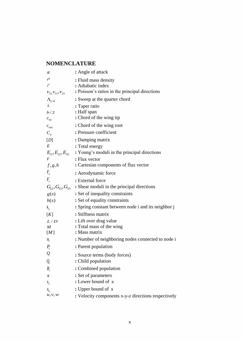
NOMENCLATURE

: Angle of attack

: Fluid mass density

: Adiabatic index

12, 13 23, : Poisson‘s ratios in the principal directions

/4c : Sweep at the quarter chord

: Taper ratio

/ 2b : Half span

tipc : Chord of the wing tip

rootc : Chord of the wing root

pC : Pressure coefficient

[ ]D : Damping matrix

E : Total energy

11 22 33, ,E E E : Young‘s moduli in the principal directions

F : Flux vector

, ,f g h : Cartesian components of flux vector

aF : Aerodynamic force

eF : External force

12 13 23, ,G G G : Shear moduli in the principal directions

( )g s : Set of inequality constraints

( )h s : Set of equality constraints

ijk : Spring constant between node i and its neighbor j

[ ]K : Stiffness matrix

/L D : Lift over drag value

M : Total mass of the wing

[ ]M : Mass matrix

in : Number of neighboring nodes connected to node i

tP : Parent population

Q : Source terms (body forces)

tQ : Child population

tR : Combined population

s : Set of parameters

Ls : Lower bound of s

us : Upper bound of s , ,u v w : Velocity components x-y-z directions respectively

xi

maxu : Maximum displacement of the wing

u : Displacement u : First time derivative of displacement u : Second time derivative of displacement U : Conservative variables

,j ix x

: Displacement of node i and its neighbor j

xii

MULTIDISCIPLINARY DESIGN OPTIMIZATION OF AEROSPACE

STRUCTURES WITH STATIC AEROELASTIC CRITERIA

SUMMARY

Multi-disciplinary design analysis and optimization has attracted attention in the past

two decades. There are many studies done with academic codes but there are few

examples of studies done with fully commercial softwares on aeroleastic

optimization. This study aims to fill this need.

In this thesis aeroelastic optimization is performed on a basic experimental wing

model based on AGARD 445.6 elastic wing configuration to obtain the objectives

maximum lift over drag ratio and minimum weight of the wing. A static aeroelastic

criteria is given as a design constraint to satisfy the maximum tip deflection. Sweep

angle at the quarter chord and the taper ratio of the wing are used as design

parameters for this study. Moreover, a genetic algorithm NSGA-II is used to control

the optimization process.

The optimization study is done by using the Multi-Objective Design Environment

(mode)FRONTIER 4.0 optimization software with the user written scripts to perform

this study: ABAQUS 6.7-1 finite element solver script to prepare the computational

structural dynamics (CSD) model, FLUENT 6.3.26 and GAMBIT 2.2.30 scripts to

prepare the computational fluid dynamics (CFD) model and Mesh based Parallel

Code Coupling Interface-MpCCI 3.0.6 script to perform loosely coupled aeroelastic

analysis.

Aeroelastic analysis is done by employing a staggered algorithm in a loosely coupled

approach. Aerodynamic surface pressures are converted to nodal forces and

transferred to the CSD code, then under these forces static analysis is performed and

nodal displacements are transfered to CFD code as mesh motion. This process is

controlled by MpCCI 3.0.6 software.

The results from the structural, fluid and aeroelastic fields are used to compare the

results with the numerical and the wind tunnel data of the AGARD 445.6 wing. Once

the wing is validated with the literature date, the aeroelastic optimization study is

performed.

The pareto set for the optimum designs are obtained at the end of the aeroelastic

optimization study to choose the best design configuration. The effect of the design

variables on objective functions and their relationship are examined by using the

optimization problem results.

xiii

UÇAK-UZAY YAPILARININ STATİK AEROELASTİK KRİTER İLE ÇOK

DİSİPLİNLİ TASARIM OPTİMİZASYONU

ÖZET

Son yirmi yılda çok disiplinli analiz ve optimizasyon konuları büyük bir oranda ilgi

çekmektedir. Aeroelastik optimizasyon konusunda akademik kodlarla yapılan bir çok

çalışmaya rastlamak mümkünken, tamamiyle ticari kodlarla yapılan çalışmalara daha

az rastlanmaktadır. Bu çalışma bu ihtiyacı doldurmak için bir şans vermiştir.

Bu tez çalışmasında aeroelastik optimizasyon AGARD 445.6 elastik kanat

konfigürasyonundan yola çıkılarak basit bir kanat için en yüksek taşıma/sürükleme

oranı ve en düşük kütle amaç fonksiyonlarına ulaşmak için yapılmıştır. Tasarım kısıtı

olarak bir statik aerolastik kriter olan en yüksek uç yer değiştirmesi verilmiştir.

Kanadın çeyrek veterdeki ok açısı ve sivrilme oranı tasarım parametreleri olarak

atanmıştır. Ayrıca bu çalışmada optimizasyon döngüsünü kontrol etmek için bir

genetik algoritma olan NSGA—II algoritması kullanılmıştır.

Optimizasyon çalışması çok amaçlı tasarım ortamı (mode)FRONTIER 4.0

optimizasyon yazılımı kullanılarak yapılmıştır. Bu çalışmayı yapmak için çeşitli

betikler yazılmıştır: ABAQUS 6.7-1 sonlu eleman çözücüsü betiği yapısal modeli

hazırlamak için, FLUENT 6.3.26 ve GAMBIT 2.2.30 betikleri hesaplamalı

akışkanlar dinamiği (HAD) modelini hazırlamak için ve çözüm ağı tabanlı paralel

kod eşleme arayüzü MpCCI 3.0.6 ise gevşek bağlaşımlı aeroelastik analizleri

yürütmek için kullanılmıştır.

Aeroelastik analizler bir sıralı―staggered‖ algoritma kullanılarak gevşek bağlaşımlı

olarak çözülmüştür. Aerodinamik yüzey yükleri düğüm bazlı kuvvetlere çevrilerek

yapısal çözücüye aktarılmakta, bu yükler altında yapılan statik analiz sonucunda

oluşan yer değiştirmeler ise akışkan koduna çözüm ağı hareketi olarak

gönderilmektedir. Bu çevrim MpCCI 3.0.6 yazılımı tarafından kontrol edilmektedir.

Yapısal, akışkan ve aeroelastik analizler sonunda alınan sonuçlar AGARD 445.6

kanadı üstüne yapılmış önceki sayısal ve rüzgar tüneli verileri ile karşılaştırılmıştır.

Karşılaştırmadan sonra geçerliliği onaylanan kanat kullanılarak aeroelastik

optimizasyon çalışması yapılmıştır.

Aeroelastik optimizasyon sonunda en uygun çözümü seçebilmek için pareto kümesi

oluşturulmuştur. Tasarım değişkenlerinin amaç fonksiyonları üzerindeki etkileri ve

aralarında ilişki sonuçlar değerlendirilerek yapılmıştır.

1

1. MULTIDISCIPLINARY DESIGN AND AEROELASTICITY

1.1 What is multidisciplinary design?

To develop new and complex design technologies in aerospace industry, high levels

of integration between different disciplines like aerodynamics, structural dynamics,

propulsion, control, acoustics, heat transfer are needed. Since the behaviors of these

disciplines are mutually interactive, they cannot be thought separately. When at least

two or more disciplines interact, the nature of the evolved problem is defined as

―multi-disciplinary‖ and the design problem regarding to these disciplines is named

as ―multi-disciplinary design‖.

One of the most commonly studied areas regarding multi-disciplinary design is the

interaction between a flexible structure and the fluid surrounding the structure which

is known as ―Fluid Structure Interaction (FSI)‖. FSI gives rise to a deep diversity of

phenomena with applications of many engineering areas, such as, the stability of an

aircraft wing, design of bridges, the flow of blood through arteries [1].

1.2 Aeroelasticity

One of the most important fields of FSI problems is ―aeroelasticity‖. According to

Bisplinghoff et al [2] aeroelasticity is the phenomena which exhibit appreciable

reciprocal interaction (static or dynamic) between aerodynamic forces and the

deformations induced thereby in the structure of a flying vehicle, its control

mechanisms, or its propulsion systems. According to the Collar‘s definition in 1946

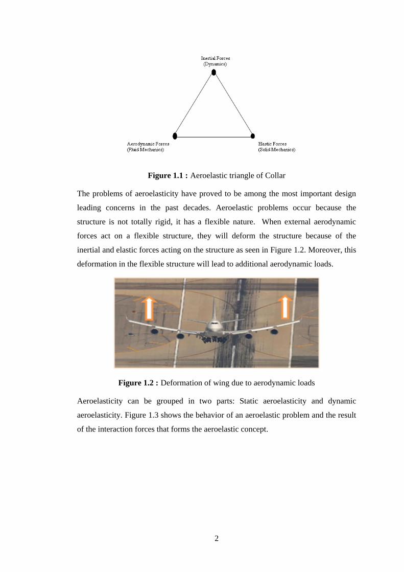
aeroelasticity could be shown as a triangle shown in Figure 1.1. More definition

about the aeroelasticity can be found in [3-5].

2

Figure 1.1 : Aeroelastic triangle of Collar

The problems of aeroelasticity have proved to be among the most important design

leading concerns in the past decades. Aeroelastic problems occur because the

structure is not totally rigid, it has a flexible nature. When external aerodynamic

forces act on a flexible structure, they will deform the structure because of the

inertial and elastic forces acting on the structure as seen in Figure 1.2. Moreover, this

deformation in the flexible structure will lead to additional aerodynamic loads.

Figure 1.2 : Deformation of wing due to aerodynamic loads

Aeroelasticity can be grouped in two parts: Static aeroelasticity and dynamic

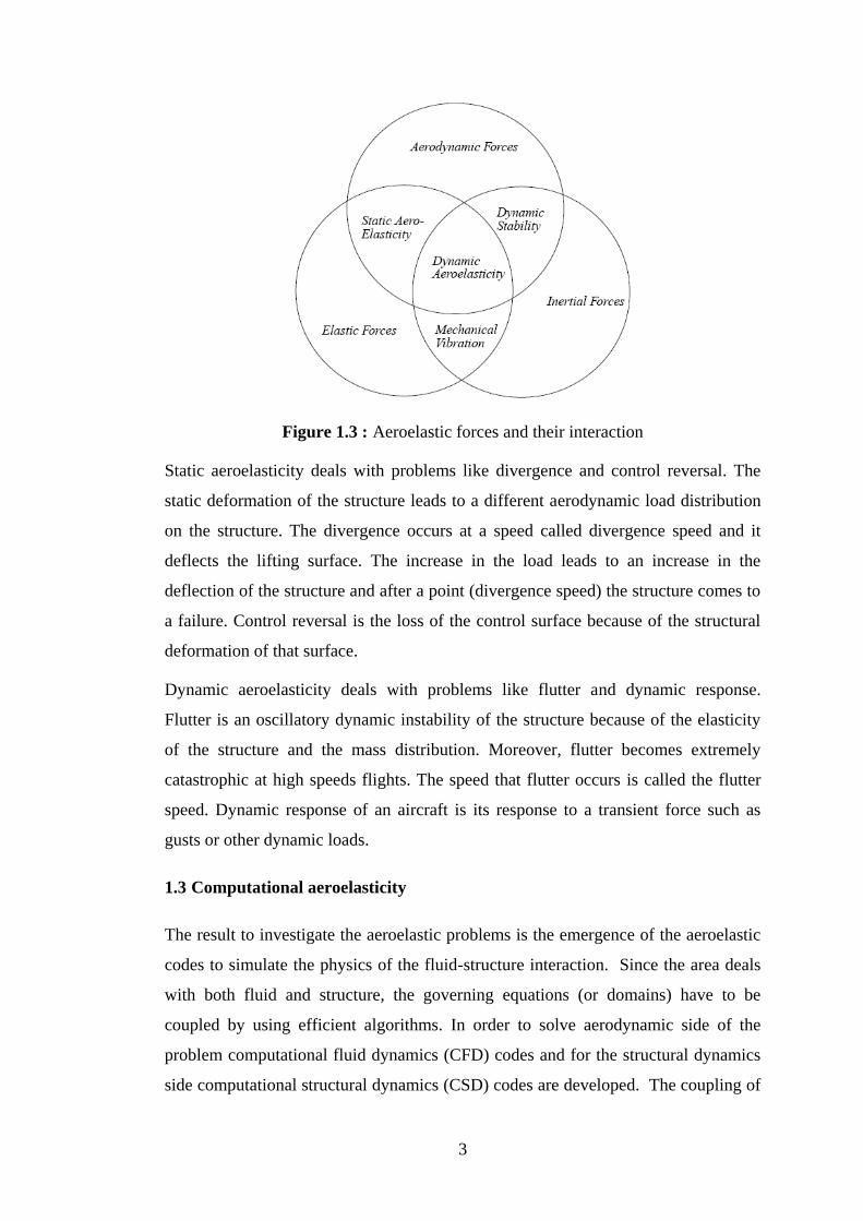
aeroelasticity. Figure 1.3 shows the behavior of an aeroelastic problem and the result

of the interaction forces that forms the aeroelastic concept.

3

Figure 1.3 : Aeroelastic forces and their interaction

Static aeroelasticity deals with problems like divergence and control reversal. The

static deformation of the structure leads to a different aerodynamic load distribution

on the structure. The divergence occurs at a speed called divergence speed and it

deflects the lifting surface. The increase in the load leads to an increase in the

deflection of the structure and after a point (divergence speed) the structure comes to

a failure. Control reversal is the loss of the control surface because of the structural

deformation of that surface.

Dynamic aeroelasticity deals with problems like flutter and dynamic response.

Flutter is an oscillatory dynamic instability of the structure because of the elasticity

of the structure and the mass distribution. Moreover, flutter becomes extremely

catastrophic at high speeds flights. The speed that flutter occurs is called the flutter

speed. Dynamic response of an aircraft is its response to a transient force such as

gusts or other dynamic loads.

1.3 Computational aeroelasticity

The result to investigate the aeroelastic problems is the emergence of the aeroelastic

codes to simulate the physics of the fluid-structure interaction. Since the area deals

with both fluid and structure, the governing equations (or domains) have to be

coupled by using efficient algorithms. In order to solve aerodynamic side of the

problem computational fluid dynamics (CFD) codes and for the structural dynamics

side computational structural dynamics (CSD) codes are developed. The coupling of

4

a CFD and a CSD code in a computational manner is defined as ―computational

aeroelasticity (CA)‖ [6].

Complexity of an aeroelastic problem depends on not only the theory or method

which will be used to solve the aerodynamic and structural forces but also the

interfacing between these forces. For the CFD side look up tables, linear analytical

methods, transonic small disturbance, full potential or high fidelity Euler/Navier-

Stokes solver can be used. For the CSD side shape functions, modal approach, 2D

finite elements, simple 3D finite elements or high fidelity 3D finite element codes

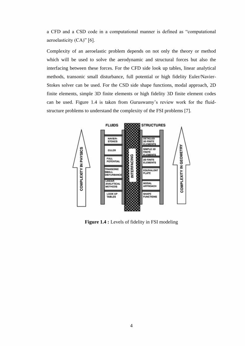
can be used. Figure 1.4 is taken from Guruswamy‘s review work for the fluid-

structure problems to understand the complexity of the FSI problems [7].

Figure 1.4 : Levels of fidelity in FSI modeling

5

2. COMPUTATIONAL AEROELASTICITY LITERATURE REVIEW

2.1 What is computational aeroelasticity?

The problems of aeroelasticity have been proved to be among the most important

design leading concerns in aircraft design in the past decades. Since the area deals

with both the fluid and the structure, the governing equations (or domains) have to be

coupled using efficient algorithms. This review of literature will make use of the

surveys published in the past few years to demonstrate where the field of

aeroelasticity is heading to. Then, published work of several prominent authors in

the field is examined.

As previously expressed, a major problem in aeroelasticity is the transformation of

physical data between fluid and structure models (i.e., pressure and displacement

field). While the structural model could be simple, this may not be the case with fluid

model or vice versa. Thus, different methods are used to couple and evaluate the

models. There are three methods of coupling the two models as mentioned in the

work of Kamakoti et al [10] and Smith et al [8].

The first of these is the fully coupled method where the governing equations of the

fluid and structure domain is written as a single set of equations and solved. Usually,

the structural model is simple such as plates and beams while the fluid solver uses

Navier-Stokes equations [8]. Fully coupling is usually considered computationally

expensive and generally used for 2D models (such as beams and plates).

The second one is the the ―closely coupled method‖ which is widely used. In this

method, the transformation of the data between two domains is done by different

modules and transformed at each step. The fluid is usually modeled using

Euler/Navier-Stokes and the solid can be modeled by using finite elements such as

solids, beams, shells and plates. Since the coupling is done with the transformation of

data at each iterative step, the fluid and structural models can be changed according

to the model [8].

6

The last method is the loosely coupled one. In loosely coupled method fluid and

structure problems are taken as two sub-systems with external interactions between

them. It is the simplest coupling type of FSI problems. It also allows designer to use

validated in house codes for the simulation of fluid-structure interactions.

Another difficulty arises when interpolating/extrapolating the data between fluid and

structure models. Such a difficulty can be overcome with an algorithm selected from

a number of efficient ones. This subject is reviewed extensively in [8-10]. It can be

said a number of efficient algorithms exist for certain types of problems, but as

suggested in [8], multiquadratic biharmonic and thin-plate splines algorithms stood

as the most promising ones.

2.2 Review of aeroelastic studies in the past decade

Huttsell, Schuster, et al [9] evaluated some aeroelastic codes used to solve

divergence, flutter, control surface buzz and a number of other aeroelastic problems.

One of the codes is CAP-TSD which solves three dimensional transonic small

disturbance potential flow equations (inviscid, compressible) for partial and complete

aircraft configurations. The structure is modeled as thin plates and represented with

modal shapes. No mesh movement is necessary so the code is computationally

efficient. Another code is ENS3DAE which uses the Euler/Navier-Stokes equations

to solve the fluid. It includes two different turbulence models and uses mode shapes

to represent the structure. It incorporates dynamic mesh algorithms and is usually run

on an 8-10 processor computer. The last one is CFL3DAE which also solves Navier-

Stokes equations and uses mode shapes that represent the structure linearly. The

primary difference between CFL3DAE and ENS3DAE is that the first uses finite

volumes as the second one uses central finite difference formulation. Several models

including an aeroelastically tailored model, an F-15 flutter model and an AV8B wind

tunnel model are employed to solve different problems (that has nonlinear behaviors)

and evaluate the codes. The results obtained are in favor of CAP-TSD for simple

geometrical and physical models. Otherwise, CFL3DAE is more robust since it has

more recent mesh and turbulence formulation with a better algorithm. However, it is

suggested that the Euler/Navier-Stokes solution of the flow should be limited to

static phenomena since it is computationally expensive for dynamical problems.

7

Dowell, Carlson et al [11] suggested two different reduced-order models for highly

nonlinear aeroelastic problems. These methods are; ―the proper orthogonal

decomposition method‖ which is analogues to structural modes and ―the harmonic

balancing model‖ which involves solving the Navier-Stokes or Euler equations

without having to integrate time integrations to predict dynamic behavior. The two

models are solved for the flow over a cylinder and the results are compared. The

results show good agreement with the experimental data.

Farhat [12] addresses some issues related to computational problems in

aeroelasticity. He concluded that the stability of arbitrary Lagrangean/Eulerian

formulation of Navier-Stokes or Euler equations is proved and a mature way to

represent dynamic meshes. It is also suggested that the spring method or co-

rotational method is used as mesh deformation algorithms. The AERO code which is

presented as an example of the mentioned accomplishments proved to solve a

complete aircraft configuration giving valuable insight to aeroelastic problems.

In the study of Gordnier et al [13], a nonlinear structural solver is coupled with a

Navier-Stokes solver to model aeroelastic effects on an isotropic plate. The finite

element model is based on the von Karman plate equations for an isotropic plate and

the mesh is composed of uniform elements with four nodes. The structural solver is

first validated for both clamped and pinned models, then the aeroelastic problem of

the plates are solved. It is stated that the results are in good agreement with

experimental data.

Lohner et al [14], has addressed the coupling issue and suggested using ALE scheme

for discretization of the fluid/structure domain and obtained efficient dynamic

meshes. Attention is also directed to some drawbacks of the ALE formulation in

certain cases.

Massjung [15], used 2D Euler and von Karman equations for fluid and structure

modelling respectively for solving flutter and bifurcation problems. The domains are

discretized with a so called ―energy budget of the continuous problem‖ method and

predictor strategies and fixed-point iterations are employed for coupling. The method

is validated for the aeroelasticity of a plate. It is also shown that the discrete

geometric conservation law for predicting the stability of dynamic grids proposed by

8

Farhat and Lesoinne is in compliance with the energy method used. The results show

that the convergence of the solution is directly dependent on the time step taken.

Newman, et al [16], has done a nonlinear aeroelastic wing analysis by solving

nonlinear Euler equations for subsonic, transonic and supersonic flows. The structure

is modeled with tetrahedrons allowing complex geometries. A convergence criterion

is established with ―interaction analysis control‖ where the interaction between two

domains is terminated when this criterion is satisfied. As a result, only 10% more

time is required for solving when compared to static wing analysis. It is also noted

that unstructured solid mesh allowed observing the stress gradients along the

structure which is impossible with modal representation.

In the work of Suleman et.al. [17], the structure is modeled with co-rotational finite

element theory and a staggered algorithm (improved serial staggered) proposed by

Farhat and Lesoinne is used. The results show that the co-rotational theory can

predict the limit cycle oscillations that are related with geometric nonlinearities

which otherwise is predicted as unstable behavior when linear structural models are

used.

In the work of Liu et.al. [18], the static aeroelastic computations for the AGARD

wing is performed. The structural model is represented as modal shapes and the flow

is solved with Euler/Navier-Stokes equations. The interpolation between the moving

grids is achieved with spline matrixes. The original code used (ACES3D) is

originally designed for solving dynamic behavior so the code is modified so that

time-accurate terms are ignored. This approach is disadvantageous if large

deformations occur so a relaxation method is employed to get convergence of the

solution for these geometries. The code partitions the flow domain into multiple

blocks that are distributed over a number of parallel processors so that computational

efficiency is maintained. The results show that only 10% more time is needed for

static aeroelastic solution when compared to a rigid solution. The relaxation method

proves to be useful to get convergence of the solution when the model endures large

deformations.

In the work of Gruswamy et.al. [19], the divergence speed, aileron reversal problems

are investigated for a wing with a control surface. The flow is solved with Reynolds

averaged Navier-Stokes (RANS) formulation while the aeroelastic equations of

9

motions is solved using Rayleigh-Ritz method which uses assumed modes to find

aeroelastic displacements. The flow equations are solved using an upwind

differencing scheme. From the results, it is shown that in the transonic regime the

Navier-Stokes equations could predict the aeroelastic behavior well though a better

turbulence model could lead to better predictions.

In the work of Relva et.al. [20], an integrated solution method is proposed by

Newmann and Newman et al [21] such that the fluid and structure equations are

solved separately and matched at boundaries. The method is compared to domain

decomposition methods which utilizes several domains while the present approach

only employs two domains (fluid and structure) and interfaces them at the boundaries

of these two domains (i.e.: the surfaces of the structures). The structure and the flow

are modeled with finite elements and the Euler equations. The aerodynamic forces

are transferred at the boundaries of the domains by using lumped forces technique.

The configuration is a full aspect ratio wing with a truss frame. Spring method is

used to move the surface mesh. System convergence criterion is the rms of the wing

surface deflections. The analysis is run for three different flow conditions including

subsonic, transonic and supersonic and loss of lift is observed especially for the

transonic case.

In the work of Karpel et.al. [22], dynamic equations for the modal representation of

the structure are solved by converging the solution to a steady state by introducing an

artificial structural damping. The configuration is a rocket with fins at the back. Euler

equations are solved for inviscid flow. Modal equations are used to overcome the

singularity problem in a free-free configuration. The analysis is run for a stream

speed of 3.5 Mach and an angle of attack of 5 degrees. The results show that while

the aeroelastic deflections can be neglected, the lift distribution and moment

coefficient changes significantly.

In the work of Schuster et.al. [23], the static aeroelastic analysis of an aeroelastically

tailored wing is performed. The aim is to predict vortices, shock waves, separated

flow in an unsteady flow using Navier-Stokes equations. The code used includes its

own grid generating technique which is called zonal grids. Either the influence

coefficient or modal equations can be used to solve static deflections. It is argued that

though the influence coefficient model demands much more memory and storage

10

(convergence requires more grid points) when compared to modal equations, the

influence coefficient model gives more reliable results and worth the extra time. A

simple algebraic method is used to deflect the grid. The pressure coefficients and

aeroelastic deflections are calculated. The results show that the turbulence model

(Baldwin-Lomax model) used predicts the flow separation location aft when

compared to the experimental data. The pressure coefficients seem to correlate with

the experimental pressure coefficients.

In the study of Liu et al [24], the closely coupled method utilizes multiple grids and

multiple domains to predict static aeroelastic behavior. The grids are interfaced using

the spline matrix interpolation method. The test case is a cantilevered wing (AGARD

445.6). The spring method is used to deflect the grids and the code is parallelized

using domain decomposition. Modal equations are used to solve static deflections by

using an artificial structural damping ratio that forces the system into steady state.

The method proposed works in case of small deformations, but for large

deformations a relaxation procedure is utilized to overcome convergence issues. Both

the Euler and Navier-Stokes equations are used to solve the flow and the solutions

are compared. Significant differences between the two solutions arose such as flow

separation prediction, twist and pressure coefficients.

In Guruswamy et al‘s work [25], an arrow-like experimental configuration is used for

unsteady transonic static aeroelastic computations. Both rigid and flexible solutions

are obtained and compared. The effect of flap deflection on the aeroelastic

characteristics is considered. An artificial damping term is introduced to dynamic

modal equations to converge the solution to steady state forcefully. The wing is

modelled as a flat plate and aeroelastic deflections at various stations along the span

and pressure distribution are evaluated. The results show that significant lift loss

(compared to rigid solution) related with aeroelastic behavior is observed. It is

concluded that the computed solution correlates well with the experimental data.

Guruswamy et al [26], argued that the use of wing box structure made modal

equations impractical since it would be difficult to find a mode shape compatible

with the aeroelastic deflection of the structure that includes a wing box. Instead finite

element analysis is employed using different kind of elements. Further, the structure

can have composite material properties which would be difficult to implement with

modal representation. The in-plane motions of the membrane elements used to model

11

panels are neglected, a so called static condensation method is used and chord wise

rigidity is assumed to decrease computation time. Several schemes for transferring

aerodynamic loads on the structure are proposed in the work. It is concluded that

promising static aeroelastic results are obtained and the most important outcome of

the work is assumed to be the usage of full finite element model which is

advantageous since stress distribution is also obtained for the structure.

Kamakoti et al [27], developed a pressure based solver for aeroelastic problems. Full

Navier-Stokes is solved for the AGARD 445.6 wing model and a membrane model

without compressibility effects. The membrane structure is modeled using shell

elements using hyper elastic Mooney‘s law. Multiple grids are used to solve structure

and fluid equations and the interfacing is done with linear interpolation and

extrapolation. The domain is divided into blocks for parallelization and new methods

such as numerical diffusion for convection and pressure terms are used. As the

turbulence model, the widely used k-ε model is adopted. The aerodynamics is solved

to obtain pressure on surface of the structure so that these values are converted to

nodal forces acting on the structure. As in similar studies, the cross section of the

AGARD wing is assumed to be rigid which leads to easy prediction of twist and

spanwise deflection. Pressure distribution and aeroelastic deflections are computed

for both models.

Posadzy et al [31] used the CFD solver TAU developed in Institute for

Aerodynamics and Flow Technology (DLR) and the CSD solver MF3 to study the

both static and the dynamic aeroelastic behavior of the AGARD 445.6 wing in a

loosely coupled manner. TAU code is a three dimensional code based on finite

volume scheme for solving Reynolds-averaged Navier-Stokes (RANS) equations.

Cavagna et al [32] in their study used an interfacing method that can be applied on

unmatching meshes based on Moving Least Squares (MLS). Conversation of

momentum and energy between the disciplines are kept by using MLS. They used

FLUENT for the fluid solver and the MSC-NASTRAN for the structural solver for

the aeroelastic analysis of the AGARD 445.6 wing. They used a user defined

function (UDF) to implement the grid deformation and scheme for the Crank-

Nicolson algorithm for FLUENT.

12

Feng and Soulaimani [33] developed a nonlinear computational aeroelasticity model

using tight coupling algorithms. They used an Euler based nonlinear CFD solver and

a linear CSD solver to use this algorithm. Moreover, they used a matcher for the

fluid-structure interface to transfer the displacement and the loads. For the dynamic

mesh motion they used the ALE formulation.

Kuntz and Menter [34] used the commercial software packages to perform an

aeroelastic analysis of the AGARD 445.6 wing. The high fidelity non-linear finite

element solver ANSYS and the general purpose finite volume based CFD code CFX-

5 are used for the fluid-structure problem. Mesh based Parallel Code Coupling

Interface (MpCCI) [35] is used for the interfacing and data transfer between CSD

and CFD solvers. Also, in this thesis study, MpCCI will be used for the aeroelastic

analysis and more information about the MpCCI will be given in the following

chapters.

Thirifay and Geuzaine [36] studied the AGARD 445.6‘s aeroelastic problems both

with steady and the unsteady approximations in a loosely coupled method. In their

study they used a three dimensional unstructured CFD solver developed in

CANAERO and a CSD solver ―the SAMCEF Mecano code‖ [37] for their analysis.

They used the ALE method for the moving mesh method. MpCCI is used for the

aeroelastic code coupling tool.

Yosibash et al [38] designed an interface to couple a parallel spectral/hp element

fluid solver ―Nektar‖ with the hp-FEM solid solver ―StressCheck‖ for the direct

numerical solution (DNS) over a wing. They validated their method on the well

documented AGARD 445.6 wing. ALE formulation is used for the fluid-structure

coupling. They used the one-way coupling method with linear assumption for the

structural response and the two-way coupling method which considers the non-linear

effects of the structure. As the solvers are run on different platforms they used

sockets for the data transfer.

Love et al [39] used the Lockheed‘s unstructured CFD solver SPLITFLOW and the

MSC/NASTRAN CSD solver for the aeroelastic computations of an F-16 model in a

max-g pull-up maneuver. They used a loosely coupled method for the analysis. Data

transfers between the codes are done by using Multi-Disciplinary Computing

Environment (MDICE).

13

Heinrich et al [40] used the DLR‘S unstructured TAU code with MSC/NASTRAN

finite element solver for the aeroelastic analysis of an A340 like aircraft. MpCCI is

used for the loosely coupling of these codes.

More information about the success, progress and challenge of computational

aeroelasticity can be found on the review work of Schuster et al [58].

2.3 Conclusion

In the last 20 years, significant advances have been gained in the field of

aeroelasticity as seen from above studies. The first studies generally aimed at solving

the flow around a rigid structure. (These studies were not included in the review.)

With more computational power, the theory of the solvers shifted from the simple

models such as transonic disturbance model to Euler and/or full Navier-Stokes

equations with turbulence models. This leaded the way to predict complex flows with

turbulence, flow separation, viscosity, compressibility etc. After these studies, the

time had come to inspect the fluid-structure interaction. In the first years of the field,

simple structural models were used to predict static elastic deflection. As more

computational power is gained in time, finite element analysis for complex structures

became more favored. Later on, the work was more focused on the problems of

aeroelastic modeling such as the interfacing of the fluid and structure domains, faster

algorithms for solving the flow and structure equations, algorithms for grid

generation and deflection, grid generation for complex models.

As the number of solvers increased, the need for experimental data arose to validate

these codes. The wind-tunnel models are specifically designed to collect data related

with flow and aeroelastic behavior. The most used and widely known ones are the

AGARD 445.6 aeroelastic configuration, the aeroelastic research wing (ARW-2) and

an arrow-like configuration [28-30].

Some of the work in the field of aeroelasticity is summarized in Table 2.1. It includes

the details such as the fluid and structure model, interfacing technique, grid moving

method etc.

The aeroelastic problems which MpCCI is used for the coupling interface are given

in Table 2.2 for a better look-up.

14

Author CFD Solver Structural

Solver

Moving

Mesh

Algorithm

Interfacing

Method

Cunningham et al [27] TSD Modal none None

Robinson et al [27] Euler Modal Spring

Method None

Lee-Rausch and

Batina [27] Navier-Stokes Modal

Spring

Method None

Soulaimani [27] FEM Based (Commercial) ALE None

Liu, et al [24] Euler FEA TFI Spline method

Farhat and Lessoine [27] Navier-Stokes FEA ALE Conservative

geometric law

Kamakoti et al [27] Navier-Stokes Bernoulli-Euler

Beam TFI

Linear

Interpolation

&

Extrapolation

Guruswamy et al [26] Navier-Stokes FEA Grid

Generation

Local

Conservation

Scheme

Newmann et al [16] Euler FEA Spring

Method

Lumped forces

technique

Liu et al [18] Euler or

Navier-Stokes Modal

AIM3D

(Grid

remesher)

Spline Method

Schuster et al [23] Euler or

Navier-Stokes

Influence

Coefficient or

Modal

Algebraic

Shearing None

Table 2.1: Review of some methodologies for aeroelastic applications

15

Author CFD Solver Structural

Solver

Interfacing

Method

Kuntz and Menter [34]

CFX-5 ANSYS MpCCI

Thirifay and Geuzine [36]

CANAERO‘s

CFD MSC/NASTRAN MpCCI

Heinrich et al [40]

DLR‘s TAU MSC/NASTRAN MpCCI

Table 2.2: Review of some couplings done by MpCCI

16

3. MULTIDISCIPLINARY DESIGN OPTIMIZATION

3.1 Need for multidisciplinary design optimization

Aircraft design is a complex engineering process that depends on the interaction of

different disciplines so that the system of these disciplines must be thought as a

coupled system.

The nature of a coupled system is that one design variable can be used by other

disciplines or an output for one discipline could be input for the other disciplines. For

instance, design of an aircraft wing with low weight would improve the

aerodynamics performance but this will increase the flexibility of the wing which

may lead to aeroelastic instability. Such a system can be solved by aeroelastic

optimization. A simple representation of aero-structural optimization is shown in the

following figure.

Figure 3.1 : Simple aero-structural optimization scheme [60]

Therefore, this contradictory situation in aircraft design optimization process

disciplines such as aerodynamics, structural dynamics, propulsion, flight controls,

etc. must be thought as a whole system to find the optimized design. Moreover

design requirements have increased with the parallel increase in computer

17

technology. Figure 3.2 shows the increase in the aircraft design requirements over

time.

Figure 3.2 : Design requirements expansion [43]

Increase in the design requirements, complexity and the computational cost issues

regarding to the multi-disciplinary design are resulted in a concept referred as

―Multi-Disciplinary Optimization (MDO)‖. According to the Alexandrov and Lewis

[41] MDO is defined as “systematic approach to optimization of complex, coupled

engineering systems”. For more definition and aspects about MDO can be found in

Sobieszczanski-Sobieski‘s survey work [42].

Solution of MDO problems can be done by using gradient based or gradient-free

algorithms. For the gradient based algorithms search direction is found by using

derivatives (sensitivities). For gradient-free algorithms (like genetic algorithms) rule

based or random combinations of the design variables are produced in a population

to find the optimum solution.

18

3.2 Aeroelastic optimization literature review

The simultaneous optimization of the aerodynamic and the structural disciplines is

the one of the most studied topic in MDO [42]. While obtaining the minimum weight

objective, the structure generally becomes more elastic and aerodynamic loading on

the structure changes. This generally yields aerodynamic loading problems. Solution

procedure of the aeroelastic optimization problem can be just done by a correct

prediction of aerodynamic and structural loads.

First studies on the coupled aerodynamic and structural analyses were based on

simple tools based on linear theories such as panel methods and beam elements. [44-

50]. Dovi et al [49] used laminated plate formulation for the structural analyses and

the lifting surface formulation for the aerodynamic analyses to perform aeroelastic

analyses of a supersonic transport aircraft. Whitflow and Bennett [44] used a

nonlinear full potential analysis code and a linear structural analysis to investigate

the static aeroelastic analysis of a three-dimensional wing. Moreover, Pitman and

Giles [46] used an equivelant plate structural analysis method for the structural

analyses part of a three-dimensional wing‘s aeroelastic design. Friedman [48] used

thin walled, rectangular box section to represent the structural members at each span-

wise station with a finite element method implementation.

Because of the fact that linear theories have some fallbacks at transonic regimes,

more capable finite element and finite volume methods have been developed for the

analyses. Advances in the computational field played a vital role in this development.

High fidelity codes are used in single discipline optimization problems for structural

[59] and aerodynamic fields [51-57]. In the studies of Burgreen and Baysal [51] and

Korivi et al [52] Euler equations were used for the aerodynamic optimization.

Navier-Stokes equations are used in the studies of Kim et al [57] and Sasaki et al

[53] for the aerodynamic optimization of a wing.

As the high fidelity codes used in the optimization problems for one discipline are

successful, multidisciplinary optimization studies have been performed by using

these codes. Aeroelastic optimization studies have been widely studied. Mostly

inviscid Euler equations are used for the computational time issues for these studies.

Newman and Anderson [61] used 3D unstructured Euler code FUN3D and finite

element analysis to perform the aeroelastic solution for the aeroelastic optimization

19

of ONERA 6 wing. For the linear structural analysis it is known that stiffness matrix

is symmetric and positive definite. For the derivation of the output functions

Automatic Differentiation of FORtran (ADIFOR) and for the derivatives complex

step method is used. For the mesh motion they used the spring analogy method.

Gumbert et al [62] performed their coupled analysis for a simple 3D wing by using a

linear finite element structural solver and an inviscid Euler solver CFL3D. They used

the simultaneous aerodynamic analysis and design optimization environment

SAADO to perform the optimization process. Gradients for the aerodynamic part are

calculated by ADIFOR. They found maximum lift over drag ratio with constraints

on maximum payload, root bending, pitching moment and minimum section

thickness, leading edge radius. Moreover, sequential quadratic programming

algorithm was used for the optimization.

Giunta and Sobieszczanski-Sobieski [63] have done their aeroelastic analysis and

optimization study by using government/commercial and off-the-shelf softwares. The

NASA Langley‘s finite element analysis- optimization package GENESIS and Euler

solver CFL3D, finite element solver MSC/NASTRAN and geometry translators

G/COTS were used. 64 optimization parameters were used to describe the wing

planform and shape to minimize the drag while lift and the chord length at the wing

leading edge break location constraints are used. They used SQP method for the

optimization of a high speed civil transport (HSCT) wing.

Barcelos et al [64] developed an Schur-Newton-Krylov method to find the gradients

for a nonlinear fluid structure problem. They studied quasi-static aeroelastic analysis

of ARW2 wing. Inviscid Euler flow was modeled with a 2nd

order finite volume

discretization with Roe flux scheme. They used a parallel PC cluster environment

with 8 processors with double precision. Their optimization problem was to

minimize the drag-to-lift ratio subjected to constraints on both for the aerodynamic

(lift-to-weight change ratio) and the structural (vertical displacements and von Mises

stress) sides.

One of the latest work on aeroelastic design optimization has been performed by

Barcelos and Maute [73] with a gradient based algorithm. Structure was modeled

with a geometrically nonlinear finite element method. Navier-Stokes equations on

20

moving grids augmented by turbulence models were used to define the flow field.

Optimization problem is similar to one used in [64].

More work on aeroelastic optimization with inviscid flow can be found in [65-68].

Optimization problems can be generally solved by gradient-based algorithms or

gradient-free algorithms. In this study optimization problem will be solved by using a

genetic algorithm which is a gradient-free algorithm. Some of the aeroelastic

optimization problems solved by gradient based algorithms are well described in [69-

72].

In the work of Maute et al [69] multidisciplinary optimization of a wing was done by

using a sequential quadratic programming algorithm to find the gradients.

Optimization variables are determined by an analytical approach. In another study of

Maute et al [70] and Nikbay [71] gradients were found by an adjoint approach for

coupled sensitivity analysis.

Genetic algorithms can also be used instead of gradient-based algorithms for the

aeroelastic optimization problems. Genetic algorithms are found to be robust for

finding the global optimum [76]. Since, genetic algorithms do not need to calculate

the gradients, they are easier to implement. Multidisciplinary optimization studies

based on genetic algorithms are well defined in [74-79].

Kim et al [74] used both genetic and gradient based algorithm to perform a

multidisciplinary design optimization of a supersonic fighter wing. They used Euler

equations for the CFD part and a 2D plate model for the structural model.

Oyama et al [75] applied genetic algorithm to a practical 3D shape optimization for

aerodynamic design of an aircraft wing. CFD part is solved by Navier-Stokes

equations. Maximizing the lift over drag ratio was the goal of the study with subject

to a structural constraint. To reduce the computation time they used a parallel

computer with 166 vector-processing elements.

Garrier [77] worked on construction of an automated MDO system for the wing

design of a HSCT (High-Speed Civil Transport) aircraft. Both gradient algorithms

SQP and a stochastic genetic algorithm GADO (Genetic Algorithm for Continuous

Design Optimization) were used during in his study. The multi-disciplinary analysis

process was composed of part of modules with simple in-house codes. ONERA

CFD solver elsA, commercial mesh generator ICEM-Cfd and commercial FEM code

21

MSC/NASTRAN were used to perform the analysis. A phyton code was written to

automate the analysis process. The objective of this study was to maximize the

aircraft range with subjected to multiple design constraints from various disciplines.

Another design optimization of a wing with genetic algorithms was studied by Sasaki

et al [53]. Their objective functions were minimizing the drag in supersonic and

transonic flight and minimizing the bending moment at the wing root. A total of 66

design variables were used to define the wing shape. Moreover, a Navier-Stokes

solver was used during the analysis.

Obayashi [78] used multiple-objective genetic algorithm (MOGA) for the

multidisciplinary optimization of transonic wing planform. Minimizing aerodynamic

drag, minimizing wing weight and maximizing fuel weight stored in wing tank were

the objectives of the study. They put some constraints for the problem. On the

aerodynamics side lift should be greater than the given aircraft wing and on the

structural side structural strength should be greater than the aerodynamic loads.

Kim et al [79] also performed multi-objective and multidisciplinary optimization of a

supersonic fighter wing. They used genetic algorithm. Moreover, control of the

multiple objectives was done by defining weights for the objective functions.

3.3 Conclusion

In aerospace industry the design requirements have increased widely with respect to

the economical and technological issues. Interaction of different disciplines is put

into a concept called multidisciplinary design (MDO). One of the most studied fields

in MDO concept is aeroelastic optimization. For the solution of this problem

optimization algorithms based on gradient and non-gradient algorithms like genetic

algorithms are used. In this thesis, both algorithms will be used and a comparison

will be done between them.

22

4. COMPUTATIONAL AEROELASTIC PROCEDURE

4.1 Computational structural dynamics solver

In this thesis study ABAQUS finite element solver is used for the structural solver.

ABAQUS is a commercial software package of finite element analysis software for

computational mechanics modeling and simulations [83]. All of the structural

analyses are done by linear static analysis approximation. Finite element method

(FEM) is based on dividing a whole structure into smaller domains. The solution

procedure for a FEM in structural analysis can be given as follows;

The first step is the processing step. In this step, the finite element model is built, the

constraints and loads are defined. Moreover, mesh is prepared in this step. Next step

is FEA solver step. In this step, the model is assembled and the system of equations

are solved. Last step is the post-processing step. In this step the results are sorted and

displayed.

The equations of motion for a structure can be written as follows in a generalized

way;

[ ]{ } [ ]{ } [ ]{ } { } { }a eM u D u K u F F (4.1)

Where;

[ ]M is the mass matrix

[ ]D is the damping matrix

[ ]K is the stiffness matrix

u is the displacement column matrix

( ) ( ) are the time derivatives

{ }aF is the aerodynamic force column matrix

{ }eF is the external load column matrix

In this study where the analysis will be performed as static analysis the time terms

with the time derivatives of the equation (4.1) will be neglected. Moreover, in the

aeroelastic analysis only the aerodynamic forces will be taken into account.

23

Therefore, by using the assumptions above the system of linear equations generated

by the finite element method can be written as follows;

[ ]{ } { }aK u F (4.2)

Displacements will be calculated by ABAQUS by using the aerodynamic loads

calculated from the flow solver.

4.2 Computational fluid dynamics solver

In this study aerodynamic loads will be calculated by FLUENT commercial

computational fluid dynamics solver. FLUENT is used for modeling fluid flow both

for structured and unstructured grids by using Navier-Stokes/Euler equations [84]. A

finite volume based approach is used to define the discrete equations. FLUENT has

two solvers: a segregated and a coupled solver [84]. The segregated solver is for

modeling the low speed or incompressible flow. In this thesis, since the flow will be

in transonic regime and the compressibility effects should be taken into account, the

coupled solver will be used [84].

The fluid solver of the FLUENT solves the governing equations of continuity,

momentum and energy simultaneously [84]. In this study flow will be assumed as

inviscid and Euler equations will be used. This is a valid approximation for high

Reynolds number flows according to the Prandtl‘s boundary layer analysis.

Moreover, according to the Barcelos and Maute [73] inviscid flow models gives

acceptable results for maximizing the lift/drag optimization problems for transonic

cruise conditions.

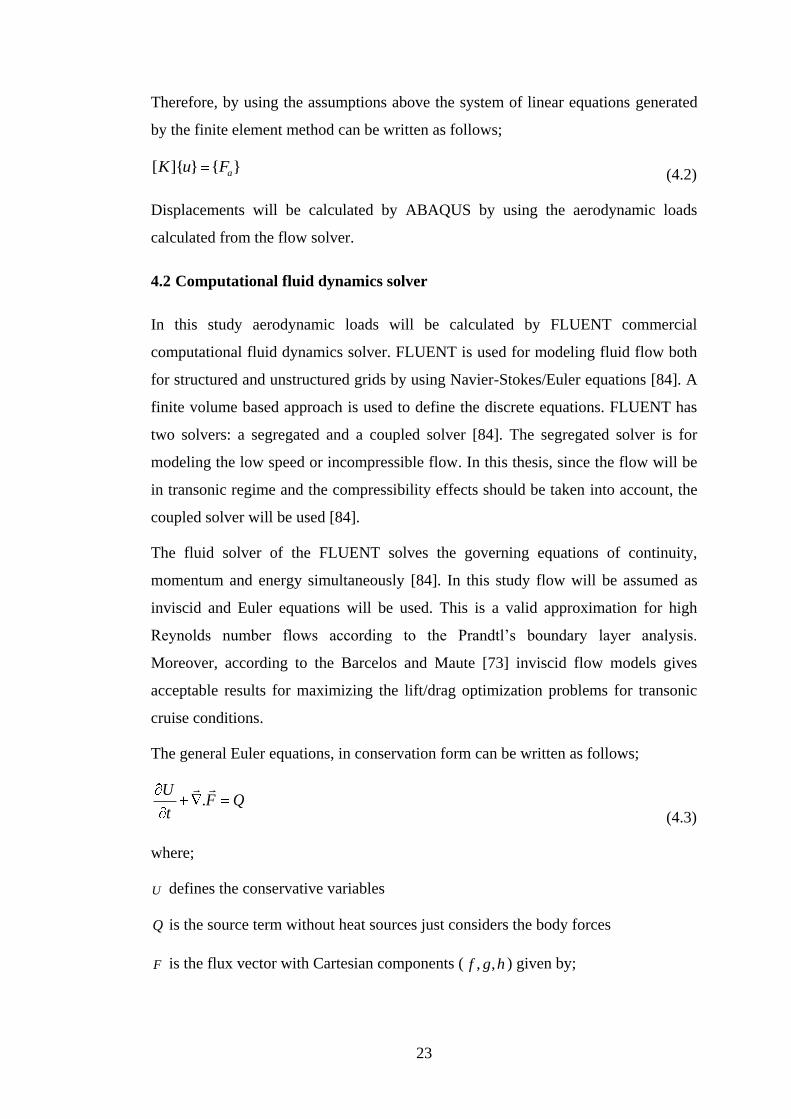
The general Euler equations, in conservation form can be written as follows;

.U

F Qt

(4.3)

where;

U defines the conservative variables

Q is the source term without heat sources just considers the body forces

F is the flux vector with Cartesian components ( , ,f g h ) given by;

24

2

2

2

( ) ( ) ( )

u v w

vuu p wu

f uv g v p h wv

uw vw w p

u E p v E p w E p (4.4)

Here;

is the fluid mass density

, ,u v w are the velocity components

E is the total energy per unit volume defined by,

2 2 21

2E e u v w

(4.5)

As seen from Euler equations there are six unknowns , , , , ,u v w p E but only five

equations to solve the system. Therefore, one more equation is needed to solve the

set of equations. It is the well known perfect gas law equation given below;

1p e (4.6)

where;

is the adiabatic index and is taken as 1.4

Governing equations are non-linear and coupled. In FLUENT in order to get

convergence several iterations are performed [84]. Iterations are;

1. Depending on the current solution, fluid properties are updated.

2. Continuity, energy and momentum equations are solved simultaneously.

3. Convergence control is done.

This procedure is applied until the convergence criteria are met.

4.2.1 Remeshing methods

In FLUENT mesh motion is accomplished according to the motion defined at the

boundaries of the volume mesh. There are three mesh motion methods in FLUENT

[84].

25

Spring based smoothing method

Dynamic layering

Local remeshing methods

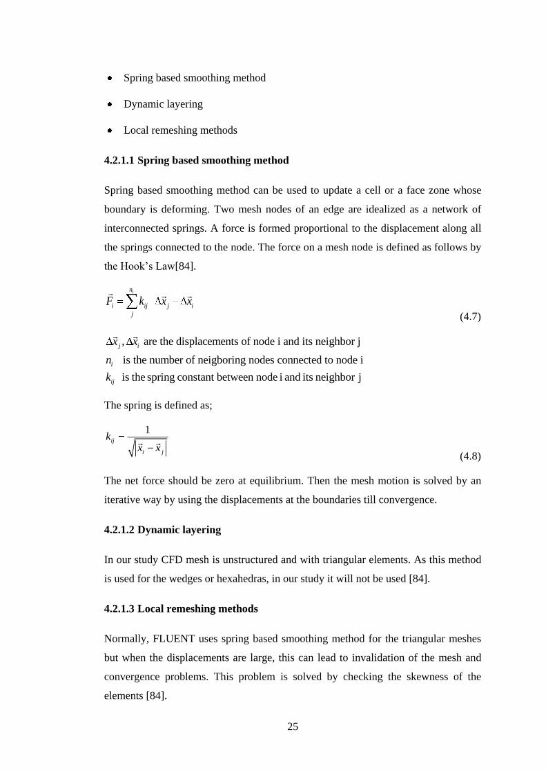
4.2.1.1 Spring based smoothing method

Spring based smoothing method can be used to update a cell or a face zone whose

boundary is deforming. Two mesh nodes of an edge are idealized as a network of

interconnected springs. A force is formed proportional to the displacement along all

the springs connected to the node. The force on a mesh node is defined as follows by

the Hook‘s Law[84].

in

i ij j i

j

F k x x

(4.7)

, are the displacements of node i and its neighbor j

is the number of neigboring nodes connected to node i

is the spring constant between node i and its neighbor j

j i

i

ij

x x

n

k

The spring is defined as;

1ij

i j

kx x

(4.8)

The net force should be zero at equilibrium. Then the mesh motion is solved by an

iterative way by using the displacements at the boundaries till convergence.

4.2.1.2 Dynamic layering

In our study CFD mesh is unstructured and with triangular elements. As this method

is used for the wedges or hexahedras, in our study it will not be used [84].

4.2.1.3 Local remeshing methods

Normally, FLUENT uses spring based smoothing method for the triangular meshes

but when the displacements are large, this can lead to invalidation of the mesh and

convergence problems. This problem is solved by checking the skewness of the

elements [84].

26

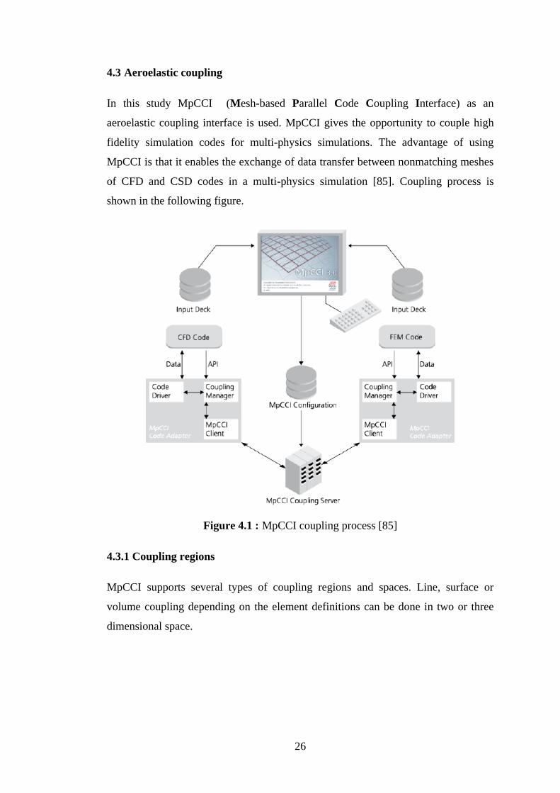
4.3 Aeroelastic coupling

In this study MpCCI (Mesh-based Parallel Code Coupling Interface) as an

aeroelastic coupling interface is used. MpCCI gives the opportunity to couple high

fidelity simulation codes for multi-physics simulations. The advantage of using

MpCCI is that it enables the exchange of data transfer between nonmatching meshes

of CFD and CSD codes in a multi-physics simulation [85]. Coupling process is

shown in the following figure.

Figure 4.1 : MpCCI coupling process [85]

4.3.1 Coupling regions

MpCCI supports several types of coupling regions and spaces. Line, surface or

volume coupling depending on the element definitions can be done in two or three

dimensional space.

27

4.3.2 Data exchange

Figure 4.2 : Data exchange for unmatching grids [85]

Data exchange process can be grouped into three phases.

4.3.2.1 Pre-contact search

First of all to make the contact search easier the elements are split into triangles in

2D or tetrahedras in 3D.(a) Search for the elements is done by using the ―Bucket

Search‖ algorithm of MpCCI [85]. Then, each triangle is bounded by a box which

includes the triangle.(b) After that step, ―buckets‖ are formed by dividing the space

into smaller squares or cubes. (c) Finally, a list is formed by listing the closer

triangles to the bucket to use for the further steps for data tansfer. Pre-Contact Search

can be seen easily in the figure below.

Figure 4.3 : Pre-contact search [85]

4.3.2.2 Minimal distance

28

Point-element relationships are used in the minimal distance algorithm. A list of

triangles which belong to elements was formed in the pre-contact search step. In this

step, the best triangle corresponding to the best element is determined and chosen.

Relative positions of the triangles and the node P is used in this process [85].

Projection of the point P is taken onto the surface of each triangle as seen in the

figure.

Figure 4.4 : Element selection [85]

4.3.2.3 Intersection

Alternative way for association of the elements is based on the element-element

association. In this algorithm, elements again divided into the smaller triangles, a

bounding box is formed for the triangles and buckets are formed. Intersected areas

are stored in a list with the results of the pre-contact search [85].

4.3.2.4 Flux and field interpolation

Interpolation of the quantitites (displacement, force, pressure,…) can be done by

using a flux or field interpolation method [85]. In flux interpolation, the integral is

preserved by adapting the value to the element sizes. This method is used for

example for forces. In field interpolation, a conservative transfer is ensured by

keeping the value of the elements. It is used for example for pressures.

4.4 Aeroelastic code coupling with MpCCI

To perform an aeroelastic coupling with MpCCI, four steps are defined [85].

29

Preparation of Model Files

In this step FLUENT and ABAQUS models are prepared separately. The

definition of the coupling surfaces (i.e. upper wing, lower wing, tip for a

wing) are given in this step. Then, model files are written in input files for the

CFD and CSD codes.

Definition of the Coupling Process

The most important step of the aeroelastic coupling process is the definition

of the coupling process step. FLUENT and ABAQUS models of the wing are

chosen via user interface. Then, coupling regions described above, transfer

quantities (nodal displacements from the CSD code and the pressure values

from the CFD code) and the coupling algorithms are selected.

Running the Co-Simulation

In this step aeroelastic analyses are performed. MpCCI controls the rest of the

coupling process till to the specified coupling iterations or time.

Post-Processing

Finally, the results for both CFD and the CSD code are examined by using

the codes own post-processing tools.

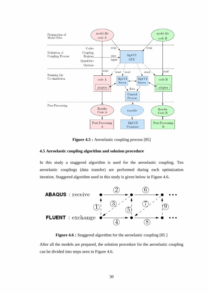
The aeroelastic coupling process written above is given in Figure 4.5. Code A

represents the CFD solver FLUENT and code B represents the CSD solver

ABAQUS.

30

Figure 4.5 : Aeroelastic coupling process [85]

4.5 Aeroelastic coupling algorithm and solution procedure

In this study a staggered algorithm is used for the aeroelastic coupling. Ten

aeroelastic couplings (data transfer) are performed during each optimization

iteration. Staggered algorithm used in this study is given below in Figure 4.6.

Figure 4.6 : Staggered algorithm for the aeroelastic coupling [85 ]

After all the models are prepared, the solution procedure for the aeroelastic coupling

can be divided into steps seen in Figure 4.6.

31

1. CFD code calculates the surface pressures and maps these pressures as nodal

forces to the CSD code.

2. CSD code calculates the deformation of the structure under these pressure

loads.

3. Calculated nodal displacement values are mapped onto the CFD modal as

mesh displacements and mesh is updated.

4. CFD code performs the analysis.

This solution strategy is performed until a specified coupling time or a number

iterations is reached.

32

5. TEST CASE FOR AEROELASTIC COUPLING WITH MpCCI

5.1 Geometric model of AGARD 445.6 aeroelastic wing

In this study the wing geometry used for the aeroelastic analysis is chosen as the

well-known AGARD (Advisory Group for Aerospace Research and Development)

445.6 wing [28]. This wing is the first aeroelastic configuration that is tested by

Yates et al [80] in the Transonic Dynamics Tunnel (TDT) at the NASA Langley

Research Center.

The AGARD 445.6 wing is a swept-back wing with a quarter-chord sweep angle of

45 degrees. Cross sections of the wing are NACA 65A004 airfoils. The wing has a

taper ratio of 0.66 and an aspect ratio of 1.65. Moreover, it is a wall-mounted model

made with laminated mahogany. The wing‘s parametric CAD model prepared with

CATIA V5 is given in Figure 5.1.

Figure 5.1 : AGARD 445.6 wing geometry

There are 2 models of the AGARD 445.6 wing: solid and weakened model. In this

study weakened model of the wing given in Figure 5.2 below is used.

33

Figure 5.2 : AGARD 445.6 weakened model

5.2 CSD model of the AGARD 445.6 weakened model and validation

The finite element model of the wing is formed in ABAQUS by using 19,610 linear

hexahedral structural elements. Static aeroelastic analysis and modal analysis are

performed. The wing is fixed from root for every degree of freedom (DOF). The

material properties of the wing are taken from the work of Yosibash et al [38] for the

solid model and applied for the weakened model by using interpolation. The material

properties of the wing are given in table below. The fiber orientation of the wood is

taken along span inclined 45 degrees.

34

Weakened Model 3

11E (MPa) 3671

22E (MPa) 240

33E (MPa) 401

12G (MPa) 321

13G (MPa) 409

23G (MPa) 136

12 0.034

13 0.033

23 0.326

The finite element model of the wing is given in the following Figure 5.3.

Figure 5.3 : The finite element model of the AGARD 445.6 wing

The AGARD 445.6 weakened model is modeled for the first four frequencies. In

order to validate the wing model, a modal analysis is performed to compare the

results of Yates et al [28]. The results of the modal analysis are tabularized in the

Table 5.2.

Table 5.1: AGARD 445.6 Material properties

35

Frequency

no.

Reference

approach [Hz]

Present study

[Hz]

Error (%)

f1 9.59 9.58 0.16

f2 38.16 36.88 3.34

f3 48.34 47.72 1.28

f4 91.54 91.11 0.47

f5 118.11 119.87 1.48

As seen from Table 5.2 the results are well agreed with the results of Yates [28]. The

error for the first five frequencies of the modelled AGARD 445.6 wing is below 5%.

Moreover, except for the 2nd

frequency the errors are below 1.5%.

In the Figure 5.4 the modes shapes on the left belongs to the reference study of the

Yates [28] and the mode shapes on the right belongs to current study.

Table 5.2: Frequency comparison for weakened model

36

Figure 5.4 : Mode shapes comparison

As seen from the results the mode shapes belong to the 1st bending, 1

st torsion, 2

nd

bending and 2nd

torsion from top to down respectively.

In conclusion, the results of the modal analysis show us that our model is free of

numerical and modeling errors and can be used for the rest of the study.

5.3 CFD model of the AGARD 445.6 weakened model

The computational grid of the wing was constructed in GAMBIT preprocessing

software by using tetrahedral elements. The computational grid has 691,000 cells,

1.35 million faces.

The flow is modeled as inviscid by using Euler equations and the free stream

velocity is 0.85 Mach. A 5o of angle of attack is given for the wing geometry. The

boundary conditions of the wing surfaces are given as wall and the flow field is given

as pressure far field in FLUENT. In the pressure far field the angle of attack is given

as cosine and sine of the angle of attack. The computational grid used in the static

aeroelastic analysis is given in the following figures.

37

Figure 5.5 : Close up mesh cross section

Figure 5.6 : Wing model and wing root

Figure 5.7 : Pressure far field computational grid

38

5.4 Aeroelastic analysis results

First of all, to validate the aeroelastic wing model, an aeroelastic analysis was

performed via MpCCI. The CFD and CSD model of the wing is given to the MpCCI

and transfer quantities (surface pressures from the CFD and nodal displacements

from the CSD) were selected. The solution algorithm used in this static aerolastic

coupling is the staggered algorithm that is described deeply in the section 4.5.

The results are compared with the results of Liu et al [24]. The pressure contours on

the upper and lower surface of the wing are given in the following figures

respectively. On the left side of the figures 5.8 to figure 5.11 the results are from the

Liu et al ‗s work for the AGARD 445.6 wing [24] and on the right side of the figures

the results are from the present study.

Figure 5.8 : Pressure distributions on the upper wing surface

Figure 5.9 : Pressure distributions on the lower wing surface

39

As seen from the figures the pressure contours are well fit with the reference results.

Moreover, the distribution of the pressure coefficients at 34% and 67% span are

given in the following figures respectively.

Figure 5.10 : Pressure coefficient distribution at 34% span (X in inches)

Figure 5.11 : Pressure coefficient distribution at 67% span (X in inches)

As seen from the figures 5.10 and 5.11 the suction picks differ with the results of Liu

et al [24]. For the 0.34 ,where is the nondimensional spanwise coordinate,

Liu et al [24] predicted a suction peak of -1.26 at 1% chord location of the upper

wing surface whereas in the present study a suction peak of -0.92 at 3.5% chord

location was predicted. Moreover for 0.67 a suction peak of -1.41 at 1% (nasil

goruluyor) chord location was predicted on the upper wing surface by Liu et al [24]

whereas in the present study a suction peak of -1.05 at 4.5% (nasil goruluyor) chord

location was predicted. The results are well agreed with the results of the reference

except for the leading edge suction sections for the upper wing surface. This

difference can be the result of the mesh type used in the studies or due to the solver

used in the studies.

The last compared result is vertical deflection of the wing along span relative to the

wing root. The deflection results are given in the following Figure 5.12 and 5.13.

40

Figure 5.12 : Vertical deflection of the wing along span relative to the wing root

As seen from the figures 5.12 and 5.13 the out of plane deformation behaviour for

the wing is well agreed the with the results of the Liu et al [24]. There are slight

differences for the leading edge section. This can be due to the different methods

used in two different studies. In the present study a 3D finite element analysis

software is used to find the displacement values whereas in the work of Liu et al [24]

used a modal structural method in order to predict the displacement values.

Below in the figure 5.13 the wing‘s initial and equilibrium positions are given. As

expected due to the aerodynamic loads the wing‘s vertical deflection along span

relative to the wing root is upwards.

Figure 5.13 : Wing‘s initial and equilibrium positions

41

6. MULTIDISCIPLINARY MULTI-OBJECTIVE DESIGN OPTIMIZATION

In recent years, design optimization of complex aircraft structures for maximum

performance and minimum weight has been a challenging research area for aircraft

manufacturer companies. The multi-objective task of attaining minimum weight and

cost with maximum reliability of structure is one of the most time-consuming phases

of an aircraft design project. Therefore, robust computational methodologies are

strongly required in order to increase the efficiency and success of this design phase.

A strong and easy-to-apply methodology can be developed by implementing the

numerical optimization techniques directly into the everyday-used analysis tools that

have been well and commonly employed in aerospace engineering. Numerical

optimization is an iterative scheme to reach the most desired design within a design

space bounded by the lower and upper limits of optimization variables. The design

criteria defined as functions of optimization variables have to be evaluated at each

optimization iteration as variables are updated. Thus, optimization studies require a

high number of sequential analyses automatically and needs longer computational

time as compared to only analysis studies. For that reason, a serious research is

focusing on developing more efficient optimization algorithms for problems with

large analysis size. For only optimization purposes simpler analysis models can be

preferred in the iterative process and parametric geometries can be used to reduce the

number of optimization variables that can sufficiently describe a problem.

In this study multi-objective and multidisciplinary optimization will be performed for

a wing configuration. As the optimization driver the multiobjective design

environment (mode) FRONTIER software will be used for its efficient optimization

algorithms.

6.1 Formulation of optimization problems

A generic optimization problem associated with a given system can be formulated as;

42

min ( )

( ) 0 ( )

( ) 0 ( )

h

g

s

s S

n

n

n

L U

z s

h s h s R

g s g s R

S s R s s s (6.1)

Where;

s is a set of sn abstract parameters restricted by lower and upper bounds

Ls and Us ,

z is a cost function of interest,

h is a set of hn equality constraints

g is a set of gn inequality constraints.

6.2 Design variables

The set of optimization variables (s) are the values that affect the optimization

problem. These can be geometry parameters like taper, sweep, aspect ratio or

thickness values like shell thicknesses of the wing. They can be either bounded with

lower and upper bounds or unbounded. Moreover, design variables can be

continuous like wing span, chord or can be discrete like number of ribs, spars.

The main geometry for the optimization problem in this thesis, is based on the

AGARD 445.6 wing described in the previous chapters. As the design variables,

taper ratio and the quarter chord sweep are selected. When these variables are

changed, the fiber orientation on the structural model, the average chord and the

planform area values will also change respectively. But these variables will not be

used as direct optimization (design) variables; they will be calculated according to

the values of sweep and taper and will be used as input variables.

Design Variables Lower Bound Upper Bound

taper ratio 0.1 0.5

sweep (degrees) 0 50

Table 6.1: Optimization variables

43

6.3 Constraints

A constraint is a condition that must be satisfied during the design. If the constraint is

satisfied the design is called feasible if not infeasible. For example, designer may

want the lift to be greater than or equal to the aircraft‘s weight or does not want the

maximum stress to exceed the value of the material‘s yield stress value.

In this study only one constraint is given. It is the maximum deformation of the wing

tip due to the aerodynamic loads over the wing. The deformation at the tip should not

exceed the one tenth of the wing span.

Constraints Less Then

Maximum tip deflection (mm) 76

6.4 Objective functions

An objective function is the goal of the optimization problem that we want to

minimize or maximize. For example, minimizing weight, displacemen, stress or

maximizing L/D, lift coefficient,…

Most of the optimization problems are single objective or can be formulated as single

objective through summation of the multi-objective functions by using weight

factors. In this study there are two objective functions and for the multiobjective

optimization problems the algorithm will try to find the pareto front.

The objective functions for this study are maximizing the L/D ratio and minimizing

the weight.

Objective Functions Goal

L/D max

weight min

Table 6.2: Constraints

Table 6.3: Objective functions

44

6.5 Optimization problem

The overall optimization problem for this thesis work can be formulated as

max

/4

min imize ( )

max imize / ( )

subject to

76

with respect to

0 50

0.1 0.5

s S

s S

c

M s

L D s

u mm

(6.2)

where;

M is the total mass of the wing

/L D is the lift over drag value for the wing

maxu is the maximum deformation of the wing tip

/4c is the sweep value at the quarter chord

is the taper ratio defined as;

tip

root

c

c (6.3)

6.6 Optimization algorithms

Optimization problems can be generally solved by either gradient based algorithms

or evolutionary algorithms. In this study multi objective optimization problem will

be solved by genetic algorithm which is an evolutionary algorithm.

Evolutionary algorithms or genetic algorithms use the evolution theory to perform

optimization. A population evolves over generations to adapt to an environment by

selection, mutation and crossover. [81]

There are three important terms corresponding to the genetic algorithms which are

fitness, individual and genes. Fitness refers to the objective function, individual

refers to the design candidate and genes refer to the design variables.

45

Multiobjective (MO) optimization tries to find the components of a vector-valued

objective function whereas the single objective optimization tries to find the single

valued objective function. [53] In MO problems, solution is a set of solutions called

―pareto-optimal set‖.

In the following figure it is seen that point ―p‖ has a minimal 2f but maximum

1f . On

the other hand, point ―r‖ has a minimal in 1f but maximum

2f . These two points are

not the solution when both of the objectives are considered. The solutions on the

curve between ―p‖ and ―r‖ are known as pareto-optimal front. Every pareto optimal

point in the set is an equally acceptable solution for a MO optimization problem. [86]

Figure 6.1 : Pareto optimal solutions

The application of the evolutionary algorithms to a MO optimization problem can be

solved by using a multiobjective genetic algorithm (MOGA). Genetic algorithms are

capable of finding the global optima within complex design spaces whereas gradient

based algorithms can sometimes get stuck at the local optima points.

Genetic algorithms can be used almost for every optimization problem, where

gradient based algorithms may have some limitations. Gradient based algorithms

needs the gradient information to compute the search direction to move in the design

space that‘s why they need the existence of derivatives. However, if once applicable,

46

gradient based algorithms may be much more computationally efficient with respect

to the genetic algorithms.

Genetic algorithms do not need to start from a point whereas gradient based

algorithms need a starting point. Genetic algorithms do not operate on design

variables directly. They use binary representation of the parameters. A basic

structure of a genetic algorithm according to the Ghosh and Dehuri [81] is given in

the following figure.

Figure 6.2 : Basic structure of genetic algorithm

6.6.1 Non-dominated sorting genetic algorithm (NSGA-II)

The scheduler used in this study is the implementation of Deb et al [82] which is

―Non-dominated Sorting Genetic Algorithm‖. NSGA-II is a fast and elitist

multiobjective evolutionary algorithm [86] .The main features of the algorithm

are[86];

47

It implements a fast non-dominated sorting procedure and it reduces the

computational time according to the classical non-dominated sorting

algorithms.

Elitism is implemented in the NSGA-II for multiobjective search. From the

start of the initial population elitism is used to form all of the populations.

Crowding distance, which finds the density of solutions in the objective

space, is used. Moreover, it uses a crowded comparison operator for the

selection process.

The work diagram of NSGA-II is given in the following figure [82].

Figure 6.3 : Work diagram of NSGA-II

First a combined populationtR is formed by combining the child population

tQ and parent populationtP . The population

tR is in size of 2N.

t t tR P Q (6.4)

Then tR population is sorted due to the non-domination. Elitism is satisfied as

the previous and current population is included intR .

New population 1tP is formed by using the solutions of different non-

dominated fronts 1 2 3,..., ,F F F according to their rank and crowded comparison

operator. Best non-dominated front is first, then the second best non-

dominated front and so on.

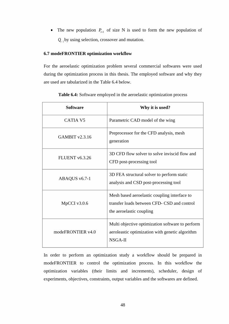
48

The new population 1tP of size N is used to form the new population of

1tQ by using selection, crossover and mutation.

6.7 modeFRONTIER optimization workflow

For the aeroelastic optimization problem several commercial softwares were used

during the optimization process in this thesis. The employed software and why they

are used are tabularized in the Table 6.4 below.

Software Why it is used?

CATIA V5 Parametric CAD model of the wing

GAMBIT v2.3.16 Preprocessor for the CFD analysis, mesh

generation

FLUENT v6.3.26 3D CFD flow solver to solve inviscid flow and

CFD post-processing tool

ABAQUS v6.7-1 3D FEA structural solver to perform static

analysis and CSD post-processing tool

MpCCI v3.0.6

Mesh based aeroelastic coupling interface to

transfer loads between CFD- CSD and control

the aeroelastic coupling

modeFRONTIER v4.0

Multi objective optimization software to perform

aeroleastic optimization with genetic algorithm

NSGA-II

In order to perform an optimization study a workflow should be prepared in

modeFRONTIER to control the optimization process. In this workflow the

optimization variables (their limits and increments), scheduler, design of

experiments, objectives, constraints, output variables and the softwares are defined.

Table 6.4: Software employed in the aeroelastic optimization process

49

Optimization workflow is prepared to automate the multiobjective multidisciplinary

optimization problem. Once the workflow is run, it controls the optimization process

automatically by using the well prepared script files and models. The working

procedure of the diagram can be explained by splitting into parts as follows;

Figure 6.4 : Scheduler

1) The scheduler NSGA-II determines the design variables and optimization

iteration begins.

2) Synchronization starts

Figure 6.5 : CFD branch

3) Optimization variables are changed via CATIA V5 node by using the

parametric CAD model.

4) The geometric model transferred as iges format to GAMBIT CFD pre-

processor

5) GAMBIT uses the journal file given in the Appendix A.1 and prepares

solution grid for CFD and gives the boundary conditions.

6) GAMBIT transfers the mesh file to FLUENT

50

7) As the area and the average chord of the wing changes in every design

iteration, FLUENT calculates them by using the design variables and imports

the mesh files. Then it prepares the flow model and gives boundary

conditions via journal file given in Appendix A.2.

8) FLUENT transfers the case file to MpCCI for the aeroelastic analysis.

Figure 6.6 : CSD branch

9) Optimization variables are changed via CATIA V5 node by using the

parametric CAD model.

10) The geometric model transferred as iges format to ABAQUS FEA

11) ABAQUS changes the fiber orientation of the wing by using the sweep value

and prepares the structural model for the aeroelastic analysis by using the

Phyton script given in Appendix A.3.

12) ABAQUS transfers the input file to MpCCI for the aeroelastic analysis.

51

Figure 6.7 : Aeroelastic analysis, post processing and optimization

13) Aeroelastic coupling is performed via MpCCI by using the FLUENT and

ABAQUS models in batch mode.

14) The results for the objective function (maximize L/D) is stored.

15) Aeroelastic analysis result file for the ABAQUS is transferred to ABAQUS

for post-processing and getting the displacement constraint result.

16) The value of the wing weight is calculated via the multiplication of the

volume information from the CATIA V5 and the material density.

17) modeFRONTIER controls the constraint violation.

18) NSGA-II controls the optimization process.

19) New iteration process starts.

This cycle goes on until the specified number of iterations or populations have

reached. After all the calculations have been performed the pareto optimal set is

found and by using the decision tools of modeFRONTIER a suitable design is found.

The optimization workflow is given in the following figure for the whole

optimization process.

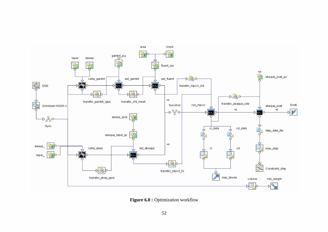
52

Figure 6.8 : Optimization workflow

53

7. OPTIMIZATION RESULTS

7.1 Results for the optimization problem

In this study a number of 12 design of experiments (DOE) with Sobol sequence

which is capable of distributing the experiments uniformly in the design space [86]

and 17 number of generations for the NSGA-II are defined. A total number of 204

designs is generated for the optimization problem.

*Total design number DOE Generations (7.5)

Solution of the problem took 23 hours 51 minutes on a workstation with Microsoft

Windows XP operating system. The system has 2 Gb of RAM and 250 Gb of

harddisk.

There are 108 different individual designs distributed as shown in the following

figure.

Figure 7.1 : Design summary

78 designs (72% of all designs) were found to be feasible that satisfies the constraint

condition given in the optimization problem and 26 designs (24% of all designs) are

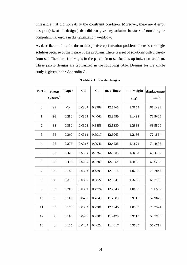
54

unfeasible that did not satisfy the constraint condition. Moreover, there are 4 error

designs (4% of all designs) that did not give any solution because of modeling or

computational errors in the opimization workflow.

As described before, for the multiobjective optimization problems there is no single

solution because of the nature of the problem. There is a set of solutions called pareto

front set. There are 14 designs in the pareto front set for this optimization problem.

These pareto designs are tabularized in the following table. Designs for the whole

study is given in the Appendix C.

Pareto

Sweep

(degree)

Taper

Cd

Cl

max_finess

min_weight

(kg)

displacement

(mm)

0 38 0.4 0.0303 0.3799 12.5465 1.3654 65.1492

1 36 0.250 0.0328 0.4062 12.3959 1.1488 72.5629

2 38 0.350 0.0308 0.3856 12.5339 1.2888 68.5509

3 38 0.300 0.0313 0.3917 12.5063 1.2166 72.1564

4 38 0.275 0.0317 0.3946 12.4528 1.1821 74.4686

5 38 0.425 0.0300 0.3767 12.5583 1.4053 63.4759

6 38 0.475 0.0295 0.3706 12.5754 1.4885 60.6254

7 30 0.150 0.0363 0.4395 12.1014 1.0262 73.2844

8 38 0.375 0.0305 0.3827 12.5341 1.3266 66.7753

9 32 0.200 0.0350 0.4274 12.2043 1.0853 70.6557

10 6 0.100 0.0405 0.4640 11.4589 0.9715 57.9876

11 32 0.175 0.0353 0.4301 12.1746 1.0552 73.3374

12 2 0.100 0.0401 0.4585 11.4429 0.9715 56.5783

13 6 0.125 0.0403 0.4622 11.4817 0.9983 55.6719

Table 7.1: Pareto designs

55

The remaining task for the optimization problem is to choose a suitable design from

the pareto set. All of the designs given in the Table 7.1 are the acceptable optimum

solutions of the problem but with different weights for the corresponding objectives.

For example an aerodynamics engineer can prefer the design with maximum lift over

drag ratio whereas a structural engineer can choose the design with minimum weight.

The relation between the objectives are given in the scatter chart of the

modeFRONTIER in the following Figure 7.2

Figure 7.2 : Scatter chart minimum weight vs maximum L/D

As seen from the Figure 7.2 the relationship between the objectives of maximum lift

over drag ratio and minimum weight is non-linear. A quadratic function can describe

this relationship. To investigate the relationship between the taper ratio and objective

functions is given in the following Figures 7.3 and 7.4.

56

Figure 7.3 : Scatter chart for taper ratio vs minimum weight

Figure 7.4 : Scatter chart for taper ratio vs maximum L/D

As seen from the Figure 7.3 there is a linear relationship between the taper ratio and

the objective function of minimum weight whereas as seen from the Figure 7.4 there

exists a non-linear relationship between the taper ratio and the objective function of

maximum lift over drag ratio. The correlation between the optimization variables and

the objective functions are given in the following Figures 7.5 and 7.6. In the

correlation charts the value changes between -1 and 1. If the value is 1 it means the

variables are perfectly positively correlated else if the value is -1 it means the

variables are perfectly negatively correlated.

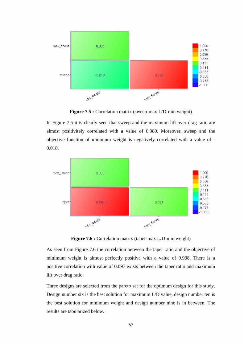
57

Figure 7.5 : Correlation matrix (sweep-max L/D-min weight)

In Figure 7.5 it is clearly seen that sweep and the maximum lift over drag ratio are

almost positivitely correlated with a value of 0.980. Moreover, sweep and the

objective function of minimum weight is negatively correlated with a value of -

0.018.

Figure 7.6 : Correlation matrix (taper-max L/D-min weight)

As seen from Figure 7.6 the correlation between the taper ratio and the objective of

minimum weight is almost perfectly positive with a value of 0.998. There is a

positive correlation with value of 0.097 exists between the taper ratio and maximum

lift over drag ratio.

Three designs are selected from the pareto set for the optimum design for this study.

Design number six is the best solution for maximum L/D value, design number ten is

the best solution for minimum weight and design number nine is in between. The

results are tabularized below.

58

Pareto

Sweep

(degree)

Taper

Cd

Cl

max_finess

min_weight

(kg)

displacement

(mm)

6 38 0.475 0.0295 0.3706 12.5754 1.4885 60.6254

9 32 0.200 0.0350 0.4274 12.2043 1.0853 70.6557

10 6 0.100 0.0405 0.4640 11.4589 0.9715 57.9876

The structural results (initial and equilibrium positions of the wing, displacement

residual) and the fluid dynamics results (pressure coefficients on the upper and lower

wing) for the design number 9 from the pareto set is given in the Appendix B.

7.2 Conclusion

In this thesis aeroelastic optimization is performed on a basic experimental wing

model based on AGARD 445.6 elastic wing configuration to obtain the objectives of

maximum lift over drag ratio and minimum weight of the wing. A static aeroelastic

criteria is given as a design constraint to satisfy the maximum tip deflection. Sweep

angle at the quarter chord and the taper ratio of the wing are used as optimization

parameters for this study. Moreover, a genetic algorithm NSGA-II is used to control

the optimization process.

The pareto set for the optimum designs are obtained at the end of the aeroelastic

optimization study to choose the best design configuration. The effect of the design

variables on objective functions and their relationship are examined by using the

modeFRONTIER 4.0‘s decision tools.

Thus, a strong and easy to apply multi-disiplinary optimization methodology is

successfully developed by implementing the numerical optimization techniques

directly into the everyday used commercial analysis tools that have been well and

commonly employed in CFD and CSD disciplines in aerospace engineering.

The future work for this study is to apply the parallel computation technology in both

CSD and CFD parts in the already developed methodology. More complicated

aircraft wing geometries and more detailed optimization problems can be studied

Table 7.2: Results for the selected pareto designs

59

with the advantages of parallelization. Finally, the study will be extended to dynamic

aeroelasticity problems with applications to aeroelastic optimization based on flutter

analysis.

60

REFERENCES

[1] Dowell, A. H. and Hall, K. C., 2001, Modelling of Fluid-Structure Interaction,

Annual Review Fluid Mechanics, 33: 445-90.

[2] Bisplinghoff, R. L. and Ashley, H., 1962, Principles of Aeroelasticity, Dover.

[3] Theodorsen, T., 1938, General Theory of Aerodynamic Instability and the

Mechanism of Flutter, NACA Report , No. 496.

[4] Fung, Y. C., 1969, An Introduction to the Theory Aeroelasticity, Dover.

[5] Dowell, E. H. et al., 1995, A Modern Course in Aeroelasticity, 3rd Ed., Kluwer.

[6] Bennet, R. M. and Edwards, J. W., 1998, An overview of recent developments

in computational aeroelasticity, Proceedings of the 29th AIAA Fluid

Dynamics Conference, Albuquerque, NM, June 15-18.

[7] Guruswamy, G. P., 2002, A review of numerical fluids/structures interface

methods for computations using high-fidelity equations, Computers

and Structures, 80:31-41.

[8] Smith, J. M. and Hodges, H. D., 2000, Evaluation of Computational Algorithms

Suitable for Fluid-Structure Interactions, Journal of Aircraft, 37 (2),

April.

[9] Huttsell, L. et al., 2001, Evaluation of Computational Aeroelasticity Codes for

Loads and Flutter, AIAA Journal, AIAA-2001-569 Aerospace Sciences

Meeting and Exhibit, 39th, Reno, NV, Jan. 8-11.

[10] Kamakoti, R. and Shyy, W., 2004, Fluid-structure Interactions for Aeroelastic

Applications, Progress in Aerospace Sciences, 40 (8); p.535-558.

[11] Carlson, H. A. and Feng, Q. J., Computational Models for Nonlinear

Aeroelasticity, AIAA Paper, 43rd AIAA Aerospace Sciences Meeting

and Exhibit, p.4143-4152.

[12] Farhat, C., 2005,CFD on Moving Grids: from theory to realistic flutter,

maneuvering and multidisciplinary optimization, International

Journal of Computational Fluid Dynamics, 19 (8).

61

[13] Gordnier E. R. and Fithen R., 2003,Coupling of a Nonlinear Finite Element

Solver with a Navier-Stokes Solver, Computers and Structures, 81 (2),

p.75-89.

[14] Lohner, R., Cebral, J., Chi Yang, Baum, J.D., Mestreau, E., Charman, C.

and Pelessone, D., 2004, Large-scale Fluid-structure Interaction

Simulations, Computing in Science and Engineering, 6 (3), p.27-37.

[15] Massjung, R., 2006, Discrete Conservation and Coupling Strategies in

Nonlinear Aeroelasticity, Computer Methods in Applied Mechanics

and Engineering, 196 (1-3); p.91.

[16] Newmann, J. C. et. al., 1999, Efficient Nonlinear Static Aeroelastic Wing

Analysis, Computers and Fluids, 28 (4-5); p.615-628.

[17] Suleman, A. and Relvas, A., 2006, Fluid Structure Modeling of Nonlinear

Aeroelastic Structures Using The Finite Element Corotational Theory,

Journal of Fluids and Structures, 22 (1); p.59-75.

[18] Liu, F., Tsai and H. M., Cai, J., 1993, Static Aeroelastic Computation with a

Coupled CFD and CSD Method, Journal Of Aircraft.

[19] Guruswamy, G. and Garcia, C. J., 1999, Static Aeroelastic Characteristics of

an Advanced Wing with a Control Surface Using Navier-Stokes

Equations, 37th

AIAA-1999-796 Aerospace Sciences Meeting and

Exhibit, Reno, NV, Jan. 11-14.

[20] Relvas, A. and Sulemani, A, 2006, Aeroelasticity of Nonlinear Structures

Using the Corotational Method, Journal of Aircraft, 43 (3).

[21] Newmann, J. C., Newman P. A., et. al., 1999, Efficient Nonlinear Static

Aeroelastic Wing Analysis, Computers and Fluids, 28 (4-5); p.615.

[22] Karpel, M., Yaniv, S. and Livshits, S. D., 1996, Integrated Solution for

Computational Static Aeroelastic Problems, 6th

Symposium on

Multidisciplinary Analysis and Optimization, Bellevue, WA, Sept. 4-6,

Technical Papers. Pt. 1.

[23] Schuster, D., Vadyak, E. and Atta, E., 1990, Static Aeroelastic Analysis of

Fighter Aircraft Using a Three-Dimensional Navier-Stokes Algorithm,

Journal of Aircraft, 27 (9) (820-825).

[24] Liu, F., Cai and J., Tsai, H. M., 2001, Static Aero-elastic Computation with a

Coupled CFD and CSD Method, 39th

AIAA-2001-717 Aerospace

Sciences Meeting and Exhibit, Reno, NV, Jan. 8-11.

62

[25] Guruswamy, G. P. and Byun, C., 1996, Static Aeroelasticity Computations

For Flexible Wing-Body Control Configurations, 6th

AIAA, NASA,

and ISSMO, Symposium on Multidisciplinary Analysis and

Optimization, Bellevue, WA, Sept. 4-6, Technical Papers. Pt. 1 (A96-

38701 10-31), Reston, VA, American Institute of Aeronautics and

Astronautics, 1996, p. 744-754.

[26] Guruswamy, G. P., Kapania, R. and Macmurdy, D., 1994, Static Aeroelastic

Analysis of Wings Using Euler/Navier-Stokes Equations Coupled

With Improved Wing-Box Finite Element Structures, 35th

AIAA-1994-

1587 IN:AIAA/ASME/ASCE/AHS/ASC Structures, Structural

Dynamics, and Materials Conference, Hilton Head, SC, Apr 18-20,

1994, Technical Papers. Pt. 4 (A94-23876 06-39), Washington, DC,

American Institute of Aeronautics and Astronautics, 1994, p. 2146-

2158.

[27] Kamakoti, R., Lian and Y., et.al., 2002, Computational Aeroelasticity Using a

Pressure-Based Solver, AIAA Journal, 40th AIAA Aerospace Sciences

Meeting and Exhibit ,14-17 January, Reno, Nevada.

[28] Yates, E. C., Jr., 1998, AGARD Standard Aeroelastic Configuration for

Dynamic Response I. AGARD 445.6, AGARD Technical Report,

REPORT No.765.

[29] Marjorie E., Munning, J. R., Hallstag, T. H. and Rogers, J. T., 1976,

Transonic Pressure Measurements and Comparison of Theory to

Experiment for an Arrow-Wing Configuration, NASA , CR-2610.

[30] Sandford, M. C., Seidel, D. A. and Eckstrom, C. V., 1994, Steady Pressure

Measurements on an Aeroelastic Research Wing, NASA, IM-I09046.

[31] Posadzy, P., Morzynski, M. and Roszak, R., 2005, Aeroelastic tool for flutter

simulation, Mathematical Modelling and Analysis, 111-116.

[32] Cavagna, L., Quaranta, G., Mantegazza, P., Merlo, E., Marchetti, D. and

Martegani, M., 2005, Preliminary assessment of the complete

aeroelastic simulation of the M-346 in transonic condition with a CFD

Navier-Stokes solver, XVIII Congresso Nazionale AIDAA, Volterra.

[33] Feng, Z. and Soulaimani, A., 2006, Nonlinear aeroelasticity computations in

transonic flows using tightly coupling algorithms, Proceedings of

2006 ASME Pressure Vessels and Piping Division Conference, July

23-27, Vancouver, BC, Canada.

63

[34] Kuntz, M., Menter, F. R., 2004, Simulation of fluid-structure interactions in

aeronautical applications, European Congress on Computational

Methods in Applied Sciences and Engineering.

[35] Wolf, K., 2001, MpCCI - a general coupling library for multidisciplinary

simulation, Workshop on Scalable Solver Software Multiscale

Coupling and Computational Earth Science.

[36] Thirifay, F. and Geuzaine, P., 2004, Numerical Simulations of Fluid-Structure

Interaction Problems using MpCCI, 5th

MpCCI User Forum, March,

Schloss Birlinghoven, Snakt Augustin, Germany.

[37] SAMTECH, 2004, SAMCEF User Manual – 11.0.

[38] Yosibash, Z., Kirby, R. M., Myers, M., Szabo, B. and Karniadakis, G.,

2003, High-order finite elements for fluid-stucture interaction

problems, 44th AIAA/ASME/ASCE/AHS Structures, Structural

Dynamics and Materials Conference, 7-10 April, Norfolk, Virginia.

[39] Love, M., De La Garza, T., Charlton, E. and Egle, D., 2000, Computaional

aeroelasticity in high performance aircraft flight loads, ICAS

CONGRESS.

[40] Heinrich, R., Ahrem, R., Guenther, G., Kersken, H. P., Krueger, W. and

Neumann, J., 2001, Aeroelastic computation using the AMANDA

simulation environment, Proceedings of the CEAS Conference on

Multidisciplinary Design and Optimization (DGLR-Bericht 2001–

2005), June 25–26, pp. 19–30.

[41] Alexandrov, N. M. and Lewis, R. M., 1999, Comparative Properties of

Collaborative Optimization and Other Approaches to MDO, First

ASMO UK/ISSMO Conference on Engineering Design Optimization,

July.

[42] Sobieszczanski-Sobieski and J., Haftka, R. T., 1996, Multidisciplinary

aerospace design optimization: Survey of recent developments, 34th

Proceedings of the AIAA Aerospace Sciences Meeting and Exhibit,

Reno, Nevada, January.

[43] AIAA Technical Committee on Multidisciplinary Design Optimization (MDO),

1991, White paper on current state of the art, American Institute of

Aeronautics and Astronautics, January.

[44] Whitlow,W., Jr. and Bennett, R.M., 1982, Application of a Transonic

Potential Flow Code to the Static Aeroelastic Analysis of Three-

64

Dimensional Wings, Proceedings of the 23rd Structures, Structural

Dynamics and Materials Conference, 2, AIAA, Washington, DC, pp.

267–276.

[45] Pittman, J. L. and Giles, G. L., 1986, Combined Nonlinear Aerodynamic and

StructuralMethod for the Aeroelastic Design of a Three-Dimensional

Wing in SupersonicFlow, Proceedings of the Applied Aerodynamics

Conference, AIAA, Washington, DC, pp. 36–44.

[46] Haftka, R., 1986, Structural optimization with aeroelastic constraints - a survey

of u.s. applications, International Journal of Vehicle Design, 7

(3):381–392.

[47] Grandhi, R., Bowman and K., Eastep, F., 1989, Structural optimization of

lifting surfaces with divergence and control reversal constraints,

Structural Optimization, 1 (1):153–161.

[48] Friedmann, P., 1991, Helicopter vibration reduction using structural

optimization with aeroelastic/multidisciplinary constraints: A survey,

Journal of Aircraft, 28 (1):8– 21.

[49] Dovi, A. R., Barthelemy, J.-F. M., Wrenn, G. and Hall, L., 1994, Supersonic

transport wing minimum design integrating aerodynamics and

structures, Journal of Aircraft, 31 (2):330–338.

[50] Dovi, A. R., Wrenn, G. A., Barthelemy, J.-F. M., Coen, G. C. and Hall, L.

E., 1995, Multidisciplinary design integration integration

methodology for a supersonic transport aircraft, Journal of Aircraft,

32 (2) :290-296.

[51] Burgreen, G. and Baysal, O., 1996, Three-dimensional aerodynamic shape

optimization using discrete sensitivity analysis, AIAA Journal,

34:1761-1770.

[52] Korivi, V. M., Newman, P. A. and Taylor, A. C., 1994, Aerodynamic

optimization studies using a 3D supersonic Euler code with efficient

calculation of sensitivity derivatives, 5th AIAA/NASA/USAF/ISSMO

Symp. On Multidisiciplinary Analysis and Optimization, Panama City

Beach, FL, AIAA Paper 94-4270-CP. AIAA.

[53]Sasaki, D., Obayashi, S. and Nakahashi, K., 2002, Navier-Stokes optimization

of supersonic wings with four objectives using evolutionary algorithm,

Journal of Aircraft, 39 (4):621-629.

65

[54] Martinelli, L. and Pierce, N. A., 1998, Optimum aerodynamic design using the

Navier-Stokes equations, Theoretical and Computational Fluid

Dynamics, 10 (1-4):213–237.

[55] Gumbert, C. R., Hou, G.J.-W. and Newman, P.A., 2001, Simultaneous

aerodynamic analysis and design optimization (SAADO) for a 3D

flexible wing, AIAA 2001-1107, 39th Aerospace Sciences Meeting &

Exhibit, January 8-11, Reno, NV.

[56] Kim, C., Kim, C. S. and Rho, O. H., 2004, Feasibility study of constant eddy-

viscosity assumption in gradient-based design optimization, Journal

of Aircraft, 40(6):1168– 1175..

[57] Kim, S., Leoviriyakit, K. and Jameson, A., 2004, Aero-structural wing

platform optimization using the navier-stokes equations. 10th

AIAA/ISSMO multidisciplinary analysis and optimization conference,

August 30 - September 1, Albany, New York.

[58] Schuster, D.M., Liu, D.D. and Hutsell, L.J., 2003, Computational

Aeroelasticity : Success, Progress, Challenge, Journal of Aircraft, 40

(5):843-856.

[59] Raveh, D. E., Levy, Y. and Karpel, M., 2000, Structural optimization using

computational aerodynamics, Journal of Aircraft, 38 (10):1974-1982.

[60] Korte, J.J., Weston, R. P. and Zang, T. A., 2007, Multidisciplinary

optimization methods for preliminary design, AGARD Interpanel

Symposium Future aerospace Technology in the Service of the

Allience, Paris.

[61] Newman, J. C., Anderson, W. K. and Whitfield, D. L., 1998,

Multidisciplinary sensitivity derivatives using complex variables,

Technical report, MSSU-COE-ERC-98-08, Mississippi State

University.

[62] Gumbert, C. R., Hou, G.J.-W. and Newman, P. A., 2001, Simultaneous

aerodynamic analysis and design optimization (SAADO) for a 3D

flexible wing, 2001-1107, 39th AIAA Aerospace Sciences Meeting &

Exhibit, January 8-11, Reno, NV.

[63] Giunta, A.A. and Sobieszczanski-Sobieski, J., 1998, Progress towards using

sensitivity derivatives in a high-fidelity aeroelastic analysis of a

supersonic transport, AIAA 98–4763, 7th AIAA/USAF/NASA/ISSMO

66

Symposium on Multidisciplinary Analysis and Optimization, St. Louis,

MO, pages 441–453.

[64] Bavestrello, H., Barcelos, M. and Maute, K., 2006, A schur-newton-krylov

solver for steadystate aeroelastic analysis and design sensitivity

analysis, Computer Methods in Applied Mechanics and Engineering,

195(17-18):2050–2069.

[65] Giunta, A. A., 2000, A Novel Sensitivity Analysis Method for High Fidelity

Multidisciplinary Optimization of Aero-Structural Systems, AIAA

Paper, 2000-0683, Jan.

[66] Maute, K. and Allen, M., 2004, Conceptual design of aeroelastic structures by

topology optimization, Structural Multidisciplinary Optimization,

27:27-42.

[67] Dovi, A. R. and Wrenn, G. A., 1995, Multidisciplinary design integration

methodology for a supersonic transport aircraft, Journal of Aircraft,

32 (2) : 290-296.

[68] Martins, J. R. R. A. and Alonso, J. J., 2004, High-fidelity aero-structural

design optimization of a supersonic business jet, Journal of Aircraft,

42 (3) :523-530.

[69] Maute, K., Lesoinne, M. and Farhat, C., 2000, Optimization of aeroelastic

systems using coupled analytical sensitivities, AIAA 2000-4825, 38th

Aerospace Science Meeting and Exhibit, January 10-13, Reno, NV.

[70] Maute, K., Nikbay, M. and Farhat, C., Sensitivity analysis and design

optimization of three-dimensional nonlinear aeroelastic systems by the

adjoint method, International Journal for Numerical Methods in

Engineering, 56(6):911–933.

[71] Nikbay, M., 2002, Coupled sensitivity analysis by discrete-analytical direct and

adjoint methods with applications to aeroelastic optimization and

sonic boom minimization, PhD thesis, Department of Aerospace

Engineering, University of Colorado.

[72] Maute, K., Nikbay, M. and Farhat, C., 2001, Coupled analytical sensitivity

analysis and optimization of three-dimensional nonlinear aeroelastic

systems, AIAA Journal, 11(11):2051–2061.

[73] Barcelos, M. and Maute, K., 2008, Aeroelastic design optimization for laminar

and turbulent flows, Computer Methods in Applied Mechanics and

Engineering, 197 :1813-1832.

67

[74] Kim, Y., Kim, J., Jeon, Y., Bang, J., Lee, D. and Kim, Y., Multidisciplinary

Aerodynamic Structural Optimization of Supersonic Fighter Wing

Using Response Surface Methodology, AIAA Paper 2002-0322,

January.

[75] Oyama, A., Obayashi, S., Nakahashi, K. and Nakamura, T., 2000,

Aerodynamic Optimization of Transonic Wing Design Based on

Evolutionary Algorithm, 3rd

International Conference on Nonlinear

Problems in Aviation and Aerospace Methods and Software, May.

[76] Goldberg, D., 1989, Genetic algorithms in Search, optimization and machine

learning, Reading, M.A. Addison-Wesley.

[77] Carrier, G., 2004, Multi-disciplinary optimization of a supersonic transport

aircraft wing planform, European Congress on Computational

Methods in Applied Sciences and Engineering.

[78] Obayashi, S., 1998, Multidisciplinary design optimization of aircraft wing

planform based on evolutionary algorithms, Systems, Man, and

Cybernetics, 4 : 3148-3153.

[79] Kim, Y., Jeon, Y. H. and Lee, D. H., 2006, Multi-objective and

multidisciplinary design optimization of supersonic fighter wing,

Journal of Aircraft, 43 (3) : 817-824.

[80] Yates, E. C. Jr., Land, N. S. and Foughner, J. T. Jr. , 1963, Measured and

Calculated Subsonic and Transonic Flutter Characteristics of a 45°

Sweptback Wing Planform in Air and in Freon-12 in the Langley

Transonic Dynamics Tunnel, AGARD TN D-1616.

[81] Ghosh, A. and Dehuri, S., 2004, Evolutionary Algorithms for Multi-Criterion

Optimization: A Survey, International Journal of computing &

Information Sciences, 2 (1) : 38-57.

[82] Deb, K., Pratap, A., Agarwal, S. and Meyarivan, T., 2000, A Fast and Elitist

Multi-Objective Genetic Algorithm-NSGA-II, KanGAL Report

Number 2000001.

[83] ABAQUS Version 6.7 Documentation.

[84] FLUENT v6.3.26 Documentation.

[85] MpCCI v3.0.6 Documentation.

[86] modeFRONTIER v4 Documentation

68

APPENDICES

APPENDIX A : Scripts for the modeFRONTIER Optimization Workflow

69

APPENDIX A.1 : GAMBIT Script to Prepare the Fluid Mesh

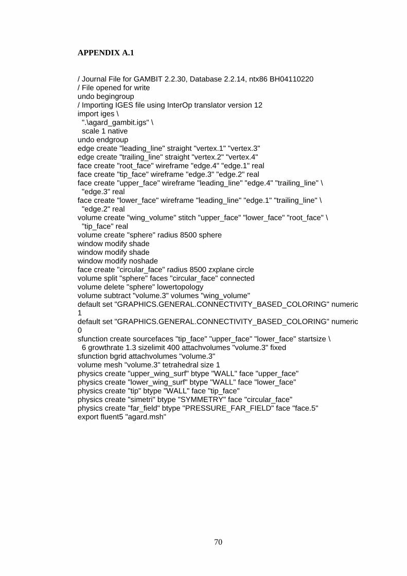
70

APPENDIX A.1

/ Journal File for GAMBIT 2.2.30, Database 2.2.14, ntx86 BH04110220 / File opened for write undo begingroup / Importing IGES file using InterOp translator version 12 import iges \ ".\agard_gambit.igs" \ scale 1 native undo endgroup edge create "leading_line" straight "vertex.1" "vertex.3" edge create "trailing_line" straight "vertex.2" "vertex.4" face create "root_face" wireframe "edge.4" "edge.1" real face create "tip_face" wireframe "edge.3" "edge.2" real face create "upper_face" wireframe "leading_line" "edge.4" "trailing_line" \ "edge.3" real face create "lower_face" wireframe "leading_line" "edge.1" "trailing_line" \ "edge.2" real volume create "wing_volume" stitch "upper_face" "lower_face" "root_face" \ "tip_face" real volume create "sphere" radius 8500 sphere window modify shade window modify shade window modify noshade face create "circular_face" radius 8500 zxplane circle volume split "sphere" faces "circular_face" connected volume delete "sphere" lowertopology volume subtract "volume.3" volumes "wing_volume" default set "GRAPHICS.GENERAL.CONNECTIVITY_BASED_COLORING" numeric 1 default set "GRAPHICS.GENERAL.CONNECTIVITY_BASED_COLORING" numeric 0 sfunction create sourcefaces "tip_face" "upper_face" "lower_face" startsize \ 6 growthrate 1.3 sizelimit 400 attachvolumes "volume.3" fixed sfunction bgrid attachvolumes "volume.3" volume mesh "volume.3" tetrahedral size 1 physics create "upper_wing_surf" btype "WALL" face "upper_face" physics create "lower_wing_surf" btype "WALL" face "lower_face" physics create "tip" btype "WALL" face "tip_face" physics create "simetri" btype "SYMMETRY" face "circular_face" physics create "far_field" btype "PRESSURE_FAR_FIELD" face "face.5" export fluent5 "agard.msh"

71

APPENDIX A.2 : FLUENT Script to Prepare the Flow Model

72

APPENDIX A.2

file/read-case agard.msh grid/scale 0.001 0.001 0.001 grid/reorder/reorder-domain define/models/viscous/inviscid yes define/materials/change-create air air yes ideal-gas define/operating-conditions/operating-pressure 0 define/boundary-conditions/pressure-far-field 0.85 320 0.997 0 0.087 solve/monitors/residual print yes solve/initialize/compute-defaults pressure-far-field report/reference-values/compute pressure-far-field report/reference-values/area 0.353148 report/reference-values/length 0.562 surface/plane-surf-aligned span-0.34 4 0.259 surface/plane-surf-aligned span-0.67 4 0.51 solve/monitors/force/lift-coefficient yes upper_wing_surf lower_wing_surf yes yes no no 0.087 0 0.996 solve/monitors/force/drag-coefficient yes upper_wing_surf lower_wing_surf yes yes no no 0.996 0 0.087 file/write-case agard.cas exit

73

APPENDIX A.3 : ABAQUS Script to Prepare the Structural Model

74

APPENDIX A.3

# # Abaqus/CAE Version 6.7-1 replay file # Run by oncu # # from driverUtils import executeOnCaeGraphicsStartup # executeOnCaeGraphicsStartup() #: Executing "onCaeGraphicsStartup()" in the site directory ... from abaqus import * from abaqusConstants import * session.Viewport(name='Viewport: 1', origin=(0.0, 0.0), width=181.640625, height=212.40234375) session.viewports['Viewport: 1'].makeCurrent() session.viewports['Viewport: 1'].maximize() from caeModules import * from driverUtils import executeOnCaeStartup executeOnCaeStartup() Mdb() #: A new model database has been created. #: The model "Model-1" has been created. session.viewports['Viewport: 1'].setValues(displayedObject=None) iges = mdb.openIges( './agard_abaqus.igs', msbo=False, trimCurve=DEFAULT, scaleFromFile=OFF) mdb.models['Model-1'].PartFromGeometryFile(name='agard_abaqus', geometryFile=iges, dimensionality=THREE_D, type=DEFORMABLE_BODY, convertToAnalytical=1, stitchEdges=1, convertToPrecise=1) p = mdb.models['Model-1'].parts['agard_abaqus'] mdb.models['Model-1'].Material(name='Material-1') mdb.models['Model-1'].materials['Material-1'].Density(table=((4.07282e-10, ), )) mdb.models['Model-1'].materials['Material-1'].Elastic( type=ENGINEERING_CONSTANTS, table=((3671.25, 240.3, 401.63, 0.034, 0.033, 0.326, 321.35, 409.46, 136.5), )) mdb.models['Model-1'].HomogeneousSolidSection(name='Section-1', material='Material-1', thickness=1.0) p = mdb.models['Model-1'].parts['agard_abaqus'] c = p.cells cells = c.getSequenceFromMask(mask=('[#1 ]', ), ) region = regionToolset.Region(cells=cells) p = mdb.models['Model-1'].parts['agard_abaqus'] p.SectionAssignment(region=region, sectionName='Section-1', offset=0.0) p = mdb.models['Model-1'].parts['agard_abaqus'] p.DatumAxisByPrincipalAxis(principalAxis=XAXIS) p = mdb.models['Model-1'].parts['agard_abaqus'] p.DatumAxisByPrincipalAxis(principalAxis=YAXIS) p = mdb.models['Model-1'].parts['agard_abaqus'] p.DatumAxisByPrincipalAxis(principalAxis=ZAXIS) p = mdb.models['Model-1'].parts['agard_abaqus'] d = p.datums p.DatumAxisByRotation(line=d[3], axis=d[5], angle=45.0)

75

p = mdb.models['Model-1'].parts['agard_abaqus'] d1 = p.datums p.DatumCsysByTwoLines(CARTESIAN, line1=d1[6], line2=d1[4], name='Datum csys-1') p = mdb.models['Model-1'].parts['agard_abaqus'] c = p.cells cells = c.getSequenceFromMask(mask=('[#1 ]', ), ) region = regionToolset.Region(cells=cells) p = mdb.models['Model-1'].parts['agard_abaqus'] datums = p.datums[7] p.MaterialOrientation(region=region, orientationType=SYSTEM, localCsys=datums) #: Specified material orientation has been assigned to the selected regions. a = mdb.models['Model-1'].rootAssembly a = mdb.models['Model-1'].rootAssembly a.DatumCsysByDefault(CARTESIAN) p = mdb.models['Model-1'].parts['agard_abaqus'] a.Instance(name='agard_abaqus-1', part=p, dependent=ON) p = mdb.models['Model-1'].parts['agard_abaqus'] p = mdb.models['Model-1'].parts['agard_abaqus'] c = p.cells pickedCells = c.getSequenceFromMask(mask=('[#1 ]', ), ) v, e, d = p.vertices, p.edges, p.datums p.PartitionCellByPlaneThreePoints(cells=pickedCells, point1=p.InterestingPoint( edge=e[2], rule=MIDDLE), point2=p.InterestingPoint(edge=e[3], rule=MIDDLE), point3=p.InterestingPoint(edge=e[1], rule=MIDDLE)) p = mdb.models['Model-1'].parts['agard_abaqus'] c = p.cells pickedCells = c.getSequenceFromMask(mask=('[#1 ]', ), ) v, e, d = p.vertices, p.edges, p.datums p.PartitionCellByPlaneThreePoints(cells=pickedCells, point1=p.InterestingPoint( edge=e[11], rule=MIDDLE), point2=p.InterestingPoint(edge=e[4], rule=MIDDLE), point3=p.InterestingPoint(edge=e[12], rule=MIDDLE)) p = mdb.models['Model-1'].parts['agard_abaqus'] c = p.cells pickedCells = c.getSequenceFromMask(mask=('[#4 ]', ), ) v1, e1, d1 = p.vertices, p.edges, p.datums p.PartitionCellByPlaneThreePoints(cells=pickedCells, point1=p.InterestingPoint( edge=e1[18], rule=MIDDLE), point2=p.InterestingPoint(edge=e1[21], rule=MIDDLE), point3=p.InterestingPoint(edge=e1[16], rule=MIDDLE)) p = mdb.models['Model-1'].parts['agard_abaqus'] c = p.cells pickedCells = c.getSequenceFromMask(mask=('[#8 ]', ), ) v, e, d = p.vertices, p.edges, p.datums p.PartitionCellByPlaneThreePoints(cells=pickedCells, point1=p.InterestingPoint( edge=e[5], rule=MIDDLE), point2=p.InterestingPoint(edge=e[4], rule=MIDDLE), point3=p.InterestingPoint(edge=e[27], rule=MIDDLE)) p = mdb.models['Model-1'].parts['agard_abaqus'] c = p.cells pickedCells = c.getSequenceFromMask(mask=('[#8 ]', ), ) v1, e1, d1 = p.vertices, p.edges, p.datums p.PartitionCellByPlaneThreePoints(cells=pickedCells, point1=p.InterestingPoint( edge=e1[36], rule=MIDDLE), point2=p.InterestingPoint(edge=e1[31], rule=MIDDLE), point3=p.InterestingPoint(edge=e1[28], rule=MIDDLE)) p = mdb.models['Model-1'].parts['agard_abaqus'] c = p.cells

76

pickedCells = c.getSequenceFromMask(mask=('[#10 ]', ), ) v, e, d = p.vertices, p.edges, p.datums p.PartitionCellByPlaneThreePoints(cells=pickedCells, point1=p.InterestingPoint( edge=e[6], rule=MIDDLE), point2=p.InterestingPoint(edge=e[41], rule=MIDDLE), point3=p.InterestingPoint(edge=e[4], rule=MIDDLE)) p = mdb.models['Model-1'].parts['agard_abaqus'] c = p.cells pickedCells = c.getSequenceFromMask(mask=('[#1 ]', ), ) v1, e1, d1 = p.vertices, p.edges, p.datums p.PartitionCellByPlaneThreePoints(cells=pickedCells, point1=p.InterestingPoint( edge=e1[4], rule=MIDDLE), point2=p.InterestingPoint(edge=e1[5], rule=MIDDLE), point3=p.InterestingPoint(edge=e1[11], rule=MIDDLE)) #mesh algoritmasi secimi p = mdb.models['Model-1'].parts['agard_abaqus'] c = p.cells pickedRegions = c.getSequenceFromMask(mask=('[#ff ]', ), ) p.setMeshControls(regions=pickedRegions, technique=SWEEP, algorithm=MEDIAL_AXIS) #gruplamalar #bc p = mdb.models['Model-1'].parts['agard_abaqus'] f = p.faces faces = f.getSequenceFromMask(mask=('[#10281050 #14 ]', ), ) p.Set(faces=faces, name='bc') #: The set 'bc' has been created (8 faces). #profil mesh seed p = mdb.models['Model-1'].parts['agard_abaqus'] e = p.edges edges = e.getSequenceFromMask(mask=('[#b049410 #21212290 ]', ), ) p.Set(edges=edges, name='profil_mesh') #: The set 'profil_mesh' has been created (16 edges). #span mesh seed p = mdb.models['Model-1'].parts['agard_abaqus'] e = p.edges edges = e.getSequenceFromMask(mask=('[#400822 #109102 ]', ), ) p.Set(edges=edges, name='span_mesh') #: The set 'span_mesh' has been created (9 edges). #mesh part seedler #profil seed p = mdb.models['Model-1'].parts['agard_abaqus'] e = p.edges pickedEdges = e.getSequenceFromMask(mask=('[#b049410 #21212290 ]', ), ) p.seedEdgeBySize(edges=pickedEdges, size=6.0) #span seed p = mdb.models['Model-1'].parts['agard_abaqus'] e = p.edges pickedEdges = e.getSequenceFromMask(mask=('[#400822 #109102 ]', ), ) p.seedEdgeBySize(edges=pickedEdges, size=20.0)

77

#enlemesine seedler p = mdb.models['Model-1'].parts['agard_abaqus'] e = p.edges pickedEdges = e.getSequenceFromMask(mask=('[#40002004 #400 ]', ), ) p.seedEdgeByNumber(edges=pickedEdges, number=3) p = mdb.models['Model-1'].parts['agard_abaqus'] e = p.edges pickedEdges = e.getSequenceFromMask(mask=('[#4800000 #2000000 ]', ), ) p.seedEdgeByNumber(edges=pickedEdges, number=4) #mesh part p = mdb.models['Model-1'].parts['agard_abaqus'] p.generateMesh() #coupling surface a = mdb.models['Model-1'].rootAssembly s1 = a.instances['agard_abaqus-1'].faces side1Faces1 = s1.getSequenceFromMask(mask=('[#adc76b8e #6b ]', ), ) a.Surface(side1Faces=side1Faces1, name='coupling_syrface') #: The surface 'coupling_syrface' has been created (24 faces). #meshi goster a = mdb.models['Model-1'].rootAssembly a.regenerate() session.viewports['Viewport: 1'].assemblyDisplay.setValues(mesh=ON) session.viewports['Viewport: 1'].assemblyDisplay.meshOptions.setValues( meshTechnique=ON) a = mdb.models['Model-1'].rootAssembly session.viewports['Viewport: 1'].setValues(displayedObject=a) p = mdb.models['Model-1'].parts['agard_abaqus'] session.viewports['Viewport: 1'].setValues(displayedObject=p) session.viewports['Viewport: 1'].partDisplay.setValues(mesh=ON) session.viewports['Viewport: 1'].partDisplay.meshOptions.setValues( meshTechnique=ON) #statik analiz ayari incrementation mdb.models['Model-1'].StaticStep(name='Step-1', previous='Initial', timeIncrementationMethod=FIXED, initialInc=0.1, noStop=OFF) session.viewports['Viewport: 1'].assemblyDisplay.setValues(step='Step-1') #bc ankastre a = mdb.models['Model-1'].rootAssembly region = a.instances['agard_abaqus-1'].sets['bc'] mdb.models['Model-1'].EncastreBC(name='BC-1', createStepName='Step-1', region=region) #gruplamalar a = mdb.models['Model-1'].rootAssembly e1 = a.instances['agard_abaqus-1'].edges edges1 = e1.getSequenceFromMask(mask=('[#0 #8000 ]', ), ) a.Set(edges=edges1, name='span_deflection') #: The set 'span_deflection' has been created (1 edge). a = mdb.models['Model-1'].rootAssembly

78

e1 = a.instances['agard_abaqus-1'].edges edges1 = e1.getSequenceFromMask(mask=('[#0 #100000 ]', ), ) a.Set(edges=edges1, name='span_deflect_c_4') #: The set 'span_deflect_c_4' has been created (1 edge). a = mdb.models['Model-1'].rootAssembly v1 = a.instances['agard_abaqus-1'].vertices verts1 = v1.getSequenceFromMask(mask=('[#20 ]', ), ) a.Set(vertices=verts1, name='leading_point') #: The set 'leading_point' has been created (1 vertex). a = mdb.models['Model-1'].rootAssembly v1 = a.instances['agard_abaqus-1'].vertices verts1 = v1.getSequenceFromMask(mask=('[#200000 ]', ), ) a.Set(vertices=verts1, name='trailing_point') #: The set 'trailing_point' has been created (1 vertex). #history outputs regionDef=mdb.models['Model-1'].rootAssembly.sets['span_deflection'] mdb.models['Model-1'].HistoryOutputRequest(name='span_deflect', createStepName='Step-1', variables=('U1', 'U2', 'U3'), region=regionDef, sectionPoints=DEFAULT, rebar=EXCLUDE) regionDef=mdb.models['Model-1'].rootAssembly.sets['span_deflect_c_4'] mdb.models['Model-1'].HistoryOutputRequest(name='span_deflect_c_4', createStepName='Step-1', variables=('U1', 'U2', 'U3'), region=regionDef, sectionPoints=DEFAULT, rebar=EXCLUDE) regionDef=mdb.models['Model-1'].rootAssembly.sets['leading_point'] mdb.models['Model-1'].HistoryOutputRequest(name='leading_point', createStepName='Step-1', variables=('U1', 'U2', 'U3'), region=regionDef, sectionPoints=DEFAULT, rebar=EXCLUDE) regionDef=mdb.models['Model-1'].rootAssembly.sets['trailing_point'] mdb.models['Model-1'].HistoryOutputRequest(name='trailing_point', createStepName='Step-1', variables=('U1', 'U2', 'U3'), region=regionDef, sectionPoints=DEFAULT, rebar=EXCLUDE) #write abaqus input file mdb.Job(name='agard', model='Model-1', type=ANALYSIS, explicitPrecision=SINGLE, nodalOutputPrecision=SINGLE, description='', parallelizationMethodExplicit=DOMAIN, multiprocessingMode=DEFAULT, numDomains=1, userSubroutine='', numCpus=1, preMemory=256.0, standardMemory=256.0, standardMemoryPolicy=MODERATE, scratch='', echoPrint=OFF, modelPrint=OFF, contactPrint=OFF, historyPrint=OFF) mdb.jobs['agard'].writeInput(consistencyChecking=OFF) #: The job input file has been written to "agard.inp".

79

APPENDIX B : Results for the Selected Pareto Design #9

80

Figure B.1 : Structural analysis results for /4 32c

and 0.2

81

Figure B.2 : Pressure coefficients for lower and upper wing surfaces respectively

for /4 32c

and 0.2

82

APPENDIX C : Total Designs for the Optimization Problem

83

Design ID Sweep Taper cd cl Displacement L/D Weight

0 26 0.30 0.0358 0.4302 54.63 12.03 1.22

1 12 0.20 0.0395 0.4573 52.04 11.58 1.09

2 38 0.40 0.0303 0.3799 65.15 12.55 1.37

3 18 0.35 0.0366 0.4315 45.84 11.78 1.29

4 44 0.15 0.0296 0.3742 110.95 12.64 1.03

5 6 0.45 0.0363 0.4175 38.71 11.49 1.45

6 32 0.25 0.0344 0.4214 65.69 12.24 1.15

7 16 0.48 0.0353 0.4132 39.88 11.71 1.49

8 42 0.28 0.0297 0.3750 87.32 12.63 1.18

9 2 0.38 0.0372 0.4259 41.07 11.46 1.33

10 28 0.18 0.0368 0.4431 67.80 12.05 1.06

11 8 0.23 0.0392 0.4523 48.86 11.53 1.12

12 2 0.33 0.0377 0.4324 42.95 11.46 1.25

13 16 0.45 0.0356 0.4176 40.89 11.72 1.45

14 28 0.20 0.0365 0.4393 64.85 12.03 1.09

15 12 0.38 0.0370 0.4304 42.46 11.62 1.33

16 12 0.25 0.0387 0.4498 48.68 11.62 1.15

17 10 0.20 0.0395 0.4566 51.24 11.56 1.09

18 32 0.35 0.0332 0.4079 58.31 12.28 1.29

19 26 0.28 0.0361 0.4339 56.24 12.03 1.18

20 40 0.18 0.0316 0.3949 91.71 12.51 1.06

21 30 0.25 0.0352 0.4270 62.63 12.14 1.15

22 46 0.28 0.0275 0.3524 105.52 12.83 1.18

23 28 0.15 0.0370 0.4454 70.65 12.04 1.03

24 32 0.33 0.0335 0.4107 59.77 12.27 1.25

25 30 0.20 0.0358 0.4340 67.64 12.12 1.09

26 36 0.25 0.0328 0.4062 72.56 12.40 1.15

27 12 0.15 0.0400 0.4630 56.16 11.56 1.03

28 10 0.40 0.0368 0.4261 40.94 11.57 1.37

29 36 0.30 0.0322 0.4001 68.40 12.41 1.22

30 14 0.25 0.0386 0.4495 49.38 11.65 1.15

31 22 0.25 0.0374 0.4438 54.44 11.88 1.15

32 38 0.35 0.0308 0.3856 68.55 12.53 1.29

33 28 0.40 0.0339 0.4107 50.69 12.12 1.37

34 30 0.10 0.0367 0.4432 80.85 12.06 0.97

38

0.20

0.0324

Table B.1: Design summary

84

36 38 0.30 0.0313 0.3917 72.16 12.51 1.22

37 30 0.18 0.0360 0.4364 70.25 12.12 1.06

38 22 0.20 0.0380 0.4507 58.50 11.86 1.09

39 20 0.18 0.0388 0.4563 58.91 11.76 1.06

40 4 0.25 0.0388 0.4458 46.71 11.49 1.15

41 38 0.28 0.0317 0.3946 74.47 12.45 1.18

42 34 0.10 0.0352 0.4289 88.51 12.20 0.97

43 36 0.18 0.0335 0.4141 80.73 12.35 1.06

44 30 0.30 0.0346 0.4204 58.98 12.15 1.22

45 28 0.45 0.0333 0.4033 48.27 12.13 1.45

46 36 0.45 0.0305 0.3817 58.48 12.50 1.45

47 38 0.25 0.0319 0.3975 77.00 12.46 1.15

48 46 0.30 0.0272 0.3498 103.06 12.86 1.22

49 34 0.30 0.0330 0.4078 64.74 12.34 1.22

50 22 0.30 0.0367 0.4364 51.15 11.88 1.22

51 46 0.18 0.0282 0.3597 117.76 12.77 1.06

52 20 0.15 0.0392 0.4602 61.49 11.75 1.03

53 28 0.35 0.0346 0.4183 53.43 12.09 1.29

54 28 0.25 0.0359 0.4330 60.36 12.06 1.15

55 36 0.15 0.0338 0.4162 84.38 12.32 1.03

56 38 0.43 0.0300 0.3767 63.48 12.56 1.41

57 38 0.48 0.0295 0.3706 60.63 12.58 1.49

58 20 0.25 0.0378 0.4461 52.99 11.81 1.15

59 44 0.25 0.0288 0.3665 98.27 12.72 1.15

61 30 0.15 0.0363 0.4395 73.28 12.10 1.03

62 32 0.28 0.0341 0.4176 63.48 12.24 1.18

63 36 0.28 0.0325 0.4033 70.46 12.42 1.18

64 38 0.33 0.0311 0.3888 70.29 12.49 1.25

65 28 0.28 0.0355 0.4296 58.28 12.11 1.18

66 36 0.20 0.0333 0.4116 77.90 12.35 1.09

67 14 0.48 0.0355 0.4141 39.30 11.66 1.49

68 38 0.18 0.0326 0.4046 85.32 12.42 1.06

69 38 0.38 0.0305 0.3827 66.78 12.53 1.33

70 48 0.33 0.0260 0.3359 112.74 12.93 1.25

71 34 0.43 0.0316 0.3913 56.66 12.38 1.41

72 46 0.20 0.0280 0.3579 114.08 12.76 1.09

73 4 0.28 0.0385 0.4418 45.38 11.47 1.18

85

75 6 0.48 0.0360 0.4140 37.94 11.49 1.49

76 46 0.48 0.0257 0.3336 89.57 12.98 1.49

77 32 0.20 0.0350 0.4274 70.66 12.20 1.09

78 38 0.15 0.0328 0.4069 88.90 12.39 1.03

79 30 0.38 0.0336 0.4097 54.20 12.21 1.33

80 36 0.40 0.0312 0.3876 61.27 12.44 1.37

81 38 0.45 0.0298 0.3741 62.09 12.55 1.45

82 34 0.45 0.0314 0.3880 55.26 12.36 1.45

83 32 0.10 0.0360 0.4365 84.23 12.13 0.97

84 48 0.20 0.0269 0.3458 126.71 12.85 1.09

85 30 0.28 0.0349 0.4238 60.78 12.14 1.18

87 30 0.23 0.0355 0.4306 65.06 12.13 1.12

88 46 0.35 0.0268 0.3457 98.34 12.90 1.29

89 38 0.10 0.0332 0.4099 97.79 12.34 0.97

90 32 0.23 0.0348 0.4239 67.75 12.19 1.12

91 6 0.10 0.0405 0.4640 57.99 11.46 0.97

93 50 0.43 0.0239 0.3146 117.46 13.14 1.41

95 4 0.48 0.0360 0.4128 37.80 11.46 1.49

96 32 0.18 0.0353 0.4301 73.34 12.17 1.06

97 14 0.20 0.0393 0.4569 52.90 11.63 1.09

98 34 0.15 0.0347 0.4246 79.84 12.25 1.03

99 22 0.43 0.0351 0.4168 44.73 11.87 1.41

100 6 0.30 0.0382 0.4399 44.49 11.51 1.22

101 36 0.38 0.0314 0.3908 62.94 12.45 1.33

102 2 0.10 0.0401 0.4585 56.58 11.44 0.97

103 6 0.13 0.0403 0.4622 55.67 11.48 1.00

104 34 0.35 0.0324 0.4012 61.17 12.38 1.29

105 28 0.10 0.0375 0.4497 78.10 11.99 0.97

106 6 0.15 0.0401 0.4596 53.38 11.47 1.03

107 34 0.38 0.0322 0.3978 59.49 12.34 1.33

86

RESUME

Levent ÖNCÜ was born in March 6th

, 1983 in Zonguldak, TURKEY. He had his

high school education in Zonguldak Atatürk Anatolian High School (ZAAL) and

Zonguldak Science High School (ZFL). He graduated 2nd

place in the graduating

class of Aeronautical Engineering Department of İstanbul Technical University

(İTÜ) Aeronautics and Astronautics Faculty in 2006. He attended the Von Karman

Institute‘s Short Training Program in Brussels, BELGIUM. He had the National

Scholarship Program for the Graduate Students of The Scientific and Technological

Research Council of Turkey (TÜBİTAK-BAYG) during his graduate study. He is

now going on his graduate in Aeronautical Engineering and working as a researcher

in the TÜBİTAK project 105M235 ―Analysis and Reliability Based Design

Optimization of Fluid-Structure Interaction Problems Subject to Instability

Phenomena‖.