
IFRS for SMEs: An Emperical Study of the KwaZulu Natal SME ...
Upload
khangminh22Category
view
1download
0
A STUDY AND IMPLEMENTATION ANALYSIS OF AN
ANTI-SAGGING DEVICE FOR POWER TRANSMISSION
LINES USING SHAPE MEMORY ALLOYS
Kevin M. Lüssi
In fulfilment of the academic requirements for the degree of Mater of Science in the Department of
Mechanical Engineering, University of KwaZulu-Natal.
EXAMINER’S COPY
As the candidate’s supervisor, I agree to the submission of this thesis.
Signed: Date:
Prof. Glen Bright (Head of School, Mechanical Engineering, UKZN) on behalf of
Prof. Dzevad Muftic (PhD. Electrical Engineering, Pr Eng.)

ii
DECLARATION
I, Kevin M. Lüssi declare that the research reported in this dissertation, except where otherwise
indicated is my original work. This dissertation has not been submitted for any degree or
examination at any other university. This dissertation does not contain other persons’ data, pictures,
graphs or other information, unless specifically acknowledged as being sourced from other persons.
This dissertation does not contain other persons’ writing, unless specifically acknowledged as being
sourced from other researchers. Where other written sources have been quoted, then:
a) Their words have been re-written but the general information attributed to them has been
referenced;
b) Where their exact words have been used, their writing has been placed inside quotation marks,
and referenced.
Where I have reproduced a publication of which I am the author, co-author or editor, I have
indicated in detail which part of the publication was actually written by myself alone and have fully
referenced such publications. This dissertation does not contain text, graphics or tables copied and
pasted from the internet, unless specifically acknowledged, and the source being detailed in the
dissertation and in the References section.
Signed,
Kevin M. Lüssi

iii
ACKNOWLEDGEMENTS
I would like to thank my supervisor, Prof Dzevad Muftic for his oversight in this dissertation, my
professor and supervisor for their expertise, direction in the inception of the degree, Kevin Smith in
the workshop for helping me build the testing rig, Greg Loubser for his help in developing the data
acquisition system, Riaz Vajeth, my manager at Trans Africa Projects for his understanding and for
accommodating my working on this project, my family for their constant support to me as a student
and my beautiful wife who makes my world go round and always encourages me to dream for the
stars and my best friend, J.C..

iv
ABSTRACT
Shape memory alloys (SMA’s) are a family of metals that exhibit properties of pseudo-elasticity
and the shape memory effect. This means that they can undergo considerable deformation from a
load and return back to their original shape while applying a “return-force” with the application of
heat. This Masters project analyses the use of the shape memory property of this family of metals in
the development of a device (by Power Transmission Solutions, Inc.) for use in South Africa’s
power transmission lines to mitigate the thermal sag in the cables. Thermal sag in power
transmission lines has always been a problem when spanning long distances due to safety issues
pertaining to ground clearances. The limiting factor has been the number of amps that can be
transmitted due to the heat generation. Being able to compensate for the sag would allow for more
amps to be transmitted resulting in more efficient transmission. The project began with a study of
the field of smart materials. A literature survey was then carried out in the field of shape memory
alloys, their properties and their processing techniques, from which an understanding of the
technology was gained. The project culminated in the design of a power line (mechanical) load-
simulating testing rig (constant tension) and the testing of a full-scale South African custom
prototype which underwent a technical performance evaluation. The outcome of the project was a
technical and economical analysis of the device that could be implemented, nation-wide, into
Eskom’s power transmission lines thus offering an innovative alternate solution to the problem of
sagging power lines and their restrictions in power transmission. Research was be focused on the
mechanical and physical properties of shape memory alloys used in the device that would be suited
to application in South Africa’s overhead power line network.

v
TABLE OF CONTENTS
DECLARATION ............................................................................................................................... ii
ACKNOWLEDGEMENTS ............................................................................................................. iii
ABSTRACT ...................................................................................................................................... iv
LIST OF FIGURES ....................................................................................................................... viii
LIST OF TABLES .......................................................................................................................... xii
1. INTRODUCTION ..................................................................................................................... 1
1.1. OVERVIEW ............................................................................................................................ 1
1.2. PARAMETERS OF THE INVESTIGATION ........................................................................ 2
2. SHAPE MEMORY ALLOYS .................................................................................................. 3
2.1. INTRODUCTION ................................................................................................................... 3
2.2. MARTENSITIC TRANSFORMATION ................................................................................. 6
2.3. MECHANISMS OF THE SHAPE MEMORY EFFECT AND SUPERELASTICITY ........ 11
2.3.1. Shape Memory .......................................................................................................... 11
2.3.2. Superelasticity ........................................................................................................... 14
2.4. PROPERTIES OF NITINOL................................................................................................. 18
3. THE SAGGING LINE MITIGATOR (SLiM) ........................................................................ 20
3.1. OVERVIEW .......................................................................................................................... 20
3.2. DESIGN ................................................................................................................................. 21
3.3. SPECIFICATIONS ................................................................................................................ 23
4. TESTING ................................................................................................................................ 29
4.1. OVERVIEW .......................................................................................................................... 29
4.2. TESTING PARAMETERS ................................................................................................... 30
4.3. TEST RIG DESIGN .............................................................................................................. 32
4.4. TESTING PROCEDURE ...................................................................................................... 37
5. RESULTS ............................................................................................................................... 40
5.1. OVERVIEW .......................................................................................................................... 40
5.2. TEST RESULTS ................................................................................................................... 41
5.2.1. Run 1 (18th June 2007): ............................................................................................ 41
5.2.2. Run 2 (19th June 2007): ............................................................................................. 43
5.2.3. Run 3 (19th June 2007): ............................................................................................. 45
5.2.4. Run 4 (21st June 2007): ............................................................................................. 47
5.2.5. Run 5 (21st June 2007): ............................................................................................. 49
vi
5.2.6. Run 6 (22nd June 2007): ............................................................................................ 51
5.2.7. Run 7 (22nd June 2007): ............................................................................................ 53
5.2.8. Run 8 (29th June 2007): ............................................................................................. 55
5.3. ANALYSIS ............................................................................................................................ 57
5.4. CONCLUSION ...................................................................................................................... 61
6. DISCUSSION ......................................................................................................................... 62
6.1. OPERATIONAL ................................................................................................................... 62
6.2. ECONOMICAL ..................................................................................................................... 66
6.3. FUTURE REGARDING SOUTH AFRICA ......................................................................... 67
7. CONCLUSION ....................................................................................................................... 69
8. REFERENCES ........................................................................................................................ 71
9. APPENDIX A – SMART MATERIALS ................................................................................ 76
9.1. INTRODUCTION ................................................................................................................. 76
9.2. PIEZOELECTRIC MATERIALS ......................................................................................... 76
9.3. ELECTROSTRICTIVE MATERIALS ................................................................................. 78
9.4. MAGNETOSTRICTIVE MATERIALS ............................................................................... 80
9.5. ELECTRORHEOLOGIC AND MAGNETORHEOLOGIC FLUIDS .................................. 82
10. APPENDIX B – ADDITIONAL INFORMATIO ON NICKEL-TITANIUM ALLOY ......... 84
10.1. CRYSTALLOGRAPHY ..................................................................................................... 84
10.2. LATTICE INVARIANT SHEAR AND DEFORMATION TWINNING .......................... 85
10.3. ALLOYING OF NiTi .......................................................................................................... 86
10.4. APLICATIONS OF NITINOL ............................................................................................ 87
11. APPENDIX C – OVERHEAD POWER LINES .................................................................... 91
11.1. INTRODUCTION ............................................................................................................... 91
11.2. BASIC THEORY ................................................................................................................ 92
11.3. PLANNING ......................................................................................................................... 93
11.4. ENVIRONMENT ................................................................................................................ 94
11.4.1. Environmental ....................................................................................................... 94
11.4.2. Corona and Electromagnetic Fields ...................................................................... 96
11.4.3. Lightning ............................................................................................................... 97
11.5. DESIGN OPTIMISATION ................................................................................................. 98
11.5.1. Electrical design optimisation ............................................................................... 99
11.5.1.1. Basic Electrical Design ..................................................................................... 99
11.5.1.2. Insulator Co-ordination ................................................................................... 100

vii
11.5.1.3. Thermal Rating ............................................................................................... 101
11.5.2. Structural and Component Design ...................................................................... 103
11.5.2.1. Conductor optimisation ................................................................................... 103
11.5.2.2. Ground Wire Optimisation ............................................................................. 105
11.5.2.3. Insulator Selection .......................................................................................... 106
11.5.2.4. Line Hardware ................................................................................................ 109
11.5.2.5. Supporting Structures ..................................................................................... 110
11.5.2.6. Foundations and Earthing ............................................................................... 113
11.5.3. Line Design ......................................................................................................... 114
11.6. CONSTRUCTION ............................................................................................................ 117
11.6.1. Foundation Construction ..................................................................................... 117
11.6.2. Tower Erection .................................................................................................... 118
11.6.3. Stringing .............................................................................................................. 119
12. APPENDIX D – TEST RIG DRAWINGS AND CALCULATIONS .................................. 123
12.1. Isometric Drawing of the Test Rig .................................................................................... 123
12.2. Working drawings ............................................................................................................. 124
12.3. Calculations ....................................................................................................................... 133
12.3.1. Shaft Calculation – Castigliano’s Method .......................................................... 133
12.3.2. Back-plate Calculation – Castigliano’s Method .................................................. 133
13. APPENDIX E – DERIVATION OF THE FORMULA FOR SAG ACCORDING TO THE
PARABOLIC MODEL ................................................................................................................... 134
viii
LIST OF FIGURES
Figure 2.1-1: The shape memory alloy concept .................................................................................. 5
Figure 2.2-1: A typical transformation versus temperature curve for a SMA under constant tension
as the specimen is cooled and then heated. H: transformation Hysteresis; Ms: martensitic start;
Mf: martensitic finish; As: austenitic start; Af: austenitic finish. ................................................ 7
Figure 2.2-2: Two-stage transformation sequence of thermo-mechanically treated 49.8 Ti-50.2 Ni
(at%) Nitinol. (Saburi 1998) ....................................................................................................... 8
Figure 2.2-3 a, b: Basic variance in martensitic transformation. (a) β phase (parent). (b)
Transformed to martensite. Self-accommodating twin-related variants A, B, C, D. (c) Shape
change from longitudinal stress σ as variant A becomes dominant. Upon heating, the specimen
reverts to its parent (β) phase and recovers its original shape. (Hodgson, Wu & Biermann
1998) ......................................................................................................................................... 10
Figure 2.3-1: Schematic of the crystal structure behaviour of a shape memory alloy upon cooling,
loading/unloading and heating. ................................................................................................ 12
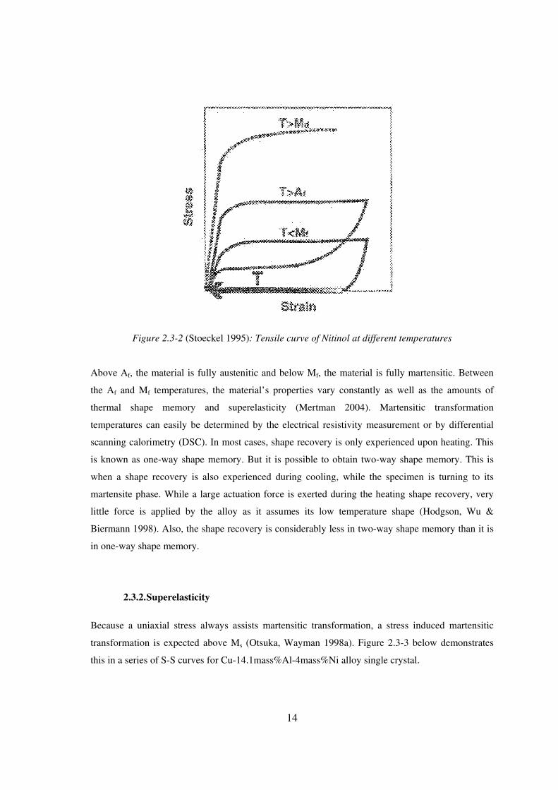
Figure 2.3-2 (Stoeckel 1995): Tensile curve of Nitinol at different temperatures ............................ 14
Figure 2.3-3: Stress-strain curves as functions of temperature for Cu-14.1mass%Al-4mass%Ni alloy
single crystal for which Ms = 242K, Mf = 241K, As = 266K and Af = 291K. (Horikawa et al.
1988) ......................................................................................................................................... 15
Figure 2.3-4: Morphological changes associated with ′
− 11 ββ stress induced transformation upon
loading and its reverse transformation upon unloading for Cu-14.2mass%Al-4.2mass%Ni
alloy single crystal. (Otsuka et al. 1976) .................................................................................. 16
Figure 2.3-5: Representation of shape memory and superelasticity on a stress versus temperature
graph. (Miyazaki, Otsuka 1989) ............................................................................................... 17
Figure 3.1-1: Sagging Line Mitigator (SLiM) (Shirmohamadi 2006b) ............................................ 20
Figure 3.2-1: Components of the SLiM (Shirmohamadi 2006b) ...................................................... 21
Figure 3.2-2: The SLiM’s nickel-titanium actuator (Shirmohamadi 2002) ...................................... 22
Figure 3.3-1: Strain versus temperature response expect for the custom SLiM device, ESK-01.
(Shirmohamadi 2006a) ............................................................................................................. 24
Figure 4.3-1: Schematic of the principle of the SLiM’s constant tension testing rig. ....................... 32
Figure 4.3-2: The SLiM testing rig. .................................................................................................. 33
Figure 4.3-3 a, b: The 22kN hydraulic ram (left) that provided the constant tension in the test-span
via a lever (right) that magnified (mechanical advantage) the ram’s displacement. ................ 34

ix
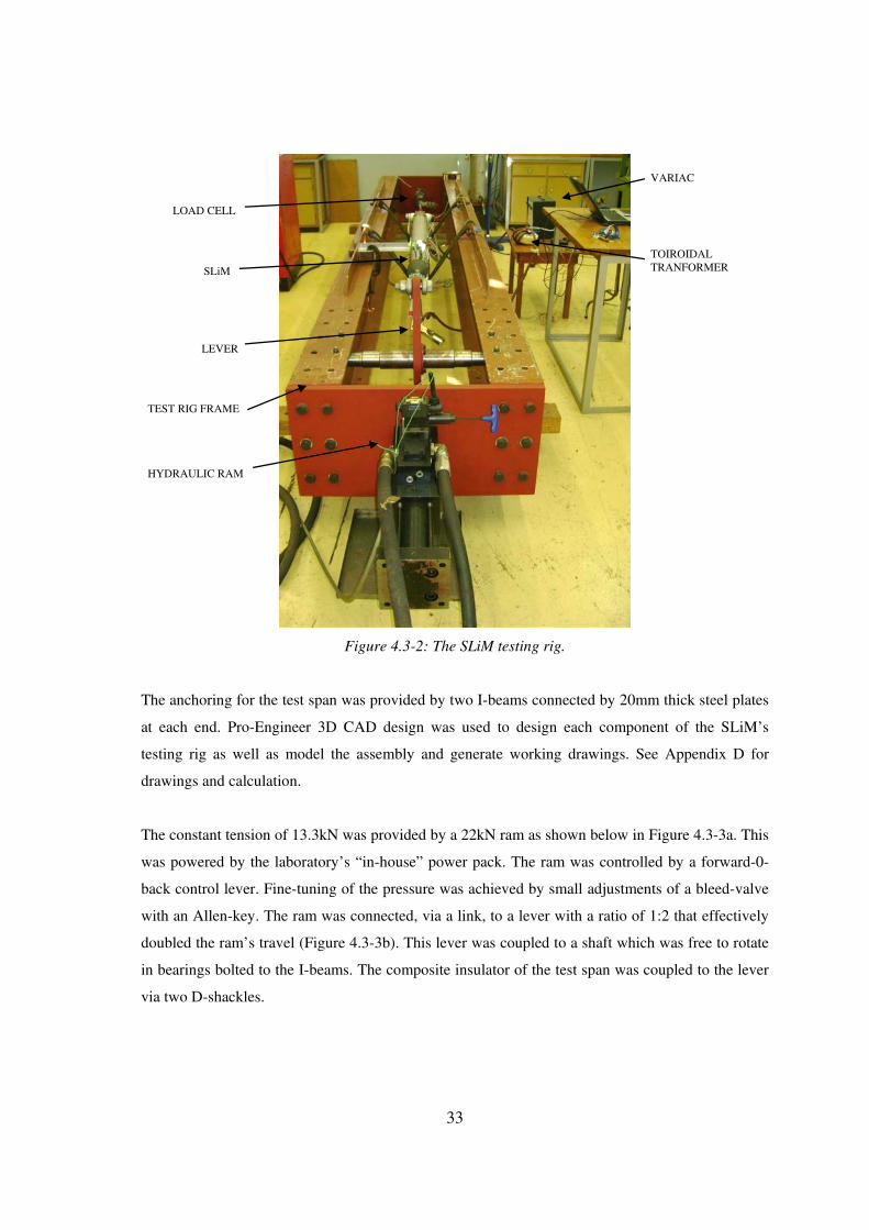
Figure 4.3-4: The 10A variac and toroidal transformer that supplied the 300A test current. ........... 35
Figure 4.3-5: The Data Acquisition system (DAQ) designed to log all the data coming in every
second, providing real-time monitoring of the heating and cooling cycles. ............................. 36
Figure 4.3-6: Mounting of the stepper motor to measure the SLiM’s linear displacement. ............. 36
Figure 4.4-1, a, b: The SLiM’s lever fully extended (left) and fully contracted (right) as a result of
the heating of its Nitinol core. .................................................................................................. 38
Figure 5.2-1: Heating curve for Run 1 .............................................................................................. 41
Figure 5.2-2: Strain curve for Run 1 ................................................................................................. 42
Figure 5.2-3: Strain vs. Temperature curve for Run 1 ...................................................................... 42
Figure 5.2-4: Heating curve for Run 2 .............................................................................................. 43
Figure 5.2-5: Strain curve for Run 2 ................................................................................................. 44
Figure 5.2-6: Strain vs. Temperature curve for Run 2 ...................................................................... 44
Figure 5.2-7: Heating curve for Run 3 .............................................................................................. 45
Figure 5.2-8: Strain curve for Run 3 ................................................................................................. 46
Figure 5.2-9: Strain vs. Temperature curve for Run 3 ...................................................................... 46
Figure 5.2-10: Heating curve for Run 4 ............................................................................................ 47
Figure 5.2-11: Strain curve for Run 4 ............................................................................................... 48
Figure 5.2-12: Strain vs. Temperature curve for Run 4 .................................................................... 48
Figure 5.2-13: Heating curve for Run 5 ............................................................................................ 49
Figure 5.2-14: Strain curve for Run 5 ............................................................................................... 50
Figure 5.2-15: Strain vs. Temperature curve for Run 5 .................................................................... 50
Figure 5.2-16: Heating curve for Run 6 ............................................................................................ 51
Figure 5.2-17: Strain curve for Run 6 ............................................................................................... 52
Figure 5.2-18: Strain vs. Temperature curve for Run 6 .................................................................... 52
Figure 5.2-19: Heating curve for Run 7 ............................................................................................ 53
Figure 5.2-20: Strain curve for Run 7 ............................................................................................... 54
Figure 5.2-21: Strain vs. Temperature curve for Run 7 .................................................................... 54
Figure 5.2-22: Heating curve for Run 8 ............................................................................................ 55
Figure 5.2-23: Strain curve for Run 8 ............................................................................................... 56
Figure 5.2-24: Strain vs. Temperature curve for Run 8 .................................................................... 56
Figure 5.3-1: Strain vs. Temperature curve for all runs .................................................................... 57
Figure 5.3-2: Graph showing the As and Af temperatures of the SLiM for all runs. ......................... 58
Figure 5.3-3: Strain of the SLiM for each run relative to the average strain. ................................... 58
Figure 5.3-4: Temperature-time response for the SLiM’s Nitinol core. (τ = 661 seconds) .............. 60
x
Figure 6.1-1: Schematic of a 400m strain-to-strain level span. ........................................................ 62
Figure 6.1-2: Schematic of 4 spans between 2 strain structures. ...................................................... 66
Figure 9.2-1: The piezoelectric effect (SMA/MEMS Research Group 2001) .................................. 77
Figure 9.3-1: Displacement as a function of field strength for PZT (piezoelectric) compared to PMN
(electrostrictive) (Tavernor 2002) ............................................................................................ 79
Figure 9.3-2: Displacement versus voltage graph representing electrostriction and its typical
hysteresis. ................................................................................................................................. 80
Figure 9.4-1: Rotation and movement of magnetic domains causing a physical length change in
magnetostrictive materials (Active Materials Laboratory 2005). ............................................. 81
Figure 9.4-2: Reorientation of the domain structure in a magnetostrictive material under load when
a magnetic field is applied (Active Materials Laboratory 2005). ............................................. 82
Figure 9.5-1: A magnetorheologic fluid is liquid on the left and then solidifies in the presence of a
magnetic field (right) (SMA/MEMS Research Group 2001). .................................................. 83
Figure 10.2-1 Shows why lattice invariant shear is necessary upon martensitic transformation; (a)
shape change upon martensitic transformation; (b) accommodation of strain by introduction of
slip; (c) accommodation of strain by twinning. (Otsuka, Wayman 1998b) .............................. 85
Figure 10.4-1 (Advanced Materials Today 2006): shape memory alloy actuator ............................. 88
Figure 10.4-2 (Smart Technology 2006): Shape memory alloy coupling ......................................... 89
Figure 10.4-3: A Simon filter (left) and a vascular stent (right). (Bard Peripheral Vascular 2008) . 90
Figure 11.1-1: An 88kV power line in Zululand ............................................................................... 91
Figure 11.2-1: Simple circuit representation of an overhead power line (Reynders et al. 2005). ..... 92
Figure 11.4-1: The electrocution of birds is a common environmental issue and has to be negated by
the use of “bird-friendly” structures that employ anti-perch devices and specific design. ...... 96
Figure 11.4-2: Lightning ground flash density map of South Africa (Gaunt, Britten & Geldenhuys
1995) ......................................................................................................................................... 98
Figure 11.5-1: Common bundle configurations ................................................................................ 99
Figure 11.5-2: Phase configurations ............................................................................................... 100
Figure 11.5-3: Examples of ACSR conductors. (Muftic, Vajeth & Dama 2005) ........................... 103
Figure 11.5-4: Examples of AAAC conductors. (Muftic, Vajeth & Dama 2005) .......................... 104
Figure 11.5-5: Conductor optimisation expression of Kelvin’s rule. (Muftic, Vajeth & Dama 2005)
................................................................................................................................................ 105
Figure 11.5-6: Single disk of a cap-and-pin insulator (Bologna 2005) ........................................... 107
Figure 11.5-7: A long-rod porcelain insulator (Bologna 2005) ...................................................... 107
Figure 11.5-8: A typical polymer insulator (Bologna 2005) ........................................................... 108

xi
Figure 11.5-9: A typical example of a suspension structure ........................................................... 111
Figure 11.5-10: A typical example of a strain structure .................................................................. 112
Figure 11.5-11: A tower connection to the steel reinforcement within the concrete foundation.
(Burger, Ramnarain & Peter 2005) ........................................................................................ 114
Figure 11.5-12: A sample profile generated in PLS Cadd (Power Line Systems, Inc 1993-2008)
showing the terrain, tower positioning and conductor templating. ........................................ 116
Figure 11.5-13: A generated 3D terrain showing a portion of line (PLS Cadd, Power Line Systems,
Inc 1993-2008) ....................................................................................................................... 116
Figure 11.6-1: The construction of a tower foundation. ................................................................. 118
Figure 11.6-2: A guyed structure being assembled on its side (left) and hoisted, once assemble, into
position by a crane (right). The crane would hold the structure in place until all four stays are
secured. ................................................................................................................................... 119
Figure 11.6-3: A dressed guyed-Vee structure being stung with the layout method. (Marais,
Badenhorst 2005) ................................................................................................................... 120
Figure 11.6-4: A typical setup for tension stringing a line. (Marais, Badenhorst 2005) ................. 121
Figure 11.6-5: A winch (left) and tensioner (right) in operation during the stringing of an overhead
power line. (Morcap Industries 2008) .................................................................................... 121
Figure 12.1-1: Assembled view of the SLiM’s test rig. .................................................................. 123
Figure 12.2-1: Assembly drawing of the SLiM test rig. ................................................................. 124
Figure 12.2-2: Working drawing – Flange 1(end plate). ................................................................. 125
Figure 12.2-3: Working drawing – Flange 2 (end plate). ................................................................ 126
Figure 12.2-4: Working drawing – Lever. ...................................................................................... 127
Figure 12.2-5: Working drawing: pin. ............................................................................................ 128
Figure 12.2-6: Working drawing – link. ......................................................................................... 129
Figure 12.2-7: Working drawing – ram end. ................................................................................... 130
Figure 12.2-8: Working drawing – reinforcement plate. ................................................................ 131
Figure 12.2-9: Working drawing – lever. ........................................................................................ 132
Figure 12.3-1: Span diagram ........................................................................................................... 134

xii
LIST OF TABLES
Table 2.1-1: Most common shape memory alloys (Hodgson, Wu & Biermann 1998)....................... 6
Table 2.4-1: Major properties of binary Ni-Ti. (Miyazaki 2005). .................................................... 18
Table 3.3-1: PTS equipment specification – custom PTS SLiM – ESK-01 ...................................... 23
Table 3.3-2: Properties of Wolf ACSR 30/7 from IEC code 158-A1/S1A-30/2,59/7/2,59 .............. 25
Table 3.3-3: Properties of the nickel-titanium actuator of the SLiM (Shirmohamadi 2002) ............ 26
Table 3.3-4: Material properties for the SLiM (Shirmohamadi 2002) .............................................. 27
Table 3.3-5: Composite bearing material properties (Shirmohamadi 2002) ..................................... 28
Table 4.2-1: Table of test parameters ................................................................................................ 31
Table 5.2-1: Parameter results of Run 1 ............................................................................................ 41
Table 5.2-2: Parameter results of Run 2 ............................................................................................ 43
Table 5.2-3Table 7.2.3.1: Parameter results of Run 3 ....................................................................... 45
Table 5.2-4: Parameter results of Run 4 ............................................................................................ 47
Table 5.2-5: Parameter results of Run 5 ............................................................................................ 49
Table 5.2-6: Parameter results of Run 6 ............................................................................................ 51
Table 5.2-7: Parameter results of Run 7 ............................................................................................ 53
Table 5.2-8: Parameter results of Run 8 ............................................................................................ 55
Table 5.3-1: Summary of parameter results from all the runs .......................................................... 57
Table 5.3-2: Table of properties for custom prototype SLiM ESK-01 ............................................. 59
Table 6.1-1: The effects of a SLiM on 4 suspension spans (modelled in PLS-Cadd Sagsec) .......... 66
Table 11.5-1: Minimum required creepage distances for operating pollution levels. (Bologna 2005)
................................................................................................................................................ 109
Table 11.5-2: Some common load-bearing hardware. (Calitz et al. 2005) ..................................... 110
1
1. INTRODUCTION
1.1. OVERVIEW
South Africa has a rapidly growing economy. This is placing a high demand on existing
infrastructure as it struggles to grow and keep up with the increasing need. One such component is
the electrical power system provided by the utility Eskom. The electric power system can be
divided into three sections, namely; generation, transmission and distribution. The rapid
urbanization and industrialisation of South Africa is resulting in increasing power demands. This
means that greater loads are required to be transmitted along Eskom’s power lines. Because lines
are designed for specific loads, it is not possible to increase the loads without adverse and possibly
disastrous effects. An increase in transmitted load results in greater heat generation in that line.
This, in turn, will cause the line to sag more than its design stringing sag, often violating statutory
clearance limits. Were this to occur over a critical span, for example, a road, then flashovers would
occur when a tall vehicle passes underneath. To upgrade the capacity of a line or, uprate the line,
would require some modification of that line. The line could either be re-strung with a larger
conductor, the strength of the structures being the limiting factor, the towers themselves could be
extended to counter the reduction in clearance or, if the increase in temperature is not an issue, then
the line could be re-tensioned. The conventional way of re-tensioning a line is to power down the
section of line that needs work and to physically shorten the conductor. This however is not always
an option especially if the line is inaccessible or is supplying a critical user that cannot
accommodate the down-time. An alternative tensioning method has been developed in the USA. It
is an in-span device called a Sagging Line Mitigator or SLiM. Once installed in the span, the SLiM
would react to the increasing temperature and shorten, thereby tensioning the conductor and
counteracting the sag. The SLiM uses shape memory alloy technology to achieve this effect. Should
this device be able to operate satisfactorily in the harsh South African climate and under the
required conditions, then the SLiM could prove to be a valuable alternative and innovative solution
to the problem of sagging power lines in South Africa. The SLiM devices were designed for the
Californian climate and have not yet been implemented for service by American utilities. Such a
new technology has great potential for South Africa. Traditionally, shape memory alloy technology
has found its uses in the bio-medical field and has only recently started finding application in other
fields.

2
1.2. PARAMETERS OF THE INVESTIGATION
The objective of this investigation is to research the smart material field, shape memory technology
and application in use around the world and to investigate in particular its implementation and its
effectiveness in the Sagging Line Mitigator. This was done by testing the device in a laboratory
with the use of a purpose-built testing rig that would provide a constant tension to the device while
supplying an actuation current to cycle the Nickel-Titanium alloy core through its heating and
cooling phases. The thesis set out to present a study of literature on shape memory alloys, in
particular Nickel-Titanium alloy as well as an overview of the intended application, namely,
electrical transmission overhead power lines.
A further objective is to identify the benefit of implementation of the anti-sagging device on South
African lines. A precise set of property parameters will be presented for the custom prototype SLiM
ESK-01. Recommendation will be made regarding the roll-out of the SLiM as a viable solution to
the problem of sagging power lines in South Africa.

3
2. SHAPE MEMORY ALLOYS
The Shape Memory Effect and Superelasticity
2.1. INTRODUCTION
The term “smart material” refers to any material with one or more properties that can be
significantly and controllably changed by an external input. As opposed to a normal material with
properties that cannot be altered. The main categories of smart materials that are undergoing
continuous research for new application are piezoelectric materials, magneto-rheostatic materials,
electro-rheostatic materials and shape memory alloys. They are already incorporated in many every-
day items with new applications being developed constantly. These smart materials each have
different properties that can be altered. These changeable properties influence the type of
application that the material can be used for. Generally, smart material systems are employed in
three ways: sensors that register important internal and external information; actuators (motors) that
can switch or apply forces; and computerised control systems. They often contain combinations of
the aforementioned system types and this is what makes them “smart”; the fact that these materials
can gather information, perform tasks, sense changing conditions and adapt accordingly. More
information on the smart material topic can be found in Appendix A.
There is a certain family of metal alloys that exhibits the shape memory phenomenon as well as
some other unusual properties. The metallurgical basis of these effects is the reversible martensitic
phase transformation from the high temperature phase austenite to the low temperature phase
martensite. This transformation is of the type that allows the alloy to be deformed by a twinning
mechanism below the transformation temperature. This deformation can then be reversed when the
twinned structure reverts upon heating to the parent phase. (The mechanics of this transformation
are explained in the next sub-section). Martensitic transformation is in itself not a new discovery.
The first recorded observation of the shape memory transformation, according to (Hodgson, Wu &
Biermann 1998), was as early as 1932 by Chang and Read. The shape memory effect was then
noted in an Au-Cd alloy in 1951 (Miyazaki, Otsuka 1989). It was also noted in the mid 1950’s that
steel that was heat treated at a high temperature and then rapidly quenched displayed martensitic
transformation although it was not crystallographically reversible and thus unable to display the
shape memory effect. The fine grain structure that was resulting from this martensitic

4
transformation was named “martensite” after the discoverer, Adolf Martens (Miyazaki). In 1963,
Nickel-Titanium alloy was found to have the shape memory effect by Buehler and co. (Miyazaki,
Otsuka 1989). It was named Nitinol after it’s elements, nickel and titanium and the place of the
discovery, the Naval Ordinance Laboratory. Within 10 years of this, several commercial products
were available on the market with interest and research in the SMA field increasing till today.
The martensitic transformation that occurs in shape memory alloys is crystallographically reversible
or thermoelastic. Although shape memory alloys have limitless engineering potential with as many
as 4000 registered patents (Miyazaki, Otsuka 1989), very few developments have actually made it
to the market to become an economic success. Recent successes have been mainly in medical
applications making use of superelasticity and biocompatibility (Stoeckel 1995). The most widely
used shape memory alloy is Ni-Ti, showing the most shape memory recovery and superelasticity as
well as biocompatibility and corrosion resistance. Copper based alloys like Cu-Zn-Al and Cu-Al-Ni
are also commercially available and less expensive than Ni-Ti but are more brittle and less stable.
Iron based shape memory alloys are being developed but have limited shape memory strain and
lack other essential properties.
The shape memory effect can be described by considering figure 2.1-1. A paperclip (A) that is made
of Nitinol.
5
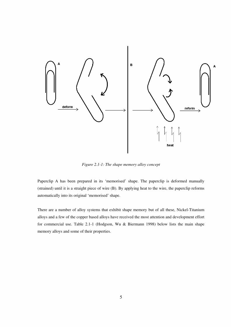
Figure 2.1-1: The shape memory alloy concept
Paperclip A has been prepared in its ‘memorised’ shape. The paperclip is deformed manually
(strained) until it is a straight piece of wire (B). By applying heat to the wire, the paperclip reforms
automatically into its original ‘memorised’ shape.
There are a number of alloy systems that exhibit shape memory but of all these, Nickel-Titanium
alloys and a few of the copper based alloys have received the most attention and development effort
for commercial use. Table 2.1-1 (Hodgson, Wu & Biermann 1998) below lists the main shape
memory alloys and some of their properties.

6
ALLOY COMPOSITION TRANSFORMATION
TEMP. (°C)
Ag-Cd 44/49 at.% Cd -190 to -50
Au-Cd 46.5/50 at.% Cd 30 to 100
Cu-Al-Ni 14/14.5 wt.% Al , 3/4.5 wt.% Ni -140 to 100
Cu-Sn Approx 15 at.% Sn -120 to 30
Cu-Zn 38.5/41.5 wt.% Zn -180 to -10
Cu-Zn-X (X = Si, Sn, Al) A few wt.% of X -180 to 200
In-Ti 18/23 at.% Ti 60 to 100
Ni-Al 36/38 at.% Al -180 to 100
Ni-Ti 49/51 at.% Ni -50 to 110
Fe-Pt Approx 25 at.% Pt Approx -130
Mn-Cu 5/35 at.% Cu -250 to 180
Fe-Mn-Si 32 wt.% Mn, 6 wt.% Si -200 to 150
Table 2.1-1: Most common shape memory alloys (Hodgson, Wu & Biermann 1998).
2.2. MARTENSITIC TRANSFORMATION
Martensitic transformation is a diffusionless phase transformation in solids where atoms move
cooperatively. In iron, the usual crystal structural change is from γ -iron (face centre cubic, f.c.c.)
to α -iron (body centre cubic, b.c.c.) where the iron is allowed to cool slowly. But if the iron is
rapidly quenched in order to suppress the phase decomposition, martensitic transformation occurs
suddenly, at about 700K (427°C), resulting in a different structural change; γ -iron (f.c.c.) to α ′ -
iron (body centred tetragonal, b.c.t.). The alloy of interest in this paper, Nickel-Titanium, changes
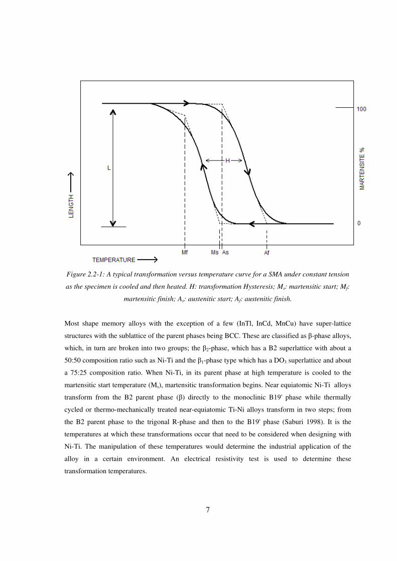
from the parent phase (β) with a B2 structure to the monoclinic B19’ phase. Figure 2.2-1 below
describes the convention for describing the crystallographically reversible martensitic
transformation in shape memory alloys.
7
Figure 2.2-1: A typical transformation versus temperature curve for a SMA under constant tension
as the specimen is cooled and then heated. H: transformation Hysteresis; Ms: martensitic start; Mf:
martensitic finish; As: austenitic start; Af: austenitic finish.
Most shape memory alloys with the exception of a few (InTl, InCd, MnCu) have super-lattice
structures with the sublattice of the parent phases being BCC. These are classified as β-phase alloys,
which, in turn are broken into two groups; the β2-phase, which has a B2 superlattice with about a
50:50 composition ratio such as Ni-Ti and the β1-phase type which has a DO3 superlattice and about
a 75:25 composition ratio. When Ni-Ti, in its parent phase at high temperature is cooled to the
martensitic start temperature (Ms), martensitic transformation begins. Near equiatomic Ni-Ti alloys
transform from the B2 parent phase (β) directly to the monoclinic B19' phase while thermally
cycled or thermo-mechanically treated near-equiatomic Ti-Ni alloys transform in two steps; from
the B2 parent phase to the trigonal R-phase and then to the B19' phase (Saburi 1998). It is the
temperatures at which these transformations occur that need to be considered when designing with
Ni-Ti. The manipulation of these temperatures would determine the industrial application of the
alloy in a certain environment. An electrical resistivity test is used to determine these
transformation temperatures.

8
Figure 2.2-2 below, shows the transformation sequence of a thermo-mechanically treated 49.8 Ti-
50.2Ni (at%) alloy. When the alloy is cooled from 373K (100°C), the electrical resistivity starts to
increase at Rs on curve (a) (electrical resistivity versus temperature). This temperature coincides
with the start temperature Rs of the differential calorimetry (DSC) curve (b). This coincidence
indicates that the resistivity increase at the first DSC peak is due to the R-phase transformation
which occurs as a first-order transformation with Rs its starting temperature. The second peak in the
DSC curve is due to the transformation from the R-phase to the B19' phase. The temperature at
which the electrical resistivity starts to decrease (Ms) coincides with the start temperature of second
peak in the DSC curve and this is the temperature where the transformation starts (Saburi 1998).
Figure 2.2-2: Two-stage transformation sequence of thermo-mechanically treated 49.8 Ti-50.2 Ni
(at%) Nitinol. (Saburi 1998)

9
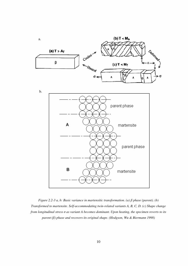
Low energy and glissile interfaces characterise thermoelastic martensites. This transformation
occurs by a shear like mechanism as shown in figure 2.2-3a below (Hodgson, Wu & Biermann
1998). The regions A and B of 2.2-3b have the same structure but different orientations. These are
known as correspondence variants and form a herringbone-like structure. Since martensite has a
lower symmetry than the parent phase, many variants can be formed from the parent phase (Otsuka,
Wayman 1998b). Because of these twin-related, self-accommodating variants, the shape change
among the variants causes very little macroscopic strain. The variants tend to “eliminate” each other
(b). When the specimen is strained, the variant that can yield the greatest shape change in the
direction of the applied stress is stabilised and becomes dominant (c).When the temperature of the
martensite is again raised, it becomes unstable and if the martensitic transformation were
crystallographically reversible, then the martensite would revert back to its parent phase in the
original orientation as it would in the above sample. The driving force for the reverse
transformation is the difference between the chemical free energy of the parent and martensite
phases above As (Miyazaki, Otsuka 1989).
10
Figure 2.2-3 a, b: Basic variance in martensitic transformation. (a) β phase (parent). (b)
Transformed to martensite. Self-accommodating twin-related variants A, B, C, D. (c) Shape change
from longitudinal stress σ as variant A becomes dominant. Upon heating, the specimen reverts to its
parent (β) phase and recovers its original shape. (Hodgson, Wu & Biermann 1998)
a.
b.

11
It can be clearly seen that martensitic transformation occurs by the cooperative movement of atoms.
Because of this, martensitic transformation is also often referred to as displacive transformation or
military transformation (Otsuka, Wayman 1998b).
2.3. MECHANISMS OF THE SHAPE MEMORY EFFECT AND SUPERELASTICITY
2.3.1. Shape Memory
The martensitic transformation that occurs in shape memory alloys is crystallographically reversible
or “thermoelastic martensitic transformation”. The total free energy change associated with
thermoelastic martensitic transformation mainly consists of two thermoelastic terms; chemical free
energy and elastic energy whereas the total free energy change associated with conventional
martensitic transformation consists of the aforementioned two terms as well as the energy of
interfaces and plastic deformation (Miyazaki 2005). Perfect shape memory recovery is dependent
on the fact that no plastic deformation occurs. The following figure 2.3-1 is used to describe the
crystal mechanism involved in the shape memory effect and superelasticity.

12
Figure 2.3-1: Schematic of the crystal structure behaviour of a shape memory alloy upon cooling,
loading/unloading and heating.
In the figure 2.3-1 above, the crystal structure is shown for the parent phase (A) of a shape memory
alloy specimen. Upon cooling, its crystal structure is perfectly transformed via diffusionless
transformation to martensite (B). The material is now below Mf and the martensite which is formed
from the parent phase consists of self accommodating twin variants. Upon loading, the martensite
is deformed by the movement of the variants that formed in the transformation (de-twinning) as the
dominant variant forms. The interface moves easily, avoiding plastic strain and retains its shape
after unloading (C) (except for elastic recovery). When the alloy is reheated to As, a reverse
13
martensitic transformation begins until the object has regained its original shape and the reverse
transformation has finished somewhere above the Af temperature.
When the object is deformed while still in its parent phase and above the Ms temperature (A) to (C),
a stress induced martensitic transformation occurs. If the specimen’s temperature remains above Af,
then a perfect recovery will occur upon unloading and the specimen will revert to its original shape
(if the temperature is below Af, then the shape recovery is not perfect upon unloading). This is
superelasticity (single crystals of specific alloys can show up to 25% pseudoelastic strain in a
certain direction (Stoeckel 1995)). As the temperature of the specimen rises above Af, it becomes
increasingly difficult to stress induce martensite. Eventually, it becomes easier for the material to
deform by conventional mechanisms and no longer observes superelastic properties. It thus behaves
like conventional materials above a certain temperature (Md). Superelasticity is only observed over
a narrow temperature range (Stoeckel 1995). The processes of shape memory and superelasticity are
both based on the same martensitic transformation and therefore show the same amount of shape
recovery (Miyazaki). The driving force for both phenomena originates from the recovery stress
associated with the reverse martensitic transformation and is strong enough to be used as an
actuating force.
Figure 2.3-2 shows the tensile curve of a Ni-Ti alloy at various temperatures. For T>Md the material
is seen to react like a normal material. At T< Md the material is martensitic. On exceeding a first
yield point, several percent strain can be accumulated with only little stress increase. The
deformation in this plateau region can be thermally recovered. Any deformation exceeding a second
yield point on the curve would not be thermally recoverable. At temperatures T> Af a plateau is
seen, this time caused by stress-induced martensite. This deformation is recovered upon unloading
where the material transforms back into austenite at a lower stress. With increasing temperature
both the loading and unloading plateaux increase linearly until Md is reached (Stoeckel 1995).
14
Figure 2.3-2 (Stoeckel 1995): Tensile curve of Nitinol at different temperatures
Above Af, the material is fully austenitic and below Mf, the material is fully martensitic. Between
the Af and Mf temperatures, the material’s properties vary constantly as well as the amounts of
thermal shape memory and superelasticity (Mertman 2004). Martensitic transformation
temperatures can easily be determined by the electrical resistivity measurement or by differential
scanning calorimetry (DSC). In most cases, shape recovery is only experienced upon heating. This
is known as one-way shape memory. But it is possible to obtain two-way shape memory. This is
when a shape recovery is also experienced during cooling, while the specimen is turning to its
martensite phase. While a large actuation force is exerted during the heating shape recovery, very
little force is applied by the alloy as it assumes its low temperature shape (Hodgson, Wu &
Biermann 1998). Also, the shape recovery is considerably less in two-way shape memory than it is
in one-way shape memory.
2.3.2. Superelasticity
Because a uniaxial stress always assists martensitic transformation, a stress induced martensitic
transformation is expected above Ms (Otsuka, Wayman 1998a). Figure 2.3-3 below demonstrates
this in a series of S-S curves for Cu-14.1mass%Al-4mass%Ni alloy single crystal.
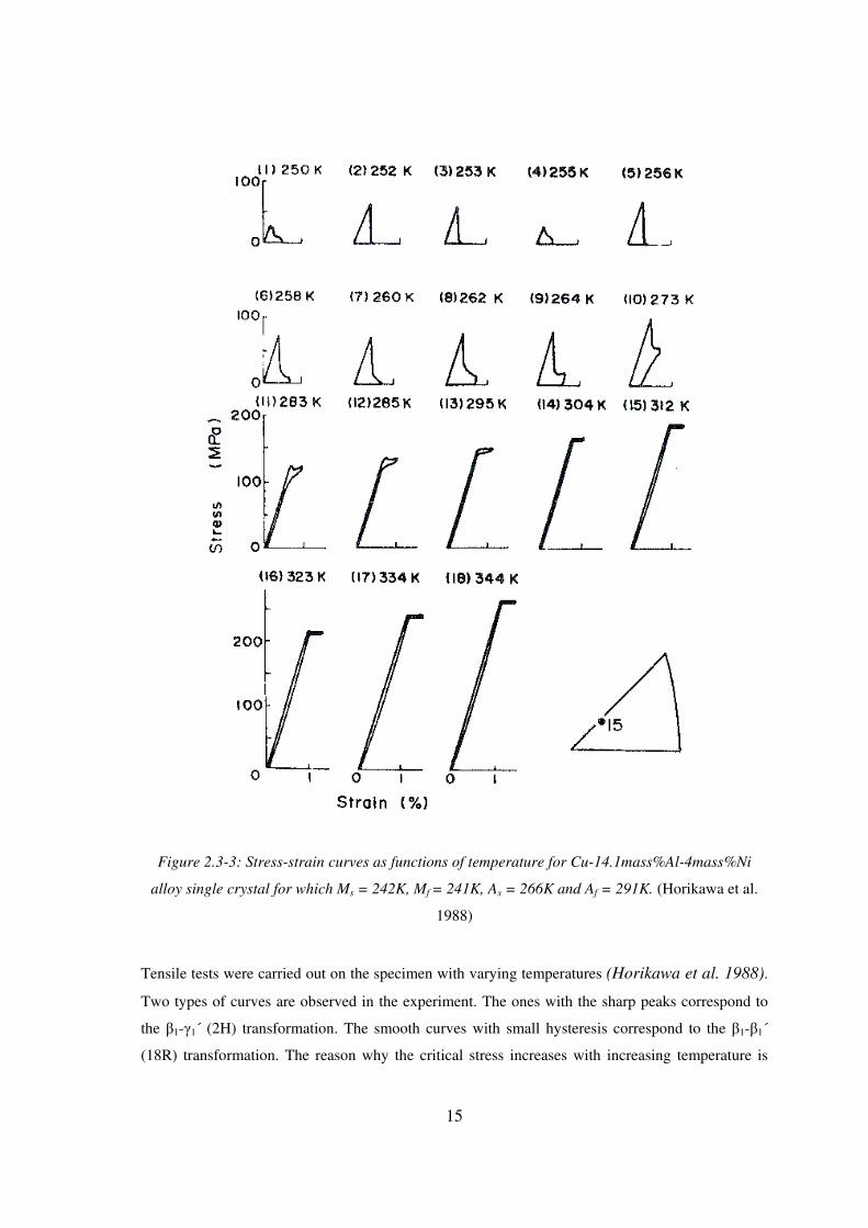
15
Figure 2.3-3: Stress-strain curves as functions of temperature for Cu-14.1mass%Al-4mass%Ni
alloy single crystal for which Ms = 242K, Mf = 241K, As = 266K and Af = 291K. (Horikawa et al.
1988)
Tensile tests were carried out on the specimen with varying temperatures (Horikawa et al. 1988).
Two types of curves are observed in the experiment. The ones with the sharp peaks correspond to
the β1-γ1´ (2H) transformation. The smooth curves with small hysteresis correspond to the β1-β1´
(18R) transformation. The reason why the critical stress increases with increasing temperature is

16
because the parent phase is more stable in higher temperature ranges (Otsuka, Wayman 1998a).
Figure 2.3-4 shows a superelastic loop along with the corresponding micrographs. It can be seen
that superelasticity is realized by the stress induces martensite transformation upon loading and the
reverse transformation back to the parent phase upon unloading. Superelasticity usually only occurs
above Af since stress induced martensite is only stable above Af while under stress. The removal of
this stress would render the stress induced martensite unstable again (Otsuka, Wayman 1998a).
Figure 2.3-4: Morphological changes associated with ′
− 11 ββ stress induced transformation upon
loading and its reverse transformation upon unloading for Cu-14.2mass%Al-4.2mass%Ni alloy
single crystal. (Otsuka et al. 1976)
Superelastic strain is orientation dependent. This orientation dependence can be explained by
calculating the transformation strain for uniaxial stress. Otsuka et al. show how this can be done
either by a calculation based on the shape strain or a calculation based on the lattice deformation B7
(Otsuka, Wayman 1998a).

17
When considering shape memory and superelasticity, it is clear that martensitic transformation can
be induced in NiTi by loading as well and cooling. Thus, at certain temperatures, combinations of
these mechanisms exist. Miyazaki and Otsuka (Miyazaki, Otsuka 1989) represent this relationship
graphically in stress versus temperature graph. Here, the Clausius-Clapeyron relationship is
satisfied in that σm and temperature having a linear relationship.
Figure 2.3-5: Representation of shape memory and superelasticity on a stress versus temperature
graph. (Miyazaki, Otsuka 1989)
In the above graph, 2.3-5, σm is the critical stress to induce martensite, σSL is the lower critical stress
for slip and σSH is the upper critical stress for slip. It can be seen that as the temperature of the
specimen increases, the critical stress to induce martensite, σm, also increases in a linear
relationship.

18
2.4. PROPERTIES OF NITINOL
Of all the alloy systems in use commercially today, Nickel-Titanium has the greatest shape recovery
of up to 8% (Hodgson, Wu & Biermann 1998). Table 2.4-1 below, describes the major properties of
basic binary Ni-Ti.
Melting temperature 1300°C
Density 6.45 g/cu.cm
Resistivity Approx. 100 µΩ/cm (austenite)
Approx. 70 µΩ/cm (martensite)
Thermal conductivity 18 W/cm. °C (austenite)
8.4 W/cm. °C (martensite)
Corrosion resistance Similar to 300 series stainless steel
Young’s modulus Approx. 83 GPa (austenite)
Approx. 28 – 41 Gpa (martensite)
Yield strength 195 – 690 MPa (austenite)
70 – 140 MPa (martensite)
Ultimate tensile strength 895 MPa
Transformation temperatures -200°C to 110°C
Latent heat of transformation 167 kJ/kg.atom
Shape memory strain 8.5% max
Max recovery stress 600 – 800 MPa
Table 2.4-1: Major properties of binary Ni-Ti. (Miyazaki 2005).
Work hardening and proper heat treatment can greatly improve the ease with which martensite is
deformed, produce an austenite with much higher yield strength and induce two-way shape
memory. Heat treating is usually done at 500°C to 800°C but it can be done as low as 300°C to
350°C (Hodgson, Wu & Biermann 1998).
Shape memory alloys (SMA) have the ability to memorize their thermal history. If the reverse
transformation of an SMA is arrested, a kinetic stop will appear in the next complete
transformation. This kinetic stop can be regarded as “memory” of the previous arrest temperature.
Unfortunately, this temperature memory effect is only operational between As and Af temperatures
and this is typically only 30K thus engineering potential is limited. Zheng, Cui and Schrooten, in

19
(Zheng, Schrooten 2004), have shown that by using prestraining and constraining treatment on
NiTi, the reverse transformation temperature window can be significantly enlarged with no adverse
effect on the temperature or shape memory effect.
Fabrication of NiTi is, on the whole, difficult. Machining by turning or milling requires special
tools and practices. Welding, brazing and soldering also do not work well.
20
3. THE SAGGING LINE MITIGATOR (SLiM)
3.1. OVERVIEW
The sagging line mitigator (SLiM) is a technology developed by Power Transmission Solutions,
Inc. (PTS) to increase overhead power line performance, reliability and safety (Figure 3.1-1). A
survey conducted by PTS indicated that a majority of utilities questioned acknowledged the
problem of sagging conductors within their systems, primarily on 115 – 230kV lines. They also
confirmed that most sag problems were less than 5ft (1.6m) (Shirmohamadi 2006b). In South
Africa, sag problems can be up to 3 times more with certain lines occasionally violating their sag
limits by more than 3m. The conventional approaches for rectifying the problems caused by
sagging conductors (i.e. the violation of electrical clearances) are to increase the tower heights,
decrease the span by adding intermediate structures, retension the existing span or construct a new
parallel line to share the load. The SLiM is a new solution offered by PTS that dynamically adjusts
the tension in the conductor by contracting when the line becomes overloaded and begins to sag and
by extending again as the load decreases and the conductor cools down, returning to its original
tension.
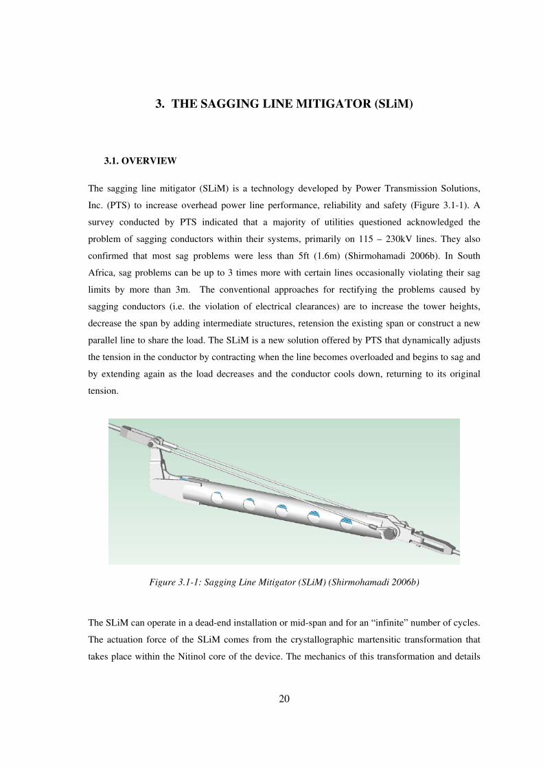
Figure 3.1-1: Sagging Line Mitigator (SLiM) (Shirmohamadi 2006b)
The SLiM can operate in a dead-end installation or mid-span and for an “infinite” number of cycles.
The actuation force of the SLiM comes from the crystallographic martensitic transformation that
takes place within the Nitinol core of the device. The mechanics of this transformation and details

21
of the shape memory effect are covered in greater detail in chapter 2. When the SLiM is installed in
a line, the current is directed through a split jumper which causes a portion of the current from the
line to flow through the shape memory alloy actuator (core) while the rest is diverted through the
body. The current flow through the core is controlled by specifically designing the split jumpers for
each application by varying the current split ratio. Ratios can range from a 20% split to as much as
70% (percentage of the total line current to be directed through the core) depending on the line’s
power transfer. Current flow in the core causes the Nitinol to heat up and “remember” its original,
shorter shape. This shortening of the core is magnified through the lever arm which in turn pulls the
sagging conductor. As the core cools, it extends again, releasing the tension in the span. The
problem of clearance violations due to a sagging conductor is thus rectified as the high temperature
of the conductor causes the SLiM to change shape and decrease the effective conductor length. This
effect cascades through adjacent suspension spans.
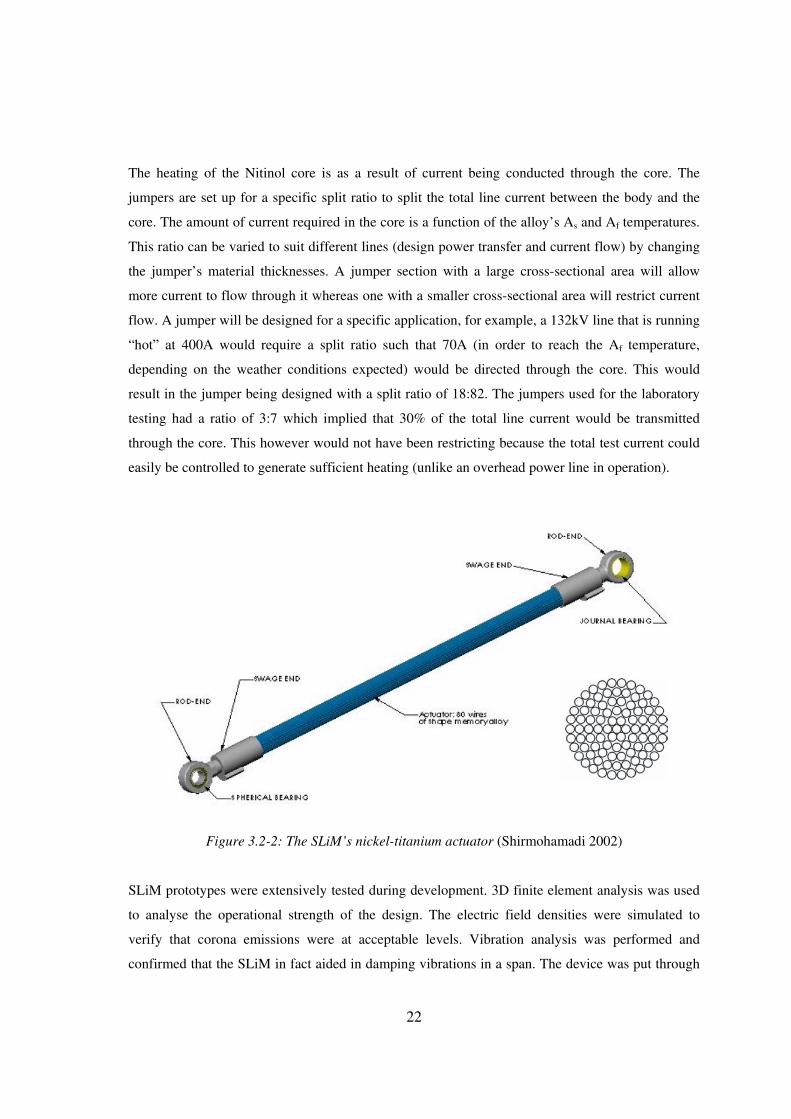
3.2. DESIGN
The SLiM relies on shape memory alloy technology (covered in more detail in Chapter 2 and
Appendix B) in the form of a nickel-titanium alloy core to provide the actuation force as it reacts to
the heat of the overloaded line and contracts (Figure 3.2-1, Figure 3.2-2). It is encased in a
machined stainless-steel pipe which acts as the fulcrum for the lever magnification. The lever arm
provides a 5.5:1 magnification.
Figure 3.2-1: Components of the SLiM (Shirmohamadi 2006b)
1.610m (OPEN) 1.410m (CLOSED)
22
The heating of the Nitinol core is as a result of current being conducted through the core. The
jumpers are set up for a specific split ratio to split the total line current between the body and the
core. The amount of current required in the core is a function of the alloy’s As and Af temperatures.
This ratio can be varied to suit different lines (design power transfer and current flow) by changing
the jumper’s material thicknesses. A jumper section with a large cross-sectional area will allow
more current to flow through it whereas one with a smaller cross-sectional area will restrict current
flow. A jumper will be designed for a specific application, for example, a 132kV line that is running
“hot” at 400A would require a split ratio such that 70A (in order to reach the Af temperature,
depending on the weather conditions expected) would be directed through the core. This would
result in the jumper being designed with a split ratio of 18:82. The jumpers used for the laboratory
testing had a ratio of 3:7 which implied that 30% of the total line current would be transmitted
through the core. This however would not have been restricting because the total test current could
easily be controlled to generate sufficient heating (unlike an overhead power line in operation).
Figure 3.2-2: The SLiM’s nickel-titanium actuator (Shirmohamadi 2002)
SLiM prototypes were extensively tested during development. 3D finite element analysis was used
to analyse the operational strength of the design. The electric field densities were simulated to
verify that corona emissions were at acceptable levels. Vibration analysis was performed and
confirmed that the SLiM in fact aided in damping vibrations in a span. The device was put through

23
tensile testing as well as thermal fatigue testing. It was also corrosion tested and because the nickel-
titanium core is inert and the body of the SLiM is stainless-steel, it was not affected by corrosive
environments. It was also shown that there is no significant change in resistance after 525 thermo-
mechanical cycles and further predicted that no resistance change would be experienced for the life
of the SLiM. The final stage of development of a SLiM prototype comprised of full-scale field
testing. This was successfully done in 2002. For a full report of the above testing and design of the
device, the Shirmohamadi 2002 report may be consulted. Field testing in South Africa of the
custom prototype SLiM ESK-01, by Eskom is scheduled for commencement.
3.3. SPECIFICATIONS
The Power Transmission Solutions, Inc. specifications for the ESK-01 custom SLiM prototype are
as follows (Kopperdahl 2006):
Voltage rating 230kV and below
Range of motion Up to 200mm
Line tension at 43°C Up to 13.3kN
Mechanical failure load > 200kN
Total weight 60 ± 4 kg
End-to-end dimension 168cm
Electrical connections 4-bolt NEMA paddles
Mechanical connections 25mm clevis pin
Table 3.3-1: PTS equipment specification – custom PTS SLiM – ESK-01
The custom SLiM device, ESK-01, was designed to start actuation at a core temperature of 50°C
and at a tension of 13.3kN (Shirmohamadi 2006a). The expected core temperature response is
represented in the graph below. This performance will be verified during the testing stage.
24
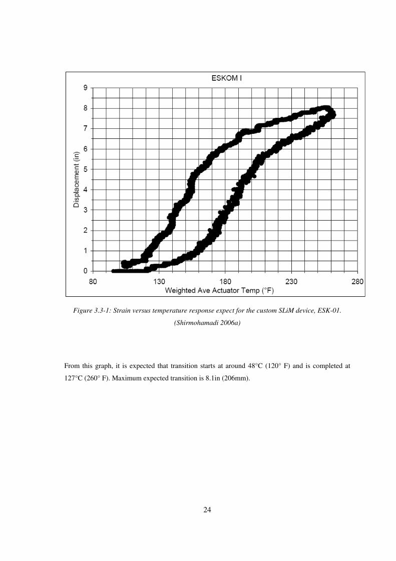
Figure 3.3-1: Strain versus temperature response expect for the custom SLiM device, ESK-01.
(Shirmohamadi 2006a)
From this graph, it is expected that transition starts at around 48°C (120° F) and is completed at
127°C (260° F). Maximum expected transition is 8.1in (206mm).

25
The custom SLiM device was designed for installation on a wolf 132kV line. The properties for
wolf conductor, listed in the IEC code 158-A1/S1A-30/2,59/7/2,59, are below:
Conductor overall diameter (mm) 18.13
Area aluminium (mm2) 158.06
Area total (mm2) 194.94
Aluminium wires (no. of/diameter mm) 30/2.59
Steel wires (no. of/diameter mm) 7/2.59
Conductor linear mass (kg/km) 730.0
Ultimate strength (kN) 69.20
Resistance dc at 20°C (ohms/km) 0.1828
Modulus of elasticity final (MPa) 83 400
Coefficient of linear expansion, β, (1/°C) 18.43*10-6
Table 3.3-2: Properties of Wolf ACSR 30/7 from IEC code 158-A1/S1A-30/2,59/7/2,59
26
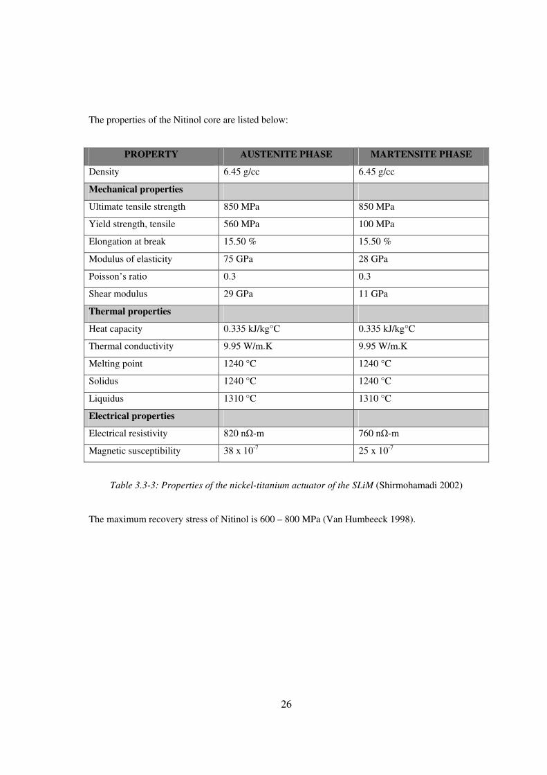
The properties of the Nitinol core are listed below:
PROPERTY AUSTENITE PHASE MARTENSITE PHASE
Density 6.45 g/cc 6.45 g/cc
Mechanical properties
Ultimate tensile strength 850 MPa 850 MPa
Yield strength, tensile 560 MPa 100 MPa
Elongation at break 15.50 % 15.50 %
Modulus of elasticity 75 GPa 28 GPa
Poisson’s ratio 0.3 0.3
Shear modulus 29 GPa 11 GPa
Thermal properties
Heat capacity 0.335 kJ/kg°C 0.335 kJ/kg°C
Thermal conductivity 9.95 W/m.K 9.95 W/m.K
Melting point 1240 °C 1240 °C
Solidus 1240 °C 1240 °C
Liquidus 1310 °C 1310 °C
Electrical properties
Electrical resistivity 820 nΩ-m 760 nΩ-m
Magnetic susceptibility 38 x 10-7 25 x 10-7
Table 3.3-3: Properties of the nickel-titanium actuator of the SLiM (Shirmohamadi 2002)
The maximum recovery stress of Nitinol is 600 – 800 MPa (Van Humbeeck 1998).
27
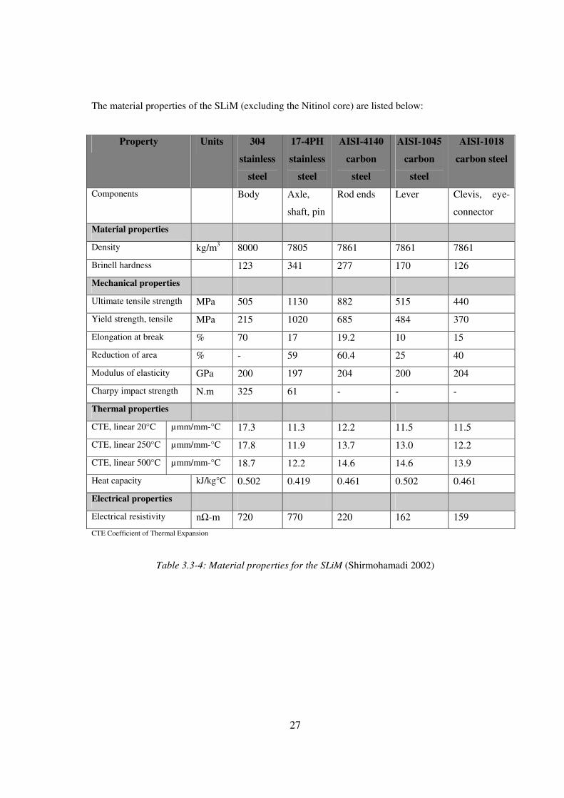
The material properties of the SLiM (excluding the Nitinol core) are listed below:
Property Units 304
stainless
steel
17-4PH
stainless
steel
AISI-4140
carbon
steel
AISI-1045
carbon
steel
AISI-1018
carbon steel
Components Body Axle,
shaft, pin
Rod ends Lever Clevis, eye-
connector
Material properties
Density kg/m3 8000 7805 7861 7861 7861
Brinell hardness 123 341 277 170 126
Mechanical properties
Ultimate tensile strength MPa 505 1130 882 515 440
Yield strength, tensile MPa 215 1020 685 484 370
Elongation at break % 70 17 19.2 10 15
Reduction of area % - 59 60.4 25 40
Modulus of elasticity GPa 200 197 204 200 204
Charpy impact strength N.m 325 61 - - -
Thermal properties
CTE, linear 20°C µmm/mm-°C 17.3 11.3 12.2 11.5 11.5
CTE, linear 250°C µmm/mm-°C 17.8 11.9 13.7 13.0 12.2
CTE, linear 500°C µmm/mm-°C 18.7 12.2 14.6 14.6 13.9
Heat capacity kJ/kg°C 0.502 0.419 0.461 0.502 0.461
Electrical properties
Electrical resistivity nΩ-m 720 770 220 162 159
CTE Coefficient of Thermal Expansion
Table 3.3-4: Material properties for the SLiM (Shirmohamadi 2002)

28
The material properties for the bearing used in the lever are listed below:
PROPERTY Duralon Rulon ACM
Allowable bearing stress (MPa) 138 – 414 276 – 524
Coefficient of friction (static-dynamic) 0.05 – 0.16 0.05 – 0.25
Max operating temperature (°C) 163 180
Coefficient of thermal expansion (µmm/mm-°C) 27 126
Table 3.3-5: Composite bearing material properties (Shirmohamadi 2002)
29
4. TESTING
4.1. OVERVIEW
From the outset, the testing of the SLiM needed to confirm the functionality of the device as well as
provide understanding and data of its operation during heating and cooling cycles. The SLiM was
designed to be installed on a power line, mid-span or in a dead-end configuration. The concept
behind the testing of the device was to simulate its installation and operational loads within a
laboratory environment while being able to safely supply sufficient current to heat up the core and
monitor all the necessary parameters. The main factors that needed to be simulated were a) stringing
under a constant tension to allow some linear displacement as the device contracted and b) a total
current flow of 300A (to be split by jumpers) to generate heating in the core. The testing
environment was at an ambient temperature of 23°C ±2 with no wind.
The constant tension capability of the test rig was needed so that, as the device contracted, the
tension would not increase. This would have damaged the Nitinol core. Conversely, the test rig had
to “re-tension” itself during cooling to extend the SLiM again. This was to simulate the weight and
tension of the cold conductors of the line physically straining the SLiM and re-extending it in its
martensitic phase. 300A was chosen as the total test current to be supplied to the conductor. Wolf
conductor has a current rating of 420A. On an average day (wind speed 0.5 m/s, 30°C), wolf
conductor would run at 50°C with just a 260A transfer (Field Cigamp software simulation)
therefore, 50°C can be considered an adequate templating temperature at which all the clearances
would be safely maintained. This would result in a power transfer of 60MVA at 132kV, a likely
scenario. Any current increase would cause the conductor running temperature to increase, in turn
causing sag and clearance violations. This is where a device such as the SLiM would be utilised. On
a hot day, as the conductor is fed 300A, an increase in conductor temperature of 32°C could be
generated. On a hot day such as this, the 50°C templating temperature would be exceeded i.e. 82°C,
and the resulting sag would become a problem. The increase in temperature of the SLiM’s core
resulting from the increased current flow would cause the SLiM to contract and mitigate the excess
sag. It is for this reason that 300A was chosen as the test current.
The testing was performed in such a way as to: a) confirm the fact that the SLiM actually works i.e.
contracts when a current, sufficient enough to heat the core above 50°C, is transmitted through it
30
and extends when the core cools down again and b) quantify the operational parameters of the
Nickel-Titanium alloy core and hence the SLiM device as a whole. To this end, 300A (as described
above, a sufficiently high current to guarantee SLiM activation) was selected to be fed to the
conductor which was then split by the jumpers for the heating cycle of the SLiM, and 0A was
transmitted to the conductor for the cooling cycle. There is a higher conductor current at which the
core would have no longer activated but this was done to determine the Nitinol’s upper and lower
limits of thermal transformation. Had the test rig exactly simulated an operational line, a current of
262A (for the ambient conditions described above) (MathCAD based Ampacity/Conductor Ratings
calculation software, Muftic 2003 – 2005) would have had to be transmitted during cooling.
Because only one set of jumpers was used (fixed ratio), differing ambient conditions i.e. higher
ambient temperature, solar radiation, would have caused the Nitinol core to operate within its upper
and lower thermal limits for transformation without reaching its absolute lowest transformation
temperature (i.e. Af). This would not have provided a basis for future jumper ration modification.
The data capture during testing needed to be automated and real-time. A Data Acquisition system
(DAQ) was developed to capture all the parameters as described in section 4.2 and write the data to
a P.C.
4.2. TESTING PARAMETERS
A description of the test inputs and outputs is set out below. A combination of sensors, gauges and
meters was used to regulate and monitor these inputs and outputs. All the data fed from the sensors
was recorded and used to analyse the SLiM’s performance.

31
UNIT DESCRIPTION INTERFACES BENCH
VALUE
Inputs
Tension N The tension as monitored in
the test-span. This is a
simulation of the actual tension
in the wolf conductors of a
power line.
Applied by a 22kN hydraulic ram
and regulated by a forward-0-
backward lever control. Monitored
with a loadcell in series with the
span.
13.3 kN
Current A
(AC)
The current supplied to the
test-span (SLiM in series).
Comparable to the current of a
132kV wolf power line.
Supplied for a 220V single phase
supple, through a 10A variac.
Transformed via a toroidal coil.
Monitored via a secondary toroidal
coil with a correction factor.
0 – 300A
± 15A
Voltage V As measured across the test-
span.
Monitored with a Fluke
multimeter.
0 – 0.04V
± .0005V
Outputs
Displacement mm The amount of contraction
provided by the SLiM as
measured at the lever-
conductor connection.
Recorded by a stepper-motor
where 1 pulse = 1.5mm.
0 – 210 mm
± 1.5 mm
Temperature °C Ambient temperature and core
temperature (x3)
Measured with thermocouples
(serial output, semiconductors type
with addressable functionality) via
the DAQ into the PC.
21 – 120°C
± 1°C
Time s Time measured per cycle: from
start of heating to end of
cooling.
Time automatically initialised at
the beginning of data capture by
PC.
–
Table 4.2-1: Table of test parameters

32
4.3. TEST RIG DESIGN
The SLiM testing rig was designed as a constant tension apparatus that would simulated the actual
mechanical loading conditions of the SLiM as if it were installed on a power line. It was designed to
allow stringing of the SLiM at a tension of 13.3kN while conducting a maximum current of 300A.
The test span, being the current path, had to be insulated from earth. All the necessary input and
output parameters needed to be monitored in real-time and recorded by an automated system.
Figure 4.3-1: Schematic of the principle of the SLiM’s constant tension testing rig.
The concept behind the design of the SLiM testing rig is illustrated in figure 4.3-1, above. The test
span was anchored while the 22kN hydraulic ram provided the constant test tension of 13.3kN. It
was installed in series with the insulated span containing the SLiM and the load cell at the other
end. A transformer connected in series with the test span provided the needed current range at a
very low voltage.
The SLiM testing rig can be seen in Figure 4.3-2:
33
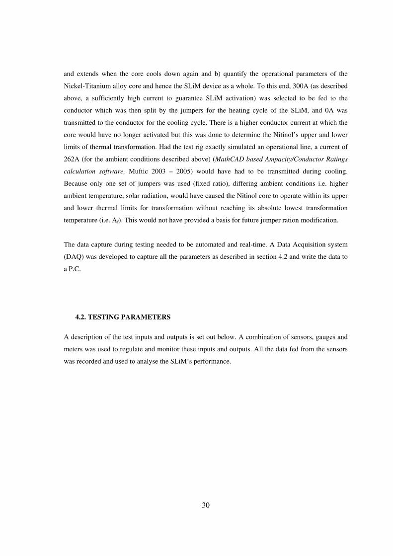
Figure 4.3-2: The SLiM testing rig.
The anchoring for the test span was provided by two I-beams connected by 20mm thick steel plates
at each end. Pro-Engineer 3D CAD design was used to design each component of the SLiM’s
testing rig as well as model the assembly and generate working drawings. See Appendix D for
drawings and calculation.
The constant tension of 13.3kN was provided by a 22kN ram as shown below in Figure 4.3-3a. This
was powered by the laboratory’s “in-house” power pack. The ram was controlled by a forward-0-
back control lever. Fine-tuning of the pressure was achieved by small adjustments of a bleed-valve
with an Allen-key. The ram was connected, via a link, to a lever with a ratio of 1:2 that effectively
doubled the ram’s travel (Figure 4.3-3b). This lever was coupled to a shaft which was free to rotate
in bearings bolted to the I-beams. The composite insulator of the test span was coupled to the lever
via two D-shackles.
HYDRAULIC RAM
TOIROIDAL TRANFORMER
VARIAC
LOAD CELL
SLiM
LEVER
TEST RIG FRAME

34
Figure 4.3-3 a, b: The 22kN hydraulic ram (left) that provided the constant tension in the test-span
via a lever (right) that magnified (mechanical advantage) the ram’s displacement.
When considering an overhead power line, the transmission voltage is a set parameter. Most often,
for wolf conductor lines, this is 132kV. The power transfer of that line is governed by the current
required to generate that power as illustrated by the power formula below (Due to the fixed voltage
of 132kV.):
IVP ×=
To transmit more power, a higher current must be used. The limiting factor for the current is the
heating and sag of the conductors. The running temperature of a conductor is, regarding power
transfer, only affected by the current in the line and not the voltage as shown by the Joule Heating,
Pj, equation below (Again, the voltage is a set parameter and cannot be changed.):
( )[ ]2000403.011000
2−+= ave
ACACj T
RIP (W/m) (Stephen et al. 2005)
Where:
IAC = conductor current (A)
RAC = AC resistance of the conductor at 20°C (Ω/km)
Tave = average temperature of the conductor (°C)
It is for this reason that the test voltage for the testing rig was able to be so small and not 132kV as
in the field. For a current of 300A to be safe in a laboratory environment, a voltage of 0.04V was
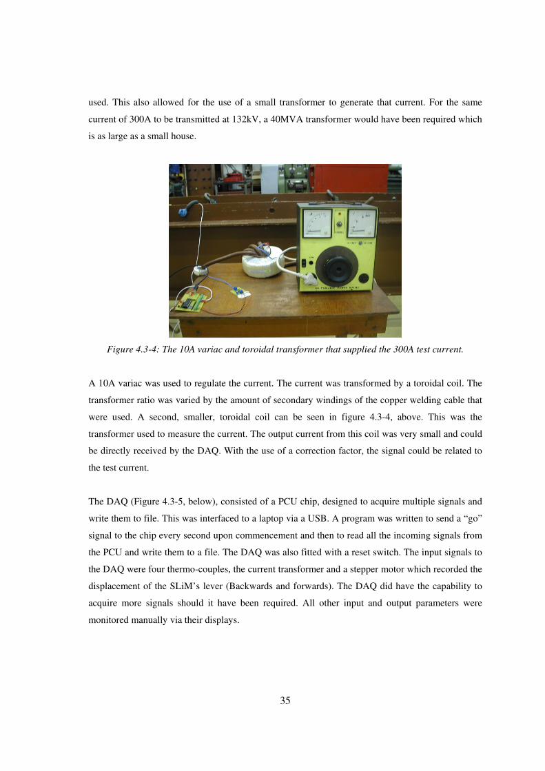
35
used. This also allowed for the use of a small transformer to generate that current. For the same
current of 300A to be transmitted at 132kV, a 40MVA transformer would have been required which
is as large as a small house.
Figure 4.3-4: The 10A variac and toroidal transformer that supplied the 300A test current.
A 10A variac was used to regulate the current. The current was transformed by a toroidal coil. The
transformer ratio was varied by the amount of secondary windings of the copper welding cable that
were used. A second, smaller, toroidal coil can be seen in figure 4.3-4, above. This was the
transformer used to measure the current. The output current from this coil was very small and could
be directly received by the DAQ. With the use of a correction factor, the signal could be related to
the test current.
The DAQ (Figure 4.3-5, below), consisted of a PCU chip, designed to acquire multiple signals and
write them to file. This was interfaced to a laptop via a USB. A program was written to send a “go”
signal to the chip every second upon commencement and then to read all the incoming signals from
the PCU and write them to a file. The DAQ was also fitted with a reset switch. The input signals to
the DAQ were four thermo-couples, the current transformer and a stepper motor which recorded the
displacement of the SLiM’s lever (Backwards and forwards). The DAQ did have the capability to
acquire more signals should it have been required. All other input and output parameters were
monitored manually via their displays.
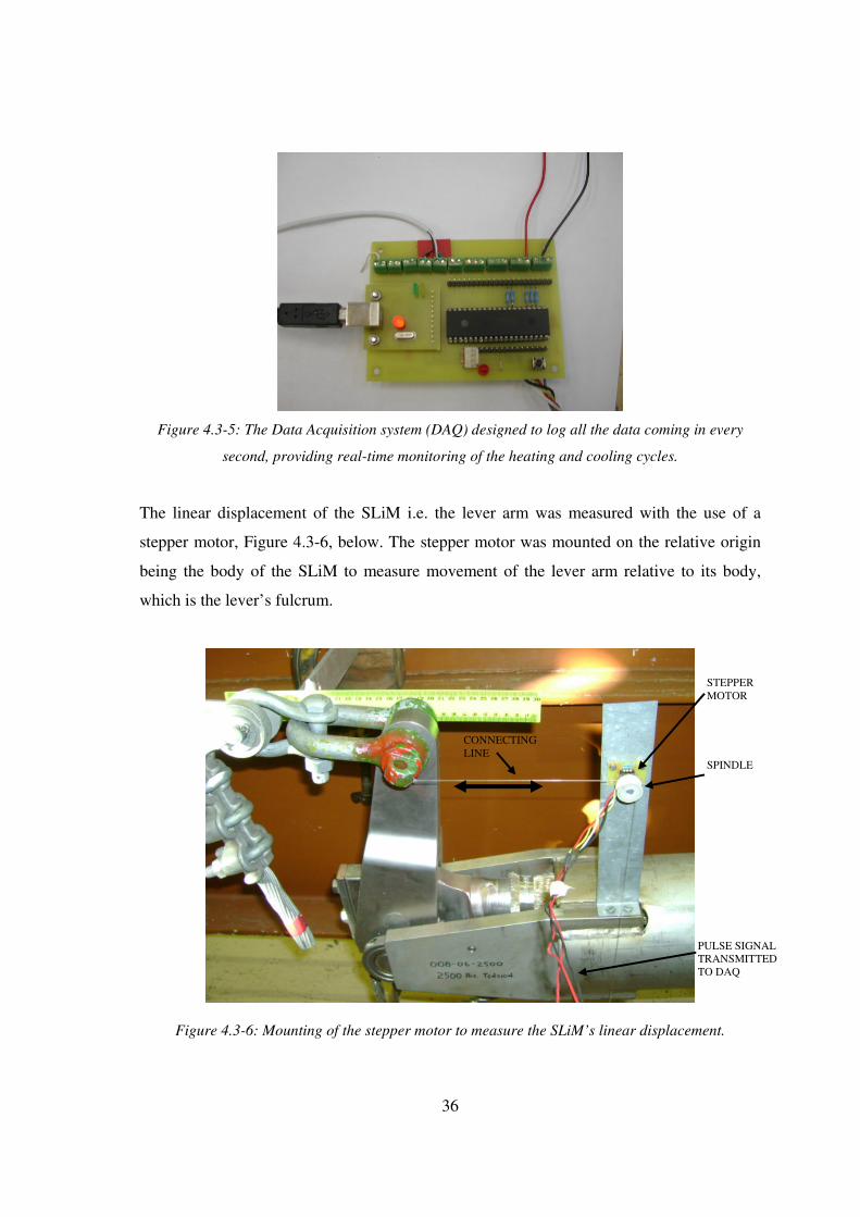
36
Figure 4.3-5: The Data Acquisition system (DAQ) designed to log all the data coming in every
second, providing real-time monitoring of the heating and cooling cycles.
The linear displacement of the SLiM i.e. the lever arm was measured with the use of a
stepper motor, Figure 4.3-6, below. The stepper motor was mounted on the relative origin
being the body of the SLiM to measure movement of the lever arm relative to its body,
which is the lever’s fulcrum.
Figure 4.3-6: Mounting of the stepper motor to measure the SLiM’s linear displacement.
STEPPER MOTOR
SPINDLE
CONNECTING LINE
PULSE SIGNAL TRANSMITTED TO DAQ
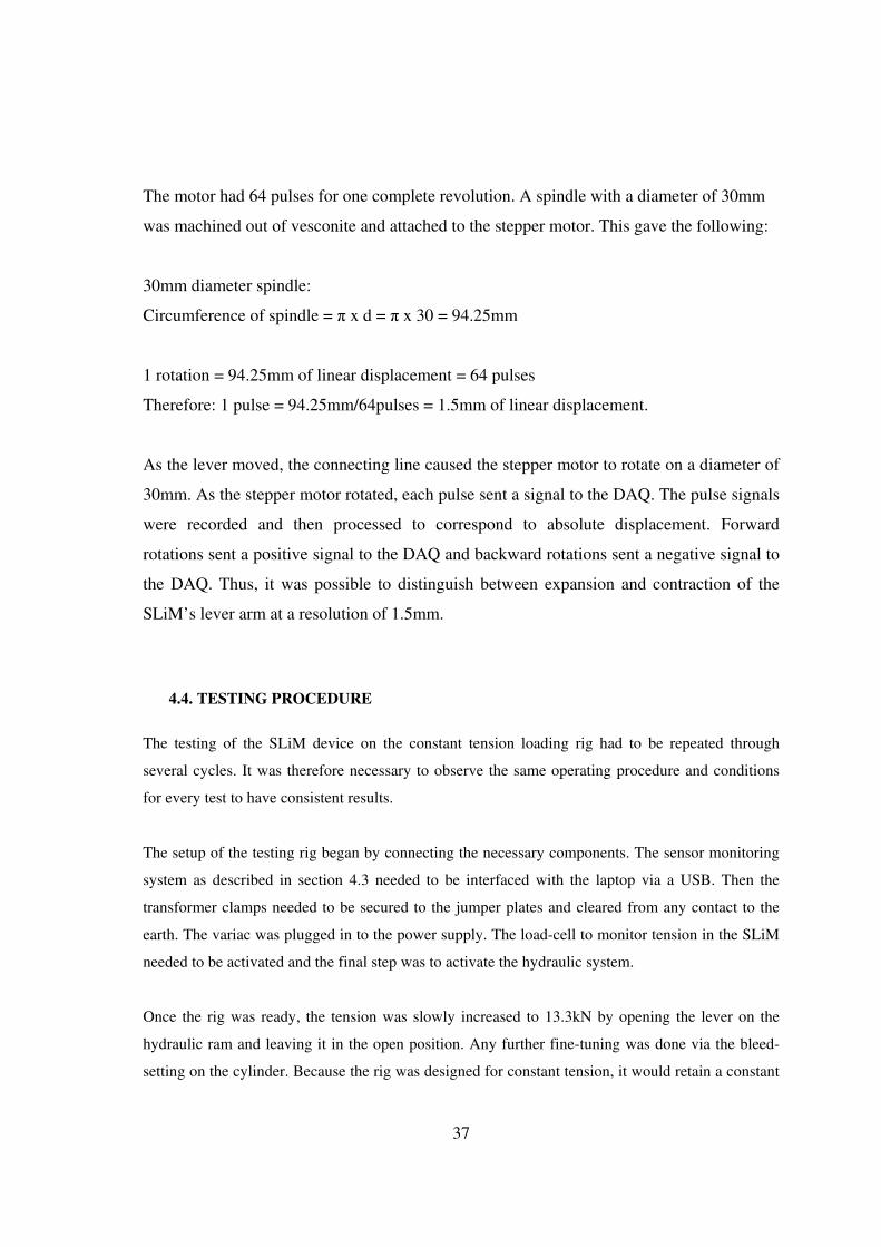
37
The motor had 64 pulses for one complete revolution. A spindle with a diameter of 30mm
was machined out of vesconite and attached to the stepper motor. This gave the following:
30mm diameter spindle:
Circumference of spindle = π x d = π x 30 = 94.25mm
1 rotation = 94.25mm of linear displacement = 64 pulses
Therefore: 1 pulse = 94.25mm/64pulses = 1.5mm of linear displacement.
As the lever moved, the connecting line caused the stepper motor to rotate on a diameter of
30mm. As the stepper motor rotated, each pulse sent a signal to the DAQ. The pulse signals
were recorded and then processed to correspond to absolute displacement. Forward
rotations sent a positive signal to the DAQ and backward rotations sent a negative signal to
the DAQ. Thus, it was possible to distinguish between expansion and contraction of the
SLiM’s lever arm at a resolution of 1.5mm.
4.4. TESTING PROCEDURE
The testing of the SLiM device on the constant tension loading rig had to be repeated through
several cycles. It was therefore necessary to observe the same operating procedure and conditions
for every test to have consistent results.
The setup of the testing rig began by connecting the necessary components. The sensor monitoring
system as described in section 4.3 needed to be interfaced with the laptop via a USB. Then the
transformer clamps needed to be secured to the jumper plates and cleared from any contact to the
earth. The variac was plugged in to the power supply. The load-cell to monitor tension in the SLiM
needed to be activated and the final step was to activate the hydraulic system.
Once the rig was ready, the tension was slowly increased to 13.3kN by opening the lever on the
hydraulic ram and leaving it in the open position. Any further fine-tuning was done via the bleed-
setting on the cylinder. Because the rig was designed for constant tension, it would retain a constant
38
13.3kN throughout the testing process. The DAQ was then activated which started taking readings
automatically every second. The variac was switched on with the dial set on 0A. This ensured an
initial current in the secondary coil (and the test span) of 0A. A test run was then ready to begin.
Figure 4.4-1, a, b: The SLiM’s lever fully extended (left) and fully contracted (right) as a result of
the heating of its Nitinol core.
While results were already being recorded every second, the current on the variac was turned up to
give 300A in the secondary winding and the test span. This was monitored via the DAQ and the
laptop. The temperature within the core of the SLiM started climbing and within 15 minutes
reached its maximum operating temperature of around 110°C. The temperature of the conductor
was not monitored due to the predetermination of the jumpers to supply enough of the 300A current
to the core in order to heat it. It thus would have been irrelevant. A simulation in Field Cigamp
shows that for the ambient conditions in the laboratory, the conductor temperature at 300A would
be 65°C.While the temperature increased the SLiM contracted through about 200mm (Pictured
above, Figure 4.4-1). The tension was fine-tuned throughout the heating cycle to stay around
13.3kN. On observing the completion of the SLiM’s contraction, the variac was turned to 0A and
switched off in order to allow complete cooling of the core and hence complete martensitic
transformation. This cut off the current flow in the SLiM and thus started the cooling cycle. The fan
was turned on to accelerate cooling and the SLiM was cooled to room temperature. The accelerated
cooling (0A and fan) was not a direct simulation of field conditions on an overhead power line. It
was done in order to achieve complete cooling and martensitic transformation so that a complete
PISTOL GRIP CONDUCTOR
A
A B
D = 200mm

39
data set for the Nitinol material, including its maximum and minimum transformation temperatures
would be recorded. A line operating at its templating temperature and, for example, and at 262A
may not allow complete martensitic transformation of the core. The ambient conditions would
determine whether complete phase change occurs or whether two phases, austenite and martensite,
are simultaneously present in the core. This would happen if the ambient conditions did not allow
the core to cool below the Mf temperature. The cooling took about 80 min. During this time, the
tension was kept to 13.3kN by adjusting the bleed-setting. A cooling power line would similarly
maintain a constant tension as the sag between suspension structures is allowed to cascade due to
the fact that suspension insulator can swing. As the core cooled down, it strained out again, under
the tension, to its elongated ‘cold shape’. Once room temperature was reached in the core, the DAQ
was terminated and the results saved for post analysis.
It was important to note that a brand new SLiM device would not have exhibited its characteristic
martensitic transformation in its first test. The procedure needed to be conducted for three trial
cycles in order to first “run in” the SMA.
40
5. RESULTS
5.1. OVERVIEW
The SLiM was put through 3 trial cycles to “run in” the shape memory alloy as suggested by
Shirmohamadi, M. of Power Transmission Solutions, Inc. and then 8 complete test cycles. A total
conductor current of 300A was used to produce the heating in the core of the SLiM while the test
span was kept at a constant tension of 13.3kN (±0.5kN). Data was captured every 1 second, written
to file and then processed. The results from the analysis of the data captured for each run are shown
below. The heating curve of each run was approximated by a polynomial (to the order of 6). This
curve was then used to determine the temperature and time taken to 2% and 98% of total strain. 2%
and 98% strain were used as benchmarks with which to compare all the runs and are a good relative
assumption for the start and finish of shape recovery. These temperatures would correspond to the
Austenite start and finish temperatures on the heating cycle and martensite finish and start
temperatures on the cooling cycle respectively.
The tension was kept constant at 13.3kN (± 0.5kN). Three core temperatures were recorded every 1
second and processed to give an average, real-time core temperature throughout each heating and
cooling cycle. An ambient temperature was also recorded every 1 second to get an average room
test temperature. The current was recorded every 1 second to confirm a constant heating current of
300A (± 10A). This output was not required for post processing. The displacement of the SLiM’s
lever was measured by a stepper motor that sent 64 pulse signals for its every 1 complete rotation.
From its spool diameter of 30mm, it was calculated that every 1 pulse equalled 1.5mm in lateral
movement.
For each run in section 5.2 below, a set of the run’s parameters are listed as well as a graph showing
the temperature response of the Nitinol core for total conductor current of 0A to 300A (± 10A)
(with jumpers with a ratio of 3:7, 90A was transmitted through the core), the displacement response
of the SLiM and a strain versus temperature response for the SLiM. In the analysis (section 5.3), the
results of all the runs were combined to define the average properties for the SLiM device (ESK-
01). Data from the tests was used to determine the Nickel-Titanium alloy’s time constant and from
this, simulate the core’s characteristic heating response for a 300A conductor current (or a 90A core
current).

41
5.2. TEST RESULTS
5.2.1. Run 1 (18th June 2007):
PARAMETER RESULTS – RUN 1
Max (absolute) strain of run (mm) 190.5
Max core temp of run (°C) 111.3
Duration of run (heating and cooling) 01:22:23
Time to max temp 00:16:54
Time to max strain 00:16:30
2% strain (mm) 3.8
Time to 2% strain 00:03:25
Temp at 2% strain (As) (°C) 38.7
98% strain (mm) 186.7
Time to 98% strain 00:15:38
Time 2% to 98% strain 00:12:13
Temp at 98% strain (Af) (°C) 107.0
Temp at 98% strain (Ms) 107.0
Temp at 2% strain (Mf) (°C) 32.7
Table 5.2-1: Parameter results of Run 1
Figure 5.2-1: Heating curve for Run 1

42
Figure 5.2-2: Strain curve for Run 1
Figure 5.2-3: Strain vs. Temperature curve for Run 1

43
5.2.2. Run 2 (19th June 2007):
PARAMETER RESULTS – RUN 2
Max (absolute) strain of run (mm) 204.0
Max core temp of run (°C) 112.3
Duration of run (heating and
cooling) 01:36:50
Time to max temp 00:16:09
Time to max strain 00:15:45
2% strain (mm) 4.1
Time to 2% strain 00:03:36
Temp at 2% strain (As) (°C) 41.7
98% strain (mm) 199.9
Time to 98% strain 00:14:55
Time 2% to 98% strain 00:11:19
Temp at 98% strain (Af) (°C) 107.3
Temp at 98% strain (Ms) 104.7
Temp at 2% strain (Mf) (°C) 28.7
Table 5.2-2: Parameter results of Run 2
Figure 5.2-4: Heating curve for Run 2
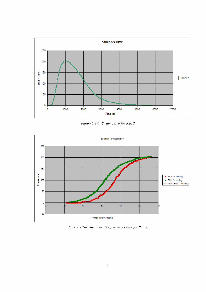
44
Figure 5.2-5: Strain curve for Run 2
Figure 5.2-6: Strain vs. Temperature curve for Run 2
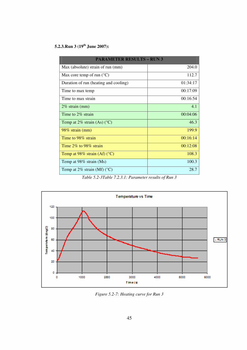
45
5.2.3. Run 3 (19th June 2007):
PARAMETER RESULTS – RUN 3
Max (absolute) strain of run (mm) 204.0
Max core temp of run (°C) 112.7
Duration of run (heating and cooling) 01:34:17
Time to max temp 00:17:09
Time to max strain 00:16:54
2% strain (mm) 4.1
Time to 2% strain 00:04:06
Temp at 2% strain (As) (°C) 46.3
98% strain (mm) 199.9
Time to 98% strain 00:16:14
Time 2% to 98% strain 00:12:08
Temp at 98% strain (Af) (°C) 108.3
Temp at 98% strain (Ms) 100.3
Temp at 2% strain (Mf) (°C) 28.7
Table 5.2-3Table 7.2.3.1: Parameter results of Run 3
Figure 5.2-7: Heating curve for Run 3
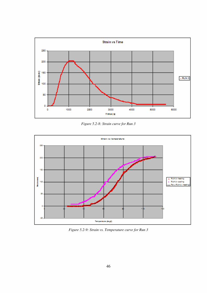
46
Figure 5.2-8: Strain curve for Run 3
Figure 5.2-9: Strain vs. Temperature curve for Run 3
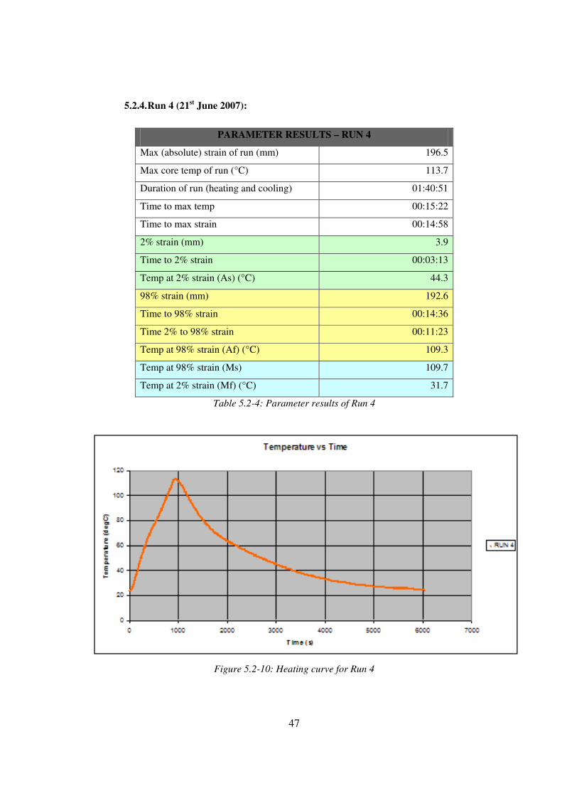
47
5.2.4. Run 4 (21st June 2007):
PARAMETER RESULTS – RUN 4
Max (absolute) strain of run (mm) 196.5
Max core temp of run (°C) 113.7
Duration of run (heating and cooling) 01:40:51
Time to max temp 00:15:22
Time to max strain 00:14:58
2% strain (mm) 3.9
Time to 2% strain 00:03:13
Temp at 2% strain (As) (°C) 44.3
98% strain (mm) 192.6
Time to 98% strain 00:14:36
Time 2% to 98% strain 00:11:23
Temp at 98% strain (Af) (°C) 109.3
Temp at 98% strain (Ms) 109.7
Temp at 2% strain (Mf) (°C) 31.7
Table 5.2-4: Parameter results of Run 4
Figure 5.2-10: Heating curve for Run 4
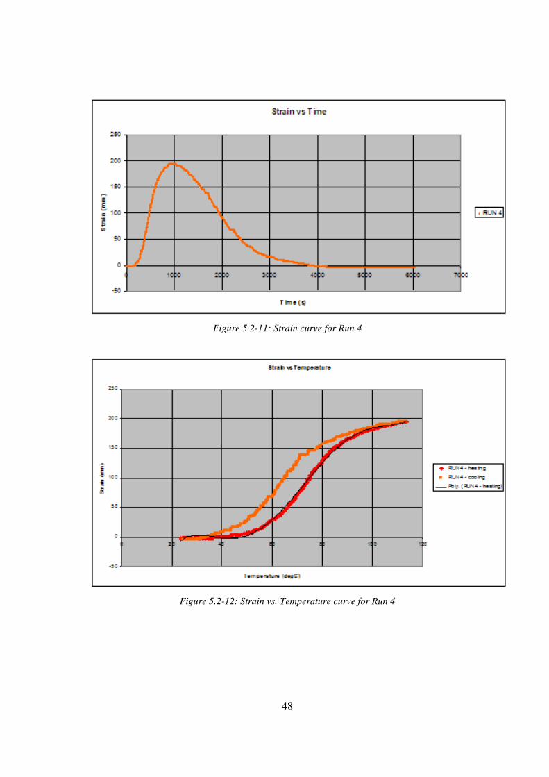
48
Figure 5.2-11: Strain curve for Run 4
Figure 5.2-12: Strain vs. Temperature curve for Run 4
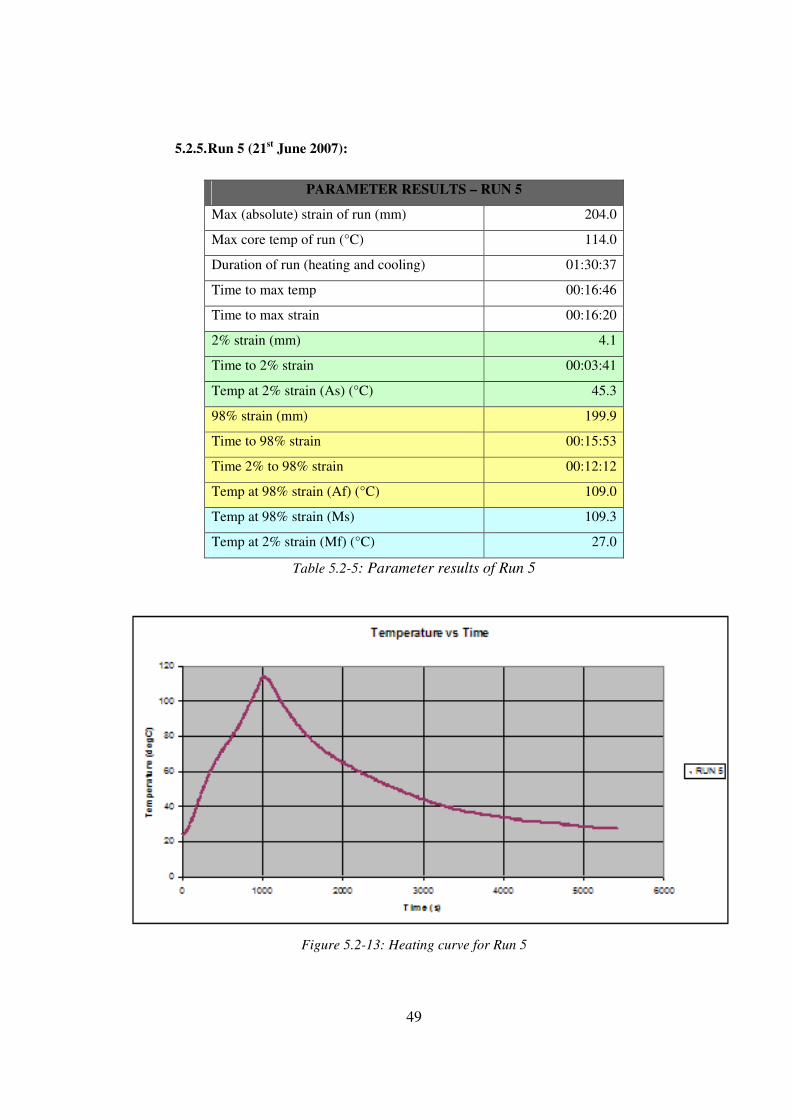
49
5.2.5. Run 5 (21st June 2007):
PARAMETER RESULTS – RUN 5
Max (absolute) strain of run (mm) 204.0
Max core temp of run (°C) 114.0
Duration of run (heating and cooling) 01:30:37
Time to max temp 00:16:46
Time to max strain 00:16:20
2% strain (mm) 4.1
Time to 2% strain 00:03:41
Temp at 2% strain (As) (°C) 45.3
98% strain (mm) 199.9
Time to 98% strain 00:15:53
Time 2% to 98% strain 00:12:12
Temp at 98% strain (Af) (°C) 109.0
Temp at 98% strain (Ms) 109.3
Temp at 2% strain (Mf) (°C) 27.0
Table 5.2-5: Parameter results of Run 5
Figure 5.2-13: Heating curve for Run 5

50
Figure 5.2-14: Strain curve for Run 5
Figure 5.2-15: Strain vs. Temperature curve for Run 5

51
5.2.6. Run 6 (22nd June 2007):
PARAMETER RESULTS – RUN 6
Max (absolute) strain of run (mm) 201.0
Max core temp of run (°C) 113.0
Duration of run (heating and cooling) 01:23:32
Time to max temp 00:17:09
Time to max strain 00:16:44
2% strain (mm) 4.0
Time to 2% strain 00:03:22
Temp at 2% strain (As) (°C) 41.7
98% strain (mm) 197.0
Time to 98% strain 00:15:53
Time 2% to 98% strain 00:12:31
Temp at 98% strain (Af) (°C) 109.0
Temp at 98% strain (Ms) 109.3
Temp at 2% strain (Mf) (°C) 27.0
Table 5.2-6: Parameter results of Run 6
Figure 5.2-16: Heating curve for Run 6
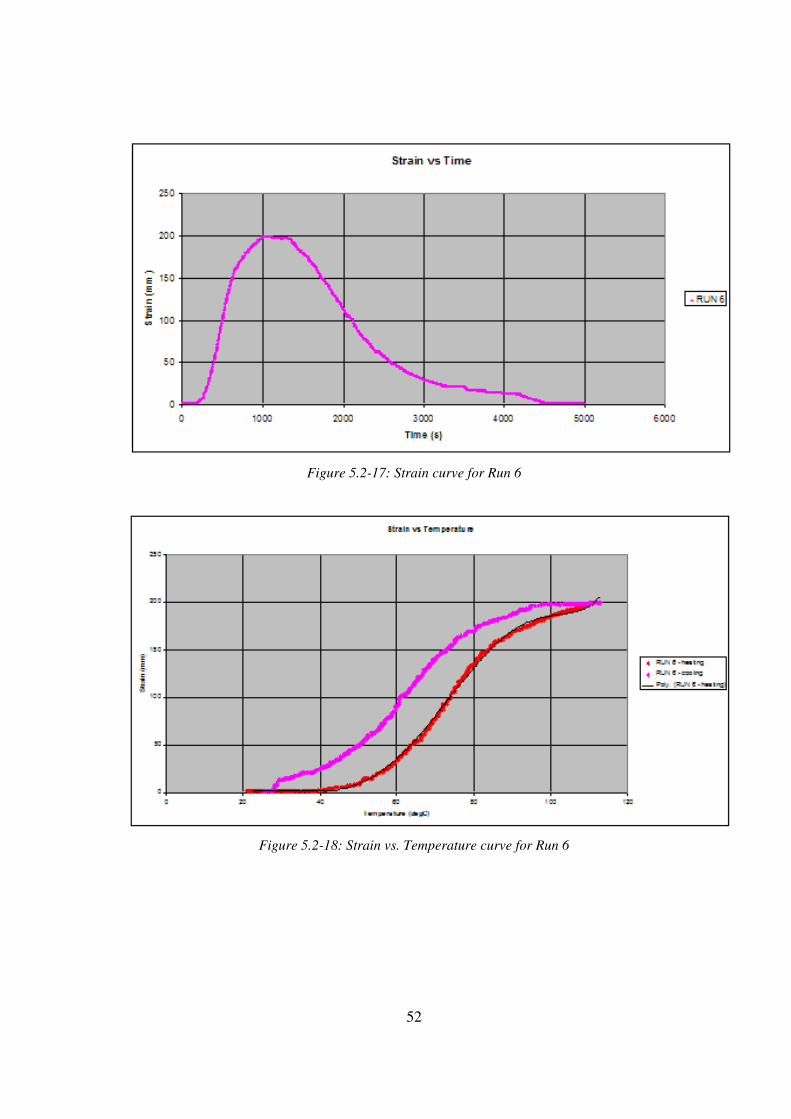
52
Figure 5.2-17: Strain curve for Run 6
Figure 5.2-18: Strain vs. Temperature curve for Run 6
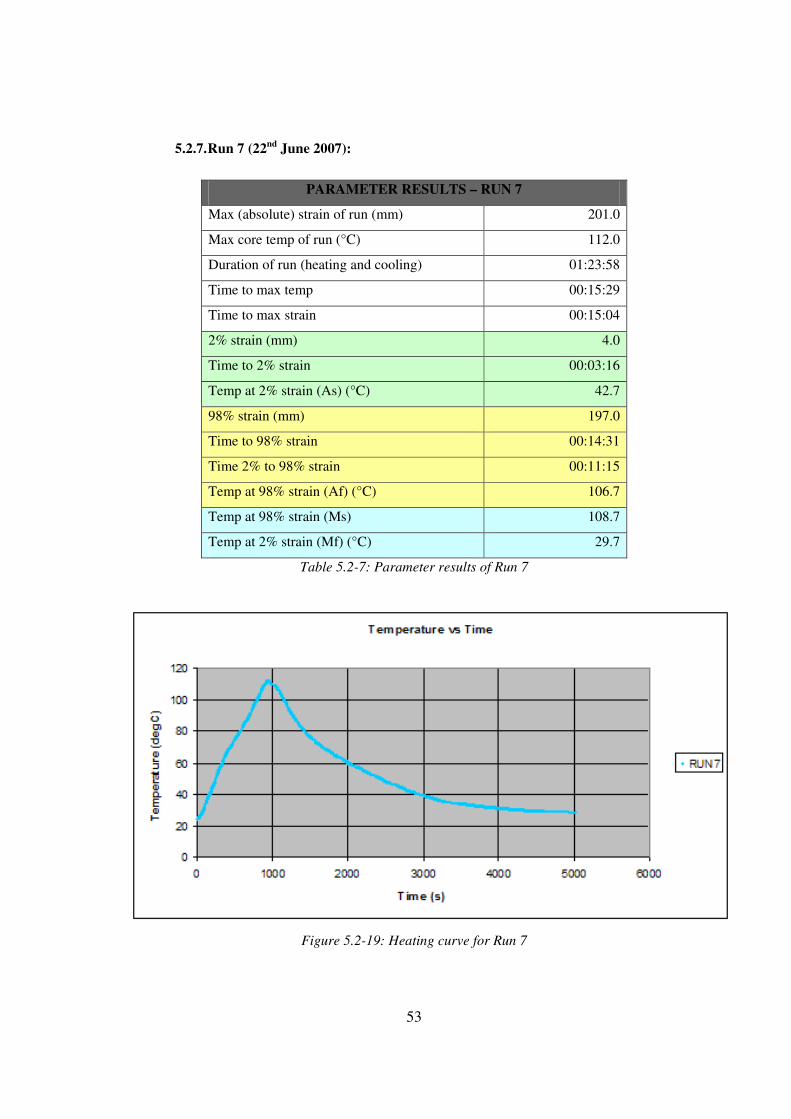
53
5.2.7. Run 7 (22nd June 2007):
PARAMETER RESULTS – RUN 7
Max (absolute) strain of run (mm) 201.0
Max core temp of run (°C) 112.0
Duration of run (heating and cooling) 01:23:58
Time to max temp 00:15:29
Time to max strain 00:15:04
2% strain (mm) 4.0
Time to 2% strain 00:03:16
Temp at 2% strain (As) (°C) 42.7
98% strain (mm) 197.0
Time to 98% strain 00:14:31
Time 2% to 98% strain 00:11:15
Temp at 98% strain (Af) (°C) 106.7
Temp at 98% strain (Ms) 108.7
Temp at 2% strain (Mf) (°C) 29.7
Table 5.2-7: Parameter results of Run 7
Figure 5.2-19: Heating curve for Run 7

54
Figure 5.2-20: Strain curve for Run 7
Figure 5.2-21: Strain vs. Temperature curve for Run 7

55
5.2.8. Run 8 (29th June 2007):
PARAMETER RESULTS – RUN 8
Max (absolute) strain of run (mm) 196.5
Max core temp of run (°C) 112.0
Duration of run (heating and cooling) 01:43:16
Time to max temp 00:16:24
Time to max strain 00:16:09
2% strain (mm) 3.9
Time to 2% strain 00:03:27
Temp at 2% strain (As) (°C) 41.7
98% strain (mm) 192.6
Time to 98% strain 00:15:28
Time 2% to 98% strain 00:12:01
Temp at 98% strain (Af) (°C) 108.0
Temp at 98% strain (Ms) 106.0
Temp at 2% strain (Mf) (°C) 33.7
Table 5.2-8: Parameter results of Run 8
Figure 5.2-22: Heating curve for Run 8
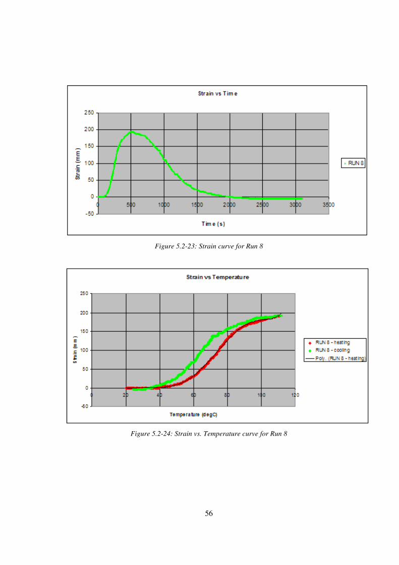
56
Figure 5.2-23: Strain curve for Run 8
Figure 5.2-24: Strain vs. Temperature curve for Run 8

57
5.3. ANALYSIS
The strain vs. temperature curves for all the runs were compiled on one graph as shown below.
Figure 5.3-1: Strain vs. Temperature curve for all runs
PARAMETER RESULTS RUN 1 RUN 2 RUN 3 RUN 4 RUN 5 RUN 6 RUN 7 RUN 8
Max (absolute) strain of run (mm) 190.5 204 204 196.5 204 201 201 196.5
Max core temp of run (°C) 111.3 112.3 112.7 113.7 114.0 113.0 112.0 112.0
Duration of run (heating & cooling) 01:22:23 01:36:50 01:34:17 01:40:51 01:30:37 01:23:32 01:23:58 01:43:16
Time to max temp 00:16:54 00:16:09 00:17:09 00:15:22 00:16:46 00:17:09 00:15:29 00:16:24
Time to max strain 00:16:30 00:15:45 00:16:54 00:14:58 00:16:20 00:16:44 00:15:04 00:16:09
2% strain (mm) 3.8 4.1 4.1 3.9 4.1 4.0 4.0 3.9
Time to 2% strain 00:03:25 00:03:36 00:04:06 00:03:13 00:03:41 00:03:22 00:03:16 00:03:27
Temp at 2% strain (As) (°C) 38.7 41.7 46.3 44.3 45.3 41.7 42.7 41.7
98% strain (mm) 186.7 199.9 199.9 192.6 199.9 197.0 197.0 192.6
Time to 98% strain 00:15:38 00:14:55 00:16:14 00:14:36 00:15:53 00:15:53 00:14:31 00:15:28
Time 2% to 98% strain 00:12:13 00:11:19 00:12:08 00:11:23 00:12:12 00:12:31 00:11:15 00:12:01
Temp at 98% strain (Af) (°C) 107.0 107.3 108.3 109.3 109.0 109.0 106.7 108.0
Temp at 98% strain (Ms) (°C) 107.0 104.7 100.3 109.7 109.3 109.3 108.7 106.0
Temp at 2% strain (Mf) (°C) 32.7 28.7 28.7 31.7 27.0 27.0 29.7 33.7
Table 5.3-1: Summary of parameter results from all the runs

58
Graph 5.3-2 below shows the As and Af temperatures of the SLiM for all runs relative to each other.
Graph 5.3-3 shows the strain (amount of contraction) of the SLiM for each run relative to the
average contraction of 199.7mm.
Reverse Transformation Temperatures (Austenite)
0.0
20.0
40.0
60.0
80.0
100.0
120.0
RUN 1 RUN 2 RUN 3 RUN 4 RUN 5 RUN 6 RUN 7 RUN 8
Tem
pera
ture
(d
eg
C)
Austenite finish temperature
Austenite start temperature
Figure 5.3-2: Graph showing the As and Af temperatures of the SLiM for all runs.
Maximum Strain per Run
0
50
100
150
200
250
1 2 3 4 5 6 7 8
Run
Str
ain
(m
m)
Strain
AVERAGE STRAIN =
199 mm
Figure 5.3-3: Strain of the SLiM for each run relative to the average strain.
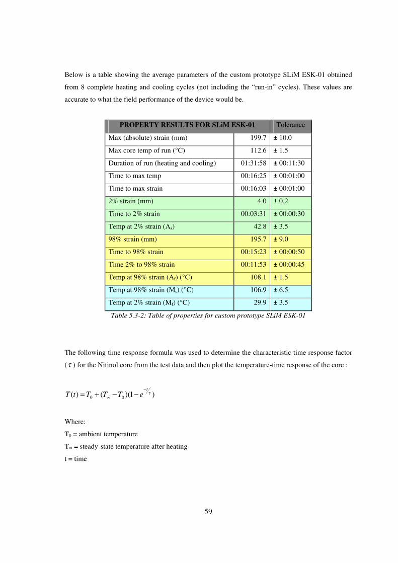
59
Below is a table showing the average parameters of the custom prototype SLiM ESK-01 obtained
from 8 complete heating and cooling cycles (not including the “run-in” cycles). These values are
accurate to what the field performance of the device would be.
PROPERTY RESULTS FOR SLiM ESK-01 Tolerance
Max (absolute) strain (mm) 199.7 ± 10.0
Max core temp of run (°C) 112.6 ± 1.5
Duration of run (heating and cooling) 01:31:58 ± 00:11:30
Time to max temp 00:16:25 ± 00:01:00
Time to max strain 00:16:03 ± 00:01:00
2% strain (mm) 4.0 ± 0.2
Time to 2% strain 00:03:31 ± 00:00:30
Temp at 2% strain (As) 42.8 ± 3.5
98% strain (mm) 195.7 ± 9.0
Time to 98% strain 00:15:23 ± 00:00:50
Time 2% to 98% strain 00:11:53 ± 00:00:45
Temp at 98% strain (Af) (°C) 108.1 ± 1.5
Temp at 98% strain (Ms) (°C) 106.9 ± 6.5
Temp at 2% strain (Mf) (°C) 29.9 ± 3.5
Table 5.3-2: Table of properties for custom prototype SLiM ESK-01
The following time response formula was used to determine the characteristic time response factor
(τ ) for the Nitinol core from the test data and then plot the temperature-time response of the core :
)1)(()( 00τ
t
eTTTtT−
∞ −−+=
Where:
T0 = ambient temperature
T∞ = steady-state temperature after heating
t = time
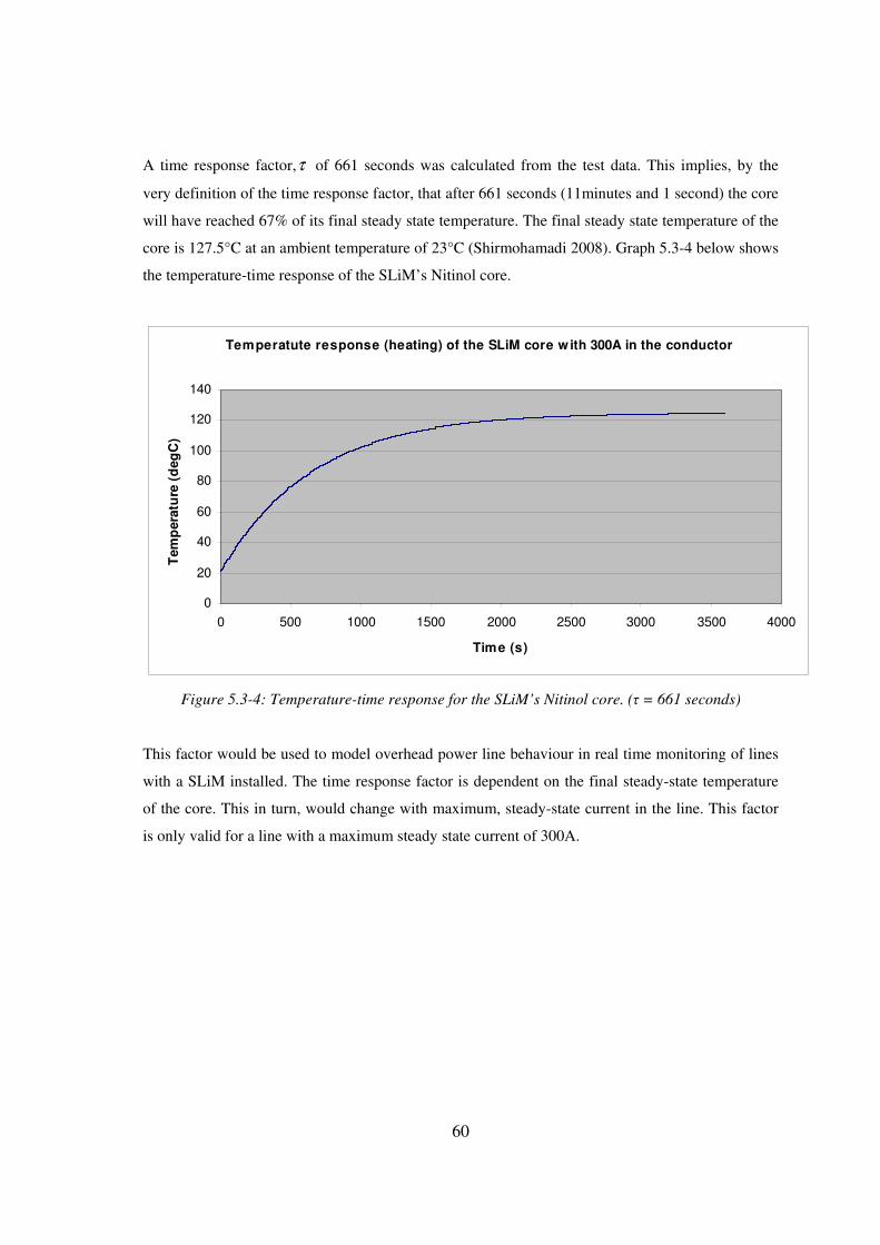
60
A time response factor,τ of 661 seconds was calculated from the test data. This implies, by the
very definition of the time response factor, that after 661 seconds (11minutes and 1 second) the core
will have reached 67% of its final steady state temperature. The final steady state temperature of the
core is 127.5°C at an ambient temperature of 23°C (Shirmohamadi 2008). Graph 5.3-4 below shows
the temperature-time response of the SLiM’s Nitinol core.
Temperatute response (heating) of the SLiM core w ith 300A in the conductor
0
20
40
60
80
100
120
140
0 500 1000 1500 2000 2500 3000 3500 4000
Time (s)
Tem
pera
ture
(d
eg
C)
Figure 5.3-4: Temperature-time response for the SLiM’s Nitinol core. (τ = 661 seconds)
This factor would be used to model overhead power line behaviour in real time monitoring of lines
with a SLiM installed. The time response factor is dependent on the final steady-state temperature
of the core. This in turn, would change with maximum, steady-state current in the line. This factor
is only valid for a line with a maximum steady state current of 300A.

61
5.4. CONCLUSION
The custom prototype SLiM ESK-01 was installed on the purpose built constant tension load testing
rig. It was subject to 3 heating and cooling cycles to “run-in” the Nitinol core. Once the core started
giving consistent performance, the SLiM was put through 8 complete heating and cooling cycles.
Real-time monitoring of the cycles recorded the following parameters: tension, current, voltage,
ambient temperature, core temperature, displacement of the SLiM’s lever and time. This data was
captured and analysed to a) verify the operation of the custom prototype SLiM ESK-01 and b) to
generate a set of properties for the custom prototype SLiM ESK-01. A time constant of 661 seconds
was calculated for the SLiM’s Nitinol core and a temperature-time response for a conductor current
of 300A was generated.
For a complete set of properties for the custom prototype SLiM ESK-01, table 5.3-2 can be
consulted. It is noted that the average As temperature recorded during testing is 42.8°C and the
average Af is 108.1°C. The As and Af temperatures expected, as indicated in figure 3.3-1, were 48°C
and 127°C respectively. This discrepancy can be attributed to the possibility of a slight variation in
element constituency in the Nitinol core used during development of the SLiM when compared to
the Nitinol used during prototype manufacture. It is important that accurate core properties are
supplied before a SLiM is implemented for operation so that correct jumpers can be specified to suit
these actuation temperatures. An operational description of the custom prototype SLiM ESK-01 is
given below:
The custom prototype SLiM ESK-01 is a device designed for use on a 132kV power line that uses
wolf conductor. When the line temperature begins to exceed its templating temperature because of
overloading i.e. more current being required through the line, the SLiM will begin contracting. The
SLiM can contract a total of 199.7mm. When the line cools down again as the load demand
decreases and the current through the line drops, the SLiM will release its tension and stretch out
again.
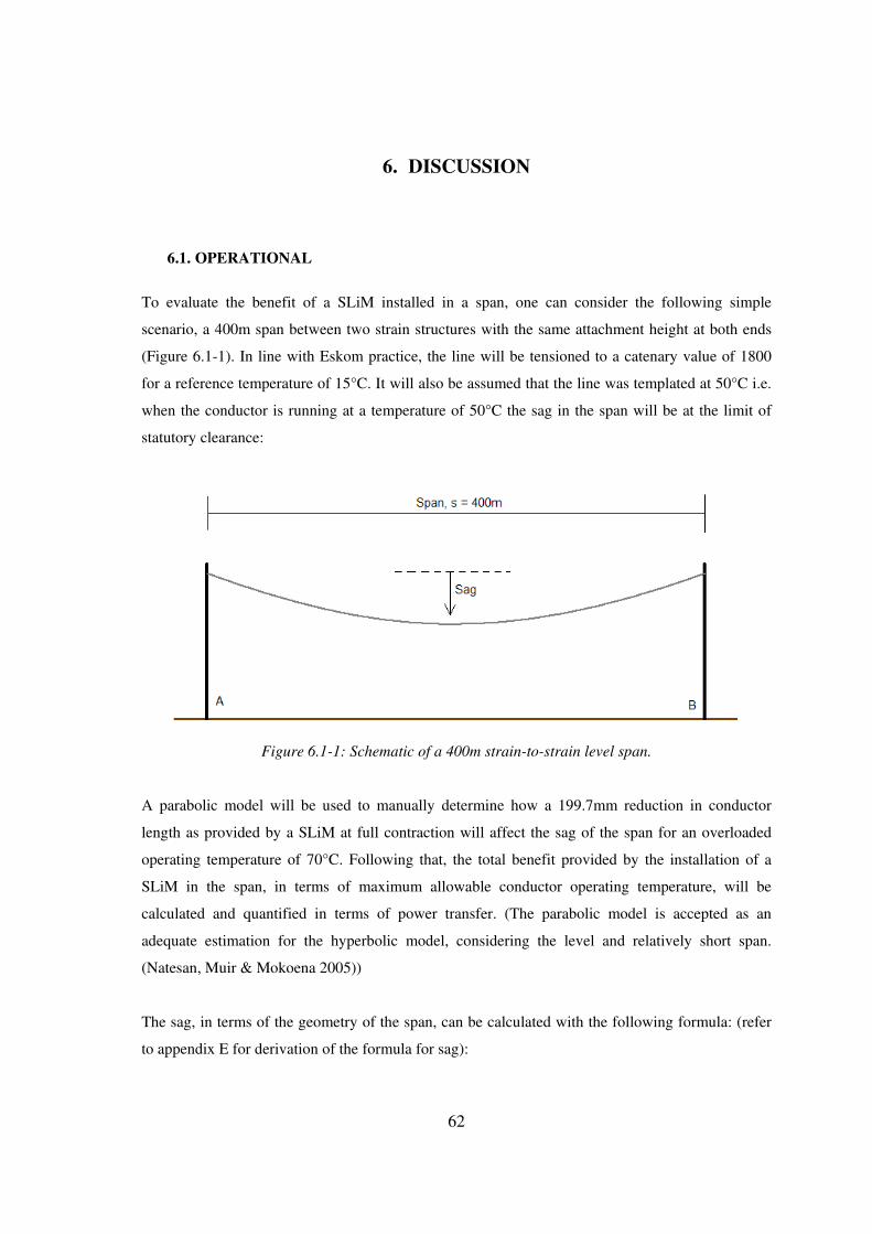
62
6. DISCUSSION
6.1. OPERATIONAL
To evaluate the benefit of a SLiM installed in a span, one can consider the following simple
scenario, a 400m span between two strain structures with the same attachment height at both ends
(Figure 6.1-1). In line with Eskom practice, the line will be tensioned to a catenary value of 1800
for a reference temperature of 15°C. It will also be assumed that the line was templated at 50°C i.e.
when the conductor is running at a temperature of 50°C the sag in the span will be at the limit of
statutory clearance:
Figure 6.1-1: Schematic of a 400m strain-to-strain level span.
A parabolic model will be used to manually determine how a 199.7mm reduction in conductor
length as provided by a SLiM at full contraction will affect the sag of the span for an overloaded
operating temperature of 70°C. Following that, the total benefit provided by the installation of a
SLiM in the span, in terms of maximum allowable conductor operating temperature, will be
calculated and quantified in terms of power transfer. (The parabolic model is accepted as an
adequate estimation for the hyperbolic model, considering the level and relatively short span.
(Natesan, Muir & Mokoena 2005))
The sag, in terms of the geometry of the span, can be calculated with the following formula: (refer
to appendix E for derivation of the formula for sag):

63
C
sSag
8
2
=
Where,
s = 400m
C = 1800m (Catenary constant for conductors used by Eskom).
Sag = 11.111m
The chord length, L, of the conductor is expressed by the following equation:
This chord length is calculated for the span strung with a catenary value of 1800 at a reference
temperature of 15°C.
+=
2
3
81
s
SagsL
(Kiessling et al. 2003)
L = 400.823m
The above span is templated at 50°C. This temperature in the conductor would cause a linear
expansion and thus a new chord length. The new chord length would, in turn, cause a new sag
distance. This sag is the maximum allowable sag in the span in order that no statutory clearances are
violated i.e. 50°C is the maximum allowable (safe) operating temperature for the conductor in terms
of conductor sag (phase-to-ground clearance). The new chord length due to thermal expansion is
calculated below:
( )[ ]
( )[ ]mL
L
TTLLL
C
C
C
082.401
15501043.18823.400823.400
50
6
50
050
=
−⋅×⋅+=
−⋅⋅+=
°
−°
° α
Where,
α = coefficient of linear expansion for wolf conductor = 18.43/°Cx10-6
Thus, the maximum allowable sag for which this span was designed is:

64
mSag
Sag
s
LsSag
C
C
C
C
740.12
8
31
400
082.401400
8
31
50
50
5050
=
⋅
−⋅=
⋅
−⋅=
°
°
°°
As more power transfer is required, the conductor would heat up. The increase in conductor
temperature causes further linear expansion of the conductor. A new chord length and sag distance
is thus calculated for the conductor operating at 70°C. At this temperature, the statutory sag
clearance would be violated:
( )[ ]
( )[ ]mL
L
TTLLL
C
C
C
230.401
15701043.18823.400823.400
70
6
70
070
=
−⋅×⋅+=
−⋅⋅+=
°
−°
° α
mSag
Sag
s
LsSag
C
C
C
C
583.13
8
31
400
230.401400
8
31
70
70
7070
=
⋅
−⋅=
⋅
−⋅=
°
°
°°
It can be seen that when the conductor is made to operate at a temperature of 70°C, the sag
clearance is violated:
mSag
Sag
SagSagSag
violation
violation
CCviolation
843.0
740.12583.13
5070
=
−=
−= °°
The installation of a SLiM in the span would effectively reduce the chord length of the span, when
it is operating at a conductor temperature of 70°C, by 0.200m. The benefit of the SLiM, in terms of
reduction of sag, is thus calculated:
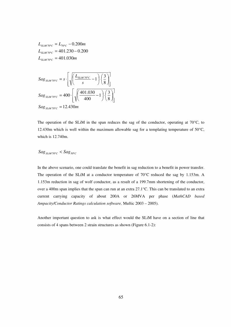
65
mL
L
mLL
CSLiM
CSLiM
CCSLiM
030.401
200.0230.401
200.0
70
70
7070
=
−=
−=
°
°
°°
mSag
Sag
s
LsSag
CSLiM
CSLiM
CSLiM
CSLiM
430.12
8
31
400
030.401400
8
31
70
70
7070
=
⋅
−⋅=
⋅
−⋅=
°
°
°°
The operation of the SLiM in the span reduces the sag of the conductor, operating at 70°C, to
12.430m which is well within the maximum allowable sag for a templating temperature of 50°C,
which is 12.740m.
CCSLiM SagSag °° < 5070
In the above scenario, one could translate the benefit in sag reduction to a benefit in power transfer.
The operation of the SLiM at a conductor temperature of 70°C reduced the sag by 1.153m. A
1.153m reduction in sag of wolf conductor, as a result of a 199.7mm shortening of the conductor,
over a 400m span implies that the span can run at an extra 27.1°C. This can be translated to an extra
current carrying capacity of about 200A or 26MVA per phase (MathCAD based
Ampacity/Conductor Ratings calculation software, Muftic 2003 – 2005).
Another important question to ask is what effect would the SLiM have on a section of line that
consists of 4 spans between 2 strain structures as shown (Figure 6.1-2):
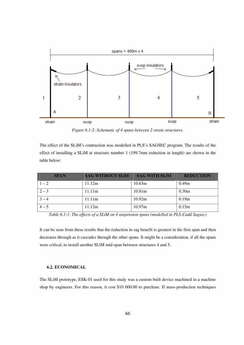
66
Figure 6.1-2: Schematic of 4 spans between 2 strain structures.
The effect of the SLiM’s contraction was modelled in PLS’s SAGSEC program. The results of the
effect of installing a SLiM at structure number 1 (199.7mm reduction in length) are shown in the
table below:
SPAN SAG WITHOUT SLiM SAG WITH SLiM REDUCTION
1 – 2 11.12m 10.63m 0.49m
2 – 3 11.11m 10.81m 0.30m
3 – 4 11.11m 10.92m 0.19m
4 – 5 11.12m 10.97m 0.15m
Table 6.1-1: The effects of a SLiM on 4 suspension spans (modelled in PLS-Cadd Sagsec)
It can be seen from these results that the reduction in sag benefit is greatest in the first span and then
decreases through as it cascades through the other spans. It might be a consideration, if all the spans
were critical, to install another SLiM mid-span between structures 4 and 5.
6.2. ECONOMICAL
The SLiM prototype, ESK-01 used for this study was a custom built device machined in a machine
shop by engineers. For this reason, it cost $10 000.00 to purchase. If mass-production techniques
1 2 3 4 5

67
were implemented for large orders, the cost would come down and the SLiM could become an
economically viable option for implementation by utilities.
Correspondence with Power Transmission Solutions, Inc. (Shirmohamadi 2008) has yielded two
preliminary economic scenario options for mass implementation:
Option 1: Power Transmission Solutions, Inc. will invest in the high mass-production processes and
produce for example, 1000 units. The utility would pay the production cost plus shipping, handling,
taxes, duty and a management/profit fee. One of the main factors would be the price of the raw
materials which fluctuates constantly and would have to be evaluated closer to the time of order to
provide an accurate cost estimate. It is estimated that for this option, unit cost could be as much as
75% of the prototype cost.
Option 2: Power Transmission Solutions, Inc. would provide design details and expertise to the
utility or a selected manufacturer for the SLiM’s to be produced locally. This would require that
production tools and methods, testing and quality assurance systems and supply chains be
developed in conjunction with PTS. The utility would pay PTS an upfront licensing fee as well as a
royalty for every unit produced. The production of the SLiM’s in this option would be subject to
local material, labour and production costs as well as taxes and duties. There would also be an
option for the manufacturer to supply the rest of Africa and possibly Europe.
A third option is that the utility would buy the Nitinol actuator cores from PTS, Inc. and
manufacture all the other SLiM components in South Africa. The SLiM’s would then be assembled
in South Africa. A licensing agreement would have to be reached here also. Alternatively, a
completely new design incorporating the same Nitinol core could be manufactured and assembled
in South Africa.
6.3. FUTURE REGARDING SOUTH AFRICA
Ultimately, the deployment of an anti-sagging mitigator in South Africa as a solution to excess sag
in conductors due to increased power transfer would depend on the unit and installation cost when
compared to more traditional solutions. For the solution to become economically viable, it would
have to be cheaper than physically re-tensioning a line or increasing a line’s attachment points by

68
extending the structures. Alternatively, a solution such as the SLiM might be considered where
permanent high tension in the line is not optimum. It is known that high tension in a line increases
the damaging effects of Aeolian vibrations. The SLiM would increase tension only when necessary,
when and as the line runs hot.
The SLiM is not limited to 132kV lines. In the USA, it is being used up to 1000A. For South Africa,
the SLiM could be developed for other bundle configurations such as twin or quad bundle
configurations.
From the knowledge gained in this research project, it is now possible to develop new applications
for the power industry to take advantage of shape memory alloys such as Nitinol. Development in
conjunction with metallurgists would produce the alloy specific to the application (regarding
actuation temperature ranges) then the alloy would be incorporated in design by engineers.
The SLiM device designed by Power Transmission Solutions, Inc. or a derivative of the technology
is an innovative approach to solving the problem of sagging power lines in the power industry.
Mechanically, it is a viable alternative. Economically, it would need to be investigated further with
mass-production costs taken into account. The success of the device in this form would depend on
ultimate unit purchase costs.
69
7. CONCLUSION
Shape memory alloy technology was investigated within its application in the power industry.
Power Transmission Solutions, Inc. (PTS) have developed a sagging line mitigator (SLiM) that
employs the shape memory alloy, Nitinol, as an actuator to counteract the effects of sagging power
lines as a result of increased power and current transfer. A custom prototype SLiM ESK-01 was
developed by PTS for use on 132kV wolf conductor power lines. A constant tension load testing rig
was developed to simulate the mechanical loading on a 132kV wolf conductor span on which the
SLiM ESK-01 was tested. From the outset, testing was required to a) confirm that the SLiM
actually works i.e. contracts when a current sufficient enough to heat the core is transmitted
through it and extends when the core cools down again and b) quantify the operational
parameters of the Nickel-Titanium alloy core and hence the SLiM device as a whole. A
complete set of material thermal-mechanical properties for the device was developed during the
heating and cooling phases of the testing resulting in a strain versus temperature response curve
being generated for the SLiM. The benefit of such a device was modelled and analysed on a single
400m span as well as four 400m spans between two strain structures in PLS Sagsec. An ampacity
model for wolf conductor was also used to determine the power transfer increase gained by the
contraction of the SLiM on a 400m span of wolf conductor.
It is recommended that a temperature versus current response curve for the Nitinol core of the SLiM
be acquired from PTS or be developed in order to further “fine-tune” the current ratios to be
transmitted through the body of the SLiM and through the core and hence jumper designs. It is
important to develop a relationship between the steady-state temperatures of wolf conductor for
different currents and the steady-state temperature of the Nitinol core at different currents. Once this
is obtained, the correct split-jumpers can be specified for different field implementation.
A loaded 132kV wolf power line would be required for field testing. The SLiM would be installed
on the line. A weather station and remote DAQ would be installed below the line to monitor the
SLiM’s performance over a period of time. All the data captured would be used in the final phase to
justify implementation of the SLiM as a viable and operational solution to the problem of sagging
power lines where dynamic tension response is required.

70
This dissertation presented a synopsis of the field of intelligent material and a more in-depth study
of Nitinol was then presented to provide a good understanding of the theory behind the SLiM’s
actuator (Chapter 2 and Appendices A and B). The study and testing of the custom prototype SLiM
ESK-01 was presented followed by the discussion of the operation and benefit of the SLiM as a
solution to the problem of sagging power lines. Recommendations were made regarding future
implementation of the device. An overview of overhead power lines was presented in Appendix C.
The technology studied in this dissertation can now be reproduced and can be used to develop new
applications using shape memory alloy technology in any field of engineering as required.
71
8. REFERENCES
Active Materials Laboratory 2005, Magnetostricive Materials [Homepage of UCLA], [Online].
Available: aml.seas.ucla.edu/research/areas/Magnetostrictive [2008, 05/09].
Advanced Materials Today, Advanced Materials Today [Homepage of Advanced Materials Today],
[Online]. Available: www.amtbe.com [2008, 05/14].
Aspey, J. 2003, Smart Structural Health Monitoring of Mining Support Units, University of
KwaZulu-Natal.
Bard Peripheral Vascular 2008, Bard Peripheral Vascular [Homepage of Bard Peripheral
Vascular], [Online]. Available: www.bardpv.com [2008, 07/14].
Bologna, F. 2005, "Insulator Selection" in The Planning, Design and Construction of Overhead
Power Lines, eds. S. Bisnath, A.C. Britten, D.H. Cretchley, D. Muftic, T. Pillay & R. Vajeth,
1st edn, Crown Publications, Johannesburg, pp. 375-408.
Burger, A., Ramnarain, R. & Peter, L. 2005, "Earthing" in The Planning, Design and Construction
of Overhead Power Lines, eds. S. Bisnath, A.C. Britten, D.H. Cretchley, D. Muftic, T. Pillay &
R. Vajeth, 1st edn, Crown Publications, Johannesburg, pp. 541-574.
Calitz, J., Haridass, B., Jacobs, B., Retief, J. & Du Plessis, P. 2005, "Line Hardware" in The
Planning, Design and Construction of Overhead Power Lines, eds. S. Bisnath, A.C. Britten,
D.H. Cretchley, D. Muftic, T. Pillay & R. Vajeth, 1st edn, Crown Publications, Johannesburg,
pp. 441-482.
Cigré 1996, Probabilistic Determination of Conductor Current Rating, WG 12, 1st edn, Electra.
Duerig, T.W. 1995, " Present and Future Applications of Shape Memory and Superelastic
Materials", Mat. Res. Soc. Symp.
Gaunt, C.T., Britten, A.C. & Geldenhuys, H.J. 1995, Insulation co-ordination of unshielded
distribution lines from 1kV to 36kV, University of Pretoria and Laboratory for Advanced
Engineering is association with the SAIEE.
72
Hillerman, A.R. 1999, Insulation Co-ordination For Power Systems, 1st edn, Marcel Dekker, Inc.,
New York.
Hodgson, D.E., Wu, M.H. & Biermann, R.J. 1998, Shape Memory Alloys, Technology Article edn,
Shape Memory Applications, Inc., USA.
Horikawa, H., Ichinose, S., Morii, K., Miyazaki, S. & Otsuka, K. 1988, Metall. Trans., vol. A, no.
19, pp. 915-916.
IEEE Working group 1993, Estimating Lightning Performance of Transmission Lines: Part 2,
Updates to Analytical Models, 1st edn, IEEE Transactions on Power Delivery.
Kiessling, F., Nefzger, P., Nolasco, J. & Kaintzyk, U. 2003, Overhead Power Lines – Planning,
Design, Construction, Springer, Heidelberg, pp. 540-546.
Kopperdahl, D. 2006, PTS Equipment Specification Document, 1st edn, Power Transmission
Solutions, Inc., California, USA.
Marais, P. & Badenhorst, B. 2005, "Construction" in The Planning, Design and Construction of
Overhead Power Lines, eds. S. Bisnath, A.C. Britten, D.H. Cretchley, D. Muftic, T. Pillay &
R. Vajeth, 1st edn, Crown Publications, Johannesburg, pp. 677-722.
Mertman, M. 2004, “Non-medical applications of Nitinol", Min Invas Ther & Allied Technol, vol.
13, no. 4, pp. 254-260.
Miyazaki, S. 2005, “Shape Memory Alloys”, Institute of Material Science Paper, edn 1, University
of Tsukuba, Tsukuba, pp.1-13.
Miyazaki, S. & Otsuka, K. 1989, "Development of Shape Memory Alloys", ISIJ International, vol.
29, no. 5, pp. 353-377.
Morcap Industries 2008, Morcap Industries [Homepage of Morcap Industries], [Online]. Available:
www.morcap.com [2008, 09/04].
Muftic, D., Narain, S. & Ramnarain, R. 2005, "Ground Wire Optimisation" in The Planning,
Design and Construction of Overhead Power Lines, eds. S. Bisnath, A.C. Britten, D.H.
Cretchley, D. Muftic, T. Pillay & R. Vajeth, 1st edn, Crown Publications, Johannesburg, pp.
355-374.
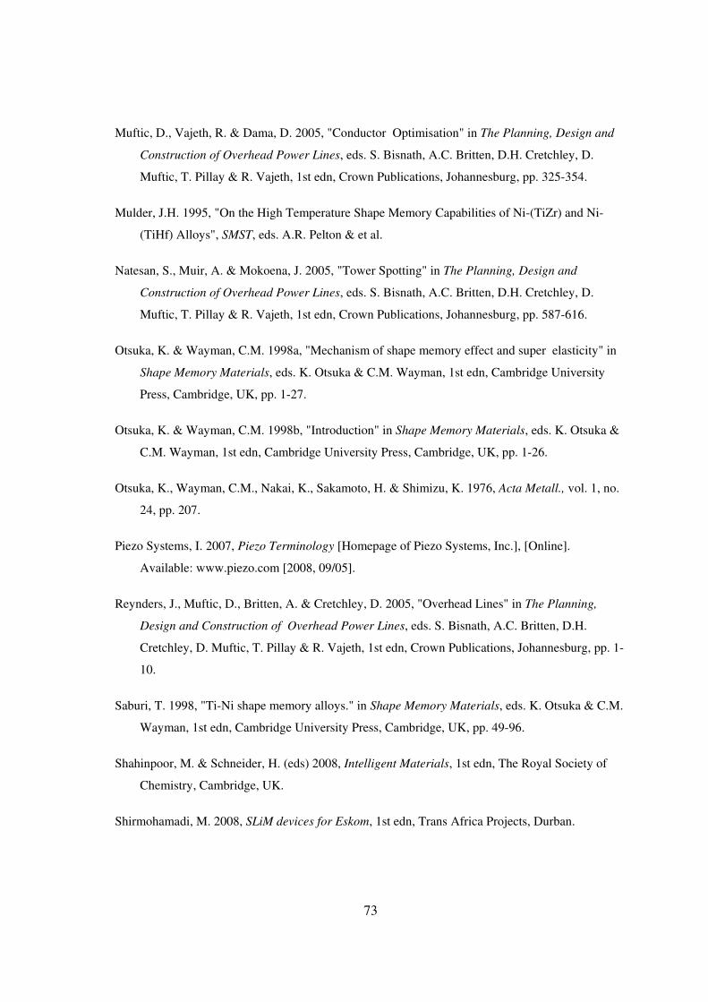
73
Muftic, D., Vajeth, R. & Dama, D. 2005, "Conductor Optimisation" in The Planning, Design and
Construction of Overhead Power Lines, eds. S. Bisnath, A.C. Britten, D.H. Cretchley, D.
Muftic, T. Pillay & R. Vajeth, 1st edn, Crown Publications, Johannesburg, pp. 325-354.
Mulder, J.H. 1995, "On the High Temperature Shape Memory Capabilities of Ni-(TiZr) and Ni-
(TiHf) Alloys", SMST, eds. A.R. Pelton & et al.
Natesan, S., Muir, A. & Mokoena, J. 2005, "Tower Spotting" in The Planning, Design and
Construction of Overhead Power Lines, eds. S. Bisnath, A.C. Britten, D.H. Cretchley, D.
Muftic, T. Pillay & R. Vajeth, 1st edn, Crown Publications, Johannesburg, pp. 587-616.
Otsuka, K. & Wayman, C.M. 1998a, "Mechanism of shape memory effect and super elasticity" in
Shape Memory Materials, eds. K. Otsuka & C.M. Wayman, 1st edn, Cambridge University
Press, Cambridge, UK, pp. 1-27.
Otsuka, K. & Wayman, C.M. 1998b, "Introduction" in Shape Memory Materials, eds. K. Otsuka &
C.M. Wayman, 1st edn, Cambridge University Press, Cambridge, UK, pp. 1-26.
Otsuka, K., Wayman, C.M., Nakai, K., Sakamoto, H. & Shimizu, K. 1976, Acta Metall., vol. 1, no.
24, pp. 207.
Piezo Systems, I. 2007, Piezo Terminology [Homepage of Piezo Systems, Inc.], [Online].
Available: www.piezo.com [2008, 09/05].
Reynders, J., Muftic, D., Britten, A. & Cretchley, D. 2005, "Overhead Lines" in The Planning,
Design and Construction of Overhead Power Lines, eds. S. Bisnath, A.C. Britten, D.H.
Cretchley, D. Muftic, T. Pillay & R. Vajeth, 1st edn, Crown Publications, Johannesburg, pp. 1-
10.
Saburi, T. 1998, "Ti-Ni shape memory alloys." in Shape Memory Materials, eds. K. Otsuka & C.M.
Wayman, 1st edn, Cambridge University Press, Cambridge, UK, pp. 49-96.
Shahinpoor, M. & Schneider, H. (eds) 2008, Intelligent Materials, 1st edn, The Royal Society of
Chemistry, Cambridge, UK.
Shirmohamadi, M. 2008, SLiM devices for Eskom, 1st edn, Trans Africa Projects, Durban.
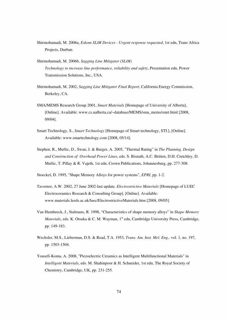
74
Shirmohamadi, M. 2006a, Eskom SLiM Devices - Urgent response requested, 1st edn, Trans Africa
Projects, Durban.
Shirmohamadi, M. 2006b, Sagging Line Mitigator (SLiM)
Technology to increase line performance, reliability and safety, Presentation edn, Power
Transmission Solutions, Inc., USA.
Shirmohamadi, M. 2002, Sagging Line Mitigator Final Report, California Energy Commission,
Berkeley, CA.
SMA/MEMS Research Group 2001, Smart Materials [Homepage of University of Alberta],
[Online]. Available: www.cs.ualberta.ca/~database/MEMS/sma_mems/smrt.html [2008,
09/04].
Smart Technology, S., Smart Technology [Homepage of Smart technology, STI.], [Online].
Available: www.smartechnology.com [2008, 05/14].
Stephen, R., Muftic, D., Swan, J. & Burger, A. 2005, "Thermal Rating" in The Planning, Design
and Construction of Overhead Power Lines, eds. S. Bisnath, A.C. Britten, D.H. Cretchley, D.
Muftic, T. Pillay & R. Vajeth, 1st edn, Crown Publications, Johannesburg, pp. 277-308.
Stoeckel, D. 1995, "Shape Memory Alloys for power systems", EPRI, pp. 1-2.
Tavernor, A.W. 2002, 27 June 2002-last update, Electrostrictive Materials [Homepage of LUEC
Electroceramics Research & Consulting Group], [Online]. Available:
www.materials.leeds.ac.uk/luec/ElectrostrictiveMaterials.htm [2008, 09/05].
Van Humbeeck, J., Stalmans, R. 1998, “Characteristics of shape memory alloys” in Shape Memory
Materials, eds. K. Otsuka & C. M. Wayman, 1st edn, Cambridge University Press, Cambridge,
pp. 149-183.
Wechsler, M.S., Lieberman, D.S. & Read, T.A. 1953, Trans. Am. Inst. Mel. Eng., vol. 1, no. 197,
pp. 1503-1504.
Yousefi-Koma, A. 2008, "Piezoelectric Ceramics as Intelligent Multifunctional Materials" in
Intelligent Materials, eds. M. Shahinpoor & H. Schneider, 1st edn, The Royal Society of
Chemistry, Cambridge, UK, pp. 231-255.

75
Zheng, Y. & Schrooten, J. 2004, "Temperature memory effect of a nickel-titanium shape memory
alloy", Applied Physics, American Institute of Physics, vol. 84, no. 1. pp.1-10.

76
9. APPENDIX A – SMART MATERIALS
9.1. INTRODUCTION
This appendix comprises of an overview of the topic of smart materials. In reading this, a synopsis
of the field of smart material will be gained. Smart materials will be defined as a topic and the
various smart materials themselves will be briefly covered. The SLiM device has a Nitinol actuator
which is a shape memory alloy. The topic of shape memory alloys will not be covered in this
section but can be found in chapter 2 and Appendix B.
The term “smart material” refers to any material with one or more properties that can be
significantly and controllably changed by an external input. As opposed to a normal material with
properties that cannot be altered. The main categories of smart materials that are undergoing
continuous research for new application are piezoelectric materials, magneto-rheostatic materials,
electro-rheostatic materials and shape memory alloys. They are already incorporated in many every-
day items with new applications being developed constantly. These smart materials each have
different properties that can be altered. These changeable properties influence the type of
application that the material can be used for. Generally, smart material systems are employed in
three ways: sensors that register important internal and external information; actuators (motors) that
can switch or apply forces; and computerised control systems. They often contain combinations of
the aforementioned system types and this is what makes them “smart”; the fact that these materials
can gather information, perform tasks, sense changing conditions and adapt accordingly.
9.2. PIEZOELECTRIC MATERIALS
Piezoelectric materials are used for two specific properties. When a piezoelectric material is
strained, it produces a small, proportional and measurable electrical discharge (refer to figure 9.2-1
below). Conversely, when an electrical current is passed through a piezoelectric material, it
experiences a significant volume change (up to 4% (SMA/MEMS Research Group 2001)). The
word piezoelectricity was derived from the Greek work “piezein” for “press” meaning “pressure
electricity”.
77
Figure 9.2-1: The piezoelectric effect (SMA/MEMS Research Group 2001)
A piezoelectric element is able to act as a sensing or transmitting element or both. Some
applications that make use of piezoelectric materials in a generating system include cigarette and
gas lighters, gramophone pick-ups, accelerometers, hydrophones and microphones. When an
alternating potential difference is placed on a piezoelectric material, it will grow and shrink at the
same frequency as that of the applied voltage. Some applications that use piezoelectric in an
actuating system are transducers, ultrasonic atomisers, fuel injection systems and piezoelectric
motors.
The piezoelectric phenomenon was discovered in 1880 by Jacques and Pierre Curie when they
found a surface electric charge on specially prepared crystals of quartz, tourmaline, topaz and cane
sugar, which were subjected to mechanical stress (Aspey 2003). The first piezoelectric transducer
was invented in 1917 by P. Langevin and co-workers. It was a steel-quartz sandwich with a
resonant frequency of about 50 kHz that was used as an ultrasonic submarine detector (Piezo
Systems 2007). Because of the difficulty in cutting piezoelectric crystals precisely, piezoceramics
were developed during World War 2. It was discovered that certain ceramic materials displayed
dielectric constants (ratio of the amount of charge a material can store compared to the charge
stored in the same volume of a vacuum) of up to 100 time greater than common cut crystals (Aspey
2003). These barium-titanate ceramics were manufactured by sintering metallic oxide powders.
Piezoceramics are inert and immune to moisture and other atmospheric conditions and therefore
ideal for any operating environment. These ceramics are mostly oxide materials on the basis of lead

78
oxide, zirconate oxide, and titanate oxide. Metal oxides of the elements lithium, magnesium, zinc,
nickel, manganese, niobium, antimony or strontium are added for the appropriate adjustment or
stabilisation of the material parameters (Yousefi-Koma 2008).
Piezoelectrics are capable of rapid volume changes and have therefore often been successfully
implemented in high frequency applications like vibration control and damping, audio speakers and
ultra-sound generators. Piezoelectric measuring devices are used as the primary choice for
applications where accurate measurement and recording of dynamic changes to mechanical
variables such as pressure, force or acceleration. Piezoelectric transducers are used mostly in
ultrasound medical imaging, non-destructive testing and under-water acoustics. Within engineering,
piezoelectrics are used for material health monitoring and evaluation in building structures, ship
structures and auto chassis. The most common materials used commercially for their piezoelectric
property are quartz and lead zirconate titanate (PZT) (Aspey 2003). Other piezoceramics sometimes
used are lead metaniobate and lead titanate (Yousefi-Koma 2008).
9.3. ELECTROSTRICTIVE MATERIALS
Electrostrictive materials, also known as relaxor ferroelectrics differ from piezoelectric materials in
that they possess no spontaneous polarisation and therefore cannot be considered piezoelectric.
Lead Magnesium Niobate (PMN) and its doped derivatives possess high permittivity (20 000 – 35
000) and extraordinarily high Electrostrictive coefficients (Tavernor 2002). When used correctly,
they can be virtually loss-free up to hundreds of kilo-Hertz. Other Electrostrictive materials include
polyurethane, polyether, amorphous polybutadiene, polydimethylsiloxane, liquid crystal elastomers
(Aspey 2003). PMN exhibits displacement proportional to the square of the applied voltage under
small signal conditions. At 0 volts, the PMN’s unit cells are centro-symmetric and as an electric
field is applied, the negative and positively charged ions separate, causing dimensional change of
the unit cell and overall expansion. This property renders them useful as actuators. The quadratic
relationship between the drive voltage and the expansion of PMN means that electrostrictive
actuators do not have a linear relationship like piezoelectric actuators do (refer to figure 9.3-1,
below) and therefore require higher drive currents for dynamic applications (Tavernor 2002).
79
Figure 9.3-1: Displacement as a function of field strength for PZT (piezoelectric) compared to
PMN (electrostrictive) (Tavernor 2002)
Electrostrictive materials also exhibit less hysteresis than piezoelectric materials and can withstand
greater pulling forces. Because their travel decreases as their temperature increases, PMN actuators
are best suited for applications with little or no temperature variations of the material.
Research is currently being conducted into electrostrictive elastomers which offer the possibility of
highly compliant actuators with some of the properties of muscle. Elastomers have high permittivity
resulting in large electric stresses and low modulii, leading in turn to large strains and hence high
electrostrictive coefficients (Aspey 2003). Figure 9.3-2 shows the relationship between
displacement and voltage for a typical electrostrictive material.
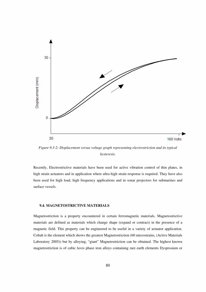
80
Figure 9.3-2: Displacement versus voltage graph representing electrostriction and its typical
hysteresis.
Recently, Electrostrictive materials have been used for active vibration control of thin plates, in
high strain actuators and in application where ultra high strain response is required. They have also
been used for high load, high frequency applications and in sonar projectors for submarines and
surface vessels.
9.4. MAGNETOSTRICTIVE MATERIALS
Magnetostriction is a property encountered in certain ferromagnetic materials. Magnetostrictive
materials are defined as materials which change shape (expand or contract) in the presence of a
magnetic field. This property can be engineered to be useful in a variety of actuator application.
Cobalt is the element which shows the greatest Magnetostriction (60 microstrains, (Active Materials
Laboratory 2005)) but by alloying, “giant” Magnetostriction can be obtained. The highest known
magnetostriction is of cubic laves phase iron alloys containing rare earth elements Dysprosium or
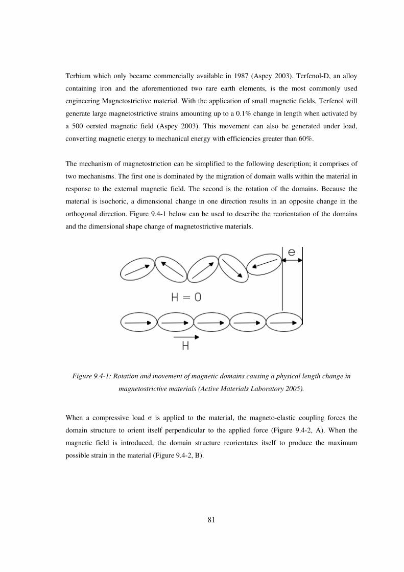
81
Terbium which only became commercially available in 1987 (Aspey 2003). Terfenol-D, an alloy
containing iron and the aforementioned two rare earth elements, is the most commonly used
engineering Magnetostrictive material. With the application of small magnetic fields, Terfenol will
generate large magnetostrictive strains amounting up to a 0.1% change in length when activated by
a 500 oersted magnetic field (Aspey 2003). This movement can also be generated under load,
converting magnetic energy to mechanical energy with efficiencies greater than 60%.
The mechanism of magnetostriction can be simplified to the following description; it comprises of
two mechanisms. The first one is dominated by the migration of domain walls within the material in
response to the external magnetic field. The second is the rotation of the domains. Because the
material is isochoric, a dimensional change in one direction results in an opposite change in the
orthogonal direction. Figure 9.4-1 below can be used to describe the reorientation of the domains
and the dimensional shape change of magnetostrictive materials.
Figure 9.4-1: Rotation and movement of magnetic domains causing a physical length change in
magnetostrictive materials (Active Materials Laboratory 2005).
When a compressive load σ is applied to the material, the magneto-elastic coupling forces the
domain structure to orient itself perpendicular to the applied force (Figure 9.4-2, A). When the
magnetic field is introduced, the domain structure reorientates itself to produce the maximum
possible strain in the material (Figure 9.4-2, B).
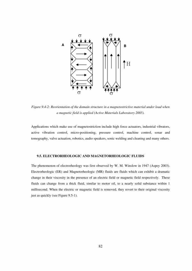
82
Figure 9.4-2: Reorientation of the domain structure in a magnetostrictive material under load when
a magnetic field is applied (Active Materials Laboratory 2005).
Applications which make use of magnetostriction include high force actuators, industrial vibrators,
active vibration control, micro-positioning, pressure control, machine control, sonar and
tomography, valve actuation, robotics, audio speakers, sonic welding and cleaning and many others.
9.5. ELECTRORHEOLOGIC AND MAGNETORHEOLOGIC FLUIDS
The phenomenon of electrorheology was first observed by W. M. Winslow in 1947 (Aspey 2003).
Electrorheologic (ER) and Magnetorheologic (MR) fluids are fluids which can exhibit a dramatic
change in their viscosity in the presence of an electric field or magnetic field respectively. These
fluids can change from a thick fluid, similar to motor oil, to a nearly solid substance within 1
millisecond. When the electric or magnetic field is removed, they revert to their original viscosity
just as quickly (see Figure 9.5-1).
A B

83
Figure 9.5-1: A magnetorheologic fluid is liquid on the left and then solidifies in the presence of a
magnetic field (right) (SMA/MEMS Research Group 2001).
There are two classes of ER fluids: the dispersion type and the uniformity type. The dispersion type
of ER fluid consists of colloidal suspensions of dielectric particles in an electrically insulating oil.
The most common type or MR fluid consists of iron particles suspended in an organic medium such
as mineral or silicone oil. MR fluids are becoming increasingly popular due to the lower field
strengths needed to activate them and the significantly higher yield strength that they have over ER
fluids.
MR fluids are being developed for use in car shocks, machine vibration damping systems,
prosthetic limbs, exercise equipment and surface polishing equipment. ER fluids are being
developed for use in clutches, valves and engine mounts to reduce noise and vibrations in vehicles
(SMA/MEMS Research Group 2001). Smart gels are an off-shoot of MR fluids and are used in
orthopaedic shoe inserts where the heat generated by the foot causes the insert to stiffen in a perfect
mould of the foot.

84
10. APPENDIX B – ADDITIONAL INFORMATIO ON NICKEL-
TITANIUM ALLOY
10.1. CRYSTALLOGRAPHY
In order to minimise strain energy between martensite variants during martensitic transformation,
the transformation must occur in such a way that their interface is an undistorted and unrotated
plane (invariant or habit plane). For these variants to form, it is necessary to introduce a lattice
invariant shear such as twins, dislocations or stacking faults. With the use of phenomenological
crystallographic theory (Wechsler, Lieberman & Read 1953), one can describe this transformation.
According to this theory, there are 3 parts to transformation: 1) a lattice deformation, B, creating the
martensite structure from the parent phase; 2) a lattice invariant shear, P2 (twinning, slip or
faulting); 3) a lattice rotation, R. With these, the total strain associated with the transformation can
be written in the following form:
P1 = R P2B
In order to solve for P1 (shape strain produced by the martensitic transformation), it must be
described as an invariant plane strain. The invariant plane is one that is undistorted, unrotated,
macroscopically homogeneous and consists of a shear strain parallel to the habit and a volume
change normal to the habit plane. It can therefore be represented in the following way:
P1 = I + m1d1p1'
Here, d1 is a unit column vector in the direction of the shape strain, I is a 3x3 identity matrix, m1 is
the magnitude of the shape strain and p1 is a unit row vector normal to the invariant plane. If the
lattice parameters of the parent and martensitic phases, the lattice correspondence and the lattice
invariant shear are known, then the matrix P1 can be determined. From here, all the
crystallographical parameters, m1, d1 and p1 can be calculated.
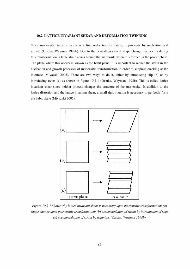
85
10.2. LATTICE INVARIANT SHEAR AND DEFORMATION TWINNING
Since martensitic transformation is a first order transformation, it proceeds by nucleation and
growth (Otsuka, Wayman 1998b). Due to the crystallographical shape change that occurs during
this transformation, a large strain arises around the martensite when it is formed in the parent phase.
The plane where this occurs is known as the habit plane. It is important to reduce the strain in the
nucleation and growth processes of martensitic transformation in order to suppress cracking at the
interface (Miyazaki 2005). There are two ways to do it, either by introducing slip (b) or by
introducing twins (c) as shown in figure 10.2-1 (Otsuka, Wayman 1998b). This is called lattice
invariant shear since neither process changes the structure of the martensite. In addition to the
lattice distortion and the lattice invariant shear, a small rigid rotation is necessary to perfectly form
the habit plane (Miyazaki 2005).
Figure 10.2-1 Shows why lattice invariant shear is necessary upon martensitic transformation; (a)
shape change upon martensitic transformation; (b) accommodation of strain by introduction of slip;
(c) accommodation of strain by twinning. (Otsuka, Wayman 1998b)
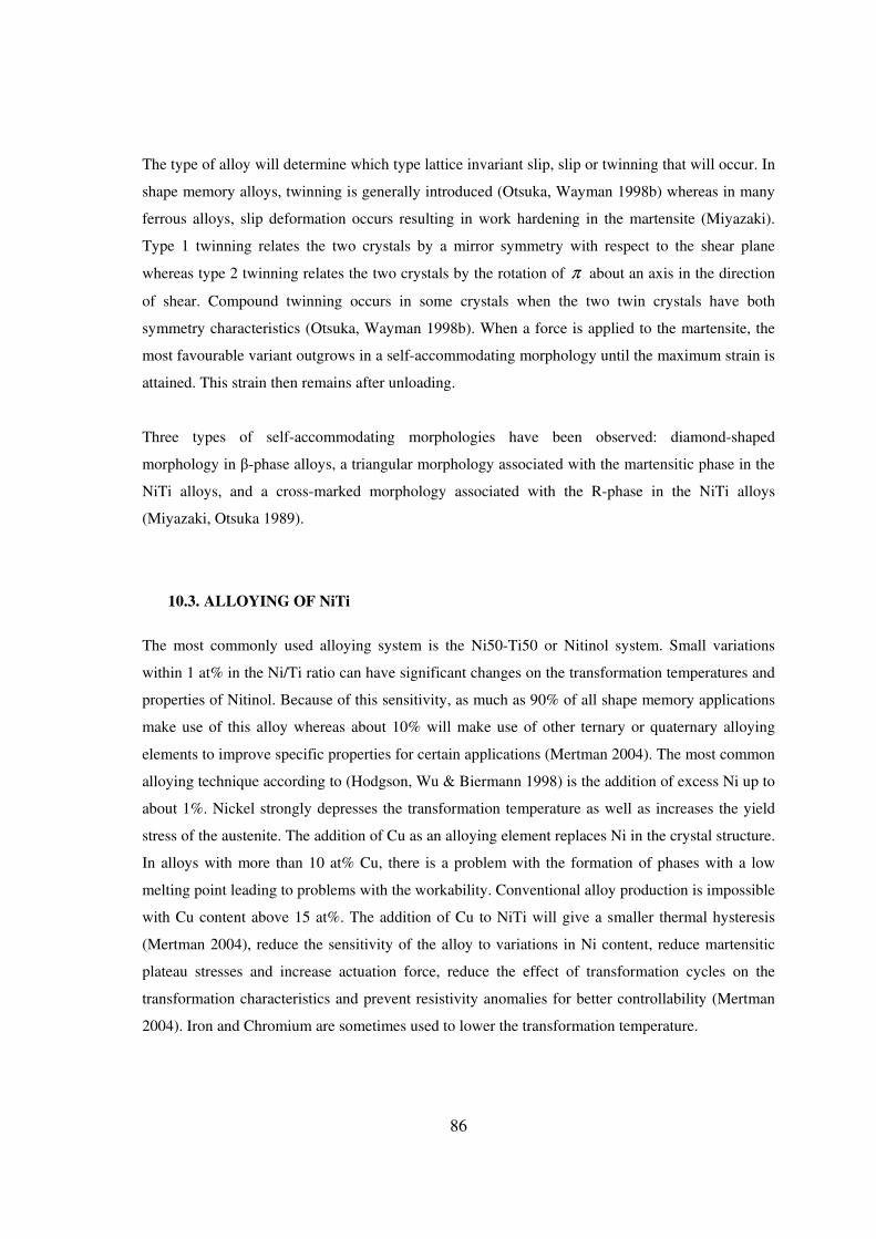
86
The type of alloy will determine which type lattice invariant slip, slip or twinning that will occur. In
shape memory alloys, twinning is generally introduced (Otsuka, Wayman 1998b) whereas in many
ferrous alloys, slip deformation occurs resulting in work hardening in the martensite (Miyazaki).
Type 1 twinning relates the two crystals by a mirror symmetry with respect to the shear plane
whereas type 2 twinning relates the two crystals by the rotation of π about an axis in the direction
of shear. Compound twinning occurs in some crystals when the two twin crystals have both
symmetry characteristics (Otsuka, Wayman 1998b). When a force is applied to the martensite, the
most favourable variant outgrows in a self-accommodating morphology until the maximum strain is
attained. This strain then remains after unloading.
Three types of self-accommodating morphologies have been observed: diamond-shaped
morphology in β-phase alloys, a triangular morphology associated with the martensitic phase in the
NiTi alloys, and a cross-marked morphology associated with the R-phase in the NiTi alloys
(Miyazaki, Otsuka 1989).
10.3. ALLOYING OF NiTi
The most commonly used alloying system is the Ni50-Ti50 or Nitinol system. Small variations
within 1 at% in the Ni/Ti ratio can have significant changes on the transformation temperatures and
properties of Nitinol. Because of this sensitivity, as much as 90% of all shape memory applications
make use of this alloy whereas about 10% will make use of other ternary or quaternary alloying
elements to improve specific properties for certain applications (Mertman 2004). The most common
alloying technique according to (Hodgson, Wu & Biermann 1998) is the addition of excess Ni up to
about 1%. Nickel strongly depresses the transformation temperature as well as increases the yield
stress of the austenite. The addition of Cu as an alloying element replaces Ni in the crystal structure.
In alloys with more than 10 at% Cu, there is a problem with the formation of phases with a low
melting point leading to problems with the workability. Conventional alloy production is impossible
with Cu content above 15 at%. The addition of Cu to NiTi will give a smaller thermal hysteresis
(Mertman 2004), reduce the sensitivity of the alloy to variations in Ni content, reduce martensitic
plateau stresses and increase actuation force, reduce the effect of transformation cycles on the
transformation characteristics and prevent resistivity anomalies for better controllability (Mertman
2004). Iron and Chromium are sometimes used to lower the transformation temperature.

87
Oxygen and carbon can easily contaminate the NiTi during manufacture. These would have
negative effects by shifting transformation temperatures and decreasing mechanical properties. It is
therefore necessary to take precautions to avoid contamination during manufacture so melting of
NiTi is done in a vacuum or an inert atmosphere.
Recently, two new systems are showing a great deal of promise: Ni-Ti-Hf and Ni-Ti-Zr which
appear to have transformation temperatures of over 300°C (Mulder, et al 1995).
10.4. APLICATIONS OF NITINOL
When developing Nitinol products for new applications, it is important to analyse a phase diagram
in order to determine what kind of heat treatment the alloy would require. There have however been
several difficulties interfering with the development of a phase diagram for Nitinol. Titanium is
highly reactive with O, C and N at high temperatures and there are several metastable phases at
intermediate temperatures which strongly affect the transformation process and the resulting shape
memory characteristics. For these reasons, there is no complete phase diagram that exists to date.
Nitinol is used in the production of actuators (see Figure 10.4-1). They can be applied either as wire
or spring actuators and can be directly heated by means of an electric current or indirectly heated
through their environment. The heating of the actuator is generally quite easily controllable whereas
the cooling is far more difficult. Depending on the size of the actuator (wire diameter, mass, etc)
cooling times can vary from seconds to several minutes (Stoeckel 1995). Generally, NiTi alloys
with 6-10% Cu have become popular for actuator application and have been shown to have the
highest possible work output per actuator volume compared to any other actuator principle. The
high force disk actuator is a recent development and is capable of providing as much as 3500N of
force and 6mm of displacement for its mere 1.25mm thickness (Mertman 2004).
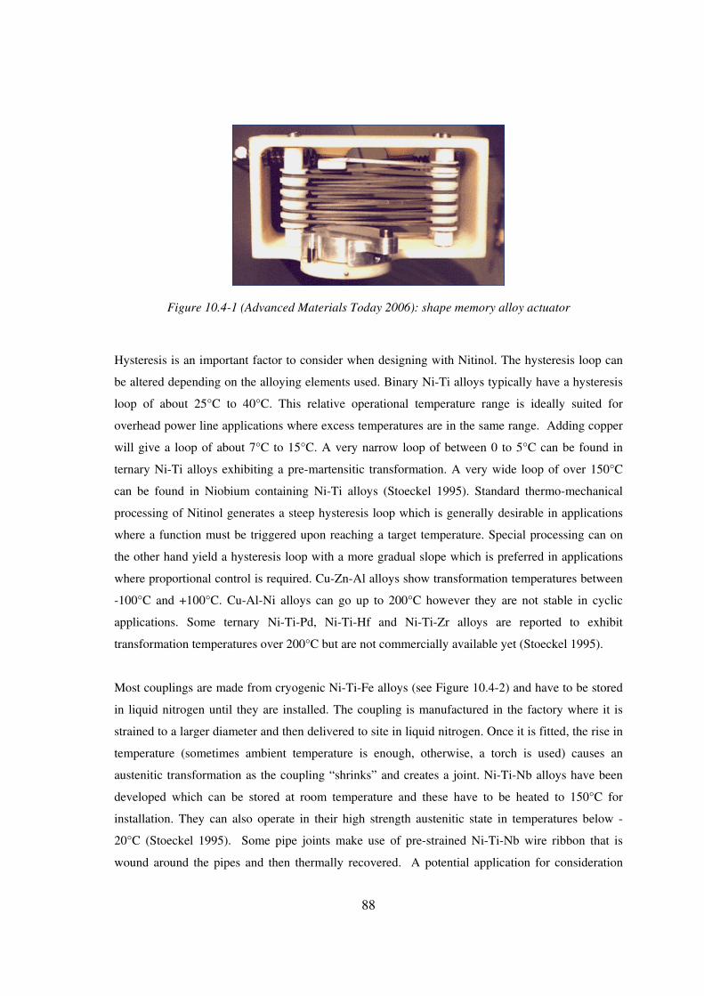
88
Figure 10.4-1 (Advanced Materials Today 2006): shape memory alloy actuator
Hysteresis is an important factor to consider when designing with Nitinol. The hysteresis loop can
be altered depending on the alloying elements used. Binary Ni-Ti alloys typically have a hysteresis
loop of about 25°C to 40°C. This relative operational temperature range is ideally suited for
overhead power line applications where excess temperatures are in the same range. Adding copper
will give a loop of about 7°C to 15°C. A very narrow loop of between 0 to 5°C can be found in
ternary Ni-Ti alloys exhibiting a pre-martensitic transformation. A very wide loop of over 150°C
can be found in Niobium containing Ni-Ti alloys (Stoeckel 1995). Standard thermo-mechanical
processing of Nitinol generates a steep hysteresis loop which is generally desirable in applications
where a function must be triggered upon reaching a target temperature. Special processing can on
the other hand yield a hysteresis loop with a more gradual slope which is preferred in applications
where proportional control is required. Cu-Zn-Al alloys show transformation temperatures between
-100°C and +100°C. Cu-Al-Ni alloys can go up to 200°C however they are not stable in cyclic
applications. Some ternary Ni-Ti-Pd, Ni-Ti-Hf and Ni-Ti-Zr alloys are reported to exhibit
transformation temperatures over 200°C but are not commercially available yet (Stoeckel 1995).
Most couplings are made from cryogenic Ni-Ti-Fe alloys (see Figure 10.4-2) and have to be stored
in liquid nitrogen until they are installed. The coupling is manufactured in the factory where it is
strained to a larger diameter and then delivered to site in liquid nitrogen. Once it is fitted, the rise in
temperature (sometimes ambient temperature is enough, otherwise, a torch is used) causes an
austenitic transformation as the coupling “shrinks” and creates a joint. Ni-Ti-Nb alloys have been
developed which can be stored at room temperature and these have to be heated to 150°C for
installation. They can also operate in their high strength austenitic state in temperatures below -
20°C (Stoeckel 1995). Some pipe joints make use of pre-strained Ni-Ti-Nb wire ribbon that is
wound around the pipes and then thermally recovered. A potential application for consideration
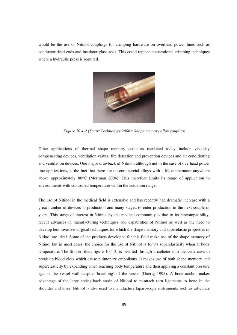
89
would be the use of Nitinol couplings for crimping hardware on overhead power lines such as
conductor dead-ends and insulator glass-rods. This could replace conventional crimping techniques
where a hydraulic press is required.
Figure 10.4-2 (Smart Technology 2006): Shape memory alloy coupling
Other applications of thermal shape memory actuators marketed today include viscosity
compensating devices, ventilation valves, fire detection and prevention devices and air conditioning
and ventilation devices. One major drawback of Nitinol, although not in the case of overhead power
line applications, is the fact that there are no commercial alloys with a Mf temperature anywhere
above approximately 80°C (Mertman 2004). This therefore limits its range of application to
environments with controlled temperature within the actuation range.
The use of Nitinol in the medical field is extensive and has recently had dramatic increase with a
great number of devices in production and many staged to enter production in the next couple of
years. This surge of interest in Nitinol by the medical community is due to its biocompatibility,
recent advances in manufacturing techniques and capabilities of Nitinol as well as the need to
develop less invasive surgical techniques for which the shape memory and superelastic properties of
Nitinol are ideal. Some of the products developed for this field make use of the shape memory of
Nitinol but in most cases, the choice for the use of Nitinol is for its superelasticity when at body
temperature. The Simon filter, figure 10.4-3, is inserted through a catheter into the vena cava to
break up blood clots which cause pulmonary embolisms. It makes use of both shape memory and
superelasticity by expanding when reaching body temperature and then applying a constant pressure
against the vessel wall despite ‘breathing’ of the vessel (Duerig 1995). A bone anchor makes
advantage of the large spring-back strain of Nitinol to re-attach torn ligaments to bone in the
shoulder and knee. Nitinol is also used to manufacture laparoscopy instruments such as articulate

90
grasping ends, steer endoscopes and hinge-less graspers. Nitinol stents are widely used to open up
clogged arteries.
Figure 10.4-3: A Simon filter (left) and a vascular stent (right). (Bard Peripheral Vascular 2008)
Future developments in the medical fields have caught momentum since the development of thin
films. These are made by spluttering laser ablation or by vapour deposition. These can be applied in
micro-valves and used in the development of small robots that would be able to travel through
gastrointestinal systems and ultimately smaller passages. Steer-able catheters are also a potential
development (Duerig 1995).
Some other applications and developments include tennis racket strings being tested in China and
the USA, plugs that are inserted into other metals to act as stoppers, non-explosive release bolts
used to release satellites in space and damping systems for suspension bridges and rail-road wheels.
Piping in nuclear reactors is being developed using pre-strained Nitinol wire. Brassières and
antennae wires are currently two of the most common users of Nitinol wire.
Nitinol is commercially available and can be easily bought from merchants. Variations in
composition are however limited with only the most commercially used Ni-Ti alloys available.
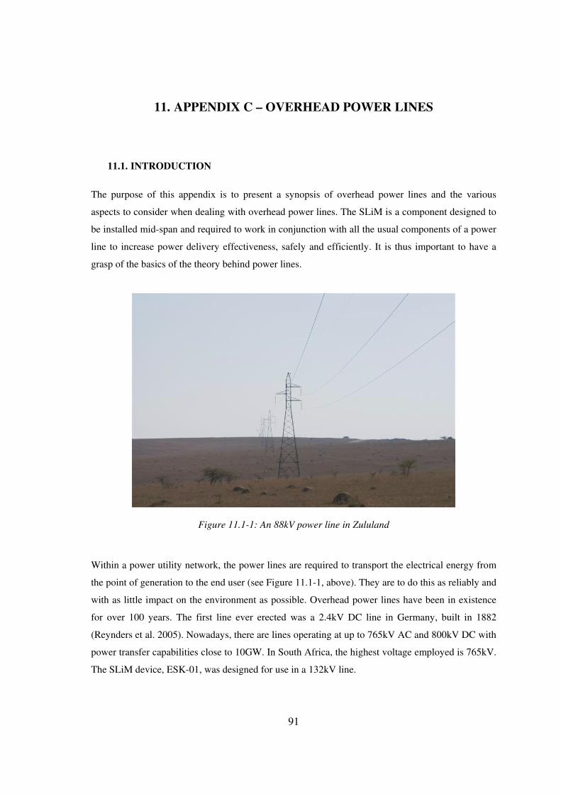
91
11. APPENDIX C – OVERHEAD POWER LINES
11.1. INTRODUCTION
The purpose of this appendix is to present a synopsis of overhead power lines and the various
aspects to consider when dealing with overhead power lines. The SLiM is a component designed to
be installed mid-span and required to work in conjunction with all the usual components of a power
line to increase power delivery effectiveness, safely and efficiently. It is thus important to have a
grasp of the basics of the theory behind power lines.
Figure 11.1-1: An 88kV power line in Zululand
Within a power utility network, the power lines are required to transport the electrical energy from
the point of generation to the end user (see Figure 11.1-1, above). They are to do this as reliably and
with as little impact on the environment as possible. Overhead power lines have been in existence
for over 100 years. The first line ever erected was a 2.4kV DC line in Germany, built in 1882
(Reynders et al. 2005). Nowadays, there are lines operating at up to 765kV AC and 800kV DC with
power transfer capabilities close to 10GW. In South Africa, the highest voltage employed is 765kV.
The SLiM device, ESK-01, was designed for use in a 132kV line.

92
When considering the topic of overhead power lines, it is useful to do this in sections. This chapter
will outlay the sections in the following manner: Basic theory, Planning, Environment, Design
Optimisation, Communication and finally, Construction. These sections will cover all the
components to be considered when designing power lines.
11.2. BASIC THEORY
(Reynders et al. 2005) outlines the basic electrical theory behind power lines in the following
manner:
The following simple electrical circuit can be used to represent a power line (Figure 11.2-1). When
considering a three-phase line, it is assumed that balanced conditions pertain and that this single-
phase circuit will be an adequate representation of the line.
Figure 11.2-1: Simple circuit representation of an overhead power line (Reynders et al. 2005).
Subscripts “s” and “r” indicate the sending and receiving ends respectively. The series resistance,
inductance and shunt capacitance can be easily calculated from the actual line geometry.
The maximum power, otherwise referred to as the steady-state limit, of a particular line is given by
the following formula:
X
VVP RS
L = (Reynders et al. 2005)

93
X is the series reactance of the line and is usually much larger than the series resistance. Some very
important properties of an overhead power line are described by this equation;
• The power that can be transferred is directly proportional to the product of the sending- and
receiving-end voltages. If these are assumed to be the same, then the power limit can be said to be
proportional to the square of the operating voltage. It is for this reason that utilities choose to
operate their power lines at high voltages. The down-side of opting for higher operating voltages is
the increase in required insulation, clearances and servitude.
• The power that can be transmitted is inversely proportional to the series reactance. This is affected
by the length of the line, the geometry of conductor bundles and phase separation.
• The series reactance is inductive and can be reduced by the use of series capacitors. This is often
implemented on lines 500km or more but at the risk of causing sub-synchronous resonance.
• For lines shorter than 100km, the above equation applies although most often, the thermal rating of
the line conductors or substation equipment becomes the limiting design factor. Voltage drop and
network instability have less of an impact.
It is evident that when designing a power line, it is desirable to minimise the reactance and optimise
the thermal rating of the hardware and equipment. The economic transfer capacity is also
determined and can be as much as 2 to 3 times less than the current rating of a line. These are
necessary for most efficient transmission and minimised losses.
11.3. PLANNING
The planning process is a very important component in the design of an overhead power line. It
comprises of some key elements that define crux design and construction parameters for the line.
The first element of planning is the modelling of the line. From here, expected electrical
performances are defined and the design requirements are conceptualised. Modern computation and
computer programs are used to predict network reactions and phenomena and can be used to

94
optimise the parameters of the power transfer. The intricacies of power line modelling will not be
covered in this chapter but are developed from the theory presented in section 11.2.
Power system analysis takes the form of planning studies that are started up to several years before
the project begins. These take into account economics, both local and international, the
environment, future development as well as all the relating technical considerations. The planning
process can be summarised in the following manner: first, the need for network expansion is
identified. Several options are then conceptualised to fulfil this need. These options are analysed
against the technical and environmental standards and parameters for the project and those that do
not comply are discarded. The best option is then selected by considering the net present value of
each option over the project life cycle. Sensitivity analyses are performed with all the uncertain
variables to ensure that the chosen option is robust and flexible. The preferred option is then
justified on an economic level. Once this is done, approval for the project is given and it is
executed. The need for network expansion i.e. a new line, can be attributed to the following causes:
increased load demands at existing supply points, new generation capacity or decommissioning of
old generation plants, the need to improve reliability or quality of a supply to a customer, the need
to reduce transmission losses, network instability or operating and maintenance losses,
refurbishment of an existing system, interconnection with neighbouring countries and utilities and
planning for contingency should catastrophic failure occur. From all these, though, load growth
forecast should be the main trigger for capital expansion of a healthy utility.
11.4. ENVIRONMENT
11.4.1. Environmental
Overhead power lines are highly useful to the economy by providing the life-blood that drives
industry: electrical power. However, they can have a severe impact on the environment and many
consider them to be unattractive, obstructive and dangerous. It is extremely difficult nowadays to
build new lines due to the increasing reluctance of public to sell servitude and the care that must be
taken to manage environmental impact. All power lines are to be built within the practises aligned
with a country’s environmental legislation. In South Africa, in addition to legislation, the ISO
14001 environmental management system and CIGRE (International Council on Large Electric
Systems) guidelines are observed.

95
Environmental Impact Assessments (EIA) are the first step to any development. They are to be
conducted by an external body and are to take into account all the concerns expressed by all the
stakeholders involved in the project. In addition to this, an EIA has to cover all the technical aspects
of the environmental impact and provide adequate explanation that all possible action has been
taken to reduce all negative impact to acceptable levels. For an overhead power line, a suitable
corridor has to be defined by the EIA and then studied by specialists who report on topographical
considerations, land-use, infrastructural and sociological issues, demographics, geology, flora and
fauna, natural and preserved areas, archaeological sites, weather and other issues. Public meetings
are held to hear the public’s concerns and the final objective of an EIA is to reach a consensus
amongst all stakeholders that all relevant issues have been appropriately considered and that the
optimum decision is taken.
When a line route is selected, the ultimate goal is to have as few bends as possible between the
source and the terminal. This is to reduce the length of the line and, ultimately, cost. However, there
are always constraints to a straight line point-to-point. Cities and towns, national parks, lakes and
mountains will require deviation. Access for construction and maintenance must also be considered
and scenic tourist areas are to be avoided. The topography of the land must be used to conceal the
line and the geology of the region must also be considered to optimise tower foundation costs. It is
important that the natural habitat of birds be avoided, such as marsh lands or vulture colonies. The
electrocution of birds is a common environmental problem especially on lines of 132kV and below
where phase clearances are relatively small (Figure 11.4-1). Birds perch on the towers and open
their wings to sun themselves. This bridges the phase-to-phase or phase-to-earth clearance and
electrocutes them.

96
Figure 11.4-1: The electrocution of birds is a common environmental issue and has to be negated
by the use of “bird-friendly” structures that employ anti-perch devices and specific design.
After a project approval, an environmental management plan is issued to the building contractor and
land-owners. This document specifies how all the environmental aspects are to be handled during
construction of the line and during the life of the line. The project manager and the environmental
control officer have to ensure that the EMP is closely followed by the contractor for the duration of
the project.
11.4.2. Corona and Electromagnetic Fields
Corona is a phenomenon to be considered amongst the environmental issues because of the impact
that it has on the environment. It does however affect many design parameters, especially at high
voltages, such as the phase geometry of the line, phase-to-phase spacings and conductor bundle
geometry. It is a phenomenon caused by the partial electrical breakdown or ionisation of the air
surrounding a conductor or piece of line hardware when energised at high voltages. The resulting
effects are luminous filaments known as burst streamers that appear to “brush” off the hardware, a
glow that emanates from the region and an audible “buzz”. Radio interference also results from
corona.
EMF, or Electromagnetic fields, has been a reason for concern for the past 30 years. Although no
results have been conclusively demonstrated, it is believed that long-term exposure to the EMF
from overhead power lines may have some association with the risk of some types of cancer in

97
humans. Due to this, many countries have taken the precaution of prescribing acceptable exposure
limits to be considered when designing overhead power lines. There are various factors that can
influence EMF such as, line voltage, tower configuration, conductor height above the ground,
conductor diameter, and the presence and size of the shield-wire. When new components or lines
are being designed, utilities can use software to model the resulting electric fields and thus adjust
their design where necessary.
11.4.3. Lightning
When designing a new overhead power line, it is very important to consider how the lightning,
prevalent in the region it is situated in, will affect the line’s performance. Lightning causes two
types of faults on a power line: back-flashovers and shielding failures. Back-flashovers are caused
when there is a direct lightning strike to the tower or shield-wire and it causes a voltage surge above
the insulation capacity of the line. This in turn causes an insulation break down and a power
frequency fault on the line. A shielding failure is when the phases are not adequately shielded by the
shield-wire and the lightning strikes directly onto a phase conductor. Power lines are designed
according to a parameter called the ground-flash density. This is measured in flashes/km2/year. In
South Africa, a map has been developed to represent this (figure 11.4-2), where the ground-flash
density of over 400 locations, country-wide, has been recorded over 11 years.
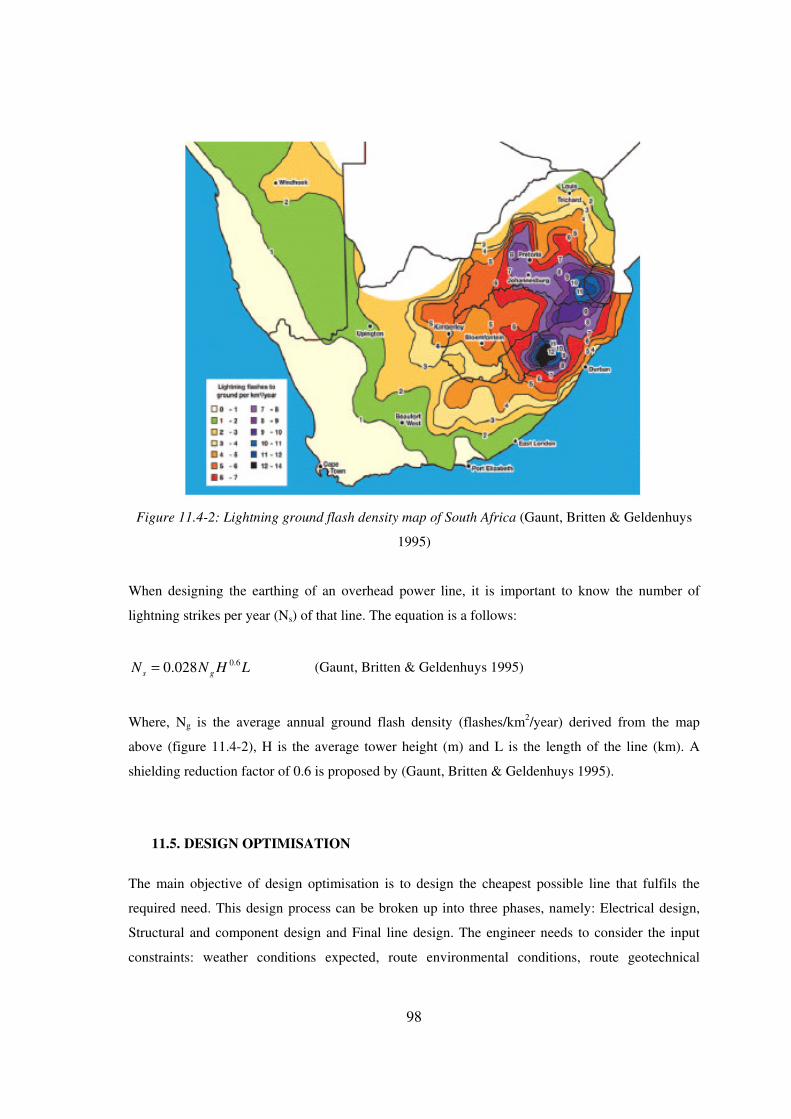
98
Figure 11.4-2: Lightning ground flash density map of South Africa (Gaunt, Britten & Geldenhuys
1995)
When designing the earthing of an overhead power line, it is important to know the number of
lightning strikes per year (Ns) of that line. The equation is a follows:
LHNN gs
6.0028.0=
(Gaunt, Britten & Geldenhuys 1995)
Where, Ng is the average annual ground flash density (flashes/km2/year) derived from the map
above (figure 11.4-2), H is the average tower height (m) and L is the length of the line (km). A
shielding reduction factor of 0.6 is proposed by (Gaunt, Britten & Geldenhuys 1995).
11.5. DESIGN OPTIMISATION
The main objective of design optimisation is to design the cheapest possible line that fulfils the
required need. This design process can be broken up into three phases, namely: Electrical design,
Structural and component design and Final line design. The engineer needs to consider the input
constraints: weather conditions expected, route environmental conditions, route geotechnical
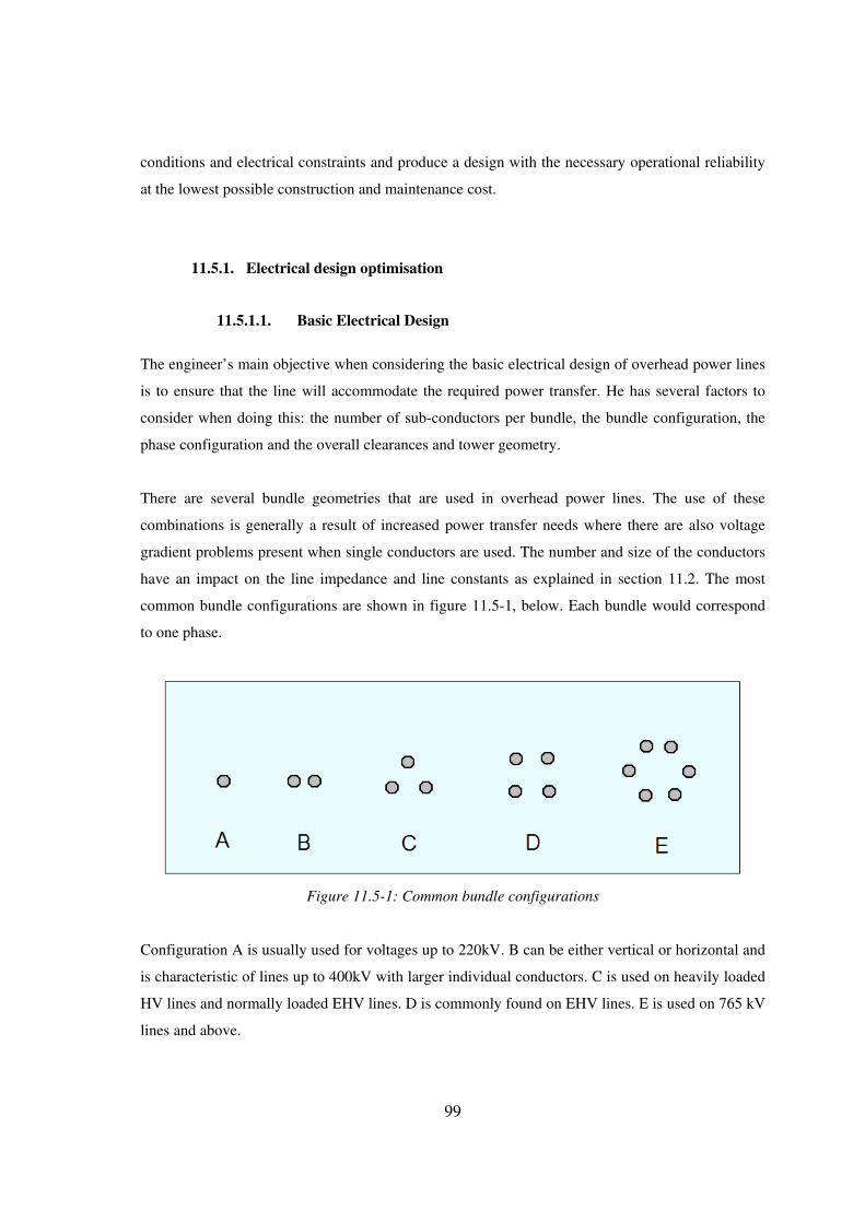
99
conditions and electrical constraints and produce a design with the necessary operational reliability
at the lowest possible construction and maintenance cost.
11.5.1. Electrical design optimisation
11.5.1.1. Basic Electrical Design
The engineer’s main objective when considering the basic electrical design of overhead power lines
is to ensure that the line will accommodate the required power transfer. He has several factors to
consider when doing this: the number of sub-conductors per bundle, the bundle configuration, the
phase configuration and the overall clearances and tower geometry.
There are several bundle geometries that are used in overhead power lines. The use of these
combinations is generally a result of increased power transfer needs where there are also voltage
gradient problems present when single conductors are used. The number and size of the conductors
have an impact on the line impedance and line constants as explained in section 11.2. The most
common bundle configurations are shown in figure 11.5-1, below. Each bundle would correspond
to one phase.
Figure 11.5-1: Common bundle configurations
Configuration A is usually used for voltages up to 220kV. B can be either vertical or horizontal and
is characteristic of lines up to 400kV with larger individual conductors. C is used on heavily loaded
HV lines and normally loaded EHV lines. D is commonly found on EHV lines. E is used on 765 kV
lines and above.
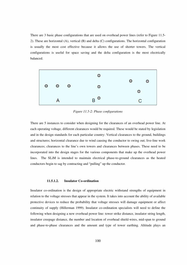
100
There are 3 basic phase configurations that are used on overhead power lines (refer to Figure 11.5-
2). These are horizontal (A), vertical (B) and delta (C) configurations. The horizontal configuration
is usually the most cost effective because it allows the use of shorter towers. The vertical
configurations is useful for space saving and the delta configuration is the most electrically
balanced.
Figure 11.5-2: Phase configurations
There are 5 instances to consider when designing for the clearances of an overhead power line. At
each operating voltage, different clearances would be required. These would be stated by legislation
and in the design standards for each particular country: Vertical clearances to the ground, buildings
and structures; horizontal clearance due to wind causing the conductor to swing out; live-line work
clearances; clearances to the line’s own towers and clearances between phases. These need to be
incorporated into the design stages for the various components that make up the overhead power
lines. The SLiM is intended to maintain electrical phase-to-ground clearances as the heated
conductors begin to sag by contracting and “pulling” up the conductor.
11.5.1.2. Insulator Co-ordination
Insulator co-ordination is the design of appropriate electric withstand strengths of equipment in
relation to the voltage stresses that appear in the system. It takes into account the ability of available
protective devices to reduce the probability that voltage stresses will damage equipment or affect
continuity of supply (Hillerman 1999). Insulator co-ordination specialists will need to define the
following when designing a new overhead power line: tower strike distance, insulator string length,
insulator creepage distance, the number and location of overhead shield-wires, mid-span to ground
and phase-to-phase clearances and the amount and type of tower earthing. Altitude plays an
101
important role in this field. Because South Africa comprises of a raised internal plateau which
places most high voltage lines at a significant altitude above sea level, much research has been
conducted on the study of the influence of reduced air density on the voltage break-down strength
and corona of overhead power lines. This has led to 400kV tower designs specific for operation at
high altitudes.
11.5.1.3. Thermal Rating
Power transfer through a conductor causes that conductor to heat up. The maximum temperature at
which a conductor can operate is determined by the permissible resulting sag, governed by statutory
requirements, the annealing and long-term creep experience by that type of conductor and the
reliability of joints and fittings (Stephen et al. 2005). Techniques of thermal rating are used by line
designers to increase the current carrying capacity of a line without infringing on statutory
conductor clearance limits. These take into account weather parameters such as wind speed and
direction, ambient temperatures and radiation levels from the sun and their effect on the temperature
of the conductor. In the past, a deterministic method was used to predict conductor behaviour and to
calculate a conductor’s current rating. Today, the probabilistic method is favoured because of its
‘real-time’ consideration of ambient conditions.
There are several factors which affect the thermal rating of a conductor and which are primarily
motivated by public safety. These are: the height of the conductor above the ground, the presence of
objects/structures under the line, the probability of a voltage surge occurring on the line and the
magnitude of that surge and the likelihood of a flashover should a specific combination of the above
occur. Each of these factors is a function of many other parameters.
The calculation of a conductor’s temperature in the steady state can be done using the following
formula as described by (Stephen et al. 2005), pp 280:
Heat Gain = Heat Loss
wrcismj PPPPPPP ++=+++ (W/m)
Where: Pj = Joule heating, Pm = Magnetic heating, Ps = Solar heating, Pi = Corona heating, Pc =
Convective cooling, Pr = Radiative cooling and Pw = Evaporative cooling.
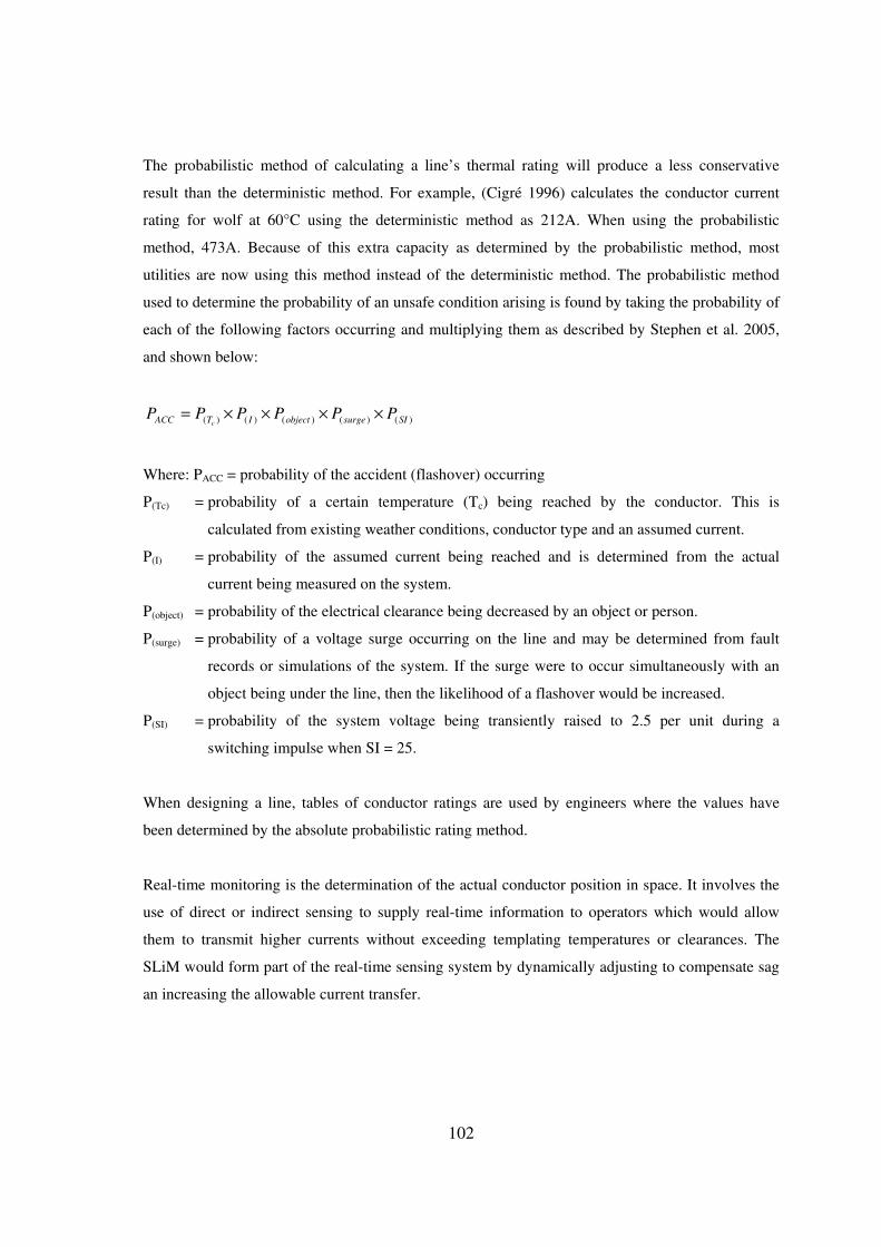
102
The probabilistic method of calculating a line’s thermal rating will produce a less conservative
result than the deterministic method. For example, (Cigré 1996) calculates the conductor current
rating for wolf at 60°C using the deterministic method as 212A. When using the probabilistic
method, 473A. Because of this extra capacity as determined by the probabilistic method, most
utilities are now using this method instead of the deterministic method. The probabilistic method
used to determine the probability of an unsafe condition arising is found by taking the probability of
each of the following factors occurring and multiplying them as described by Stephen et al. 2005,
and shown below:
)()()()()( SIsurgeobjectITACC PPPPPPc
××××=
Where: PACC = probability of the accident (flashover) occurring
P(Tc) = probability of a certain temperature (Tc) being reached by the conductor. This is
calculated from existing weather conditions, conductor type and an assumed current.
P(I) = probability of the assumed current being reached and is determined from the actual
current being measured on the system.
P(object) = probability of the electrical clearance being decreased by an object or person.
P(surge) = probability of a voltage surge occurring on the line and may be determined from fault
records or simulations of the system. If the surge were to occur simultaneously with an
object being under the line, then the likelihood of a flashover would be increased.
P(SI) = probability of the system voltage being transiently raised to 2.5 per unit during a
switching impulse when SI = 25.
When designing a line, tables of conductor ratings are used by engineers where the values have
been determined by the absolute probabilistic rating method.
Real-time monitoring is the determination of the actual conductor position in space. It involves the
use of direct or indirect sensing to supply real-time information to operators which would allow
them to transmit higher currents without exceeding templating temperatures or clearances. The
SLiM would form part of the real-time sensing system by dynamically adjusting to compensate sag
an increasing the allowable current transfer.

103
11.5.2. Structural and Component Design
11.5.2.1. Conductor optimisation
Over the years, conductor has evolved from simple copper wire to combinations of aluminium, steel
and aluminium alloys. The conductor on an overhead power line is considered to be the most
important component of the line. It can contribute up to 40% of the overall capital cost of a new
power line. The most common types of conductors in use in South Africa are Aluminium Conductor
Steel Reinforced (ACSR) and All Alloy Aluminium Conductors (AAAC) pictured below (Figure
11.5-3).
Figure 11.5-3: Examples of ACSR conductors. (Muftic, Vajeth & Dama 2005)
ACSR conductor (pictured above) is the most popular conductor in use today. It combines the
advantages of the mechanical strength of the inner steel core with the high conductivity of the outer
aluminium layers. AAAC conductor (Figure 11.5-4) increases its conducting properties by
sacrificing some of its mechanical strength. It is made from a homogeneous aluminium alloy,
usually an aluminium-magnesium-silicon alloy.

104
Figure 11.5-4: Examples of AAAC conductors. (Muftic, Vajeth & Dama 2005)
Some other conductor options that are available are: Aluminium Conductor Alloy Reinforced
(ACAR) which has some corrosion advantages over ACSR; All Aluminium Conductor (AAC) used
mostly within substations for slack spans; Aluminium Conductor Steel Reinforced/Trapezoidal
Wire (ACSR/TW) which has a compact cross-sectional area that reduces wind and ice loading;
Aero-Z Conductor which has superior mechanical and electrical performance to ACSR and has
been widely used in Belgium; Aluminium Conductor Steel Reinforced/Self-Damping (ACSR/SD)
which provides self damping of aeolian vibrations; Aluminium Conductor Steel Reinforced/Air
Expanded (ACSR/AE) which has an increased cross-sectional area to reduce corona; Aluminium
Conductor Steel Reinforced/Twisted Pair Of Conductors (ACSR/T-2) which is used to decrease
galloping and sub-span oscillations; Aluminium Conductor Steel Supported (ACSS or ACSS/TW)
which can operate at temperatures up to 200°C; High Temperature Aluminium Conductor Steel
Reinforced (TACSR) which can also operate at up to 200°C and is a popular solution in Japan;
Gap-Type High Temperature Aluminium Conductor Steel Reinforced (G(Z)TACSR) which can
operate up to 210°C and has excellent self damping properties; Extra-High Temperature Aluminium
Conductor Invar Reinforced ((Z)TACIR) which can operate at temperatures up to 210°C and
experiences reduced sagging; and Aluminium Conductor Composite Reinforced (ACCR) which is
currently under development.
When selecting a conductor for an overhead power line, designers need to evaluate both technical
and economical considerations. The capital outlay needs to be weighed up against the life-cycle
electrical losses of the conductor and an optimal solution must be found. Lord Kelvin stated the
following:
105
“The most economical area of conductor is that for which the annual cost of energy wasted is equal
to the interest on that portion of the capital outlay which may be considered as proportional to the
weight of conductor.”
This concept is illustrated by (Muftic, Vajeth & Dama 2005) in the following graph (Figure 11.5-5):
Figure 11.5-5: Conductor optimisation expression of Kelvin’s rule. (Muftic, Vajeth & Dama 2005)
11.5.2.2. Ground Wire Optimisation
Initially, ground wires were used to protect an overhead power line from direct lightning strikes.
Nowadays, the ground wire is considered an important part of the earthing system providing a
return path for short circuit currents. When specifying a ground wire for an overhead power line,
two important factors need to be considered: the positioning of the ground wire and the selection of
that ground wire.
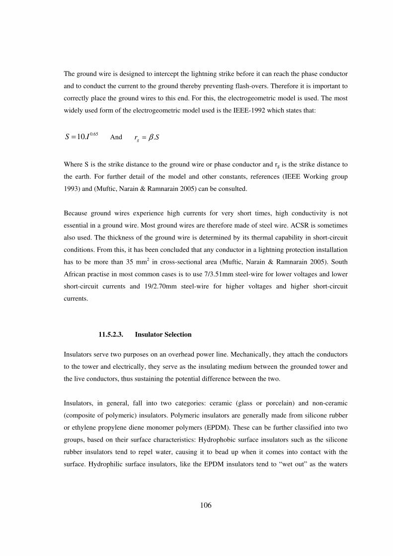
106
The ground wire is designed to intercept the lightning strike before it can reach the phase conductor
and to conduct the current to the ground thereby preventing flash-overs. Therefore it is important to
correctly place the ground wires to this end. For this, the electrogeometric model is used. The most
widely used form of the electrogeometric model used is the IEEE-1992 which states that:
65.0.10 IS = And Srg .β=
Where S is the strike distance to the ground wire or phase conductor and rg is the strike distance to
the earth. For further detail of the model and other constants, references (IEEE Working group
1993) and (Muftic, Narain & Ramnarain 2005) can be consulted.
Because ground wires experience high currents for very short times, high conductivity is not
essential in a ground wire. Most ground wires are therefore made of steel wire. ACSR is sometimes
also used. The thickness of the ground wire is determined by its thermal capability in short-circuit
conditions. From this, it has been concluded that any conductor in a lightning protection installation
has to be more than 35 mm2 in cross-sectional area (Muftic, Narain & Ramnarain 2005). South
African practise in most common cases is to use 7/3.51mm steel-wire for lower voltages and lower
short-circuit currents and 19/2.70mm steel-wire for higher voltages and higher short-circuit
currents.
11.5.2.3. Insulator Selection
Insulators serve two purposes on an overhead power line. Mechanically, they attach the conductors
to the tower and electrically, they serve as the insulating medium between the grounded tower and
the live conductors, thus sustaining the potential difference between the two.
Insulators, in general, fall into two categories: ceramic (glass or porcelain) and non-ceramic
(composite of polymeric) insulators. Polymeric insulators are generally made from silicone rubber
or ethylene propylene diene monomer polymers (EPDM). These can be further classified into two
groups, based on their surface characteristics: Hydrophobic surface insulators such as the silicone
rubber insulators tend to repel water, causing it to bead up when it comes into contact with the
surface. Hydrophilic surface insulators, like the EPDM insulators tend to “wet out” as the waters
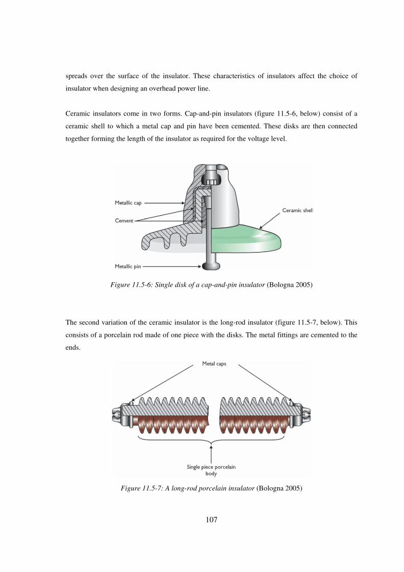
107
spreads over the surface of the insulator. These characteristics of insulators affect the choice of
insulator when designing an overhead power line.
Ceramic insulators come in two forms. Cap-and-pin insulators (figure 11.5-6, below) consist of a
ceramic shell to which a metal cap and pin have been cemented. These disks are then connected
together forming the length of the insulator as required for the voltage level.
Figure 11.5-6: Single disk of a cap-and-pin insulator (Bologna 2005)
The second variation of the ceramic insulator is the long-rod insulator (figure 11.5-7, below). This
consists of a porcelain rod made of one piece with the disks. The metal fittings are cemented to the
ends.
Figure 11.5-7: A long-rod porcelain insulator (Bologna 2005)
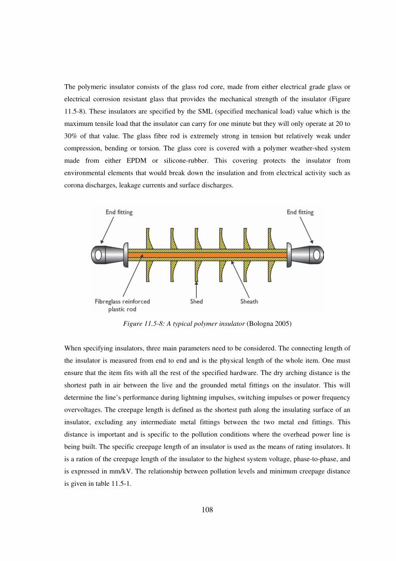
108
The polymeric insulator consists of the glass rod core, made from either electrical grade glass or
electrical corrosion resistant glass that provides the mechanical strength of the insulator (Figure
11.5-8). These insulators are specified by the SML (specified mechanical load) value which is the
maximum tensile load that the insulator can carry for one minute but they will only operate at 20 to
30% of that value. The glass fibre rod is extremely strong in tension but relatively weak under
compression, bending or torsion. The glass core is covered with a polymer weather-shed system
made from either EPDM or silicone-rubber. This covering protects the insulator from
environmental elements that would break down the insulation and from electrical activity such as
corona discharges, leakage currents and surface discharges.
Figure 11.5-8: A typical polymer insulator (Bologna 2005)
When specifying insulators, three main parameters need to be considered. The connecting length of
the insulator is measured from end to end and is the physical length of the whole item. One must
ensure that the item fits with all the rest of the specified hardware. The dry arching distance is the
shortest path in air between the live and the grounded metal fittings on the insulator. This will
determine the line’s performance during lightning impulses, switching impulses or power frequency
overvoltages. The creepage length is defined as the shortest path along the insulating surface of an
insulator, excluding any intermediate metal fittings between the two metal end fittings. This
distance is important and is specific to the pollution conditions where the overhead power line is
being built. The specific creepage length of an insulator is used as the means of rating insulators. It
is a ration of the creepage length of the insulator to the highest system voltage, phase-to-phase, and
is expressed in mm/kV. The relationship between pollution levels and minimum creepage distance
is given in table 11.5-1.
109
Table 11.5-1: Minimum required creepage distances for operating pollution levels. (Bologna 2005)
11.5.2.4. Line Hardware
When pertaining to overhead power lines, the term hardware refers to all the components used to
connect the phase conductor to the insulators and the insulators to the tower. It also includes the
various vibration dampers, warning devices and bird flight diverters.
When designing hardware assemblies for overhead power lines, the hardware critical design load is
derived from the maximum resultant conductor or ground wire load for which the towers are
designed. The critical design load incorporates strength factors for the number of components
subjected to maximum load intensity as well as strength factors for the coordination of strength. The
strength classes used in South Africa are 120kN, 210kN, 300kN, 400kN and 500kN. Below are
some examples of load-bearing hardware (Table 11.5-2).

110
Table 11.5-2: Some common load-bearing hardware. (Calitz et al. 2005)
The overall length of the assembly must be designed so as not to infringe on live conductor
clearances under normal and maximum swing conditions. The strength rating and dimension of
components are selected according to standard IEC specifications from supplier catalogues and to
fulfil the code of practice requirements.
11.5.2.5. Supporting Structures
The purpose of the structures in an overhead power line is to support to conductors and ground
wires. The structures are designed according to the specifications employed by the utility. The
designer is required to design structures that can withstand the conductor and ground wire loads
under the expected climatic conditions. All legislated minimum clearances need to be maintained by
the structure under those climatic conditions and the towers need to be designed in such a way as to
facilitate construction and maintenance. This means that attachment points for maintenance crew
need to be incorporated into the design. All these design criteria need to be accomplished at the
lowest possible cost.

111
Generally, structures are divided according to the voltage for which they were purposed. Within that
voltage, there will be families of structures with slightly different purposes or shapes and within
each family, will be the suspension structures, in-line strain structures, angle strain structures and
terminal structures. For each of these structures, there will be different attachment heights (as a
result of various body and leg extensions). Suspension structures are usually the lightest structures
within a family. They are designed to be used in straight lines between strain structures and simply
suspend the conductor in the air, thus, they can only carry vertical and wind loads and not
longitudinal (tension) loads. As seen in figure 11.5-9, below, they only need one insulator per
phase.
Figure 11.5-9: A typical example of a suspension structure
In-line strain structures are essentially a lighter version of the strain structures designed to take
longitudinal loading but in a straight line. There are usually two or three versions of the strain
structure within a family: a small angle, a large angle and sometimes an intermediate angle. A strain
structure is designed for corners and bends. It carries all the longitudinal tension of the conductors
as well as the transverse loading resulting from the angle of the bend. As can be seen in figure 11.5-

112
10 below, strain structures break the conductor. They do this with the use of two insulator sets per
phase and a jumper connecting the conductor “around” the tower.
Figure 11.5-10: A typical example of a strain structure
Strain structures are much heavier and more expensive than suspension structures because of the
large loads to which they are subjected. Terminal structures are usually similar to the heavy strain
structures but have been designed with the ability to carry the unbalanced load of conductor only on
one side of the tower. They are designed with this capability to be used to terminate the line when
entering a substation. This means that they carry a tensioned span on one side and a slack span on
the other side.
There are several materials which are used to construct structures within overhead power lines.
Wooden poles are the cheapest option and are most practical for lower voltages, however, they
require constant maintenance and are susceptible to environmental degradation. The most popular
option for constructing structures is galvanised steel. It is most often used in the form of angle
section or tube. The steel needs to be galvanised for corrosion protection and this offers an
acceptable trade-off between cost and durability. Some maintenance of steel structures is, however,
113
required in corrosive environments such as coastlines. Concrete poles are also being used for lower
voltages (up to 132kV) and offer an economical solution. They are however limited because they
have to be cast in one piece and are difficult to transport. In inaccessible areas, galvanised steel
lattice structures would be the most economical solution as they can be transported in pieces and
then assembled on site.
11.5.2.6. Foundations and Earthing
Foundations need to be specified for each structure when designing an overhead power line. They
need to be specific to the rock or soil conditions on which each tower will be placed. The
foundations need to safely transfer the applied loads from the structure to the surrounding soil, they
need to limit the displacements within the tolerances of the structure, they need to be strong enough
to withstand the loads from the structure and they need to operate for the complete life of the line
without failure. The earthing for the structure is also incorporated into the foundation.
Before the towers are constructed, geotechnical investigations are needed to determine and classify
the types of soils that are found along the line route. The soils are classified into 4 categories and
the foundations specified accordingly:
• Soil Type 1 – Hard granular soil – a competent engineering soil.
• Soil Type 2 – Stiff clay or dense sand – a less competent soil.
• Soil Type 3 – Loose sand or soft clay – a very incompetent soil.
• Soil Type 4 – Saturated or submerged soft ground below the seasonal water table.
There are several foundation types that are used in overhead power line design. These are selected
according to the type of structure and application and the soil nominations. Spreader type
foundations include pad and column foundations, guyed tower mast pads, block anchors and steel
grillage foundations. The pile type foundations include single pile or large diameter drilled shafts,
multiple piles, Auger and caisson anchors and other specialised anchors and pile. Rock anchors and
pole foundations are also often used.
When designing the foundation, it is important to provide an electrical connection from the tower to
the earth so that short-circuit and lightning currents can flow to the earth without developing

114
dangerous contact voltages and overvoltages on the network that could damage equipment or give
rise to a poor quality of supply. The connection has to provide a sufficiently low resistance so that it
becomes the preferred path for the fault and lightning currents.
Figure 11.5-11: A tower connection to the steel reinforcement within the concrete foundation.
(Burger, Ramnarain & Peter 2005)
As seen in figure 11.5-11 above, the earthing connection is usually made from the steel lattice
structure to the reinforcing bars in the concrete foundation. If a need to reduce the tower footing
resistance of a particular tower were identified, then additional counterpoise earth electrodes would
be installed. This would be in the form of vertical rod electrode or buried trench electrodes.
11.5.3. Line Design
With consideration of the above components that make up an overhead power line, it can be seen
that line design is an extensive and multi-disciplinary process. It requires much iteration and
constant adjustment of variables before a design is complete and construction can begin. A basic
and high level overview of the design process will be presented below. This does not even include
the complex process of designing a new structure or a family of structures. Structure development is
a specialised field on its own and requires the use of finite element analysis tools such as PLS
Tower or PLS Pole (Power Line Systems, Inc 1993-2008).

115
The overhead power line design process could be described in the following manner:
First, the basic requirement parameters need to be set. This is usually done by the power system
planners, and then given to the line designer. The following parameters would be required:
- Location of the start and end of the line
- Load (projected) profile (i.e. required power transfer)
- Voltage
- Date of need for the line
With these parameters, the electrical design of the line would begin. The most optimal conductor
would be chosen, ground wire would be selected and the insulation requirement would be specified.
This would include the selection of the insulators. From here, an environmental process would need
to begin. This process usually takes a long time and contributes to a large part of the time taken
from project start to completion. The environmental process comprises of several aspects and would
need the following outputs:
- Up to 3 line route options (The best one is then selected)
- Approval from the relevant governmental departments for the use of the land
- Public participation forum approval
- Negotiated title deeds for the servitude from land owners
- Environmental Impact Assessment (EIA)
- Environment management plan
The negotiation of servitude with landowners can sometimes take several years, especially in scenic
or urban areas. The acquisition of new servitudes is most often not possible in developed, 1st world
countries. In these cases, multi-circuit towers would be used and vacant circuits would be stored for
future stringing as the need arises. With the above outputs, the route of the line would be chosen.
The route would now need to be surveyed so that accurate geographical data can be used to spot and
template the line. Surveying of line corridors is either done on foot by a land-surveyor or, in the
case of longer lines, can be done by an aerial laser survey. The data from the survey is then loaded
into the tower spotting software, such as PLS Cadd (Power Line Systems, Inc 1993-2008), to
generate a virtual terrain. With the ground profile simulated, the designer can spot the towers.

116
Figure 11.5-12: A sample profile generated in PLS Cadd (Power Line Systems, Inc 1993-2008)
showing the terrain, tower positioning and conductor templating.
The towers are positioned on the terrain profile (shown in figure 11.5-12, above) and the conductor
and ground wire are templated. The simulated line is then tested for various weather conditions,
such as high wind or ice loading, and towers are checked to verify that they don’t experience
overloading. Clearances are also simulated to ensure that under the expected climatic conditions,
they are not violated. The terrain can is fully modelled in 3-D as shown below in Figure 11.5-13.
Figure 11.5-13: A generated 3D terrain showing a portion of line (PLS Cadd, Power Line Systems,
Inc 1993-2008)

117
With the line fully modelled and meeting all the design criteria and specifications, staking tables
and stringing charts are generated for the construction contractor. Construction is then begun.
11.6. CONSTRUCTION
The construction of an overhead power line is fairly specialised and requires intricate logistical
planning. This is due to the fact that the workable corridor is less than 100m wide and can be
hundreds of kilometres long, often crossing rugged, isolated and difficult to access areas. Heavy
machinery is required to erect towers and every piece of material used needs to be transported to
site.
The construction process will be broken down into three sections; foundation construction, tower
erection and stringing of conductors.
11.6.1. Foundation Construction
Once the line has been profiled and the towers have been spotted, a surveyor will go and peg the
towers. He will mark where each leg of the tower will be. The contractor will construct the
foundations at these pegged locations (Figure 11.6-1). The soil nominations and foundation
selections will have been done well before excavation. In most cases, an excavator or a tractor
loader backhoe (TLB) is used to excavate the foundations. Sometimes, drilling equipment is used
when pile foundations have been specified. After the excavation, the foundation stubs or anchor
links are placed in the holes and then the reinforcing is installed. A 25 MPa concrete is then mixed
and poured into the hole. Backfilling is an important requirement due to the fact that the uplift load
on a tower is often the most critical. It is therefore necessary to compact soil layers of about 300mm
at a time over the foundation. The foundations will undergo quality control to check that
workmanship and materials are of a suitable standard and to ensure that the foundations will not fail
during the service life of the power line.
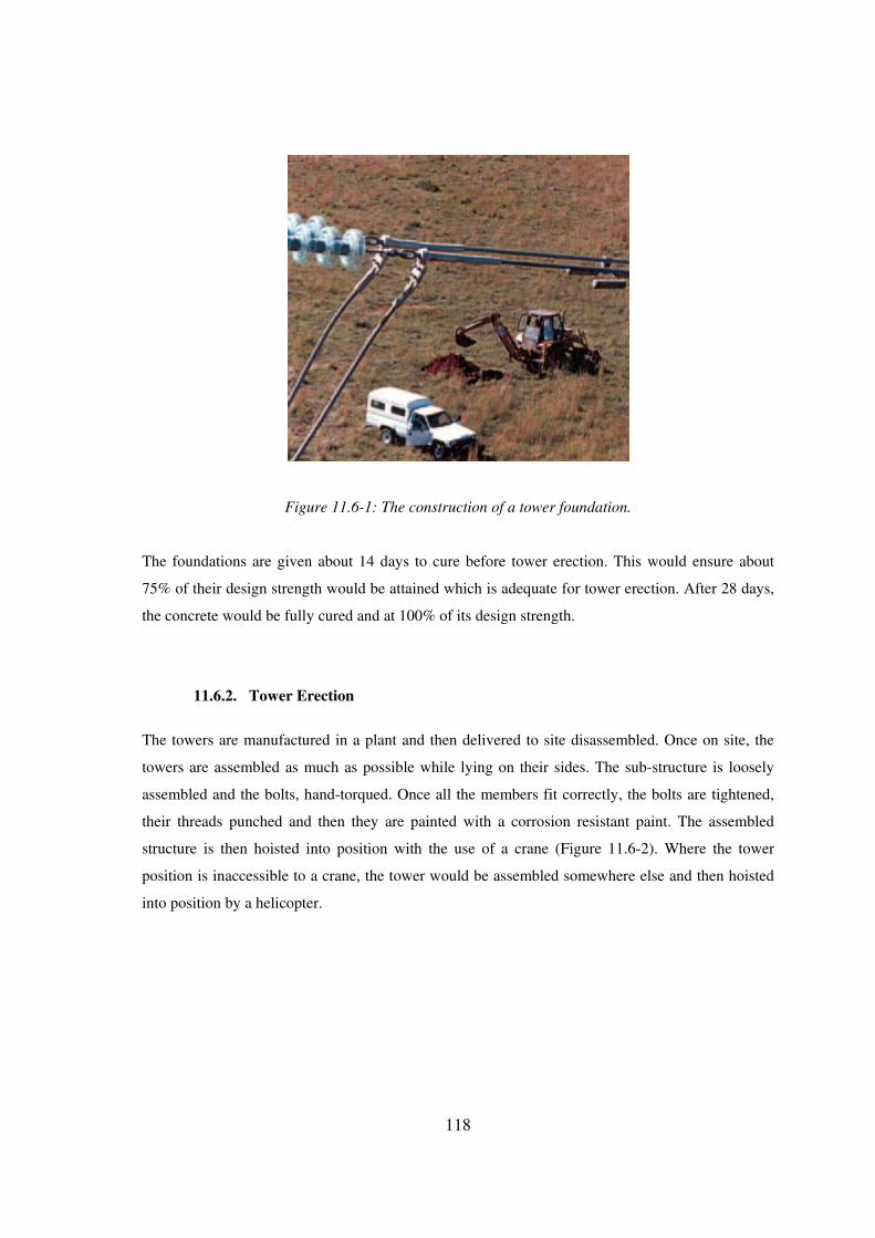
118
Figure 11.6-1: The construction of a tower foundation.
The foundations are given about 14 days to cure before tower erection. This would ensure about
75% of their design strength would be attained which is adequate for tower erection. After 28 days,
the concrete would be fully cured and at 100% of its design strength.
11.6.2. Tower Erection
The towers are manufactured in a plant and then delivered to site disassembled. Once on site, the
towers are assembled as much as possible while lying on their sides. The sub-structure is loosely
assembled and the bolts, hand-torqued. Once all the members fit correctly, the bolts are tightened,
their threads punched and then they are painted with a corrosion resistant paint. The assembled
structure is then hoisted into position with the use of a crane (Figure 11.6-2). Where the tower
position is inaccessible to a crane, the tower would be assembled somewhere else and then hoisted
into position by a helicopter.

119
Figure 11.6-2: A guyed structure being assembled on its side (left) and hoisted, once assemble, into
position by a crane (right). The crane would hold the structure in place until all four stays are
secured.
11.6.3. Stringing
Stringing a power line can sometimes be a complicated process. Once all the towers of a certain
section to be strung are erected, preparation is made to begin stringing. All roads, railways and
other power line crossings would have implications. Outages need to be booked and live-line covers
need to be installed. These are temporary wood pole structures that span a net over the lines to be
crossed. The same can be done over roads and railways. High voltage lines would require
temporary bypasses to avoid outages.
The erected towers are dressed for the conductor. This involves equipping the structures with all the
necessary hardware for stringing. All the suspension structures have running-blocks attached to
their insulators. On strain structures, the running-blocks are attached directly to their landing plates.
There are two methods of stringing conductor. The layout method (Figure 11.6-3), more commonly
used on lower voltages, has the conductor placed on the ground along the line and then lifted up to
the assembly in running-blocks. This method has limitations in that it is not always possible to lay
out the conductor when there are obstructions along the servitude. In addition, the conductor

120
becomes very vulnerable to damage while unrolled on the ground. The conductor needs to be kept
free of any kinks or even surface scratches as these cause corona when energised.
Figure 11.6-3: A dressed guyed-Vee structure being stung with the layout method. (Marais,
Badenhorst 2005)
The other method of stringing conductor is the tension stringing method (Figure 11.6-4). Here, a
pilot wire is fed through all the running-blocks on the towers and it pulls through the conductor. The
conductor has minimal contact with the ground and is well protected from obstacles.
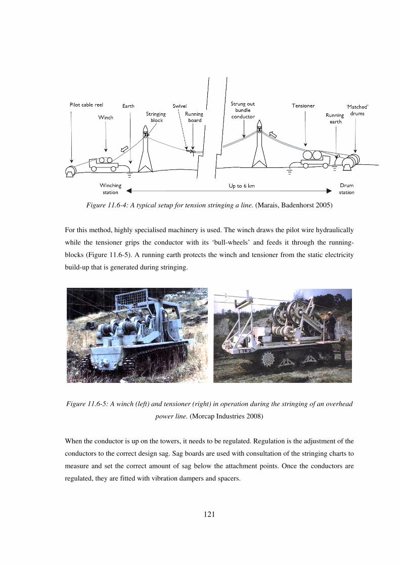
121
Figure 11.6-4: A typical setup for tension stringing a line. (Marais, Badenhorst 2005)
For this method, highly specialised machinery is used. The winch draws the pilot wire hydraulically
while the tensioner grips the conductor with its ‘bull-wheels’ and feeds it through the running-
blocks (Figure 11.6-5). A running earth protects the winch and tensioner from the static electricity
build-up that is generated during stringing.
Figure 11.6-5: A winch (left) and tensioner (right) in operation during the stringing of an overhead
power line. (Morcap Industries 2008)
When the conductor is up on the towers, it needs to be regulated. Regulation is the adjustment of the
conductors to the correct design sag. Sag boards are used with consultation of the stringing charts to
measure and set the correct amount of sag below the attachment points. Once the conductors are
regulated, they are fitted with vibration dampers and spacers.

122
The last step in the construction of an overhead power line to be completed by the contractor is the
environmental rehabilitation. All temporary constructions, including bypasses, roads and bridges
are to be removed. Wherever vegetation has been damaged, replanting is necessary and all
precautions must be taken to mitigate any potential future soil erosion. This requires the
construction of retaining walls, gabions or similar measures. The construction camps and batching
plants are also to be rehabilitated. After this is done, a final inspection is conducted of the whole
line before the project is considered complete.

123
12. APPENDIX D – TEST RIG DRAWINGS AND CALCULATIONS
12.1. Isometric Drawing of the Test Rig
Figure 12.1-1: Assembled view of the SLiM’s test rig.
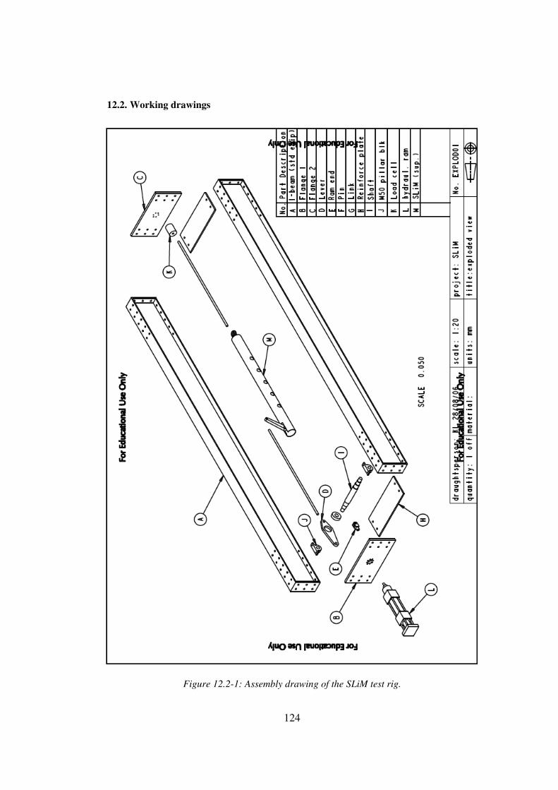
124
12.2. Working drawings
Figure 12.2-1: Assembly drawing of the SLiM test rig.
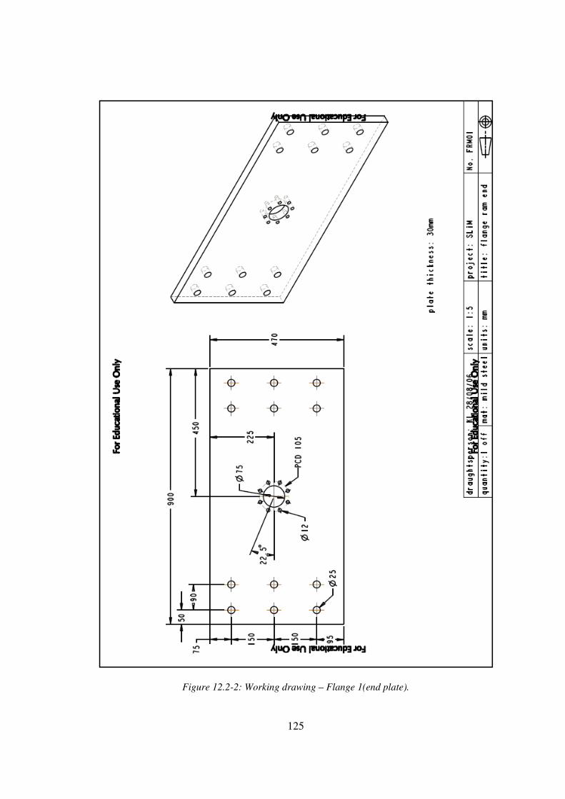
125
Figure 12.2-2: Working drawing – Flange 1(end plate).
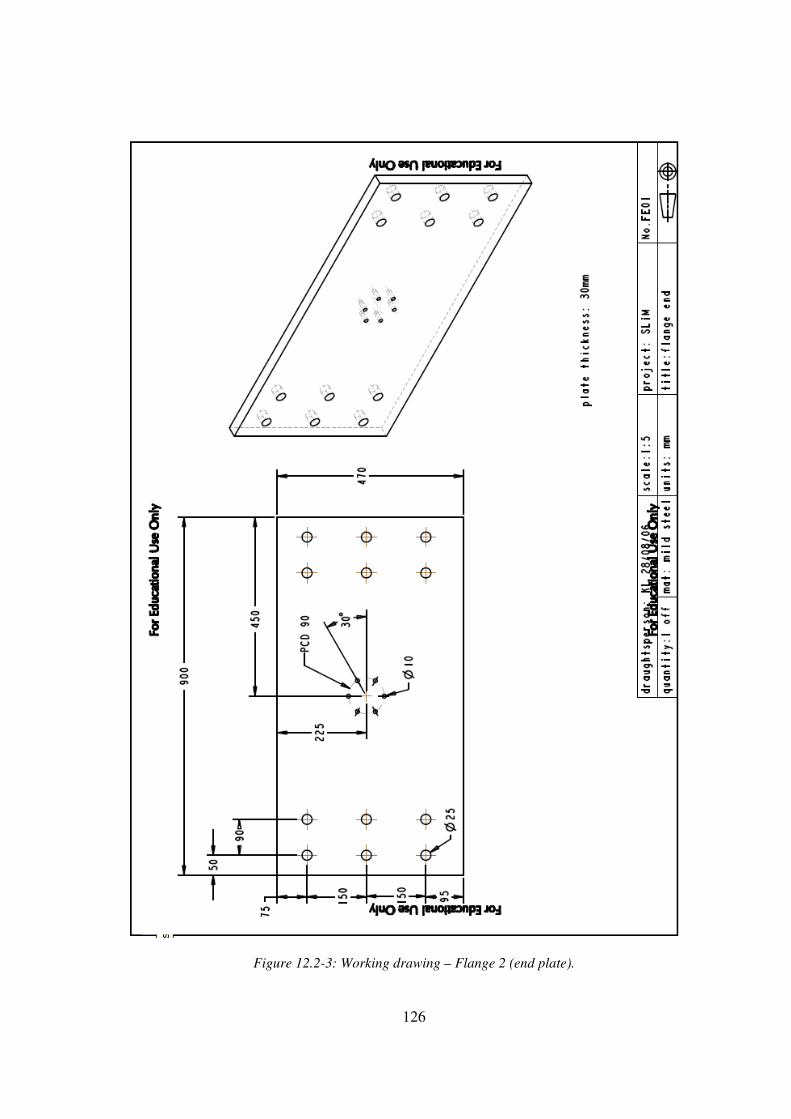
126
Figure 12.2-3: Working drawing – Flange 2 (end plate).

127
Figure 12.2-4: Working drawing – Lever.
128
Figure 12.2-5: Working drawing: pin.

129
Figure 12.2-6: Working drawing – link.
130
Figure 12.2-7: Working drawing – ram end.
131
Figure 12.2-8: Working drawing – reinforcement plate.
132
Figure 12.2-9: Working drawing – lever.
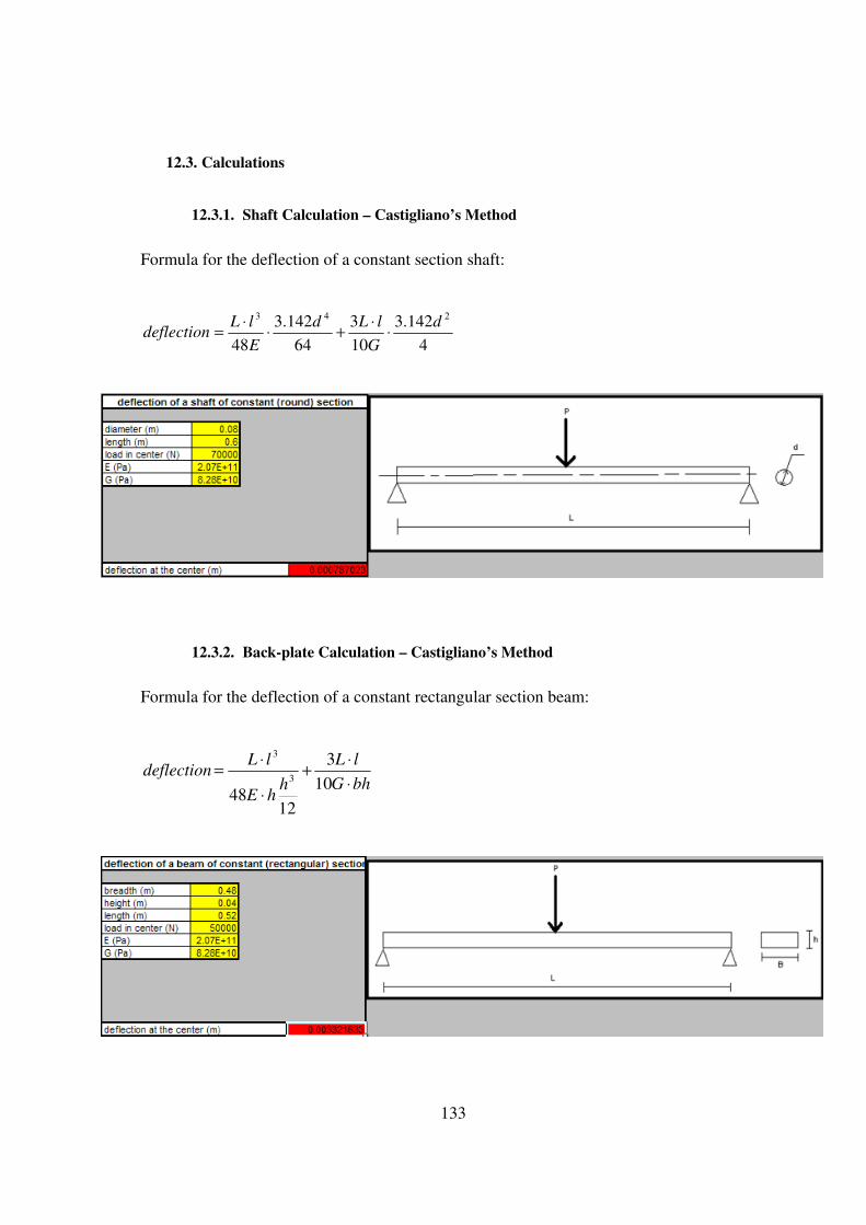
133
12.3. Calculations
12.3.1. Shaft Calculation – Castigliano’s Method
Formula for the deflection of a constant section shaft:
4
142.3
10
3
64
142.3
48
243d
G
lLd
E
lLdeflection ⋅
⋅+⋅
⋅=
12.3.2. Back-plate Calculation – Castigliano’s Method
Formula for the deflection of a constant rectangular section beam:
bhG
lL
hhE
lLdeflection
⋅
⋅+
⋅
⋅=
10
3
1248
3
3
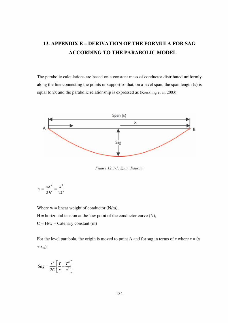
134
13. APPENDIX E – DERIVATION OF THE FORMULA FOR SAG
ACCORDING TO THE PARABOLIC MODEL
The parabolic calculations are based on a constant mass of conductor distributed uniformly
along the line connecting the points or support so that, on a level span, the span length (s) is
equal to 2x and the parabolic relationship is expressed as (Kiessling et al. 2003):
Figure 12.3-1: Span diagram
C
x
H
wxy
22
22
==
Where w = linear weight of conductor (N/m),
H = horizontal tension at the low point of the conductor curve (N),
C = H/w = Catenary constant (m)
For the level parabola, the origin is moved to point A and for sag in terms of τ where τ = (x
+ xA):
−=
2
22
2 ssC
sSag
ττ

135
Substituting τ = s/2 for the maximum sag, the following equation is obtained:
C
sSag
8
2
max =
Copyright © 2022 FDOKUMEN