Lumped-Element Planar Strip Array (LPSA) for Parallel MRI

Ray F. Lee1,*, Christopher J. Hardy2, Daniel K. Sodickson3, and Paul A. Bottomley4

1Department of Radiology, New York University, New York, New York. 2GE Global Research Center,Schenectady, New York. 3Beth Israel Deaconess Medical Center, Harvard Medical School, Boston,Massachusetts. 4Department of Radiology, Johns Hopkins University, Baltimore, Maryland.

AbstractThe recently introduced planar strip array (PSA) can significantly reduce scan times in parallel MRIby enabling the utilization of a large number of RF strip detectors that are inherently decoupled, andare tuned by adjusting the strip length to integer multiples of a quarter-wavelength (λ/4) in thepresence of a ground plane and dielectric substrate. In addition, the more explicit spatial informationembedded in the phase of the signals from the strip array is advantageous (compared to loop arrays)for limiting aliasing artifacts in parallel MRI. However, losses in the detector as its natural resonancefrequency approaches the Larmor frequency (where the wavelength is long at 1.5 T) may limit thesignal-to-noise ratio (SNR) of the PSA. Moreover, the PSA’s inherent λ/4 structure severely limitsour ability to adjust detector geometry to optimize the performance for a specific organ system, asis done with loop coils. In this study we replaced the dielectric substrate with discrete capacitors,which resulted in both SNR improvement and a tunable lumped-element PSA (LPSA) whosedimensions can be optimized within broad constraints, for a given region of interest (ROI) and MRIfrequency. A detailed theoretical analysis of the LPSA is presented, including its equivalent circuit,electromagnetic fields, SNR, and g-factor maps for parallel MRI. Two different decoupling schemesfor the LPSA are described. A four-element LPSA prototype was built to test the theory withquantitative measurements on images obtained with parallel and conventional acquisition schemes.

Keywordsstrip array; MRI; parallel imaging; lumped-element; decoupling

The strip array (1) has a number of advantages over conventional loop-resonator arrays (2) inhigh-field and parallel MRI. For instance, it allows a large number of non-adjacent elementsto simultaneously receive MRI signals, with minimal coupling between elements (3).Compared with a loop array, the more explicit spatial information in the phase of the signalsfrom a strip array makes parallel reconstruction less susceptible to aliasing artifacts. Also, itenables phased-array applications in open-geometry magnets, where conventional loop arraysare limited by field orientation. The basic element of a planar strip array (PSA) is a microstripwith both substrate and superstrate (the electrical length of which is either π/2 or π) terminatedin either an open circuit or a short circuit (1). Its geometric length must be a quarter or half ofthe resonant wavelength λ of the electromagnetic (EM) field at the MRI frequency, or integermultiples thereof. Under these conditions, the array has the unique advantage that the PSAelements are intrinsically isolated from each other. However, at commonly used fields of 1.5T(63.87 MHz), λ is around 4.7 m (if the substrate is air), so a PSA with λ/4 and λ/2 wouldgenerally be too long.

*Correspondence to: Ray F. Lee, Department of Radiology, New York University Medical Center, 650 First Ave., Suite 600A, NewYork, NY 10016. E-mail: ray.lee@med.nyu.edu

NIH Public AccessAuthor ManuscriptMagn Reson Med. Author manuscript; available in PMC 2007 October 10.

Published in final edited form as:Magn Reson Med. 2004 January ; 51(1): 172–183.

NIH

-PA Author Manuscript

NIH

-PA Author Manuscript

NIH

-PA Author Manuscript

The use of high-dielectric-constant substrates, instead of air, allows some reduction of λ tolengths practical for human imaging. However, the dielectric constant of a substrate is ingeneral not easily varied, nor are there suitable materials available that possess a continuumof dielectric constants from which to choose. This limits our ability to arbitrarily adjust thePSA geometry in order to optimize its MRI performance in applications to a particular organat a particular field strength. Nevertheless, the PSA elements are intrinsically isolated fromone other, as long as their lengths are integer multiples of a quarter wavelength. Anotherdisadvantage of the original PSA is that losses associated with the high-dielectric-constantsubstrate and large size of the distributed element can reduce the signal-to-noise ratio (SNR).

If instead of using a high-dielectric constant substrate to reduce the wavelength, one createsan artificial or “reduced-length” transmission line (RTL) (4) by deploying two or more discretehigh-Q shunted capacitors along the strip, two advantages can be realized. First, the discretecapacitors reduce the electrical length of the PSA transmission line strips, and potentiallyenable the design of PSAs with much smaller geometric dimensions that can be adjusted for agiven field strength. Second, the losses associated with the dielectric substrate and superstratecan be reduced, thereby increasing the SNR. Moreover, the geometric configuration can beadjusted to maximize the SNR for each specific application without being bound by the λ/4criterion as applied to the physical strip length.

In this study we developed a lumped-element PSA (LPSA), employing RTLs for the arrayelements (5,6). In the LPSA, the electrical function of the substrate is replaced in part orsubstantially with two or more distributed shunt capacitors, yielding the equivalent electricallength of π/2 at 63.87 MHz with a much shorter strip length. At this frequency, an LPSA witha strip length of about 30 cm can be tuned with just two shunted 100 –200pF capacitors, whileit can also be tuned with more uniformly distributed capacitors. A benefit of using only twocapacitors in this situation (1.5T) is that the LPSA maintains a relatively homogeneous B1 fieldwhile it is tuned to an electrical length of π/2. The interstrip decoupling mechanisms of theLPSA are different from those of the PSA. In the PSA, because of its quasi-transverse EM(TEM) field distribution, contributions from incident and reflected waves along a λ/4 stripcancel one another (1), so that the PSA is inherently decoupled. However, in the LPSA, at 1.5Tthe physical length of each strip can be much shorter than λ/4, and the condition of intrinsicdecoupling is difficult to achieve.

In this study, we first apply a lumped-element circuit model to analyze the resonance conditionand Q-factor of an RTL, and calculate its field and SNR. Second, interelement coupling,sensitivity profiles, and g-factor maps of the LPSA are evaluated in detail. Third, we describetwo different schemes to isolate the RTL strips and substantially eliminate mutual coupling.In the past, shared (7) and interconnected (8) capacitors have been used to decouple loop MRIcoils, as well as to couple transmission line sections (9), and in the first scheme we useinterconnecting capacitors to decouple each nearest-neighbor pair. Low-input impedancepreamplifiers are then deployed to decouple the remaining strips, as was implemented in theoriginal phased array (2,10). The other scheme is to make the ratio of the strip spacing to thestrip-to-ground distance large enough to achieve isolation (6). This approach limits theminimum separation between neighboring strips. Fourth, quantitative measurements of arraycharacteristics and MRI experiments are used to demonstrate that the LPSA can produce high-quality in vivo MR images at 1.5 T with either phased-array or parallel data acquisition.

THEORYRTL—The Basic Element of the LPSA

Whereas the basic detector element of the PSA is a transmission line resonator (1), the LPSA’sbasic element can be viewed as an RTL resonator, in which the electrical length is achieved

Lee et al. Page 2

Magn Reson Med. Author manuscript; available in PMC 2007 October 10.

NIH

-PA Author Manuscript

NIH

-PA Author Manuscript

NIH

-PA Author Manuscript

by combining a transmission line and shunt capacitors, as shown in Fig. 1a (a special casewhere only two capacitors are used). There is flexibility in adjusting the physical length, l, ofthe RTL. The RTL can initially be treated as a two-port network, which is commonlycharacterized by the “ABCD” matrix formalism that relates the input voltage and current, V1and I1, to the output voltage and current, V2 and I2, via:

V1I1

= A BC D

V2I2

. [1]

If the two shunt capacitors at the ends of the line have value Cgs, then the “ABCD” matrix for

the RTL is

A BC D =

1 0

jωCgs 1

cosh γl Z0 sinh γlsinh γl / Z0 cosh γl

×1 0

jωCgs 1 ,

[2]

where ω is the angular frequency of the EM field, Z0 is the characteristic impedance of thetransmission line, and γ is known as the propagation constant (11). These last two are givenby

Z0 = R ′+ jωL ′

G ′+ jωC ′, γ = (R ′+ jωL ′)(G ′+ jωC ′). [3]

Here R′ is the series resistance per unit length of the transmission line, G′ is the shunt resistanceper unit length, L′ is the series inductance per unit length, and C′ is the shunt capacitance perunit length. When the strip length is physically much less than one wavelength, cosh γl ≈ 1 andsinh γl ≈ γl. Then Eq. [2] becomes

A BC D =

1 0

jωCgs 1

1 Rt + jωL tGt + jωCt 1

×1 0

jωCgs 1 .

[4]

If we assume that loading along the strip is uniform, then the series resistance, shunt resistance,series inductance, and shunt capacitance of the transmission line are Rt = R′l, Gt = G′l, Lt = L′l, and Ct = C′l, respectively.

The distance h between the strip and the ground has a significant effect on the field patterns ofthe RTL, especially for the electric field. When h is so small that the electric field lines areconcentrated mostly between each strip and the ground plane, then the EM field of the RTLcan be considered as quasi-TEM. But if h is relatively large (>5 mm), the electric field isoriented mostly along the strip (non-TEM). We consider only this second scenario, and avoidthe first scenario and the other transition situations between these two scenarios. While thetransmission line shunt capacitance, Ct, will decrease as h increases, its net effect may still beappreciable for choices of l and h, respectively, in a range of ~20 cm and ~1 cm (which isdesirable for human studies), especially if a dielectric substrate is deployed to separate thestrips from the ground plane (6). To simplify the analysis, we incorporate Ct into the lumped-element capacitance Cg, and neglect the shunt resistance (Gt ≈ 0). The RTL has a simple lumped

Lee et al. Page 3

Magn Reson Med. Author manuscript; available in PMC 2007 October 10.

NIH

-PA Author Manuscript

NIH

-PA Author Manuscript

NIH

-PA Author Manuscript

LCR equivalent circuit as shown in Fig. 1c, where Cg ∼ Cgs + Ct / 2 is the effective shunt

capacitance, and Rt represents the net loss resistance. Eq. [3] becomes

A BC D =

1 0jωCg 1

1 Rt + jωL t0 1

1 0jωCg 1 [5]

The admittance of the RTL can be derived from the ABCD matrix by letting the load at oneport ZL be infinity:

Y = GY + jBY =C + DYLA + BYL

= CA

=− ω2RtCg

2 + j(2ωCg − ω3L tCg

2)

1 − ω2L tCg + jωRtCg.

[6]

Here GY is the conductance and BY is the susceptance, where

GY =Cg

2Rtω2

1 − 2CgL tω2 + Cg

2Rt2ω2 + Cg

2L t2ω4

BY =2Cgω + ( − 3Cg

2L t + Cg3Rt

2)ω3 + Cg3L t

2ω5

1 − 2CgL tω2 + Cg

2Rt2ω2 + Cg

2L t2ω4

[7]

A low-frequency estimate of the inductance of the strip over the ground plane is (12,13):

L t =μ0lπ ln 2l

w + 12 − ln ( l

2h + 1 + l 2

(2h )2 ) + 1 + (2h )2

l 2 − 2hl . [8]

The resistance Rt is essentially the sum of the conductor losses and the sample losses.

Resonance Condition of the RTL—To calculate the resonance frequency of the RTL, onecan set the susceptance BY = 0 in Eq. [7], and derive

ω = 12

3L tCg

−Rt

2

L t2 ±

L t2 − 6L tCgRt

2 + Cg2Rt

4

CgL t2 ≈ 2

L tCg∣ Rt≈0. [9]

The impedance has a maximum value at resonance frequency ο in Eq. [9] only when the plussign of the ± is chosen. If the minus sign is chosen, the admittance instead has a maximumvalue, a case that is not presently of interest.

The ω in Eq. [9] is not always a real number, which means that the RTL only resonates undercertain conditions. To derive the resonance condition, one can let B = 0 in Eq. [7] and solvefor Cg and Lt:

Lee et al. Page 4

Magn Reson Med. Author manuscript; available in PMC 2007 October 10.

NIH

-PA Author Manuscript

NIH

-PA Author Manuscript

NIH

-PA Author Manuscript

Cg =3ωL t + ω2L t

2 − 8Rt2

2ω(Rt2 +ω2L t

2)

L t =3 + 1 − 4Cg

2Rt2ω2

2Cgω2 .

[10]

To ensure that Cg and Lt remain real, the inductance of the strip and the equivalent capacitanceof the shunt capacitors must satisfy the following conditions:

L t ≥2 2Rtω

Cg ≤1

2ωRt.

[11]

For a given resonance frequency, the minimum inductance of the strip and maximum shuntcapacitance are determined by the net sample and conductor resistance Rt. By combining Lt inEqs. [8] and [11], one can estimate the minimum viable strip dimensions. Details of thecalculation of Rt are given below.

Q Factor and Loading Factor of the RTLThe quality factor, Q, of the RTL, and the effect of a sample load, are measures of detectorperformance. The Q can be calculated from the admittance in Eq. [7]:

Q =ωr

2GY

dBYdω ∣ ω=ωr

=

2 + (Cg2Rt

2 − 5CgL t)ω2 + (5Cg

2L t2 − 5Cg

3L tRt2

+Cg4Rt

4)ω4 + (2Cg4L t

2Rt2 − 3Cg

3L t3)ω6 + Cg

4L t4ω8

2CgRtω + (2Cg3Rt

3 − 4Cg2L tRt)ω

3 + 2Cg3L t

2Rtω5

[12]

At the resonance frequency οr, Cg and Lt are interrelated via Eq. [10]. Substituting theexpression for Cg from Eq. [10] into Eq. [12] yields the Q in terms of strip inductance Lt andthe equivalent net loss resistance Rt in Fig. 1c:

Q =

− 8Rt6 − 20L t

2Rt4ω2 + 38L t

4Rt2ω4 − 4L t

6ω6

+(4L tRt4ω + 18L t

3Rt2ω3 − 4L t

5ω5) ω2L t2 − 8Rt

2

14L tRt5ω + 10L t

3Rt3ω3 − 4L t

5Rtω5 + (2Rt

5

− 2L t2Rt

3ω2 − 4L t4Rtω

4) ω2L t2 − 8Rt

2

[13]

On the other hand, substituting the expression for Lt from Eq. [10] into Eq. [12] yields the Qin terms of Cg and Rt:

Q =2Cgω

2 − 7Cg3Rt

2ω4 + (2Cgω2 − Cg

3Rt2ω4) 1 − 4Cg

2Rt2ω2

Cg2Rtω

3(1 + 1 − 4Cg2Rt

2ω2). [14]

With the strip loaded with a sample, the value of the equivalent resistance Rt = RL will differfrom the unloaded value, Rt = RU, leading to different loaded and unloaded Qs, QL and QU,

Lee et al. Page 5

Magn Reson Med. Author manuscript; available in PMC 2007 October 10.

NIH

-PA Author Manuscript

NIH

-PA Author Manuscript

NIH

-PA Author Manuscript

respectively. The behavior of Eqs. [13] and [14] as a function of typical RTL equivalentimpedances Rt, Cg, and Lt, and loading ratios RL/RU and QU/QL, are plotted in Fig. 2 at 64MHz (parts a–d) and at 128 MHz (parts e–h). Despite the complexity of Eq. [13], Fig. 2a ande show that the relation between Q and Lt is almost linear with load resistance. Figure 2c andg show that larger values of Cg produce lower Qs. When RL/RU is 2 (1Ω/0.5Ω), 5 (5Ω/1Ω), or10 (5Ω/0.5Ω), Fig. 2b, d, f, and h show that as Lt increases, or as Cg decreases, the loadingfactor QU/QL approaches RL/RU. However, when Lt is relatively small, or Cg is relatively large,an increase in sample load disproportionately reduces Q, so that QU/QL is much higher thanRL/RU (Fig. 2b and h), where the electrical field loading on the capacitor becomes aconsiderable factor. To avoid this situation, it is preferable to increase Lt and reduce Cg.

B Field and E FieldThe RF magnetic and electric fields of an RTL with unit current can be derived from the vectorpotential. According to the reciprocity principle, they also represent the magnetic and electricfields detected by the RTL. The MR signal is proportional to the transverse component of themagnetic field, B1. The MR noise is proportional to the square root of the noise resistance(14), which in turn can be determined from the integral of the square of the electric field (15)over the half space that extends from the ground plane of the RTL through the sample.Therefore, once the magnetic and electric fields of the RTL are known, the SNR can beevaluated.

To simplify the field calculations while preserving the characteristics of the RTL, weapproximate the strip by a filament of length l along the z-direction of a Cartesian coordinatesystem (x, y, z) with the z-axis parallel to the static magnetic field B0. The x- and y-axes arethe horizontal and vertical directions, respectively. The filament has coordinates denoted by(x0, y0, z0), and spans the region from z0 = −l/2 to z0 = l/2. The vector potential of the filament(16) is then

A = μ4π∭v=current_volume

Jr dv = μ

4π ∫−l/2l/2 I

r dz0z

= μI4π ∫−l/2

l/2 dz0(x − x0)2 + (y − y0)2 + (z − z0)2

z

= μI4π ln

l / 2 − z + (x − x0)2 + (y − y0)2 + (z − l / 2)2

− l / 2 − z + (x − x0)2 + (y − y0)2 + (z + l / 2)2z.

[15]

Here J is the current density, I is the current, r is the distance between (x0, y0, z0) and an arbitraryspatial point (x, y, z), and μ is the permeability. The transverse magnetic field B1 of the filamentis

B1 = ∇ × A = B1xx + B1yy. [16]

Let rxy2 = (x − x0)2 + (y − y0)2. Then

B1x = μI4π

y − y0r 2 ( l / 2 + z

r 2 + (z + l / 2)2+ l / 2 − z

r 2 + (z − l / 2)2 )B1y = − μI

4πx − x0

r 2 ( l / 2 + zr 2 + (z + l / 2)2

+ l / 2 − zr 2 + (z − l / 2)2 ) [17]

The electric field E of the filament can be derived from (17):

Lee et al. Page 6

Magn Reson Med. Author manuscript; available in PMC 2007 October 10.

NIH

-PA Author Manuscript

NIH

-PA Author Manuscript

NIH

-PA Author Manuscript

E = − ∂A∂t = jωA

= ωμI4π ln

l / 2 − z + (x − x0)2 + (y − y0)2 + (z − l / 2)2

− l / 2 − z + (x − x0)2 + (y − y0)2 + (z + l / 2)2z

[18]

Note that this is the non-TEM case. As mentioned before, this only true when h is large enough.

When the conducting filament at y0 = 0 is parallel to a conducting ground plane (zx), then,using the method of images (12), the magnetic field B1 and electric field E1 at (x, y, z) are givenby:

B1 = B(y0 = 0) − B(y0 = − 2h ) [19]

E1 = E(y0 = 0) − E(y0 = − 2h ). [20]

Equations [19] and [20] give the analytic expressions for the magnetic and electric fields ofthe RTL. For example, for l = 30 cm and h = 2 cm, the horizontal (B1x), vertical (B1y), magnitude(|B1|), and phase (∠B1= atan[B1y/B1x]) components of B1 in the z = 0 plane are illustrated inFig. 3.

SNR—The SNR of the RTL can be defined as (18):

SNR =jωμM · B14kTΔ f RL

=jωμ(MxB1x + M yB1y)

4kTΔ f RL, [21]

where M = Mxx + Myy is the transverse magnetization, k is Boltzmann’s constant, T is theabsolute temperature, and Δf is the receive bandwidth. Thus, for a given object, fixed T, andΔf, the SNR is determined by the ratio of ∣ B1 ∣ / RL . The intrinsic SNR, which includessample losses and excludes losses in the detector, is proportional to ∣ B1 ∣ / RL ,S , whereRL,S is the portion of RL contributed by a sample with conductivity σ (19). We calculateRL,S under conditions where QU/QL ≈ RL/RU (see the section entitled Q Factor and LoadingFactor of the RTL), by numerical integration of (18):

RL ,S = σ∫V /2E12dx dy dz, [22]

and determine E1 and B1 from Eqs. [17]–[20].

Figure 4a shows RL,S/σ vs. strip-to-ground distance h. Figures 4b and c show |B1|, and theintrinsic SNR ∼ ∣ B1 ∣ / RL ,S vs. y at the z = 0 plane, with σ = 1 S/m. Although Fig. 4bdemonstrates some |B1| enhancement when h is increased, Fig. 4c shows that the intrinsic SNRscales inversely with h in the range of 1–5 cm, but becomes insensitive to h as depth increases.Thus, when h is above a certain value (non-TEM), increasing h may not provide an SNR gainfor RTLs.

Array AnalysisWhen a number of RTLs are laid side by side in parallel, both the SNR and the field patternsmay be altered by mutual coupling between the RTLs if they are close enough. A generalcoupling analysis of a multiple-element system was outlined previously in Ref. 20. Here weonly consider the special case where the mutual couplings are relatively weak, and the methods

Lee et al. Page 7

Magn Reson Med. Author manuscript; available in PMC 2007 October 10.

NIH

-PA Author Manuscript

NIH

-PA Author Manuscript

NIH

-PA Author Manuscript

used in Ref. 2 to describe mutual couplings are valid. This is only sufficient when the numberof elements of the LPSA is small.

Strip Coupling—The mutual coupling usually includes signal coupling and noise coupling,which can be quantitatively characterized by mutual inductance and mutual resistance,respectively. If two simple filaments are located at x0 = 0 and x0 = d, their mutual inductancecan be analytically calculated from (12,13):

M (l, d) =μ0l2π ln ( l

d + 1 + ( ld )2) − 1 + ( d

l )2 + dl . [23]

Here l is the filament length and d is the spacing between filaments. The mutual inductancebetween two neighboring RTLs, Mij, can be calculated from Eq. [23] using the method ofimages. Assuming l2 + d2 ≫ 4h2, where h is the strip-to-ground distance, we have

Mij = 2M (l, d) − 2M (l, d 2 + 4h 2)

≈μ0π (d − d 2 + 4h 2 + l ln 1 + 4h 2

d 2 ). [24]

Note that the relative values of h and d determine the mutual inductance. When 2h ≪d, themutual inductance, and thus the mutual signal coupling, approach zero.

The mutual noise resistance (2) between an RTL at x0 = 0 and one at x0 = d is given by

Rm = σ∫V /2E1(x0 = 0) · E1(x0 = d) dV , [25]

which can be numerically calculated with E1 from Eq. [20].

The signal and noise coupling coefficients can also be calculated numerically from Ref. 2:

kij =Mij

L iiL jj, and ψij =

RijRiiR jj

. [26]

Here Mij, Lii, Ljj, Rij, Rii, and Rii can be calculated from Eqs. [8], [22], [24], and [25].

For example, consider a four-element LPSA. If the couplings are relatively weak, they can becharacterized by a 4 × 4 signal coupling matrix K and a noise coupling matrix Ψ (2):

K = ( 1 − k12 − k13 − k14− k12 1 − k23 − k24− k13 − k23 1 − k34− k14 − k24 − k34 1

),Ψ = ( 1 ψ12 ψ13 ψ14

ψ12 1 ψ23 ψ24ψ13 ψ23 1 ψ34ψ14 ψ24 ψ34 1

). [27]

If the mutual signal couplings are strong, then the diagonal terms are no longer unity and thematrices are more complex (20).

Lee et al. Page 8

Magn Reson Med. Author manuscript; available in PMC 2007 October 10.

NIH

-PA Author Manuscript

NIH

-PA Author Manuscript

NIH

-PA Author Manuscript

B1 Profiles and g-Factor Maps for the LPSAIn the LPSA, the coupling of the magnetic field B1 between strips is proportional to the couplingof the currents (20) in the strips. The coupling matrix for the currents can be simplified to Kin Eq. [27], in the case where coupling is weak and there is no propagation of coupled currentsamong the RTLs (20). For a four-element LPSA, we describe the coupled and uncoupledmagnetic fields, respectively, as

B̂1C = (B1a

C

B1bC

B1cC

B1dC

) and B̂1 = (B1aB1bB1cB1d

), [28]

Then the B1 profiles of the LPSA are related by

B̂1C = KB̂1. [29]

For example, for a strip length l = 30 cm, width w = 1.27 cm, strip-to-ground distance h = 2cm, and strip spacing d = 6 cm, the B1 coupling matrix calculated from Eqs. [8], [24], and [27]for weakly coupled strips is:

K = ( 1 − 0.0587 − 0.0140 − 0.0054− 0.0587 1 − 0.0587 − 0.0140− 0.0140 − 0.0587 1 − 0.0587− 0.0054 − 0.0140 − 0.0587 1

) [30]

Figure 5 shows the magnitude and phase components of the coupled magnetic field B1 of thefour-element LPSA calculated from Eqs. [19], [29], and [30]. Note that the field patterns ofthe outermost RTL differ from the inner ones: symmetry can be improved by adding an extrastrip on each side as a “guard” (1).

The g-factor map provides a quantitative measure of the performance of a phased array forparallel imaging applications (21,22). It is given by

g = (SHΨ−1S)−1ρ,ρ(SHΨ−1S)ρ,ρ. [31]

Here S is the matrix of complex coil sensitivities of superimposed imaging areas from differentcoils (22). Table 1 shows the results of noise coupling calculations for three differentcombinations of h and d based on Eqs. [22], [25], and [26]. From Table 1, one can derive thenoise coupling matrices from Eq. [27]:

Lee et al. Page 9

Magn Reson Med. Author manuscript; available in PMC 2007 October 10.

NIH

-PA Author Manuscript

NIH

-PA Author Manuscript

NIH

-PA Author Manuscript

Ψ1(h = 2cm, d = 10cm) = ( 1 0.48 0.27 0.160.48 1 0.48 0.270.27 0.48 1 0.480.16 0.27 0.48 1

),Ψ2(h = 2cm, d = 6cm) = ( 1 0.69 0.44 0.31

0.69 1 0.69 0.440.44 0.69 1 0.690.31 0.44 0.69 1

),Ψ3(h = 1cm, d = 6cm) = ( 1 0.53 0.33 0.23

0.53 1 0.53 0.330.33 0.53 1 0.530.23 0.33 0.53 1

).[32]

Assuming that the signal from each RTL is isolated from the others, the axial-plane g-factormaps of Ψ1, Ψ2, and Ψ3 at reduction factors of 2, 3, and 4 are shown in Fig. 6 for d = 6 and 10cm and h = 1 and 2 cm. Overall, the figure shows little variation in g-factor performance forthe different reduction factors. However, the larger the spacing d, the better the g-factor becausethe noise coupling is reduced. Also, g-factor performance deteriorates as h is reduced, becausethe spatial distinction between the B1 fields generated by the different RTLs is less, even thoughthe noise coupling is also reduced.

DecouplingAlthough an RTL can have the same electrical length as the λ/4 transmission line, thedecoupling mechanisms for the PSA (1) do not necessarily hold. In particular, the intrinsicnarrowband decoupling of the PSA may be lost if the length of the conductor strip in the RTLis much less than λ/4, and there is no standing wave to ensure that the coupling between theincident and reflected waves fully cancel. Here we describe two alternative decoupling schemesfor the LPSA.

Interconnecting Capacitor Method—One way to decouple the LPSA is to placeinterconnecting capacitors between two RTLs at both ends of the strips to decouple nearestRTL pairs, which is analogous to the use of interconnected capacitive circuits to decouplemultiple MRI loop detectors (8), and then use low-input impedance preamplifiers to decouplethe remaining RTL pairs, as in the original NMR phased array (2). The coupling between twoRTLs can be derived from even–odd mode theory (4). Here elements A and C in the ABCDmatrix are Ae and Ce for the even mode, and Ao and Co for the odd mode. For the even mode,where currents in the two RTLs are the same, Ae and Ce are derived from Eq. [6] by replacingLt with Lt +M, where M is the mutual inductance.

Ae = 1 − ω2(L t + M )Cg + jωRtCgCe = − ω2RtCg

2 + j(2ωCg − ω3(L t + M )Cg

2)[33]

For the odd mode, where currents in the two RTLs have the same amplitude but opposite phase,Ao and Co are obtained from Eq. [6] by replacing Lt with Lt– M and Cg with Cg+2Cc. HereCc is the interconnecting capacitor.

Ao = 1 − ω2(L t − M )(Cg + 2Cc) + jωRt(Cg + 2Cc)

Ce = − ω2Rt(Cg + 2Cc)2 + j(2ω(Cg + 2Cc) − ω3(L − M )(Cg + 2Cc)2)[34]

Then the even and odd reflection coefficients are

Lee et al. Page 10

Magn Reson Med. Author manuscript; available in PMC 2007 October 10.

NIH

-PA Author Manuscript

NIH

-PA Author Manuscript

NIH

-PA Author Manuscript

Γe =Ae − CeZ0Ae + CeZ0

, and Γo =Ao − CoZ0Ao + CoZ0

. [35]

Using Eq. [11] from Ref. 1, we find that the coupling k between two RTLs is

kc =Γe − Γo

2 − ΓG(Γe + Γo) . [36]

Here ΓG is the reflection coefficient from the receiver at the input port of the RTL. To achievedecoupling, kc = 0, one needs to solve the equation Γe – Γo = 0 to derive the decouplingcapacitance:

Cc = ( − b ± b2 − 4ac) / 2a, [37]

where

a = 2ω2(L t − M )(ω2Cg(L t + M ) − 1)

b = 2 − 2ω2Cg(L t + M ) +ω4Cg2(L t

2 − M 2)

c = − ω2Cg2M .

[38]

Equation [37] gives the value of the interconnecting capacitor that will decouple an RTL pair.

This decoupling method works well when the number of array elements is relatively low. Asthe number of elements grows large, the array is more appropriately treated as an integratedsystem (20).

Broadband Decoupling—The LPSA, like the PSA, exhibits broadband decoupling (6);however, the decoupling criterion for the LPSA generally differs from that of the PSA whenthe EM fields on the LPSA do not have a TEM or quasi-TEM mode. The criterion for LPSAbroadband decoupling can be derived from Eq. [24]: if d ≫ 2h, then d2 + 4h2 ≈ d2, the mutualinductance approaches zero, and the LPSA is broadband-decoupled.

EXPERIMENTSBecause the MRI system on which we tested our method experimentally was limited to fourchannels (5,6), and our analysis example is a four-element LPSA, we constructed several four-element prototypes to test the SNR, the above decoupling schemes, and the in vivo MRIperformance with both conventional and parallel sensitivity-encoded acquisitions.

Geometric Parameters of the LPSA: l, w, and hThe choice of geometric parameters for the LPSA affects its tuning. As shown by Eq. [8], thevalues of l, w, and h determine the inductance Lt of the RTL. At resonance, Lt and the shuntcapacitance Cg are related by Eq. [9], and must satisfy Eqs. [10] and [11] for the RTL toresonate. The ratio of d and h determines the mutual inductance of an RTL pair, per Eq. [24].Within this basic framework, the geometric parameters can be chosen to optimize theperformance of the LPSA for a given application.

As an example, consider an LPSA designed for MRI of human muscle at 63.87 MHz (1.5 T).For muscle, σ = 0.86 S/m (23) ~ 1 S/m, as assumed for Fig. 4. From Eq. [22] and Fig. 4a, withh = 1–5 cm, Rt = 2.6–27.5Ω, assuming sample dominant noise. Equation [11] requires Lt >

Lee et al. Page 11

Magn Reson Med. Author manuscript; available in PMC 2007 October 10.

NIH

-PA Author Manuscript

NIH

-PA Author Manuscript

NIH

-PA Author Manuscript

18nH and Cg < 480pF when Rt= 2.6 Ω, and Lt > 194nH and Cg < 45pF for Rt = 27.5Ω at 63.87MHz, with actual values given by Eq. [10]. Because increasing h reduces the maximum valueof Cg, LPSAs with smaller h values are easier to tune.

Another consideration is the loading factor. As shown in Fig. 2, there is a minimum thresholdinductance, Lm, beyond which the loading factor is substantially determined by the ratio ofloaded and unloaded resistances. The dimensions of a strip should be chosen so that the stripinductance L > Lm. From Fig. 2b, if RL/RU = 2, Lm ≪ 50 nH for 1.5T. With RU/RL = 5, Lm isabout 250 nH. With RL/RU = 10, Lm is about 300 nH. Thus, the smaller the loading factor, thesmaller the value of Lm. Based on Eq. [8], for a 30-cm-long, 1.27-cm-wide strip with h = 2 cm,L = 302 nH. Figure 2b shows that this maintains L > Lm for a loading factor of up to about 10at 1.5 T. At higher frequencies (e.g., 3T), Lm is smaller (see Fig. 2f) and h can be much lessthan 2 cm, provided that the transmission line shunt capacitance does not exceed the value ofCg needed to tune the strips, per the assumptions made for Eq. [5].

LPSA PrototypeAn LPSA prototype was designed and built according to the above principles. Each RTL inthe prototype had strip length l = 30 cm, strip width w = 1.27 cm, a strip-to-ground separationof h = 2 cm, and strip spacing d = 10 cm. Figure 7 shows the LPSA and its circuit diagram.

Each strip was separately tuned to the same frequency with the other strips open-circuited.Without any capacitors Cc connected between any nearest RTL pair, four resonant peaks areobserved in the impedance spectrum due to the coupling between the strips, as shown in Fig.8a. When the nearest RTL pairs are interconnected with capacitors Cc, the impedance spectrumof each RTL merges into a single peak, as seen in Fig. 8b. If channel 4 of the LPSA is shortedto simulate connection with a low-input-impedance preamplifier, the single peak remains, asseen in Fig. 8c. In Fig. 8c, QU ≈ 480 and QL ≈ 80 when loaded with a human chest, yielding aloading factor of 6. Every RTL was matched to 50Ω when loaded. The circuit’s S21 parametercurve of two RTLs is shown in Fig. 8d.

If the ground plane of the LPSA is a solid conducting sheet, eddy currents induced by thegradients may affect image quality. To avoid this effect, the ground plane was segmented basedon principles outlined in Ref. 12. The gap between two segments of conductors was 1 mm, andthe gap spacing was 4.5 cm. The gaps were bridged with 2700 pF capacitors, which gave theground plane an impedance of 0.9 Ω at 63.87 MHz and 5.9 kΩ at 10 kHz.

Experimental ResultsThe four-channel LPSA was connected to a four-channel GE LX CVi scanner (GE MedicalSystems, Milwaukee, WI) for both conventional phased-array and parallel imaging. The arraywas laid flat with strips oriented parallel to the main field, producing optimum sensitivityencoding along the horizontal or x-axis. Figure 9 shows phantom and in vivo images obtainedusing the LPSA for conventional phased-array reconstruction. Figure 9a–d show images fromeach individual channel, and Fig. 9e shows the composite image from all four channels. Thelocalization of signals in Fig. 9a–d demonstrates that every strip actively receives signalswithout significant coupling artifacts. Finally, Fig. 9f shows an axial image from the humanknee.

Parallel Imaging With the LPSA—For parallel imaging, two different reconstructionschemes were used. One was GE’s implementation of the SENSE method (22), and the otherwas the general encoding matrix (GEM) method (21). For the SENSE reconstruction, in vivoT1-weighted images of human legs were acquired with a fast gradient-echo pulse (fGRE)sequence, as shown in Fig. 10. These images in the coronal plane illustrate the uniformity of

Lee et al. Page 12

Magn Reson Med. Author manuscript; available in PMC 2007 October 10.

NIH

-PA Author Manuscript

NIH

-PA Author Manuscript

NIH

-PA Author Manuscript

the strip’s sensitivity along the strip length, compared with the original PSA (1). Figure 10a isa conventional coronal image of the knees acquired in 25 s, while Fig. 10b was acquired withSENSE in 13 s with a reduction factor of 2.

With the four-channel LPSA, the GEM method yielded two-, three-, or fourfold scan-timereductions, as shown in Fig. 11. These images were reconstructed using a generalized encodingmatrix with known k-space positions and measured coil sensitivities as described in Ref. 21.The matrix was inverted and multiplied by the raw signal data collected in all array elementsto yield the accelerated images.

Comparison Between the RTL and a Circular Loop—Conventional MR phased arrays(2) typically use circular or rectangular loops as their basic elements. While it is presentlyunclear which specific loop and LPSA geometries can be meaningfully compared, given theirinherently different sensitivities, the SNR for one element of the 30-cm prototype LPSA (withthe other three elements open-circuit), and that of a GE single 15-cm-diameter circular loop,are shown as a function of depth in Fig. 12. In this case, the background noise levels from thestrip and the loop are identical, with standard deviations (SDs) of 0.43 for both, and the netstrip/coil lengths are roughly comparable. It is seen that the signal levels from the strip and theloop are also comparable overall, with the strip providing higher signal near the surface butlower signal at depths greater than ~3 cm for a profile through the mid-line (Fig. 12c), andsignal levels at least as high as the loop at all depths, for a profile 4 cm away from the midline(Fig. 12d).

CONCLUSIONSWe have introduced a new type of MRI planar strip detector array, the LPSA, which can betuned with lumped elements. The LPSA has an advantage over the original PSA in that itsgeometry is not limited by dielectric material and the wavelength therein, but can be arbitrarilyadjusted within flexible guidelines that enable its performance to be optimized to suit aparticular anatomy or region of interest (ROI) for a given MRI magnetic field strength. Wehave presented analytical expressions for the resonance conditions, Qs, magnetic field patterns,and SNR of the basic element of the LPSA—the RTL—along with criteria for choosing thegeometric design and tuning elements that substantially eliminate coupling between the PSAelements. We analyzed the mutual coupling and g-factor maps of the LPSA, and fabricated aprototype LPSA according to the principles expounded. This LPSA demonstrated conventionalphased-array MRI, as well as accelerated parallel sensitivity-encoded MRI of both phantomsand humans, with an underlying SNR of individual RTL elements comparable to that of astandard loop coil. These results affirm the potential of the LPSA as a useful, practical detectorfor multiple-channel MRI.

Although our strip arrays have been limited by our four-channel MRI system configuration(1,5), both the PSA and LPSA detector designs may provide important advantages over loopsas the number of elements in the phased array increases to 8 or 16 or more channels. Increasingthe number of elements in a conventional array comprised of loops increases the mutualcoupling between loops, rendering them increasingly difficult to match, tune, and control (2,7,8). For strip arrays, mutual coupling problems may be minimized via intrinsic decouplingmechanisms in the case of the PSA (1), or by applying the design criteria for the LPSA discussedherein. In addition, for a given FOV, increasing the number of elements in a loop array forparallel sensitivity-encoded MRI eventually necessitates a reduction in loop size, and thus areduction in the depth sensitivity of the entire detector. Strip arrays are not directly susceptibleto this problem because the depth sensitivity does not depend on spacing between strips,although adequate decoupling must be maintained as the strips are positioned closer and closertogether. Therefore, they have greater potential for packing more elements into a given FOV

Lee et al. Page 13

Magn Reson Med. Author manuscript; available in PMC 2007 October 10.

NIH

-PA Author Manuscript

NIH

-PA Author Manuscript

NIH

-PA Author Manuscript

for the purposes of parallel imaging and/or retaining depth sensitivity, and thus represent apromising approach for massively parallel MRI (3).

The explicit phase relation between the LPSA and imaged objects can be used to simplify theparallel reconstruction, and the field orientation of the LPSA makes it a good candidate foropen-field MRI. In addition, the naturally shielded structure of the LPSA may help prevent thesevere coil losses often experienced at high fields.

Acknowledgements

We thank Randy Giaquinto, Charles Rossi, and William Edelstein at GE GRC for their valuable help.

Grant sponsor: NIH; Grant number: 1R01 RR15396-01A1.

References1. Lee RF, Westgate CR, Weiss RG, Newman DC, Bottomley PA. Planar strip array (PSA) for MRI.

Magn Reson Med 2001;45:673–683. [PubMed: 11283996]2. Roemer PB, Edelstein WA, Hayes CE, Souza SP, Mueller OM. The NMR phased array. Magn Reson

Med 1990:192–225. [PubMed: 2266841]3. McDougall, MP.; Wright, SM.; Brown, DG. A 64 channel planar RF coil array for parallel imaging at

4.7 Tesla; Proceedings of the 11th Annual Meeting of ISMRM; Toronto, Canada. 2003. p. 4724. Mongia, R.; Bahl, IJ.; Bhartia, P. RF and microwave coupled-line circuits. Boston: Artech House;

1999.5. Lee, RF.; Edelstein, WA.; Bottomley, PA.; Sodickson, DK.; Kenwood, G.; Hardy, CJ. Lumped-element

planar strip array (LPSA) for MRI at 1.5T; Proceedings of the 10th Annual Meeting of ISMRM;Honolulu. 2002. p. 321

6. Kumar, A.; Bottomley, PA. Tunable planar strip array antenna; Proceedings of the 10th Annual Meetingof ISMRM; Honolulu. 2002. p. 322

7. Wang, J. A novel method to reduce the signal coupling of surface coils for MRI; Proceedings of the4th Annual Meeting of ISMRM; New York. 1996. p. 1434

8. Lian, J.; Roemer, PB. MRI RF coil. US patent. 5,804,969. 1998.9. Hogerheiden J, Ciminera M, Jue G. Improved planar spiral transformer theory applied to a miniature

lumped element quadrature hybrid. IEEE Trans Microwave Theory Techniques 1997;45:543–545.10. Duensing GR, Brooker HR, Fitzsimmons JR. Maximizing signal-to-noise ratio in the presence of coil

coupling. J Magn Reson Ser B 1996;111:230–235. [PubMed: 8661287]11. Rizzi, PA. Microwave engineering passive circuits. Englewood Cliffs, NJ: Prentice Hall; 1988.12. Jin, J. Electromagnetic analysis and design in magnetic resonance imaging. Boca Raton, FL: CRC

Press; 1998.13. Thompson M. Inductance calculation techniques. Part 1: classical methods. Power Control Intell

Motion 1999;25:40–45.14. Hoult DI, Lauterbur PC. The sensitivity of the zeugmatographic experiment involving human samples.

J Magn Reson 1979;34:425–433.15. Ocali O, Atalar E. Ultimate intrinsic signal-to-noise ratio in MRI. Magn Reson Med 1998;39:462–

473. [PubMed: 9498603]16. Kraus, JD. Electromagnetics. New York: McGraw-Hill, Inc; 1991.17. Schenck, JF.; Boskamp, EB.; Schaefer, DJ.; Barber, WD.; Vander Heiden, RH. Estimating local SAR

produced by RF transmitter coils: examples using the birdcage body coil; Proceedings of the 6thAnnual Meeting of ISMRM; Sydney, Australia. 1998. p. 649

18. Wang J, Reykowski A, Dickas J. Calculation of the signal-to-noise ratio for simple surface coils andarrays of coils. IEEE Trans Biomed Eng 1995;42:908–917. [PubMed: 7558065]

19. Edelstein WA, Glover GH, Hardy CJ, Redington RW. The intrinsic signal-to-noise ratio in NMRimaging. Magn Reson Med 1986;3:604–618. [PubMed: 3747821]

Lee et al. Page 14

Magn Reson Med. Author manuscript; available in PMC 2007 October 10.

NIH

-PA Author Manuscript

NIH

-PA Author Manuscript

NIH

-PA Author Manuscript

20. Lee RF, Giaquinto R, Hardy CJ. Coupling and decoupling theory and its applications to the MRIphased-array. Magn Reson Med 2002;48:203–213. [PubMed: 12111947]

21. Sodickson DK, McKenzie CA. A generalized approach to parallel magnetic resonance imaging. MedPhys 2001;28:1629–1643. [PubMed: 11548932]

22. Pruessmann KP, Weiger M, Scheidegger MB, Boesiger P. SENSE: sensitivity encoding for fast MRI.Magn Reson Med 1999;42:952–962. [PubMed: 10542355]

23. Bottomley PA, Andrew ER. RF magnetic field penetration, phase shift and power dissipation inbiological tissue: implications for NMR imaging. Phys Med Biol Sci 1978;23:630–643.

Lee et al. Page 15

Magn Reson Med. Author manuscript; available in PMC 2007 October 10.

NIH

-PA Author Manuscript

NIH

-PA Author Manuscript

NIH

-PA Author Manuscript

FIG 1.Schematics of a resonant transmission line (a), an RTL (b), and the equivalent circuit of theRTL (c).

Lee et al. Page 16

Magn Reson Med. Author manuscript; available in PMC 2007 October 10.

NIH

-PA Author Manuscript

NIH

-PA Author Manuscript

NIH

-PA Author Manuscript

FIG 2.Dependence of quality factors, Q, on the loaded and unloaded RTL equivalent impedencescalculated from Eqs. [13] and [14]. a: Quality factor Q of the RTL vs. Lt assuming differentRt values of 0.5Ω, 1Ω, and 5Ω at 1.5T. b: Ratio of unloaded to loaded quality factors, QU/QL vs. Lt assuming different ratios of unloaded to loaded Rt values, RL/RU at 1.5T. c: Q vs.various Cg and Rt values at 1.5 T. d: QU/QL vs. Cg and RL/RU at 1.5 T. e: Q vs. typical valuesof Lt and Rt at 3T. f: QU/QL vs. Lt and RL/RU at 3T. g: Q vs. Cg and Rt at 3T. h: QU/QL vs.Cg and RL/RU at 3T. At 1.5T, QU/QL is more sensitive to Lt variations; at 3T, QU/QL is moresensitive to Cg variations.

Lee et al. Page 17

Magn Reson Med. Author manuscript; available in PMC 2007 October 10.

NIH

-PA Author Manuscript

NIH

-PA Author Manuscript

NIH

-PA Author Manuscript

FIG 3.Axial view of the B1 field in the z = 0 plane of a 30-cm-long RTL with h = 2 cm, and the x-axis horizontal. a and b: Contour plots of vector components Bx and By. c: Magnitude |B1|.d: Arctan[B1y/B1x], which could translate into a phase of the received signal if a homogeneousB1 transmitting field were supplied by an external coil. The contours span the ranges of (a) −0.6 to + 0.7 μT, (b) ±0.7 μT, (c) +0.1 to 1.4 μT, and (d) ± π. Contour intervals are at one-eighthof the range. FOV = 40 cm × 20 cm.

Lee et al. Page 18

Magn Reson Med. Author manuscript; available in PMC 2007 October 10.

NIH

-PA Author Manuscript

NIH

-PA Author Manuscript

NIH

-PA Author Manuscript

FIG 4.a: Ratio of noise resistance of the RTL to sample conductivity as a function of strip-to-grounddistance h. b: Magnitude of B1 of the RTL as a function of vertical depth y from the center ofthe strip. c: SNR of the RTL as a function of vertical depth y from the center of the strip. |B1|and SNR exhibit quite different behaviors. Here the dashed, solid, and dash-dot linescorrespond to h = 1 cm, 2 cm, and 4 cm, respectively.

Lee et al. Page 19

Magn Reson Med. Author manuscript; available in PMC 2007 October 10.

NIH

-PA Author Manuscript

NIH

-PA Author Manuscript

NIH

-PA Author Manuscript

FIG 5.Axial view of the B1 field in the z = 0 plane of a weakly coupled four-element LPSA with l =30 cm, h = 2 cm, width w = 1.27 cm, and strip spacing d = 6 cm. Parts a, c, e, and g are theamplitude of four channels, and b, d, f, and h are their corresponding arctan[B1y/B1x], whichcould translate into phase of the received signal in four channels if a homogeneous B1transmitting field were supplied by an external coil. Here the FOV is 20 cm × 20 cm with thex-axis horizontal. The contours span the ranges of (a–d) 0.16 –1.4 μT and (e– h) ±π. Contourintervals are at one-eighth of the range.

Lee et al. Page 20

Magn Reson Med. Author manuscript; available in PMC 2007 October 10.

NIH

-PA Author Manuscript

NIH

-PA Author Manuscript

NIH

-PA Author Manuscript

FIG 6.Axial view of the g-factor maps in the z = 0 plane for a four-element LPSA: for h = 2 cm, d =10 cm, with a reduction factor of (a) 2, (b) 3, and (c) 4; for h = 2 cm, d = 6 cm, with a reductionfactor of (d) 2, (e) 3, and (f) 4; for h = 1 cm, d = 6 cm, with a reduction factor of (g) 2, (h) 3,and (i) 4. The x-axis is horizontal, and scales (top right) indicate the g-value with contourintervals at one-tenth of the range.

Lee et al. Page 21

Magn Reson Med. Author manuscript; available in PMC 2007 October 10.

NIH

-PA Author Manuscript

NIH

-PA Author Manuscript

NIH

-PA Author Manuscript

FIG 7.Schematic (a) and photo (b) of the prototype LPSA.

Lee et al. Page 22

Magn Reson Med. Author manuscript; available in PMC 2007 October 10.

NIH

-PA Author Manuscript

NIH

-PA Author Manuscript

NIH

-PA Author Manuscript

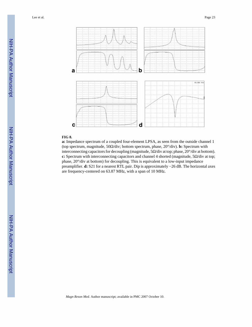
FIG 8.a: Impedance spectrum of a coupled four-element LPSA, as seen from the outside channel 1(top spectrum, magnitude, 50Ω/div; bottom spectrum, phase, 20°/div). b: Spectrum withinterconnecting capacitors for decoupling (magnitude, 5Ω/div at top; phase, 20°/div at bottom).c: Spectrum with interconnecting capacitors and channel 4 shorted (magnitude, 5Ω/div at top;phase, 20°/div at bottom) for decoupling. This is equivalent to a low-input impedancepreamplifier. d: S21 for a nearest RTL pair. Dip is approximately −26 dB. The horizontal axesare frequency-centered on 63.87 MHz, with a span of 10 MHz.

Lee et al. Page 23

Magn Reson Med. Author manuscript; available in PMC 2007 October 10.

NIH

-PA Author Manuscript

NIH

-PA Author Manuscript

NIH

-PA Author Manuscript

FIG 9.a–d: MR images acquired from each of the four different strips of the LPSA from a 27-cm-high, 20-cm-diameter phantom. e: Composite image produced using the root of the sum-of-the-squares method. Images were acquired with an FSE pulse sequence (echo train length(ETL) = 8, TE = 85 ms, TR = 2 s, NEX = 1, data-acquisition matrix 256 × 160, FOV = 36 cm).f: Composite phased-array axial image of the knees of a normal volunteer (TR = 150 ms, TE= 3.3 ms, NEX = 1, flip angle = 70, FOV = 48 cm, slice thickness = 7 mm, data matrix = 256× 160, FOV = 48 cm).

Lee et al. Page 24

Magn Reson Med. Author manuscript; available in PMC 2007 October 10.

NIH

-PA Author Manuscript

NIH

-PA Author Manuscript

NIH

-PA Author Manuscript

FIG 10.SENSE MRI of a normal volunteer acquired with four-element LPSA. a: Phased-array coronalimage of a leg through the knees (TR = 150 ms, TE = 3.3 ms, NEX = 1, flip angle = 70, FOV= 48 cm, slice thickness = 7 mm, data matrix = 256 × 160, scan time = 25 s). b: Same sectionacquired with the same parameters, but for a reduction factor of 2 (scan time = 13 s).

Lee et al. Page 25

Magn Reson Med. Author manuscript; available in PMC 2007 October 10.

NIH

-PA Author Manuscript

NIH

-PA Author Manuscript

NIH

-PA Author Manuscript

FIG 11.Images of the 27-cm-high, 20-cm-diameter phantom obtained with the GEM parallelreconstruction scheme. a: Fully gradient phase-encoded image. b–d: Images acquired with areduction factor of 2 (b), 3 (c), and 4 (d). with a gradient-echo pulse sequence (TE = 6.7 msp,TR = 150 ms, flip angle = 30°, data acquisition matrix used to extract the sensitivity profile =256 × 160, 256 × 256 points, NEX = 1, FOV = 34 cm, slice thickness = 5 mm). The coronalslice was 6 cm above the LPSA.

Lee et al. Page 26

Magn Reson Med. Author manuscript; available in PMC 2007 October 10.

NIH

-PA Author Manuscript

NIH

-PA Author Manuscript

NIH

-PA Author Manuscript

FIG 12.Comparison of a strip and a loop acquired from a phantom with the identical MRI sequence.a: Image acquired with one RTL (l = 30 cm, h = 2 cm). b: Image acquired with one circularloop (15-cm diameter). c and d: Profile comparisons of different rows in images a and b,respectively (horizontal scale is 1–256).

Lee et al. Page 27

Magn Reson Med. Author manuscript; available in PMC 2007 October 10.

NIH

-PA Author Manuscript

NIH

-PA Author Manuscript

NIH

-PA Author Manuscript

NIH

-PA Author Manuscript

NIH

-PA Author Manuscript

NIH

-PA Author Manuscript

Lee et al. Page 28

Table 1Noise Resistance, Mutual Resistance and Noise Coupling Coefficients Calculations

h (cm) d (cm) R11/σ R12/σ R13/σ R14/σ Ψ12 Ψ13 Ψ14

2 6 8.755 6.02 3.834 2.712 0.69 0.44 0.312 10 8.755 4.222 2.329 1.394 0.48 0.27 0.161 6 3.06 1.631 0.999 0.697 0.53 0.33 0.23

Magn Reson Med. Author manuscript; available in PMC 2007 October 10.