
LSST Science Book - Fermilab | Technical Publications
596
LSST Science Book Version 2.0 November 2009 Prepared by the LSST Science Collaborations, with contributions from the LSST Project. FERMILAB-TM-2495-A FERMILAB-TM-2495-A Operated by Fermi Research Alliance, LLC under Contract No. DE-AC02-07CH11359 with the United States Department of Energy
-
Upload
khangminh22 -
Category
Documents
-
view
0 -
download
0
Transcript of LSST Science Book - Fermilab | Technical Publications

LSST Science Book
Version 2.0
November 2009
Prepared by the LSST Science Collaborations,
with contributions from the LSST Project.
FERMILAB-TM-2495-AFERMILAB-TM-2495-A
Operated by Fermi Research Alliance, LLC under Contract No. DE-AC02-07CH11359 with the United States Department of Energy

This book is a living document. The most recent version can be found at http://www.lsst.org.
The front cover of the Science Book features an image of the LSST created from mechanicaldrawings by Todd Mason, Mason Productions, Inc., shown against an image created from DeepLens Survey data. The back cover shows a simulated 15-second LSST exposure from one of the4 K× 4 K CCDs in the focal plane. Graphic design by E. Acosta (LSSTC).
For more information, contact:J. Anthony Tyson, Director 530.752.3830 – [email protected] W. Sweeney, Project Manager 925.487.2134 – [email protected] A. Strauss, Chair of Science Collaborations 609.258.3808 – [email protected]
LSST is a public-private partnership. Design and development activity is supported in part by theNational Science Foundation. Additional funding comes from private foundation gifts, grants touniversities, and in-kind support of Department of Energy laboratories and other LSST MemberInstitutions. The project is overseen by the LSST Corporation, a non-profit 501(c)3 corporationformed in 2003, with headquarters in Tucson, AZ.
c© 2009 by the LSST CorporationNo part of this book may be reproduced or utilized in any form or by any means without the priorwritten permission from the LSST Corporation.
LSST Corporation933 North Cherry Avenue
Tucson, AZ 85721-0009520.881.2626
[email protected]://www.lsst.org
2

Contents
Preface . . . . . . . . . . . . . . . . . . . . . . . . . . . . . . . . . . . . . . . . . . . . . . . 91 Introduction . . . . . . . . . . . . . . . . . . . . . . . . . . . . . . . . . . . . . . . . . . 111.1 Astronomy-Physics Interaction . . . . . . . . . . . . . . . . . . . . . . . . . . . . . . 111.2 What a Telescope with Enormous Etendue can Accomplish . . . . . . . . . . . . . . 121.3 The History of the Idea . . . . . . . . . . . . . . . . . . . . . . . . . . . . . . . . . . 121.4 Overview of LSST Science . . . . . . . . . . . . . . . . . . . . . . . . . . . . . . . . . 131.5 The LSST Science Requirements . . . . . . . . . . . . . . . . . . . . . . . . . . . . . 181.6 Defining the Telescope Design Parameters . . . . . . . . . . . . . . . . . . . . . . . . 20
References . . . . . . . . . . . . . . . . . . . . . . . . . . . . . . . . . . . . . . . . . . 242 LSST System Design . . . . . . . . . . . . . . . . . . . . . . . . . . . . . . . . . . . . . 252.1 The LSST Observing Strategy . . . . . . . . . . . . . . . . . . . . . . . . . . . . . . . 252.2 Observatory Site . . . . . . . . . . . . . . . . . . . . . . . . . . . . . . . . . . . . . . 272.3 Optics and Telescope Design . . . . . . . . . . . . . . . . . . . . . . . . . . . . . . . 282.4 Camera . . . . . . . . . . . . . . . . . . . . . . . . . . . . . . . . . . . . . . . . . . . 322.5 Data Management System . . . . . . . . . . . . . . . . . . . . . . . . . . . . . . . . . 372.6 Photometric Calibration . . . . . . . . . . . . . . . . . . . . . . . . . . . . . . . . . . 452.7 Astrometric Calibration . . . . . . . . . . . . . . . . . . . . . . . . . . . . . . . . . . 50
References . . . . . . . . . . . . . . . . . . . . . . . . . . . . . . . . . . . . . . . . . . 523 System Performance . . . . . . . . . . . . . . . . . . . . . . . . . . . . . . . . . . . . . 533.1 Operations Simulator . . . . . . . . . . . . . . . . . . . . . . . . . . . . . . . . . . . . 533.2 Exposure Time Calculator . . . . . . . . . . . . . . . . . . . . . . . . . . . . . . . . . 563.3 Image Simulator . . . . . . . . . . . . . . . . . . . . . . . . . . . . . . . . . . . . . . 573.4 Stray and Scattered Light . . . . . . . . . . . . . . . . . . . . . . . . . . . . . . . . . 623.5 The Expected Accuracy of Photometric Measurements . . . . . . . . . . . . . . . . 653.6 Accuracy of Trigonometric Parallax and Proper Motion Measurements . . . . . . . 673.7 Expected Source Counts and Luminosity and Redshift Distributions . . . . . . . . . 693.8 Photometric Redshifts . . . . . . . . . . . . . . . . . . . . . . . . . . . . . . . . . . . 73
References . . . . . . . . . . . . . . . . . . . . . . . . . . . . . . . . . . . . . . . . . . 854 Education and Public Outreach . . . . . . . . . . . . . . . . . . . . . . . . . . . . . . . 874.1 Introduction . . . . . . . . . . . . . . . . . . . . . . . . . . . . . . . . . . . . . . . . . 874.2 National Perspective on Education Reform . . . . . . . . . . . . . . . . . . . . . . . . 874.3 Teaching and Learning in the Classroom . . . . . . . . . . . . . . . . . . . . . . . . . 884.4 Outside the Classroom — Engaging the Public . . . . . . . . . . . . . . . . . . . . . 914.5 Citizen Involvement in the Scientific Enterprise . . . . . . . . . . . . . . . . . . . . . 924.6 Diversity . . . . . . . . . . . . . . . . . . . . . . . . . . . . . . . . . . . . . . . . . . . 944.7 Summary . . . . . . . . . . . . . . . . . . . . . . . . . . . . . . . . . . . . . . . . . . 95
References . . . . . . . . . . . . . . . . . . . . . . . . . . . . . . . . . . . . . . . . . . 955 The Solar System . . . . . . . . . . . . . . . . . . . . . . . . . . . . . . . . . . . . . . . 97
3

Contents
5.1 A Brief Overview of Solar System Small Body Populations . . . . . . . . . . . . . . . 975.2 Expected Counts for Solar System Populations . . . . . . . . . . . . . . . . . . . . . 995.3 The Orbital Distributions of Small Body Populations . . . . . . . . . . . . . . . . . . 1055.4 The Main Belt: Collisional Families and Size Distributions . . . . . . . . . . . . . . . 1105.5 Trans-Neptunian Families and Wide Binaries . . . . . . . . . . . . . . . . . . . . . . 1155.6 The Size Distribution for Faint Objects—“Shift and Stack” . . . . . . . . . . . . . . 1175.7 Lightcurves: Time Variability . . . . . . . . . . . . . . . . . . . . . . . . . . . . . . . 1205.8 Overlapping Populations . . . . . . . . . . . . . . . . . . . . . . . . . . . . . . . . . . 1225.9 Physical Properties of Comets . . . . . . . . . . . . . . . . . . . . . . . . . . . . . . . 1265.10 Mapping of Interplanetary Coronal Mass Ejections . . . . . . . . . . . . . . . . . . . 1275.11 The NEA Impact Hazard . . . . . . . . . . . . . . . . . . . . . . . . . . . . . . . . . 1285.12 NEAs as Possible Spacecraft Mission Targets . . . . . . . . . . . . . . . . . . . . . . 132
References . . . . . . . . . . . . . . . . . . . . . . . . . . . . . . . . . . . . . . . . . . 1336 Stellar Populations . . . . . . . . . . . . . . . . . . . . . . . . . . . . . . . . . . . . . . 1376.1 Introduction . . . . . . . . . . . . . . . . . . . . . . . . . . . . . . . . . . . . . . . . . 1376.2 The Magellanic Clouds and their Environs . . . . . . . . . . . . . . . . . . . . . . . . 1386.3 Stars in Nearby Galaxies . . . . . . . . . . . . . . . . . . . . . . . . . . . . . . . . . 1446.4 Improving the Variable Star Distance Ladder . . . . . . . . . . . . . . . . . . . . . . 1466.5 A Systematic Survey of Star Clusters in the Southern Hemisphere . . . . . . . . . . 1506.6 Decoding the Star Formation History of the Milky Way . . . . . . . . . . . . . . . . 1556.7 Discovery and Analysis of the Most Metal Poor Stars in the Galaxy . . . . . . . . . 1606.8 Cool Subdwarfs and the Local Galactic Halo Population . . . . . . . . . . . . . . . 1626.9 Very Low-Mass Stars and Brown Dwarfs in the Solar Neighborhood . . . . . . . . . 1666.10 Eclipsing Variables . . . . . . . . . . . . . . . . . . . . . . . . . . . . . . . . . . . . . 1716.11 White Dwarfs . . . . . . . . . . . . . . . . . . . . . . . . . . . . . . . . . . . . . . . . 1756.12 A Comparison of Gaia and LSST Surveys . . . . . . . . . . . . . . . . . . . . . . . . 192
References . . . . . . . . . . . . . . . . . . . . . . . . . . . . . . . . . . . . . . . . . . 1967 Milky Way and Local Volume Structure . . . . . . . . . . . . . . . . . . . . . . . . . . 2017.1 Introduction . . . . . . . . . . . . . . . . . . . . . . . . . . . . . . . . . . . . . . . . . 2017.2 Mapping the Galaxy – A Rosetta Stone for Galaxy Formation . . . . . . . . . . . . . 2027.3 Unravelling the Secular Evolution of the Bulge and Disk . . . . . . . . . . . . . . . . 2087.4 A Complete Stellar Census . . . . . . . . . . . . . . . . . . . . . . . . . . . . . . . . 2097.5 Three-Dimensional Dust Map of the Milky Way . . . . . . . . . . . . . . . . . . . . . 2117.6 Streams and Structure in the Stellar Halo . . . . . . . . . . . . . . . . . . . . . . . . 2167.7 Hypervelocity Stars: The Black Hole–Dark Halo Link? . . . . . . . . . . . . . . . . . 2217.8 Proper Motions in the Galactic Halo . . . . . . . . . . . . . . . . . . . . . . . . . . . 2227.9 The Darkest Galaxies . . . . . . . . . . . . . . . . . . . . . . . . . . . . . . . . . . . 2247.10 Stellar Tracers of Low-Surface Brightness Structure in the Local Volume . . . . . . . 2287.11 Globular Clusters throughout the Supralocal Volume . . . . . . . . . . . . . . . . . . 235
References . . . . . . . . . . . . . . . . . . . . . . . . . . . . . . . . . . . . . . . . . . 2398 The Transient and Variable Universe . . . . . . . . . . . . . . . . . . . . . . . . . . . . 2458.1 Introduction . . . . . . . . . . . . . . . . . . . . . . . . . . . . . . . . . . . . . . . . . 2458.2 Explosive Transients in the Local Universe . . . . . . . . . . . . . . . . . . . . . . . . 2478.3 Explosive Transients in the Distant Universe . . . . . . . . . . . . . . . . . . . . . . 2548.4 Transients and Variable Stars in the Era of Synoptic Imaging . . . . . . . . . . . . . 2618.5 Gravitational Lensing Events . . . . . . . . . . . . . . . . . . . . . . . . . . . . . . . 268
4

Contents
8.6 Identifying Variables Across the H-R Diagram . . . . . . . . . . . . . . . . . . . . . . 2748.7 Pulsating Variable Stars . . . . . . . . . . . . . . . . . . . . . . . . . . . . . . . . . . 2808.8 Interacting Binaries . . . . . . . . . . . . . . . . . . . . . . . . . . . . . . . . . . . . . 2848.9 Magnetic Activity: Flares and Stellar Cycles . . . . . . . . . . . . . . . . . . . . . . 2908.10 Non-Degenerate Eruptive Variables . . . . . . . . . . . . . . . . . . . . . . . . . . . . 2968.11 Identifying Transiting Planets with LSST . . . . . . . . . . . . . . . . . . . . . . . . 2998.12 EPO Opportunities . . . . . . . . . . . . . . . . . . . . . . . . . . . . . . . . . . . . . 302
References . . . . . . . . . . . . . . . . . . . . . . . . . . . . . . . . . . . . . . . . . . 3039 Galaxies . . . . . . . . . . . . . . . . . . . . . . . . . . . . . . . . . . . . . . . . . . . . 3099.1 Introduction . . . . . . . . . . . . . . . . . . . . . . . . . . . . . . . . . . . . . . . . . 3099.2 Measurements . . . . . . . . . . . . . . . . . . . . . . . . . . . . . . . . . . . . . . . . 3119.3 Demographics of Galaxy Populations . . . . . . . . . . . . . . . . . . . . . . . . . . . 3139.4 Distribution Functions and Scaling Relations . . . . . . . . . . . . . . . . . . . . . . 3169.5 Galaxies in their Dark-Matter Context . . . . . . . . . . . . . . . . . . . . . . . . . . 3199.6 Galaxies at Extremely Low Surface Brightness . . . . . . . . . . . . . . . . . . . . . 3309.7 Wide Area, Multiband Searches for High-Redshift Galaxies . . . . . . . . . . . . . . 3349.8 Deep Drilling Fields . . . . . . . . . . . . . . . . . . . . . . . . . . . . . . . . . . . . 3379.9 Galaxy Mergers and Merger Rates . . . . . . . . . . . . . . . . . . . . . . . . . . . . 3389.10 Special Populations of Galaxies . . . . . . . . . . . . . . . . . . . . . . . . . . . . . . 3409.11 Public Involvement . . . . . . . . . . . . . . . . . . . . . . . . . . . . . . . . . . . . . 341
References . . . . . . . . . . . . . . . . . . . . . . . . . . . . . . . . . . . . . . . . . . 34210 Active Galactic Nuclei . . . . . . . . . . . . . . . . . . . . . . . . . . . . . . . . . . . . 34510.1 AGN Selection and Census . . . . . . . . . . . . . . . . . . . . . . . . . . . . . . . . 34610.2 AGN Luminosity Function . . . . . . . . . . . . . . . . . . . . . . . . . . . . . . . . . 35410.3 The Clustering of Active Galactic Nuclei . . . . . . . . . . . . . . . . . . . . . . . . . 35710.4 Multi-wavelength AGN Physics . . . . . . . . . . . . . . . . . . . . . . . . . . . . . . 36210.5 AGN Variability . . . . . . . . . . . . . . . . . . . . . . . . . . . . . . . . . . . . . . 36610.6 Transient Fueling Events: Temporary AGNs and Cataclysmic AGN Outbursts . . . 36710.7 Gravitationally Lensed AGNs . . . . . . . . . . . . . . . . . . . . . . . . . . . . . . . 37110.8 Public Involvement with Active Galaxies and Supermassive Black Holes . . . . . . . 372
References . . . . . . . . . . . . . . . . . . . . . . . . . . . . . . . . . . . . . . . . . . 37311 Supernovae . . . . . . . . . . . . . . . . . . . . . . . . . . . . . . . . . . . . . . . . . . . 37911.1 Introduction . . . . . . . . . . . . . . . . . . . . . . . . . . . . . . . . . . . . . . . . . 37911.2 Simulations of SN Ia Light Curves and Event Rates . . . . . . . . . . . . . . . . . . 38111.3 Simulations of Core-Collapse Supernova Light Curves and Event Rates . . . . . . . . 38511.4 SN Ia Photometric Redshifts . . . . . . . . . . . . . . . . . . . . . . . . . . . . . . . 38811.5 Constraining the Dark Energy Equation of State . . . . . . . . . . . . . . . . . . . . 39111.6 Probing Isotropy and Homogeneity with SNe Ia . . . . . . . . . . . . . . . . . . . . . 39511.7 SN Ia Evolution . . . . . . . . . . . . . . . . . . . . . . . . . . . . . . . . . . . . . . . 39511.8 SN Ia Rates . . . . . . . . . . . . . . . . . . . . . . . . . . . . . . . . . . . . . . . . . 39711.9 SN Ia BAO . . . . . . . . . . . . . . . . . . . . . . . . . . . . . . . . . . . . . . . . . 39911.10 SN Ia Weak Lensing . . . . . . . . . . . . . . . . . . . . . . . . . . . . . . . . . . . . 40111.11 Core-Collapse Supernovae . . . . . . . . . . . . . . . . . . . . . . . . . . . . . . . . . 40111.12 Measuring Distances to Type IIP Supernovae . . . . . . . . . . . . . . . . . . . . . . 40311.13 Probing the History of SN Light using Light Echoes . . . . . . . . . . . . . . . . . . 40411.14 Pair-Production SNe . . . . . . . . . . . . . . . . . . . . . . . . . . . . . . . . . . . . 405
5

Contents
11.15 Education and Public Outreach with Supernovae . . . . . . . . . . . . . . . . . . . . 406References . . . . . . . . . . . . . . . . . . . . . . . . . . . . . . . . . . . . . . . . . . 409
12 Strong Lenses . . . . . . . . . . . . . . . . . . . . . . . . . . . . . . . . . . . . . . . . . 41312.1 Basic Formalism . . . . . . . . . . . . . . . . . . . . . . . . . . . . . . . . . . . . . . 41312.2 Strong Gravitational Lenses in the LSST Survey . . . . . . . . . . . . . . . . . . . 41712.3 Massive Galaxy Structure and Evolution . . . . . . . . . . . . . . . . . . . . . . . . 42712.4 Cosmography from Modeling of Time Delay Lenses and Their Environments . . . . 42912.5 Statistical Approaches to Cosmography from Lens Time Delays . . . . . . . . . . . 43212.6 Group-scale Mass Distributions, and their Evolution . . . . . . . . . . . . . . . . . 43412.7 Dark Matter (Sub)structure in Lens Galaxies . . . . . . . . . . . . . . . . . . . . . 43612.8 Accretion Disk Structure from 4000 Microlensed AGN . . . . . . . . . . . . . . . . 44112.9 The Dust Content of Lens Galaxies . . . . . . . . . . . . . . . . . . . . . . . . . . . 44212.10 Dark Matter Properties from Merging Cluster Lenses . . . . . . . . . . . . . . . . . . 44512.11 LSST’s Giant Array of Cosmic Telescopes . . . . . . . . . . . . . . . . . . . . . . . . 44812.12 Calibrating the LSST Cluster Mass Function using Strong and Weak Lensing . . . . 45012.13 Education and Public Outreach . . . . . . . . . . . . . . . . . . . . . . . . . . . . . . 455
References . . . . . . . . . . . . . . . . . . . . . . . . . . . . . . . . . . . . . . . . . . 45713 Large-Scale Structure . . . . . . . . . . . . . . . . . . . . . . . . . . . . . . . . . . . . . 46113.1 Introduction . . . . . . . . . . . . . . . . . . . . . . . . . . . . . . . . . . . . . . . . . 46113.2 Galaxy Power Spectra: Broadband Shape on Large Scales . . . . . . . . . . . . . . . 46213.3 Baryon Acoustic Oscillations . . . . . . . . . . . . . . . . . . . . . . . . . . . . . . . 46813.4 Primordial Fluctuations and Constraints on Inflation . . . . . . . . . . . . . . . . . . 47613.5 Galaxy Bispectrum: Non-Gaussianity, Nonlinear Evolution, and Galaxy Bias . . . . 47913.6 The LSST Cluster Sample . . . . . . . . . . . . . . . . . . . . . . . . . . . . . . . . . 48113.7 Cross-Correlations with the Cosmic Microwave Background . . . . . . . . . . . . . . 49013.8 Education and Public Outreach . . . . . . . . . . . . . . . . . . . . . . . . . . . . . . 494
References . . . . . . . . . . . . . . . . . . . . . . . . . . . . . . . . . . . . . . . . . . 49414 Weak Lensing . . . . . . . . . . . . . . . . . . . . . . . . . . . . . . . . . . . . . . . . . 49914.1 Weak Lensing Basics . . . . . . . . . . . . . . . . . . . . . . . . . . . . . . . . . . . . 49914.2 Galaxy-Galaxy Lensing . . . . . . . . . . . . . . . . . . . . . . . . . . . . . . . . . . 50214.3 Galaxy Clusters . . . . . . . . . . . . . . . . . . . . . . . . . . . . . . . . . . . . . . . 50614.4 Weak Lensing by Large-scale Structure . . . . . . . . . . . . . . . . . . . . . . . . . . 51314.5 Systematics and Observational Issues . . . . . . . . . . . . . . . . . . . . . . . . . . . 518
References . . . . . . . . . . . . . . . . . . . . . . . . . . . . . . . . . . . . . . . . . . 52615 Cosmological Physics . . . . . . . . . . . . . . . . . . . . . . . . . . . . . . . . . . . . . 52915.1 Joint Analysis of BAO and WL . . . . . . . . . . . . . . . . . . . . . . . . . . . . . . 53015.2 Measurement of the Sum of the Neutrino Mass . . . . . . . . . . . . . . . . . . . . . 53615.3 Testing Gravity . . . . . . . . . . . . . . . . . . . . . . . . . . . . . . . . . . . . . . . 54015.4 Anisotropic Dark Energy and Other Large-scale Measurements . . . . . . . . . . . . 54515.5 Cosmological Simulations . . . . . . . . . . . . . . . . . . . . . . . . . . . . . . . . . 548
References . . . . . . . . . . . . . . . . . . . . . . . . . . . . . . . . . . . . . . . . . . 554A Assumed Cosmology . . . . . . . . . . . . . . . . . . . . . . . . . . . . . . . . . . . . . 557
References . . . . . . . . . . . . . . . . . . . . . . . . . . . . . . . . . . . . . . . . . . 557B Analysis methods . . . . . . . . . . . . . . . . . . . . . . . . . . . . . . . . . . . . . . . 559B.1 Basic Parameter Estimation . . . . . . . . . . . . . . . . . . . . . . . . . . . . . . . . 559B.2 Assigning and Interpreting PDFs . . . . . . . . . . . . . . . . . . . . . . . . . . . . . 561
6

Contents
B.3 Model Selection . . . . . . . . . . . . . . . . . . . . . . . . . . . . . . . . . . . . . . . 562B.4 PDF Characterization . . . . . . . . . . . . . . . . . . . . . . . . . . . . . . . . . . . 564
References . . . . . . . . . . . . . . . . . . . . . . . . . . . . . . . . . . . . . . . . . . 573C Common Abbreviations and Acronyms . . . . . . . . . . . . . . . . . . . . . . . . . . . 575
References . . . . . . . . . . . . . . . . . . . . . . . . . . . . . . . . . . . . . . . . . . 588D Authors . . . . . . . . . . . . . . . . . . . . . . . . . . . . . . . . . . . . . . . . . . . . 591
7


Preface
Major advances in our understanding of the Universe over the history of astronomy have oftenarisen from dramatic improvements in our ability to observe the sky to greater depth, in previouslyunexplored wavebands, with higher precision, or with improved spatial, spectral, or temporalresolution. Aided by rapid progress in information technology, current sky surveys are againchanging the way we view and study the Universe, and the next-generation instruments, andthe surveys that will be made with them, will maintain this revolutionary progress. Substantialprogress in the important scientific problems of the next decade (determining the nature of darkenergy and dark matter, studying the evolution of galaxies and the structure of our own MilkyWay, opening up the time domain to discover faint variable objects, and mapping both the innerand outer Solar System) all require wide-field repeated deep imaging of the sky in optical bands.
The wide-fast-deep science requirement leads to a single wide-field telescope and camera whichcan repeatedly survey the sky with deep short exposures. The Large Synoptic Survey Telescope(LSST), a dedicated telecope with an effective aperture of 6.7 meters and a field of view of 9.6deg2, will make major contributions to all these scientific areas and more. It will carry out a surveyof 20,000 deg2 of the sky in six broad photometric bands, imaging each region of sky roughly 2000times (1000 pairs of back-to-back 15-sec exposures) over a ten-year survey lifetime.
The LSST project will deliver fully calibrated survey data to the United States scientific commu-nity and the public with no proprietary period. Near real-time alerts for transients will also beprovided worldwide. A goal is worldwide participation in all data products. The survey will enablecomprehensive exploration of the Solar System beyond the Kuiper Belt, new understanding of thestructure of our Galaxy and that of the Local Group, and vast opportunities in cosmology andgalaxy evolution using data for billions of distant galaxies. Since many of these science programswill involve the use of the world’s largest non-proprietary database, a key goal is maximizing theusability of the data. Experience with previous surveys is that often their most exciting scientificresults were unanticipated at the time that the survey was designed; we fully expect this to be thecase for the LSST as well.
The purpose of this Science Book is to examine and document in detail science goals, opportunities,and capabilities that will be provided by the LSST. The book addresses key questions that willbe confronted by the LSST survey, and it poses new questions to be addressed by future study.It contains previously available material (including a number of White Papers submitted to theASTRO2010 Decadal Survey) as well as new results from a year-long campaign of study andevaluation. This book does not attempt to be complete; there are many other scientific projectsone can imagine doing with LSST that are not discussed here. Rather, this book is intended asa first step in a collaboration with the world scientific community to identify and prepare for thescientific opportunities that LSST will enable. It will also provide guidance to the optimization and
9

implementation of the LSST system and to the management and processing of the data producedby the LSST survey.
The ten LSST Science Collaborations, together with others in the world astronomy and physicscommunity, have authored this Science Book; the full list of over 200 contributors may be foundin Appendix D. These collaborations perform their work as semi-autonomous organizations inconjunction with the LSST Project, and provide access to the LSST and its support infrastructurefor large numbers of scientists. These scientists are laying the groundwork necessary to carry outLSST science projects, defining the required data products, and developing optimal algorithmsand calibration strategies for photometry, astrometry, photometric redshifts, and image analysis.Membership in the science collaborations is open to staff at the member institutions, and two UScommunity-wide open call for applications for membership have already been issued. There willbe regular future opportunities to join the science collaborations.
This Science Book is a living document. Our understanding of the scientific opportunities thatLSST will enable will surely grow, and the authors anticipate future updates of the material inthis book as LSST approaches first light.
November 2009
10

1 Introduction
Anthony Tyson, Michael A. Strauss, Zeljko Ivezic
Wide-angle surveys have been an engine for new discoveries throughout the modern history ofastronomy, and have been among the most highly cited and scientifically productive observingfacilities in recent years. Over the past decade, large scale sky surveys in many wavebands, suchas the Sloan Digital Sky Survey (SDSS), Two-Micron All Sky Survey (2MASS), Galaxy EvolutionExplorer (GALEX), Faint Images of the Radio Sky at Twenty-centimeters (FIRST), and manyothers have proven the power of large data sets for answering fundamental astrophysical questions.This observational progress, based on advances in telescope construction, detectors, and above all,information technology, has had a dramatic impact on nearly all fields of astronomy and many areasof fundamental physics. The hardware and computational technical challenges and the excitingscience opportunities are attracting scientists from high-energy physics, statistics, and computerscience. These surveys are most productive and have the greatest impact when the data from thesurveys are made public in a timely manner. The LSST builds on the experience of these surveysand addresses the broad scientific goals of the coming decade.
1.1 Astronomy-Physics Interaction
The astronomical discovery that ordinary matter, i.e., that made of familiar atoms, comprises only4% of the mass-energy density of the Universe is the most dramatic in cosmology in the past severaldecades, and it is clear that new physics will be needed to explain the non-baryonic dark matterand dark energy. At the same time, data from particle physics suggests a corresponding need forphysics beyond the Standard Model. Discovering and understanding the fundamental constituentsand interactions of the Universe is the common subject of particle physics and cosmology. In recentyears, the frontier questions in both fields have become increasingly intertwined; in addition to thedark matter and dark energy questions, astronomical observations have provided the best evidenceto date for non-zero neutrino masses, have suggested phase transitions leading to inflation in theearly Universe, give the best constraints on alternative theories of gravity on large scales, and allowus to test for time variations in the fundamental physical constants.
The emerging common themes that astrophysics and particle physics are addressing have crystal-lized a new physics-astronomy community. The number of particle physicists taking active rolesin astrophysics has increased significantly. Understanding the origin of dark matter and dark en-ergy will require simultaneous progress in both particle physics and cosmology, in both theoryand experiment. Discoveries with LSST and the Large Hadron Collider will rely on scientistscovering a broader intellectual frontier, and require enhanced collaboration between theorists andexperimentalists in particle physics, cosmology, and astrophysics generally.
11

Chapter 1: Introduction
1.2 What a Telescope with Enormous Etendue can Accomplish
A survey that can cover the sky in optical bands over wide fields to faint magnitudes with a fastcadence is required in order to explore many of the exciting science opportunities of the next decade.The most important characteristic that determines the speed at which a system can survey the skyto a given depth is its etendue (or grasp): the product of its primary mirror area (in square meters)and the area of its field-of-view (in square degrees). Imaging data from a large ground-based activeoptics telescope with sufficient etendue can address many scientific missions simultaneously ratherthan sequentially. By providing unprecedented sky coverage, cadence, and depth, the LSST makesit possible to attack multiple high-priority scientific questions that are far beyond the reach of anyexisting facility.
The effective etendue for LSST will be 319 m2deg2, more than an order of magnitude larger thanthat of any existing facility. Full simulations of LSST’s capabilities have been carried out, asdescribed below. The range of scientific investigations that will be enabled by such a dramaticimprovement in survey capability is extremely broad. These new investigations will rely on thestatistical precision obtainable with billions of objects. Thus hundreds of deep exposures arerequired in each band to gain control of low-level systematics. Hundreds of deep and short exposuresare also required in order to fully explore the faint time domain on short timescales. This wide-fast-deep requirement led to the LSST design. The history of astronomy has taught us that thereare unanticipated surprises whenever we view the sky in a new way. The wide-fast-deep surveycapability of LSST promises significant advances in virtually all areas of astrophysics.
1.3 The History of the Idea
The value of wide area imaging of the sky has long been recognized: motivated by the opportunitiesof statistical astronomy, telescope and detector research and development (R&D) campaigns inthe 1930s and 1940s at Caltech and Kodak gave rise to the Palomar Observatory Sky Survey(POSS, 1948-1957). While POSS enabled significant advances in astronomy through follow-upobservations, the next revolution – very deep imaging – had to wait 25 years for digital datafrom a new detector technology. Early Charge-Coupled Devices (CCDs) were ten thousand timessmaller in area than the POSS plates, but the promise of high quantum efficiency for astronomicalapplications (including the Hubble Space Telescope (HST)) kept R&D on scientific grade CCDsalive in the 1970s and 1980s. With their higher sensitivity and linearity, these early CCDs led tomany astronomical advances. Eventually larger scientific CCDs were developed, leading to focalplane mosaics of these CCDs in the early 1990s. The Big Throughput Camera (Wittman et al.1998, BTC) on the 4-meter Blanco telescope enabled the surveys that discovered high-redshiftsupernovae and suggested the existence of dark energy. A mosaic of these same CCDs led to theSloan Digital Sky Survey (York et al. 2000, SDSS), which has imaged over 10,000 deg2 of sky in fivebroad bands. SDSS has been hugely successful because the high etendue of the telescope/cameracombination enabled a wide survey with well-calibrated digital data.
Wide surveys are very productive; the SDSS, for example, was cited as the most productive tele-scope in recent years (Madrid & Macchetto 2009). The discovery space could be made even largerif the survey could be made deep and with good time resolution (fast). LSST had its origin in the
12

1.4 Overview of LSST Science
realization in the late 1990s – extrapolating from the BTC on the 4-meter telescope – that a wide-fast-deep optical sky survey would be possible if the size and field of view of the camera+telescopewere scaled up. The challenge was to to design a very wide field telescope with state-of-the-artimage quality. Originally, 4-meter designs with several square degrees field of view were studied.However, it was soon realized that larger etendue and better image performance than realizable intwo-mirror+corrector designs would be required to address a broad range of science opportunitiessimultaneously with the same data. Indeed the three-mirror modified Paul-Baker design suggestedby Roger Angel in 1998 for the “Dark Matter Telescope” (DMT) had its origin in two very differentwide-fast-deep survey needs: mapping dark matter via weak gravitational lensing and detectingfaint Solar System bodies (Angel et al. 2000; Tyson et al. 2001).
Plans for the “6-meter class” DMT wide field telescope and camera were presented at a workshopon gravity at SLAC National Accelerator Laboratory in August 1998 (Tyson 1998). The sciencecase for such a telescope was submitted to the 2000 Astronomy and Astrophysics Decadal Surveyin June 1999. That National Research Council (NRC) report recommended it highly as a facility todiscover near-Earth asteroids as well as to study dark matter, and renamed it the Large SynopticSurvey Telescope (LSST). In order to explore the science opportunities and related instrumentrequirements, a Science Drivers Workshop was held at the National Optical Astronomy Observatory(NOAO) in November 2000. A summer workshop on wide field astronomy was held at the AspenCenter for Physics in July 2001, arguably the beginning of wide involvement by the scientificcommunity in this project. Many alternative system designs were studied, but the need for short,deep, and well sampled wide-field exposures led naturally to a single large telescope and camera.At the behest of the National Science Foundation (NSF) astronomy division, NOAO set up anational committee in September 2002, with Michael Strauss as chair, to develop the LSST designreference mission (Strauss et al. 2004). Plans for a Gigapixel focal plane (Starr et al. 2002), aswell as initial designs for the telescope-camera-data system (Tyson 2002), were presented in 2002.In 2002 the NSF funded development of the new imagers required for LSST, supplementing aninvestment already made by Bell Labs. Lynn Seppala modified Roger Angel’s original three-mirroroptical design (Angel et al. 2000), creating a wider, very low distortion field. Also in 2002 the LSSTCorporation was formed to manage the project. A construction proposal was submitted to theNSF in early 2007 and favorably reviewed later that year. In 2008 the LSST 8.4-m primary-tertiarymirror (§ 2.3) was cast, and in early 2009 the secondary mirror blank was cast as well.
1.4 Overview of LSST Science
Guided by community-wide input, the LSST is designed to achieve multiple goals in four mainscience themes: Taking an Inventory of the Solar System, Mapping the Milky Way, Exploring theTransient Optical Sky, and Probing Dark Energy and Dark Matter. These are just four of the manyareas on which LSST will have enormous impact, but they span the space of technical challengesin the design of the system and the survey and have been used to focus the science requirements.
The LSST survey data will be public with no proprietary period in the United States, with a goalto make it world-public. As was the case with SDSS, we expect the scientific community willproduce a rich harvest of discoveries. Through the science collaborations, the astronomical andphysics communities are already involved in the scientific planning for this telescope.
13

Chapter 1: Introduction
Each patch of sky will be visited 1000 times (where a visit consists of two 15-second exposuresback to back in a given filter) in ten years, producing a trillion line database with temporalastrometric and photometric data on 20 billion objects. The 30 terabytes of pipeline processeddata (32 bit) obtained each night will open the time domain window on the deep optical universe forvariability and motion. Rarely observed events will become commonplace, new and unanticipatedphenomena will be discovered, and the combination of LSST with contemporary space-based near-infrared (NIR) missions will provide powerful synergies in studies of dark energy, galaxy evolution,and many other areas. The deep coverage of ten billion galaxies provides unique capabilities forcosmology. Astrometry, six-band photometry, and time domain data on 10 billion stars will enablestudies of Galactic structure. All LSST data and source code will be non-proprietary, with publicaccessibility and usability a high priority. A goal is to have worldwide participation in all dataproducts.
This book describes in detail many of the scientific opportunities that LSST will enable. Here weoutline some of the themes developed in the chapters that follow:
• A Comprehensive Survey of the Solar System (Chapter 5):
The small bodies of the Solar System offer a unique insight into its early stages. Theirorbital elements, sizes, and color distributions encode the history of accretion, collisionalgrinding, and perturbations by existing and vanished giant planets. Farther out, runawaygrowth never occurred, and the Kuiper belt region still contains a portion of the early planetpopulation. Understanding these distributions is a key element in testing various theories forthe formation and evolution of our planetary system. LSST, with its unprecedented powerfor discovering moving objects, will make major advances in Solar System studies. Thebaseline LSST cadence will result in orbital parameters for several million moving objects;these will be dominated by main belt asteroids (MBAs), with light curves and colorimetryfor a substantial fraction of detected objects. This represents an increase of factors of tento one hundred over the numbers of objects with documented orbits, colors, and variabilityinformation.
Our current understanding of objects beyond Neptune (trans-Neptunian Objects, or TNOs)is limited by small sample sizes. Fewer than half of the ∼ 1000 TNOs discovered to dateare drawn from surveys whose discovery biases can be quantified, and only several hundredTNOs have measured colors. The LSST will survey over half the celestial sphere for asteroids,get superb orbits, go tremendously faint, and measure precise colors, allowing measurementof light curves for thousands of TNOs, producing rotation periods and phase curves, yieldingshape and spin properties, and providing clues to the early environment in the outer SolarSystem. Moreover, these objects fall into a wide variety of dynamical classes, which encodeclues to the formation of the Solar System.
Many asteroids travel in Earth-crossing orbits, and Congress has mandated that NationalAeronautics and Space Administration (NASA) catalog 90% of all potentially hazardousasteroids larger than 140 meters in diameter. The LSST is the only ground-based surveythat is capable of achieving this goal (Ivezic et al. 2008).
• Structure and Stellar Content of the Milky Way (Chapters 6 and 7):
Encoded in the structure, chemical composition and kinematics of stars in our Milky Way isa history of its formation. Surveys such as 2MASS and SDSS have demonstrated that the
14

1.4 Overview of LSST Science
halo has grown by accretion and cannibalization of companion galaxies, and it is clear thatthe next steps require deep wide-field photometry, parallax, proper motions, and spectra toput together the story of how our Galaxy formed. LSST will enable studies of the distri-bution of numerous main sequence stars beyond the presumed edge of the Galaxy’s halo,their metallicity distribution throughout most of the halo, and their kinematics beyond thethick disk/halo boundary, and will obtain direct distance measurements below the hydrogen-burning limit for a representative thin-disk sample. LSST is ideally suited to answering twobasic questions about the Milky Way Galaxy: What is the structure and accretion history ofthe Milky Way? What are the fundamental properties of all the stars within 300 pc of theSun?
LSST will produce a massive and exquisitely accurate photometric and astrometric data set.Compared to SDSS, the best currently available optical survey, LSST will cover an area morethan twice as large, using hundreds of observations of the same region in a given filter insteadof one or two, and each observation will be about two magnitudes deeper. LSST will detectof the order 1010 stars, with sufficient signal-to-noise ratio to enable accurate light curves,geometric parallax, and proper motion measurements for about a billion stars. Accuratemulti-color photometry can be used for source classification (1% colors are good enough toseparate main sequence and giant stars, Helmi et al. 2003), and measurement of detailedstellar properties such as effective temperatures to an rms accuracy of 100 K and metallicityto 0.3 dex rms.
To study the metallicity distribution of stars in the Sgr tidal stream (Majewski et al. 2003)and other halo substructures at distances beyond the presumed boundary between the innerand outer halo (∼ 30 kpc, Carollo et al. 2007), the coadded depth in the u band must reach∼ 24.5. To detect RR Lyrae stars beyond the Galaxy’s tidal radius at ∼ 300 kpc, the single-visit depth must be r ∼ 24.5. In order to measure the tangential velocity of stars to anaccuracy of 10 kms−1 at a distance of 10 kpc, where the halo dominates over the disk, propermotions must be measured to an accuracy of at least 0.2 mas yr−1. The same accuracy followsfrom the requirement to obtain the same proper motion accuracy as Gaia (Perryman et al.2001) at its faint limit (r ∼ 20). In order to produce a complete sample of solar neighborhoodstars out to a distance of 300 pc (the thin disk scale height), with 3σ or better geometricdistances, trigonometric parallax measurements accurate to 1 mas are required. To achievethe required proper motion and parallax accuracy with an assumed astrometric accuracy of10 mas per observation per coordinate, approximately 1,000 observations are required. Thisrequirement on the number of observations is close to the independent constraint implied bythe difference between the total depth and the single visit depth.
• The Variable Universe (Chapter 8):
Characterization of the variable optical sky is one of the true observational frontiers in astro-physics. No optical telescope to date has had the capability to search for transient phenomenaat faint levels over enough of the sky to fully characterize the phenomena. Variable and tran-sient phenomena have historically led to fundamental insights into subjects ranging from thestructure of stars to the most energetic explosions in the Universe to cosmology. Existingsurveys leave large amounts of discovery parameter space (in waveband, depth, and cadence)as yet unexplored, and LSST is designed to start filling these gaps.
LSST will survey the sky on time scales from years down to 15 seconds. Because LSST extends
15

Chapter 1: Introduction
time-volume space a thousand times over current surveys, the most interesting science maywell be the discovery of new phenomena. With its repeated, wide-area coverage to deeplimiting magnitudes, LSST will enable the discovery and analysis of rare and exotic objects,such as neutron star and black hole binaries and high-energy transients, such as opticalcounterparts to gamma-ray bursts and X-ray flashes (at least some of which apparentlymark the deaths of massive stars). LSST will also characterize in detail active galacticnuclei (AGN) variability and new classes of transients, such as binary mergers and stellardisruptions by black holes. Perhaps even more interesting are explosive events of types yetto be discovered, such as predicted mergers among neutron stars and black holes. Thesemay have little or no high-energy emission, and hence may be discoverable only at longerwavelengths or in coincidence with gravitational wave events.
LSST will also provide a powerful new capability for monitoring periodic variables suchas RR Lyrae stars, which will be used to map the Galactic halo and intergalactic spaceto distances exceeding 400 kpc. The search for transients in the nearby Universe (within200 Mpc) is interesting and urgent for two reasons. First, there exists a large gap in theluminosity of the brightest novae (−10 mag) and that of sub-luminous supernovae (−16 mag).However, theory and reasonable speculation point to several potential classes of objects inthis “gap”. Such objects are best found in the Local Universe. Next, the nascent fieldof gravitational wave astronomy and the budding fields of ultra-high energy cosmic rays,TeV photons, and astrophysical neutrinos are likewise limited to the Local Universe due tophysical effects (GZK effect, photon pair production) or instrumental sensitivity (neutrinosand gravitational waves). Unfortunately, the localization of these new telescopes is poor,precluding identification of the host galaxy (with corresponding loss of distance informationand physical diagnostics). Both goals can be met with a fast wide field optical imaging surveyin concert with follow-up telescopes.
• The Evolution of Galaxies (Chapters 9 and 10):
Surveys carried out with the current generation of ten-meter-class telescopes in synergywith deep X-ray (Chandra X-ray Observatory, X-ray Multi-mirror Mission) and infrared(Spitzer Space Telescope) imaging have resulted in the outline of a picture of how galaxiesevolve from redshift 7 to the present. We now have a rough estimate, for example, of thestar formation history of the Universe, and we are starting to develop a picture of howthe growth of supermassive black holes is coupled to, and influences, the growth of galaxybulges. But the development of galaxy morphologies and the dependence on environmentare poorly understood. In spite of the success of the concordance cosmological model andthe hierarchical galaxy-formation paradigm, experts agree that our understanding of galaxyformation and evolution is incomplete. We do not understand how galaxies arrive at theirpresent-day properties. We do not know if the various discrepancies between theory andobservations represent fundamental flaws in our assumptions about dark matter, or problemsin our understanding of feedback on the interstellar medium due to star formation or AGNactivity. Because the process of galaxy formation is inherently stochastic, large statisticalsamples are important for making further progress.
The key questions in galaxy evolution over cosmic time require a deep wide-area surveyto complement the more directed studies from HST, James Webb Space Telescope (JWST),and Atacama Large Millimeter Array (ALMA) and other narrow-field facilities. The essential
16

1.4 Overview of LSST Science
correlation of galaxy properties with dark matter — both on small scales in the local Universeand in gravitational lenses, and on the Gpc scales required for large-scale structure — requiresa new generation wide-area survey. LSST promises to yield insights into these problems.
It is likely that AGN spend most of their lives in low-luminosity phases, outshone by their hostgalaxies, but recognizable by their variability. These will be revealed with great statisticalaccuracy by LSST in synergy with other facilities. The systematic evolution of AGN opticalvariability is virtually unexplored in large samples and would provide a new window intoaccretion physics.
• Cosmological Models, and the Nature of Dark Energy and Dark Matter (Chap-ters 11-15):
Surveys of the Cosmic Microwave Background (CMB), the large-scale distribution of galaxies,the redshift-distance relation for supernovae, and other probes, have led us to the fascinatingsituation of having a precise cosmological model for the geometry and expansion history ofthe Universe, whose principal components we simply do not understand. A major challengefor the next decade will be to gain a physical understanding of dark energy and dark matter.Doing this will require wide-field surveys of gravitational lensing, of the large-scale distribu-tion of galaxies, and of supernovae, as well as next-generation surveys of the CMB (includingpolarization).
Using the CMB as normalization, the combination of these LSST deep probes over widearea will yield the needed precision to distinguish between models of dark energy, with crosschecks to control systematic error. LSST is unique in that its deep, wide-field, multi-colorimaging survey can undertake four cosmic probes of dark matter and dark energy physicswith a single data set and with much greater precision than previously: 1) Weak lensingcosmic shear of galaxies as a function of redshift; 2) Baryon acoustic oscillations (BAO) inthe power spectrum of the galaxy distribution; 3) Evolution of the mass function of clustersof galaxies, as measured via peaks in the weak lensing shear field; and 4) measurements ofredshifts and distances of type Ia supernovae. The synergy between these probes breaksdegeneracies and allows cosmological models to be consistently tested. By simultaneouslymeasuring the redshift-distance relation and the growth of cosmic structure, LSST data cantest whether the recent acceleration is due to dark energy or modified gravity. Because of itswide area coverage, LSST will be uniquely capable of constraining more general models ofdark energy. LSST’s redshift coverage will bracket the epoch at which dark energy began todominate the cosmic expansion. Much of the power of the LSST will come from the fact thatall the different measurements will be obtained from the same basic set of observations, usinga facility that is optimized for this purpose. The wide-deep LSST survey will allow a uniqueprobe of the isotropy and homogeneity of dark energy by mapping it over the sky, using weaklensing, supernovae and BAO, especially when normalized by Planck observations.
Gravitational lensing provides the cleanest and farthest-reaching probe of dark matter in theUniverse, which can be combined with other observations to answer the most challenging andexciting questions that will drive the subject in the next decade: What is the distribution ofmass on sub-galactic scales? How do galaxy disks form and bulges grow in dark matter halos?How accurate are CDM predictions of halo structure? Can we distinguish between a need fora new substance (dark matter) and a need for new gravitational physics? What is the darkmatter made of anyway? LSST’s wide-field, multi-filter, multi-epoch optical imaging survey
17

Chapter 1: Introduction
will probe the physics of dark matter halos, based on the (stackable) weak lensing signalsfrom all halos, the strong lensing time domain effects due to some, and the distribution of 3billion galaxies with photometric redshifts. LSST will provide a comprehensive map of darkmatter over a cosmological volume.
1.5 The LSST Science Requirements
The superior survey capability enabled by LSST will open new windows on the Universe andnew avenues of research. It is these scientific opportunities that have driven the survey and systemdesign. These “Science Requirements” are made in the context of what we forecast for the scientificlandscape in 2015, about the time the LSST survey is planned to get underway. Indeed, LSSTrepresents such a large leap in throughput and survey capability that in these key areas the LSSTremains uniquely capable of addressing these fundamental questions about our Universe. Thelong-lived data archives of the LSST will have the astrometric and photometric precision neededto support entirely new research directions which will inevitably develop during the next severaldecades.
We have developed a detailed LSST Science Requirements Document1, allowing the goals of all thescience programs discussed above (and many more, of course) to be accomplished. The require-ments are summarized as follows:
1. The single visit depth should reach r ∼ 24.5 (5σ, point source). This limit is primarily drivenby need to image faint, fast-moving potentially hazardous asteroids, as well as variable andtransient sources (e.g., supernovae, RR Lyrae stars, gamma-ray burst afterglows), and byproper motion and trigonometric parallax measurements for stars. Indirectly, it is also drivenby the requirements on the coadded survey depth and the minimum number of exposuresrequired by weak lensing science (Chapter 14) to average over systematics in the point-spreadfunction.
2. Image quality should maintain the limit set by the atmosphere (the median free-air seeing is0.7 arcsec in the r band at the chosen site, see Figure 2.3), and not be degraded appreciablyby the hardware. In addition to stringent constraints from weak lensing, the requirement forgood image quality is driven by the required survey depth for point sources and by imagedifferencing techniques.
3. Photometric repeatability should achieve 5 millimag precision at the bright end, with zeropointstability across the sky of 10 millimag and band-to-band calibration errors not larger than5 millimag. These requirements are driven by the need for photometric redshift accuracy,the separation of stellar populations, detection of low-amplitude variable objects (such aseclipsing planetary systems), and the search for systematic effects in Type Ia supernova lightcurves.
4. Astrometric precision should maintain the limit set by the atmosphere of about 10 mas rmsper coordinate per visit at the bright end on scales below 20 arcmin. This precision is drivenby the desire to achieve a proper motion uncertainty of 0.2 mas yr−1 and parallax uncertaintyof 1.0 mas over the course of a 10-year survey (see § 1.6.1).
1http://www.lsst.org/Science/docs.shtml
18
1.5 The LSST Science Requirements
5. The single visit exposure time (including both exposures in a visit) should be less than abouta minute to prevent trailing of fast moving objects and to aid control of various systematiceffects induced by the atmosphere. It should be longer than ∼20 seconds to avoid significantefficiency losses due to finite readout, slew time, and read noise (§ 1.6.2).
6. The filter complement should include six filters in the wavelength range limited by atmo-spheric absorption and silicon detection efficiency (320–1050 nm), with roughly rectangularfilters and no large gaps in the coverage, in order to enable robust and accurate photometricredshifts and stellar typing. An SDSS-like u band is extremely important for separating low-redshift quasars from hot stars and for estimating the metallicities of F/G main sequencestars. A bandpass with an effective wavelength of about 1 micron will enable studies of sub-stellar objects, high-redshift quasars (to redshifts of ∼7.5), and regions of the Galaxy thatare obscured by interstellar dust.
7. The revisit time distribution should enable determination of orbits of Solar System objectsand sample SN light curves every few days, while accommodating constraints set by propermotion and trigonometric parallax measurements.
8. The total number of visits of any given area of sky, when summed over all filters, should beof the order of 1,000, as mandated by weak lensing science, the asteroid survey, and propermotion and trigonometric parallax measurements. Studies of variable and transient sourcesof all sorts also benefit from a large number of visits.
9. The coadded survey depth should reach r ∼ 27.5 (5σ, point source), with sufficient signal-to-noise ratio in other bands to address both extragalactic and Galactic science drivers.
10. The distribution of visits per filter should enable accurate photometric redshifts, separationof stellar populations, and sufficient depth to enable detection of faint extremely red sources(e.g., brown dwarfs and high-redshift quasars). Detailed simulations of photometric redshiftestimators (see § 3.8) suggest an approximately flat distribution of visits among bandpasses(because the system throughput and atmospheric properties are wavelength-dependent, theachieved depths are different in different bands). The adopted time allocation (see Table 1.1)gives a slight preference to the r and i bands because of their dominant role in star/galaxyseparation and weak lensing measurements.
11. The distribution of visits on the sky should extend over at least ∼ 20, 000 deg2 to obtain therequired number of galaxies for weak lensing studies, to study the distribution of galaxies onthe largest scales and to probe the structure of the Milky Way and the Solar System, withattention paid to include “special” regions such as the ecliptic, the Galactic plane, and theLarge and Small Magellanic Clouds.
12. Data processing, data products, and data access should enable efficient science analysis. Toenable a fast and efficient response to transient sources, the processing latency for objectsthat change should be less than a minute after the close of the shutter, together with a robustand accurate preliminary classification of reported transients.
Remarkably, even with these joint requirements, none of the individual science programs is severelyover-designed. That is, despite their significant scientific diversity, these programs are highlycompatible in terms of desired data characteristics. Indeed, any one of the four main sciencedrivers: the Solar System inventory, mapping the Milky Way, transients, and dark energy/darkmatter, could be removed, and the remaining three would still yield very similar requirements for
19

Chapter 1: Introduction
most system parameters. As a result, the LSST system can adopt a highly efficient survey strategywhere a single data set serves most science programs (instead of science-specific surveys executedin series). One can think of this as massively parallel astrophysics.
About 90% of the observing time will be devoted to a uniform deep-wide-fast (main) survey mode.All scientific investigations will utilize a common database constructed from an optimized observingprogram. The system is designed to yield high image quality as well as superb astrometric andphotometric accuracy. The survey area will cover 30,000 deg2 with δ < +34.5 deg, and will beimaged many times in six bands, ugrizy, spanning the wavelength range 320–1050 nm. Of this30,000 deg2, 20,000 deg2 will be covered with a deep-wide-fast survey mode, with each area of skycovered with 1000 visits (summed over all six bands) during the anticipated 10 years of operations.This will result in measurements of 10 billion stars to a depth of 27.7 mag and photometry for aroughly equal number of galaxies. The remaining 10% of the observing time will be allocated tospecial programs such as a Very Deep + Fast time domain survey, in which a given field is observedfor an hour every night.
The uniform data quality, wavelength coverage, deep 0.7 arcsec imaging over tens of thousandsof square degrees together with the time-domain coverage will be unmatched. LSST data will beused by a very large fraction of the astronomical community – this is a survey for everyone.
1.6 Defining the Telescope Design Parameters
Given the science requirements listed in the previous section, we now discuss how they are trans-lated into constraints on the main system design parameters: the aperture size, the survey lifetime,and the optimal exposure time. The basic parameters of the system are outlined in Table 1.1.
1.6.1 The Aperture Size
The product of the system’s etendue and the survey lifetime, for given observing conditions, deter-mines the sky area that can be surveyed to a given depth. The LSST field-of-view area is set to thepractical limit possible with modern optical designs, 10 deg2, determined by the requirement thatthe delivered image quality be dominated by atmospheric seeing at the chosen site (Cerro Pachonin Northern Chile; § 2.2). A larger field-of-view would lead to unacceptable deterioration of theimage quality. This leaves the primary mirror diameter and survey lifetime as free parameters.Our adopted survey lifetime is ten years. Shorter than this would imply an excessively large andexpensive mirror (15 meters for a three-year survey and 12 meters for a five-year survey), while amuch smaller telescope would require much more time to complete the survey with the associatedincrease in operations cost and evolution of the science goals.
The primary mirror size is a function of the required survey depth and the desired sky coverage.Roughly speaking, the anticipated science outcome scales with the number of detected sources.For practically all astronomical source populations, in order to maximize the number of detected
20

1.6 Defining the Telescope Design Parameters
Main System and Survey Characteristics
Etendue 319 m2 deg2
Area and diameter of field of view 9.6 deg2 (3.5 deg)
Effective clear aperture (on-axis) 6.7 m (accounting for obscuration)
Wavelength coverage (full response) 320-1080 nm
Filter set u, g, r, i, z, y (five concurrent in camera at a time)
Sky coverage 20,000 deg2 (Main Survey)
Telescope and Site
Configuration three-mirror, Alt-azimuth
Final f/ratio; plate scale f/1.23 50 microns/arcsec
Physical diameter of optics M1: 8.4m M2: 3.4m M3: 5.02 m
First camera lens; focal plane diameter Lens: 1.55 m field of view: 63 cm
Diameter of 80% encircled energy u: 0.26′′ g: 0.26′′ r: 0.18′′ i: 0.18′′ z: 0.19′′ y: 0.20′′
spot due to optics
Camera
Pixel size; pixel count 10 microns (0.2 arcsec); 3.2 Gpixels
Readout time 2 sec
Dynamic range 16 bits
Focal plane device configuration 4-side buttable, > 90% fill factor
Filter change time 120 seconds
Data Management
Real-time alert latency 60 seconds
Raw pixel data/night 15 TB
Yearly archive rate (compressed) Images; 5.6 PB; Catalogs: 0.6 PB
Computational requirements Telescope: <1 Tflop; Base facility: 30 Tflop;
Archive Center: 250 Tflop by year 10
Bandwidth: Telescope to base: 40 Gbits/sec
Base to archive: 2.5 Gbits/sec avg
System Capability
Single-visit depths (point sources; 5σ) u: 23.9 g: 25.0 r: 24.7 i: 24.0 z: 23.3 y: 22.1 AB mag
Baseline number of visits over 10 years u: 70 g: 100 r: 230 i: 230 z: 200 y: 200
Coadded depths (point sources; 5σ) u: 26.3 g: 27.5 r: 27.7 i: 27.0 z: 26.2 y: 24.9 AB mag
Photometry accuracy (rms mag) repeatability: 0.005; zeropoints: 0.01
Astrometric accuracy at r = 24 (rms) parallax: 3 mas; proper motion: 1 mas yr−1
Table 1.1: LSST System Parameters
21

Chapter 1: Introduction
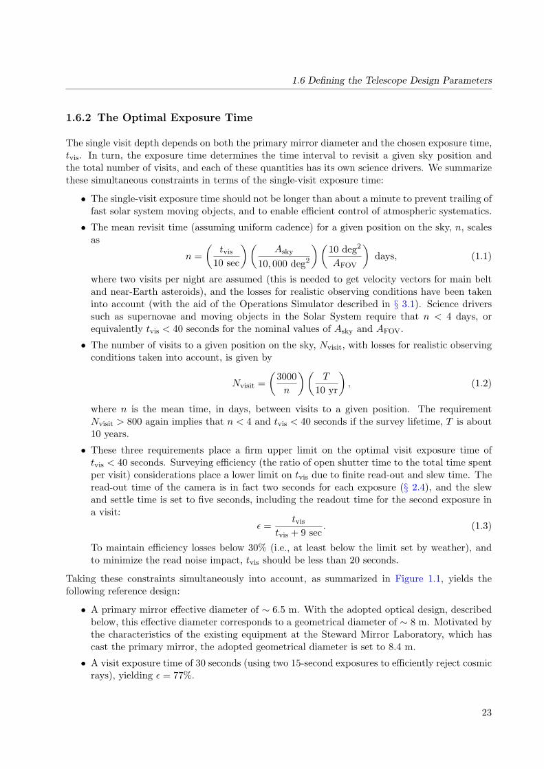
Figure 1.1: (a) The coadded depth in the r band (AB magnitudes) vs. the effective aperture and the surveylifetime. It is assumed that 22% of the total observing time (corrected for weather and other losses) is allocated forthe r band, and that the ratio of the surveyed sky area to the field-of-view area is 2,000. (b) The single-visit depth inthe r band (5σ detection for point sources, AB magnitudes) vs. revisit time, n (days), as a function of the effectiveaperture size. With a coverage of 10,000 deg2 in two bands, the revisit time directly constrains the visit exposuretime, tvis = 10n seconds; these numbers can be directly scaled to the 20,000 deg2 and six filters of LSST. In additionto direct constraints on optimal exposure time, tvis is also driven by requirements on the revisit time, n, the totalnumber of visits per sky position over the survey lifetime, Nvisit, and the survey efficiency, ε (see Equation 1.3).Note that these constraints result in a fairly narrow range of allowed tvis for the main deep-wide-fast survey. FromIvezic et al. (2008).
sources, it is more advantageous to maximize first the area and then the detection depth.2 Forthis reason, the sky area for the main survey is maximized to its practical limit, 20,000 deg2,determined by the requirement to avoid large airmasses (X ≡ sec(zenith distance)), which wouldsubstantially deteriorate the image quality and the survey depth. With the adopted field-of-viewarea, the sky coverage and the survey lifetime fixed, the primary mirror diameter is fully driven bythe required survey depth. There are two depth requirements: the final (coadded) survey depth,r ∼ 27.5, and the depth of a single visit, r ∼ 24.5. The two requirements are compatible ifthe number of visits is several hundred per band, which is in good agreement with independentscience-driven requirements on the latter. The required coadded survey depth provides a directconstraint, independent of the details of survey execution such as the exposure time per visit,on the minimum effective primary mirror diameter of 6.5 m, as illustrated in Figure 1.1. This isthe effective diameter of the LSST taking into account the actual throughput of its entire opticalsystem.
2The number of sources is proportional to area, but rises no faster than Euclidean with survey depth, which increasesby 0.4 magnitude for a doubling of exposure time in the sky-dominated regime; see Nemiroff (2003) for moredetails.
22
1.6 Defining the Telescope Design Parameters
1.6.2 The Optimal Exposure Time
The single visit depth depends on both the primary mirror diameter and the chosen exposure time,tvis. In turn, the exposure time determines the time interval to revisit a given sky position andthe total number of visits, and each of these quantities has its own science drivers. We summarizethese simultaneous constraints in terms of the single-visit exposure time:
• The single-visit exposure time should not be longer than about a minute to prevent trailing offast solar system moving objects, and to enable efficient control of atmospheric systematics.
• The mean revisit time (assuming uniform cadence) for a given position on the sky, n, scalesas
n =(
tvis
10 sec
)(Asky
10, 000 deg2
)(10 deg2
AFOV
)days, (1.1)
where two visits per night are assumed (this is needed to get velocity vectors for main beltand near-Earth asteroids), and the losses for realistic observing conditions have been takeninto account (with the aid of the Operations Simulator described in § 3.1). Science driverssuch as supernovae and moving objects in the Solar System require that n < 4 days, orequivalently tvis < 40 seconds for the nominal values of Asky and AFOV.
• The number of visits to a given position on the sky, Nvisit, with losses for realistic observingconditions taken into account, is given by
Nvisit =(
3000n
)(T
10 yr
), (1.2)
where n is the mean time, in days, between visits to a given position. The requirementNvisit > 800 again implies that n < 4 and tvis < 40 seconds if the survey lifetime, T is about10 years.
• These three requirements place a firm upper limit on the optimal visit exposure time oftvis < 40 seconds. Surveying efficiency (the ratio of open shutter time to the total time spentper visit) considerations place a lower limit on tvis due to finite read-out and slew time. Theread-out time of the camera is in fact two seconds for each exposure (§ 2.4), and the slewand settle time is set to five seconds, including the readout time for the second exposure ina visit:
ε =tvis
tvis + 9 sec. (1.3)
To maintain efficiency losses below 30% (i.e., at least below the limit set by weather), andto minimize the read noise impact, tvis should be less than 20 seconds.
Taking these constraints simultaneously into account, as summarized in Figure 1.1, yields thefollowing reference design:
• A primary mirror effective diameter of ∼ 6.5 m. With the adopted optical design, describedbelow, this effective diameter corresponds to a geometrical diameter of ∼ 8 m. Motivated bythe characteristics of the existing equipment at the Steward Mirror Laboratory, which hascast the primary mirror, the adopted geometrical diameter is set to 8.4 m.
• A visit exposure time of 30 seconds (using two 15-second exposures to efficiently reject cosmicrays), yielding ε = 77%.
23

Chapter 1: References
• A revisit time of three days on average per 10,000 deg2 of sky (i.e., the area visible at anygiven time of the year), with two visits per night (particularly useful for establishing propermotion vectors for fast moving asteroids).
To summarize, the chosen primary mirror diameter is the minimum diameter that simultaneouslysatisfies the depth (r ∼ 24.5 for single visit and r ∼ 27.5 for coadded depth) and cadence (revisittime of 3-4 days, with 30 seconds per visit) constraints described above.
References
Angel, R., Lesser, M., Sarlot, R., & Dunham, E., 2000, in Astronomical Society of the Pacific Conference Series, Vol.195, Imaging the Universe in Three Dimensions, W. van Breugel & J. Bland-Hawthorn, eds., p. 81
Carollo, D. et al., 2007, Nature, 450, 1020Helmi, A. et al., 2003, ApJ , 586, 195Ivezic, Z. et al., 2008, ArXiv e-prints, 0805.2366Madrid, J. P., & Macchetto, D., 2009, ArXiv e-prints, 0901.4552Majewski, S. R., Skrutskie, M. F., Weinberg, M. D., & Ostheimer, J. C., 2003, ApJ , 599, 1082Nemiroff, R. J., 2003, AJ , 125, 2740Perryman, M. A. C. et al., 2001, A&A, 369, 339Starr, B. M. et al., 2002, Society of Photo-Optical Instrumentation Engineers (SPIE) Conference Series, Vol. 4836,
LSST Instrument Concept, J. A. Tyson & S. Wolff, eds. pp. 228–239Strauss, M. A. et al., 2004, Towards a Design Reference Mission for the Large Synoptic Survey Telescope. A report
of the Science Working Group of the LSST prepared under the auspices of the National Optical AstronomicalObservatories, http://www.noao.edu/lsst/DRM.pdf
Tyson, J. A., 1998, in SLAC Summer Institute 1998: Gravity from the Planck Era to the Present, SLAC/DOE Pub.SLAC-R-538, http://www.slac.stanford.edu/gen/meeting/ssi/1998/man_list.html, pp. 89–112
—, 2002, Society of Photo-Optical Instrumentation Engineers (SPIE) Conference Series, Vol. 4836, Large SynopticSurvey Telescope: Overview, J. A. Tyson & S. Wolff, eds. pp. 10–20
Tyson, J. A., Wittman, D. M., & Angel, J. R. P., 2001, in Astronomical Society of the Pacific Conference Series,Vol. 237, Gravitational Lensing: Recent Progress and Future Goals, T. G. Brainerd & C. S. Kochanek, eds., p.417
Wittman, D. M., Tyson, J. A., Bernstein, G. M., Smith, D. R., & Blouke, M. M., 1998, Society of Photo-Optical Instrumentation Engineers (SPIE) Conference Series, Vol. 3355, Big Throughput Camera: the first year,S. D’Odorico, ed. pp. 626–634
York, D. G. et al., 2000, AJ , 120, 1579
24

2 LSST System Design
John R. Andrew, J. Roger P. Angel, Tim S. Axelrod, Jeffrey D. Barr, James G. Bartlett, JacekBecla, James H. Burge, David L. Burke, Srinivasan Chandrasekharan, David Cinabro, Charles F.Claver, Kem H. Cook, Francisco Delgado, Gregory Dubois-Felsmann, Eduardo E. Figueroa, JamesS. Frank, John Geary, Kirk Gilmore, William J. Gressler, J. S. Haggerty, Edward Hileman, ZeljkoIvezic, R. Lynne Jones, Steven M. Kahn, Jeff Kantor, Victor L. Krabbendam, Ming Liang, R. H.Lupton, Brian T. Meadows, Michelle Miller, David Mills, David Monet, Douglas R. Neill, MartinNordby, Paul O’Connor, John Oliver, Scot S. Olivier, Philip A. Pinto, Bogdan Popescu, VeljkoRadeka, Andrew Rasmussen, Abhijit Saha, Terry Schalk, Rafe Schindler, German Schumacher,Jacques Sebag, Lynn G. Seppala, M. Sivertz, J. Allyn Smith, Christopher W. Stubbs, Donald W.Sweeney, Anthony Tyson, Richard Van Berg, Michael Warner, Oliver Wiecha, David Wittman
This chapter covers the basic elements of the LSST system design, with particular emphasis onthose elements that may affect the scientific analyses discussed in subsequent chapters. We startwith a description of the planned observing strategy in § 2.1, and then go on to describe the keytechnical aspects of system, including the choice of site (§ 2.2), the telescope and optical design(§ 2.3), and the camera including the characteristics of its sensors and filters (§ 2.4). The keyelements of the data management system are described in § 2.5, followed by overviews of theprocedures that will be invoked to achieve the desired photometric (§ 2.6) and astrometric (§ 2.7)calibration.
2.1 The LSST Observing Strategy
Zeljko Ivezic, Philip A. Pinto, Abhijit Saha, Kem H. Cook
The fundamental basis of the LSST concept is to scan the sky deep, wide, and fast with a singleobserving strategy, giving rise to a data set that simultaneously satisfies the majority of the sciencegoals. This concept, the so-called “universal cadence,” will yield the main deep-wide-fast survey(typical single visit depth of r ∼ 24.5) and use about 90% of the observing time. The remaining10% of the observing time will be used to obtain improved coverage of parameter space such asvery deep (r ∼ 26) observations, observations with very short revisit times (∼ 1 minute), andobservations of “special” regions such as the ecliptic, Galactic plane, and the Large and SmallMagellanic Clouds. We are also considering a third type of survey, micro-surveys, that would useabout 1% of the time, or about 25 nights over ten years.
The observing strategy for the main survey will be optimized for the homogeneity of depth andnumber of visits over 20,000 deg2 of sky, where a “visit” is defined as a pair of 15-second exposures,performed back-to-back in a given filter, and separated by a four-second interval for readout andopening and closing of the shutter. In times of good seeing and at low airmass, preference is
25

Chapter 2: LSST System Design
given to r-band and i-band observations, as these are the bands in which the most seeing-sensitivemeasurements are planned. As often as possible, each field will be observed twice, with visitsseparated by 15-60 minutes. This strategy will provide motion vectors to link detections of movingobjects, and fine-time sampling for measuring short-period variability. The ranking criteria alsoensure that the visits to each field are widely distributed in position angle on the sky and rotationangle of the camera in order to minimize systematics that could affect some sensitive analyses,such as studies of cosmic shear.
The universal cadence will also provide the primary data set for the detection of near-Earth Ob-jects (NEO), given that it naturally incorporates the southern half of the ecliptic. NEO surveycompleteness for the smallest bodies (∼ 140 m in diameter per the Congressional NEO mandate1)is greatly enhanced, however, by the addition of a crescent on the sky within 10 of the northernecliptic. Thus, the “northern Ecliptic proposal” extends the universal cadence to this region usingthe r and i filters only, along with more relaxed limits on airmass and seeing. Relaxed limitson airmass and seeing are also adopted for ∼ 700 deg2 around the South Celestial pole, allowingcoverage of the Large and Small Magellanic Clouds.
Finally the universal cadence proposal excludes observations in a region of 1,000 deg2 aroundthe Galactic Center, where the high stellar density leads to a confusion limit at much brightermagnitudes than those attained in the rest of the survey. Within this region, the Galactic Centerproposal provides 30 observations in each of the six filters, distributed roughly logarithmically intime (it may not be necessary to use the bluest u and g filters for this heavily extincted region).The resulting sky coverage for the LSST baseline cadence, based on detailed operations simulationsdescribed in § 3.1, is shown for the r band in Figure 2.1. The anticipated total number of visitsfor a ten-year LSST survey is about 2.8 million (∼ 5.6 million 15-second long exposures). Theper-band allocation of these visits is shown in Table 1.1.
Although the uniform treatment of the sky provided by the universal cadence proposal can satisfythe majority of LSST scientific goals, roughly 10% of the time may be allocated to other strategiesthat significantly enhance the scientific return. These surveys aim to extend the parameter spaceaccessible to the main survey by going deeper or by employing different time/filter sampling.
In particular, we plan to observe a set of “deep drilling fields,” whereby one hour of observingtime per night is devoted to the observation of a single field to substantially greater depth inindividual visits. Accounting for read-out time and filter changes, about 50 consecutive 15-secondexposures could be obtained in each of four filters in an hour. This would allow us to measure lightcurves of objects on hour-long timescales, and detect faint supernovae and asteroids that cannotbe studied with deep stacks of data taken with a more spread-out cadence. The number, location,and cadence of these deep drilling fields are the subject of active discussion amongst the LSSTScience Collaborations; see for example the plan suggested by the Galaxies Science Collaborationat § 9.8. There are strong motivations, e.g., to study extremely faint galaxies, to go roughly twomagnitudes deeper in the final stacked images of these fields than over the rest of the survey.
These LSST deep fields will have widespread scientific value, both as extensions on the main surveyand as a constraint on systematics. Having deeper data to treat as a model will reveal critical
1H.R. 1022: The George E. Brown, Jr. Near-Earth Object Survey Act;http://www.govtrack.us/congress/bill.xpd?bill=h109-1022
26

2.2 Observatory Site
Figure 2.1: The distribution of the r band visits on the sky for one simulated realization of the baseline mainsurvey. The sky is shown in Aitoff projection in equatorial coordinates and the number of visits for a 10-year surveyis color-coded according to the inset. The two regions with smaller number of visits than the main survey (“mini-surveys”) are the Galactic plane (arc on the left) and the so-called “northern Ecliptic region” (upper right). Theregion around the South Celestial Pole will also receive substantial coverage (not shown here).
systematic uncertainties in the wider LSST survey, including photometric redshifts, that impact themeasurements of weak lensing, clustering, galaxy morphologies, and galaxy luminosity functions.
A vigorous and systematic research effort is underway to explore the enormously large parameterspace of possible survey cadences, using the Operations Simulator tool described in § 3.1. Thecommissioning period will be used to test the usefulness of various observing modes and to explorealternative strategies. Proposals from the community and the Science Collaborations for specializedcadences (such as mini-surveys and micro-surveys) will also be considered.
2.2 Observatory Site
Charles F. Claver, Victor L. Krabbendam, Jacques Sebag, Jeffrey D. Barr, Eduardo E. Figueroa,Michael Warner
The LSST will be constructed on El Penon Peak (Figure 2.2) of Cerro Pachon in the NorthernChilean Andes. This choice was the result of a formal site selection process following an extensivestudy comparing seeing conditions, cloud cover and other weather patterns, and infrastructureissues at a variety of potential candidate sites around the world. Cerro Pachon is located tenkilometers away from Cerro Tololo Inter-American Observatory (CTIO) for which over ten yearsof detailed weather data have been accumulated. These data show that more than 80% of the nightsare usable, with excellent atmospheric conditions. Differential image motion monitoring (DIMM)measurements made on Cerro Tololo show that the expected mean delivered image quality is 0.67′′
in g (Figure 2.3).
27

Chapter 2: LSST System Design
Figure 2.2: Artist’s rendering of the LSST and dome enclosure on the summit of Cerro Pachon. The Auxiliarycalibration telescope (§ 2.6) is also illustrated on a neighboring peak. (Image Credit: Michael Mullen Design, LSSTCorporation.)
Cerro Pachon is also the home of the 8.2-m diameter Gemini-South and 4.3-m diameter SouthernAstrophysical Research (SOAR) telescopes. Observations with those telescopes have confirmedthe excellent image quality that can be obtained from this site. In addition, LSST will benefitfrom the extensive infrastructure that has been created on Cerro Pachon and La Serena to supportthese other facilities. The property is owned by the Association of Universities for Research inAstronomy (AURA), which also supports operation of CTIO, Gemini-South, and SOAR.
The LSST Observatory as a whole will be distributed over four sites: the Summit Facility on ElPenon, the Base Facility, the Archive Center, and the Data Centers. The Base Facility will be at theAURA compound in the town of La Serena, 57 km away from the mountain. The Archive Centerwill be at the National Center for Supercomputing Applications (NCSA) on the campus of theUniversity of Illinois at Urbana-Champaign. There will be two Data Centers, one co-located withthe Archive Center at NCSA, and one at the Base Facility in La Serena. Although the four facilitiesare distributed geographically, they are functionally connected via dedicated high-bandwidth fiberoptic links.
2.3 Optics and Telescope Design
Victor L. Krabbendam, Charles F. Claver, Jacques Sebag, Jeffrey D. Barr, John R. Andrew, Srini-vasan Chandrasekharan, Francisco Delgado, William J. Gressler, Edward Hileman, Ming Liang,
28

2.3 Optics and Telescope Design
Figure 2.3: The distribution of “seeing” (FWHM of the image of a point source) at 500 nm based on ten years ofmeasurements from CTIO (10 km from the LSST site). The red curve shows results from a Differential Image MotionMonitor (DIMM), while the blue curve shows the delivered image quality. The mean is 0.67′′, and the median is0.59′′.
Michelle Miller, David Mills, Douglas R. Neill, German Schumacher, Michael Warner, OliverWiecha, Lynn G. Seppala, J. Roger P. Angel, James H. Burge
The LSST optical design shown in Figure 2.4 is a modified Paul-Baker three-mirror system (M1,M2, M3) with three refractive lenses (L1, L2, L3) and a color filter before the sensor at thefocal plane. Conceptually, it is a generalization of the well-known Mersenne-Schmidt family ofdesigns and produces a large field of view with excellent image quality (Wilstrop 1984; Angel et al.2000; Seppala 2002). Spot diagrams are shown in the figure inset; these are made quantitative inFigure 2.5, which shows the encircled energy diameters at 50% and 80% in each filter as deliveredby the baseline optical design. The uniformity across the field is striking.
The LSST etendue (including the effects of camera vignetting) is 319 m2deg2. The effective focallength of the optical system is 10.3 m, making the final f/number 1.23. The plate scale is 50microns per arcsecond at the focal surface. This choice of effective focal length represents anoptimum balance of image sampling, overall system throughput, and manufacturing feasibility.The on-axis collecting area is 35 m2, equivalent to a 6.7-m diameter unobscured clear aperture.
The primary mirror (M1) is 8.4 m in diameter with a 5.1-m inner clear aperture. The tertiarymirror (M3) is 5 m in diameter. The relative positions of M1 and M3 were adjusted during thedesign process so that their surfaces meet with no axial discontinuity at a cusp, allowing M1 andM3 to be fabricated from a single substrate (see Figure 2.6). The 3.4-m convex secondary mirror(M2) has a 1.8-m inner opening. The LSST camera is inserted through this opening in order toaccess the focal surface.
The three reflecting mirrors are followed by a three-element refractive system that corrects fieldflatness and chromatic aberrations introduced by the filter and vacuum window. The 3.5 field of
29

Chapter 2: LSST System Design
Figure 2.4: The optical design configuration showing the telescope (left) and camera (right) layouts. Diffractionimages in r for three field radii, 0, 1.0, and 1.75 degrees, are shown in boxes 0.6 arcseconds square (3× 3 pixels).
view (FOV) covers a 64-cm diameter flat focal surface. Spectral filters reside between the secondand third refractive lens as shown on the right side of Figure 2.4.
The image brightness is constant to a field radius of 1.2 degrees and gradually decreases afterwardby about 10% at the 1.75-degree field edge. The intrinsic image quality from this design is excellent.The design also has very low geometrical distortion, with the distortion in scale ∆l/l < 0.1% overthe full FOV, making the LSST an excellent system for positional astrometry.
There are five aspheric surfaces in the optical design: each of the three mirror surfaces and onesurface each on two of the camera lenses. The asphericity on the two concave surfaces of M1and M3 are well within standard fabrication methods used for astronomical mirrors. During theoptimization process, the asphericity of M2 was minimized to 18.9 microns of departure from thebest-fit sphere in order to reduce the technical challenge for this optic. The three fused-silicarefractive elements, which have clear apertures of 1.55 m, 1.10 m, and 0.72 m, while large, donot present any particular challenge in their fabrication. The 0.75-m diameter spectral filter islocated just prior to L3. The filter thickness varies from 13.5 to 26.2 mm depending on the choiceof spectral band, and is used to maintain the balance of lateral chromatic aberration. The zero-power meniscus shape of the filters keeps the filter surface perpendicular to the chief ray over thefull field of view. This feature minimizes shifting of the spectral band wavelength with field angle.The last refractive element, L3, is used as the vacuum barrier to the detector cryostat. The centralthickness of L3 is 60 mm to ensure a comfortable safety margin in supporting the vacuum stresses.
The proposed LSST telescope is a compact, stiff structure with a powerful set of drives, makingit one of the most accurate and agile large telescopes ever built. The mount is an altitude overazimuth configuration (Figure 2.7). The telescope structure is a welded and bolted steel systemdesigned to be a stiff metering structure for the optics and a stable platform for observing (Neill2006, 2008). The primary and tertiary mirrors are supported in a single cell below the elevationring; the camera and secondary mirror are supported above it. The design accommodates some on-telescope servicing as well as efficient removal of the mirrors and camera, as complete assemblies,for periodic maintenance.
30

2.3 Optics and Telescope Design
Figure 2.5: The 50% (plain symbols) and 80% (symbols with lines) encircled energy diameter as a function ofradius in the field of view for the LSST baseline optical design. The image scale is 50 microns per arcsec, or 180 mmper degree.
Figure 2.6: Design and dimensions of the primary and tertiary mirror, showing that the two are built out of asingle mirror blank.
The stiffness of this innovative design is key to achieving a slew and settle time that is beyond thecapability of today’s large telescopes. The size and weight of the systems are a particular challenge,but the fast optical system allows the mount to be short and compact. Finite element analysis hasbeen used to simulate the vibrational modes of the telescope system, including the concrete pier.The frequencies of the four modes with largest amplitudes are (in order):
• 8.3 Hz: Transverse telescope displacement;
• 8.7 Hz: Elevation axis rotation;
• 11.9 Hz: Top end assembly optical axis pumping; and
• 12.6 Hz: Camera pivot.
As described in § 2.1, the standard visit time in a given field is only 34 seconds, quite short for mosttelescopes. The time required to reorient the telescope must also be short to keep the fraction oftime spent in motion below 20% (§ 1.6.2). The motion time for a nominal 3.5 elevation move and
31

Chapter 2: LSST System Design
Figure 2.7: Rendering of the telescope, showing mirror support structures, top end camera assembly, and integratedbaffles.
a 7 azimuth move is five seconds. In two seconds, a shaped control profile will move the telescope,which will then settle down to less than 0.1′′ pointing error in three seconds. The stiffness ofthe support structure and drive system has been designed to limit the amplitude and damp outvibrations at these frequencies within this time. The mount uses 400 horsepower in the azimuthdrive system and 50 horsepower in the elevation system. There are four motors per axis configuredin two sets of opposing pairs to eliminate hysteresis in the system. Direct drive systems werejudged overly complicated and too excessive, so the LSST design has each motor working througha multi-stage gear reduction, with power applied through helical gear sets. The 300-ton azimuthassembly and 151-ton elevation assembly are supported on hydrostatic bearings. Each axis usestape encoders with 0.001′′ resolution. Encoder ripple from these tapes often dominates controlsystem noise, so LSST will include adaptive filtering of the signal in the control loop. All-skypointing performance will be better than 2′′. Pointing will directly impact trailing and imagingsystematics for LSST’s wide field of view, so accurate pointing is key to tracking performance.Traditional closed loop guiding will achieve the final level of tracking performance.
2.4 Camera
Kirk Gilmore, Steven M. Kahn, John Geary, Martin Nordby, Paul O’Connor, John Oliver, Scot S.Olivier, Veljko Radeka, Andrew Rasmussen, Terry Schalk, Rafe Schindler, Anthony Tyson, RichardVan Berg
The LSST camera, shown in Figure 2.8, contains a 3.2-gigapixel focal plane array (Figure 2.9)comprised of 189 4 K× 4 K CCD sensors with 10 µm pixels. The focal plane is 0.64 m in diameter,and covers 9.6 deg2 field-of-view with a plate scale of 0.2′′ pixel−1. The CCD sensors are deepdepletion, back-illuminated devices with a highly segmented architecture, 16 channels each, thatenable the entire array to be read out in two seconds (Figure 2.10).
32

2.4 Camera
Figure 2.8: Cutaway drawing of the LSST camera. The camera body is approximately 1.6 m in diameter and 3.5m in length. The optic, L1, is 1.57 m in diameter.
Figure 2.9: With its 189 sensors, each a 4 K × 4 K charge-coupled device (CCD), the focal plane of the cameraimages 9.6 deg2 of the sky per exposure. Note the presence of wavefront sensors, which are fed back to the mirrorsupport/focus system, and the guide sensors, to keep the telescope accurately tracking on a given field.
33

Chapter 2: LSST System Design
Figure 2.10: A schematic of the LSST sensor, showing the segmentation into 16 channels, each of which is read outin parallel.
The detectors are grouped into 3×3 arrays called “rafts.” All the rafts are identical; each containsits own dedicated front-end and back-end electronics boards, which fit within the footprint of itssensors, thus serving as a 144-Megapixel camera on its own. The rafts and associated electronicsare mounted on a silicon carbide grid inside a vacuum cryostat, with an intricate thermal controlsystem that maintains the CCDs at an operating temperature of −100C. The grid also containstwo guide sensors and a wavefront sensor positioned at each of the four corners at the edge of thefield. The entrance window to the cryostat is the third of three refractive lenses, L3 in Figure 2.8.The other two lenses, L1 and L2, are mounted in an “optics housing” at the front of the camerabody. The camera body also contains a mechanical shutter and a filter exchange system holdingfive large optical filters, any of which can be inserted into the camera field of view for a givenexposure. The system will in fact have six filters; the sixth filter can replace any of the five via anautomated procedure accomplished during daylight hours.
2.4.1 Filters
The LSST filter complement (u, g, r, i, z, y) is modeled on the system used for the SDSS (Fukugitaet al. 1996), which covers the available wavelength range with roughly logarithmic spacing whileavoiding the strongest telluric emission features and sampling the Balmer break. Extension of theSDSS system to longer wavelengths (y-band) is possible because the deep-depletion CCDs havehigh sensitivity to 1 µm (Figure 2.11).
The current LSST baseline design has a goal of 1% relative photometric calibration (§ 1.5), which
34

2.4 Camera
Table 2.1: Design of Filters: Transmission Points in nanometers
Filter Blue Side Red Side Comments
u 320 400 Blue side cut-off depends on AR coating
g 400 552 Balmer break at 400 nm
r 552 691 Matches SDSS
i 691 818 Red side short of sky emission at 826 nm
z 818 922 Red side stop before H2O bands
y 950 1080 Red cut-off before detector cut-off
Figure 2.11: The left panel shows the transmission efficiency of the ugrizy filters by themselves as calculated frommodels of the filter performance. The total throughput, accounting for the transmission through the atmosphereat the zenith, the reflectivity of the reflective optics, the transmissivity of the refractive optics, and the quantumefficiency of the sensors is displayed in the panel on the right.
drives the requirements on the filter set. The filter set wavelength design parameters and theapproximate FWHM transmission points for each filter are given in Table 2.1 and in Figure 2.11.
The filters consist of multi-layer dielectric interference coatings deposited on fused silica substrates.The baseline design has the first surface of the filters concentric about the chief ray in order to keepthe angles of the light rays passing through the filters as uniform as possible over the entire rangeof field positions. The central thickness and the curvature of the second surface are optimized forimage quality.
2.4.2 Sensors
The heart of the camera is the science sensor. Its key characteristics are as follows:
High quantum efficiency from 320 to 1080 nm. This is achieved using a large depletion depth(100 µm) and implementation of the sensor in a back-illuminated configuration with a thin entrancewindow.
Minimal detector contribution to the point spread function. To reduce charge diffusion, the sensoris fully depleted, and a high internal field is maintained within the depletion region. This is made
35

Chapter 2: LSST System Design
possible by the use of high resistivity substrates, high applied voltages, and back-side contacts.Light spreading prior to photo-conversion at longer wavelengths is a minor contributor at the100 µm depletion depth.
Tight flatness tolerances. The fast LSST beam (f/1.23) yields a short depth of field, requiring< 10 µm peak-to-valley focal plane flatness with piston, tip, and tilt adjustable to ∼ 1µm. Thisis achieved through precision alignment and mounting both within the rafts, and within the focalplane grid.
High fill factor. A total of 189 4 K × 4 K sensors are required to cover the 3200 cm2 focal plane.To maintain high throughput, the sensors are mounted in four-side buttable packages and arepositioned in close proximity to one another with gaps of less than a few hundred µm. Theresulting “fill factor,” i.e., the fraction of the focal plane covered by pixels, is 93%.
Fast readout. The camera is read out in two seconds. To reduce the read noise associated withhigher readout speeds, the sensors are highly segmented. The large number of I/O connections thenrequires that the detector electronics be implemented within the cryostat to maintain a manageablenumber of vacuum penetrations.
Our reference sensor design is a CCD with a high degree of segmentation, as illustrated in Fig-ure 2.10. A 4 K × 4 K format was chosen because it is the largest footprint consistent with goodyield. Each amplifier will read out 1,000,000 pixels (a 2000×500 sub-array), allowing a pixel read-out rate of 500 kHz per amplifier. The sensors are mounted on aluminum nitride (AlN) packages.Traces are plated directly to the AlN insulator to route signals from the CCD to the connectorson the back of the package. The AlN package provides a stiff, stable structure that supports thesensor, keeps it flat, and extracts heat via a cooling strap.
2.4.3 Wavefront Sensing and Guiding
Four special purpose rafts, mounted at the corners of the science array, contain wavefront sensorsand guide sensors (Figure 2.9). Wavefront measurements are accomplished using curvature sensing,in which the spatial intensity distribution of stars is measured at equal distances on either sideof focus. Each curvature sensor is composed of two CCD detectors, with one positioned slightlyabove the focal plane, the other positioned slightly below the focal plane. The CCD technology forthe curvature sensors is identical to that used for the science detectors in the focal plane, exceptthat the curvature sensor detectors are half-size so they can be mounted as an in-out defocus pair.Detailed analyses have verified that this configuration can reconstruct the wavefront to the requiredaccuracy. These four corner rafts also hold two guide sensors each. The guide sensors monitor thelocations of bright stars at a frequency of ∼ 10 Hz to provide feedback for a loop that controlsand maintains the tracking of the telescope at an accurate level during an exposure. The baselinesensor for the guider is the Hybrid Visible Silicon hybrid-CMOS detector. We have carried outextensive evaluation to validate that its characteristics (including wide spectral response, high fillfactor, low noise, and wide dynamic range) are consistent with guiding requirements.
36

2.5 Data Management System
2.5 Data Management System
Tim S. Axelrod, Jacek Becla, Gregory Dubois-Felsmann, Zeljko Ivezic, R. Lynne Jones, Jeff Kan-tor, R. H. Lupton, David Wittman
The LSST Data Management System (“DMS”) is required to generate a set of data products andto make them available to scientists and the public. To carry out this mission the DMS performsthe following major functions:
• Continually processes the incoming stream of images generated by the camera system duringobserving to produce transient alerts and to archive the raw images.
• Roughly once per year2, creates and archives a Data Release (“DR”), which is a static self-consistent collection of data products generated from all survey data taken from the date ofsurvey initiation to the cutoff date for the Data Release. The data products include optimalmeasurements of the properties (shapes, positions, fluxes, motions) of all objects, includingthose below the single visit sensitivity limit, astrometric and photometric calibration of thefull survey object catalog, and limited classification of objects based on both their staticproperties and time-dependent behavior. Deep coadded images of the full survey area areproduced as well.
• Periodically creates new calibration data products, such as bias frames and flat fields, thatwill be used by the other processing functions.
• Makes all LSST data available publicly through an interface and databases that utilize, tothe maximum possible extent, community-based standards such as those being developedby the Virtual Observatory (“VO”), and facilitates user data analysis and the production ofuser-defined data products at Data Access Centers and at external sites.
The geographical layout of the DMS facilities is shown in Figure 2.12; the facilities include theMountain Summit/Base Facility at Cerro Pachon and La Serena, the central Archive Center atNCSA, the Data Access Centers at NCSA and La Serena, and a System Operations Center. Thedata management system begins at the data acquisition interface between the camera and telescopesubsystems and flows through to the data products accessed by end users. On the way, it movesthrough three types of managed facilities supporting data management, as well as end user sites thatmay conduct science using LSST data or pipeline resources on their own computing infrastructure.
• The data will be transported over existing high-speed optical fiber links from the MountainSummit/Base Facility in Chile to the archive center in the U.S. Data will also flow from theMountain Summit/Base Facility and the archive center to the data access centers over existingfiber optic links. The Mountain Summit/Base Facility is composed of the mountaintoptelescope site, where data acquisition must interface to the other LSST subsystems, and theBase Facility, where rapid-turnaround processing will occur for data quality assessment andnear real-time alerts.
• The Archive Center is a super-computing-class data center with high reliability and avail-ability. This is where the data will undergo complete processing and re-processing andpermanent storage. It is also the main repository feeding the distribution of LSST data tothe community.
2In the first year of operations, we anticipate putting out data releases every few months.
37

Chapter 2: LSST System Design
Figure 2.12: A schematic map of the LSST DMS facilities. The LSST Telescope Site, located on Cerro Pachon,Chile, is connected to the Base Facility, located in La Serena, Chile by a dedicated fiber link. The Base Facility isconnected to the Archive Center, located at the National Center for Supercomputing Applications in Illinois usingcommercial high-speed network links. The Archive Center, in turn, fans out data to Data Access Centers whichserve the data to clients, and may be located anywhere in the world. The System Operations Center monitors andcontrols the overall operation of the DMS facilities, and provides end-user support facilities.
• Data Access Centers for broad user access are envisioned, according to a tiered access model,where the tiers define the capacity and response available especially to computationally ex-pensive queries and analyses. There are two project-funded Data Access Centers co-locatedwith the Base Facility and the Archive Center. These centers provide replication of all of theLSST data to ensure that disaster recovery is possible. They provide Virtual Observatoryinterfaces to the LSST data products. LSST is encouraging non-US/non-Chilean fundingfor potential partner institutions around the world to host additional Data Access Centers,which could increase end user access bandwidth, provide local high-end computation, andhelp amortize observatory operations costs.
• The System Operations Center provides a control room and large-screen display for super-visory monitoring and control of the DM System. Network and facility status are availableas well as the capability to “drill down” to individual facilities. The Center will also provideDM support to observatory science operations, as well as an end user help desk.
2.5.1 LSST Data Product Overview
Level 1, 2, and 3 Data Products
The data products are organized into three groups, based largely on where and when they areproduced.
38

2.5 Data Management System
• Level 1 products are generated by pipeline processing the stream of data from the camerasystem during normal observing. Level 1 data products are, therefore, continuously generatedand/or updated every observing night. This process is of necessity highly automated, andmust proceed with absolutely minimal human interaction. Level 1 products include alerts,i.e., announcements that the flux or position of a given object has changed significantlyrelative to the long-term average. The alerts will be released within 60 seconds of the closingof the shutter at the end of a visit (§ 1.5). In addition to science data products, a numberof Level 1 science data quality assessment (“SDQA”) data products are generated to assessquality and to provide feedback to the Observatory Control System.
• Level 2 products are generated as part of a yearly Data Release. Level 2 products useLevel 1 products as input, and include data products for which extensive computation isrequired (such as variability information, detection, and measurement of the properties offaint objects, and so on), often because they combine information from the stack of manyexposures. Although the steps that generate Level 2 products will be automated, significanthuman interaction may be required at key points to ensure the quality of the data.
• Level 3 data products are derived from Level 1 and/or Level 2 data products to supportparticular science goals, often requiring the combination of LSST data across significant ar-eas on the sky. The DMS will facilitate the creation of Level 3 data products, for exampleby providing suitable Applications Programming Interfaces (APIs) and computing infras-tructure, but is not itself required to create any Level 3 data product. Instead these dataproducts are created externally to the DMS, using software written by, for example, sciencecollaborations. Once created, Level 3 data products may be associated with Level 1 andLevel 2 data products through database federation3. In rare cases, the LSST Project, withthe agreement of the Level 3 creators, may decide to incorporate Level 3 data products intothe DMS production flow, thereby promoting them to Level 2 data products.
Level 1 and Level 2 data products that have passed quality control tests will be accessible tothe public without restriction. Additionally, the source code used to generate them will be madeavailable, and LSST will provide support for building the software system on selected platforms.The access policies for Level 3 data products will be product- and source-specific, and in somecases will be proprietary.
Overview of Pipeline Processing
In the overall organization of the DMS pipelines and productions, “production” has a particularmeaning: it is a coordinated group of pipelines that together carry out a large-scale DMS function.
Alert Production Astronomers interested in transient phenomena of many sorts (Chapter 8)need to know of objects whose flux has changed significantly as soon as possible after the dataare taken. Therefore, the most visible aspect of Level 1 processing is the production of alerts, i.e.,announcements of such variability. The Alert Production is directly fed by the output data streamfrom the camera Science Acquisition System (SDS) during observing. This data stream contains
3See Wikipedia’s article on the subject at http://en.wikipedia.org/wiki/Federated_database.
39

Chapter 2: LSST System Design
both unprocessed (raw) camera images, and images that have been corrected for crosstalk by theSDS on the mountain. At the end of a visit, the Alert Production:
• Acquires the raw science images from the camera, and moves them to the Archive Center forpermanent storage.
• Processes the crosstalk-corrected images from the camera to detect transient events within60 seconds of shutter closure for the second exposure in a visit. This will probably be donewith a variant of the Alard & Lupton (1998) image-subtraction algorithm.
• Packages catalog information, together with postage-stamp images of detected transients asalerts and past history of the object, and distributes them to the community as VO events.
• Continuously assesses the data quality of the data stream.
The major steps in the processing flow are:
• Image processing of the raw exposures to remove the instrumental signature, such as bias,flat-field, bad columns, and so on.
• Determination of the World Coordinate System (WCS), image Point-Spread Function (PSF),and rough photometric zeropoint. This produces processed exposures.
• Subtraction of a registered template exposure (a co-addition of previous high-quality imagesof a given field, created in an earlier data release) from the processed exposure, producing adifference exposure.
• Detection of sources (both positive and negative!) in the difference exposure, producing whatwe refer to hereafter as “DIASources.”
• Visit processing logic, which compares the DIASources from the two exposures in the visitto discriminate against cosmic rays, and to flag very rapidly moving Solar System objects.
• “FaintSources,” abbreviated measurements of low signal-to-noise ratio (S/N) detections, areproduced for objects of particular interest, e.g., predicted positions for Solar System objects,or objects that have previously produced alerts.
• Comparison of positive flux DIASources with predictions from the Moving Object Pipeline(MOPS; see § 2.5.3) for already known Solar System objects, as contained in the MovingObject table.
• The Association Pipeline is run to match DIASources to already known astronomical objects,as contained in the Object table.
• DIASources that are detected in both exposures of a visit, and are not matched to a knownSolar System object, produce an alert.
• Quality Assessment is performed at every pipeline stage, stored in database tables, and fedto the Observatory Control System as required.
• The Moving Object Pipeline (§ 2.5.3) is run during the day to interpret each new detectionof a moving object as a new measurement of a Solar System object already in the MovingObject table, or as a previously unknown object, which will be added to the Moving Objecttable. All orbits are refined based on the new measurements from the night.
40

2.5 Data Management System
The community has strongly expressed the preference that alerts not be significantly filtered priorto distribution so that science opportunities are not closed off. We have, therefore, adopted verysimple criteria for issuing an alert: 5σ DIASources seen in both exposures of a visit which are notconsistent with cosmic ray events.
Note that no explicit classification of an alert is provided, but users can readily construct classifiersand filters based on information in the Science Database; indeed, this is likely to be part of Level 3software produced by the transient, stellar populations, and supernova science collaborations. Theinformation that could be used for this classification includes the light curve, colors, and shapeinformation for the associated object. Additionally, database queries can readily be formulatedwhich will identify exposures that have generated anomalously large numbers of alerts, presumablydue to image artifacts or processing problems.
As the raw images arrive at the Archive Center, the same processing flow is performed there, withthe consistency of the databases at the Base and Archive Centers being periodically checked. Theduplication of processing is carried out to reduce the data bandwidth required between the Baseand Archive Centers.
Data Release Production At yearly intervals (more often during the first year of the survey)a new Data Release (DR) is produced. A DR includes all data taken by the survey from day oneto the cutoff date for the DR, and is a self-contained set of data products, all produced with thesame pipeline software and processing parameters. The major steps in the processing flow are:
• As in the Alert Production, all raw exposures from the camera are processed to remove theinstrumental signature, and to determine the WCS and PSF, producing processed exposures.This is done with the best available calibration products, which in general will be superiorto those available when the processing was initially done.
• The survey region is tessellated into a set of sky patches of order the size of a CCD, andseveral co-added exposures are produced for each patch from the processed exposures. Theseare a per-band template co-add used for image subtraction; a detection co-add used in theDeep Detection Pipeline (see next item), possibly per-band; and a RGB co-add used forvisualization.
• The Deep Detection Pipeline is run, populating the Object, Source, and FaintSource tables.Rather than working from the co-add, Deep Detection will use the “Multifit” algorithm(§ 2.5.2; Tyson et al. 2008), whereby a model (e.g., a PSF for a stellar object or an exponentialprofile for a disk galaxy) is fit to the entire stack of exposures which contain the object. Thuseach exposure is fit using its own PSF; this results in a set of optimal measurements of theobject attributes over the full time span of the survey, including astrometric parameters suchas proper motion and parallax.
• The Image Subtraction Pipeline is run, as in the Alert Production, yielding DIASources andFaintSources for transient objects.
• The Moving Object Pipeline is run on DIASources, to yield a complete set of orbits for SolarSystem Objects in the Moving Object table.
41

Chapter 2: LSST System Design
• The Photometric Calibration Pipeline is run on the full set of measurements in the Source,DIASource, and FaintSource catalogs, incorporating measurements from the Auxiliary Tele-scope and other sources of data about the atmosphere to perform a global photometriccalibration of the survey (§ 2.6). In addition to accurate photometry for every measurement,this yields an atmosphere model for every exposure.
2.5.2 Detection and Measurement of Objects
Here we provide more detail on the specific algorithms used to define and measure object propertiesthat are issued with the Data Releases:
Deep Detection Processing
The survey region is organized into overlapping sky patches of order the size of a CCD, and a deepco-added image is created for each patch. The details of the co-add algorithm are still undecided,but the current baseline is to use the Kaiser (2004) algorithm on the full stack of survey imagescontained within the Data Release. The Kaiser algorithm convolves each image with the reflectionof its PSF, and then accumulates with weight inversely proportional to the sky variance. Care willbe taken to ensure that rapidly moving objects, such as Solar System objects, do not appear inthe co-add. An object detection algorithm is then run on the co-add, generating an initial Objectcatalog. An “Object” at this stage is nothing more than a pixel footprint on the sky, possibly withlinks to related Objects in a segmentation tree that has been created by segmenting (deblending)overlapping Objects. The tree will be organized so that the root node is the largest object inthe hierarchy, with the leaf nodes being the smallest. The segmentation/deblending algorithm tobe employed is still under investigation, with Sextractor (Bertin & Arnouts 1996) or the SDSSphotometric pipeline (Stoughton et al. 2002) being examples of the kind of processing involved.The properties of the Objects that are segmented in this way are then determined with Multifitas described below.
Difference Exposure Processing
A new object is created whenever a transient source that is detected in both difference images froma visit does not match any object already in the table. The match will take account of extendednessas well as position on the sky, so that a new point source at the location of a galaxy already in thecatalog (for example, due to a supernova or variable AGN) will result in a new object.
Note that this process cannot be perfect, since measuring the extendedness of objects near thePSF size will always be uncertain. Consequently, there will be cases where flux from a supernovaor AGN point source will be incorrectly added to the underlying galaxy rather than to a new pointsource. Between successive Data Releases, however, these errors will decrease in severity: As thesurvey goes deeper, and accumulates images in better seeing, extendedness will be better measuredby the Multifit procedure, as discussed below.
42

2.5 Data Management System
Measuring the Properties of Objects
The image pixels containing an object from all relevant exposures are fit to one or more objectmodels using Multifit, generating model parameters and a covariance matrix. Our choice of modelsis driven by astrophysics, by characteristics of the LSST system, and by computing practicalities.The initial model types are as follows:
Slowly Moving Point Source Model. The Slowly Moving Point Source (SMPS) Model isintended to account for the time varying fluxes and motion on the sky of point sources (usuallystars) with proper motions between zero and roughly 10′′ yr−1. The model accounts for motion withrespect to the local astrometric reference frame that is generated by proper motion, parallax, andpossibly orbital motion with respect to a binary companion. The object properties are measuredin every exposure that contains it. If the S/N in the exposure is above a predetermined threshold,perhaps 5, the measurement generates a row in the Source table. If the S/N is lower than thethreshold, a FaintSource row is generated instead. Lang et al. (2009) have successfully used asimilar modeling and measurement approach to detect very faint brown dwarfs with high propermotion.
The SMPS Model will be fit only to objects that are leaf nodes in the segmentation tree.
Small Object Model. The Small Object (SO) Model is intended to provide a robust parametriza-tion of small (diameter < 1′) galaxy images for weak lensing shear measurement and determinationof photometric redshifts. The definition of the model flux profile is still undecided (Sersic profiles?Superpositions of exponential and de Vaucouleurs profiles?), but should be driven by the needs ofphotometric redshifts (§ 3.8). The measurement of the elliptical shape parameters will be drivenby the needs of weak lensing (Chapter 14).
The SO Model will be fit only to objects that are leaf nodes in the segmentation tree.
Large Object Model. A “large” object is one for which the 20 mag/arcsec2 isophotal diameteris greater than 1′, and less than 80% of the patch size. This includes, for example, the majorityof NGC galaxies. The vast majority of the LSST science will be accomplished with measurementsmade using the SMPS and SO Models, but much valuable science and numerous EPO applicationswill be based on larger objects found in LSST images. To at least partially satisfy this need, largeobjects will have entries in the Object table, but will not have any model fitting performed byMultifit.
Solar System Model. The predicted ephemerides from the orbit for an object in the movingobject table constitutes an object model which is used to measure the object properties in each ex-posure that contains the object. It is not yet decided whether the measurements of faint detectionsshould be at a position entirely fixed by the orbit prediction, or should be allowed to compensatefor prediction error by “peaking up” within some error bound around the prediction.
The Multifit Algorithm
Objects are detected on co-added images, but their models will be fit to the full data set ofexposures on which they appear (n ∼ 400 at the end of the survey in each filter). The motivationfor doing this is two-fold (Tyson et al. 2008). First, the co-add will have a very complicated and
43

Chapter 2: LSST System Design
discontinuous PSF and depth patchiness due to detector gaps and masked moving objects. Second,although the Kaiser co-add algorithm is a sufficient statistic for the true sky under the assumptionsthat sky noise dominates, and is Gaussian, those assumptions do not strictly hold in real data.
An initial model will be fit to the co-add, to provide a good starting point for the fit to the full dataset. Multifit will then read in all the pixels from the n exposures and perform a maximum likelihoodfit for the model which, when convolved with the n PSFs, best matches the n observations. Thisnaturally incorporates the effects of varying seeing, as the contribution of the better-seeing imagesto the likelihood will be sharper. This approach also facilitates proper accounting for masked areas,cosmic rays, and so on. The best-fit model parameters and their uncertainties will be recorded inan Object table row.
Model Residuals
The measurement process will produce, in conjunction with every source, a residual image thatis the difference of the associated image pixels and the pixels predicted from the model over thefootprint of the model. Characterizing these residuals is important for science such as stronglensing and merging galaxies, that will identify interesting candidates for detailed analysis throughtheir residuals. Selecting the most useful statistical measures of the residuals will be the outcomeof effort during the continuing design and development phase of the project.
2.5.3 The Moving Object Processing System (MOPS)
Identifying moving objects and linking individual detections into orbits, at all distances and solarelongations, would be a daunting task for LSST without advanced software. Each observation fromthe telescope is differenced against a “template” image (built from many previous observations),allowing detection of only transient, variable, or moving objects in the result. These detections arefed into the Moving Object Processing System (MOPS), which attempts to link these individualdetections into orbits.
MOPS uses a three-stage process to find new moving objects (Kubica 2005; Kubica et al. 2005,2007). In the first stage, intra-night associations are proposed by searching for detections forminglinear “tracklets.” By using loose bounds on the linear fit and the maximum rate of motion,many erroneous initial associations can be ruled out. In the current model of operations, LSSTwill revisit observed fields twice each night, with approximately 20–45 minutes between theseobservations. These two detections are what are linked into tracklets. In the second stage, inter-night associations are proposed by searching for sets of tracklets forming a quadratic trajectory.Again, the algorithm can efficiently filter out many incorrect associations while retaining most ofthe true associations. However, the use of a quadratic approximation means that a significantnumber of spurious associations still remains. Current LSST operations simulations (§ 3.1) showthat LSST will image the entire visible night sky approximately every three nights - thus theseinter-night associations of “tracklets” into “tracks” are likely to be separated by 3–4 nights.
In the third stage, initial orbit determination and differential corrections algorithms (Milani et al.2008) are used to further filter out erroneous associations by rejecting associations that do notcorrespond for a valid orbit. Each stage of this strategy thus significantly reduces the number
44

2.6 Photometric Calibration
of false candidate associations that the later and more expensive algorithms need to test. Afterorbit determination has occurred, each orbit is checked against new or previously detected (butunlinked) tracklets, to extend the orbit’s observational arc.
To implement this strategy, the LSST team has developed, in a collaboration with the Pan-STARRSproject (Kaiser et al. 2002), a pipeline based on multiple k-dimensional- (kd-) tree data structures(Kubica et al. 2007; Barnard et al. 2006). These data structures provide an efficient way to indexand search large temporal data sets. Implementing a variable tree search we can link sources thatmove between a pair of observations, merge these tracklets into tracks spread out over tens ofnights, accurately predict where a source will be in subsequent observations, and provide a setof candidate asteroids ordered by the likelihood that they have valid asteroid tracks. Tested onsimulated data, this pipeline recovers 99% of correct tracks for near-Earth and main belt asteroids,and requires less than a day of CPU time to analyze a night’s worth of data. This represents aseveral thousand fold increase in speed over a naıve linear search. It is noteworthy that comparableamounts of CPU time are spent on the kd-tree based linking step (which is very hard to parallelize)and on posterior orbital calculations to weed out false linkages (which can be trivially parallelized).
2.5.4 Long-term Archive of LSST Data
The LSST will archive all observatory-generated data products during its entire 10-year survey. Asingle copy of the resultant data set will be in excess of 85 petabytes. Additional scientific analysesof these data have the potential to generate data sets that significantly exceed this amount.
The longer-term curation plan for the LSST data beyond the survey period is not determined, butit is recognized as a serious concern. This issue is important for all large science archives and itis impractical (perhaps impossible) for individual facilities or researchers to address this problemunilaterally.
The NSF has recognized this issue and has begun soliciting input for addressing long-term curationof scientific data sets via the DataNet and other initiatives. The LSST strongly endorses the needfor this issue to be addressed at the national level, hopefully via a partnership involving government,academic, and industry leaders.
2.6 Photometric Calibration
David L. Burke, Tim S. Axelrod, James G. Bartlett, David Cinabro, Charles F. Claver, James S.Frank, J. S. Haggerty, Zeljko Ivezic, R. Lynne Jones, Brian T. Meadows, David Monet, BogdanPopescu, Abhijit Saha, M. Sivertz, J. Allyn Smith, Christopher W. Stubbs, Anthony Tyson
2.6.1 Natural LSST Photometric System
A ground-based telescope with a broad-band detector will observe the integral of the source specificflux density at the top of the Earth’s atmosphere, Fν(λ), weighted by the normalized response
45

Chapter 2: LSST System Design
function (which includes the effects of the atmosphere and all optical elements), φb(λ),
Fb =∫ ∞
0Fν(λ)φb(λ)dλ, (2.1)
where the index b corresponds to a filter bandpass (b = ugrizy). The chosen units for Fb are Jansky(1 Jansky = 10−26 W Hz−1 m−2 = 10−23 erg cm−2 s−1 Hz−1), and by definition,
∫∞0 φb(λ)dλ = 1.
The corresponding astronomical magnitude is defined as
mb ≡ −2.5 log10
(FbFAB
). (2.2)
The flux normalization FAB = 3631 Jy follows the standard of Oke & Gunn (1983).
The normalized response function is defined as
φb(λ) ≡ λ−1Tb(λ)∫∞0 λ−1Tb(λ)dλ
. (2.3)
The λ−1 term reflects the fact that the CCDs used as sensors in the camera are photon-countingdevices rather than calorimeters. Here, Tb(λ) is the system response function,
Tb(λ) = T instrb (λ)× T atm(λ), (2.4)
where T atm is the optical transmittance from the top of the atmosphere to the input pupil of thetelescope, and T instrb is the instrumental system response (“throughput”) from the input pupil todetector (including filter b). This function is proportional to the probability that a photon startingat the top of the atmosphere will be recorded by the detector. Note that the overall normalizationof both T instrb and T atm cancels out in Equation 2.3.
An unavoidable feature of ground-based broad-band photometry is that the normalized responsefunction, φb(λ), varies with time and position on the sky and detector due to variations in shapes(spectral profiles) of T atm(λ) and T instrb (λ). Traditionally, these effects are calibrated out using aset of standard stars. Existing data (e.g., from SDSS) demonstrate that this method is insufficientto deliver the required photometric precision and accuracy in general observing conditions. Instead,the LSST system will measure T atm(λ) and T instrb (λ) (yielding measured quantities Satm and Sinstrb )on the relevant wavelength, temporal, and angular scales.
In summary, the basic photometric products will be reported on a natural photometric system,which means that for each photometric measurement, Fmeasb , a corresponding measured normalizedresponse function, φmeasb (λ), will also be available. Of course, error estimates for both Fmeasb andφmeasb (λ) will also be reported. The survey will collect ∼ 1012 such (Fmeasb ,φmeasb ) pairs over a tenyear period – one pair for each source detection.
2.6.2 Standardized Photometric System
One of the fundamental limitations of broad-band photometry is that measurements of flux, Fmeasb ,cannot be accurately related to Fν(λ) unless φb(λ) is known. An additional limitation is that Fmeasb
can vary even when Fν(λ) is constant because φb is generally a variable quantity. This variation
46

2.6 Photometric Calibration
needs to be accounted for, for example, when searching for low-amplitude stellar variability, orconstruction of precise color-color and color-magnitude diagrams of stars.
Traditionally, this flux variation is calibrated out using atmospheric extinction and color terms,which works for sources with relatively smooth spectral energy distributions. However, strictlyspeaking this effect cannot be calibrated out unless the shape of the source spectral energy distri-bution,
fν(λ) = Fν(λ)/F0, (2.5)
where F0 is an arbitrary normalization constant, is known. If fν(λ) is known, then for a pre-defined “standard” normalized response function, φstdb (λ) (obtained by appropriate averaging ofan ensemble of φmeasb during the commissioning period), the measurements expressed on the naturalphotometric system can be “standardized” as
mstdb −mmeas
b ≡ ∆mstd = 2.5 log
(∫∞0 fν(λ)φmeasb (λ)dλ∫∞0 fν(λ)φstdb (λ)dλ
), (2.6)
where we have used magnitudes for convenience. While this transformation is in principle exact,mstdb inherits measurement error in mmeas
b , as well as an additional error due to the differencebetween the true φb(λ) and the measured φmeasb which will be used in practice. Uncertainties inour knowledge of fν(λ) will contribute an additional error term to mstd
b . Depending on the sciencecase, users will have a choice of correcting mmeas
b using pre-computed ∆mstd for typical spectralenergy distributions (various types of galaxies, stars, and solar system objects, average quasarspectral energy distribution, etc.), or computing their own ∆mstd for their particular choice offν(λ).
2.6.3 Measurement of Instrumental System Response, Ssysb
A monochromatic dome projector system will be used to provide a well-controlled source of lightfor measurement of the relative throughput of the full LSST instrumental system. This includes thereflectivity of the mirrors, transmission of the refractive optics and filters, the quantum efficiencyof the sensors in the camera, and the gain and linearity of the sensor read-out electronics.
An array of projectors mounted in the dome of the LSST enclosure will be illuminated withboth broadband (e.g., quartz lamp) and tunable monochromatic light sources. These “flat-field”projectors are designed to fill the LSST etendue with uniform illumination, and also to limit straylight emitted outside the design acceptance of the system. A set of precision diodes will be used tonormalize the photon flux integrated during flat-field exposures. These photodiodes, together withtheir read-out electronics, will be calibrated at the U.S. National Institute of Standards (NIST) to∼ 0.1% relative accuracy across wavelength from 450 nm to 950 nm. The response of these diodesvaries smoothly across this range of wavelength and provides a well-behaved reference (Stubbs2005). Adjustment of the wavelength of the light source can be as fine as one nanometer, andwill allow precise monitoring of the shape of the bandpasses of the instrumental system during thecourse of the survey (Stubbs & Tonry 2006).
It is anticipated that the shapes of the bandpasses will vary only slowly, so detailed measurementwill need be done only once per month or so. But build-up of dust on the surfaces of the optics
47

Chapter 2: LSST System Design
will occur more rapidly. The dimensions of these particles are generally large, and their shadowswill be out of focus at the focal plane. So the loss of throughput due to them will be independentof wavelength – i.e., “gray”, and the pixel-to-pixel gradients of their shadows will not be large.Daily broadband and “spot-checks” at selected wavelengths with the monochromatic source willbe used to measure day-to-day changes in the system passbands.
2.6.4 Measurement of Atmospheric Transmittance, Satm
Many studies have shown that atmospheric transmission can be factored into the product of afrequency dependent (“non-gray”) part that varies only on spatial scales larger than the telescopefield-of-view and temporal scales long compared with the interval between LSST exposures; anda frequency independent part (“gray” cloud cover) that varies on moderately short spatial scales(larger than the PSF) and temporal scales that may be shorter than the interval between exposures:
Satm(alt, az, t, λ) = Satmg (alt, az, t)× Satmng (alt, az, t, λ). (2.7)
The measurement strategies to determine Satmg and Satmng are quite different:
• Satmng is determined from repeated spectroscopic measurements of a small set of probe starsby a dedicated auxiliary telescope.
• Satmg is determined from the LSST science images themselves, first approximately as eachimage is processed, and later more precisely as part of a global photometric self-calibrationof the survey. The precise measurement of Satmg is based on the measured fluxes of a verylarge set of reference stars that cover the survey area and are observed over many epochs.Every exposure contains a large enough set of sufficiently stable stars that a spatial map canbe made of Satmg across each image.
The LSST design includes a 1.2-m auxiliary calibration telescope located on Cerro Pachon nearthe LSST that will be used to measure Satmng (alt, az, t, λ). The strategy is to measure the fullspatial and temporal variation in atmospheric extinction throughout each night independently ofoperations of the main survey telescope. This will be done by repeatedly taking spectra of a smallset of probe stars as they traverse the sky each night. These stars are spaced across the sky tofully cover the area surveyed by the LSST main telescope. The calibration will use state-of-the-artatmospheric models (Stubbs et al. 2007) and readily available codes (MODTRAN4) to accuratelycompute the signatures of all significant atmospheric components in these spectra. This will allowthe atmospheric mix present along any line of sight at any time to be interpolated from themeasured data. The probe stars will be observed many times during the LSST survey, so the SEDof each star can be bootstrapped from the data. The instrumental response of the spectrographcan also be bootstrapped from the data by including stars with a variety of SEDs over a broadrange of airmass.
2.6.5 Calibration Procedure
Two levels of LSST calibration will be carried out at differing cadences and with differing per-formance targets. A nightly data calibration based on the best available set of prior calibrated
48

2.6 Photometric Calibration
observations will provide “best-effort” precision and accuracy. This calibration will be used forquality assurance, generation of alerts to transients, and other quantities appropriate for Level 1Data Products (§ 2.5.1). A more complete analysis will recalibrate the data accumulated by thesurvey at periodic “Data Release” dates (Level 2 in the terminology of § 2.5.1). It is this repeatedcalibration of the accumulated survey that will be held to the survey requirements for photometricrepeatability, uniformity, and accuracy.
LSST photometric calibration is then separated into three parts that address different sciencerequirement specifications:
• Relative calibration: normalization of internal (instrumental) measurements in a given band-pass relative to all other measurements made in the same bandpass across the sky.
• Absolute calibration of colors: determination of the five unique differences between fluxnormalizations of the six bands (color zero points).
• Absolute calibration of flux: definition of the overall physical scale of the LSST magnitudesystem, i.e., normalization to FAB in Equation 2.2.
Relative Calibration
Precision relative calibration of LSST photometry will be accomplished by analysis of the repeatedobservations of order 108 selected bright (17 < r < 20) isolated stars during science operationsof the survey. The LSST image processing pipelines will extract raw ADU counts for these starsfrom each image, and the data release Calibration Pipeline will process data from the calibra-tion auxiliary subsystems to determine the optical bandpass appropriate for each image. Thesemeasurements will be used to determine calibrations for all sources detected on each image.
After reduction of each image in the accumulated survey, the Calibration Pipeline will executea global self-calibration procedure that will seek to minimize the dispersion of the errors in allobservations of all reference stars. This process is based on techniques used in previous imagingsurveys (Glazebrook et al. 1994; MacDonald et al. 2004), and the specific implementation usedby LSST will be based on the “Ubercal” procedure developed for SDSS (Padmanabhan et al.2008). “Calibration patches” of order the size of a single CCD will be defined on the camera focalplane. The LSST survey will dither pointings from epoch to epoch to control systematic errors,so stars will fall on different patches on different epochs across the sky. The measured magnitudesof reference stars will be transformed (Equation 2.6) to the LSST standard bandpass using theaccumulated estimates of the colors of each star and the corresponding measured observationalbandpasses. The Calibration Pipeline will minimize the relative error δb(p, j) in the photometriczero-point for each patch, p, on each image, j, of the accumulated survey by minimizing,
χ2 =∑(i,j)
(mstd,measb (i, j)−
(mstd,trueb (i) + δb(p, j)
))2
(δmstd,meas
b (i, j))2 , (2.8)
where the magnitudes are in the standard system, and the summation is over all stars, i, in allimages, j. These δb(p, j) will be used to correct the photometry for all other sources in patch, p,on image, j.
49

Chapter 2: LSST System Design
Absolute Calibration of Colors and Flux
There are six numbers, ∆b, for the entire survey that set the zeropoints of the standard bandpassesfor the six filters. These six numbers can be expressed in terms of a single fiducial band, which wetake to be the r band,
∆b = ∆r + ∆br. (2.9)
The LSST strategy to measure the observational bandpass for each source is designed to reduceerrors, ∆br, in the five color zero points, to meet specifications in the survey requirements. Thisprocess will be validated with the measured flux from one or more celestial sources, most likelyhot white dwarfs whose simple atmospheres are reasonably well-understood.
At least one external flux standard will be required to determine ∆r (one number for the wholesurvey!). While one celestial standard would be formally sufficient, choosing a number of such stan-dards would provide a powerful test for ∆r. Identification of such a standard, or set of standards,has not yet been done.
2.7 Astrometric Calibration
David Monet, David L. Burke, Tim S. Axelrod, R. Lynne Jones, Zeljko Ivezic
The astrometric calibration of LSST data is critical for many aspects of LSST operations (pointing,assessment of camera stability, etc.) and scientific results ranging from the measurement of stellarparallaxes and proper motions to proper performance of difference image analysis.
The core of the astrometric algorithm is the simultaneous solution for two types of unknowns, thecoefficients that transform the coordinates on the focal plane measured in a given exposure intosome common coordinate system (absolute astrometry), and the positions and motions of eachstar (relative astrometry). Whereas a direct solution exists, it involves the inversion of relativelylarge matrices and is rarely used. Instead, the solution is based on an iterative improvement giventhe prior knowledge of positions of a relatively small number of stars (from a reference catalogor similar). All observations for all stars in a small area of sky are extracted from the database.Using the catalog positions for the stars as a first guess, the transformations from each observationto the catalog system are computed, and then all measures for each star are used to compute thenew values for position and motion.
2.7.1 Absolute Astrometry
The current realization of the International Celestial References Frame (ICRF) is defined by thestars in ESA’s Hipparcos mission catalog. ESA’s Gaia mission, set to launch in 2012, will improvethe ICRS and ICRF by another two orders of magnitude down to the level of a few micro-arcseconds.
Absolute calibration consists of computing the positions of all the detected sources and objects inthe LSST imaging with respect to the ICRF. Were no improved catalogs available between nowand LSST commissioning, the reference catalogs would be the US Naval Observatory’s UCAC-3catalog for bright optical stars (down to about 16th magnitude, uncomfortably close to LSST’s
50

2.7 Astrometric Calibration
saturation limit) or the NASA 2MASS catalog whose near-IR positions for optical stars have anaccuracy of 70-100 milli-arcseconds (mas) for individual stars and systematic errors in the range of10-20 mas. There are large numbers of 2MASS stars in each and every LSST field of view, so theastrometric calibration is little more than the computation of a polynomial that maps position onthe focal plane into the system of right ascension and declination defined by the measured positionsof catalog objects. The transformation is encapsulated in the World Coordinate System (WCS)keywords in the Flexible Image Transport System (FITS) header for each image.
One of the key astrometric challenges in generating and using these WCS solutions is the distinctionbetween “observed” and “catalog” coordinates. When LSST takes an image, the stars and galaxiesare at their observed positions. These positions include the astrometric effects of proper motion,parallax, differential refraction, differential aberration, and others. Most applications work incatalog coordinates such as the J2000 positions for objects or the equivalent for image manipulation.The astrometric calibration will provide a rigorous method for going between these coordinatesystems.
2.7.2 Differential Astrometry
Differential astrometry is for most science the more important job to be done. The differentialsolution, which provides measures for the stellar parallax, proper motion, and perturbations (e.g.,due to binary companions), can be substantially more accurate than the knowledge of the absolutecoordinates of an object. The task is to measure centroids on images and to compute the trans-formation from the current frame into the mean coordinate system of other LSST data, such asthe deep image stacks or the different images from the multi-epoch data set. The photon noiselimit in determining the position of the centroiding of a star is roughly half the FWHM of theseeing disk, divided by the signal-to-noise ratio of the detection of the star. The expectation isthat atmospheric seeing will be the dominant source of astrometric error for sources not dominatedby photon statistics. Experiments with wide-field imaging on the Subaru Telescope (§ 3.6) suggestthat accuracy will be better than 10 mas per exposure in the baseline LSST cadence, although itmay be worse with objects with unusual SEDs such that simple differential color refraction analysisfails, or for exposures taken at extreme zenith angles.
Perhaps the biggest unknown in discussion of differential astrometry is the size of the “patch” onthe sky over which the astrometric solution is taken. If the patch is small enough, the astrometricimpact of the unaveraged turbulence can be mapped with a simple polynomial, and the differentialastrometric accuracy approaches that set by the photon statistics. Our current understanding ofatmospheric turbulence suggests that we will be able to work with patches between a few and 10arcmin in size, small enough that the geometry can fit with low-order spatial polynomials. Thecurrent approach is to use the JPL HEALPix tessellation strategy. For each solution HEALPix(el),separate spatial transformations are computed for each CCD of each observation. These producemeasures for each object in a mean coordinate system, and these measures can be fit for position,proper motion, parallax, refraction, perturbations from unseen companions, and other astrometricsignals. Given the very faint limiting magnitude of LSST, there should be be a sufficient numberof astrometrically useful galaxies to deliver a reasonable zero-point within each HEALpix4. The
4Quasars will be less useful; they are less numerous, and their very different SEDs cause different refraction fromstars.
51

Chapter 2: References
characterization of the zero-point errors and the astrometric utility of galaxies will be the majorwork area for the astrometric calibration team.
References
Alard, C., & Lupton, R. H., 1998, ApJ , 503, 325Angel, R., Lesser, M., Sarlot, R., & Dunham, E., 2000, Astronomical Society of the Pacific Conference Series, Vol.
195, Design for an 8-m Telescope with a 3 Degree Field at f/1.25: The Dark Matter Telescope, W. van Breugel &J. Bland-Hawthorn, eds. p. 81
Barnard, K. et al., 2006, Society of Photo-Optical Instrumentation Engineers (SPIE) Conference, Vol. 6270, TheLSST moving object processing pipeline
Bertin, E., & Arnouts, S., 1996, A&AS , 117, 393Fukugita, M., Ichikawa, T., Gunn, J. E., Doi, M., Shimasaku, K., & Schneider, D. P., 1996, AJ , 111, 1748Glazebrook, K., Peacock, J. A., Collins, C. A., & Miller, L., 1994, MNRAS , 266, 65Kaiser, N., 2004, Unpublished Pan-STARRS Document PSDC-002-011Kaiser, N. et al., 2002, Society of Photo-Optical Instrumentation Engineers (SPIE) Conference, Vol. 4836, Pan-
STARRS: A Large Synoptic Survey Telescope Array, J. A. Tyson & S. Wolff, eds. pp. 154–164Kubica, J., 2005, PhD thesis, Carnegie Mellon University, United States – PennsylvaniaKubica, J. et al., 2005, Bulletin of the American Astronomical Society, Vol. 37, Efficiently Tracking Moving Sources
in the LSST. p. 1207—, 2007, Icarus, 189, 151Lang, D., Hogg, D. W., Jester, S., & Rix, H.-W., 2009, AJ , 137, 4400MacDonald, E. C. et al., 2004, MNRAS , 352, 1255Milani, A., Gronchi, G. F., Farnocchia, D., Knezevic, Z., Jedicke, R., Denneau, L., & Pierfederici, F., 2008, Icarus,
195, 474Neill, D. R., 2006, Society of Photo-Optical Instrumentation Engineers (SPIE) Conference Series, Vol. 6267, LSST
telescope mount concept—, 2008, LSST Telescope Pier. LSST Docushare Document-3347Oke, J. B., & Gunn, J. E., 1983, ApJ , 266, 713Padmanabhan, N. et al., 2008, ApJ , 674, 1217Seppala, L. G., 2002, Society of Photo-Optical Instrumentation Engineers (SPIE) Conference Series, Vol. 4836,
Improved optical design for the Large Synoptic Survey Telescope (LSST), J. A. Tyson & S. Wolff, eds. pp.111–118
Stoughton, C. et al., 2002, AJ , 123, 485Stubbs, C. W., 2005, An Overview of the Large Synoptic Survey Telescope (LSST) System, Presentation 180.02 at
the 205th Annual Meeting of the American Astronomical SocietyStubbs, C. W. et al., 2007, PASP , 119, 1163Stubbs, C. W., & Tonry, J. L., 2006, ApJ , 646, 1436Tyson, J. A., Roat, C., Bosch, J., & Wittman, D., 2008, in Astronomical Society of the Pacific Conference Series,
Vol. 394, Astronomical Data Analysis Software and Systems XVII, R. W. Argyle, P. S. Bunclark, & J. R. Lewis,eds., p. 107
Wilstrop, R. V., 1984, MNRAS , 210, 597
52

3 LSST System Performance
Steven M. Kahn, Justin R. Bankert, Srinivasan Chandrasekharan, Charles F. Claver, A. J. Con-nolly, Kem H. Cook, Francisco Delgado, Perry Gee, Robert R. Gibson, Kirk Gilmore, Emily A.Grace, William J. Gressler, Zeljko Ivezic, M. James Jee, J. Garrett Jernigan, R. Lynne Jones,Mario Juric, Victor L. Krabbendam, K. Simon Krughoff, Ming Liang, Suzanne Lorenz, AlanMeert, Michelle Miller, David Monet, Jeffrey A. Newman, John R. Peterson, Catherine Petry,Philip A. Pinto, James L. Pizagno, Andy Rasmussen, Abhijit Saha, Samuel Schmidt, Alex Szalay,Paul Thorman, Anthony Tyson, Jake VanderPlas, David Wittman
In this chapter, we review the essential characteristics of the LSST system performance. We beginwith descriptions of the tools that have been developed to evaluate that performance: the Oper-ations Simulator (§ 3.1), the Exposure Time Calculator (§ 3.2), the Image Simulator (§ 3.3), andraytrace calculations used to evaluate stray and scatter light (§ 3.4). We then discuss the expectedphotometric accuracy that will be achieved (§ 3.5), and the expected accuracy of trigonometricparallax and proper motion measurements (§ 3.6). Next, we provide estimates of discrete sourcecounts in the main LSST survey, both for stars in the Milky Way (§ 3.7.1), and for galaxies as afunction of redshift (§ 3.7.2). We conclude with a discussion of the accuracy with which redshiftsof galaxies can be determined from LSST photometry (§ 3.8).
3.1 Operations Simulator
Philip A. Pinto, R. Lynne Jones, Kem H. Cook, Srinivasan Chandrasekharan, Francisco Delgado,Zeljko Ivezic, Victor L. Krabbendam, K. Simon Krughoff, Michelle Miller, Cathy Petry, AbhijitSaha
During its ten-year survey, LSST will acquire ∼ 5.6 million 15-second images, spread over ∼2.8 million pointings. Their distribution on the sky, over time, and among its six filters hasa strong impact on how useful these data are for almost any astronomical investigation. TheLSST Project has developed a detailed operations simulator (LSST OpSim : http://www.noao.edu/lsst/opsim) in order to develop algorithms for scheduling these exposures – addressing thequestion “what observation should be made next?” – and to quantitatively evaluate the observingstrategies discussed in § 2.1. These algorithms will become a fundamental component of the LSSTdesign, as part of the scheduler driving the largely robotic observatory. In addition, the simulatorwill remain an important tool allowing LSST to adapt and evaluate its observing strategy inresponse to the changing scientific demands of the astronomical community.
The operations simulator incorporates detailed models of the site conditions and hardware per-formance, as well as the algorithms for scheduling observations. It creates realizations of the setof visits (back-to-back 15 second exposures in a given filter) that the LSST will make during a
53

Chapter 3: System Performance
ten-year survey, this being the primary output of the OpSim. These outputs include the positionon the sky, time, and filter of each visit, and the signal-to-noise ratio achieved. These outputs canbe further processed to generate estimates of the depth of the final stacked images in each filteras a function of position on the sky (Figure 2.1), histograms of the airmass distribution of visits(Figure 3.3), or other figures of merit relevant to particular science goals.
The simulation of observing conditions includes a model for seeing drawn from observing recordsat Cerro Tololo (Figure 2.3). This model is consistent with the auto-correlation spectrum of seeingwith time over intervals from minutes to seasons as measured at the site on Cerro Pachon. Weatherdata, including their correlations, are taken from ten years of hourly measurements made at nearbyCerro Tololo. The 5σ PSF depth of each observation is determined using a sky background modelwhich includes the dark sky brightness in each filter passband, the effects of seeing and atmospherictransparency, and an explicit model for scattered light from the Moon and/or twilight at eachobservation.
The time taken to slew the telescope from one observation to the next is given by a detailed model ofthe camera, telescope, and dome. It includes such effects as the acceleration/deceleration profilesemployed in moving in altitude, azimuth, camera rotator, dome azimuth, and wind/stray lightscreen altitude, the time taken to damp vibrations excited by each slew, cable wrap, and the timetaken for active optics lock and correction as a function of slew distance, filter changes, and focalplane readout. The detail of this model ensures an accurate relation between system parametersand modeled performance, making the operations simulator a valuable tool for optimizing design.
After each visit, all possible next visits are assigned a score according to a set of scientific require-ments, which depend upon the current conditions and the past history of the survey. For example,if a location in the ecliptic has been observed in the r-band, the score assigned to another r-bandvisit to the same location will initially be quite low, but it will rise with time to peak about an hourafter the first observation, and decline thereafter. This results in these observations being acquiredas pairs of visits roughly an hour apart, enabling efficient association of near-Earth object (NEO)detections. To ensure uniform sky coverage, locations on the sky with fewer previous visits willbe scored more highly than those observed more frequently. Observations with higher expectedsignal-to-noise ratio are ranked more highly, leading to a majority of visits being made near thelocal meridian, and a tendency for visits in redder bands to be made closer to twilight and atbrighter phases of the Moon. Higher scores are given to observations in the r- and i-bands duringperiods of better seeing to aid in shape determination for weak lensing studies.
Once all possible next visits have been ranked for scientific priority, their scores are modifiedaccording to the cost of making the observation. Visits to locations which require more slew timeare penalized, as are those which require filter changes, unwrapping cables in the camera rotator,and so on. After this modification according to cost, the highest-ranked observation is performed,and the cycle repeats. The result of a simulator run is a detailed history of which locationshave been observed when, in what filter, and with what sky backgrounds, airmass, seeing, andother observing conditions. A detailed history of all telescope, dome, and camera motions is alsoproduced for engineering studies.
Each of the two exposures in a visit requires 16 seconds to complete; while every pixel is exposedfor 15 seconds, the shutters require one second to traverse the entire 63 cm of the active area inthe focal plane. Two seconds are required to read out the array between exposures. After the
54

3.1 Operations Simulator
Figure 3.1: The number of visits in one realization of a simulated ten-year survey in all six LSST filters, shownin Equatorial coordinates. The project goals are to have 56, 80, 180, 180, 164, and 164 visits in the u, g, r, i, z, yfilters, respectively, over 20,000 deg2 of sky. One of the deep-drilling field is apparent at α = 90, δ = −32.
second exposure, a minimum of five seconds is required to slew to an adjacent location on the sky,settle, and acquire active optics lock and correction, during which time the array is read out forthe second time. Thus a complete visit to an adjacent field, with no filter change, takes a minimumof 39 seconds to perform; this amounts to spending 87% of the time exposing the detector to thesky. This, of course, does not take into account the time spent in changing filters (two minutesper change) or any of the scientific requirements on scheduling. In one specific realization of thefull ten-year survey, 80% of the available time (i.e., when weather permitted) was spent exposingon the sky, which is about 92% of the naıve estimate above.
Figure 3.1 shows the number of visits across the sky in this simulation, while Figure 3.2 showsthe 5 σ limiting magnitude for point sources achieved in the stacked images. Figure 3.3 shows ahistogram of the air-mass and seeing delivered during observations in each filter.
The current output from the OpSim assumes each visit is taken with the field centers placed ontoa fixed grid on an optimally packed tessellation. This gives a variation of the effective depth acrossthe sky, as is shown in the dashed line in Figure 3.4. To evaluate the effects of dithering on LSSTperformance, we simply added a small (< 0.5 times the field of view) dithering pattern to theposition of each pointing, leaving other aspects of the simulation unchanged. We added a differentoffset in right ascension (RA) and declination (dec) for each night of the survey, following a patternwhich stepped through a hexagonal grid on the field of view. This dithering makes the coveragesubstantially more uniform, as is shown by the solid line in Figure 3.4.
We are continuing to work on developing improved scheduling algorithms, replacing the algorithmwhich simply observes the field with the highest score at each step with one which looks aheadfor a few hours, using a path optimization algorithm to further reduce the slew time required,
55

Chapter 3: System Performance
Figure 3.2: The 5σ stacked point-source depth of the simulated ten-year survey shown in Figure 3.1. The scale ineach panel shows the depth of the stack relative to the fiducial values of 25.8, 27.0, 27.2, 27.0, 25.7, and 24.4 in u,g, r, i, z, y respectively.
and including more feedback from science metrics (on already acquired data) into the schedulingalgorithms. We are also working with the LSST Science Collaborations to refine our currentcadences to enhance the utility of the LSST data set for the widest possible applicability.
3.2 Exposure Time Calculator
Anthony Tyson, Perry Gee, Paul Thorman
In order to enable fast predictions of the signal-to-noise ratio for the detection of both point anddiffuse sources, we have developed an Exposure Time Calculator (ETC; http://lsst.org/etc).The ETC incorporates models of the extinction, telescope and camera optics, detector efficiency,and filter response to calculate the throughput of the system in each band. It uses a sky brightnessmodel based on data taken at CTIO, United Kingdom Infra-red Telescope (UKIRT), and SDSS.
An input source model is shifted to the correct redshift and normalized to a selected brightness orsurface brightness. The resulting flux density is multiplied by the system response as a functionof wavelength for a given filter band to produce a predicted photon count-rate within a specifiedaperture. The integral sky brightness is also calculated for the same aperture, so that the signal-to-noise ratio for detection can be calculated. The aperture is fully adjustable, and an option forPSF-weighted photometry is also provided.
The ETC allows the source spectral energy distribution, surface brightness profile, the extinction,and the redshift to be varied, and includes a library of stellar and extragalactic source spectra.For specified seeing, Moon and cloud conditions, and for multiple exposures of a specified time
56

3.3 Image Simulator
Figure 3.3: Histograms of the delivered seeing and airmass distributions for all visits in the simulated survey shownin Figure 3.1. Also shown in the legend are the 25-, 50-, and 75-percentile values in each filter.
and fraction of exposure on source, the ETC estimates both the signal-to-noise ratio for a singleexposure and the exposure time required to achieve a threshold signal-to-noise ratio.
In Table 3.1 we provide the predicted signal-to-noise ratios (S/N) for some canonical source types.For each object, we quote S/N based on a single visit, and on the full ten-year survey. Thecalculations in the table are based on z = 0 template spectra of galaxies, quasars, and stars, withoutevolution (although the absolute magnitudes of galaxies at each redshift are rough estimates ofM∗). The quoted S/N includes sky subtraction and PSF-optimized filtering for galaxies of typicalangular size at the given redshift, but no provision for other systematic errors (thus values of S/Nmore than several hundred should be taken with a grain of salt). The sky background was estimatedassuming three-day-old lunar phase and solar minimum sky levels. The seeing was assumed to be0.7′′ in r-band with clear skies. For the high-redshift quasars, no entries are given below the Lymanlimit; the flux is taken to be essentially zero at shorter wavelengths.
The ETC also allows estimates of the saturation limits of the LSST camera. In 0.7′′ seeing underphotometric skies, and for a 15 sec exposure, the detectors will saturate with a star of u, g, r, i, z, y =14.7, 15.7, 15.8, 15.8, 15.3 and 13.9, respectively.
3.3 Image Simulator
John R. Peterson, J. Garrett Jernigan, Justin R. Bankert, A. J. Connolly, Robert R. Gibson, KirkGilmore, Emily A. Grace, M. James Jee, R. Lynne Jones, Steven M. Kahn, K. Simon Krughoff,Suzanne Lorenz, Alan Meert, James L. Pizagno, Andrew Rasmussen
The project team has developed a detailed Image Simulator (http://lsst.astro.washington.edu) to evaluate the system sensitivity for particular science analyses, and to test data analysispipeline performance on representative mock data sets. The simulated images and catalogs that itproduces extend to r = 28 (deeper than the expected ten year depth of the LSST stacked images).These have proven useful in designing and testing algorithms for image reduction, evaluating the
57

Chapter 3: System PerformanceT
able
3.1
:T
ypica
lapparen
tm
agnitu
des
and
Sig
nal-to
-Noise
ratio
s,S/N
Ob
jectu
gr
iz
y
mag
S/Nm
agS/N
mag
S/Nm
agS/N
mag
S/Nm
agS/N
visit/fullvisit/full
visit/fullvisit/full
visit/fullvisit/full
Stars
O5V
,100
kpc18.6
190/160019.0
250/350019.6
240/360020.0
140/220020.2
65/93020.5
17/250
A0V
,100
kpc21.0
46/38020.3
170/170020.5
140/210020.7
86/130020.9
39/56020.6
13/180
G2V
,100
kpc25.9
0.8/6.624.7
5.6/5624.3
6.6/10024.1
4.6/6924.1
2.2/3124.0
0.7/9.9
K4III,
100kpc
23.56.6/55
20.6154/1500
19.4260/3900
19.0270/4000
18.8200/2800
18.395/1300
M3V
,1
kpc25.6
1.1/8.923.0
23/23021.8
55/83020.6
92/140020.0
79/110019.3
42/590
L1
Dw
arf,500
pc-
--
-27.1
0.48/7.424.8
2.4/3723.2
4.8/6922.2
4.2/59
Elliptical
z=
0.5,M
B=−
20.824.2
3.4/2822.8
31/33021.1
91/140020.2
130/190019.8
93/130019.5
47/670
z=
1,MB
=−
21.325.3
1.3/1125.0
4.2/4523.7
11/17022.6
17/26021.6
20/28021.0
13/190
z=
2,MB
=−
21.925.7
0.9/7.325.6
2.2/2325.6
2.0/3025.2
1.6/2424.5
1.4/2023.6
1.2/17
Spiral
z=
0.5,M
B=−
20.922.6
14/12022.0
59/63020.8
110/170020.2
120/180020.2
67/95019.5
43/610
z=
1,MB
=−
21.223.7
5.7/4723.6
15/16023.0
19/29022.1
26/39021.7
18/25021.0
12/170
z=
2,MB
=−
21.923.6
6.9/5724.0
9.9/11023.9
8.8/13023.7
6.3/9523.5
3.7/5223.1
1.9/27
Quasar
z=
1,MB
=−
24.418.8
170/140018.7
430/460018.5
430/650018.5
360/540018.4
250/350018.2
140/2000
z=
3,MB
=−
26.022.8
14/12021.3
93/93020.8
110/170020.7
84/130020.7
44/62020.5
19/270
z=
5,MB
=−
26.0-
-26.9
0.7/7.224.1
7.3/11021.6
41/63021.3
26/37021.2
10/140
z=
7,MB
=−
26.0-
--
--
--
--
-21.4
9.1/130
58

3.3 Image Simulator
r-bandNon-DitheredDithered
Frac
tion
of A
rea
0
0.05
0.1
0.15
Co-Added 5σ limiting magnitude27.4 27.6 27.8 28
Figure 3.4: Histogram of the r band 5σ limiting magnitude of the ten-year stacked image depth. The histogramrepresents the stacked limiting magnitude evaluated over the full survey footprint on a grid with resolution of 0.6′,much finer than the grid of field centers. The dashed line indicates the 5σ stacked depth in the non-ditheredsimulation, with two discrete peaks where fields are not overlapped (peak near 27.6 mag) and where they do overlap(peak near 27.9). The solid line indicates the 5σ stacked depth evaluated in the same simulation, with dithering addedto each field’s central position. Dithering increases the median 5σ stacked depth by approximately 0.2 magnitudes.
capabilities and scalability of the analysis pipelines, testing and optimizing the scientific returnsof the LSST survey, and providing realistic LSST data to the science collaborations. Figure 3.5shows the flow of data through the LSST simulation framework.
The image simulator (Peterson et al. 2005) is a set of fast codes that begins with a catalog ofobjects (possibly lensed), and then traces photons through the atmosphere and the refractive andreflective optics, and into the detector where they photo-convert into electrons. The simulation canhave extremely high fidelity in that all wavelength-dependent optics, detector, and atmosphericeffects can be readily incorporated. The code is also sufficiently fast that a single 15-second 3.2Gigapixel image from the LSST camera can be simulated in ∼ 6 or 7 hours using a large pool ofparallel machines.
The simulator constructs catalogs of objects drawn from cosmological and Galactic structure mod-els (base catalogs), which are then used to generate a view of the sky above the atmosphere. Thesebase catalogs include the spectral, photometric, astrometric, and morphological properties of theastronomical sources. The base catalogs are queried based on simulated observation sequencesfrom the Operations Simulator (§ 3.1) creating a series of instance catalogs. Given the time, RAand Dec of each pointing, the appropriate airmass, sky background, and observing conditions canbe determined.
59

Chapter 3: System Performance
Figure 3.5: The flow of information through the image simulation. The top level describes a static view of the skythat is sampled to provide instance catalogs (based on the operations simulations, § 3.1). These catalogs are thenpassed into the Image Simulator resulting in a set of FITS images and catalogs.
Each object in the catalog has a sky position, magnitude at some wavelength, and spectral energydistribution (SED) file to determine the probabilities with which wavelengths are assigned tophotons. Each object can either be represented by a set of parameters describing a spatial modelor a hyper-resolved image to determine the probability distribution of where the photons areemitted. Additionally, objects can vary in flux during the exposure, they can move during theexposure (in the case of Solar System objects), or can be distorted due to gravitational lensing.Photons are drawn from this catalog in proportion to their magnitude and both the SED andspatial model are sampled. In this way, photons are chosen one at a time with two sky positions,a wavelength, and a time.
Galaxy positions and properties in the simulations are taken from the Millennium cosmologicalSimulation, with baryon physics included following Kitzbichler & White (2007). Galaxy SEDs useBruzual & Charlot (2003) models, giving apparent magnitudes in all the LSST bands. Every galaxyis further assigned a realistic morphological profile via a disk-to-total flux ratio, position angle inthe sky, inclination along the line-of-sight, bulge radius, and disk radius. More accurate galaxy
60

3.3 Image Simulator
Figure 3.6: A schematic of the key steps leading to the production of a simulated image. First, a cosmologicalsimulation is used to produce a three-dimensional dark matter map of a limited region of sky (upper left). Thisis then decorated with galaxies, which, along with a set of stars generated from an associated Milky Way model,are collected into a catalog of objects in the field (upper middle). This catalog is sampled to generate Monte Carlophotons in angle and color, which are propagated through a set of turbulent atmospheric screens (upper right) thatmove as a function of time according to input wind velocity vectors. Photons are then reflected and refracted throughthe mirrors and lenses of the LSST optics with an assumed set of displacements and distortions (lower right), andpropagated into the detector (lower middle) where they convert to photoelectrons detected in a pixel. Backgroundsky counts are added to produce the final simulated image of a single 15-second exposure at the lower left.
profiles, including high-frequency spatial structure such as H II regions and spiral arms, can besimulated using FITS images as input into the Image Simulator. The use of more detailed galaxymorphological profiles in the Image Simulator will allow LSST to study how galaxy morphologyvaries with environment and redshift.
Currently, stars are included in the Image Simulator with full SEDs, spatial velocities, and po-sitions. The SEDs for stars are derived from Kurucz models. The model used to generate mainsequence stars is based on work done by Mario Juric and collaborators. The model includesuser-specified amounts of thick-disk, thin-disk, and halo stars. Each version of a catalog containsmetadata on metallicity, temperature, luminosity-type, and surface gravity, allowing the user tosearch for correlations between observed LSST photometry and physical information about starsusing the simulated data. The catalog will be updated to include dwarf and giant stars.
After the photons are selected from the astronomical source list, they are propagated through theatmosphere and are refracted due to atmospheric turbulence. The model of the atmosphere isconstructed by generating roughly half a dozen atmospheric screens as illustrated in Figure 3.6.These model screens incorporate density fluctuations following a Kolmogorov spectrum, truncatedboth at an outer scale (typically known to be between 20 m and 200 m) and at an inner scale(representing the viscous limit). In practice the inner scale does not affect the results. Thescreens are moved during the exposure according to wind velocity vectors, but, consistent with thewell-established “frozen-screen approximation,” the nature of the turbulence is assumed to stayapproximately fixed during the relatively short time it takes for a turbulent cell to pass over theaperture. With these screens, we start the photons at the top of the atmosphere and then altertheir trajectory according to the refractions of the screen at each layer. The part of the screen
61

Chapter 3: System Performance
that a given photon will hit depends on the time that photon is emitted in the simulation and thewind vector of the screen.
After passing through the atmosphere, photons enter the telescope and are appropriately reflectedand refracted as they hit the mirrors and lenses. On the surface of the mirrors we introducea spectrum of perturbations that has been obtained by inverting wavefront data from existingtelescopes. We also allow the orientation of each optic to be perturbed in six degrees of freedomwithin expected tolerances. The raytrace uses extremely fast techniques to find the interceptson the aspheric surface and alter the trajectory by reflection or wavelength-dependent refraction.Photons can be “destroyed” as they pass through the filter in a Monte Carlo sense with a probabilityrelated to the wavelength and angle-dependent transmission function. The raytrace for the LSSTconfiguration is illustrated in Figure 3.6. The raytrace has been compared with commercial raytracecodes and is found to be accurate to a fraction of a micron. We also incorporate diffraction spikesappropriate for the design of the spider of the telescope.
In the last step, photons are ray-traced into the silicon in the detector. Both the wavelengthand temperature dependent conversion probability and refraction at the interface of the silicon areincluded. The photons are then converted into photoelectrons which drift to the readout electrodesaccording to the modeled electric field profile. The misalignments and surface roughness of thesilicon can also be included. The positions of the photoelectrons are pixelated and can includeblooming, charge saturation, cross-talk, and charge transfer inefficiency to simulate the readoutprocess. Finally, a simulated image is built as the photoelectrons reach the readout. The read noiseand sky background are added in a post-processing step. The sky background is generated basedon an SED for the full Moon and an SED for the dark sky, with an empirically derived angularfunction for the Rayleigh scattering of the Moon’s light. The background is vignetted accordingto the results of raytrace simulations.
The simulator can generate about 22,000 photons per second on a typical workstation. For brightstars that saturate, it can simulate photons much faster since tricks can be used during the sim-ulation to figure out if a pixel will saturate. Thus, we have a fast simulator with high fidelity.Figure 3.7 shows images of stars with various components of the simulator turned on or off. Fig-ure 3.8 shows a simulated image from one LSST CCD.
3.4 Stray and Scattered Light
Charles F. Claver, Steven M. Kahn, William J. Gressler, Ming Liang
Stray and scattered light is a major concern given the extremely large field of view of LSST. Thereare two major categories of stray and scattered light: structured and diffuse. Structured stray lightcomes from diffraction, ghosts from the refractive optics, and semi-focused scattering from surfacesnearby the focal plane. Diffuse scattered light is generated from the micro-surface qualities of themirrors, dust on the optical surfaces, and scattering from non-optical surfaces in the telescope anddome.
62

3.4 Stray and Scattered Light
Figure 3.7: The capabilities of the simulator are demonstrated by examples of the point-spread function (PSF) fora single star 1.32 off-axis seen in the r filter, in which various components of the simulator are turned on or off.The images show a region 5.6′′ on a side, and the stretch is logarithmic. The panels are from top left to bottomright: only optical aberrations of the system design, adding mirror perturbation and misalignments, adding diffusionof charge in the detector, adding a static atmosphere, adding an atmosphere with wind, and a full atmosphere but aperfect telescope. Both atmosphere and the optics contribute to the ellipticity of the PSF. The FWHM of the PSFwith telescope, atmosphere and wind is about 0.6′′, with an ellipticity of 7%.
3.4.1 Structured Stray Light
The fast optical beam and physical geometry of LSST help to minimize the impact of structuredstray light at the focal plane. The relatively small cross-section (∼ 0.7 m2) of the support vanesholding the secondary and camera assemblies results in very low intensity diffraction spikes. Thediffraction spike in the r band (see Figure 3.9) is down by six orders of magnitude from the peakat a radius of 4′′.
Structured stray light from ghosting in the refractive elements is further reduced by using state-of-the art broad band anti-reflection coatings. The relative surface brightness of the ghost imagesare calculated using optical ray tracing with the lens surface treated both transmissively (firstpass) and reflectively (second pass); see Figure 3.10. The reflective properties of the detector areassumed to be 1−QE(λ). This overestimates the ghost brightness at the extreme red wavelengthsince the QE performance is dominated by the mean free path of the photon in silicon rather thanthe reflection at the surface. In any case, for any reasonably bright source in the LSST’s field ofview, the ghost image surface brightness will be well below that of the natural night sky.
3.4.2 Diffuse Scattered Light
The first line of defense for unwanted diffuse scattered light is the dome enclosure. LSST’s dome,like most modern domes, is well ventilated to equalize the inside temperature with the exteriorambient temperature, and is also well-baffled to reject external sources of light. A key feature inthe LSST dome vent design is light-restricting blackened louvers that have been aerodynamicallyoptimized to minimize restriction in air flow. Light passing through the vents must scatter from
63

Chapter 3: System Performance
Figure 3.8: A simulated image of a 15-second exposure of one LSST CCD (4K×4K) with 0.2′′ pixels, 0.4′′ seeing anda field of view 13.7′× 13.7′, representing roughly 0.5% of the LSST focal plane. The brightest stars in the image are∼ 12 magnitude. An object of brightness ∼ 33 magnitude would emit ∼ 1 photon in a 15 second exposure. The imageis a true color composite of three images, with the g, r, and i filters mapped into B, G, and R colors respectively.Each color channel is on a logarithmic intensity scale. In its ten-year survey, LSST will produce ∼ 2×10⁹ single-bandimages of the same size.
at least two louver surfaces before entering the dome. Using a specialized coating (AeroglazeZ306) these dome vents will allow < 3% of the incident light through, while having > 95% airflow efficiency. The wind screen within the dome slit will provide a circular aperture to restrictunwanted light outside the LSST’s field of view from entering the dome. Even with these measuressome light will naturally enter the dome and illuminate objects in a way that will create unwantedlight at the focal plane. A detailed analysis using non-sequential ray tracing and three-dimensional
64

3.5 The Expected Accuracy of Photometric Measurements
Figure 3.9: The log intensity of the r-band point-spread function along a diffraction spike. The plot spans 32′′.
Figure 3.10: Calculated two-surface ghost images on-axis (left panel) and 1 off axis (right panel). The LSST’sfull field of view is represented by the yellow circle. Note that this does not yet take into account the reduction ofdetected surface brightness for the designed anti-reflection coating performance, and thus somewhat overestimatesthe effect of ghosts.
CAD models of the dome, telescope, and camera has been done to quantify the diffuse scatteringcontribution to the overall natural sky background. The initial analysis (Figure 3.11) computesthe Point Source Transmittance (PST) for a single point source at various angles with respect tothe telescope’s optical axis. The PST is the integrated flux over the entire focal plane from thepoint source including the desired optical path and all first- and second-order scattered light. Eachsurface is specified with properties anticipated for the realized design, including contamination onthe optical surfaces, micro-surface roughness, paint on non-optical surfaces, and so on.
The PST analysis shown in Figure 3.11 indicates that the LSST has excellent rejection of diffusescattered light from out-of-field objects, with the PST dropping nearly three orders of magnitudebeyond the imaging field of view (Ellis et al. 2009). Spreading this over the field of view of theLSST, the surface brightness contribution of a point source from diffuse scattering is at least 11orders of magnitude below that of the direct image of the source.
3.5 The Expected Accuracy of Photometric Measurements
Zeljko Ivezic
65

Chapter 3: System Performance
Figure 3.11: The LSST Point Source Transmittance (PST) as a function of source angle along five selected azimuthscans. The primary sources of scattering are identified along the scans.
The expected photometric error for a point source in magnitudes (roughly the inverse of signal-to-noise ratio) for a single visit (consisting of two back-to-back 15-second exposures) can be writtenas
σ21 = σ2
sys + σ2rand, (3.1)
where σrand is the random photometric error and σsys is the systematic photometric error (whichincludes errors due to, for example, imperfect modeling of the point spread function, but does notinclude errors in the absolute photometric zeropoint). For more details, see Section 3.3.1 in theLSST overview paper, Ivezic et al. (2008b). For N stacked observations, we assume σrand(N) =σrand/
√N . This theoretically expected behavior has been demonstrated for repeated SDSS scans
for N as large as 50 (Ivezic et al. 2007; Sesar et al. 2007; Bramich et al. 2008). The LSSTcalibration system and procedures are designed to maintain σsys < 0.005 mag and this is the valuewe adopt for a single LSST visit. Some effects that contribute to σsys will be uncorrelated betweenobservations (e.g., errors due to imperfect modeling of the point spread function) and their impactwill decrease with the number of stacked observations similarly to random photometric errors. Forthe final irreducible errors in LSST stacked photometry, we adopt σsys=0.003 mag (which willbe probably dominated by errors in the transfer of the photometric zeropoints across the sky).LSST’s photometry will be limited by sky noise, and the random photometric error as a functionof magnitude (per visit) can be described by
σ2rand = (0.04− γ)x+ γ x2 (mag2), (3.2)
with x = 100.4 (m−m5). Here m5 is the 5 σ depth (for point sources) in a given band, and γ dependson the sky brightness, readout noise, and other factors. Using the LSST exposure time calculator(§ 3.2), we have obtained the values of γ listed in Table 3.2. The 5 σ depth for point sources isdetermined from
m5 = Cm + 0.50 (msky − 21) + 2.5 log10
0.7θ
+
+1.25 log10
tvis30− km(X − 1) (3.3)
66

3.6 Accuracy of Trigonometric Parallax and Proper Motion Measurements
Table 3.2: The Parameters from Equation 3.2 and Equation 3.3
u g r i z y
masky 21.8 22.0 21.3 20.0 19.1 17.5
θb 0.77 0.73 0.70 0.67 0.65 0.63
γc 0.037 0.038 0.039 0.039 0.040 0.040
Cdm 23.60 24.57 24.57 24.47 24.19 23.74
kem 0.48 0.21 0.10 0.07 0.06 0.06
mf5 23.9 25.0 24.7 24.0 23.3 22.1
∆mg5 0.21 0.16 0.14 0.13 0.13 0.13
a The expected median zenith sky brightness at Cerro Pachon, assuming mean solar cycle and three-dayold Moon (mag/arcsec2).b The expected delivered median zenith seeing (arcsec). For larger airmass, X, seeing is proportional toX0.6.c The band-dependent parameter from Equation 3.2.d The band-dependent parameter from Equation 3.3.e Adopted atmospheric extinction.f The typical 5 σ depth for point sources at zenith, assuming exposure time of 2×15 sec, and observingconditions as listed. For larger airmass the 5 σ depth is brighter; see the bottom row.g The loss of depth at the median airmass of X = 1.2 due to seeing degradation and increased atmosphericextinction.
where msky is the sky brightness (mag/arcsec2), θ is the seeing (FWHM, in arcsec), tvis is theexposure time (seconds), k is the atmospheric extinction coefficient, and X is airmass. The con-stants, Cm, depend on the overall throughput of the instrument and are determined using theLSST exposure time calculator. The assumptions built into the calculator were tested using SDSSobservations and by comparing the predicted depths to the published performance of the Subarutelescope (Kashikawa et al. 2003). The adopted values for Cm and k are listed in Table 3.2, aswell as the expected m5 in nominal observing conditions. See also Table 3.3 for the expectedphotometric accuracy at higher S/N.
3.6 Accuracy of Trigonometric Parallax and Proper MotionMeasurements
Zeljko Ivezic, David Monet
Given the observing sequence for each sky position in the main survey provided by the LSSTOperations Simulator (§ 3.1), we generate a time sequence of mock astrometric measurements.The assumed astrometric accuracy is a function of S/N . Random astrometric errors per visit aremodeled as θ/(S/N), with θ = 700 mas and S/N is determined using expected LSST 5 σ depthsfor point sources. The estimated proper motion and parallax accuracy at the bright end (r < 20)is driven by systematic errors due to the atmosphere. Systematic errors of 10 mas are added in
67

Chapter 3: System Performance
Figure 3.12: Differential astrometric error as a function of angular separation derived from a sequence of 10-second Subaru Suprime-Cam observations. The upper curve is computed from transformation using only offsetsbetween frames. The middle curve includes linear transformation coefficients and the bottom curve includes cubictransformation coefficients. The improvement in astrometric accuracy suggests that low-order polynomials are areasonable model for the geometric impact of atmospheric turbulence over spatial scales of several arcminutes. FromSaha & Monet (2005), with permission.
quadrature, and are assumed to be uncorrelated between different observations of a given object.Systematic and random errors become similar at about r = 22, and there are about 100 stars perLSST sensor (0.05 deg2) to this depth (and fainter than the LSST saturation limit at r ∼ 16) evenat the Galactic poles.
Precursor data from the Subaru telescope (Figure 3.12) indicate that systematic errors of 10 mason spatial scales of several arc-minutes are realistic. Even a drift-scanning survey such as SDSSdelivers uncorrelated systematic errors (dominated by seeing effects) at the level of 20-30 mas rmsper coordinate (measured from repeated scans, Pier et al. 2003), and the expected image qualityfor LSST will be twice as good as for SDSS. Furthermore, there are close to 1000 galaxies per sensorwith r < 22, which will provide exquisite control of systematic astrometric errors as a function ofmagnitude, color, and other parameters, and thus enable absolute proper motion measurements.
The astrometric transformations for a given CCD and exposure, and proper motion and parallaxfor all the stars from a given CCD, are simultaneously solved for using an iterative algorithm(§ 2.7). The astrometric transformations from pixel to sky coordinates are modeled using low-order polynomials and standard techniques developed at the U.S. Naval Observatory (Monet et al.2003). The expected proper motion and parallax errors for a ten-year long baseline survey, as afunction of apparent magnitude, are summarized in Table 3.3. Roughly speaking, trigonometricparallax errors can be obtained by multiplying the astrometric errors by 0.039, and proper motionerrors (per coordinate) can be obtained by multiplying the single-visit astrometric errors by 0.014yr−1.
Blue stars (e.g., F and G stars) fainter than r ∼ 23 will have about 50% larger proper motion and
68

3.7 Expected Source Counts and Luminosity and Redshift Distributions
Table 3.3: The expected proper motion, parallax, and accuracy for a ten-year long baseline survey.
r σaxy σbπ σcµ σd1 σeC
mag mas mas mas/yr mag mag
21 11 0.6 0.2 0.01 0.005
22 15 0.8 0.3 0.02 0.005
23 31 1.3 0.5 0.04 0.006
24 74 2.9 1.0 0.10 0.009a Typical astrometric accuracy (rms per coordinate per visit).b Parallax accuracy for 10-year long survey.c Proper motion accuracy for 10-year long survey.d Photometric error for a single visit (two 15-second exposures).e Photometric error for stacked observations (see Table 1).
parallax errors than given in the table due to decreased S/N in z and y. The impact on red starsis smaller due to the relatively small number of observations in the u and g bands, but extremelyred objects, such as L and T dwarfs, will definitely have larger errors, depending on details of theirspectral energy distribution. After the first three years of the survey, the proper motion errors areabout five times as large, and parallax errors will be about twice as large as the values given inTable 3.3; the errors scale as t−3/2 and t−1/2 respectively.
For comparison with Table 3.3, the SDSS-POSS proper motion measurements have an accuracyof ∼ 5 mas/yr per coordinate at r = 20 (Munn et al. 2004). Gaia is expected to deliver parallaxerrors of 0.3 mas and proper motion errors of 0.2 mas/yr at its faint end at r ∼ 20. Hence, LSSTwill smoothly extend Gaia’s error vs. magnitude curve four magnitudes fainter, as discussed indetail in § 6.12.
3.7 Expected Source Counts and Luminosity and RedshiftDistributions
Zeljko Ivezic, A. J. Connolly, Mario Juric, Jeffrey A. Newman, Anthony Tyson, Jake VanderPlas,David Wittman
The final stacked image of LSST will include about ten billion galaxies and ten billion stars,mostly on the main sequence. The data sources and assumptions used to derive these estimatesare described here. Of course, LSST will also detect very large samples of many other types ofobjects such as asteroids, white dwarfs, and quasars (roughly ten million in each category). Wedefer discussion of those more specific topics to the relevant science chapters that follow.
69

Chapter 3: System Performance
3.7.1 Stellar Counts
In order to accurately predict stellar source counts for the LSST survey, both a Galactic structuremodel and a detailed estimate of the stellar luminosity function are required. SDSS data can beused to guide these choices. Figure 3.13 shows the stellar counts, as a function of distance and color,for stars observed with SDSS towards the North Galactic Pole. Stars are selected to have colorsconsistent with main sequence stars following criteria from Ivezic et al. (2008a, hereafter I08). Thiscolor selection is sufficiently complete to represent true stellar counts, and sufficiently efficient thatcontamination by giants, white dwarfs, quasars, and other non-main sequence objects is negligible.Distances are computed using the photometric parallax relation and its dependence on metallicityderived by I08. The displayed density variation in the horizontal direction represents the luminosityfunction, and the variation in the vertical direction reflects the spatial volume density profiles ofdisk and halo stars. Both effects need to be taken into account in order to produce reliable countsfor the LSST survey.
To extrapolate stellar counts from the SDSS faint limit at r = 22.5 to the faint limit of thestacked LSST map (r = 27.5), we use the Milky Way model by Juric et al. (2008, hereafter, J08).This model reproduces the SDSS count data to within 10% (except in regions with significantsubstructure) as shown in Figure 3.13, as well as the count variation as a function of position onthe sky. Using photometric data for 50 million stars from SDSS Data Release 4, sampled over adistance range from 100 pc to 15 kpc, J08 showed that the stellar number density distribution,ρ(R,Z, φ) can be well described (apart from local overdensities; the J08 best-fit was refined usingresidual minimization algorithms) as a sum of two cylindrically symmetric components,
ρ(R,Z, φ) = ρD(R,Z) + ρH(R,Z). (3.4)
The disk component can be modeled as a sum of two exponential disks
ρD(R,Z) = ρD(R)×[e−|Z+Z|/H1−(R−R)/L1 + εDe−|Z+Z|/H2−(R−R)/L2
], (3.5)
and the halo component requires an oblate power-law model
ρH(R,Z) = ρD(R) εH
(R2
R2 + (Z/qH)2
)nH/2. (3.6)
The best-fit parameters are discussed in detail by J08. For LSST simulations, we have adoptedparameters listed in the second column of their Table 10.
This Galaxy model gives star counts accurate only to about a factor of two, due to our incompleteknowledge of the three-dimensional dust distribution in the Galactic plane, and the uncertainlocation of the edge of the stellar halo. As illustrated in Figure 3.13, if this edge is at 100 kpcor closer to the Galactic center, it will be detected as a sudden drop in counts of blue faint starsbeyond some color-dependent flux limit. For example, blue turn-off stars with Mr < 5 shoulddisplay a sharp decrease in their differential counts for r > 25, if there is a well-defined end to thedistribution of halo stars at 100 kpc. We obtain approximate estimates by extrapolating counts forr < 21 from USNO-B all-sky catalog to fainter magnitudes using models described above. There
70

3.7 Expected Source Counts and Luminosity and Redshift Distributions
0 0.5 1 1.5 2 2.5 3 3.5
Figure 3.13: The volume number density (stars/kpc3/mag, log scale according to legend) of ∼2.8 million SDSS starswith 14 < r < 21.5 and b > 70, as a function of their distance modulus (distances range from 100 pc to 25 kpc)and their g − i color. The sample is dominated by color-selected main sequence stars. The absolute magnitudes aredetermined using the photometric parallax relation from I08. The metallicity correction is applied using photometricmetallicity for stars with g − i < 0.7, and by assuming [Fe/H] = −0.6 for redder stars. The relationship betweenthe MK spectral type and g − i color from Covey et al. (2007) is indicated above the g − i axis; g − i = 0.7 roughlycorresponds to G5. The two vertical arrows mark the turn-off color for disk stars and the red edge of the M dwarfcolor distribution. The [Fe/H] label shows the color range (g− i < 0.7) where the photometric metallicity estimatorfrom I08 performs best. The two diagonal dashed lines, marked r = 14 and r = 21.5, show the apparent magnitudelimits for SDSS data. At a distance of ∼ 2-3 kpc (DM = 12), halo stars begin to dominate the counts. Thediagonal solid lines mark the apparent magnitude limits for Gaia (r < 20), LSST’s single epoch data (r < 24, 10σ), and LSST’s stacked data (r < 27, 10 σ). The dashed line in the lower right corner marks the distance limits forobtaining 10% accurate trigonometric distances using LSST data. The two dot-dashed lines mark analogous limitsfor obtaining 1% and 10% accurate trigonometric distances using Gaia’s data (§ 6.12).
71

Chapter 3: System Performance
Table 3.4: Stellar counts based on USNO-B and model-based extrapolations
N(r < 24.5)a ratio(24.5/21) ratio(27.8/24.5) ratio(27.8/21)
Galactic center 172 6.4 3.8 24
anticenter 120 4.5 2.4 11
South Galactic Pole 4 2.6 2.0 5a The number of stars with r < 24.5 in thousands per deg2. The entries are computed using countsbased on the USNO-B catalog and extrapolated from its r = 21 limit using model-based countratios, listed in the second column. LSST will detect ∼ 4 billion stars with r < 24.5 and 10 billionstars with r < 27.8.
are 109 stars with r < 21 in the USNO-B catalog, and this count is probably accurate to betterthan 20%, which is a smaller uncertainty than extrapolations described below.
The ratio of stellar counts to r < 24.5 and r < 27.8 (LSST’s single visit and stacked depths)to those with r < 21 varies significantly across the sky due to Galactic structure effects and theinterstellar dust distribution. For the dust distribution, we assume an exponential dependence inradial and vertical directions with a scale height of 100 pc and a scale length of 5 kpc. We assumea dust opacity of 1 mag/kpc (in the r band) which produces extinction of 0.1 mag towards theNorth Galactic pole, 20 mag towards the Galactic center, and 5 mag towards the anticenter, inagreement with “common wisdom.” Using the stellar counts model described above, and this dustmodel, we evaluate the counts’ ratios as a function of location on the sky and integrate over the skyto be covered by LSST’s main survey. In the regions observed by SDSS, the predicted counts agreeto better than 20% (the models were tuned to SDSS observations, but note that the normalizationcomes from USNO-B). The counts’ ratios for several special directions are listed in Table 3.7.1.The predicted total number of stars is 4 billion for r < 24.5 with an uncertainty of ∼50%, and 10billion for r < 27.8, with an uncertainty of at most a factor of 2.
3.7.2 Galaxy Counts
Model-independent, empirical estimates of galaxy counts with LSST can be gleaned from a numberof deep multicolor photometric surveys that have been performed over the last decade. These aresufficient to predict the counts for the LSST galaxies (e.g., Ilbert et al. 2006b) with an uncertainty ofabout 20% (most of this uncertainty comes from photometric systematics and large-scale structure).Based on the CFHTLS Deep survey (Hoekstra et al. 2006; Gwyn 2008), the cumulative galaxycounts for 20.5 < i < 25.5 are well described by
Ngal = 46× 100.31(i−25) galaxies arcmin−2. (3.7)
The so-called “gold” sample of LSST galaxies with a high S/N defined by i < 25.3 (correspondingto S/N > 20 for point sources assuming median observing conditions), will include four billiongalaxies (or 55 arcmin−2) over 20,000 deg2 of sky (see Figure 3.14). The effective surface densityof galaxies useful for weak lensing analysis in the “gold” sample will be about 40 arcmin−2 withan uncertainty of 20%. The total number of galaxies detected above the faint limit of the stacked
72

3.8 Photometric Redshifts
map (r < 27.5, corresponding to i ∼ 26 given the typical colors of galaxies) will be close to 10billion over 20,000 deg2.
The redshift and rest-frame color distributions of these sources are much less well understood dueto the lack of any complete spectroscopic sample to the depth of the LSST. To estimate the redshiftdistributions for the LSST we, therefore, use both simple extrapolation of observations and moresophisticated simulations that have been designed to match available observational data sets. InFigure 3.15, we show a prediction for the redshift distribution of galaxies of the form
p(z) =1
2z0
(z
z0
)2
exp (−z/z0). (3.8)
This functional form fits DEEP2 data well (after completeness corrections) for i < 23. We estimatez0 for the i < 25 sample by extrapolating the tight linear relationship between z0 and limiting imagnitude in the DEEP2 survey, z0 = 0.0417 i − 0.744 (measured for 21.5 < i < 23). The meanredshift of a sample is 3z0 and the median redshift is 2.67z0; for the i < 25 sample, the meanredshift is 0.9 and the median is 0.8.
This prediction is compared to a model based on an empirical evolving luminosity function, andto the simulations of Kitzbichler & White (2007, hereafter KW07). Based on the Millenniumsimulations (Springel et al. 2005), the baryonic physics in KW07 models includes gas cooling,heating from star formation, supernovae, and radio mode feedback. Comparisons with existingimaging surveys has shown that the model for the dust used in KW07 provides a good match tothe color-luminosity relation seen in deep surveys to z ∼ 1.4 (although the simulations predictmore than the K-band number counts).
3.8 Photometric Redshifts
A. J. Connolly, Jeffrey A. Newman, Samuel Schmidt, Alex Szalay, Anthony Tyson
The estimation of galaxy redshifts from broad band photometry, i.e., photometric redshifts (Baum1962; Koo 1985; Loh & Spillar 1986; Connolly et al. 1995), has become a widely used tool inobservational cosmology (Collister & Lahav 2004; Wadadekar 2005; Carliles et al. 2008; Gwyn &Hartwick 1996; Lanzetta et al. 1996; Sawicki et al. 1997; Budavari et al. 2000; Ilbert et al. 2006a).These probabilistic redshift (and galaxy property) estimates are derived from characteristic changesin the observed colors of galaxies due to the redshifting of features in galaxy spectral energydistributions through a series of broad band filters. At optical and ultraviolet wavelengths, theLyman and Balmer breaks (at 1000A and 4000A respectively) are the primary source of the redshiftinformation. To first order, the accuracy to which we can determine the position of these breaksfrom the observed colors determines the scatter within the photometric redshift relation, and ourability to correctly distinguish between the breaks determines the amount of systematic error (orcatastrophic outliers) in the relation.
The LSST reference filter system, covering the u, g, r, i, z, and y passbands, provides leverage forredshift estimation from z = 0 to z > 6 (although, as we will describe later, the redshift interval,1.4 < z < 2.5, will be less well constrained as the Balmer break has transitioned out of the y bandand the Lyman break has yet to enter the u band). We describe here the expected photometric
73

Chapter 3: System Performance
Figure 3.14: Cumulative galaxy counts in the SDSS i band. The triangles show SDSS counts from the so-called“stripe 82” region (Abazajian et al. 2009) and the squares show counts from the CFHTLS Deep survey (Gwyn2008). The dashed diagonal line is based on the Millennium Simulation (Springel et al. 2005) and the solid line is asimulation based on a model with evolving luminosity function from the DEEP2 and VVDS surveys (measured atredshifts up to unity) and non-evolving SEDs. The two dashed horizontal lines are added to guide the eye. LSSTwill detect 4 billion galaxies with i < 25.3, which corresponds to an S/N of at least 20 for point sources in medianobserving conditions. The full LSST sample may include as many as 10 billion galaxies.
Figure 3.15: The redshift probability distributions for faint galaxies. The dashed curve shows a best fit to themeasured and debiased DEEP2 redshift distribution for galaxies with i < 23, and extrapolated to i < 25 (see text).The other two curves show model predictions for galaxies with i < 25 (magenta: the Millennium Simulation; green:an evolving luminosity function; see Figure 3.14).
74

3.8 Photometric Redshifts
redshift performance for LSST based on empirical studies and simulations (including scatter, bias,and the fraction of sources that are catastrophic outliers) and describe ongoing work to characterizeand minimize these uncertainties.
3.8.1 Photometric Redshifts for the LSST
Photometric redshifts for LSST will be applied and calibrated over the redshift range 0 < z < 4for galaxies to r ∼ 27.5. For the majority of science cases, such as weak lensing and BAO, a subsetof galaxies with i < 25.3 will be used. For this high S/N gold standard subset (§ 3.7.2) over theredshift interval, 0 < z < 3, the photometric redshift requirements are:
• The root-mean-square scatter in photometric redshifts, σz/(1+z), must be smaller than 0.05,with a goal of 0.02.
• The fraction of 3σ outliers at all redshifts must be below 10%.
• The bias in ez = (zphoto−zspec)/(1+zspec) must be below 0.003 (§ 14.5.1, or 0.01 for combinedanalyses of weak lensing and baryon acoustic oscillations); the uncertainty in σz/(1+z) mustalso be known to similar accuracy.
Figure 3.16 and Figure 3.17 show the expected performance for the LSST gold sample on completionof the survey. These results are derived from simulated photometry that reproduces the distributionof galaxy colors, luminosities, and colors as a function of redshift as observed by the COSMOS(Lilly et al. 2009), DEEP2 (Newman et al. 2010, in preparation), and VVDS (Garilli et al. 2008)surveys. The simulations include the effects of evolution in the stellar populations, redshift, andtype dependent luminosity functions, type dependent reddening, and of course photometric errors.The photometric redshifts are determined using a likelihood technique as outlined below.
Figure 3.17 shows the residuals, fraction of outliers, dispersion, and bias associated with the pho-tometric redshifts as a function of i band magnitude and redshift. For this case, magnitude andsurface brightness priors have been applied to the data and all sources with broad or multiplypeaked redshift probability functions have been excluded (see §3.8.3). For the brighter sample,(i < 24), the photometric redshifts meet or exceed our performance goals for all except the highestredshift bin. For the gold sample, the photometric redshifts meet the science requirements on dis-persion and bias at all redshifts. At redshifts z > 2, the fraction of outliers is a factor of two largerthan the goal for LSST. These outliers reduce the size of the samples with usable photometric red-shifts by approximately 10%. Other cuts and priors will reduce the outlier fraction further. Thisdemonstrates that highly accurate photometric redshifts should be attainable with LSST photom-etry, assuming perfect knowledge of SED templates (or equivalently the span of galaxy properties).For selected subsets of objects (e.g., bright red sequence galaxies), we may be able to do muchbetter attaining σz/(1 + z) of 0.01 or less.
3.8.2 Dependence on Filter Specification and Signal-to-Noise Ratio
The accuracy of LSST photometric redshift depends on both the characteristics of the filter systemand our ability to photometrically calibrate the data. For the LSST reference filters the scatterin the photometric redshifts in simulated data scales approximately linearly with S/N, with a
75

Chapter 3: System Performance
Figure 3.16: Impact of using the u filter to improve measurement and resolve degeneracies in photometricallydetermined redshifts. On the left is the correlation between the photometric redshifts and spectroscopic redshiftswith the full complement of LSST filters. The right panel shows the photometric redshift relation for data excludingthe u filter. The addition of u data reduces the scatter substantially for z < 0.5 and removes degeneracies over thefull redshift range.
floor of σz ∼ 0.02 (when including all galaxy types). This is consistent with the σz obtained forphotometric redshifts obtained for r < 17.77 galaxies in SDSS (e.g., Ball et al. 2008; Freeman et al.2009), several magnitudes brighter than the depths of the photometry (and hence in some waysanalogous to the gold sample).
However, it is significantly better than has been achieved to date for photometric redshift algorithmsfor fainter samples and to higher redshifts, likely due to the fact that such samples must handlea broader range of galaxy types over a broader redshift range, and are increasingly dominatedby strongly star forming galaxies (which possess only weak 4000A breaks) as they extend fainterand to higher redshifts. With CFHT Legacy Survey deep ugriz imaging, Ilbert et al. (2006a)achieve σz ∼ 0.03 for i < 21.5, degrading to 0.04 − 0.05 for 22.5 < i < 24; while with deep16-band photometry, and restricting to a subset of galaxies with z < 1.2 and K < 21.6 (AB),Mobasher et al. (2007) attain σz ∼ 0.03 for a sample with 20 < i < 24. Unfortunately, thesenumbers are difficult to compare due to the larger number of bands and the K band limit (whichwill favor massive, lower star formation rate galaxies at higher redshifts) used by Mobasher et al.(2007). The fundamental limitation which puts a floor on σ in these empirical tests is unclear(likely depending on poorly known template spectra, errors in photometric measurements dueto blended galaxies, and variations in the emission line properties of galaxies with redshift andtype). The number of catastrophic failures also depends on S/N, but the exact scaling remainsunclear (Mobasher et al. 2007); in Ilbert et al. (2006a), the catastrophic failure rate is < 1%for i < 21.5, ∼ 2% for 21.5 < i < 22.5, ∼ 4% for 22.5 < i < 23.5, and ∼ 9% for 23.5 < i < 24.Regardless, based upon the SDSS experience, we can expect that with greater zero point uniformity,better bandpass characterization, and improved calibration LSST should yield significantly betterphotometric redshift results than previous optical broad-band surveys.
76

3.8 Photometric Redshifts
Figure 3.17: Illustration of the photometric redshift performance as a function of apparent magnitude and redshift,for a simulation based on the LSST filter set (ugrizy). Red points and curves correspond to the gold sample definedby i < 25, and blue points and curves to a subsample with i < 24. The photometric redshift error is defined asez = (zphoto−zspec)/(1+zspec). Top left: ez vs. photometric redshift. The two histograms show redshift distributionsof the simulated galaxies. Top right: the root-mean-square scatter (rms, determined from the interquartile range) ofez as a function of photometric redshift. The horizontal dashed line shows the science driven design goal. Middle left:ez vs. observed i band magnitude. Two histograms show the logarithmic differential counts (arbitrary normalization)of simulated galaxies. The two horizontal cyan lines show the 3σ envelope around the median ez (where σ is the rmsfrom the top right panel). Middle right: the fraction of 3σ outliers as a function of redshift. The horizontal dashedline shows the design goal. Bottom left: the median value of ez (bias) as a function of apparent magnitude. The twodashed lines show the design goal for limits on bias. Bottom right: the median value of ez (i.e., the bias in estimatedredshifts) as a function of redshift. The two dashed lines show the design goal for this quantity.
77

Chapter 3: System Performance
In Figure 3.16 we show the impact of the u band filter for redshift estimation assuming a surveyto the nominal depth of the LSST and including magnitude and surface brightness priors. Atlow redshift the redshifting of the Balmer break through the u filter enables the estimation of thephotometric redshifts for z < 0.5 (where the break moves into the g and r bands). At higherredshift, the transition of the Lyman break into the u band filter increases the accuracy of thephotometric redshifts for z > 2.5. The result of this is two-fold; the scatter in the redshift estimationis decreased at low redshift, improving studies of the properties of galaxies in the local Universeand reducing the number of catastrophic outliers (mistaking the Lyman break for the Balmer breakresults in a degeneracy between z = 0.2 and z = 3 galaxies) by a factor of two. Removal of the uband results in a deterioration of the photometric redshifts for z < 0.6 to such an extent that theyfail to meet the required performance metrics as described above.
At redshifts 1.3 < z < 1.6, the photometric redshift constraints are most dependent upon the yfilter. For z > 1.6 the Balmer break transitions out of the y band and hence the photometricredshifts are only poorly constrained until the Lyman break enters the u band at z > 2.5.
Addition of near-infrared passbands from, for example, a space-based imager yielding S/N=10photometry in both the J and H bands at an AB magnitude of 25 results in a reduction in σz, thefraction of outliers, and the bias by approximately a factor of two for z > 1.5. At redshifts z < 1.5there is no significant improvement in photometric redshift performance from near-infrared data,in contrast to the u band data which impacts photometric redshifts below z = 1 (even when the Jand H bands are included already).
3.8.3 Priors in Redshift Estimation
In order to mitigate catastrophic failures in photometric redshifts, Bayesian approaches for redshiftestimation have been developed (Benıtez 2000). In this case we search for the two-dimensionalposterior distribution P (z, T |C,O), where z is the redshift of the galaxy, T is the “template” orgalaxy type, C is the vector of fluxes from the data, and O is a vector of galaxy observablesindependent of the fluxes, such as size, brightness, morphology, or environment. If we make theassumption that O and C are independent then,
P (z, T |C,O) =P (C|z, T )P (z, T |O)
P (C). (3.9)
The posterior distribution P (z, T |C,O) is given in terms of the likelihood function P (C|z, T ) andthe prior distribution P (z, T |O); the prior encompasses all knowledge about galaxy morphology,evolution, environment, brightness, or other quantities.
The most common prior used in photometric redshifts has been magnitude (Benıtez 2000); e.g.a prediction for the overall redshift distribution of galaxies given an apparent magnitude andtype. Other priors that have been considered include morphological type and surface brightness(Stabenau et al. 2008). Surface brightness for a given galaxy scales as (1 + z)4, suggesting itshould be a powerful constraint, but it evolves strongly with redshift, depends on spectra type,and depends on accurate measurements of the size of galaxies close to the seeing size, makingit less useful. However, Stabenau et al. (2008) show that if a ground-based survey can preciselymeasure the angular area of galaxies, achieve a seeing of 1′′ or less, and attain a surface brightness
78
3.8 Photometric Redshifts
sensitivity below 26.5 mag/arcsec2, then it should be able to do almost as well as one from space inconstraining photometric redshifts via surface brightness (resulting in a decrease in the photometricredshift bias of up to a factor of six).
In general even with the use of priors, photometric redshifts are typically taken to be simplythe redshift corresponding to the maximum likelihood point of the redshift probability function.Template-based photometric redshift algorithms, however, can provide a full probability distribu-tion over the entire redshift and spectral type range. Using the full redshift probability distributionfunction for each galaxy can significantly reduce the number of catastrophic outliers by, for exam-ple, excluding galaxies with broad or multiply peaked probability distributions.
By identifying and pre-filtering problematic regions in photometric redshift space, we can excludethe galaxies most likely to produce outliers while retaining the galaxies that have redshifts that arewell-constrained. For most statistical studies, it is far more important to eliminate outliers than tomaximize the total number of galaxies in the sample. Application of a simple photometric redshiftspace filter (for example, excluding galaxies classified as blue galaxies at 1.5 < z < 1.8, which areparticularly susceptible to catastrophic failure) gives an outlier fraction for an i < 25.3 sample afactor of two smaller than those we’ve described in this section. Other priors can further reduceoutliers.
Both the specific photometric redshift technique used, the appropriate selection methods, priors,and their weights will be science case specific. For high redshift galaxies or for searches for unusualobjects, heavily weighting priors based on galaxy properties may suppress those sources. Forscience cases requiring galaxies of specific types (e.g., baryon acoustic oscillation measurements,§ 13.3) or for galaxies with particular observed attributes (e.g., resolved galaxies for weak lensingstudies), methods for optimizing priors must be defined.
3.8.4 Photometric Redshift Calibration: Training Sets
Calibration of photometric zero points, SEDs, and priors will be critical for developing photometricredshifts for the LSST. If the range of spectral types is only coarsely sampled, the uncertainty inpredicted redshift will increase, as the exact SED for an individual galaxy may not be present inthe training set. For example, if we use only 50% of the model galaxy templates used to generatespectra when computing photometric redshifts with the methods used for Figures 3.16 and 3.17,the scatter (σz) increases by 40% and the bias by 50% overusing all of the templates. This outcomehighlights the need for significant numbers of spectroscopic galaxies to train our template SEDs,and also illustrates the need for training sets to span the properties of galaxies in the samples towhich we apply photometric redshifts.
It remains unclear both how small a subset of the complete data is sufficient to determine theoverall redshift structure, and how we might select that subset. If the objects we seek reside onlyin certain regions of color space or have some specific properties, then simple sampling strategiescan be used to pick an appropriate subset for spectroscopy (e.g., Bernstein & Huterer 2009). Weoften cannot, however, isolate a problematic population a priori. We could rely on the “standard”technique of either applying a sharp selection threshold in a particular attribute (e.g., galaxy sizeor magnitude) or picking a suitable random fraction of the underlying sample and then studying
79

Chapter 3: System Performance
this population in detail. Neither of these naıve techniques is optimal in any statistical sense; theironly appeal is their apparent simplicity.
For certain well-defined parameter estimation problems there are classical stratification techniques(Neyman 1938) if we want the optimum variance estimator over a sample consisting of discrete“classes,” each with its own variance. These stratified sampling strategies lie between the limitingcases of totally randomly sampling from the full ensemble or randomly sampling each category.In astronomy, however, it is quite rare that a single estimator will suffice. More likely we seek adistribution of a derived quantity; that is, we seek the distribution of an intrinsic quantity but haveonly the observed quantity available (consider measurements of the luminosity function: we seekto determine the probability distribution of the true physical brightnesses of a population whenonly apparent magnitude can be measured).
Sampling strategies using Local Linear Embedding (LLE, Roweis & Saul 2000) can preserve thedistribution of spectral types of galaxies in local spectroscopic surveys with ∼ 10, 000 galaxies(compared to an initial sample of 170,000 spectra). This is done by considering how much newinformation is added as we increase the number of galaxies within a sample (VanderPlas & Connolly2009). This reduction in sample size required to encapsulate the full range of galaxy types is alsoconsistent with the sample sizes used for Principal Component Analyses of SDSS spectra (Yipet al. 2004).
Based on this fact, one approach would be to generate a series of selected fields distributed acrossthe sky with galaxies to r ∼ 26 calibrated via selected deep spectroscopy. We would need sufficientnumbers of galaxies per redshift bin to beat down the statistical errors to at least the level ofthe systematic errors. If we take the previously stated dark energy systematic targets as a goal(δz = 0.003(1+z), ∆σz = 0.004(1+z)), then we need ∼ 6000 galaxies per bin. In fact, given thatwe need to characterize the full distribution function, as it is non-Gaussian, it is more likely that wewould need ∼ 100, 000 galaxies total if the sample were split up into ten redshift bins. The numberneeded can, however, be reduced by almost a factor of two by sampling the redshift distributionin an optimized manner (Ma & Bernstein 2008). This number is comparable to that needed forcalibration of the templates and zero points. For the gold sample, i < 25, obtaining redshifts for50,000 galaxies over several calibration fields is not an unreasonable goal by 2015; there are existingsamples of comparable size already down to somewhat brighter magnitude limits. For instance, theDEEP2 Galaxy Redshift Survey has obtained spectra of > 50, 000 galaxies down to RAB = 24.1(Newman et al. 2010, in preparation), while VVDS (Garilli et al. 2008) and zCOSMOS (Lillyet al. 2009) have both obtained spectra of & 20, 000 galaxies down to i = 22.5, and smaller samplesextending to i = 24.
3.8.5 Photometric Redshift Calibration: Cross-correlation
An alternative method that can get around any incompleteness issues in determining redshiftdistributions is to employ cross-correlation information (Newman 2008). Past experience suggestswe may not be successful in obtaining redshifts for all of the galaxies selected for spectroscopy;recent relatively deep (i < 22.5 or R < 24.1) surveys have obtained high-confidence (> 95%certainty) redshifts for from 42% (VVDS; Garilli et al. 2008) to 61% (zCOSMOS; Lilly et al. 2009)
80

3.8 Photometric Redshifts
to 75% (DEEP2; Newman et al. 2010, in preparation) of targeted galaxies, and extremely high-confidence (> 99.5%) redshifts for 21% (VVDS) – 61% (DEEP2). Surveys of fainter galaxies haveeven higher rates of failure (Abraham et al. 2004). Redshift success rate in these surveys is a strongfunction of both galaxy properties and redshift; i.e., the objects missed are not a fair sample.
Deep infrared spectroscopy from space has problems of its own. The field of view of JWST is quitesmall, resulting in large cosmic variance and small sample size, and Joint Dark Energy Mission(JDEM) or Euclid spectroscopy will be limited to emission-line objects. Even with a spectroscopiccompleteness as high as that of SDSS (∼ 99%; Strauss et al. 2002), the missed objects are nota random subsample, enough to bias redshift distributions beyond the tolerances of dark energyexperiments (Banerji et al. 2008).
Even if spectroscopic follow-up systematically misses some populations, however, any well-designedspectroscopic campaign will have a large set of faint galaxies with well-determined redshifts. Thesecan then be used to determine the actual redshift distribution for any set of galaxies selectedphotometrically, such as objects in some photometric redshift bin, via angular cross-correlationmethods.
Because galaxies cluster together over only relatively small distances, any observed clusteringbetween a photometric sample and galaxies at some fixed redshift, zs, can only arise from galaxiesin the photometric sample that have redshifts near zs (Figure 3.18). Therefore, by measuringthe angular cross-correlation function (the excess number of objects in one class near an objectof another class on the sky, as a function of separation) between a photometric sample and aspectroscopic sample as a function of the known spectroscopic z, we can recover information aboutthe redshift distribution of the photometric sample (hereafter denoted by np(z); Newman 2008).If we only measure this cross-correlation, the redshift distribution would be degenerate with thestrength of the intrinsic three-dimensional clustering between the two samples; however, the two-point autocorrelation functions of the photometric and spectroscopic samples provide sufficientinformation to break that degeneracy. Other cross-correlation techniques for testing photometricredshifts have been developed (Zhan & Knox 2006; Schneider et al. 2006), but they do not breakthe clustering-redshift distribution degeneracy.
In the limit where sample cosmic variance is negligible (e.g., because many statistically independentfields on the sky have been observed spectroscopically), and spectroscopic surveys cover & 10 deg2
on the sky, Monte Carlo simulations (Newman 2008) find that the errors in determining either 〈z〉or σz for a Gaussian np(z) for a single photometric redshift bin are nearly identical, and are fitwithin 1% by:
σ = 9.1× 10⁻⁴( σz
0.1
)1.5(
Σp
10
)−1/2(dNs/dz
25, 000
)−1/2(4h−1 Mpcr0,sp
)γ (10h−1 Mpcrmax
)2−γ, (3.10)
where σz is the Gaussian sigma of the true redshift distribution, Σp is the surface density of objectsin the given photometric redshift bin in galaxies arcmin−2, dNs/dz is the number of objects withspectroscopic redshifts per unit z, r0,sp is the true scale length of the two-point cross-correlationfunction between spectroscopic and photometric galaxies (the method provides a measurement ofthis quantity as a free byproduct); and rmax is the maximum radius over which cross-correlationsare measured (larger radii will reduce the impact of nonlinearities, at the cost of slightly lower
81

Chapter 3: System Performance
Figure 3.18: Cartoon depiction of cross-correlation photometric redshift calibration (Newman 2008). Panel A) showsthe basic situation: we have imaging for many galaxies (circles/ellipses), some of which fall in a photometric redshiftbin of interest (red). Galaxies that are near each other in three dimensions cluster together on the sky. We alsoknow the spectroscopic redshifts of a smaller sample of objects (stars). The true redshift distribution for the objectsin the photometric redshift bin is here assumed to be a Gaussian with mean 0.7 (plot); the stars are color-codedaccording to the redshift range the galaxy in question was determined to lie in with the color-coded ranges shown onthe plot. B) For spectroscopic redshift objects that do not overlap in z with the photometric redshift objects, therewill be no excess of neighbors that lie in the photometric redshift sample. C) If there is some overlap with the trueredshift range of the photometric redshift sample, there will be some excess of neighbors around the spectroscopicobject that lie in the photometric redshift bin. D) The strength of this clustering signal will be stronger the greaterthe fraction of the photometric redshift sample lies at the same z as the spectroscopic object in question. Because ofthis, we can reconstruct the true redshift distribution of the photometric redshift sample by measuring its clusteringwith objects of known redshift as a function of the spectroscopic z.
82

3.8 Photometric Redshifts
Figure 3.19: Results from Monte Carlo simulations of uncertainties in cross-correlation measurements of redshiftdistributions. Plotted are the rms errors in the recovery of the mean and sigma of a photometric sample distributedas a Gaussian in z with σz = 0.1, as a function of the surface density of that sample (representing objects in asingle photometric redshift bin) on the sky. We assume a fiducial spectroscopic survey of 25,000 galaxies per unitredshift. Current and planned spectroscopic samples are sufficient to reach the required LSST photometric redshiftcalibration tolerances at z < 2.5, but larger sets of redshifts than currently available at z > 2.5 may be required.
S/N). Typical values of r0 and γ for both local and z ∼ 1 galaxy samples are 3-5 h−1 Mpc and1.7–1.8, respectively (Zehavi et al. 2005; Coil et al. 2006).
Errors are roughly 50% worse in typical scenarios if sample variance is significant (i.e., a smallnumber of fields, covering relatively area, are sampled); see Figure 3.19 for an example of thesescalings. Detecting non-Gaussianities such as tails in the photometric redshift distributions isstraightforward in this method. The number of spectroscopic galaxies required to meet LSSTphotometric redshift bias and error characterization requirements is similar to the number incurrent and funded redshift samples for z < 2.5. More details on cross-correlation photometricredshift calibration and on potential systematics are given in Newman (2008).
We have tested these Monte Carlo simulations by applying cross-correlation techniques to mockcatalogs produced by incorporating semi-analytic galaxy evolution prescriptions into the Millen-nium Run simulation (Croton et al. 2006; Kitzbichler & White 2007). Although these simulationsdo not perfectly match reality, they do present the same sorts of obstacles (e.g., clustering evolu-tion) as we will encounter with LSST samples. As seen in Figure 3.20, cross-correlation techniquescan accurately reconstruct the true redshift distribution of a sample of faint galaxies using onlyspectroscopy of a subset of bright (R < 24.1) objects over 4 deg2 of sky. The dominant uncertaintyin the Millennium Run reconstructions is due to the variance in the integral constraint (Bernstein1994), which was not included in the error model of Newman (2008). This variance can be sup-pressed, however, by use of an optimized correlation estimator (e.g., Padmanabhan et al. 2007),and is negligible if spectroscopic surveys cover & 10 deg2 fields.
Cross-correlation methods can accurately determine photometric error distributions for faint galax-ies even if we obtain spectra of only the brightest objects at a given redshift (there are many z = 2galaxies with R < 24, for instance, or z = 3 galaxies with R < 25). This is in contrast to methodswhich calibrate photometric redshifts via spectroscopic samples, due to the differences in SEDs be-tween bright and faint galaxies and the substantial impact of confusion/blending effects on samples
83

Chapter 3: System Performance
Figure 3.20: A demonstration of the recovery of redshift distributions with cross-correlation techniques. Resultsfor a single redshift bin are shown. The solid line is the true redshift distribution of a subset of those galaxieswith MB − 5logh < −17 in 24 0.5×2 degree light-cone mock catalogs constructed from the Millennium Simulationsemi-analytic models of Croton et al. (2006), with the probability of being included in the set given by a Gaussianin redshift, centered at z = 0.8 and with dispersion σz = 0.2. Deviations from a Gaussian curve are due to sample(or “cosmic”) variance in the redshift distribution. Points and error bars show the median and rms variation in thecross-correlation reconstruction of this true distribution using a spectroscopic sample consisting of 60% of all galaxiesdown to RAB = 24.1 in only 4 of the 24 fields. The true distribution may be reconstructed to the accuracy requiredby LSST using spectroscopic samples of realistic size.
of faint, high-redshift galaxies (Newman et al. 2010, in preparation). To apply cross-correlationtechniques, we do not need an excessively deep sample, nor must it be uniformly complete, onlywell-defined. The proposed BigBOSS survey (Schlegel et al. 2009) or a proposed wide-field spec-trograph on Subaru would be ideal for these purposes, providing samples of millions of galaxies,Lyman α absorbers, and QSOs with spectroscopic redshifts to z = 2.5, each with different cluster-ing characteristics facilitating cross-checks. Even if BigBOSS only overlaps with LSST around theCelestial Equator, it should provide large enough numbers of redshifts to meet LSST calibrationgoals.
It would, of course, be preferable to obtain statistically complete spectroscopy down to a limitapproaching the LSST photometric depth rather than relying on these less direct techniques. Evenif spectroscopy does not prove to be sufficiently complete to test calibrations, the closer we cancome to that goal, the better the photometric redshift algorithms we will be able to develop.It would be extremely difficult to tune those algorithms using cross-correlation techniques alone,without also using a set of objects with well-known redshifts and SEDs. Furthermore, as seen inEquation 3.10, the better our photometric redshifts are (i.e., the smaller σz is), the more preciselywe can calibrate them. Making sure we are achieving the tight calibration requirements for LSSTdark energy studies will require cross-checks. Cross-correlation techniques will allow us to do thisby repeating the analysis with very different spectroscopic samples; if all is working properly, theredshift distributions from each spectroscopic sample should agree. As an example, one could useone set of spectroscopy going faint in the deep LSST calibration fields, and another, shallower orsparser set, covering the main wide field LSST survey. Alternatively, one could use spectroscopicsubsamples with very different clustering properties (e.g., star forming galaxies versus luminous
84

Chapter 3: References
red galaxies) to do the test. The recovered redshift distribution for a photometric redshift bin mustbe consistent when applying any variety of type, redshift, and magnitude cuts to the spectroscopicsample if the reconstruction is accurate.
References
Abazajian, K. N. et al., 2009, ApJS , 182, 543Abraham, R. G. et al., 2004, AJ , 127, 2455Ball, N. M., Brunner, R. J., Myers, A. D., Strand, N. E., Alberts, S. L., & Tcheng, D., 2008, ApJ , 683, 12Banerji, M., Abdalla, F. B., Lahav, O., & Lin, H., 2008, MNRAS , 386, 1219Baum, W. A., 1962, in IAU Symposium, Vol. 15, Problems of Extra-Galactic Research, G. C. McVittie, ed., p. 390Benıtez, N., 2000, ApJ , 536, 571Bernstein, G., & Huterer, D., 2009, ArXiv e-prints, 0902.2782Bernstein, G. M., 1994, ApJ , 424, 569Bramich, D. M. et al., 2008, MNRAS , 386, 887Bruzual, G., & Charlot, S., 2003, MNRAS , 344, 1000Budavari, T., Szalay, A. S., Connolly, A. J., Csabai, I., & Dickinson, M., 2000, AJ , 120, 1588Carliles, S., Budavari, T., Heinis, S., Priebe, C., & Szalay, A., 2008, in Astronomical Society of the Pacific Conference
Series, Vol. 394, Astronomical Data Analysis Software and Systems XVII, R. W. Argyle, P. S. Bunclark, & J. R.Lewis, eds., p. 521
Coil, A. L., Newman, J. A., Cooper, M. C., Davis, M., Faber, S. M., Koo, D. C., & Willmer, C. N. A., 2006, ApJ ,644, 671
Collister, A. A., & Lahav, O., 2004, PASP , 116, 345Connolly, A. J., Csabai, I., Szalay, A. S., Koo, D. C., Kron, R. G., & Munn, J. A., 1995, AJ , 110, 2655Covey, K. R. et al., 2007, AJ , 134, 2398Croton, D. J. et al., 2006, MNRAS , 365, 11Ellis, S. et al., 2009, Proceedings of the August 2009 Meeting of the SPIE, San Diego. in pressFreeman, P. E., Newman, J. A., Lee, A. B., Richards, J. W., & Schafer, C. M., 2009, MNRAS , 1053Garilli, B. et al., 2008, A&A, 486, 683Gwyn, S. D. J., 2008, PASP , 120, 212Gwyn, S. D. J., & Hartwick, F. D. A., 1996, ApJL, 468, L77Hoekstra, H. et al., 2006, ApJ , 647, 116Ilbert, O. et al., 2006a, A&A, 457, 841—, 2006b, A&A, 453, 809Ivezic, Z. et al., 2008a, ApJ , 684, 287—, 2007, AJ , 134, 973—, 2008b, ArXiv e-prints, 0805.2366Juric, M. et al., 2008, ApJ , 673, 864Kashikawa, N. et al., 2003, AJ , 125, 53Kitzbichler, M. G., & White, S. D. M., 2007, MNRAS , 376, 2Koo, D. C., 1985, AJ , 90, 418Lanzetta, K. M., Yahil, A., & Fernandez-Soto, A., 1996, Nature, 381, 759Lilly, S. J. et al., 2009, VizieR Online Data Catalog, 217, 20070Loh, E. D., & Spillar, E. J., 1986, ApJ , 303, 154Ma, Z., & Bernstein, G., 2008, ApJ , 682, 39Mobasher, B. et al., 2007, ApJS , 172, 117Monet, D. G. et al., 2003, AJ , 125, 984Munn, J. A. et al., 2004, AJ , 127, 3034Newman, J. A., 2008, ApJ , 684, 88Neyman, J., 1938, Lectures and Conferences on Mathematical StatisticsPadmanabhan, N., White, M., & Eisenstein, D. J., 2007, MNRAS , 376, 1702Peterson, J. R. et al., 2005, Bulletin of the American Astronomical Society, Vol. 37, LSST Atmosphere and Instrument
Simulation. p. 1205
85

Chapter 3: References
Pier, J. R., Saha, A., & Kinman, T. D., 2003, Information Bulletin on Variable Stars, 5459, 1Roweis, S. T., & Saul, L. K., 2000, Science , 290, 2323Saha, A., & Monet, D., 2005, Bulletin of the American Astronomical Society, Vol. 37, LSST Astrometric Science. p.
1203Sawicki, M. J., Lin, H., & Yee, H. K. C., 1997, AJ , 113, 1Schlegel, D. J. et al., 2009, ArXiv e-prints, 0904.0468Schneider, M., Knox, L., Zhan, H., & Connolly, A., 2006, ApJ , 651, 14Sesar, B. et al., 2007, AJ , 134, 2236Springel, V. et al., 2005, Nature, 435, 629Stabenau, H. F., Connolly, A., & Jain, B., 2008, MNRAS , 387, 1215Strauss, M. A. et al., 2002, AJ , 124, 1810VanderPlas, J., & Connolly, A., 2009, AJ , submittedWadadekar, Y., 2005, PASP , 117, 79Yip, C. W. et al., 2004, AJ , 128, 585Zehavi, I. et al., 2005, ApJ , 630, 1Zhan, H., & Knox, L., 2006, ApJ , 644, 663
86

4 Education and Public Outreach
Suzanne H. Jacoby, Kirk D. Borne, Julia K. Olsen, M. Jordan Raddick, Sidney C. Wolff
4.1 Introduction
Goals of the Education and Public Outreach (EPO) program include engaging a broad audience inLSST’s science mission, increasing public awareness of scientific research, contributing to science,technology, engineering, and math (STEM) education, and enhancing 21st century workforce skills.LSST will contribute to the national goals of improving scientific literacy and increasing the globalcompetitiveness of the US science and technology workforce. The open data access policy andsurvey operations mode of LSST facilitates the active engagement of a broad audience in manyvenues: in the classroom, through science centers, and in our homes, anywhere with access tothe Internet. The LSST project will provide value-added products to enable both student andpublic participation in the process of scientific discovery. The LSST EPO program is well planned,tuned to our audience needs, aligned with national education standards, and integrated with thescience mission of LSST. The program is organized around three main threads: 1) inquiry-based,scientifically authentic exploration in the classroom; 2) visualization of LSST data in science centersand on computer screens of all sizes; and 3) support of public involvement in activities that maybe as simple as browsing through the data or as sophisticated as contributing to active researchprojects through Citizen Science opportunities.
4.2 National Perspective on Education Reform
Scientific literacy, defined as the “knowledge and understanding of scientific concepts and processesrequired for personal decision making, participating in civic and cultural affairs, and economicproductivity,” is a requirement in today’s complex society (National Research Council 1996). Yet,only 28% of American adults currently qualify as scientifically literate; nearly 70% of Americansadults cannot read and understand the Science Times section of the New York Times (Miller 2007).Policy makers, scientists and educators have expressed growing concern over the fact that mostpeople in this country lack the basic understanding of science that they need to make informeddecisions about many complex issues affecting their lives (Singer et al. 2005).
The influential report “A Nation at Risk” investigated the declining state of the educational systemin the US, identified specific problem areas, and offered various recommendations for improvement(Bell 1983). The report specifically documented the need for greatly improved science education inthis country and galvanized the inclusion of the quality of education as a prominent element of thenational political agenda. A succession of education reform efforts set forth to remedy the situation:
87

Chapter 4: Education and Public Outreach
standards-based reform, the establishment in 1989 of National Education Goals, National ScienceEducation Standards put forth by the National Research Council in 1996, and most recently theNo Child Left Behind legislation. All have sought to standardize classroom learning goals, improveinstructional methods, and enforce accountability.
Today, science education standards exist for content, teaching, and assessment, such as the Na-tional Science Education Standards (National Research Council 1996) or Project 2061 (AmericanAssociation for the Advancement of Science 1994). Consistent with the “A Nation at Risk” report,expectations are defined for high school graduates, whether or not they plan additional education.These expectations include the ability to know, use, and interpret specific mathematical and scien-tific concepts, but also the ability to evaluate scientific evidence, understand scientific development,and participate in scientific practices and discourse. Beyond mere facts, it is these “habits of mind”that result in a scientifically literate populace, capable of participating in an increasingly complexglobal society.
In a changing world, new kinds of knowledge and skills are as valuable as core subjects. The 21stcentury worker must have strengths and attitudes dramatically different from typical workers oftoday, who were trained in the 20th century. In particular, three areas of proficiency must beaddressed in preparing the 21st century workforce: core knowledge in science, mathematics, andother content areas; learning and thinking skills; and information and communications technology.Critical for workers of the future is the ability to incorporate high-level cognitive abilities withinventive thinking skills such as flexibility, creativity, problem solving, effective communication,and collaboration. The use of technology as a tool for research, organization, evaluation andcommunication of information is an integral aspect for the future workforce. It is skillfulness inboth proactive learning and response to innovation that will separate students who are preparedfor the work environment of the 21st century from those who are not. Scientific literacy, educationreform, and workforce preparedness are all elements of the educational environment in which LSSTis poised to contribute.
4.3 Teaching and Learning in the Classroom
LSST data can become a key part of projects emphasizing student-centered research in middleschool, high school, and undergraduate settings. Taught in an exemplary fashion, using technologyto its best advantage, students can participate in cutting-edge discovery with authentic classroomresearch opportunities developed through the LSST EPO effort. The LSST education program willdesign and develop a number of student research projects in conjunction with a teacher professionaldevelopment program.
As described in “How People Learn” (Bransford et al. 2000), the goal of education is to helpstudents develop needed intellectual tools and learning strategies, including how to frame and askmeaningful questions about various subject areas. This ability will help individuals to becomeself-sustaining, lifelong learners.
Engaging students by using real data to address scientific questions in formal education settingsis known to be an effective instructional approach (Manduca & Mogk 2002). The National Sci-ence Education Standards (National Research Council 1996) emphasize that students should learn
88

4.3 Teaching and Learning in the Classroom
science through inquiry (Science Content Standard A: Science as Inquiry) and should understandthe concepts and processes that shape our natural world (Science Content Standard D: Earth andSpace Science). Students learn best if they are not passive recipients of factual information butrather are engaged in the learning process (Wandersee et al. 1994; Hake 1998; Prather et al. 2004;Duncan 2006).
Professional development, including the preparation and retention of highly qualified teachers,plays a critical role. The importance of teachers cannot be underestimated. The most direct routeto improving mathematics and science achievement for all students is better mathematics andscience teaching. In fact, “. . . teacher effectiveness is the single biggest factor influencing gains inachievement, an influence bigger than race, poverty, parent’s education, or any of the other factorsthat are often thought to doom children to failure” (Carey 2004).
One goal of having teachers and their students engage in data analysis and data mining, is to helpthem develop a sense of the methods scientists employ, as well as a familiarity with the tools theyuse to “do science.” The common lecture-textbook-recitation method of teaching, still prevalentin today’s high schools, prevents students from applying important scientific, mathematical, andtechnological skills in a meaningful context. This model of teaching science is akin to teaching allthe rules of a sport, like softball, to a child – how to bat, catch, throw, slide, and wear the uniform– but never letting the child actually play in a game (Yager 1982).
In order to support implementation of scientific inquiry in classrooms using public databases, theLSST EPO team is exploring the technological and pedagogical barriers to educational use ofdata mining and integrating that knowledge into planned professional development and classroomimplementation modules. We refer to this effort as CSI: The Cosmos, capitalizing on public appealof crime scene investigation television shows. We model a research question as a crime scene,with a mystery to be solved, and answers are found through clues mined from the database.Our goal is to develop a feasible plan promoting data mining as an instructional approach andsuccessful classroom implementation, facilitating authentic research experiences using the LSSTdatabase. This approach provides an authentic experience of astronomy as a forensic (evidence-based) science. What is learned and what is known about our Universe comes entirely from evidencethat is presented to us for observation through telescopes and preserved by us for exploration indatabases. The CSI model of learning science resonates with the inquisitiveness of the human mind— everyone loves a good detective story.
The LSST EPO group has adopted the formal process of Understanding by Design (Wiggins &McTighe 2005) to facilitate the cohesive planning and implementation of LSST education forspecific audiences. Experience shows that the most successful classroom research projects fall intotwo categories, both of which are natural outcomes of the LSST database:
1. projects that use the same analysis techniques with a changing data set, e.g., measuringlightcurves of a series of novae or supernovae, and
2. the classification or organization of large samples of a particular object type, such as galaxies.
Sample Learning Experiences being explored for formal settings are all aligned with NRC con-tent standards for Earth & Space Science, Technology, and Physical Science. Those involvinglarge number statistics and classification are aligned with mathematical content standards. All
89

Chapter 4: Education and Public Outreach
can be taught in an inquiry-based approach and supported with appropriate professional teacherdevelopment. These Learning Experiences include:
1. Wilderness of Rocks: Students classify asteroids (by rotation curve, light curve, and colors),make maps of their interplanetary distribution and orbital paths, and use colors to determinecomposition. Students also deduce the shape, orientation, and family membership (and pos-sible binarity of the system) from LSST asteroid observations. Learning goal: to understandscientific classification and inference through synthesis of information; to understand the sci-entific measurement process, data calibration, and reduction; and to understand propertiesof primordial Solar System bodies. This broad area of investigation could be implementedat middle school, high school, or undergraduate levels.
2. Killer Asteroids: Students measure the locations of small Solar System bodies in multipleLSST images to calculate their orbital parameters and to see if a planetary impact is possible.If an asteroid will pass near a planet, the odds of an impact are also determined. Learninggoal: to understand orbits, hazards from space, detection methods, and mitigation strategies.
3. Type Ia Supernovae in the Accelerating Universe: An analysis of Type Ia Supernovae lightcurves could be developed in partnership with the SDSS-II survey during the LSST con-struction phase. Students would monitor the images of ∼ several hundred nearby galaxies asmeasured by LSST, and try to find supernovae. This project is most appropriate for physicsclasses and astronomy research classes at the high school and undergraduate levels. Learninggoal: to understand scientific data collection, and to understand fundamental physics as itapplies to cosmology and stars.
4. Photometric Redshifts: Using optical colors from the LSST database, students apply thephotometric redshift technique to measure the distance to high-redshift galaxies and to esti-mate their star formation history. Learning goal: to understand the concepts of photometricredshift, star and galaxy evolution, and model-fitting.
5. Galaxy Crash (Train Wreck): Using deep, wide surveys at many wavelengths, students trackthe rate of galaxy collisions as a function of redshift. While we can’t watch individual galaxiescollide and merge, we can use a wide survey to catch an ensemble of colliding galaxies inall stages of interaction in order to understand the processes of environment-driven galaxy-building and cosmological mass assembly. Learning goal: to understand galaxy evolutiontimescales and the concepts of dynamical evolution, hierarchical galaxy formation, and thedevelopment of the Hubble sequence of galaxies.
6. Star Cluster Search: Students search for overdensities of stars, to determine if a star clusteror star stream may be contained within the data. Students plot a simple H-R diagramand estimate the age of the star cluster or star stream (from the H-R diagram). If theoverdensity looks promising, students can check lists of known clusters (e.g., WEBDA1) todetermine other properties of the star system and to verify their age estimate. Learning goal:to understand the HR diagram, star formation in groups, stellar evolution, the differencebetween apparent and absolute magnitudes, gravitational clustering in astrophysical settings,and how to check online databases.
1http://www.univie.ac.at/webda/
90

4.4 Outside the Classroom — Engaging the Public
4.4 Outside the Classroom — Engaging the Public
The formal education system does not exist in a vacuum; students, teachers, and families are allpart of the broader context in which we learn. Opportunities that exist for learning outside theclassroom include Informal Science Education (ISE), Out-of-School Time (OST), and the worldof Citizen Science, where non-specialist volunteers assist scientists in their research efforts bycollecting, organizing, or analyzing data. More than a decade of research now shows that sustainedparticipation in well-executed OST experiences can lead to increases in academic achievement andpositive impact on a range of social and developmental outcomes (Harvard Family Research Project2008).
Adults play a critical role in promoting children’s curiosity, and persistence studies show that thatone of the best indicators of likely success in the educational system (i.e., matriculation all ofthe way to graduation) is a home environment that is supportive of education (NIU College ofEducation, Center for Child Welfare and Education 2009). Engagement of parents in informaleducation, visits to museums and planetaria, and now Citizen Science can all help to create anenvironment that encourages young people to pursue challenging courses in math and science. Asthen-candidate Barack Obama said in his speech, “What is Possible for our Children” in May 2008,“There is no program and no policy that can substitute for a parent who is involved in their child’seducation from day one” (Denver Post 2008).
“Experiences in informal settings can significantly improve science learning outcomes for individualsfrom groups, which are historically underrepresented in science, such as women and minorities.Evaluations of museum-based and after-school programs suggest that these programs may alsosupport academic gains for children and youth in these groups” (Bell et al. 2009).
Two concepts are under development to engage the interested public in LSST through the Internetoutside of the classroom. It is expected that these public interfaces can provide a gateway to moreformal activities in the classroom as described above, once interest is established.
1. Cosmic News Network (CN2): A web-based news report on “changes” in the world of physicsand astronomy; that is, a News, Weather, and Traffic Report of the Universe. Presented in theformat of an online popular news source like cnn.com or msnbc.com, we will collect, organize,and present information on everything that could be reported as news in the Universe: phasesof the Moon, eclipses, planet positions, satellite locations, the discovery of new asteroids, newKuiper Belt objects, extra-solar planet transits, supernovae, gamma ray bursts, gravitationalmicrolensing events, unusual optical transients, particle physics experiments, solar weatherdata, launches, comets, hot stories, and more. New media technologies will be used on thesite, including an LSST blog and links to existing podcasts and video casts, RSS feeds andwidgets of interest. Just as someone checks the morning on-line or on-paper news sourceto learn what happened overnight in the world, they would access the CN2 web portal tolearn about recent happenings in the Universe, including daily reports of the most significantLSST alerts and transient events.
2. LSST@HOME: A way for the general public or classrooms to adopt a piece of the celestialhighway and call it their own. As in the public “Adopt-A-Highway” service along our nation’shighways, individuals and organizations would register at no cost to be identified with a patchof the Universe. “Owners” of the patch can contribute their own inputs: images, links to other
91

Chapter 4: Education and Public Outreach
data and information resources for sources in the region, news events based in that region,tracks of asteroids that have passed or that will pass through the area, new measurements(astrometry, photometry, redshifts), links to related published papers, etc. These celestialpatches may provide the starting point for robotic telescope observation requests for ancillarydata on objects and/or LSST events within the region. We will develop a mechanism tocollect, distribute, and archive all metadata about the adoptable, small parcels of the “LSSTsky” (e.g., one square degree), including a table of historical VOEvents within the region. Auser will be able to click anywhere on the LSST sky to learn about objects and discoverieswithin the selected stamp. Some users will be interested only in monitoring their patch of sky,while active users will be able to explore events and return their findings to the professionalscientific community, for follow-up observations or publication. The gateway to the data canbe provided through the World-Wide Telescope (WWT) or Google Sky interfaces. The LSSTEPO Database would serve the cutouts. The VOEvent database would serve the alerts.
With survey projects like LSST (and its predecessors) on the sky, the role of amateur astronomerswill shift away from discovery space into opportunities for follow-up and data mining. LSSTsaturates at magnitude 16, well within the reach of many well-equipped amateurs. Thousands ofalerts per night will point to objects to be understood and monitored. Two windows of opportunityare particularly well suited to amateur observations: 1) following an object’s brightness as its lightcurve rises above what LSST can observe and 2) filling in observations between LSST visits toincrease time coverage of suitable objects. Working with the American Association of VariableStar Observers (AAVSO), pro-am collaborations and Citizen Science venues will be developed intopartnerships that extend the scientific productivity of LSST.
4.5 Citizen Involvement in the Scientific Enterprise
Citizen Science is emerging as a popular approach to engaging the general public and studentsin authentic research experiences that contribute to the mission of a scientific research project(Raddick et al. 2009). Citizen Science specifically refers to projects in which volunteers, many ofwhom have little or no specific scientific training, perform or manage research-related tasks suchas classification, observation, measurement, or computation. As reported at the Citizen ScienceToolkit Conference held in Ithaca, NY, June 20th-23rd, 2007, successful Citizen Science projectsare known to include authentic contributions to the field, not just “busy work,” as well as validationfor volunteer’s effort. LSST recognizes the importance of Citizen Scientists in the astronomicalendeavor and the vital contributions to research activities made by volunteers from the AmericanAssociation of Variable Star Observers (AAVSO), NASA’s Lunar Impact Monitoring project, andothers.
Citizen Science is one approach to informal science education, engaging the public in authenticscientific research. Figure 4.1 illustrates design considerations for Citizen Science Projects, showingthree overlapping circles: projects that people want to do, projects that people can do, and projectsthat scientists want done. A recent and highly successful astronomy Citizen Science project, GalaxyZoo, sits in the sweet spot of the intersection of these three circles. Galaxy Zoo has involved morethan 200,000 armchair astronomers from all over the world in classifying the morphology of galaxies
92

4.5 Citizen Involvement in the Scientific Enterprise
Stardust@home
Research thePublic Can Do
Research Scientists
Care About
Research Thatis Interesting to
the Public
Galaxy Zoo
Design Considerations for Citizen Science Projects
Carney and Raddick private communication
Figure 4.1: Citizen Science offers volunteers a fun and meaningful way to contribute to science. It offers scientific researchersthe means to complete projects that are otherwise impossible to do on a reasonable time scale. The most successful projectsmaximize volunteer contributions and scientific value. Three overlapping circles symbolize design considerations for CitizenScience projects: Research the Public Can Do, Research that is Interesting to the Public, and Research that Scientists CareAbout. Finding out exactly why a particular project occupies one portion of the diagram over another is a key part of theresearch agenda for Citizen Science. In all cases, Citizen scientists work with real data and perform duties of value to theadvancement of science.
from the SDSS, resulting in four papers published in peer-reviewed journals already (Land et al.2008; Lintott et al. 2008; Slosar et al. 2009; Bamford et al. 2009). In the 18 months prior to February2009, 80 million classifications of galaxies were submitted on 900,000 galaxies at galaxyzoo.org.
The Stardust@home project (Mendez Bryan 2008) where volunteers pass a test to qualify to par-ticipate in the search for grains of dust in aerosol gels from the NASA Stardust Mission, hasattracted smaller numbers of Citizen Scientists (24,000), perhaps because of the more sophisti-cated training and analysis required by participants, or perhaps because images of galaxies areinherently more interesting to the larger public than cracks in an aerosol gel. In all cases, CitizenScientists work with real data and perform authentic research tasks of value to the advancement ofscience. The human is better at pattern recognition (Galaxy Zoo) and novelty (outlier) detection(Stardust@home) tasks than a computer, making Galaxy Zoo’s galaxy classification activity andothers like it good candidates for successful Citizen Science projects.
Within the realm of LSST, many Citizen Science projects are possible, including these proposedby the Science Collaboration Teams:
1. Galaxy Zoo Extension: Continue the Galaxy Zoo classification project with LSST data,adding billions of candidates to the sample. Extend classification categories to include lowsurface brightness galaxies and mergers. Put interacting galaxies in a sequence, and under-stand the timescales for the collision to produce detectable distortions in the galaxies and for
93

Chapter 4: Education and Public Outreach
the eventual merger of the two galaxies. Explore how to use a large sample to probe changesover a Hubble time (Chapter 9).
2. Light Curve Zoo: Classify light curves generated from the automatically provided photometryof variable objects. Use trained human volunteers for the initial classifications (Chapter 8).The AGN group offers several suggestions (§ 10.8): Once a gravitationally lensed AGN hasbeen identified via the presence of multiple images, one of the key projects would be tomeasure the brightness of the lensed images as the magnification caustics sweep across theaccretion disk. These light curves will then be used in a sophisticated statistical analysis toinfer AGN accretion disk sizes. One important and attainable project would be a study ofthe light curves of different classes of Active Galactic Nuclei, which are then used to modelthe differences due to obscuration and luminosity.
3. Lens or Not: Find new gravitational lens candidates via the Galaxy Zoo model. Humanrecognition of arcs, rings, and multiply-imaged sources can supplement the pattern recog-nition tools within the LSST image processing pipeline and aid in the discovery of rareunique objects. This investigation could be extended to the classroom by having studentsinteractively model variables of mass, light, and placement to recreate the observed lensedcandidates. (Chapter 12).
4. Human Computing: Label and annotate LSST images, along the lines of the Google imagelabeler (http://images.google.com/imagelabeler/) or the ESP Guessing Game(http://www.gwap.com) in which participants select words to describe and annotate eachimage; the most popular descriptors become part of the image header.
4.6 Diversity
A negative trend over the past 25 years is the increasing numbers of students – now nearly 1/3 –who do not graduate from high school (Greene & Winters 2005) and who therefore do not possesthe minimum education required to be functioning Citizens and workers in a global environment.A disproportionate number of these students are from groups of ethnic and racial minorities,students from low-income families, and recent immigrants, all of whom have been ill-served by oureducational system. The Greene and Winters study said: “the national graduation rate2 for theclass of 1998 was 71%. For white students the rate was 78%, while it was 56% for African-Americanstudents and 54% for Latino students.” Sixteen of the 50 largest school districts in the US failedto graduate more than half of their African-American students. All but 15 of the districts forwhich rates can be computed have Latino graduation rates below 50%. Minorities comprise thefastest growing segment of the US workforce, yet these are the same individuals most likely to beundereducated and consequently unqualified for positions in the science and technology fields. Thestatistics underscore the importance of diversity and inclusion, as aging baby boomers leave theworkforce to an increasingly diverse pool of replacement workers.
LSST is well positioned to broaden participation of underrepresented groups in astronomy andphysics with its open access policy and EPO plan integrating science and education. The data-intensive aspects of LSST includes research and education opportunities specifically in the contexts
2Graduation rate is defined by the Manhattan Institute study to be: graduation rate = regular diplomas from 1998divided by adjusted 8th grade enrollment from 1993.
94

4.7 Summary
of computer science, instrumentation, and the data sciences (Borne & Jacoby 2009). Thinkingbeyond the traditional types of students will open up a vastly larger pool of talent encompassinga diversity of disciplinary backgrounds and educational levels. LSST scientists and engineersthroughout the project will partner with Faculty and Student Teams (FaST) from minority-servinginstitutions to develop long-term research and educational opportunities. This work builds on twoyears experience with NSF/DOE sponsored FaST teams at three LSST institutions: BNL (focalplane sensor development), SLAC (system calibration), and UW (variability detection sensitivity).
4.7 Summary
The challenge of today is not only to build excellence in students and teachers, but also to provideaccess to this excellence – quality education for all. To do this, we engage the entire community– students, teachers, parents, and the public – with pathways to lifelong learning. With its opendata policy and data products that offer vast potential for discovery, congruence with educationalstandards, and relevance to problems that are inherently interesting to students, LSST offers aunique opportunity to blend research and education and to achieve the national goal of qualityeducation for all students and enhanced scientific literacy for all citizens.
This engagement of the public in LSST-enabled formal and informal education is not entirelyaltruistic on our part. Full exploration of the LSST databases (to maximize specific scientificgoals) is likely to require the engagement of large numbers of people outside the formal LSSTproject structure, and even beyond the traditional professional astronomy research community.By welcoming educators, students, and amateur astronomers to the LSST database, the doors willbe opened wide to all. “And why not open the doors wide? It’s hard to imagine that this datawill ever get used up – that all the good discoveries will one day be wrung out of it – so the moreminds working away at it, the better” (Becker 2009).
LSST is uniquely positioned to have high impact with the interested public and K-16 educationalprograms. Engaging the public in LSST activities has, therefore, been part of the project designfrom the beginning. This involvement and active participation will allow LSST to fulfill its publicresponsibility and extend its scientific potential – a truly transformative idea for the 21st centurytelescope system.
References
American Association for the Advancement of Science, 1994, Benchmarks for Science Literacy. Project 2061, OxfordUniversity Press
Bamford, S. P. et al., 2009, MNRAS , 393, 1324Becker, K., 2009, Old Data, Fresh Eyes. http://www.dailycamera.com/news/2009/feb/13/
science-old-data-fresh-eyes/
Bell, P., Lewenstein, B., Shouse, A., & Feder, M., 2009, Learning Science in Informal Environments: Places, Peopleand Pursuits. National Research Council, National Academy Press.
Bell, T. H., 1983, A Nation at Risk, The Imperative for Educational Reform. National Center for Excellence inEducation
Borne, K., & Jacoby, S., 2009, The Revolution in Astronomy Education: Data Science for the Masses. ASTRO2010Decadal Survey Position Paper.
95

Chapter 4: References
Bransford, J., Brown, A., & Cocking, R., 2000, How People Learn: Brain, Mind, Experience, and School. NationalAcademy Press
Carey, K., 2004, Thinking K-16, The Education Trust, 8, 3Denver Post, 2008, Full text of Obama’s education speech. Denver Post.Duncan, D., 2006, Astronomy Education Review, 5, 70Greene, J. P., & Winters, M. A., 2005, Manhattan Institute Education Working Paper. Manhattan Institute, from
http://www.manhattan-institute.org/html/ewp/08.htm
Hake, R. R., 1998, Am. J. Phys., 66, 64Harvard Family Research Project, 2008. Harvard Family Research Project, from http://www.hfrp.org/
out-of-school-time
Land, K. et al., 2008, MNRAS , 388, 1686Lintott, C. J. et al., 2008, MNRAS , 389, 1179Manduca, C. A., & Mogk, D. W., 2002, Using Data in Undergraduate Science Classrooms. Final report of the
National Science Digital Libary WorkshopMendez Bryan, J. H., 2008, SpaceScience@Home: Authentic Research Projects that Use Citizen Scientists; in EPO
and a Changing World, ASP Conference Series, C. Garmany, M. Gibbs and J. W. Moody, (editors), 389, 219Miller, J., 2007, Scientific Literacy: How Do American’s Stack Up? From http://www.sciencedaily.com/releases/
2007/02/0702181
National Research Council, 1996, National Science Education Standards. National Research Council, NationalAcademy Press
NIU College of Education, Center for Child Welfare and Education, 2009, Supporting Youth in the Middle and HighSchool Years. From http://www.cedu.niu.edu/ccwe/publications/
Prather, E., Slater, T., Adams, J., Bailey, J., Jones, L., & Dostal, J., 2004, Astronomy Education Review, 3, 122Raddick, M. J., Bracey, G., Carney, K., Gyuk, G., Borne, K., Wallin, J., & Jacoby, S., 2009, Citizen Science: Status
and Research Directions for the Coming Decade. ASTRO2010 Decadal Survey Position PaperSinger, S. R., Hilton, M. L., & Schweingruber, H. A., 2005, America’s Lab Report: Investigations in High School
Science. Committee on High School Science Laboratories: Role and Vision, National Research CouncilSlosar, A. et al., 2009, MNRAS , 392, 1225Wandersee, J. H., Mintzes, J. J., & Novak, J. D., 1994, Research on Alternative Conceptions in Science. Handbook
of Research on Science Teaching and Learning, D. L. Gabel (Editor), New York: Macmillan Publishing Company.Wiggins, G. P., & McTighe, J., 2005, Understanding by Design. Prentice HallYager, R. E., 1982, What Research Says to the Science Teacher, Volume 4. National Science Teachers Association,
p. 117
96

5 The Solar System
R. Lynne Jones, Steven R. Chesley, Paul A. Abell, Michael E. Brown, Josef Durech, Yanga R.Fernandez, Alan W. Harris, Matt J. Holman, Zeljko Ivezic, R. Jedicke, Mikko Kaasalainen, NathanA. Kaib, Zoran Knezevic, Andrea Milani, Alex Parker, Stephen T. Ridgway, David E. Trilling,Bojan Vrsnak
LSST will provide huge advances in our knowledge of millions of astronomical objects “close tohome’”– the small bodies in our Solar System. Previous studies of these small bodies have ledto dramatic changes in our understanding of the process of planet formation and evolution, andthe relationship between our Solar System and other systems. Beyond providing asteroid targetsfor space missions or igniting popular interest in observing a new comet or learning about a newdistant icy dwarf planet, these small bodies also serve as large populations of “test particles,”recording the dynamical history of the giant planets, revealing the nature of the Solar Systemimpactor population over time, and illustrating the size distributions of planetesimals, which werethe building blocks of planets.
In this chapter, a brief introduction to the different populations of small bodies in the Solar System(§ 5.1) is followed by a summary of the number of objects of each population that LSST is expectedto find (§ 5.2). Some of the Solar System science that LSST will address is presented through therest of the chapter, starting with the insights into planetary formation and evolution gained throughthe small body population orbital distributions (§ 5.3). The effects of collisional evolution in theMain Belt and Kuiper Belt are discussed in the next two sections, along with the implications forthe determination of the size distribution in the Main Belt (§ 5.4) and possibilities for identifyingwide binaries and understanding the environment in the early outer Solar System in § 5.5. Utilizinga “shift and stack” method for delving deeper into the faint end of the luminosity function (andthus to the smallest sizes) is discussed in § 5.6, and the likelihood of deriving physical propertiesof individual objects from light curves is discussed in the next section (§ 5.7). The newly evolvingunderstanding of the overlaps between different populations (such as the relationships betweenCentaurs and Oort Cloud objects) and LSST’s potential contribution is discussed in the nextsection (§ 5.8). Investigations into the properties of comets are described in § 5.9, and using themto map the solar wind is discussed in § 5.10. The impact hazard from Near-Earth Asteroids (§ 5.11)and potential of spacecraft missions to LSST-discovered Near-Earth Asteroids (§ 5.12) concludesthe chapter.
5.1 A Brief Overview of Solar System Small Body Populations
Steven R. Chesley, Alan W. Harris, R. Lynne Jones
97

Chapter 5: The Solar System
A quick overview of the different populations of small objects of our Solar System, which aregenerally divided on the basis of their current dynamics, is:
• Near-Earth Asteroids (NEAs) are defined as any asteroid in an orbit that comes within1.3 astronomical unit (AU) of the Sun (well inside the orbit of Mars). Within this group,a subset in orbits that pass within 0.05 AU of the Earth’s orbit are termed PotentiallyHazardous Asteroids (PHAs). Objects in more distant orbits pose no hazard of Earthimpact over the next century or so, thus it suffices for impact monitoring to pay specialattention to this subset of all NEAs. Most NEAs have evolved into planet-crossing orbitsfrom the Main Asteroid Belt, although some are believed to be extinct comets and some arestill active comets.
• Most of the inner Solar System small bodies are Main Belt Asteroids (MBAs), lyingbetween the orbits of Mars and Jupiter. Much of the orbital space in this range is stable forbillions of years. Thus objects larger than 200 km found there are probably primordial, leftover from the formation of the Solar System. However, the zone is crossed by a number ofresonances with the major planets, which can destabilize an orbit in that zone. The majorresonances are clearly seen in the distribution of orbital semi-major axes in the AsteroidBelt: the resonances lead to clearing out of asteroids in such zones, called Kirkwood gaps.As the Main Belt contains most of the stable orbital space in the inner Solar System andthe visual brightness of objects falls as a function of distance to the fourth power (due toreflected sunlight), the MBAs also compose the majority of observed small moving objectsin the Solar System.
• Trojans are asteroids in 1:1 mean-motion resonance with any planet. Jupiter has the largestgroup of Trojans, thus “Trojan” with no clarification generally means Jovian Trojan (“TR5”is also used below as an abbreviation for these). Jovian Trojan asteroids are found in twoswarms around the L4 and L5 Lagrangian points of Jupiter’s orbit, librating around theseresonance points with periods on the order of a hundred years. Their orbital eccentricity istypically smaller (<0.2) than those of Main Belt asteroids, but the inclinations are compara-ble, with a few known Trojans having inclinations larger than 30 degrees. It seems likely thateach planet captured planetesimals into its Trojan resonance regions, although it is not clearat what point in the history of the Solar System this occurred or how long objects remain inTrojan orbits, as not all Trojan orbits are stable over the lifetime of the Solar System.
• Beyond Neptune, the Trans-Neptunian Objects (TNOs) occupy a large area of stableorbital space. When these objects were first discovered, it was thought that they weretruly primordial remnants of the solar nebula, both dynamically and chemically primordial.Further discoveries proved that this was not the case and that the TNOs have undergonesignificant dynamical processing over the age of the Solar System. Recent models also indicatethat they are likely to have been formed much closer to the Sun than their current location, aswell as being in high relative velocity, collisionally erosive orbits. Thus, they are likely to alsohave undergone chemical processing. TNOs can be further broken down into Scattered DiskObjects (SDOs), in orbits which are gravitationally interacting with Neptune (typically e >0.3, q < 38 AU); Detached Objects, with perihelia beyond the gravitational perturbationsof the giant planets; Resonant Objects, in mean-motion resonance (MMR) with Neptune(notably the “Plutinos,” which orbit in the 3:2 MMR like Pluto); and the Classical KuiperBelt Objects (cKBOs), which consist of the objects with 32 < a < 48 AU on stable
98

5.2 Expected Counts for Solar System Populations
orbits not strongly interacting with Neptune (see Gladman et al. 2008 for more details onclassification within TNO populations). The Centaurs are dynamically similar in manyways to the SDOs, but the Centaurs cross the orbit of Neptune.
• Jupiter-family comets (JFCs) are inner Solar System comets whose orbits are dominantlyperturbed by Jupiter. They are presumed to have derived from the Kuiper Belt in much thesame manner as the Centaur population. These objects are perturbed by the giant planetsinto orbits penetrating the inner Solar System and even evolve into Earth-crossing orbits.The Centaurs may be a key step in the transition from TNO to JFC. The JFCs tend to haveorbital inclinations that are generally nearly ecliptic in nature. A second class of comets, so-called Long Period comets (LPCs), come from the Oort Cloud (OC) 10,000 or moreAU distant, where they have been in “deep freeze” since the early formation of the planetarysystem. Related to this population are the Halley Family comets (HFCs), which mayalso originate from the Oort Cloud, but have shorter orbital periods (traditionally under 200years). Evidence suggests that some of these HFCs may be connected to the Damocloids,a group of asteroids that have dynamical similarities to the HFCs, and may be inactive orextinct comets. A more or less constant flux of objects in the Oort Cloud is perturbed intothe inner Solar System by the Galactic tide, passing stars, or other nearby massive bodiesto become the LPCs and eventually HFCs. These comets are distinct from JFCs by havingvery nearly parabolic orbits and a nearly isotropic distribution of inclinations. Somewhatconfusingly, HFCs and JFCs are both considered “short-period comets” (SPCs) despite thefact that they likely have different source regions.
5.2 Expected Counts for Solar System Populations
Zeljko Ivezic, Steven R. Chesley, R. Lynne Jones
In order to estimate expected LSST counts for populations of small solar system bodies, three setsof quantities are required:
1. the LSST sky coverage and flux sensitivity;
2. the distribution of orbital elements for each population; and
3. the absolute magnitude (size) distribution for each population.
Discovery rates as a function of absolute magnitude can be computed from a known cadence andsystem sensitivity without knowing the actual size distribution (the relevant parameter is thedifference between the limiting magnitude and absolute magnitude). For an assumed value ofabsolute magnitude, or a grid of magnitudes, the detection efficiency is evaluated for each modeledpopulation. We consider only observing nights when an object was observed at least twice, andconsider an object detected if there are three such pairs of detections during a single lunation. Thesame criterion was used in recent NASA NEA studies.
Figure 5.1 summarizes our results, and Table 5.2 provides differential completeness (10%, 50%,90%) values at various H magnitudes1. The results essentially reflect the geocentric (and for
1The absolute magnitude H of an asteroid is the apparent magnitude it would have 1 AU from both the Sun andthe Earth with a phase angle of 0.
99

Chapter 5: The Solar System
NEAs, heliocentric), distance distribution of a given population. The details in orbital elementdistribution are not very important, as indicated by similar completeness curves for NEAs andPHAs, and for classical and scattered disk TNOs.
The next subsections provide detailed descriptions of the adopted quantities.
Figure 5.1: Cumulative counts of asteroids detected by LSST vs. size for dominant populations of Solar Systembodies, as marked. The total expected numbers of objects detected by LSST are 5.5 million Main Belt asteroids,100,000 NEAs, 280,000 Jovian Trojans, and 40,000 TNOs (marked KBO).
5.2.1 LSST Sky Coverage and Flux Sensitivity
A detailed discussion of the LSST flux limits for moving objects and impact of trailing losses ispresented in Ivezic et al. (2008), §3.2.2. Here we follow an identical procedure, except that weextend it to other Solar System populations: Near-Earth Asteroids, Main Belt asteroids, JovianTrojans, and TNOs.
The sky coverage considered for the cumulative number of objects in each population includes theuniversal cadence fields and the northern ecliptic spur, as well as the “best” pairs of exposures fromthe deep drilling fields. However, the increased depth in the deep drilling fields which is possible
100

5.2 Expected Counts for Solar System Populations
Table 5.1: Absolute magnitude at which a given detection completeness is reacheda
Population H(90%) H(50%) H(10%) NbLSST
PHA 18.8 22.7 25.6 —
NEA 18.9 22.4 24.9 100,000
MBA 20.0 20.7 21.9 5.5 million
TR5 17.5 17.8 18.1 280,000
TNO 7.5 8.6 9.2 40,000
SDO 6.8 8.3 9.1 —aTable lists absolute magnitude H values at which a differential completeness of 90%, 50% or10% is reached. This is not a cumulative detection efficiency (i.e. completeness for H > X),but a differential efficiency (i.e. completeness at H = X). bApproximate total number of objectsdetected with LSST, in various populations. PHAs and SDOs are included in the counts of NEAsand TNOs.
from co-adding the exposures using shift-and-stack methods is not considered here. Instead, theresults of deep drilling are examined in § 5.6.
5.2.2 Assumed Orbital Elements Distributions
We utilize orbital elements distributed with the MOPS code described in § 2.5.3. The MOPS codeincorporates state-of-the-art knowledge about various Solar System populations (Grav et al. 2009).The availability of MOPS synthetic orbital elements made this analysis fairly straightforward. Inorder to estimate the efficiency of LSST cadence for discovering various populations, we extract1000 sets of orbital elements from MOPS for each of the model populations of NEAs, PHAs, MBAs,Jovian Trojans, TNOs and SDOs.
Using these orbital elements, we compute the positions of all objects at the time of all LSSTobservations listed in the default cadence simulation (see § 3.1). We use the JPL ephemeris codeimplemented as described in Juric et al. (2002). We positionally match the two lists and retain allinstances when a synthetic object was within the field of view. Whether an object was actuallydetected or not depends on its assumed absolute magnitude, drawn from the adopted absolutemagnitude distribution (see § 5.2.3).
These orbital element distributions are, of course, only approximate. However, they represent thebest current estimates of these populations, and are originated from a mixture of observations andtheoretical modeling. This technique provides an estimate of the fraction of detectable objects ineach population, at each absolute magnitude. The results of this analysis are shown in Figure 5.2.
5.2.3 The Absolute Magnitude Distributions
LSST’s flux limit will be about five magnitudes fainter that the current completeness of variousSolar System catalogs. Hence, to estimate expected counts requires substantial extrapolation of
101

Chapter 5: The Solar System
6 8 10 12 14 16 18 20 22 24 26 280
10
20
30
40
50
60
70
80
90
100
110
Figure 5.2: A comparison of LSST discovery efficiency for dominant populations of Solar System bodies. Solid linescorrespond to classical TNOs (red), Jovian Trojans (magenta), Main Belt Asteroids (green), and NEAs (blue). Thered dashed line corresponds to scattered disk objects, and the blue dashed line to PHAs. Note that the completenessfor NEAs and PHAs does not reach 100% even for exceedingly large objects (due to finite survey lifetime).
known absolute magnitude distributions. We adopt the following cumulative distributions, whichare illustrated in Figure 5.3.
For MBAs, we adopt the shape of the cumulative counts curve based on SDSS data and given byEquation 12 of Ivezic et al. (2001), including their normalization of 774,000 objects larger thanD = 1 km
NMBAcum = 267, 000
100.43x
100.18x + 10−0.18x, (5.1)
where x = H − 15.7 and a fiducial albedo of 0.14 is assumed (so that H = 22 corresponds to a sizeof 140 m, as discussed in the NEA context, see § 5.11). This normalization agrees within 10% withthe (Durda & Dermott 1997) result that there are 67,000 objects with H < 15.5 (assuming a meanalbedo for MBAs of 0.10), and is consistent at the same level with the latest SDSS results (Parkeret al. 2008). This approach is accurate to only several tens of a percent, because the shape of thecount vs. H curve varies across the belt and between families and background, as well as amongindividual families. At this level of accuracy, there are about a million Main Belt Asteroids largerthan 1 km. We note that the MOPS normalization implies twice as many objects as given by thisnormalization. About half of this discrepancy could be due to faulty H values in contemporaryasteroid catalogs (for more details, see Parker et al. 2008). For other populations, we adopt thecumulative counts implemented in MOPS.
For NEAs, we adopt the Bottke et al. (2002) result
NNEAcum = 960× 100.35(H−18). (5.2)
102

5.2 Expected Counts for Solar System Populations
8 10 12 14 16 18 20 22 24 26 28 30
Figure 5.3: A comparison of cumulative count vs. absolute magnitude curves for dominant populations of SolarSystem bodies. The solid portion of the line for Main Belt Asteroids signifies directly constrained counts; all dashedlines are extrapolations from brighter H. The horizontal line at N = 106 is added to guide the eye. The objectdiameters marked on top correspond to an albedo of 0.14. Populations with low median albedo, such as JovianTrojans and TNOs, have 2-3 times larger D for a given H. In particular, there are comparable numbers of MainBelt Asteroids and Jovian Trojans down to the same size limit.
For Jovian Trojans, we adopt the Szabo et al. (2007) result
NTr5cum = 794× 100.44(H−12). (5.3)
This expression was constrained using SDSS data to H = 14, and implies similar counts of JovianTrojans and Main Belt Asteroids down to the same size limit, for sizes larger than ∼10 km. Notethat this does not imply similar observed number counts of Jovian Trojans and MBAs, since theMain Belt is much closer. The extrapolation of this expression to H > 14 may be unreliable. Inparticular, the Jovian Trojan counts become much larger than the cumulative counts of MBAs forH > 20, because the counts slope at the faint end becomes smaller for the latter. A recent studybased on SDSS data by Szabo & Kiss (2008) demonstrated that existing moving object catalogsare complete to r ∼ 19.5, or to a size limit of about 20 km, giving a total count of the order athousand known Jovian Trojans.
For TNOs, we adopt results obtained by Trujillo et al. (2000, 2001)
NTNOcum = 71, 400× 100.63(H−9.1), (5.4)
where we assumed a normalization of 71,400 objects larger than 100 km, and an albedo of 0.04.This normalization includes classical, scattered disk and resonant TNOs, with equal numbers ofclassical and resonant objects and 0.8 Scattered Disk Objects per classical TNO.
103

Chapter 5: The Solar System
5.2.4 Expected Cumulative Counts
Given the adopted cumulative counts (§ 5.2.3) and completeness curves (§ 5.2.2), it is straightfor-ward to generate the expected observed counts. Table 5.2 provides the expected LSST sample sizefor each population.
Unsurprisingly, the largest observed sample will be MBAs, which will be probed to a size limit assmall as ∼ 100 m. It is remarkable that the Jovian Trojan sample will include ∼ 280, 000 objects,on the order of the number of currently known MBAs – currently there are only a few thousandknown Jovian Trojans. In addition, the expected detection of 40,000 objects in the TNO sample,with accurate color and variability measurements for a substantial fraction of these objects, willenable investigation of these distant worlds with a thoroughness that is currently only possible forMBAs.
Figure 5.4 shows the median number of expected LSST observations (based on the OperationsSimulator; § 3.1) for dominant populations of Solar System bodies. We do not include nights withonly one detection. A significant fraction of discovered objects will have several hundred detections.For example, more than 150 observations will be available for about 500 NEAs, one million MBAs,50,000 Jovian Trojans and 7,000 TNOs. The corresponding counts for objects with more than 100observations are 1,400 NEAs, 1.6 million MBAs, 80,000 Jovian Trojans, and 11,000 TNOs. Theselarge numbers of multi-color light curves will enable numerous novel research directions in studiessuch as light-curve inversion for a significant fraction of these Solar System populations.
6 8 10 12 14 16 18 20 22 240
100
200
300
400
Figure 5.4: The median number of expected LSST detections of a given object as a function of H for dominantpopulations of Solar System bodies. Solid lines correspond to classical TNOs (red), Jovian Trojans (magenta), MBAs(green), and NEAs (blue). The red dashed line corresponds to Scattered Disk Objects, and the blue dashed line toPHAs. Nights with only one detection are not counted.
104

5.3 The Orbital Distributions of Small Body Populations
5.3 The Orbital Distributions of Small Body Populations
R. Lynne Jones, Michael E. Brown
LSST will produce large catalogs of well-measured orbits for moving objects throughout the So-lar System from NEAs to TNOs. These orbital catalogs are important for many reasons, themost obvious of which is the necessity of predicting highly accurate ephemerides (positions andmagnitudes) for the study of individual objects in greater detail. Just as (or more) important,however, is the study of the ensemble of orbits (as the distribution of orbital parameters) in orderto understand the current state and previous evolution of each population of small bodies, as thisis inextricably linked to the evolution of the giant planets. Information about this evolution ispreserved in the orbital parameters of the small bodies.
The importance of this record was first clearly realized when the discovery of large numbers of TNOsin mean-motion resonance with Neptune, together with the discovery of giant extrasolar planetsat small distances from their stars, created a new vision of our Solar System. Instead of a staticplace, where the giant planets formed in their current locations, Malhotra (1995) proposed thata gradual outward migration in Neptune’s orbit could have gathered TNOs into 2:3 mean-motionresonance (MMR) with Neptune. This migration trapped TNOs (Plutinos in this resonance) intothe 2:3 MMR resonance at a density higher than in the rest of the Kuiper Belt. In this new visionof a more dynamic Solar System, the orbital distributions of large populations of small bodiesserve as “test particles” and preserve an invaluable fossil record of the orbital evolution of thegiant planets.
In recent years, the Nice model (Tsiganis et al. 2005) has proposed that all giant planets formed atless than 14 AU from the Sun and the solar nebula was truncated near 30 AU. The giant planetsand small bodies in the Solar System subsequently evolved to their current state through planetarymigration due to angular momentum exchange with planetesimals. The Nice model presents anintriguing theory which could account for many previously unexplained problems in various smallbody populations: the mass depletion observed in the Kuiper Belt (Levison et al. 2008b) and theAsteroid Belt (O’Brien et al. 2007), the orbital distribution of Trojans (Morbidelli et al. 2005), andthe late heavy bombardment (Gomes et al. 2005). However, the Nice model has no obvious wayto produce the detached TNOs with perihelion beyond 50 AU (such as 2004 XR190) and also hasproblems reproducing the orbital distribution (particularly the inclinations) of the cold classicalKuiper Belt.
There are other older but still competitive theories: models related to the slow planetary migrationfirst detected in the Plutino fraction (Gomes 2003; Gomes et al. 2004; Hahn & Malhotra 2005),models where a rogue planetary embryo or large planetesimal pass through or orbit briefly in theouter Solar System (Petit et al. 1999; Gladman & Chan 2006), or models of nearby stellar passagesearly in the history of the Solar System (Ida et al. 2000; Kenyon & Bromley 2004; Morbidelli &Levison 2004; Brasser et al. 2008; Kaib & Quinn 2008). Each of these theories has particularstrengths. The stellar flyby model is able to produce objects with large semi-major axes, highperihelions, and high eccentricities such as Sedna. The rogue planetary embryo model is able toproduce objects like 2004 XR190 with perihelion beyond the reach of Neptune’s perturbation, highinclination or eccentricity, but semi-major axis just outside the classical belt, without perturbingthe classical belt as strongly as the stellar flyby model would. The slow migration model can drop
105

Chapter 5: The Solar System
objects into low eccentricity orbits, perhaps even to the level of creating the dynamically coldclassical belt, while creating a distribution of inclinations. A major problem with all of these the-ories beyond various problems recreating specifics of the inclination and eccentricity distributionsis that the mass required to build the largest objects we see in the Kuiper Belt today is muchlarger than the total mass detected (Stern & Colwell 1997); therefore the mass must have beendepleted somehow. The amount of mass depletion required would likely have left its trace in theorbit of Neptune (Gomes et al. 2004), resulting in a different orbit than observed today (circularat 30 AU). However, none of these models has been conclusively ruled out, and it seems likelythat one or more of these mechanisms has contributed to the current distribution of TNOs, inparticular since migration is known to have occurred in some form, and passing stars in the solarbirth environment is likely (Lada & Lada 2003).
It becomes clear from this range of models that can potentially fit the available data that thecurrent statistical sample of TNOs (< 2, 000 objects) is unable to make strong distinctions amongthe theories. With a vastly increased sample size, LSST will provide much stronger statisticaltests. In particular, the inclination and eccentricity distributions of the classical belt will bewell measured, along with obtaining griz color measurements for further understanding of the“cold” and “hot” classical belt members – this alone should provide strong constraints on theNice model and determine whether a rogue embryo or planetesimal must have passed through theprimordial Kuiper Belt. By measuring the perihelion distribution of Scattered Disk Objects togreater distances (LSST can detect objects down to 400 km in diameter as far as 100 AU assumingan albedo of 0.1) and larger amounts of sky than currently possible, LSST will provide direct testsof the stellar flyby models.
In addition, the detection of “rare” objects can provide strong leverage to distinguish amongmodels, or even rule out theories which are unable to create such objects. As an example of acurrently known rare population, there are a handful of TNOs, called “detached” TNOs (Gladmanet al. 2008), which generally show the signature of some strong dynamical perturbation in thepast through a current high eccentricity or inclination but without a strong indication of the causeof this perturbation. As the detached TNOs have perihelia beyond ∼ 45 AU, the perturbationscannot be due to gravitational interaction with the giant planets. For some of these detachedobjects, such as 2000 CR105 (Gladman et al. 2002) or Sedna (Brown et al. 2004) (whose orbit isentirely contained beyond the outer edge of the classical Kuiper Belt, ∼ 50 AU, and inside theinner edge of the Oort Cloud, ∼ 20, 000 AU), interaction with a passing star seems the most likelycause (Morbidelli & Levison 2004). For others, such as 2004 XR190 (Allen et al. 2006) or 2008 KV42
(Gladman et al. 2009) (the first known retrograde TNO, having an inclination of 102), the sourceof the perturbation is much less clear. A complication in the interpretation of these unusual objectsis knowing if the newly discovered TNO is just an unlikely outlier of an underlying distribution, orif it truly is the “first discovery of its kind.” Many of these problems in interpretation are due toobservational selection biases in flux, inclination, and observational followup (Kavelaars et al. 2008)or miscalculated orbits (Jones et al. 2009). For example, retrograde TNOs are not only difficult todetect due to their apparent rarity, but in a short series of observations (a few days), the orbit canappear to be that of a much more common nearby high-eccentricity asteroid instead of a distantretrograde or high-inclination TNO. The frequent observing schedule and well-characterized inlimiting magnitude and sky coverage of LSST will minimize the effect of these biases. With thetotal sample size of ∼ 40, 000 TNOs expected by LSST, it will also be possible to characterizethese rare objects, which likely compose at most a few percent of the observed population.
106

5.3 The Orbital Distributions of Small Body Populations
In general, a large sample of TNOs with well-measured orbits, detected in a well-characterizedsurvey, will provide strong statistical tests for the current theories of Solar System evolution andstrong pointers to where the models need to go for the next generation of theories.
These tests can be carried on into the inner Solar System, although in these regions the populationshave been much more strongly affected by perturbations from the planets. For example, resonancesin the Main Asteroid Belt were long ago cleared of primordial objects, since these resonancesare unstable to gravitational perturbations from Jupiter. Asteroids which chance to drift intothese zones (i.e., by Yarkovsky drift), will be promptly removed by resonant perturbations tobecome planet-crossing, and from there suffer collision or ejection by close encounters with majorplanets. Interestingly, the Main Belt itself seems to have been severely depleted of mass, beyondthe expected losses due to ejection by gravitational perturbation from the planets in their currentlocations. The Main Belt inclination distribution also has been dynamically excited, in a mannersimilar to the classical Kuiper Belt. Theories to explain this mass depletion and/or dynamicalexcitation include similar models as used to explain the mass depletion or dynamical excitation ofthe Kuiper Belt – a planetary embryo (or large planetesimal) passing through the region (Petit et al.2001), secular resonances sweeping through the Main Belt (Nagasawa et al. 2000), or gravitationalperturbations resulting from the large-scale rearrangement of the Solar System occurring duringthe rapid evolution phase of the Nice model (O’Brien et al. 2007; Minton & Malhotra 2009). In theAsteroid Belt, the colors of objects are strongly correlated with the history of the object’s formationand dynamical evolution, suggesting that obtaining griz colors as well as orbital parameters willprovide further strong constraints for these models.
The orbital distribution of Jovian Trojans also provides useful constraints on the environment ofthe early Solar System. One hypothesis for the origin of the Trojans is that they were formedsimultaneously with Jupiter and then captured and stabilized near the growing Jupiter’s L4 andL5 points (Peale 1993). An alternative hypothesis suggests they were captured over a much longerperiod after forming elsewhere in the Solar System (Jewitt 1996). The colors of many knownTrojans are similar to SDOs from the outer Solar System and others appear similar to the colorsof outer MBAs, as in Figure 5.5, lending support to the second hypothesis, with implications forthe importance of gas drag in the early Solar System. The Nice model suggests a more complexpicture, where the present permanent Trojan population is built up by planetesimals trapped afterthe 1:2 mean-motion resonance crossing of Saturn and Jupiter (Morbidelli et al. 2005).
A clear picture of the orbital distribution of small bodies throughout the entire Solar System wouldprovide the means to test each of these models and provide constraints for further model develop-ment. In particular, these orbital distributions need to be accompanied by a clear understandingof the selection biases present in the observed distributions.
5.3.1 Adding Colors: ugrizy Photometry
Combining the orbits with color information accurate to ∼ 0.01−0.02 magnitudes for a significantfraction of the objects allows for additional exploration of sub-populations and investigation ofsimilarities among the different groups. This is complicated by the fact that LSST will not takesimultaneous color measurements; observations in different filters will often be separated by at least30 minutes. For slow rotators this will not be a significant problem, especially when combined with
107

Chapter 5: The Solar System
Figure 5.5: The dots show the sine of the osculating orbital inclination vs. orbital semi-major axis (a) distributionof ∼ 43,000 unique moving objects detected by the SDSS, and matched to objects with known orbital parameters.The dots are color-coded according to their colors measured by SDSS. About 1,000 Jovian Trojans are seen at a ∼5.2 AU, and display a correlation between the color and orbital inclination (Szabo et al. 2007). LSST will enable theconstruction of such a diagram with several million objects, including about 300,000 Jovian Trojans (50,000 withmore than 150 detections).
many repeat measurements over the lifetime of the survey (however, it may increase the effectiveerror in LSST color measurements).
This color information is useful in providing insights beyond the orbital distributions as shown instudying differences between the “hot” and “cold” classical Kuiper Belt. These two populations arejust barely distinguishable by looking at the statistical distribution of inclinations of classical beltobjects. However, the statistical color differences between the two groups are clear (Doressoundi-ram et al. 2008, 2005; Elliot et al. 2005), indicating a strong likelihood of significantly differentdynamical histories, rather than just a bimodal distribution of inclinations. The colors of “cold”
108

5.3 The Orbital Distributions of Small Body Populations
(low inclination, low eccentricity) classical belt members tend to be only red, while the colors of“hot” (wider range of inclination and eccentricity) classical belt members range from red to gray.These differences are hard to explain with any of the current models of the outer Solar System,thus providing an important challenge for testing these and future models of the evolution of theSolar System.
As another example of the application of color data to understanding the history of small bodies,giant planet irregular satellites with a variety of inclinations show clear “families” when theirorbital parameters are combined with color information (Grav et al. 2003; see Figure 5.6). Withthe addition of this information, the likelihood of different methods of capture mechanisms — gasdrag capture of a series of small bodies versus capture of one parent body which was then brokenapart through tidal stresses or collisions — can be evaluated.
Figure 5.6: Distribution of irregular satellites around the giant planets. The x-axis is the component of the distanceof the semi-major axis of each satellite along the axis of rotation of the planet, normalized by the planet’s Hill-sphereradius; the y-axis is the component perpendicular to the axis. Irregular satellites with measured colors have beenbinned into “gray” or “red” color bins and are plotted according to blue for “gray” objects and red for “red.” Thecolored ellipses indicate the area of a− i space where each cluster could disperse, given a catastrophic fragmentationevent. From Grav et al. (2003), with permission.
109

Chapter 5: The Solar System
5.4 The Main Belt: Collisional Families and Size Distributions
Due to its large intrinsic and nearby (thus bright) population, the Main Asteroid Belt has histor-ically provided the largest observational samples of small body populations. The size and colordistributions of the Main Belt signal the history of individual bodies and their place within thelarger population, providing clues to their history of accretion and collisional disruption. It isnecessary to understand the role collisions and accretion play within each population if we are tounderstand planetary formation in detail.
5.4.1 Identifying Collisional Families in the Main Belt
Zoran Knezevic, Andrea Milani
Collisional families provide constraints on all parameters appearing in evolutionary theories of smallbody populations: collision frequency and mean lifetime between disruptions, material strength ofthe bodies, timescales of dynamical diffusion due to chaos, secular resonances and non-gravitationalperturbations, space weathering of surfaces, evolution of multiple systems, and rotation states.LSST is more likely to discover statistically significant numbers of collisional families (and theirmembers) in the Main Belt rather than in the Kuiper Belt, due to the lower ratio of velocitydispersion (among the family members) to relative velocities (compared to non-family members).
The primary requirement for identifying collisional families in the Main Belt is obtaining accurateproper orbital elements for all objects which are “regular” or at least in stable chaos. Orbital ele-ments calculated from observations are “osculating elements” – most reported orbital elements areosculating elements. “Proper elements” can be computed, starting from the osculating elements,in different ways: a typical method is to integrate the osculating orbital elements forward over along time scale, averaging the osculating elements to calculate proper elements. The distinctiveproperty of proper elements is that they are nearly constant over very long time scales, thus asimilarity of the orbits is preserved for the same time span.
The algorithms to compute proper orbital elements depend on the orbital region of the object. Inthe Main Asteroid Belt, proper elements are stable for time spans between a few times 106 anda few times 108 years. If a catastrophic disruption event occurred even a very long time ago, theproper elements show clustering. These clusterings can be identified because the ejection velocitiesof the fragments, which are of the order of the escape velocity from the parent body, are smallerthan the orbital velocities by two orders of magnitude. The ratio increases as catalogs reach smallersizes of bodies.
The processing load for the computation of proper elements is expected to be quite significant forLSST’s expected rate of discovery. Sophisticated tools of parallel computing are being developedto calculate proper elements. Development is ongoing in identifying clustered groups of objectswithin a denser background. The main families within each orbital region can be identified, usingonly comparatively large objects to avoid the chaining effects which prevent the use of currentlyknown mathematical taxonomy methods for overly dense samples. Thus “core families” with largerobjects can be formed with well tested methods, such as hierarchical clustering with the nearestneighbor metric. Given these defined families, the smaller objects can be tested for classificationinto potential families within their same orbital region. There is unavoidably some potential for
110

5.4 The Main Belt: Collisional Families and Size Distributions
objects being classified in more than one family, the removal of this ambiguity can be obtained, atleast partially, by using multicolor photometry.
Adding information about the photometric colors can aid in identifying families, as objects comingfrom the same parent body might be expected to have similar colors. The most striking exampleof this is the Vesta family, which is too large (also as a result of non-gravitational perturbations)to be discriminated by proper elements only, but is characterized by a very distinctive spectralsignature. It should be noted that this is only an aid in identifying some potential families; if theparent object was differentiated and then completely disrupted, the family members could havevery different spectral signatures (and thus colors) depending on their point of origin in the parentbody.
The families act as a probe of the orbital stability of their members, taking into account bothconservative chaotic diffusion and non-gravitational perturbations such as the Yarkovsky effect.The instability gaps and leaks detected in the families should be investigated for their dynamicalmechanism and long-term evolution. They allow one to estimate the age of the families, as withthe Veritas family, and to constrain physical properties such as thermal conductivity. Combinedwith the sparse light curve inversion, which should allow the determination of the rotation axis, thefamily member leakage could be used to validate and constrain Yarkovsky effect models. Anothermethod to estimate the family age uses the distribution of proper semi-major axis as a function ofabsolute magnitude and thus size.
Individual objects break up due to collisions, tidal and rotational instabilities, and possibly othercauses. A goal for future work is to identify recent and small events, as opposed to the large andancient (millions of years) disruptions documented by the families. It is necessary to use veryaccurate proper elements in combination with direct numeric and semi-analytic computations tofind and analyze such cases. Very recent breakups could belong to two categories: disruption ofa binary into a two-component family or collisional catastrophic disruption of small bodies. Veryrecent collisional breakups with ages of the order of a million years are already known, and theirnumber should increase very significantly by increasing the inventory of small objects.
There is an excess of pairs of asteroids on very similar orbits that indicates a common origin betweenthe paired objects. Given the extremely low relative velocities (down to < 1 m s−1), these casesappear most likely to be generated by fission of a solitary body or separation of binary components.Mapping the frequency, size distribution, and other properties of these pairs will provide constraintson the rate and nature of the fissions induced by tides and/or non-gravitational perturbations. Withthe single-visit limiting magnitude r = 24.7, LSST will produce a more complete catalog down toa given size range, which should increase the number of identified asteroid pairs enormously. Thisapplies in particular to the Hungaria region, which is the subset of asteroids best observable fromEarth in the context of a very large field of view survey such as LSST. Given the expected limitingmagnitude of LSST, Hungaria family members with absolute magnitudes H up to 23 should bevery well observable, and their number is expected to be comparable to the total number of MBAspresently known. Pairs with a primary of less than 500 m diameter, and a secondary around 200 mdiameter should be found. This in turn will constrain the rate of formation and the stability ofbinary asteroids although most of them will not be directly observable with LSST.
111

Chapter 5: The Solar System
5.4.2 The Size Distribution of Main Belt Asteroids
Zeljko Ivezic, Alex Parker, R. Lynne Jones
The size distribution of asteroids is one of most significant observational constraints on theirhistory and is considered to be the “planetary holy grail” (Jedicke & Metcalfe 1998, and referencestherein). It is also one of the hardest quantities to determine observationally because of strongselection effects in the extant catalogs. Based on a comparison of recent known object catalogs (theASTORB compilation of asteroid orbits from January 2008, Bowell 2009) and the SDSS MovingObject Catalog 4 (Ivezic et al. 2001), Parker et al. (2008) concluded that the former is completeto r = 19.5. LSST will produce a moving object catalog complete to a limit 5 magnitudes fainter.
Determining the size distribution of Main Belt Asteroids requires unraveling a complex combinationof the background size distribution and varying size distributions of asteroid families. Asteroiddynamical families are identified as groups of asteroids in orbital element space (Gradie et al.1979, 1989; Valsecchi et al. 1989). This clustering was first discovered by Hirayama (Hirayama1918, for a review see Binzel 1994), who also proposed that families may be the remnants of parentbodies that broke into fragments. About half of all known asteroids are believed to belong tofamilies; for example, Zappala et al. (1995) applied a hierarchical clustering method to a sampleof 12,487 asteroids and found over 30 families.
Asteroid families are traditionally defined as clusters of objects in orbital parameter space, butSDSS data shows that they often have distinctive optical colors (Ivezic et al. 2002). Recently, Parkeret al. (2008) studied the asteroid size distribution to a sub-km limit for Main Belt families usingmulti-color photometry obtained by SDSS. They showed that the separation of family membersfrom background interlopers can be significantly improved with the aid of colors as a qualifier forfamily membership, although this method is not generally applicable for families resulting from thebreakup of a differentiated parent body whose members could have significantly different colors.
Using a data set with ∼ 88,000 objects, they defined 37 statistically robust asteroid families withat least 100 members (see Figure 5.7). About 50% of objects in this data set belong to families,with the fraction increasing from about 35% to 60% as asteroid size drops below ∼ 25 km.
According to Parker et al. (2008), the size distribution varies significantly among families, and istypically different from the size distributions for background populations. The size distributionsfor 15 families display a well-defined change of slope and can be modeled as a “broken” doublepower-law (see Figure 5.8). These complex differences between size distributions probably dependon the collisional history of individual families and offer an observational tool to study the evolutionof the Solar System.
The currently available data set is limited to H ∼ 15, and includes several hundred thousandobjects. The LSST data set will include several million objects, and will extend these studies toH ∼ 20 (a limit ten times smaller, corresponding to about several hundred meters). In addition,over 150 detections will be available for about million objects (see § 5.2.4) enabling studies ofasteroid rotation via light curve inversion, (see § 5.7) and providing exquisitely accurate colorsfor taxonomy. While taxonomy is not representative of composition, it can provide a first set ofguidelines if spectra is not available.
112

5.4 The Main Belt: Collisional Families and Size Distributions
Figure 5.7: Illustration of the decomposition of the Main Belt asteroid population into families and backgroundobjects using proper orbital elements and color (adapted from Parker et al. 2008). The top three panels show thesine of the orbital inclination vs. orbital eccentricity diagrams for three regions of the Main Asteroid Belt definedby semi-major axis range (see the top labels). Each dot represents one object, and is color-coded according to itscolor measured by SDSS (see also Figure 5.5 for a “zoomed-out” view). The three middle panels show objects from37 identified families, and the bottom three panels show the background population. Examples of size distributionsfor several families are shown in Figure 5.8. These results are based on about 88,000 objects. The LSST data setwill include several million objects and will also provide exquisite time domain information.
Previous surveys have shown that the albedo distribution of asteroids is bimodal, with one peakhaving a mean albedo of 0.06 while the other peak has a mean of 0.20 in g or about 0.25 in r or i.These two different albedo peaks are correlated with asteroid color, representing their taxonomictypes. Low albedo MBAs are C-, D-, and P-types asteroids, while those MBAs with higher albedosare S-, R-, V-, E-, and M-type asteroids.
LSST data can be used to measure MBA taxonomies, which may be used to constrain the albedos
113

Chapter 5: The Solar System
10 11 12 13 14 15 16 17 180
0.5
1
1.5
2
2.5
3
3.5
4
4.5
10 11 12 13 14 15 16 17 180
0.5
1
1.5
2
2.5
3
3.5
4
4.5
10 11 12 13 14 15 16 17 180
0.5
1
1.5
2
2.5
3
3.5
4
4.5
10 11 12 13 14 15 16 17 180
0.5
1
1.5
2
2.5
3
3.5
4
4.5
10 11 12 13 14 15 16 17 180
0.5
1
1.5
2
2.5
3
3.5
4
4.5
10 11 12 13 14 15 16 17 180
0.5
1
1.5
2
2.5
3
3.5
4
4.5
10 11 12 13 14 15 16 17 180
0.5
1
1.5
2
2.5
3
3.5
4
4.5
10 11 12 13 14 15 16 17 180
0.5
1
1.5
2
2.5
3
3.5
4
4.5
10 11 12 13 14 15 16 17 180
0.5
1
1.5
2
2.5
3
3.5
4
4.5
Figure 5.8: The differential absolute magnitude distributions from SDSS data for selected asteroid families (seeFigure 5.7), shown as symbols with Poisson error bars (adapted from Parker et al. 2008). The green solid line in eachpanel shows the distribution for the whole Main Belt with amplitude fit to the data. The two dashed lines show thebest-fit power-law fits for the bright (blue) and faint (red) ends separately. The two arrows show the best-fit breakmagnitude (left) and the adopted completeness limit (right). The current catalogs are limited to H < 15; the LSSTdata set will extend these studies to H ∼ 20.
of the MBA population. However, it is important to note that asteroids of the same taxonomic typecan have a wide range of compositions and albedos. In addition, asteroids of disparate compositionsmay appear to belong to the same taxonomic group, but have completely different albedo values.Hence any broad generalizations about the MBA population albedo distribution with respect totaxonomy should be made with the utmost of caution. Even with this caveat, the real power ofthe LSST photometry will be in its large number statistics, which may help in improving the sizeestimates of a large portion of the MBA population, perhaps improving the uncertainty on the sizeestimate from 30% – 50%.
114

5.5 Trans-Neptunian Families and Wide Binaries
5.4.3 Determining the Masses of Large Main Belt Asteroids
Steven R. Chesley, Zoran Knezevic, Andrea Milani
While the size distribution is estimated from the photometric observations of color and absolutemagnitude, one can also attempt to measure the masses of larger asteroids directly from theperturbation of other, typically smaller, “test particle” asteroids that pass near the perturber.At present only a few dozen asteroids have mass estimates based on perturbations, but LSSTwill produce astrometry that is both prolific and precise, at the same time that it dramaticallyexpands the pool of potential test particles. LSST data should allow the estimation of the mass ofseveral hundred or so main belt asteroids with an uncertainty of ∼ 30% or less. These estimates willprovide many more mass bulk density estimates than are currently known, constraining the internalstructure and/or mineralogy of many asteroids. Moreover, asteroid mass uncertainty remains thelargest source of error for precise asteroid (and planetary) ephemerides. Driving this uncertaintylower will afford more precise predictions of asteroid and planetary trajectories.
The main problem of this technique is the complexity of explicit, simultaneous computation of alarge number of asteroid orbits; while the target objects for which the mass may be computed arefew, the list of objects potentially having a close approach is on the order of millions. To avoidintractable computational complexity, the candidate couples need to be selected through a sequenceof filters. After an elementary selection based on absolute magnitude, perihelia and aphelia, oneof the filters is based on the computation of the Minimum Orbital Intersection Distance (MOID)between two asteroids; this computation can be refined by also taking into account the orbitaluncertainties. If the MOID is small, the maximum amount of deflection can be computed from atwo-body hyperbolic formula. Only when the result of these preliminary computations indicate thepossibility of a measurable deflection, then an accurate orbit propagation for the smaller asteroid,including the larger asteroid in the dynamic model, needs to be performed. If the close approachactually occurs with an observable signal, for the given (or expected) set of observations, thenactual orbit determination with mass as an additional fit parameter takes place (this both insimulated/predicted cases and in actual data processing).
5.5 Trans-Neptunian Families and Wide Binaries
Michael E. Brown, R. Lynne Jones, Alex Parker
Only one collisional family of objects is currently known in the outer Solar System. Haumea, thefourth largest object known beyond Neptune, orbits within a dynamical cloud of debris left overfrom a giant impact with a comparably-sized object (Brown et al. 2007). Such a giant impact isexceedingly improbable in the current environment, and even difficult to explain in a more denseearlier environment. Levison et al. (2008c) realized that collisions between objects being scatteredby Neptune could potentially explain this family. This suggests that many collisional familiesshould exist in the outer Solar System and their orbital distributions could trace the scatteringhistory of the early Kuiper Belt.
The Haumea family was recognized only because each of its members shares the same distinctinfrared spectrum: a surface dominated by almost pure water ice. Without the spectra, the family
115

Chapter 5: The Solar System
could not have been recognized as no statistically significant concentration could be identified bydynamics alone (Figure 5.9). The icy surface of the family members is likely the result of thedifferentiation of proto-Haumea before impact, where the family members are pieces of the pureice mantle. As there are strongly identifiable spectral features associated with only a few TNOs,other collisional families in the Kuiper Belt cannot currently be identified by their spectra, butrather will have to be identified as significant concentrations in dynamical space, as the asteroidfamilies are identified. Such identification may be possible with LSST due to the large numberof TNOs discovered with well-measured orbits, and will be aided by information on colors andperhaps other physical properties (such as rotation rate).
Figure 5.9: Figure from Brown et al. (2007). The open circles give the proper orbital elements of the KBOsthought to be part of a collisional family with Haumea. The widely dispersed small dots show the orbital elementspossible from a collision centered on the average position of the fragments and with a dispersive velocity of 400m s−1. The more tightly concentrated dots show orbital elements expected if the collision had a dispersive velocityof 140 m s−1. The orbital dispersion from these collisions indicates that identifying collisional families in the KuiperBelt will require accurate orbital elements for a large number of objects and may be strongly aided by color or otherphysical measurements.
Along with collisional families, Kuiper Belt binaries offer a unique window into understandingthe physical structure and composition of TNOs. Accurate mutual orbits allow determination ofcomponent masses and, if coupled with size measurements derived from thermal observations ordirect detection, densities. The ice-to-rock fraction of objects in the Kuiper Belt is not constrainedother than in the Pluto-Charon system, but is a strong indicator of the chemical environment atthe time of formation (Lunine 1993). Density measurements are therefore essential in establishingthe composition in the early solar nebula, similar in importance to the compositional gradientobserved in the Main Belt of asteroids.
Binarity in the Kuiper Belt looks distinctly different than that in the Main Belt: known TNObinaries are likely to be widely separated and roughly equal mass. Among NEAs and small MBAs,
116

5.6 The Size Distribution for Faint Objects—“Shift and Stack”
binaries tend to be closely bound with the primary rapidly spinning, suggesting that they haveformed by fission, perhaps due to over-spinning of a single body by the YORP radiation torqueas described below in § 5.7.1. Widely separated binaries of nearly equal-sized bodies suggestcompletely different formation mechanisms, and as a result of the different evolutionary history inthe Main Belt compared to the Kuiper Belt, most resolved binary systems detected by LSST willbe wide TNO binaries.
A number of theories describe the formation of TNO binaries, and to some degree offer testablepredictions. In the early dense environment, satellites can be captured by the effects of dynamicalfriction (Goldreich et al. 2002), through two-body collisions, or exchange reactions in the presenceof a third planetesimal (Weidenschilling 2002; Funato et al. 2004). Large Kuiper Belt objectsappear to have tiny satellites formed as a result of giant impacts (Brown et al. 2006), which maybe related to yet-unidentified collisional families. Each of these processes preserves traces of theenvironments of the regions where the objects formed, which are likely dramatically different fromthe current Kuiper Belt environment, where low interaction rates among TNOs make formingbinaries extremely unlikely.
Work with the Hubble Space Telescope (HST) has shown that the cold classical Kuiper Belt hasa significantly higher fraction of resolved satellites than any other TNO population: 22% ratherthan 5.5% (Noll et al. 2008). However, the sample of known binaries is small. LSST, in thecourse of detecting > 20, 000 TNOs, will also find many satellites (∼ 50 − 100) separated byarcseconds, allowing detailed study of these systems. Measuring the statistical properties of thelarge-separation binary orbit distribution, which are most sensitive to disruption and formationmechanisms, will tell us which mechanism(s) were at work, provide constraints on the dynamicalhistory and space densities of the Kuiper Belt, and help us understand how those objects surviveduntil present time in the disruptive dynamical environment of the Kuiper Belt.
5.6 The Size Distribution for Faint Objects—“Shift and Stack”
Steven R. Chesley, R. Lynne Jones, David E. Trilling
In addition to measuring the size distribution through a near complete inventory of larger objects,LSST can extend the size distribution estimate to much smaller sizes through a special programof deep fields (§ 2.1), capitalizing on the large LSST aperture and quick CCD read-out times tosearch for very faint TNOs, Trojans, MBAs, and potentially even NEAs.
The strategy for such an LSST “deep drilling” project is to maintain a given pointing for successiveexposures until the desired depth can be obtained in a sum, or “stack,” of all images. For routinefollow up and recovery work the individual images are stacked with the known rate of motion of thetarget body, but for initial discovery with LSST deep fields, a family of stacks is necessary to coverthe range of motion vectors for each of the target populations. The large number of stacks, in thethousands for MBAs, leads to a non-trivial computational problem, with the challenge proportionalto the time duration of the stack, since more stacking rates are required to avoid trailing of a giventarget in at least one of the stacks. Thus single night stacks are significantly more attractive thanmulti-night stacks.
117

Chapter 5: The Solar System
As an example, LSST will be able to track a single opposition field for up to eight hours in winter,during which time it could obtain about 850 “single-visit” exposures of 30 seconds each. Since thesignal-to-noise ratio for N exposures follows
√N , the stack from these images will reveal detections
about 3.7 magnitudes fainter than the single visit 5σ limit of r = 24.7. However, 7σ limits aregenerally more appropriate for detections in deep stacks, and so we estimate that a single nightstack will reach r ≈ 28.0. This translates to diameters more than 5 times smaller than the singlevisit limit. To reach this limiting magnitude, stacking will have to be done with a few thousanddifferent assumed rates, the vast majority being at main belt rates. All observations would becarried out in the same filter—probably r. Potentially, exposure times other than 30 secondswould be explored for this mode of operation to reduce the number of images required to shift andstack.
The first epoch is repeated at a later time, ideally on the next night so that more than 90% ofMBAs will remain in the field, which, for opposition fields, is generally sufficient to obtain a reliabletopocentric distance and hence absolute magnitude. For TNOs, the field should be repeated a fewmonths later when it is at a significantly lower solar elongation. In that case, it may take twopartial nights of staring to reach the desired limiting magnitude, since the field is not observablethe entire night. However, the stacking requirements for TNOs are much less demanding (theymove much more slowly!), and so multi-night stacking appears tractable. At a cost of 1-2% ofsurvey time, this three-night deep-drilling cadence process could be repeated annually on the samefield for a few years, building up a large set of MBA detections and solidifying the orbits of theTNOs in the field.
The deep TNO survey should have several unique pointings overall. In consultation with otherscience drivers, these should be divided between ecliptic and off-ecliptic pointings. The eclipticpointings—at various ecliptic longitudes—would allow a longitudinal probe of the outer SolarSystem small body population. This is particularly important since the sky density membershipof resonant objects – a key probe of outer Solar System evolution – varies as a function of eclipticlatitude and longitude. The off-ecliptic pointings would provide a three-dimensional map of theouter Solar System down to very small sizes. It is worth noting that other science drivers wouldprofit from the same deep stack data sets.
Deep drilling fields targeting the outer Solar System could profitably also include the Trojan cloudsof Jupiter and Neptune (as well as hypothesized Trojan clouds of Saturn and Uranus, though noTrojan asteroids for these planets are currently known). Jupiter and Neptune are in conjunctionin mid-2022, and so their leading and trailing Trojan clouds will be respectively aligned at thistime, making it a good opportunity to probe the Trojan populations of both planets—in additionto MBAs and TNOs—with a minimum of telescope time. About four years earlier, in 2018, theleading Jupiter cloud coincides with the trailing Neptune cloud, forming another good opportunity.
The deepest search for TNOs to date reached r ∼ 29 over 0.02 deg2, obtained with HST/ACS(Bernstein et al. 2004). Thus, a deep drilling experiment with even a single LSST field willincrease the areal coverage by a factor of ∼ 500. Using the Bernstein et al. (2004) result to predictLSST results at r ∼ 28, we expect something like 1000 TNOs per deep drilling field on the ecliptic;off-ecliptic fields may have densities one tenth this value. For MBAs, each deep field should yieldsupwards of 20,000 detections.
118

5.6 The Size Distribution for Faint Objects—“Shift and Stack”
Successfully detecting faint (r ∼ 28) MBAs enables science in a different size regime than theprojects described in § 5.4.2. For example, the size distribution of MBAs is known to have signif-icant structure that records the intrinsic strength of asteroids (e.g., O’Brien & Greenberg 2005),and probing to this size regime will allow studies of the global internal properties of asteroids.Additionally, small MBAs are the direct predecessors of NEAs (that is, the sizes of typical NEAsare comparable to those of “very small” MBAs that are only available through an LSST-type deepdrilling project as described in § 2.1). Therefore, by measuring the properties of very small MBAs(i.e., size distribution, orbital distribution), we can probe the links and processes by which MBAsbecome NEAs. A study of the MBA-NEA connection is only possible with both an NEA surveyand a very deep MBA survey such as described here. This link between the two is described furtherin § 5.8.1.
5.6.1 Detection of Extremely Faint Objects through Real-Time Collisions
R. Jedicke
We will measure or set a limit on the collision rate of MBAs too small to detect directly with LSST.We will do this by searching for signatures of the transient dust clouds produced in the catastrophiccollision of two objects that are otherwise too small to detect, or by detecting transient increasesin the brightness of asteroids. This will allow us to
• test whether the size–frequency distribution (SFD) measured for the larger Main Belt objectscan be extrapolated to smaller sizes,
• test and refine collisional models, and
• understand the physical structure of asteroids.
There is expected to be roughly one catastrophic disruption of a 10 m diameter main belt objectevery day and, given LSST’s sky coverage, we expect to image about one of these disruptions everyweek. As the dust cloud from a catastrophic disruption expands, its apparent brightness increasesas long as the optical depth τ > 1 after which the clouds brightness will decrease. A 10 m diameterasteroid’s disruption could create a dust cloud 1 km in diameter which would have the apparentbrightness of a 1 km diameter asteroid (easily detected by LSST).
The difficulty lies in knowing the expansion rate of the dust cloud and therefore determining howlong the cloud is visible. If the cloud is visible for many days to a week we might detect theexpanding dust cloud on each of three nights during a lunation. The brightness of the cloud couldvary dramatically from night to night, and it will be impossible to recover the object or assign adetection to a previously detected object. If the dust cloud does not last that long it is possiblethat we will detect bright but ‘orphaned’ tracklets that are impossible to link to other tracklets.
It may also be possible to detect the collision of small objects into larger objects that are easilydetected by LSST. By continuously monitoring many objects over the LSST operational lifetime wecan search for unusual and unrepeated brightening of asteroids as a signature of a recent collision.
With a sufficient number of collisions we may determine the collision rate of these objects. Therate at which the dust clouds brighten and fade will provide details on the physical structure of theasteroids. Color measurements or detailed spectroscopic followup of the dust clouds will provide
119

Chapter 5: The Solar System
information on the dust properties. If the collisions produce enough large grains, the clouds maybe observable in the infrared for much longer if followup could be obtained from space.
5.7 Lightcurves: Time Variability
Stephen T. Ridgway, R. Lynne Jones
The variation in the apparent brightness of solid Solar System bodies can be a valuable sourceof information about their history, their surfaces and even their interiors. Cyclic variations canshow the rotational period and rotational axis orientation, the shape, compositional clues, thedensity, and information about the surface roughness. Many objects have brightness variations onthe order of only 0.2 magnitudes, and require accurate, well sampled light curves for unambiguousinterpretation. LSST will provide outstanding period coverage through the method of sparse light-curve inversion.
Asteroidal rotation and the direction of its spin axis are an obvious consequence of the accretionand collision process. Photometry can provide periods, and in some cases the spin axis can beestimated by the timing of brightness extrema (Taylor & Tedesco 1983). On the order of a fewthousand asteroids have reliably measured rotation rates – Harris & Pravec (2006) provide a briefoverview on asteroid rotational periods, which range from 2 hours up to about a day, reflectingtensile strengths and rubble pile or monolithic structures. Kryszczynska et al. (2007) point to anonline catalog of asteroid spin states and pole positions, illustrating a non-random distribution ofpole axis positions likely due to radiation pressure torques. Some fraction of the asteroids will havedetectable rotational lightcurves, which will allow determination of their rotational periods.
The amplitude of a rotational light curve can give a measure of the object shape, commonlymodeled as a triaxial ellipsoidal. Contact or small separation (unresolved) binaries can be inferredfrom characteristic brightness variations, or in some cases, eclipses. Observed brightness variationsmay not be due entirely to object shape, but may also depend on varying albedo associatedwith compositional variations across the surface. Multicolor measurements can support separationof these effects, thanks to the known colors of a number of surface compositions – mineral orcarbonaceous materials, or in the outer Solar System, ices. The albedo and apparent brightnessthen support a reliable estimate of object size. For rapidly rotating objects, the size gives a lowerlimit to the mass consistent with a rubble structure. Even for unresolved binary objects, theorbital period gives a dynamical measurement of the masses. Mass and size provide a measureof the densities, which constrain the ratio of minerals to ices and the porosity of the object.Kaasalainen & Torppa (2001) and Kaasalainen et al. (2001) have shown that several hundredaccurate phase data are sufficient to support optimal inversion of lightcurves to determine shapeand albedo distributions (see § 5.7.1 for more information).
To date, even after painstaking work, little is known about rotations of objects in the outer SolarSystem (Sheppard et al. 2008). At present, to measure a rotation, each object must be individuallytracked and monitored with a large telescope for hours or days. Some rotations show up easily onthese time scales, some are heavily aliased or too subtle for detection and the current sample ofobjects with known rotation periods is small. Nonetheless, a few interesting objects stand out. Thelarge objects Varuna and Haumea have extremely rapid rotations (six and four hours respectively),
120

5.7 Lightcurves: Time Variability
which cause them to elongate into triaxial ellipsoids (Lacerda & Jewitt 2007). Haumea is suspectedto have suffered a family-producing collision, which likely imparted the spin. No such family has yetbeen dynamically linked to Varuna. Observations of rotations have suggested with poor statisticsthat a large fraction of objects could be contact binaries (Sheppard & Jewitt 2004). Such contactbinaries could be a natural consequence of the dynamical-friction induced capture in the earlySolar System (Goldreich et al. 2002) if the dense-early environment persisted for long periods oftime allowing orbits of captured satellites to decay.
Small bodies do not normally reflect as Lambertian surfaces owing to shadowing in the surfacemicrostructure. Thus the asteroid magnitude system employs two numbers to represent the bright-ness: a mean (normalized) magnitude, H, and also a phase factor, G, that describes the observedbrightness variation as a function of the scattering angle. More detailed models attempt to relatethe phase effect to the surface microstructure. LSST photometry will provide a massive body ofhomogeneously obtained phase data for on the order of a million asteroids (see § 5.2.4). Measure-ments at very small phase angles (< 2) are particularly valuable (Domingue & Hapke 1989), andwhile LSST will observe most of these asteroids near opposition as a matter of regular operations,additional follow-up targeted measurements could be scheduled at other facilities.
5.7.1 Sparse lightcurve inversion
Josef Durech, Mikko Kaasalainen
LSST will provide us with accurate photometry of a large number of asteroids. As has beensuggested by many simulations (Kaasalainen 2004; Durech et al. 2005, 2007), this so-called “sparsephotometry” can be used the same way as standard dense lightcurves to derive basic physicalparameters of observed asteroids: the global shape, the spin axis direction, and the rotation period.Simulations that have been done so far showed that, roughly speaking, once we have at least∼ 100 sparse brightness measurements of an asteroid over ∼ 5 years calibrated with a photometricaccuracy of ∼ 5% or better, a coarse model can be derived. This approach is much more time-efficient than the usual lightcurve photometry. The sparse data inversion gives correct resultsalso for fast (0.2 − 2 h) and slow (> 24 h) rotators, although it may give best results with largeamplitude variations and moderate periods.
As can be seen in Figure 5.4 the number of observations of individual asteroids is generally sufficientfor lightcurve inversion. The median number of expected LSST detections over 10 years is ∼ 190for NEAs with H ≤ 15 mag and ∼ 260 for MBAs with H ≤ 16 mag.
An important issue is to use all available data, so we will combine LSST sparse photometry withsparse and dense data from other sources (e.g., Pan-STARRS, follow-up observations, existingdatabases, etc.). Photometry can be also combined with adaptive optics images (Marchis et al.2006) and occultation profiles to obtain more detailed models with accurate dimensions.
We expect to derive about 104 to 105 Main Belt and Near-Earth Asteroid shape models fromLSST photometry, which means that we will be able to map a substantial part of the asteroidpopulation. This will bring new insights into its structure, history, and evolution. We will beable to detect Yarkovsky and Yarkovsky-Radzievskii-O’Keefe-Paddock (YORP) effects that cansecularly change orbits and spins of asteroids. Both effects are caused by the anisotropic thermal
121

Chapter 5: The Solar System
emission of the heated surface. While the Yarkovsky effect describes the change of the orbit causedby the net thermal force, the YORP effect describes the influence of the thermal net torque on thespin state (see Bottke et al. 2006 for a review). The distribution of spin rates and obliquities willallow us to quantify the YORP evolution. We also expect to reveal new populations in spin-orbitresonances (Vokrouhlicky et al. 2003). In addition, by constraining the Yarkovsky effect, this wouldbe potentially very important in discerning the history of genetic pairs.
For TNOs, the viewing/illumination geometry changes very slowly and the full solution of theinverse problem is not possible. However, accurate sparse photometry can be used for perioddetermination.
Due to the stability and uniqueness properties of the inverse problem solution derived from the disk-integrated photometry, asteroids are mostly modeled as convex bodies. LSST sparse photometrycan be also used for detecting (but not modeling) “non-standard” cases such as binary and tumblingasteroids. A fully synchronous binary system behaves like a single body from the photometric pointof view (Durech & Kaasalainen 2003). Its binary nature can be revealed by the rectangular pole-onsilhouette and/or large planar areas of the convex model. In some cases – when mutual events aredeep enough – asynchronous binaries can be detected from sparse photometry. Interesting objectscan then be targeted for follow-up observations.
5.8 Overlapping Populations
As we discover and characterize more small bodies throughout the Solar System, more surprises areuncovered. One such area is the discovery of linkages and overlaps between different populationsof objects. The discovery of asteroids showing cometary activity is an example of the overlap ofphysical properties between different populations. Simulations demonstrating that objects can haveorbits which slowly cycle between the inner Oort Cloud and the Scattered Disk or even Centaurregions, or from the MBAs into NEA orbits, imply that to fully understand each of these groupsrequires understanding the Solar System as a whole.
5.8.1 The Relationship between NEAs and MBAs
Alan W. Harris, Steven R. Chesley, Yanga R. Fernandez, R. Lynne Jones
Orbits crossing the orbits of the giant planets have lifetimes of only thousands of years; thosecrossing the terrestrial planets have lifetimes of millions of years, which is still short enough thatnone of the current population of NEAs is “primordial” in their current orbits. Their dynamicallifetimes are only on the order of 106 to 108 years due to interactions with other objects in the innerSolar System that cause them to either impact one of the inner planets or the Sun, or be ejectedfrom the Solar System altogether (Morbidelli & Gladman 1998). Hence the continued presence ofthese objects within near-Earth space requires a mechanism(s) and source region(s) to replenishand maintain the NEA population over time.
Current dynamical models and orbit integrations (Bottke et al. 2002) suggest that NEAs aredelivered primarily from specific regions within the Main Belt that are particularly affected bycertain secular and mean-motion resonances. However the Yarkovsky effect can push objects from
122

5.8 Overlapping Populations
different parts of the Main Belt into orbits that make them more likely to be thrown inward.Therefore it is crucial to study the migration within the Main Belt if we are to learn where NEAmaterial comes from.
A key to understanding the transfer of MBAs into near-Earth orbital space is to determine thepopulation of both classes, especially in the same size range. Presently, we only know the sizefrequency distribution (SFD) of MBAs down to a size of several km diameter. Unfortunately, onlythe largest hundred or so NEAs are that large, so there is very little overlap of our measured SFDof NEAs with that of MBAs. LSST will extend that overlap down to sizes of ∼ 100 meters diameterin the Main Belt, providing enough overlap to examine the differences of the SFDs. This will shedlight on the efficiency of migration into Earth-crossing orbits versus size, or whether close planetaryencounters modify the distribution, say by tidal disruptions, and the effect that Yarkovsky andYORP have in these transfer mechanisms.
By the time LSST begins operations in 2014, nearly all of the NEAs with diameters greater than 1km will have been cataloged by surveys such as Pan-STARRS. At smaller sizes, down to perhaps150m, LSST, over its lifetime, will discover and catalog nearly all (∼ 90%) of the NEAs. In thesize ranges where nearly all of the NEAs have been discovered, the orbits of each asteroid can bepropagated forward to determine the probability of future impacts with the Earth and the Moon.At sizes smaller than that at which the catalog is complete, characterizing the future impacthazard will remain a statistical problem of estimating size frequency distributions and orbitaldistributions from a limited sample of objects. At these smaller sizes, a statistical description ofthe size frequency distribution and orbital distribution along with taxonomic identifications canyield insight into the source regions that resupply the NEAs and whether the resupply processesdiffer by size. There is also utility in characterizing the past impact flux on the Earth, the Moon,and other bodies, in comparison with the cratering record, to understand whether and how impactfluxes have changed over the history of the Solar System.
5.8.2 Damocloids and Main Belt Comets: Asteroids on Cometary Orbits andComets on Asteroidal Orbits
Paul A. Abell, Yanga R. Fernandez
The Main Belt asteroids have been recognized as one of the primary sources of material for the NEApopulation (McFadden et al. 1985), but several investigators have suggested that a non-negligibleportion of the NEA population could also be replenished by cometary nuclei that have evolveddynamically into the inner Solar System from such reservoirs as the Edgeworth-Kuiper Belt andthe Oort Cloud (Weissman et al. 2002). Evidence used to support the hypothesis of a cometarycomponent to the NEA population has been based on: observations of asteroid orbits and associatedmeteor showers (e.g., 3200 Phaethon and the Geminid meteor shower); low activity of short-periodcomet nuclei, which implied nonvolatile surface crusts (e.g., 28P/Neujmin 1, 49P/Arend-Rigaux);lack of recent cometary activity in NEAs observed to have apparent transient cometary activity inthe past (e.g., 4015 Wilson-Harrington); and a similarity of albedos among cometary nuclei andasteroids in comet-like orbits. Recent studies have estimated that approximately 5 – 10% of theentire NEA population may be extinct comets (Fernandez et al. 2005; DeMeo & Binzel 2008).
123

Chapter 5: The Solar System
Thus several observational investigations have focused on examining low-activity short periodcomets or asteroids in apparent comet-like orbits. A population that has been thought to haveprobable connections to the Oort Cloud and the isotropic comets are the Damocloid asteroids.The Damocloid-class objects are thought to be possible dormant or extinct comets because theseasteroids have high-inclinations and large semi-major axes just like those of Halley-family andlong-period comets (Asher et al. 1994; Bailey & Emel’Yanenko 1996). About 50 such objects areknown (as of Sept 2009), although all of the objects so far seem to have evolved orbits. Thatis, none of the objects is new in the Oort sense. Most observations of these objects suggest thatthey have similar spectral characteristics to those of Jupiter-family comets and outer Main Beltasteroids, but show no evidence of coma (Jewitt 2005). However, at least one Damocloid object(C/2001 OG108) demonstrated intense coma during its perihelion passage 1 AU from the Sun aftershowing no coma for several months beforehand, which supports the notion that Damocloids ingeneral could be dynamically evolved objects from the Oort Cloud (Abell et al. 2005).
In addition, it seems that the conventional dynamical and physical demarcation between asteroidsand comets is becoming even less clear. Observations of a few objects located within the Main Beltasteroid population show degrees of activity that are normally a characteristic of cometary objects(Hsieh & Jewitt 2006). Dynamical modeling of the dust generated from these Main Belt objectssuggests that this level of activity requires a sustained source, and is not the result of impulsivecollisions. Thus it is plausible that an additional cometary reservoir exists within the Solar Systemamong the main belt asteroids (Hsieh & Jewitt 2006). If these objects were formed in-situ, theywould suggest that condensed water ice survived to the present-day much closer than traditionallybelieved. However there could be dynamical mechanisms that can place outer Solar System objectsinto low-eccentricity, outer Main Belt orbits (Levison et al. 2008a), so the origin of these objectsis an important science question. Only four such main belt comets (MBCs) have been discoveredto date, but given the low level of activity in these objects, many more could be present below thecurrent detection limits of existing ground-based sensors.
During survey operations, the LSST will discover many more low albedo Damocloid objects, andhave the capability to detect faint/transient activity from MBC candidates. A large statisticaldatabase of several hundred Damocloids and MBCs would be an invaluable resource for under-standing volatile distribution in the Solar System and thermal evolution of small bodies. In addi-tion, objects originating in the different cometary reservoirs (Oort Cloud, Edgeworth-Kuiper Belt,and potentially the Main Belt) may have distinct physical characteristics. LSST will not only bethe optimal system for discovering a majority of these objects, but will let us use gross physicalproperties (e.g., lightcurve, colors, taxonomy, etc.) to make comparisons across many Solar Sys-tem populations at different stages of their evolution. This will enable investigators to get a muchclearer picture of these enigmatic Damocloid and MBC populations as a whole, which in turn willaid in the refinement of Solar System formation models.
5.8.3 The Source(s) of Centaurs
Nathan A. Kaib
Identifying the source population for Centaurs, which are similar in dynamical properties to Scat-tered Disk Objects but have orbits which cross interior to Neptune and are unstable over the
124

5.8 Overlapping Populations
lifetime of the Solar System, has proven difficult. The generally accepted source region for Cen-taurs is the Scattered Disk. As SDOs chaotically diffuse into Neptune-crossing orbits on Gyrtimescales, they naturally produce a population of unstable planet-crossers qualitatively similar toobserved Centaurs. However, due to perturbations from passing stars and the Galactic tide, theOort Cloud also steadily injects bodies into planet-crossing orbits. Because the Oort Cloud has amuch higher typical semi-major axis than the Scattered Disk, objects with an Oort Cloud originwill dominate the high-a range of Centaurs, whereas objects from the Scattered Disk will domi-nate the low-a population of Centaurs (Kaib et al. 2009). However, energy kicks from planetaryencounters will act to smear these two a-distributions leading to an Oort Cloud contribution evenfor Centaurs with semi-major axes less than that of the actual Oort Cloud.
With a semi-major axis of 796 AU, 2006 SQ372 was recently shown to have the highest probabilityof an Oort Cloud origin for any known Centaur (Kaib et al. 2009). Even using a conservativeestimate for the total population of Oort Cloud objects, it was shown that this body is 16 timesmore likely to originate from the Oort Cloud compared to the Scattered Disk. Furthermore, thesame analysis showed another known centaur, 2000 OO67 is 14 times as likely to come from the OortCloud as from the Scattered Disk. Even more intriguingly, dynamical modeling of these objects’production shows that they almost exclusively come from the inner 104 AU of the Oort Cloud.Known LPCs only provide an upper limit on the population of objects in this region and provideno constraints on the actual radial distribution of material in the Oort Cloud (Kaib & Quinn 2009),which is intimately linked to the Sun’s formation environment (Fernandez 1997). Any additionalconstraints on this reservoir would be highly valuable. Although little information can be gleanedfrom only the two currently known objects of 2000 OO67 and 2006 SQ372, LSST will have nearly100 times the sky coverage of the survey that detected 2006372. LSST will also be able to detectobjects 4 magnitudes fainter as well. As a result, it is reasonable to expect LSST to discover ahundreds to thousands of objects analogous to 2006 SQ372. Studying the orbital distributions ofa large sample of these types of bodies will be able to further constrain the population size andprovide the first constraints on the radial distribution of objects in the Oort Cloud.
5.8.4 The Source(s) of Comet Families
Yanga R. Fernandez
The conventional idea is that Halley Family comets (HFC) and Long Period comets (LPC) originatefrom the Oort Cloud. However, dynamical modeling finds this very challenging to reconcile withcurrent theories about the state of the Oort Cloud (see e.g., Duncan 2008). The difficulty liesin determining what structural differences there are (if any) between the inner and outer OortClouds, and how the physical aging and fading of HFCs and LPCs changes the population overtime from what is injected into the inner Solar System to what we observe today. There is alsoa hypothesis that the Scattered Disk is responsible for some of the HFCs (Levison et al. 2006),which is interesting in light of recent compositional studies showing that there is more overlapin parent-molecule abundance between Jupiter Family Comets (JFCs) and LPCs than previouslythought (Disanti & Mumma 2008). LSST will be able to address this situation by dramaticallyimproving the number of HFCs and LPCs that are known. In particular, astrometry of LPCs whilethey are far from the Sun will make it easier to identify those that are new in the Oort sense (i.e.,on their first trip in from the Oort Cloud) more quickly. The orbital elements of the HFCs and
125

Chapter 5: The Solar System
LPCs will give us a less biased view of the current distribution of these comets in our Solar System,thereby constraining the dynamical models.
5.9 Physical Properties of Comets
Yanga R. Fernandez
Comets are the most pristine observable remnants left over from the era of planet formation inour Solar System. As such, their composition and structure can in principle tell us much aboutthe chemical and thermophysical conditions of our protoplanetary disk. This can then be used tounderstand the place of our Solar System in the wider context of planetary disks throughout ourGalaxy.
Achieving this understanding of the protoplanetary disk using comets requires determining theevolutionary processes that have affected the comets we see today. In the 4.5 Gyr since formation,and even before the comets felt significant insolation by traveling into the inner Solar System,they suffered various processes – e.g., collisions, cosmic-ray bombardment, flash heating by nearbysupernovae – that changed their physical and chemical properties from the primordial. It is crucialto understand evolutionary processes of small bodies in order to interpret what they may tell usabout planetary formation. While this applies to all small bodies throughout the Solar System,it is particularly interesting in the case of comets (and especially comets inbound from the OortCloud for the first time) because they may be closer to the primordial state.
Currently only about 350 JFCs and 50 HFCs are known. LSST will discover on the order of 10,000comets, with 50 observations or more of each of them (Solontoi et al. 2009). This will dwarf thecurrent roster, providing answers to many questions regarding the physical properties of today’scometary population.
The size distribution will tell us about the competing evolutionary processes that affect a comet’sradius, e.g., its creation as a collisional fragment, its self-erosion from activity, and its stochasticejection of significant fragments. The shape of the JFC size distribution is starting to be understood(for example, Meech et al. 2004), although there are still strong discovery biases in the knownpopulation, as evinced by the fact that many large JFCs ( 3-4 km radius) with perihelia beyond 2AU have only been discovered in the last few years (Fernandez et al. 2008). LSST will provide uswith a much more complete survey of the JFC population, since it will see 400-m radius inactivenuclei at 3 to 4 AU and even 1-km radius nuclei at 6 AU (the typical JFC aphelion). Perhapseven more important will be LSST’s discoveries of HFCs and LPCs. The size distributions ofthese groups are completely unknown, suffering from low-number statistics and the fact that thesecomets are discovered or recovered inbound only after they have become active.
While adequately explaining the measured color distributions of TNOs and Centaurs has provedchallenging, the dichotomy between TNO/Centaur colors and cometary colors is striking (Jewitt2002; Grundy 2009). Cometary nuclei seem to be on average less red than their outer SolarSystem counterparts. In the case of the JFCs, the nuclei are presumably direct descendants ofCentaurs and TNOs, so understanding how a comet’s surface changes as it migrates deeper intothe center of the Solar System is an important question. Perhaps cometary activity rapidly changessurface properties, but if so, then there should be a correlation between colors of comets and active
126

5.10 Mapping of Interplanetary Coronal Mass Ejections
Centaurs. In addition to finding TNOs and Centaurs that are closer in size to cometary nuclei,LSST will provide us with a large number of cometary colors with which to make statisticallystrong comparisons. In particular, LSST will let us measure the colors of HFCs and LPCs, a fieldthat is right now almost totally unexplored. A very exciting possibility is that LSST will discoversome “new-in-the-Oort-sense” LPCs that have not yet turned on, giving us an opportunity to studya cometary surface unchanged from its time in the deep freeze of the Oort Cloud.
Traditionally, comets were thought to “turn off” beyond 3 AU, but in recent years that paradigmhas started to change as we observe low but definitely non-zero mass loss from comets even all theway to aphelion in the case of JFCs (e.g., Snodgrass et al. 2008; Mazzotta Epifani et al. 2008) andout beyond 25 AU in the case of Hale-Bopp (Szabo et al. 2008). LSST’s 10-year lifespan and deepmagnitude limit will allow us to monitor many comets for outgassing activity over a significantinterval of time (and for JFCs, over all or nearly all their orbits). The excellent spatial resolutionwill let us monitor even low levels of activity using point spread function comparisons, where thecomet shows some coma that extends just slightly beyond the seeing disk. LSST will also beable to address how long comets stay active after perihelion and for what fraction of comets iscrystallization of water ice and/or supervolatile sublimation a source of energy at high heliocentricdistances.
Understanding the gas-to-dust ratio of comets and how this varies among comets of differentdynamical classes and ages could let us understand the nature of the cometary activity processitself. The LSST u-band peaks near the CN violet (0-0) band at 387 nm. While CN is not themost abundant dissociation product from cometary volatiles, its violet band is second in intrinsicbrightness only to the OH (0-0) band at 309 nm, which is much harder to observe. Thus CNemission can be used as a proxy for the overall gas production rate. This u-band throughputpeak occurs at the longward edge of the bandpass; the rest of the bandpass will detect shorterwavelength continuum, and since a comet’s continuum is reflected sunlight, it gets weaker towardthe violet and near-UV. So the u-band will be particularly sensitive to a comet’s gas coma. Incombination with the r, i, z, and y bandpasses, which will be mostly sensitive to the continuum, acomet’s colors should yield a rough estimate of the CN band strength and hence an approximate CNproduction rate. Thus LSST provides the very exciting opportunity to produce a large database ofCN production rates for the known comets and for many of the new comets that it will discover.Existing databases (A’Hearn et al. 1995; Schleicher & Bair 2008) will not be able to match the sizeof an LSST-produced catalog. Trends of the gas-to-dust ratio as a function of other parameters– perihelion distance, heliocentric distance, active fraction, statistical age, dynamical group – willgive clues about how pulsed insolation affects the evolution of a comet’s surface.
5.10 Mapping of Interplanetary Coronal Mass Ejections
Bojan Vrsnak, Zeljko Ivezic
Large-scale solar eruptions, called coronal mass ejections (CMEs), are the most powerful explosiveevents in the Solar System, where the total released energy can be as high as 1026 J. During theeruption, a magnetic flux of the order 1023 Weber is launched into interplanetary space at velocitiesof the order of 1000 km s−1, carrying along 1011 − 1014 kg of coronal plasma. The Earth-directedCMEs, and the shocks they drive, are the main source of major geomagnetic storms (Gosling et al.
127

Chapter 5: The Solar System
1990), so understanding their propagation through interplanetary space is one of central issues ofSpace Weather research.
The propagation of CMEs in the high corona can be traced by space-borne coronagraphs on-board spacecraft missions such as the Solar and Heliospheric Observatory (SoHO) and the SolarTerrestrial Relations Observatory (STEREO). At larger heliocentric distances, the interplanetarycounterparts of CMEs (hereafter ICMEs) can be followed with very high sensitivity coronagraphsonboard STEREO and Solar Mass Ejection Imager (SMEI) missions, by mapping the interplane-tary scintillation of distant radio sources (Manoharan 2006), or by employing the long-wavelengthradio type II bursts excited at shocks that are driven by ICMEs (Reiner et al. 2007). The physicalcharacteristics of ICMEs can also be directly determined by in situ measurements of various spaceprobes that register solar wind characteristics.
LSST will offer a novel method for three dimensional mapping of ICME propagation, when com-bined with in situ solar wind measurements. This method has already been applied, although in avery limited form, in the 1970s (Dryer et al. 1975). The cometary plasma is affected by the passageof an ICME due to the enhanced ram and magnetic-field pressure associated with the ICME. Thiscauses sudden changes of the cometary brightness and morphological changes of the coma and thetail2 (Dryer et al. 1975, 1976). The comprehensive spatial and temporal LSST sky coverage willlocate a sufficient number of comets that could be used as probes to detect passages of ICMEs.The three-day time resolution of the LSST deep-wide-fast survey is sufficient to track ICME-forcedchanges at distances larger than a few AU (Dryer et al. 1975). At closer distances the changescould be monitored by a network of large amateur telescopes, which will be provided by the cometpositions from LSST, as well as by monitoring comet activity by STEREO and SMEI.
The unprecedented capabilities of LSST, in combination with comet observations by STEREO andSMEI, as well as by follow-up observations by networks of telescopes such as those anticipated forthe Las Cumbres Observatory, will provide a high-quality monitoring of a large number of comets,and enable exquisite three dimensional mapping of the ICME activity in interplanetary space. Thedetected passages of ICMEs and their shocks will be used to:
• measure kinematic properties of the ICME propagation (position and velocity as functionsof time), which will provide valuable information about forces acting on ICMEs;
• determine the angular extent of ICMEs and their shocks;
• estimate the distance range up to which ICMEs preserve their identity; and
• study interaction of cometary plasma with solar wind.
5.11 The NEA Impact Hazard
Alan W. Harris, R. Lynne Jones
Although the possibility of a catastrophic impact of an asteroid or comet with the Earth hasbeen recognized for decades and even centuries (Edmund Halley articulated the possibility in hispublication of the orbit of the comet that now bears his name), only in the past few decades have
2For an impressive demonstration, please see http://smei.nso.edu/images/CometHolmes.mpg.
128

5.11 The NEA Impact Hazard
surveys targeted Near Earth Asteroids (NEAs) with the specific intent of cataloging all or as manyobjects as possible in order to understand this risk.
In 2005, Congress issued a mandate calling for the detection and tracking of 90% of all NEAslarger than 140 m in diameter by 2020. This has typically been interpreted as applying to 90%of all Potentially Hazardous Asteroids (PHAs), which are NEAs with a perihelion distance of lessthan 1.3 AU. The date deadline was chosen to be 15 years after signing the mandate, which atthe time seemed a reasonable period to build a system (either space or Earth-based) to catalogthese PHAs. The size limit (140 m in diameter) and completeness level (90%) were chosen througha careful calculation of potential risks from impactors, weighed against increasing costs to detectsmaller and smaller objects, as well as a consideration for previous cataloging efforts.
Previous and on-going surveys such as Spacewatch and the Catalina Sky Survey have already comeclose to identifying 90% of all PHAs larger than 1 km in diameter (NASA’s so-called “Spaceguard”goal), using modest sized (< 2m) telescopes with limiting magnitudes in the range of V ∼ 21.These 1 km PHAs would be capable of causing global catastrophe if one impacted the Earth. Todate, over 800 PHAs have been detected above this size limit and while tracking must be ongoing(particularly for objects which pass particularly close to gravitational perturbation sources such asEarth), none is currently known to be on an impacting orbit.
However, smaller PHAs certainly could be on impact trajectories. This was recently brought homeby the asteroid 2008 TC3, detected less than 24 hours before it entered the Earth’s atmosphere,ultimately impacting in a remote part of Sudan (Jenniskens et al. 2009; McGaha et al. 2008; Chesleyet al. 2008). While 2008 TC3 was a small PHA and impacts of this size are actually fairly common,it does illustrate that the possibility exists for larger PHAs to hit the Earth. By cataloging allPHAs above 140 m in diameter, the congressional mandate is intended to increase our awarenessof potential risk in terms of death and property damage by approximately an order of magnitudebeyond that which had been posed by 1 km objects. Figure 5.10 and its caption describes more ofthe hazards posed by various sizes of PHAs.
Technology has improved beyond that available when the 2005 Congressional mandate was issued,although the funding available to fulfill this mandate has not materialized. A 140 m PHA has anabsolute magnitude of approximately H = 22. Integrating models of the orbital distribution ofPHAs to determine their positions and distances indicate that 10% of PHAs larger than 140 mnever become brighter than V = 23.5 over a 10 year period. In addition, PHAs can move up toa few degrees per day, thus requiring detection during short exposure times. This short exposuretime, coupled with this required limiting magnitude and the necessary sky coverage, requires asystem with a large field of view and sensitive detection limit. LSST has the potential to reach thegoal of detecting 90% of all PHAs larger than 140 m by 2028, as described in § 5.11.1.
5.11.1 The NEA Completeness Analysis
Zeljko Ivezic
To assess the LSST completeness for PHAs, the PHA population is represented by a size-limitedcomplete sample of 800 true PHAs whose orbital elements are taken from the Minor Planet Center.The simulated baseline survey is used to determine which PHAs are present in each exposure and
129

Chapter 5: The Solar System
Figure 5.10: Various estimates of the size vs. impact frequency of NEAs (dashed lines). Equivalent astronomicalabsolute magnitude and impact in megatons are shown. The potential damage from a cosmic impact can be dividedroughly into four categories. Below a diameter of ∼ 30 m, incoming bodies explode high enough in the atmospherethat no ground damage occurs in the form of a blast wave. In the next size range extending up to 100-150 m or so,most of the impact energy is released in the atmosphere resulting in ground damage more or less similar to a largenuclear blast. Over land this has the potential to create major devastation as can be seen by the scar of the Tunguskaevent of a century ago. Even larger events in which the incoming body would reach the ground still traveling atcosmic velocity would cause even greater damage over land, but it is expected that the larger risk in this size range isfrom tsunami from impacts occurring into the ocean. At some size, variously estimated between 1 and 2 km diameter,it is expected that the impact event would lead to a global climatic catastrophe (for either land or sea impact) due todust lofted into the stratosphere, with the possibility of ending civilization, perhaps killing a quarter or more of thehuman population from famine, disease, and general failure of social order. An example of this mass-extinction levelevent is the K-T Impactor. (Alan W. Harris, modified from http://neo.jpl.nasa.gov/neo/report2007.html).
at what signal-to-noise ratio they were observed. In addition to seeing, atmospheric transparency,and sky background effects, the signal-to-noise computation takes into account losses due to non-optimal filters and object trailing. Using SDSS observations of asteroids (Ivezic et al. 2001), weadopt the following mean colors to transform limiting (AB) magnitudes in LSST bandpasses to an‘effective’ limiting magnitude in the standard V band: V −m = (−2.1,−0.5, 0.2, 0.4, 0.6, 0.6) form = (u, g, r, i, z, y). Due to very red V − u colors, and the relatively bright limiting magnitude inthe y band, the smallest objects are preferentially detected in the griz bands. The correction for
130

5.11 The NEA Impact Hazard
Figure 5.11: Completeness of the LSST survey for PHAs brighter than a given absolute magnitude (related to thesize of the object and albedo; H=22 mag is equivalent to a typical 140 m asteroid and H=24 mag is equivalent toa 50 m asteroid). Two scenarios are shown: the lower curve is the 10-year long baseline survey where 5% of thetotal observing time is spent on NEA-optimized observations in the Northern Ecliptic (NE) region, and it reaches acompleteness of 84% after 10 years. The upper dashed curve results from spending 15% of the observing time in anNEA-optimized mode, and running the survey for 12 years. It meets the 90% completeness level for 140 m objectsmandated by the U.S. Congress.
trailing is implemented by subtracting from the 5σ limiting magnitude for point sources
∆mtrailing5 = 1.25 log10
(1 + 0.0267
v tvisθ
), (5.5)
where the object’s velocity, v, is expressed in deg/day. For the nominal exposure time (tvis) of 30seconds and seeing θ = 0.7′′, the loss of limiting magnitude is 0.16 mag for v = 0.25 deg day−1,typical for objects in the main asteroid belt, and 0.50 mag for v = 1.0 deg day−1, typical of NEAspassing near Earth.
The completeness of LSST in cataloging NEAs was calculated by propagating a model NEA sourcepopulation (taken from the MOPS Solar System model, as in § 2.5.3), over the lifetime of theLSST survey mission, and simply counting the number of times LSST would be expected to detectthe object under a variety of methods of operation (more on these observing cadences below). Anobject’s orbit is considered to be cataloged if the object was detected on at least three nights duringa single lunation, with a minimum of two visits per night. The same criterion was used in NASAstudies3, and is confirmed as reliable by a detailed analysis of orbital linking and determinationusing the MOPS code (§ 2.5.3). The MOPS software system and its algorithms are significantlymore advanced than anything fielded for this purpose to date. Realistic MOPS simulations show> 99% linking efficiency across all classes of Solar System objects.
3The NASA 2007 NEA study is available from http://neo.jpl.nasa.gov/neo/report2007.html.
131

Chapter 5: The Solar System
For the LSST baseline cadence (§ 2.1), objects counted as cataloged are observed on 20 differentnights on average over ten years. A more stringent requirement that an object must be detected onat least five nights decreases the completeness by typically 3%. The completeness is also a functionof the assumed size distribution of NEAs: the flatter the distribution, the higher the completeness.If the latest results for the NEA size distribution by Alan W. Harris (personal communication)are taken into account, the completeness increases by 1-2%. Due to these issues, the completenessestimates have a systematic uncertainty of at least 2%. Once the completeness rises above 60%,an increase in 10% in completeness corresponds to roughly a decrease of one magnitude in H.
The LSST baseline cadence provides orbits for 82% of PHAs larger than 140 m after 10 years ofoperations. With a minor change of this cadence, such as requiring that all observations in the so-called North Ecliptic (NE) region, defined by δ > 5) are obtained in the r band, the completenessfor 140 m and larger PHAs is 84%, with 90% completeness reached for 200 m and larger objects.The completeness curve as a function of an object’s size is shown in Figure 5.11 (lower curve). Theobserving cadence described here spends only 5% of the total observing time on NEA-optimizedobservations in the NE region.
Various adjustments to the baseline cadence can boost the completeness for 140 m and largerPHAs to 90%. We find that such variations can have an unacceptably large impact on otherscience programs, if the 90% completeness is to be reached within the 10 year survey lifetime.However, with a minor adjustment of the baseline cadence, such that 15% of the time is spent inthe NE region to reach fainter limiting magnitudes, this completeness level can be reached with a12-year long survey, and with a negligible effect on other science goals. The completeness curve asa function of an object’s size for such a modified cadence is shown in Figure 5.11 (upper curve).
Our analysis assumes that no NEAs are known prior to LSST. Currently known NEAs do not havea significant impact on this calculation. However, if a precursor survey, such as Pan-STARRS 4,operated for three years prior to LSST, the time to fulfill the Congressional mandate by LSSTcould be shortened by about a year.
5.12 NEAs as Possible Spacecraft Mission Targets
Paul A. Abell
LSST has the capability of detecting and characterizing more than 90% of the NEAs equal to,or larger than 140 m in diameter in just 12 years of operation. This is not only important forcharacterizing the potential impact threat from these objects, but these observations will alsoprovide a wealth of information on possible spacecraft targets for future investigation. NEAs areobjects of interest from a hazard perspective given that their orbits can bring them into closeproximity with the Earth. However, this makes them prime candidates for in situ investigationgiven that they are also some of the easiest objects to reach in the Solar System. These objectshave relatively low velocities relative to Earth (5 to 7 km s−1) and are good targets for possiblefuture science and sample return missions. NASA’s NEAR Shoemaker spacecraft to (433) Eros,JAXA’s Hayabusa probe to (25143) Itokawa, and ESA’s Rosetta mission to comet 67P/Churyumov-Gerasimenko are examples of the types of missions that can be sent to NEAs. Given that a subsetof the total NEA population has orbital parameters similar to that of the Earth (i.e., low inclination
132

Chapter 5: References
and low eccentricity), new discoveries made by LSST will expand the currently known target listfor future robotic and human-led spacecraft missions.
NASA’s Constellation Program is developing the next generation of vehicles for human exploration,as mandated by the United States Space Exploration Policy. These vehicles are currently underdevelopment for missions to the International Space Station (ISS) and the Moon. However, thesemissions are not the only ones currently under consideration at NASA. Crewed voyages to NEAsare also being analyzed as possible alternative missions for NASA. The 2009 Augustine Committeereview of U.S. human spaceflight plans has included NEAs as high-profile astronaut destinations inseveral of its exploration options. In addition, an agency-sponsored internal study has determinedthat the new Constellation vehicles have the capability to reach several NEAs, conduct detailedscientific and exploration operations of these objects, and return to Earth after 180 days. Usingthe existing NEA database, currently only about ten known targets are reachable using NASA’sConstellation systems within the desired 2020 to 2035 time-frame. New data from LSST wouldexpand this list of dynamically viable targets by more than an order of magnitude and help to refinetarget selection based on the observed physical characteristics (taxonomy, rotation state, etc.) ofthe objects discovered. LSST is uniquely qualified for this type of effort given its sensitivity fordetecting and characterizing NEAs.
The next stages in the human exploration and exploitation of space will be highly dependent on thefeasibility of extracting materials (primarily water and minerals) from in situ sources. In addition,to their accessibility from Earth, NEAs are potentially the most cost-efficient sources for providingpropulsion and life support, and for building structures in space. It is highly probable that thesuccess and viability of human expansion into space beyond low-Earth orbit depends on the abilityto exploit these potential resources. Therefore, a detailed physical and compositional assessmentof the NEA population will be required before any human missions are sent to these objects. LSSTwill be a key asset in NEA discovery and play a significant role in the initial reconnaissance ofpotential NEA resources necessary for future human exploration of the Solar System.
References
Abell, P. A. et al., 2005, Icarus, 179, 174A’Hearn, M. F., Millis, R. L., Schleicher, D. G., Osip, D. J., & Birch, P. V., 1995, Icarus, 118, 223Allen, R. L., Gladman, B., Kavelaars, J. J., Petit, J.-M., Parker, J. W., & Nicholson, P., 2006, ApJL, 640, L83Asher, D. J., Bailey, M. E., Hahn, G., & Steel, D. I., 1994, MNRAS , 267, 26Bailey, M. E., & Emel’Yanenko, V. V., 1996, MNRAS , 278, 1087Bernstein, G. M., Trilling, D. E., Allen, R. L., Brown, M. E., Holman, M., & Malhotra, R., 2004, AJ , 128, 1364Binzel, R. P., 1994, in Astronomical Society of the Pacific Conference Series, Vol. 63, 75 Years of Hirayama Asteroid
Families: The Role of Collisions in the Solar System History, Y. Kozai, R. P. Binzel, & T. Hirayama, eds., p. 251Bottke, W. F., Morbidelli, A., Jedicke, R., Petit, J.-M., Levison, H. F., Michel, P., & Metcalfe, T. S., 2002, Icarus,
156, 399Bottke, Jr., W. F., Vokrouhlicky, D., Rubincam, D. P., & Nesvorny, D., 2006, Annual Review of Earth and Planetary
Sciences, 34, 157Bowell, E., 2009, VizieR Online Data Catalog, 1, 2001Brasser, R., Duncan, M. J., & Levison, H. F., 2008, Icarus, 196, 274Brown, M. E., Barkume, K. M., Ragozzine, D., & Schaller, E. L., 2007, Nature, 446, 294Brown, M. E., Trujillo, C., & Rabinowitz, D., 2004, ApJ , 617, 645Brown, M. E. et al., 2006, ApJL, 639, L43
133

Chapter 5: References
Chesley, S., Chodas, P., & Yeomans, D., 2008, Asteroid 2008 TC3 Strikes Earth: Predictions and ObservationsAgree. http://neo.jpl.nasa.gov/news/2008tc3.html
DeMeo, F., & Binzel, R. P., 2008, Icarus, 194, 436Disanti, M. A., & Mumma, M. J., 2008, Space Science Reviews, 138, 127Domingue, D., & Hapke, B., 1989, Icarus, 78, 330Doressoundiram, A., Boehnhardt, H., Tegler, S. C., & Trujillo, C., 2008, Color Properties and Trends of the Transnep-
tunian Objects, The Solar System Beyond Neptune, pp. 91–104Doressoundiram, A., Peixinho, N., Doucet, C., Mousis, O., Barucci, M. A., Petit, J. M., & Veillet, C., 2005, Icarus,
174, 90Dryer, M., Ershkovich, A. I., & Shen, W.-W., 1976, Journal of Geophysical Research, 81, 6184Dryer, M., Eviatar, A., Frohlich, A., Jacobs, A., Joseph, J. H., & Weber, E. J., 1975, Journal of Geophysical Research,
80, 2001Duncan, M. J., 2008, Space Science Reviews, 138, 109Durda, D. D., & Dermott, S. F., 1997, Icarus, 130, 140Durech, J., Grav, T., Jedicke, R., Denneau, L., & Kaasalainen, M., 2005, Earth Moon and Planets, 97, 179Durech, J., & Kaasalainen, M., 2003, A&A, 404, 709Durech, J., Scheirich, P., Kaasalainen, M., Grav, T., Jedicke, R., & Denneau, L., 2007, in IAU Symposium, Vol. 236,
IAU Symposium, G. B. Valsecchi, D. Vokrouhlicky, & A. Milani, eds., pp. 191–200Elliot, J. L. et al., 2005, AJ, 129, 1117Fernandez, J. A., 1997, Icarus, 129, 106Fernandez, Y. R., Jewitt, D. C., & Sheppard, S. S., 2005, AJ , 130, 308Fernandez, Y. R. et al., 2008, LPI Contributions, 1405, 8307Funato, Y., Makino, J., Hut, P., Kokubo, E., & Kinoshita, D., 2004, Nature, 427, 518Gladman, B., & Chan, C., 2006, ApJL, 643, L135Gladman, B., Holman, M., Grav, T., Kavelaars, J., Nicholson, P., Aksnes, K., & Petit, J.-M., 2002, Icarus, 157, 269Gladman, B. et al., 2009, ApJL, 697, L91Gladman, B., Marsden, B. G., & Vanlaerhoven, C., 2008, Nomenclature in the Outer Solar System, The Solar System
Beyond Neptune, pp. 43–57Goldreich, P., Lithwick, Y., & Sari, R., 2002, Nature, 420, 643Gomes, R., Levison, H. F., Tsiganis, K., & Morbidelli, A., 2005, Nature, 435, 466Gomes, R. S., 2003, Icarus, 161, 404Gomes, R. S., Morbidelli, A., & Levison, H. F., 2004, Icarus, 170, 492Gosling, J. T., Bame, S. J., McComas, D. J., & Phillips, J. L., 1990, Geophysical Research Letters, 17, 901Gradie, J. C., Chapman, C. R., & Tedesco, E. F., 1989, in Asteroids II, R. P. Binzel, T. Gehrels, & M. S. Matthews,
eds., pp. 316–335Gradie, J. C., Chapman, C. R., & Williams, J. G., 1979, Families of minor planets, T. Gehrels, ed., pp. 359–390Grav, T., Holman, M. J., Gladman, B. J., & Aksnes, K., 2003, Icarus, 166, 33Grav, T., Jedicke, R., Denneau, L., Holman, M., Spar, T. B., & Chesley, S., 2009, in preparationGrundy, W. M., 2009, Icarus, 199, 560Hahn, J. M., & Malhotra, R., 2005, AJ, 130, 2392Harris, A. W., & Pravec, P., 2006, in IAU Symposium, Vol. 229, Asteroids, Comets, Meteors, L. Daniela, M. Sylvio
Ferraz, & F. J. Angel, eds., pp. 439–447Hirayama, K., 1918, AJ , 31, 185Hsieh, H. H., & Jewitt, D., 2006, Science, 312, 561Ida, S., Larwood, J., & Burkert, A., 2000, ApJ , 528, 351Ivezic, Z. et al., 2008, ArXiv e-prints, 0805.2366Ivezic, Z. et al., 2002, AJ , 124, 2943—, 2001, AJ , 122, 2749Jedicke, R., & Metcalfe, T. S., 1998, Icarus, 131, 245Jenniskens, P. et al., 2009, Nature, 458, 485Jewitt, D., 1996, Earth Moon and Planets, 72, 185—, 2005, AJ , 129, 530Jewitt, D. C., 2002, AJ , 123, 1039Jones, R. L., Parker, J. M., Bieryla, A., Marsden, B. G., Gladman, B., Kavelaars, J., & Petit, J. M., 2009, AJ,
submittedJuric, M. et al., 2002, AJ , 124, 1776
134

Chapter 5: References
Kaasalainen, M., 2004, A&A, 422, L39Kaasalainen, M., & Torppa, J., 2001, Icarus, 153, 24Kaasalainen, M., Torppa, J., & Muinonen, K., 2001, Icarus, 153, 37Kaib, N. A. et al., 2009, ApJ , 695, 268Kaib, N. A., & Quinn, T., 2008, Icarus, 197, 221—, 2009, Science, 325, 1234Kavelaars, J., Jones, L., Gladman, B., Parker, J. W., & Petit, J.-M., 2008, The Orbital and Spatial Distribution of
the Kuiper Belt, The Solar System Beyond Neptune, pp. 59–69Kenyon, S. J., & Bromley, B. C., 2004, Nature, 432, 598Kryszczynska, A., La Spina, A., Paolicchi, P., Harris, A. W., Breiter, S., & Pravec, P., 2007, Icarus, 192, 223Lacerda, P., & Jewitt, D. C., 2007, AJ , 133, 1393Lada, C. J., & Lada, E. A., 2003, ARAA, 41, 57Levison, H. F., Bottke, W., Gounelle, M., Morbidelli, A., Nesvorny, D., & Tsiganis, K., 2008a, AAS/Division of
Dynamical Astronomy Meeting, Vol. 39, Chaotic Capture of Planetesimals into Regular Regions of the SolarSystem. II: Embedding Comets in the Asteroid Belt. p. 12.05
Levison, H. F., Duncan, M. J., Dones, L., & Gladman, B. J., 2006, Icarus, 184, 619Levison, H. F., Morbidelli, A., Vanlaerhoven, C., Gomes, R., & Tsiganis, K., 2008b, Icarus, 196, 258Levison, H. F., Morbidelli, A., Vokrouhlicky, D., & Bottke, W. F., 2008c, AJ , 136, 1079Lunine, J. I., 1993, Science, 261, 697Malhotra, R., 1995, AJ, 110, 420Manoharan, P. K., 2006, Solar Physics, 235, 345Marchis, F., Kaasalainen, M., Hom, E. F. Y., Berthier, J., Enriquez, J., Hestroffer, D., Le Mignant, D., & de Pater,
I., 2006, Icarus, 185, 39Mazzotta Epifani, E., Palumbo, P., Capria, M. T., Cremonese, G., Fulle, M., & Colangeli, L., 2008, MNRAS , 390,
265McFadden, L. A., Gaffey, M. J., & McCord, T. B., 1985, Science, 229, 160McGaha, J. E. et al., 2008, Minor Planet Electronic Circulars, 50Meech, K. J., Hainaut, O. R., & Marsden, B. G., 2004, Icarus, 170, 463Minton, D. A., & Malhotra, R., 2009, Nature, 457, 1109Morbidelli, A., & Gladman, B., 1998, Meteoritics and Planetary Science, 33, 999Morbidelli, A., & Levison, H. F., 2004, AJ, 128, 2564Morbidelli, A., Levison, H. F., Tsiganis, K., & Gomes, R., 2005, Nature, 435, 462Nagasawa, M., Tanaka, H., & Ida, S., 2000, AJ , 119, 1480Noll, K. S., Grundy, W. M., Chiang, E. I., Margot, J.-L., & Kern, S. D., 2008, Binaries in the Kuiper Belt, The
Solar System Beyond Neptune, pp. 345–363O’Brien, D. P., & Greenberg, R., 2005, Icarus, 178, 179O’Brien, D. P., Morbidelli, A., & Bottke, W. F., 2007, Icarus, 191, 434Parker, A., Ivezic, Z., Juric, M., Lupton, R., Sekora, M. D., & Kowalski, A., 2008, Icarus, 198, 138Peale, S. J., 1993, Icarus, 106, 308Petit, J.-M., Morbidelli, A., & Chambers, J., 2001, Icarus, 153, 338Petit, J.-M., Morbidelli, A., & Valsecchi, G. B., 1999, Icarus, 141, 367Reiner, M. J., Kaiser, M. L., & Bougeret, J.-L., 2007, ApJ , 663, 1369Schleicher, D. G., & Bair, A. N., 2008, LPI Contributions, 1405, 8174Sheppard, S. S., & Jewitt, D., 2004, AJ , 127, 3023Sheppard, S. S., Lacerda, P., & Ortiz, J. L., 2008, Photometric Lightcurves of Transneptunian Objects and Centaurs:
Rotations, Shapes, and Densities, The Solar System Beyond Neptune, pp. 129–142Snodgrass, C., Lowry, S. C., & Fitzsimmons, A., 2008, MNRAS , 385, 737Solontoi, M. et al., 2009, Icarus, 10.1016/j.icarus.2007.11.033Stern, S. A., & Colwell, J. E., 1997, AJ , 114, 841Szabo, G. M., Ivezic, Z., Juric, M., & Lupton, R., 2007, MNRAS , 377, 1393Szabo, G. M., & Kiss, L. L., 2008, Icarus, 196, 135Szabo, G. M., Kiss, L. L., & Sarneczky, K., 2008, ApJL, 677, L121Taylor, R. C., & Tedesco, E. F., 1983, Icarus, 54, 13Trujillo, C. A., Jewitt, D. C., & Luu, J. X., 2000, ApJL, 529, L103—, 2001, AJ , 122, 457Tsiganis, K., Gomes, R., Morbidelli, A., & Levison, H. F., 2005, Nature, 435, 459
135

Chapter 5: References
Valsecchi, G. B., Carusi, A., Knezevic, Z., Kresak, L., & Williams, J. G., 1989, in Asteroids II, R. P. Binzel,T. Gehrels, & M. S. Matthews, eds., pp. 368–385
Vokrouhlicky, D., Nesvorny, D., & Bottke, W. F., 2003, Nature, 425, 147Weidenschilling, S. J., 2002, Icarus, 160, 212Weissman, P. R., Bottke, Jr., W. F., & Levison, H. F., 2002, Evolution of Comets into Asteroids. pp. 669–686Zappala, V., Bendjoya, P., Cellino, A., Farinella, P., & Froeschle, C., 1995, Icarus, 116, 291
136

6 Stellar Populations in the Milky Way andNearby Galaxies
Abhijit Saha, Kevin R. Covey, Timothy C. Beers, John J. Bochanski, Pat Boeshaar, Adam J.Burgasser, Phillip A. Cargile, You-Hua Chu, Charles F. Claver, Kem H. Cook, Saurav Dhital,Laurent Eyer, Suzanne L. Hawley, Leslie Hebb, Eric J. Hilton, J. B. Holberg, Zeljko Ivezic, MarioJuric, Jason Kalirai, Sebastien Lepine, Lucas M. Macri, Peregrine M. McGehee, David Monet,Knut Olsen, Edward W. Olszewski, Joshua Pepper, Andrej Prsa, Ata Sarajedini, Sarah Schmidt,Keivan G. Stassun, Paul Thorman, Andrew A. West, Benjamin F. Williams
6.1 Introduction
Stellar populations, consisting of individual stars that share coherent spatial, kinematic, chemical,or age distributions, are powerful probes of a wide range of astrophysical phenomena. The coherentproperties of stellar populations allow us to use measurements of an individual member to informour understanding of the larger system and vice versa. As examples, globular cluster metallicitiesare often derived from measurements of the brightest few members, while the overall shape of thecluster color magnitude diagram (CMD) enables us to assign ages to an individual star within thesystem. Leveraging the wealth of information available from such analyses enables us to develop aremarkably detailed and nuanced understanding of these complex stellar systems.
By providing deep, homogeneous photometry for billions of stars in our own Galaxy and throughoutthe Local Group, LSST will produce major advances in our understanding of stellar populations.In the sections that follow, we describe how LSST will improve our understanding of stellar popu-lations in external galaxies (§ 6.2 and § 6.3) and in our own Milky Way (§§ 6.4–6.6), and will allowus to study the properties of rare stellar systems (§§ 6.7–6.11).
Many of the science cases in this chapter are based on the rich characterization LSST will providefor stars in the solar neighborhood. This scientific landscape will be irrevocably altered by theGaia space mission, however, which will provide an exquisitely detailed catalog of millions ofsolar neighborhood stars shortly after its launch (expected in 2011). To illuminate the scientificareas where LSST provides a strong complement to Gaia’s superb capabilities, § 6.12 develops aquantitative comparison of the astrometric and photometric precision of the two missions; thiscomparison highlights LSSTs ability to smoothly extend Gaia’s solar neighborhood catalog toredder targets and fainter magnitudes.
137

Chapter 6: Stellar Populations
6.2 The Magellanic Clouds and their Environs
Abhijit Saha, Edward W. Olszewski, Knut Olsen, Kem H. Cook
The Large and Small Magellanic Clouds (LMC and SMC respectively; collectively referred tohereafter as “the Clouds”) are laboratories for studying a large assortment of topics, ranging fromstellar astrophysics to cosmology. Their proximity allows the study of their individual constituentstars: LSST will permit broad band photometric “static” analysis to MV ∼ +8 mag, probing wellinto the M dwarfs; and variable phenomena to MV ∼ +6, which will track main sequence stars 2magnitudes fainter than the turn-offs for the oldest known systems.
A sense of scale on the sky is given by the estimate of “tidal debris” extending to 14 kpc fromthe LMC center (Weinberg & Nikolaev 2001) based on 2MASS survey data. Newer empirical data(discussed below) confirm such spatial scales. The stellar bridge between the LMC and SMC isalso well established. Studies of the full spatial extent of the clouds thus require a wide areainvestigation of the order of 1000 deg2. We show below that several science applications call forreaching “static” magnitudes to V or g ≈ 27 mag, and time domain data and proper motionsreaching 24 mag or fainter. The relevance of LSST for these investigations is unquestionable.
Nominal LSST exposures will saturate on stars about a magnitude brighter than the horizontalbranch luminosities of these objects, and work on such stars is not considered to be an LSSTforte. Variability surveys like MACHO and SuperMACHO have already covered much ground ontime-domain studies, with SkyMapper to come between now and LSST. We do not consider topicsdealing with stars bright enough to saturate in nominal LSST exposures.
6.2.1 Stellar Astrophysics in the Magellanic Clouds
For stellar astrophysics studies, the Clouds present a sample of stars that are, to first order, ata common distance, but contain the complexity of differing ages and metallicities, and hence anassortment of objects that star clusters within the Galaxy do not have. In addition, the age-metallicity correlation in the Clouds is known to be markedly different from that in the Galaxy.This allows some of the degeneracies in stellar parameters that are present in Galactic stellarsamples to be broken.
LSST’s extended time sampling will reveal, among other things, eclipsing binaries on the mainsequence through the turn-off. We plan to use them to calibrate the masses of stars near the oldmain sequence turnoff. Only a small number of such objects are known in our own Galaxy, butwide area coverage of the Clouds (and their extended structures) promises a sample of ∼ 80, 000such objects with 22 < g < 23 mag, based on projections from MACHO and SuperMACHO.Binaries in this brightness range track evolutionary phases from the main sequence through turn-off. The direct determination of stellar masses (using follow-up spectroscopy of eclipsing binariesidentified by LSST) of a select sub-sample of eclipsing binaries in this range of evolutionary phasewill confront stellar evolution models, and especially examine and refine the stellar age “clock,”which has cosmological implications.
For this question, we need to determine the number of eclipsing binaries (EB) that LSST candetect within 0.5 magnitudes of the old turn-off (r ∼ 22.5). Additionally, because the binary mass
138

6.2 The Magellanic Clouds and their Environs
depends on (sin i)3, we need to restrict the EB sample to those with i = 90 ± 10 in order todetermine masses to 5%. Such accuracy in mass is required for age sensitivity of ∼ 2 Gyr atages of 10-12 Gyr. We determined the number of LMC EBs meeting these restrictions that couldbe discovered by LSST by projecting from the 4631 eclipsing binaries discovered by the MACHOproject (e.g. Alcock et al. 1995). Selecting only those MACHO EBs with colors placing them onthe LMC main sequence, we calculated the minimum periods which these binaries would need tohave in order for them to have inclinations constrained to be 90±10, given their masses and radiion the main sequence. Of the MACHO EB sample, 551 systems (12%) had periods longer than theminimum, with the majority of the EBs being short-period binaries with possibly large inclinations.Next, we constructed a deep empirical LMC stellar luminosity function (LF) by combining the V-band luminosity function from the Magellanic Clouds Photometric Survey (Zaritsky et al. 2004,MCPS) with the HST-based LMC LF measured by Dolphin (2002a), using Smecker-Hane et al.(2002) observations of the LMC bar, where we scaled the HST LF to match the MCPS LF overthe magnitude range where the LFs overlapped. We then compared this combined LF to the LFof the MACHO EBs, finding that EBs comprise ∼ 2% of LMC stellar sources. Finally, we usedour deep combined LF to measure the number of LMC stars with 22 < V < 23, multiplied thisnumber by 0.0024 to account for the fraction of sufficiently long-period EBs, and found that LSSTshould be able to detect ∼ 80, 000 EBs near the old main sequence turnoff. Based on the MACHOsample, these EBs will have periods between ∼ 3 and ∼ 90 days, with an average of ∼ 8 days.
LSST is expected to find ∼ 105 RR Lyrae stars over the full face of both Clouds (the specific ratioof RR Lyraes can vary by a factor of 100, and the above estimate, which is based on 1 RR Lyrae per∼ 104L, represents the geometric mean of that range and holds for HST discoveries of RR Lyraestars in M31 and for SuperMACHO results in the Clouds). The physics behind the range ofsubtler properties of RR Lyrae stars is still being pondered: trends in their period distributions aswell as possible variations in absolute magnitude with period, age, and metallicity. Our empiricalknowledge of these comes from studying their properties in globular clusters, where the distancedeterminations may not be precise enough (at the 20% level). The range of distances within theLMC is smaller than the uncertainty in relative distances between globular clusters in our Galaxy.Ages and metallicities of the oldest stars (the parent population of the RR Lyraes) in any givenlocation in the Clouds may be gleaned from an analysis of the local color-magnitude diagrams, aswe now discuss, and trends in RR Lyrae properties with parent population will be directly mappedfor the first time.
6.2.2 The Magellanic Clouds as “Two-off” Case Studies of Galaxy Evolution
The Clouds are the only systems larger and more complex than dwarf spheroidals outside ourown Galaxy where we can reach the main sequence stars with LSST. Not only are these the mostnumerous, and therefore the most sensitive tracers of structure, but they proportionally representstars of all ages and metallicities. Analyzing the ages, metallicities, and motions of these stars isthe most effective and least biased way of parsing the stellar sub-systems within any galaxy, andthe route to understanding the history of star formation, accretion, and chemical evolution of thegalaxy as a whole. Decades of work toward this end have been carried out to define these elementswithin our Galaxy, but the continuing task is made difficult not only because of the vastness on thesky, but also because determining distances to individual stars is not straightforward. The Clouds
139

Chapter 6: Stellar Populations
are the only sufficiently complex systems (for the purpose of understanding galaxy assembly) wherethe spatial perspective allows us to know where in the galaxy the stars we are examining lie, while atthe same time being close enough for us to examine and parse its component stellar populations inan unbiased way through the main sequence stars. LSST will provide proper motions of individualstars to an accuracy of ∼ 50km s−1 in the LMC, but local ensembles of thousands of stars on spatialscales from 0.1 to several degrees will be able to separate disk rotation from a “stationary” halo.Internal motions have been seen using proper motions measured with only 20 positional pointingswith the HST’s Advanced Camera for Surveys (ACS) with only a few arc-min field of view and a2-3 year time baseline (Piatek et al. 2008).
Color-magnitude and Hess diagrams from a composite stellar census can be decomposed effectivelyusing stellar evolution models (e.g., Tolstoy & Saha 1996; Dolphin 2002b). While the halo of ourGalaxy bears its oldest known stars, models of galaxy formation lead us to expect the oldeststars to live in the central halo and bulge. Age dating the oldest stars toward the center of theGalaxy is thwarted by distance uncertainties, complicated further by reddening and extinction.The Clouds present objects at a known distance, where color-magnitude diagrams are a sensitivetool for evaluating ages. A panoramic unbiased age distribution map from the CMD turn-off isnot possible at distances larger than 100 kpc. The Clouds are a gift in this regard.
6.2.3 The Extended Structure of the Magellanic Clouds
Knowledge of the distribution and population characteristics in outlying regions of the LMC/SMCcomplex is essential for understanding the early history of these objects and their place in theΛCDM hierarchy. In our Galaxy the most metal poor, and (plausibly) the oldest observed starsare distributed in a halo that extends beyond 25 kpc. Their spatial distribution, chemical compo-sition and kinematics provide clues about the Milky Way’s early history, as well as its continuedinteraction with neighboring galaxies. If the Clouds also have similar halos, the history of theirformation and interactions must also be written in their stars. In general how old are the stars inthe extremities of the Clouds? How are they distributed (disk or halo dominated)? How far dosuch stellar distributions extend? What tidal structure is revealed? Is there a continuity in thestellar distribution between the LMC and SMC? Do they share a common halo with the Galaxy?What do the kinematics of stars in outlying regions tell us about the dark matter distribution? Isthere a smooth change from disk to non-disk near the extremities?
Past panoramic studies such as with 2MASS and DENIS have taught us about the LMC diskinterior to 9 kpc (10, e.g., van der Marel 2001). Structure beyond that had not been systematicallyprobed in an unbiased way (studies using HII regions, carbon stars, and even RR Lyrae exist, butthey are heavily biased in age and metallicity) until a recent pilot study (NOAO Magellanic OuterLimits Survey) with the MOSAIC imager on the Blanco 4-m telescope at Cerro Tololo Inter-American Observatory, which uses main sequence stars as tracers of structure. Even with theirvery selective spatial sampling of a total of only ∼ 15 deg2 spread out over a region of interestcovering over ∼ 1000 deg2, the LMC disk is seen to continue out to 10 disk scale lengths, beyondwhich there are signs either of a spheroidal halo that finally overtakes the disk (a simple scaledmodel of how our own Galaxy must look when viewed face on), or a tidal pile-up. Main sequencestars clearly associated with the LMC are seen out to 15 degrees along the plane of the disk(Figure 6.1). This exceeds the tidal radius estimate of 11 kpc (12.6) by Weinberg (2000), already
140

6.2 The Magellanic Clouds and their Environs
Figure 6.1: The color-magnitude diagrams in C − R vs. R for two fields, 14 (left) and 19 (right) due north ofthe LMC center. The stub-like locus of stars near C − R ∼ 0.7 and I > 21.0 that can be seen on the left panel forthe 14 field corresponds to the locus of old main sequence stars from the LMC, which have a turn-off at I ∼ 21.0.This shows that stars associated with LMC extend past 10 disk scale lengths. The feature is absent in the 19 field,which is farther out. Mapping the full extent of the region surrounding the Clouds on these angular scales is onlyfeasible with LSST.
a challenge to existing models of how the LMC has interacted with the Galaxy. (This extendedLMC structure has a surface brightness density of ∼ 35 mag per square arc-sec, which underscoresthe importance of the Clouds and the opportunity they present, because this technique will notwork for objects beyond 100 kpc from us.) In contrast, the structure of the SMC appears to bevery truncated, at least as projected on the sky. Age and metallicity of these tracer stars are alsoderived in straightforward manner.
Not only will LSST map the complete extended stellar distribution (where currently less than 1%of the sky region of interest has been mapped) of the Clouds using main sequence stars as tracersthat are unbiased in age and metallicity, but it will also furnish proper motions. The accuracy ofensemble average values for mapping streaming motions, such as disk rotation and tidal streams,depends eventually on the availability of background quasars and galaxies, which do not move onthe sky. The HST study of proper motions (Kallivayalil et al. 2006b,a; Piatek et al. 2008) was ableto use quasars with a surface density of 0.7 deg−2. We expect that LSST, using the hugely morenumerous background galaxies as the “zero proper motion reference,” and a longer time baselineshould do even better. Individual proper motions of stars at these distances can be measured tono better than ∼ 50 km s−1, but the group motions of stars will be determined to much higheraccuracy, depending ultimately on the positional accuracy attainable with background galaxies.Over scales of 0.1, statistical analysis of group motions can be expected to yield systemic motionswith accuracies better than 10 km s−1. This would not only discriminate between disk and halocomponents of the Clouds in their outer regions but also identify any tidally induced structures attheir extremities.
141

Chapter 6: Stellar Populations
6.2.4 The Magellanic Clouds as Interacting Systems
In addition to interacting gravitationally with each other, both Clouds are in the gravitationalproximity of the Galaxy. Until recently, it was held that the Clouds are captive satellites of theGalaxy and have made several passages through the Galaxy disk. The extended stream of HI,called the Magellanic Stream, which emanates from near the SMC and wraps around much of thesky, has been believed to be either a tidal stream or stripped by ram pressure from passages throughthe Galaxy disk. This picture has been challenged recently by new proper motion measurementsin the Clouds from HST data analyzed by two independent sets of investigators (Kallivayalil et al.2006b,a; Piatek et al. 2008). Their results indicate significantly higher proper motions for bothsystems, which in turn imply higher space velocities. Specifically, the LMC and SMC may nothave begun bound to one another, and both may be on their first approach to the Milky Way, notalready bound to it. Attempts to model the motion of the Clouds together with a formation modelfor the Magellanic Stream in light of the new data (e.g., Besla et al. 2009) are very much works inprogress. Even if a higher mass sufficient to bind the Clouds is assumed for the Galaxy, the orbitsof the Clouds are changed radically from prior models: specifically, the last peri-galacticon couldnot have occurred within the last 5 Gyrs with the high eccentricity orbits that are now necessary(Besla et al. 2009), indicating that the Magellanic Stream cannot be tidal. The proper motionanalyses have also determined the rotation speed of the LMC disk (Piatek et al. 2008). The newresult of 120± 15 kms−1 is more reliable than older radial velocity-based estimates for this nearlyface-on galaxy, and as much as twice as large as some of the older estimates. This new scenariochanges the expected tidal structures for the Clouds and argues against a tidal origin for theMagellanic Stream. These expectations are empirically testable with LSST. For instance, a tidalorigin requires a corresponding stream of stars, even though the stellar stream can be spatiallydisplaced with respect to the gas stream: to date, such a star stream, if its exists, has escapeddetection. A definitive conclusion about whether such a stellar stream exists or not, awaits a deepmulti-band wide area search to detect and track main sequence stars, which are the most sensitivetracers of such a stellar stream.
Aside from the specific issue of a stellar stream corresponding to the Magellanic gas stream, thefull area mapping of extremities via the main sequence stars described in § 6.2.3 will reveal anytidally induced asymmetries in the stellar distributions, e.g., in the shape of the LMC disk asresult of the Galactic potential as well as from interaction with the SMC. Proper motions of anytidal debris (see § 6.2.3) will contribute to determining the gravitational field, and eventually to amodeling of the halo mass of the Galaxy. How far out organized structure in the LMC persists,using kinematic measures from proper motions, will yield the mass of the LMC, and thus the sizeof its dark matter halo.
6.2.5 Recent and On-going Star Formation in the LMC
You-Hua Chu
Studies of recent star formation rate and history are complicated by the mass dependence of thecontraction timescale. For example, at t ∼ 105 yr, even O stars are still enshrouded by circumstellardust; at t ∼ 106 yr, massive stars have formed but intermediate-mass stars have not reached the
142

6.2 The Magellanic Clouds and their Environs
Figure 6.2: Hα image of the LMC. CO contours extracted from the NANTEN survey are plotted in blue to showthe molecular clouds. Young stellar objects with 8.0 µm magnitude brighter than 8.0 are plotted in red, and thefainter ones in yellow. Roughly, the brighter objects are of high masses and the fainter ones of intermediate masses.Adapted from Gruendl & Chu (2009).
main sequence; at t ∼ 107 yr, the massive stars have already exploded as supernovae, but thelow-mass stars are still on their way to the main sequence.
The current star formation rate in the LMC has been determined by assuming a Salpeter initialmass function (IMF) and scaling it to provide the ionizing flux required by the observed Hαluminosities of HII regions (Kennicutt & Hodge 1986). Individual massive stars in OB associationsand in the field have been studied photometrically and spectroscopically to determine the IMF,and it has been shown that the massive end of the IMF is flatter in OB associations than in thefield (Massey et al. 1995).
The Spitzer Space Telescope has allowed the identification of high- and intermediate-mass youngstellar objects (YSOs), representing ongoing (within 105 yr) star formation, in the LMC (Cauletet al. 2008; Chen et al. 2009). Using the Spitzer Legacy program SAGE survey of the central 7×7
area of the LMC with both IRAC and MIPS, YSOs with masses greater than ∼ 4M have beenidentified independently by Whitney et al. (2008) and Gruendl & Chu (2009). Figure 6.2 shows thedistribution of YSOs, HII regions, and molecular clouds, which represent sites of on-going, recent,and future star formation respectively. It is now possible to fully specify the formation of massivestars in the LMC.
The formation of intermediate- and low-mass stars in the LMC has begun to be studied onlyrecently by identifying pre-main sequence (PMS) stars in (V − I) vs V color-magnitude diagrams(CMDs), as illustrated in Figure 6.3. Using HST WFPC2 observations, low-mass main sequencestars in two OB associations and in the field have been analyzed to construct IMFs, and differentslopes are also seen (Gouliermis et al. 2006a,b, 2007).
Using existing HST image data in LMC molecular clouds to estimate how crowding will limit
143

Chapter 6: Stellar Populations
Figure 6.3: V-I vs. V color-magnitude diagram of stars detected in the OB association LH95 (left), surroundingbackground region (middle), and the difference between the two (right). The zero-age main sequence is plotted as asolid line, and PMS isochrones for ages 0.5, 1.5, and 10 Myr are plotted in dashed lines in the right panel. Adaptedfrom Gouliermis et al. (2007) with permission.
photometry from LSST images, we estimate that PMS stars can be detected down to 0.7-0.8 M(g ∼ 24 mag: see right hand panel of Figure 6.3). LSST will provide a mapping of intermediate- tolow-mass PMS stars in the entire LMC except the bar, where crowding will prevent reliable photom-etry at these magnitudes. This young lower-mass stellar population, combined with the known in-formation on massive star formation and distribution/conditions of the interstellar medium (ISM),will allow us to fully characterize the star formation process and provide critical tests to differenttheories of star formation.
Conventionally, star formation is thought to start with the collapse of a molecular cloud that isgravitationally unstable. Recent models of turbulent ISM predict that colliding HI clouds can alsobe compressed and cooled to form stars. Thus, both the neutral atomic and molecular componentsof the ISM need to be considered in star formation. The neutral atomic and molecular gas in theLMC have been well surveyed: the ATCA+Parkes map of HI (Kim et al. 2003), the NANTENsurvey of CO (Fukui et al. 2008), and the MAGNA survey of CO (Ott et al. 2008, Hughes et al.,in prep.). Figure 6.2 shows that not all molecular clouds are forming massive stars: How aboutintermediate- and low-mass stars? Do some molecular clouds form only low-mass stars? Do starsform in regions with high HI column density but no molecular clouds? These questions cannot beanswered until LSST has made a complete mapping of intermediate- and low-mass PMS stars inthe LMC.
6.3 Stars in Nearby Galaxies
Benjamin F. Williams, Knut Olsen, Abhijit Saha
144

6.3 Stars in Nearby Galaxies
6.3.1 Star Formation Histories
General Concepts
Bright individual stars can be distinguished in nearby galaxies with ground-based observations.In galaxies with no recent star formation (within ∼1 Gyr), the brightest stars are those on theasymptotic giant branch (AGB) and/or the red giant branch (RGB). The color of the RGB de-pends mostly on metallicity, and only weakly on age, whereas the relative presence and luminositydistribution of the AGB stars is sensitive to the star formation history in the range 2 < t < 8 Gyrs.The brightest RGB stars are at I ∼ −4, and in principle are thus visible to LSST out to distances∼ 10 Mpc. The presence of significant numbers of RR Lyrae stars indicates an ancient populationof stars, 10 Gyrs or older. RR Lyrae, as well the brightest RGB stars, are standard candles thatmeasure the distance of the host galaxy.
In practice, object crowding at such distances is severe for galaxies of any significant size, andresolution of individual RGB stars in galaxies with MV ∼ −10 and higher will be limited todistances of ∼ 4 Mpc, but that includes the Sculptor Group and the Centaurus and M83 groups.Within the Local Group, the “stacked” photometry of individual stars with LSST will reach belowthe Horizontal Branch, and certainly allow the detection of RR Lyraes in addition to the RGB.
Galaxies that have made stars within the last 1 Gyrs or so contain luminous supergiant stars (bothblue and red). The luminosity distributions of these stars reflect the history of star formationwithin the last 1 Gyr. The brightest stars (in the youngest systems) can reach MV ∼ −8, buteven stars at MV ∼ −6 (including Cepheids) will stand out above the crowding in LSST imagesof galaxies at distances of ∼ 7 Mpc.
A great deal of work along these lines is already being done, both from space and the ground.LSST’s role here will be to (1) cover extended structures, and compare, for example, how popula-tions change with location in the galaxies – important clues to how galaxies were formed, and (2)identify the brighter variables, such as RR Lyraes, Cepheids, and the brighter eclipsing binarieswherever they are reachable.
Methods and Techniques
Methods of deriving star formation histories (the distribution of star formation rate as a functionof time and chemical composition) from Hess diagrams given photometry and star counts in twoor more bands (and comparing with synthetic models) are adequately developed, e.g., Dolphin(2002b). For extragalactic systems and in the solar neighborhood, where distances are knownindependently, the six-band LSST data can be used to self-consistently solve for extinction andstar formation history. This is more complicated if distances are not known independently, such aswithin the Galaxy, where other methods must be brought to bear. For nearby galaxies, distancesare known at least from the bright termination of the RGB.
Analysis of a composite population, as observed in a nearby galaxy, is performed through detailedfitting of stellar evolution models to observed CMDs. An example CMD of approximately LSSTdepth is shown in Figure 6.4, along with an example model fit and residuals using the stellar evolu-tion models of Girardi et al. (2002) and Marigo et al. (2008). The age and metallicity distribution
145

Chapter 6: Stellar Populations
from this fit are shown in Figure 6.5. These kinds of measurements can show how star formationhas progressed within a galaxy over the past Gyr (e.g. Dohm-Palmer et al. 2002; Williams 2003),and provides the possibility of looking for radial trends that provide clues about galaxy formation.
This work requires obtaining as much information as possible about the completeness and photo-metric errors as a function of position, color, and magnitude. The most reliable way to determinethese values is through artificial star tests in which a point spread function typical of the LSSTseeing at the time of the each observation is added to the LSST data, and then the photometryof the region is remeasured to determine 1) if the fake star was recovered and 2) the differencebetween the input and output magnitude. This action must be performed millions of times to geta good sampling of the completeness and errors over the full range in color and magnitude overreasonably small spatial scales. Furthermore, extinction in the field as a function of position mustbe well-characterized, which requires filters that are separated by the Balmer break. The LSST ufilter fits the bill nicely.
In order to be able to perform detailed studies of the age and metallicity distribution of stars in theLSST data, we will need to add artificial stars to the data to test our completeness. We will alsoneed a reliable model for foreground Galactic contamination, because the halos of nearby galaxiesmay be sparsely populated and contain stars with colors and apparent magnitudes similar to thoseof the Galactic disk and halo.
6.4 Improving the Variable Star Distance Ladder
Lucas M. Macri, Kem H. Cook, Abhijit Saha, Ata Sarajedini
Pulsating variable stars such as Cepheids and RR Lyraes have been indispensable in the questto understand the scale of the Universe. The Cepheid Period-Luminosity-Color relation has beenlong established and used initially to determine the distance to the Large Magellanic Cloud, andthen to our nearest spiral neighbor M31. Their shorter period and fainter cousins, the RR Lyraes,are ubiquitous in globular clusters and among the field star population; they can also be used in arelatively straightforward manner to measure distances.
6.4.1 Cepheids and Long Period Variables
There is a major scientific interest in the use of Cepheid variables to calibrate the absolute lumi-nosity of type Ia supernovae (SNe) and other cosmological distance indicators like the Tully-Fisherrelation, leading to improved determination of the Hubble constant (H0). The discovery of darkenergy a decade ago brought new attention to this topic because an increase in the precision of themeasurement of H0 results in a significant reduction of the uncertainty in w, the parameter thatdescribes the equation of state of dark energy (Appendix A).
Current efforts are aimed at measuring H0 with a precision of 5% or better, through a robustand compact distance ladder that starts with a maser distance to NGC 4258. Next comes thediscovery of Cepheids in that galaxy using optical data (acquired with HST, Gemini, and LBT),which is followed up in the near-infrared with HST to establish a NIR period-luminosity relationthat is accurately calibrated in terms of absolute luminosity and exhibits small scatter. Lastly,
146

6.4 Improving the Variable Star Distance Ladder
Figure 6.4: Best fit to a CMD from an archival Hubble Space Telescope Advanced Camera for Surveys field in M33.Upper left: The observed CMD. Upper right: The best-fitting model CMD using stellar evolution models. Lower left:The residual CMD. Redder colors denote an overproduction of model stars. Bluer colors denote an underproductionof model stars. Lower right: The deviations shown in lower left normalized by the Poisson error in each CMD bin,i.e., the statistical significance of the residuals. Only the red clump shows statistically significant residuals.
147

Chapter 6: Stellar Populations
10.00 1.00 0.10 0.01Age (Gyr)
0.000.020.040.060.08
SFR
(Msu
n/yr/d
eg2 ) 5 2 1 0.5 0.2 0.1 0.05 0.02 0.01 0.005 0.002 0.001
Redshift (z)
10.00 1.00 0.10 0.01Age (Gyr)
-2.5-2.0-1.5-1.0-0.50.00.5
[M/H
]
5 2 1 0.5 0.2 0.1 0.05 0.02 0.01 0.005 0.002 0.001Redshift (z)
1.2 1.0 0.8 0.6 0.4 0.2 0.0Age (Gyr)
0.000.02
0.04
0.06
0.08
SFR
(Msu
n/yr/d
eg2 ) 0.1 0.05 0.02 0.01
Redshift (z)
Figure 6.5: The star formation history from the CMD shown in Figure 6.4. Top: The solid histogram marks thestar formation rate (normalized by sky area) as a function of time for the past 14 Gyr. The dashed line marksthe best-fitting constant star formation rate model. Middle: The mean metallicity and metallicity range of thepopulation as a function of time. Heavy error bars mark the measured metallicity range, and lighter error bars markhow that range can slide because of errors in the mean metallicity. Bottom: Same as top, but showing only theresults for the past 1.3 Gyr.
Cepheids are discovered in galaxies that were hosts to modern type Ia SNe to calibrate the absoluteluminosity of these events and determine H0 from observations of SNe in the Hubble flow.
In the next few years before LSST becomes operational, we anticipate using HST and the ladderdescribed above to improve the precision in the measurement of H0 to perhaps 3%. Any furtherprogress will require significant improvement in several areas, and LSST will be able to contributesignificantly to these goals as described below.
• We need to address the intrinsic variation of Cepheid properties from galaxy to galaxy. Thiscan only be addressed by obtaining large, homogeneous samples of variables in many galaxies.LSST will be able to do this for all southern spirals within 8 Mpc.
• We need to calibrate the absolute luminosity of type Ia SNe more robustly, by increasingthe number of host galaxies that have reliable distances. Unfortunately HST cannot dis-cover Cepheids (with an economical use of orbits) much further out than 40 Mpc, and its
148

6.4 Improving the Variable Star Distance Ladder
days are numbered. Here LSST can play a unique role by accurately characterizing long-period variables (LPVs), a primary distance indicator that can be extended to much greaterdistances.
• LPVs are hard to characterize because of the long time scales involved (100-1000 days). Majorbreakthroughs were enabled by the multi-year microlensing surveys of the LMC (MACHO andOGLE) in combination with NIR data from 2MASS, DENIS and the South African/JapaneseIRSF. An extension to Local Group spirals (M31, M33) is possible with existing data. LSSTwould be the first facility that could carry out similar surveys at greater distances and helpanswer the question of intrinsic variation in the absolute luminosities of the different LPVperiod-luminosity relations.
• The LSST observations of these nearby (D < 8 Mpc) spirals would result in accurate Cepheiddistances and the discovery of large LPV populations. This would enable us to accuratelycalibrate the LPV period-luminosity relations for later application to galaxies that hostedtype Ia SNe or even to galaxies in the Hubble flow. This would result in further improvementin the measurement of H0.
6.4.2 RR Lyrae Stars
While the empirical properties of RR Lyrae stars have been well studied due to their utility asstandard candles, theoretical models that help us understand the physics responsible for theseproperties are not as advanced. For example, it has been known for a long time that Galacticglobular clusters divide into two groups (Oosterhoff 1939) based on the mean periods of their ab-type RR Lyrae variables - those that pulsate in the fundamental mode. As shown in Figure 6.6,Oosterhoff Type I clusters have ab-type RR Lyraes with mean periods close to ∼0.56 days whiletype II clusters, which are more metal-poor, harbor RR Lyraes with mean periods closer to ∼0.66days (Clement et al. 2001). There have been numerous studies focusing on the Oosterhoff dichotomytrying to understand its origin (e.g. Lee et al. 1990; Sandage 1993). There is evidence to suggestthat globular clusters of different Oosterhoff types have different spatial and kinematic properties,perhaps from distinct accretion events in the Galactic halo (Kinman 1959; van den Bergh 1993).There is also evidence favoring the notion that the Oosterhoff Effect is the result of stellar evolutionon the horizontal branch (HB). In this scenario, RR Lyraes in type I clusters are evolving fromthe red HB blueward through the instability strip while those in type II clusters are evolving fromthe blue HB becoming redward through the instability strip (Lee & Carney 1999). Yet anotherexplanation proposes that the Oosterhoff gap is based on the structure of the envelope in thesepulsating stars. Kanbur & Fernando (2005) have suggested that understanding the physics behindthe Oosterhoff Effect requires a detailed investigation of the interplay between the photosphere andthe hydrogen ionization front in an RR Lyrae variable. Because these features are not co-moving ina pulsating atmosphere, their interaction with each other can affect the period-color relation of RRLyraes, possibly accounting for the behavior of their mean periods as a function of metallicity and,therefore, helping to explain the Oosterhoff Effect. Clearly the Oosterhoff Effect is one example ofa mystery in need of attention from both observers and theoreticians.
One reason there are so many open questions in our theoretical understanding of RR Lyraesand other pulsating variables is that progress requires observations that not only cover the timedomain in exquisite detail but also the parameter space of possible pulsation properties in all of
149

Chapter 6: Stellar Populations
their diversity. This is where the LSST will make a significant contribution. We expect to have asubstantial number of complete light curves for RR Lyraes in Galactic and Large Magellanic Cloudglobular clusters (see the estimate of the RR Lyrae recovery rate in § 8.6.1). In addition, the dataset will contain field RR Lyraes in the Milky Way, the LMC, and the SMC, as well as a number ofdwarf spheroidal galaxies in the vicinity of the Milky Way. Some of these RR Lyraes may turn outto be members of eclipsing binary systems, further adding to their utility, as described in detail in§ 6.10. The depth and breadth of this variability data set will be unprecedented thus facilitatingtheoretical investigations that have been heretofore impossible.
–2.0–1.5–1.0
0.60
0.70
[Fe/H]
< P a
b >
Oosterhoff Gap
Oosterhoff II
Oosterhoff I
Figure 6.6: Plot of the mean fundamental period for RR Lyraes in Galactic globular clusters, as a function of thecluster metal abundance (from data compiled by Catelan et al. 2005). The two types of Oosterhoff clusters dividenaturally on either side of the Oosterhoff gap at 0.6 days.
6.5 A Systematic Survey of Star Clusters in the SouthernHemisphere
Jason Kalirai, Peregrine M. McGehee
6.5.1 Introduction – Open and Globular Star Clusters
Nearby star clusters in the Milky Way are important laboratories for understanding stellar pro-cesses. There are two distinct classes of clusters in the Milky Way, population I open clusters,which are lower mass (tens to thousands of stars) and mostly confined to the Galactic disk, andpopulation II globular clusters (tens of thousands to hundreds of thousands of stars), which are verymassive and make frequent excursions into the Galactic halo. The systems are co-eval, co-spatial,and iso-metallic, and, therefore, represent controlled testbeds with well-established properties. Theknowledge we have gained from studying these clusters grounds basic understanding of how starsevolve, and enables us to interpret light from unresolved galaxies in the Universe.
150

6.5 A Systematic Survey of Star Clusters in the Southern Hemisphere
Despite their importance to stellar astrophysics, most rich star clusters have been relatively poorlysurveyed, a testament to the difficulty of observing targets at large distances or with large angularsizes. The advent of wide-field CCD cameras on 4-meter class telescopes has recently providedus with a wealth of new data on these systems. Both the CFHT Open Star Cluster Survey(Kalirai et al. 2001a, see Figure 6.7) and the WIYN Open Star Cluster Survey (Mathieu 2000)have systematically imaged nearby northern hemisphere clusters in multiple filters, making possiblenew global studies. For example, these surveys have refined our understanding of the fundamentalproperties (e.g., distance, age, metallicity, reddening, binary fraction, and mass) of a large set ofclusters and begun to shed light on the detailed evolution of stars in post main sequence phases(e.g., total integrated stellar mass loss) right down to the white dwarf cooling sequences (Kaliraiet al. 2008).
Even the CFHT and WIYN Open Star Cluster Surveys represent pencil beam studies in com-parison to LSST. The main LSST survey will provide homogeneous photometry of stars in allnearby star clusters in the southern hemisphere (where no survey of star clusters has ever beenundertaken). The LSST footprint contains 419 currently known clusters; of these, 179 are within1 kpc, and several are key benchmark clusters for testing stellar evolution models. Only 15 ofthe clusters in the LSST footprint, however, have more than 100 known members in the WEBDAdatabase, demonstrating the relative paucity of information known about these objects. LSST’sdeep, homogeneous, wide-field photometry will greatly expand this census, discovering new, pre-viously unknown clusters and providing a more complete characterization of the properties andmembership of clusters already known to exist. Analysis of this homogeneous, complete clustersample will enable groundbreaking advances in several fields, which we describe below.
6.5.2 New Insights on Stellar Evolution Theory
A century ago, Ejnar Hertzsprung and Henry Norris Russell found that stars of the same tem-perature and the same parallax and, therefore, at the same distance, could have very differentluminosities (Hertzsprung 1905; Russell 1913, 1914). They coined the terms “giants” and “dwarfs”to describe these stars, and the initial work quickly evolved into the first Hertzsprung-Russell (H-R)Diagram in 1911.
The H-R diagram has since become one of the most widely used plots in astrophysics, and under-standing stellar evolution has been one of the most important pursuits of observational astronomy.Much of our knowledge in this field, and on the ages of stars, is based on our ability to under-stand and model observables in this plane, often for nearby stellar populations. This knowledgerepresents fundamental input into our understanding of many important astrophysical processes.For example, stellar evolution aids in our understanding of the formation of the Milky Way (e.g.,through age dating old stellar populations, Krauss & Chaboyer 2003), the history of star forma-tion in other galaxies (e.g., by interpreting the light from these systems with population synthesismodels), and chemical evolution and feedback processes in galaxies (e.g., by measuring the rateand timing of mass loss in evolved stars).
With the construction of sensitive wide-field imagers on 4-m and 8-m telescopes, as well as thelaunch of the HST, astronomers have recently been able to probe the H-R diagram to unprece-dented depths and accuracy for the nearest systems (e.g., Richer et al. 2008). These studies have
151

Chapter 6: Stellar Populations
0 1 2
25
20
15
10
0 1 2
25
20
15
10
0 1 2
25
20
15
10
0 1 225
20
15
10
0 1 225
20
15
10
0 1 225
20
15
10
Figure 6.7: Color-magnitude diagrams of six rich open star clusters observed as a part of the Canada-France-HawaiiTelescope Open Star Cluster Survey (Kalirai et al. 2001a). The clusters are arranged from oldest in the top-leftcorner (8 Gyr) to the youngest in the bottom-right corner (100 Myr). Each color-magnitude diagram presents a rich,long main sequence stretching from low mass stars with M . 0.5 M up through the turn-off, including post-mainsequence evolutionary phases. The faint blue parts of each color-magnitude diagram illustrate a rich white dwarfcooling sequence (candidates shown with larger points).
152

6.5 A Systematic Survey of Star Clusters in the Southern Hemisphere
made possible detailed comparisons of not only the positions of stars in the H-R diagram withrespect to the predictions of theoretical models, but also a measurement of the distribution of starsalong various evolutionary phases (e.g., Kalirai & Tosi 2004). Such comparisons provide for a moreaccurate measurement of the properties of each system (e.g., the age), and also yield important in-sight into the binary fraction, initial mass function, and initial mass of the clusters. Unfortunately,these comparisons have thus far been limited to those clusters that are nearby and for which wehave such photometry, thus only sampling a small fraction of age/metallicity space.
LSST will yield homogeneous photometry of star clusters in multiple bands down to well below themain sequence turn-off, out to unprecedented distances, and, therefore, will provide a wealth ofobservational data to test stellar evolution models. With a detection limit of 24 – 25th magnitudein the optical bandpasses in a single visit, and a co-added 5-σ depth in the r-band of 27.8, LSST willyield accurate turn-off photometry of all star clusters in its survey volume out to beyond the edgeof the Galaxy. For a 12 Gyr globular cluster, this photometry will extend over three magnitudesbelow the main sequence turn-off.
The H-R diagrams LSST will produce for thousands of star clusters will completely fill the metal-licity/age distribution from [Fe/H] = −2, 12 Gyr globular clusters to super-solar open clusters withages of a few tens of millions of years (including those in the LMC and SMC). The multi-bandphotometry will constrain the reddenings to each cluster independently and, therefore, allow fordetailed tests of the physics involved in the construction of common sets of models, as well as atmo-spheric effects. For example, slope changes and kinks along the main sequence can yield valuableinsights into the treatment of convection and core-overshooting, the importance of atomic diffusionand gravitational settling (Vandenberg et al. 1996; Chaboyer 2000), and the onset of rotationalmixing in massive stars (e.g., younger clusters). Examples of these effects on the color-magnitudediagrams can be seen in Figure 6.7, for example, from the morphology of the hook at the mainsequence turn-off in NGC 6819, NGC 7789, and NGC 2099, and the slope of the main sequencein NGC 2099 at V = 14 – 16. For the first time, these comparisons can be carried out in setsof clusters with different ages but similar metallicity, or vice versa, thus fixing a key input of themodels. Taken further, the data may allow for new probes into the uncertainties in opacities,nuclear reaction rates, and the equation of state, and, therefore, lead to new understandings onboth the micro- and macrophysics that guide stellar evolution theory.
6.5.3 The Stellar Mass Function
An important goal of stellar astrophysics in our local neighborhood is to characterize the prop-erties of low luminosity stars on the lower main sequence; such studies will be greatly advancedby the LSST data, as described in more detail in § 7.4. Such studies feed into our knowledge ofthe color-magnitude relation and the initial mass function of stars, which themselves relate to thephysics governing the internal and atmospheric structure of stars. In fact, knowledge of possiblevariations in the initial mass function has widespread consequences for many Galactic and extra-galactic applications (e.g., measuring the star formation mechanisms and mass of distant galaxies).Measuring these distributions in nearby star clusters, as opposed to the field, offers key advantagesas the stars are all at the same distance and of the same nature (e.g., age and metallicity).
153

Chapter 6: Stellar Populations
Previous surveys such as the SDSS and 2MASS have yielded accurate photometry of faint M dwarfsout to distances of ∼2 kpc. LSST, with a depth that is two and five magnitudes deeper than Pan-STARRS and Gaia respectively, will enable the first detection of such stars to beyond 10 kpc.At this distance, the color-magnitude relation of hundreds of star clusters will be established andpermit the first systematic investigation of variations in the relation with age and metallicity. Thepresent day mass functions of the youngest clusters will be dynamically unevolved and, therefore,provide for new tests of the variation in the initial mass function as a function of environment.Even for the older clusters, the present day mass function can be related back to the initial massfunction through dynamical simulations (e.g., Hurley et al. 2008), enabling a comparison betweenthese cluster mass functions and that derived from LSST detections of Milky Way field stars.
6.5.4 A Complete Mass Function of Stars: Linking White Dwarfs to MainSequence Stars
The bulk of the mass in old stellar populations is now tied up in the faint remnant stars of moremassive evolved progenitors. In star clusters, these white dwarfs can be uniquely mapped to theirprogenitors to probe the properties of the now evolved stars (see § 6.11 below). The tip of thesequence, formed from the brightest white dwarfs, is located at MV ∼ 11 and will be detectedby LSST in thousands of clusters out to 20 kpc. For a 1 Gyr (10 Gyr) cluster, the faintest whitedwarfs have cooled to MV = 13 (17), and will be detected in clusters out to 8 kpc (1 kpc). Thesewhite dwarf cooling sequences not only provide direct age measurements (e.g., Hansen et al. 2007)for the clusters and, therefore, fix the primary leverage in theoretical isochrone fitting, allowingsecondary effects to be measured, but also can be followed up with current Keck, Gemini, Subaru,and future (e.g., TMT and/or GMT) multi-object spectroscopic instruments to yield the massdistribution along the cooling sequence. These mass measurements represent the critical inputto yield an initial-final mass relation (Kalirai et al. 2008) and, therefore, provide the progenitormass function above the present day turn-off. The relations, as a function of metallicity, willalso yield valuable insight into mass loss mechanisms in post-main sequence evolution and test formass loss-metallicity correlations. The detection of these white dwarfs can, therefore, constraindifficult-to-model phases such as the asymtotic giant branch (AGB) and planetary nebula (PN)stages.
6.5.5 The Utility of Proper Motions
The temporal coverage of LSST will permit the science discussed above to be completed on aproper motion cleaned data set. To date, only a few star clusters have such data down to thelimits that LSST will explore. Those large HST data sets of specific, nearby systems that we docurrently possess (e.g., Richer et al. 2008) demonstrate the power of proper motion cleaning toproduce exquisitely clean H-R diagrams. Tying the relative motions of these cluster members toan extragalactic reference frame provides a means to measure the space velocities of these systemsand, therefore, constrain their orbits in the Galaxy. As open and globular clusters are largelyconfined to two different components of the Milky Way, these observations will enable each ofthese types of clusters to serve as a dynamical tracer of the potential of the Milky Way and help
154

6.6 Decoding the Star Formation History of the Milky Way
us understand the formation processes of the disk and halo (e.g., combining the three-dimensionaldistance, metallicity, age, and star cluster orbit).
6.5.6 Transient Events and Variability in the H-R Diagram
The finer cadence of LSST’s observations will also yield the first homogeneous survey of transientand variable events in a well studied sample of clusters (cataclysmic variables, chromosphericallyactive stars, dwarf novae, etc.). For each of these systems, knowledge of their cluster environmentyields important insight into the progenitors of the transients, information that is typically missingfor field stars. Virtually all of the Galactic transient and variable studies outlined in this chapterand in Chapter 8 will be possible within these star clusters.
6.6 Decoding the Star Formation History of the Milky Way
Kevin R. Covey, Phillip A. Cargile, Saurav Dhital
Star formation histories (SFHs) are powerful tools for understanding galaxy formation. Theoreticalsimulations show that galaxy mergers and interactions produce sub–structures of stars sharing asingle age and coherent spatial, kinematic, and chemical properties (Helmi & White 1999; Loebmanet al. 2008). The nature of these sub–structures places strong constraints on models of structureformation in a ΛCDM universe (Freeman & Bland-Hawthorn 2002).
The Milky Way is a unique laboratory for studying these Galactic sub-structures. Detailed catalogsof stars in the Milky Way provide access to low contrast substructures that cannot be detected inmore distant galaxies. Photometric and spectroscopic surveys have identified numerous spatial–kinematic–chemical substructures: the Sagittarius dwarf, Palomar 5’s tidal tails, the MonocerosRing, etc. (Ibata et al. 1994; Odenkirchen et al. 2001; Yanny et al. 2003; Grillmair 2006; Belokurovet al. 2006). LSST and ESO’s upcoming Gaia mission will produce an order of magnitude increasein our ability to identify such spatial–kinematic substructures (see Sections 7.1, 7.2, and 6.12).
Our ability to probe the Galactic star formation history has severely lagged these rapid advancesin the identification of spatial–kinematic–chemical sub–structures. Age distributions have beenconstructed for halo globular clusters and open clusters in the Galactic disk (de la Fuente Marcos& de la Fuente Marcos 2004), but the vast majority of clusters dissipate soon after their formation(Lada & Lada 2003), so those that persist for more than 1 Gyr are a biased sub–sample of eventhe clustered component of the Galaxy’s star formation history. The star formation histories ofdistributed populations are even more difficult to derive: in a seminal work, Twarog (1980) usedtheoretical isochrones and an age–metallicity relation to estimate ages for Southern F dwarfs andinfer the star formation history of the Galactic disk. The star formation history of the Galacticdisk has since been inferred from measurements of several secondary stellar age indicators: chro-mospheric activity–age relations (Barry 1988; Soderblom et al. 1991; Rocha-Pinto et al. 2000; Giziset al. 2002; Fuchs et al. 2009); isochronal ages (Vergely et al. 2002; Cignoni et al. 2006; Reid et al.2007); and white dwarf luminosity functions (Oswalt et al. 1996; Harris et al. 2006). Despite thesesignificant efforts, no clear consensus has emerged as to the star formaiton history of the thin diskof the Galaxy: most derivations contain episodes of elevated or depressed star formation, but these
155

Chapter 6: Stellar Populations
episodes rarely coincide from one study to the next, and their statistical significance is typicallymarginal (∼ 2σ).
Two questions at the next frontier in stellar and Galactic archeology are: How well can we under-stand and calibrate stellar age indicators? What is the star formation history of the Milky Way,and what does it tell us about galaxy formation and evolution? Answering these questions requiresLSST’s wide-field, high-precision photometry and astrometry to measure proper motions, paral-laxes, and time–variable age indicators (rotation, flares, and so on) inaccessible to Gaia. Aspectsof LSST’s promise in this area are described elsewhere this science book; see, for example, the dis-cussions of LSST’s promise for measuring the age distribution of Southern Galactic Star Clusters(§ 6.5), identifying the lowest metallicity stars (§ 6.7), and deriving stellar ages from white dwarfcooling curves (§ 6.11). Here, we describe three techniques (gyrochronology, age–activity relations,and binary star isochronal ages) that will allow LSST to provide reliable ages for individual fieldstars, unlocking fundamentally new approaches for understanding the SFH of the Milky Way.
6.6.1 Stellar Ages via Gyrochronology
Since the seminal observations by Skumanich (1972), we have known that rotation, age, andmagnetic field strength are tightly coupled for solar–type stars. This relationship reflects a feedbackloop related to the solar–type dynamo’s sensitivity to inner rotational shear: fast rotators generatestrong magnetic fields, launching stellar winds that carry away angular momentum, reducing thestar’s interior rotational shear and weakening the star’s magnetic field. This strongly self–regulatingprocess ultimately drives stars with the same age and mass toward a common rotation period.
Over the past decade, the mass–dependent relationship between stellar rotation and age has beencalibrated for the first time (Barnes 2003; Meibom et al. 2008; Mamajek & Hillenbrand 2008).These calibrations are based on rotation periods measured for members of young clusters (t < 700Myrs) and the Sun, our singular example of an old (t ∼ 4.5 Gyrs), solar–type star with a precise ageestimate. The Kepler satellite is now acquiring exquisite photometry for solar–type stars in NGC6819 and NGC 6791, providing rotation periods for stars with ages of 2.5 and 8 Gyrs, respectively,and placing these gyrochronology relations on a firm footing for ages greater than 1 Gyr (Meibom2008).
We have performed a detailed simulation to identify the domain in age–distance–stellar mass spacewhere LSST will reliably measure stellar rotation periods, and thus apply gyrochronology relationsto derive ages for individual field stars. We begin with a detailed model of a rotating, spotted star,kindly provided by Frasca et al. (private communication). Adopting appropriate synthetic spectrafor the spotted and unspotted photosphere, the disk-averaged spectrum is calculated as a functionof stellar rotational phase; convolving the emergent flux with the LSST bandpasses producessynthetic light curves for rotating spotted stars (see Figure 6.8). Using this model, we produceda grid of synthetic r band light curves for G2, K2, and M2 dwarf stars with ages of 0.25, 0.5, 1.0,2.5, and 5.0 Gyrs. The rotation period and spot size were set for each model to reproduce the age-period-amplitude relations defined by Mamajek & Hillenbrand (2008) and Hartman et al. (2009).An official LSST tool (Interpolator0.9, S. Krughoff, private communication) then sampled thisgrid of synthetic light curves with the cadence and observational uncertainties appropriate for themain LSST survey.
156

6.6 Decoding the Star Formation History of the Milky Way
Figure 6.8: Left: Comparison of our synthetic model of a 5 Gyr solar analog (top panel; image produced by A.Frasca’s star spot light curve modeling code, Macula.pro) with an actual image of the Sun (bottom panel) from LoydOvercash, with permission. Right: Synthetic LSST light curves for the 5 Gyr Solar analog model shown above (solidline), as well as for a 1 Gyr K2 dwarf.
We identify rotation periods from these simulated LSST light curves using a Lomb-Scargle peri-odogram (Scargle 1982; Horne & Baliunas 1986), where we identify the most significant frequencyin the Fourier transform of the simulated light curve. Folding the data at the most significantfrequency then allows visual confirmation of the rotation period. Figure 6.9 shows the unfoldedlight curve, the periodogram, and the folded light curve for a K2 star of age 2.5 Gyr “observed”at r = 19 and 21. As the first panel of each row shows, the noise starts to swamp the signal atfainter magnitudes, making it harder to measure the period. This problem is most important forthe oldest stars: with diminished stellar activity producing small starspots, these stars have lightcurves with small amplitudes. However, with LSST’s accuracy, we will still be able to measureperiods efficiently for G, K, and early-M dwarfs with r ≤ 20 and ages .2 Gyr. All periods in theseregimes were recovered, without prior knowledge of the rotation period. At older ages and faintermagnitudes, the periodogram still finds peaks at the expected values, but the power is low and thefolded light curves are not convincing. Periods could potentially be recovered from lower amplitudeand/or noisier light curves by searching for common periods across LSST’s multiple bandpasses;with coverage in the ugrizy bands, at least four of the bands are expected to exhibit the periodicity.This will allow us to confirm rotation periods using light curves with low amplitudes in a singleband by combining the results at the various bands.
Our simulations indicate LSST will be able to measure rotation periods of 250 Myr solar analogsbetween 1 and 20 kpc; the inner distance limit is imposed by LSST’s r ∼ 16 saturation limit, andthe outer distance limit identifies where LSST’s photometric errors are sufficiently large to preventdetection of photometric variations at the expected level. Older solar analogs will have smallerphotometric variations, reducing the distance to which periods can be measured: LSST will measureperiods for 5 Gyr solar analogs over a distance range from 1 to 8 kpc. Lower mass M dwarfs,which are significantly fainter but also much more numerous, will have reliable rotation periodmeasurements out to 500 pc for stars as old as 5 Gyrs. Measuring photometric rotation periodsfor thousands of field stars in a variety of Galactic environments, LSST will enable gyrochronologyrelations to map out the SFH of the Galactic disk over the past 1-2.5 Gyrs, and as far back as 5Gyrs for brighter stars within the extended solar neighborhood.
157

Chapter 6: Stellar Populations
0 1000 2000 3000JD (50000+)
18.96
19.00
19.04
mag
0 20 40 60 80 100Period (Days)
020406080
100
Powe
r
0.0 0.5 1.0 1.5phase
19.00
19.01
mag
0 1000 2000 3000JD (50000+)
20.96
21.00
21.04
mag
0 20 40 60 80 100Period (Days)
04
8
12Po
wer
0.0 0.5 1.0 1.5phase
20.96
21.00
21.04
mag
Figure 6.9: The unfolded light curve, Lomb-Scargle periodogram, and the folded light curve for a K2 dwarf of age2.5 Gyr with r = 19 and 21 magnitudes. We were able to easily recover the period at the bright end, with theefficiency decreasing at the faint end, especially for older stars, as noise starts to dominate. Our search throughparameter space shows that rotation periods can be recovered for G to early–M spectral types, for ages up to a fewGyrs, and up to r = 21 (see text for a detailed description).
LSST will also significantly improve our understanding of the gyrochronology relations that formthe foundation of this analysis. One fundamental requirement of any stellar dating technique,including gyrochronology, is that it should be able to accurately predict the age of an object (orcollection of objects) whose age(s) we know very well from an independent measure. Open clusters(§ 6.5) with precise age determinations are essential to this calibration process.
The LSST footprint contains several open clusters that are critical testbeds for testing of stellarevolution theory over the first 0.5 Gyrs (see Table 6.1). These clusters have precise age estimatesfrom robust dating techniques (e.g., lithium depletion boundary ages) and, therefore, will providethe necessary calibration to accurately determine how stellar rotation evolves with age over theinitial portion of each star’s lifetime.
Table 6.1: Young LSST Benchmark Open Clusters
Cluster Age Distance [Fe/H] Known Spectral Type Mz
[Myr] [pcs] Members at LSST Limit limit
ONC (NGC 1976) 1 414 0.00 733 L3 15.92
NGC 2547 35 474 -0.16 69 L1 15.65
IC 2602/IC 2391 50 145/149 -0.09 196/94 T5 17.93
Blanco 1 80 207 0.04 128 L6 16.84
NGC 2516 120 344 0.06 130 L2 15.79
NGC 3532 355 411 -0.02 357 L1 15.51
158

6.6 Decoding the Star Formation History of the Milky Way
Table 6.2: Selection of Old LSST Open Clusters
Cluster Age Distance [Fe/H] Known Spectral Type Mz
[Myr] [pcs] Members at LSST Limit limit
IC 4651 1140 888 0.09 16 L0 14.08
Ruprecht 99 1949 660 ... 7 L1 14.83
NGC 1252 3019 640 ... 22 L2 14.94
NGC 2243 4497 4458 -0.44 8 M5 10.68
Berkeley 39 7943 4780 -0.17 12 M5 10.43
Collinder 261 8912 2190 -0.14 43 M6 11.90
In addition, the WEBDA open cluster database lists over 400 known open clusters in the LSSTfootprint; many of these have poorly constrained cluster memberships (e.g., fewer than 20 knownmembers), especially for the oldest clusters (for example, see Table 6.2). LSST’s deep, homogeneousphotometry and proper motions will significantly improve the census of each of these cluster’smembership, providing new test cases for gyrochronology in age domains not yet investigated withthis dating technique.
6.6.2 Stellar Ages via Age–Activity Relations
Age–activity relations tap the same physics underlying the gyrochronology relations (West et al.2008; Mamajek & Hillenbrand 2008), and provide an opportunity to sample the star formation his-tory of the Galactic disk at ages inaccessible to gyrochronology. Although inherently intermittentand aperiodic, stellar flares, which trace the strength of the star’s magnetic field, are one photo-metric proxy for stellar age that will be accessible to LSST. The same cluster observations thatcalibrate gyrochronology relations will indicate how the frequency and intensity of stellar flaresvary with stellar age and mass (see § 8.9.1), allowing the star formation history of the Galacticdisk to be inferred from flares detected by LSST in field dwarfs. The primary limit on the lookbacktime of a star formation history derived from stellar flare rates relations is the timescale when flaresbecome too rare or weak to serve as a useful proxy for stellar age. We do not yet have a calibrationof what this lifetime is, but early explorations suggest even the latest M dwarfs become inactiveafter ∼5 Gyrs (Hawley et al. 2000; West et al. 2008).
6.6.3 Isochronal Ages for Eclipsing Binaries in the Milky Way Halo
Halo objects are ∼0.5% of the stars in the local solar neighborhood, so the ages of nearby highvelocity stars provide a first glimpse of the halo’s star formation history. The highly substructurednature of the Galactic halo, however, argues strongly for sampling its star formation history in situto understand the early Milky Way’s full accretion history. The stellar age indicators describedin the previous sections are not useful for probing the distant halo, as stellar activity indicators(rotation, flares) will be undetectable for typical halo ages.
159

Chapter 6: Stellar Populations
Eclipsing binary stars (EBs; § 6.10), however, provide a new opportunity for measuring the SFH ofthe distributed halo population. Combined analysis of multi-band light curves and radial velocitymeasurements of detached, double–lined EBs yield direct and accurate measures of the masses,radii, surface gravities, temperatures, and luminosities of the two stars (Wilson & Devinney 1971;Prsa & Zwitter 2005). This wealth of information enables the derivation of distance independentisochronal ages for EBs by comparing to stellar evolution models in different parameter spaces,such as the mass–radius plane. Binary components with M > 1.2M typically appear co–evalto within 5%, suggesting that the age estimates of the individual components are reliable at thatlevel (Stassun et al. 2009). Lower mass binary components have larger errors, likely due to thesuppression of convection by strong magnetic fields (Lopez-Morales 2007); efforts to include theseeffects in theoretical models are ongoing, and should allow for accurate ages to be derived forlower–mass binaries as well. By identifying a large sample of EBs in the Milky Way halo, LSSTwill enable us to begin mapping out the star formation history of the distributed halo population.
6.7 Discovery and Analysis of the Most Metal Poor Stars in theGalaxy
Timothy C. Beers
Metal-poor stars are of fundamental importance to modern astronomy and astrophysics for avariety of reasons. This long and expanding list includes:
• The Nature of the Big Bang: Standard Big Bang cosmologies predict, with increasingprecision, the amount of the light element lithium that was present in the Universe after thefirst minutes of creation. The measured abundance of Li in very metal-poor stars is thoughtto provide a direct estimate of the single parameter in these models, the baryon-to-photonratio.
• The Nature of the First Stars: Contemporary models and observational constraintssuggest that star formation began no more than a few hundred million years after the BigBang, and was likely to have been responsible for the production of the first elements heavierthan Li. The site of this first element production has been argued to be associated withthe explosions of stars with characteristic masses up to several hundred solar masses. Theseshort-lived objects may have provided the first “seeds” of the heavy elements, thereby stronglyinfluencing the formation of subsequent generations of stars.
• The First Mass Function: The distribution of masses with which stars have formedthroughout the history of the Universe is of fundamental importance to the evolution ofgalaxies. Although the Inital Mass Function (IMF) today appears to be described well bysimple power laws, it is almost certainly different from the First Mass Function (FMF), associ-ated with the earliest star formation in the Universe. Detailed studies of elemental abundancepatterns in low-metallicity stars provide one of the few means by which astronomers mightpeer back and obtain knowledge of the FMF.
• Predictions of Element Production by Supernovae: Modern computers enable in-creasingly sophisticated models for the production of light and heavy elements by supernovae
160

6.7 Discovery and Analysis of the Most Metal Poor Stars in the Galaxy
explosions. Direct insight into the relevant physics of these models can be obtained from in-spection of the abundances of elements in the most metal-deficient stars, which presumablyhave not suffered pollution from numerous previous generations of stars.
• The Nature of the Metallicity Distribution Function (MDF) of the Galactic Halo:Large samples of metal-poor stars are now making it possible to confront detailed Galacticchemical evolution models with the observed distributions of stellar metallicities. Tests forstructure in the MDF at low metallicity, the constancy of the MDF as a function of distancethroughout the Galactic halo, and the important question of whether we are approaching,or have already reached, the limit of low metallicity in the Galaxy can all be addressed withsufficiently large samples of very metal-poor stars.
• The Astrophysical Site(s) of Neutron-Capture Element Production: Elements be-yond the iron peak are formed primarily by captures of neutrons, in a variety of astrophysicalsites. The two principal mechanisms are referred to as the slow (s)-process, in which the timescales for neutron capture by iron-peak seeds are longer than the time required for beta de-cay, and the rapid (r)-process, where the associated neutron capture occurs faster than betadecay. These are best explored at low metallicity, where one is examining the production ofheavy elements from a limited number of sites, perhaps even a single site.
Owing to their rarity, the road to obtaining elemental abundances for metal-poor stars in theGalaxy is long and arduous. The process usually involves three major observational steps: 1)A wide-angle survey must be carried out, and candidate metal-poor stars selected; 2) Moderate-resolution spectroscopic follow-up of candidates is required to validate the genuine metal-poorstars among them; and finally, 3) High-resolution spectroscopy of the most interesting candidatesemerging from step 2) must be obtained.
The accurate ugriz photometry obtained by LSST will provide for the photometric selection ofmetal-poor candidates from the local neighborhood out to over 100 kpc from the Galactic center.Similar techniques have been (and are being) employed during the course of SDSS-II and SDSS-IIIin order to identify candidate very metal-poor ([Fe/H] < −2.0) stars for subsequent follow-up withmedium-resolution (R = 2000) spectroscopic study with the SDSS spectrographs. This approachhas been quite successful, as indicated by the statistics shown in § 6.7, based on work reported byBeers et al. (2009). See Beers & Christlieb (2005) for more discussion of the classes of metal-poorstars.
Table 6.3: Impact of SDSS on Numbers of Metal-Poor Stars
[Fe/H] Pre SDSS-II Post SDSS-II
< −1.0 ∼ 15000 150000+
< −2.0 ∼ 3000 30000+
< −3.0 ∼ 400 1000+
< −4.0 5 5
< −5.0 2 2
< −6.0 0 0
LSST photometric measurements will be more accurate than those SDSS obtains (Ivezic et al.
161

Chapter 6: Stellar Populations
2008a) (Table 1.1). This has three immediate consequences: 1) Candidate metal-poor stars will befar more confidently identified, translating to much more efficient spectroscopic follow-up; 2) Accu-rate photometric metallicity estimates will be practical to obtain down to substantially lower metal-licity (perhaps [Fe/H] < −2.5) than is feasible for SDSS photometric selection ([Fe/H] ' −2.0);and 3) The much deeper LSST photometry means that low-metallicity stars will be identifiableto 100 kpc, covering a thousand times the volume that SDSS surveyed. The photometrically de-termined metallicities from LSST will be of great scientific interest, as they will enable studies ofthe changes in stellar populations as a function of distance based on a sample that includes over99% of main sequence stars in the LSST footprint. This sample will also enable studies of thecorrelations between metallicity and stellar kinematics based on measured proper motions (for anSDSS-based example, see Ivezic et al. 2008a). Detailed metallicity measurements will of courserequire high S/N, high-resolution spectroscopic follow-up of the best candidates.
Proper motions obtained by LSST will also enable spectroscopic targeting of what are likely to besome of the most metal-poor stars known, those belonging to the so-called outer-halo population.Carollo et al. (2007) used a sample of some 10,000 “calibration stars” with available SDSS spec-troscopy, and located within 4 kpc of the Sun, to argue that the halo of the Galaxy comprises (atleast) two distinct populations: a slightly prograde inner halo (which dominates within 10 kpc)with an MDF that peaks around [Fe/H] = −1.6 and an outer halo (which dominates beyond 15-20kpc) in net retrograde rotation with an MDF that peaks around [Fe/H] = −2.2. The expectationis that the tail of the outer-halo MDF will be populated by stars of the lowest metallicities known.Indeed, all three stars recognized at present with [Fe/H] < −4.5, including two stars with [Fe/H]< −5.0, exhibit characteristics of membership in the outer-halo population. Stars can be selectedfrom LSST with proper motions that increase their likelihood of being members of this populationeither based on large motions consistent with the high-energy outer-halo kinematics, or with propermotion components suggesting highly retrograde orbits.
6.8 Cool Subdwarfs and the Local Galactic Halo Population
Sebastien Lepine, Pat Boeshaar, Adam J. Burgasser
Cool subdwarfs are main sequence stars, which have both a low mass and a low abundance of metals.Locally they form the low-mass end of the stellar Population II. Cool subdwarfs have historicallybeen identified from catalogs of stars with large proper motion, where they show up as high velocitystars. Kinematically they are associated with the local thick disk and halo populations. Becausethey are the surviving members of the earliest generations of stars in the Galaxy with evolutionarytimescales well exceeding a Hubble time, cool subdwarfs are true fossils of the early history ofstar formation in the Galaxy, and hold important clues to the formation of the Galactic system.While these stars have already traveled dozens of orbits around the Galaxy and undergone somedynamical mixing, a study of their orbital characteristics and metallicity distribution can still shedlight on the formation and dynamical evolution of our Galaxy. In particular, cool subdwarfs do notundergo any significant enrichment of their atmospheres, but largely retain their original elementalcomposition from the time of their birth. This makes them perfect tracers of the early chemicalcomposition of the gas that formed these first generations of low-mass stars.
162

6.8 Cool Subdwarfs and the Local Galactic Halo Population
Cool stars of spectral type M have atmospheres that are dominated by molecular bands frommetal hydrides and oxides, most notably CaH, FeH, TiO, and VO. Metallicity variations result inmarked differences in the absolute and relative strengths of these bands. As a result, M dwarfsand subdwarfs also display significant variations in their broadband colors depending on theirmetal abundances. The significantly metal-poor subdwarfs from the Galactic halo populate adistinct locus in the g − r/r − i color-color diagram. The strong color-dependence makes the Msubdwarfs easy to identify (Figure 6.10), and also potentially allows one to determine the metallicityfrom broadband photometry alone. The only caveat is that this part of color-color space is alsopopulated by extragalactic sources, which may be distinguishable by their extent and their zeroproper motions.
In Figure 6.11 panels, the blue line shows the mean positions of Pickles (1998) main sequence stars,the dots refer to quasars from z = 0 to 5, and the mean position of the coolest ultra-, extreme-, andM subdwarfs are noted by crosses in grizy color space. Redshifting the locally observed ellipticalgalaxy template (Coleman et al. 1980) over the range z = 0−2 clearly results in colors that occupythe same color space as the subdwarfs of all classes, and even extend into the region of the coolestsubdwarfs. Estimates from the Deep Lens Survey (Boeshaar et al. 2003) indicate that at highGalactic latitudes, up to 30% of the “stellar” objects with M subdwarf colors detected at 23-25mag in ≥ 1′′ seeing will actually be unresolved ellipticals at z = 0.25 − 1. The g − z vs. z − yplot clearly separates the high redshift quasars from the subdwarf region, but quasars should beonly a minor contaminant due to their low spatial density. The net effect of including evolutioninto stellar population models is to shift the elliptical tracks by several tenths of a magnitude ing − r and r − i. Thus unresolved ellipticals may still fall within the overlap envelope. Additionalsynthetic z− y colors for stars, brown dwarfs plus quasars and unevolved galaxies as a function ofredshift with color equations between the UKIRT Wide-Field Camera and SDSS can be found inHewett et al. (2006). A proper motion detection is thus required for formal identification.
Very large uncertainties in the luminosity function and number density of such objects exist (Digbyet al. 2003). It is not known whether the subdwarfs have a mass function similar to that of thedisk stars. Their metallicity distribution is also poorly constrained. The main limitation in usingthe low-mass subdwarfs to study the Galactic halo resides in their relatively low luminosities. Msubdwarfs have absolute magnitudes in the range 10 < Mr < 15. With the SDSS magnitude limitof r = 22 and proper motion data to only r = 20, M subdwarfs can thus only be detected out to afew hundred parsecs. With a local density yielding ∼ 1,000 objects within 100 parsecs of the Sun(all-sky), SDSS can only formally identify a few thousand M subdwarfs.
LSST will open the way for a study of the low-mass halo stars on a much grander scale. Withphotometry to r ' 27 and proper motion data available to r = 24.5, the LSST survey will detectall stellar subdwarfs to 1 kiloparsec. In the Sun’s vicinity, halo stars have large transverse velocities(vT > 100 km s−1), which yield proper motions µ > 20 mas yr−1 up to 1 kpc. With the requiredproper motion accuracy of 0.2 mas yr−1 for LSST, virtually all the subdwarfs will be confirmedthrough proper motion detection. The ability to estimate metallicity classes for the halo subdwarfsbased on the LSST gri magnitudes alone will make it possible to determine the approximatemetallicity distribution of the halo stars from an unprecedented sample of >500,000 objects.
Relatively accurate photometric distances can also be determined for low-mass stars, yieldingdistances generally accurate to better than 50%. These, combined with the proper motion data,
163

Chapter 6: Stellar Populations
Figure 6.10: Distribution of cool subdwarfs in the g−r/r−i color-color diagram. The four metallicity classes (dwarfs,subdwarfs, extreme subdwarfs, and ultrasubdwarfs) are represented in different colors. The segregation according tometallicity class allows one to identify the halo subdwarfs and estimate their metallicities (and temperatures) basedon photometry alone. Photometric data and spectroscopic confirmation of the stars have been obtained from SDSS.
will make it possible to plot large numbers of stars in tangential velocity space and search forpossible substructure in the tangential velocity space distribution.
Besides determining the subdwarf number density and distribution in metallicity, mass, and lu-minosity, the exploration of the time domain by LSST will identify eclipsing doubles, monitorrotational modulation, and search for unexpected flaring activity. The multiplicity fraction ofthe halo population is only weakly constrained due to the paucity of subdwarfs and their greaterdistances relative to their main sequence counterparts. A direct comparison with the number ofeclipsing binaries also expected to be discovered among the disk stars will determine whether closedouble stars are more or less common in the halo population. More critically, no eclipsing systemcomprised of cool subdwarfs has ever been identified, but LSST’s systematic monitoring has ex-cellent prospects for finding at least several sdM+sdM eclipsing systems. Such systems would beimmensely useful in determining the mass and radii of low-mass, metal-poor stars, which is nowpoorly constrained due to a paucity of known binary systems.
Beyond building up very large samples of M-type subdwarfs, LSST will also uncover the first sub-stantial samples of cooler L-type subdwarfs, metal-deficient analogs to the L dwarf population ofvery low mass stars and brown dwarfs (Burgasser et al. 2008). L subdwarfs have masses spanningthe metallicity-dependent, hydrogen-burning limit, making them critical probes of both low-massstar formation processes in the halo and thermal transport in partially degenerate stellar interi-ors. The subsolar metallicities of L subdwarfs are also important for testing chemistry models oflow-temperature stellar and brown dwarf photospheres, in particular condensate grain and cloudformation, a process that largely defines the properties of L dwarfs but may be inhibited or absentin L subdwarfs (Burgasser et al. 2003a; Reiners & Basri 2006). Only a few L subdwarfs have been
164
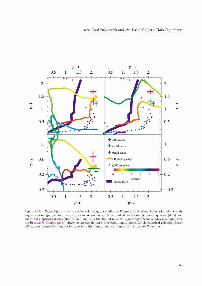
6.8 Cool Subdwarfs and the Local Galactic Halo Population
Figure 6.11: Upper left: g − r/r − i color-color diagram similar to Figure 6.10 showing the location of the mainsequence stars (purple line), mean position of extreme-, ultra-, and M subdwarfs (crosses), quasars (dots) andunevolved elliptical galaxies (thin colored line) as a function of redshift. Upper right: Same as previous figure withthe Bruzual & Charlot (2003) single stellar population 5 Gyr evolutionary model for the elliptical galaxies. Lowerleft: g-r/z-y color-color diagram for objects in first figure. See also Figure 10.1 in the AGN chapter.
165

Chapter 6: Stellar Populations
identified to date, largely serendipitously with 2MASS and SDSS. But with 15 . Mi . 18, theywill be detected in substantial numbers with LSST, with volume-complete samples out to at least200 pc. LSST should also discover specimens of the even cooler T-type subdwarfs, whose spec-tral properties are as yet unknown but likely to be substantially modified by metallicity effects.Collectively these low-temperature subdwarfs will facilitate the first measurement of the hydrogen-burning gap in the halo luminosity function, a population age indicator that can constrain theformation history of the low-mass halo and its subpopulations (e.g. Burrows et al. 1993).
6.9 Very Low-Mass Stars and Brown Dwarfs in the SolarNeighborhood
Kevin R. Covey, John J. Bochanski, Paul Thorman, Pat Boeshaar, Sarah Schmidt, Eric J. Hilton,Mario Juric, Zeljko Ivezic, Keivan G. Stassun, Phillip A. Cargile, Saurav Dhital, Leslie Hebb,Andrew A. West, Suzanne L. Hawley
6.9.1 The Solar Neighborhood in the Next Decade
The least–massive constituents of the Galactic population are brown dwarfs, objects too small tosustain hydrogen fusion in their cores. These are divided into L dwarfs (Kirkpatrick et al. 1999),which have Teff between 1500K and 2200K, whose spectra show weakening of the TiO absorptionbands, and T dwarfs with Teff between 800K and 1500K, which show the presence of CH4 in theiratmospheres. An additional spectral type, the Y dwarf (after Kirkpatrick et al. 1999), has beenreserved to describe possible dwarfs with even cooler temperatures, which are expected to showNH3 absorption, a weakening in the optical alkali lines, and a reversal of the blueward J−K trendcaused by CH4 absorption in T dwarfs (Kirkpatrick 2005). Although their masses are low, thesebrown dwarfs are relatively common in the solar neighborhood, with 600 L and 150 T dwarfs nowconfirmed. Most of these have been discovered by combining near–infrared imaging (e.g. 2MASS;Skrutskie et al. 2006) with optical surveys (e.g. SDSS; York et al. 2000); the faintness of theseobjects at optical wavelengths (Mz > 13) and the depth of existing NIR imaging are such that thesebrown dwarfs are overwhelmingly located within the immediate solar neighborhood (d < 65 pc).Informing theoretical models of these objects requires measurements of precise physical parameterssuch as radius and mass.
A number of ongoing or near–term surveys will expand the census of brown dwarfs by 2017, whenLSST will begin standard survey operations. The largest single epoch catalog of warm (i.e., Land early T) brown dwarfs will be compiled by the UKIDSS NIR survey (Hewett et al. 2006),which is currently in progress and capable of detecting L0 dwarfs in the J-band within ∼ 250 pc.At the cool end, the upcoming WISE mid-IR space telescope (Mainzer et al. 2005) will provide[3.3]-[4.7] µm colors for early T dwarfs within 200 pc (assuming colors and magnitudes from Pattenet al. 2006) and all T9 dwarfs within 20 pc, and exquisite sensitivity to cooler Y dwarfs. Multi-epoch photometric surveys enable initial measurements of a source’s trigonometric parallax andpotential binarity, such that brown dwarfs detected by such surveys have significantly more valuefor constraining theoretical models. The SkyMapper survey (SSSS Keller et al. 2007), a large-areaimaging survey covering the southern sky to depths similar to SDSS, will begin within the next few
166

6.9 Very Low-Mass Stars and Brown Dwarfs in the Solar Neighborhood
years. SkyMapper’s six-year campaign will produce parallaxes for brown dwarfs within 20 pc. ThePan-STARRS PS1 survey will detect L0 dwarfs in the i band out to 400 pc and measure parallaxesfor those within 100 pc; the volume sampled shrinks for fainter, cooler brown dwarfs.
6.9.2 Simulating LSST’s Yield of Solar Neighborhood MLTY Dwarfs
Unlike previous surveys, LSST will not depend on separate NIR surveys in order to distinguish Land T dwarfs from possible contaminants such as transient detections, high-redshift quasars, andred galaxies (see Figure 10.6). A narrow range of late L dwarfs may overlap with z ' 6.25 quasarsin color; shortly after the start of the survey, even these brown dwarfs will be identifiable by theirproper motions. The addition of the y band allows color identification based on detection in onlythe three reddest LSST bands, allowing LSST to detect (5 σ in full 10-year co-adds) L0 dwarfsout to 2100 pc, and T0 dwarfs to 100 pc. This L dwarf detection limit extends well into the Thickdisk, enabling LSST to probe the physics of old, metal–poor substellar objects (see § 6.7), andpotentially decode the star formation history of the thick and thin disks of the Milky Way fromthe age distribution of field brown dwarfs.
We have constructed a detailed simulation of the very-low mass (VLM) stars and brown dwarfs inthe solar neighborhood; using the baseline specifications for the LSST system, we have identified thesubsets of this population that LSST will characterize with varying degrees of precision. To modelthe stellar population in the stellar neighborhood, we have adopted ugriz absolute magnitudesfor VLM stars as tabulated by Kraus & Hillenbrand (2007), synthetic z − y colors calculatedfrom optical and infrared template spectra provided by Bochanski et al. (2007) and Cushing et al.(2005), and the mass function and space densities of low-mass stars measured by Bochanski et al.(in preparation).
The lack of a hydrogen-burning main sequence in the brown dwarf regime introduces strong degen-eracies into the relationships between the masses, ages, and luminosities of substellar objects. Thesedegeneracies are an important consideration for studies of the properties of field brown dwarfs, asthe properties of brown dwarfs in the solar neighborhood are sensitive to the star formation historyof the Milky Way and the shape of the stellar/substellar mass function. We are currently develop-ing simulations that explore the brown dwarf samples LSST would observe assuming different starformation histories and mass functions; for simplicity, however, the simulations described belowassume a single population of 3 Gyr brown dwarfs. In detail, this substellar population is describedby:
• For 2100 > Teff > 1200 (L dwarfs and the earliest Ts) we adopt empirical SDSS riz mag-nitudes (Schmidt et al. in preparation), supplemented by synthetic ugy magnitudes fromcloudy Burrows et al. (2006) models.
• For 1200 > Teff > 600 (mid-late Ts), we adopt synthetic ugrizy magnitudes calculated fromcloud-free Burrows et al. (2006) models.
• For Teff > 600 (as yet undiscovered Y dwarfs), we adopt synthetic ugrizy magnitudescalculated from the ultra-cool Burrows et al. (2003) models.
• We adopt the Cruz et al. (2007) luminosity function for L dwarfs; for T and Y dwarfs, wedefine a luminosity function with a linear extrapolation anchored by the coolest bin of the
167

Chapter 6: Stellar Populations
Table 6.4: LSST’s MLTY Dwarf Sample
Spectral Class Nrizy Nizy Nzy Nπ
M >347,000 >347,000 >347,000 >347,000
L 18,500 27,500 35,600 6,550
T ∼3-4 50 2,300 ∼260
Y 0 0 ∼18 ∼5
Cruz et al. luminosity and the empirical T dwarf space density measured by Metchev &Hillenbrand (2007).
Using the above parameters as inputs, we simulated the properties of field stars and brown dwarfswithin 200 pc of the Sun. Table 6.4 summarizes the number of stars and brown dwarfs LSST willlikely detect in various filter combinations as a function of spectral type with reliable parallaxes,to the single-visit depth. To make this estimate, we assume the relationship between parallaxuncertainty vs. r band magnitude reported in Table 3.3, but we increase these uncertainties by afactor of 1.25 to reflect that many stars and brown dwarfs will lack u and g band detections.
These results indicate that LSST will greatly expand the sample of ultra–cool objects with reliableparallax measurements. These extremely red objects are ill-suited for parallax measurementswith Gaia’s blue filterset, while LSST’s greater depth and astrometric precision will enable it tomeasure parallaxes for brown dwarfs significantly beyond the parallax limit of Pan-STARRS. Thissample will, therefore, provide a key set of well-characterized brown dwarfs which can confront thepredictions of theoretical models of brown dwarf and planetary atmospheres.
While we focus here primarily on brown dwarfs in the Galactic field, we also note that LSST’s deepphotometric limits and its ability to select cluster members via high-precision proper motions willprovide a high-fidelity census of the very-low-mass populations of many Southern open clusters.LSST will be able to easily identify VLM objects near or below the hydrogen-burning limit inmost of the clusters listed in Tables 6.1 and 6.2, with ages ranging from 1 Myr to ∼10 Gyr andto distances as far as ∼1.5 kpc. LSST will provide colors and magnitudes for a large sample ofL and T dwarfs with ages and metallicities derived from the morphology of each cluster’s uppermain sequence. This sample will define empirical brown dwarf cooling curves over a wide rangeof ages, providing a key calibration for understanding the properties of nearby field brown dwarfswhose ages are almost entirely undetermined.
6.9.3 Science Results
Measuring Fundamental Physical Parameters of VLM stars and Brown Dwarfs
The wide areal coverage, depth, precision, and temporal coverage of LSST photometry make it anideal instrument for the detection and characterization of low–mass (M < 0.8M) eclipsing binarieswithin the Milky Way. Currently, only ∼ 15 low–mass eclipsing binaries are known (Demory et al.2009), and even fewer VLM binaries, presumably due to their intrinsic faintness (L < 0.05L fora 0.4M early M dwarf) and a stellar binary fraction that decreases with mass (Duquennoy &
168

6.9 Very Low-Mass Stars and Brown Dwarfs in the Solar Neighborhood
Mayor 1991; Burgasser et al. 2007). The large volume probed by LSST, with typical low-masspairs being detected at d < 200 pc, will discover a slew of these rare systems.
To quantify the expected yield of VLM star and brown dwarf EBs, we start with the expected yieldof MLTY dwarfs from the Nzy column of Table 6.4. Such objects will already have LSST lightcurves in the z and y bands, which can be complemented by follow-up light curves in the JHKbands. A five-band light curve analysis is sufficient for modeling the EB parameters to ∼ 1% (e.g.Stassun et al. 2004). Assuming that approximately 1/10 of the M dwarfs are M9 brown dwarfs,then the total brown dwarf yield from Table 6.4 is ∼ 70, 000. Recent surveys of binarity amongbrown dwarfs yield fractions of 10–15% for visual binaries with separations of > 1 AU (e.g., Martınet al. 2003; Bouy et al. 2003). Thus a very conservative estimate for the overall binary fraction ofbrown dwarfs is 10%. Next, assuming a distribution of binary separations similar to that for Mdwarfs (Fischer & Marcy 1992) implies that ∼ 10% of these will be tight, spectroscopic binarieswith physical separations < 0.1 AU. Finally, among these, the probability of an eclipse is of order(R1 + R2)/a, where R1 and R2 are the component radii and a is the semi-major axis, so for twobrown dwarfs each with R ∼ 0.1 R and a ∼ 0.1 AU, we have an eclipse probability of ∼ 1%. Thusthe overall expected brown dwarf EB yield will be 0.1 × 0.1 × 0.01 × 70, 000 ≈ 7. With only onebrown dwarf EB currently known (Stassun et al. 2006, 2007), the LSST yield represents a criticalforward advance for substellar science. The calculation above implies an overall yield of ∼ 40 VLMeclipsing binary systems, a factor of several increase over the number currently known.
These fundamental astrophysical laboratories will redefine the empirical mass–radius relations,for which current data are sparse and derived from heterogeneous sources. For nearby eclipsingsystems, native LSST parallaxes will result in model–free luminosity estimates, and can help con-strain the effective temperature distribution of low–mass stars. This will be especially importantat smaller masses (M < 0.1M), where only one eclipsing binary is known (Stassun et al. 2006)1.This regime will be well suited to LSST’s survey specifications and complement the Pan-STARRSsurvey as LSST will be probing a different area of the sky (the Southern Hemisphere). At largedistances, the currently elusive halo binaries, identified kinematically through proper motions, mayserve as probes for changes in low–mass stellar structure due to metallicity. Low–mass stars in-habit an interesting regime in stellar structure. At masses ∼ 0.4M, the interiors of low–massstars transition from a convective core surrounded by a radiative shell to a fully convective in-terior. Observations do not currently constrain how metallicity may affect this transition, andonly the deep photometry that LSST will provide will enable an empirical investigation of thisphenomenon. The eclipsing binaries discovered in LSST will enable new science and redefine theempirical understanding of stellar structure and binary properties. With the “brown dwarf desert”significantly limiting the existence of F/G/K+brown dwarf binaries2, VLM+brown dwarf eclipsingbinaries are the only systems in which masses and radii of brown dwarfs can be measured—alongwith their temperatures.
High-resolution near-infrared spectroscopic follow-up on 10-m class telescopes will be critical fordetermining the radial velocity orbit solutions for the discovered eclipsing binaries. For example,the one known brown dwarf eclipsing binary (Stassun et al. 2006, 2007) is in the Orion Nebula
1This system exhibits interesting behavior: the hotter component (primary) is actually fainter than its companion.2For example, Grether & Lineweaver (2006) find that approximately 16% of solar-type stars have companions withP < 5 yr, M > 1 MJup. Of these, 4.3 ± 1.0% have companions of planetary mass, 0.1% have brown dwarfcompanions, and 11.2± 1.6% have companions of stellar mass.
169

Chapter 6: Stellar Populations
cluster at a distance of ∼ 500 pc, the outer limit for the systems included in the estimated yieldscalculated above. Its radial velocity curve was obtained with the Phoenix spectrograph on theGemini South 8-m telescope operating in the H band (1.5 µm).
Variability of VLM Stars and Brown Dwarfs
The temporal coverage of LSST opens a window on the time variability of VLM stars, includingflares, spot modulation, and rotation periods. Additionally, by discovering new eclipsing binaries,LSST will provide new laboratories for measuring fundamental stellar parameters like mass andradius.
Stellar magnetic activity has been observed and studied on M dwarfs for several decades (see§ 8.9.1 for a review of this subject), but much less is known about activity on brown dwarfs. Thefraction of stars with Hα in emission, an indicator of magnetic activity, peaks around M7 anddecreases through mid-L (Gizis et al. 2000; West et al. 2004; Schmidt et al. 2007; West et al.2008) although the changing continuum level with spectral type makes this an imperfect tracer ofmagnetic field strength. Burgasser et al. (2003b) report three T dwarfs with Hα activity, one ofwhich has strong, sustained emission (Burgasser et al. 2002). Flares on brown dwarfs appear tobe less frequent than on M dwarfs, but have been seen in both X-ray (Rutledge et al. 2000) andradio (Berger et al. 2001). Optical spectra have shown variable Hα emission in L dwarfs (Hall2002; Liebert et al. 2003; Schmidt et al. 2007; Reiners & Basri 2008) that may be the result offlares. LSST’s new observations of such a large number of brown dwarfs over dozens of epochs willprovide much–needed empirical determinations of flare rates.
LSST’s temporal coverage will permit precise, dense coverage of most main sequence stars withspots. This subject is modeled in detail in § 6.6, and discussed below in the context of low–massstars and brown dwarfs. Starspots, analogous to their solar counterparts, provide a measure ofthe relative magnetic field strength for stars of a given spectral type (and mass), assuming thatthe spot coverage is not so uniform as to prevent rotational modulation of the star’s observed flux.If spot variations can be detected, the ugrizy light curves of these stars can be used to estimatetemperature, from relative depths due to spot modulation, and filling factors, from the absolutedeviations from a pristine stellar photosphere.
Furthermore, the photometric signatures imprinted by these cooler regions provide the opportunityto measure rotation periods that are shorter than the lifetime of a typical starspot (∼weeks tomonths). As demonstrated in § 6.6, LSST will be adept at measuring the rotation periods ofcoherently spotted, magnetically active, low–mass stars. Combining the measured rotation periodswith other proxies of stellar magnetic activity will provide a fundamental test of magnetic dynamogeneration theory. This is particularly interesting within the low–mass regime. At masses∼ 0.4M,the interior of low–mass stars transition from an convective core surrounded by a radiative shellto a fully convective interior. The transition region between convective core and radiative exterioris thought to drive magnetic activity in earlier type low–mass stars (West et al. 2008).
170

6.10 Eclipsing Variables
Substellar Subdwarfs
The deep LSST survey imaging will photometrically identify statistically significant numbers of Ldwarfs at large distances from the Galactic plane. These dwarfs will allow the spatial distributionof dwarfs in the thin and thick disk populations to be determined, and allow a search for additionalmembers of a halo population of metal–poor subdwarf brown dwarfs to be discovered (e.g., Cushinget al. 2009). The kinematics of the L dwarf and subdwarf populations will also provide an empiricaltest of the metallicity dependence of the hydrogen burning limit, based on the model coolingcurves. The existence of a population of substellar subdwarfs may also indicate star formation dueto infalling primordial gas, or be a relic of the Milky Way’s recent merger history.
6.10 Eclipsing Variables
Andrej Prsa, Keivan G. Stassun, Joshua Pepper
The importance of eclipsing binary stars (EBs) can hardly be overstated. Their analysis provides:
• Calibration-free physical properties of stars (i.e., masses, radii, surface temper-atures, luminosities). Masses are measured dynamically via radial velocities with no sin iambiguity because the eclipses provide an accurate measure of sin i. Radii are measureddirectly from the eclipse durations, the temperature ratio from the eclipse depths. The radiiand temperatures together yield the luminosities.
• Accurate stellar distances. With luminosities measured directly from the componentradii and temperatures, the distance to the EB follows directly from the observed fluxes.
• Precise stellar ages. By comparing the measured mass-radius relationship with stellarevolution models, precise stellar ages can be determined. The accuracy of the age determi-nation is of course model dependent and also mass dependent, with typical accuracy of ∼ 5%for M? > 1.2 M and ∼ 50% for M? < 0.8 M (Stassun et al. 2009).
• Stringent tests of stellar evolution models. With accurate, directly determined proper-ties of the two stars in the EB, the basic predictions of stellar evolution models can be tested.For example, the two stars should lie on a single model isochrone under the assumption thatthey formed together as a binary, or the observed parameter relationships (mass-radius,temperature-luminosity, and so on) can be compared against the model predictions.
The products of state-of-the-art EB modeling are seminal to many areas of astrophysics:
• calibrating the cosmic distance scale;
• mapping clusters and other stellar populations (e.g., star-forming regions, streams, tidal tails,etc) in the Milky Way;
• determining initial mass functions and studying stellar population theory;
• understanding stellar energy transfer mechanisms (including activity) as a function of tem-perature, metallicity, and evolutionary stage;
• calibrating stellar color-temperature transformations, mass-radius-luminosity relationships,and other relations basic to a broad array of stellar astrophysics; and
171

Chapter 6: Stellar Populations
Table 6.5: Distance Limits for LSST Detection of Sample EBs.
Sample Binarya Type Binary Absolute Magnitude Distanceb for r = 22.0 [kpc] Distanceb for r = 19.5 [kpc]
M5V + M5V 12.9 0.7 0.2
M2V + M2V 9.0 4.0 1.3
K0V + K0V 5.0 25.1 7.9
G2V + MxV 4.6 30.2 9.5
G5III + GxV 2.9 66.1 20.1
aScientifically interesting EB systems. EBs with M-dwarf components are rare in the literature. Their discoverywill permit detailed testing of stellar models in this important mass regime. G-dwarf/M-dwarf pairs will beparticularly valuable for pinning down the properties of M-dwarfs, since the temperature scale of G-dwarfs isrelatively well established. A particularly exciting prospect are Cepheids (G giants) in EB systems.
bAssuming no extinction.
• studying stellar dynamics, tidal interactions, mass transfer, accretion, chromospheric activity,etc.
LSST will be ideally suited for extensive mapping of EBs. As the simulations described belowdemonstrate, LSST will detect essentially all EBs with orbital periods less than 0.3 days, and 50%of those with periods up to ∼10 days (see Figure 6.13). This completeness estimate is based onanalysis of a single passband; simultaneous analysis of all six LSST bands will in reality improvethis completeness. With a nominal detection limit of r = 24.5, a magnitude of r = 22.0 shouldallow detection of targets with a S/N of 3.5, r = 19.5 will have S/N of 10 per data point. Table 6.5shows the distance out to which certain fiducial EB types can be detected. For example, a pair ofeclipsing M2 dwarfs will be detected out to 1 kpc with S/N of 10.
We can estimate the number of EBs that LSST will be able to fully characterize (our experiencemodeling EB light curves shows that S/N ∼ 3.5 per data point typically suffices for the determi-nation of physical and geometric parameters to a few percent). Gaia will observe ∼1 billion starsdown to r ∼ 20.5 over the whole sky. We can expect that LSST will observe ∼0.5 billion stars tothis same depth in the southern hemisphere. Extrapolating the results from Hipparcos (917 EBsin the sample of 118,218 observed stars; or 0.8%), the LSST sample will contain ∼16 million EBsdown to r ∼ 22.0. The average detection rate for EBs over all periods will be around 40% (∼ 100%for P < 0.3 days, ∼50% for P ∼ 10 days, ∼ 20% for P < 30 days; Figure 6.13), bringing the totalnumber to ∼6.4 million EBs. Roughly 25% of those will have components of similar luminosities(double-lined systems), yielding ∼1.6 million EBs with S/N≥ 10 for ready detailed modeling.
6.10.1 Simulating LSST’s Harvest of Eclipsing Binary Stars
With LSST’s six-band photometry and a cut-off magnitude of r ∼ 24.5, the limiting factor forthe detection of EB stars will be the cadence of observations. To estimate LSST’s EB detectionefficiency, we set up a test-bed by employing PHOEBE (Prsa & Zwitter 2005), a Wilson & Devinney(1971) based eclipsing binary modeling suite. We first partitioned the sky into 1558 fields, coveringall right ascensions and declinations between −90 and 10. The cadence of observations of thesefields was then determined from the Simulated Survey Technical Analysis Report (SSTAR) for theoperations simulations described in § 3.1.
172

6.10 Eclipsing Variables
Figure 6.12: Schematic view of an EB light curve. Surface brightness ratio B2/B1 directly determines the ratio ofdepths of both eclipses, and can be roughly approximated by the temperature ratio T2/T1. The sum of fractionalradii ρ1 + ρ2 determines the baseline width of the eclipses, while e sinω determines the ratio between the widths ofeach eclipse, d1 and d2. The phase separation of the eclipses is governed by e cosω, and the overall amplitude of thelight curve, as well as the shape of eclipses, are determined by sin i.
To estimate LSST detection effectiveness, we synthesized light curves for five EBs that are represen-tative of the given morphology type: well detached, intermediate detached, close detached, close,and contact. These most notably differ in fractional radii and orbital periods, hence in the numberof observed data points in eclipses. Each EB light curve is described by its ephemeris (HJD0 andperiod P0) and five principal parameters: T2/T1, ρ1 + ρ2, e sinω, e cosω and sin i (cf. Figure 6.12;for a thorough discussion about the choice of principal parameters please refer to Prsa et al. 2008).
Let N1 and N2 be the numbers of data points observed in each eclipse. To detect and correctlyclassify light curves, we need as many points in both eclipses as possible. We thus selected theproduct C = N1N2 for the cost function. This way, if all data points are observed during oneeclipse but not the other, this quantity will be zero. Consecutive observations of long period EBspresent another complication: although they contribute equally to the in-eclipse count, they coveressentially the same point in phase space because of the prolonged duration of eclipses. To accountfor that, all adjacent data points in phase space that are separated by less than some thresholdvalue – in our simulation we used 1/1000 of the period – are counted as a single data point.
The cost function C, shaped according to these insights, was computed for all five synthesized EBs(the details of the study are presented in Prsa et al. 2009). The light curves are computed in phasespace, assuming that periodicity can be found correctly by a period search algorithm if the S/N ofa single data point exceeds 3.5 (or, in terms of LSST, r < 22.0). Simulation steps are as follows:
1. given the P0, pick a random phase shift between 0.0 and 1.0 and convert the time array tothe phase array;
2. sort the array and eliminate all data points with adjacent phases closer than the thresholdvalue required to resolve them;
3. given the ρ1 + ρ2, count the number of data points in eclipses (N1, N2);
4. compute the cost function value C = N1N2;
173

Chapter 6: Stellar Populations
0
20
40
60
80
100
-1 -0.5 0 0.5 1 1.5 2 2.5 3
Det
ecti
on r
ate
in %
log(P)
Expected LSST harvest of eclipsing binaries
well detachedintermediate detached
close detachedclose
contact
Figure 6.13: The detection rate of eclipsing binary stars based on their morphology and their orbital period.Assuming that S/N≥ 3.5 per data point suffices for reliable recovery of orbital periods, LSST will detect almostall short period EBs, around 50% of intermediate EBs, and around 10% of long period EBs down to r ∼ 22.0.The simulation is based on a single passband, implying that the values quoted here correspond to the worst casescenario. Since short and intermediate period EBs are most interesting for stellar population studies, it is clear thatthe expected LSST harvest of EB stars will be unprecedented.
5. repeat steps 1-4 for a predefined number of times (say, 100), and find the average value of C;
6. repeat steps 1-5 for all 1588 fields (αi, δi); and
7. repeat steps 1-6 for a range of periods sampled from a uniform distribution in log(P0) ∈[−1, 3].
Figure 6.13 depicts the results of our simulation. Under the assumption that the variability analysisprovides correct periods, the LSST sample of short period eclipsing binary stars will be essentiallycomplete to r ∼ 24.5; these stars have the best characteristics to serve as calibrators – both becauseof their physical properties and because of the feasibility for the follow-up studies.
6.10.2 Effectiveness of EB Parameter Determination from LSST Data
To further qualify LSST’s harvest of EBs, we generated a sample of 10,000 light curves across thesouthern sky, using the cadence coming out of the Operations Simulations (§ 3.1). The values ofprincipal parameters were sampled randomly, according to the following probability distributionfunctions:
• T2/T1 is sampled from a normal distribution G(1.0, 0.18);
• P0 is sampled from a log-uniform distribution [−1, 4];
174

6.11 White Dwarfs
• ρ1+ρ2 is sampled from a uniform distribution [0.05, δmax−0.05], where δmax is the morphologyconstraint parameter that depends exponentially on the value of logP0:
δmax(logP0) = 0.7 exp(−1 + logP0
4
);
• The eccentricity e is sampled from an exponential distribution E(0.0, εmax/2), where εmax isthe attenuation parameter that depends exponentially on the value of ρ1 + ρ2:
εmax = 0.7 exp(−ρ1 + ρ2 − 0.05
1/6
);
• The argument of periastron ω is sampled from a uniform distribution [0, 2π]; the combinationof the e and ω distributions produces a sharp, normal-like distribution in e sinω and e cosω;
• The inclination i is sampled from a uniform distribution [igrazing, 90], where igrazing is theinclination of a grazing eclipse.
Once the light curve sample was created, we added random Gaussian errors with σ ranging from0.001 to 0.2 (simulating different distances and, hence, different S/N), and we measured best fitparameters with ebai (Eclipsing Binaries via Artificial Intelligence; Prsa et al. 2008), an efficientartificial intelligence based engine for EB classification via trained neural networks. Backpropa-gation network training, the only computationally intensive part of ebai, needs to be performedonly once for a given passband; this is done on a 24-node Beowulf cluster using OpenMPI. Oncetrained, the network works very fast; 10,000 light curves used in this simulation were processed in0.5 s on a 2.0GHz laptop, where most of this time was spent on I/O operations.
Figure 6.14 depicts the results of ebai: 80% of all stars passed through the engine have less than15% error in all five parameters. A 15% error might seem large at first (typical error estimatesof state-of-the-art EB modeling are close to 2-3%), but bear in mind that ebai serves to providean initial estimate for parameter values that would subsequently be improved by model-basedmethods such as Differential Corrections or Nelder & Mead’s Simplex, as implemented in PHOEBE.
These two simulations indicate LSST will provide a sample of short period EBs (< 1 day) essentiallycomplete to r ∼ 22.0; a sample of EBs with periods of tens of days will be ∼50% complete; a sampleof long-period EBs will be ∼10% complete. Since short period EBs carry the most astrophysicalsignificance, and since parameter determination is most accurate for those stars because of thelarge number of data points in eclipses, LSST’s high detection efficiency and accurate parametermeasurements promise to revolutionize EB science and the many fields that EBs influence.
6.11 White Dwarfs
Jason Kalirai, Charles F. Claver, David Monet, Zeljko Ivezic, J.B. Holberg
175

Chapter 6: Stellar Populations
0
0.5
1
1.5
2
2.5
3
0 0.2 0.4 0.6 0.8 1
Outp
ut
val
ues
of
par
amet
ers
Input values of parameters
T2/T1
ρ1+ρ2
e sin ω
e cos ω
sin i
0
20
40
60
80
100
2.50 5.00 7.50 10.00 12.50 15.00 17.50 20.00
Fra
ctio
n o
f li
ght
curv
es [
%]
O-C differences [%]
LSST efficiency on 10,000 noise-free EB light curves
T2/T1ρ1+ρ2
e sin ωe cos ω
sin i
0
20
40
60
80
100
2.50 5.00 7.50 10.00 12.50 15.00 17.50 20.00
Cumulative distribution
Figure 6.14: Left: comparison between input and ebai-computed values of orbital parameters in a simulation ofLSST-observed eclipsing binaries. For neural network optimization purposes, parameter values were rescaled to theinterval [0.1, 0.9]. Successive parameters are vertically offset by 0.5 and correlation guidelines are provided to facilitatecomparison. Right: histogram of the residuals computed by ebai. Parameter T2/T1 is most weakly determined (26%of all light curves have a corresponding error less than 2.5%) – this is due to the only approximate relationshipbetween T2/T1 and the surface brightness ratio B2/B1. Parameters sin i and e cosω have the highest success rate(75% and 68% of all light curves have sin i and e cosω, respectively, determined to better than 2.5%), meaning thatthe cadence suffices for accurate determination of orbital properties. The inset depicts the cumulative distributionof the residuals: over 80% of the sample has errors in all parameters less than 15%.
6.11.1 The Milky Way White Dwarf Population
Over 97% of all stars end their lives passively, shedding their outer layers and forming low masswhite dwarfs. These stellar cinders are the burnt out cores of low and intermediate mass hydrogenburning stars and contain no more nuclear fuel. As time passes, white dwarfs will slowly cooland release stored thermal energy into space becoming dimmer and dimmer. Although they aredifficult to study given their intrinsic faintness, successful observations of white dwarfs can shedlight on a very diverse range of astrophysical problems.
The largest sample of white dwarfs studied to date comes from SDSS, which has increased theknown population of these stars by over an order of magnitude to more than 10,000 stars (Eisen-stein et al. 2006). This has enhanced our knowledge of stellar chemical evolution beyond themain sequence, uncovered new species of degenerate stars such as highly magnetized white dwarfsand accretion disk objects that may harbor planets, and provided a more accurate white dwarfluminosity function for the Galactic disk (Harris et al. 2006).
The luminosity function of white dwarfs rises with increasing photometric depth, such that LSST’ssensitivity and wide areal coverage is expected to yield over 13 million white dwarfs with r < 24.5and over 50 million to the final co-added depth (model luminosity functions are presented later).LSST will completely sample the brightest white dwarfs in our Galaxy (with MV ∼ 11) to 20 kpcand beyond. This broadband study of white dwarfs will yield important leverage on the overallbaryon mass budget of the Milky Way and provide an unprecedented sample of white dwarfs, of allspectral types, to improve our understanding of a variety of astrophysical problems. For example,based on MACHO predictions, LSST will be sensitive to thousands of dark halo white dwarfs andcan therefore verify or rule out whether an appreciable fraction of the Galactic dark matter is tied
176

6.11 White Dwarfs
Figure 6.15: The color-magnitude diagram of NGC 6397 from HST observations with ACS (Richer et al. 2008) basedon all stars (center) and proper motion members over a fraction of the field (right). The proper motion diagram(left) illustrates the motion of the cluster with respect to the field, over a 10 year baseline. The rich white dwarfcooling sequence of the star cluster (faint-blue end) is modeled in Hansen et al. (2007) to yield an independent agefor the cluster of t = 11.5 ± 0.5 Gyr.
up in these stars (Alcock et al. 2000). LSST’s photometry of white dwarfs will also be more thanthree times as precise as SDSS photometry, particularly in the u band, which is often definitive forthese stars. This greatly facilitates the matching of observed colors with predicted colors at the 1%level making it possible to estimate white dwarf temperatures, gravities, and spectral types over amuch wider range of parameter space then is now practical. Below we outline several of the keyscience cases that LSST will address, followed by a specific discussion of the simulated distributionof white dwarfs that LSST will be sensitive to.
6.11.2 White Dwarfs as Chronometers – Dating Stellar Components of theMilky Way
Although SDSS found abundant white dwarfs in the Galactic disk, the survey was too shallow touncover large numbers of halo white dwarfs. These distant objects, which LSST will detect, willallow for the first time the construction of a luminosity function for field halo white dwarfs (see§ 6.11.6 for the expected white dwarf spatial distribution). The structure in this luminosity function(and in particular, the turnover at the faint end) holds important clues about the formation time ofeach specific Galactic component because the white dwarfs cool predictably with time. Therefore,an older population of white dwarfs is expected to show a fainter turnover as the stars have hadmore time to cool. As we show in § 6.11.6, a simulation of the expected LSST white dwarf numbercounts indicates that over 400,000 halo white dwarfs will be measured to r < 24.5.
The faintest white dwarfs in the nearest globular star clusters have now been detected with HST(see Figure 6.15); at MV & 16 (Hansen et al. 2007), they are a full magnitude fainter than theircounterparts in the Galactic disk (Harris et al. 2006). This work provides independent age mea-surements for nearby globular clusters and suggests that these objects formed several Gyr beforethe Galactic disk. By extending these studies to the remnants in the Milky Way field halo, LSSTwill provide us with a direct measurement of the age of the Galactic halo, a vital input into theconstruction of Galactic formation models. These measurements can not only help answer when
177

Chapter 6: Stellar Populations
our Galaxy formed, but also constrain the formation timescales of different populations within thesame component. For example, the age distribution of Milky Way globulars can be contrasted withthe field halo population to shed light on the formation processes of the clusters themselves (e.g.,in situ formation vs. accretion).
LSST will also improve, by several orders of magnitude, the statistics of the field Milky Way diskwhite dwarf luminosity function. Harris et al. (2006) comment on the lack of a precise (σ ∼2 Gyr) age measurement (Leggett et al. 1998; Hansen et al. 2002) given the low numbers of low-luminosity white dwarfs in the SDSS sample. LSST will not only constrain the age of the oldeststars in the Galactic disk to a much higher accuracy than currently possible, but also map out thecomplete star formation history of the disk. Epochs of enhanced star formation in the Galacticdisk’s history will leave imprints on the white dwarf luminosity function in the form of brighterpeaks. The luminosity and width of these peaks can be inverted to shed light on the formationtime and timescale of the star forming events. In § 6.11.6 we simulate the expected LSST whitedwarf disk luminosity function.
A key component of LSST’s study of Milky Way white dwarfs will be a kinematic analysis. WithLSST we will look for dependencies of the white dwarf luminosity function in the disk with thepopulation’s velocity, and therefore verify the age difference between the thin and thick disks. Thevelocity may also be correlated with other Galactic parameters, such as metallicity, to give indirectage-metallicity estimates. Alternatively, dependencies of the luminosity function (and, therefore,age) may exist with scale height above/below the Galactic plane, improving our understandingof Galactic structure. The expected kinematic separation of these populations, based on LSSTstatistics, is also discussed near the end of this chapter.
6.11.3 White Dwarfs in Stellar Populations
The comparison of theoretical isochrones to observational color-magnitude diagrams has histori-cally been used to infer the age of a nearby stellar population, provided that the distance is knownthrough independent methods (e.g., main sequence fitting with the Hyades cluster, for which in-dividual parallax measurements exist). In practice this comparison is often limited by our lackof knowledge of fundamental quantities (e.g., the distance and metallicity) and so the isochronesare used to estimate multiple parameters at once. When combined with the uncertainties in themicrophysics of the models (e.g., the role of gravitational settling or the treatment of convectivecore overshooting), the absolute uncertainty on the age of any stellar population using the mainsequence turn-off method is ∼2 Gyr for old stellar populations (D’Antona 2002). At higher red-shifts, the theoretical isochrones are used to interpret light from distant galaxies in terms of theproperties of the systems (e.g., age and metallicity). These age and metallicity measurements forma major component of our understanding of galaxy formation and evolution.
The study of white dwarfs with LSST will naturally extend to stellar populations such as nearbystar clusters (§ 6.5). LSST will detect the tip of the white dwarf cooling sequence in star clusterslocated over 20 kpc from the Sun. It will also completely map the entire white dwarf coolingsequence in nearby globular and open clusters. For example, the faintest white dwarfs in a clusterwith t = 1 Gyr have MV = 13, and will be seen out to 8 kpc. The white dwarf cooling sequences ofthese clusters provide age and distance measurements (Hansen et al. 2007). This age measurement
178

6.11 White Dwarfs
Figure 6.16: The white dwarf cooling ages of several nearby solar metallicity open star clusters are compared withtheir corresponding main sequence turn-off ages based on a set of theoretical isochrones. The two independent agemeasurements are in good agreement with one another for the assumed models and would not agree if for example,core-overshooting was not allowed. Taken from DeGennaro et al. (2009).
is not affected by our knowledge of rotation, diffusion, overshooting, even metallicity, and is,therefore, independent of the main sequence turn-off approach. By fixing the age and distance ofthe stellar population using white dwarf cooling theory, we will be able to test stellar evolutionmodels in exquisite detail and constrain many of the microphysics. These improved models willdirectly impact our ability to deconvolve the colors of distant galaxies using population synthesismethods.
In Figure 6.16, we compare the main sequence turn-off age with the white dwarf cooling agefor the handful of open star clusters where both measurements exist (DeGennaro et al. 2009, inpreparation). This work has already shown that synthetic color-magnitude diagrams, based onvarious sets of theoretical isochrones, that do not adopt convective core-overshooting yield ages aretoo low to fit the white dwarf cooling measurements (Kalirai et al. 2001b; Kalirai & Tosi 2004).LSST will increase the sample of clusters in which these measurements exist by over an orderof magnitude, and thus allow these comparisons to be made over a substantial range in age andmetallicity to test a broad region of parameter space in the models.
6.11.4 White Dwarfs as Probes of Stellar Evolution
As an intermediate or low mass star evolves off the main sequence and onto the red giant andasymptotic giant branch, it quickly sheds its outer layers into space. The mass loss mechanisms(e.g., helium flash and thermal pulses on the asymptotic giant branch) are poorly understoodtheoretically (Habing 1996) and observational constraints are rare given the very short lifetimes ofstars in these phases (∼105 years) and heavy obscuration by dusty shells. The end products of this
179

Chapter 6: Stellar Populations
stellar evolution are white dwarfs, and studying these stars in detail beyond the initial imagingobservations can directly constrain the total integrated stellar mass loss.
As a follow up study to the initial imaging observations that LSST will undertake, the brightest(i.e., youngest) white dwarfs in nearby stellar populations can be spectroscopically measured withmulti-object technology on 8 – 10-m ground-based telescopes (and possibly with TMT or GMT).The spectra of the DA white dwarfs are remarkably simple, showing pressure broadened Balmerlines caused by the thin hydrogen envelope in the atmosphere of the stars. These Balmer lines canbe easily modeled to yield the temperature and gravity of the stars, and, therefore, the individualstellar masses (Bergeron et al. 1995). These mass measurements can be uniquely connected to theinitial mass of the progenitor star for each white dwarf (e.g., the total cluster age is the sum ofthe white dwarf cooling age and the main sequence lifetime of the progenitor), and, therefore, aninitial-to-final mass relation can be constructed as shown in Figure 6.17 (Kalirai et al. 2008).
LSST will revolutionize our study of the initial-to-final mass relation. The new relation, consistingof hundreds of data points over the full range in initial mass of stars that will form white dwarfs,will directly constrain the amount of mass loss that occurs through stellar evolution. This formsa powerful input to chemical evolution models of galaxies (including enrichment in the interstellarmedium) and, therefore, enhances our understanding of star formation efficiencies in these systems(Somerville & Primack 1999). Moreover, LSST will provide new insights into how stellar evolutionand mass loss rates are affected by metallicity variations. Theoretically it is expected that massloss rates in post main sequence evolution depend on metallicity (e.g., see Kalirai et al. 2007, andreferences therein). These dependencies can be directly tested by constructing relations specificallyfor clusters of different metallicities that LSST will observe.
LSST’s detection of white dwarfs in the youngest stellar systems will also provide new insightsinto the threshold mass that separates white dwarf production from type II SNe formation. Forexample, the most massive singly evolved white dwarf that can be connected to a progenitor massin Figure 6.17 is currently the Pleiades star, which has Minitial = 6.5 M. However, the remnantstar of this progenitor is 1.0 M, much smaller than the Chandrasekhar limit, suggesting thatmore massive singly evolving white dwarfs remain to be found in star clusters. Theoretically, thisthreshold mass is difficult to constrain as models do not include rotation and are very sensitive toovershooting and rotationally induced mixing. A shift in the critical mass from 9 M (as suggestedby an extrapolation of the present initial-final mass relation above) to 6 M (as suggested by severalmodels for the ignition of carbon in the core of the star, e.g., Girardi et al. 2000) results in a 80%increase in the numbers of type II SNe based on a Salpeter mass function. This changes theamount of kinetic energy imparted into the inter-galactic medium (IGM) and would, in fact, be inbetter agreement with some observations of the IGM (Binney 2001) as well as the mass functionof stars in the solar neighborhood (van den Bergh & Tammann 1991). Such an effect should beseen as a steepening of the initial-final mass relation at higher masses, which LSST will probe bysampling white dwarf populations in successively younger systems. For example, LSST’s detectionof white dwarfs in a cluster of age 50 Myr, where 8 M stars are still burning hydrogen on the mainsequence, would suggest that the critical mass is above 8 M. Such young open clusters do existin the southern hemisphere but lack current deep imaging data (e.g., NGC 2451 and NGC 2516).
180

6.11 White Dwarfs
Figure 6.17: Top: The relation between the masses of white dwarf progenitors and their final masses from Kaliraiet al. (2008), with best linear fit. The entire white dwarf population of a given cluster is represented by a singledata point. For the older clusters (e.g., lower initial masses), the white dwarf cooling lifetimes are negligible relativeto the age of the cluster, and, therefore, all of the stars at the top of the cooling sequence came from progenitorswith the same approximate mass. For the younger clusters, this method averages over small ranges in initial andfinal mass within each star cluster. The relation shows a roughly linear rise in the remnant mass as a function ofthe initial mass (see empirical relation on the plot). Bottom: The lower panel illustrates the total integrated stellarmass lost through standard evolution, directly constrained from the initial-final mass relation. The individual datapoints, except at the low mass end, correspond to individual progenitor-white dwarf measurements.
6.11.5 Rare White Dwarf Species and the Physics of Condensed Matter
The temporal coverage of LSST observations in multiple filters will lead to exciting discoveries ofexotic stellar species that are astrophysically important. These will include eclipsing short perioddouble degenerate systems, transits of white dwarfs by planetary bodies and other accretion diskobjects down to asteroidal dimensions (see also the discussion in § 8.11), and a very large numberof pre-cataclysmic variable/post-common envelope systems. The synoptic nature of LSST will becritical in identifying these systems. For some classes, such as eclipses by planets, it may thatthe LSST cadence will be adequate only for identifying candidates requiring follow-up on smallertelescopes with a much faster cadence.
Eclipsing short period double-degenerate systems are of great interest for several reasons. Follow-upstudies of such systems will yield direct determinations of white dwarf radii as well as astromet-ric masses, which can be used to accurately populate the degenerate mass-radius relation. Thecatastrophic merger of double degenerate systems is believed to be one potential source of typeIa supernova events. Identifying such systems through their eclipse signals with LSST is a realpossibility. Continued monitoring of such systems could reveal the gravitational decay rate of themutual orbit. It is even conceivable that particular systems found with LSST could be linkedto specific gravitational wave signals detected by Laser Interferometer Space Antenna (LISA),since merging white dwarf systems are thought to constitute a major source of the Galactic noisebackground for LISA.
Some white dwarfs are now known to be orbited by dusty disks and even more show spectral features
181

Chapter 6: Stellar Populations
of heavy elements (Si, Mg, Ca, Fe, and so on), which quickly settle out of the atmosphere indicatingon-going accretion. In both cases the source of the dust is believed to be collisions of asteroidalbodies in tight orbits around the white dwarf. Because white dwarfs have small diameters, it isquite possible that favorable orbital plane orientations will reveal transits of substantial bodiesfrom the size of massive Jupiters to asteroids having diameters of tens of km. The gravitationalperturbations of such massive bodies are thought to play a role in promoting asteroidal collisionsand in maintaining any dusty ring structures that result.
Finally, it should be possible to identify a large number of pre-cataclysmic variable and post-common envelope systems. In general, eclipses (although helpful) are not even necessary sincereflection effects produced by the hot white dwarf on the low mass secondary are a frequentsignature of these sources. Having a large number of such systems to study will help map out thespectrum of stellar masses and orbital separations that constitute the end states of post-commonenvelope evolution.
With large numbers of detected white dwarfs, LSST can select those that are variable to the limitof LSST’s photometric precision (∼ 1%), and therefore identify new candidate pulsating whitedwarfs. Follow-up time-series photometry of these candidates on other telescopes will lead to asubstantial number of new white dwarf pulsators, and, therefore, provide a more accurate mappingof the boundaries of the known white dwarf instability strips for pulsation (DAV - H, DBV - He,PG1159 - C) in the HR diagram and in log g vs Teff , and also allow exploration to search forpreviously unknown instability strips along the white dwarf cooling sequence. A more detaileddiscussion of LSST’s connection to pulsating white dwarfs is provided in § 8.7.2.
LSST will provide a new test for the internal physics of white dwarf stars. The low luminosityend of the white dwarf luminosity functions (WDLF), log(L/L) < −3, contains informationabout the equation of state of condensed (degenerate) matter. The shape of the disk WDLFat the turnover (discussed in § 6.11.1) due to the disk’s finite age is affected by the release oflatent heat of crystallization of the carbon-oxygen white dwarf core. The release of latent heatprovides an energy source in an otherwise dead star and slows the white dwarf cooling process.This slowdown manifests itself as an increase in number density of white dwarfs over the luminosityrange corresponding to the crystallization event. Even more intriguing is the possibility of havinga halo WDLF that is sufficiently populated that we can fully resolve the crystallization bump.LSST’s large white dwarf sample will determine if the crystallization bump is indeed present,and if so, at what luminosity (i.e., age), providing new constraints on the equation of state forcarbon-oxygen white dwarfs.
6.11.6 The LSST White Dwarf Model Sample
In the following sections we calculate the expected distributions of white dwarfs that LSST willsee. The main purpose of these simulations is to estimate the accuracy LSST will obtain incalibrating the white dwarf photometric parallax relation, kinematically separating the disk andhalo populations, and measuring their luminosity functions.
In order to generate a simulated sample of disk and halo white dwarfs, five sets of quantities needto be adopted:
182

6.11 White Dwarfs
1. The expected astrometric and photometric measurement errors.
2. The spatial distribution for each Galaxy component.
3. The distributions of three velocity components.
4. The bolometric luminosity functions.
5. The mapping from bolometric luminosity to broad-band luminosity in each LSST bandpass.
The astrometric and photometric measurement errors are computed as described in Chapter 3.We proceed with detailed descriptions of the remaining quantities.
The Spatial Distribution
LSST will detect white dwarfs to distances much larger than the scale heights and lengths of theGalactic disk. Hence the spatial variation of volume density in the Galaxy must be taken intoaccount. We assume that the spatial distribution of white dwarfs traces the distribution of mainsequence stars, both for halo and disk populations (the impact of their different ages is handledthrough adopted luminosity functions). We ignore bulge white dwarfs in the simulations as theyrepresent only a small fraction of the population. The adopted spatial distribution of main sequencestars, based on recent SDSS-based work by Juric et al. (2008) is described in § 3.7.1.
The Kinematic Distributions
We assume that the kinematics (distributions of three velocity components) of white dwarfs are thesame as the corresponding distribution of main sequence stars, both for halo and disk populations.The adopted kinematic distribution of main sequence stars is based on recent SDSS-based workby Ivezic et al. (2008a).
The White Dwarf Luminosity Function
For disk stars, we adopt the measured luminosity function based on SDSS data (Harris et al. 2006).Using their Figure 4, we obtained the following parameters for a power-law approximation to themeasured bolometric Φ (the number of white dwarfs per cubic parsec and magnitude),
log Φ = −2.65 + 0.26 (Mbol − 15.3) for 7 < Mbol < 15.3log Φ = −2.65− 1.70 (Mbol − 15.3) for 15.3 < Mbol < 17.0, (6.1)
which agrees with the data to within 10% at the faint end. The observational knowledge of thehalo white dwarf luminosity function is much poorer. Theoretical predictions (Torres et al. 2005,and references therein) indicate an overall shift of the halo luminosity distribution toward fainterabsolute magnitudes due to its larger age compared to the disk. Motivated by these predictionsand the desire to test the ability to distinguish different luminosity functions when analyzing thesimulated sample, we simply shift the Harris et al. (2006) luminosity function by 0.7 mag towardthe faint end.
183

Chapter 6: Stellar Populations
Figure 6.18: Simulated differential luminosity function for candidate hydrogen white dwarfs in the disk sample(normalized to solar neighborhood). The dots with error bars show the result obtained by binning the cumulativeluminosity function computed using Lynden-Bell’s C− method in 0.1 mag wide Mr bins (based on ∼ 200,000 stars).The red line shows the input luminosity function in the simulation. Note the “feature” in the input luminosityfunction at Mr = 11.8.
We re-express the luminosity function per unit Mr magnitude, Φr by multiplying by dMbol/dMr,determined from the spectral energy distribution, described below. The resulting luminosity func-tions for disk and halo white dwarfs are shown in Figures 6.18 and 6.19, respectively. The integralof the adopted disk luminosity function is 0.0043 stars pc−3 (about 1/10 of the integrated luminos-ity function for main sequence stars). The disk luminosity function reaches its maximum aroundMr = 15.4, and the halo luminosity function at Mr = 16. Both luminosity functions show a ∼ 0.2mag wide and 20-30% strong “feature” at Mr ∼ 11.8 which is due to the behavior of dMbol/dMr.
We assume that 90% of all white dwarfs are hydrogen (DA) white dwarfs and the rest are helium(DB) white dwarfs, but assumed the same luminosity function for both.
The White Dwarf Spectral Energy Distribution
We use models by Bergeron et al. (1995), which produce color tracks that agree with SDSS mea-surements at the ∼0.02 mag level (Eisenstein et al. 2006). Using a sample of ∼ 10,000 white dwarfswith SDSS spectroscopic data, Eisenstein et al. (2006) found a very narrow distribution (0.1 dex)of log g centered on log g = 7.9. Motivated by this result and the desire to simplify analysis of thesimulated sample, we adopt a fixed value of log g = 8.0 (Bergeron’s models are computed with alog g step of 0.5 dex). Hence, for a given type of white dwarf atmosphere (hydrogen vs. helium),the models provide unique relationships between Mr and all relevant colors (including bolometriccorrections). For hydrogen white dwarfs with log g = 8.0, Mr = 15.4 corresponds to an effective
184

6.11 White Dwarfs
Figure 6.19: Similar to Figure 6.18, now showing the luminosity function for the candidate halo sample.
temperature of 4500 K, mass of 0.58 M and age of 7.6 Gyr. For Mr = 16, the effective tempera-ture is 3900 K, the mass is unchanged and the age is 9.3 Gyr. A 13 Gyr old hydrogen white dwarf,according to Bergeron’s models, would have Mr = 17.4 and an effective temperature of 2250 K.
Preliminary Analysis of the Simulated White Dwarf Sample
The simulated sample includes ∼ 35 million objects with r < 24.5 over the whole sky. Herewe briefly describe the expected counts of white dwarfs in the main (deep-wide-fast, DWF; see§ 2.1) LSST survey, discuss how objects with good trigonometric parallax measurements can beused to derive an empirical photometric parallax relation, and how this relation can be used withproper motion measurements to separate disk and halo candidates. We conclude with preliminaryestimates of the accuracy of disk and halo white dwarf luminosity function measurements.
Counts of Simulated White Dwarfs
The main DWF LSST survey is expected to deliver about 1000 visits (summed over all bands) overa ∼ 20,000 deg2 area, and without including the Galactic plane. Figure 6.20 compares cumulativewhite dwarf counts for several samples. The simulations predict that Gaia’s all-sky survey willdetect about 240,000 white dwarfs with r < 20. Of those, about 1,200 will be halo white dwarfs.These counts are in fair agreement with the results of Torres et al. (2005) who simulated Gaia’sperformance on white dwarfs. We have also compared the simulated counts to photometricallyselected white dwarf candidates from SDSS (see bottom left panel in Fig. 24 of Ivezic et al. 2007).We selected 355 white dwarf candidates over 203 deg2 defined by 330 < α < 50 and |δ| < 1.267;
185

Chapter 6: Stellar Populations
Figure 6.20: A comparison of cumulative white dwarf counts for several samples. The triangles (blue curve) show thecounts over the full sky in the magnitude range corresponding to Gaia survey (r < 20). The squares (red curve) showthe counts of white dwarfs from the main LSST survey (about 1/2 of the sky) that have anticipated signal-to-noiseratio for trigonometric parallax measurements greater than 10. The circles (magenta curve) show the counts of allwhite dwarfs from the main LSST survey that will have proper motion measurements (r < 24.5). The predictedmagnitudes are not corrected for the interstellar dust extinction. The dashed line shows the behavior expected fora spatially uniform distribution of sources (log[N(< r)] ∝ 0.6 r) - the impact of Galactic structure is evident in themuch shallower slope for simulated counts around r = 24.
we required that the objects be non-variable (rms scatter less than 0.07 mag in g) and have16 < g < 20, −0.3 < u − g < 0.5, −0.4 < g − r < −0.2. With the same color-magnitudecriteria, the simulated sample includes 340 objects in the same sky region. Given that the observedcolor-selected sample might include some contamination, this is a robust verification of the modelcount normalization. The simulations do not include the effects of interstellar extinction, but theextinction over this area is small, and most white dwarfs are close enough to be in front of themajority of the dust.
As illustrated in Figure 6.20, there will be about 13 million white dwarfs with r < 24.5 in theDWF survey. While the number of all detected white dwarfs in LSST will be much larger (about50 million for the r < 27.5 limit of co-added data), here we focus only on objects with r < 24.5because they will have, in addition to highly accurate photometry, trigonometric parallax andproper motion measurements. In particular, about 375,000 simulated objects have anticipatedsignal-to-noise ratio for trigonometric parallax measurements greater than 5 and 104,000 greaterthan 10. This latter subsample (whose cumulative counts are shown in Figure 6.20) can be usedto empirically constrain photometric parallax relations for hydrogen and helium white dwarfs andto train color-based classification algorithms, as described next. In the remainder of this analysis,we assume no knowledge of the input model parameters except when estimating the performanceparameters such as sample completeness and contamination.
186

6.11 White Dwarfs
Figure 6.21: The calibration of the photometric parallax relation, Mr(g − r), for white dwarfs. The Mr values arebased on trigonometric parallax and “measured” r band magnitudes. The dots represent ∼ 100,000 simulated objectswith the signal-to-noise ratio for trigonometric parallax measurements greater than 10. The middle dashed line isthe color-magnitude separator described in the text. The other two lines are the median Mr vs. g − r photometricparallax sequences. The true relations used to generate the simulated sample are indistinguishable (rms ∼ 0.01 mag)from these empirically determined median values.
White Dwarf Photometric Parallax Relations
The distribution of the difference between trigonometric and true distance moduli for the 104,000white dwarfs with parallax S/N> 10 is close to Gaussian, with a median value of −0.03 mag andan rms scatter of 0.15 mag. For the subset of 10,000 objects with r < 18, the rms scatter is 0.10mag and the bias is below 0.01 mag.
The absolute magnitude based on “measured” trigonometric parallax as a function of “measured”g − r color is shown in Figure 6.21. The two sequences that correspond to hydrogen and heliumwhite dwarfs are easily discernible. A simple separator of hydrogen and helium color-magnitudesequences is obtained by shifting the median Mr vs. g − r curve for hydrogen white dwarfs by0.4 mag towards the bright end. A slightly better choice would be to account for the shape ofthe helium sequence as well. The application of this separator results in correct classification for99.6% of the objects in the candidate hydrogen sample and for 96.3% of the objects in the candidatehelium sample.
Photometric Separation of Hydrogen and Helium White Dwarfs
The separation of hydrogen and helium white dwarfs based on the Mr vs. g−r diagram is possibleonly for objects with high S/N trigonometric parallax measurements. Since such objects representonly about 1% of the full r < 24.5 LSST white dwarf sample, a color separation method is requiredto classify the latter sample. Although helium white dwarfs represent only 10% of all objects, the
187

Chapter 6: Stellar Populations
Figure 6.22: The distribution of the simulated white dwarfs in the g− r vs. u− g color-color diagram. Black pointsshow objects with r < 24.5 and b > 60. Yellow points show a subsample of predominantly brighter sources thathave 10σ or better “measurement” of the trigonometric parallax. The two sequences correspond to He and H whitedwarfs. The distribution of low-redshift (z < 2.2) quasars observed by SDSS is shown by blue contours. The bluepart of the stellar locus (dominated by F and G stars), as observed by SDSS, is shown by the red contours. LSSTphotometry will be sufficiently accurate not only to separate white dwarfs from quasars and main sequence stars,but also to separate hydrogen from helium white dwarfs (the sequences do not overlap in the multi-dimensional colorspace, see text).
differences in Mr vs. g−r relations between helium and hydrogen white dwarfs might significantlybias the luminosity function determination.
We use the two candidate samples with good trigonometric parallax measurements to quantifytheir multi-dimensional color tracks. Figure 6.22 shows the two-dimensional projection of thesetracks. At the hot end, the tracks for hydrogen and helium objects are well separated. Althoughthey appear to cross around g−r = 0.2, they are still separated in the four-dimensional color spacespanned by the u− g, g − r, r − i and i− z colors3.
For each sample, we compute the median u − g, r − i and i − z color for each 0.01 mag wide binof g − r color. Using these tracks, for each star we compute the shortest distance to each locus,denoted here DHe and DH . The difference between these two four-dimensional color distances(4DCD) can be used as a simple color-based classifier. For the training sample, which has smallphotometric errors due to the relatively bright flux limit imposed by requiring high trigonometricparallax signal-to-noise ratio, the separation is essentially perfect (mis-classification rate, or samplecontamination, is less than 1%).
We assess the performance of color separation at the faint end by resorting to true input class,and study the completeness and contamination of candidate samples as a function of δ4DCD =
3Reliable colors are not yet available for the y band so we do not consider it here.
188

6.11 White Dwarfs
Figure 6.23: The completeness and contamination for color-selected subsamples of hydrogen and helium white dwarfs,as a function of the difference between distances to each four-dimensional color sequence (δ4DCD = DHe − DH).The solid lines show completeness and dashed lines show contamination. The blue lines correspond to hydrogensubsample, and red lines to helium subsample. Objects are classified as helium white dwarfs if their δ4DCD is smallerthan the adopted cut-off value. The panel shows a flux-limited sample with r < 23.5.
DHe − DH (see Figure 6.23). The optimal value of δ4DCD for separating two object types isa trade-off and depends on whether a particular science case requires high completeness or lowcontamination. Typically the best δ4DCD value is not zero because hydrogen white dwarfs areten times as numerous as helium white dwarfs. These effects can be elegantly treated using theBayesian formalism developed by Mortlock et al. (2008), hereafter MPI08. Here we follow asimpler approach and, informed by the results shown in Figure 6.23, adopt δ4DCD = −0.05 forthe rest of the analysis presented here. For r < 23.5, the candidate helium sample completenessand contamination are 79% and 0.2%, respectively (see the right panel in Figure 6.23). Wherer < 24.5, the completeness of 99% with a contamination of 3% for the candidate hydrogen sample,and 73% and 14%, respectively, for the candidate helium sample, the degraded but still remarkableperformance being attributed to larger photometric errors.
We note that despite high completeness for the helium subsample, there are ranges of Mr, such asMr ∼ 12.5, where it is sufficiently small to induce large systematic errors in luminosity function.To properly treat the helium subsample, a more sophisticated method, such as that described byMPI08, is required. Nevertheless, the simplistic δ4DCD method used here produces sufficientlyclean samples of candidate hydrogen white dwarfs for further analysis.
189

Chapter 6: Stellar Populations
Figure 6.24: The dependence of tangential velocity on apparent magnitude for white dwarfs with b > 60. Themap shows counts of stars in each bin on logarithmic scale, increasing from blue to red. The tangential velocity iscomputed from each star’s measured proper motion and distance estimate from the photometric parallax relationshown in Figure 6.21. At faint magnitudes (r > 22), the sample contains a large fraction of halo white dwarfs. Thehorizontal line at 180 km s−1 separates disk and halo stars with sample completeness and contamination of 99% and3%, respectively, for disk stars, and 78% and 6%, respectively, for halo stars.
Kinematic Separation of Disk and Halo White Dwarfs
The measured proper motion and distance estimate can be used to probabilistically assign diskor halo membership, if suitable kinematic models exist, for an arbitrary direction on the sky. Inthe general case, the observed proper motion depends on a linear combination of all three velocitycomponents, and the probabilistic class assignment can be computed following the approach out-lined in MPI08 (the standard method for separating disk and halo stars based on reduced propermotion diagram will fail at kpc distances probed by LSST, see Appendix B in Sesar et al. 2008).In this preliminary analysis, we limit our sample to the region with b < −60, where proper motionprimarily depends on radial, vR, and azimuthal (rotational), vφ, components, while the verticalvelocity component, vZ , is by and large absorbed into the radial (along the line of sight) velocitycomponent.
From ∼ 273,000 simulated objects with r < 24.5 and b < −60 (2,680 deg2), we select ∼ 250,000candidate hydrogen white dwarfs using the color-based classification described above. We deter-mine their distances using a photometric parallax relation, and compute the absolute value of theirtangential velocity, vtan. The distribution of vtan as a function of measured apparent r band mag-nitude for this sample is shown in Figure 6.24. The median difference between the “measured” andtrue vtan is 3 km s−1, and ranges from 1 km s−1 at distances smaller than 400 pc, to 30 km s−1 ata distance of 5 kpc.
The vtan distribution is clearly bimodal, with high vtan stars corresponding to the halo sample.Notably a significant fraction of halo white dwarfs is seen only at r > 22. Just as in the case ofcolor separation of the hydrogen and helium sequences, the optimal separation of disk and halo
190

6.11 White Dwarfs
Figure 6.25: The completeness and contamination of candidate disk and halo subsamples selected by tangentialvelocity. The solid lines show completeness and dashed lines show contamination. The blue lines correspond to halosubsample, and red lines to disk subsample. Objects are classified as disk candidates if their tangential velocity issmaller than the adopted cut-off value.
candidates by vtan includes a trade-off between completeness and contamination, as illustrated inFigure 6.25.
Informed by Figure 6.25, we select ∼ 195,000 candidate disk members by requiring vtan < 100km s−1, and ∼ 19,000 candidate halo members by requiring vtan > 200 km s−1. These samplesare optimized for low contamination: the sample contamination for halo candidates is 3.5% and0.5% for disk candidates. The sample completeness is 70% for the halo sample and 87% for thedisk sample. We proceed to determine the luminosity function for these two samples.
Determination of Disk and Halo White Dwarf Luminosity Functions
There are many different methods for estimating a luminosity function from data (e.g., Kellyet al. 2008, and references therein). In the case of uncorrelated variables (the luminosity functionis independent of position once disk and halo candidates are separated. With real data thisassumption can be tested, e.g., Fan et al. 2001). One of the best methods is the C− method(Lynden-Bell 1971), because it requires binning in only one coordinate. We used the C− methodto determine the luminosity functions shown in Figures 6.18 and 6.19.
Although the sample analyzed here (b < −60) includes only about 10% of the total DWF area(and ∼2% of the white dwarf counts for the entire LSST sample), the random (statistical) errorsfor both disk and halo luminosity functions are negligible. The dominant systematic errors (withan rms scatter of about 10%) are due to errors in the photometric parallax relation: when the trueMr values are used, the C− method reproduces the input luminosity function essentially perfectly.
191

Chapter 6: Stellar Populations
This nearly perfect agreement also demonstrates that the hydrogen vs. helium separation, anddisk vs. halo separation algorithms have satisfactory performance. Most importantly, the faintend of the luminosity functions for both disk and halo samples is correctly reproduced to within0.1-0.2 mag.
6.12 A Comparison of Gaia and LSST Surveys
Laurent Eyer, Zeljko Ivezic, David Monet
In this section, we compare the design predictions for the astrometric and photometric perfor-mance of the Gaia mission and the LSST system. For Gaia’s performance, we have collected andparametrized predictions from various technical documents, and discussed the adopted model withGaia key technical personnel. For LSST performance, we adopted parameters listed in Chapter 1.While the various adopted errors are probably accurate to much better than a factor of two for bothGaia and LSST, their ultimate values cannot be more precisely known before their data productsare delivered.
6.12.1 Photometric Errors
To determine photometric errors for Gaia and LSST, we follow the discussion in § 3.5. For Gaia, weadopt σsys = 0.001 mag and σsys = 0.0005 mag for single transit and the end-of-mission values inthe G band, respectively. For LSST, we adopt σsys = 0.003 mag. We model random photometricerrors (per transit) for Gaia as
σrand = 0.02× 100.2(G−20) (mag), (6.2)
where G is the Gaia’s broad-band magnitude4. We described the model for LSST’s photometricerrors in Equation 3.2.
The behavior of photometric errors as a function of r band magnitude for Gaia, LSST and SDSSis illustrated in the top panel in Figure 6.26 (for SDSS, we used Equation 3.2 and m5 = 22.1 inthe r band).
6.12.2 Trigonometric Parallax and Proper Motion Errors
Similarly to our treatment of photometric errors, we add systematic and random astrometric errorsin quadrature(see Equation 3.1). For Gaia, we set a systematic trigonometric parallax error of 0.007mas, and model the random errors as
σπrand = 0.30× 100.22(G−20) (mas). (6.3)
4More elaborate models have been produced, for example by C. Jordi; however, for our purpose this simplifiedmodel is a sufficiently accurate approximation.
192

6.12 A Comparison of Gaia and LSST Surveys
We obtain proper motion errors (per coordinate) by multiplying trigonometric parallax errors by0.66 yr−1. We compute LSST trigonometric parallax and proper motion errors using identicalexpressions with performance parameters listed in Table 3.3.
The behavior of trigonometric parallax and proper motion errors as function of r band magnitudefor Gaia and LSST is illustrated in the bottom two panels in Figure 6.26. For comparison, we alsoshow proper motion error behavior for the current state-of-the-art large-area database constructedby Munn et al. (2004) using SDSS and Palomar Observatory Sky Survey data (a baseline of 50years). Following Bond et al. (2009), the SDSS-POSS proper motion errors (per coordinate) aremodeled as
σµSDSS−POSS = 2.7 + 2.0× 100.4(r−20) (mas/yr). (6.4)
(Compare with Table 3.3 to see how much better LSST will do.) All adopted performance param-eters for LSST and Gaia are summarized in Table 6.6.
6.12.3 Implications for Science Projects
Gaia will provide an all-sky map with exquisite trigonometric parallax, proper motion and photo-metric measurements to r ∼ 20 for about billion stars. LSST will extend this map to r ∼ 27 overhalf of the sky, and detect about 10 billion stars. Due to Gaia’s superb astrometric and photometricmeasurements, and LSST’s significantly deeper data, the two surveys are highly complementary:Gaia will map the Milky Way’s disk with unprecedented detail, and LSST will extend this map allthe way to the halo edge.
For example, stars just below the main sequence turn-off with Mr = 4.5 will be detected by Gaiato a distance limit of ∼10 kpc (r < 20), and to ∼100 kpc with LSST’s single-epoch data (r < 24.5).Ivezic et al. (2008b) estimated that LSST will obtain metallicity measurements accurate to 0.2 dexor better, with proper motion measurements accurate to ∼0.2 mas/yr or better, for about 200million F/G dwarf stars within 100 kpc. For intrinsically faint stars, such as late M dwarfs, L/Tdwarfs, and white dwarfs, the deeper limit of LSST will enable detection and characterization ofhalo populations. A star with Mr = 15 will be detectable to a distance limit of 100 pc with Gaiaand ∼800 pc with LSST, and hence LSST samples will be about 100 times larger. For a substantialfraction of red stars with r > 20, LSST will provide trigonometric parallax measurements accurateto better than 10% (see Figure 3.13). In summary, LSST will represent a deep complement toGaia.
193

Chapter 6: Stellar Populations
Figure 6.26: A comparison of photometric, proper motion and parallax errors for SDSS, Gaia and LSST, as a functionof apparent magnitude r, for a G2V star (we assumed r = G, where G is the Gaia’s broad-band magnitude). Inthe top panel, the curve marked “SDSS” corresponds to a single SDSS observation. The red curves correspond toGaia; the long-dashed curve shows a single transit accuracy, and the dot-dashed curve the end of mission accuracy(assuming 70 transits). The blue curves correspond to LSST; the solid curve shows a single visit accuracy, andthe short-dashed curve shows accuracy for co-added data (assuming 230 visits in the r band). The curve marked“SDSS-POSS” in the middle panel shows accuracy delivered by the proper motion catalog of Munn et al. (2004).In the middle and bottom panels, the long-dashed curves correspond to Gaia, and the solid curves to LSST. Notethat LSST will smoothly extend Gaia’s error vs. magnitude curves four magnitudes fainter. The assumptions usedin these computations are described in the text.
194

6.12 A Comparison of Gaia and LSST Surveys
Table 6.6: Adopted Gaia and LSST Performance
Quantity Gaia LSST
Sky Coverage whole sky half sky
Mean number of epochs 70 over 5 yrs 1000 over 10 yrs
Mean number of observations 320a over 5 yrs 1000b over 10 yrs
Wavelength Coverage 320–1050 nm ugrizy
Depth per visit (5σ, r band) 20 24.5; 27.5c
Bright limit (r band) 6 16-17
Point Spread Function (arcsec) 0.14×0.4 0.70 FWHM
Pixel count (Gigapix) 1.0 3.2
Syst. Photometric Err. (mag) 0.001, 0.0005d 0.005, 0.003e
Syst. Parallax Err. (mas) 0.007f 0.40f
Syst. Prop. Mot. Err. (mas/yr) 0.004 0.14a One transit includes the G-band photometry (data collected over 9 CCDs), BP and RP spec-trophotometry, and measurements by the SkyMapper and RVS instruments.b Summed over all six bands (taken at different times).c For co-added data, assuming 230 visits.d Single transit and the end-of-mission values for the G band (from SkyMapper; integrated BPand RP photometry will be more than about 3 times less precise).e For single visit and co-added observations, respectively.f Astrometric errors depend on source color. The listed values correspond to a G2V star.
195

Chapter 6: References
References
Alcock, C. et al., 1995, AJ , 109, 1653—, 2000, ApJ , 542, 281Barnes, S. A., 2003, ApJ , 586, 464Barry, D. C., 1988, ApJ , 334, 436Beers, T. C., & Christlieb, N., 2005, ARAA, 43, 531Beers, T. C., Lee, Y. S., Peruta, C., Sivarani, T., Allende Prieto, C., Aoki, W., Carollo, D., & SDSS, 2009, American
Astronomical Society Meeting Abstracts, Vol. 213, The Lowest Metallicity Stars from SDSS/SEGUE. p. 416Belokurov, V. et al., 2006, ApJL, 642, L137Berger, E. et al., 2001, Nature, 410, 338Bergeron, P., Liebert, J., & Fulbright, M. S., 1995, ApJ , 444, 810Besla, G., Kallivayalil, N., Hernquist, L., van der Marel, R. P., Cox, T. J., Robertson, B., & Alcock, C., 2009, in
IAU Symposium, Vol. 256, The binarity of the Clouds and the formation of the Magellanic Stream, pp. 99–104Binney, J., 2001, in Astronomical Society of the Pacific Conference Series, Vol. 240, Gas and Galaxy Evolution, J. E.
Hibbard, M. Rupen, & J. H. van Gorkom, eds., p. 355Bochanski, J. J., West, A. A., Hawley, S. L., & Covey, K. R., 2007, AJ , 133, 531Boeshaar, P. C., Margoniner, V., & The Deep Lens Survey Team, 2003, in IAU Symposium, Vol. 211, Brown Dwarfs,
E. Martın, ed., p. 203Bond, N. A., Ivezic, Z., Sesar, B., Juric, M., & Munn, J., 2009, ArXiv e-prints, 0909.0013Bouy, H., Brandner, W., Martın, E. L., Delfosse, X., Allard, F., & Basri, G., 2003, AJ , 126, 1526Bruzual, G., & Charlot, S., 2003, MNRAS , 344, 1000Burgasser, A. J. et al., 2003a, ApJ , 592, 1186Burgasser, A. J., Kirkpatrick, J. D., Liebert, J., & Burrows, A., 2003b, ApJ , 594, 510Burgasser, A. J., Lepine, S., Lodieu, N., Scholz, R. D., Delorme, P., Jao, W. C., Swift, B. J., & Cushing, M. C.,
2008, Proc. of the 15th Cambridge Workshop on Cool Stars, Stellar Systems, and the Sun, in prep., arXiv:astro-ph/0810.0569
Burgasser, A. J., Liebert, J., Kirkpatrick, J. D., & Gizis, J. E., 2002, AJ , 123, 2744Burgasser, A. J., Reid, I. N., Siegler, N., Close, L., Allen, P., Lowrance, P., & Gizis, J., 2007, in Protostars and
Planets V, B. Reipurth, D. Jewitt, & K. Keil, eds., pp. 427–441Burrows, A., Hubbard, W. B., Saumon, D., & Lunine, J. I., 1993, ApJ , 406, 158Burrows, A., Sudarsky, D., & Hubeny, I., 2006, ApJ , 640, 1063Burrows, A., Sudarsky, D., & Lunine, J. I., 2003, ApJ , 596, 587Carollo, D. et al., 2007, Nature, 450, 1020Catelan, M., Stephens, A. W., & Contreras, R. P., 2005, American Astronomical Society Meeting Abstracts, 207,
128.11Caulet, A., Gruendl, R. A., & Chu, Y.-H., 2008, ApJ , 678, 200Chaboyer, B., 2000, in Liege International Astrophysical Colloquia, Vol. 35, Liege International Astrophysical Col-
loquia, A. Noels, P. Magain, D. Caro, E. Jehin, G. Parmentier, & A. A. Thoul, eds., p. 451Chen, C.-H. R., Chu, Y.-H., Gruendl, R. A., Gordon, K. D., & Heitsch, F., 2009, ApJ , 695, 511Cignoni, M., Degl’Innocenti, S., Prada Moroni, P. G., & Shore, S. N., 2006, A&A, 459, 783Clement, C. M. et al., 2001, AJ , 122, 2587Coleman, G. D., Wu, C.-C., & Weedman, D. W., 1980, ApJS , 43, 393Cruz, K. L. et al., 2007, AJ , 133, 439Cushing, M. C., Looper, D., Burgasser, A. J., Kirkpatrick, J. D., Faherty, J., Cruz, K. L., Sweet, A., & Sanderson,
R. E., 2009, ApJ , 696, 986Cushing, M. C., Rayner, J. T., & Vacca, W. D., 2005, ApJ , 623, 1115D’Antona, F., 2002, in IAU Symposium, Vol. 207, Extragalactic Star Clusters, D. P. Geisler, E. K. Grebel, &
D. Minniti, eds., p. 599de la Fuente Marcos, R., & de la Fuente Marcos, C., 2004, New Astronomy, 9, 475DeGennaro, S. et al., 2009, in prep.Demory, B. et al., 2009, ArXiv e-prints, 0906.0602Digby, A. P., Hambly, N. C., Cooke, J. A., Reid, I. N., & Cannon, R. D., 2003, MNRAS , 344, 583Dohm-Palmer, R. C., Skillman, E. D., Mateo, M., Saha, A., Dolphin, A., Tolstoy, E., Gallagher, J. S., & Cole, A. A.,
2002, AJ , 123, 813
196

Chapter 6: References
Dolphin, A. E., 2002a, in Astronomical Society of the Pacific Conference Series, Vol. 274, Observed HR Diagramsand Stellar Evolution, T. Lejeune & J. Fernandes, eds., p. 503
—, 2002b, MNRAS , 332, 91Duquennoy, A., & Mayor, M., 1991, A&A, 248, 485Eisenstein, D. J. et al., 2006, ApJS , 167, 40Fan, X. et al., 2001, AJ , 121, 54Fischer, D. A., & Marcy, G. W., 1992, ApJ , 396, 178Freeman, K., & Bland-Hawthorn, J., 2002, ARAA, 40, 487Fuchs, B., Jahreiß, H., & Flynn, C., 2009, AJ , 137, 266Fukui, Y. et al., 2008, ApJS , 178, 56Girardi, L., Bertelli, G., Bressan, A., Chiosi, C., Groenewegen, M. A. T., Marigo, P., Salasnich, B., & Weiss, A.,
2002, A&A, 391, 195Girardi, L., Bressan, A., Bertelli, G., & Chiosi, C., 2000, A&A, 141, 371Gizis, J. E., Monet, D. G., Reid, I. N., Kirkpatrick, J. D., Liebert, J., & Williams, R. J., 2000, AJ , 120, 1085Gizis, J. E., Reid, I. N., & Hawley, S. L., 2002, AJ , 123, 3356Gouliermis, D., Brandner, W., & Henning, T., 2006a, ApJ , 641, 838—, 2006b, ApJL, 636, L133Gouliermis, D. A., Henning, T., Brandner, W., Dolphin, A. E., Rosa, M., & Brandl, B., 2007, ApJL, 665, L27Grether, D., & Lineweaver, C. H., 2006, ApJ , 640, 1051Grillmair, C. J., 2006, ApJL, 645, L37Gruendl, R. A., & Chu, Y.-H., 2009, ArXiv e-prints, 0908.0347Habing, H. J., 1996, A&AS , 7, 97Hall, P. B., 2002, ApJL, 580, L77Hansen, B. M. S. et al., 2007, ApJ , 671, 380—, 2002, ApJL, 574, L155Harris, H. C. et al., 2006, AJ , 131, 571Hartman, J. D. et al., 2009, ApJ , 691, 342Hawley, S. L., Reid, I. N., & Tourtellot, J. G., 2000, in Very Low-mass Stars and Brown Dwarfs, Cambridge University
Press, UK, R. Rebolo & M. R. Zapatero-Osorio, eds., p. 109Helmi, A., & White, S. D. M., 1999, MNRAS , 307, 495Hertzsprung, E., 1905, Zeitschrift fur Wissenschaftliche Photographie, 3, 442Hewett, P. C., Warren, S. J., Leggett, S. K., & Hodgkin, S. T., 2006, MNRAS , 367, 454Horne, J. H., & Baliunas, S. L., 1986, ApJ , 302, 757Hurley, J. R. et al., 2008, AJ , 135, 2129Ibata, R. A., Gilmore, G., & Irwin, M. J., 1994, Nature, 370, 194Ivezic, Z. et al., 2008a, ApJ , 684, 287—, 2007, AJ , 134, 973—, 2008b, ArXiv e-prints, 0805.2366Juric, M. et al., 2008, ApJ , 673, 864Kalirai, J. S., Bergeron, P., Hansen, B. M. S., Kelson, D. D., Reitzel, D. B., Rich, R. M., & Richer, H. B., 2007,
ApJ , 671, 748Kalirai, J. S., Hansen, B. M. S., Kelson, D. D., Reitzel, D. B., Rich, R. M., & Richer, H. B., 2008, ApJ , 676, 594Kalirai, J. S. et al., 2001a, AJ , 122, 257Kalirai, J. S., & Tosi, M., 2004, MNRAS , 351, 649Kalirai, J. S., Ventura, P., Richer, H. B., Fahlman, G. G., Durrell, P. R., D’Antona, F., & Marconi, G., 2001b, AJ ,
122, 3239Kallivayalil, N., van der Marel, R. P., & Alcock, C., 2006a, ApJ , 652, 1213Kallivayalil, N., van der Marel, R. P., Alcock, C., Axelrod, T., Cook, K. H., Drake, A. J., & Geha, M., 2006b, ApJ ,
638, 772Kanbur, S. M., & Fernando, I., 2005, MNRAS , 359, L15Keller, S. C. et al., 2007, Publications of the Astronomical Society of Australia, 24, 1Kelly, B. C., Fan, X., & Vestergaard, M., 2008, ApJ , 682, 874Kennicutt, Jr., R. C., & Hodge, P. W., 1986, ApJ , 306, 130Kim, S., Staveley-Smith, L., Dopita, M. A., Sault, R. J., Freeman, K. C., Lee, Y., & Chu, Y.-H., 2003, ApJS , 148,
473Kinman, T. D., 1959, MNRAS , 119, 559
197

Chapter 6: References
Kirkpatrick, J. D., 2005, ARAA, 43, 195Kirkpatrick, J. D. et al., 1999, ApJ , 519, 802Kraus, A. L., & Hillenbrand, L. A., 2007, AJ , 134, 2340Krauss, L. M., & Chaboyer, B., 2003, Science, 299, 65Lada, C. J., & Lada, E. A., 2003, ARAA, 41, 57Lee, J.-W., & Carney, B. W., 1999, AJ , 118, 1373Lee, Y.-W., Demarque, P., & Zinn, R., 1990, ApJ , 350, 155Leggett, S. K., Ruiz, M. T., & Bergeron, P., 1998, ApJ , 497, 294Liebert, J., Kirkpatrick, J. D., Cruz, K. L., Reid, I. N., Burgasser, A., Tinney, C. G., & Gizis, J. E., 2003, AJ , 125,
343Loebman, S. et al., 2008, in American Institute of Physics Conference Series, Vol. 1082, SDSS Observations of the
Milky Way vs. N-body Models: A Comparison of Stellar Distributions in the Position-Velocity-Metallicity Space,pp. 238–242
Lopez-Morales, M., 2007, ApJ , 660, 732Lynden-Bell, D., 1971, MNRAS , 155, 95Mainzer, A. K., Eisenhardt, P., Wright, E. L., Liu, F.-C., Irace, W., Heinrichsen, I., Cutri, R., & Duval, V., 2005, in
Society of Photo-Optical Instrumentation Engineers (SPIE) Conference Series, Vol. 5899, Preliminary design ofthe Wide-Field Infrared Survey Explorer (WISE), H. A. MacEwen, ed., pp. 262–273
Mamajek, E. E., & Hillenbrand, L. A., 2008, ArXiv e-prints, 0807.1686Marigo, P., Girardi, L., Bressan, A., Groenewegen, M. A. T., Silva, L., & Granato, G. L., 2008, A&A, 482, 883Martın, E. L., Barrado y Navascues, D., Baraffe, I., Bouy, H., & Dahm, S., 2003, ApJ , 594, 525Massey, P., Lang, C. C., Degioia-Eastwood, K., & Garmany, C. D., 1995, ApJ , 438, 188Mathieu, R. D., 2000, in Astronomical Society of the Pacific Conference Series, Vol. 198, Stellar Clusters and
Associations: Convection, Rotation, and Dynamos, R. Pallavicini, G. Micela, & S. Sciortino, eds., p. 517Meibom, S., 2008, ArXiv e-prints, 0812.5078Meibom, S., Mathieu, R. D., & Stassun, K. G., 2008, ArXiv e-prints, 0805.1040Metchev, S. A., & Hillenbrand, L., 2007, in Bulletin of the American Astronomical Society, Vol. 38, The Mass
Function of Brown Dwarf and Stellar Companions, p. 781Mortlock, D. J., Peiris, H. V., & Ivezic, Z., 2008, ArXiv e-prints, 0810.5123Munn, J. A. et al., 2004, AJ , 127, 3034Odenkirchen, M. et al., 2001, ApJL, 548, L165Oosterhoff, P. T., 1939, The Observatory, 62, 104Oswalt, T. D., Smith, J. A., Wood, M. A., & Hintzen, P., 1996, Nature, 382, 692Ott, J. et al., 2008, Publications of the Astronomical Society of Australia, 25, 129Patten, B. M. et al., 2006, ApJ , 651, 502Piatek, S., Pryor, C., & Olszewski, E. W., 2008, AJ , 135, 1024Pickles, A. J., 1998, PASP , 110, 863Prsa, A., Guinan, E. F., Devinney, E. J., DeGeorge, M., Bradstreet, D. H., Giammarco, J. M., Alcock, C. R., &
Engle, S. G., 2008, ApJ , 687, 542Prsa, A., Pepper, J., & Stassun, K., 2009, PASP , in preparationPrsa, A., & Zwitter, T., 2005, ApJ , 628, 426Reid, I. N., Turner, E. L., Turnbull, M. C., Mountain, M., & Valenti, J. A., 2007, ApJ , 665, 767Reiners, A., & Basri, G., 2006, AJ , 131, 1806—, 2008, ApJ , 684, 1390Richer, H. B. et al., 2008, AJ , 135, 2141Rocha-Pinto, H. J., Scalo, J., Maciel, W. J., & Flynn, C., 2000, ApJL, 531, L115Russell, H. N., 1913, The Observatory, 36, 324—, 1914, The Observatory, 37, 165Rutledge, R. E., Basri, G., Martın, E. L., & Bildsten, L., 2000, ApJL, 538, L141Sandage, A., 1993, AJ , 106, 687Scargle, J. D., 1982, ApJ , 263, 835Schmidt, S. J., Cruz, K. L., Bongiorno, B. J., Liebert, J., & Reid, I. N., 2007, AJ , 133, 2258Sesar, B., Ivezic, Z., & Juric, M., 2008, ApJ , 689, 1244Skrutskie, M. F. et al., 2006, AJ , 131, 1163Skumanich, A., 1972, ApJ , 171, 565Smecker-Hane, T. A., Cole, A. A., Gallagher, III, J. S., & Stetson, P. B., 2002, ApJ , 566, 239
198

Chapter 6: References
Soderblom, D. R., Duncan, D. K., & Johnson, D. R. H., 1991, ApJ , 375, 722Somerville, R. S., & Primack, J. R., 1999, MNRAS , 310, 1087Stassun, K. G., Hebb, L., Lopez-Morales, M., & Prsa, A., 2009, IAU Symposium, Vol. 258, Eclipsing binary stars as
tests of stellar evolutionary models and stellar ages, E. E. Mamajek, D. R. Soderblom, & R. F. G. Wyse, eds. pp.161–170
Stassun, K. G., Mathieu, R. D., & Valenti, J. A., 2006, Nature, 440, 311—, 2007, ApJ , 664, 1154Stassun, K. G., Mathieu, R. D., Vaz, L. P. R., Stroud, N., & Vrba, F. J., 2004, ApJS , 151, 357Tolstoy, E., & Saha, A., 1996, ApJ , 462, 672Torres, S., Garcıa-Berro, E., Isern, J., & Figueras, F., 2005, MNRAS , 360, 1381Twarog, B. A., 1980, ApJ , 242, 242van den Bergh, S., 1993, MNRAS , 262, 588van den Bergh, S., & Tammann, G. A., 1991, ARAA, 29, 363van der Marel, R. P., 2001, AJ , 122, 1827Vandenberg, D. A., Stetson, P. B., & Bolte, M., 1996, ARAA, 34, 461Vergely, J.-L., Koppen, J., Egret, D., & Bienayme, O., 2002, A&A, 390, 917Weinberg, M. D., 2000, ApJ , 532, 922Weinberg, M. D., & Nikolaev, S., 2001, ApJ , 548, 712West, A. A., Hawley, S. L., Bochanski, J. J., Covey, K. R., Reid, I. N., Dhital, S., Hilton, E. J., & Masuda, M.,
2008, AJ , 135, 785West, A. A. et al., 2004, AJ , 128, 426Whitney, B. A. et al., 2008, AJ , 136, 18Williams, B. F., 2003, AJ , 126, 1312Wilson, R. E., & Devinney, E. J., 1971, ApJ , 166, 605Yanny, B. et al., 2003, ApJ , 588, 824York, D. G. et al., 2000, AJ , 120, 1579Zaritsky, D., Harris, J., Thompson, I. B., & Grebel, E. K., 2004, AJ , 128, 1606
199


7 Milky Way and Local Volume Structure
Beth Willman, John J. Bochanski, James S. Bullock, Roelof de Jong, Victor P. Debattista, DouglasFinkbeiner, Carl J. Grillmair, Todd J. Henry, Kathryn V. Johnston, Mario Juric, Jason Kalirai,Peregrine M. McGehee, Rok Roskar, Ata Sarajedini, Joshua D. Simon, Jay Strader, Michael A.Strauss
7.1 Introduction
Kathryn V. Johnston, James S. Bullock, Michael A. Strauss
The last decade has seen a renaissance in the study of our own and other galaxies in the LocalVolume (LV). The multi-dimensional, contiguous maps of the Milky Way (MW) provided by star-by-star surveys (e.g. HIPPARCOS, 2MASS, and SDSS) have demonstrated that the smooth fittingfunctions developed to describe the properties of galaxies and popularized by integrated lightstudies are neither accurate nor complete descriptions of galaxy structure (e.g. Belokurov et al.2006; Juric et al. 2008; Ivezic et al. 2008; Bell et al. 2008). The tomographic studies facilitatedby the wide-field, depth, and uniformity of the SDSS data set have revolutionized the way thatthe structure of the Milky Way can be mapped. With only the photometric catalog of the SDSS,photometric abundances were determined for millions of Milky Way stars and proper motions werederived by comparison with earlier observations.
Vast numbers of resolved stars and the addition of new dimensions have revealed: structures inthe disk due to dynamical resonances (Dehnen 2000); lumps in the halo from hierarchical structureformation (e.g. Newberg et al. 2002; Majewski et al. 2003; Belokurov et al. 2006); the shapes oftails in abundance and velocity distributions (Helmi et al. 2006; Kollmeier et al. 2008); and a newpopulation of satellite galaxies that have challenged previous conceptions about the faint thresholdof galaxy formation (Willman et al. 2005; Belokurov et al. 2007b). At the same time, simulationsof structure formation in the cosmological context have for the first time resolved dark matterstructure within Galactic-scale halos (Moore et al. 1999; Klypin et al. 1999) and made predictionsfor the contribution of substructure to the stellar halo distribution (Bullock & Johnston 2005;Johnston et al. 2008). These observational and theoretical advances have combined to launcha new discipline of “near-field cosmology.” The LSST will generate an unprecedentedly largedata set of photometric measurements of use for Galactic structure studies. It will continue anddramatically accelerate this shift towards mapping studies of the Galaxy started by recent surveyssuch as 2MASS and SDSS.
Another triumph of the last decade was to demonstrate the broad consistency of our expectationsfrom hierarchical models of structure formation with the discovery of substructure (both boundand unbound) in the stellar halo (Bell et al. 2008; Tollerud et al. 2008; Koposov et al. 2009). The
201

Chapter 7: Milky Way and Local Volume Structure
challenge of the next decade is to move beyond “consistency” checks to fully exploit the potentialof upcoming LV data sets as probes of galaxy formation more generally. The Dark Energy + ColdDark Matter hierarchical paradigm provides the necessary theoretical framework that allows theinterpretation of local data within a larger context: the stars that make galaxies are expectedto form within dark matter halos that are themselves growing through gravitational collapse andmergers. In fact, we are very fortunate to live in a hierarchical Universe where the LV galaxiescontain the signatures not only of their own formation, but also of the hundreds of galaxies thatthey accreted and merged with. Assuming that every galaxy in the Universe is shaped by the sameunderlying physics, the LV can then be thought of as a laboratory for testing how stars form overa range of timescales, within a variety of masses of dark matter halos, in different environments inthe early Universe, and with different interaction histories.
LSST will contribute the vital framework for this endeavor, producing the first maps of the stellardistribution in space reaching throughout the LV — maps that will define the limits of volumeprobed and surface brightness sensitivity feasible in this field for the next decade. In simplestterms, these maps will provide a census of LV structures. But this global view will tell us not onlynumbers — it will also tell us how the properties of structures (morphology, density, and extent)vary as a function of location, allowing us to make connections both to the local environment today,and to early-Universe influences. Combining this understanding with stellar populations studiesto make chemo-dynamical-spatial maps of local galaxies will provide insight into their assemblyhistories and star formation trajectories unrivaled by any studies that rely on integrated lightfrom the far field. Only LSST will have the volume sensitivity necessary to generalize the resultsfrom high-resolution spectroscopic studies, which will be feasible for smaller, nearby samples, to astatistical set of objects on larger scales.
This chapter outlines in more detail the maps attainable using various tracers within the MilkyWay and beyond, as well as raising specific science questions that can be addressed by these data.
7.2 Mapping the Galaxy – A Rosetta Stone for Galaxy Formation
Mario Juric, James S. Bullock
Historically Milky Way surveys have suffered from lack of data, and instead relied on sparsesamples and analytic density laws (fitting functions often inspired by extra-galactic observations)to characterize results. But large, deep, and uniform data sets, exemplified by the SDSS, haveshifted the emphasis from model fitting toward multidimensional mapping. Such model-free mapswere instrumental in correctly characterizing the overall smooth distribution of stars in the Galaxy(Juric et al. 2008), as well as revealing a number of coherent, localized substructures (Newberg et al.2002; Rocha-Pinto et al. 2003; Juric et al. 2008) that would have been missed or misinterpreted bypencil-beam surveys. Interestingly, some of these structures have been found in the disk, suggestinga more complex assembly history for the disk than previously suspected (Kazantzidis et al. 2008).
Moreover, only recently has the distribution of Milky Way stars in metallicity space revealed amore complete view of the Milky Way and its formation than possible with number counts alone.Ivezic et al. (2008) calibrated the relation between the position on the u − g, g − r diagram to[Fe/H] using SDSS imaging (for colors) and SEGUE spectra (for Fe/H) estimates. This calibration
202

7.2 Mapping the Galaxy – A Rosetta Stone for Galaxy Formation
provides photometric metallicity estimates good to ∼ 0.1 dex. The per-star estimate uncertaintyis almost entirely determined by the photometric precision in the u band. One caveat is that thiscalibration assumes that [α/Fe] does not have a large influence on the u− g, g− r–[Fe/H] relation.
Using photometric metallicity indicators, one of the discovered substructures (the Monocerosstream) was revealed as having a distinct signature in metallicity space (Ivezic et al. 2008), therebyproviding an important constraint on its origin. Finally, the SDSS has also mapped the distribu-tion of metallicities of near turn-off stars to distances of D = 8 kpc, and found an intriguing lackof radial metallicity gradients at Z > 500 pc as well as a tantalizing lack of correlation betweenmetallicity and kinematics throughout the observed disk volume (Ivezic et al. 2008). The latterdiscovery questions the physical meaning of traditional decomposition of the Galactic disk into twodistinct and simple components (thin vs. thick) and hints at a kinematic and chemical continuumthat arises from a more complex formation process.
Despite these substantial benchmarks, studies of the Milky Way based on SDSS are limited indistance and in coverage. Except for a limited number of imaging stripes, the SDSS nearly avoidedthe Galactic disk, where most of the stellar mass, and all of the star formation, actually occur.Thus all inferences about the disk drawn from the SDSS come from stars a few scale heights abovethe midplane, or a sample limited to a few hundred parsecs around the position of the Sun. LSSTwill have none of these limitations. Between now and 2014, several other ground-based, wide-field,multi-filter imaging surveys will take place, such as Pan-STARRS1, the Southern Sky Survey, andthe Dark Energy Survey. However, none of these has the depth, width, and temporal coverage, aswell as the simultaneous chemical characterization capability, needed to obtain a complete map ofour Galaxy.
LSST will provide a uniform, multidimensional, star-by-star phase space map of all Milky Waycomponents, including two orders of magnitude more stars than visible with SDSS. It will for thefirst time open the window to a complete picture of the spatial, kinematic, and chemical makeup ofGalactic components. LSST will uniformly cover the Galactic plane, as well as provide up to onethousand epochs of time-domain information. This information holds the promise of becoming atrue Rosetta Stone for galactic disk formation and structure. It will provide a powerful complementto large scale galaxy surveys, and may well be a linchpin in our efforts to build a consensus theoryof cosmology and galaxy formation.
7.2.1 Mapping the Milky Way with LSST
Specifically, LSST’s data set will enable:
• The mapping of stellar number density with observations of ∼ 10 billion main sequence starsto (unextincted) distances of 100 kpc over 20,000 deg2 of sky.
• The mapping of stellar metallicity over the same volume, using observations of photometricmetallicity indicators in ∼ 200 million near turn-off main sequence (F/G) stars.
• Construction of maps of other more luminous tracers, such as RR Lyrae variables, to as faras 400 kpc – the approximate virial radius of the Milky Way.
• High fidelity maps of tangential velocity field to at least 10 kpc (at 10 km s−1 precision) andas far as as 25 kpc (at 60 km s−1 precision).
203

Chapter 7: Milky Way and Local Volume Structure
LSST can achieve such a complete map of the Milky Way only because it has combined a series ofunique enabling capabilities:
• The existence of the u band, allowing the measurement of stellar metallicities of near turn-offstars and its mapping throughout the observed disk and halo volume.
• The near-IR y band, allowing the mapping of stellar number densities and proper motionseven in regions of high extinction.
• Well sampled time domain information, allowing for the unambiguous identification and char-acterization of variable stars (e.g., RR Lyrae), facilitating their use as density and kinematictracers to large distances.
• Proper motion measurements for stars 4 magnitudes fainter than will be obtained by Gaia(see § 3.6).
• The depth and wide-area nature of the survey, which combined with the characteristics listedabove, permits a uniquely uniform, comprehensive, and global view of all luminous Galacticcomponents.
With these characteristics, LSST will achieve a two orders of magnitude increase in the amountof data that will be available for Milky Way science (Ivezic et al. 2008). The typical resolution ofLSST Galactic maps will be on order of ∼ 10 − 15% in distance and 0.2 − 0.3 dex in metallicity.The former is fundamentally limited by unresolved multiple systems (Sesar et al. 2008), while thelatter is limited by calibration and accuracy of u band photometry.
7.2.2 The Science Enabled by LSST Maps
The science immediately enabled by LSST maps of the stellar distribution (Figures 7.1 and 7.2)can be divided into a number of headings:
• Characterization and understanding the overall smooth distribution of stars in the MilkyWay (this section, § 7.4) and other nearby galaxies (§ 7.10)
• Characterization and understanding large-scale chemical gradients in the Milky Way (thissection)
• Discovery and characterization of localized features, such as clumps and streams, in metal-licity and phase space (Milky Way disk - this section; MW bulge - § 7.3; MW halo - § 7.6,§ 7.9; § 7.10)
• Inferring the distribution of mass and the potential of the Milky Way (§ 7.8)
The stellar number density and proper motion maps will allow measurements of structural param-eters of all Galactic components (bulge, disk, halo) including the hitherto poorly observed ones(e.g., the disk scale length). Together with kinematic information, these will facilitate the construc-tion of global dynamical models of the Milky Way and may break the disk/halo degeneracies stillpresent in today’s models (Binney & Tremaine 1987). This would put observational constraints onthe distribution of matter in the Galactic disk and halo, and most interestingly, the distributionof dark matter in the inner Galaxy.
204

7.2 Mapping the Galaxy – A Rosetta Stone for Galaxy Formation
Figure 7.1: LSST view of the inner Galaxy. A plane-parallel slice through a simulated three-dimensional map ofstellar number density (stars kpc−3, log scale) taken at Z = −2.1 kpc (south of the Galactic plane). The simulationincludes a full SDSS-like model of realistic instrumental and methodological uncertainties, and is directly comparableto Figs. 12-14 of Juric et al. (2008, hereafter J08). The projected positions of the Galactic center and the Sun are atX = Y = 0 and X = 8 kpc, Y = 0, respectively. The stars were distributed according to the J08 density law, withthe addition of an inner triaxial halo/bulge/bar component, and a nearly plane-parallel Monoceros-like tidal streamin the outer regions. Only data at Galactic latitudes |b| > 10 are shown. The missing piece in the first quadrant isdue to the δ < 34.5 limit of the survey. The small dotted circle centered at the position of the Sun denotes the reachof the J08 SDSS study, and plotted within it are the actual J08 SDSS data from the Z = +2.1 kpc slice. Neitherthe outer stream nor the triaxiality of the inner halo/bulge were detected by the SDSS. LSST will easily detect andcharacterize both.
205

Chapter 7: Milky Way and Local Volume Structure
Figure 7.2: The map of median photometric metallicity for ∼ 2.5 million main sequence turn-off stars from SDSSDR6 in cylindrical Galactic coordinates R and |Z| (adapted from Ivezic et al. 2008). There are ∼ 40, 000 pixels (50pc x 50 pc) contained in this map, with a minimum of 5 stars per pixel and a median of 33 stars. Note the strongvertical metallicity gradient, and a marked difference of metallicity of the region coincident with the Monocerosstream (as marked). LSST will produce equivalent three dimensional maps with ∼ 200 million stars, that will extendto 100 kpc in the halo and provide coverage of the Galactic plane (as allowed by extinction).
206

7.2 Mapping the Galaxy – A Rosetta Stone for Galaxy Formation
In addition to mapping the overall smooth distribution, the maps will facilitate the discoveryand characterization of disk (|Z| . 2 kpc) substructure to at least D = 12 kpc heliocentricdistance (Figure 7.1) and at density contrasts of ∆ρ/ρ & 20%. In regions of small or well-measuredextinction, detection of substructure will be possible to significantly deeper levels1. Furthermore,the uniform coverage of the Galactic plane will yield data for numerous star-forming regions, andthe y band data will penetrate through the interstellar dust layer.
These data will provide constraints on the merger history of the Milky Way and shed light on howthe thin disk formed and survived since z = 1. Structure formation in the concordance cosmologymodel (and the vast majority of suggested variants) is fundamentally hierarchical: galaxies andtheir halos are assembled from the continuous merging of smaller systems (e.g., Purcell et al. 2008;Kazantzidis et al. 2009). Meanwhile, the majority of Milky-Way size galaxies in the Universe aredominated by thin, cold disks of stars, which seem to be relatively unmolested by violent mergers.This is one of the most pressing problems of galaxy formation today, and any formulation of galaxyformation must account for this tension. Indeed there are a number of competing suggestions aimedat explaining how thin disks may survive and/or emerge from the expected bombardment. To firstorder, the competing theories are designed to reproduce the broad-brush statistics obtained fromlarge galaxy surveys (e.g., the fraction of galaxies that are disks). In contrast, the rich kinematic,spatial, and chemical data set offered by the Milky Way disk itself provides an entirely disjointtesting ground for models aimed at explaining disk formation in a cosmological context. The LSSTmaps described here will provide such a data set.
Some of the detected disk substructure may be of secular (dynamical) and not merger origin(e.g., due to spiral arms; § 7.3). Their detection and identification as such can constrain thedistribution of matter as well as the pattern speeds of non-axisymmetric features in the Galacticdisk. Furthermore, recent simulations of galaxy formation in a fully cosmological context (Readet al. 2008) have reopened the discussion about the existence and distribution of disk dark matter.While its dynamical influence is (theoretically) expected to be small, it is highly uncertain and maystill be detectable in global disk kinematics, or in local kinematics and morphology of phase-spacesubstructure.
Photometric metallicity measurements will be available for about 200 million main sequence F/Gstars. These will sample the disk to the extent allowable by extinction, provide three-dimensionalmaps of the metallicity distribution, and reveal large-scale metallicity gradients both in the diskand the halo. As well as being crucial for differentiating between various models of chemicalevolution and disk assembly, this metallicity information will aid in determining the nature ofdetected substructures. Both have been powerfully demonstrated on a smaller sample by the SDSS(Figure 7.2). LSST will be capable of producing analogous maps that are fully three dimensional,extend up to 5 magnitudes deeper, and cover the Galactic plane.
The metallicity of the halo will be mapped to distances of 100 kpc. No other existing or plannedsurvey will provide such a comprehensive data set to study the outer halo (including Gaia, which isflux limited at r = 20, and Pan-STARRS, which does not have the u band). Maps of RR Lyrae andclassical novae will extend the observable distances to ∼ 400kpc and enable the exploration of theextent and structure of Galactic halo out to beyond the presumed virial radius. Thus, the LSST
1With a single-epoch limiting magnitude of r = 24.7, near turn-off stars can be observed to ∼ 80 kpc distance onclear sightlines.
207

Chapter 7: Milky Way and Local Volume Structure
will enable studies of the distribution of main sequence stars beyond the presumed edge of Galaxy’shalo, of their metallicity distribution throughout most of the halo, and of their kinematics beyondthe thick disk/halo boundary. It will also obtain direct distance measurements via trigonometricparallax below the hydrogen-burning limit for a representative thin-disk sample.
Taken together, these six dimensional phase-space (two angular positions, one photometric dis-tance, two proper motions, and metallicity) maps of the Galaxy will provide a detailed accountingof the Galaxy’s true makeup and have the potential to spawn a revolution in our understanding ofgalaxy formation in general. They will facilitate comprehensive dynamical and chemical modelingof the structure and evolution of all Galactic components, including mergers in the full cosmolog-ical context, and provide a rich data set with detailed features whose explanation will present achallenge for the decades to come.
7.3 Unravelling the Secular Evolution of the Bulge and Disk
Victor P. Debattista, Rok Roskar, Mario Juric, Jay Strader
7.3.1 The Bulge
The Milky Way is a barred spiral galaxy of Hubble type SBbc with a triaxial bulge (Gerhard &Vietri 1986; Binney et al. 1991; Nakada et al. 1991; Weiland et al. 1994; Dwek et al. 1995; Zhao1996; Binney et al. 1997; Stanek et al. 1997). The bar and spiral arms break the axisymmetry ofthe disk and lead to secular evolution as gas is transported to the central regions where it formsstars. Heating of stars in the center can also occur as disk stars scatter off a bar (Kormendy &Kennicutt 2004).
Bulges formed secularly in this manner are termed pseudobulges, as distinct from the merger-built bulges that inhabit early-type spirals. Pseudobulges have shallow, exponential light profiles(corresponding to n . 2 in Sersic fits) and may be flattened. The kinematics of a pseudobulge aredominated by rotation.
The Milky Way presents one of the largest challenges to the pseudobulge hypothesis. Its bulge isboxy and flattened, with cylindrical kinematics (Howard et al. 2009)—all pseudobulge character-istics. Yet the stars in the bulge are old, metal-rich, and enhanced in α-elements (Zoccali et al.2006); such properties are inconsistent with gradual secular enrichment.
Observationally, it is clear that LSST will provide a unique map of the kinematic properties andmetallicity distribution of the bulge. However, more theoretical work is needed to determine themost informative way to constrain bulge formation in detail. It is worth recalling that LSST bulgestudies will take place in the context of other large upcoming surveys, such as SDSS-III/APOGEE,which will obtain high-resolution near-IR spectra of 105 bulge giants to determine precise radialvelocities and chemical abundances for many elements.
Let us consider the kinematic constraints available with LSST. Old main sequence turn-off starshave unextinguished magnitudes of r ∼ 19 in the bulge. Recalling the proper motion limits of§ 3.6, single stars with r = 21 will have proper motion accuracies of ∼ 8 km s−1, increasing to
208

7.4 A Complete Stellar Census
∼ 40 km s−1 at r = 24. These apparent magnitudes correspond to extinctions of Ar ∼ 2 and ∼ 5mag respectively. Using the extinction map of Popowski et al. (2003), these mean extinctions arereached at b = 4 (550 pc—this is the latitude of Baade’s Window) and b = 1.6 (220 pc) movingtoward the Galactic Center. Thus the detailed kinematics of the bulge, well into the central parts,can be studied quite readily with proper motions of turn-off stars.
Estimating stellar metallicities will be more challenging, since there is a degeneracy between metal-licity and extinction for main sequence stars. Red clump giants can be used as standard candlesto give reddening-independent magnitudes and estimate the local extinction; these values can thenbe applied to turn-off stars to yield intrinsic colors and thus metallicities.
7.3.2 Spiral Structure
Surprisingly little is known about the spiral arms of the Milky Way, from their vertical structure toeven whether there are two or four arms (Bissantz & Gerhard 2002). Spiral structure drives large-scale radial mixing of stars without heating the disk. In models of inside-out disk formation, suchmixing tends to erase correlations between age and metallicity that would otherwise be present ata given radius (Sellwood & Binney 2002; Roskar et al. 2008a,b). It should be possible to use LSSTdata to trace the evolution of the stellar populations of the disk toward the l = 270 edge.
While there is strong theoretical motivation for LSST to study the spiral structure of the disk, morework remains to be done to make predictions specific to LSST. This work should include properimage simulations to estimate the effects of crowding, saturated bright stars, and extinction onstudies of the disk.
7.4 A Complete Stellar Census
John J. Bochanski, Jason Kalirai, Todd J. Henry
Hydrogen burning low–mass stars (M < 0.8M) and evolved white dwarfs are the dominant stellarconstituents of the Milky Way and comprise nearly 70% of all stars. Because they dominate theGalaxy in both mass and numbers and have endured since the Galaxy’s formation, these sampleshold unique information about the entire chemical enrichment and dynamical history of the Galaxy.Yet until recently, their low intrinsic luminosities (L . 0.4L) have limited observational studiesof these stars to distances ∼ 500 pc. Surveys such as 2MASS and SDSS have ameliorated thissituation, providing accurate, precise photometry that is sensitive to M dwarfs at distances upto ∼ 2 kpc. The upcoming Gaia mission will provide parallaxes out to only 10 pc for the latestM dwarfs. LSST is poised to revolutionize this field, with precise photometry of M dwarfs todistances ∼ 30 kpc and trigonometric parallaxes of stars within 300 pc (see § 3.6 and Table 3.3).The photometric sample will contain ∼ 7 billion stars, providing a database of unprecedentedmagnitude. The parallactic sample will be a critical component of future investigations, includingthe luminosity function and corresponding mass function. Studies of white dwarfs (WDs), the mostcommon stellar remnant, have also been limited by their diminutive luminosities. The sensitivityof LSST photometry will extend the white dwarf luminosity function by several magnitudes asdiscussed in detail in § 6.11. The structure and cutoff of the WD luminosity function are sensitive to
209

Chapter 7: Milky Way and Local Volume Structure
the star formation history, progenitor initial mass function, and the initial epoch of star formation.Combining the initial mass functions measured by M dwarfs and white dwarfs, along with estimatesof the star formation history, will provide a unique glimpse into the evolution of the Galactic diskand halo, and provide a complete census of nearby Galactic stellar populations.
Accurate distances are essential to a complete stellar census. Distance estimates from LSST datawill come in two forms: direct, trigonometric parallaxes and photometric parallaxes from color–magnitude relations (CMRs). The accuracy of LSST trigonometric parallaxes is described in§ 3.6. LSST will measure accurate parallaxes for millions of low–mass hydrogen burning dwarfs,with spectral types M4 and later (compare with SDSS, for which only 10-20 stars have measuredtrigonometric parallax and native 2.5-m photometry). These distances will be used to constructCMRs in the native LSST system, augmented with Gaia parallaxes. These CMRs will be usedto map the distribution of stars within ∼ 2 kpc with unprecedented resolution and place newconstraints on the initial mass function above and below the hydrogen burning limit.
These vastly improved CMRs and trigonometric parallaxes will make possible a volume–completesample of low–mass dwarfs within 300 pc. In 2009, the largest volume–complete sample extendsto ∼ 25 pc, containing roughly 500 systems (Reid et al. 2002). With LSST parallaxes, this volumelimit will grow by three orders of magnitude and contain millions of stars. Furthermore, a volume–complete, trigonometric parallax sample will obviate any systematics introduced by the assumedCMR. In order to correctly account for unresolved binaries, follow–up radial velocity studies willbe necessary, although statistical corrections can be made from existing data sets. This project willyield a precise measurement of the low–luminosity LF (Mr > 16), with a data set of unprecedentedsize.
The CMRs and parallaxes from the LSST data set will also facilitate a simultaneous mapping ofthe local Galaxy structure and the stellar luminosity function. This map will be made based onthe stellar luminosity function technique introduced by Bochanski et al. (2008). For this technique,distances are first assigned to each star using a CMR (in this case, measured directly by LSST).Stellar density maps (similar to Juric et al. 2008) are constructed for small slices in absolutemagnitude. A Galactic density profile is fit to the maps, and the local density is recorded for eachslice in absolute magnitude. An example of the stellar density profile and corresponding model forone slice in absolute magnitude is shown in Figure 7.3. These local densities plotted as a functionof absolute magnitude form the luminosity function. Applying this technique, the local Galacticstructure and luminosity function are thus measured simultaneously. LSST observations wouldextend the distance limits to ∼ 30 kpc for the brightest M dwarfs, mapping out the thin andthick disk with unprecedented precision. This stellar census will provide an estimate of Galacticstructure and the total stellar mass of the thin and thick disks. It will also be sensitive to changesin the LF and IMF as a function of position in the Galaxy. The vast numbers of low-mass andlow-luminosity stars to be revealed by LSST will yield important constraints on the overall stellarmass content of the Galaxy, the stellar initial mass function and the star formation history of theMilky Way. White dwarfs trace the distribution of previous stellar generations, and their coolingcurves provide a rough age estimate. Since 97% of all stars exhaust their fuel and cool to becomewhite dwarfs, these stars become powerful tracers of the Milky Way’s star formation history andevolution. Given the age of the Galactic halo, most of the mass in this component is now tiedup in these remnant stars, which LSST will uncover. See § 6.11 for a more detailed and nuanceddiscussion of the white dwarf science that will be uniquely possible with LSST.
210

7.5 Three-Dimensional Dust Map of the Milky Way
Figure 7.3: Left Panel: The stellar density profile of stars in a small (0.5 mag) slice in absolute magnitude, centeredon Mr = 9.75. Right Panel: The corresponding Galactic density model. The luminosity function and correspondingmass function is constructed by iterating this analysis over absolute magnitude. Figures adapted from Bochanskiet al. (2008).
7.5 Three-Dimensional Dust Map of the Milky Way
Peregrine M. McGehee, Douglas Finkbeiner
Interstellar dust is a significant constituent of the Galaxy. Its composition and associated extinctionproperties tell us about the material and environments in which stars and their planets are formed.Dust also presents an obstacle for a wide-range of astronomical observations, causing light fromstars in the plane of the Milky Way to be severely dimmed and causing the apparent colors ofobjects observed in any direction to be shifted from their intrinsic values. These color shiftsare dependent upon the dust column density along the line of sight and the radiative transportproperties of the dust grains.
The wavelength dependence of the absorption due to dust is parametrized in the widely used modelof Cardelli et al. (1989) by the ratio of general to selection extinction in the Johnson B and Vbands, defined as RV = AV /E(B − V ). The value of RV depends on the dust composition andgrain size along the line of sight. In the low-density diffuse ISM, RV has a value ∼ 3.1, while indense molecular clouds, RV can be higher with values 4 < RV < 6.
The fundamental importance of a well-characterized dust map to astronomy is underscored by the> 5, 000 citations to the dust and extinction maps by Schlegel et al. (1998), henceforth SFD98.The SFD98 maps are based on far-infrared observations and predict reddening in specific bands byassuming a dust model and RV = 3.1 as appropriate for sky areas away from the Galactic plane.
Despite the great contribution that the SFD98 extinction map has made to the field, these mapssuffer from several issues that limit their utility in some regimes of study. 1) While the SFD98map seems to be well calibrated at low column density, various tests using galaxy counts, starcounts and colors, and stellar spectrophotometry indicate that SFD98 overpredicts dust by ∼ 30%above E(B − V ) ∼ 1 mag. Because this overcorrection appears especially in cold clouds, it islikely related to the temperature correction adopted in the SFD98 model. 2) In some cases,
211
Chapter 7: Milky Way and Local Volume Structure
especially at low Galactic latitudes, RV variation is important and is not tracked by SFD98. 3)For study of low-redshift, large-scale structure, contamination by unresolved point sources can beimportant (see Yahata et al. 2007). 4) Finally, the resolution of the SFD98 map is ∼ 6′, whichis larger than the angular scales subtended by nearby, resolved, galaxies for which a carefullycharacterized foreground dust distribution is particularly important. For all these reasons, LSSTstellar photometry, which can constrain the temperature correction, overall calibration, and pointsource contamination of SFD98, is valuable.
For the study of stellar populations and objects within the Galactic disk it is also important todetermine both the line of sight extinction and the value of RV at a specific distance, neither ofwhich is dealt with by SFD98. By analysis of the observed reddening of stellar colors, we will verifyboth the dust column density and RV values predicted by these maps and can also determine thelocal spatial distribution of the dust. We will do this utilizing two specific stellar populations - theM dwarfs and the F turn-off stars.
The reddening of stellar colors due to the presence of interstellar dust along the line of sight can,in principle, be used to map the three-dimensional distribution of that dust. This requires thattwo important parameters are determined - the amount the observed stellar color is reddened andthe distance to the star. By comparison of the color excess measured in stars at varying distanceswe can infer the location of the extincting medium. However, given lack of an a priori knowledgeof the light of sight extinction, which is the very quantity we wish to measure, it can be difficultto accurately assign intrinsic stellar colors and luminosities in order to determine the amount ofcolor excess and the distance. This difficulty can be surmounted, however, if we utilize reddening-invariant combinations of colors whose values can be used to infer location on the stellar locusand hence intrinsic colors and luminosities. This technique is viable if we use LSST photometry ofM dwarfs as the stellar locus in ugriz colors is nearly parallel to the reddening vector for all butcoolest stars.
7.5.1 Spatial Distribution of Dust
The use of stellar samples to create three-dimensional extinction maps has an established historybeginning with the work of Neckel & Klare (1980); however these, including studies based on SDSSphotometry, are typically limited to heliocentric distances of 1−2 kpc. In the full co-added survey,LSST will be able to map dust structures out to distances exceeding 15 kpc, thus revealing adetailed picture of this component of the Milky Way Galaxy.
Mapping of the dust component of the Galactic ISM requires detection of the reddening in thecolors of stars at known distances. The reddening is determined from the color excess deducedby comparison of the observed colors with those expected based on the stellar spectral type. Inthe absence of identifying spectra, the spectral type can be inferred by dereddening the observedcolors (assuming a specific extinction law, i.e., a particular value of RV ) back to the unreddenedstellar locus in a color-color diagram. This dereddening is equivalent to assignment of reddening-free colors along the stellar locus, which measure the location in the color-color diagram alongthe direction perpendicular to the reddening vector. Once the effective line of sight reddening hasbeen computed, the distance to each star can be determined using dereddened photometry andwell-calibrated color-absolute magnitude relations.
212

7.5 Three-Dimensional Dust Map of the Milky Way
Figure 7.4: The relation between reddening-invariant colors Qugr (upper left), Qgri (upper right), and Qriz (lowerleft) and intrinsic g− i color is shown here for the SDSS median stellar locus (Covey et al. 2007). These indices, as awhole, show little variation for stars earlier than M0. The vertical axis in these three plots spans three magnitudesin order to facilitate comparison of the index ranges. The lower right panel shows the selection of M0 to M5 starsbased on Qgri and Qriz, where the latter cut is primarily to discard earlier and more luminous background stars.
Reddening-invariant Indices
Reddening-free colors were defined in the SDSS ugriz system by McGehee et al. (2005) for char-acterization of embedded pre-main sequence stars and were subsequently used as part of the SDSSphotometric quality analysis system (Abazajian et al. 2009). The general definition is
Qxyz = (x− y)− (y − z)× E(x− y)E(y − z) (7.1)
where (x − y) and (y − z) are the colors used to construct the color-color diagram. This extendsthe definition by Johnson & Morgan (1953) whose original Q would be defined here as QUBV . Thereddening coefficients adopted by the SDSS (Stoughton et al. 2002) follow SFD98 and assume the“standard” dust law of RV = 3.1 and a z = 0 elliptical galaxy spectral energy distribution.
In Figure 7.4 we compare the variation of the three reddening-invariant indices formed from theugriz passbands (Qugr, Qgri, and Qriz) with g − i, a proxy for stellar spectral type (Covey et al.2007). For g − i < 1.9 (spectral type earlier than M0) there is little variation in any of theseindices, indicating that the stellar locus is approximately parallel to the reddening vector in thecorresponding color-color diagrams. For the M dwarfs we see that the Qgri has the largest rangebetween M0 and M5, and thus is of the greatest utility for determination of spectral type.
213

Chapter 7: Milky Way and Local Volume Structure
Selection of Reddening Probes
For determination of spectral type and intrinsic stellar colors to be accurate, the stars used asreddening probes must reside on the portion of the stellar locus that is not aligned with thereddening vector in a color-color diagram. As we have seen, this condition is fulfilled by stars ofspectral types M0 and later. In the final panel of Figure 7.4 we show the criteria used to selectfor early and mid M dwarfs based on the Qgri and Qriz indices, where the latter is used to filterout earlier and more luminous background stars whose Qgri colors are similar to M0 dwarfs. Thethreshold at M5 is chosen to remove the later spectral type stars, which are too intrinsically faintto serve as probes for all but the nearest dust structures.
Analysis of the LSST imaging data will adapt the following procedure as used in the SDSS HighLatitude Cloud Survey (McGehee 2009):
• The intrinsic g − i color ((g − i)0) is determined from the observed Qgri color based on afifth-order polynomial fit using the median stellar locus (Covey et al. 2007) and assumingRV = 3.1.
• The total reddening to each star is computed from the g − i color excess.
• Distances are assigned based on the color-absolute magnitude relations of Ivezic et al. (2008)using the dereddened photometry.
• E(B − V ) maps are created at specific distance ranges using the adaptive technique ofCambresy et al. (2005) in which the reddening at each pixel is the median of that com-puted for the N nearest extinction probes.
Example maps from the SDSS project are depicted in Figure 7.5 for a 10 by 10 field containing thehigh latitude molecular cloud HRK 236+39. These maps are based on the reddening computed forstars having distance moduli of 7.0 < m−M < 8.0, 8.0 < m−M < 9.0, and 9.0 < m−M < 10.0.The reddening shown at each pixel is computed as the median of the E(B − V ) values obtainedfor the N = 5 nearest stars. The reddening associated with the HRK 236+39 cloud is discernibleat m−M > 7.0 (d > 250 pc) and is obvious at m−M > 8.0 (d > 400 pc).
Distance and AV Limits
It has been demonstrated that accurate three-dimensional mapping of the local ISM within a fewkpc is possible using SDSS photometry of M dwarfs (McGehee 2009). Analysis of the g − i colorexcess in regions effectively free of interstellar reddening shows that distance modulus limits of 7.0(at M5) to 11.2 (at M0) result in a volume-limited survey nearly free of the systematic color biasesinherent in this g-band limited data set.
These limits correspond to g ∼ 20.6 and σg ∼ 0.02−0.03 for single-epoch SDSS observations. Giventhe relative g-band 5σ limits of SDSS and the LSST single epoch and final co-added surveys, weestimate that the the co-added LSST data will reach 5 magnitudes deeper in m-M, allowing theLSST to probe dust structures across a significant portion of the Galaxy. In Figure 7.6 we depictthe portion of the Galactic disk accessible by the LSST single and co-added surveys as well as theSDSS assuming the vertical and radial scale height dust model outlined in § 3.7.1.
214

7.5 Three-Dimensional Dust Map of the Milky Way
Figure 7.5: Reddening maps from SDSS data for a 10 × 10 field containing the high latitude molecular cloudHRK 236+39. The computed reddening is shown for M dwarfs having distance moduli spanning 7.0-8.0 (left), 8.0-9.0(center), and 9.0-10.0 (right). The two circles centered on the cloud position are based on the core and envelope sizeas tabulated by Dutra & Bica (2002).
Figure 7.6: This plane-parallel view of the Galaxy (left) taken at Z=0.0 kpc (the Galactic plane) is used to illustratethe dust mapping limit at specific Galactic latitudes for the SDSS (blue), single epoch LSST observations (red), andthe full LSST survey (black, assuming 100 visits in g). The survey limits at |b| = 0, 2, 4, 6, 8, and 10 are computedusing the vertical and radial exponential scale Galactic dust model described in § 3.7.1. The projected positions ofthe Galactic center and the Sun are at X = Y = 0 and X = 8 kpc, Y = 0, respectively. The shaded region indicatesthe portion of the Galactic plane north of δ = 34.5 limit of the survey. The survey limits are shown on the right inprojection onto the X −Z plane to illustrate the ability of LSST to probe structures several kpc above the Galacticdisk at significant distances within the plane.
215

Chapter 7: Milky Way and Local Volume Structure
7.5.2 Variation in Extinction Laws
Changes in the absorption properties of dust grains, as parametrized by RV , result in a shift inboth the direction and length (for a specific dust column density) of the reddening vector in acolor-color diagram. This is reflected in the reddening-free colors by variations in the scaling factorused when defining the linear combination of colors, e.g., in the E(g − r)/E(r − i) term for Qgri.By analysis of the observed color shifts due to reddening it is possible to constrain the value of RValong the line of sight and gain insight into the nature and composition of the interstellar dust inthat region of the Galaxy.
The LSST will be in a unique position to measure the changes in the observed reddening vectordue to RV variations due to its superb photometric accuracy (see § 2.6). The specifications forLSST are a factor of two more stringent than typically achieved in previous surveys, including theSDSS (except for limited photometric conditions).
F turn-off stars (gabs ∼ 4) reside on the blue tip of the stellar locus in ugriz color space and forg > 19 trace the total Galactic extinction along high-latitude lines of sight. This method willprovide a verification of the far-infrared-based SFD98 extinction model and allow study of thevariations in dust grain sizes as inferred from RV . The value of RV provides a general indicator ofgrain size, with the RV ∼ 4.5− 5 values seen in star formation regions suggestive of grain growthin cold molecular clouds.
The slope of the reddening vector is sensitive to the value of RV as shown in Figure 7.7. For theSDSS passbands and an assumed F star source SED, the value of E(u−g)/E(g−r) is larger for smallRV and decreases with a slope of approximately −0.11 with increasing RV . This analysis mandatesprecise and well-calibrated photometry. For example, determination of RV to within σRV = 0.5requires the slope of the reddening vector to be measured to σm = 0.06. If E(B−V ) = 1 along theline of sight, then the required photometric accuracy is 2%. The photometric accuracy requirementbecomes proportionally more stringent as the dust column density decreases due to the reducedmovement of the blue tip in the color-color diagram. LSST, with better than 1% photometricaccuracy in the final co-added survey, will be able to study RV variations in both Galactic planeand high latitude environments.
7.6 Streams and Structure in the Stellar Halo
Carl J. Grillmair, Ata Sarajedini
Cosmological simulations predict that the halo of our Galaxy should be composed at least partlyof tidal debris streams from disrupted dwarf galaxies (Bullock & Johnston 2005). Some fraction ofthe halo is also believed to be made up of debris streams from both existing and disrupted globularclusters (Grillmair et al. 1995; Gnedin & Ostriker 1997). At least 11 substantial streams have nowbeen detected in the SDSS and 2MASS (Newberg et al. 2002; Yanny et al. 2003; Majewski et al.2003; Odenkirchen et al. 2003; Rocha-Pinto et al. 2004; Grillmair & Dionatos 2006b; Grillmair &Johnson 2006; Belokurov et al. 2006; Grillmair & Dionatos 2006a; Belokurov et al. 2007a; Grillmair2006b,a, 2009). The more prominent of these are shown in Figure 7.8. In this section, we focuson identifying the stellar streams around the Milky Way that can be studied with individual stars.
216

7.6 Streams and Structure in the Stellar Halo
Figure 7.7: The position of the blue tip of the stellar locus, populated by F turn-off stars, can be used to constrainRV , the ratio of general to selective extinction. On the left panel is shown reddening vectors of length E(B−V ) = 0.1for RV = 2.6, 3.1, and 3.6. The slope of the reddening vector (E(u − g)/E(g − r)) is a monotonic function of RV ,having a mean derivative of ∼ −0.11 in the domain 2 < RV < 6 (right).
The detection and study of very low surface brightness stellar streams based on diffuse light isdiscussed in § 9.6. Using the proper motions of tidal stream stars to derive their orbits is discussedin § 7.8.
Tidal streams provide powerful and sensitive new probes for studies of Galactic structure andformation. For example, the mapping of the positions and motions of stars in tidal streams is themost accurate method known for determining the mass distribution of the Galactic halo (Johnstonet al. 1999; Odenkirchen et al. 2000). For dwarf galaxies and globular clusters, tidal stripping is arelatively weak process, and the stripped stars are left with very small random velocities (σ ≈ 1−10km s−1). These stars therefore travel in orbits almost identical to those of their progenitors. Bysampling the motions of stream stars at various points along the orbit, it becomes possible toaccurately measure the exchange of potential and kinetic energies, and thus the potential field ofthe Galaxy (e.g. Grillmair 1998; Johnston et al. 1999). With a sample of many tidal streams, boththeir orbits and the shape of the Galactic potential can be determined in a self-consistent manner.Globular cluster streams are particularly useful in this respect as they will be both numerous anddynamically cold (Combes et al. 1999). They will not only help to constrain the overall shape ofGalactic potential, but also to probe its lumpiness and perhaps reveal the existence of pure darkmatter subhalos (Murali & Dubinski 1999; Johnston et al. 2002).
Tidal streams also provide a new window on the formation process of the Galaxy. The streamsdiscovered to date appear to be very long-lived structures, and simply counting streams will greatlyimprove estimates of the number and distribution of dwarf galaxies and star clusters which, throughdisruption, contributed to the buildup of the Galactic halo (Bullock & Johnston 2005). Cosmolog-ical models suggest that there may be considerably more substructure at larger radii (R > 50 kpc),with orbits becoming predominantly radial for the more remote objects. As photometric and kine-
217

Chapter 7: Milky Way and Local Volume Structure
Figure 7.8: A composite, filtered surface density map of stars in the SDSS Data Release 5. Stars in DR5 havebeen filtered to select stellar populations at different distances with color-magnitude sequences similar to that ofthe globular cluster M 13 (Grillmair 2009). Lighter shades indicate areas of enhanced surface density, and differentportions of the field have been filtered for stars at different distances. Varying noise levels are a consequence of thevery different levels of foreground contamination using these different filters. The distances of the streams rangefrom 4 kpc for Acheron, to 9 kpc for GD-1 and the Anticenter Stream, to 50 kpc for Sagittarius and Styx.
matic surveys reach ever further and wider, we can look forward to a day when we will be able tolay out a precise, chronological sequence of the major events that led to the Galaxy as we see ittoday.
The detection of tidal streams is now reaching the limit of what is possible with the SDSS; the mostrecently discovered streams having been detected at the ∼ 7σ level (Grillmair 2009). However,by virtue of its areal coverage and much fainter limiting magnitude, the LSST survey will be ableto detect many more streams, both locally and throughout the Local Group. Current simulationspredict that at least 20% of detectable dwarf galaxy debris streams reside at R > 50 kpc (Johnstonet al. 2008). Due to both the limiting magnitude of the SDSS and a selection bias that stronglyfavors long features in the plane of the sky (e.g. Grillmair 2009), the seven known globular clusterstreams all lie within 10 degrees of being perpendicular to our line of sight. Assuming that theorbits should be oriented more or less isotropically, and that this selection bias can be overcomewith deeper photometry (to reach the populous turn-off and main sequence) and improved searchtechniques, then scaling to all possible orientations one would expect another ∼ 80− 170 globularcluster streams within 50 kpc waiting to be discovered in the LSST survey area. Some fractionof these will be found by SkyMapper and Pan-STARRS, but the more tenuous, inclined, anddistant streams will require the extended reach of LSST. If globular cluster progenitors and theirdebris fall off as R−3, then LSST could find another 60 to 130 debris streams beyond 50 kpc. Theactual number will presumably depend on the supply of relatively loosely bound clusters at thesedistances, and/or whether the orbits are sufficiently radial that tidal stresses can remove largenumbers of stars.
218

7.6 Streams and Structure in the Stellar Halo
The use of matched filters in color-magnitude space (Rockosi et al. 2002; Grillmair 2009) is cur-rently the most efficient way to detect dwarf galaxies, tidal streams, and other low surface densitystructures (§ 7.9.3). This technique is particularly well suited to LSST-like data. By its nature,the matched filter makes optimal use of every star in a structure of interest based on its color andmagnitude and how these relate to the color-magnitude distribution of contaminating foregroundstars and the unresolved background galaxies. To first order, the signal-to-noise ratio of a streamdetection goes as Ns/
√Nf , where Ns refers to the number of stars in the stream and Nf to the
number of foreground stars in the same color-magnitude space. By going deeper and improvingthe photometry at all magnitudes, LSST will both greatly increase Ns, and significantly reducethe relative contribution of foreground stars. For example, the globular cluster stream Lethe at13 kpc is detected at the 7σ level in the SDSS (Grillmair 2009). Using the luminosity function ofΩ−Cen (de Marchi 1999) and the Besancon model of the Galaxy (Robin et al. 2003) to estimatethe stream and field star populations down to g = 25, we find that a single LSST pass would detectthis stream at the ≈ 20σ significance level.
The end-of-survey photometric depth that will be achieved by LSST is important for two reasons:1) a larger portion of the main sequence will be accessible, where the stellar luminosity functionprovides many more stars that can contribute directly to the signal and 2) the useful range ofa main sequence matched filter can be extended much further out into the local volume. Whilematched filters have been used to find dwarf galaxies and tidal streams in the SDSS out to ∼ 50kpc, the same techniques applied to end-of-survey LSST data will enable similar detections outto nearly 0.5 Mpc (where the main sequence turn-off for old populations falls below the detectionlimit). The volume sampled by LSST will thus be nearly three orders of magnitude larger thanthat of SDSS.
With a magnitude limit similar to SDSS, SkyMapper (Keller et al. 2007) is expected to find thestrongest substructures within 50 kpc in the southern hemisphere. Working to a limit of g ∼ 24,Pan-STARRS (PS-4) is expected to find such structures out to 100 kpc in a single pass of the3π survey, and perhaps 250 kpc at end-of-survey. Gaia is not expected to find new structures atdistances greater than 20 kpc. End-of-survey LSST data will therefore sample a volume almost anorder of magnitude larger than any other existing or planned survey.
At least three factors will tend to limit the value of increasing depth: 1) The lower main sequenceof even very old and metal poor stars will have colors very similar to the bulk of the foregroundpopulation, and a properly constructed filter will unweight these stars to a degree where it becomespointless to include them. Where this happens will depend critically on the photometric precision- a very narrow matched filter can be carried much further through the sea of foreground starsthan a broad one. 2) For nearby streams (r < 40 kpc), LSST photometry will ultimately push wellbeyond the peak of the stream’s stellar luminosity function, to where the increase in the number ofstream stars (the signal) is vastly exceeded by the increase in the number of intervening foregroundstars and of unresolved galaxies (the noise). The matched filter will naturally compensate for thisby unweighting the faintest stars, but it sets an upper limit on the signal-to-noise ratio that canbe achieved. 3) If the number of dwarf galaxies and tidal structures surrounding the Galaxy fallsoff faster than R−3, then fewer of them will be found at the faintest magnitudes. (This of coursewould be an important finding in itself).
Using several colors can yield significant improvement in signal-to-noise ratio, provided that thephotometric precision is similar among the wave bands. Multiple colors can help to remove some
219

Chapter 7: Milky Way and Local Volume Structure
fraction of unresolved non-stellar sources (i.e., those with power-law spectra), which at the faintestLSST magnitudes will vastly outnumber stars. More importantly, since each color represents anindependent measurement, using all available colors can improve the placement of a given starwithin the matched filter by the square root of the number of colors used, and reduce the noiseaccordingly.
The end-of-survey proper motions from LSST will also be useful, both for detecting streams andsubstructures and for constraining their orbits (see § 7.8). Indeed, as a completely independentmeasurement, proper motions will enable the identification of much fainter or diffuse remnantsthan would be possible with color-magnitude filtering alone. Unequivocally demonstrating a phys-ical association of stars in very large, sparse, amorphous, broken up, or widely separated structuresalmost certainly will require measuring similar (or at least consistent) mean proper motions amongall components. While proper motion measurements for individual stars in the halo will be un-certain (σ ∼ 100 km s−1 at 100 kpc), the uncertainties are expected to be dominated by randommeasurement errors and thus be amenable to averaging. Combining proper motion measurementsfor many hundreds of stars selected by color-magnitude filtering will reduce the error in the meanto a level (< 10 km s−1) where widely spaced or fragmentary detections can be confidently relatedto one another, or significant constraints can be placed on the orbits of structures or on the Galac-tic potential (e.g. Grillmair 2009). Since the measured dispersion in the tangential velocities willbe a convolution of the intrinsic tangential velocity dispersion of stars in the structure with themeasurement errors, simply demonstrating that the intrinsic velocity dispersion must be nearlyzero (as opposed to ≈ 100 km s−1 for random halo stars) will enhance the significance of otherwisemarginal photometric detections. Finally, for a prescribed Galactic potential, proper motions canbe used to put strong constraints on the orbit of the progenitor, even in the absence of radialvelocity measurements (Eyre & Binney 2009).
Distances to streams will be estimated using both main sequence fitting techniques (Grillmair 2009)and (depending on the natures of the progenitors) RR Lyrae stars. LSST data will be particularlyimportant in both respects, as the faint, end-of-survey magnitude limit will enable robust, age-independent, main sequence comparisons, and any RR Lyrae stars in these streams will mostlikely have been discovered by LSST as well. For streams detected in the SDSS, relative distancesestimated via matched-filtered, main sequence fitting to two or three magnitudes below the turn-offare precise to ∼ 5 − 10% (Grillmair & Dionatos 2006a; Grillmair 2009), with absolute accuracieslimited both by age and metallicity mismatches between the stellar populations in the streams andthose in the globular clusters used as templates, and by the RR Lyrae distance estimates to thesesame globular clusters. Similar methods using LSST photometry are expected to improve precisionby at least factor of two simply by virtue of the greater extent of the main sequence available forfitting. Accuracy will continue to be limited by template mismatches and RR Lyrae distances totemplate globular clusters.
RR Lyrae stars in streams and substructures are useful for a number of other reasons. First,their presence usually suggests that the stellar population is older than ∼10 Gyr. The intrinsiccolor of the ab-type RR Lyraes, those pulsating in the fundamental mode, is constant with verylittle dependence on metal abundance (Sturch 1966; Guldenschuh et al. 2005), suggesting thatreddenings to these RR Lyraes can be determined with an error of ±0.02 mag in E(B − V ). Inaddition, a number of investigators (Sandage 1993; Alcock et al. 2000) have found a correlationbetween period and metal abundance for ab-type and c-type RR Lyraes, those pulsating in the
220

7.7 Hypervelocity Stars: The Black Hole–Dark Halo Link?
first overtone. This relation can yield individual abundances to ±0.3 dex but will do much betterfor populations of these stars in establishing their relative metallicity scales. This in turn will aidin the selection of an appropriate template population with which to map the stream. RR Lyraestars, and the science that they will facilitate, are discussed in more detail in § 6.4.2.
Using debris streams as precision mass tracers will require considerable follow-up work with wide-field, multiplexing spectrographs to obtain radial velocities of individual stars. However, the singlegreatest hurdle in unraveling the halo remains the detection, unique identification, and tracingof these streams. With its unprecedented combination of depth, areal coverage, and wavelengthsampling, LSST will provide the most extensive and detailed map of the structure of the Galactichalo yet conceived.
7.7 Hypervelocity Stars: The Black Hole–Dark Halo Link?
Jay Strader, James S. Bullock, Beth Willman
Hypervelocity stars (HVS) were discovered as stars in the Milky Way’s halo with anomalously highvelocities (Brown et al. 2005, 2006a). Their large Galactic rest frame velocities (v > 500 km s−1)suggest ejection from the center of the Galaxy in a three-body interaction with the supermassiveblack hole. Velocities of 1000 km s−1, coupled with an estimated production rate of one HVSevery ∼ 105 years (for binary-black hole interactions; Yu & Tremaine 2003), give an estimatedtotal population of 1000 HVS within 100 kpc. However, there will be a range of ejection velocities,and all HVS will decelerate on their way out of the Galaxy, so the actual number of observableHVSs may be higher.
The study of HVS can: 1) provide important constraints on the dynamics near the center of theGalaxy, including limits on multiple black halos or black hole binaries; 2) distinguish among triaxialmodels for the halo with an estimate accurate to several km s−1 for the three-dimensional motionsfor two or three HVS (Gnedin et al. 2005); and 3) provide an estimate of the initial mass functionin the Galactic Center, based on the relative numbers of low- and high-mass HVS (Kollmeier &Gould 2007).
Three-body ejection of stars by supermassive black holes is not a unique interpretation for theobserved population of hypervelocity stars. Runaway ejections of stars from binaries can accountfor a fraction of the low-velocity tail of HVS. Abadi et al. (2009) have suggested that many HVScould be stars tidally stripped from accreted dwarf galaxies, though this proposal requires a highvirial mass for the Galaxy (2.5× 10¹²M).
Most known HVS were discovered by radial velocity surveys of late B stars (mass ∼ 2.5− 4M) inthe outer halo (Brown et al. 2006b). Such stars are uncommon in the halo but have long enoughmain sequence lifetimes to have traveled from the Galactic Center at their high velocities (this isgenerally not the case for early B or O stars, while stars of spectral type A and later are commonin the halo).
Because the Sun is close to the Galactic Center, the transverse velocities of distant HVS will besmall compared to their radial velocities, independent of the ejection vector. The magnitude ofthe effect is vtr ∼ (8 kpc/d) vtot. Known HVS lie at ∼ 50− 100 kpc and so will have small proper
221

Chapter 7: Milky Way and Local Volume Structure
motions. Beyond ∼ 20 kpc, it will be difficult to separate candidate HVS from normal halo starson the basis of kinematics alone, although other stellar properties (such as metallicity, since HVSshould be relatively metal-rich) may be used to distinguish HVS from halo dwarfs.
For this reason, an LSST search for HVS would focus on a volume within ∼ 10−20 kpc of the Sun.Gaia will obtain more accurate proper motions than LSST for stars with r < 20; this magnitudelimit corresponds roughly to the old main sequence turn-off at a distance of 10 kpc. For V > 20,LSST will dominate, with estimated proper motion accuracy of ∼ 10 km s−1 at a distance of 10kpc. It follows that the HVS niche for LSST is in finding low-mass HVS. As an example, an HVS10 kpc from the Sun with a transverse velocity of 500 km s−1 will have a proper motion of 10mas yr−1. The proper motion error at the single-visit limit of the survey (r = 24) is ∼ 1 mas yr−1,so HVS with absolute magnitudes as faint as Mr = 9 (mass ∼ 0.4M) will be identified. Suchstars are too faint to be studied by Gaia, and are so rare in the solar neighborhood that they areunlikely to be selected by any radial velocity survey.
If we assume a total of 103 HVS emitted at uniform angles, LSST alone should discover ∼ 10HVS within 20 kpc of the Sun. It will be the only proposed survey sensitive to low-mass HVSover a significant volume. If properties such as metallicity can be used to efficiently separate HVSfrom halo stars, then the yield could be higher by a factor of several, especially if coupled with afollow-up radial velocity survey.
7.8 Proper Motions in the Galactic Halo
Joshua D. Simon, James S. Bullock
LSST will provide a major step forward in our understanding of the Milky Way in a cosmologicalcontext by enabling a new set of precise constraints on the total mass, shape, and density profile ofits dark matter halo. The key LSST deliverable that will allow these advances is unprecedentedlyaccurate proper motion measurements for millions of main sequence stars and hundreds of tracerobjects in the outer halo (see § 3.6 and § 7.2 for details on proper motion measurements). Theorbits of the tracer populations (e.g., dwarf galaxies, globular clusters, and high-velocity stars) willalso provide an important means for testing models of the formation and evolution of the tracersthemselves.
Constraints on the dark matter halo of the Milky Way are motivated by at least three distinctscientific goals. First, the total dark matter mass of the Milky Way halo is an important zero-pointfor models of galaxy formation (e.g. Somerville et al. 2008; Maller & Bullock 2004). Second, theglobal shape of the Milky Way dark halo can be compared directly to ΛCDM predictions for theshapes of dark matter halos (Allgood et al. 2006). Finally, the overall mass of the Milky Way halois a critical normalizing constraint for the local velocity dispersion of dark matter particles, whichis an important input for dark matter direct detection experiments (see review by Gaitskell 2004).
Because the Milky Way is the galaxy that we can study in the most detail, it necessarily providesthe benchmark normalization for semi-analytic modeling of galaxies, which is a valuable tool forcomparing a wide variety of observations of galaxy evolution to theoretical predictions. The stellarmass and cold gas mass of the Galaxy are already well-known; what remains uncertain at thefactor of ∼ 2 − 3 level is the mass of the dark matter halo (e.g., Klypin et al. 2002; Battaglia
222

7.8 Proper Motions in the Galactic Halo
et al. 2005). Improved measurements of the Milky Way halo mass will also offer new possibilitiesfor solving the missing baryon problem: the observation that the observed baryons in galaxiesaccount for half or less of the Big Bang nucleosynthesis value of Ωb (Fukugita et al. 1998; Maller& Bullock 2004). Similarly, with current halo mass estimates the observed baryon fraction of theMilky Way is fb ∼ 0.05, well below the cosmic value of fb = 0.20 (Komatsu et al. 2009). Since thedifference between the Milky Way baryon fraction and the universal one is similar in magnitudeto the uncertainty of the halo mass, nailing down the total mass of the Milky Way’s dark matterhalo could have important implications for the severity of the discrepancy and the location of themissing baryons.
In addition to mapping out the Galactic potential, the orbits of Milky Way satellite galaxies are acritical input to models of the formation of dwarf galaxies. HST observations of the star formationhistories of Local Group dwarf galaxies reveal that each galaxy has a unique history (Orban et al.2008). This result suggests that the individual epochs of star formation and quiescence experiencedby each dwarf could be related to tidal effects from the Milky Way. If so, detailed knowledge oftheir orbits will allow predictions for star formation histories that can be compared directly withobservations. Such measurements are particularly important for the Magellanic Clouds, whererecent HST proper motions have suggested that the LMC and SMC are on their first passagearound the Milky Way (Besla et al. 2007), rendering preferred explanations for the origin of theMagellanic Stream extremely problematic. More fundamentally, the discovery of the ultra-faintdwarf galaxies (§ 7.9) has raised a number of burning questions: how did such incredibly tinygalaxies manage to form? Are they merely the remnants of much more luminous objects — similarto the classical dSphs — that have lost most of their mass from tidal stripping? Or did they nevercontain more than the 103 − 105 stars that they host today? Theoretical modeling has arguedagainst the tidal stripping hypothesis (Penarrubia et al. 2008), but the only conclusive test will beto derive orbits for the ultra-faint dwarfs and determine whether they have been subject to strongenough tidal forces to remove nearly all of their stars.
Finally, full orbits from proper motions will offer the potential to match dwarf galaxies and globularclusters to the tidal streams they leave behind as they are assimilated into the halo. Most of thestreams identified in SDSS data (see § 7.6) lack an obvious progenitor object, compromising theirutility as tracers of the Galaxy’s accretion history. Likewise, identifying the signatures of tidalstripping in dwarf galaxies other than Sagittarius has proven to be controversial (Munoz et al. 2006,2008; Sohn et al. 2007; Mateo et al. 2008; Lokas et al. 2008). Confirming kinematic associationsbetween stripped stars and their parent objects will both clarify the impact of tidal interactionson dark matter-dominated systems and provide new insight into the buildup of the Milky Way’sstellar halo by the destruction of dwarf galaxies and star clusters.
LSST observations will produce resolved proper motion measurements for individual stars in nearbydwarf galaxies and globular clusters. Coupled with pre-existing line-of-sight velocities, these datawill yield three-dimensional orbital velocities for virtually all bright satellites over more than halfof the sky. The orbits will substantially strengthen constraints on the mass distribution of theGalaxy, particularly at large radii. Radial velocities alone do not improve upon existing halomass constraints, but three-dimensional velocities will enable new mass measurements out to radiibeyond 200 kpc, approaching the expected virial radius of the Milky Way’s dark matter halo.
As summarized in Table 3.3 and discussed in § 3.6, LSST will provide 0.2 mas yr−1 (1 mas yr−1)proper motion accuracy for objects as bright as r = 21 (24) over its 10-year baseline. For main
223

Chapter 7: Milky Way and Local Volume Structure
sequence stars at a distance of ∼ 15 kpc (60 kpc), this proper motion accuracy corresponds toapproximately ∼ 15 km s−1 (300 km s−1) velocity accuracy per star. Measurements at these levelsfor more than 200 million stars will enable high-precision mass models of the Milky Way halo. Bythe end of the survey, tangential velocities with accuracies better than 100 km s−1 will be availablefor every red giant star within 100 kpc.
While some of the measurements described in this section, particularly orbital motions for theclosest dwarf galaxies, may be obtained by HST by the time LSST is operational, the completelyindependent observations obtained by LSST will be extremely valuable. With its large field ofview and deep multicolor photometry, LSST is better suited to astrometric measurements of verylow surface density and very distant (but spatially extended) objects like many of the Milky Waydwarfs. Moreover, the recent controversy over and revision of the proper motions of such nearby andwell-studied objects as the Magellanic Clouds demonstrate the importance of multiple independentmeasurements for deriving reliable proper motions.
7.9 The Darkest Galaxies
Beth Willman, James S. Bullock
The 11 dwarf galaxy companions to the Milky Way known prior to 2000 have been extensivelystudied. The properties of these shallow potential well objects are highly susceptible to ionizingradiation (reionization), tides, and supernova feedback - poorly understood processes of funda-mental importance to galaxy formation on all scales. Moreover, their resolved stellar populationsprovide a unique picture of star formation and chemical enrichment in the early Universe, and mayprovide direct information on the sources that reionized the Universe. § 6.3 describes the methodthat can be used to derive the detailed formation histories of resolved galaxies using LSST. To usethese detailed histories to disentangle the competing effects of reionization, tides, and supernovaerequires a statistically significant sample of nearby resolved dwarf galaxies, over the largest possibledynamic ranges of mass and environment.
In 1999, simulations of structure formation in a cold dark matter (CDM) dominated Universehighlighted the discrepancy between the number of dark matter halos observed to be lit up bythese 11 Milky Way dwarf galaxies and the number of dark matter halos predicted to orbit aroundthe Milky Way (Klypin et al. 1999; Moore et al. 1999). As simulation resolution improved, themagnitude of this apparent discrepancy increased, with the most recent simulation containing300,000 gravitationally bound dark matter halos within the virial radius of a galaxy with the massof the Milky Way (Springel et al. 2008).
There are three potential explanations for this observed discrepancy: 1) The present CDM dom-inated cosmological model is wrong; 2) Astrophysical processes prevent the vast majority of lowmass, dark matter halos from forming stars; or 3) The dwarf galaxies are there, but have not yetbeen found. These explanations are not mutually exclusive. The least luminous dwarf galaxiesthus bear great potential to simultaneously reveal the micro- and macroscopic properties of darkmatter and the effects of environment and feedback on galaxy suppression. To fully exploit thispotential requires an unbiased and carefully characterized census of dwarf galaxies to the faintest
224

7.9 The Darkest Galaxies
possible limits. LSST is the only planned survey with the depth, filter set, and wide-field necessaryto search for the very least luminous dwarf galaxies out to the virial radius of the Milky Way.
Since 2004, 25 dwarf galaxy companions to the Milky Way and M31 have been discovered thatare less luminous than any galaxy known before (e.g., Willman et al. 2005; Zucker et al. 2006;Belokurov et al. 2007b; McConnachie et al. 2008). These new discoveries underscored the role ofincompleteness in past attempts to use nearby dwarf galaxies to pursue the answers to cosmologicalquestions. These “ultra-faint” dwarfs have absolute magnitudes of only −2 mag < MV < −8 mag(LV ' 103 − 105 L, a range extending below the luminosity of the average globular cluster) andcan be detected only as slight overdensities of resolved stars in deep, uniform imaging surveys.Follow-up spectroscopy reveals that these, the least luminous galaxies known, are also the mostdark matter dominated (Martin et al. 2007; Simon & Geha 2007; Strigari et al. 2008) and mostmetal poor (Kirby et al. 2008) galaxies known.
7.9.1 The Edge of a Vast Discovery Space
Both empirical and theoretical evidence suggest that the LSST data set is likely to reveal hundredsof new galaxies with luminosities comparable to those of this new class of ultra-faint dwarfs. Therecent discovery of Leo V by Belokurov et al. (2008), and the 30 statistically significant - yetpreviously unknown - stellar overdensities identified by Walsh et al. (2009) highlight the possibilitythat more ultra-faint dwarfs may yet be found in the relatively shallow SDSS data set, and thatmany more may be hiding beyond the edge of detectability. Unfortunately, there will still be anunavoidable luminosity bias in searches for dwarf galaxies possible with SDSS, the Southern SkySurvey, and Pan-STARRS-1. The distances of the dwarf galaxies known within 1 Mpc are plottedversus their MV in the left panel of Figure 7.9 (Figure 9 of Tollerud et al. 2008). The overplottedblue line shows that the known dwarfs fill the volume accessible by SDSS. The depth of the co-added LSST survey (purple dashed line) could reveal objects, like the very least luminous nowknown (MV ∼ −2) to distances of 600 kpc – several thousand times the volume searchable bySDSS. A straightforward luminosity bias correction suggests there may be as many as 500 ultra-faint dwarf galaxies within the virial radius of the Milky Way (Tollerud et al. 2008). A survey ofthe depth of LSST should detect all known Milky Way satellite galaxies within 420 kpc, assuminga population of satellites similar to those known. The right panel of Figure 7.9 shows the predictedluminosity function of Milky Way dwarf satellites, overplotted with the expected number thatcould be discovered in an LSST-like survey.
7.9.2 New and Longstanding Questions
The depth and wide field of LSST will facilitate a complete census (within LSST’s footprint) ofthe Milky Way’s satellite galaxies and will reveal ultra-faint dwarf galaxies beyond the edge of theLocal Group. These improvements will revolutionize knowledge of the ultra-faints in several waysthat will only be possible with an LSST-like survey:
• Taking the Temperature of Dark Matter: A census that reveals the total number of dwarfgalaxies without assumptions may yield a large enough number of dwarfs to rule out dark mattermodels with reduced power on small scales, although numerical effects presently inhibit concrete
225

Chapter 7: Milky Way and Local Volume Structure
Figure 7.9: Left panel: Maximum detection distance of dwarf galaxies in the SDSS Data Release 5 stellar catalogs,and projected for future surveys. The dwarf galaxies known within 1 Mpc are overplotted in red. Right panel: Thepredicted luminosity function of dwarf galaxies within 400 kpc of the Milky Way (blue line) over 4π steradians.Overplotted are the expected number of these dwarfs that may be discovered over the entire sky with survey datasimilar to the upcoming SkyMapper Southern Sky Survey (Keller et al. 2007) and LSST. The green line for LSST ishiding behind the blue line. Both figures are from Tollerud et al. (2008), with permission.
predictions of such models (Wang & White 2007). Moreover, dwarf galaxy kinematic studies willbe useful in placing limits on (or measuring the existence of) a phase-space limited core in theirdark matter halos. This will provide an important constraint on the nature of dark matter. Theability for dark matter to pack in phase space is limited by its intrinsic properties such as massand formation mechanism. CDM particles have negligible velocity dispersion and very large centralphase-space density, resulting in cuspy density profiles over observable scales. Warm Dark Matter(WDM), in contrast, has smaller central phase-space density, so that density profiles saturate toform constant central cores.
• Low-luminosity Threshold of Galaxy Formation: The discovery of dark-matter dominated galax-ies that are less luminous than a star cluster raises several basic questions, including the possibilityof discovering a threshold luminosity for galaxy formation. LSST will enable discovering, enumer-ating, and characterizing these objects, and in doing so provide a testing ground for the extremelimits of galaxy formation.
• The Underlying Spatial Distribution of the Milky Way’s Dwarf Galaxy Population: The epochof reionization and its effect on the formation of stars in low mass dark matter halos also leavesan imprint on both the spatial distribution (Willman et al. 2004; Busha et al. 2009) and massfunction of MW satellites (Strigari et al. 2007; Simon & Geha 2007). Other studies have claimedthat the spatial distribution of MW satellites is inconsistent with that expected in a Cold DarkMatter-dominated model (Kroupa et al. 2005; Metz et al. 2008). The interpretation of such resultshinges critically on the uniformity of the MW census with direction and with distance.
226

7.9 The Darkest Galaxies
• Indirect Detection of Dark Matter: Detecting dark matter through the products of its decay orself-annihilation in an astrophysical system is an exciting prospect. It is possibly the only way wecan infer or confirm the physical nature of the dark matter in the Universe. Dark matter modelsfrom theories with new physics at the weak scale generically predict high-energy annihilationproducts such as gamma-rays. The closest and densest dwarf galaxies are expected to be thebrightest sources (Strigari et al. 2008) after the Galactic Center.
7.9.3 General Search Technique
The known ultra-faint dwarfs are up to ten million times less luminous than the Milky Way, andare invisible (except for Willman 1 and Leo T) in the SDSS images that led to their discoveries,even in hindsight. How can these invisible galaxies be discovered? They are found as statisticallysignificant fluctuations in the number densities of cataloged stellar objects, not from analysis of theimages themselves. Figure 7.10 illustrates the general technique that has been used to search forultra-faint dwarfs by Koposov et al. (2008) and Walsh et al. (2009), among others. This generalprocedure, which can also be used to find streams in the halo (§ 7.6), will be one way to findultra-faint dwarfs in the LSST era, although more sophisticated algorithms will also be utilizedthen.
To filter out as much noise from the Milky Way stars and unresolved galaxies as possible, acolor-magnitude filter is applied to cataloged stars. The middle panel of Figure 7.10 shows thedistribution of stellar sources brighter than r = 21.5 that remain after a color-magnitude filterdesigned to select old, metal-poor stars at 100 kpc has been applied to the SDSS star counts ina region around the Ursa Major I ultra-faint dwarf. A spatial smoothing filter is applied to thestars passing the color-magnitude filter to enhance the signal from stellar associations with theangular size expected for nearby dwarf galaxies. The right panel of Figure 7.10 shows the strongenhancement of the Ursa Major I dwarf that results from this spatial smoothing.
A well-defined and systematic search for ultra-faint dwarf galaxies with LSST will differ in severalimportant ways from analogous searches performed on shallower data sets. Some of these arediscussed in more detail in Willman (2009). The first difference is that unresolved galaxies will bethe primary source of noise diluting the signal from dwarf galaxy stars in the LSST stellar catalog.In SDSS-based searches, Milky Way stars have been the primary noise. Another difference will bethat the final LSST co-added stellar catalog will provide point source photometry as deep as can beobtained from the ground over a wide field-of-view. The strategy used to identify and study newobjects thus necessarily will be different from that used with with shallower surveys, where deep,wide-field follow-up is often used to confirm the veracity of a tentative dwarf galaxy detection andthen to study its detailed properties. Spectroscopic follow-up of ultra-faint dwarfs discoverable inLSST, but not in the shallower SkyMapper Southern Sky Survey, will largely be impossible untilthe advent of 30-m telescopes.
227

Chapter 7: Milky Way and Local Volume Structure
Figure 7.10: Far left: Map of all stars with r < 21.5 in the field around the Ursa Major I dwarf satellite, MV = −5.5,d =100 kpc. Middle: Map of stars passing a color-magnitude filter projected m −M = 20.0 Far right: Spatiallysmoothed number density map of the stars in the middle panel. The galaxy has a central V -band surface brightnessof only 27.5 mag arcsec−2 (Martin et al. 2008). Figure and caption from Willman (2009) with permission. Datafrom SDSS Data Release 7.
7.10 Stellar Tracers of Low-Surface Brightness Structure in theLocal Volume
Beth Willman, Jay Strader, Roelof de Jong, Rok Roskar
The unprecedented sensitivity to point sources and large sky coverage of LSST will for the firsttime enable the use of resolved stellar populations to uniformly trace structure in and around acomplete sample of galaxies within the Local Volume. This section focuses on the science that canbe done by using resolved stars observed by LSST to discover and study low-surface brightnessstellar structures beyond the virial radius of the Milky Way. Chapter 6 of this Science Bookfocuses on the science that can be done by using resolved stars observed by LSST to study stellarpopulations. § 9.3 and § 9.6 of this Science Book focus on the study of low surface brightnessstructures using diffuse light.
7.10.1 The Landscape of the Local Volume
The groups, galaxies, and voids that compose the Local Volume are the landscape that resolvedstars in LSST will be used to map. In this subsection, we provide an overview of this landscape.We then detail specific studies in the remainder of this Section.
Karachentsev et al. (2004) (KK04) cataloged 451 galaxies within the Local Volume (d.10 Mpc),hereafter referred to as the KK04 catalog. In a conference proceeding, Karachentsev et al. (2007)report that the KK04 catalog has been updated to include 550 galaxies, half of which have beenimaged with HST and thus have distances measured with an accuracy of ∼ 8%. The searchablevolume reachable by LSST is expected to include over an order of magnitude more galaxies thancurrently known in that volume (see also § 7.9 and § 9.6).
228

7.10 Stellar Tracers of Low-Surface Brightness Structure in the Local Volume
The KK04 catalog includes 13 galaxies to be LSST’s footprint brighter than MV = −17.5 mag,that are beyond the Local Group and within 5 Mpc of the Milky Way. These galaxies are luminousand nearby enough for LSST to facilitate detailed studies of their stellar halos and outer stellardisks with individual stars.
The distribution of galaxies in the Local Volume is highly inhomogeneous, and includes a numberof groups (e.g. M81, IC 342 - aka Maffei, Cen A/M83, Leo I, M101, NGC 6946, Sculptor filament;Karachentsev 2005) and voids - where void is defined to be a volume of space that contains nocurrently known galaxy. LSST will be used to trace the structure and assembly histories of thesegalaxy groups with individual stars. LSST will also provide the first opportunity to search thesevoids for the faintest dwarf galaxies.
LSST Feasibility Limits within the Local Volume
The kind of stars that can be used to trace and investigate low surface brightness systems andfeatures within the Local Volume has been described in § 6.3. The magnitude limits of the LSSTare such that within the Local Group one can use RR Lyraes and blue horizontal branch starsto trace structures. However, beyond the Local Group these stars become too faint even for the10-year LSST data stack, and we have to rely on old (& 1 Gyr) RGB stars, intermediate age (& 0.5Gyr) AGB stars and young (. 0.5 Gyr) red and blue super giants. For populations younger than50 Myr we can also detect main sequence stars.
Of these populations, the RGB stars have been most widely used to detect faint structures. Theyare very numerous, and have a well-defined upper luminosity for populations older than 3 Gyr(Salaris & Girardi 2005), providing Tip-of-the-RGB (TRGB) distance estimates. If we obtainphotometry to at least 1.5 mag below the TRGB, we can measure accurate colors for the brightest(and most metallicity-sensitive) RGB stars, and can detect all the brighter stellar types mentionedabove.
The TRGB is almost independent of metallicity at Mi ∼ −3.6 mag and r−i colors of about 0.5–1.0depending on metallicity. With 10-year LSST survey limits of r = 27.7, i = 27.0 (Table 1.1), thepure detection distance limit for tracing faint structures (with stars to 1.5 mag below the TRGB)is about m −M ∼ 29, or about 6 Mpc. However, the surface brightnesses that can be reachedare not primarily limited by the point-source detection limit, but by low number statistics andcontamination (mainly unresolved background galaxies) at the low surface brightness end, and byimage crowding at the high surface brightness end.
The faint limit of the equivalent surface brightness LSST can reach is mainly determined by itsability to perform star-galaxy separation. About half the galaxies brighter than the detection limitof r = 27.7 have half light radii < 0.2′′, giving a potential contamination of about 100 unresolvedgalaxies arcmin−2 at this depth. Careful multi-color selection may reduce the contamination ofbackground galaxies, but many background galaxies have colors quite similar to RGB stars at lowS/N. For a target galaxy at m−M = 28 (where most galaxies can be found in the Local Volume)and local surface brightness of µ = 29 r-mag arcsec−2 we expect about 40 stars arcmin−2 brighterthan r = 27.7. This results in a S/N of 40/
√40 + 100 = 3.3 arcmin−2. Many nearby targets have
extended halo structures of at least 30 arcmin diameter, so we have many arcmin2 to average topush detections toward µ ∼ 30 r-mag arcsec−2. One might be able to improve the contamination
229

Chapter 7: Milky Way and Local Volume Structure
by weighting the deep stack of LSST photometry (§ 2.5.2) more to the best-seeing images, reducingdepth a bit but improving star-galaxy separation.
The highest surface brightness magnitude limit we can reach is determined by image crowding,which scales directly with distance modulus and image resolution ares (i.e., µlim [mag arcsec−2]+(m−M)[mag]+5 log(ares[arcsec]) is constant). The theory of image crowding or confusion limited pho-tometry has been extensively studied (e.g., Hogg 2001; Olsen et al. 2003, and references therein),but a general rule of thumb states that photometry becomes confusion-limited when the back-ground surface brightness equals that which would be produced if the light from the star werespread over about 30 resolution elements, depending somewhat on the steepness of the luminosityfunction of sources. Figure 1 of Olsen et al. (2003) shows that confusion sets in for a star 1 magbelow the TRGB (MV ∼ −2) at µ ∼ 27 V mag arcsec−2 for a galaxy at 4 Mpc or m−M = 28 andwith a 0.7′′ PSF. Brighter AGB and super giant stars can be resolved to µ ∼ 25 V mag arcsec−2 atthose distances. For nearer systems LSST can trace old populations to higher surface brightnesses;for instance, for galaxies at 1.5 Mpc TRGB stars can be resolved at µ ∼ 25 V mag arcsec−2, in theLocal Group even much brighter.
7.10.2 Stellar Halos in External Galaxies
Stellar halos around other galaxies can be studied to very low surface brightnesses with star countsof red giants. The outstanding examples of such work are that of Ferguson et al. (2002) and Ibataet al. (2007), who used star counts to study the outer disk and halo of M31. They discovered anastounding array of features that indicate an active accretion history for M31, including a giantstream and warps or tidal features in the outer disk. Their star counts utilized only the brightest∼ 1 mag of the red giant branch, with color cuts to isolate giant stars of different metallicities.
In hierarchical structure formation, stellar halos are largely built from the disruption of accretedsatellites. Much of this hierarchical accretion is happening in small units at high redshift, for theforeseeable future not measurable by direct observations, but information about this process isstored in the fossil record of galactic stellar halos. And while much information about stellar haloscan be gleaned from studying the Milky Way and M31 halo in detail, observations of other halosare needed to place the local, detailed information in the overall context.
RGB stars in stellar halos can be detected to about 6 Mpc using the 10-year co-added LSST stackas described in § 7.10.1 . Within this distance, the two main accessible galaxy groups are theSculptor Filament and the NGC 5128/M83 Group. The former has four galaxies with MB < −18(NGC 55, NGC 247, NGC 253, and NGC 7793); the latter group also has four galaxies above asimilar luminosity limit (NGC 5128, M83, NGC 4945, and NGC 5102). NGC 5128 itself is thenearest massive early-type galaxy. There are three other galaxies of similar luminosity outsideof bound groups: NGC 1313, E274-01, and the Circinus galaxy (the latter is behind the GalacticPlane and highly extinguished). In addition to these luminous galaxies, there are hundreds offainter dwarfs, many of them still to be discovered.
The primary quantity to derive is the luminosity (or even better mass) of stellar halos as function oftotal galaxy luminosity/mass. Purcell et al. (2007) predict that the stellar mass fraction in diffuse,intrahalo light should rise on average from ∼ 0.5% to ∼ 20% from small galaxy halos (∼ 1011M)to poor groups (∼ 1013M), and increase only slowly to roughly ∼ 30% on massive clusters scales
230

7.10 Stellar Tracers of Low-Surface Brightness Structure in the Local Volume
Figure 7.11: The diffuse light fraction as a function of host halo mass, for systems with virial mass between 1010.5Mand 1015M. The diamonds denote the mean of the distribution of intra-halo light (IHL) fractions at fixed massbased on 1000 realizations of the analytic model. The light shaded region shows the 95% range of the distribution ofIHL fractions at fixed mass and the dark shaded region contains 68% of the distribution. The solid lines show themedian of the distribution. Note that the median differs markedly from the mean at small host masses, illustratingthe skewness of the IHL distribution in that range. The dashed line represents the preparatory IHL fraction, withoutthe addition of pre-processed diffuse material already in subhalos at the time of accretion. The upper axes show thecorresponding central galaxy (BHG) luminosity. Figure and caption from Purcell et al. (2007), with permission.
(∼ 1015M) (see Figure 7.11). The mass-dependent diffuse light fraction is governed primarily bythe empirical fact that the mass-to-light ratio in galaxy halos must vary as a function of halo mass.Galaxy halos have little diffuse light because they accrete most of their mass in small subhalos thatthemselves have high mass-to-light ratios; stellar halos around galaxies are built primarily fromdisrupted dwarf-irregular-type galaxies with M∗ ∼ 108.5M. While measurements of the diffuse,accreted component at the massive end of the distribution can be measured with integrated lightmeasurements, only LSST can provide enough statistics to nail down the halo light fraction at thelow mass end.
Beyond simple luminosities, it should be possible to derive the halo density profiles with LSST—both radially and azimuthally. The halos are predicted to have Sersic like density profiles (Abadiet al. 2006), but their scale size will depend critically on the star formation history of the satellitesbefore they are being accreted, which will depend in turn on the epoch of reionization and theability of supernovae to remove gas from small systems (e.g., Bekki & Chiba 2005). While halomeasurements for a few massive systems can be made from the ground with targeted observations,only LSST will detect and fully map enough smaller systems (Vrot < 100 km s−1) to quantify haloshapes for smaller galaxies.
In M31, substantial spectroscopic followup is necessary to study the halo density distribution (e.g.,Kalirai et al. 2006; Chapman et al. 2006) because of confusion of M31 giants with Galactic dwarfstars. The other issue is that the angular size of M31 is huge, enabling the spectroscopic study ofonly a small portion of the halo at a time. For more distant galaxies these issues will be minimized:a single spectroscopic pointing can cover a large fraction of the galaxy, and the main contaminants
231

Chapter 7: Milky Way and Local Volume Structure
will be distant unresolved galaxies that can be efficiently rejected through multi-band imaging.The 30-m class telescopes with adaptive optics will enable this kind of followup enabling kinematicand abundance pattern analysis out to at least 3 Mpc.
The next step up in complexity in parametrizing stellar halos will be quantifying streams, minormergers, and other such events in the halos of nearby galaxies. In hierarchical structure formation,stellar halos are largely built from the disruption of accreted satellites, and most of the mass isdonated by a relatively small number of massive satellites (Bullock & Johnston 2005). This scenariogives specific predictions about (a) the typical frequency and amplitude of accretion features instellar halos, (b) the typical orbits of satellites currently being accreted, and (c) the expectedvariation in these features among galaxies of a range of halo masses. Current predictions indicatethat more massive accreted satellites have sunk to the center of the potential well of the maingalaxy and have been completely disrupted to make a fairly smooth halo. At the present time, it ismostly smaller satellites that are being accreted and disrupted, resulting in a radial increase of theamount of substructure relative to the smooth light profile. These predictions can be directly testedwith LSST observations of nearby galaxy halos. The width of the streams is partly determined byhow deep the baryons have sunk into the potential well dominated by dark matter. This is still apoorly determined parameter in the galaxy models and LSST measurements of streams may helpconstrain this parameter.
For the nearest galaxies (within a few Mpc), we can go significantly deeper than 1 mag belowthe RGB tip, increasing the contrast between halo stars and background contaminants. In suchgalaxies, photometric metallicity estimates will be available for individual giant stars, enablingthe study of abundance gradients and measurements of abundance variations due to substructure.With more massive, and hence more self-enriched, satellites sinking deeper to the center, we expectthe smooth underlying stellar halo of totally disrupted satellites to have a metallicity gradientdecreasing radially outward. However, satellites currently being accreted and disrupted had moretime to chemically enrich themselves, and hence the substructure of streams and loops is expectedto have higher abundances than the smooth underlying stellar halo component (Font et al. 2008).LSST can be expected to test these predictions for the roughly ten nearest galaxies that are massiveenough to have sizable accretion features.
This is a field in which there is clear synergy between LSST and a 30-m class telescope. Thecombination of spatial information and rough photometric metallicities (from LSST) with kine-matics and more detailed abundances (from 30-m spectroscopy) would allow a comprehensive testof models of halo formation.
7.10.3 Exploring Outer Disks
In addition to testing hierarchical merging predictions with detailed anatomical studies of galactichalos, observations of resolved stars can also shed light on the faint outer disks of spiral galaxies.Outer disks of spiral galaxies offer a unique window into the process of galaxy growth and, whilesignificant strides have been made in recent years toward their understanding, new puzzles havealso arisen with new data. A large number of disks, both in the local Universe (van der Kruit1979; Pohlen et al. 2002; Trujillo & Pohlen 2005) and at higher redshifts (Perez 2004), deviatefrom single-exponential surface brightness distribution in their outskirts. The largest fraction have
232

7.10 Stellar Tracers of Low-Surface Brightness Structure in the Local Volume
down-bending profiles, only a small fraction are pure-exponential disks (e.g. NGC300 Bland-Hawthorn et al. 2005), and a few have up-bending profiles. A slew of mechanisms have beenproposed for down-bending profiles, including disk response to bar formation (Debattista et al.2006), some variant of star formation suppression (Kennicutt 1989; Elmegreen & Parravano 1994;Elmegreen & Hunter 2006), and the interplay of secular evolution processes with the finite extentof star forming disks (Roskar et al. 2008b). Up-bending profiles are believed to be relics of recentinteractions (Younger et al. 2007).
Resolved star data for galaxies such as NGC4244 (de Jong et al. 2007), NGC300 (Vlajic et al.2009), and M33 (Barker et al. 2007; Williams et al. 2009) are beginning to reveal how complexthese tenuous outer regions of galaxies may be, thereby providing important constraints on pos-sible formation models. Current models are reaching sufficient complexity to formulate detailedpredictions regarding stellar populations in the outer disks (e.g., Roskar et al. 2008b,a), thereforeenabling the interpretation of the wealth of information contained in resolved star disk studies.Several studies have found very old stars in these outermost regions, defying the usual assumptionsabout inside-out disk growth (e.g., Barker et al. 2007; Vlajic et al. 2009), which stipulate that theoutermost part of the disk should also be the youngest. One enticing explanation is that theseold stars originated in the inner disk and migrated outwards via spiral arm scattering (Sellwood& Binney 2002; Roskar et al. 2008b; Haywood 2008). Based on truncated Hα radial profiles, outerdisks were thought to be mainly devoid of star formation (Kennicutt 1989). However, recent obser-vations appear to defy our definitions of where star formation should take place within a galaxy, asevidenced by isolated Hii regions (Ferguson et al. 1998) and UV emission (Gil de Paz et al. 2005;Thilker et al. 2005, 2007) well beyond the Hα star forming disk.
The LSST imaging of the Local Volume will allow us to create a complete census of the outerdisks of LV galaxies. While these galaxies have certainly been studied extensively in the past,the observational expense required to reliably detect individual stars at Mpc distances has limitedthe exploration to a few localized pointings. The LSST will instead yield an unbiased view ofentire disks and combined with other recent and upcoming nearby galaxy surveys (e.g., THINGS,SINGS), enable for the first time a detailed multi-wavelength study of outer disks. The outer disksmay, therefore, at the same time provide us with a view of disk assembly in progress as well as aglimpse of our Galactic neighborhood’s history. As our theoretical understanding of disk formationand evolution within the ΛCDM paradigm develops in the coming decade, the LSST view of theLV will become an invaluable testbed for these models.
7.10.4 Discovering New Galaxies
In § 7.9, we described the search for new dwarf galaxies in the Milky Way by identifying subtlestatistical overdensities of stars. LSST will also allow an unbiased search for new low surfacebrightness galaxies throughout accessible regions of the Local Volume (see also § 9.6).
The census of dwarf galaxies within 2 Mpc is certainly not complete, and the completeness ofthe dwarf galaxy census in this volume substantially exceeds the completeness of the entire LocalVolume galaxy census as of 2004. Assuming that the census of galaxies in their catalog is completewithin 2 Mpc, KK04 estimate their catalog to be 70 - 80% complete within 8 Mpc. This estimateonly accounts for the apparent magnitude limit of the Karachentsevs’ galaxy surveys, but does
233

Chapter 7: Milky Way and Local Volume Structure
not account for surface brightness limitations of past surveys or the correlation between surfacebrightness and absolute magnitude observed in galaxies. § 9.6 demonstrates that a simple extrapo-lation of the galaxy luminosity function observed at brighter luminosities predicts 8× 10³ galaxiesbrighter than MV = −10 within 10 Mpc, compared with the 550 galaxies now known within theLocal Volume.
Most current and planned future strategies to find new nearby galaxies have focused on deepimaging of known galaxy groups or clusters, with a variety of subsequent detection algorithms.However, identifying low surface brightness galaxies in low-density environments is more challeng-ing. A substantial fraction of the Local Volume is occupied by underdense regions. Tikhonov &Karachentsev (2006) used the KK04 catalog to show that a sphere of 7.5 Mpc radius is home tosixvoids of more than 30 Mpc3 each. The six detected voids occupy 58% of the volume within 7.5Mpc. Four of these voids lie at, or overlap with, negative declination.
LSST will be able to identify LSB galaxies through their resolved giant stars, in the same mannerthat stellar halos of nearby galaxies will be studied. This project will be the first large-volumesurvey for low surface brightness galaxies that is not strongly biased (e.g., to the presence of activestar formation).
7.10.5 Intragroup Stars - The Local Group, NGC 5128, and Sculptor
Stars outside of individual virialized halos are a natural consequence of structure formation in ahierarchical model (Purcell et al. 2007). Simulations suggest that the fraction of “intrahalo” lightranges from below 1% for sub-L∗ spiral galaxies, to 20%-30% on the mass scale of groups andclusters. Observationally, searches for planetary nebulae in massive clusters like Virgo have foundestimated intrahalo light fractions of 10-20% (e.g., Feldmeier et al. 2004) and similar values fromthe direct detection of diffuse light (Mihos et al. 2005). However, little or no intergalactic light hasbeen detected in nearby groups such as Leo and the M81 Group (Castro-Rodrıguez et al. 2003;Feldmeier et al. 2001), in apparent conflict with the theoretical expectations.
LSST will offer several routes to studying intergalactic stars. Imaging of the nearby (∼ 4 Mpc)Sculptor and NGC 5128 groups will allow a direct search for intragroup light through the mostluminous red giants. The co-added 10-year imaging will reach ∼ 1.5 mag below the tip of thered giant branch for an old metal-poor population; the sensitivity limits are somewhat worse by∼ 0.5− 1.0 mag for more metal-rich stars.
Red giants are poor choices to study intergalactic light in the Local Group, since their distancescannot be accurately estimated. However, RR Lyraes and blue horizontal branch stars are bothviable alternatives, and can be identified to the edge of the Local Group (1–1.5 Mpc) in the 10-year coadd. Both tracers carry the unfortunate bias that they are most populous in metal-poorpopulations, and will be less effective if the intragroup stars are largely metal-rich. Nonetheless, thespecific frequency of RR Lyraes in metal-poor stellar populations is very high (1 per ∼ 1.5×10⁴L;Brown et al. 2004), and so they should be numerous.
An intriguing alternative to these tracers is planetary nebulae. Work with SDSS has indicated thatplanetary nebulae can be selected solely from ugr imaging with a surprising efficiency (> 80%;Kniazev et al. 2005); they have very unusual colors due to strong emission in the g and r bands.
234

7.11 Globular Clusters throughout the Supralocal Volume
The specific frequency of planetary nebulae 2.5 mag fainter than the most luminous objects is oneper ∼2 × 10⁷ L of integrated stellar luminosity; if we go only 1.0 mag fainter than the mostluminous planetary nebulae, there is still one object per ∼2× 10⁸ L (Feldmeier et al. 2004). Theu-band is the limiting factor for this work, and scaling from the M31 results of Kniazev et al. (2005),the single epoch distance limits for these two depths are ∼800 kpc and ∼1.7 Mpc; corresponding10-year limits are ∼2.1 and ∼4.2 Mpc.
If we assume that the total stellar luminosity of the Local Group is 5 × 10¹⁰L (van den Bergh1999) and only 1% of the stars are in intergalactic space, then there should be 50–100 intragroupplanetary nebulae to LSST depth. Some fraction of these will be in the Northern sky and sounobservable by LSST. Of course, this estimate scales directly with the fraction of intergalacticlight; if this is 10%, then there should be more than 500 nebulae, so a solid null result will putan important upper limit to the fraction of stars outside of virialized galaxies in the Local Group.Follow-up spectroscopy will probably be required for the success of this project, since a portion ofthe candidates will be emission line galaxies at moderate to high redshifts.
7.11 Globular Clusters throughout the Supralocal Volume
Jay Strader
Globular star clusters (GCs) are powerful probes of the formation epochs, assembly mechanisms,and subsequent evolution of galaxies (Brodie & Strader 2006). This potency springs from thegeneral association of GC formation with the major star-forming episodes in a galaxy’s history,and from the survival of GCs through the long course of galaxy assembly as largely unalteredbright beacons—particularly in galaxy halos. As simple stellar populations, GCs are far moreeasily analyzed and understood than a galaxy’s diffuse field starlight, which is a complicated mixof stars of different ages and abundances.
All galaxies but the faintest dwarfs have GCs. Two flavors of GCs dominate most systems: oldmetal-poor halo clusters and old metal-rich bulge clusters. However, the formation of GCs continuesto the present day, and there are substantial numbers of young and intermediate-age GCs in star-forming disk galaxies and in recent merger remnants.
LSST will offer a complete photometric characterization of the GC systems of essentially everygalaxy within ∼ 30 Mpc in the LSST footprint, with partial coverage extending to much largerdistances (see below).
7.11.1 Properties of Globular Cluster Systems
The fundamental properties of GC systems that can be estimated using broadband photometryare: 1) total numbers of GCs, usually normalized to galaxy mass (“specific frequency” or TN ), 2)two-dimensional spatial densities, 3) mass functions (estimated from luminosity functions with aknowledge of distance), and 4) color distributions, used to infer GC ages and metallicities undercertain assumptions. The following subsections discuss a subset of science questions that can beanswered with such data, including ancillary topics such as intergalactic stellar populations.
235

Chapter 7: Milky Way and Local Volume Structure
Total GC Populations
Specific frequencies vary in a systematic manner with galaxy mass. Very massive ellipticals anddwarf galaxies have more GCs per unit stellar mass than do L∗ galaxies. The characteristic U -shape of specific frequency with stellar mass is similar to that of the mass-to-light ratios for galaxies(Peng et al. 2008). The dispersion in specific frequency is highest for dwarf galaxies—some, likethe Fornax dSph have surprisingly large GC populations, while other dwarfs of similar stellar masshave no GCs.
GCs can offer important conclusions from simple observations of total populations. Spirals havefewer metal-poor GCs per unit mass than ellipticals (Rhode et al. 2007); since relatively recentmergers should primarily involve enriched gas (and thus produce metal-rich GCs), the immediateconclusion is that the progenitor disk galaxies that built current ellipticals are a fundamentallydifferent population than nearby disk galaxies.
It is not clear what physical parameters control these variations. In the Milky Way, at least, weknow that the metal-poor and metal-rich GCs form in very different proportions to their associatedfield star populations (halo and bulge stars, respectively). The ratio of stellar to GC mass is ∼ 50for the halo and ∼ 1000 for the bulge (Strader et al. 2005). In nearby elliptical galaxies there isalso an offset in the efficiency of the formation of the two GC populations, though the exact ratio isdifficult to estimate because stellar halo masses cannot be accurately determined. Upper limits onthe mass of the metal-poor stellar halo can be set by (for example) optical spectroscopy at severaleffective radii.
If we make the assumption that the efficiency of metal-poor GC formation does not vary stronglyamong galaxies, the number density of GCs can be used to estimate masses of stellar halos. Despitethe uncertainties, these estimates are the best available by any method that can be expected forthe foreseeable future.
Spatial Distributions
All available data suggest that metal-poor GCs are broadly accurate tracers of metal-poor stellarhalos. In the Milky Way and M31, the radial distribution and mean metallicity of the metal-poorGCs matches that of the stellar halo.
Such observations inspire the use of metal-poor GCs as general tracers of stellar halos. Except inthe nearest galaxies, it is not possible to study the halo on a star-by-star basis. Radial distributionsof metal-poor GCs will be derived with LSST for literally thousands of galaxies, allowing statisticalestimates of such distributions as a function of galaxy mass and environment.
To first order, radial distributions give collapse times. Less massive halos that collapsed earlierare more centrally concentrated. This simple prediction is consistent with existing observations:metal-poor GCs in ∼ 1012M halos like the Milky Way and M31 have three-dimensional radialdistributions that go as ∼ r−3.5, while those in giant elliptical galaxies are more typically ∼ r−2.5
(Bassino et al. 2006). Assumptions about the typical redshifts and halo masses of metal-poor GCformation then yield predictions of radial distributions as a function of halo mass.
236

7.11 Globular Clusters throughout the Supralocal Volume
Very little is known about the azimuthal distribution of GCs. There is some evidence that the haloof the Milky Way is flattened (see the review of Helmi 2008), and if non-spherical stellar halos aretypical, then this should be detected with high significance by stacking the GC systems of manygalaxies together. To do this project independent of LSST would require a significant investmentof large telescope time for pointed observations of many nearby galaxies.
Stellar Populations with Globular Clusters
Broadband photometry can provide the metallicity distributions of old GCs, and with the u-bandthere is some hope of discriminating between old and intermediate-age (1–5 Gyr) metal-rich GCs.For systems with younger star clusters—for example, in ongoing galaxy mergers or in disk galaxies,broadband photometry gives little metallicity information, but is useful in age-dating clusters.
It is well-established that the mean metallicity of the metal-poor GCs is correlated with the stellarmass of their parent galaxies (Peng et al. 2006; Strader et al. 2004). In simple terms, dwarfspheroidals have metal-poor GCs of lower metallicity than does the Milky Way or M87. To firstorder this indicates that the accreted dwarfs that built the stellar halo of the Milky Way are adifferent population from the surviving dwarfs observed today. This same point is frequently notedin discussions of the chemical abundance of the stellar halo: typical halo stars are enhanced in α-elements, while stars in dwarfs have solar enhancement. The resolution of this dilemma is generallyconsidered to be star formation timescales. Extant dwarfs have had a Hubble time to enrich theirstars to solar abundances, while those that formed the halo were probably accreted early beforesuch enrichment had taken place.
The constraints from metal-poor GCs are actually much stronger. Current populations of MilkyWay dwarfs cannot be representative of those that were accreted to form the halo in terms of theirold stellar populations. Subsequent enrichment is irrelevant.
The science case for age-dating metal-rich GCs rests on the star formation history of bulges.Ellipticals are made by mergers, but the formation and assembly histories of the stars in ellipticalsare partially decoupled; stars may have been formed in mergers at early times and only beenassembled into their final galaxy in more recent “dry” mergers.
Violent star formation—the kind found in gas-rich mergers—produces prodigious populations ofstar clusters. If the mass functions of old and young star clusters are similar, and the dynamicaldestruction of massive clusters a minor factor, then one can set upper limits to the amount of starformation in the last few Gyr by searching for intermediate-age GCs down to a certain luminositylimit (younger GCs are brighter than older GCs). The distance limits are more stringent for thissort of work because u is required to identify intermediate-age GCs due to the age-metallicitydegeneracy in standard optical colors.
Studying the recent GC formation history of actively star-forming galaxies will be possible giventhe ugrizy filter set. Here the u is also crucial because it breaks the degeneracy between extinctionand age in dusty galaxies. Example science projects here would be deriving the star formationhistories of galaxies like the Antennae through their star clusters (see below).
237

Chapter 7: Milky Way and Local Volume Structure
Intergalactic Globular Clusters
A substantial fraction of the stellar mass in galaxy groups and clusters exists outside of the virialradii of individual galaxies (§ 7.10.5). This “intergalactic” or “intracluster” light makes up asmuch as 15-20% of the total stellar mass in the Virgo Cluster (e.g, Villaver & Stanghellini 2005).The prevailing formation model for this light is that in the galaxy mergers common in groups andproto-clusters, stars in the outer parts of galaxies are frequently sent on high-energy, radial orbitsthat escape the local potential. The total amount and distribution of intergalactic stars constrainmodels of galaxy assembly. Intergalactic GCs can be isolated with LSST by broadband imagingalone. Since stars are preferentially stripped from the outer parts of galaxies, most intergalacticGCs should be metal-poor.
The expected density of intergalactic GCs is poorly constrained, but some estimates are available.In the Virgo cluster estimates range from 0.2–0.3 GCs/arcmin2 (Tamura et al. 2006; Williams et al.2007). Of course, this density will not be constant across the entire cluster, but it is reasonable toexpect well over 104 intergalactic GCs in relatively low-mass galaxy clusters like Virgo and Fornax.More distant, richer clusters will have more such GCs but the detection limits will be at a higherluminosity. The theoretical expectation is that galaxy groups will have a small fraction of theirlight in intergalactic space; this can be directly tested by looking for intragroup GCs.
7.11.2 Detection Limits
The mass function of old GCs can be represented as a broken power law or an evolved Schechterfunction (Jordan et al. 2007). Thus, in magnitudes the GC luminosity function has a characteristic“turnover” above which ∼ 50% of the clusters (and 90% of the mass in the GC system) lie; thisturnover is analogous to the L∗ galaxy luminosity in a traditional Schechter function fit.
In an old GC system, the turnover is located at Mr ∼ −7.7, equivalent to ∼ 2× 10⁵M. Reaching∼ 3 mag beyond this value finds > 90% of the GC system and gives essentially complete coverageof all of the GCs in a galaxy. Conversely, the brightest GCs in a galaxy are typically ∼ 3 magbrighter than the turnover (∼ 3× 10⁶M, although some objects are even more massive). We canthen define three distance limits for LSST: galaxies with full GC system coverage, those with datato the turnover, and those “stretch” galaxies for which we barely hit the bright end of the GCsequence.
We can use the single-visit and 10-year co-added 5σ depths to estimate the r-band distance limitsin these three regimes. These are complete (7 and 30 Mpc), 50% (30 and 115 Mpc) and stretch(120 and 450 Mpc). Of course, these distances are upper limits to the true distance limits, sincefor nearly all goals GCs need to be detected in multiple filters, some fraction of the GC systemis projected onto its brighter host galaxy, and for the most distant GC systems, cosmological,crowding, and projection effects become important.
If we impose the requirement that GCs must be detected in all of griz, then the principal limitscome from the z-band for metal-poor GCs and from g for the metal-rich GCs, especially theformer. The joint constraints for GCs in the outer regions of galaxies are then: complete (5 and17 Mpc), 50% (18 and 65 Mpc), and stretch (70 and 260 Mpc). In terms of touchstone objects,over the 10-year mission we will have complete (or nearly so) GC samples to the Virgo and Fornax
238

Chapter 7: References
clusters and better than 50% GC coverage to the Centaurus-Hydra supercluster. Interpreted as aluminosity distance, the stretch distance of 260 Mpc corresponds roughly to z ∼ 0.06. However,the color information available will be limited for these objects, and only massive ellipticals willhave substantial numbers of sufficiently bright clusters. As a comparison, the most distant GCsystem detected with HST imaging is in a massive galaxy cluster at z ∼ 0.18 (Mieske et al. 2004).
For studying young star cluster populations in star-forming and interacting galaxies, the limitingfilter is u. A solar metallicity, 100 Myr old 105M star cluster has Mu ∼ −9.2. This gives single-visit and 10-year coadd 5σ distance limits of ∼ 40 and 125 Mpc. These distances are similar tothose of the r-band alone for old globular cluster systems, even given the lower mass assumed,owing to the much larger luminosities of young clusters.
At a given distance, the actual detection limits for each galaxy will, on average, be brighter thanthat for isolated clusters as outlined above. This is because many of the GCs will be superimposedon their host galaxy, and even in the case of an extremely smooth background (for example, anelliptical galaxy), shot noise over the scale of a seeing disk will swamp the light from the faintestclusters.
For a quantitative example, let us consider the single-visit limits for an L∗ elliptical at 20 Mpc.r = 24.7 corresponds to Mr = −6.8, about 1 mag fainter than the turnover of the globular clusterluminosity function, encompassing > 95% of the mass of the cluster system. Such a galaxy mighthave a typical effective radius of re ∼ 50′′ = 5 kpc, with a galaxy surface brightness of 19.6 rmag/arcsec2 at 1 re. At this isophote, the 5σ sensitivity is about 0.9 mag brighter (Mr = −7.7),but by mass nearly 90% of the globular cluster system is still detected.
Photometry in the LSST Pipeline
Extragalactic GCs present special issues for data processing in LSST. Those clusters in the out-ermost regions of galaxies (beyond an approximate isophote of 26 mag arcsec−2) can be treatedas normal sources. However, accurate photometry for those GCs superimposed on the inner re-gions of galaxies must be properly deblended. This problem is tractable for the case of a slowlychanging background (for example, elliptical galaxies), but more challenging for GCs in spirals orstar-forming dwarfs, in which there is structure on many scales. This is an example of a Level 3science application in the language of § 2.5, which the Milky Way science collaboration plans todevelop.
References
Abadi, M. G., Navarro, J. F., & Steinmetz, M., 2006, MNRAS , 365, 747—, 2009, ApJL, 691, L63Abazajian, K. N. et al., 2009, ApJS , 182, 543Alcock, C. et al., 2000, AJ , 119, 2194Allgood, B., Flores, R. A., Primack, J. R., Kravtsov, A. V., Wechsler, R. H., Faltenbacher, A., & Bullock, J. S.,
2006, MNRAS , 367, 1781Barker, M. K., Sarajedini, A., Geisler, D., Harding, P., & Schommer, R., 2007, AJ , 133, 1138Bassino, L. P., Faifer, F. R., Forte, J. C., Dirsch, B., Richtler, T., Geisler, D., & Schuberth, Y., 2006, A&A, 451, 789Battaglia, G. et al., 2005, MNRAS , 364, 433
239

Chapter 7: References
Bekki, K., & Chiba, M., 2005, ApJL, 625, L107Bell, E. F. et al., 2008, ApJ , 680, 295Belokurov, V. et al., 2007a, ApJ , 658, 337—, 2008, ApJL, 686, L83—, 2006, ApJL, 642, L137—, 2007b, ApJ , 654, 897Besla, G., Kallivayalil, N., Hernquist, L., Robertson, B., Cox, T. J., van der Marel, R. P., & Alcock, C., 2007, ApJ ,
668, 949Binney, J., Gerhard, O., & Spergel, D., 1997, MNRAS , 288, 365Binney, J., Gerhard, O. E., Stark, A. A., Bally, J., & Uchida, K. I., 1991, MNRAS , 252, 210Binney, J., & Tremaine, S., 1987, Galactic dynamics. Princeton, NJ, Princeton University Press, 1987, 747 p.Bissantz, N., & Gerhard, O., 2002, MNRAS , 330, 591Bland-Hawthorn, J., Vlajic, M., Freeman, K. C., & Draine, B. T., 2005, ApJ , 629, 239Bochanski, J. J., Hawley, S. L., Reid, I. N., Covey, K. R., West, A. A., Golimowski, D. A., & Ivezic, Z., 2008, ArXiv
e-prints, 0810.2343Brodie, J. P., & Strader, J., 2006, ARAA, 44, 193Brown, T. M., Ferguson, H. C., Smith, E., Kimble, R. A., Sweigart, A. V., Renzini, A., & Rich, R. M., 2004, AJ ,
127, 2738Brown, W. R., Geller, M. J., Kenyon, S. J., & Kurtz, M. J., 2005, ApJL, 622, L33—, 2006a, ApJL, 640, L35—, 2006b, ApJ , 647, 303Bullock, J. S., & Johnston, K. V., 2005, ApJ , 635, 931Busha, M. T., Alvarez, M. A., Wechsler, R. H., Abel, T., & Strigari, L. E., 2009, ArXiv e-prints, 0901.3553Cambresy, L., Jarrett, T. H., & Beichman, C. A., 2005, A&A, 435, 131Cardelli, J. A., Clayton, G. C., & Mathis, J. S., 1989, ApJ , 345, 245Castro-Rodrıguez, N., Aguerri, J. A. L., Arnaboldi, M., Gerhard, O., Freeman, K. C., Napolitano, N. R., & Capac-
cioli, M., 2003, A&A, 405, 803Chapman, S. C., Ibata, R., Lewis, G. F., Ferguson, A. M. N., Irwin, M., McConnachie, A., & Tanvir, N., 2006, ApJ ,
653, 255Combes, F., Leon, S., & Meylan, G., 1999, A&A, 352, 149Covey, K. R. et al., 2007, AJ , 134, 2398de Jong, R. S. et al., 2007, ApJL, 667, L49de Marchi, G., 1999, AJ , 117, 303Debattista, V. P., Mayer, L., Carollo, C. M., Moore, B., Wadsley, J., & Quinn, T., 2006, ApJ , 645, 209Dehnen, W., 2000, AJ , 119, 800Dutra, C. M., & Bica, E., 2002, A&A, 383, 631Dwek, E. et al., 1995, ApJ , 445, 716Elmegreen, B. G., & Hunter, D. A., 2006, ApJ , 636, 712Elmegreen, B. G., & Parravano, A., 1994, ApJL, 435, L121Eyre, A., & Binney, J., 2009, ArXiv e-prints, 0908.2081Feldmeier, J. J., Ciardullo, R., Jacoby, G. H., & Durrell, P. R., 2004, ApJ , 615, 196Feldmeier, J. J., Durrell, P. R., Ciardullo, R., & Jacoby, G. H., 2001, ArXiv Astrophysics e-prints, arXiv:astro-
ph/0112435Ferguson, A. M. N., Irwin, M. J., Ibata, R. A., Lewis, G. F., & Tanvir, N. R., 2002, AJ , 124, 1452Ferguson, A. M. N., Wyse, R. F. G., Gallagher, J. S., & Hunter, D. A., 1998, ApJL, 506, L19Font, A. S., Johnston, K. V., Ferguson, A. M. N., Bullock, J. S., Robertson, B. E., Tumlinson, J., & Guhathakurta,
P., 2008, ApJ , 673, 215Fukugita, M., Hogan, C. J., & Peebles, P. J. E., 1998, ApJ , 503, 518Gaitskell, R. J., 2004, Annual Review of Nuclear and Particle Science, 54, 315Gerhard, O. E., & Vietri, M., 1986, MNRAS , 223, 377Gil de Paz, A. et al., 2005, ApJL, 627, L29Gnedin, O. Y., Gould, A., Miralda-Escude, J., & Zentner, A. R., 2005, ApJ , 634, 344Gnedin, O. Y., & Ostriker, J. P., 1997, ApJ , 474, 223Grillmair, C. J., 1998, in Astronomical Society of the Pacific Conference Series, Vol. 136, Galactic Halos, D. Zaritsky,
ed., p. 45—, 2006a, ApJL, 645, L37
240

Chapter 7: References
—, 2006b, ApJL, 651, L29—, 2009, ApJ , 693, 1118Grillmair, C. J., & Dionatos, O., 2006a, ApJL, 641, L37—, 2006b, ApJL, 643, L17Grillmair, C. J., Freeman, K. C., Irwin, M., & Quinn, P. J., 1995, AJ , 109, 2553Grillmair, C. J., & Johnson, R., 2006, ApJL, 639, L17Guldenschuh, K. A. et al., 2005, PASP , 117, 721Haywood, M., 2008, MNRAS , 388, 1175Helmi, A., 2008, A&A, 15, 145Helmi, A. et al., 2006, ApJL, 651, L121Hogg, D. W., 2001, AJ , 121, 1207Howard, C. D. et al., 2009, ArXiv e-prints, 0908.1109Ibata, R., Martin, N. F., Irwin, M., Chapman, S., Ferguson, A. M. N., Lewis, G. F., & McConnachie, A. W., 2007,
ApJ , 671, 1591Ivezic, Z. et al., 2008, ApJ , 684, 287Johnson, H. L., & Morgan, W. W., 1953, ApJ , 117, 313Johnston, K. V., Bullock, J. S., Sharma, S., Font, A., Robertson, B. E., & Leitner, S. N., 2008, ApJ , 689, 936Johnston, K. V., Sigurdsson, S., & Hernquist, L., 1999, MNRAS , 302, 771Johnston, K. V., Spergel, D. N., & Haydn, C., 2002, ApJ , 570, 656Jordan, A. et al., 2007, ApJS , 171, 101Juric, M. et al., 2008, ApJ , 673, 864Kalirai, J. S. et al., 2006, ApJ , 648, 389Karachentsev, I. D., 2005, AJ , 129, 178Karachentsev, I. D., Karachentseva, V., Huchtmeier, W., Makarov, D., Kaisin, S., & Sharina, M., 2007, ArXiv
e-prints, 0710.0520Karachentsev, I. D., Karachentseva, V. E., Huchtmeier, W. K., & Makarov, D. I., 2004, AJ , 127, 2031Kazantzidis, S., Bullock, J. S., Zentner, A. R., Kravtsov, A. V., & Moustakas, L. A., 2008, ApJ , 688, 254Kazantzidis, S., Zentner, A. R., & Bullock, J. S., 2009, 254, 417Keller, S. C. et al., 2007, Publications of the Astronomical Society of Australia, 24, 1Kennicutt, R. C., 1989, ApJ , 344, 685Kirby, E. N., Simon, J. D., Geha, M., Guhathakurta, P., & Frebel, A., 2008, ApJL, 685, L43Klypin, A., Kravtsov, A. V., Valenzuela, O., & Prada, F., 1999, ApJ , 522, 82Klypin, A., Zhao, H., & Somerville, R. S., 2002, ApJ , 573, 597Kniazev, A. Y., Grebel, E. K., Zucker, D. B., Bell, E. F., Rix, H.-W., Martınez-Delgado, D., & Harris, H. C., 2005, in
American Institute of Physics Conference Series, Vol. 804, Planetary Nebulae as Astronomical Tools, R. Szczerba,G. Stasinska, & S. K. Gorny, eds., pp. 15–19
Kollmeier, J. A., & Gould, A., 2007, ApJ , 664, 343Kollmeier, J. A., Gould, A., Knapp, G., & Beers, T. C., 2008, ArXiv e-prints, 0810.3651Komatsu, E. et al., 2009, ApJS , 180, 330Koposov, S. et al., 2008, ApJ , 686, 279Koposov, S. E., Yoo, J., Rix, H.-W., Weinberg, D. H., Maccio, A. V., & Miralda-Escude, J., 2009, ArXiv e-prints,
0901.2116Kormendy, J., & Kennicutt, R. C., 2004, ARAA, 42, 603Kroupa, P., Theis, C., & Boily, C. M., 2005, A&A, 431, 517 Lokas, E. L., Klimentowski, J., Kazantzidis, S., & Mayer, L., 2008, MNRAS , 390, 625Majewski, S. R., Skrutskie, M. F., Weinberg, M. D., & Ostheimer, J. C., 2003, ApJ , 599, 1082Maller, A. H., & Bullock, J. S., 2004, MNRAS , 355, 694Martin, N. F., de Jong, J. T. A., & Rix, H.-W., 2008, ApJ , 684, 1075Martin, N. F., Ibata, R. A., Chapman, S. C., Irwin, M., & Lewis, G. F., 2007, MNRAS , 380, 281Mateo, M., Olszewski, E. W., & Walker, M. G., 2008, ApJ , 675, 201McConnachie, A. W. et al., 2008, ApJ , 688, 1009McGehee, P. M., 2009, The SDSS High Latitude Cloud Survey, The Evolving ISM in the Milky Way and Nearby
Galaxies, The Fourth Spitzer Science Center Conference, Pasadena, California, Dec. 2007McGehee, P. M., West, A. A., Smith, J. A., Anderson, K. S. J., & Brinkmann, J., 2005, AJ , 130, 1752Metz, M., Kroupa, P., & Libeskind, N. I., 2008, ApJ , 680, 287Mieske, S. et al., 2004, AJ , 128, 1529
241

Chapter 7: References
Mihos, J. C., Harding, P., Feldmeier, J., & Morrison, H., 2005, ApJL, 631, L41Moore, B., Ghigna, S., Governato, F., Lake, G., Quinn, T., Stadel, J., & Tozzi, P., 1999, ApJL, 524, L19Munoz, R. R., Majewski, S. R., & Johnston, K. V., 2008, ApJ , 679, 346Munoz, R. R. et al., 2006, ApJ , 649, 201Murali, C., & Dubinski, J., 1999, AJ , 118, 911Nakada, Y., Onaka, T., Yamamura, I., Deguchi, S., Hashimoto, O., Izumiura, H., & Sekiguchi, K., 1991, Nature,
353, 140Neckel, T., & Klare, G., 1980, A&A, 42, 251Newberg, H. J. et al., 2002, ApJ , 569, 245Odenkirchen, M. et al., 2000, Astronomische Gesellschaft Meeting Abstracts, Vol. 17, Detection of the Tidal Tail of
the Globular Cluster Pal 5 with SDSS Commissioning Data, R. E. Schielicke, ed. p. 58—, 2003, AJ , 126, 2385Olsen, K. A. G., Blum, R. D., & Rigaut, F., 2003, AJ , 126, 452Orban, C., Gnedin, O. Y., Weisz, D. R., Skillman, E. D., Dolphin, A. E., & Holtzman, J. A., 2008, ApJ , 686, 1030Penarrubia, J., Navarro, J. F., & McConnachie, A. W., 2008, ApJ , 673, 226Peng, E. W. et al., 2006, ApJ , 639, 95—, 2008, ApJ , 681, 197Perez, I., 2004, A&A, 427, L17Pohlen, M., Dettmar, R.-J., Lutticke, R., & Aronica, G., 2002, A&A, 392, 807Popowski, P., Cook, K. H., & Becker, A. C., 2003, AJ , 126, 2910Purcell, C. W., Bullock, J. S., & Zentner, A. R., 2007, ApJ , 666, 20—, 2008, MNRAS , 391, 550Read, J. I., Lake, G., Agertz, O., & Debattista, V. P., 2008, MNRAS , 389, 1041Reid, I. N., Gizis, J. E., & Hawley, S. L., 2002, AJ , 124, 2721Rhode, K. L., Zepf, S. E., Kundu, A., & Larner, A. N., 2007, AJ , 134, 1403Robin, A. C., Reyle, C., Derriere, S., & Picaud, S., 2003, A&A, 409, 523Rocha-Pinto, H. J., Majewski, S. R., Skrutskie, M. F., & Crane, J. D., 2003, ApJL, 594, L115Rocha-Pinto, H. J., Majewski, S. R., Skrutskie, M. F., Crane, J. D., & Patterson, R. J., 2004, ApJ , 615, 732Rockosi, C. M. et al., 2002, AJ , 124, 349Roskar, R., Debattista, V. P., Quinn, T. R., Stinson, G. S., & Wadsley, J., 2008a, ApJL, 684, L79Roskar, R., Debattista, V. P., Stinson, G. S., Quinn, T. R., Kaufmann, T., & Wadsley, J., 2008b, ApJL, 675, L65Salaris, M., & Girardi, L., 2005, MNRAS , 357, 669Sandage, A., 1993, AJ , 106, 687Schlegel, D. J., Finkbeiner, D. P., & Davis, M., 1998, ApJ , 500, 525Sellwood, J. A., & Binney, J. J., 2002, MNRAS , 336, 785Sesar, B., Ivezic, Z., & Juric, M., 2008, ApJ , 689, 1244Simon, J. D., & Geha, M., 2007, ApJ , 670, 313Sohn, S. T. et al., 2007, ApJ , 663, 960Somerville, R. S., Hopkins, P. F., Cox, T. J., Robertson, B. E., & Hernquist, L., 2008, MNRAS , 391, 481Springel, V. et al., 2008, MNRAS , 391, 1685Stanek, K. Z., Udalski, A., Szymanski, M., Kaluzny, J., Kubiak, M., Mateo, M., & Krzeminski, W., 1997, ApJ , 477,
163Stoughton, C. et al., 2002, AJ , 123, 485Strader, J., Brodie, J. P., Cenarro, A. J., Beasley, M. A., & Forbes, D. A., 2005, AJ , 130, 1315Strader, J., Brodie, J. P., & Forbes, D. A., 2004, AJ , 127, 3431Strigari, L. E., Bullock, J. S., Kaplinghat, M., Diemand, J., Kuhlen, M., & Madau, P., 2007, ApJ , 669, 676Strigari, L. E., Koushiappas, S. M., Bullock, J. S., Kaplinghat, M., Simon, J. D., Geha, M., & Willman, B., 2008,
ApJ , 678, 614Sturch, C., 1966, ApJ , 143, 774Tamura, N., Sharples, R. M., Arimoto, N., Onodera, M., Ohta, K., & Yamada, Y., 2006, MNRAS , 373, 601Thilker, D. A. et al., 2005, ApJL, 619, L79—, 2007, ApJS , 173, 538Tikhonov, A. V., & Karachentsev, I. D., 2006, ApJ , 653, 969Tollerud, E. J., Bullock, J. S., Strigari, L. E., & Willman, B., 2008, ApJ , 688, 277Trujillo, I., & Pohlen, M., 2005, ApJL, 630, L17van den Bergh, S., 1999, in IAU Symposium, Vol. 192, The Stellar Content of Local Group Galaxies, P. Whitelock
242

Chapter 7: References
& R. Cannon, eds., p. 3van der Kruit, P. C., 1979, A&AS , 38, 15Villaver, E., & Stanghellini, L., 2005, ApJ , 632, 854Vlajic, M., Bland-Hawthorn, J., & Freeman, K. C., 2009, ArXiv e-prints, 0903.1855Walsh, S. M., Willman, B., & Jerjen, H., 2009, AJ , 137, 450Wang, J., & White, S. D. M., 2007, MNRAS , 380, 93Weiland, J. L. et al., 1994, ApJL, 425, L81Williams, B. F. et al., 2007, ApJ , 654, 835Williams, B. F., Dalcanton, J. J., Dolphin, A. E., Holtzman, J., & Sarajedini, A., 2009, ApJL, 695, L15Willman, B., 2009, Submitted to Advances in Astronomy, Dwarf Cosmology issueWillman, B. et al., 2005, ApJL, 626, L85Willman, B., Governato, F., Dalcanton, J. J., Reed, D., & Quinn, T., 2004, MNRAS , 353, 639Yahata, K., Yonehara, A., Suto, Y., Turner, E. L., Broadhurst, T., & Finkbeiner, D. P., 2007, PASJ , 59, 205Yanny, B. et al., 2003, ApJ , 588, 824Younger, J. D., Cox, T. J., Seth, A. C., & Hernquist, L., 2007, ApJ , 670, 269Yu, Q., & Tremaine, S., 2003, ApJ , 599, 1129Zhao, H. S., 1996, MNRAS , 283, 149Zoccali, M. et al., 2006, A&A, 457, L1Zucker, D. B. et al., 2006, ApJL, 650, L41
243


8 Transients and Variable Stars
R. Lynne Jones, Lucianne M. Walkowicz, Julius Allison, Scott F. Anderson, Andrew C. Becker,Joshua S. Bloom, John J. Bochanski, W. N. Brandt, Mark W. Claire, Kem H. Cook, Christopher S.Culliton, Rosanne Di Stefano, S.G. Djorgovski, Ciro Donalek, Derek B. Fox, Muhammad Furqan,A. Gal-Yam, Robert R. Gibson, Suzanne L. Hawley, Eric J. Hilton, Keri Hoadley, Steve B. Howell,Zeljko Ivezic, Stylani (Stella) Kafka, Mansi M. Kasliwal, Adam Kowalski, K. Simon Krughoff,Shrinivas Kulkarni, Knox S. Long, Julie Lutz, Ashish A. Mahabal, Peregrine M. McGehee, DanteMinniti, Anjum S. Mukadam, Ehud Nakar, Hakeem Oluseyi, Joshua Pepper, Arne Rau, James E.Rhoads, Stephen T. Ridgway, Nathan Smith, Michael A. Strauss, Paula Szkody, Virginia Trimble,Andrew A. West, Przemek Wozniak
8.1 Introduction
Rosanne Di Stefano, Knox S. Long, Virginia Trimble, Lucianne M. Walkowicz
Transient and variable objects have played a major role in astronomy since the Chinese began toobserve them more than two millennia ago. The term nova, for example, traces back to Pliny.Tycho’s determination that the parallax of the supernova of 1576 was small (compared to a comet)was important in showing the Universe beyond the Solar System was not static. In 1912, HenriettaLeavitt reported that a class of pulsating stars (now known as Cepheid variables) had a regularrelation of brightness to period (Leavitt & Pickering 1912). Edwin Hubble’s subsequent discovery,in 1929, of Cepheids in the Andromeda nebula conclusively showed that it was a separate galaxy,and not a component of the Milky Way (Hubble 1929).
Fritz Zwicky’s 18-inch Palomar Schmidt program was the first systematic study of the transientsky. He undertook a vigorous search for supernovae, and with Walter Baade promoted themas distance indicators and the source of cosmic rays (Baade & Zwicky 1934a,b). Just 10 yearsago, supernovae came back into the mainstream. The first indication of a new constituent of theUniverse, dark energy, was deduced from the dimming of type Ia supernovae located at cosmologicaldistances (Perlmutter et al. 1999; Riess et al. 1998). The last decade has seen a flowering ofthe field of gamma ray bursts, the most relativistic explosions in nature. Meanwhile, the mostaccurate metrology systems ever built await the first burst of gravitational radiation to surpasstheir sensitivity threshold, revealing the signature of highly relativistic interactions between twomassive, compact bodies.
Astronomical progress has been closely linked to technological progress. Digital sensors (CCDs andIR detectors) were invented and funded by military and commercial sectors, but their impact on
245

Chapter 8: The Transient and Variable Universe
astronomy has been profound. Thanks to Moore’s law1, astronomers are assured of exponentiallymore powerful sensors, computing cycles, bandwidth, and storage. Over time, such evolutionbecomes a revolution. This windfall is the basis of the new era of wide field optical and near-infrared (NIR) imaging. Wide-field imaging has become a main stream tool as can be witnessedby the success of the Sloan Digital Sky Survey (SDSS). The renaissance of wide field telescopes,especially telescopes with very large etendue (the product of the field of view and the light collectingarea of the telescope, § 1.2), opens new opportunities to explore the variable and transient sky.LSST will add to this legacy by exploring new sky and reaching greater depth.
The types of variability LSST will observe depends on both intrinsic variability and limitations ofsensitivity. From an observational perspective, transients are objects that fall below our detectionthreshold when they are faint and for which individual events are worthy of study, whereas byvariables, we generally mean objects are always detectable, but change in brightness on varioustimescales. From a physical perspective, transients are objects whose character is changed by theevent, usually as the result of some kind of explosion or collision, whereas variables are objectswhose nature is not altered significantly by the event. Furthermore, some objects vary not becausethey are intrinsically variable, but because some aspect of their geometry causes them to vary.Examples of this kind of variability are objects whose light is amplified by gravitational lenses, orsimply binary systems containing multiple objects, including planets, which occult other systemcomponents.
In this chapter, we discuss some of the science associated with “The Transient and Variable Uni-verse” that will be carried out with LSST: transients, or objects that explode (§ 8.2-§ 8.4); objectswhose brightness changes due to gravitational lensing (§ 8.5); variable stars (§ 8.6-§ 8.10); andplanetary transits (§ 8.11). In this chapter we focus on what the variability tells us about the ob-jects themselves; using such objects to map the structure of galaxies, characterize the intraclustermedium, or study cosmology is discussed elsewhere in this book.
As discussed in § 8.2, LSST has a fundamental role in extending our knowledge of transientphenomena. Its cadence is well-suited to the evolution of certain objects in particular, such asnovae and supernovae. The combination of all-sky coverage, consistent long-term monitoring,and flexible criteria for event identification will allow LSST to probe a large unexplored regionof parameter space and discover new types of transients. Many types of transient events areexpected on theoretical grounds to inhabit this space, but have not yet been observed. For example,depending on the initial mass of a white dwarf when it begins accreting matter, it may collapseupon achieving the Chandrasekhar mass instead of exploding. This accretion-induced collapse isexpected to generate an event whose characteristics are difficult to predict, and for which we haveno good candidates drawn from nature. LSST should be sensitive to accretion-induced collapse -just one of a wider range of transient phenomena than we have not yet been able to observe.
As described in § 8.5, geometrical effects can cause the amount of light we receive from a starto increase dramatically, even when the star itself has a constant luminosity. Such a transientbrightening occurs when starlight is focused by an intervening mass, or gravitational lens. LSSTwill either discover MAssive Compact Halo Objects (MACHOs) by their microlensing signatures,or preclude them. LSST will also detect tens of thousands of lensing events generated by members
1The number of transistors in commodity integrated circuits has been approximately doubling every two years forthe past five decades.
246

8.2 Explosive Transients in the Local Universe
of ordinary stellar populations, from brown dwarfs to black holes, including nearby sources thathave not been revealed by other measurement techniques. Microlensing can detect exoplanets inparameter ranges that are difficult or impossible to study with other methods. LSST identificationof lensing events will, therefore, allow it to probe a large range of distant stellar populations atthe same time as it teaches us about the nature of dark and dim objects, including black holes,neutron stars, and planets in the solar neighborhood.
LSST will make fundamental contributions to our understanding of variability in stars of manytypes as is described in § 8.6. It will identify large numbers of known variable types, needed bothfor population studies (as in the case of cataclysmic variables) and for studies of Galactic structure(as in the case of RR Lyrae stars). Photometric light curves over the ten-year lifetime of LSST ofvarious source populations will establish patterns of variability, such as the frequency of dwarf novaoutbursts in globular clusters and the time history of accretion in magnetic cataclysmic variableand VY Sculptoris stars, differing behaviors of the various types of symbiotic stars, and activitycycles across the main sequence. Huge numbers of eclipsing systems and close binary systems willbe revealed, allowing detailed studies of binary frequency in various populations. The automaticgeneration of light curves will effectively support all detailed studies of objects in the LSST fieldof view during the period of LSST operations.
Finally in § 8.11, we describe another form of geometric variability: the dimming of stars as theyare occulted by transiting planets. The cadence of the survey makes LSST most sensitive to largeplanets with short orbital periods. Much will be known about planets and planetary transits bythe time LSST is operational, both from ongoing studies from the ground and from space-basedmissions. However, LSST has the distinct advantages of its brightness and distance limits, whichwill extend the extrasolar planet census to larger distances within the Galaxy. Thousands of “hotJupiters” will be discovered, enabling detailed studies of planet frequency as a function of, forexample, stellar metallicity or parent population.
8.2 Explosive Transients in the Local Universe
Mansi M. Kasliwal, Shrinivas Kulkarni
The types of objects that dominate the Local Universe differ from those typically found at cos-mological distances, and so does the corresponding science. The following discussion of explosivetransient searches with LSST reflects this distinction: we first discuss transients in the LocalUniverse, followed by more distant, cosmological transients.
Two different reasons make the search for transients in the nearby Universe (d <∼ 200 Mpc) in-teresting and urgent. First, there exists a large gap in the luminosity of the brightest novae(Mv ∼ −10 mag) and that of sub-luminous supernovae (Mv ∼ −16 mag). However, theory andreasonable speculation point to several potential classes of objects in this “gap.” Such objects arebest found in the Local Universe. Second, the nascent field of Gravitational Wave (GW) astronomyand the budding fields of ultra-high energy cosmic rays, TeV photons, and astrophysical neutrinosare likewise limited to the Local Universe by physical effects (Greisen-Zatsepin-Kuzmin (GZK)effect, photon pair production), or instrumental sensitivity (in the case of neutrinos and GWs).Unfortunately, the positional information provided by the telescopes dedicated to these new fields
247

Chapter 8: The Transient and Variable Universe
is poor, and precludes identification of the host galaxy (with attendant loss of distance and physi-cal diagnostics). Both goals can be met with wide field imaging telescopes acting in concert withfollow-up telescopes.
8.2.1 Events in the Gap
Figure 8.1: The phase space of cosmic transients : peak V -band luminosity as a function of duration, withcolor a measure of the true color at maximum. Shown are the known explosive (supernovae) and eruptive (novae,luminous blue variables (LBV) transients. Also shown are new types of transients (all found over the last two years):the peculiar transients M 85 OT2006-1, M31-RV, and V838 Mon, which possibly form a new class of “luminous rednovae,” for which a variety of models have been suggested – core collapse, common envelope event, planet plunginginto star, a peculiar nova, and a peculiar AGB phase; the baffling transient with a spectrum of a red-shifted carbonstar, SCP 06F6 (see Barbary et al. 2009; Soker et al. 2008); a possible accretion induced collapse event SN 2005E(Perets et al. 2009); the extremely faint, possibly fallback, SN 2008ha (Valenti et al. 2009); and peculiar eruptiveevents with extremely red progenitors SN 2008S and NGC300-OT (Thompson et al. 2008; Smith et al. 2008; Bondet al. 2009) Figure adapted from Kulkarni et al. (2007).
A plot of the peak luminosity versus characteristic duration (based on physics or convention) is aconvenient way to summarize explosive events. We first focus on novae and supernovae of type Ia(SN Ia). As can be seen from Figure 8.1, novae and SNe Ia form distinctly different loci. Brightersupernovae take a longer time to evolve (the Phillips relation; Phillips 1993) whereas the oppositeis true of novae: the faster the nova decays the higher the luminosity (the “Maximum MagnitudeRate of Decline”, MMRD relation; see, for example, Della Valle & Livio 1995; Downes & Duerbeck2000).
The primary physical parameter determining the optical light curve in SN Ia is the amount of nickelsynthesized. There is almost a factor of 10 variation between the brightest (“1991T-like”) and thedimmest (“1991bg-like”) SN Ia. The Phillips relation has been quantified with high precision, andthe theory is well understood. In contrast, the MMRD does not enjoy the same quantity or quality
248

8.2 Explosive Transients in the Local Universe
of light curves as those of type Ia supernovae. Fortunately, dedicated ongoing nova searches inM31 and the P60-FasTING project have vastly increased the number of well-sampled light curves.
A discussion of potential new classes of events in the gap would benefit from a review of the basicphysics of explosions. An important factor is the potential heat source at the center: a hot whitedwarf (novae) or gradual release of radioactive energy (supernovae).
The primary physical parameters are: the mass of the ejecta (Mej), the velocity of the ejecta(vs), the radius of the progenitor star (R0), and the total energy of the explosion (E0). Twodistinct sources of energy contribute to the explosive energy: the kinetic energy of the ejecta,Ek ≡ (1/2)Mejv
2s , and the energy in the photons (at the time of the explosion), Eph.
Assuming spherical symmetry and homogeneous density, the following equation describes the gainsand losses suffered by the store of heat (E):
E = ε(t)Mej − L(t)− 4πR(t)2Pv(t). (8.1)
Here, L(t) is the luminosity radiated at the surface and ε(t) is the heating rate (energy per unittime) per gram from any source of energy (e.g., radioactivity or a long-lived central source). P isthe total pressure and is given by the sum of gas and photon pressure.
Next, we resort to the so-called “diffusion” approximation (see Arnett 1996; Padmanabhan 2000),
L = Eph/td, (8.2)
where Eph = aT 4V is the energy in photons (V is the volume, (4π/3)R3), and
td = BκMej/cR (8.3)
is the timescale for a photon to diffuse from the center to the surface. The pre-factor B inEquation 8.3 depends on the geometry and, following Padmanabhan, we set B = 0.07. κ is themass opacity.
We will make one simplifying assumption: most of the acceleration of the ejecta takes place on theinitial hydrodynamic timescale, τh = R0/vs, and subsequently coasts at R(t) = R0 + vst.
First, let us consider a “pure” explosion i.e., no subsequent heating (ε(t) = 0). If photon pressuredominates then P = 1/3(E/V ) and an analytical formula for L(t) can be obtained (Arnett 1996):
L(t) = L0 exp(− tτh + t2/2
τhτd
); (8.4)
here, τd = B(κMej/cR0) is the initial diffusion timescale and L0 = Eph/τd.
From Equation 8.4 one can see that the light curve is divided into 1) a plateau phase which lastsuntil about τ =
√τdτh after which 2) the luminosity undergoes a (faster than) exponential decay.
The duration of the plateau phase is
τ =√BκMej
cvs(8.5)
and is independent of R0. The plateau luminosity is
Lp = Eph/τd =cv2sR0
2BκEph
Ek. (8.6)
249

Chapter 8: The Transient and Variable Universe
As can be seen from Equation 8.6 the peak luminosity is independent of the mass of the ejecta butdirectly proportional to R0. To the extent that there is rough equipartition2 between the kineticenergy and the energy in photons, the luminosity is proportional to the square of the final coastingspeed, v2
s .
Pure explosions satisfactorily account for supernovae of type IIp. Note that since Lp ∝ R0 thelarger the star the higher the peak luminosity. SN 2006gy, one of the brightest supernovae, can beexplained by invoking an explosion in a “star” which is much larger (160 AU) than any star (likelythe material shed by a massive star prior to its death; see Smith & McCray 2007).
Conversely, pure explosions resulting from the deaths of compact stars (e.g., neutron stars, whitedwarfs, or even stars with radius similar to that of the Sun) will be very faint. For such progenitors,visibility in the sky would require some sort of additional subsequent heat input, which is discussednext.
First we will consider “supernova”-like events, i.e., events in which the resulting debris is heatedby radioactivity. One can easily imagine a continuation of the type Ia supernova sequence. Weconsider three possible examples for which we expect a smaller amount of radioactive yield and arapid decay (timescales of days): coalescence of compact objects, accreting white dwarfs (O-Ne-Mg), and final He shell flash in AM CVn systems.
Following Li & Paczynski (1998), Kulkarni (2005) considers the possibility of the debris of neutronstar coalescence being heated by decaying neutrons. Amazingly (despite the 10-min decay time offree neutrons) such events (dubbed as “macronovae”) are detectable in the nearby Universe over aperiod as long as a day, provided even a small amount (& 10−3M) of free neutrons is released insuch explosions. Bildsten et al. (2007) consider a helium nova (which arise in AM CVn systems).For these events (dubbed “Ia” supernovae), not only radioactive nickel but also radioactive ironis expected. Intermediate mass stars present two possible paths to sub-luminous supernovae. TheO-Ne-Mg cores could either lead to a disruption (bright SN but no remnant) or a sub-luminousexplosion (Kitaura et al. 2006). Separately, the issue of O-Ne-Mg white dwarfs accreting matterfrom a companion continues to fascinate astronomers. The likely possibility is a neutron star,but the outcome depends severely on the unknown effects of rotation and magnetic fields. Onepossibility is an explosion with low nickel yield (see Metzger et al. 2008 for a recent discussion andreview of the literature).
An entirely different class of explosive events is expected to arise in massive or large stars: birth ofblack holes (which can range from very silent events to gamma-ray bursts (GRBs) and everythingin between), strong shocks in supergiants (van den Heuvel 2008) and common envelope mergers.Equations 8.5 and 8.6 provide guidance to the expected appearance of such objects. Fryer et al.(2007) developed a detailed model for faint, fast supernovae due to nickel “fallback” into the blackhole. For the case of the birth of a black hole with no resulting radioactive yield (the newlysynthesized material could be advected into the black hole), the star will slowly fade away on atimescale of min(τd, τ). Modern surveys are capable of finding such wimpy events (Kochanek et al.2008).
2This is a critical assumption and must be checked for every potential scenario under consideration. In a relativisticfireball most of the energy is transferred to matter. For novae, this assumption is violated (Shara, personalcommunication).
250

8.2 Explosive Transients in the Local Universe
In the spirit of this open-ended discussion of new transients, we also consider the case where thegas pressure could dominate over photon pressure. This is the regime of weak explosions. If so,P = 2/3(E/V ) and Equation 8.1 can be integrated to yield:
L(t) =L0
(t/τh + 1)exp
(− τht+ t2/2
τhτd
). (8.7)
In this case the relevant timescale is the hydrodynamic timescale. This regime is populated byluminous blue variables and hypergiants. Some of these stars are barely bound and suffer frombouts of unstable mass loss and photometric instabilities.
As can be gathered from Figure 8.1 the pace of discoveries over the past two years gives greatconfidence to our expectation of filling in the phase space of explosions.
8.2.2 New Astronomy: Localizing LIGO Events
LSST’s new window into the local transient Universe will complement four new fields in astronomy:the study of cosmic rays, very high energy (TeV and PeV) photons, neutrinos, and gravitationalwaves. Cosmic rays with energies exceeding 1020 eV are strongly attenuated owing to the pro-duction of pions through interaction with the cosmic microwave background (CMB) photons (thefamous GZK effect). Recently, the Pierre Auger Observatory (The Pierre Auger Collaboration2007) has found evidence showing that such cosmic rays with energies above 6 × 10¹⁹ eV are cor-related with the distribution of galaxies in the local 75-Mpc sphere. Similarly, very high energy(VHE) photons (TeV and PeV) have a highly restricted horizon. The TeV photons interact withCMB photons and produce electron-positron pairs. A number of facilities are now routinely detect-ing extra-galactic TeV photons from objects in the nearby Universe (VERITAS, MAGIC, HESS,CANGAROO). Neutrino astronomy is another budding field with an expected vast increase insensitivity. The horizon here is primarily limited by sensitivity of the telescopes (ICECUBE). GWastronomy suffers from both poor localization (small interferometer baselines) and sensitivity. Thehorizon radius is 50 Mpc for enhanced LIGO (e-LIGO) and about 200 Mpc for advanced LIGO(a-LIGO) to observe neutron star coalescence. The greatest gains in these areas, especially GWastronomy, require arc-second electromagnetic localization of the event.
Table 8.1: Galaxy Characteristics in LIGO Localizations
E-LIGO A-LIGO
10% 50% 90% 10% 50% 90%
GW Localization (deg2) 3 41 713 0.2 12 319
Galaxy Area (arcmin2) 4.4 26 487 0.15 20.1 185
Galaxy Number 1 31 231 1 76 676
Log Galaxy Luminosity (M) 10.3 11.2 12.1 10.9 12.0 13.0
We simulated a hundred GW events (Kasliwal et al. 2009a, in preparation) and computed theexact localization on the sky (assuming a neutron-star neutron-star merger waveform and triplecoincidence data from LIGO-Hanford, LIGO-Louisiana and Virgo). The localizations range be-tween 3–700 deg2 for e-LIGO and 0.2–300 deg2 for a-LIGO (range quoted between 10th and 90th
251

Chapter 8: The Transient and Variable Universe
percentile). The Universe is very dynamic and the number of false positives in a single LSST im-age is several tens for a median localization (see Figure 8.2). Fortunately, the sensitivity-limited,
Figure 8.2: Number of false positives in a single LSST image in searching for gravitational wave events. For e-LIGO(blue circles), we assume the median localization of 41 deg2 and follow-up depth of r < 21. For a-LIGO (red stars),we use the median localization of 12 deg2 and follow-up depth of r < 24. Filled symbols denote false positivesin the entire error circle and open symbols show false positives that are spatially coincident with nearby galaxies.Dwarf novae and M-dwarf (dM) flares constitute the foreground fog and the error bars on numbers represent thedependence on galactic latitude. Supernovae (Ia,IIp) constitute background haze.
< 200 Mpc horizon of GW astronomy is a blessing in disguise. The opportunity cost can be sub-stantially reduced by restricting follow-up to those transients that are spatially coincident withgalaxies within 200 Mpc. Limiting the search to the area covered by galaxies within a LIGO lo-calization reduces a square degree problem to a square arc-minute problem — a reduction in falsepositives by three orders of magnitude!
Given the total galaxy light in the localization, we also find that the number of false positives dueto unrelated supernovae or novae within the galaxy is negligible. To be sensitive to transients withpeak absolute magnitude as faint as −13 (fainter than the faintest observed short hard gammaray burst optical afterglow), e-LIGO needs at least a 1-m class telescope for follow-up (going tom < 21, or 50 Mpc) and a-LIGO an 8-m class (m < 24, 200 Mpc). Given the large numbersof galaxies within the localization (Table 8.1), a large field of view camera (> 5 deg2) will helpmaximize depth and cadence as compared to individual pointings. Thus in the present, the PalomarTransient Factory (PTF; Law et al. 2009; § 8.2.4) is well-positioned to follow up e-LIGO events,and in the years to come, LSST to follow up a-LIGO events.
8.2.3 Foreground Fog and Background Haze
Unfortunately, all sorts of foreground and background transients will be found within the severalto tens of deg2 of expected localizations. Studying each of these transients will result in significant“opportunity cost.” Ongoing projects of modest scope offer a glimpse of the pitfalls on the road
252

8.2 Explosive Transients in the Local Universe
to understanding local transients. Nightly monitoring of M31 for novae (several groups) and aPalomar 60-inch program of nearby galaxies (dubbed “P60-FasTING”) designed to be sensitive tofaint and fast transients already show high variance in the MMRD relation (Figure 8.3). The largescatter of the new novae suggests that in addition to the mass of the white dwarf, other physicalparameters play a role (such as accretion rate, white dwarf luminosity, for example, Shara 1981).
A nightly targeted search of nearby rich clusters (Virgo, Coma, and Fornax) using the CFHT(dubbed “COVET”) and the 100-inch du Pont (Rau et al. 2008) telescopes has revealed the ex-tensive foreground fog (asteroids, M dwarf flares, dwarf novae) and the background haze (distant,unrelated SN). However, even faint Galactic foreground objects will likely be detected in 3-4 ofLSST bands. If they masquerade as transients in one band during outburst, basic classificationdata may be used to identify these sources and thus remove them as a source of “true” transientpollution. The pie-chart in Figure 8.4 dramatically illustrates that new discoveries require efficientelimination of foreground and background events.
Figure 8.3: A plot of the peak absolute magnitudes versus decay timescale of novae discovered by the Palomar P60-FasTING project (low luminosity region of Figure 8.1). The shaded gray region represents the Maximum MagnitudeRate of Decline (MMRD) relationship bounded by ±3σ (Della Valle & Livio 1995). The data that defined thisMMRD are shown by green circles. Squares indicate novae discovered by P60-FasTING in 2007-2008. (Preliminaryresults from Kasliwal et al. 2009b, in preparation.)
8.2.4 The Era of Synoptic Imaging Facilities
There is widespread agreement that we are now on the threshold of the era of synoptic and widefield imaging at optical wavelengths. This is best illustrated by the profusion of operational (Palo-mar Transient Factory, Pan-STARRS1), imminent (SkyMapper, VST, ODI), and future facilities(LSST).
253

Chapter 8: The Transient and Variable Universe
Figure 8.4: 28 COVET transients were discovered during a pilot run in 2008A (7 hours) – two novae and theremainder background supernovae and AGN. Transients with no point source or galaxy host to a limiting magnitudeof r > 24 are classified as hostless. Of the 2,800 candidates, the COVET pipeline automatically rejected 99% asasteroids or Galactic objects. (Preliminary version from Kasliwal et al. 2009c, in preparation.)
In Table 8.2 and Figure 8.5, we present current best estimates for the rates of various events andthe “grasp” of different surveys.
Table 8.2: Properties and Rates for Optical Transientsa
Class Mv τ b Universal Rate (UR) PTF Rate LSST Rate
[mag] [days] [yr−1] [yr−1]
Luminous red novae −9..− 13 20..60 (1..10)× 10−13 yr−1 L−1,K 0.5..8 80..3400
Fallback SNe −4..− 21 0.5..2 < 5× 10⁻⁶ Mpc−3 yr−1 <3 <800
Macronovae −13..− 15 0.3..3 10−4..−8 Mpc−3 yr−1 0.3..3 120..1200
SNe .Ia −15..− 17 2..5 (0.6..2)× 10−6 Mpc−3 yr−1 4..25 1400..8000
SNe Ia −17..− 19.5 30..70 c 3× 10⁻⁵ Mpc−3 yr−1 700 200000d
SNe II −15..− 20 20..300 (3..8)× 10−5 Mpc−3 yr−1 300 100000d
aTable from Rau et al. (2009b); see references therein. bTime to decay by 2 magnitudes from peak. cUniversalrate at z < 0.12. dFrom M. Wood-Vasey, personal communication.
The reader should be cautioned that many of these rates are very rough. Indeed, the principal goalof the Palomar Transient Factory is to accurately establish the rates of foreground and backgroundevents. Finding a handful of rare events with PTF will help LSST to define the metrics neededto identify these intriguing needles in the haystack. It is clear from Figure 8.5 that the impressivegrasp of LSST is essential to uncovering and understanding the population of these rare transientevents in the Local Universe.
8.3 Explosive Transients in the Distant Universe
Przemek Wozniak, Shrinivas Kulkarni, W. N. Brandt, Ehud Nakar, Arne Rau, A. Gal-Yam, Mansi
254

8.3 Explosive Transients in the Distant Universe
Figure 8.5: Volume probed by various surveys as a function of transient absolute magnitude. The cadence periodto cover the volume is shown in days: e.g., 5DC for a five-day cadence. Red crosses represent the minimum surveyvolume needed to detect a single transient event (the uncertainty in the y-axis is due to uncertainty in rates).Palomar Transient Factory (PTF-5DC, blue-solid) is more sensitive than Texas Supernova Search (TSS, dotted),SkyMapper (dot-dashed), Supernova Legacy Survey (SNLS-3DC, dashed), and SDSS Supernova Search (SDSS-2DC,double-dot dashed), and is competitive with PanSTARRS-1 (PS1-4DC, long dashed). Lines for each survey representone transient event in the specified cadence period. PTF-1D (green solid line) represents a targeted 800 deg2 surveyprobing luminosity concentrations in the local Universe, with a factor of three larger effective survey volume than ablind survey with same solid angle. PTF will discover hundreds of supernovae and possibly several rare events suchas “0.Ia”, Luminous Red Novae (LRNe) and Macronovae (MNe) per year. The LSST (Deep Wide Fast Survey) willdiscover hundreds of rare events in the Local Universe. The corresponding plot for distant cosmological transients isshown in Figure 8.10. (Adapted from figure by Bildsten et al. 2009, in preparation.)
Kasliwal, Derek B. Fox, Joshua S. Bloom, Michael A. Strauss, James E. Rhoads
We now discuss the role of LSST in discovering and understanding cosmological transients. Thephase space of transients (known and anticipated) is shown in Figure 8.6. The region marked by abig question mark is at present poorly explored and in some sense represents the greatest possiblerewards from a deep wide field survey such as LSST. Here, we discuss a few example areas inwhich LSST will provide exciting new discoveries and insights. We leave the discussion of transientfueling events in active galactic nuclei due to tidal disruption of stars by the central black hole to§ 10.6.
8.3.1 Orphan GRB Afterglows
Gamma-ray bursts (GRBs) are now established to be the most relativistic (known) explosions inthe Universe and as such are associated with the birth of rapidly spinning stellar black holes. Webelieve that long duration GRBs result from the deaths of certain types of massive stars (Woosley& Bloom 2006). The explosion is deduced to be conical (“jetted”) with opening angles rangingfrom less than a degree to a steradian. The appearance of the explosion depends on the locationof the observer (Figure 8.7). An on-axis observer sees the fastest material and thus a highly
255

Chapter 8: The Transient and Variable Universe
beamed emission of gamma rays. The optical afterglow emission arises from the interaction of therelativistic debris and the circumstellar medium. Due to decreasing relativistic beaming in thedecelerating flow, the light curve will show a characteristic break to a steeper decline at tjet ∼ 1–10days after the burst (Rhoads 1999; Sari et al. 1999). An observer outside the cone of the jet missesthe burst of gamma-ray emission, but can still detect the subsequent afterglow emission (Rhoads1997). The light curve will first rise steeply and then fade by ∼1 mag over a timescale of roughly∆t ∼ 1.5tjet (days to weeks). We will refer to these objects as “off-axis” orphan afterglows. The“beaming fraction” (the fraction of sky lit by gamma-ray bursts) is estimated to be between 0.01and 0.001, i.e., the true rate of GRBs is 100 to 1000 times the observed rate. Since a supernovais not relativistic and is spherical, all observers can see the supernovae that accompany GRBs.Finally, there may exist entire classes of explosive events which are not as relativistic as GRBs(e.g., the so-called “X-ray Flashes” are argued to be one such category; one can imagine “UVFlashes,” and so on). Provided the events have sufficient explosive yield, their afterglows will alsoexhibit the behavior shown in Figure 8.7 (case B). We will call these “on-axis” afterglows withunknown parentage.
Figure 8.6: Discovery space for cosmic transients. Peak absolute r-band magnitude is plotted vs. decay timescale(typically the time to fade from peak by ∼ 2 mag) for luminous optical transients and variables. Filled boxesmark well-studied classes with a large number of known members (classical novae, SNe Ia, core-collapse supernovae,luminous blue variables (LBVs)). Vertically hatched boxes show classes for which only a few candidate membershave been suggested so far (luminous red novae, tidal disruption flares, luminous supernovae). Horizontally hatchedboxes are classes which are believed to exist, but have not yet been detected (orphan afterglows of short and longGRBs). The positions of theoretically predicted events (fall back supernovae, macronovae, 0.Ia supernovae (.Ia))are indicated by empty boxes. The brightest transients (on-axis afterglows of GRBs) extend to MR ∼ −37.0. Thecolor of each box corresponds to the mean g − r color at peak (blue, g − r < 0 mag; green, 0 < g − r < 1 mag; red,g − r > 1 mag). LSST will be sensitive to transients with a wide range of time scales and will open for explorationnew parts of the parameter space (question mark). Figure adapted from Rau (2008).
Pending SKA3, the most efficient way to detect all three types of events discussed above is viasynoptic imaging of the optical sky. Statistics of off-axis afterglows, when compared to GRBs, will
3Square Kilometer Array, planned for the next decade, is designed to cover an instantaneous field of view of 200deg2 at radio frequencies below 1 GHz.
256

8.3 Explosive Transients in the Distant Universe
yield the so-called “beaming fraction,” and more importantly, the true rate of GRBs. The totalnumber of afterglows brighter than R ∼ 24 mag visible per sky at any given instant is predictedto be ∼ 1,000, and rapidly decreases for less sensitive surveys (Totani & Panaitescu 2002). Withan average afterglow spending 1–2 months above that threshold, we find that monitoring 10,000deg2 every ∼ 3 days with LSST will discover 1,000 such events per year. LSST will also detect“on-axis” afterglows. The depth and cadence of LSST observations will, in many cases, allow theon- or off-axis nature of a fading afterglow to be determined by careful light curve fitting (Rhoads2003). Continuous cross-correlation of optical light curves with detections by future all-sky highenergy missions (e.g., EXIST) will help establish the broad-band properties of transients, includingthe orphan status of afterglows.
In Figure 8.8 we show model predictions of the forward shock emission from a GRB jet propagatinginto the circumstellar medium. The ability of LSST to detect GRB afterglows, and the off-axisorphan afterglows in particular, is summarized in Figure 8.9. Time dilation significantly increasesthe probability of detecting off-axis orphans at redshifts z > 1 and catching them before or nearthe peak light. The peak optical flux of the afterglow rapidly decreases as the observer moves awayfrom the jet. At θobs ' 20 only the closest events (z < 0.5) are still accessible to LSST and evenfewer will have well-sampled light curves. However, the true rate of GRBs and the correspondingrate of the off-axis orphans are highly uncertain. Indeed, the discovery of orphan GRB afterglowswill greatly reduce that uncertainty.
It is widely agreed that the detailed study of the associated supernovae is the next critical step inGRB astrophysics, and synoptic surveys will speed up the discovery rate by at least a factor of 10relative to GRB missions. Finally, the discovery of afterglows with unknown parentage will openup entirely new vistas in studies of stellar deaths, as we now discuss.
Figure 8.7: Geometry of orphan GRB afterglows. Observer A detects both the GRB and an afterglow. Observer Bdoes not detect the GRB due to a low Lorentz factor of material in the line of sight, but detects an on-axis orphanafterglow that is similar to the one observed by A. Observer C detects an off-axis orphan afterglow with the flux riseand fall that differs from the afterglow detected by observers A and B (from Nakar & Piran 2003).
257

Chapter 8: The Transient and Variable Universe
10-1 100 101 102 103
t−t0 (day)
15
20
25
r (m
ag)
GRB afterglows θj =4
θobs=0
θobs=5
θobs=10
θobs=15
θobs=20
θobs=25
Figure 8.8: Predicted light curves of GRB afterglows. The model of the forward shock emission is from Totani &Panaitescu 2002 (code courtesy of Alin Panaitescu). The adopted global and microphysical parameters reproduce theproperties of well observed GRBs: jet half opening angle θj = 4, the isotropic equivalent energy of Eiso = 5×1053erg,ambient medium density n = 1 g cm−3, and the slope of the electron energy distribution p = 2.1. The apparentr-band magnitudes are on the AB scale assuming a source redshift z = 1 and a number of observer locations withrespect to the jet axis θobs.
8.3.2 Hybrid Gamma-Ray Bursts
The most popular explanation for the bimodal distribution of GRB durations invokes the existenceof two distinct physical classes. Long GRBs typically last 2–100 seconds and tend to have softerγ-ray spectra, while short GRBs are typically harder and have durations below ∼ 2 seconds,sometimes in the millisecond range (see review in Nakar & Piran 2003). Short GRBs are expectedto result from compact binary mergers (NS-NS or NS-BH), and the available limits rule out anysignificant supernova component in optical emission (Bloom et al. 2006; Fox et al. 2005).
Recent developments suggest a richer picture. Deep imaging of GRB 060614 (Gal-Yam et al. 2006;Della Valle et al. 2006; Fynbo et al. 2006) and GRB 060505 (Ofek et al. 2007b; Fynbo et al. 2006)exclude a supernova brighter than MV ∼ −11. The data for GRB 060614 rule out the presence of asupernova bump in the afterglow light curve up to a few hundred times fainter than bumps seen inother bursts. The host galaxy of this burst shows a smooth morphology and a low star formationrate that are atypical for long GRB hosts (Gal-Yam et al. 2006). A very faint (undetected) eventcould have been powered with a small amount of 56Ni (e.g., Fynbo et al. 2006), as in the originalcollapsar model with a relativistic jet, but without a non-relativistic explosion of the star (Woosley1993). Such events would fall in the luminosity gap between novae and supernovae discussed in§ 8.2. Alternatively, a new explosion mechanism could be at play.
258

8.3 Explosive Transients in the Distant Universe
0.0 0.5 1.0 1.5 2.0redshift
0.0
0.2
0.4
0.6
0.8
1.0
dete
ctio
n e
ffic
iency
0.0 0.5 1.0 1.5 2.0redshift
0.0
0.2
0.4
0.6
0.8
1.0
dete
ctio
n e
ffic
iency
0.0 0.5 1.0 1.5 2.0redshift
0.0
0.1
0.2
0.3
0.4
0.5
0.6
0.7
0.8
fract
ion o
f earl
y d
ete
ctio
ns
0.0 0.5 1.0 1.5 2.0redshift
0.0
0.1
0.2
0.3
0.4
0.5
0.6
0.7
0.8
fract
ion o
f earl
y d
ete
ctio
ns
GRB afterglows θj =4
θobs 0.0 5.0 10.0 15.0 20.0
Figure 8.9: Predicted efficiency of detecting GRB afterglows in LSST (upper) and the fraction of early detections(lower) using models from Figure 8.8. The main survey area (left) is compared to the seven deep drilling fields (right).The efficiency calculation assumes that a transient is detected as soon as variability by 0.1 mag with S/N > 10 fromat least two 5σ detections can be established. The early detections are those that occur before the maximum lightor within 1 mag of the peak on the fading branch.
8.3.3 Pair-Instability and Anomalous Supernovae
The first stars to have formed in the Universe were likely very massive (M > 100M) and died asa result of thermonuclear runaway explosions triggered by e+e− pair production instability and theresulting initial collapse. The predicted light curve of a pair-instability supernova is quite sensitiveto the initial mass and radius of the progenitor with the brightest events exceeding MV ∼ −22at maximum, lasting hundreds of days and sometimes showing more than one peak (Kasen et al.2008). The pair instability should not take place in metal-enriched stars, so the best place to lookfor the first stellar explosions is the distant Universe at z ≥ 5, where events would appear mostluminous in the K band and take up to 1,000 days to fade away due to cosmological time dilation.Short of having an all-sky survey sensitive down to KAB = 25, the best search strategy is a deepsurvey in red filters on a cadence of a few days and using monthly co-added images to boost thesensitivity.
Recently, there have been random discoveries of anomalously bright (e.g., SN 2005ap; Quimbyet al. 2007) and in one case also long-lived (SN 2006gy; Ofek et al. 2007a) supernovae in the LocalUniverse. While there is no compelling evidence that these objects are related to explosive pairinstability, there is also no conclusive case that they are not. In fact, star formation and metal
259

Chapter 8: The Transient and Variable Universe
enrichment are very localized processes and proceed throughout the history of the Universe in avery non-uniform fashion. Pockets of very low metallicity material are likely to exist at moderateredshifts (z ∼ 1 − 2), and some of those are expected to survive to present times (Scannapiecoet al. 2005). The anticipated discoveries of pair-instability SN and the characterization of theirenvironments can potentially transform our understanding of the interplay between the chemicalevolution and structure formation in the Universe.
8.3.4 The Mysterious Transient SCP 06F6
The serendipitous discovery of the peculiar transient SCP 06F6 (Barbary et al. 2009) has baffledastronomers, and its unique characteristics have inspired many wild explanations. It had a nearlysymmetric light curve with an amplitude >6.5 mag over a lifetime of about 200 days with noevidence of a quiescent host galaxy or star at that position down to i > 27.5 mag. Its spectrumwas dissimilar to any transient or star ever seen before, and its broad absorption features havebeen identified tentatively as redshifted Swan bands of molecular carbon. One of the suggestedexplanations (Gaensicke et al. 2008) postulates an entirely new class of supernovae – a core collapseof a carbon star at redshift z = 0.143. However, the X-ray flux being a factor of ten more thanthe optical flux and the very faint host (M > −13.2) appear inconsistent with this idea. Sokeret al. (2008) proposed that the emission comes from a CO white dwarf being tidally ripped byan intermediate mass black hole in the presence of a strong disk wind. Another extragalactichypothesis is that the transient originated in a thermonuclear supernova explosion with an AGBcarbon star companion in a dense medium. A Galactic scenario involves an asteroid at a distanceof 1.5 kpc (∼ 300 km across; mass ∼ 1019 kg) colliding with a white dwarf in the presence of verystrong magnetic fields. The nature of this transient remains unknown.
8.3.5 Very Fast Transients and Unknown Unknowns
As can be seen from Figure 8.6 the discovery space of fast transients lasting from seconds to minutesis quite empty.
On general grounds there are two distinct families of fast transients: incoherent radiators (e.g., γ-ray bursts and afterglows) and coherent radiators (e.g., pulsars, magnetar flares). It is a well-knownresult that incoherent synchrotron radiation is limited to a brightness temperature of Tb ∼ 1012 K.For such radiators to be detectable from any reasonable distance (kpc to Gpc) there must be arelativistic expansion toward the observer, so that the source appears brighter due to the Lorentzboost. Coherent radiators do not have any such limitation and can achieve very high brightnesstemperature (e.g., Tb ∼ 1037 K in pulsars).
Scanning a large fraction of the full sky on a time scale of ∼ 1 minute is still outside the reach oflarge optical telescopes. However, large telescopes with high etendue operating on a fast cadencewill be the first to probe a large volume of space for low luminosity transients on very short time-scales. One of the LSST mini-surveys, for example, will cover a small number of 10 deg2 fields every∼ 15 seconds for about an hour out of every night (Ivezic et al. 2008). Fast transients can also bedetected by differencing the standard pair of 15-second exposures taken at each LSST visit. Giventhe exceptional instantaneous sensitivity of LSST and a scanning rate of 3,300 deg2 per night, we
260

8.4 Transients and Variable Stars in the Era of Synoptic Imaging
can expect to find contemporaneous optical counterparts to GRBs, early afterglows, giant pulsesfrom pulsars, and flares from anomalous X-ray pulsars. But perhaps the most exciting findings willbe those that cannot be named before we look. The vast unexplored space in Figure 8.6 suggestsnew discoveries lie in wait.
Figure 8.10: Volume probed by various surveys as a function of transient absolute magnitude. The cadence periodto cover the volume is shown in days: e.g., 5DC for a five-day cadence. Red crosses represent the minimum surveyvolume needed to detect a single transient event. The uncertainties in the rates and luminosities translate to thedisplayed “error.” LSST will cover 10,000 deg2 every three days down to the limiting magnitude r = 24.7, andwill have the grasp to detect rare and faint events such as orphan afterglows of Long Soft Bursts (LSB) and ShortHard Bursts (SHB) out to large distances in a single snapshot. The main LSST survey will also discover a largenumber of Tidal Disruption Flares (TDF). Palomar Transient Factory (PTF-5DC, blue-solid) is more sensitive thanTexas Supernova Search (TSS, dotted), SkyMapper (dot-dashed), Supernova Legacy Survey (SNLS-3DC, dashed),and SDSS Supernova Search (SDSS-2DC, double-dot dashed) and competitive with PanSTARRS-1 (PS1-4DC, longdashed). Lines for each survey represent one transient event in specified cadence period. For example, TSS discoversone type Ia supernova every day - however, since type Ia supernovae have a lifetime of one month, TSS discoversthe same type Ia supernova for a month. The corresponding plot for transients in the Local Universe is shown inFigure 8.5. (Original figure provided by L. Bildsten, UCSB.)
8.4 Transients and Variable Stars in the Era of Synoptic Imaging
Ashish A. Mahabal, Przemek Wozniak, Ciro Donalek, S.G. Djorgovski
The way we learn about the world was revolutionized when computers—a technology which hadbeen around for more than 40 years—were linked together into a global network called the WorldWide Web and real-time search engines such as Google, were first deployed. Similarly, the nextgeneration of wide field surveys is positioned to revolutionize the study of astrophysical transientsby linking heterogeneous surveys with a wide array of follow-up instruments as well as rapiddissemination of the transient events using various mechanisms on the Internet.
261

Chapter 8: The Transient and Variable Universe
Table 8.3: Properties and Rates for Optical Cosmological Transientsa
Class Mv τ b Universal Rate (UR) LSST Rate
[mag] [days] [yr−1]
Tidal disruption flares (TDF) −15..− 19 30..350 10−6 Mpc−3 yr−1 6, 000
Luminous SNe −19..− 23 50..400 10−7 Mpc−3 yr−1 20, 000
Orphan afterglows (SHB) −14..− 18 5..15 3× 10⁻⁷..−9 Mpc−3 yr−1 ∼10–100
Orphan afterglows (LSB) −22..− 26 2..15 3× 10⁻¹⁰..−11 Mpc−3 yr−1 1, 000
On-axis GRB afterglows ..− 37 1..15 10−11 Mpc−3 yr−1 ∼50
aUniversal rates from Rau et al. (2009a); see references therein.bTime to decay by 2 magnitudes from peak.
In Figure 8.10 we compare the ability of various surveys to detect cosmological transients. LSSTwill be the instrument of choice for finding very rare and faint transients, as well as probing thedistant Universe (z ∼ 2− 3) for the most luminous events. It will have data collecting power morethan 10 times greater than any existing facility, and will extend the time-volume space availablefor systematic exploration by three orders of magnitude. In Table 8.3 we summarize the expectedevent rates of cosmological transients that LSST will find.
The main challenges ahead of massive time-domain surveys are timely recognition of interestingtransients in the torrent of imaging data, and maximizing the utility of the follow-up observations(Tyson 2006). For every orphan afterglow present in the sky there are about 1,000 SNe Ia (Totani& Panaitescu 2002) and millions of other variable objects (quasars, flaring stars, microlensingevents). LSST alone is expected to deliver tens of thousands of astrophysical transients everynight. Accurate event classification can be achieved by assimilating on the fly the required con-text information: multi-color time-resolved photometry, galactic latitude, and possible host galaxyinformation from the survey itself, combined with broad-band spectral properties from externalcatalogs and alert feeds from other instruments—including gravitational wave and neutrino detec-tors. While the combined yield of transient searches in the next decade is likely to saturate theresources available for a detailed follow-up, it will also create an unprecedented opportunity fordiscovery. Much of what we know about rare and ephemeral objects comes from very detailedstudies of the best prototype cases, the “Rosetta Stone” events. In addition to the traditionaltarget of opportunity programs that will continue to play a vital role, over the next few years wewill witness a global proliferation of dedicated rapid follow-up networks of 2-m class imagers andlow resolution spectrographs (Tsapras et al. 2009; Hidas et al. 2008). But in order to apply thisapproach to extremely data intensive sky monitoring surveys of the next decade, a fundamentalchange is required in the way astronomy interacts with information technology (Borne et al. 2008).
Filtering time-critical actionable information out of ∼ 30 Terabytes of survey data per night (Ivezicet al. 2008) is a challenging task (Borne 2008). In this regime, the system must be capable of auto-matically optimizing the science potential of the reported alerts and allocating powerful but scarcefollow-up instruments. In order to realize the science goals outlined in previous sections, the futuresky monitoring projects must integrate state of the art information technology such as computervision, machine learning, and networking of the autonomous hardware and software components.A major investment is required in the development of hierarchical, distributed decision engines
262

8.4 Transients and Variable Stars in the Era of Synoptic Imaging
capable of “understanding” and refining information such as partially degenerate event classifica-tions and time-variable constraints on follow-up assets. A particularly strong emphasis should beplaced on: 1) new classification and anomaly detection algorithms for time-variable astronomicalobjects, 2) standards for real-time communication between heterogeneous hardware and softwareagents, 3) new ways of evaluating and reporting the most important science alerts to humans, and4) fault-tolerant network topologies and system architectures that maximize the usability. Theneed to delegate increasingly complex tasks to machines is the main driver behind the emergingstandards for remote telescope operation and event messaging such as RTML (Remote TelescopeMarkup Language), VOEvent and SkyAlert (Williams et al. 2009). These innovations are gradu-ally integrated into working systems, including the GRB Coordinates Network (GCN), a pioneeringeffort in rapid alert dissemination in astronomy. The current trend will continue to accelerate overthe next decade.
By the time LSST starts getting data, the field of time domain astronomy will be much richer interms of availability of light curves and colors for different types of objects. Priors, in general, willbe available for a good variety of objects. LSST will add to this on a completely different scale interms of cadence, filters, number of epochs, and so on. Virtual Observatory (VO) tools that linknew optical transient data with survey and archival data at other wavelengths are already provinguseful. Newer features being incorporated include semantic linking as well as follow-up informationin the form of a portfolio based on expert inputs, active automated follow-up in the form of newdata from follow-up telescopes as well as passive automated follow-up in terms of context-basedannotators such as galaxy proximity, apparent motion, and so on, which help in the classificationprocess.
Since a transient is an object that has not been seen before (by definition), we are still in thedata paucity regime, except for the possibility that similar objects are known. The approach toreliable classification involves the following steps: 1) quick initial classification, involving rejectionof several classes and shortlisting a few likely classes, 2) deciding which possible follow-up resourcesare likely to disambiguate the possible classes best, 3) obtaining the follow-up, 4) reclassificationby folding in the additional data. This schema can then be repeated if necessary. All these stepscan be carried out using Bayesian formalism.
1) Quick initial classification can be done using a) a Bayesian Network, and/or b) Gaussian ProcessRegression. The advantage of the Bayesian Network over some other Machine Learning applicationsis that it can operate better when some or most of the input data are missing. The best approachis to use both the Bayesian and Machine Learning approaches playing those to their strengths.The inputs from the priors of different classes are colors, contextual information, light curves, andspectra. With a subset of these available for the transient, one can get probabilities of that objectbelonging to the different classes. Figure 8.11 represents such a schematic including both Bayesianand Machine Learning. There is a lot of work that still needs to be done on this topic. Currentlythe priors for different classes are very non-uniform in terms of number of examples in differentmagnitude ranges, sampling rates, length of time, and so on. Moreover, to understand transients,we will have to understand variables better. A resource such as Gaia will be exceptional in thisregard.
Gaussian Process Regression, illustrated in Figure 8.12, is a technique can be used to build tem-plate average light curves if they are reasonably smooth. One can use the initial LSST epochs
263

Chapter 8: The Transient and Variable Universe
Figure 8.11: A schematic illustration of the desired functionality of the Bayesian Event Classification (BEC) enginefor classifying variables and transients. The input is generally sparse discovery data, including brightness in variousfilters, possibly the rate of change, position, possible motion, etc., and measurements from available multi-wavelengtharchives; and a library of priors giving probabilities for observing these particular parameters if the event belongs toa class X. The output is an evolving set of probabilities of belonging to various classes of interest. Figure reproducedwith permission from Mahabal et al. (2008a).
to determine if the transient is likely to belong to such a class and if so, at what stage of evolu-tion/periodicity it lies.
2) Spectroscopic follow-up for all transients is not possible. Different research groups are inherentlyinterested in different types of objects as well as different kinds of science. Some observatoriesare already beginning the process of evaluating optimal modes and spectroscopic instruments formaximal use of LSST transient data. A well-designed follow-up strategy must include end-to-endplanning and must be in place before first light.
The very first observations of a transient may not reveal its class right away, and follow-up pho-tometric observations will be required for a very large number of objects. Here too there willbe a choice between different bands, available apertures, and sites. For example, follow-up witha specific cadence may be necessary for a suspected eclipsing binary, but with a very differentcadence for a suspected nova. Follow-up resource prioritization can be done by choosing a set-upthat reduces the classification uncertainty most. One way of accomplishing this is to use an infor-mation/theoretic approach (Loredo & Chernoff 2003) by quantifying the classification uncertaintyusing the conditional entropy of the posterior for y, given all the available data – in other words, byquantifying the remaining uncertainty in y given a set of “knowns” (the data). When an additionalobservation, x+, is taken, the entropy (denoted here as H) decreases from H(y|x0) to H(y|x0, x+).This is illustrated in Figure 8.13. where the original classification, p(y|x0), is ambiguous and maybe refined in one of two ways. The refinement for particular observations, xA versus xB, is shown.
3) For fast or repeating transients, the LSST deep drilling sub-survey (§ 2.1) will yield the highestquality data with excellent sampling. Much of the transient science enabled by LSST will rely onadditional observations of selected transient objects on other facilities based on early classificationusing the LSST data. Some of the additional observations will be in follow-up mode, while otherswill be in a co-observing mode in which other multi-wavelength facilities monitor the same skyduring LSST operations. For relatively bright transients, smaller robotic telescopes around the
264

8.4 Transients and Variable Stars in the Era of Synoptic Imaging
Figure 8.12: Illustrated here is the use of the Gaussian Process Regression (GPR) technique to determinethe likelihood that a newly detected transient is a supernova. The solid line in the first panel is a modelobtained using GPR. The two observed points with given change in magnitude, dm, over the correspondingtime interval, dt, allow one to estimate which phase of the model they are likely to fit best. Three specificepochs are shown as dotted lines. The second panel shows the log marginal likelihood that the pair ofobserved points correspond to the entire model light curve. In order to make the best estimate for the classof a given transient, a similar likelihood curve has to be obtained for models of different variable types. Thesemodel curves are obtained using covariance functions, where different types of variability require the use ofdifferent covariance functions. As more observed points become available for comparison, a progressivelylarger number of previously competing hypotheses can be eliminated, thus strengthening the classification.The boxes below the second panel show the distinct possibilities when three observations are present: ineach case, the larger box represents the two previously known data points, which are decreasing in dm/dt,while the smaller box indicates the direction of the light curve based on the new data point. For example,the first of the possibilities begins to brighten after initially decreasing in brightness, which is inconsistentwith the behavior of a supernova light curve. The three other possibilities, where the object continues todim, dims after an initial brightening, or continues to brighten, would all be consistent with different phasesin a SN light curve. Figure reproduced with permission from Mahabal et al. (2008b, Figure 2).
265

Chapter 8: The Transient and Variable Universe
Figure 8.13: A schematic illustration of follow-up observation recommendations: At left, the initial estimatedper-class probabilities for eight object classes, showing high entropy resulting from ambiguity between the objectclasses numbered 1, 6, and 7. Follow-up observations from two telescopes are possible (center). Their resolvingcapacity is shown as a function of class y (left axis) and observed value (right axis parallel to green arrows). In thediagram, for telescope 1, as observed value, xA, moves up the green arrow, class 6 becomes increasingly preferred.For telescope 2, moderate values (near the crossbar in the arrow) indicate class 6, and other values indicate class 7.Finally, at right, are typical updated classifications. The lower-entropy classification at the top is preferred. Sincethe particular values used for refinement (xA, xB) are unknown at decision time, appropriate averages of entropymust be used, as described in the text. Figure reproduced with permission from Mahabal et al. (2008a, Figure 3).
world can be deployed for follow-up. An example is the Las Cumbres Observatory Global TelescopeNetwork of 2-m telescopes and photometric + IFU instruments dedicated to follow-up.
The information from these follow-up observations needs to be fed back to the LSST classification.VO tools and transient portfolios will allow LSST and non-LSST observations of the same objectto be properly grouped for the next iteration of classification.
4) Together with any such new data the classification steps are repeated until a set thresholdis reached (secure classification, or ∆t exceeded for best classification, or classification entropycannot be decreased further with available follow-up resources, etc.) In addition to semanticlinking mentioned earlier, iterated and interleaved citizen science and expert plus machine learningclassification will be heavily used.
8.4.1 Prospects for Follow-up and Co-observing
LSST will probe 100 times more volume than current generation transient searches such as Pan-STARRS1 and PTF. It will also have somewhat faster cadence and superb color information in sixphotometric bands. Much of the science on repeating transients as well as on explosive one-timeevents will be accomplished largely from the LSST database, combined with other multi-wavelength
266

8.4 Transients and Variable Stars in the Era of Synoptic Imaging
data sets. The logarithmic cadence of the primary survey and the deep drilling sub-survey aredesigned to optimize the time sampling for a wide range of variability patterns, both known andpredicted from theory. As the number of multi-wavelength facilities continuously observing variousareas of the sky continues to grow, “co-observing” is becoming an increasingly important avenue todiscovery. However, in order to maximize the science return of LSST, a well designed program ofdetailed follow-up observations for a smaller sample of carefully selected transients will be required.
LSST is expected to deliver data on tens of thousands of transients every night. By the time ofthe initial alert, the survey will have collected detailed information on the presence, morphology,and photometric properties of the host galaxy, including a photometric redshift. For a majority oftransients, existing catalogs will provide useful limits on the progenitor across the electromagneticspectrum, and for some sources a positive identification can be made. A small fraction of thebest candidates for follow-up will have a high energy identification and possibly a simultaneousdetection by one of the next-generation all-sky monitors such as EXIST to follow the Swift andFermi missions. With the help of expert systems based on Bayesian belief and decision networks,the long list of ongoing transients will be prioritized on science potential. Transients will naturallyfall into two categories: 1) rare bright events and/or well covered transients with the most completedata and frequently found well before the peak light and 2) numerous fainter (22-24th mag) objectswith less coverage, but suitable for statistical studies.
Transients in the first category will be relatively rare, and efficient follow-up would focus on oneobject at a time. New classes of exotic transients can usually be established based on a few excep-tionally well-observed events. LSST will enable early detection of prototype cases for a number oftheoretically predicted explosive transients which we’ve already discussed, including orphan GRBafterglows, accretion induced collapse events, fall-back and pair-instability supernovae, and the socalled SN 0.Ia. Several groups are developing systems for multi-band simultaneous photometryand Integrated Field Unit (IFU) spectroscopy on rapidly deployed telescopes around the worldthat can continuously follow transients brighter than ∼ 22nd mag. An example is the Las Cum-bres Observatory Global Telescope Network of 2-m telescopes and photometric/IFU instrumentsdedicated to follow-up.
Historically, cutting-edge instruments have not been focussed on science that can be done withbright objects. It will be important that 1–4-m telescopes be instrumented to follow brief tran-sients to their peak brightnesses, which can get to naked-eye level (Racusin et al. 2008). Theleaders in this type of follow-up are observatories that respond to new discoveries of gravitationalmicrolensing events (e.g., Microlensing Follow-Up Network (µ-FUN) and Robonet-II). Target-of-opportunity programs on specialized X-ray, infrared and radio observatories such as today’s Chan-dra, XMM/Newton, Spitzer, and VLA will continue to provide broad-band spectra and imagingacross the electromagnetic spectrum. With ALMA and projects such as Constellation-X, IXO,and JWST in the queue, we may expect higher resolution and more sensitive multi-wavelengthfollow-up resources to be available by the time LSST starts operating.
Somewhat less detailed follow-up will be obtained for significant numbers of fainter transients.For photometry, LSST itself provides sparsely time-sampled follow-up on timescales of hours todays. Spectroscopic and multi-wavelength follow-up is the key to breaking degeneracies in theclassifications and unraveling the physics, and will necessarily be a world effort. The amount oflarge telescope time required to determine the redshift of optical afterglows accompanying GRBslocalized by Swift is 0.5-2.5 hours, with a mean response time of 10 hours. The list of world’s large
267

Chapter 8: The Transient and Variable Universe
optical telescopes includes about half dozen instruments in each of the classes: 9–10 m, 8–9 m, and5–8 m. As of 2009, there are ∼ 20 optical telescopes with diameter of 3 meters or larger which canaccess the Southern Hemisphere at least in part; these are the facilities which will be well-placesto follow up fainter LSST transients.
Several design studies for extremely large optical telescopes are in progress (Euro50, E-ELT,MaxAT, LAMA, GMT, TMT). They will further reduce the integration time required for spectro-scopic follow-up of faint sources. Major observatories around the world such as ESO and NOAO,and the astrophysics community at large are developing optimized observing modes and evaluatingspectroscopic instruments that will better utilize LSST transient data. Because we expect manytransients per LSST field of view, efficient spectroscopic follow-up would best be carried out withmulti-slit or multi-IFU systems. BigBOSS is a newly proposed instrument for the Mayall or Blanco4-m telescopes, capable of simultaneously measuring 4,000 redshifts over a 3 diameter field of view.Wide field follow-up would be possible with AAT/AAOmega and Magellan/IMACS instruments.Some northern facilities will partially overlap with the LSST survey: BigBOSS at the Mayall, GTC,Keck MOSFIRE and DEIMOS, MMT/Hectospec, and LAMOST. Smaller field of view spectro-scopic follow-up in the south can be accomplished with Gemini/GMOS, the VLTs/FORS1, andSALT/RSS. It is reasonable to expect that new instruments will be built for these and otherspectroscopic facilities by the time LSST sees first light.
8.5 Gravitational Lensing Events
Rosanne Di Stefano, Kem H. Cook, Przemek Wozniak, Andrew C. Becker
Gravitational lensing is simply the deflection of light from a distant source by an interveningmass. There are several regimes of lensing. In strong lensing (Chapter 12), the source is typicallya quasar or very distant galaxy, and the lens is a galaxy or galaxy cluster at an intermediatedistance. Lensed quasars typically have multiple images, each a distorted and magnified view ofthe unlensed quasar. Lensed galaxies may appear as elongated arcs or rings. Weak lensing isdiscussed in Chapter 14. Weak lensing is also a geometrical effect. While no single distant sourcemay exhibit wildly distorted images, the lensing effect can be measured through subtle distortionsof many distant sources spread out over a field behind the lens. In these cases, the main effects oflensing are detected in the spatial domain. In this chapter we focus on those cases in which theprimary signature of lensing is in the time domain. That is, we discuss lensing events, in which thetime variability arises because of the relative motion of source, lens, and observer. This is generallyreferred to as microlensing. When the lens is nearby, however, the Einstein ring becomes largeenough that spatial effects can also be detected. Because of this and other observing opportunitiesmade possible by the proximity of the lens, nearby lensing is referred to as mesolensing (Di Stefano2008a,b). LSST will play a significant role in the discovery and study of both microlensing andmesolensing events.
A lensing event occurs when light from a background source is deflected by an intervening mass.Einstein (1936) published the formula for the brightening expected when the source and lens arepoint-like. The magnification is 34% when the angular separation between source and lens is equal
268

8.5 Gravitational Lensing Events
to θE , an angle now referred to as the Einstein angle.
θE =
[4GM(1− x)
c2DL
] 12
= 0.01′′[
(1− x)( M
1.4M
)(100 pcDL
)] 12
. (8.8)
In this equation, M is the lens mass, DL is the distance to the lens, DS is the distance to thesource, and x = DL/DS . The time required for the source-lens separation to change by an Einsteindiameter is
τE =2 θEω
= 70 days[50 km s−1
vT
][ M
1.4MDL
100 pc(1− x)
] 12
. (8.9)
Einstein did not consider the effect to be observable because of the low probability of such closepassages and also because the observer would be too “dazzled” by the nearby star to detect changesin the background star. Paczynski (1986) answered both of these objections by noting that low-probability events could be detected because monitoring of large numbers of stars in dense sourcefields had become possible, and by suggesting lensing as a way to test for the presence of compactdark objects. The linking of the important dark matter problem to lensing, at just the time whennightly monitoring of millions of stars had become possible, sparked ambitious new observingprograms designed to discover lensing events. Given the fact that episodic stellar variability ofmany types is 100 − 1, 000 times more common than microlensing, success was not assured. Tobe certain that events they discovered had actually been caused by lensing, the monitoring teamsadopted strict selection criteria.
In fact, these early teams and their descendants have been wildly successful. They have convinc-ingly demonstrated that they can identify lensing events. More than 4, 000 candidate events arenow known,4, among them several “gold standard” events which exhibit effects such as parallaxand lens binarity.
Perhaps the greatest influence these programs have had is in demonstrating the power affordedby frequent monitoring of large fields. In addition to discovering rare events, the “needles-ina-haystack” of other variability, they have also yielded high returns for a number of other astro-physical investigations, including stellar structure, variability, and supernova searches. One mayargue that the feasibility and scientific return of wide field programs such as LSST was establishedby the lensing monitoring programs. Every year LSST data will contain the signature of tens ofthousands of lensing events (§ 8.5.2). Many will remain above baseline for several months. Thismeans that, with a sampling frequency of once every few nights, LSST will obtain dozens of mea-surements of the magnification as the event progresses. Meaningful fits to a point-lens/point-sourcelight curve can be obtained with fewer than a dozen points above baseline. LSST will therefore beable to test the hypothesis that an ongoing event is caused by lensing.
In fact, LSST will also be able to discover if lensing events display deviations from the point-lens/point-source form. Such deviations will be common, because they are caused by ubiquitousastrophysical phenomena, such as source binarity, lens binarity, and parallax. The black light curve
4Most of the events discovered so far were generated by low-flux stellar masses along the direction to the bulge (see,e.g., Udalski 2003).
269

Chapter 8: The Transient and Variable Universe
0
0.2
0.4
0.6
0
0.2
0.4
0.6
t(days)
400 600 800 1000 1200
0
0.2
0.4
0.6
Figure 8.14: Sample lensing light curves. These particular light curves were generated by high-mass lenses(black holes with M = 14M, and DL = 200 pc) and the deviations from baseline last long enough andevolve slowly enough that LSST can track the event and provide good model fits. Cyan curves includeparallax effects due to the motion of the Earth around the Sun; black curves do not. Top: The lens isan isolated black hole. Middle and Bottom: The lens has a white dwarf companion with orbital periodappropriate for the end of mass transfer. The orbital phase at the time of peak is the distinguishing featurebetween the middle and bottom panels. In these cases, data collected by LSST alone could identify thecorrect models. For short duration events or for some planet lenses, LSST could discover events and sparkalerts to allow more frequent monitoring.
in the top panel of Figure 8.14 shows a point-lens/point-source light curve, and the blue light curvein the same panel shows the parallax effects expected if the lens is 200 pc away. In this case, thedeviation introduced by parallax is several percent and lasts for a significant fraction of the event.The middle and bottom panels of Figure 8.14 illustrate that deviations caused by lens binaritysimilarly influence the magnification over extended times in ways that can be well-modeled (see DiStefano & Perna 1997, for a mathematical treatment).
The good photometric sensitivity of LSST will allow it to detect these deviations. By pinningdown the value of the magnification every few days, LSST will provide enough information toallow detailed model fits. We have demonstrated that the fits can be derived and refined, even asthe event progresses (Di Stefano 2007). This allows sharp features (such as those in the bottompanel of Figure 8.14) to be predicted, so that intensive worldwide monitoring can be triggered.The LSST transient team will develop software to classify events in real time to allow it to callreliable alerts (§ 8.4). While there are some examples of light curves on which we will want tocall alerts (some planet-lens light curves for example), many special effects will be adequately fitthrough LSST monitoring alone.
Figure 8.14 illustrates another point as well: many lenses discovered through LSST’s wide areacoverage will be nearby. That is, they will be mesolenses. The black hole in this example wouldcreate a detectable astrometric shift. The size of its Einstein angle could thereby be measured,while the distance to the lens could be determined through the parallax effects in the light curve.Equation 8.8 then allows the lens mass to be determined. Similarly, when nearby low-mass stars
270

8.5 Gravitational Lensing Events
serve as lenses, radiation from the lens provides information that can also break the degeneracyand measure the lens mass.
8.5.1 What Can Lensing Events Teach Us?
1) Dark Matter: It is still controversial whether or not the existing lensing programs have suc-cessfully established the presence or absence of MACHOs in the Galactic halo. The upper limiton the fractional component of MACHOs was found to be approximately 20% by Alcock et al.(2000). However, if the experiments on which these estimates are based are overestimating theirdetection efficiencies (perhaps by missing some lens events that deviate from the point-lens/point-source form, as suggested by the under-representation of binary lenses and binary source events inthe data; Night et al. 2008), the true rate and perhaps the number of MACHOs, would be largerthan presently thought. Additional monitoring can definitively answer the questions of whetherMACHOs exist and, if they do, whether they comprise a significant component of Galactic darkmatter. To achieve this, we need to develop improved event identification techniques and reliablecalculations of the detection efficiencies for events of different types.
2) Planets: The search for planets is an important ongoing enterprise (§ 8.11). Lensing cancontribute to this search in several important ways. For example, in contrast to transit andradial velocity methods, lensing is sensitive to planets in face-on orbits. In addition, lensing iseffective at discovering both low-mass planets and planets in wide orbits. Finally, it is ideallysuited to discovering planets at large distances and, therefore, over vast volumes. In addition,we have recently begun to explore the opportunities of using lensing to study planets orbitingnearby (< 1 kpc) stars (Di Stefano 2007; Di Stefano & Night 2008). Fortuitously, the Einstein ringassociated with a nearby M dwarf is comparable in size to the semi-major axes of orbits in theM dwarf’s zone of habitability (Figure 8.15). Events caused by nearby planets can be discoveredby monitoring surveys or through targeted follow-up lensing observation.
3) Distant stellar populations: Lensing can teach us about both the star serving as the lens and thesource star that was lensed. Both source and lens can be members of a distant dense source field,and binary-lens effects and/or binary-source effects should be detectable for a significant fraction ofevents. When the selection effects are well-understood, the fraction and characteristics of binariesin external galaxies can be derived. It is noteworthy that, unlike eclipse studies, lensing is sensitiveto binaries with orbits of all orientations. In addition, finite-source effects provide informationabout surface features of the source star.
4) The solar neighborhood: A significant fraction of all lensing events are generated by nearbymasses, most M dwarfs. As noted, lensing is particularly sensitive to planets in the habitable zonesof nearby M dwarfs. LSST will also discover lensing by white dwarfs, neutron stars, and blackholes (see § 8.5.2). Particularly because few nearby neutron stars and no nearby black holes areknown, all-sky monitoring has the potential to make important contributions.
8.5.2 What Does LSST Bring to These Studies?
LSST will sample most parts of the sky every few days. Although the telescopes will return tosome regions more frequently, the cadence is not well suited to study the rapid changes that can
271

Chapter 8: The Transient and Variable Universe
Figure 8.15: Separation between α vs. DL for the habitable zones (HZs) of low-mass stars. Each colored barrepresents a star with a given mass: M = 0.1 M on the lower left, increasing by a factor of 2.5 for each subsequentbar. The lower (upper) part of each bar corresponds to the inner (outer) edge of the HZ for a star of that mass.The upper horizontal dashed line at α = 1.6 marks the approximate boundary between “wide” systems, in which theplanet and star act as independent lenses (Di Stefano & Scalzo 1999a,b), and “close” systems in which distinctivenon-linear effects, such as caustic crossings provide evidence of the planet (Mao & Paczynski 1991; Gould & Loeb1992). All of the planets detected so far have model fits with α lying between 0.7 and 1.6. In this range, the effects ofcaustics are the most pronounced. As α decreases, the effect of the planet on the lensing light curve becomes moredifficult to discern; the horizontal dashed line at α = 0.2 is an estimate of a lower limit. Contours with constantvalues of the ratio τE/P, where P is the orbital period, are also shown. This is because the probability of detectingthe planet in close systems (α ≤ 0.5) is increased by the orbital motion. For α > 0.2, systems with large orbitalmotion are potentially detectable by current observations.
be associated with, for example, caustic crossings. Nevertheless, LSST will become a major playerin the study of lensing. It has several important advantages:
1) All-sky coverage: LSST will be able to find lensing events across most of the sky. It willprobe the Galactic halo in many directions, discovering MACHOs or placing tight limits on theirexistence, and exploring the stellar populations of the halo. Lensing of stars will be detected in awide range of external galaxies, including Local Group dwarf galaxies and galaxies within severalMpc. In addition, lensing of stars in our own Galaxy will also be observed. To illustrate, we notethat limited monitoring has already discovered the lensing of an A0 star just one kpc away by anunknown intervening mass (Fukui et al. 2007; Gaudi et al. 2008).
2) Excellent photometric sensitivity: When an event deviates from the point-source/point-lensform, the deviations are typically long-lasting, even if the most dramatic effects occur during ashort time interval. Sampling the light curve with good photometric sensitivity at a modest numberof points can therefore identify its unique features and help determine the physical characteristicsof the lens.
3) The opportunity to develop superior selection criteria: When the lensing monitoring teams firststarted, they had to prove that it is possible to identify lensing events among the much largerbackground “noise” of intrinsic variations exhibited by stellar systems. They, therefore, used strict
272

8.5 Gravitational Lensing Events
Table 8.4: Nearby Microlens Event Rates
Past Present Future Future
per decade per decade per decade per decade
Lens type per deg2 per deg2 per deg2 over 150 deg2
M dwarfs 2.2 46 920 1.4× 10⁵
L dwarfs 0.051 1.1 22 3200
T dwarfs 0.36 7.6 150 2.3× 10⁴
WDs 0.4 8.6 170 2.6× 10⁴
NSs 0.3 6.1 122 1.8× 10⁴
BHs 0.018 0.38 7.7 1200
Each predicted rate is valid for the direction toward the Bulge (see Di Stefano 2008a,b, for details). Past:the observing parameters apply to the first generation of monitoring programs, including MACHO. Present:applies to the present generation, including OGLE III and MOA. Future: applies to upcoming projects suchas Pan-STARRS and LSST. The effective area containing high-density source fields is ∼ 150 deg2; this is usedin the last column. In fact, near-field source stars spread across the sky will also be lensed, adding to the rateof lensing by nearby masses; the above estimates for lensing by nearby masses are fairly conservative.
criteria designed to identify the point-lens/point-source light curves first predicted by Einstein.Despite their remarkable success, with more than 4,000 lensing candidates identified, many of theevents that should be associated with common astrophysical systems (binary sources, binary lenses,etc.) have been found only rarely. The detection efficiencies are not well understood, making itdifficult to draw general conclusions based on the events that have been discovered. We have theopportunity to use the years before LSST data acquisition to develop procedures to identify alllensing events with an efficiency that can be calculated.
4) The opportunity to predict mesolensing events: LSST will identify and track the motions ofmany nearby stars, measuring parallaxes and proper motions. This detailed look at the local skywill supplement what has been learned from SDSS and other surveys (see, e.g., Lepine 2008), andwill allow us to predict when nearby stars will pass close enough to distant objects to generatedetectable lensing events. The ability to predict lensing events, based on LSST data, will turnlensing into a more flexible tool for astronomical studies. While the predicted events may bedetected with LSST, other telescopes can learn a good deal by providing frequent multiwavelengthmonitoring.
5) Studies of both the astrometric and photometric effects for mesolensing events: LSST willmake sensitive astrometric as well as sensitive photometric measurements. Because lensing createsmultiple images, whose positions and intensities change as the event progresses, astrometric shiftsare expected (see, e.g., Dominik & Sahu 2000). For nearby lenses, the shifts can be several milli-arcseconds, potentially measurable with LSST. Indeed, a unique combination of astrometric as wellas photometric monitoring is possible with LSST and can be valuable to both discover and studylensing events.
The bottom line is that LSST can advance fundamental science through the detection, identifi-cation, and correct interpretation of lensing events. In order for this to happen, we will have to
273

Chapter 8: The Transient and Variable Universe
devote significant effort to laying the necessary foundation in theory, event selection, and analysis.
8.6 Identifying Variables Across the H-R Diagram
Steve B. Howell, Dante Minniti
The LSST will address three major science objectives related to variable stars: 1) production of verylarge samples of already known variable types, 2) discovery of theoretically predicted populations ofvariables not yet discovered, and 3) discovery of new variable types. Large samples for specific typesof variable star provide enormous leverage in terms of the statistical properties attributed to ordeduced from them. For example, small color deviations, unnoticeable in samples of 100-500, mayillustrate metallicity effects and other evolutionary properties for the class. Theoretical modelsoften set boundaries in Teff and log g space for classes of pulsators. These can be exquisitelydetermined from big samples. Additionally, large samples obtained in a systematic way withuniform properties and biases enable stronger conclusions from limited samples. This type of newknowledge about old, “well studied” variable star classes was very well shown by the MACHOobservations of RR Lyrae and Cepheids toward the Galactic bulge.
Several classes of variable stars are shown in Figure 8.16. The figure primarily includes pulsatingvariables, which are likely to be the focus of many LSST research programs. Known types ofperiodic variables are either quite luminous, MV < +2.5, or are pulsating variable stars. Figure 8.16also shows non-periodic type low-mass M dwarfs, intrinsically variable objects which produce largeamplitude (>1 mag) transient flares, and the T Tauri stars. Additional periodic variable startypes include eclipsing binaries and solar-like stars, which show a rotational modulation due tostar spots.
Figure 8.16 shows that all known pulsating variables (with the exception of white dwarfs), haveMV < +2.5. The major reason for this “bright limit” is observational selection effects in terms ofareal coverage, limiting magnitude, observed sample size, photometric precision, and time coverage.LSST will lessen all of these biases by orders of magnitude, which will completely revolutionize thescience of periodic variable stars.
A useful overview of stellar variability is presented in the recent paper by Eyer & Mowlavi (2008).Gathering summary information from the MACHO, OGLE-II and III, HAT, ASAS, SuperWASP,HIPPARCOS, and other surveys, Eyer and Mowlavi attempt to separate variables based on type(periodic or not) and subtype while providing summary statistics for each group. While timesampling and photometric precision vary among the surveys, very useful general trends and pa-rameters are apparent. Stars are variable throughout the H-R diagram but not with the sameobserved frequency. For example, red giants are nearly 100% variable while the A main sequencestars only show about a 5% rate. For all periodic variables, classification work often begins withperiod and amplitude, the two common photometrically measured parameters, with star color be-ing of additional importance. The majority of periodic variables are normal pulsators and covera large range in period and amplitude. Figure 8.17 gives a schematic view of the known pulsatortypes shown in period-amplitude space. Each point represents a single well-studied member of thevariable star class, and we can see the general trend for pulsators in that the larger the pulsationamplitude the longer the pulsation period. The smallest amplitude limit is about 0.01 mag and
274

8.6 Identifying Variables Across the H-R Diagram
Figure 8.16: H-R Diagram showing the locations of currently known classes of variable stars, mostly comprised ofpulsating variables: slowly pulsating B stars (SPBs), red semi-regular variables (red SRs), pulsating white dwarfs(DAV and DAB), and long period variables (LPVs). Also shown are cool flare stars and T Tauri stars. Note thatwhile the absolute luminosity scale covers many orders of magnitude, the present day set of pulsators is limited tothose variables that are bright. The exception to this is the pulsating white dwarfs due to their special status andtargeted study. LSST will provide large uniform samples of pulsating variables and will allow the remainder of theH-R Diagram to be explored for additional variable types.
the period limits are ∼0.1 day to 1,000 days, values that will be greatly improved upon by theLSST, thereby likely increasing the discovery space even for normal pulsators.
Pietrukowicz et al. (2009) recently carried out a deep variability survey in a field in the Galacticplane using VLT/VIMOS, allowing an experimental quantification of the numbers and types ofvariable stars that the LSST survey may ultimately detect. This work is well suited for compar-ison with the LSST due to the large telescope aperture, similar exposure times, similar limitingmagnitudes, and light curve quality. The survey lasted only four nights, but due to its depth andimproved precision, the total number of variable stars found in this survey was higher than previousshallower surveys (like MACHO, OGLE, ASAS, etc.). Over this short time baseline, 0.69% of theobserved stars had detectable variability.
Extrapolating from their results suggest that LSST will discover of order 135 million variable stars.Of these, 57 million will be eclipsing/ellipsoidal variables, 59 million will be pulsating variables,2.7 million will be flaring stars, and 0.78 million will exhibit variability due to extrasolar planetarytransits.
From a sample of four photometric surveys designed to discover variability, Howell (2008) discusses
275

Chapter 8: The Transient and Variable Universe
Figure 8.17: The Period-Amplitude diagram for different classes of pulsating variables as known today: δ Scutis(DSCT), SX PHe (SXPHE), γ Dor (GDOR), β Cepheid (BCEP), Cepheids (CEP), RR Lyraes (RRL), semi-regularvariables (SR), slowly pulsating B stars (SPB), and M dwarfs (M). Light curve measurements of pulsating variablesprovide two fundamental parameters; the pulsation period and the light curve amplitude. These measured parametershave a scaling relationship as they are proxies to energy transport within a stellar atmosphere. The larger theamplitude of a pulsation, the longer it takes for energy to be displaced and thus the period of this action is longer aswell. The LSST will extend this diagram in the regions of longer periods and smaller amplitudes as well as identifycompletely new members to add to the plot. (Adapted from Eyer & Mowlavi 2008).
the relationship between variable fraction and the photometric precision of the survey. The generalfinding, shown schematically in Figure 8.18, illustrates the exponential increase in variable fractionof the observed sources as a function of improved photometric precision of the survey. This plot isaveraged over a number of observational biases, survey lengths, and other parameters and should beviewed as an approximate guideline. However, its predictions for the number of variables a surveywill find at a specific photometric precision are in fair agreement with the numerical results of theHIPPARCOS, ASAS, and OGLE surveys. For the LSST baseline relative photometric precisionper 15 sec exposure at r magnitude of 17-19 (1σ ∼ 0.005 mag), it is probable that several tens ofpercent of the observed sources will be variable in some manner. For r magnitudes of 22 to 23, theprecision will be of order 0.01 mag, suggesting that ∼5% of the sources in this magnitude rangewill be variable.
276

8.6 Identifying Variables Across the H-R Diagram
Figure 8.18: Schematic diagram relating the percentage of variable sources a given survey will detect compared withthe best photometric precision of that survey. Combining the information gleaned from many surveys designed tosearch for variability, the figure shows the general trend observed. As the photometric precision of a survey improves,the number of sources observed to be variable goes up, steeping considerably below 0.005 mag.
8.6.1 Models of Variable Star Light Curves
K. Simon Krughoff, R. Lynne Jones, Andrew C. Becker, Steve B. Howell
In order to assess the output light curves that the LSST survey will produce for variable stars, wehave produced model outputs based on the LSST light curve interpolation tool, which convolvestemplate light-curves of objects with the expected cadence of observations (§ 3.1).
The Light Curve Interpolation Tool
In brief, the light curve interpolation tool is intended to facilitate the simulation of observationsof time variable objects with LSST cadences. Developed in Python by K. Simon Krughoff atthe University of Washington, the tool operates in three phases. Phase one is interpolation ofthe input time series with optional error estimates. One of two fitting methods may be chosen.A univariate splining method may be used for smoothly varying idealized curves. If the inputtime series contains noise or has sharp discontinuities (as is the case with transiting exoplanets,for example), the polyfit (http://phoebe.fiz.uni-lj.si/?q=node/103) method is optimal. Inphase two, the user specifies the data necessary to turn the time series into an observed light curve.These parameters include period, position, and version of the Operations Simulator output. Thetool turns this information into a MySQL query and sends it to the database. Exposure time inMJD and the 5σ limiting magnitude for all pointings in the Operations Simulation (§ 3.1) thatoverlap the specified position (defined as the 1.75 radius circular aperture) are returned to the tool.Phase three is construction of the observed “light curve” for the input time series. The time seriesis sampled at the times specified by the operations simulation pointings that overlap the position.
277

Chapter 8: The Transient and Variable Universe
The photometric errors are calculated based on the returned 5σ limiting magnitude. Optionally,the interpolated points are randomly “jiggled” by an amount consistent with the computed error,assuming normal errors.
Example Observations of Variable Stars
For a preliminary evaluation of LSST’s ability to identify and characterize different types of variablestars, we have taken ten well known variable stars of various types, generated “template” lightcurves for each star, and produced “observations” of each star as would be seen by LSST usingthe light curve interpolation tool described above.
The template light curves were created from AAVSO V band data chosen to cover a representativetwo-year interval and assigned to the g band. We generated input light curves for the remainingfive filters through a simple scaling of the g band light curve to brighter or fainter magnitudesbased on the known colors of each type of variable star. While many variables actually changecolor as they vary, this is a second order effect to our goals in this preliminary effort. The set of sixlight curves (u, g, r, i, z, y) were then scaled to represent LSST observed stars with g magnitudes of18 to 27, in one magnitude steps, each with properly scaled uncertainties. The input light curveswere smoothed a bit to reduce their sensitivity to day/night and seasonal variations and to lightcurve value uncertainty for a given night.
The results show that in some regions there is a good chance that a variable star could be reliablyidentified after some time period of data is collected. We have baselined this time period here to betwo years to allow the reader to get a sense of the sampling efficiency and temporal nature. Usingvariability time scale, amplitude, and color information, gross categorization of variable sourcesfrom LSST observations can begin within the first few months of operations. Not surprisingly,the most complete variability information comes from the deep drilling fields (§ 2.1) with theirrapid candence. Identification also depends on the average magnitude of the source itself; some-times fields are observed when the star is below the limiting magnitude in the field, and thusno measurements were simulated with our tool (although the imaging pipeline will still report ameaningful upper limit for that position). Our preliminary study shows that matching each vari-able source light curve (time scale, amplitude, color) to well-observed templates can provide verygood to good classification probabilities, especially as the database grows over the ten years of thesurvey, although further study must be done to expand the range of templates tested.
We show two examples of reasonably well observed variables in Figure 8.19. The input light curvetemplates for these variables are AAVSO observed light curves for the RV Tau star, Z UMa, andthe cataclysmic variable, SS Cyg. These templates were assembled as described above. Z UMachanges its brightness due to pulsations where a fundamental and fist overtone period tend tooperate simultaneously. SS Cyg has small amplitude variability while the larger (2 magnitude)brightenings are due to semi-regular dwarf nova outbursts. These figures show the “observations”that LSST would make for each star; with a knowledge of the typical template light curve, thedifference between these variable stars is measurable.
278

8.6 Identifying Variables Across the H-R Diagram
Figure 8.19: In these figures we have used the light curve sampling tool to generate “observations” of two verydifferent variable stars, SS Cyg and Z UMa (left and right respectively), as they (or stars like them) would besampled by LSST for approximately one and two years (respectively), if the average magnitude of each variable were〈g〉 = 22 or 〈g〉 = 23 (respectively). The stars were assumed to be placed in the deep drilling fields. The dashedline indicates the input variability light-curve, while the filled circles illustrate the “observations” LSST would makein each filter, u, g, r, i, z, and y. Estimated errors on each datapoint are shown, but are smaller than the circles.These figures show that template light curve fitting for LSST should be able to distinguish between variable starsof different types, as long as those templates are known. These observations come from what is potentially the bestcase scenario for variable stars in LSST’s observing cadence – the deep drilling (or “supernova”) fields.
8.6.2 A Study of RR Lyrae Period Recovery
Hakeem Oluseyi, Julius Allison, Andrew C. Becker, Christopher S. Culliton, Muhammad Furqan,Keri Hoadley
Here we explore LSST’s light curve recovery capability for RR Lyrae stars as a function of stellardistance and LSST observing cadence.
Templates for input to the light curve tool (see § 8.6.1) were obtained from Marconi et al. (2006).The non-linear, non-local time-dependent convective RR Lyrae stellar models used for this studyspan a range of metallicity, helium content, stellar mass, and luminosity for both fundamental andfirst overtone pulsators.
The RR Lyrae light curves were tested against a set of many locations on the sky, distributedbetween universal cadence overlap regions (which receive roughly twice the number of observationsas the bulk of the sky) and deep drilling fields.
The ugriz light-curves of the Marconi et al. (2006) RR Lyrae model were placed in each observationfield and sampled with the LSST simulation tool, which returned realistic limiting magnitudes andphotometric scatter based on historic seeing and weather data at the LSST site on Cerro Pachon,Chile. The LSST y-band data were simulated by using Marconi’s z-band data. The g-band stellarmagnitudes 〈mg〉 ranged from 17th to 26th with ∆〈mg〉 = 0.5 mag, for survey lengths of 1, 2, 5and 10 years.
The period of the unequally spaced time-sampled and noised periodic data was fit using peri-odograms and least squares estimation methods (Reimann 1994). The simulated data was thenphased and fit, via a χ2 minimization, to a Fourier series of the form:
279

Chapter 8: The Transient and Variable Universe
mi (t) = 〈mi〉 +5∑
k=1
Akcos [2πkf (t− t0) + φk] , (8.10)
where 〈mi〉 represents the mean stellar magnitude in filter i, Ak is the amplitude of the k-componentof the Fourier series, f = 1/P is the frequency (where P is period of the magnitude variation), andφk is the phase of the k-component at t− t0. Only the first five Fourier terms were included in theseries, consistent with typical fits described in the literature.
The calculated period and Fourier parameters were compared with the input values. A period wasconsidered successfully determined if it was within 0.1% of the input value. Figure 8.20 showsLSST’s ability to successfully recover light curves as a function of stellar magnitude and surveylength, using only g band data. The ability to successfully recover the pulsational periods andlight curve shapes depended on magnitude, field, and filter. Two years of data were sufficient torecover 〈90% of the periods for RR Lyraes brighter than g = 24 in the deep drilling fields, whilecloser to six years of data were required for the overlap fields covered by the universal cadence.
Figure 8.20: Percentage of the time that the g-band light curves of RR Lyrae stars placed in the overlap cadenceoverlap regions (left) or deep drilling fields (right) were successfully recovered, as a function of 〈mg〉 and surveylength. A successful recovery was defined as determination of the light curve’s period to within 0.1%.
8.7 Pulsating Variable Stars
Pulsating stars make up the vast majority of periodic variables on the H-R diagram. The pe-riod/luminosity (PL) relations of RR Lyrae, Cepheids and Miras make them useful for calibratingthe cosmic distance ladder and tracing Galactic structure. The pulsations of these stars can alsoshed light on the fundamental physics of stellar atmospheres, e.g., by studying how metallicityvariations affect the period/luminosity relationship. Because of their far-reaching utility as a pop-ulation, these pulsators are discussed in a number of other sections in this book (see, for example,§ 6.4.2).
We focus this section on pulsators not extensively covered elsewhere: asymptotic giant branch stars(AGB stars, also discussed briefly in Chapter 6) and pulsating white dwarfs.
280

8.7 Pulsating Variable Stars
8.7.1 AGB Stars
Stephen T. Ridgway, Kem H. Cook, Zeljko Ivezic
The Asymptotic Giant Branch (AGB) phase of stellar evolution occurs when core helium is ex-hausted but the star is not massive enough to ignite its carbon/oxygen core, so there is helium andhydrogen shell burning. The helium shell burning is exquisitely temperature sensitive and thusunstable, resulting in shell “flashes,” which can dredge up carbon. This mixes CNO products to thesurface and creates carbon stars. Stars on the AGB are bright, unstable, and produce prodigiousmass loss, returning a large part (up to 50-70%) of their mass, including nucleosynthetic products,to the interstellar medium. While all low and intermediate mass stars are believed to pass throughthe AGB stage, they are rare owing to the brief AGB lifetime. Thanks to their ubiquity and theirhigh luminosity, they are a guide to the evolution of stellar populations. Accounting for their num-bers and colors is important to modeling color evolution of galaxies (Maraston et al. 2009). Thereare many targets for study. Fraser et al. (2005) catalog 22,000 AGB variable stars in the LargeMagellanic Cloud. Jackson et al. (2002) estimate an AGB population of 200,000 for the MilkyWay. LSST will obtain good photometric time series for AGB stars throughout the Galaxy andthe Local Group. Near-infrared photometry for these stars already exists in the 2MASS survey.AGB stars will be easy to identify from a combination of O/IR colors and variability patterns. TheLSST colors will show an extremely red star, reddened by a circumstellar shell, with long periodvariability. The infrared colors will show emission from the photosphere and from the shell. TheLSST sampling cadence is well matched to these slowly varying stars.
The Mira stars are AGB stars in the fundamental mode of pulsation. For the Miras, distancescan be obtained to about 10% from a PL relation. With this information for a large, unbiased setof objects, it is possible to investigate questions of Galactic structure in the Milky Way (Feast &Whitelock 2000, see Chapter 7) and in other galaxies (Girardi & Marigo 2007). For example, Miraperiods select for main sequence mass, and hence age, and thus periods greater or less than ∼ 300days can be used to distinguish membership in the thick or thin disk (Jura 1994). By qualifyingthis technique in the Local Group, a powerful tool will be available for population studies farbeyond the Local Goup when future larger apertures with higher spatial resolution are available.
A deep catalog will show throughout the Galaxy where AGB stars are actively returning nucleosyn-thesis products to the interstellar medium. From AGB distributions, one can infer past rates ofstar formation and the current production rates of planetary nebulae and stellar remnants. Com-plementary mid-infrared measurements, such as from WISE (Mainzer et al. 2005), will stringentlyconstrain the actual mass loss rates.
Mira stars in the solar neighborhood and the Magellanic Clouds are consistent with a universalPL relationship (Whitelock et al. 2008), and have been used to extend Mira-calibrated distancesbeyond the local group to Cen A, with ±0.11 uncertainty in distance modulus (Rejkuba 2004).Parallaxes from the coming Gaia mission, augmented with LSST astrometry for the most extinctedobjects (Saha & Monet 2005), can be used to strengthen the PL relation, offering the opportunityto further refine the usefulness of Miras as a distance indicator. For a single visit 5σ magnitude ofy = 22, LSST will detect Mira stars at minimum brightness to a distance of 2.5 Mpc. With typicalperiods of several hundred days, and a y band amplitude ∼ 2 magnitudes (Alvarez et al. 1997),
281

Chapter 8: The Transient and Variable Universe
Mira stars are easily recognized from their light curves, and with 100-200 measurements over a10-year program, mean periods will be measured to ∼ 1%.
AGB stars occasionally show period, amplitude, or mode shifts. Some of these simply show thecomplexity of pulsation with multiple resonances and mixed modes, but some must be associatedwith changes in the internal structure involving mixing, shell flashes, or relaxation. A very largedata set will reveal or strongly bound the frequency and character of such events (Templeton et al.2005). Mira light curve shapes may in some cases reveal the action of nucleosynthesis at the baseof the convective envelope (Feast 2008).
8.7.2 Pulsating White Dwarfs
Anjum S. Mukadam
Non-interacting white dwarf pulsators are found in distinct instability strips along the coolingtrack. Hydrogen atmosphere white dwarf pulsators (DAVs or ZZ Ceti stars) are observed topulsate between 11,000 K and 12,000 K. Helium atmosphere white dwarf variables (DBVs) pulsatearound 25,000 K, while hot white dwarf pulsators are observed in the broad range of 70,000 K to140,000 K. All pulsating white dwarfs exhibit nonradial gravity-mode pulsations. Pulsations probeup to the inner 99% of the mass of white dwarf models; pulsating white dwarfs provide us with aunique opportunity to probe the stellar interior through seismology. Each pulsation frequency isan independent constraint on the structure of the star. A unique model fit to the observed periodsof the variable white dwarf can reveal information about the stellar mass, core composition, age,rotation rate, magnetic field strength, and distance.
The observed pulsation periods of the DAVs and DBVs lie in the range of about 50-1,400 s withamplitudes in the range of 0.1% to 10% (0.001 to 0.1 mag). Hot white dwarf pulsators showpulsation periods in the range of a few hundred to a few thousand seconds. High amplitude whitedwarf pulsators will exhibit a higher photometric scatter in LSST photometry than non-pulsatingwhite dwarfs. Detection probability increases with the number of measurements irrespective ofcadence. White dwarf pulsators of all amplitudes can be discovered by selecting suitable candidatesfrom a u − g vs. g − r diagram (0.3 ≤ u − g ≤ 0.6; −0.26 ≤ g − r ≤ −0.16; see Figure 6.22) forfollow-up photometry with an expected success rate of ∼ 25% (Mukadam et al. 2004). Sixty whitedwarf pulsators were known in 2002; discoveries from the SDSS have increased to more than 150.Follow-up photometry of suitable candidates from LSST should increase the known population ofwhite dwarf pulsators brighter than 20th mag to well over a thousand.
What Can We Learn from White Dwarf Pulsators?
The core composition of a white dwarf is effectively determined by nuclear reaction rates in the redgiant stage. Therefore, pulsating white dwarfs allow us the opportunity to study nuclear reactionrates 12C(α, γ)16O in red giant cores (Metcalfe et al. 2001). White dwarf models with Teff≥25,000 Kshow plasmon neutrinos as a dominant form of energy loss. Measuring the cooling rates of thesestars can serve as a strong test of electroweak theory (Winget et al. 2004). Montgomery (2005)fit the observed non-sinusoidal light curves of large amplitude pulsating white dwarfs to studyconvection, a fundamental pursuit widely applicable in several domains of physics and astronomy.
282

8.7 Pulsating Variable Stars
Figure 8.21: SDSS color–color diagram for objects near the white dwarf cooling sequence. The right panel showsthe colors for all sources seen to be non–variable over many epochs, but only shows their photometric measurementsfrom one epoch. The left panel shows the mean colors for these objects over all epochs, and resolves cooling sequencesmuch less apparent in the single epoch photometry. Adapted from Figure 24 of Ivezic et al. (2007). A simulatedcolor-color diagram of these two white dwarf sequences as observed in LSST is shown in Figure 6.22.
Pulsating low mass (log g ≤ 7.6) white dwarfs are expected to be helium core white dwarfs. Theirpulsations should allow us to probe their currently unknown equation of state with tremendousimplications for fundamental physics. Metcalfe et al. (2004) present strong seismological evidencethat the massive (log g ≥ 8.5) cool white dwarf pulsator BPM 37093 is 90% crystallized; thisdirectly tests the theory of crystallization in stellar plasma (Winget et al. 1997). Such a study alsohas implications for models of neutron stars and pulsars, which are thought to have crystallinecrusts.
Measuring the cooling rates of pulsators helps in calibrating the white dwarf cooling curves, whichreduces the uncertainty in using cool white dwarfs at Teff≤ 4, 500 K as Galactic chronometers.We can also use the cooling rates of ZZ Ceti pulsators to study exotic particles such as axions(Isern et al. 1992; Bischoff-Kim et al. 2008). Should stable white dwarf pulsators have an orbitingplanet around them, their reflex motion around the center of mass of the system would provide ameans of detecting the planet. Winget et al. (2003) describe the sensitivity of this technique andMullally et al. (2008) find that GD 66 may harbor a 2 MJ planet in a 4.5-yr orbit. We can use theseflickering candles to measure distances that are typically more accurate than what we determinefrom measured parallax (e.g., Bradley 2001).
An illustrative experiment was carried out by Ivezic et al. (2007), using data from SDSS repeatobservations. Figure 8.21 shows the colors of non–variable (σg < 0.05;σr < 0.05) objects near thewhite dwarf cooling sequences. The rightmost panel shows single–epoch colors taken from SDSSDR5. The left panel shows the averaged colors of the objects over ∼ 10 epochs. With the higherS/N photometry, multiple sequences are apparent, two of which correspond to the cooling curves ofH and He white dwarfs (Bergeron et al. 1995). These are fundamental tests of degenerate matterthat cannot be replicated in the lab. While LSST can identify the variability, followup observationsin a blue filter will be needed to pin down the pulsation periods, and spectra will be needed todetermine accurate temperatures.
283

Chapter 8: The Transient and Variable Universe
8.8 Interacting Binaries
Paula Szkody, Scott F. Anderson, Julie Lutz
As the majority of stars are binaries, it is astrophysically important to understand the implicationsof binaries for stellar evolution. Binaries that form close enough that they will interact at sometimein their evolutionary lifetime are particularly interesting for LSST, as the interaction alters theevolution process in many ways that can result in spectacular transient and variable phenomena.In addition, the mass transfer and angular momentum losses during the interaction time havedramatic consequences on the evolution of the individual stars. For common low-mass stars, thisevolution involves starting as two normal non-interacting main sequence stars, followed by the giantstage of the more massive star, which causes a common envelope resulting in angular momentumloss which brings the stars much closer together (Nelemans & Tout 2005). This stage is followedby the subsequent evolution of a normal star with a remnant white dwarf until continued angularmomentum losses bring the stars close enough so the companion fills its Roche lobe and starts masstransfer (Verbunt & Zwaan 1981). Variations on this type of scenario can result in X-ray binariesand symbiotic stars (for more massive stars), cataclysmic variables (including novae, dwarf novaeand novalikes) and ultimately, the AM CVn systems (Tutukov & Yungelson 1996).
The variability that is known so far for these types of systems is summarized in Table 8.5 below.The challenge for LSST lies in detecting the variability and determining that the object is oneof these types. As discussed in § 8.6.1, templates of various light curves have been run throughthe simulators to determine detectability. Determining the type of object requires both color andvariability information. Close binaries that have not yet begun mass transfer will be easy to pickout because the colors of WD+MS stars are well known from SDSS (Smolcic et al. 2004; Silvestriet al. 2006, 2007). Other objects such as novae and dwarf novae will be selected on the basis of theirvariability. Objects with disks have a wide range in color based on the characteristics of the disksbut generally are blue in color because they contain hot sources. This means that the selectionwill improve as LSST completes the full color information of the survey area and as templates oflight curves of various objects are available for match up. After two years of survey operations,we anticipate both of these will be in place. While individual science goals (discussed below)vary for each type of object, a common goal for all close binaries for LSST lies in determiningthe correct space density of objects. LSST will reach to much fainter magnitudes (hence greaterdistances from Earth), and be more complete in reaching binaries with lower mass companionsand with lower mass transfer rates than previous surveys. The derivation of the correct numberswill be matched with population and evolution models to determine the correct scenario for closebinary evolution. In all cases, followup of candidates from the ground will enhance the scienceoutput. This includes determinations of orbital period, mass, and distance from spectroscopy andtime-resolved photometry. Much of this work will involve the amateur community of observers inconjunction with professional astronomers.
8.8.1 Cataclysmic Variables
By definition, cataclysmic variables (CVs) are close binaries with mass transfer from a late typemain sequence star to a primary white dwarf. Depending on the magnetic field strength of thewhite dwarf, the mass transfer will result in an accretion disk around the white dwarf (fields under
284

8.8 Interacting Binaries
a MG), an accretion ring with inner area funneled to the magnetic poles for fields of 1-10 MG(intermediate polars), or direct transfer to the magnetic poles for fields over 10 MG (polars). Theorbital periods range from 67 min to 2 days, with the majority of systems having periods under 2hrs. A comprehensive review of all CVs can be found in Warner (1995).
For systems with disks, the mass transfer can lead to a thermonuclear runaway on the whitedwarf (nova). When the H-rich accreted matter reaches about 10−5 M and 1 km depth, thepressure becomes large enough to start nuclear fusion, which becomes a runaway due to the electrondegeneracy. The rapid nuclear energy release causes the large rise in luminosity (7-15 mags) andthe ejection of the envelope. These novae outbursts repeat on timescales of 10 yrs (recurrentnovae) to 104 yrs. Between nova outbursts, the systems exist as dwarf novae or novalikes. Thedwarf nova outbursts are due to a disk instability and can recur on timescales of days to decades,with a particular timescale and amplitude associated with the mass transfer rate. At high rates,the disk is stable with no outbursts and the systems are termed novalikes. At the lowest rates,the buildup to an outburst takes decades and the resulting outburst is very large (8 mags). Forunknown reasons, the mass transfer can also stop completely for months to years, causing a dropin brightness by 4-5 mags (these times are termed low states). Since polars have no disks, they donot outburst and only show high and low states of accretion.
Table 8.5: Summary of Close Binary Timescales and Amplitudes
Variability Typical Timescale Amplitude (mag)
Flickering sec – min tenths
WD pulsation 4–10 min 0.01–0.1
AM CVn orbital period 10–65 min 0.1–1
WD spin (intermediate polars) 20–60 min 0.02–0.4
CV orbital period 10 min–10hrs 0.1–4
Accretion Disks 2–12 hrs 0.4
AM CVn Outbursts 1–5 days 2–5
Dwarf novae Outbursts 4 days–30 yrs 2–8
Symbiotic Outbursts weeks–months 1–3
Symbiotic orbital period months–yrs 0.1–2
Novalike High-Low states days–years 2–5
Recurrent Novae 10–20 yrs 6–11
Novae 1000–10,000 yrs 7–15
The colors of CVs are clues to their accretion rates and their types. High mass transfer rate CVsare very blue (u−g < 0.0) because their light is dominated by the accretion disk or column. Polarscan be very red (i− z ∼ 1), when their emission is primarily from cyclotron harmonics. Very lowmass transfer systems are both blue and red, because the accretion disk or column becomes aminor contributor to the optical light and the underlying star can be seen. Because the color rangeis so large, the optimum search for CVs must involve both variability and color.
In some cases, both stars have evolved to white dwarfs and the binary periods can be even shorter
285

Chapter 8: The Transient and Variable Universe
(10 min) while the outbursts will be hotter due to the presence of a helium rather than a hydrogenaccretion disk (AM CVns, see § 8.8.2). The orbital period can be revealed from photometry whenthe inclination is high enough to cause an eclipse, when there is a prominent hot spot on the diskwhere the mass transfer stream intersects the disk, or when the accretion area in a polar passesby the line of sight. In the latter case, the strong magnetic field locks the spin of the white dwarfto the orbit so all variation is at the orbital period. For intermediate polars, the spin of the whitedwarf is seen as a periodic 10-20 min variation in the blue. If the white dwarf is in a specifictemperature range (11,000–16,000K), it may have non-radial pulsations on the order of minutes.
If the mass transfer continues onto a white dwarf near the Chandrasekhar limit, a Type I SN mayresult (Ruiz-Lapuente et al. 2004); see the discussion in § 8.2.1.
Below we summarize two major science drivers for CVs in LSST:
Determining the Space Density of CVs
Identification of cataclysmic variables with LSST is important primarily for understanding thelong term evolution and ages of close binary systems. Population models predict almost all closebinaries should have evolved to the period minimum in the lifetime of the Galaxy (see Figure 8.22below from Howell et al. 2001). Past surveys have been skewed by selection effects, which findthe brightest and most active systems with outbursts. The true numbers of systems at variousorbital periods are needed to sort out the evolution for different categories of systems, which isdependent on the angular momentum losses. The CVs found in SDSS have shown (Gansicke et al.2009) that the evolution model predictions of Howell et al. (2001) are correct in terms of predictingpercentages of systems at various orbital periods down to 21st mag and in predicting an orbitalperiod spike near 81 min (critical for confirming the angular momentum prescription and the whitedwarf history). This model predicts the majority of CVs (70%) should be past the period minimumand have magnitudes of 22–24 (Politano 2004). LSST will be the first survey to test this endpointof evolution. While LSST will identify the faintest CVs, followup observations (either continuousphotometry to detect orbital variations due to hot spots in the disk or on the magnetic white dwarfor spectroscopy with large telescopes to obtain radial velocity curves) will be needed to find thecorrect periods.
While no disk CVs are known with periods between two and three hours, the period distributionof magnetic systems does not show this gap. This, and the unknown effects of a strong magneticfield on angular momentum losses, suggests that the evolution of the two types should be different,which might manifest itself as different number densities of the two populations. A related questionis how much time systems spend in low states as they evolve. Also, the numbers of systems thatcontain pulsating white dwarfs is important in order to determine the instability zones of accretingpulsating white dwarf vs. non-interacting ones (Szkody et al. 2007).
SDSS was able to probe deeper than previous surveys and determine a space density of CVs of 0.03deg−2 down to r ∼ 21 (Szkody et al. 2003) and Mv = 11.6± 0.7 at the period minimum (Gansickeet al. 2009). However, SDSS observed primarily out of the Galactic plane, where the space densityis lower. Estimates of the space density of these objects range from 10−4 to 10−6 pc−3, with amillion objects expected in our Galaxy. LSST will go almost four mag deeper and closer to the
286

8.8 Interacting Binaries
Figure 8.22: Predicted present-day population of cataclysmic variables in the Milky Way (from Howell et al. 2001).The models are presented in the mass transfer (M) - orbital period plane and shown as a density distribution. Thescale on the right side gives the number of CVs per colored dot as a log scale and the majority of present-day systemsare expected to lie at very short orbital period (less than two hours) and have very little mass transfer, and thus willbe intrinsically very faint. The LSST survey will be the first survey to allow the majority of the systems modeledhere to be discovered.
Galactic plane, the coverage will extend to larger distances and lower mass transfer rates (both ofwhich contribute to fainter observed magnitudes).
Novae as Probes of Mass, Composition, and Distance
Novae are the intrinsically brightest CVs during outburst (Mv = −6 to −9) and can thus serveas a probe of conditions in our own Galaxy as well as other galaxies. While novae generallyhave fast rise times of a few days, the decline time and shape give important information as tothe mass, distance, and composition. Due to the mass-radius relation of white dwarfs, there is atight correlation of a nova peak luminosity and time to decline by 2-3 magnitudes (Shara 1981).Slow novae are more common, have absolute magnitudes fainter than −7, show FeII lines in their
287

Chapter 8: The Transient and Variable Universe
spectra, and are located in the bulge of our Galaxy (Della Valle & Livio 1998). Fast novae occuron more massive white dwarfs, are brighter, show He and N in their spectra, forbidden lines of O,Ne, and Mg in their ejecta (Gehrz et al. 1986; Starrfield et al. 1992), and are generally found inthe disk.
Since the two types of novae are found in different locations and are important in the productionof CNO isotopes, the correct rates are needed to understand Galactic chemical evolution and starformation history (the latter since the rate is dependent on binary star formation and evolution).LSST will be able to find the fainter novae to greater distance in our Galaxy and provide improvedestimates of the nova rate and type in the Milky Way to compare to those found in other galaxies.Estimates of the nova rate in the Milky Way currently are on the order of 35 ± 10/yr, with rates inother galaxies scaling as the mass (Shafter 2002). While LSST will only observe a few novae fromthe Milky Way each year, some of these will be close enough to observe the precursor star withina few days of the actual outburst, thus providing new information on the outburst process. Thenumbers of recurrent novae are thought to be underestimated by a factor of 100 (Schaefer 2009)due to missed outbursts. This number is especially important to pin down because these could beType Ia SN progenitors.
8.8.2 AM CVn Systems
AM CVn binaries are extremely rare relatives of cataclysmic variables with ultra-short orbitalperiods; the most extreme cases have orbital periods of tens of minutes, arguably encompassingthe shortest orbital periods of any known class of binaries (see review by Nelemans 2005). AMCVn systems are so compact that both binary components must be degenerate (or least partiallyso), likely with mass-transfer driven by gravitational radiation from a helium-rich degenerate (∼0.02M) onto a more standard white dwarf. Their optical spectra are distinct from typical CVs:membership in the AM CVn class requires a near absence of hydrogen, and helium lines are insteadprominent. There are about 20 known at the present time.
The unusual nature of the prototype, AM CVn, was recognized some time ago (Smak 1967;Paczynski 1967), but the next four decades yielded less than a dozen additional discoveries. Thoughelusive, AM CVns have emerged as objects of renewed interest for several reasons: their evolu-tionary link to and possible insights about an earlier common envelope phase; as possible SN Iaprogenitors (e.g., Liebert et al. 1997); and perhaps notably on the LSST timescale, as one of themost common objects likely detectable by upcoming gravitational wave experiments. For exam-ple, some formation and evolutionary models suggest that up to ∼ 104 AM CVns and relateddouble-degenerates may be detected/resolved in gravity waves by LISA (Nelemans et al. 2004).
Eight new AM CVn systems have been discovered in the past few years especially from SDSS(Roelofs et al. 2005; Anderson et al. 2005), including the first eclipsing AM CVn. The bulk ofknown AM CVns occupy a relatively small region of multicolor space (see Figure 2 in Andersonet al. 2005), and so (similar) LSST-filter imaging should provide a basis for multicolor selection.However, there are still plenty of other objects in this region of color space, such as normal whitedwarfs, quasars, and ordinary CVs, and only a small fraction of randomly selected objects withsuch colors in SDSS (to m ≤ 20.5) are subsequently verified as AM CVns. Multicolor selectionalone is not efficient.
288

8.8 Interacting Binaries
The additional time domain information available in LSST imaging will provide an importantadditional sieve to find these rare objects, as the variability of AM CVns will distinguish themfrom normal white dwarfs. Groups are currently engaged in variability-selection programs focusedespecially on AM CVns, and these results can guide LSST efforts. Optical variability for AM CVn’sis typically ∼ 0.1 mag on orbital timescales of tens of minutes, but ∼ 1 mag for the one knowneclipsing case (sharp 1-minute eclipses on a 28 min orbital period); and, often a few tenths of amag on longer timescales (weeks, months, years). Strong variations of up to several magnitudesare seen in the substantial subset of AM CVn’s that show outbursts.
The surface density of AM CVns is highly uncertain, due to survey completeness. SDSS discoveriessuggest a surface density ≥ 0.001deg−2 (Anderson et al. 2005). But some AM CVn populationmodels (Nelemans et al. 2004) predict a population of thousands of AM CVn to a modest depthof m < 22, easily accessible to LSST.
The availability of accurate LSST colors, plus LSST light curve information, should yield an ex-cellent list of AM CVn candidates with quantifiable selection. Followup confirmation via detailedlight curves and/or spectroscopy will be required in many cases. Candidate lists from LSST should,of course, also be cross-correlated with available all-sky X-ray surveys (most AM CVn are X-raysources), and ultimately (but more speculatively) future catalogs of sources of gravitational radi-ation. As example science, the AM CVn orbital period distribution (usually from the optical),coupled with mass-transfer rates (often from X-ray measures), are key ingredients in testing evolu-tionary models for AM CVn and related double degenerates in the presence of marked gravitationalradiation (e.g., Nelemans 2005).
8.8.3 Symbiotic Stars
Symbiotic stars (SS) show variability on a variety of timescales and magnitude ranges. The classicsymbiotic system has an M-type star (often a giant, which is called the primary in these systems)in a binary system with a white dwarf (secondary) that is close, but not so close that the systemexhibits the sort of chaotic phenomena present in cataclysmic variables. Some of the primariesin SS are Mira variables with periods of hundreds of days and amplitudes of several magnitudes,while others are semi-regular variables with smaller amplitudes. Some don’t appear to be variableat all. Not all the primaries are red stars. There is a group of SS known as the “yellow symbioticstars” which have F, G, or K stars as the primary. In addition, a few systems have K stars insteadof white dwarf secondaries. SS show two distinct groups in the near-infrared (S-type symbioticstars have declining flux while D-type show the signature of warm dust accretion disks, presumablyaround the dimmer stars). Thus, the range of colors of SS is large.
Some SS have dramatic sudden non-periodic outbursts of several magnitudes. The brighter onesare sometimes called “slow novae” because they brighten by a few magnitudes and remain brightfor months. Others outburst and decline in weeks. LSST will contribute greatly to SS researchby determining the number, timescales, and shapes of the outbursts. LSST alerts will enableintensive followup observations as soon as an outburst is reported. Some SS also show flickering inthe u filter (caused by the accretion disk or hot spot(s)) on timescales of minutes to hours. LSSTwill determine if there are long-term changes or periodicities in these systems. For many SS, notenough observations have been made to know for sure whether or not they are variable. They were
289

Chapter 8: The Transient and Variable Universe
identified as SS in a spectroscopic survey (M-type star plus chromospheric emission lines). Thisis especially true in the southern hemisphere, where there are many in the plane of the Galaxy atdeclinations < −25. Thus, LSST can refine the definition of the SS class (e.g., how many SS arereally variable and with what timescales and magnitudes in various wavelength bands?).
8.9 Magnetic Activity: Flares and Stellar Cycles
8.9.1 Flaring in Cool Stars
Eric J. Hilton, Adam Kowalski, Suzanne L. Hawley, Lucianne M. Walkowicz, Andrew A. West
Because low mass stars comprise nearly 70% of stars in the Galaxy, their flares represent a majorsource of transient variability in time domain surveys such as LSST (§ 8.2.2). These flares aremanifestations of internal magnetic field production and the subsequent emergence of these fieldsat the stellar surface – processes which are poorly understood even in the Sun, but particularlyelude physical description in late-type M dwarfs. As stars become fully convective below ∼ 0.3M(Chabrier & Baraffe 1997), the nature of the magnetic dynamo changes, which may alter therelationship between quiescent magnetic activity (persistent chromospheric and coronal emissionin the optical, UV, and X-ray) and the large transient increases in the continuum and line emissioncaused by flare activity. The flare rate may also be influenced by the effective temperature ofthe star, with lower temperatures inhibiting field emergence in the quiescent state, but promotingfield storage and eruption of huge flares (Mohanty et al. 2002). Stellar flares also have interestingimplications for astrobiology because the cumulative effect of high energy irradiation by flares mayimpact the evolution and eventual habitability of planets (Lammer et al. 2007). Because low mass,largely convective M dwarfs are the most numerous of potential planetary hosts, it is essential tounderstand how frequently and powerfully these stars flare.
LSST will obtain an unprecedented data set of M dwarf flares over a range in activity level, mass,and age. Since individual flares will only be observed once or at most twice by LSST, these sparselysampled light curves of M dwarfs require sophisticated interpretation. Using repeat photometricobservations of SDSS Stripe 82 (∼ 250 deg2) in combination with a new model of the Galaxy, weare currently developing the analysis tools needed for interpreting the LSST flare data. Our newGalactic model includes the most current mass and luminosity functions of low mass stars (Coveyet al. 2008; Bochanski et al. 2007a, 2008; West et al. 2008). In this section, we present preliminaryestimates of the flares that LSST will observe using this model Galaxy.
Activity in Low Mass Stars
Previous large scale surveys have been instrumental in understanding activity in low mass stars.Observations of over 38,000 M dwarfs in the SDSS revealed that the fraction of “active” stars(those which have Hα emission with equivalent width > 1A) increases dramatically from typesM0 to M6, peaking near spectral type M7-M8. The observed active fraction depends on distance;stellar activity declines with age, and stars that are further out of the plane are likely to be olderthan nearby stars (West et al. 2008). Although cool stars are designated as active or inactive bywhether they have Hα in emission or absorption, most so-called “inactive” stars actually possess
290

8.9 Magnetic Activity: Flares and Stellar Cycles
low to moderate levels of magnetic activity. Therefore, while most flare stars will belong to the“active” population, low to moderate activity stars may also flare.
Flares have been observed throughout the M spectral class, as well as on the less massive L dwarfs(e.g., Liebert et al. 1999; Schmidt et al. 2007). It has been suggested that activity in ultra-cooldwarfs is confined primarily to large flares, with little or no “quiescent” emission (Rutledge et al.2000; Linsky et al. 1995; Fleming et al. 2000). In contrast, UV spectra of active M7-M9 dwarfs haveshown that quiescent transition region (C IV) emission is present at levels comparable to thoseseen in earlier active M dwarfs (Hawley & Johns-Krull 2003). Activity (in the form of persistentHα emission) has been detected on a number of nearby T dwarfs, but to date no T dwarf flareshave been observed (Burgasser et al. 2002).
Flare light curves (see Hawley & Pettersen 1991; Eason et al. 1992; Hawley et al. 2003; Martın& Ardila 2001, for examples and discussion) generally consist of a sudden increase in brightnessthat is most extreme in the near UV and blue optical, followed by a long tail as the star graduallyreturns to its quiescent state. The largest flares cause brightness enhancements of ∼ 5 magnitudesin u and persist for over an hour, although small flares of fractions of a magnitude and a fewminutes’ duration are much more common. The magnitude changes associated with flares aredependent on both the spectral type of the object and the observation filter. In early M dwarfs,the quiescent flux in the optical is much higher than in the ultra-cool M and L dwarfs– thereforethe optical contrast between the quiescent star and the flare emission is higher in later type stars.While the flare contrast is greatest in u, most flares will be visible (although with a smaller increasein brightness) in g, r, and to a lesser extent in i.
Preparing for LSST: Results from SDSS Repeat Photometry
The repeat photometry of SDSS Stripe 82 (Ivezic et al. 2007) provides a useful test set of obser-vations for developing analysis tools for LSST. Although the sky area (250 deg2) is much smaller,the data less deep and the cadence less frequent, the Stripe 82 data are qualitatively similar tothose that LSST will produce. We here summarize the results of the flare analysis of Kowalskiet al. (2009).
Considering stars of spectral types M0–M6 with uquiet < 22 on Stripe 82, SDSS detected 270flares with a u-band magnitude change of at least 0.7. Flares as large as ∆u ∼ 5 magnitudeswere observed in both early and late type M stars, but flares of ∆u < 2 magnitude dominate thesample. Later type stars show a higher flaring rate. Ninety-two percent of the stars that havespectra and also show flares in the SDSS photometry have Hα emission during quiescence. Oneof 10,000 total SDSS observations of M dwarfs show flares, but the flare fraction rises to ∼ 30 outof 10,000 observations of active M dwarfs (i.e., those with emission lines) show flares. Clearly thestars that have quiescent magnetic activity are more likely to flare.
The observed flare rate is very strongly dependent on the line of sight through the Galaxy, sincethis changes both the number of stars per deg2, and the age and activity of the stars observed.Given the high flare rate for active stars, it is not surprising that the flaring fraction decreasessharply with Galactic Z for all spectral types: ∼ 95% of the flaring observations occur on stars thatare within 300 pc of the plane, and the flare rate ranges from 0 to 8 flares, hr−1 deg−2 dependingon Galactic latitude.
291

Chapter 8: The Transient and Variable Universe
-2.5 -2.0 -1.5 -1.0 -0.5 0.0Log ! (hr-1)
26
27
28
29
30
Log
L (e
rg s
-1)
YZ CMiStripe 82
Figure 8.23: The flare luminosity distribution of ∼ 40 M4-5 stars in SDSS Stripe 82 compared to extensive flareobservations of the M4.5 flare star YZ CMi (from Lacy et al. 1976). We will similarly be able to compare sparselysampled photometric observations of millions of M dwarfs in LSST to a handful of closely monitored, well-knownflare stars in the solar neighborhood.
Analyzing flares at the Stripe 82 cadence (or even that of LSST) is difficult because any individualflare is only observed once. Without time resolution, it is impossible to determine when duringthe flare the observation occurred, and therefore know the total energy, peak luminosity, or flareduration. However, we can use the instantaneous luminosity of the flare to infer its properties.Figure 8.23 compares the distribution of flare luminosities of ∼ 40 M4-5 dwarfs in Stripe 82 toresults from the optical flare rate survey of Lacy et al. (1976) for the M4.5 dwarf YZ CMi. Inthe case of the YZ CMi observations, where the light curve captures the entire flare, we calculatethe average flare luminosity. The close agreement between the flare luminosity distributions foundfrom the Stripe 82 sparsely sampled light curves and the very well-sampled light curves of YZCMi shows that we are able both to confidently identify flares in the data and to determine theiraverage luminosity.
Flares in LSST
In addition to being astrophysically interesting, stellar flares also represent a source of confusionfor “true” transient events, as stars that are below the detection limit in quiescence may be visibleduring flare events (§ 8.2.2). The flare energy cut-off, spectral types, stellar ages, and activitystatus, along with the line of sight, all contribute to the flaring rate determined for an observedsample of M dwarfs.
In order to understand the rate and energy distribution of flares LSST will observe, we are devel-oping a new model of M dwarf flares in the Galaxy. Existing observations will be combined witha new flare monitoring effort (E. Hilton, PhD thesis, in preparation) to empirically determine therate and energy distribution of M dwarf flares. We can then use this flare frequency distributionto construct light curves for each M dwarf in our model Galaxy. Every star in the model has a
292

8.9 Magnetic Activity: Flares and Stellar Cycles
position, distance, and quiescent magnitude in each SDSS/LSST filter, and a light curve populatedwith flares, allowing us to “observe” stars using simulated LSST cadences.
In Figure 8.24, we demonstrate how our model may be used to interpret flare observations in LSST.The top panel shows our theoretical prediction for how often a star is observed at a given increasein brightness (∆u). Since stars are in quiescence much of the time, this distribution peaks at ∆u= 0, and because large flares are much less frequent than smaller flares, the distribution has a longtail towards larger ∆u. The red and blue lines represent two flare frequency distributions, givenby log ν = α+ β log Eu , where ν is the number of flares per hour, Eu is the total flare energy inergs/sec, β = −1, and α varies from 21.5 to 22.0.
The bottom panel shows the result of sampling this theoretical distribution using the LSST oper-ations simulation cadences (§ 3.1) for 300 identical u = 20 M dwarfs at eight different telescopepointings. Photon sky noise gives the broad peak around ∆u = 0 magnitudes. For flares with ∆u& 0.07 magnitudes, the two distributions are quite distinct.
0.00010.00100.01000.10001.0000
10.0000100.0000
Theoretical! = 22.0! = 21.5
0.0 0.2 0.4 0.6 0.8 1.0 1.2" u
0.00010.00100.01000.10001.0000
10.0000
N
orm
aliz
ed N
umbe
r
! = 22.0! = 21.5"Observed"
Figure 8.24: Top panel: Model flare frequency distributions. Bottom panel: These distributions “observed” for 300identical stars at u = 20 using the operations simulation and simulated seeing effects.
The model can also be used to calculate the amount of time a flare will appear to be a trulytransient event, i.e., how often a star not detected in quiescence will brighten above the detectionlimit. In Figure 8.25, we show the number of stars along a particular line of sight in our model,along with the number of stars that are invisible as a function of survey limiting magnitude. Thesuperior depth of LSST, particularly in the deep drilling fields, means that for certain lines of sightwe will likely observe all M dwarfs.
Using our model, we can thus predict the number and brightness of flares that LSST will see beforedata collection begins. These predictions will be useful to separate flares from other variable objectsof interest. Once LSST is gathering data, we will compare our model predictions to the empiricaldata to refine the model and produce a better description of M dwarf flare frequency distributionsas a function of spectral type.
The unique power of LSST to open the time domain will allow us to statistically determine theflare frequency distribution as a function of stellar type, age, and activity level with unprecedented
293

Chapter 8: The Transient and Variable Universe
5 10 15 20 25 30Apparent z mag
0
500
1000
1500
2000
2500
Num
ber
15 20 25 30Survey Limiting z mag
0
5.0•103
1.0•104
1.5•104
2.0•104
# of
invi
sible
star
s
Figure 8.25: The apparent z magnitude distribution of M dwarfs along a line of sight in a model representation ofthe Milky Way. The model includes the most current mass and luminosity functions of low mass stars (Covey et al.2008; Bochanski et al. 2007a, 2008; West et al. 2008). The blue line is the SDSS z-band limiting magnitude. Theblack lines are LSST single visit, co-add, and deep drilling limits. Notice that for this sight line, SDSS is unable todetect a large fraction of the M dwarfs in the Galaxy, while LSST will detect the vast majority. Shown on the rightis the number of objects not seen in quiescence as a function of survey limiting depth. As expected, it decreasesmonotonically. Note that it becomes completely negligible around z = 27. Flares on objects not seen in quiescencewill appear as true optical transients, whereas flares on known objects will be easier to categorize.
accuracy. The flare rates will be interpreted from the data with the aid of models and toolsfor finding flares with sparsely sampled light curves that are already in development. At theexcellent photometric accuracy of LSST, it will be possible to resolve even relatively small flares,and therefore constrain chromospheric and coronal heating mechanisms in the outer atmospheresof these stars.
8.9.2 Resolving the Stellar Dynamo: Activity Cycles Across the MainSequence
Stylani (Stella) Kafka
The Mount Wilson Observatory HK survey (Wilson 1982) produced the first comprehensive sampleof long-term stellar light curves of stars with spectral types F5 to M2. These light curves indicatedthat while most stars have activity cycles, which are not necessarily similar to the solar cycle inamplitude and duration. Since then, studies of stellar activity have revealed fundamental propertiesof magnetic field generation and evolution in stars of all spectral types, but these revelations haveproduced a rather confusing picture. Olah et al. (2007) report variations of the length of stellar andsolar activity cycles and a connection with stellar rotation in that stars with long rotation periodshave longer cycle periods (Olah et al. 2000). The Baliunas et al. (1995) study of 111 dwarfs withspectral types between G0 and K7 from the Mount Wilson HK sample, indicate that only 1.5% ofthe stars display cycles similar to the Sun’s. According to that study, F dwarfs seem to either havenon-detectable cycles or very long ones, while K dwarfs seem to have very pronounced cycles, andMaunder-minima-like activity levels are detected only in solar-like stars. Activity cycles in fastrotating, young solar-type stars seem to range from 2.1 to ∼ 10 years (Messina & Guinan 2003).At the same time, the existing theory of magnetic field generation and stellar activity dictates thatan αΩ type dynamo acting in the interface between the convection zone and radiative core of stars
294

8.9 Magnetic Activity: Flares and Stellar Cycles
(the tachocline) is responsible for the large-scale, solar-like dipole field. Such a dynamo is in actionfor all stars with a tachocline, and it provides the means for magnetic braking which is the mainangular momentum loss mechanism in stars. However, the diversity in the cycle behavior – evenwithin the same stellar spectral types – suggests that our understanding of the stellar magneticfield generation and evolution is still not clear.
Current studies of stellar activity use snapshot observations of a large number of field stars toassess the properties of activity for stars of various spectral types. However, we still have not beenable to reach a coherent picture of the properties (amplitude, duration, variability, and so on)of activity cycles for stars across the main sequence, especially when it comes to the lower massobjects (late K and M dwarfs). Although the simple model of solar-like magnetic field generationshould not apply in these low mass, fully convective stars, the level and character of their activityseems to be indistinguishable from that of earlier spectral type stars. A plethora of new modelshave attempted to explain this phenomenon by focusing on the effects of fast rotation alone onmagnetic field generation (e.g., Chabrier & Kuker 2006; Baliunas et al. 2006) with no satisfactoryresults. The lack of evidence that activity changes character when stars become fully convectiveand the numerous alternative proposed mechanisms (none of which can be securely confirmedor dismissed) demonstrate the need of a large, unbiased statistical sample to study properties ofactivity cycles in main sequence stars.
An ideal sample would consist of a number of open star cluster members for which ages andmetallicities are easily extracted. Existing data are restricted to the brighter cluster members,leaving late K and M stars out of the equation. Long-term monitoring of order thousands ofK/M dwarfs would provide solid and secure results freed from small number statistic biases andserendipitous discoveries. Spot coverage during activity cycles is a ubiquitous fingerprint of theunderlying dynamo action over long periods of time; therefore, long-term monitoring is desired inorder to reveal the mechanism in action for stars of different spectral types and in different envi-ronments. Thus far the few existing studies of stellar cycles resulted from visual observations ofbright nearby stars by amateur astronomers and/or observations with 1-m class automatic photo-metric telescopes (APTs) focused on specific objects and/or limited parts of the sky. Especially forlate K/M dwarfs, the length and intensity of relevant activity cycles has not been systematicallyinvestigated. One of the few examples is Proxima Centauri (M5.5V), which is found to have a ∼ 6year activity cycle (Jason et al. 2007)5. Prior to LSST, CoRoT and Kepler will define properties ofshort-term (minutes to months) secular stellar brightness variations due to starspot evolution onfield stars (over a small portion of their activity cycle). However, even those observations are timeand frequency limited, and address an inhomogeneous stellar population (field stars). Long-term,multi-epoch observations, covering the time and frequency domain for a large number of objectssharing common properties, are essential to reveal the characteristics of activity cycles of stars ofall spectral types.
For the first time, LSST will provide the large (and faint!) sample population required to revealproperties of activity cycles in stars of different spectral types and ages. Using LSST data we willbuild the first long-term, multi-frequency light curves of stars past the mass limit of full convection.This will suffice to reach the end of the main sequence in a large number of open star clusters,observing stars of all ages and metallicities – parameters that are hard to obtain for field stars.With a limiting magnitude of r = 24.7 per visit, LSST will provide ∼1,000 points for each star
5Although this star is fully convective, its activity characteristics appear to be solar-like.
295

Chapter 8: The Transient and Variable Universe
(in each filter) during the first 5 years of its operation. Although activity cycles can be longer (5years is ∼ 50% of the cycle for a solar twin), a five-year coverage will allow us to detect long-termmodulations in the light curves of thousands of stars. In turn, these long baseline light curves willallow us to probe the character and evolution of stellar activity cycles in an unbiased way, derivingcorrelations between cycle duration, stellar ages, and spectral type (or depth of the convectivezone) for cluster members.
The length of activity cycles will provide constraints for existing dynamo models and identifytrends in various stellar cluster populations. We will be able to determine average timescales andthe amplitude of variations in stellar cycles, answering fundamental questions: How does the stellardynamo evolve over a cycle for different stellar masses? Is there a dependence of the amplitudeand duration of cycles on stellar age and/or metallicity for stars of specific spectral types? Canwe identify changes of the dynamo properties (in terms of activity cycle characteristics) in M starsat the mass regime where their interior becomes fully convective? Do fully convective stars haveactivity cycles? Do all stars have Maunder minimum-like characteristics? Furthermore, LSST willresolve how cycle-related stellar flux variations affect a star’s habitable zone, providing essentialinformation on how common the Earth’s environment is in the Universe.
8.10 Non-Degenerate Eruptive Variables
8.10.1 The Death Rattle of High Mass Stars: Luminous Blue Variables andCool Supergiants
Nathan Smith, Lucianne M. Walkowicz
The scarcity of high mass stars poses a serious challenge to our understanding of stellar evolutionatop the H-R diagram. As O-type stars evolve off the main sequence, they may become LuminousBlue Variables (LBVs), red supergiants, yellow hypergiants, blue supergiants, or they may evolvethrough several of these phases sequentially, depending on their initial mass, metallicity, androtation (e.g., Chiosi & Maeder 1986; Meynet et al. 1994; Langer 2004). These death throes cansometimes be characterized by extreme mass loss and explosive outbursts that in some cases areshort-lived and possibly intermittent (Smith & Owocki 2006; Humphreys & Davidson 1994). Thereare only a handful of nearby massive stars that are caught in this phase at any given time (as in thecase of η Carinae), and as a result, they appear unique or exceptional when considered in contextwith other stars. They may nevertheless represent a very important phase that most massive starspass through, but it is difficult to judge how representative they are or how best to account fortheir influence in models of stellar evolution. The lack of extensive data for these stars makesit very difficult to connect distant explosions (supernovae and GRBs) to their underlying stellarpopulations.
Although LBV outbursts can be seen up to 80 Mpc away, the best-studied LBVs are in the plane ofour own Galaxy (predominantly in the southern hemisphere). Unfortunately, the Galactic LBVsare few, and so these and cooler outbursting stars have eluded meaningful statistical study todate. A small number of them have been studied in very nearby galaxies (e.g., Hubble & Sandage1953; Tammann & Sandage 1968; Humphreys & Davidson 1994; Drissen et al. 1997; Massey et al.2007). However, the improved breadth and sensitivity of LSST are ideally suited to the study of
296

8.10 Non-Degenerate Eruptive Variables
these intrinsically rare objects. LSST will make these extremely luminous stars accessible in manygalaxies, offering a new opportunity to improve the sample of known evolved massive stars.
Time resolved observations of variability in the new sample provided by LSST will quantify thestatistical distribution of time dependent mass loss rate, luminosity, radiated energy, total ejectedmass, duration of outbursts, time between outbursts, and connections to the pre-outburst stars.Outbursts last anywhere from ∼ 100 days to a year, so the universal cadence of LSST will revisittheir evolving light curves several times in multiple passbands as the outburst progresses. In thecase of red supergiants, variability provides a key discriminating factor between foreground reddwarfs and extragalactic massive stars. Time domain observations may also resolve the evolutionin the amplitude and timescale of variability as these stars expand and cast off their outer layers.
New observations will inform models of massive star evolution, providing prescriptions for the time-dependent properties mentioned above so that they can be included in stellar evolution codes in ameaningful way. Stellar evolution codes that predict the fates of massive stars over a range of massand metallicity (e.g., Heger et al. 2003) do not currently include the effects of LBV-like outburstsbecause an empirical assessment of their properties as functions of initial mass and metallicity doesnot yet exist. LBV eruptions are currently ignored in stellar evolution codes, even though theymay dominate the total mass lost by a massive star in its lifetime and may, therefore, be key to theformation of Wolf-Rayet stars and GRB progenitors over a range of metallicity (Smith & Owocki2006). Many model grids do not extend to sufficiently cool temperatures at high masses, leavingthe formation of the most luminous red supergiants largely unexplained by detailed theory. Mostevolution codes also do not include the effects of pulsations that drive large temperature variationsin red supergiants, in some cases pushing them far cooler than the Hayashi limit for periods oftime (although see Heger et al. 1997).
By providing a new sample of these stars in other galaxies, LSST will also enable studies of highmass stellar evolution as a function of metallicity. Absorption by lines of highly ionized metalsplays a major role in accelerating winds in these objects (e.g., Castor et al. 1975), thereby drivingmass loss and affecting the duration of late stages of evolution (Chiosi & Maeder 1986). Currenttheory holds that metallicity affects the relative number of blue versus red supergiants by changingthe duration of these end stages (Meynet et al. 1994), but these models do not include the effects ofpulsation-driven or outburst-driven mass loss. In a complementary fashion, further study of thesestars will also improve our understanding of their contribution to galactic feedback and enrichmentof the interstellar medium.
LSST will also bring insight to another open question: the true nature of core collapse supernova(CCSN) progenitors (e.g., Smartt et al. 2009). A large sample of evolved massive stars will propelour understanding of the diversity of CCSN progenitors. Among the large sample of luminous starsmonitored in nearby galaxies, some will explode while they are being monitored. This will providenot only an estimate of the star’s pre-explosion luminosity and temperature, but also its variabilityand potential instability in the final years of its life. For example, red supergiants that explode asType II-P SNe may exhibit strong photometric variability, and this must be accounted for whenusing pre-explosion data to infer the star’s initial mass and radius. Additionally, there is growingevidence that a subset of massive stars suffer violent precursor outbursts, ejecting large amountsof mass in the decades leading up to core collapse (Smith et al. 2007). The resulting SNe are calledType IIn because of the narrow H lines that arise in the dense shocked circumstellar gas (Filippenko1997). These Type IIn SNe come in a wide range of luminosity and spectral properties and may
297

Chapter 8: The Transient and Variable Universe
trace a diverse group of progenitors that suffer precursor outbursts. These pre-SN outbursts areneither predicted by nor explained by current stellar evolution theory. With an observed record ofpre-SN variability, we can connect properties of these precursor outbursts and the resulting SN todetermine which outbursts are pre-SN and which are not. Furthermore, the enormous outburstsof LBVs themselves may masquerade as low luminosity Type IIn SNe (e.g., Van Dyk et al. 2000).Time resolved observations of relatively large samples of potential CCSN progenitors will providenew insight into the nature of this intriguing population. With high enough imaging resolution,stellar population studies of the surrounding field stars can constrain the local star formationhistory, and thus constrain the delay time between star formation and core collapse.
8.10.2 Eruptive Variability in Pre-Main Sequence Stars
Peregrine M. McGehee
Variability is one of the distinguishing features of pre-main sequence stars and can result from adiverse collection of physical phenomena including rotational modulation of large starspots due tokiloGauss magnetic fields, hot spots formed by the impact of accretion streams onto the stellarphotosphere, variations in the mass accretion rate, thermal emission from the circumstellar disk,and changes in the line of sight extinction. These physical processes generate irregular variabilityacross the entire LSST wavelength range (320–1040 nm) with amplitudes of tenths to severalmagnitudes on timescales ranging from minutes to years and will be detectable by LSST.
Due to its sensitivity and anticipated ten-year operations lifetime, LSST will also address the issueof the eruptive variability found in a rare class of young stellar objects - the FUor and EXor stars.FUor and EXor variables are named after the prototypes FU Orionis (Hartmann & Kenyon 1996)and EX Lupi (Herbig et al. 2001) respectively. These stars exhibit outburst behavior characterizedby an up to 6 magnitude increase in optical brightness, with high states persisting from several yearsto many decades. Both classes of objects are interpreted as pre-main sequence stars undergoingsignificantly increased mass accretion rate possibly due to instabilities in the circumstellar accretiondisk. The mass accretion rates during eruption have been observed to increase by 3 to 4 ordersof magnitude over the ∼ 10−9 to 10−7M per year typical of Classical T Tauri stars. WhetherFUor/EXor eruptions are indeed the signature of an evolutionary phase in all young stars andwhether these outbursts share common mechanisms and differ only in scale is still an open issue.
To date only about 10 FUors, whose eruptions last for decades, having been observed to transitioninto outburst(Aspin et al. 2009) with the last major outburst being that of V1057 Cyg (Herbig1977). Repeat outbursts of several EXors have been studied, including those of EX Lupi (Herbiget al. 2001) and V1647 Ori (Aspin et al. 2009), the latter erupting in 1966, 2003, and 2008. Theoutbursts of EXors only persist for several months to roughly a year in contrast those of FUors,which may last for decades: for example, the prototype FU Ori has been in a high state for over70 years. These eruptions can occur very early in the evolution of a protostar as shown by thedetection of EXor outbursts from a deeply embedded Class I protostar in the Serpens star formationregion (Hodapp et al. 1996). The observed rarity of the FUor/EXor phenomenon may be due tothe combination of both the relatively brief (less than 1 Myr) duration of the pre-T Tauri stageand the high line of sight extinction to these embedded objects hampering observation at opticaland near-IR wavelengths.
298

8.11 Identifying Transiting Planets with LSST
Figure 8.26: This series of images from Aspin et al. (2009) shows the region containing McNeil’s Nebula and theEXor V1647 Orionis (seen at the apex of the nebula). The observations span (left) 2004 to (middle right) 2008 andinclude two outbursts and an intervening quiescent period. On the right is the difference image between the 2004and 2008 outbursts.
V1647 Ori is a well-studied EXor found in the Orion star formation region (m − M = 8) andthus is a suitable case study for discussion of LSST observations. Figure 8.26 shows r′ and Rimaging of V1647 Ori (Aspin et al. 2009) demonstrating the appearance of the protostar andsurrounding nebulosity during the two most recent eruptions and the intervening low state. Theinferred extinction is Ar ∼ 11 magnitudes which coupled with the observed r range of 23 to nearly17 during outburst (McGehee et al. 2004) suggest that Mr varies from 4 to −2 magnitudes.
The LSST single visit 5σ depth for point sources is r ∼ 24.7, thus analogs of V1647 Ori willbe detectable in the r band during quiescence to (m −M) + Ar = 20.5 and at maximum lightto (m − M) + Ar = 26.5. The corresponding distance limits are 800 pc to 12 kpc assumingAr = 11. For objects at the distance of Orion the extinction limits for LSST r-band detections ofa V1647 Ori analog are Ar = 12.5 and Ar = 17.5. These are conservative limits as V1647 Ori wasseveral magnitudes brighter at longer wavelengths (iz bands) during both outburst and quiescenceindicating that the LSST observations in izy will be even more sensitive to embedded FUor/EXorstars.
LSST will increase the sample size for detailed follow-up observations due its ability to surveystar formations at large heliocentric distances and to detect variability in embedded and highlyextincted young objects that would otherwise be missed in shallower surveys. During its operationsLSST will also provide statistics on the durations of high states, at least for the shorter durationEXor variables.
8.11 Identifying Transiting Planets with LSST
Mark W. Claire, John J. Bochanski, Joshua Pepper
Large planets in close orbits (a.k.a “hot Jupiters”) spend 1–5% of their orbital period transitingtheir host stars, if viewed edge-on. Thus, given optimal geometry, 10-50 of the ∼ 1,000 LSSTobservations of a given star with a transiting hot Jupiter will occur in eclipse. Preliminary resultsfrom the Operations Simulator (§ 3.1) indicate that LSST will dramatically increase the numberof known hot Jupiter systems, expanding their census to greater Galactic depths.
299

Chapter 8: The Transient and Variable Universe
8.11.1 What Will We Learn about Transiting Planets from LSST?
The primary scientific gains will lie in three areas:
Studying the hot Jupiter frequency distribution at large distances. By the conclusion of LSST’sten-year science run, the frequency of nearby hot Jupiters should be relatively well-known as afunction of spectral type and metallicity due to dedicated radial velocity (eg., MARVELS, HARPS)and transit (eg., COROT, Kepler) surveys. LSST may detect thousands to tens of thousands ofplanetary transit candidates – numbers which should remain significant in the mid 2020s. LSSTwill thus enable investigation of how hot Jupiter frequencies derived for the solar neighborhoodextrapolate to thick disk and halo stars. Within the thin disk, LSST will constrain radial gradientsin planetary frequency, and if these are correlated, with metallicity.
Providing statistical constraints on planetary migration theory. Hot Jupiters are not thought toform in situ, and hence require migration through protoplanetary discs. Planetary migration theoryis still in its infancy and cannot yet predict distributions of feasible planetary radii and distances.LSST will enable statistically significant constraints of various formation theories by revealing howplanetary system architecture varies with stellar/planetary masses and metallicity.
Examining the effects of intense stellar irradiation on planetary atmospheres. The atmospheresof hot Jupiters can be heated enough to drive hydrodynamic escape. By identifying the shortestperiod planets, LSST will help constrain the energy absorption limit beyond which a hot Jupitercannot maintain its atmosphere for the life of the stellar system (Koskinen et al. 2007).
Any transiting planet candidates found will require follow-up for full confirmation. Even in 2025,radial velocity studies with sufficient precision will likely be difficult at the distances of most LSSTstars. Given that active follow-up on potentially tens of thousands of targets may be infeasible,results drawn from LSST may be statistical in nature (Sahu et al. 2006), and care must be takento identify the best candidates for follow-up.
8.11.2 How Many Planets will LSST Detect?
Q1) What is LSST’s Chance of Detecting a Transiting Planet Around a Given Star?
A simulation pipeline is initiated by specifying values of stellar radius (Rs), planetary radius (Rp),period (P ), ra (α), dec (δ), distance (d), and inclination (i). A normalized planetary transit lightcurve (Seager & Mallen-Ornelas 2003) is assigned a random initial phase (φ). Stellar ugriz colorsare interpolated from Covey et al. (2007), and y colors are estimated by the integration of Kuruczmodel fluxes through LSST filter curves for warm stars and with template spectra (Cushing et al.2005; Bochanski et al. 2007b) for cool stars. The specified distance is used to create apparentmagnitude light curves in each filter, which are then realized through the Operations Simulationvia the light curve simulation tool (§ 8.6.1), assuming dithering of field locations.
Points with excellent photometry from a six-filter normalized light curve are scanned for box typeperiodicity from 0.5 to 40 days in one second intervals. Nearly all pipelines runs return either anexact period/alias or a complete non-detection of a period, with very few (<0.1%) “false positives”in which a periodic signal is detected that was not present in the initial light curve. Of these false
300

8.11 Identifying Transiting Planets with LSST
positives, ∼ 60% are periods of ' 1 day, which can be easily screened. False positives are reportedas negative results in these estimates, but potentially ∼ 1 of every 1,000 planets “detected” bythis method might be spurious due to inability to cull false positives. Further complicating factorssuch as correlated red noise and binary contamination may also increase false positives, and requirefuture attention.
Assuming that detection probabilities (Φ) from changing distance, inclination, and position onthe sky are independent of the parameters of the planetary systems enables computation ofΦ = Φdetect(Rs,Rp, P, φ) × Φdetect(α, δ) × Φdetect(d) × Φdetect(i). The effects of initial phase andinstrument properties are averaged over as described below.
Stars of different spectral types have distance-dependent changes in their magnitude errors, givendiffering bright and faint limits in each filter. In addition, the transit depth signal varies as(Rp/Rs)2. As Rs is not independent of the other parameters under consideration, Rs is fixed anda suite of results for differing spectral types is constructed. A “best-case scenario” distance is chosenso that a star of that spectral type will be observable at 1% photometry in a maximum numberof LSST filters. With Rs and d fixed (and with i = 90), the remaining independent variables(Rp, P, φ) are explored. Φdetect(Rs,Rp, P, φ) is reported as the number of positive detections in 50pipeline runs of varying initial phase.
Figure 8.27 is a contour plot of Φdetect(Rs,Rp, P, φ) for hot Jupiters around a 0.7 R star at 1 kpc,calculated for a star at (248,−30). To test the effect of changing sky position, deviations from acase where Φdetect(Rs,Rp, P, φ) = 100% were computed. The simulation results (not shown) show∼10% deviations in Φdetect(α, δ), and generally follow the pattern seen in the number of visits perfield (Figure 2.1).
Figure 8.28 examines Φdetect(d) as a 0.7 R star with a 1.35 Jupiter radii planet in a 2.725 dayperiod observed at (248,−30) is placed at various distances from the Sun.
Q2) How Many Transiting Hot Jupiters will LSST Detect?
To predict the number of hot Jupiters that LSST might detect requires an estimate of the number ofobservable stars as a function of spectral type, position, and distance on the sky, making allowancesfor the fractions of stars that are non-variable and non-binary, and those that might have planetsin edge-on configurations. A Monte Carlo simulation over relevant planetary system parametersapplied to computed detection probabilities will allow quantification of the number of detectableplanets in that volume using methodology similar to Pepper & Gaudi (2005).
A simple analytic calculation predicts that LSST could observe ∼ 20,000 transiting hot Jupiters(Gaudi 2007), but cites the need for the more detailed treatment that is underway. The calculationsare too preliminary to provide an answer to Question 2 at this moment, but the project outlinedabove will provide predictions that are more closely tied to the actual observation conditions.LSST’s planet finding capabilities will be immense, given that most of the stars in the sky haveradii smaller than 0.7 R, and thus will have an expanded phase space in which Φdetect = 100%.
301

Chapter 8: The Transient and Variable Universe
0.7 0.8 0.9 1.0 1.1 1.2 1.3 1.4Planetary Radius (RJ)
10
20
30
40
Pla
neta
ry P
erio
d (d
ays)
0.1
0.1
0.1
0.2
0.3
0.4
0.5
0.6 0.7
Figure 8.27: Planetary transit detection probabilities for a 0.7 R star at 1 kpc, calculated at each grid point asthe period recovery percentage for 50 runs at random initial phases. Planetary radii are in units of Jupiter radii.
8.12 EPO Opportunities
Paula Szkody, Steve B. Howell, Robert R. Gibson
After the first year or two of operations, LSST will have a large collection of well sampled, multi-color light curves. These can be used by the project to assign a confidence level to a new “event”such as a transient or for assignment of a sparsely sampled light curve to a specific variable type(§ 8.4). A useful tool for the presentation of the template observations and the additional LSSTlight curves would be to develop a “VO Broker” that allows a database search ability and canproduce a light curve, a phased light curve, and other variable star tools. This tool would behighly useful to the project, other scientists, and the interested public.
Citizen scientists can play a role in classifying light curves in this initial archive of several hundredthousand variable stars from the early science proposal. By comparing the shape of light curvesin the LSST sample against templates of known sources, initial classifications can be assigned forfurther weighting and analysis by researchers. This idea could be developed as part of the LightCurve Zoo Citizen Science Project described in Chapter 4.
Light curves, the graphical representation of changes in brightness with time, have educationalvalue in several settings. Learning to read, construct, and interpret line graphs are critical skillsat all levels of the National Council of Teachers of Mathematics’ Standards as is the ability to userepresentations to model and interpret physical, social, and mathematical phenomena (National
302

Chapter 8: References
Figure 8.28: Planetary transit detection probability as a function of distance of the star. Saturation of the LSSTdetectors (§ 3.2) was taken into account.
Council of Teachers of Mathematics 2000). Light curves also can be converted to audio andrepresented by sound, letting people “listen to the light curve” and hear differences between lightcurves of different types of variable objects. A supernova light curve would sound different froman AGN light curve, which is different from a Cepheid light curve, and so on. This learningtechnique would be useful to multiple learning styles including the visually impaired, and couldbe explored in a web-based tutorial on variability and integrated into a training module on lightcurve identification.
Amateur astronomers can provide a valuable service in following up the brighter sources with theirtelescopes, enabling identifications in addition to those completed by professional astronomers.Tens of thousands of variable object alerts are predicted nightly, a rate beyond the capabilityof professional telescopes to monitor. Effective partnerships between professionals and amateurscan be developed that capitalize on the opportunities offered by LSST alerts and increasingly so-phisticated capabilities of the amateur community. AAVSO (American Association of VariableStar Observers), VSNET (Variable Star Network in Japan) and CBA (Center for Backyard Astro-physics) are prime organizations with a record of CCD observations of variables and high interestin their communities.
References
Alcock, C. et al., 2000, ApJ , 541, 270Alvarez, R., Mennessier, M.-O., Barthes, D., Luri, X., & Mattei, J. A., 1997, A&A, 327, 656Anderson, S. F. et al., 2005, AJ , 130, 2230Arnett, D., 1996, Supernovae and Mucleosynthesis: An Investigation of the History of Matter from the Big Bang to
the Present. Princeton: Princeton University PressAspin, C. et al., 2009, ApJL, 692, L67
303

Chapter 8: References
Baade, W., & Zwicky, F., 1934a, Proceedings of the National Academy of Science, 20, 259—, 1934b, Proceedings of the National Academy of Science, 20, 254Baliunas, S., Frick, P., Moss, D., Popova, E., Sokoloff, D., & Soon, W., 2006, MNRAS , 365, 181Baliunas, S. L. et al., 1995, ApJ , 438, 269Barbary, K. et al., 2009, ApJ , 690, 1358Bergeron, P., Saumon, D., & Wesemael, F., 1995, ApJ , 443, 764Bildsten, L., Shen, K. J., Weinberg, N. N., & Nelemans, G., 2007, ApJL, 662, L95Bischoff-Kim, A., Montgomery, M. H., & Winget, D. E., 2008, ApJ , 675, 1512Bloom, J. S. et al., 2006, ApJ , 638, 354Bochanski, J. J., Hawley, S. L., Reid, I. N., Covey, K. R., West, A. A., Golimowski, D. A., & Ivezic, Z., 2008, ArXiv
e-prints, 0810.2343Bochanski, J. J., Munn, J. A., Hawley, S. L., West, A. A., Covey, K. R., & Schneider, D. P., 2007a, AJ , 134, 2418Bochanski, J. J., West, A. A., Hawley, S. L., & Covey, K. R., 2007b, AJ , 133, 531Bond, H. E., Bonanos, A. Z., Humphreys, R. M., Berto Monard, L. A. G., Prieto, J. L., & Walter, F. M., 2009,
ArXiv e-prints, 0901.0198Borne, K., Becla, J., Davidson, I., Szalay, A., & Tyson, J. A., 2008, in American Institute of Physics Conference
Series, Vol. 1082, American Institute of Physics Conference Series, C. A. L. Bailer-Jones, ed., pp. 347–351Borne, K. D., 2008, Astronomische Nachrichten, 329, 255Bradley, P. A., 2001, ApJ , 552, 326Burgasser, A. J., Liebert, J., Kirkpatrick, J. D., & Gizis, J. E., 2002, AJ , 123, 2744Castor, J. I., Abbott, D. C., & Klein, R. I., 1975, ApJ , 195, 157Chabrier, G., & Baraffe, I., 1997, A&A, 327, 1039Chabrier, G., & Kuker, M., 2006, A&A, 446, 1027Chiosi, C., & Maeder, A., 1986, ARAA, 24, 329Covey, K. R. et al., 2008, AJ , 136, 1778—, 2007, AJ , 134, 2398Cushing, M. C., Rayner, J. T., & Vacca, W. D., 2005, ApJ , 623, 1115Della Valle, M. et al., 2006, Nature, 444, 1050Della Valle, M., & Livio, M., 1995, ApJ , 452, 704—, 1998, ApJ , 506, 818Di Stefano, R., 2007, Bulletin of the American Astronomical Society, Vol. 38, Microlensing, Mesolensing, and Wide
Field Monitoring. p. 166—, 2008a, ApJ , 684, 59—, 2008b, ApJ , 684, 46Di Stefano, R., & Night, C., 2008, ArXiv e-prints, 0801.1510Di Stefano, R., & Perna, R., 1997, ApJ , 488, 55Di Stefano, R., & Scalzo, R. A., 1999a, ApJ , 512, 564—, 1999b, ApJ , 512, 579Dominik, M., & Sahu, K. C., 2000, ApJ , 534, 213Downes, R. A., & Duerbeck, H. W., 2000, AJ , 120, 2007Drissen, L., Roy, J.-R., & Robert, C., 1997, ApJL, 474, L35Eason, E. L. E., Giampapa, M. S., Radick, R. R., Worden, S. P., & Hege, E. K., 1992, AJ , 104, 1161Einstein, A., 1936, Science, 84, 506Eyer, L., & Mowlavi, N., 2008, Journal of Physics Conference Series, 118, 012010Feast, M. W., 2008, ArXiv e-prints, 0806.3019Feast, M. W., & Whitelock, P. A., 2000, MNRAS , 317, 460Filippenko, A. V., 1997, ARAA, 35, 309Fleming, T. A., Giampapa, M. S., & Schmitt, J. H. M. M., 2000, ApJ , 533, 372Fox, D. B. et al., 2005, Nature, 437, 845Fraser, O. J., Hawley, S. L., Cook, K. H., & Keller, S. C., 2005, AJ , 129, 768Fryer, C. L., Hungerford, A. L., & Young, P. A., 2007, ApJL, 662, L55Fukui, A. et al., 2007, ApJ , 670, 423Fynbo, J. P. U. et al., 2006, Nature, 444, 1047Gaensicke, B. T., Levan, A. J., Marsh, T. R., & Wheatley, P. J., 2008, ArXiv e-prints, 0809.2562Gal-Yam, A. et al., 2006, Nature, 444, 1053Gansicke, B. T. et al., 2009, MNRAS , submitted
304

Chapter 8: References
Gaudi, B. S. et al., 2008, ApJ , 677, 1268Gaudi, S., 2007, in Astronomical Society of the Pacific Conference Series, Vol. 366, Transiting Extrapolar Planets
Workshop, C. Afonso, D. Weldrake, & T. Henning, eds., p. 273Gehrz, R. D., Grasdalen, G. L., & Hackwell, J. A., 1986, ApJL, 306, L49Girardi, L., & Marigo, P., 2007, in Astronomical Society of the Pacific Conference Series, Vol. 378, Why Galaxies
Care About AGB Stars: Their Importance as Actors and Probes, F. Kerschbaum, C. Charbonnel, & R. F. Wing,eds., p. 20
Gould, A., & Loeb, A., 1992, ApJ , 396, 104Hartmann, L., & Kenyon, S. J., 1996, ARAA, 34, 207Hawley, S. L. et al., 2003, ApJ , 597, 535Hawley, S. L., & Johns-Krull, C. M., 2003, ApJL, 588, L109Hawley, S. L., & Pettersen, B. R., 1991, ApJ , 378, 725Heger, A., Fryer, C. L., Woosley, S. E., Langer, N., & Hartmann, D. H., 2003, ApJ , 591, 288Heger, A., Jeannin, L., Langer, N., & Baraffe, I., 1997, A&A, 327, 224Herbig, G. H., 1977, ApJ , 217, 693Herbig, G. H., Aspin, C., Gilmore, A. C., Imhoff, C. L., & Jones, A. F., 2001, PASP , 113, 1547Hidas, M. G., Hawkins, E., Walker, Z., Brown, T. M., & Rosing, W. E., 2008, Astronomische Nachrichten, 329, 269Hodapp, K.-W., Hora, J. L., Rayner, J. T., Pickles, A. J., & Ladd, E. F., 1996, ApJ , 468, 861Howell, S. B., 2008, AN , 329, 259Howell, S. B., Nelson, L. A., & Rappaport, S., 2001, ApJ , 550, 897Hubble, E., & Sandage, A., 1953, ApJ , 118, 353Hubble, E. P., 1929, ApJ , 69, 103Humphreys, R. M., & Davidson, K., 1994, PASP , 106, 1025Isern, J., Hernanz, M., & Garcia-Berro, E., 1992, ApJL, 392, L23Ivezic, Z. et al., 2007, AJ , 134, 973Ivezic, Z. et al., 2008, ArXiv e-prints, 0805.2366Jackson, T., Ivezic, Z., & Knapp, G. R., 2002, MNRAS , 337, 749Jason, M., Guinan, E., Engle, S., & Pojmanski, G., 2007, Bulletin of the American Astronomical Society, Vol. 38,
Living With A Red Dwarf: Rotation, Starspots, Activity Cycles, Coronal X-ray Activity And X-uv IrradiancesOf Proxima Centauri. p. 921
Jura, M., 1994, Ap&SS , 217, 101Kasen, D., Heger, A., & Woosley, S., 2008, in American Institute of Physics Conference Series, Vol. 990, First Stars
III, B. W. O’Shea & A. Heger, eds., pp. 263–267Kitaura, F. S., Janka, H.-T., & Hillebrandt, W., 2006, A&A, 450, 345Kochanek, C. S., Beacom, J. F., Kistler, M. D., Prieto, J. L., Stanek, K. Z., Thompson, T. A., & Yuksel, H., 2008,
ApJ , 684, 1336Koskinen, T. T., Aylward, A. D., & Miller, S., 2007, Nature, 450, 845Kowalski, A., Hawley, S. L., Hilton, E. J., Becker, A. C., West, A. A., Bochanski, J. J., & Sesar, B., 2009, ArXiv
eprint, 0906.3637Kulkarni, S. R., 2005, ArXiv Astrophysics e-prints, arXiv:astro-ph/0510256Kulkarni, S. R. et al., 2007, Nature, 447, 458Lacy, C. H., Moffett, T. J., & Evans, D. S., 1976, ApJS , 30, 85Lammer, H. et al., 2007, Astrobiology, 7, 185Langer, N., 2004, Rotation in core collapse progenitors: single and binary stars, P. Hoflich, P. Kumar, & J. C.
Wheeler, eds., p. 191Law, N. M. et al., 2009, ArXiv e-prints, 0906.5350Leavitt, H. S., & Pickering, E. C., 1912, Harvard College Observatory Circular, 173, 1Lepine, S., 2008, AJ , 135, 2177Li, L.-X., & Paczynski, B., 1998, ApJL, 507, L59Liebert, J., Arnett, D., & Benz, W., 1997, in Advances in Stellar Evolution, R. T. Rood & A. Renzini, eds., p. 253Liebert, J., Kirkpatrick, J. D., Reid, I. N., & Fisher, M. D., 1999, ApJ , 519, 345Linsky, J. L., Wood, B. E., Brown, A., Giampapa, M. S., & Ambruster, C., 1995, ApJ , 455, 670Loredo, T. J., & Chernoff, D. F., 2003, Bayesian adaptive exploration, E. D. Feigelson & G. J. Babu, eds., Springer,
pp. 57–70Mahabal, A. et al., 2008a, Astronomische Nachrichten, 329, 288—, 2008b, American Institute of Physics Conference Series, Vol. 1082, Towards Real-time Classification of Astro-
305

Chapter 8: References
nomical Transients. pp. 287–293Mainzer, A. K., Eisenhardt, P., Wright, E. L., Liu, F.-C., Irace, W., Heinrichsen, I., Cutri, R., & Duval, V., 2005,
Society of Photo-Optical Instrumentation Engineers (SPIE) Conference Series, Vol. 5899, Preliminary design ofthe Wide-Field Infrared Survey Explorer (WISE), H. A. MacEwen, ed. pp. 262–273
Mao, S., & Paczynski, B., 1991, ApJL, 374, L37Maraston, C., Stromback, G., Thomas, D., Wake, D. A., & Nichol, R. C., 2009, MNRAS , 394, L107Marconi, M., Cignoni, M., Di Criscienzo, M., Ripepi, V., Castelli, F., Musella, I., & Ruoppo, A., 2006, MNRAS ,
371, 1503Martın, E. L., & Ardila, D. R., 2001, AJ , 121, 2758Massey, P., McNeill, R. T., Olsen, K. A. G., Hodge, P. W., Blaha, C., Jacoby, G. H., Smith, R. C., & Strong, S. B.,
2007, AJ , 134, 2474McGehee, P. M., Smith, J. A., Henden, A. A., Richmond, M. W., Knapp, G. R., Finkbeiner, D. P., Ivezic, Z., &
Brinkmann, J., 2004, ApJ , 616, 1058Messina, S., & Guinan, E. F., 2003, in The Future of Cool-Star Astrophysics: 12th Cambridge Workshop on Cool
Stars, Stellar Systems, and the Sun, A. Brown, G. M. Harper, & T. R. Ayres, eds., Vol. 12, pp. 941–945Metcalfe, T. S., Montgomery, M. H., & Kanaan, A., 2004, ApJL, 605, L133Metcalfe, T. S., Winget, D. E., & Charbonneau, P., 2001, ApJ , 557, 1021Metzger, B. D., Piro, A. L., & Quataert, E., 2008, ArXiv e-prints, 0812.3656Meynet, G., Maeder, A., Schaller, G., Schaerer, D., & Charbonnel, C., 1994, A&AS , 103, 97Mohanty, S., Basri, G., Shu, F., Allard, F., & Chabrier, G., 2002, ApJ , 571, 469Montgomery, M. H., 2005, ApJ , 633, 1142Mukadam, A. S., Winget, D. E., von Hippel, T., Montgomery, M. H., Kepler, S. O., & Costa, A. F. M., 2004, ApJ ,
612, 1052Mullally, F., Winget, D. E., Degennaro, S., Jeffery, E., Thompson, S. E., Chandler, D., & Kepler, S. O., 2008, ApJ ,
676, 573Nakar, E., & Piran, T., 2003, New Astronomy, 8, 141National Council of Teachers of Mathematics, 2000, Principles and Standards for School Mathematics. National
Council of Teachers of Mathematics, p. 402Nelemans, G., 2005, in Astronomical Society of the Pacific Conference Series, Vol. 330, The Astrophysics of Cata-
clysmic Variables and Related Objects, J.-M. Hameury & J.-P. Lasota, eds., p. 27Nelemans, G., & Tout, C. A., 2005, MNRAS , 356, 753Nelemans, G., Yungelson, L. R., & Portegies Zwart, S. F., 2004, MNRAS , 349, 181Night, C., Di Stefano, R., & Schwamb, M., 2008, ApJ , 686, 785Ofek, E. O. et al., 2007a, ApJ , 659, L13—, 2007b, ApJ , 662, 1129Olah, K., Kollath, Z., & Strassmeier, K. G., 2000, A&A, 356, 643Olah, K., Strassmeier, K. G., Granzer, T., Soon, W., & Baliunas, S. L., 2007, Astronomische Nachrichten, 328, 1072Paczynski, B., 1967, Acta Astronomica, 17, 287Paczynski, B., 1986, ApJ , 304, 1Padmanabhan, P., 2000, Theoretical astrophysics. Vol.1: Astrophysical processes. Cambridge, MA: Cambridge Uni-
versity PressPepper, J., & Gaudi, B. S., 2005, ApJ , 631, 581Perets, H. B. et al., 2009, ArXiv e-prints, 0906.2003Perlmutter, S. et al., 1999, ApJ , 517, 565Phillips, M. M., 1993, ApJL, 413, L105Pietrukowicz, P. et al., 2009, ArXiv e-prints, 0905.4275Politano, M., 2004, ApJ , 604, 817Quimby, R. M., Aldering, G., Wheeler, J. C., Hoflich, P., Akerlof, C. W., & Rykoff, E. S., 2007, ApJ , 668, L99Racusin, J. L. et al., 2008, Nature, 455, 183Rau, A., 2008, PASP , submittedRau, A. et al., 2009a, ArXiv eprint, 0906.5350—, 2009b, ArXiv e-prints, 0906.5355Rau, A., Ofek, E. O., Kulkarni, S. R., Madore, B. F., Pevunova, O., & Ajello, M., 2008, ApJ , 682, 1205Reimann, J. D., 1994, PhD thesis, University of California, BerkeleyRejkuba, M., 2004, A&A, 413, 903Rhoads, J. E., 1997, ApJL, 487, L1
306
Chapter 8: References
—, 1999, ApJ , 525, 737—, 2003, ApJ , 591, 1097Riess, A. G. et al., 1998, AJ , 116, 1009Roelofs, G. H. A., Groot, P. J., Marsh, T. R., Steeghs, D., Barros, S. C. C., & Nelemans, G., 2005, MNRAS , 361,
487Ruiz-Lapuente, P. et al., 2004, Nature, 431, 1069Rutledge, R. E., Basri, G., Martın, E. L., & Bildsten, L., 2000, ApJL, 538, L141Saha, A., & Monet, D., 2005, Bulletin of the American Astronomical Society, Vol. 37, LSST Astrometric Science. p.
1203Sahu, K. C. et al., 2006, Nature, 443, 534Sari, R., Piran, T., & Halpern, J. P., 1999, ApJL, 519, L17Scannapieco, E., Madau, P., Woosley, S., Heger, A., & Ferrara, A., 2005, ApJ , 633, 1031Schaefer, B. E., 2009, American Astronomical Society Meeting Abstracts, Vol. 213, Comprehensive Photometric
Histories of All Known Galactic Recurrent Novae. p. #491.04Schmidt, S. J., Cruz, K. L., Bongiorno, B. J., Liebert, J., & Reid, I. N., 2007, AJ , 133, 2258Seager, S., & Mallen-Ornelas, G., 2003, ApJ , 585, 1038Shafter, A. W., 2002, in American Institute of Physics Conference Series, Vol. 637, Classical Nova Explosions,
M. Hernanz & J. Jose, eds., pp. 462–471Shara, M. M., 1981, ApJ , 243, 926Silvestri, N. M., Hawley, S. L., Dang, L. C., Krogsrud, D. A., Smoke, K., Wolfe, M. A., & Mannikko, L., 2006, Bulletin
of the American Astronomical Society, Vol. 38, New Close Binary Systems from the SDSS-I (Data Release Five)and the Orbital Periods for a Subset of Close White Dwarf + M Dwarf Systems. p. 1128
Silvestri, N. M. et al., 2007, AJ , 134, 741Smak, J., 1967, Acta Astronomica, 17, 255Smartt, S. J., Eldridge, J. J., Crockett, R. M., & Maund, J. R., 2009, MNRAS , 395, 1409Smith, N., Ganeshalingam, M., Li, W., Chornock, R., Steele, T. N., Silverman, J. M., Filippenko, A. V., & Mobberley,
M. P., 2008, ArXiv e-prints, 0811.3929Smith, N. et al., 2007, ApJ , 666, 1116Smith, N., & McCray, R., 2007, ApJL, 671, L17Smith, N., & Owocki, S. P., 2006, ApJL, 645, L45Smolcic, V. et al., 2004, ApJL, 615, L141Soker, N., Frankowski, A., & Kashi, A., 2008, ArXiv e-prints, 0812.1402Starrfield, S., Shore, S. N., Sparks, W. M., Sonneborn, G., Truran, J. W., & Politano, M., 1992, ApJL, 391, L71Szkody, P. et al., 2003, AJ , 126, 1499—, 2007, ApJ , 658, 1188Tammann, G. A., & Sandage, A., 1968, ApJ , 151, 825Templeton, M. R., Mattei, J. A., & Willson, L. A., 2005, AJ , 130, 776The Pierre Auger Collaboration, 2007, Science, 318, 938Thompson, T. A., Prieto, J. L., Stanek, K. Z., Kistler, M. D., Beacom, J. F., & Kochanek, C. S., 2008, ArXiv
e-prints, 0809.0510Totani, T., & Panaitescu, A., 2002, ApJ , 576, 120Tsapras, Y. et al., 2009, Astronomische Nachrichten, 330, 4Tutukov, A., & Yungelson, L., 1996, MNRAS , 280, 1035Tyson, J. A., 2006, Nature, 442, 364Udalski, A., 2003, Acta Astronomica, 53, 291Valenti, S. et al., 2009, ArXiv e-prints, 0901.2074van den Heuvel, E. P. J., 2008, Nature, 451, 775Van Dyk, S. D., Peng, C. Y., King, J. Y., Filippenko, A. V., Treffers, R. R., Li, W., & Richmond, M. W., 2000,
PASP , 112, 1532Verbunt, F., & Zwaan, C., 1981, A&A, 100, L7Warner, B., 1995, Cambridge Astrophysics SeriesWest, A. A., Hawley, S. L., Bochanski, J. J., Covey, K. R., Reid, I. N., Dhital, S., Hilton, E. J., & Masuda, M.,
2008, AJ , 135, 785Whitelock, P. A., Feast, M. W., & van Leeuwen, F., 2008, MNRAS , 386, 313Williams, R. D., Djorgovski, S. G., Drake, A. J., Graham, M. J., & Mahabal, A., 2009, ArXiv e-prints, 0906.2186Wilson, O. C., 1982, ApJ , 257, 179
307

Chapter 8: References
Winget, D. E. et al., 2003, in Astronomical Society of the Pacific Conference Series, Vol. 294, Scientific Frontiers inResearch on Extrasolar Planets, D. Deming & S. Seager, eds., pp. 59–64
Winget, D. E., Kepler, S. O., Kanaan, A., Montgomery, M. H., & Giovannini, O., 1997, ApJL, 487, L191Winget, D. E., Sullivan, D. J., Metcalfe, T. S., Kawaler, S. D., & Montgomery, M. H., 2004, ApJL, 602, L109Woosley, S. E., 1993, ApJ , 405, 273Woosley, S. E., & Bloom, J. S., 2006, ARAA, 44, 507
308

9 Galaxies
Henry C. Ferguson, Lee Armus, L. Felipe Barrientos, James G. Bartlett, Michael R. Blanton,Kirk D. Borne, Carrie R. Bridge, Mark Dickinson, Harold Francke, Gaspar Galaz, Eric Gawiser,Kirk Gilmore, Jennifer M. Lotz, R. H. Lupton, Jeffrey A. Newman, Nelson D. Padilla, Brant E.Robertson, Rok Roskar, Adam Stanford, Risa H. Wechsler
9.1 Introduction
The past decade of research has given us confidence that it is possible to construct a self-consistentmodel of galaxy evolution and cosmology based on the paradigm that galaxies form hierarchicallyaround peaks in the dark matter density distribution. Within this framework, astronomers havemade great progress in understanding the large-scale clustering of galaxies, as biased tracers of theunderlying dark matter. We have started to understand how baryonic gas within the dark matterhalos cools and collapses to form stars, and how the energy from star formation can feed back intothe surrounding gas and regulate subsequent star formation.
However, at a fundamental level we still lack a solid understanding of the basic physics of galaxyevolution. We do not know for certain that all galaxies form at peaks in the dark matter densitydistribution. There is considerable debate about cold versus hot accretion of gas onto dark matterhalos, and even more debate about which feedback mechanisms regulate star formation (photo-ionization, supernova winds, AGN, massive stellar feedback, etc.). We are reasonably certain thatvarious feedback processes depend on environment, being different in rich clusters than in the low-density field, but the mechanisms are not understood. Some environmental and feedback effects(e.g., photo-ionization) can have an influence over long distances, which can in principle affect howstars connected to dark matter halos in different environments. We have a long way to go beforedeclaring victory in our understanding of galaxy formation.
The galaxy evolution process is stochastic. The hierarchical paradigm tells us statistically whendark matter peaks of various masses and overdensities collapse and virialize. It tells us the statisti-cal distribution of dark matter halo angular momenta, and it tells us statistically how dark matterhalos grow via successive mergers and accretion. On top of this dark matter physics, we layer ourunderstanding of gas cooling, star formation, and feedback. We know that our current prescrip-tions for these processes are vastly oversimplified, but hope to learn about how these processesoperate – when averaged over entire galaxies – by comparison to observations.
Because the overall process is stochastic, some of the most important tests of the models are againstlarge statistical data sets. These data sets must be uniform, with known, well-defined selectionfunctions. SDSS has demonstrated the power of such large-area surveys, and we can anticipatefurther progress from SkyMapper, PS1, DES, and other surveys before LSST comes on line. There
309

Chapter 9: Galaxies
will also undoubtedly be progress in smaller-area deep surveys following on from the Hubble DeepFields, GOODS, COSMOS, and the Subaru Deep Fields.
LSST will be a unique tool to study the universe of galaxies. The database will provide photometryfor 1010 galaxies, from the local group to redshifts z > 6. It will provide useful shape measurementsand six-band photometry for about 4 × 10⁹ galaxies (§ 3.7.2). Figure 9.1 and Figure 9.2 provideindications of the grasp of LSST relative to other existing or planned surveys.
22 23 24 25 26 27 28 29 30Limiting AB Magnitude
10-3
10-2
10-1
100
101
102
103
104
105
Solid
angle
(sq
. degre
es)
LSSTPS1
SkyM
apper
DES
SD
SS
CFH
TLS
PS1
MD
NO
AO
DW
S
MC
G
CO
SM
OS
EIS
GO
OD
S
CA
DIS
WH
TD
F
HU
DF
HD
F
Figure 9.1: Comparison of survey depth and solid angle coverage. The height of the bar shows the solid anglecovered by the survey. The color of the bar is set to indicate a combination of resolution, area, and depth withrgb values set to r = V/V (HUDF), g = (mlim − 15/)/16, and b = θ/2′′, where V is the volume within which thesurvey can detect a typical L∗ galaxy with a Lyman-break spectrum in the r band, mlim is the limiting magnitude,and θ is the resolution in arcseconds. The surveys compared in the figure are as follows: SDSS: Sloan Digital SkySurvey; MGC: Millennium Galaxy Catalog (Isaac Newton Telescope); PS1: PanSTARRS-1 wide survey, starting in2009 in Hawaii; DES: Dark Energy Survey (Cerro-Tololo Blanco telescope starting 2009); EIS: ESO Imaging survey(complete); CADIS: Calar Alto Deep Imaging Survey; CFHTLS: Canada France Hawaii Telescope Legacy Survey;NOAODWS: NOAO Deep Wide Survey; COSMOS: HST 2 deg2 survey with support from many other facilities;PS1MD: PanSTARRS-1 Medium-Deep Survey covering 84 deg2; GOODS: Great Observatories Origins Deep Survey(HST, Spitzer, Chandra, and many other facilities); WHTDF: William Herschel Telescope Deep Field; HDF, HUDF:Hubble Deep Field and Ultra Deep Field.
A key to testing our understanding of galaxy formation and evolution will be to examine the fullmulti-dimensional distributions of galaxy properties. Tools in use today include the luminosityfunction of galaxies, the color-luminosity relation, size-luminosity relation, quantitative morphol-ogy, and the variation of these distributions with environment (local density or halo mass). Asdata sets and techniques evolve, models will be tested not just by their ability to reproduce themean trends but by their ability to reproduce the full distribution in multiple dimensions. Studiesof the tails of these distributions – e.g., galaxies of unusual surface brightness or morphology – giveus the leverage to understand short-lived phases of galaxy evolution and to probe star formationin a wide range of environments.
310

9.2 Measurements
0 1 2 3 4 5 6Redshift
105
106
107
108
109
1010
1011
1012
L¤Volume(Mpc3)
LSST
PS1
SkyM
apper
DES
SD
SS
CFH
TLS
PS1
MD
NO
AO
DW
S
MC
G
CO
SM
OS
EIS
GO
OD
S
CA
DIS
WH
TD
F
HU
DF
HD
F
Mill
enniu
m S
im
Figure 9.2: Co-moving volume within which each survey can detect a galaxy with a characteristic luminosityL∗ (MB ∼ −21) assuming a typical Lyman-break galaxy spectrum. LSST encompasses about two orders of mag-nitude more volume than current or near-future surveys or the latest state-of-the-art numerical simulations. Thisfigure shows the same surveys as the previous diagram, with the addition of the Millennium Simulation (Springelet al. 2005).
The core science of the Galaxies Science Collaboration will consist of measuring these distributionsand correlations as a function of redshift and environment. This will make use of the all-sky surveyand the deep fields. Accurate photometric redshifts will be needed, as well as tools to measurecorrelation functions, and catalogs of clusters, groups, overdensities on various scales, and voids,both from LSST and other sources.
The layout of this chapter is as follows. We begin (§ 9.2) by outlining the measurements andsamples that will be provided by LSST. We then focus on topics that emphasize counting objectsas a function of redshift, proceeding from detection and characterization of objects to quantitativemeasurements of evolutionary trends (§ 9.3-§ 9.9). In § 9.5, we turn to environmental studies,beginning with an outline of the different types of environment and how they can be identifiedwith LSST alone or in conjunction with other surveys and discussing measurements that can becarried out on the various environment-selected galaxy catalogs. We conclude in § 9.11 with adiscussion of public involvement in the context of galaxy studies.
9.2 Measurements
Over the ∼ 12 billion years of lookback time accessible to LSST, we expect galaxies to evolve inluminosity, color, size, and shape. LSST will not be the deepest or highest resolution survey inexistence. However, it will be by far the largest database. It will resolve scales of less than ∼ 3
311

Chapter 9: Galaxies
kpc at any redshift. It is capable of detecting typical star-forming Lyman-break galaxies L > L∗
out to z > 5.5 and passively evolving L > L∗ galaxies on the red sequence out to z ∼ 2 over20,000 deg2. For comparison, the combined area of current surveys to this depth available in 2008is less than 2 deg2. In deep drilling fields (§ 2.1), the LSST will go roughly ten times deeper overtens of square degrees. The basic data will consist of positions, fluxes, broad-band spectral energydistributions, sizes, ellipticities, position angles, and morphologies for literally billions of galaxies(§ 3.7.2). Derived quantities include photometric redshifts (§ 3.8), star-formation rates, internalextinction, and stellar masses.
9.2.1 Detection and Photometry
The optimal way to detect an object of a known surface brightness profile is to filter the imagewith that surface brightness profile, and apply a S/N threshold to that filtered image. In practice,this is complicated by the wide variety of shapes and sizes for galaxies, combined with the factthat they can overlap with each other and with foreground stars. The LSST object catalog willbe a compromise, intended to enable a broad spectrum of scientific programs without returning tothe original image data.
Perhaps the most challenging aspect of constructing a galaxy catalog is the issue of image segmen-tation, or deblending. Galaxies that are either well resolved, or blended with a physical neighboror a chance projection on the line-of-sight can be broken into sub-components (depending on theS/N and PSF). Improperly deblending overlaps can result in objects with unphysical luminosities,colors, or shapes. Automated deblending algorithms can be quite tricky, especially when galaxiesare irregular or have real substructure (think of a face-on Sc in a dense stellar field). It will beimportant to keep several levels of the deblending hierarchy in the catalog, as well as have an effi-cient way to identify close neighbors. Testing and refining deblending algorithms is an importantaspect of the near-term preparations for LSST.
9.2.2 Morphology
The excellent image quality that LSST will deliver will allow us to obtain morphological informationfor all the extended objects with sufficient signal-to-noise ratio, using parametric model fitting andnon-parametric estimation of various morphology indices. The parametric models, when the PSF isproperly accounted for, will produce measurements of the galaxy axial ratio, position angle and size.Possible models are a general Sersic model and more classical bulge and disk decomposition. In thecase of an r1/4−law, the size corresponds to the bulge effective radius, while for an exponential disk,it is the disk scale-length. This process naturally produces a measurement of the object surfacebrightness, either central or median. An example of such a fit is shown in Figure 9.3 (Barrientoset al. 2004).
The median seeing requirement of 0.7′′ corresponds to ∼ 4 kpc at z = 0.5, which is smaller than atypical L∗ galaxy scale-length. Therefore, parametric models will be able to discriminate betweenbulge or disk dominated galaxies up to z ∼ 0.5 − 0.6, and determine their sizes for the brightestones. Non-parametric morphology indicators include concentration, asymmetry, and clumpiness
312

9.3 Demographics of Galaxy Populations
Target Symmetrized Bulge Disk Bulge+disk residuals residuals residuals
Bulge+disk Bulge+diskBulge component Disk component
Bulge+diskBulge only Disk only
Figure 9.3: Example of two-dimensional galaxy light profile fitting. The top left panel corresponds to the targetgalaxy, the next to the right is its symmetrized image, the next three show the residuals from bulge, disk, and bulgeplus disk models respectively. The corresponding models are shown in the lower panel, with the bulge and disk (ofthe bulge plus disk model) components in the third row. This galaxy is best fit by an r1/4−law or a bulge plus diskmodel.
(CAS; Conselice 2003) as well as measures of the distribution function of galaxy pixel flux values(the Gini coefficient) and moments of the galaxy image (M20; Lotz et al. 2004).
9.3 Demographics of Galaxy Populations
It is useful for many purposes to divide galaxies into different classes based on morphological orphysical characteristics. The boundaries between these classes are often fuzzy, and part of thechallenge of interpreting data is ensuring that the classes are defined sensibly so that selectioneffects do not produce artificial evolutionary trends. Increasingly realistic simulations can help todefine the selection criteria to avoid such problems. Here we briefly discuss the detectability ofseveral classes of galaxies of interest for LSST. We shall discuss the science investigations in moredepth later in this chapter.
Passively evolving galaxies. Early-type galaxies, with little or no star formation, represent roughlyone-half of the present day stellar mass density (Bell et al. 2003). These galaxies formed theirstars earlier and more rapidly than late-type galaxies. They are more strongly clustered. It islikely that mergers played an important role in their formation, contributing to their rapid starformation rates and their kinematically hot structure. It is also likely that some form of feedbackor “strangulation” prevented the subsequent accretion and cooling of gas that would have led tofurther star formation. With good sensitivity in the i, z, and y bands, LSST will be sensitive to L∗
early-type galaxies out to redshifts z ∼ 2 for the wide area survey, and, depending on observing
313

Chapter 9: Galaxies
Figure 9.4: The spectrum of a fiducial red-sequence galaxy as a function of redshift. The spectral energy distributionis from a Maraston (2005) model, with solar metallicity, Salpeter IMF, with a star formation timescale of 0.1 Gyr,beginning to form stars at z = 10, and normalized to an absolute BAB mag of −20.5 at z = 0. Magnitude limits areindicated as blue triangles in the optical for LSST, red triangles in the near-IR for VISTA and yellow triangles inthe mid-IR for Spitzer and WISE. The wide top of the triangle shows the limits corresponding to surveys of roughly20,000 deg2 (the VISTA Hemisphere Survey, and the WISE all-sky survey). The point of the triangle correspondsto depths reached over tens of square degrees. For LSST we use a strawman for the deep drilling fields (§ 2.1) thatcorresponds to putting 1% of the time into each field (i.e., 10% if there are 10 separate fields). Apportioning the timein these fields at 9, 1, 2, 9, 40, 39% in ugrizy yields 5σ point source detection depths of 28.0, 28.0, 28.0, 28.0, 28.0, 26.8,which is what is shown. For VISTA the deep fields correspond to the VIDEO survey; for Spitzer they correspond toSWIRE.
strategy, to z ∼ 3 for the deep-drilling fields. Figure 9.4 shows the LSST survey limits comparedto a passively-evolving L∗ early type galaxy.
High-redshift star forming galaxies. In the past decade or so, deep surveys from the ground andspace have yielded a wealth of data on galaxies at redshifts z > 2. Photometric sample sizes havegrown to > 104 galaxies at z ∼ 3 and > 103 galaxies at z > 5. (Spectroscopic samples are roughlyan order of magnitude smaller.) However, we still have only a rudimentary understanding of howstar formation progresses in these galaxies, we do not know how important mergers are, we andhave only very rough estimates of the relations between galaxy properties and halo mass. LSSTwill provide data for roughly 109 galaxies at z > 2, of which ∼ 107 will be at z > 4.5. Detectionlimits for LSST compared to a fiducial evolving L∗ Lyman break galaxy are shown in Figure 9.5.
Dwarf galaxies. LSST will be very useful for studies of low luminosity galaxies in the nearbyUniverse. Blind H I surveys and slitless emission-line-galaxy surveys have given us reasonableconstraints on the luminosity function and spatial distribution of gas-rich, star forming galaxies.However, most of the dwarfs in the local group lack H I or emission lines. Such dE or dSph galaxiestend to have low surface brightnesses (§ 9.6) and are difficult to find in shallow surveys like the
314

9.3 Demographics of Galaxy Populations
Figure 9.5: Fiducial Lyman-break galaxy as a function of redshift. The spectral energy distribution is a Bruzual& Charlot (2003) model, with solar metallicity, a Salpeter IMF, an age of 0.2 Gyr and a constant star formationrate, viewed through a Calzetti et al. (2000) extinction screen with E(B − V ) = 0.14 (Reddy et al. 2008). This isnormalized to an absolute AB mag at 1600 A of −20.97,−20.98,−20.64,−20.24, and −19.8 at z = 3, 4, 5, 6, and7 respectively (Reddy & Steidel 2009; Bouwens et al. 2008). Magnitude limits are the same as those shown inFigure 9.4.
SDSS or 2MASS, and are also difficult targets for spectroscopy. Our census of the local Universeis highly incomplete for such galaxies. Figure 9.6 shows some typical example morphologies.Figure 9.7 shows the magnitude–radius relation for dwarf galaxies at a variety of distances. Nearbydwarf galaxies within a few Mpc and distant faint galaxies are well-separated in this space; theirlow photometric redshifts will further help to distinguish them. An important question will be theextent to which systematic effects in the images (scattered light, sky subtraction issues, deblending,flat-fielding) will limit our ability to select these low surface brightness galaxies.
Mergers and interactions. The evolution of the galaxy merger rate with time is poorly constrained,with conflicting results in the literature. LSST will provide an enormous data set not only forcounting mergers as a function of redshift, but also for quantifying such trends as changes incolor with morphology or incidence of AGN versus merger parameters. LSST is comparable tothe CFHTLS-Deep survey in depth, wavelength coverage, seeing, and plate scale — but covers anarea 5000× larger. Scaling from CFHTLS, we expect on the order of 15 million galaxies will havedetectable signs of strong tidal interactions. At low redshift, LSST will be useful for detectinglarge-scale, low surface brightness streams, which are remnants of disrupted dwarf galaxies (§ 9.9).
315

Chapter 9: Galaxies
Figure 9.6: Dwarf spheroidal galaxy visibility. Dwarfs ofvarious distances and absolute magnitudes have been in-serted into a simulated LSST image. The simulation is for50 visits (1500s) each in dark time with g, r, i. The back-ground image is from the GOODS program (Giavaliscoet al. 2004), convolved with a 0.7′′ PSF with appropriatenoise added. Sizes and colors for the dwarfs are computedfrom the size-magnitude and mass-metallicity relations ofWoo et al. (2008) assuming a 10-Gyr old population.
Figure 9.7: The colored points and lines show the half-light radii in arcsec for dwarf galaxies as a function of mag-nitude for distances ranging from 2 to 128 Mpc computedfrom the scaling relation of Woo et al. (2008). The graypoints show the sizes of typical background galaxies mea-sured from the simulation in Figure 9.6. A dwarf galaxywith MV = −4 should be visible and distinguishable fromthe background out to ∼ 4 Mpc; a dwarf with MV = −14at 128 Mpc will be larger than most of the backgroundgalaxies of the same apparent magnitude.
9.4 Distribution Functions and Scaling Relations
One of the key goals of the Galaxy Science Collaboration is to measure the multivariate propertiesof the galaxy population including trends with redshift and environment. This includes observedgalaxy properties, including luminosities, colors, sizes, and morphologies, as well as derived galaxyproperties, including stellar masses, ages, and star formation rates, and how the joint distributionof these galaxy properties depends on redshift and environment as measured on a wide range ofscales.
Galaxy formation is inherently stochastic, but is fundamentally governed (if our theories are cor-rect) by the statistical properties of the underlying dark matter density field. Determining howthe multivariate galaxy properties and scaling relations depend on this density field, and on theunderlying distribution and evolution of dark matter halos, is the key step in connecting the resultsof large surveys to theoretical models of structure formation and galaxy formation. We describethis dark matter context further in the following section.
A complete theory of galaxy formation should reproduce the fundamental scaling relations ofgalaxies and their scatter as a function of redshift and environment, in the high dimensional spaceof observed galaxy properties. Unexplained scatter, or discrepancies in the scaling relations, signalsmissing physics or flaws in the model. We need to be able to subdivide by galaxy properties andredshift with small enough errors to quantify evolution at a level compatible with the predictive
316

9.4 Distribution Functions and Scaling Relations
capability of the next generation of simulations. By going both deep and wide, LSST is unique inits ability to quantify the global evolution of the multivariate distribution galaxy properties.
Indeed, the consistency of these properties (e.g., the luminosity function in different redshift slices)across the full survey may well be an important cross-check of calibration and photometric redshiftaccuracy. The massive statistics may reveal subtle features in these distributions, which in turncould lead to insight into the physics that governs galaxy evolution.
9.4.1 Luminosity and Size Evolution
The tremendous statistics available from billions of galaxies will allow the traditional measuresof galaxy demographics and their evolution to be determined with unprecedented precision. Theluminosity function, N(L) dL, gives the number density of galaxies with luminosity in the interval[L,L+ dL]. It is typically parametrized by a Schechter (1976) function. LSST data will enable usto measure the luminosity functions of all galaxy types at all redshifts, with the observed bandscorresponding to rest-frame ultraviolet-through-near-infrared at low redshift (z < 0.3), rest-frameultraviolet-to-optical at moderate redshift (0.3 < z < 1.5), and rest-frame ultraviolet at highredshift (z > 1.5). We will also determine the color distribution of galaxies in various redshiftbins, where color is typically measured as the difference in magnitudes in two filters e.g., g − r,and this has a direct correspondence to the effective power law index of a galaxy’s spectrum inthe rest-frame optical. Color reveals a combination of the age of a galaxy’s stellar population andthe amount of reddening caused by dust extinction, and we will use the great depth of LSST datato expand studies of the galaxy color-morphology relation to higher redshift and lower luminosity.Image quality of 0.7′′ in deep r-band images will allow us to measure the sizes of galaxies (typicallyparametrized by their half-light or effective radii) out to z ∼ 0.5 and beyond. Size studies at higherredshift are hampered by the nearly unresolved nature of galaxies caused by the gradual decrease ingalaxy sizes with redshift and the increase in angular diameter distance until its plateau at z > 1.Nevertheless, LSST will provide unique data on the incidence of large galaxies at high redshifts,which may simply be too rare to have appeared in any great quantity in existing surveys.
9.4.2 Relations Between Observables
Broadly speaking, galaxies fall into two populations, depending on their mass and their current starformation rate (Kauffmann et al. 2003; Bell et al. 2004). Massive galaxies generally contain old,passively evolving stellar populations, while galaxies with ongoing star formation are less massive.This bimodality is clearly expressed in color-magnitude diagrams. Luminous galaxies populate atight red sequence, and star forming ones inhabit a wider and fainter blue cloud, a landscape thatis observed at all times and in all environments from the present epoch out to at least z ∼ 1.
The origin of this bimodality, and particularly of the red sequence, dominates much of the presentdiscussion of galaxy formation. The central questions include: 1) what path in the color-magnitudediagram do galaxies trace over their evolutionary history? 2) what physical mechanisms are re-sponsible for the necessary “quenching” of star formation which may allow galaxies to move fromthe blue cloud to the red sequence? and 3) in what kind of environment do the relevant mechanismsoperate during the passage of a typical galaxy from the field into groups and clusters? Answering
317

Chapter 9: Galaxies
the first question would tell us whether galaxies are first quenched, and then grow in mass alongthe red sequence (e.g., by dry mergers, in which there are no associated bursts of star formation),or grow primarily through star formation and then quench directly onto their final position on thered sequence (see e.g., Faber et al. 2007). The latter two issues relate more specifically to galaxyclusters and dense environments in general. We know that galaxies move more quickly to thered sequence in denser environments – the red sequence is already in place in galaxy clusters byz ∼ 1.5 when it is just starting to form in the field. So by studying the full range of environmentswe should be able to make significant advances in answering the central questions.
Because a small amount of star formation is enough to remove a galaxy from the red sequence, itis of great interest to quantify the distribution of galaxy colors near the red sequence, in multiplebands, and in multiple environments. This should allow us to make great progress in distinguishingbursty and episodic star formation from star formation that is being slowly quenched.
Blanton et al. (2003, 2005) have looked at the paired relations between photometric quantities inthe SDSS, and such relations have provided insights into the successes and failures of the currentgeneration of galaxy evolution models (Gonzalez et al. 2008). LSST will push these relations tolower luminosities and surface brightnesses and reveal trends as a function of redshift with highlevels of statistical precision.
The physical properties of galaxies can be more tightly constrained when LSST data are used inconjunction with data from other facilities. For high-redshift galaxies, the rest-frame ultravioletluminosity measured by LSST reveals a combination of the “instantaneous” star formation rate(averaged over the past ∼ 10 Myr) and the dust extinction; the degeneracy is broken by determiningthe dust extinction from the full rest-ultraviolet-through-near-infrared spectral energy distribution(SED) and/or by revealing the re-radiation of energy absorbed by dust at far-infrared-to-millimeterwavelengths. At lower redshifts, LSST probes the stellar mass, stellar age, and dust extinction atrest-frame optical wavelengths, and degeneracies can be mitigated using the full rest-ultraviolet-through-near-infrared SED to measure stellar mass. Luminosities in additional wavebands such asLX , LNIR, LMIR, LFIR, Lmm, and Lradio can be added to the distribution function, revealing addi-tional fundamental quantities including the AGN accretion rate, dust mass, and dust temperature.Because most surveys that are deep enough to complement LSST will cover much smaller area,coordinating the locations of the LSST deep fields to maximize the overlap with other facilitieswill be important.
9.4.3 Quantifying the Biases and Uncertainties
Because much of the power of LSST for galaxies will come from the above-mentioned statisticaldistributions, it will be crucial to quantify the observational uncertainties, biases, and incomplete-ness of these distributions. This will be done through extensive simulations (such as those inFigure 9.6), analyzed with the same pipelines and algorithms that are applied to real data. The re-sults of these simulations can be used to construct transfer functions, which simultaneously captureuncertainties, bias and incompleteness as a function of the input model properties of the galaxies.A given galaxy image will suffer from different noise and blending issues depending on where itfalls in which images with which PSFs. With thousands of realizations sampling the observationalparameter space of galaxies, one can build a smooth representation of the probability distribution
318

9.5 Galaxies in their Dark-Matter Context
of recovered values with respect to the input parameters, and thus quantify errors and biases. Thedeep drilling fields can be used to validate these transfer functions for the wide-deep survey. Theseprobability distributions can then be used when trying to derive true scaling relations from theLSST data or to compare LSST data to theoretical predictions.
9.5 Galaxies in their Dark-Matter Context
In the modern galaxy formation paradigm, set in the context of ΛCDM, structure forms hierar-chically from small to large scales. Galaxies are understood to form at the densest peaks in thishierarchical structure within bound dark matter structures (halos and subhalos). The propertiesof galaxies themselves are determined by the physics of gas within the very local overdensity thatforms the galaxy (which depends on density, metallicity, and angular momentum), and on the in-teractions between that specific overdensity and the nearby overdensities (mergers, tides, and laterincorporation into a larger halo). For instance, the dark matter dominates the potential well depthand hence the virial temperature of a halo, which sets the equilibrium gas temperature, determin-ing whether infalling material can cool efficiently and form stars (Silk 1977; Rees & Ostriker 1977;Binney 1977; White & Rees 1978; Keres et al. 2009; Dekel et al. 2009). Similarly, galaxy propertiescan change radically during mergers; and the merger history of a galaxy is also intimately relatedto the merger history of its underlying halo, which can be very different in halos of different masses(e.g., Lacey & Cole 1993, Wechsler et al. 2002).
Connecting galaxies to their underlying dark matter halos allows one to understand their cosmolog-ical context, including, in a statistical sense, their detailed merging and formation histories. Theserelationships are not merely theoretical; the distribution of galaxy properties changes radicallyfrom the low-mass, high star formation rate galaxies near cosmic voids, where halo masses are low,to the quiescent, massive early-type galaxies found in the richest clusters, where dark matter halomasses are very high.
9.5.1 Measuring Galaxy Environments with LSST
One way of exploring these relationships is to measure the variation of galaxy properties as afunction of the environment in which a galaxy is found (e.g., cluster vs. void), using the local over-density of galaxies as a proxy for the local dark matter density. However, environment measuresfor individual galaxies are noisy even with spectroscopic samples, due to sparse sampling and theincrease of peculiar velocities in dense environments; a solution is to measure the average overden-sity of galaxies as a function of their properties (Hogg et al. 2003), a formulation which minimizeserrors and bin-to-bin correlations. The situation is much worse for photometric samples, as simu-lations demonstrate that local overdensity is very poorly determined if only photometric redshiftsare available (Cooper et al. 2005). The problem is straightforward to see: the characteristic sizeof clusters is ∼ 1h−1 Mpc co-moving, and the characteristic clustering scale length of galaxies is∼ 4h−1 Mpc co-moving for typical populations of interest, but even a photometric redshift erroras small as 0.01 in z at z = 1 corresponds to an 18 h−1 Mpc error in co-moving distance.
As a consequence, with photometric redshifts alone it is impossible to determine whether an indi-vidual object is inside or outside a particular structure. Hence, just as with spectroscopic surveys,
319

Chapter 9: Galaxies
it is far more robust to measure the average overdensity as a function of galaxy properties, ratherthan galaxy properties as a function of overdensity. This may seem like an odd thing to do -after all, we tend to think of mechanisms that affect a galaxy associated with a particular sort ofenvironment – but in fact, a measurement of average overdensity is equivalent to a measurement ofthe relative large-scale structure bias of a population – a familiar way of studying the relationshipbetween galaxies and the underlying dark matter distribution.
There are a variety of methods we will apply for this study. Simply counting the average number ofneighbors a galaxy has (within some radius and ∆z) as a function of the central galaxy’s properties,will provide a straightforward measure of overdensity analogous to environment measures used forspectroscopic surveys (Hogg et al. 2003; Cooper et al. 2006). This idea is basically equivalent tomeasuring the cross-correlations between galaxies (as a function of their properties) and some tracerpopulation, a technique that can yield strong constraints on the relationship between galaxies andthe underlying dark matter (§ 9.5.4).
These cross-correlation techniques can even be applied to study galaxy properties as a functionof environment, rather than the reverse: given samples of clusters (or voids) in LSST, we candetermine their typical galaxy populations by searching for excess neighbors around them witha particular set of galaxy properties. Such techniques (analogous to stacking the galaxy popula-tions around a set of clusters) have a long history (e.g., Oemler 1974; Dressler 1980; more recentlyHansen et al. 2009), but will have unprecedented power in LSST data thanks to the accurate pho-tometric redshifts (reducing contamination), great depth (allowing studies deep into the luminosityfunction), and the richness of galaxy properties to be measured.
9.5.2 The Galaxy–Halo Connection
Given our knowledge of the background cosmology (e.g., at the pre-LSST level, assuming thatstandard dark energy models are applicable, Appendix A), we can calculate the distribution ofdark matter halo masses as a function of redshift (Tinker et al. 2008), the clustering of thosehalos (Sheth et al. 2001), and the range of assembly histories of a halo of a given mass (Wechsleret al. 2002). Both semi-analytic methods and N-body simulations can predict these quantities,with excellent agreement. Uncertainties in the processes controlling galaxy evolution are currentlymuch greater than the uncertainties in the modeling of dark matter.
What is much less constrained now, and almost certainly will still be unknown in many detailsin the LSST era, is how visible matter relates to this underlying network of dark matter. It is ingeneral impossible to do this in an object-by-object manner (except in cases of strong gravitationallensing, Chapter 12), but in recent years there has been considerable success in determining howmany galaxies of given properties will be found in a halo of a given dark matter mass (e.g., Bullocket al. 2002; Zehavi et al. 2004; van den Bosch et al. 2007; Yang et al. 2008; Zheng et al. 2007;Conroy & Wechsler 2009).
The connection between a population of galaxies and dark matter halos can be specified by itshalo occupation distribution (or HOD) (Berlind & Weinberg 2002), which specifies the probabilitydistribution of the number of objects of a given type (e.g., luminosity, stellar mass, color, or starformation rate) and their radial distribution given the properties of the halo, such as its mass(and/or formation history). The HOD and the halo model have provided a powerful theoretical
320

9.5 Galaxies in their Dark-Matter Context
framework for quantifying the connection between galaxies and dark matter halos. They representa great advance over the linear biasing models used in the past, which assume that the clusteringproperties of some population of interest will simply be stronger than the clustering of dark matterby a constant factor at all scales.
In the simplest HOD model, the multiplicity function P (N |M) (the probability distribution of thenumber of subhalos found within halos of mass M) is set by the dark matter (Kravtsov et al. 2004),and the details of galaxy star formation histories map this multiplicity function to a conditionalluminosity function, P (L|M). This deceptively simply prescription appears to be an excellentdescription of the data (van den Bosch et al. 2003; Zheng et al. 2005; Cooray 2006; van den Boschet al. 2007). A variety of recent studies have also found that this approach can be greatly simplifiedwith a technique called abundance matching, in which the most massive galaxies are assigned to themost massive halos monotonically (or with a modest amount of scatter). This technique has alsobeen shown to accurately reproduce a variety of observational results including various measures ofthe redshift– and scale–dependent spatial clustering of galaxies (Colın et al. 1999; Kravtsov et al.2004; Conroy et al. 2006; Vale & Ostriker 2006).
There are several outstanding issues. In the HOD approach, it is unclear whether the galaxy distri-bution can be described solely by properties of the halo mass, or whether there are other relevanthalo or environmental properties that determine the galaxy populations. Most studies to date haveconsidered just one galaxy property (e.g., luminosity or stellar mass). With better observations, theHOD approach can be generalized to encompass the full range of observed properties of galaxies.Instead of the conditional luminosity function P (L|M) at a single epoch, we need to be consideringmulti-dimensional distributions that capture the galaxy properties we would like to explain andthe halo properties that we believe are relevant: P (L, a, b, c, ...|M,α, β, γ, ...), where a, b, c, ... areparameters such as age, star formation rate, galaxy type, etc., and α, β, γ, ... are parameters of thedark-matter density field such as overdensity on larger scales or shape.
Measuring the distributions of galaxy properties (§ 9.4) and their relationship to environment(i.e., average overdensity) and clustering (§ 9.5.4) measurements on scales ranging from tens ofkiloparsecs to hundreds of Megaparsecs will allow us to place strong constraints on this function,determining the relationship between galaxy properties and dark matter, which will be key fortesting theories of galaxy evolution and for placing galaxies within a cosmological context. Inaddition to providing an unprecedentedly large sample, yielding high precision constraints, LSSTwill be unique in its ability to determine the dark matter host properties for even extremely rarepopulations of galaxies. We describe several of the techniques we can apply to LSST data to studythe relationship between galaxies and dark matter in the remainder of this section. In general, theyare applicable to almost any galaxy property that can be measured for a sample of LSST galaxies,and thus together they give extremely powerful constraints on galaxy formation and structureformation models.
9.5.3 Clusters and Cluster Galaxy Evolution
The large area and uniform deep imaging of LSST will allow us to find an unprecedented numberof galaxy clusters. These will primarily be out to z ∼ 1.3 where the LSST optical bands aremost useful, although additional information can be obtained using shear-selected peaks out to
321

Chapter 9: Galaxies
substantially higher redshift (Abate et al. 2009). This new sample of clusters will be an excellentresource for galaxy evolution studies over a wide redshift range. LSST will allow studies of thegalaxy populations within hundreds of ∼ 1 × 10¹⁵M clusters as well as hundreds of thousandsof intermediate mass clusters at z > 1. For a discussion of cluster-finding algorithms, the use ofclusters as a cosmological probe and estimates of sample sizes, see § 13.6 and § 12.12.
Of particular interest will be the study of the red sequence populated by early type galaxies, whichis present in essentially all rich clusters today. This red sequence appears to be in place in at leastsome individual clusters up to z ∼ 1.5. As an example, Figure 9.8 shows that the red sequence isalready well defined in the cluster RDCS1252.9-2927 at z = 1.24. The homogeneity in the colorsfor this galaxy population indicates a high degree of coordination in the star formation historiesfor the galaxies in this cluster. In general however, the role of the galaxy cluster environment inthe evolution of its member galaxies is not yet well understood. Issues include on what timescaleand with what mechanism the cluster environment quenches star formation and turns galaxies red,and how this relation evolves with cosmic time.
Galaxy populations in a photometric survey can be studied using the cross-correlation of galaxieswith clusters, allowing a full statistical characterization of the galaxy population as a function ofcluster mass and cluster-centric radius, and avoiding many of the issues with characterizing galaxyenvironment from photometric redshift surveys. This has been applied with much success to thephotometric sample of the SDSS (Hansen et al. 2009), where excellent statistics have allowedselecting samples, which share many common properties (e.g., by color, position, and whethercentral or satellite) to isolate different contributions to galaxy evolution. Although such studieswill be substantially improved by pre-LSST work e.g., from DES, LSST will be unique in a fewrespects: 1) studies of the galaxy population for the most massive clusters above z ∼ 1; 2) studiesof faint galaxies in massive clusters for a well-defined sample from z ∼ 1.3 to the present; and 3)studies of the impact of large scale environment on the galaxy population. At lower redshifts orwith the aid of follow-up high-resolution imaging, LSST will also allow these studies to be extendedto include galaxy morphology information, so that the morphological Butcher-Oemler effect (Gotoet al. 2004) can be studied as a function of redshift for large samples over a wide luminosity range.
We are only beginning to systematically examine the outskirts of clusters and their infalling groupsat moderate redshifts, and this effort will most likely be ongoing when LSST begins operations.LSST will be able to produce significant gains over the state of cluster research in the middle of thenext decade by focusing on the interface regions between cluster cores, groups, and superclusters.These areas are particularly hard to study currently because the galaxy densities are too low fortargeted spectroscopic follow-up, and large area spectroscopic studies do not cover enough volumeat moderate redshifts to effectively sample the relatively rare supercluster type environments.
9.5.4 Probing Galaxy Evolution with Clustering Measurements
The parameters of halo occupation models of galaxy properties (described in § 9.5.2) may beestablished by measuring the clustering of the population of galaxies of interest. This may be asample of galaxies selected from LSST alone or in concert with photometry at other wavelengths.The principal measure of clustering used is the two-point correlation function, ξ(r): the excessprobability over the expectation for a random, unclustered distribution that one object of a given
322

9.5 Galaxies in their Dark-Matter Context
Figure 9.8: Color-magnitude diagram for the cluster RDCS1252-2927 at z = 1.24 (Blakeslee et al. 2003). Acolor-magnitude diagram of this quality will be achieved with LSST in a single visit in two bands.
class will be a distance r away from another object in that class. This function is generally closeto a power law for observed populations of galaxies, ξ(r) = (r/r0)−γ , for some scale length r0,typically ∼ 3 − 5h−1 Mpc co-moving for galaxy populations of interest, and slope γ, typically inthe range 1.6–2. However, there is generally a weak break in the correlation function correspondingto the transition between small scales (where the clustering of multiple galaxies embedded withinthe same dark matter halos is observed, the so-called “one-halo regime”) to large scales (where theclustering between galaxies in different dark matter halos dominates, the “two-halo regime”). Themore clustering properties are measured (e.g., higher-order correlation functions or redshift-spacedistortions, in addition to projected two-point statistics), the more precisely the parameters of therelevant halo model may be determined (Zehavi et al. 2004; Tinker et al. 2008).
Measuring Angular Correlations with LSST
While models predict the real-space correlation function, ξ(r), for a given sample, we are limited tophotometric redshifts, and thus we we will measure the angular two-point auto-correlation functionw(θ): the excess probability over random of finding a second object of some class (e.g., selectedin a slice in photometric redshift) an angle θ away from the first one. Given modest assumptions,the value of w(θ) can be determined from knowledge of ξ(r) through Limber’s Equation (Limber1953; Peebles 1980):
w(θ) =
∫dz(dNdz
)2 ∫dl ξ(r(θ, l), z)(∫
dNdz dz
)2 , (9.1)
where dN/dz is the redshift distribution of the sample (which may have been selected, e.g., byphotometric redshifts, to cover a relatively narrow range), l is the co-moving separation of twoobjects along the line of sight, and z is their mean redshift. The quantity r ≈ (D2
cθ2 + l2)1/2, where
Dc is the co-moving angular size distance. The amplitude of w will increase proportionally as ξ
323

Chapter 9: Galaxies
10!3
10!2
10!1
100
101
rp (h!1 Mpc)
!("
)
i<25.0
0.02 0.24 2.43
i<25.5
0.02 0.24 2.43 24.35
1 10 10010!3
10!2
10!1
100
" (arcsec)
i<26.0
1 10 100 1000
i<26.5
Figure 9.9: Left: A prediction for the correlation function ξ(r) from the halo model. The dotted line shows thetwo-point real-space correlation function for dark matter in a consensus cosmology (Appendix A), while the solidblack curve shows the predicted correlation function for a sample of local galaxies with r-band absolute magnitudeMr < −21.7. This is the sum of two contributions. The first is from galaxies within the same dark matter halo (the“one-halo term”), reflecting the radial distribution of galaxies within halos, and shown by the red dashed curve. Thesecond contribution comes from the clustering between galaxies in different dark matter halos, reflecting the clusteringof the underlying halos; this “two-halo term” will be greater for populations of galaxies found in more massive (andhence more highly biased) dark matter halos. Figure provided by A. Zentner. Right: Projected correlation functionfor galaxies at z ∼ 4 from the GOODS survey, compared to a model based on abundance matching with dark matterhalos and subhalos. The scale of the typical halo hosting the galaxies is clearly seen even in the projected correlations.Figure from Conroy et al. (2006).
grows greater, but decrease as the redshift distribution dNdz grows wider, as the angular correlations
are diluted by projection effects.
If we assume that ξ(r) evolves only slowly with redshift, then for a sample of galaxies with redshiftdistribution given by a Gaussian centered at z0 with RMS σz (e.g., due to photometric redshifterrors or other sample selection effects), the amplitude of w will be proportional to σ−1
z . For thesparsest LSST samples, the error in measuring w(θ) within some bin will be dominated by Poissonor “shot” noise, leading to an uncertainty σ(w) = (1 + w(θ))Np(θ)−1/2, where Np is the numberof pairs of objects in the class whose separations would fall in that bin if they were randomlydistributed across the sky. This is Np = 1
2NgalΣgal(2πθ∆θ), where Ngal is the number of objectsin the class of interest, Σgal is the surface density of that sample on the sky, and ∆θ is the widthof the bin in θ; since Np scales as Σ2
gal, σ(w) decreases proportional to Σ−1gal.
For large samples or at large scales, the dominant contribution to errors when measuring correla-tions with standard techniques is associated with the variance of the integral constraint (Peebles1980). This variance is related to the “cosmic” or sample variance due to the finite size of a field– i.e., it is a consequence of the variation of the mean density from one subvolume of the Universeto another – and is roughly equal to the integral of w(θ) as measured between all possible pairs oflocations within the survey (Bernstein 1994). This error is independent of separation and is highly
324

9.5 Galaxies in their Dark-Matter Context
covariant amongst all angular scales. However, it may be mitigated or eliminated via a suitablechoice of correlation estimator (e.g., Padmanabhan et al. 2007). For a 20,000 deg2 survey withsquare geometry (the most pessimistic scenario), for a sample with correlation length, r0, correla-tion slope, γ = 1.8, and redshift distribution described by a uniform distribution about z = 1 withspread, ∆z, the amplitude of w(θ) will be
w = 0.359(
θ
1 arcmin
)1−γ ( r0
4h−1Mpc
)γ (∆z0.1
)−1
, (9.2)
while the contribution to errors from the variance of the integral constraint will be approximately(Newman & Matthews, in preparation):
σw,ic ≈ 5.8× 10⁻⁴
(r0
4h−1Mpc
)γ (∆z0.1
)−1
. (9.3)
For sparse samples at modest angles, where Poisson noise dominates (or equivalently if we canmitigate the integral constraint variance) if we assume the sample has a surface density of Σgal
objects deg−2 over the whole survey, the signal-to-noise ratio for a measurement of the angularcorrelation function in a bin in angle with width 10% of its mean separation will be
S/N = 47.4(
r0
4h−1Mpc
)γ (∆z0.1
)−1( Σgal
100 deg−2
)(θ
1 arcmin
)2−γ. (9.4)
In contrast, for larger samples (i.e., higher Σgal), for which the variance in the integral con-straint dominates, the S/N in measuring w will be nearly independent of sample properties,∼ 600(θ/1 arcmin)1−γ . Thus, even if the variance in the integral constraint is not mitigated,w should be measured with S/N of 25 or better at separations up to ∼ 0.9, and with S/N of 5or better at separations up to ∼ 7. The effectiveness of LSST at measuring correlation functionschanges slowly with redshift: the prefactor in Equation 9.4 is 91, 55, 50, or 71 for z = 0.2, 0.5, 1.5,or 3.
As a consequence, even for samples of relatively rare objects – for instance, quasars (see § 10.3and Figure 10.10), supernovae, or massive clusters of galaxies – LSST will be able to measureangular correlation functions with exceptional fidelity, thanks to the large area of sky covered andthe precision of its photometric redshifts. This will allow detailed investigations of the relationshipbetween dark matter halos and galaxies of all types: the one-halo–two-halo transition (cf. § 9.5.4)will cause ∼ 10% deviations of w(θ) from a power law at ∼ Mpc scales in correlation functions forsamples spanning ∆z ∼ 0.1 (Blake et al. 2008), which will be detectable at ∼ 5σ even with highlyselected subsamples containing < 0.1% of all galaxies from LSST. The ensemble of halo models (orparameter-dependent halo models) resulting from measurements of correlation functions for subsetsof the LSST sample split by all the different properties described in § 9.2 will allow us to determinethe relationship between the nature of galaxies and their environments in unprecedented detail. Inthe next few years, we plan to develop and test techniques for measuring halo model parametersfrom angular correlations using simulated LSST data sets, so that we may more precisely predictwhat can and cannot be measured in this manner.
Measuring the spatial clustering of the dark matter halos hosting galaxies over a wide range ofcosmic time will allow us to trace the evolution of galaxy populations from one epoch to another by
325

Chapter 9: Galaxies
identifying progenitor/descendant relationships. Equation 9.5.4 shows an example of what LSSTwill reveal about the clustering of galaxy populations as a function of redshift. Here, “bias” refersto the average fluctuation in number density of a given type of galaxies divided by that of the darkmatter particles. The redshift bins were chosen to have width of δz = 0.05× (1+z), i.e., somewhatbroader than the expected LSST photometric redshift uncertainties. In this illustrative model,high-redshift galaxies discovered by LSST are broken into 100 subsets, with three of those subsetscorresponding to the bluest, median, and reddest rest-ultraviolet color plotted. Those three subsetswere assumed to have a correlation length evolving as (1 + z)0.1. Uncertainties were generated byextrapolating results from the 0.25 deg2 field of Francke et al. (2008), assuming Poisson statisticsand a constant observed galaxy number density over 1 < z < 4 that falls by a factor of ten byz = 6 due to the combination of intrinsic luminosity evolution and the LSST imaging depths.In this particular model, the bluest galaxies at z = 6 evolve into typical galaxies at z ∼ 2, andtypical galaxies at z = 6 evolve into the reddest galaxies at z ∼ 3. The breakdown into 100 galaxysubsets based on color, luminosity, size, etc. with such high precision represents a tremendousimprovement over current observations; the figure illustrates the large error bars that result whenbreaking current samples into 2–3 bins of color (points labeled C08,A05b) or luminosity (pointslabelled L06,Ou04).
Higher-order Correlation Functions
Measuring higher-order correlation statistics (such as the three-point function – the excess prob-ability of finding three objects with specified separations from each other – or the bispectrum,its Fourier counterpart) provides additional constraints on the relationship between galaxies anddark matter not available from two-point statistics alone (e.g., Verde et al. 2002, see also § 13.5).Whereas the techniques for measuring two-point statistics (Martınez & Saar 2002) are quite ma-ture, measuring and interpreting higher-order correlation functions is an active field which willevolve both before and during LSST observations. Therefore, although these higher-order correla-tion functions will be used to constrain the relationship of galaxies to dark matter for broad galaxysamples (e.g., linear, non-linear, or stochastic biasing models, or HOD-based models), we expectthat most of the effort in this field in the LSST context will be in the large-scale-structure context,as described in § 13.5, rather than focused specifically on galaxy evolution. The ultimate result ofthis research will be a calibration of the large-scale structure bias of samples of galaxies observedby LSST, putting relative bias measurements coming from two-point functions on an absolute scaleand improving all halo modeling.
Cross-correlations
As described above, the auto-correlation function – which measures the clustering of objects insome class with other objects of the same type – can provide information about the relationship ofthose objects to the underlying hierarchy of large-scale structure. A related quantity, the angulartwo-point, cross-correlation function (the excess probability over Poisson of finding an object ofone type near an object of a second type, measured as a function of separation) is a sensitive probeof the underlying relationships between any two different classes of extragalactic objects.
326

9.5 Galaxies in their Dark-Matter Context
!
!
!
!
!
!
!
!
!
!
!
""""
"
!!
!!
!!
###### ## # ## ## ## ## ## ## #
####
###### ## ## ## ## ############
####### ## ## ###############
Bluest 1"
Median 1"
Reddest 1"
A05a
A05a
A05bK#20.5
A05b 20.5#K#21.5A05bK$21.5
L06
L06
L06
Ou04
Ou04
Ou04
F08
0.1 L%0.4 L%1.0 L%2.5 L%
6.0 L%
Rich Clusters
C08 Red
C08 Blue
0 1 2 3 4 5 60
2
4
6
8
10
redshift
bias
factor
Figure 9.10: Evolution of galaxy bias versus redshift for three LSST galaxy samples at 1 < z < 6. The three samplesare selected to be the 1% of all LSST galaxies at each redshift that is the bluest/median/reddest in rest-ultravioletcolor. The dashed evolutionary tracks show the evolution in bias factor versus redshift based on the Sheth-Tormenconditional mass function. Points with error bars show a compilation of literature bias values for z = 1.7 color-selected galaxies (A05a, Adelberger et al. 2005b), z = 2.1 color selected galaxies (A05b, Adelberger et al. 2005a),z ∼ 3 Lyman break galaxies (A05a; F08, Francke et al. 2008; L06, Lee et al. 2006), and z > 4 Lyman break galaxies(Ou04, Ouchi et al. 2004). Also shown are z ∼ 1 galaxies separated by color (C08, Coil et al. 2008), z ∼ 0 galaxieslabeled by their optical luminosity, from Zehavi et al. (2005) and rich galaxy clusters from Bahcall et al. (2003).
As an example, the clustering of galaxies of some type (e.g., blue, star-forming galaxies) aroundcluster centers provides a measurement of both the fraction of those galaxies that are associatedwith clusters, and their average radial distribution within a cluster. Hence, even though withphotometric redshifts we cannot establish whether any individual galaxy belongs to one particularcluster, we can determine with high precision the average galactic populations of clusters of a givensort (mass, richness, and so on).
Cross-correlation functions are particularly valuable for studying rare populations of objects forwhich they may be measured with much higher S/N than auto-correlations. The amplitude of theangular correlation function between two classes, A and B, with redshift distributions, dNA/dzand dNB/dz, is:
wAB(θ) =
∫dz dNAdz
∫dz′ ξAB(rθ, z′) dNBdz′(∫
dz′ dNAdz′
)(∫dz dNBdz
) . (9.5)
In the weak-clustering regime, which will generally be applicable for LSST samples at small scales,
327

Chapter 9: Galaxies
the error in wAB(θ) will be (1+wAA)1/2(1+wBB)1/2NAB(θ)−1/2, where wAA is the auto-correlationof sample A, wBB is the auto-correlation of sample B, and NAB is the number of pairs of objectsin each class separated by θ, if the samples were randomly distributed across the sky.
In the limit that the redshift distributions of samples A and B are identical (e.g., because photo-metric redshift errors are comparable for each sample), the auto-correlations and cross-correlationsof samples A and B have the familiar power law scalings, the S/N for measuring wAB will be largerthan that of wAA on large scales by a factor of (r0,AB/r0,AA)γ(ΣB/ΣA)1/2, where ΣA and ΣB arethe surface densities of samples A and B on the sky and r0,AB and r0,AA are the scale lengths forthe cross-correlation and auto-correlation functions.
Cross-correlations as a Tool for Studying Galaxy Environments
It would be particularly desirable to measure the clustering of galaxies of a given type with theunderlying network of dark matter. One way of addressing this is measuring the lensing of back-ground galaxies by objects in the class of interest (§ 14.2); this is not possible for rare objects,however. An alternative is to determine the cross-correlation between objects in some class of in-terest with all galaxies at a given redshift (“tracers”). This function, integrated to some maximumseparation rmax, will be proportional to the average overdensity of galaxies within that separationof a randomly selected object. For linear biasing, this quantity is equal to the bias of the tracergalaxy sample times the overdensity of dark matter, so it is trivial to calculate the underlyingoverdensity. The mapping is more complicated if biasing is not linear; however, the exquisitelysensitive correlation function measurements that LSST will provide will permit halo modeling ofnonlinear bias allowing accurate reconstruction.
This measurement is essentially equivalent to the average overdensity measured from large-scalegalaxy environment studies (Blanton & Berlind 2007; Blanton et al. 2005; Cooper et al. 2008);an advantage is that clustering measurements can straightforwardly probe these correlations as afunction of scale. With LSST, such comparisons will be possible for even small samples, estab-lishing the relationship between a galaxy’s multivariate properties and the large-scale structureenvironment where it is found; see Figure 9.11 for an example of the utility of cross-correlationtechniques.
The cross-correlation of two samples is related to their auto-correlation functions by factors in-volving both their relative bias and the stochastic term (Dekel & Lahav 1999), thus one can learnsomething about the extent that linear deterministic bias holds for the two samples (Swanson et al.2008). As another example, associating blue, star forming galaxies with individual galaxy clus-ters will be fraught with difficulties given photometric redshift errors, but the cluster-blue galaxycross-correlation function will determine both the fraction of blue galaxies that are associated withclusters and also their average radial distribution within their host clusters (see Coil et al. 2006 foran application with spectroscopic samples). This will allow us to explore critical questions such aswhat has caused the strong decrease in galaxies’ star formation rates since z ∼ 1, what mechanismsuppresses star formation in early-type galaxies, and so on.
AGN may provide one critical piece of this puzzle; feedback from AGN can influence the cooling ofgas both on the scale of galaxies and within clusters (Croton et al. 2006; Hopkins et al. 2008) andthe black-hole mass/bulge-mass correlation strongly suggests that black hole growth and galaxy
328

9.5 Galaxies in their Dark-Matter Context
growth go hand-in-hand. By measuring the cross-correlation of AGN (e.g., selected by variability)with galaxies (as a function of their star formation rate, for instance) and with clusters, we cantest detailed scenarios for these processes. See the discussion in § 10.3. The evolution of low-massgalaxies within larger halos could also be influenced by tides, mergers, gas heating and ionizationfrom nearby galaxies, and other effects; mapping out the types of galaxies found as a function ofcluster mass and clustocentric distance can constrain which of these phenomena is most important.
Cross-correlation against LSST samples will also boost the utility of a variety of future, complemen-tary multi-wavelength data sets. Even unidentified classes of objects found at other wavelengths(e.g., sub-millimeter sources, sources with extreme X-ray to optical brightness ratios, etc.) may belocalized in redshift and their dark matter context identified by measuring their correlation withgalaxies or structures of different types and at different redshifts; cross-correlations will be strongonly when objects of similar redshift and halo mass are used in the correlation. In this way, LSSTdata will be a vital tool for understanding data sets which may be obtained long after the survey’scompletion.
13
Fig. 2.— Left: The projected cross-correlation function, wp(rp), between SDSS quasars and the DEEP2 galaxy sample. The observedcorrelation function is shown as a dashed line, while the solid line shows results corrected for the DEEP2 target slitmask algorithm. Thesolid error bars are derived from jacknife resampling, while the dotted error bars reflect the standard deviation in the mock galaxy catalogs.Right: The projected correlation function for all three quasar samples, shown with jacknife errors.
Fig. 3.— Left: The projected cross-correlation function between SDSS and DEEP2 quasars and all DEEP2 galaxies is shown as a solidline, while the dashed line shows the auto-correlation function of DEEP2 galaxies within !z = 0.1 of the quasars (see text for details).Right: The solid line shows the relative bias between quasars and all DEEP2 galaxies as a function of scale, while the dotted (dashed) linesshows the relative bias between red (blue) galaxies and all galaxies in the DEEP2 data.
Figure 9.11: A demonstration of the power of cross-correlation techniques for rare samples, from Coil et al. (2007).The left panel shows the projected two-point cross-correlation between a sample of only 52 quasars at 0.7 < z < 1.4identified using spectroscopy from the SDSS or the DEEP2 Galaxy Redshift Survey, and a comparison sample of∼ 5000 DEEP2 galaxies. The dashed curve indicates the auto-correlation of the comparison galaxy sample. Fromthese measurements, Coil et al. determined the relative bias of quasars to the DEEP2 galaxy sample, and withsimilar techniques measure the relative bias of blue or red galaxies within DEEP2 to the overall sample, as shown inthe right panel. See Figure 10.10 for predicted errors for LSST data.
Cross-correlations as a Tool for Studying Galaxy Dust
Another application of cross-correlation techniques is to measure properties of the dust content ofdark matter halos and the intergalactic medium. For a given redshift slice of galaxies, the lightfrom galaxies behind the sample has to travel through the dust associated with the foregroundgalaxies. Menard et al. (2009b) show that the dust halos surrounding field galaxies in the SDSSgenerates a detectable reddening in the colors of background quasars. By cross-correlating quasarcolors (rather than the positions of quasars) with foreground galaxy density, Menard et al. (2009b)were able to detect dust halos extending well beyond 100h−1kpc for typical 0.5L∗ galaxies. This, in
329

Chapter 9: Galaxies
turn, leads to an opacity of the Universe which is a potential source of systematic bias for plannedsupernova surveys (Menard et al. 2009a).
With LSST, we will be able to extend these measurements in a number of ways. Of particularinterest is looking at the evolution of these dust halos as a function of redshift. With the relativelyshallow depth of the SDSS data (and the need for high foreground and background object densityon the sky to detect the signal), measurements with current data will be limited to redshifts belowz ∼ 0.5. With the much greater depth available in LSST, these limits should be doubled at theleast, perhaps even taken as high as z ∼ 2, depending on the efficiency of finding r and i band drop-out galaxies. Going to higher redshifts will mean a stronger signal as the rest-frame wavelengthof the background sample light shifts to the ultraviolet where extinction should be stronger. Moreimportantly, however, this shift into the UV will break a number of degeneracies in the currentmeasurements, which are unable to distinguish between Milky Way or LMC-like extinction curves.This, in turn, would tell us if the bulk of the dust was more silica or graphite-based (Draine & Lee1984) and offer clues as to how these extended dust halos may have formed.
9.6 Galaxies at Extremely Low Surface Brightness
As the deepest wide-field optical survey currently planned, LSST will push observations of galaxiesto lower surface brightness than has ever been available over such a large field. This capabilitywill allow a better understanding of the outskirts of galaxies, of the merger history of galaxies, ofthe role of tidal stripping in groups and clusters, and of the lowest surface brightness dwarfs andtheir evolution. In § 7.9, we discussed the discovery of nearby examples of extremely faint galaxiesin resolved stars; here we do so in diffuse light. To push LSST data to its faintest limits willrequire a dedicated analysis effort; as found in SDSS, detection, deblending, and photometry atlow surface brightness levels requires a different analysis than that necessary for stellar photometry.For example, while the formal signal-to-noise ratio of the data will be sufficient to detect signal atless than 1/1000 the sky level on scales of many arcseconds, clearly to really achieve that precisionrequires an exquisite understanding of scattered light and other systematics, to distinguish truegalaxies with, for example, ghosts from bright stars, variations in the background sky, and otherartifacts.
9.6.1 Spiral Galaxies with Low Surface Brightness Disks
Low surface brightness (LSB) spirals are diffuse galaxies with disk central surface brightness fainterthan 22.5 mag arcsec−2 in the B band. They are generally of quite low metallicity, and thus exhibitlittle dust or molecular gas, but have quite large neutral hydrogen content (O’Neil et al. 2000a,b,2003; Galaz et al. 2002, 2006, 2008) and star formation rates lower than 1M yr−1 (Vallenari et al.2005). Rotation curves of LSBs extend to large radii (de Blok & Bosma 2002), and, therefore, theirdynamics are dark matter dominated. Several studies have shown that LSBs dominate the volumedensity of galaxies in the Universe (e.g., Dalcanton et al. 1997), and thus it is of prime importanceto understand them in the context of the formation of spiral galaxies.
Given the depth and scattered light control that LSST will have (§ 3.4), it should be sensitiveto galaxies with central surface brightness as low as 27 mag arcsec−2 in r in the ten-year stack –
330

9.6 Galaxies at Extremely Low Surface Brightness
compared with SDSS, where the faintest galaxies measured have µr ∼ 24.5 mag arcsec−2 (Zhonget al. 2008). Scaling from the estimates of LSB surface density from Dalcanton et al. (1997), weconservatively estimate that LSST will discover 105 objects with µ0 > 23 mag arcsec−2. Indeed,this estimate is quite uncertain given our lack of knowledge of the LSB population demographics.LSST’s combination of depth and sky coverage will allow us to settle at last the contribution ofvery low surface brightness galaxies to the volume density of galaxies in the Universe.
LSST will also discover large numbers of giant LSB spirals, of which only a few, such as Malin 1(Impey & Bothun 1989), are known, and tie down the population of red spiral LSBs. ALMA willbe ideal for studying the molecular content and star formation of these objects.
9.6.2 Dwarf Galaxies
The other prominent members of the LSB world are dwarf galaxies. Low luminosity galaxies arethe most numerous galaxies in the Universe, and are interesting objects for several reasons. Theytend to have had the least star formation per unit mass of any systems, making them interestinglypristine tests of small-scale cosmology. For the same reason, they are important testbeds forgalaxy formation: Why is their star formation so inefficient? Does the molecular cloud model ofstar formation break down in these systems? Do outflows get driven from such galaxies? Doesreionization photo-evaporate gas in the smallest dwarfs? However, dwarf galaxies also tend to bethe galaxies of lowest surface brightness. For this reason, discovery of the faintest known galaxieshas been limited to the Local Group, where they can be detected in resolved stellar counts (§ 7.9).Here we discuss the discovery of such objects in diffuse light at larger distances.
We know that for larger galaxies, the effects of environment are substantial — red galaxies arepreferentially foud in dense environments. Thus, we need to study dwarfs in environments beyondthe Local Group. Questions about the importance of reionization relative to ram pressure and tidalstripping hinge crucially on the field dwarf population — and extremely deep, wide-field surveysare the only way to find these galaxies, especially if reionization has removed their gas.
Based on the early-type galaxy luminosity function of Croton et al. (2005), with a faint-end slopeα = −0.65, we can expect ∼ 2 × 10⁵ early-type dwarfs brighter than MV = −14 within 64 Mpc.Figure 9.6 and Figure 9.7 suggest that such galaxies will be relatively easy to find within thisdistance. Pushing to lower luminosities, the same luminosity function predicts 8 × 10³ dwarfspheroidal galaxies at D < 10 Mpc brighter than MV = −10. However, we have no businessextrapolating this luminosity function to such low luminosities. Using the same M∗ and φ∗, butchanging the slope to α = −1, changes the prediction to 2.5 × 10⁵ galaxies. Clearly, probing tosuch low luminosities over large areas of the sky will provide a lot of leverage for determining thetrue faint end slope and its dependence on environment.
Spectroscopy may not be the most efficient way to confirm that these are actually nearby dwarfgalaxies (Figure 9.7). At MV = −10, the surface brightnesses are generally too low for most spec-trographs. However, many will be well enough resolved to measure surface-brightness fluctuations(Figure 9.12). Followup observations with HST, JWST, or JDEM can resolve the nearby galaxiesinto individual stars, confirming their identification and measuring distances from the tip of thered-giant branch.
331

Chapter 9: Galaxies
Figure 9.12: LSST surface brightness fluctuations, whereby mottling of the galaxy image due to the finite numberof stars in each pixel is a measure of the distance to the galaxy. The curves moving upwards to the right showdistance modulus vs. absolute magnitude for distance modulus determination to a precision of 0.5 mag for 50, 200,and 1,000 r-band visits (the latter appropriate to the deep drilling fields). This is derived by scaling from the realisticimage simulations of Mieske et al. (2003), which include the effects of photon statistics, resolution, and image size.The curves moving upwards to the left show the expected number of galaxies in a 20,000 deg2 survey (solid lines) ora 10 deg2 deep-drilling field with 1,000 visits (dashed line near the bottom). Numbers are based on the luminosityfunction of Croton et al. (2005).
9.6.3 Tidal Tails and Streams
One of the major recent advances in astronomy has been the discovery of ubiquitous tidal streamsof disrupted dwarf galaxies surrounding the Milky Way and other nearby galaxies (§ 7.6). Theexistence of such streams fits well into the hierarchical picture of galaxy formation, and has causeda re-assessment of traditional views about the formation and evolution of the halo, bulge, and diskof our Galaxy.
The streams can be studied in detail through resolved stars, but only a few galaxies are close enoughto be studied in this way. Studies of more distant galaxies in diffuse light will be important forunderstanding the demographics of streams in general. Such studies have a bearing on a varietyof interesting issues. The streams are heated by interaction with dark matter sub-halos withinthe larger galaxy halo. Statistical studies of the widths of tidal streams may thus provide someconstraints on the clumpiness of dark matter halos. This is important because ΛCDM modelspredict hundreds of dwarf galaxy mass halos in Milky Way size galaxies, whereas we only know ofa few dozen such galaxies. This could be telling us that the dark matter power spectrum cuts offat dwarf galaxy scales, or it could be signaling that star formation is suppressed in low-mass halos.The shapes of tidal streams also provide constraints on the shapes of galaxy halos. This can bestudied statistically using large samples of tidal streams revealed by deep images (e.g. Figure 9.13,Figure 9.14). By the time LSST begins observing, we expect that hundreds of individual galaxieswill have been targeted for deep study with other facilities. LSST, however, will allow us to create
332

9.6 Galaxies at Extremely Low Surface Brightness
a deep, unbiased statistical survey of thousands more galaxies.
Figure 9.13: Low surface brightness tidal streams surrounding NGC5907. This is a > 10 hr exposure taken ona 0.5-meter telescope; the faintest features apparent have a surface brightness below 28 mag arcsec−2 in r. FromMartınez-Delgado et al. (2008).
At z = 0.1, a semi-major axis of 50 kpc corresponds to 27′′. A dwarf galaxy of absolute magnitudeMR,AB = −16 stretched uniformly around a circular stream of radius 27′′ with a half-light widthof 2 kpc will have a mean surface brightness of µR,AB = 29.2, 0.07% the mean dark-sky brightness.The ability to detect and measure the parameters of such streams depends critically on the flatnessof the LSST sky background or the ability to model it.
9.6.4 Intracluster Light
Moving from individual galaxies to groups and clusters, we expect the tidal streams that existedduring the early stages of galaxy formation to have been smoothed out into a diffuse stellar halointerspersed between the galaxies. Purcell et al. (2007) calculate that the fraction of the totalstellar mass in this intra-halo population should range from ∼ 8% to ∼ 20% for halo massesranging from 1013 to 1015M; these numbers are roughly confirmed in the deep imaging study ofthe Virgo cluster by Mihos et al. (2005). The uniformity of the LSST data should enable carefulmeasurements of this diffuse light with very large samples of nearby groups and clusters, to probeboth the trend with group mass and the trends with other properties of the groups. Stacking large
333

Chapter 9: Galaxies
Figure 9.14: Left: MUSYC UV R image of a z = 0.1 galaxy with red low surface brightness features revealing arecent interaction without active star formation (van Dokkum 2005). This image reaches a 1σ surface brightnesslimit of mag 29.5 arcsec−2, a good match to the expected LSST depth. Right: SDSS gri image of the same 3′ × 2′
piece of sky, showing that these features are not accessible to the current generation of full-sky surveys beyond thevery local Universe.
numbers of groups after masking the galaxies will enable the mean halo light profile to be tracedto very low surface brightness.
Novae will provide a unique way to probe diffuse light. Shara (2006) estimates that LSST willobtain good light curves and hence distance estimates for ∼ 50 tramp novae per year within 40Mpc if the diffuse stellar mass is 10% of the stellar mass in galaxies. We might consider puttingone of the LSST deep drilling fields (§ 2.1) on a nearby cluster of galaxies such as Fornax. If 10%of the total stellar mass of Fornax (∼ 2.3 × 10¹¹M) in intracluster light, and we observed it 9months of every year, we would discover roughly 170 intra-cluster novae.
9.7 Wide Area, Multiband Searches for High-Redshift Galaxies
Deep, narrow surveys with space-borne telescopes have identified new populations of high-redshiftgalaxies at redshifts z > 5 through photometric dropout techniques. While these observationalefforts have revolutionized our view of the high-redshift Universe, the small fields of such surveysseverely limit their constraining power for understanding the bright end of the high-redshift galaxyluminosity function and for identifying other rare objects, including the most massive, oldest, anddustiest galaxies at each epoch. By combining the power of multi-band photometry for dropoutselection and the unprecedented combination of wide area and deep imaging, LSST will uncover therarest high-redshift galaxies (Figure 9.5). The discovery and characterization of the most massivegalaxies at high redshift will provide new constraints on early hierarchical structure formation andwill reveal the galaxy formation process associated with high-redshift quasars (§ 10.1.1).
Observations of i-dropout and z-dropout galaxies in the Hubble Ultra Deep and GOODS fieldshave enabled a determination of the rest-UV luminosity function of z ∼ 6 galaxies (e.g., Dickinsonet al. 2004; Bunker et al. 2004; Yan & Windhorst 2004; Malhotra et al. 2005; Yan et al. 2006;Bouwens et al. 2004, 2006). There is a scatter of 1-2 orders of magnitude in determinations of thebright end of the LF. Figure 9.15 shows the galaxy source count surface densities for 5.5 . z . 7galaxies in the z-band calculated from a range of z ∼ 6 rest-frame UV luminosity functions takenfrom the literature. LSST will increase the counts of galaxy candidates at z > 5.5 by ∼ 5 ordersof magnitude. The LSST survey will probe almost the entire luminosity range in this figure and
334

9.7 Wide Area, Multiband Searches for High-Redshift Galaxies
Figure 9.15: Fits to measured galaxy source count surface densities for 5.5 . z . 7 galaxies in the z-band, asmeasured by different surveys. Note the tremendous variation, especially at the bright end, caused by the smallareas that these surveys cover.
should find hundreds of z850 ∼ 23 − 24 galaxies at z ∼ 6. The resulting uncertainty on theirabundance will be a few percent, 2–3 orders of magnitude better than currently available.
Observatories such as JWST will reach extremely deep sensitivities, but it cannot survey largeareas of sky; for example, the Deep Wide Survey discussed in Gardner et al. (2006) will be only∼100 arcmin2. For extremely rare objects such as luminous high-redshift galaxies, JWST willrely on wide-area survey telescopes such as LSST for follow-up observations. Wide-area surveysof the far infrared, submillimeter, and millimeter sky may also be capable of finding rare, massivegalaxies at high-redshift through dust emission powered by star formation or AGN activity. TheHerschel-ATLAS survey1 will survey 550 deg2 at 110− 500µm down to sensitivities of < 100 mJy.The SCUBA-2 “All-Sky” Survey2 will map the entire 850µm sky available to the James ClerkMaxwell Telescope to 30 mJy/beam. The South Pole Telescope (Carlstrom et al. 2009) will detectdusty galaxies over 4000 deg2 at 90− 270 GHz to a 1σ sensitivity of 1 mJy at 150 GHz. Surveyssuch as these will complement the LSST wide area optical survey by providing star formation rateand bolometric luminosity estimates for rare, high-redshift galaxies.
A primary goal for studying rare, high-redshift galaxies will be to understand the galaxy formationprocess associated with luminous quasars at z = 5 − 6 with supermassive black holes (SMBHs)of mass > 109M. This problem, first popularized by Efstathiou & Rees (1988), involves findinga robust way of growing SMBHs quickly in the limited time available before z ∼ 6. Recent worksimulating the formation of a z ∼ 6 quasar with a SMBH mass of ∼ 109 M (Li et al. 2007)has provided a theoretical argument that high-redshift quasars can be explained naturally in the
1http://h-atlas.astro.cf.ac.uk/science/h-atlas_final_proposal.pdf2http://www.jach.hawaii.edu/JCMT/surveys/sassy/
335

Chapter 9: Galaxies
Figure 9.16: Estimated survey parameters required to find z & 7 quasar progenitors and quasar descendants atredshifts 7 & z & 4. Shown is the fractional sky coverage and AB magnitude limit needed to build V606-dropout(purple), i775-dropout (blue), and z850-dropout (green) samples that include a galaxy more massive than the virialmass Mvir (solid line) or 0.5Mvir (dashed line) of the simulated z ∼ 6 quasar host from Li et al. (2007). As thedropout selection moves to redder bands and higher redshifts, the co-moving volume and redshift interval overwhich massive galaxies satisfy the selection criteria decreases. The co-moving number density of massive galaxies,calculated using the Sheth & Tormen (1999) mass function, also declines rapidly at high redshifts. The combinationof these effects requires large fractional sky coverage to find starbursting quasar progenitors at z & 7. The circlesshow the parameters of the existing Hubble UDF (i775- and z850-bands, open circles), GOODS (i775- and z850-bands, triangles), SDSS (i- and z-bands, squares), and NOAO Wide Deep Field Survey (I- and J-bands, diamonds)observations. Future wide area surveys with red sensitivity, such as LSST (i, z, and y Single Visit and Final Depths,solid circles), or possibly the Pan-STARRS Medium Deep Survey (z- and Y -band, hexagons), could find quasarprogenitors at z & 6 if their two reddest bands reach & 22 AB magnitude sensitivity. Adapted from Robertson et al.(2007).
336

9.8 Deep Drilling Fields
context of the formation of galaxies in rare density peaks in the ΛCDM cosmology. A clear test ofthis picture is the predicted population of very rare, massive starburst galaxies at redshifts z > 5.Robertson et al. (2007) performed a detailed characterization of the observable ramifications ofthis scenario, the foremost being the possible detection of the starbursting progenitors of z ∼ 4−6quasars with massive stellar populations (M∗ ∼ 1011−12M) at higher redshifts in wide area,Lyman-break dropout samples. Such objects should be very strongly clustered, as is found forhigh-redshift quasars (Shen et al. 2007; see the discussion in § 10.3).
Figure 9.16 shows the area and depth required for a photometric survey to identify the high-redshiftprogenitors of z ∼ 4− 6 quasars. To find a single such galaxy in i-dropout and z-dropout samplesat z > 5 and z > 6, a survey must cover > 5% of the sky with a depth of zAB ∼ 23 − 24 andy ∼ 21.7− 22.5, respectively. These requirements are remarkably well-matched to the single visitLSST limiting magnitudes (zAB ∼ 23.3, y ∼ 22.1, see Figure 9.5). Given that these requirementsare unlikely to be realized by surveys before LSST, the identification of rare high-redshift galaxiescould provide an exciting early LSST science discovery. With the substantially deeper co-addeddepth of the repeated LSST visits, the sample of rare, high-redshift galaxies would increase rapidly.
9.8 Deep Drilling Fields
The currently planned LSST cadence (§ 2.1) involves ∼10 pointings on the sky that will be observedmore frequently, with a cadence and filter distribution that can be optimized for finding e.g.,supernovae. Significantly enhanced science can be achieved by spending proportionally more timein uzy than gri in order to achieve more equal depth in the six filters. By switching to a fractionalobserving time distribution of 9, 1, 2, 9, 40, 39 % in ugrizy respectively, and 1% of total the LSSTobserving time on each drilling field, we would achieve 5σ point source detection depths of 28.0,28.0, 28.0, 28.0, 28.0, and 26.8 respectively3. This is shown by the triangles in Figure 9.5. Thiswould also avoid hitting the confusion depth at g and r of ∼ 29 mag.
These deep drilling fields present a number of opportunities for coordinated deep multiwavelengthimaging to select targets for narrow field follow-up with JWST, ALMA, and other facilities. Deepinfrared coverage is critical for photometric redshifts. Ideal field locations for extragalactic workare those at high Galactic latitude with minimal dust extinction. There are several existing fieldswith wide-deep multiwavelength coverage that represent likely locations for LSST Deep Fields,e.g., the Extended Chandra Deep Field-South, COSMOS/Ultravista, the equatorial complex ofSubaru-XMM Deep Survey/Deep2 Field 4/VVDS 0226-0430/CFHT LS D1/XMM-LSS/NDWFSCetus/UKIDDS UDS/SpUDS, VISTA VIDEO fields, and the Akari Deep Field-South. None ofthese yet covers a full LSST field of view at the desired depth for complementary wavelengths,but once the LSST Deep Field locations are declared, the international astronomy communitywill be encouraged to conduct wide-deep surveys with near-infrared (VISTA, NEWFIRM), mid-infrared (warm Spitzer), far-infrared (Herschel), ultraviolet (GALEX), sub-millimeter (APEX,ASTE, LMT), and radio (EVLA, SKA) telescopes on these locations.
These multiwavelength concentrations will be natural locations for extensive spectroscopic follow-up, yielding three-dimensional probes of large-scale structure and allowing the calibration of LSST-
3The detection limit for resolved galaxies will be brighter than that for point sources.
337

Chapter 9: Galaxies
only photometric redshifts for use elsewhere on the sky. They will enable a nearly complete censusof baryonic matter out to z ∼ 7 traced via the star formation rate density (rest-ultraviolet plusfar-infrared to get the total energy from stars), stellar mass density, and gas mass density as afunction of redshift. Thus LSST will move us towards a complete picture of galaxy formation andevolution.
9.9 Galaxy Mergers and Merger Rates
Galaxies must grow with time through both discrete galaxy mergers and smooth gas accretion.When and how this growth occurs remains an outstanding observational question. The smoothaccretion of gas and dark matter onto distant galaxies is extremely challenging to observe, andcomplex baryonic physics makes it difficult to infer a galaxy’s past assembly history. In contrast,counting galaxy mergers is relatively straightforward. By comparing the frequency of galaxy merg-ers to the mass growth in galaxies, one can place robust constraints on the importance of discretegalaxy mergers in galaxy assembly throughout cosmic time. The mass accretion rate via merg-ers is likely to be be a strong function of galaxy mass, merger ratio, environment, and redshift(Stewart et al. 2009); these dependencies can test both the cosmological model and the galaxy-haloconnection.
In addition to contributing to the overall buildup of galaxy mass, the violent processes associ-ated with mergers are expected to significantly influence the star formation histories, structures,and central black hole growth of galaxies. However, other physical mechanisms may influencegalaxy evolution in similar ways, so direct observations of galaxy mergers are needed to answer thefollowing questions:
• What fraction of the global star formation density is driven by mergers and interactions? Is thefrequency of galaxy mergers consistent with the “tightness” of the star formation per unit massvs. stellar mass relation throughout cosmic time?
• Are typical red spheroids and bulges formed by major mergers, or by secular evolution? Do z > 1compact galaxies grow in size by (minor) mergers?
• Are today’s most massive ellipticals formed via dissipationless mergers? If so, when?
• Do gas-rich mergers fuel active galactic nuclei? Which forms first, the bulge or super massiveblack hole?
In a ΛCDM model, the rate at which dark matter halos merge is one of the fundamental processes instructure formation. Numerical simulations predict that this rate evolves with redshift as (1+z)m,with 1.0 < m < 3.5 (Gottlober et al. 2001; Berrier et al. 2006; Fakhouri & Ma 2008; Stewartet al. 2009). It is difficult to directly compare the predicted dark matter halo merger rate with theobserved galaxy merger rate due to the uncertainty in the halo occupation number. However, ifthis comparison is done self-consistently, measuring the merger frequency as a function of cosmicepoch can place powerful constraints on models of structure formation in the Universe.
Numerous observational studies over the past two decades have focused on measuring the galaxymerger rate, yielding highly discrepant values of m, ranging from no evolution (m ∼ 0) to strongevolution (m ∼ 5) (Zepf & Koo 1989; Carlberg et al. 1994, 2000; Patton et al. 2000, 2002; Bundy
338

9.9 Galaxy Mergers and Merger Rates
et al. 2004; Lin et al. 2004; Bridge & Carlberg 2007; Lotz et al. 2008a). As a consequence, theimportance of galaxy mergers to galaxy assembly, star formation, bulge formation, and super-massive black hole growth is strongly debated. These observational discrepancies may stem fromsmall sample sizes, improperly accounting for the timescales over which different techniques aresensitive, and the difficulty in tying together surveys at high and low redshift with different selectionbiases.
The galaxy merger rate is traditionally estimated by measuring the frequency of galaxies residingin close pairs, or those with morphological distortions associated with interactions (e.g., doublenuclei, tidal tails, stellar bridges). The detection of distortions is done either by visual analysisand classification (Le Fevre et al. 2000; Bridge et al. 2009 in preparation) or through the use ofquantitative measures (Abraham et al. 1996; Conselice 2003; Lotz et al. 2008b). A key uncertaintyin calculating the galaxy merger rate is the timescale associated with identifying a galaxy merger.The merger of two comparable mass galaxies may take 1–2 Gyr to complete, but the appearance ofthe merger changes with the merger stage, thus a given merger indicator (i.e., a close companionor double nucleus) may only be apparent for a fraction of this time (Lotz et al. 2008b). Galaxiesat z < 1 with clear signatures of merger activity are relatively rare (<10-15% of ∼ L∗ galaxies atz < 1, <5% at z = 0), although the fraction of galaxies which could be considered to be ‘merging’may be significantly higher.
No single study conducted so far has been able to uniformly map the galaxy merger rate fromz = 0 to z ≥ 2, as current studies must trade off between depth and volume. An additionallimiting factor is the observed wavelength range, as galaxy morphology and pair luminosity ratiosare often a strong function of rest-frame wavelength. Very few merger studies have been done withSDSS (optimized for the z < 0.2 Universe). SDSS fiber collisions and low precision photometricredshifts prevent accurate pair studies, while the the relatively shallow imaging and moderate(∼ 1.4′′) seeing reduce the sensitivity to morphological distortions. Deeper spectroscopic andimaging studies probe the z ∼ 0.2− 1 Universe, but do not have the volume to also constrain thelow redshift Universe or the depth at near-infrared (rest-frame optical) wavelengths to constrainthe z > 1 Universe. Ultra-deep Hubble Space Telescope studies (GOODS, UDF) can detect L∗
mergers at z > 1, but have very small volumes and are subject to strong cosmic variance effects.The CFHTLS-Deep survey is well matched to the proposed LSST depths, wavelengths, and spatialresolution, but, with an area 5000 times smaller, is also subject to cosmic variance (Bridge et al.,2009, in preparation).
Unlike the current studies, LSST has the depth, volume, and wavelength coverage needed toperform a uniform study of L∗ mergers out to z ∼ 2, and a statistical study of bright galaxymergers out to z ∼ 5. The wide area coverage of LSST will be critical for addressing the effects ofcosmic variance on measures of the merger rate, which can vary by a factor of two or more even onprojected scales of a square degree (Bridge et al., 2009, in preparation). A variety of approacheswill be used to identify mergers in the LSST data:
• Short-lived strong morphological disturbances, such as strong asymmetries and double nuclei,which occur during the close encounter and final merger stages and are apparent for onlya few 100 Myr. These will be most easily found in z . 0.2 galaxies, where the LSST 0.7′′
spatial resolution corresponds to 1–2 kpc. Lopsidedness in galaxy surface brightness profilescan provide statistical constraints on minor mergers and requires similar spatial resolution.
339

Chapter 9: Galaxies
• Longer-lived but lower surface brightness extended tidal tails, which occur for ∼ 0.5 Gyrafter the initial encounter and for up to 1 Gyr after the merger event. These tails are thelongest-lived merger signatures for disk-galaxy major mergers, and should be easily detectedat z ≤ 1 in the full depth LSST r i z images (Figure 9.17 and Figure 9.14). Scaling from theCFHTLS-Deep survey, LSST should detect on the order of 15 million galaxies undergoing astrong tidal interaction.
• Residual fine structures (faint asymmetries, shells, and dust features) detected in smooth-model subtracted images. These post-merger residual structures are visible for both gas-richand gas-poor merger remnants, and contribute < 1–5% of the total galaxy light, with surfacebrightnesses ∼ 28 mag arcsec−2.
• The statistical excess of galaxy pairs with projected separations small enough to give ahigh probability for merging within a few hundred Myr. With ∼ 0.7′′ seeing, galaxies withprojected separations > 10 kpc will be detectable to z ∼ 5. LSST’s six-band photometrywill result in photometric redshift accuracies of about 0.03(1 + z) (§ 3.8). This is comparableto or better than those used in other studies for the identification of close galaxy pairs, andwill allow for the selection of merging galaxies with a wide range in color. With LSST’s highquality photometric redshifts and large number statistics, it will be possible to accuratelymeasure the galaxy pair fraction to high precision (although the identification of any givenpair will be uncertain). Current surveys detect only about 50-70 red galaxy pairs per squaredegree for 0.1 < z < 1.0. With LSST, we should be able to observe more than a million“dry” mergers out to z ∼ 1.0.
One of the advantages of the LSST survey for studying the evolving merger rate is the densesampling of parameter space. A large number of merger parameters — galaxy masses and massratio, gas fractions, environment — are important for understanding the complex role of mergers ingalaxy evolution. For example, mergers between gas-poor, early-type galaxies in rich environmentshave been invoked to explain the stellar mass build-up of today’s most massive ellipticals (e.g.,van Dokkum 2005; Bell et al. 2007. Each of the approaches given above will yield independentestimates of the galaxy merger rate as a function of redshift, stellar mass, color, and environment.However, each technique probes different stages of the merger process, and is sensitive to differentmerger parameters (i.e., gas fraction, mass ratio). Therefore, the comparison of the large mergersamples selected in different ways can constrain how the merger sequence and parameter spacesare populated.
Finally, the cadence of the LSST observations will open several exciting new avenues. It will bepossible to identify optically variable AGN (§ 10.5) in mergers and constrain the SMBH growthas a function of merger stage, mass, and redshift. With millions of galaxy mergers with highstar formation rates, we will detect a significant number of supernovae over the ten-year LSSTsurvey. We will be able to determine the rate of SN I and II (Chapter 11) in mergers, and obtainindependent constraints on the merger star formation rates and initial stellar mass functions.
9.10 Special Populations of Galaxies
There are a variety of approaches to classifying galaxies and searching for outliers. In broad terms,one attempts to define a manifold of galaxies through the multi-dimensional space of the measured
340

9.11 Public Involvement
Figure 9.17: At full LSST depth, strong asymmetries, tidal tails, and post-merger fine structures will be observablefor gas-rich major mergers at z & 1. These images show the progression of a gas-rich equal mass disk merger, asit would appear at z = 1 in r − i − z color. These are from a hydrodynamical simulation which includes gas, starformation, and dusty radiative transfer (Lotz et al. 2008b). During the initial encounter at t = 0.6 Gyr and the finalmerger at t = 1.7 Gyr, strong blue distortions are visible on scales of a few arc-seconds. After the first pass at t = 1Gyr, tidal tails of ∼ 5− 10′′ are detectable at µi < 27 mag/arcsec2. Faint shells, tidal features, and blue tidal dwarfswill be apparent at full LSST depth for up to a Gyr after the final merger (t = 2.3− 2.8 Gyr), and are observed indeep HST and CFHTLS images.
parameters. Scientific discoveries come both from defining this manifold — which is equivalent tomeasuring galaxy scaling relations, their linearity, and their scatter — and trying to understandthe outliers.
Approaches to defining the manifold include training sets and neural networks, principal componentanalysis, decision trees, self-organizing maps, and a variety of others. Training sets of millions ofobjects in each redshift interval will reveal subtle variations within known astrophysical phenomena.For example, for well-resolved galaxies at z . 0.2, LSST can characterize lopsidedness – as afunction of color and environment – at a much higher S/N than any previous survey. Phenomenathat were either overlooked or ascribed to cosmic variance in smaller samples will be revealed andquantified using the LSST images and database.
With millions of high S/N training examples to define the locus of “normal” galaxies, we can expecta wealth of scientific discoveries in the outlier population. The outlier population will include rarekinds of strong gravitational lenses (Chapter 12), which may have slipped through automated lensfinders. It will include unusual galaxy interactions — e.g., ring galaxies, polar ring galaxies, orthree and four-body interactions — follow-up studies of which may yield insights into the shapesof dark-matter halos (Iodice et al. 2003) or how star formation is triggered in merger events (diMatteo et al. 2008). It will include rare projections of galaxies that can be used to probe dustwithin spiral arms (Holwerda et al. 2007).
9.11 Public Involvement
We have already described in § 4.5 the very successful Galaxy Zoo project, whereby hundreds ofthousands of citizen scientists have made a real contribution to scientific research by classifyingthe SDSS images of galaxies by eye. This motivates a new generation of “Zoos”, and one thatwould provide equally remarkable science value will be Merger Zoo. In fact, the SDSS Galaxy Zooteam has specifically indicated that this is needed. Galaxy Zoo-Classic provides morphologicalclassifications of spirals and ellipticals and “mergers.” All oddball galaxies that cannot be placedinto one of the other two classes are classified as mergers. When LSST generates deeper images oflarger numbers of mergers, at increasing look-back times, then something must be done to classify
341

Chapter 9: References
these mergers (§ 9.9). Over the past three decades, collision/merger modelers have succeeded inderiving reasonable (unique?) models for of order 100–200 merging systems. This is a very smallnumber. It is exceedingly hard because there are one to two dozen input parameters to even thesimplest models, there are unknown viewing angles, and there is an unknown age for each system.It is virtually impossible to train a computer model to emulate the human pattern recognitioncapabilities that our eyes and our brains provide. This has been tried with genetic algorithms withlimited success. Fortunately, as Galaxy Zoo has demonstrated, we can enlist the aid of hundredsof thousands of pairs of eyes to look at merger models, to compare with images, and to decidewhich model matches a given observation. Plans for Merger Zoo are now under way, involvingthe original Galaxy Zoo team, plus merger scientists at George Mason University and outreachspecialists at Adler Planetarium and Johns Hopkins University. It will be deployed to work withSDSS mergers, so that Merger Zoo (or more likely, its descendant) will be ready for the flood ofgalaxy data from LSST in the future.
References
Abate, A., Wittman, D., Margoniner, V. E., Bridle, S. L., Gee, P., Tyson, J. A., & Dell’Antonio, I. P., 2009, ApJ ,702, 603
Abraham, R. G., van den Bergh, S., Glazebrook, K., Ellis, R. S., Santiago, B. X., Surma, P., & Griffiths, R. E.,1996, ApJS , 107, 1
Adelberger, K. L., Erb, D. K., Steidel, C. C., Reddy, N. A., Pettini, M., & Shapley, A. E., 2005a, ApJL, 620, L75Adelberger, K. L., Steidel, C. C., Pettini, M., Shapley, A. E., Reddy, N. A., & Erb, D. K., 2005b, ApJ , 619, 697Bahcall, N. A., Dong, F., Hao, L., Bode, P., Annis, J., Gunn, J. E., & Schneider, D. P., 2003, ApJ , 599, 814Barrientos, L. F., Schade, D., Lopez-Cruz, O., & Quintana, H., 2004, ApJS , 153, 397Bell, E. F., McIntosh, D. H., Katz, N., & Weinberg, M. D., 2003, ApJS , 149, 289Bell, E. F. et al., 2004, ApJ , 608, 752Bell, E. F., Zheng, X. Z., Papovich, C., Borch, A., , & Meisenheimer, K., 2007, ApJ , 663, 834Berlind, A. A., & Weinberg, D. H., 2002, ApJ , 575, 587Bernstein, G. M., 1994, ApJ , 424, 569Berrier, J. C., Bullock, J. S., Barton, E. J., Guenther, H. D., Zentner, A. R., & Wechsler, R. H., 2006, ApJ , 652, 56Binney, J., 1977, ApJ , 215, 483Blake, C., Collister, A., & Lahav, O., 2008, MNRAS , 385, 1257Blakeslee, J. P. et al., 2003, ApJL, 596, L143Blanton, M. R., & Berlind, A. A., 2007, ApJ , 664, 791Blanton, M. R., Eisenstein, D., Hogg, D. W., Schlegel, D. J., & Brinkmann, J., 2005, ApJ , 629, 143Blanton, M. R. et al., 2003, ApJ , 594, 186Bouwens, R. J., Illingworth, G. D., Blakeslee, J. P., & Franx, M., 2006, ApJ , 653, 53Bouwens, R. J., Illingworth, G. D., Franx, M., & Ford, H., 2008, ApJ , 686, 230Bouwens, R. J. et al., 2004, ApJL, 606, L25Bridge, C., & Carlberg, R., 2007, Bulletin of the American Astronomical Society, Vol. 38, The CFHTLS-Deep
Catalog of Interacting Galaxies: Evolution of the Merger Fraction from 0.2 < z < 1.0. p. 956Bruzual, G., & Charlot, S., 2003, MNRAS , 344, 1000Bullock, J. S., Wechsler, R. H., & Somerville, R. S., 2002, MNRAS , 329, 246Bundy, K., Fukugita, M., Ellis, R. S., Kodama, T., & Conselice, C. J., 2004, ApJL, 601, L123Bunker, A. J., Stanway, E. R., Ellis, R. S., & McMahon, R. G., 2004, MNRAS , 355, 374Calzetti, D., Armus, L., Bohlin, R. C., Kinney, A. L., Koornneef, J., & Storchi-Bergmann, T., 2000, ApJ , 533, 682Carlberg, R. G. et al., 2000, ApJL, 532, L1Carlberg, R. G., Pritchet, C. J., & Infante, L., 1994, ApJ , 435, 540Carlstrom, J. E. et al., 2009, ArXiv e-prints, 0907.4445Coil, A. L. et al., 2006, ApJ , 638, 668Coil, A. L., Hennawi, J. F., Newman, J. A., Cooper, M. C., & Davis, M., 2007, ApJ , 654, 115
342

Chapter 9: References
Coil, A. L. et al., 2008, ApJ , 672, 153Colın, P., Klypin, A. A., Kravtsov, A. V., & Khokhlov, A. M., 1999, ApJ , 523, 32Conroy, C., & Wechsler, R. H., 2009, ApJ , 696, 620Conroy, C., Wechsler, R. H., & Kravtsov, A. V., 2006, ApJ , 647, 201Conselice, C. J., 2003, ApJS , 147, 1Cooper, M. C. et al., 2006, MNRAS , 370, 198Cooper, M. C., Newman, J. A., Madgwick, D. S., Gerke, B. F., Yan, R., & Davis, M., 2005, ApJ , 634, 833Cooper, M. C., Tremonti, C. A., Newman, J. A., & Zabludoff, A. I., 2008, MNRAS , 390, 245Cooray, A., 2006, MNRAS , 365, 842Croton, D. J. et al., 2005, MNRAS , 356, 1155—, 2006, MNRAS , 365, 11Dalcanton, J. J., Spergel, D. N., Gunn, J. E., Schmidt, M., & Schneider, D. P., 1997, AJ , 114, 635de Blok, W. J. G., & Bosma, A., 2002, A&A, 385, 816Dekel, A. et al., 2009, Nature, 457, 451Dekel, A., & Lahav, O., 1999, ApJ , 520, 24di Matteo, P., Bournaud, F., Martig, M., Combes, F., Melchior, A.-L., & Semelin, B., 2008, A&A, 492, 31Dickinson, M. et al., 2004, ApJL, 600, L99Draine, B. T., & Lee, H. M., 1984, ApJ , 285, 89Dressler, A., 1980, ApJ , 236, 351Efstathiou, G., & Rees, M. J., 1988, MNRAS , 230, 5PFaber, S. M. et al., 2007, ApJ , 665, 265Fakhouri, O., & Ma, C.-P., 2008, MNRAS , 386, 577Francke, H. et al., 2008, ApJL, 673, L13Galaz, G., Cortes, P., Bronfman, L., & Rubio, M., 2008, ApJL, 677, L13Galaz, G., Dalcanton, J. J., Infante, L., & Treister, E., 2002, AJ , 124, 1360Galaz, G., Villalobos, A., Infante, L., & Donzelli, C., 2006, AJ , 131, 2035Gardner, J. P. et al., 2006, Space Science Reviews, 123, 485Giavalisco, M. et al., 2004, ApJL, 600, L93Gonzalez, J. E., Lacey, C. G., Baugh, C. M., Frenk, C. S., & Benson, A. J., 2008, ArXiv e-prints, 0812.4399Goto, T., Yagi, M., Tanaka, M., & Okamura, S., 2004, MNRAS , 348, 515Gottlober, S., Klypin, A., & Kravtsov, A. V., 2001, ApJ , 546, 223Hansen, S. M., Sheldon, E. S., Wechsler, R. H., & Koester, B. P., 2009, ApJ , 699, 1333Hogg, D. W. et al., 2003, ApJL, 585, L5Holwerda, B. W., Keel, W. C., & Bolton, A., 2007, AJ , 134, 2385Hopkins, P. F., Hernquist, L., Cox, T. J., & Keres, D., 2008, ApJS , 175, 356Impey, C., & Bothun, G., 1989, ApJ , 341, 89Iodice, E., Arnaboldi, M., Bournaud, F., Combes, F., Sparke, L. S., van Driel, W., & Capaccioli, M., 2003, ApJ ,
585, 730Kauffmann, G. et al., 2003, MNRAS , 341, 33Keres, D., Katz, N., Fardal, M., Dave, R., & Weinberg, D. H., 2009, MNRAS , 395, 160Kravtsov, A. V., Berlind, A. A., Wechsler, R. H., Klypin, A. A., Gottlober, S., Allgood, B., & Primack, J. R., 2004,
ApJ , 609, 35Lacey, C., & Cole, S., 1993, MNRAS , 262, 627Le Fevre, O. et al., 2000, MNRAS , 311, 565Lee, K.-S., Giavalisco, M., Gnedin, O. Y., Somerville, R. S., Ferguson, H. C., Dickinson, M., & Ouchi, M., 2006,
ApJ , 642, 63Li, Y. et al., 2007, ApJ , 665, 187Limber, D. N., 1953, ApJ , 117, 134Lin, L. et al., 2004, ApJL, 617, L9Lotz, J. M. et al., 2008a, ApJ , 672, 177Lotz, J. M., Jonsson, P., Cox, T. J., & Primack, J. R., 2008b, MNRAS , 391, 1137Lotz, J. M., Primack, J., & Madau, P., 2004, AJ , 128, 163Malhotra, S. et al., 2005, ApJ , 626, 666Maraston, C., 2005, MNRAS , 362, 799Martınez, V. J., & Saar, E., 2002, Statistics of the Galaxy Distribution. Published by Chapman & Hall/CRC, Boca
Raton
343

Chapter 9: References
Martınez-Delgado, D., Penarrubia, J., Gabany, R. J., Trujillo, I., Majewski, S. R., & Pohlen, M., 2008, ApJ , 689,184
Menard, B., Kilbinger, M., & Scranton, R., 2009a, ArXiv e-prints, 0903.4199Menard, B., Scranton, R., Fukugita, M., & Richards, G., 2009b, ArXiv e-prints, 0902.4240Mieske, S., Hilker, M., & Infante, L., 2003, A&A, 403, 43Mihos, J. C., Harding, P., Feldmeier, J., & Morrison, H., 2005, ApJL, 631, L41Oemler, A. J., 1974, ApJ , 194, 1O’Neil, K., Hofner, P., & Schinnerer, E., 2000a, ApJL, 545, L99O’Neil, K., Schinnerer, E., & Hofner, P., 2003, ApJ , 588, 230O’Neil, K., Verheijen, M. A. W., & McGaugh, S. S., 2000b, AJ , 119, 2154Ouchi, M. et al., 2004, ApJ , 611, 685Padmanabhan, N., White, M., & Eisenstein, D. J., 2007, MNRAS , 376, 1702Patton, D. R., Carlberg, R. G., Marzke, R. O., Pritchet, C. J., da Costa, L. N., & Pellegrini, P. S., 2000, ApJ , 536,
153Patton, D. R. et al., 2002, ApJ , 565, 208Peebles, P. J. E., 1980, The large-scale structure of the universe. Princeton University PressPurcell, C. W., Bullock, J. S., & Zentner, A. R., 2007, ApJ , 666, 20Reddy, N. A., & Steidel, C. C., 2009, ApJ , 692, 778Reddy, N. A., Steidel, C. C., Pettini, M., Adelberger, K. L., Shapley, A. E., Erb, D. K., & Dickinson, M., 2008,
ApJS , 175, 48Rees, M. J., & Ostriker, J. P., 1977, MNRAS , 179, 541Robertson, B., Li, Y., Cox, T. J., Hernquist, L., & Hopkins, P. F., 2007, ApJ , 667, 60Schechter, P., 1976, ApJ , 203, 297Shara, M. M., 2006, AJ , 131, 2980Shen, Y. et al., 2007, AJ , 133, 2222Sheth, R. K., Mo, H. J., & Tormen, G., 2001, MNRAS , 323, 1Sheth, R. K., & Tormen, G., 1999, MNRAS , 308, 119Silk, J., 1977, ApJ , 211, 638Springel, V. et al., 2005, Nature, 435, 629Stewart, K. R., Bullock, J. S., Barton, E. J., & Wechsler, R. H., 2009, ApJ , 702, 1005Swanson, M. E. C., Tegmark, M., Blanton, M., & Zehavi, I., 2008, MNRAS , 385, 1635Tinker, J., Kravtsov, A. V., Klypin, A., Abazajian, K., Warren, M., Yepes, G., Gottlober, S., & Holz, D. E., 2008,
ApJ , 688, 709Vale, A., & Ostriker, J. P., 2006, MNRAS , 371, 1173Vallenari, A., Schmidtobreick, L., & Bomans, D. J., 2005, A&A, 435, 821van den Bosch, F. C., Yang, X., & Mo, H. J., 2003, MNRAS , 340, 771van den Bosch, F. C. et al., 2007, MNRAS , 376, 841van Dokkum, P. G., 2005, AJ , 130, 2647Verde, L. et al., 2002, MNRAS , 335, 432Wechsler, R. H., Bullock, J. S., Primack, J. R., Kravtsov, A. V., & Dekel, A., 2002, ApJ , 568, 52White, S. D. M., & Rees, M. J., 1978, MNRAS , 183, 341Woo, J., Courteau, S., & Dekel, A., 2008, MNRAS , 390, 1453Yan, H., Dickinson, M., Giavalisco, M., Stern, D., Eisenhardt, P. R. M., & Ferguson, H. C., 2006, ApJ , 651, 24Yan, H., & Windhorst, R. A., 2004, ApJL, 612, L93Yang, X., Mo, H. J., & van den Bosch, F. C., 2008, ApJ , 676, 248Zehavi, I. et al., 2004, ApJ , 608, 16—, 2005, ApJ , 630, 1Zepf, S. E., & Koo, D. C., 1989, ApJ , 337, 34Zheng, Z. et al., 2005, ApJ , 633, 791Zheng, Z., Coil, A. L., & Zehavi, I., 2007, ApJ , 667, 760Zhong, G. H., Liang, Y. C., Liu, F. S., Hammer, F., Hu, J. Y., Chen, X. Y., Deng, L. C., & Zhang, B., 2008,
MNRAS , 391, 986
344

10 Active Galactic Nuclei
W. N. Brandt, Scott F. Anderson, D. R. Ballantyne, Aaron J. Barth, Robert J. Brunner, GeorgeChartas, Willem H. de Vries, Michael Eracleous, Xiaohui Fan, Robert R. Gibson, Richard F.Green, Mark Lacy, Paulina Lira, Jeffrey A. Newman, Gordon T. Richards, Donald P. Schneider,Ohad Shemmer, Howard A. Smith, Michael A. Strauss, Daniel Vanden Berk
Although the numbers of known quasars and active galactic nuclei (AGN) have grown considerablyin the past decade, a vast amount of discovery space remains to be explored with much larger anddeeper samples. LSST will revolutionize our understanding of the growth of supermassive blackholes with cosmic time, AGN fueling mechanisms, the detailed physics of accretion disks, the con-tribution of AGN feedback to galaxy evolution, the cosmic dark ages, and gravitational lensing.The evolution of galaxies is intimately tied with the growth and energy output from the supermas-sive black holes which lie in the centers of galaxies. The observed correlation between black holemasses and the velocity dispersion and stellar mass of galaxy bulges seen at low redshift (Tremaineet al. 2002), and the theoretical modeling that suggests that feedback from AGN regulates starformation, tell us that AGN play a key role in galaxy evolution.
The goal of AGN statistical studies is to define the changing demographics and accretion historyof supermassive black holes (SMBHs) with cosmic time, and to relate these to the formation andevolution of galaxies. These results are tightly coupled to the evolution of radiation backgrounds,particularly the ultraviolet ionizing background and extra-Galactic X-ray background, and the co-evolution of SMBHs and their host galaxies. The LSST AGN sample (§ 10.1) will be used by itselfand in conjunction with surveys from other energy bands to produce a measurement of the AGNluminosity function and its evolution with cosmic time (§ 10.2) and the evolution of the bolometricaccretion luminosity density. LSST will break the luminosity-redshift degeneracy inherent to mostflux-limited samples and will do so over a wide area, allowing detailed explorations of the physicalprocesses probed by the luminosity function. Indeed, the AGN sample will span a luminosity rangeof more than a factor of one thousand at a given redshift, and will allow detection of AGN out toredshifts of approximately seven, spanning ∼ 95% of the age of the Universe.
AGN clustering is a reflection of the dark matter halos in which these objects are embedded.LSST’s enormous dynamic range in luminosity and redshift will place important constraints onmodels for the relationship between AGN and the dark matter distribution, as described in § 10.3.LSST will significantly increase the number of high-redshift quasars, where the average co-movingseparation of currently known luminous quasars is as high as 150 h−1 Mpc (at z ∼ 4) — so sparseas to severely limit the kinds of clustering analyses that be can done, hindering our ability todistinguish between different prescriptions for AGN feedback.
AGN are an inherently broad-band phenomenon with emission from the highest-energy gamma-rays to long-wavelength radio probing different aspects of the physics of the central engine. LSSTwill overlap surveys carried out in a broad range of wavelengths, allowing studies of a large number
345

Chapter 10: Active Galactic Nuclei
of multi-wavelength phenomena (§ 10.4). LSST’s multiwavelength power comes from the abilityto compare with both wide-area and “pencil-beam” surveys at other wavelengths. The former areimportant for investigations of “rare” objects, while the latter probe intrinsically more numerous,but undersampled populations.
In all, the LSST AGN survey will produce a high-purity sample of at least ten million well-defined,optically-selected AGNs (§ 10.1). Utilizing the large sky coverage, depth, the six filters extendingto 1µm, and the valuable temporal information of LSST, this AGN survey will dwarf the largestcurrent AGN samples by more than an order of magnitude. Each region of the LSST sky will receiveroughly 1000 visits over the decade-long survey, about 200 in each band, allowing variability tobe explored on timescales from minutes to a decade, and enabling unique explorations of centralengine physics (§ 10.5).
The enormous LSST AGN sample will enable the discovery of extremely rare events, such astransient fueling events from stars tidally disrupted in the gravitational field of the central SMBH(§ 10.6) and large numbers of multiply-lensed AGN (§ 10.7). Lastly, the giant black holes that powerAGN inspire strong interest among students and the general public, providing natural avenues foreducation and public outreach (§ 10.8).
10.1 AGN Selection and Census
Scott F. Anderson, Xiaohui Fan, Richard F. Green, Gordon T. Richards, Donald P. Schneider,Ohad Shemmer, Michael A. Strauss, Daniel Vanden Berk
10.1.1 AGN Selection
There are three principal ways in which AGN will be identified in LSST data: from their colorsin the LSST six-band filter system, from their variability, and from matches with data at otherwavelengths.
Color Selection
Unobscured AGN with a broad range of redshifts can be isolated in well-defined regions of optical–near-IR multicolor space (Fan 1999; Richards et al. 2001). At low redshifts (z . 2.5), quasarsare blue in u− g and g − r (these are the ultraviolet excess sources of Sandage 1965 and Schmidt& Green 1983), and are well-separated from stars in color-color space. At higher redshift, theLy-α forest (starting at 1216A) and the Lyman limit (at 912A) march to ever longer wavelengths,making objects successively redder.
Figure 10.1 shows the colors of quasars and stars as convolved with the LSST filters, with datataken from the SDSS. The u-band data are crucial for selection of low-redshift (z < 2) AGN;observations in this filter allow one to distinguish between AGN and stars (in particular whitedwarfs and A and B stars). High-redshift AGN will be easily distinguished; as we discuss in moredetail below, the y filter should allow quasars with redshifts of 7.5 to be selected (compare SDSS,
346

10.1 AGN Selection and Census
whose filter set ends with the z band; it has discovered quasars with redshift up to 6.4, Fan et al.2006a). As with SDSS, most of the sample contamination is in the range 2.5 < z < 3, wherequasar colors overlap the stellar locus in most projections. It is also difficult to select quasars atz ∼ 3.5, where Lyman-limit systems cause quasars to be invisible in u and g but quasars havesimilar colors to hot stars at longer wavelengths. However, lack of proper motion and variabilitywill allow quasars to be efficiently separated from stars in these redshift ranges, as we describebelow.
AGN color selection will proceed in much the same manner as for the SDSS; however, LSST’sincreased depth and novel observing strategy require consideration of the following issues:
• LSST (unlike SDSS) will not measure a given area of sky through the various filters simul-taneously. Because of variability, the colors measured will, therefore, not exactly reflect thecolors of the object at a given moment in time. However, the large number of epochs in eachbandpass mean that the average colors of objects will be exactly what they would have beenif the observations in each bandpass were simultaneous.
• For low-luminosity systems, the colors of AGN will be contaminated by the colors of theirhosts. Simulated LSST images (e.g., § 3.3) will help to characterize this effect. Variability willallow objects with appreciable host-galaxy contribution to be selected, as will photometricmeasurements of unresolved point sources in the centers of galaxies.
• The majority of quasars used in Figure 10.1 are not significantly reddened. However, there isgreat interest in the reddened population (Richards et al. 2003; Maddox et al. 2008). Whilethe most heavily obscured (“type 2”) quasars will not be recognized as AGNs using LSSTalone, LSST will detect millions of type 2 quasars via emission from their host galaxies andnarrow-line regions. These objects can be recognized as AGNs by their infrared, radio, orX-ray emission, as we describe below.
Selection by Lack of Proper Motion
Lack of proper motion will further distinguish faint quasars from stars. The 3σ upper limit onproper motion for the full 10 years of the LSST survey is intended to be 3 milli-arcsec at r ∼ 24,and five times better at r = 21. The stringent upper limit on proper motions will essentiallyeliminate the relatively nearby L and T dwarfs as contaminants of the very high-redshift quasarcandidate lists, and will also remove many of the white dwarfs and subdwarfs.
It is illustrative to consider the case of contamination of the color selection by white dwarfs, whichcan overlap as ultraviolet excess objects at low redshift, and (for cooler white dwarfs) as objectswith similar colors to 3.2 < z < 4.0 quasars. For each quasar redshift, we use the white dwarfcolor-absolute magnitude diagram to estimate the white dwarf properties most closely matchedto the quasar energy distribution as Holberg & Bergeron (2006). The typical distances of theseobjects at r = 24 place these contaminants in the thick disk population.
The width of the distribution of the thick disk component of the velocity dispersion is ∼ 60 km s−1
(Beers & Sommer-Larsen 1995). With a Gaussian form for the velocity dispersion and the 3σupper limits for proper motion quoted above, we compute the fraction of the thick disk whitedwarfs excluded.
347

Chapter 10: Active Galactic Nuclei
Figure 10.1: Color-color plots of known quasars from SDSS (colored dots) and stars (black dots) in the LSSTphotometric system. The quasars are color coded by redshift according to the color key, and for clarity, the dot sizeis inversely proportional to the expected surface density as a function of redshift. Since there is no y filter in theSDSS system, a random Gaussian color offset has been added to the z− y color according to the width of the stellarlocus in the i − z color. The quasar colors become degenerate with those of F stars at redshifts between about 2.5and 3. See Figure 10.5 and Figure 10.6 for redshifts above 5.
348

10.1 AGN Selection and Census
Table 10.1: Elimination of White Dwarf Contaminants
Quasar z WD MV for WD Teff Distance (pc) 3σ limit vtan Fraction
quasars (V − I) at r = 24 km s−1 excluded
3.2 13.7 6500 1260 17.6 77%
3.6 15.7 4500 660 9.4 88%
4.0 16.5 3500 500 7.1 92%
If we consider a halo subdwarf at the main sequence turn-off detected at r = 24, the distanceis some 50 kpc. Even then, the proper motion upper limit rejects half of the tangential velocitydistribution of the outer halo, with its dispersion of ∼ 130 km s−1.
The conclusion is, therefore, that moderate to low-temperature white dwarfs will be effectivelyscreened. The space distributions of hotter white dwarfs and main sequence stars earlier than Kspectral type place the vast majority of them in the brighter magnitude range typical of the currentSDSS samples. They would, therefore, not be expected to be significant contaminants at thesefaint magnitudes. An increasing fraction of the halo subdwarfs will remain as contaminants as theLSST survey limits are approached. The surface density of very distant halo main sequence starsis lower, which will minimize the contamination due to the poorer proper motion measurementsat the faintest survey magnitudes.
Selection by Variability
Variability will add a powerful dimension to AGN selection by LSST, since AGN vary in brightnessat optical and ultraviolet wavelengths with a red-noise power spectrum. It is expected that theefficiency of AGN selection by variability may be comparable to the color selection efficiency (Sesaret al. 2007). The amplitude of AGN variability depends upon rest-frame variability timescale, wave-length, luminosity, and possibly redshift (e.g., Vanden Berk et al. 2004). We use the parametrizeddescription of AGN variability from the SDSS (Ivezic et al. 2004), extrapolated to fainter apparentmagnitudes, to estimate the fraction of AGN in the LSST that may be detected as significantlyvariable. Given the depth of individual LSST exposures, we calculate the magnitude difference atwhich only 1% of the non-variable stars will be flagged as variable candidates due to measurementuncertainty, first assuming two measurement epochs separated by a month, and also assuming 12measurement epochs spanning a year in total.
The probability that the single-band rms magnitude difference of an AGN will exceed this value,and will, therefore, be flagged as a variable candidate, depends upon redshift (as it determines restwavelength and rest-frame variability timescale), luminosity, observed temporal baseline, and thenumber of observing epochs. Here we follow the model of Ivezic et al. (2004), and show the resultsin Figure 10.2.
Even with only two epochs separated by 30 days, a large fraction of AGN will be detected asvariable objects. The fraction of AGN detected depends strongly on absolute magnitude at eachredshift; intervening Lyman series absorption shortward of the 1216A Lyman α emission line alsoaffects the detection probability. After 12 epochs with a total temporal baseline of 360 days, nearly
349

Chapter 10: Active Galactic Nuclei
Figure 10.2: The probability of detecting an AGN as variable as a function of redshift and absolute magnitude. Left:two epochs separated by 30 days. Right: 12 epochs spanning a total of 360 days. Nearly all of the AGN between thelimiting apparent magnitudes would be detected as variable after one year.
all of the AGN to a limiting apparent magnitude of 24 will be detected as variable. The detectionfraction will increase as the number of epochs increases, and the use of all six bands will improvethe detection fraction even further. Ultimately, LSST will provide ∼ 200 epochs for each AGNcandidate in each band, thus increasing the detection fraction as well as increasing the limitingmagnitude.
The LSST temporal information will be especially useful for selecting low-luminosity AGN whichwould otherwise be swamped by their hosts, as well as radio-loud AGN, which have larger variabilityamplitudes and shorter variability timescales (e.g., Giveon et al. 1999). Variability will also allowselection of AGN which are confused with stars of similar color, particularly at z ∼ 2.7 where SDSSis highly incomplete. Variability timescales, coupled with LSST’s 6-band photometry will allowclean separation of AGNs from variable stars. For example, RR Lyrae stars have similar colors toAGNs but have very different variability timescales (Ivezic et al. 2003), and can thus efficiently beidentified as contaminants.
Selection by Combination with Multiwavelength Surveys
Cross-correlation of LSST imaging with multi-mission, multiwavelength surveys will also contributeto the AGN census by allowing selection of sources, such as optically obscured quasars, that cannoteasily be identified as AGN by color selection, lack of proper motion, or variability. LSST’s “deep-wide” nature will allow it to be combined both with shallower all-sky surveys at other wavelengthsin addition to having both the areal coverage and depth to be paired with the growing numberof multi-wavelength pencil beam surveys. For example, cross-correlations of LSST images withChandra or XMM-Newton observations can reveal obscured AGN that are not easily identifiablevia standard optical techniques; X-ray sources that have no LSST counterparts in any band may be
350

10.1 AGN Selection and Census
Figure 10.3: Distribution of the difference between photometric and spectroscopic redshifts (∆z = zspec− zphot) forUV-excess (z ≤ 2.2) quasars (at higher redshifts, the sharp discontinuity in the spectral energy distribution (SED)caused by the onset of the Lyα forest is measureable by the LSST filter set, making photometric redshifts quiteaccurate). Results for known SDSS quasars to i = 19.1 (dashed) are compared with expected results from LSST tor ∼ 26.5 (solid). LSST results assume the full 10-year co-added photometry. The simulated LSST quasar colors followFan (1999) (see also Richards et al. 2006a), using a distribution of power-law colors modulated by broad emissionline features and inter-galactic hydrogen absorption. Photometric redshifts were determined using the algorithm ofWeinstein et al. (2004). The dotted line shows the results from simulated SDSS quasars; they do better than the realdata because of the limitations of our simulations. LSST’s deeper imaging will allow accurate photometric redshiftsto much fainter magnitudes than SDSS, while the addition of the y bandpass reduces the overall scatter.
candidates of z > 7.5 quasars. Many high-redshift AGN may also be detected by matching LSSTimages with a growing array of future multi-wavelength surveys; see § 10.4 for further discussion.
10.1.2 Photometric Redshifts
As LSST is a purely photometric survey and AGN science generally requires having accurateredshifts, photometric redshift determinations are a crucial part of the project. To zeroth order,the continuum of an unobscured quasar longward of Lyα is a power-law, and thus its colorsare independent of redshift. However, the broad strong emission lines of high equivalent widthmodulate the colors as a function of redshift, allowing photometric redshifts to be determined withsurprising fidelity (Weinstein et al. 2004; Richards et al. 2009), especially once the Lyα forest entersthe filter set. SDSS was able to determine photometric redshifts for quasars to ∆z = ±0.3 for 80%of SDSS quasars (i ∼ 19; Richards et al. 2009). Even without the y-band LSST will do at leastthat well to i ∼ 24.
Figure 10.3 shows that for UV-excess quasars, LSST will produce considerably more precisephotometric redshifts, with more than 80% of quasars having photometric redshifts accurate to∆z = ±0.1 (SDSS did this well for only 60% of quasars). With LSST’s exquisite astrometry(§ 6.12), the subtle effects of emission lines on chromatic aberration will be measureable, allowingan independent estimate of redshift (Kaczmarczik et al. 2009). When combined with photometric
351

Chapter 10: Active Galactic Nuclei
redshifts, we estimate that the fraction of quasars with redshifts correct to ∆z = ±0.1 will be oforder 90%.
10.1.3 Expected Number of AGN
The growth in the benchmark sizes of individual quasar samples is impressive over the past severaldecades, starting at N ∼ 100−1 (e.g., Schmidt 1963, 1968), but growing rapidly to 102 (e.g.,Braccesi et al. 1970; Schmidt & Green 1983), and then to N ∼ 103 (e.g., Hewett et al. 1993) bythe 1990s. The most recent decade has seen the continuation of an exponential expansion in thenumber of quasars identified in homogeneously selected samples, extending to moderate depth:25,000 color-selected quasars to bJ < 20.85 are included in the final 2dF QSO Redshift Surveycatalog (Croom et al. 2004), and SDSS is approaching N ∼ 105 spectroscopic quasars (mostlywith i < 19.1) (Schneider et al. 2007), and N ∼ 106 photometrically-selected quasars to i < 21.3(Richards et al. 2009). LSST will provide a major leap forward in quasar sample size, plausiblyidentifying over 107 quasars to beyond m ∼ 24 through the variety of selection approaches we’vejust outlined.
An estimate of LSST’s coverage of the quasar redshift-magnitude plane is given in Table 10.2.The numbers of quasars in the various bins were calculated using the quasar luminosity functionof Hopkins et al. (2007b), extrapolated to low luminosities. Hopkins et al. (2007b) combines themost recent measurements of the luminosity function from optical, IR, and X-ray data to providethe most robust determination available to date of the bolometric luminosity function over theredshift and luminosity ranges that LSST will survey. These results are in good agreement withthose of the 2dF SDSS Luminous Red Galaxy and Quasar Survey data (Croom et al. 2009b), whichis restricted to lower redshift and lower luminosity than LSST will probe. In all, LSST will detectover 10 million type 1 AGN with Mi ≤ −20, i ≤ 24.5 and redshifts below 6.5; this number rises toas many as 16 million for i ≤ 26.25.
At very high redshift (z > 6) and faint luminosities, a better estimate is provided by the Fan et al.(2006b) and Jiang et al. (2009) samples. Predictions for z > 6 quasars from these studies are shownin Figure 10.4. LSST can detect significant number of quasars up to z ∼ 7.5, after which quasarsbecome y drop-outs. Indeed, one of the most important discoveries of LSST is expected to be thedetection of many AGN at the end of the cosmic “Dark Ages.” Figure 10.6 shows that the y-bandfilter will permit selection of quasars out to z ∼ 7.5 and down to moderate AGN luminosities(≈ 1045 ergs s−1) in impressively high numbers due to the steepness of the luminosity functionat high redshifts. Such quasars should be detected as z-band dropouts and will be followed upspectroscopically from the ground and with JWST. This will exceed the current number of themost distant SDSS quasars at 5.7 < z < 6.4 by an order of magnitude (e.g., Fan et al. 2006a). TheLSST census of z ∼ 7 quasars will place tight constraints on the cosmic environment at the end ofthe reionization epoch and on the SMBH accretion history in the Universe.
The Chandra Deep Fields show a surface density of order 7000 AGN per deg2 (e.g., Bauer et al.2004; Brandt & Hasinger 2005), which, when extrapolated to the 20,000 deg2 of LSST, implies atotal count of over 108 AGN, an order of magnitude larger than the optical AGN luminosity functionwould predict. This may be thought of as a reasonable upper limit to the number of AGN thatLSST might find, as it includes optically obscured objects and may include objects of intrinsically
352

10.1 AGN Selection and Census
i 0.5 1.5 2.5 3.5 4.5 5.5 6.5 Total
16 666 597 254 36 0 0 0 155017 4140 4630 1850 400 54 0 0 1110018 19600 28600 10700 1980 321 19 0 6120019 68200 131000 53600 8760 1230 115 0 26300020 162000 372000 194000 35000 4290 441 1 76700021 275000 693000 453000 113000 14000 1380 34 155000022 336000 1040000 756000 269000 41200 3990 157 245000023 193000 1440000 1060000 476000 103000 10900 527 328000024 0 1370000 1360000 687000 205000 27400 1520 366000025 0 314000 1540000 888000 331000 60800 4100 314000026 0 0 279000 760000 358000 86800 7460 1490000
Total 1060000 5390000 5720000 3240000 1060000 192000 13800 16700000
Table 10.2: Predicted Number of AGN in 20,000 deg2 over 15.7 < i < 26.3 and 0.3 < z < 6.7 with Mi ≤ −20. Theranges in each bin are ∆i = 1 and ∆zem = 1, except in the first and last bins where they are 0.8 and 0.7, respectively.
Figure 10.4: Number of high-redshift (z > 6) quasars expected to be discovered in a 20,000 deg2 area as a functionof redshift and limiting magnitude. We use the luminosity function (LF) at z ∼ 6 measured by Jiang et al. (2009).We assume that the density of quasars declines with redshift as measured in Fan et al. (2001, 2006a) and continuesto z > 6, with the same LF shape. Two vertical dashed lines indicate the 10-σ detection limit for LSST for a singlevisit and for the final coadd.
353

Chapter 10: Active Galactic Nuclei
Figure 10.5: LSST z − y vs. y color-magnitude diagram, showing the expected region in which z ∼ 7 quasarcandidates will lie. The region limits are defined by the 5 σ y-magnitude detection limits, and 2 σ z-magnitudedetection limits, as a function of the number of co-added 15 s exposures. An object is considered a z ∼ 7 candidate ifit is detected at the > 5 σ level in the y-band, and does not exceed the z band 2 σ detection limit. The y-magnitudesand z − y color limits are shown for simulated z = 7 quasars at three different 5100 A continuum luminosities. Theopen stars show the minimum z− y color limits required for a single 15 s exposure, and the ends of the arrows showthe limits for 400 exposures (the full extent of the 10-year survey). The expected z − y colors of stars (green) andz < 6 quasars (blue), based on results from the SDSS, are shown for comparison.
lower luminosity than we have assumed, and may also point to errors in our extrapolation of themeasured luminosity function. Indeed, this gives us motivation to measure the luminosity function,as we discuss below in § 10.2.
10.2 AGN Luminosity Function
Scott F. Anderson, Richard F. Green, Gordon T. Richards, Donald P. Schneider, Ohad Shemmer
The census of AGN through cosmic time, tracing the evolution of supermassive black holes, maybe quantified via the AGN luminosity function (hereafter, LF), as well as closely related empiricalmeasures such as the logN − logS curve. The LF impacts studies of the ionizing backgroundradiation, the X-ray background, and quasar lensing, and constrains a variety of parameters inphysical models for the evolution of AGNs, including black hole masses, accretion rates and Ed-dington ratios, the fraction of massive galaxies (perhaps most) that undergo an AGN phase andthe lifetime of this phase, and cosmic down-sizing (e.g., Kauffmann & Haehnelt 2000; Wyithe &Loeb 2002; Hopkins et al. 2007b). The variety and sensitivity of LSST-enabled, AGN-selectionmetrics will result in a high-quality, representative AGN sample required for detailed LF studies.In particular, the large area, depth, and dynamic range of LSST form a superb basis to study thepopulous faint end of the LF at moderate to high redshifts.
354

10.2 AGN Luminosity Function
Figure 10.6: Distribution of objects in i − z, z − y color space. Ordinary stars are shown as the black contours,while low-redshift quasars are the green contours; those quasars with redshift above 5 are red dots. The loci showthe expected tracks of higher-redshift quasars (with redshifts labeled), and brown dwarfs of type L, T, and Y, aslabelled.
While there has been exponential growth in quasar survey samples in the last few decades (§ 10.1.3),there has been far less progress at “ultrafaint” (m > 22.5) magnitudes that sample the low-luminosity end of the LF. For example, the pioneering photographic studies of Koo, Kron, andcollaborators (e.g., Koo et al. 1986) which extend to B < 22.6 over 0.3 deg2, are still often quoted incurrent studies as among the handful of reliable points in LF studies of the faint AGN population.Significant expansions in areal coverage from a few m ∼ 22.5 modern CCD-based surveys areunderway (e.g., 3.9 deg2 in the SDSS faint quasar survey of Jiang et al. 2006).
Yet there are strong motivations in LF studies to explore much fainter than the break in the numbercounts distribution, and this sparsely sampled ultrafaint regime is one where LSST is poised tohave significant impact on LF studies. Only ultrafaint (m > 22.5) surveys can probe the populous,faint end of the AGN LF, especially at moderate to high redshifts. For example, an AGN withabsolute magnitude M = −23, i.e., a high space density object from the faint end of the luminosityfunction, will have apparent magnitude m > 22.5 at z > 2.1.
Figure 10.7 shows our current understanding of the optical AGN counts as a function of magnitude.Among the most reliable points well beyond m > 22.5 are those of the Wolf et al. (2003) COMBO-17 survey, although there are a handful of other smaller area optical surveys using a variety ofselection criteria that give similar results at least for AGNs out to z < 2.1. This figure suggeststhat LSST will discover on the order of 500 photometric AGNs/deg2 to m < 24.5 and z < 2.1,in rough agreement with the numbers we found above. To the extent that we can identify AGNsfrom the co-added data below the single-visit limits, we should be able to find appreciably moreobjects.
Given the very large numbers of AGNs that LSST will find, a bin of a few tenths in redshift
355

Chapter 10: Active Galactic Nuclei
Figure 10.7: A summary of our current understanding of the numbers of AGNs per square degree of sky brighterthan a given apparent magnitude, adapted from Beck-Winchatz & Anderson (2007). The ultrafaint points are fromthe COMBO-17 survey (purple stars; Wolf et al. 2003) and HST based surveys (pink circles and green squares;Beck-Winchatz & Anderson 2007). Shown for broad comparison are: brighter 2SLAQ points (blue, upside-downtriangles; Richards et al. 2005); a simple extrapolation of 2SLAQ points to ultrafaint magnitudes (solid line); andthe Hartwick & Schade (1990) compilation (small, red triangles), which incorporates many earlier quasar surveys.The data show ∼ 500 AGNs deg−2 to m < 24.5 and z < 2.1. The LSST AGN surveys will extend both fainter andacross a much wider redshift range, suggesting a sample of at least ∼ 107 AGNs.
covering a decade in luminosity will include thousands of AGNs over much of the redshift range,allowing statistical errors to be negligible, and systematic errors (due to errors in photometricredshifts, bolometric corrections, or selection efficiency) will dominate our measurements. Of coursethe efficacy of any AGN census for establishing the LF is not measured merely by the numbersof objects sampled. Survey depth, sky coverage, dynamic range, completeness, contamination,redshift range, and wavelength selection biases/limitations, are all additional key elements. Asan example, a recent survey embodying many of these as attributes is the 2SLAQ survey of 8700AGNs over 190 deg2, which extends to g < 21.85 (Croom et al. 2009a). But the dynamic range,redshift range, depth, and sky coverage of the LSST AGN sample will be much more impressive.
The impact of LSST depth and dynamic range in magnitude and redshift for ultrafaint AGN LFstudies may be seen in the context of current LF models. One popular form for the LF consideredin many recent studies is a double power law with characteristic break at luminosity L∗. TheLF shape might evolve with redshift in either luminosity, density, or both (e.g., Schmidt & Green1983). For several decades, studies tended to favor pure luminosity evolution models, but somerecent studies from various wavebands (some extending quite deep in small areas, such as the X-ray studies of Ueda et al. 2003; Hasinger et al. 2005) have found markedly disparate evolutionary
356

10.3 The Clustering of Active Galactic Nuclei
rates, depending on their energy selection wavebands. Preliminary indications are that the slopeof the AGN luminosity function varies considerably from z = 2 to z = 6 (Richards et al. 2006b;Jiang et al. 2008). In reconciling multiple survey results from various wavebands, there has been arecent resurgence in combined luminosity/density evolution models (e.g., Schmidt & Green 1983;Hasinger et al. 2005; Croom et al. 2009a), which incorporate “cosmic downsizing” (Cowie et al.1996) scenarios for the LF. These are well represented by the bolometric LF studies of Hopkinset al. (2007b), who argue that the peak of the AGN space density occurs at increasing redshiftsfor more luminous AGNs (see also Croom et al. 2009b).
In the currently popular merger plus feedback model of Hopkins et al. (2006), the faint-end slope ofthe luminosity function is a measure of how much time quasars spend accreting at sub-Eddingtonrates (either before or after a maximally accreting state). The bright-end slope, on the other hand,tells us about the intrinsic properties of quasar hosts (such as merger rates). If these two slopesare fixed with cosmic time, then the space density of AGN will peak at the same redshift at allluminosities — contrary to recent results demonstrating downsizing, whereby less luminous AGNspeak at lower redshift as the average mass of accreting supermassive black holes moves to lowerscales with cosmic time. Thus, understanding the evolution of the bright- and faint-end quasar LFslopes is central to understanding cosmic downsizing.
Figure 10.8 (adapted from figure 8 of Hopkins et al. 2007b) shows a realization of one of thesedownsizing models: it adopts the usual double power-law shape, but allows for a break luminosityL∗ that evolves with redshift, as shown by the solid line. Superposed are dotted red curvesrepresentative of the faint limits of the 2SLAQ and the SDSS photometric surveys (Richards et al.2005, 2009). These surveys, however, don’t probe significantly beyond the break luminosity forredshifts much larger than 2. The bright limit is indicated by the cyan curve, and the faint limitin a single visit probes to the break luminosity to z = 4.5, and to z = 5.5 in the co-added images,even in this model in which the break luminosity decreases rapidly at high redshift. Thus theLSST-determined quasar LF will provide crucial insights to our understanding of AGN feedbackin the early Universe and how it influences the evolution of massive galaxies.
With the large number of objects in the sample, the dominant uncertainties in LF studies will besystematics, such as the contamination of the sample by non-AGNs, completeness, and uncertain-ties associated with photometric redshifts. Internal comparison of LSST color-, variability-, andproper motion-selected AGN surveys will limit contamination and enhance completeness (§ 10.1.1),while comparison with deep Chandra X-ray and Spitzer mid-IR data will allow the selection effectsto be quantified. There is clearly a need as well for spectroscopic follow-up of a modest subset ofthe full LSST sample to further quantify the contamination of the sample from non-AGN.
10.3 The Clustering of Active Galactic Nuclei
Michael A. Strauss, Robert J. Brunner, Jeffrey A. Newman
One way that we can get a handle on the physical nature of the galaxies that host AGN and theconditions that cause infall and growth of the black hole is to study the spatial clustering of theAGN. The relationship between AGN clustering and that of “ordinary” galaxies can give importantclues about how the two are physically related.
357

Chapter 10: Active Galactic Nuclei
LSST single-visit limit
LSST faint limit
LSST bright limit
SDSS photometric
2SLAQ
Figure 10.8: Depth and redshift coverage of large, optical surveys, compared to a representation of the LF ofHopkins et al. (2007b). The evolution of the break luminosity L∗ with redshift is shown by the solid black curve(adapted from Hopkins et al.). The corresponding sensitivity of two current large quasar surveys is depicted bythe dotted red curves (2SLAQ and SDSS photometric surveys; Richards et al. 2005, 2009). The depth of the LSSTAGN survey will permit a much more sensitive measure of the break luminosity evolution at intermediate to highredshifts, encompassing (in a single sample) 0 < z < 4.5 (magenta curve reflecting LSST single-visit depth), andperhaps 0 < z < 5.5 (lower cyan curve reflecting final, stacked LSST depth). The cyan curve to the upper left reflectsthe bright limit of LSST (in a single visit).
The luminous parts of galaxies of course represent only a small fraction of the clustered massdensity of the Universe, and there is no guarantee that the clustering apparent from the matterthat we see matches that of the underlying dark matter perfectly (§ 9.5). A common hypothesis,which is predicted, e.g., in so-called threshold bias models in which galaxies form only in regionsof high density contrast in the dark matter, is that the fractional density contrast δ(r) ≡ ρ(r)−〈ρ〉
〈ρ〉as measured for galaxies is proportional to that of the dark matter:
δgalaxies = b δdark matter.
Here where the bias factor b may be a function of the smoothing scale on which ρ is measured.This simple relation is often referred to as a linear bias model (as opposed to models which includehigher-order terms or scatter around this simple deterministic relation; see also the discussion ofhalo occupation distribution models in § 9.4 and § 9.5.4).
In threshold bias models, the bias factor b is directly related to the value of the threshold. Thus onecan determine the characteristic mass of the dark matter halos associated with a given sample ofgalaxies directly from a measurement of their clustering. The higher the halo mass associated with
358

10.3 The Clustering of Active Galactic Nuclei
the galaxy population in question, the higher the bias, and, therefore, the stronger the expectedclustering.
In practice, clustering is quantified by measuring the correlation function ξ(r) (or its FourierTransform, the power spectrum) of the galaxy sample, as described in § 9.5.4, and comparing itwith that of the underlying dark matter as predicted from linear theory (on large scales) or N-bodysimulations (on smaller, non-linear scales). The linear bias model states
ξgalaxies = b2ξdark matter, (10.1)
where again b may be a function of scale. Our current cosmological model is precise enough toallow a detailed prediction for ξdark matter to be made.
The galaxy correlation function at low redshift has been measured precisely, using samples ofhundreds of thousands of galaxies (from the redshift survey of the SDSS; see, e.g., Zehavi et al.2005; Eisenstein et al. 2005), allowing quite accurate determination of the bias as a function ofscale for various subsets of galaxies. However, AGN are rarer, and the measurements are not asaccurate (for example, the mean separation between z ∼ 3 quasars in the SDSS is of order 150co-moving Mpc). The enormous AGN samples selectable from LSST data (§ 10.1) will cover a verylarge range of luminosity at each redshift, allowing the clustering, and thus bias and host galaxyhalo mass, to be determined over a large range of cosmic epoch and black hole accretion rate.
While gravitational instability causes the contrast and, therefore, the clustering of dark matterto grow monotonically with time, observations of galaxies as a function of redshift shows theirclustering strength measured in co-moving units to be essentially independent of redshift (albeitwith increasingly larger error bars at higher redshift). This is roughly as expected, if (for a givenpopulation of galaxies) the characteristic halo mass is independent of redshift. As one goes tohigher redshift, and therefore further back in time, the amplitude of the underlying dark matterclustering decreases, meaning that this characteristic halo mass represents an ever-larger outlierfrom the density contrast distribution, and is therefore ever more biased. Quantifying this relationallows one to measure the characteristic halo mass of galaxies as a function of redshift (Ouchi et al.2005).
We would like to do the same for AGN, to determine the masses of those halos that host them.The observed correlation function of luminous quasars at all redshifts below z ∼ 3 is very similarto that of luminous red ellipticals, suggesting that they live in similar mass halos, and perhaps thatthese quasars are hosted by these elliptical galaxies (e.g., Ross et al. 2009, and references therein).
How does the clustering depend on AGN luminosity? The AGN luminosity depends on the massof the central black hole, and the Eddington ratio. It has been suggested that the mass of thecentral black hole is correlated with that of its host halo at low redshift (Ferrarese 2002); afterall, these black holes are correlated with the mass of the spheroidal components of galaxies, andthe masses of these spheroids are plausibly correlated with the mass of the halo, as modern HaloOccupation Distribution (HOD) models would suggest. Thus if most AGN are accreting at close tothe Eddington limit (Kollmeier et al. 2006; Shen et al. 2008a), one might imagine a fairly significantcorrelation of clustering strength with luminosity. If, on the other hand, luminosity is driven moreby a range of Eddington ratios, such luminosity dependence becomes quite weak (Lidz et al. 2006).Models of black hole growth differ largely on questions of the duration of the accretion and the
359

Chapter 10: Active Galactic Nuclei
level and constancy of the Eddington ratio, thus measurements of the luminosity dependence ofthe clustering strength become particularly important.
Current samples, however, simply do not have the dynamic range in luminosity at any givenredshift to allow this test to be done robustly. For example, the SDSS quasar sample (Richardset al. 2006b) has a range of only about two magnitudes (a factor of less than 10 in luminosity)over most of its redshift range. Samples going deeper do exist over small areas of sky, but do notprobe the large scales where the linear clustering is best measured. The current measurements ofthe luminosity dependence are poor: the data are consistent with no luminosity dependence at all(although there is a hint of an upturn for the highest luminosity decile, Shen et al. 2008b), but theerror bars are large, the range of luminosities tested is small, and redshift and luminosity evolutionare difficult to separate out.
LSST will increase the dynamic range enormously over existing samples. At most redshifts, wewill be able to select AGN with absolute magnitudes ranging from −29 to −20 (Table 10.2), afactor of several thousand in luminosity, and the numbers of objects in moderate luminosity binswill certainly be large enough to measure the correlations with high significance. There must bea luminosity dependence to the clustering at some level if black hole masses are at all correlatedwith halo masses; this may only become apparent with samples of such large dynamic range.
At higher redshifts, Shen et al. (2007) have found that the clustering length grows with redshift:17 ± 2h−1Mpc at z ∼ 3.2, and 23 ± 3h−1Mpc at z ∼ 4; (Shen et al. 2007). This suggests boththat the most luminous objects at these redshifts are accreting at close to the Eddington limit(and, therefore, their luminosities reflect their black hole masses), and the black hole masses aretightly coupled to their halo masses (White et al. 2008). Exploring these connections at lowerluminosities is crucial, as has been emphasized by Hopkins et al. (2007a), where different modelsfor AGN feeding can be distinguished by the luminosity dependence of clustering at z > 3. Thisis illustrated in Figure 10.9, which shows the substantial dependence of the quasar bias and co-moving clustering length on redshift and luminosity as predicted in various models. Most of theluminosity dependence, and the distinction between models, becomes apparent at z > 3, whereexisting data are very limited. Figure 10.10 shows both the angular quasar auto-correlation, andthe quasar-galaxy cross-correlation, that we might expect for a sample of 250,000 quasars with2.75 < z < 3.25 with g < 22.5 (i.e., easily visible in a single visit). The error bars are calculatedusing the formalism of Bernstein (1994). In fact, our photometric redshifts will be good enough toexplore clustering in substantially finer redshift bins, strengthening the clustering signal (§ 10.1.2).Even with broad redshift bins, correlation function errors are small enough that we can divide thesample into many bins in luminosity, color, or other properties, allowing us to explore both theredshift and luminosity dependence of the clustering strength. For cross-correlation studies, errorsin the clustering measurements at small scales depend only weakly on sample size (as 1/sqrtN),allowing S/N > 10 measurements even for samples 10 times smaller than the one shown here.
From the measurement of quasar clustering, we get an estimate of the minimum mass of the haloshosting them. Given a cosmological model, the number density of halos of that mass can bepredicted, and the ratio to the observed number density of quasars allows inference of the dutycycles of quasars. With existing data (Shen et al. 2007), this test gives uncertainties of an orderof magnitude; with LSST, this can be done much more precisely and explored as a function ofluminosity, thereby further constraining models of AGN growth.
360

10.3 The Clustering of Active Galactic Nuclei
Figure 10.9: The bias (top panels) and comoving clustering length (lower panels) of quasars in three models ofquasar growth, for samples of various limiting magnitude. LSST will be able to probe to limiting magnitudes ofm ∼ 26 reliably. Measured data points, entirely limited to z < 2.5, are shown as colored points with error bars.Note that the models are essentially entirely degenerate, with no luminosity dependence, in this redshift range; allthe action is at z > 3. Even at z > 3, one needs to go appreciably fainter than the SDSS magnitude limit to breakthe degeneracy. The three models are (left to right): an efficient feedback model (in which infall to the SMBH haltsimmediately after a quasar episode); a model in which SMBHs grow smoothly to z = 2; and a model in which blackhole growth is tied to that of the dark matter halo to z = 2. Figure from Hopkins et al. (2007a), with permission.
Figure 10.10: The predicted angular auto-correlation of quasars (black) and cross-correlation between quasars andgalaxies (blue), for a sample of 250,000 quasars with g < 22.5 with redshifts between 2.75 and 3.25. The underlyingthree-dimensional auto- and cross-correlation functions are assumed for the purposes of the figure to be the samepure powerlaw, ξ(r) = (r/10h−1Mpc)−1.8 in co-moving coordinates. The galaxy sample extends to i < 25. Theerror bars are calculated using the formalism of Bernstein (1994). Even 10× smaller quasar samples will yield usefulclustering measurements via cross-correlation techniques.
361

Chapter 10: Active Galactic Nuclei
The small-scale clustering of AGN can be studied in great detail with LSST; the co-added pho-tometry will go deep enough to see host clusters, for example, to at least z = 4. This givesan independent test of bias relations as a function of redshift; given that the highest-redshiftquasars are so strongly biased, they live in particularly massive halos and, therefore, are likelyto lie in regions in galaxy overdensity. These data will allow us to explore how quasars fit intothe Halo Occupation Distribution picture as a function of luminosity and redshift (§ 9.4). Indeed,the quasar-galaxy cross-correlation function can be measured to much higher precision than theauto-correlation function, simply because there are so many more galaxies in the sample (see thediscussion in § 9.5.4). As Padmanabhan et al. (2008) describe, the cross-correlation of quasarswith either the general galaxy population or specific galaxy subsamples can be directly comparedto the auto-correlation of that galaxy sample to place constraints on the quasar bias, its evolutionwith redshift and luminosity, and the quasar host halo mass at different cosmic epochs (Coil et al.2007).
LSST will also be able to resolve close companion galaxies to quasars, allowing us explore howmergers drive quasar activity. Finally, the stacked images will go to low enough surface brightnessand have enough dynamic range to separate out quasar host galaxy light; an important exercisefor the future is to quantify to what extent this will be doable as a function of luminosity andredshift.
Finally, LSST will explore the nature of quasar pairs and the quasar correlation function on small(< 1 Mpc) scales. It is known that quasars show an excess of pairs over what is expected givenan extrapolation of the power-law from larger scales (Djorgovski 1991; Hennawi et al. 2006; Myerset al. 2006). Is this excess due to triggering of quasar activity in dense environments? This willbe explored with exquisite statistics and over a wide range of luminosity and redshift with LSST.Even projected pairs are tremendously useful; follow-up spectroscopy allows the environments(IGM, companion galaxies) and isotropy of the emission of the foreground object to be probedfrom their signature in the absorption spectra of the background object (Hennawi & Prochaska2007).
10.4 Multi-wavelength AGN Physics
Scott F. Anderson, D.R. Ballantyne, Robert R. Gibson, Gordon T. Richards, Ohad Shemmer
AGN emit strongly across a very broad energy range, typically with prodigious luminosity spanningat least from the infrared through the X-ray, and sometimes extending to radio and/or gamma-ray energies as well. Although a power-law is often used to describe the broad underlying spectralenergy distribution (SED) of AGNs, such a characterization is a marked oversimplification: quasarsdisplay a rich diversity of radiation emission and absorption features that add complexity to theirSEDs, but also enable a more detailed understanding of their complicated, multi-region structure.In many cases, a specific structure — such as an accretion disk, a disk corona, a jet, or an outflowingwind — is primarily associated with emission or absorption in a particular energy band. A multi-wavelength view of AGN is needed to understand the total (bolometric) energy output of AGN,and also to study particular structures that may differ dramatically among AGN subclasses. Forexample, dust-obscured quasars are more readily found and studied in the infrared, and some
362

10.4 Multi-wavelength AGN Physics
quasar central engines enshrouded by moderately thick columns of intrinsic absorbing gas are beststudied via hard X-rays.
Observations at other wavelengths are thus essential companions to LSST optical studies to obtaina reliable physical understanding of the structure of AGN, and to count and classify the wide rangeof observed multi-wavelength AGN phenomena with minimal bias. Moreover, the combination ofmulti-epoch LSST optical photometry with overlapping contemporaneous multiwavelength obser-vations will provide unprecedented, time-dependent coverage of the AGN SED. Because LSST isrepeatedly scanning a large portion of the sky, it will be possible to match LSST optical obser-vations to any overlapping fields or individual AGN sources targeted contemporaneously by othermissions, providing a near-simultaneous, multi-wavelength “snapshot” of the SED, as well as a de-scription of the history and evolution of the source in LSST wavebands. Such time-dependent datawill, for example, expand our knowledge of the co-evolution of accretion structures (e.g. VandenBerk et al. 2004), and provide a unique view of remarkable sources such as blazars, highly-absorbedquasars, and perhaps new types of AGN that LSST will discover. LSST AGN studies will benefitfrom data taken with other telescopes or observatories of sources in the LSST sky, including up-coming or ongoing wide surveys such as VISTA (Sutherland 2009), WISE (Eisenhardt et al. 2009),EXIST (Grindlay 2009), JANUS (Burrows 2009), and Fermi (Michelson 2003), and existing widesurveys such as NVSS (Condon et al. 1998), SUMSS (Bock et al. 1999), 2MASS (Skrutskie et al.2006), COSMOS (Scoville et al. 2007), GALEX (Martin et al. 2005), ROSAT (Truemper 1982),and XMM-Newton (Jansen et al. 2001).
10.4.1 Multi-wavelength AGN Classification
The depth and sky coverage provided by LSST are essential for characterizing and classifyingoptically faint AGN that are prominent in other wavebands, but that cannot be studied withshallower optical surveys such as the SDSS (York et al. 2000). Any sky areas—whether by designor by serendipity—in which past, present, or future deep multiwavelength surveys overlap withLSST sky coverage, will be promoted by LSST investigations to “optical plus multiwavelengthSelected Areas.” Figure 10.11 demonstrates that AGN SEDs are well probed across a broad rangeof wavelengths both in terms of depth and areal coverage. LSST AGN with multiwavelength dataavailable will have less selection bias than AGN selected by LSST optical colors alone (§ 10.1),allowing large samples to be constructed that are representative of the overall AGN population.Combining multi-wavelength data sets with the LSST optical catalogs will also reveal new viewsof the wide range of AGN phenomena.
For example, overlapping X-ray observations will be a valuable component of source-classificationalgorithms for LSST AGN; X-ray-to-optical flux ratios of AGN are roughly ∼ 0.1 − 10 (e.g.,Schmidt et al. 1998; Barger et al. 2003; Bauer et al. 2004). The ROSAT All-Sky Survey (Vogeset al. 1999) and the XMM-Newton Slew Survey (Saxton et al. 2008) will overlap the LSST surveyregion, giving at least shallow to moderate-depth X-ray coverage to nearly all LSST AGN. There arealready ∼ 102 deg2 of sky covered with Chandra to a depth sufficient to detect 102 AGN deg−2 (e.g.,Green et al. 2009), and of course this area will continue to expand. LSST imaging of the ChandraDeep Field South region in the “deep drilling” LSST mode (§ 2.1) will enable detailed studies ofheavily obscured AGN. Although such deep Chandra data are concentrated in a few pencil-beamfields, they yield very impressive AGN surface densities of ∼ 7000 deg−2, and the obscured sources
363

Chapter 10: Active Galactic Nuclei
Figure 10.11: top: Type 1 quasar SED (Richards et al. 2006a) at z = 4 compared to the overlapping depth of theCOSMOS (Sanders et al. 2007) data in the mid-IR, the proposed VISTA-VIKING (Arnaboldi et al. 2007) survey inthe near-IR, the LSST single epoch data in the optical, and the GALEX (Martin et al. 2005) Deep Imaging Survey(DIS) in the UV. bottom: Type 2 quasar SED (Zakamska et al. 2003) at z = 1 compared to the overlapping depthof the SERVS (Lacy & SERVS team 2009), VISTA-VIDEO (Arnaboldi et al. 2007), and multi-epoch LSST surveys.
comprise a significant fraction of the AGN population that are missed by shallower optical surveys(e.g., Brandt & Hasinger 2005). X-ray observations can also reveal important AGN characteristicsthat can be compared to optically-derived measures of spectral shape, luminosity, and temporalevolution. For example, the X-ray SED slope (represented by the ratio between hard and softX-ray flux) is an indicator of X-ray absorption, and can be used to classify Type 2 AGN (e.g.,Mainieri et al. 2002).
Heavily obscured LSST AGN may also be identified by combining LSST optical colors with sub-millimeter surveys (e.g., Alexander et al. 2005), or mid-IR photometry from Spitzer (e.g., Pollettaet al. 2006). There are of order 102 deg2 of deep mid-IR imaging data from surveys like SWIRE(Lonsdale et al. 2003); these surveys have AGN surface densities approaching 103 deg−2. CombiningLSST data with these surveys and X-ray data may even be used to identify Compton thick AGNs,and mid-infrared photometry can also improve photometric redshift estimates over purely opticalestimates. Cross-correlating mid–far-IR data (e.g., from Spitzer and Herschel) with LSST AGNwill also improve our understanding of the starburst-AGN connection across cosmic time.
Radio survey data of LSST AGN will allow us to distinguish between radio-loud and radio-quietAGN, test the dependence of radio power on luminosity and redshift, and probe unification models.The combination of X-ray, radio, and LSST photometry may identify new blazars from their un-usual location in X-ray-radio-optical multi-band diagrams (e.g., Perlman et al. 2001). Additionalgamma-ray information from the Fermi Gamma-ray Space Telescope will improve our understand-
364

10.4 Multi-wavelength AGN Physics
ing of how accretion processes accelerate immense jets of material to nearly the speed of light.Although only early Fermi results are available at the time of writing, more than ∼ 103 gamma-ray blazars may be selected and monitored at high energies (e.g., Abdo et al. 2009). Moreover,LSST may contribute significantly to Fermi blazar identifications: for example, LSST may dis-cover transient/variable optical objects coincident with radio sources and inside Fermi persistentgamma-ray error circles, or transients/variables may be caught flaring contemporaneously in bothLSST and Fermi. Blazars display dramatic SED changes, which are associated with the jet ac-celeration mechanism. LSST will provide optical light curve information on few day (or better)timescales for 102−3 Fermi blazars (with m > 17) in the LSST sky region; Fermi’s lifetime willplausibly suffice to provide extraordinary contemporaneous blazar gamma-ray lightcurves extend-ing down to intra-day time resolution, for high-energy comparison to corresponding LSST opticallightcurves of the full ensemble.
Multiwavelength data for the LSST AGN census will produce the largest inventory of AGN SEDsover a very wide wavelength range, allowing better constraints on typical accretion and reprocessingmechanisms. A combination of multiwavelength data from optical, radio, infrared, ultraviolet, andX-ray bands is also essential to avoid missing “drop-outs” from sources that are atypically faintin some wavebands, including such interesting classes as high-redshift AGN, obscured AGN (e.g.,Brandt & Hasinger 2005), “X-ray bright, optically-normal galaxies” (XBONGs; e.g., Comastriet al. 2002), or intrinsically X-ray weak AGN (e.g., Just et al. 2007; Leighly et al. 2007). LSSTwill likely also discover interesting AGN that cannot be straightforwardly classified based on theirmultiwavelength properties, highlighting the most promising subset for follow-up. Such sources mayinclude remarkable outliers, “borderline” sources in classification schemes, as well as interestingclasses of AGN that are strongly distinguished by their unusual radio, infrared, optical-UV, and/orX-ray colors.
10.4.2 Time-Dependent SEDs
Augmenting LSST photometry with multiwavelength data will also enable unprecedented temporalinvestigations. For example, AGN that flare or exhibit other unusual temporal behavior in LSSTwill trigger alerts for multiwavelength follow-up in other relevant energy bands. In principle, thesealert criteria could be quite complex, identifying the onset of strong absorption or a “state change”in the variation properties (§ 10.5). In such cases, it will be particularly interesting to obtainmultiwavelength observations to determine how the inner AGN regions (e.g., the jet base or diskcorona) are affected.
LSST will, over its lifetime, measure optical variation amplitudes and colors for AGN over a widerange of luminosities and redshifts. Hundreds of repeat LSST observations in each band will revealthe extent to which the scatter in measured SED shapes (e.g., Steffen et al. 2006; Gibson et al.2008a) can be attributed to emission or absorption variability over observed time scales of daysto a few years. Additionally, any AGN in the LSST sky coverage targeted contemporaneously(purposefully or serendipitously) in another energy band by future ground- or space-based obser-vations can be matched to the most recent LSST optical photometry in order to derive statisticalinferences about the shape of the AGN SED and its evolution on shorter time scales.
365

Chapter 10: Active Galactic Nuclei
SED variation will be particularly interesting for strongly-absorbed AGN in order to constrain thesize scales, evolution, lifetimes, and large-scale impact of absorbing outflows. As one example,Broad absorption line (BAL) outflows, and their AGN hosts, have been studied in the radio,infrared, optical-UV, and X-rays (e.g., Gibson et al. 2009, and references therein). Their SEDsreveal information about the structure and evolution of UV and X-ray absorbers in the centralregion of an AGN. LSST will monitor the light curves and colors of the ∼ 5000 BAL quasarsidentified in current catalogs (Gibson et al. 2009), and (at least) thousands more will be identifiedin the LSST fields by SDSS–III and future surveys. LSST monitoring will enable other observatoriesto trigger follow-up observations based on dramatic changes in the absorption of these sources, andwill provide detailed light curves useful for studies of absorber photoionization. Multi-wavelengthfollow-up observations will examine connections among the various structures that absorb radiationin the different wavebands.
In some cases, AGN have demonstrated coordinated variability across multiple wavebands thatis presumably driven by physical relations among the structures responsible for emission in eachwaveband (e.g., Uttley & Mchardy 2004). Coordinated campaigns to monitor AGN in other wave-bands could, in principle, generate multi-wavelength light curves for large numbers of AGN (or forinteresting classes of AGN) sampled on rest-frame time scales of days or shorter. Because SEDwavebands are associated with different physical processes, the correlations (including lead or lagtimes) between wavebands can reveal relationships among emitting structures such as the accretiondisk and its corona.
10.5 AGN Variability
W. N. Brandt, Willem H. de Vries, Paulina Lira, Howard A. Smith
One of the key characteristics of AGNs is that their emission is variable over time. In additionto aiding effective AGN selection (see § 10.1), this time dependence offers a probe of the physicsassociated with the accretion process. While there is no model capable of explaining all aspects ofAGN variability in a compelling manner, accretion-disk instabilities, changes in accretion rate, theevolution of relativistic jets, and line-of-sight absorption changes have all been invoked to modelthe observed variability.
The characteristics of AGN variability are frequently used to constrain the origin of AGN emission(e.g., Kawaguchi et al. 1998; Trevese et al. 2001; Kelly et al. 2009). AGN variability is observed todepend upon luminosity, wavelength, time scale, and the presence of strong radio jets. However,despite considerable efforts over last few decades, conflicting claims about correlations with physicalproperties exist. This is at least in part due to the fact that many early studies included at mostonly 50–300 objects and had a limited number of observation epochs (see Giveon et al. 1999;Helfand et al. 2001).
Significant progress in the description of AGN variability has recently been made by employingSDSS data (de Vries et al. 2003, 2005; Vanden Berk et al. 2004; Ivezic et al. 2004; Wilhite et al.2005, 2006; Sesar et al. 2006). Vanden Berk et al. (2004) used two-epoch photometry for 25,000spectroscopically confirmed quasars to constrain how quasar variability in the optical/UV regimedepends upon rest-frame time scale (up to ∼ 2 years in the observed frame), luminosity, rest
366

10.6 Transient Fueling Events: Temporary AGNs and Cataclysmic AGN Outbursts
wavelength, redshift, and other properties. They found that accretion-disk instabilities are themost likely mechanism causing the majority of observed variability. de Vries et al. (2005) andSesar et al. (2006) utilized SDSS and Palomar Observatory Sky Survey (POSS) measurements for40,000 quasars spectroscopically confirmed by SDSS, and constrained quasar continuum variabilityon time scales of 10–50 yr in the observer’s frame. In the context of a shot-noise light-curve model,de Vries et al. (2005) found evidence for multiple variability timescales in long-term variabilitymeasurements. Using SDSS repeat spectroscopic observations obtained more than 50 days apartfor 315 quasars which showed significant variations, Wilhite et al. (2005) demonstrated that thedifference spectra are bluer than the ensemble quasar spectrum for rest-frame wavelengths shorterthan 2500 A with very little emission-line variability. The difference spectra in the rest-framewavelength range 1300–6000 A could be fit by a standard thermal accretion-disk model with avariable accretion rate (Pereyra et al. 2006).
However, the above efforts were limited in what they could study, given that each object in theirsample was observed only twice. The LSST variability survey will be unrivaled in its combina-tion of size (millions of AGNs), number of observation epochs, range of timescales probed (rest-frame minutes-to-years), multi-color coverage, and photometric accuracy. Relations between AGNvariability properties and luminosity, redshift, rest-frame wavelength, time scale, color, radio-jetemission, and other properties will be defined with overwhelming statistics over a wide range ofparameter space. Degeneracies between the potential controlling parameters of variability willthereby be broken, enabling reliable determination of which parameters are truly fundamental.With appropriate spectroscopic follow-up, it will also be possible to relate AGN variability toemission-line and absorption-line properties, as well as physical parameters including black-holemass and Eddington-normalized luminosity (e.g., O’Neill et al. 2005). Both the observed luminos-ity and spectral variability of the optical/UV AGN continuum will used to test accretion and jetmodels.
The LSST AGN variability survey will also greatly improve our categorization of the range andkinds of AGN variability. Rare but physically revealing events, for example, will be detectedin sufficient numbers for useful modeling. These are expected to include transient optical/UVobscuration events due to gas and dust moving temporarily into the line of sight (e.g., Goodrich1995; Lundgren et al. 2007; Gibson et al. 2008b), strong intranight variability events (e.g., Stalinet al. 2005; Czerny et al. 2008), and perhaps quasi-periodic oscillations. Notable events discoveredby LSST will trigger rapid follow-up with other facilities, and LSST photometry will automaticallysynergize with many AGN monitoring efforts (e.g., wide-field X-ray and gamma-ray monitors;reverberation-mapping projects). AGN lifetimes, or at least the timescales over which they makeaccretion-state transitions, will also be constrained directly by looking for objects that either riseor drop strongly in flux (e.g., Martini & Schneider 2003).
10.6 Transient Fueling Events: Temporary AGNs andCataclysmic AGN Outbursts
Aaron J. Barth, W. N. Brandt, Michael Eracleous, Mark Lacy
367

Chapter 10: Active Galactic Nuclei
Strong transient outbursts from galactic nuclei can occur when a star, planet, or gas cloud istidally disrupted and partially accreted by a central SMBH. The tidal field of a SMBH is sufficientto disrupt solar-type stars that approach within ∼ 5M−2/3
7 Schwarzschild radii, where MSMBH =M7 × 107M (Hills 1975). An optical flare lasting several months is expected when the stardisintegrates outside the event horizon, i.e., for M7 < 20. Transient variability may also ariseduring the inspiral and merger phases of binary SMBHs. LSST will be a premier facility fordiscovering and monitoring such transient SMBH phenomena, enabling and aiding studies acrossthe electromagnetic spectrum as well as detections with gravitational waves.
10.6.1 Tidal Disruption Events by Supermassive Black Holes
Models of tidal disruptions predict optical emission from a hot optically thick accretion disk dom-inating the continuum and enhanced by line emission from unbound ejecta (Roos 1992; Ulmer1999). The peak brightness can reach MR = −14 to −19 mag approaching that of a super-nova. The expected full sky rate of events down to a 24 mag threshold (z ∼ 0.3) is 104M
3/27 yr−1.
Multi-epoch X-ray and UV observations have discovered about eight candidates for tidal-disruptionevents in the form of large-amplitude nuclear outbursts (e.g., Donley et al. 2002; Komossa et al.2004; Vaughan et al. 2004; Gezari et al. 2006, 2008). These events have large peak luminosities of∼ 1043–1045 erg s−1, optical-to-X-ray spectral properties broadly consistent with those expectedfrom tidal disruptions, and decay timescales of months. The inferred event rate per galaxy is10−5–10−4 yr−1 (Donley et al. 2002; Gezari et al. 2008; Luo et al. 2008), roughly consistent withthe predicted rate for stellar tidal disruptions (e.g., Wang & Merritt 2004). These X-ray and UVoutbursts are theoretically expected and in some cases observed (Brandt et al. 1995; Grupe et al.1995; Gezari et al. 2008) to induce accompanying optical nuclear variability that will be detectableby LSST.
LSST will dramatically enlarge the sample of detected tidal-disruption events, thereby providingby far the best determination of their rate. Gezari et al. (2008) and Gezari et al. (2009) haveused the currently known UV/optical events to estimate rates, and predict that LSST shoulddetect at least 130 tidal disruptions per year. With such a large sample, it will be possible tomeasure outburst rates as a function of redshift, host-galaxy type, and level of nuclear activity.This will allow assessment of the role that tidal disruptions play in setting the luminosity functionof moderate-luminosity active galaxies (e.g. Milosavljevic et al. 2006).
An interesting subset of tidal-disruption events involves the disruption of a white dwarf by a blackhole of mass < 105 M (e.g., Rosswog et al. 2008; Sesana et al. 2008). Such events are interestingfor the following reasons. First, the debris released from the disruption of a white dwarf is virtuallydevoid of hydrogen, giving rise to a unique spectroscopic signature. Second, since white dwarfsare tightly bound objects, their tidal disruption radius is smaller than the Schwarzschild radiusof a black hole for black hole masses greater than 2 × 10⁵ M. In other words, black holes moremassive than this limit will swallow white dwarfs whole without disrupting them. Third, unlikemain sequence stars, the strong tidal compression during the disruption of a white dwarf triggersthermonuclear reactions which release more energy than the gravitational binding energy of thewhite dwarf (Rosswog et al. 2008). Thus, such an event could resemble a supernova, albeit with adifferent light curve and a different spectral evolution. Fourth, the disruption of a white dwarf in
368

10.6 Transient Fueling Events: Temporary AGNs and Cataclysmic AGN Outbursts
an initially bound orbit around a black hole is accompanied by a strong gravitational wave signal,detectable by LISA, considerably stronger than that of a main sequence star.
Detection of the prompt optical flash of such a white dwarf disruption event with the LSST wouldallow rapid follow-up spectroscopy to confirm the nature of the event through the composition ofthe debris and the shape of the light curve. Such events are of particular interest because theycan reveal the presence of moderately massive black holes in the nuclei of (presumably dwarf)galaxies. Black holes in this mass range are “pristine” examples of the seeds that grow to form themost massive black holes known today (see Volonteri 2008, and references therein). As such theyprovide useful constraints on models of hierarchical galaxy assembly and growth of their centralblack holes.
The tidal disruption events that have been discovered to date were mostly identified after theywere largely over. However, LSST data processing will provide near-instant identification of tran-sient events in general and new tidal disruptions in particular (§ 2.5), so that intensive opticalspectroscopic and multiwavelength follow-up studies will be possible while the events are in theirearly stages. Prompt and time-resolved optical spectroscopy, for example, will allow the gas mo-tions from the tidally disrupted object to be traced and compared with computational simulationsof such events (e.g., Bogdanovic et al. 2004). Joint observations with LSST and X-ray missionssuch as the Black Hole Finder Probe (e.g., Grindlay 2005), JANUS, and eROSITA will allowthe accreting gas to to be studied over the broadest possible range of temperatures and will alsoconstrain nonthermal processes such as Compton upscattering and shocks. LSST identificationsof tidal disruptions will also complement LISA detections as these events are expected to creategravitational-wave outbursts (e.g., Kobayashi et al. 2004).
10.6.2 Inspirals of Binary Supermassive Black Holes
SMBH mergers are an expected component of models of galaxy evolution and SMBH growth. Thecorrelation of the masses of the central SMBHs in galaxies today and the velocity dispersions oftheir bulges suggests a close link between the build-up of mass in galaxies and in their centralSMBHs, perhaps driven by mergers, as many models suggest (e.g., Kauffmann & Haehnelt 2000;Di Matteo et al. 2008).
Several dual SMBH systems have already been found in the form of quasar pairs, but most haverelatively wide (∼ 10 kpc) separations (Hennawi et al. 2006, Comerford et al. 2008). At lowerredshift, there are now several examples of dual AGN with ∼ kpc separation in merging galaxies,the best-known case being NGC 6240 (e.g., Komossa et al. 2003). True binary systems, in whichthe two SMBHs are tightly gravitationally bound to each other, have proved more difficult to find,and the single nearby example is a binary with 7 pc separation discovered in the radio with VLBI(Rodriguez et al. 2006). Theory indicates that dynamical friction will cause the SMBHs in galaxymerger events to sink to the bottom of the common potential well formed at the end of the mergeron a timescale of ∼ 107 yr. There they form a SMBH binary system with pc-scale separation,primarily by ejecting stars from the core of the galaxy (e.g., Begelman et al. 1980). These binarysystems may be, however, resistant to further decay (Yu 2002) until the separation reaches lessthan about 10−3 pc, when gravitational radiation becomes an effective mechanism for angularmomentum loss (the “inspiral” phase).
369

Chapter 10: Active Galactic Nuclei
The solution to the stalling of the binary separation at the parsec scale probably lies in gas. In themost-likely case of an unequal mass merger, an accretion disk around the primary SMBH can exerta torque on the secondary component, reducing its angular momentum over a period of ∼ 107 yr(e.g., Armitage & Natarajan 2002). Furthermore, in this scenario, a spike in the accretion ratewill occur during the inspiral phase as gas trapped between the two SMBHs is accreted (over aperiod of ∼ 103 yr). More detailed predictions of the accretion rate as a function of time duringthe binary phase were performed by Cuadra et al. (2009). They argue that the accretion rate ontoboth SMBHs will vary on timescales corresponding to the binary period. For example, a ∼ 0.01 pcseparation of two ∼ 3× 10⁶ M SMBHs leads to a variability period of ∼ 1 month, well suited fordetection within the enormous sample of LSST AGN with high-quality photometric monitoring.
Another prominent observational signature of sub-pc binaries can come about from the interactionof one of the two black holes with the accretion disk surrounding the other. Such an interaction (andthe resulting signal) is likely to be periodic, but with periods on the order of decades to centuries.Thus, we are likely to observe individual events and perceive them to be isolated flares. Some initialtheoretical work attempting to predict the observational signature of such an interaction has beencarried out by Bogdanovic et al. (2008). Candidates for such systems have also been found. Thebest known example is OJ 287 where more than a dozen pairs of outbursts have been observedwith a recurrence time between pairs of 10–12 years (e.g., Valtonen 2007; Valtonen et al. 2008, andreferences therein). Less persuasive claims for recurring outbursts have also been made for 3C 390.3and PKS 0735+178 (Qian & Tao 2004; Tao et al. 2008). The role of the LSST in identifying similaroutbursts will be extremely important. After the initial identification, candidates can be studiedfurther with continued long-term photometry and spectroscopy, in order to verify the nature of thesystem and derive its properties.
10.6.3 Mergers of Binary Supermassive Black Holes
The proposed gravitational wave telescope LISA will have the capability to detect gravitationalwaves from SMBH mergers out to z ∼ 10 or higher. In favorable cases, LISA will be able tolocalize a source to within a few arc-minutes to a few degrees on the sky. Furthermore, thegravitational-wave signal from binary SMBH coalescence serves as a “standard siren” that givesthe luminosity distance to the event (limited by uncertainties in gravitational lensing along the line-of-sight), so LISA can provide a three-dimensional localization for a detected event. Determinationof the luminosity distance is possible because the shape of the gravitational waveform (i.e., thevariation of the frequency as a function of time) depends on the chirp mass of the binary (M ≡[(M1M2)3/(M1 + M2)]1/5, where M1 and M2 are the masses of the two components), while theamplitude of the wave depends on the ratio of the chirp mass to the luminosity distance (Hughes2009). Therefore, fitting the waveform yields the chirp mass, which can then be combined with themeasured amplitude to yield the luminosity distance. The uncertainty in the luminosity distance isultimately set by the signal-to-noise ratio of the gravitational-wave amplitude (see Finn & Chernoff1993). Identification of the electromagnetic counterparts to such events will be of great importance,both for studying the physics of accretion during SMBH mergers (e.g., Milosavljevic & Phinney2005) and for measurement of the redshift. The redshift can be combined with the luminositydistance measured by LISA to provide new constraints on cosmological parameters (e.g. Holz &Hughes 2005).
370

10.7 Gravitationally Lensed AGNs
The LSST data stream has the potential to be one of the most important resources for identifyingthe electromagnetic counterparts to SMBH mergers. During the final month before SMBH coa-lescence, there may be a periodic signature in the accretion luminosity due to the binary orbit,with a period of minutes to hours. The electromagnetic afterglow following the coalescence maybe primarily luminous in X-rays (Milosavljevic & Phinney 2005), but reprocessing or ionization ofemission-line gas could make the source detectable in the optical and near-infrared. And once thecoalescence takes place, LSST will be able to localize the host object (Kocsis et al. 2006). Indeed,the LISA error volume in angle and distance may be small enough to identify the object uniquely,given LSST’s photometric redshifts and AGN identification.
10.7 Gravitationally Lensed AGNs
W. N. Brandt, George Chartas
As discussed in the strong lens chapter (§ 12.2), we estimate that in its single-visit images, LSSTwill discover ∼ 4000 luminous AGN that are gravitationally lensed into multiple images (§ 12.8).This more than ten-fold increase in the number of known gravitationally-lensed quasar systems,combined with the high cadence of observations of these systems will allow a variety of studies ofthese systems. We discuss the lensing-specific issues in § 12.8, while here we focus on what we canlearn about the AGN themselves.
10.7.1 Microlensing as a Probe of AGN Emission Regions
Resolving the emission regions of distant quasars is beyond the capabilities of present-day tele-scopes, and thus indirect methods have been applied to explore these regions. Such methodsinclude reverberation mapping of the broad line region (e.g., Peterson 1993; Netzer & Peterson1997), measurements of occultations of the central X-ray source by absorbing clouds (Risaliti et al.2007), and microlensing of the continuum and emission-line regions (e.g., Grieger et al. 1988, 1991;Schneider et al. 1992; Gould & Gaudi 1997; Agol & Krolik 1999; Mineshige & Yonehara 1999;Yonehara et al. 1999; Chartas et al. 2002; Popovic et al. 2003; Blandford et al. 2006; Kochaneket al. 2007; Pooley et al. 2006, 2007; Jovanovic et al. 2008; Morgan et al. 2008).
Since LSST will be monitoring the fluxes of ' 4000 gravitationally lensed AGN, it is ideallysuited to tracking microlensing events in these systems. These events are produced by the lensingeffect of a star or group of stars in the lensing galaxy. As the caustic network produced by thestars traverses the AGN accretion disk and other emission sources, regions near the caustics will bemagnified. This causes uncorrelated variability in the brightnesses of the images of a lensed quasar,where the amplitude of the variability is determined by the ratio of the emission regions to theEinstein radius (e.g., Lewis et al. 1998; Popovic & Chartas 2005). The largest components, such asthe radio and optical emission-line regions, should show little or no microlensing variability. Thethermal continuum emission from the disk should show greater variability at shorter wavelengths,corresponding to smaller disk radii and higher temperatures. This wavelength dependent variabilityhas been observed by Anguita et al. (2008) and Poindexter et al. (2008), and LSST should enableits study for large numbers of gravitationally lensed AGN.
371

Chapter 10: Active Galactic Nuclei
The timescale of a microlensing event will depend in general on the size of the source, the relativetransverse velocity of the caustic with respect to the source, and the angular diameter distancesDos and Dol, where the subscripts o, s, and l refer to the observer, source, and lens respectively.The caustic crossing time can be expressed as tcross = (1 + zlens)(Rsource/v)(Dol/Dos), where zlens
is the redshift of the lens, Rsource is the size of the emitting region, and v is the relative transversevelocity of the caustic with respect to the source. Thus, for AGNs with redshifts in the range of1–4 we expect typical timescales for a caustic to cross the optical emission region of the disk to beof the order of a few weeks. The cadence of LSST is, therefore, well suited to map out microlensinglight curves of AGNs.
10.7.2 LSST Microlensing Constraints on Accretion Disks
The first step in large scale LSST microlensing studies will necessarily be the identification ofthe lensed AGN. Good candidates for lensed AGN will be identified using photometric redshiftinformation for objects with small angular separations. These candidates may then be confirmedeither via follow-up spectroscopic observations or via LSST studies of intrinsic variability. In thelatter case, one will be searching for similar light curves from the putative lensed AGN imagesthat are temporally shifted due to the different light-travel times associated with each image. Thedetection in deep LSST images of a foreground galaxy or cluster that could act as the lens willalso aid the identification process and allow lenses to be distinguished from binary quasars.
Once the light-travel time delay is determined via a cross-correlation analysis from a given lenslight curve, the data can be searched for evidence of microlensing. The LSST cadence will besufficient for many microlensing analyses. However, to obtain even better temporal sampling (e.g.,for rare, high-magnification events that have relatively short duration), it will make sense to targetidentified microlensing events with additional telescopes. Ultraviolet and X-ray observations usingfacilities with sufficient angular resolution, such as Chandra in the X-ray band, will also be pursuedas appropriate.
The large number of lensed quasars from z ≈ 1–6 will allow a search for evolution of AGN structureacross this redshift range and a large range of luminosity and Eddington ratio. For example, achange in the mode of accretion from the standard thin accretion-disk solution may be revealedby changes in the scalings between wavelength, emission radius, and SMBH mass. Microlensinganalyses will help to determine whether the observed “downsizing” in the luminosity function(§ 10.2) is accompanied by downsizing in accretion-disk size and SMBH mass.
10.8 Public Involvement with Active Galaxies and SupermassiveBlack Holes
W. N. Brandt, Ohad Shemmer
Active galaxies and the supermassive black holes that power them are of strong interest to thepublic. LSST will greatly advance understanding of both the demography and physics of activegalaxies, and thus there are numerous approaches that can be used to involve non-astronomers inLSST active-galaxy discoveries. Effective themes for engaging the public include understanding
372

Chapter 10: References
the engines of the most powerful sources in the Universe, using active galaxies to trace large-scalestructures, and finding the most distant cosmic objects.
Advanced high-school students, college students, and science teachers (at the elementary schoolthrough high school levels) can learn about the methods by which LSST finds active galaxies byworking with multi-color and multi-epoch LSST images. These students will categorize the varioustypes of cosmic objects LSST detects using their color and variability properties, and then isolatethe ranges of these properties corresponding to active galactic nuclei (for example, strong blueemission and significant variability). This can lead to discussions of why active galaxies have thecolors they do (i.e., accretion disks around supermassive black holes), the sizes and structuresof their central engines, and extreme strong-gravity conditions. Special rare cases of color andvariability behaviors will be used to explore remarkable objects. For example, the highest redshiftquasars found by LSST that probe the cosmic dark ages will appear in only the reddest filter.Similarly, remarkable variability can be used to identify transient fueling events of supermassiveblack holes by stellar tidal disruptions.
We will include computer-based modules on the LSST World Wide Web site that will illustratebasic LSST active galaxy concepts to the general public. These will include a tool that shows theconnection between an active galaxy’s spectrum and its multi-band LSST images (with connectionsto photometric redshifts for advanced learners) and interactive three-dimensional movies of theUniverse as traced by the LSST AGN population. These modules will also include elementaryschool activities such as building, with basic materials (e.g., beads and string), a patch of theUniverse based on LSST active-galaxy large-scale structure data.
Dedicated amateur astronomers acting as “Citizen Scientists,” including faculty and students atsmall colleges and high schools, can play a valuable role by spectroscopically investigating remark-able bright LSST active galaxy phenomena. For example, amateur groups with access to telescopesof 32′′ or more using modern spectrographs can study the optical spectra of many mr < 19 AGNthat LSST will detect during its 10-year mission. Such studies may also include real-time spec-troscopy of active-galaxy flares and spectroscopic variability monitoring aimed at revealing active-galaxy structure. This will allow the Citizen Scientists to complement the research of professionalastronomers by making many instruments available at a particular moment of interest with theadvantage of increased flexibility and shortening of observational response times. Citizen Scientistswill also be employed to classify the morphologies of nearby active galaxies via an “Active GalaxyZoo” (see § 4.5 and § 9.11).
References
Abdo, A. A. et al., 2009, ApJ , 700, 597Agol, E., & Krolik, J., 1999, ApJ , 524, 49Alexander, D. M., Bauer, F. E., Chapman, S. C., Smail, I., Blain, A. W., Brandt, W. N., & Ivison, R. J., 2005, ApJ ,
632, 736Anguita, T., Schmidt, R. W., Turner, E. L., Wambsganss, J., Webster, R. L., Loomis, K. A., Long, D., & McMillan,
R., 2008, A&A, 480, 327Armitage, P. J., & Natarajan, P., 2002, ApJL, 567, L9Arnaboldi, M., Neeser, M. J., Parker, L. C., Rosati, P., Lombardi, M., Dietrich, J. P., & Hummel, W., 2007, The
Messenger, 127, 28
373

Chapter 10: References
Barger, A. J., Cowie, L. L., Capak, P., Alexander, D. M., Bauer, F. E., Brandt, W. N., Garmire, G. P., & Horn-schemeier, A. E., 2003, ApJL, 584, L61
Bauer, F. E., Alexander, D. M., Brandt, W. N., Schneider, D. P., Treister, E., Hornschemeier, A. E., & Garmire,G. P., 2004, AJ , 128, 2048
Beck-Winchatz, B., & Anderson, S. F., 2007, MNRAS , 374, 1506Beers, T. C., & Sommer-Larsen, J., 1995, ApJS , 96, 175Begelman, M. C., Blandford, R. D., & Rees, M. J., 1980, Nature, 287, 307Bernstein, G. M., 1994, ApJ , 424, 569Blandford, R. D., Oguri, M., Marshall, P., Baltz, E. A., Bradac, M., Fassnacht, C. D., & LSST collaboration, 2006,
American Astronomical Society Meeting Abstracts, 209, 86.12Bock, D. C.-J., Large, M. I., & Sadler, E. M., 1999, AJ , 117, 1578Bogdanovic, T., Eracleous, M., Mahadevan, S., Sigurdsson, S., & Laguna, P., 2004, ApJ , 610, 707Bogdanovic, T., Smith, B. D., Sigurdsson, S., & Eracleous, M., 2008, ApJS , 174, 455Braccesi, A., Formiggini, L., & Gandolfi, E., 1970, A&A, 5, 264Brandt, W. N., & Hasinger, G., 2005, ARAA, 43, 827Brandt, W. N., Pounds, K. A., & Fink, H., 1995, MNRAS , 273, L47Burrows, D. N., 2009, in Bulletin of the American Astronomical Society, Vol. 41, Bulletin of the American Astro-
nomical Society, p. 487Chartas, G., Agol, E., Eracleous, M., Garmire, G., Bautz, M. W., & Morgan, N. D., 2002, ApJ , 568, 509Coil, A. L., Hennawi, J. F., Newman, J. A., Cooper, M. C., & Davis, M., 2007, ApJ , 654, 115Comastri, A. et al., 2002, ApJ , 571, 771Comerford, J. M. et al., 2008, ArXiv e-prints, 0810.3235Condon, J. J., Cotton, W. D., Greisen, E. W., Yin, Q. F., Perley, R. A., Taylor, G. B., & Broderick, J. J., 1998, AJ ,
115, 1693Cowie, L. L., Songaila, A., Hu, E. M., & Cohen, J. G., 1996, AJ , 112, 839Croom, S. M. et al., 2009a, MNRAS , 392, 19—, 2009b, ArXiv e-prints, 0907.2727Croom, S. M., Smith, R. J., Boyle, B. J., Shanks, T., Miller, L., Outram, P. J., & Loaring, N. S., 2004, MNRAS ,
349, 1397Cuadra, J., Armitage, P. J., Alexander, R. D., & Begelman, M. C., 2009, MNRAS , 393, 1423Czerny, B., Siemiginowska, A., Janiuk, A., & Gupta, A. C., 2008, MNRAS , 386, 1557de Vries, W. H., Becker, R. H., & White, R. L., 2003, AJ , 126, 1217de Vries, W. H., Becker, R. H., White, R. L., & Loomis, C., 2005, AJ , 129, 615Di Matteo, T., Colberg, J., Springel, V., Hernquist, L., & Sijacki, D., 2008, ApJ , 676, 33Djorgovski, S., 1991, Astronomical Society of the Pacific Conference Series, 21, 349Donley, J. L., Brandt, W. N., Eracleous, M., & Boller, T., 2002, AJ , 124, 1308Eisenhardt, P. R. et al., 2009, Bulletin of the American Astronomical Society, Vol. 41, WISE: The Wide-field Infrared
Survey Explorer. p. 363Eisenstein, D. J. et al., 2005, ApJ , 633, 560Fan, X., 1999, AJ , 117, 2528Fan, X. et al., 2006a, AJ , 132, 117—, 2006b, AJ , 131, 1203—, 2001, AJ , 121, 54Ferrarese, L., 2002, ApJ , 578, 90Finn, L. S., & Chernoff, D. F., 1993, Phys. Rev. D , 47, 2198Gezari, S. et al., 2008, ApJ , 676, 944—, 2006, ApJL, 653, L25—, 2009, Astronomy, 2010, 88Gibson, R. R., Brandt, W. N., & Schneider, D. P., 2008a, ApJ , 685, 773Gibson, R. R., Brandt, W. N., Schneider, D. P., & Gallagher, S. C., 2008b, ApJ , 675, 985Gibson, R. R. et al., 2009, ApJ , 692, 758Giveon, U., Maoz, D., Kaspi, S., Netzer, H., & Smith, P. S., 1999, MNRAS , 306, 637Goodrich, R. W., 1995, ApJ , 440, 141Gould, A., & Gaudi, B. S., 1997, ApJ , 486, 687Green, P. J. et al., 2009, ApJ , 690, 644Grieger, B., Kayser, R., & Refsdal, S., 1988, A&A, 194, 54
374

Chapter 10: References
Grieger, B., Kayser, R., & Schramm, T., 1991, A&A, 252, 508Grindlay, J. E., 2005, New Astronomy Review, 49, 436—, 2009, Bulletin of the American Astronomical Society, Vol. 41, The Energetic X-ray Imaging Survey Telescope
(EXIST). p. 388Grupe, D., Beuermann, K., Mannheim, K., Bade, N., Thomas, H.-C., de Martino, D., & Schwope, A., 1995, A&A,
299, L5Hartwick, F. D. A., & Schade, D., 1990, ARAA, 28, 437Hasinger, G., Miyaji, T., & Schmidt, M., 2005, A&A, 441, 417Helfand, D. J., Stone, R. P. S., Willman, B., White, R. L., Becker, R. H., Price, T., Gregg, M. D., & McMahon,
R. G., 2001, AJ , 121, 1872Hennawi, J. F., & Prochaska, J. X., 2007, ApJ , 655, 735Hennawi, J. F. et al., 2006, AJ , 131, 1Hewett, P. C., Foltz, C. B., & Chaffee, F. H., 1993, ApJL, 406, L43Hills, J. G., 1975, Nature, 254, 295Holberg, J. B., & Bergeron, P., 2006, AJ , 132, 1221Holz, D. E., & Hughes, S. A., 2005, ApJ , 629, 15Hopkins, P. F., Hernquist, L., Cox, T. J., Di Matteo, T., Robertson, B., & Springel, V., 2006, ApJS , 163, 1Hopkins, P. F., Lidz, A., Hernquist, L., Coil, A. L., Myers, A. D., Cox, T. J., & Spergel, D. N., 2007a, ApJ , 662, 110Hopkins, P. F., Richards, G. T., & Hernquist, L., 2007b, ApJ , 654, 731Hughes, S. A., 2009, ArXiv e-prints, 0903.4877Ivezic, Z. et al., 2003, Memorie della Societa Astronomica Italiana, 74, 978Ivezic, Z.. et al., 2004, in IAU Symposium, Vol. 222, The Interplay Among Black Holes, Stars and ISM in Galactic
Nuclei, T. Storchi-Bergmann, L. C. Ho, & H. R. Schmitt, eds., pp. 525–526Jansen, F. et al., 2001, A&A, 365, L1Jiang, L. et al., 2008, AJ , 135, 1057—, 2009, AJ , 138, 305—, 2006, AJ , 131, 2788Jovanovic, P., Zakharov, A. F., Popovic, L. C., & Petrovic, T., 2008, MNRAS , 386, 397Just, D. W., Brandt, W. N., Shemmer, O., Steffen, A. T., Schneider, D. P., Chartas, G., & Garmire, G. P., 2007,
ApJ , 665, 1004Kaczmarczik, M. C., Richards, G. T., Mehta, S. S., & Schlegel, D. J., 2009, AJ , 138, 19Kauffmann, G., & Haehnelt, M., 2000, MNRAS , 311, 576Kawaguchi, T., Mineshige, S., Umemura, M., & Turner, E. L., 1998, ApJ , 504, 671Kelly, B. C., Bechtold, J., & Siemiginowska, A., 2009, ArXiv e-prints, 0903.5315Kobayashi, S., Laguna, P., Phinney, E. S., & Meszaros, P., 2004, ApJ , 615, 855Kochanek, C. S., Dai, X., Morgan, C., Morgan, N., & Poindexter, S. C. G., 2007, Astronomical Society of the Pacific
Conference Series, 371, 43Kocsis, B., Frei, Z., Haiman, Z., & Menou, K., 2006, ApJ , 637, 27Kollmeier, J. A. et al., 2006, ApJ , 648, 128Komossa, S., Burwitz, V., Hasinger, G., Predehl, P., Kaastra, J. S., & Ikebe, Y., 2003, ApJL, 582, L15Komossa, S., Halpern, J., Schartel, N., Hasinger, G., Santos-Lleo, M., & Predehl, P., 2004, ApJL, 603, L17Koo, D. C., Kron, R. G., & Cudworth, K. M., 1986, PASP , 98, 285Lacy, M., & SERVS team, 2009, Bulletin of the American Astronomical Society, Vol. 214, The Spitzer Extragalactic
Representative Volume Survey (SERVS) - fields and coverages. p. 408.01Leighly, K. M., Halpern, J. P., Jenkins, E. B., & Casebeer, D., 2007, ApJS , 173, 1Lewis, G. F., Irwin, M. J., Hewett, P. C., & Foltz, C. B., 1998, MNRAS , 295, 573Lidz, A., Hopkins, P. F., Cox, T. J., Hernquist, L., & Robertson, B., 2006, ApJ , 641, 41Lonsdale, C. J. et al., 2003, PASP , 115, 897Lundgren, B. F., Wilhite, B. C., Brunner, R. J., Hall, P. B., Schneider, D. P., York, D. G., Vanden Berk, D. E., &
Brinkmann, J., 2007, ApJ , 656, 73Luo, B., Brandt, W. N., Steffen, A. T., & Bauer, F. E., 2008, ApJ , 674, 122Maddox, N., Hewett, P. C., Warren, S. J., & Croom, S. M., 2008, MNRAS , 386, 1605Mainieri, V., Bergeron, J., Hasinger, G., Lehmann, I., Rosati, P., Schmidt, M., Szokoly, G., & Della Ceca, R., 2002,
A&A, 393, 425Martin, D. C. et al., 2005, ApJL, 619, L1Martini, P., & Schneider, D. P., 2003, ApJL, 597, L109
375

Chapter 10: References
Michelson, P. F., 2003, Society of Photo-Optical Instrumentation Engineers (SPIE) Conference Series, Vol. 4851,Instrumentation for the Gamma-ray Large Area Space Telescope (GLAST) mission, J. E. Truemper & H. D.Tananbaum, eds. pp. 1144–1150
Milosavljevic, M., Merritt, D., & Ho, L. C., 2006, ApJ , 652, 120Milosavljevic, M., & Phinney, E. S., 2005, ApJL, 622, L93Mineshige, S., & Yonehara, A., 1999, PASJ , 51, 497Morgan, C. W., Eyler, M. E., Kochanek, C. S., Morgan, N. D., Falco, E. E., Vuissoz, C., Courbin, F., & Meylan,
G., 2008, ApJ , 676, 80Myers, A. D. et al., 2006, ApJ , 638, 622Netzer, H., & Peterson, B. M., 1997, Astrophysics and Space Science Library, 218, 85O’Neill, P. M., Nandra, K., Papadakis, I. E., & Turner, T. J., 2005, MNRAS , 358, 1405Ouchi, M. et al., 2005, ApJL, 635, L117Padmanabhan, N., White, M., Norberg, P., & Porciani, C., 2008, ArXiv e-prints, 0802.2105Pereyra, N. A., Vanden Berk, D. E., Turnshek, D. A., Hillier, D. J., Wilhite, B. C., Kron, R. G., Schneider, D. P.,
& Brinkmann, J., 2006, ApJ , 642, 87Perlman, E. S., Padovani, P., Landt, H., Stocke, J. T., Costamante, L., Rector, T., Giommi, P., & Schachter,
J. F., 2001, in Astronomical Society of the Pacific Conference Series, Vol. 227, Blazar Demographics and Physics,P. Padovani & C. M. Urry, eds., p. 200
Peterson, B. M., 1993, PASP , 105, 247Poindexter, S., Morgan, N., & Kochanek, C. S., 2008, ApJ , 673, 34Polletta, M. d. C. et al., 2006, ApJ , 642, 673Pooley, D., Blackburne, J. A., Rappaport, S., & Schechter, P. L., 2007, ApJ , 661, 19Pooley, D., Blackburne, J. A., Rappaport, S., Schechter, P. L., & Fong, W.-f., 2006, ApJ , 648, 67Popovic, L. C., & Chartas, G., 2005, MNRAS , 357, 135Popovic, L. C., Mediavilla, E. G., Jovanovic, P., & Munoz, J. A., 2003, A&A, 398, 975Qian, B., & Tao, J., 2004, PASP , 116, 161Richards, G. T. et al., 2005, MNRAS , 360, 839—, 2001, AJ , 121, 2308—, 2003, AJ , 126, 1131—, 2006a, ApJS , 166, 470—, 2009, ApJS , 180, 67—, 2006b, AJ , 131, 2766Risaliti, G., Elvis, M., Fabbiano, G., Baldi, A., Zezas, A., & Salvati, M., 2007, ApJL, 659, L111Rodriguez, C., Taylor, G. B., Zavala, R. T., Peck, A. B., Pollack, L. K., & Romani, R. W., 2006, ApJ , 646, 49Roos, N., 1992, ApJ , 385, 108Ross, N. P. et al., 2009, ArXiv e-prints, 0903.3230Rosswog, S., Ramirez-Ruiz, E., & Hix, W. R., 2008, ApJ , 679, 1385Sandage, A., 1965, ApJ , 141, 1560Sanders, D. B. et al., 2007, ApJS , 172, 86Saxton, R. D., Read, A. M., Esquej, P., Freyberg, M. J., Altieri, B., & Bermejo, D., 2008, A&A, 480, 611Schmidt, M., 1963, Nature, 197, 1040—, 1968, ApJ , 151, 393Schmidt, M., & Green, R. F., 1983, ApJ , 269, 352Schmidt, M. et al., 1998, A&A, 329, 495Schneider, D. P. et al., 2007, AJ , 134, 102Schneider, P., Ehlers, J., & Falco, E. E., 1992, Gravitational Lenses, P. Schneider, J. Ehlers, & E. E. Falco, eds.Scoville, N. et al., 2007, ApJS , 172, 1Sesana, A., Vecchio, A., Eracleous, M., & Sigurdsson, S., 2008, MNRAS , 391, 718Sesar, B. et al., 2007, AJ , 134, 2236—, 2006, AJ , 131, 2801Shen, Y., Greene, J. E., Strauss, M. A., Richards, G. T., & Schneider, D. P., 2008a, ApJ , 680, 169Shen, Y. et al., 2007, AJ , 133, 2222—, 2008b, ArXiv e-prints, 0810.4144Skrutskie, M. F. et al., 2006, AJ , 131, 1163Stalin, C. S., Gupta, A. C., Gopal-Krishna, Wiita, P. J., & Sagar, R., 2005, MNRAS , 356, 607Steffen, A. T., Strateva, I., Brandt, W. N., Alexander, D. M., Koekemoer, A. M., Lehmer, B. D., Schneider, D. P.,
376

Chapter 10: References
& Vignali, C., 2006, AJ , 131, 2826Sutherland, W., 2009, in Science with the VLT in the ELT Era, A. Moorwood, ed., p. 171Tao, J., Fan, J., Qian, B., & Liu, Y., 2008, AJ , 135, 737Tremaine, S. et al., 2002, ApJ , 574, 740Trevese, D., Kron, R. G., & Bunone, A., 2001, ApJ , 551, 103Truemper, J., 1982, Advances in Space Research, 2, 241Ueda, Y., Akiyama, M., Ohta, K., & Miyaji, T., 2003, ApJ , 598, 886Ulmer, A., 1999, ApJ , 514, 180Uttley, P., & Mchardy, I. M., 2004, Progress of Theoretical Physics Supplement, 155, 170Valtonen, M. J., 2007, ApJ , 659, 1074Valtonen, M. J. et al., 2008, Nature, 452, 851Vanden Berk, D. E. et al., 2004, ApJ , 601, 692Vaughan, S., Edelson, R., & Warwick, R. S., 2004, MNRAS , 349, L1Voges, W. et al., 1999, A&A, 349, 389Volonteri, M., 2008, Evolution of Supermassive Black Holes, B. Aschenbach, V. Burwitz, G. Hasinger, & B. Lei-
bundgut, eds. p. 174Wang, J., & Merritt, D., 2004, ApJ , 600, 149Weinstein, M. A. et al., 2004, ApJS , 155, 243White, M., Martini, P., & Cohn, J. D., 2008, MNRAS , 390, 1179Wilhite, B. C., Vanden Berk, D. E., Brunner, R. J., & Brinkmann, J. V., 2006, ApJ , 641, 78Wilhite, B. C., Vanden Berk, D. E., Kron, R. G., Schneider, D. P., Pereyra, N., Brunner, R. J., Richards, G. T., &
Brinkmann, J. V., 2005, ApJ , 633, 638Wolf, C., Wisotzki, L., Borch, A., Dye, S., Kleinheinrich, M., & Meisenheimer, K., 2003, A&A, 408, 499Wyithe, J. S. B., & Loeb, A., 2002, ApJ , 581, 886Yonehara, A., Mineshige, S., Fukue, J., Umemura, M., & Turner, E. L., 1999, A&A, 343, 41York, D. G. et al., 2000, AJ , 120, 1579Yu, Q., 2002, MNRAS , 331, 935Zakamska, N. L. et al., 2003, AJ , 126, 2125Zehavi, I. et al., 2005, ApJ , 630, 1
377


11 Supernovae
W. Michael Wood-Vasey, David Arnett, S. J. Asztalos, Stephen Bailey, Joseph P. Bernstein, RahulBiswas, David Cinabro, Kem H. Cook, Jeff Cooke, Willem H. de Vries, Benjamin Dilday, Brian D.Fields, Josh Frieman, Peter Garnavich, Mario Hamuy, Saurabh W. Jha, Richard Kessler, StephenKuhlman, Amy Lien, Sergei Nikolaev, Masamune Oguri, Scot S. Olivier, Philip A. Pinto, JeongheeRho, Evan Scannapieco, Benjamin D. Wandelt, Yun Wang, Patrick Young, Hu Zhan
11.1 Introduction
Josh Frieman, W. Michael Wood-Vasey
In 1998, measurements of the Hubble diagram of Type Ia supernovae (SNe Ia) provided the firstdirect evidence for cosmic acceleration (Riess et al. 1998; Perlmutter et al. 1999). This discoveryrested on observations of several tens of supernovae at low and high redshift. In the interveningdecade, several dedicated SN Ia surveys have together measured light curves for over a thousandSNe Ia, confirming and sharpening the evidence for accelerated expansion.
Despite these advances (or perhaps because of them), a number of concerns have arisen aboutthe robustness of current SN Ia cosmology constraints. The SN Ia Hubble diagram is constructedfrom combining low- and high-redshift SN Ia samples that have been observed with a variety oftelescopes, instruments, and photometric passbands. Photometric offsets between these samplesare degenerate with changes in cosmological parameters. In addition, the low-redshift SN Iameasurements that are used both to anchor the Hubble diagram and to train SN Ia distanceestimators were themselves compiled from combinations of several surveys using different telescopesand selection criteria. When these effects are combined with uncertainties in intrinsic SN Ia colorvariations and in the effects of dust extinction, the result is that the current constraints are largelydominated by systematic as opposed to statistical errors.
Roughly 103 supernovae have been discovered in the history of astronomy. In comparison, LSSTwill discover over ten million supernovae during its ten-year survey, spanning a very broad range inredshift and with precise, uniform photometric calibration. This will enable a dramatic step forwardin supernova studies, using the power of unprecedented large statistics to control systematic errorsand thereby lead to major advances in the precision of supernova cosmology. This overwhelmingcompendium of stellar explosions will also allow for novel techniques and insights to be brought tobear in the study of large-scale structure, the explosion physics of supernovae of all types, and starformation and evolution. The LSST sample will include hundreds of thousands of well-measuredType Ia supernovae (SNe Ia), replicating the current generation of SN Ia cosmology experimentsseveral hundred times over in different directions and regions across the sky, providing a stringenttest of homogeneity and isotropy. Subsamples as a function of redshift, galaxy type, environment,
379

Chapter 11: Supernovae
and supernova properties will allow for detailed investigations of supernova evolution and of therelationship between supernovae and the processing of baryons in galaxies, one of the keys tounderstanding galaxy formation. Such large samples of supernovae, supplemented by follow-upobservations, will reveal details of supernova explosions both from the large statistics of typicalsupernovae and the extra leverage and perspective of the outliers of the supernova population. Theskewness of the brightness distribution of SNe Ia as a function of redshift will encode the lensingstructure of the massive systems traversed by the SN Ia light on the way to us on Earth. Therewill even be enough SNe Ia to construct a SN Ia-only baryon acoustic oscillation measurement thatwill provide independent checks on the more precise galaxy-based method as well as allowing fora SN Ia-only constraint on Ωm. This will allow SNe Ia alone to constrain σ8 and Ωm, as well asthe properties of dark energy over the past 10 billion years of cosmic history. Finally, millions ofsupernovae will allow for population investigations using supernovae that were once reserved forlarge galaxy surveys (Wood-Vasey et al. 2009).
Supernovae are dynamic events that occur on time scales of hours to months, but they allow usto probe billions of years into the past. From studying nearby progenitors of these violent deathsof stars, to studying early massive stellar explosions and connecting with the star formation inbetween, to probing properties of host galaxies, clusters and determining the arrangement of thegalaxies themselves, supernovae probe the scales of the Universe from an AU to a Hubble radius.
The standard LSST cadence of revisits every several days carried out over years, in addition tospecialized “deep-drilling” fields to monitor for variations on the time scale of hours (§ 2.1), offersthe perfect laboratory to study supernovae. In this chapter we consider the science possible withtwo complementary cadences for observations with the LSST, one based on the standard cadenceof 3–4 days (the “main” survey in what follows) and another survey over a smaller area of skyusing a more rapid cadence, going substantially deeper in a single epoch (the “deep” survey). Asdescribed in § 2.1, the detailed plans for the deep-drilling fields are still under discussion, but theyhave two potential benefits: allowing us to get improved light curve coverage for supernovae atintermediate redshifts (z ∼ 0.5), and pushing photometry deep enough to allow SNe Ia to z ∼ 1 tobe observed. With this in mind, the ideal cadence would be repeat observations of a single field ona given night, totalling 10-20 minutes in any given band. We would return to the field each nightwith a different filter, thus cycling through the filters every five or six nights. Because the SNe Iadiscovered in this mode will be in a small number of such deep fields, it is plausible to imaginecarrying out a follow-up survey of their host galaxies with a wide-field, multi-object spectrographto obtain spectroscopic redshifts.
The outline of this chapter is as follows. § 11.2 describes detailed simulations of SN Ia light curvesfor both the main and deep LSST fields and the resulting expected numbers of measured SNe Iaas a function of redshift for different selection criteria, while § 11.3 quantifies the contamination ofthe SN Ia sample by core-collapse supernovae. In § 11.4 we discuss photometric redshift estimationwith SN Ia light curves, the expected precision of such redshift estimates, and their suitability foruse in cosmological studies. § 11.5 describes the constraints on dark energy that will result fromsuch a large SN Ia sample. The large sky coverage of the LSST SN Ia sample will enable a novelprobe of large-scale homogeneity and isotropy, as described in § 11.6. § 11.7, presents the issue ofSN Ia evolution, a potential systematic for SN Ia cosmology studies. In § 11.8 we discuss SN Iarate models and the use of LSST to probe them. § 11.9 describes how SN Ia measurements can beused to measure the baryon acoustic oscillation feature in a manner complementary to that using
380

11.2 Simulations of SN Ia Light Curves and Event Rates
the galaxy distribution. The effects of weak lensing on the distribution of SN Ia brightness andits possible use as a cosmological probe are described in § 11.10. We then turn to core-collapseSN, discussing their rates in § 11.12 and their use for distance measurements and cosmology in§ 11.12. § 11.13 discusses the prospects for measuring SN light echoes with LSST. Pair-productionSNe, the hypothetical endpoints of the evolution of supermassive stars, are the subject of § 11.14.Finally, we conclude with a discussion of the opportunities for education and outreach with LSSTsupernovae in § 11.15.
11.2 Simulations of SN Ia Light Curves and Event Rates
Stephen Bailey, Joseph P. Bernstein, David Cinabro, Richard Kessler, Steve Kuhlman
We begin with estimates for the anticipated SN Ia sample that LSST will observe. We put emphasison those objects with good enough photometry that detailed light curves can be fit to them, asthese are the objects that can be used in cosmological studies as described below.
SNe Ia are simulated assuming a volumetric rate of
rV (z) = 2.6× 10⁻⁵(1 + z)1.5 SNe h370 Mpc−3 yr−1 (11.1)
based on the rate analysis in Dilday et al. (2008). See § 11.8 for how LSST can improve themeasurement of SNe Ia rates. At redshifts beyond about z ' 1, the above rate is likely anoverestimate since it does not account for a correlated decrease with star formation rates at higherredshifts. We simulated one year of LSST data; thus the total numbers of SNe we present belowshould be multiplied by ten for the full survey.
For each observation the simulation determines the (source) flux and sky noise in photoelectronsmeasured by the telescope CCDs, and then estimates the total noise, assuming PSF fitting, thatwould be determined from an image subtraction algorithm that subtracts the host galaxy and skybackground. For this initial study we have ignored additional sky noise from the deep co-addedtemplate used for the image subtraction, as well as noise from the host galaxy; we expect theseeffects to be small.
We use the outputs of the Operations Simulator (§ 3.1) to generate SN Ia light curves with arealistic cadence, including the effects of weather. The light curves were made by SNANA (Kessleret al. 2009b), a publicly available1 simulation and light curve fitter. We carry out simulationsseparately for the universal cadence, and for seven deep drilling fields, which are visited in eachfilter on a five-day cadence (see the discussion in § 2.1).
We explore the contamination of the SN Ia sample by other types of SNe in § 11.3.
1http://www.sdss.org/supernova/SNANA.html
381

Chapter 11: Supernovae
11.2.1 Light Curve Selection Criteria
A SN Ia light curve depends on a number of parameters: a stretch (shape) parameter, redshift,extinction, intrinsic color, and so on. Fitting for all these parameters requires high-quality photo-metric data. Here, we apply a series of cuts on the data to identify those supernovae with goodenough repeat photometry of high signal-to-noise ratio (S/N) in multiple bands to allow a high-quality light curve to be fit to it. Defining Trest as the rest-frame epoch where Trest = 0 at peakbrightness, the selection requirements are
• at least one epoch with Trest < −5 days (no S/N cut);
• at least one epoch with Trest > +30 days (no S/N cut);
• at least seven different nights with one or more observations, −20 < Trest < +60 (no S/Ncut);
• largest “near-peak” gap in the coverage (no S/N cut) is < 15 rest-frame days, where “near-peak” means that the gap overlaps the −5 to +30 day region;
• at least Nfilt passbands that have a measurement with S/Nmax > 10, 15, 20 (we explorevariations in S/Nmax below).
• All observations used in the cuts above satisfy 3000 < λobs/(1 + z) < 9000 A, where λobs isthe mean wavelength of the observer-frame filter.
We applied no S/N requirement on the light curve sampling requirements; the S/N requirement ismade only on the highest S/N value in a given number of passbands. The large temporal coverage(−5 to +30 days) is motivated by the necessity to reject non-Ia SNe based solely on photometricidentification (see § 11.3).
11.2.2 Rate Results
Figure 11.1 compares distributions of various observables obtained from the deep drilling and mainfields. As expected, the deep survey has several times more total observations per light curve thanthe main survey, and the deep fields probe higher redshifts. However, the number of nights withan observation (third panel down) is comparable for the deep and main surveys. The distributionof the largest time with no photometric data points is slightly narrower for the deep survey.
A total of 104 and 1.4 × 10⁵ SNe Ia were generated for the deep and main surveys, respectivelyin a single year. Each deep field is sampled more than 1,000 times, and each main survey field issampled about 40 times in that year. The number of SNe Ia per season after selection requirementsis shown in Figure 11.2. The SN sample size is plotted as a function of Nfilt for S/Nmax values of10, 15, and 20. Even with the strictest requirements of four filters with S/Nmax > 20, we recover500 SNe Ia per season in the deep fields and roughly 10,000 in the main survey.
382

11.2 Simulations of SN Ia Light Curves and Event Rates
0100200300
0 0.2 0.4 0.6 0.8 1 1.2
050
100150200
0 20 40 60 80 100 120 140 160
0200400600
0 20 40 60 80 100 120 140 160
redshift
Nfilt(SNRmax>15) >= 2
Entri
es DEEPMAIN
Nobs (total)
Entri
es
Nnight (1 or more obs)
Entri
es
Max Gap near peak (rest-frame days)
Entri
es
0200400600
0 5 10 15 20 25 30
0100200300400
0 0.2 0.4 0.6 0.8 1 1.2
0
50
100
150
0 20 40 60 80 100 120 140 160
0100200300400
0 20 40 60 80 100 120 140 160
redshift
Nfilt(SNRmax>15) >= 3
Entri
es DEEPMAIN
Nobs (total)
Entri
es
Nnight (1 or more obs)
Entri
es
Max Gap near peak (rest-frame days)
Entri
es
0
200
400
0 5 10 15 20 25 30
Figure 11.1: Distributions of SN Ia lightcurve characteristics for our Monte Carlo simulations of one yearof the deep and main surveys, where the main field histograms have been scaled to have the same statisticsas for the deep fields. The quantities shown are the redshift distribution of SN Ia (top), the total numberof obervations of each supernova (summed over filters, second row), the total number of nights each objecthas been observed (third row; thus the ratio of Nobs to Nnight is a measure of the number of observationsof the supernova per night), and the largest gap in days of the coverage of the supernova. The S/N-relatedcut (see text) is indicated at the top of each column. All selection requirements have been applied, exceptfor the cut on the maximum gap in the light curve in the bottom plot. The vertical arrow at 15 days showsthis nominal cut.
383

Chapter 11: Supernovae
0
50
100
150
200
250
300
1 2 3 4Nfilt(SNRmax)
LSST MAIN fields (SN-model = SALT2)SNRmax> 10SNRmax> 15SNRmax> 20
NSN
/ ye
ar (t
hous
ands
)
Nfilt(SNRmax)
mea
n re
dshi
ft
0.20.25
0.30.35
0.40.45
0.50.55
0.60.65
1 2 3 4
0
0.5
1
1.5
2
2.5
3
1 2 3 4Nfilt(SNRmax)
LSST DEEP fields (SN-model = SALT2)SNRmax> 10SNRmax> 15SNRmax> 20
NSN
/ ye
ar (t
hous
ands
)
Nfilt(SNRmax)
mea
n re
dshi
ft
0.2
0.3
0.4
0.5
0.6
0.7
1 2 3 4
Figure 11.2: The upper panels show the number of SNe Ia detected in a single year in the deep drillingfields (left) and universal cadence fields (right) which have good enough photometry to allow fitting of ahigh-quality light curve, using the criteria outlined in the text, for various values of S/Nmax. The more filtersin which high-quality photometry is available, the better the resulting constraint on supernova parameters;the number of filters is shown along the x-axis. The lower panel shows the mean redshift of the resultingSNe Ia samples. These simulations use the SALT-II model (Guy et al. 2007) to generate light curves; wefind similar results using the MLCS method (Jha et al. 2007).
11.2.3 Visual Examination of SN Light Curves
Not surprisingly, the main survey light curves are considerably sparser than for the deep survey,as shown in simulated data for the two in Figure 11.3 and Figure 11.4. All light curves satisfy therequirement Nfilt(S/Nmax > 15) ≥ 3 so that we have at least two well-measured colors.
For the deep fields, the excellent sampling in all passbands results in measured colors that donot require any interpolation between data points. In contrast, the main fields typically havepoor sampling in any one passband, even though the combined sampling passes the selectionrequirements. SN 40001 (Figure 11.3, center panel), for example, has just one observation beforethe peak in the y-band, and hence no pre-max color measurements. SN 40004 (left panel) has adecent y− z color measured near peak, but the g, r, i measurements are so far past peak that thereis essentially no second color measurement near peak. Although one can introduce more ad-hocselection requirements to ensure visually better sampling in multiple passbands, it would be betterto define cuts based on how the sampling quality is related to the precision of the cosmologicalparameters.
Future work should include running light curve fits on large simulated SN samples to extract both
384

11.3 Simulations of Core-Collapse Supernova Light Curves and Event Rates
0
25
50
0
100
0
50
100
0
50
100
SN 40011 z=0.4926
g
r
i
z
Y
Tobs − 49462.9
Flux
0
100
-20 0 20 40 60 80 100
0
50
0
100
0
100
0
100
SN 40001 z=0.3866
g
r
i
z
Y
Tobs − 49622
Flux
0
50
-20 0 20 40 60 80 100
0
200
0
200
0
200
0
200
SN 40004 z=0.2195
g
r
i
z
Y
Tobs − 49362.6
Flux
0
200
-20 0 20 40 60 80 100
Figure 11.3: Simulated SNe Ia light curves (dots), along with the best fit model (green curve), for threerepresentative SNe Ia from the main field that satisfy the selection requirements (§ 11.2.1) with three ormore passbands having a measurement with S/N> 15. The redshift is shown above each panel. The dashedgreen curve represents the model error. The red stars are measurements excluded from the fit becauseTrest < −15 days or Trest > +60 days.
a distance modulus and redshift (i.e., a photometric redshift fit; § 11.4), and then determining thecosmological constraints, biases, and contamination. These results can then be used to optimizethe light curve sampling requirements per passband.
11.3 Simulations of Core-Collapse Supernova Light Curves andEvent Rates
Joseph P. Bernstein, David Cinabro, Richard Kessler, Stephen Kuhlman
Because the vast majority of SNe that LSST will observe have no spectroscopic follow-up, thescientific return from LSST SNe will be strongly dependent on the ability to use photometric typingto classify and determine redshifts for these events. In this section we consider the contaminationrate of the cosmological sample of SNe Ia by core-collapse SNe. The simulations described hereassume that we have spectroscopic redshifts for either the SNe or, more likely, the SN host galaxy.This is certainly not going to be the case for LSST, and these investigations need to be repeatedin the context of photometric redshifts.
Light curves of core-collapse SNe (henceforth “SNcc”; i.e., SNe Ib/c and SNe II) are less standardand less comprehensively studied than are the detailed models of normal SNe Ia we used above.Therefore, we take a template approach to modeling SNcc. We utilized the following spectraltemplates constructed by Peter Nugent2:
2http://supernova.lbl.gov/~nugent/nugent_templates.html
385

Chapter 11: Supernovae
0
10
20
0
10
20
30
40
0
20
40
SN 40006 z=0.8065
r
i
z
Y
Tobs − 49617.9
Flux
0
20
40
-20 0 20 40 60 80 100
0
10
20
0
10
20
30
0
20
40
SN 40003 z=0.598
r
i
z
Y
Tobs − 49453.4
Flux
0
10
20
30
40
-20 0 20 40 60 80 100
0
50
0
100
0
100
0
100
SN 40002 z=0.3866
g
r
i
z
Y
Tobs − 49621.6
Flux
0
50
-20 0 20 40 60 80 100
Figure 11.4: Same as for Figure 11.3, but now for the deep drilling survey. Note how much better sampledthe light curves are than for the main survey fields.
• SNe Ib/c based on SN1999ex, which lies in the middle of the range defined by the three SNediscussed in Hamuy et al. (2002);
• SNe IIl from Gilliland et al. (1999);
• SNe IIn based on SN1999el as discussed in Di Carlo et al. (2002) (note however that thissupernova is almost 2 magnitudes dimmer than a typical SN IIn; we have corrected this backto “normal” luminosity, which we correct for),
• composite SNe IIp based on Baron et al. (2004),
As discussed in Nugent et al. (2002), one should use caution when applying the above templatesto for example, making K-corrections for determination of rates or cosmology.
These templates do not include intrinsic magnitude or color fluctuations. We added intrinsicmagnitude fluctuations, coherent in all passbands, based on Richardson et al. (2002).
In order to simulate SNcc with SNANA, one must define the input supernova rate. Dilday et al. (2008)found the SN Ia rate from SDSS to be of the form α(1+z)β with αIa = 2.6×10⁻⁵ SNe Mpc−3 yr−1
and βIa = 1.5. For SNcc, we take βcc = 3.6 to match the observed star formation rate. Variousstudies, the most recent being the SuperNova Legacy Survey (SNLS) (Bazin et al. 2009), have shownthis assumption to be valid, albeit with low statistics and limited redshift range. We normalizethe SNcc rate using the observed ratio of cc/Ia from the SNLS survey of 4.5 at z < 0.4, givingαcc = 6.8×10⁻⁵ SNe Mpc−3 yr−1. Further discussion may be found in § 11.11. The relative numbersof different types of core-collapse supernovae are poorly known. Our guesses, which we used in thesimulations, are shown in Table 11.1; they are based on Mannucci et al. (2005) and Cappellaroet al. (1999) for the Ib/c’s, Cappellaro et al. (1999) for SNe IIn, and private communications fromPeter Nugent for SNe IIl.
Given these assumptions, we simulated a population of core-collapse objects using the SNANA codedescribed in § 11.2. We then fit the simulated photometry of each object in the combined SNe Ia
386

11.3 Simulations of Core-Collapse Supernova Light Curves and Event Rates
1
10
10 2
10 3
-10 -9 -8 -7 -6 -5 -4 -3 -2 -1 0
10 2
10 3
10 4
10 5
-10 -9 -8 -7 -6 -5 -4 -3 -2 -1 0
log10(MLCS fit-prob)
DEEPSNe Ianon1a SNe
log10(MLCS fit-prob)
MAIN
Figure 11.5: Demonstrating our ability to distinguish SNe Ia and core-collapse supernovae from light curvedata alone. We fit each simulated SN Ia and SNcc light curve with an SN Ia model, and from the χ2 of thefit, tabulated Pχ2 , the probability of getting a value of χ2 larger than that value. Plotted is the distributionof values (note the logarithmic y-axis) for those objects that are true core-collapse SN (dashed line) andtrue SN Ia (solid line), for simulations of the deep drilling fields and the main survey fields. Cutting on highPχ2 gives a clean SN Ia sample with little contamination.
SN Type Relative Fraction of Core-Collapse SNe
IIP 0.70
Ib/c 0.15
IIL 0.10
IIn 0.05
Table 11.1: Assumed Distribution of Different Types of Core-Collapse Supernovae
387

Chapter 11: Supernovae
0
0.5
1
1.5
2
2.5
3
1 2 3 4Nfilt(SNRmax)
DEEP Survey, Pfit > .1SNRmax> 10SNRmax> 15SNRmax> 20
N SN /
year
(tho
usan
ds)
Nfilt(SNRmax)
nonI
a/Ia
ratio
0
0.05
0.1
0.15
0.2
0.25
1 2 3 40
25
50
75
100
125
150
175
200
225
250
1 2 3 4Nfilt(SNRmax)
MAIN Survey, Pfit > .1SNRmax> 10SNRmax> 15SNRmax> 20
N SN /
year
(tho
usan
ds)
Nfilt(SNRmax)
nonI
a/Ia
ratio
0
0.1
0.2
0.3
0.4
0.5
0.6
0.7
1 2 3 4
Figure 11.6: Left : Rates of Type Ia and Non-Ia supernovae are shown as a function of the number of filters passingS/N cuts plus Pχ2 >0.1 for the deep sample. Right : Same but for the main sample. Note that both samples use anassumed host galaxy spectroscopic redshift.
and core-collapse sample to templates using the SNe Ia MLCS2k2 model of Jha et al. (2007). Ourhope is that the goodness of fit (as quantified in terms of the probability of observing a value ofχ2 greater than the measured value, Pχ2) would be a clean way to distinguish the two classes ofobjects. This was borne out, as shown in Figure 11.5. The distributions of Pχ2 peaked sharply nearPχ2 = 1 for SN Ia, and are very flat, extending to low probabilities for core collapse supernovae.Figure 11.6 is analogous to Figure 11.2, now showing the number of SNe Ia with an additional cutof Pχ2 > 0.1, and the contamination rate. The main sample has 2–3 times more contaminationdue to the sparser light curves. Figure 11.7 shows the redshift distributions for the deep and mainsamples, for the SNe Ia and different types of core collapse supernovae. The contamination withour assumptions is dominated by SNe Ib/c, with the bright SNe IIn contributing at large redshift.
Improvements in our knowledge of the fraction of Type Ib/c supernovae would help us better under-stand the overall contamination of the LSST SN Ia sample. The LSST SN Ia supernova cosmologysamples will have some level of core collapse contamination, and minimizing and understandingthat contamination is important for precision cosmology.
11.4 SN Ia Photometric Redshifts
Scot S. Olivier, Sergei Nikolaev, Willem H. de Vries, Kem H. Cook, S. J. Asztalos
Supernova cosmology is currently based on measurements of two observable SN Ia quantities: thebrightness at several epochs (light curve) observed in one or more bands and the redshift of featuresin the spectrum of the supernova (or the host galaxy).
Only a small fraction of the SNe Ia discovered by LSST will have spectroscopic measurements ofredshift. Instead the redshift determination for most of these SNe Ia will be based on photometricmeasurements of the broad-band colors from either the host galaxy or the SN. Redshift determi-nations of galaxies, for which spectroscopy was unavailable, have been estimated based on theircolors (§ 3.8). This type of “photometric redshift” can also be used for SNe Ia (Barris et al. 2004;Wang 2007; Wang et al. 2007).
388

11.4 SN Ia Photometric Redshifts
1
10
10 2
0 0.2 0.4 0.6 0.8 1 1.2redshift
DEEP Survey with Selection cuts
Entri
es p
er .1
reds
hift
bin
IaIbcIInIIPIIL
10 2
10 3
10 4
0 0.2 0.4 0.6 0.8 1 1.2redshift
MAIN Survey with Selection cuts
Entri
es p
er .1
reds
hift
bin
IaIbcIInIIPIIL
Figure 11.7: Left : Rates of Type Ia and Non-Ia supernovae are shown as a function of the redshift for the deepsample. Right : Same but for the main sample. Note that both samples use an assumed host galaxy spectroscopicredshift.
Figure 11.8: High quality SN Ia spectra at z = 0 (black) and z = 0.7 (red) overlaid with the LSST filter bands.The observed relative intensity in each filter (i.e., the colors) can be used to estimate the redshift.
389

Chapter 11: Supernovae
SN Ia spectra are characterized by broad emission and absorption features. Figure 11.8 shows anominal SN Ia spectrum at two redshifts along with the wavelength bands for the LSST filters.If the intrinsic spectrum is known a priori, the colors have the potential to accurately determinethe redshift. Errors in this redshift estimate will be introduced by noise in the photometric mea-surements, variability in the intrinsic spectrum, degeneracies in the redshift determination, anduncorrected extinction due to dust along the line of sight. Since SN Ia spectra evolve in time, errorsin the redshift estimate are also introduced by imprecise knowledge of the epoch of observationrelative to the time of the explosion. However, this time evolution also provides an opportunity touse observations at multiple epochs in order to improve the redshift estimation.
Figure 11.9 shows the evolution of SN Ia spectra as well as their variability limits as a functionof stretch and rest-frame epoch. For each stretch-epoch bin, the average spectrum was derivedby co-adding SN Ia “normal” spectra from the literature (e.g., Jha et al. 2006; Matheson et al.2008; Foley et al. 2008). The spectra can be calibrated to absolute flux units by comparing to theactual measured magnitudes of Type Ia (after the latter have been corrected for reddening andstandardized based on the observed stretch). Focusing on the variability of spectra derived fromreal supernovae allows for more realistic simulations of supernovae observed by LSST.
The LSST SN Science Team is currently studying the accuracy with which the redshifts of SNe Iacan be estimated using the broadband photometry provided by the LSST observations. Theapproach is based on simulating the supernovae using the methods described in § 11.2.
The redshift of the supernova is then another free parameter in a model which includes the stretchand intrinsic color of the SN light curve and the dust extinction (de Vries et al. 2009). Thisprocedure does not use the apparent brightness as an indicator of redshift, but uses the shapeand color of the light curve as it evolves over time and across different passbands. Therefore,it is sensitive to the (1 + z) time dilation effect which, like a spectroscopic redshift, provides adistance-modulus independent measurement.
Fitting the light curve of each model supernova gives the estimate of the photometric redshiftand stretch, which can be compared to the original values used in generating the supernova.Figure 11.10 shows the accuracy of the photometric redshift and stretch determination basedon simulation of 100 SNe Ia. These SNe Ia were selected uniformly from z = [0, 1], stretchs = [0.86, 1.16], and randomly across the LSST sky. Each SN Ia light curve was then propagatedthrough the results of the Operations Simulator (§ 3.1) and photometric uncertainties were appliedaccording to the LSST exposure time calculator (§ 3.2). The light curves were then fit with thephotometric redshift fitting code.
In the figure, we turned off the effects of reddening and the variability in the Type Ia spectra. Red-dening in particular will have an important impact of our ability to recover photometric redshift.If RV = 3.1 as in the Milky Way, we will be able to calibrate out the effect of reddening on redshiftdetermination to an accuracy of a percent in (1 + z), but if the reddening law is unconstrained,one might get biases in estimated (1 + z) at the few percent level.
This is explored in a bit more detail in Figure 11.11, which focuses on the deep drilling fields; theability to recover photometric redshift, distance modulus, and reddening (again assuming a fiducialvalue for RV ) from our light curves is shown.
390

11.5 Constraining the Dark Energy Equation of State
Although initial results quantifying the accuracy of photometric redshifts for SNe Ia are promising,more work is needed in order to fully understand the effect of photometric errors and intrinsicspectral variability, as well as inaccuracies in the spectral templates and incompleteness in thelight curve sampling.
11.5 Constraining the Dark Energy Equation of State
Philip A. Pinto, Peter Garnavich, W. Michael Wood-Vasey, Rahul Biswas, Benjamin D. Wandelt
Type Ia supernovae (SNe Ia) are the best standard candles at large distances (Gibson et al. 2000;Parodi et al. 2000). Supernovae provided the first of the triad of observational constraints onwhich the now-standard dark energy-dominated model of cosmology is based (Riess et al. 1998;Perlmutter et al. 1999). The challenge of the next decade of supernova research is to explore thephysics of supernovae themselves, their relationship with their environments, and the nature of theredshift-luminosity relation for SNe Ia. Massive samples of supernovae at all redshifts with superbdata are required for these goals. As we have seen in § 11.2, the LSST data will produce on theorder of 50,000 SNe Ia per year with photometry good enough for accurate light curve fitting. Thesample will have a mean redshift of z ∼ 0.45, stretching up to z ∼ 0.8.
Supernova color statistics and good light curves, combined with a relatively small number (∼ 1%) ofsample spectra, will reveal any dependence of the supernova standard candle relation on parametersother than light curve shape and extinction, shedding light on any systematic errors in the SN Iatechnique.
The large number of supernovae detected allows for a number of different approaches. Roughmodels show that even ∼ 10, 000 SNe Ia with intrinsic scatter in the distance indicator of 0.12mag can constrain a constant equation of state w for a flat cosmology to better than 10% with noadditional priors (Figure 11.12). Over 10 years one should thus have ∼ 50 independent measure-ments of w, each to 10%. This of course assumes that there is no systematic floor in the supernovadistance determination. With such a large sample, we could imagine deriving w independentlyfor subsamples of supernovae with identical properties (e.g., light curve decay times, host galaxytypes, etc.), to look for such systematics. Each subclass will provide an independent estimate of w,and consistency will indicate lack of serious systematic effects such as supernova evolution (§ 11.7).
With a sample of 50,000 SNe Ia (i.e., about one tenth of the full sample LSST will gather in tenyears), one can put constraints better than 5% on a constant dark energy equation of state w(Appendix A). With a redshift-dependent equation of state, these data will constrain w0 to 0.05,and wa to accuracy of order unity (Figure 11.13).
With weak lensing (Chapter 14), constraining cosmological parameters requires a model for thegrowth of structure with epoch. By contrast, SN Ia luminosity distances constrain cosmology bydirectly measuring the redshift-distance relation, and therefore the metric itself. If dark energy is amanifestation of something radically new in space-time gravity, a comparison of the two approacheswill reveal discrepancies, which will give us clues about this new physics.
391

Chapter 11: Supernovae
Figure 11.9: SN Ia spectra and their variability limits in “stretch-rest frame epoch” space. Each bin shows theaverage rest-frame spectrum in relative units (red) and ±1σ limits (black). The x and y labels indicate the binboundaries in stretch and rest-frame epoch (in days); the wavelength scale within each bin is from 1, 000A to15, 000A. A stretch factor of unity corresponds to a supernova whose light curve drops by 1.0 mag in 15 days in theB band (Jha et al. 2006).
392

11.5 Constraining the Dark Energy Equation of State
−0.10 −0.05 0.00 0.05 0.10
Δz−0.10
−0.05
0.00
0.05
0.10
Δs
Figure 11.10: Recovery of spectroscopic redshifts and stretch using photometric information alone for 100 SNe Iasimulated from 0 < z < 1, randomly populated across the LSST-visible sky, and propagated through the LSSTOperations Simulator cadence for those fields. Milky Way reddening (with RV = 3.1) is assumed here; the redshiftdetermination is likely to be worse if this assumption is not valid.
Figure 11.11: Simulations showing the errors in recovering z < 1 SN properties from light curves obtained in thedeep-drilling mode. (clockwise from top left): 1) redshift errors; mean = −0.0004, σz = 0.007. 2) distance modulusµ error; mean = −0.006, σµ = 0.16. 3) reddening error; mean = 0.002, σAV = 0.03. 4) correlation between redshiftand distance modulus errors. The covariance is weak.
393

Chapter 11: Supernovae
0.1 0.2 0.3 0.4
−1.4
−1.3
−1.2
−1.1
−1
−0.9
−0.8
−0.7
−0.6
w
ΩΜ
-0.2
0
0.2
0.4
0.6
0.8
1
1.2
-1.6 -1.4 -1.2 -1 -0.8 -0.6 -0.4
P(w
)
w
10,000 SNe Ia
Photo-zSpec -z
Figure 11.12: Forecasted constraints on a constant equation of state w in a flat cosmology from about 10,000supernovae. The left panel shows the joint posterior distribution on Ωm and w, assuming an intrinsic distribution inthe distance indicator of 0.12 mag. The green and cyan contours show the 68% and 95% constraints when photometricredshifts are used, while the red and blue contours show the same constraints with spectroscopic redshifts. The rightpanel shows the constraints on w marginalized over ΩM . Results are shown separately assuming that we havespectroscopic redshifts for all supernova hosts, and the more realistic case of photometric redshifts only. No otherpriors were used.
w0
w a
−1.1 −1 −0.9 −0.8 −0.7−4
−3
−2
−1
0
1
2
Figure 11.13: Forecast for joint posterior distribution on the parameters of a time evolving equation of stateparametrized by w(a) = w0 + wa(1 − a) in a flat cosmology from 50,000 supernovae (i.e., one year of the LSSTsurvey). The green and cyan contours show the 68% and 95% constraints including photometric errors on redshiftas a Gaussian with an error σz = 0.01(1 + z), while the red and blue contours ignore photometric errors and onlyinclude an intrinsic dispersion of 0.12 mag in the distance indicator.
394

11.6 Probing Isotropy and Homogeneity with SNe Ia
11.6 Probing Isotropy and Homogeneity with SNe Ia
W. Michael Wood-Vasey
The most basic cosmological question about dark energy is whether it is constant in space, time,and local gravitational potential (§ 15.4). One of the most powerful properties of SNe Ia ascosmological probes is that even a single object provides useful constraints.
For general cosmological investigations it will be possible to minimize various systematic difficultiesinherent in the analysis of SNe Ia by calibrating the LSST SN Ia sample vs. other cosmologicalprobes. But one can then start to determine whether the dark energy is uniform across space andtime.
The all-sky nature of the sample of 500,000 SNe Ia that the LSST will identify in its 10 years ofoperations will enable searches for an angular dependence in the redshift-distance relation, thusdetermining whether the dark energy equation of state as characterized by w, and possibly evenwa, are directionally dependent. Any such signature would surely be an indication of fundamentalnew physics.
To investigate isotropy, one can divide up the LSST SNe Ia into 500 40 deg2 pixels on the sky,each containing one thousand SNe Ia (Figure 11.14). Given the Hubble diagram for each pixel,one obtains 500 independent measures of w to look for variations which violate assumptions ofisotropy and homogeneity: What is the rms for w over all the pixels? If there is variation in w,is it smoothly varying (i.e., correlated), and is the variance correlated with large-scale structure?These isotropy tests will be directly comparable to the large-scale structure maps that will comefrom galaxy photometric redshift surveys, weak lensing, and strong-lensing from clusters. Furtherexplorations can be made by investigating shells of redshift and the correlation of SN Ia vs. localenvironment, both in galaxy properties and gravitational potential. See § 15.4 for further probesof the isotropy of dark energy.
11.7 SN Ia Evolution
David Cinabro, Saurabh W. Jha
One reason for a focus on SNe Ia is their observational homogeneity. When a small subset ofpeculiar SNe Ia are removed, easily identified by unusual colors at the peak of the light curve, thedispersion of SN Ia peak luminosities at rest-frame blue bands is about 20%, corresponding to 10%dispersion in distance. This is perfectly adequate for measurements of cosmological parameters withsample sizes of a few hundred. But without understanding the physical origins of this dispersion,and whether it has systematic effects that depend on redshift, we will not be able to use the fullstatistical power of the tens to hundreds of thousands of SNe Ia that LSST will find. Already thelatest measurements of cosmology parameters with SNe Ia (Hicken et al. 2009; Kessler et al. 2009a)have uncertainties with significant contributions from systematic effects.
With such a large sample size it becomes possible to test for the underlying causes of the intrinsicdispersion of SN Ia peak luminosity. Dependence on cosmic time, or redshift, would most likely
395

Chapter 11: Supernovae
Figure 11.14: Testing the isotropy of dark energy by obtaining SN Ia luminosity-redshift measurements in each of500 pixels on the sky. Each such pixel of 40 deg2 will have on the order of 1000 SNe Ia, and cosmological parameterscan be estimated from each of these independently. The background sky image is from the 2MASS survey, and showsthe distribution of nearby galaxies.
indicate evolution of the SN Ia progenitor population. There is already good evidence for a dif-ference in the properties of SNe Ia as a function of host galaxy type. Higher luminosity, slowlybrightening, and slowly declining SNe Ia are preferentially associated with star-forming galaxies,while dimmer, fast brightening, and rapidly declining SNe Ia are preferentially in passive galaxies(Sullivan et al. 2006). At the present level of measurement, the two populations of supernovaefollow the same correlation between light curve stretch and peak luminosity, but it is suggestivethat more subtle effects may be associated with the SN Ia environment such as the host galaxy’shistorical development and properties such as metallicity. Indeed there is good evidence for a cor-relation between age, or metallicity, and SN Ia peak luminosities. In a study of 29 galaxy spectrathat hosted SNe Ia, Gallagher et al. (2008) show that SN Ia peak luminosities are correlated withstellar population age and therefore metallicity as well. They also note a suggestive correlationbetween age, or metallicity, and residual on the Hubble diagram.
The effect is large, of the same order as the 20% intrinsic scatter, and validates theoretical modelsof the effect of population age, or metallicity, on SN Ia progenitor composition (Hoeflich et al.1998; Umeda et al. 1999; Timmes et al. 2003). Given that stellar populations will naturallybe younger in higher redshift supernovae, this could lead to a systematic effect as a function ofredshift. Measurement of SN Ia evolution, or lack thereof, will provide valuable constraints on thesemodels. LSST will allow correlations of supernovae properties with those of their host galaxies. Forexample, Howell et al. (2009) correlated SN Ia luminosities with host metallicities estimated fromthe host photometric colors, and Hicken et al. (2009) found that host morphology correlates withSN Ia extinction and scatter on the Hubble diagram. The large LSST sample would allow one tosubdivide by galaxy properties, measuring cosmological parameters for each subsample separately.
Our lack of understanding of what SNe Ia progenitors really are (§ 11.8) limits our confidence in
396

11.8 SN Ia Rates
using them for cosmology at a precision level. We would like to understand the progenitors andexplosion models that lead to both the intrinsic scatter of normal SN Ia properties and give rise tothe peculiar population. Understanding the physical causes of peculiar SNe Ia, such as SN 2005hk(Sahu et al. 2008; Stanishev et al. 2007; Phillips et al. 2007; Chornock et al. 2006) and 2005gj(Hughes et al. 2007; Prieto et al. 2007; Aldering et al. 2006), has the promise to constrain modelsfor normal SNe Ia and illuminate the underlying reason for the diversity of normal SNe Ia. Wenow have only a handful of truly peculiar objects, i.e., objects not well described by the family oflight curves with one free parameter, because they are only a few percent of all SNe Ia. The LSSTsample of SNe Ia will yield a larger sample of peculiar objects that can be targeted for furtherstudy.
11.8 SN Ia Rates
Evan Scannapieco, Benjamin Dilday, Saurabh W. Jha
There is now broad consensus that a Type Ia supernova is the thermonuclear explosion of acarbon-oxygen white dwarf star that accretes mass from a binary companion until it approachesthe Chandrasekhar mass limit (e.g., Branch et al. 1995). However, much remains to be learnedabout the physics of SNe Ia, and there is active debate about both the nature of the progenitorsystems and the details of the explosion mechanism. For example, the binary companion may bea main sequence, giant, or sub-giant star (the single-degenerate scenario), or a second white dwarf(the double-degenerate scenario). The type of the companion star determines in part the predictedtime delay between the formation of the binary system and the SN event (Greggio 2005). The timedelay can be constrained observationally by comparing the SN Ia rate as a function of redshift tothe star formation history (Strolger et al. 2004; Cappellaro et al. 2007; Pritchet et al. 2008).
In order to test such a model for the evolution of the SN Ia rate, improved measurements of therate as a function of redshift and of host galaxy properties are needed. The LSST is well suitedto provide improved measurements of the SN Ia rate, with unprecedented statistical precision,and over a wide range of redshifts. Rate studies are much less sensitive to photometric redshiftuncertainties than SN Ia cosmology measurements (e.g., Dilday 2009), and the vast photometricLSST SN Ia sample will be directly applicable to this problem.
The insight into the nature of the progenitor systems that SN Ia rate measurements providecan also potentially strengthen the utility of SNe Ia as cosmological distance indicators (§ 11.7).Although the strong correlation between SN Ia peak luminosity and light curve decline rate wasfound purely empirically (Pskovskii 1977; Phillips 1993), the physics underlying this relation hasbeen extensively studied (Hoflich et al. 1995, 1996; Kasen & Woosley 2007). There is hope thatimproved physical understanding and modeling of SNe Ia explosions, coupled with larger high-quality observational data sets, will lead to improved distance estimates from SNe Ia. As part ofthis program, deeper understanding of the nature of the progenitor systems can help narrow therange of initial conditions that need to be explored in carrying out the costly simulations of SNeIa explosions that in principle predict their photometric and spectroscopic properties.
Measurement of the SN Ia rate may also have a more direct impact on the determination ofsystematic errors in SN Ia distance estimates. The empirical correlation discussed in § 11.7 between
397

Chapter 11: Supernovae
stretch parameter and stellar populations in the host (Hamuy et al. 1996; Howell 2001; van denBergh et al. 2005; Jha et al. 2007) suggest connection between the age of the stellar populationand the SN Ia rate, e.g., a “prompt” channel from progenitors found in star-forming regions anda “delayed” channel which depends perhaps only on the integrated star formation history of thehost.
Mannucci et al. (2006), Scannapieco & Bildsten (2005), Neill et al. (2006), Sullivan et al. (2006),and Aubourg et al. (2008) have argued that a two-component model of the SN Ia rate, in which aprompt SN component follows the star formation rate and a second component follows the totalstellar mass, is strongly favored over a single SN Ia channel. In this picture, since the cosmologicalstar formation rate increases sharply with lookback time, the prompt component is expected todominate the total SN Ia rate at high redshift. Mannucci et al. (2006) and Howell et al. (2007)pointed out that this evolution with redshift can be a potential source of systematic error inSN Ia distance estimates, if the two populations have different properties and are not properlydisentangled.
To model the contributions of each of these two types of progenitors, Scannapieco & Bildsten(2005) write the total SN Ia rate as
RateIa(t) = AM?(t) +BM?(t) (11.2)
Here the A-component or delayed component is proportional to the total stellar mass of the host,and the B-component or prompt component is proportional to the instantaneous star formationrate (as measured from model fits to the broad-band spectra energy distribution (SED) of thehost). Sullivan et al. (2006) later measured these proportionality constants to be A = 5.3± 1.1×10⁻¹⁴M−1
yr−1 and B = 3.9±0.7×10⁻⁴M−1 , and the large sample of SNe Ia from the LSST will
clearly improve these error bars. However, pinning the prompt component to the instantaneousstar formation rate is theoretically unpleasing since the formation time of a white dwarf is no lessthan 40 Myr. It is far more likely that the “prompt” component exhibits a characteristic shortdelay τ , namely,
RateIa(t) = AM?(t) +BM?(t− τ) (11.3)
Mannucci et al. (2006) proposed modeling the B-component as a Gaussian centered at 50 Myr, butthe true value of this delay remains extremely uncertain. Recently, Fruchter et al. (2006) developedan observational method that constrains the properties of core-collapse SNe and gamma-ray bursts(GRBs). The method involves observing the spatial locations of SNe in their host galaxies andcalculating the fraction of the total host galaxy light contained in pixels fainter than these locations.Transients associated with recent star-formation are systematically located in the brightest pixels,while transients arising from older stellar populations are anti-correlated with the brightest regions.
Raskin et al. (2008) carried out detailed modeling to interpret such data and proposed a modifiedpixel method that can be used to constrain the properties of SNe Ia progenitors. What is neededis a procedure that correlates SNe Ia with the properties of their immediate environment in thegalaxy, rather than with the host as a whole. In a spiral host, the ideal method for constrainingSNe Ia progenitors would be to measure the relative brightness of pixels within annuli. In thiscase, as the density wave of star formation moves around the annulus, SNe Ia would appear behindit at a characteristic surface brightness determined by the level to which a stellar population fadesaway before SNe Ia appear. However, observations are never ideal, and observing a single annulus
398
11.9 SN Ia BAO
of a spiral host is subject to complications such as spurs, knots, and gaps. The solution to thisproblem is the doughnut method, which builds directly on the method described in Fruchter et al.(2006). The idea is to expand an annulus radially by some small but appreciable radius, so as toencompass enough of the host’s morphological peculiarities to have a good representative sample,yet narrow enough to represent local variations in the host light. In Raskin et al. (2009), thismethod was applied to SDSS images using a sample of 50 local SNe Ia, finding clear evidence thatthe delay time τ associated with the B component exceeds 200 Myr. In the LSST data set with 0.7′′
resolution, the method can be applied to SNe Ia hosts out to ∼250 Mpc. This will give over 1,000SNe Ia from the main LSST survey per year, which will be sufficient to map out the short-timedistribution of SNe Ia in exquisite detail, providing strong constraints on the relationship betweenstar formation and SN Ia production.
11.9 SN Ia BAO
Hu Zhan
Since SNe Ia explode in galaxies, they can, in principle, be used as the same tracer of the large-scalestructure as their hosts to measure baryon acoustic oscillations (BAOs, see § 13.3 for details) inthe power spectrum of their spatial distribution. Considerations for measuring BAO with SNe Iaare as follows.
• As described elsewhere in this chapter, SNe Ia have rich and time-varying spectral features, sothat their photometric redshifts can be determined more accurately than galaxy photometricredshifts § 11.4, which compensates for the sparsity of the SN Ia sample for constraining darkenergy. Indeed, within the same redshift range of z < 0.8, measuring BAO with the LSSTSN Ia sample will place slightly tighter constraints on w0 and wa than the LSST galaxy BAO.
• The SN Ia sample has a very different selection function from conventional galaxy samplesthat are selected by luminosity or color. Hence, SN Ia BAO can provide a weak consistencycheck for galaxy BAO.
• SNe Ia are standardizable candles. The narrow range of the standardized SN Ia intrinsicluminosity reduces the effect of Malmquist-like biases and luminosity evolution, as seen ingalaxy surveys.
• Although SN Ia BAO only places weak constraints on w, it can significantly improve theconstraints from SN Ia luminosity distances of the same data, leading to results comparableto those of LSST WL two-point shear tomography. In other words, the extra informationfrom SN Ia BAO can make LSST SNe Ia more competitive with other LSST probes.
For the BAO technique to be useful, one must survey a large volume uniformly at a sufficientsampling density. Although SN Ia events are rare, the spatial density of SNe Ia accumulated byLSST over several years will be comparable to the densities targeted for future spectroscopic galaxyBAO surveys. In its wide survey mode, LSST will obtain half a million SNe Ia over 20,000 deg2 toredshift z = 0.8 (§ 11.2). Such a sample is capable of measuring the baryon signature in the SN Iaspatial power spectrum. The significance of detection, however, depends on the assumptions aboutcosmology. For example, the baryon signature has been detected at the ∼ 3σ level (constrainingωm to 10%) from SDSS Luminous Red Galaxies, both spectroscopically (Eisenstein et al. 2005)
399

Chapter 11: Supernovae
Figure 11.15: Left panel : Marginalized 1σ error contours of the dark energy EOS parameters w0 and wa from SN IaBAO with Planck (dashed line), luminosity distances with Planck (dotted line), and the two combined with (shadedarea) and without (solid line) Planck. The mean curvature parameter, Ωk, is allowed to float. Even though resultsof the SN Ia BAO and SN Ia DL techniques are sensitive to CMB priors individually, the combined result is muchless so. Right panel : The error product σ(wp)× σ(wa) from LSST SN Ia BAO as a function of the rms photometricredshift error σz. The error σ(wp) equals the error on w0 when wa is held fixed. The priors on the photometricredshift biases are taken to be 0.5σz (solid lines) and 0.05σz (dashed lines), which correspond to calibrations withfour and four hundred spectra per redshift bin, respectively, in the Gaussian case. To reduce the dimensions, wepeg the prior on the photometric redshift rms to that on the photometric redshift bias: σP(σz) =
√2σP(δz). For
comparison, LSST weak lensing, galaxy BAOs, and the two combined will achieve error products of ∼ 0.01, 0.02,and 0.002, respectively (Zhan 2006). The behavior of the SN Ia BAO error product as a function of the photometricredshift rms is not specific to SNe Ia and is generally applicable to any photometric redshift BAO survey. Figurefrom Zhan et al. (2008), with permission.
and photometrically (Blake et al. 2007; Padmanabhan et al. 2007). These detections assume aflat Universe with a cosmological constant and a fixed scalar spectral index ns. Under the sameassumptions, LSST 20,000 deg2 SN Ia BAO can constrain ωm to 8% and ωb to 15% (Zhan et al.2008). If ωb is fixed as well (as in Eisenstein et al. 2005), the same SN Ia BAO data can achieveσ(lnωm) = 1.5%.
Dark energy constraints from SN Ia BAOs are much weaker than those from luminosity distances ofthe same SNe Ia, but these two techniques are highly complementary to each other. The left panelof Figure 11.15 illustrates that the combination of the two techniques improves the dark energyconstraints significantly over those of luminosity distances, and the results are no longer sensitivelydependent on CMB priors. The right panel of Figure 11.15 shows the degradation to dark energyconstraints from LSST SN Ia BAO as a function of the photometric redshift rms and priors on thephotometric redshift parameters. The slope of the error product changes around σz ∼ 0.01(1 + z),because radial BAO information becomes available when photometric redshift errors are smallenough.
400

11.10 SN Ia Weak Lensing
11.10 SN Ia Weak Lensing
Yun Wang
The effect of weak lensing adds an additional uncertainty to using SNe Ia as cosmological standardcandles at high redshift. Fluctuations in the matter distribution in our Universe deflect the lightfrom SNe Ia, causing either demagnification or magnification (see, e.g., Kantowski et al. 1995;Branch & Khokhlov 1995; Frieman et al. 1997; Wambsganss et al. 1997; Holz 1998; Metcalf 1999;Wang 1999; Valageas 2000; Munshi & Jain 2000; Barber 2000; Premadi et al. 2001). The weaklensing effect of SNe Ia can be analytically modeled by a universal probability distribution function(UPDF) derived from the matter power spectrum (Wang 1999; Wang et al. 2002). Wang (2005)derived the observational signatures of weak lensing by convolving the intrinsic distribution inSN Ia peak luminosity, p(LSN ), with magnification distributions of point sources derived from theUPDF, p(µ). Figure 11.16 shows the difference between peak brightness and that predicted bythe best-fit cosmological model for 63 SNe Ia with 0.5 ≤ z ≤ 1.4 (top panels) and 47 SNe Ia with0.02 ≤ z ≤ 0.1 (bottom panels), taken from the data of Riess et al. (2004). The distributionof residuals of the low-z SNe Ia from current data is consistent with a Gaussian (in both fluxand magnitude), while the high-z SNe Ia seem to show both signatures of weak lensing (highmagnification tail and demagnification shift of the peak to smaller flux).
With hundreds of thousands of low- to medium-redshift SNe Ia from the LSST, and the thousandsof high-redshift SNe Ia from the Joint Dark Energy Mission (JDEM), the error bars in the measuredSN Ia peak brightness distributions at low, medium, and high redshifts will shrink by 1-2 ordersof magnitude compared to the current data. This will enable us to rigorously study weak lensingeffects on the SN Ia peak brightness distribution and derive parameters that characterize p(LSN )and p(µ). Since SNe Ia are lensed by the foreground matter distribution, the large scale structuretraced by galaxies in the foreground can be used to predict p(µ) directly, allowing us to cross-correlate with the p(µ) derived from the measured SN Ia brightness distributions.
The measured p(µ) is a probe of cosmology, since it is sensitive to the cosmological parameters(Figure 11.17) (Wang 1999). Thus the weak lensing of SNe Ia can be used to tighten constraintson cosmological parameters, and cross check the dark energy constraints from other LSST data(Wang 1999; Cooray & Caldwell 2006; Dodelson & Vallinotto 2006).
11.11 Core-Collapse Supernovae
Amy Lien, Brian D. Fields
The LSST will discover nearly as many Type II supernovae as Type Ia supernovae (§ 11.3) and willsimilarly obtain finely-sampled light curves in many colors. Core-collapse and Type Ia supernovaeshare very similar observational properties (light curve histories, maximum brightness), and thusthe LSST strategies for optimizing Type Ia discovery will automatically discover an enormousnumber of core-collapse events. Indeed, the LSST will harvest core-collapse supernovae in numbersorders of magnitude greater than have ever been observed to date.
401

Chapter 11: Supernovae
Figure 11.16: The distributions of fractional differences between the peak flux and that predicted by the best-fitmodel (Wang & Tegmark 2004) of 63 SNe Ia with 0.5 ≤ z ≤ 1.4 (top panel) and 47 SNe Ia with 0.02 ≤ z ≤ 0.1(bottom panel). The weak lensing predictions are the solid lines in the top panels (with the error bars indicatingthe Poisson noise of these predictions), and depend on the assumption that the SN Ia intrinsic peak brightnessdistribution is Gaussian in flux. Figure used with permission from Wang (2005).
Figure 11.17: Magnification distributions of point sources for three different cosmological models at z = 2. Usedwith permission from Wang (1999).
402

11.12 Measuring Distances to Type IIP Supernovae
Most SNe II can be distinguished from other types of SN by the duration and color evolution oftheir light curves. The supernova rates themselves, together with photometric redshifts which theLSST will obtain of their host galaxies (§ 3.8), will be a direct measure of the star formation historyof the Universe. Late-time light curves will provide a direct measure of type II supernova 56Ni(and hence iron) yields. The amount of iron which is released in the supernova explosion dependssensitively on the fraction of the total produced by explosive burning in the silicon shell that fallsback into the compact object at the center. The watershed mass coordinate dividing what fallsback from what escapes (the so-called “mass cut”) can be measured from the 56Ni yield, and iscrucial for our understanding of cosmic chemical evolution of iron-group elements and the massfunction of compact remnants.
The survey will map out the cosmic core-collapse supernova redshift distribution via direct counting,with very small statistical uncertainties out to a redshift depth that is a strong function of thesurvey limiting magnitude (§ 11.3; see also Lien & Fields 2009). Over all redshifts, the total annualharvest of core-collapse supernovae with one or more photometric points is predicted by Lien &Fields (2009) to be ∼ 3× 10⁵ events to r = 23.
The core-collapse supernova redshift history encodes rich information about cosmology, star forma-tion, and supernova astrophysics and phenomenology; the large statistics of the supernova samplewill be crucial to disentangle possible degeneracies among these issues. For example, the cosmicsupernova rate can be measured to high precision out to z ∼ 0.5 for all core-collapse types, and outto redshift z ∼ 1 for Type IIn events if their intrinsic properties remain the same as those measuredlocally. Lien & Fields (2009) showed that in a single year of observation, LSST will determine thecosmic core-collapse supernova rate to an accuracy of 10% to z ∼ 0.9.
A precise knowledge of the cosmic supernova rate would remove the cosmological uncertainties inthe study of the wealth of observable properties of the cosmic supernova populations and theirevolution with environment and redshift. Because of the tight link between supernovae and starformation, synoptic sky surveys will also provide precision measurements of the normalization andz ≤ 1 history of cosmic star-formation rate in a manner independent of, and complementary to,current data based on UV and other proxies for massive star formation.
Furthermore, Type II supernovae can serve as distance indicators and would independently cross-check Type Ia distances measured in the same surveys (§ 11.12). Arguably the largest and least-controlled uncertainty in all of these efforts comes from the poorly understood evolution of dustobscuration of supernovae in their host galaxies; Lien & Fields (2009) outline a strategy to deter-mine empirically the obscuration properties by leveraging large supernova samples over a broadrange of redshift.
11.12 Measuring Distances to Type IIP Supernovae
Mario Hamuy
The subclass of Type II plateau supernovae can be used as distance indicators in a manner com-plementary to SNe Ia, although to smaller redshifts due their fainter intrinsic luminosities. Themethod is called the Expanding Photosphere Method (EPM) (Schmidt et al. 1994; Hamuy et al.2001; Jones et al. 2009), and relies on the fact that the velocity of expansion of the photosphere (as
403

Chapter 11: Supernovae
measured from emission lines in the supernova spectrum) determines the size, and thus luminosity,of the photosphere. This technique needs at least two photometric observations over the first 50days since discovery, using two optical filters (optimally in the g − i range), as well as at leasttwo spectroscopic observations contemporaneous to the photometric data in order to determinethe photospheric expansion velocity as a function of time. Thus such work will require extensiveaccess to 8-10-meter class telescopes with spectrographs. The calibration of the EPM is basedon theoretical atmosphere models. Systematic differences in the two model sets available to date(Eastman et al. 1996; Dessart & Hillier 2005) lead to 50% differences in the EPM distances. How-ever, once corrected to a common zero-point, both models produce relative distances with a 12%scatter (Jones et al. 2009), which reflects the internal precision of this technique. This is somewhathigher than the 7-10% internal precision that characterizes the techniques based on Type Ia super-novae. Since only relative distances are required for the determination of cosmological parameters,the thousands of Type II supernovae that LSST will discover will enable a completely independentdetermination of cosmological parameters.
Type II plateau supernovae can also be used for the determination of distances using the SCM(Standardized Candle Method), which does not require a theoretical calibration (Hamuy & Pinto2002; Nugent et al. 2006; Olivares & Hamuy 2007; Poznanski et al. 2009). This technique, whichrelies on an empirical correlation between expansion velocity and peak luminosity, requires observa-tions through two filters (e.g., r and i), at least on two epochs toward the end of the plateau phase(Olivares & Hamuy 2007). Because this technique is based on an empirical luminosity-velocityrelation, a minimum of one spectroscopic observation is needed (preferentially contemporaneousto the photometric data), although two spectra would be desirable. This method yields relativedistances with a precision of 10-15% (Olivares & Hamuy 2007; Poznanski et al. 2009), thus offeringa independent route to cosmological parameters.
While EPM employs early-time data and SCM requires late-time observations, the two techniquesare independent of one another. Thus two independent and complementary Hubble diagramswill be produced from the same data set of Type II plateau events. Since these objects are verydifferent from SNe Ia in their explosion physics and progenitors, these data will provide a valuableassessment of the potential systematic errors that may affect the distances obtained from SNe Ia.
Optical observations covering the first 100 days of evolution of the Type II plateau events willprovide information to estimate their bolometric luminosities (Bersten & Hamuy 2009), plateaulengths, and luminosity function. Through a comparison with hydrodynamic models (Litvinova& Nadezhin 1985; Utrobin 2007), these observables can be converted into physical parameterssuch as explosion energy and progenitor mass. This information will provide important advancesin our understanding of the progenitor stars that produce these supernovae and their explosionmechanisms.
11.13 Probing the History of SN Light using Light Echoes
Jeonghee Rho
The light from supernovae can be visible as scattered-light echoes centuries after the explosion,whereby light from the supernova (in our own Milky Way or nearby galaxies) scatters off interstellar
404

11.14 Pair-Production SNe
dust. These are identified in wide-field difference imaging on timescales over which the supernovaevolves (weeks). This has been used to identify the type of supernovae associated with supernovaremnants. There are a few light echo measurements that have been carried out of LMC supernovaremnants (Rest et al. 2005), and light curve constructions using light echoes have been done for afew objects in nearby galaxies (Rest et al. 2008). Searching for light echoes from historic GalacticSNe has been challenging because of the need for repeated deep wide-angle imaging. Echoes ofGalactic supernova remnants were first found in the infrared in Cas A (Krause et al. 2005) with theSpitzer Space Telescope. Here the infrared “echo” is the result of dust absorbing the SN outburstlight, being heated and then re-radiating at longer wavelengths. Optical follow-up observationsrevealed the directly scattered light echo of Cas A (Rest et al. 2008).
LSST offers excellent opportunities to find the structures and evolution of light echoes of supernovaremnants both in the Milky Way and in nearby galaxies. The structures of echoes change ontimescales of days, months, and years, allowing one to construct accurate light curves and toconstrain the properties of the progenitors.
Constraints on the light curves and accurate masses of progenitors of young supernova remnantsare important for understanding nucleosynthesis and dust formation in SNe. Many species ofnucleosynthetic yields and dust emission are more easily observable in supernova remnants thanin supernovae, because after the reverse shock encountered by the ejecta, both the ejecta and dustare sufficiently heated to emit in both optical and infrared wavelengths.
11.14 Pair-Production SNe
Evan Scannapieco, David Arnett
Pair-production supernovae (PPSNe; § 8.3.3) are the uniquely calculable result of non-rotatingstars that end their lives in the 140–260 M mass range (Heger & Woosley 2002). Their collapseand explosion result from an instability that generally occurs whenever the central temperatureand density of a star moves within a well-defined regime (Barkat et al. 1967). While this instabilityarises irrespective of the metallicity of the progenitor star, PPSNe are expected only in primordialenvironments. In the present metal-rich Universe, it appears that stars this massive are neverassembled, as supported by a wide range of observations (e.g. Figer 2005; Oey & Clarke 2005).However, molecular hydrogen is a relatively inefficient coolant, so under primordial conditions thefragmentation of primordial molecular clouds was likely to have been biased towards the formationof stars with very high masses (Nakamura & Umemura 1999; Abel et al. 2000; Schneider et al.2002; Tan & McKee 2004). Indeed, because very massive stars are only loosely bound and theyexhibit large line-driven winds which scale with metallicity as Z1/2 or faster (Vink et al. 2001;Kudritzki 2002), 140–260 M mass stars would quickly shed a large fraction of their gas unlessthey were extremely metal poor.
Scannapieco et al. (2005) calculated approximate PPSNe light curves, varying parameters to blan-ket the range of theoretical uncertainties and possible progenitor masses. These are shown inFigure 11.18, in which they are compared with SN Ia and core-collapse SN light curves. Despiteenormous kinetic energies of ∼ 50× 1051 ergs, the peak optical luminosities of PPSNe are similarto those of other SNe, even falling below the luminosities of SNe Ia and SNe II in many cases. This
405

Chapter 11: Supernovae
is because the higher ejecta mass produces a large optical depth and most of the internal energy ofthe gas is converted into kinetic energy by adiabatic expansion (see, e.g., Arnett 1982). The colorsof the PPSN curves are also similar those to more usual SNe.
Thus distinguishing PPSNe from other SNe will require multiple observations that constrain thetime evolution of these objects. In particular, there are two key features that are uniquely char-acteristic to PPSNe. The first is a dramatically extended intrinsic decay time, which is especiallynoticeable in the models with the strongest enrichment of CNO in the envelope. This is due tothe long adiabatic cooling times of supergiant progenitors, whose radii are ∼ 20 AU, but whoseexpansion velocities are similar to, or even less than, those of other SNe. Second, PPSNe are theonly objects that show an extremely late rise at times ≥ 100 days. This is due to energy releasedby the decay of 56Co, which unlike in the SN Ia case, takes months to dominate over the internalenergy imparted by the initial shock.
Such constraints will require an extremely long cadence, roughly 100 days in the rest frame, or ∼ 1year for SNe at theoretically interesting redshifts ≥ 1. While the very faintest PPSNe, such as the150 M models in Figure 11.18 cannot be meaningfully constrained by LSST, co-adding the ∼ 16images taken of each patch of sky each year in the z band will place exquisite constraints on 200M and 250 M progenitor models. Indeed observations down to z = 26.0 covering 16,000 deg2
will be able to detect thousands of 200 − 250M PPSN if very massive metal-free stars make upeven 0.01% of the stars formed at a redshift of 2, well within the range of theoretical uncertainties(Scannapieco et al. 2003; Jimenez & Haiman 2006; Tornatore et al. 2007). Even if very massivemetal-free star formation does not occur below z = 2, hundreds of z = 2−4 PPSNe will be detectedby LSST (Figure 11.19). At the same time such long-cadence studies will turn up large numbersof long duration SNe, such as the extremely bright SN 2006gy (Smith et al. 2007), which, whilenot likely to be of primordial origin, nevertheless will provide unique probes into extreme eventsin stellar evolution (§ 8.2.1).
11.15 Education and Public Outreach with Supernovae
W. Michael Wood-Vasey
Supernovae have always fascinated and engaged the public. The great wealth of supernovae thatwill come from a decade of LSST are an excellent opportunity to share the discoveries and science ofLSST with the world. The hexa-color LSST movie of the sky leads to natural learning opportunitiesfrom elementary students through college and life-long learners. See Chapter 4 for a generaldiscussion of EPO activities in the context of LSST. Here we focus on the unique engagement andeducational opportunities related to supernova science.
Students can search for and study supernovae in the LSST data. From simple exercises in visualcomparison, school children will learn that supernovae rise and fall in brightness and that theyare associated with galaxies. This level of understanding is the perfect time to talk about bright-ness, cooling due to expansion, and radioactivity (the decay 56Ni is the dominant source of energyafter a week or two in a supernova). More advanced college students can learn about the imagedifferencing, the expansion of the Universe, the life cycle of stars, and the surface brightness of
406

11.15 Education and Public Outreach with Supernovae
Figure 11.18: Comparison of light curves of a SN Ia, a SN IIp, a bright SN IIl, and PPSNe models with varyingprogenitor masses and levels of dredge-up. The models are labeled by the level of mixing from the core into theenvelope (W-weak; I-Intermediate; S-Strong) and the mass of the progenitor star (150, 200, and 250 M). In all casesthe solid lines are absolute V-band AB magnitudes, the dot-dashed lines are the absolute B-band AB magnitudes,and the dashed lines are the absolute U-band AB magnitudes. In general, less mixing leads to more 56Ni production,which makes the SNe brighter at late times, while more mixing expands the envelope, which makes the SNe brighterat early times. Peak brightness also increases strongly with progenitor mass. Figure from Scannapieco et al. (2005),with permission.
407

Chapter 11: Supernovae
Figure 11.19: Number of PPSNe per unit redshift observable by LSST in y (top) and z (bottom) per unit redshiftin a single 9.6 deg2 field. Lines show models in which metal-free star formation occurs at a rate of 1% of the overallstar-formation rate (red lines) or at a fixed rate of 0.001 M yr−1 Mpc−3 (blue lines), assuming one PPSN per1000M of metal-free stars formed.
408

Chapter 11: References
expanding explosions. By measuring the light curve of a supernova, they will learn about mea-surement uncertainties and fitting data to empirical and analytic curves. Using the brightness ofSNe Ia to measure the expansion of the Universe has already become a standard lab in astronomycourses. With LSST, each student could take their own patch of the Universe and compare withtheir classmates to learn about systematic errors, methods, techniques, and “global” measure-ments. More advanced opportunities to identify the type of supernovae based on their light curveproperties could be effectively done either as individual labs or as a Supernova Zoo-type CitizenScience Project (c.f., the Palomar Transient Factory, http://www.astro.caltech.edu/ptf/ orGalaxy Zoo collaboration, http://www.galaxyzoo.org/) to benchmark and test the automatedtransient classification of LSST while teaching participants about redshift and time-dilation, color,luminosity, and every astronomer’s favorite topic, extinction due to dust.
The basic scientific investigations that will be one of the important science topics for supernovascience with LSST are extremely accessible. Do supernovae come from big galaxies or small? Arethey close in to the center of galaxies or are they found in intra-cluster spaces? These topics willbenefit from visual inspection and will teach basic concepts of sizes, projected distance, angles, aswell as more advanced topics of cosmological distances, galaxy evolution, and metallicity.
The participation of the amateur/semi-professional astronomical community has always been a keyaspect of time-domain astronomy. These opportunities will multiply a thousand-fold in the LSSTera, and integration with robotic and individual telescopes and observing programs around theworld will both share the LSST science with the world and significantly contribute to a numberof the main LSST supernova science topics. By thoroughly examining the patterns of supernovaeacross the sky, students and the public can learn how supernovae match the distribution of galaxiesand about the structure of the cosmos. At the most basic level, the general public and studentswill learn how the dramatic deaths of stars throughout the cosmos tells us about the fundamentalnature of our Universe and the elements that make life possible.
References
Abel, T., Bryan, G. L., & Norman, M. L., 2000, ApJ , 540, 39Aldering, G. et al., 2006, ApJ , 650, 510Arnett, W. D., 1982, ApJ , 253, 785Aubourg, E., Tojeiro, R., Jimenez, R., Heavens, A., Strauss, M. A., & Spergel, D. N., 2008, A&A, 492, 631Barber, A. J., 2000, MNRAS , 318, 195Barkat, Z., Rakavy, G., & Sack, N., 1967, Phys. Rev. Lett., 18, 379Baron, E., Nugent, P. E., Branch, D., & Hauschildt, P. H., 2004, ApJL, 616, L91Barris, B. J. et al., 2004, ApJ , 602, 571Bazin, G. et al., 2009, A&A, 499, 653Bersten, M. C., & Hamuy, M., 2009, ApJ , 701, 200Blake, C., Collister, A., Bridle, S., & Lahav, O., 2007, MNRAS , 374, 1527Branch, D., & Khokhlov, A. M., 1995, Phys. Rep., 256, 53Branch, D., Livio, M., Yungelson, L. R., Boffi, F. R., & Baron, E., 1995, PASP , 107, 1019Cappellaro, E., Botticella, M. T., & Greggio, L., 2007, in American Institute of Physics Conference Series, Vol. 937,
Supernova 1987A: 20 Years After: Supernovae and Gamma-Ray Bursters, S. Immler, K. Weiler, & R. McCray,eds., pp. 198–205
Cappellaro, E., Evans, R., & Turatto, M., 1999, A&A, 351, 459Chornock, R., Filippenko, A. V., Branch, D., Foley, R. J., Jha, S., & Li, W., 2006, PASP , 118, 722Cooray, A., & Caldwell, R. R., 2006, Phys. Rev. D , 73, 103002
409

Chapter 11: References
de Vries, W. et al., 2009, in preparationDessart, L., & Hillier, D. J., 2005, A&A, 439, 671Di Carlo et al., 2002, ApJ , 573, 144Dilday, B., 2009, in preparationDilday, B. et al., 2008, ApJ , 682, 262Dodelson, S., & Vallinotto, A., 2006, Phys. Rev. D , 74, 063515Eastman, R. G., Schmidt, B. P., & Kirshner, R., 1996, ApJ , 466, 911Eisenstein, D. J. et al., 2005, ApJ , 633, 560Figer, D. F., 2005, Nature, 434, 192Foley, R. J. et al., 2008, ApJ , 684, 68Frieman, J. A. et al., 1997, in The Evolution of the Universe: report of the Dahlem Workshop on the Evolution of
the Universe, G. Borner & S. Gottlober, eds., p. 141Fruchter, A. S. et al., 2006, Nature, 441, 463Gallagher, J. S., Garnavich, P. M., Caldwell, N., Kirshner, R. P., Jha, S. W., Li, W., Ganeshalingam, M., &
Filippenko, A. V., 2008, ApJ , 685, 752Gibson, B. K. et al., 2000, ApJ , 529, 723Gilliland, R. L., Nugent, P. E., & Phillips, M. M., 1999, ApJ , 521, 30Greggio, L., 2005, A&A, 441, 1055Guy, J. et al., 2007, ArXiv Astrophysics e-prints, astro-ph/0701828Hamuy, M., Phillips, M. M., Suntzeff, N. B., Schommer, R. A., Maza, J., Smith, R. C., Lira, P., & Aviles, R., 1996,
AJ , 112, 2438Hamuy, M., & Pinto, P. A., 2002, ApJL, 566, L63Hamuy, M. et al., 2001, ApJ , 558, 615—, 2002, AJ , 124, 417Heger, A., & Woosley, S. E., 2002, ApJ , 567, 532Hicken, M., Wood-Vasey, W. M., Blondin, S., Challis, P., Jha, S., Kelly, P. L., Rest, A., & Kirshner, R. P., 2009,
ArXiv e-prints, 0901.4804Hoeflich, P., Wheeler, J. C., & Thielemann, F. K., 1998, ApJ , 495, 617Hoflich, P., Khokhlov, A., Wheeler, J. C., Phillips, M. M., Suntzeff, N. B., & Hamuy, M., 1996, ApJL, 472, L81Hoflich, P., Khokhlov, A. M., & Wheeler, J. C., 1995, ApJ , 444, 831Holz, D. E., 1998, ApJL, 506, L1Howell, D. A., 2001, ApJL, 554, L193Howell, D. A. et al., 2009, ApJ , 691, 661Howell, D. A., Sullivan, M., Conley, A., & Carlberg, R., 2007, ApJL, 667, L37Hughes, J. P., Chugai, N., Chevalier, R., Lundqvist, P., & Schlegel, E., 2007, ApJ , 670, 1260Jha, S. et al., 2006, AJ , 131, 527Jha, S., Riess, A. G., & Kirshner, R. P., 2007, ApJ , 659, 122Jimenez, R., & Haiman, Z., 2006, Nature, 440, 501Jones, M. I. et al., 2009, ArXiv e-prints, 0903.1460Kantowski, R., Vaughan, T., & Branch, D., 1995, ApJ , 447, 35Kasen, D., & Woosley, S. E., 2007, ApJ , 656, 661Kessler, R. et al., 2009a, ArXiv e-prints, 0908.4274—, 2009b, PASP , 121, 1028Krause, O. et al., 2005, Science, 308, 1604Kudritzki, R. P., 2002, ApJ , 577, 389Lien, A., & Fields, B. D., 2009, Journal of Cosmology and Astro-Particle Physics, 1, 47Litvinova, I. Y., & Nadezhin, D. K., 1985, Soviet Astronomy Letters, 11, 145Mannucci, F., Della Valle, M., & Panagia, N., 2006, MNRAS , 370, 773Mannucci, F., Della Valle, M., Panagia, N., Cappellaro, E., Cresci, G., Maiolino, R., Petrosian, A., & Turatto, M.,
2005, A&A, 433, 807Matheson, T. et al., 2008, AJ , 135, 1598Metcalf, R. B., 1999, MNRAS , 305, 746Munshi, D., & Jain, B., 2000, MNRAS , 318, 109Nakamura, F., & Umemura, M., 1999, ApJ , 515, 239Neill, J. D. et al., 2006, AJ , 132, 1126Nugent, P., Kim, A., & Perlmutter, S., 2002, PASP , 114, 803
410

Chapter 11: References
Nugent, P. et al., 2006, ApJ , 645, 841Oey, M. S., & Clarke, C. J., 2005, in Astrophysics and Space Science Library, Vol. 327, The Initial Mass Function
50 Years Later, E. Corbelli, F. Palla, & H. Zinnecker, eds., Springer, Dordrecht, p. 187Olivares, F., & Hamuy, M., 2007, in VI Reunion Anual Sociedad Chilena de Astronomia (SOCHIAS), p. 40Padmanabhan, N. et al., 2007, MNRAS , 378, 852Parodi, B. R., Saha, A., Sandage, A., & Tammann, G. A., 2000, ApJ , 540, 634Perlmutter, S. et al., 1999, ApJ , 517, 565Phillips, M. M., 1993, ApJL, 413, L105Phillips, M. M. et al., 2007, PASP , 119, 360Poznanski, D. et al., 2009, American Astronomical Society Meeting Abstracts, Vol. 213, The Standard Candle
Method For Type II-P Supernovae - New Sample And PTF Perspective. p. 469.09Premadi, P., Martel, H., Matzner, R., & Futamase, T., 2001, ApJS , 135, 7Prieto, J. L. et al., 2007, ArXiv e-prints, 0706.4088Pritchet, C. J., Howell, D. A., & Sullivan, M., 2008, ApJL, 683, L25Pskovskii, I. P., 1977, Soviet Astronomy, 21, 675Raskin, C., Scannapieco, E., Rhoads, J., & Della Valle, M., 2008, ApJ , 689, 358—, 2009, ApJ , submittedRest, A. et al., 2005, ApJ , 634, 1103—, 2008, ApJL, 681, L81Richardson, D., Branch, D., Casebeer, D., Millard, J., Thomas, R. C., & Baron, E., 2002, AJ , 123, 745Riess, A. G. et al., 1998, AJ , 116, 1009—, 2004, ArXiv Astrophysics e-prints, astro-ph/0402512Sahu, D. K. et al., 2008, ApJ , 680, 580Scannapieco, E., & Bildsten, L., 2005, ApJL, 629, L85Scannapieco, E., Madau, P., Woosley, S., Heger, A., & Ferrara, A., 2005, ApJ , 633, 1031Scannapieco, E., Schneider, R., & Ferrara, A., 2003, ApJ , 589, 35Schmidt, B. P. et al., 1994, AJ , 107, 1444Schneider, R., Ferrara, A., Natarajan, P., & Omukai, K., 2002, ApJ , 571, 30Smith, N. et al., 2007, ApJ , 666, 1116Stanishev, V. et al., 2007, in American Institute of Physics Conference Series, Vol. 924, The Multicolored Landscape
of Compact Objects and Their Explosive Origins, T. di Salvo, G. L. Israel, L. Piersant, L. Burderi, G. Matt,A. Tornambe, & M. T. Menna, eds., pp. 336–341
Strolger, L.-G. et al., 2004, ApJ , 613, 200Sullivan, M. et al., 2006, ApJ , 648, 868Tan, J. C., & McKee, C. F., 2004, ApJ , 603, 383Timmes, F. X., Brown, E. F., & Truran, J. W., 2003, ApJL, 590, L83Tornatore, L., Ferrara, A., & Schneider, R., 2007, MNRAS , 382, 945Umeda, H., Nomoto, K., Kobayashi, C., Hachisu, I., & Kato, M., 1999, ApJL, 522, L43Utrobin, V. P., 2007, A&A, 461, 233Valageas, P., 2000, A&A, 354, 767van den Bergh, S., Li, W., & Filippenko, A. V., 2005, PASP , 117, 773Vink, J. S., de Koter, A., & Lamers, H. J. G. L. M., 2001, A&A, 369, 574Wambsganss, J., Cen, R., Xu, G., & Ostriker, J. P., 1997, ApJL, 475, L81Wang, Y., 1999, ApJ , 525, 651—, 2005, Journal of Cosmology and Astro-Particle Physics, 3, 5—, 2007, ApJL, 654, L123Wang, Y., Holz, D. E., & Munshi, D., 2002, ApJL, 572, L15Wang, Y., Narayan, G., & Wood-Vasey, M., 2007, MNRAS , 382, 377Wang, Y., & Tegmark, M., 2004, Phys. Rev. Lett., 92, 241302Wood-Vasey, W. M. et al., 2009, American Astronomical Society Meeting Abstracts, Vol. 213, Cosmology, Clusters,
and Chemistry: How Supernovae Trace and Shape The Universe. p. 460.16Zhan, H., 2006, Journal of Cosmology and Astro-Particle Physics, 8, 8Zhan, H., Wang, L., Pinto, P., & Tyson, J. A., 2008, ApJL, 675, L1
411


12 Strong Gravitational Lenses
Phil Marshall, Marusa Bradac, George Chartas, Gregory Dobler, Ardıs Elıasdottir, Emilio Falco,Chris Fassnacht, James Jee, Charles Keeton, Masamune Oguri, Anthony Tyson
LSST will contain more strong gravitational lensing events than any other survey preceding it, andwill monitor them all at a cadence of a few days to a few weeks. Concurrent space-based opticalor perhaps ground-based surveys may provide higher resolution imaging: the biggest advances instrong lensing science made with LSST will be in those areas that benefit most from the largevolume and the high accuracy, multi-filter time series. In this chapter we propose an array ofscience projects that fit this bill.
We first provide a brief introduction to the basic physics of gravitational lensing, focusing on theformation of multiple images: the strong lensing regime. Further description of lensing phenomenawill be provided as they arise throughout the chapter. We then make some predictions for theproperties of samples of lenses of various kinds we can expect to discover with LSST: their numbersand distributions in redshift, image separation, and so on. This is important, since the principalstep forward provided by LSST will be one of lens sample size, and the extent to which newlensing science projects will be enabled depends very much on the samples generated. From § 12.3onwards we introduce the proposed LSST science projects. This is by no means an exhaustive list,but should serve as a good starting point for investigators looking to exploit the strong lensingphenomenon with LSST.
12.1 Basic Formalism
Ardıs Elıasdottir, Christopher D. Fassnacht
The phenomenon of strong gravitational lensing, whereby multiple images of a distant objectare produced by a massive foreground object (hereafter the “lens”), provides a powerful tool forinvestigations of cosmology and galaxy structure. The 2006 Saas Fee lectures provide an excellentintroduction to the physics of gravitational lenses (Schneider 2006; Kochanek 2006); we providehere a short summary of the basics. An extension of the discussion here with details more relevantto weak lensing can be found in Chapter 14.
12.1.1 The Lens Equation
The geometrical configuration of the lensing setup is most simply expressed in terms of angulardiametric distances, which are defined so that “normal” Euclidean distance-angle relationships
413

Chapter 12: Strong Lenses
Figure 12.1: Cartoon showing lens configuration. The light coming from the source, S, is deflected due to thepotential of the lensing object, L. Dl is the angular diameter distance from the observer to the lens, Ds is theangular diameter distance from the observer to the source and Dls is the angular diameter distance from the lensto the source (note that Dls 6= Ds − Dl). Due to the lensing effect, an observer O sees two images I1 and I2 ofthe original background source. The images are viewed at an angle θ which differs from the original angle β by thereduced deflection angle α(θ) = (Dls/Ds)α(θ). The magnitude of the deflection angle α is determined by its impactparameter (b) and the distribution of mass in the lensing object. Figure from Fassnacht (1999).
hold. From Figure 12.1 one sees that for small angles
α (θ)Dls + βDs = θDs (12.1)
i.e.,β = θ − α (θ) (12.2)
where α (θ) ≡ DlsDsα (θ) is the reduced deflection angle. Equation 12.2 is referred to as the lens
equation, and its solutions θ give the angular position of the source as seen by the observer. It isin general a non-linear equation and can have multiple possible solutions of θ for a given sourceposition β.
For a point mass M and perfect alignment between the observer, lens and source (i.e. β = 0), thesolution to the lens equation is given by
θE =√
Dls
DlDs
4GMc2
, (12.3)
which defines a ring centered on the lens with angular radius, θE, called the Einstein radius. TheEinstein radius defines the angular scale for a lensing setup, i.e., the typical separation of multipleimages for a multiply imaged background source. For an extended mass distribution that hascircular symmetry in its projected surface mass density, the Einstein ring radius is given by
θE =
√Dls
DlDs
4GM(θE)c2
, (12.4)
414

12.1 Basic Formalism
where M(θE) is the projected mass contained within a cylinder of radius R = DlθE. For a galaxy,the typical Einstein radius is of the order of 1′′, while for galaxy clusters the Einstein radii areof the order of 10′′. This direct relationship between the Einstein ring radius and the mass ofthe lensing object provides a powerful method for making precise measurements of the masses ofdistant objects.
Various relations and quantities in lensing can be simplified by expressing them in terms of theprojected gravitational potential. This potential, ψ(θ), is just the three-dimensional Newtoniangravitational potential of the lensing object, Φ(r), projected onto the plane of the sky and scaled:
ψ(~θ) =Dls
DlDs
2c2
∫Φ(Dl
~θ, z)dz, (12.5)
where z represents the coordinate along the line of sight. The scaled potential can also be writtenin terms of the mass surface density of the lensing object:
ψ(θ) =1π
∫κ(θ
′) ln∣∣∣θ − θ′∣∣∣d2θ
′, (12.6)
where κ is the dimensionless surface mass density (or convergence)
κ ≡ Σ/Σcrit, (12.7)
and Σcrit is the “critical surface mass density” defined as
Σcrit =c2
4πGDs
DlDls. (12.8)
The distortion and magnification of the lensed images is given by the magnification tensor
M(~θ) = A−1(~θ), (12.9)
where
A(~θ) =∂β
∂~θ=
(δij −
∂2ψ(~θ)∂θi∂θj
)=
(1− κ− γ1 −γ2
−γ2 1− κ+ γ1
)(12.10)
is the Jacobian matrix and γ ≡ γ1 + iγ2 is the shear (see also Chapter 14). The shape distortionof the lensed images is described by the shear while the magnification depends on both κ and γ.
12.1.2 The Fermat Potential and Time Delays
Another useful quantity is the Fermat potential, τ(θ;β), defined as
τ(θ;β) =12
(θ − β)2 − ψ(θ), (12.11)
which is a function of θ with β acting as a parameter. The lensed images form at the extrema ofτ(θ), namely at values of θ that satisfy the lens equation, Equation 12.2, with the deflection angleα = ∇θψ(θ).
415

Chapter 12: Strong Lenses
The travel time of the light ray is also affected by gravitational lensing. The delay compared toa light ray traveling on a direct path in empty space is given in terms of the Fermat potential(Equation 12.11) and equals
∆t =DlDs
cDls(1 + zl) τ(θ;β) + constant, (12.12)
where zl is the redshift of the lens plane and the constant arises from the integration of the potentialalong the travel path. The indeterminate constant term means that the time delay for a particularsingle image cannot be calculated. However, the difference in the travel time between two images,A and B, for a multiple imaged source can be measured, and is given by
∆tA,B =DlDs
cDls(1 + zl) (τ(θA;β)− τ(θB;β)) . (12.13)
The time delay equation provides a direct link between the distribution of mass in the lens, whichdetermines ψ, and the time delay, scaled by the factor outside the brackets on the right handside of the equation, which is inversely proportional to H0 through the ratio of angular diameterdistances:
DlDs
Dls=
1H0
f(zl, zs,Ωm,ΩΛ). (12.14)
The dependence of this ratio on the cosmological world model (Ωm,ΩΛ) is rather weak, changingby ∼10% over a wide range of parameter choices. Thus, if ∆tA,B can be measured and observationscan constrain ψ for a given lens, the result is a determination of H0 modulo the choice of (Ωm,ΩΛ).Conversely, if H0 is known independently and ∆tA,B is measured, the lens data provide clearinformation on the mass distribution of the lensing galaxy. This simple and elegant approach,developed by Refsdal (1964) long before the discovery of the first strong lens system, relies ona time variable background object such as an active galactic nucleus. LSST opens up the timedomain in a way no previous optical telescope has: many of the most exciting LSST strong lenseswill have variable sources.
12.1.3 Effects of the Environment
Frequently galaxy-scale lenses reside in dense environments and, therefore, it is necessary to con-sider not only the lensing effects of the main lensing object but also that of the environment. Inmodeling, these are referred to as “external convergence” and “external shear.”
To first order the external convergence can often be taken to be a constant over the relevant area(approximately 1′′ radius around the main lensing object for a galaxy-scale lens) and, therefore,cannot be separated from the convergence of the main lensing object. This is due to an effectcalled the “mass-sheet degeneracy,” which simply states that if κ(~θ) is a solution to the lensingconstraints (image positions) then κ′(~θ) = λ + (1 − λ)κ(~θ) is also a solution (where λ is a realnumber). The first term is equivalent to adding a constant convergence, hence the name “mass-sheet.” Additional information about the projected mass associated with the lens environmentor density profile must be supplied in order to break this degeneracy: in practice, this can comefrom stellar dynamics, the image time delays plus an assumed Hubble constant, weak lensingmeasurements of the surrounding field, and so on. The external shear does have a non-degenerateeffect on the image configuration, and is frequently needed in lens models to achieve satisfactoryfits to the observational constraints.
416

12.2 Strong Gravitational Lenses in the LSST Survey
12.2 Strong Gravitational Lenses in the LSST Survey
Masamune Oguri, Phil Marshall
LSST will discover an enormous number of strong gravitational lenses, allowing statistical studiesand exploration of rare classes of lenses not at present possible with the small samples currentlyknown. In 2009, when the first version of this book was published, strong lenses were still consideredto be rather rare objects – in the LSST era this will no longer be the case. The large number ofstrong lenses expected to be found with LSST suggests that it will also be effective in locatingrare, exotic strong lensing events (Figure 12.2). A big advantage of LSST will be its excellentimage quality. The high spatial resolution is crucial for strong lens searches, as the typical angularscales of strong lensing are quite comparable to the seeing sizes of ground-based observations (seeFigure 12.3).
In this section we give a brief overview of the samples of strong lenses we expect to find in theLSST database; these calculations are used in the individual project sections. We organize ourprojected inventory in order of increasing lens mass, dividing the galaxy-scale lenses by source typebefore moving on to groups and clusters of galaxies.
12.2.1 Galaxy-scale Strong Lenses
Most of the cross-section for strong gravitational lensing in the Universe is provided by massiveelliptical galaxies (Turner et al. 1984). A typical object’s lensing cross-section is a strong functionof its mass; the cross-section of an object is (roughly) proportional to its central velocity dispersionto the fourth power. However, the mass function is steep, and galaxies are far more numerous thanthe more massive groups and clusters – the total lensing optical depth peaks at around 220 km s−1.The larger the cross-section of an object, the larger its Einstein radius; the predicted distributionof strong lens Einstein radii is shown in Figure 12.4.
A good approximation for computing the lensing rate at galaxy scales is then to focus on themassive galaxies. The observed SDSS velocity dispersion function (e.g., Choi et al. 2007) gives ameasure of the number density of these objects at low redshift (z ∼ 0.1 or so). We must expectthis mass function to have evolved since redshift 1, but perhaps not by much – attempts to usethe observed numbers of lenses as a way of measuring cosmic volume (and hence, primarily, ΩΛ),get answers for the cosmological parameters in agreement with other cosmographic probes withouthaving to make any such evolution corrections (e.g., see Mitchell et al. 2005; Oguri et al. 2008).
The simplest realistic model for a galaxy mass distribution is the elliptical extension of the singularisothermal sphere ρ(r) ∝ r−2, namely the singular isothermal ellipsoid (e.g. Kormann et al. 1994):
κ(θ) =θE
21√
(1− e)x2 + (1− e)−1y2, (12.15)
θE = 4π(σc
)2 Dls
Ds. (12.16)
This turns out to be remarkably accurate for massive galaxies that are acting as strong lenses (seee.g., Rusin & Kochanek 2005; Koopmans et al. 2006). For our model lenses, the ellipticity of the
417

Chapter 12: Strong Lenses
Figure 12.2: Lensed quasar SDSS J1004+4112 (Inada et al. 2003). Shown is a color-composite HST image fromhttp://hubblesite.org/newscenter/archive/releases/2006/23/. The lens is a cluster of galaxies, giving rise tofive images with a maximum separation of 15′′. LSST will act as a finder for exotic objects such as this.
Figure 12.3: A comparison of the images of gravitationally lensed quasars. The left panel shows the image of SDSSJ1332+0347 (Morokuma et al. 2007) (a double lens with a separation of 1.14′′) obtained by the SDSS (median seeingof 1.4′′), while the right panel shows an image of the same object taken with Suprime-Cam on Subaru, with seeingof 0.7′′, comparable to that of LSST. The drastic difference of appearance between these two images demonstratesthe importance of high spatial resolution for strong lens searches.
418

12.2 Strong Gravitational Lenses in the LSST Survey
Figure 12.4: The distribution of lens image separations (approximately twice the Einstein radius) for three differentscales: galaxy, group, and cluster-scales, predicted by a halo model (figure from Oguri 2006). The total distributionis shown by the thick line.
lenses is assumed to be distributed as a Gaussian with mean of 0.3 and scatter of 0.16. We alsoinclude external shear, with median of 0.05 and scatter of 0.2 dex, which is the level expectedin ray-tracing simulations (e.g., Dalal 2005). The orientation of the external shear is taken to berandom.
Given the lens ellipticity and external shear distribution, together with a suitable distribution ofbackground sources, we can now calculate the expected galaxy-scale lens abundance. We considerthree types of sources: faint blue galaxies, quasars and AGN, and supernovae. Of course the lattertwo also have host galaxies – but these may be difficult to detect in the presence of a bright pointsource. As we will see, in a ground-based imaging survey, time-variable point-like sources are theeasiest to detect.
Galaxy-Galaxy Strong Lenses
We expect the galaxy-scale lens population to be dominated by massive elliptical galaxies at red-shift 0.5–1.0, whose background light sources are the ubiquitous faint blue galaxies. The typicalgravitational lens, therefore, looks like a bright red galaxy, with some residual blue flux aroundit. The detection of such systems depends on our ability to distinguish lens light from sourcelight – this inevitably means selecting against late-type lens galaxies, whose blue disks provideconsiderable confusion. An exception might be edge-on spirals: the high projected masses makefor efficient lenses and the resulting cusp-configuration arcs are easily recognizable.
419

Chapter 12: Strong Lenses
Figure 12.5: Galaxy-scale strong lenses detected in the CFHTLS images, from the sample compiled by Gavazzi etal. (in prep.). All were confirmed by high resolution imaging with HST. Color images kindly provided by R. Cabanacand the SL2S collaboration.
The SLACS survey has provided the largest sample of galaxy-scale lenses to date, with almost100 lenses detected and measured (Bolton et al. 2008): the sources are indeed faint blue galaxies,selected by their emission lines appearing in the (lower redshift) SDSS luminous red galaxy spectra.Due to their selection for spectroscopic observation, the lens galaxies tend to be luminous ellipticalgalaxies at around redshift 0.2. Extending this spectroscopic search to the SDSS-III “BOSS” surveyshould increase this sample by a factor of two or more (A. Bolton, private communication), to coverlens galaxies at somewhat higher redshift. Optical imaging surveys are beginning to catch up, withvarious HST surveys beginning to provide samples of several tens of lenses (e.g., Moustakas et al.2007; Faure et al. 2008, Marshall et al. in preparation). From the ground, the SL2S survey isfinding similar numbers of galaxy-scale lenses in the CFHTLS survey area (Cabanac et al. 2007).
Figure 12.5 shows a gallery of galaxy-galaxy lenses detected in the CFHT legacy survey images bythe SL2S project team (Cabanac et al. 2007, Gavazzi et al. in preparation). This survey is verywell matched to what LSST will provide: the 4 deg2 field is comparable in depth to the LSST10-year stack, while the 170 deg2 wide survey is not much deeper than a single LSST visit.1
The SL2S galaxy-scale lens sample contains about 15 confirmed gravitational lenses or about 0.11The service-mode CFHTLS is quite uniform, having image quality around 0.9′′ with little scatter. The “best-seeing”
stack has image quality closer to 0.65′′. With LSST we expect median seeing of better than 0.7′′ (Figure 2.3),but a broader distribution of PSF widths.
420

12.2 Strong Gravitational Lenses in the LSST Survey
Figure 12.6: Number of galaxy-galaxy strong lenses expected in the 20,000 deg2 LSST survey, as a function of seeingFWHM and surface brightness limit. The dashed lines show the approximate expected surface brightness limit forone visit and the approximate seeing FWHM in the best visit’s image. The dotted lines mark the median seeing forthe survey and the approximate surface brightness limit of the 10-year stacked image.
deg−2. Higher resolution imaging (from HST) was used to confirm the lensing nature of theseobjects, at a success rate of about 50%. The number of cleanly detected CFHT-only lenses israther lower, perhaps just a handful of cases in the whole 170 deg2 survey. This is in broadagreement with a calculation like that described above, once we factor in the need to detect thelens features above the sky background. The results of this calculation are shown in Figure 12.6,which shows clearly how the detection rate of galaxy-scale strong lenses is a strong function ofimage quality. The right-hand dotted cross-hair shows the expected approximate image qualityand surface brightness limit of the 10-year stack, or equivalently, the Deep CFHTLS fields, andsuggests a lens detection rate of 0.075 per square degree. The left-hand cross-hair shows the surfacebrightness limit of a single LSST visit, and the best expected seeing. By optimizing the imageanalysis (to capitalize on both the resolution and the depth) we can expect to discover ∼ 104
galaxy-galaxy strong lenses in the 10-year 20,000 deg2 LSST survey. The challenge is to make thefirst cut efficient: fitting simple models to galaxy images for photometric and morphological studieswill leave residuals that contain information allowing lensing to be detected, but these residualswill need to be both available and well-characterized. This information is also required by, forexample, those searching for galaxy mergers (§ 9.9). Given its survey depth, the Dark EnergySurvey (DES) should yield a number density of lenses somewhere in between that of the CFHTLSWide and Deep fields, and so in its 4000 deg2 survey area DES will discover at least a few hundredstrong galaxy-galaxy lenses. Again, this number would increase with improved image quality andanalysis.
In § 12.3 below we describe the properties of these lenses, and their application in galaxy evolution
421

Chapter 12: Strong Lenses
Figure 12.7: The number of lensed quasars expected in LSST. Left: The number of lenses in 20,000 deg2 regionas a function of i-band limiting magnitude. Dashed lines are numbers of lenses for each image multiplicity (double,quadruple, and three-image naked cusp lenses). The total number is indicated by the red solid line. Limitingmagnitudes in SDSS and LSST are shown by vertical dotted lines. Right: The redshift distributions of lensedquasars (blue) and lensing galaxies (magenta) adopting ilim = 24.
science.
Galaxy-scale Lensed Quasars
Galaxy-scale lensed quasars were the first type of strong lensing to be discovered (Walsh et al.1979); the state of the art in lensed quasar searching is the SDSS quasar lens survey (Oguri et al.2006), which has (so far) found 32 new lensed quasars and rediscovered 13 more. The bright andcompact nature of quasars makes it relatively easy to locate and characterize such strong lenssystems (see Figure 12.3 for an example). An advantage of lensed quasars is that the sources arevery often variable: measurable time delays between images provide unique information on boththe lens potential and cosmology (see § 12.4 and § 12.5). We expect that lensed quasars in LSSTwill be most readily detected using their time variability (Kochanek et al. 2006a). In § 12.8 wealso discuss using strong lenses to provide a magnified view of AGN and their host galaxies.
We compute the expected number of lensed quasars in LSST as follows. We first construct amodel quasar luminosity function of double-power-law form, fit to the SDSS results of Richardset al. (2006), assuming the form of the luminosity evolution proposed by Madau et al. (1999). Totake LSST observable limits into account, we reject lenses with image separation θ < 0.5′′, andonly include those lenses whose fainter images (the third brightest images for quads) have i < 24.0.Thus these objects will be detectable in each visit, and thus recognizable by their variability. Thiswill also allow us to measure time delays in these objects.
Figure 12.7 shows the number of lensed quasars expected in LSST as a function of limiting magni-tude. We expect to find ∼ 2600 well-measured lensed quasars. Thus the LSST lensed quasar samplewill be nearly two orders of magnitude larger than the current largest survey of lensed quasars.There are expected to be as many as ∼ 103 lensed quasars detectable in the PS1 3π survey, butthese will have only sparsely-sampled light curves (six epochs per filter in three years). The 4000
422

12.2 Strong Gravitational Lenses in the LSST Survey
Figure 12.8: The abundance of expected lensed SNe observed with the 10-year LSST survey as a function of theredshift. The left panel shows the unlensed population in blue, for comparison. Dashed curves show core-collapseSNe, solid curves type Ia SNe. In the right panel, the contribution of each SN type to the number of lensed SNe isshown.
deg2 DES should also contain ∼ 500 lensed quasars, but with no time variability information toaid detection or to provide image time delay information.
The calculation above also predicts the distribution of image multiplicity. In general, the numberof quadruple lenses decreases with increasing limiting magnitude, because the magnification biasbecomes smaller for fainter quasars. For the LSST quasar lens sample, the fraction of quadruplelenses is predicted to be ∼ 14%. The lensed quasars are typically located at z ∼ 2− 3, where thespace density of luminous quasars also peaks (e.g., Richards et al. 2006). The lensing galaxies aretypically at z ∼ 0.6, but a significant fraction of lensing is produced by galaxies at z > 1. Wediscuss this in the context of galaxy evolution studies in § 12.3.
Galaxy-scale Lensed Supernovae
Strongly lensed supernovae (SNe) will provide accurate estimates of time delays between images,because we have an a priori understanding of their light curves. Furthermore, the SNe fade,allowing us to study the structure of the lensing galaxies in great detail.
We calculate the number of lensed SNe as follows. First we adopt the star formation rate fromHopkins & Beacom (2006, assuming the initial mass function of Baldry & Glazebrook 2003). TheIa rate is then computed from the sum of “prompt” and “delay” components, following Sullivanet al. (2006, see the discussion in § 11.8). The core-collapse supernova (SN) rate is assumed to besimply proportional to the star-formation rate (Hopkins & Beacom 2006). For the relative rateof the different types of core-collapse supernovae (Ib/c, IIP, IIL, IIn), we use the compilation inOda & Totani (2005). The luminosity functions of these SNe are assumed to be Gaussians (inmagnitude) with different means and scatters, which we take from Oda & Totani (2005). Forlensed SNe to be detected by LSST, we assume that the i-band peak magnitude of the fainterimage must be brighter than i = 23.3, which is a conservative approximation of the 10σ point
423

Chapter 12: Strong Lenses
Figure 12.9: Group-scale strong lenses detected in the CFHTLS images, from the sample compiled by Limousinet al. (2008). Color images kindly provided by R. Cabanac and the SL2S collaboration.
source detection limit for a single visit. We insist the image separation has to be larger than 0.5′′
for a clean identification, arguing that the centroiding of the lens galaxy, and first image, will begood enough that the appearance of the second image will be a significantly strong trigger to justifyconfirmation follow-up of some sort. We return to the issues of detecting and following-up lensedSNe in § 12.5. We assume that each patch of the sky is well sampled for three months during eachyear; thus for a 10-year LSST survey the effective total monitoring duration of the SN search is 2.5years. The right-hand panel of Figure 12.8 shows the expected total number of strongly lensed SNein the 10-year LSST survey, as a function of redshift, compared to their parent SN distribution.It is predicted that 330 lensed SNe will be discovered in total, 90 of which are type Ia and 240are core-collapse SNe. Redshifts of lensed SNe are typically ∼ 0.8, while the lenses will primarilybe massive elliptical galaxies at z ∼ 0.2. Similar distributions may be expected for DES and PS1prior to LSST – but the numbers will be far smaller due to the lower resolution and depth (PS1)or lack of cadence (DES). While we may expect the first discovery of a strongly lensed supernovato occur prior to LSST, they will be studied on an industrial scale with LSST.
12.2.2 Strong Lensing by Groups
Strong lensing by galaxy groups has not been studied very much to date, because finding group-scale lensing requires a very wide field survey. Galaxy groups represent the transition in massbetween galaxies and clusters, and are crucial to understand the formation and evolution of massive
424

12.2 Strong Gravitational Lenses in the LSST Survey
Figure 12.10: Example of giant arcs in massive clusters. Color composite Subaru Suprime-cam images of clustersAbell 1703 and SDSS J1446+3032 are shown (Oguri et al. 2009).
galaxies. Limousin et al. (2008) presented a sample of 13 group-scale strong lensing from the SL2S(see Figure 12.9), and used it to explore the distribution of mass and light in galaxy groups. Byextrapolating the SL2S result (see also Figure 12.4), we can expect to discover ∼ 103 group-scalestrong lenses in the 10-year LSST survey. Strong lensing by groups is often quite complicated, andthus is a promising site to look for exotic lensing events such as higher-order catastrophes (Orbande Xivry & Marshall 2009). This is an area where DES and PS1 are more competitive, at least forthe bright, easily followed-up arcs. LSST, like CFHTLS, will probe to fainter and more numerousarcs.
12.2.3 Cluster Strong Lenses
Since the first discovery of a giant arc in cluster Abell 370 (Lynds & Petrosian 1986; Soucail et al.1987), many lensed arcs have been discovered in clusters (Figure 12.10). The number of lensed arcsin a cluster is a strong function of the cluster mass, such that the majority of the massive clusters(> 1015M) exhibit strongly lensed background galaxies when observed to the depth achievable inthe LSST survey (e.g., Broadhurst et al. 2005). Being able to identify systems of multiple imagesvia their colors and morphologies, requires high resolution imaging. It is here that LSST will againhave an advantage over precursor surveys like DES and PS1.
In Figure 12.11 we plot estimates for the number of multiple-image systems produced by massiveclusters. As can be seen in this plot, we can expect to detect several thousand massive clustersin the stacked image set whose Einstein radii are 10′′ or greater. Not all will show strong lensing:the number of multiple image systems detectable with LSST is likely to be ∼ 1000, but with themore massive clusters being more likely to host many multiple image systems. Very roughly, weexpect that clusters with Einstein radius greater than ∼ 30′′ should host more than one strong lenssystem detectable by LSST: there will be ∼ 50 such massive systems in the cluster sample. Giventhe relative scarcity of these most massive clusters, we consider the sample of LSST strong lensing
425

Chapter 12: Strong Lenses
Figure 12.11: Estimated numbers of clusters with larger Einstein radii (top) and cluster multiple image systems(bottom) in the i = 27 LSST survey, based on the semi-analytic model of Oguri & Blandford (2009), which assumessmooth triaxial halos as lensing clusters. Here we consider only clusters with M > 1014M. The background galaxynumber density is adopted from Zhan et al. (2009). Although our model does not include central galaxies, the effectof the baryonic concentration is not very important for our sample of lensing clusters with relatively large Einsteinradius, > 10′′. The magnification bias is not included, which provides quite conservative estimates of multiple imagesystems. The number of multiple image systems available is of order 103, with these systems roughly evenly dividedover a similar number of clusters.
clusters to number 1000 or so, with the majority displaying a single multiple image system (arcsand counter arcs). This number is quite uncertain: the detectability and identifiability of stronglylensed features is a strong function of source size, image quality, and the detailed properties ofcluster mass distributions: detailed simulations will be required to understand the properties ofthe expected sample in more detail, and indeed to reveal the information likely to be obtained oncluster physics and cosmology based on arc statistics.
Strong lensing by clusters is enormously useful in exploring the mass distribution in clusters. Forinstance, merging clusters of galaxies serve as one of the best astronomical sites to explore propertiesof dark matter (§ 12.10). Strong lensing provides robust measurements of cluster core masses and,therefore, by combining them with weak lensing measurements, one can study the density profileof clusters over a wide range in radii, which provides another test of structure formation models(§ 12.12). Once the mass distribution is understood, we can then use strong lensing clusters to findand measure distant faint sources by making use of these high magnification and low background“cosmic telescopes” (§ 12.11).
426

12.3 Massive Galaxy Structure and Evolution
12.3 Massive Galaxy Structure and Evolution
Phil Marshall, Christopher D. Fassnacht, Charles R. Keeton
The largest samples of strong lenses discovered and measured with LSST will be galaxy-scaleobjects (§ 12.2), which (among other things) will allow us to measure lens galaxy mass. In thissection we describe several approaches towards measuring the gross mass structure of massivegalaxies, allowing us to trace their evolution since they were formed.
12.3.1 Science with the LSST Data Alone
Optimal combination of the survey images should permit:
• accurate measurements of the image positions (±0.05′′), fluxes, and time delays (±few days)for several thousand (§ 12.2) lensed quasars, AGN, and supernovae and
• detection and associated modeling, of ' 104 lensed galaxies.
The multi-band imaging will yield photometric redshift estimates for the lens and source. The mostrobust output from all these data will be the mass of the lens galaxy enclosed within the Einsteinradius. When combined with the photometry, this provides an accurate aperture mass-to-lightratio for each strong lens galaxy regardless of its redshift. Rusin & Kochanek (2005, and referencestherein) illustrate a method to use strong lens ensembles to probe the mean density profile andluminosity evolution of early-type galaxies. The current standard is the SLACS survey (Boltonet al. 2006, 2008, and subsequent papers): with 70 spectroscopically-selected low redshift (median0.2), luminous lenses observed with HST, the SLACS team was able to place robust constraints onthe mean logarithmic slope of the density profiles (combining the lensing image separations withthe SDSS stellar velocity dispersions). However, the first thing we can do with LSST lenses isincrease the ensemble size from tens to thousands, pushing out to higher redshifts and lower lensmasses.
Note the distinction between ensemble studies that do not require statistical completeness andstatistical studies that do. LSST will vastly expand both types of samples. Statistical studieswill be more easily carried out with the lensed quasar sample, where the selection function ismore readily characterized. The larger lensed galaxy sample will require more work to render itsselection function.
The first thing we can do with a large, statistically complete sample from LSST is measure themass function of lens galaxies. Since we know the weighting from the lensing cross section, we willbe able to probe early-type (and, with fewer numbers, other types!) galaxy mass evolution overa wide range of redshift, up to and including the era of elliptical galaxy formation (zl ' 1 − 2).From the mock catalogue of well-measured lensed quasars described in § 12.2.1, we expect about25% (' 600) of the lenses to lie at zd > 1, and 5% (' 140) to lie at zd > 1.5, if the assumption of anon-evolving velocity function is valid to these redshifts. While it seems to be a reasonable modelat lower redshifts (Oguri et al. 2008), it may not be at such high redshifts: the high-z lenses aresensitive probes of the evolving mass function.
427

Chapter 12: Strong Lenses
The time delays contain information about the density profiles of the lensing galaxies although itis combined with the Hubble parameter (Kochanek 2002). Kochanek et al. (2006b) fixed H0 andthen used the time delays in the lens HE 0435−1223 to infer that the lens galaxy has a densityprofile that is shallower than the mean, quasi-isothermal profile of lens galaxies. With the LSSTensemble we can consider simultaneously fitting for H0 and the mass density profile parameters ofthe galaxy population (see § 12.4 and § 12.5 for more discussion of strong lens cosmography).
The lensed quasar sample has a further appealing property: it will be selected by the propertiesof the sources, not the lenses. When searching for lensed galaxies in ground-based imaging data,the confusion between blue arcs and spiral arms is severe enough that one is often forced to focuson elliptical galaxy lens candidates. In a source-selected lensed quasar, however, the lens galaxiesneed not be elliptical, or indeed regular in any way. This means we can aspire to compile samplesof massive lens galaxies at high redshift that are to first order selected by their mass.
Understanding the distribution of galaxy density profiles out to z ∼ 1 will strongly constrainmodels of galaxy formation, including both the hierarchical formation picture (what range ofdensity profiles are expected if ellipticals form from spiral mergers?) and environmental effectssuch as tidal stripping (how do galaxy density profiles vary with environment?). In this way, weanticipate LSST providing the best assessment of the distribution of galaxy mass density profilesout to z ∼ 1.
12.3.2 Science Enabled by Follow-up Data
While the LSST data will provide a wealth of new lensing measurements, we summarize very brieflysome of the additional opportunities provided by various follow-up campaigns:
• Spectroscopic redshifts. While the LSST photometric redshifts will be accurate to 0.04(1+zl) for the lens galaxies (§ 3.8.4), the source redshifts will be somewhat more uncertain. Highaccuracy mass density profiles will require spectroscopic redshifts. Some prioritization of thesample may be required: we can imagine, for example, selecting the most informative imageconfiguration lenses in redshift bins for spectroscopic follow-up.
• Combining lensing and stellar dynamics. Stellar velocity dispersions provide valuableadditional information on galaxy mass profiles, to first order providing an additional aperturemass estimate at a different radius to the Einstein radius (see e.g., Treu & Koopmans 2004;Koopmans et al. 2006; Trott et al. 2008). More subtly the stellar dynamics probe the three-dimensional potential, while the lensing is sensitive to mass in projection, meaning that somedegeneracies between bulge, disk, and halo can be broken. Again, since these measurementsare expensive, we can imagine focusing on a particular well-selected subset of LSST lenses.
• High resolution imaging. The host galaxies of lensed quasars may appear too faint in thesurvey images – but distorted into Einstein rings, they provide valuable information on thelens mass distribution. They are also of interest to those interested in the physical propertiesof quasar host galaxies, since the lensing effect magnifies the galaxy, making it much moreeasily studied that it otherwise would be.
• Infrared imaging. There is an obvious synergy with concurrent near-infrared surveyssuch as VISTA and SASIR. Infrared photometry will enable the study of lens galaxy stellarpopulations; one more handle on the mass distributions of massive galaxies.
428

12.4 Cosmography from Modeling of Time Delay Lenses and Their Environments
Note that the study of massive galaxies and their evolution with detailed strong lensing measure-ments can be done simultaneously with the cosmographic study discussed in § 12.4: there willbe some considerable overlap between the cosmographic lens sample and that defined for galaxyevolution studies. The optimal redshift distribution for each ensemble is a topic for research in thecoming years.
12.4 Cosmography from Modeling of Time Delay Lenses andTheir Environments
Christopher D. Fassnacht, Phil Marshall, Charles R. Keeton, Gregory Dobler, Masamune Oguri
12.4.1 Introduction
Although gravitational lenses provide information on many cosmological parameters, historicallythe most common application has been the use of strong lens time delays to make measurementsof the distance scale of the Universe, via the Hubble Constant, H0 (Equation 12.13). The currentsample of lenses with robust time delay measurements is small, ∼ 20 systems or fewer, so thatthe full power of statistical analyses cannot be applied. In fact, the sample suffers from furtherproblems in that many of the lens systems have special features (two lensing galaxies, the lensgalaxy sitting in a cluster potential, and so on) that complicate the lens modeling and wouldconceivably lead to their being rejected from larger samples. The large sample of LSST time delaylenses will enable the selection of subsamples that avoid these problems. These subsamples may bethose showing promising signs of an observable point source host galaxy distorted into an Einsteinring, those with a particularly well-understood lens environment, those with especially simple lensgalaxy morphology. While all current time delay lenses have AGN sources, a significant fraction ofthe LSST sample will be lensed supernovae (§ 12.2.1). These will be especially useful if the lensedsupernova is a Type Ia, where it may be possible to directly determine the magnification factorsof the individual images.
In § 12.2 we showed that the expected sizes of the LSST samples of well-measured lensed quasarsand lensed supernovae are some 2600 and 330 respectively; 90 of the lensed SNe are expected to betype Ia. Assuming the estimated quad fraction of 14%, we can expect to have some 400 quadruply-imaged variable sources to work with. Cuts in environment complexity and lens morphology willreduce this further – a reasonable goal would be to construct a sample of 100 or more high qualitytime delay lenses for cosmographic study. From simple counting statistics this represents an orderof magnitude increase in precision over the current sample.
We can imagine studying this cosmographic sample in some detail: with additional information onthe lens mass distribution coming from the extended images observed at higher resolution (withJWST or ground-based adaptive optics imaging) and from spectroscopic velocity dispersion mea-surements, and with spectroscopically-measured lens and source redshifts, we can break some ofthe modeling degeneracies and obtain quite tight constraints on H0 given an assumed cosmology(e.g., Koopmans et al. 2003). With a larger sample, we can imagine relaxing this assumption and
429

Chapter 12: Strong Lenses
providing an independent cosmological probe competitive with those from weak lensing (Chap-ter 14), supernovae (Chapter 11), and BAO (Chapter 13). Note that the approach described hereis complementary to the statistical method of § 12.5, which aims to use much larger numbers ofindividually less-informative (often double-image) lenses.
12.4.2 H0 and the Practicalities of Time Delay Measurements
As shown in Equation 12.13, the measurement of H0 using a strong lens system requires that thetime delay(s) in the system be measured. In the past, this has been a challenging exercise. Themeasurement of time delays relies on regular monitoring of the lens system in question. Dependingon the image configuration and the mass of the lens, time delays can range from hours to overa year. The monitoring should return robust estimates of the image fluxes for each epoch. Thiscan be easily achieved in the monitoring of radio-loud lenses (e.g., Fassnacht et al. 2002), wherecontamination from the lensing galaxy is typically not a concern. With optical monitoring, however,the fluxes of the lensed AGN images must be cleanly disentangled from the emission from thelensing galaxy itself. The standard difference imaging pipeline may not provide accurate enoughlight curves, and in most cases we anticipate needing to use the high resolution exposures toinform the photometry in the poorer image quality exposures: to achieve this, fitting techniquessuch as those developed by Courbin et al. (1998) or Burud et al. (2001) must be employed. Thesetechniques are straightforwardly extended to incorporate even higher-resolution follow-up imaging(e.g., from HST or adaptive optics) of the system as a basis for the deconvolution of the imaging.
Once obtained, the light curves must be evaluated to determine the best-fit time delays between thelensed components. The statistics of time delays has a rich history (e.g., Press et al. 1992a,b; Peltet al. 1994, 1996), driven in part by the difficulty in obtaining a clean delay from Q0957+561 (thefirst lensed quasar discovered) until a sharp feature was finally seen in the light curves (Kundic et al.1995, 1997). Most lens monitoring campaigns do not obtain regular sampling; dealing properlywith unevenly sampled data is a crucial part of a successful light curve analysis. Two successfulapproaches are the “dispersion” method of Pelt et al. (1994, 1996), which does not require any datainterpolation, and fitting of smooth functions to the data (e.g., Legendre polynomials; Kochaneket al. 2006b). With these approaches and others, time delays have now been successfully measuredin ∼ 15 lens systems (e.g., Barkana 1997; Biggs et al. 1999; Lovell et al. 1998; Koopmans et al. 2000;Burud et al. 2000, 2002b,a; Fassnacht et al. 2002; Hjorth et al. 2002; Kochanek et al. 2006b; Vuissozet al. 2007, 2008). Figure 12.12 shows an example of light curves from a monitoring program thatled to time delay measurements in a four-image lens system.
It is yet to be seen what time delay precision the LSST cadence will allow: experiments withsimulated image data need to be performed based on the operations simulator output. We notethat the proposed main survey cadence (§ 2.1) leads to an exposure in some filter being taken everyweek (or less) for an observing season of three months or so. This cadence is not very different fromthe typical optical monitoring campaigns referred to above. However, the length of the monitoringseason is significantly shorter, as lens monitoring campaigns are typically conducted for the entireperiod that the system is visible in the night sky, pushing to much higher airmass than the LSSTwill use. That being said, typical time delays for four-image galaxy-scale lens systems range froma few days to several tens of days (e.g., Fassnacht et al. 2002), so a three-month observing seasonwill be adequate for measuring delays if the lensed AGN or supernova varies such that the leading
430

12.4 Cosmography from Modeling of Time Delay Lenses and Their Environments
Figure 12.12: Example of time-delay measurement. Left: light curves of the four lensed images of B1608+656,showing three “seasons” of monitoring. The seasons are of roughly eight months in duration and measurements wereobtained on average every 3 to 3.5 days. Each light curve has been normalized by its mean flux and then shifted byan arbitrary vertical amount for clarity. Right: the B1608+656 season 3 data, where the four images’ light curveshave been shifted by the appropriate time delays and relative magnifications, and then overlaid (the symbols matchthose in the left panel). Figures from Fassnacht et al. (2002).
image variation occurs near to the beginning of the season. Ascertaining the precise effect of theseason length on the number of well-measured lens systems will require some detailed simulations.This program could also be used to assess the gain in time delay precision in the 10-20% of systemsthat lie in the field overlap regions, and hence get observed at double cadence.
A further systematic process that can affect optical lens monitoring programs is microlensing,whereby individual stars in the lensing galaxy can change the magnification of individual lensedimages. Both gradual changes, due to slow changes in the magnification pattern as stars in thelensing galaxy move, and short-scale variability, due to caustic crossings, have been observed (e.g.,Burud et al. 2002b; Colley & Schild 2003).
12.4.3 Moving Beyond H0
Fundamentally a time delay in a given strong lens system measures the “time delay distance,”
D ≡ DlDs
Dls=
∆tobs
fmod, (12.17)
where Dl and Ds are angular diameter distances to the lens (or deflector) and the source, Dls isthe angular diameter distance between the lens and source, and fmod is a factor that must beinferred from a lens model. In individual lens systems people have used the fact that D ∝ H−1
0
to measure the Hubble constant. With a large ensemble, however, we can reinterpret the analysisas a measurement of distance (the time delay distance) versus redshift (actually both the lens andsource redshifts), which opens the door to doing cosmography in direct analogy with supernovae,BAO, and the CMB.
431

Chapter 12: Strong Lenses
In principle, strong lensing may be able to make a valuable contribution to cosmography becauseof its independence from and complementarity to these other probes. Figure 12.13 illustrates thispoint by comparing degeneracy directions of cosmological constraints from lens time delays withthose from CMB, BAO, and SNe. The lensing constraints look quite different from the others,with the notable feature that the contours are approximately horizontal — and thus particularlysensitive to the dark energy equation of state parameter w — in much of the region of interest. Thevalue of strong lensing complementarity is preserved even when generalized to a time-dependentdark energy equation of state (Linder 2004).
In practice, of course, the challenge for strong lensing cosmography is dealing with uncertainties inthe fmod factor in Equation 12.17. In this section we discuss an approach that involves modelingindividual lenses as carefully as possible, while in § 12.5 we discuss a complementary statisticalapproach.
One way to minimize uncertainties in fmod is to maximize the amount and quality of lens data. Wewill require not just image positions and time delays but also reliable (ideally spectroscopic) lensand source redshifts; we would like to have additional model constraints in the form of arc or ringimages of the host galaxy surrounding the variable point source, or some other background galaxy;and we would make good use of dynamical data for the lens galaxy if available. All of this callsfor follow-up observations, likely with JWST or laser guide star adaptive optics on 10-m class orlarger telescopes. We expect to use the full sample of time delay lenses to select good sub-samplesfor such follow-up, as described in § 12.4.1.
There are systematic errors associated not just with the lens galaxy but also with the influence ofmass close to the line of sight, either in the lens plane or otherwise (e.g., Keeton & Zabludoff 2004;Fassnacht et al. 2006; Momcheva et al. 2006). Some constraints on this “external convergence”(§ 12.1.3) can be placed by modeling all the galaxies in the field using the multi-filter photometry,and perhaps the weak lensing signal (e.g., Nakajima et al. 2009). This degeneracy between lens andenvironment can also be broken if we know the magnification factor itself, which is approximatelytrue if the source is a type Ia supernova, whose light curves may be guessed a priori. The hundredor so multiply-imaged SNeIa (Figure 12.8) will be especially valuable for this time delay lenscosmography (Oguri & Kawano 2003), and may be expected to make up a significant proportionof the cosmographic strong lens sample.
12.5 Statistical Approaches to Cosmography from Lens TimeDelays
Masamune Oguri, Charles R. Keeton, Phil Marshall
The large number of strong lenses discovered by LSST will permit statistical approaches to cosmog-raphy – the measurement of the distance scale of the Universe, and the fundamental parametersassociated with it – that complement the detailed modeling of individual lenses. Statistical meth-ods will be particularly powerful for two-image lenses, which often have too few lensing observablesto yield strong modeling constraints, but will be so abundant in the LSST sample (see § 12.2) thatwe can leverage them into valuable tools for cosmography. Note that to first order we do not
432

12.5 Statistical Approaches to Cosmography from Lens Time Delays
Figure 12.13: Contours of key cosmological quantities that are constrained from CMB (upper left), BAO (upperright), lensing time delay (lower left), and Supernovae Ia (lower right), which indicate the degeneracy direction fromeach observation. For CMB and BAO, we plot contours of DA(zCMB = 1090)
√ΩMh2 and DA(zBAO = 0.35)
√ΩMh2,
respectively which are measures of the angular scale of the acoustic peak at two redshifts. For time delays, ∆t, weshow contours of D ≡ DlDs/Dls, where we adopted zl = 0.5 and zs = 1.8. Contours of SNe are simply constantluminosity distance, DL(zSNe = 0.8). All the contours are shown on the ΩM -w plane, assuming a flat Universe.
need a complete sample of lenses for this measurement: we can work with any ensemble of lenses,provided we understand the form of the distributions of its members’ structural parameters.
The basic idea is to construct a statistical model for the likelihood function Pr(d|q,p), where thedata d concisely characterize the image configurations and time delays of all detected lenses, whileq represents parameters related to the lens model (the density profile and shape, evolution, masssubstructure, lens environment, and so on), and p denotes the cosmological parameters of interest.We can then use Bayesian statistics to infer posterior probability distributions for cosmological
433

Chapter 12: Strong Lenses
parameters, marginalizing over the lens model parameters q (which are nuisance parameters fromthe standpoint of cosmography) with appropriate priors.
Here we illustrate the prospects for cosmography from statistical analysis of a few thousand timedelay lenses that LSST is likely to discover. We use the statistical methods introduced by Oguri(2007), working with the “reduced time delay” between images i and j, Ξij ≡ 2c∆tijDls/[DlDs(1+zl)(r2
i − r2j )], which allows us to explore how time delays depend on the “nuisance parameters”
related to the lens model. Here ri and rj are the distances of the two images from the center of thelens galaxy. Following Oguri (2007), we conservatively model systematics associated with the lensmodel using a log-normal distribution for Ξ with dispersion σlog Ξ = 0.08. We can then combine thisstatistical model for Ξ with observed image positions and time delays to infer posterior probabilitydistributions for cosmological parameters (which enter via the distances Dl, Ds, and Dls). See Coe& Moustakas (2009) for detailed discussions of how Ξ depends on various cosmological parameters.
From the mock catalog of lensed quasars in LSST (see § 12.2), we choose two-image lenses becausethey are particularly suitable for statistical analysis. We only use systems whose image separationsare in the range 1′′ < ∆θ < 3′′ and whose configurations are asymmetric with respect to the lensgalaxy: specifically, we require that the asymmetry parameter Rij ≡ (ri − rj)/(ri + rj) be in therange 0.15 < Rij < 0.8, where Ξ is less sensitive to the complexity of lens potentials. This yieldsa sample of ∼ 2600 lens systems. We assume positional uncertainties of 0.01′′ and time delayuncertainties of 2 days. We assume no errors associated with lens and source redshifts.
Figure 12.14 shows the corresponding constraints on the dark energy equation of state, w0 and wa,from a Fisher matrix analysis (§ B.4.2) of the combination of CMB data (expected from Planck),supernovae (measured by a SNAP-like JDEM mission), and the strong lens time delays measuredby LSST. In all cases, a flat Universe is assumed. This figure indicates that the constraint fromtime delays can be competitive with that from supernovae. By combining both constraints, we canachieve higher accuracy on the dark energy equation of state parameters.
One important source of systematics in this analysis is related to the (effective) slope of lens galaxydensity profiles. While the mean slope only affects the derived Hubble constant, any evolution ofthe slope with redshift would affect other cosmological parameters as well. We anticipate thatthe distribution of density slopes (including possible evolution) may be calibrated by other stronglensing data (see § 12.3). In practice, this combination will have to be done carefully to avoid usingthe same data twice. Another important systematic error comes from uncertainties in the lens andsource redshifts. The effect may be negligible if we measure all the redshifts spectroscopicallyas we assumed above, but this would require considerable amounts of spectroscopic follow-upobservations. Instead we can use photometric redshifts for lenses and/or sources; in this case,errors on the redshifts will degrade the cosmological use of time delays (see Coe & Moustakas2009).
12.6 Group-scale Mass Distributions, and their Evolution
Christopher D. Fassnacht
Galaxy groups are the most common galaxy environment in the local Universe (e.g., Turner &Gott 1976; Geller & Huchra 1983; Eke et al. 2004). They may be responsible for driving much
434

12.6 Group-scale Mass Distributions, and their Evolution
Figure 12.14: Forecast constraints on cosmological parameters in the w0-wa plane, assuming a flat Universe. TheCMB prior from Planck is adopted for all cases. The SN constraint represents expected constraints from a futureSNAP-like JDEM mission supernova survey. Constraints from time delays in LSST are denoted by ∆t.
of the evolution in galaxy morphologies and star formation rates between z ∼ 1 and the present(e.g., Aarseth & Fall 1980; Barnes 1985; Merritt 1985), and their mass distributions represent atransition between the dark-matter dominated NFW profiles seen on cluster scales and galaxy-sizedhalos that are strongly affected by baryon cooling (e.g., Oguri 2006). LSST will excel in findinggalaxy groups beyond the local Universe and measuring the evolution in the mass function.
Groups have been very well studied at low redshift (e.g., Zabludoff & Mulchaey 1998; Mulchaey& Zabludoff 1998; Osmond & Ponman 2004) but very little is known about moderate-redshift(0.3 < z < 1) groups. This is because unlike clusters they are difficult to discover beyond thelocal Universe. At optical wavelengths, their modest galaxy overdensities make these systemsdifficult to pick out against the distribution of field galaxies, while their low X-ray luminositiesand cosmological dimming have confounded most X-ray searches. This situation is beginning tochange with the advent of sensitive X-ray observatories such as Chandra and XMM (e.g., Williset al. 2005; Mulchaey et al. 2006; Jeltema et al. 2006, 2007). However, the long exposure timesrequired to make high-SNR detections of the groups have kept the sample sizes small and biaseddetections toward the most massive groups, i.e., those that could be classified as poor clusters.Large spectroscopic surveys are also producing samples of group candidates, although many of thecandidates are selected based on only 3–5 redshifts and, thus, the numbers of false positives in thesamples are large. Here, too, the sample sizes are limited by the need for intensive spectroscopicfollowup in order to confirm the groups and to measure their properties (e.g., Wilman et al. 2005).
Both X-ray and spectroscopic data can, in principle, be used to measure group masses. However,these mass estimates are based on assumptions about, for example, the virialization of the group,and may be highly biased. Furthermore, velocity dispersions derived from only a few redshifts ofmember galaxies may be poor estimators of the true dispersions (e.g., Zabludoff & Mulchaey 1998;Gal et al. 2008), further biasing dynamical mass estimates. In the case of the X-ray measurements,
435

Chapter 12: Strong Lenses
even deep exposures (∼100 ksec) may not yield high enough signal-to-noise ratios to measurespectra and, thus, determine the temperature of the intragroup gas (e.g., Fassnacht et al. 2008).
In § 12.2, we estimated that ∼ 103 galaxy groups will be detected by their strong lensing alone.This will greatly advance the state of group investigations. The number of known groups beyondthe local Universe will be increased by a factor of 10 or more. These groups should fall in abroad range of redshifts, including higher redshifts than those probed by X-ray–selected samples,which are typically limited to z ≤ 0.4. More importantly, however, these lens-selected groups willall have highly precise mass measurements that are not reliant on assumptions about hydrostaticequilibrium or other conditions. Strong lensing provides the most precise method of measuringobject masses beyond the local Universe, with typical uncertainties of ∼5% or less (Paczynski &Wambsganss 1989). The combination of a wide redshift range, a large sample size, and robustmass measurements will enable unprecedented explorations of the evolution of structure in thiselusive mass range.
12.7 Dark Matter (Sub)structure in Lens Galaxies
Gregory Dobler, Charles R. Keeton, Phil Marshall
Gravitationally lensed images of distant quasars (Figure 12.15) contain a wealth of informationabout small-scale structure in both the foreground lens galaxy and the background source. Keyscales in the lens galaxy are:
• Macrolensing (∼ 1 arcsec) by the global mass distribution sets the overall positions, fluxratios, and time delays of the images;
• Millilensing (∼ 1 mas) by dark matter substructure perturbs the fluxes by tens of percentor more, the positions by several to tens of milli-arcseconds and the time delays by hours todays; and
• Microlensing (∼ 1 µas) by stars sweeping across the images causes the fluxes to vary on scalesof months to years (Figure 12.16).
Additional scales are set by the size of the source. Broad-band optical observations measure lightfrom the quasar accretion disk, which can be comparable in size to the Einstein radius of a star inthe lens galaxy. Differences in the size of the source at different wavelengths can make microlensingchromatic (see Figure 12.17 and § 12.8).
The various phenomena have distinct observational signatures that allow them to be disentangled.Time delays cause given features in the intrinsic light curve of the source to appear in all thelensed images but offset in time; so they can be found by cross-correlating image light curves.Microlensing causes uncorrelated, chromatic variations in the images; so it is revealed by residualsin the delay-corrected light curves. Millilensing leads to image fluxes, positions, and time delaysthat cannot be explained by smooth lens models; it can always be identified via lens modeling, andin certain four-image configurations the detection can be made model-independent (Keeton et al.2003, 2005).
The key to all this work is having the well-sampled, six-band light curves provided by LSST. Theplanned cadences should make it possible to determine the time delays of most two-image lenses,
436

12.7 Dark Matter (Sub)structure in Lens Galaxies
Figure 12.15: Two of the most extreme “flux ratio anomalies” in four-image lenses. Left: HST image ofSDSS J0924+0219 (from Keeton et al. 2006). A quasar at redshift zs = 1.52 is lensed by a galaxy at zl = 0.39into four images, which lie about 0.9′′ from the center of the galaxy. Microlensing demagnifies the image at thetop left by a factor > 10, relative to a smooth mass distribution. Right: Keck adaptive optics image of B2045+265(from McKean et al. 2007) showing the lensing galaxy (G1) and four lensed images of the background AGN (A–D).Smooth models predict that image B should be the brightest of the three close lensed images, but instead it is thefaintest, suggesting the presence of a small-scale perturbing mass. The adaptive optics imaging reveals the presenceof a small satellite galaxy (G2) that may be responsible for the anomaly.
and multiple time delays in many four-image lenses. The multicolor light curves will have morethan enough coverage to extract microlensing light curves, which will not only enable their ownscience but also reveal the microlensing-corrected flux ratios that can be used to search for CDMsubstructure (§ 12.7.1).
In this section we discuss using milli- and microlensing to probe the distribution of dark matterin lens galaxies on sub-galactic scales. In § 12.8 and § 10.7 we discuss using microlensing to probethe structure of the accretion disks in the source AGN.
12.7.1 Millilensing and CDM Substructure
Standard lens models often fail to reproduce the fluxes of multiply-imaged point sources, sometimesby factors of order unity or more (see Figure 12.15). In many cases these “flux ratio anomalies”are believed to be caused by subhalos in the lens galaxy with masses in the range ∼ 106–1010M.CDM simulations predict that galaxy dark matter halos should contain many such subhalos thatare nearly or completely dark (for some recent examples, see Diemand et al. 2008; Springel et al.2008). Strong lensing provides a unique opportunity to detect mass clumps and thus test CDMpredictions, probe galaxy formation on small scales, and obtain astrophysical evidence about thenature of dark matter (e.g., Metcalf & Madau 2001; Chiba 2002).
437

Chapter 12: Strong Lenses
Figure 12.16: Microlensing-induced variability in the “Einstein Cross” lens Q2237+0305, from Lewis, Irwin, etal., http://apod.nasa.gov/apod/ap961215.html. The relative fluxes in the four images are noticeably different inimages taken three years apart.
The LSST lens sample should be large enough to allow us to probe the mass fraction containedin substructure, its evolution with redshift, the mass function and spatial distribution of subhaloswithin parent halos, and the internal density profiles of the subhalos. LSST monitoring of thelenses will be essential to remove flux perturbations from smaller objects in the lens galaxy, namelymicrolensing by stars. This will enable us to expand millilensing studies from the handful of four-image radio lenses available today to a sample of well-monitored optical lenses that is some twoorders of magnitude larger.
Flux Ratio Statistics
Millilensing by CDM substructure is detected not through variability (the time scales are too long)but rather through observations of image flux ratios, positions, and time delays that cannot beproduced by any reasonable smooth mass distribution. Flux ratio anomalies consistent with CDMsubstructure have already been observed in a small sample of four-image lenses; they provide theonly existing measurement of the amount of substructure in galaxies outside the Local Group(Dalal & Kochanek 2002).
Presently, constraints on substructure in distant galaxies are limited by sample size because theanalysis has been restricted to four-image radio lenses. Four-image lenses have been the mainfocus for millilensing studies because they provide many more constraints than two-image lenses,and that will continue to be the case with LSST. Radio flux ratios have been required to datebecause optical flux ratios are too contaminated by stellar microlensing (only at radio wavelengthsis the source large enough to be insensitive to stars). The breakthrough with LSST will come fromexploiting the time domain information to measure microlensing well enough to remove its effectsand uncover the corrected flux ratios. In this way LSST will finally make it possible to use optical
438

12.7 Dark Matter (Sub)structure in Lens Galaxies
Figure 12.17: The maps in the top panels show examples of the lensing magnification for a very small patch ofthe source plane just 30RE cm on a side, where RE ∼ 5 × 1016 cm is the Einstein radius of a single star in thelens galaxy. The panels have the same total surface mass density but a different fraction f∗ of mass in stars (theremaining mass is smoothly distributed). The magnification varies over micro-arcsecond scales due to light bendingby individual stars. As the background source moves relative to the stars (as shown by the white line in the upperleft panel), it feels the changing magnification leading to variability in the light curves as shown in the bottom panel.The variability amplitude depends on wavelength because AGN have different effective sizes at different wavelengths(see § 12.8). From Keeton et al. (2009).
flux ratios to study CDM substructure. The data volume will increase the sample of four-imagelenses available for millilensing by some two orders of magnitude.
The statistics of flux ratio anomalies reveal the overall abundance of substructure (traditionallyquoted as the fraction of the projected surface mass density bound in subhalos), followed by theinternal density profile of the subhalos (Shin & Evans 2008). These lensing measurements areunique because most of the subhalos are probably too faint to image directly. With the largesample provided by LSST, it will be possible to search for evolution in CDM substructure withredshift (see below).
Time Delay Perturbations
In addition to providing flux ratios, LSST will open the door to using time delays as a new probeof CDM substructure. Figure 12.18 shows an example of how time delays are perturbed by CDMsubhalos. The perturbations could be detected either as residuals from smooth model fits (Keeton& Moustakas 2009) or as inconsistencies with broad families of smooth models (Congdon et al.
439

Chapter 12: Strong Lenses
Figure 12.18: Left: sample mass map of CDM substructure (after subtracting away the smooth halo) from semi-analytic models by Zentner & Bullock (2003). The points indicate example lensed image positions, and the criticalcurve is shown. Right: histograms of the time delays between the images, for 104 Monte Carlo simulations of thesubstructure (random positions and masses). The dotted lines show what the time delays would be if all the masswere smoothly distributed. (Figures from Keeton 2009b)
2009). Time delays are complementary to flux ratios because they probe a different moment of themass function of CDM subhalos, which is sensitive to the physical properties of the dark matterparticle. Also, time delay perturbations are sensitive to the entire population of subhalos in agalaxy, whereas flux ratios are mainly sensitive to subhalos projected in the vicinity of the lensedimages (Keeton 2009a).
The number of LSST lenses with time delays accurate enough (. 1 day) to constrain CDM sub-structure will depend on the cadence distribution and remains to be determined. It is clear, though,that LSST will provide the first large sample of time delays, which will enable qualitatively newsubstructure constraints that provide indirect but important astrophysical evidence about the na-ture of dark matter.
The Evolution of CDM Substructure
The lens galaxies and source quasars LSST discovers will span a wide range of redshift, and hencecosmic time (§ 12.2). The sample will be large enough that we can search for any change inthe amount of CDM substructure with redshift/time. Determining whether the amount of CDMsubstructure increases or decreases with time will reveal whether the accretion of new subhalosor the tidal disruption of old subhalos drives the abundance of substructure. Also, the cosmicevolution of substructure is a key prediction of dark matter theories that is not tested any otherway.
440

12.8 Accretion Disk Structure from 4000 Microlensed AGN
12.7.2 Microlensing Densitometry
It is not surprising that the amplitude and frequency of microlensing fluctuations are sensitiveto the density of stars in the vicinity of the lensed images. What may be less obvious is thatmicrolensing is sensitive to the density of smoothly distributed (i.e., dark) matter as well. Thereason is twofold: first, the global properties of the lens basically fix the total surface mass densityat the image positions, so decreasing the surface density in stars must be compensated by increasingthe surface density in dark matter; second, there are nonlinearities in microlensing such that thesmooth matter can actually enhance the effects of the stars (Schechter & Wambsganss 2002). Theseeffects are illustrated in Figure 12.17.
The upshot is that measuring microlensing fluctuations can reveal the relative densities of stars anddark matter at the positions of the images. This makes microlensing a unique tool for measuringlocal densities (as opposed to integrated masses) of dark matter in distant galaxies. The largeLSST sample of microlensing light curves will make it possible to measure stellar and dark matterdensities as a function of both galactic radius and redshift.
12.8 Accretion Disk Structure from 4000 Microlensed AGN
George Chartas, Charles R. Keeton, Gregory Dobler
Microlensing by stars in the lens galaxy creates independent variability in the different lensedimages. With a long, high-precision monitoring campaign, the microlensing variations can be dis-entangled from intrinsic variations of the source. While light bending is intrinsically achromatic,color effects can enter if the effective source size varies with wavelength (see Figure 12.17). Chro-matic variability is indeed observed in lensed AGN, indicating that the effective size of the emissionregion – the accretion disk – varies with wavelength. This effect can be used to probe the temper-ature profile of distant accretion disks on micro-arcsecond scales. The LSST sample will be twoorders of magnitude larger than the lensed systems currently known, so we can study accretiondisk structure as function of AGN luminosity, black hole mass, and host galaxy properties.
This is a joint project with the AGN science collaboration. § 10.7 contains the AGN science case;here we discuss very briefly the microlensing physics.
Quasar Accretion Disks under a Gravitational Microscope
Individual stars in a lens galaxy cause the lensing magnification to vary across micro-arcsecondscales. As the quasar and stars move, the image of the accretion disk responds to the changingmagnification, leading to variability that typically spans months to years but can be more rapidwhen the source crosses a lensing caustic. We show typical microlensing source-plane magnificationmaps in Figure 12.17; the caustics are the bright bands. The variability amplitude depends on thequasar size relative to the Einstein radius of a star (projected into the source plane), which is
RE ∼ 5× 1016cm×(m
M
)1/2
(12.18)
441

Chapter 12: Strong Lenses
for typical redshifts. According to thin accretion disk theory, the effective size of the thermalemission region at wavelength λ is
Rλ ' 9.7× 1015cm×(λ
µm
)4/3( MBH
109M
)2/3( L
ηLEdd
)1/3
, (12.19)
where η is the accretion efficiency. By comparing the variability amplitudes at different wave-lengths, we can determine the relative source sizes and test the predicted wavelength scaling.With black hole masses estimated independently from emission line widths, we can also test themass scaling. These methods are in use today (e.g., Kochanek et al. 2006a), but the expense ofdedicated monitoring has limited sample sizes to a few.
12.9 The Dust Content of Lens Galaxies
Ardıs Elıasdottir, Emilio E. Falco
The interstellar medium (ISM) in galaxies causes the extinction of light passing through it, withthe dust particles scattering and absorbing the incoming light and re-radiating them as thermalemission. The resulting extinction curve, i.e., the amount of dust extinction as a function ofwavelength, is dependent on the composition, amount, and grain size distribution of the interstellardust. Therefore, extinction curves provide important insight into the dust properties of galaxies.
Probing dust extinction at high redshift is a challenging task: the traditional method of comparinglines of sight to two standard stars is not applicable, since individual stars cannot be resolvedin distant galaxies. Various methods have been proposed to measure extinction at high redshift,including analysis of SNe curves (Riess et al. 1998; Perlmutter et al. 1997; Riess et al. 1996;Krisciunas et al. 2000; Wang et al. 2006), gamma-ray burst light curves (Jakobsson et al. 2004;Elıasdottir et al. 2008), comparing reddened (i.e., dusty) quasars to standard quasars (see e.g.,Pei et al. 1991; Murphy & Liske 2004; Hopkins et al. 2004; Ellison et al. 2005; York et al. 2006;Malhotra 1997), and lensed quasars.
Gravitationally lensed multiply imaged background sources provide two or four sight-lines throughthe deflecting galaxy (see Figure 12.1), allowing the differential extinction curve of the interveninggalaxy to be deduced. This method has already been successfully applied to the current, rathersmall, sample of multiply imaged quasars (see e.g., Falco et al. 1999; Wucknitz et al. 2003; Munozet al. 2004; Wisotzki et al. 2004; Goicoechea et al. 2005; Elıasdottir et al. 2006).
As discussed in § 12.2, it is expected that the LSST will discover several thousand gravitationallylensed quasars with lens galaxy redshifts ranging from 0–2. In addition, around 300 gravitationallylensed SNe are expected to be found. This combined sample will allow us to conduct statisticalstudies of the extinction properties of high redshift galaxies and the evolution of those dust distri-butions with redshift. Furthermore, it will be possible to determine the differences in the extinctionproperties as a function of galaxy type. Although lensing galaxies are predominantly early-type,we expect that 20–30% may be late-type. The study of dust extinction properties of spiral galaxieswill be especially relevant for SNe studies probing dark energy, as dust correction could be one ofthe major sources of systematic error in the analysis. The lensing sample will provide an indepen-dent and complementary estimate of the dust extinction for use in these surveys. All these studies
442

12.9 The Dust Content of Lens Galaxies
will be possible as a function of radius from the center of the lensing galaxy, since the images oflensed quasars typically probe lines of sight at different radii.
One of the major strengths of the LSST survey is that it will monitor all lens systems over along period, making it possible to correct for contamination from both microlensing and intrinsicvariation in the background object. In addition, for the lensed SNe, once the background sourcehas faded, it will be possible to do a followup study of the dust emission in the lensing galaxy.This will make it possible for the first time to do a comparative study of dust extinction and dustemission in galaxies outside the Local Group.
12.9.1 Lens Galaxy Differential Extinction Curves with the LSST
The LSST sample will yield extinction curves from the ultraviolet to the infrared; different regionsof the extinction curve will be sampled in different redshift bins. The infrared slope of extinctioncurves will be best constrained by the lower-redshift systems, whereas the UV slope will be bestconstrained by the higher-redshift systems. One of the most prominent features of the MilkyWay extinction curve, a “bump” at about 2200 A of excess extinction, possibly due to polycyclicaromatic hydrocarbons (PAHs), will be probed by any system at a redshift of zl & 0.4.
It is important to keep in mind that the derived extinction curves will be differential extinctioncurves and not absolute ones, except in the limit where one line of sight is negligibly extinguishedcompared to the other. Therefore, the derived total amount of extinction (e.g., scaled to the V-band, AV), is always going to be a lower bound on the absolute extinction for the more extinguishedline of sight.
The differential extinction law is of the same type for both linear (Small Magellanic Cloud, SMC)and Milky Way (MW) extinction laws. Defining RV ≡ AV/E, where the reddening E = E(B−V )between the B and V bands is given by E ≡ AB − AV, we can write the differential extinctionbetween images A and B for MW dust as (for details, see Elıasdottir et al. 2006):
RdiffV
RBV
=EB − EARA
V/RBV
EB − EA(12.20)
= 1 +EA
EB − EA
(1−
RAV
RBV
)≡ 1 + η.
This says that the error due to the non-zero extinction of image A that is introduced when usingRdiff
V as an estimator for RV is
η =EA/EB
1− EA/EB
(1−
RAV
RBV
). (12.21)
A biased estimate will only arise if either the amount of extinction along the two lines of sight is verysimilar, or if the type of extinction along the two lines of sight is very different (see Figure 12.19). Inthe first case, the measured differential extinction will, however, be close to zero, so these systemscan be automatically excluded from the sample. In the second case, we must consider how much
443

Chapter 12: Strong Lenses
Figure 12.19: A contour plot showing the bias in the derived value of RdiffV due to extinction along both lines of
sight. The bias is negligible if the extinction along one line of sight dominates the other or if the RV’s along the twolines of sight are similar. Figure taken from Elıasdottir et al. (2006).
the extinction law might vary within a given galaxy. For SMC, LMC and MW dust most linesof sight have very similar values of RV, but outliers do exist. For example, if we take the mostextreme values of the Milky Way we need EA/(EB − EA) ≤ 0.05 for reaching a 10% accuracy inRV.
12.9.2 Dealing with Microlensing and Intrinsic Variations
While lensing is in general achromatic, microlensing can resolve color gradients in accretion disks(§ 12.8), therefore can cause a color variation which may mimic dust extinction. Microlensingtypically causes changes in brightness . 1 mag, and the chromatic variation is typically . 10%,so for strongly extinguished systems this effect is expected to be minor (see e.g., Mosquera et al.2008). However, as LSST will monitor the lenses over long time spans, independent estimatesof the potential microlensing bias will be obtained, and a correction can be made if necessary.Likewise, the intrinsic (and chromatic) variability of the AGN can be corrected for, provided thelens time delay between images is known. The long-term monitoring will be essential for this: howwell the time delayed intrinsic variations can be removed with three-month monitoring seasons isto be demonstrated.
12.9.3 Follow-up Observations
It would be desirable to obtain X-ray measurements for at least a subsample of the gravitationallylensed systems studied in this survey (see e.g., Dai & Kochanek 2008). In the case where dust
444

12.10 Dark Matter Properties from Merging Cluster Lenses
extinction is detected, an X-ray measurement can provide the neutral hydrogen column densityalong the two (or four) image sight-lines. This can be used to check the reliability that one line ofsight is significantly less extinguished than the other and to estimate the dust-to-gas ratio. Also,one can get an estimate of how many of the “zero differential extinction” systems contain dust andhow many of them are truly dust free. An X-ray telescope with a resolution of the order of ∼ 1′′
will be required for such a followup to resolve the different lines of sight. Chandra could easilybe used if still in operation, while the planned resolution for the International X-ray Observatory(IXO) would limit the study to large separation lenses.
In the case of the multiply imaged SNe, a deep study of the lensing galaxies can be obtained oncethe SNe have faded. The PAHs thought to give rise to the bump in the MW extinction curve havecharacteristic emission lines in the infrared which can be measured to give an estimate on the PAHabundance (see e.g., Draine et al. 2007). With the lensing information about the type of dustextinction, it would be possible to correlate the strength of the bump to the PAH abundance. Ifthe bump is due to the PAHs, a strong correlation should be seen.
12.9.4 Technical Feasibility
LSST data are expected to have ample sensitivity and dynamic range to yield a sample of lensedquasars with measured extinction curves up to two orders of magnitude larger than the existing one.Clear requirements for extracting high-quality extinction curves are broad wavelength coverage,seeing consistently below 1 arcsec, and stable and consistent PSFs. The high resolution and broadwavelength coverage make the LSST data set ideal for such a dust study while the frequent samplingwith a consistent set of filters will be crucial to address the systematic effects of microlensing andtime delays. While PS1 and DES are expected to yield similar data sets, they lack the frequentsampling required to deal with these systematic effects.
A reasonably accurate redshift for the lensing galaxy is also required to calibrate the extinctioncurves and to reliably search for the excess extinction around 2200 A. The photometric redshiftsfrom the LSST should be sufficient: an uncertainty of 0.04(1 + z) per galaxy (§ 3.8.4) in thephotometric redshift translates to an ∼ 150 A uncertainty in the center of the bump for a lensinggalaxy at z ∼ 0.8, which is smaller than the typical width of the bump.
The PAH abundance study will require additional follow-up observations of selected systems in theinfrared. The PAH emission features range from 3–11 µm in the rest-frame which will correspondto a range of 7–23 µm for redshifts of z = 1.0. The planned MIRI spectrograph on the JWSThas imaging capabilities and a spectrograph capable of covering this range with a sensitivity farsuperior to that of current facilities.
12.10 Dark Matter Properties from Merging Cluster Lenses
Marusa Bradac, Phil Marshall, Anthony Tyson
Clusters of galaxies are composed of large amounts of dark matter. These clusters are unique intheir power to directly probe and place limits on the self-interaction cross-section of dark matter(Clowe et al. 2006; Bradac et al. 2006, 2008a). Furthermore, in clusters we can probe the spatial
445

Chapter 12: Strong Lenses
Figure 12.20: The color composite of the Bullet cluster 1E0657−56 (left) and MACS J0025.4−1222 (right).Overlaid in blue shade is the surface mass density map from the weak lensing mass reconstruction. The X-rayemitting plasma is shown in red. Both images subtend ∼ 10 arcmin on the vertical axis. Credit (left): X-rayNASA/CXC/CfA Optical: NASA/STScI; Magellan/U.Arizona; Clowe et al. (2006); Bradac et al. (2006) (right)X-ray (NASA/CXC/Stanford/S.Allen); Optical/Lensing (NASA/STScI/UCSB/M.Bradac); Bradac et al. (2008b).
distribution of dark matter and its interplay with the baryonic mass component (e.g., as shown withRXJ1345−1145; Bradac et al. 2008b), and thereby study effectively the formation and evolutionof clusters, one of the more robust predictions of currently favored ΛCDM cosmologies.
12.10.1 Merging Galaxy Clusters as Dark Matter Laboratories
The standard Cold Dark Matter model makes definite predictions for the characteristics of darkmatter halos, including their inner slopes and concentrations. These predictions have not beentested accurately yet. Massive clusters are the best places we know for doing so; the dark matterdistribution in clusters even has the potential of constraining the interaction cross-sections of thedark matter particles themselves.
The most striking examples of such investigations to date have been the Bullet cluster 1E0657−56(Clowe et al. 2006; Bradac et al. 2006) and MACS J0025.4−1222 (Bradac et al. 2008a). Theseare examples of merging or colliding clusters, where the interaction has happened in the plane ofthe sky; the (almost) collisionless dark matter and galaxies have ended up with different, morewidely-separated distributions than the collisional X-ray emitting gas, which remains closer to theinteraction point. In these systems, the positions of the gravitational potential wells and the domi-nant baryonic component are well separated, leading us to infer the clear presence and dominationof a dark matter mass component (see Figure 12.20). A union of the strong lensing data (infor-mation from highly distorted arcs) and weak lensing data (weakly distorted background galaxies)for the cluster mass reconstruction has been demonstrated to be very successful in providing ahigh-fidelity, high signal-to-noise ratio mass reconstruction over a large area (Bradac et al. 2006,2008a). It was this gravitational lensing analysis that first allowed the presence of dark matter tobe confirmed, and then limits on the self-interaction cross-section of dark matter particles to beestimated. The latter are currently at σ/m < 0.7 cm2g−1 (Randall et al. 2008). LSST can act as a
446

12.10 Dark Matter Properties from Merging Cluster Lenses
finder for more massive, merging systems, and allow accurate lensing measurements of the relativepositions of the stellar and dark matter distributions.
12.10.2 Breaking Degeneracies with Multiple Data Sets
Merging clusters are, however, not the only places where dark matter can be studied. It wasfirst proposed by Navarro et al. (1997) that the dark matter halos on a variety of scales shouldfollow a universal profile (the so-called Navarro Frenk and White or NFW profile) within thecurrently accepted ΛCDM paradigm. The three-dimensional density distribution of dark mattershould follow ρDM ∝ r−1 within a scale radius rs and fall off more steeply at radii beyond that(ρDM ∝ r−3). In practice, however, the density profiles of simulated clusters appear to be lessconcentrated and often at odds with gravitational lensing observations (Limousin et al. 2007;Broadhurst et al. 2005; Sand et al. 2008). A central baryon enhancement that could explainthese discrepancies is not observed, leaving us with a puzzle. However, now for the first timesupercomputers and simulations have become powerful enough to give clear predictions of notonly the distribution and amounts of dark matter, but also its interplay with the baryons and theeffects the baryons have on the formation of dark matter halos (e.g., through adiabatic contraction,Gnedin et al. 2004; Nagai et al. 2007).
It is, therefore, high time that the predictions of simulations are paired with state-of-the-art obser-vations of evolving clusters. A high-resolution, absolutely-calibrated mass map of galaxy clustersin various stages of evolution at all radii will allow us to measure the slopes of dark matter andbaryonic profiles, which are a critical test of cosmology and a key to understanding the compli-cated baryonic physics in galaxy clusters. Several works have previously studied mass distributionsin number of clusters using combined strong (information from highly distorted arcs) and weak(weakly distorted background galaxies) lensing reconstruction (see e.g., Bradac et al. 2006, 2008b;Natarajan & Kneib 1996; Kneib et al. 2003; Marshall et al. 2002; Diego et al. 2005; Jee et al. 2007;Limousin et al. 2007) and combined strong lensing and stellar kinematics data of the dominatingcentral galaxy (Sand et al. 2008). These approaches offer valuable constraints for determining themass distributions. At present, results range from consistent to inconsistent with ΛCDM (Bradacet al. 2008b; Sand et al. 2008; Medezinski et al. 2009, see also Figure 12.23). However, thesestudies all lack either a sophisticated treatment of baryons or a self-consistent combination of dataon either large (around the virial radius) or small scales (around the core radius). It is, therefore,crucial to use a combination of weak and strong lensing data, matched with the method allowingmass reconstruction in the full desired range, from the inner core (∼ 100 kpc) to the outskirts(& 1000 kpc), with accuracy in total mass estimates of . 10%, and proper account of baryons.
12.10.3 A Kilo-cluster Sample with LSST
LSST will be well-placed to support this project, since it combines multi-color high-resolutionimaging over a large field of view. This will allow us to detect clusters in two different ways: byoptical and photometric redshift overdensity and by weak lensing shear strength. We can expectthe LSST massive cluster sample to number in the thousands (§ 12.2, § 14.3.7), with the fractionof clusters showing strong lensing effects increasing to unity at the high mass end.
447

Chapter 12: Strong Lenses
Once found, the high quality cluster images will permit the identification of large numbers ofstrongly lensed multiple imaged systems, as well as allow us to perform weak lensing measurementsall the way out to the virial radius (& 1000 kpc). One significant technical challenge will be toautomate the multiple image system identification procedure: currently, each individual cluster isanalyzed in great detail, with a mass model being gradually built up as more and more systemsare visually identified.
The statistical uncertainties in the measured photometric redshifts of these systems will be morethan adequate for this project. The “catastrophic outliers” do not pose a significant problem,since the geometry of lensing is redshift-dependent, allowing us to distinguish a low from high-redshift solution. The spectroscopic follow-up is therefore not crucial, however it eases the analysisconsiderably, increases the precision, and can be achieved with a moderate/high investment (300nights on a 10-m class telescope for a total of 1000 clusters).
To study the influence of baryons, auxiliary X-ray data to study the gas distribution in the clusterswill be needed. Many clusters already have such data available (typically one needs 20 ks exposureswith Chandra for a z ∼ 0.3 cluster), and we expect many more to be covered with current and futureX-ray surveys. To probe dark matter properties with merging clusters, an additional requirementwill be a deeper X-ray follow up. These follow-ups are currently already possible with Chandraand since the sample for this part of the study is much smaller (10-100), we expect to be able touse future X-ray missions to achieve this goal.
With a sample of & 1000 clusters capable of strong lensing paired with accurate mass reconstructionfrom the very center to the outskirts, LSST will be able to achieve a number of interesting sciencegoals:
1. Clusters of galaxies are unique in their power to directly probe and place limits on the self-interaction cross-section of dark matter. With a subsample of clusters that are mergingclusters (10 − 100 out of ∼ 1000 capable of strong lensing), these limits can be signifi-cantly improved and systematic errors inherent to studies of single clusters (1E0657−56,MACSJ0025-1222) can be reduced to negligible amounts.
2. Studying the distribution of dark matter in & 1000 clusters of galaxies will allow us to followthe growth of dark matter structure through cosmic time, including its interplay with thebaryonic mass component, thereby allowing us to effectively study cluster formation andevolution and test a scenario which is one of the more robust predictions of currently favoredΛCDM cosmology. Examples of CDM-predicted quantities that can be probed are the profileconcentration (and its relation to halo mass and redshift), halo ellipticity, and substructuremass function.
3. Well-calibrated clusters can also be used as cosmic telescopes (see § 12.11), thereby enablingthe study of intrinsically lower luminosity galaxies than would otherwise be observable witheven the largest telescopes.
12.11 LSST’s Giant Array of Cosmic Telescopes
Marusa Bradac, Phil Marshall
448

12.11 LSST’s Giant Array of Cosmic Telescopes
What are the sources responsible for cosmic reionization? The most efficient way to study galaxypopulations shortly after the reionization epoch is to use clusters of galaxies as gravitational tele-scopes. With a cluster-scale gravitational lens one can gain several magnitudes of magnification,enabling the study of intrinsically lower luminosity galaxies than would otherwise be observablewith even the largest telescopes (e.g., Ellis et al. 2001; Richard et al. 2006; Hu et al. 2002). With asample of well-chosen clusters (to achieve the best efficiency and to beat the cosmic variance) theproperties of these first galaxies can be determined, enabling us to address the question of whetherthese objects were responsible for reionizing the Universe. Furthermore, gravitational lensing isvery efficient in rejecting possible interlopers (cool stars, z ≈ 2 old galaxies) that plague suchsurveys in the field environment.
12.11.1 Galaxy Clusters as Tools to Explore Reionization
Theoretical studies suggest that the Universe underwent a transition from highly neutral to ahighly ionized state in a relatively short period (“reionization”) at z > 6 (Dunkley et al. 2008).It is thought that z > 6 proto-galaxies were responsible for this process. However, the luminosityfunction of z & 7 objects is quite uncertain (e.g., Stanway et al. 2008; Henry et al. 2007; Starket al. 2007; Bouwens et al. 2008), as is their role in reionization. If these objects did indeed reionizethe Universe, non-standard properties (such as unusually high abundance of faint sources, largestellar masses, and/or very low metallicities) may need to be invoked. These results are based ontiny samples (. 10) and so need to be confirmed with larger samples across different patches ofsky in order to beat the sample variance. Finding more sources at the highest redshifts is thereforecrucial. Observations at these high redshifts are extremely challenging, not only due to the largeluminosity distance to these objects, but also due to their intrinsically low luminosity (stemmingfrom their presumably lower stellar masses compared to moderate redshifts).
12.11.2 Observational Issues
One can find high redshift galaxies by searching for the redshifted Lyman break using broad-bandphotometry (§ 9.7. z ' 6 objects will not be detected at i and blueward, and z ' 7–8 will bez-band dropouts (e.g., Henry et al. 2007; Stanway et al. 2008; Bouwens et al. 2008). The mainlimitations of experiments to look for such objects to date have been the small fields examined andthe difficulty of spectroscopic confirmation.
Both these observational issues can, however, be addressed when using galaxy clusters as gravita-tional telescopes. This technique was proposed shortly after the discovery of the first arcs in galaxyclusters (Soucail 1990) and has been consistently delivering record holders in the quest for thesearch for high redshift galaxies (Kneib et al. 2004; Bradley et al. 2008, see also Figure 12.21a,b):the brightest objects of a given class are often, if not always lensed. This is of course also the caseat “lower” (z ∼ 3) redshifts, some of the examples are the “Cosmic Eye” (Smail et al. 2007) andthe bright sub-mm galaxy behind the Bullet Cluster (Gonzalez et al. 2009; Wilson et al. 2008, seealso Figure 12.21c,d). The magnification effect provided by the deep gravitational potential well ofa massive cluster allows detections of objects more than a magnitude fainter than the observationlimit. Hence, clusters of galaxies offer the best opportunity to study the faintest, smallest and most
449

Chapter 12: Strong Lenses
distant galaxies in the Universe. Due to this magnification, the solid angle of the search area effec-tively decreases — but since the luminosity function is practically exponential at the magnitudesone needs to probe, we can make substantial gains using the lensing magnification. In addition,these sources are observed with increased spatial resolution. As a result, we can resolve smallerphysical scales than would otherwise be possible, and begin to actually measure the properties ofz & 7 galaxies on an individual basis.
Searches for z & 7 objects in the field are plagued by the fact that, based on optical and IR colorsalone, it is very difficult to distinguish between z & 7 objects, old and dusty elliptical galaxies(the 4000 Abreak at z ≈ 2 can potentially be mistaken for a Lyman break at z > 7), and coolT and L-dwarf stars (see e.g., Stanway et al. 2008). As shown by these authors, Spitzer/IRACdata can help to exclude some, but not all, of the interlopers. Gravitational lensing alleviates allthese problems if the objects observed are multiply imaged. Since the geometry of the multipleimages is redshift dependent, we can not only remove stars as main contaminants, but also removecontaminant galaxies at redshifts . 3 by using the constrained lens model to essentially measure a“geometric redshift,” and rule out low redshift false positives. In addition, even if the sources arenot multiply imaged, they will likely be highly distorted, allowing one to discriminate them fromstellar objects and unlensed lower redshift galaxies.
12.11.3 The Need for a Well-calibrated Telescope
LSST will help us measuring the luminosity function of z & 7 galaxies by using ∼ 1000 galaxyclusters as cosmic telescopes. One will also need J and H-band follow-up imaging to a depth ofat least HAB = 27.5, which will require future space-based missions such as JWST. The resultingsample of & 2000 sources at z & 7 will allow us to measure the full shape of the luminosity functionat z & 7. Comparing the results with simulations (see e.g., Choudhury & Ferrara 2007) will allowus to answer the question of whether this population was responsible for reionization.
At z ∼ 3− 4, LSST will study the lensed galaxy population to a depth far beyond the luminositiesreached by the deepest field surveys (§ 9.7), albeit surveying a substantially smaller solid angle.In combination, these surveys will provide a very accurate luminosity function of Lyman breakgalaxies (LBGs) from the bright to the faint end.
12.12 Calibrating the LSST Cluster Mass Function using Strongand Weak Lensing
M. James Jee, Marusa Bradac, Phil Marshall
12.12.1 Introduction
The cluster mass function dn(M)/dz is one of the four most promising dark energy probes that theDark Energy Task Force (DETF) recommends (Albrecht et al. 2006). Both growth and expansionrates due to the presence of dark energy sensitively affect the abundance of collapsed structures,and the sensitivity increases toward the high mass end (Figure 12.22). The cluster counting
450

12.12 Calibrating the LSST Cluster Mass Function using Strong and Weak Lensing
(a) (b)
(c) (d)
Figure 12.21: (a) This close-up of the galaxy cluster Abell 2218 shows a z ∼ 7 galaxy that was magnified by thecluster acting as a gravitational telescope (Kneib et al. 2004). (b) z ∼ 7.6 galaxy behind A1689 (Bradley et al.2008). (c) LBG J2135-0102 (also known as the “Cosmic Eye”) is a typical star-forming galaxy at z = 3.07. Resolvedspectroscopy was made possible for this high redshift, regular star-forming galaxy because of the magnifying powerof the foreground galaxy (Smail et al. 2007). (d) Bright IRAC (shown) and sub-mm source at a redshift of z = 2.7,lensed by the Bullet Cluster (Gonzalez et al. 2009).
451

Chapter 12: Strong Lenses
Figure 12.22: Left: schematic representation of the dependence of mass function on cosmological parameter σ8.The sensitivity to cosmological parameters is highest at the high-mass end. Right: the number of clusters above anobservable mass threshold as a function of redshift for different values of dark energy equation-of-state parameter w(Mohr 2005). The volume effect is dominant at z ∼ 0.5 whereas the growth rate sensitivity determines the clusternumbers at z ∼ 1.5.
cosmology experiment is introduced in § 13.6, which we recommend be read for context for thepresent discussion. In this section we discuss the contribution that strong lensing can make towardsa better calibrated cluster mass function.
Most of the galaxy clusters in the high mass regime have core surface densities high enough to createconspicuous strong lensing features such as multiple images, arcs, and arclets. A critical curve,whose location depends on the source redshift, defines the aperture inside which the total projectedmass becomes unity2 Therefore, more than one multiple image system at significantly differentredshifts enables us to obtain an absolutely calibrated mass profile. The superb image resolutionof LSST, as well as the deep six-band data, will facilitate the identification of multiple systems,which can be automated by robotic searches (e.g., Marshall et al. 2009). Still, not all clusterswill show strong lensing features; we can expect a sub-set of all weak lensing or optically selectedclusters to be suitable for strong plus weak lensing mass measurement. How this “calibration set”should be optimally combined with the larger sample is a topic for research.
An absolutely calibrated mass profile is useful for revealing systematic errors in weak lensing suchas shear calibration, source redshift estimation, PSF modeling, and so on. Even when the clusterfield does not reveal more than one multiple image system at different redshifts, the ellipticity ofthe strongly distorted galaxies can put strong constraints on the mass slope, again because thereare many such arclets sampling the gravitational field at many radii. Once properly calibratedthrough the above method, the signal strength is often comparable to that from strong lensing.Therefore, the slope ambiguity arising from using only a single multiple image system can beeffectively lifted by including the more numerous arclets, which sample the location of the critical
2Here the mass is defined in units of the critical density Σcrit defined in Equation 12.8.
452

12.12 Calibrating the LSST Cluster Mass Function using Strong and Weak Lensing
curves at different redshifts. Currently, one of the major obstacles in this approach is the lack ofreliable redshift information for the individual sources: the well-calibrated photometric redshiftsneeded for LSST weak lensing studies should enable robust statistical cluster analyses as well.
The most significant merit of LSST in cluster mass estimation lies in its ability to measure shearseven a few Mpcs away from the cluster center (see Chapter 14) thanks to its unprecedentedly largefield of view. Because the mass-sheet degeneracy (κ −→ λκ+ (1− λ)) is small in the low κ ( 1)region, weak lensing cluster masses from LSST (estimated with e.g., aperture mass densitometry(Fahlman et al. 1994) or some variation Clowe et al. e.g., 1998) should be relatively free of thiseffect. In any case, if the weak lensing data are combined with strong lensing constraints, the mass-sheet degeneracy can be broken in the intermediate regime (where κ is not close to zero) becausethe redshift distribution of the source galaxies serves as an alternative source plane different fromthe one defined by the strong lensing galaxies (see Figure 12.23 for an example).
Of course, the tangential shears around the cluster at a few Mpcs are non-negligibly contaminatedby cosmic shear and thus without correcting the effect, it is not feasible to reduce the total halo massuncertainty to smaller than ∼ 10% (Hoekstra 2003); extending the field beyond the 10−15 arcminradius does not decrease the uncertainty. However, considering the ever improving photometricredshift techniques (§ 3.8) and the LSST wavelength coverage from ultraviolet to near-infraredwith significant depth, we anticipate that future tomographic weak lensing analysis (Hu 2002) willprovide a high quality, three-dimensional map of the target field and enable us to separate thecluster mass from the background structure. How well we will be able to do this in practice can bedetermined from ray tracing simulations: such a program will yield a quantified cluster detectionfunction, essential for accurate cosmology studies.
The LSST weak lensing survey will enable the detection of tens of thousands of clusters over awide mass range (§ 14.3.7), the number showing detectable strong lensing signatures will be lower.While the highest mass clusters will contain many arcs, clusters of all masses will be represented inthe strong lens sample. LSST will detect & 1000 clusters with giant arcs (§ 12.2), and so provideefficient, unbiased probes of these cluster masses from the cluster core (10−100 kpc) to well beyondthe virial radius ( 1 Mpc). This will offer a unique opportunity to study the cluster dynamics inunprecedented detail, to construct a well-calibrated mass function, and thus to quantify the effectsof dark energy.
12.12.2 Science with LSST Data Alone
Most of the calibration methods above can be implemented without follow-up data. We cansummarize the cluster mass function science program in the following steps:
• Cluster search with red-sequence and/or weak lensing analysis. This should provide a well-understood sample of clusters, selected by mass and/or richness (see § 13.6 and § 14.3.7 fordiscussion of these selection techniques).
• Multiple image identification with morphology and color based on initial mass model. Withcurrent data, this step is carried out by hand: with such a large sample of clusters, we caneither a) enlist many more lensing analysts to do the image identification (see § 12.13) or b)attempt to automate the process.
453

Chapter 12: Strong Lenses
• Shear calibration from the comparison with the strong-lensing constraints in the non-linearregime. This requires a good strong lensing mass model, based on the identified multiple-images, which are the end-product of the previous step.
• Mass distribution estimation. This can be done with the parametrized models built up duringthe image identification process, or by moving to more flexible grid-based methods. Sincethe shear calibration was carried out using the strong plus weak lensing data, the majorremaining source of systematic error is in the choice of mass model parametrization, andthus it makes sense to use several approaches to probe this systematics.
• Construction of cluster mass function, based on the different mass modeling methods. Accu-rate uncertainties on the cluster masses will be important, especially in clusters lying closeto the mass threshold.
• The mass functions obtained in the previous step at different redshifts are used to quantifydark energy via the evolution of the cluster mass function (§ 13.6). Statistical inference of themean density profile, concentration-mass relation, and so on can be carried out simultaneously(see § 12.10 for more discussion of this project).
12.12.3 Science Enabled by Follow-up Observations
Although the above science can be carried out with LSST alone, follow-up observations provideimportant cross-checks on systematics:
• Spectroscopic observations will confirm the multiple image identification, as well as improveupon the photometric redshift obtained from the LSST photometry. Large optical telescopeswith multi-object spectrographs will be required: exploring synergies with spectroscopic sur-veys may be worthwhile, since observing more than a few tens of clusters may be impractical.
• X-ray analysis of the clusters detected by LSST will determine the bias factor present inthe X-ray mass estimation method, and suggest an improved approach to convert the X-ray observables into cluster masses. Detailed comparison of gas density and temperaturestructure with the mass maps per se provides a crucial opportunity to learn about clusterphysics and perhaps the properties of dark matter.
• Near-infrared follow-up would improve the accuracy of the arc photometric redshifts, and thusenhance our ability to break the mass-sheet/slope ambiguity. Imaging at high resolution withJWST should provide better arc astrometry and morphology (to confirm the multiple imageidentification). More lensed features should also come into view, as small, faint, high redshiftobjects come into view.
12.12.4 Technical Feasibility
The idea of utilizing both strong and weak lensing data simultaneously in a single mass reconstruc-tion is not new (e.g., Abdelsalam et al. 1998), and the technique has improved substantially inthe past decade to the point where reconstructing cluster mass distributions on adaptive pixelizedgrids is now possible (Bradac et al. 2006; Jee et al. 2007). Mass distribution parameters (surface
454

12.13 Education and Public Outreach
Figure 12.23: Left: the projected mass density Σ profile of RX J1347−1145 showing separately the stellar massprofile (filled triangles – green), the gas profile (stars - blue), dark matter profile (open triangles – black) and the totalprofile from strong and weak lensing (hexagons – red). The dark matter profile has been fitted using the generalizedNFW model - shown is the best fit model (inner slope β = 0, scale radius rs = 160kpc), and also a best fit NFWmodel (β = 1, rs = 350kpc). We we combine with constraints on larger scale (from weak lensing) we will be ableto break these degeneracies. Right: Comparison of the projected total mass profiles for RX J1347−1145 determinedfrom the strong-plus-weak lensing analysis (red hexagons), the Chandra X-ray data (black crosses), and strong lensinganalysis where a profile slope has been assumed (blue triangles). The presence of significant non-thermal pressuresupport would cause the X-ray measurements to underestimate the total mass. Data from Bradac et al. 2008b.
density, or lens potential, pixel values) are inferred from the data via a joint likelihood, consist-ing of the product of a weak lensing term with a strong lensing term. Although the explorationand optimization of the thousands of parameters (e.g., a mass/potential 50 × 50 grid has 2,500parameters to be constrained) involved is certainly a CPU-intensive operation, future paralleliza-tion of the mass reconstruction algorithm will overcome this obstacle and allow us to significantlyextend the grid size limits. Automatic searches for multiple images have been implemented forgalaxy-scale lenses (Marshall et al. 2009). Although a significant fraction of the machine-identifiedcandidates will need to be individually confirmed by human eyes, it still dramatically exceeds thepurely manual identification rate. Adapting this to cluster scale will require an iterative scheme,mimicking the current human approach of trial-and-error cluster modeling. The central principlewill remain; however, confirmation of a lensing event requires a successful mass model.
12.13 Education and Public Outreach
Phil Marshall
In this final section we give brief outlines of two possible EPO projects connected to strong lensingscience. Both are based around the “Galaxy Zoo” concept described in the Galaxies and EPOchapters (§ 9.11 and § 4.5 respectively).
455

Chapter 12: Strong Lenses
12.13.1 Finding Complex Lenses
Simple galaxy-scale lenses and giant arcs can be found using automated detection routines. How-ever, more exotic lenses are more difficult to find. Group-scale lenses may contain a lot of confusinglens-plane structure, while arguably the most interesting lenses are the ones least likely to be foundby robots trained on more typical lenses. To date, many complex lenses have been found by eye-ball inspection of images – this process can be continued into the LSST era provided we increasethe number of eyeballs accordingly. The Citizen Science website, Galaxy Zoo, has, at the timeof writing, a community of over 200,000 people enthusiastically inspecting images of galaxies andclassifying their morphology. Systematic lens-finding will be a feature of the second generation“Zoo2” site, from which we will learn much about how the process of lens detection and identi-fication can be “crowd-sourced.” Starting from the simple tutorial and decision tree of Zoo2, wecan imagine moving on from simple lens configurations and building up to the truly exotic lensesin time for LSST. Interestingly, the Galaxy Zoo forum thread, “Are these gravitational lenses,” isafter a promising beginning already overflowing with low-probability lens candidates, illustratingthe need for well-designed tutorials and sources of more information. This is the motivation forthe second Galaxy Zoo strong lensing EPO project.
Eyeball classification works on color JPG images made from cutout “postage stamp” images.Ideally, these images will represent the optimal resolution and signal-to-noise ratio available. Wemight consider providing deconvolved images (where the deconvolution is performed in a stable,inferential way) as a way of increasing the resolution over the basic stacked images, but this willincur a significant image processing overhead. Even at 1 sec per cutout, deconvolving the 108
bright, massive galaxies detected by LSST would take 3.2 CPU-years (12 days on a 100-CPUfarm).
12.13.2 Modeling Gravitational Lenses by Hand
A key feature of the previous project is that it touches a particular nerve of the Citizen Sciencecommunity: the strong desire to be the first to discover a new and exciting celestial object. Still,the bulk of the Galaxy Zoo classifications will be done (it seems) by infrequent or low attentionspan users, whose drive for discovery wanes after ∼ 100 galaxy inspections. However, there isa particular class of Zooites who actively want to spend time investigating a smaller number ofsystems in some detail, and spend significant amounts of time and energy learning about newthings that are posted to the discussion forums (often from each other). We can think of reachingthis community not just by providing more data, but better tools with which to investigate theinteresting subset of data they have themselves distilled from the survey. We propose to have thisteam perform the necessary “expert” human classification of lens candidates generated in the firstproject above.
The only difference between professional gravitational lens astrophysicists and the amateur as-tronomers of the Galaxy Zoo community is that the former are able, through experience andphysical intuition, to quickly assess a lens candidate’s status: they do this by essentially modelingthe system as a lens in their heads, and rejecting objects that do not fit. The Zooites will beable to do this just as well, if they are provided with a tool for modeling gravitational lenses. Wecan imagine a web interface where the model parameters can be dialed up and down, and the
456

Chapter 12: References
corresponding predicted image displayed and compared with the LSST object postage stamp inreal time.
This modeling process will not only yield a much purer sample of new complex lenses, it will alsoprovide an excellent platform for teaching scientific data analysis and inference in the classroom. Itwill introduce the key concept of fitting a model to data in a very clear and, one hopes, satisfyingway. One can imagine basing a high school lesson series or an undergraduate laboratory exerciseon this tool.
References
Aarseth, S. J., & Fall, S. M., 1980, ApJ , 236, 43Abdelsalam, H. M., Saha, P., & Williams, L. L. R., 1998, AJ , 116, 1541Albrecht, A. et al., 2006, ArXiv Astrophysics e-prints, arXiv:astro-ph/0609591Baldry, I. K., & Glazebrook, K., 2003, ApJ , 593, 258Barkana, R., 1997, ApJ , 489, 21Barnes, J., 1985, MNRAS , 215, 517Biggs, A. D., Browne, I. W. A., Helbig, P., Koopmans, L. V. E., Wilkinson, P. N., & Perley, R. A., 1999, MNRAS ,
304, 349Bolton, A. S., Burles, S., Koopmans, L. V. E., Treu, T., Gavazzi, R., Moustakas, L. A., Wayth, R., & Schlegel, D. J.,
2008, ApJ , submittedBolton, A. S., Burles, S., Koopmans, L. V. E., Treu, T., & Moustakas, L. A., 2006, ApJ , 638, 703Bouwens, R. J., Illingworth, G. D., Franx, M., & Ford, H., 2008, ApJ , 686, 230Bradac, M., Allen, S. W., Treu, T., Ebeling, H., Massey, R., Morris, R. G., von der Linden, A., & Applegate, D.,
2008a, ApJ , 687, 959Bradac, M. et al., 2006, ApJ , 652, 937—, 2008b, ApJ , 681, 187Bradley, L. D. et al., 2008, ApJ , 678, 647Broadhurst, T. et al., 2005, ApJ , 621, 53Burud, I. et al., 2002a, A&A, 383, 71—, 2002b, A&A, 391, 481—, 2000, ApJ , 544, 117Burud, I., Magain, P., Sohy, S., & Hjorth, J., 2001, A&A, 380, 805Cabanac, R. A. et al., 2007, A&A, 461, 813Chiba, M., 2002, ApJ , 565, 17Choi, Y.-Y., Park, C., & Vogeley, M. S., 2007, ApJ , 658, 884Choudhury, T. R., & Ferrara, A., 2007, MNRAS , 380, L6Clowe, D., Bradac, M., Gonzalez, A. H., Markevitch, M., Randall, S. W., Jones, C., & Zaritsky, D., 2006, ApJL,
648, L109Clowe, D., Luppino, G. A., Kaiser, N., Henry, J. P., & Gioia, I. M., 1998, ApJL, 497, L61Coe, D., & Moustakas, L., 2009, ArXiv e-prints, 0906.4108Colley, W. N., & Schild, R. E., 2003, ApJ , 594, 97Congdon, A. B., Keeton, C. R., & Nordgren, C. E., 2009, ApJ , submittedCourbin, F., Lidman, C., Frye, B. L., Magain, P., Broadhurst, T. J., Pahre, M. A., & Djorgovski, S. G., 1998, ApJL,
499, L119Dai, X., & Kochanek, C. S., 2008, ArXiv e-prints, 0803.1679Dalal, N., 2005, in 25 Years After the Discovery: Some Current Topics on Lensed QSOs, L. J. Goicoechea, ed.Dalal, N., & Kochanek, C. S., 2002, ApJ , 572, 25Diego, J. M., Tegmark, M., Protopapas, P., & Sandvik, H. B., 2005, ArXiv e-prints astro-ph/0509103Diemand, J., Kuhlen, M., Madau, P., Zemp, M., Moore, B., Potter, D., & Stadel, J., 2008, Nature, 454, 735Draine, B. T. et al., 2007, ApJ , 663, 866Dunkley, J. et al., 2008, ArXiv e-prints, 0803.0586Eke, V. R. et al., 2004, MNRAS , 355, 769
457

Chapter 12: References
Elıasdottir, A. et al., 2008, ArXiv e-prints, 0810.2897Elıasdottir, A., Hjorth, J., Toft, S., Burud, I., & Paraficz, D., 2006, ApJS , 166, 443Ellis, R., Santos, M. R., Kneib, J.-P., & Kuijken, K., 2001, ApJL, 560, L119Ellison, S. L., Hall, P. B., & Lira, P., 2005, AJ , 130, 1345Fahlman, G., Kaiser, N., Squires, G., & Woods, D., 1994, ApJ , 437, 56Falco, E. E. et al., 1999, ApJ , 523, 617Fassnacht, C. D., 1999, PhD thesis, California Institute of TechnologyFassnacht, C. D., Kocevski, D. D., Auger, M. W., Lubin, L. M., Neureuther, J. L., Jeltema, T. E., Mulchaey, J. S.,
& McKean, J. P., 2008, ApJ , 681, 1017Fassnacht, C. D. et al., 2006, ApJ , 651, 667Fassnacht, C. D., Xanthopoulos, E., Koopmans, L. V. E., & Rusin, D., 2002, ApJ , 581, 823Faure, C. et al., 2008, ApJS , 176, 19Gal, R. R., Lemaux, B. C., Lubin, L. M., Kocevski, D., & Squires, G. K., 2008, ApJ , 684, 933Geller, M. J., & Huchra, J. P., 1983, ApJS , 52, 61Gnedin, O. Y., Kravtsov, A. V., Klypin, A. A., & Nagai, D., 2004, ApJ , 616, 16Goicoechea, L. J., Gil-Merino, R., & Ullan, A., 2005, MNRAS , 360, L60Gonzalez, A. H., Clowe, D., Bradac, M., Zaritsky, D., Jones, C., & Markevitch, M., 2009, ApJ , 691, 525Henry, A. L., Malkan, M. A., Colbert, J. W., Siana, B., Teplitz, H. I., McCarthy, P., & Yan, L., 2007, ApJL, 656,
L1Hjorth, J. et al., 2002, ApJL, 572, L11Hoekstra, H., 2003, MNRAS , 339, 1155Hopkins, A. M., & Beacom, J. F., 2006, ApJ , 651, 142Hopkins, P. F. et al., 2004, AJ , 128, 1112Hu, E. M., Cowie, L. L., McMahon, R. G., Capak, P., Iwamuro, F., Kneib, J.-P., Maihara, T., & Motohara, K.,
2002, ApJL, 568, L75Hu, W., 2002, Phys. Rev. D , 66, 083515Inada, N. et al., 2003, Nature, 426, 810Jakobsson, P. et al., 2004, A&A, 427, 785Jee, M. J. et al., 2007, ApJ , 661, 728Jeltema, T. E., Mulchaey, J. S., Lubin, L. M., & Fassnacht, C. D., 2007, ApJ , 658, 865Jeltema, T. E., Mulchaey, J. S., Lubin, L. M., Rosati, P., & Bohringer, H., 2006, ApJ , 649, 649Keeton, C. R., 2009a, preprint arXiv:0908.3001—, 2009b, in Identification of Dark Matter 2008, J. Edsjo, ed., Proceedings of ScienceKeeton, C. R., Burles, S., Schechter, P. L., & Wambsganss, J., 2006, ApJ , 639, 1Keeton, C. R., Gaudi, B. S., & Petters, A. O., 2003, ApJ , 598, 138—, 2005, ApJ , 635, 35Keeton, C. R., & Moustakas, L. A., 2009, ApJ , 699, 1720Keeton, C. R., & Zabludoff, A. I., 2004, ApJ , 612, 660Keeton, II, C. R., Chartas, G., Roodman, A., Dobler, G., Fassnacht, C., Marshall, P., Oguri, M., & LSST Strong
Lensing Science Collaboration, 2009, Bulletin of the American Astronomical Society, Vol. 41, LSST Strong Lensing:Galaxies And Their Nuclei Under A Gravitational Microscope. p. 369
Kneib, J. et al., 2003, ApJ , 598, 804Kneib, J.-P., Ellis, R. S., Santos, M. R., & Richard, J., 2004, ApJ , 607, 697Kochanek, C. S., 2002, ApJ , 578, 25—, 2006, in Gravitational Lensing: Strong, Weak & Micro, G. Meylan, P. Jetzer, & P. North, eds., Lecture Notes of
the 33rd Saas-Fee Advanced Course, Springer-Verlag: BerlinKochanek, C. S., Mochejska, B., Morgan, N. D., & Stanek, K. Z., 2006a, ApJL, 637, L73Kochanek, C. S., Morgan, N. D., Falco, E. E., McLeod, B. A., Winn, J. N., Dembicky, J., & Ketzeback, B., 2006b,
ApJ , 640, 47Koopmans, L. V. E., de Bruyn, A. G., Xanthopoulos, E., & Fassnacht, C. D., 2000, A&A, 356, 391Koopmans, L. V. E., Treu, T., Bolton, A. S., Burles, S., & Moustakas, L. A., 2006, ApJ , 649, 599Koopmans, L. V. E., Treu, T., Fassnacht, C. D., Blandford, R. D., & Surpi, G., 2003, ApJ , 599, 70Kormann, R., Schneider, P., & Bartelmann, M., 1994, A&A, 284, 285Krisciunas, K., Hastings, N. C., Loomis, K., McMillan, R., Rest, A., Riess, A. G., & Stubbs, C., 2000, ApJ , 539, 658Kundic, T. et al., 1995, ApJL, 455, L5—, 1997, ApJ , 482, 75
458

Chapter 12: References
Limousin, M. et al., 2008, ArXiv e-prints, 0812.1033—, 2007, ApJ , 668, 643Linder, E. V., 2004, Phys. Rev. D , 70, 043534Lovell, J. E. J., Jauncey, D. L., Reynolds, J. E., Wieringa, M. H., King, E. A., Tzioumis, A. K., McCulloch, P. M.,
& Edwards, P. G., 1998, ApJL, 508, L51Lynds, R., & Petrosian, V., 1986, Bulletin of the American Astronomical Society, Vol. 18, Giant Luminous Arcs in
Galaxy Clusters. p. 1014Madau, P., Haardt, F., & Rees, M. J., 1999, ApJ , 514, 648Malhotra, S., 1997, ApJL, 488, L101Marshall, P. J., Hobson, M. P., Gull, S. F., & Bridle, S. L., 2002, MNRAS , 335, 1037Marshall, P. J., Hogg, D. W., Moustakas, L. A., Fassnacht, C. D., Bradac, M., Schrabback, T., & Blandford, R. D.,
2009, ApJ , 694, 924McKean, J. P. et al., 2007, MNRAS , 378, 109Medezinski, E., Broadhurst, T., Umetsu, K., Oguri, M., Rephaeli, Y., & Benıtez, N., 2009, ArXiv e-prints, 0906.4791Merritt, D., 1985, ApJ , 289, 18Metcalf, R. B., & Madau, P., 2001, ApJ , 563, 9Mitchell, J. L., Keeton, C. R., Frieman, J. A., & Sheth, R. K., 2005, ApJ , 622, 81Mohr, J. J., 2005, in Astronomical Society of the Pacific Conference Series, Vol. 339, Observing Dark Energy, S. C.
Wolff & T. R. Lauer, eds., p. 140Momcheva, I., Williams, K., Keeton, C., & Zabludoff, A., 2006, ApJ , 641, 169Morokuma, T. et al., 2007, AJ , 133, 214Mosquera, A. M., Munoz, J. A., & Mediavilla, E., 2008, ArXiv e-prints, 0810.1626Moustakas, L. A. et al., 2007, ApJL, 660, L31Munoz, J. A., Falco, E. E., Kochanek, C. S., McLeod, B. A., & Mediavilla, E., 2004, ApJ , 605, 614Mulchaey, J. S., Lubin, L. M., Fassnacht, C., Rosati, P., & Jeltema, T. E., 2006, ApJ , 646, 133Mulchaey, J. S., & Zabludoff, A. I., 1998, ApJ , 496, 73Murphy, M. T., & Liske, J., 2004, MNRAS , 354, L31Nagai, D., Kravtsov, A. V., & Vikhlinin, A., 2007, ApJ , 668, 1Nakajima, R., Bernstein, G. M., Fadely, R., Keeton, C. R., & Schrabback, T., 2009, ArXiv e-prints, 0903.4182Natarajan, P., & Kneib, J.-P., 1996, MNRAS , 283, 1031Navarro, J. F., Frenk, C. S., & White, S. D. M., 1997, ApJ , 490, 493Oda, T., & Totani, T., 2005, ApJ , 630, 59Oguri, M., 2006, MNRAS , 367, 1241—, 2007, ApJ , 660, 1Oguri, M., & Blandford, R. D., 2009, MNRAS , 392, 930Oguri, M. et al., 2009, ApJ , 699, 1038—, 2006, AJ , 132, 999Oguri, M., & Kawano, Y., 2003, MNRAS , 338, L25Oguri, M. et al., 2008, AJ , 135, 512Orban de Xivry, G., & Marshall, P., 2009, ArXiv e-prints, 0904.1454Osmond, J. P. F., & Ponman, T. J., 2004, MNRAS , 350, 1511Paczynski, B., & Wambsganss, J., 1989, ApJ , 337, 581Pei, Y. C., Fall, S. M., & Bechtold, J., 1991, ApJ , 378, 6Pelt, J., Hoff, W., Kayser, R., Refsdal, S., & Schramm, T., 1994, A&A, 286, 775Pelt, J., Kayser, R., Refsdal, S., & Schramm, T., 1996, A&A, 305, 97Perlmutter, S. et al., 1997, ApJ , 483, 565Press, W. H., Rybicki, G. B., & Hewitt, J. N., 1992a, ApJ , 385, 404—, 1992b, ApJ , 385, 416Randall, S. W., Markevitch, M., Clowe, D., Gonzalez, A. H., & Bradac, M., 2008, ApJ , 679, 1173Refsdal, S., 1964, MNRAS , 128, 307Richard, J., Pello, R., Schaerer, D., Le Borgne, J.-F., & Kneib, J.-P., 2006, A&A, 456, 861Richards, G. T. et al., 2006, AJ , 131, 2766Riess, A. G. et al., 1998, AJ , 116, 1009Riess, A. G., Press, W. H., & Kirshner, R. P., 1996, ApJ , 473, 588Rusin, D., & Kochanek, C. S., 2005, ApJ , 623, 666Sand, D. J., Treu, T., Ellis, R. S., Smith, G. P., & Kneib, J.-P., 2008, ApJ , 674, 711
459

Chapter 12: References
Schechter, P. L., & Wambsganss, J., 2002, ApJ , 580, 685Schneider, P., 2006, in Gravitational Lensing: Strong, Weak & Micro, G. Meylan, P. Jetzer, & P. North, eds., Lecture
Notes of the 33rd Saas-Fee Advanced Course, Springer-Verlag: BerlinShin, E. M., & Evans, N. W., 2008, MNRAS , 385, 2107Smail, I. et al., 2007, ApJL, 654, L33Soucail, G., 1990, APSS, 170, 283Soucail, G., Fort, B., Mellier, Y., & Picat, J. P., 1987, A&A, 172, L14Springel, V. et al., 2008, MNRAS , 391, 1685Stanway, E. R., Bremer, M. N., Squitieri, V., Douglas, L. S., & Lehnert, M. D., 2008, MNRAS , 386, 370Stark, D. P., Ellis, R. S., Richard, J., Kneib, J.-P., Smith, G. P., & Santos, M. R., 2007, ApJ , 663, 10Sullivan, M. et al., 2006, ApJ , 648, 868Treu, T., & Koopmans, L. V. E., 2004, ApJ , 611, 739Trott, C. M., Treu, T., Koopmans, L. V. E., & Webster, R. L., 2008, ArXiv e-prints, 0812.0748Turner, E. L., & Gott, III, J. R., 1976, ApJS , 32, 409Turner, E. L., Ostriker, J. P., & Gott, III, J. R., 1984, ApJ , 284, 1Vuissoz, C. et al., 2008, A&A, 488, 481—, 2007, A&A, 464, 845Walsh, D., Carswell, R. F., & Weymann, R. J., 1979, Nature, 279, 381Wang, X., Wang, L., Pain, R., Zhou, X., & Li, Z., 2006, ApJ , 645, 488Willis, J. P. et al., 2005, MNRAS , 363, 675Wilman, D. J., Balogh, M. L., Bower, R. G., Mulchaey, J. S., Oemler, A., Carlberg, R. G., Morris, S. L., & Whitaker,
R. J., 2005, MNRAS , 358, 71Wilson, G. W. et al., 2008, MNRAS , 390, 1061Wisotzki, L., Becker, T., Christensen, L., Jahnke, K., Helms, A., Kelz, A., Roth, M. M., & Sanchez, S. F., 2004,
Astronomische Nachrichten, 325, 135Wucknitz, O., Wisotzki, L., Lopez, S., & Gregg, M. D., 2003, A&A, 405, 445York, D. G. et al., 2006, MNRAS , 367, 945Zabludoff, A. I., & Mulchaey, J. S., 1998, ApJ , 496, 39Zentner, A. R., & Bullock, J. S., 2003, ApJ , 598, 49Zhan, H., Knox, L., & Tyson, J. A., 2009, ApJ , 690, 923
460

13 Large-Scale Structure and BaryonOscillations
Hu Zhan, Wayne A. Barkhouse, James G. Bartlett, Sebastien Fromenteau, Eric Gawiser, Alan F.Heavens, Leopoldo Infante, Suzanne H. Jacoby, Christopher J. Miller, Jeffrey A. Newman, RyanScranton, Anthony Tyson, Licia Verde
13.1 Introduction
The six-band (ugrizy) LSST survey will yield a sample of ten billion galaxies (§ 3.7.2) over ahuge volume. It will be the largest photometric galaxy sample of its time for studies of the large-scale structure of the Universe, and will characterize the distribution and evolution of matter onextragalactic scales through observations of baryonic matter at a broad range of wavelengths. Instandard cosmology, structures on scales from galaxies to superclusters grow gravitationally fromprimordial adiabatic fluctuations that were modified by radiation and baryons between the BigBang and recombination. Therefore, the large-scale structure encodes crucial information aboutthe contents of the Universe, the origin of the fluctuations, and the cosmic expansion backgroundin which the structures evolve.
In this Chapter, we focus on the potential of LSST to constrain cosmology with a subset oftechniques that utilize various galaxy spatial correlations, counts of galaxy clusters, and crosscorrelation between galaxy overdensities and the cosmic microwave background (CMB) as describedbelow. Chapter 14 describes the measurement of weak lensing with LSST, and in Chapter 15, wecombine these with each other and other cosmological probes to break degeneracies and put thetightest possible constraints on cosmological models.
The shape of the galaxy two-point correlation function (or power spectrum in Fourier space) de-pends on that of the primordial fluctuations and imprints of radiation and baryons, which arewell described by a small set of cosmological parameters (§ 13.2). Hence, one can constrain theseparameters with the galaxy power spectrum after accounting for the galaxy clustering bias rela-tive to the underlying dark matter. Of particular interest is the imprint on galaxy clustering ofbaryon acoustic oscillations (BAOs), which reflects the phases of acoustic waves at recombinationas determined by their wavelengths and the sound horizon then (∼ 100h−1Mpc). The BAO scalesare sufficiently small that it is possible to measure them precisely with a large volume survey; yet,they are large enough that nonlinear evolution does not alter the scales appreciably. The BAOfeatures can be used as a standard ruler to measure distances and constrain dark energy (§ 13.3).One can measure not only the auto-correlation of a galaxy sample but also cross-correlations be-tween different samples (§ 9.5.4). The latter can provide valuable information about the redshiftdistribution of galaxies (see also § 3.8). The matter power spectrum on very large scales has not
461

Chapter 13: Large-Scale Structure
been modified significantly by radiation or baryons, so it is one of the few handles we have onprimordial fluctuations and inflation (§ 13.4). The bispectrum will arise from nonlinear evolutioneven if the perturbations are Gaussian initially. It contains cosmological information and can beused to constrain the galaxy bias (§ 13.5). The abundance of clusters as a function of mass andredshift is sensitive to cosmological parameters, and the required knowledge of the mass–observablerelation and its dispersion may be achieved through multi-wavelength observations (§ 13.6, see also§ 12.12). Finally, CMB photons traveling through a decaying potential well, such as an overdenseregion in the ΛCDM universe, will gain energy. In other words, the large-scale structure causessecondary anisotropies in the observed CMB. This effect can be measured from the correlationbetween galaxy overdensities and CMB temperature fluctuations, and it provides direct evidencefor the existence of dark energy (§ 13.7).
13.2 Galaxy Power Spectra: Broadband Shape on Large Scales
Christopher J. Miller, Hu Zhan
The overall shape of the matter power spectrum is determined by the physical matter density, ωm,the physical baryon density ωb, the primordial spectral index, ns, the running of the index, αs,and neutrino mass, mν . For example, the prominent turnover at k ∼ 0.02hMpc−1 is related tothe size of the particle horizon at matter–radiation equality and hence is determined by ωm (andTCMB, which is precisely measured). The most significant component to the broadband shape ofthe power spectrum is this turnover, which has yet to be robustly detected in any galaxy survey.LSST provides the best opportunity to confirm this turnover and probe structure at the largestscales.
13.2.1 The Large Scale Structure Power Spectrum
For discrete Fourier modes, we define the three-dimensional power spectrum to be P (k) ∝ 〈|δk|2〉,where δk is the Fourier transform of the density perturbation field, i.e., the overdensity, in a finitevolume (see also Equation B.23 – Equation B.25). The choice of the underlying basis used toestimate the spatial power spectrum can be tailored to best suit the shape of the data; however,most work is expressed in the Fourier basis where the power spectrum is the Fourier inverse of thetwo-point spatial correlation function (Vogeley et al. 1992; Fisher et al. 1993; Park et al. 1994; daCosta et al. 1994; Retzlaff et al. 1998; Miller & Batuski 2001; Percival et al. 2001, 2007b). In thecase of the CMB, we are accustomed to measuring the two-dimensional power spectrum, C(`) oftemperature fluctuations on the sky via spherical harmonics (e.g., Bond et al. 1998). The LSSTsurvey will be studied using two-dimensional projections of the galaxy data as well (see § 13.3),but in this section we focus on the three-dimensional Fourier power spectrum.
Theoretical models for the shape of the power spectrum, which governs structure formation, startfrom the primordial Ppr(k) spectrum. These primordial fluctuations are thought to have beengenerated during an inflationary period where the Universe’s expansion was driven by a potential-dominated scalar field (e.g., Liddle & Lyth 2000). If this scalar field has a smooth potential, thenPpr(k) ∝ kns with ns ∼ 1. However, it is possible that the scalar field was based on multipleor non-smooth potentials. Thus, determining the primordial power spectrum remains one of the
462

13.2 Galaxy Power Spectra: Broadband Shape on Large Scales
most important challenges for cosmology. In the specific case of a galaxy survey we measure thespectrum of galaxy density fluctuations, and relate this to the matter density fluctuations througha bias model, as described, e.g., in § 9.4.
Over time, the shape of the primordial power spectrum is modified by the effects of self-gravitation,pressure, dissipative processes, and the physical processes that determine the expansion rate; theseeffects take place on scales smaller than the horizon size at any given epoch. To account for theseeffects, the power spectrum is usually written as: P (k, z) = T 2(k, z)Ppr(k), where T (k, z) is thematter transfer function.
Calculating the transfer function involves solving the Boltzmann equation for all the constituentsthat play a role. For adiabatic models, the value of T (k) approaches unity on large scales anddecreases towards smaller scales. The degree of damping depends on the type of particles andprocesses. For instance, pure Cold Dark Matter (CDM) models produce less damping than HotDark Matter universes. Regardless of the species of matter, a turnover in the power spectrum willoccur at the scale where pressure can effectively oppose gravity in the radiation-dominated era,halting the growth of perturbations on small scales. This bend in the shape of the power spectrumdepends solely on the density of matter, ωm, in the Universe and will be imprinted in the observedpower spectrum.
Non-cosmological effects also change the shape of the observed power spectrum. The bias parameterbetween the dark matter and the galaxies will change the amplitude. While it is often assumedthat bias is scale-independent (Scherrer & Weinberg 1998), there are observational (e.g., Percivalet al. 2007b) and theoretical (§ 13.4.2) reasons to think otherwise. An unknown scale-dependentand stochastic bias will limit our ability to determine the matter power spectrum. The powerspectrum of SDSS galaxies (Tegmark et al. 2004) is consistent with a bias independent of scaleover 0.02 Mpc−1 < k < 0.1 Mpc−1, but the data are not terribly constraining, and there is roomfor subtle effects, which will become more apparent with better data. Extensive studies with thehalo model, weak lensing, and simulations (Hoekstra et al. 2002; Hu & Jain 2004; Weinberg et al.2004; Seljak et al. 2005b) will help us better understand the limits of galaxy bias. In this section,we assume that the bias is known and scale independent on scales of interest; see further discussionin § 13.5.
Any interactions between dark matter particles and baryonic matter will dampen the power atsmall scales (Miller et al. 2002), and photometric redshift errors will even suppress power on fairlylarge scales. In particular, in the presence of these errors, the observed power spectrum will becomeP ′(k) ∝ P (k) exp[−(k||σz)2], where k|| are the modes parallel to the observer’s line of sight and σzare the errors on the photometric redshifts (Seo & Eisenstein 2003). This damping will be largefor scales smaller than 150 Mpc.
Thus while LSST’s galaxy photometric redshift survey will be both very wide and very deep, theerrors on these redshifts will greatly reduce its statistical power compared to spectroscopic surveysof the same size (e.g., Blake & Glazebrook 2003). Regardless of the challenges to measuring thepower spectrum described here, LSST will provide the community with the largest view of ourUniverse in terms of the effective survey volume (see Figure 13.1), defined as
Veff(k) =∫ [
ng(r)P ′g(k)ng(r)P ′g(k) + 1
]2
d3r, (13.1)
463

Chapter 13: Large-Scale Structure
Figure 13.1: Effective survey volumes (see Equation 13.1). The survey data, except that of LSST, are fromEisenstein et al. (2005). LSST survey parameters are for the fiducial 20,000 deg2 survey. The curve labeled with0.01n(r) approximates the case where subvolumes or subsamples of LSST data are selected to explore systematiceffects.
where ng(r) is the galaxy number density, and P ′g(k) is the galaxy power spectrum in photometricredshift space.
13.2.2 Measuring the Turnover in the Power Spectrum for PhotometricRedshift Surveys
In § 13.2.1, we discussed the various ways in which the observed power spectrum of galaxies differsfrom the true underlying dark matter power spectrum. In past and current galaxy surveys, thesize and shape of the survey volume limited the largest scale for which power could be accuratelymeasured. There is a minimum survey volume that is required to detect the turnover in the powerspectrum, and LSST will be the first experiment to go well beyond that required size.
The shape and size of the survey volume affects the power spectrum by damping and smearingthe power. Ideally, the survey volume would allow one to measure power in Fourier modes thatare independent and uncorrelated between adjacent nodes. In practice, the size and shape of thevolume puts limits on which nodes can be used in any analysis before severe window convolutionand aliasing effects destroy the signal. In practice, the true underlying power spectrum, Ptrue(k),is convolved with the survey window, W (k):
〈Pwindowed(k)〉 ∝∫|W (k− k′)|2Ptrue(k′)k′2dk′. (13.2)
Figure 13.2 graphically describes these window effects for various modes within the LSST volumevia the integrand of Equation 13.2, where we assume that the ratio of the observed power to the
464

13.2 Galaxy Power Spectra: Broadband Shape on Large Scales
Figure 13.2: Measurement of the power spectrum at a given wavenumber invariably involves a window function,quantifying the range of values of k contributing (Lin et al. 1996). In a survey of infinite volume, the windows wouldbe a series of δ functions. Shown are effective survey volume window functions for the LSST survey at z = 3 andthe equivalent for the SDSS LRG sample. This is the integrand of Equation 13.2 multiplied by k′ln10∆(log10k
′) inthis log-linear plot. The width and shape of the k-mode windows depend on the shape and size of the volume usedfor the Fourier analysis. The LSST windows are compact compared to the SDSS LRG windows. The LSST volumeis large enough for the windows to provide uncorrelated measurements of the power spectrum to very large scalesbeyond the turnover (i.e., k ∼ 0.006hMpc−1). The window heights have been renormalized to emphasize the shapesand widths of adjacent windows.
true power is constant over the small k-range of each window (see Lin et al. 1996). The narrowerthe window, the cleaner the measurement. Indeed, the modes are essentially independent of oneanother and the survey volume window function biases the measurement little for 0.006hMpc−1 ≤k < 0.02hMpc−1, and for k > 0.002hMpc−1, there is little or no “leakage” or aliasing of powerinto nearby bins. Compare with the SDSS LRG sample (Tegmark et al. 2006), where modesk ≤ 0.01hMpc−1 are strongly overlapping1.
For shallow galaxy redshift surveys at low z, measuring P (k) is straightforward. First, galaxyredshifts are converted to distances using the Hubble Law. The comoving density can then bedetermined. The power spectrum is then directly measured in Fourier space. The most significantchallenge here is dealing with the window function, which describes the angular geometry of thesurvey. If the geometric basis used to estimate the power spectrum is not entirely orthogonalto the survey geometry, an effective window will distort the shape of the power spectrum andcan even smear out sharp features like the baryon acoustic oscillations (e.g., Miller et al. 2002).From a statistical perspective, the problem here is that the power measured in any given wave-band becomes correlated with other wave-bands. This is not a significant issue for inferring thecosmological parameters, as one simply convolves the model power spectra with the same windowduring the analysis (e.g., Miller & Batuski 2001; Tegmark et al. 1998). This convolution comes atthe expense of lost statistical power in the determination of the inferred parameters.
For deep photometric redshift surveys at high z, measuring P (k) becomes more challenging. Ar-guably, if the window of a photometric survey like LSST is large and contiguous, then the windoweffects seen in many of the shallow low-redshift data sets (e.g., SDSS, the 2dF Survey) will not be
1Note this situation can be mitigated by using Karhunen-Loeve eigenfunctions to find statistically independentmodes (Szalay et al. 2003; Vogeley & Szalay 1996; Tegmark et al. 2004).
465

Chapter 13: Large-Scale Structure
significant. However, the Hubble Law no longer suffices as a distance estimator. In addition, theevolution of the bias parameter (how light traces mass) and its dependence on scale also becomeissues. Last but not least, the photometric errors and their distributions affect the shape of themeasured power spectrum.
Blake & Glazebrook (2003) and Seo & Eisenstein (2003) compare the power of redshift and pho-tometric surveys to measure the power spectrum. They find that photometric surveys require 10– 20 times more sky coverage than redshift surveys; there are fewer useful radial Fourier modes inphotometric surveys because of the large errors in the photometric redshifts. On the other hand,Blake & Bridle (2005) show how the tangential modes, which are not affected by photometricredshift errors, can be used to provide good constraints on the large-scale shape of the large-scalestructure power spectrum.
However, on the largest scales (i.e., comparable to the turnover scale), all Fourier modes canbe used in the analysis. As an example from Blake & Bridle (2005), for a survey with σ0 =σz/(1 + z) ∼ 0.03 (§ 3.8) with a survey volume effective depth corresponding to z = 0.5, all modeswith k < 0.02hMpc−1 will survive the damping caused by the use of photometric redshifts. Theyfind the turnover at good statistical confidence (99.5%) for a photometric survey of 10,000 deg2
to a limiting magnitude of r = 24. The LSST large-scale structure galaxy survey will have amuch larger effective volume (due to its larger area and deeper magnitude limit) with photometricredshift errors comparable to σ0 ∼ 0.03 as used in Blake & Bridle (2005).
13.2.3 Other Systematics
In addition to the major systematics caused by the photometric redshifts, the large-scale structurepower spectrum is also sensitive to effects such as star/galaxy misclassifications, dust extinctionfluctuations on the sky, seeing fluctuations, color errors, which bias the photometric redshifts, andso on. In this section, we discuss how large these effects might be.
On very large scales, the variance of density fluctuations in logarithmic k bins is very small, e.g.,∆2(k) ≡ k3P (k)/2π2 ∼ 10−3 at k = 0.01 Mpc−1. An uncorrected-for varying Galactic extinctionover the wide survey area can cause fluctuations in galaxy counts that may swamp the signal. Ifthe logarithmic slope of galaxy counts ng(< m) as a function of magnitude is s = d log ng/dm,then the fractional error in galaxy counts is
δng
ng= ln 10 s δm = 2.5 s
δf
f, (13.3)
where δf/f is the fractional error in flux caused by, e.g., extinction correction residuals. Observa-tionally, s varies from 0.6 at blue wavelengths to 0.3 in the red (e.g., Tyson 1988; Pozzetti et al.1998; Yasuda et al. 2001), and tends to be smaller for fainter galaxies (Metcalfe et al. 2001; Liskeet al. 2003). To keep this systematic angular fluctuation well below ∆(k), one has to reduce the fluxerror to 1% or better over the whole survey area (thus motivating our requirements on photometricuniformity; see § 1.5). This is a very conservative estimate, because the power spectrum receivescontributions from not only angular clustering but also radial clustering of galaxies on large scales,which is much less affected by extinction or photometry errors.
466

13.2 Galaxy Power Spectra: Broadband Shape on Large Scales
Figure 13.3: Rms fluctuations of galaxy counts on the sky due to the extinction (dotted line), galaxy clustering
(solid line), and Poisson noise 1/pNg (dashed line) within an angular window of size θM. The histogram shows
the contribution to the number of independent modes, Nk (k ∼ 0.019 Mpc−1 with ∆k = 0.16k), from each band ofmultipoles in the spherical harmonic analysis. The scale of the histogram is marked on the right axis. For lowerwavebands, the distribution moves to lower multipoles. The multipole number, l, is related to θM by l ∼ 360o/θM.Figure from Zhan et al. (2006), with permission.
To understand how these effects might affect our measurements of galaxy fluctuations, we introducesome formalism from Zhan et al. (2006). The average number of galaxies within an angular windowΘ(r) is
Ng =∫ng(r)Θ(r)d3r, (13.4)
and the variance is
σ2Ng
=∑lm
∫P (k)|nl(k)Θlm|2k2dk, (13.5)
where ng is the mean number density, P (k) is the matter power spectrum at z = 0,
nl(k) =
√2π
∫ng(z)b(z)g(z)jl(kr)dz,
Θlm =∫
Θ(r)Y ∗lm(r)dr,
b(z) is the linear galaxy bias, and g(z) is the linear growth function of the large-scale structure.Since the scales of interest are very large, the linear approximation for the galaxy power spectrumis sufficient.
Zhan et al. (2006) use a Gaussian window function to demonstrate the effects:
Θ(θ, φ) ≡ Θ(θ) = e−θ2/2θ2
M ,
467

Chapter 13: Large-Scale Structure
where θ and φ are respectively the polar and azimuthal angles. For Galactic extinction, the Schlegelet al. (1998) map is used, and the Galactic latitude is restricted to |bc| > 20o + 1.5θM. The rmsfluctuation of g-band galaxy counts within the window function due to reddening alone is calculatedwith the conversion δng/ng ∼ δAB = 4.3δE(B − V ).
The results are shown in Figure 13.3. The Galactic extinction (if it were not corrected for!)would dominate over galaxy clustering. However, we can 1) correct for the extinction to fairly highaccuracy, using maps like that of Schlegel et al. (1998), and 2) use photometric redshifts to measurethe clustering, thus greatly reducing the projection effects and increasing the true clustering signal.Analysis based on SDSS data demonstrates that the error caused by extinction (and photometrycalibration) is an order of magnitude lower than the signal, the angular galaxy power spectrum, atmultipoles of a few hundred (Tegmark et al. 2002). With better photometric calibrations (§ 2.6)and additional mapping of Galactic dust using the stellar locus (§ 7.5), LSST will be likely toreduce the error even further.
The rms fluctuations in projected galaxy number density due to large-scale structure is well under1% on scales above several degrees, suggesting that the galaxy counts can be used to constrainphotometric calibration drifts on these large scales. Further improvement on the relative flux erroris possible by combining galaxy counts with multi-band galaxy photometry (e.g., Babbedge et al.2005), HI and CO surveys, and stellar locus analyses (§ 7.5). An advantage of counting galaxies isthat it does not rely on color information and, hence, is sensitive to gray dust. Since the Poissonnoise in the galaxy counts is an order of magnitude lower than that caused by galaxy clustering,one can also divide the galaxies into groups of similar properties and compare them in one fieldwith those in another to better determine the differential extinction.
13.3 Baryon Acoustic Oscillations
Hu Zhan
13.3.1 Introduction
Before the Universe became neutral for the first time at recombination, the cosmic plasma wastightly coupled with photons. Perturbations (acoustic waves) in the relativistic fluid propagatedat the speed of sound (vs ∼ c/
√3 for a relativistic fluid) but stopped after recombination when
the fluid lost pressure support by the photons. The primary CMB temperature anisotropy is asnapshot of these acoustic waves at the last scattering surface, which can be characterized by thesound horizon, rs (∼ 100h−1Mpc co-moving), at that time (Peebles & Yu 1970; Bond & Efstathiou1984; Holtzman 1989).
The low-redshift signature of the acoustic waves before recombination is a slight enhancement of thecorrelation between density fluctuations separated by a distance, rs, and it is named after the sourceof the effect – Baryon Acoustic Oscillations (BAOs). Because there is only a single scale in effect,the acoustic peak can be easily identified in the two-point correlation function in configurationspace (Eisenstein et al. 2005). In Fourier space, the imprint becomes a series of oscillations in thepower spectrum at k ∼ 0.1hMpc−1. Since galaxies trace matter fairly well on large scales, and
468

13.3 Baryon Acoustic Oscillations
since there is no known astrophysical process that can produce similar oscillatory features on thesame scale, the BAO features must exist in the galaxy distribution as well. Indeed, they havebeen detected from SDSS and 2dF galaxy surveys, both spectroscopically and photometrically(Eisenstein et al. 2005; Cole et al. 2005; Padmanabhan et al. 2006; Blake et al. 2006; Percival et al.2007a, 2009).
The scale of the BAO features shifts only slightly after recombination due to nonlinear evolution(e.g., Seo & Eisenstein 2005; Huff et al. 2007; Crocce & Scoccimarro 2008), which can be quan-tified by cosmological simulations (e.g., Seo et al. 2008). Hence, the BAO scale can be used as aCMB-calibrated standard ruler for measuring the angular diameter distance and for constrainingcosmological parameters (Eisenstein, Hu, & Tegmark 1998; Cooray et al. 2001; Hu & Haiman2003; Blake & Glazebrook 2003; Linder 2003; Seo & Eisenstein 2003; Wang 2006; Zhan 2006;Zhan, Knox, & Tyson 2009). Of particular interest are the dark energy equation of state and themean curvature of the Universe.
LSST will observe ∼ 1010 galaxies over 20,000 deg2 with redshifts estimated from its six-bandphotometry data. As we discussed in the previous section, the errors in the photometric redshifts(photometric redshifts) severely suppress the radial BAO information (Seo & Eisenstein 2003; Blake& Bridle 2005). Therefore, LSST will consider angular BAO only in redshift (or “tomographic”)shells. With their superior photometric redshifts, supernovae should allow a full three-dimensionalanalysis; see the discussion in § 11.9.
Errors in photometric redshift cause bins in redshift to overlap in reality, giving rise to correlationsbetween fluctuations of galaxy number density in adjacent bins. Such cross-bin correlations canbe fairly strong when there is a significant overlap between two galaxy distributions, and, hence,provide useful information about the photometric redshift error distribution (see § 3.8). This is acrucial advantage of jointly analyzing galaxy and shear power spectra (see § 15.1).
For the science case presented here, we assume that by the time LSST is in full operation, wewill have essentially perfect knowledge of the matter power spectrum at least in the quasi-linearregime (see § 15.5), so that we can sufficiently account for the slight evolution of the BAO featuresto achieve percent-level measurements of distances. We also assume that practical issues such asmasks and angularly varying selection functions will be handled in such a way as to give systematiceffects much smaller than the statistical errors of measured quantities. Finally, even though weadopt a very simple photometric redshift error model, we expect the results to be valid for amore realistic photometric redshift error distribution if the distribution can be modeled by a smallnumber of parameters with high fidelity.
The rest of this section is organized as follows. § 13.3.2 describes the galaxy auto- and cross-powerspectra in multipole space that will be measured by LSST. It also elaborates the assumed surveydata and configuration for the forecasts. Treatment of photometric redshift errors is provided in§ 13.3.3. Our estimates of constraints on distance, dark energy equation of state, and curvatureare given in § 13.3.4. We demonstrate the constraining power of galaxy cross power spectra on thephotometric redshift error distribution in § 13.3.5. We discuss limitations of the results, furtherwork, and computational needs in § 13.3.6.
469

Chapter 13: Large-Scale Structure
13.3.2 Galaxy Angular Power Spectra
As discussed in § 13.2 and § B.4.2, the power spectrum P (k) completely characterizes the statisticsof a Gaussian random field, which is a reasonable approximation for the cosmic density field onlarge scales, if primordial non-Gaussianity is negligible. With the Limber approximation (Limber1954; Kaiser 1992), we project the three-dimensional matter power spectrum ∆2
δ(k) into angularpower spectra P (`) in multipole space
Pij(`) =2π2
c`3
∫ ∞0
dz H(z)DA(z)Wi(z)Wj(z)∆2δ(k; z) + δK
ij
1ni
(13.6)
Wi(z) = b(z)ni(z)/ni,
where subscripts correspond to different photometric redshift bins, H(z) is the Hubble parameter,DA(z) is the comoving angular diameter distance, ∆δ(k; z) = k3P (k; z)/2π2, k = `/DA(z), themean surface density ni is the total number of galaxies per steradian in bin i, δK
ij is the Kroneckerdelta function, and b(z) is the linear galaxy clustering bias. (See § 9.5.4 for calculations of the two-point correlation function in configuration space.) The true redshift distribution of galaxies in theith tomographic bin, ni(z), is an average of the underlying three-dimensional galaxy distributionover angles. It is sampled from an overall galaxy redshift distribution, n(z), with a given photo-metric redshift model, as described in the next subsection. The last term in Equation 13.6 is theshot noise due to discrete sampling of the continuous density field with galaxies. The covariancebetween the power spectra Pij(`) and Pmn(`) per angular mode is
Cij,mn(`) = Pim(`)Pjn(`) + Pin(`)Pjm(`), (13.7)
and the 1σ statistical error of Pij(`) is then
σ[Pij(`)] =
[Pii(`)Pjj(`) + P 2
ij(`)fsky(2`+ 1)
]1/2
, (13.8)
where fsky = 0.485, corresponding to the sky coverage of 20,000 deg2.
For the forecasts in this section, we only include galaxy power spectra on largely linear scales, sothat we can map the matter power spectrum to galaxy power spectrum with a scale-independentbut time-evolving linear galaxy bias (Verde et al. 2002; Tegmark et al. 2004). Specifically, we requirethat the dimensionless power spectrum ∆2
δ(k; z) < 0.4 in each tomographic bin. In addition, onlymultipoles in the range 40 ≤ ` ≤ 3000 are used. Very large-scale information is excluded here, butsee § 13.4, § 13.7, and § 15.4 for its applications in testing non-standard models, such as primordialnon-Gaussianity and dark energy clustering.
The linear galaxy bias assumes a fiducial model of b(z) = 1 + 0.84z, which is estimated from thesimulation results in Weinberg et al. (2004). The exact value of b(z) is not important for ourpurpose, though a higher bias does produce stronger signals (galaxy power spectra) and hencetighter parameter constraints. The dependence of the dark energy equation of state (w) erroron the power spectrum amplitude can be found in Zhan (2006). We use cmbfast version 4.5.1(Zaldarriaga & Seljak 2000) to calculate the matter transfer function at z = 0, and then apply thelinear growth function and Peacock & Dodds (1996) fitting formula to obtain the nonlinear matter
470

13.3 Baryon Acoustic Oscillations
Figure 13.4: Left panel: Galaxy angular auto power spectra in five redshift bins (shifted for clarity). The centralphotometric redshift of each bin is as labeled, and the bin width is proportional to 1 + z, increasing from 0.07 to0.16 for the bins shown. We assume photometric redshift errors with rms σz = 0.05(1 + z). The BAO features areprominent at multipole ` of several hundred. The gray area indicates the statistical error (cosmic variance and shotnoise) per multipole for the bin centered at z = 1.66. Each power spectrum is shown to a value of ` beyond whichnonlinear evolution would significantly contaminate our analysis. The flattening of the power spectra at ` & 1000,visible for the high-redshift curves, is due to shot noise. Right panel: Cross power spectra Pij(`) between bin icentered at z = 1.66 and bin j centered at z = 1.22 (4th neighbor, dotted line), 1.43 (2nd neighbor, dashed line),1.66 (solid line), 1.92 (2nd neighbor, dash-dotted line), and 2.20 (4th neighbor, long-dash-dotted line). These quantifythe effect of overlap between these bins, and can be used to quantify the photometric redshift error distribution.
power spectrum at any redshift. A direct application of the fitting formula to the CDM powerspectrum would cause a large shift of the BAO features. In addition, it has difficulty processingpower spectra that have an oscillating logarithmic slope (Zhan 2006). Thus, we calculate themultiplicative nonlinear correction to a linear matter power spectrum with no BAO features thatotherwise matches the CDM power spectrum (Eisenstein & Hu 1999), and apply this ratio to thelinear CDM power spectrum with BAO features (see also Eisenstein et al. 2005).
We assign LSST galaxies to 30 bins from photometric redshift of 0.15 to 3.5 with the bin widthproportional to 1 + z in order to match the photometric redshift rms, σz = 0.05(1 + z). The leftpanel of Figure 13.4 shows five auto power spectra labeled with their central photometric redshift.One can clearly identify the BAO features at multipole ` & 100 despite the radial averaging overthe bin width. Note that the broadband turnover in Figure 13.4 between ` = 10 and 100 does notdirectly correspond to the broadband turnover in the three-dimensional matter power spectrumP (k). In full calculations without the Limber approximation, the angular power spectrum becomesflat on large scales (see, e.g., Loverde & Afshordi 2008). Since we exclude modes ` < 40 and sincesmaller scale modes carry more statistical power, the errors of the Limber approximation on largescales have little impact on our results. The flattening of the z = 2.05 and 2.50 power spectra at` & 1000 is due to the shot noise. However, this is not relevant, because the shot noise dependson binning (hence, ni); what is relevant is the amount of information that can be extracted witha particular binning scheme (see Zhan 2006).
The right panel of Figure 13.4 shows four cross power spectra between the bin centered on z = 1.66and its neighbors. The auto spectrum at z = 1.66 is included for reference. The amplitude of thecross power spectrum is largely determined by the overlap between the two bins in true redshift
471

Chapter 13: Large-Scale Structure
space, so it decreases rapidly with the bin separation (given our Gaussian photometric redshiftmodel). The cross-bin power spectra can be used to self-calibrate the photometric redshift errordistribution (see also § 3.8.5 and § 9.5.4).
13.3.3 Photometric Redshift Treatment
We assume that the photometric redshift error distribution follows a truncated Gaussian:
P(zp; z) ∝
exp[− (zp−z−δz)2
2σ2z
]zp ≥ 0
0 zp < 0,(13.9)
where the subscript p signifies photometric redshifts, δz is the photometric redshift bias, and σzis the photometric redshift rms error. Since any photometric redshift bias known a priori can betaken out, one can set the fiducial value δz = 0 and allow it to float. For the rms, we adopt thefiducial model σz = σz0(1 + z) with σz0 = 0.05. The truncation in Equation 13.9 implies thatgalaxies with negative photometric redshifts have been discarded from the sample, which is notessential to our analysis. The photometric redshift bias and rms error at an arbitrary redshift arelinearly interpolated from 30 photometric redshift bias, δzi, and rms, σzi, parameters evenly spacedbetween z = 0 and 4 (Ma, Hu, & Huterer 2006; Zhan 2006); they are linearly extrapolated fromthe last two rms and bias parameters between z = 4 and 5, beyond which we assume practicallyno galaxy in the sample. We describe in § 13.3.5 how we might constrain these quantities. Notethat the photometric redshift parameters are assigned in true-redshift space independent of galaxybins, which are specified in photometric redshift space.
The underlying galaxy redshift distribution can be characterized by (Wittman et al. 2000)
n(z) ∝ zα exp[−(z/z∗)β
](13.10)
with α = 2, z∗ = 0.5, β = 1, and a projected galaxy number density of ntot = 50 per squarearc-minute for LSST (see § 3.7.2). This distribution peaks at z = 1 with approximately 10% ofthe galaxies at z > 2.5. The galaxy distribution ni(z) in the ith bin is sampled from n(z) by (Maet al. 2006; Zhan 2006)
ni(z) = n(z)P(zBp,i, z
Ep,i; z), (13.11)
where zBp,i and zE
p,i define the extent of bin i, and P(a, b; z) is the probability of assigning a galaxythat is at true redshift z to the photometric redshift bin between zp = a and b. With Equation 13.9,the probability becomes
P(zBp,i, z
Ep,i; z) = I(zB
p,i, zEp,i; z)/I(0,∞; z),
I(a, b; z) =1√
2π σz
∫ b
adzp exp
[−(zp − z − δz)2
2σ2z
].
We have discarded the possibility of negative photometric redshifts here by normalizing the prob-ability with I(0,∞; z). It is worth mentioning that even though the probability distribution ofphotometric redshifts at a given true redshift is assumed Gaussian, the reverse is not true. Inother words, the Gaussian assumption is flexible enough to allow for modeling of more complexgalaxy distributions in tomographic bins (Ma et al. 2006).
472

13.3 Baryon Acoustic Oscillations
13.3.4 Constraints on Distance, Dark Energy, and Curvature
We apply the Fisher matrix analysis (e.g., Tegmark 1997, see § B.4.2 for details) to estimate the pre-cisions LSST BAO can achieve on distance, dark energy, and curvature parameters. This involvestwo separate calculations: 1) estimating the constraints on distance (and growth) parameters witha set of cosmological and nuisance parameters that are modified to have no effect on distance (orgrowth of the large-scale structure), and 2) estimating the constraints on the set of cosmologicaland nuisance parameters specified in Appendix A and previous subsections. The latter can bedone by a projection of the results of the former. We give a brief account here; a full discussion ofthe subtle details is given in Zhan et al. (2009).
We assign 14 co-moving distance parameters Di (i = 1 . . . 14) at redshifts evenly spaced in log(1+z)from z1 = 0.14 to z14 = 52. For the BAO measurement, we’ll need the standard angular diameterdistance. But for the weak lensing analysis (Chapter 14), we will find it useful to define the moregeneral co-moving angular diameter distance DA(z, z′) of z′ as viewed from z. This quantity isrelated to the co-moving radial distance D(z, z′) between z′ and z via
DA(z, z′) =
K−1/2 sin[D(z, z′)K1/2] K > 0
D(z, z′) K = 0
|K|−1/2 sinh[D(z, z′)|K|1/2] K < 0
, (13.12)
where the curvature K = −Ω′k(H0/c)2. Since the co-moving distance is interpolated from the dis-tance parameters, the curvature parameter has no effect on distance except through Equation 13.12.Hence, we label it as Ω′k to distinguish from the real curvature parameter Ωk.
Constraints on Ω′k will hold for any model that preserves the Friedmann-Robertson-Walker metricand (the form of) Equation 13.6, whereas curvature constraints from exploiting the full functionaldependence of the angular diameter distance or luminosity distance on Ωk (e.g., Knox, Song, &Zhan 2006; Spergel et al. 2007) are valid only for a particular cosmological model. For this reason,measurements of Ω′k are considered pure metric tests for curvature (Bernstein 2006). However,because BAO (or weak lensing) alone does not constrain Ω′k (Bernstein 2006; Zhan et al. 2009),we defer further discussion until § 15.1 where joint analyses of multiple techniques are presented.
The left panel of Figure 13.5 demonstrates that LSST BAO can achieve percent level precisionon nine co-moving distances between z = 0.29 and 3.1 with WMAP five-year priors (Komatsuet al. 2009, solid line). Stronger priors from Planck will further reduce the errors to ∼ 0.5% (opencircles). The results include an additive noise power of 10−8 per galaxy bin. The galaxy bias andgrowth parameters are allowed to float freely. We have applied fairly weak priors to the photometricredshift parameters described at the beginning of the previous subsection: σP (δz) = 2−1/2σP (σz) =0.2σz, which would take only 25 galaxy spectra for calibration around each photometric redshiftbias parameter (and given the spacing of these parameters, this corresponds to 188 spectra perunit redshift) in the Gaussian case.
2The actual calculation is done with 15 Hubble parameters Hi (i = 0, . . . , 14) and then projected into Di (i =1, . . . , 14 and H0 unchanged) for reasons stated in Zhan et al. (2009). We include 15 growth parameters as well,but the growth measurements contribute little to the cosmological constraints in this section.
473

Chapter 13: Large-Scale Structure
Figure 13.5: Left panel: Marginalized 1-σ errors on the co-moving distance from LSST angular BAO measurements.We have assumed that the photometric redshift bias δzi is known within ±0.2σz,i, or σP (δzi) = 0.01(1 + zi), perredshift interval of ∼ 0.13 from independent sources. For Gaussian photometric redshift errors, this prior on δziwould mean a calibration sample of 188 galaxy spectra per unit redshift. Figure from Zhan et al. (2009), withpermission. Right panel: Marginalized 1-σ error contours of the dark energy equation of state parameters w0
and wa. The innermost contour assumes that the linear galaxy clustering bias bi is known within 15% and thatσP (δzi) = 0.05σz,i, i.e., 3000 spectra per unit redshift for calibration in the Gaussian case. The outer contour of thegreen shaded area corresponds to no prior on the galaxy bias [for numerical reasons, we take σP (ln bi) = 1000] andσP (δzi) = 0.05σz,i. The outermost contour further relaxes σP (δzi) to 0.4σz,i. To reduce the number of parametersthat are varied, we peg the uncertainty in the photometric redshift rms to σP (σz,i) =
√2σP (δzi) in both panels.
The right panel of Figure 13.5 shows error contours of the dark energy equation of state parameters,w0 and wa, with different priors on the galaxy bias b and photometric redshift parameters. Theinnermost contour assumes σP (b)/b = 15%, which is aggressive but comparable to current deter-mination for low redshift galaxies (Hoekstra et al. 2002; Verde et al. 2002; Seljak et al. 2005a), andσP (δz) = 2−1/2σP (σz) = 0.05σz, i.e., 400 spectra for calibration around each photometric redshiftbias parameter in the Gaussian case. The intermediate contour allows the galaxy bias parametersto float freely while keeping the same photometric redshift priors. The outermost contour also al-lows b to float freely but relaxes the photometric redshift priors to σP (δz) = 2−1/2σP (σz) = 0.4σz.It is not surprising that the LSST BAO constraints on w0 and wa change only mildly with wildvariations in the priors, because the distances are determined from the BAO features in the galaxyangular power spectra not from the amplitudes and because the cross-bin power spectra can self-calibrate the photometric redshift error distribution.
The curvature constraint depends on the parametrization of the dark energy equation of state.With the equation of state parametrized as w(a) = w0 + wa(1 − a), LSST BAO can achieveσ(Ωk) ∼ 10−3 (Zhan 2006; Knox et al. 2006). This is an order of magnitude improvement over thecurrent result with the assumption of a constant equation of state (e.g., Spergel et al. 2007).
13.3.5 Constraining Photometric Redshift Parameters
§ 3.8 discusses direct methods for determining galaxy photometric redshifts, including calibrationof the photometric redshift error distribution using cross-correlations between the photometric red-shift sample and a spatially overlapping spectroscopic sample (Newman 2008). Here we present
474

13.3 Baryon Acoustic Oscillations
Figure 13.6: Left panel: Marginalized 1σ constraints on the photometric redshift bias parameters from the galaxyauto power spectra (open circles) and full set of galaxy auto and cross power spectra (filed circles). The thin dashedline marks the imposed weak prior σP (δzi) = 0.4σz,i = 0.02(1 + zi). The cross power spectra can self-calibrate thephotometric redshift bias to 10−3 level, which is very useful for weak lensing. Right panel: Same as the left panelbut for the photometric redshift rms parameters.
another method to calibrate the photometric redshift error distribution using cross-power spectrabetween photometric redshift samples themselves (Zhan 2006; Schneider et al. 2006). Even binsthat don’t overlap in photometric redshift will overlap in true redshift and, therefore, include galax-ies that are physically correlated with one another. Figure 13.6 shows marginalized 1σ constraintson the photometric redshift bias (left panel) and rms3 (right panel) parameters corresponding tothe outermost contour in the right panel of Figure 13.5. Results of using only the auto power spec-tra are shown in open circles (which are statistically incorrect because the correlations between thebins – the cross power spectra – have been neglected), and those from the full set of power spectraare in filled circles. The thin dashed line in each panel represents the priors. It is remarkable thatthe cross-bin power spectra can place such tight constraints on the photometric redshift parame-ters. This explains why the dark energy constraints in Figure 13.5 are not very sensitive to thephotometric redshift priors. Moreover, as we discuss in § 15.1, the capability of self-calibrating thephotometric redshift error distribution with galaxy power spectra is a crucial advantage for com-bining BAO with weak lensing over the same data. However, we emphasize as well that the BAOself-calibration of the photometric redshift parameters cannot replace spectroscopic calibrations,because without knowing how to faithfully parametrize the photometric redshift error distribution,the self-calibration will be less informative.
3The smallest errors of the rms occur at z ∼ 1.9 where the galaxy bin widths match the photometric redshiftparameter spacing of ∆z = 0.13. We have replaced the uniform sampling of the galaxy distribution ni(z) inZhan (2006) by an adaptive sampling to improve the accuracy of the tails of ni(z). This, in turn, leads to tighterconstraints on σz in Figure 13.6 than those in Zhan (2006), adjusted for different number of parameters andnumber of galaxy bins.
475

Chapter 13: Large-Scale Structure
13.3.6 Discussion
Photometric redshift errors are one of the most critical systematics for an imaging survey, asredshift errors directly affect the interpretation of the distance–redshift and growth–redshift rela-tions, from which constraints on dark energy and other cosmological parameters are derived. Eventhough the galaxy cross power spectra can self-calibrate the parameters of a Gaussian photometricredshift error model, such capability must be quantified for realistic photometric redshift errors.Another method of calibrating the photometric redshift error distribution is to cross-correlate thephotometric redshift sample with a spatially overlapping spectroscopic sample (Newman 2008, see§ 3.8), which does not have to be as deep as the photometric redshift sample. These indirectmethods hold promise for application to future surveys, though it is also noted that lensing byforeground galaxies can produce spurious cross-correlations and contaminate the results (Loverde,Hui, & Gaztanaga 2008; Bernstein & Huterer 2009).
The Limber approximation is accurate only when the width of the redshift bin is much larger thanthe linear size corresponding to the angular scale of interest (Limber 1954; Kaiser 1992). In otherwords, the angular power spectra calculated using Equation 13.6 are not accurate on large scales(low `s) (e.g., Loverde & Afshordi 2008). Since we do not use multipoles ` < 40, the impact on ourresults is small. Nevertheless, the inaccuracy of the Limber approximation is not necessarily a lossof information, but one should do the full calculation without the approximation if low multipolesare included in the parameter estimation. Similarly, one should model the correlations induced bylensing (Loverde et al. 2008) based on the foreground galaxy distribution.
The two-point correlations in configuration space are calculated by counting pairs and hence scalewith N2, where N is the number of objects. With a hierarchical algorithm, the computational costcan be reduced to N logN . In Fourier space, the power spectrum calculation scales as N logNwith Fast Fourier Transforms. The advantage of working in Fourier space is that the errors of themodes are independent of each other, but one has to deconvolve unavoidable masks and anisotropicselection function to obtain the true power spectra, which can give rise to correlations between themodes.
13.4 Primordial Fluctuations and Constraints on Inflation
Licia Verde, Hu Zhan
Very large-scale fluctuations in the matter distribution entered the horizon after the epoch ofmatter–radiation equality and grew primarily under gravity since then. Therefore, these fluctua-tions preserve the imprint of primordial quantum perturbations. This provides a handle on modelsof inflation. More specifically, the overall shape of the primordial matter power spectrum, as de-scribed by the primordial spectral index and its running, is controlled by inflationary slow-rollparameters, which also determine the shape of the inflation potential. Furthermore, any departurefrom the approximately featureless power law or non-Gaussianity detected on very large scales willrequire some detailed modeling in the context of inflation. Of course, other causes such as darkenergy clustering are equally interesting to explore.
476

13.4 Primordial Fluctuations and Constraints on Inflation
Figure 13.7: Effect of depth (zmax) on error forecasts for measurements of the matter power spectrum with LSST(Zhan et al. 2006). A 20,000 deg2 photometric galaxy redshift survey is assumed. The solid line is the fiducial modelpower spectrum, while the dotted line is the power spectrum generated by the step inflation potential (Peiris et al.2003). The error bars are 1σ statistical errors of the power spectrum measured in non-overlapping logarithmic binswith bin width ∆k ∼ 0.16k. The inner error bars are based on simple mode-counting in a cubic volume, while theouter ones count spherical harmonic modes. All the power spectra are scaled to z = 0. Figure from Zhan et al.(2006), with permission.
13.4.1 Features in the Inflation
Features in the inflation can generate features in the primordial spectrum of perturbations thatmake it deviate from a simple power law. For example, it can induce features such as a step ora bump, which should then be detectable in the CMB power spectrum and in the galaxy powerspectrum. Figure 13.7 illustrates that a step inflation potential consistent with WMAP three-yeardata (Peiris et al. 2003) induces oscillations in P (k) that can be detected by the full ten-year LSSTsurvey (Zhan et al. 2006).
On scales larger than k ∼ 0.05 Mpc−1, CMB data are already cosmic variance dominated. A deepand wide photometric redshift galaxy survey such as LSST can provide measurements on thesescales with comparable errors. Moreover, those features should be more pronounced in the three-dimensional matter power spectrum (even with photometric redshift errors) than in the projectedtwo-dimensional CMB temperature power spectrum. Figure 13.8 demonstrates that the estimatedstatistical errors of the primordial power spectrum from LSST (Zhan et al. 2006) are competitivewith those from the CMB (Hu & Okamoto 2004). Hence, the addition of large-scale structure datawill significantly improve our knowledge about the primordial fluctuations.
477

Chapter 13: Large-Scale Structure
Figure 13.8: Forecasts of sample variance errors on the primordial matter power spectrum (Zhan et al. 2006). Forthe LSST, we set zmax = 1.0 (dotted line) and 2.5 (solid line). The forecast for the CMB (open squares) includesboth temperature and polarization information, and it is taken from Hu & Okamoto (2004). Both forecasts assumea binning of ∆k = 0.05k. Figure from Zhan et al. (2006), with permission.
13.4.2 Non-Gaussianity from Halo Bias
Dalal et al. (2008) and Matarrese & Verde (2008) have shown that primordial non-Gaussianityaffects the clustering of dark matter halos, inducing a scale-dependent bias, arising even forGaussian initial conditions. The workhorse non-Gaussian model is the so-called local model:Φ = φ+fNL(φ2−〈φ2〉) where φ denotes a Gaussian random field, Φ denotes the Bardeen potential(which on sub-horizon scales reduces to the negative of the gravitational potential), and fNL is thenon-Gaussian parameter. Local non-Gaussianity arises in inflationary models where the densityperturbations are created outside the horizon and can have a large fNL in models like the curvationor in multi-field inflation. In this case, the non-Gaussian correction ∆bFNL , to the standard halobias increases as ∼ 1/k2 at large scales and roughly as (1 + z) as function of redshift. Galaxysurveys can be used to detect this effect, which would appear as a difference between the shape ofthe observed power spectrum on large scales, and that expected for the dark matter. The signa-ture of non-Gaussianity is a smooth feature, thus photometric surveys are well suited to study thiseffect. Carbone et al. (2008) estimate that LSST would yield a 1-σ error on fNL . 1. Figure 13.9illustrates the effect of the large-scale non-Gaussian bias. This error could be in principle reducedfurther if cosmic variance could be reduced (see Seljak 2009; Slosar 2009). In any case this limit ofσ(fNL) . 1 is particularly interesting for two reasons: 1) it is comparable to, if not better than,the limit achievable from an ideal CMB experiment, making this approach highly complementaryto the CMB approach and 2) inflationary models such as curvation or multi-fields can yield fNLas large as ∼ 10, while fNL from standard slow-roll inflation is expected to be 1; a constraintof σ(fNL) . 1 from LSST can be a useful test for these inflationary models.
478

13.5 Galaxy Bispectrum: Non-Gaussianity, Nonlinear Evolution, and Galaxy Bias
Figure 13.9: Effect on the large scale observed galaxy power spectrum of a primordial non-Gaussianity of thelocal type described by an fNL parameter of the values ±5. Such departure from Gaussian initial conditions can bedetected at the level of several σ by LSST, while the CMB Planck experiment is expected to have an error bound ofσ(fNL) = 5. While the simplest, single field, slow-roll inflation models predict fNL < 1, several models (multi-fieldmodels, non-slow roll models) yield much larger deviations from Gaussianity, which would be detectable with LSST.We have adopted the same conventions as in Figure 13.7.
13.5 Galaxy Bispectrum: Non-Gaussianity, Nonlinear Evolution,and Galaxy Bias
Licia Verde, Alan F. Heavens
The classic paper of Kaiser (1984) suggested that galaxies form at high peaks of the dark matterdistribution, and are thus biased tracers of the mass distribution (§ 9.4). There are many theoreticalmodels for galaxy bias, and observations have shown that it depends on galaxy type, redshift, andpossibly scale (e.g., Swanson et al. 2008; Blanton et al. 2006; Zehavi et al. 2005; Mo et al. 1997;Cresswell & Percival 2009; Norberg et al. 2001). However to a good approximation (and ignoringthe effects of primordial non-Gaussianity described above), on large scales the effect of bias can besummarized as
Pg = b2PDM , (13.13)
where Pg denotes the galaxy power spectrum, PDM denotes the underlying dark matter powerspectrum, and b denotes the bias parameter. The relative bias of galaxies is relatively straightfor-ward to measure using the power spectrum or two-point function of galaxy clustering split by type(§ 9.5.4), but the absolute bias is more difficult to establish. It can be measured from the observedgalaxy power spectrum, given predictions for the underlying clustering of dark matter given ourconcordance cosmological model (e.g., Lahav et al. 2002). However, if we had an independentmeasurement of the bias factor, we could combine CMB and galaxy clustering measurements tomake more precise measurements of cosmological parameters and the growth rate of large-scalestructure under gravity. In linear theory one cannot use measurements of large-scale structure todistinguish between bias and the growth rate of structure. However, to second order, the degen-eracy is lifted (Fry 1994). The second-order corrections depend on the gravitational clustering ofdark matter, and one can determine the bias factor by measuring the shape dependence of the
479

Chapter 13: Large-Scale Structure
Figure 13.10: Predicted 1σ and 2σ uncertainties on the first- and second-order bias parameter as measured fromthe bispectrum of galaxies in redshift shells. Only alternate redshift bins are shown to illustrate the scaling of theerrors with redshift.
480

13.6 The LSST Cluster Sample
three-point correlation function (or its Fourier analogue, the bispectrum). Indeed, going to secondorder in perturbation theory suggests going to second order in the bias model, and we parametrizebias as:
δ(r)galaxies = b1δ(r)DM + b2(δ2(r)DM −
⟨δ2DM
⟩). (13.14)
The Fry (1994) approach allows both b1 and b2 to be determined. While primordial perturbationsare expected to be Gaussian (§ 13.4), the observed galaxy distribution is non-Gaussian for tworeasons: 1) non-linear gravitational instability introduces a skewness in the density distributionand thus non-Gaussianity and 2) the non-linear bias of Equation 13.14 also skews the distribution.
The bispectrum approach has been applied successfully to spectroscopic surveys to measure bias(e.g., Verde et al. 2002). Photometric redshift errors will not allow us to use any radial clusteringinformation in the LSST data on the mildly nonlinear scales of relevance. Verde et al. (2000)computed the expected errors on the bias parameters for a photometric survey with the depth ofAPM (r ∼ 20). We scale these results to LSST as follows: 1) we can use photometric redshifts todivide the LSST sample in shells of width ∆z = 0.1 yielding negligible cross-correlation betweenshells; 2) in each of these shells we compute how many volumes of the Verde et al. (2000) set-upwill fit within the volume, and rescale the errors accordingly; 3) we assume that the shot noise levelis similar to that of Verde et al. (2000); 4) we conservatively assume that in all shells perturbationtheory breaks down at the same scales as it does at z < 0.1; and 5) we assume the effects of biasevolution and growth factor with redshift cancel. The resulting predicted uncertainties in b1 andb2 are shown in Figure 13.10 for a few redshift slices. In the figure b1 = blinear ×G(z), where G(z)is the linear growth factor.
We can do better if we assume a functional form for the evolution of bias. For example, for aone-parameter toy model where blinear(z) = b1/G(z), the constraint on b1 (marginalized over b2),we estimate 1σ and 2σ errors on b1 of 0.045 and 0.1 respectively.
13.6 The LSST Cluster Sample
James G. Bartlett, Wayne A. Barkhouse, Sebastien Fromenteau, Licia Verde, Jeffrey A. Newman
The number density of clusters as a function of redshift depends on the rate at which cosmicstructures grow; it also depends on the cosmic volume element as a function of redshift. It,therefore, probes both dynamical and geometrical aspects of the cosmological model as a functionof redshift. This is a powerful combination for discovering the nature of dark energy and anydeviations from standard gravity (see also § 12.12), as emphasized, for example, by the DarkEnergy Task Force (Albrecht et al. 2006, 2009).
The method relies on our ability to accurately predict cluster abundance and its evolution as afunction of observable cluster properties and of the cosmological parameters. The feasibility ofthis, in turn, rests on connecting observable cluster properties to those of the host dark matterhalos. N-body simulations then robustly provide the halo abundance function, often fit by simpleanalytical forms (Press & Schechter 1974; Sheth et al. 2001; Jenkins et al. 2001).
The critical link is the relationship between observable quantities of clusters, and the propertiesof the halos in which clusters live. Fortunately, clusters obey a number of simple scaling relations
481

Chapter 13: Large-Scale Structure
between cluster observables themselves, on the one hand, and halo mass and redshift on the other.In other words, there is a one–to–one relation (albeit with scatter) between a cluster and its hosthalo governed by well–defined correlations. This differs significantly from the case of a typicalgalaxy, which does not on average identify with an individual dark matter halo.
We can, therefore, view clusters as dark matter halos “tagged” with different observational signa-tures: a grouping of galaxies in physical and color space; X–ray emission from the hot intraclustermedium; the Sunyaev–Zel’dovich (SZ) signal in the Cosmic Microwave Background caused by thesame hot gas; and peaks in gravitational shear maps (§ 14.3.8). The existence of many differentobservational signatures plays an important role in identifying and controlling cluster modelingand corresponding systematic effects in cosmological analyses.
As we discuss in this section, LSST will produce a large catalog of clusters detected through theirmember galaxy population out to and beyond redshift unity. This catalog will on its own enablean important cosmological study of dark energy and gravity. Moreover, a number of wide–areacluster surveys in other wavebands will also have produced catalogs in the LSST era, including theSPT SZ survey (Ruhl et al. 2004; Staniszewski et al. 2008) over several thousand deg2, the Planckall–sky SZ 4 survey and an all–sky X–ray survey from eROSITA5.
For all of these, LSST will identify optical counterparts and provide deep optical–band imaging.The resulting host of multi–band catalogs will be highly valuable for two reasons: Firstly, the com-parison of catalogs in different wavebands will allow us to ferret out systematics related to clusterdetection and will tighten the modeling of survey selection functions. Secondly, the deep imagingwill allow us to calibrate the cluster observables–mass distribution function through gravitationallensing measures of cluster mass (§ 12.12, where the use of clusters to constrain cosmologicalparameters is discussed).
13.6.1 The Method
In this section we describe implementation of the cluster counting method in detail. We keep thediscussion general to serve as a reference not only to analysis of LSST’s own cluster catalog, butalso to the improvements LSST will bring in its application to catalogs at other wavebands.
We may usefully break the method down into three main steps:
1. Catalog construction
2. Mass determination
3. Cosmological analysis
At the heart of catalog construction is the cluster detection algorithm, which determines the catalogselection function (completeness) and contamination rate by false detections. In the case of LSST,for example, we detect clusters via the observation of their member galaxies in the six LSSTbands; X–ray satellites and SZ observations, on the other hand, detect clusters through their hotintracluster medium. In the following, we refer to the completeness function as Π (M, z,ΘN ) andtreat it as a function of halo mass M , redshift z and a set of parameters ΘN . The latter depend
4http://sci.esa.int/science-e/www/area/index.cfm?fareaid=175http://www.mpe.mpg.de/projects.html#erosita
482

13.6 The LSST Cluster Sample
on the nature of the cluster detection algorithm and describe both observational effects as well asastrophysical effects tied to cluster physics.
In addition to position and redshift, we characterize our clusters with a set of measurable observ-ables, ~O, such as member galaxy count (richness), X-ray flux or SZ signal. Via the cluster scalingrelations, we use these to construct an estimate of cluster mass, referred to in the following as thecluster observable mass, MO. The key quantity then is the distribution between the observablemass and true cluster halo mass, M : P (MO|M, z,ΘN ). Specifically, this is the probability distri-bution of MO given the true mass M and redshift; it also depends on a number of parameters, mostnotably astrophysical parameters describing cluster physics, which we include among the nuisanceparameters, ΘN .
The objective is to relate the observed cluster distribution to the theory through the cosmologicalparameters, ΘC :
dN
dzdMO=
dV
dz(z,ΘC)
∫d lnM P (MO|M, z,ΘN ) Π (M, z,ΘN )
dn
d lnM(M, z,ΘC)
+dN
dzdMO
∣∣∣∣false
(13.15)
Here, the last term accounts for catalog contamination and the quantity dn/d lnM is the massfunction of dark matter halos giving their co-moving number density as a function of mass, redshiftand cosmological parameters. This function can be written as
dn
d lnM=
ρ
MF (M, z,ΘC) (13.16)
where ρ as the co-moving mass density and the function, F , as the multiplicity function – oftensimply referred to as the mass function itself. Numerical N–body simulations confirm the theoreticalexpectation (Jenkins et al. 2001) for a universal function, F , dependent only on the amplitude ofthe matter power spectrum at each redshift: σ(M, z,ΘC) = g(z,ΘC)σ(M, z = 0,ΘC), where gis the linear growth factor (defined so that g = 1 at z = 0). In Gaussian theories, the massfunction is, in fact, an exponential function of this amplitude, giving the method strong leverageon cosmological parameters.
The cosmological parameters are constrained by fitting the above equation to the observed distri-bution, dN/dzdMO, and marginalizing over the nuisance parameters, ΘN , incorporating as muchprior information as possible on the latter. The nuisance parameters account for a host of sys-tematic effects in the procedure, and their proper definition is crucial to an unbiased cosmologicalanalysis including the selection effects of the sample. Properly defined nuisance parameters allowus to incorporate what are often strong prior constraints on their values when marginalizing in thefinal analysis.
Mock catalogs of a given survey and catalog construction algorithm guide the choice of parame-ters describing the selection function. We also empirically control cluster selection functions bycomparing different kinds of surveys, e.g., optical versus X-ray versus SZ surveys, all of which willbe available in the LSST era. The LSST survey will, in fact, find so many clusters that we willbe able to use comparison of different catalog construction methods and different selection cuts onthe survey data itself as a powerful control of the selection function.
483

Chapter 13: Large-Scale Structure
Parameters of the observable mass-distribution are primarily related to cluster physics, a subjectof great interest in its own right. Cluster masses can be determined directly through applicationof the virial theorem to member galaxy dynamics, through application of hydrostatic equilibriumto observations (X–ray, SZ) of the intracluster medium, and through gravitational lensing exper-iments. The latter two methods have been particularly powerful in the establishment of clusterscaling relations in recent years. With LSST we will use gravitational lensing to constrain theobservable–mass relation; for example, by stacking objects it is possible to calibrate the meanrelation down to very low masses (e.g., Johnston et al. 2007b). Furthermore, LSST lensing mea-surements will help calibrate observable mass relations for other wavebands, such as the X–ray andmillimeter (SZ catalogs).
13.6.2 The LSST Cluster Catalog
Numerous methods exist and have successfully been used for finding clusters in large multi-bandimaging surveys. They are distinguished by their emphasis on different aspects of the clustergalaxy population. This is a strength, because it will be important to implement a variety ofcluster detection methods to best understand the selection criteria defining the final catalog. Allmethods provide, in the end, a list of cluster positions, photometric redshifts, and observableproperties, such as richness, total luminosity, and so on. We here describe one such method, basedon Voronoi tessellation of galaxies on the red sequence. Many other approaches, including matchedfilters, will also be considered.
The Cluster Red Galaxy Population
Most detection methods rely on the presence of the characteristic red, early-type galaxy populationin clusters, which displays a well–defined color-magnitude relation known as the “red sequence”(RS). The detectability of this population as a function of cluster mass and redshift is therefore acentral issue for most detection algorithms.
To address this point, we show the estimated mass detection threshold as a function of redshift,Mdet(z), individually for the LSST r, i, z and y bands in Figure 13.11. We consider as detectedthose clusters for which ten red–sequence galaxies with LR > 0.4L∗ are seen at > 10σ in the bandin question. For our cluster model we use red–galaxy conditional luminosity functions from SDSS(Yang et al. 2008) evolved with passive stellar evolution to higher redshift (Fromenteau et al., inpreparation). Fromenteau et al. examine the appropriateness of passive evolution by comparingthe cluster red galaxy luminosity functions from this model to luminosity functions extracted fromthe halo occupation distribution (§ 9.4) constrained in the NOAO deep wide field by Brown et al.(2008).
That comparison supports the idea that the colors of red sequence cluster populations are welldescribed by passive evolution out to z ∼ 1. Less certain is what fraction of clusters will possess ared sequence, however, and how many members that red sequence will have. A number of studieshave found that the abundance of red galaxies with luminosities of L∗ and below has increased bya factor of 2-4 since z ∼ 1 (Brown et al. 2008; Willmer et al. 2006), so we know the overall redsequence population must have grown since z ∼ 1. Detailed investigations of galaxy populations
484

13.6 The LSST Cluster Sample
Figure 13.11: Minimum detectable cluster mass as a function of redshift for r, i, z and y bands (blue to redcurves). Cluster detection requires at least ten red–sequence galaxies detected in–band at 10σ and with LR > 0.4L∗(Fromenteau et al., in preparation). The dashed lines correspond to single-visit images and the solid lines to thecomplete ten–year survey.
Figure 13.12: Estimated cluster photometric redshift errors for single–visit (dashed) and full ten-year (solid) surveyimages. They are underestimated because the model uses a single red–galaxy template, but give an idea of theexpected errors and their variation with redshift.
485

Chapter 13: Large-Scale Structure
in groups and low-mass clusters (Gerke et al. 2007) and of the dependence of galaxy color onenvironment (Cooper et al. 2007) to z ∼ 1.4 have found that the fraction of red galaxies in clustersof modest mass (& 1013M) is indistinguishable from the fraction in the field at z ∼ 1.35, butgrows steadily at lower redshifts. Since it takes ∼ 1 Gyr for a galaxy’s color to turn red after starformation ends, this requires that star formation began to be strangled in clusters with a mass of& 1013M around redshift 2, with the process ongoing to z = 1 or beyond. However, at least somemassive systems do contain a well-defined red sequence at z > 1; e.g., the z = 1.24 system studiedby Figure 9.8.
As expected in hierarchical structure formation models, it appears that galaxy evolution proceedsfastest in the most massive clusters, which also will host the most massive galaxies. In thosesystems, a red sequence may be apparent by z ∼ 1.5− 2, while in lower-mass clusters or groups itmay appear only after z ∼ 1. This is predicted in models where the near total quenching of starformation necessary to produce a red sequence galaxy requires the presence of a dark matter haloabove the threshold mass where cooling becomes inefficient (e.g., Silk 1977; Rees & Ostriker 1977;Binney 1977; White & Rees 1978; Croton et al. 2006). In such a scenario, massive clusters passthat threshold mass at z ∼ 3, while a typical weak cluster or group will pass it at z ∼ 2 or later,consistent with observations. Our uncertainty in the evolution of galaxies within clusters to highredshift is one reason it will be important to compare cluster samples selected via different means.
Assuming the the red sequence galaxy fraction does not change with redshift, LSST will be ableto detect clusters well down into the group range, in both single visit and complete survey images(Figure 13.11). The mass threshold decreases as we move redward because the RS galaxies aredominated by red light, and inflects upwards in a given band when the 4000A break moves throughthat band. Single visit r, i and z images will be comparable in depth to the Dark Energy Survey(DES) survey. The LSST y band and the deeper imaging of the complete survey will allow us togo to appreciably higher redshifts at a given mass threshold than is possible for DES.
In Figure 13.12 we give an estimate of the expected photometric redshift errors for a clusterof 1014M as a function of redshift (Fromenteau et al., in preparation). The errors are slightlyunderestimated, especially at low redshift, because we have only employed a single galaxy templatefor this estimate. Nevertheless, we see that cluster photometric redshifts should be very good outto redshift unity, after which they suffer some degradation for single visit images; the degradation,however, is not severe. The redshift precision remains very good out to z = 2 with the deepercomplete survey images.
Galaxy Cluster Finder: Red-Sequence Voronoi Tessellation and Percolation Method
The detection of galaxy clusters based on the red-sequence Voronoi tessellation and percolationmethod (VTP) utilizes the red-sequence property of early-type cluster galaxies. The methodworks by dividing the galaxy spatial plane into polyhedral cells, each containing a unique galaxy(see Figure 13.13). The cells are then grouped together using a percolation method, and galaxyclusters are detected as over densities of cells from that expected for a random distribution. Inorder to maximize the signal-to-noise ratio of a given cluster above the background field population,the galaxy plane is first divided into multiple overlapping red-sequence slices based on the expectedcolor of early-type cluster galaxies for a range in redshifts (Figure 13.14). Galaxy clusters are then
486

13.6 The LSST Cluster Sample
Figure 13.13: The Voronoi tessellation on the galaxy distribution (from the CTIO and KPNO 4-m telescopes) inthe field of an extended X-ray source observed by Chandra. Only galaxies satisfying the r− i color cut expected fora cluster red sequence at z = 0.475 are depicted. The imaging data used here do not go as deep as a single LSSTvisit. Figure from Barkhouse et al. (2006), with permission.
0.4
0.6
0.8
1.0
1.2
1.4
12 14 16 18 20 22 24
r!" i!
i!
0.10.2
0.30.4
0.5
0.6
0.7
Figure 13.14: Selected red-sequence model color slices used to choose galaxies for a range of redshifts (indicatedto the left of the lines) for the VTP cluster detection method (Barkhouse et al. 2006). The solid circles indicatepositions of the brightest cluster galaxies. Figure from Barkhouse et al. (2006), with permission.
487

Chapter 13: Large-Scale Structure
detected using individual color slices, with overlapping detections in adjacent slices merged basedon the significance of the detected clusters as output by the VTP algorithm. The non-parametricVTP method employs no assumption regarding cluster shape; thus the VTP technique is sensitiveto symmetric as well as irregular clusters. However, with this and other optical cluster-findingalgorithms, it will be necessary to determine the relationship of the identified systems to theindividual virialized halos counted in cosmological tests; e.g., these techniques will often identifythe combined population of groups along the line of sight as belonging to a single cluster (e.g.,Gladders et al. 2007).
Relation to Other Cluster Catalogs (X–ray, SZ, IR, Shear)
SZ Cluster Scaling Relations
Sealfon et al. (2006) showed how to place constraints on cluster physics by stacking the weak lensingsignal from multiple clusters found through the SZ effect. The next generation of SZ surveys willprovide a catalog of thousands of clusters (Carlstrom et al. 2002). The SZ flux is proportional tothe integral of the product of the density and the temperature of the hot gas in the cluster (Sunyaev& Zeldovich 1980), and the flux limit of the catalogs will approximately translate into a mass limit.However, the actual value of the cluster’s mass for a given SZ flux depends on the details of theSZ-mass relation, which in turn is governed by cluster physics. Cluster scaling relations involvingSZ have been extensively studied as a tool to investigate cluster physics (e.g., da Silva et al. 2004;Benson et al. 2002; McCarthy et al. 2003; Verde et al. 2002).
Recent work has explored the SZ-mass relation using numerical simulations (e.g., Oh & Benson2003; da Silva et al. 2004; Motl et al. 2005; Nagai 2005) and analytical approximations (e.g.,Dos Santos & Dore 2001; Reid & Spergel 2006; Roychowdhury et al. 2005; Ostriker et al. 2005).Numerical models find that the SZ-mass relation is expected to be very tight, implying that clustermasses can be directly read out from the SZ observations once the SZ-mass relation has beencalibrated.
One possibility is to calibrate this relation on cosmological simulations, but this requires un-derstanding and modeling all the relevant baryonic physics. Alternatively, we would like a ro-bust method to estimate cluster masses directly from observations, independently of intra-clustermedium (ICM) modeling, and without relying on numerical simulations. Gravitational lensingprovides the most direct way to measure the mass of clusters, and we discuss this in detail in§ 12.12 and § 14.3.8.
With ground-based experiments, a direct mass determination is possible only for fairly massiveclusters, ≈ 1015M (e.g., Marian & Bernstein 2006). However Sealfon et al. (2006) argue thatby stacking the weak lensing signals from multiple clusters with roughly the same SZ luminosity,otherwise undetectable shear signal can be amplified, allowing one to determine an average massin bins of SZ luminosity.
While a non-parametric technique to reconstruct the average mass profile from measurements ofclusters-shear correlation function has been presented in Johnston et al. (2007a,b), for this signal-to-noise ratio calculation we will take a complementary approach followed by Sealfon et al. (2006):
488

13.6 The LSST Cluster Sample
∆z = 0.2 M -LSZ M -y0
bin Amplitude Slope Amplitude Slope
z ∼ 0.1 2.8% 2.4% 2.4% 3.6%
z ∼ 0.5 1.6 % 1.2% 1.6% 2.4%
z ∼ 1 9 % 9% 5.3% 12%
Table 13.1: Forecasted fractional errors on the slope and amplitude of the scaling relations between mass and SZluminosity and Compton parameter y0. Despite having larger scatter, the M -y0 relation is flatter, yielding fractionalerrors on the amplitude comparable (or better) than those for the M -LSZ relation.
we assume a cluster profile (a Navarro-Frenk-White (NFW) radial cluster profile; Navarro et al.1997) and we will recover the average mass.
Both the total SZ luminosity and the central Compton parameter y0 are expected to dependon cluster mass approximately as power laws, with some intrinsic scatter. It is customary toparametrize these relations over a range of masses as power laws with two free parameters (anamplitude and a slope of a linear fit in log-log space) and study how these parameters are expectedto change for different assumptions about cluster physics.
Table 13.1 shows the constraints on these parameters from a 5000 deg2 SZ survey overlappingthe LSST footprint. Given these errors, we will be able to distinguish at more than the 3σ levelbetween:
• A self-similar model with only gravitational physics (i.e. no heating nor cooling), where thegas temperature is given solely by the dark matter virial temperature;
• a model with a pre-heating and a cooled gas fraction of fcool = 0.42;
• a model with an accretion pressure decreased by a factor of 3.5 from self-similar sphericalcollapse;
• a model with an accretion pressure increased by a factor of 3.5 from self-similar sphericalcollapse;
• a purely adiabatic cluster model from one that includes cooling and a star formation model;
• models in which the exponent of the radial entropy profile are 1.1 and 1.5, respectively; and
• models in which the entropy profile normalization differ by a factor of 1.5.
These small error bars suggest that we may be able to constrain how the mass-SZ scaling evolveswith redshift. A mass measurement from weak lensing and a SZ measurement in different redshiftbins can constrain the evolution of hot gas as a function of redshift, which in turn would enableone to constrain feedback evolution.
The approach presented here can, of course, be applied also to other analytical models and topredictions from numerical work. In the cases where the two-parameter fit yields a S/N > 5, onecould add parameters to the fit to test, e.g., if deviations from a power law in the scaling relationcan yield additional information about cluster physics.
489

Chapter 13: Large-Scale Structure
13.7 Cross-Correlations with the Cosmic Microwave Background
Ryan Scranton, Leopoldo Infante
Cross-correlations between a large galaxy survey like the LSST and a map of the cosmic microwavebackground radiation from either WMAP or Planck can provide a number of useful measurementsof various physical processes. The most studied of these is the detection of the late IntegratedSachs-Wolfe (ISW) effect (Sachs & Wolfe 1967), a positive cross-correlation between foregroundgalaxies and background CMB temperature induced by dark energy. In the first year of operation,LSST should measure the ISW effect to greater precision than current efforts involving combina-tions of galaxy catalogs from multiple sources. Over the longer term, measuring the ISW withLSST has the potential to provide unique insight into the nature of dark energy by placing con-straints on the smoothness of the dark energy potential at the 3-5% level on scales around 1 Gpc.The richness of the LSST galaxy sample will also allow us to greatly expand upon related mea-surements involving galaxy-CMB cross-correlations. This will include magnification-induced ISWsignal at high redshifts, ISW detection using superclusters and voids and cluster peculiar velocitymeasurements through the kinetic Sunyaev-Zel’dovich effect.
13.7.1 Dark Energy and Structure Formation
As the Universe expands, light travels from the surface of last scattering through the interveninglarge scale structure to observers here on Earth. In doing so, it passes through any number of localgravitational potentials (i.e., regions in which structure is forming), experiencing a gravitationalblueshift as they fall into the potential and a redshift as they exit it. During the matter-dominatedphase of the Universe’s evolution (when Ωmatter ≈ 1), the rate of structure growth matches therate of universal expansion to first order, so the extra energy lost by photons climbing out of po-tential wells that have been growing during the photon’s traversal matches the general expansionof the Universe. Thus, the photon energy is practically identical to one that avoided the potentialaltogether. As the Universe transitions to a dark energy dominated phase, the universal expansionbegins to accelerate, outpacing the growth of structure. Hence, photons passing through interven-ing potentials will not lose all the energy they gained when they entered, as the potential wellsare shallower as they leave. This induces a positive correlation between the background CMBtemperature and the projected matter (or galaxy) density.
The first measurements of the ISW effect were done using CMB maps from the COBE DMRmission cross-correlated with the NVSS (radio) and HEAO-1 (X-ray) galaxy surveys. With therelease of higher resolution CMB maps from WMAP, a second wave of analysis was done cross-correlating the CMB against galaxy surveys from 2MASS (Afshordi et al. 2004), SDSS (Scrantonet al. 2003; Fosalba et al. 2003), NVSS (Raccanelli et al. 2008), and the photometric quasar surveyfrom the SDSS (Giannantonio et al. 2006). Each of these measurements yielded detections of theexpected signal in the 2-3 σ range. The current state of the art comes from combining the variousmeasurements from the various surveys into a single detection (Giannantonio et al. 2008; Ho et al.2008). This allows for a redshift coverage from 0 < z < 2, albeit with varying sky coverage overthe course of that range. These assemblies yield detections in the 3.5-4.5 σ range. While the ISWsignal itself is not currently capable of constraining cosmological parameters to the extent of other
490

13.7 Cross-Correlations with the Cosmic Microwave Background
probes, its likelihood contours are very complementary to those from baryon acoustic oscillations,CMB, supernovae, and weak lensing.
13.7.2 ISW Formalism
The ISW effect dominates the cross-correlation signal at an angular scale of θ & 1 (at this scale,the choice of WMAP or Planck for the CMB map should be irrelevant), while at smaller angularscales, the signal is dominated by the thermal SZ effect. The cross-correlation function of fieldsA and B, ωAB(θ) can be written in terms of the angular power spectrum multipoles (CAB(l)) byexpanding it with Legendre polynomials,
ωAB(θ) =∞∑l=0
(2l + 1)4π
CAB(l)Pl(cos θ), (13.17)
where Pl is the Legendre polynomial of order l. It is possible to show that for small angles, orlarge l, (Afshordi et al. 2004; Cooray 2002)
CAB(l) =∫ ∞
0
dr
r2P (k) WA(k, r) WB(k, r), (13.18)
where P (k) is the initial power spectrum of matter, k = l+1/2r , and WX(k, r) is the window function
of the field X. This approximation holds up to a good degree of accuracy for l ≥ 2.
The window function of the anisotropy field in the CMB map generated by the ISW effect can bewritten as
W ISW (r, k) = −3T0Ωm
k2
H20
c2
∂G(z)(1 + z)∂z
, (13.19)
where T0 is the mean temperature of the CMB, Ωm is the matter density of the Universe in units ofthe critical density, H0 is Hubble’s constant, c is the speed of light, and G(z) is the growth factorof the gravitational potential.
For the galaxy side, the window function is given by
W g = bgH(z)c
G(z) n(z), (13.20)
where bg is the bias factor, H(z) is the Hubble parameter as a function of redshift, and n(z) is thegalaxy density distribution, which will depend directly on the characteristics of the observations.This model of bias is very simple, obviously, but we are only interested in the signal on large scaleand, as will be seen shortly, the signal-to-noise ratio is independent of our choice.
The variance (σ2CgT
) on each multipole of the angular cross-power spectrum, (CgT ), is given by
σ2cgT
(l) =1
fsky(2l + 1)
C2gT (l) + CTT (l)
[Cgg(l) +
1N
], (13.21)
where CTT and Cgg are the CMB and galaxy angular power spectra, respectively. N is the meannumber of galaxies per steradian on the survey (the “shot-noise” term in the galaxy map) and
491

Chapter 13: Large-Scale Structure
fsky is the fraction of the sky used for the cross-correlation. This can be propagated to the cross-correlation function, such that
σ2ωgT
=∑l
(2l + 1)fsky(4π)2
P 2l (cos θ)
C2gT (l) + CTT (l)
[Cgg(l) +
1N
]. (13.22)
13.7.3 Cross-Correlating the CMB and the Stacked LSST Galaxy Sample
With the full LSST survey, we will be able to cross-correlate the CMB fluctuations with differentsubsamples of galaxies selected by redshift or type. This will allow us to measure how the ISWsignal changes over the course of the history of the Universe, how different populations experiencemultiple effects that contribute to their cross-correlation with the CMB, and how the local over-(under-)densities contribute to the correlation.
Dark Energy Clustering
As mentioned above, the ISW constraints on the cosmological parameters for the fiducial model(Appendix A) are relatively weak. However, for more exotic models of dark energy this is not true.In particular, if the dark energy field can cluster, ISW measurements become our best means todetect this effect, which would be a key indicator for physical dark energy models.
Hu & Scranton (2004) consider a dark energy model where the clustering is parametrized by thesound speed (cs) of the dark energy field (which we here assume to be independent of w). Giventhis speed, one can determine a scale η at which perturbations in the fluid enter the horizon andbegin to gravitationally collapse. At this point, dark energy would begin to fall into gravitationalpotentials on the largest scales, and the freezing out process that began as dark energy became thedriver for the expansion of the Universe would reverse itself. Since this happens on the largest scalesand proceeds inward, the effect would be first detectable in the ISW effect, as well as presentingthe longest baseline for measuring dark energy clustering.
For the calculations presented in Hu & Scranton (2004), the fiducial model used has w = −0.8, cS =0.1 c. The survey depth considered is 70 galaxies arcmin−2, which is approximately what wouldbe possible with LSST if we only require 10σ photometry in the three deepest bands (§ 3.7.2).With these model parameters, they estimate that the smoothness of the dark energy potentialcould be constrained at 3% on scales of 1 Gpc. While cs remains largely unconstrained by currentmeasurements, the combined constraints from CMB, baryon oscillations, and supernovae put thevalue of w used in those calculations outside of the 95% contours for a constant w model.
Magnification
The peak in expected ISW S/N for a ΛCDM cosmology happens for galaxies around z ∼ 0.5.The window function for the CMB side of the cross-correlation peaks at z = 0, but the competingvolume effects push the peak in S/N to somewhat higher redshift. For z > 1, the effects of acosmological constant are generally too small to generate a deviation from simple CDM growth
492

13.7 Cross-Correlations with the Cosmic Microwave Background
measurable via the ISW effect. However, as pointed out by Loverde et al. (2007), this ignores theeffects of magnification.
For higher redshift samples, we need to include the effect of lensing by foreground structure.While the dark matter potentials will not have experienced significant decay at those redshifts,the galaxies inside those potentials will be lensed by foreground structures where the ISW effectis considerably stronger. This replaces the galaxy window function from Equation 13.20 with
Wµ,i = 3ΩmH2
0
c2(2.5si − 1) G(z) (1 + z)g(z, zi), (13.23)
where si is the power-law slope of a given photometric redshift bin’s galaxy number counts. g(z, zi)is the lensing weight function for that redshift bin,
g(z, zi) = χ(z)∫dz′
χ(z′)− χ(z)χ(z′)
ni(z′), (13.24)
where χ is the comoving distance and ni(z) is the redshift distribution for the bin. For a given setof galaxies around χ, g will peak at roughly χ/2. This, in turn, implies that even a set of galaxiesat z > 2 can experience significant cross-correlation with the CMB due to lensing by galaxies atmuch lower redshift. This signal is, of course, dependent on the value of s for that sample, althoughas pointed out by Menard & Bartelmann (2002), one can apply an optimal estimator where eachgalaxy is weighted by 2.5s− 1, which only yields a null result for s = 0.4.
Using two samples which are roughly equivalent to the first year and full LSST data set, Loverdeet al. (2007) show that the contribution of magnification for a given high redshift bin (z ∼ 3.5) canresult in nearly an order of magnitude increase in the expected cross-correlation. This in turn leadsto an increase in the S/N at those redshifts, although the aggregate S/N as a function of redshiftdoes not improve significantly due to strong correlations between the signals in each redshift binsinduced by the magnification. More importantly, including the effects of magnification improvesthe constraints on w at higher redshift from ISW by roughly a factor of 2, bringing them in line withthe constraints at lower redshifts (δw ∼ 0.2 at z ∼ 1). With the galaxy color information availablein LSST, this could be further enhanced by looking at galaxy sub-populations like luminous redgalaxies or Lyman-break galaxies which have especially steep number count relations (2.5s− 1 &2).
Superclusters and Voids
The standard detection of the ISW effect is through cross-correlation between the local large scalestructure and CMB temperature fluctuations. These detections have been at levels below 3σ. Incoming years through large area surveys (DES, VST, and so on), the S/N for ISW detection willbe increased by perhaps ∼ 50% and by a factor of 4 with the early LSST 20,000 deg2 data. Arecent paper by Granett et al. (2008) claims a S/N > 4 detection of the ISW effect. To trace thehighest and lowest density peaks, which presumably trace the highest and lowest mass structures,they identified 50 candidate superclusters and 50 potential supervoids at redshifts ∼ 0.5 from theSDSS data. They stacked the WMAP five-year temperature pixels corresponding to these regions,and found an increase in temperature towards the potential superclusters and a decrease towardsthe potential supervoids, detecting the ISW effect at above 4 σ.
493

Chapter 13: References
To carry out this experiment with LSST, we will need to clearly identify massive supercluster-scalestructures on scales up to 150 Mpc. LSST will provide photometric redshifts as good as 0.02(1+z)for luminous red galaxies (LRGs) (§ 3.8). We will be able to identify coherent structures to z ∼ 1.5,where ∆z ∼ 0.04 corresponds to ∆(Dcom) ∼ 93 Mpc or θ ∼ 3.
Extrapolating from the Granett et al. (2008) results and scaling by the larger solid angle of theLSST analysis, we estimate that we will be able to detect the ISW effect in this way to 7σ totalusing perhaps half a dozen redshift shells to z ∼ 2.
13.8 Education and Public Outreach
Eric Gawiser, Suzanne H. Jacoby
The Large-Scale Structure Science Collaboration explores “the big picture” of how the Universe isorganized on a grand scale and over grand expanses of time. Characterizing the evolution of thedistribution of matter on extragalactic scales is a primary science goal. The large-scale structureof the Universe encodes crucial information about its contents, how it is organized and how thisorganization has evolved with time. This way of viewing the Universe is well aligned with several“big ideas” in science education reform as described in Project 2061: Science for All Americans6
and the National Science Education Standards (National Research Council 1996). These ideas,called Unifying Concepts, include concepts such as systems, order, and organization; patterns ofchange, evolution, and scale. Unifying Concepts can serve as a focus for instruction at any gradelevel; they provide a framework within which science can be learned and a context for fosteringan understanding of the nature of science. The Large-Scale Structure team will support the EPOgroup in providing this framework of Unifying Concepts in materials developed for classroomlearning experiences.
One thread of the LSST Education and Public Outreach program emphasizes visualization of LSSTdata in science centers and on computer screens of all sizes. Each LSST public data release canbe viewed using two- and three-dimensional visualization programs (e.g., Google Sky, WWT, theDigital Universe). Large-Scale Structure Science Collaboration team members will assist informalscience centers in incorporating the LSST data into their visualization platforms and conveyingtheir meaning to the public. This will enable LSST discoveries to be featured in weekly, liveplanetarium shows and to actively involve our audience in LSST’s mission of mapping the structureof all matter in the Universe. The use of LSST data in an informal museum or science center settingrepresents an ideal opportunity to expose large numbers of people to the magnificence of the vastLSST data set. Image browsers such as Google Sky, WWT, and the Digital Universe will broadenLSST’s availability to everyone with a home computer or laptop (or PDA or cellphone, given therapid growth of technology), to truly enable visualization on “computer screens of all sizes.”
References
Afshordi, N., Loh, Y.-S., & Strauss, M. A., 2004, Phys. Rev. D , 69, 083524
6http://www.project2061.org/publications/sfaa/default.htm
494

Chapter 13: References
Albrecht, A. et al., 2009, ArXiv e-prints, 0901.0721—, 2006, Astrophysics e-prints, arXiv:astro-ph/0609591Babbedge, T. S. R., Whitaker, R., & Morris, S., 2005, MNRAS , 361, 437Barkhouse, W. A. et al., 2006, ApJ , 645, 955Benson, A. J., Reichardt, C., & Kamionkowski, M., 2002, MNRAS , 331, 71Bernstein, G., 2006, ApJ , 637, 598Bernstein, G., & Huterer, D., 2009, ArXiv e-prints, 0902.2782Binney, J., 1977, ApJ , 215, 483Blake, C., & Bridle, S., 2005, MNRAS , 363, 1329Blake, C., Collister, A., Bridle, S., & Lahav, O., 2006, ArXiv Astrophysics e-prints, arXiv:astro-ph/0605303Blake, C., & Glazebrook, K., 2003, ApJ , 594, 665Blanton, M. R., Eisenstein, D., Hogg, D. W., & Zehavi, I., 2006, ApJ , 645, 977Bond, J. R., & Efstathiou, G., 1984, ApJL, 285, L45Bond, J. R., Jaffe, A. H., & Knox, L., 1998, Phys. Rev. D , 57, 2117Brown, M. J. I. et al., 2008, ApJ , 682, 937Carbone, C., Verde, L., & Matarrese, S., 2008, ApJL, 684, L1Carlstrom, J. E., Holder, G. P., & Reese, E. D., 2002, ARAA, 40, 643Cole, S. et al., 2005, MNRAS , 362, 505Cooper, M. C. et al., 2007, MNRAS , 376, 1445Cooray, A., 2002, Phys. Rev. D , 65, 103510Cooray, A., Hu, W., Huterer, D., & Joffre, M., 2001, ApJL, 557, L7Cresswell, J. G., & Percival, W. J., 2009, MNRAS , 392, 682Crocce, M., & Scoccimarro, R., 2008, Phys. Rev. D , 77, 023533Croton, D. J. et al., 2006, MNRAS , 365, 11da Costa, L. N., Vogeley, M. S., Geller, M. J., Huchra, J. P., & Park, C., 1994, ApJL, 437, L1da Silva, A. C., Kay, S. T., Liddle, A. R., & Thomas, P. A., 2004, MNRAS , 348, 1401Dalal, N., Dore, O., Huterer, D., & Shirokov, A., 2008, Phys. Rev. D , 77, 123514Dos Santos, S., & Dore, O., 2001, Astrophysics e-prints, arXiv:astro-ph/0106456Eisenstein, D. J., & Hu, W., 1999, ApJ , 511, 5Eisenstein, D. J., Hu, W., & Tegmark, M., 1998, ApJL, 504, L57Eisenstein, D. J. et al., 2005, ApJ , 633, 560Fisher, K. B., Davis, M., Strauss, M. A., Yahil, A., & Huchra, J. P., 1993, ApJ , 402, 42Fosalba, P., Gaztanaga, E., & Castander, F. J., 2003, ApJL, 597, L89Fry, J. N., 1994, Phys. Rev. Lett., 73, 215Gerke, B. F. et al., 2007, MNRAS , 376, 1425Giannantonio, T. et al., 2006, Phys. Rev. D , 74, 063520Giannantonio, T., Scranton, R., Crittenden, R. G., Nichol, R. C., Boughn, S. P., Myers, A. D., & Richards, G. T.,
2008, Phys. Rev. D , 77, 123520Gladders, M. D., Yee, H. K. C., Majumdar, S., Barrientos, L. F., Hoekstra, H., Hall, P. B., & Infante, L., 2007, ApJ ,
655, 128Granett, B. R., Neyrinck, M. C., & Szapudi, I., 2008, ArXiv e-prints, 0805.2974Ho, S., Hirata, C., Padmanabhan, N., Seljak, U., & Bahcall, N., 2008, Phys. Rev. D , 78, 043519Hoekstra, H., van Waerbeke, L., Gladders, M. D., Mellier, Y., & Yee, H. K. C., 2002, ApJ , 577, 604Holtzman, J. A., 1989, ApJS , 71, 1Hu, W., & Haiman, Z., 2003, Phys. Rev. D , 68, 063004Hu, W., & Jain, B., 2004, Phys. Rev. D , 70, 043009Hu, W., & Okamoto, T., 2004, Phys. Rev. D , 69, 043004Hu, W., & Scranton, R., 2004, Phys. Rev. D , 70, 123002Huff, E., Schulz, A. E., White, M., Schlegel, D. J., & Warren, M. S., 2007, Astroparticle Physics, 26, 351Jenkins, A., Frenk, C. S., White, S. D. M., Colberg, J. M., Cole, S., Evrard, A. E., Couchman, H. M. P., & Yoshida,
N., 2001, MNRAS , 321, 372Johnston, D. E., Sheldon, E. S., Tasitsiomi, A., Frieman, J. A., Wechsler, R. H., & McKay, T. A., 2007a, ApJ , 656,
27Johnston, D. E. et al., 2007b, ArXiv e-prints, 0709.1159Kaiser, N., 1984, ApJL, 284, L9—, 1992, ApJ , 388, 272
495

Chapter 13: References
Knox, L., Song, Y.-S., & Zhan, H., 2006, ApJ , 652, 857Komatsu, E. et al., 2009, ApJS , 180, 330Lahav, O. et al., 2002, MNRAS , 333, 961Liddle, A. R., & Lyth, D. H., 2000, Cosmological Inflation and Large-Scale Structure, A. R. Liddle & D. H. Lyth,
eds.Limber, D. N., 1954, ApJ , 119, 655Lin, H., Kirshner, R. P., Shectman, S. A., Landy, S. D., Oemler, A., Tucker, D. L., & Schechter, P. L., 1996, ApJ ,
471, 617Linder, E. V., 2003, Phys. Rev. D , 68, 083504Liske, J., Lemon, D. J., Driver, S. P., Cross, N. J. G., & Couch, W. J., 2003, MNRAS , 344, 307Loverde, M., & Afshordi, N., 2008, Phys. Rev. D , 78, 123506Loverde, M., Hui, L., & Gaztanaga, E., 2007, Phys. Rev. D , 75, 043519—, 2008, Phys. Rev. D , 77, 023512Ma, Z., Hu, W., & Huterer, D., 2006, ApJ , 636, 21Marian, L., & Bernstein, G. M., 2006, Phys. Rev. D , 73, 123525Matarrese, S., & Verde, L., 2008, ApJL, 677, L77McCarthy, I. G., Babul, A., Holder, G. P., & Balogh, M. L., 2003, ApJ , 591, 515Menard, B., & Bartelmann, M., 2002, A&A, 386, 784Metcalfe, N., Shanks, T., Campos, A., McCracken, H. J., & Fong, R., 2001, MNRAS , 323, 795Miller, C. J., & Batuski, D. J., 2001, ApJ , 551, 635Miller, C. J., Nichol, R. C., & Chen, X., 2002, ApJ , 579, 483Mo, H. J., Jing, Y. P., & White, S. D. M., 1997, MNRAS , 284, 189Motl, P. M., Hallman, E. J., Burns, J. O., & Norman, M. L., 2005, ApJ , 623, L63Nagai, D., 2005, Astrophysics eprint, ArXiv:astro-ph/0512208National Research Council, 1996, National Science Education Standards. National Academy Press, 22.Navarro, J. F., Frenk, C. S., & White, S. D., 1997, ApJ , 490, 493Newman, J. A., 2008, ApJ , 684, 88Norberg, P. et al., 2001, MNRAS , 328, 64Oh, S. P., & Benson, A. J., 2003, MNRAS , 342, 664Ostriker, J. P., Bode, P., & Babul, A., 2005, ApJ , 634, 964Padmanabhan, N. et al., 2006, ArXiv Astrophysics e-prints, arXiv:astro-ph/0605302Park, C., Vogeley, M. S., Geller, M. J., & Huchra, J. P., 1994, ApJ , 431, 569Peacock, J. A., & Dodds, S. J., 1996, MNRAS , 280, L19Peebles, P. J. E., & Yu, J. T., 1970, ApJ , 162, 815Peiris, H. V. et al., 2003, ApJS , 148, 213Percival, W. J. et al., 2001, MNRAS , 327, 1297Percival, W. J., Cole, S., Eisenstein, D. J., Nichol, R. C., Peacock, J. A., Pope, A. C., & Szalay, A. S., 2007a,
MNRAS , 381, 1053Percival, W. J. et al., 2007b, ApJ , 657, 645—, 2009, ArXiv e-prints, 0907.1660Pozzetti, L., Madau, P., Zamorani, G., Ferguson, H. C., & Bruzual A., G., 1998, MNRAS , 298, 1133Press, W. H., & Schechter, P., 1974, ApJ , 187, 425Raccanelli, A., Bonaldi, A., Negrello, M., Matarrese, S., Tormen, G., & de Zotti, G., 2008, MNRAS , 386, 2161Rees, M. J., & Ostriker, J. P., 1977, MNRAS , 179, 541Reid, B. A., & Spergel, D. N., 2006, ApJ , 651, 643Retzlaff, J., Borgani, S., Gottlober, S., Klypin, A., & Muller, V., 1998, New Astronomy, 3, 631Roychowdhury, S., Ruszkowski, M., & Nath, B. B., 2005, Astrophysics e-prints, arXiv:astro-ph/0508120Ruhl, J. et al., 2004, Society of Photo-Optical Instrumentation Engineers (SPIE) Conference Series, Vol. 5498, The
South Pole Telescope, C. M. Bradford, P. A. R. Ade, J. E. Aguirre, J. J. Bock, M. Dragovan, L. Duband, L. Earle,J. Glenn, H. Matsuhara, B. J. Naylor, H. T. Nguyen, M. Yun, & J. Zmuidzinas, eds. pp. 11–29
Sachs, R. K., & Wolfe, A. M., 1967, ApJ , 147, 73Scherrer, R. J., & Weinberg, D. H., 1998, ApJ , 504, 607Schlegel, D. J., Finkbeiner, D. P., & Davis, M., 1998, ApJ , 500, 525Schneider, M., Knox, L., Zhan, H., & Connolly, A., 2006, ApJ , 651, 14Scranton, R. et al., 2003, ArXiv Astrophysics e-prints, arXiv:astro-ph/0307335Sealfon, C., Verde, L., & Jimenez, R., 2006, ApJ , 649, 118
496

Chapter 13: References
Seljak, U., 2009, Phys. Rev. Lett., 102, 021302Seljak, U. et al., 2005a, Phys. Rev. D , 71, 043511—, 2005b, Phys. Rev. D , 71, 103515Seo, H.-J., & Eisenstein, D. J., 2003, ApJ , 598, 720—, 2005, ApJ , 633, 575Seo, H.-J., Siegel, E. R., Eisenstein, D. J., & White, M., 2008, ApJ , 686, 13Sheth, R. K., Mo, H. J., & Tormen, G., 2001, MNRAS , 323, 1Silk, J., 1977, ApJ , 211, 638Slosar, A., 2009, Journal of Cosmology and Astro-Particle Physics, 3, 4Spergel, D. N. et al., 2007, ApJS , 170, 377Staniszewski, Z. et al., 2008, ArXiv e-prints, 0810.1578Sunyaev, R. A., & Zeldovich, I. B., 1980, ARAA, 18, 537Swanson, M. E. C., Tegmark, M., Blanton, M., & Zehavi, I., 2008, MNRAS , 385, 1635Szalay, A. S. et al., 2003, ApJ , 591, 1Tegmark, M., 1997, Phys. Rev. Lett., 79, 3806Tegmark, M. et al., 2004, ApJ , 606, 702—, 2002, ApJ , 571, 191—, 2006, Phys. Rev. D , 74, 123507Tegmark, M., Hamilton, A. J. S., Strauss, M. A., Vogeley, M. S., & Szalay, A. S., 1998, ApJ , 499, 555Tyson, J. A., 1988, AJ , 96, 1Verde, L., Haiman, Z., & Spergel, D. N., 2002, ApJ , 581, 5Verde, L., Heavens, A. F., & Matarrese, S., 2000, MNRAS , 318, 584Verde, L. et al., 2002, MNRAS , 335, 432Vogeley, M. S., Park, C., Geller, M. J., & Huchra, J. P., 1992, ApJL, 391, L5Vogeley, M. S., & Szalay, A. S., 1996, ApJ , 465, 34Wang, Y., 2006, ApJ , 647, 1Weinberg, D. H., Dave, R., Katz, N., & Hernquist, L., 2004, ApJ , 601, 1White, S. D. M., & Rees, M. J., 1978, MNRAS , 183, 341Willmer, C. N. A. et al., 2006, ApJ , 647, 853Wittman, D. M., Tyson, J. A., Kirkman, D., Dell’Antonio, I., & Bernstein, G., 2000, Nature, 405, 143Yang, X., Mo, H. J., & van den Bosch, F. C., 2008, ApJ , 676, 248Yasuda, N. et al., 2001, AJ , 122, 1104Zaldarriaga, M., & Seljak, U., 2000, ApJS , 129, 431Zehavi, I. et al., 2005, ApJ , 630, 1Zhan, H., 2006, Journal of Cosmology and Astro-Particle Physics, 8, 8Zhan, H., Knox, L., & Tyson, J. A., 2009, ApJ , 690, 923Zhan, H., Knox, L., Tyson, J. A., & Margoniner, V., 2006, ApJ , 640, 8
497


14 Weak Gravitational Lensing
David Wittman, Bhuvnesh Jain, Douglas Clowe, Ian P. Dell’Antonio, Rachel Mandelbaum, MorganMay, Masahiro Takada, Anthony Tyson, Sheng Wang, Andrew Zentner
Weak lensing (WL) is the most direct probe of the mass distribution in the Universe. It has beenapplied successfully on many different scales, from galaxy halos to large-scale structure. Thesemeasurements in turn allow us to constrain models of dark matter, dark energy, and cosmology.The primary limitation to date has been statistical: Lensing causes a small perturbation to theinitially random orientations of background galaxies, so large numbers of background galaxies arerequired for high signal-to-noise ratio measurements. The LSST survey, encompassing billions ofgalaxies, will dramatically improve the statistical power of weak lensing observations. At largescales, cosmic variance is the limiting factor, and the extremely wide footprint of the LSST surveywill bring this limit down as well. At the same time, the greatly increased statistical power meansthat systematic errors must be carefully examined and controlled.
The key observables to be extracted from the LSST data set are shear from galaxy shapes and sourceredshifts from photometric estimates. These must be derived for as many galaxies as possible, overas wide a range in redshift as possible. Subsequent analysis can be in terms of two- or three-pointcorrelation functions, or shear profiles or mass maps depending on the specific project, but nearlyall analyses rest on these two fundamental quantities. The projects are listed below in increasingorder of angular scale. In combination (and especially when combined with LSST baryon acousticoscillation data normalized by Planck data; § 15.1), these WL measurements will provide powerfulconstraints on dark energy and modified gravity, the mass power spectrum, and on the distributionand mass profiles of galaxy and cluster halos. Due to its precision and wide-area coverage, theLSST WL survey data will uniquely probe the physics of dark matter and cosmological issues oflarge-scale isotropy. Below, after reviewing weak lensing basics (§ 14.1), we discuss lensing bygalaxies (§ 14.2), lensing by clusters of galaxies (§ 14.3), lensing by large scale structure (§ 14.4),and finally systematic issues which touch on all these areas (§ 14.5).
14.1 Weak Lensing Basics
Massive structures along the line of sight deflect photons originating from distant galaxies. Fig-ure 12.1 shows the geometry in the general case where multiple photon paths from source toobserver are possible. Outside the densest lines of sight, only one, slightly deflected, path is pos-sible, and this is the domain of weak lensing. If the source is small compared to the scales onwhich the deflection angle varies, the effect is a (re)mapping of f s, the source’s surface brightnessdistribution (see Bartelmann & Schneider 2001 for more details):
499

Chapter 14: Weak Lensing
fobs(θi) = f s(Aijθj), (14.1)
where A is the distortion matrix (the Jacobian of the transformation)
A =∂(δθi)∂θj
= (δij −Ψ,ij) =
(1− κ− γ1 −γ2
−γ2 1− κ+ γ1
). (14.2)
Here Ψ is the two-dimensional lensing potential introduced in Equation 12.5, and Ψ,ij ≡ ∂2Ψ/∂θi∂θj .The lensing convergence κ, defined in Equation 12.7, is a scalar quantity which can also be definedas a weighted projection of the mass density fluctuation field:
κ(θ) =12∇2Ψ(θ) =
∫dχW (χ)δ[χ, χθ], (14.3)
where the Laplacian operator ∇2 ≡ ∂2/∂θ2 is defined using the flat sky approximation, δ is thefractional deviation of the density field from uniformity, and χ is the co-moving distance (wehave assumed a spatially flat Universe). Note that χ is related to redshift z via the relationdχ = dz/H(z), where H(z) is the Hubble parameter at epoch z. The lensing efficiency functionW is given by
W (χ) =32
Ωm0H20a−1(χ)χ
∫dχs ns(χs)
χs − χχs
, (14.4)
where ns(χs) is the redshift selection function of source galaxies and H0 is the Hubble constanttoday. If all source galaxies are at a single redshift zs, then ns(χ) = δD(χ− χs).
In Equation 14.2 we introduced the components of the complex shear γ ≡ γ1 + iγ2, which canalso be written as γ = γ exp(2iα), where α is the orientation angle of the shear. The Cartesiancomponents of the shear field are related to the lensing potential through
γ1 =12
(Ψ,11 −Ψ,22) and γ2 = Ψ,12. (14.5)
In the weak lensing regime, the convergence κ gives the magnification (increase in size) of animage and the shear γ gives the ellipticity induced on an initially circular image (see Figure 14.1for an illustration). Under the assumption that galaxies are randomly oriented in the absence oflensing, the strength of the tidal gravitational field can be inferred from the measured ellipticitiesof an ensemble of sources (see § 14.5.3 for a discussion of intrinsic alignments). In the absence ofobservational distortions, the observed ellipticity, eobs, is related to its unlensed value, eint, through(Seitz & Schneider 1997; Bartelmann & Schneider 2001):
eobs =eint + γ
1 + γ∗eint, (14.6)
where e ' [(1− b/a)/(1 + b/a)] exp(2iα) for an ellipse with major and minor axes, a and b, re-spectively and orientation angle α. γ∗ is the complex conjugate of the lensing shear. The averagevalue of eobs ≈ γ in the weak lensing regime. To be more precise, the observable is the reducedshear γ/(1 − κ). Hence, the unbiased measurement of the shapes of background galaxies (which
500

14.1 Weak Lensing Basics
Figure 14.1: The primary observable effect of weak lensing is to impose an apparent tangential ellipticity onbackground galaxies which are truly randomly aligned.
constitute the small, faint end of the galaxy sample) lies at the heart of any weak lensing analysis.Some of the difficulties inherent in this task are discussed in § 14.5.
Shear and magnification are both observable. Shear is inferred from the distribution of galaxyshapes; it is assumed that galaxy shapes are randomly distributed in the absence of lensing (butsee § 14.5.3 for violations of that assumption and how they may be dealt with). More concretely, ifgalaxies are approximated as ellipses with ellipticity, εi, and position angles, φi, then the ellipticitycomponents, ε1,i ≡ εi cos(2φi), and ε2,i ≡ εi sin(2φi) are randomly distributed with zero mean.Shifts away from zero mean are proportional to the shear (about a 1% effect in a typical area ofsky), but the constant of proportionality depends on various factors, thus making shear calibrationa potential source of systematic error (discussed in § 14.5.2). In addition, the intrinsic spreadpresents a source of noise, shape noise, which can only be reduced by averaging together moregalaxies per unit area of sky. We can write the shear noise in a one-arcminute patch of sky asγrms/
√Neff , where γrms encodes the shape noise, which we take to be 0.4/
√2 = 0.28 per component,
and Neff is the effective number of galaxies. The effective number of galaxies is defined to accountfor the fact that many galaxies are imaged at low S/N and therefore do not fully contribute tobeating down the shape noise. The effective number is the number of perfectly measured galaxieswhich would be required to yield the same shear noise as the actual set of measured galaxies:
Neff =ngals∑i=1
σ2SN
σ2SN + σ2
meas,i
, (14.7)
are themselves imperfectly measured where σmeas,i is the measurement error on the shape of theith galaxy and σSN is the rms shape noise (distinct from γrms only because this calculation is inshape rather than shear space).
501

Chapter 14: Weak Lensing
Contributions to σmeas,i come from photon noise and from finite angular resolution. Photon noisedetermines the uncertainty in measuring the shape as observed after convolution with the PSF.This uncertainty is then amplified when extrapolating to the true pre-PSF shape, by a factorwhich depends on the relative sizes of the galaxy and the PSF, but which is never less than unity.Therefore, to maximize the effective number of galaxies, a survey must go deep and have goodangular resolution. LSST will have both, and will maximize angular resolution by taking data in rand i (the most sensitive bands and the ones to be used for lensing) only when the seeing is betterthan 0.7′′.
How many galaxies per square arcminute will LSST effectively measure, and what shear noise levelwill it reach? Figure A.1 of Clowe et al. (2006b) shows the shear noise level in 45-minute and 2-hourexposures taken with the 8.2-m VLT in various seeing conditions. These data show that for LSSTresolution and depth in r or i band (slightly better than 0.7′′, maintained over 200 30-second visits)the shear noise is 0.05 arcmin−2; this corresponds to Neff = 31 galaxies arcmin−2 for our fiducialγrms. Neff will be increased by combining information from multiple filters, boosting more galaxiesabove the useful S/N threshold. Jarvis & Jain (2008) showed that the number density scales as thesquare root of the number of filters, assuming the filters are roughly equally deep. Counting onlyr and i for LSST, this yields Neff = 44 arcmin−2. The actual gain is likely to be somewhat lowerbecause the additional galaxies will be the least well resolved and the most affected by crowding,background estimation errors, etc, and so we adopt Neff = 40 arcmin−2 in the sections below. Weemphasize that LSST will detect many more galaxies, as estimated in § 3.7.2; this is the effectivenumber usable for weak lensing.
We are now beginning to analyze high-fidelity simulations (§ 3.3), which will give us more concretenumbers for LSST data (including the redshift distribution, not just the overall number, of usablegalaxies). The statistical errors over 20,000 deg2, even including cosmic variance, are very smalland naturally raise the question of the systematic error floor. This is a primary concern of theweak lensing collaboration, and we devote § 14.5 to it.
Measuring magnification is more difficult than shear because the unlensed distribution of galaxyfluxes is roughly a power law, making it difficult to measure the small departures induced by lensing.It has been observed and can be used in some cases to break degeneracies involved in using shearalone, but by and large weak lensing projects focus almost exclusively on shear. Magnification willfind some uses in the cluster context, but as far as large-scale statistics are concerned, magnificationcan only be measured as a cross-correlation with foreground galaxies (and so far with lower signal-to-noise ratio than the shear). Whether this will prove to be a useful complementary measure oflensing for LSST remains to be determined.
14.2 Galaxy-Galaxy Lensing
Rachel Mandelbaum
502

14.2 Galaxy-Galaxy Lensing
14.2.1 Motivation and Basic Concepts
Weak lensing around galaxies (or galaxy-galaxy lensing, hereafter, g-g lensing) provides a directprobe of the dark matter that surrounds galaxies (for a review, see Bartelmann et al. (2001); see also§ 9.5 for a galaxy-based view of some of the issues examined here). Gravitational lensing inducestangential shear distortions of background galaxies around foreground galaxies, allowing directmeasurement of the galaxy-mass correlation function around galaxies. The distortions induced byindividual galaxies are small (on the order of 0.1%), but by averaging over all foreground galaxieswithin a given subsample, we obtain high signal-to-noise ratio in the shear as a function of angularseparation from the galaxy. If we know the lens redshifts or some approximation thereof (e.g.,photometric redshift estimates), the shear signal can be related to the projected mass density asa function of proper distance from the galaxy. Thus we can observe the averaged dark matterdistribution around any given galaxy sample.
Mathematically, g-g lensing probes the connection between galaxies and matter via their cross-correlation function
ξgm(~r) = 〈δg(~x)δm(~x+ ~r)〉, (14.8)
where δg and δm are overdensities of galaxies and matter respectively. This cross-correlation canbe related to the projected surface density,
Σ(R) = ρ
∫ [1 + ξgm
(√R2 + χ2
)]dχ (14.9)
(for r2 = R2 + χ2), where we ignore the radial window, which is much broader than the typicalextent of the lens. This surface density is then related to the observable quantity for lensing,
∆Σ(R) = γt(R)Σc = Σ(< R)− Σ(R), (14.10)
where the second relation is true only for a matter distribution that is axisymmetric along the lineof sight. This observable quantity can be expressed as the product of two factors, a tangentialshear, γt, and a geometric factor, the critical surface density
Σc =c2
4πGDS
DLDLS, (14.11)
where DL and DS are angular diameter distances to the lens and source, DLS is the angulardiameter distance between the lens and source. Note that the κ defined in § 14.1 is equal to Σ
Σc.
Typical practice is to measure the g-g weak lensing signal around a stacked sample of lenses toobtain the average ∆Σ(R) for the whole sample, as the signal from a individual galaxy is too weakto be detected over the shape noise. For shallow surveys it may be necessary to stack tens ofthousands of galaxy-mass lenses to obtain reasonable S/N (Mandelbaum et al. 2006c); clearly, forthe much deeper LSST, an equal S/N can be achieved by stacking far fewer lenses, thus allowingfiner divisions in galaxy properties and more information to be extracted. This stacked lensingsignal can be understood in terms of what information is available on different scales. The lensingsignal on . 0.3h−1Mpc scales tells us about the dark matter halo in which the galaxy resides; thesignal from ∼ 0.3 – 1h−1Mpc reveals the local environment (e.g., group/cluster membership) of thegalaxy; and the signal on larger scales indicates the large-scale correlations of the galaxy sample,similar to the information present in the galaxy-galaxy autocorrelations.
503

Chapter 14: Weak Lensing
The shear systematics requirements for g-g lensing are less rigorous than for cosmic shear becauseg-g lensing is a cross-correlation function. As a result, if the shape measurements of galaxies usedto compute the shear have some multiplicative and additive bias, the additive bias term can beentirely removed through cross-correlation with a random lens sample, and the multiplicative biasenters only once.
14.2.2 Applications with LSST
Galaxy-galaxy lensing on its own can be used to explore many properties of galaxies, to relatethem to the underlying host dark matter halos and, therefore, to constrain galaxy formation andevolution. Below are two examples of applications of g-g lensing.
Galaxy Host Halo Mass as a Function of Stellar Mass
After estimating the stellar mass of galaxies (using luminosities and colors) and binning the galaxiesby stellar mass, it is possible to study the lensing properties of the galaxies as a function of stellarmass. The results would provide important information about the connection between the visible(stellar) component of the galaxy, and its underlying dark matter halo. Thus, they would be veryuseful for constraining theories of galaxy formation and evolution.
This procedure has been done in several surveys at lower redshift, such as SDSS (see Figure 14.2,Mandelbaum et al. 2006c) and RCS (Hoekstra et al. 2005), and as high as z = 0.8 but with relativelylow S/N using GEMS (Heymans et al. 2006a). LSST will have the power to vastly improve theprecision of these constraints, which would be particularly interesting at the low stellar mass end,below L ∼ L∗, where these previous surveys lack the statistical power to make any interesting weaklensing constraints (and where strong lensing constraints are unlikely because lower mass galaxiesare typically not strong lenses). Furthermore, LSST will enable studies to at least a lens redshiftz ∼ 1, thus giving a measure of galaxy mass assembly and the relation between stellar and halomass over the second half of the lifetime of the universe. Finally, LSST will be able to extend allthese measurements out to much larger angular scales, up to 10h−1 Mpc, with high S/N .
Halo Ellipticity
Dark matter halo ellipticity, a robust prediction of ΛCDM according to N-body and hydrodynamicsimulations, can in principle be detected using galaxy-galaxy weak lensing. Ellipticity of darkmatter halo profiles has been predicted in CDM N-body simulations (e.g., Dubinski & Carlberg1991), and observed with non-lensing methods on scales < 20 kpc (for a review, see Sackett 1999).
Given the need to stack multiple objects, a measurement of dark matter halo ellipticity naturallydepends on alignment between the ellipticity of the light distribution and of the matter distribution.Current measurements have relatively poor signal-to-noise ratio (Hoekstra et al. 2004; Mandelbaumet al. 2006a; Parker et al. 2007) though there is a suggestion of halo ellipticity in CFHTLS dataand for very luminous red galaxies in SDSS. A robust measurement of halo ellipticity would bothconfirm the predictions of simulations, and serve as a measurement of the alignment between thelight and mass distributions in galaxies, which is in itself an important clue to environmental
504

14.2 Galaxy-Galaxy Lensing
Figure 14.2: At left, measured lensing signal from SDSS for a stellar mass bin containing Milky Way-type galaxies,with a model shown as the smooth lines. Such fits were used as input for the figure at the right, which shows centralhalo mass (top) and conversion efficiency in central galaxy η = (M∗/Mhalo)/(Ωb/Ωm) (bottom) as a function ofstellar mass for early-type and late-type galaxies. Constraints are extremely weak for galaxies with low stellar massand for the relatively rare high stellar mass late-type galaxies. Figure uses data originally published in Mandelbaumet al. (2006c).
effects on galaxy shapes during their formation and evolution. Again, due to the depth of LSST,it should be possible to explore the ellipticity of dark matter halos as a function of galaxy typeand of redshift to unprecedented precision relative to what is possible now. These results may alsobe a stringent test of the theory of gravity particularly for isolated halos (Milgrom 1983; Sanders1986).
14.2.3 Combining Galaxy-Galaxy Lensing with Galaxy Clustering
Galaxy-galaxy lensing is a powerful probe of cosmological parameters when combined with mea-surements of the clustering of galaxies. The former measures the galaxy-mass correlations, ξgm,whereas the latter measures the galaxy autocorrelations, ξgg. On large scales, where the mass andgalaxy fluctuations are highly correlated (though with possible multiplicative offsets in amplitude,known as “galaxy bias”), the two probes together can be used to estimate the matter correla-tion function, ξmm. Furthermore, the galaxy bias estimated in this way is not limited by cosmicvariance, because the same exact density fluctuations are used for both measurements. Becausethe systematics in g-g lensing are different than in cosmic shear, this measurement is a usefulcross-check on the matter power spectrum reconstructed from cosmic shear.
505

Chapter 14: Weak Lensing
14.3 Galaxy Clusters
Clusters of galaxies are the largest virialized structures in the Universe and are useful both as cos-mological probes and as astrophysical laboratories in their own right. The two aspects are heavilyintertwined, because we must understand the physical processes in clusters to have confidencethat they can be used as accurate cosmological probes. Readers interested in the astrophysicallaboratory aspect are referred to § 13.6 and § 9.5 respectively.
Clusters represent the most extreme overdensities, and thus probe the growth of structure. Anaccurate census of clusters by mass and redshift can thus be used to infer cosmological parameters.Weak lensing can play a critical role here because it can measure total cluster mass without regardto baryon content, star formation history, or dynamical state. Thus, even if clusters are discoveredby optical, X-ray, or Sunyaev-Zel’dovich (SZ) surveys, lensing is crucial for calibrating the mass-observable relation. § 13.6 explores in more detail searches for clusters in the galaxy distributionand the synergies with future surveys at other wavelengths. Weak lensing studies of clustersalso naturally complement the studies of cluster-scale strong lensing (§ 12.12). Strong lensingreconstructions of mass distributions in the cluster cores can eliminate mass sheet degeneracies inthe weak lensing measurements (Broadhurst et al. 1995), allowing more accurate total masses tobe calculated. At the same time, weak lensing measurements are essential to refining models forthe mass distribution and substructure in cluster cores (Bradac et al. 2006).
We focus here on what weak lensing measurements of clusters of galaxies with LSST will meanfor the study of the properties of clusters themselves. First, we examine mass measurements ofindividual clusters. Then, we briefly discuss searching for clusters with lensing, and finally wegeneralize this to a search for peaks in the shear field, regardless of whether they are truly clustersof galaxies. We show that the shear peak distribution revealed by LSST will provide a powerfulprobe of cosmology.
14.3.1 Cluster Mass Distributions
Douglas Clowe, Ian P. Dell’Antonio
LSST will generate the largest and most uniform sample to date of galaxy clusters with gravitationallensing measurements. This sample of clusters will be important for cosmological measurementsand for the study of the assembly history of galaxy clusters.
At their most basic level, the cluster weak lensing measurements will consist of measurementsof shapes, magnitudes, and colors (and hence photometric redshift estimates) for ∼ 40 galaxiesarcmin−2 behind the clusters (for low redshift clusters at least; some of these galaxies will be infront of higher redshift clusters, and so would not be distorted). These measurements can becombined many different ways to constrain the mass profiles of clusters and the mass distributionin clusters. For the regions of sky that comprise the LSST deep fields (§ 2.1), we expect almost70% more resolved galaxies, with much more precise SED measurements for them. These deepfields will be very useful as calibrators of the contamination at the faint end of the LSST weaklensing mass distribution.
506

14.3 Galaxy Clusters
14.3.2 One-dimensional Cluster Lensing: Radial Cluster Profile Fitting
The mean radial density profile of clusters can be calculated from the azimuthally averaged tan-gential reduced shears of the background galaxies (e.g., Tyson et al. 1990). The deflection of agalaxy at an observed radius, r, from the cluster center is a function of the enclosed mass. Becausethe distortion of a galaxy is a function of the deflection and its gradient, the tangential shear as afunction of radius encodes information about the slope of the profile.
In these one-dimensional measurements (and also in two-dimensional lensing maps), the quantitythat is calculated depends on the line-of-sight surface density (the integral of the mass densityalong the line of sight) modulated by the changes in Σcrit with the redshift of the mass. As aresult, all of these techniques are sensitive to projection effects whereby unrelated (and often quitedistant) structures along the line-of-sight contribute to the signal. Some progress can be made indisentangling the signal along the line of sight using photometric redshifts, but in general there isalways contamination because the redshift dependence of the lensing kernel is weak, and becauselarge-scale structure at very similar redshift to the target clusters cannot be resolved by photometricredshifts. Nevertheless, one-dimensional techniques can provide powerful (and comparatively highS/N) measures of cluster properties.
Two complementary approaches have been introduced to recover the mass distribution from theshear profile. Fahlman et al. (1994) introduced a non-parametric technique of “aperture densito-metry,” based on the realization that the difference between the mean surface mass density insidea radius, R, and the mean surface mass density out to some fiducial outer annulus or radius, Rm,is given by an integral over the (seeing-corrected) tangential shear between R and Rm:
ζ = κ(r < R)− κ(R < r < Rm) =2
(1−R2/R2m)
∫ Rm
R〈γT 〉d ln r. (14.12)
The 〈〉 notation indicates an azimuthally averaged value around a chosen cluster center. A varianton this statistic which uses a fixed outer aperture instead of one which extends all the way to R is:
ζc = κ(r < R1)− κ(R2 < r < Rm) = 2∫ R2
R1
〈γT 〉d ln r +2
(1−R22/R
2m)
∫ Rm
R1
〈γT 〉d ln r, (14.13)
where R1 is the radius inside which one is measuring the mean surface density and R2 is the radiusof the inner edge of the fixed outer aperture (Clowe et al. 2000). In the case where Rm R1, R2,as can be the case for LSST studies, these two statistics become identical and the error on bothis simply σζ = σγ/
√πR2
1n, where n is the number density of background galaxies in the survey.From this we get an estimate for LSST that σζ = 0.028/R1 with R1 measured in arcseconds. Aswith κ, one can convert this to a surface density by multiplying by Σcrit.
The aperture densitometry technique has the advantage of being non-parametric. However, it islimited by the extent to which the outer annulus can be measured (which has been a limiting factorup to now but will be a non-issue given LSST’s sky coverage). Furthermore, a radial profile madefrom ζ has points that are strongly correlated, and it provides only a measurement of the integratedsurface density with no way to convert to a three-dimensional mass density profile. Finally, theabove analysis assumes that one is measuring the shear γ when in fact one measures the reducedshear g = γ/(1 − κ). This latter effect leads to severe overestimation of the surface density ofclusters in their cores.
507

Chapter 14: Weak Lensing
A related statistic which can be used to compute κ as a function of radius is:
κ(R) = 1− 11− g(R)
exp
− Rm∫R
2〈g〉r(1− 〈g〉)
dr − 2〈g(Rm)〉α
, (14.14)
which assumes that at r > Rm the reduced shear profile behaves as a power law, 〈g(r)〉 ∝ r−α
(Clowe & Schneider 2001). This assumption is usually the limiting factor in the accuracy of thisstatistic outside of the cluster core. For the LSST survey, however, Rm can be made so largethat 〈g(Rm)〉 → 0 and, therefore, the effect of the power-law assumption is negligible. While thisstatistic properly uses g instead of γ and is, therefore, valid in massive cluster cores, it is still ameasurement of the surface density, the individual radial κ points are still strongly correlated, andone is still sensitive to superposition of unrelated structures along the line-of-sight. A final statisticin this family is the aperture mass statistic (Schneider et al. 1998), which sums up 〈g〉 convolvedwith a given radial kernel over a given aperture, and is mostly used to detect mass peaks andmeasure their significance of detection in a non-parametric method.
Alternatively, one can use parametric fitting techniques in which a parametrized radial profilefamily (usually as an NFW profile) is assumed, and the measured tangential reduced shear iscompared to the model to fit the parameters of the model (e.g., Clowe & Schneider 2001). Althoughthe choice of model family can affect the results (because the model is “forced” to follow the profileeven in the presence of other signals such as extra substructure), this technique allows one to convertthe two-dimensional lensing measurement to a three-dimensional density measurement assumingthe chosen model family is valid. It also allows for an easier calculation of the significance ofmeasurement, as one can easily compute a ∆χ2 between the best fit model and a zero mass modelor similar statistic. The primary uncertainties with this technique, aside from the noise in the shearmeasurement and the question about whether the assumed mass profile family is valid, are thetriaxiality in the cluster population (the model families are usually spherically symmetric) and thepresence of significant mass substructure. Despite the biases, one-dimensional measurements willprovide the highest significance detections of the lowest mass systems. With LSST, we should beable to measure the masses of clusters with mass M200 > 1.5×10¹⁴M to 10% statistical accuracy.Given the area coverage of LSST, this level of accuracy will be reached for approximately 20,000clusters of galaxies (Hamana et al. 2004). To measure the mean properties of even less massivesystems, we can combine the tangential shear around large samples of systems selected throughoptical, X-ray, or SZ techniques. This “stacking” (Sheldon et al. 2001, 2007; Johnston et al. 2007)of clusters sorted according to an observable will allow the precise calibration of the relationshipbetween mass and observable (§ 12.12).
Systematic errors arise in individual clusters due to projection effects, both non-local (multipleclusters or groups widely separated along the line-of-sight) and local (clusters embedded in locallarge-scale structure). The availability of accurate photometric redshift information will allow thecalibration of the first of the two projection effects, but the second effect will remain an irreduciblesource of error in the mass measurements. Other sources of error include intrinsic alignments(Mackey et al. 2002; see § 14.5.3), although these can be minimized with the photometric red-shift information (Heymans et al. 2004) and effects from the triaxiality and substructure withinindividual clusters. Because a one-dimensional treatment necessarily averages over the actual dis-tribution of matter, it will produce a biased measurement for systems that depart greatly from
508

14.3 Galaxy Clusters
spherical symmetry. While the stacking or shear cross-correlation methods mentioned above canremove these effects for mean measurements of large samples, they are not applicable to the studyof individual systems, which will be subject to bias due to departures from spherical symmetry. Todeal with this bias, two-dimensional weak lensing techniques will need to be employed. Neverthe-less, because one-dimensional lensing can be used to detect lower mass systems, one-dimensionalmeasures will be essential for constructing the cluster mass function both in a fixed redshift rangeand as a function of redshift (which provides an independent test of hierarchical clustering).
14.3.3 Two-dimensional Cluster Lensing Maps
Given a catalog of galaxy positions, sizes and reduced shears, one can construct a two-dimensionalmap of the convergence either directly through a convolution of the reduced shears with a windowfunction (Kaiser & Squires 1993; Kaiser et al. 1995; Tyson & Fischer 1995) or indirectly by modelingthe gravitational potential and matching the predicted shear to the observations (Seitz & Schneider1996; Seitz et al. 1998; Bradac et al. 2005; Khiabanian & Dell’Antonio 2008). The resulting mapcan be used to detect samples of clusters and the cluster mass function for cosmological purposes(§ 12.12), but also to study the distribution of mass in individual clusters. In particular, LSST willbe sensitive (at roughly 4σ) to individual clusters with σ > 500 km s−1 or M200 > 0.5× 10¹⁴M.Furthermore, the weak lensing data will lead to detection of substructures with M/Mcl greaterthan 10% for approximately 104 clusters of galaxies with 0.05 < z < 0.7. This large sample willbe an extremely important comparison set to match with the gravitational clustering simulations(Springel et al. 2005) to constrain the growth of structure, and to compare with the galaxy spatialand star formation distribution to study the evolution properties of galaxies as a function of massenvironment. Just as fundamentally, the LSST measurements of these clusters will determine masscentroids for these clusters accurate to better than 1 arcminute. These centroids can be comparedwith the optical and x-ray centroids of the cluster to determine whether there are offsets betweenthe various components. The presence of mass offsets in merging clusters provides a sensitive testof modified gravity theories (Clowe et al. 2006a; see also § 12.7).
14.3.4 Magnification by Clusters
LSST will also study the magnification induced by cluster lenses. Unlike shear, magnification isnot affected by the mass-sheet degeneracy (§ 12.1). This means that magnification measurementscan be combined with shear measurements to calibrate the masses of clusters derived from shearlensing, even in the absence of any strong lensing features. Although there have been attempts touse magnification to determine the properties of clusters (cf. Broadhurst et al. 1995), it is difficultto measure for two reasons. First, the competing effects of the dilution of objects due to themagnification of the background area and the increase in detected objects due to the magnificationmeans that for different classes of objects, the magnification can either enhance or decrease thenumber counts at a given flux level. More seriously unlike shear lensing, there is not an a prioridetermination of what the unmagnified population should look like. However, LSST will probe asignificant fraction of the observable Universe at these redshifts, allowing the mean number densityof galaxies to be measured to great accuracy. Stacking a large number of clusters, LSST will beable to measure the mean magnification for the ensemble of clusters Mvir > 5 × 10¹⁴ M and
509

Chapter 14: Weak Lensing
0.1 < z < 0.6 (of which LSST should detect ∼ 3000) with a statistical error smaller than 0.2%(of course, the systematic errors in field-to-field photometric calibration will likely limit the overallmass scale calibration to ∼ 1%.)
One of the systematic sources of uncertainty in magnification measurements is ignorance aboutthe number counts of objects in the magnitude range immediately below the magnitude limit ofthe survey. Here, the LSST deep fields will prove exceptionally valuable – they will cover enougharea to reach a representative sample of the faint Universe, and will allow accurate estimates ofthe population of galaxies up to 1 magnitude deeper than the main survey. This should reduce thecontribution of the unknown slope of the number counts to the magnification calculation belowthe 1% level.
14.3.5 Three-dimensional Cluster Lensing
We can study the variation of the shear signal from clusters as a function of photometric redshift(§ 3.8), which allows fundamentally new science. First, it provides an independent technique formeasuring the angular diameter distance to clusters. Wittman et al. (2003) have demonstratedthat one can estimate the redshift of a galaxy cluster to an accuracy of roughly 0.1 simply basedon the variation of the shear of the background galaxies with redshift. Second, the exact shape ofthe shear versus redshift profile is a function of the cosmological parameters. This has importantconsequences for cosmology. Jain & Taylor (2003) showed that for a large enough sample ofclusters, one could use the variation of shear with redshift as a tomographic measurement. Fora given foreground mass distribution, the measured shear at a fixed angular position (θ, φ) isonly a function of the angular diameter distance ratio, DLDLS/DS . Thus, the shear tomographyprovides a geometry-only measurement of the dark energy equation of state; a measurement thatis complementary to the cosmological measurement derived from shear correlation functions.
Tomographic measurements such as these can also be used to test photometric redshift estimatesfor large samples of galaxies that are too faint to be measured spectroscopically. Using the ensembleof weak lensing detected clusters of galaxies, comparison of the shear vs. photometric redshift forgalaxies both bright enough for spectroscopic confirmation and too faint for spectroscopy shouldallow the tomographic profile of the former to calibrate the redshift normalization for the latter,effectively extending the magnitude limit for verifying photometric redshift estimates by at leastone magnitude.
14.3.6 Panoramic Mass Maps
The techniques for surface mass density reconstruction we’ve discussed will be applied to theentire 20,000 deg2 LSST survey area, yielding a 2.5-dimensional atlas of “where mass is” that willsimultaneously be useful to professional astronomers and fascinating for the public. Astronomerswill use these maps to examine galaxy properties as a function of environment. “Environment” inthis context is usually defined in terms of neighboring galaxies, but mass maps covering half thesky will enable a new way of looking at the concept of environment. With the LSST sample itwill be possible to map galaxy bias (§ 14.2.3) over the sky, cross-correlate with the CMB to map
510

14.3 Galaxy Clusters
CMB lensing, and cross-correlate with supernovae to map (and possibly reduce the scatter due to)supernova lensing (§ 11.10).
Mass distributions are also important for testing alternative theories of gravity (§ 15.3). Unam-biguous examples of discrepancies on large scales between the mass and galaxy distribution willnot only constrain these theories, but will also derive astrophysical constraints on dark matterinteraction cross sections, as was done for the visually stunning example of the Bullet Cluster(Markevitch et al. 2004, § 12.10).
At the same time, these maps are a prime opportunity to bring science to the public. Everyoneunderstands maps, and the public will be able to explore mass (and other) maps over half the sky.The maps will also have some coarse redshift resolution, enabling them to gain a sense of cosmictime and cosmic history.
14.3.7 Shear-selected Clusters
The mass maps lead naturally to the idea of searching for clusters with weak lensing. Weak lensinghas traditionally been used to provide mass measurements of already known clusters, but fields ofview are now large enough(2–20 deg2) to allow blind surveys for mass overdensities (Wittman et al.2006; Dietrich et al. 2007; Gavazzi & Soucail 2007; Miyazaki et al. 2007; Massey et al. 2007b). Basedon these surveys, a conservative estimate is that LSST will reveal two shear-selected clusters deg−2
with good signal-to-noise ratio, or 40,000 over the full survey area. Results to date suggest thatmany of these will not be strong X-ray sources, and many strong X-ray sources will not be selectedby shear. This is an exciting opportunity to select a large sample of clusters based on mass only,rather than emitted light, but this field is currently in its infancy. Understanding selection effectsis critical for using cluster counts as a cosmological tool (see Figure 12.22 and § 13.6) because mass,not light, clustering is the predictable quantity in cosmological models; simulations of structureformation in these models (§ 15.5) will be necessary to interpret the data. Shear selection providesa unique view of these selection effects, and LSST will greatly expand this view.
Because shear selection uses background galaxies rather than cluster members, it is difficult todetect clusters beyond z ∼ 0.7. Hence the proposed deep LSST fields will be very useful inaccumulating a higher redshift, shear-selected sample in a smaller (but still ∼ 100 deg2!) area.This will be critical in comparing with X-ray, optically, and SZ selected samples, which all go tohigher redshift.
Shear selection has the property that it selects on projected mass density. Therefore, shear peaksmay not be true three-dimensional density peaks. From a cluster expert’s point of view, this resultsin “false positives,” which must be eliminated to get a true shear-selected cluster sample. Usingsource redshift information to constrain the structure along the line of sight (tomography) helpssomewhat but does not eliminate these “false positives” (Hennawi & Spergel 2005), because thelensing kernel is quite broad. We will see in the next section how to turn this around and useshear peaks as a function of source redshift (rather than lens redshift) to constrain cosmologicalparameters.
511

Chapter 14: Weak Lensing
14.3.8 Cosmology with Shear Peaks
Sheng Wang, Morgan May
Structure formation is a hierarchical process in which gravity is constantly drawing matter togetherto form increasingly larger structures. Clusters of galaxies currently sit atop this hierarchy as themost massive objects that have had time to collapse under the influence of their own gravity.Their appearance on the cosmic scene is relatively recent, but they also serve as markers for thoselocations of the highest density fluctuations in the early Universe (Bardeen et al. 1986), whichmake them unique tracers of cosmic evolution (Haiman et al. 2001). Analytic predictions existfor the mass function of these rare events per unit co-moving volume per unit cluster mass (Press& Schechter 1974; Bond et al. 1991, see also Figure 12.22 and § 13.6). Gravitational N -bodysimulations can produce even more precise predictions of the mass function (Sheth & Tormen1999; Jenkins et al. 2001, see also § 15.5).
The abundance of clusters on the sky is sensitive to dark energy in two ways: first, the co-movingvolume element depends on dark energy, so cluster counts depend upon the cosmological expansionhistory; second, the mass function itself is sensitive to the amplitude of density fluctuations (in factit is exponentially sensitive to the growth function at fixed mass); see Figure 12.22 and § 13.6. TheLSST weak lensing selected lensing sample of mass selected clusters will be ideal for dark energydiagnostics.
Common two-point statistics, such as the cosmic shear power spectra (§ 14.4), do not contain allthe statistical information of the WL field, and clusters are a manifestation of the non-Gaussiannature of the field. Recent studies (Fang & Haiman 2007; Takada & Bridle 2007) have shownthat by combining the power spectrum with the redshift evolution of the cluster abundance, theconstraints on dark energy parameters from shear power spectra can be tightened by roughly afactor of two.
However, even with photometric redshifts, one has little radial information (White et al. 2002;Hamana et al. 2004; Hennawi & Spergel 2005). All matter along the line-of-sight to the distantsource galaxies contributes to the lensing signal. Consequently false detections of overdensitiesarise, due mostly to this projection effect: small mass objects along the same line of sight butphysically separated in redshift would be attributed to a single object. Wang et al. (2009) suggesta simple alternative observable to cluster abundance, the fractional area of high significance hotspots in WL mass maps to determine background cosmological parameters. A similar idea is touse the projected WL peaks (Jain & Van Waerbeke 2000; Marian et al. 2008) regardless of whetherthey correspond to real galaxy clusters.
Here we focus on the fractional area of the high convergence regions, which has the advantagethat it takes into account projection effects by construction. Analogous to the Press & Schechter(1974) formalism, it is determined by the high convergence tail of the probability distributionfunction (PDF). Previous works have shown that the one-point PDF is a simple yet powerful toolto probe non-Gaussian features (Reblinsky et al. 1999; Jain et al. 2000; Kruse & Schneider 2000;Valageas et al. 2005). Since the non-Gaussianity in the convergence field is induced by the growthof structure, it holds cosmological information mainly from the nonlinear regime and complementsthe well-established statistics in the linear regime.
512

14.4 Weak Lensing by Large-scale Structure
Wang et al. (2009) used a Fisher matrix approach to forecast LSST cosmological parameter con-straints with this method, dividing the galaxies into three bins with mean redshift zs = 0.6, 1.1,and 1.9 so that each bin contains the same number of galaxies. They took a Gaussian smoothingscale of θG = 1 arcmin, and considered seven different S/N thresholds, from ν = 2.0 to 5.0 in in-crements of ∆ν = 0.5, in each redshift bin to utilize the information contained in the shape of thePDF. They assumed a 20,000 deg2 survey with an rms shear noise of 0.047 per square arcminute,just slightly lower than the 0.05 cited in the introduction to this chapter, and a fiducial σ8 of 0.9(the assumed σ8 has a strong effect on peak statistics). They also examined “pessimistic” and “op-timistic” scenarios for systematic errors, the former being 1% priors on additive and multiplicativeshear errors, and the latter being 0.01% and 0.05% priors respectively. (Note that neither of theseaccounts for photometric redshift errors.) They found, for example, a w0 precision ranging from0.55 for the pessimistic scenario to 0.16 for the optimistic scenario for LSST alone, decreasing to0.12 and 0.043 respectively for LSST plus Planck priors.
Further theoretical work is needed to exploit this statistic. The one-point PDF has not beentested extensively in simulation for different cosmologies. For instance, Wang et al. (2009) adoptthe expression given by Das & Ostriker (2006), which has been checked for only one flat ΛCDMcosmology with Ωm = 0.3. In order not to dominate the observational errors, the theoreticalprediction for the PDF has to be accurate at the ∼ 1% level, a level at which it has not beentested as a function of cosmological model. However, the one-point PDF is such a simple statistic,and its derivation adds almost no extra computational cost, once WL simulations are made. Oneexpects to obtain accurately calibrated formulas for the PDF from currently ongoing or plannedlarge WL simulations (§ 15.5).
14.4 Weak Lensing by Large-scale Structure
Lensing by large-scale structure (cosmic shear) is best characterized by two- and three-point corre-lation functions, or equivalently their Fourier transforms: power spectra. Much of the informationcontained in shear correlations measured by LSST will lie in the nonlinear regime of structureformation. Analytical models such as the halo model, N-body simulations, and hydrodynamicalsimulations (§ 15.5) are all required to obtain accurate predictions from arcminute to degree scales.
LSST will measure these correlation functions in source redshift shells, as well as cross-correlationsbetween redshift shells. These correlations are sensitive to both the growth of structure and theexpansion history of the Universe, making this a particularly powerful cosmological probe. Thegrowth of structure can be separated from the expansion history in combination with expansion-history probes such as Type Ia Supernovae and baryon acoustic oscillations (§ 15.1), thus providingstringent tests of dark energy and modified gravity models.
14.4.1 Two-point Shear Correlations and Tomography
Bhuvnesh Jain, Anthony Tyson
513

Chapter 14: Weak Lensing
To quantify the lensing signal, we measure the shear correlation functions from galaxy shapecatalogs. The two-point correlation function of the shear, for source galaxies in the ith and jth
redshift bin, is defined asξγiγj (θ) = 〈γi(θ1) · γ∗j (θ2)〉, (14.15)
with θ = |θ1 − θ2|. Note that the two-point function of the convergence is identical to thatof the shear. It is useful to separate ξγ into two separate correlation functions by using the+/× decomposition: the + component is defined parallel or perpendicular to the line connectingthe two points taken, while the × component is defined along 45. This allows us to definethe rotationally invariant two-point correlations of the shear field: ξ+(θ) = 〈γi+(θ1)γj+(θ2)〉,and ξ×(θ) = 〈γi×(θ1)γj×(θ2)〉. The correlation function of Equation 14.15 is simply given byξγiγj = ξ+ + ξ−.
There is information beyond tangential shear. The lensing signal is caused by a scalar potential inthe lens and, therefore, should be curl-free. We can decompose each correlation function into onethat measures the divergence (E-mode) and one that measures the curl (B mode). The measuredtwo-point correlations can be expressed as contributions from E- and B-modes (given by linearsuperpositions of integrals over θ of ξ+ and ξ−). Since lensing is essentially derived from a scalarpotential, it contributes (to a very good approximation) only to the E-mode. A more direct way toperform the E/B decomposition is through the mass aperture variance, M2
ap(θ), which is a weightedsecond moment of the tangential shear measured in apertures. This provides a very useful test ofsystematics in the measurements; we will not use it here, but refer the reader to Schneider et al.(2002). All two-point statistics such as M2
ap(θ) can be expressed in terms of the shear correlationfunctions defined above.
The shear power spectrum at angular wavenumber ` is the Fourier transform of ξγiγj (θ). It isidentical to the power spectrum of the convergence and can be expressed as a projection of themass density power spectrum, Pδ. For source galaxies in the ith and jth redshift bin, it is (Kaiser1992; Hu 1999):
Cγiγj (`) =∫ ∞
0dz
Wi(z)Wj(z)χ(z)2H(z)
Pδ
(`
χ(z), z
), (14.16)
where the indices i and j cover all the redshift bins. The geometric factors Wi and Wj are definedin Equation 14.4. The redshift binning is assumed to be provided by photometric redshifts (§ 3.8).The redshift binning is key to obtaining dark energy information from weak lensing. A wealth ofcosmological information can be extracted by using shear-shear correlations, galaxy-shear cross-correlations (§ 14.2) and galaxy clustering in multiple redshift bins. As discussed in § 14.5, thismust be done in the presence of several systematic errors, which have the potential to degradeerrors on cosmological parameters. Note that if both source galaxy bins are taken at redshift zs,then the integral is dominated by the mass fluctuations at a distance about half-way to the sourcegalaxies. This is a useful guide in estimating the lens redshift best probed by a set of sourcegalaxies.
Figure 14.3 shows the predicted power spectra from the ten-year LSST stack for galaxies split intothree redshift bins: z < 0.7, 0.7 < z < 1.2, 1.2 < z < 3. The fiducial ΛCDM model is usedfor the predictions and the error bars indicate experimental uncertainty due to sample variance(which dominates at low `) and shape noise (which dominates at high `). The thin curves show thepredictions for a w = −0.9 model. The figure shows that for much of the range in ` and z accessible
514

14.4 Weak Lensing by Large-scale Structure
to LSST, such a model can be distinguished using a single bin alone (based on statistical errors);by combining the information in all bins, it can be distinguished at very high significance. Notethat the actual measured power spectra include contributions from systematic errors, not includedhere but discussed in § 14.5. We also discuss below the covariance between spectra in differentwavenumber bins due to nonlinear effects which degrade the errors at high `. We have plottedjust three spectra in Figure 14.3 for illustrative purposes. With LSST we expect to use manymore bins, and also utilize cross-correlations between redshifts. About ten redshift bins exhaustthe available weak lensing information in principle, but in practice up to twenty bins are likely tobe used to carry out tests related to photometric redshifts and intrinsic alignments and to studyquestions such as the relation of luminous tracers to dark matter.
Equation 14.16 shows how the observable shear-shear power spectra are sensitive both to thegeometric factors given by Wi(z) and Wj(z), and to the growth of structure contained in themass density power spectrum, Pδ. Both are sensitive to dark energy and its possible evolution,which determine the relative amplitudes of the auto- and cross-spectra shown in Figure 14.3. Pδalso contains information about the primordial power spectrum and other parameters such asneutrino masses. In modified gravity theories, the shape and time evolution of the density powerspectrum can differ from that of a dark energy model, even one that has the same expansionhistory. Lensing is a powerful means of testing for modifications of gravity as well (Knox et al.2006; Amendola et al. 2008; Jain & Zhang 2008; Heavens et al. 2007; Huterer & Linder 2007).The complementarity with other probes of each application of lensing is critical, especially withthe CMB and with measurements of the distance-redshift relation using Type Ia Supernovae andbaryonic acoustic oscillations in the galaxy power spectrum.
The mass power spectrum is simply related to the linear growth factor D(z) on large scales (low`): Pδ ∝ D2(z). However, for source galaxies at redshifts of about 1, observable scales ` & 200receive significant contributions from nonlinear gravitational clustering. So we must go beyond thelinear regime using simulations or analytical fitting formulae to describe the nonlinear mass powerspectrum (Jain & Seljak 1997; Jain et al. 2000; White 2004; Francis et al. 2007). To the extentthat only gravity describes structures on scales larger than the sizes of galaxy clusters, this can bedone with high accuracy. There is ongoing work to determine what this scale is precisely and howto model the effect of baryonic gas on smaller scales (Zentner et al. 2008), as discussed in moredetail in § 14.5.4.
14.4.2 Higher-order Correlations
Masahiro Takada
Weak Lensing Covariances
It is important to understand the statistical precision of cosmic shear observables and error prop-agation in the determination of cosmological parameters. Since cosmic shear probes the projectedmass distribution, the statistical properties of the cosmic shear field reflect those of the massdistribution. The statistical precision of the cosmic shear power spectrum is determined by thecovariance, which contains three terms: shot noise contamination due to intrinsic ellipticities,
515

Chapter 14: Weak Lensing
Figure 14.3: The lensing power spectra constructed from galaxies split into three broad redshift bins: z < 0.7, 0.7 <z < 1.2, and 1.2 < z < 3. The solid curves are predictions for the fiducial ΛCDM model and include nonlinearevolution. The boxes show the expected measurement error due to the sample variance and intrinsic ellipticity errors(see text for details). The thin curves are the predictions for a dark energy model with w = −0.9. Clearly such amodel can be distinguished at very high significance using information from all bins in ` and z. Note that many moreredshift bins are expected from LSST than shown here, leading to over a hundred measured auto- and cross-powerspectra.
and Gaussian and non-Gaussian sample variance caused by imperfect sampling of the fluctuations(Scoccimarro et al. 1999; Cooray & Hu 2001; Takada & Jain 2009). The non-Gaussian sample vari-ance arises from the projection of the mass trispectrum weighted with the lensing efficiency kernel.In fact, most of the useful cosmological information contained in the lensing power spectrum lieson small angular scales, which are affected by nonlinear clustering. Therefore, the non-Gaussianerrors can be significant in weak lensing measurements, and cannot be ignored in the precisionmeasurements delivered by LSST.
The non-Gaussian errors cause two additional uncertainties in measuring the cosmic shear powerspectrum. First, they degrade accuracies in measuring band powers of the spectrum at eachmultipole bin via the trispectrum contribution to the power spectrum covariance. Second, nonlin-earities in the mass distribution cause correlations between the band powers at different multipoles,decreasing the effective number of independent degrees of freedom of multipoles measured fromLSST.
Takada & Jain (2009) investigated the impact of the non-Gaussian errors on the cosmic shearpower spectrum measurement using a dark matter halo approach. In the ΛCDM scenario, thecumulative signal-to-noise ratio for measuring the power spectrum over a range of angular scales,from degrees down to a few arcminutes scale, can be degraded by up to a factor of two comparedto the Gaussian error case. Adding the tomographic redshift information slightly mitigates thedegradation, but the non-Gaussian errors remain significant.
Given the LSST measurements, accuracies of estimating cosmological parameters can be obtainedby propagating the statistical uncertainties of power spectrum measurements into parameter space.The marginalized errors on individual parameters would be degraded by less than 10-20% after the
516

14.4 Weak Lensing by Large-scale Structure
proper analyses. The smaller degradation is primarily because: 1) individual parameters in a high-dimensional parameter space are degraded much less than the volume of the full Fisher ellipsoid ina multi-dimensional parameter space; 2) lensing involves projections along the line-of-sight, whichreduce the non-Gaussian effect; and 3) some of the cosmological information comes from geometricfactors which are not degraded at all. These are promising prospects; a large number of ray-tracing simulations will be needed to calibrate the impact of the non-Gaussian covariances on theparameter estimations, taking into account the effects of survey geometry and masking (§ 15.5).
Three-point Correlation Functions of Cosmic Shear
The non-Gaussian signatures measured via the higher-order moments themselves carry additionalinformation that cannot be extracted with the power spectrum. In fact, the higher-order momentsare complementary to the power spectrum because they depend differently on the lensing efficiencyfunction, which in turn is sensitive to the geometry of the Universe. Takada & Jain (2004) showedthat combining the three-point correlation of cosmic shear or the Fourier transform, bispectrum,with the power spectrum can improve the cosmological constraints by up to a factor of three.
However a more realistic forecast is needed that takes into account the non-Gaussian covariancesof the bispectrum, which requires knowledge to the six-point correlation functions to calculate.The preliminary result is that bispectrum tomography is more degraded by non-Gaussian errorsthan is the power spectrum, but combining the two- and three-point correlation information canimprove the dark energy constraints. This result indicates that most of the cosmological infor-mation inherent in cosmic shear can be extracted by using the two- and three-point correlationfunctions in CDM-dominated structure formation (we need not go to the four-point correlation!).This is because nonlinear clustering is physically driven by the quadratures of density and velocityperturbations in the continuity and Euler equations, which derive originally from Gaussian seedfluctuations. That is, the power spectrum gives us most of the Gaussian information in the originaldensity field. The bispectrum encodes most of the non-Gaussian signatures that arise from nonlin-ear mode-coupling of the Gaussian field and the quadrature fields. The most important systematicin our understanding of the non-linear part of the mass spectrum is the effect of baryons (§ 14.5.4),which will have to modeled statistically.
The complementary sensitivities of the two- and three-point correlations to cosmological parametersoffer a useful way of discriminating cosmological information from systematic errors in cosmic shear(such as shape measurement, photometric redshifts). The two- and three-point correlations areaffected by these systematics in different ways. If we can model the systematic errors by physicallymotivated models with a small number of nuisance parameters, combining the two spectra allowsdetermination of cosmological parameters and the nuisance parameters simultaneously, protectingthe cosmological information against systematic errors – the self-calibration regime (Huterer et al.2006). This method will be a powerful tool for controlling systematics and achieving the desiredaccuracy for constraining dark energy parameters with LSST.
517

Chapter 14: Weak Lensing
14.5 Systematics and Observational Issues
LSST weak lensing using a sample of several billion galaxies provides wonderful statistical preci-sion. Realizing that potential involves significant effort using multiple cross checks to detect andthen control systematic errors. Here, we address observational systematics, including photometricredshift errors (§ 14.5.1), shear calibration and additive shear errors (§ 14.5.2), and intrinsic align-ments of galaxies (§ 14.5.3). We also discuss our limited theoretical understanding of the effects ofbaryons on the small-scale lensing signal in § 14.5.4.
14.5.1 Photometric Redshift Systematics
David Wittman
Accurate inference of source galaxy redshifts is a fundamental requirement for weak lensing. Thephotometric redshift performance of the LSST survey is discussed in § 3.8. Here we discuss howphotometric redshift errors relate to weak lensing science, and how systematics can be controlledto the required level.
Unlike some other science areas, in weak lensing and in BAO, the accuracy and precision ofthe photometric redshifts, zp, matter less than how well we know the distribution function ofphotometric redshift errors in any photometric redshift bin. Because the weak lensing kernel isbroad in redshift, wide photometric redshift bins may be used. The science analysis proceeds byintegrating over the distribution and is biased only to the extent that the assumed distributionis incorrect. In the simplified case of a Gaussian distribution, Huterer et al. (2006) found thatthe mean and scatter of the distribution should be known to about 0.003 in each redshift bin.Ma & Bernstein (2008) extended this to arbitrary distributions, which can be represented as asum of Gaussians, but this more sophisticated analysis did not qualitatively change the result.Huterer et al. (2006) also investigated the effect of zp systematics on combined two-point andthree-point statistics, and found that requirements are much reduced: with only a 20-30% darkenergy constraint degradation, zp errors could be self-calibrated from the data (§ 14.4.2). However,this assumed a very simple zp error model, and so may be overly optimistic. It may not be necessaryto reach a precision of 0.003 per bin for precision cosmology: combining WL and BAO data cansignificantly reduce the required photometric redshift precision (§ 15.1).
It is traditional to “measure” the zp bias and scatter by obtaining spectroscopic redshifts of asubset of galaxies. If this were true, the spectroscopic sample requirement is simply to amass alarge enough sample to beat down the noise in each bin to less than 0.003. In this context, Ma& Bernstein (2008) estimate that 105 − 106 spectroscopic redshifts would be sufficient for LSST.However, estimates of bias and scatter from the zp − zs relation contain systematics because thespectroscopic sample is never completely representative of the photometric sample, especially fordeep photometric surveys where spectroscopy cannot go as faint as the photometry. Even for lessdeep surveys (r ∼ 24), the spectroscopic incompleteness rate is a function of type, magnitude,color, and redshift (e.g., Cannon et al. 2006).
We are currently modeling photometric redshifts with the LSST filter set and depth to betterunderstand the range of possible systematic errors. We have already found one way to dramaticallyreduce systematic errors, namely using a full probability distribution, p(z), rather than a single
518

14.5 Systematics and Observational Issues
point estimate for each galaxy (Wittman 2009). Mandelbaum et al. (2008b) also found this in thecontext of galaxy-galaxy lensing. We plan to store a full p(z), or a compressed version of it, foreach galaxy.
Systematic errors in the zp distribution will be a function of type, color, magnitude and redshift.We are planning a “super-photometric redshift” field observed in a large number of filters by thetime of LSST commissioning to calibrate these quantities; see § 3.8.4. We are also developing a newmethod of calibrating redshift distributions using angular cross-correlations with a spectroscopicsample (Newman 2008); see § 3.8.5 for more details. One potential difficulty relates to lensing:magnification induces angular cross-correlations between foreground structures and backgroundgalaxy populations (Bernstein & Huterer 2009). However, the deep fields can be used to charac-terize the fainter population available for magnification into the gold sample, and thus correct forthis effect.
14.5.2 Shear Systematics
Shear Calibration
David Wittman, Anthony Tyson
The primary systematic of concern in weak lensing is the smearing of galaxy shapes due to thetelescope point-spread function (PSF). LSST delivered image quality will be good, with a nominal0.7′′ FWHM cutoff for weak lensing observations, but it still will be a challenge to accurately inferthe true shapes of galaxies, which are often smaller than this.
There are many contributions to the PSF: atmospheric turbulence or “seeing,” optics and pertur-bations on the optics, non-flatness of the focal plane and the CCDs, charge diffusion in the detector,etc. Simulations that include these effects are discussed in detail in § 3.3. Here we discuss theseissues as they relate to weak lensing specifically and describe how systematics will be controlled tothe required level.
If the PSF were perfectly round (isotropic), it would change galaxy shapes by making them appearmore round, thus diluting the lensing signal. Recovering the true amplitude of the shear is aproblem referred to as shear calibration, or reducing multiplicative errors. Real PSFs are themselvesanisotropic, and thus may imprint additive shear systematics onto the galaxies, as we discuss in thenext subsection. In any case, the observed galaxy shape is the true galaxy shape convolved withthe PSF. Thus, for barely resolved galaxies, this effect is very large and must be removed to highprecision. Huterer et al. (2006) found that for LSST to maintain precise dark energy constraints,shear must be calibrated to 0.1%. And as with photometric redshifts, they found that combiningthe two- and three-point functions substantially reduced this requirement.
The current state of the art is 1% calibration accuracy, based on blind analysis of simulated data(Heymans et al. 2006b; Massey et al. 2007a). The lensing community is now working with thestatistics community, bringing in new ideas through blind analysis challenges (Bridle et al. 2008).Meanwhile, the LSST Weak Lensing Science Collaboration is developing LSST-specific ways toreduce this problem. Among them are:
519

Chapter 14: Weak Lensing
• MultiFit as described in detail in § 2.5.2, whereby properties of each galaxy are determinednot by a co-addition of all the images covering a given field, but by a simultaneous fit to eachimage. This uses the PSF information of each exposure in an optimal way, and thus shouldallow maximal control of PSF-related systematics.
• Jain et al. (2006) suggested a method of canceling out many PSF-related errors: whencomputing correlation functions, cross-correlate shapes from two separate sets of images ofa given field. The PSFs are independent, so the correlation functions should be free of PSF-related systematics, again barring a very global systematic. This idea can be combined withthe previous idea by cross-correlating shapes produced by MultiFit from two separate sets of100 exposures each, for example.
• High-fidelity image simulations as described in § 3.3 are underway to test the LSST pipeline’sability to model the PSF. Subtle effects such as color dependence of the PSF from differentialchromatic refraction will be included.
• Jarvis & Jain (2004) demonstrated the effectiveness of principal component analysis (PCA)for accurately modeling PSF variations in data sets where many images were taken with thesame instrument. LSST is the ultimate in this regard, with several million images to be takenby a single camera. The PCA can also be augmented with a physically motivated opticalmodel (Jarvis et al. 2008), which takes advantage of the extensive modeling done for LSST.
Simulations including everything from all relevant cosmological effects to PSF distortions due tothe atmosphere and telescope optics, will be invaluable for testing this machinery. Typically onechecks for systematics by measuring the B-mode, which should be very near zero in the absenceof systematics. However, multiplicative errors can change the E-mode more than they change theB-mode, by up to an order of magnitude (Guzik & Bernstein 2005). The LSST image simulator(§ 3.3) will allow these tests to be carried out. The LSST deep fields (§ 2.1) will also be valuablefor assessing the accuracy of shear measurements using the faintest galaxies, by comparing shearmeasurements using only the main imaging data and those using the deep data.
Additive Shear Errors
David Wittman
Even if shear calibration were perfect, spurious shear can be added by an anisotropic PSF. Inthis section we highlight several tests that demonstrate that this effect can be controlled to highprecision. There are three main sources of PSF anisotropy: focal plane, optics, and atmosphere.
In long-exposure astronomical images, PSF anisotropy induced by atmospheric turbulence is neg-ligible because the turbulence flows across the aperture and averages out after several seconds.LSST’s exposure time of 15 seconds is just short enough that atmospheric anisotropy must beconsidered. Wittman (2005) examined a set of 10 and 30 second exposures from the Subaru Tele-scope, which is a good match to LSST, with roughly the same aperture and a wide field camera(Suprime-Cam). These exposures contained a high density (8 arcmin−2) of well-measured stars; arandomly selected subset representing typical survey densities (∼ 1 arcmin−2) were used to builda PSF model and the remaining ∼7 stars arcmin−2 used to assess residuals. On the 0.3-3 ar-cminute scales examined, the residual “shear” correlations were 1–2 orders of magnitude below the
520

14.5 Systematics and Observational Issues
Figure 14.4: Absolute value of shear residuals as a function of angular separation, for a simulated exposure. Asdescribed in the text and in Jee et al. (2007), the simulated image includes atmosphere, perturbed LSST optics,and focal plane non-flatness. The simulation included zero true lensing signal, thus assessing additive errors only.About one high-S/N star arcmin−2 (close to the density that the LSST data will have) was used to model the spatialvariation of the PSF, while many additional point sources were used to assess the residuals (a luxury we will nothave with the real data!). LSST statistical errors on the shear will be roughly 1% of the lensing signal for the scalesshown here. Note that because the absolute value is shown, residuals are actually consistent with zero beyond 0.25.
cosmological signal in a single exposure, and were further averaged down by multiple exposures.After five exposures, the residuals were less than the projected LSST statistical error on scales 3arcmin and larger. On larger scales, the effects of the atmosphere falls off quite rapidly, and othersystematics are more worthy of attention as described below. On smaller scales, it seems likelythat this systematic will be well controlled with hundreds of LSST exposures, but large data setsor simulations will be required to prove this assertion.
Jee et al. (2007) extended this type of analysis to 3 scales using simulated star fields (§ 3.3) imagedthrough a simulated atmosphere, a model of the LSST optics with realistic perturbations, andsimulated focal plane departures from flatness, including piston errors and potato chip curvatureof the sensors. Figure 14.4 shows the residual correlations in a single image full of high-S/N stars.The residuals are three orders of magnitude less than the lensing signal out to 0.25 scales, beyondwhich they are consistent with zero (Figure 14.4 shows the absolute value of the residuals; in fact,the sign fluctuates at large scales). For comparison, LSST statistical errors are typically abouttwo orders of magnitude smaller than the signal over the range of scales shown. Note that thisdiscussion applies to additive errors only, as the simulations lacked input shear. More sophisticatedsimulations are now being assembled to assess the ability to recover a given input shear.
The Power of Many Exposures
The large number of exposures in the LSST survey provides built-in advantages for reducing shearerrors. Hundreds of dithered exposures per filter at various pupil rotations and image rotations will
521

Chapter 14: Weak Lensing
help isolate and reduce systematics. In addition to the MultiFit, PCA, and cross-image correlationmethods described above, the LSST data set will enable many windows into systematics which arenot available today. For example, one could divide the data set into seeing bins and examine thetrends of cosmic shear with seeing. Furthermore, the LSST scheduler will be able to control someimportant aspects such as instrument rotation, so that each field will be seen by many differentrotations and dither positions. This will allow us to examine the systematics in many differentsubsets and use this information to further control systematics.
14.5.3 Intrinsic Alignments of Galaxies
Rachel Mandelbaum
Weak lensing analyses begin with the assumption that galaxy shapes are uncorrelated in the absenceof gravitational shears. Intrinsic alignments of galaxy shapes violate this assumption, and aretypically due to correlations with local tidal fields and/or the larger scale cosmic web. ΛCDM N -body simulations and analytic models show that such alignments of dark matter halos are expectedon large scales (Croft & Metzler 2000; Heavens et al. 2000; Catelan et al. 2001; Crittenden et al.2001; Jing 2002; Hopkins et al. 2005), but the question of whether observed galaxy shapes, i.e., theshapes of the baryonic components, also show such alignments cannot be answered with N -bodysimulations. While many observational studies have found intrinsic alignments within structuressuch as galaxy groups and clusters (e.g., Binggeli 1982; Fuller et al. 1999; West & Blakeslee 2000;Pereira & Kuhn 2005; Agustsson & Brainerd 2006; Faltenbacher et al. 2007), of greater concernare alignments that persist on the large scales used for cosmological lensing studies.
Alhough this section focuses on intrinsic alignments as a contaminant to lensing surveys, thesealignments are also an interesting problem in galaxy formation. In brief, observations of intrinsicalignments can help us learn 1) how the shape of a galaxy is affected by tidal fields as it is formed;2) how that shape evolves with time given the (also-evolving) tidal field of large-scale structure;and finally, 3) how galaxy interactions and mergers erase information about the original projectedshapes of the galaxies. Because these questions depend on the galaxy formation history, we expectthe intrinsic alignment signal to depend on morphology, luminosity, and possibly environment (andthus redshift).
To determine the effects of intrinsic alignments on the measured lensing signals, we express theshape of a galaxy as the sum of three shear terms,
γ = γrand + γI + γG. (14.17)
The first term is simply the random shape and orientation of the galaxy on the sky, the second is thetidal shear that causes intrinsic alignment with local or large-scale structures, and the third is thegravitational lens shear from foreground mass. In the absence of γI , shear-shear autocorrelations(cosmic shear) simply measure 〈γGγG〉. However, if γI 6= 0, the shear-shear autocorrelation signalacquires two additional terms, 〈γIγI〉 and 〈γGγI〉.
The 〈γIγI〉 term (e.g., Croft & Metzler 2000), often known as the II alignment, is due to thefact that galaxies that experience the same local tidal field become aligned with that field and,therefore, with each other. Consequently, this term is important only for two galaxies at the
522

14.5 Systematics and Observational Issues
same redshift. The 〈γGγI〉 term (Hirata & Seljak 2004), often known as the GI alignment, ariseswhen a tidal field at some redshift causes intrinsic alignment of a galaxy at that redshift, andalso gravitationally shears a more distant galaxy, anticorrelating their shapes. Similarly, one candefine intrinsic alignment terms for any other lensing statistic determined using galaxy shapemeasurements (e.g., three-point functions have GGI, GII, and III intrinsic alignment terms).
Because intrinsic alignments are difficult to predict theoretically, observational measurements haveattempted to determine at what level these alignments will contaminate the lensing signal forsurveys such as LSST. Observations of II alignments at low redshift (Mandelbaum et al. 2006b;Okumura et al. 2008) suggest that while II alignments may be present at a low level particularlyfor luminous red galaxies, these alignments should affect the cosmic shear signal for an LSST-like survey at the several percent level (at most) if not removed. The GI term, which has beenrobustly detected for red galaxies to tens of Mpc, may be more important than the II term, possiblycontaminating the estimated σ8 inferred from the cosmic shear signal for an r < 24 survey at the−2% level, or most pessimistically −10% (Mandelbaum et al. 2006b; Hirata et al. 2007). Ourcurrent understanding will likely be supplemented in the coming years with constraints for fainterand bluer galaxies, and at higher redshift. It is clear, however, that an LSST-like survey mustestimate and remove this GI alignment term.
The use of photometric redshifts to avoid correlating galaxies at the same redshift can eliminateII alignments (King & Schneider 2002; Heymans & Heavens 2003; King & Schneider 2003; Takada& White 2004). Unfortunately, this scheme will actually exacerbate the GI alignments, since theGI alignment depends on the correlation with a gravitational shear that increases as the pairseparation in redshift space increases. However, Joachimi & Schneider (2008, 2009) have exploreda method that works perfectly in the presence of spectroscopic redshifts to remove both the II andGI terms, based on their known dependence on the redshifts of the galaxy pairs. This geometricscheme results in the loss of some statistical power that depends on the number of redshift bins, asquantified in Joachimi & Schneider (2008), but typically expands the areas of confidence regionsin parameter space by several tens of percent for a large number of bins. Joachimi & Schneider(2009) show that the need to remove intrinsic alignments in this way places stringent requirementson the photometric redshift quality.
Other schemes, such as that proposed by King (2005), project out the II and GI terms using somedependence on galaxy type, redshift, transverse separation on the sky, and luminosity. In thatcase, observations that already have constrained these dependencies serve as model inputs, so thatone can avoid losing as much information as when using the Joachimi & Schneider (2008) method.Bridle & King (2007) find that intrinsic alignments can double the number of tomographic binsrequired to recover 80% of the available information from the lensing analysis, while requiring threetimes smaller photometric redshift errors than in the case of no intrinsic alignment contamination.However, 10%-level priors on the intrinsic alignment power spectrum, which should be achievablegiven data that will be available at the start of LSST, are very helpful in minimizing informationloss due to intrinsic alignments.
Other useful diagnostics that may help minimize the contamination of the LSST cosmic shearmeasurement by intrinsic alignments include the intrinsic alignments three-point functions (Sem-boloni et al. 2008), the galaxy-galaxy lensing signal, and the B-mode signal (Hirata & Seljak 2004;Heymans et al. 2006c; Bridle & King 2007). Since most of the weak lens source galaxies are faint
523

Chapter 14: Weak Lensing
and blue, and no significant alignment for that population has yet been found, it is possible thatthe intrinsic alignment corrections will be small.
14.5.4 Theory Systematics: The Effect of Baryons
Andrew Zentner
Utilizing shear correlations to constrain dark energy puts demands on theorists to make accuratepredictions for these quantities. In particular, the matter power spectrum must be computed onscales k ∼ a few Mpc−1 to better than a percent to render biases in dark energy parametersnegligible (Huterer & Takada 2005). This goal may be achievable with dissipationless N -body sim-ulations of cosmological structure growth in the near future. However, current N -body calculationsamount to treating all matter as dark matter and neglecting the non-gravitational interactions ofthe baryonic component of the Universe during structure growth and the gravitational response ofthe dark matter to the redistribution of baryons (§ 15.5). The process of galaxy formation is notwell understood in its detail, and this introduces a potentially important theoretical uncertaintyin predictions of lensing observables. However, it is likely that this challenge can be addressedadequately and weak lensing observables from LSST used to constrain the physics of both darkenergy and galaxy formation.
Following earlier analytic studies (White 2004; Zhan & Knox 2004), recent simulations have ad-dressed the influences of baryonic processes on lensing observables. Alhough results differ in theirdetails, all studies indicate that baryonic effects can modify lensing statistics relative to dissipa-tionless N -body predictions by amounts that are large compared to the statistical limits of LSST(Jing et al. 2006; Rudd et al. 2007). If unaccounted for, these offsets translate into biases in darkenergy parameters comparable to or larger than their statistical uncertainties (Zentner et al. 2008).One could apply a nulling procedure to mitigate the contamination of small-scale processes, butthe cost is a factor of ∼ 3 increase in dark energy equation-of-state constraints and a correspond-ing factor of ∼ 10 decrease in the Dark Energy Task Force (Albrecht et al. 2006) figure of merit(Zentner et al. 2008).
It should be feasible to model such effects in the near future and salvage much of the informationcontained in the high-multipole range of the power spectrum. The power spectra of the Rudd et al.(2007) simulations differ from N -body results in a regular fashion. These authors showed that thebulk of the difference is due to markedly different mass distributions within dark matter halos inbaryonic simulations compared to the same halos in N -body simulations. To the degree that this isvalid, standard N -body-based techniques can be corrected for baryonic effects, eliminating biaseson scales ` < 5000, by modifying the internal structures of halos. Scales of ` < 2000 are importantfor cosmic shear.
It is necessary to re-assess cosmological constraints in models that contain the additional parameterfreedom of a baryonic correction. Zentner et al. (2008) studied the influence of the additional pa-rameter freedom on dark energy constraints from shear power spectra under various assumptionson the relationship between halo concentration and mass. With reliable tomographic binning,the additional freedom is not strongly degenerate with dark energy and the degradation in theconstraints on w0 and wa is less than 20% in one specific (and reasonable) model for the concen-tration. Alternatively, theoretical or observational prior knowledge of the concentrations of halos
524

14.5 Systematics and Observational Issues
near M ∼ 1014h−1M of better than 30% significantly reduce the influence of the degradationdue to baryonic effects on halo structure (Zentner et al. 2008). Contemporary constraints fromgalaxy-galaxy lensing are already approaching this level (Mandelbaum et al. 2008a). This is alsoconstrained by requiring consistency with galaxy-galaxy lensing. Finally, strong+weak lensingprecision studies of several thousand clusters, taken together with optical and X-ray data, willconstrain baryon-mass models.
A comprehensive simulation program is underway to assess baryonic effects, understand them, andaccount for them (§ 15.5). This program will result in a robust treatment of lensing observablesmeasured with LSST and will be a boon for galaxy modelers as well. Internal calibration ofhalo structure in an analysis of shear spectra will translate into valuable information about galaxyformation. The program has two aspects. One is to simulate several self-consistent models of galaxyformation in cosmologically large volumes. Such simulations are limited due to computationalexpense. The second aspect is to treat baryonic processes with effective models that are not self-consistent, but aim to capture the large-scale dynamical influences of baryonic condensation andgalaxy formation in a manner that is computationally inexpensive. This second set of simulationsallows for some exploration of the parameter space of cosmology and baryonic physics.
14.5.5 Systematics Summary
We have examined both multiplicative and additive shear systematics. Multiplicative systematicsarise from the convolution of a galaxy image with a finite PSF. These systematics are a functionof galaxy size relative to the PSF and the limiting surface brightness of the image. Additive shearsystematics arise from anisotropic PSFs and also depend on galaxy size. We have described abovehow the telescope design, survey strategy, and algorithmic advances incorporated into the LSSTimage analysis will enable us to control and mitigate shear systematics.
Our methods need to be thoroughly tested through simulations, such as the ones we discussed inthis chapter, § 3.3, and § 15.5. One of the most challenging areas for systematics will be at largescales. Many of the tests we have cited apply mostly to small scales of a focal plane or less. Thecurrent record for largest scale cosmic shear detection is 4, which is just larger than an LSST focalplane. The cosmic shear signal is small at very large scales and experience is limited. However,large scales do have some advantages, such as the large number of PSF stars. More work must bedone to assure the control of systematics on these scales including simulations of different ditherpatterns.
Beyond shear systematics, the three primary sources of systematics we addressed relate to pho-tometric redshifts, intrinsic alignments, and theoretical uncertainties. While advances in method-ology and modeling will help mitigate these, empirical information will provide the surest check.Thus for both photometric redshift errors and intrinsic alignments, spectroscopic data at highredshifts will enable us to calibrate and marginalize over the systematic error contributions. Forthe uncertainty in theoretical predictions at small scales, a powerful consistency check (within thehalo model framework) will be provided by high precision measurements of the shear profiles ofclusters of different masses. Thus the LSST data set will itself provide the most reliable test of thetheoretical model.
525

Chapter 14: References
References
Agustsson, I., & Brainerd, T. G., 2006, ApJL, 644, L25Albrecht, A. et al., 2006, Astrophysics eprints, ArXiv:astro-ph/0609591Amendola, L., Kunz, M., & Sapone, D., 2008, Journal of Cosmology and Astro-Particle Physics, 4, 13Bardeen, J. M., Bond, J. R., Kaiser, N., & Szalay, A. S., 1986, ApJ , 304, 15Bartelmann, M., King, L. J., & Schneider, P., 2001, A&A, 378, 361Bartelmann, M., & Schneider, P., 2001, Phys. Rep., 340, 291Bernstein, G., & Huterer, D., 2009, ArXiv e-prints, 0902.2782Binggeli, B., 1982, A&A, 107, 338Bond, J. R., Cole, S., Efstathiou, G., & Kaiser, N., 1991, ApJ , 379, 440Bradac, M. et al., 2006, ApJ , 652, 937Bradac, M., Schneider, P., Lombardi, M., & Erben, T., 2005, A&A, 437, 39Bridle, S., & King, L., 2007, New Journal of Physics, 9, 444Bridle, S. et al., 2008, ArXiv e-prints, 0802.1214Broadhurst, T. J., Taylor, A. N., & Peacock, J. A., 1995, ApJ , 438, 49Cannon, R. et al., 2006, MNRAS , 372, 425Catelan, P., Kamionkowski, M., & Blandford, R. D., 2001, MNRAS , 320, L7Clowe, D., Bradac, M., Gonzalez, A. H., Markevitch, M., Randall, S. W., Jones, C., & Zaritsky, D., 2006a, ApJL,
648, L109Clowe, D., Luppino, G. A., Kaiser, N., & Gioia, I. M., 2000, ApJ , 539, 540Clowe, D., & Schneider, P., 2001, A&A, 379, 384Clowe, D. et al., 2006b, A&A, 451, 395Cooray, A., & Hu, W., 2001, ApJ , 554, 56Crittenden, R. G., Natarajan, P., Pen, U.-L., & Theuns, T., 2001, ApJ , 559, 552Croft, R. A. C., & Metzler, C. A., 2000, ApJ , 545, 561Das, S., & Ostriker, J. P., 2006, ApJ , 645, 1Dietrich, J. P., Erben, T., Lamer, G., Schneider, P., Schwope, A., Hartlap, J., & Maturi, M., 2007, A&A, 470, 821Dubinski, J., & Carlberg, R. G., 1991, ApJ , 378, 496Fahlman, G., Kaiser, N., Squires, G., & Woods, D., 1994, ApJ , 437, 56Faltenbacher, A., Li, C., Mao, S., van den Bosch, F. C., Yang, X., Jing, Y. P., Pasquali, A., & Mo, H. J., 2007,
ApJL, 662, L71Fang, W., & Haiman, Z., 2007, Phys. Rev. D , 75, 043010Francis, M. J., Lewis, G. F., & Linder, E. V., 2007, MNRAS , 380, 1079Fuller, T. M., West, M. J., & Bridges, T. J., 1999, ApJ , 519, 22Gavazzi, R., & Soucail, G., 2007, A&A, 462, 459Guzik, J., & Bernstein, G., 2005, Phys. Rev. D , 72, 043503Haiman, Z., Mohr, J. J., & Holder, G. P., 2001, ApJ , 553, 545Hamana, T., Takada, M., & Yoshida, N., 2004, MNRAS , 350, 893Heavens, A., Refregier, A., & Heymans, C., 2000, MNRAS , 319, 649Heavens, A. F., Kitching, T. D., & Verde, L., 2007, MNRAS , 380, 1029Hennawi, J. F., & Spergel, D. N., 2005, ApJ , 624, 59Heymans, C. et al., 2006a, MNRAS , 371, L60Heymans, C., Brown, M., Heavens, A., Meisenheimer, K., Taylor, A., & Wolf, C., 2004, MNRAS , 347, 895Heymans, C., & Heavens, A., 2003, MNRAS , 339, 711Heymans, C. et al., 2006b, MNRAS , 368, 1323Heymans, C., White, M., Heavens, A., Vale, C., & van Waerbeke, L., 2006c, MNRAS , 371, 750Hirata, C. M., Mandelbaum, R., Ishak, M., Seljak, U., Nichol, R., Pimbblet, K. A., Ross, N. P., & Wake, D., 2007,
MNRAS , 381, 1197Hirata, C. M., & Seljak, U., 2004, Phys. Rev. D , 70, 063526Hoekstra, H., Hsieh, B. C., Yee, H. K. C., Lin, H., & Gladders, M. D., 2005, ApJ , 635, 73Hoekstra, H., Yee, H. K. C., & Gladders, M. D., 2004, ApJ , 606, 67Hopkins, P. F., Bahcall, N. A., & Bode, P., 2005, ApJ , 618, 1Hu, W., 1999, ApJL, 522, L21Huterer, D., & Linder, E. V., 2007, Phys. Rev. D , 75, 023519Huterer, D., & Takada, M., 2005, Astroparticle Physics, 23, 369
526

Chapter 14: References
Huterer, D., Takada, M., Bernstein, G., & Jain, B., 2006, MNRAS , 366, 101Jain, B., Jarvis, M., & Bernstein, G., 2006, Journal of Cosmology and Astro-Particle Physics, 2, 1Jain, B., & Seljak, U., 1997, ApJ , 484, 560Jain, B., Seljak, U., & White, S., 2000, ApJ , 530, 547Jain, B., & Taylor, A., 2003, Phys. Rev. Lett., 91, 141302Jain, B., & Van Waerbeke, L., 2000, ApJL, 530, L1Jain, B., & Zhang, P., 2008, Phys. Rev. D , 78, 063503Jarvis, M., & Jain, B., 2004, Astrophysics e-prints, arXiv:astro-ph/0412234—, 2008, Journal of Cosmology and Astro-Particle Physics, 1, 3Jarvis, M., Schechter, P., & Jain, B., 2008, Astrophysics e-prints, 0810.0027Jee, M. J. et al., 2007, Bulletin of the American Astronomical Society, Vol. 38, Ellipticity Correlation of the LSST
PSF and Optimal Interpolation Scheme. p. 983Jenkins, A., Frenk, C. S., White, S. D. M., Colberg, J. M., Cole, S., Evrard, A. E., Couchman, H. M. P., & Yoshida,
N., 2001, MNRAS , 321, 372Jing, Y. P., 2002, MNRAS , 335, L89Jing, Y. P., Zhang, P., Lin, W. P., Gao, L., & Springel, V., 2006, ApJL, 640, L119Joachimi, B., & Schneider, P., 2008, A&A, 488, 829—, 2009, ArXiv e-prints, 0905.0393Johnston, D. E. et al., 2007, ArXiv e-prints, 0709.1159Kaiser, N., 1992, ApJ , 388, 272Kaiser, N., & Squires, G., 1993, ApJ , 404, 441Kaiser, N., Squires, G., & Broadhurst, T., 1995, ApJ , 449, 460Khiabanian, H., & Dell’Antonio, I. P., 2008, ApJ , 684, 794King, L., & Schneider, P., 2002, A&A, 396, 411King, L. J., 2005, A&A, 441, 47King, L. J., & Schneider, P., 2003, A&A, 398, 23Knox, L., Song, Y.-S., & Tyson, J. A., 2006, Phys. Rev. D , 74, 023512Kruse, G., & Schneider, P., 2000, MNRAS , 318, 321Ma, Z., & Bernstein, G., 2008, ApJ , 682, 39Mackey, J., White, M., & Kamionkowski, M., 2002, MNRAS , 332, 788Mandelbaum, R., Hirata, C. M., Broderick, T., Seljak, U., & Brinkmann, J., 2006a, MNRAS , 370, 1008Mandelbaum, R., Hirata, C. M., Ishak, M., Seljak, U., & Brinkmann, J., 2006b, MNRAS , 367, 611Mandelbaum, R., Seljak, U., & Hirata, C. M., 2008a, Journal of Cosmology and Astro-Particle Physics, 8, 6Mandelbaum, R. et al., 2008b, MNRAS , 386, 781Mandelbaum, R., Seljak, U., Kauffmann, G., Hirata, C. M., & Brinkmann, J., 2006c, MNRAS , 368, 715Marian, L., Smith, R. E., & Bernstein, G. M., 2008, ArXiv e-prints, 0811.1991Markevitch, M., Gonzalez, A. H., Clowe, D., Vikhlinin, A., Forman, W., Jones, C., Murray, S., & Tucker, W., 2004,
ApJ , 606, 819Massey, R. et al., 2007a, MNRAS , 376, 13—, 2007b, Nature, 445, 286Milgrom, M., 1983, ApJ , 270, 365Miyazaki, S., Hamana, T., Ellis, R. S., Kashikawa, N., Massey, R. J., Taylor, J., & Refregier, A., 2007, ApJ , 669,
714Newman, J. A., 2008, ApJ , 684, 88Okumura, T., Jing, Y. P., & Li, C., 2008, ArXiv e-prints, 0809.3790Parker, L. C., Hoekstra, H., Hudson, M. J., van Waerbeke, L., & Mellier, Y., 2007, ApJ , 669, 21Pereira, M. J., & Kuhn, J. R., 2005, ApJL, 627, L21Press, W. H., & Schechter, P., 1974, ApJ , 187, 425Reblinsky, K., Kruse, G., Jain, B., & Schneider, P., 1999, A&A, 351, 815Rudd, D. H., Zentner, A. R., & Kravtsov, A. V., 2007, ApJ , 672, 19Sackett, P. D., 1999, Astronomical Society of the Pacific Conference Series, 182, 393Sanders, R. H., 1986, MNRAS , 223, 539Schneider, P., van Waerbeke, L., Jain, B., & Kruse, G., 1998, MNRAS , 296, 873Schneider, P., van Waerbeke, L., & Mellier, Y., 2002, A&A, 389, 729Scoccimarro, R., Zaldarriaga, M., & Hui, L., 1999, ApJ , 527, 1Seitz, C., & Schneider, P., 1997, A&A, 318, 687
527
Chapter 14: References
Seitz, S., & Schneider, P., 1996, A&A, 305, 383Seitz, S., Schneider, P., & Bartelmann, M., 1998, A&A, 337, 325Semboloni, E., Heymans, C., van Waerbeke, L., & Schneider, P., 2008, MNRAS , 388, 991Sheldon, E. S. et al., 2001, ApJ , 554, 881—, 2007, ArXiv e-prints, 0709.1153Sheth, R. K., & Tormen, G., 1999, MNRAS , 308, 119Springel, V. et al., 2005, Nature, 435, 629Takada, M., & Bridle, S., 2007, New Journal of Physics, 9, 446Takada, M., & Jain, B., 2004, MNRAS , 348, 897—, 2009, astro-ph/0810.4170, astro-ph/0810.4170Takada, M., & White, M., 2004, ApJL, 601, L1Tyson, J. A., & Fischer, P., 1995, ApJL, 446, L55Tyson, J. A., Wenk, R. A., & Valdes, F., 1990, ApJL, 349, L1Valageas, P., Munshi, D., & Barber, A. J., 2005, MNRAS , 356, 386Wang, S., Haiman, Z., & May, M., 2009, ApJ , 691, 547West, M. J., & Blakeslee, J. P., 2000, ApJL, 543, L27White, M., 2004, Astroparticle Physics, 22, 211White, M., van Waerbeke, L., & Mackey, J., 2002, ApJ , 575, 640Wittman, D., 2005, ApJL, 632, L5—, 2009, ArXiv e-prints, 0905.0892Wittman, D., Dell’Antonio, I. P., Hughes, J. P., Margoniner, V. E., Tyson, J. A., Cohen, J. G., & Norman, D., 2006,
ApJ , 643, 128Wittman, D., Margoniner, V. E., Tyson, J. A., Cohen, J. G., Becker, A. C., & Dell’Antonio, I. P., 2003, ApJ , 597,
218Zentner, A. R., Rudd, D. H., & Hu, W., 2008, Phys. Rev. D, 77, 043507Zhan, H., & Knox, L., 2004, ApJL, 616, L75
528

15 Cosmological Physics
Hu Zhan, Asantha Cooray, Salman Habib, Alan F. Heavens, Anthony Tyson, Licia Verde, Risa H.Wechsler
The ultimate goal of astronomical surveys is to deepen our fundamental understanding of theUniverse. One specific question to be addressed is the cosmological framework within which weinterpret the observations. Because it is not feasible to physically perturb the Universe for inves-tigation, cross checks and confirmations by multiple lines of evidence are extremely important incosmology. The acceptance of dark matter by the community nearly 50 years after the seminalproposal of Zwicky (1933, 1937) is a perfect example of how observations of galaxy rotational curves(e.g., Rubin, Thonnard, & Ford 1978), dynamics of galaxy groups and clusters (for a review, seeFaber & Gallagher 1979), and galaxy X-ray emission (e.g., Fabricant, Lecar, & Gorenstein 1980)from various surveys, working in unison, eventually shifted our paradigm of the Universe.
The accelerated cosmic expansion, inferred from luminosity distances of type Ia supernovae (Riesset al. 1998; Perlmutter et al. 1999) and reinforced by large-scale structure and CMB observations(Spergel et al. 2003) has led to yet another puzzle – dark energy. It poses a challenge of suchmagnitude that, as stated by the Dark Energy Task Force (DETF), “nothing short of a revolutionin our understanding of fundamental physics will be required to achieve a full understanding ofthe cosmic acceleration” (Albrecht et al. 2006).
The lack of multiple complementary precision observations is a major obstacle in developing linesof attack for dark energy theory. This lack is precisely what LSST will address via the powerfultechniques of weak lensing (WL, Chapter 14) and baryon acoustic oscillations (BAO, Chapter 13)– galaxy correlations more generally – in addition to SNe (Chapter 11), cluster counts (§ 13.6),and other probes of geometry and growth of structure (such as H0 from strong lensing time delaymeasurements in § 12.4). The ability to produce large, uniform data sets with high quality formultiple techniques is a crucial advantage of LSST. It enables not only cross checks of the resultfrom each technique but also detections of unknown systematics and cross-calibrations of knownsystematics. Consequently, one can achieve far more robust and tighter constraints on cosmologicalparameters and confidently explore the physics of the Universe beyond what we know now.
Because the observables of these probes are extracted from the same cosmic volume, correlationsbetween different techniques can be significant. New observables can also emerge, e.g., galaxy-shearcorrelations. A joint analysis of all the techniques with LSST must involve careful investigationsof the cross-correlations between these techniques.
In this Chapter, we describe several cosmological investigations enabled by the combination ofvarious LSST and external data sets. § 15.1 mainly demonstrates the complementarity betweenBAO (galaxy angular power spectra, § 13.3) and WL (shear power spectra, § 14.4) techniquesin constraining the dark energy equation of state (EOS), especially in the presence of systematic
529

Chapter 15: Cosmological Physics
uncertainties. Results from LSST SNeIa and cluster counts are shown at the end of this section.Density fluctuations measured by BAO and WL are sensitive to the sum of the neutrino masses.We estimate in § 15.2 that LSST, in combination with Planck, can constrain the neutrino massto ∆mν < 0.1 eV and determine the mass hierarchy. Conventional dark energy affects the growthof structure indirectly through the expansion background, i.e., the Hubble “drag,” assuming thatdark energy clusters occur only on very large scales and with small amplitude. In contrast, gravitythat deviates from General Relativity (“modified gravity”) can have a direct impact on clusteringat all scales. Because the probes mentioned above and in previous chapters are sensitive to both theexpansion history of the Universe and the growth of structures, LSST can place useful constraintson gravity theories as well. Several examples are given in § 15.3. § 15.4 shows that LSST can takethe advantage of being a very wide and deep survey to test the isotropy of distance measurementsacross the sky and constrain anisotropic dark energy models. We finish with a discussion ofrequirements on the cosmological simulations needed for carrying out the analyses described inthis and previous chapters. The details of the statistical analyses are given in Appendix B.
15.1 Joint Analysis of Baryon Oscillations and Weak Lensing1
Hu Zhan
15.1.1 Introduction
BAO (galaxy power spectra, § 13.3) and WL (shear power spectra, § 14.4) techniques each havetheir own systematics and parameter degeneracies. When the shear and galaxy distribution areanalyzed jointly, one gains from the extra information in the galaxy–shear cross power spectra,which is not captured in either technique alone. Moreover, the two techniques can mutuallycalibrate some of their systematics and greatly strengthen parameter constraints.
The WL technique extracts cosmological information from the distribution of minute distortions(shear) to background galaxies caused by foreground mass (see § 14.1). It has the advantage that itmeasures the effect of all matter, luminous or not, so that the shear statistics reflect the clusteringproperties of the bulk of the matter – dark matter, for which gravity alone can provide fairlyrobust predictions via linear theory on large scales and N -body simulations on small scales. Toachieve its power, however, the WL technique requires unprecedented control of various systematiceffects. One example is the photometric redshift error distribution. Because the kernel of theWL shear power spectrum peaks broadly between the observer and the source, the shear powerspectrum is not very sensitive to the redshift distribution of source galaxies. For a redshift binat z = 2, a shift of the bin by ∆z = 0.1 causes very little change in the shear power spectrum.However, the inference for cosmological parameters can change more markedly with the redshiftdifference ∆z = 0.1. In other words, one must know the true-redshift distribution of galaxies ineach photometric redshift bin accurately in order to interpret the WL data correctly.
1Weak lensing in this section refers to two-point shear tomography (§ 14.4.1) only. In the joint analysis of baryonoscillations and weak lensing, galaxy–shear cross power spectra (§ 14.2) are also included.
530

15.1 Joint Analysis of BAO and WL
Galaxies provide a proxy for mass. One may relate fluctuations in the galaxy number densityto those in all matter by the galaxy clustering bias, which evolves with time and is assumedto be scale independent only on large scales. Although this does not severely impact the BAOtechnique, which utilizes the small oscillatory features in the galaxy power spectrum to measuredistances (see § 13.3), knowing the galaxy bias accurately to the percent level does help improvecosmological constraints from BAO. Because the kernel of the galaxy (angular) power spectrumis determined by the true-redshift distribution of galaxies in a photometric redshift bin, galaxypower spectra can be sensitive to the photometric redshift error distribution. For instance, withthe Limber approximation, the cross power spectrum between two redshift bins is given by theoverlap between the two bins in true-redshift space. A small shift to one of the redshift bins canchange the amplitude of the cross power spectrum significantly, suggesting that the galaxy powerspectra can help calibrate the photometric redshift error distribution (§ 14.5.1).
15.1.2 Galaxy and Shear Power Spectra
We extend the definition of galaxy power spectrum in § 13.3 and shear power spectrum in § 14.4to include the galaxy–shear power spectrum (Hu & Jain 2004; Zhan 2006)
PXYij (`) =2π2`
c
∫ ∞0
dz H(z)DA(z)WXi (z)W Y
j (z)∆2φ(k; z), (15.1)
where lower case subscripts correspond to the tomographic bins, upper case superscripts label theobservables, i.e., X = g for galaxies or γ for shear; H(z) is the Hubble parameter, DA(z) is the co-moving angular diameter distance, ∆2
φ(k; z) is the dimensionless power spectrum of the potentialfluctuations of the density field, and k = `/DA(z). BAO and WL do not necessarily use the samebinning. In other words, the bin number is defined for each technique separately. The windowfunction is
WXi (z) =
ni(z)ni
2a b(z)3ΩmH2
0D2A(z)
X = g1
cH(z)DA(z)
∫∞z dz′ ni(z
′)ni
DA(z,z′)DA(z′) X = γ,
(15.2)
where b(z) is the linear galaxy clustering bias, and Ωm and H0 are, respectively, the matter fractionat z = 0 and Hubble constant. The galaxy redshift distribution, ni(z), in the ith tomographic binis an average of the underlying three-dimensional galaxy distribution over angles, and the meansurface density, ni, is the total number of galaxies per steradian in bin i. The distribution, ni(z),is broader than the nominal width of the tomographic bin (defined in photometric redshift space)because of photometric redshift errors.
We only include galaxy power spectra on largely linear scales, e.g., the scales of BAOs, in ouranalysis, so that we can map the matter power spectrum to galaxy power spectrum with a scale-independent but time-evolving linear galaxy bias (Verde et al. 2002; Tegmark et al. 2004). Onemay extend the analysis to smaller scales with a halo model to describe the scale dependency ofthe galaxy bias and, in fact, can still constrain the scale-dependent galaxy bias to 1% level (Hu &Jain 2004).
531

Chapter 15: Cosmological Physics
The observed power spectra have contributions from galaxy shot (shape) noise n−1i (γ2
rmsn−1i ),
multiplicative errors fXi , and additive errors AXi :
(CXY` )ij = (1 + δKXγf
Xi + δK
Y γfYj )PXYij (`) + δK
XY
[δKij
X2rms
ni+ ρXijA
Xi A
Yj
(`
`X∗
)ηX], (15.3)
where δKXY and δK
ij are Kronecker delta functions, ρXij determines how strongly the additive errors oftwo different bins are correlated, and ηX and `X∗ account for the scale dependence of the additiveerrors. Again, X and Y refer to galaxies g or shear γ. For galaxies, grms ≡ 1, and, for theshear, γrms ∼ 0.2 is due to the intrinsic shape of galaxies and measurement errors. Note that themultiplicative error of galaxy number density is degenerate with the galaxy clustering bias andis hence absorbed by bi. Below the levels of systematics future surveys aim to achieve, the mostimportant aspect of the (shear) additive error is its amplitude (Huterer et al. 2006), so we simplyfix ρX = 1 and ηX = 0. For more comprehensive accounts of the above systematic uncertainties,see Huterer et al. (2006), Jain et al. (2006), Ma et al. (2006), and Zhan (2006).
We forecast LSST performace with a Fisher matrix analysis. See § B.4.2 for a detailed descriptionof the Fisher matrix calculation. The BAO aspect of the calculations, which includes the galaxybinning, galaxy bias, and photometric redshift treatment, is the same as that in § 13.3. WL resultsin this section are based on the two-point shear tomography described in § 14.4, and the joint BAOand WL results include the galaxy–shear power spectra (Equation 15.3) as well. We use 10 shearbins evenly spaced between z = 0.001 and 3.5.
15.1.3 Complementarity Between BAO and WL
BAO and WL have their unique strengths and are very complementary to each other. A jointanalysis benefits from the strength of each technique: BAO can help self-calibrate the photometricredshift error distribution, while WL can help constrain the galaxy bias as the different powerspectra have different dependence on the galaxy bias.
Photometric redshift errors are one of the most critical systematics for WL tomography. Red-shift errors directly affect the interpretation of the distance–redshift and growth–redshift relations.Because of its broad lensing kernel, WL cannot self-calibrate the photometric redshift error distri-bution, but, as shown in § 13.3, the cross-bin galaxy power spectra can calibrate the photometricredshift rms and bias parameters to ∼ 10−3(1 + z), which is sufficient for WL (Ma et al. 2006;Zhan 2006).
Figure 15.1 demonstrates that while the WL constraints on the dark energy EOS parameters, w0
and wa, are sensitive to systematic uncertainties in the photometric redshift error distribution, thejoint BAO and WL results remain fairly immune to these systematics. The dramatic improvementof the BAO+WL results over the WL-alone results is due to the cross-calibration of galaxy bias andphotometric redshift uncertainties and is independent of the dark energy EOS parametrization.
The statistics-only results in Figure 15.1 are marginalized over the other nine cosmological param-eters listed in Table A.1 and 30 galaxy clustering bias parameters. We impose no prior on thegalaxy bias (for numerical reasons, we take σP (ln bi) = 1000). The photometric redshift parametersare fixed, and the power spectra errors in Equation 15.3 are not included.
532

15.1 Joint Analysis of BAO and WL
Figure 15.1: 1–σ error contours of the dark energy EOS parameters w0 and wa from LSST WL shear power spectra(left panel) and joint LSST WL and BAO (right panel). The shaded areas represent the results with statisticalerrors only. The solid contours correspond to those with the anticipated level of systematic errors, which include theuncertainty in the photometric redshift error distribution and additive and multiplicative errors in the power spectra(see, e.g., § 3.8 and § 14.5). The assumed photometric redshift systematics would require a redshift calibrationsample of 3000 spectra per unit redshift interval if the photometric redshift error distribution were Gaussian. Thedotted contours relax the requirement to 188 spectra per unit redshift. A much larger sample will be needed forrealistic photometric redshifts. The joint WL and BAO results are less affected by the systematics because of theability to self-calibrate the systematics. See text for details of the calculations.
For anticipated systematics, we assume that σP (δzi) = 2−1/2σP (σz,i) = 0.05σz,i = 0.0025(1 + z),σP (fi) = 0.005, Ag
i = 10−4, and Aγi = 10−5. For larger systematics, we relax the photometricredshift priors to σP (δzi) = 2−1/2σP (σz,i) = 0.2σz,i = 0.01(1 + z) and Aγi = 10−4.5. See § 3.8 and§ 14.5 for discussions about the systematics.
The linear galaxy clustering bias, b, is degenerate with the linear growth function, G, for theangular BAO technique. Therefore, one cannot extract much useful information from the growthof the large-scale structure with photometric redshift BAO. One can break this degeneracy byjointly analyzing the galaxy and shear power spectra, because the galaxy–galaxy, galaxy–shear,and shear–shear power spectra depend on different powers of the linear galaxy bias (b2, b1, and b0
respectively). CMB data help as well by providing an accurate normalization of the matter powerspectrum. The resulting constraints on the linear galaxy bias parameters can reach the percentlevel (Hu & Jain 2004; Zhan 2006; Zhan, Knox, & Tyson 2009), so that growth information canbe recovered from galaxy power spectra as well.
15.1.4 Precision Measurements of Distance and Growth Factor
Dark energy properties are derived from variants of the distance–redshift and growth–redshiftrelations. Different dark energy models feature different parameters, and various phenomenologicalparametrizations may be used for the same quantity such as the EOS. In contrast, distance andgrowth measurements are model-independent, as long as dark energy does not alter the matterpower spectrum directly. Hence, it is desirable for future surveys to provide results of the distance
533

Chapter 15: Cosmological Physics
Figure 15.2: Marginalized 1σ errors on the co-moving distance (open triangles) and growth factor (open circles)parameters from the joint analysis of LSST BAO and WL (galaxy–galaxy, galaxy–shear, and shear–shear powerspectra) with a conservative level of systematic uncertainties in the photometric redshift error distribution andadditive and multiplicative errors in the shear and galaxy power spectra. The maximum multiple used for WL is2000, and that for BAO is 3000 (with the additional requirement ∆2
δ(`/DA; z) < 0.4). The growth parameters,G0 . . . D14, are evenly spaced in log(1 + z) between z = 0 and 5, and the distance parameters, D1 . . . D14, start atz1 = 0.14 (see text for details). The error of each distance (growth) parameter is marginalized over all the otherparameters including growth (distance) parameters and other distance (growth) parameters. The joint constraintson distance are relatively insensitive to the assumed systematics. Figure from Zhan et al. (2009), with permission.
and growth of structure, so that different theoretical models can be easily and uniformly confrontedwith the data.
Figure 15.2 demonstrates that joint LSST BAO and WL can achieve ∼ 0.5% precision on thedistance and ∼ 2% on the growth factor from z = 0.5 to 3 in each interval of ∆z ∼ 0.3 (Zhan et al.2009). Such measurements can test the consistency of dark energy or modified gravity models(e.g., Knox 2006; Heavens et al. 2007).
15.1.5 Constraining the Mean Curvature
The mean curvature of the Universe has a significant impact on dark energy measurements. Forexample, the curvature parameter Ωk is completely degenerate with a w = −1/3 dark energy ifdark energy clustering (§ 13.7) is neglected. In the concordance ΛCDM model (w = −1), allowingΩk to float greatly weakens the ability of supernovae at z < 1.7 to constrain wa (Linder 2005b;Knox 2006). LSST BAO and WL can determine Ωk to ∼ 10−3 separately and < 10−3 jointly,and their results on w0 and wa are not affected in practice by the freedom of Ωk (Zhan 2006;Knox 2006). The reason is that low-redshift growth factors, which can be measured well by WL,and high-redshift distances, which can be measured well by BAO, are very effective for measuringΩk and, hence, lifting the degeneracy between Ωk and wa (Zhan & Knox 2006). Given its largearea, LSST can place a tight upper limit on curvature fluctuations, which are expected to be small(∼ 10−5) at the horizon scale in standard inflation models.
534

15.1 Joint Analysis of BAO and WL
Figure 15.3: Joint w0–wa constraints from LSST BAO (dashed line), cluster counting (dash-dotted line), supernovae(dotted line), WL (solid line), joint BAO and WL (green shaded area), and all combined (yellow shaded area). TheBAO and WL results are based on galaxy–galaxy, galaxy–shear, and shear–shear power spectra only. Adding otherprobes such as strong lensing time delay (§ 12.4), ISW effect (§ 13.7), and higher-order galaxy and shear statistics(§ 13.5 and § 14.4) will further improve the constraints.
The aforementioned results are obtained either with the assumption of matter dominance at z & 2and precise independent distance measurements at z & 2 and at recombination (Knox 2006) orwith a specific dark energy EOS: w(z) = w0 + waz(1 + z)−1 (Knox et al. 2006b; Zhan 2006).However, if one assumes only the Robertson-Walker metric without invoking the dependence ofthe co-moving distance on cosmology, then the pure metric constraint on curvature from a simplecombination of BAO and WL becomes much weaker: σ(Ω′k) ' 0.04f−1/2
sky (σz0/0.04)1/2 (Bernstein2006)2.
Our result for Ω′k from LSST WL or BAO alone is not meaningful, in agreement with Bernstein(2006). However, because WL and BAO measure very different combinations of distances (see,e.g., Figure 6 of Zhan et al. 2009), breaking the degeneracy between Ω′k and other parameters, thejoint analysis of the two leads to σ(Ω′k) = 0.017, including anticipated systematics in photometricredshifts and power spectra for LSST. This result is better than the forecast derived from the shearpower spectra and galaxy power spectra in Bernstein (2006) because we include in our analysismore information: the galaxy–shear power spectra.
15.1.6 Results of Combining BAO, Cluster Counting, Supernovae, and WL
We show in Figure 15.3 w0–wa constraints combining four LSST probes of dark energy: BAO,cluster counting, supernovae, and WL. The cluster counting result is from Fang & Haiman (2007)and the supernova result is based on Zhan et al. (2008). Because each probe has its own parameterdegeneracies, the combination of any two of them can improve the result significantly. As mentioned
2Ωk affects both the co-moving distance and the mapping between the co-moving distance and the angular diameterdistance, while Ω′k affects only the latter. See Equation 13.12.
535

Chapter 15: Cosmological Physics
Figure 15.4: Eigensystem analysis of joint LSST BAO and WL (galaxy–galaxy, galaxy–shear, and shear–shearpower spectra) constraints on a 30-dimensional dark energy EOS model. The dark energy EOS is spline-interpolatedbetween 30 EOS parameters evenly spaced between a = 0 and 1 with a fiducial model of w = −1. Left panel : Thefirst three best-determined dark energy EOS eigenmodes (departure from w = −1) with LSST BAO+WL. Rightpanel : 1-σ errors of the EOS eigenmodes. The errors will be proportional to the square root of the dimension of thedark energy EOS for sufficiently large dimensions.
above, BAO and WL are highly complementary to each other. Much of the complementarityis actually in parameter space (such as photometric redshifts and galaxy bias) that has beenmarginalized over. In Figure 15.3, we see that cluster counting is quite effective in constrainingw0 and that it is directly complementary to WL and BAO in the w0–wa plane. When all the fourprobes are combined, the error ellipse area decreases by ∼ 30% over the joint BAO and WL result.
The w0–wa parametrization in Figure 15.3 does not capture the complexity of all dark energymodels. It also significantly underestimates the full capabilities of Stage 4 surveys (Albrecht &Bernstein 2007), such as that of the LSST. More generally, one may allow the EOS to vary inde-pendently at different redshifts and let the data determine the EOS eigenmodes and their errors,which can then be used to constrain dark energy models. Figure 15.4 presents the best determineddark energy EOS eigenmodes and their errors from LSST BAO+WL for a 30-dimensional EOSmodel (Albrecht & Bernstein 2007; Albrecht et al. 2009). It is seen that the best determined modeis sensitive to the dark energy EOS at z ∼ 0.8. The eigensystem analysis gives the expected noiseof the eigenmodes, and one can then project dark energy models into the orthogonal eigenmodespace to constrain the models. Detailed calculations show that LSST can eliminate a large spaceof quintessence models (e.g., Barnard et al. 2008).
15.2 Measurement of the Sum of the Neutrino Mass
Licia Verde, Alan F. Heavens
Current limits on the neutrino mass from cosmology come most robustly from the CMB,∑mν <
1.3 eV at 95% confidence (Dunkley et al. 2009), and with the addition of large-scale structureand supernova data to < 0.6 eV (Komatsu et al. 2009). With the addition of Lyman α data, the
536

15.2 Measurement of the Sum of the Neutrino Mass
10-3 10-2 10-1 110-2
10-1
1
10
mlight HeVL
mto
tHeV
L
Figure 15.5: Forecasted constraints in the context of what is known to date from neutrino oscillations experiments.The x-axis is the mass of the lightest neutrino in eV, and the y-axis is the sum of neutrino masses (also in eV). Thenarrow green band represents the normal hierarchy and the narrow red band the inverted one: for light neutrinosthe two hierarchies are in principle distinguishable. The light blue (horizontal shaded) regions represent the 1 − σconstraints for the combination Planck+LSST three-dimensional lensing, for two fiducial models of massive andnearly massless lightest neutrino, consistent with the normal hierarchy. The lighter regions are 1 − σ constraintsfor a general cosmological model with massive neutrinos (see text for details). The darker horizontal band showsthe forecasted 1 − σ constraint obtained in the context of a power-law P (k), ΛCDM + massive neutrinos model.These constraints offer the possibility in principle to distinguish between the normal and inverted hierarchies. Figurecourtesy of E. Fernandez-Martinez.
limits may be pushed as low as 0.17 eV (Seljak et al. 2006), with model-dependent assumptions.For a summary of experimental limits on neutrino masses, see Fogli et al. (2008). In the future,the primary robust tools for constraining massive neutrinos are the CMB combined with a largescale structure survey and measurement of the three-dimensional cosmic shear. In the three-dimensional cosmic shear technique (Heavens 2003; Castro et al. 2005; Heavens et al. 2006; Kitchinget al. 2007) the full three-dimensional shear field is used without redshift binning, maximizing theinformation extracted. Massive neutrinos suppress the growth of the matter power spectrum in ascale-dependent way, and it is from this signature that cosmic shear measurements can constrainneutrino properties. Inevitably, there is a degeneracy with dark energy parameters, as dark energyalso affects the growth of perturbations (Kiakotou et al. 2008). Following Kitching et al. (2008a)we explore the constraints on neutrino properties obtained with a Fisher matrix approach for asurvey with the characteristics of LSST assuming a Planck prior. Unless otherwise stated, thereported constraints are obtained allowing for running of the spectral index of the primordialpower spectrum, non-zero curvature and for a dark energy component with equation of stateparametrization given by w0, wa; all results on individual parameters are fully marginalized overall other cosmological parameters.
By combining three-dimensional cosmic shear constraints achievable with a survey like LSST withconstraints achievable with Planck’s data, the massive neutrino (fiducial values mν = 0.66 eV ;Nν = 3) parameters could be measured with marginal errors of ∆mν ∼ 0.03 eV and ∆Nν ∼ 0.08,a factor of 4 improvement over Planck alone. If neutrinos are massless or have a very small mass
537

Chapter 15: Cosmological Physics
Figure 15.6: The 68% and 95% confidence intervals for the sum of neutrino masses and the fraction of mass inthe heaviest neutrino, using Planck and LSST’s WL survey. marginalized over other parameters in a 10-parametercosmological model. Figure from De Bernardis et al. (2009), with permission.
(fiducial model mν = 0 eV ; Nν = 3) the marginal errors on these parameters degrade (∆mν ∼ 0.07eV and ∆Nν ∼ 0.1), but there is still a similar improvement over Planck alone. This degradation inthe marginal error occurs because the effect of massive neutrinos on the matter power spectrum andhence on three-dimensional weak lensing is non-linear. These findings are in good agreement withan independent analysis (Hannestad et al. 2006). Alternatively, the constraints could improve byas much as a factor of 2 if complementary data sets (such as direct measurements of the expansionhistory from BAO or supernovae) were used to lift the degeneracies between mν and the running ofthe spectral index, wa and w0 (Kitching, private communication). As discussed in Kitching et al.(2008b) and Kitching et al. (2008a), a degradation in errors by a factor of ∼
√2 is expected due
to systematics.
Figure 15.5 shows these constraints in the context of what is known currently from neutrinooscillations experiments. Particle physics shows that neutrinos come in three flavors: muon, tau,and electron neutrinos and that they oscillate i.e., as they propagate they can change flavor; theneutrino flavor eigenstates are not the same as the neutrino mass eigenstates (simply called 1 2 3).In the standard model for particle physics, the existence of flavor oscillations implies a non-zeroneutrino mass because the amount of mixing between the flavors depend on their mass differences.The properties of the mixing are described by a “mixing matrix” which is like a rotation matrixspecified by the mixing angles θ12, θ13, etc. Oscillation experiments have so far determined absolutevalues of neutrino mass differences, one mass difference being much smaller than the other one.However neither the sign of the mass difference nor the absolute mass scale are known. Thereare, therefore, two possibilities: a) the “normal hierarchy,” two neutrinos are much lighter thanthe third or b) an “inverted hierarchy,” in which one neutrino is much lighter than the other two.Cosmology, being sensitive to the sum of the neutrino masses, can offer complementary informationto particle physics experiments in two ways: a) a determination of the total neutrino mass will givean absolute mass scale and b) since in the normal hierarchy the sum of neutrino masses is lower(by up to a factor of 2, depending on the absolute mass scale) than in the inverted hierarchy, adetermination of the total neutrino mass with an error 0.1 eV may select the neutrino hierarchy.
538

15.2 Measurement of the Sum of the Neutrino Mass
Figure 15.7: The predicted evidence for the number Nν of neutrinos individually for three-dimensional cosmic shearusing the fiducial survey combined with a Planck prior. The solid line shows the conditional evidence assuming thatthe other parameter is fixed at its fiducial value, the dashed line shows the marginal expected evidence when thepossible values of the hidden parameter are taken into account. The dot-dashed lines show the defining evidencelimits on the Jeffreys scale where lnB < 1 is “inconclusive,” 1 < lnB < 2.5 is “substantial” evidence in favor of amodel, 2.5 < lnB < 5 is “strong,” and lnB > 5 is “decisive.” Reprinted figure with permission from Kitching et al.(2008a), http://link.aps.org/abstract/PRD/v77/e103008.
This can be appreciated in the green and red narrow bands of Figure 15.5.
Particle physics experiments that will be completed by the time of LSST do not guarantee adetermination of the neutrino mass Σmν if it lies below 0.2 eV. Neutrino-less double beta decayexperiments will be able to constrain neutrino masses only if the hierarchy is inverted and neutrinosare Majorana particles (i.e., their own anti-particle). On the other hand, oscillation experimentswill determine the hierarchy only if the composition of electron flavor in all the neutrino mass statesis large (i.e., if the mixing angle θ13 is large). Cosmological observations are principally sensitiveto the sum of neutrino masses. However, there is some sensitivity to individual masses, due tofeatures in the power spectrum arising from the different redshifts when the neutrinos become non-relativistic. The effects are weak (Slosar 2006), but a large, deep weak lensing survey in combinationwith Planck, could exploit this signal and tighten the above constraints further. Thus, the LSSTsurvey, together with CMB observations, could offer valuable constraints on neutrino propertieshighly complementary to particle physics parameters.
De Bernardis et al. (2009) parametrized neutrino masses using α, where m3 ≡ α∑mν under the
weak assumption that m1 = m2. α ∼ 1 represents the normal hierarchy for very low mass ofthe lightest neutrino, and α ' 0 represents the inverted hierarchy. They compute the expectedmarginal error on α for a fiducial model consistent with the direct hierarchy: this is shown inFigure 15.6: distinguishing the hierarchy is within reach of a large-scale weak lensing survey suchas could be undertaken with LSST, with an expected marginal error on α of 0.22 (for normalhierarchy). De Bernardis et al. (2009) also point out that assumption of the wrong hierarchy canbias other cosmological estimates by as much as 1− 2σ.
These constraints have also been considered in the framework of Bayesian evidence (Kitching et al.
539

Chapter 15: Cosmological Physics
2008a). The Bayes factor is a tool for model selection, and can be used to quantify an experiment’sability to distinguish one model from another (§ B.3). The standard model predicts three neutrinospecies; corrections to account for quantum electrodynamics (QED) effects and for neutrinos beingnot completely decoupled during electron-positron annihilation imply Neff = 3.04. Any lightparticle that does not couple to electrons, ions, and photons will act as an additional relativisticspecies. Departures from the standard model, which are described by a deviation Neff 6= 3.04,can arise from the decay of dark matter particles, quintessence, exotic models, and additionalhypothetical relativistic particles such as a light majoron or a sterile neutrino. Such hypotheticalparticles are constrained from standard big bang nucleosynthesis (BBN), where the allowed extrarelativistic degrees of freedom areNBBN
eff = 3.1+1.4−1.2 (see e.g., Mangano et al. 2007). BBN constraints
rely on different physics and the energy density in relativistic species may easily change from thetime of BBN to the later Universe.
Figure 15.7 shows the predicted evidence for the numberNν of neutrinos from the analysis describedabove. The solid line shows the conditional evidence assuming that the other parameter is fixed atits fiducial value, the dashed line shows the marginal expected evidence when the possible valuesof the hidden parameter are taken into account. We see that only if Neff > 3.4 will the evidenceagainst the standard model be decisive.
To summarize: the errors on the sum of the neutrino masses from a weak lensing analysis of afiducial LSST survey are impressively small, and there is some sensitivity to individual neutrinomasses, enough in principle to distinguish between the normal and inverted hierarchies. Improve-ment in constraints on the effective number of neutrinos is also possible, but the constraints arenot expected to be particularly tight.
15.3 Testing Gravity
Alan F. Heavens, Licia Verde
15.3.1 Introduction
The acceleration of the Universe is such an unexpected feature that it has spawned a number ofexplanations, many of which are very far-reaching in their consequences. The simplest solution isfound in Einstein’s General Theory of Relativity (GR), in the form of the infamous cosmologicalconstant. In a more modern guise, this term is placed on the opposite side of Einstein’s fieldequation, as a source term, and is interpreted as a vacuum energy density. This opens up a wealthof more general possibilities that the source is not actually vacuum, but a slowly rolling dark energyfield, which may evolve. Since this field would need to account for about 75% of the Universe’senergy budget, determining its properties and nature is essential for a full understanding of theUniverse. In addition to this possibility, there is an even more radical solution. As a cosmologicalconstant, Einstein’s term represents a modification of the gravity law itself, rather than an unusualsource of gravity. Thus it is compelling to raise the question of whether the acceleration is drivenby a new, beyond-Einstein theory of gravity. Although no compelling theory currently exists,suggestions include modifications to GR arising from extra dimensions, as might be expected fromstring theory braneworld models. There are potentially measurable effects of such exotic gravity
540

15.3 Testing Gravity
models that LSST could probe (e.g., Lue et al. 2004; Song 2005; Ishak et al. 2006; Knox et al.2006a; Zhang et al. 2007), and finding evidence for extra dimensions would of course signal a radicaldeparture from our conventional view of the Universe.
In this section we focus on measurements that might be made to distinguish GR from modifiedgravity models. We will restrict the discussion to scalar perturbations, and how they are related toobservation. The interval in the conformal Newtonian gauge may be written in terms of two scalarperturbations, ψ being the potential fluctuation and φ the curvature perturbation, as follows
ds2 = a2(η)[(1 + 2ψ)dη2 − (1− 2φ)d~x2
], (15.4)
where we assume a flat background Universe for simplicity. This assumption is easily relaxed. a(η)is the scale factor as a function of conformal time.
In GR, and in the absence of anisotropic stresses (a good approximation for epochs when photonand neutrino streaming are unimportant), φ = ψ. In essence, the information is all contained inthese potentials and how they evolve, and these will depend on the gravity model. In modifiedgravity, one expects that the Poisson law is modified, changing the laws for ψ and φ. WL andspectroscopic galaxy surveys together can provide consistency tests for the metric perturbations,density fluctuations, and velocity field in the GR framework (e.g., Zhang et al. 2007; Song & Dore2008). Furthermore, (Zhang et al. 2007) show that the ratio of the Laplacian of the Newtonianpotentials to the peculiar velocity divergence can be a clean probe of modified gravity – independentof galaxy-mass bias and the scale of mass perturbations.
The difference between φ and ψ can be characterized (Daniel et al. 2009) by the slip, $. Since thismay be scale- and time-dependent, we define in Fourier space
ψ(k, a) = [1 +$(k, a)]φ(k, a), (15.5)
where $ ≡ 0 in GR. We may also write the modified Poisson equation in terms of the matterperturbation δm and density ρm as (Amendola et al. 2008)
− k2φ = 4πGa2ρmδmQ(k, a), (15.6)
which defines Q as an effective change in the Gravitational Constant G.
Different observables are sensitive to ψ and φ in different ways (Jain & Zhang 2008). For example,the ISW effect depends on ψ + φ, but the effect is confined to large scales, and cosmic varianceprecludes accurate use for testing modified gravity. Peculiar velocities are sourced by ψ, and LSSTmay be a useful source catalog for later spectroscopic surveys to probe this. Lensing is sensitiveto ψ + φ, and this is the most promising route for LSST to probe beyond-Einstein gravity. ThePoisson-like equation for ψ + φ is
− k2(ψ + φ) = 2Σ3H2
0 Ωm
2aδm, (15.7)
where Σ ≡ Q(1 +$/2). For GR, Q = 1, Σ = 1, and $ = 0. The Dvali-Gabadadze-Porrati (DGP)braneworld model (Dvali et al. 2000) has Σ = 1, so mass perturbations deflect light in the sameway as GR, but the growth rate of the fluctuations differs. Thus we have a number of possible
541

Chapter 15: Cosmological Physics
observational tests of these models, including probing the expansion history, the growth rate offluctuations, and the mass density-light bending relation.
Some methods, such as study of the luminosity distance of Type Ia supernovae (SNe; e.g., Riesset al. 1998), baryonic acoustic oscillations (BAO; e.g., Eisenstein & Hu 1998), or geometric weaklensing methods (e.g., Taylor et al. 2007) probe only the expansion history, whereas others such asthree-dimensional cosmic shear weak lensing or cluster counts can probe both. Models with mod-ified gravity laws predict Universe expansion histories which can also be explained with standardGR and dark energy with a suitable equation of state parameter w(z). In general, however, thegrowth history of cosmological structures will be different in the two cases, allowing the degeneracyto be broken (e.g., Knox et al. 2006a; Huterer & Linder 2007; but see Kunz & Sapone 2007).
15.3.2 Growth Rate
The growth rate of perturbations in the matter density ρm, δm ≡ δρm/ρm, is parametrized as afunction of scale factor a(t) by
δma≡ g(a) = exp
∫ a
0
da′
a′[Ωm(a′)γ − 1
], (15.8)
where Ωm(a) is the density parameter of the matter. In the standard GR cosmological model,γ ' 0.55, whereas in modified gravity theories it deviates from this value (Linder 2005a). As astrawman example, the flat DGP braneworld model (Dvali et al. 2000) has γ ' 0.68 on scales muchsmaller than those where cosmological acceleration is apparent (Linder & Cahn 2007). While thisis not the most general model (in principle γ might, for example, depend on scale) this offers aconvenient Minimal Modified Gravity parametrization (Linder & Cahn 2007; Huterer & Linder2007).
Measurements of the growth factor can be used to determine the growth index γ. It becomes avery interesting question to ask whether a given method or observational set up could distinguishbetween the dark energy and modified gravity scenarios. In contrast to parameter estimation,this is an issue of model selection, which has been the subject of recent attention in cosmology.That is, one might compare a dark energy model that has a fixed GR value for γ with a modifiedgravity model whose γ is determined by the data and ask “do the data require the additionalparameter and therefore signal the presence of new physics?” This question may be answered withthe Bayesian evidence, B, which is proportional to the ratio of probabilities of two or more models,given some data (see § B.3 for more details). To quantify how LSST will help in addressing theissue of testing gravity using the growth of structures, we follow Heavens et al. (2007).
Figure 15.8 shows how the Bayesian evidence for GR changes with increasing true deviation of γfrom its GR value for a combination of a Stage 4 WL survey (comparable to our fiducial LSSTsurvey) and Planck (Heavens et al. 2007). The expected evidence ratio changes with progressivelygreater differences from the GR growth rate. The combination of WL and Planck could stronglydistinguish between GR and minimally-modified gravity models whose growth index deviates fromthe GR value by as little as δγ = 0.048. Even with the WL data alone, one should be able todecisively distinguish GR from the DGP model at lnB ' 11.8, or, in the frequentist view, 5.4σ(Heavens et al. 2007). The combination of WL+Planck+BAO+SN should be able to distinguish
542

15.3 Testing Gravity
Figure 15.8: Bayesian evidence B for GR as a function of the true deviation of the growth index from GR,δγ = γ − 0.55, for a Stage 4 WL survey comparable to our fiducial survey in combination with Planck. The largerthe B value, the greater the statistical power of this survey to distinguish the models. If modified gravity is thetrue model, GR will be favored by the data to the left of the cusp (B > 1), and increasingly disfavored to theright (B < 1). The Jeffreys scale of evidence (Jeffreys 1961) is as labeled. Joint BAO and WL will place strongerconstraints. Figure from Heavens et al. (2007), with permission.
δγ = 0.041 at 3.41σ. A vacuum energy General Relativity model will be distinguishable from aDGP modified-gravity model with log evidence ratio lnB ' 50 with LSST + Planck; the three-dimensional lensing data alone should still yield a “decisive” lnB ' 11.8. An alternative approachis to explore whether the expansion history and growth rate are consistent assuming GR (Lue et al.2004; Song 2005; Ishak et al. 2006; Knox et al. 2006a).
Next we turn to constraints on the slip. Considering a simplified model (Daniel et al. 2009),where $ = $0(1 + z)−3 is a specific function of scale factor only, the expected errors on $0, aftermarginalizing over other cosmological parameters, are shown in Figure 15.9. We see that LSSTcould improve vastly on what is currently possible.
An alternative approach is to look for inconsistencies in the w derived from the growth rate andthat derived from the distance-redshift relation. Given a dark energy parameter, such as theenergy density ΩΛ or equation of state w, we split it into two parameters with one controllinggeometrical distances, and the other controlling the growth of structure. Observational data arethen fitted without requiring the two parameters to be equal. Recently, Wang et al. (2007) appliedthis parameter-splitting technique (Simpson & Bridle 2005; Zhang et al. 2005; Zhan et al. 2009)to the current data sets, and Figure 15.10 shows the main result. It reveals no evidence of adiscrepancy between the two split meta-parameters. The difference is consistent with zero at the2σ level for the quintessence(Q)-CDM model. The existing data sets already pose tight constraintson w derived from geometry. However, the constraint is much weaker for w derived from growth,because currently galaxy data are limited by the uncertainty of the bias factor and WL data arerestricted by both the width and depth of the survey. LSST will open these windows dramatically.
The parameter-splitting technique can also check for internal inconsistency within any one dataset, such as shear tomography, that is sensitive to both geometry and growth. It can be thought ofas a crude way to parametrize the space of these theories. As such, the constraints can be viewed
543

Chapter 15: Cosmological Physics
!0
"m
−2 0 2 4 6 8
0.2
0.25
0.3
0.35
Figure 15.9: Projected 68% and 95% likelihood contours of the matter fraction Ωm and gravitational slip $0 forWMAP 5-year data (blue), adding current weak lensing and ISW data (red). Yellow is mock Planck CMB data, andgreen adds weak lensing from a 20,000 deg2 survey. Figure from Daniel et al. (2009), with permission.
-2.8 -2.4 -2.0 -1.6 -1.2 -0.8
-2.8
-2.4
-2.0
-1.6
-1.2
-0.8
Figure 15.10: Joint constraints on w(geom) and w(grow) in a model in which the two EOS parameters are allowedto be different. The contours show the 68% confidence limits from the marginalized distributions. The thick grayline shows w(geom) = w(grow). Different contours and curves represent constraints from different combinations ofthe current data sets (CMB, SNe, galaxies and WL). The smallest contour and the most narrow curve (black solidline) represent constraints from all the data. No significant difference is found and deviations are constrained tow(geom) − w(grow) = 0.37+0.37+1.09
−0.36−0.53 (68% and 95% C.L.). The star-shaped symbol corresponds to the effectivew(geom) and w(grow), which approximately match the expansion history and the growth history, respectively, of aflat DGP model with our best-fit Ωm. Adapted from Wang et al. (2007).
544

15.4 Anisotropic Dark Energy and Other Large-scale Measurements
0.48 0.5 0.52 0.54 0.56 0.58 0.6 0.62Γ
-0.04
-0.02
0
0.02
0.04
S0
Figure 15.11: Projected 68% likelihood contours of Σ, the parameter describing the effective modification to thelensing potential, and the growth index γ for weak lensing surveys from a full sky survey with median z = 0.9, andsurface densities of sources of 35, 50, and 75 galaxies per arcminute. LSST is likely to achieve a surface density nearthe bottom of this range. Errors scale inversely with the square root of the sky fraction. Figure from Amendolaet al. (2008), with permission.
as putting restrictions on modified gravity theories, with the caveat that the precise constraints onany particular theory must be worked out on a case by case basis.
Finally, we show in Figure 15.11 how accurately LSST could measure evolution of Σ, which de-scribes the modification to the lensing potential (Equation 15.7). Assuming Σ = 1 + Σ0a, Σ0 maybe determined to an accuracy of a few hundredths (Amendola et al. 2008). One caveat on allof these conclusions is that WL requires knowledge of the nonlinear regime of galaxy clustering,and this is reasonably well-understood for GR, but for other models, further theoretical work isrequired. This has already started (Schmidt et al. 2008).
15.4 Anisotropic Dark Energy and Other Large-scaleMeasurements
Anthony Tyson, Hu Zhan
By providing measurements of WL shear, BAO, and other observables in different directions onthe sky covering ∼ 100 scales, LSST will address specific questions related to clustering on thelargest scales. These range from the clustering of dark energy to exotic models that require horizonscale tests (see also § 13.4 and § 13.7). Because of its wide and deep coverage, the 20,000 deg2
LSST survey of billions of galaxies has the power to test isotropy to percent level precision.
There is compelling evidence that the mean expansion of the Universe is accelerating. At thistime there are no plausible theoretical models for the dark energy. We are far from understanding
545

Chapter 15: Cosmological Physics
the nature of this phenomenon. In some respects this is similar to the earliest days of the CMBobservations. We should, therefore, examine the consequences of an anisotropic dark energy incosmological models and estimate their observability.
While there are even fewer plausible theories of anisotropic dark energy, there are several logicalpossibilities that can be checked through direct observation. It is in principle possible to haveanisotropy in an otherwise homogeneous Universe described by a cosmological constant. If darkenergy is something other than a cosmological constant, it will in general have anisotropic stressesat some level. This is also a generic prediction of modified gravity theories. Because covarianceimplies that a time-varying field is equivalently spatially-varying, dynamical dark energy is neces-sarily inhomogeneous. Inhomogeneities in the surrounding radiation and matter fields can drivefluctuations in dynamical dark energy. Spatial variations in the expansion rate should accompanyfluctuations in dark energy. Distortions of the expansion rate and luminosity distance may alsoarise if the observed cosmic acceleration is due to gravitational effects in a strongly inhomogeneousUniverse.
In some models the small Jeans scale of the effective dark energy forms small wavelength per-turbations which can be probed via weak lensing (Amendola et al. 2008). In general, it maybe possible to distinguish between cosmological constant, dynamical dark energy, and modifiedgravity. Jimenez & Maroto (2007) studied the consequences of a homogeneous dark energy fluidhaving a non-vanishing velocity with respect to the matter and radiation large-scale rest frames.They found that in scaling models, the contributions to the quadrupole can be non-negligible fora wide range of initial conditions. Anisotropies have been considered as potentially observableconsequences of vector theories of dark energy (Armendariz-Picon 2004).
15.4.1 Possible Relation to CMB Large Scale Anisotropy
The CMB exhibits less power on large scales than predicted (Spergel et al. 2003). Perhaps thisis a statistical fluke, due to cosmic variance in an ensemble of possible universes. However, weshould also explore alternative explanations. Perturbations whose wavelengths enter the horizonconcurrent with dark energy domination distort the CMB during the late time acceleration. Isthe cosmological principle more fundamental than general relativity? It is worthwhile to obser-vationally study this assumption of perfect homogeneity on large scales. We know that largeimhomogeneities exist on smaller scales. Large scale CMB anisotropies develop for off-center ob-servers in a spherically symmetric inhomogeneous universe (Alnes & Amarzguioui 2006; Enqvist& Mattsson 2007). Koivisto & Mota (2008) investigated cosmologies where the accelerated expan-sion of the Universe is driven by a field with an anisotropic pressure. In the case of an anisotropiccosmological constant, they find that in the current data the tightest bounds are set by the CMBquadrupole.
15.4.2 Matter Inhomogeneities
One might ask if we can tell the difference between anisotropic matter cosmic variance and darkenergy cosmic variance. Depending on the redshift, that could be settled by looking at the galaxynumber count quadrupole, etc. over a cosmological volume. What effects might be present in
546

15.4 Anisotropic Dark Energy and Other Large-scale Measurements
Figure 15.12: Detectable deviation between LSST measurements of dark energy parameter, wp, and error productas a function of the number of patches. The constraints are derived from the joint BAO and WL (galaxy–galaxy,galaxy–shear, and shear–shear power spectra) analysis in § 15.1. Note that there is little degradation in sensitivityas one goes from quadrupole to higher moments if the other marginalized cosmological parameters are shared: a 16patch survey degrades the error product per patch by less than a factor of two. The red curves labeled “single” arefor independent determination of all parameters for each patch. Estimated LSST systematics are included.
LSST data if there were an anisotropic distribution of matter on Gpc scales (viz. Caldwell &Stebbins 2008)? Our current framework for cosmology will be violated if the anisotropy is at alevel well above the cosmic variance. If the cosmological principle does not hold, we cannot assumethat physics here applies to other places in the Universe. Hence, there is a logical inconsistencyin predicting observables for a truly anisotropic Universe (i.e., more anisotropic than allowed bycosmic variance) based on the Friedman-Robertson-Walker (FRW) model. Anisotropic matteris in some sense worse than anisotropic dark energy, only because we know more about matterfluctuations and hence their cosmic variance. Our ignorance about the appropriate cosmic variancefor dark energy gives us some room for anisotropy.
15.4.3 Observations Enabled by LSST
Anisotropic dark energy can be probed via distance and growth measurements over the sky with allthe dark energy probes. LSST is particularly suited for testing the anisotropy of dark energy. Itswide survey area enables one to measure dark energy properties in many patches and to potentiallydetect their variations across the sky; its deep imaging not only results in more usable galaxies formore accurate measurements of the distances and growth function, but also allows one to probethe differences in the evolution of dark energy properties across the patches.
The results of dark energy anisotropy tests using the joint LSST BAO (galaxy power spectra)and WL (shear power spectra) analysis are shown in Figure 15.12. See § 15.1 for details of thecalculation such as the anticipated systematics and priors. The only difference from § 15.1 is that
547

Chapter 15: Cosmological Physics
we let each patch of sky have its own w0 and wa in this section. The rest of the parameters areassumed not to vary from patch to patch and, thus, are shared among the patches.
In Figure 15.12 we find only a small degradation in sensitivity to the dark energy EOS parametersthat are allowed to vary independently in up to ∼ 10 different patches of the LSST survey area, ifthe other marginalized cosmological parameters are shared between patches. Each patch achievesnearly the same precision of measurement of the dark energy parameters as the full 20,000 deg2
survey. For comparison, the red curves labeled “single” are for independent determination of allparameters for each patch. The single patch σ(wp) line (and the single patch error product) iswhat one would get from just doing the LSST survey over that smaller patch area.
In the single patch case, the Fisher matrix (see § B.4.2) is proportional to the area of the survey3,so that the estimated error on a single parameter scales as square root of the number of patches,Npat, and the error product wp × wa ∝ Npat. Because w0 and wp consist only a small subsetof many cosmological and nuisance parameters that BAO and WL can constrain, increasing thedegrees of freedom of the dark energy EOS to 2Npat does not inflate individual parameter errorsby a factor of N1/2
pat . Therefore, the “all” results in Figure 15.12 degrades more slowly than the“single” results.
Adding SNeIa would have little impact in Figure 15.12, just as they do over the whole sky (seeFigure 15.3). A SN-only survey will behave very much like the single patches in Figure 15.12, be-cause the only shared parameter among all patches on which SNeIa have some marginal constraintis curvature; in particular, the evolution parameters are not constrained. In other words, the gainof the “all” results over the “single” results is due to sharing these parameters across the sky.
A separate investigation using the angular power spectrum of SNeIa luminosity by Cooray et al.(2008) finds that an LSST-like survey of one million SNeIa at z . 1 can limit rms dark energyfluctuations at the horizon scale down to a fractional energy density of ∼ 10−4. This limit ismuch higher than the 1.92× 10⁻⁵ horizon-scale matter fluctuations measured from COBE (Bunn& White 1997), but as we have demonstrated above with the dark energy EOS, one can combinemore LSST probes as well as external data sets to improve the constraints on dark energy densityfluctuations.
15.5 Cosmological Simulations
Salman Habib, Risa H. Wechsler
An enormous amount of science can be extracted from a synoptic survey as deep, wide, and richas LSST. In order to maximize the quantity and quality of the science, the underlying theorymust be developed – as far as possible – to a point where analysis and interpretation of thedata are not systematics-limited. In contrast to the analysis of the CMB temperature anisotropy,where, for the most part, only linear physics need be considered, predictions for LSST observationsand analysis of the data will overwhelmingly involve nonlinear aspects of structure and galaxyformation. The nonlinear aspects include gravity, hydrodynamics, and a variety of astrophysicalfeedback mechanisms. Cosmological numerical simulations thus play a critical role in combining
3CMB observations are reduced to the same area.
548

15.5 Cosmological Simulations
these into a precision theoretical framework. Meeting the demands of LSST requires a numericalsimulation campaign at the cutting edge of present and future computational astrophysics andcosmology.
15.5.1 The Simulation Context
In the context of a deep, wide survey such as LSST, which is exploring new regimes in parameterspace, there are four general uses for cosmological simulations. The first is an accurate calculationof the underlying dark matter framework for a given cosmological model. Because dark matteroutweighs baryons by roughly a factor of five, gravity-only N-body simulations provide the bedrockon which all other techniques rest. The second use is a detailed prediction of the observed galaxypopulation and other observables in the survey, including all relevant baryonic effects. Third,simulation based mock-catalogs provide an essential tool for the planning of the LSST surveystrategy and for testing its technical aspects. The final critical use of simulations is to provide aframework for interpreting the LSST data in the context of models, both cosmological models andmodels of baryonic physics.
These different uses require a wide range of input physics into the simulation. Ideally, we would liketo be able to simulate the full structure formation problem, including galaxy and star formation, ina box the size of the LSST survey volume. However, it will not be possible now, or in the foreseeablefuture, to develop an accurate first principles simulation capability that can address the needs ofall of the observational probes enabled by LSST; the dynamic range is too vast and the underlyingphysics too complex. On the largest scales where gravity from dark matter dominates, gravity-onlysimulations are sufficient for predictions of structure. However, on scales smaller than a few Mpc,complex baryonic physics also enters requiring the modeling of (magneto-)hydrodynamic, thermal,chemical, and radiative processes. The computational challenges are immense, even in the darkmatter only case, and become prohibitive when solving the full baryonic problem.
To overcome the computational hurdle, several strategies exist. To begin with, we will need toproduce a large, LSST-volume simulation of the dark matter distribution at modest resolutionwith as many simulation particles as possible. This will provide the backbone of the simulationanalysis. What is required is a collection of robust phenomenological approaches for combiningthe observations with simulation results, appropriately tuned for each of the observational probes.We will refer to these approaches collectively as examples of “self-calibration.” One technique isto incorporate results from hydrodynamic simulations done over small yet representative volumesby developing semi-analytic models that can be used in large-volume, gravity-only simulations.Statistical methods can also be used to add galaxies to the N-body simulation. These shouldreproduce the observed distribution of galaxies with as much fidelity as possible based on existingdata, including upcoming stage III experiments such as DES and PanSTARRS as well as the resultsfrom deeper smaller volume surveys from the ground and from space.
A more computationally intensive approach is the use of large-scale hydrodynamical simulationswith sub-grid models developed using smaller runs. As simulation capabilities continue their ex-plosive growth (supercomputer performance has increased by a factor of 10,000 over the last 15years), we can expect a major improvement in the sophistication of self-calibration techniques overwhat is available now. Indeed, many of the phenomenological modeling ideas currently in use will
549

Chapter 15: Cosmological Physics
be obsolete by the time the LSST data stream is in full flow. The LSST simulation campaign musthave the flexibility to change as this situation evolves.
Finally, LSST is developing a detailed image simulation pipeline, described in § 3.3, which uses theproperties of galaxies in cosmological simulations as a key input. These simulations are essentialfor developing the data reduction, management, and analysis pipelines and also provide criticalinput to the various science teams in planning and running their analysis.
It is also important to keep in mind that, because LSST will exist on the same timescale as otherimportant large scale structure probes (JDEM, eROSITA, SKA), there will be substantial overlapin the simulation requirements. The power of combining various data sets will significantly lowerthe systematics floor and impose additional demands on simulations. For example, the simple darkenergy parametrizations currently in use may have to be abandoned in favor of a non-parametricapproach embedded within the simulation framework. Additionally, an advanced framework ofsimulations will be necessary in guiding how we combine the multiple data sets from differentsurveys. This will become easier as computer power grows enabling “end-to-end” style modeling.
15.5.2 LSST Simulations I: Main Requirements
The large-scale distribution of matter (on scales greater than several Mpc) is determined primarilyby gravity. Therefore, the first set of simulation desiderata are determined by what is requiredof N-body simulations. For LSST, the largest scales of interest cover studies of Baryon AcousticOscillations (BAO), which occur on scales of 150 h−1Mpc. LSST BAO studies will require 0.1%accuracy for the matter power spectrum to scales k ∼ 0.3 hMpc−1 over a range of redshifts0.1 < z < 5 (for a recent discussion of BAO simulation errors, see Nishimichi et al. 2008). In thehigh redshift range, perturbation theory may suffice, but for z < 1, perturbative results rapidly loseaccuracy in ways that are difficult to predict (Carlson et al. 2009). In any case, the mock catalogsrequired to develop BAO analysis as well as to understand the dependence on galaxy propertiescan only be carried out with simulations.
Additionally, the cluster-scale halo mass distribution and its dependence on cosmology can becalibrated with N-body simulations. It is already known to be non-universal in a way that caninfluence precision cosmological analyses (Reed et al. 2007; Lukic et al. 2007; Tinker et al. 2008;Lukic et al. 2009; Bhattacharya et al. 2009). Because significant constraints come from the high endof the mass function, where the number density drops exponentially, simulation of large volumesare also needed to more accurately characterize the mass function in this range.
In general, the N-body simulation task for galaxy clustering and cluster counts is targeted atprecision studies of the dark matter halo and subhalo distribution, construction of sufficiently fine-grained merger trees for improved empirical and semi-analytic modeling of the galaxy distribution,and running a large number of simulations to understand errors and their covariances. The fun-damental science requirements are: 1) sufficient mass resolution to resolve dark matter halos andsubhalos hosting the target galaxies, 2) sufficient volume to control sample variance uncertainties,and 3) enough information to model galaxy bias. For LSST, this translates into simulations withmulti-Gpc box-sizes and particle counts in the 1011−12 range (for mass resolutions of order 109 M),all with ∼kpc force resolution. These simulations will probe the scales of superclusters, voids, and
550

15.5 Cosmological Simulations
large-scale velocity fields, and are well-matched to petascale computing resources (Habib et al.2009).
Full-up simulations of this kind cannot be performed with petascale resources but require going tothe exascale: resolving subhalos in a Hubble volume demands 1013−14 particles, in turn requiring1024 flop of computation. By 2015, assuming current trends hold, computing performance willbe at the 100 Petaflop level. Therefore, provided that N-body code development keeps pace witharchitecture developments, simulations at the scale demanded by LSST will be available by thetime the data makes its appearance.
While such simulations will provide a significant amount of power for understanding the LSST data,they need additional refinement. In particular, we will need targeted simulations which investigatehigher resolution to calibrate the impact of the smaller scale clustering and simulations includinggas physics to understand the impact of baryons on the dark matter distribution. Finally, we willneed models for putting LSST observables into the N-body simulations. These models can take theform of direct hydrodynamical simulations of small scales, semi-analytic modeling of high-resolutionmerger trees that incorporate sub-grid physics calibrated to the higher resolution simulations, andempirically constrained statistical models for incorporating the observational galaxy distributioninto the simulation.
Simulations with smaller box sizes (linear scales of Gpc and less) are needed to deal with furtherchallenges posed by LSST weak lensing observations, requiring absolute error control at the sub-percent/percent level up to scales of k ∼ 10 hMpc−1 (Huterer & Takada 2005). Currently, the bestdemonstrated N-body error control is at the 1% level out to k ∼ 1 hMpc−1 (Heitmann et al. 2008),and this can be extended and improved to k ∼ 10 hMpc−1 with a petascale computing campaign.
Recent studies have shown that the evolution of the baryonic component of the Universe imprintsitself even on the largest scales, including a roughly 5% impact on the cluster mass functionand the BAO peak (Stanek et al. 2009). This is also true on larger scales than may have beenexpected for the weak lensing power spectrum; baryonic effects become important beyond scales ofk ∼ 1 hMpc−1 (White 2004; Zhan & Knox 2004; Jing et al. 2006; Rudd et al. 2008). This creates asystematic error present in any attempt to extract cosmological parameters calibrated using N-bodyonly simulations. Unfortunately, the computational power necessary for even a rough treatment ofthe baryons on the LSST scales is not present. It will, therefore, be necessary to complement ourabove large volume simulations with a series of much smaller, higher-resolution simulations thatinclude accurate treatment of the gas physics. Although a full treatment will require AMR andSPH simulations with absolute error controls and physics treatments beyond the current state ofthe art, there are encouraging signs that self-calibration approaches can be used successfully. Inparticular, Zentner et al. (2008, see also § 14.5.4) showed that the impact of baryonic physics onthe weak lensing power spectrum can be measured from hydrodynamic simulations and added asa correction to dark matter only simulations with high accuracy.
Similar self-calibration approaches can be applied to modeling cluster counts, which for LSST willbe in the hundreds of thousands. The critical requirement for simulations is to properly modelthe form of various mass–observable relations; the parameters specifying this form can them beself-calibrated with the data itself (e.g., Rozo et al. 2009). Still, it is essential to determine thesensitivity of these relations to baryonic treatment and the full range cosmological parameter space.
551

Chapter 15: Cosmological Physics
Although this is a very large computational task, petascale capabilities are sufficient to accomplishit within the next few years.
The associated simulations are an order of magnitude more expensive than the underlying pure N-body runs, and extensive numerical exploration is required to understand the effects of parametricvariations in sub-grid models. Additionally, it must be kept in mind that modeling of varioussources of systematic error, such as intrinsic galaxy alignments (§ 14.5.3) and the photometricredshift distribution, is actually a bigger concern for weak lensing measurements, and will requiresubstantial observational input.
Finally, resolving the smallest length scales using a series of nested boxes will be necessary forinvestigating the physics and dark matter and baryonic structure of individual galaxies and galaxyclusters. These simulations will be useful for providing an additional source of sub-grid inputs intothe large-scale codes and will also be essential for weak and strong lensing studies of cluster massesespecially the influence of substructure. Detailed simulations for investigations of the propertiesof dark matter-dominated dwarf satellite galaxies of the Milky Way are needed, incorporatingmodifications of CDM (e.g., warm and interacting dark matter). Detecting these galaxies is aprime target for LSST as described in Chapters 7 and 9.
Given the computational challenges of hydrodynamical simulations, as well as the fact that theystill involve significant unresolved sub-grid physics that impacts the observations, it is essentialto develop in parallel empirical and semi-analytic models for connecting the well-modeled darkmatter distribution with the observed galaxy distribution. Current approaches range from thosewhich require resolved substructure (Conroy et al. 2006), to halo occupation approaches (Berlind& Weinberg 2002) that only require resolving central halos, to algorithms which are designedspecifically for modeling larger volumes with poor resolution (ADDGALS; Wechsler et al. 2009).Generically, these models use available data to constrain a statistical relation between the observedgalaxy and properties of the dark matter distributions. Such models let us build mock galaxycatalogs that are designed to reproduce particular observed galaxy properties, such as clustering,bias, and mass-richness relations. These models can be run on top of the lightcone outputs ofN-body simulations to create mock catalogs that will help us bridge this gap between dark mattersimulations and observable properties. Indeed, with the level of precision that modern cosmologyhas reached, understanding of the dark matter-observable relation will likely be a dominant sourceof error when extracting cosmological information from LSST data.
The requirements of such mock catalogs for LSST are quite stringent. In order to test the fullanalysis pipeline, these catalogs should produce galaxies with realistic photometric and morpho-logical properties down to r = 28 and cover as much volume as possible, and must be producedfor a range of cosmological models (described more fully in the following section). Additionally,mocks should include the correlation between galaxy properties and, for example, AGN propertiesand supernovae, and should include the full range of source light curves is needed to model thetypes of variability that will be seen by LSST.
15.5.3 LSST Simulations II: New Directions
Aside from investigating the role of dark energy as a background phenomenon, LSST observationscan put constraints on dark energy anisotropy and clustering, enable tests of gravity on cosmological
552

15.5 Cosmological Simulations
and astrophysical scales, investigate the primordial density fluctuation power spectrum includingthe existence of features and running of the spectral index, and study primordial non-Gaussianities(§ 13.4.2). A suite of simulations must be developed to address all of these questions. Most of thesimulation capability would be based around that discussed above, but several new directions willbe explored.
Fully self-consistent simulations for dynamical dark energy models, with initial conditions setby transfer functions incorporating dark energy fluctuations, will be necessary to make realisticpredictions for LSST observations. Because dark energy clustering occurs on very large scales, thebasic simulation requirements are not too different from those for galaxy clustering. The addedwrinkle will be the need for a PDE-solver for the quintessence field, but the dynamic range for thisis limited and will not be a significant overhead.
Investigations of the primordial power spectrum essentially involve running the standard simula-tions but with a modified initial condition. Although large scales may be in the linear or quasi-linearregime, simulations are important in understanding systematics issues, such as the role of scale-dependent bias and modeling of galaxy evolution. Explorations outside the simple assumptionsunderlying current approaches (adiabatic Gaussian fluctuations, power-law primordial spectra) areessential to establish the robustness of inferences made from the observations, especially since – theinflationary paradigm notwithstanding – there is no firmly established theory of initial conditions.An example of this sort of exploration is scale-dependent halo bias induced by non-Gaussianity(Dalal et al. 2008; Matarrese & Verde 2008, see also § 13.4.2) in the initial conditions. Primordialnon-Gaussianity has been traditionally parametrized by the parameter, fNL, which LSST can con-strain extremely tightly (to fNL ∼ 1, Carbone et al. 2008), however, this is only a particular case,and other aspects of non-Gaussianity should be investigated (for example, by using the Edgeworthexpansion to set up initial conditions).
Simulations aiming to study the effects of modified gravity are based either on the use of specificmodels or on the so-called parametrized post-Friedmann approach, which uses one post-Newtonianparameter, γ, to signify departures from general relativity (e.g., Bertschinger & Zukin 2008).Simulations such as Stabenau & Jain (2006), Laszlo & Bean (2008), Oyaizu (2008), and othersthat include long-range dark matter interactions (Nusser et al. 2005), will be useful foils for themain line of the numerical effort, important to clarify the precise nature of LSST observationalresults (in terms of acceptance or rejection of alternative models).
15.5.4 Calibration Frameworks
The simulation requirements for next-generation cosmological surveys such as LSST are very de-manding and cover not only scanning over cosmological and physical modeling parameters, butin the case of end-to-end modeling, a slew of observational and instrumental variables. The finalnumber of parameters can range from tens to thousands, depending on the particular application.While post-processing results from expensive simulations can sometimes be used to incorporatemore parameters, this approach is far from being universal. The basic difficulty that must be facedis that the number of complex simulations that can be performed will always be finite – basedon this finite set of results, one has to effectively interpolate across a high-dimensional space ofparameters.
553

Chapter 15: References
The most direct way to approach this problem is through a brute-force comparison of simulatedoutput with the most recent observational data. A number of upcoming surveys are expected to bein the final stages of taking data by the time LSST comes online in 2015. In particular, the DarkEnergy Survey (DES) and Pan-STARRS are expected to map out thousands of square degreesdown to 24th magnitude, roughly the depth of a single LSST exposure.
Incorporating observational information such as color distributions and clustering from these sur-veys into, for example, galaxy halo occupation distribution (HOD) modeling, as well as comparingwith predictions from hydro simulations and semi-analytic modeling, will be necessary to beginimmediate analysis of the LSST data as it becomes available. In particular, this will allow us tocreate a stronger understanding of our mass-observable relations, and, with the help of a realistictransfer function for creating mock sky images, can help in getting an initial handle on system-atics. However, these comparisons will only help to understand how to accurately represent thegalaxy distribution of a given (simulated) cosmology and set of model parameters, making it verydifficult to scan across a wide range of cosmological models, not all of which will have been directlysimulated.
Recent advances in applications of Bayesian and other statistical techniques to modeling simulationresults has resulted in the development of the cosmic calibration framework (Heitmann et al. 2006;Habib et al. 2007; Schneider et al. 2008), an approach targeted precisely to the problem identifiedabove. Given a smooth enough response surface in the high-dimensional parameter space, thismethodology has been shown to give excellent results, in particular, percent level predictions forthe nonlinear matter power spectrum (Heitmann et al. 2009). The procedure consists of fourinterlocking steps: 1) defining the simulation design, which determines at what parameter settingsto generate the training sets, 2) generation of the emulator – using PCA-based Gaussian processmodels – which replaces the simulator as a predictor of results away from the points that were usedto generate the training set, 3) an uncertainty and sensitivity analysis associated with the emulator,and 4) the (self-) calibration against data via MCMC methods to determine parameter constraints.The calibration methodology can be adapted to multiple tasks within the LSST science campaignand, significantly, can be used similarly for cosmological parameters, the parameters specifying theempirical or semi-analytic models, as well as uncertainties in the instrumental response. In eachcase unknown parameters can be determined in the final MCMC calibration against observationalresults.
References
Albrecht, A. et al., 2009, ArXiv e-prints, 0901.0721Albrecht, A., & Bernstein, G., 2007, Phys. Rev. D , 75, 103003Albrecht, A. et al., 2006, ArXiv Astrophysics e-prints, astro-ph/0609591Alnes, H., & Amarzguioui, M., 2006, Phys. Rev. D , 74, 103520Amendola, L., Kunz, M., & Sapone, D., 2008, Journal of Cosmology and Astro-Particle Physics, 4, 13Armendariz-Picon, C., 2004, Journal of Cosmology and Astro-Particle Physics, 7, 7Barnard, M., Abrahamse, A., Albrecht, A., Bozek, B., & Yashar, M., 2008, Phys. Rev. D , 78, 043528Berlind, A. A., & Weinberg, D. H., 2002, ApJ , 575, 587Bernstein, G., 2006, ApJ , 637, 598Bertschinger, E., & Zukin, P., 2008, Phys. Rev. D , 78, 024015Bhattacharya, D. et al., 2009, in prep.
554

Chapter 15: References
Bunn, E. F., & White, M., 1997, ApJ , 480, 6Caldwell, R. R., & Stebbins, A., 2008, Phys. Rev. Lett., 100, 191302Carbone, C., Verde, L., & Matarrese, S., 2008, ApJL, 684, L1Carlson, J., White, M., & Padmanabhan, N., 2009, Astrophyics eprint, 0905.0479Castro, P. G., Heavens, A. F., & Kitching, T. D., 2005, Phys. Rev. D , 72, 023516Conroy, C., Wechsler, R. H., & Kravtsov, A. V., 2006, ApJ , 647, 201Cooray, A., Holz, D. E., & Caldwell, R., 2008, ArXiv e-prints, 0812.0376Dalal, N., Dore, O., Huterer, D., & Shirokov, A., 2008, Phys. Rev. D , 77, 123514Daniel, S. F., Caldwell, R. R., Cooray, A., Serra, P., & Melchiorri, A., 2009, ArXiv e-prints, 0901.0919De Bernardis, F., Kitching, T. D., Heavens, A., & Melchiorri, A., 2009, ArXiv e-prints, 0907.1917Dunkley, J. et al., 2009, ApJS , 180, 306Dvali, G., Gabadadze, G., & Porrati, M., 2000, Phys. Lett. B, 485, 208Eisenstein, D. J., & Hu, W., 1998, ApJ , 496, 605Enqvist, K., & Mattsson, T., 2007, Journal of Cosmology and Astro-Particle Physics, 2, 19Faber, S. M., & Gallagher, J. S., 1979, ARAA, 17, 135Fabricant, D., Lecar, M., & Gorenstein, P., 1980, ApJ , 241, 552Fang, W., & Haiman, Z., 2007, Phys. Rev. D , 75, 043010Fogli, G. L. et al., 2008, Phys. Rev. D , 78, 033010Habib, S. et al., 2009, in prep.Habib, S., Heitmann, K., Higdon, D., Nakhleh, C., & Williams, B., 2007, Phys. Rev. D , 76, 083503Hannestad, S., Tu, H., & Wong, Y. Y., 2006, Journal of Cosmology and Astro-Particle Physics, 6, 25Heavens, A., 2003, MNRAS , 343, 1327Heavens, A. F., Kitching, T. D., & Taylor, A. N., 2006, MNRAS , 373, 105Heavens, A. F., Kitching, T. D., & Verde, L., 2007, MNRAS , 380, 1029Heitmann, K., Higdon, D., Nakhleh, C., & Habib, S., 2006, ApJL, 646, L1Heitmann, K., Higdon, D., White, M., Habib, S., Williams, B. J., & Wagner, C., 2009, ArXiv e-prints, 0902.0429Heitmann, K., White, M., Wagner, C., Habib, S., & Higdon, D., 2008, ArXiv e-prints, 0812.1052Hu, W., & Jain, B., 2004, Phys. Rev. D , 70, 043009Huterer, D., & Linder, E. V., 2007, Phys. Rev. D , 75, 023519Huterer, D., & Takada, M., 2005, Astroparticle Physics, 23, 369Huterer, D., Takada, M., Bernstein, G., & Jain, B., 2006, MNRAS , 366, 101Ishak, M., Upadhye, A., & Spergel, D. N., 2006, Phys. Rev. D , 74, 043513Jain, B., Jarvis, M., & Bernstein, G., 2006, Journal of Cosmology and Astro-Particle Physics, 2, 1Jain, B., & Zhang, P., 2008, Phys. Rev. D , 78, 063503Jeffreys, H., 1961, Theory of Probability. Oxford University PressJimenez, J. B., & Maroto, A. L., 2007, Phys. Rev. D , 76, 023003Jing, Y. P., Zhang, P., Lin, W. P., Gao, L., & Springel, V., 2006, ApJL, 640, L119Kiakotou, A., Elgarøy, Ø., & Lahav, O., 2008, Phys. Rev. D , 77, 063005Kitching, T. D., Heavens, A. F., Taylor, A. N., Brown, M. L., Meisenheimer, K., Wolf, C., Gray, M. E., & Bacon,
D. J., 2007, MNRAS , 376, 771Kitching, T. D., Heavens, A. F., Verde, L., Serra, P., & Melchiorri, A., 2008a, Phys. Rev. D , 77, 103008Kitching, T. D., Taylor, A. N., & Heavens, A. F., 2008b, MNRAS , 389, 173Knox, L., 2006, Phys. Rev. D , 73, 023503Knox, L., Song, Y.-S., & Tyson, J. A., 2006a, Phys. Rev. D , 74, 023512Knox, L., Song, Y.-S., & Zhan, H., 2006b, ApJ , 652, 857Koivisto, T., & Mota, D. F., 2008, Journal of Cosmology and Astro-Particle Physics, 6, 18Komatsu, E. et al., 2009, ApJS , 180, 330Kunz, M., & Sapone, D., 2007, Phys. Rev. Lett., 98, 121301Laszlo, I., & Bean, R., 2008, Phys. Rev. D , 77, 024048Linder, E. V., 2005a, Phys. Rev. D , 72, 043529—, 2005b, Astroparticle Physics, 24, 391Linder, E. V., & Cahn, R. N., 2007, Astroparticle Physics, 28, 481Lue, A., Scoccimarro, R., & Starkman, G., 2004, Phys. Rev. D , 69, 044005Lukic, Z., Heitmann, K., Habib, S., Bashinsky, S., & Ricker, P. M., 2007, ApJ , 671, 1160Lukic, Z., Reed, D., Habib, S., & Heitmann, K., 2009, ApJ , 692, 217Ma, Z., Hu, W., & Huterer, D., 2006, ApJ , 636, 21
555

Chapter 15: References
Mangano, G., Melchiorri, A., Mena, O., Miele, G., & Slosar, A., 2007, Journal of Cosmology and Astro-ParticlePhysics, 3, 6
Matarrese, S., & Verde, L., 2008, ApJL, 677, L77Nishimichi, T. et al., 2008, ArXiv e-prints, 0810.0813Nusser, A., Gubser, S. S., & Peebles, P. J., 2005, Phys. Rev. D , 71, 083505Oyaizu, H., 2008, Phys. Rev. D , 78, 123523Perlmutter, S. et al., 1999, ApJ , 517, 565Reed, D. S., Bower, R., Frenk, C. S., Jenkins, A., & Theuns, T., 2007, MNRAS , 374, 2Riess, A. G. et al., 1998, AJ , 116, 1009Rozo, E. et al., 2009, Astrophyics eprint, 0902.3702Rubin, V. C., Thonnard, N., & Ford, Jr., W. K., 1978, ApJL, 225, L107Rudd, D. H., Zentner, A. R., & Kravtsov, A. V., 2008, ApJ , 672, 19Schmidt, F., Lima, M., Oyaizu, H., & Hu, W., 2008, ArXiv e-prints, 0812.0545Schneider, M. D., Knox, L., Habib, S., Heitmann, K., Higdon, D., & Nakhleh, C., 2008, Phys. Rev. D , 78, 063529Seljak, U., Slosar, A., & McDonald, P., 2006, Journal of Cosmology and Astro-Particle Physics, 10, 14Simpson, F., & Bridle, S., 2005, Phys. Rev. D , 71, 083501Slosar, A., 2006, Phys. Rev. D , 73, 123501Song, Y.-S., 2005, Phys. Rev. D , 71, 024026Song, Y.-S., & Dore, O., 2008, ArXiv e-prints, 0812.0002Spergel, D. N. et al., 2003, ApJS , 148, 175Stabenau, H. F., & Jain, B., 2006, Phys. Rev. D , 74, 084007Stanek, R., Rudd, D., & Evrard, A. E., 2009, MNRAS , 394, L11Taylor, A. N., Kitching, T. D., Bacon, D. J., & Heavens, A. F., 2007, MNRAS , 374, 1377Tegmark, M. et al., 2004, ApJ , 606, 702Tinker, J., Kravtsov, A. V., Klypin, A., Abazajian, K., Warren, M., Yepes, G., Gottlober, S., & Holz, D. E., 2008,
ApJ , 688, 709Verde, L. et al., 2002, MNRAS , 335, 432Wang, S., Hui, L., May, M., & Haiman, Z., 2007, Phys. Rev. D , 76, 063503Wechsler, R. et al., 2009, in prep.White, M., 2004, Astroparticle Physics, 22, 211Zentner, A. R., Rudd, D. H., & Hu, W., 2008, Phys. Rev. D , 77, 043507Zhan, H., 2006, Journal of Cosmology and Astro-Particle Physics, 8, 8Zhan, H., & Knox, L., 2004, ApJL, 616, L75—, 2006, ArXiv Astrophysics e-prints, astro-ph/0611159Zhan, H., Knox, L., & Tyson, J. A., 2009, ApJ , 690, 923Zhan, H., Wang, L., Pinto, P., & Tyson, J. A., 2008, ApJL, 675, L1Zhang, J., Hui, L., & Stebbins, A., 2005, ApJ , 635, 806Zhang, P., Liguori, M., Bean, R., & Dodelson, S., 2007, Physical Review Letters, 99, 141302Zwicky, F., 1933, Helvetica Physica Acta, 6, 110—, 1937, ApJ , 86, 217
556

A Assumed Cosmology
Hu Zhan
One of the most important scientific goals of the LSST is to refine and rigorously test our current“standard model” of cosmology. In predictions of LSST’s performance, however, we must agree ona fiducial cosmology, which we describe here. This book will describe our predictions for LSST’sability to tighten our constraints on these parameters, test for consistency among a variety ofcosmological probes, and test some of the basic assumptions of the model, from the CosmologicalPrinciple, to the clustering and isotropy of dark energy.
Our fiducial model is a cold dark matter (CDM) universe with a large fraction of its energydensity in the form of dark energy that has an equation of state w = p/ρ (wCDM). This model ischaracterized by the 11 parameters listed in Table A.1, which are taken from the WMAP five-yeardata analysis (Dunkley et al. 2009). We use the WMAP-only results to avoid dealing with thecomplex correlations between LSST probes and other probes incorporated in Dunkley et al. (2009).Slight changes to the fiducial model do not affect our assessment of the LSST performance. Sincethe cosmic microwave background (CMB) alone cannot constrain all 11 parameters, we center thefiducial model on the concordance ΛCDM model (i.e., w0 = −1, wa = 0, and Ωk = 0) and allowall the 11 parameters to float in the forecasts.
We adopt a phenomenological parametrization for the dark energy equation of state used by thereport of the Dark Energy Task Force (Albrecht et al. 2006): w(a) = w0 + wa(1 − a), where a isthe expansion factor. The rest of the parameters are chosen to be convenient for techniques suchas baryon acoustic oscillations (BAO) and weak lensing and for combining LSST constraints withCMB results. For example, the lensing potential scales with the physical matter density ωm, notby the matter fraction Ωm alone (ωm = Ωmh
2 and h is the reduced Hubble constant). Likewise,the BAO features are determined by ωm and the physical baryon density ωb = Ωbh
2, where Ωb isthe baryon fraction.
In addition to Table A.1, we also make standard assumptions about other parameters and processes,e.g., adiabatic initial condition, standard recombination history, three effective number of neutrinospecies, etc. We fix the neutrino mass to zero in all but § 15.2 where we estimate the upper limitthat can be placed by LSST shear and galaxy clustering data. The actual values of the neutrinomasses have little impact on most forecasts, as long as they are held fixed.
References
Albrecht, A. et al., 2006, ArXiv Astrophysics e-prints, astro-ph/0609591Dunkley, J. et al., 2009, ApJS , 180, 306
557

Appendix A: References
Table A.1: Cosmological parameters from WMAP five-year results†
Symbol Value Remarks
w0 −1 dark energy equation of state at z = 0
wa 0 rate-of-change of the dark energy EOS as in w(a) = w0 + wa(1− a)
ωm 0.133 physical matter density ωm = Ωmh2, Ωm = 0.258
ωb 0.0227 physical baryon density ωb = Ωbh2, Ωb = 0.0441
θs 0.596 angular size of the sound horizon at the last scattering surface
Ωk 0 curvature parameter
τ 0.087 optical depth to scattering by electrons in the reionized
intergalactic medium
Yp 0.24 primordial helium mass fraction
ns 0.963 spectral index of the primordial scalar perturbation power spectrum
αs 0 running of the primordial scalar perturbation power spectrum
∆2R 2.13× 10⁻⁹ normalization of the primordial curvature power spectrum at
k∗ = 0.05 Mpc−1 (σ8 = 0.796 or ∆2R = 2.41× 10⁻⁹ at k∗ = 0.002 Mpc−1 )
† The reduced Hubble constant h = 0.719 and the present equivalent matter fraction of dark energyΩX = 0.742 are implicit in this parametrization, meaning that either one of them can replace θs or anyparameter that affects θs.
558

B Analysis Methods
Phil Marshall, Licia Verde, Hu Zhan
This chapter describes the statistical analysis methods that are used in previous chapters either toforecast LSST performance or as suggested to analyze LSST data. We start with an introductoryreview before moving on to some practical examples.
B.1 Basic Parameter Estimation
Very readable introductions to probabilistic data analysis are given by Sivia (1996), MacKay(2003) and Jaynes (2003); an introduction to the basics is given in this section. A single pieceof experimental data is often presented in the form x = x0 ± σ0, with x0 being the result ofthe measurement and σ0 the estimate of its uncertainty. This is shorthand for something like thestatement “I believe that the quantity I am trying to measure, x, is most likely from my experimentsto be x0, but I could also believe that it was actually less than or greater than this by roughlyσ0.” That is, the relation x = x0 ± σ0 is a compressed version of the probability distribution (orprobability density function, PDF) Pr (x0|x,H), to be read as the probability of getting x0 givenassumptions about x and H. When written as a function of the model parameters, this PDF isreferred to as the likelihood. Since our observed data come in probability distribution form, anyconclusions we draw from them will necessarily be probabilistic in nature as well.
Traditionally there are two interpretations of probability: “Frequentist” and “Bayesian.” Forfrequentists, probabilities are just frequencies of occurrence: P = n/N where n denotes the numberof successes and N the total number of trials. Probability is then defined as the limit for the numberof independent trials going to infinity. In the example above if one were to repeat the experimentan infinite number of times, then x will fall in the range [x0 − σ0, x0 + σ0], say, 68% of the time.Bayesians instead interpret probability as a degree of belief in a hypothesis – a quantified versionof the original statement above.
In cosmology, statistical analysis tends to be carried out in the Bayesian framework. It is easy tounderstand why: cosmic variance makes cosmologists only too aware of the limited informationavailable to them. Only one realization of the CMB anisotropy and the large scale structure isaccessible to our telescopes, and so while this is not a technical barrier to our happily simulatinglarge numbers of fictitious universes in order to either compute or interpret our uncertainties, itis perhaps something of a psychological one, promoting the acceptance of the Bayesian notion ofprobability.
Bayesian cosmologists, seeking a steady point for their lever, assume that the observable universe isjust one particular realization of a true underlying stochastic model of the Universe: the cosmolog-ical parameters of this model can be inferred from this one realization via the rules of probability.
559

Appendix B: Analysis methods
Only if we could average all possible (unobservable) realizations of the underlying model could werecover the true values of the parameters with certainty – but since we can only observe one of theinfinite possible realizations of it, we have to settle for probability distributions for the parametersof the underlying model instead.
This mental approach has the distinct advantage that it keeps cosmologists honest about theassumptions they are making, not only about the underlying world model, but also every otheraspect of the data set they are attempting to model: systematic errors should, in principle, bealready at the forefront of her mind! The catch is that to interpret probability as a degree ofbelief in an hypothesis, Bayesian cosmologists have to assume a probability distribution for thehypothesis itself. This step can be somewhat arbitrary and thus subjective: this is the age-oldpoint of friction between frequentists and Bayesians. In this appendix we will use the Bayesianframework, in keeping with the tradition of cosmology. We will nevertheless try to point out wherethe “subjectivity” of being Bayesian is introduced (and where it is not).
After this aside, let us return to practicalities. The precise functional form of the likelihood isalways unknown, and so an assumption must be made about it before any interpretation of thedata can occur. This assumption forms part of a model for the data, which we denote by H,whilst x is a variable parameter of this model. More often than not, the physical nature of theobject being studied is best understood in terms of some different parameter, θ, rather than x: inthis case the model still allows the datum x0 to be predicted, and describes how its probabilityis distributed through Pr (x0|θ,H). If more than one datum is available, and they came fromindependent attempted measurements of x, we can write the joint likelihood as
Pr (x0, x1, x2, . . . |θ,H) = Pr (x0|θ,H)Pr (x1|θ,H)Pr (x2|θ,H) . . . , (B.1)
the product rule for combining independent probabilities. This makes clearer the distinction be-tween the parameter θ and the data (which can be conveniently packaged into the vector d havingcomponents xi). Indeed, a more complicated model for the data would make use of more thanone parameter when predicting the data; these can be described by the parameter vector θ. Thegeneralization of Equation B.1 to Nd independent data sets, dj, is then:
Pr (d|θ, H) =Nd∏j=1
Pr (dj |θ, H). (B.2)
Within a given model then, the likelihood Pr (d|θ, H) can be calculated for any values of the modelparameters θ. However, as outlined above, cosmologists want statistical inferences, i.e., we wantto learn more about our model and its parameters from the data, by calculating the posteriordistribution Pr (θ|d, H). This distribution contains all the information about the model suppliedby the data, as well as all the information we had about the model other than that provided bythe data: this can be seen by applying the product rule of conditional probability to give Bayes’theorem,
Pr (θ|d, H) =Pr (d|θ, H) Pr (θ|H)
Pr (d|H). (B.3)
The prior Pr (θ|H) encodes the additional information (this is where the subjectivity of theBayesian approach comes in), and is a PDF normalized over the parameter space. The likeli-hood is also a frequentist quantity (without dependence on the prior) while the posterior is a
560

B.2 Assigning and Interpreting PDFs
Bayesian construct. In practical applications of Bayesian parameter inference it is good practicetherefore to check how much the reported result depend on the choice of prior: reliable results de-pend very weakly on the prior chosen. This is in fact a form of model comparison: for Bayesians,a complete data model consists of a parameter set and the prior PDF for those parameters: somepriors are more appropriate than others. We discuss quantitative model comparison below: in thiscontext it provides a way of recovering some objectivity in Bayesian analysis.
B.2 Assigning and Interpreting PDFs
As Equation B.3 shows, computing the probability distribution for a parameter (and hence mea-suring it) necessarily involves the assignment of a prior PDF for that parameter. There are twotypes of prior we can assign:
• Uninformative priors, such as uniform distributions in the parameter or its logarithm(the Jeffreys prior) are often assumed. Sometimes we genuinely know very little, and sominimizing the average information content of a prior PDF (or maximizing its entropy) makessense. In other situations we do know something about a model parameter, but choose toassign an uninformative prior in order to investigate cleanly the information content of thedata. Sometimes the reason given is to “give an unbiased result.” This makes less sense,given that Bayesian inferences are biased by design – biased towards what is already knownabout the system.
• Informative priors: it is very rare to know nothing about a model and its parameters. Anexperiment has usually been carried out before, with different data! The best kind of priorPDF is the posterior PDF of a previous experiment – this is exactly equivalent to combiningdata sets in a joint analysis (Equation B.2 above).
Given suitably assigned priors and likelihoods then, the posterior distribution gives the probabilityof the parameter vector lying between θ and (θ + dθ). This is the answer to the problem, thecomplete inference within the framework of the model. However, we typically need to present somecompressed version of the posterior PDF: what should we do?
The probability distribution for a single parameter θN is given by marginalization over the otherparameters,
Pr (θN |d, H) =∫
Pr (θ|d, H) dN−1θ. (B.4)
This is the addition rule for probabilities, extended to the continuous variable case1. This sin-gle parameter, one-dimensional marginalized posterior is most useful when the parameter is theonly one of interest. In other cases we need to represent the posterior PDF and the parameterconstraints that it describes in higher dimensions – although beyond two dimensions the posteriorPDF becomes very difficult to plot.
The one-dimensional marginalized posterior PDFs can be further compressed into their means,or medians, or confidence intervals containing some fraction of the total probability – confidence
1Sometimes Equation B.4 is used with the posterior Pr (θ|d, H) substituted by the likelihood. Even in this case aBayesian step has been taken: a uniform prior is “hidden” in the parameter space “measure” dN−1θ.
561

Appendix B: Analysis methods
intervals need to be defined carefully as the integrals can be performed a number of different ways.However, note that the set of one-dimensional marginalized posterior means (or medians, etc.)need not itself represent a model that is a good fit to the data. The “best-fit” point is the positionin parameter space where the likelihood function has a global maximum. This point is of mostinterest when the prior PDF is uninformative: in the case of uniform prior PDFs on all parameters,the peak of the likelihood coincides with the peak of the posterior PDF, but in general it doesnot. Moreover, the maximum likelihood model is necessarily the model most affected by the noisein the data – if any model “over-fits” the data, it is that one! Graphical displays of marginalizedposterior PDFs remain the most complete way to present inferences; propagating the full posteriorPDF provides the most robust estimates of individual parameters.
One class of parameters that are invariably marginalized over in the final analysis are the so-callednuisance parameters. The model H is a model for the data, not just the physical system of interest:often there are aspects of the experimental setup that are poorly understood, and so best includedin the model as functions with free parameters with estimated prior PDFs. This procedure allowsthe uncertainty to be propagated into the posterior PDF for the interesting parameters. Examplesof nuisance parameters might include: calibration factors, unknown noise or background levels,point spread function widths, window function shapes, supernova dust extinctions, weak lensingmean source redshifts, and so on. If a systematic error in an experiment is identified, parametrizedand then that nuisance parameter marginalized over, then it can be said to have been translatedinto a statistical error (seen as a posterior PDF width): a not unreasonable goal is to translate allsystematic errors into statistical ones.
B.3 Model Selection
While the goal of parameter estimation is to determine the posterior PDF for a model’s parame-ters, perhaps characterized simply by the most probable or best-fit values and their errors, modelselection seeks to distinguish between different models, which in general will have different sets ofparameters. Simplest is the case of nested models, where the more complicated model has addi-tional parameters, in addition to those in the simpler model. The simpler model may be interpretedas a particular case for the more complex model, where the additional parameters are kept fixedat some fiducial values. The additional parameters may be an indication of new physics, thusthe question one may ask is: “would the experiment provide data with enough statistical powerto require additional parameters and therefore to signal the presence of new physics if the newphysics is actually the true underlying model?” Examples of this type of question are: “do theobservations require a modification to general relativity as well as a universe dominated by darkenergy?”(§ 15.3), or, “do the observations require a new species of neutrino?” (§ 15.2). However,completely disparate models, with entirely different parameter sets can also be compared usingthe Evidence ratio. In this case, in is even more important to assign realistic and meaningful priorPDFs to all parameters.
These questions may be answered in a Bayesian context by considering the Bayesian Evidenceratio, or Bayes factor, B:
B =Pr (d|H1)Pr (d|H2)
, (B.5)
562

B.3 Model Selection
where H1 and H2 represent the two models being compared. The Bayes factor is related to theperhaps more desirable posterior ratio
Pr (H1|d)Pr (H2|d)
=Pr (d|H1)Pr (d|H2)
Pr (H1)Pr (H2)
. (B.6)
by the ratio of model prior probabilities. The latter is not, in general straightforward to assignwith differences of opinion between analysts common. However, the Bayes factor itself can becalculated objectively once H1 and H2 have been defined, and so is the more useful quantity topresent.
If there is no reason to prefer one hypothesis over another other than that provided by the data,the ratio of the probabilities of each of the two models being true is just given by the ratio ofevidences. Another way of interpreting a value of B greater than unity is as follows: if modelsH1 and H2 are still to be presented as equally probable after the experiment has been performed,then proponents of the lower-evidence model H2 must be willing to offer odds of B to one againstH1. In practice, the Bayesian Evidence ratio can be used simply to say that “the probability ofgetting the data would be B times higher if model H2 were true than if H2 were.” Indeed, Jeffreys(1961) proposed that 1 < lnB < 2.5 be considered as “substantial” evidence in favor of a model,2.5 < lnB < 5 as “strong,” and lnB > 5 as “decisive.” Other authors have introduced differentterminology (e.g., Trotta 2007a).
The evidence Pr (d|H) is the normalization of the posterior PDF for the parameters, and so isgiven by integrating the product of the likelihood and the prior over all N parameters:
Pr (d|H) =∫
Pr (d|θ, H) Pr (θ|H) dNθ. (B.7)
There is ample literature on applications of Bayesian Evidence ratios in cosmology (e.g. Jaffe 1996;Hobson et al. 2002; Saini et al. 2004; Liddle et al. 2006; Marshall et al. 2006; Parkinson et al. 2006;Mukherjee et al. 2006a; Pahud et al. 2006; Szyd lowski & God lowski 2006b,a; Trotta 2007b; Pahudet al. 2007). The evidence calculation typically involves computationally expensive integrationSkilling (2004); Trotta (2007a); Beltran et al. (2005); Mukherjee et al. (2006a,b); Parkinson et al.(2006); however, it can often be approximated just as the model parameter posterior PDF can. Forexample, Heavens et al. (2007) shows how, by making simplifying assumptions in the same spiritof Fisher’s analysis (Fisher 1935), one can compute the expected evidence for a given experiment,in advance of taking any data, and forecast the extent to which an experiment may be able todistinguish between different models. We implement this in § 15.2 and § 15.3. In § 15.2 we considerthe issue of deviations from the standard number of three neutrino species. The simplest modelhas three neutrino species, but effectively this number can be changed by the existence of a lightparticle that does not couple to electrons, ions or photons, or by the decay of dark matter particles,or indeed any additional relativistic particle. Given the observables and errors achievable from asurvey with given specifications, we use the evidence in order to address the issue of how muchdifferent from the standard value the number of neutrino species should be such that the alternativemodel should be favored over the reference model.
In § 15.3 we also employ the Bayesian evidence: this time the reference model is a cold dark matter+ dark energy model, where gravity is described by General Relativity (GR). In the alternativemodel, GR is modified so that the growth of cosmological structure is different. Again, given the
563

Appendix B: Analysis methods
observables and errors achievable from a survey with given specifications, we use the evidence toquantify how different from the GR prediction the growth of structure would have to be such thatthe alternative model should be preferred.
B.4 PDF Characterization
The conceptually most straightforward way to carry out parameter inference (and model selec-tion) is to tabulate the posterior PDF Pr (θ|d, H) on a suitable grid, and normalize it via simplenumerical integration. This approach is unlikely to be practical unless the number of parame-ters is very small and the PDF is very smooth. The number of function evaluations requiredincreases exponentially with the dimensionality of the parameter space; moreover, the followingmarginalization integrals will all be correspondingly time-consuming. In this section we considertwo more convenient ways to characterize the posterior PDF — the multivariate Gaussian (orLaplace) approximation, and Markov Chain Monte Carlo sampling.
B.4.1 The Laplace Approximation
By the central limit theorem, the product of a set of convex functions tends to the Gaussianfunctional form in the limit of large set size (Jaynes 2003); the posterior probability distributionof Equation B.3 often fits this bill, suggesting that the Gaussian distribution is likely to be a goodapproximation to the posterior density. Approximating probability distributions with Gaussiansis often referred to as the Laplace approximation (see e.g. Sivia 1996; MacKay 2003).
In one dimension, a suitable Gaussian can be found by Taylor expansion about the peak positionθ0 of the logarithm of the posterior PDF P (θ) (where the conditioning on the data and the modelhave been dropped for clarity):
logP (θ) ≈ logP (θ0) +12
(θ − θ0)2d2P
dθ2
∣∣∣∣θ0
. (B.8)
Exponentiating this expression gives the Gaussian approximation to the function,
g(θ) ≈ P (θ0) exp[−(θ − θ0)2
2σ2
]. (B.9)
The width σ of this Gaussian satisfies the following relation:
d2 logPdθ2
∣∣∣∣θ0
= − 1σ2. (B.10)
The extension of this procedure to multivariate distributions is straightforward: instead of a singlevariance σ2, an N ×N covariance matrix C is required, such that the posterior approximation is
g(θ) = P (θ0) exp[−1
2(θ − θ0)TC−1(θ − θ0)
], (B.11)
564

B.4 PDF Characterization
and the covariance matrix has components
(C−1
)ij
= −∂2 logP∂θi∂θj
∣∣∣∣θ0
. (B.12)
(This matrix is very unlikely to be diagonal – correlations, or degeneracies, between parametersare encoded in its off-diagonal elements.) The problem is now reduced to finding (numerically)the peak of the log-posterior, and its second derivatives at that point. When the data quality isgood, one may expect the individual datum likelihoods to be already quite convex, giving a verypeaky unimodal posterior: in this case the Gaussian approximation is likely to be both accurate,and more quickly and easily located. More commonly, techniques such as simulated annealing maybe necessary when finding the maximum of complex functions of many parameters; in this case aGaussian may not be such a good approximation anyway.
B.4.2 Fisher Matrices
The Fisher information matrix (Fisher 1935) is widely used for forecasting survey performanceand for identifying dominant systematic effects (see e.g., Albrecht et al. 2009). The Fisher matrixformalism is very closely related to the Laplace approximation to the parameter posterior describedabove. The discussion that follows may seem unconventional to those more familiar with itsfrequentist origins and presentation: our aim is to show how the formalism has been adapted tomodern Bayesian cosmology.
The Fisher matrix was originally defined to be
Fαβ = −⟨∂2 lnP (x |q)∂qα∂qβ
⟩, (B.13)
where x is a data vector, q is the vector of model parameters, and 〈. . .〉 denotes an ensembleaverage. If the prior PDFs are non-uniform, we must replace the likelihood P (x |q) by the posteriorP (q |x ). In any case, we recognize the Laplace approximation and identify (by comparison withEquation B.12) the ensemble average covariance matrix of the inferred parameters as F−1.
This estimate of the forecast parameter uncertainties really corresponds to the best case scenario,as dictated by the Cramer-Rao theorem. More specifically, the estimated error of the parameterqα is σ(qα) ≥ (Fαα)−1/2 if all other parameters are known precisely, or σ(qα) ≥ [(F−1)αα]1/2 if allthe parameters are estimated from the data.
Cosmological applications of the Fisher matrix were introduced by Jungman et al. (1996); Vogeley& Szalay (1996); Tegmark et al. (1997); Tegmark (1997). The key is to identify the correctlikelihood function P (x |q) (which is anyway crucial for all inference techniques). However, theFisher matrix analysis has a further limitation due to the Gaussian approximation of P (q |x ) withrespect to q : the likelihood, priors and indeed choice of parametrization need to be such thatthis approximation is a good one. Usual practice is to approximate the likelihood function asGaussian, and assert either Gaussian or uniform priors (both of which guarantee the Gaussianityof the posterior PDF).
565

Appendix B: Analysis methods
If we approximate the likelihood function by a Gaussian distribution then,
P (x |q) =1
(2π)N/2 det[C (q)]exp
[x − x (q)]T
C−1(q)2
[x − x (q)], (B.14)
where N is the dimension of the observables x , x (q) is the ensemble average of x , C (q) =〈(x − x )(x − x )T〉 is the covariance of x . The Fisher matrix is then (Tegmark et al. 1997)
Fαβ =12
Tr(
C−1 ∂C
∂qαC−1∂C
∂qβ
)+∂x
∂qαC−1 ∂x
∂qβ, (B.15)
where we have dropped the variables q in C and x for clarity. To avoid confusion, we note thatC is the covariance matrix of the data x , whereas F−1 is the covariance matrix of the parametersq .
In the Gaussian approximation, marginalization, and moment-calculating integrals are analytic.Independent Fisher matrices are additive; a Gaussian prior on qα, σP(qα), can be introduced viaF newαα = Fαα + σ−2
P (qα). A Fisher matrix of the parameters q can be projected onto a new set ofparameters p via
F newµν =
∑α,β
∂qα∂pµ
Fαβ∂qβ∂pν
. (B.16)
Fixing a parameter is equivalent to striking out its corresponding row and column in the Fishermatrix. To obtain a new Fisher matrix after marginalizing over a parameter, one can strike outthe parameter’s corresponding row and column in the original covariance matrix (i.e., the inverseof the original Fisher matrix) and then invert the resulting covariance matrix2.
B.4.3 Examples
At this point, we give two worked examples from observational cosmology, describing the datamodel and Fisher matrix forecasts of parameter uncertainties.
Example 1: Type Ia SupernovaeFor SNe, the observables are their peak magnitudes in a certain band
mi = m(q , zi) + ni, (B.17)
where the subscript i labels each SN, m is the mean value of the SN peak magnitude at redshiftzi, the parameters q include both cosmological and nuisance parameters, and ni represents theobservational noise and intrinsic scatter of the peak magnitude. The mean peak magnitude is givenby
mi = M + 5 log [DL(w0, wa,Ωm,Ωk, h, . . . , z)] + evolution terms + const, (B.18)
where M3 is the mean absolute peak magnitude at z = 0, DL is the luminosity distance, and theevolution terms account for a possible drift of the mean absolute peak magnitude with time. Ina number of forecasts, the evolution terms are simply model with a quadratic function az + bz2
(e.g., Albrecht et al. 2006; Knox et al. 2006; Zhan et al. 2008).2For a better numerical treatment, see Albrecht et al. (2009).3M is degenerate with the Hubble constant.
566

B.4 PDF Characterization
We assume that the scatter ni 1) does not depend on cosmology or redshift, 2) is uncorrelatedwith each other, and 3) is normally distributed, i.e.,
〈(mi − mi)(mj − mj)〉 = σ2mδ
Kij , (B.19)
P (m |q) = ΠiP (mi|q , σm) = Πi1√
2πσmexp
[−(mi − mi)2
2σ2m
], (B.20)
where δKij is the Kronecker delta function, and σm ∼ 0.15, then Fisher matrix reduces to
Fαβ = Σi∂mi
∂qα
1σ2m
∂mi
∂qβ. (B.21)
With a photometric redshift SN sample, the Fisher matrix has to be integrated over the photometricredshift error distribution (Zhan et al. 2008):
Fαβ =1σ2
m
∫np(zp)
∂mp(zp)∂qα
∂mp(zp)∂qβ
dzp (B.22)
mp =∫
[5 logDL(w0, wa,Ωm,Ωk, h, . . . , z) +M + evol. terms + const.] p(z|zp)dz,
the subscript p signifies photometric redshift space, np(zp) is the SN distribution in photometricredshift space, and p(z|zp) is the probability density of a SN at z given its photometric redshift zp.
Example 2: Gaussian Random FieldsThe power spectrum is the covariance of the Fourier modes of the field. For an isotropic field, themodes are uncorrelated, i.e.,
〈δ(k)δ∗(k ′)〉 = P (k)(2π)3δD(k − k ′), (B.23)
where P (k) is the power spectrum, and δD(k − k ′) is the Dirac delta function. By definition,the modes δ(k) have zero mean. Since surveys are limited by volume, the wavenumbers must bediscrete. For a cubic survey of volume V = L3, we have
〈δ(k)δ∗(k ′)〉 = P (k)V δKn ,n ′ , (B.24)
where k = 2πn/L, and n = (n1, n2, n3) with integer nis running from −∞ to ∞. If the densityfield is discretized, e.g., on a grid, then nis are limited by the Nyquist frequency. For convenience,we use k and n interchangeably, with the understanding that k is discrete. If the power spectrumis calculated based on discrete objects, e.g., galaxies, then we have
Pg(k) = P (k) + n−1g , (B.25)
where ng is the galaxy number density.
For a Gaussian random field sampled by galaxies, the modes are normally distributed and are com-pletely characterized by the power spectrum Pg(k). Using the Fourier modes (rather than the powerspectrum) as observables, we obtain the Fisher matrix using Equation B.15 and Equation B.24
Fαβ =12
Σn∂ lnPg(n)
∂qα
∂ lnPg(n)∂qβ
, (B.26)
567

Appendix B: Analysis methods
where the summation runs over all available modes. When the survey volume is sufficiently large,one can replace the summation in Equation B.26 with an integral (Tegmark 1997)
Fαβ =V
2
∫∂ lnPg(k)∂qα
∂ lnPg(k)∂qβ
k2dk
4π2. (B.27)
In terms of angular power spectra, the Fisher matrix becomes
Fαβ = fsky
∑`
2`+ 12
Tr[P−1(`)
∂P(`)∂qα
P−1(`)∂P(`)∂qβ
], (B.28)
where fsky is the fraction of sky covered by the survey, and for each multipole `, P(`) is a matrixof power spectra between pairs of redshift bins (see e.g, Equation 13.6 and Equation 15.3).
B.4.4 Sampling Methods
Probability distributions calculated on high-dimensional regular grids are rather unwieldy. AGaussian approximation allows integrals over the posterior to be performed analytically – but maynot provide sufficient accuracy especially if the PDF is not unimodal.
A far more useful characterization of the posterior PDF is a list of samples drawn from the dis-tribution. By definition, the number density of these samples is proportional to the probabilitydensity, such that (given enough samples) a smoothed histogram is a good representation of theprobability density function. Each histogram bin value is an integral over this PDF, as are allother inferences. By sampling from the distribution, these integrals are calculated by Monte Carlointegration (as opposed to the simple summation of a gridding algorithm). Marginal distributionsare trivial to calculate – the histogram needs only to be constructed in the required dimensions,usually just one or two. Samples are also useful for the simple reason that they represent accept-able fits: visualization of the model corresponding to each sample can provide much insight intothe information content of the data.
The problem is now how to draw samples from a general PDF P (θ). The Metropolis-Hastingsalgorithm (and various derivatives) provides a flexible solution to this problem: see the booksby e.g. Gilks et al. (1996); O Ruanaidh & Fitzgerald (1996); Neal (1993); MacKay (2003) forgood introductions. This is the basic Markov chain Monte Carlo method, and works as follows.A Markov chain is a series of random variables (specifically representing points in a parameterspace) whose values are each determined only by the previous point in the series. Generation ofa Markov chain proceeds as follows: a candidate sample point is drawn from a suitably chosen“proposal density” S(θ′,θ), and then accepted with probability A(θ′,θ) – if not accepted, thecurrent sample is repeated to preserve the invariance of the target distribution. In the Metropolis-Hastings algorithm, the acceptance probability is given by
A(θ′,θ) = min[1,P (θ)P (θ′)
], (B.29)
provided the proposal distribution S is symmetric about the previous sample point.
In other words, we accept the new sample if the probability density at that point is higher, andotherwise accept it with probability equal to the ratio of new to old probability densities. Note
568

B.4 PDF Characterization
that since the sampling procedure depends only on a probability ratio; the normalization of thePDF need not be known: this is just the situation we find ourselves in when analyzing data, ableonly to calculate the unnormalized product of likelihood and prior.
As seen in the previous paragraphs, the basic MCMC algorithm is very simple; whilst it guaranteesthat the output list of sample points will have been drawn from the target density P , that is not thesame as fully sampling the distribution in a finite time. Consequently, the computational challengelies in the choice of proposal density S. If S is too compact, the chains take too long to explore theparameter space; too broad, and the sample rejection rate becomes very high as too much time isspent testing regions of low likelihood.
Lewis & Bridle (2002) provide a useful primer to the use of MCMC in cosmological parameterestimation, and in particular CMB analysis. In the next sections we show some example sampledPDFs, and then outline some common problems encountered when sampling.
Example: WMAP5
The WMAP team provide their cosmological parameter inferences in Markov Chain form, down-loadable from their website4 (see the papers by Dunkley et al. 2009; Komatsu et al. 2009, fordetails). In Figure B.1 we display posterior PDFs in a 4-dimensional cosmological parameter spaceby plotting the WMAP team’s MCMC samples, marginalizing by projecting the samples onto twodifferent planes, and color-coding them by the samples’ Hubble constant values in order to visualizethis third dimension. In the top row, the likelihood function is for the WMAP 5th year data setalone, while in the second row the likelihood for the “SN all” combined supernova type Ia data sethas been multiplied in.
MCMC Sampling Issues
MCMC sampling is often the preferred way to approximate a posterior PDF: the CPU time takenscales (in principle) only linearly with the number of parameter space dimensions (as opposed toexponentially in the case of brute-force gridding), it provides (in principle) accurate statisticaluncertainties that take into account the various (often non-linear) parameter degeneracies, andavoids (in principle) the false maxima in the PDF that can cause Laplace approximation maximizerseither to need restarting in multiple locations, or worse, to give misleading results.
However, MCMC sampling can be affected by a number of problems. We give a very brief overviewhere and refer the reader to the cited textbooks for more information. As the number of dimensionsincreases, finding isolated sharp peaks in the very large volumes involved is a particularly difficultproblem. “Cooling” the process (starting by sampling from the prior, and gradually increasingthe weight of the likelihood during a “burn-in” phase) can help alleviate this – this also allowsevidence estimation via “thermodynamic integration” (O Ruanaidh & Fitzgerald 1996). Theseburn-in samples are to be discarded.
It also gets progressively more difficult to move away from a false maximum: proposal distributionsthat are too broad can lead to very high sample rejection rates and low chain mobility. Similarly
4http://lambda.gsfc.nasa.gov/
569

Appendix B: Analysis methods
Figure B.1: Marginalized posterior PDFs for cosmological parameters given the WMAP 5 year data set, representedby MCMC sample density. Top: Pr(Ωm,ΩX |WMAP5 only) (left) and Pr(Ωm, w0|WMAP5 only) (right). Bottom:Pr(Ωm,ΩX |WMAP5 + SNe) (left) and Pr(Ωm, w0|WMAP5 + SNe) (right). In each row, uniform priors were assumedfor Ωm, ΩX (the dark energy density parameter), w0 (the non-evolving dark energy equation of state) and H0.Samples are color-coded by H0 to allow a third dimension to be visualized. The dashed lines are loci representinguniverses with flat geometry amd a cosmological constant. The Markov chains in the two rows contain differentnumbers of samples.
very narrow degeneracies also lead to high sample rejection rates. In these cases, the design of theproposal distribution is key! One partial solution is to re-parametrize such that the degeneraciesare not so pronounced: a simple example is in CMB analysis, where working with ωb = Ωbh
2
instead of Ωb removes a particularly pronounced “banana” degeneracy. However, the prior PDFsneed especially careful attention in this case, since a uniform prior in A is never a uniform priorin B(A).
To increase efficiency, updating the covariance matrix of the proposal distribution as samplingproceeds has some considerable appeal (arising from the intuition that the best proposal distribu-tion must be close to the target PDF itself), but the updating must be done carefully to preservedetailed balance in the chains. Finally, how do you know when you are finished? Various conver-
570

B.4 PDF Characterization
gence tests on the chains have been proposed (e.g., Gelman & Rubin 1992); Dunkley et al. look atthe chain power spectrum to check for unwanted correlations. In general, it is usually found thatrunning multiple parallel Markov chains allow more tests and provide greater confidence.
Importance Sampling
We can incorporate new information into an MCMC inference by importance-sampling the poste-rior distribution (see e.g., Lewis & Bridle 2002, for an introduction). This procedure allows us tocalculate integrals (such as means and confidence limits) over the updated posterior PDF, P2, byre-weighting the samples drawn from the original PDF, P1. For example, the posterior mean valueof a parameter x:
〈x〉2 =∫x · P2(x) dx,
=∫xP2(x)P1(x)
· P1(x) dx. (B.30)
By weighting the samples from P1 by the ratio P2(x)/P1(x), we can emulate a set of samplesdrawn directly from P2. It works most efficiently when P1 and P2 are quite similar, and fails ifP1 is zero-valued over some of the range of P2 or if the sampling of P1 is too sparse. In manycases though, it provides an efficient way to explore the effects of both additional likelihoods andalternative priors.
As an example, Figure B.2 shows the same marginalized posterior PDF from the WMAP 5-yeardata set as in Figure B.1, but after importance sampling using the Hubble constant measurementof H0 = 74.2± 3.6kms−1Mpc−1 by Riess et al. (2009). To make this plot, we interpret the Riess etal. measurement as the Gaussian PDF Pr(H0|Riess), and then write the updated posterior PDFarising from a joint analysis of the WMAP 5-year data and the Riess et al. data as follows:
Pr(H0, q|WMAP5, Riess) ∝ Pr(WMAP5|H0, q) · Pr(H0|Riess) Pr(q) (B.31)
= Pr(H0, q|WMAP5 only) · Pr(H0|Riess)Pr(H0)
. (B.32)
Here, for clarity, the cosmological parameters other than H0 are denoted by the “vector” q =Om,ΩX , w0, . . ..
In the second line, we have substituted the original posterior PDF, Pr(H0, q|WMAP5 only): fromthis equation it is clear that the weight, P2(x)/P1(x), from Equation B.30 is just given by thevalue of the PDF, Pr(H0|Riess), if (as was the case) the original prior on H0 was uniform. Tomake the plots, each sample was added to a two-dimensional histogram according to its weight;the histogram was then minimally smoothed and contours computed.
571

Appendix B: Analysis methods
Figure B.2: Marginalized posterior PDFs for cosmological parameters given the WMAP 5 year data set andthe Riess et al. (2009) Hubble constant measurement, obtained by importance-sampling (red curves). Left:Pr(Ωm,ΩX |WMAP5, Riess) and right: Pr(Ωm, w0|WMAP5, Riess). The contours shown contain 68% and 95%of the integrated posterior probability: the gray contours in the background show the PDFs without the Riess et alHubble constant constraint.
572

Appendix B: References
References
Albrecht, A. et al., 2009, ArXiv e-prints, 0901.0721—, 2006, ArXiv Astrophysics e-prints, astro-ph/0609591Beltran, M., Garcıa-Bellido, J., Lesgourgues, J., Liddle, A. R., & Slosar, A., 2005, Phys. Rev. D , 71, 063532Dunkley, J. et al., 2009, ApJS , 180, 306Fisher, R. A., 1935, J. Roy. Stat. Soc., 98, 39Gelman, A., & Rubin, D. B., 1992, Statistical Science, 7, 457Gilks, W. R., Richardson, S., & Spiegelhalter, D. J., 1996, Markov-Chain Monte-Carlo In Practice. Cambridge:
Chapman and HallHeavens, A. F., Kitching, T. D., & Verde, L., 2007, MNRAS , 380, 1029Hobson, M. P., Bridle, S. L., & Lahav, O., 2002, MNRAS , 335, 377Jaffe, A., 1996, ApJ , 471, 24Jaynes, E., 2003, Probability Theory: The Logic of Science. Cambridge: CUPJeffreys, H., 1961, Theory of Probability. Oxford University PressJungman, G., Kamionkowski, M., Kosowsky, A., & Spergel, D. N., 1996, Phys. Rev. D , 54, 1332Knox, L., Song, Y.-S., & Zhan, H., 2006, ApJ , 652, 857Komatsu, E. et al., 2009, ApJS , 180, 330Lewis, A., & Bridle, S., 2002, Phys. Rev. D , 66, 103511Liddle, A. R., Mukherjee, P., Parkinson, D., & Wang, Y., 2006, Phys. Rev. D , 74, 123506MacKay, D., 2003, Information Theory, Inference and Learning Algorithms. Cambridge: CUPMarshall, P., Rajguru, N., & Slosar, A., 2006, Phys. Rev. D , 73, 067302Mukherjee, P., Parkinson, D., Corasaniti, P. S., Liddle, A. R., & Kunz, M., 2006a, MNRAS , 369, 1725Mukherjee, P., Parkinson, D., & Liddle, A. R., 2006b, ApJL, 638, L51Neal, R., 1993, Probabilistic inference using markov chain monte carlo methods. Tech. Rep. CRG-TR-93-1, Depart-
ment of Computer Science, University of TorontoO Ruanaidh, J., & Fitzgerald, W., 1996, Numerical Bayesian Methods Applied to Signal Processing. New York:
Springer-VerlagPahud, C., Liddle, A. R., Mukherjee, P., & Parkinson, D., 2006, Phys. Rev. D , 73, 123524—, 2007, MNRAS , 381, 489Parkinson, D., Mukherjee, P., & Liddle, A. R., 2006, Phys. Rev. D , 73, 123523Riess, A. G. et al., 2009, ApJ , 699, 539Saini, T. D., Weller, J., & Bridle, S. L., 2004, MNRAS , 348, 603Sivia, D., 1996, Data Analysis: A Bayesian Tutorial. Oxford: OUPSkilling, J., 2004, Available at. http://www.inference.phy.cam.ac.uk/bayesysSzyd lowski, M., & God lowski, W., 2006a, Phys. Lett. B, 639, 5—, 2006b, Phys. Lett. B, 633, 427Tegmark, M., 1997, Phys. Rev. Lett., 79, 3806Tegmark, M., Taylor, A. N., & Heavens, A. F., 1997, ApJ , 480, 22Trotta, R., 2007a, MNRAS , 378, 72—, 2007b, MNRAS , 378, 819Vogeley, M. S., & Szalay, A. S., 1996, ApJ , 465, 34Zhan, H., Wang, L., Pinto, P., & Tyson, J. A., 2008, ApJL, 675, L1
573


C Common Abbreviations and Acronyms
Michael A. Strauss
This glossary of abbreviations used in this book is not complete, but includes most of the morecommon terms, especially if they are used multiple times in the book. We split the list into generalastrophysics terms and the names of various telescopic facilities and surveys.
General Astrophysical and Scientific Terms
• ΛCDM: The current “standard” model of cosmology, in which Cold Dark Matter (CDM) anda cosmological constant (designated “Λ”), together with a small amount of ordinary baryonicmatter, together give a mass-energy density sufficient to make space flat. Sometimes writtenas “LCDM”.
• AAAS: American Association for the Advancement of Science.
• AAVSO: American Association of Variable Star Observers (http://www.aavso.org).
• ADDGALS: An algorithm for assigning observable properties to simulated galaxies in anN-body simulation.
• AGB: Asymptotic Giant Branch, referring to red giant stars with helium burning to carbonand oxygen in a shell.
• AGN: Active Galactic Nucleus.
• AM CVn: An AM Canum Venaticorum star, a cataclysmic variable star with a particularlyshort period.
• AMR: Adaptive Mesh Refinement, referring to a method of gaining dynamic range in theresolution of an N-body simulation.
• APT: Automatic Photometric Telescope, referring to small telescopes appropriate for pho-tometric follow-up of unusual variables discovered by LSST.
• BAL: Broad Absorption Line, a feature seen in quasar spectra.
• BAO: Baryon Acoustic Oscillation, a feature seen in the power spectra of the galaxy distri-bution and in the fluctuations of the Cosmic Microwave Background.
• BBN: Big-Bang Nucleosynthesis, whereby deuterium, helium, and trace amounts of lithiumwere synthesized in the first minutes after the Big Bang.
• BD: Brown Dwarf star.
• BH: Black Hole.
• CCD: Charge-Coupled Device, the sensors to be used in the LSST camera.
575

Appendix C: Common Abbreviations and Acronyms
• CCSN: Core-Collapse Supernovae, due to the implosion of a massive star. As opposed toType Ia supernovae, in which a white dwarf exceeds the Chandrasekhar limit.
• CDM: Cold Dark Matter. See ΛCDM.
• CMB: Cosmic Microwave Background.
• CMD: Color-Magnitude Diagram, relating the brightnesses and colors of stars or galaxies.
• CME: Coronal Mass Ejection, from the Sun.
• CMR: Color-Magnitude Relation; see CMD.
• CPU: Central Processing Unit, referring to processing power in a computer.
• CV: Cataclysmic Variable, a close binary star consisting of a white dwarf with mass transferfrom a secondary.
• DAV: Pulsating white dwarf stars with hydrogen atmospheres.
• DBV: Pulsating white dwarf stars with helium atmospheres.
• DETF: Dark Energy Task Force, which produced an influential report (Albrecht et al. 2006)outlining future experimental probes of dark energy.
• DWF: “Deep-Wide-Fast”, characterizing LSST’s ability to survey the sky.
• EOS: Equation of State, referring to the relationship between density and pressure of darkenergy.
• EPM: Expanding Photosphere Method, a method of measuring distances to Type II super-novae.
• EPO: Education and Public Outreach.
• ETC: Exposure Time Calculator, which returns estimates of survey depth and S/N underdifferent assumptions.
• EXors: EX Lupi-type stars, a type of T Tauri star that undergoes irregular outbursts. Seealso FUOr.
• FMF: First Mass Function, referring to the mass distribution of the first generation of stars.
• FOV: Field of View (of a telescope).
• FUOr: FU Orionis Stars, which differ from EXors in that their outbursts last for a longertime.
• FWHM: Full Width at Half Maximum.
• GCVS: General Catalogue of Variable Stars.
• GRB: Gamma-Ray Burst.
• GZK: Greisen-Zatsepin-Kuzmin effect, whereby photons and cosmic rays with energies above∼ 1019 eV scatter off CMB photons inelastically to produce pions. This causes the Universeto be opaque to such high-energy particles at distances above roughly 100 Mpc.
• HOD: Halo Occupation Distribution, referring to the distribution of galaxies within darkmatter halos.
• HFC: Halley Family Comet.
576

• HR or H-R diagram: The Hertzsprung-Russell diagram, plotting the luminosity (or abso-lute magnitude) of stars versus their surface temperature (or color).
• HVS: Hypervelocity stars, i.e., stars in the Milky Way travelling above the escape speed ofthe Galaxy.
• ICM: Intercluster Medium, i.e., the hot gas within clusters of galaxies.
• ICME: Interplanetary Coronal Mass Ejections, i.e., the gas associated with the CME atlarge heliocentric distances.
• ICRF: International Celestial Reference Frame, with respect to which astrometric calibrationwill be done.
• ISM: Interstellar Medium, the gas and dust between the stars.
• ISW: Integrated Sachs-Wolfe Effect, an imprint in the CMB fluctuations due to the propa-gation of photons through the potential field of matter in an Ωm 6= 1 Universe.
• IFU: Integrated Field Unit, an instrument which can obtain spatially resolved spectra ofobjects.
• JFC: Jupiter Family Comet.
• KBO: Kuiper Belt Object, an asteroid with an orbit beyond that of Neptune.
• LBV: Luminous Blue Variable star.
• LGRB: Long duration Gamma-Ray Burst
• LGSAO: Laser Guide Star Adaptive Optics, a technique to correct for atmospheric turbu-lence in imaging from ground-based telescopes.
• LMC: Large Magellanic Cloud, a companion galaxy to the Milky Way.
• LPC: Long Period Comet.
• LPV: Long Period Variable star.
• LRG: Luminous Red Galaxy.
• LRN: Luminous Red Novae.
• LSB: Long Soft gamma-ray Burst, or Low Surface Brightness galaxy.
• LV: Local Volume, referring to the galaxies with 10-20 Mpc of the Milky Way.
• MBA: Main Belt Asteroid, i.e., with an orbit between that of Mars and Jupiter.
• MBC: Main Belt Comet, i.e., with an orbit between that of Mars and Jupiter.
• MCMC: Markov-Chain Monte-Carlo, a technique for exploring likelihood surfaces in mul-tiparameter space.
• MDF: Metallicity Distribution Function of stars.
• ML: Machine Learning
• MMR: Mean-Motion Resonance, referring to resonance between orbits of different SolarSystem bodies.
• MMRD: Maximum Magnitude Rate of Decline, referring to the rate at which transientobjects, such as novae, decline in brightness.
577

Appendix C: Common Abbreviations and Acronyms
• MN: Macronova, a subrelativistic stellar explosion with sub-supernova energies and emissionpowered by radioactive decay.
• MOID: Minimum Orbital Intersection Distance of asteroids.
• MOPS: The Moving Object Processing System, the software package LSST will use todetermine orbits of asteroids.
• MS: Main Sequence (of stars on the Hertzsprung-Russell Diagram).
• MySQL: My Structured Query Language, a relational database management system.
• NAS: National Academy of Sciences.
• NASA: National Aeronautics and Space Administration.
• NEA: Near-Earth Asteroid, i.e., an asteroid whose orbit takes it within 1.3 AU of the Sun.
• NEO: Near-Earth Object, including Near-Earth Asteroids and Near-Earth Comets.
• NFW: Navarro-Frenk-White, referring to a standard density profile for dark matter halos(Navarro et al. 1997).
• NIR: Near Infrared, typically referring to the wavelength range from 1 to 2.5 microns (al-though some will call wavelengths as short as 0.7 microns, and as long as 8 microns, as partof the NIR range).
• NRC: National Research Council.
• NS Neutron Star.
• OC: Oort Cloud, where most long-period comets are thought to reside.
• PAH: Polycyclic Aromatic Hydrocarbon, complex organic molecules that are found in theinterstellar medium.
• PDE: Partial Differential Equation.
• PDF: Probability Distribution Function (also UPDF, the Universal Probability DistributionFunction).
• PHA: Potentially Hazardous Asteroid, the subset of NEAs that pass within 0.05 AU of theEarth’s orbit.
• PMS: Pre-Main Sequence star, i.e., one which is still gravitationally collapsing before cominginto hydrostatic equilibrium on the main sequence.
• PPSN: Pair-Production Supernova (sometimes called Pair Instability Supernova), the resultof collapse of stars in the 140-260M mass range, where the energy density in the center islarge enough to create electron-positron pairs. This reduces the internal thermal pressure,leading to contraction, further heating, and catastrophic collapse.
• PSF: Point Spread Function, referring to the response of the telescope plus camera to apoint source of light, such as a star.
• QED: Quantum Electrodynamics.
• QSO: Quasi-Stellar Object, synonymous with Quasar.
• RGB: Red Giant Branch. See also TRGB.
578

• RS: The Red Sequence, a narrow locus of red elliptical galaxies on a color-magnitude dia-gram.
• RTML: Remote Telescope Markup Language.
• SBF: Surface Brightness Fluctuation, the mottling of the images of nearby elliptical galaxiesdue to the finite number of stars in each pixel.
• SCM: Standardized Candle Method, a method of determining the distances to core-collapsesupernovae.
• SDO: Scattering Disk Objects, a subclass of Trans-Neptunian Objects in orbits that gravi-tationally interact with Neptune.
• SED: Spectral Energy Distribution, i.e., the spectrum of an astronomical object over a broadrange of wavelengths.
• SETI: Search for Extraterrestrial Intelligence.
• SFD: The Size-Frequency Distribution of asteroids. The acronym can also refer to the paperby Schlegel et al. (1998) giving Galactic extinction maps.
• SFH: Star Formation History.
• SFR: Star Formation Rate.
• SGRB: Short duration Gamma-Ray Burst.
• SHB: Short Hard gamma-ray Burst.
• SMBH: Super-Massive Black Hole.
• SMC: Small Magellanic Cloud, a companion galaxy to the Milky Way.
• SNIa: Type Ia Supernova, i.e., one caused by the collapse of a white dwarf star pushed overthe Chandrasekhar limit.
• SNR: Signal-to-Noise Ratio, or Supernova Remnant
• SPC: Short-Period Comet.
• SPH: Smooth-Particle Hydrodynamics, a computational technique for including hydrody-namical effects into N-body simulations.
• SZ: Sunyaev-Zel’dovich effect, whereby Cosmic Microwave Background photons are Compton-scattered to higher energy in interactions with electrons in the hot gas in clusters of galaxies.
• TDF: Tidal Disruption Flare, the disruption of a star by a super-massive Black Hole.
• TNO: Trans-Neptunian Object, an asteroid with orbit beyond that of Neptune.
• TO: Turn-off (of stars from the main sequence on the Hertzsprung-Russell Diagram).
• TRGB: Tip of the Red Giant Branch, referring to the fact that red giant branch stars in agiven stellar population have a well-defined upper limit of luminosity, making this a usefuldistance indicator.
• VHE: Very High Energy Photon, i.e., one with energies of at least TeV.
• VLM: Very Low Mass (stars), i.e., M stars and later.
• VLBI: Very Long Baseline Interferometry, a technique for high resolution imaging at radiowavelengths.
579

Appendix C: Common Abbreviations and Acronyms
• VO: Virtual Observatory.
• VOEvent: A National Virtual Observatory standard for exchanging information on astro-nomical transients.
• VTP: Voronoi Tessellation and Percolation method, a way to look for clusters in point data.
• WCS: World Coordinate System, a transformation between coordinates on the focal planeand those on the sky (such as right ascension and declination).
• WD: White Dwarf star.
• WDLF: White Dwarf Luminosity Function.
• WL: Weak (gravitational) Lensing, the subtle distortion of galaxy images by the gravitationalfield of foreground overdensities.
• YORP: The Yarkovsky-Radzievskii-O’Keefe-Paddock effect, whereby the spin state of anasteroid is systematically changed by anisotropic thermal emission of its surface.
• YSO: Young Stellar Object.
Past, Present, and Future Astronomical Facilities, Surveys, andOrganizations
• 2dF: Two-Degree Field, referring to a wide-field multi-object spectrograph on the Anglo-Australian Telescope.
• 2dFGRS: The Two-Degree Field Galaxy Redshift Survey, which obtained redshifts for al-most 250,000 galaxies. http://www2.aao.gov.au/2dFGRS/.
• 2MASS: Two-Micron All-Sky Survey, which surveyed the entire sky in J , H, and K. http://www.ipac.caltech.edu/2mass/.
• 2QZ: The 2dF Quasar Redshift Survey, which obtained redshifts of over 23,000 quasars.http://www.2dfquasar.org/.
• 2SLAQ: The 2dF-SDSS LRG and QSO survey, which obtained spectra of LRGs (op.cit.)and QSOs from catalogs selected from SDSS imaging data. http://www.2slaq.info/.
• AAOmega: A multiobject/integral-field spectrograph at the Anglo-Australian Telescope.http://www.aao.gov.au/local/www/aaomega/.
• AAT: The Anglo-Australian Telescope, 3.9 m in diameter. http://www.aao.gov.au/.
• AGES: The AGN and Galaxy Evolution Survey, a redshift survey in the NOAO Deep WideField. http://cmb.as.arizona.edu/~eisenste/AGES/.
• AKARI: A Japanese satellite that mapped the sky at infrared wavelengths.http://www.ir.isas.jaxa.jp/ASTRO-F/Outreach/index_e.html.
• ALMA: Atacama Large Millimeter Array, operating between 0.3 and 9.6 mm.http://www.alma.nrao.edu.
• A-LIGO: Advanced LIGO; the proposed next generation of the Laser Interferometer WaveObservatory, http://www.ligo.caltech.edu/advLIGO/scripts/summary.shtml.
580

• APEX: The Atacama Pathfinder Experiment, a 12-meter sub-millimeter telescope placedin the Chilean Andes. http://www.mpifr-bonn.mpg.de/div/mm/apex.html.
• APM: Automated Plate Measuring facility, which digitized photographic sky survey platesto make one of the premier galaxy catalogs in the 1990s. Maddox et al. (1990).
• ASAS: All-Sky Automated Survey, which repeatedly images the entire sky to about 14thmagnitude to look for variable stars. http://www.astrouw.edu.pl/asas/
• ASTE: The Atacama Submillimeter Telescope Experiment, a 10-meter sub-millimeter tele-scope placed in the Chilean Andes. http://www.ioa.s.u-tokyo.ac.jp/~kkohno/ASTE/.
• ATCA: The Australia Telescope Compact Array is a six-dish radio interferometer.http://www.narrabri.atnf.csiro.au/.
• AURA: Association of Universities for Research in Astronomy, the parent organization thatoperates the Gemini Observatory and NOAO, among others. http://www.aura-astronomy.org/.
• BigBOSS: A proposed multi-object spectrograph to study baryon acoustic oscillations.http://bigboss.lbl.gov/.
• Black Hole Finder Probe: A proposed NASA satellite to study accretion onto blackholes, as part of their “Beyond Einstein” mission concept. EXIST (see below) is one possibleimplementation of this concept.
• BOSS: The Baryon Oscillation Spectroscopic Survey, a redshift survey over 10,000 deg2 ofgalaxies to z = 0.7 and quasars to z ∼ 3 to study baryon oscillations. One of the componentsof the SDSS-III. http://www.sdss3.org.
• BTC: Big Throughput Camera, a wide-field imaging camera on the 4-meter Blanco Telescopeat CTIO.
• CADIS: Calar Alto Deep Imaging Survey, covering 0.3 deg2 in three broad bands and 13medium bands, Meisenheimer et al. (1998).
• CANGAROO: Collaboration of Australia and Nippon for a GAmma Ray Observatoryin the Outback, an array of imaging Cherenkov telescopes to search for very high-energygamma-rays. http://icrhp9.icrr.u-tokyo.ac.jp/.
• Catalina Sky Survey: Uses telescopes in the US and Australia to look for asteroids andcomets. http://www.lpl.arizona.edu/css/.
• CBA: Center for Backyard Astrophysics, a global network of small telescopes dedicated tothe photometry of cataclysmic variables. http://cbastro.org/.
• CFHT: The Canada-France-Hawaii Telescope, a 3.6-meter optical telescope on Mauna Keain Hawaii. http://www.cfht.hawaii.edu/.
• CFHTLS: The Canada France Hawaii Telescope Legacy Survey, which is surveying up to400 deg2 in optical bands. http://www.cfht.hawaii.edu/Science/CFHLS/.
• Chandra X-ray Observatory: One of NASA’s Great Observatories.http://chandra.harvard.edu/.
• COBE: Cosmic Background Explorer, which made the first detection of fluctuations in theCMB in an all-sky map. http://lambda.gsfc.nasa.gov/product/cobe/.
581

Appendix C: Common Abbreviations and Acronyms
• COMBO-17: Classifying Objects by Medium-Band Observations, an imaging survey carriedout on the Calar Alto 3.5m telescope of one deg2 through 17 medium bands.http://www.mpia-hd.mpg.de/COMBO/combo_index.html.
• COROT: COnvection, ROtation, and planetary Transits, a European space mission to lookfor transiting planets. http://smsc.cnes.fr/COROT/.
• COSMOS: Cosmological Evolution Survey over 2 deg2 with the Hubble Space Telescope,together with follow-up with many other facilities.http://cosmos.astro.caltech.edu/index.html.
• COVET: A repeat imaging survey of nearby clusters of galaxies to search for transients.
• CTIO: Cerro Tololo Inter-American Observatory. Cerro Tololo is adjacent to Cerro Pachon,where LSST will be sited.
• DEEP and DEEP2: The Deimos Extragalactic Probe, a redshift survey of roughly 50,000galaxies with redshifts of order unity, carried out on the Keck Telescopes.http://deep.berkeley.edu/.
• DEIMOS: DEep Imaging Multi-Object Spectrograph on the Keck-II telescope.
• DENIS: The Deep Near Infrared Survey of the Southern Sky, similar in scope to 2MASS.http://www-denis.iap.fr/denis.html.
• DES: Dark Energy Survey, a wide-angle survey to be carried out on the 4-meter BlancoTelescope at CTIO. https://www.darkenergysurvey.org/.
• DLS: The Deep Lens Survey, a deep four-band survey of 20 deg2 carried out with on theCTIO 4-meter Blanco Telescope. http://dls.physics.ucdavis.edu.
• DMT: Dark Matter Telescope, an early incarnation of the LSST concept.
• E-ELT: The European Extremely Large Telescope, a proposed telescope with a mirror 42meters in diameter. http://www.eso.org/sci/facilities/eelt/.
• E-LIGO: Enhanced LIGO; intermediate between LIGO and A-LIGO.
• EIS: The ESO Imaging survey, covering several deg2 in optical and near-IR bands.http://www.eso.org/sci/activities/projects/eis/.
• eROSITA: The extended ROentgen Survey with an Imaging Telescope Array, a plannedmedium-energy X-ray survey of the sky. http://www.mpe.mpg.de/projects.html#erosita.
• Euro50: A proposed 50-meter optical and infrared telescope http://www.astro.lu.se/
~torben/euro50/.
• ESA: The European Space Agency.
• ESO: The European Southern Observatory, which operates telescopes at La Silla and CerroParanal in the Chilean Andes.
• ESSENCE: “Equation of State: SupErNovae trace Cosmic Expansion”, an imaging surveyto find supernovae on the CTIO 4-meter Blanco Telescope.http://www.ctio.noao.edu/essence/.
• EUCLID:, Proposed European near-infrared wide-angle sky survey from space to exploredark energy. http://sci.esa.int/science-e/www/area/index.cfm?fareaid=102.
582

• EVLA: The Expanded Very Large Array, an extension of the premier radio interferometerfacility in the world. http://www.aoc.nrao.edu/evla/.
• EXIST: Energetic X-ray Imaging Survey Telescope, a proposed hard X-ray survey of thesky. http://exist.gsfc.nasa.gov/
• FASTSOUND: Fiber Multi-Object Spectrograph Ankoku Shindo Tansa Subaru Observa-tion Understanding Nature of Dark Energy, a proposed spectroscopic survey on the SubaruTelescope to study baryon oscillations.
• Fermi Gamma-Ray Space Telescope: Formerly known as GLAST, this is surveying thesky at 10 keV to 300 GeV. http://fermi.gsfc.nasa.gov/.
• FIRST: Faint Images of the Radio Sky at Twenty Centimeters, a VLA survey at 1.4 GHz.http://sundog.stsci.edu.
• FORS: Visual and near UV FOcal Reducer and low dispersion Spectrograph for the VeryLarge Telescope. http://www.eso.org/instruments/fors1/.
• Gaia: A planned European satellite for precision astrometry. http://www.rssd.esa.int/Gaia.
• Galaxy Zoo: A project to visually classify over a million galaxies from the Sloan DigitalSky Survey. http://www.galaxyzoo.org/
• GALEX: The Galaxy Evolution Explorer, which is surveying the sky in the ultraviolet.http://www.galex.caltech.edu/.
• GCN: Gamma-Ray Burst (GRB) Coordinates Network.
• GTC: The Gran Telescopio Canarias, a 10.4-meter telescope on the Canary Islands.http://www.gtc.iac.es/en/.
• Gemini: A pair of 8-meter telescopes, one on Mauna Kea (Hawaii), and the other on CerroPachon (Chile). http://www.gemini.edu.
• GEMS: Galaxy Evolution From Morphology and SEDs, a wide-field imaging survey withthe Hubble Space Telescope. http://www.mpia-hd.mpg.de/GEMS/home0.htm.
• GMOS: Gemini Multi-Object Spectrographs (one one each of the two telescopes).http://www.gemini.edu/node/10625.
• GMT: The Giant Magellan Telescope, a proposed telescope with an effective aperture of24.5 meters. http://www.gmto.org/
• GOODS: The Great Observatories Origins Deep Survey, a wide-field imaging survey withthe Hubble Space Telescope and other facilities. http://www.stsci.edu/science/goods/.
• Google Sky: A display of wide-field imaging data for the public. http://www.google.com/sky/.
• GSMT: The Giant Segmented Mirror Telescope, a generic name for a future US 20-30 metertelescope.
• HAT: The Hungarian-made Automated Telescope, a network of small wide-field telescopesto survey the sky. http://www.cfa.harvard.edu/~gbakos/HAT/.
• HDF, HUDF: Hubble Deep Field and Ultra Deep Field, extremely deep exposures of thesky with the Hubble Space Telescope.
583

Appendix C: Common Abbreviations and Acronyms
• HEAO-1: The High-Energy Astrophysics Observatory, one of the first X-ray surveys of thesky in the 1970s. http://heasarc.gsfc.nasa.gov/docs/heao1/heao1.html.
• Hectospec: A moderate-resolution, multi-object optical spectrograph fed by 300 opticalfibers, on the Multiple Mirror Telescope. http://www.cfa.harvard.edu/mmti/.
• HESS: The High Energy Stereoscopic System, a system of Imaging Atmospheric CherenkovTelescopes that investigates cosmic gamma rays in the 100 GeV to 100 TeV energy range.http://www.mpi-hd.mpg.de/hfm/HESS/.
• HIPPARCOS: High Precision Parallax Collecting Satellite, which did accurate astrometryof bright stars over the entire sky.http://www.rssd.esa.int/index.php?project=HIPPARCOS.
• HSC: Hyper-SuprimeCam, a planned wide-field imager for the Subaru Telescope.
• HST: The Hubble Space Telescope.
• IceCube: A telescope in Antartica which uses Cherenkov light in deep ice from secondaryparticles due to collisions from high-energy neutrinos. http://icecube.lbl.gov/.
• IMF: Initial Mass Function, the distribution of masses of stars when they are first born.
• IMACS: The Inamori Magellan Areal Camera and Spectrograph, for the Magellan Telescopeat Las Campanas, Chile.
• IRAC: The Infrared Array Camera on the Spitzer Space Telescope, with filters at 3.6, 4.5,5.8, and 8 microns. http://ssc.spitzer.caltech.edu/irac/.
• ISO: Infrared Space Observatory, a European space-based mission of the 1990s.http://iso.esac.esa.int/.
• IXO: International X-ray Observatory, a proposed facility with superior collecting area andspectral resolution. http://ixo.gsfc.nasa.gov/.
• JANUS: A proposed near-infrared low-resolution spectroscopic survey of the sky, designedto find high-redshift quasars and gamma-ray bursts.
• JDEM: The Joint Dark Energy Mission, the generic name for the proposed NASA satellitemission to study dark energy.
• JWST: James Webb Space Telescope, a 6.4-meter telescope sensitive from 0.6 to 25µm,which NASA will launch in 2014. http://www.jwst.nasa.gov/.
• KAIT: The Katzman Automatic Imaging Telescope, which is surveying nearby galaxies tosearch for supernovae. http://astro.berkeley.edu/~bait/kait.html.
• Kepler: A NASA mission doing photometry of stars to look for transiting planets.http://kepler.nasa.gov.
• KPNO: Kitt Peak National Observatory. http://www.noao.edu/kpno.
• LAMA: Large-Aperture Mirror Array, a proposed array of 10-meter liquid-mirror telescopes.http://www.astro.ubc.ca/lmt/lama/.
• LAMOST: Large Sky Area Multi-Object Fibre Spectroscopic Telescope, a Chinese 4-metertelescope devoted to spectroscopic surveys. http://www.lamost.org/en/.
• LBT: The Large Binocular Telescope, a pair of 8.4-meter telescopes on a common mount.http://medusa.as.arizona.edu/lbto/.
584

• LCOGTN: Las Cumbres Observatory Global Telescope Network, dedicated to study oftransient and variable objects. http://lcogt.net/.
• LIGO: The Laser Interferometer Gravitational Wave Observatory, now in operation.http://www.ligo.caltech.edu/.
• LISA: The Laser Interferometer Space Antenna, a proposed space-based gravitational-wavedetector. http://lisa.nasa.gov
• MACHO: Massive Compact Halo Object, which can cause gravitational microlensing ofbackground objects. Also, a survey carried out with the Anglo-Australian Telescope to findsuch objects, Alcock et al. (1997).
• MAGIC: Major Atmospheric Gamma Imaging Cherenkov. A pair of telescopes looking forCherenkov radiation from high-energy cosmic rays. http://magic.mppmu.mpg.de/.
• MaxAT: the Maximum Aperture Telescope, a generic name for a future 30-50 meter tele-scope. See also GSMT.
• MGC: Millennium Galaxy Catalog, a 37.5 deg2 imaging survey carried out on the IsaacNewton Telescope to a depth of B ∼ 24. http://www.eso.org/~jliske/mgc/.
• Micro-FUN: Microlensing Follow-Up Network, which uses small telescopes to get high timeresolution on microlensing stars. http://www.astronomy.ohio-state.edu/~microfun/.
• MIPS: The Multiband Imaging Photometer for SIRTF, on the Spitzer Space Telescope, withfilters at 24, 70, and 160 microns. http://ssc.spitzer.caltech.edu/mips/.
• MIRI: Mid-Infrared Instrument, for the JWST. http://ircamera.as.arizona.edu/MIRI/.
• MMT: Multiple Mirror Telescope, a 6.5-meter single-mirror telescope, despite its name.http://www.mmto.org/.
• MOA: Microlensing Observations in Astrophysics, a 0.6-meter telescope in New Zealandused for studies of gravitational microlensing. http://www.phys.canterbury.ac.nz/moa/.
• MOSAIC: A wide-field imaging camera used on the 4-meter telescopes at CTIO and KPNO.
• MOSFIRE: Multi-Object Spectrometer for Infra-Red Exploration, being built for the KeckTelescopes. http://irlab.astro.ucla.edu/mosfire/.
• NANTEN: A 4-meter submillimeter telescope in Chile.http://www.astro.uni-koeln.de/nanten2/.
• NCSA: National Center for Supercomputing Applications at the University of Illinois.bhttp://www.ncsa.illinois.edu/.
• NDWFS: NOAO Deep Wide-Field Survey, an optical/near-IR imaging survey of 9 deg2.http://www.noao.edu/noao/noaodeep/.
• NEWFIRM: The NOAO Extremely Wide-Field Infrared Imager, a imaging camera with afield of view of 1/4 deg2 for the KPNO 4-meter Mayall Telescope. http://www.noao.edu/ets/newfirm/.
• NOAO: National Optical Astronomical Observatory, the parent organization of CTIO andKPNO. http://www.noao.edu.
• NVSS: The NRAO VLA Sky Survey, which covered the entire Northern sky at 1.4 GHz.http://www.cv.nrao.edu/nvss/.
585

Appendix C: Common Abbreviations and Acronyms
• ODI: One Degree Imager on the WIYN 3.5-m telescope at Kitt Peak.http://www.noao.edu/wiyn/ODI/.
• OGLE: Optical Gravitational Lensing Experiment, which carries out repeat imaging of thesky. http://www.astrouw.edu.pl/~ftp/ogle/.
• P60-FasTING: Palomar 60-inch Fast Transients in Nearby Galaxies carries out repeatimaging of nearby galaxies. http://www.astro.caltech.edu/ptf/.
• Pan-STARRS: Panoramic Survey Telescope and Rapid Response System. A dedicatedsurvey telescope based at the University of Hawaii. Pan-STARRS1 consists of a single 1.8-meter telescope with a 3 field of view, and has seen first light. Pan-STARRS4 will consist offour such telescopes on a common mount. http://pan-starrs.ifa.hawaii.edu/public/.
• Planck: A recently launched satellite which is mapping fluctuations in the Cosmic MicrowaveBackground. http://www.rssd.esa.int/index.php?project=planck.
• POSS: Palomar Observatory Sky Survey, a photographic survey of the sky started in the1950s. http://www.astro.caltech.edu/~wws/poss2.html.
• PS1, PS4: Abbreviations for Pan-STARRS1, Pan-STARRS4. See above.
• PSCz: Point-Source Catalog Redshift Survey, of galaxies detected by the Infrared Astro-nomical Satellite at 60 microns, Saunders et al. (2000).
• PTF: Palomar Transit Survey. See P60-FasTING above.
• ROSAT: The Rontgen Satellite, which carried out an X-ray survey of the sky.http://www.mpe.mpg.de/xray/wave/rosat/.
• RSS: The Robert Stobie Spectrograph on the SALT telescope.http://www.salt.ac.za/telescope/instrumentation/rss/.
• SAGE: Surveying the Agents of Galaxy Evolution, a Spitzer imaging study of the MagellanicClouds. http://sage.stsci.edu.
• SALT: Southern African Large Telescope, with a primary mirror 11 meters across.http://www.salt.ac.za/.
• SASIR: The Synoptic All-Sky Infrared Survey, a dedicated 6.5-meter telescope which willgo appreciably deeper than 2MASS. http://sasir.org.
• SDSS: The Sloan Digital Sky Survey, an imaging and spectroscopic survey of the NorthernSky. http://www.sdss.org.
• SEGUE: Sloan Extension for Galactic Understanding and Exploration, a component of theSDSS focussed on the structure of the Milky Way. http://ww.sdss.org/segue.
• SERVS:, The Spitzer Extragalactic Representative Volume Survey, an imaging survey of 18deg2 of high-latitude sky at 3.6 and 4.5 microns.http://www.its.caltech.edu/~mlacy/servs.html.
• SINGS: Spitzer Infrared Nearby Galaxies Survey, a comprehensive survey of 75 nearbygalaxies in the infrared. http://sings.stsci.edu.
• SKA: The Square Kilometre Array, a proposed enormous radio survey telescope.http://www.skatelescope.org/
586

• SkyMapper: A 1.3-meter telescope at Siding Spring Observatory, which is imaging theSouthern skies. It will produce the SkyMapper Southern Sky Survey (SSSS).http://msowww.anu.edu.au/skymapper/.
• SMEI: Solar Mass Ejection Imager, which is flying on the US Air Force’s Coriolis spacecraft.http://smei.ucsd.edu/.
• SNLS: The SuperNova Legacy Survey, which was carried out as part of the CFHTLS (seeabove). http://cfht.hawaii.edu/SNLS/.
• SOAR: Southern Astrophysical Research Telescope, a 4.1-m telescope located on CerroPachon in Chile. http://www.soartelescope.org/.
• SOFIA: The Stratospheric Observatory for Infrared Astronomy, a mid-infrared 2.5-metertelescope in development, which flies on a specially modified airplane.http://www.sofia.usra.edu/.
• SkyAlert: A website that collects and distributes astronomical events (such as transients)over the Internet in near-real time. http://www.skyalert.org/.
• Spacewatch: This project uses telescopes at Kitt Peak to search for asteroids.http://spacewatch.lpl.arizona.edu/.
• Spitzer Space Telescope: One of NASA’s Great Observatories, it is sensitive from 3 to160 microns. http://www.spitzer.caltech.edu/.
• SPT: South Pole Telescope, a 10-meter millimeter telescope designed to measure fluctuationsin the CMB. http://pole.uchicago.edu.
• STEREO: The Solar Terrestrial Relations Observatory, a pair of spacecraft which monitorthe Sun. http://stereo.gsfc.nasa.gov/.
• Subaru Telescope: A 8.2-meter wide-field optical telescope operated by the Japanese as-tronomical community. http://www.naoj.org.
• SUMSS: The Sydney University Molonglo Sky Survey, which covered the Southern sky at843 MHz. http://www.physics.usyd.edu.au/sifa/Main/SUMSS.
• SuperCOSMOS: Digitized scans of photographic survey plates.http://www-wfau.roe.ac.uk/sss/.
• SUPERMACHO: A survey for gravitational microlenses and supernovae using the MO-SAIC imager on the CTIO 4-meter Blanco Telescope. http://www.ctio.noao.edu/supermacho/.
• SuperWASP: Wide-Angle Search for Planets, which consists of two imaging telescopeslooking for planetary transit events. http://www.superwasp.org.
• Swift: A gamma-ray burst satellite. http://swift.gsfc.nasa.gov/.
• SWIRE: The Spitzer Wide-area InfraRed Extragalactic survey, a legacy mapping programcovering 50 deg2 with the Spitzer Space Telescope.http://swire.ipac.caltech.edu/swire/swire.html.
• THINGS: The HI Nearby Galaxy Survey of 34 galaxies observed with the Very Large Arrayat 21 cm. Walter et al. (2008).
• TMT: Thirty Meter Telescope, a proposed telescope whose name says it all. http://www.tmt.org.
587

Appendix C: References
• TSS: The Texas Supernova Search, carried out with a telescope from the ROTSE collabo-ration. http://grad40.as.utexas.edu/~quimby/tss/index.html.
• UKIDSS: The UKIRT (United Kingdom InfraRed Telescope) Infrared Deep Sky Survey,covering 7500 deg2. http://www.ukidss.org/.
• USNO-B: The United States Naval Observatory astrometric calibration and catalog of thePOSS plates. http://www.nofs.navy.mil/data/fchpix/.
• Veritas: Very Energy Radiation Imaging Telescope System, an array of atmospheric Cherenkovtelescopes at Mount Hopkins. http://veritas.sao.arizona.edu/.
• VISTA: The Visible and Infrared Survey Telescope for Astronomy, a dedicated 4-metersurvey telescope operated by the European Southern Observatory. http://www.vista.ac.uk/.
• VLT: The Very Large Telescope, a set of four 8-meter telescopes at Cerro Paranal in Chile,operated by the European Southern Observatory. http://www.eso.org/projects/vlt/.
• VST: The VLT Survey Telescope, a 2.6-meter telescope with a 1 deg2 Field of View at CerroParanal in Chile. http://vstportal.oacn.inaf.it/.
• VVDS: The VIRMOS-VLT Deep Survey, a spectroscopic redshift survey of 150,000 faintgalaxies over 16 deg2. http://www.oamp.fr/virmos/vvds.htm.
• WEBDA: A database of open star clusters, http://www.univie.ac.at/webda/.
• WHTDF: William Herschel Telescope Deep Field, a 7′× 7′ survey imaged to close to LSSTco-added depths. http://astro.dur.ac.uk/~nm/pubhtml/herschel/herschel.php.
• Wigglez: A spectroscopic survey of galaxies to z ∼ 1 on the Anglo-Australian Telescope tostudy baryon acoustic oscillations. http://wigglez.swin.edu.au/.
• WISE: Wide-field Infrared Survey Explorer, a NASA satellite that will survey the sky from3.3 to 23 microns. http://www.astro.ucla.edu/~wright/WISE/.
• WMAP: The Wilkinson Microwave Anisotropy Probe, a satellite that has made full-skymaps of fluctuations in the Cosmic Microwave Background. http://map.gsfc.nasa.gov/.
• WWT: The WorldWide Telescope, a web resource for exploring images of the sky.http://www.worldwidetelescope.org/Home.aspx.
• XMM-Newton: The X-ray Multi-Mirror Mission is an X-ray telescope with particularlyhigh throughput. http://xmm.esac.esa.int/.
• zCOSMOS: A spectroscopic follow-up survey of the COSMOS field.http://cosmos.astro.caltech.edu/index.html.
References
Albrecht, A. et al., 2006, ArXiv e-prints, arXiv:astro-ph/0609591Alcock, C. et al., 1997, ApJ , 486, 697Maddox, S. J., Efstathiou, G., Sutherland, W. J., & Loveday, J., 1990, MNRAS , 243, 692Meisenheimer, K. et al., 1998, in Astronomical Society of the Pacific Conference Series, Vol. 146, The Young Universe:
Galaxy Formation and Evolution at Intermediate and High Redshift, S. D’Odorico, A. Fontana, & E. Giallongo,eds., p. 134
588

Appendix C: References
Navarro, J. F., Frenk, C. S., & White, S. D., 1997, ApJ , 490, 493Saunders, W. et al., 2000, MNRAS , 317, 55Schlegel, D. J., Finkbeiner, D. P., & Davis, M., 1998, ApJ , 500, 525Walter, F., Brinks, E., de Blok, W. J. G., Bigiel, F., Kennicutt, R. C., Thornley, M. D., & Leroy, A., 2008, AJ , 136,
2563
589

D List of Contributing Authors
An asterisk indicates those responsible for the overall editing of this book.
Paul A. Abell Planetary Science Institute/NASA Johnson Space CenterJulius Allison Alabama A&M UniversityScott F. Anderson University of WashingtonJohn R. Andrew National Optical Astronomy Observatory (NOAO)J. Roger P. Angel University of ArizonaLee Armus Spitzer Science CenterDavid Arnett University of ArizonaS. J. Asztalos Lawrence Berkeley National LaboratoryTim S. Axelrod LSST CorporationStephen Bailey Laboratoire de Physique Nucleaire et des Hautes Energies, CNRS/IN2P3D. R. Ballantyne Georgia Institute of TechnologyJustin R. Bankert Purdue UniversityWayne A. Barkhouse University of North DakotaJeffrey D. Barr National Optical Astronomy ObservatoryL. Felipe Barrientos Universidad Catolica de ChileAaron J. Barth University of California, IrvineJames G. Bartlett Universite Paris DiderotAndrew C. Becker University of WashingtonJacek Becla SLAC National Accelerator LaboratoryTimothy C. Beers Michigan State UniversityJoseph P. Bernstein Argonne National LaboratoryRahul Biswas University of Illinois at Urbana-ChampaignMichael R. Blanton New York UniversityJoshua S. Bloom University of California, BerkeleyJohn J. Bochanski Massachusetts Institute of TechnologyPat Boeshaar University of California, DavisKirk D. Borne George Mason UniversityMarusa Bradac University of California, DavisW. N. Brandt Pennsylvania State UniversityCarrie R. Bridge California Institute of TechnologyMichael E. Brown California Institute of TechnologyRobert J. Brunner University of Illinois at Urbana-ChampaignJames S. Bullock University of California, IrvineAdam J. Burgasser University of California, San DiegoJames H. Burge University of ArizonaDavid L. Burke SLAC National Accelerator Laboratory
591

Appendix D: Authors
Phillip A. Cargile Vanderbilt UniversitySrinivasan Chandrasekharan National Optical Astronomy ObservatoryGeorge Chartas Pennsylvania State UniversitySteven R. Chesley Jet Propulsion LaboratoryYou-Hua Chu University of Illinois at Urbana-ChampaignDavid Cinabro Wayne State UniversityMark W. Claire University of WashingtonCharles F. Claver National Optical Astronomy ObservatoryDouglas Clowe Ohio UniversityA. J. Connolly University of WashingtonKem H. Cook Lawrence Livermore National LaboratoryJeff Cooke University of California, IrvineAsantha Cooray University of California, IrvineKevin R. Covey Cornell UniversityChristopher S. Culliton Florida Institute of TechnologyRoelof de Jong Astrophysikalisches Institut PotsdamWillem H. de Vries Lawrence Livermore National LaboratoryVictor P. Debattista Universty of Central LancashireFrancisco Delgado NOAO/Cerro Tololo Inter-American ObservatoryIan P. Dell’Antonio Brown UniversitySaurav Dhital Vanderbilt UniversityRosanne Di Stefano Harvard Smithsonian Center for AstrophysicsMark Dickinson National Optical Astronomy ObservatoryBenjamin Dilday Rutgers, The State University of New JerseyS.G. Djorgovski California Institute of TechnologyGregory Dobler Harvard Smithsonian Center for AstrophysicsCiro Donalek California Institute of TechnologyGregory Dubois-Felsmann SLAC National Accelerator LaboratoryJosef Durech Charles University, Czech RepublicArdıs Elıasdottir Princeton UniversityMichael Eracleous Pennsylvania State UniversityLaurent Eyer Observatoire de GeneveEmilio E. Falco Harvard Smithsonian Center for AstrophysicsXiaohui Fan University of ArizonaChristopher D. Fassnacht University of California, DavisHarry C. Ferguson Space Telescope Science InstituteYanga R. Fernandez University of Central FloridaBrian D. Fields University of Illinois at Urbana-ChampaignDouglas Finkbeiner Harvard Smithsonian Center for AstrophysicsEduardo E. Figueroa NOAO/Cerro Tololo Inter-American ObservatoryDerek B. Fox Pennsylvania State UniversityHarold Francke Universidad Catolica de ChileJames S. Frank Brookhaven National LaboratoryJosh Frieman University of Chicago/FermilabSebastien Fromenteau Universite Paris Diderot
592

Muhammad Furqan Florida Institute of TechnologyGaspar Galaz Pontifica Universidad Catolica de ChileA. Gal-Yam Weizmann Institute of SciencePeter Garnavich University of Notre DameEric Gawiser Rutgers, The State University of New JerseyJohn Geary Harvard Smithsonian Center for AstrophysicsPerry Gee University of California, DavisRobert R. Gibson University of WashingtonKirk Gilmore SLAC National Accelerator LaboratoryEmily A. Grace Purdue UniversityRichard F. Green Large Binocular Telescope ObservatoryWilliam J. Gressler National Optical Astronomy ObservatoryCarl J. Grillmair Infrared Processing and Analysis CenterSalman Habib Los Alamos National LaboratoryJ. S. Haggerty Brookhaven National LaboratoryMario Hamuy Universidad de ChileAlan W. Harris Space Science InstituteSuzanne L. Hawley University of WashingtonAlan F. Heavens University of EdinburghLeslie Hebb Vanderbilt UniversityTodd J. Henry Georgia State UniversityEdward Hileman National Optical Astronomy ObservatoryEric J. Hilton University of WashingtonKeri Hoadley Florida Institute of TechnologyJ. B. Holberg University of ArizonaMatt J. Holman Harvard Smithsonian Center for AstrophysicsSteve B. Howell National Optical Astronomy ObservatoryLeopoldo Infante Universidad Catolica de ChileZeljko Ivezic∗ University of WashingtonSuzanne H. Jacoby∗ LSST CorporationBhuvnesh Jain University of PennsylvaniaR, Jedicke Institute for Astronomy, HawaiiM. James Jee University of California, DavisJ. Garrett Jernigan University of California, BerkeleySaurabh W. Jha Rutgers, The State University of New JerseyKathryn V. Johnston Columbia UniversityR. Lynne Jones University of WashingtonMario Juric Institute for Advanced Study, PrincetonMikko Kaasalainen University of HelsinkiStyliani (Stella) Kafka Spitzer Science CenterSteven M. Kahn SLAC National Accelerator LaboratoryNathan A. Kaib University of WashingtonJason Kalirai Space Telescope Science InstituteJeff Kantor LSST CorporationMansi M. Kasliwal California Institute of TechnologyCharles R. Keeton Rutgers, The State University of New Jersey
593

Appendix D: Authors
Richard Kessler University of ChicagoZoran Knezevic Astronomical Observatory, BelgradeAdam Kowalski University of WashingtonVictor L. Krabbendam National Optical Astronomy ObservatoryK. Simon Krughoff University of WashingtonShrinivas Kulkarni California Institute of TechnologyStephen Kuhlman Argonne National LaboratoryMark Lacy Spitzer Science CenterSebastien Lepine American Museum of Natural HistoryMing Liang National Optical Astronomy ObservatoryAmy Lien University of Illinois at Urbana-ChampaignPaulina Lira Universidad de ChileKnox S. Long Space Telescope Science InstituteSuzanne Lorenz Purdue UniversityJennifer M. Lotz National Optical Astronomy ObservatoryR. H. Lupton Princeton UniversityJulie Lutz University of WashingtonLucas M. Macri Texas A&M UniversityAshish A. Mahabal California Institute of TechnologyRachel Mandelbaum Institute for Advanced Study, PrincetonPhil Marshall∗ University of California, Santa BarbaraMorgan May Brookhaven National LaboratoryPeregrine M. McGehee Infrared Processing and Analysis CenterBrian T. Meadows University of CincinnatiAlan Meert Purdue UniversityAndrea Milani University of PisaChristopher J. Miller National Optical Astronomy ObservatoryMichelle Miller National Optical Astronomy ObservatoryDavid Mills National Optical Astronomy ObservatoryDante Minniti Universidad Catolica de ChileDavid Monet U.S. Naval ObservatoryAnjum S. Mukadam University of WashingtonEhud Nakar Tel Aviv UniversityDouglas R. Neill National Optical Astronomy ObservatoryJeffrey A. Newman University of PittsburghSergei Nikolaev Lawrence Livermore National LaboratoryMartin Nordby SLAC National Accelerator LaboratoryPaul O’Connor Brookhaven National LaboratoryMasamune Oguri Stanford UniversityJohn Oliver Harvard UniversityScot S. Olivier Lawrence Livermore National LaboratoryJulia K. Olsen University of ArizonaKnut Olsen National Optical Astronomy ObservatoryEdward W. Olszewski University of ArizonaHakeem Oluseyi Florida Institute of TechnologyNelson D. Padilla Universidad Catolica de Chile
594

Alex Parker University of VictoriaJoshua Pepper Vanderbilt UniversityJohn R. Peterson Purdue UniversityCatherine Petry University of ArizonaPhilip A. Pinto University of ArizonaJames L. Pizagno University of WashingtonBogdan Popescu University of CincinnatiAndrej Prsa Villanova UniversityVeljko Radcka Brookhaven National LaboratoryM. Jordan Raddick Johns Hopkins UniversityAndrew Rasmussen SLAC National Accelerator LaboratoryArne Rau MPE, GermanyJeonghee Rho Infrared Processing and Analysis CenterJames E. Rhoads Arizona State UniversityGordon T. Richards Drexel UniversityStephen T. Ridgway National Optical Astronomy ObservatoryBrant E. Robertson University of ChicagoRok Roskar University of WashingtonAbhijit Saha National Optical Astronomy ObservatoryAta Sarajedini University of FloridaEvan Scannapieco Arizona State UniversityTerry Schalk University of California, Santa CruzRafe Schindler SLAC National Accelerator LaboratorySamuel Schmidt University of California, DavisSarah Schmidt University of WashingtonDonald P. Schneider Pennsylvania State UniversityGerman Schumacher NOAO/Cerro Tololo Inter-American ObservatoryRyan Scranton University of California, DavisJacques Sebag National Optical Astronomy ObservatoryLynn G. Seppala Lawrence Livermore National LaboratoryOhad Shemmer University of North TexasJoshua D. Simon Observatories of the Carnegie Institute of WashingtonM. Sivertz∗ Brookhaven National LaboratoryHoward A. Smith Harvard Smithsonian Center for AstrophysicsJ. Allyn Smith Austin Peay State UniversityNathan Smith University of California, BerkeleyAnna H. Spitz∗ LSST CorporationAdam Stanford University of California, DavisKeivan G. Stassun Vanderbilt UniversityJay Strader Harvard Smithsonian Center for AstrophysicsMichael A. Strauss∗ Princeton UniversityChristopher W. Stubbs Harvard Smithsonian Center for AstrophysicsDonald W. Sweeney LSST CorporationAlex Szalay Johns Hopkins UniversityPaula Szkody University of WashingtonMasahiro Takada The Institute for the Physics and Mathematics of the Universe (IPMU)
595

Appendix D: Authors
Paul Thorman University of California, DavisDavid E. Trilling Northern Arizona UniversityVirginia Trimble University of California, IrvineAnthony Tyson∗ University of California, DavisRichard Van Berg University of PennsylvaniaDaniel Vanden Berk St. Vincent CollegeJake VanderPlas University of WashingtonLicia Verde ICREA, Barcelona, SpainBojan Vrsnak Hvar Observatory, Zagreb, CroatiaLucianne M. Walkowicz University of California, BerkeleyBenjamin D. Wandelt University of Illinois at Urbana-ChampaignSheng Wang University of ChicagoYun Wang University of OklahomaMichael Warner NOAO/Cerro Tololo Inter-American ObservatoryRisa H. Wechsler Stanford UniversityAndrew A. West Boston UniversityOliver Wiecha National Optical Astronomy ObservatoryBenjamin F. Williams University of WashingtonBeth Willman Haverford CollegeDavid Wittman University of California, DavisSidney C. Wolff∗ LSST CorporationW. Michael Wood-Vasey University of PittsburghPrzemek Wozniak Los Alamos National LaboratoryPatrick Young University of ArizonaAndrew Zentner University of PittsburghHu Zhan National Astronomical Observatories of China
596