arX

iv:1

212.

1122

v2 [

nucl

-th]

23

May

201

3UM-DOE/ER/40762-527

The low lying modes of triplet-condensed neutron matter and their effective theory

Paulo F. Bedaque∗ and Amy N. Nicholson†

Maryland Center for Fundamental Physics, Department of Physics,

University of Maryland, College Park MD 20742-4111, USA

The condensation of neutrons into a 3P2 superfluid phase occurs at densities relevant for the

interior of neutron stars. The triplet pairing breaks rotational symmetry spontaneously and leadsto the existence of gapless modes (angulons) that are relevant for many transport coefficients andto the star’s cooling properties. We derive the leading terms of the low energy effective field theory,including the leading coupling to electroweak currents, valid for a variety of possible 3

P2 phases.

I. INTRODUCTION

While understanding the phases of QCD at various densities and temperatures is at the forefront of nuclear physicsresearch, this goal remains an elusive one due to the nonperturbative nature of QCD at all but the highest densitiesand temperatures. Of particular interest for the study of the cores of neutron stars is that of nuclear matter abovenuclear matter density, ρnm, at temperatures which are low relative to the Fermi energy. For low densities interactingnucleons may be used to describe the low-temperature properties of a system, while at asymptotically high densitiesQCD becomes deconfined and a number of possible ground states have been proposed. At moderate densities (∼ ρnm)it is expected that neutrons will condense to form a superfluid state. The spontaneous breaking of any continuoussymmetries by the condensate will lead to massless Goldstone bosons, which then dominate the low-energy propertiesof the system.At approximately 1.5 times ρnm, s-wave interactions, which dominate at lower densities, become repulsive and 3P2

interactions dominate. This suggests that the order parameter for the superfluid phase in this regime will be of theform

〈nTσ2σi←→∇ jn〉 = ∆ije

iα , (1)

where n are neutron field operators, the Pauli matrices act in spin space, and α refers to the U(1) phase associatedwith spontaneously broken baryon number. Because the neutrons couple to form a spin-2 object, ∆ij is a symmetrictraceless tensor. The condensate spontaneously breaks rotational invariance, thus there will be new massless modesassociated with this breaking in addition to the usual superfluid phonon1 (for a review concerning Goldstone bosonsin systems lacking Lorentz invariance, see [1]). These massless modes, referred to as angulons [2], have been shownto provide a mechanism for neutrino emission in neutron stars. Recently, interest in the 3P2 phase of neutron matterand its transport properties has been rekindled by the observation of rapid cooling of the neutron star in CassiopeiaA [3], the youngest known neutron star in the Milky Way, interpreted by two groups as evidence for triplet pairing[4][5][6][7][8]. A systematic understanding of the properties of 3P2 condensed matter is necessary for sharpening thisconclusion.There are also further theoretical motivations for the calculations presented in this paper. One is that the very

existence of angulons has recently been put into question [9]. Also, due to the spontaneous breaking of rotationalsymmetry, a large number of terms in the action are allowed by the symmetries and it does not seem possible to fixtheir coefficients by the usual matching procedure unless the ground state has a condensate of a special form likephase B, below. In fact, reference [2] assumes the ground state to be in phase B simply to avoid the problems thatthe other phases raise.While the form of the order parameter is dictated by Eq. 1, different symmetric traceless tensors break different

symmetries and there are several possible 3P2 phases. We may choose some orthonormal frame to write down three

∗Electronic address: bedaque@umd.edu†Electronic address: amynn@umd.edu1 In some circumstances, like 3He, spin and orbital rotations are separate approximate symmetries and their breaking would lead toadditional approximately gapless modes. In this paper we will not assume that spin and orbital rotations are separate symmetries andonly the exactly gapless modes generated by the breaking of rotation symmetry ( corresponding to the diagonal group of combined spinand orbital rotations) are considered. See Sec. IVD for more discussion of this point.

2

simple symmetry breaking patterns:

∆0 = ∆̄

−1/2 0 00 −1/2 00 0 1

Phase A (2a)

∆0 = ∆̄

e2iπ/3 0 00 e−2iπ/3 00 0 1

Phase B (2b)

∆0 = ∆̄

1 0 00 −1 00 0 0

Phase C (2c)

In Phase A, rotational invariance is maintained in one plane, leading to two angulons associated with the breaking ofrotational invariance in the remaining two planes. Phase B fully breaks rotational invariance, leading to three angulons,and was considered in [2] due to the simplicity of the effective theory for a unitary order parameter. Phase C leads toonly one angulon due to the lack of a condensate in the third direction, but also contains gapless neutron modes. Itis currently unclear which phase corresponds to the ground state for the relevant regions of neutron stars, and morecomplicated phases than the three simple ones presented here are certainly possible. Near the critical temperature,Ginsburg-Landau arguments can be applied and the form of the condensate is known to be a real symmetric matrix[10]. Estimating the coefficients of the Ginsburg-Landau free energy by the BCS approximation (weak coupling)one finds that phase A is favored (phase C is a close second). Strong coupling corrections to BCS reinforce thisconclusion [11]. At lower temperatures the problem is more complicated, even in the BCS approximation. However,it was pointed out in [12][13] that, when mixing between 3P2 and 3F2 channels can be neglected, the relative orderingbetween the different 3P2 phases is independent of temperature, density and even neutron-neutron interactions. The3F2 − 3P2 mixing alters this result somewhat by lifting some degeneracies[14]. In view of this uncertainty on theprecise form of the condensate we will try to be as general as possible and derive the effective theory for a generalnodeless phase (one where ∆0 has no zero eigenvalues). This generality can be maintained only up to some point.Final explicit expressions for the numerical values of the coefficients will be given for phase A although they can bereadily obtained for any other phase using the same methods.Because it is not clear whether an effective theory may be derived for a general phase using the standard matching

procedure, we choose instead the less elegant way of deriving the effective theory directly from a microscopic modelby performing a derivative expansion to eliminate high momentum modes. In this way, both the form of the effectiveLagrangian and the couplings may be determined simultaneously. The result may seem to depend strongly on thechoice of the microscopic model but, in fact, most of the dependence is embedded in the value of the neutron gap (∆̄above). By writing the effective theory coefficients in terms of the value of the neutron gap most of the dependenceon the microscopic model disappears.

II. MICROSCOPIC MODEL

To derive an effective theory describing the low-energy modes of neutron matter in a 3P2 condensed phase directlyfrom QCD is not currently possible due to its nonperturbative nature. However, as we are only interested in low-energyproperties near the Fermi surface it is sufficient to begin with a model which encapsulates the relevant properties.We choose a simple model which reproduces the leading order low-energy observables, the Fermi speed and the gap,consisting of two species (corresponding to spin states) of non-relativistic neutrons with an attractive, short rangepotential and a common chemical potential,

L = ψ† (i∂0 − ǫ(−i∇))ψ −g2

4

(

ψ†σiσ2←→∇ jψ

∗)

χklij

(

ψTσ2σk←→∇ lψ

)

, (3)

where χklij = 1

2 (δikδjl + δilδjk − 23δijδkl) is the projector onto the 3P2 channel satisfying χkl

ijχijmn = χkl

mn.

There are two ways of interpreting the calculation we are about to describe. One is to take ǫ(p) = p2/2M − µ (orits relativistic counterpart) and adjust the coupling g2 so the vacuum neutron-neutron 3P2 phase-shift is reproduced.This would make eq. (3) a reasonable schematic model of neutron matter leading to pairing in the 3P2 channel. Themodel would correctly predict the form of the effective theory for the angulons, as well as give an estimate of thevalue of the low energy coefficients appearing in it.We will argue, however, that our calculation can be placed in a more rigorous framework, showing that it is likely

capable of more quantitative predictions. Fermi liquid theory [15], a theory for the low lying excitations around the

3

Fermi surface, can be cast as the effective theory obtained by integrating out neutron modes far from the Fermisurface [16–18]. The explicit degrees of freedom of the Fermi liquid theory of neutron matter are quasiparticles withneutron quantum numbers whose kinetic energy is ǫ(p) = vF (p − kF ), where vF is the Fermi velocity and kF is theFermi momentum.The interactions between quasiparticles are described by interaction terms (Landau’s fL, gL parameters ), including

multi-body forces whose contributions to observables are suppressed compared to those of two-body forces. Theessential point is that even in systems that are strongly interacting, like neutron matter, and where perturbationtheory has limited validity, it is possible to have a Fermi liquid theory description that is weakly coupled. Theeffect of the strong interactions is to renormalize the neutron mass and Fermi velocity, as well as change the effectiveinteraction at the Fermi surface. If the renormalized interactions are small, the Fermi liquid description of the systemis weakly coupled in the sense that the neutron quasiparticles around the Fermi surface interact weakly, despite thefact that neutrons in the bulk of the Fermi sphere are strongly interacting. In such cases the non-perturbative effectsare encapsulated in the values of the Fermi velocities, effective masses, and Landau parameters. These values maythen be used perturbatively in the computation of many observables.There is evidence that the Fermi liquid effective theory of neutron matter is indeed weakly coupled [19]. For instance,

the fact that model calculations give pairing gaps much smaller than the Fermi energy suggests that all attractivechannels are weakly coupled. This is not surprising given that we observe that even the bare, unrenormalized nuclearphase shifts at momenta close to the Fermi surface are very modest. In any case, it will be an assumption of thepresent work that the interaction between quasiparticles is weak. We only keep the interaction in eq. (3) since, as it iswell known, even small attractive interactions lead to pairing and should receive special treatment (in renormalizationgroup language the pairing interaction is marginally relevant).As we will see, the value of the low energy constants we derive are combinations of the density of states at the

Fermi surface and geometrical factors coming from the geometry of the manifold of degenerate ground states; thequasiparticle interactions will appear only through the values of vF and kF . Other interactions not included ineq. (3) (assuming they are indeed perturbative) only perturbatively change the value of the low energy constants, asdo higher loop effects. It would be very important to include the effect of these other interactions in a consistentmanner, verify their perturbative nature and quantify its effects. Due to the difficulty involved we will leave this toanother publication. Our calculation thus can be seen as one link in a chain of effective field theories connecting thephenomenology of neutron stars to “first principles”: QCD → effective theory for neutron interactions → neutronmatter Fermi liquid theory → angulon effective theory→ phenomenology.Since the angulons, as Goldstone bosons, correspond to spacetime-dependent rotations of the order parameter, we

will start by rewriting the theory defined by eq. (3) in terms of the condensate. For that we introduce an auxiliaryfield, ∆ij , in the neutron pair (BCS) channel

S[∆, ψ] =

∫

d4x

[

ψ† (i∂0 − ǫ(−i∇))ψ +1

4g2Ơ

ij∆ji +∆†

ij

4

(

ψTσ2σi←→∇ jψ

)

− ∆ji

4

(

ψ†σiσ2←→∇ jψ

∗)]

=

∫

d4x

[1

4g2Ơ

ij∆ji +1

2

(ψ† ψ

)(i∂0 − ǫ(−i∇) −∆jiσiσ2∇j

∆†ijσ2σi∇j i∂0 + ǫ(−i∇)

)(ψψ∗

)]

,

where we have dropped the projectors with the understanding that the functional integration is restricted to only the∆ij that are traceless and symmetric. We may now perform the gaussian integration over the fermions resulting inthe following action,

S[∆] =

∫

d4x

[1

4g2Ơ

ij∆ji − iTr ln(i∂0 − ǫ(−i∇) −∆jiσiσ2∇j

∆†ijσ2σi∇j i∂0 + ǫ(−i∇)

)]

. (4)

Up to now our calculation is exact. However, for a generic space-time dependent ∆ij this action is complicated andhighly non-local. As we are only interested in deriving a low-energy effective theory, we can obtain a useful expressionif we perform a derivative expansion of S[∆]. Keeping only the leading order terms in such an expansion gives a localaction in which high momentum modes have been removed. We may then parametrize the auxiliary field in terms ofour effective degrees of freedom, the angulons, to find the angulon dispersion relations and interactions for a givenphase.

III. EFFECTIVE THEORY

Following [20–23] we perform a derivative expansion on the logarithm in Eq. 4 by first separating the auxiliary fieldinto its constant ground state plus spatial variations, ∆(x)→ ∆0 +∆(x). As outlined in detail in App. VI, this leads

4

to the following expansion for the action,

S[∆] =

∫

d4x

[1

4g2Ơ

ij∆ji − iTr lnD−10 (p)

− i

∫d4p

(2π)4

∫ 1

0

dztr∞∑

n=0

(−z)n[

D0(p)∑

m=1

∂mµm!

pj[δD−1(x)

]

j(i∂pµ

)m

]n

D0(p)pk[δD−1(x)

]

k

]

, (5)

where

D−10 (p) =

(p0 − ǫ(p) i∆0

jiσiσ2pj−i∆0†

ij σ2σipj p0 + ǫ(p)

)

,[δD−1(x)

]

j=

(0 i∆ji(x)σiσ2

−i∆†(x)ijσ2σi 0

)

, (6)

and tr corresponds to a trace over Gorkov indices. The first two terms are the one-loop effective potential evaluatedat ∆ = ∆0. The remaining terms give the space-time variation of the field ∆, which describes not only the Goldstonebosons but also other, gapped degrees of freedom. Later, we will identify ∆ = R(α)∆0RT (α), where R is an SO(3)rotation matrix; the Goldstone boson fields α are the ones parametrizing the space-time dependent rotation R(α).The leading order term in the derivative expansion contains two derivatives. This is given by the m = 2, n = 1

term in eq. (5) and leads to the following action,

S2[∆] = − i4

∫

d4x

∫d4p

(2π)4tr[D0(p)∂µ∂νδD

−1(x)∂pµ∂pν

D0(p)δD−1(x)

], (7)

where we have dropped the constant terms associated with the vacuum energy. These terms can be minimized forconstant ∆ to determine which phase corresponds to the ground state. However, as discussed in the Introduction,there already exists extensive literature on this issue, including the effects of the non-zero coupling to interactions inthe 3F2 channel [12–14].From Eq. 7 we disentangle the dependence on the field ∆ by performing the matrix multiplication. Upon integrating

by parts we find,

S2[∆] =

∫

d4x[

Aµ,i,j,ν,k,l∂µ∆†ij∂ν∆

†kl + Bµ,i,ν,j

[∂µ∆ · ∂ν∆†

]

ij+ A†

µ,i,j,ν,k,l∂µ∆ji∂ν∆lk

]

, (8)

where we have used the shorthand Dab ≡ [D0(p)]ab (a, b are Gorkov indices), and the coefficients are given by

Aµ,i,j,ν,k,l ≡ −i

4

∫d4p

(2π)4tr[∂pµ

(D12pj)σ2σi∂pν(D12pl)σ2σk

],

Bµ,i,ν,j ≡ −i

4

∫d4p

(2π)4tr[−2∂pµ

(D11pi) ∂pν(D22pj)

]. (9)

The derivatives of the propagator are

∂pµD11(p) =

1

(p20 − E2p)

2

[(−p20 − 2p0ǫ(p)− E2

p

)δµ,0

+

(

vFpkp((p0 + ǫ(p))2 − p ·∆0†∆0 · p) + 2(p0 + ǫ(p))p ·∆0†∆0

k

)

δµ,k

]

∂pµD12(p) =

1

(p20 − E2p)

2

[(2ip0∆

0jiσiσ2pj

)δµ,0

− i∆0jiσiσ2

[

2ǫ(p)vFpkpjp

+ (p20 − E2p)δjk + 2

(p.∆0†∆0

)

k

]

δµ,k

]

∂pµD22(p) =

1

(p20 − E2p)

2

[(−p20 + 2p0ǫ(p)− E2

p

)δµ,0

+

(

vFpkp(−(p0 − ǫ(p))2 + p ·∆0†∆0 · p) + 2(p0 − ǫ(p))p ·∆0†∆0

k

)

δµ,k

]

,

(10)

with the definition Ep ≡√

ǫ(p)2 + p ·∆0†∆0 · p. We find that the coefficients for the temporal derivative terms aregiven by the integrals

A0,i,j,0,k,l = ∆0ca∆

0db(δaiδbk − δabδik + δakδib)aajbl

5

aajbl ≡ 2i

∫d4p

(2π)4p20papjpbpl(p20 − E2

p)4= − 1

16

∫d3p

(2π)3papjpbplE5

p

≈ − MkF24π2∆̄2

I(2)ajbl

B0,i,0,j = i

∫d4p

(2π)4pipj

(p20 − E2p)

4

((p20 + E2

p)2 − 4p20ǫ(p)

2)

=1

8

∫d3p

(2π)3pipj(2ǫ(p)

2 + p ·∆0∆0† · p)(ǫ(p)2 + p ·∆0∆0† · p)5 ≈ MkF

6π2∆̄2I(1)ij , (11)

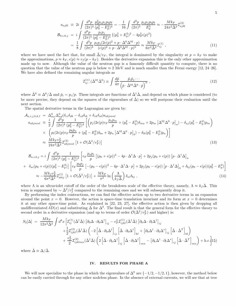
where we have used the fact that, for small ∆̄/vF , the integral is dominated by the singularity at p = kF to makethe approximations, p ≈ kF , ǫ(p) ≈ vf (p− kF ). Besides the derivative expansion this is the only other approximationmade up to now. Although the value of the neutron gap is a famously difficult quantity to compute, there is noquestion that the value of the neutron gap is below ≈ 2 MeV and is much smaller than the Fermi energy [12, 24–26].We have also defined the remaining angular integrals as

I(α)ij···(∆̂0†∆̂0) ≡

∫dp̂

4π

p̂ip̂j · · ·(

p̂ · ∆̂0†∆̂0 · p̂)α , (12)

where ∆̂0 ≡ ∆0/∆̄ and p̂i = pi/p. These integrals are functions of ∆̂†∆̂, and depend on which phase is considered (to

be more precise, they depend on the squares of the eigenvalues of ∆̂) so we will postpone their evaluation until thenext section.The spatial derivative terms in the Lagrangian are given by:

Aa,i,j,b,k,l = ∆0mc∆

0nd(δciδdk − δcdδik + δckδid)aabjmnl

aabjmnl ≡i

2

∫d4p

(2π)41

(p20 − E2p)

4

[(

pj(2ǫ(p)vFpapmp

+ (p20 − E2p)δma + 2pm

[∆0†∆0 · p

]

a)− δaj(p20 − E2

p)pm

)

×(

pl(2ǫ(p)vFpbpnp

+ (p20 − E2p)δbn + 2pn

[∆0†∆0 · p

]

b)− δlb(p20 − E2

p)pn

)]

≈ MkF v2F

24π2∆̄2I(2)abjmnl

[1 +O(∆̄2/v2F )

](13)

Ba,i,b,j = i

∫d4p

(2π)41

(p20 − E2p)

4

[

vFpapip

[(p0 + ǫ(p))2 − 4p ·∆†∆ · p

]+ 2pj(p0 + ǫ(p))

[p ·∆†∆

]

a

+ δai(p0 + ǫ(p))(p20 − E2p)][

vFpbpjp

[−(p0 − ǫ(p))2 − 4p ·∆†∆ · p

]+ 2pj(p0 − ǫ(p))

[p ·∆†∆

]

b+ δbj(p0 − ǫ(p))(p20 − E2

p)

]

≈ −Mkfv2F

6π2∆̄2I(1)abij

[1 +O(∆̄2/v2F )

]+MkFπ2

ln

(Λ

kf ∆̄

)

δaiδbj , (14)

where Λ is an ultraviolet cutoff of the order of the breakdown scale of the effective theory, namely, Λ ≈ kf ∆̄. Thisterm is suppressed by ∼ ∆̄2/v2f compared to the remaining ones and we will subsequently drop it.By performing the index contractions, we can find the effective action up to two derivative terms in an expansion

around the point x = 0. However, the action is space-time translation invariant and its form at x = 0 determinesit at any other space-time point. As explained in [22, 23, 27], the effective action is then given by dropping allundifferentiated δD(x) and substituting ∆ for ∆0. The final result is that the general form for the effective theory tosecond order in a derivative expansion (and up to terms of order O(∆̄2/v2F ) and higher) is:

S2[∆] =MkF

12π2∆̄2

∫

d4x[

I(1)ij (∆̂†∆̂)[∂0∆ · ∂0∆†

]

ij− v2FI

(1)ijkl(∆̂

†∆̂)[∂k∆ · ∂l∆†

]

ij

+1

2I(2)ijkl(∆̂

†∆̂)

(

−2[

∆̂ · ∂0∆†]

ij

[

∆̂ · ∂0∆†]

kl+[∂0∆

† · ∂0∆∗]

ij

[

∆̂ · ∆̂T]

kl

)

+v2F2I(2)ijklmn(∆̂

†∆̂)

(

2[

∆̂ · ∂k∆†]

ij

[

∆̂ · ∂l∆†]

mn−[∂k∆

† · ∂l∆∗]

ij

[

∆̂ · ∆̂T]

mn

)

+ h.c.

]

,(15)

where ∆̂ ≡ ∆/∆̄.

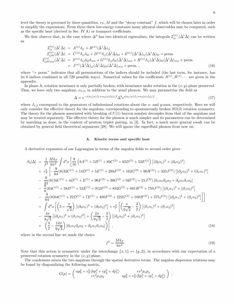
IV. RESULTS FOR PHASE A

We will now specialize to the phase in which the eigenvalues of ∆0 are {−1/2,−1/2, 1}, however, the method belowcan be easily carried through for any other nodeless phase. In the absence of external currents, we will see that at tree

6

level the theory is governed by three quantities, vF ,M and the “decay constant” f , which will be chosen later in orderto simplify the expressions. From these three low-energy constants many physical observables may be computed, suchas the specific heat (derived in Sec. IVA) or transport coefficients.

We first observe that, in the case where ∆0 has two identical eigenvalues, the integrals I(α)ij···(∆̂†∆̂) can be written

as

I(α)ij (∆̂†∆̂) = A(α)δij +B(α)(∆̂†∆̂)ij

I(α)ijkl(∆̂†∆̂) = C(α)δijδkl +D(α)δij(∆̂

†∆̂)kl + E(α)(∆̂†∆̂)ij(∆†∆)kl + perm.

I(α)ijklmn(∆̂†∆̂) = F (α)δijδklδmn +G(α)δijδkl(∆̂

†∆̂)mn +H(α)δij(∆̂†∆̂)kl(∆̂

†∆̂)mn + perm.

+ J (α)(∆̂†∆̂)ij(∆̂†∆̂)kl(∆̂

†∆̂)mn + perm. , (16)

where “+ perm.” indicates that all permutations of the indices should be included (the last term, for instance, hasits 6 indices combined in all 720 possible ways). Numerical values for the coefficients A(α), B(α) · · · are given in theappendix.In phase A, rotation invariance is only partially broken, with invariance under rotation in the (x, y)-plane preserved.

Thus, we have only two angulons, α1,2, in addition to the usual phonon. We may parametrize the field as

∆ = e−i(α1(x)J1+α2(x)J2)/f∆0ei(α1(x)J1+α2(x)J2)/f , (17)

where J1,2 correspond to the generators of infinitesimal rotations about the x- and y-axes, respectively. Here we willonly consider the effective theory for the angulons, corresponding to spontaneously broken SO(3) rotation symmetry.The theory for the phonon associated with breaking of U(1) baryon number decouples from that of the angulons andmay be treated separately. The effective theory for the phonon is much simpler and its parameters can be determinedby matching as done, in the context of neutron triplet pairing, in [2]. In fact, a much more general result can beobtained by general field theoretical arguments [28]. We will ignore the superfluid phonon from now on.

A. Kinetic terms and specific heat

A derivative expansion of our Lagrangian in terms of the angulon fields to second order gives

S2[∆] =1

f2

MkF6π2

∫

d4x

[9

16

(

8A(1) + 5B(1) + 80C(2) + 62D(2) + 53E(2)) [

(∂0α1)2 + (∂0α2)

2]

+ v2F

[

− 9

64(8(32C(1) + 14D(1) + 5E(1) + 288F (2) + 162G(2) + 90H(2)) + 333J (2))

[(∂yα2)

2 + (∂xα1)2]

− 9

32(8(16C(1) + 4D(1) + E(1) + 96F (2) + 30G(2) + 9H(2)) + 21J (2)) [∂xα1∂yα2 + ∂yα1∂xα2]

− 9

8(64C(1) + 58D(1) + 52E(1) + 912F (2) + 852G(2) + 801H(2) + 759J (2))

[(∂zα1)

2 + (∂zα2)2]

− 9

64(8(64C(1) + 22D(1) + 7E(1) + 480F (2) + 222G(2) + 108H(2)) + 375J (2))

[(∂yα1)

2 + (∂xα2)2]]]

=

∫

d4x

[(

3 +π√3

)[(∂0α1)

2 + (∂0α2)2]+ v2F

[(π

9√3− 3

2

)[(∂zα1)

2 + (∂zα2)2]

− 4π

3√3

[(∂yα1)

2 + (∂xα2)2]+

(2π

9√3− 3

2

)[(∂yα2)

2 + (∂xα1)2]

+

(3

2− 14π

9√3

)

[∂xα1∂yα2 + ∂yα1∂xα2]

)]

, (18)

where in the second line we made the choice

f2 =MkF6π2

. (19)

Note that this action is symmetric under the interchange {x, 1} ↔ {y, 2}, in accordance with our expectation of apreserved rotation symmetry in the (x, y)-plane.The condensate mixes the two angulons through the spatial derivative terms. The angulon dispersion relations may

be found by diagonalizing the following matrix,

G(p) =

(ap20 + v2F (bp

2z + cp2y + dp2x) ev2pxpy

ev2pxpy ap20 + v2F (bp2z + cp2x + dp2y)

)

,

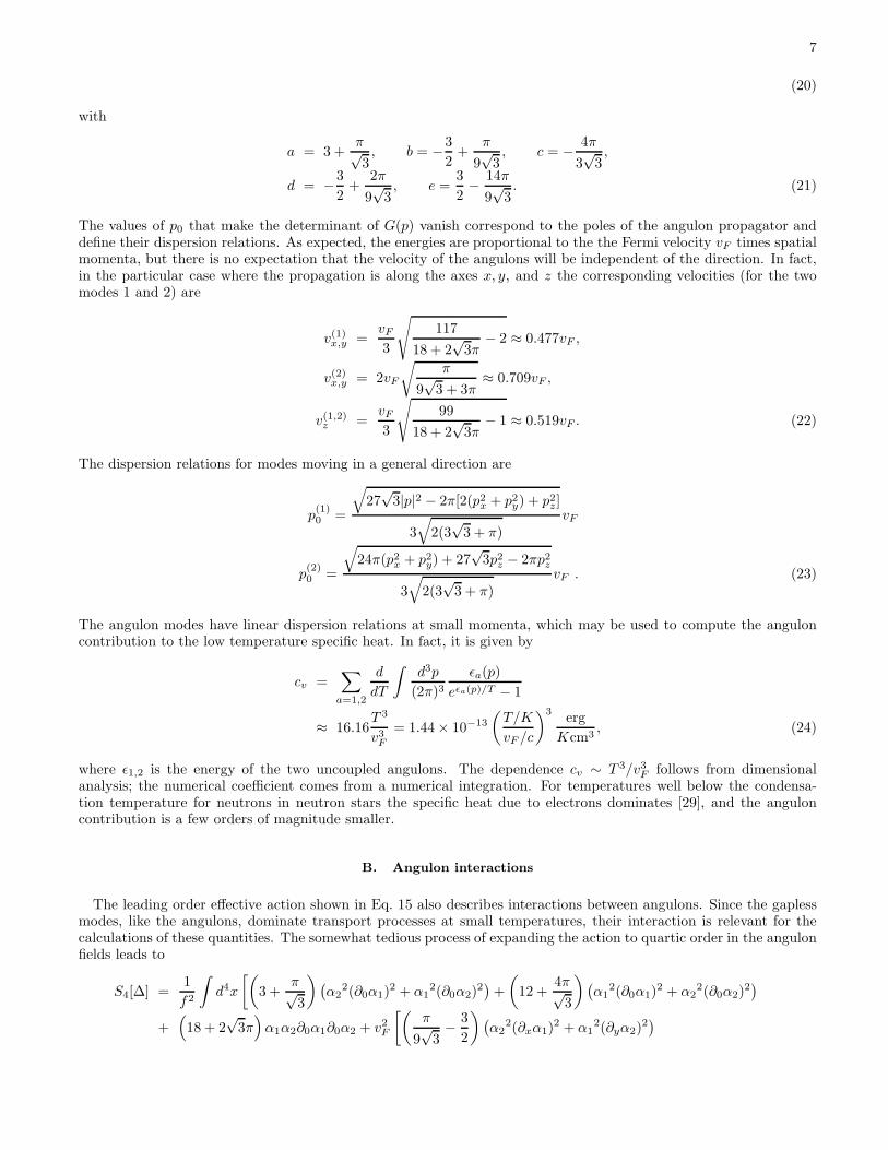
7

(20)

with

a = 3 +π√3, b = −3

2+

π

9√3, c = − 4π

3√3,

d = −3

2+

2π

9√3, e =

3

2− 14π

9√3. (21)

The values of p0 that make the determinant of G(p) vanish correspond to the poles of the angulon propagator anddefine their dispersion relations. As expected, the energies are proportional to the the Fermi velocity vF times spatialmomenta, but there is no expectation that the velocity of the angulons will be independent of the direction. In fact,in the particular case where the propagation is along the axes x, y, and z the corresponding velocities (for the twomodes 1 and 2) are

v(1)x,y =vF3

√

117

18 + 2√3π− 2 ≈ 0.477vF ,

v(2)x,y = 2vF

√π

9√3 + 3π

≈ 0.709vF ,

v(1,2)z =vF3

√

99

18 + 2√3π− 1 ≈ 0.519vF . (22)

The dispersion relations for modes moving in a general direction are

p(1)0 =

√

27√3|p|2 − 2π[2(p2x + p2y) + p2z]

3√

2(3√3 + π)

vF

p(2)0 =

√

24π(p2x + p2y) + 27√3p2z − 2πp2z

3√

2(3√3 + π)

vF . (23)

The angulon modes have linear dispersion relations at small momenta, which may be used to compute the anguloncontribution to the low temperature specific heat. In fact, it is given by

cv =∑

a=1,2

d

dT

∫d3p

(2π)3ǫa(p)

eǫa(p)/T − 1

≈ 16.16T 3

v3F= 1.44× 10−13

(T/K

vF /c

)3erg

Kcm3, (24)

where ǫ1,2 is the energy of the two uncoupled angulons. The dependence cv ∼ T 3/v3F follows from dimensionalanalysis; the numerical coefficient comes from a numerical integration. For temperatures well below the condensa-tion temperature for neutrons in neutron stars the specific heat due to electrons dominates [29], and the anguloncontribution is a few orders of magnitude smaller.

B. Angulon interactions

The leading order effective action shown in Eq. 15 also describes interactions between angulons. Since the gaplessmodes, like the angulons, dominate transport processes at small temperatures, their interaction is relevant for thecalculations of these quantities. The somewhat tedious process of expanding the action to quartic order in the angulonfields leads to

S4[∆] =1

f2

∫

d4x

[(

3 +π√3

)(α2

2(∂0α1)2 + α1

2(∂0α2)2)+

(

12 +4π√3

)(α1

2(∂0α1)2 + α2

2(∂0α2)2)

+(

18 + 2√3π)

α1α2∂0α1∂0α2 + v2F

[(π

9√3− 3

2

)(α2

2(∂xα1)2 + α1

2(∂yα2)2)

8

+

(8π

9√3− 6

)(α1

2(∂xα1)2 + α2

2(∂yα2)2)− 4π

3√3

(α1

2(∂xα2)2 + α2

2(∂yα1)2)

+

(

3− 28π

9√3

)(α1

2∂xα1∂yα2 + α22∂xα1∂yα2 + α1

2∂xα2∂yα1 + α22∂xα2∂yα1

)

+

(

3− 10π

3√3

)

(α1α2∂xα1∂yα1 + α1α2∂xα2∂yα2)−(16π

9√3+ 6

)

(α1α2∂xα1∂xα2 + α1α2∂yα1∂yα2)

−(35π

9√3+

3

2

)(α2

2(∂xα2)2 + α1

2∂yα12)+

(2π

9√3− 3

2

)(α2

2(∂zα1)2 + α1

2(∂zα2)2)

−(π√3+

9

2

)(α1

2(∂zα1)2 + α2

2(∂zα2)2)−(22π

9√3+ 6

)

α1α2∂zα1∂zα2

]]

. (25)

C. Weak interactions

Angulons couple to electroweak currents. Since they are not electrically charged, at leading order in the Fermiconstant GF the only possible coupling is with the neutral current mediated by the Z boson. In this section we derivethis coupling.We begin by adding the following interaction terms to the microscopic Lagrangian,

LW = CV Z00ψ

†ψ + CAZ0i ψ

†σiψ , (26)

where Z00 , Z

0i are the temporal and spatial components, respectively, of the Z0 boson, and the couplings are given by

C2V,A = C̃2

V,A

GFM2Z

2√2

, (27)

where C̃V = −1 by vector current conservation, and C̃A ∼ 1.1± 0.15 [30] is given by the sum of the nucleon isovectoraxial coupling, gA, and the matrix element of the strange axial-current in the proton, ∆s. Here we choose the vacuumform of the interactions as little is known about their renormalization when modes far from the Fermi surface areremoved.The action for the angulons including the weak vertex is

S[∆] = −i∫

d4xTr ln[D−10 + δD−1 + CAZ

0mΣm]

≈ −i∫

d4xTr(ln[D−1

0 + δD−1] + (D−10 + δD−1)−1CAZ

0mΣm

)(28)

where

Σm ≡(σm 00 σ2σmσ2

)

, (29)

and we have taken only the leading order in a weak coupling expansion. We may now perform a derivative expansionof the propagator using the method outlined in App. VI,

(D−10 + δD−1)−1 =

∫d4p

(2π)4tr

(∑

n

[

D0(p)∑

m=1

∂mµm!

pj [δD−1(x)]j(i∂pµ

)m

]n

D0(p)

)

. (30)

The leading order term in the derivative expansion of the weak interaction contribution to the Lagrangian is givenby m = n = 1. The only non-zero terms are

LW [∆] = CAZ0m

∫d4p

(2π)4tr[D0(p)∂0pj [δD

−1(x)]j∂p0D0(p)Σm

]

= iCAZ0m

∫d4p

(2π)4pjtr [D12∂0δ∆

†ijσ2σi∂p0

D11σm −D11∂0δ∆jiσiσ2∂p0D21σm

+ D22∂0δ∆†ijσ2σi∂p0

D12σ2σmσ2 −D21∂0δ∆jiσiσ2∂p0D22σ2σmσ2]

= CAZ0m∂0δ∆

†ij∆kl

∫d4p

(2π)4pjpktr

[

−1p20 − E2

p

σlσ2σ2σi−p20 − 2p0ǫp − E2

p

(p20 − E2p)

2σm

9

+p0 − ǫpp20 − E2

p

σ2σi2p0σlσ2

(p20 − E2p)

2σ2σmσ2

]

+ h.c.

= −2iǫlimCAZ0m∂0δ∆

†ij∆kl

∫d4p

(2π)4pjpk

−p20 + 4p0ǫp + E2p

(p20 − E2p)

3+ h.c.

=1

2ǫlimCAZ

0m∂0δ∆

†ij∆kl

∫d3p

(2π)3pjpkE3

p

+ h.c.

≈ ǫlimCAZ0m∂0δ∆

†ij∆kl

MkF2π2|∆̄|2 I

(1)jk + h.c.

→ 3f2ǫlimCAZ0m∂0∆

†ij∆klI(1)jk + h.c., (31)

where in the last step we used the translation invariance of the effective lagrangian, as explained previously whenderiving the strong interactions. Expanding this in terms of the angulon fields α gives the leading contribution to theaction from the angulon-neutral current vertex

SW [∆] = CA

∫

d4x

[27

8(4A(1) + 3B(1))f(Z0

2∂0α2 − Z01∂0α1) +

27

8(4A(1) + 3B(1))Z0

3 (α2∂0α1 − α1∂0α2) + · · ·]

= CA

∫

d4x[9f(Z0

2∂0α2 − Z01∂0α1) + 9Z0

3(α2∂0α1 − α1∂0α2) + · · ·]. (32)

D. Higher orders and regime of validity

The effective action shown in eq. (15) is, to the extent that terms with more derivatives may be neglected, equivalentto our starting point (eq. (3)). We will argue now that is legitimate to use eq. (15) at tree level to capture the low energydynamics of the system. The crucial observation is that the effective action shown in eq. (15) shares certain propertieswith other low energy effective actions, such as those describing low energy pions in zero-density/temperature QCD ormagnons in an anti-ferromagnet, and power counting of diagrams in such theories is well understood. The contributionsof bosonic fluctuations (angulons) are described by loops. A generic loop diagram will have an even number of powersof f in the denominator coming from the vertices in eq. (15). By dimensional arguments, these powers of f must beoffset by powers of the external momentum Q so that loops are suppressed by powers of (Q/f)2 compared to treelevel and are therefore suppressed at low energies 2.This is not to say that the range of validity of the angulon effective theory is Q < f . We have neglected in our

derivation contributions suppressed by ∆̄/vF that may be larger than corrections of order (Q/f)2. For astrophysicalapplications, where solid estimates are more necessary than precise calculations, those corrections are of limitedinterest.The generic form of the effective theory we obtained could have been foreseen. It is indeed the most general

action involving a symmetric tensor field ∆ obeying rotation symmetry up to two derivatives. Higher powers of ∆,not appearing in eq. (15), are not independent since ∆ has only two independent eigenvalues. The only terms notappearing in eq. (15) are the ones with repeated powers of ∆2, as opposed to ∆†∆. They are excluded because ourstarting point eq. (3) has, in addition to rotational symmetry

∆→ R∆RT , (33)

where R is a rotation matrix, the enhanced symmetry

∆→ RS∆RTL , (34)

where RS , RL are independent spin and orbital rotations. Nuclear forces do not have this enhanced symmetry (amongneutrons due mostly to the existence of spin-orbit forces). As with any of the other interactions left out of eq. (3)(assuming they do not affect the phase of the theory) and as discussed above, they are expected to contribute to thelow energy constants of the angulon theory we have calculated by a perturbatively small amount, even though theymay contribute significantly to the renormalization of kF and vF . Notice that for this to be true the renormalizedspin-orbit forces at the Fermi surface do not have to be smaller than the interaction in eq. (3); it is enough that their

2 The detailed accounting of powers of Q/f is similar to the one in Chiral Perturbation Theory and is discussed at length in [31].

10

contribution to the energy be smaller than the neutron kinetic energy, as the low energy coefficients we computed areindependent of the coupling g. This observation also indicates that terms like

L ∼ Tr(∆), (35)

forbidden only by the enhanced symmetry should be small. These terms give a mass to the approximate Goldstonemodes related to the enhanced symmetry eq. (34). We ignored these massive modes here entirely as they are irrelevantat small enough energies and observe that the smallness of their mass is behind some of the near degeneracies of 3P2

states found in model calculations. Further work is needed to evaluate the approximate Goldstone masses. If it turnsout that their masses are smaller than ∼ ∆̄/vF they will set the scale of breakdown of the angulon effective theory.

V. SUMMARY

We have derived a low-energy effective theory describing the Goldstone bosons associated with broken rotationalsymmetry in a 3P2 condensed neutron superfluid (angulons). Because transport properties are dominated by thelow lying excitation modes, this theory provides a link connecting the theory of nuclear forces to many quantitiesof interest in neutron star phenomenology. Since there is still controversy as to which of the many 3P2 phases arerealized in nature we have tried to keep our calculation as general as possible. Ultimately, however, the numericalvalue of the coefficients of the effective action do depend on the particular 3P2 phase and we give explicit values forthe “phase A” as defined in Eq. 2. This effective theory is valid for angulon energies below the energy scale ∼ 2kf ∆̄(or the mass of the approximate Goldstone bosons related to independent spin and orbital rotations, whichever issmaller) where other degrees of freedom, like unpaired neutrons, appear.A simple application of the effective theory, the calculation of the angulon contribution to the specific heat, was

discussed. We also considered the coupling of angulons to neutral currents, since quantities like neutrino opacity andemission rates depend on this coupling, and gave an explicit form for the angulon-angulon-Z vertex.A series of improvements and extensions to the effective theory discussed here are desirable. For applications to

neutron stars, we should consider the presence of both protons and neutrons. The protons are superconducting andlead only to another gapped mode but they are important in mediating the interaction between angulons (with whomthey interact through strong forces) and the gapless electron (with whom they interact electromagnetically). In ourmicroscopic action for neutrons we have included only the dominant forces leading to 3P2 pairing. While expectedto be repulsive and weaker, neutron interactions in other channels can have an influence on the angulon effectivetheory. It would be very desirable to quantify this effect. We have not given much attention to the gapped modescorresponding to a change in the eigenvalues of ∆. Although their importance is exponentially suppressed at smalltemperatures they can be numerically important at temperatures of relevance to some stages of neutron star evolution.Our method of deriving the effective theory by performing a derivative expansion on a microscopic theory allows usto address this question and we plan to come back to it in a future publication. Finally, the energy difference betweendifferent 3P2 phases is small. In particular, the condensation energy of phase C in Eq. 2 is only a few percent abovethat for phase A. This restricts the validity of the effective theory somewhat and it would be important to quantifythe importance of the other nearby minima to the low energy physics of the system.

VI. APPENDIX: THE DERIVATIVE EXPANSION

In order to set up the derivative expansion of

Tr lnD−1(i∂, x) = Tr ln[D−10 (i∂)

︸ ︷︷ ︸

D−1(i∂,0)

+δD−1(i∂, x)] (36)

we first use the relation

Tr ln(A+B) = Tr lnA+Tr ln(1 +A−1B) = Tr lnA+Tr ln(1 +BA−1)

= Tr lnA+∞∑

n=0

Tr1

n+ 1(A−1B)n+1

= Tr lnA+Tr

∫ 1

0

dz (1 + zA−1B)−1A−1B

= Tr lnA+Tr

∫ 1

0

dz (A+ zB)−1B (37)

11

to find

Tr lnD−10 +

∫ 1

0

dz Tr1

D−10 + zδD−1

δD−1. (38)

The second term contains the dependence on the space-time variation of ∆. This term is complicated to computebecause it contains ∂ and x which do not commute. One trick to deal with this is to substitute in the integrand∂ → ip, x → x + i∂p and integrate over p [23] . To do this, we first need to find the inverse of the operator

D−10 + zδD−1 in terms of p, ∂p, so we look at

[D−1

0 + zδD−1]−1 ≡ G(x, y) =

∫d4p

(2π)4eip·yG(p, i∂p)e

−ip·x . (39)

Using

(D−1

0 + zδD−1)G(x, y) = δ4(x− y) =

∫d4p

(2π)4eip·y

(D−1

0 + zδD−1)G(p, i∂p)e

−ip·x , (40)

we find

G(p, i∂p) =[

D−10 (p) + zpj

[δD−1(i∂p)

]

j

]−1

, (41)

where

D−10 (p) =

(p0 − ǫ(p) ipj∆

0jiσiσ2

−ipj∆0†ij (σ2σi p0 + ǫ(p)

)

,

[δD−1(i∂p)

]

j=

(0 i∆ji(i∂p)σiσ2

−i∆†ij(i∂p)σ2σi 0

)

. (42)

We may now expand the second term in Eq. 38 as

∫d4p

(2π)4

∫ 1

0

dztr[

D−10 (p) + zpj

[δD−1(i∂p + x)

]

j

]−1

pk[δD−1(x)

]

k

=

∫d4p

(2π)4

∫ 1

0

dztr

[

D−10 (p) + zpj

[δD−1(x)

]

j+ zpj

∑

m=1

(i∂pµ)m

m!∂mµ[δD−1(x)

]

j

]−1

pk[δD−1(x)

]

k

=

∫d4p

(2π)4

∫ 1

0

dztr

[

1 + zpj(D−1

0 (p) + zpk[δD−1(x)

]

k

)−1 ∑

m=1

(i∂pµ)m

m!∂mµ[δD−1(x)

]

j

]−1

×[

D−10 (p) + zpj

[δD−1(x)

]

j

]−1

pk[δD−1(x)

]

k

=

∫d4p

(2π)4

∫ 1

0

dztr

∞∑

n=0

(−z)n[

D0(p)∑

m=1

∂mµm!

pj[δD−1(x)

]

j(i∂pµ

)m

]n

D0(p)pk[δD−1(x)

]

k, (43)

VII. APPENDIX: COEFFICIENTS FOR THE INTEGRALS I(α)ij···

Here we show how to compute the numerical coefficients A(α), B(α), · · · appearing in Eq. 16. Consider, for instance,

I(1)ij . We first multiply the upper equation in Eq. 16 by (∆̂†∆̂)ij and δij to obtain

∫dp̂

4π

1

p̂.(∆̂†∆̂).p̂︸ ︷︷ ︸

4π

3√

3

= 3A(1) + tr(∆̂†∆̂)︸ ︷︷ ︸

3/2

B(1)

∫dp̂

4π︸ ︷︷ ︸

1

= tr(∆̂†∆̂)︸ ︷︷ ︸

3/2

A(1) + tr(∆̂†∆̂)2︸ ︷︷ ︸

9/8

B(1). (44)

12

Solving this system of equations we find

A(1) =4

3

(π√3− 1

)

, B(1) =8

3− 16π

9√3

(45)

The same method can be easily implemented in computer algebra packages and we find

C(1) = − 4

27+

145π

1458√3, D(1) =

14

27− 220π

729√3, E(1) = −10

27+

152π

729√3

C(2) =11

36− 25π

243√3, D(2) = −10

9+

128π

243√3, E(2) =

8

9− 112π

243√3

F (2) =43

1080− 263π

13122√3, G(2) = − 59

270+

256π

2187√3, H(2) =

16

45− 424π

2187√3, J (2) = − 8

45+

640π

6561√3.

(46)

Acknowledgments

This work was supported in part by U.S. DOE grant No. DE-FG02-93ER-40762.

[1] T. Brauner, Symmetry 2, 609 (2010), 1001.5212.[2] P. F. Bedaque, G. Rupak, and M. J. Savage, Phys.Rev. C68, 065802 (2003), nucl-th/0305032.[3] C. O. Heinke and W. C. Ho, Astrophys.J. 719, L167 (2010), 1007.4719.[4] D. Page, M. Prakash, J. M. Lattimer, and A. W. Steiner, Phys.Rev.Lett. 106, 081101 (2011), 1011.6142.[5] P. S. Shternin, D. G. Yakovlev, C. O. Heinke, W. C. Ho, and D. J. Patnaude, Mon.Not.Roy.Astron.Soc. 412, L108 (2011),

1012.0045.[6] D. G. Yakovlev, W. C. Ho, P. S. Shternin, C. O. Heinke, and A. Y. Potekhin, Mon.Not.Roy.Astron.Soc. 411, 1977 (2011),

1010.1154.[7] D. Page (2012), 1206.5011.[8] D. Page, M. Prakash, J. M. Lattimer, and A. W. Steiner (2011), 1110.5116.[9] L. Leinson, Phys.Rev. C85, 065502 (2012), 1206.3648.

[10] R. Richardson, Phys.Rev. D5, 1883 (1972).[11] V. Vulovic and J. Sauls, Phys.Rev. D29, 2705 (1984).[12] T. Takatsuka and R. Tamagaki, Prog.Theor.Phys.Suppl. 112, 27 (1993).[13] V. Khodel, V. Khodel, and J. W. Clark, Phys.Rev.Lett. 81, 3828 (1998), nucl-th/9807034.[14] V. Khodel, J. W. Clark, and M. Zverev, Phys.Rev.Lett. 87, 031103 (2001), nucl-th/0101045.[15] A. Migdal, Theory of finite Fermi systems, and applications to atomic nuclei, Interscience monographs and texts in physics

and astronomy (Interscience Publishers, 1967), URL http://books.google.com/books?id=M-NEAAAAIAAJ.[16] R. Shankar, Rev.Mod.Phys. 66, 129 (1994).[17] G. Benfatto and G. Gallavotti, Phys.Rev. B42, 9967 (1990).[18] J. Polchinski (1992), hep-th/9210046.[19] B. Friman, K. Hebeler, and A. Schwenk, Lect.Notes Phys. 852, 245 (2012), 1201.2510.[20] C. Fraser, Z.Phys. C28, 101 (1985).[21] O. Cheyette, Phys.Rev.Lett. 55, 2394 (1985).[22] O. Cheyette (1987).[23] L. Chan, Phys.Rev.Lett. 54, 1222 (1985).[24] M. Baldo, O. Elgarøy, L. Engvik, M. Hjorth-Jensen, and H.-J. Schulze, Phys. Rev. C 58, 1921 (1998), URL

http://link.aps.org/doi/10.1103/PhysRevC.58.1921 .[25] L. Amundsen and E. Ostgaard, Nucl.Phys. A442, 163 (1985).[26] W. Zuo, C. X. Cui, U. Lombardo, and H.-J. Schulze, Phys. Rev. C 78, 015805 (2008), URL

http://link.aps.org/doi/10.1103/PhysRevC.78.015805.[27] A. K. Das and M. B. Hott, Phys.Rev. D50, 6655 (1994), hep-ph/9407283.[28] D. Son (2002), hep-ph/0204199.[29] D. Yakovlev, K. Levenfish, and Y. Shibanov, Phys.Usp. 42, 737 (1999), astro-ph/9906456.[30] M. J. Savage and J. Walden, Phys.Rev. D55, 5376 (1997), hep-ph/9611210.[31] S. Weinberg, Physica A96, 327 (1979).