Dynamics of Condensed Phase Proton and Electron Transfer Processes
32
CHAPTER 92 Dynamics of Condensed Phase Proton and Electron Transfer Processes Raymond Kapral, Alessandro Sergi Chemical Physics Theory Group, Department of Chemistry, University of Toronto, Toronto, Canada CONTENTS 1. Introduction ..................................... 2 2. Chemical Reaction Rates ............................ 2 2.1. Microscopic Expressions for Rate Constants ......... 2 2.2. Classical Mechanical Rate Expression .............. 4 2.3. Blue Moon Ensemble .......................... 5 3. Free Energy Along the Reaction Coordinate .............. 6 3.1. Imaginary Time Path Integral Molecular Dynamics .... 6 3.2. Electron Solvation in Reverse Micelles ............. 8 3.3. Proton Transfer in Nanoscale Molecular Clusters ..... 10 4. Adiabatic Reaction Dynamics ........................ 13 4.1. Quantum-Classical Adiabatic Dynamics ............ 13 4.2. Adiabatic Proton-Transfer Reactions in Solution ...... 15 4.3. Proton Transfer Dynamics in Nanoclusters .......... 16 5. Mean Field and Surface Hopping Dynamics ............. 18 5.1. Mean-Field Method .......................... 19 5.2. Surface-Hopping Dynamics ..................... 19 5.3. Nonadiabatic Proton Transfer in Nanoclusters ....... 20 6. Quantum-Classical Liouville Equation ................. 21 6.1. Simulation Algorithm ......................... 24 7. Nonadiabatic Reaction Dynamics ..................... 25 7.1. Quantum-Classical Reactive Flux Correlation Functions .................................. 25 7.2. Two-Level Model for Transfer Reactions ........... 26 7.3. Two-Level Reaction Simulation Results ............ 28 ISBN: 1-58883-042-X/$35.00 Copyright © 2005 by American Scientific Publishers All rights of reproduction in any form reserved. 1 Handbook of Theoretical and Computational Nanotechnology Edited by Michael Rieth and Wolfram Schommers Volume 1: Pages (1–32)
Transcript of Dynamics of Condensed Phase Proton and Electron Transfer Processes
CHAPTER 92
Dynamics of CondensedPhase Proton and ElectronTransfer Processes
Raymond Kapral, Alessandro SergiChemical Physics Theory Group, Department of Chemistry,University of Toronto, Toronto, Canada
CONTENTS
1. Introduction . . . . . . . . . . . . . . . . . . . . . . . . . . . . . . . . . . . . . 2
2. Chemical Reaction Rates . . . . . . . . . . . . . . . . . . . . . . . . . . . . 22.1. Microscopic Expressions for Rate Constants . . . . . . . . . 22.2. Classical Mechanical Rate Expression . . . . . . . . . . . . . . 42.3. Blue Moon Ensemble . . . . . . . . . . . . . . . . . . . . . . . . . . 5
3. Free Energy Along the Reaction Coordinate . . . . . . . . . . . . . . 63.1. Imaginary Time Path Integral Molecular Dynamics . . . . 63.2. Electron Solvation in Reverse Micelles . . . . . . . . . . . . . 83.3. Proton Transfer in Nanoscale Molecular Clusters . . . . . 10
4. Adiabatic Reaction Dynamics . . . . . . . . . . . . . . . . . . . . . . . . 134.1. Quantum-Classical Adiabatic Dynamics . . . . . . . . . . . . 134.2. Adiabatic Proton-Transfer Reactions in Solution . . . . . . 154.3. Proton Transfer Dynamics in Nanoclusters . . . . . . . . . . 16
5. Mean Field and Surface Hopping Dynamics . . . . . . . . . . . . . 185.1. Mean-Field Method . . . . . . . . . . . . . . . . . . . . . . . . . . 195.2. Surface-Hopping Dynamics . . . . . . . . . . . . . . . . . . . . . 195.3. Nonadiabatic Proton Transfer in Nanoclusters . . . . . . . 20
6. Quantum-Classical Liouville Equation . . . . . . . . . . . . . . . . . 216.1. Simulation Algorithm . . . . . . . . . . . . . . . . . . . . . . . . . 24
7. Nonadiabatic Reaction Dynamics . . . . . . . . . . . . . . . . . . . . . 257.1. Quantum-Classical Reactive Flux Correlation
Functions . . . . . . . . . . . . . . . . . . . . . . . . . . . . . . . . . . 257.2. Two-Level Model for Transfer Reactions . . . . . . . . . . . 267.3. Two-Level Reaction Simulation Results . . . . . . . . . . . . 28
ISBN: 1-58883-042-X/$35.00Copyright © 2005 by American Scientific PublishersAll rights of reproduction in any form reserved.
1
Handbook of Theoretical and Computational NanotechnologyEdited by Michael Rieth and Wolfram Schommers
Volume 1: Pages (1–32)
2 Dynamics of Condensed Phase Proton and Electron Transfer Processes
8. Conclusions . . . . . . . . . . . . . . . . . . . . . . . . . . . . . . . . . . . . 30References . . . . . . . . . . . . . . . . . . . . . . . . . . . . . . . . . . . . . 31
1. INTRODUCTIONProton and electron transfer reactions are ubiquitous in chemistry and govern many impor-tant physical and biological functions [1–3]. In order to understand the mechanisms throughwhich such reactions take place and to determine their rates, one must account for the quan-tum nature of these transferring particles. This feature provides challenges for theory andsimulation because quantum dynamics in many-body environments is difficult to carry out.
The rate constants that characterize the interconversion of chemical species can be com-puted from a knowledge of reactive flux correlation functions. In this chapter, we sketchthe derivation of these microscopic formulas for rate constants that can be used to computeelectron and proton transfer rates. For activated chemical rate processes, where chemicalreactions take place on timescales that are long compared to typical microscopic relaxationtimes accessible in computer simulation methods, one must devise schemes for samplingrare reactive events. We discuss one such method, the blue moon ensemble, which can beused to obtain the rate from short time simulations of the dynamics. The reactive flux for-malism provides a natural decomposition of the rate constant expression into a transitionstate theory contribution and a transmission coefficient that accounts for dynamical recross-ing events. Because the transition state theory rate depends on the free energy along thereaction coordinate, this quantity is an important ingredient in estimating the reaction rate.We give examples of the computation of the free energy for reactions occurring in bulkcondensed phases as well as in materials with nanoscale dimensions such as clusters andmicelles.
The main focus of this chapter is on quantum mechanical rate processes, such as thoseassociated with electron and proton transfer processes, and we describe methods for com-puting rates of these reactions. The methods will be illustrated by considering again simplemodels for such processes in bulk and cluster environments. The emphasis of this presenta-tion is on the theoretical methods and the basic elements of the physical mechanisms thatunderlie and govern such processes.
2. CHEMICAL REACTION RATESA phenomenological description of the dynamics of a chemical reaction A� B can be givenin terms of the mass action rate law,
dnA�t�
dt= −kf nA�t�+ kr nB�t� (1)
where nA�t� and nB�t� are the mean number densities of species A and B, respectively. Ifwe let �� = �nA = nA − n
eqA = −�nB = −�nB − n
eqB � be the deviations of the species densities
from their equilibrium values, the rate law takes the form,
d��dt
= −�kf + kr��� (2)
Our goals are to determine microscopic expressions for the rate constants and to constructalgorithms to compute the forward kf and reverse kr = kfK
−1eq (Keq is the equilibrium con-
stant) rate constants by molecular dynamics simulation.
2.1. Microscopic Expressions for Rate Constants
We present a quantum mechanical formulation of reaction rates because our primary interestis in proton and electron transfer processes. However, as we shall see below, the classicallimit results can be used in some circumstances to obtain approximations to quantum rates.The rate at which the A and B species interconvert can be determined from the reactive
Dynamics of Condensed Phase Proton and Electron Transfer Processes 3
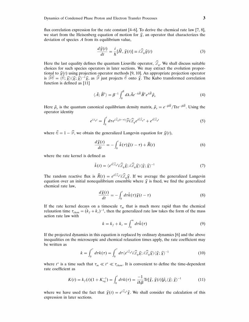
flux correlation expression for the rate constant [4–6]. To derive the chemical rate law [7, 8],we start from the Heisenberg equation of motion for ��, an operator that characterizes thedeviation of species A from its equilibrium value,
d���t�dt
= i
��H� ���t�� ≡ i�q ���t� (3)
Here the last equality defines the quantum Liouville operator, �q . We shall discuss suitablechoices for such species operators in later sections. We may extract the evolution propor-tional to ���t� using projection operator methods [9, 10]. An appropriate projection operatoris � �� = ���� ������ ��−1 ��, as � just projects �� onto ��. The Kubo transformed correlationfunction is defined as [11]
� A� �B† = �−1∫ �
0d� Ae−�H �B†e�H �e (4)
Here �e is the quantum canonical equilibrium density matrix, �e = e−�H/Tre−�H . Using theoperator identity
ei�q t =∫ t
0d�ei�q�t−���i�qe
i���q� + ei���q t (5)
where �� = 1− �, we obtain the generalized Langevin equation for ���t�,d���t�dt
= −∫ t
0k������t − ��+ R�t� (6)
where the rate kernel is defined as
k�t� = �ei���q ti�q ��� i�q ������ ��−1 (7)
The random reactive flux is R�t� = ei���q ti�q ��. If we average the generalized Langevin
equation over an initial nonequilibrium ensemble where �� is fixed, we find the generalizedchemical rate law,
d ���t�dt
= −∫ t
0d�k��� ���t − �� (8)
If the rate kernel decays on a timescale �m that is much more rapid than the chemicalrelaxation time �chem = �kf + kr�−1, then the generalized rate law takes the form of the massaction rate law with
k = kf + kr =∫
0d�k��� (9)
If the projected dynamics in this equation is replaced by ordinary dynamics [6] and the aboveinequalities on the microscopic and chemical relaxation times apply, the rate coefficient maybe written as
k =∫ t∗
0d�k��� =
∫ t∗
0d��ei�q ti�q ��� i�q ������ ��−1 (10)
where t∗ is a time such that �m � t∗ � �chem. It is convenient to define the time-dependentrate coefficient as
K�t� = kf �t��1+K−1eq � =
∫ t
0d�k��� = −1
i��Tr���� ���t�� �e���� ��−1 (11)
where we have used the fact that ���t� = ei�q t ��. We shall consider the calculation of thisexpression in later sections.

4 Dynamics of Condensed Phase Proton and Electron Transfer Processes
2.2. Classical Mechanical Rate Expression
To formulate the classical statistical mechanical description of chemical reactions, considera molecular system containing N atoms with Hamiltonian H = K�p� + V �r�, where K�p�is the kinetic energy, V �r� is the potential energy, and �p� r� denotes the 6N momenta andcoordinates defining the phase space of the system.
We suppose that the progress of the reaction can be characterized on a microscopic levelby a scalar reaction coordinate !�r� that is a function of the positions of the particles in thesystem. For the reaction A� B, we assume that a dividing surface at !‡ serves to partitionthe configuration space of the system into two A and B domains that contain the metastableA and B species. (In general, it is not always clear what a suitable choice of a reactioncoordinate is for any given problem. There is an active area of research devoted to thedevelopment of schemes for the determination of reaction paths and suitable coordinates todescribe the reaction [12–16]. Here we assume that such microscopic coordinates are knownand show how to compute the rate.) The microscopic variable determining the fraction ofsystems in the A domain is ��r� = nA�r� − �nA�r� = #�!‡ − !�r�� − n
eqA , where # is the
Heaviside function. The angular brackets denote an equilibrium canonical average, �· · · =Q−1
∫dr dr exp%−�H& · · · , where Q is the partition function and n
eqA is the equilibrium
density of species A. Likewise, the fraction of systems in the B domain is nB�r� = #�!�r�−!‡�. The time rate of change of nA�r� is
nA�r� = −!�r���!�r�− !‡� (12)
The time-dependent forward rate coefficient can be expressed in terms of the equilibriumcorrelation function of the initial flux of A with the B species density at time t as [4]
kf �t� =1neqA
�nA�r�nA�r� t� =1neqA
⟨{!��!�r�− !‡�
}#{!�r�t��− !‡
}⟩(13)
For an activated rate process, the reactive flux correlation function will decay rapidly initially,followed by a much slower decay that occurs on the timescale of the slow chemical intercon-version process. The rate constant can be determined from the “plateau” value establishedduring the slow decay of this time-dependent rate coefficient [6, 7].
Static and dynamic contributions to the rate coefficient can be defined by multiplying anddividing each term on the right-hand side of Eq. (13) by ���!�r�− !‡� to obtain
kf �t� ={⟨!��!�r�− !‡�#�!�r�t��− !‡�
⟩���!�r�− !‡�
}{���!�r�− !‡�
neqA
}
= ⟨!#%!�r�t��− !‡&
⟩cd!‡
{e−�W�!‡�∫
!′<!‡ d!′ e−�W�!′�
}(14)
where �· · · cd!‡
defines an average conditional on !�r� = !‡,
�· · · cd!′ = �· · · ��!�r�− ! ′����!�r�− ! ′� (15)
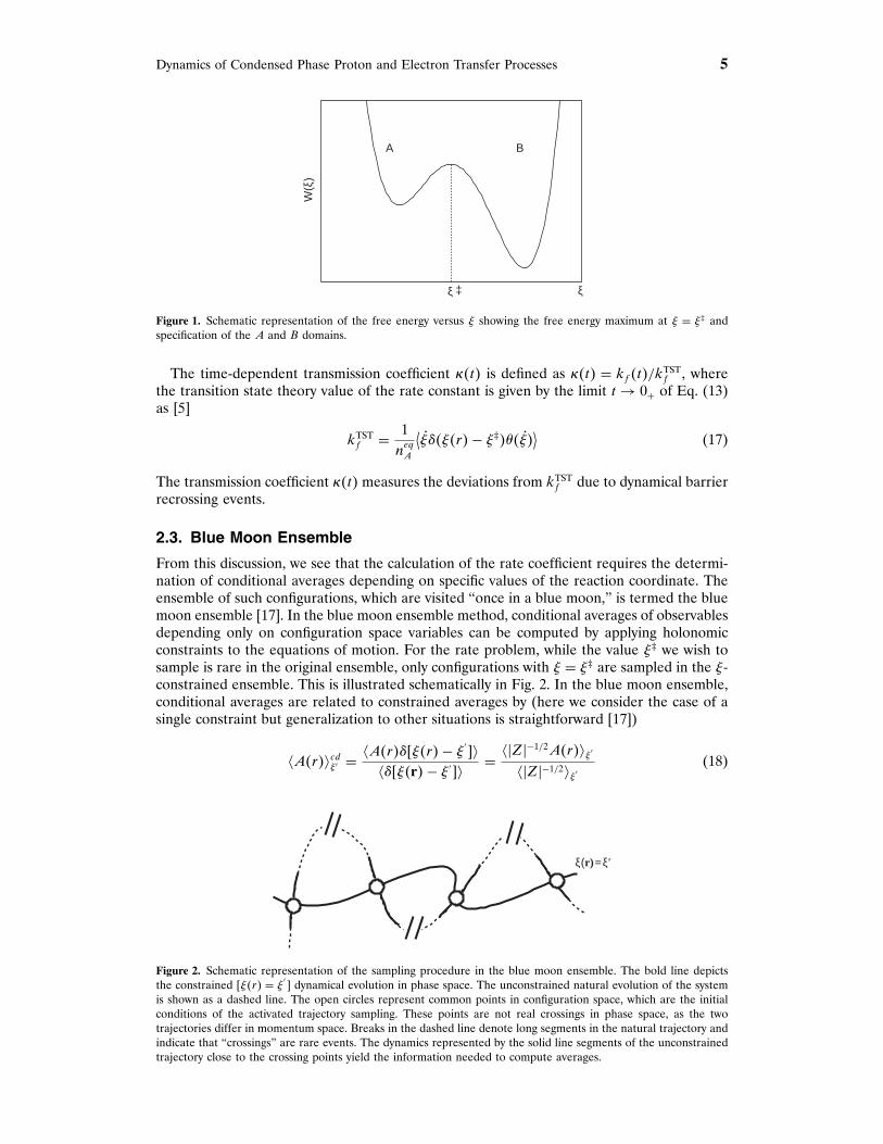
In writing the second factor in Eq. (14), we used the fact that the equilibrium average���!�r�−!‡� = P�!‡� is the probability density of finding the value !�r�= !‡ of the reactioncoordinate. The free energy W�! ′� associated with the reaction coordinate is defined byW�! ′� = −�−1 ln�P�! ′�/Pu�, where Pu is a uniform probability density of ! ′. Typically, thefree energy will have the form shown schematically in Fig. 1. A high free energy barrierat ! = !‡ separates the metastable reactant and product states. The equilibrium density ofspecies A is
neqA = ⟨
#�!‡ − !�r��⟩ = ∫
!′<!‡d! ′P�! ′� (16)
Dynamics of Condensed Phase Proton and Electron Transfer Processes 5
W(ξ
)ξ ‡ ξ
A B
Figure 1. Schematic representation of the free energy versus ! showing the free energy maximum at ! = !‡ andspecification of the A and B domains.
The time-dependent transmission coefficient ,�t� is defined as ,�t� = kf �t�/kTSTf , where
the transition state theory value of the rate constant is given by the limit t → 0+ of Eq. (13)as [5]
kTSTf = 1
neqA
⟨!��!�r�− !‡�#�!�
⟩(17)
The transmission coefficient ,�t� measures the deviations from kTSTf due to dynamical barrier
recrossing events.
2.3. Blue Moon Ensemble
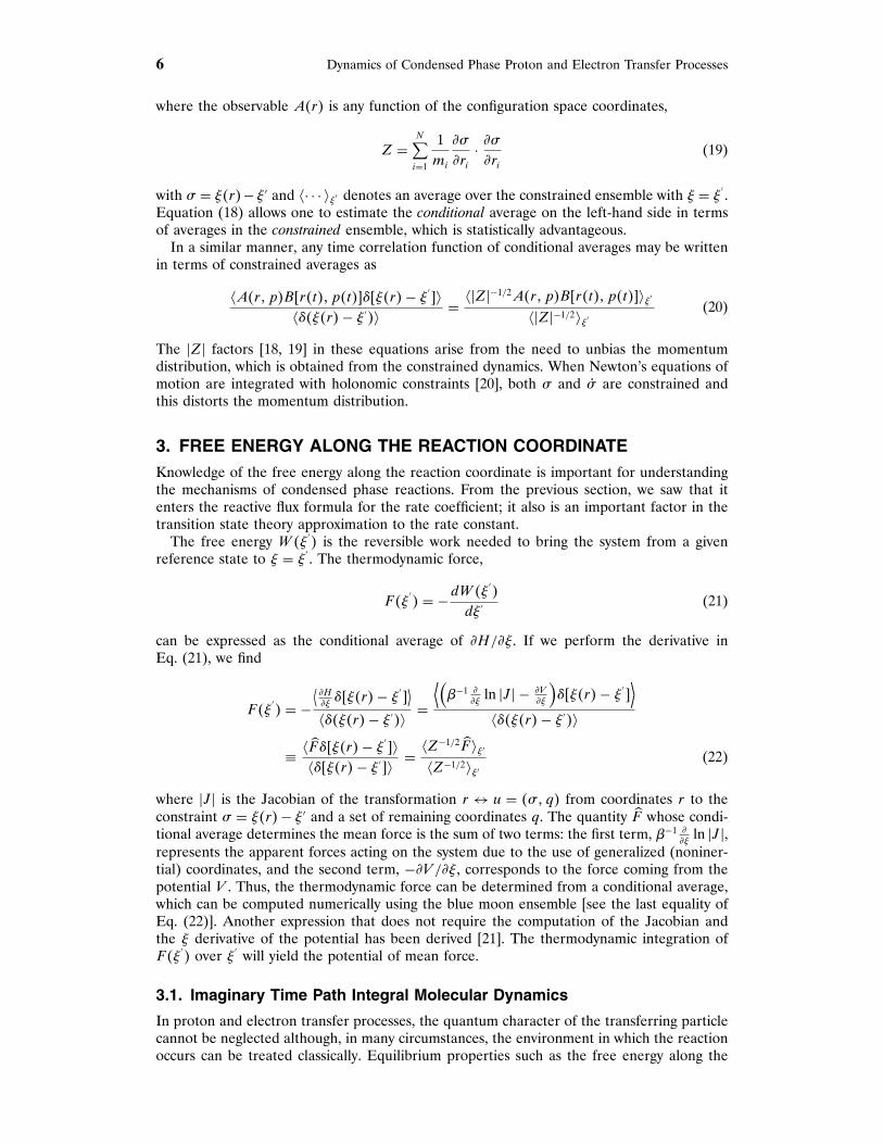
From this discussion, we see that the calculation of the rate coefficient requires the determi-nation of conditional averages depending on specific values of the reaction coordinate. Theensemble of such configurations, which are visited “once in a blue moon,” is termed the bluemoon ensemble [17]. In the blue moon ensemble method, conditional averages of observablesdepending only on configuration space variables can be computed by applying holonomicconstraints to the equations of motion. For the rate problem, while the value !‡ we wish tosample is rare in the original ensemble, only configurations with ! = !‡ are sampled in the !-constrained ensemble. This is illustrated schematically in Fig. 2. In the blue moon ensemble,conditional averages are related to constrained averages by (here we consider the case of asingle constraint but generalization to other situations is straightforward [17])
�A�r�cd!′ = �A�r���!�r�− !′�
���!�r�− ! ′ � = ��Z�−1/2A�r�!′��Z�−1/2!′
(18)
ξ(r)=ξ′
Figure 2. Schematic representation of the sampling procedure in the blue moon ensemble. The bold line depictsthe constrained �!�r� = !
′� dynamical evolution in phase space. The unconstrained natural evolution of the system
is shown as a dashed line. The open circles represent common points in configuration space, which are the initialconditions of the activated trajectory sampling. These points are not real crossings in phase space, as the twotrajectories differ in momentum space. Breaks in the dashed line denote long segments in the natural trajectory andindicate that “crossings” are rare events. The dynamics represented by the solid line segments of the unconstrainedtrajectory close to the crossing points yield the information needed to compute averages.
6 Dynamics of Condensed Phase Proton and Electron Transfer Processes
where the observable A�r� is any function of the configuration space coordinates,
Z =N∑i=1
1mi
./
.ri· ./.ri
(19)
with / = !�r�−! ′ and �· · · !′ denotes an average over the constrained ensemble with ! = !′ .
Equation (18) allows one to estimate the conditional average on the left-hand side in termsof averages in the constrained ensemble, which is statistically advantageous.
In a similar manner, any time correlation function of conditional averages may be writtenin terms of constrained averages as
�A�r� p�B�r�t�� p�t����!�r�− !′�
���!�r�− ! ′� = ��Z�−1/2A�r� p�B�r�t�� p�t��!′��Z�−1/2!′
(20)
The �Z� factors [18, 19] in these equations arise from the need to unbias the momentumdistribution, which is obtained from the constrained dynamics. When Newton’s equations ofmotion are integrated with holonomic constraints [20], both / and / are constrained andthis distorts the momentum distribution.
3. FREE ENERGY ALONG THE REACTION COORDINATEKnowledge of the free energy along the reaction coordinate is important for understandingthe mechanisms of condensed phase reactions. From the previous section, we saw that itenters the reactive flux formula for the rate coefficient; it also is an important factor in thetransition state theory approximation to the rate constant.
The free energy W�!′� is the reversible work needed to bring the system from a given
reference state to ! = !′ . The thermodynamic force,
F �!′� = −dW�!
′�
d! ′ (21)
can be expressed as the conditional average of .H/.!. If we perform the derivative inEq. (21), we find
F �!′� = −
⟨.H.!��!�r�− !
′�⟩
���!�r�− ! ′� =⟨(�−1 .
.!ln �J � − .V
.!
)��!�r�− !
′�⟩
���!�r�− ! ′�
≡ � �F ��!�r�− !′�
���!�r�− ! ′ � = �Z−1/2 �F !′�Z−1/2!′
(22)
where �J � is the Jacobian of the transformation r ↔ u = �/� q� from coordinates r to theconstraint / = !�r�− ! ′ and a set of remaining coordinates q. The quantity �F whose condi-tional average determines the mean force is the sum of two terms: the first term, �−1 .
.!ln �J �,
represents the apparent forces acting on the system due to the use of generalized (noniner-tial) coordinates, and the second term, −.V /.!, corresponds to the force coming from thepotential V . Thus, the thermodynamic force can be determined from a conditional average,which can be computed numerically using the blue moon ensemble [see the last equality ofEq. (22)]. Another expression that does not require the computation of the Jacobian andthe ! derivative of the potential has been derived [21]. The thermodynamic integration ofF �!
′� over ! ′ will yield the potential of mean force.
3.1. Imaginary Time Path Integral Molecular Dynamics
In proton and electron transfer processes, the quantum character of the transferring particlecannot be neglected although, in many circumstances, the environment in which the reactionoccurs can be treated classically. Equilibrium properties such as the free energy along the

Dynamics of Condensed Phase Proton and Electron Transfer Processes 7
reaction coordinate for quantum activated processes can be computed using Feynman’s pathintegral approach to quantum mechanics in imaginary time [22]. In this representation ofquantum mechanics, quantum particles are mapped onto closed paths r�t� in imaginarytime t, 0 ≤ t ≤ ��. To see this isomorphism, consider a single quantum particle of mass mwith coordinate and momentum operators r and p, respectively. The Hamiltonian operator is
H = p2
2m+ V �r� (23)
where V is the potential energy operator. The path integral formalism is derived by evaluat-ing the trace in the definition of the quantum canonical partition function ZQ = Tr exp�−�H�in the coordinate representation,
ZQ =∫dr⟨r �e−�
(p22m+V �r�
)�r⟩
(24)
Using the Trotter formula, this can be rewritten as
ZQ = limP→
∫dr⟨r �[e−
�2P V �r�e−
�P
p22m e−
�2P V �r�
]P �r⟩ (25)
This equation involves the product of P operators. One can insert P − 1 identity operatorsin the coordinate basis I = ∫
dr �r�r � to obtain
ZQ =∫ P∏
i=1
dri
[P∏i=1
⟨ri�e−
�2P V �r�e−
�P
p22m e−
�2P V �r��ri+1
⟩](26)
where, because of the trace, the condition rP+1 = rP must be imposed. The matrix elementhas the form, ⟨
ri�e−�2P V �r�e−
�P
p22m e−
�2P V �r��ri+1
⟩ = e−�2P V �ri�
⟨ri�e−
�P
p22m �ri+1
⟩e−
�2P V �ri+1� (27)
The coordinate matrix elements of the kinetic energy operator p2/�2m� can be evaluated byinserting the identity operator in terms of momentum eigenstates, I = ∫
dp �p�p�, using thescalar product between coordinate and momentum eigenstates �r �p = �23��−1/2 exp�ipr/��,and performing the resulting gaussian momentum integral. One obtains
⟨ri�e−
�P
p22m �ri+1
⟩ = (mP
23��2
)1/2
exp[− mP
2��2�ri+1 − ri�
2
](28)
With this result, the path integral expression for the canonical partition function becomes
ZQ = limP→
(mP
23��2
)1/2 ∫ P∏i=1
drie−∑P
i=1
[mP
2��2�ri+1−ri�2+ �
P V �ri�]
(29)
In simulations, a finite number P of beads is chosen. Equation (29) is the starting point fora classical isomorphism: the single quantum particle with coordinate r is mapped to a closedor ring polymer with P beads with coordinates ri [23]. The configurational statistics of thepolymer is governed by the effective potential,
Veff �r� =Pm
2����2
P∑i=1
�ri+1 − ri�2 + 1
P
P∑i=1
V �ri� (30)
The problem is then reduced to sampling from a classical canonical distribution involv-ing Veff . In molecular dynamics, this can be achieved by defining the Hamiltonian Heff =∑P
i=1�1/2�meff r2i + Veff �ri�, where meff is an arbitrary mass assigned to the polymer beads.
The number of polymer beads P enters into the definition of the effective potential Veff intwo different ways: it scales the magnitude of the interaction potential acting on the quantumparticle (the higher P the smaller this effect); and it determines the harmonic spring constant
8 Dynamics of Condensed Phase Proton and Electron Transfer Processes
keff = Pm/�2����2�, which represents quantum dispersion effects; it is stiffer for higher P .This stiffness makes it difficult to obtain an ergodic sampling of the dynamics. Moreover, thelarger P , the larger the number of degrees of freedom one must integrate numerically. Thus,although a very large P is desirable to represent quantum effects accurately and calculateaverages correctly, in practice a compromise is needed.
This formulation can be generalized easily to a single quantum particle interacting witha bath of classical particles. In this case, the bath particles are simply described by a singlepolymer bead, and the potential operator Veff �r�R� is
Veff �r�R� = Veff �r�+ Vc�r�R�+ Vb�R� (31)
where Vb�R� describes the energy of the bath of classical particles with coordinates R andVc�r�R� the interaction between the quantum particle (polymer beads) and the classicalbath particles. Again, the Hamiltonian Heff used for molecular dynamics sampling must beaugmented by the kinetic energy of the classical particles:
∑Nj=1�1/2�MjR
2j , where N is the
number of classical particles and Mj are their masses. Extension to a bath of distinguishablequantum particles is straightforward. If the bath particles are indistinguishable, then samplingis more difficult.
The path integral approach has been used by Gillan [24] to study rates of quantum acti-vated processes with the centroid density as a reaction coordinate. This approach has beendeveloped extensively by Voth [25]. In this scheme, the reaction coordinate is identified withthe position of the centroid of the quantum path rc
!�r� ≡ rc =1P
P∑i=1
ri (32)
With this definition of the reaction coordinate and the isomorphism to a classical ring poly-mer, the classical blue moon ensemble can be applied straightforwardly to compute the freeenergy,W�!�, using the relations given earlier specialized to the centroid reaction coordinate,
e−�W�!‡� ∝ ���!�r�− !‡� ∝∫dR
P∏i=1
dri��!�r�− !‡�e−�Veff �r�R� (33)
These equations form the basis for the calculation of free energy in transfer processes of aquantum particle embedded in a bath of classical degrees of freedom.
3.2. Electron Solvation in Reverse Micelles
As the first example of the computation of the free energy along a reaction coordinate,we consider the solvation of an electron in aqueous reverse micelle [26]. Reverse micellesare formed when surfactants are dissolved in neat organic solvents or in organic phasescontaining small amounts of water. In the latter case, the reverse micelles are roughly spher-ical pools of water surrounded by the polar head groups of the surfactant molecules. Thewater/surfactant ratio determines the micellar size and properties. Reverse micelles are use-ful as microreactors for chemical and biochemical reactions [27, 28]. Chemical reactions canbe carried out in confined environments where the encounter rates between species are rapidcompared to those in the bulk phases and, because polar and nonpolar environments are inclose proximity, reactions that are difficult to achieve in bulk homogeneous environmentsmay be carried out efficiently.
Many of the unusual properties of reverse micelles have their origin in the nature of thewater phase within the micelle. Micellar water is often partitioned into two zones corre-sponding to surface water, that is, water tightly bound to the surfactant head groups andassociated counterions, and bulk water in the center of the micelle. The size of the reversemicelle and the relative amounts of these two water phases can be tuned by changing theratio w0 = �water�/�surfactant�. The water structure within the micelles is often studiedthrough its interactions with probe species and solvated electrons, produced by radiolysisor other means. Such studies have provided insight into the nature of the reverse micellar
Dynamics of Condensed Phase Proton and Electron Transfer Processes 9
structure. Chemical and biochemical reactions in reverse micelles often involve electrontransfer processes.
Molecular-level studies of electron solvation in reverse micelles are difficult. The micellarstructure is complex because it involves the formation of the micelle by arrangement of thesurfactant head groups around the water pool. The configurational degrees of freedom ofthe tail groups play an important part in the stabilization of the micelle. Microscopic stud-ies of micelles in which the full structure of the surfactant molecules has been taken intoaccount have been carried out [29]. Faeder and Ladanyi [30] constructed a simple model forthe surfactant molecules to study micellar structure. The tail groups were neglected by sup-posing that the interior of the micelle was confined by a spherical potential. The surfactanthead groups extended into the water pool and were free to move on the micellar surface.This model mimics micelles formed using the sodium bis(2-ethylhexyl)sulfosuccinate (AOT)surfactant in dilute mixtures of water in nonpolar solvents. For this model, the effects ofthe hydrophobic portions of the amphiphiles and the nonpolar phase are taken into accountthrough a confining potential that gives the micelle a spherical structure with radius R. TheSO−
3 head groups and Na+ counter ions of the surfactant molecules are taken into accountexplicitly.
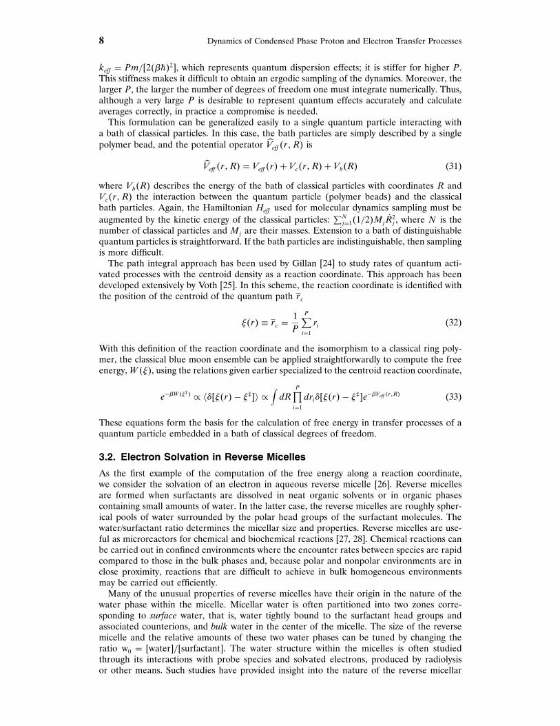
Electron solvation in reverse micelles was studied by treating the electron by an imaginarytime path integral representation [22]. The model of Faeder and Ladanyi was used for themicelle. Figure 3 shows a molecular configuration for the w0 = 775 micelle with a solvatedelectron–polymer in the interior of the aqueous pool.
The coupling of the electron to the other molecules in the micelle was described bythe potential Ves , which has three main contributions, Ves = Ve−w + Ve−SO−
3+ Ve−Na+ . Here
Ve−w is the electron–water potential, which was taken from the pseudopotential model ofSchnitker and Rossky [31]. Assuming a united atom model for SO−
3 groups, the electron-SO−
3 interaction Ve−SO−3was taken to consist of pairwise additive Coulombic terms. For the
electron-counter ion contribution Ve−Na+ , the local pseudopotential form given in Bacheletet al. [32] was adopted. The potential energy among the classical particles Vcl was takenfrom Faeder and Ladanyi [30], except for the water–water interactions where the SPC model
Figure 3. Cross section of the micelle showing a molecular configuration of the internal structure of a w0 = 775aqueous reverse micelle with the electron–polymer (light gray) solvated in the central (bulk water) part of theaggregate. The counter ion and surfactant head groups at the micelle boundary are rendered in black and darkgray shading, respectively.

10 Dynamics of Condensed Phase Proton and Electron Transfer Processes
was employed [33]. To sample the phase space of this system governed by an effectivepotential Veff of the form in Eq. (31), the multiple time step integration of Newton’s equationof motion [34] and the staging algorithm [35] were implemented. A chain [36] of Nosé-Hoover thermostats was used to simulate canonical dynamics. Chains consisting of threeNosé-Hoover thermostats set at T = 298 K were coupled to each Cartesian coordinate of thepolymer–electron; an additional chain was also attached to the rest of the classical particles.
We now describe the results of simulations of electron solvation on micelles whose sizeslie in the nanometer range and were characterized by the ratios w0 = 3 (R = 1372 Å) and775 (R = 1974 Å). To investigate the solvation of the electron in the micelle, the electroncentroid,
rC = 1��
∫ ��
0r�t� dt = 1
P
P∑i=1
ri (34)
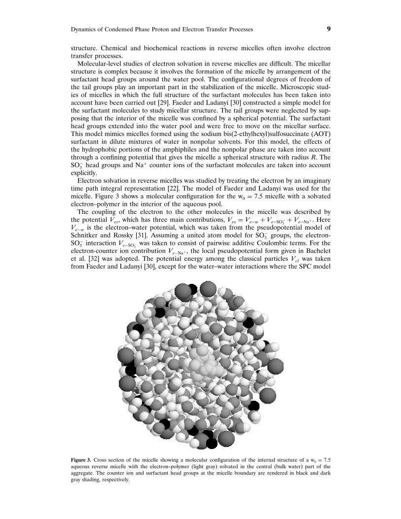
was fixed at a given distance from the micelle center by a holonomic constraint. The freeenergy was computed as a function of this distance from the micelle center from MD simula-tions of the constrained equations of motion using the SHAKE algorithm [37]. The centroidfree energies WC�r� for two micelle sizes are presented in Fig. 4. One can see that themost favorable radial positions for the electron solvation in w0 = 3 and w0 = 775 micellescorrespond to rC ≈ 2 and ≈5.5 Å, respectively. A rough estimate of the actual radial domainwithin which the electron centroid is likely to be found can be obtained by consideringregions where WC�r� remains comparable to normal thermal energies. For w0 = 375, thisregion is a spherical shell defined by 075 ≤ r ≤ 3 Å, whereas for w0 = 775 the correspondingshell is shifted and is defined by 375 ≤ r ≤ 7 Å. These calculations show that the electron ispreferentially solvated in the interior of the micelle. Additional, more detailed, informationon the electron solvation structure has been obtained from such path integral simulationstudies [26].
3.3. Proton Transfer in Nanoscale Molecular Clusters
Clusters are an interesting environment for the study of solvent influenced reactions. Thecompetition between bulk and surface solvation forces influences the reaction dynamicsand modifies the reaction rate. We present results for the proton transfer free energy inlarge liquid clusters whose linear dimensions are in the nanometer range [38]. Such clus-ters lie between the microscopic and macroscopic domains and possess unusual properties.We examine the mechanism for proton transfer in a strongly hydrogen bonded proton–ioncomplex in a cluster that consists of a classical solvent of polar diatomic molecules. Theactivation free energy in strongly hydrogen bonded systems arises almost exclusively fromsolvent effects and proton transfer provides a sensitive probe of cluster solvent structure anddynamics.
0 10r(Å)
0
2
4
6
βWc
8642
Figure 4. Free energy as a function of the position of the electron centroid for different micelle sizes: w0 = 3 (solidline); w0 = 775 (dot-dashed line). The zeros of the mean potential were arbitrarily set at the curve minima.

Dynamics of Condensed Phase Proton and Electron Transfer Processes 11
The proton transfer is assumed to take place between two A− ions in a proton–ioncomplex,
A −H · · ·A−� A− · · ·H−A
embedded in a cluster of N diatomic molecules composing the solvent. The two ions arefixed at R1� 2 = �0� 0�±173� Å. The solvent diatomic molecules have a dipole moment of< = 570 D. The interactions among the cluster solvent molecules, as well as those betweenthe A− ions and the solvent, arise from Lennard-Jones and Coulomb forces. The protoninteracts with the solvent via Coulomb forces. The proton–ion potential was constructedto model strongly hydrogen bonded systems and has a negligibly small intrinsic barrier.Simulations were carried out for clusters with N = 40 solvent molecules at a temperature of220 K, where the cluster (solvent plus proton–ion complex) is in the liquid state.
The calculations of the proton free energy along the reaction coordinate were performedby treating the proton quantum mechanically and the solvent ions classically as discussed ear-lier for electron solvation. The equilibrium averages involved in the computation of the freeenergy were estimated from time averages over trajectories of a system with the Hamiltonianobtained by using fictitious masses for the polymer beads representing the quantum proton.Sampling from a canonical distribution was carried out using Nosé-Hoover dynamics [39,40]. In order to achieve a proper thermalization of the proton degrees of freedom, a secondthermostat, acting exclusively on the proton–polymer degrees of freedom, was included [41].
The free energy was computed using the formulas given earlier, again choosing the zcoordinate of the centroid of the proton quantum path in imaginary time, z = !��t�� [24, 42,43] as the reaction coordinate. The free energy as a function of z is shown in Fig. 5. The cal-culations were carried out using the constrained dynamics method described above, namely,the mean force was calculated by constraining z and the free energy was obtained by inte-gration of the average force acting on z. The activation energy (barrier height) is estimatedto be W�0� = 4794 kT (2715 K cal/mol) and the minima of the free energy profile are locatedat zmin = ±0768 Å. Because the intrinsic (bare) barrier is negligibly small (072 K cal/mol),essentially all of the activation free energy arises from solvent effects. Figure 5 also shows thefree energy determined from a histogram of P�!� obtained in a 2 ns unconstrained MD run.
0.0–0.5 0.5
0.0
2.0
β W
z
6.0
4.0
Figure 5. Free energy profiles for the proton transfer reaction. The large dots correspond to the results obtained byintegration of the mean force for the quantum proton. The heavy solid line is the interpolation curve to the aboveresults. The open circles are the results from the unconstrained calculation for the quantum proton. The smallerdots and thin line correspond to the results obtained by integration of the mean force for the classical proton.
12 Dynamics of Condensed Phase Proton and Electron Transfer Processes
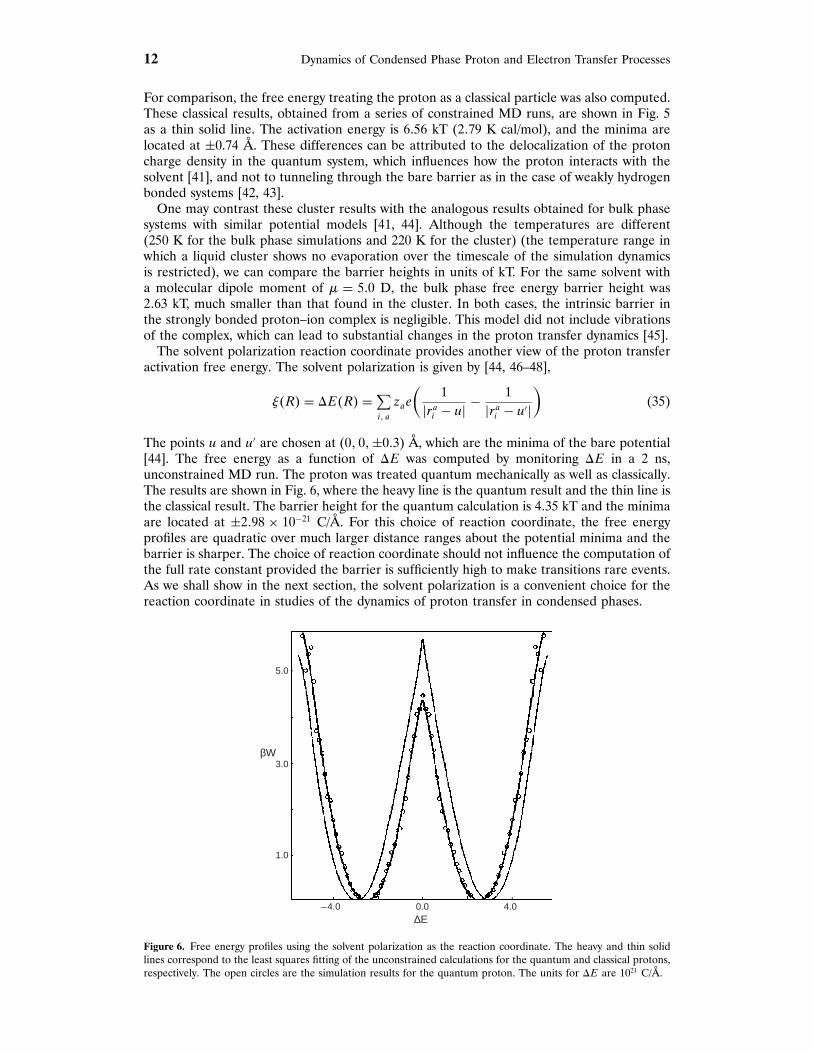
For comparison, the free energy treating the proton as a classical particle was also computed.These classical results, obtained from a series of constrained MD runs, are shown in Fig. 5as a thin solid line. The activation energy is 6756 kT (2779 K cal/mol), and the minima arelocated at ±0.74 Å. These differences can be attributed to the delocalization of the protoncharge density in the quantum system, which influences how the proton interacts with thesolvent [41], and not to tunneling through the bare barrier as in the case of weakly hydrogenbonded systems [42, 43].
One may contrast these cluster results with the analogous results obtained for bulk phasesystems with similar potential models [41, 44]. Although the temperatures are different(250 K for the bulk phase simulations and 220 K for the cluster) (the temperature range inwhich a liquid cluster shows no evaporation over the timescale of the simulation dynamicsis restricted), we can compare the barrier heights in units of kT. For the same solvent witha molecular dipole moment of < = 570 D, the bulk phase free energy barrier height was2763 kT, much smaller than that found in the cluster. In both cases, the intrinsic barrier inthe strongly bonded proton–ion complex is negligible. This model did not include vibrationsof the complex, which can lead to substantial changes in the proton transfer dynamics [45].
The solvent polarization reaction coordinate provides another view of the proton transferactivation free energy. The solvent polarization is given by [44, 46–48],
!�R� = >E�R� =∑i� a
zae
(1
�rai − u� −1
�rai − u′�)
(35)
The points u and u′ are chosen at (0� 0�±073) Å, which are the minima of the bare potential[44]. The free energy as a function of >E was computed by monitoring >E in a 2 ns,unconstrained MD run. The proton was treated quantum mechanically as well as classically.The results are shown in Fig. 6, where the heavy line is the quantum result and the thin line isthe classical result. The barrier height for the quantum calculation is 4735 kT and the minimaare located at ±2798 × 10−21 C/Å. For this choice of reaction coordinate, the free energyprofiles are quadratic over much larger distance ranges about the potential minima and thebarrier is sharper. The choice of reaction coordinate should not influence the computation ofthe full rate constant provided the barrier is sufficiently high to make transitions rare events.As we shall show in the next section, the solvent polarization is a convenient choice for thereaction coordinate in studies of the dynamics of proton transfer in condensed phases.
0.0–4.0 4.0
1.0
3.0
5.0
βW
∆E
Figure 6. Free energy profiles using the solvent polarization as the reaction coordinate. The heavy and thin solidlines correspond to the least squares fitting of the unconstrained calculations for the quantum and classical protons,respectively. The open circles are the simulation results for the quantum proton. The units for >E are 1021 C/Å.

Dynamics of Condensed Phase Proton and Electron Transfer Processes 13
4. ADIABATIC REACTION DYNAMICSThus far, we have focused on the free energy along the reaction coordinate. In this section,we consider dynamics and the computation of the reaction rate constant. Instead of treatingthe most general situation of nonadiabatic dynamics, which is the topic of the next section,we begin with a study of the adiabatic dynamics of a quantum reactive system in bath orenvironment of classical particles. Adiabatic dynamics has been used to compute protontransfer rates [44, 49].
From a theoretical perspective, the treatment of adiabatic dynamics is conceptually simple;one needs to solve the Schrödinger equation for the relevant quantum degrees of freedomin the fixed field field of the classical particles to determine the ground state energy as afunction of the positions of the classical particles. The motions of the classical particles are,in turn, governed by Newton’s equations of motion with Hellmann-Feynman forces derivedfrom the ground state potential energy function. Here we outline how such a descriptionfollows from an approximation to the full quantum correlation function expression for therate coefficient and present examples to illustrate adiabatic reaction dynamics.
4.1. Quantum-Classical Adiabatic Dynamics
We begin by sketching a derivation of the expression for the rate of a chemical reaction forquantum-classical adiabatic dynamics [6]. The starting point of the analysis is the quantummechanical expression for the reaction rate given earlier [see Eq. (11)].
We suppose that the quantum system is described by the Hamiltonian
H =�P 2
2M+ p2
2m+ V � q� Q� (36)
where q and Q are the coordinate operators of the quantum subsystem and bath, respec-tively, and the potential energy operator is V � q� Q�. Also, we denote the correspondingmomentum operators and masses by lower and upper case letters, respectively. We shallconsider the limit where the masses M of the bath particles are much larger than those ofthe quantum subsystem particles, M � m.
To begin, we rewrite the trace in the quantum expression for the rate kernel K�t� inEq. (11) in the %Q& representation for the bath degrees of freedom and retain the abstractnotation for the quantum subsystem degrees of freedom,
K�t� = −1i��
���� ��−1Tr′∫dQ �Q����� ���t�� �e�Q (37)
The prime on the trace indicates that only the subsystem degrees of freedom are traced over.Next, we introduce a partial Wigner representation [50] of the bath degrees of freedom. Thepartial Wigner transform of any operator A is
AW�R�P� =∫dZ e−iP ·Z/�
⟨R+ Z
2� A�R− Z
2
⟩(38)
and the partial Wigner transform of the equilibrium density matrix is
� �e�W �R� P� = �23��−3N∫dZ eiP ·Z/�
⟨R− Z
2� �e�R+ Z
2
⟩(39)
These quantities are still operators in the subsystem degrees of freedom.The evaluation of the rate kernel requires the computation of the matrix elements of
triple operator products whose partial Wigner transform is [51]∫dQ�Q� A �B �e�Q =
∫dRdP
[ AW�R�P�e�A/2i �BW�R�P�
]� �e�W �R� P� (40)
where
A = ←−B P · −→B R −←−
B R · −→B P (41)
14 Dynamics of Condensed Phase Proton and Electron Transfer Processes
and the directions of the arrows on the gradient operators indicate the directions in whichthese operators should be applied. Using these results the rate kernel takes the form,
K�t� = ���� ��−1 1−i��Tr
′∫dRdP
[��W�R� P�e�A/2i ��W�R� P� t�− ��W�R� P� t�e�A/2i ��W�R� P�
]� �e�W �R� P� (42)
where ��W�R� P� t� ≡ ��W�t� is the solution of the equation of motion
d��W�t�dt
= i
�
[HWe
�A/2i ��W�t�− ��W�t�e�A/2iHW
](43)
Here the partial Wigner representation of the Hamiltonian is
HW �R� P� =P 2
2M+ p2
2m+ VW � q�R� (44)
Next, we take the limit where the bath particles are massive compared to those of thequantum subsystem. It is convenient to introduce scaled variables such that the momenta ofthe heavy particles have the same order of magnitude as the momenta of the light particles.Consequently, we scale distances by the characteristic wavelength of the light particles, �m =��2/mC0�
1/2, time in units of t0 = �/C0. Here C0 is an energy unit, typically C0 = �−1. Inthese units the light particle momenta are scaled by pm =m�m/t0 = �m/C0�
1/2 and the heavyparticle momenta by PM = �MC0�
1/2. In scaled units �A/�2i�→ <A/�2i�, and we may expandthe equation of motion in the small parameter < = �m/M�1/2. Expanding to linear orderin < and then returning to unscaled units, the equation of motion, Eq. (43), becomes [6].
d��W�t�dt
= i
��HW � ��W�t��−
12
(%HW � ��W�t�&− %��W�t�� HW&
)(45)
This is a quantum-classical Liouville equation for a dynamical variable [6, 52]. Carrying outa similar < expansion, the rate kernel, Eq. (42), takes the form,
K�t�= 1����� ��−1Tr′
∫dRdP
(i
����W� ��W�t��−
12�%��W� ��W�t�&−%��W�t�� ��W&�
)� �e�W (46)
We may evaluate this expression (45) in any convenient representation and for this purposewe choose the basis of adiabatic eigenstates of the Hamiltonian operator hW �R� = p2/2m+VW �q�R�:
hW �R��E�R = EE�R��E�R (47)
Equation (46) can also be represented in this basis. This analysis is the starting point for asystematic approach to nonadiabatic dynamics which will be presented in some detail in thenext section. Here we will be concerned solely with the adiabatic limit where the dynamics isassumed to take place on a single adiabatic surface. In this case, the adiabatic representationof Eq. (45) takes an especially simple form,
d�EW�t�
dt= %�EW �t��H
EW& (48)
where �EW = �E�R� ��W�t��E�R and HEW = P 2/2M +EE�R�. This is just a classical evolution
equation but with Hellmann-Feynman forces,
F EW = −�E�R�BhW �R��E�R = −.EE�R�
.R(49)
determined by the potential EE�R� obtained from the solution of the Schrödinger equationfor the E adiabatic eigenstate. The rate kernel may be written in the adiabatic limit as
KE�t� = ��EW�EW −1 1�
∫dRdP %�EW�t�� �
EW&�
EWe (50)
Dynamics of Condensed Phase Proton and Electron Transfer Processes 15
with �EWe�R� P� = e−�HEW /
∫dRdP e−�HE
W . The algorithm for adiabatic mixed quantum-classical dynamics is simple. The dynamical variables depend on the classical coordinates�R� P� and the adiabatic state �E�R. The classical coordinates evolve by Newton’s equa-tions of motion but with Hellmann-Feynman forces corresponding to the E adiabatic statedetermined as a function of the instantaneous position R.
4.2. Adiabatic Proton-Transfer Reactions in Solution
We now return to the study of proton transfer reactions in strongly hydrogen bonded com-plexes but now embedded in a bulk solvent of dipolar molecules with dipole moment 5.0 D.The molecular dynamics calculations we describe were carried out for a system of N = 342solvent molecules, two ions, and a proton in a cubic box with periodic boundary conditions[44]. The simulations of the dynamics of the quantum proton coupled to the classical solventwere carried out as follows. Given a configuration of the solvent, the Schrödinger equation,
H�r�R�F�r�R� = E�R�F�r�R� (51)
where H�r�R� is the Hamiltonian for the proton with coordinate r in the fixed field of theclassical particles with coordinates R, was solved by expanding the proton wave function ina set of n = 156 localized Gaussian functions Gi�r� as
F�r�R� =n∑i=1
ci�R�Gi�r� (52)
yielding a standard (nonorthogonal) eigenvalue problem from which the energies and eigen-functions were obtained. After calculating the proton ground state wave function F0�r�R�and energy E0�R�, the proton contribution to the force acting on every site of the solventwas calculated. Given these forces, the solvent equations of motion,
MiRi = −BRiE0�R� (53)
were integrated.Solution of the eigenvalue problem in the absence of the solvent yields an energy spacing
between the ground and first excited states which is somewhat greater than kBT , just withinthe region of validity of the adiabatic approximation. In the presence of solvent, the energygap is large when the proton is hydrogen bonded to one of the ions (reactant or productconfigurations) but is comparable to that in the absence of solvent when the proton is in thevicinity of the activated region. Proton transfer events are triggered by solvent fluctuationsthat provide no preferential solvation for either ion, making this an interesting reaction inwhich to study solvent effects on quantum reactive events.
The choice of the reaction coordinate depends on the nature of the transition process,and there are a number of possible ways to construct a function of the solvent coordinatesthat can be used to monitor the proton transfer. A possible choice of the reaction coordinateis the mean value of the z component of the position of the proton,
!�R� = z�R� = �F0�R��z�F0�R� (54)
If the reaction involves the passage of the proton from a region near one ion to the other,configurations with negative and positive values for ! would correspond to reactant andproduct states, respectively. By symmetry, the activated state is located at ! = !‡ = 0.
The solvent polarization >E�R� [see Eq. (35)] is another, more convenient, choice for thereaction coordinate because it reflects the participation of the solvent in the proton transferprocess. Furthermore, because >E�R� is an analytical function of the solvent coordinates, itis easy to generate trajectories in which the initial states are located at the transition stateusing blue moon sampling.
The expression (17) for the TST rate constant, specialized to the polarization reactioncoordinate is
kTST = �23��1/2�D1/2��>E − >E‡��#�>E − >E‡� (55)
16 Dynamics of Condensed Phase Proton and Electron Transfer Processes
where
D = 12m
∑i
(∑E
Bi� E>E
)2
(56)
assuming all solvent masses are equal. The reaction coordinate >E and its time derivativeare not statistically independent, and the expected value in the expression for kTST does notfactor into coordinate and velocity contributions [17].
Equation (55) can be calculated in the blue moon ensemble as discussed earlier [seeEq. (18)] using the expression,
kTST = �23��−1/2 ���>E − >E‡��D−1/2>E=0�#�>E − >E‡� (57)
Using this formula, the TST value for the rate coefficient was found to be kTST = �4703 ±0729�× 109 s−1 [44].
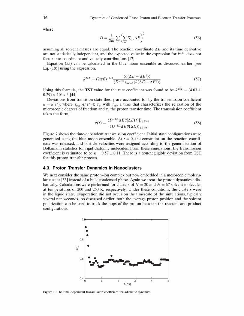
Deviations from transition-state theory are accounted for by the transmission coefficient, = ,�t∗�, where �mic � t∗ � �p, with �mic a time that characterizes the relaxation of themicroscopic degrees of freedom and �p the proton transfer time. The transmission coefficienttakes the form,
,�t� = �D−1/2>E#�>E�t��>E=0
�D−1/2>E#�>E�>E=0
(58)
Figure 7 shows the time-dependent transmission coefficient. Initial state configurations weregenerated using the blue moon ensemble. At t = 0, the constraint on the reaction coordi-nate was released, and particle velocities were assigned according to the generalization ofBoltzmann statistics for rigid diatomic molecules. From these simulations, the transmissioncoefficient is estimated to be , = 0757± 0711. There is a non-negligible deviation from TSTfor this proton transfer process.
4.3. Proton Transfer Dynamics in Nanoclusters
We next consider the same proton–ion complex but now embedded in a mesoscopic molecu-lar cluster [53] instead of a bulk condensed phase. Again we treat the proton dynamics adia-batically. Calculations were performed for clusters of N = 20 and N = 67 solvent moleculesat temperatures of 200 and 260 K, respectively. Under these conditions, the clusters werein the liquid state. Evaporation did not occur on the timescale of the simulations, typicallyseveral nanoseconds. As discussed earlier, both the average proton position and the solventpolarization can be used to track the hops of the proton between the reactant and productconfigurations.
0.4
0.6
0.8
1
0 1 2 3 4 5
k(t
)
t (ps)
Figure 7. The time-dependent transmission coefficient for adiabatic dynamics.

Dynamics of Condensed Phase Proton and Electron Transfer Processes 17
The cluster solvent molecules tended to strongly solvate the part of the proton–ion com-plex with the more exposed negative charge; that is, the end of the complex that is lessstrongly bonded to the H+ ion. This suggests that the complex tends to “float” on the surfaceof the cluster. When the H+ ion is strongly bound to one A− ion, this A−H dipole has asmaller dipole moment than that of a solvent molecule. Consequently, the solvent–solventinteractions are stronger than the interactions between a solvent molecule and this part ofthe proton–ion complex. These energetic arguments suggest that it may be favorable for thisend of the proton–ion complex to reside on the surface of the cluster, a fact supported bythe simulation results. Of course, both entropic as well as energetic factors come into play indetermining the structure of mixed clusters [54] but, in the cases studied, energetic factorsplayed a dominant role.
The position of the proton–ion complex in the cluster has a strong influence on the natureof the proton transfer dynamics. In the case of a 20 molecule cluster the complex resides forlong portions of time on the surface of the cluster and long portions of time in the interiorof the cluster. If the complex is on the surface of the cluster, then transitions rarely occur;however, if the complex makes an excursion into the interior, then this excursion correlateswith a proton transfer. The picture is somewhat different for the 67 molecule cluster. Theproton–ion complex rarely penetrates deeply into the cluster. Some of the proton transferevents correlate with excursions of the complex into the cluster, but only one solvent layerdeep and never far from the surface. However, even when the complex floats on the surfaceof the cluster, there are frequent proton transfer events. Figure 8 shows such a protontransfer event. Initially, the proton (gray) is strongly bound to the one of the ions (black)in the complex. The complex resides on the surface of the cluster with one end, to whichthe proton is weakly bound, solvated in the cluster, and the other end extending out of thecluster. In the course of time, a fluctuation occurs that causes the complex to assume aconfiguration parallel to the surface so that there is a more nearly equal solvation of the twoends of the complex. This is a favorable configuration for the proton transfer so that it takesplace in frame (a) of this figure. Once the proton transfer is complete, then the favorablecomplex configuration is for the now strongly hydrogen bonded end to protrude from thecluster and the weakly bound end to lie within the cluster [frame (b)].
Thus, the mechanism of the proton transfer depends on the size of the cluster. For smallerclusters, fluctuations lead to penetration of the complex into the interior of the clusterwhere proton transfer is likely. For larger clusters, transitions occur primarily by orientationalmotion of the complex on the surface of the cluster or when the complex makes shallowpenetrations into the cluster. Deep penetrations of the complex into the cluster are rare.For the smaller 20 molecule cluster, presumably the orientational motion of the complex isrestricted on the surface due to the larger surface forces.
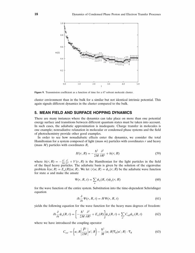
Figure 9 shows the transmission coefficient as a function of time for the 67 molecule cluster.The results in this figure show a rapid decay on a timescale that is less than a picosecondfollowed by a somewhat longer decay, of the order of a few picoseconds, to a plateau value.From this graph, the transmission coefficient may be determined from the plateau values andone finds , = 074. The timescale for the establishment of a plateau in ,�t� is longer in the
(b)(a)
Figure 8. Cluster configurations during (a) and after (b) a proton transfer event for a 67 molecule cluster.
18 Dynamics of Condensed Phase Proton and Electron Transfer Processes
0.2
0.4
0.6
0.8
1.0
0.0 1.0 2.0 3.0 4.0 5.0
κ (t)
t
Figure 9. Transmission coefficient as a function of time for a 67 solvent molecule cluster.
cluster environment than in the bulk for a similar but not identical intrinsic potential. Thisagain signals different dynamics in the cluster compared to the bulk.
5. MEAN FIELD AND SURFACE HOPPING DYNAMICSThere are many instances where the dynamics can take place on more than one potentialenergy surface and transitions between different quantum states must be taken into account.In such cases, the adiabatic approximation is inadequate. Charge transfer in molecules isone example; nonradiative relaxation in molecular or condensed phase systems and the fieldof photochemistry provide other good examples.
In order to see how nonadiabatic effects enter the dynamics, we consider the totalHamiltonian for a system composed of light (mass m) particles with coordinates r and heavy(mass M) particles with coordinates R,
H�r�R� = − �2
2M.2
.R2+ h�r�R� (59)
where h�r�R� = − �2
2m.2
.r2+ V �r�R� is the Hamiltonian for the light particles in the field
of the fixed heavy particles. The adiabatic basis is given by the solution of the eigenvalueproblem h�E�R = EE�R��E�R. We let �r �E�R = GE�r�R� be the adiabatic wave functionfor state E and make the ansatz
F�r�R� t� =∑E
IE�R� t�GE�r�R� (60)
for the wave function of the entire system. Substitution into the time-dependent Schrödingerequation
i�.
.tF�r�R� t� = HF�r�R� t� (61)
yields the following equation for the wave function for the heavy mass degrees of freedom:
i�.
.tIE�R� t� =
[− �
2
2M.2
.R2+ EE�R�
]IE�R� t�+
∑E′CE�IE′�R� t� (62)
where we have introduced the coupling operator
CEE′ =⟨E�R
∣∣∣∣ �P 2
2M
∣∣∣∣E′�R⟩− �
2
M�E�R�BR�E′�R · BR (63)
Dynamics of Condensed Phase Proton and Electron Transfer Processes 19
where �P 2/2M is the kinetic energy operator. The diagonal elements CEE give corrections tothe adiabatic eigenvalues EE, and the off-diagonal terms describe the coupling between thedifferent quantum states. When CE� ≈ 0 (Born-Oppenheimer approximation), we recoveradiabatic dynamics.
We next consider various schemes for constructing mixed quantum-classical dynamics thatallow for nonadiabatic effects. The quantum and classical degrees of freedom interact andtheir dynamics must be treated in a consistent fashion. Time-dependent variations of theclassical degrees of freedom induce transitions between quantum states of the light masssubsystem and these transitions, in turn, modify the forces that govern the motion of the clas-sical particles. Ehrenfest (or mean-field) and surface-hopping schemes are two approximatemixed quantum-classical methods to describe nonadiabatic dynamics [55]. Quantum-classicalLiouville dynamics provides a more rigorous approach to nonadiabatic dynamics.
5.1. Mean-Field Method
The mean field approach is based on Ehrenfest’s equations of motion for the evolutionof the position and momentum operators of the heavy mass particles. Assuming that theexpectation value of a function can be approximated by the function of the expectation value,we obtain the following mean field equations,
dR�t�
dt= P�t�
M
dP�t�
dt= −B�I�R�t�� t��h�R�t���I�R�t�� t�
(64)
where the wave function evolves through the time-dependent Schrödinger equation,
i�.
.t�I�R�t�� t� = h�R�t���I�R�t�� t� (65)
According to these equations, the heavy mass degrees of freedom evolve classically alonga single mean trajectory determined by the effective potential energy surface Eef �R�t�� =�I�R�t�� t��h�R�t���I�R�t�� t�. Mean-field methods have been used to compute protontransfer rates. [56, 57] Outside strong interaction regions, the quantum system will typicallycollapse onto a given state, and the mean field equations will likely be a poor approximationto the dynamics. Surface-hopping algorithms have been devised to account for this difficulty.
5.2. Surface-Hopping Dynamics
In surface-hopping dynamics, the system evolves on specified adiabatic energy surfaces inter-spersed by quantum transitions that occur probabilistically and change the state of the sys-tem. Observables are computed from an average over an ensemble of such surface-hoppingtrajectories. A variety of such schemes have been proposed. One of the most popular isTully’s fewest switches algorithm [55, 58]. In this method, the time-dependent Schrödingerequation (65) is solved by expanding the wave function in the instantaneous adiabatic eigen-states of the Hamiltonian h�R�t��, h�R�t���E�R�t� = EE�R�t���E�R�t�,
�F�R�t�� t� =∑E
cE�t��E�R�t� (66)
yielding the evolution equation for the coefficients
i�dCE�t�
dt= �EE − E0�CE�t�− i�
∑E′
P
M· dEE′CE′�t� (67)
where dEE′ = �E�R�t��BR�t��E�R�t� is the nonadiabatic coupling matrix element and
CE�t� = cE�t� exp{i∫ t
0dt′E0�R�t
′��/�}
(68)
During each molecular dynamics time step >, the classical degrees of freedom evolveby Newton’s equation of motion subject to Hellmann-Feynman forces that depend on

20 Dynamics of Condensed Phase Proton and Electron Transfer Processes
instantaneous adiabatic eigenstates. The probability of a hop from state E to E′ is given by
wEE′ = KEE′#�KEE′� (69)
where #�x� is the Heaviside function and
KEE′ =−2�{�∗E′E�t + >��P�t�/M� · dEE′ �R�t��>
}�EE�t + >�
(70)
Here �EE′�t� is a matrix element of the density matrix in the adiabatic basis, �EE′�t� =
�E�R�t�� ��t��E′�R�t� = �E�R�t��F�R�t�� t��F�R�t�� t��E′�R�t� = c∗E�t�cE′�t�.Pechukas [59] presented a description of nonadiabatic dynamics based on an analysis of the
Feynman path integral expression for the propagator. The equations of motion for the bathdegrees of freedom involve a nonlocal quantum force. Surface-hopping schemes that useapproximations to this nonlocal force have been constructed by Rossky et al. [60] and Cokeret al. [61]. In particular, Coker and Xiao [61] have shown that a short time approximationthat localizes the Pechukas force leads to Tully’s algorithm.
5.3. Nonadiabatic Proton Transfer in Nanoclusters
Surface-hopping schemes have been used to study proton and hydrogen atom transfer ratesin the condensed phase [62] and in biosystems [63]. We begin with an investigation ofnonadiabatic effects on proton transfer rates in nanoclusters using Tully’s surface-hoppingdynamics [53].
The model system is the same as that described in Section 4.3, namely, a proton–ioncomplex embedded in a cluster of polar diatomic molecules. The average position of theproton z�R� = �E�R�t� � z � E�R�t� is shown in Fig. 10 (bottom panel) as a function oftime for a nonadiabatic reactive trajectory. The upper panel of the figure shows the protonic
1
2
3
–0.9
–0.6
–0.3
0.0
0.3
0.6
0.9
0.0 150.0 300.0 450.0t
zst
ate
Figure 10. (top) Protonic state, (bottom) expectation value of the position of the proton z as a function of timefor a 67-molecule cluster.
Dynamics of Condensed Phase Proton and Electron Transfer Processes 21
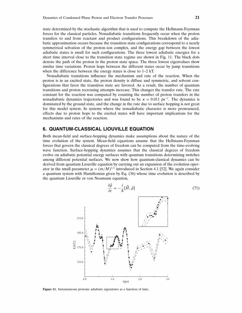
state determined by the stochastic algorithm that is used to compute the Hellmann-Feynmanforces for the classical particles. Nonadiabatic transitions frequently occur when the protontransfers to and from reactant and product configurations. This breakdown of the adia-batic approximation occurs because the transition state configurations correspond to a nearlysymmetrical solvation of the proton–ion complex, and the energy gap between the lowestadiabatic states is small for such configurations. The three lowest adiabatic energies for ashort time interval close to the transition state regime are shown in Fig. 11. The black dotsdenote the path of the proton in the proton state space. The three lowest eigenvalues showsimilar time variations. Proton hops between the different states occur by jump transitionswhen the difference between the energy states is close to 1–2 kT.
Nonadiabatic transitions influence the mechanism and rate of the reaction. When theproton is in an excited state, the proton density is diffuse and symmetric, and solvent con-figurations that favor the transition state are favored. As a result, the number of quantumtransitions and proton recrossing attempts increase. This changes the transfer rate. The rateconstant for the reaction was computed by counting the number of proton transfers in thenonadiabatic dynamics trajectories and was found to be , = 07011 ps−1. The dynamics isdominated by the ground state, and the change in the rate due to surface hopping is not greatfor this model system. In systems where the nonadiabatic character is more pronounced,effects due to proton hops to the excited states will have important implications for themechanisms and rates of the reaction.
6. QUANTUM-CLASSICAL LIOUVILLE EQUATIONBoth mean-field and surface-hopping dynamics make assumptions about the nature of thetime evolution of the system. Mean-field equations assume that the Hellmann-Feynmanforces that govern the classical degrees of freedom can be computed from the time-evolvingwave function. Surface-hopping dynamics assumes that the classical degrees of freedomevolve on adiabatic potential energy surfaces with quantum transitions determining switchesamong different potential surfaces. We now show how quantum-classical dynamics can bederived from quantum Liouville equation by carrying out an expansion of the evolution oper-ator in the small parameter < = �m/M�1/2 introduced in Section 4.1 [52]. We again considera quantum system with Hamiltonian given by Eq. (36) whose time evolution is described bythe quantum Liouville or von Neumann equation,
. �
.t= − i
��H� �� (71)
0.0 1.0 2.0 3.0t(ps)
155.0
175.0
195.0
215.0
E(k
T)
Figure 11. Instantaneous protonic adiabatic eigenstates as a function of time.

22 Dynamics of Condensed Phase Proton and Electron Transfer Processes
If we take the partial Wigner transform [defined in Eqs. (38) and (39)] of this equation weobtain,
. �W�R� P� t�.t
= − i
�
[�H ��W − � �H�W
]= − i
�
[HW �R� P�e
�A/2i �W�R� P� t�− �W�R� P� t�e�A/2iHW �R� P�]
(72)
which is the analog of Eq. (45) for a dynamical variable. The operator A is defined inEq. (41) and is the negative of the Poisson bracket operator. Scaling variables as discussedearlier for adiabatic dynamics, expanding in < and finally returning to unscaled variables weobtain the quantum-classical Liouville equation [52, 64–68],
. �W�R� P� t�.t
= − i
��HW �R� P�� �W�R� P� t��
+ 12
({HW �R� P�� �W�R� P� t�
}−{�W�R� P� t�� HW �R� P�
})≡ − i� �W�R� P� t� = −�HW � �W�R� P� t�� (73)
where the last line defines the quantum-classical Liouville operator, �, and the quantum-classical bracket, �·� ·� [69, 70].
To construct a surface-hopping picture of the dynamics we consider the representation ofthis equation in a basis of adiabatic eigenstates defined in Eq. (47). Taking matrix elementsof Eq. (73) and letting �EE′W �R�P� = �E�R� �W�R� P��E′�R, we obtain
.�EE′
W �R�P� t�
.t=∑
��′−i�EE′� ��′�
��′W �R�P� t� (74)
where
−i�EE′� ��′ = �−iMEE′ − iLEE′��E��E′�′ + JEE′� ��′ ≡ −i�0EE′ + JEE′� ��′ (75)
where MEE′�R� = �EE�R�− EE′�R��/� = >EEE′/� and J is defined by
JEE′� ��′ = − P
M· dE�
(1+ 1
2SE� ·
.
.P
)�E′�′ −
P
M· d∗
E′�′
(1+ 1
2S∗E′�′ ·
.
.P
)�E� (76)
and the nonadiabatic coupling matrix element is dEE′ = �E�R�./.R�E′�R0, and
SE� = >EEE′dE�
(P
M· dE�
)−1
(77)
The classical Liouville operator involving the mean of the Hellmann-Feynman forces forstates E and E′ is
iLEE′ =P
M· .
.R+ 1
2�F E
W + F E′W � ·
.
.P(78)
The quantum-classical Liouville equation may be integrated and solved by iteration toyield a representation of the dynamics as a sequence of terms involving increasing numbersof nonadiabatic transitions [52],
�E0E
′0
W �R�P� t� = e−i�0
E0E′0t�E0E
′0
W �R�P�+ ∑n=1
∑�E1E
′1�···�EnE′n�
∫ t0
0dt1
∫ t1
0dt2 · · ·
∫ tn−1
0dtn
×n∏k=1
[e−i�0
Ek−1E′k−1
�tk−1−tk�JEk−1E
′k−1� EkE
′k
]e−i�0
EnE′ntn�
EnE′n
W �R� P� (79)

Dynamics of Condensed Phase Proton and Electron Transfer Processes 23
Here �EE′
W �R�P� is the initial value of the density matrix element. In this equation, thediagonal part of the quantum-classical evolution operator, exp%i�0
EE′ t&, may be written interms of classical evolution on the �EE′� surface and a phase factor as,
e−i�0EE′ �t−t′� = e−i
∫ t′t d� MEE′ �REE′ � � �e−iLEE′ �t−t
′�
≡ WEE′�t� t′�e−iLEE′ �t−t
′� (80)
The successive terms in the series correspond to increasing numbers of nonadiabatic tran-sitions, starting with the first term that describes simple adiabatic dynamics. As an example,consider the calculation of the diagonal element of the density matrix, �EEW �R� P� t�. Thecontributions to this matrix element are determined by backward evolution from time t totime 0. The first term in the series corresponds to adiabatic evolution on state E. The nextterm accounts for single nonadiabatic transitions to states � (� = E�, which occur at times t′
intermediate between t and 0. These transitions are accompanied by continuous momentumchanges in the environment specified by the term in J involving a momentum derivative.Because a single quantum transition takes place, this contribution must come from an off-diagonal density matrix element, �E�W at time 0. During the portion of the evolution segmentfrom t′ to 0, the classical bath phase space coordinates are propagated on the mean of thetwo E and � adiabatic surfaces and a phase factor WE� contributes to the population instate E.
The terms involving the bath momentum derivative in J are difficult to evaluate exactly.Consequently, we make a “momentum-jump” approximation that gives J the structure of amomentum translation operator whose effect on any function of the momentum is to shiftthe momentum by some value [52, 70]. To derive this approximation, we first consider theoperator identity, �SE�/2� · .
.P= >EE�M
.
.�P ·dE��2. The action of the operator on any function
f �P� of the momentum may be written approximately as[1+ >EE�M
.
.�P · dE��2]f �P� ≈ e>EE�M./.�P ·dE��2f �P�
= f
[d⊥E��P · d⊥
E��+ dE�sgn�P · dE��√�P · dE��2 + >EE�M
]= f �P + dE�>P� (81)
where >P = −�dE� · P� + sgn�P · dE��√�P · dE��2 + >EE�M . In the second approximate
equality on the right-hand side of this equation, we have replaced the sum by an exponen-tial. The momentum vector may be written in terms of its components along dE� and aperpendicular vector d⊥
E�, P = dE��dE� · P�+ d⊥E��d
⊥E� · P�. In the last line, we used the fact
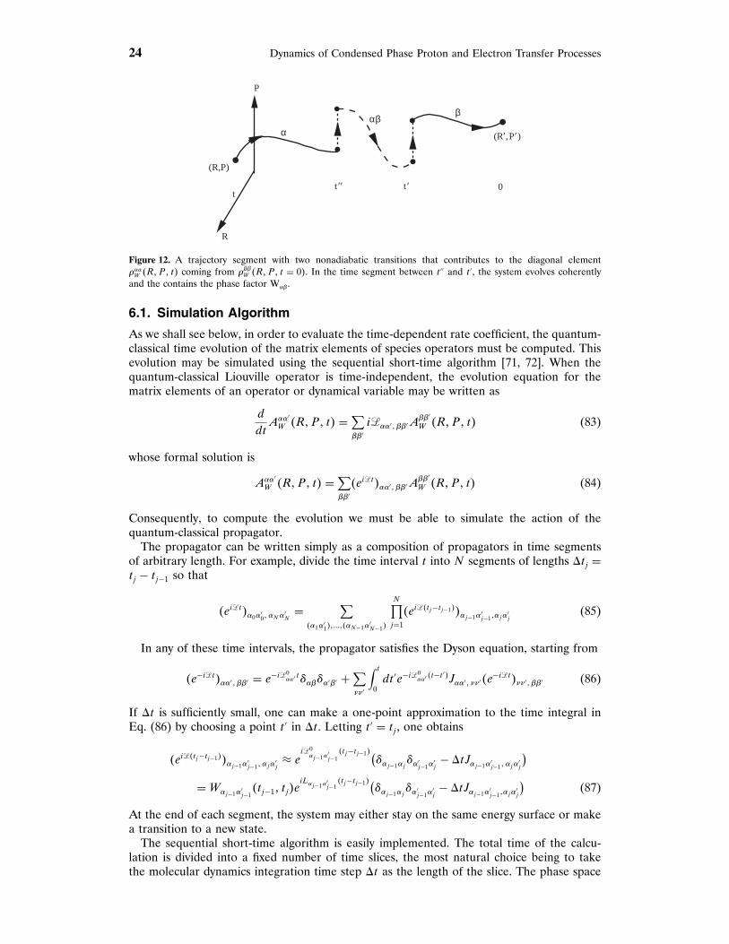
that the exponential operator is a translation operator in the variable �P · dE��2. Using thismomentum jump approximation, a member of the ensemble of trajectories that is used tocompute the density matrix elements is shown schematically in Fig. 12.
A similar set of equations with similar interpretations can be written for an operatorAW�R�P�. We have,
AE0E
′0
W �R�P� t� = ei�0
E0E′0tAE0E
′0
W �R�P�+ ∑n=1
�−1�n∑
�E1E′1�···�EnE′n�
∫ t
0dt1
∫ t
t1
dt2 · · ·∫ t
tn−1
dtn
×n∏k=1
[ei�0
Ek−1E′k−1
�tk−tk−1�JEk−1E
′k−1�EkE
′k
]ei�0
EnE′n�t−tn�AEnE
′n
W �R� P� (82)
In order to compute correlation functions, we require the quantum-classical time evolutionof operators as we shall see when we consider the calculation of rate constants using thisformalism.
24 Dynamics of Condensed Phase Proton and Electron Transfer Processes
P
R
t0
αββ
α
t ′′ t ′
(R,P)
(R′,P′ )
Figure 12. A trajectory segment with two nonadiabatic transitions that contributes to the diagonal element�EEW �R� P� t� coming from ���W �R� P� t = 0�. In the time segment between t′′ and t′, the system evolves coherentlyand the contains the phase factor WE�.
6.1. Simulation Algorithm
As we shall see below, in order to evaluate the time-dependent rate coefficient, the quantum-classical time evolution of the matrix elements of species operators must be computed. Thisevolution may be simulated using the sequential short-time algorithm [71, 72]. When thequantum-classical Liouville operator is time-independent, the evolution equation for thematrix elements of an operator or dynamical variable may be written as
d
dtAEE′W �R�P� t� =∑
��′i�EE′� ��′A
��′W �R�P� t� (83)
whose formal solution is
AEE′W �R�P� t� =∑
��′�ei�t�EE′� ��′A
��′W �R�P� t� (84)
Consequently, to compute the evolution we must be able to simulate the action of thequantum-classical propagator.
The propagator can be written simply as a composition of propagators in time segmentsof arbitrary length. For example, divide the time interval t into N segments of lengths >tj =tj − tj−1 so that
�ei�t�E0E′0� EN E
′N= ∑
�E1E′1��777��EN−1E
′N−1�
N∏j=1
�ei��tj−tj−1��Ej−1E′j−1�EjE
′j
(85)
In any of these time intervals, the propagator satisfies the Dyson equation, starting from
�e−i�t�EE′� ��′ = e−i�0EE′ t�E��E′�′ +
∑PP′
∫ t
0dt′e−i�
0EE′ �t−t′�JEE′� PP′�e
−i�t�PP′� ��′ (86)
If >t is sufficiently small, one can make a one-point approximation to the time integral inEq. (86) by choosing a point t′ in >t. Letting t′ = tj , one obtains
�ei��tj−tj−1��Ej−1E′j−1� EjE
′j≈ e
i�0Ej−1E
′j−1
�tj−tj−1�(�Ej−1Ej
�E′j−1E′j− >tJEj−1E
′j−1� EjE
′j
)= WEj−1E
′j−1�tj−1� tj�e
iLEj−1E′j−1
�tj−tj−1�(�Ej−1Ej
�E′j−1E′j− >tJEj−1E
′j−1�EjE
′j
)(87)
At the end of each segment, the system may either stay on the same energy surface or makea transition to a new state.
The sequential short-time algorithm is easily implemented. The total time of the calcu-lation is divided into a fixed number of time slices, the most natural choice being to takethe molecular dynamics integration time step >t as the length of the slice. The phase space

Dynamics of Condensed Phase Proton and Electron Transfer Processes 25
coordinates are propagated adiabatically in a time step, and the phase factor W is computedif the evolution is on the mean of two adiabatic surfaces. At the end of each time step, theprobabilities Q = ��P/M� · d�>t �1+ ��P/M� · d�>t�−1 and R = 1−Q are respectively usedfor acceptance or rejection of a quantum transition.
7. NONADIABATIC REACTION DYNAMICSIn this section we sketch a general formulation of the statistical mechanics of nonadiabaticchemical rate processes and give reactive flux correlation function expressions for the rateconstant. We then illustrate the formalism with calculations on a two-level model systemthat captures the essential features of may transfer rate processes.
7.1. Quantum-Classical Reactive Flux Correlation Functions
The reactive-flux correlation functions that may be used to determine the rate constant foractivated quantum processes can be derived using linear response theory [73]. We considera multicomponent system where r independent chemical reactions take place. We may asso-ciate progress variables, ��i and affinities �i, (i = 1� 7 7 7 � r), with each independent reactionstep. From linear irreversible thermodynamics, the chemical rate law describing the timeevolution of the reaction rates �i takes the form [74],
�i ≡d ��idt
= −r∑j=1
Lij��j (88)
where Lij is an Onsager coefficient.To derive this rate law using linear response theory, we suppose the system is subject to
external time-dependent forces (affinities) that couple to microscopic species variables ��Wi.The time-dependent Hamiltonian in the presence of the external forces is
�W�t� = HW −r∑i=1
��†Wi�i�t� (89)
where the dagger stands for the adjoint. The species variables are in general operators inHilbert space and functions of the classical phase space variables, ��Wi�R� P�.
The chemical rate law can be derived by calculating the nonequilibrium average of �� W�i,
�i ≡d��Wi�t�dt
= Tr′∫dRdP �� Wi �W�R� P� t� (90)
to linear order in the affinities. Assuming the time dependence of the affinities can berepresented by a single Fourier component �i�t� = exp�iMt��i�M�, linear response theorygives
d ��Wi�t�dt
=r∑j=1
Sij�M��j �t� (91)
where the one-sided Fourier transform of the matrix response function is given by
Sij�M� =∫
0dt⟨( �� Wi�t�� ��†Wj
)⟩e−iMt (92)
Although the zero frequency limit of Eq. (91) has the same form as the phenomenologicalrate law (88), the zero frequency limit of Eq. (92) may be shown to be identically zero.This is the well-known plateau value problem, which is solved by using a projection operatorformalism to project out the time variations that occur on the timescale of the chemicalrelaxation processes [6, 7]. Provided the timescales of the chemical relaxation processes, �c,
26 Dynamics of Condensed Phase Proton and Electron Transfer Processes
are much slower than those for other microscopic relaxation processes in the system, �m, thephenomenological coefficients may be obtained through the correlation function expression,
�Lij = −∫ t∗
0dt′ Tr′
∫dRdP �� Wi�t
′�(��†Wj� �We
)(93)
where �m � t∗ � �c. In writing this expression, we have moved the quantum-classical bracketto act on the equilibrium density and the initial value of the species operator. It is alsoconvenient to define the time-dependent Onsager coefficients by
�Lij�t� = −∫ t
0dt′ Tr′
∫dRdP �� Wi�t
′�(��†Wj� �We
)= −Tr′
∫dRdP ��Wi�t�
(��†Wj� �We
)(94)
where the time integral has been performed to obtain the second line of this equation.The true phenomenological coefficients, appearing in Eq. (88), may be determined from theplateau value of this expression, should such a plateau exist. In quantum-classical dynamicsthe Onsager reciprocal relations are valid to ��<2�. This is a consequence of the fact thatthe quantum-classical bracket satisfies the Jacobi identity only to ��<2� [73].
7.2. Two-Level Model for Transfer Reactions
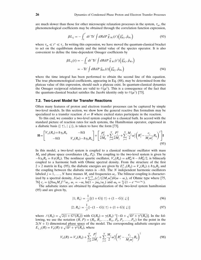
Often many features of proton and electron transfer processes can be captured by simpletwo-level models. In this section, we show how the general reactive flux formalism may bespecialized to a transfer reaction A� B where excited states participate in the reaction.
To this end, we consider a two-level system coupled to a classical bath. In accord with thestandard picture of reaction rates for such systems, the Hamiltonian operator, expressed ina diabatic basis %� ↑� � ↓&, is taken to have the form [73].
H=[Vn�R0�+�K0R0 −�T
−�T Vn�R0�−�K0R0
]+[P 20
2M0+
N∑j=0
P 2j
2Mj
+N∑j=1
Mj
2M2j
(R2j −
cj
MjM2j
R0
)2]I
(95)
In this model, a two-level system is coupled to a classical nonlinear oscillator with massM0 and phase space coordinates �R0� P0�. The coupling to the two-level system is given by−�K0R0 = �K�R0�. The nonlinear quartic oscillator, Vn�R0� = aR4
0/4 − bR20/2, is bilinearly
coupled to a harmonic bath with Ohmic spectral density. From the structure of the first2× 2 matrix in Eq. (95), the diabatic energies are given by Ed
1� 2�R0� = Vn�R0�± �K0R0 andthe coupling between the diabatic states is −�T. The N independent harmonic oscillatorslabeled j = 1� 7 7 7 �N have massesMj and frequencies Mj . The bilinear coupling is character-ized by a spectral density, J �M� = 3
∑Nj=1�c
2j /�2MjM
2j ���M− Mj�, of Ohmic type where [75,
76] cj = �!�M0Mj�1/2Mj , Mj = −Mc ln�1− jM0/Mc� and M0 = Mc
N�1− e−Mmax/Mc �.
The adiabatic states are obtained by diagonalization of the two-level system hamiltonian(95) and are given by,
�1�R0 =1���1+G�� ↑ + �1−G�� ↓� (96)
�2�R0 =1��−�1−G�� ↑ + �1+G�� ↓� (97)
where � �R0� =√2�1+G2�R0�� with G�R0� = K�R0�
−1�−T + √T2 + K2�R0��. In the fol-
lowing, we use the notation �R� P� = �R0�R1� 7 7 7 � RN � P0� P1� 7 7 7 � PN � for the point in the2�N + 1� dimensional phase space of the model. The corresponding adiabatic energies areE1� 2�R� = Vb�R�∓
√T2 + K2�R0�, where
Vb�R� = Vn�R0�+N∑j=0
P 2j
2Mj
+N∑j=1
Mj
2M2j
(R2j −
cj
MjM2j
R0
)2
(98)
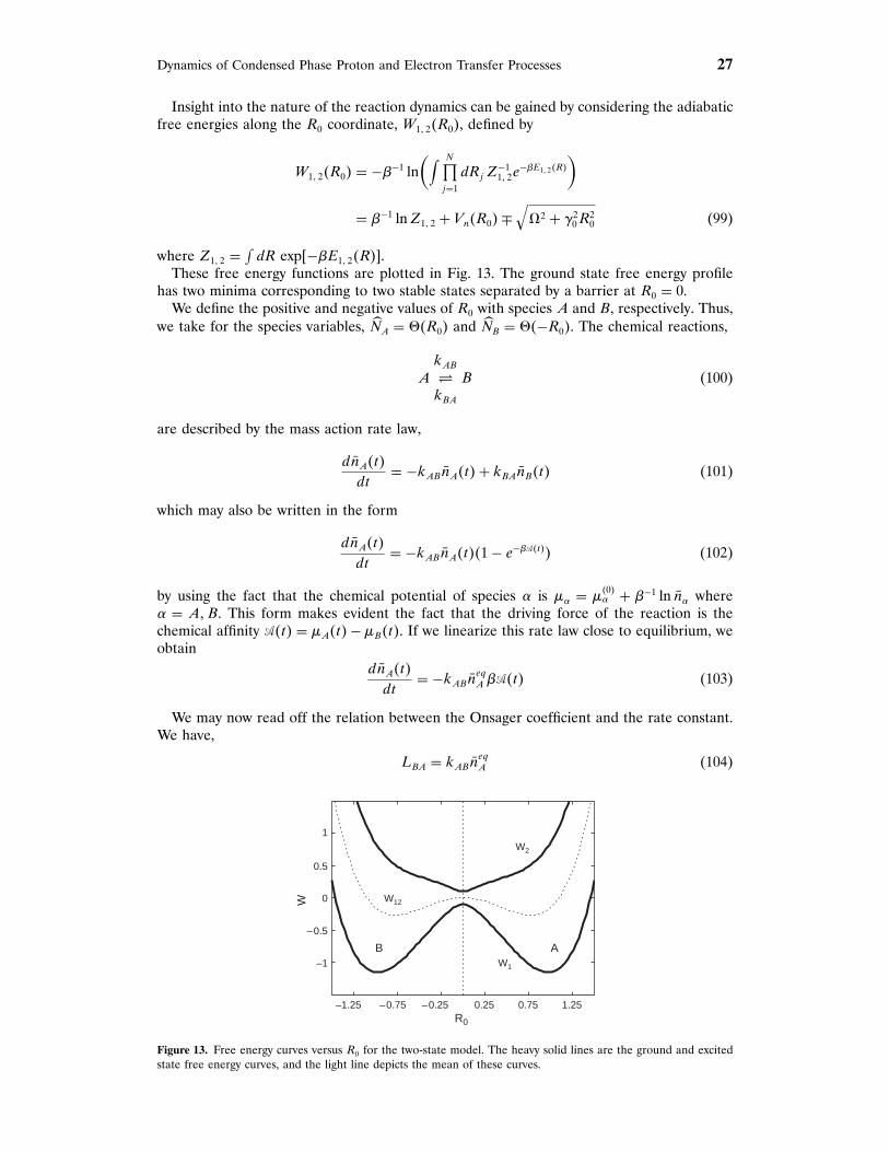
Dynamics of Condensed Phase Proton and Electron Transfer Processes 27
Insight into the nature of the reaction dynamics can be gained by considering the adiabaticfree energies along the R0 coordinate, W1� 2�R0�, defined by
W1� 2�R0� = −�−1 ln(∫ N∏
j=1
dRj Z−11� 2e
−�E1� 2�R�
)= �−1 lnZ1� 2 + Vn�R0�∓
√T2 + K2
0R20 (99)
where Z1� 2 =∫dR exp�−�E1� 2�R��.
These free energy functions are plotted in Fig. 13. The ground state free energy profilehas two minima corresponding to two stable states separated by a barrier at R0 = 0.
We define the positive and negative values of R0 with species A and B, respectively. Thus,we take for the species variables, NA = V�R0� and NB = V�−R0�. The chemical reactions,
AkAB�
kBA
B (100)
are described by the mass action rate law,
dnA�t�
dt= −kABnA�t�+ kBAnB�t� (101)
which may also be written in the form
dnA�t�
dt= −kABnA�t��1− e−���t�� (102)
by using the fact that the chemical potential of species E is <E = <�0�E + �−1 ln nE where
E = A�B. This form makes evident the fact that the driving force of the reaction is thechemical affinity ��t� = <A�t�−<B�t�. If we linearize this rate law close to equilibrium, weobtain
dnA�t�
dt= −kABneqA ���t� (103)
We may now read off the relation between the Onsager coefficient and the rate constant.We have,
LBA = kABneqA (104)
–1
–0.5
0
0.5
1
–1.25 –0.75 –0.25 0.25 0.75 1.25
W
R0
B AW1
W2
W12
Figure 13. Free energy curves versus R0 for the two-state model. The heavy solid lines are the ground and excitedstate free energy curves, and the light line depicts the mean of these curves.
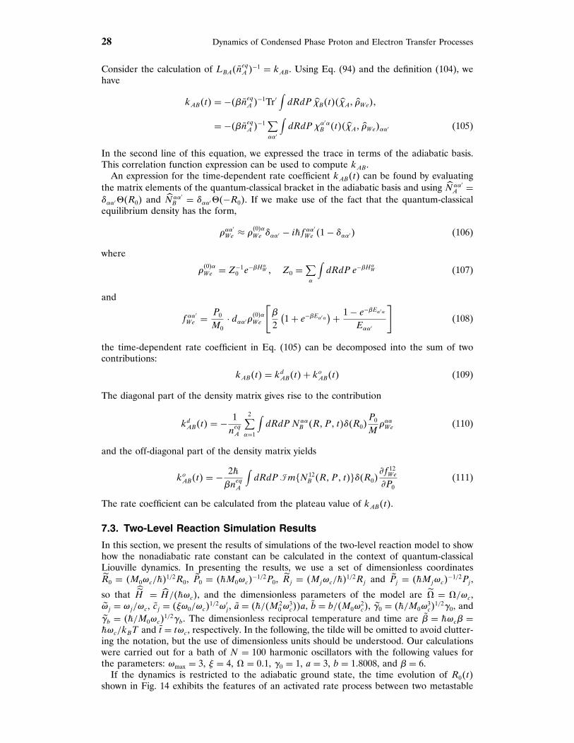
28 Dynamics of Condensed Phase Proton and Electron Transfer Processes
Consider the calculation of LBA�neqA �
−1 = kAB. Using Eq. (94) and the definition (104), wehave
kAB�t� = −��neqA �−1Tr′∫dRdP ��B�t����A� �We��
= −��neqA �−1∑EE′
∫dRdP �E
′EB �t����A� �We�EE′ (105)
In the second line of this equation, we expressed the trace in terms of the adiabatic basis.This correlation function expression can be used to compute kAB.
An expression for the time-dependent rate coefficient kAB�t� can be found by evaluatingthe matrix elements of the quantum-classical bracket in the adiabatic basis and using N EE′
A =�EE′V�R0� and N EE′
B = �EE′V�−R0�. If we make use of the fact that the quantum-classicalequilibrium density has the form,
�EE′
We ≈ ��0�EWe �EE′ − i�f EE
′We �1− �EE′� (106)
where
��0�EWe = Z−1
0 e−�HE
W � Z0 =∑E
∫dRdP e−�H
EW (107)
and
f EE′
We = P0
M0· dEE′��0�EWe
[�
2
(1+ e−�EE′E
)+ 1− e−�EE′E
EEE′
](108)
the time-dependent rate coefficient in Eq. (105) can be decomposed into the sum of twocontributions:
kAB�t� = kdAB�t�+ koAB�t� (109)
The diagonal part of the density matrix gives rise to the contribution
kdAB�t� = − 1neqA
2∑E=1
∫dRdP NEE
B �R� P� t���R0�P0
M�EEWe (110)
and the off-diagonal part of the density matrix yields
koAB�t� = − 2��n
eqA
∫dRdP m%N 12
B �R� P� t�&��R0�.f 12
We
.P0(111)
The rate coefficient can be calculated from the plateau value of kAB�t�.
7.3. Two-Level Reaction Simulation Results
In this section, we present the results of simulations of the two-level reaction model to showhow the nonadiabatic rate constant can be calculated in the context of quantum-classicalLiouville dynamics. In presenting the results, we use a set of dimensionless coordinatesR0 = �M0Mc/��
1/2R0, %P0 = ��M0Mc�−1/2P0, Rj = �MjMc/��
1/2Rj and %Pj = ��MjMc�−1/2Pj ,
so that &H = H/��Mc�, and the dimensionless parameters of the model are T = T/Mc,
%Mj = Mj/Mc, cj = �!M0/Mc�1/2M′
j , a = ��/�M20M
3c��a, b = b/�M0M
2c�, %K0 = ��/M0M
3c�
1/2K0, and%Kb = ��/M0Mc�
1/2Kb. The dimensionless reciprocal temperature and time are � = �Mc� =�Mc/kBT and t = tMc, respectively. In the following, the tilde will be omitted to avoid clutter-ing the notation, but the use of dimensionless units should be understood. Our calculationswere carried out for a bath of N = 100 harmonic oscillators with the following values forthe parameters: Mmax = 3, ! = 4, T = 071, K0 = 1, a = 3, b = 178008, and � = 6.
If the dynamics is restricted to the adiabatic ground state, the time evolution of R0�t�shown in Fig. 14 exhibits the features of an activated rate process between two metastable

Dynamics of Condensed Phase Proton and Electron Transfer Processes 29
–1
0
1
0 1500 3000 4500R
0(t
)
t
Figure 14. Time series of the coordinate R0�t� along a trajectory evolving on the ground state surface, typical ofclassical activated barrier crossing dynamics.
states. In the adiabatic limit, only the first term in Eq. (87) contributes, and the time-dependent rate coefficient in Eqs. (109) and (110) reduces to
kadAB�t� =1neqA
∫dRdP �eiL11tV�R0����R0�
P0
M0�11We (112)
the standard reactive flux autocorrelation expression for a classical activated rate process.This adiabatic time-dependent rate coefficient is plotted in Fig. 15. It has an initial rapiddecay followed by a much slower decay, which takes place on the timescale of the chemicalrate process. The adiabatic rate constant can be determined from the extrapolation of thisslowly decaying portion of the dynamics to t = 0.
In order to compute the nonadiabatic rate constant, we must calculate the contributionscoming from the two terms in Eq. (109). The term kdAB�t� in Eq. (110) involves even numbersof quantum transitions, whereas koAB in Eq. (111) requires an odd number of transitions.Figure 16 shows the nonadiabatic transmission coefficient including both terms in Eq. (109)for up to two quantum transitions per trajectory. For this contribution, the trajectory starts att = 0 from the ground state at the top of the barrier and evolves on the ground state surfaceuntil time �1 where a quantum transition occurs. Between the times �1 and �2, evolutionoccurs on the mean surface. The jump at time �2 must bring the trajectory back either tothe ground or to the excited state surface after which the evolution proceeds adiabaticallyuntil time t. Thus, one has three trajectory segments: the first and the last have no quantumphase factor but the middle trajectory segment has a nonzero phase factor arising from thecoherent evolution on the mean surface �E1�R�+ E2�R��/2.
0.5
0.6
0.7
0.8
0.9
1
0 3 6 9 12 15t
κ AB(t
)d
Figure 15. Transmission coefficient ,dAB�t� = kadAB�t�/kTSTAB versus time for adiabatic dynamics.
30 Dynamics of Condensed Phase Proton and Electron Transfer Processes
0
0.2
0.4
0.6
0.8
1
0 1 2 3 4 5t
κ AB(t
)i
Figure 16. Time-dependent transmission coefficients ,iAB�t� = kAB�t�/kTSTAB . The lower curve shows the off-diagonal
contribution (,oAB). The middle curve arises from the sum of all the nonadiabatic corrections [,dAB�t� + ,oAB�t�]considering up to two quantum transitions. For comparison, the upper curve shows the adiabatic result ,adAB�t�.
Figure 16 shows also the nonadiabatic term ,oAB�t� = koAB/kTSTAB versus time. Only odd
numbers of nonadiabatic transitions contribute to this term. The contribution koAB�t� inEq. (111) depends on the off-diagonal part of bracket �NA� �We�EE′ and the off-diagonalpart of the species variable NE′E
B �t�, (E = E′). One can see that this off-diagonal term givesa negligible contribution so that the main physics is contained in kdAB�t�. Finally, the fulltime-dependent rate constant in Fig. 16 shows that the inclusion of nonadiabatic transitionssignificantly reduces the rate constant below that obtained using adiabatic dynamics.
8. CONCLUSIONSThe rates of proton and electron transfer reactions in condensed phase environments aredifficult to determine because the quantum nature of the transferring particle must be takeninto account. In most circumstances, we can use a mixed quantum-classical approach tostudy such reactions because solvent molecules are typically much heavier than the protonor electron being transferred in the reaction. Equilibrium properties such as the free energyalong the reaction coordinate may be computed using Feynman path integral methods. Thefree energy provides information on the reaction mechanism and is an important ingredientin the transition state theory approximation to the rate constant. Dynamical properties,such as the full rate constant, are much more difficult to compute. Mixed quantum-classicaldynamical schemes may be used to determine transport properties. Adiabatic dynamics,where the motion of the classical degrees of freedom takes place on a single potential energysurface, is the simplest such scheme. However, this approach breaks down when transitionsamong the quantum states take place. In this case, nonadiabatic dynamics must be used. Thequantum-classical Liouville equation and the associated statistical mechanical derivation ofthe nonadiabatic reactive flux formula for the rate of the reaction provide a way to studynonadiabatic proton and electron transfer rates.
If charge transfer reactions take place in domains with nanometer dimensions, then thecompetition between bulk and surface forces leads to interesting effects on reaction mecha-nisms and rates. Our examples of electron solvation in reverse micelles and proton transferin polar molecule clusters served to illustrate such effects.
ACKNOWLEDGMENTSThis work was supported in part by a grant from the Natural Sciences and EngineeringResearch Council of Canada.
Dynamics of Condensed Phase Proton and Electron Transfer Processes 31
REFERENCES1. M. D. Joesten and L. J. Schaad, “Hydrogen Bonding.” Marcel-Deckker, New York, 1974.2. R. P. Bell, “The Proton in Chemistry.” Chapmann & Hall, London, 1973.3. J. Ulstrup, “Charge Transfer Processes.” Springer, New York, 1979.4. T. Yamamoto, J. Chem. Phys. 33, 281 (1960).5. D. Chandler, J. Chem. Phys. 68, 472 (1978).6. S. Constas, R. Kapral, and L. McWhirter, in “Classical and Quantum Dynamics in the Condensed Phase”
(G. Ciccotti, B. Berne, and D. Coker, Eds.), p. 583. World Scientific, Singapore, 1998.7. R. Kapral, J. Chem. Phys. 56, 1842 (1972).8. F. Garisto and R. Kapral, J. Chem. Phys. 58, 3129 (1973).9. H. Mori, Prog. Theor. Phys. 33, 423 (1965).10. R. Zwanzig, Phys. Rev. 124, 983 (1961).11. R. Kubo, J. Phys. Soc. (Japan) 12, 570 (1957); Repts. Prog. Phys. 29, 255 (1966).12. W. E and E. Vanden-Eijnden, “Metastability, Conformational Dynamics, and Transition Pathways in Complex
Systems, in Multiscale Modelling and Simulation” (S. Attinger and P. Koumoutsakos, Eds.), Lecture Notes inComputational Science and Engineering, Vol. 39. Springer, Berlin, 2004.
13. W. E, W. Ren, and E. Vanden-Eijnden, “Finite Temperature String Method for the Study of Rare Events,”J. Phys. Chem. B (submitted).
14. H. Jónsson, G. Mills, and K. W. Jacobsen, in “Classical and Quantum Dynamics in Condensed Phase Simula-tions” (B. J. Berne, G. Ciccotti, and D. F. Coker, Eds.). World Scientific, Singapore, 1998.
15. R. Elber, A. Ghosh, and A. Cardenas, Acc. Chem. Res. 35, 396 (2002).16. C. Dellago, P. G. Bolhuis, and P. L. Geissler, Adv. Chem. Phys. 123, 1 (2002).17. E. Carter, G. Ciccotti, J. T. Hynes, and R. Kapral, Chem. Phys. Lett. 156, 472 (1989).18. M. Fixman, Proc. Natl. Acad. Sci. U.S.A. 71, 3050 (1974).19. N. G. van Kampen, Am. J. Phys. 52, 419 (1984).20. H. Goldstein, “Classical Mechanics.” Addison-Wesley Reading, MA, 1980.21. M. Sprik and G. Ciccotti, J. Chem. Phys. 109, 7737 (1998).22. R. P. Feynman, “Statistical Mechanics.” Addison-Wesley, Reading MA, 1972.23. D. Chandler and P. G. Wolynes, J. Chem. Phys. 74, 4078 (1981).24. M. Gillan, J. Phys. C 20, 3621 (1987).25. G. A. Voth, Adv. Chem. Phys. 93, 135 (1996).26. D. Laria and R. Kapral, J. Chem. Phys. 117, 7712 (2002).27. P. L. Luisi and B. E. Straub, Eds., “Reverse Micelles.” Plenum, New York, 1984.28. M. P. Pelini, Ed., “Structure and Reactivity in Reverse Micelles.” Elsevier, Amsterdam, 1989.29. B. Derecskei, A. Derecskei-Kovacs, and Z. A. Schelly, Langmuir 15, 1981 (1999).30. J. Faeder and B. Ladanyi, J. Phys. Chem. B 104, 1033 (2000); J. Phys. Chem. B 105, 11148 (2001).31. J. Schnitker and P. J. Rossky, J. Chem. Phys. 86, 3462 (1987).32. G. B. Bachelet, D. R. Hamann, and M. Schlüter, Phys. Rev. B 26, 4199 (1982).33. H. J. C. Berendsen, J. R. Grigera, and T. P. Straatsma, J. Phys. Chem. 91, 6269 (1987).34. M. Tuckerman, G. J. Martyna, and B. J. Berne, J. Chem. Phys. 97, 1990 (1992).35. G. J. Martyna, M. E. Tuckerman, D. J. Tobias, and M. L. Klein, Mol. Phys. 87, 1117 (1996).36. G. J. Martyna, M. L. Klein, and M. Tuckerman, J. Chem. Phys. 97, 2635 (1992).37. J. P. Ryckaert, G. Ciccotti, and H. J. C. Berendsen, J. Comp. Phys. 23, 327 (1977); G. Ciccotti and J. P. Ryckaert,
Comp. Phys. Rep. 4, 345 (1986).38. S. Consta and R. Kapral, J. Chem. Phys. 101, 10908 (1994).39. S. Nosé, Mol. Phys. 52, 255 (1984); J. Chem. Phys. 81, 511 (1984); Mol. Phys. 57, 187 (1986); Prog. Theor. Phys.
Suppl. 103, 1 (1991).40. W. Hoover, Phys. Rev. A 31, 1695 (1985).41. D. Laria, G. Ciccotti, M. Ferrario, and R. Kapral, Chem. Phys. 180, 181 (1994).42. D. Li and G. Voth, J. Phys. Chem. 95, 10425 (1991).43. J. Lobaugh and G. Voth, Chem. Phys. Lett. 198, 311 (1992); J. Chem. Phys. 100, 3039 (1994).44. D. Laria, G. Ciccotti, M. Ferrario, and R. Kapral, J. Chem. Phys. 97, 378 (1992).45. D. C. Borgis, S. Lee, and J. T. Hynes, Chem. Phys. Lett. 19, 162 (1989); D. C. Borgis and J. T. Hynes, J. Chem.
Phys. 94, 3619 (1991).46. R. A. Marcus and N. Sutin, Biochim. Biophys. Acta 811, 265 (1985).47. A. Warshel, J. Am. Chem. Soc. 86, 2218 (1982).48. D. A. Zichi, G. Ciccotti, J. T. Hynes, and M. Ferrario, J. Phys. Chem. 93, 6261 (1989).49. H. Azzouz and D. C. Borgis, J. Chem. Phys. 98, 7361 (1993).50. E. Wigner, Phys. Rev. 40, 749 (1932).51. K. Imre, E. Özizmir, M. Rosenbaum, and P. F. Zwiefel, J. Math. Phys. 5, 1097 (1967)52. R. Kapral and G. Ciccotti, J. Chem. Phys. 110, 8919 (1999).53. S. Consta and R. Kapral, J. Chem. Phys. 104, 4581 (1996).54. A. S. Clarke, R. Kapral, B. Moore, G. Patey, and X.-G. Wu, Phys. Rev. Lett. 70, 3283 (1993); A. S. Clarke,
R. Kapral, and G. N. Patey, J. Chem. Phys. 101, 2432 (1994).55. J. C. Tully, “Modern Methods for Multidimensional Dynamics Computations in Chemistry” (D. L. Thompson,
Ed.), p. 34. World Scientific, NY, 1998.
32 Dynamics of Condensed Phase Proton and Electron Transfer Processes
56. H. J. Berendsen and J. Mavri, J. Phys. Chem. 97, 13464 (1993).57. P. Bala, B. Lesyng, and J. A. McCammon, Chem. Phys. Lett. 219, 259 (1994).58. J. C. Tully, J. Chem. Phys. 93, 1061 (1990); J. C. Tully, Int. J. Quantum Chem. 25, 299 (1991); S. Hammes-Schiffer
and J. C. Tully, J. Chem. Phys. 101, 4657 (1994).59. P. Pechukas, Phys. Rev. 181, 166, 174 (1969).60. F. Webster, P. J. Rossky, and P. A. Friesner, Comp. Phys. Comm. 63, 494 (1991); F. Webster, E. T. Wang, P. J.
Rossky, and P. A. Friesner, J. Chem. Phys. 100, 483 (1994).61. L. Xiao and D. F. Coker, J. Chem. Phys. 100, 8646 (1994); D. F. Coker and L. Xiao, J. Chem. Phys. 102, 496
(1995); H. S. Mei and D. F. Coker, J. Chem. Phys. 104, 4755 (1996).62. S. Hammes-Schiffer and J. C. Tully, J. Chem. Phys. 103, 8528 (1995).63. S. R. Billeter, S. P. Webb, T. Iordanov, P. K. Agarwal, and S. Hammes-Schiffer, J. Chem. Phys. 114, 6925 (2001).64. V. I. Gerasimenko, Repts. Ukranian Acad. Sci. 10, 65 (1981); V. I. Gerasimenko: Theor. Math. Phys. 50, 77 (1982);
D. Ya. Petrina, V. I. Gerasimenko, and V. Z. Enolskii, Sov. Phys. Dokl. 35, 925 (1990).65. I. V. Aleksandrov, Z. Naturforsch. 36a, 902 (1981).66. W. Boucher and J. Traschen, Phys. Rev. D 37, 3522 (1988).67. W. Y. Zhang and R. Balescu, J. Plasma Phys. 40, 199 (1988); R. Balescu and W. Y. Zhang, J. Plasma Phys. 40,
215 (1988).68. C. C. Martens and J.-Y. Fang, J. Chem. Phys. 106, 4918 (1996); A. Donoso and C. C. Martens, J. Phys. Chem.
102, 4291 (1998).69. S. Nielsen, R. Kapral, and G. Ciccotti, J. Chem. Phys. 115, 5805 (2001).70. R. Kapral and G. Ciccotti, “A Statistical Mechanical Theory of Quantum Dynamics in Classical Environ-
ments, in Bridging Time Scales: Molecular Simulations for the Next Decade” (P. Nielaba, M. Mareschal, andG. Ciccotti, Eds.), SIMU Conference, 2001. Springer, Berlin, 2003.
71. D. Mac Kernan, G. Ciccotti, and R. Kapral, J. Phys.: Condens. Matt. 14, 9069 (2002).72. A. Sergi, D. Mac Kernan, G. Ciccotti, and R. Kapral, Theor. Chem. Acc. 110, 49 (2003).73. A. Sergi and R. Kapral, J. Chem. Phys. 118, 8566 (2003).74. S. R. de Groot and P. Mazur, “Non-Equilibrium Thermodynamics.” North-Holland, Amsterdam, 1962.75. N. Makri and K. Thompson, Chem. Phys. Lett. 291, 101 (1998); K. Thompson and N. Makri, J. Chem. Phys.
110, 1343 (1999); N. Makri, J. Phys. Chem. B 103, 2823 (1999).76. D. Mac Kernan, R. Kapral, and G. Ciccotti, J. Chem. Phys. 116, 2346 (2002).