Low and optically thin cloud measurementsusing a Raman–Mie lidar

Yonghua Wu,* Shuki Chaw, Barry Gross, Fred Moshary, and Sam AhmedOptical Remote Sensing Laboratory, The City College of New York, New York, New York 10031, USA

*Corresponding author: yhwu@ccny.cuny.edu

Received 4 September 2008; revised 5 December 2008; accepted 27 January 2009;posted 29 January 2009 (Doc. ID 100867); published 19 February 2009

We analyze the potential of measuring low-altitude optically thin clouds with a Raman-elastic lidar in thedaytime. Optical depths of low clouds are derived by two separate methods from nitrogen Raman andelastic-scattering returns. By correcting for aerosol influences with the combined Raman–elastic returns,Mie retrievals of low-cloud optical depth can be dramatically improved and show good agreement withthe direct Raman retrievals. Furthermore, a lidar ratio profile is mapped out and shown to be consistentwith realistic water phase cloud models. The variability of lidar ratios allows us to explore the distribu-tion of small droplets near the cloud perimeter. © 2009 Optical Society of America

OCIS codes: 010.3640, 280.3640, 280.0280.

1. Introduction

Low-altitude clouds play an important role in globalclimate forcing, weather, and precipitation [1,2]. Inparticular, low clouds often have large liquid waterpath (LWP) and are involved in interactions withanthropogenic aerosols and the atmospheric bound-ary layer [3–5]. Unfortunately, for satellite sensorswith visible and near-infrared channels, measure-ment of low and optically thin clouds from space isvery difficult due to their partial transparency, landsurface emission, and the fact that they are relativelywarm [6]. Even though a single layer of low cloudusually simplifies modeling, intercomparisonsamong different retrievals and instruments indicatelarge discrepancies of LWP and optical depth [3].Therefore, it is a significant challenge to accuratelymeasure and model their optical and microphysicalproperties in order to assimilate them into global cli-mate models [2,3,6]. On the other hand, lidar hasbeen extensively demonstrated for observing cloudproperties. However, most previous work [7–10] withlidar techniques concentrates on high and thin cirrusclouds at night. To measure thin cloud optical depth,

Young [7] presented a method based solely on theelastic lidar returns above and below the cloud layer.In that method, the actual lidar elastic returns belowand above clouds are fitted to theoretical molecularscattering returns, which work well for high cirrusbecause any residual aerosols can be ignored at highaltitudes both above and below the cloud. Cadet et al.[10] showed that the variability of the lidar ratio(extinction-to-backscatter ratio) within the cloudssignificantly influences cloud optical depth retrievalin the particular integration method using theelastic returns. Ansmann et al. [9] compared Raman-elastic-scattering inversions and found that the Klettsolution [11] of the cirrus extinction profile and opti-cal depth strongly depended on the lidar ratiovariation along the measuring range.

For low-altitude clouds, a direct measurement ofthe extinction and, therefore, of cloud optical depth(COD) using a nitrogen (N2) Raman lidar is possible.Unfortunately, the weak Raman signal makes it dif-ficult to apply to clouds with significant optical depth(particularly in daytime conditions). Furthermore,the low signal-to-noise ratio (SNR) inherent in pull-ing out the extinction coefficient within the cloudmakes it difficult to rely solely on the Raman retrie-val of extinction.0003-6935/09/061218-10$15.00/0

© 2009 Optical Society of America

1218 APPLIED OPTICS / Vol. 48, No. 6 / 20 February 2009

To address this issue, it would be advantageous touse multiple approaches to verify COD measure-ments. A reasonable approach is to apply the regres-sion approach commonly used for high cirrus. How-ever, for low clouds, corrections for aerosol influenceshave tobecarefully treateddue tohighaerosol loadingin the lower atmosphere. For this correction, the accu-rate backscatter profiles from Raman–Mie lidar dur-ing clear sky or cloud breaks conditions would behelpful because they are not sensitive to lidar-ratio.We focus on using multiple retrieval methods to

explore the accuracy and limits of measuring low-altitude optically thin cloud measurements with aRaman–Mie lidar under daylight conditions and toassess the errors due to heavy aerosol loading aboveand below the cloud. To begin, cloud base and cloudtop altitudes are identified through a wavelet trans-form analysis of elastic returns. After defining thecloud boundary levels, optical depths of low-altitudeclouds are derived using two independent methods.The first method is based on a direct measurementof the extinction coefficient profile in the cloud usingthe direct N2 Raman-return retrieval method [9] fol-lowed by an integration of the extinction profile of thecloud between the cloud boundaries. This methodwill be referred to as “Raman retrieval.” The secondmethod is based on the regression matching techni-que [7] where the COD results in a modification ofthe regression slopes obtained both above and belowthe cloud. This method will be referred to as “Mieretrieval.” When comparing Mie retrieval to Ramanretrieval, significant errors result if the aerosol load-ing above and below the cloud is not quantified. Onesimple correction for the Mie-retrieval method is touse the Fernald inversion [12] method with an apriori lidar ratio in the clear sky patches. However,we show that an accurate correction for aerosol influ-ences can only be achieved by retrieving the aerosolprofiles using the combined N2 Raman and elasticreturns. When this correction is used, we findthat consistent results are obtained between theRaman-retrieval method and the corrected Mie-retrieval method as long as optical depths are smal-ler than 1.5 at 355nm. Once the extinction profilesare validated, we can then calculate the lidar ratiowithin these clouds. In fact, integrated lidar ratiomeasurements obtained in this manner are shownto be consistent with those expected from waterphase clouds calculated from Mie scattering usingreasonable gamma distributed water droplet sizedistribution models. From this model, we also findsignificant variation of the lidar ratios that allowsus to probe for small droplets within the bulk cloud.In Section 2, the Raman–Mie lidar system is

briefly described. In Section 3, the retrievalalgorithms used for processing the lidar data aredeveloped and, in Section 4, results of the inter-comparisons are provided illustrating the needfor a combined Raman–Mie processing approach.Furthermore, the lidar-ratio profiles are obtainedand shown to be consistent with water phase clouds

and the variability of the lidar ratio is explored.Finally, in Section 5, multiple-scattering effects thatdirectly impact COD measurements are quantifiedusing a simple multiple-scattering model for ourlidar specifications and cloud properties geometries.

2. Instrument Description of Raman-Mie Lidar

A multiple-wavelength Raman–Mie lidar located onthe City College of New York campus (40:82°N=73:95°W) in New York City is in operation, providingaerosol, water vapor, and cloud measurements. TheNd:YAG laser emits at 355–532–1064nm with a30Hz repetition rate and a 7ns pulse length. Theconfiguration of the optical receiver is given in Fig. 1.A Newtonian telescope with diameter 50:8 cm is usedto collect all the backscatter returns. Elastic scatter-ing (Mieþ Rayleigh) returns at the three wave-lengths, together with N2 and H2O Raman-shiftedreturns excited by a 355nm laser beam are simulta-neously detected. Photomultiplier tubes (PMT) areemployed to detect UV–visible returns while a Siavalanche photodiode (APD) detector is used forthe 1064nm channel. Narrow-band interference fil-ters (Barr Associates) are used to suppress the sky-light background noise. The interference filters forthe Raman channels have a specifically high blockingratio at the 355nm laser line, which can efficientlyreduce the cross talk of elastic return at that channel.This capability is well verified by comparing strongelastic returns to weak Raman returns by low clouds.A multichannel Licel transient recorder acquires thelidar signal data with the combined analog-to-digitalconverter (40MHz, 12 bit) and photon-counting(250MHz) techniques. The lidar return profiles arerecorded at 1 min time averaging with a nominal3:75nm range resolution. With coaxial transmit-ter–receiver geometry, full return signals startingfrom an altitude of 300m can be detected, makingthis lidar efficient for detecting low clouds. Currently,regular observations are performed in the daytimefor three days per week on average. The main speci-fications are listed in Table 1.

3. Retrieval of Cloud Optical Depth with aMie–Raman lidar

Here we provide a brief overview of extinction andbackscatter retrievals with the combined Raman–Mie lidar. Considering only single-scattering returns,the extinction coefficient of particulates (aerosol orcloud) can be directly derived from the N2 Ramanreturn [13,14]:

αpðλ0; zÞ ¼1

1þ�

λNλ0

�−v

�ddz

�ln

NðzÞPðλN ; zÞz2

�

− αmðλ0; zÞ�1þ

�λNλ0

�−4��

; ð1Þ

where α is the extinction coefficient and subscripts pand m refer to particles and molecules, respectively,and PðλN ; zÞ is the N2 Raman-return intensity at

20 February 2009 / Vol. 48, No. 6 / APPLIED OPTICS 1219

range z. NðzÞ is the molecular number density. Here,λ is the wavelength where subscripts o andN refer tothe laser andN2 Raman-shifted wavelengths, respec-tively. The Angstrom coefficient ν is taken to be 1.2for aerosol and 0 for cloud [9,14]. αp is changed toαc in Eq. (1) for the cloud. Integrating the Raman-retrieved extinction profile from cloud base zb totop zt, provides the first direct approach (i.e., Ramanmethod as described in Section 1) for the determina-tion of the COD:

τC ¼Zztzb

αcðzÞdz: ð2Þ

This method directly solves the cloud extinction coef-ficient without assuming a lidar ratio and a calibrat-ing system constant, but its measuring capabilitywould be limited by the much weaker Raman returnsthan elastic returns.From the N2 Raman and elastic-scattering

returns, particle-scattering ratio Rðλ0; zÞ and back-scatter βðλ0; zÞ can be written as

Rðλ0; zÞ ¼βpðλ0; zÞ þ βmðλ0; zÞ

βmðλ0; zÞ

¼ Pðλ0; zÞPðλN ; zÞ

Rðλo; zref ÞPðλN2; zref ÞPðλ0; zref Þ

×exp

�−

Rzrefz ½αpðλ0; z0Þ þ αmðλ0; z0Þ�dz0

�

exp�−

Rzrefz ½αpðλN ; z0Þ þ αmðλN ; z0Þ�dz0

� ; ð3Þ

βpðλ0; zÞ ¼ ½Rðλ0; zÞ − 1�βmðλ0; zÞ ð4Þ

where βpðλ0; zÞ and βmðλ0; zÞ refer to particle and mo-lecular backscatter coefficients, respectively, at thelaser wavelength and range z. Here, zref is a referencealtitude where the aerosol-scattering ratio Rref is as-sumed to be known and is usually chosen to be withinan aerosol-free region. Molecular extinction andnumber density are calculated from radiosondedata at the Brookhaven National Laboratory site(Upton, New York, National Weather Service), which

Fig. 1. (Color online) Optical layout of the Raman–Mie lidar receiver.

Table 1. Main Specifications of Raman–Mie Lidar System at City College of New York

Laser Quanta-Ray PRO-230 Nd:YAG, 30Hz 950mJ at 1064nm, 475mJ at 532nm, 300mJ at 355nmTelescope Newtonian, f =3:5; diameter: 50:8 cm; FOV, 1:5mradInterferenceFilters

Barr Associates Inc., central wavelength/bandwidth/peak transmission Mie channel, 1064, 532,355=0:3∼ 1nm=T > 50%; N2 Raman, 386:7=0:3nm=T ¼ 65%; H2O (vapor) Raman, 407:5=0:5nm=T ¼ 65%

Detectors EG&G Si:APD for 1064nm; Hamamatsu PMT: H6780-20, R2693P, R1527PData acquisition Licel TR 40-160, 12bit and 40MHz A/D, 250MHz photon-countingRange resolution 3:75m

1220 APPLIED OPTICS / Vol. 48, No. 6 / 20 February 2009

is about 90km from the lidar site. The ratio of thetransmission terms in Eq. (3) is usually close to unitybecause of the small difference between wavelengthsλ0 and λN . Finally, the extinction-to-backscatter ratio,or lidar ratio, or the S ratio can be calculated. Thelidar ratio depends on the physical and chemicalproperties of particles.The second method for deriving COD following

Young’s approach [7] first requires the calculationof the molecular-scattering return according to

Pmðλ0; zÞ ¼ βmðλ0; zÞ × T2mðλ0; zÞ=z2: ð5Þ

Once the molecular profile is calculated, the mea-sured elastic-scattering returns are regressedagainst the molecular profile both below and abovethe cloud. Taking into account that aerosol layerscan exist both above and below the cloud, the re-gressed slopes below the cloud (z1 to z2) and abovethe cloud (z3 to z4) can be written as

mbot ¼ CT2aðz0; z1Þ�Rbotðz1; z2Þ;

mtop ¼ CT2aðz0; z1Þ�Rtopðz3; z4ÞT2

c ; ð6Þ

where C is the lidar system constant, z0 is the initiallidar altitude, Ta and Tc are aerosol and cloud trans-missions, respectively, and �R is the average of theaerosol-scattering ratio over the regression ranges.In the regressions performed above, we assume aconstant aerosol-scattering ratio and ignore aerosolattenuation within the regressed range window. Thiswindow is variable dependent on cloud height, aero-sol variability, and SNR, but it has been found thatregression windows between 0.1 and 0:2km, whereaerosol-scattering ratios generally vary little, aresuitable. Clearly, COD can be derived from Eq. (6) as

τC ¼�log

�mbot

mtop

�− log

��Rbot

Rtop

��=2; ð7Þ

where logð�Rbot=�RtopÞ is called the aerosol correctionfactor and the COD uncertainty is given as

δτC¼12

ffiffiffiffiffiffiffiffiffiffiffiffiffiffiffiffiffiffiffiffiffiffiffiffiffiffiffiffiffiffiffiffiffiffiffiffiffiffiffiffiffiffiffiffiffiffiffiffiffiffiffiffiffiffiffiffiffiffiffiffiffiffiffiffiffiffiffiffiffiffiffiffiffiffiffiffiffiffiffiffiffiffiffiffiffiffiffiffiffiffiffiffiffiffiffi�δmbot

mbot

�2þ�δmtop

mtop

�2þ�δ�Rbot

Rbot

�2þ�δ�Rtop

�Rtop

�2

s;

ð8ÞThis second method to obtain optical depth from

Eq. (7) using elastic-returns regression is what wereferred to in Section 1 as Mie retrieval. This methodis especially accurate for high and thin cirrus be-cause nearly free-aerosol layers exist below andabove the cloud so that aerosol influence can be ig-nored. On the other hand, aerosol loading is usuallyhigh at low altitudes, so it is necessary to estimatethe aerosol itemRbot=Rtop in Eq. (7). Clearly, the ratio(Rbot=Rtop) can be obtained from the combinedRaman–Mie signals, as seen in Eq. (3) and, moreover,it is quite insensitive to the assigned Rzref and lidar

ratio. Because of poor signal penetration of theRaman channel, we prefer to perform this analysisin clear sky patches found within the cloud decksand assume that the vertical structure of the aero-sol-scattering ratio is fairly stable over small timeperiods. This is quite reasonable for the low opticalthickness cases considered where clear sky patchesare numerous. This is the unique advantage ofRaman–Mie lidars over elastic lidar retrievals alone,where the aerosol ratios would depend strongly onthe assumed lidar ratio and the reference valueRref (which is not the case when the Mie–Raman li-dar is used). The level of improvement in derivingCOD due to more robust aerosol correction is ex-plored in Subsection 4.B. In all subsequent discus-sion, retrievals using only the N2 Raman signalsin Eq. (2) are referred to Raman retrieval, whilethe use of elastic returns with regression in Eq. (7)is referred to Mie retrieval for deriving the COD.

In both retrieval methods an important issue is toaccurately and objectively determine the cloud baseand top. For this purpose, a wavelet transformanalysis of elastic returns is used. The covariancetransform is defined as [15,16]

Wða; bÞ ¼Zz0z0

�PðzÞh

�z − ba

��dz; ð9Þ

where PðzÞ is the elastic-scattering lidar signal fromrange z, h is the wavelet function, and a and b are thedilation and translation parameters of the wavelet(Mexican hat) function, respectively. The locationsof cloud base and top can be found by minimizingthe covariance transform over a wide distributionof wavelet parameters. This method works well forthe single-layer cases we are considering.

4. Result and Discussion

A. Cloud Profiles

To illustrate the capability of the Raman lidar to pro-vide cloud properties in daylight, Figs. 2(a) and 2(b)show a representative profile of cloud optical para-meters obtained on 15 March 2006. A cloud layerclearly appears in the backscatter profile at between2 and 3km altitude. Raman processing allows usto calculate the profile of cloud extinction-to-backscatter ratios, or lidar ratios, which we observeare significantly smaller than those of aerosols. Inparticular, we find the mean value of cloud lidarratios at 355nm is 18:6 sr with a standard deviationof 3:9 sr. This value is comparable with previousobservations and numerical analysis [17,18] and isconsistent with Mie-scattering calculations using anormalized gamma mode of cloud droplet size distri-bution. In particular, the value of the lidar ratiobased on the Mie-scattering model is calculated tobe 18:9� 0:4 sr at 355nm over the wide range ofmode parameters [17].

20 February 2009 / Vol. 48, No. 6 / APPLIED OPTICS 1221

B. Regression of Cloud Optical Depth with ElasticReturns

Figure 3(a) shows the background noise subtractedelastic and N2 Raman-scattering returns on 6 April2006. A 10 min data average is used to reduce thenoise. Elastic returns indicate a cloud layer over1:5–1:9km altitude, while the N2 Raman signalshows a large gradient caused by cloud attenuationin this range. In the figure, the range intervals usedin the regression are also marked both below andabove the cloud for subsequent Mie retrieval ofCOD. Figure 3(b) plots the covariance of the wavelettransform of elastic returns. Clearly, cloud base andtop are well identified by the minimal values ofcovariance.Figure 4 shows the regressions details for the cloud

optical depth on 16 June 2006 for different times.Eight vertical profiles are plotted in Fig. 4(a), whichdisplay cloud in the range of 2:3–3:3km. In thesecases, high aerosol loading appears below the cloudwith overall mean aerosol-scattering ratios rangingfrom 2:13–2:76 below the cloud. On the other hand,

aerosol loading above the cloud is found to vary withthe scattering ratio in the 1:056–1:063 range.Figure 4(b) plots CODs derived independently usingboth the Raman-retrieval and elastic-retrieval meth-ods. We see clearly that, without correcting for theaerosol -scattering ratio, a systematic and significantoverestimate of optical depth using the Mie-retrievalmethod (circles) is made. After suitably correcting forthe aerosols, the Mie retrieval (squares) shows goodagreement with that of Raman retrieval.

Another aspect of COD retrieval to consider is thefact that, without the Raman returns, particularlybelow the cloud, the correction factor for the aerosolratio is expected to be significantly less accurate. Tosee this clearly, we have reanalyzed the optical depthretrieval using the Mie-scattering method but usingthe correction factors obtained only from the elasticchannel in which an assumption on the lidar S ratiois needed. The results of this retrieval relative tothe combined Raman–Mie approach to correct forthe aerosol ratio are given in Fig. 5. In this figure,[Mie-uncor] refers to Mie retrieval without aerosol

Fig. 2. (a) Cloud backscatter, extinction coefficient, and (b) their ratio at 355nm on 15 March 2006.

Fig. 3. (a) Elastic- and N2 Raman-scattering signals and (b) covariance of wavelet transform on 6 April 2006.

1222 APPLIED OPTICS / Vol. 48, No. 6 / 20 February 2009

correction, [Mie-Cor-1] refers to the case where onlythe elastic channel was used to retrieve the aerosolcorrection factor, while [Mie-Cor-2] refers to the casewhere the combined Raman–Mie signals are used forthe aerosol correction. Clearly, a significant improve-ment is obtained when both the Raman andMie lidarchannels are used together.Another concern is the fact that high COD will sig-

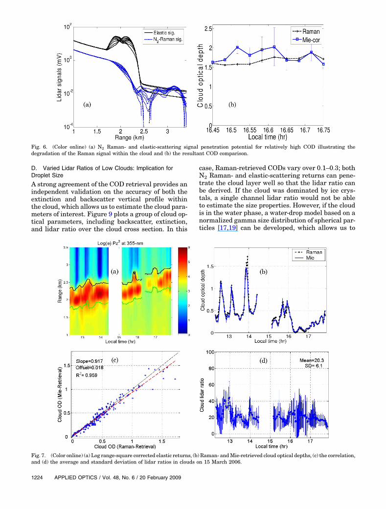
nificantly attenuate the lidar signal, degrading theretrieval, particularly when the N2 Raman profilesare used. In addition, the strong background signalnoise in the daytime will significantly reduce theSNR. These results are seen in Fig. 6(a), which showsthat, for sufficiently high COD, the N2 Raman signaldegrades below the noise threshold prior to the cloudthreshold, unlike the elastic return. This results in aclear underestimation of COD using the Raman-return technique for highCOD, as illustrated in Fig. 6

(b). In this situation, the previous aerosol-scatteringratio profile derived from Raman-elastic returns willbe used for the aerosol correction in Mie retrieval. Itshould, however, be pointed out that, if the degradedsignal is still used to calculate extinction coefficient,the error may not always be biased low but can leadto noise-induced overestimates of extinction.

C. Comparisons of Cloud Optical Depth Between Ramanand Mie Retrievals

A representative example (15 March 2006) for alarge time interval in which the COD undergoessignificant change is shown in Figs. 7(a)–7(d).Range-square corrected elastic returns are plottedin Fig. 7(a), which characterize cloud heights of1:8–3km marked by the two lines. Complementaryradiosonde data are used to identify that the cloudis most likely water phase dominated. As Fig. 7(b)shows, after aerosol contamination is eliminated,the two retrievals are nearly coincident with eachother and CODs vary from 0.1 to 1.7 at a 355nm wa-velength. A good correlation between the retrievals isseen in Fig. 7(c) , with R2 ¼ 0:959. However, we donote that discrepancies become larger at higherCODs, as expected. The mean and standard devia-tion of lidar ratios in cloud layers are shown inFig. 7(d) and it is observed that they mostly fluctuateabout the 20 sr line with standard deviation of 6:3 sr,indicative of the dominance of the water phase inthe cloud.

To assess these methods over a larger data sample,a 17 d data set with a total of 2042 pair points is sta-tistically analyzed. The results are shown in Fig. 8.Figure 8(a) illustrates a strong correlation of R2 ¼0:94with a regression slope close to 1.0. Clearly, datapairs begin to scatter at larger CODs. In Fig. 8(b), themean values of the absolute differences are calcu-lated as a function of COD. Over a wide range ofCOD (i.e., 0.3 to 1.5), fractional errors are of the orderof 10% but the error gets larger as COD goes higherthan 1.5.

Fig. 4. (Color online) (a) Elastic- and N2 Raman-scattering signals and (b) comparison of cloud optical depth retrieval on 16 June 2006.Raman, Raman retrieval; Mie-uncorr., Mie retrieval without aerosol correction; Mie-cor, Mie retrieval with aerosol correction.

Fig. 5. (Color online) Comparison of cloud optical depth retrie-vals. Mie-uncor, Mie retrieval without aerosol correction; Mie-cor-1, Mie retrieval with aerosol correction from only the elasticreturns; Mie-cor-2, Mie retrieval with aerosol correction fromthe combined Raman-elastic return.

20 February 2009 / Vol. 48, No. 6 / APPLIED OPTICS 1223

D. Varied Lidar Ratios of Low Clouds: Implication forDroplet Size

A strong agreement of the COD retrieval provides anindependent validation on the accuracy of both theextinction and backscatter vertical profile withinthe cloud, which allows us to estimate the cloud para-meters of interest. Figure 9 plots a group of cloud op-tical parameters, including backscatter, extinction,and lidar ratio over the cloud cross section. In this

case, Raman-retrieved CODs vary over 0:1–0:3; bothN2 Raman- and elastic-scattering returns can pene-trate the cloud layer well so that the lidar ratio canbe derived. If the cloud was dominated by ice crys-tals, a single channel lidar ratio would not be ableto estimate the size properties. However, if the cloudis in the water phase, a water-drop model based on anormalized gamma size distribution of spherical par-ticles [17,19] can be developed, which allows us to

Fig. 6. (Color online) (a) N2 Raman- and elastic-scattering signal penetration potential for relatively high COD illustrating thedegradation of the Raman signal within the cloud and (b) the resultant COD comparison.

Fig. 7. (Color online) (a) Log range-square corrected elastic returns, (b) Raman- andMie-retrieved cloud optical depths, (c) the correlation,and (d) the average and standard deviation of lidar ratios in clouds on 15 March 2006.

1224 APPLIED OPTICS / Vol. 48, No. 6 / 20 February 2009

roughly connect the lidar ratio to an effective dropletmean diameter. The model calculated lidar ratiosversus water droplet effective diameters are shownin Fig. 9(b), with the mode width parameter μ giventhe value of 2. Clearly, lidar ratios show a strong de-pendence on the effective diameters for small clouddroplets (<3 μm) and then become fairly stable fordroplet sizes of 3–20 μm, with a value of 20 sr. Thisis in agreement with lidar ratios obtained in denseportions of the cloud, which confirms the basicassumption that the cloud is primarily in waterphase. Also, we see that, as we extend to the cloudboundaries, the lidar ratio increases markedly andthis implies the presence of smaller droplets, suchas would be associated either with new condensationor evaporation of the droplets near the cloud edge.Additional improvements in the range of droplet sizeretrieval can be obtained if we include long wave-length backscatter, as well as being able to moreaccurately distinguish ice from water phase. In par-ticular, Eberhard [19] has discussed a similar ap-proach to determining droplet size according tolidar ratio at a long laser wavelength (∼10:6 μm).Further analysis is needed to explore this interestingphenomenon, which would be of great interest for themicrophysical and dynamic processes of low clouds.In evaluating the lidar ratio, we needed to ensure

that all measurements were taken in the cloud inter-ior. To verify that these measurements are from thecloud, histograms of particles’ backscatter coeffi-cients are plotted in Fig. 9(c). The dotted curve showsthe data from 1.9 to 3:1km altitudes, including aero-sol and cloud [see Fig. 7(a)]. A bimodal distributionseparately represents aerosols and cloud. The solidcurve plots a histogram of backscatters over only2:6–2:8km altitudes, which are definitely abovethe cloud threshold.

E. Multiple-Scattering Effects

Until now, we have only considered single scattering,but for low-altitude clouds, multiple scattering alsoaffects the measurement and can lead to further dis-

crepancies at high AOD. In general, multiple scatteris a complex process [20–22] that depends on clouddroplet size, optical depth, field of view of receiver,and laser beam spot size in clouds, etc. In fact, thispaper only focuses on low-altitude optically thinclouds where the CODs are mostly smaller than1.5, the geometric thicknesses is of the order of afew hundred meters, and the receiver field of viewis 1:5mrad. Therefore, multiple scattering may beshown to be a fairly small correction. Using a modeldeveloped by Eloranta [20], multiple-scattering fac-tors can be first estimated with the lidar parametersand cloud profiles in Fig. 3, then the COD differencesbetween considering only single-scattering andmultiple-scattering effects are estimated in Ramanretrieval [21]. Table 2 gives the percentage of multi-ple-scattering contributions to Raman retrievals atdifferent droplet radii and optical depths of cloud.Clearly, multiple-scattering influences increase withthe effective radius and optical depth. With theMODIS/Terra-retrieved cloud effective radius of7:4 μm near our lidar site, we estimate that thecontribution of multiple scattering is around16–18% for low to moderate cloud optical depth.While such errors should not be ruled out, we mustemphasize that these errors would apply equally toall COD methods considered. Meanwhile, with thesmaller FOV (0:8mrad), multiple-scattering influ-ences can be largely reduced below the errorestimates we have encountered.

5. Conclusion

We analyzed the retrievals of low-altitude opticallythin clouds using both the N2 Raman and elastic-scattering returns approaches. We illustrated thatthe elastic-return regression approach would overes-timate CODs unless the aerosol correction items areaccurately estimated. In particular, we showed that,by using the combined Mie–Raman returns obtainedfor nearby clear sky patches, we can better estimatethe aerosol-scattering ratio profile, which results in asignificant improvement in the COD retrieval.

Fig. 8. (a) Correlation and (b) absolute differences among Raman- and Mie-retrieved cloud optical depths.

20 February 2009 / Vol. 48, No. 6 / APPLIED OPTICS 1225

Validation of the Raman-retrieved COD with the re-trieval using the combined Raman–Mie returns hasthe added benefit of providing a means to assess thequality of our backscatter and extinction vertical pro-file in the cloud. From these measurements, we wereable to provide three-dimensional profile maps of thelidar extinction/backscatter ratio (S). In particular,the S ratio statistics have a mean value near 20 sr,which was found to be consistent with a commonly

used water phase cloud model. Within the waterphase assumption, the lidar-ratio profiles were usedfor preliminary sizing of effective cloud droplet sizes,which allowed us to map areas within the cloud withsmall condensing droplets.

In a statistical comparison, the CODs retrievedfrom the Mie-returns regression method with aerosolcorrection and the direct Raman method showexcellent agreement, and a strong correlation withR2 ¼ 0:94 and the regressed linear slope of 0.98 isobserved. In general, errors between the two meth-ods are less than 10%. However, we also show thatthe direct Raman method becomes less accurate athigh COD since the N2 Raman signals are attenu-ated by the cloud more severely than the elastic sig-nal. This is illustrated by the fact that discrepanciesbetween the methods grow larger when CODs aregreater than 1.5. Finally, multiple-scattering effectson deriving CODwere calculated for the optical para-meters relevant to our study and they indicate thatcorrections of the order of 18% must be made. Thisinfluence can be reduced largely using the smallerfield of view (FOV) of the receiver. Unfortunately,since both optical depth approaches are affected bymultiple-scattering effects, no independent correc-tion of the multiple scattering can be made.

In summary, we find that Mie-returns regressionmethod provides the better COD measurement forthe larger CODs (>1:5), although the Raman extinc-tion method works well for COD < 1:5. However, theMie method depends critically on the ability to esti-mate aerosols beneath the cloud layer, which can bebest accomplished using a combined Mie–Ramanlidar measurement. It is also expected that deter-mining the cloud phase and subsequent sizing ofcloud droplets within the water phase will also be sig-nificantly improved using a properly calibrated1064nm backscatter lidar channel; this will be dis-cussed in a separate paper.

This work is partially supported by the researchprojects of National Oceanic and AtmosphericAdministration (NOAA)NA17AE1625 and NationalAeronautics and Space Administration (NASA)NCC-1-03009. The authors appreciate the computingcodes of multiple scattering from Edwin Elorantaand Robin Hogan and the kind e-mail communica-tions with Ulla Wandinger about multiple-scatteringestimation.

Fig. 9. (Color online) (a) Cloud backscatter, extinction, and ex-tinction-to-backscatter ratio on 15 March 2006, (b) lidar ratio ver-sus particle effective diameter, and (c) histogram of backscattercoefficients of aerosol and cloud on 15 March 2006.

Table 2. Percentage of Multiple-Scattering Influences on Raman-Retrieved Cloud Optical Depth

Re ¼ 3:5 μm` 5 μm 7:4 μm b 10 μm

FOV ¼ 1:5mradCOD ¼ 0:5 6.50% 10.40% 16.20% 21.60%COD ¼ 1:2 7.80% 12.00% 18.00% 23.40%

FOV ¼ 0:8mradCOD ¼ 1:2 3.20% 5.20% 8.70% 12.30%`Re, effective radius of cloud droplet.bMODIS retrieval value.

1226 APPLIED OPTICS / Vol. 48, No. 6 / 20 February 2009

References1. C. S. Bretherton, T. Uttal, C. W. Fairall, S. Yuter, R. Weller, D.

Baumgardner, K. Comstock, R. Wood, and G. Raga, “The EPIC2001 stratocumulus study,” Bull. Am. Meteorol. Soc. 85, 967–977 (2004).

2. J. Verlinde, J. Y. Harrington, G. M. McFarquhar,V. T. Yannuzzi, A. Avramov, S. Greenberg, N. Johnson,G. Zhang, M. R. Poellot, J. H. Mather, D. D. Turner,E. W. Eloranta, B. D. Zak, A. J. Prenni, J. S. Daniel,G. L. Kok, D. C. Tobin, R. Holz, K. Sassen, D. Spangenberg,P. Minnis, T. P. Tooman, M. D. Ivey, S. J. Richardson,C. P. Bahrmann, M. Shupe, P. J. DeMott, A. J. Heymsfield,and R. Schofield, “The mixed-phase arctic cloud experiment,”Bull. Am. Meteorol. Soc. 88, 205–221 (2007).

3. D. D. Turner, A. M. Vogelmann, R. T. Austin,J. C. Barnard,K. Cady-Pereira, J. C. Chiu, S. A. Clough, C. Flynn,M. M. Khaiyer, J. Liljegren, K. Johnson, B. Lin, C. Long,A. Marshak, S. Y. Matrosov, S. A. McFarlane, M. Miller,Q. Min, P. Minnis, W. O’Hirok, Z. Wang, and W. Wiscombe,“Optically thin liquid water clouds: their importance andour challenge,” Bull. Am. Meteorol. Soc. 88, 177–190 (2007).

4. Y. J. Kaufman, I. Koren, L. A. Remer, D. Rosenfeld, andY. Rudich, “The effect of smoke, dust, and pollution aerosolon shallow cloud development over the Atlantic Ocean,” Proc.Natl. Acad. Sci. 102, 11207–11212 (2005).

5. S. E. Schwartz, Harshvardhan, and C. M. Benkovitz,“Influence of anthropogenic aerosol on cloud optical depthand albedo shown by satellite measurements and chemicaltransport modeling,” Proc. Natl. Acad. Sci. 99, 1784–1789(2002).

6. B. A. Baum and S. Platnick, “Introduction to MODIS cloudproducts,” in Earth Science Satellite Remote Sensing, Vol. 1:Science and Instruments, J. J. Qu, W. Gao, M. Kafatos,R. E. Murphy, and V. Salomonson, eds. (Springer-Verlag,2006), pp 74–91.

7. S. A. Young, “Analysis of lidar backscatter profiles in opticalthin clouds,” Appl. Opt. 34, 7019–7030 (1995).

8. D. N. Whiteman, K. D. Evans, B. Demoz, D. O’C Starr,E. W. Eloranta, D. Tobin, W. Feltz, G. J. Jedlovec, S. I. Gutman,G. K. Schwemmer, M. Cadirola, S. H. Melfi, and F. Schmidlin,“Raman lidar measurements of water vapor and cirrus cloudsduring the passage of Hurricane Bonnie,” J. Geophys. Res.106, 5211–5225 (2001).

9. A. Ansmann, U. Wandinger, M. Riebesell, C. Weitkamp, andW. Michaelis, “Independent measurement of extinction andbackscatter profiles in cirrus clouds using a combined Ramanelastic-backscatter lidar,” Appl. Opt. 31, 7113–7131 (1992).

10. B. Cadet, V. Giraud, M. Haeffelin, P. Keckhut, A. Rechou, andS. Baldy, “Improved retrievals of the optical properties of cir-rus clouds by a combination of lidar methods,” Appl. Opt. 44,1726–1734 (2005).

11. J. D. Klett, “Stable analytical inversion solution for processinglidar returns,” Appl. Opt. 20, 211–220 (1981).

12. F. G. Fernald, “Analysis of atmospheric lidar observations:some comments,” Appl. Opt. 23, 652–653 (1984).

13. A. Ansmann, M. Riebesell, and C. Weitkamp, “Measurementof atmospheric aerosol extinction profiles with a Ramanlidar,”Opt. Lett. 15, 746–748 (1990).

14. R. A. Ferrare, S. H. Melfi, D. N. Whiteman, K. D. Evans, andR. Leifer, “Raman lidar measurements of aerosol extinctionand backscattering. 1. Methods and comparisons,” J. Geophys.Res. 103, 19663–19672 (1998).

15. Y. Morille, M. Haeffelin, P. Drobinski, and J. Pelon, “STRAT:an automated algorithm to retrieve the vertical structure ofthe atmosphere from single channel lidar data,” J. Atmos.Ocean. Technol. 24, 761–775 (2007).

16. K. J. Davis, N. Gamageb, C. R. Hagelbergc, C. Kiemled,D. H. Lenschowe, and P. P. Sullivane, “An objective methodfor deriving atmospheric structure from airborne lidar obser-vations,” J. Atmos. Ocean. Technol. 17, 1455–1468 (2000).

17. E. J. O’Connor, A. J. Illingworth, and R. J. Hogan, “A techniquefor autocalibration of cloud lidar,” J. Atmos. Ocean. Technol.21, 777–778 (2004).

18. R. G. Pinnick, S. G. Jennings, P. Chýlek, C. Ham, andW. T. Grandy Jr., “Backscatter and extinction in water cloud,”J. Geophys. Res. 88, 6787–6796 (1983).

19. W. L. Eberhard, “CO2 lidar technique for observing character-istic drop size in water cloud,” IEEE Trans. Geosci. RemoteSens. 31 (1), 56 (1993).

20. E. W. Eloranta, “A practical model for the calculation of multi-ply scattered lidar returns,” Appl. Opt. 37, 2464–2472 (1998).

21. U.Wandinger, “Multiple-scattering influence on extinction andbackscatter coefficient measurements with Raman and high-spectral-resolutionlidars,”Appl.Opt.37,417–427(1998).

22. R. J. Hogan, “Fast approximate calculation of multiply scat-tered lidar returns,” Appl. Opt. 45, 5984–5992 (2006).

20 February 2009 / Vol. 48, No. 6 / APPLIED OPTICS 1227