arX

iv:g

r-qc

/060

7043

v2 2

Oct

200

6

DF/IST-4.2006

Lorentz Symmetry Derived from Lorentz Violation in the Bulk

Orfeu Bertolami∗ and Carla Carvalho†

Departamento de Fısica, Instituto Superior Tecnico

Avenida Rovisco Pais 1, 1049-001 Lisboa, Portugal

Abstract

We consider bulk fields coupled to the graviton in a Lorentz violating fashion. We expect that

the overly tested Lorentz symmetry might set constraints on the induced Lorentz violation in the

brane, and hence on the dynamics of the interaction of bulk fields on the brane. We also use the

requirement for Lorentz symmetry to constrain the cosmological constant observed on the brane

∗Email address: orfeu@cosmos.ist.utl.pt†Email address: ccarvalho@ist.edu

1

I. INTRODUCTION

Lorentz invariance is one of the most well tested symmetries of physics. Nevertheless,

the possibility of violation of this invariance has been widely discussed in the recent liter-

ature (see e.g. [1]). Indeed, the spontaneous breaking of Lorentz symmetry may arise in

the context of string/M-theory due to the existence of non-trivial solutions in string field

theory [2], in loop quantum gravity [3], in noncommutative field theories [4, 5] or via the

spacetime variation of fundamental couplings [6]. This putative breaking has also implica-

tions in ultra-high energy cosmic ray physics [7, 8]. Lorentz violation modifications of the

dispersion relations via five dimensional operators for fermions have also been considered

and constrained [9]. It has also been speculated that Lorentz symmetry is connected with

the cosmological constant problem [10]. However, the main conclusion of these studies is

that Lorentz symmetry holds up to about 2 × 10−25 [1, 8].

Efforts to examine a putative breaking of Lorentz invariance have been concerned mainly

with the phenomenological aspects of the spontaneous breaking of Lorentz symmetry in

particle physics and only recently have the implications for gravity been more closely studied

[11, 12]. The idea is to consider a vector field coupled to gravity that undergoes spontaneous

Lorentz symmetry breaking by acquiring a vacuum expectation value in a potential.

Moreover, recent developments in string theory suggest that we may live in a braneworld

embedded in a higher dimensional universe. In the context of the Randall-Sundrum cosmo-

logical models, the warped geometry of the bulk along the extra spacial dimension suggests

an anisotropy which could be associated with the breaking of the bulk Lorentz symmetry.

In this paper we study how spontaneous Lorentz violation in the bulk repercusses on the

brane and how it can be constrained. We consider a vector field in the bulk which acquires

a non-vanishing expectation value in the vacuum and introduces spacetime anisotropies in

the gravitational field equations through the coupling with the graviton. For this purpose,

we derive the field equations and project them parallel and orthogonally to the brane.

We then establish how to derive brane quantities from bulk quantities by adopting Fermi

normal coordinates with respect to the directions on the brane and continuing into the bulk

using the Gauss normal prescription.

We parameterize the worldsheet in terms of coordinates xA = (tb,xb) intrinsic to the

brane. Using the chain rule, we may express the brane tangent and normal unit vectors in

2

terms of the bulk basis as follows:

eA =∂

∂xA= Xµ

A

∂

∂xµ= Xµ

Aeµ,

eN =∂

∂n= Nµ ∂

∂xµ= Nµeµ, (1)

with

gµνNµNν = 1, gµνN

µXνA = 0, (2)

where g is the bulk metric

g = gµν eµ ⊗ eν = gAB eA ⊗ eB + gAN eA ⊗ eN + gNB eN ⊗ eB + gNN eN ⊗ eN (3)

To obtain the metric induced on the brane we expand the bulk basis vectors in terms of

the coordinates intrinsic to the brane and keep the doubly brane tangent components only.

It follows that

gAB = XµAXν

B gµν (4)

is the (3 + 1)-dimensional metric induced on the brane by the (4 + 1)-dimensional bulk

metric gµν . The induced metric with upper indices is defined by the relation

gAB gBC = δAC . (5)

It follows that we can write any bulk tensor field as a linear combination of mutually

orthogonal vectors on the brane, eA, and a vector normal to the brane, eN . We illustrate

the example of a vector Bµ and a tensor Tµν bulk fields as follows

B = BA eA + BN eN , (6)

T = TAB eA ⊗ eB + TAN eA ⊗ eN + TNB eN ⊗ eB + TNN eN ⊗ eN . (7)

Derivative operators decompose similarly. We write the derivative operator ∇ as

∇ = (XµA + Nµ)∇µ = ∇A + ∇N . (8)

Fixing a point on the boundary, we introduce coordinates for the neighborhood choosing

them to be Fermi normal. All the Christoffel symbols of the metric on the boundary are thus

set to zero, although the partial derivatives do not in general vanish. The non-vanishing

connection coefficients are

∇AeB = −KAB eN ,

3

∇AeN = +KAB eB,

∇N eA = +KAB eB,

∇N eN = 0, (9)

as determined by the Gaussian normal prescription for the continuation of the coordinates

off the boundary. For the derivative operator ∇∇ we find that

∇∇ = gµν∇µ∇ν

= gAB [(XµA∇µ)(X

νB∇ν) − Xµ

A(∇µXνB)∇ν ] + gNN [(Nµ∇µ)(N

ν∇ν) − Nµ(∇µNν)∇ν ]

= gAB [∇A∇B + KAB∇N ] + ∇N∇N . (10)

We can now decompose the Riemann tensor, Rµνρσ, along the tangent and the normal

directions to the surface of the brane as follows

RABCD = R(ind)ABCD + KADKBD − KACKBD, (11)

RNBCD = KBC;D − KBD;C , (12)

RNBND = KBCKDC − KBC,N , (13)

from which we find the decomposition of the Einstein tensor, Gµν , obtaining the Gauss-

Codacci relations

GAB = G(ind)AB + 2KACKCB − KABK − KAB,N −

1

2gAB

(

3KCDKDC − K2 − 2K,N

)

, (14)

GAN = KAB;B − K;A, (15)

GNN =1

2

(

−R(ind) − KCDKDC + K2)

. (16)

II. BULK VECTOR FIELD COUPLED TO GRAVITY

We consider a bulk vector field B with a non-trivial coupling to the graviton in a five-

dimensional anti-de Sitter space. The Lagrangian density consists of the Hilbert term,

the cosmological constant term, the kinetic and potential terms for B and the B–graviton

interaction term, as follows

L =1

κ2(5)

R − 2Λ + λBµBνRµν −1

4BµνB

µν − V (BµBµ ± b2), (17)

where Bµν = ∇µBν − ∇νBµ is the tensor field associated with Bµ and V is the potencial

which induces the breaking of Lorentz symmetry once the B field is driven to the minimum

4

at BµBµ ± b2 = 0, b2 being a real positive constant. As discussed in the introduction, this

model has been proposed in order to analyse the impact on the gravitational sector of the

breaking of Lorentz symmetry [11, 12]. Furthermore, in the present model κ2(5) = 8πGN =

M3P l, MP l is the five-dimensional Planck mass and λ is a dimensionless coupling constant

that we have inserted to track the effect of the interaction. In the cosmological constant

term Λ = Λ(5) + Λ(4) we have included both the bulk vacuum value Λ(5) and that of the

brane Λ(4), described by a brane tension σ localized on the locus of the brane, Λ(4) = σδ(N).

By varying the action with respect to the metric, we obtain the Einstein equation

1

κ2(5)

Gµν + Λgµν − λLµν − λΣµν =1

2Tµν , (18)

where

Lµν =1

2gµνB

ρBσRρσ − (BµBρRρν + RµρB

ρBν) , (19)

Σµν =1

2[∇µ∇ρ(BνB

ρ) + ∇ν∇ρ(BµBρ) −∇2(BµBν) − gµν∇ρ∇σ(BρBσ)] (20)

are the contributions from the interaction term and

Tµν = BµρBνρ + 4V ′BµBν + gµν

[

−1

4BρσBρσ − V

]

(21)

is the contribution from the vector field for the stress-energy tensor. For the equation of

motion for the vector field B, obtained by varying the action with respect to Bµ, we find

that

∇ν (∇νBµ −∇µBν) − 2V ′Bµ + 2λBνRµν = 0, (22)

where V ′ = dV/dB2.

We now proceed to project the equations parallelly and orthogonally to the surface of the

brane. Following the prescription used in the derivation of the Gauss-Codacci relations, we

derive the components of the stress-energy tensor and of the interaction terms. Similarly,

the equation of motion for the vector field B decomposes as follows

∇C (∇CBA −∇ABC) + ∇N (∇NBA −∇ABN)

+ 2KAC (∇CBN −∇NBC) + K (∇NBA −∇ABN) − 2V ′BA

+ 2λ[

BC

(

R(ind)AC + 2KADKDC − KACK − KAC,N

)

+ BN (KAC;C − K;A)]

= 0, (23)

∇C (∇CBN −∇NBC) − 2V ′BN

5

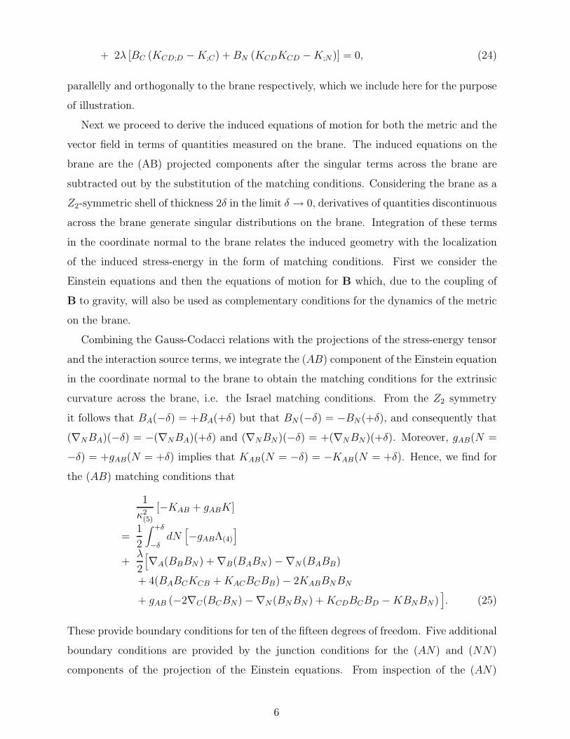
+ 2λ [BC (KCD;D − K;C) + BN (KCDKCD − K;N)] = 0, (24)

parallelly and orthogonally to the brane respectively, which we include here for the purpose

of illustration.

Next we proceed to derive the induced equations of motion for both the metric and the

vector field in terms of quantities measured on the brane. The induced equations on the

brane are the (AB) projected components after the singular terms across the brane are

subtracted out by the substitution of the matching conditions. Considering the brane as a

Z2-symmetric shell of thickness 2δ in the limit δ → 0, derivatives of quantities discontinuous

across the brane generate singular distributions on the brane. Integration of these terms

in the coordinate normal to the brane relates the induced geometry with the localization

of the induced stress-energy in the form of matching conditions. First we consider the

Einstein equations and then the equations of motion for B which, due to the coupling of

B to gravity, will also be used as complementary conditions for the dynamics of the metric

on the brane.

Combining the Gauss-Codacci relations with the projections of the stress-energy tensor

and the interaction source terms, we integrate the (AB) component of the Einstein equation

in the coordinate normal to the brane to obtain the matching conditions for the extrinsic

curvature across the brane, i.e. the Israel matching conditions. From the Z2 symmetry

it follows that BA(−δ) = +BA(+δ) but that BN (−δ) = −BN (+δ), and consequently that

(∇NBA)(−δ) = −(∇NBA)(+δ) and (∇NBN)(−δ) = +(∇NBN)(+δ). Moreover, gAB(N =

−δ) = +gAB(N = +δ) implies that KAB(N = −δ) = −KAB(N = +δ). Hence, we find for

the (AB) matching conditions that

1

κ2(5)

[−KAB + gABK]

=1

2

∫ +δ

−δdN

[

−gABΛ(4)

]

+λ

2

[

∇A(BBBN) + ∇B(BABN) −∇N(BABB)

+ 4(BABCKCB + KACBCBB) − 2KABBNBN

+ gAB (−2∇C(BCBN) −∇N(BNBN ) + KCDBCBD − KBNBN )]

. (25)

These provide boundary conditions for ten of the fifteen degrees of freedom. Five additional

boundary conditions are provided by the junction conditions for the (AN) and (NN)

components of the projection of the Einstein equations. From inspection of the (AN)

6

component, we note that

GAN = KAB;B − K;A

= −∇B

(

∫ +δ

−δdN GAB

)

= −κ2(5)∇BTAB = 0 (26)

which vanishes due to conservation of the induced stress-energy tensor TAB on the brane.

From integration of the (NN) component in the normal direction to the brane, we find the

following junction condition

∇C(BCBN) + 3KBNBN − KCDBCBD = σ, (27)

which we substitute back in, obtaining

1

κ2(5)

1

2

(

−R(ind) − KCDKCD + K2)

=1

2

[

−1

4BCDBCD − V

]

+1

2

[

−∇C∇D(BCBD) −∇C∇C(BNBN ) + 12BN∇C∇CBN − 20V ′BNBN

+ 2 (KCD − gCDK)∇C(BDBN) + 2KCDBD(∇CBN ) + KCD;CBDBN

+(

7KCDKCD − K2)

BNBN + (7KCEKED + KKCD) BCBD

]

. (28)

However, the Israel matching conditions also contain terms which depend on the prescrip-

tion for the continuation of B out of the brane and into the bulk, namely ∇NBA and

∇NBN . The five additional boundary conditions required are those for the vector field B.

In Ref. [13] the boundary conditions for bulk fields were derived subject to the condition

that modes emitted by the brane into the bulk do not violate the gauge defined in the bulk.

Here, however, we integrate the (A) and (N) components of the equation of motion for B,

Eq. (23) and Eq. (24) respectively, to find the corresponding junction condition for BA and

for BN across the brane. From Eq. (23) we have that

∫ +δ

−δdN [∇N (∇NBA −∇ABN ) − 2KAC(∇NBC) − 2λBCKAC,N ] = 0. (29)

If δ is sufficiently small, the difference between KAB;N and KAB,N is negligibly small. It

follows that, in the limit where δ → 0, we can assume that ∇N ≈ ∂N . It then follows that

∇NBA −∇ABN − 2KACBC = 0. (30)

Similarly, from Eq. (24) we find that

∫ +δ

−δdN [−∇N∇CBC − λ∇N(KBN )] = 0, (31)

7

which becomes

∇CBC + λKBN = 0. (32)

The junction conditions Eq. (30) and Eq. (32) offer the required (4+1) boundary conditions

respectively for BA and BN on the brane. Substituting the junction condition for BA back

in Eq. (23) and using the result from GAN = 0, we find for the induced equation of motion

for BA on the brane that

∇C (∇CBA −∇ABC) + 2KAC(∇CBN ) − 2V ′BA + 2λBC

(

R(ind)AC + 2KADKDC

)

= 0. (33)

Similarly, substituting the junction condition for BN back in Eq. (24) we obtain

∇C∇CBN − 2V ′BN + λ [K(∇NBN) + BNKCDKCD] = 0. (34)

Thus, Eq. (30) provides the value at the boundary for ∇NBA and Eq. (34) provides that

for ∇NBN . Using the results derived above in the Israel matching conditions we find that

1

κ2(5)

[−KAB + gABK]

= −gAB σ +1

2

[

(∇ABB)BN + (∇BBA)BN

]

+ BABCKCB + KACBCBB − KABBNBN

+ gAB

[

−∇C(BCBN) +1

2KCDBCBD −

1

2KBNBN

+1

K(BN∇C∇CBN − 2V ′BNBN + BNBNKCDKCD)

]

. (35)

The Israel matching conditions provide an equation for the trace of the extrinsic curvature,

K. Finally, using Eq. (28) in the (AB) Einstein equation, we find for the Einstein equation

induced on the brane that

1

κ2(5)

[

G(ind)AB + 2KACKBC − KABK +

1

2gAB

(

−R(ind) − 4KCDKCD + 2K2)

]

+ gABΛ(5)

+1

2

[

−BACBBC − 4V ′BABB +1

2gAB (BCDBCD + 6V )

]

=1

2gAB

[

−2∇C∇D(BCBD) −∇C∇C(BNBN) + 12BN∇C∇CBN − 20V ′BNBN

+ 4(KCD − gCDK)∇D(BCBN ) + 6KCDBD(∇CBN) + KBC(∇CBN)

+ BCBDR(ind)CD + 9KCDKCDBNBN + 14KCEKDEBCBD − Kσ

]

+1

2

[

∇A∇C(BBBC) + ∇B∇C(BABC) −∇C∇C(BABB)

− 2KAC∇C(BBBN ) − 2KAC(BB∇CBN + BC∇BBN )

− 2KBC∇C(BABN ) − 2KBC(BA∇CBN + BC∇ABN)

8

+ KBN (∇ABB + ∇BBA) − 2KABBN(∇CBC)

−8

KKAB(∇C∇CBN − 2V ′BN + BNKCDKCD)

− 2BABC

(

R(ind)CB + 2KCDKBD

)

− 2BBBC

(

R(ind)CA + 2KADKCD

)

+ (KAC;B + KBC;A − 2KAB;C)BNBN + (KACBB + KBCBA)(−5KDCBD + KBC)

− 6KACKBDBCBD − 2KAB(3KBNBN − σ)]

. (36)

The results obtained above show both the coupling of the bulk to the brane and the

coupling of the vector field B to the geometry of the spacetime. The first is manifested in

the dependence on normal components in the induced equations; the latter is manifested

in the presence of terms of the form (RABBCBD). Terms of the form (KABBN) illustrate

both couplings, where BN relates with K and BA by Eq. (32). The directional dependence

on the N direction is encapsulated in the extrinsic curvature. In the fourth line we can

substitute the Israel matching condition found above. However, the derivatives of the

extrinsic curvature along directions parallel to the brane which appear in the twelfth line

are not reducible to quantities intrinsic to the brane.

III. BULK VECTOR FIELD WITH A NON-VANISHING VACUUM EXPECTA-

TION VALUE

In this section we particularize the formalism developed above for the case when the bulk

vector field B acquires a non-vanishing vacuum value by spontaneous symmetry breaking

akin to the Higgs mechanism. The vacuum value generates the breaking of the Lorentz

symmetry by selecting the direction orthogonal to the plane of the brane. The tangential

part of the vector field with respect to the brane will acquire an expectation value, 〈BA〉 6= 0,

whereas the expectation value of the normal component is chosen, for simplicity, to vanish

on the brane, 〈BN〉 = 0, as we are interested in the effect that Lorentz symmetry breaking

in the bulk has on the brane. Choosing instead 〈BA〉 = 0 and 〈BN〉 6= 0 would also violate

Lorentz symmetry on the brane. However, the implied matching conditions would be

incompatible with the condition for the convariant conservation of the vacuum expectation

value of the field B, ∇A 〈BC〉 = 0 [11, 12]. Moreover, the vacuum value is at a zero of both

the potential V and its derivative V ′. The junction conditions from the equations for BA,

BN , GNN and GAB reduce respectively to

∇N 〈BA〉 − 2KAC 〈BC〉 = 0 (37)

9

∇C 〈BC〉 = 0 (38)

−KCD 〈BC〉 〈BD〉 = σ (39)

1

κ2(5)

[−KAB + gABK] = −gAB σ + 〈BA〉 〈BC〉KCB + 〈BB〉 〈BC〉KAC (40)

and the induced equations of motion become

∇C (∇C 〈BA〉 − ∇A 〈BC〉) + 2 〈BC〉(

R(ind)AC + 2KADKDC

)

= 0 (41)

for BA,

1

κ2(5)

1

2

(

−R(ind) − KCDKCD + K2)

=1

2

[

−1

4〈BCD〉 〈BCD〉 − ∇C∇D(〈BC〉 〈BD〉) + 7KCEKED 〈BC〉 〈BD〉 − Kσ

]

(42)

for GNN and finally

1

κ2(5)

[

G(ind)AB + 2KACKBC −

1

2KABK +

1

2gAB

(

R(ind) − KCDKCD − K2)

]

+ gABΛ(5)

−1

2〈BAC〉 〈BBC〉

=1

2

[

1

4〈BA〉∇C (5∇C 〈BB〉 − 9∇B 〈BC〉) +

1

4〈BB〉∇C (5∇C 〈BA〉 − 9∇A 〈BC〉)

+ ∇A∇C(〈BB〉 〈BC〉) + ∇B∇C(〈BA〉 〈BC〉) − 2(∇C 〈BA〉)(∇C 〈BB〉)

+5

2〈BA〉 〈BC〉R

(ind)CB +

5

2〈BB〉 〈BC〉R

(ind)AC − 6KACKBD 〈BC〉 〈BD〉 + 2KABσ

]

+1

2gAB

[

〈BC〉 〈BD〉R(ind)CD + 2Kσ

]

(43)

from GAB, where we used also the previous results, namely the GNN equation, the Israel

matching condition and the BA equation.

Imposing that ∇A 〈BC〉 = 0, it follows that 〈BAC〉 = ∇A 〈BC〉 − ∇C 〈BA〉 = 0, which

enables us to further simplify Eq. (43):

1

κ2(5)

[

G(ind)AB + 2KACKBC −

1

2KABK +

1

2gAB

(

R(ind) − 2KCDKCD − K2)

]

+ gABΛ(5)

=1

2

[

5

2〈BA〉 〈BC〉R

(ind)CB +

5

2〈BB〉 〈BC〉R

(ind)AC − 6KACKBD 〈BC〉 〈BD〉 + 2KAB σ

]

+1

2gAB

[

〈BC〉 〈BD〉R(ind)CD + 2Kσ

]

. (44)

Hence, in order to obtain a vanishing cosmological constant and ensure that Lorentz in-

variance holds on the brane, we must impose respectively that

Λ(5) = Kσ (45)

10

and that

2KACKBC −1

2KABK +

1

2gAB

(

R(ind) − 2KCDKCD − K2)

= κ2(5)

[

5

4〈BA〉 〈BC〉R

(ind)CB +

5

4〈BB〉 〈BC〉R

(ind)AC +

1

2gAB 〈BC〉 〈BD〉R

(ind)CD

−3KACKBD 〈BC〉 〈BD〉 + KAB σ]

(46)

We observe that there is close relation between the vanishing of the cosmological constant

and the keeping of the Lorentz invariance on the brane. These conditions are enforced so

that the higher dimensional signatures encapsulated in the induced geometry of the brane

cancel the Lorentz symmetry breaking inevitably induced on the brane, thus reproducing

the observed geometry. The first condition, Eqn. (45), can be modified to account for

any non-vanishing value for the cosmological constant, as appears to be suggested by the

recent Wilkinson Microwave Anisotropy Probe (WMAP) data, by defining the observed

cosmological constant Λ such that Λ(5) = Λ + Λ(5). A much elaborate fine-tuning, however,

is required for the Lorentz symmetry to be observed on the brane, as described by the

condition in Eqn. (46). To our knowledge this is a new feature in braneworld models, as in

most models Lorentz invariance is a symmetry shared by both the bulk and the brane. We

shall examine further implications of this mechanism elsewhere [14]. In this future study

the inclusion of a scalar field will also be discussed.

IV. DISCUSSION AND CONCLUSIONS

In this paper we analyse the spontaneous symmetry breaking of Lorentz invariance in

the bulk and its consequent effect on the brane. For this purpose, we considered a bulk

vector field subject to a potential which endows the field with a non-vanishing vacuum

expectation value, thus allowing for the spontaneous breaking of the Lorentz symmetry.

This bulk vector field is directly coupled to the Ricci tensor, so that after the breaking of

Lorentz invariance the loss of this symmetry is transmitted to the gravitational sector of

the model. For simplicity, we assumed that the vacuum expectation value of the component

of the vector field normal to the brane vanishes. The complex interplay between matching

conditions and the Lorentz symmetry breaking terms was examined. We found that Lorentz

invariance on the brane can be made exact via the dynamics of the graviton, vector field

and the geometry of the extrinsic curvature of the surface of the brane. As a consequence

of the exact reproduction of Lorentz symmetry on the brane, we found a condition for

11

the matching of the observed cosmological constant in four dimensions. This tuning does

not follow from a dynamical mechanism but is imposed by phenomenological reasons only.

From this point of view, both the value of the cosmological constant and the Lorentz

symmetry seem to be a consequence of a complex fine-tuning. We aim to further study

the implications of our mechanism by considering also the inclusion of a scalar field in a

forthcoming publication [14].

Acknowledgments

C. C. thanks Fundacao para a Ciencia e a Tecnologia (Portuguese Agency) for financial

support under the fellowship /BPD/18236/2004. C. C. thanks Martin Bucher, Georgios

Kofinas and Rodrigo Olea for useful discussions, and the National and Kapodistrian Uni-

versity of Athens for its hospitality.

[1] CPT and Lorentz Symmetry III, Alan Kostelecky, ed. (World Scientific, Singapore, 2005);

O. Bertolami, Gen. Rel. Gravitation 34 (2002) 707; O. Bertolami, Lect. Notes Phys. 633

(2003) 96, hep-ph/0301191; R. Lehnert, hep-ph/0312093.

[2] V.A. Kostelecky and S. Samuel, Phys. Rev. D39 (1989) 683; Phys. Rev. Lett. 63 (1989) 224;

V.A. Kostelecky and R. Potting, Phys. Rev. D51 (1995) 3923; Phys. Lett. B381 (1996) 89 .

[3] R. Gambini and J. Pullin, Phys. Rev. D59 (1999) 124021; J. Alfaro, H.A. Morales-Tecotl

and L.F. Urrutia, Phys. Rev. Lett. 84 (2000) 2318.

[4] S.M. Carroll, J.A. Harvey, V.A. Kostelecky, C.D. Lane and T. Okamoto, Phys. Rev. Lett.

87 (2001) 141601.

[5] O. Bertolami and L. Guisado, Phys. Rev. D67 (2003) 025001; JHEP 0312 (2003) 013;

O. Bertolami, Mod. Phys. Lett. A20 (2005) 1359.

[6] V.A. Kostelecky, R. Lehnert and M.J. Perry, Phys. Rev. D68 (2003) 123511; O. Bertolami,

R. Lehnert, R. Potting and A. Ribeiro, Phys. Rev. D69 (2004) 083513.

[7] H. Sato, T. Tati, Prog. Theor. Phys. 47 (1972) 1788; S. Coleman and S.L. Glashow,

Phys. Lett. B405 (1997) 249; Phys. Rev. D59 (1999) 116008; L. Gonzales-Mestres,

hep-ph/9905430.

[8] O. Bertolami and C. Carvalho, Phys. Rev. D61 (2000) 103002.

[9] O. Bertolami and J.G. Rosa, Phys. Rev. D71 (2005) 097901.

12

[10] O. Bertolami, Class. Quantum Gravity 14 (1997) 2785.

[11] V.A. Kostelecky, Phys. Rev. D69 (2004) 105009; R. Bluhm and V.A. Kostelecky, Phys. Rev.

D71 (2005) 065008.

[12] O. Bertolami and J. Paramos, Phys. Rev. D72 (2005) 044001.

[13] M. Bucher and C. Carvalho, Phys. Rev. D71 (2005) 083511.

[14] O. Bertolami and C. Carvalho, in preparation.

13