Long-term soil moisture variability from a new P-E

water budget method

Ning Zeng1,

2 Jin-Ho Yoon1, Annarita Mariotti2,3 and Sean Swenson 4

1Department of Atmospheric and Oceanic Science

University of Maryland, USA

2Earth System Science Interdisciplinary Center

University of Maryland, USA

3ENEA Climate section, Rome, Italy

4University of Colorado, USA

1Corresponding author address: Department of Atmospheric and Oceanic Science, University of Mary-land, College Park, MD 20742-2425, USA; email: zeng@atmos.umd.edu; http://www.atmos.umd.edu/˜ zeng

Abstract

Basin-scale soil moisture is traditionally estimated using either land-surface model

forced by observed meteorological variables or atmospheric moisture convergence from

atmospheric analysis and observed runoff. Interannual variability from such meth-

ods suffer from major uncertainties due to the sensitivity to small imperfections in

the land-surface model or the atmospheric analysis. Here we introduce a novel P-E

method in estimating basin-scale soil moisture, or more precisely apparent land water

storage (AWS). The key input variables are observed precipitation and runoff, and

reconstructed evaporation. We show the results for the tropics using the example of

the Amazon basin. The seasonal cycle of diagnosed soil moisture over the Amazon is

about 200mm, compares favorably with satellite estimate from the GRACE mission,

thus lending confidence both in this method and the usefulness of space gravity based

large-scale soil moisture estimate. This is about twice as large as estimates from sev-

eral traditional methods, suggesting that current models tend to under estimate the

soil moisture variability. The interannual variability in AWS in the Amazon is about

150mm, also consistent with GRACE data, but much larger than model results. We

also apply this P-E method to the midlatitude Mississippi basin and discuss the impact

of major 20th century droughts such as the dust bowl period on the long-term soil

moisture variability. The results suggest the existence of soil moisture memories on

decadal time scales, significantly longer than typically assumed seasonal timescales.

1

1 Introduction

Freshwater stored on the continents in the soil, at the surface or underground is fundamental for life

on land. These water reservoirs, especially soil moisture are also important in climate variability as

they provide potential feedback mechanisms for climate variability (e.g., Yeh et al. 1984; Delworth

and Manabe 1993; Zeng et al. 1999; Koster et al. 2004). Motivated partly by the prospect of

improving seasonal-interannual climate prediction using the knowledge of soil moisture state, there

has been significant interest in soil moisture variability in recent years.

Several methods have been used in obtaining soil moisture information including in situ

observations, satellite remote sensing, offline land-surface model simulations, land data assimilation

using both data and model, basin-scale budget analysis. Table 1 lists some of these methods and

examples as well as their main characteristics. Each of these method has its own advantages and

limitations. While there is a reasonable understanding of the climatological seasonal cycles of

all aspects of the hydrological cycle, there is a significant lack of knowledge on the interannual

variability of terrestrial hydrological variables including soil moisture.

A clarification of terminology is warranted here. While all other methods in Table 1 estimate

near surface soil moisture, the two budget approaches (Moisture convergence and P-E) and the

satellite gravity sensor measure total column water storage. This apparent land water storage

(AWS) includes moisture in the soil, but also surface and underground water, as well as water stored

in vegetation. In the case of satellite gravity, other factors such as change in biomass could also

contribute, but the water-related changes should dominate. Deep soil moisture and underground

water change may be of importance as discussed later, but given the lack of knowledge and a clear

definition of these differences in literature, we also use ‘soil moisture’ for general discussion, with

the understanding that apparent water storage AWS is a more precise term in the budget methods.

Here we present a new budget method in which basin-scale water storage is diagnosed using

observed precipitation and runoff. We present this method in section 2 and contrast it with the

more traditional method using atmospheric moisture convergence (Rasmusson 1968). We then

2

discuss the seasonal cycle and interannual variability from this method for the Amazon basin in

sections 3 and 4, and compare the results with the moisture convergence method and satellite

gravity based observations. In section 5, the long-term soil moisture variability is presented for

the Mississippi basin using streamflow measurement from Vicksburg. Potential limitations of the

method is discussed in section 6.

2 Methodology

2.1 The moisture convergence (MC) method

The traditional moisture convergence method (Rasmusson 1968; Roads et al. 1994; Zeng 1999;

Masuda et al. 2001) considers the atmosphere and land-surface over a drainage basin as one single

box, thus precipitation and evaporation vanish as interior fluxes for the total water budget. In this

method (Fig. 1), moisture convergence (C; the vertically integrated water vapor flux) and observed

streamflow at the river mouth (runoff integrated over the whole basin) are integrated to obtain the

change in atmosphere (W ) and soil water storage (S):

d(W + S)

dt= C − R (1)

Using the recent atmospheric reanalyses, this method appears to produce reasonable esti-

mates of the seasonal cycles over various basins around the world (Roads et al. 1994; Zeng 1999;

Masuda et al. 2001; Seneviratne et al. 2004). After some initial success using the NASA/DAO

reanalysis (Schubert et al. 1993) for the Amazon basin (Zeng 1999; Fig. 2c), we were hopeful reason-

ing that unlike the earlier analyses, a single reanalysis system is stable over time so that they may

capture the interannual variability well enough despite potential bias in the climatology. However,

when we recently applied this method to long-term soil moisture variability over the Amazon using

the longer NCEP/NCAR 50 year (Kalnay et al. 1996) and ECMWF 15 year reanalyses (ERA15;

Gibson et al. 1997), this method produced apparently unreasonable changes, in particular over

the earlier periods (Fig. 2a,b). Both the amplitudes are too large and the variability are often not

consistent with the known ENSO correlation in this region.

3

Further analysis (not shown) suggests that precipitation variability in these analyses are

often very different from the observations, and the associated moisture convergence variabilities

are not reliable enough for the purpose of soil moisture diagnosis. For instance, ERA15 shows

an apparent unrealistic difference around 1988 (Fig. 2b). Betts et al. (2005) also identified an

unexplained sudden jump around 1972-73 in the Amazon hydrological cycle in the newer ECMWF

40 year reanalysis. Part of the reason the moisture convergence is unreliable over the Amazon is

the sparse atmospheric sounding data available to constrain the model in such a remote tropical

region. Another potential problem is that the long-term changes in observational technique and

instrumentation are difficult to identify and correct. Such problems may be significantly alleviated if

the observed precipitation is used in place of moisture convergence because precipitation is generally

a better observed quantity over longer period of time, and this leads us to the P-E method.

2.2 The P-E method

In the P-E method, only the land surface is considered (Fig. 3). The water budget equation for the

land box is:

dS

dt= P − E − R (2)

where S is the apparent land water storage and P is precipitation, E is evapotranspiration.

In this method, precipitation and runoff (averaged over the basin) are from observations,

but no basin-scale evaporation observation is available. Instead, evaporation (in this work, we

use evaporation and evapotranspiration inter-exchangeably for simplicity) is calculated using a

land surface model driven by observed precipitation and other surface atmospheric variables such

as temperature, wind speed and radiation. Similar to the correction to moisture convergence

(Rasmusson 1968; see discussions of this technique in Zeng 1999), a constant correction is added

to E such that P − E∗− R (E∗ = E+correction) integrated over time is zero. As a result, the

diagnosed soil moisture has the same value at the beginning and the end of the integration. This

is equivalent to removing a linear trend (which is often unrealistically large as to mask out real

4

changes) in soil moisture. Thus only the relative changes within the integration period can be

inferred from such methods.

The above equation is then integrated to obtain soil water S as a function of time, which

can only be determined up to an integral constant S0. We choose S0 such that the minimum of

S is zero. Equation (2) is used to derive the soil water storage at a time step of one month. The

diagnosed quantity S is not only soil moisture, it also includes the changes in surface water such

as rivers and lakes within the basin, underground water, and storage of water in vegetation. We

thus term the quantity S apparent land water storage (AWS) as discussed above.

The observed precipitation for 1901-2000 from the Climate Research Unit of University of

East Anglia (CRU; New et al. 1999) was used in Eq.2. The precipitation and temperature from

the same dataset was also used in conjunction with the climatological values of surface wind and

vapor pressure, along with radiation from NCEP/NCAR reanalysis to drive an offline model SLand

(Simple-Land, Zeng et al. 2000) coupled to a dynamic vegetation model VEGAS (Zeng et al.

2005). We also used the precipitation data from Xie and Arkin (1996) based on gauge and satellite

measurements and the results are found similar to those using CRU precipitation, and here only

the results from the longer CRU dataset are shown. The Southern Oscillation Index (SOI) is used

as an index for the atmospheric variability over the tropical Pacific Ocean for comparison purpose

because the Amazon climate and hydrological variability are largely controlled by ENSO.

The monthly historical streamflow records for the Amazon River at Obidos, and for the

Xingu River at Altamira (3◦12′S) were used to reconstruct the Amazon basin runoff, following

the method used by Zeng (1999). In the following 3 sections, we present the seasonal cycle and

variability from 1970 to 1997 for the Amazon basin, and long-term variability from 1928 to 1998

for the Mississippi basin.

5

3 Seasonal cycle over the Amazon basin

A climatological seasonal cycle was derived as the average of the 28 year diagnosed apparent land

water storage. Figure 4 shows this seasonal cycle for the Amazon basin. The 3 MC method

analyses (Fig. 4a) have similar seasonal amplitude of 150mm, while the satellite gravity based

estimate from GRACE and the P-E method have an amplitude of about 300mm (Fig. 41b). The

two offline models, SLand (Zeng et al. 2000) and the CPC Leaky Bucket model (Fan and van den

Dool, 2004), also have an amplitude of about 150mm. Both GRACE and the P-E method give

a maximum in April-May and minimum in October-November after the drier boreal summer (the

basin averages tend to be dominated by the larger southern Amazon). The models and reanalyses

produced maximum and minimum somewhat earlier by 1-2 months.

To the extent that GRACE measurement can be considered as a good observation of the

basin scale water storage, the P-E method appears to capture this observed change. The reanalyses

and the two offline models thus tend to underestimate somewhat the seasonal cycle amplitude in

the Amazon. Given the uncertainties in all these methods and large interannual variability (below),

the seasonal cycle of Amazon water storage can be given as 250±100 mm. However, the two basin

budget methods (GRACE and P-E) include all the changes from surface to underground water,

thus providing an upper limit to the models which normally include only a fraction of the active

soil moisture as discussed further below.

4 Amazon interannual and decadal variability 1970-1997

Figure 5a shows the water input (P-E*) and the observed runoff R of the Amazon basin at monthly

resolution. There is a robust seasonal cycle over which P-E surpasses R during winter and spring,

when soil moisture is recharged. P-E is less than R from early summer to fall when soil moisture is

discharged (Fig.4b). Overall, R has a seasonal amplitude about factor of two smaller and a phase

lag of 3-4 months relative to P-E* (also see Zeng 1999). This reduced amplitude and phase lag is

6

typical because soil moisture is a damped and delayed response to the driving precipitation due to

its memory effect.

The diagnosed soil moisture shows large interannual to interdecadal variability on which the

seasonal cycle is superimposed. The long-term variability can be seen more clearly by filtering out

the seasonal cycle using a simple 12 month running mean (Fig.6). On multidecadal time scale,

there is a major recharge period from 1971 to 1985, followed by a discharge afterwards. The overall

amplitude over the 27 years is about 600 mm. It is worth noting that, the correction in E* (section

2.2) removes any long term trend so that over the whole analysis period there is no net gain in soil

water storage. Thus the lowest frequency change can only be viewed as relative, i.e., the decrease

in the latter half is only relative to the increase in the first half of the 27 years.

The large change of 600 mm in soil moisture is remarkable, as many land-surface models have

field capacity (the maximum change in soil moisture a model can produce) comparable or smaller

than this. Although we currently have no other means to validate the magnitude of such long-

term change, the general trend can be assessed because Amazon hydrological cycle is dominated by

ENSO related interannual variability. For instance, the period with largest recharge during 1974-75

corresponds to two major La Nina events before the 1976-77 decadal climate shift in the Pacific

Ocean, as indicated by the Southern Oscillation Index (SOI). In the other direction, the major

discharge period of early 1990s was caused by the protracted El Nino of 1991-1993.

A simple high-pass filter was applied to the diagnosed soil moisture in Fig. 6b to remove

the frequencies lower than 7 years. The remaining signal is mostly interannual (Fig. 7), showing

decreasing soil moisture during events such as 1982-83 El Nino. However, even in this case, the

major peaks reflect the lower frequency variations such as the two La Nina events around 1975 and

early 1990 El Nino. Also plotted in Fig. 7 are the model simulated soil moisture from SLand and

the Leaky Bucket model, and both show significantly smaller variability at about 1/2 to 1/3 of the

diagnosed amplitude on interannual time scales, while the decadal and longer-term variability is

even smaller (cf. Fig. 6b).

7

The advent of recent satellite gravity based measurement from NASA’s GRACE mission

provides an independent means to validate the interannual variability of the diagnosis method.

Figure 8 shows the GRACE measurement of Amazon water change for the two year period of April

2002 to May 2004. The first half of this period has a larger seasonal variation of about 400 mm,

while the second half has a smaller seasonal amplitude of about 250 mm (the seasonal amplitude

in Fig.4 is an estimate over the whole 2 yr period), following the El Nino of 2002-2003. Thus

the interannual change is about 150 mm, comparable to the amplitude of interannual variability

derived using the P-E method (Fig. 7). Since the 2002-2003 El Nino is a relatively small one, the

GRACE data indicates a potentially very large interannual variability in the land-surface water

storage, consistent with our diagnostic approach (with the caveat that the GRACE data has its

own uncertainties and the observation period is too short to actually verify the diagnosis approach).

Such large differences especially on longer time scales are striking. While the diagnosis may

overestimate the amplitude of these slow variations (section 6), the models appear to significantly

underestimate it. One contributor of the smaller model changes is that current land-surface models

typically only represent the water holding capacity of the top 1-2 meters of soil. Among the two

models, SLand has a field capacity of 500 mm, while the Leaky Bucket model has 750 mm. Thus

it is understandable that these models underestimate the multi-decadal change on the order of 600

mm. However, simple increase in model soil depth may not be sufficient if deep soil water can not

be utilized by vegetation (section 6).

5 Long-term variability in the Mississippi basin

It is also of great interest to see how the P-E method works for midlatitude regions. We have

applied the method to the Mississippi basin (Fig.9). The apparent water storage in the Mississippi

decreases by about 400 mm from the 1920s to the end of the 1930s (the Dust Bowl period), followed

by a recharge period in the 1940s. The drought in the 1950s plunged soil moisture to the lowest

level, and then recovered to high level during the following two decades of pluvial period (Seager et

8

al. 2005). Smaller drought events also left their impact on the soil moisture, such as 1988. Further

analysis (not shown) suggests that these changes are largely influenced by the west part of the

basin, in particular, the Great Plain region.

A long soil moisture memory is again implied here. For instance, the discharge during the

Dust Bowl period is somewhat larger than that of the 1950’s drought, as seen by the larger shaded

area with negative P-E*-R values for the 1930s in Fig.9a, yet soil moisture is at a minimum at the

end of the 1950’s drought. This is because the recharge in the 1940s is not sufficient to recover

the water loss in the 1930s. Thus the memory of the Dust Bowl period was not forgotten until

a few decades later! While uncertainties in the data and methodology may hamper the accuracy

of such detailed interpretation, the results suggest a longer soil moisture memory than typically

represented in models.

6 Discussions and conclusions

The large change of 500-600 mm in soil moisture over multidedadal timescales is remarkable, as

many land-surface models have field capacity (the maximum change in soil moisture a model can

produce) comparable or smaller than this. Theoretically speaking, the diagnosed AWS variability

is larger than or equal to any modeled soil moisture variability because the diagnosis includes all

the possible changes in the basin, including surface and underground water and water stored in

vegetation, while models typically only simulate soil moisture change in the top 1-2 meter. For

example, during flooding season, Amazon river expands into adjacent forest and the surface water

can account for about 10% of the seasonal soil moisture change. However, the major contributor

missing in simple land-surface models is likely the deeper soil moisture storage including ground

water. Such deep water storage is utilized by deep forest roots. In one instance, Nepstad et al.

(1994) found deep root water uptake down to 8 m below surface that sustained normal growth

during a prolonged dry period. Even deeper roots have been observed in many other regions

(Schenk and Jackson 2005).

9

More sophisticated models may include several soil layers which would increase the effective

filed capacity and thus the amplitude of variation. However, the lack of deep roots may prevent

the model to utilize deep water storage as efficiently as Nature does. Further analysis with these

models is obviously needed.

The large change on decadal to multidedadal timescales found by the current diagnosis ap-

proach suggest that current models may significantly underestimate such variations. An important

implication is that land-surface may have a memory beyond one year related to the change in the

apparent water storage1, significantly longer than the typically cited 1 month to 1 season.

Although the general ups and downs in the diagnosed AWS appear realistic, we can not

exclude the possibility that the method overestimates the magnitude of changes. The observed

precipitation and runoff might have different biases that change in time as precipitation and stream-

flow are measured differently and the techniques change in time. The sparse raingauge coverage

in the Amazon might be another source of potential bias. Even if the observations were perfect,

evapotranspiration is calculated using a model, forced by observed precipitation and temperature.

If the variability of evapotranspiration is underestimated, as may be the case because models tend

to underestimate long-term soil moisture variability and the variability in surface radiation is not

considered, then the P-E method would lead to overestimate of soil moisture variability. Since

model uses P as input (in a way similar to Eq.2), and the diagnostic approach also uses observed

R, our results suggest that model may overestimate runoff variability. To put it the other way, real

land surface seems to be able to hold up more water when it is wet, and releases more when it is

dry, while models’ runoff tend to be more sensitive to change in precipitation. It is worth noting

that the modeled variability may behave differently from modeled mean runoff which is not studied

here.

The P-E budget approach is very unique, and there has been a lack of independent means to

validate this method. Recent satellite gravity based measurement from NASA’s GRACE mission

1time scale can be estimated as capacity divided by flux. Assuming a field capacity of 1000 mm for the Amazon,then the time scale is 1000 mm / (5 mm d−1) = 200 days

10

provides such a means. Unlike numerical models, both methods yield only basin-scale total changes

because one is limited by the spatial resolution of measurement from space, and the other by the

fact that runoff data is only available for whole drainage basin. But both methods provide change in

the total water storage on land, thus they provide an upper limit for the numerical models or point

observation. The general consistency between the two completely independent methods suggest

that we may be on the right track in quantifying the interannual and longer-term variability in

land water storage.

Acknowledgments. We thank discussions with H. van den Dool, A. Robock, J. Wahr and P.

Dirmeyer. This research was supported by NSF grant ATM-0328286, NOAA grants NA04OAR4310091

and NA04OAR4310114.

11

References

Betts, A. K., J. H. Ball, P. Viterbo, and others, 2005: Hydrometeorology of the Amazon in ERA-40.

J. Hydrometeorology, submitted.

Delworth, T. L., and Manabe, S., 1993. Climate variability and land-surface processes. Advances in

Water Resources, 16, 3-20.

Dirmeyer, P, A, A. J. Dolman, and N. Sato, 1999: The pilot phase of the Global Soil Wetness Project.

Bull. Amer. Meteor. Soc., 80, 851-878.

Engman, E. T., and N. Chauhan, 1995: Status of microwave soil moisture measurements with remote

sensing. Remote Sensing of Environ., 51 (1), 189-198.

Fan, Y., and H. van den Dool, 2004: Climate Prediction Center global monthly soil moisture data set

at 0.5 degrees resolution for 1948 to present. J. Geophys. Res., 109 (D10): Art. No. D10102.

Gibson, J. K., Kallberg, S., Hernandez, A., Uppala, S., Nomura, A. and co-authors, 1997: ERA

Description, ECMWF Reanalysis Project Report Series Vol. 1, ECMWF, Shinfield Park, Reading,

RG2 9AX, UK, 72 pp.

Kalnay, E., et al., 1996: The NCEP/NCAR 40 year reanalysis project. Bull. Amer. Meteor. Soc.,

77, 437-471.

Koster, R. D., P. A. Dirmeyer, Z. C. Guo, et al., 2004: Regions of strong coupling between soil moisture

and precipitation. Science, 305 (5687), 1138-1140.

Masuda, K., Y. Hashimoto, H. Matsuyama, et al., 2001: Seasonal cycle of water storage in major river

basins of the world Geophy. Res. Lett., 28 (16), 3215-3218.

Nepstad, D. C., and coauthors, 1994: The role of deep roots in the hydrological and carbon cycles of

Amazonian forests and pastures. Nature, 372, 666-669.

New, M., M. Hulme, P. Jones, 1999: Representing twentieth-century space-time climate variability.

Part I: Development of a 1961-90 mean monthly terrestrial climatology. J. Clim., 12, 829-856.

Rasmusson, E. M., 1968: Atmospheric water vapor transport and the water balance of North America.

Part II: large-scale water balance investigation. Mon. Wea. Rev., 96, 720-734.

12

Roads, J. O., S.-C. Chen, A. K. Guetter, and K. P. Georgakakos, 1994: Large-scale aspects of the

United States hydrologic cycle. Bull. Amer. Meteor. Soc., 75, 1589-1610.

Robock, A., K. Y. Vinnikov, G. Srinivasan, J. K. Entin, S. E. Hollinger, N. A. Speranskaya, S. Liu,

and A. Namkhai, 2000: The Global Soil Moisture Data Bank. Bull. Amer. Meteor. Soc., 81,

1281-1299.

Rodell, M., P. R. Houser, U. Jambor, and others, 2004: The global land data assimilation system.

Bull. Amer. Meteor. Soc., 85 (3), 381-394.

Seneviratne, S. I., P. Viterbo, D. Luthi, et al., 2004: Inferring changes in terrestrial water storage

using ERA-40 reanalysis data: The Mississippi River basin. J. Climate, 17 (11), 2039-2057.

Schenk, H. J., and R. B. Jackson, 2005: Mapping the global distribution of deep roots in relation to

climate and soil characteristics. Geoderma, in press.

Schubert, S. D., R. B. Rood, and J. P. Pfaendtner, 1993: An assimilated dataset for Earth science

applications. Bull. Amer. Meteor. Soc., 74, 2331-2342.

Seager, R., Y. Kushnir, C. Herweijer, N. Naik, and J. Velez, 2005: Modeling of tropical forcing of

persistent droughts and pluvials over western North America: 1856-2000. J. Climate, submitted.

Wahr, J., S. Swenson, V. Zlotnicki, I. Velicogna, 2004: Time-variable gravity from GRACE: First

results. Geophys. Res. Lett., 31, L11501, doi:10.1029/2004GL019779.

Xie, P., and P. A. Arkin, 1996: Analyses of global monthly precipitation using gauge observations,

satellite estimates, and numerical model predictions. J. Climate, 9, 840-858.

Yeh, T.-C., T. T. Wetherald, and S. Manabe, 1984: The effect of soil moisture on the short-term

climate and hydrology change – a numerical experiment. Mon. Wea. Rev., 112, 474-490.

Zeng, N., 1999: Seasonal cycle and interannual variability in the Amazon hydrologic cycle. J. Geophys.

Res., 104, D8, 9097-9106.

Zeng, N., J. D. Neelin, W. K.-M. Lau, and C. J. Tucker, 1999: Enhancement of interdecadal climate

variability in the Sahel by vegetation interaction. Science, 286, 1537-1540.

Zeng, N., J. D. Neelin, and C. Chou, 2000: A quasi-equilibrium tropical circulation model–implementation

and simulation. J. Atmos. Sci., 57, 1767–1796.

13

Zeng, N., A. Mariotti, and P. Wetzel, 2005: Terrestrial mechanisms of interannual CO2 variability,

Global Biogeochem. Cycle, 19, GB1016, doi:10.1029/2004GB002273.

14

List of Figures

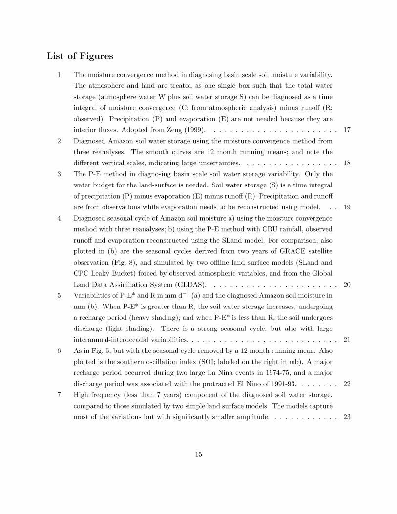
1 The moisture convergence method in diagnosing basin scale soil moisture variability.

The atmosphere and land are treated as one single box such that the total water

storage (atmosphere water W plus soil water storage S) can be diagnosed as a time

integral of moisture convergence (C; from atmospheric analysis) minus runoff (R;

observed). Precipitation (P) and evaporation (E) are not needed because they are

interior fluxes. Adopted from Zeng (1999). . . . . . . . . . . . . . . . . . . . . . . . 17

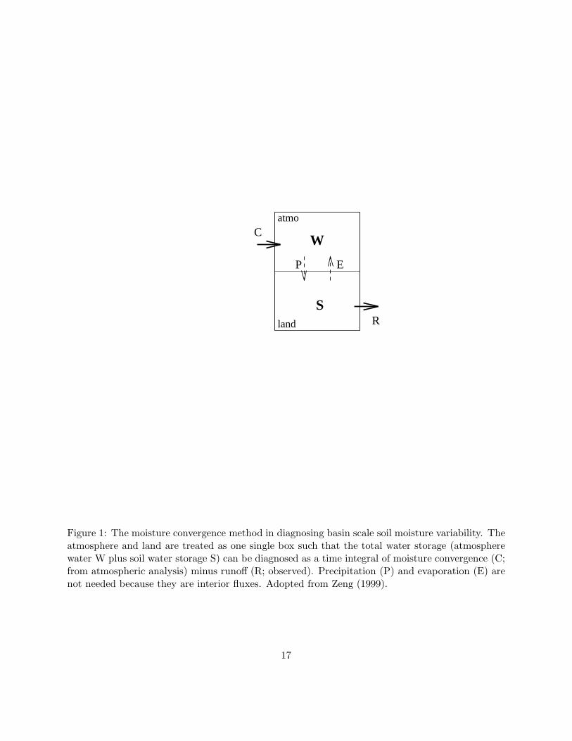
2 Diagnosed Amazon soil water storage using the moisture convergence method from

three reanalyses. The smooth curves are 12 month running means; and note the

different vertical scales, indicating large uncertainties. . . . . . . . . . . . . . . . . . 18

3 The P-E method in diagnosing basin scale soil water storage variability. Only the

water budget for the land-surface is needed. Soil water storage (S) is a time integral

of precipitation (P) minus evaporation (E) minus runoff (R). Precipitation and runoff

are from observations while evaporation needs to be reconstructed using model. . . 19

4 Diagnosed seasonal cycle of Amazon soil moisture a) using the moisture convergence

method with three reanalyses; b) using the P-E method with CRU rainfall, observed

runoff and evaporation reconstructed using the SLand model. For comparison, also

plotted in (b) are the seasonal cycles derived from two years of GRACE satellite

observation (Fig. 8), and simulated by two offline land surface models (SLand and

CPC Leaky Bucket) forced by observed atmospheric variables, and from the Global

Land Data Assimilation System (GLDAS). . . . . . . . . . . . . . . . . . . . . . . . 20

5 Variabilities of P-E* and R in mm d−1 (a) and the diagnosed Amazon soil moisture in

mm (b). When P-E* is greater than R, the soil water storage increases, undergoing

a recharge period (heavy shading); and when P-E* is less than R, the soil undergoes

discharge (light shading). There is a strong seasonal cycle, but also with large

interannual-interdecadal variabilities. . . . . . . . . . . . . . . . . . . . . . . . . . . . 21

6 As in Fig. 5, but with the seasonal cycle removed by a 12 month running mean. Also

plotted is the southern oscillation index (SOI; labeled on the right in mb). A major

recharge period occurred during two large La Nina events in 1974-75, and a major

discharge period was associated with the protracted El Nino of 1991-93. . . . . . . . 22

7 High frequency (less than 7 years) component of the diagnosed soil water storage,

compared to those simulated by two simple land surface models. The models capture

most of the variations but with significantly smaller amplitude. . . . . . . . . . . . . 23

15

8 Two years of observed changes in Amazon soil water storage (mm) from the GRACE

satellite gravity measurements. A much smaller seasonal cycle was seen following

the 2002-2003 El Nino compared to the year before. . . . . . . . . . . . . . . . . . . 24

9 As in Fig. 6, but for the Mississippi basin. The major discharge periods are the Dust

Bowl in the 1930s, drought in the 1950s. A major recharge took place during the

pluvial period from the 1960s to the 1990s. . . . . . . . . . . . . . . . . . . . . . . . 25

16

C

R

P E

atmo

land

W

S

Figure 1: The moisture convergence method in diagnosing basin scale soil moisture variability. Theatmosphere and land are treated as one single box such that the total water storage (atmospherewater W plus soil water storage S) can be diagnosed as a time integral of moisture convergence (C;from atmospheric analysis) minus runoff (R; observed). Precipitation (P) and evaporation (E) arenot needed because they are interior fluxes. Adopted from Zeng (1999).

17

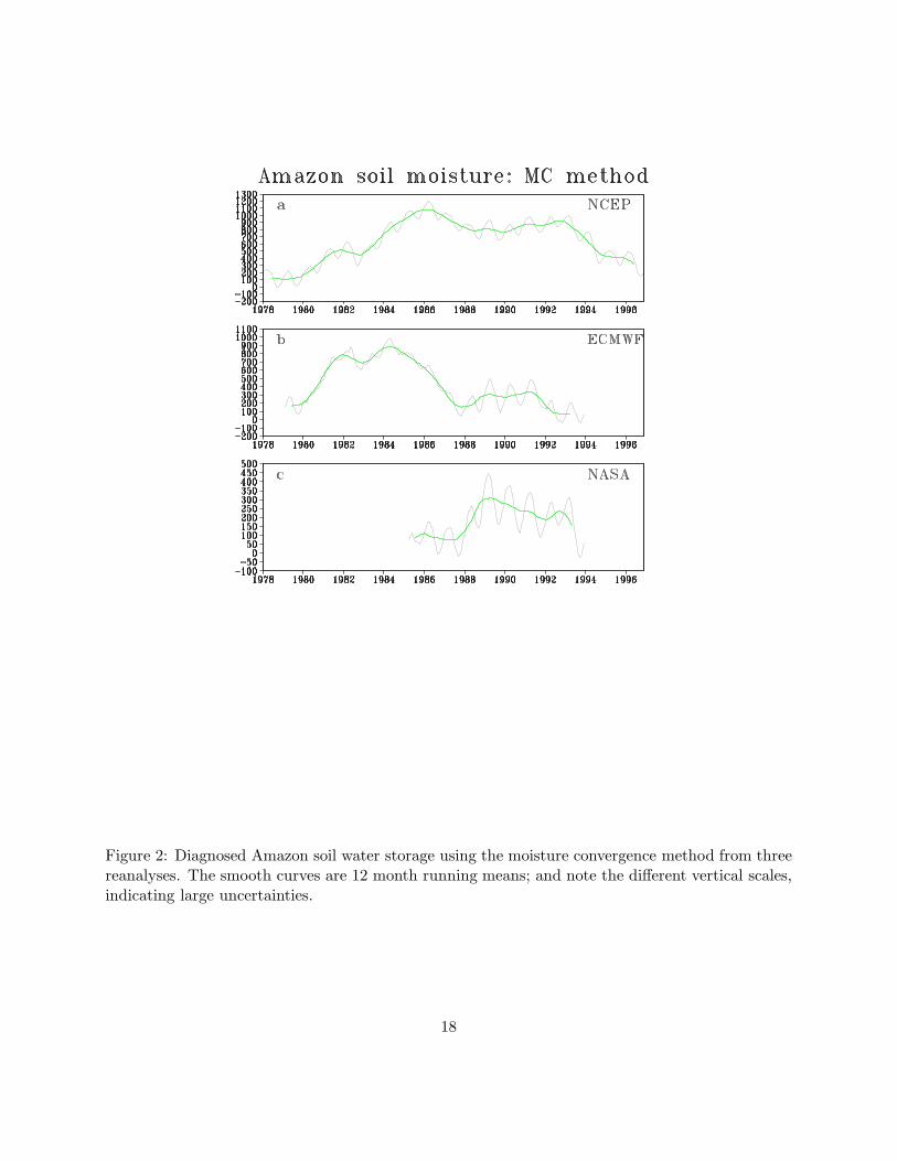
Figure 2: Diagnosed Amazon soil water storage using the moisture convergence method from threereanalyses. The smooth curves are 12 month running means; and note the different vertical scales,indicating large uncertainties.

18

Figure 3: The P-E method in diagnosing basin scale soil water storage variability. Only the waterbudget for the land-surface is needed. Soil water storage (S) is a time integral of precipitation(P) minus evaporation (E) minus runoff (R). Precipitation and runoff are from observations whileevaporation needs to be reconstructed using model.

19

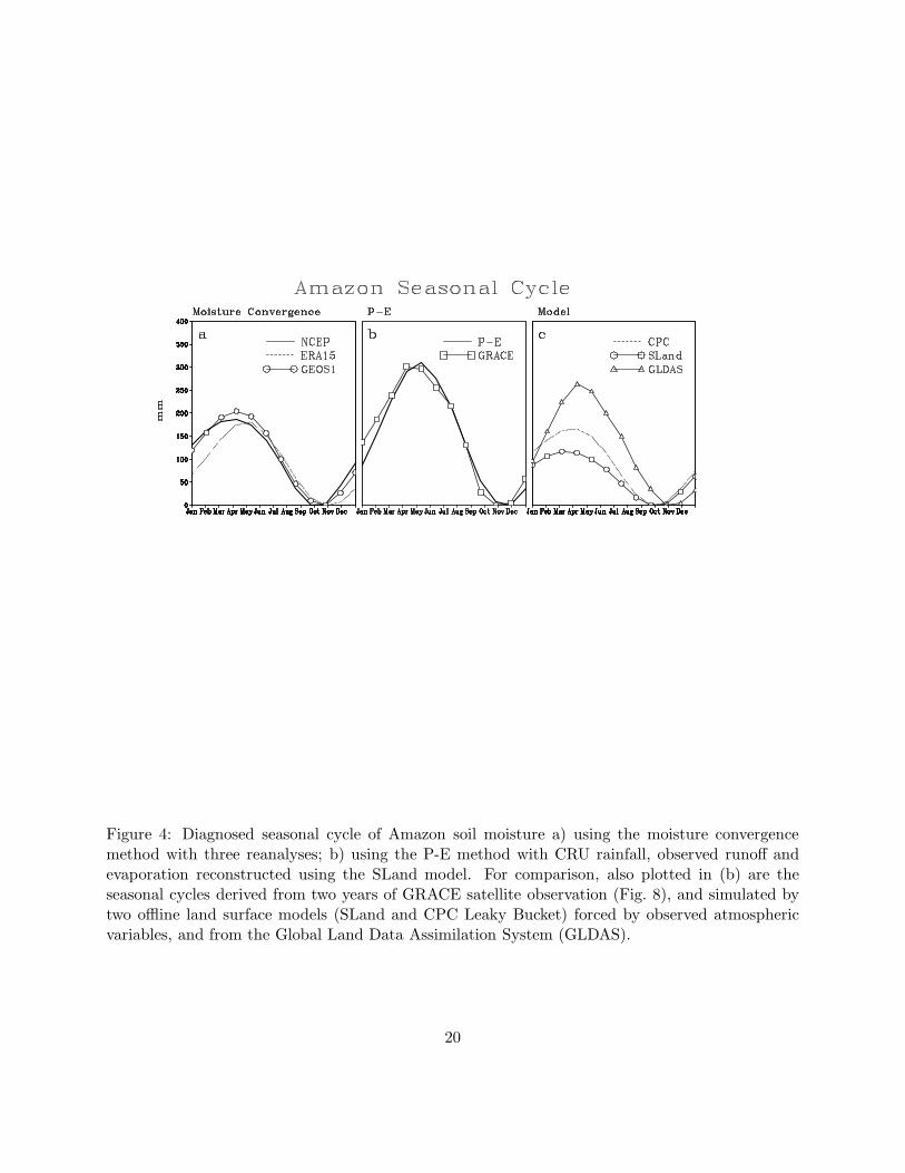
Figure 4: Diagnosed seasonal cycle of Amazon soil moisture a) using the moisture convergencemethod with three reanalyses; b) using the P-E method with CRU rainfall, observed runoff andevaporation reconstructed using the SLand model. For comparison, also plotted in (b) are theseasonal cycles derived from two years of GRACE satellite observation (Fig. 8), and simulated bytwo offline land surface models (SLand and CPC Leaky Bucket) forced by observed atmosphericvariables, and from the Global Land Data Assimilation System (GLDAS).

20

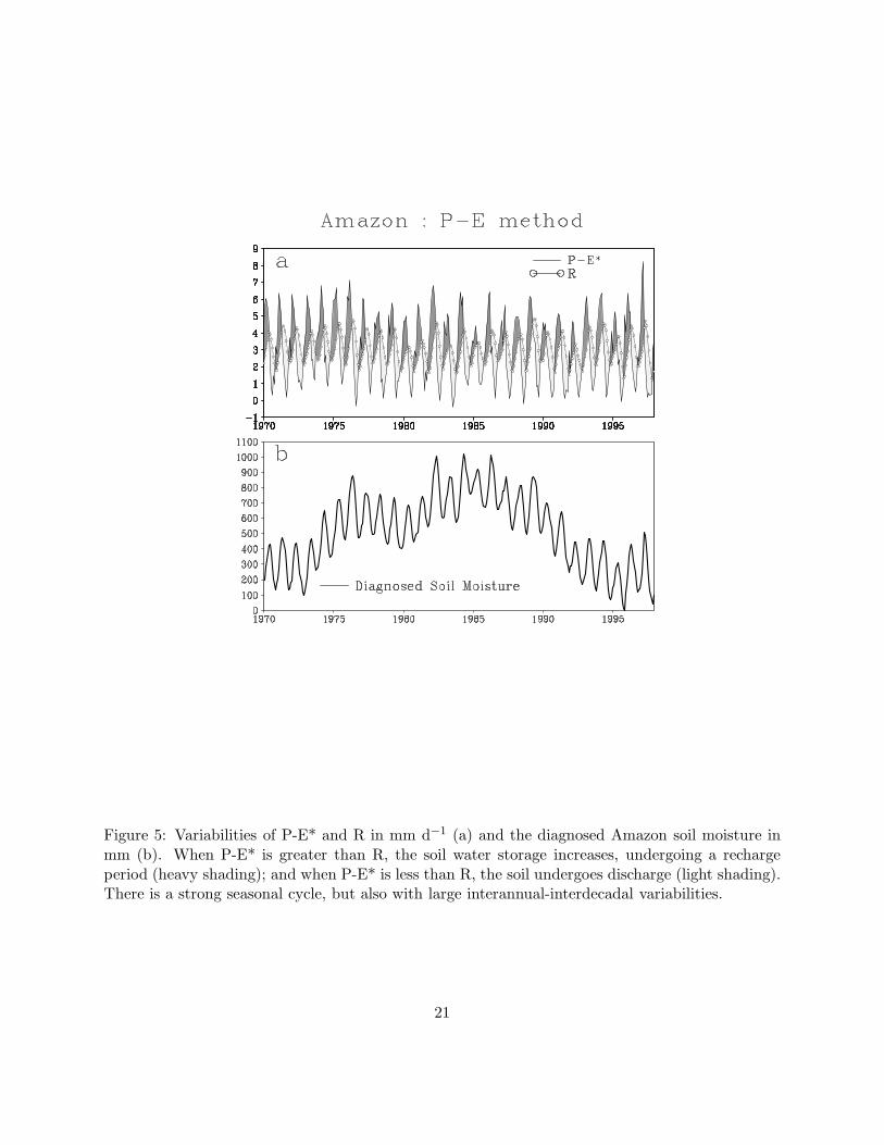
Figure 5: Variabilities of P-E* and R in mm d−1 (a) and the diagnosed Amazon soil moisture inmm (b). When P-E* is greater than R, the soil water storage increases, undergoing a rechargeperiod (heavy shading); and when P-E* is less than R, the soil undergoes discharge (light shading).There is a strong seasonal cycle, but also with large interannual-interdecadal variabilities.

21

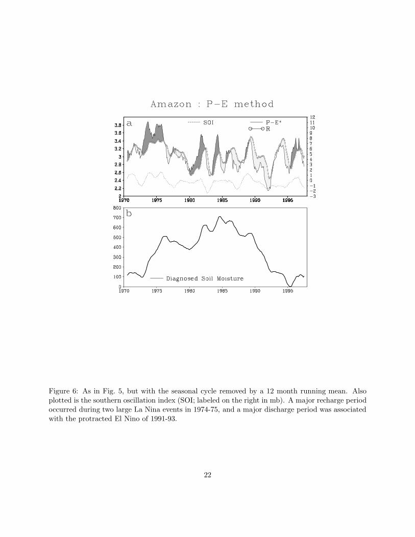
Figure 6: As in Fig. 5, but with the seasonal cycle removed by a 12 month running mean. Alsoplotted is the southern oscillation index (SOI; labeled on the right in mb). A major recharge periodoccurred during two large La Nina events in 1974-75, and a major discharge period was associatedwith the protracted El Nino of 1991-93.

22

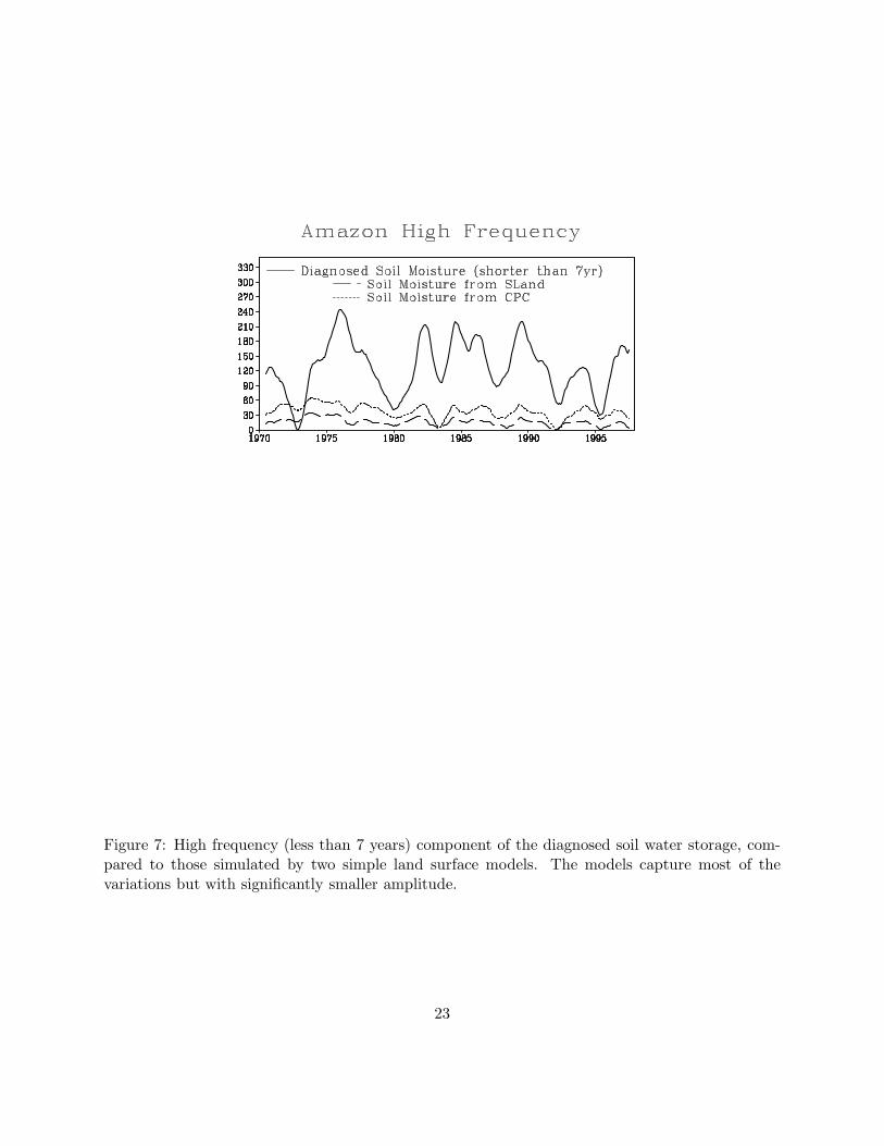
Figure 7: High frequency (less than 7 years) component of the diagnosed soil water storage, com-pared to those simulated by two simple land surface models. The models capture most of thevariations but with significantly smaller amplitude.

23

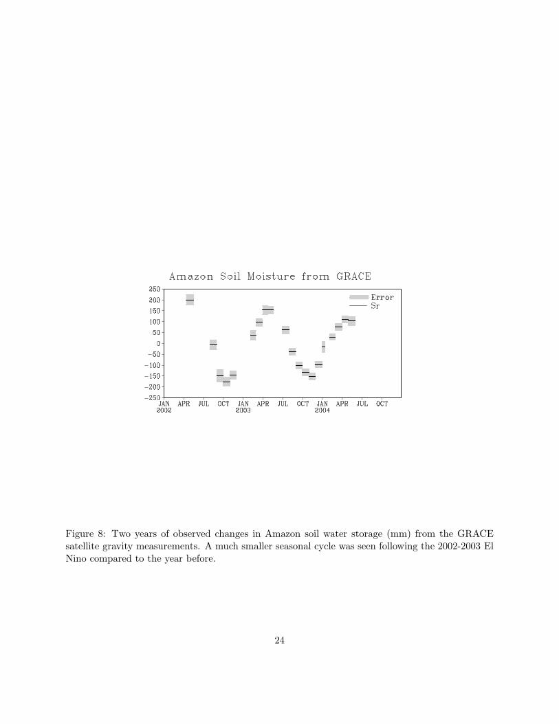
Figure 8: Two years of observed changes in Amazon soil water storage (mm) from the GRACEsatellite gravity measurements. A much smaller seasonal cycle was seen following the 2002-2003 ElNino compared to the year before.

24

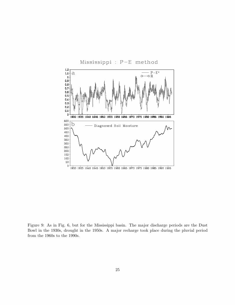
Figure 9: As in Fig. 6, but for the Mississippi basin. The major discharge periods are the DustBowl in the 1930s, drought in the 1950s. A major recharge took place during the pluvial periodfrom the 1960s to the 1990s.

25

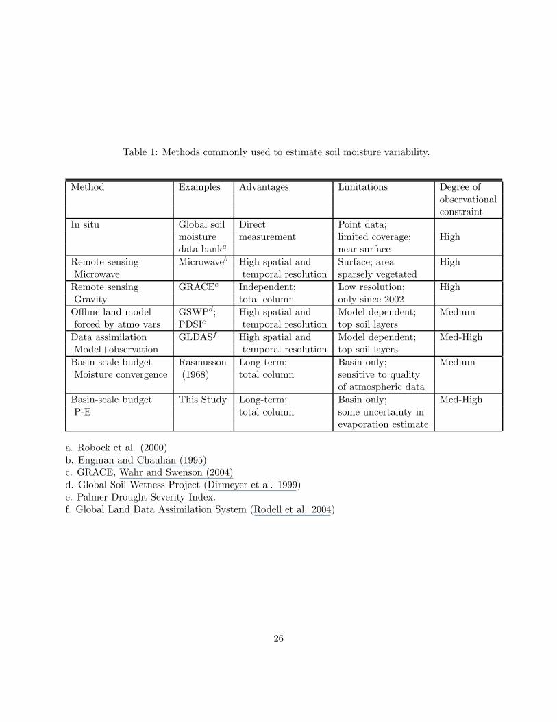
Table 1: Methods commonly used to estimate soil moisture variability.

Method Examples Advantages Limitations Degree ofobservationalconstraint

In situ Global soil Direct Point data;moisture measurement limited coverage; Highdata banka near surface

Remote sensing Microwaveb High spatial and Surface; area HighMicrowave temporal resolution sparsely vegetated

Remote sensing GRACEc Independent; Low resolution; HighGravity total column only since 2002

Offline land model GSWPd; High spatial and Model dependent; Mediumforced by atmo vars PDSIe temporal resolution top soil layers

Data assimilation GLDASf High spatial and Model dependent; Med-HighModel+observation temporal resolution top soil layers

Basin-scale budget Rasmusson Long-term; Basin only; MediumMoisture convergence (1968) total column sensitive to quality

of atmospheric data

Basin-scale budget This Study Long-term; Basin only; Med-HighP-E total column some uncertainty in

evaporation estimate

a. Robock et al. (2000)b. Engman and Chauhan (1995)c. GRACE, Wahr and Swenson (2004)d. Global Soil Wetness Project (Dirmeyer et al. 1999)e. Palmer Drought Severity Index.f. Global Land Data Assimilation System (Rodell et al. 2004)

26