
Long-term evolution of the coupled boundary layers (Stratus) mooring recovery and deployment cruise...
172
1 Woods Hole Oceanographic Institution WHOI- 2002 Technical Report February 2002 Long-Term Evolution of the Coupled Boundary Layers (STRATUS) Mooring Recovery and Deployment Cruise Report NOAA Research Vessel R H Brown Cruise RB-01-08 9 October - 25 October 2001 by Charlotte Vallée * Robert A. Weller * Paul R. Bouchard * William M. Ostrom * Jeff Lord * Jason Gobat * Mark Pritchard * Toby Westberry + Jeff Hare # Taneil Uttal # Sandra Yuter ^ David Rivas Ω Darrel Baumgardner Ω Brandi McCarty # Jonathan Shannahoff β M.A. Walsh * Frank Bahr * * Woods Hole Oceanographic Institution (WHOI), + the University of California, Santa Barbara (UCSB), # NOAA Environmental Technology Laboratory (ETL), ^ the University of Washington (UW), Ω the University Nacional Autonoma de Mexico (UNAM), β the R/V R H Brown. U P P E R O C E A N P R O C E S S E S G R O U P • W H O I Upper Ocean Processes Group Woods Hole Oceanographic Institution Woods Hole, Massachusetts 02543 UOP Technical Report 02-01
Transcript of Long-term evolution of the coupled boundary layers (Stratus) mooring recovery and deployment cruise...

1
Woods Hole Oceanographic Institution WHOI- 2002Technical Report
February 2002
Long-Term Evolution of the Coupled Boundary Layers (STRATUS)
Mooring Recovery and Deployment Cruise Report NOAA Research Vessel R H Brown
Cruise RB-01-08 9 October - 25 October 2001
by
Charlotte Vallée *Robert A. Weller *Paul R. Bouchard *
William M. Ostrom *Jeff Lord *
Jason Gobat *Mark Pritchard *Toby Westberry +
Jeff Hare #Taneil Uttal #Sandra Yuter ^David Rivas Ω
Darrel Baumgardner ΩBrandi McCarty #
Jonathan Shannahoff βM.A. Walsh *Frank Bahr *
* Woods Hole Oceanographic Institution (WHOI), + the University of California, Santa Barbara (UCSB),# NOAA Environmental Technology Laboratory (ETL), ^ the University of Washington (UW), Ω the
University Nacional Autonoma de Mexico (UNAM), β the R/V R H Brown.
UP
PE
R
OC E A N P R O C
ES
SE
SG
RO
U
P•WHOI
Upper Ocean Processes GroupWoods Hole Oceanographic Institution
Woods Hole, Massachusetts 02543
UOP Technical Report 02-01

2

3
Abstract
This report documents the work done on cruise RB-01-08 of the NOAA R/V Ron Brown. Thiswas Leg 2 of R/V Ron Brown’s participation in Eastern Pacific Investigation of Climate (EPIC) 2001, astudy of air-sea interaction, the atmosphere, and the upper ocean in the eastern tropical Pacific. Thescience party included groups from the Woods Hole Oceanographic Institution (WHOI), NOAAEnvironmental Technology Laboratory (ETL), the University of Washington (UW), the University ofCalifornia, Santa Barbara (UCSB), and the University Nacional Autonoma de Mexico (UNAM). Thework done by these groups is summarized in this report. In addition, the routine underway data collectedwhile aboard R/V Ron Brown is also summarized here.

4

5
Table of Contents:
Abstract………………………………………………………………………………………………………. 3Table of contents…………………………………………………………………………………………….. 5List of Figures………………………………………………………………………………………………... 7List of Tables………………………………………………………………………………………………… 10SECTION 1: Introduction………………………………………………………………………………….. 11SECTION 2: Cruise chronology………………………………………………………………..…………... 17SECTION 3: UCSB Optical/CTD Profiles………………………………………………………………… 21SECTION 4: ETL Flux system……………………………………………………………………………... 27SECTION 5: C-Band Radar………………………………………………………………………………... 43SECTION 6: Cloud radar and microwave radiometer…………………………………………………… 49SECTION 7: Lidar………………………………………………………………………………………….. 57SECTION 8: Aerosols………………………………………………………………………………………. 59SECTION 9: The WHOI IMET surface moorings……………………………………………………….. 61A. The WHOI surface moorings – Overview……………………………………………………………... 641. Meteorological Instrumentation……………………………………………………………………………. 64 a. Improved METeorological System…………………………………………………………………. 65 b. Stand-alone Relative Humidity/Temperature Instrument…………………………………………... 65 c. Onset StowAway Tidbit Temperature Loggers (only for the Stratus 1 mooring)… ………………. 662. Oceanographic Instrumentation……………………………………………………………………………. 66 a. Floating SST Sensor………………………………………………………………………………… 66 b. Sub-surface Argos Transmitter…………………………………………………………………….. 66 c. SEACAT Conductivity and Temperature Recorders………………………………………………. 66 d. MicroCAT Conductivity and Temperature Recorder………………………………………….…… 67 e. Branker Temperature Recorders……………………………………………………………….…… 67 f. SBE-39 Temperature Recorder……………………………………………………………………... 67 g. Onset StowAway Tidbit Temperature Loggers…………………………………………………….. 67 h. Vector Measuring Current Meters………………………………………………………………….. 67 i. Falmouth Scientific Instruments Currents Meter (only for the Stratus 1 mooring) ………………… 68 j. RDI Acoustic Doppler Current Profiler……………………………………………………………... 68 k. Chlorophyll Absorption Meter (only for the Stratus 1 mooring)……………… …………………... 68 l. Acoustic Rain Gauge………………………………………………………………………………... 69 m. Acoustic Release………………………………………………………………………….………… 69B. Stratus 1 mooring – recovery……………………………………………………………………….…… 71C. Stratus 2 mooring – deployment………………………………………………………………………… 75D. Intercomparison of buoy and ship IMET sensors……………………………………………………… 82E. CTD stations……………………………………………………………………………………………… 88SECTION 10: Argo floats…………………………………………………………………………………... 93SECTION 11: Ancillary shipboard meteorological and oceanographic instrument……………………. 951. Introduction………………………………………………………………………………………………… 952. Doppler radar system and Seabeam……………………………………………………………………….. 95 a. Multibeam echo sounding system………………………………………………………………….. 95 b. Hydrographic/Sub-Bottom profiler…………………………………………………………………. 96 c. Depth recorder/indicator system……………………………………………………………………. 96 d. Acoustic Doppler Current Profiler…………………………………………………………………. 96 e. Doppler speed log…………………………………………………………………………………... 96 f. Conductivity, Temperature, Depth (CTD) system………………………………………………….. 96 g. Global Positioning System (GPS)………………………………………… ………… …………….3.Data collected during the Leg 2 cruise on the R/V R H Brown…………………………………………….
9698
Acknowledgments…………………………………………………………………………………………… 110References………………………………………………………………………………………….………… 110APPENDIX 1: WHOI instrumentation recovered during Stratus 1……………………………………..APPENDIX 2: Moored station log of Stratus 1…………………………………………………………….
111113
APPENDIX 3: WHOI instrumentation deployed during Stratus 2……………………………………… 122APPENDIX 4: Moored station log of Stratus 2…………………………………………………………… 124APPENDIX 5: Stratus mooring deployment procedures…………………………………………………. 132

6
APPENDIX 6: Stratus antifouling paint study…………………………………………….……………… 144APPENDIX 7: Stratus 2 cruise logistics…………………………………………………………………… 152APPENDIX 8: Cruise participants…………………………………………………………………………. 157APPENDIX 9: Plan of the days onboard R H Brown – Leg 2……………………………………………. 158 Plan 1: Plan of the October 10………………………………………………………………………... 158 Plan 2: Plan of the October 11………………………………………………………………………... 159 Plan 3: Plan of the October 12………………………………………………………………………... 160 Plan 4: Plan of the October 13………………………………………………………………………... 161 Plan 5: Plan of the October 14………………………………………………………………………... 162 Plan 6: Plan of the October 15………………………………………………………………………... 163 Plan 7: Plan of the October 16………………………………………………………………………... 164 Plan 8: Plan of the October 17………………………………………………………………………... 165 Plan 9: Plan of the October 18………………………………………………………………………... 166 Plan 10: Plan of the October 20…………………………………………………………….………… 167 Plan 11: Plan of the October 21………………………………………………………….…………… 168 Plan 12: Plan of the October 22……………………………………………………….……………… 169 Plan 13: Plan of the October 23……………………………………………………….……………… 170 Plan 14: Plan of the October 24…………………………………………………………….………… 171

7
List of Figures:
Figure 1 Stratus mooring cruise schedule………………………………………………………….. 12Figure 2 NOAA research vessel Ron H. Brown …...……………………………………………… 13Figure 3 Cruise track and mooring location......................................................................................15Figure 4 Contour plot of the bottom topography mapped during the survey
prior to the deployment of Stratus 2……………………………………………………… 18Figure 5 Target track path (black line) and ship’s track (green) recorded by
GPS during the mooring deployment, the acoustic survey of theanchor position, and the subsequent occupation of a position 1/4mile downwind of the surface buoy……………………………………………………… 19
Figure 6 Figure showing the intersection of three horizontal range arcs basedon slant ranges obtained at three survey points. The small blue circleis the position at which the anchor was deployed and the X marks abest estimate of the position on the bottom of the anchor...................................................19
Figure 7 Chlorophyll along the 95 W transect. Values are taken at 0.5°intervals and 20m depths…………………………………………………………………. 22
Figure 8 Chlorophyll profiles in the upper 200m at the stations from 1°to 8°S…………………… 23Figure 9 Time series of near - surface ocean temperature and 15m air
Temperature……………………………………………………………………………….30
Figure 10 Time series of 18m wind speed………………………………………….……………….. 31Figure 11 Time series of downward solar flux……………………………………………………… 32Figure 12 Time series of downward infrared radiative flux………………………………………… 33Figure 13 Time series of surface net heat flux components in meteorological coordinates.
Sensible, latent, net infrared (downwelling minus upwelling), andrain……………………………………………………………………………………….. 34
Figure 14 Time series of ocean temperature. Blue line is 5-meter depth shipthermosalinograph intake, green dots are the ETL seasnake(approximately 5 cm depth)……………………………………………………………… 35
Figure 15 Time series of sea surface temperature (from ETL seasnake) and18m air temperature (ETL) for the Epic 2001 Leg 2 time period………………………... 36
Figure 16 Time series of wind speed (upper panel), northerly wind component (middle panel), andeasterly wind component (lower panel)………………………………………………….. 37
Figure 17 Time series of 24-hour rain accumulation for Leg 2…………………….……………….. 38Figure 18 Time series of daily-averaged flux components: solar radiative
Flux (dashed blue), net infrared radiative flux (cyan x), sensibleheat flux (green solid), and latent heat flux (red dots)………………………………….... 39
Figure 19 Time series of daily-averaged net heat flux into the ocean……………………………….40Figure 20 : Diurnal average of rainfall for the Epic 2001 Leg 2 period…………………………….. 41Figure 21 Diurnal average of temperatures (red - 5m SCS; green - 5cm;
blue - 15m air temperature) for the Epic 2001 Leg 2 period (days 283-297)……………………………………………………………………………
42Figure 22 Horizontal cross-section of C-band radar data from 11 UTC
October 21 (Day 294)…………………………………………………………………….. 45

8
Figure 23 Upper-air sounding launched at 11 UTC October 21 (Day 294). No quality control hasbeen applied. Dew point is curve to left and temperature is curve toleft………………………………………………………………………………………… 46
Figure 24 Relative humidity time-height plot from upper-air soundingsevery three hours throughout Leg 2………………………………………………………
47Figure 25 Cloud photo looking eastward at about 11:15 UTC on
October 21 (Day 294)…………………………………………………………………….. 47Figure 26 Photo of the MMCR Package showing the radar antenna
(roof) and MWR reflector (right side)……………………………………………………. 49Figure 27 Example of radar reflectivity (upper panel), Doppler velocity
(middle panel) and the spectral width (bottom panel) of theDoppler spectrum for a 24 hour period…………………………………………………... 52
Figure 28 Comparison of net heat flux (blue) with deep echo (red)…………………………………53Figure 29 Example of the radar reflectivity superimposed with the data
on cloud base heights from the ceilometer……………………………………………….. 54Figure 30 Raw brightness temperatures from the three channels of the
Microwave radiometer…………………………………………………………………… 54Figure 31 Stratus 1 mooring diagram –recovery……………………………………………………. 62Figure 32 Stratus 2 mooring diagram deployment………………………………………………….. 63Figure 33 Some of the instrumentation recovered on the deck……………………………………...72Figure 34 TPOD instrument at 250 m depth……………………………………………………….. 72Figure 35 MICROCAT instrument at 85 m depth………………………………….………………. 73Figure 36 VMCM instrument at 20 m depth………………………………………………………... 73Figure 37 SEACAT instrument at 3.71 m depth……………………………………………………. 74Figure 38 Stratus buoy IMET towertop…………………………………………….………………. 76Figure 39 Buoy spin orientation for pre-deployment test at WHOI………………………………… 79Figure 40 Pre-deployment buoy spin at WHOI……………………………………………………... 79Figure 41 Buoy orientation for the spin done in Seattle, WA……………………………………..... 81Figure 42 Spin data plot for Seattle, WA……………………………………………………………. 81Figure 43 Comparison of Stratus 1 and 2 buoys IMET data on Barometric
Pressure (mb)…………………………………………………………………………….. 83Figure 44 : Comparison of Stratus 1 and 2 buoys IMET data on Relative
Humidity (%)…………………………………………………………………………….. 83Figure 45 Comparison of Stratus 1 and 2 buoys IMET data, ship and ETL
data on Sea Surface Temperature (°C)…………………………………………………... 84Figure 46 Comparison of Stratus 1 and 2 buoys IMET data, ship and ETL
data on Air Temperature (°C)……………………………………………………………. 84Figure 47 Comparison of Stratus 1 and 2 buoys and ship IMET data on
Wind Speed (m/s)………………………………………………………………………… 85Figure 48 Comparison of Stratus 1 and 2 buoys and ship IMET data on
Wind Direction (m/s)……………………………………………………………………... 85Figure 49 Comparison of Stratus 1 and 2 buoys IMET and ETL data on
Incoming Shortwave (W/m2)……………………………………………………………. 86Figure 50 Comparison of Stratus 1 and 2 buoys IMET and ETL data on
Incoming Longwave (W/m2)…………………………………………………………….. 86Figure 51 Comparison of Stratus 1 and 2 buoys IMET and ETL data on
Specific Humidity (g/kg)…………………………………………………………………. 87Figure 52 Comparison of Stratus 2 buoy IMET and ship TSG data on
Sea Surface Salinity (psu)………………………………………………………………...89
Figure 53 CTD Station 20, cast # 64………………………………………………………………... 90Figure 54 CTD Station 21, cast # 65………………………………………………………………... 91

9
Figure 55 CTD Station 23, cast # 67……………………………………………………………….. 91Figure 56 CTD Station 24, cast # 68………………………………………………………………... 92Figure 57 SOLO deployments on the New Horizon and Ron Brown
Cruises in EPIC 2001……………………………………………………………………..94
Figure 58 Ship Course, Speed and Bathymetry…………………………………….………………. 98Figure 59 Air Temperature, relative Humidity, Short wave and
Barometric pressure from Shipboard IMET sensors…………………………………….. 99Figure 60 Precipitation, Sea Surface Temperature, Wind direction
and Wind speed………………………………………………………………………….. 100Figure 61 Sea Surface Temperature, Sea Surface Conductivity, Sea
Surface Salinity and Fluoro-Value……………………………………………………….. 101Figure 62 NOAA image dated from the 9 October 2001…………………………………………....102Figure 63 NOAA image dated from the 11 October 2001………………………….……………….103Figure 64 Zonal and Meridional Currents velocity for the shipboard
ADCP…………………………………………………………………….………………. 105Figure 65 ADCP vectors for vertical layers of 21m to 75m…………………………………………106Figure 66 ADCP vectors for vertical layers of 75m to 175m………………………………………..107Figure 67 ADCP vectors for vertical layers of 175m to 275m………………………………………108Figure 68 ADCP vectors for vertical layers of 275m to 375m………………………………………109Figure 69 Basic deck equipment and deck layout………………………………………………...…133Figure 70 Three slip lines rigged on the discuss to maintain constant
swing control during the lift………………………………………………………..……. 135Figure 71 Block hung from the A-Frame………………………………………………………...…. 137Figure 72 H-Bit winding for releasing the final 2000m of line……………………………………... 139Figure 73 Position of the line handler and assistant............................................................................140Figure 74 Deployment of glass balls………………………………………………………………... 141Figure 75 Diagram describing insertion of RDI ADCP into cage…………………………………...143Figure 76 Bottom view of buoy……………………………………………………………………... 146Figure 77 Discus buoy after recovery……………………………………………………………….. 149Figure 78 TPOD 3763 at 13m………………………………………………………………………. 150Figure 79 TPOD 3263 at 100m……………………………………………………………………… 150Figure 80 Diagram of the discus buoy and painting scheme………………………………………...151

10
List of Tables:
Table 1 CTD depths, locations and times...................................................................................24
Table 2 SPMR locations and times.............................................................................................25
Table3 Upper - air soundings observations...............................................................................44Table 4 Instrument Package Characteristics for cloud radar and radiometers…………………50
Table 5 Stratus mooring recovery information………………………………………………... 61
Table 6 Stratus mooring deployment information…………………………………………….. 61
Table 7 IMET sensor specifications…………………………………………………………... 69Table 8 Meteorological sensor serial numbers Stratus 1 WHOI discus buoy…………………71
Table 9 Meteorological sensor serial numbers Stratus 2 WHOI discus buoy…………………77
Table 10 Pre-deployment Stratus 2: buoy spin done at WHOI………………………………...78Table 11 Buoy spin done on the dock in Seattle, WA. IMET 1 and 2
compass/vane listings…………………………………………………………………80
Table 12 Argo floats locations and times………………………………………………………. 93
Table 13 Instruments and measurements for air-sea interaction, cloud, andprecipitation studies in EPIC 2001……………………………………………………
97
Table 14 Instrumentation mounted on 3 meter discus buoy of Stratus 1………………………..111
Table 15 Instrumentation mounted on the mooring line of the 3 meter discusbuoy of Stratus 1………………………………………………………………………
112
Table 16 Instrumentation mounted on 3 meter discus buoy of Stratus 2………………………..122
Table 17 Instrumentation mounted on the mooring line of the 3 meter discusbuoy of Stratus 2………………………………………………………………………
123
Table 18 The corresponding tachometer reading for a given ship's speed……………………...138Table 19 A list of exposed instrumentation and equipment and respective
antifouling treatments…………………………………………………………………147
Table 20 Degree of fouling expressed as the number of organisms per square foot……………148

11
SECTION 1: Introduction
The purpose of this cruise was to conduct air-sea interaction, atmospheric and oceanographicresearch in the eastern tropical Pacific. As part of the Eastern Pacific Investigation of Climate processesin the Coupled Ocean-Atmosphere System (EPIC), several different science groups were on board theR/V R H Brown (Figure 1) to carry out studies in the air, in the ocean, and at the air-sea interface. EPICis a CLIVAR study with the goal of investigating links between sea surface temperature variability in theeastern tropical Pacific and climate over the American continents. Important to that goal is anunderstanding of the role of clouds in the eastern Pacific in modulating atmosphere-ocean coupling.
EPIC is a long-running program with process studies embedded within it. As part of the enhancedmonitoring component of EPIC, the Upper Ocean Processes (UOP) Group of the Woods HoleOceanographic Institution (WHOI) had deployed in October 2001 a surface mooring under thestratocumulus deck in order to collect accurate time series of surface forcing and upper ocean variability.The mooring is located near 20°S 85°W, at the western edge of the stratocumulus cloud deck found westof Peru and Chile, and is being maintained at that site for 3 years with cruises in October 2000, October2001, October 2002 and October 2003.
The buoy was equipped with meteorological instrumentation, including two ImprovedMETeorological (IMET) systems. The mooring also carried Vector Measuring Current Meters, single-point temperature recorders, and conductivity and temperature recorders located in the upper meters ofthe mooring line. In addition to the instrumentation noted above, a variety of other instruments, includingan acoustic current meter, an acoustic doppler current profiler, a bio-optical instrument package, and anacoustic rain gauge, were deployed.
The science objectives of the WHOI UOP effort are, over several annual cycles, to observe thesurface forcing, to observe the temporal evolution of the vertical structure of the upper 500 m of theocean, and to document and quantify the local coupling of the atmosphere and ocean in this region. Theapproach taken to meet these objectives is to establish and maintain a well-instrumented surface mooringfor three years under the stratus deck and to seek cooperative participation by other investigators to makeadditional oceanographic and meteorological observations at the site and to use the in-situ data sets toinvestigate how well oceanic, atmospheric, and coupled models perform in this region.
In the fall of 2001, September-October, the EPIC 2001 process study was conducted (seehttp://www.pmel.noaa.gov/epic for more information on EPIC 2001). In September, two research vessels,R H Brown and New Horizon, worked together with research aircraft along 95°W north of the Ecuador.They spent 10 days in the ITCZ at around 10°N. While New Horizon returned to San Diego, Ron Brownsailed to the Galapagos to exchange the science party and continue south of the equator.

12
The second leg of the R/V Ron H Brown’s fall 2001 expedition, departed Puerto Ayora, Isla SantaCruz, Galapagos, on October 9, 2001, at ~ 10:15 AM hours local time (16:15 UTC, October 9, 2001) witha science party (Appendix 1) from Woods Hole Oceanographic Institution (WHOI), ServicioHydrográfico y Oceanográfico de la Armada de Chile (SHOA), University of California at Santa Barbara(UCSB), National Oceanic and Atmospheric Administration (NOAA), University of Washington (UW),University Nacional Autonoma de Mexico (UNAM), NOAA Environmental Technology Laboratory,Boulder (ETL), INstituto OCeanografico de la ARmada de Ecuator (INOCAR) and the Center for OceanLand Atmosphere Studies, George Mason University (COLA).
Participants from INOCAR and SHOA were on board as national observers from Ecuador andChile, respectively. The support of these countries allowed sampling to be carried out in their nationalwaters. Also on board were a NOAA Teacher-at-sea, Jane Temoshok (http://www.ogp.noaa.gov/epic) andphotographer, John Kermond, from NOAA.
One of the goals of the cruise was to recover and re-deploy the surface mooring (continuing a 3-year occupation of that site, Figure 2).
The others goals of the cruise were to: 1) repair TAO buoys at 2°S, 95°W and 8°, 95°W; 2)measure air-sea fluxes along the cruise track, south along 95°W, at the WHOI mooring, and eastwardunder the stratus clouds off northern Chile; 3) investigate with radar and LIDAR, and balloon soundings,the structure of the atmosphere and its clouds; 4) investigate the absorption of light in the upper ocean, itsspatial variability, and the variability of the biology of the upper ocean associated with changes in lightabsorption; 5) sample aerosols, and 6) collect routine shipboard meteorological and oceanographicobservations in this data sparse region of the eastern tropical Pacific.
October 2000 October 2001 October 2002 October 2003
Cook 2 Leg 2R/V Melville R/V Ron H Brown
deployment redeployment turn-around recover recover
Figure 1: Stratus mooring cruise schedule.

13
Figure 2: NOAA research vessel Ronald H. Brown.

14

15
The cruise track (Figure 3) started at Puerto Ayora at the Galapagos Islands. The first station wasat 1°S 95°W. Work continued south along 95°W until 8°S. From there, R/V Ron Brown steamed to theWHOI IMET mooring site, where six days of work was done. Then R/V Brown steamed east along 20°Sbefore leaving that latitude at 73 °W to enter Arica, Chile. The next section provides a more detailedcruise chronology as an overview before the work of each of the groups on board and the ship’s routineunderway data is described.
Cruise track and mooring locations
100oW 95oW 90oW 85oW 80oW 75oW 70oW 30oS
25oS
20oS
15oS
10oS
5oS
0o
5oN
10oN
galapagos Is.
repair buoy
repair buoy
IMET mooringChile
Peru
Ecuator
Figure 3 : Cruise track and mooring location.

16

17
SECTION 2: Cruise chronology
On October 6, 2001, the R/V R H Brown arrived at Puerto Ayora, Santa Cruz Island, Galapagos.The ship departed Galapagos on October 9 at ~ 10:15 hours local at 0°44’59.3”S 90°18’09.5”W. Thescience party on board leg 2 included the UCSB ocean radiant heating group, the UNAM airaerosol/chemistry group, an University of Washington group working with the C-band radar andradiosondes, the ETL cloud radar group, the ETL lidar group, the ETL flux group, the WHOI surfacemooring group and SHOA and INOCAR personnel participating as national observers from Chile andEcuador.
Because of the difficulty of shipping equipment to the Galapagos, all science groups on leg 2 hadloaded their equipment earlier.
From Galapagos, the ship steamed to 1°S 95°W to begin a series of combined CTD(conductivity, temperature, depth) profiles to 500m with water sampling along with SPMR (solarradiative flux) profiles every 0.5° southward along 95°W until 8°S (see Section 3). At 2°S and again at8°S repairs were made to TAO buoys. CTD and SPMR profiles were made at local noon while the shipwas at 20°S 85°W.
During the cruise, one Argo float was deployed along 95°W, followed by three Argo floats alongthe transect toward the mooring site at 20° S, then two more floats were deployed between the IMETbuoy and Arica, Chile. (see details Section 10)
On October 13, the WHOI group tested 2 acoustic releases down to 1000 m on the tractionwinch.
Arriving at the site for the mooring (85°W, 20°S) at ~1800 local on October 15, R/V R H Brownapproached the WHOI IMET mooring. A visual inspection was done, using the rescue boat and showedthe mooring to be in good condition. Then, R/V Brown parted downwind of the buoy to begin a ship-buoy comparison, collecting data telemetered from the buoy by its Argos transmitters. This comparisonwas interrupted only to move further away to make two 4,000 m CTD profiles. On October 17, themooring deployed one year earlier was recovered without problem. The recovery began at 06:00 hourslocal on deck and the first instrument was out of water at 08:30.
On October 18, the new mooring was wound onto the TSE winch and final preparations made tothe instrumentation, including application of antifouling paint, and grease to the ADCP transducer heads.Also on October 18, a bottom survey was carried out (Figure 4) using the ship’s Sea Beam. A large, flatregion was located that allowed the ship to steam into the wind (toward 140°), and this site was adoptedas the target for the second deployment. Atmospheric sampling continued at the site on October 18.

18
Figure 4: Contour plot of the bottom topography mapped during the survey prior to thedeployment of Stratus 2.
On October 19, the new surface mooring was deployed. The deployment began with staging theinstrumentation on deck at 06:00 hours local on October 19. The attaching of instruments to the buoy andlowering them over the side began at 07:45. The anchor was dropped at 14:46 hours local (19:46 UTC)on October 19, 2001 at 20° 08’45.1”S, 85° 08’18.0” W. Following the anchor drop, an acoustic survey ofthe anchor position was carried out. Figure 5 shows the track during the mooring deployment relative tothe target track line as well as the ship’s maneuvering during the acoustic survey and the subsequent dayspent next to the surface buoy. Following the acoustic survey the release was disabled. The anchorlocation was identified as 20°08.597’S, 85°08.4351’W, approximately 310 m of the water depth awayfrom the anchor drop site. Alongside the buoy, Sea Beam gave a water depth of 4454 meters (Figure 6).

19
Figure 5: Target track path (black line) and ship’s track (green) recorded by GPS duringthe mooring deployment, the acoustic survey of the anchor position, and the subsequent occupation
of a position 1/4 mile downwind of the surface buoy.
Figure 6: Figure showing the intersection of three horizontal range arcs based on slantranges obtained at three survey points. The small blue circle is the position at which the anchor was
deployed and the X marks a best estimate of the position on the bottom of the anchor.

20
After the anchor survey, the ship was positioned roughly a quarter of a mile downwind for a 24-hour comparison of ship and buoy meteorological sensors. Meteorological data from the buoy beingtelemetered were collected without problem onboard R/V R H Brown.
Atmospheric sampling continued and buoy–ship comparisons were restarted; two 4,000 m deepCTD’s were taken on October 20. Tradewinds have been steady in direction with some variation instrength.
At 04:00 hours local on October 22, R/V R H Brown departed the mooring site, sailing eastwardtransit along 20°S. The RHB arrived Arica, Chile on October 25 at ~ 06:00 hours local.
After leaving the mooring site, it was learned that the Argos transmitter on IMET system #2 hadfailed. To provide a backup for obtaining buoy position, a transmitter was taken off Stratus 1 and placedwith batteries in a waterproof box. During the subsequent leg, this box was lashed to the deck of theStratus 2 buoy by the crew of R/V Brown.
The Plans of the Day (POD) aboard the R/V R H Brown ship during Leg 2 are shown in Appendix7.

21
SECTION 3: UCSB optical / CTD profiles
1. Introduction
The subject of the University of California, Santa Barbara group (UCSB group) is the study of thetime and space variability of the underwater light field and the light absorbing components of the upperocean. The heat budget of the mixed layer is a direct function of these light absorbing componentsthrough their modulation of the quality and quantity of light available, and light that passes through themixed layer. Quantifying the role of this radiation penetration was their primary goal in the EPICprogram. This is achieved through the measurement of surface irradiance, in-water solar fluxes, CTDprofiles, and discrete samples taken for chlorophyll a and nutrient (NO3, PO4) analyses. Additionally,acquisition of high resolution (~1 km) SeaWiFS ocean color data complements the shipboardmeasurements with spatial variability of the observed variables.
2. Selected samples
The UCSB sampling during this cruise consisted of continuous 0.5° resolution along 95°W southof the equator and temporal sampling at the IMET buoy site. Data collected along the 95°W meridiangave a good understanding of chlorophyll and nutrient distributions across the cold tongue region andallowed to examine their role on upper ocean radiant heating rates in this dynamic region.
A total of 27 CTD stations (Table 1) taken on Leg 2 resulted in ~200 chlorophyll a samples and~300 nutrient samples. Chlorophyll concentrations were highest near the equator (Figure 7 and 8). Watersamples were filtered to measure chlorophyll concentration aboard the R/V R H Brown, and watersamples were frozen and stored for nutrient analysis in the lab back at UCSB. In addition, 33 SPMRprofiles shown in table 2 were collected and ~19 SeaWiFS overpasses were recorded.
The Satlantic Inc. SPMR (SeaWiFS Profiling Multichannel Radiometer) is a long (~ 120 cm),slender (~ 9 cm diameter) hand-deployed instrument that measures downwelling irradiance and upwellingradiance in 11 spectral bands (340 to 685 nm). The measured quantities are transmitted through a datacable and recorded on a computer set up in the ship’s lab. An SPMR profile to 100 m was made everyhour during daylight while at each of the long-term stations. A similar single profile (100m) wasperformed at each CTD station made during daylight hours.
An SPMR profile involves hand-lowering the instrument into the water with the ship movingslowly (~ 1 knot) forward so that ship-SPMR separation occurs. Once the instrument is ~ 30 m from theship the SPMR is allowed to free-fall to 100 m. The instrument is kept away from the ship to avoid shipmotion and shadowing effects. Once 100 m is reached the SPMR is pulled in by hand with the help of asmall manual winch/spool.
Figure 7 is a vertical section of the chlorophyll data along the 95W transect. The cold tongueregion is easily seen as an area of elevated chlorophyll values due to nutrient input from vigorousupwelling near the equator, while values fall off relatively quickly away from the equator. This is incontrast to the profiles collected at the IMET site which shows much lower, uniform values throughoutthe mixed layer (Figure 8). These differences will invariably be important to the structure of theunderwater light field.

22
The optical data requires further processing in order to compute heat fluxes. Once done, theseestimates can be combined with the observed chlorophyll and nutrient measurements to examine theirrole on the solar flux divergence. The SeaWiFS data can be used in much the same way, and also requiresfurther processing.
Figure 7 : Chlorophyll along the 95°°°°W transect. Values are taken at 0.5°°°° intervals and 20m depths.

23
0 0.1 0.2 0.3 0.4 0.5 0.6 0.7
0
20
40
60
80
100
120
140
160
180
200
Chl (mg m3)
Dep
th (
m)
1S 1.5S2S 2.5S3S 3.5S4S 5S 5.5S6S 6.5S7S 7.5S8S mean
Figure 8: Chlorophyll profiles in the upper 200 m at the stations from 1°°°° to 8°°°° S.
Chlorophyll concentrations (mg/m3) represented above for the stations taken at 0.5 degreesintervals from 1°S to 8°S along the 95°W in the upper 200 m, were highest near the equator and havemore elevated values near the surface reaching 0.55 mg/m3 at 1°S. Chlorophyll values decrease quicklypast 40 m due to the reduced nutrient and the lack of oxygen. There is no more trace of chlorophyll fromthe lower 150 m except for the stations at 4°S and 5°S.

24
Table 1: CTD depths, locations and times.
CTD CTD Cast # Date Start time (UTC) Start latitude Start longitude Bottom Depths CTD depths
Stations 2001 (UTC) (ddmm.mm') (ddmm.mm') (m) (m)
1 4 5 10-Oct 13:46 1°00.12 95°00.02 3330 500
2 4 6 10-Oct 16:48 1°30.027 95°10.054 3327 500
3 4 7 10-Oct 22:23 1°54.936 95°19.103 3398 500
4 4 8 11-Oct 2:29 2°30.074 95°08.463 3441 500
5 4 9 11-Oct 5:55 3°00.057 95°00.046 3550 500
6 5 0 11-Oct 9:20 3°29.934 95°00.010 3080 500
7 5 1 11-Oct 12:39 4°00.09 95°00.07 3654 500
8 5 2 11-Oct 16:05 4°30.010 95°00.00 3857 500
9 5 3 11-Oct 19:25 5°00.00 94°59.97 3984 500
1 0 5 4 11-Oct 22:54 5°29.892 95°00.035 3848 500
1 1 5 5 12-Oct 2:09 5°59.923 95°00.090 3838 500
1 2 5 6 12-Oct 5:23 6°30.022 94°59.939 3894 500
1 3 5 7 12-Oct 8:46 6°59.920 95°00.022 3985 500
1 4 5 8 12-Oct 12:01 7°29.98 95°03.18 3960 500
1 5 5 9 12-Oct 17:47 7°59.93 95°09.64 3939 500
1 6 6 0 13-Oct 18:13 11°53.20 91°55.59 2878 500
1 7 6 1 14-Oct 17:45 15°23.22 89°05.62 4142 500
1 8 6 2 15-Oct 17:44 19°23.66 85°47.01 4335 500
1 9 6 3 16-Oct 1:47 20°09.349 85°10.925 4434 100
2 0 6 4 16-Oct 14:57 20°06.335 85°20.402 4398 4000
2 1 6 5 16-Oct 18:03 20°06.15 85°20.76 4426 4000
2 2 6 6 18-Oct 17:08 20°08.43 85°11.26 4514 500
2 3 6 7 20-Oct 14:06 20°02.424 85°19.152 4528 4000
2 4 6 8 20-Oct 16:01 20°02.504 85°18.838 4550 4000
2 5 6 9 21-Oct 17:50 20°07.13 85°10.31 4514 500
2 6 7 0 22-Oct 16:49 20°07.53 83°16.16 4495 500
2 7 7 1 23-Oct 16:35 20°07.69 77°54.66 4700 500

25
Table 2: SPMR locations and times
SPMR Date Start times Start latitude Start longitude Bottom Depths
Numbers 2001 (UTC) (ddmm.mm') (ddmm.mm') (m)
1 10-Oct 13:12 1°00.10 94°59.81 3325
2 10-Oct 17:30 1°29.97 95°10.40
3 10-Oct 22:03 1°54.45 95°18.56 3425
4 11-Oct 15:51 4°30.02 95°00.17 3854
5 11-Oct 19:13 4°59.98 94°59.95 3981
6 11-Oct 22:37 5°29.99 95°00.08 3865
7 12-Oct 16:04 7°59.88 95°09.63 3937
8 13-Oct 18:01 11°53.15 91°55.61 2987
9 14-Oct 17:34 15°23.23 89°05.65 4138
1 0 15-Oct 17:32 19°23.70 85°47.06 4330
1 1 16-Oct 13:30 20°09.09 85°10.90 4431
1 2 16-Oct 17:44 20°06.27 85°20.53 4415
1 3 16-Oct 20:39 20°06.15 85°20.74 4426
1 4 18-Oct 13:24 20°09.28 85°10.27
1 5 18-Oct 14:32 20°09.15 85°10.42
1 6 18-Oct 15:52 20°08.91 85°09.98
1 7 18-Oct 16:55 20°08.41 85°11.31
1 8 18-Oct 19:08 19°59.96 85°18.63 4510
1 9 18-Oct 20:21 20°00.44 85°18.16 4497
2 0 20-Oct 15:24 20°02.43 85°18.46 4571
2 1 20-Oct 18:48 20°02.50 85°18.80 4554
2 2 20-Oct 20:36 20°07.46 85°10.33 4504
2 3 20-Oct 21:55 20°07.43 85°10.20 4510
2 4 20-Oct 23:00 20°07.42 85°10.28 4512
2 5 21-Oct 13:18 20°07.10 85°07.18 4402
2 6 21-Oct 14:45 20°07.09 85°09.95 4469
2 7 21-Oct 15:59 20°07.20 85°10.00 4480
2 8 21-Oct 17:33 20°07.14 85°10.35 4522
2 9 21-Oct 18:55 20°07.27 85°10.10
3 0 21-Oct 20:20 20°07.41 85°10.04 4501
3 1 21-Oct 22:00 20°07.32 85°09.99 4512
3 2 22-Oct 16:37 20°07.44 83°16.18 4500
3 3 23-Oct 16:20 20°07.62 77°54.84 4706

26

27
SECTION 4: ETL Flux system
1. Background on Measurement Systems
The ETL air-sea flux group conducted measurements of fluxes and near-surface bulk meteorologyduring Leg 2 of the EPIC2001 field program. The ETL flux system was installed initially in San Diego inOctober 2000 and brought back into full operation in Seattle in mid-August, 2001. It consists of fivecomponents: (1) a fast turbulence system with ship motion corrections mounted on the jackstaff. Thejackstaff sensors are: Gill-Solent Sonic anemometer/thermometer, Ophir IR-2000 Infrared hygrometer,LiCor LI-7500 fast CO2/H2O gas analyzer, and a 3-axis Systron-Donner accelerometer/rotation ratesensor package; (2) a mean T/RH sensor (Vaisala) in an aspirator on top of the bow tower; (3) solar andinfrared radiometers (Eppley pyranometer/pyrgeometer) mounted on the tower; (4) a near surface seasurface temperature sensor consisting of a floating thermistor deployed off port side with outrigger(“seasnake”); (5) a set of four optical rain gauges mounted on the bow tower. The mean meteorologicaldata (Tair, RH, solar, IR, rain, Tsea) are digitized on Campbell 23x datalogger and transmitted via RS-232 as 1-minute averages. A central data acquisition computer logs all sources of data via RS-232 digitaltransmission:
1. Sonic anemometer/thermometer2. Licor CO2/H2O3. Slow means (Campbell 23x)4. Unused5. Ophir hygrometer6. Systron-Donner Motion-Pak7. Ship’s SCS8. GPS
At sea, we run a set of programs each day for preliminary data analysis and quality control. Aspart of this process, we produce a quick-look ascii file that is a summary of fluxes and means. The data inthis file comes from three sources: The ETL sonic anemometer (acquired at 20.83 Hz), the ships SCSsystem (acquired at 2 sec intervals), and the ETL mean measurement systems (sampled at 10 sec andaveraged to 1 min). The sonic is 5 channels of data; the SCS file is 17 channels, and the ETL meansystem is 39 channels. A series of programs are run that read these data files, decode them, and writedaily text files at 1 min time resolution. A second set of programs reads the daily 1-min text files, timematches the three data sources, averages them to 5 or 30 minutes, computes fluxes, and writes new dailyflux files. A set of time series graphs is also stored each day. The 30-min daily flux files have beencombined and rewritten as a single file to form the file ‘flux30_sum.txt’. The daily graphs and the 5-mindaily ascii file are stored in the individual dayDDD directories (DDD=yearday where 000 GMT January1, 2001 =1.00). File structure is described in epic_flux_readme.txt.
ETL also operated two auxiliary remote sensors: a Vaisala CT-25K cloud base ceilometer and anETL 915 MHz wind profiler. The ceilometer is a vertically pointing lidar that determines the height ofcloud base from time-of-flight of the backscatter return from the cloud. The time and spatial resolutionsare 15 second and 30 meters, respectively. The raw backscatter profile is stored in one file and cloud baseheight information deduced from the instrument’s internal algorithm is stored in another. The ceilometerfile structure is described in ceilo_readme.txt. The 915 MHz wind profiler uses 5 beams (one vertical andfour tilted at 15 degrees from zenith oriented N-S and E-W) to measure profiles of the wind vector fromabout 200 to 5000 m, depending on the scattering conditions. Raw data are processed to 1-hr consensus

28
files. Preliminary images of daily time-height wind vector diagrams are presently available. Considerablereprocessing is needed to remove velocity effects of precipitation and eliminate outliers caused by shipmaneuvers.
2. Selected Samples
a. Flux Data
Preliminary flux data is shown for yearday=293 (October 20, 2001). The time series of ocean andair temperature is given in Figure 9. The water temperature is about 18.5°C and the air temperature isabout 17.5°C until it rises at mid-day to about 18.0°C. A perusal of the Leg 2 temperature plots shows theubiquitous nature of the Leg 2 stratus environment, where the dynamics are suppressed and convectiveactivity is at a minimum. The wind speed during that period is shown in Figure 10, with an initial value ofabout 9 m/s, dropping to around 7.5 m/s by the end of the Julian day. The solar flux time series (Figure11) which show maximum mid-day values around 1100 Wm-2, with significant modulation of theincoming solar due to the stratus cloud ceiling. The effect of clouds on the downward IR radiative flux isillustrated in Figure 12, where the daytime flux is relatively high (390W m-2), as the low-level waterclouds are strong emitters of IR radiation and their presence causes the warming. Nighttime scatteredclearing appears to show modulation of the flux. Figure 13 shows the time series of the four of the fiveprimary components of the surface heat balance of the ocean (solar flux has been omitted for clarity). Thelargest term is the latent heat (evaporation) flux, followed by the net IR flux (downward minus upward),the sensible heat flux, and the flux carried by precipitation (zero). Typical values in the Pacific warmpools (Leg 2 is conducted within the upwelling regime) for the first three are about 100 Wm-2 for latent, -50 Wm-2 for net IR, and 10 Wm-2 for sensible heat. We are using the meteorological sign convention forthe turbulent fluxes so all three fluxes actually cool the interface in this case. The time series of net heatflux to the ocean includes the contribution due to net solar radiative flux. The sum of the components inFigure 13 is about -160 Wm-2, which can be seen in the night time values; the large positive peak duringthe day is due to the solar flux. The integral over the entire day gives an average flux of 61 Wm-2,indicating warming of the ocean mixed layer. The sea surface temperature is seen in Figure 14.

29
b. Ceilometer and Wind Profiler Data
A sample ceilometer 12-hr time-height cross section for October 20 (12 - 24 GMT). The upperpanel shows cloud base heights as white dots and obscured conditions as purple dots. The lower panel iscolor-coded backscatter intensity. The vertical scale must be multiplied by 2 (i.e., maximum range is 8km). This day had 86% cloud cover and a steady cloud base of about 900 meters. As was typical for theLeg 2 regime, no rain fell during this day.
A sample radar wind profiler 24-hr time-height vector diagram for October 20. Note that time isplotted backwards in this graph. The arrows indicate wind direction and the colors wind speed. This dayhas low level easterlies and south easterlies of about 5 ms-1 which change to 10 ms-1 easterly above 1 km.
3. Cruise Summary Results
a. Basic Time Series
The 30-minute time resolution time series for sea/air temperature are shown in Figure 15 and forwind speed and N/E components in Figure 16. Time series for flux quantities are shown as dailyaverages. Figure 17 gives the 24hr rainfall accumulation, Figure 18 the flux components, Figure 19 thenet heat flux to the ocean. The ubiquitous nature of the dry stratus regime is clearly evident in these timeseries.
b. Diurnal Cycles
We have computed mean diurnal cycles (in local time) for selected variables. The time period forthe averages is days 283 - 296, which encompasses the Leg 2 cruise. In Figure 20, we show the compositerainfall; Figure 21 shows sea/air temperatures. Very little rain fell at the ship during the Leg 2 cruise, andthe total rainfall (uncorrected) for the entire experiment was approximately 7 mm. The net heat fluxshows the typical night time cooling is around 100 Wm-2, while the average net heat flux for the entireexperiment was about +90 Wm-2. This is a stark contrast to the Leg 1 data, as net cooling of about 20Wm-2 occurred north of the Equator. For comparison, typical values in the tropical west Pacific warmpool are around +35 Wm-2. The diurnal cycle of air temperature is smaller than that for SST, which istypical of this area and is, again, a stark contrast to the Leg 1 observations.

30
Figure 9: Time series of near – surface ocean temperature and 15 m air temperature.

31
Figure 10: Time series of 18 m wind speed.

32
Figure 11: Time series of downward solar flux.

33
Figure 12: Time series of downward infrared radiative flux.

34
Figure 13: Time series of surface net heat flux components in meteorological coordinates. Sensible,latent, net infrared (downwelling minus upwelling), and rain.

35
Figure 14: Time series of ocean temperature. Blue line is 5 – meter depth ship thermosalinographintake, green dots are the ETL seasnake (approximately 5 – cm depth).

36
Figure 15: Time series of sea surface temperature (from ETL seasnake) and 18 m air temperature(ETL) for the Epic 2001 Leg 2 time period.

37
Figure 16: Time series of wind speed (upper panel), northerly wind component (middle panel), andeasterly wind component (lower panel).

38
Figure 17: Time series of 24 – hour rain accumulation for Leg 2.

39
Figure 18: Time series of daily – averaged flux components: solar radiative flux (dashed blue), netinfrared radiative flux (cyan x), sensible heat flux (green solid), and latent heat flux (red dots).

40
Figure 19: Time series of daily – averaged net heat flux into the ocean.

41
Figure 20: Diurnal average of rainfall for the Epic 2001 Leg 2 period.

42
Figure 21: Diurnal average of temperatures (red – 5m SCS; green – 5cm; blue – 15m airtemperature) for the Epic 2001 Leg 2 period (days 283-297).

43
SECTION 5: C-Band-Radar and upper-air soundings
The main goal of the University of Washington (UW) observations was to assess the degree towhich the depletion of cloud water by precipitation processes, such as drizzle, regulates the southeastPacific subtropical stratocumulus cloud cover and liquid water path. To accomplish this goal, the UWteam employed several types of observations, including radar, upper air soundings, WMO weatherobservations, cloud photography, and drizzle drop collection.
Scanning C-band radar observations yield information on the three-dimensional structure,distribution, and evolution of drizzle-bearing clouds. Azimuthal scans were performed at 11 differentelevation angles every five minutes for most of the cruise. A full set of azimuthal scans is called a volumescan. Sets of vertical scans were also performed 10 times per hour. The vertical scans were obtained infour directions (north, south, east and west) from 0.5 to 20 degrees elevation. Surveillance scans(azimuthal scans at coarser resolution and greater range than the volume scans) were performed everythirty minutes.
At approximately 5 a.m. local time (11 UTC) on October 21 (Day 294) the radar data in Figure 22were obtained. The figure shows an interpolated horizontal cross-section at 0.95 km altitude of the radarvolume data. The range rings mark 3 km range intervals from the ship, which is located in the center ofthe image. The radar reflectivity scale, in dBZ, is shown on the right. This figure illustrates the cellularnature of the drizzle that was seen throughout the cruise. Drizzle cells with radar reflectivity > ~ 15 dBZare present with some particularly strong cells to the NNW of the ship position. Most models and theoriesrepresent the cloud and drizzle characteristics of the stratocumulus region as varying diurnally but assumehorizontal homogeneity at a given time. The data collected in Leg 2 of the EPIC cruise illustrate theinhomogeneity of the instantaneous drizzle structure across the area sampled by the ship radar.
GPS upper-air soundings documented the vertical profile of temperature, moisture and windwithin and above the boundary layer. The upper air soundings or "weather balloons," directly measuretemperature, pressure, and relative humidity. Through communication with at least three GPS satellites,environmental wind speed and wind direction can also be determined. Upper air soundings werelaunched every three hours for the duration of the cruise starting at 17 UTC October 10 (Day 283) andending at 02 UTC on October 25 (Day 298).
The upper-air sounding that corresponds to the radar data in Figure 22 is shown in Figure 23. Asharp temperature inversion (temperature increase with increasing height) occurs at cloud top at ~1.2 kmaltitude associated with a rapid decrease in the dew point temperature (moisture). The inversion heightwas fairly consistent throughout Leg 2 of the cruise. Cloud base is approximately the point below theinversion where the dew point temperature and air temperature first become equal.
Because the boundary layer was only about one kilometer thick, a sounding reaching fivekilometers would include all of the data necessary to analyze the boundary layer, including above-inversion conditions. Data collected between 5 and 15 km shows additional large-scale features, such assubsidence, discussed below. Table 3 gives a summary of the heights reached by the upper air soundings.

44
Table 3: Upper-air Sounding information
Figure 24 shows a time plot of relative humidity, created by using all of the upper air soundingdata from the cruise. The data shown are the raw data without quality control. The inversion can beidentified by the rapid vertical transition from saturated (stratocumulus clouds) to dry conditions.Evidence of large-scale subsidence, which causes the inversion to be particularly strong in this region, isshown by features (e.g. dry and moist layers) that slope downward with time. The cruise started at theGalapagos Islands (vicinity of Day 284), which are not in the stratocumulus region, and are characterizedby different, moister conditions. The upper-level moisture visible toward the end of the cruise (Days 295-298) is probably due to "blow-off" from the Andes Mountains. In some cases, 100% relative humidityconditions extend to the surface, indicating drizzle. At other times, the air just below the inversion is notcompletely saturated, indicating a break in the clouds.
Weather observations, performed hourly, were important in keeping a written record of theobserved changes in environmental conditions. Cloud photography provided a visual context forinterpreting the radar and upper-air sounding data. During daylight hours, cloud photos were taken with adigital camera at 12 stations around the ship to obtain a 360-degree view. The photo in Figure 25 showsthe eastward view at 11:15 UTC October 21 2001. This time approximately corresponds to the radar datain Figure 22 and the sounding in Figure 23. The cloud deck is somewhat broken, and a significant patchof drizzle is apparent in the center on the horizon. This photo is a typical example of the non-uniformdrizzle conditions that were frequently observed.
To better quantify the size and rate of the drizzle, paper coated with water-sensitive dye(methylene blue) was exposed briefly during several drizzle events. Thirty-three samples were collectedduring 23 separate drizzle episodes on seven days during Leg 2. The drops on each sample sheet will becounted and categorized into different drop-size bins. The analysis will give approximate rain rateinformation, and it will provide information on the drizzle drop-size distribution at the surface. Severaldrizzle samples were collected during the day, which was unexpected. In theory, the clouds should thinduring the day and thicken again after sunset, causing drizzle to occur at night and during the pre-dawnhours. Radar data also corroborate this new finding with several instances of drizzle cells appearingduring the daytime.
Total number of soundings 116
Number reaching 5 km 106
Number reaching 15 km 69

45
Figure 22: Horizontal cross-section of C-band radar data from 11 UTC October 21 (Day 294).

46
Figure 23: Upper-air sounding launched at 11 UTC October 21 (Day 294). No quality control hasbeen applied. Dew point is curve to left and temperature is curve to left.

47
Figure 24: Relative humidity time-height plot from upper-air soundings every three hoursthroughout Leg 2.
Figure 25: Cloud photo looking eastward at about 11:15 UTC on October 21 (Day 294).

48

49
SECTION 6: Cloud radar and microwave radiometers
1. Introduction
Clouds play vitally important roles in climate and water resources by virtue of their ability totransform radiant energy and water phase in the atmosphere. Research on climate change in the 1990swas a major motivation for accelerated development of remote sensing technologies to observe cloudproperties from land, sea, air and space. NOAA/ETL has been a major contributor to these advances inthe areas of millimeter-wave “cloud” radar and the use of microwave and infrared radiometers forground-based cloud observations.
NOAA/ETL began designing and operating dual-frequency microwave radiometers and Ka- bandcloud radars around 1980. More recently, it also designed the unattended cloud-profiling Ka- band radars,known as the Millimeter-wave Cloud Radar (MMCR), for the U.S Department of Energy’s Cloud andRadiation Test-bed sites. These radars are intended to operate for at least a decade at remote locations. Anearly identical radar is also operated by NOAA/ETL for field experiments of shorter duration on landand ships. This radar is joined in the same sea container by a dual-channel microwave radiometer (MWR)and a narrow-band infrared radiometer (IRR).
Figure 26: Photo of the MMCR Package showing the radar antenna (roof) and MWR reflector(right side).

50
2. Instrument background
The NOAA/ETL Millimeter cloud radar package, used aboard the R/V R H Brown, is composedof a Ka- radar with Doppler capabilities, a narrow band infrared radiometer, and a multi-channelmicrowave radiometer. Simultaneous data from these instruments provide the input for retrievingmicrophysical features of the overlying tropospheric clouds. These include estimates of the profiles ofcloud particle median size, total concentration, and mass content for ice clouds and liquid water clouds.Combining the instruments in a single container (Figure 26) provides a powerful, self contained cloudresearch system. The following Table summarizes the operating specifications of the instruments in thispackage.
Table 4: Instrument Package Characteristics for cloud radar and radiometers.
----- Combined System -----
Major Capabilities: Multi-wavelength remote sensing, unattended operations, transportable.
Primary Uses: Monitoring cloud layer heights and thickness, water vapor and liquid water path, cloudbase temperature, and retrievals of profiles of hydrometeor median size,
total concentration, and mass content.Platform: 6.1-m sea container.
----- Cloud Radar (MMCR) -----Major Capabilities: Ultra-high sensitivity, Doppler.Primary Uses: vertical profiles of clouds, drizzle, snowfall and very light rain.Frequency: 34.86 GHz (= 8.6 mm)Transmit Power: 100 W peak, with up to 25 W avg.Transmitter: Traveling Wave Tube (>20,000 h life)Antenna: 1.8-m diameter; tilted flat radome.Beam Width: 0.3 deg., circular.Height Coverage/ Resolutions: ~20 km / 45 & 90 m;(255 and 495-m resolutions also available).Polarization: transmit and receive H.Sensitivity: approx. -40 dBZ at height of 10 km.Doppler Processing: FFT.Data System: wind profiler POP with 2 computers.
----- Microwave Radiometer (MWR) -----Primary Uses: Monitoring vertical water vapor path and liquid water path.Frequencies: 20.6, 31.65, and 90.0 (optional) GHz.Beam Width: 5 deg.
----- IR Radiometer (IRR) -----
Primary Uses: Sensing presence of cloud overhead, estimating base temp. of optically thick clouds.
Wavelength: 9.9-11.4 µm or 10.6-11.3 µm.Field of View: 2 deg.(Table taken from “NOAA/ETL’S VERTICAL-PROFILING CLOUD RADAR AND RADIOMETERPACKAGE” Brooks E. Martner, Duane A. Hazen, Kenneth P. Moran, Taneil Uttal, M.J. Post, and Wendi B. MadsenNOAA Environmental Technology Laboratory, Boulder, Colorado, USA)

51
Collectively, the instruments are called the “MMCR Package”. The system is a vertical profiler.
MMCRThe MMCR is the heart of the system. Many of the radar operating characteristics are computer-
selectable. Although it transmits only 100W of peak power, the radar can detect extremely weaktropospheric clouds overhead, including multiple layer and optically thick cloud situations that opticalsensors usually cannot penetrate. It achieves its excellent sensitivity (-40 dBZ at 10 km) through the useof a high duty cycle, large antenna (for this wavelength), long sample times (~ 1s), and pulse compressiontechniques. The radar normally cycles through four operating modes that have different sensitivities,height resolutions and coverages, and susceptibilities to various artifacts, such as range side lobe clutter,2nd –trip echoes, and folded velocities. Data from the four modes are merged in post-processing usingalgorithms developed at Penn State University. The resolutions of the merged data are 45 m and 10s. FullDoppler spectra can be recorded at each gate, but generally only the Doppler moments (reflectivity, meanvelocity, and spectral width) computed from the spectra are recorded to reduce data rates. The radar dataare recorded in netCDF format on optical disks.
MWRThe dual-frequency MWR design is a Real-time conversion of the measured down-welling
brightness temperatures to waper vapor path (precipitable water vapor) and liquid water path is madeusing algorithms that incorporate site-specific climatological radiosonde data. The radiometer’s viewperiodically switches between the sky and a reference calibration source. An external reflector plate spinscontinuously to centrifuge rainwater, condensation and slush away. Either of two commercial IRRs(Barnes or Heitronics) is available with the Package. The measured IRR brightness temperatureapproximates the physical temperature of cloud base for optically dense clouds. Temporal resolutions of30-60s are typical for data from the radiometers, as used in the MMCR package.
3. Data samples
Figure 27 shows an example of radar reflectivity (upper panel), Doppler velocity (middle panel)and the spectral width (bottom panel) of the Doppler spectrum for a 24 hour period with a height scale of0-5 km ASL (note: Data was collected from 0-20 km ASL). Radar reflectivity is a strong function ofcloud droplet size with a secondary dependence on concentration, Doppler velocities indicate total dropletfall speed (air motion + droplet terminal velocity). Comparison of net heat flux (blue) with deep echo(red) is shown in figure 28. Net heat flux includes sensible and latent turbulent heat fluxes and upwellingand downwelling solar and infrared radiant flux. Deep echo represents the number of hours per day(times 10) with radar echo depth (cloud + precip) exceeding 10 km.
Figure 29 shows an example of the radar reflectivity superimposed with the data on cloud baseheights from the ceilometer. The radar echo beneath the ceilometer base is indicative of virga, and drizzlebelow cloud base, which for the radar is indistinguishable from cloud. Annotations from surfaceobservations indicate periods when clouds visually appeared to create overcast, partially overcastconditions, visible virga etc.
Figure 30 shows raw brightness temperatures from the three channels of the microwaveradiometer. These brightness temperatures will be recalibrated in post processing using “tip-curve” datawhich is collected when the atmosphere is as cloud free as possible, and then processed with retrievaltechniques which will result in integrated values of total atmospheric column liquid water and watervapor.

52
Figure 27: Example of radar reflectivity (upper panel), Doppler velocity (middle panel) and thespectral width (bottom panel) of the Doppler spectrum for a 24 hour period.

53
Figure 28: Comparison of net heat flux (blue) with deep echo (red).

54
Figure 29: Example of the radar reflectivity superimposed with the data on cloud base heights fromthe ceilometer.
Figure 30: Raw brightness temperatures from the three channels of the microwave radiometer.

55
In contrast to the first leg of EPIC that was characterized by deep, precipitating ITCZ clouds, theclouds during Leg 2 were persistent, low-level boundary clouds with tops typically around 1 to 1.3 kmASL. There were no upper level clouds observed during the period, and the weaker, thinner cloudsbetween 16:00 and 24:00 were typical of the diurnal cycle that was observed. The radiometers indicatedthat integrated vapor values decreased steadily as the R/V Ron Brown moved south from the Equator,with values at 10°south being about half the value of those at 0°.

56

57
SECTION 7: Lidar
The ETL mini-MOPA is a CO2 Doppler lidar, integrated with a stabilized scanning system thatcan measure a variety of sub-cloud layer turbulence properties including stress and turbulent kineticenergy profiles. This Doppler lidar can obtain detailed information on the vertical and horizontal structureof the boundary layer wind fields.
During the EPIC experiment, the mini-MOPA was operated to probe the atmosphere to acquiremeasurements that, with processing, provide data on cloud boundaries, sub-cloud wind direction andvelocity, and water vapor profiles. The system provides data with a 150 meter range resolution at200–300 Hertz pulse repetition frequency. Time averaging varies depending on the desired results. Cloudboundary and wind data are averaged less, and the water vapor measurements require more averaging toobtain profiles. The instrument has scanning capabilities, and thus can provide information on thesevariables, not only horizontally and vertically but hemispherically.
EPIC LEG 2 mini-MOPA OPERATING TIMES(All times are in UTC)
October 9:October 10:October 11:October 12:October 13:October 14October 15October 16October 17October 18October 19October 20October 21October 22
20:00 – 03:3019:00 –05:3015:00 – 23:00
02:00 – 03:30, 11:30 – 23:0000:00 – 01:00, 10:54 – 22:20Down for amplifier RepairsDown for amplifier Repairs
20:00 – 03:3913:00 – 00:4514:15 – 01:1509:50 – 21:1510:30 – 21:4014:40 – 01:3014:00 – 00:30
In order to obtain data reflecting the different types of atmospheric regimes, we operated atvarious times of the day. We operated during periods of transition, (dusk and dawn), in order to capture apotential change due to, or lack of, solar radiation on wind structure, turbulence, and velocity, and watervapor content. We took data before and after those periods as well, in order to document thecharacteristics of this Eastern Pacific region during the day and night.
On October 19 at 00:04, and on October 22 at 00:16, we operated for two satellite overpasses ofthe ship. We acquired measurements by taking shallow ppi scans (slices of the atmosphere constant inelevation) and shallow rhi scans (slices of the atmosphere constant in azimuth).
Explicit information on the mini-MOPA instrument itself, as well as, data examples can beviewed at http://www2.etl.noaa.gov/mini-mopa.html.

58

59
SECTION 8: Aerosols
1. Introduction
The Aerosol Physics Group of the Universidad Nacional Autonoma de Mexico (UNAM) wasparticipating in the EPIC project to study the interaction of clouds and aerosols. Cloud formation andevolution is dependent upon the concentration, composition and size distribution of cloud condensationnuclei (CCN) that are subset of the atmospheric aerosols. The properties of CCN can be modified afterthey have been processed by clouds, i.e. after the particles have been in cloud water droplets or icecrystals. Sea salt and sulfate particles coming directly or indirectly from the ocean are expected to be theprimary sources of CCN for clouds in the EPIC research area. Thus, measurements are needed of aerosolsand precursor gases near the ocean surface, aerosols near cloud boundaries, and particles within theclouds. The UNAM research group was measuring source gases and aerosols on R/V Ron Brown; inaddition, the group analyzed the evolution of these gases and aerosols into the cloud particles on theaircraft (the NSF C-130 aircraft) during Leg 1 and complementary gas, aerosol, cloud and meteorologicalmeasurements being made on the ship.
2. DMS
Biological production of the volatile compound dimethylsulfide in the ocean is the main naturalsource of tropospheric sulfur on a global scale, with important consequences for the radiative balance ofthe Earth. Recent advances have shown that volatile sulfur is a result of ecological interactions andtransformation processes through planktonic food webs. It is not only phytoplankton biomass, taxonomyor activity, but also food-web structure and dynamics that drive the oceanic production of atmosphericsulfur.
3. Samples
During the second leg, the UNAM group measured DMSP and DMS which were produced by thephytoplankton, SO2 gas concentration was continuously measured in the air that is a product of the DMS,sulfate concentration of particles that are formed by gas to particle conversion, total particleconcentration, and the size distribution of particles in the diameter range from 0.1 to 3 micrometer.
DMS and DMSP were analyzed from water samples using gas chromatography. SO2 wasmeasured by UV fluorescence. Sulfate concentration on particles less than 1 micrometer was analyzed byion chromatography on aerosol samples taken on quartz filters in a PM1.0 impactor. A TSI 3010condensation nuclei counter measured total particle concentration of particles larger than approximately0.005 µm, and the size distribution of particles from 0.1 to 3 µm was measured by an optical particlecounter.
On the aircraft, the group measured total aerosol concentration with a condensation nucleicounter, the size distribution of aerosols from 0.1 to 20 micrometers with a PMS Passive Cavity AerosolSpectrometer Probe and Forward Scattering Spectrometer Probe. They measured cloud condensationnuclei in the supersaturation range from 0.2 to 1%, in 0.2% steps, and cloud droplet, drizzle andprecipitation size distribution with a variety of optical particle counters.

60
The CN measurements measured by the ship at approximately 10m above the sea surface with CNand CCN measurements made from the aircraft at 30 m were compared.

61
SECTION 9: The WHOI IMET surface moorings
The surface mooring was first deployed at 20°9.4’S, 85°9.0’W during cruise Cook 2 of the R/VMelville on October 7, 2000 (ref. Table 5 and Figure 31 of Stratus 1). During Leg 2 of RHB’s EPICcruise, the mooring deployed last October was recovered on the 17 October 2001, and another mooringwith almost identical instrumentation was deployed on the 19 October 2001 in its place at 20°8.6’S,85°8.4’W (Table 6 and Figure 32 of Stratus 2) (see below meteorological and oceanographicinstrumentation). The recovery, clean up, preparation and deployment required six days of intensive workat and around the mooring site. The Appendices 1 and 2 show the moored Station logs (serial numbers1052 and 1080) which give a complete chronology and account of both the Stratus 1 recovery and Stratus2 deployment respectively.
Table 5 : Stratus mooring recovery information
Mooring DeploymentDate and Time
RecoveryDate and Time
Anchor Position
Anchor overWHOI Stratus 1 Discus Buoy(WHOI Moor.Reference No.
1052)
7 October 2000@ 20:43:00 UTC
17 October 2001@12:39:00 UTC
20° 07.409’S085° 08.432’W
Water Depth: 4440m
Table 6: Stratus mooring deployment information
Mooring DeploymentDate and Time
RecoveryDate and Time
Anchor Position
Anchor overWHOI Stratus 2 Discus Buoy(WHOI Moor.Reference No.
1080)
19 October 2001@ 19:46:00 UTC
20° 08.597’S085° 08.4351’W
Water Depth: 4454m
The buoy, meteorological and oceanographic equipment, mooring hardware, and related gearwere shipped to the port of Seattle, WA USA in August 2001. Prior to this, the oceanographic andmeteorological instrumentation had been tested and calibrated at WHOI. Further, the IMETmeteorological instrumentation had been mounted to the buoy and that buoy included in anintercomparison on the R/V R H Brown with similar meteorological instrumentation from NOAA PMEL.In conjunction with that intercomparison the entire buoy had been rotated through 360°, stopping every90° to record measured heading against true heading in order to quantify the uncertainty in measuredwind direction due to the anemometers’ compasses.
Final preparations were done on the boat in Puerto Ayora, Galapagos Islands. This work was donein the first week of October 2001. The buoy meteorological instrumentation and telemetry of themeteorological data were checked out, and all VMCMs, Brancker temperature recorders (TPODS),SEACATs, microCATS, SBE39s, and other instruments were prepared.

62
Depth, Meters
SPECIAL WIRE/NYLONTERMINATION
SEACAT, AND BACKUP ARGOS TRANSMITTER
WET WT. 8000 LBS (AIR WT. 9300 LBS)
BRIDLE WITH IMET TEMPERATURE SENSORS at 1Meter Depth,
81
ACOUSTIC RELEASE
ANCHOR (DEPTH - 4440M.)
10
20
25
100 M. 3/8" WIRE200 M. 7/8" NYLON ONE PIECE, WRAPPED TERMINATION
500 M. 7/8" NYLON
1400 M. 1 1/8" POLYPROONE PIECE, TO BE SPLICED AT SEA
81 17" BALLS ON 1/2" TRAWLER CHAIN
5 M. 1/2" TRAWLER CHAIN
5 M. 1/2" TRAWLER CHAIN20 M. 1" SAMSON NYSTRON
STRATUS MOORING
5 M. 1/2" TRAWLER CHAIN
3/4" Cage VMCM
3/4" Cage VMCM
500 M. 7/8" NYLON
1.3 M. 3/4" PROOF COIL CHAIN
2.06 M. 3/4" PROOF COIL CHAIN 7
13
16
35
1.78 M. 3/4" PROOF COIL CHAIN
2.26 M. 3/4" PROOF COIL CHAIN
23.5
3.7 M. 3/4" PROOF COIL CHAIN
100 M. 1" NYLON
A
C
D
E
F
G
HHH
T-POD w/Load Bar
T-POD w/ Load Bar
55
77.5
85
92.5
100
115
6.2 M. 7/16" WIRE
6.2 M. 7/16" WIRE
3.710.48 M. 3/4" PROOF COIL CHAIN (7 Links)
TERMINATION CODES
1" ENDLINK, 7/8" CHAIN SHACKLEBRIDLE: U-JOINT, 1" CHAIN SHACKLEA
B
3/4" CHAIN SHACKLE, 7/8" ENDLINK,3/4" CHAIN SHACKLE
3/4" CHAIN SHACKLE,3/4" ANCHOR SHACKLE
C
3/4" ANCHOR SHACKLE, 7/8"ENDLINK,3/4" ANCHOR SHACKLE
D
7/8" CHAIN SHACKLE, 7/8" ENDLINK,7/8" CHAIN SHACKLE
E
1" ANCHOR SHACKLE, 7/8" ENDLINK,5/8" CHAIN SHACKLE
F
5/8" CHAIN SHACKLE, 7/8" ENDLINK,5/8" CHAIN SHACKLE
G
5/8" CHAIN SHACKLE, 7/8" ENDLINK,7/8" ANCHOR SHACKLEH
100 M 3/8" WIRE
100 M 3/8" WIRE
500 M 3/8" WIRE
500 M. 7/8" NYLONHARDWARE REQUIRED(INCLUDES APPROX. 20% SPARES)
1" CHAIN SHACKLES 2
1" ANCHOR SHACKLES 2
1" WELDLESS END LINK 2
7/8" ANCHOR SHACKLES 4
7/8" CHAIN SHACKLES 2
7/8" WELDLESS LINKS 120
3/4" CHAIN SHACKLES 163
3/4" ANCHOR SHACKLES 11
5/8" CHAIN SHACKLES 60
MAXIMUM DIAMETER OF BUOYWATCH CIRCLE = 3.72 N. MILES
T-POD w/ Load Bar
3.77 M. 3/4" PROOF COIL CHAIN
47.5
70 T-POD w/ Load Bar
6.2 M. 7/16" WIRE
T-POD w/ Load Bar
3.43 M. 3/4" PROOF COIL CHAIN
T-POD w/ Load Bar
MicroCat40
30
62.56.2 M. 7/16" WIRE
6.2 M. 7/16" WIRE
First Deployment
0.96 M. 3/4" PROOF COIL CHAIN (14 Links)
0.48 M. 3/4" PROOF COIL CHAIN (7 Links)
* Note: No adjustment required if the water depth is within plus or minus 100 Meters.
*
SEACAT
SEACAT2.74 M. 3/4" PROOF COIL CHAIN
6.2 M. 7/16" WIRE
MicroCat
T-POD w/ Load Bar
T-POD w/ Load Bar
6.2 M. 7/16" WIRE
6.2 M. 7/16" WIRE
9.4 M. 7/16" WIRE
Chlam/With SBE-39
T-POD w/ Load Bar
ADCP
T-POD w/ Load BarT-POD w/ Load Bar
130
135
145
160
MicroCat190
T-POD w/ Load Bar220
T-POD w/ Load Bar250
14 M. 7/16" WIRE
3.43 M. 3/4" PROOF COIL CHAIN
8.5 M. 7/16" WIRE
14 M. 7/16" WIRE
28.5 M. 7/16" WIRE
28.5 M. 7/16" WIRE
13 M. 7/16" WIRE
14 M. 7/16" WIRE
200 M 3/8" WIRE
150 M. 7/8" NYLON (ADJUSTABLE, See Anchor Note Below)
G. Tupper/E.Greeley 30 Dec 99
SBE-39Sea Surf. Temp
Note: All instruments without cages
have protective trawler guards
0.82 M. 3/4" PROOF COIL CHAIN (12 Links)
FSI 3D-ACM235
Rev 1 - 31 Jan 00
500 M 3/8" WIRE
300 M 3/8" WIRE
EGG Model 322
5 M. 1/2" TRAWLER CHAIN
B.A.C.S Acoustic Release withLoad Bar, for long-term test.Tygon-covered Safety Chain
possible failure causing mooring loss
Rev 2 - 23 Mar 00
(Upward Looking)
350 New Gen VMCM(3/4" cage)
Rev 3 - 11 Jul 00
No Foul & Clear
Coat TBT on cages
above 70 m.
Rev 5 - 18 Jul 00
Rev 4 - 11 Jul 00
3 meter Discus Buoy with following Equipment:- 2 IMET, both with Argos Telemetry- 1 Additional ASIMET HRH with Vaisala sensor- Floating Sea Surface Temperature Sensor
Seacat at1 Meter depth
NOTE: All Tpods, Microcats, Seacatsand SBE-39s are to be installed on the mooring with the sensors up. with Tidbit Temperature logger
with TidBit temperature logger
w/Load Bar
w/Load Bar
w/Load Bar
w/Load Bar
w/Load Bar
349 SBE-39 Clamped on just above bottom termination of wire
SBE-39 Clamped on just above bottom termination of wire450
around it to prevent
Rev 6 - 8 Aug 00
Rain Gauge(Transducer Up)
0.61 M. 3/4" PROOF COIL CHAIN(9 Links)
(Sensors Down)
Rev 7 - 30 Nov 01(As Launched)
SEACAT w/Load Bar
SEACAT w/Load Bar
MicroCat w/Load Bar
MicroCat w/Load Bar
Launched 7 Oct 2000Recovered 17 Oct 2001
Position - 20 Degrees 09.4 Minutes South Latitude 85 Degrees 09.1 Minutes West Longitude
Rev 8 - 13 Dec 01
Figure 31 : Stratus 1 mooring diagram – recovery.

63
Depth, Meters
SPECIAL WIRE/NYLONTERMINATION
SEACAT, AND BACKUP ARGOS TRANSMITTER
WET WT. 8000 LBS (AIR WT. 9300 LBS)
BRIDLE WITH IMET TEMPERATURE SENSORS at 1Meter Depth,
80
ACOUSTIC RELEASE
ANCHOR (DEPTH - 4440M.)
10
20
25
100 M. 3/8" WIRE200 M. 7/8" NYLON ONE PIECE, WRAPPED TERMINATION
500 M. 7/8" NYLON
1400 M. 1 1/8" POLYPROONE PIECE, TO BE SPLICED AT SEA
80 17" BALLS ON 1/2" TRAWLER CHAIN
5 M. 1/2" TRAWLER CHAIN
5 M. 1/2" TRAWLER CHAIN
20 M. 1" SAMSON NYSTRON
STRATUS-2 MOORING
3/4" Cage VMCM
3/4" Cage VMCM
150 M. 7/8" NYLON (ADJUSTABLE, See Anchor Note Below)
1.3 M. 3/4" PROOF COIL CHAIN (19 Links)
1.98 M. 3/4" PROOF COIL CHAIN (29 Links) 7
13
16
35
1.71 M. 3/4" PROOF COIL CHAIN (25 Links)
2.26 M. 3/4" PROOF COIL CHAIN (33 Links)
0.55 M. 3/4" PROOF COIL CHAIN (8 Links)
100 M. 1" NYLON
A
C
D
E
F
G
H
H
H
T-POD w/Load Bar
T-POD w/ Load Bar
55
77.5
85
92.5
100
115
6.2 M. 7/16" WIRE
6.2 M. 7/16" WIRE
3.710.48 M. 3/4" PROOF COIL CHAIN (7 Links)
TERMINATION CODES
1" ENDLINK, 7/8" CHAIN SHACKLEBRIDLE: U-JOINT, 1" CHAIN SHACKLEA
3/4" CHAIN SHACKLE, 7/8" ENDLINK,3/4" CHAIN SHACKLE
3/4" CHAIN SHACKLE,3/4" ANCHOR SHACKLE
C
3/4" ANCHOR SHACKLE, 7/8"ENDLINK,3/4" ANCHOR SHACKLE
D
E
1" ANCHOR SHACKLE, 7/8" ENDLINK,5/8" CHAIN SHACKLE
F
5/8" CHAIN SHACKLE, 7/8" ENDLINK,5/8" CHAIN SHACKLE
G
5/8" CHAIN SHACKLE, 7/8" ENDLINK,7/8" ANCHOR SHACKLEH 100 M 3/8" WIRE
100 M 3/8" WIRE
500 M 3/8" WIRE
500 M. 7/8" NYLONHARDWARE REQUIRED(INCLUDES APPROX. 20% SPARES)
1" CHAIN SHACKLES 2
1" ANCHOR SHACKLES 2
1" WELDLESS END LINK 2
7/8" ANCHOR SHACKLES 4
7/8" CHAIN SHACKLES 2
7/8" WELDLESS LINKS 120
3/4" CHAIN SHACKLES 163
3/4" ANCHOR SHACKLES 11
5/8" CHAIN SHACKLES 60
MAXIMUM DIAMETER OF BUOYWATCH CIRCLE = 3.69 N. MILES
T-POD w/ Load Bar
1.25 M. 3/4" PROOF COIL CHAIN
47.5
70 T-POD w/ Load Bar
6.2 M. 7/16" WIRE
T-POD w/ Load Bar
T-POD w/ Load Bar
40
SEACAT
30
62.5
6.2 M. 7/16" WIRE
6.2 M. 7/16" WIRE
Second Deployment
2.48 M. 3/4" PROOF COIL CHAIN (14 Links)
* Note: No adjustment required if the water depth is within plus or minus 100 Meters.
*
SEACAT
SEACAT
6.2 M. 7/16" WIRE
T-POD w/ Load Bar
T-POD w/ Load Bar
6.2 M. 7/16" WIRE
6.2 M. 7/16" WIRE
T-POD w/ Load Bar
SEACAT
ADCP
T-POD w/ Load Bar
T-POD w/ Load Bar
130
135
145
160
190
T-POD w/ Load Bar220
T-POD w/ Load Bar250
14 M. 7/16" WIRE
3.09 M. 3/4" PROOF COIL CHAIN
8.5 M. 7/16" WIRE
14 M. 7/16" WIRE
28.5 M. 7/16" WIRE
28.5 M. 7/16" WIRE
13 M. 7/16" WIRE
13 M. 7/16" WIRE
200 M 3/8" WIRE
500 M. 7/8" NYLON
SBE-39Sea Surf. Temp
Note: All instruments without cages
have protective trawler guards
0.75 M. 3/4" PROOF COIL CHAIN (11 Links)
235
500 M 3/8" WIRE
300 M 3/8" WIRE
EGG Model 322
5 M. 1/2" TRAWLER CHAIN
(Upward Looking)
350 New Gen VMCM(3/4" cage)
No Foul & Clear
Coat TBT on cages
above 70 m.
3 meter Discus Buoy with following Equipment:- 2 IMET, both with Argos Telemetry- 1 Additional ASIMET HRH with Vaisala sensor- Floating Sea Surface Temperature Sensor
Seacat at1 Meter depth
NOTE: All Tpods, Seacatsand SBE-39s are to be installed on the mooring with the sensors up.
w/Load Bar
w/Load Bar
w/Load Bar
w/Load Bar
w/Load Bar
w/Load Bar
349 SBE-39 Clamped on just above bottom termination of wire
SBE-39 Clamped on just above bottom termination of wire450
Rain Gauge(Transducer Up)
SEACAT w/Load Bar
SEACAT
T-POD w/ Load Bar3.7 M. 3/4" PROOF COIL CHAIN
SEACATw/Load Bar
SEACAT
14 M. 7/16" WIRE
SEACAT w/ Load Bar
VMCM Bearing Test Cage
G. Tupper 2 July 01Rev 1 - 30 Nov 01 (As Launched)
3/4" Cage VMCM32.50.55 M. 3/4" PROOF COIL CHAIN (8 Links)
37.51.25 M. 3/4" PROOF COIL CHAIN
Launched 19 Oct 2001
Position - 20 Degrees 08.6 Minutes South Latitude 85 Degrees 08.4 Minutes West Longitude
Figure 32 : Stratus 2 mooring diagram - deployment

64
A. The WHOI Surface Moorings - Overview
The three meter discus buoys were equipped with meteorological instrumentation, including twoImproved METeorological (IMET) recorders, and a stand-alone humidity and temperature recorder. Thetwo WHOI moorings also carried vector measuring current meters; and conductivity and temperaturerecorders located in the upper 450 meters of the mooring line, as well as an Acoustic Doppler currentprofiler and an acoustic rain gauge. The Stratus 1 mooring carried a Falmouth Scientific Instruments(FSI) current meter, 4 Onset Tidbit temperature loggers and a Chlorophyll absorption meter. Thefollowing Figures 31 and 32 schematically show the moorings diagram and the location of the sub-surface instrumentation.
All of the instrumentation used on the WHOI moorings had some type of pre-deployment timemarks applied. The pre–deployment time marks for Stratus 1 and Stratus 2 are included in theAppendices 1 and 3 respectively (Tables 14, 15 and Tables 16, 17). The post-deployment time marks arealso shown in Appendix 1.
The two Improved METeorological (IMET) recorders had their short-wave radiation sensorsblack bagged for two record cycles. The VMCMs had their rotors spun. All of the temperature recorderswere put in an ice bath for their time intervals. The time marks will be used to verify the accuracy of theinstrument’s clock in data processing. The Appendices 1 and 3 have a complete listing of allinstrumentation recovered and deployed respectively onboard R/V R H Brown. For each instrument type,the listings show the instrument type, sampling interval, instrument serial number and the correspondingdepth. All the instrumentation can also be found in the Stratus 1 and 2 moored Station logs in theAppendices 2 and 4, respectively.
These WHOI moorings are an inverse catenary design utilizing wire rope, chain, nylon andpolypropylene line and a scope of 1.25 (Scope = slack length/water depth). The surface buoys are a three-meter diameter discus buoy with a two-part aluminum tower and rigid bridle.
The design of these surface moorings took into consideration the predicted currents, winds, andsea-state conditions expected during the deployment duration. Further, they were constructed usinghardware and designs that had been proven in the recent PACS deployment.
The instrument systems recovered on the Stratus 1 mooring and deployed on the Stratus 2mooring are described in detail below.
1. Meteorological Instrumentation
The discus buoy for both Stratus 1 and Stratus 2 was outfitted with two separate and redundantmeteorological packages. The meteorological data recording system, IMET, logged data from eightmeteorological sensors at one minute intervals; this data was averaged into one hour intervals andtelemetered via Service Argos. A separate relative humidity and air temperature instrument made anindependent measurement and recorded the data internally. Figure 36 shows the mounting locations andorientations of the instruments as they were deployed on the Stratus 2 mooring.

65
Figure 38 shows a top view of the meteorological instrumentation mounted on the WHOI discusbuoys; Table 8 and Table 9 give the serial numbers of the sensors and modules of the meteorologicalinstruments for Stratus 1 and Stratus 2 respectively. Two buoy spins of the Stratus 2 buoy wereperformed. The first was done as part of the pre-deployment procedure at WHOI and the second at thedock in Seattle to confirm that the compasses of each IMET were in proper working order. The data fromthe pre-deployment buoy spins are as follows: Table 10 IMET system 1, 2; Figure 39 buoy spinorientation; Figure 40 plots of buoy spin data. The Seattle spin data is listed in Table 11, Figure 41 andFigure 42.
a. Improved METeorological System
The IMET systems for the Stratus 1and 2 discus buoys consisted of eight IMET sensor modulesand one Argos transmitter module to telemeter data via satellite back to WHOI through Service Argos.Table 7 details IMET sensor specifications. The modules measure the following parameters:
1. relative humidity with temperature2. barometric pressure3. air temperature (R. M. Young passive shield)4. sea surface temperature5. precipitation6. wind speed and direction7. short-wave radiation8. long-wave radiation
All IMET modules for the Stratus experiment were modified for lower power consumption so thata non-rechargeable alkaline battery pack could be used.
The data logger for the system was based on an Onset Computer Corp. model 7 Tattletalecomputer with hard drive, also configured and programmed with power conservation in mind. Anassociated interface board ties the model 7 via individual power and RS-485 communications lines toeach of the nine IMET modules, including the PTT module.
b. Stand-alone Relative Humidity/Temperature Instrument
A self-contained relative humidity and air temperature instrument was mounted on the tower ofthe WHOI discus buoys. This instrument, developed and built by members of the UOP Group, takes asingle point measurement of both relative humidity and temperature at a desired record interval. Thesensor used was a Rotronics MP-101A. The relative humidity and temperature measurements are madeinside a protective Gortex shield. The logger is an Onset Computer, Corp., model 4A Tattletale, withexpanded memory to 512K. The unit is powered by its own internal battery pack. The instrument intervalwas set to 1 minute for the Stratus 1 Experiment.
c. Onset StowAway TidbiT Temperature Loggers (only for the Stratus 1 mooring)
The Tidbit temperature logger is a completely sealed, small (~3 cm diameter) medallion liketemperature logger. It is depth rated to approximately 300 m (1,000 ft.) and has an operating temperaturerange of -20° to +50°C. The tidbit uses optical communication via an Optical Base Station that plugs intoa standard PC serial port. One Tidbit was placed on the IMET system #2 air temperature module, co-located with the sensor. The sampling rate was set to once every 30 minutes.

66
.
2. Oceanographic Instrumentation
The measured water line for the Stratus 1 and 2 buoys was 0.43 meters below the buoy deck.Figures 29 and 30 illustrate the location of the sub-surface sensors attached to the discus bridle of theStratus 1 and 2 buoys. The depths of the instruments, parameters sampled, and sampling rates of Stratus 1and 2 are summarized in Tables 15 and 17 respectively. Whenever possible, instruments were protectedfrom being fouled by fishing lines by “trawl-guards” designed and fabricated at WHOI. These guards aremeant to keep lines from hanging up on the in-line instruments.
a. Floating SST Sensor
A Sea-Bird SBE-39 was placed in a floating holder (a buoyant block of synthetic foam sliding upand down along 3 stainless steal guide rods) in order to sample the sea temperature as close as possible tothe sea surface. Visual check of this sensor after deployment indicated a depth of ~2 cm. The Sea-Birdmodel SBE-39 is a small, light weight, durable and reliable temperature logger that was set to record thesea surface temperature every 5 minutes.
b. Sub-surface Argos Transmitter
An NACLS, Inc. Sub-surface Mooring Monitor (SMM) was mounted upside down on the bridleof the discus buoy. This was a backup recovery aid in the event that the mooring parted and the buoyflipped upside down.
c. SEACAT Conductivity and Temperature Recorders
There were five, Sea-Bird, Inc., SEACAT conductivity and temperature recorders deployed on theWHOI surface mooring. The model SBE 16 SEACAT was designed to measure and record temperatureand conductivity at high levels of accuracy while deployed in either a fixed or moored application.Powered by internal batteries, a SEACAT is capable of recording data for periods of a year or more. Dataare acquired at intervals set by the user. An internal back-up battery supports memory and the real-timeclock in the event of failure or exhaustion of the main battery supply. Communication with the SEACATis over a three-wire RS-232 link. The SEACAT is capable of storing a total of 260,821samples. A samplerate of 225 seconds was used on the Stratus 1 SEACATs. The shallowest SEACAT was mounted directlyto the bridle the discus buoy. The others were mounted on in-line tension bars and deployed at variousdepths throughout the moorings. The conductivity cell is protected from bio-fouling by the placement ofanti-foulant cylinders at each end of the conductivity cell tube.
d. MicroCAT Conductivity and Temperature Recorder
The MicroCAT, model SBE37, is a high-accuracy conductivity and temperature recorder withinternal battery and memory. It is designed for long-term mooring deployments and includes a standardserial interface to communicate with a PC. Its recorded data are stored in non-volatile FLASH memory.The temperature range is -5° to +35ºC, and the conductivity range is 0 to 6 Siemens/meter. The pressurehousing is made of titanium and is rated for 7,000 meters. The MicroCAT is capable of storing 419,430samples of temperature, conductivity and time. The sampling interval of the Stratus 1 MicroCATs was225 seconds (3.75 minutes). These instruments were mounted on in-line tension bars and deployed at

67
various depths throughout the moorings. The conductivity cell is protected from bio-fouling by theplacement of anti-foulant cylinders at each end of the conductivity cell tube.
e. Brancker Temperature Recorders
The Brancker temperature recorders are self-recording, single-point temperature loggers. Theoperating temperature range for this instrument is 2° to 34°C. It has internal battery and logging, with thecapability of storing 24,000 samples in one deployment. A PC is used to communicate with the Branckervia serial cable for instrument set-up and data download. The Stratus 1and 2 Branckers were set to recorddata every 30 minutes. A total of 13 Brancker temperature loggers were deployed on the discus mooring.
f. SBE-39 Temperature Recorder
The Sea-bird model SBE-39 is a small, light weight, durable and reliable temperature logger thatwas set to record temperature every 5 minutes.
g. Onset StowAway TidbiT Temperature Loggers
The Tidbit temperature logger is a completely sealed, small (~3 cm diameter) medallion liketemperature logger. It is depth rated to approximately 300 m (1,000 ft.) and has an operating temperaturerange of -20° to +50°C. The Tidbit uses optical communication via an Optical Base Station that plugsinto a standard PC serial port. A total of three Tidbit temperature loggers were placed on the Stratus 1 and2 mooring line. In order to make a reliable comparison of performance, all of the Tidbits were co-locatedwith other temperature recording devices: one on the (IMET system #1) 1 m Sea Surface temperaturemodule, one on the 10 m VMCM temperature sensor, and one on the 16 m SEACAT loadbar. Thesampling rate was set to once every 30 minutes.
h. Vector Measuring Current Meters
The VMCM had two orthogonal cosine response propeller sensors that measured the componentsof horizontal current velocity parallel to the axles of the two-propeller sensors. The orientation of theinstrument relative to magnetic north was determined by a flux gate compass. East and north componentsof velocity were computed continuously, averaged and then stored on cassette magnetic tape.Temperature was also recorded using a thermistor mounted in a fast response pod, which was mounted onthe top end cap of the VMCM. The VMCMs were set to record every 7.50 minutes.
A new generation VMCM was deployed at the 350m depth on the Stratus 1 and 2 discus buoys. Ithas all of the same external components as the previous original VMCM but has a new circuit board andflash card memory module. It can store up to 40 Mb of data on the flash card therefore the sampling ratewas set to once per minute.
A total of 3 VMCMs were deployed on the surface moorings. All of the VMCMs had a compassspin performed at the dock in Arica and Seattle to verify that the instrument was not damaged intransport.
i. Falmouth Scientific Instruments Current Meter ( only for the Stratus 1 mooring )
The 3D ACM, s/n 1325a, is an acoustic current meter on trial deployment from FalmouthScientific Instruments, Inc. (FSI). The FSI current meter uses four perpendicularly oriented transducers toextract a single-point measurement. In addition to current values of north, east and up, the instrument also

68
records temperature, tilt, direction and time. The instrument was set to record once every 30 minutes withan averaging interval of 450 seconds.
j. RDI Acoustic Doppler Current Profiler
An RD Instruments (RDI) Workhorse Acoustic Doppler Current Profiler (ADCP, ModelWHS300-1, Serial number TSN-1218) was mounted at 135 m looking upwards on the mooring line. TheRDI ADCP measures a profile of horizontal current velocities. The data sampling rates and parametersare user-definable, and were set as follows: 12 velocity bins of 10 m each, starting 11.98 m from thetransducers and ending at 131.98 m; 30 pings per ensemble with one ping per second; and a 30-minuteinterval between the start of ensembles. These settings provided an approximately 400-day deploymentlifetime on the internal battery. These particular settings are only available using the Windows version ofthe RDI deployment software (the DOS version limits you to 8 m bins). The time between pings must beset manually in the text-based deployment file before it is sent to the instrument.
k. Chlorophyll Absorption Meter (only for the stratus 1 mooring )
A WETLabs CHlorophyll Absorption Meter (CHLAM), model number 9510005, serial numberACH0126, was placed on the Stratus 1 discus mooring at a depth of 25 meters. The CHLAM wasmounted on a frame that fits inside a standard VMCM cage. A Sea-Bird pump drew water through amesh filter and the CHLAM, and past two brominating canisters arranged end-to-end. Between samples,the bromide diffused through the system to reduce bio-fouling. Data were stored in a WET Labs MPAKdata logger, serial number PK-023. The CHLAM/MPAK recorded a reference and signal from threeoptical wavelengths (650, 676 and 712 nanometers) and an internal temperature. The sample interval rateis 2 hours. At each sample, the pump is turned on for 10 seconds to flush the system. Ten seconds ofsampling follow, with the 10-second average of signal and reference stored in the MPAK. The completesystem was powered by two, 10 D-cell alkaline battery packs and should last for approximately 400 days.
l. Acoustic Rain Gauge
An Acoustic Rain Gauge from Jeff Nystuen at the Applied Physics Laboratory at the Universityof Washington was deployed at a depth of 37.5 meters on the Stratus 2 mooring; One was deployed thelast year on the Stratus 1 mooring at a depth of 23.5 m. This instrument uses a hydrophone and listens toambient noise. Rain falling on the sea surface produces noise at certain frequencies, and these frequenciesare sampled by this instrument. Data from the IMET rain gauges on the surface buoy as well as from theacoustic rain gauge can be compared.
m. Acoustic Release
On the Stratus mooring there are 2 different acoustic releases. A primary release used for recoveryof the mooring, and a secondary release used for test purposes. The primary release is an EG&G model322 acoustic release. The Interrogate Frequency is 11.0 kHz. The Reply Frequency is 10.0 kHz. Thecodes are as follows: Enable=42, Disable=41, and Release=43. The test release is a Burn-wire AcousticRelease Transponder modified to be motor driven with a WHOI fabricated load bar. The InterrogateFrequency is 11.0 kHz. The Reply Frequency is 12.0 kHz. The codes are as follows: Enable=302632,Disable=302657, and Release=323616.
The test release has a titanium strength bar which was designed at WHOI. It was cut using acomputer driven water jet. The strength member is rated for 60,000 lbs. This is being tested for the firsttime because the release mechanism on the BACS release can not handle the load it sees during thelaunch of the mooring and anchor drop. There is a piece of 1/2"trawler chain inside 2" tygon tubing in

69
parallel with the release. If the release fails or the strength member fails, the mooring will be held by thetrawler chain. Then the recovery will be done with the primary release.
Table 7: IMET sensor specifications
Parameter Sensor NominalAccuracy
Air temperature Platinum ResistanceThermometer
+/-.25°C
Sea temperature Platinum ResistanceThermometer
+/-.005°C
Relative humidity Rotronic MP-100F +/- 3%
Barometricpressure (Stratus1 buoy)
Quartz crystal; AIR S2B +/- .5 mbar
Barometricpressure (Stratus2 buoy)
AIR SB- 2A +/- .2 mbar
Wind speed andwind direction
R.M. Young model 5103Wind Monitor
-3% (speed);+/- 1.5° (dir)
Short-waveradiation
Temperature CompensatedThermopile; Eppley PSP
+/- 3%
Long-waveradiation
Pyrometer; Eppley PIR +/- 10%
Precipitation R.M. Young Model 50201Self-siphoning rain gauge
+/- 10%

70
The logger polls all IMET modules at one-minute intervals (takes several seconds) and then goes to low-power sleep mode for the rest of the minute. Data are written to disk once per hour. The logger alsomonitors main battery and aspirated temperature battery voltage.
The air temperature, sea surface temperature, barometric pressure, relative humidity, long-wave radiationand precipitation modules take a sample once per minute and then go to low-power sleep mode for therest of the minute.
The vane on the wind module is sampled at one-second intervals and averaged over 15 seconds. Thecompass is sampled every 15 seconds and the wind speed is averaged every 15 seconds. East and northcurrent components are computed every 15 seconds.
Once a minute, the logger stores east and north components that are an average of the most recent four15-second averages. In addition average speed from four 15 second averages is stored, along with themaximum and minimum speed during the previous minute, average vane computed from four 15-secondaverages, and the most recent compass reading.
In addition, an IMET Argos PTT module is set for three IDs and transmits via satellite the most recent sixhours of one-hour averages from the IMET modules. At the start of each hour, the previous hour’s dataare averaged and sent to the PTT, bumping the oldest hour’s data out of the data buffer.

71
B. Stratus 1 mooring – recovery
A total of 41 recording instruments with 72 sensors deployed the last year were recovered on thesurface mooring (Figure 31). There are two meteorological systems, one stand-alone relative humidity/airtemperature recorder (SAHTR), one floating sea surface temperature recorder, three current meter,sixteen temperature data loggers, ten conductivity/temperature-recording instruments, one chlorophyllabsorption meter (CHLAM), one acoustic rain gauge, and one acoustic current meter. The moored stationlog which gives a complete chronology and account of Stratus 1 recovery is shown in Appendix 1.
Table 8: Meteorological sensor serial numbers Stratus 1 WHOI discus buoy.
IMET 1 IMET 2
WND 104 WND 105SWR 111 SWR 109LWR 101 LWR 006HRH 108 HRH 110BPR 107 BPR 106SST 003 SST 104TMP AT 102 TMP AT 104
PRC 102 PRC 101LOGGER 117 LOGGER 226PTT PTTARGOS I.D. #1 27916 ARGOS I.D. #1 27919ARGOS I.D. #2 27917 ARGOS I.D. #2 27920ARGOS I.D. #3 27918 ARGOS I.D. #3 27921
STAND-ALONEHRH 204
All instruments recovered on October 17 were first collected on the deck in order to check theircondition and see if all of the instrumentation deployed the last year was recovered (Figure 33). Figures34, 35, 36 and 37 show examples of instruments recovered from different depths. The instrumentationand hardware of the Stratus 1 buoy were in good shape, with some bio-fouling seen in the upper 30 m bygooseneck barnacles and no fouling on instruments below 100 m. The CHLAM instrument of Stratus 1failed due to water getting into the battery housings (2 each). This was caused by having the wrong sizeo-rings installed into the pressure case. The APL Rain Gauge failed as well as the FSI.

72
Figure 33: Some of the Instrumentation recovered on the deck.
Figure 34: TPOD instrument at 250 m depth.

73
Figure 35: MICROCAT instrument at 85 m depth.
Figure 36: VMCM instrument at 20 m depth.

74
Figure 37: SEACAT instrument at 3.71 m depth.

75
C. Stratus 2 mooring - deployment
The buoy, meteorological and oceanographic equipment, mooring hardware, and related gearwere shipped to Seattle, WA, on August 17 2001. Prior to this, the oceanographic and meteorologicalinstrumentation had been tested and calibrated at WHOI. Further, the IMET meteorologicalinstrumentation had been mounted to the buoy and that buoy included in an intercomparison on the R/VRon H Brown with similar meteorological instrumentation from NOAA PMEL. In conjunction with thatintercomparison the entire buoy had been rotated through 360°, stopping every 90° to record measuredheading against true heading in order to quantify the uncertainty in measured wind direction due to theanemometers’ compasses. See following for detailed results of the pre-deployment buoy spin.
Final preparations were done on the boat in Puerta Ayora, Galapagos Islands. This work was donein the first week of October 2001. The buoy meteorological instrumentation and telemetry of themeteorological data were checked out. VMCMs, Brancker temperature recorders (TPODS), SEACATS,microCATS, SBE39s and other instruments were prepared.
The surface mooring deployed has sixteen meteorological sensors mounted on the top half of thebuoy tower (Figure 38) and are described in this section. Four near-surface oceanographic sensors areattached to the bridle and buoy hull. In addition to the buoy-mounted instruments, the Stratus 2 mooringsupports an additional 34 recording packages, some of which have multiple sensors.
The Stratus 2 surface mooring has a total of 39 recording instruments with 66 sensors. There aretwo meteorological systems (loggers 1 and 2), one stand-alone relative humidity/air temperature recorder(SAHTR), and one stand-alone wind module, one floating sea surface temperature recorder, three currentmeters, sixteen temperature data loggers, ten conductivity/temperature-recording instruments, oneacoustic rain gauge, and one acoustic current meter. The moored Station log which gives a completechronology and account of Stratus 2 is shown in Appendix 4.

76
Figure 38: Stratus Buoy IMET Towertop.

77
Table 9: Meteorological sensor serial numbers Stratus 2 WHOI discus buoy.
IMET 1 IMET 2
WND 207 WND 212SWR 102 SWR 002LWR 104 LWR 103HRH 223 HRH 217BPR 106 BPR 110SST 1834 SST 1837
PRC 004 PRC 109LOGGER STR2_01 LOGGER STR2_02PTT PTTARGOS I.D. #1 09805 ARGOS I.D. #1 09819ARGOS I.D. #2 09807 ARGOS I.D. #2 09833ARGOS I.D. #3 09811 ARGOS I.D. #3 25078
STAND-ALONEWND 213HRH 218

78
Table 10: Pre-deployment Stratus 2 Buoy spin done at WHOI. IMET 1, 2 compass / vane listings.
STRATUS PRE-DEPLOYMENT BUOY SPIN TESTWHOI - 309 degrees 15 -Jun-01
POSITION # DIRECTION VANE COMPASS
1 IMET - 1 309.8 240.2 69.61 IMET - 2 314.1 240.5 73.6
2 IMET - 1 307.3 177.4 129.92 IMET - 2 311.2 181.8 129.4
3 IMET - 1 309.9 116.9 193.03 IMET - 2 313.9 119.6 194.3
4 IMET - 1 312.4 60.6 251.84 IMET - 2 311.2 59.6 251.6
5 IMET - 1 313.3 1.0 317.35 IMET - 2 309.0 359.2 309.8
6 IMET - 1 304.3 289.9 14.46 IMET - 2 309.1 302.3 6.8
IMET 1 =DATA LOGGER S/N STR2_01 IMET 1 = WND207IMET 2 =DATA LOGGER S/N STR2_02 IMET 2 = WND212

79
Figure 39: Buoy spin orientation for pre-deployment test at WHOI.
Figure 40 : Pre-deployment Buoy spin at WHOI.

80
Table 11: Buoy Spin done on the dock in Seattle, WA. IMET 1 and 2 compass/vane listings.
STRATUS 2 PRE-DEPLOYMENT BUOY SPIN TESTSeattle, WA - 126.5 ° AT LIGHT POLE ON DOCK 17 Aug 01
POSITION # DIRECTION VANE COMPASS
1 IMET - 1 125.7 239.1 246.61 IMET - 2 122 238.8 243.2
2 IMET - 1 130.9 182.0 308.92 IMET - 2 124.1 190.1 294.0
3 IMET - 1 128.2 119.0 9.23 IMET - 2 122.9 128.3 354.6
4 IMET - 1 128.3 342.0 146.34 IMET - 2 122.0 319.7 162.3
5 IMET - 1 126.2 356.1 129.75 IMET - 2 126.0 0.6 125.4
6 IMET - 1 126.8 299.1 187.76 IMET - 2 126.0 302.4 183.6
IMET 1 = WIND S/N WND 207IMET 2 = WIND S/N WND 212

81
Figure 41: Buoy orientation for the spin done in Seattle, WA
Figure 42: Spin data plot for Seattle, WA.

82
D. Intercomparison of buoy and ship IMET sensors
After comparing the data from the buoys, ETL and ship IMET, we are confident that the shipIMET sensors were reasonably well calibrated and that the electronic logging was functioning correctly.The Figures listed below were plotted using data from when the ship was at the WHOI mooring site(20°S, 85°W) where it remained for 6 days, 15-22 October. No data from the buoys was used from 18and 19 October as the Stratus 1 and 2 buoys were on deck.
Figures 43 and 44 show overplots of barometric pressure and relative humidity data for the Stratus1 and 2 buoy two IMET systems, respectively, which agree well.
Figures 45 and 46 represent overplots of surface temperature and air temperature data for the ship,Stratus 1 and 2 buoys IMET and ETL. Sea surface temperature (Figure 45) shows a correspondencebetween ETL, ship and buoy readings. ETL readings were slightly higher (by about 0.1°C) than the ship’sIMET sensor.
Comparison of air temperature (Figure 46) suggests the Stratus 1 buoy temperatures. The buoystemperatures are slightly higher than the ETL data (by about 0.2°C). SST is shown for reference.
During the ship's stay at the mooring site, the wind speed and wind direction shown in Figures 47and 48 showed generally a good agreement between the buoy and ship data; except for the wind directionof system # 1 of the Stratus 1 buoy (Figure 48), which was later found to have a stiff bearing in thedirection encoder.
Figures 49, 50 and 51 illustrate the buoy and ETL readings of incoming short-wave and long-wave and specific humidity, respectively. The incoming short-wave readings (Figure 49) were similar toreadings from the buoys and ETL data. The data from one system on Stratus 1 incoming long-wave(Figure 50) were lower than the ETL sensor (by about 4Wm-2). Data from systems 1 and 2 for the Stratus2 buoy were lower than the ETL sensor by almost 20W m-2, and they will be checked in post-calibration.
The buoys’ readings on specific humidity (Figure 51) were slightly higher than the ETL readings,but no height correction has been made.
Figure 52 shows an overplot of Stratus 2 buoy and ship TSG data on Sea surface salinity. Thebuoy data are higher by about 0.1 psu than the ship sensor, but problems with the TSG pump wereexperienced.

83
Figure 43: Comparison of barometric pressure (mb) data from the two IMET systems on theStratus 1 (left) and 2 (right) buoys.
Figure 44: Comparison of relative humidities (%) from the two IMET systems on the Stratus 1(left) and 2 (right) buoys.
Note that data points from Stratus 1 are labelled ob1 and ob2, while data from Stratus 2 are labelled nb1and nb2.

84
Figure 45: Comparison of buoy Sea Surface Temperature (°°°°C) from Stratus 1 (left) and 2 (right)buoys with ship and ETL data.
Figure 46: Comparison of buoy air temperatures (°°°°C) from Stratus 1 (left) and 2 (right) buoys withship and ETL data. For reference, IMET SST, which is ~1°°°° warmer is shown.

85
Figure 47: Comparison of wind speeds (m/s) from the two systems on the Stratus 1 (left) and 2(right) buoys with the ship IMET data.
Figure 48: Comparison of wind directions (m/s) from the two systems on the Stratus 1 (left) and 2(right) buoys with ship IMET data.

86
Figure 49: Comparison of incoming short-wave (W/m2) from the two IMET systems on the Stratus1 (left) and 2 (right) buoys with ETL data.
Figure 50: Comparison of incoming long-wave (W/m2) from the two IMET systems on the Stratus 1(left) and 2 (right) buoys with ETL data.

87
Figure 51: Comparison of specific humidity (g/kg) from the two IMET systems on the Stratus 1(left) and 2 (right) buoys with ETL data.
Figure 52: Comparison of Sea Surface Salinity (psu) from the two IMET systems on the Stratus 2buoy with ship TSG data.

88
E. CTD stations
A total of 27 CTD stations were taken from R/V R H Brown during EPIC 2001. The ship’sCTD/Rosette system with 12 bottles was used for all stations. Water samples were collected inconjunction with the casts.
Most of the CTD stations (18 CTDs) were made every 0.5° of latitude to 500-meter depth alongthe transect 95°W South toward the WHOI mooring (see Table 1: CTD depth, locations and times inSection 3).
At the location of the WHOI mooring, personnel from UCSB and WHOI effected 7 CTD stationswith 4 deep stations down to 4,000 meters. 2 deep CTDs were made one day before the recovery ofStratus 1 buoy, on 16 October 2001 and 2 others were made one day after the deployment of Stratus 2buoy, on 20 October 2001. More details on the CTD’s schedules are in Appendix 9 which is the Plan ofthe days onboard R/V R H Brown –Leg 2.
After completing the mooring work during 6 days, the CTDs were continued, with the 2 lastCTDs made along the transit toward Arica, Chile.
Figures 53 through 56 are profiles of temperature, salinity and density from the CTD data at4,000-meter depth collected during the Epic 2001 cruise.

89
Figure 53: CTD Station 20, cast #64.

90
Figure 54: CTD Station 21, cast # 65.

91
Figure 55: CTD Station 21, cast # 67.

92
Figure 56: CTD Station 24, cast # 68.

93
SECTION 10: Argo floats
1. SOLO Deployments
Profiling floats from Russ Davis (Scripps Institution of Oceanography) were deployed on Leg 2(see deployment SOLO track in Figure 57). This was done in scientific support of the Argo project ofglobal profiling float coverage by the Consortium on the Ocean’s Role in Climate’s program to observethe eastern tropical Pacific, and the EPIC program itself. The floats allow to report profiles of temperatureand salinity from 900 meters to the surface approximately every 10 days. It also measures velocity overthose 10 days, alternately drifting at 200 m and 900 m. Figure 57 shows the Argos locations requestedduring Leg 1 and Leg 2.
There are already a number of floats in the area and the requested deployment locations areintended to fill holes in the array and to extend it to the South East. The requested deployment locationswere approximate and a departure of 0.5o in latitude or over 1o of longitude was acceptable.
During Leg 2, six Argo floats were deployed (see details in Table 12).
Table 12: Argo floats locations and times.
# ID latitude longitude Time (UTC) Date
2098 1°54’26”S 95°18’31” W 21:40 10 Oct 01
1145 9°55’36” S 93°33’48” W 6:12 13 Oct 01
1155 13°59’84” S 90°13’08” W 9:01 14 Oct 01
2097 18°00’11” S 86°56’30” W 9:23 15 Oct 01
2057 20°07’58” S 83°15’97” W 17:20 22 Oct 01
2091 20°07’53” S 77°15’63” W 20:15 23 Oct 01

94
Figure 57: SOLO deployments on the New Horizon and Ron Brown cruises in EPIC 2001.

95
SECTION 11. Ancillary Shipboard Meteorological and OceanographicInstrumentation
1. Introduction
Launched in May 1996 at the Halter Marine Group shipyard in Moss Point, Mississippi, andsponsored by Mrs. Alma Brown, NOAA research vessel Ronald H.Brown (RHB) participated in theEastern Pacific Investigation of Climate Processes in the Coupled Ocean-Atmosphere System (EPIC) tostudy several aspects of the Inter-Tropical Convergence Zone (ITCZ) the Atmospheric Boundary Layer(ABL)/Cold Tongue and the Stratocumulus region during the EPIC 2001 field program.
The RHB is a multi-purpose vessel equipped with a balanced mix of oceanographic andatmospheric observation capabilities. With its sophisticated state-of-art sampling equipment andshipboard scientific computer system (SCS), R/V Ronald H. Brown can collect data that enable scientiststo make critical near-term forecasts of global climate variability and predictions of climate changes ondecadal-to-centennial time scales. The emphasis is on observations of precipitating systems, clouds, andatmospheric boundary layer structure and their coupling to oceanic mixed layer structure through the seasurface temperature field. Table 17 summarizes the underway instrumentation.
2. Doppler radar system and Seabeam
A Doppler radar system, characterized by a 12-foot diameter dome that sits atop the aftermast,provides NOAA its first opportunity to understand precipitation and storm dynamics over the ocean. ASeabeam sonar system provides support for exploration of undersea volcanic events and bathymetricmapping of the ocean floor. Typical missions of the R/V Ronald H. Brown include oceanographicsampling of surface, midwater and ocean floor parameters; collection of meteorological data; towingscientific packages and remotely operated vehicles; shipboard data processing and sample analysis, andstation keeping to support deep ocean mooring arrays.
a. Multibeam echo sounding system, SeaBeam 2112, is a 12 KHz swath sonar system capable ofbathymetric mapping and seafloor feature studies in water depths ranging from 50m to 11,000m with upto 151 sonar beams. Swath coverage varies as a function of depth from 150 degrees at 1000m, 120degrees at 5000m, and 90 degrees at 11,000m.
b. Hydrographic/Sub-bottom profiler , Ocean Data Equipment Corporation (ODEC) Bathy2000, is a flexible dual-frequency (3.5/12 KHz) system providing survey capability from shallow inlandwaterways to full ocean depth. The 12 KHz deep/shallow bottom profiler provides single beam depth datato 10,000m for bottom profiling or for tracking acoustic pingers in the water column. The 3.5 KHz sub-bottom profiler uses an array of TR-109 transducers to provide shallow sub-bottom penetration with a 35degree beam in water depths to 10,000m.
c. Depth recorder/indicator system, Raytheon Model RD-500, is an 80 KHz chart recordingfathometer that measures depths to 500 m. One unit is located in the Pilot House, and one is located in theComputer Lab.

96
d. Acoustic Doppler Current Profiler, RD Instruments Model VM-150-18HP, is a 153.6 KHzsystem providing vertical profiles of ocean current speed and direction at depths up to 380m.
e. Doppler Speed Log, ODEC Model DSN-450, is a 200 KHz dual-axis, four beam system thatprovides accurate indications of ship’s speed, distance traveled, and water depth. Ship’s speed isreferenced to the sea bottom in shallow water and to the surrounding water mass at deeper depths. Thissystem provides speed input to numerous shipboard electronic systems including navigational radars,SeaBeam, Bathy 2000, Dynamic Positioning System, and MK-39 Attitude and Heading ReferenceSystem.
f. Conductivity, Temperature, Depth (CTD) system, Sea-Bird Model 911 plus, providesprofiles of conductivity and temperature versus depth from the surface to 6800m. The system is equippedwith a 12- bottle rosette with Sea-Bird RS-232 tripping mechanism that allows for the collection ofdiscrete water samples at various depths.
g. Global Positioning System (GPS), is a worldwide satellite-based radio navigation system thatcan provide navigational, geodetic position, and velocity data in three dimensions. The multiple onboardsystems have P-code or differential (DGPS) capabilities and are interfaced to the Dynamic PositioningSystem, the electronic chart display in the Pilot House, and the ship’s Scientific Computer System.

97
Table 13: Instruments and measurements for air-sea interaction, cloud, and precipitationstudies in EPIC 2001.
Item System Measurements1 Air-sea flux system Motion corrected turbulent fluxes
2 Pyranometer & Pyrgeometer Downward solar radiative, IR flux
3 Bulk meteorology SST, Tair, RH, wind speed
4 Ceilometer Cloud-base height
5 0.92 Ghz Doppler radar profiler Wind & precipitation Profiles
6 Raingauges Rainrate
7 35 Ghz Doppler cloud radar Cloud microphysical properties
8 20.31 GHz microwave radiometer Integrated cloud liquid water, total vapor
9 Upward pointed IR thermometer Cloud-base radiative temperature
1 0 Mini-MOPA Doppler Lidar Sub-cloud air motions
1 1 DIAL Lidar (also Mini-MOPA) Water vapor profiles
1 2 BNL Portable Radiative Flux Pack Direct/diffuse solar, IR fluxes
1 3 Atmospheric Particle Samplers Aerosols
1 4 Modular Microstructure Profiler (MMP) T, Sal., velocity fluctuations
1 5 Ocean Profiling Radiometer (SPMR) Optical properties
1 6 Rawinsonde Wind, temperature, humidity prof.
1 7 Scanning C-band Doppler radar Precipitation 3-D structure
1 8 CTD Ocean T, S profiles
1 9 ADCP Ocean current profiles
2 0 Terrascan Satellite receiving system NOAA AVHRR, GMS, GOES, SeaWiFs
2 1 IMET Meteorology
2 2 Scientific Computer System (SCS) All ship's sensors
2 3 Thermosalinograph Near-surface T, S
2 4 AOML underway CO2 system Water-air CO2 concentrations + O2
2 5 AOML Turner Designs Fluorometer Chlorophyll concentration

98
3. Data collected during the Leg 2 Cruise on the R/V R H Brown.
NOAA data
Ship navigation data
The navigation data are recorded to the R/V R H Brown ’s main computer log files in 1-minuteintervals. Each record includes the GPS (PCODE) time and location, ship speed and heading. Theunderway file is in ASCII format. It has a file name that is PCODE. The files are in space separated,formatted, ASCII format. The column headers are: Pcode_Time (hhmmss), where ‘hh’ is the two digithour, ‘mm’ is the two digit minute, ‘ss’ is the two digit second, Pcode_Lat (Degmin), Pcode_Lon(Degmin), Pcode_Cog which is ship course (Degrees), Pcode_Sog which is ship speed (Knots). An otherfile name was used to sample the bathymetry which is nodc, and with a column header named Bathy-Depth (Meters). The navigation data during the Epic Leg 2 are shown in Figure 58. The full multi-beamSeaBeam mapping data are contained in the directories in .mb41. Software to read and produce theSeabeam maps can be viewed at: http://www.scecdc.scec.org/larse/LMapp5.html.
Figure 58: Ship course, Speed and Bathymetry.

99
Shipboard IMET and Thermo-Salinograph sensors.
The meteorological and oceanographic data sampled by the IMET and Thermo-Salinographinstruments are recorded to the R/V R H Brown’s main computer log files in 1-minute intervals. Eachrecord includes the IMET data with short radiation and wind, Thermo-Salinograph data, GPS (PCODE)time and location, and ship speed and heading. These files are kept in the IMET/directory and are inASCII format. The file names are OBS and WIND, OCEAN and BNL. The column hearders are: Imet-Temp (Deg), Imet-Rel-Hum (Percent), Imet-Shortwave (watts/m2), Baro-CorrectedSeaLevel (mb), Imet-Rwind2-dir (degrees), Imet-Rwind2-spd-knts (Knots),Imet-rain (mm), TSG-Unit-Temp (Deg.C),TSG-Conductivity (Mega_Mhos), TSG-Salinity (PPT) and Fluoro-Value (FSU). IMET and Thermo-Salinograph data are shown in Figure 59 through Figure 61.
Figure 59: Air Temperature, Relative Humidity, Short-wave and Barometric pressure fromShipboard IMET sensors.

100
Figure 60: Precipitation, Sea Surface Temperature, Wind direction and Wind speed.

101
Figure 61: Sea Surface Temperature, sea Surface Conductivity, Sea Surface salinity and Fluoro-Value.
.

102
Terascan : Ship’s satellite images
Figures 62 and 63 represent two images taken a board the R/V R H Brown by satellite.
Figure 62: NOAA image dated from the 9 October 2001.

103
Figure 63: NOAA image dated from the 11 October 2001.

104
Shipboard ADCP data
The RD Instruments vessel mounted Acoustic Doppler Current Profiler (ADCP) recorded thezonal (U – East) and Meridional (V – North) vector current velocities when the ship spent 6 days onstation during the Leg 2 cruise. The raw data were stored in the standard RDI ADCP binary formatpingdata.###. Processing was done with the free CODAS software package developed at the Universityof Hawaii (information can be found at
http://www.ncdc.noaa.gov/coare/catalog/data/ocean_large_scale/adcp_coare.html).
The converted pingdata and the corresponding current velocities are shown in Figure 64. AverageADCP vectors within a 1/4 degree by 1/4 degree longitude/latitude grid for a series of standard verticalaverages are shown in Figure 65 through Figure 68.

105
Figure 64: Zonal and Meridional Currents velocity for the shipboard ADCP.

106
Figure 65: ADCP vectors for vertical layers of 21m to 75m.

107
Figure 66: ADCP vectors for vertical layers of 75m to 175m.

108
Figure 67: ADCP vectors for vertical layers of 175m to 275m.

109
Figure 68: ADCP vectors for vertical layers of 275m to 375m.

110
Acknowledgments
The captain, Don Dreves, the Executive officer, George White, the field operations officer, RobertKamphaus, the junior officer, the junior officer, Cathy Martin, the survey technician, JonathanShannahoff and crew of the R/V R H Brown, deserve special thanks for their hard work and dedication inmaking Leg 2 a total success.
This work was supported by the National Oceanic and Atmospheric Administration Grant No.NA96GP0429 and NA17RJ1223.
References
Lisanne E. Lucas, Bryan S. Way, Robert A. Weller, Paul R. Bouchard, William M. Ostrom, TermEvolution of the Coupled Boundary Layers (Stratus 1), Mooring Deployment Cruise Report, R/VMelville Cruise Number Cook 2, 2 October – 14 October 2000. Upper Ocean Processes Group,UOP Technical Report 00-01, Woods Hole Oceanographic Institution Technical Report WHOI-00-01, 94 pages.
Trask, Richard P., Bryan S. Way, William M. Ostrom, Geoffrey P. Allsup, and Robert A. Weller, 1995.Arabian Sea Mixed Layer Dynamics Experiment, Mooring Deployment Cruise Report, R/VThomas Thompson Cruise Number 40, 11 October-25 October 1994. Upper Ocean ProcessesGroup, UOP Technical Report 95-1, Woods Hole Oceanographic Institution Technical ReportWHOI-95-01, 64 pages
Heinmiller, Robert H., 1976. Mooring Operations Techniques of the Buoy Project at the Woods HoleOceanographic Institution. Woods Hole Oceanographic Institution Technical Report, WHOI-76-69, 94 pp.
Trask, Richard P., and Robert A. Weller, 1995. Cyclic Fatigue Testing of Surface Mooring Hardware forthe Arabian Sea Mixed Layer Dynamics Experiment. Upper Ocean Processes Group, UOPTechnical Report 95-15, Woods Hole Oceanographic Institution Technical Report, WHOI-95-16,66 pp.

111
APPENDIX 1 : WHOI Instrumentation recovered during RB-01-08
Table 14: Instrumentation mounted on 3 meter discus buoy of Stratus 1.
Parameter Sensor ID Elevationrelative tobuoy deck(meters)
Elevationrelative to waterline (meters)
Measurement location
IMET system 1 Logger 117
Wind speed WND 104 2.96 3.39 Prop axis
Wind direction WND 104 2.96 3.39 Prop axis
Air Temperature TMP 102 1.61 2.04 End of probe
Relative Humidity HRH 108 2.31 2.74 Tip of sensor
BarometricPressure
BPR 107 2.36 2.79 Center of port
Precipitation PRC 102 2.71 3.14 Top of funnel
Long-waveRadiation
LWR 101 3.15 3.48 Base of dome
Short-waveRadiation
SWR 111 3.14 3.47 Base of dome
Sea Temperature SST 003 -1.00 -0.57 End of probe
IMET system 2 Logger 226
Wind speed WND 105 2.89 3.32 Prop axis
Wind direction WND 105 2.89 3.32 Prop axis
Air Temperature TMP 104 1.59 2.02 End of probe
Relative Humidity HRH 110 2.34 2.77 Tip of sensor
BarometricPressure
BPR 106 2.40 2.83 Center of port
Precipitation PRC 101 2.74 3.17 Top of funnel
Long-waveRadiation
LWR 006 3.15 3.58 Base of dome
Short-waveRadiation
SWR 109 3.14 3.57 Base of dome
Sea Temperature SST 104 -1.00 -0.57 End of probe
Stand-aloneRelative Humidity
HRH 204 2.32 2.75 Tip of sensor
Tid-bit Air Temp 358910 1.77 2.20 Tied to TMP 104
SBE-39 FloatingSST
0072 surface 0
Tid-bit Sea Temp 358909 -1.00 -0.57 Near SST 003
SeaCatConductivity/Temperature
1878 -1.00 -0.57 Center of cell

112
Table 15: Instrumentation mounted on the mooring line of the 3 meter discus buoy of Stratus 1.
Instrument SerialNumber
Depth fromMooringDiagram(meters)
SamplingRate/Record
Rate
TimeDeployed
(7 Oct.2000)(UTC)
Time Spike(UTC)
Start - Finish
Timerecovered(17 Oct.2001)(UTC)
Parameter(s)
Measured
SeaCat 1875187323251880
3.7171630
3.75 Min. 13:27:3013:26:5013:38:1713:21:20
20:29 - 20:3828 Sept. 2000
20:45:2020:46;2020:51:2020:58:40
Temperature
Salinity
Conductivity
BranckerT-Pod
3763449133013831383037643258326344954485422838363259
1335
47.55570
77.592.5100115145160220250
30 Min. 13:30:2213:18:2013:59:3014:02:4014:07:5014:09:3014:12:3514:17:5514;21:1014:30:2814:34:4514:40:0214:46:10
19:59 – 21:0128 Sept 2000
20:50:0021:00:0019:47:3519:45:4619:41:3019:39:1819:33:4519:31:4519:28:2019:20:3519:16:1519:07:0418:59:50
Temperature
VMCM
New GenVMCM
VM038
VM037
VM01
10
20
350
7.5 Min. 13:30:45
13:19:01
14:54:10
7 Oct 2000(Bands Off)
1 17:33:002 20:03:001 17:35:002 20:04:001 17:32:002 20:05:003 Oct 2000
(Rotor Spin)
20:47:30
20:53:10
18:51:54
East and NorthCurrents
MicroCat 13281326130513301306
4062.585130190
3.75 Min.13:18:2014:04:2514:11:5014:24:5514:38:45
20:15 - 20:2828 Sept 2000
19:49:1019:43:4019:35:1519:25:0019:11:20
TemperatureConductivity
SBE-39 00500048
0049
25 (on Chlam)349
450
5 Min. 13:21:4014:49:2515:10:45
22:01 - 22:1128 Sept 2000
20:57:2018:51:5018:45:35
Temperature
Chlam ACH0126 25 2 Hours 13:21:40 20:57:20
ADCP TSN-1218 135 30 Min 14:29:20 19:23:22 East and NorthCurrents
FSI 1325A 235 30 Min 14:44:25 19:02:35 East and NorthCurrents
Tidbit 358909358907358908
(on bridle)10 (on VMCM)16 (on SeaCat)
30 Mins13:30:4513:38:17
19:23-20:1429 Sept. 2000
1 (on bridle)20:47:3020:51:20
AcousticRain Gauge
F9 23.5 13:21:40 20:50:40 Precipitation

113
APPENDIX 2: Moored Station Log of Stratus 1

114

115

116

117

118

119

120

121

122
APPENDIX 3: WHOI Instrumentation deployed during RB-01-08.
Table 16: Instrumentation mounted on 3 meter discus buoy of Stratus 2.
Parameter Sensor ID Elevationrelative tobuoy deck(meters)
Elevationrelative towater line(meters)
Measurementlocation
IMET system 1 STR2_01
Wind speed WND 207 2.97 3.4 Prop axis
Wind direction WND 207 2.97 3.4 Prop axis
Relative Humidity HRH 223 2.5 2.93 Tip of sensor
Barometric Pressure BPR 106 2.385 2.815 Center of port
Precipitation PRC 004 2.735 3.165 Top of funnel
Longwave Radiation LWR 104 3.15 3.58 Base of dome
Shortwave Radiation SWR 102 3.15 3.58 Base of dome
Sea Temperature SB 37- 1834 -1.00 -0.57 End of probe
IMET system 2 STR2_02
Wind speed WND 212 2.97 3.4 Prop axis
Wind direction WND 212 2.97 3.4 Prop axis
Relative Humidity HRH 217 2.73 3.16 Tip of sensor
Barometric Pressure BPR 110 2.395 2.825 Center of port
Precipitation PRC 109 2.735 3.165 Top of funnel
Longwave Radiation LWR 103 3.15 3.58 Base of dome
Shortwave Radiation SWR 002 3.15 3.58 Base of dome
Sea Temperature SB 37- 1837 -1.00 -0.57 End of probe
Stand-alonewind module
WND 213 2.57 3 Tip of sensor
Stand-alone
Relative humidity
HRH 218 2.735 3.165 Tip of sensor
SBE-39 Floating SST 0477 surface 0
SeaCat Conductivity/Temperature
1882 -1.1 -0.67 Center of cell

123
Table 17: Instrumentation mounted on the mooring line of the 3 meter discus buoy of Stratus 2.
Instrument SerialNumber
Depth fromMooringDiagram(meters)
SamplingRate/Record
Rate
TimeDeployed
(19Oct.2001)(UTC)
Time Spike(UTC)
Start - Finish
Timerecovered
()(UTC)
Parameter(s)
Measured
SeaCatSBE-16
994232423222323144927928993146
3.717163040
62.585130190
13:05:3013:00:0012:54:0012:45:0013:41:2513:47:4013:59:5014:16:41
17:49 - 19:0118 Oct. 2001
Temperature
Salinity
Conductivity
BranckerT-Pod
33053761448932833833448836674481330937013704448344933703
132535
47.55570
77.592.5100115145160220250
13:01:3012:55:5012:48:2013:36:1913:39:2813:43:5313:46:07
13:54:1513:57:4414:07:2014:12:3514:20:4314:27:49
17:35 – 18:5218 Oct 2001
Temperature
VMCM
New GenVMCM
VM031
VM023
VM-027
VM-na
VM-001
10
20
32.5
235
350
13:01:30
12:56:30
12:50:20
14:22:40
14:35:40
1 17:33:002 20:03:001 17:35:002 20:04:001 17:32:002 20:05:003 Oct 2000
(Rotor Spin)
East and NorthCurrents
SBE-39 0282 0276
349 450
14:38:3214:50:47
22:01 - 22:1128 Sept 2000
Temperature
ADCP TSN-1220 135 14:03:49 East and NorthCurrents
AcousticRain Gauge
IBIS 37.5 12:47:20 Precipitation

124
APPENDIX 4: Moored Station Log of Stratus 2

125

126

127
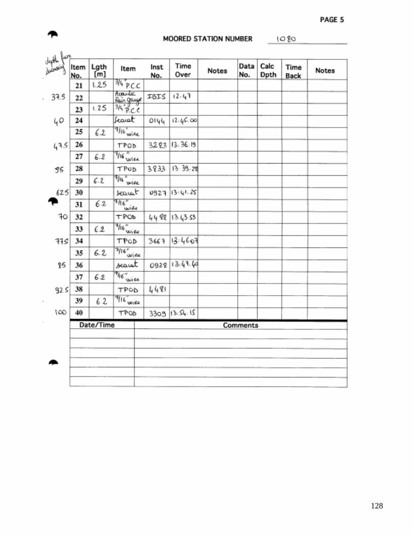
128

129

130

131

132
APPENDIX 5: Stratus mooring deployment procedures
The Stratus surface mooring deployed from the R/V Ronald H. Brown was set using the UOP twophase mooring technique. Phase 1 involved the lowering of approximately 40 meters of instrumentationover the port side of the ship. Phase 2 was the deployment of the buoy into the sea. The benefits oflowering the first 40 meters of instrumentation are three fold in that: (1) it allows for the controlledlowering of the upper instrumentation; (2) the suspended instrumentation, attached to the buoy’s bridle,acts as a sea anchor to stabilize the buoy during the deployment; and (3) the 90 meter length of paid outmooring wire and instrumentation provides adequate scope for the buoy to clear the stern withoutcapsizing or hitting the ship. The remainder of the mooring is deployed over the stern. The followingnarrative is the actual step-by-step procedure used for the Stratus 2 mooring, deployed from the R/VRonald H. Brown. The basic deck equipment and deck layout is illustrated in figure 69. The mooring gearused in the deployment of the surface mooring included: the TSE winch, port and starboard side pedestalcranes, HIAB jib crane, A-frame, and the standard complement of blocks, chain grabs, stopper and sliplines.
The TSE winch drum was pre-wound with the following mooring components, listed from deep toshallow:
150 m 7/8” nylon200 m 7/8” nylon vinyl tarp barrier interface100 m 3/8” wire200 m 3/8” wire500 m 3/8” wire500 m 3/8” wire300 m 3/8” wire100 m 3/8” wire100 m 3/8” wire
A vinyl tarp was placed between the nylon and wire rope to prevent the wire from burying into thenylon line under tension. A tension cart was used to pretension the nylon and wire during the windingprocess.
The personnel used during the first phase of the operation were: a deck supervisor, winchoperator, 4 mooring wire handlers, air tugger operator, and jib crane operator.

133
HIAB
hanger bay
crane
01crane
UOP - van leg 2 wire/nylon
capstan poly/nylon line baskets
UW/APL van
TSE winch
H-bit
air tugger
fair leadplate
deck box
bulwarksspare wire/nylon
UOP leg 290 17" glass spheres
UOP anchors
PMEL anchors
dragging gear
UOP discus leg 2
PMEL chainwinding carts
removed bulwarks
Aframe
R/V Ron Brown - STRATUS 2 deck layout
Figure 69: Basic deck equipment and deck layout
Prior to the deployment of the mooring, the top 100-meter length of 3/8” diameter wire rope waspaid out from the TSE winch. Its bitter end was passed through the center of the A-frame and around theaft port quarter and up forward along the port rail to the instrument lowering area.
The four hauling wire handlers were positioned for deployment. Their positions were in front ofthe TSE winch, the center of the A-frame, aft port quarter, and approximately 5 meters forward along theport rail. The wire handler’s job was to keep the hauling wire from fouling in the ship’s propellers andpass the wire around the stern to the closest line handlers on the port rail.
Prior to the starting the mooring deployment, the ship hove to with the ship’s bow positioned sothat the wind was slightly on the port bow. The jib crane was extended out so that there wasapproximately four meters of free whip hanging over the instrument lowering area. An air tugger (smallpneumatic winch) was rigged as a stopper line, approximately eight feet inboard of the instrumentlowering area. All sub-surface instruments were staged, in order of deployment, on the port side maindeck. Instrumentation from 40 meters to the surface had a pre-connected shot of chain shackled to the topof the instrument. Instrumentation below 40 meters had chain or wire shots secured to the bottom of theinstrument.
The first instrument segment to be lowered was the 6.2-meter length of 7/16” wire rope, 40-meterdepth SEACAT, and 1.25-meter length of 3/4” chain. The instrument lowering commenced by shacklingthe bitter end of the hauling wire to the free end of the 6.2 meter length of 7/16” wire rope shot. The cranewhip hook suspended over the instrument lowering area was lowered to approximately 1 meter from thedeck. A 4 foot “Lift All” sling barrel hitched through a 3/4” chain grab was attached to the crane hook.The chain grab was hooked onto the 1.25-meter chain approximately .5 meters from the free end. Thecrane whip was raised so the chain and instruments were lifted off the deck approximately 0.5 meters.The crane was instructed to lower its whip and the attached mooring components down into the water.

134
The TSE winch simultaneously paid out the hauling wire. The wire handlers positioned around the sterneased the hauling wire over the port side, allowing only enough wire over the side to keep the deepestmooring segment vertical in the water. The 1.25 meter 3/4” chain was stopped off .5 meter above theship’s deck, using a 3/4” chain grab attached to an Ingersol Rand 1000 lb. line pull air tugger line. Thecrane was then directed to its 3/4” chain grab to the deck. The air tugger’s line hauled in enough to takethe load from the crane. The crane’s hook was removed.
The next segment in the mooring to be lowered was the 32.5 meter Acoustic Rain Gauge, and1.25 m length of chain. The instrument and chain were brought into the instrument lowering area with theinstrument bottom end pointing outboard so it could be shackled to the top of the stopped off chain shot.The loose end of the chain, fitted with a 3/4” chain shackle and 7/8” end link, was again hooked onto thechain grab on the crane whip. The crane whip was raised, bringing the chain and instrument into avertical position, 0.5 m off the deck. Once the crane’s whip had the load of the mooring componentshanging over the side, the stopper line was slacked and removed. The TSE winch paid out the haulingwire as the crane whip was lowered to the deck.
The operation of lowering the upper mooring components in conjunction with the pay out of thehauling wire was repeated up to the 2-meter shot of 3/4” chain shackled to the 7 meter depth SEACAT.The air tugger line was hooked into the shot of chain above the SEACAT and drawn tight as the cranewhip lowered the chain to the deck edge. The crane whip and chain grab were removed. The bottom ofthe 3.71 meter depth SEACAT was attached to the chain segment at the top of the instrument arraypreviously lowered into the water. The free end of 0.48 meter 3/4” chain was then shackled to the 1” endlink attached to discus bridle universal joint. At this point the chain segment attached to the top of theSEACAT was stopped off to the deck by inserting a 1/2” screw pin shackle and 5/8” pear ring into themiddle of the 0.48 meter length of 3/4” chain. A slip line was passed through the pear link and made fastto a deck cleat. The air tugger line was slacked and removed.
The second phase of the operation was the launching of the discus buoy. There were three sliplines rigged on the discus to maintain constant swing control during the lift. Lines were positioned on thebridle bail, a buoy deck bail, and on the instrument tower (Figure 70). The 30 ft. bridle slip line was usedto stabilize the bridle and allow the hull to pivot on the bridle’s apex at the start of the lift. The 60 ft.tower slip line was rigged to check the tower swing as the hull swings outboard. A 75 ft. buoy deck bailslip line was the most important slip line. This line prevents the buoy from spinning as it settles out in thewater. It important that the quick release hook, hanging from the crane’s whip, can be released withoutfouling against the discus tower. The buoy deck bail slip line was removed just following the release ofthe discus into the sea. One additional line called the whip tag line was used in this operation. This tagline was tied to the crane whip headache ball to help pull the whip away from the tower’s meteorologicalsensors once the quick release hook was released and the discus cast adrift.
The personnel used for this phase of the operation included a deck supervisor, TSE winchoperator, three hauling wire handlers, three slip line handlers, a crane operator, a crane whip tag linehandler and quick release hook handler.
With all three slip lines in place, the crane was directed to swing over the discus buoy. Theextension of the crane’s boom was approximately 50 ft. The crane’s whip was lowered to the discus andthe quick release hook, on a 2 foot sling, was attached to the main lifting bail. Slight tension was taken upon the whip to hold the buoy. The chain lashings, binding the discus to the deck, were removed. The slipline holding the suspended 40 meters of mooring string up the apex of the discus bridle was eased off toallow the discus to take the hanging tension. The buoy was then raised up and swung outboard as the sliplines kept the hull in check. The bridle slip line was removed first, followed by the tower bail slip line.Once the discus had settled into the water (approximately 25 ft. from the side of the ship), and the release
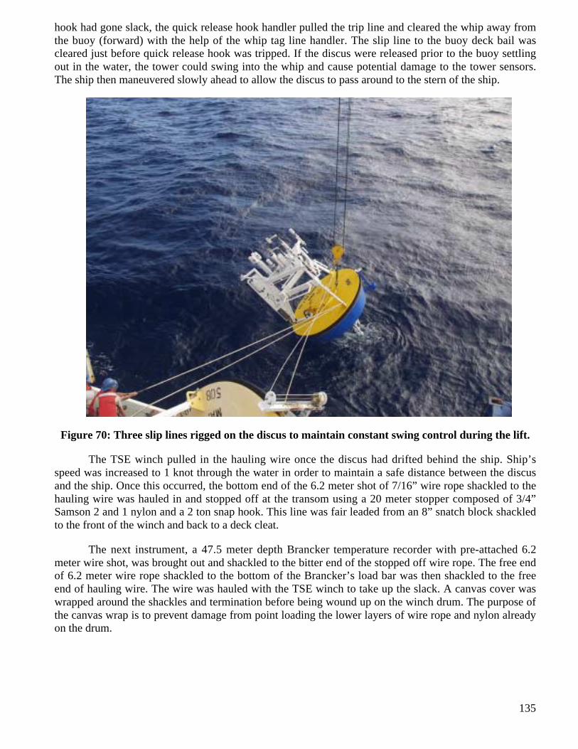
135
hook had gone slack, the quick release hook handler pulled the trip line and cleared the whip away fromthe buoy (forward) with the help of the whip tag line handler. The slip line to the buoy deck bail wascleared just before quick release hook was tripped. If the discus were released prior to the buoy settlingout in the water, the tower could swing into the whip and cause potential damage to the tower sensors.The ship then maneuvered slowly ahead to allow the discus to pass around to the stern of the ship.
Figure 70: Three slip lines rigged on the discus to maintain constant swing control during the lift.
The TSE winch pulled in the hauling wire once the discus had drifted behind the ship. Ship’sspeed was increased to 1 knot through the water in order to maintain a safe distance between the discusand the ship. Once this occurred, the bottom end of the 6.2 meter shot of 7/16” wire rope shackled to thehauling wire was hauled in and stopped off at the transom using a 20 meter stopper composed of 3/4”Samson 2 and 1 nylon and a 2 ton snap hook. This line was fair leaded from an 8” snatch block shackledto the front of the winch and back to a deck cleat.
The next instrument, a 47.5 meter depth Brancker temperature recorder with pre-attached 6.2meter wire shot, was brought out and shackled to the bitter end of the stopped off wire rope. The free endof 6.2 meter wire rope shackled to the bottom of the Brancker’s load bar was then shackled to the freeend of hauling wire. The wire was hauled with the TSE winch to take up the slack. A canvas cover waswrapped around the shackles and termination before being wound up on the winch drum. The purpose ofthe canvas wrap is to prevent damage from point loading the lower layers of wire rope and nylon alreadyon the drum.

136
Prior to lowering instruments over the stern, a line from an air tugger was reeved through a blockon the A-frame. A quick release hook was attached to the free end of the line in preparation for assistinginstruments over the transom with damaging them.
The TSE winch slowly took the mooring tension away from the stopper line hooked onto the 6.2meter wire rope. The stopper, line was removed. As the TSE winch paid out, the Branker was raised ofthe deck with the air tugger/quick release set-up. Once the instrument was clear of the stern, the tuggerline was slacked and the hook released from the instrument. As the bottom end of 6.2 meter wire shotcame off the winch, the canvas wrap was removed. A stopper line was hooked onto the 7/8” end link,which was shackled between the hauling wire and 6.2 meter wire shot. The winch paid out the mooringwire slowly and pulled the stopper line aft to approximately 2 meters from the transom edge. The stopperline was secured to the deck cleat. The TSE winch transferred the mooring tension to the deck cleat. Thehauling wire was unshackled, and the next instrument and wire shot were brought out to the stopped offwire. The process of instrument insertion was repeated for the remaining instruments.
To elevate the mooring wire and prevent chafing during pay out of the remaining wire and nylon,a block was hung from the A-Frame. A line was passed from a heavy-duty air tugger, through a block onthe frame, and into a “hanging” block. The block was hooked around the mooring wire, forward oftermination hardware (Figure 71). The tugger line was hauled in, lifting the mooring wire off the transomedge. The ship’s speed during this phase of the mooring operations was approximately 1 knot. Once theremaining wire had been deployed, the small hanging snatch block was removed. A large throated trawlblock, capable of passing nylon and polypropylene line, terminations, shackles and rings through it, washung in its place.

137
Figure 71: Bock hung from the A-Frame.
The long lengths of wire and nylon were paid out approximately 10% slower than the ship’s speedthrough the water. This was accomplished by using a digital tachometer, Ametek model #1726, tocalculate the mooring pay out speed verses the ship’s speed through the water. The selected readout fromthe tachometer was in Revolutions per Second. Table 18 shows for a given ship’s speed thecorresponding tachometer reading.

138
Table 18: The corresponding Tachometer readings for a given ship’s speed
Pay out speed readings
(knots) ( rev/sec)
0.25 3.221
0.5 6.441
0.75 9.662
1 12.883
1.25 16.103
1.5 19.324
1.75 22.545
2 25.766
2.25 28.986
2.5 32.207
3 38.648
3.5 45.09
4 51.531
4.5 57.973
5 64.414
All the mooring wire and nylon on the TSE winch drum was paid out. The end of the nylon wasstopped off to a deck cleat. The mooring was set up for towing in the following manner. A 5-meter lengthof 1/2” trawler chain was secured to the stopped off nylon end. A second stopper line was hooked ontothe chain. Both stoppers were eased out so that 1 to 2 meters of the chain shot was past the stern andsecured to deck cleats. The speed of the ship was around 1 knot. A Reel-O-Matic tension cart waspositioned along side the TSE winch. A 500 meter reel of 7/8” nylon was mounted to the cart. The nylonwas fairleaded to the TSE winch and wound up onto the drum. A second 500 meter reel of 7/8” nylonwas wound on the winch in the same manner. Approximately one hour was required for this operation.
While the nylon / polypropylene line was being paid out, the port crane was used to lift 80 glassballs out of the rag top container. The balls were staged fore and aft on the port rail. The eighty glass ballswere bolted on 1/2” trawler chain in 4 ball/4 meter increments. Four segments were shackled together toform 16 meter strings in preparation for deployment.
The free end of the nylon on the winch was shackled to the stopped off 1/2” chain and hauled in,pulling the deployed nylon termination back onto the deck. This termination was stopped off and thetowing chain was removed. The nylon terminations were shackled together and pay out continued. Themooring was stopped off 1 meter from the transom using a stopper line.
A 2000 meter shot of line, made up of 500 meters 7/8” nylon, spliced into 100 meters 1” nylon,spliced into1400 meters 1-1/8” polypropylene line, was the next component to be deployed. This line wasstaged in two wire baskets on the port side of the TSE winch. An H-bit cleat was positioned in front ofthe winch and secured to the deck. The free end of the shot of nylon/polypropylene was bent around theH-bit and passed on to the stopped off mooring line. Figure 72 and details how this line was reevedaround the H-bit. The shackle connection between the two nylon shots was made. The line handler at theH-bit pulled all the residual slack in the line and held the line tight against the H-bit. The stopper line wasthen eased off and removed. It was very important that the H-bit line handler keep the mooring line

139
parallel to the H-bit, with constant back tension, while the mooring tension was on the H-bit. The positionof the line handler is detailed in photograph Figure 73. While one person hauled line out of the wire.
high tension
low tension
AFT FORWARD
2'-4"
2'-4"
0'-6 1/2"
1'-8"0'-9 1/2"
0'-8"
0'-4 1/2"
0'-1"
3'-7"
H-Bitscale 1"= 12"
H-Bit line fair lead detail
Figure 72: H-Bit winding for releasing the final 2000 m of line.

140
Figure 73: Position of the line handler and assistant.
basket, the H-bit line handler eased line out at an appropriate speed, relative to the ship’s speed throughthe water.
Once the end of the polypropylene line was reached, pay out was stopped. A Yale grip wasinstalled on the high tension side of the line. A stopper line was connected to the Yale grip and secured toa deck cleat. The mooring line was eased around the H-bit, and the TSE winch tag line was shackled tothe end of the polypropylene line. The winch line and mooring line were wound up taking the mooringtension away from the stopper line. The stopper line was removed. The TSE winch paid out the mooringline so that its thimble was approximately 1 meter from the ship’s transom.
The deployment of eighty 17” glass balls was accomplished by using two 20 meter long 3/4”Sampson stopper lines fitted with 2 ton snap hooks and chain grabs (Figure 74 ). Each line was ledthrough an 8” snatch block secured to the front of the TSE winch. This configuration of the deck stopperfair lead allowed for the maximum available distance between the TSE winch and the transom whilekeeping the mooring components centered in the front of the winch. The first string of glass balls wasdragged aft up to the stopped off polypropylene line. The string was stretched forward, to the winch. Astopper line was used to stop off the ball string close to the winch. The winch paid out to transfer the loadto the stopper line.

141
Figure 74: Deployment of glass balls
The stopper was paid out slowly and several deck personnel assisted in dragging the remainingglass balls aft. The stopper line was paid out so that the adjacent glass ball out board of the stopper’shook remained on deck with a segment of 1/2” trawler chain bent over the deck edge. The stopper linewas secured to the deck. Another string of 16 glass balls was shackled to the free end of the stringattached to the mooring. The free stopper line was hooked into the chain close to the TSE winch. Tensionwas pulled up, and the line cleated, then the aft stopper line was eased off and removed. The next 16 glassball segment was pulled aft and shackled onto the end of the stopped off glass balls. The swappingstopper lines technique repeated until the 5 meter length of 1/2” trawler chain shackled to the last ballstring was stopped off 1 meter from the transom.
The acoustic release and attached 1/2” trawler chain segments were deployed using an air tuggerhauling line reeved through a block hung in the A-frame and the heavy-duty air tugger. Shackled to theend of tugger line was a 1/2” chain grab. The 20 meter 1” Samson anchor pennant was previouslyshackled to the TSE winch tag line and pre-wound onto the winch drum. The acoustic release waspositioned on the fantail 1 meter from the transom. The stopped off 5 meter length of 1/2” trawler chainwas shackled to the top of the release. A 5 meter length of 1/2” chain was shackled to the bottom ofrelease, and the loose end of the chain secured to the anchor pennant.
The A-frame was positioned so the hanging air tugger line and chain grab was over the top end ofthe release. The tugger line was lowered and hooked onto the 1/2” chain approximately 1 meter from thebottom end of the release. The anchor pennant was drawn up so that all available slack in the line wastaken up on the winch drum. The tugger line was hauled in lifting the release 1.5 meters off the deck. The

142
A-Frame was shifted out board with the TSE winch slowly paying out its line. The tugger line hauled inand paid out during this shift out board in order to keep the release off the deck as the instrument passedover the transom. Once the release had cleared the deck, the TSE winch pay out was stopped and thetugger line was removed. The 5 meter 1/2” chain was then stopped off with a stopper line and the anchorpennant was removed.
As the ship approached the target site, the anchor pennant was paid out and shackled to the 5meter shot of chain. Tension was taken on the mooring, and the two stopper lines were removed. Theanchor pennant was paid out, and personnel held chafing gear around the line, where it bent over thetransom. The 5 meter, 1/2” chain shackled to the anchor was lead out over the stern and back onto thedeck. The bottom end of the anchor pennant was paid out parallel to the end of the 1/2” trawler chain.The free end of the 1/2” chain was then shackled to the stopped off end link. A 1/2” screw pin shackleand a 5/8” pear ring were also secured to the end link. A deck cleat was bolted to the deck, positionedfore and aft, 1 meter forward of the stopped off anchor pennant. This deck cleat was bolted down with a1” eyebolt positioned on its aft end. A 20 meter length of 3/4” Samson line was bent through the 5/8”pear ring and one of its free ends tied in a bowline on to the cleat’s eye bolt. The free end of the line waspull tight and secured onto the horns of the cleat. The TSE winch tag line was eased off and removed.
The starboard crane was shifted so that the crane whip hung over, and slightly aft of the anchor.The whip was lowered and the whip hook secured to the tip plate chain bridle. A slight strain was appliedto the bridle. The chain lashings were removed from the anchor, and tip plate bolts removed from thedeck. The Samson line was slipped off transferring the mooring tension to the 1/2” chain and anchor. Theline was pulled clear and the crane whip raised 0.5 meters, lifting the forward side of the tip plate andcausing the anchor to slide over board. NOTE: In order to use the WHOI tip plate on the stern of the R/VR H Brown, a 12” steel extension was bolted to the aft section of the tip plate.

143
INSTRUCTIONS FOR LOADING THE RDI WORKHORSE ADCP IN TO CAGE
The fit of the instrument into its titanium cage is very tight, and the following insertion procedure(Figure 75) works successfully.
1 2 3 4
Slide ADCP intocage tailfirst
Swing head betweenclamps
Slide headdownwards,just clearing lower clamp
Twist head ifnecessaryto fit into place
5
Loosely attachclamps withtitanium hardware,then slide neopreneinto place beforetightening.
Figure 75: Diagram describing insertion of RDI ADCP into cage.

144
APPENDIX 6: Stratus antifouling paint study
(Provided by W.Ostrom, WHOI and M.A Walsh, E-Paint Company,Inc.)
The Stratus 1 discus hull was used as a platform to evaluate two antifouling coatings in an ongoing study to identify coatings suitable for controlling marine biofouling on moored aluminum buoyhulls and subsurface instrumentation.
Background
The purpose of this research is two-fold, 1) to identify environmentally compliant alternatives tooranotin-based antifoulants, and 2) to develop test methodology useful for evaluating antifouling coatingssuitable for use on moored aluminum buoy hulls, oceanographic instrumentation and the like.
The Upper Ocean Processes group has traditionally relied on organotin-based antifouling paintssuch as Amercoat #635 (Ameron International Protective Coatings Group) and Micron 33 (InternationalPaint) to protect buoy hulls and instrumentation from the colonization of fouling organisms. However,this class of antifouling paint has been banned by the International Maritime Organization (IMO), withuse of these products phased out by 2003. Fears of an imminent ban of organotin antifouling paints aswell as environmental and toxicological concerns with their use prompted members of the Upper OceanProcesses group to identify alternatives. Work began in the early 90’s to identify an environmentallycompliant replacement. Years of foul-resistance testing using discus and guard buoys as platformsmoored throughout the world have identified an effective replacement for organotin antifouling paints, EPaint Company’s SN-1.
Instead of the age-old method of leaching toxic heavy metals, the patented E Paint approach takesvisible light and oxygen in water to create peroxides that inhibit the settling larvae of fouling organisms.Photogeneration of peroxides and the addition of an organic co-biocide, which rapidly degrades in waterto benign by-products, make E Paint Company’s SN-1 an effective alternative to organotin antifoulingpaints. This paint has been repetitively tested in the field and has shown good bonding and anti-foulingcharacteristics as well as a service life up to 8 months (UOP technical report 98-02 pg. 98-101.)
This research effort investigates the erosion characteristics of two No Foul SN-1 formulations inan attempt to correlate erosion rates with service life. Two SN-1 formulations were evaluated for thisstudy, SN-1 and SN-1+.SN-1+ is a self-polishing version of the SN-1 reported to erode at a more uniformrate to provide a longer service life. Prolonged service life of No Foul SN-1, 2-3 years or equal toorganotin-based antifoulants, has not been demonstrated scientifically.
Developing methodologies to rapidly screen environmentally compliant antifouling coatings likeE Paint’s SN-1 is crucial to identifying alternatives to organotin antifoulants. Traditional methods ofevaluating antifouling coatings involve static panel tests in esturine environments or patch tests onoceangoing ships. Both methodologies have their shortcomings. The major drawback to panel testing isthat the coatings tested are not subjected to “real world” conditions that would be experience by a ship atsea. The drawback to patch testing on vessels in service is that most studies are conducted on the bottomof the ship totally ignoring fouling conditions in the photic zone. It is difficult to monitor the effects ofwater temperature and other environmental conditions on fouling rates. And, use of unprotected controlsis often not feasible. Using moored oceanographic environmental sensing stations as platforms for

145
antifouling paint testing has proved useful to rapidly identifying effective environmentally compliantsystems.
The benefits of using moored oceanographic environmental sensing stations as platforms forantifouling paint testing cannot be overstated. Patch testing on the mooring hull exposes prospectivecoatings to all conditions experienced by a vessel at sea. Currents, wind and wave action, simulatemovement. Direct exposure to the sun simulates exposure typical to the sides of a ship. Treatment ofequipment, support frames and/or treated panels below the buoy allow for exposures at different depths.Perhaps most important is the wealth of environmental data available for evaluating coating systems.Wind speed, wave height, water temperature, and chemical properties of the water are recorded and maybe used to extrapolate how these conditions affected coating performance. The increased number ofmoored sensing stations allows for the testing of prospective coatings throughout the world. This latestdeployment and recovery is part of an ongoing effort to establish methodologies for testing antifoulingcoatings on moored oceanographic environmental sensing stations as platforms.
This effort was successful in accomplishing the following research goals:
Foul-resistance of E Paint Company’s SN-1 was established and compared favorably to theorganotin antifouling coating used as a control.
Foul-resistance of E Paint Company’s SN-1 was established on oceanographic equipment andsupport frames.
Erosion rates of the antifouling coatings tested were determined and theoretical service life percoating thickness estimated.
Methodology to test antifouling coatings on moored oceanographic environmental sensingstations as platforms was established.
MATERIALS AND METHODS
Application of Test Coatings to the Discus Buoy:
The discus buoy was previously coated with many layers of old antifouling paint. The hull waspressure washed to remove loose or flaking paint and primed with an epoxy barrier coat, Devoe Bar-Rust235. This primer served as a tie-coat between the underlying layers of old paint and the new antifoulingpaint. The product was pigmented gray.
The primed hull of the buoy was section off by masking areas designated for test formulations andcontrols. A diagram of the buoy is presented below in Figure 76:

146
SECTION B
Unpainted Control
Ocean SurfaceTemperature Bracket Wind Vane Bracket
SECTION A
Diagram not drawn to scale.
Figure 76: Bottom view of buoy.
While the epoxy tie-coat was tack-free but soft to finger pressure, as recommended by themanufacturer, the first coats of No Foul SN-1 were applied. Two different formulations of No Foul SN-1were applied. Both were pigmented white. To section A, the standard SN-1 was applied. To section B, anexperimental version of SN-1, with additives to improve resistance to UV light exposure, was applied.All paints were applied using a roller. Both coatings dried overnight prior to application of the secondcoat. The weights of products applied were measured and weights applied per area determined. Weightsof product applied were recorded.
The procedure for application of the first coat was repeated for the second coat. The productapplied as the second coat was tinted gray for contrast and latter determination of coating erosion rates.
Application of the third coats of paint was to be similar to that of the second. An attempt wasmade to apply a blue version of the experimental SN-1+ over the gray on section B. Unfortunately thiswas not completed due to application difficulties with the formulation. Instead, blue No Foul SN-1 wasapplied to both sections. Two coats were applied to both sections of the buoy.
An organo-tin based product was applied as a comparative control in two areas, one near thesurface ocean temperature sensor mount and the other near the mount for the wind vane. The product,Micron 33 manufactured by International Paint (Union, NJ), is comprised of the following activeingredients: TBT methacrylate, TBTO and cuprous thiocyanate. This product is considered one of themost effective antifoulants currently available in the United States. However this and all organo-tin basedcoatings have been banned by the United States and the IMO (International Maritime Organization).
Upon recovery the conditions of the coatings applied to the discus hull were assessed and foul-resistance determined. All the test coatings were photographed and samples taken to determine residualpaint film thickness. The type and degree of fouling present on discus hull was documented.
Table 19 below details the preventive measures taken in protecting the subsurface instrumentationfrom marine biofouling.

147
Table 19: A List of Exposed Instrumentation and Equipment and Respective AntifoulingTreatments.
Instrument Paint C olor Coat/mils. Applied Date Applied
VMCM cage SN-1 white 2 / 6 mils. spray Aug-00
VMCM sting SN-1 white 1 / 3 mils. spray Aug-00
VMCM fans SN-1 white 1 / 3 mils. spray Aug-00
VMCMassembled
TempoTBT
clear 1 / 3 mils. spray Oct-00
MicroCat trawlguard
SN-1 white 1 / 3 mils. spray Oct-00
MicroCat trawlguard
TempoTBT
clear 1 / 3 mils. spray Oct-00
SEACAT trawlguard
SN-1 white 1 / 3 mils. spray Oct-00
SEACAT trawlguard
TempoTBT
clear 1 / 3 mils. spray Oct-00
SEACATsensor shield
SN-1 white 1 / 3 mils. spray Oct-00
Branckerthermister
SN-1 white 3 / 3 mils. brush Oct-00
Brancker trawlguard
SN-1 white 1 / 3 mils. spray Oct-00
Brancker trawlguard
TempoTBT
clear 1 / 3 mils. spray Oct-00
Chlam cage SN-1 white 2 / 6 mils. spray Aug-00
Rain gauge TempoTBT
clear 1 / 3 mils. spray Oct-00
FSST frame SN-1 white 2 / 6 mils. brush Oct-00
FSST frameassembled
TempoTBT
clear 1 / 3 mils. spray Oct-00
discus bridlelegs
SN-1 white 3 / 9 mils. brush Oct-00
discus bridlelegs
SN-1 blue 1 / 3 mils. brush Oct-00
discus hull SN-1 white 1 / 5 mils. roll Aug-00
discus hull SN-1 gray 1 / 5 mils. roll Aug-00
discus hull SN-1 blue 2 / 5 mils. roll Aug-00
discus hull SN-1 white 1 / 5 mils. roll Oct-00
discus hull SN-1+ white 1 / 5 mils. roll Aug-00

148
discus hull SN-1+ gray 1 / 5 mils. roll Aug-00
discus hull SN-1 blue 2 / 5 mils. roll Aug-00
RESULTS
Discus Buoy Hull Evaluation
Roughly 25% of the discus buoy hull was fouled with gooseneck barnacle. Though barnacleswere the predominate fouling organism reported in this study, a bacterial/algal slime is also visible inphotographs of recovered equipment. Gooseneck barnacles fouled close to 100% of unprotected controlregions of the hull. The average length and width of these organisms attached to unprotected regions was6-9 inches (15-23cm) and 0.25-0.375 inches (0.6-1.0cm) respectively. Gooseneck barnacles fouledtreated surfaces to a lesser degree. The extent of fouling is reported in Table 20 as the number oforganisms, and their length, per square foot.
Table 20: Degree of fouling expressed as the number of organisms per square foot.
Coating # Barnacles Maximum BarnacleLength (inches)
E Paint SN-1 15 3"Micron 33 15 9"Control Completely Fouled 6 to 9"
This research effort investigates the erosion characteristics of two No Foul SN-1 formulations inan attempt to correlate erosion rates with service life.
-based comparative control exhibited comparable foul-resistance. The smaller barnacle size fouling theSN-1 treated regions of the hull suggest that the coating resisted fouling longer than the Micron 33.Fouling to treated regions of the hull was reported to occur in small clusters of three to four organisms.Fouling occurred in large clusters in unprotected regions where the paint chipped or flaked away.
Figure 77 below shows the discus hull after recovery:

149
Figure 77: Discus Buoy after Recovery.
The image above shows a discoloration of surfaces treated with SN-1. A yellow/gray filmbelieved to be algae is visible coating the treated surface. This film more heavily coated the hull near andabove the waterline. On both sides A and B, the blue SN-1 has faded and an underlying layer of deeperblue paint is visible. At the waterline the topcoat had completely eroded as had 50% of the second coat ofblue. Gray and white underlying coats of paint are visible near the waterline.
Fouling on Instrumentation:
Prolific gooseneck barnacle fouling was observed on unprotected instrumentation and supportframes to 30m below the surface. Fouling rates decreased at greater depths. VMCM instrument casesexposed at 100m were fouled 50% with the barnacles where cage rods, VMCM stings and fans treatedwith SN-1 were <2% fouled. The TBTO clear coat also effectively controlled fouling on instrumentation.Figures 78 and 79 show the effect of depth on fouling rates.

150
Figures 78 and 79: TPOD 3763 at 13m and TPOD 3263 at 100m
The ability to evaluate the efficacy of antifouling coatings at different depths (up to 300m) isunique to this testing methodology.
DISCUSSION
Methods to utilize moored oceanographic environmental sensing stations as platforms todemonstrate the efficacy of new environmentally compliant antifouling coatings were established. Thiseffort demonstrated the viability of E Paint Company’s SN-1 as a replacement to organotin antifoulingpaints. Foul-resistance of SN-1 was comparable to that of Micron 33 after 12 months exposure. Judgingby the amount of paint remaining on the hull, service life of the 4 coats of SN-1 would have exceeded 18months at this test site. Closer examination of the coatings after the buoy returns to WHOI shouldconfirm this claim. Further coating longevity studies with SN-1 are warranted.
FUTURE WORK
Coatings applied to the discus buoy hull will be more closely evaluated upon the return of the testplatform to Woods Hole, Massachusetts. The film thickness of each coating will be measured in severallocations from the waterline to the bottom of the hull. The effect of photo-degradation on coating erosionwill be determined. In addition, the adhesion and physical integrity of test coatings will be determinedfollowing ASTM protocols.
Further testing involving longer exposure periods is warranted. Studies to determine the effect ofcoating thickness on foul-resistance as a function of time in different geographical locations would be ofinterest.

151
AFT
FORWARD
FORWARDAFT
SN-1 (old formulation)SN-1+ (improved formulation)Micron 33 (standard)control (unprotected)
STRATUS discus hull - leg 1anti-fouling paint testscale 1" = 2'W.Ostrom
Figure 80: Diagram of the Discus Buoy and Painting Scheme.

152
APPENDIX 7: Stratus 2 cruise logistics
Logistics for the Stratus 2 buoy turn around included shipping all cruise gear to Seattle, WA fortransit to the Galapagos. This avoided the complications and expense of trying to ship gear to theGalapagos Islands. In addition, buoy build up and check out was done in Seattle and allowed for anextended burn in during transit. This also meant less time was required in the Galapagos to prepare forthe cruise.
At the end of EPIC Leg 2, Stratus gear would remain on the R/V Brown until it arrived in Port atCharleston, SC.
To finalize logistics and cruise planning, it was necessary to visit the R/V Ronald H. Brown, andthe NOAA Marine Operations Center, Pacific. During 24-27 June, Robert Weller and Jeff Lord traveledto Victoria, B.C., and Seattle, WA, to make these arrangements.
The RH Brown had a three-day port call in Victoria, BC, Canada. Scientists from ETL, UW andWHOI agreed to meet with ship’s crew to discuss plans for science activities, deck load, and lab use.Although the crew was busy preparing for its upcoming cruise, we were able to cover a lot of ground in avery short period of time.
Cruise reports describing similar buoy operations, pictures and a videotape of the Stratus 1 buoydeployment were distributed to the crew. Deployment and recovery procedures as well as deck spacerequirements were discussed with the boson, Captain, and Field Operations Officer.
EPIC cruise participants discussed lab space needs and agreed on the amount of space available toWHOI prior to Leg 2 of the EPIC cruise. Tentative plans for loading in Seattle were made as well.
Following the meeting on the R/V Brown, Lord and Weller traveled to Seattle to meet with BillBrandenburg at the NOAA Marine Operations Center. Arrangements were made to stage gear and set upthe Stratus buoy at the NOAA facility prior to loading the R/V Brown for the cruise.
Mr. Brandenburg offered use of a garage for staging, forklifts as required, and outside storage forthe rest of the cruise gear. We notified him about the size of our shipment, the duration of our stay, andour need for crane service. Again, this meeting was brief, but very valuable. We left Seattle confident thatstaging for the cruise would be trouble free.
During the last week of July, burn in of the ASIMET systems and data logger were concluded.The buoy was disassembled, and all support gear was packed and inventoried for shipping to Seattle.
On August 7-8 all Stratus gear was loaded on trucks bound for Seattle. A lowboy flatbed, a 48-foot flatbed, and a 54-foot enclosed trailer were required for the gear. On August 7, the 48-foot flatbedwas loaded with two 20’ seatainers containing all mooring components and deck gear. Also on August7th, the lowboy flatbed was loaded with the buoy hull, 2 anchors, and 2 winches (one for UW). On August8, the 54 foot enclosed trailer was loaded with the remaining cargo. This included lab supplies, primaryand spare tower tops, instruments, tools and personal gear.
A total of 70,000 pounds of mooring components and support gear were shipped to Seattle for theStratus 2 mooring turn around.

153
On 14 August, 5 people flew to Seattle to prepare the buoy and load equipment onto the R/V RHBrown. The three trucks arrived in Seattle before 11:00 am on 15 August. A shore crane, provided byNess Crane Service, removed the two 20’ containers from the truck, and loaded them directly onto theship. The crane also put the winch and two anchors on the ship, and positioned the buoy hull in ourstaging area.
The 54 foot enclosed trailer was unloaded and gear was separated into two groups. Gear to loadon the ship, and gear required for buoy assembly and check out.
During the afternoon of 15 August, the buoy was assembled and some gear was loaded onto theship. For the rest of the week, buoy assembly and check out continued, the lab was set up as much aspossible, and some instruments were checked out.
On 20 August, the remaining gear, except the buoy, was loaded on board. The University ofWashington’s container arrived and was loaded. From August 20-24 remaining science gear fromorganizations participating in the EPIC program, and PMEL’s TAO buoy maintenance gear arrived andwas loaded on board. WHOI personnel assisted with this loading as well as the loading of ship’s storesfor the voyage. The WHOI discus buoy was loaded on board after everything else was loaded on deck.
A last-minute air shipment, consisting of a spare wind instrument and a few odds and ends,arrived in San Diego by September 5 for the R/V R H Brown’s final departure from the United States.
Six WHOI personnel participated in the EPIC cruise, Leg 2, from Puerto Ayorro, Galapagos, toArica, Chile. Travel included a flight from Boston to Miami, Miami to Quito, Ecuador, and a governmentcontrolled flight from Quito to Baltra. Since reservations could not be guaranteed on the flight to Baltra,we decided to leave a few days early in the event of any difficulties or delays in catching the flight toBaltra.
On 2 October, personnel arrived in Quito and spent the night. A 9:30 am flight to Baltra on 3October had us checking in at the airport at 7:00 am. The check in process, and the flight to Baltra, wasuneventful. We crossed the island and checked into the Angermeyer Hotel where we would stay for thenext five days.
The R/V R H Brown arrived in the Galapagos at 8:00 am on October 6. After a brief visit to theship by Lord and Weller to discuss logistics for set up and departure, it was clear that WHOI work couldnot commence until the morning of 7 October. And so it did.
Cruise details are discussed elsewhere in this report.
The R/V Ronald H. Brown arrived back in Charleston, SC on 13 December. The File OperationsOfficer scheduled offloading with each organization so it was very efficient. WHOI was the last group tounload.
Paul Bouchard and Jeff Lord traveled to Charleston on 16 December. On 17 December the buoy,anchor, winch, and 2-20’ containers were removed from the ship and loaded onto trucks. On 18December, all other loose gear from the deck, and all the gear stowed in the lab was offloaded from theship, and loaded onto a 48’ box truck. On 19 December, Bouchard and Lord returned to Woods Hole.

154
STRATUS 2 LOGISTICS CONTACTS
RONALD H. BROWN
Home Port – Charleston, SCE-MAIL CONTACTS
INMARSAT B: Personnel on board:[email protected]
011-874-336-899 620 Voice Field Operations Officer:[email protected]
011-874-336 899 621 Fax Commanding Officer:[email protected]
INMARSAT A: - only if B is down 011-874-154-2463 Voice 011-874-154-2644 Fax
INMARSAT Mini M:011-874-761 831 360Voice
Cellular: 757-635-0678 (Ship)206-910-3584 (OOD)206-910-8152 (CO)
206-910-0184 (CME)
SEATTLE
NOAA Marine Operations Center Mr. Bill Brandenberg1801 Fairview Ave., East Phone: (206) 553-4597Seattle, WA 98102 Email: [email protected]
Ness Crane ServicePO Box 70545Seattle, WA 98107-0545
(206) 784-1054
Silver Cloud Inn Phone 206.447.95001150 Fairview Ave. Fax 206.812.4900Seattle, WA 98109

155
ECUADOR
Quito
Used Maxiviajes Ecuador Tours SA (ECUADOR TOURS ONLINE.com) in Quito to meet us in theairport, get us in to the hotel, and get us checked in to the airport for the flight to Galapagos. $ 90 for 7people and bus service.
Samuel Fritz # 275 y 6 de DiciembrePO Box 17-11-4781Quito, Ecuador
Phone 593 2 241-1174-240-3433Or (02) 409-675-403-433FAX 593 2 240-3434www.EcuadorToursOnline.cominfotours@EcuadorToursOnline.com
Four Points by Sheraton Quito( $ 115)Avienda Naciones Unidas y Republica de el SalvadorQuito, Ecuador011 (593) 2 297-0002 Voice011(593) 2 243-3906 Fax
Galapagos
Hotel AngermeyerAve. Charles DarwinPuerto Ayora, Isla Santa Cruz011-593-5-526-066 Voice011-593-2-269-626Email: [email protected]
Other options would be Hotel Galapagos and The Red Mangrove Inn
Agent – GuayaquilTransportes Maritimos & Fluviales S.A.593-4-2208082 / 81593-4-2207909 / 10Christian Merizalde
ARICA, CHILE
Arica HotelAv. Commandante San Martin 599

156
Arica, Chile(011) 56-58 254 540 Voice(011) 56-58 231 133email: [email protected]
Agents
Naviera Portuaria Arica S.A. Edmundo AvilaMaximo Lira,Street N/N Humerto VildosoExplanada Muelle NorteArica, Chile
Phone: (011) 056-58-231715Fax: (011) 056-58-231949
[email protected]@[email protected]
or
Inchape Shipping ServicesOperations DepartmentPhone : + 56-32-217681Fax : + 56-32-239632Mobile: + 56-9-3314169

157
APPENDIX 8: Cruise Participants
WHOIRobert Weller, Chief ScientistPaul R.BouchardJeffrey LordJason GobatMark PritchardCharlotte ValléeWilliam M. Ostrom
Environmental Technology Laboratory (ETL)Jeffrey HareTaneil UttalScott AbbottDuane HazenScott SandbergBrandi McCarty
Ecuadorian Navy Oceanography Institute (INOCAR)Edgar RivasChilean Navy Hydrographic and Oceanographic Service (SHOA)Claudia ValenzuelaUniversity of Washington (UW)Sandra YuterKimberly ComstockSungsu ParkRobert SchaafJoe Adelbrook
CICESEDavid Rivas CamargoUCSBOlga PolyakovToby Westberry
National Oceanic and Atmospheric Administration (NOAA)John KermondCenter for Ocean land Atmosphere studies (COLA)Robert BurgmanTeacher-at-sea : Jane Temoshok

158
APPENDIX 9: Plan of the days onboard R/V R H Brown – LEG 2
RB-01-08: EPIC IPlan of the Day:
Wednesday, 10 October 2001(DOY: 283)
SUNRISE: 0601 LAN: 1207 SUNSET: 1811(Local Apparent Noon)
Weather Forecast:
It doesn’t get much nice than this out here! Enjoy the mostly sunny skies and calm winds. Expect lightSE trade winds as we head south along the 95 W line. Seas: 0-1 ft. Swell: SE 2-3 ft.
Temps: High: 24 C (76 F), Low: 19 C (66 F)
CTD TRANSECT ALONG 95°°°° W
0715 - 0815 SPMR and 500 m CTD at 1 S
1030 - 1130 SPMR and 500 m CTD at 1.5 S
1140 SEAWIFS Satellite pass (9 min duration)(W-NW heading to receive complete pass)
1330 – 1530 2 S Buoy repair (fishing opportunity)
1545 – 1645 SPMR and 500 m CTD 1 nm S of buoy
1945 –2030 500 m CTD at 2.5 S
2300 – 2345 500 m CTD at 3 S
0215 - 0300 500 m CTD at 3.5 S
0515 - 0600 500 m CTD at 4 S
Plan 1: Plan of October 10.

159
RB-01-08: EPIC IPlan of the Day:
Thursday, 11 October 2001(DOY: 284)
SUNRISE: 0601 LAN: 1207 SUNSET: 1813(Local Apparent Noon)
Weather Forecast:
We’ll have mostly cloudy skies today, otherwise nice weather. Expect SE trade winds as we continuesouth along 95 W. Winds: SE 7-10 kts. Seas: 1-2 ft. Swell: SE 3-4 ft.
Temps: High: 22 C (72 F), Low: 18 C (64 F)
CTD TRANSECT ALONG 95°°°° W
0945 - 1045 SPMR and 500 m CTD at 4.5 S
1222 SEAWIFS Satellite pass (10 min duration)(S heading should work OK to receive complete pass)
1330 – 1430 SPMR and 500 m CTD at 5 S
(Note: The buoy drifted away)
1715 - 1815 SPMR and 500 m CTD at 5.5 S
2100 – 2145 500 m CTD at 6 S
0015 - 0100 500 m CTD at 6.5 S
0345 - 0430 500 m CTD at 7 S
0715 - 0815 SPMR and 500 m CTD at 7.5 S
Plan 2: Plan of October 11.

160
RB-01-08: EPIC IPlan of the Day:
Friday, 12 October 2001(DOY: 285)
SUNRISE: 0559 LAN: 1206 SUNSET: 1812(Local Apparent Noon)
Weather Forecast:
SE trade winds and low clouds will continue. We’ll have overcast skies most of the day. SE trade winds.08 - 12 kts. Seas: 2-4 ft. Swell: SE 3-5 ft.
Temps: High: 22 C (72 F), Low: 18 C (64 F)
FINISH FIRST CTD TRANSECT; TRANSIT TO 20 S
0915 - 1030 Attempt to locate buoy at 8 S
- if located, inspect buoy (fishing opp)
- if not located, go to SPMR and CTD
1030 – 1130 SPMR and 500m CTD 1nm S of buoy
1128 SEAWIFS Satellite pass (8 min duration)(W-NW heading should work OK to receive complete pass)
Once complete, begin 3 day transit to IMET buoy location
(20 S, 85 W) stopping daily around local noon for SPMR, CTD, and SeaWiFS satellite pass. ETA toIMET: late night 15 Oct.
Deploy Drifters when crossing: 10 S, 14 S, and 18 S
Plan 3: Plan of October 12.

161
RB-01-08: EPIC IPlan of the Day:
Saturday, 13 October 2001(DOY: 286)
SUNRISE: 0548 LAN: 1154 SUNSET: 1801(Local Apparent Noon)
Weather Forecast:
SE trade winds and low clouds will continue. Overcast skies may break up a bit, but it will be mostlycloudy. SE trade winds strengthen a bit, 10 - 15 kts. Seas: 3-5 ft. Swell: SE 3-5 ft.
Temps: High: 23 C (73 F), Low: 19 C (66 F)
TRANSIT TO 20 S
1200 –1300Daily stop for SPMR, 500 m CTD, and
SeaWiFS satellite pass
1209 SEAWIFS Satellite pass (10 min duration)(SE heading to receive complete pass)
1300 - 1400 Test of WHOI acoustic releases
(down to 1000m on traction winch)
ETA to IMET buoy: evening of 15 Oct.
Deploy Drifters when crossing 14 S and 18 S
Plan 4: Plan of October 13.

162
RB-01-08: EPIC IPlan of the Day:
Sunday, 14 October 2001(DOY: 287)
SUNRISE: 0533 LAN: 1142 SUNSET: 1753(Local Apparent Noon)
Weather Forecast:
SE trade winds and low clouds will continue. We’ll have a few breaks in the overcast skies, but don’texpect to see too much sun. Occassional showers are possible, but will be brief.
Winds: SE10 - 15 kts. Seas: 3-5 ft. Swell: SE 3-5 ft.
Temps: High: 23 C (73 F), Low: 19 C (66 F)
TRANSIT TO 20 S
1116 SEAWIFS Satellite pass (9 min duration)(NW heading to receive complete pass)
1130 –1230Daily stop for SPMR, 500 m CTD, and
SeaWiFS satellite pass
1256 SEAWIFS Satellite pass (5 min duration)(SE heading will receive complete pass)
Deploy Drifter when crossing 18 S (ETA 0400 L)
ETA to IMET buoy: evening of 15 Oct.
Plan 5: Plan of October 14.

163
RB-01-08: EPIC I
Plan of the Day:Monday, 15 October 2001
(DOY: 288)
SUNRISE: 0618 LAN: 1229 SUNSET: 1843(Local Apparent Noon)
Weather Forecast:
Same as yesterday, only a bit cooler. SE trade winds and low clouds continue. Occassional showers arepossible.
Winds: SE 8 - 12 kts. Seas: 3-4 ft. Swell: SE 3-5 ft.
Temps: High: 21C (70 F), Low: 17 C (63 F)
Arrive at IMET Station, begin buoy comparison
1230 –1330Daily stop for SPMR and 500 m CTD
1259 SEAWIFS Satellite pass (10 min duration)
(SE heading will receive complete pass)
ETA to IMET buoy: 1800.
LOOKING AHEAD
6 Days on station at IMET buoy
Tuesday – buoy comparison, 2 deep (4000 m) CTD’s
Wednesday – buoy recovery
Thursday – clean and stow all recovered gear
Friday – deploy new IMET buoy in same location
Saturday - buoy comparison, 2 deep (4000 m) CTD’s
Plan 6: Plan of October 15.

164
RB-01-08: EPIC IPlan of the Day:
Tuesday, 16 October 2001(DOY: 289)
SUNRISE: 0609 LAN: 1227 SUNSET: 1844(Local Apparent Noon)
Weather Forecast:
Expect little change. SE trade winds and low clouds continue. Occasional showers are possible.
Winds: E-SE 8 - 12 kts. Seas: 2-3 ft. Swell: SE 3-5 ft.
Temps: High: 21C (70 F), Low: 17 C (63 F)
IMET Station -- Day 1 -- buoy comparison
0800- 0830 Small boat operations to inspect IMET buoy
0930 – 1200 Deep CTD #1 – 10 nm downwind of IMET buoy
1201 SEAWIFS Satellite pass (15 min duration)
(W-NW heading will receive complete pass)
1215 – 1230 SPMR
1230 – 1500 Deep CTD # 2 – 10 nm downwind of IMET buoy
1500 – Transit back to 0.25 nm from IMET buoy;
continue comparison
** Additional SPMR casts as other operations permit.
Plan 7: Plan of October 16.

165
RB-01-08: EPIC IPlan of the Day:
Wednesday, 17 October 2001(DOY: 290)
SUNRISE: 0609 LAN: 1226 SUNSET: 1844(Local Apparent Noon)
Weather Forecast:
A weather front to our SW will begin to influence our weather. SE trade winds will freshen and lowclouds continue. Showers are possible. As the front approaches we should see broken clouds and windsshifting around to the N-NW and increase.
Winds: E-SE 10 - 15 kts, until late tonight.
Seas: 2-4 ft. Swell: SE 3-5 ft and W as the front approaches.
Temps: High: 20 C (68 F), Low: 17 C (63 F)
IMET Station -- Day 2 -- buoy recovery
0740 Buoy released
0830- 1700 IMET buoy recovery
- small boat ops to hook into glass balls
- small boat ops to hook into buoy
1246 SEAWIFS Satellite pass (10 min duration)
(E-SE heading will receive complete pass)
** SPMR casts as other operations permit.
Plan 8: Plan of October 17.

166
RB-01-08: EPIC IPlan of the Day:
Thursday, 18 October 2001(DOY: 291)
SUNRISE: 0609 LAN: 1226 SUNSET: 1844(Local Apparent Noon)
Weather Forecast:
A weather front to our SW will continue to influence our weather. Fresh SE trade winds and low cloudscontinue. Brief drizzle is possible. Winds: E-SE 10 - 15 kts, until late tonight.
Seas: 3-5 ft. Swell: SE 3-5 ft and W as the front approaches.
Temps: High: 20 C (68 F), Low: 17 C (63 F)
IMET Station -- Day 3 -- clean instruments
SPMRs roughly every hour throughout daylight hours
(as other opertations permit)
1151 SEAWIFS Satellite pass (9 min duration)
(W-NW heading will receive complete pass)
1200 – 1230 Daily 500m CTD cast
1300 – 1500 Buoy deployment set and drift test (bridge only)
and SEABEAM
1500 – 1800 Complete SEABEAM survey
Plan 9: Plan of October 18.

167
RB-01-08: EPIC IPlan of the Day:
Saturday, 20 October 2001(DOY: 293)
SUNRISE: 0607 LAN: 1226 SUNSET: 1845(Local Apparent Noon)
Weather Forecast:
We’re starting to see the front approach from the SW. Fresh SE trade winds and low clouds continue.Brief rain and periods of broken clouds are likely. Winds: E-SE 15 - 20 kts.
Seas: 5-6 ft. Swell: SE 4-6 ft.
Temps: High: 20 C (68 F), Low: 16 C (61 F)
IMET Station -- Day 5 -- New buoy comparison
0745 – 1015 Deep (4000 m) CTD cast # 1
1030 – 1045 SPMR
1115 – 1400 Deep (4000 m) CTD cast #2
(lube cable on way up ~1230).
1138 SEAWIFS Satellite pass (8 min duration)
IF POSSIBLE (W-NW heading will receive complete pass)
1315 SEAWIFS Satellite pass (8 min duration)
(E-SE heading will receive complete pass)
1400 – 1415 SPMR
1430 – 1530 Transit back to IMET buoy
** Additional SPMRs as operations permit
Plan 10: Plan of October 20.

168
RB-01-08: EPIC IPlan of the Day:
Sunday, 21 October 2001(DOY: 294)
SUNRISE: 0607 LAN: 1226 SUNSET: 1845(Local Apparent Noon)
Weather Forecast:
The front has stayed to our south, but will continue to influence our weather. Fresh SE trade winds andlow clouds continue. Brief rain and periods of broken clouds are likely.
Winds: E-SE 12 - 16 kts. Seas: 3-5 ft. Swell: SE 4-5 ft.
Temps: High: 20 C (68 F), Low: 16 C (61 F)
IMET Station -- Day 6 -- Continue buoy comparison
SPMRs roughly every hour throughout daylight hours
1219 SEAWIFS Satellite pass (10 min duration)
(W-NW heading will receive complete pass)
1245 – 1315 Daily 500m CTD cast
2200 (+5) TIME CHANGE. Move clocks ahead 1 hour to observe +4 time zone (1 more timechange before arrival)
Looking Ahead
Monday - 22 October
0400 (+4) Depart station. Enroute to Arica, daily CTDs
Plan 11: Plan of October 21.

169
RB-01-08: EPIC IPlan of the Day:
Monday, 22 October 2001(DOY: 295)
SUNRISE: 0702 LAN: 1317 SUNSET: 1933(Local Apparent Noon)
Weather Forecast:
SE trade winds have lightened a bit and we’re back under the stratocumulus layer of low clouds. Expecta few brief periods of rain and hopefully a few periods of broken clouds.
Winds: E-SE 8 - 12 kts. Seas: 2-4 ft. Swell: SE 3-5 ft.
Temps: High: 20 C (68 F), Low: 16 C (61 F)
Transit to Arica, Chile; Daily CTD station
1225 SEAWIFS Satellite pass (6 min duration)
(W-NW heading will receive complete pass)
1245 – 1330 Daily SPMR + 500m CTD cast
(83 W Drifter upon departure)
1401 SEAWIFS Satellite pass (9 min duration)
(E heading should receive complete pass OK)
Looking Ahead
ETA to Arica: 0800 on Thursday, 25 October
Plan 12: Plan of October 22.

170
RB-01-08: EPIC IPlan of the Day:
Tuesday, 23 October 2001(DOY: 296)
SUNRISE: 0640 LAN: 1255 SUNSET: 1911(Local Apparent Noon)
Weather Forecast:
Should be a nice day, if you like clouds and cooler weather. The winds have lightened and the cloudlayer has thinned out.
We should see some sun breaks in the afternoon.
Winds: E 5 - 10 kts. Seas: 1-3 ft. Swell: SE 3-4 ft.
Temps: High: 20 C (68 F), Low: 15 C (59 F)
Transit to Arica, Chile; Daily CTD station
1215 – 1300 Daily SPMR + 500m CTD cast
1305 SEAWIFS Satellite pass (10 min duration)
(E-SE heading will receive complete pass)
1315 LIVE Internet broadcast
~1700 Drifter deployment 77 W
1930 SCIENCE NIGHT – Project summary in Library
24 October
0200 (+4) TIME CHANGE – Advance clocks one hour to 0300 (+3)
Looking Ahead
ETA to Arica: 0800 on Thursday, 25 October
Plan 13: Plan of October 23.

171
RB-01-08: EPIC IPlan of the Day:
Wednesday, 24 October 2001(DOY: 297)
SUNRISE: 0719 LAN: 1335 SUNSET: 1951(Local Apparent Noon)
Weather Forecast:
Another calm day. Clouds and cooler weather.
We should see some sun breaks in the afternoon.
Winds: Light and variable, becoming light from the south
Seas: 0-1 ft. Swell: S 2-3 ft.
Temps: High: 19 C (66 F), Low: 15 C (59 F)
Transit to Arica, Chile
No operations planned today
Thursday, 25 October 2001SUNRISE: 0707 SUNSET: 1946
ETA to Arica pilot station: 0800
ETA alongside pier 0830
Plan 14: Plan of October 24.

172