Long term dynamic monitoring of a PSC box girder bridge

Alexandre CURY Ph.D. student Laboratoire Central des Ponts et Chaussées, Paris, France alexandre.cury@lcpc.fr Alexandre Cury, born 1983, received his civil engineering and M.Sc. degrees from the Federal University of Juiz de Fora, Brazil. Currently, is a PhD student at Paris-Est Univ./LCPC in France.

Christian CREMONA Dr. HDR Ministry for Sustainable Development, Paris, France christian.cremona@

development-durable.gouv.fr After 15 years of research activities in LCPC, Christian Cremona joined the Direction for research and innovation of the Ministry for Sustainable Development as Head of the civil engineering and construction group.

Summary

Structural Health Monitoring (SHM) aims to determine whether damage is present or not based on

the analysis of measured dynamic characteristics of a monitored system. Normal changes are

usually caused by modifications in environmental conditions such as humidity, wind and most

important, temperature. Conversely, abnormal changes are generally caused by the presence of

damage i.e. loss of structural mass and/or stiffness. This paper reports on the effect of temperature

changes on the natural frequencies of the PI-57 motorway bridge located at Senlis, France.

Dynamic measurements were carried out during almost two years and the goal is to develop a

methodology for separating environmental influences from possible damage events. Hence, several

regression and model fitting methods are used such as multiple linear regression and neural

networks. It is observed that possible structural modifications show up as outliers in the statistical

frequency-temperature relations.

Keywords: Structural health monitoring, regression analysis, temperature effects.

1. Introduction

In the past years, numerous methods for structural damage assessment were proposed in the

literature. The simplest (but not necessary the easiest) objective is to determine whether a structure

presents an abnormal behaviour or not. A feature sensitive to damage is a quantity extracted from

the measured system’s response that is able to indicate the presence of a structural modification.

Identifying features that can accurately distinguish a damaged structure from an undamaged one is

the focus of most SHM techniques [1]. Fundamentally, the feature extraction process is based on

fitting some model, either physics-based or data-based, to the measured system’s response. The

parameters of these models or the predictive errors associated with them become the damage-

sensitive features.

One of the most common methods of feature extraction comes from correlating observations of

measured quantities with posterior observations of the degrading system. Many techniques have

been proposed to locate and quantify damage considering deviations in the structures' modal

parameters [2]. These methods usually determine the baseline parameters through acquisition of

forced or ambient vibration test data. Damage detection is then based on the principle that damage

in the structure will produce changes in the measured vibration data. Most of these techniques,

however, neglect the important effects of environmental changes on the original structure.

Modifications in load, boundary conditions, temperature and humidity can have a significant effect

on the original modal parameters of large civil structures. In fact, sometimes these variations can be

much larger than those caused by structural damage [3].

Numerous researchers have demonstrated that modifications of structural dynamic properties are

related with environmental and operational variations. Temperature, for example, is reported to

change stiffness as well as boundary conditions [4]. Wind-induced vibration is known to have a

significant influence on dynamics of long span bridges by changing their damping characteristics

[5]. Traffic loadings are also reported to alter the measured natural frequencies and damping ratios

[6]. Therefore, in order to develop a robust SHM system, it is important to distinguish the effects of

damage from those caused by environmental and operational variations.

This paper mainly studies the thermal effects on modal parameters of the PI-57 Bridge due to

temperature changes. As a matter of fact, very few researches have addressed such a problem. In

this sense, two regression and model fitting methods are used such as: multiple linear regression

and neural networks. The idea is to calibrate a model capable to discriminate deviations of natural

frequencies due to temperature changes from those caused by other factors, either environmental or

imposed structural modification. When the measured frequencies fall outside some predicted

confidence intervals, the model can provide a reliable indication that structural changes are likely

caused by factors other than thermal effects at least with a small probability of false alarm.

Experimental data used in this work were acquired through two separate campaigns of dynamic

measurements. These tests were carried out during almost two years on a highway bridge located at

Senlis, France.

2. Model formulation

In this section, an overview of the regression techniques used in this paper is presented. First, a

simple linear model is introduced. Then, some concepts regarding a non-linear regression model

based on neural networks are outlined.

2.1 Linear model

The architecture of the linear regression model takes a subset of temperature profiles as inputs and

delivers a vector output that represents the estimated (or predicted) natural frequencies.

Suppose that n observations are available for s temperature sensors. The following relationship can

be defined:

εTwf (1)

where T is the sn input temperature matrix, w is a 1n vector of coefficients that weights each

temperature input, ε is the 1n regression error and f is the 1n output vector, represented by the

natural frequency. In order to minimize the error, a Least Mean Squares (LMS) procedure is applied.

The optimal solution for Eq. (1) can be written as:

1

* t t

w TT Tf (2)

Once the model is calibrated i.e. optimal weights are evaluated, new data can be used as input for

predicting new frequency values. For example, let pT denote a matrix of new temperature readings.

A prediction vector pf of a natural frequency can be calculated as:

*'wTf pp (3)

Evidently, it is practically impossible to obtain a perfect match of the predicted and measured

frequencies due to numerical errors, uncertainties in measurements, etc. Of greater importance,

however, is to evaluate confidence intervals around these predicted observations. Thus, the upper

and lower bounds of a (1 ) confidence interval can be evaluated as [3]:

ppsnip tf TTTT

1''2,2 )(1 with

n

i

iip

sn

ff

1

2

2 (4, 5)

where ipf and if are the ith observations of vector pf and ,f respectively. The value of snt ,2

can be evaluated from a statistical table of the t distribution and 2 is the mean squared error. One of

the advantages of using this type of regression is that many processes in science and engineering are

well-described by linear models. This is essentially because over short ranges, any process can be

well-approximated by a linear model. However, with large datasets, the resulting regression model

might not be well suited. In addition, this technique often gives optimal estimates of the unknown

weights but is very sensitive to the presence of abnormal data points. In order to deal with these

possible limitations, a non-linear regression model is presented in the next section.

2.2 Neural Networks

Neural networks have proved themselves as proficient classifiers and are particularly well suited for

addressing linear but also non-linear problems [7]. Given the nature of real world phenomena, like

the regression of modal parameters, neural networks are a potential approach for dealing with this

problem.

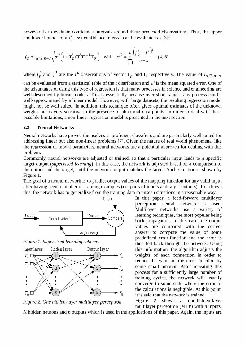
Commonly, neural networks are adjusted or trained, so that a particular input leads to a specific

target output (supervised learning). In this case, the network is adjusted based on a comparison of

the output and the target, until the network output matches the target. Such situation is shown by

Figure 1.

The goal of a neural network is to predict output values of the mapping function for any valid input

after having seen a number of training examples (i.e. pairs of inputs and target outputs). To achieve

this, the network has to generalize from the training data to unseen situations in a reasonable way.

In this paper, a feed-forward multilayer

perceptron neural network is used.

Multilayer networks use a variety of

learning techniques, the most popular being

back-propagation. In this case, the output

values are compared with the correct

answer to compute the value of some

predefined error-function and the error is

then fed back through the network. Using

this information, the algorithm adjusts the

weights of each connection in order to

reduce the value of the error function by

some small amount. After repeating this

process for a sufficiently large number of

training cycles, the network will usually

converge to some state where the error of

the calculations is negligible. At this point,

it is said that the network is trained.

Figure 2 shows a one-hidden-layer

multilayer perceptron (MLP) with n inputs,

K hidden neurons and n outputs which is used in the applications of this paper. Again, the inputs are

Figure 1. Supervised learning scheme.

Figure 2. One hidden-layer multilayer perceptron.

the temperatures and the outputs, the natural frequencies. Each input iT is multiplied by adjustable

weights denoted ilw before being fed to the lth neuron in the hidden/output layers, yielding:

K

liiili bTwnetff

1

)( , ni ,...,1 (6)

where ib represents the bias of each perceptron.

In order to adjust weights properly, a general method for non-linear optimization called gradient

descent is applied [8]. Briefly, the derivative of the error function with respect to the network

weights is calculated, and the weights are then changed such that the error decreases (thus going

downhill on the surface of the error function). Equation 7 shows the expression to evaluate the

updated weights of this network:

Klniw

Jtwtw

ililil ,...,1,,...,1 ,)()1(

(7)

where is the learning rate, t is the iteration step and J is mean error for a perceptron, written as:

n

iii fd

nJ

1

2)(2

1 (8)

where if represent the measured frequencies and id the observed outputs evaluated by the neural

network. For the simulations presented in this paper a free Matlab toolbox named Netlab developed

by [9] was used. A potential difficulty with the use of non-linear regression is the possibility of over

fitting data. To avoid this issue, data is divided into two sets: a training and a validation dataset. In

so doing, a more robust regression model is obtained for the prediction phase using unseen data.

3. Experimental program

The PI-57 Bridge is located near the town of Senlis, France (Figure 3). This bridge allows the A1

motorway to cross the Oise River and to connect

Paris to Lille. It is a 120 m prestressed concrete

bridge which underwent a reinforcement work in the

summer of 2009. This bridge was constructed in the

1960s and is approximately aligned in the north and

south direction. The dynamic monitoring program

consists in installing accelerometers before and after

reinforcement. The idea is to attest the effectiveness

of this procedure by analyzing the structure’s

dynamic behaviour before and after the procedure.

The first campaign of measurements took place

between November 21, 2008 and April 3, 2009. The

second campaign, after reinforcement, started in

November 21, 2009 and will finish in April, 2010.

The instrumentation was installed by the Technical Centre of Public Works (CETE) “South-West”

from the Ministry for Sustainable Development. Dynamic tests are performed under ambient

excitation: the traffic is used as source of excitation. In this sense, 1V/g accelerometers are used and

placed inside the bridge cross-section. Measurements were filtered within the 0-30 Hz frequency

range. Sampling was set to 0.004s for 5 mn records every 3 hours over a 24-hour time period. For

Figure 3. PI-57 Bridge over the Oise River.

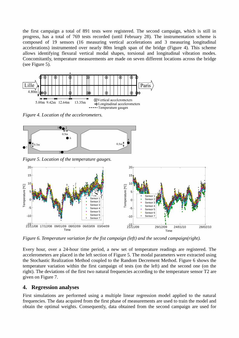
the first campaign a total of 891 tests were registered. The second campaign, which is still in

progress, has a total of 769 tests recorded (until February 28). The instrumentation scheme is

composed of 19 sensors (16 measuring vertical accelerations and 3 measuring longitudinal

accelerations) instrumented over nearly 80m length span of the bridge (Figure 4). This scheme

allows identifying flexural vertical modal shapes, torsional and longitudinal vibration modes.

Concomitantly, temperature measurements are made on seven different locations across the bridge

(see Figure 5).

Figure 4. Location of the accelerometers.

Figure 5. Location of the temperature gauges.

21/11/08 17/12/08 09/01/09 08/02/09 06/03/09 03/04/09-15

-10

-5

0

5

10

15

20

Time

Te

mp

era

ture

[ºC

]

Sensor 1

Sensor 2

Sensor 3

Sensor 4

Sensor 5

Sensor 6

Sensor 7

21/11/09 29/12/09 24/01/10 28/02/10-15

-10

-5

0

5

10

15

20

Time

Te

mp

era

ture

[ºC

]

Sensor 1

Sensor 2

Sensor 3

Sensor 4

Sensor 5

Sensor 6

Sensor 7

Figure 6. Temperature variation for the fist campaign (left) and the second campaign(right).

Every hour, over a 24-hour time period, a new set of temperature readings are registered. The

accelerometers are placed in the left section of Figure 5. The modal parameters were extracted using

the Stochastic Realization Method coupled to the Random Decrement Method. Figure 6 shows the

temperature variation within the first campaign of tests (on the left) and the second one (on the

right). The deviations of the first two natural frequencies according to the temperature sensor T2 are

given on Figure 7.

4. Regression analyses

First simulations are performed using a multiple linear regression model applied to the natural

frequencies. The data acquired from the first phase of measurements are used to train the model and

obtain the optimal weights. Consequently, data obtained from the second campaign are used for

prediction using the calibrated regression filter. In addition, 95% confidence intervals are evaluated.

-15 -10 -5 0 5 10 15 202

2.5

3

3.5

4

4.5

5

5.5

6

Temperature - Sensor 2 [ºC]

Fre

qu

en

cy [H

z]

1st

frequency

2nd

frequency

-15 -10 -5 0 5 10 152

2.5

3

3.5

4

4.5

5

5.5

6

Temperature - Sensor 2 [ºC]

Fre

qu

en

cy [H

z]

1st

frequency

2nd

frequency

Figure 7. Frequency deviations according to sensor 2 for the 1st (left) and 2nd (right) campaigns.

The idea is to separate modifications caused by temperature variations from other phenomena i.e.

structural modifications possible due to the reinforcement works. In this sense, each measurement

that falls outside these confidence boundaries is considered to be an outlier. As a remark, the

temperature sensor #5 will not be considered in this study since it is placed at the adjacent section

of the bridge, where there are no accelerometers. Instead of representing the actual value of the

natural frequency, a normalized frequency ratio can be used:

0f

fr ii , ni ,...,1 (9)

where n is the number of observations and 0f is the natural frequency at 0ºC. Thus, by using the

normalized value ir , it would be possible to better distinguish the real effects of temperature

changes from those caused by structural modifications using the same temperature baseline (0°C).

0 50 100 150 200 250 300 350 400 450 5000.4

0.6

0.8

1

1.2

1.4

Observations

No

rma

lize

d fre

qu

en

cy r

atio

Data

CIinf

CIsup

183 outliers

Figure 8. Linear model applied to the normalized frequency ratio (first frequency).

The training dataset used to calibrate the model consisted in 808 observations (temperature vs.

frequency pairs) whereas the prediction dataset consisted in 541. Figure 8 presents the confidence

intervals obtained by the linear regression. 183 (34%) observations fall outside these boundaries. It

is possible to state that these outliers represent actual structural modifications due to effects other

than thermal changes. In addition, one might say that the linear model cannot filter the entire

influence of temperature without this complementary approach. Figure 9 presents the same analysis,

now carried out using the second natural frequency. A total of 786 observations are used for the

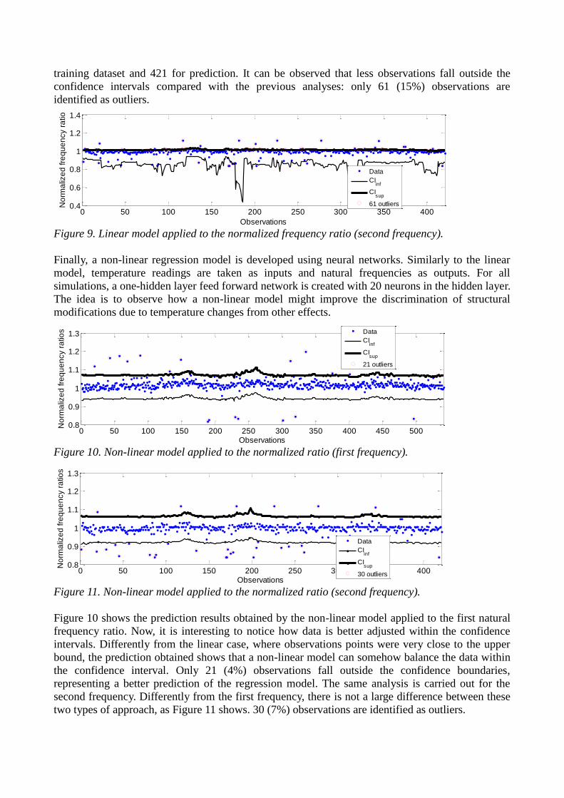
training dataset and 421 for prediction. It can be observed that less observations fall outside the

confidence intervals compared with the previous analyses: only 61 (15%) observations are

identified as outliers.

0 50 100 150 200 250 300 350 4000.4

0.6

0.8

1

1.2

1.4

Observations

No

rma

lize

d fre

qu

en

cy r

atio

Data

CIinf

CIsup

61 outliers

Figure 9. Linear model applied to the normalized frequency ratio (second frequency).

Finally, a non-linear regression model is developed using neural networks. Similarly to the linear

model, temperature readings are taken as inputs and natural frequencies as outputs. For all

simulations, a one-hidden layer feed forward network is created with 20 neurons in the hidden layer.

The idea is to observe how a non-linear model might improve the discrimination of structural

modifications due to temperature changes from other effects.

0 50 100 150 200 250 300 350 400 450 5000.8

0.9

1

1.1

1.2

1.3

Observations

No

rma

lize

d fre

qu

en

cy r

atio

s

Data

CIinf

CIsup

21 outliers

Figure 10. Non-linear model applied to the normalized ratio (first frequency).

0 50 100 150 200 250 300 350 4000.8

0.9

1

1.1

1.2

1.3

Observations

No

rma

lize

d fre

qu

en

cy r

atio

s

Data

CIinf

CIsup

30 outliers

Figure 11. Non-linear model applied to the normalized ratio (second frequency).

Figure 10 shows the prediction results obtained by the non-linear model applied to the first natural

frequency ratio. Now, it is interesting to notice how data is better adjusted within the confidence

intervals. Differently from the linear case, where observations points were very close to the upper

bound, the prediction obtained shows that a non-linear model can somehow balance the data within

the confidence interval. Only 21 (4%) observations fall outside the confidence boundaries,

representing a better prediction of the regression model. The same analysis is carried out for the

second frequency. Differently from the first frequency, there is not a large difference between these

two types of approach, as Figure 11 shows. 30 (7%) observations are identified as outliers.

5. Discussion

This paper presented a study for giving insights about predicting and discriminating changes in

natural frequencies due to environmental temperature from other effects. Experimental data

obtained from a long-term SHM system mounted on a prestressed concrete Bridge in Senlis, France

was used to develop a baseline for monitoring the effects of a reinforcement procedure. In order to

separate thermal effects from possible structural modification events, two regression techniques

were used. Moreover, confidence intervals were defined in order to explicitly identify observations

that could represent an abnormal behaviour. Firstly, a multiple linear regression was employed and

results have shown that a great number of observations were identified as outliners. This could be

explained by the fact that a linear model might not be well-suited for dealing with this kind of

problem, possibly raising a large number of false alarms. Thus, a non-linear model was proposed by

taking into account neural networks. In this case, it was observed that a smaller number of

observations fell outside the confidence boundaries. Normalized frequency ratios have been used

instead the natural frequencies themselves. The idea was to eliminate the influence of temperature

by normalizing all observations in respect to the frequency identified at 0ºC. It should be kept in

mind that the regression models presented in this paper were developed for a particular bridge under

particular environmental conditions. Moreover, although this study has considered a single external

variable (temperature), the same approach can be applied to other environmental effects. Finally, it

is important to stand out that the regression models are complementary to each other and that the

results obtained must be analyzed as a whole.

6. Acknowledgement

This research is financially supported by the SANEF motorways network and the Ile de France

County. The authors would also like to express their most grateful thanks to Y. Jeanjean from

SANEF bridge division, Y. Gautier and J. Dumoulin from CETE Sud-Ouest for their technical help

and for having made this study possible.

7. References

[1] DOEBLING S.W. and al., “Damage identification and health monitoring on structural and

mechanical systems form changes in their vibration characteristics: a literature review”, Los

Alamos National Laboratory, Report LA-13070-MS, 1996

[2] YAN Y.J. and al., “Development in vibration-based structural damage detection technique”,

Mechanical Systems and Signal Processing, Vol. 21, 2007, pp. 2198-2211.

[3] SOHN H. and al., “An Experimental Study of Temperature Effects on Modal Parameters of

the Alamosa Canyon Bridge”, Earthquake Engineering and Structural Dynamics, Vol. 28,

1999, pp. 879-897,

[4] MOORTY S., and ROEDER C.W., "Temperature-dependent bridge movements", ASCE

Journal of Structural Engineering, No. 118,1992, pp. 1090–1105.

[5] FUJINO Y., and YOSHIDA Y., “Wind induced vibration and control of trans-Tokyo bay

crossing bridge”, ASCE Journal of Structural Engineering, Vol. 128, No.8, 2002, pp. 1012–

1025.

[6] ZHANG Q.W. and al., “Traffic-induced variability in dynamic properties of cable-stayed

bridge”, Earthquake Engineering and Structural Dynamics, No.31, 2002, pp. 2015–2021.

[7] CURY, A., and CREMONA, C, “Novelty detection based on symbolic data analysis applied

to structural health monitoring”, In Proceedings of the 5th International Conference on

Bridge Maintenance, Safety and Management, Philadelphia, USA, 2010.

[8] PRINCIPE, J. and al., C, Neural and Adaptive Systems, Wiley, London, 2000.

[9] BISHOP C., Neural Networks for Pattern Recognition, Oxford University Press, 1995.